Hybrid vision-based navigation for mobile robots in mixed indoor/outdoor environments
Upload
khangminh22Category
view
1download
0
λογος
Human Data Understanding
Sensors, Models, Knowledge
Editors: Frank Deinzer & Marcin Grzegorzek
Frank Ebner
Smartphone-Based
3D Indoor Localization
and Navigation


Human Data Understanding
Sensors, Models, Knowledge
Vol. 1

Human Data Understanding
Sensors, Models, Knowledge
Volume 1
Herausgegeben von
Prof. Dr.-Ing. Frank Deinzer
Hochschule fur angewandte Wissenschaften
Wurzburg-Schweinfurt
Prof. Dr.-Ing. Marcin Grzegorzek
Universitat zu Lubeck

Frank Ebner
Smartphone-Based 3D Indoor Localization
and Navigation
Logos Verlag Berlin
λογος

Bibliographic information published by Die Deutsche Bibliothek
Die Deutsche Bibliothek lists this publication in the Deutsche National-bibliografie; detailed bibliographic data is available in the Internet athttp://dnb.d-nb.de.
Logos Verlag Berlin GmbH 2021
ISBN 978-3-8325-5232-9ISSN 2701-9446
Logos Verlag Berlin GmbHGeorg-Knorr-Str. 4, Gebaude 1012681 Berlin
Tel.: +49 (0)30 / 42 85 10 90Fax: +49 (0)30 / 42 85 10 92http://www.logos-verlag.de

From the Institute of Medical Informaticsof the University of Lubeck
Director: Prof. Dr. rer. nat. habil. Heinz Handels
“Smartphone-Based 3D Indoor Localization and Navigation”
Dissertation
for Fulfillment of
Requirements
for the Doctoral Degree
of the University of Lubeck
from the Department of Computer Sciences and Technical Engineering
Submitted by
Frank Ebner
from Werneck
Lubeck 2020

First referee: Prof. Dr.-Ing. M. Grzegorzek
Second referee: Prof. Dr.-Ing. A. Schrader
Third referee: Prof. Dr.-Ing. F. Deinzer
Date of oral examination: 21.09.2020
Approved for printing: Lubeck, 30.09.2020

Acknowledgements
During my master’s thesis, which covered the essentials of Wi-Fi location estimation, I came incontact with the concepts of indoor localization, and multi sensor fusion. Having attracted myinterest, I hereafter joined the Faculty of Computer Science and Business Information Systemsat the University of Applied Sciences Wurzburg-Schweinfurt as a research assistant. Duringthat time I conducted the majority of my research on indoor localization and navigation, whichfinally lead to writing this work.
I would like to thank my colleagues during that time, but especially my local doctoral adviserProf. Dr. Frank Deinzer. Not only did he guide me towards earning a doctors degree, he alsoprovided extensive feedback to all publications, always ensuring utmost scientific quality. Iwould also like to thank my external doctoral adviser and first referee Prof. Dr. habil. MarcinGrzegorzek for his trust, all provided feedback, and the warm welcome within his researchgroup. I also owe gratitude to my co-workers Lukas, Toni, and Markus. Without hours ofmutual feedback, technical input, paired programming, data acquisition, and networking, thiswork would not have been possible. Likewise, I also wish to thank Prof. Dr. Karsten Huffstadtand Prof. Dr. Arndt Balzer for helping with funding my initial employment.
In order to develop a generic indoor localization and navigation solution, the presentedsystem was deployed to and tested within several unique buildings. For this, special thanksgo to Dr. Hellmuth Mohring from the RothenburgMuseum in Rothenburg ob der Tauber, Prof.Dr. Gunther Moosbauer from the Gaubodenmuseum in Straubing, Angelika Schreiber fromthe Hutmuseum in Lindenberg, the Landesstelle fur die nichtstaatlichen Museen in Bayern, andthe Sparkassenstiftung. By providing access and enabling temporal hardware installations theyallowed gathering data within a range of unique and representative public buildings, enhancingthe quality of the developed system, and the experiments provided within this work.
Thanks also go to Markus, Christin, Alexander, and Maximilian, not only for spendingnumerous hours of their spare time with proof reading and feedback, but also for all emotionalsupport while conducting my research and writing this work. The same goes to my parents, foralways supporting me, and my education.
To Katharina, who has been a true friend, and will never be forgotten.
Frank Ebner

Abstract
With the steadily increasing need and wish to travel, people often have to reach locations theyhave never been to before. Modern means of transportation, like cars, ships and planes, thuscome equipped with onboard navigation systems, assisting with this task, based on the globalpositioning system (GPS), or a derivative. However, the navigation task is not solely limitedto outdoor environments. Reaching the correct gate within an airport, finding a ward in an un-known hospital, or the auditorium within a new university, represent navigation problems aswell. With the GPS requiring a direct line of sight towards the sky, it is unavailable for absolutelocation estimation indoors. Therefore, the question for suitable indoor navigation techniquesarises. Besides localization accuracy, additional factors should be met for such a new systemto become a success. It should be easy to set up and maintain, limiting required working hoursand costs. Likewise, hardware for the users themselves should be cheap, and readily available.Due to the ubiquity of smartphones, these devices represent a desirable platform for pedestrians,backed by the variety of sensors installed in these devices. Within this work, smartphone-basedpedestrian indoor localization and navigation is discussed in detail. This covers examining thesuitability of several available sensors: step-detection using readings from the accelerometer,relative turn-detection utilizing the turn rates of the gyroscope, absolute heading estimationsbased on the magnetometer’s indications, and altitude evaluation from the barometer. While allaforementioned sensors do not require any additional infrastructure, thus suitable for all sortsof buildings, they only allow for relative location estimations. Absolute localization can utilizeWi-Fi, as it is supported by all smartphones, and most public buildings already contain the re-quired infrastructure. Due to the behavior of radio signals, the smartphone’s current locationcan be approximated by examining signal strengths of nearby transmitters. This aspect is of-ten utilized by Wi-Fi fingerprinting, which, however, requires a time consuming setup process.Therefore, an alternative is developed that allows for significantly faster setup times. Addition-ally, the building’s 3D floorplan is included, modeling potential pedestrian movements, limit-ing impossible walks to improve estimation results, and to provide routing towards a desireddestination. For this, two spatial floorplan representations are derived and examined. All afore-mentioned aspects are hereafter combined probabilistically, using recursive density estimationbased on the particle filter. This allows for fusioning all sensor observations while respectingtheir individual uncertainties, and the building’s floorplan as additional constraints.
To summarize, the system described within this work covers probabilistic 3D pedestrianindoor localization, using commodity smartphones, contained sensors, a building’s existing in-frastructure and floorplan, all combined by the particle filter to derive an indoor localization andnavigation system that is easy to set up and maintain.

Zusammenfassung
Mit dem stetig zunehmenden Reisewunsch finden sich Menschen immer haufiger vor der Auf-gabe, bislang unbekannte Orte zu erreichen. Moderne Transportmittel, wie Autos, Schiffe undFlugzeuge sind deshalb mit GPS-basierten Navigationssystemen ausgestattet, die hierbei un-terstutzen. Allerdings ist der Navigationsaspekt selten nur auf den Außenbereich beschrankt.Das richtige Gate im Flughafen zu finden, eine Station im Krankenhaus, oder den Horsaal in derneuen Universitat, ist oft ahnlich anspruchsvoll. Da das GPS jedoch eine direkte Sichtverbin-dung benotigt, steht dieses innerhalb von Gebauden nicht zur Verfugung. Hier stellt sich deshalbdie Frage nach geeigneten Alternativen. Fur Neuentwicklungen mussen neben der Positionsge-nauigkeit auch andere Aspekte berucksichtigt werden. Das System sollte nicht nur wartbar, son-dern auch kostengunstig ausrollbar sein. Auch fur die Nutzer sollten die Anschaffungskostenso gering wie moglich ausfallen. Smartphones stellen aufgrund ihrer Allgegenwartigkeit undVielzahl von Sensoren deshalb eine ideale Zielplattform dar. In dieser Arbeit werden verfugbareSensoren auf ihre Tauglichkeit untersucht: Schritterkennung mittels Beschleunigungssensor,Laufrichtungsschatzung via Magnetometer, Laufrichtungsanderungen gemessen durch das Gy-roskop, und Hohenbestimmung per Barometer. Diese Sensoren stellen zwar keinerlei An-forderungen an das Zielgebaude, liefern jedoch lediglich relative Informationen bzgl. moglicherAufenthaltsorte. Eine absolute Positionsbestimmung wird uber Wi-Fi ermoglicht, welches vonallen Smartphones unterstutzt wird und in den meisten offentlichen Gebauden verfugbar ist.Basierend auf dem Verhalten von Funksignalen lasst sich der aktuelle Standort des Smartphonesaus den Signalstarken der nahegelegenen Access Points ableiten. In der Literatur wird hierfurhaufig auf Fingerprinting zuruckgegriffen, welches zwar genau, aber aufwending in der Ein-richtung ist. Deshalb wird eine Alternative erarbeitet, die die Einrichtungszeit und Kosten starkreduziert. Zusatzlich wird ein 3D Gebaudeplan verwendet, der mogliche und unmogliche Be-wegungen von Fußgangern bestimmen, und die kurzeste Route zu einem gewunschten Zielberechnen kann. Beides dient der Verbesserung der Vorhersagen des Gesamtsystems. Hierfurwerden zwei verschiedene Reprasentationen des Gebaudeplans erzeugt und untersucht. Allevorherigen Komponenten werden schließlich uber rekursive Dichte-Schatzung mittels Partikel-Filter zusammengefuhrt. Mit dieser lassen sich alle Sensor Messungen inklusive ihrer Un-sicherheiten kombinieren, und auch der Gebaudeplan kann als zusatzliche Rahmenbedingungintegriert werden, um unmogliche Bewegungen auszufiltern.
Zusammenfassend beschreibt diese Arbeit ein auf Wahrscheinlichkeitsrechnung basierendes3D Lokalisations- und Navigations-System fur Fußganger in Gebauden, das alle Informationenmittels Partikel Filter kombiniert, einfach einzurichten und zu warten ist. Vorausgesetzt werdenlediglich ein Smartphone, eine vorhandene WLAN-Infrastruktur und ein Gebaudeplan.


Contents
1 Introduction 11.1 Navigation within Buildings . . . . . . . . . . . . . . . . . . . . . . . . . . . 3
1.2 Research Objective . . . . . . . . . . . . . . . . . . . . . . . . . . . . . . . . 7
1.3 State of the Art . . . . . . . . . . . . . . . . . . . . . . . . . . . . . . . . . . 9
1.4 Scientific Contribution . . . . . . . . . . . . . . . . . . . . . . . . . . . . . . 12
1.5 Structure . . . . . . . . . . . . . . . . . . . . . . . . . . . . . . . . . . . . . . 13
2 Probabilistic Sensor Models 152.1 Sensor Errors . . . . . . . . . . . . . . . . . . . . . . . . . . . . . . . . . . . 16
2.2 Probabilistic Problem Formulation . . . . . . . . . . . . . . . . . . . . . . . . 19
2.3 Global Positioning System . . . . . . . . . . . . . . . . . . . . . . . . . . . . 21
2.4 Inertial Measurement Unit . . . . . . . . . . . . . . . . . . . . . . . . . . . . 27
2.4.1 Step-Detection . . . . . . . . . . . . . . . . . . . . . . . . . . . . . . 30
2.4.2 Turn-Detection . . . . . . . . . . . . . . . . . . . . . . . . . . . . . . 37
2.4.3 eCompass . . . . . . . . . . . . . . . . . . . . . . . . . . . . . . . . . 47
2.5 Barometer . . . . . . . . . . . . . . . . . . . . . . . . . . . . . . . . . . . . . 53
2.6 Activity-Detection . . . . . . . . . . . . . . . . . . . . . . . . . . . . . . . . 58
2.7 Wi-Fi and Bluetooth Beacons . . . . . . . . . . . . . . . . . . . . . . . . . . . 62
2.7.1 Signal-Strength and Propagation . . . . . . . . . . . . . . . . . . . . . 63
2.7.2 Signal-Strength Prediction Models . . . . . . . . . . . . . . . . . . . . 67
2.7.3 Probabilistic Location Estimation . . . . . . . . . . . . . . . . . . . . 73
2.7.4 Location Estimation Using Lateration . . . . . . . . . . . . . . . . . . 75
2.7.5 Location Estimation Using Fingerprints . . . . . . . . . . . . . . . . . 78
2.7.6 Location Estimation Using Propagation Models . . . . . . . . . . . . . 85
2.7.7 Error Compensation . . . . . . . . . . . . . . . . . . . . . . . . . . . 95
2.8 Summary . . . . . . . . . . . . . . . . . . . . . . . . . . . . . . . . . . . . . 99
i

3 Probabilistic Movement Models 1013.1 Probabilistic Problem Formulation . . . . . . . . . . . . . . . . . . . . . . . . 102
3.2 Simple Models without Floorplan Information . . . . . . . . . . . . . . . . . . 106
3.3 Simple Models with 2D Floorplan . . . . . . . . . . . . . . . . . . . . . . . . 112
3.4 Overview on Spatial Models for Indoor Floorplans . . . . . . . . . . . . . . . 118
3.5 Regular Spatial Models for 3D Movement Prediction . . . . . . . . . . . . . . 120
3.5.1 Generation Based on an Existing Floorplan . . . . . . . . . . . . . . . 123
3.5.2 Random Walks on Graphs . . . . . . . . . . . . . . . . . . . . . . . . 128
3.5.3 Navigation . . . . . . . . . . . . . . . . . . . . . . . . . . . . . . . . 135
3.5.4 Continuous Results . . . . . . . . . . . . . . . . . . . . . . . . . . . . 138
3.6 Irregular Spatial Models for 3D Movement Prediction . . . . . . . . . . . . . . 141
3.6.1 3D Navigation Meshes . . . . . . . . . . . . . . . . . . . . . . . . . . 144
3.6.2 Movement Prediction . . . . . . . . . . . . . . . . . . . . . . . . . . . 145
3.6.3 Navigation . . . . . . . . . . . . . . . . . . . . . . . . . . . . . . . . 150
3.7 Summary . . . . . . . . . . . . . . . . . . . . . . . . . . . . . . . . . . . . . 153
4 Recursive Density Estimation 1554.1 Probabilistic Information Fusion . . . . . . . . . . . . . . . . . . . . . . . . . 159
4.2 Bayes Filter . . . . . . . . . . . . . . . . . . . . . . . . . . . . . . . . . . . . 161
4.3 Kalman Filter . . . . . . . . . . . . . . . . . . . . . . . . . . . . . . . . . . . 166
4.4 Extended Kalman Filter . . . . . . . . . . . . . . . . . . . . . . . . . . . . . . 172
4.5 Particle Filter . . . . . . . . . . . . . . . . . . . . . . . . . . . . . . . . . . . 175
4.5.1 Random Sampling . . . . . . . . . . . . . . . . . . . . . . . . . . . . 181
4.5.2 Resampling . . . . . . . . . . . . . . . . . . . . . . . . . . . . . . . . 185
4.5.3 Estimation . . . . . . . . . . . . . . . . . . . . . . . . . . . . . . . . 187
4.6 Summary . . . . . . . . . . . . . . . . . . . . . . . . . . . . . . . . . . . . . 190
5 Indoor Navigation 1915.1 Complex Indoor Maps . . . . . . . . . . . . . . . . . . . . . . . . . . . . . . 192
5.2 Fusing All Components . . . . . . . . . . . . . . . . . . . . . . . . . . . . . . 195
5.2.1 Update Frequency . . . . . . . . . . . . . . . . . . . . . . . . . . . . 197
5.2.2 Including Observations . . . . . . . . . . . . . . . . . . . . . . . . . . 199
5.2.3 Handling Impossible Movements . . . . . . . . . . . . . . . . . . . . 202
5.2.4 Detecting and Handling Deadlocks . . . . . . . . . . . . . . . . . . . 205
5.3 Real-World Considerations . . . . . . . . . . . . . . . . . . . . . . . . . . . . 207
5.3.1 Sensitive Locations . . . . . . . . . . . . . . . . . . . . . . . . . . . . 207
ii

5.3.2 Data Acquisition . . . . . . . . . . . . . . . . . . . . . . . . . . . . . 208
5.4 Performance Considerations . . . . . . . . . . . . . . . . . . . . . . . . . . . 210
5.4.1 Precomputed Model Predictions . . . . . . . . . . . . . . . . . . . . . 210
5.4.2 Code Optimization . . . . . . . . . . . . . . . . . . . . . . . . . . . . 212
5.5 Summary . . . . . . . . . . . . . . . . . . . . . . . . . . . . . . . . . . . . . 213
6 Experiments 2156.1 Testbeds and Data Acquisition . . . . . . . . . . . . . . . . . . . . . . . . . . 216
6.2 Evaluation of Sensor Components . . . . . . . . . . . . . . . . . . . . . . . . 221
6.2.1 Sensor Overview . . . . . . . . . . . . . . . . . . . . . . . . . . . . . 221
6.2.2 Step Detection . . . . . . . . . . . . . . . . . . . . . . . . . . . . . . 222
6.2.3 Relative and Absolute Heading Estimation . . . . . . . . . . . . . . . 226
6.2.4 Pedestrian Dead Reckoning . . . . . . . . . . . . . . . . . . . . . . . 234
6.2.5 Altitude Estimation . . . . . . . . . . . . . . . . . . . . . . . . . . . . 238
6.2.6 Activity Detection . . . . . . . . . . . . . . . . . . . . . . . . . . . . 241
6.2.7 Wi-Fi Location Estimation . . . . . . . . . . . . . . . . . . . . . . . . 244
6.3 Evaluation of Movement Models . . . . . . . . . . . . . . . . . . . . . . . . . 256
6.3.1 Spatial Floorplan Representation . . . . . . . . . . . . . . . . . . . . . 256
6.3.2 Navigation . . . . . . . . . . . . . . . . . . . . . . . . . . . . . . . . 259
6.3.3 Floorplan-Based Probabilistic Pedestrian Dead Reckoning . . . . . . . 262
6.3.4 Limitations . . . . . . . . . . . . . . . . . . . . . . . . . . . . . . . . 268
6.4 Evaluation of the Overall System . . . . . . . . . . . . . . . . . . . . . . . . . 273
6.5 Summary . . . . . . . . . . . . . . . . . . . . . . . . . . . . . . . . . . . . . 278
7 Summary 281
8 Future Work 285
List of Figures 289
List of Tables 295
List of Symbols 297
Bibliography 301
Appendix 329A.1 Tilt Compensation Example . . . . . . . . . . . . . . . . . . . . . . . . . . . 329
iii

A.2 Step-Detection Filters . . . . . . . . . . . . . . . . . . . . . . . . . . . . . . . 331A.3 Additionally Used Maps . . . . . . . . . . . . . . . . . . . . . . . . . . . . . 332A.4 Final System Results . . . . . . . . . . . . . . . . . . . . . . . . . . . . . . . 334
iv

Chapter 1
Introduction
Finding a specific place or location one has never been to, or hasn’t been to for a long time,is a common task that everybody encounters from time to time. Back in the days, almosteveryone had a road map stowed away within the car’s glovebox, ready to use, whenever needed.However, without a co-driver, reading the map and providing instructions, this was a quitecumbersome solution for getting from A to B. This situation changed in the year 2000, whenthe former military-only global positioning system (GPS) became freely available for civilianuse. Now it was possible to locate objects anywhere on the earth, with an accuracy down to afew meters, using just a single receiver. Combined with digitized maps, this allowed for both,self-localization and navigation [DH10].
Starting from there, it only took several months for receivers to become both, significantlycheaper and smaller, and companies like TomTom or Garmin started developing products formotor vehicles, using digital maps from vendors such as Tele Atlas or Navtech. At first, naviga-tion systems were either installed directly within a vehicle, or required fully featured hardware,like portable computers equipped with an external receiver. Yet, with the advent of Personal
Digital Assistants (PDAs), containing even smaller GPS receivers and mass storage devicesbased on flash memory, navigation systems became portable. Today, almost every new smart-phone is suitable for GPS-based navigation, using its built-in sensors, as well as a piece ofsoftware that includes the necessary maps and navigation algorithms.
Inexpensive receivers for GPS, new similar systems, like GLONASS, and (freely) availablemaps for almost every place on earth, lead to the ubiquity of navigation systems. Thus, theirsuccess was not only based on demand, but also on the availability of relatively affordablecomponents for hardware, software, and low running costs. At least for the customer: Consumerhardware can be used for several years, and, depending on the vendor, map updates are eitherfree of charge, part of an annual subscription, or charged per update.
1

2 CHAPTER 1. INTRODUCTION
For providers, however, the situation is different. Additionally to several billion dollars forthe initial development and setup, the infrastructure behind GPS has to be kept up and running,costing additional millions – per day. While licensing fees, e.g. for access to increased accuracy,compensate for some of these costs, the remaining part is paid by the US government. Runningcosts for the vendors of navigation appliances can be expected to be much cheaper. However,due to rapid changes in infrastructure, they have to provide up-to-date mapping data, resultingin many companies charging for updates [Pac+95; DH10]
Due to ever-increasing globalization and transnational business connections, the need andwish to move or travel is constantly increasing. Besides getting to airports, train stations orcompany compounds, the buildings themselves often represent a navigation problem as well:Finding the correct terminal within an airport, the conference room in a large company, a roomwithin a townhall, or the correct ward within hospitals, isn’t always straightforward. With thisin mind, localization and navigation indoors becomes of increasing importance as well.
However, while working perfectly for most navigation purposes, e.g. for cars, pedestriansand cyclists, currently available systems are unsuited, as both, the sensors and the typical mapformats, are intended for outdoor use. For good location estimations, GPS relies on a directline-of-sight between satellites and receiver, and older devices thus had to be installed on top ofthe car, in order to function properly. Similarly, the format of most digitized maps is focused onoutdoor purposes, as the underlying data structures mainly use a two-dimensional representationof roads, lanes, and intersections, unsuited for modeling a building’s interior.
Furthermore, when considering indoor environments, completely different use cases, be-sides typical navigation from A to B, arise as well. Starting from finding a specific productwithin a large supermarket, to the economy’s interest in location-based services, e.g. placingads for nearby products as well. Also covering cultural aspects, like guided tours through amuseum, presenting useful information on exhibits, based on the visitor’s current location andviewing direction. Depending on the building and intended use case, requirements can be com-pletely different. This especially concerns the aspect of localization accuracy. While a coarseGPS location estimation is sufficient for a car driving along the motorway, it can be too er-roneous for a slowly paced pedestrian, walking through an area with many small alleyways.The same holds true for localization indoors, where estimating the current whereabouts on aroom-level scale might be sufficient for some intentions, like presenting information on nearbyexhibits. For others scenarios, such as navigation, however, estimations should be as accurateas possible, for audible commands and visualizations given to the user, to be helpful instead ofmisleading.
Therefore, the question arises, how such a multi-purpose indoor localization and navigationsystem can be developed, and what criteria should be met for it to be valuable.

1.1. NAVIGATION WITHIN BUILDINGS 3
1.1 Navigation within Buildings
Based on the previous aspects, it becomes clear that the topic of localization indoors is not solelyrelated to sensors and achievable accuracy, but also to costs, for initial setup, maintenance overtime, software and hardware required by the consumer, and by the system’s operator. In case oflocalization indoors, the latter is unlikely to be a government, like it is for the GPS, GLONASSor Galileo, but more likely the owner of the building to deploy the system to, like an airport,hospital, supermarket or museum. This gives even more importance to the aspect of costs,as many public buildings that benefit from indoor localization, like townhalls or museums,typically are on a tight budget. Closely coupled with costs is the time required for setup andservicing, as they also arise per building, additionally dependent on its size. As known fromother projects, the solution is a tradeoff between quality (accuracy), time and costs.
Similar aspects apply to the required building maps. As it is unlikely for a global companyto create maps for every single building, where indoor localization could possibly be used, thisdata has to be supplied by the operator or a public community, dedicated to this task [Ope].Furthermore, in contrast to maps for navigation outdoors, indoor maps can be rather eclectic,as they have to support buildings with multiple floors, elevators, escalators, and different typesof stairs [EBS16; Elh+14]. Depending on the intended use case, they should also supportadding semantic information, like room numbers, points of interest, and access restrictions orlimitations. The latter is especially relevant to the disabled, who are unable to take stairs, orrequire additional audible information when visually impaired. These aspects can also affectthe topic of navigation, as the shortest path towards the destination might not be the best solutionfor all pedestrians, especially not for those being handicapped or injured.
Based on the previously mentioned thoughts, a non-exhaustive list of requirements for in-door localization and navigation thus contains the following aspects:
• Software and Hardware required by the consumer should be as cheap as possible, withrequired components being small and always at hand, if possible.
• The system’s accuracy must be sufficient for a pedestrian to be localized within the build-ing, and to provide navigation guidance. Hereby, sufficient is not quantifiable, stronglydepends on the intended use case, and the building’s architecture, as narrow corridorswith many adjacent rooms require a higher accuracy than e.g. large, open shopping malls.
• Time and costs for the initial system setup should be as low as possible. This includescosts for all necessary hardware components, time for their setup, and effort needed toprovide a digital map of the building’s floorplan.

4 CHAPTER 1. INTRODUCTION
• Time and costs for maintenance after the initial setup should be as low as possible. Ideally,the system is easily adaptable to architectural changes, like new/removed drywalls.
• Partial failures of the infrastructure should not completely disable the whole system, onlymay affect the provided accuracy.
Besides use case-dependent details, the question of suitable hardware components is themost critical. As existing positioning methods like GPS and GLONASS do rarely work indoors,other sensors are required to infer an absolute location. As of today, there is no establishedsolution, and this matter is still open for new suggestions. However, to conform with previousdiscussions, it should not only be accurate, but also cheap, and easily available. Therefore, mostongoing research is targeted at smartphones, as they are ubiquitous, almost always at hand, andcontain an increasing number of sensors [Tia+15; Gui+16; Ndz+17; Ye+14; Mou+15; Kir+18].
That is in contrast to outdoor navigation, where new platforms started to develop around theexistence of a single sensor. For indoor localization and navigation, a desirable target platform isalready available, and the question arises, whether it is suitable for the intended task. This leadto numerous new research topics, analyzing the suitability of certain sensors, that are installedwithin commodity smartphones. Most of them are adapted from previous research in differentfields, where some sensor or component has already been proven helpful.
This e.g. covers velocity and heading, estimated from an accelerometer and a gyroscope,together providing the base for dead reckoning [ND97], which allows relative (incremental)location estimations, if initial whereabouts are known. This technique already underwent ex-tensive research to adapt it from vehicles to pedestrians. Yet, the focus was mainly on multiple
sensors, attached to different parts of the body, picking up leg movement and turning behaviorof a pedestrian, well-suited for motion estimations [SD16; TS12; Goy+11]. With the risinginterest in indoor localization, it began to be adapted to smartphone-only setups, where theorientation of the device has to be considered, when the pedestrian e.g. holds the smartphoneupfront, looking at its screen while navigating through a building [PHP17; Yu+19; Kus+15].
Yet, with dead reckoning providing information on relative movements, it is only suitablewhen initial whereabouts are known, and it is likely to fail over time, due to increasing errors.For actual indoor localization, hints on absolute whereabouts are mandatory. For this, formerresearch on Wi-Fi-based location estimation [BP00] became of interest again. By using signalstrength observations from nearby access points, it is possible to roughly estimate the distancetowards them, and thus a coarse, absolute location information. This strategy also conformswith most aforementioned requirements: As of today, most public buildings are equipped withWi-Fi, already containing the required infrastructure, and Wi-Fi is supported by all modernsmartphones. However, besides these positive aspects, achievable accuracy is either too coarse,

1.1. NAVIGATION WITHIN BUILDINGS 5
50 m
Figure 1.1: Example of a complex single-floor, with large open spaces and small adjacent rooms. Firstfloor of the UAH building of the University of Alcala de Henares, Spain.
or a manual and time-consuming setup is required beforehand. During the latter, accuracyis increased by actually measuring the behavior of the installed infrastructure’s radio signals,throughout the whole architecture. Thus, this area is still undergoing extensive research.
In contrast to navigation outdoors, there is not yet a single sensor that solves the problemformulation with sufficient accuracy. Instead, research tends towards employing combinationof multiple components, each of which providing a contribution to the overall result. Besidesthe two mentioned examples for relative and absolute estimations, various other sensors, suchas the camera, magnetometer or barometer, which are also found within smartphones, can thusbe of interest as well [HB08; Shu+15; Mur+14].
Alongside sensors, where some components already seem established, mapping still re-quires extensive research. In outdoor navigation, a graph data structure is ideal to model rivers,roads and interconnections, for both, displaying and routing. Considering indoor use cases,however, there is not yet a clear best-candidate among potential data structures [ARC12]. In-door environments are less restrictive and often inhomogeneous, ranging from narrow hallwayswith multiple adjacent rooms, to large open spaces, as can be seen in figure 1.1 and 1.2. Thisscalability must be supported by the chosen model, including minor details where needed, yetwithout requiring too much memory. Furthermore, the map has to provide all the semantic infor-mation that might be required for some sort of sensor component. Additionally, multiple floorsand their interconnections, like stairs, escalators or elevators, are also a strong requirement. Notto mention editability, as the map has to be generated for each and every building, with supportfor including future architectural changes. The problem of creating a 3D representation of sucha multistory building has already been solved by computer graphics [KSS17]. Yet, determin-ing whether a particular movement is possible, calculating the shortest path towards a roomor point of interest, correctly including stairs and elevators, all while being computationallyefficient, still is a topic of active research.

6 CHAPTER 1. INTRODUCTION
Deutsches Hutmuseum Lindenberg, Germany RothenburgMuseum, Germany
Figure 1.2: Two complex multi-floor buildings. While the left one is stacked almost evenly, the right oneis irregular in size, shape, and floor-level. The distance between floors was increased for visualization.
Mentioned earlier, the floorplan not only serves as a visualization to the user, it contributesvaluable information as well. The map within car navigation systems is also used to compensateuncertainties of the GPS, e.g. by placing the virtual car onto the nearest road. Additionally, whenthe car drives through a tunnel, and the GPS signal is lost, the last known velocity and headingcan be used to continue predicting the car’s whereabouts, based on the underlying mappinginformation. Similar aspects apply to localization and navigation indoors, where the map isused to denote possible movements, limit impossible movements, and to prevent the impactof sensor uncertainties and errors. For example, assuming two subsequent absolute locationobservations to be ten meter apart from each other. Such a change in location is likely, whenboth locations refer to the same floor, and several seconds have passed between the two sensorobservations. Similarly, such a change is unlikely, when e.g. only one second has passed, orboth locations belong to two different floors, and neither stairs nor elevators nor escalators arenearby. By combining assumptions on pedestrian walking behavior and information providedby the floorplan, probabilities for potential location changes can be inferred.
Aforementioned aspects lead to the requirement for a technique, which fuses all availableinformation, to derive the overall result. As every sensor provides its own point of view, thereis no straight-forward solution of combining all observations. Especially in case of sensorsindicating relative location changes, restrictions of the floorplan should be included to rule outphysically impossible movements. Furthermore, every single component is subject to differenttypes of errors that must be considered as well. The overall task thus is to determine the most
likely whereabouts, based on all sensor observations, assumptions, and the building’s floorplan.Depending on the complexity of the latter, and the number of sensors, this task can exceed thecapabilities of embedded devices, and represents an extensive research topic on its own [Gus10].
Based on all presented thoughts and requirements, the research objective of this work isformulated within the following.

1.2. RESEARCH OBJECTIVE 7
1.2 Research Objective
In contrast to outdoor navigation, where most devices were developed around a single sensor,with its accuracy sufficient for most use cases, as of today, pedestrian indoor localization relieson multiple sensors, with the smartphone representing a desirable target platform. The goalof this work is to derive a scalable system for pedestrian indoor localization and navigation,targeting this platform. Thus, the focus is solely on smartphones, the sensors available within,and to build a system that is suitable for most use cases, easy to set up and maintain. Neitherrequiring large amounts of time, nor cost for setup and infrastructure. While considering solelysensors and infrastructure available as of today, the discussed system is intended to be scalable,allowing for easily including new sensors in the future. For the use case of localization andnavigation, the smartphone is expected to be held upfront by the pedestrian, e.g. looking atnavigational advice, presented on the device’s screen. This aspect is relevant to certain sensorsand corresponding coordinate systems, discussed throughout the course of this work.
With GPS being unavailable indoors, Wi-Fi is considered the main component for absolutelocation information, as required infrastructure is available within most buildings where local-ization or navigation are a benefit, and it is supported by most of today’s smartphones [BP00;YA05; Roo+02; Liu+12]. Yet, with the expected accuracy being insufficient for navigation, ad-ditional sensors are required. Here, the focus is on well-known dead reckoning techniques thatare adapted for use on smartphones. This e.g. covers the smartphone being held upfront by thepedestrian, therefore applying required compensation techniques. Besides, additional sensors,such as the barometer and magnetometer, will also be considered, providing further informationto increase the overall accuracy, without affecting setup, costs or maintenance. As discussed,every sensor component is subject to different types of errors that have to be handled accord-ingly. Therefore, the focus is on probabilistic approaches, including all sensor observationsbased on their likelihood. That is, for every individual component, a probabilistic model willbe derived, describing the likelihood of some whereabouts or movements, from every sensor’spoint of view.
Not only relevant for visualization purposes, but also for limiting impossible movements orfor providing routing information to derive the best path towards some destination, the build-ing’s floorplan represents the second major research objective. Conforming with sensors andaforementioned aspects, probabilistic movement models will be derived, where the floorplan isused to describe potential and unlikely pedestrian movements.
The information from individual smartphone sensors is combined by sensor fusion, basedon recursive density estimation [MU49; Mar51; Sar13]. This is used to determine the globallymost likely whereabouts, based on all sensors observations since starting the estimation process.

8 CHAPTER 1. INTRODUCTION
Acceleromter Gyroscope Magnetometer
IMU
Wi-Fi GPS Barometer
SensorsR
ecur
sive
Den
sity
Est
imat
ion
3D MapMovement Prediction
Evaluation
Location Estimation
Navigation Grid
Navigation Mesh
Floorplan
Editor
Rec
ursi
on
Figure 1.3: Brief overview of the overall system. Floorplan and Sensors represent the main source ofinformation, combined via recursive density estimation, determining the most likely whereabouts.
By considering the history of all sensor observations, relative location information, like afore-mentioned dead reckoning, are supported as well, and results are refined over time. Throughoutthis process, the floorplan will be included, used to e.g. filter impossible movements that wouldcross a wall or other obstacles. To include individual errors, chances and similar, all requiredcalculations are given on a probabilistic basis.
Figure 1.3 provides an overview of the overall system, its individual components, and theway they interact with each other. This figure is intended to provide a brief impression on theglobal research objective, without going into details of each and every component. As can beseen, the sensors and the building’s floorplan represent the two main sources of information,combined via recursive density estimation. Both, sensors and floorplan, are intended to beinterchangeable, with the ability to include new sensors and spatial models, scaling with newfuture components. To get an impression on the impact of choosing some specific data structure,two different spatial floorplan models, as well as their advantages and disadvantages, will bediscussed. This also addresses the topic of how to include semantic information, e.g. to label aroom, or to include additional information, useful for routing or people with special needs.
To summarize, the focus of this research is on deriving a smartphone-based pedestrian in-door localization and navigation system, enabling to localize oneself within a building, e.g. fornavigating to a desired destination. This is achieved by adapting existing techniques to this usecase, combining the information form several smartphone sensors with movement predictionbased on the building’s floorplan, by using probabilistic sensor fusion. Other use cases, such aslocalizing all pedestrians currently residing within a building [Xu+13], are not covered by thiswork. Also excluded are topics that are related to indoor localization, but not to pedestrians,like determining the current location of some equipment within a large industrial compound[Nuc+04; Kar+17]. Furthermore, the focus is solely on ubiquitous components. Special hard-ware for accurate localization indoors, such as ultra-wideband [FG02], is thus not considered.

1.3. STATE OF THE ART 9
1.3 State of the Art
This section provides a brief overview on the current state of the art, concerning the maintopics identified during previous remarks and the research objective. More detailed overviews,and related work from other researchers, are given within each of the chapters, and individuallyfor every topic.
While indoor localization and navigation became of increasing interest to researchers duringthe last decade, there is no standardized solution yet. Even when referring solely to smartphone-based systems, the sensors used, the way they are integrated and combined, the required infras-tructure, and the underlying spatial models for the floorplan, if used, are completely varying.Most systems refer to some sort of probabilistic setup, combining individual components, basedon likelihoods. However, the scale of integration, that is, the number of sensors that are com-bined, and the degree of additional information added, like the floorplan, is significantly vary-ing. Often, limited fusion techniques are applied, being computationally efficient, but unable tofully include all available information, such as obstacles, or the pedestrian’s desired destination[Tia+15; Hel+13; Ndz+17; NRP16; EBS16; Zha+18b].
Probabilistic Sensor Models As mentioned, core components of the system are sensors, pro-viding information on whereabouts or movements. While the latter can be performed usingsolely dead reckoning, that is, starting from a known location with incremental updates basedon detected movements, this also leads to incremental errors [Ser28]. These errors eventuallywere considered, estimating the likelihood for certain whereabouts, and their changes over time[Goy+11; Li+12]. Yet, the degree of considered information varies significantly. While someworks consider only two sensors and their respective uncertainties, others include additionalobservations from other components, and further assumptions, affecting the way the proba-bilistic models are defined and handled [Hel+13; KGD14; Tia+15]. As shown by others, anddiscussed in a later chapter, probabilistic sensor models that consider prior information, such asthe floorplan, can mitigate growing uncertainties, and increase the quality [NRP16; Kna17].
Probabilistic Wi-Fi Localization With Wi-Fi representing an infrastructure already availablewithin most public buildings, it is also part of many indoor localization and navigation systems.Yet, implementations often rely on a complex and time-consuming setup procedure, conduct-ing fine-grained measurements throughout the whole building, to estimate the behavior of radiosignal propagation, required for inferring potential whereabouts [Men+11; YWL12; Zha+18b].These initial measurements can later be compared against readings from the pedestrian’s smart-phones, to determine the best matching one, representing the current whereabouts. This variantof localization is rather discrete, and based on the density of these initial measurements. While

10 CHAPTER 1. INTRODUCTION
interpolation techniques exist, they suffer from various drawbacks, and come with a computa-tional overhead, often exceeding the capabilities of embedded devices [Par62]. Furthermore,resulting accuracy comes at the cost of setup and maintenance times, whenever the architectureor Wi-Fi infrastructure is modified. When on a tight budget, different approaches are required.
These are e.g. given by describing radio signal behavior, using some sort of model [SR92;PC94; JLH11]. Similarly to the initial measurements approach described above, the model’spredictions can then be compared against current readings from the smartphone. However, asthe model is typically able to perform this prediction for any location within the building, it iscontinuous, and does not require for additional interpolation. Yet, for every prediction modelseveral parameters are required to describe the behavior of radio signals. The prediction qualitythus not only depends on the accuracy of the model itself, but also on the chosen parameters[Sey05; Hee+11]. For use cases where a reduced accuracy is sufficient, empiric values can bechosen, allowing for a fast deployment and adaption to infrastructural changes.
However, for most setups, a compromise between both techniques represents a viable trade-off, with sufficient accuracy and fast setup times, thus being the focus within this work.
Building Floorplans and Probabilistic Movement Prediction With the floorplan represent-ing an important component of every localization and navigation system, not only for visualiza-tion but also for limiting impossible movements and routing, it is part of many state of the artsystems. Yet, as there is no standardized format for indoor floorplans, and many spatial repre-sentations are suitable [Led06; Yan06; Wu10; ARC12], different approaches have establishedover time, most of which limited to a specific use case.
Simple 2D setups e.g. describe each floor with lines that can be used for intersection tests, todetermine impossible walks [EBS16]. This, however, is not suitable for most buildings, as theyconsist of multiple stories. Therefore, 2.5D setups were derived, created by stacking multiple2D floors, with a discrete connection in between [GF06]. Yet, these setups suffer from variousdrawbacks. On the one hand, intersection tests are costly, thus requiring some sort of pre-calculated approximation for use on embedded devices [Kop+12; NRP16]. On the other hand,due to the discrete interconnection, changing floors requires some sort of heuristic or additionalsensor information. Besides, this also yields a reduced user experience in visualization.
For both, visualization and prediction, actual 3D representations thus are preferred. To besuited for use on smartphones, the spatial model should be conservative in use of memory.Viable is e.g. a polygonal representation of the walkable surface [WH08], or some other type ofprimitive [BJK05]. Referring to the aforementioned problem of costly intersection tests, the 3Dspatial model should also be able to quickly determine whether two whereabouts are connectedor separated by an obstacle, and, if navigation is desired, the shortest path in between.

1.3. STATE OF THE ART 11
Independent of the chosen inclusion and spatial representation, the floorplan must be definedin some way or another. Besides manual creation, crowd-based approaches can be suitable, e.g.determining the walkable area by recordings from hundreds of pedestrians, refined over time[AY12]. Yet, this only allows for a coarse representation, not ideal for visualization purposes.
Alternatives are e.g. given by robots equipped with a laser-scanner, recording the building’sinterior to derive a 3D representation [SCI13; Hes+16], using several panoramic images toestimate depth [CF14], or scanning the blueprint and using algorithms to derive walls, doors,stairs and similar [Liu+17]. However, dependent on the chosen strategy, expensive hardwaremight be required, stairs are not supported, or semantic information, like room numbers, stillhas to be added manually.
The quality of the resulting floorplan strongly depends on the chosen technique and thebuilding’s architecture. The same holds true for the time needed to acquire all required infor-mation. A manual setup, using some sort of editor, thus also is a viable choice.
Sensor and Information Fusion As identified earlier, individual sensors and informationshould be fused together, including the history of all observations, to derive the globally bestsolution, based on all previous inputs. Ideally, individual uncertainties are included as well,to decide how trustworthy each information is. The domain of sensor/information fusion, alsoreferred to as recursive density estimation, is well-researched, both, analytically and experimen-tally. Initial analytical approaches were limited to linear and Gaussian problems only [Kal60].While this is sufficient for some setups, such as basic inertial predictions [Meh70], or generaltracking approaches [CHP79], for more complex problems, such as indoor localization andnavigation, including the building’s floorplan, it is not.
When relaxing some requirements, and slightly modifying the analytical process, nonlin-ear problems are supported as well [SSM62]. Concerning indoor localization, these changesadd support for basic parts of the overall system, like step-detection and tracking [Goy+11;Jim+12; Gar+16]. Yet, more complex information, such as a building’s floorplan, can still notbe included, as it is impossible to describe the impact of walls, stairs, and similar, on a purelyanalytical basis.
For this, non-analytical variants were developed, approximating the recursive density esti-mation problem via simulations [Del96; LC98; Del98; IB98]. In doing so, they also supportdiscrete and discontinuous problems, like a wall abruptly blocking all movements. However,they either come at the cost of reduced accuracy, or require significantly more computations,as the approximation’s quality depends on the number of simulations [CGM07]. Nevertheless,with the steady increase in computational power, they became viable even for use on embeddeddevices, such as smartphones.

12 CHAPTER 1. INTRODUCTION
1.4 Scientific Contribution
Throughout the course of this work, a smartphone-based indoor localization and navigationsystem is derived. While many of the required topics, like pedestrian dead reckoning and prob-abilistic sensor fusion, are already well researched, some transfer is required to make themsuitable for smartphone use, not requiring any additional sensors attached to the pedestrian’sbody. Similarly, the building’s floorplan is to be considered as well, not only for visual rep-resentations, but also for determining valid movements, and for navigation indoors. Besidesdiscussing all required theoretical mathematical backgrounds to determine implications and po-tential limitations of each individual component, the following scientific contributions will beprovided throughout the course of this work:
Probabilistic Sensor Models While dead reckoning [Ser28; ND97], pedestrian dead reck-oning [Li+12; Cas+14], step-detection [Goy+11; TS12; SD16; PHP17; Kir+18], and activity-detection [Elh+14; Zho+15; Zha+18a] all are well-established fields of research, only few worksfocus on predictions that rely solely on a smartphone. Holding the device upfront, e.g. requiredfor navigating while looking at the device’s screen, represents a special case, as information onleg movement or similar is unavailable, and the pedestrian’s step size can hardly be determined.Furthermore, when using probabilistic relative movements, the building’s floorplan imposesconstraints that are to be considered.
Therefore, besides discussing required theory, all sensors installed within commodity smart-phones are examined concerning their contribution towards smartphone-based indoor local-ization and navigation, with holding the device upfront in mind. For each of the sensors, aprobabilistic model is derived, denoting the likelihood of potential pedestrian movements, withrespect to recently received sensor readings, and the building’s floorplan.
Probabilistic Wi-Fi Localization While some works focused on a probabilistic point of view,they often imply either a tremendous setup time for conducting measurements throughout thebuilding, and/or are based on very simple signal strength prediction models, coarsely approxi-mating real-world behavior. For most setups, a tradeoff between both is required, delivering anaccuracy sufficient for the intended use case, while minimizing setup and maintenance times.
Therefore, a fast setup strategy is presented, using a few reference measurements and nu-merical optimization to train advanced signal strength prediction models. Each of which isexamined, regarding quality and suitability for probabilistic evaluations. Additionally, strate-gies for enhancing the quality of predictions, suitable for most public buildings, are introduced.Finally, probabilistic evaluations are presented, denoting the likelihood of certain whereabouts,based on some arbitrary signal strength prediction model.

1.5. STRUCTURE 13
Building Floorplans and Probabilistic Movement Prediction For every localization andnavigation system, a corresponding map is required to perform calculations and for a visual rep-resentation to the user. Recently, other systems started to integrate the building’s floorplan, notonly for visualization, but also for limiting impossible walks, similar to car navigation [WH08;AY12; ARC12; Hil+14; NRP16]. However, this is often limited to 2D or 2.5D representations,using discretely connected floors and relying on intersection tests to determine the validity ofsome potential movement.
Therefore, two novel strategies are introduced, using a spatial representation of the building,to predict potential pedestrian movements. The introduced approaches are computationallyefficient, well suited for smartphone use, and allow for true 3D estimations. In contrast to otherresearch, these models are combined with sensor observations and additional knowledge, toestimate pedestrian movement predictions indoors. This also covers the use case of navigation,deriving realistic routes for the pedestrian to reach a desired destination.
Sensor and Information Fusion All aforementioned aspects are combined using establishedsensor fusion algorithms [GSS93; IB98]. After discussing the required theoretical backgroundto determine potential limitations, suitable approaches for fusing all components are presented.These will be mainly based on aforementioned simulations, which can be briefly thought of:Instead of describing the result analytically, try several potential movements, that conform withrecent sensor observations and uncertainties, removing physically impossible ones by consider-ing the floorplan, with the remaining denoting potential new whereabouts.
As computational power on smartphones is limited, and calculations affect battery life,strategies for an efficient fusion of sensor observations, floorplan-based movement prediction,and additional knowledge are introduced. This also covers the topic of simulations, and how toreduce their number required for a stable and computationally efficient approximation.
1.5 Structure
The structure of this work is divided into four main categories: First, the three initial chaptersprovide a theoretical overview on smartphone sensors suitable for indoor localization, pedes-
trian movement prediction and the fusion of both. Second, the overall system is derived, andseveral real-world aspects are discussed, concerning required indoor floorplans and considera-tions for being used on smartphones. Third, all aforementioned aspects are examined experi-mentally, followed by a summary and outlook.
Chapter 2 provides an overview on sensors installed within commodity smartphones, andtheir contribution towards indoor localization and navigation. They can be divided into two

14 CHAPTER 1. INTRODUCTION
major groups: sensors providing absolute information, that is, hints on potential whereabouts,and sensors providing relative information, or hints on potential movements. To also considersensor noise and errors, the focus is on a probabilistic analysis, determining the likelihood ofcurrent sensor observations matching with certain pedestrian movements or whereabouts.
Chapter 3 introduces the topic of pedestrian movement prediction, and resulting differenceswhen additionally including the building’s floorplan. Again, the focus is on a probabilistic inter-pretation, determining the likelihood for certain movements, restricted by the floorplan, and, ifavailable, additional knowledge. This e.g. includes the aspect of navigation, how to determinerealistic walking paths within buildings, and how to include them when predicting potentialpedestrian movements. Intentions are comparable to a navigation system for cars, where poten-tial movements are limited by the car’s velocity, roads, and the requested destination.
Having introduced two viewpoints of indoor localization and navigation, the perspective ofsensors observations, and restrictions imposed by pedestrian walking behavior and a floorplan,chapter 4 discusses the theoretical background required for fusing all available informationprobabilistically. This topic is examined from both, an analytical viewpoint, limited to certaintypes of problems, and a simulation-based implementation, required for the overall system.
Hereafter, several peculiarities are discussed briefly in chapter 5. This covers implicationsfor the intended use on smartphones with limited memory and computational power, optimiza-tions for real-world scenarios, as well as generating required building floorplans.
All aforementioned aspects are examined experimentally in chapter 6. To ensure the gen-eral suitability of each sensor and component, several synthetic tests are performed beforehand.Hereafter, actual pedestrian walks, conducted within several buildings, are used to examine thecontribution of the individual components, presented in chapter 2 and chapter 3. The experi-ments conclude with localization results, determined from the combined, final system.
Finally, all discussed aspects are summarized in chapter 7, accompanied by an outlook ontopics to address and improve in the future, given in chapter 8.

Chapter 2
Probabilistic Sensor Models
As shown in figure 1.3, core component of localization and navigation systems are sensors, re-turning a plethora of data, used to infer the current location and guide the navigation process.Depending on the sensor’s type, the source for its data, the way provided readings are handled,and the contribution to the overall system, can be completely different. Concerning the local-ization problem, two major groups can be identified. Sensors providing absolute informationon the location or orientation of the pedestrian, and relative ones, describing location or orienta-tion changes. Within car navigation systems, the GPS returns approximate whereabouts of thecar, and thus an absolute information. The speedometer allows for inferring the distance takenwithin some time period, that is, details on relative changes. At a first glance, relative sensorsmight appear unnecessary, and absolute sensor components seem able to solve the problem oflocalization on their own. However, they are similarly valuable to the overall system. On theone hand, to compensate for sensor faults, e.g. when a car drives through a tunnel and the GPSis lost, on the other hand, to stabilize the overall system performance. While the speedometerdoes not provide any absolute location, the returned data is more stable, compared to the GPS.Yet, neither of both sensors return exact readings, and every indication contains some degreeof uncertainty. That must be known and addressed, when working with the provided data. Thesame facts hold true for smartphone-based indoor localization and navigation, relying on a vari-ety of different sensors, installed in today’s smartphones. Within this section, available sensors,their potential contribution towards indoor localization and navigation, as well as how to han-dle their readings on a probabilistic basis, including expected errors, will be examined. Whilemost sensor outputs belong to exactly one of the two groups, absolute or relative, some can beapplied to both, resulting in different advantages and disadvantages. The following discussionswill later be revisited and combined with other prior information to derive the overall system.
15

16 CHAPTER 2. PROBABILISTIC SENSOR MODELS
0
20
40
60
80
12 m/s 13 m/s 14 m/s 15 m/s
true valuemeanaccuracy
precision
sam
ples
Figure 2.1: Several synthetic readings from a velocity sensor, observing a constant velocity of 14 m/s.The histogram of all observed samples indicates that the sensor’s accuracy is off by 0.5 m/s. The widthof the histogram, that is, the amount of deviation around the mean value, denotes the sensor’s precision,where smaller is better. Adapted from [Smi99, p. 33].
2.1 Sensor Errors
If every sensor always provided exact readings, one absolute sensor on its own would sufficeto solve the problem of (indoor) localization, and many other problem formulations as well.For real-world conditions, every sensor faces some sort of error present within its readings.Depending on the requirements, this error is either acceptable or needs to be addressed in someway. Early car navigation systems used the GPS as single data source, and even though providedreadings were off by several meters, this was sufficient for large scale outdoor navigation. Majordrawbacks only occurred when the car slowed down and had to take an intersection in locationswith several possible options. For addressing such situations, the error of the sensor must beknown. Yet, the term error is ambiguous, as there are two main types, each sensor is influencedby, and thus must be distinguished. Both are shown in figure 2.1.
On the one hand, the sensor might not provide the true value. In such cases, there is an offset
between every indicated value and the corresponding truth. This is referred to as the accuracy
of the sensor’s measurements. The second type of error addresses the sensor’s noise. Whenmeasuring the same constant measurand several times, provided readings will not be constantbut varying. The amount of variation denotes the sensor’s precision.
From a statistic point of view, the difference between a constant measurand and the mean
of several measurements, represents the accuracy, and the variance among all measurementsequals the sensor’s precision. Ideally, the sensor provides both, a high accuracy and a highprecision. Either, or both, requirements will often not hold true for real-world scenarios. Whileaccuracy issues can be addressed via calibration, precision is a given factor that can not bealtered directly. At least, it can not when referring to only a single measurement [Smi99].
To improve a sensor’s accuracy by calibration, its offset from the true value must be deter-mined. Depicted in figure 2.2, several offset types must be distinguished. Additive offsets canbe addressed by subtracting a calibrated constant. The same holds true for multiplicative offsets,

2.1. SENSOR ERRORS 17
(a) noise
targetactualaverage
(b) additive + noise (c) multiplicative + noise (d) non-linear + noise
Figure 2.2: Types of errors observable between a target value (x) and its measurement (y). The mostdesirable is just noise around the target value (a), and should be provided by calibrated sensors. Withoutcalibration, the sensor might provide readings that are: shifted by a constant offset (b), scaled by aconstant offset (c), a combination of both, or, at worst, a non-linear modification of the target value (d).
using a division by a calibrated factor. Non-linear modifications of the underlying target-value,however, require a linearization of the actual readings. When used within digital components,this can e.g. be achieved by using a calibrated lookup table (LUT), containing several pairs ofactual sensor readings and corresponding true values, provided by a calibrator. Entries must beprovided for the whole measuring range, and spaced as closely as possible. To reduce the num-ber of samples needed, readings are often assumed to behave linearly between adjacent entries,which allows for linear interpolation [LC13]. The three error types, additive, multiplicative andnon-linear are also referred to as offset, gain and linearization errors [PPG05].
What kind of calibration procedure is the best, depends not only on the use-case and thetype of error, but also on the kind of data provided by the sensor. For single valued sensors, likespeed or temperature, a simple n-point calibration is often sufficient. Here, n pairs of sensorreading and corresponding true value are used to estimate the sensor’s behavior between twoadjacent pairs, similar to the aforementioned LUT approach. While a one-point calibrationcan only mitigate offset errors, a two-point calibration is able to address both, offset and gain.For non-linear sensors, like many temperature sensors that are based on electric resistance (NTCthermistor), more than two reference measurements are required [JP04; SB13; LC13]. In case ofmulti-valued sensors, the correct calibration strategy depends on whether the individual valuesare independent or connected in some way. For a 3-axis accelerometer, it is apparent, thatall three axes are dependent on each other, and should be calibrated together, e.g. by rotatingit around all three axes, hereafter ensuring that the observed measurements denote a sphere[Ols+16]. However, if the three axes are misaligned, no sphere can be constructed and additionalcompensations are required. That is, several levels of calibration complexity can be identified.
Besides this obvious case of dependency, others are less apparent, and dependencies canalso exist between physically unconnected sensors. Temperature and Hall effect sensors (mag-netometer) seem independent at a first glance, but the latter is dependent on the ambient tem-perature, and its readings will vary with changing ambient conditions [Cho+12]. To receive

18 CHAPTER 2. PROBABILISTIC SENSOR MODELS
correct readings for various working conditions, independent of the current temperature, themagnetometer must be calibrated for several temperature ranges beforehand.
Due to the behavior of many electronic components, most sensors can only be calibratedfor specific environmental conditions, and calibration procedures are required to follow strictambient conditions. The German Accreditation Office (DAkkS), for example, requires officialcalibration documents to contain the values of all influencing ambient conditions, prevailingduring the calibration [Deu10]. For electronic devices, the ambient temperature is the most crit-ical value. In rare cases, relative humidity and atmospheric pressure are also required [VDIb].Detailed calibration requirements are mentioned within the series [VDIa], and depend on thetype of the unit under test. Many vendors thus explicitly specify allowed conditions for usingtheir equipment. A temperature around (23± 5) °C and relative humidity < 90 % are commonrequirements for using calibrated electronic devices [Flu99].
Besides aforementioned simple n-point calibrations there are many other variants, differingin required calibration time, computational complexity, necessary amounts of memory duringruntime, resulting accuracy, and whether they need to be supervised. Bouhedda [Bou13] sug-gests using neural networks for calibrating non-linear sensors, and compares a network-basedcalibration of a temperature sensor against using a LUT and a known polynomial describing thesensor’s nonlinearity. He concludes that this approach is very accurate and requires only a fewbasic mathematical operations, making it suitable for implementation within FPGAs.
If a sensor is used outside of its calibrated range for temperature and humidity, the indicatedvalues might not match the calibrated ones, due to new errors in both accuracy and precision.Even if a sensor is calibrated, changing ambient conditions can affect provided readings. Thishas to be kept in mind, to avoid unexpected drifting and other issues, e.g. by adjusting theexpected precision accordingly. Depending on sensor and measurand, self-calibration mightbe supported and automatically triggered, whenever the values returned by the sensor seemquestionable. Such recalibrations and other strategies are presented and compared in [PPG05].
Besides ambient conditions, the sensor’s error can be affected by multiple other factors.Clausen et al. [Cla+17] describe various sources, influencing accuracy and precision of a gy-roscope and how to address them via calibration in a stochastic manner. Furthermore, theyenvision to apply their approach over time, to compensate for changes of stochastic environ-mental influences on the sensor. Additional calibration schemes, as well as their advantagesand disadvantages can be found in [LC13; JP04; Ols+16; SB13].
The sensor’s expected precision, or uncertainty, within each measurement is usually deter-mined during calibration, but may also be estimated on its own, when the calibration resultsare unknown or undisclosed. Latter is important, as many (smartphone) sensors are factorycalibrated, but their precision is unknown to the user. It can e.g. be estimated by taking several

2.2. PROBABILISTIC PROBLEM FORMULATION 19
samples of a constant measurand and creating a histogram, as depicted in figure 2.1. Accord-ing to the central limit theorem, the histogram usually follows a normal distribution, with σdenoting the precision, and, for calibrated sensors, its mean equal to the measurand’s true value[Smi99]. While σ often is a constant value throughout the whole range of the sensor – same un-certainty when measuring e.g. 0 °C or 100 °C – the applied calibration can modify the constantthroughout the measuring range. Quantization noise, for example, induced by the analog-to-digital converter (ADC) present within most sensors, is an additive zero mean uniform noise,independent of the magnitude of the to-be-digitized value x, with the simplified representation
fquant (x) = bx+ 0.5c , εquant = (x− fquant (x)) ∼uniform distribution︷ ︸︸ ︷U (−0.5,+0.5) . (2.1)
When a calibration function fcalib (fquant (x)) performs (non-linear) scaling on the quantizedresult, εquant is also scaled, yielding a change in precision throughout the measuring range.
Often, the precision can be increased, e.g. by averaging several measurements. Success,however, is strongly related to the initial cause of the precision error. Depending on the usedmeasurement hardware and the measurand, various sources for stochastic and non-stochasticerrors exist. While typical sampling errors, like quantization noise, can be reduced by averaging,(temporal) environmental influences like temperature, humidity or ambient surroundings, cannot [Cla+17]. Furthermore, as a moving average filter is the same as a convolution with severalconstants, that is, a rectangle, it introduces a delay to the filtered output [Smi99]. Especially forsensors with low sample rates, this might introduce new use case dependent issues. Success ofaveraging, and other filtering approaches thus strongly depends on the sample rate of the sensor,the amount of noise present, and the delay introduced by the filter.
2.2 Probabilistic Problem Formulation
Instead of reducing the error via filtering, potentially introducing new issues, inaccuracies canbe included within calculations, using probabilities for all indicated values, based on the sen-sor’s known precision. Assuming the GPS to indicate a current location ρ using Cartesian co-ordinates (x, y, z)T with an estimated error of 3 m. When observations are provided only onceper second [TY09], averaging increases delays beyond limits acceptable for car navigation. In-stead, the 3 m uncertainty can be addressed probabilistically, assigning a certain likelihood tothe indicated location and its vicinity. While the observation from the GPS might describe themost likely whereabouts of the receiver, depending on the error, surroundings are likely as well.

20 CHAPTER 2. PROBABILISTIC SENSOR MODELS
From the user’s point of view, this might read as: “assuming I am currently here, how likely
is it to receive the values that are currently indicated by the GPS?”, that is
p(ρ | ρ), ρ, ρ = (x, y, z)T , (2.2)
the probability of the GPS indicating ρ as current location while actually residing at ρ. Yet,this formulation is not limited to 3D positions and GPS sensors. In general, an observation o
provided by a sensor, yields a hint on some current state q, which e.g. refers to a 3D location, acurrent speed, heading, or other metric relevant to a given problem. Matching with the recursivenature briefly mentioned in the introduction (cf. figure 1.3), both, observation and state, aretime-dependent, and there is not a single instance, but many, belonging to different points intime. They are therefore referred to as ot and qt, and are part of a time series
〈o〉t = o1:t = o1, . . . ,ot−1,ot with 〈o〉t = 〈(. . .)〉t〈q〉t = q0:t = q0, . . . , qt−1, qt with 〈q〉t = 〈(. . .)〉t ,
(2.3)
where o1 is the first observation at time t = 1, ot the current observation at time t, and ot−1 theprevious one. The general version of (2.2) is thus given by the probability (2.4), of receivingsensor observations ot at a point t in time, given some state qt
p(ot | qt) . (2.4)
As (2.4) uses a direct comparison between a state and various sensor observations, it is limitedto sensors providing absolute values concerning the problem, like the GPS when questioningthe current location. Referring to the introduction, velocity readings, from e.g. a speedometer,denote a relative indication. The currently indicated speed can not be directly compared againsta potential location, but only against a change in location. Relative sensor observations can beincluded by considering both, the current state qt and the previous one qt−1, yielding
p(ot | qt, qt−1) . (2.5)
(2.5) allows for both, absolute and relative comparisons, hereafter referred to as evaluation, asit evaluates the probability for observations ot, given a state qt, or change in state qt−1 → qt.
The point of view can be inverted to “assuming the previous state was qt−1, and the previous
sensor observations were ot−1, what could the next state qt look like?”, written as
p(qt | qt−1,ot−1) , (2.6)
and hereafter referred to as transition, as it describes potential transitions from a previous stateqt−1 into a new state qt, given some sensor observations ot−1. The minor difference of (2.5)

2.3. GLOBAL POSITIONING SYSTEM 21
using ot and (2.6) using ot−1 as observation, is due to mathematical definition, and can beconsidered to be identical [TBF05]. While both viewpoints hereafter appear to be the same,there is an important difference between both, that will become relevant within chapter 4.
Due to essential differences in requirements for absolute and relative sensors, the contents ofot and qt are dependent on available sensors, and the actual problem formulation. Throughoutthis work, ot contains values provided by various sensors installed within commodity smart-phones, discussed within this chapter. The state qt contains attributes needed to locate, trackor navigate a pedestrian within a building. For single floors, this covers at least the current 2Dlocation (x, y)T . For multistory buildings, (x, y, z)T is required, to include the current floor.Depending on the sensors available within a phone, additional attributes, such as the currentwalking direction Θ, can also be part of the state. When individual values from the state orobservation are used within equations, this is indicated by e.g. q(x)
t from qt, or o(Θ)t−1 from ot−1.
The following sections focus on several sensors available within modern smartphones, pro-viding valuable information towards localization and navigation within a building. For everysensor, its group (absolute/relative), potential calibration approaches, to be expected errors, andcontributions towards the overall system are examined. Depending on the sensor’s group anduse case, probabilistic models for (2.4), (2.5) and (2.6) are derived and discussed in detail.
2.3 Global Positioning System
As of today, the global positioning system (GPS) is a well-known method for outdoor localiza-tion almost anywhere on earth. Being expensive at first, receivers are now available as cheapmodules, installed within tracking devices, smartphones, and portable navigation systems, offer-ing outdoor localization on land, sea and in the air. While GPS does not work indoors [Och+14;GGB12], the sensor is still valuable for indoor localization and navigation, e.g. directly beforeentering, or when walking between adjacent buildings [Hut+16; CPP10; Tor+17]. Furthermore,many aspects discussed for the GPS apply to other localization components as well.
To provide location information, a receiver listens for data frames from moving satellites,equipped with high-precision atomic clocks. Each frame contains the satellite’s current positionand the timestamp it was sent at. Combining the frames from several satellites allows thereceiver to use the time difference of arrival (TDOA) method, to infer the time needed for thesignals to travel from each satellite, hereafter converted into a distance, based on the speed oflight. Each estimated distance denotes the radius of a sphere around the known position of itscorresponding satellite. The receiver’s location can be inferred using multiple measurements,and resides where all their spheres intersect. For a 3D estimation (including altitude) at leastfour measurements are required. This process is known as lateration or multilateration [DH10].
22 CHAPTER 2. PROBABILISTIC SENSOR MODELS
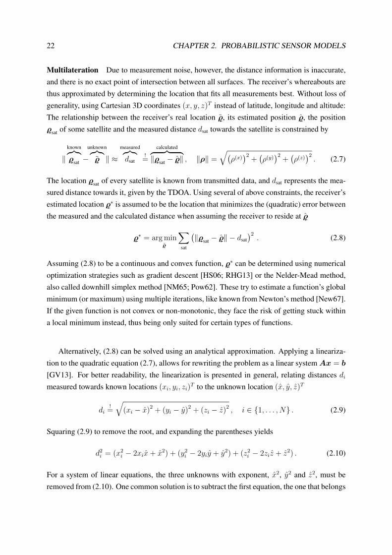
Multilateration Due to measurement noise, however, the distance information is inaccurate,and there is no exact point of intersection between all surfaces. The receiver’s whereabouts arethus approximated by determining the location that fits all measurements best. Without loss ofgenerality, using Cartesian 3D coordinates (x, y, z)T instead of latitude, longitude and altitude:The relationship between the receiver’s real location ρ, its estimated position ρ, the positionρsat of some satellite and the measured distance dsat towards the satellite is constrained by
‖known︷︸︸︷ρsat −
unknown︷︸︸︷ρ ‖ ≈
measured︷︸︸︷dsat
!=
calculated︷ ︸︸ ︷‖ρsat − ρ‖ , ‖ρ‖ =
√(ρ(x))2
+(ρ(y))2
+(ρ(z))2. (2.7)
The location ρsat of every satellite is known from transmitted data, and dsat represents the mea-sured distance towards it, given by the TDOA. Using several of above constraints, the receiver’sestimated location ρ∗ is assumed to be the location that minimizes the (quadratic) error betweenthe measured and the calculated distance when assuming the receiver to reside at ρ
ρ∗ = arg minρ
∑sat
(‖ρsat − ρ‖ − dsat
)2. (2.8)
Assuming (2.8) to be a continuous and convex function, ρ∗ can be determined using numericaloptimization strategies such as gradient descent [HS06; RHG13] or the Nelder-Mead method,also called downhill simplex method [NM65; Pow62]. These try to estimate a function’s globalminimum (or maximum) using multiple iterations, like known from Newton’s method [New67].If the given function is not convex or non-monotonic, they face the risk of getting stuck withina local minimum instead, thus being only suited for certain types of functions.
Alternatively, (2.8) can be solved using an analytical approximation. Applying a lineariza-tion to the quadratic equation (2.7), allows for rewriting the problem as a linear systemAx = b
[GV13]. For better readability, the linearization is presented in general, relating distances dimeasured towards known locations (xi, yi, zi)
T to the unknown location (x, y, z)T
di!
=
√(xi − x)2 + (yi − y)2 + (zi − z)2 , i ∈ 1, . . . , N . (2.9)
Squaring (2.9) to remove the root, and expanding the parentheses yields
d2i = (x2
i − 2xix+ x2) + (y2i − 2yiy + y2) + (z2
i − 2ziz + z2) . (2.10)
For a system of linear equations, the three unknowns with exponent, x2, y2 and z2, must beremoved from (2.10). One common solution is to subtract the first equation, the one that belongs

2.3. GLOBAL POSITIONING SYSTEM 23
to d1, from all others d2, . . . , dN, resulting in a system of N − 1 equations [Li+05]:
d2i − d2
1 =((x2
i − 2xix+ x2) + (y2i − 2yiy + y2) + (z2
i − 2ziz + z2))−(
(x21 − 2x1x+ x2) + (y2
1 − 2y1y + y2) + (z21 − 2z1z + z2)
)=x2
i − x21 + 2x(x1 − xi) + y2
i − y21 + 2y(y1 − yi) + z2
i − z21 + 2z(z1 − zi) ,
(2.11)
which can hereafter be rewritten as a system of linear equations,Ax = bx1−x2 y1−y2 z1−z2
x1−x3 y1−y3 z1−z3
...
x1−xi y1−yi z1−zi
xyz
=1
2
(d2
2 − d21) + (x2
1 − x22) + (y2
1 − y22) + (z2
1 − z22)
(d23 − d2
1) + (x21 − x2
3) + (y21 − y2
3) + (z21 − z2
3)...
(d2i − d2
1) + (x21 − x2
i ) + (y21 − y2
i ) + (z21 − z2
i )
. (2.12)
When more than four equations are given, the system is overdetermined and (2.12) can be solvedusing x = A+b, where A+ is the Moore–Penrose inverse A+ = (ATA)−1AT [Pen55]. Thisyields an approximate solution ρ∗ = (x, y, z) that, similar to (2.8), minimizes the quadratic errorbetween measured and calculated distances. However, due to the linearization via subtraction,the result represents an approximation, slightly differing from the one provided by (2.8) [Li+05].
For simplicity, above calculations were based on 3D Cartesian coordinates. The values gprovided from actual GPS sensors, however, are polar coordinates with latitude g(lat), longi-
tude g(lon), an altitude g(alt) and an error estimation g(err), e.g. returned by the NMEA protocol[AAO11] of portable receivers, or smartphone operating system APIs. The longitude is givenbetween −180° and 180° or from west to east. When walking along the equator, only the lon-gitude is changed. It will hereafter be referred to as the x-axis within the building’s coordinatesystem. The latitude runs from −90° to 90° or from south to north, and is referred to as y-axis.
Floorplan Mapping For being used by indoor localization, coordinates supplied by the GPSmust be converted to the coordinate system of the floorplan. This requires a calibrated reference(reflon, reflat, refalt) → (refx, refy, refz), e.g. for the building’s center, and a rotation angle refα,aligning the x and y axes with longitude and latitude, depending on the building’s orientation.As the GPS is only intended for outdoor use, altitude information can usually be omitted. Here-after, changes in longitude and latitude around their reference correspond with changes in x andy around the building’s center. While the transformation between both is nonlinear due to theearth’s curvature, it can be assumed as linear throughout the relatively small size of the building.Using the earth’s perimeter around the equator and converting this value to m/°
2πrearth
360°=
400 007 862 m
360°= 111 132.95 m/° , (2.13)

24 CHAPTER 2. PROBABILISTIC SENSOR MODELS
yields a constant, relating changes of ° in latitude to m, valid at alt = 0 m. As the earth’slatitudinal-perimeter decreases when moving towards the poles, the reference for changes inlongitude along this perimeter is varying, dependent on the current latitude:
flat (∆lat) = ∆lat 111 132.95 , flon (∆lon) = ∆lon(
cos(reflat) 111 132.95). (2.14)
As the earth is not perfectly round, but an ellipsoid, (2.14) represents a simplification. Usuallyseveral compensation terms are added to the equation to improve correctness [MS10]. Alterna-tively, other approaches, such as the one presented by Vincenty [Vin75], can be used. However,using this linear approach with a constant value, yields a computationally efficient, yet suffi-ciently accurate solution for the intended use case. The final conversion from polar coordinateswithin g to Cartesian coordinates, including the calibrated reference, is hereafter given by
posgps (g) =
refx
refy
refz
+
cos (refα) − sin (refα) 0
sin (refα) cos (refα) 0
0 0 1
flon
(g(lon) − reflon
)flat(g(lat) − reflat
)(g(alt) − refalt)
. (2.15)
Independent of the strategy used to estimate the location ρ of the GPS receiver, it will deviatefrom the device’s actual position. Depending on satellite visibility, quality of the time measure-ments and used hardware components, the sensor’s precision and accuracy will vary. Most GPSreceivers provide an error estimation g(err) (in m), that yields an indication on the quality of thecurrent location estimation. This value is determined by the sensor itself, in a similar way toexamining the variance among all individual distance errors from (2.8):
σ2gps = E(X 2)− (E(X ))2 , X =
∣∣‖ρsat − ρ∗‖ − dsat
∣∣ | ∀sat . (2.16)
The resulting error indication can be used to describe the likelihood of the receiver residing di-rectly at, or near the estimated position, also addressing bad reception conditions when buildingsor trees occlude the satellite signals [AAO11]. Based on the notation introduced in section 2.2
GPS evaluation︷ ︸︸ ︷pgps (ot | qt) =
normal distribution︷ ︸︸ ︷N(d∣∣ 0, σ2
gps
),
difference between GPS indication and unknown state︷ ︸︸ ︷d = ‖posgps
(o
(g)t
)− posxyz (qt) ‖
〈o〉t = 〈(g, . . .)〉t︸ ︷︷ ︸observations (2.3)
, 〈q〉t = 〈(x, y, z, . . .)〉t︸ ︷︷ ︸unknown state (2.3)
, g = (lon, lat, alt, err)︸ ︷︷ ︸GPS receiver provides
, σgps = g(err)︸ ︷︷ ︸uncertainty
,(2.17)
(2.17) denotes the corresponding evaluation (2.4). It describes a probabilistic relation betweenpotential pedestrian whereabouts (x, y, z)T , part of the unknown state qt, and current GPS read-ings g, part of the observation ot. This probability depends on the distance between both, es-

2.3. GLOBAL POSITIONING SYSTEM 25
-0.2
0
0.2
-2 -1.5 -1 -0.5 0 0.5 1 1.5 2
σ 2σ
Figure 2.3: GPS localization deviation (in m) for a static receiver under good reception conditions.Assuming normally distributed measurements, the two ellipses depict the corresponding confidence in-tervals for σ(≈ 68 %) and 2σ(≈ 95 %). Shape and rotation depend on the actual location on earth. Axislabels are therefore omitted. The median (left dot) does not resemble the average (centered dot).
timated after converting the GPS readings to the building’s Cartesian coordinate system using(2.15), and extracting (x, y, z)T from the unknown state
posxyz (qt) =(q
(x)t , q
(y)t , q
(z)t
)T. (2.18)
That is, (2.17) relates unknown states and the observation from the GPS by using a normaldistribution based on their distance, and the uncertainty indication g(err), given by the receiver.
Sensor Uncertainty For many sensors and use-cases, their error/noise is assumed to follow azero mean Gaussian distribution, like in (2.17) [Smi99]. This implies, that the values returnedby some sensor are symmetrically distributed around the real value, and the average of an in-finite number of measurements, produces the real value. While being a correct assumption formost calibrated sensors, aforementioned environmental conditions can affect the measurementnoise. Especially a bad line of sight towards the sky can greatly affect the accuracy of the lo-cation estimations returned by a GPS receiver [Och+14; DH10]. Such conditions can yield anon zero mean measurement noise, where all estimations drift from the actual location. Figure2.3 depicts several measurements from a static receiver with a clear line of sight towards thesky. Even under ideal conditions, they can be influenced and might be shifted from the actuallocation. Comparing their median (left dot) and average (centered dot) indicates that this is thecase for the depicted observations. Still assuming a zero mean Gaussian noise in such cases,yields an error, as the density is shifted from the real value.
With the direction of the shift unknown, and the sensor only providing a hint on its amount,a uniform distribution comes to mind as potential alternative. However, while this ensures thatevery location within the confidence-radius around the sensor’s estimation has the same prob-ability, all values outside of this region receive a likelihood of zero, which is usually incorrect.This can be addressed by combining both aforementioned distributions: A uniform distributionfor all values within the range of the indicated error g(err) and a normal distribution for all valuesoutside of this region. The transition between both distributions should be continuous and the

26 CHAPTER 2. PROBABILISTIC SENSOR MODELS
0
0.1
0.2
0.3
0.4
-4 -3 -2 -1 0 1 2 3 4
raR(x|µ,r
a)
cropped normal distributionnormal distribution
Figure 2.4: Modification of the normal distribution, created by inserting a uniform distribution in thecenter. The filled and crossed parts denote the redistribution, ensuring the result sums to 1.0.
area of the resulting probability density function (PDF) must satisfy∫ ∞−∞
p(x) dx = 1.0 . (2.19)
To meet those requirements, the overall density can e.g. be conceived as an equal split betweenthe uniform and the normal distribution, shown in figure 2.4. The true location often residessomewhere within the region of ±g(err) around the indicated value, or µ± ra in general. This iscovered by a uniform distribution U (µ− ra, µ+ ra) around the center µ. The width 2ra of thedistribution is variable and depends on the error currently indicated by the receiver. Consideringjust the uniform distribution, the height rh must be chosen to ensure the area satisfies (2.19),that is: 2 ra rh = 1.0. To seamlessly connect both distributions, the normal distribution’s highestpoint has to be on par with the height of the uniform distribution. Its σ is thus constrained by
rh!
= max(N (. . . , σ2)
)=
1√2πσ2
⇒ σ =1√
2πrh. (2.20)
The combined distribution is calculated by making each input variable x zero mean, condition-ing the next step on whether this intermediate value resides within the uniform or within thenormal distribution, and normalizing the result by 0.5, to satisfy (2.19), summing up to 1.0
R (x | µ, ra) =1
2
U(x′ | −ra,+ra) for x′ < ra
N (x′ − ra | 0, σ2) else
x′ = |x− µ| , rh =ra
2, σ =
1√2πrh
.
(2.21)
When using (2.21), the evaluation (2.17) of the pedestrian’s whereabouts is rewritten as
pgps (ot | qt) = R(d∣∣ 0, g(err)) . (2.22)
One major issue presented by the GPS is the time needed until the first fix, or location informa-tion, is provided. Especially when leaving a building to move between adjacent complexes, the

2.4. INERTIAL MEASUREMENT UNIT 27
amount of time can be too short for a fix to become available. Furthermore, in case of adjacentbuildings, the signal might be shadowed, increasing the time even further, hereafter providingonly coarse location estimations due to bad satellite visibility [DH10; Ebn+17]. Another draw-back is presented by increased energy consumption when a smartphone’s GPS is active. Thus,it should only be enabled when it is expected to provide viable results, that is, outside of a build-ing [Cap+17]. Therefore, Zhou et al. [Zho+12] proposed a system that uses other smartphonecomponents, such as the light sensor, or the celltower signal strength, to distinguish betweenindoors and outdoors. However, they also denote that the accuracy outdoors will greatly varydepending on surroundings and weather conditions. For large error indications it thus makessense to ignore readings provided by the GPS, and rely on other sensors instead.
2.4 Inertial Measurement Unit
As mentioned initially, a navigation system for cars benefits from additional information besidesthe GPS, such as the current driving speed or direction. Both values can be used to stabilizethe localization when the GPS is unreliable, or to provide location updates whenever it is un-available, e.g. when driving through a tunnel. A similar procedure has been used by seafarersfor decades, estimating the ship’s current location based on its revolution counter and a com-pass, when astronomical fixes, such as stars, were invisible or ambiguous [Ser28]. Approachesbased on those two parameters, speed and heading, are known as inertial navigation systemsINS, or dead reckoning. They predict the current position based on the previously known posi-tion and heading, using recent information for movement/speed and heading/direction-changes,thus representing a relative location estimation. It also applies to aviation, where the current air-speed, measured by Pitot tubes, is combined with the heading provided by a magnetic compassand gyroscope, to navigate relatively between landmarks with known absolute locations [Pit32].When the initial location and heading are known, dead reckoning can be applied for pedestrianindoor navigation and localization as well. In many scenarios a pedestrian enters a building at aknown location, or this location can be provided by the last GPS readings, just before enteringthe building [Hut+16; Och+14]. Starting from this known state, dead reckoning can be used toupdate the pedestrian’s location based on relative movements. This itself is a well establishedfield of research, known as pedestrian dead reckoning (PDR).
Almost all modern smartphones contain a so-called inertial measurement unit (IMU), whichis a group of several individual sensors, related to inertial measurements. As of today, the IMUwithin most devices provides an accelerometer for absolute gravity/pose measurements, a gyro-scope for relative pose changes, and a magnetometer for absolute magnetic field measurements.Based on those three sensors, it can be inferred whether the pedestrian is currently walking,

28 CHAPTER 2. PROBABILISTIC SENSOR MODELS
taking stairs, or changing the heading. While walking speeds can roughly be approximated[Yu+19], the quality strongly depends on how the pedestrian holds the smartphone while walk-ing. Dedicated foot-mounted accelerometers are more suited for this estimation, as the impactof acceleration is very pronounced, and can be used to estimate the distance taken with everysingle step [NPM13]. This, however, is impracticable when dealing with smartphone-basedindoor localization and navigation, where the pedestrian often holds the phone in front of thebody. Here, the required forward acceleration is mainly measurable when starting or stoppingto walk, and can easily be confused with shaking the phone during the walk [KWS12].
While aforementioned velocity estimation is rather unstable, single steps made by the pedes-trian create a measurable change in acceleration, representing the base for step-detection. Com-bined with average human step lengths, the walking speed is approximated [TS12; Kop+14;SD16]. Likewise, the gyroscope measures relative changes in pitch, roll and yaw, and thusprovides a corresponding turn-detection for the pedestrian [Ebn+15; Jan+15; Li+12]. Due toonly capturing relative changes, the current absolute heading depends on the availability of theinitial heading, which is hereafter adjusted by all measured changes. This drawback can bemitigated by readings from a magnetometer, which serves as an eCompass, providing a coarseinformation on the current absolute heading, yet, prone to errors e.g. induced by nearby metalobjects [Goy+11; ND97; She+09; Goz+11].
Despite apparent simplicity, this topic is still under extensive research. Even though sensoraccuracies are steadily increasing, filtering is still required. Not only to distinguish betweenactual data and sensor noise, but also to prevent temporal errors, like metallic objects influencingthe compass, and to stabilize the resulting estimations over time [Tia+15; ND97]. While mostof today’s sensors provide very accurate readings, with small amounts of noise [Mou+15], theirvalues do not allow for absolute location estimations, but only for relative changes, representingone of the major issues of dead reckoning. Even if individual readings only face a small errorε, they contribute to every relative adjustment and thus accumulate over time
dt+1 = dt + (v + ε)∆t , dt+2 = dt+1 + (v + ε)∆t → dt+n = dt + n(v + ε)∆t . (2.23)
Within (2.23), the distance dt from an initially known position is adjusted at fixed time intervals∆t by using the current velocity-indication v, which faces an error ε. As mentioned earlier, thiserror is often assumed to be normally distributed. The resulting cumulative errorE is thus givenby a normal distribution, with mean and uncertainty dependent on the number of cumulations
εi ∼ N (µ, σ2) , E =N∑i=1
εi ⇒ E ∼ N (Nµ,Nσ2) . (2.24)

2.4. INERTIAL MEASUREMENT UNIT 29
x
y
z
x
y
z
Figure 2.5: Coordinate system of most smartphone’s IMU-sensors [Goob; App] (left). When the pedes-trian holds the device in front, slightly tilting it for a good view angle, this coordinate system is rotatedwith respected to the world’s coordinate system (right), affecting the readings from contained sensors.
For calibrated sensors, the error should be zero mean, and thus Nµ = 0. Cumulation stillyields an average of zero and only the variance σ2 increases linearly with N . That is, the resultafter cumulation is close to the true value, but its uncertainty has increased, yielding a lowerprecision. For most real-world scenarios, however, accuracy is not ideal and a constant offset µcumulates over time, yielding results which are neither accurate, nor precise [Smi99].
Assuming an object to travel with 14 m/s, and the error of its velocity sensor to be zeromean Gaussian with σ = 0.5 m/s. According to (2.24), after 120 s it traveled 1680 m, with anuncertainty σ = 5.5 m. Based on the integral
∫ +2σ
−2σN (1680, 5.52), the real distance is within
(1680± 11) m, with a confidence of ≈ 95 %. Even though the uncertainty of 0.5 m/s and thetimeframe of 120 s are rather large, ±11 m is small compared to 1680 m. However, if the sen-sor is slightly off, indicating 14.1 m/s instead, the object is expected to have moved 1692 m
after 120 s. The small offset of 0.1 m/s yields an average result, outside of the previous confi-dence interval of (1680± 11) m. Especially for problems with cumulative errors, such as deadreckoning, offsets in accuracy must be prevented. To address those offsets, the sensor requirescalibration to determine both, the type (cf. figure 2.2) and amount of the induced error [Tia+15].
For constrained use-cases, where a cumulative error is tolerable, and both, starting positionand heading, are well known, just using PDR without additional sensors might already be suf-ficient. State of the art PDR solutions provide viable results with minimal sensor requirementsand little or no prior knowledge about the walkable area. For longer walks within complexarchitecture, however, PDR will suffer from increasing errors and requires stabilization usingabsolute location information [CHP16; JPP18; Kna17].
To use a smartphone’s IMU for PDR, the observations from its sensors must be interpretedcorrectly. As of today, the contained accelerometers, gyroscopes, and magnetometers all pro-vide readings for three orthogonal axes. Typically, all three sensors are placed in the same way,

30 CHAPTER 2. PROBABILISTIC SENSOR MODELS
sharing the same alignment of these axes. Figure 2.5 depicts the coordinate system used withinmost smartphones [Goob; App]. When the device is placed display-up on a table, the sensors arealigned parallel to the earth’s surface, with the z-axis pointing upwards, and measurements fromthe accelerometer are approximately ≈ (0, 0, 9.81) m/s2. Within the following discussions, thepedestrian is expected to hold the smartphone in one hand in front of the body, slightly tiltingit for a good display viewing angle (cf. figure 2.5). This pose is expected to be typical for mostpedestrians using indoor navigation, watching routing advice on the device’s screen. Due to thetilt, the smartphone’s coordinate system is rotated, affecting the readings provided by all IMUsensors. This rotation must be considered to correctly interpret sensor readings, aligning themwith the coordinate system assumed for the world, that is, the building’s floorplan.
The following sections discuss IMU-based approaches that are viable for a smartphone-based indoor localization and navigation system. This covers the three main topics of step-detection, turn-detection and eCompass. Handling the rotation induced by the pedestrian tiltingthe smartphone will be covered in detail. Discussions also include expected errors, to deriveprobabilistic models including each sensor’s uncertainty. Where applicable, potential calibra-tions, to increase accuracy, are examined as well.
2.4.1 Step-Detection
As previously mentioned, determining the pedestrian’s current walking speed based on availablesmartphone sensors is inaccurate, at least when the device is held upfront. This drawback ismitigated by step-detection, serving as an approximate velocity indicator for the dead reckoningprocess. When a pedestrian walks along a corridor, each step creates a measurable change inacceleration, once when a foot is lifted, and once when touching the ground [TS12]. Thosechanges yield a unique pattern, detectable for all smartphone poses, within the data provided bythe accelerometer, measuring the current gravity.
Due to the IMU coordinate system (cf. figure 2.5), measurements a = (x, y, z) provided bythe accelerometer are approximately a ≈ (0, 0, 9.81)m/s2 when the phone is placed display-upon the ground. When holding the device in the same way while walking, that is, parallel to theearth’s surface, only the z-axis experiences aforementioned acceleration changes, and fluctuatesaround 9.81 m/s2, denoting individual steps. When navigating, the pedestrian usually looks atthe smartphone’s display by slightly tilting the upper screen edge towards the head, resulting ina rotation around the x-axis (see figure 2.5). After applying this rotation to the readings fromthe sensor, the x-value still stays near zero and only contains the natural left-right-fluctuation ofhumans moving their hands while walking. The earth’s gravity, however, is redistributed amongthe y and z-axis, depending on the tilting angle, and the step-pattern can also be observed when

2.4. INERTIAL MEASUREMENT UNIT 31
−4
0
4
8
12
2 s 4 s 6 s 8 s 10 s 12 s 14 s 16 s 18 s 20 s
z
y
x
acce
lera
tion
(m/s2
)
Figure 2.6: Readings from a smartphone’s 3-axis accelerometer sensor over time, sampled at 20 Hz for abetter visibility. The pedestrian walked along a hallway, holding the smartphone slightly tilted in front ofthe body (cf. figure 2.5), ≈1.3 m above ground. Each major spike on the z or y-axis denotes one singlestep. The x-axis is based on left-right-movements of the pedestrian’s right arm during the walk.
examining the data of the y-axis. A matching example is shown within figure 2.6. While theused smartphone holding pattern is typical for indoor navigation, it can not be assumed to bea given, and the pedestrian might refer to other poses, such as landscape-mode, or carrying thephone within trouser pockets, listening to navigation advice via earphones [Kus+15].
As the direction of change in acceleration is not required for detecting steps, rotation invari-ancy is achieved by using the magnitude of the sensor readings [SD16]. That is, the Euclideannorm ‖(a(x), a(y), a(z))T‖ of the measurement. This value still yields an average of≈ 9.81 m/s2,and preserves the deviations imposed by each step. However, this will usually introduce someside-effects and generate spikes that are not related to actual steps, e.g. when the pedestrianshakes the device, or changes the orientation from landscape to portrait or vice versa [Ebn+15].
Alternatively to using the magnitude, the accelerometer readings can be transformed. Thisis achieved by undoing the rotation introduced by the pedestrian tilting the device. Hereafter,the adjusted sensor readings are similar to the ones from the phone placed parallel to the ground,where a(x) and a(y) are almost 0 and a(z) fluctuates around 9.81 m/s2, containing the typical steppattern [Tia+15]. Mathematical details on how to undo the rotation induced by the pedestrianholding the smartphone will be discussed in section 2.4.2. When e.g. carrying the phone withintrouser pockets, this rotation is not constant, but changes throughout every step. Furthermore,vibrations and the effect of acceleration changes are different when the device is carried in thisway. Park et al. [PHP17] suggest additional machine learning via SVM classification to detectpotential smartphone poses, improving rotation invariance and the overall detection of steps.
Independent of the approach chosen for rotation invariance, the resulting data features astep-specific pattern, consisting of a steep increase, followed by a steep decrease [TS12; Li+12].Basic strategies thus e.g. determine peaks that are above an empiric threshold. If a peak is de-tected, the process is stopped for some time, to prevent multiple small peaks in sequence, usu-ally vibration or noise, from also triggering detected steps. This blocking-period is a heuristic,dependent on the expected step frequency [PHP17]. The requirement for this delay can clearly

32 CHAPTER 2. PROBABILISTIC SENSOR MODELS
be identified when looking at the z-axis signal course in figure 2.6. While the steps between7 s and 14 s are relatively clear, many occurrences of minor local peaks can be observed as well(around 6 s or 19 s), yielding too many step-detections when not being suppressed.
More robust approaches focus on finding local maxima within a certain timeframe. Using awindow of several samples provides the same effect as aforementioned delay times, preventingseveral nearby peaks from triggering too many detected steps [TS12]. Besides local maxima,zero crossings can also be used to realize step detection, where two zero crossings denote onestep. For this to work, readings from the accelerometer must be approximately zero mean. Incase of the magnitude-based approach this is e.g. achieved by subtracting the constant gravity of9.81 m/s2, or, in general, by subtracting a long-term average of the signal from itself [Kir+18].Both techniques, detecting zero crossings and making a signal zero mean, are computationallyinexpensive, thus ideal for use on embedded devices, such as smartphones [Goy+11].
Efficient Noise Reduction As indicated in figure 2.6 and figure 2.7, there is a significantamount of noise within the measurements, affecting the step-detection process. Using zerocrossings and local maxima detection mitigates the problem only to some degree. For a morerobust stabilization, independent of the used detection method, the input signal should be filteredbeforehand. With noise typically being a fast-changing component, a low-pass filter can be usedto remove high frequencies from the signal [Kir+18]. The most simple low-pass is the movingaverage filter, using the average of several consecutive samples to suppress fast changes. Whilebeing computationally efficient, its configurability is rather limited.
For frequency-based filters to be used on a discretely sampled signal, it must be provided at aconstant sample-rate [Smi99]. However, as neither sensor nor API of common smartphones arerequired to provide samples at equidistant intervals, a constant sample rate can not be assumedin general. This also imposes potential issues when searching for a specifically-shaped patternwithin the provided sensor data. To construct a fixed sample rate, a combination of interpolationand resampling can be applied to the incoming measurements. Update rates provided by anaccelerometer usually are high, 200 Hz and above, thus requiring for downsampling to lowerrates, sufficient for the step-detection process. This is e.g. achieved by selecting the nearestneighbor, the reading that is temporally next to the required output, or by interpolating betweenthe two nearest ones. If the sample rate of the sensor is much higher than the required output,using the nearest neighbor is sufficient in terms of precision [Smi99]. For all following steps,measurements are assumed to occur at a fixed rate of 100 Hz, which is an empiric choice that issufficiently fast to detect individual steps, yet conserving computational power [SD16; PHP17].
With the signal now available at a fixed sample rate, a configurable low-pass can be applied,by using either a finite impulse response (FIR) or an infinite impulse response (IIR) filter. Gen-

2.4. INERTIAL MEASUREMENT UNIT 33
7
9
11
13
15
10 s 20 s 30 s 0 Hz 2 Hz 4 Hz 6 Hz
mag
nitu
de(m/s
2)
ampl
itude
Figure 2.7: Magnitude of accelerometer readings, fluctuating around 9.81 m/s2, for a pedestrian walkingalong a hallway while holding the smartphone in front of the body (left). The corresponding frequencyspectrum (right) denotes the signal’s composition, and indicates the pedestrian’s step-rate of ≈ 1.8 Hz.
erally, the latter is computationally less complex, but the former provides better results. In thiscontext, better refers to undesired frequencies being removed more effectively, without affect-ing the desired ones. That is, the cut-off between required and unwanted parts of the signal ismore rapid, and the attenuation of the unwanted stopband is higher. However, while the IIRinvolves just a few multiplications and additions with small delays, the improved attenuation ofFIR filters comes at the cost of required computational power, and larger delays [Smi99].
To be consistent with the notation typically used in digital signal processing, the followingfilter equations will re-purpose previously introduced variables.
A well known variant of IIR is the second-order or biquad filter, using three coefficientsb0, b1, b2 on the discrete input signal x[ ], and three a0, a1, a2 on previous discrete outputs y[ ],thus creating an infinite recursion. An implementation in so-called direct form 1 is given by
y[n] =1
a0
(b0x[n] + b1x[n−1] + b2x[n−2] − a1y[n−1] − a2y[n−2]
). (2.25)
It only requires a few multiplications, additions and a history of two previous inputs and outputs,well suited for realtime use. The coefficients a0, a1, a2 and b0, b1, b2 are determined based onthe desired effect. Noise can e.g. be removed from the input signal by configuring a low-passfilter, removing all frequencies above a certain cut-off frequency. The required values for thesix components can directly be calculated based on the desired cut-off frequency, and sensorsample rate. Equations and further details are found in [Ror93; WT06; Smi99].
The low-pass’ cut-off frequency depends on the pedestrian’s walking speed, shown on theright side of figure 2.7. Its result is sufficient for most step-detection strategies, such as afore-mentioned peak detection. Others, like searching for zero-crossings, require the signal to be zeromean, with the constant gravity offset removed. To include this additional requirement, a band-pass filter can be used, keeping only the desired frequencies around ≈ 1.8 Hz (cf. figure 2.7).While all six coefficients are again directly calculable, there is less control on the actual sizeof the passband, which, however, is an important requirement to correctly adapt to significantly

34 CHAPTER 2. PROBABILISTIC SENSOR MODELS
−2
−1
0
1
2
10 s 20 s 30 s 40 s
mag
nitu
de(m/s
2)
step
Figure 2.8: Band-pass filtered zero mean accelerometer magnitude, using the input from figure 2.7. Theapplied step-detection searches for local maxima that are above a certain threshold (grey line).
varying individual step frequencies [Sau+11]. More control is given by cascading multiple IIRfilters. For example, one high-pass to remove the constant gravity and low frequency noise, likethe pedestrian shaking the phone while walking, and one low-pass to suppress noise.
More versatile, in terms of configurability, are FIR filters, based on a discrete convolution ofthe input signal with some kernel. As a convolution in the time domain equals a multiplicationin the frequency domain, the kernel can easily be created by choosing the frequencies to keep,and applying an inverse Fourier transform [Smi99]. The drawback of this approach is increasedcomputational overhead. The filter’s quality directly depends on the size kernel, which is thusrequired to have a decent size. Furthermore, the convolution introduces delays based on thissize, delaying the output of the accelerometer, and thus the step-detection process. For example,a sample rate of 100 Hz required N ≥ 101 coefficients for the band-pass’ kernel, yielding aN−1
2≥ 500 ms delay. Further details and considerations can be found in [Ror93; Smi99].
Besides using an IIR or FIR band-pass, low frequency noise and the constant gravity offsetcan also be removed by subtracting the input’s moving average of size N ′ from it
y[n] = x[n] −1
N ′
N ′∑n′=0
x[n−n′] , (2.26)
hereafter sending the result through a low-pass filter to remove high frequency noise. While themoving average also introduces a delay based on N ′, it can be neglected, as the to-be-removedcomponents (e.g. gravity) are approximately constant, not causing any delays for the actualstep-pattern. Which of the discussed filtering variants serves best for an actual system, stronglydepends on required quality, acceptable delays, and available computational performance.
Probabilistic Assembly After filtering, one of the described strategies can be used to detect ifthe n-th sample denotes a step. A local maximum detection on the discrete, filtered magnitude
A[ ] = filter(‖a[ ]‖
)(2.27)

2.4. INERTIAL MEASUREMENT UNIT 35
requires values before and after the maximum for a correct identification, that is, future values,thus introducing slight delays to drop this requirement when evaluating live readings
fstep(A[ ], n
)= (A[n−2∆] < A[n−∆]) ∧ (A[n−∆] > A[n]) , ∆ ∈ N>0 . (2.28)
Whether a detected maximum denotes a step also depends on its magnitude [Kop+14; PHP17].This is depicted in figure 2.8, where only peaks above a certain threshold heuristic are classifiedas steps. Instead of a constant, heuristic threshold, the signal’s moving variance could be used,detecting all peaks that are beyond the signal’s average fluctuation. Yet, this imposes issues forsituations where the pedestrian isn’t walking. Standing still yields a low overall variance, andpeaks induced by noise can cause false-positives, thus requiring additional handling [TS12].
As mentioned earlier, when computational power is limited, step-detection can be performedwithout prior filtering, at the expense of accuracy. The maximum detection (2.28) is still viable,but requires a dead-time after each detected step to prevent noisy spikes within the magni-tude from causing false positives. While more sophisticated algorithms can cope with multiplesmaller peaks and are also able to search for periodic occurrences within the signal, well-suitedfor step-detection [SBW12], they come at the expense of required computational power.
All of the mentioned detection approaches performed a binary yes/no classification for steps,based on some metric or heuristic. For values that are far beyond the chosen threshold, theclassification is clear. If the value is only slightly above or below the threshold, the correctnessof the algorithms classification is uncertain. This can be addressed by using a probabilisticclassification instead, where each potentially detected step is assigned a probability for it torepresent a real step. The probability e.g. depends on how pronounced the step appears withinthe accelerometer readings, where the magnitude can be used to infer a probability pstep
(A[n]
)for A[n] to denote a step, by applying a probability distribution. As more pronounced peaksusually are more likely to represent a step, the corresponding probability can e.g. be inferred bysending the reciprocal of A[n] into an exponential distribution with some value for λ
pstep(A[n]
)= λ exp
(−λ(A[n]
)−1), λ > 0 , A[n] ≥ 0 . (2.29)
When results are preferred within the range of [0, 1], (2.29) can be unnormalized
pstep’(A[n]
)= exp
(−λ(A[n]
)−1). (2.30)
The result of applying this unnormalized version to the data from figure 2.8, is shown in fig-ure 2.9. The probability of all obvious steps is approximately the same. Peaks that were belowthe threshold within figure 2.8 are now also detected, but rated with a much lower probability.

36 CHAPTER 2. PROBABILISTIC SENSOR MODELS
0
0.2
0.4
0.6
0.8
1
10 s 20 s 30 s 40 s
pst
ep’( A [n
])
Figure 2.9: Result after applying (2.30) with λ = 0.15 to the data from figure 2.8, omitting all values≤ 0. While all obvious steps share approximately the same probability, uncertain steps are still detected,but rated with a much lower probability.
Koping et al. mention that, while more pronounced peaks usually denote an increased proba-bility, peaks above a certain threshold might not be related to steps, but to other events, like thesmartphone being shaken by the pedestrian. Therefore they propose using a Gamma distributioninstead, to model an area of interest up to a certain threshold [KGD14].
Independent of whether a binary or probabilistic classification is used, step-detection onlyestimates the number of steps taken. Unlike a car’s speedometer, there is no hint on the currentwalking speed, which also depends on the pedestrian’s step size. This size not only varies fromperson to person, but also over time, and is dependent on current ambient conditions. Whileclimbing stairs, the pedestrian usually takes one tread at a time, and the step size matches thewidth of each tread. For stairs to be comfortable, the tread size should follow some rules, basedon average step sizes along ground and the stair’s inclination, first mentioned by Blondel inthe 17th century [Blo83, pp. 672]. As of today, most stairs use a tread size somewhere around29 cm [RRF02; SJP13]. The step size on ground, however, is more variable, and depends onage and sex of the pedestrian. Saunier et al. mention that reliable sources for pedestrian stepsizes are hard to find, and thus conducted own experiments with subjects from several countries.Depending on the dataset, they conclude that the average step size is around 0.68 m with a highdeviation of ±0.22 [Sau+11]. Other approaches therefore try to dynamically estimate the steplength, which is only practical when the smartphone is held in a specific pose [Yu+19].
Combining the mentioned aspects, an evaluation (2.5) working for both, discrete yes/noo
(step)t ∈ 0, 1, and continuous probabilistic o(step)
t ∈ [0, 1] step observations, is given by
pstep(ot | qt, qt−1
)=
step made︷ ︸︸ ︷o
(step)t N
(d∣∣ µstep, σ
2step
)+
no step made︷ ︸︸ ︷(1− o(step)
t )N(d∣∣ 0, σ2
stand
)d = distxy
(qt−1, qt
), 〈q〉t = 〈(x, y, z, . . .)〉t , 〈o〉t = 〈(step, . . .)〉t ,
(2.31)
using the two dimensional Euclidean distance
distxy(qt−1, qt
)= ‖posxy
(qt−1
)− posxy (qt) ‖ (2.32)

2.4. INERTIAL MEASUREMENT UNIT 37
between two states, based on the two dimensional location contained within each one
posxy (qt) =(q
(x)t , q
(y)t
)T. (2.33)
(2.31) converts every potential state change from qt−1 to qt into a distance, which is comparedusing two normal distributions, depending on whether a step has been detected, o(step)
t = 1, ornot o(step)
t = 0. When detected, this distance should be near the pedestrian’s step size µstep, withsome uncertainty σstep. Otherwise, there should be no movement, thus comparing against a zeromean normal distribution. The same holds true if o(step)
t is not a discrete yes/no decision, but acontinuous probability for the current detection to denote a step. Here, the two distributions arecombined based on the value of o(step)
t ∈ [0, 1], resulting in a mixture distribution.
Depending on the pedestrian’s step frequency [Sau+11] and the timeframe between qt andqt−1, more than a single step might have occurred. For handling such cases, the discrete o(step)
t
could e.g. be replaced by a number of detected steps, resulting in
psteps(ot | qt, qt−1
)=
N(d∣∣ nµstep, nσ
2step
)n > 0
N (d | 0, σ2stand) n = 0
n = o(steps)t , o
(steps)t ∈ N0 , 〈q〉t = 〈(x, y, z, . . .)〉t , 〈o〉t = 〈(steps, . . .)〉t .
(2.34)
All presented evaluations used the readings from a phone’s accelerometer, to infer the likelihoodof potential movements based on detected steps. Combined with either an estimated or empiricchoice for the step size, it constrains the distance, walkable within a certain timeframe.
2.4.2 Turn-Detection
Besides the distance moved within a certain timeframe, inferred by e.g. a car’s speedometer,or step detection for pedestrians, this movement’s direction is also required, to perform relativelocation updates. In case of outdoor navigation within cars, this heading is only of minor impor-tance, as potential movements are spatially limited by the road network. Assuming the driver tostay on the last known road, the direction of the movement is defined by this road’s course. Incase of U-turns and intersections, however, heading changes are mandatory. A sensor directlyinstalled within the car’s steering wheel is able to provide very high resolutions at almost noerror [XYH09], and yields the current steering angle, chosen by the driver. Combined with thecar’s velocity, a turn-rate in °/s can be determined. The sensor thus provides relative headingchanges, requiring the previous heading to be known. For car navigation, this value can oftenbe estimated, e.g. by using the course of the currently expected road as absolute heading.

38 CHAPTER 2. PROBABILISTIC SENSOR MODELS
Within open environments, as in seafaring, aviation or large buildings, estimating the head-ing based on the current location often is unfeasible, as potential directions are rarely con-strained by the environment. Furthermore, in contrast to the sensor of the car’s streering wheel,sensors within a ship’s or airplane’s rudder are less reliable, as the actual direction is also af-fected by ocean current, crosswinds or similar. That is, even though the sensor’s indication itselfis precise and accurate, the actual direction can deviate due to environmental influences. Con-cerning pedestrians, the problem is even more pronounced, requiring for different approaches.
While a compass is one of the first sensors that comes to mind when thinking of heading,there are several drawbacks. The earth’s magnetic field is relatively weak, compared to the in-fluence of metal objects or magnets near the sensor. Provided readings are thus easily distorted,and often unreliable, especially indoors [Goz+11]. Furthermore, the compass relies on a decli-
nation angle, to relate magnetic and geographic north. As the earth’s magnetic field is subject tochanges, this value is not constant, and also depends on the current location on earth, requiringthe absolute location on earth to be approximately known [MMM96]. Aforementioned issueslead to the compass not being the first sensor-choice for heading estimation indoors.
Typically, cars, airplanes, ships and pedestrians move within a plane that is parallel to theground, which, regarding the coordinate system from figure 2.5, is the (x, y)-plane. Changes inheading are thus given by a rotation around the perpendicular z-axis. As building floors, andthus the (x, y)-plane, are parallel to the earth’s surface, gravity manifests along the z-axis of thiscoordinate system. Rotating around this axis will therefore not affect the measurable gravity,and accelerometers are unable to infer the current heading when moving along that plane.
To address the problem, ships use a so-called gyrocompass. This instrument contains afast-spinning flywheel, attached to a gimbal ring, aligning itself parallel to the earth’s rotationaxis, and thus pointing towards geographic north/south, independent of a magnetic field. Theflywheel keeps this alignment, similar to the wheels of a fast moving bicycle. When turning thegyrocompass, the gimbal ring allows the wheel to stay as-is. The device thus provides the ship’scurrent absolute heading with respect to the earth’s geographic north/south [Lu+94; Wes50].
Airplanes often rely on a more general version of the gyrocompass, called gyroscope, al-lowing for more degrees of freedom, needed for the plane’s attitude, heading and turn. Thegyroscope also features a fast spinning flywheel, but is allowed to rotate freely around all threeaxes. Due to spinning, the flywheel keeps its orientation, even when its exterior (the plane itself)is moving. Compared to the gyrocompass, there is no absolute alignment for the flywheel. Itjust keeps the pose it had during the time of spin-up. Especially within smaller aircrafts, thepilot thus has to manually adjust the instrument to display the correct value for the current pointin time, e.g. by using an additional compass. Hereafter, the instrument shows all movements

2.4. INERTIAL MEASUREMENT UNIT 39
relative to this initial position [ND97]. Due to the relative aspect and mechanically movingparts, the instrument is expected to suffer from drifts, increasing over time [FM63].
This type of sensor, yet much smaller and less mechanical, is installed within most smart-phones’ IMU. Opposed to instruments found in ships and airplanes, this sensor does not providean absolute angle θ′(t) with respect to the earth’s north/south (ship’s gyrocompass), or the initialspin-up (airplane’s gyroscope), but denotes how fast it is currently being turned by influencesfrom the outside. This angular velocity ω′(t) is given in rad/s (or °/s) for any given instantin time t. An absolute value is thus given by cumulating all changes since t = 0, that is, theintegral over all consecutive readings
ω′(t) =dθ′
dt, θ′(t) =
∫ t
0
ω′(t) dt , ω′ = (x, y, z)T . (2.35)
When dealing with discrete sensor readings ω′[ ], provided by a smartphone’s operating system,
an approximation of (2.35) must be used instead. As mentioned earlier, readings will not neces-sarily be provided at equidistant points in time. Therefore, the (varying) time ∆t since the lastreading has to be included as well, to correctly convert rad/s to rad
θ′(t) ≈N∑n=1
∆tω′[n−1] , ∆t = ftime (n)− ftime (n− 1) , ftime (N) ≤ t . (2.36)
(2.36) approximates the continuous integral, with the error becoming infinitesimally small for∆t → 0. However, this value depends on the sensor’s sample rate and e.g. callbacks providedby a smartphone’s operating system. Besides other workarounds, the trapezoid rule (2.37) is anoften used improvement when dealing with discrete integrals [KU94]:
θ′(t) ≈N∑n=1
∆tω′[n−1] + ∆t
ω′[n] − ω′
[n−1]
2=
N∑n=1
∆tω′
[n−1] + ω′[n]
2. (2.37)
(2.36) and (2.37) provide the three angles θ′(x), θ′(y) and θ′(z) in rad, the gyroscope has been ro-tated by since t = 0. When adding the initial, absolute alignment, this derives the smartphone’scurrent pose. To prevent errors, ∆t should not only be as small as possible, according to aboveequations, it should be as exact as possible. Every error in measuring this time difference willdirectly affect the result of (2.36) and (2.37). If it is off by 1 %, so is the cumulated output.
As long as the IMU’s z-axis is aligned parallel to the world’s z-axis, that is, the smartphonebeing placed parallel to the ground, ω′(z) read from the gyroscope directly denotes the pedes-trian’s change in heading per second. If the phone is not parallel to the ground, this turn-rate issplit among all three axes, ω′(x), ω′(y) and ω′(z), depicted in figure 2.10. This is similar to the
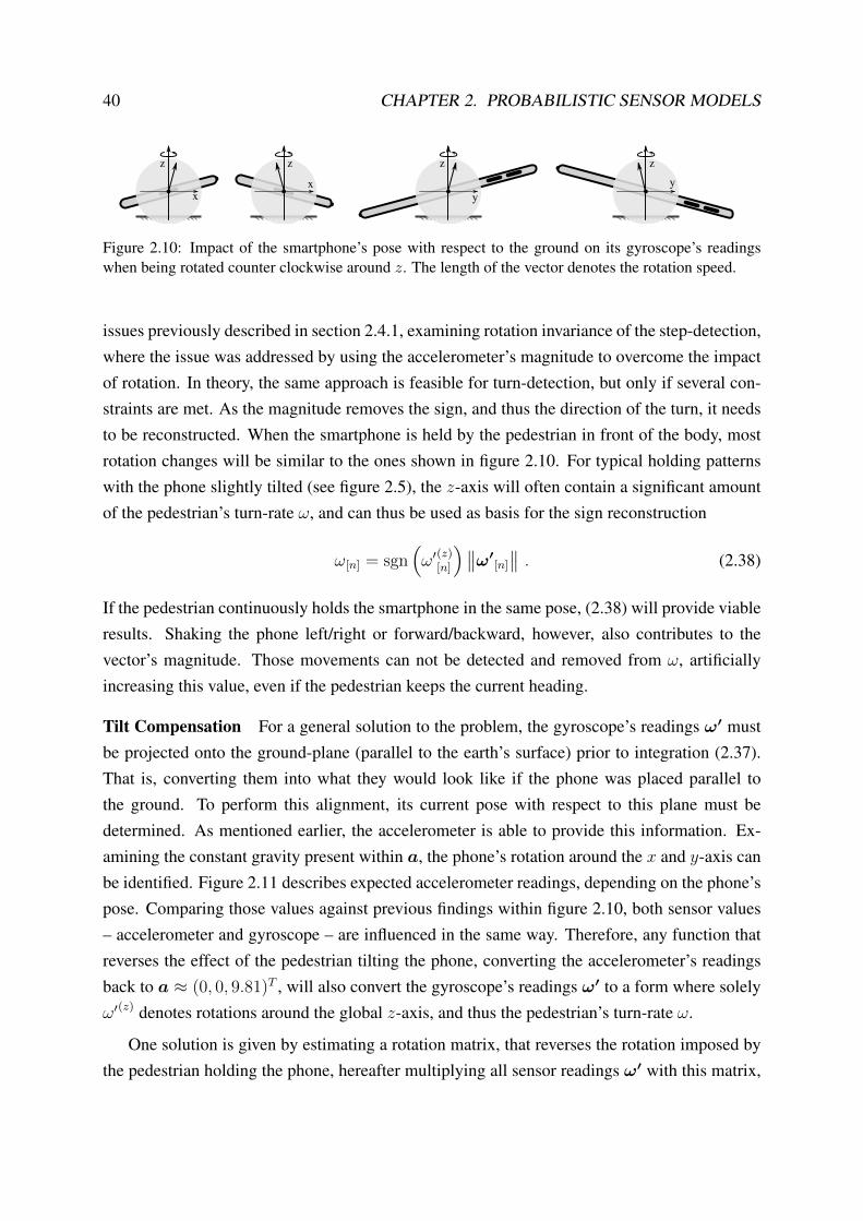
40 CHAPTER 2. PROBABILISTIC SENSOR MODELS
z
x
z
x
z
y
z
y
Figure 2.10: Impact of the smartphone’s pose with respect to the ground on its gyroscope’s readingswhen being rotated counter clockwise around z. The length of the vector denotes the rotation speed.
issues previously described in section 2.4.1, examining rotation invariance of the step-detection,where the issue was addressed by using the accelerometer’s magnitude to overcome the impactof rotation. In theory, the same approach is feasible for turn-detection, but only if several con-straints are met. As the magnitude removes the sign, and thus the direction of the turn, it needsto be reconstructed. When the smartphone is held by the pedestrian in front of the body, mostrotation changes will be similar to the ones shown in figure 2.10. For typical holding patternswith the phone slightly tilted (see figure 2.5), the z-axis will often contain a significant amountof the pedestrian’s turn-rate ω, and can thus be used as basis for the sign reconstruction
ω[n] = sgn(ω′
(z)[n]
)∥∥ω′[n]
∥∥ . (2.38)
If the pedestrian continuously holds the smartphone in the same pose, (2.38) will provide viableresults. Shaking the phone left/right or forward/backward, however, also contributes to thevector’s magnitude. Those movements can not be detected and removed from ω, artificiallyincreasing this value, even if the pedestrian keeps the current heading.
Tilt Compensation For a general solution to the problem, the gyroscope’s readings ω′ mustbe projected onto the ground-plane (parallel to the earth’s surface) prior to integration (2.37).That is, converting them into what they would look like if the phone was placed parallel tothe ground. To perform this alignment, its current pose with respect to this plane must bedetermined. As mentioned earlier, the accelerometer is able to provide this information. Ex-amining the constant gravity present within a, the phone’s rotation around the x and y-axis canbe identified. Figure 2.11 describes expected accelerometer readings, depending on the phone’spose. Comparing those values against previous findings within figure 2.10, both sensor values– accelerometer and gyroscope – are influenced in the same way. Therefore, any function thatreverses the effect of the pedestrian tilting the phone, converting the accelerometer’s readingsback to a ≈ (0, 0, 9.81)T , will also convert the gyroscope’s readings ω′ to a form where solelyω′(z) denotes rotations around the global z-axis, and thus the pedestrian’s turn-rate ω.
One solution is given by estimating a rotation matrix, that reverses the rotation imposed bythe pedestrian holding the phone, hereafter multiplying all sensor readings ω′ with this matrix,

2.4. INERTIAL MEASUREMENT UNIT 41
a = (0, 9.81, 0)T a = (9.81, 0, 0)T
a = (0, 0, 9.81)T
x
z
z z
z
y
yx
xy
y
x
z
y
Figure 2.11: Impact of the smartphone’s pose with respect to the ground on its accelerometer’s readings.
prior to the integration step (2.37). As shown within figure 2.11, the accelerometer’s readingsa denote the z-axis of the phone’s coordinate system with respect to the world’s coordinatesystem. The two remaining axes are created using the cross product and an auxiliary vector,which must not be parallel to z. As rotations around the z-axis do not need to be considered toproject the gyroscope’s readings, (1, 0, 0)T or (0, 1, 0)T are viable choices. Depending on thechosen temporal vector, its cross product with a either denotes the y or x-axis. The order withinthe cross product is important, to ensure that a right-handed coordinate system is created. Thethird axis is then given by the cross product of z and the one just created. After normalizing eachto a length of 1, they denote an orthonormal coordinate system and a rotation matrix R, thatconverts (0, 0, 9.81)T into a. The inverseR−1 ofR, given byR−1 = RT due to orthogonality,then represents the required rotation matrix that reverses the effect of tilting the phone
uz = a
ux = (0, 1, 0)T × uzuy = uz × ux
R =
(ux‖ux‖
uy‖uy‖
uz‖uz‖
)R−1 = RT .
(2.39)
The projected turn-rate ω is then given by
ω =(R−1ω′)(z)
. (2.40)
However, when projecting the gyroscope’s readings to undo the rotation, changing the phone’sorientation, e.g. from portrait to landscape, manifests as a large heading change. This problemcan be addressed by examining the behavior of the accelerometer’s readings a. The vector’sdirection changes only slightly while walking and turning, but rapidly, when the phone’s ori-entation is changed. Whenever detected, e.g. by using a Principal Component Analysis (PCA),readings from the gyroscope should be ignored or assumed to be uncertain [Ebn+15].
Similarly, previous discussions of the accelerometer’s readings indicated the presence ofnoise (cf. figure 2.6), demanding for low-pass filtering to derive a stable smartphone pose esti-mation (2.39). Overmuch filtering, however, will suppress minor pose changes, yielding poten-

42 CHAPTER 2. PROBABILISTIC SENSOR MODELS
tially incorrect projections, and thus divergent turn-rates (2.40). A similar effect occurs whenthe pedestrian turns rapidly, creating a measurable change in acceleration, and thus invalid poseestimations, affecting the turn-rate.
Besides turns, the three axes of the gyroscope also provide information on pose changes,and, due to the integration step, suffer from a reduced amount of high frequency zero meannoise, at the drawback of increasing drifts [Smi99]. Examining the advantages and disadvan-tages of both sensors, it becomes clear that the accelerometer, due to its noise level, is wellsuited for slow changes and absolute indications. In contrast, the gyroscope very well capturesrapid changes, but suffers from cumulating drifts. By combining both sensors, the best of eachcan be used. For the described use case, this sensor fusion is e.g. provided by a complementary
filter [GY15], depicted in figure 2.12, meant for combining the data x′[ ] and x′′[ ] from two sensorsusing a low-pass fLo (), and complementary high-pass filter fHi ()
y[ ] = fLo(x′[ ]
)+ fHi
(x′′[ ]
), (2.41)
with both filters together satisfying
fLo(x[ ]
)+ fHi
(x[ ]
) != x[ ] . (2.42)
Designing a complementary low-pass and high-pass is simple for FIR based filters, describedin section 2.4.1, as a direct complement can be calculated for every filter kernel [Smi99]. Forsecond- and higher order IIR filters, designing complements is possible, but results will notalways satisfy (2.42). This requires special complementary versions, like Linkwitz-Riley filters[Har+13]. For both setups, the two sensors are required to provide readings at the same instantin time, sharing a well known sample rate. As discussed, this can not be guaranteed when refer-ring to smartphone sensors. However, as exact cut-off frequencies are not necessarily requiredfor gyroscope/accelerometer fusion, real-world setups often refer to a simpler form of (2.41),inspired by IIR filters, satisfying (2.42), and mitigating aforementioned requirements [Isl+16]
y[n] = κ(y[n−1] +
∆x′[n]︷ ︸︸ ︷(
x′[n] − x′[n−1]
) )︸ ︷︷ ︸
high-pass
+ (1− κ)x′′[n]︸ ︷︷ ︸low-pass
, 0.0 < κ < 1.0 . (2.43)
κ within (2.43) adjusts the strength of the high-pass, and (1 − κ) the complementary low-pass. As x′[ ] is high-pass filtered, it can be provided as relative input ∆x′[ ], just like turn-ratesfrom the gyroscope. The low-pass on x′′[ ] filters accelerometer readings. By combining both,the accelerometer provides a stable pose, delayed by the low-pass, which is compensated by

2.4. INERTIAL MEASUREMENT UNIT 43
ω′
a
ω′ 7→ rω′
a 7→ ra
HP
LP
+ r
Σrω′
gyroscope:
accelerometer: 0
1
ampl
itude
frequency
low-passhigh-passcombined
Figure 2.12: Layout and behavior of a complementary filter which combines the values provided byan accelerometer and a gyroscope. After converting their readings to absolute rotations, the convertedresults are applied to a low-pass and a high-pass filter, which are complementary to each other.
the relative adjustments from the gyroscope, passed through the high-pass. Using this setupprovides a low-noise, yet low-delay, pose estimation for the phone without drift [YN01].
However, as both sensors supply different kinds of data, angular velocity from the gyro-scope, and absolute acceleration from the accelerometer, readings must be converted into ashared unit, before (2.43) can be used.
One option is to convert both into Euler angles, describing a rigid body’s orientation by threeconsecutive rotations around orthogonal axes [Die06]. According to figure 2.11 and [Jan+15],these three Euler angles α, β, γ, consecutively rotating around x, y, and z, can be derived fromthe direction of the constant gravity, present within the accelerometer’s readings a
α = atan2(a(y), a(z)
), β = atan2
(−a(x),
√(a(y))2
+(a(z))2), γ = 0 , (2.44)
where atan2 (y, x) is a modified version of tan−1(y/x), respecting the four possible quadrants.As mentioned earlier, the accelerometer does not provide any valuable information on the rota-tion around the z-axis with respect to the world coordinate system, and thus γ = 0 in (2.44).
At first glance, the integration (2.37) seems sufficient for deriving a similar representationfrom the gyroscope readings ω′. However, they describe changes based on the sensor’s pointof view, often referred to as body frame [NPM13]. With respect to the outside view, or inertial
frame, the orientation changes after every new sensor reading. This would require a cumulativeadjustment prior to the integration, converting the angular velocityω′ as seen from the sensor, toa change in Euler angles, or Euler angle rates, as seen from the outside, described in [Jan+15].However, due to required trigonometric operations, this approach is limited to [−π,+π], caus-ing discontinuous behavior near ±90°. While not being a problem in general, this imposesissues when applying digital filters, e.g. fading from −π to +π or vice versa. Furthermore,required calculations suffer from constraints, known as Gimbal lock problem [Jan+15].
All issues can be addressed by using quaternions Q instead of Euler angles [Vin17]. Inplace of three consecutive rotations, orientation is described using a complex representation of

44 CHAPTER 2. PROBABILISTIC SENSOR MODELS
a rotation axis u and a corresponding angle α to rotate around it
Q = (α,u) =(
cos(α
2
)+ sin
(α2
)(u(x)i + u(y)j + u(z)k
)), Q ∈ H
with i2 = j2 = k2 = ijk = −1 , |u| != 1 .
(2.45)
Similar to (2.39), in order to convert the orientation measured by the accelerometer into a quater-nion, the rotation axis must be chosen so that rotating around it converts a to≈ (0, 0, 9.81)T , or(0, 0, 1)T when normalized. It is thus given by the normalized cross product between those twovectors. The amount of rotation is denoted by the angle between both, that is, their dot product
Qa[n] =
(α,
u
‖u‖
), α = cos−1
(a[n]∥∥a[n]
∥∥ • (0, 0, 1)T
),
u = a[n] × (0, 0, 1)T =(a
(y)[n] ,−a
(x)[n] , 0
)T.
(2.46)
The angular velocity ω′, provided by the gyroscope, can directly be converted into a quaternionQω
′, where the normalized vector describes the rotation axis, and the rotation angle is defined
by the vector’s magnitude, multiplied with the elapsed time
Qω′
[n] =
(∆t∥∥ω′
[n]
∥∥ , ω′[n]∥∥ω′[n]
∥∥). (2.47)
Subsequent Qω′
[n] can then be cumulated by quaternion multiplication. In contrast to using Eulerangles, a prior adjustment of the current readings is not required, as the quaternion multiplica-tion directly adjusts the rotation axis
Qθ′
[N ] =N∏n=1
Qω′
[n] ⇒ Qθ′
[n] = Qω′
[n]Qθ′
[n−1] . (2.48)
This aspect simplifies using gyroscope readings within the complementary filter
Q[n] = κ
integral like (2.48)︷ ︸︸ ︷(Qω
′
[n]Q[n−1]
)+(1− κ)Qa[n] , 0 < κ < 1 . (2.49)
(2.49) multiplies the current turn-rates Qω′
[n] from the gyroscope with the previous filter outputQ[n−1]. This represents an integration similar to (2.48), and denotes the high-pass part. Its resultis interpolated with the quaternion Qa[n] from the accelerometer, which contributes slowly by(1 − κ), representing the low-pass. For increased accuracy, a spherical interpolation [Vin17]should be used. The required rotation matrixR−1 can hereafter be derived by converting Q intoa 3× 3 rotation matrix, as shown in [Die06]. An example is provided in appendix A.1.

2.4. INERTIAL MEASUREMENT UNIT 45
(2.49) provides a stable pose estimation, suppressing drift and noise. The resulting rotationmatrixR−1 is used within (2.40), undoing the effect of the pedestrian tilting the phone, derivingthe projected turn-rate ω. Hereafter, mentioned discrete integration techniques are applied tocumulate the turn-rate, yielding the change in heading within a certain timeframe
θt =∑n
∆tω[n] , (t− 1) ≤ ftime (n) < t , (2.50)
or the absolute heading with respect to the pedestrian’s initial orientation Θ0
Θt = Θ0 +∑n
∆tω[n] , 0 ≤ ftime (n) < t . (2.51)
Probabilistic Assembly Both values can be used for a probabilistic evaluation of potentialpedestrian movements, constrained on the absolute heading Θ, or the change in heading θ withina certain timeframe. While the latter can be expected to be stable for shorter timeframes, theabsolute Θ will suffer from cumulating errors, independent of the chosen pose estimation andgyroscope projection, as it can not be compensated by the sensor fusion with the accelerometer.Depending on the building’s architecture, one way of dealing with drifts and cumulating uncer-tainties is to discretize turns, e.g. to multiples of 90°. Using discrete options, no-turn, 90° leftand 90° right, mitigates the impact of cumulating sensor drift and spreading uncertainties, yet,at the cost of accuracy, especially when walking within large, open areas [Kop+14; Ebn+14].
Drifts and other errors are therefore addressed by probabilistic models, including uncertain-ties when comparing the observed absolute heading against the pedestrian’s walking directionin the (x, y) plane, given by the angle between two states, with respect to the x-axis
∠xy(qt−1, qt
)= atan2
(q
(y)t − q
(y)t−1, q
(x)t − q
(x)t−1
). (2.52)
The smallest signed difference between two angles in rad is then given by
∠∆ (α, β) = atan2 (sin(β − α), cos(β − α)) . (2.53)
This difference, between the angle qt−1 → qt and the absolute observed heading, should beclose to 0, including an uncertainty, e.g. given by a normal distribution
pabsTurn(ot | qt, qt−1
)= N
(∠∆
(α, o
(Θ)t
) ∣∣∣ 0, σ2turn
)α = ∠xy
(qt−1, qt
), 〈q〉t = 〈(x, y, . . .)〉t , 〈o〉t = 〈(Θ, . . .)〉t .
(2.54)

46 CHAPTER 2. PROBABILISTIC SENSOR MODELS
Due to o(Θ)t suffering from cumulating errors, the corresponding uncertainty σturn must increase
over time. Furthermore, this approach requires the pedestrian’s initial heading offset Θ0 to beknown. Both drawbacks can be mitigated by using relative comparisons instead.
To compare potential pedestrian movements with an observed change in heading, threeconsecutive states qt−2 → qt−1 → qt must be considered. The heading change is then definedby the difference between the two absolute walking angles ∠xy
(qt−2, qt−1
), and ∠xy
(qt−1, qt
).
This change is then compared against the observed one, also including an uncertainty:
prelTurn’(ot | qt, qt−1, qt−2
)= N
(∠∆
(α, o
(θ)t
) ∣∣∣ 0, σ2turn
)α = ∠∆
(∠xy
(qt−2, qt−1
),∠xy
(qt−1, qt
))〈q〉t = 〈(x, y, . . .)〉t , 〈o〉t = 〈(θ, . . .)〉t .
(2.55)
To omit the need for including qt−2 within the equation, the previous heading ∠xy(qt−2, qt−1
)can be remembered by adding it as a variable to the state, slightly altering above equation
prelTurn(ot | qt, qt−1
)= N
(∠∆
(α, o
(θ)t
) ∣∣∣ 0, σ2turn
)α = ∠∆
(q
(Θ)t−1,∠xy
(qt−1, qt
)), 〈q〉t = 〈(x, y,Θ, . . .)〉t , 〈o〉t = 〈(θ, . . .)〉t .
(2.56)
While the normal distributions used in (2.54), (2.55) and (2.56) are a common choice for mod-eling uncertainties, they are not ideal when referring to angular units, as
∫ +π
−π N (x | 0, σ2) dx
will only sum up to ≈ 1.0, and only for smaller σ, yielding potential normalization issues. Thiscan be addressed by using distributions intended for angular use cases, with the range of ±π inmind, such as the von Mises distribution [Mis18; For+10]. By being both, normalized for theinterval [−π,+π], and periodic, angular uncertainties are handled more suitably.
Independent of the chosen distribution, an uncertainty value must be determined. Keller etal. [KWS12] provide an overview on expected uncertainties, by examining sensors within both,laboratory and real-world conditions. They estimated noise levels, scale offsets and long-termdrifts of gyroscope sensors, by using accurate references. Hereafter, they compared the resultsof an 80 m long walk using step and turn detection, with and without prior sensor calibration,clearly indicating calibration improvements. While hardware based drifts or scale offsets canbe estimated during a calibration process, the behavior of the pedestrian can not [ST14]. Asmentioned earlier, some movements, like fast turns, affect the measured acceleration, and thusthe pose estimation and gyroscope projection, yielding incorrect turn-rates. It therefore makessense to not assume a constant uncertainty in rad/s or °/s, but also a dynamic amount that isincreased whenever major changes within the gyroscope or accelerometer readings are detected.

2.4. INERTIAL MEASUREMENT UNIT 47
605550454035
3025
55
354045
5055
6065
-20° -40° -60°-80°
0°+20°+40°+60°
0°
-10°+10°
+10° -10°
0°
+20°
Figure 2.13: Local intensity of the magnetic field (magnitude of B′) in µT, and declination correctionΘdec. Adapted from the World Magnetic Model 2019, developed by NOAA/NCEI/CIRES [NOA].
A potential heuristic for smaller timeframes could thus read as follows:
σturn = ∆t
constant︷ ︸︸ ︷(1 °/s
π
180°
)+
variable︷ ︸︸ ︷(κ |o(θ)
t |), κ ≥ 0 . (2.57)
Within (2.57), a constant turn error in °/s is combined with a variable component, dependingon the amount of change, with its impact adjusted by κ. Both values are an empiric choice anddepend on the quality of the sensors installed within a phone. For a truly dynamic uncertaintyestimation, based on observations and other prior knowledge, more sophisticated approachesare required [Bra+05; CYJ15]. Especially when working with absolute headings (2.54), theuncertainty depends on the time elapsed since start, and eventually reaches a level where thesensor stops to provide usable information. Thus, the gyroscope is mainly suited for relativepredictions, such as (2.56). For absolute indications, other sensors are better suited.
2.4.3 eCompass
As shown, relative turn information suffers from cumulating errors, eventually becoming un-stable. This is mitigated by sensors providing absolute heading indications. Mentioned earlier,ships use a gyrocompass pointing towards the earth’s geographic north/south by aligning itselfonto the rotation axis. A compass provides similar information, except that the alignment isbased on magnetism, and that it points towards the earth’s geomagnetic north. The geomag-netic north differs from the geographic north, and is subject to changes over time, currentlymoving by over 55 km per year from Canada towards Siberia [Cla16; Wit19].
The indication from an analog compass is provided by a magnetized needle that is allowed tospin freely around one axis. If this axis is aligned parallel to the earth’s z-axis, pointing upwards,the needle aligns itself towards north/south of the earth’s magnetic field. Within smartphones,similar readings are provided by the magnetometer, present within most IMUs. Instead of a

48 CHAPTER 2. PROBABILISTIC SENSOR MODELS
yx
y
z
S
N
geographic North Polegeomagnetic North Polex
y
z
B′
inclination
declinationN
Figure 2.14: Behavior of the earth’s magnetic field and its relation to the geographic poles. If a smart-phone is placed parallel to the surface, just like an analog compass, the direction towards magnetic northis given by the magnetometer’s readings B′(x) and B′(y). Right half adapted from [Cla16, p. 198].
magnetized needle, the sensor’s internals leverage the principle of the Hall effect. When aconstant current is passed through a conductive material, every magnetic force perpendicularto the movement direction of the electrons passing the conductor, deflects them in a directionthat is perpendicular to both, the moving direction and the magnetic flux, forcing the electronstowards one side of the conductor (Lorentz force). Between this side and its opposite, a voltageproportional to the applied magnetic force can be measured [Pop+07]. In contrast to otherprobes, such as inductors, Hall sensors are also capable of measuring the influence of static
magnetism, like non-moving magnetic objects [Cul56]. Most smartphones are equipped with a3-axis magnetometer where three Hall sensors are combined, measuring the current magnetic
flux density B′ = (x, y, z) in µT, along three orthogonal directions. Actual intensities arelocation dependent, with typical values shown in the left half of figure 2.13.
Figure 2.14 depicts the geographic and magnetic relations needed to derive a heading fromthe readings B′ of a magnetometer. While the earth’s geographic north and south poles (truenorth/south) are defined by its rotation axis, the geomagnetic north and south poles are definedby its internal magnetic field, which is slightly different. This difference is called declination,depends on the actual location on earth and, as mentioned, is subject to changes over time.Current values are shown in the right half of figure 2.13.
The geomagnetic north pole can be thought of the magnetic south pole of a dipole barmagnet, the compass points to. If a smartphone is placed parallel to the ground, the directiontowards geomagnetic north ΘNmag is given by the magnetometer’s readings in x and y
ΘNmag = atan2(B′
(y), B′
(x)). (2.58)
To derive the angle ΘNgeo towards the geographic north, the current location’s declination cor-rection Θdec from figure 2.13 must be added
ΘNgeo = ΘNmag + Θdec . (2.59)

2.4. INERTIAL MEASUREMENT UNIT 49
yx x
y
portraitupright
portraitupside down
orientation condition yaw Ψ
portrait upright∣∣a(x)
∣∣ < ∣∣a(y)∣∣ ∧ a(y) ≥ 0 (90± 45)°
portrait upside down∣∣a(x)
∣∣ < ∣∣a(y)∣∣ ∧ a(y) < 0 (270± 45)°
landscape left∣∣a(x)
∣∣ ≥ ∣∣a(y)∣∣ ∧ a(x) < 0 (180± 45)°
landscape right∣∣a(x)
∣∣ ≥ ∣∣a(y)∣∣ ∧ a(x) ≥ 0 (0± 45)°
landscape left
landscape right
y
x
x
y
Table 2.1: Smartphone orientation dependent on accelerometer readings. Adapted from [Bos14].
While Θdec is location dependent, it changes hardly within the range of a few hundred kilome-ters, visualized in figure 2.13. For indoor localization and navigation scenarios, it can thus e.g.be stored within a floorplan, where the building is aligned towards the geographic north.
Shown in figure 2.14, there is another angle besides ΘNgeo . The inclination, or angle ofdip, describes the upwards/downwards direction of the magnetic field, mainly dependent on thecurrent latitude. While the exact direction of the magnetic field is defined by those two anglescombined, inclination is usually omitted for north/south estimations [Cla16].
To determine ΘNmag for arbitrary smartphone poses, a combination of magnetometer andaccelerometer, also referred to as eCompass [KC15], is required. This need can be confirmedwhen referring to the previously discussed turn-detection, but also when observing an analogcompass. To prevent its needle from touching the casing, the latter must be aligned parallel tothe angle of dip, which is approximately parallel to the ground, when not residing near the poles.Just like earlier for the turn-rate, a heading estimation requires a projectionR−1 onto the world’s(x, y)-plane, using the techniques discussed in section 2.4.2, referred to as tilt compensation
ΘNmag = atan2(B(y), B(x)
), B = R−1B′ . (2.60)
Due to sensor noise, low-pass filtering is advisable, if not already conducted by the magnetome-ter itself [Pop+07; BS12; KS18]. To prevent jumps near 0° ↔ 360° or −180° ↔ +180°, theinput vectors B′ or B, should be filtered instead of ΘNmag . In (2.60), all candidates for esti-mating R−1, previously described in section 2.4.2, are applicable. However, in contrast to therelative turn-detection based on the gyroscope, the absolute eCompass requires more caution asthe result from (2.60) rotates together with the phone. This refers to the four different smart-phone orientations: landscape and portrait, each up and down. Changing the orientation directlyaffects the eCompass’ heading indication. To compensate this, the pedestrian is either requiredto hold the phone using an exactly defined pose, as it is the case for most analog compasses, orthe system must be able to distinguish between several pre-defined poses, such as portrait andlandscape mode [Ngu+16]. Integrated sensor components therefore contain some heuristic to

50 CHAPTER 2. PROBABILISTIC SENSOR MODELS
distinguish between various orientations, based on the current accelerometer readings a and theresulting yaw angle Ψ = atan2
(a(y), a(x)
)shown in table 2.1 [Bos14]. A general solution for
the pedestrian e.g. carrying the phone within trouser pockets, requires additional sensors besidesthe smartphone. To relate the tilt-compensated compass’ north with the pedestrian’s current axisof forward motion. When estimating this axis using just the smartphone’s sensors, results canbe unstable, and are subject to delays [Kus+15]. The heading provided by the eCompass isusually off by several degrees [Cas+14]. Using the phone’s estimated orientation for projectionthus is a viable choice for smartphone-only indoor localization and especially navigation, wherethe pedestrian faces the phone’s display, similar to holding an analog compass.
Besides tilting issues, everything that affects the magnetic field will also cause a measur-able effect on the sensor’s readings and thus the heading estimation. While this is often not aproblem within large, open-space outdoor environments, it is a problem indoors, where manymetal objects, such as steel-reinforced concrete, handrails, door handles, elevators and inductiveelectricity, are present [Goz+11; Par+06].
However, despite negative influences on heading estimation, this allows for completely dif-ferent inputs towards indoor localization. Architectural effects on the magnetic field can be veryunique for different regions within a building, allowing for magnetic matching [Goz+11]. Here,the readings of the magnetic field are recorded once, for many locations within the building.Every recording describes the magnetic behavior at a location, serving as its fingerprint. Dur-ing the localization process, the current readings from the phone’s magnetometer are comparedagainst all known fingerprints. The location of the best matching one is likely to denote thepedestrian’s current whereabouts [Shu+15]. However, it requires significant effort to record thefingerprint database, which is also subject to changes over time. Setup and update issues canbe mitigated, e.g. using a self location and mapping (SLAM) approach, where localization isinitially provided by other sensors and the, yet unknown, magnetic field is recorded during thelocalization process. The system then stabilizes itself over time, refining both, the localizationand the magnetic information, with every additional walk through the building [KS18].
Alternatively to complex fingerprinting, Ehrlich et al. [EBS16] suggest installing a few spe-cial coil-transmitters within the building, each creating a unique magnetic signature within aconfined area. Those signatures can be measured by the magnetometer, and compared against adatabase of known transmitter signatures. This approach allows for additional location hints byusing a controlled setup, as the strong coil-signature is barely affected by ambient conditions. Ifthree or more signatures can be detected by the magnetometer, even multilateration is possible(cf. section 2.3) by inferring the distance from the strength of the magnetic field.
However, within this work, the focus is on absolute heading estimation, not requiring addi-tional hardware installations or time-demanding setups.

2.4. INERTIAL MEASUREMENT UNIT 51
Sensor Calibration Independent of the chosen approach, the magnetometer must be cali-brated to compensate for soft iron and hard iron effects. Magnetic or metallic objects mountedtogether with the magnetometer, like the phone’s speaker, introduce hard iron effects. They off-set all provided readings, independent of the phone’s current orientation. On the other hand, softiron effects are induced by the outside world, through nearby objects, thus yielding influenceson sensor readings, dependent on its location and orientation. Therefore, location independenthard iron effects are easier to calibrate [Kon09]. While alignment differences between the ac-celerometer, providing the pose projection, and the magnetometer should be considered as well,this is not an issue for today’s smartphones, as the alignment is usually accurate [ZY15].
When placing the smartphone parallel to the ground, and rotating it around the z-axis (cf.figure 2.14), the measurements (B′(x), B′(y))T provided by a calibrated magnetometer denotea circle, centered at (0, 0)T . As the actual magnitude of the sensor readings is not required toderive the heading (2.60), the calibrated circle’s radius can be of any size. When performinga manual calibration, normalizing the measurements to denote a unit-circle is thus fine for theintended use case. The same holds true for the three dimensional case. Rotating the phonearound all three axes, the resulting sensor readings should denote a sphere centered at (0, 0, 0)T .A corresponding mean squared error metric for both cases is thus given by
ε =1
N
N∑n=1
(1−
∥∥B′[n]
∥∥)2
, B′ =
(x, y)T for 2D
(x, y, z)T for 3D .(2.61)
During the calibration process, allB′[ ] are adjusted using a set of parameters, depending on thecalibrations to address, to reduce the error (2.61). Deviations from the center (0, 0, 0)T can beaddressed by one offset parameter per axis. Similarly, the scale for each axis can be adjustedusing one scale parameter for each. Calibration hereafter represents an optimization problem
arg minu,w
N∑n=1
(1−
∥∥(B′[n] − u)w
∥∥)2
, (2.62)
where the offset is adjusted by subtracting u, and the scale is corrected by a componentwisemultiplication with w. By calculating the 2nd partial derivative for all to-be-optimized pa-rameters, and examining the requirements for each derivative to be> 0, it can be shown that thefunction is convex for typical sensor inputs, offsets starting at (0, 0, 0)T , and scales > 0. Thus,optimization can be performed using common approaches such as gradient descent [HS06] ordownhill simplex method [Pow62; NM65]. (2.62) covers most constellations, but omits rarecases where readings provided by the sensor denote a rotated ellipse/ellipsoid, requiring addi-

52 CHAPTER 2. PROBABILISTIC SENSOR MODELS
tional rotation parameters for correction [Fan+11]. In case of many outliers, (2.62) will not pro-vide ideal results. A solution can be the random sample consensus (RANSAC) [FB81], wherenot all, but a (random) fraction of all inputs is used for the optimization. This step is repeatedseveral times, depending on the amount of outliers, eventually deriving a superior result.
As shown later, for many smartphone models aforementioned manual calibration schemesare not required, as they are integrated directly into the operating system or sensor. The proce-dure is triggered whenever the sensor is active, and the user rotates the phone around all threeaxes, hereafter removing the influences of constant offsets, such as hard iron effects.
Probabilistic Assembly While, in theory, the eCompass can hereafter be used as single (ab-solute) heading source, its practical use is limited by aforementioned environmental effects andthe pedestrian. Together with the turn detection from section 2.4.2, however, it can compensatethe cumulating heading drifts on the z-axis, the accelerometer isn’t able to address [Har+03].Besides directly fusing both readings, e.g. via a complementary filter, the sensor can be eval-uated on its own, using a probabilistic approach to model expected uncertainties, allowing forlater combination. Similarly to the heading evaluation for the gyroscope, the current eCompassheading ΘNmag is compared against the pedestrian’s potential heading, either given by qt−1 → qt
or q(Θ)t . The difference between geomagnetic north from the sensor, and the orientation of the
building is addressed by Θbldg, describing the angle between the floorplan’s x-axis and geomag-netic north, estimated once per building. Potential walks are hereafter evaluated by
pcomp(ot | qt, qt−1
)= N
(∠∆
(α, o
(ΘNmag )
t
) ∣∣∣ 0, σ2comp
)α = ∠xy
(qt−1, qt
)+ Θbldg , 〈q〉t = 〈(x, y, . . .)〉t , 〈o〉t = 〈(ΘNmag , . . .)〉t .
(2.63)
If the heading is stored as part of the unknown state, (2.63) simplifies to
pcomp (ot | qt) = N(∠∆
(α, o
(ΘNmag )
t
) ∣∣∣ 0, σ2comp
)α = q
(Θ)t + Θbldg , 〈q〉t = 〈(x, y,Θ, . . .)〉t , 〈o〉t = 〈(ΘNmag , . . .)〉t .
(2.64)
The value for σcomp depends not only on the quality of accelerometer and magnetometer, butalso on the pedestrian’s behavior when holding the phone (steady/shaking), and nearby metallicor magnetized objects. The resulting heading precision can thus vary between errors as low as1° [Kon09] and up to tens of degrees depending on location and tilt [Li+12; Hil+14; WGN15].Changes in tilt can be detected when analyzing the accelerometer’s readings within the poseestimation. The same holds true for changes of the magnetic field. Without architectural in-fluences, the magnitude ‖B′‖ varies only slightly throughout the building. Whenever largechanges are detected, σcomp can be increased accordingly. Similarly, the uncertainty can be in-

2.5. BAROMETER 53
creased whenever the eCompass reports major heading changes, but the gyroscope does not.Depending on hardware and surrounding architecture, it thus can be advisable to use a discretecomparison instead, limiting potential directions based on heuristics κcomp and τ comp [Ebn+17]
pcomp (ot | qt) = η
κcomp ∠∆
(α, o
(ΘNmag )
t
)< τ comp
(1− κcomp) else, α = q
(Θ)t + Θbldg , (2.65)
or a compromise between (2.64) and (2.65), using the distribution from (2.21)
pcomp (ot | qt) = R(∠∆
(α, o
(ΘNmag )
t
) ∣∣∣ 0, σ2comp
). (2.66)
Yet, in case of e.g. turn rates beyond the pedestrian’s normal behavior, the eCompass can beconsidered unstable, not providing a viable evaluation and thus pcomp (ot | qt) = const.
2.5 Barometer
The first sensor providing absolute location hints is the barometer. It measures the currentatmospheric pressure in hPa, which is influenced by the amount of air that is “piled up” abovethe sensor, allowing to infer the current altitude, usually measured above mean sea level. If thisaltitude increases, the amount of air above the sensor decreases, indicating a drop in pressure.This change of atmospheric pressure can be measured e.g. by analyzing the change in size of anair-filled, flexible object, like a balloon. An increasing height above mean sea level will yield agrowing balloon, as the outside pressure decreases, while the pressure inside remains constant.Most common analog barometers used another approach, based on a vertical column filled withmercury, placed within a reservoir. Depending on the surrounding pressure, mercury is pressedfrom the reservoir into the column, or moves from the column into the reservoir. This yieldsa vacuum of varying size within the column, which adjusts until the forces inside and outsideare equal. The height of mercury remaining within the column is proportional to the currentatmospheric pressure. Therefore, besides hPa, inch of mercury (inHg), millimeter of mercury
(mmHg) or Torr also are common measuring units for atmospheric pressure [Tor44; Tim82].
As of today, some smartphone models are equipped with a barometer sensor, based onpiezo-resistive pressure sensing [Bos15; Bos18]. Initially, it was intended to speed-up the GPS’initialization times by providing a coarse altitude information. However, experiments indicatedthat its success was questionable, as GPS lock times did not improve with a barometer present[KWS12]. As the sensor remained present within many newer models, its contribution towardsindoor localization and navigation was examined [Mur+14], e.g. by relating atmospheric pres-

54 CHAPTER 2. PROBABILISTIC SENSOR MODELS
T0 288.15 ° K temperature at sea level %0 1013.25 hPa pressure at sea levelR 8.314 46 Nm/molK (ideal) gas constant L 0.0065 ° K/m temperature lapse rateg 9.806 65 m/s2 gravity of earth M 0.028 96 kg/mol molar mass of dry air
Table 2.2: Constants required to relate atmospheric pressure and altitude [TT08; Stu15].
sure and altitude above the mean sea level
f% (h) = %0
(T0
T0 + Lh
) gMRL
fh (%) =T0
L
((%
%0
)−RLgM
− 1
). (2.67, 2.68)
(2.67) and (2.68) require several physical and chemical constants listed in table 2.2 [TT08;Stu15]. To be consistent with their typical notation, some previously introduced variables arere-purposed for the barometer. For both relations, the pressure at the mean sea level is assumedto remain constant at %0 = 1013.25 hPa, at a temperature of T0 = 15 °C, decreasing constantlywith L = 6.5 °C/km, referred to as standard atmosphere. The ideal gas law derives the air’sdensity, expecting it to be absolutely dry (0 % rel. humidity). It thus relates atmospheric pres-sure to a column of height h, filled with a gas of some density. Corresponding results are validup to ≈ 11 km in altitude, before the temperature lapse rate L becomes zero [OAS76; Stu15]
For pedestrian navigation indoors and outdoors, the first few hundred meters above sea levelare the most important. The 6.5 °C/km change in temperature can thus be omitted. Hereafter,the relation of altitude and pressure is approximately exponential, and (2.67)/(2.68) simplify to
f% (h) ≈ %0 e
(−gMRT0
h)
≈ %0 e
(−0.0342° K/m
T0h) fh (%) ≈
ln(%%0
)T0
−0.0342 ° K/m, (2.69, 2.70)
where all constants are combined as a single value [Stu15]. Figure 2.15 shows the relationbetween altitude and pressure. While the approximations are similar in shape during the firstfew hundred meters, a closer look reveals a noticeable offset, potentially causing issues whenworking with absolute pressure readings and altitudes, e.g. yielding an invalid floor numberestimation for the pedestrian. However, due to aforementioned assumptions on dry air, fixedtemperature and pressure at mean sea level, the more correct equations also represent an approx-imation. Every change in climatic conditions will void these assumptions, producing incorrectresults, decreasing or increasing local pressure indications, as visualized in figure 2.16.
For compensation, pilots e.g. adjust their plane’s altimeter to a reference pressure duringtakeoff and landing, currently measured at the corresponding airport, known as QNH or QFE. Indoing so, the instrument denotes the height above the airport with respect to the current weatherconditions [Eur04]. During flight, the exact altitude is less important, as long as obstacles like

2.5. BAROMETER 55
700
800
900
1000
0 m 1000 m 2000 m 3000 m
902905908
pres
sure
(hP
a)
(2.67)(2.69)
700 hPa800 hPa900 hPa1000 hPa0
1000
2000
3000
930
960
heig
htab
ove
sea
(m)
(2.68)(2.70)
Figure 2.15: Relation between atmospheric pressure and height above sea level according to (2.67),(2.69) and (2.68), (2.70). As can be seen within the zoomed regions, the approximation is only suited forrelative comparisons due to absolute errors of several meters.
mountains are safely overflown. The distance towards other airplanes nearby is more important,and pilots therefore adjust their altimeter to the same reference of 1013.25 hPa. While the indi-cated height above ground will change with weather conditions, nearby aircrafts are influencedby the same effect, ensuring that their distance in altitude remains measurable [Fed16].
Probabilistic Assembly Azevedo and Crisostomo propose a similar approach for smartphonebased localization. The current relative pressure at several known points is recorded and sharedwith the phone, to provide a relative alignment. This data is e.g. provided by nearby weatherstations and hereafter interpolated to estimate the pressure at the building’s altitude [AC16]. Orthe weather station resides within the building itself [EBS16]. Instead of using the pressurereadings from nearby transmitters, readings from the phone itself can also be used. Here, aninitial measurement %ref from the barometer at a known altitude href serves as reference. Thisalso prevents potential calibration offsets, mitigates the impact of current weather conditions,and does not require additional infrastructure or a data connection to a server. The altitude href
of this reference measurement can e.g. be inferred by using the last GPS fix before enteringthe building [AY12], performing an optical localization using the phone’s camera [HB08], thepedestrian scanning nearby QR-Codes or RFID/NFC tags [Lee+14; Jim+12].
In order to include an obtained reference, (2.67) and (2.68) must be adjusted, to operaterelative to an arbitrary altitude instead of the mean sea level [OAS76]. The current altitude canhereafter be estimated directly based on incoming sensor readings, as long as local climaticconditions are not changing, and the reference remains valid [KWS12]
f% (h) = %ref
(T0
T0 + L(h− href)
) gMRL
fh (%) = href +T0
L
(( %
%ref
)−RLgM − 1
). (2.71, 2.72)
The readings from the barometer can hereafter be converted to an altitude, and compared againstpotential whereabouts. However, all barometer altitudes are with respect to mean sea level, andthe pedestrian’s unknown z-location with respect to e.g. the first floor of the building. Thus, an

56 CHAPTER 2. PROBABILISTIC SENSOR MODELS
990.2
990.3
990.4
5 min 10 min 15 min 20 min
191.5
192.5
193.5
992.45
992.55
5 min 10 min 15 min 20 min
173.7
174
174.3
174.6
pres
sure
(hP
a)
pressure avg(pressure) avg(altitude)
altit
ude
(m)
Figure 2.16: Readings from a barometer at a fixed location on two different days (left and right). Whilethe left shows a significant variation of> 2.5 m in altitude, the right one denotes only≈ 1 m of variation.However, due to different climatic conditions there is an absolute difference of ≈ 20 m between both.
offset constant hbldg is required, to relate both. Independent of whether (2.68), (2.70) or (2.72) isused, the pedestrian’s potential whereabouts in z can then be compared against the barometer’sreadings, e.g. by using a normal distribution to model sensor uncertainties
pbaroAbs (ot | qt) = N(q
(z)t + hbldg
∣∣∣ fh (o(%)t
), σ2
alt
)〈q〉t = 〈(z, . . .)〉t, 〈o〉t = 〈(%, . . .)〉t .
(2.73)
As discussed, a pressure reference requires either additional hardware or infrastructure withinthe building, or the correct altitude of a reference measurement observed by the phone itself. Todrop those requirements, but still benefiting from the advantages of relative pressure readings,a workaround is required. By changing (2.73) from an absolute to a relative comparison, withrespect to the first smartphone pressure reading, the reference becomes obsolete. In other words,an initial atmospheric pressure is known from the barometer, but the corresponding altitude isnot. That is, the pedestrian is assumed to have started at an unknown height. While walking,the sensor’s pressure readings, and the pedestrian’s altitude, both change with respect to theirinitial values. Even though the starting altitude is unknown, the evaluation can examine if thepedestrian’s change in altitude since the start at t = 0 resembles the barometer’s change inpressure since t = 0 [Ebn+15; Tor+17].
To compare pressure changes with altitude changes, the relative relation between both isrequired. That is, the change in pressure per meter of altitude (hPa/m) at a certain altitude habove sea-level, given by the derivative of (2.67)
f% (h) = −gM%0T0
(T0
T0+Lh
) gMLR−1
R (T0 + Lh)2 . (2.74)
For buildings with rather few floors, only a small range of the function is required. Within thisrange, (2.67) can be assumed to behave linearly, and its derivative (2.74) denotes a constant,

2.5. BAROMETER 57
Altitude h f% (h)(2.67) f% (h)(2.74) 1/f% (h)(2.74)
0 m 1013.25 hPa 0.120 hPa/m 8.32 m/hPa200 m 989.56 hPa 0.117 hPa/m 8.56 m/hPa400 m 966.53 hPa 0.114 hPa/m 8.81 m/hPa600 m 944.13 hPa 0.110 hPa/m 9.05 m/hPa
Table 2.3: Expected atmospheric pressure and corresponding change rate, dependent on the altitude.
solely dependent on the building’s height above mean sea level hbldg. Resulting change rates fortypical altitudes are shown in table 2.3. The adjusted evaluation
pbaroRel (ot | qt) = N( ∆hPa→∆m︷ ︸︸ ︷
∆%
f% (hbldg)
∣∣∣∣ ∆z, σ2alt
)〈q〉t = 〈(z, . . .)〉t , 〈o〉t = 〈(%, . . .)〉t , ∆z = q
(z)t − q
(z)0 , ∆% = o
(%)t − o
(%)0 ,
(2.75)
matches the pedestrian’s potential whereabouts against current sensor readings, by comparingthe change in altitude ∆z since start t = 0 with the change in atmospheric pressure ∆% sincestart. For comparing, the latter is converted to meters based on the expected pressure change permeter at the building’s altitude hbldg, given by the reciprocal of (2.74). To remove the requiredo0 from (2.75), a virtual barometer sensor can be created, directly providing the required ∆%
as its observation. Similarly, ∆z can be added directly to the unknown state, and is hereafterupdated for every movement qt−1 → qt, dropping the requirement for q0. However, even withpressure readings relative to the start of the walk, changing weather conditions, opening/closingdoors or windows, can still cause several meters of fluctuation. Changing weather conditionsusually take at least several minutes to manifest. Those long-term changes become relevant forlonger localization and navigation scenarios, where the initial reference %ref or o(%)
0 gets invalid.This can e.g. be addressed by not using t = 0 as reference within (2.75), but a short timeframeof several seconds, sufficient for determining floor changes [Mur+14].
Ye et al. [Ye+14] compensate ambient conditions by crowdsourcing, using measurementsfrom other smartphones within the same building. Local temporal effects can be compensated,as they manifest similarly for all users. This allows to distinguish them from pressure changesdue to stairs or elevators. Their approach could also be used to estimate σalt, which is barelypossible without additional information. As depicted in figure 2.16, temporal effects can causepressure changes similar to changes in altitude > 1 m, and a floor-correct estimation is not al-ways possible [Mur+14]. When considering data from nearby pedestrian’s, σalt can be adjustedaccordingly, based on ambient conditions. Yet, due to the requirement of a server for exchang-

58 CHAPTER 2. PROBABILISTIC SENSOR MODELS
ing the data, this imposes potential data privacy issues, and requires other pedestrians using thesame software within the same building at the same instant in time.
Another option for uncertainty estimation and/or suppression of temporal influences is sim-ilar to approaches described in section 2.4.3. By including additional sensors, it becomes moreclear whether pressure is changing due to taking stairs/elevators, or temporal effects, as e.g. thepedestrian’s step interval and pattern will change when stairs are involved (cf. section 2.4.1).
However, with ambient conditions changing rather slowly, it can also make sense to use thebarometer only for short-term indications, to e.g. determine whether the pedestrian is currentlytaking stairs or not.
2.6 Activity-Detection
Previous components provided a continuous estimation of absolute and relative changes in po-sition or heading, but suffered from various uncertainties, such as drifts, which can be hard toaddress. Besides a direct indication of location or heading, a discrete classification can be used,e.g. to determine the pedestrian’s current activity. As mentioned for the barometer, due to envi-ronmental effects, it can be more robust to determine whether the pedestrian is currently takinga stair, than estimating a continuous change in altitude on a per meter basis [Fet+16; Ebn+17].The same holds true for other sensors besides the barometer, allowing to distinguish betweenvarious types of activities for the pedestrian. Among the most common for indoor localizationand navigation are standing, walking, turning, and using stairs, elevators or escalators [Fet+16;Elh+14; ABA11]. For an overview, the following activity classes Ω are distinguished
Ω ∈ standing, walking, stair↑, stair↓ . (2.76)
Recognition is based on sensor data, observed during a certain timeframe, estimating the activitythat took place within. The actual classification can be as simple as a binary decision tree,with multiple yes/no paths based on some features, extracted from the windowed sensor data[Elh+14; Fet+16]. As described earlier in section 2.4.1, steps cause an observable fluctuation ofthe accelerometer’s magnitude ‖a‖. The variance fσ(a[ ],∆N) of all readings within a certaintimeframe can thus be used to estimate whether steps were made or not. For better readability,the timeframe is defined by the most recent ∆N samples, received from the sensor
fσ(a[ ],∆N) =
√√√√ 1
∆N
∑n
(‖a[n]‖
)2 −(
1
∆N
∑n
‖a[n]‖)2
with N −∆N < n ≤ N , N = |a[ ]| .
(2.77)

2.6. ACTIVITY-DETECTION 59
fΩ
(a[ ], %[ ],∆N
)fσ(a[ ],∆N) < τ accel
|f∆(%[ ],∆N)| < τ baro
|f∆(%[ ],∆N)| < τ baro
standing
f∆(%[ ],∆N) < 0potentiallyelevator orescalator
walking
f∆(%[ ],∆N) < 0stair↑
stair↓
yes
no
yes
no
yes
no
yes
no
Figure 2.17: Binary decision tree example for activity recognition based on accelerometer and barom-eter. If there is few variation within the accelerometer’s magnitude, the pedestrian is either standing,or e.g. taking an elevator or escalator, distinguishable by the barometer. If there is variation within themagnitude, this is either due to walking normally or taking stairs, distinguishable by the barometer.
If (2.77) is above a certain threshold, the pedestrian is expected to be currently walking alonga floor or taking stairs. Accelerating and decelerating elevators also affect the magnitude, how-ever, usually in a much less pronounced way than steps do [Zho+15]. It is important to noticethat the two sums from (2.77) can suffer from precision issues, when implemented using float-ing point numbers. The result will be incorrect for
∑x[ ] x[n], that is, larger ∆N . This issue
can be addressed by data types offering more precision, if available, or via compensated sum-
mation, e.g. by using the Kahan summation algorithm, tracking individual summation errorsand adjusting a compensation value, included for the next addition [Hig02].
While both, step pattern and (2.77), are slightly different when taking stairs compared towalking along a hallway (cf. figure 2.7), information provided by the barometer is more valuableto distinguish between walking and stair↑/stair↓. The change of pressure within a shorttimeframe indicates changes in altitude, and is invariant to environmental long-term influences
f∆(%[ ],∆N) = %[N ] − %[N−∆N ] , N = |%[ ]| . (2.78)
Similarly, elevators should manifest as anomalies within the magnetometer’s readings [She+09].However, this is rarely described in literature, or the sensor’s actual contribution is hidden be-hind machine learning and neural networks [Zha+18a]. Elevators can also be detected by ex-amining precise gravity changes, yielding a hint on the change in altitude, by integrating theaccelerometer’s tilt compensated z-axis [Cil+14]. For a simple yes/no decision, elevators couldbe assumed when a change in altitude is indicated by the barometer, but no steps are detected.
Decision Tree Classification Figure 2.17 shows a binary decision tree, combining the men-tioned aspects to determine the current activity Ω = fΩ
(a[ ], %[ ],∆N
). The two required
thresholds τ accel and τ baro are estimated empirically. To compare the detected activity with po-tential pedestrian movements, the building’s floorplan needs semantic information on the type

60 CHAPTER 2. PROBABILISTIC SENSOR MODELS
of ground for every reachable location ρ, indicating whether it belongs to a stair, escalator, el-evator or normal ground [Ebn+17]. This information is assumed to be provided by a functionftype (ρ). To support all activities from (2.76), two types are distinguished
type ∈ floor, stair , (2.79)
where stair is only used for the skewed stair parts, and plateaus are handled by the same type asnormal ground floor. Potential locations within the building can then be evaluated by comparingthe detected activity with a location’s type. The uncertainty within the activity recognition ismodeled by an empiric mixing value κmatch
pactivity(ot | qt, qt−1
)=
κmatch d < τ dist
(1− κmatch) else
o(Ω)t = standing
κmatch d > τ dist ∧ type = floor(1− κmatch) else
o(Ω)t = walking
κmatch d > τ dist ∧∆z > 0 ∧ type = stair(1− κmatch) else
o(Ω)t = stair↑
κmatch d > τ dist ∧∆z < 0 ∧ type = stair(1− κmatch) else
o(Ω)t = stair↓
d = distxy(qt−1, qt
), type = ftype
(posxyz (qt)
), ∆z = q
(z)t − q
(z)t−1
〈q〉t = 〈(x, y, z, . . .)〉t , 〈o〉t = 〈(Ω, . . .)〉t .
(2.80)
To estimate the required thresholds τ accel, τ baro, τ dist and the impact κmatch, labeled training datacan be used. It is e.g. obtained from recorded pedestrians walks, where each part of the walkis labeled with the current activity. This data is hereafter passed through (2.77) and (2.78), toderive the two features after every sensor reading. All features for one activity can then be usedto estimate thresholds, and plotting the entirety yields a hint on separability [Nie83].
Naive Bayes Classification Instead of a binary decision tree, the training data can be usedto derive one multidimensional normal distribution for each activity class Ω, by estimating themean µΩ and covariance ΣΩ of all extracted features c belonging to it
p(c | Ω) = N (c | µΩ,ΣΩ) , c =(fσ(a[ ],∆N)(2.77), f∆(%[ ],∆N)
(2.78)
)T. (2.81)
In the simplest case, omitting any prior knowledge, the most likely activity Ω is the one wherethe associated normal distribution yields the largest result for a new feature c
Ω∗ = arg maxΩ
N (c | µΩ,ΣΩ) , (2.82)

2.6. ACTIVITY-DETECTION 61
often referred to as Naive Bayes classifier. Required derivations, corresponding proof and reper-cussions can be found in [Nie83]. Ω∗ from (2.82) can be used to replace the result of the decisiontree within (2.80). However, doing so discards additionally available information, as only themost likely activity is considered, while others might be likely as well. This is especially im-portant for a transition (2.6) , where potential movements are predicted based on the likelihoodof current activities, derived from sensor readings. Depending on the estimated probability ofeach known activity, some transitions might use the stair, while others stay on the same floor,acknowledging the likelihood for every single activity
pactivity(qt | qt−1,ot−1
)∝
p(c | standing) when qt−1 → qt is not moving
p(c | walking) when qt−1 → qt moves along floor
p(c | stair↑) when qt−1 → qt moves upstairs
. . . .
(2.83)
Besides indoor localization, the field of human activity recognition also attracts public interest,e.g. for supervising elderly people living on their own, where recognized activities are usedto detect whether the person might have fallen, and needs assistance [KSG18]. With othertypes of sensors, such as wristbands, even typical household activities, like vacuuming, can bedetected [ABA11]. This information can e.g. be used to detect whether elderly people can copewith their daily chores. Furthermore, detecting changes within the daily routine, gathered overlonger periods, allows for early diagnostics of diseases. Using more sophisticated classificationapproaches such as the support vector machine (SVM), artifical/convolutional neural networks(ANN, CNN) and similar, even more fine grained activities, such as whether a drawer is beingopened or closed, can be distinguished [Li+18]. Here, calculations like (2.77) and (2.78) areoften not required, as the raw sensor data within some timeframe is used instead.
Li et al. [Li+18] compare a multitude of different approaches with varying number of sen-sors towards a detailed activity recognition. As expected, by using more sensors, more finegrained distinctions between activities become possible. With rising pervasiveness of smart-watches, and increasing computational power available from CPUs, GPUs and AI accelerators,aforementioned classification and recognition approaches become of interest for smartphone-based indoor localization and navigation as well.
Yet, while recognized activities can already be used to reduce the number of potential where-abouts, e.g. when taking stairs, elevators or escalators is detected, this technique does not pro-vide absolute location hints in general. Thus, other sensors still are required to solve the overallproblem of smartphone-based indoor localization and navigation.
62 CHAPTER 2. PROBABILISTIC SENSOR MODELS
2.7 Wi-Fi and Bluetooth Beacons
Aforementioned sensors either provided relative location changes, only limited hints on ab-solute indications, or were intended for outdoor use. Even if the pedestrian’s initial positionwithin the building is known, e.g. from the last GPS fix before entering, most sensors allow forincremental updates only. Any error of the initial whereabouts will thus propagate and, due tocumulating errors, increase over time. Therefore the question arises, whether there is a compo-nent that is able to provide absolute estimations for the phone’s current whereabouts indoors,at least at a coarse level, but preferably as accurate as the GPS. Matching with section 1.1, thiscomponent should be available within every modern smartphone, and the requirements con-cerning the building itself should be as small as possible. Every architectural style should besupported, and it should not require costly hardware, setup or maintenance.
Back in 2000, Bahl and Padmanabhan conducted an experiment with three Wi-Fi trans-mitters, statically installed within a floor about 44 × 23 m in size. A portable receiver pickedup those signals and measured their strength, referred to as received signal strength indication
(RSSI). Due to physical effects and obstacles within the floor, the three measurable RSSIs varydepending on the receiver’s location. The authors used this effect to roughly determine thereceivers current location, by comparing the three received measurements to what should bemeasurable given a certain location. Thereby they created a positioning system, similar to theGPS, but operating indoors, working with almost every Wi-Fi equipped hardware [BP00].
As of today, every smartphone contains a Wi-Fi component, capable of measuring RSSIsby scanning for nearby transmitters. Likewise, the required infrastructure, namely Wi-Fi accesspoints, is present within an increasing number of public buildings, where localization and navi-gation would provide a benefit, such as airports, rail stations, universities and hospitals. Whenthis infrastructure is not yet available, such as in older museums, a cheap solutions is given byinstalling small, inexpensive transmitters within the area of interest [Fet+18]. One drawback ofthis approach is the time, and thus costs, required for an initial setup and maintenance in caseof changes afterwards. The behavior of the signal strength has to be well known throughout thewhole building, for the described location estimation to work.
To determine how this comparison is conducted, which components and information are re-quired, the following sections will first examine the basic behavior of radio signal propagation.Hereafter, several comparison techniques with their benefits and drawbacks will be discussed,including required prior knowledge, and how to obtain it. Finally, several strategies to signifi-cantly reduce setup and maintenance times will be presented and discussed in detail.

2.7. WI-FI AND BLUETOOTH BEACONS 63
−80 dBm −60 dBm −40 dBm −20 dBm 0 dBm 20 dBm
PGPLG
RSSI
Figure 2.18: Influences on RSSI, adapted from [Rac07, p. 117]. P denotes the power used by the hard-ware, transmitting signals into the sending antenna. This antenna might bundle the energy, yielding anincreaseG . While traveling towards the receiver, the signal is attenuated by PL, increasing with distance.Finally, bundling by the receiving antenna yields another increase G, resulting in the final RSSI.
2.7.1 Signal-Strength and Propagation
The main metric in the approach presented by Bahl and Padmanabhan is the RSSI of the threetransmitters, measured by the portable receiver. This value provides information on the strengthof a signal that remains at the location it was picked up by a receiver. Generally, it decreases withincreasing distance, thus providing a rough hint on the distance towards its transmitter. Both, theactual power of a radio signal, and the corresponding RSSI, are given in dBm or dBmW. How-ever, how the RSSI is measured is not standardized, and different devices can provide varyingreadings for the same absolute power [CB07]. Also, the signal’s strength is strongly affectedby the architecture between transmitter and receiver, varying with the receiver’s whereabouts.Several studies thus concluded that the RSSI is too unreliable to provide a viable localization[PHU09; Lui+11; Jun+12]. While this is true for the analytical relation between RSSI anddistance, depending on required accuracy, distance-based localization is still possible [BP00;YA05]. Furthermore, architectural effects often yield unique RSSI behavior, which can be usedfor matching approaches, to infer a location [JLH11; Sen+12; Zha+18b]. Nevertheless, due tothe rising interest in location based services and similar, newer wireless standards aim to includeadditional metrics besides RSSI. For instance, travel-time measurement, especially targeting lo-calization, addressing aforementioned drawbacks [BSA16; Ibr+18; Dvo+19]. Gradually, theymight replace RSSI-based approaches, as soon as hardware and software are commonly avail-able. For now, using the RSSI is still the most versatile approach.
Figure 2.18 gives an overview on all components influencing RSSI readings, for a sig-nal traveling from a transmitter, called access point (AP) or base station, towards a receiver.The first component is the transmitter itself, where the strength is influenced by the configuredtransmission power P . While increasing the power yields an increased range for the signal,this factor is limited by local authorities to prevent pollution of radio frequencies and collisionsbetween nearby devices. The generated signal is passed through an antenna, distributing it intothe transmitter’s surroundings, causing an additional gain G , depending on the antenna. Radio

64 CHAPTER 2. PROBABILISTIC SENSOR MODELS
Figure 2.19: Simplified radiation pattern of a dipole antenna, dependent on the opening angle. Thedistance from the antenna denotes the amount of energy transmitted into a certain direction. Widerellipses transmit more power to the horizontal plane than to the vertical plane.
waves hereafter propagate through air and architectural obstacles, losing a major part of theirinitial power, referred to as path loss (PL). The receiving antenna slightly increases the power byG, as multiple beams are picked up and accumulated. The receiving circuit then measures thesignal’s power, resulting in the RSSI. Whether this circuit recognizes a signal or not, dependson its remaining power. If it is below a certain threshold, or the amount of ambient noise is toohigh, there will be no indication at all [Rac07]. Due to environmental, physical and technicalinfluences on radio waves, the resulting reception quality is often distributed unevenly amongall places where it is required.
A countermeasure to weak signal qualities often suggested among hobbyists, is using alarger transmitter antenna, to increase G . This, however, does rarely work as expected andusually presents other drawbacks. As the transmission power P of the base station is constant,the overall output after an antenna also remains the same, independent of the chosen antenna.Different models only affect the way this input energy is distributed into free space. The mostcommon antenna type for Wi-Fi is the dipole. It transmits the signals in a pattern often describedas “donut shaped”, shown in figure 2.19. Dependent on the antenna’s opening angle, the patternapproximates a torus, stretched into a certain direction. Antennae with a smaller opening angledistribute most of the energy to the horizontal plane, and the signal strength, measurable bydevices on the same floor, will increase. Energy distribution to the vertical plane, or adjacentfloors, however, is reduced. This is similar to the effect of a satellite dish, focusing the signalinto a narrow beam, significantly increasing the transmission distance, without changing theoverall amount of energy [CB07]. Yet, for a robust two-way communication, the receiver shoulduse the same kind of antenna, to reliably transmit a response back to the transmitter. Antennaeinfluence how available energy is distributed from a transmitter into its surrounding area, andhow these radio signals are captured on the receiving side. It thus represents a crucial componentwhen relating to signal strengths and RSSI.

2.7. WI-FI AND BLUETOOTH BEACONS 65
After the antenna, each radio wave follows a straight line, until obstacles are encountered,affecting the signal in both, direction and strength. The latter is also reduced by air molecules,yielding an attenuation, increasing with distance. Combined with the attenuation by obstacles,this is referred to as path loss. Common effects on radio waves along their path are shown infigure 2.20 and described hereafter [Rac07; Sey05]:
Absorption/Shadowing Architectural materials, but also humans, can absorb high frequencyradio signals [Gra+11]. Within buildings, this often occurs for steel-reinforced concrete wallsand floors. Dependent on the spacing of the contained steel grid, the wall’s thickness, and usedradio frequency, signals can be completely absorbed. Due to the wavelength’s impact, 5 GHz
signals, e.g. used within 802.11ac, behave differently for the same materials.
Reflection Smooth surfaces, such as metal or glass, tend to reflect the majority of incomingradio waves. For rough surfaces, such as walls, reflection, if any, is usually less pronounced.The amount of reflection also depends on the signal’s angle with respect to the surface. Someof the signal’s energy is lost within this process, yielding a redirected, weaker signal. This canyield multiple “copies” of the original signal, reaching the recipient with differing delays.
Scattering Similar to reflection is scattering. Instead of one reflection with a well-knownangle, multiple reflections with varying angles are created. This mainly occurs among roughsurfaces, where a smooth reflection is impossible. This effect can also be observed when thesurrounding air is filled by many small particles, such as water. Rain, fog and snow will yieldlarge amounts of reflection and scattering, often causing transmissions to fail.
Refraction The effect of refraction is well-known from water surfaces, affecting the directionof light, due to a change in media. For radio signals, this mainly occurs among thick obstaclesof a monotonic structure, such as solid concrete objects. When the signal leaves the wall, thedirection is changed again. This also causes the signal’s overall traveling distance to increase.
Diffraction Obstacles are unable to occlude a light source in a binary on/off way. As lightrays are able to slightly bend around corners, shadows do not exhibit sharp edges, but are faded.The same holds true for radio signals. After doors or corners, a slow fade in signal strength canbe recognized between the line of sight towards the transmitter and the edge of the obstacle.
Attenuation/Free Space Loss All aforementioned effects cause attenuation, reducing thesignal’s strength. However, due to the surrounding air molecules, attenuation also occurs alongthe line of sight between a transmitter and receiver. The amount of attenuation depends on theused wireless standard, and 2.4 GHz signals behave differently than 5 GHz versions [Hee+11].

66 CHAPTER 2. PROBABILISTIC SENSOR MODELS
diffraction
shadowing refraction
reflection
scattering
free space loss
absorption
Figure 2.20: Effects on radio signals due to air and architectural components. While some influencesjust reduce the signal’s strength, others also affect the direction, or split it into multiple, weaker signals.
Multipath Propagation The effect of multiple signal copies reaching the recipient via differ-ent paths, is called multipath propagation. The delay and attenuation along each path is crucial.If two copies are equal in strength, but delayed by half the wavelength, they cancel each otherout. Likewise, it is possible that the first signal reaching the recipient isn’t the strongest signal,as there might be longer paths with less attenuation. Therefore, multipath propagation plays avital role concerning reception quality, and indicated strength of the received signal [Dvo+19].
After propagation, signals are picked up by the receiving antenna and hardware. For thelatter, the Wi-Fi standard defines minimum requirements regarding acceptable error rates forcertain signal strengths [IEE12; IEE16]. These are a hint towards receiver sensitivity, and theweakest signal that will be receivable by hardware. Yet, actual hardware might be better thanthe minimum requirements demand. Thus, a weak−90 dBm signal might be recognized by onesmartphone, but not by another [Liu+07]. This aspect imposes potential issues when comparingRSSI readings to infer the current location.
Figure 2.21 shows real-world RSSI readings and aforementioned influences. Even for di-rect line of sight conditions between a transmitter and a smartphone, used as receiver, signalstrength readings are varying (figure 2.21a). If pedestrians are crossing this line of sight, the av-erage signal strength is slightly reduced and the variance around this average value is increased(figure 2.21b). This clearly depicts the mentioned influence of the pedestrian. Similarly, whenholding the smartphone while walking along a hallway, all transmitters behind the pedestrianwill be attenuated, yielding smaller RSSIs [Gra+11]. This effect can even be used for passive lo-calization. Youssef et al. [YMA07] presented a system with several transmitters and receivers,all installed at well-known locations. Humans walking between them affect the measurablesignal strengths, allowing for wireless human presence detection, and even a coarse locationestimation. The impact of antennae is shown in figure 2.21c, where the phone, and thus its an-tenna, is slowly rotated, at a constant distance of 10 m. While the change of the average value isinsignificant, rotating the antenna increases the variance significantly. Most readings are within

2.7. WI-FI AND BLUETOOTH BEACONS 67
−80 dBm
−70 dBm
−60 dBm
−50 dBm
−40 dBm
−30 dBmµ = −56.36, σ = 1.18
(a)
µ = −57.56, σ = 2.88
(b)
µ = −55.40, σ = 5.78
(c) (d)
Figure 2.21: Time behavior of measurable signal strength outdoors under line of sight conditions with10 m distance between phone and transmitter (a), 10 m distance and pedestrians walking between trans-mitter and phone (b), 10 m distance and changing the phone’s orientation (c), a pedestrian holding thephone and walking towards the transmitter (50 m to 1 m) at a constant speed (d).
a ±10 dB boundary around the mean, with one −20 dB outlier. For comparison, figure 2.21dshows the readings for a pedestrian, 50 m away from the receiver, walking towards it. The signalstrength of the outlier from figure 2.21c is below the one at a distance of 50 m.
As shown, the value of RSSI readings depends on surroundings, hardware and antennae.The next section revisits aforementioned aspects from an analytical viewpoint, discussing mod-els that can be used to predict signal strength behavior within buildings.
2.7.2 Signal-Strength Prediction Models
As discussed, free space and obstacles attenuate radio waves during their propagation. Theseeffects can be simulated by signal strength prediction models, providing an estimation of thesignal strength, that is expectable at a given distance or location. Such models are often usedto predict where, and how many, transmitters should be installed, when buildings are newlyequipped with Wi-Fi [Raj+96]. However, as discussions will show, they can also be used forWi-Fi-based indoor location estimation.
Simple models only focus on aforementioned free space loss, within line of sight conditions,where the signal is solely attenuated by the surrounding air. For walls, floors and other obstaclesto be considered as well, more advanced models are required, to include corresponding effectson radio waves. This section provides an overview on models often used in the context of Wi-Fiand indoor localization. While simple free space models offer analytical benefits, they are notwell suited for more complex architecture. Therefore, additional parameters and techniques toapproximate the buildings architecture will be discussed as well.
Log-Distance Model Most of the simple models are intended for outdoor use, line of sightconditions, and are related to Frii’s transmission equation [Fri46]:
P
P=λ2G
4π
λ2G
4π
1
d2λ2= GG
(λ
4πd
)2
. (2.84)

68 CHAPTER 2. PROBABILISTIC SENSOR MODELS
Office 1 Office 2 Grocery Store Retail Store Textile Metalworking
MHz 914 914 914 914 4000 1300γ 3.5 4.3 1.8 2.2 2.1 3.3σrssi 12.8 dB 13.3 dB 5.2 dB 8.7 dB 9.7 dB 6.8 dB
[SR92] [SR92; ARY95] [ARY95]
Table 2.4: Typical values for γ and uncertainty σrssiwithin (2.85), both varying significantly based onsurroundings and used radio frequency. Details on the actual structure of the listed environments are ofless importance here, but can be found within the provided sources.
(2.84) describes the ratio between the power P used by the transmitter and the power P remain-ing at the receiver, dependent on their antennae, used wavelength λ and the distance d betweenboth devices. Antennae are modeled using aforementioned gain factors G and G, which de-pend on the chosen type [Fri71]. For isotropic antennae, which distribute energy equally into alldirections, G ,G = 1. The wavelength λ depends on the used Wi-Fi standard (2.4 GHz/5 GHz).Both power indications, P and P , are absolute, and given in dBm. The equation indicates adirect connection between the RSSI, given by P , and the distance d from a transmitter.
For Wi-Fi and indoor use, (2.84) is modified, to approximate the impact of air and obstaclesalong the line of sight, using an attenuation factor γ. Put simply, γ describes the average signalattenuation per meter. This modified version is often referred to as log-distance model [Rap02]
P (d) = P0 − 10γ log10
d
d0
optional︷ ︸︸ ︷+ X , X ∼ N (0, σ2
rssi) . (2.85)
Here, the power P measurable by a receiver, depends on the distance d from the transmitter,the attenuation factor γ, and a reference P0. The latter describes the signal strength, measurableat a known distance d0 from the transmitter’s antenna, serving the same purpose as P within(2.84). In literature, P0 is often given at a distance d0 = 1 m [SR92; Sey05]. As mentionedearlier, P , and thus P0, depend on regulations made by local authorities. Typical values for Pof the hardware circuit are around 15 dBm to 23 dBm (≈ 32 mW to 200 mW), and −40 dBm
to −20 dBm for P0, after a distance of one meter, when using typical Wi-Fi antennae [Liu+07;Hee+11; Che+12; OCV12]. Uncertainties due to noise and ambient conditions, such as mul-tipath effects, scattering and similar (cf. figure 2.21) are modeled by the zero mean Gaussianrandom variable X . When this variable is present, the model is also referred to as log-normal
shadowing model [Rap02]. The degree of attenuation per increase in distance from the transmit-ter is modeled by the path loss exponent γ, where higher values denote an increased attenuation,similar to more obstacles along the line of sight. Typical values for γ and σrssi are shown in ta-

2.7. WI-FI AND BLUETOOTH BEACONS 69
−70 dBm
−60 dBm
−50 dBm
−40 dBm
5 m 10 m 15 m 20 m
20 m
40 m
60 m
80 m
100 m
−90 dBm−70 dBm−50 dBm
γ = 2.5
γ = 2.0
γ = 3.0
−69 dBm
−69 dBm
−57 dBm
5 m
Figure 2.22: Signal strength prediction heat map for a transmitter (black dot), using (2.85) or (2.87) withγ = 2.5 and P0 = −40 dBm at d0 = 1 m. The reference-circles are 2 m apart. The charts on the leftdepict the relation between signal strength and distance, when varying the path loss exponent γ,
ble 2.4, whereby the actual structure of the listed surroundings is unimportant. But, as can beseen, due to different architectural materials, like drywall, metal and concrete, the number ofobstacles, and their placement, values are varying significantly, including a notable uncertainty.
Similar to (2.84), (2.85) clearly relates the power measurable by a receiver to its distancefrom the transmitter. This relation can be inverted, to directly convert a signal strength readinginto an estimated distance towards its transmitter, based on aforementioned model parameters
dLD (P ) = d0 10(P0−P +X )/(10γ) . (2.86)
As can be seen, (2.86) is a crucial component towards absolute location estimation based onthe measurable signal strength of radio waves. Omitting X for now, a single RSSI reading candirectly be converted into a distance. If the location of the signal’s transmitter is known, thelocation of the receiver can be constrained using (2.86), similar to earlier for the GPS (2.7).Potential whereabouts then denote a circle around the transmitter for the 2D case, and a spherefor the 3D variant, with the radius equal to the estimated distance. By using measurements fromseveral transmitters, multilateration (see section 2.3) provides a coarse location estimation forthe receiver, e.g. a smartphone, depending on the model’s correctness.
For an impression of the model’s quality, it is applied to an example floorplan with drywallinterior and concrete exterior, using a typical transmission power of P0 = −40 dBm at d0 =
1 m, and a path loss exponent γ = 2.5. The results are depicted in figure 2.22. As can beseen, the attenuation always follows the shown curves. Neither walls nor windows affect thesignal strength. γ approximates all of the transmitters surroundings as a single value, withoutany locality. While this will yield large regional errors, not matching real-world behavior, thislocation invariance is the basis, required for the existence of the inverse equation (2.86).

70 CHAPTER 2. PROBABILISTIC SENSOR MODELS
Dependent on the use case, more accurate model predictions, considering walls and otherobstacles, can be required. To include local elements, the transmitter’s and receiver’s locationsmust be part of the equations. Within the following, d is therefore replaced by the Euclideandistance between the known location ρ of the transmitter and the location ρ• to estimate thesignal strength for. To ensure readability, all parameters required for a certain model are groupedwithin the tuple ψ, and d0
!= 1 m, to remove the fraction, changing (2.85) to
PLD(ρ• ,ψ
)= P0 − 10γ log10
∥∥ρ− ρ•∥∥+ X
P0, γ,ρ,X ∈ ψ , X ∼ N (0, σ2rssi) .
(2.87)
Extended Log-Distance Model Especially within larger buildings, using a mixture of mas-sive concrete and decent drywalls, the approximation given by the single path loss exponentγ will yield model predictions that are too strong behind concrete walls, and too weak for theremaining regions of each floor. Therefore, Seidel and Rappaport proposed an extension to thelog-distance model, including local effects of floors and walls, named floor attenuation factor
path loss model (FAF) [SR92]. This extension was picked up by the work of Bahl and Padman-abhan. They slightly adjusted the model and named it wall attenuation factor model (WAF)[BP00]. The idea behind both versions is basically the same, and given as
PeLD(ρ• ,ψ
)= P0 − 10γ log10
∥∥ρ− ρ•∥∥+ Γ(ρ,ρ• ,φ) + X
P0, γ,ρ,X ,φ ∈ ψ .(2.88)
The additional Γ(ρ,ρ• ,φ) denotes attenuations by floors, walls and other obstacles, blockingthe line of sight between the transmitter and the location, the signal strength is estimated for.Based on the type/material of the obstacle, a certain amount is removed from the signal strength.This negative attenuation factor for each material – like drywall, glass or concrete – must bechosen beforehand, either by measuring, or using values from literature. After determining allobstacles within the line of sight, each single object contributes to the signal strength estimation,by removing a constant factor based on its type, briefly described as
Γ(ρ,ρ• ,φ) =∑
i∈isects
fφ (i) ,
isects = all walls intersecting the line from ρ to ρ•
φ = φceiling, φconcrete, φdrywall, . . .
fφ : i 7→ φ ∈ φ .
(2.89)
(2.89) determines all obstacles intersecting the line of sight between ρ and ρ• , and sums theirattenuation factors φ, describing each material’s attenuation as a negative number.

2.7. WI-FI AND BLUETOOTH BEACONS 71
Window Drywall Door Brickwall Concrete Wire Frame
[Wil02] −0.5 −0.5 −4.4 −21.0[Ric+00] −6.4 −2.6 −5.9 −7[Rac07, p. 116] −2 to −8 −2 to −4 −5 to −8 −10 to −15 −5 to −8
Table 2.5: Attenuation factors φ for typical building materials, examined using different measuring meth-ods, under varying ambient conditions.
Regarding the influences described earlier, (2.88) additionally models the effects of absorp-tion and shadowing. While reflection, refraction, diffraction and scattering are still omitted, thisrepresents a major improvement compared to (2.87). This, however, comes at the cost of draw-backs. To determine the attenuation by walls and floors (2.89), the building’s floorplan mustbe known, including semantic information. While a scanned image can be sufficient for inter-section testing, it does not provide semantic information on used materials, thus enforcing thesame attenuation factor for every obstacle, representing an unnecessary approximation [BP00].Another drawback of (2.88) is its irreversibility. It can not be solved for a distance d or locationρ• , due to the required intersection tests. Furthermore, these tests are costly, especially withincreasing complexity of the floorplan, thus potentially unsuited for embedded use [Ebn+15].Depending on required accuracy, a compromise might be to only include floors and concretewalls, omitting minor obstacles with small attenuation values. These values can either be deter-mined by measurements, or taken from literature. As can be seen in table 2.5, however, thereis a large variation among different sources. This is due to variations within the architecturalstructure, real vs. laboratory conditions, and the used signal frequency [Wil02].
Figure 2.23 depicts a heat map for the example floor when using (2.88). Compared to fig-ure 2.22, the value for γ is reduced to an empirical 2.2, and mainly models free space loss, aswall attenuations are now given separately. White elements depict drywalls, dark gray elementsrepresent concrete walls, including cutouts for windows. Interior obstacles, such as tables andchairs, are not considered by this propagation model. While they do affect the signal strength[Raj+96], including them within the model would require even more computational power.Furthermore, their location is volatile, requiring maintenance, whenever furniture is relocated.Thus, only static furniture, such as cabinets within a museum, should be considered [Fet+18].Examining the chart in the left half of Figure 2.23, the behavior of the extended model is clearlyvisible. As soon as a wall is encountered, the estimated signal strength is reduced by the ob-stacle’s constant attenuation factor. For the depicted example, (2.87) and (2.88) provide similarestimations, until the concrete exterior is encountered, ≈ 13 m along the line of sight.

72 CHAPTER 2. PROBABILISTIC SENSOR MODELS
−70 dBm
−60 dBm
−50 dBm
−40 dBm
5 m 10 m 15 m
log-distancelog-distance + walls
−76 dBm
−78 dBm
−57 dBm
5 m
Figure 2.23: Signal strength prediction for a transmitter (black dot), using (2.88) with γ = 2.2, P0 =−40 dBm, φdrywall = −1 dB, φdoor = −3 dB, φwindow = −4 dB, φconcrete = −8 dB. The left depicts acomparison between (2.87) and (2.88) along the path towards the lower right reference, clearly indicatingthe concrete wall’s attenuation.
Ray Tracing To further enhance predictions, including reflection and refraction, more com-plex approaches, not relying on a line of sight assumption, must be used. One potential can-didate is ray tracing, known from computer vision, e.g. used for rendering photo-realistic 3Dimages [Shi03]. Here, one ray per pixel is sent from a virtual camera, eventually colliding withobjects, placed within a virtual scene. After hitting an object, its color and lighting informationis determined, based on the location and angle it was hit. The same technique can be used tosimulate signal strength propagation within a building, by emitting several rays from a trans-mitter’s location. As soon as a ray encounters an obstacle, the collision angle is calculated todetermine further actions. Depending on this angle, and the encountered material, the signal isshadowed, absorbed, reflected or refracted, by emitting new rays, starting at the collision, into adirection defined by the physical effect to simulate. This process continues, until the way alongconsecutive rays reached a certain length, and the signal is too weak to be recognized. Actualsignal strengths are then determined similarly to the extended log-distance model, dependingon the distance, encountered obstacles, and reflections along a ray. Most locations are crossedby more than one ray. Their signal strength is thus e.g. given by the maximum encountered,or the one from the first ray reaching it, that is, the one with the smallest distance towards thetransmitter [ElK+10; Raj+96].
Figure 2.24 depicts a potential prediction result, using the same transmitter parameters andattenuation factors as figure 2.23. Both results are similar, but differ in some regions, especiallyvisible near windows. Signal strengths were estimated by rasterizing all emitted rays. Whensome location within the building is not traversed by a ray, its signal strength remains unknown.Thus, this approach does not allow for determining the signal strength for arbitrary positions,but relies on a computationally complex simulation for the whole building. To perform actual

2.7. WI-FI AND BLUETOOTH BEACONS 73
−75 dBm
−78 dBm
−57 dBm
5 m
Figure 2.24: General ray tracing procedure (left) with refraction (red), reflection (blue) and both com-bined (black). The corresponding signal strength prediction (right) for the transmitter located at theblack dot uses γ = 2.2, P0 = −40 dBm, φdrywall = −1 dB, φdoor = −3 dB, φwindow = −4 dB,φconcrete = −8 dB.
lookups, this prediction is calculated once, and persisted hereafter. The amount of requiredmemory depends on the size of the building, and the number of installed transmitters. Further-more, this technique requires an accurate floorplan representation, including semantic detailson obstacle material and thickness. Especially for the 3D case, walls and floors must be mod-eled in a non-intersecting way, for the ray tracing to correctly determine when the obstacle isentered and left, requiring a complex and semantic 3D model. Hence, ray tracing is mentionedfor completeness, but focus remains on aforementioned signal strength prediction models.
2.7.3 Probabilistic Location Estimation
Having discussed signal propagation and prediction by models, localization strategies are nowexamined. Here, three techniques, varying in complexity and accuracy, will be distinguished.
The simplest approach uses lateration via (2.86), to provide a coarse location estimation,only requiring each access point’s position within the building, and two parameters P0 and γ.However, depending on architecture and use case, results can be too vague [Ebn+17].
To overcome these limitations, and include surrounding architecture, a discrete approachcan be used, where real-world measurements throughout a building serve as reference. Record-ing such initial measurements once, is often referred to as offline phase [YA05]. Localizing thepedestrian then represents the online phase, where current smartphone readings are comparedagainst the offline-database, to determine the most likely whereabouts [BP00]. In literature, thisis referred to as fingerprinting, as each location within the building presents a unique combina-tion of visible transmitters and signal strengths [CPP10; Lui+11]. While being accurate, due toreal-world measurements, initial setups are time-consuming, costly and hard to maintain.

74 CHAPTER 2. PROBABILISTIC SENSOR MODELS
Therefore, a compromise between simple lateration and costly fingerprinting will be dis-cussed, allowing for rapid and inexpensive setups within new environments, still providingviable accuracy for most use cases [Ebn+15; Ebn+17]. Due to aforementioned influences onradio signals, several drawbacks need to be addressed, independent of the chosen localizationprocedure. Techniques to compensate uncertainty must be examined as well as approachesmitigating the influence of different software, hardware and antennae [YA05; Ebn+17; Fet+17].
To conduct a smartphone-based Wi-Fi signal strength location estimation, the current RSSIsof all nearby transmitters are required, including an unique identifier for each of them. In caseof Android, this is e.g. achieved by triggering a Wi-Fi scan, searching for all access pointsnearby, returning their unique MAC address and corresponding RSSI. In general, two differentscan-types are available: active scan, which is the default, and passive scan [Baw+15; YA05].By briefly discussing the two, some limitations on Wi-Fi location estimation are made clear.
For the active variant, the Wi-Fi hardware selects a channel to scan, broadcasts a request andwaits a short period for access points to respond. Transmitters might be overlooked, dependenton the time waiting for this response, the number of nearby devices and package collisions.This procedure must be repeated for every available Wi-Fi channel, which depends on the usedWi-Fi standard, and local regulations [IEE07]. For 2.4 GHz, usually 13 or 14 channels areavailable. For the 5 GHz variants, even more channels are usable, but local regulations arestrongly varying. European regulations on available channels and allowed transmission powersare given in [ETS12]. Depending on the hardware component, not all of the allowed channelswill be available. The number of 5 GHz channels thus can be up to approximately 30, requiringmore time for scanning than 2.4 GHz. While a Google Nexus 6 takes around 600 ms to scanthe 2.4 GHz band for nearby transmitters, a Samsung Galaxy S5, scanning both 2.4 GHz and5 GHz, needs around 3500 ms. Scanning times thus add a noticeable delay to the localization.
The passive variant relies on beacon frames, periodically sent by access points, usually every100 ms, carrying similar information as responses to scan requests. Passive scans take longer, aseach channel must be surveyed for at least 100 ms, to reliably detect all transmitters. However,not actively probing keeps the radio channel clean, as no additional frames are transmitted,which can be a benefit, when many smartphones are using the system. As of today, this variantis not available for most smartphone’s firmware, and can only be used by dedicated hardware.
Throughout the following, the current signal strength readings for nearby transmitters mea-sured by the pedestrian’s smartphone are given by
s = (sap1, sap2
, . . .) , (2.90)

2.7. WI-FI AND BLUETOOTH BEACONS 75
where the MAC address allows for a direct mapping between any sap and its transmitter, includ-ing all required parameters, such as its position. For fingerprinting, training of signal strengthprediction models, and performance evaluation, additional reference measurements throughouta building are required. They are conducted by placing a receiver at various locations within thebuilding, and scanning for nearby transmitters multiple times, to provide a robust estimation forevery part of the building. This offline database is given by
ς = (. . . , ςfp,ap,n, . . .) , (2.91)
containing n consecutive measurements, at a location denoted by fp, for the access point givenby ap. The central question is then given by
p(ρ | s) , (2.92)
the probability for the pedestrian to reside at ρ, given the smartphone currently measures thesignal strengths s. However, as only the signal strength’s behavior given a certain location isknown, determined either by fingerprints or a prediction model, the two operands of (2.92) mustbe swapped. Both points of view are related by Bayes’ rule
p(ρ | s) =p(s | ρ) p(ρ)
p(s)∝ p(s | ρ) = pwifi (ot | qt)
assuming p(ρ), p(s) = const , 〈q〉t = 〈(x, y, z, . . .)〉t , 〈o〉t = 〈(s, . . .)〉t .(2.93)
When omitting prior knowledge, assuming p(ρ) and p(s) to be constant, both viewpoints areproportional. This notation also matches with the evaluation (2.4), introduced in section 2.2.
2.7.4 Location Estimation Using Lateration
As mentioned, the simplest Wi-Fi localization approach is based on multilateration (cf. GPS insection 2.3), using the signal strengths of nearby Wi-Fi base stations, received by the smart-phone. If an access point’s transmission power P0 and path loss exponent γ are known, (2.86)can be used to convert its measured RSSI into an approximate distance dap towards it. Similarto GPS satellites, for a transmitter to serve as a localization reference, its position ρap must alsobe known. The connection between the receiver’s real whereabouts ρ, potential whereabouts ρ,and the measured signal strength sap, converted to a distance dap, is given by
‖known︷︸︸︷ρap −
unknown︷︸︸︷ρ ‖ ≈
measured︷︸︸︷dap
!=
calculated︷ ︸︸ ︷‖ρap − ρ‖ , dap = dLD (sap)(2.86) , sap = P . (2.94)

76 CHAPTER 2. PROBABILISTIC SENSOR MODELS
When the phone receives a decent number of transmitters, its estimated location ρ∗ is the onethat minimizes the differences between measured and actual distances towards each transmitter
ρ∗ = arg minρ
∑ap
(‖ρap − ρ‖ − dap
)2. (2.95)
As (2.12) for the GPS, (2.95) can be estimated using numerical optimization, or by solving alinearized version of the equation [Pow62; Li+05; DH10]. Depending on the chosen approach,at least four measurements are required, to estimate 3D whereabouts. The result is a singlelocation the pedestrian might currently reside at. Similar to (2.17), as nearby locations arelikely as well, the evaluation is given by the distance of a potential state qt from ρ∗
pwifiLatD (ot | qt) = N(d∣∣ 0, σ2
ld
), d = ‖ρ∗ − posxyz (qt) ‖ . (2.96)
Exemplary measurements and corresponding location results are shown in figure 2.25. As canbe seen, there might be real-world constellations, where outliers distort the localization result.While the two leftmost results provide a viable localization for the given reference points anddistances, the two rightmost might differ from expectations. In 2.25c, four crossings can be ob-served, not denoting a clear solution, but (2.96) estimates the result to reside directly within thecenter. In 2.25d, a single outlier affects the ideal intersection between the three other referencepoints, shifting the estimation (2.96) away from this intersection.
In contrast to common GPS receivers, where only the result ρ∗ is disclosed by the hardware,for the described Wi-Fi scenario, all individual distances from the transmitters are known. Byassigning an uncertainty to every single distance estimation, and assuming statistical indepen-dence between the measurements, they can be combined into a mixture distribution, which isable to address aforementioned issues, by introducing multimodalities
pwifiLatC (ot | qt) =∏ap
N(∥∥∥ρap − posxyz (qt)
∥∥∥ ∣∣∣ dap, σ2lc
), dap = dLD (sap)(2.86) . (2.97)
Instead of estimating a single location, and applying an uncertainty hereafter, (2.97) directly in-cludes every distance within its own uncertainty. The most likely whereabouts are given by thelocation where all probabilities join together. While (2.97) uses a normal distribution to modelthese uncertainties, other distributions can be applied as well, such as the one discussed in sec-tion 2.3. For visualization reasons, figure 2.26 depicts the evaluation results, when using anexponential distribution. As shown, size and shape of the likely area (dark regions) directly de-pend on the quality of the calculated distances. In case of accurate observations (figure 2.26a),the probable region is rather small. For poor distance estimations, like within 2.26b and 2.26c,

2.7. WI-FI AND BLUETOOTH BEACONS 77
(a) (b) (c) (d)
Figure 2.25: Discrete lateration results (black dot) when using (2.95) on four reference points (gray dots)with the measured distances (arrows). While the two leftmost results seem viable, the two rightmostestimations might not be as expected.
the probable area is spreading. In contradictory cases, such as 2.26d, the resulting mixture den-sity adjusts its shape and size to match the distance estimations. While this seems ideal at thefirst glance, the amount of adjustment in shape and size strongly depends on the chosen distri-bution and uncertainty σlc. While larger values allow for joining, when distance estimations arebad, they unnecessarily increase the uncertainty when estimations are good.
One advantage of the discrete approach (2.96) over the continuous (2.97), is quantitative er-ror estimation. While the density (2.97) somewhat adjusts its shape and size, this error can onlybe visualized, but not directly quantified. (2.95), however, allows for comparing the estimatedwhereabouts with all measured distances, to infer an error approximation, similar to the onediscussed for the GPS. For some use cases, this might be the preferred solution, as the qualityof signal strength readings can be quantified, e.g. to suppress potential outliers.
This leads to the question of actual values for σld and σlc. While σld can be estimatedusing aforementioned error quantification, e.g. by using the standard deviation of all differencesbetween measured and actual distance towards (2.95)
σ2ld = E(X 2)− (E(X ))2 , X =
∣∣ ∥∥∥ρap − ρ∗∥∥∥− dap
∣∣ | ∀ap, (2.98)
σlc is a rather empiric choice, based on signal strength variations, discussed in section 2.7.1.
To summarize, lateration enables a simple, computationally efficient localization, able toprovide continuous evaluation results. However, localization quality suffers from the simplic-ity of the underlying signal strength model (2.86), where walls and other obstacles can not beincluded. Furthermore, to convert measured RSSIs to distances using (2.86), the position ρ,transmission power P0 and path loss exponent γ of all transmitters, must be known. While P0
and γ can be chosen empirically, the position is crucial, but might be unavailable within somebuildings, e.g. due to non-disclosure agreements or data privacy issues. Furthermore, measuringand recording the exact position of all transmitters is a time consuming task. Chintalapudi etal. [CPP10] therefore suggested a big data approach, where all three parameters are assumed

78 CHAPTER 2. PROBABILISTIC SENSOR MODELS
(a) (b) (c) (d)
Figure 2.26: Continuous lateration results when using (2.97), but with an exponential distribution, on fourreference points (gray) with given distances (circles’ radius). The intensity of the background denotesthe likelihood to reside at a certain location, where dark areas are more likely.
unknown. Based on signal strengths recorded by pedestrians with smartphones walking throughthe building, they optimize a model, containing not only each transmitter’s parameters ρ, P0 andγ, but also the unknown pedestrian locations ρ at the time of each measurement. To estimateabsolute positions with respect to the building, they include information provided by a few GPSfixes, while the pedestrians walked outdoors. If GPS fixes are unavailable, other landmarks,such as stairs or elevators, can be detected, using additional sensors (see section 2.6), and com-pared against the building’s floorplan, providing the same absolute mapping [AY12]. While notrequiring prior parameter knowledge, this approach demands for a large dataset of pedestrianmeasurements, throughout all parts of the building, not easily available. Similar and alternativeevaluation and optimization strategies thus are the topic of the following sections.
2.7.5 Location Estimation Using Fingerprints
Depending on the building’s architecture, and the multitude of environmental influences dis-cussed in section 2.7.1, simple signal strength prediction models will often be inaccurate. Astraightforward, yet time consuming, solution to this problem is given by conducting actualreal-world measurements at known locations throughout the whole building, capturing the re-alities of the signal strength’s behavior. Due to architectural influences and other effects, RSSIreadings will vary greatly throughout the building, and sometimes even within several meters.This uniqueness is similar to the one of human fingerprints, therefore in literature often referredto as fingerprinting [Li+05; CPP10; Lui+11; Pal+11]. Mentioned earlier, it was first introducedby Bahl and Padmanabhan [BP00], even though they named it offline phase. Their installationcontained three transmitters within an 980 m2 office floor, with 70 fingerprints, recorded solelyalong the floor’s hallway, with a varying distance of approximately 2 m. To achieve a stable es-timation, the average of 20 consecutive readings was stored. After recording this database, theyperformed several walks using the same receiving hardware. Current RSSI measurements werecompared with the database, using the Euclidean distance between the three currently received

2.7. WI-FI AND BLUETOOTH BEACONS 79
Figure 2.27: Real-world fingerprint example for an area of 110 × 21 m and eight nearby access points.At each location, the average RSSI for every of the eight APs is denoted by a bar, where the highestsignal strength is black. If a bar is missing (white), the transmitter could not be received at this location.
RSSIs and the three recorded for each fingerprint. The pedestrian’s most likely whereabouts aregiven by the fingerprint with the smallest indicated distance in this signal space. Their approachyielded a median distance error of 2.94 m along all measurements, indicating that Wi-Fi signalstrength and fingerprinting is a viable solution for absolute indoor localization.
For an impression of discriminability, figure 2.27 depicts a 110×21 m section of a real-worldscenario with eight access points installed along the floor. The eight bars beside each finger-print denote the RSSI for every of the eight transmitters, where black describes the strongestsignal. Even for directly adjacent fingerprints, some variation can be observed. This effectwill intensify with the number of installed transmitters, as each is affected by different environ-mental influences, increasing the chance for separability. Missing bars indicate that the accesspoint’s signal was too weak to be detected. Only for one in 18 fingerprints, all transmitters werevisible. This represents a crucial aspect for the comparison between the smartphone’s currentRSSI readings and the fingerprint database. Test arrangements often focus on a small area,where every transmitter can be received at each potential location. For real-world scenarios,like large buildings with multiple floors, this assumption won’t hold [BP00]. When the phonereceives a transmitter, that is unknown to the database, e.g. due to newly installed hardware ortemporal Wi-Fi hot spots, effects are similar. While both cases can be addressed by ignoringthe respective entries, doing so discards available information, or might render entries incom-parable. If a transmitter was recorded with a weak signal during the time of fingerprinting, itis likely for the smartphone to not receive this transmitter, depending on the sensitivity of theinternal Wi-Fi component (see section 2.7.1). If the signal was strong while fingerprinting, itis unlikely for the phone to miss this transmitter. Cheng et al. [Che+05] even suggested usingthe amount of invisibility of a transmitter as metric, as it strongly depends on the distance fromit. This, however, requires several consecutive measurements to provide viable results, addingdelays to the localization process. Roos et al. [Roo+02] replace missing entries with a weakdummy signal strength, as the transmitter might just be temporarily unavailable or was recentlyremoved. Yet, without additional prior knowledge, there is no ideal answer to the question of

80 CHAPTER 2. PROBABILISTIC SENSOR MODELS
how to handle missing RSSI readings. Furthermore, it strongly depends on how the actual com-parison between current readings from the phone and offline database is conducted, to infer themost likely whereabouts.
Comparison with Euclidean Distances The simplest approach to determine the best match-ing fingerprint compares the difference between live and offline RSSI readings by calculatingthe distance between both, e.g. via the Euclidean or Manhattan distance metric. Intended for ge-ometrical comparisons, it works reasonably well for comparisons in signal space [BP00]. Whilethe phone’s current RSSI readings s contain just a single signal strength per nearby transmit-ter, the fingerprint database contains multiple measurements, to accurately capture the signal’sbehavior at every location. For comparison, all offline measurements for one transmitter mustbe combined into a single one. The most common approach uses the average of all consecu-tive measurements for one transmitter and location [YA05; YMA07]. The comparison betweencurrent smartphone readings s and the offline database ς at the fingerprint fp is given by
∆euclid (s, ς, fp) =
√∑ap
(sap − E(ς fp,ap)
)2, (2.99)
comparing the RSSI sap of each access point received by the smartphone with its correspondingaverage from the database
E(ς fp,ap) =1
|ς fp,ap|∑n
ςfp,ap,n . (2.100)
The number of access points contained within ς fp varies depending on the fingerprint fp, astwo fingerprints will probably contain a different number of visible APs (cf. figure 2.27). Forfingerprints to be comparable using (2.99), the same number of transmitters must be considered,independent of the fingerprint. All access points present within s, but missing within ς , cansafely be omitted, as the offline database has no knowledge about them. Vice versa, if onetransmitter is not present within the smartphone readings s, but visible at some fingerprint, thisis viable information, and must not be ignored. To ensure that the number of comparisons isthe same for every fingerprint, all comparisons consider the entirety of all transmitters knownto the offline database. Missing entries, sap or ς fp,ap, are replaced by a constant. As this valuemodels a missing/invisible transmitter, it can e.g. be chosen to be near the receivers sensitivity,approximately around ≈ −90 dBm [Roo+02]. Hereafter, all fingerprints, and the smartphone’scurrent readings, contain the same number of entries, equal to the total number of transmittersknown to the database, allowing for a valid comparison. The pedestrian’s current whereabouts

2.7. WI-FI AND BLUETOOTH BEACONS 81
are then given by the fingerprint that minimizes the distance to the phone’s current readings
fp∗ = arg minfp
∆euclid (s, ς, fp) . (2.101)
Due to its simplicity, (2.99) suffers from an important drawback. By incorporating fingerprintsusing just the average of several long-term readings, information on the signal’s actual behavioris discarded. This is addressed by using a probabilistic comparison instead.
Comparison with Probability Distributions Depending on architectural surroundings, theRSSI of a transmitter behaves differently throughout a building. Due to multipath propagation,there will often be more than one way for a signal to reach a location. This not only causesits average strength to be different between locations, but also its variance. Depending onpaths and architectural influences along them, the variance ranges from small to pronounced.Using all consecutive scans at every location from the offline fingerprint database, the variancecan be determined alongside the mean, afterwards allowing for a more profound comparisonwith the smartphone’s readings. Youssef et al. [YA05; YAA05] suggest using the fingerprintmeasurements to estimate a normal distribution for every access point and location. These arethen used to calculate the probability for each of the phone’s current readings to match
p(sap | ς fp,ap) = N(sap∣∣ µ, σ2
)with µ = E(X ) , σ2 = E(X 2)− (E(X ))2 , X = ςfp,ap,n ∈ ς fp,ap .
(2.102)
Assuming statistical independence of all access points installed within a building, a fingerprint’soverall likelihood is given by the product of the individual probabilities from (2.102)
p(s | ς, fp) =∏ap
p(sap | ς fp,ap) . (2.103)
When using probabilities for comparing live RSSI readings against fingerprints, transmittersunseen by the phone can be handled in similar ways as described earlier. They can either bereplaced with a small constant probability or by a constant, weak RSSI, that is hereafter appliedto (2.102), or to a distribution around the weak constant, if the transmitter is unknown to thecurrent fingerprint. While the latter seems to be the most profound solution, as it directly yieldsthe likelihood of measuring a weak signal, the actual value can not be quantified directly.
While using a normal distribution instead of the mean value yields improvements, it is stillnot ideal. Due to multipath propagation, the mean value might not be the one with the highestprobability, and there can be situations where a transmitter’s long-term signal for some locationdenotes multiple peaks, as it arrives via more than one path. In those cases, the signal strength’sbehavior is non Gaussian, requiring for approaches that support multimodalities.

82 CHAPTER 2. PROBABILISTIC SENSOR MODELS
0
0.04
0.08
0.12
0.16
−90 dBm −80 dBm −70 dBm
(a)|X | = 120w = 1 dB
−90 dBm −80 dBm −70 dBm
(b)µ = −74.95σ = 5.28
−90 dBm −80 dBm −70 dBm
(c)bw = 1.00bw = 2.15
Figure 2.28: Strategies to approximate the signal strength distribution for one access point and location.A histogram of all readings (120) using a bin size w = 1 dB (a) with the mean (dashed) for comparison,a normal distribution estimated around this mean (b), and a KDE for two different bandwidths (c), wherethe dashed bw = 1.00 is an empiric choice, and bw = 2.15 was determined using (2.108).
Comparison with Histograms One way to model arbitrary distributions of measurements isthe histogram [Pea95; Smi99; YAS03; YA05]. All RSSI readings for one access point at onelocation from the offline phase are grouped into bins, where each bin denotes the number ofmeasurements contributing to it. After normalizing the sum of all bins to one, each bin directlydenotes the likelihood of measuring a signal strength within the range covered by it
p(sap | ς fp,ap) =1
|ς fp,ap|∑n
1 bin(sap) = bin(ςfp,ap,n)
0 else, bin(x) =
⌊xw
⌋. (2.104)
The bin size w can be chosen freely, but is hard to determine correctly. Using w = 1 dBm perbin directly resembles RSSI readings, usually provided as integers by the underlying hardware.This, however, might yield single bins with a count of zero, causing gaps within the histogram(see figure 2.28). Meng et al. [Men+11] therefore suggest using a w = 2 dBm to address thisproblem and simultaneously halve the amount of memory required for storing the histogram.Using larger bins decreases the overall quality, as similar RSSI readings might be treated withthe same likelihood. This problem can be addressed by interpolating between adjacent bins,using a weighted result, creating a more continuous output [McC86; DT05].
Besides gaps, the edge-areas of the histogram are difficult to handle as well, as every RSSInot encountered during the offline phase is assigned a probability of zero. This is correct fromthe histogram’s point of view, but does not resemble real-world conditions, where the likelihoodis not zero but infinitesimally small. When (2.104) is used within (2.103), a single zero makesthe whole fingerprint unlikely. Roos et al. address this issue by pre-assigning a very smallconstant likelihood to every bin contained within the histogram [Roo+02]. While this mitigatesthe problem, it is still incorrect, as the probability is not constant, but varying depending onthe distance towards the nearest and actually covered bin. Both of the discussed issues can betargeted by smoothing the histogram, e.g. by using a kernel density estimation (KDE).

2.7. WI-FI AND BLUETOOTH BEACONS 83
Comparison with Kernel Density Estimation For a continuous result, the histogram’s dis-crete binning (2.104) is replaced by a continuous function, referred to as kernel, e.g. being somenarrow distribution, shaped like a smoothed bin. The idea is the same as for aforementionedlateration approaches, including every measured distance by its probability. Therefore, all in-dividual probabilities, given by comparing all offline readings for one location and transmitterwith the corresponding one from the smartphone, are summed up, and normalized
p(sap | ς fp,ap) =1
|ς fp,ap|bw
∑n
K
(sap − ςfp,ap,n
bw
). (2.105)
While most use cases refer to a Gaussian kernel
KGauss(x) =1√2πe−
12x2
= N (x | 0, 1) , (2.106)
differently shaped functions can be used as well [Roo+02; GCC12]. The overall process is oftenreferred to as kernel density estimation (KDE) or Parzen/Rosenblatt estimation [Par62; Ros56].For Gaussian kernels, (2.105) can be rewritten, emphasizing its essence
p(sap | ς fp,ap) =1
|ς fp,ap|∑n
N(sap∣∣ ςfp,ap,n, σ
2), σ = bw . (2.107)
By using the KDE, gaps within the histogram are closed, and multimodalities are preserved.Yet, the result strongly depends on the chosen bw, referred to as bandwidth. While small valuespreserve tiny variations, gaps will remain open. On the other hand, larger values create smootherresults, but suppress minor variations. Literature covers a variety of metrics to estimate the bestbandwidth, to minimize the error between the KDE and the unknown density function [SS09;BN09]. For many use cases, the rule-of-thumb described by Silverman [Sil86] provides viableresults, whenever a Gaussian kernel is used. Here, the bandwidth depends on the number andstandard deviation of all signal strengths recorded for one access point and location
bw(ς fp,ap) =
(4σ5
3|X |
) 15
, σ =
√E(X 2)− (E(X ))2 , X = ςfp,ap,n ∈ ς fp,ap . (2.108)
Figure 2.28 depicts a comparison of all discussed techniques using 120 real-world readings forone transmitter at one location. As can be seen within the histogram 2.28a, the measured RSSIsare split into two large groups. The average is exactly between both of them, indicating majordrawbacks for the simple Euclidean distance approach. The same holds true for the normaldistribution 2.28b, relying on the same mean value. Using the histogram itself is slightly better,yet there are major gaps throughout the recorded data, yielding near-zero probabilities for someRSSIs. Both issues are addressed by the KDE in 2.28c, where gaps are closed, but still included.

84 CHAPTER 2. PROBABILISTIC SENSOR MODELS
Location Estimation Previously discussed techniques yield a distance/probability for everyfingerprint within the building, based on the current phone RSSIs s. The pedestrian’s mostlikely whereabouts are given by the position of the fingerprint which matches best. Similar tolateration described in section 2.7.4, this yields a single, discrete location, even if nearby loca-tions are just as likely. When two, or more, fingerprints are similar, they can easily be confusedwith each other, independent of the chosen metric, potentially causing large localization errorsand jumps [Liu+12]. Just like with lateration, this can be addressed by letting every singlefingerprint contribute to the solution, instead of solely focusing on the best one.
Bahl and Padmanabhan [BP00] suggested using the average of the positions of the k nearestfingerprints. While this provides a more continuous result, all k fingerprints are treated equally,even though their Euclidean distance might vary. While the resulting location is not bound tofingerprint positions, it is still a discrete location. Therefore, Youssef et al. [YA05] focusedon discussed probability metrics, to hereafter estimate the regional weighted average positionamong the k most likely fingerprints, weighted by their probabilities. While including weightsyields more viable results, the output is still a single, discrete position.
As each fingerprint’s probability represents a discrete, weighted sample, like a bin withinthe histogram, the KDE can be used to estimate the unknown continuous density, by combiningadjacent fingerprints [TBF05]. In contrast to the KDE applied to signal strengths, a three dimen-sional kernel is required for estimating a position within the building. However, when assumingthe same bandwidth bw for all three dimensions, the kernel can be reduced to a single dimen-sion, using the distance d between each fingerprint’s three dimensional position posxyz (fp) anda potential location posxyz (qt) within the building. The evaluation of the pedestrian’s currentRSSI readings depending on this location is then given by
pwifiKDE (ot | qt) =∑
fp
distance kernel︷ ︸︸ ︷N(d∣∣ 0, σ2
) fingerprint probability︷ ︸︸ ︷p(s | ς, fp)(2.103)∑
fp
(1 + p(s | ς, fp)(2.103)
)with d = ‖posxyz (fp)− posxyz (qt) ‖ , σ = bw ,
(2.109)
where the denominator is required for normalization. (2.109) provides viable results if the band-width bw is determined correctly, and the building is covered by a decent number of fingerprints.However, this approach relies on multiple nested loops. One for all fingerprints, one for all ac-cess points for each fingerprint (2.103), and, dependent on the chosen comparison strategy, allconsecutive measurements for every fingerprint and access point (2.104) or (2.105). This yieldsO(n3) as worst case scenario for every single location evaluation, potentially causing issues forembedded use when multiple locations are evaluated, and many fingerprints must be examined.

2.7. WI-FI AND BLUETOOTH BEACONS 85
2.7.6 Location Estimation Using Propagation Models
The approaches from section 2.7.4 and 2.7.5 come with different benefits and drawbacks.
Lateration solely requires the positions of all access points installed within the buildingsand some empirically chosen parameters for P0 and γ. Yet, it only supports simple invertiblesignal strength prediction models, thus tendentially providing poor results, especially under theinfluence of heavily attenuating concrete walls, which can not be included individually.
Fingerprinting addresses this problem via real-world signal strength measurements. How-ever, the time needed for the initial setup, creating hundreds of fingerprints, each with severalconsecutive measurements, is tremendous. Recommendations for those repetitions range be-tween 20 [BP00] and 1000 [Men+11], being almost unfeasible for large buildings like airports,or other multi-level architecture. Palaniappan et al. [Pal+11] therefore suggest using robots toperform required measurements automatically. While this can reduce setup/maintenance timeand costs, necessary efforts are still notable. Furthermore, fingerprints are discrete and requirefor costly computations, such as the kernel density estimation, to infer continuous results. Whiletechniques to perform rapid KDE approximations exist [Bul+18], required computational poweris still a concern for recent smartphone CPUs/GPUs, especially when considering the third di-mension as well. Also, fingerprinting needs special treatment of invisible transmitters for validcomparisons with smartphone readings. Thus, neither of the two approaches represents an idealchoice for an indoor localization system that is accurate, fast to set up and easy to maintain.
A compromise between both is utilizing advanced signal strength prediction models. Asthey usually are not invertible, they can not be used to convert a phone’s measured RSSI intoa distance estimation, like performed in section 2.7.4. Instead, the models are used to estimateeach transmitter’s signal strength, that is, predicting what fingerprints would look like [ElK+10].Thus, the strategies presented in section 2.7.5 are applicable, comparing smartphone readingswith model predictions, instead of fingerprints. However, in contrast to the latter, model pre-dictions are calculable for every single location within a building. Thus, transmitters are neverinvisible to the model, and this approach is completely continuous. This reduces computationalcosts, not requiring any interpolation steps, such as the KDE. To use this strategy, the parame-ters required by a chosen model, like γ and P0, must be determined in some way. Dependingon available prior knowledge, like known transmitter locations, and the chosen model, these pa-rameters can either be determined empirically, or must be estimated. This can e.g. be performedby training, based on a few reference measurements. While these measurements are similar tofingerprinting, they are much more sparse, and thus significantly faster to set up and maintain.For this approach, setup and maintenance times are reduced at the cost of accuracy, dependingon the chosen model and reference measurements [Ebn+14; Ebn+15; Ebn+17].

86 CHAPTER 2. PROBABILISTIC SENSOR MODELS
The following discussions focus on comparing RSSIs received by the phone with modelpredictions, and how to determine necessary model parameters. They are provided in a generalform, independent of a chosen model. That is, they apply to all signal strength predictionmodels, including the three representatives (log-distance model, extended log-distance model,ray tracing) discussed in section 2.7.2. Implementation examples are provided afterwards.
Comparing RSSIs With Model Predictions In the following, a model’s signal strength pre-diction for a location ρ• and access point ap is referred to as Pmdl
(ρ• ,ψap
). It is based on the
parameters ψap required for a transmitter, containing e.g. its location (cf. section 2.7.2). Theprobability for residing at ρ• is then given by comparing sap measured by the phone with themodel’s prediction (cf. section 2.7.5). For example, by using a probability density function(PDF), including the model’s uncertainty, and the signal’s multipath behavior at this location
p(sap | ρ• ,ψap) = p(sap |
model prediction︷ ︸︸ ︷Pmdl
(ρ• ,ψap
),
PDF dep.︷︸︸︷. . .)︸ ︷︷ ︸
PDF for model/multipath uncertainty
, ρap ,
model dep.︷︸︸︷. . . ∈ ψap︸ ︷︷ ︸
model parameters for one AP
. (2.110)
Type, shape and additional parameters of the PDF strongly depend on the chosen model. Thelog-distance model, and its extended version, predict the mean signal strength given one loca-tion, with the uncertainty being a zero mean random variableX ∼ N (0, σ2
rssi) (cf. section 2.7.2).Here, the PDF from (2.110) can be chosen to be a normal distribution. Its σrssi is either deter-mined empirically, or estimated, e.g. by comparing the model predictions with reference mea-surements. However, for more advanced prediction models, supporting multipath propagation,such as ray tracing, more complex PDFs are required, including support for multimodalities[Ebn+14]. Every single ray reaching the location in question could e.g. be added to a histogram,hereafter applying a KDE to estimate the signal’s unknown distribution for this location. Again,this represents a tradeoff between quality, and memory/computational complexity.
Assuming statistical independence of all access points, the evaluation of the phone’s currentRSSI values s against a state qt is given by the product of the individual probabilities (2.110)
pwifiMdl (ot | qt) =∏ap
p(sap | posxyz (qt) ,ψap
)(2.110)
〈q〉t = 〈(x, y, z, . . .)〉t , 〈o〉t = 〈(s, . . .)〉t .(2.111)
As mentioned, compared to fingerprinting, prediction models are always able to provide a sig-nal strength estimation, even if the resulting value is far below the sensitivity of the receivinghardware. This reduces the problem of invisible transmitters solely to the smartphone side,where unknown entries can simply be ignored, using only transmitters that are both, currentlyseen by the phone and known to the model [Ebn+14].

2.7. WI-FI AND BLUETOOTH BEACONS 87
Model Parameter Estimation To calculate Pmdl(ρ• ,ψap
)in (2.110), the parametersψap, for a
certain model and transmitter, must be known. Shown earlier, most models require the transmit-ter’s location ρap, to infer the distance towards it, and to perform intersection tests. Besides, theye.g. require values for the signal’s attenuation within free space, or for encountered obstacles,discussed in section 2.7.2. The following discussions examine potential estimation strategies.
For simple models it is possible to use the positions of all transmitters installed within abuilding, and using empirical choices for the remaining parameters [Ebn+14; Ebn+15]. How-ever, for larger public buildings it can be hard to gain access to documents containing thesepositions, if available. Also, physical access to the transmitting hardware can be prohibited, orthe number of installed transmitters is too large for this approach to be worthwhile [Tor+17].
Alternatively, by conducting several reference measurements at known locations throughoutthe walkable area, numerical optimization can be used to estimate all required parameters. Goalof the optimization is to determine ψap (e.g. ρ, P0, γ or φ), so that the model’s predictionshereafter match with real-world signal strength behavior. Being similar to recording a fewfingerprints, reference measurements are also referred to as fp, stored within the database ς .
When referring to the extended log-distance model, every transmitter has its own locationρap and transmission power P0ap. In theory, the remaining parameters γ and φ, are identicalamong all transmitters, and could thus be optimized together. However, this model represents avague approximation of the signal’s real behavior, omitting many physical effects. Estimatingparameters per transmitter instead of globally will thus often increase its prediction quality[Ebn+17]. For more realistic models, such as ray tracing, a global parameter estimation canbe suitable, as it increases the amount of available training data, and allows for a more robustestimation, e.g. of the individual attenuation factorsφ, also reducing the risk of overfitting. Withthe required equations being marginally different, the following focuses on the per transmitter
optimization only, without loss of generality.
Independent of the chosen model, its predictions must match real-world conditions as closelyas possible. This is achieved by comparing predictions with conducted reference measurements,determining their difference. The to-be-optimized target function for a single transmitter’smodel parameters ψap is defined as the sum of squared errors between each reference mea-surement at position posxyz (fp) for this transmitter, and the corresponding model prediction
εap(ς, ap,ψap
)=∑
fp
repetitions︷︸︸︷∑n
( measured︷ ︸︸ ︷ςfp,ap,n −
model prediction, e.g. (2.87)︷ ︸︸ ︷Pmdl
(posxyz (fp) ,ψap
) )2
. (2.112)
As can be verified, this error should be as small as possible. For a quantification of resultingvalues, it makes sense to also determine the Root Mean Square Error (RMSE), dividing (2.112)

88 CHAPTER 2. PROBABILISTIC SENSOR MODELS
by the total number N of the two nested summations, and extracting the square root
RMSEap(ς, ap,ψap
)=
√1
Nεap(ς, ap,ψap
). (2.113)
Concerning optimization, there is no difference between (2.112) and (2.113), as the general be-havior remains the same, and actual values are unimportant, as long as the minimum is reached.However, due to requiring less mathematical operations, optimizing (2.112) is faster. Thus, thebest model parameters ψ∗ap for one access point are the ones that minimize (2.112) or (2.113)
ψ∗ap = arg minψap
εap(ς, ap,ψap
)= arg min
ψap
RMSEap(ς, ap,ψap
). (2.114)
(2.114) is solved by using the previously mentioned optimization algorithms. Which one per-forms best, strongly depends on the chosen signal strength prediction model. While simplemodels can denote continuous convex target functions, advanced variants often show discontin-uous behavior, with many local minima. Details are now discussed by using a synthetic examplefor the log-distance and the extended log-distance model.
Optimizing the Log-Distance Model When using the log-distance model (2.87) as imple-mentation for Pmdl
(ρ• ,ψap
), five model parameters ψap must be optimized for every transmitter
ρap, P0ap, γap ∈ ψap , ρap = (x, y, z)T . (2.115)
Figure 2.29 depicts an example setup, optimizing these parameters based on 14 reference mea-surements, shown in the upper left corner. The 14 values were generated by the ray tracingsimulation, depicted in figure 2.24. Minimizing (2.113), minimizes the difference betweenthese 14 reference measurements and corresponding model predictions, by adjusting ψap. Theoptimal result ψ∗ap corresponds to the one with the smallest error. Resulting differences in dB,between reference measurements and predictions based on ψ∗ap, are shown in the upper right.The floorplan is drawn transparently, to emphasize that the log-distance model is unaware ofany obstacles. The RMSE of 0.6 dB can be verified by squaring each of the 14 differences, sum-ming the squared values, and taking the sum’s square root. As can be seen, the error betweenmodel predictions and reference measurements is negligible, and the black cross, indicating theestimated access point position ρap, almost matches the actual location. The same holds true forP0ap and γap, both being close to values used for generating the reference from figure 2.24. Thefive plots below denote the change in error (2.113) when using ψ∗ap, but modifying one of thefive parameters. That is, keeping all values as determined by the optimization process, but e.g.moving the access point left or right. Denoted by the first three plots, changing the transmitter’s

2.7. WI-FI AND BLUETOOTH BEACONS 89
-56 -67
-63
-54
-53-52-56
-60 -64
-64-62-48
-55
-55
5 m
+0.3 +0.9
-0.5
+0.8
-0.8+0.6
-0.4
+0.0 +0.4
-0.9+0.1-0.3
+0.5
-0.8
0
5
10
15
−5 5 15 −5 5 15 −6 −1 4 9 −41 −36 −31 2.3 2.8 3.3
erro
r(d
B)
x-position (m)
ρ(x)ap
y-position (m)
ρ(y)ap
z-position (m)
ρ(z)ap
TX-power (dBm)
P0ap
path loss exponent
γap
Figure 2.29: Optimizing the log-distance model (2.87), by minimizing (2.113) to match the 14 referencemeasurements shown in upper left (in dBm), with the two axes denoting (0, 0). Resulting model param-eters ψ∗ap were ρap = (5.6, 5.0,−0.4), P0ap = −36.0 and γap = 2.8, yielding a RMSE of 0.6 dB. Allindividual errors are depicted in the upper right (in dB), where blue denotes a model prediction lower,and red higher than the reference measurement. The five plots below depict the change in RMSE (2.113)when manually adjusting a single parameter from ψ∗ap.
location can yield non-convex behavior of the error function, with causes shown in figure 2.22.Due to the nonlinear behavior of the log-distance model, individual errors behave in the sameway. Depending on the location of each reference measurement, the change in error betweenprediction and reference is different when moving the transmitter, yielding non-convex behav-ior. In contrast, changing P0ap or γap denotes a convex output, as they represent an addition anda multiplication, affecting the signal strength prediction model (2.87) linearly.
While results are encouraging, there is a major caveat, as the presented setup referred to adrywall-only environment. Typically, drywalls attenuate radio signals only slightly, approxi-mately matching with the continuous behavior of the log-distance model. Within most build-ings, other materials, such as concrete and metallized glass, significantly attenuate radio propa-gation, causing discontinuous behavior. Repercussions are determined by adding four additionalreference measurements, residing behind concrete walls, shown in figure 2.30. The four newreference measurements are strongly attenuated by the concrete, yielding a rapid depletion insignal strength. This behavior does not match with the floorplan-agnostic log-distance model.The impact is shown within the upper right part of the figure, depicting the differences betweenpredictions and reference measurements, where the three leftmost entries clearly deviate fromtheir reference measurements. While the center one (−3.0 dB) is within the line of sight to thetransmitter, the upper (+3.8 dB) and lower (+3.6 dB) ones are occluded by concrete. To miti-gate this impact, the optimization process chose the path loss exponent to be γap = 8.1, which

90 CHAPTER 2. PROBABILISTIC SENSOR MODELS
-56 -67
-63
-54
-53-52-56
-60 -64
-64-62
-68 -79
-75-67-48
-55
-55
5 m
-1.6 -3.1
-1.4
+3.2
-0.2-0.6
+2.1
+1.2 -0.9
-3.2+1.2
+3.6 +3.0
-0.1+3.8
-2.2-1.5
-3.0
0
10
20
−13 −3 7 17 −5 5 15 −13−6 1 8 15 14 19 24 7.3 7.7 8.1 8.5 8.9
erro
r(d
B)
x-position (m)
ρ(x)ap
y-position (m)
ρ(y)ap
z-position (m)
ρ(z)ap
TX-power (dBm)
P0ap
path loss exponent
γap
Figure 2.30: Optimizing the log-distance model (2.87), by minimizing (2.113) to match the 18 ref-erence measurements, shown in upper left (in dBm). Resulting model parameters ψ∗ap were ρap =(6.7, 5.1,−5.7), P0ap = 19. and γap = 8.1, yielding a RMSE of 2.3 dB. The four new reference mea-surements cause significant errors, due to the attenuating concrete.
is unnaturally high, and causes a more rapid drop in signal strength with increasing distance.Additionally, the process placed the transmitter 5.7 m below ground, increasing the distancetowards all reference measurements. In doing so, the optimization tries to increase the dis-tance/path loss towards the four exterior reference measurements, to match their lower RSSIs.By increasing the distance towards all reference measurements, the process works within analmost linear range of the log-distance model, explaining why changing the transmitter’s x or ynow looks more convex than earlier. To compensate for the large γap and increased distances, theoptimization determined the transmission power to be P0ap = 19 dBm, which is numerous timesthe typical value of≈ −40 dBm, indicating an overfitting to the given problem. When referencemeasurements on additional floors above and below are introduced, the situation changes, as thez-coordinate can not be used for compensation. With γap being the only remaining parameter,the model will yield unsatisfying results for most multistory buildings [Ebn+17].
Optimizing the Extended Log-Distance Model When using the extended log-distance model(2.88) for Pmdl
(ρ• ,ψap
), γap mainly models free space attenuation. Walls and ceilings along the
line of sight are included as separate attenuations based on their material. Within the following,six materials are distinguished
φ = (φceiling, φconcrete, φdrywall, φglass, φmetalGlass, φdoor) , (2.116)
where φdoor is only required when doors are considered, and assumed to be closed. The corre-sponding optimization process estimates the same parameters as for the log-distance model, but

2.7. WI-FI AND BLUETOOTH BEACONS 91
additionally includes the attenuation factors φ
ρap, P0ap, γap,φ ∈ ψap , (2.117)
yielding a highly multidimensional optimization problem. As discussed earlier, this model rep-resents a discontinuous function. When the line of sight intersects an obstacle from the floor-plan, its attenuation is added, yielding a jump of the predicted signal strength, also affecting theto-be-optimized target function. Previously used optimization algorithms will rarely convergewhen dealing with discontinuous functions. Yet, brute force approaches might not convergeeither, due to the “curse of dimensionality” [Nie83].
Another option is given by choosing optimization algorithms that are better suited for dis-continuous and non-convex problems. Typical representatives are all types of genetic algorithms[Rec73; Sch77; HNG94], where optimization is performed by creating a population of severalentities. Every entity is e.g. initialized by drawing a random value for each to-be-optimizedmodel parameter. Hereafter, the whole population is sorted by its fitness, e.g. using (2.113),determining the quality of the parameters within each entity. The best entities, with the lowesterrors, are randomly combined with each other, e.g. by exchanging, averaging or mutating theirvalues, hopefully using the best parts of both, hereafter replacing unfit entities. Sorting andcombining is repeated several times, until a limit is reached. Due to the random approach, theprobability of finding a better, global minimum is increased, yet, not guaranteed to converge.
The chance for convergence can be increased by a few adjustments. For the discussed targetfunction/model, the range of the individual parameters is approximately known beforehand.This knowledge can be included during the process, by randomly creating the initial populationbased on the provided min/max range for every parameter of ψap. The access points can e.g. beassumed to reside somewhere within the building’s bounding box. Similarly, typical values forP0, γ and the attenuations φ were presented in section 2.7.2. After sorting the population by itsfitness (2.114), some % of best entries are kept as they are, in order to not lose good results. Theremaining population is replaced by randomly combining fit entities, and/or creating a copy ofa random fit entity, with slightly mutated values. In order to find a stable minimum, the amountallowed for these changes starts with a fraction of the known parameter range, and is furtherreduced over time, inspired by cooling from simulated annealing [KGV83]. Using such randomadjustments of promising starting values needs some time to converge, but often yields viableresults for hard optimization problems, such as the presented one [Ebn+17]. The same strategycan be applied to other complex signal strength prediction models, like ray tracing.
Figure 2.31 depicts the result of using (2.88) in (2.113), with the reference measurementsfrom figure 2.30. The RMSE of 0.3 dB denotes a viable estimation, confirmed by the 18 indi-

92 CHAPTER 2. PROBABILISTIC SENSOR MODELS
-56 -67
-63
-54
-53-52-56
-60 -64
-64-62
-68 -79
-75-67-48
-55
-55
5 m
+0.0 -0.6
+0.2
+0.2
-0.3-0.2
-0.0
+0.1 +0.2
+0.2-0.4
+0.3 +0.5
-0.4-0.2
-0.2+0.2
+0.0
0
5
10
15
20
−5 5 15 −5 5 15 −3 0 3 6 −45 −40 −35 1.75 2.25 2.75 −11 −8 −5
erro
r(d
B)
x-position (m)
ρ(x)ap
y-position (m)
ρ(y)ap
z-position (m)
ρ(z)ap
TX-power (dBm)
P0ap
path loss exponent
γap
concrete attenuation
φconcrete
Figure 2.31: Optimizing the extended log-distance model (2.88), by minimizing (2.113) to match the 18reference measurements, shown in upper left (in dBm). Resulting model parameters ψ∗ap were ρap =(5.8, 5.2, 2.3), P0ap = −39.5, γap = 2.2, φconcrete = −7.9 and φdrywall = −0.9, yielding a RMSE of0.3 dB. Changing the transmitter’s position yields highly discontinuous behavior, clearly denoting thelocation of the exterior concrete wall, ground-floor and ceiling.
vidual errors within the upper right of the figure. Furthermore, all resulting parameters are closeto the ones used for the ray tracing that generated the synthetic reference measurements (cf. fig-ure 2.24). Shown in the plots below, the behavior when changing the transmitter’s location ishighly discontinuous. The first two plots modify its x and y, clearly indicating the location ofthe exterior concrete wall as an abrupt change in error by φconcrete. Similarly, adjusting z denotesthe location of ground-floor and ceiling. As earlier, changing γap and P0ap yields a linear impact,as does changing the attenuations φ, which represent an additive factor, defined in (2.89).
While the presented optimization will consume significant amounts of time for larger build-ings and numerous transmitters, it needs to be performed only once. During the localizationof the pedestrian’s smartphone, however, many intersection tests must be performed, in orderto determine all attenuations induced by obstacles. Depending on the building’s architecture,these intersection tests can be costly. Furthermore, for being used within the prediction model,the floorplan should be detailed, and must include information on each obstacle’s material. Forreal-world scenarios, and use on smartphones, a compromise between both, the log-distancemodel and the extended log-distance model, should be taken into account.
Regional Log-Distance Model To be suited for use on smartphones, the complexity of theextended log-distance model must be reduced, e.g. by lowering the number of needed intersec-tion tests. One way of doing so is focusing only on obstacles imposing major attenuations, likeceilings, concrete walls and metallized glass. The latter are mainly found along a building’sexterior, affecting localization outdoors, where GPS is available, and thus might be irrelevant,

2.7. WI-FI AND BLUETOOTH BEACONS 93
(a) (b) (c) (d)
Figure 2.32: Potential encounters with floors/ceilings between a transmitter and some other location, inmulti-level buildings. Several floors of equidistant height (a), cutouts for stairs or elevators (b), adjacent,shifted floors with different heights (c), atriums or galleries (d).
depending on the use case and building. Also, many modern buildings use steel-reinforced con-crete in a few regions for structural purposes, and can thus be omitted as well. If the intersectionproblem is reduced to just ceilings, computational complexity can be decreased even further.
For buildings with stacked and similarly sized floors, ceilings can be expected everywhere,except a few small cutouts for stairs, and elevators. One option for modeling the effect offloor/ceiling attenuation is then given by artificially scaling the z-distance within the model. Byincreasing the distance towards the transmitter, the attenuation is increased as well. Doing soyields a target function similar to the one presented for the log-distance model, allowing fortypical optimization algorithms. However, besides other drawbacks, such as invalid predictionsalong stairs, this approach is only suitable for buildings with equidistant floor heights.
Alternatively, the intersection test is replaced by discretely counting the number of floors be-tween the transmitter’s z-coordinate, and the one of the location in question. This also supportsvarying floor heights. Within older buildings, however, floors often are not evenly stacked, andmultiple floors of different altitudes are adjacent to each other [Fet+18]. Here, the number offloors in between is (x, y) location dependent, requiring a different approach. The same holdstrue when floors contain larger cutouts, yielding a direct line of sight towards other levels, oftenencountered within modern architecture, with atriums, galleries, light wells, and observationplatforms. When near such regions, counting the number of floors/ceilings will yield resultsdiffering from an actual intersection test [Ebn+17], with the signal strength estimation of themodel far below real-world readings, due to invalid attenuations. The discussed cases are shownin figure 2.32, where counting the number of floors (dashed lines) between transmitter (blackdot) and location in question (gray dot) is not always equal to an intersection test (cross).
One way to address aforementioned issues is given by splitting the building into sections,and to estimate one model for each such region. This is achieved by defining several boundingboxes, e.g. one per floor. All reference measurements that belong to one bounding box are usedto optimize one log-distance model for every transmitter receivable within this bounding box.For evaluating the pedestrian’s potential whereabouts based on current smartphone readings,the models that belong to the bounding box containing the location in question are compared

94 CHAPTER 2. PROBABILISTIC SENSOR MODELS
Figure 2.33: Example separation for a regional signal strength prediction model. By dividing a building’sarea into several regions, signal strength prediction models can focus on special needs within everysection, thus reducing prediction errors.
with the phone’s readings. As the check, whether a bounding box contains some point, is cheap,especially for axis-aligned bounding boxes, this approach yields major performance improve-ments compared to intersection tests. Furthermore, it is possible to use additional boundingboxes for sensitive areas, where the optimization process indicates major model errors, e.g.within stairwells, surrounded by massive concrete walls, shown in figure 2.33. However, everysingle bounding box needs at decent number of reference measurements for the optimization toconverge, and to prevent overfitting [Ebn+17]. Also, similar to fingerprinting, invisible accesspoints must be considered, as not all transmitters are visible within every bounding box, thusnot yielding a model that provides predictions for every transmitter and location.
Bluetooth Beacons While aforementioned discussions were solely focused on RSSIs fromWi-Fi, they also apply to different radio hardware available for pedestrian smartphone local-ization, such as Bluetooth beacons. Independent of varying transmission protocols, they usesimilar frequencies, and are thus influenced by the same effects. One major difference is givenby the transmission powers P and P0. Like with access points, P is configurable for beacons.Yet, P0 is also broadcasted by the protocol, making it visible to receiving clients. In theory,this value can thus be omitted from the presented optimization processes. However, as previ-ous discussions have shown, models represent an approximation of real-world conditions, andparameters resulting from optimization are not necessarily equal to real-world parameters. Fur-thermore, beacons often are battery powered, thus using lower transmission powers than accesspoints, also ceasing gradually. Thus, they are mainly suited for coarse location based services,or as supplement, used in locations, where Wi-Fi reception is poor [Ebn+15; Ebn+16].

2.7. WI-FI AND BLUETOOTH BEACONS 95
2.7.7 Error Compensation
All of the discussed Wi-Fi localization approaches suffer from similar types of errors and un-certainties. Many of them could be addressed by using specialized hardware, which is not (yet)available within commodity smartphones. While current development is promising, eventuallyproviding new components that increase the accuracy of smartphone-based location estimation[Ibr+18; Dvo+19; BSA16], it will take time for them to become widely available. The follow-ing paragraphs thus focus on the most common issues encountered for signal strength-basedlocation estimation, and how to mitigate them.
Effects on RSSI As mentioned in section 2.7.1, different kinds of antennae strongly affect theRSSI measurable by the smartphone. They are encountered as an additive gain sap = s′ap + G,present within all readings received by the phone (cf. (2.84) and figure 2.18), affecting all evalu-ations presented earlier. Chintalapudi et al. [CPP10] address this problem by treating the indoorlocalization as crowd-based global optimization problem, where all unknowns, pedestrian lo-cations and model parameters, are optimized together via genetic algorithms. While they alsocompensate for individual antenna gains, this is a big data approach with huge computationalcomplexity, mainly intended for offline use. Wang et al. [Wan+11b] propose a more versatilesolution. As antenna gain is a constant factor, all readings from a phone are affected in the sameway. By evaluating relative instead of absolute signal strengths, the additive gain is removed
sap1= s′ap1
+G , sap2= s′ap2
+G
sap2− sap1
= (s′ap2+G)− (s′ap1
+G) = s′ap2− s′ap1
.(2.118)
To use relative RSSIs, a common basis must be defined. Wang et al. suggest using the strongesttransmitter received by the smartphone as reference, where all of the RSSIs within s are con-verted to be relative to the strongest one. Depending on the setup, the same step is appliedto each fingerprint, or the values returned from signal strength prediction models. They areconverted to be relative to the transmitter that was the strongest within the phone’s readings.Discussed evaluations pwifi (ot | qt) can hereafter be performed analogously [Ebn+14]. Whilethis approach will often work as expected, the influence of the pedestrian shadowing all trans-mitters behind the phone can cause severe estimation errors. However, the same effect is alsonoticeable when using absolute readings [Zha+11].
Human Influence As water strongly affects propagation of radio waves, and human bodiesmainly consist of water, they strongly absorb Wi-Fi signals. When a pedestrian carries thephone upfront (cf. figure 2.5), all transmitters behind the pedestrian are attenuated, causingerrors within the fingerprint or model comparison. If the current position and absolute walking

96 CHAPTER 2. PROBABILISTIC SENSOR MODELS
direction are known, e.g. from a previous location estimation or the phone’s eCompass, andthe pedestrian is assumed to carry the phone upfront, the measured RSSIs for all transmittersbehind the pedestrian can be artificially increased, to compensate the effect of the human body.
Grouping Virtual Access Points Another major drawback is presented by signal strengthfluctuation due to environmental effects, such as multipath propagation, influences betweennearby transmitters, and other pedestrians moving within the building, absorbing radio waves[YAS03]. While this can be addressed by low-pass filtering incoming RSSI readings, this causesalready discussed side-effects, such as increased delays, affecting responsiveness [Ebn+14].
Network infrastructure within public buildings is often separated into domains with vary-ing access rights. While staff members log into Wi-Fi A, guests use Wi-Fi B. To not requiretwo identical installations for such scenarios, most access points support virtual access points(VAPs). Here, the same hardware supplies several networks, usually on the same channel[Kit06]. This fact can be exploited while scanning for nearby transmitters, as each VAP willsend its own response to a phone’s scan request. VAPs can usually be identified by analyzing theMAC address, where only the last byte is different. This yields several RSSIs for the same phys-ical hardware, sent with a minuscule time delay between them. By using the measurements’mean or median, the RSSI can be stabilized without introducing notable delays [Ebn+17].
This strategy especially applies to passive scans. If the receiving hardware supports promis-
cuous mode, which captures every single packet on one Wi-Fi channel, each data frame sentby a transmitter can be used as RSSI measurement. Within public buildings, where a constantamount of traffic can be expected, this provides dozens of additional signal strength indications,on each currently examined channel.
Varying Infrastructure A major problem for all discussed Wi-Fi localization approaches arechanges in infrastructure. When new transmitters are installed, or existing ones are (re)moved,new fingerprints or reference measurements must be conducted, or models must be adjusted.While new installations do not directly affect the location estimation, the system will not ben-efit from them until they are added. The impact of removing transmitters strongly depends onhow invisible access points are handled within comparisons (cf. section 2.7.6). When exist-ing transmitters are relocated, the evaluation becomes inoperable, as future smartphone RSSIreadings do not match with fingerprints or model predictions. Similarly, within most build-ings, there are more Wi-Fi transmitters besides the permanently installed infrastructure, such assmart TVs, digital projectors, medical equipment, personal hot spots, etc. Such non-stationarydevices must be omitted within fingerprints or reference measurements, to ensure system oper-ability. Besides consulting the building’s IT Service Center to get an explicit list containing allpermanent transmitters, manual approaches can be used as well. Usually, most administrators
2.7. WI-FI AND BLUETOOTH BEACONS 97
will tend to install a single brand of devices for the Wi-Fi network architecture. By using theMAC address, the hardware vendor of a transmitter can often be identified.
Setup and Maintenance Times For new installations, or major changes of the Wi-Fi infras-tructure, fingerprints and reference measurements must be (re)created. In case of fingerprinting,robots can be used to automate and speed up the process [Pal+11]. Instead of conducting indi-vidual measurements at fixed locations, walks along several ground truth points can be used toreduce the amount of time required for reference measurements [Tor+17]. Here, a few locationswithin the building are selected, and connected to denote a path. A person carrying a smart-phone walks along this path at a constant speed, meanwhile recording the current signal strengthreadings and confirming whenever a ground truth point is reached. The constant walking speedallows for linear interpolation between adjacent ground truth locations. Combined with thetimings of whenever such a location was reached, the pedestrian’s position during the time ofany RSSI measurement recorded by the phone can be determined [Gui+16]. This is similar toindividual reference measurements, and can hereafter be used for model optimizations.
Overfitting When optimizing models based on training data, there is always a risk of overfit-ting. Thus, a decent number of reference measurements is required, especially when optimizingregional models for smaller fractions of the building. Another way to prevent such issues isgiven by including prior knowledge within the optimization process [SS09; GI10]. Appliedto the presented target functions, the unknown parameters can be limited to a range, which isexpected to be sane for real-world values. Whenever one of the parameters is outside of its sanerange, the output of the target function is artificially increased, e.g. by adding a large penalty.The penalty should not be introduced abruptly but e.g. in a linear fashion, depending on how farthe parameters are out-of-range, to not render the target function unnecessarily discontinuous.
Other Metrics Predicting signal strengths often is erroneous. Complex models, detailedfloorplans, and reference measurements are required to achieve good results. Even if the modelsproduce accurate results, or fingerprints are used, the pedestrian carrying the smartphone andthe phone’s antennae affect the RSSIs. This leads to the question of alternative metrics besidesRSSI, that are more stable, less affected by architecture, and require reduced setup efforts.
Sen et al. [Sen+12] proposed a fingerprint-based approach, including additional informationfrom the hardware layer of the Wi-Fi component. By using the phase and magnitude of multiplesignal subcarriers instead of the RSSI, they achieved an accuracy of ≈ 1 m. While the usedhardware components were typical consumer products, the required metric is neither availableby every commodity hardware, nor exported by smartphone operating systems.
Ancient seafarers and surveyors often used visible landmarks at known positions, such asspecial buildings, to estimate the current position. As the distance towards them was unknown,

98 CHAPTER 2. PROBABILISTIC SENSOR MODELS
they referred to angles, drawing lines, cutting each landmark at the observed angle, hereafterrevealing the own position where all drawn lines intersect, known as triangulation. Applied toradio waves, multiple antennae, or antenna arrays, can be used to estimate the angle a signalis arriving from. Due to discussed multipath effects, however, there often might be more thanone angle, or the required line of sight angle is not observed due to attenuation [DLK07]. Fur-thermore, smartphones and/or transmitters would require special antennae, potentially affectingtheir cost or normal use of Wi-Fi data transmission [HBS09].
Another complex thus focuses on the time needed for the signal to travel from the transmittertowards the receiver, referred to as time of arrival (TOA). Slight variations use the time differ-
ence of arrival (TDOA), where the timing difference between several signals is used instead,known from the GPS. The signal transit time is less affected by obstacles than the RSSI and thusmore reliable [GH05]. Yet, multipath effects still play an important role [Ibr+18; McC+00].Due to the speed of light, radio waves just need ≈ 3.3 ns to travel 1 m. Distance measurementsbased on such timings thus require complex and fast dedicated hardware components, sufferingfrom drifting over time, demanding for compensation techniques [McC+00; KAO08]. Guntherand Hoene [GH05] suggested an approach that is intended to work with consumer hardware,measuring the round trip time between transmitter and receiver on the hardware level, using acertain part of the Wi-Fi standard, where the receiver is required to immediately respond to areceived packet. As their hardware only contained timers with 1 µs accuracy (≈ 300 m), theyutilized several statistical effects to estimate more accurate timings by combining many individ-ual measurements. They point out that a viable distance estimation from a transmitter is possibleafter approximately 1000 measurements, or ≈ 1 s. With at least three distances required for a2D location estimation, the resulting delays are too substantial for indoor navigation.
Lately, distance measurements based on the signal’s time of flight (TOF) have been addedto the Wi-Fi standard [IEE16], referred to as fine timing measurement (FTM). Hardware com-ponents supporting this standard are able to infer their distance towards each other, using theTOA. By adding this to the standard, upcoming smartphones and corresponding operating sys-tems will, or already do include this technique [Gooa], yielding completely new attempts forsmartphone based indoor localization. While Ibrahim et al. [Ibr+18] have recently shown thatthis approach works in general, they still observed large errors due to multipath and similareffects. Nevertheless, this approach is expected to be refined over time, offering new fields ofresearch, increasing the accuracy of upcoming Wi-Fi-based localization techniques.

2.8. SUMMARY 99
2.8 Summary
Throughout this chapter, sensors available within commodity smartphones were examined, con-cerning their suitability for indoor localization and navigation. Therefore, sensor errors werediscussed, distinguishing between accuracy and precision. Hereafter, these errors and indoorlocalization were brought together, by giving a probabilistic problem formulation, introducingthe concept of evaluation and transition. Both relate to an unknown state, which is problemand sensor dependent, and e.g. denotes the pedestrian’s unknown whereabouts, and the walkingdirection. Then, the general functionality of every sensor was presented, including requiredequations, providing an impression on repercussions, advantages and disadvantages. Thereby,a new probabilistic model was derived for every component, implementing the evaluation, de-noting the probability for certain sensor observations, given some potential state.
Unavailable indoors, the global positioning system was mentioned for reference, and todiscuss the concept of multilateration, which applies to other sensors as well. The locationinformation provided by this sensor often is not zero mean. Therefore, a new probability densityfunction was introduced, similar to a normal distribution, but without a clear mean value. Thisdensity is applicable to other sensors and components as well.
After introducing (pedestrian) dead reckoning, the smartphone’s IMU was presented. Its ac-celerometer was used to perform a step-detection, by analyzing the behavior of the measurablegravity. To enhance detection results, sensor noise was suppressed using digital filters, whichwere introduced briefly. With steps being not always clearly measurable, the concept of prob-abilistic steps was introduced. Afterwards, step-detection was accompanied by turn-detection,using the gyroscope to estimate the pedestrian’s turning behavior. For this to work, the readingsfrom the gyroscope must be projected into what they would look like if the phone was placedparallel to the ground. This tilt compensation was given by the accelerometer’s gravity read-ing, which was improved by the complementary filter, including readings from the gyroscope.However, due to the nature of the gyroscope, the probabilistic evaluations developed hereafter,suffer from cumulating drifts and increasing uncertainties.
The magnetometer was then presented as a source for absolute heading indications. Similarto the gyroscope, it required a prior projection, based on aforementioned concepts. Hereafter,probabilistic evaluations were developed and presented. With the sensor being subject to en-vironmental effects, causing offsets, the density introduced for the GPS was applied to thisevaluations as well. While not providing accurate results, the sensor can be used in conjunctionwith the gyroscope to suppress cumulating drifts.
Afterwards, the barometer was introduced as absolute altitude estimator. However, based onbrief experiments, the influence of ambient conditions was depicted. Relative-pressure strate-

100 CHAPTER 2. PROBABILISTIC SENSOR MODELS
gies were introduced, to mitigate some of the resulting offsets. Yet, results are only valid aslong as ambient conditions remain stable. Therefore, a relative probabilistic evaluation wasdeveloped besides the absolute variant.
With the barometer being mainly suited for short-term information, the field of activity-detection was briefly discussed. Here, the barometer was e.g. used to detect short-term altitudechanges, to infer whether the pedestrian is currently taking stairs or walking along ground. Thedeveloped probabilistic evaluation provided a coarse absolute location estimation, for exampleby limiting potential whereabouts to staircases.
With neither of the previous sensors providing true 3D location estimations, Wi-Fi wasintroduced as a potential source for 3D localization indoors. After discussing physical effectson radio waves, the relation between signal strength and distance became clear. Hereafter,signal strength prediction models were briefly introduced. One of them was used to convertmeasured signal strengths into distances, allowing for lateration, as introduced for the GPS.With the resulting accuracy being too coarse, and results limited to a single result, the concept offingerprinting was introduced. Based on numerous real-world measurements, they allow for anaccurate, yet discrete, probabilistic localization. A compromise was developed, using advancedsignal strength prediction models, predicting what fingerprints should look like. This allowedfor a continuous and probabilistic location estimation, but required several model parametersto be estimated. The latter was performed using a few reference measurements, and numericaloptimization. Hereafter, several workarounds were developed, improving the localization result.
Based on the presented models, potential pedestrian movements and whereabouts can nowbe evaluated in a probabilistic manner. However, it is yet unclear how to combine the infor-mation of all individual sensors. Furthermore, with only Wi-Fi providing 3D localization, ad-ditional information and constraints are required, like from the building’s floorplan. Similarly,for navigation to be performed, this mapping information is required as well. These aspectsrepresent the topics of the two following chapters.
Chapter 3
Probabilistic Movement Models
One of the main problems with previously discussed sensors is measurement noise, even if theiruncertainty is known beforehand and modeled via probability densities. The location estimationgiven e.g. by a GPS sensor can span several meters, even under good conditions. While weatherhas only a minor effect on accuracy, occlusion by trees and tall buildings affects performance,reducing the number of usable satellites [Oga11]. However, no commercial navigation systemdisplays a virtual car jumping around the screen, while waiting at a red traffic light, surroundedby skyscrapers. For the described situation, additional information, such as the car’s currentvelocity, might be used to suppress movement due to GPS measurement noise, e.g. by using thepresented complementary filter [Bon+01; AP99; SND99]. While this approach will work for anon-moving vehicle, it is only a partial solution when moving, as the known velocity can onlybe used to limit the distance of the movement, not to constrain its direction.
As cars can be expected to reside on a road most of the time, mapping information providesadditional constraints. Therefore, navigation systems e.g. snap the virtual car onto the streetnearest to the estimated position, using some sort of heuristic or geometric rules [JSZ04]. Yet,if there is more than one street nearby, like for trunks and intersections, this approach can yieldincorrect results, snapping the estimation onto the wrong street (cf. figure 3.1a). Furthermore,while this ensures the virtual car to be located on some street, measurement noise can still causeleaps along, or jumps between adjacent roads. As with the sensor estimations from chapter 2,such discrete approaches often do not provide a satisfying solution to the problem. Instead,the derived continuous probabilities for sensor readings should be used, and combined with themap. To suppress invalid locations on a probabilistic basis, leaving only those that match withthe surroundings, shown in figure 3.1c. When additional information, such as the current drivingdirection is available, potential whereabouts can be constrained even further. In figure 3.1d, asingle road remains likely, with the car’s location uncertainty distributed alongside.
101

102 CHAPTER 3. PROBABILISTIC MOVEMENT MODELS
?
(a) (b) (c) (d)
Figure 3.1: Example combinations of sensor readings and map data for car navigation. Snapping discreteGPS indications to the nearest street (a), using probabilities without map knowledge (b), combining mapand probability information (c), additionally including movement direction information (d).
The described approach does not only improve the current location estimation, but can alsobe used to refine subsequent steps. Dependent on the receiver, the GPS provides the next loca-tion reading between one and ten times per second [TY09]. Hereafter, the car’s new locationis not only constrained by recent sensor values and the map. New whereabouts also dependon the previous location, the elapsed timeframe, current driving speed, surroundings, like thetype of street (highway, farm road), nearby intersections, one way streets, and similar. The roadmap, and some set of rules on typical car movements, can be used to create a model, statis-tically predicting the car’s potential movements, incorporating additional information, such asspeed limits, the size of the vehicle, whether it has to slow down to take a certain road witha narrow turn, the driver’s desired destination, and many more. Instead of simply snapping asingle discrete measurement onto the nearest street, the probabilistic prediction of the model iscombined with recent measurements, including their uncertainty. New potential whereaboutsare then given where both, the model and the sensor readings, agree.
3.1 Probabilistic Problem Formulation
The same applies to the scenario of indoor localization and navigation, where the model de-scribes potential pedestrian movements within a certain timeframe. Instead of road maps, thebuilding’s floorplan is used to limit potential walks and whereabouts. This prevents noisy sen-sor data from yielding unlikely or impossible movements, by including walls, obstacles, stairs,and elevators. Describing the change, or transition, from one location, or state, to a new onewithin some timeframe, it is referred to as transition model. It defines the probability of a newstate qt after some time ∆t, given an old state qt−1. The probability to “move” from one stateto another during some time ∆t is written as
p(qt | qt−1) . (3.1)
A simple 1D transition model is depicted in figure 3.2. The pedestrian is assumed to walk to the

3.1. PROBABILISTIC PROBLEM FORMULATION 103
t = 0 t+ 1 t+ 2 t+ 3 t+ 4 t+ 5 t+ 6
µstepσstep
Figure 3.2: Several one-dimensional transitions using (3.2), starting from a known position at time t = 0.Each transition makes one step to the right, using an average step size µstep with some uncertainty σstep.The uncertainty of the potential whereabouts increases with every additional transition.
right, with an average step-size µstep, and uncertainty σstep, modeled by a Gaussian. Walking islimited solely to the x-dimension, and initial whereabouts q(x)
0 at time t = 0 are known exactly
p(qt | qt−1) = N(q
(x)t
∣∣∣ q(x)t−1 + µstep, σ
2step
), 〈q〉t = 〈(x)〉t . (3.2)
Regarding probabilities, the exactly known initial position q(x)0 is denoted by a single spike.
A transition from this position is similar to the pedestrian taking one step, introducing someuncertainty, which is equal to σstep after the first step. Intuitively, this uncertainty increases withevery subsequent transition, similarly to the cumulative sensor errors discussed in section 2.4.
For predicting actual pedestrian movements indoors, the state is required to contain at leastthe current 2D location for single floors, or 3D for multistory buildings. The actual formulationstrongly depends on available knowledge. Based on the initial car navigation example, a floor-plan, the current walking speed, and heading represent a valuable contribution. The followingdiscussions gradually include prior knowledge, starting without using sensor information at all.
The model’s suggestion for new whereabouts is constrained by the distance a pedestrian isable to walk within a certain timeframe. Depending on age and gender, the average walkingspeed ranges around 1.4 m/s with a deviation of approximately 0.1 m/s [KPN96; Bro+06],varying with the current surroundings. Regarding pedestrian walking behavior near outdoorstreet crossings, or indoors when taking stairs, the deviation in walking speed among severalstudy participants was as large as 0.25 m/s [GB15; FT04]. In case of stairwells, the taken stepsize directly depends on the tread length of the stair [TG91]. If the model is able to distinguishbetween situations, such as walking outdoors, indoors or along stairs, it could simply rely onaverage speeds from literature. However, the pedestrian might not be moving at all, resting atthe current position. This behavior could be described by a model including both cases, wheresome transitions use the average velocity, and others do not move at all. Alternatively, thevelocity could be completely randomized. Yet, this mainly yields movement predictions notresembling real-world conditions [Ebn+14; KGD14].

104 CHAPTER 3. PROBABILISTIC MOVEMENT MODELS
While walking speeds can be included using values from literature, this does not apply to thecurrent heading and its changes. Even if the previous heading is given, the amount of changewithin a certain timeframe is unknown for pedestrians. Unlike with cars, where the drivingdirection can be assumed to follow the course of the road until some intersection is reached,indoor navigation is often open-spaced, providing fewer limitations on potential movements.While there are experimental analysis of human walking behaviors, e.g. for pedestrian groupsleaving narrow passages conducted by Daamen and Hoogendoorn [DH03], it usually does notmake sense to assume a fixed heading deviation for the pedestrian, as directional adjustmentsare based on desired destination, obstacles, and building architecture. While simply using anempiric best-fit choice as heading deviation is possible, a single value does not model all poten-tial walks, as the pedestrian might turn at any point in time. Like with walking and resting, thereare several options to address this issue. Assuming a large heading deviation per second, usinga small deviation but allowing multiple directions (forward, left, right, turning backwards), oromitting the heading information completely, to allow walking into any reachable direction.Especially the latter reveals an important aspect on the behavior of transition models.
To examine the impact, (3.2) is altered, omitting the known movement direction towardsthe right, by replacing +µstep with ±µstep. For the newly created model there now is a majordifference between one prediction of a 5 s timeframe and five consecutive predictions, with 1 s
each. For the first case, the velocity is simply increased by a factor of 5, with the result denotingtwo peaks. One to the left, one to the right, both at a distance equal to the adjusted velocity. Forthe second case, the behavior is far more complex. After the first of five steps, two peaks withtheir distance equal to 1 s of walking are created. The second transition starts from this result,again into an unknown direction, yielding two new peaks for each of the previous ones. Afterfive steps, this produces a highly complex, non Gaussian, and possibly unexpected result.
This lack of prediction quality, resulting from the unknown heading, can e.g. be improvedby information from turn-detection or the eCompass (cf. section 2.4) [Ebn+14; Ebn+15]. Toinclude such observed sensor data within the transition in general, (3.1) is adjusted, yielding thesame notation as (2.6), previously discussed in chapter 2
p(qt | qt−1,ot−1) . (3.3)
Depending on the information available, the prediction of the model will look completely dif-ferent. Furthermore, its behavior depends on the required dimensionality. In a two dimensionalsetup, sufficient for single floor buildings, possible movements can be described using velocityand a heading angle Θ, restricted by walls or obstacles. Referring to three dimensional se-tups, implementation strongly depends on the surroundings. For mid-air airplanes, for example,

3.1. PROBABILISTIC PROBLEM FORMULATION 105
samples KDE Gaussian KDE samples
≈ 6=
simulation of a Gaussian simulation of a non Gaussiananalytical
Figure 3.3: Brief comparison between analytical and simulated probability density estimation. Whenusing random samples and a KDE, arbitrary non-analytical densities can be modeled. Shown in theright, this e.g. allows for obstacles (dashed-line) to be considered within predictions.
there is no limitation on potential movements in 3D space, described by a velocity and, at least,two angles, or a 3D heading vector. In pedestrian indoor localization, however, only stairs,escalators and elevators allow for changes along the z-axis. Most of the time, movements arerestricted to the (x, y)-plane, and the possibility of z-changes depends on the underlying archi-tecture. This drops the requirement for a second angle, and the floorplan represents the mostimportant information to constrain potential walks.
As walking through walls is impossible, and movements in the z-direction require stairs,escalators or elevators, the floorplan adds discrete constraints on potential transitions. A wallwithin figure 3.2 would prevent movements, causing an abrupt drop in probability for all loca-tions behind it. Due to this discontinuous impact, analytical solutions, such as (3.2), are oftenunavailable, and the density can neither be calculated nor visualized directly.
Complex transition models are thus statistically approximated by simulation. For everyinput state qt−1, potential output samples qt are created by a random process, approximatingp(qt | qt−1) or p(qt | qt−1,ot−1), with theoretical backgrounds examined in chapter 4. Theresulting density is described by a set of multiple samples. Similar to the discussions on finger-printing (see section 2.7), a continuous representation can hereafter be derived, e.g. by applyinga KDE to these samples. A brief comparison between a 1D analytical and simulated represen-tation is shown in figure 3.3, where a wall abruptly limits density propagation. The numberof samples required for such an approximation strongly depends on the to-be-approximateddensity, where broader densities require more samples for a viable result. However, due tocomputational costs, this number is a crucial aspect, concerning use on embedded devices.
This chapter focuses on presenting different types of movement models, with and withoutadditional sensor information, ranging from simple analytical setups without prior knowledge,towards complex discontinuous approaches based on a floorplan. Though not explicitly men-tioned within above notation, all models can utilize this floorplan. For now, it is assumed tobe given, including all semantic details, potentially required for a specific model, shown in fig-ure 3.4. This mainly covers individual floors including their walls, obstacles, doors, stairs, and

106 CHAPTER 3. PROBABILISTIC MOVEMENT MODELS
5 m
Figure 3.4: Example showing a 3D and top-view of a single floor with a corridor and adjacent rooms.Besides walls, there can be other types of obstacles. The upper floors can be reached via a stairwell.
elevators, which are relevant to localization and navigation. The actual creation of the floorplanis discussed later in chapter 5.
Due to the work’s focus on smartphone-based pedestrian indoor localization and naviga-tion, computational complexity and memory constraints are examined as well. This not onlyaffects the complexity of the possible movement models, but also the complexity of includedprior information, such as the floorplan. Depending on the actual use case, simple analyticalmodels without architectural knowledge might be sufficient, and allow for fast calculations withsmall memory footprint. For fully featured navigation, more sophisticated setups, including theactual architecture, are required. Resulting constraints, advantages, and disadvantages of theindividual approaches will also be part of the following discussions. Furthermore, the differentrequirements between single-floor 2D and multi-floor 3D setups are examined as well.
3.2 Simple Models without Floorplan Information
Similar to sensors in chapter 2, models for potential movements should include uncertainty ex-pectations, as depicted for the unconstrained one dimensional walk in figure 3.2. Instead ofusing a single scalar value to describe new whereabouts, a distribution models the likelihood ofnearby locations as well. The most simple setup uses a normal distribution to describe this un-certainty around the mean, or expected value. This section introduces simple transition models,based on such analytical distributions, and examines the required steps to adapt them for 2D and3D localization setups. While being both, computationally efficient and continuous, environ-mental information, such as a floorplan, can not be considered. Due to the continuous nature,the distribution propagates through walls and other obstacles, reducing the number of use cases.

3.2. SIMPLE MODELS WITHOUT FLOORPLAN INFORMATION 107
Similar to the 1D case from figure 3.2, for a simple setup with no obstacles nearby, a 2D/3Dvariant is given by the multivariate normal distribution, describing the uncertainty around amean value µ using a matrix Σ, resulting in a multidimensional Gaussian:
p(q) = N (q | µ,Σ) =1√
(2π)d det (Σ)exp
(−1
2(q − µ)TΣ−1(q − µ)
). (3.4)
In (3.4), q and µ e.g. denote a 2D location (x, y)T or 3D location (x, y, z)T . The covariance
Σ describes the uncertainty around µ. For the 1D case, the uncertainty σ distributes equally toeither side of the mean. For the multidimensional case, it distributes into as many directionsas the problem has dimensions. While the distribution is still symmetric around µ, it is neitherdistributed with the same amount into each dimension, nor are the dimensions required to bealigned with the axes of the coordinate system, as long as they are orthogonal. This can easilybe verified when looking at pedestrian movements. Depending on current heading and speed,x, y and z will be affected differently. The amounts and directions of uncertainty distributionsare modeled within the covariance matrix Σ [BC12; HTF09].
Assuming a 2D localization problem, where the pedestrian’s initial position q0 = (x, y)T
at time t = 0 is known with some uncertainty, and no additional information is available.The initial whereabouts q0 can be described using a two dimensional normal distribution, withthe mean equal to the known position, and the covariance as diagonal matrix with the sameuncertainty in x and y, and no dependency between both
p(q0) = N (µ0,Σ0) , q0 = µ0 = (x, y)T , Σ0 =
(σ2 0
0 σ2
). (3.5)
The 1σ contour of (3.5) denotes a circle around the mean that ensures with ≈ 68 % confidencethat the pedestrian resides within. If neither the current heading nor the velocity are known, thisuncertainty is expected to grow around the initial center over time. This is achieved by keepingµ as-is, and increasing σ, e.g. by the average walking speed of 1.4 m/s, every second. Theresulting 1σ contour still contains the pedestrian with a confidence of 68 %, when not walkingfaster than 1.4 m/s on average
p(qt) = N (µ0,Σt) , Σt =
(((t+ 1)σ
)20
0((t+ 1)σ
)2
)= (t+ 1)2
(1.42 0
0 1.42
). (3.6)
As (3.6) describes σ linearly increasing with t, visualizing the 1σ contour for several t yields aset of circles with their radius increasing by a constant factor, shown in figure 3.5. This absolutenotation, describing the uncertainty at time t, can be converted to the initially introduced relative

108 CHAPTER 3. PROBABILISTIC MOVEMENT MODELS
notation (3.1), describing the change in uncertainty between two timesteps, by using the linearincrement that must occur for every such step
p(qt | qt−1) = N(d1
∣∣ ζd2, σ2), σ → 0
d1 = distxy (q0, qt) , d2 = distxy(q0, qt−1
), 〈q〉t = 〈(x, y)〉t , ζ =
t+ 2
t+ 1.
(3.7)
Assuming p(q0) was well defined, e.g. by using (3.5), (3.7) ensures that all subsequent stepspropagate in the same manner. If qt−1 was d away from the initial q0, qt must be ζd awayfrom it, where ζ enforces the linear growth from (3.6). When not insisting on this growth to belinear, just allowing some variation within every timestep, the relative update from (3.7) can bereduced to a significantly simpler, straightforward representation [Ebn+15]:
p(qt | qt−1) = N(qt∣∣ qt−1,Σ
), Σ =
σ2xy 0 0
0 σ2xy 0
0 0 σ2z
, 〈q〉t = 〈(x, y, z)T 〉t . (3.8)
(3.8) enforces qt to be within the vicinity of qt−1, and also applies to the 3D case, allowing fora different variation along the z axis, which is usually smaller than for x and y [Ebn+15].
While (3.6) is an absolute analytical model that is directly calculable, (3.7) and (3.8) arenot. As they are relative, they depend on the previous density, to perform the adjustments. Thecoherence between both is given by the law of total probability [BC12, pp. 69]:
p(qt) =
∫p(qt | qt−1) p(qt−1) dqt−1 . (3.9)
As can be seen, (3.9) denotes a recursive chain that propagates until the terminal p(q0) isreached. Whether it can be calculated in an analytical way, depends on the used probabilitydensity functions (PDFs). While (3.7) can be calculated analytically by (3.6), most transitionmodels presented within this chapter can not, and are approximated by simulation. To derivep(qt), the simulation starts with the set of samples for p(q0), and applies (3.9) recursively, whereeach qt−1 leads to a new sample set for p(qt). To accurately approximate the resulting density, adecent number of samples is required, strongly dependent on its size and shape. An example isshown in Figure 3.5, containing both, the analytical 1σ contours shown as circles, and simulatedsamples shown as dots. In the right, the expected continuous output after applying a KDE to thesamples from the left, is shown as dark background shading. While the 1σ contour increasesconstantly over time, the figure clearly shows that major parts of the probability mass remaincentered around the mean value, typical for a single Gaussian. Intuitively, this setup does notrepresent true expectations on pedestrian movements indoors.

3.2. SIMPLE MODELS WITHOUT FLOORPLAN INFORMATION 109
−15
−10
−5
0
5
10
15
−15−10 −5 0 5 10 15
t = 0
−15−10 −5 0 5 10 15
t = 4
5 m
Figure 3.5: Behavior of (3.6)/(3.7) during five timesteps, with corresponding 1σ contours as circles. Thetwo left images denote the simulated sample sets and contours for t = 0 and t = 4. In the right, thecontours for t ∈ 0, . . . , 4 are shown together with p(qt) at t = 4 denoted as dark shading.
A slightly more realistic model is given by the following assumption: At any point in timet, a pedestrian could either be walking with a velocity µwalk, or resting, with the information e.g.provided by an observed activity o(Ω)
t−1 (see section 2.6):
p(qt | qt−1,ot−1) =
N (d | µwalk, σ2walk) o
(Ω)t−1 = walking
N (d | 0, σ2stand) o
(Ω)t−1 = standing
d = distxy(qt−1, qt
), 〈q〉t = 〈(x, y, . . .)〉t , 〈o〉t = 〈(Ω, . . .)〉t .
(3.10)
The standing case of (3.10) is similar to the previous model, and describes an increase in uncer-tainty, around the previous location estimation qt−1. The walking case, however, is completelydifferent, and models the next whereabouts to reside along the circumference of a circle, withthe radius defined by the expected walking speed µwalk. Even though the walking case is de-scribed using a normal distribution, the resulting likelihood denotes a non Gaussian distribution(cf. figure 3.6). If the information, whether the pedestrian is walking or resting, is unavailable,heuristic assumptions can be made instead [Ebn+15]:
p(qt | qt−1) = κw/sN(d∣∣ µwalk, σ
2walk
)+ (1− κw/s)N
(d∣∣ 0, σ2
stand
). (3.11)
Using κw/s ∈ [0, 1], a general empiric probability for walking or resting can be used to mix bothcases. Figure 3.6 shows a simulation for κw/s = 0.9, with the chance of standing to be 10 %,and a small uncertainty σwalk = σstand = 0.05 for visualization reasons. After one timestep, theresult is as expected. One inner spot that kept the previous position, and a circle µwalk = 1.4 m
apart. The results of the followings steps are rather unexpected. As (3.10) and (3.11) do notcontain any constraints on the walking direction, all movements from (b) to (c) are completely

110 CHAPTER 3. PROBABILISTIC MOVEMENT MODELS
−4
−2
0
2
4
−4 −2 0 2 4 −4 −2 0 2 4 −4 −2 0 2 4 −4 −2 0 2 4
−4
−2
0
2
4
−4 −2 0 2 4
(a)
t = 0
−4 −2 0 2 4
(b)
t = 1
−4 −2 0 2 4
(c)
t = 2
−4 −2 0 2 4
t = 3
Figure 3.6: Simulated behavior of (3.11) using µwalk = 1.4 m and σwalk = σstand = 0.05. While thefirst step is as expected, all following steps behave differently. This is due to (3.11) not constraining thewalking direction, just staying at or departing from the previous location by a given distance. All samplesfrom (b) end up in (c) somewhere nearby (when resting), or are located along a circle (when walking).
undirected, and solely enforced to either rest with a chance of 10 %, or move by approximately1.4 m. This yields each simulated sample from (b), to end up in (c) with the same spot/circlepattern, as from (a) to (b). An unrestricted heading for every subsequent step within a smalltimeframe does not resemble human walking behavior. As within chapter 2, considering theheading in some way seems mandatory.
Again, this can be addressed by adding a heading information Θ to the unknown state q.If no prior information is available, the initial heading q(Θ)
0 at time t = 0 remains unknown,and thus q(Θ)
0 ∼ U (0, 2π). When simulating p(q0), this yields a set of samples, with uniformlydistributed heading. All subsequent transitions use this heading, and allow only slight deviationsfrom it, modeling a pedestrian walking almost straight from the starting position. Assumingstatistical independence, this is achieved by multiplying another probability as constraint
p(qt | qt−1,ot−1) = N(α∣∣ 0, σ2
turn
)p(qt | qt−1,ot−1)(3.10)
p(qt | qt−1) = N(α∣∣ 0, σ2
turn
)p(qt | qt−1)(3.11)
α = ∠∆
(q
(Θ)t−1,∠xy
(qt−1, qt
)), 〈q〉t = 〈(x, y,Θ, . . .)〉t .
(3.12)
The additional constraint enforces the state’s heading to be kept approximately, yielding almoststraight walks. This is achieved by comparing the expected direction q(Θ)
t−1 against every potentialheading, given by the angle between previous and new whereabouts ∠xy
(qt−1, qt
)(2.52). The
difference ∠∆ (α, β) between the expected and the potential angle is provided by (2.53). Thisangular difference should be rather small, and is thus applied to a zero mean normal distributionwith some uncertainty, to allow slight variations. Again, other PDFs, such as the von Misesdistribution [Mis18], are possible as well. The simulated result of (3.12) is shown in figure 3.7,and resembles water drops, with several equidistant circles, denoting the potential whereaboutsafter consecutive transitions.

3.2. SIMPLE MODELS WITHOUT FLOORPLAN INFORMATION 111
−4
−2
0
2
4
−4 −2 0 2 4 −4 −2 0 2 4 −4 −2 0 2 4 −4 −2 0 2 4
−4
−2
0
2
4
−4 −2 0 2 4
t = 0
−4 −2 0 2 4
t = 1
−4 −2 0 2 4
t = 2
−4 −2 0 2 4
t = 3
Figure 3.7: Simulated behavior of (3.12) with uniform initial heading q(Θ)0 ∼ U (0, 2π), walking speed
µwalk = 1.4 m/s, and uncertainties σwalk = σstand = σturn = 0.1. The result looks similar to sea waves,where the equidistant circles denote potential whereabouts, created by the underlying model.
(3.12) is versatile, and also applies when the pedestrian’s initial heading is known, e.g.from an eCompass, or prior knowledge. However, it does not define how this assumed headingmight change between q(Θ)
t−1 and q(Θ)t , e.g. when the pedestrian is turning. Therefore, another
component is added. It describes the probability of the new state’s heading, based on observedchanges (2.50), absolute indications (2.51) and (2.60), or when unobserved by sensors
p(qt | qt−1,ot−1) = phead(qt | qt−1,ot−1
)p(qt | qt−1,ot−1)(3.12)
phead(qt | qt−1,ot−1
)=
N(q
(Θ)t
∣∣ q(Θ)t−1 + o
(θ)t−1, σ
2turn
), 〈o〉t = 〈(θ, . . .)〉t relative
N(q
(Θ)t
∣∣ o(Θ)t−1, σ
2turn
), 〈o〉t = 〈(Θ, . . .)〉t absolute
N(q
(Θ)t
∣∣ q(Θ)t−1, σ
2turn
)unobserved .
(3.13)A simulation of (3.13) for a synthetic scenario, where the pedestrian’s initial whereabouts andheading are approximately known, and updated relatively hereafter, is shown in figure 3.8. Upuntil (c), the behavior is similar to the one from figure 3.7, except that the whereabouts onlydenote a fraction of a circle, due to the initially known heading. As soon as a sensor indicatesrelative changes, this rotation affects the shape of the whole probability density. After several45° turns, the result in (h) does not resemble an arc, but looks similar to a Gaussian. This effectoccurs after consecutive larger turns, increasing the uncertainty in multiple directions, based onσturn. For longer straight walks, the density will often be shaped as seen in (b) and (c).
When not distinguishing between walking and resting, or this information is provided bysome sensor, it is possible to approximate aforementioned model analytically. Using a singlenormal distribution with a relative update function, the model becomes directly calculable, anddoes not require simulation. The current covariance, omitting time indices for readability, can bederived by using an uncertainty for the walking speed, and one for the heading. This diagonalcovariance matrix Σ is hereafter transformed by a 2D rotation matrix R (see section 2.4.2),

112 CHAPTER 3. PROBABILISTIC MOVEMENT MODELS
(a) (b) (c) (d) (e) (f) (g) (h)
Figure 3.8: Simulated behavior of (3.13) with narrow initial heading q(Θ)0 ∼ N (0, 0.1), walking speed
µwalk = 1.4 m/s, and uncertainties σwalk = σstand = 0.05 for speed, and σturn = 0.25 for heading.Visible in (b) and (c), the approximately known initial heading yields only a fraction of the circle fromfigure 3.7. When the heading starts to change between (c) and (d), the shape of potential whereabouts isaffected, and rotated as well. After several 45° turns, the result in (h) is similar to a Gaussian.
defined by the current heading q(Θ)t . RΣRT (see [CK08]) rotates the uncertainties in speed and
direction, defined in Σ, to match the current heading. The covariance at time t can be combinedwith the previous one from t− 1, adjusting its shape and size over time. The new mean value µat time t is given, by adding a vector denoting the current walking direction (cos q
(Θ)t , sin q
(Θ)t )T
times the estimated walking speed µstep, to the previous mean from t − 1. Even though beingan approximation of the unique shapes from figure 3.8, such basic analytical setups, also like(3.8), can already be sufficient for certain use cases.
However, neither of the presented methods considered actual floorplan information whenderiving new whereabouts. Shown in figure 3.5, this creates potential issues, with predictionscrossing walls. Including obstacles is non-trivial, as it results in discontinuous behavior. Deriv-ing movement models with support for such information will be the topic of the next section.
3.3 Simple Models with 2D Floorplan
To accurately predict potential whereabouts after a certain amount of time, constraints givenby the surroundings must be considered. Similar to car navigation systems, which limit poten-tial movements based on mapping data. Within indoor environments, walls and other obstacleslimit the pedestrian’s potential movements. When currently residing in front of a wall, the pos-sibility of being located on the opposite side after a certain amount of time is rather small, andstrongly depends on the presence of nearby doors. Including such constraints in an analyticalway, where one equation describes a probability density function based on the current where-abouts, considering obstacles, is not feasible. Literature suggests several strategies, which aremainly based on aforementioned approximation, by simulating several potential movements,each considering the ambient surroundings.
Proceeding from one of the previous relative movement models, such as (3.13). A simplesolution for considering obstacles is then given by adding a new probability, testing whether the

3.3. SIMPLE MODELS WITH 2D FLOORPLAN 113
5 m
Figure 3.9: Potential whereabouts (3.14) after 1, 3 and 5 consecutive transitions, starting from the blackdot, walking straight with µwalk = 1.4 m/s and σwalk = 0.1, into an unknown direction q(Θ)
0 = U (0, 2π).Darker shadings denote an increased likelihood. After 1 s, whereabouts are placed along a circle, similarto figure 3.7. As soon as obstacles are encountered, the potential walk is blocked. After 5 steps, thecircular shape is still visible, split into several fractions, where movements were not blocked by obstacles.
potential movement from location posxy
(qt−1
)towards posxy (qt) is blocked by an obstacle,
and, if so, assign this movement a zero or near-zero probability [Ebn+14]:
p(qt | qt−1,ot−1) = pfree(qt | qt−1
)p(qt | qt−1,ot−1)(3.13)
pfree(qt | qt−1
)=
1.0 qt−1 → qt free
0.0 qt−1 → qt blocked .
(3.14)
A simulation example for p(qt | qt−1)(3.14) is shown in figure 3.9. It starts from the positionindicated by the black dot, with an initially unknown heading. Each heading is kept approxi-mately, using σturn = 0.05. The mean walking distance µwalk is 1.4 m with an uncertainty ofσwalk = 0.1. The three figures denote the resulting density p(qt) after 1, 3 and 5 consecutivesimulations. When no obstacles are blocking the movement, results are similar to figure 3.7. Incase of obstacles, walking is prevented, and rooms can only be entered using doors.
How to determine whether there is an obstacle between qt−1 and qt, depends on the way thefloorplan is modeled. For two dimensional setups, walls could e.g. be given as lines betweentwo points, allowing for a simple geometric intersection test [Ber17; Sch17] of the line betweenposxy
(qt−1
)and posxy (qt), and each wall from the floorplan. However, depending on the
number of required samples, and the number of obstacles within the floorplan, the amount ofrequired intersection tests can be significant. Especially when used on smartphones, realtimeusage is limited [Ebn+14].
Besides describing obstacles by lines, there are other options for storing the building’s floor-plan, such as the occupancy grid [Mor88], often used for mobile robots and simultaneous local-

114 CHAPTER 3. PROBABILISTIC MOVEMENT MODELS
ization and mapping (SLAM) [GSB05; Elf89; Thr03]. Here, a discrete grid with many smallcells is used to remember whether a location contains an obstacle (is occupied), or not. This al-lows for quickly testing whether a known location is blocked. Furthermore, it corresponds withsensors measuring distances, often used for mobile robots, such as the LIDAR [Hes+16]. Theycan be used to populate the grid, and to compare measurements against it. This storage strategyaffects the intersection testing between the potential walk from qt−1 to qt and known obstacles.The way from A to B is blocked, if there is one occupied grid cell along it. Performance thusdirectly depends on the distance between both points, scaling linearly with the number of cellsto be checked for occupancy. The provided result is an approximation, depending on the size ofeach grid cell, used for discretization. Furthermore, depending on the size of the floorplan andthe chosen cell size, the grid might require large amounts of memory for storage, demandingfor special data structures to reduce this overhead [JGB14].
The grid’s concept of locality can be applied to the line-based representation, reducing thenumber of required intersection tests, by only examining walls that are of interest when movingfrom qt−1 towards qt. That is, all obstacles which are near the potential walk, and thus might af-fect it. This question can quickly be answered using data structures such as the octree [Mea80]or k-d tree [Ben75], both dividing multidimensional space into smaller sections, storing all ob-jects belonging to them. This allows for fast lookups of all obstacles that are near posxy
(qt−1
)and posxy (qt), and potentially block this transition. The strategy is also applicable to threedimensional setups, where walls and obstacles are defined as 3D objects. By adding them toa spatial hierarchy, fast spatial lookups are possible. This is well-known from ray tracing incomputer graphics, where data structures, such as the bounding volume hierarchy, are used tospeed up required intersection tests [Shi03].
Nurminen et al. [NRP16] propose a different solution to prevent time consuming intersectiontests at runtime, by moving them into an offline phase. Therefore, they divide the walkablearea into a grid of 0.5 m sized cells. For every such cell an intersection test is performed,starting from the cell’s center into each possible direction 0° to 360° using 5° steps. For theresulting 72 rays, the distance to the nearest intersection is determined and remembered. Thisapproach yields a database containing the nearest obstacle, depending on the current positionand walking direction, with some degree of uncertainty due to the discretization to 0.5 m inlocation, and 5° in direction. This database not only allows fast lookups whether a potentialmovement is restricted by architecture, but also favoring movements into more open spaces. Asit is less likely for pedestrians to walk near or to approach obstacles, directions with no nearbyintersections are more likely to be taken. Therefore, Nurminen et al. converted their databaseinto a PDF, describing the likelihood for walking into some direction, based on the distances of

3.3. SIMPLE MODELS WITH 2D FLOORPLAN 115
surrounding obstacles. Due to the 0.5 m spacing, memory consumption is moderate, and onlycritical for large multistory buildings.
Though simple in implementation, this approach shows an important drawback. p(qt | qt−1)
and p(qt | qt−1,ot−1) are small, when the movement is blocked by an obstacle. Even if there is adoor, or other type of entrance, nearby. Thus, this approach will not provide viable predictions,whenever an obstacle can be avoided, or circumvented. Yet, as each detour takes additionaltime, this flaw becomes mainly relevant when predicting movements for larger timeframes. Itis unlikely for a pedestrian to circumvent a wall with a door nearby during one footstep or onesecond. After five or more seconds, however, chances are much more likely.
Thus, for all following discussions, the timeframe used for the prediction will be considered,as most models work better for small timeframes up to a few seconds. Similarly, the visualrepresentation of a navigation system is more appealing to the user, when updates occur moreoften. This can be verified by comparing today’s car navigation systems with older ones. Recentdevices update the location estimation several times per second. Older ones only every one ortwo seconds. However, while increasing accuracy, more updates require more calculations, andthus easily exceed the limits of embedded computation power and battery life [Ebn+15].
To address the problem of including potential detours within the movement prediction pro-cess, a different approach is required. Previous models were based on the assumption of thepedestrian walking straight most of the time. In case of obstacles, this is incorrect. Most likely,the pedestrian uses the shortest way possible to circumvent the obstacle. That is, the shortestdistance required to reach any arbitrary location from the starting point must be considered.This still matches with the previous discussions, as walking straight yields the shortest distancetowards a target location. Potential whereabouts after a certain timeframe are given by locations,where expected walking distance µwalk, and the smallest distance dist∗xyz
(qt−1, qt
)required for
reaching, are similar:
pdist(qt | qt−1
)= N
(d∗∣∣ µwalk, σ
2walk
), d∗ = dist∗xyz
(qt−1, qt
)(3.15)
Within this example, the probability of the pedestrian currently resting instead of walking, andthe current heading, are omitted, to focus solely on the impact of detours. To determine theshortest path dist∗xyz
(qt−1, qt
)between two locations qt−1 and qt, algorithms such as Dijkstra
[Dij59], or its modificationA∗ [HNR68], can be used. Both require a graph-based data structure,using vertices connected by edges, to derive the shortest possible connection between two ver-tices, if there is one. To apply this algorithm to navigation indoors, a graph must be built basedon the building’s floorplan beforehand. Discussed in detail later, vertices are placed throughoutthe whole walkable area, e.g. using an equidistant spacing as placement pattern, similar to the

116 CHAPTER 3. PROBABILISTIC MOVEMENT MODELS
5 m 5 m
Figure 3.10: Simulation of (3.15) for a 1 s, 3 s and 5 s timeframe, assuming the pedestrian to use theshortest way possible to reach a location, starting from the black dot, walking with ≈ 1.4 m/s into anunknown direction. The shortest path is estimated using a graph based data structure, partially shown onthe left. After 1 s, whereabouts are placed along a circle, denoting straight walks from the center. Whenobstacles prevent straight movements, the shortest detour is used. For the 5 s timeframe, the circularshape vanishes and is split into several arcs, e.g. after entering a room through a narrow door.
approach presented by [NRP16]. Hereafter, adjacent vertices are connected by a bidirectionaledge, if there is no obstacle in between [Ebn+15]. An exemplary fraction of such a graph isshown in the left of figure 3.10. This data structure is able to determine the shortest possibleway dist∗xyz
(qt−1, qt
)between two locations qt−1 and qt within the building, by following the
created edges. As the state q contains a continuous 2D or 3D location, determining the ver-tices corresponding to qt−1 and qt involves numerical rounding of the coordinates. If there isno direct correspondence in location between the state and a vertex, the nearest vertex can e.g.be used instead. The quality of the returned result thus directly depends on the distance cho-sen for placing the vertices, where smaller distances, that is, more vertices, yield better results.Again, the simulated timeframe must be considered. For longer timeframes, the approximationimposed by larger vertex distances is barely noticeable. For shorter ones, like 1 s or 1.4 m, theimpact of a larger vertex spacing is significant. This correlation results in a tradeoff betweenrequired precision, resulting memory footprint, and computation time [Ebn+16; Hil+14].
A simulated result of (3.15) is shown in figure 3.10, using a 20 cm distance between thevertices. The left shows an excerpt of the underlying graph, using 50 cm vertex spacing forvisualization. Potential whereabouts, when starting from q0, are simulated for walking dura-tions of 1 s, 3 s and 5 s. All resulting locations qt are placed directly on the vertices, that is,all resulting coordinates are multiples of 20 cm. Within 1 s, no obstacles are encountered, andthe whereabouts predicted by (3.15) are equal to the ones from (3.12), denoting a circle. Forlonger simulation timeframes, µwalk and its uncertainty σwalk were adjusted accordingly. Assoon as obstacles are encountered, the overall circular shape vanishes, and smaller circles start

3.3. SIMPLE MODELS WITH 2D FLOORPLAN 117
to form immediately after narrow passages, such as doors, visible within the room in the lowerright corner. Compared to figure 3.9, figure 3.10 indicates potential whereabouts near the oneswithin the line of sight from the starting point, yielding more realistic results.
One important drawback of this approach is computation time. Mentioned earlier, multi-ple samples are required to approximate pdist
(qt | qt−1
)by simulation. That is, the shortest
path algorithm must be executed for every unique qt−1, to determine which qt are reachable.Depending on the actual implementation, Dijkstra’s algorithm has a time complexity betweenO(|V | log |V |+ |E|) and O(|V |2 + |E|) for the number |V | of vertices and |E| edges within thegraph [Cor09]. Together, this prevents realtime use on embedded devices. Even though the A∗
variant is faster, computational requirements are still significant.
Similar to the aforementioned enhancements from Nurminen et al., Koping et al. addressthis issue by pre-calculating all costly operations once during an offline phase, yielding a datastructure that provides efficient lookups [Kop+12; KGD14]. However, a data structure contain-ing the shortest distance from every single vertex towards all other vertices within a building,will consume large amounts of memory, and does not scale for larger floorplans [ARC12].
Furthermore, (3.15) does not consider prior knowledge on the current heading, introduced in(3.12). This absence will yield a similar behavior as shown in figure 3.6. For every consecutivesimulation, starting from a previous result, the walking direction is completely randomized,causing unexpected behavior. Yet, it is unclear how to correctly combine the shortest pathapproach with heuristic heading constraints, such as (3.12). Especially when longer walks aresimulated and detours due to obstacles are required, as taking a detour does not match withthe assumption of the pedestrian walking straight. For small timeframes, however, a movementprediction based on shortest paths requires a very dense graph-based data structure, to preventerrors, introduced by rounding. Furthermore, when the simulated timeframe is decently small,shortest path calculations can often be completely omitted, as detours rarely occur within shorttimeframes. The shortest path approach is thus mainly suited for smaller buildings, and forlonger simulation timeframes, e.g. stabilized by additional sensor observations.
One important drawback that concerns most models discussed within this section, is theirapplicability to three dimensional setups. For the 2D case, movements in (x, y) are sufficient.For true three dimensional approaches, a continuous z-coordinate is required as well, to modelmovements along stairs, escalators and elevators. Assuming the floorplan contains the requiredsemantic information, some sort of data structure is needed for the transition model. It denotes,when the z-component must remain static, due to walking along ground floor, and when itrequires adjustment, due to using stairs, escalators or elevators.
The additional z-component also affects intersection tests discussed for (3.14). Simple 2Dline-line intersections will not work, when the pedestrian is taking a stair, escalator or elevator,

118 CHAPTER 3. PROBABILISTIC MOVEMENT MODELS
due to insufficient information on the third dimension. For most floors, the (x, y) coordinate ofa 3D setup can be assumed to be unique, as walking below stairs is rarely possible or required,and typical stairs reach the next floor with ≤ 180° turns, that is, the stair does not overlapitself in (x, y) within the same floor. While the discussed shortest paths, based on a grid, areclose to being suited for 3D, they need adjustments as well, to properly include the additionalz-component, and to correctly model potential and invalid movements in all three dimensions.
To prevent requiring large amounts of memory for 3D representations, many approachesfound in literature revert to a tradeoff, keeping each floor continuous in (x, y), but using dis-crete values for z, simply representing the current floor level [GF06; Hil+14; WH08]. Those2.5D approaches allow for using all of the techniques discussed above, and discretely changeto another floorlevel, when needed. The current level can be determined e.g. by using currentbarometer readings [EBS16; Ebn+15], or Wi-Fi measurements [Zha+18b; Ebn+17], represent-ing a discretization of the approaches discussed in chapter 2. While this is a viable solution interms of data structures and implementation, user experience is reduced [Ebn+16].
Referring to user experience, additional aspects are important for indoor localization andnavigation. For wheelchair users, semantic information whether some area is passable, or theelevator is suited, represents crucial information. Partially blind pedestrians might benefit fromrestricting the walkable area, to proactively avoid nearby obstacles for a safer navigation. Withinsecurity aware areas, access rights to certain doors or elevators might be viable as well. Again,those requirements clearly denote that a single Gaussian and most other analytical representa-tions are unable to model movement predictions, considering all environmental constraints.
The following sections will focus on movement models allowing for true three dimensionalsetups with respect to the building’s floorplan, including a continuous z-component for stairs,escalators and elevators, providing realistic predictions with support for prior information, suchas the current heading, still being computationally efficient, suited for smartphone use.
3.4 Overview on Spatial Models for Indoor Floorplans
To calculate realistic movement predictions within indoor environments, the building’s floorplanmust be considered in some way [AY12; Fro+13; Ebn+14]. Literature provides an extensivelist of strategies for creating required spatial models, supporting for different types of lookupsneeded for localization and navigation. A brief example is shown in figure 3.11. Afyouni et al.[ARC12] and Yanbing [Yan06] conducted a survey on different options, mainly related to thefield of geographic information systems (GIS), yet also applicable to indoor use cases. Amongall presented variations, two major groups can be identified, either using a regular or irregular
way of representing the underlying architecture.

3.4. OVERVIEW ON SPATIAL MODELS FOR INDOOR FLOORPLANS 119
Figure 3.11: Brief overview on various spatial representations for the single floor in the left.
The group of regular patterns can be summarized as a sort of equidistant rasterization of afloor’s or building’s architecture. Either in 2D or 3D space, dividing the architecture e.g. intoseveral, equally sized rectangles (2D) or cubes (3D). This group is often related to autonomousmobile robots, having to navigate within their surroundings [Sie04; Sch+12]. One simple im-plementation are 2D or 3D arrays, where each index corresponds with a real-world location.The values stored in such an array e.g. denotes whether an index’ location, and its vicinity, be-long to free space, or represent a blocking obstacle. This type of representation is thus oftenreferred to as occupancy grid [Mor88]. The size of the array’s dimensions depends on the sizeof the modeled architecture, as well as the required resolution. More entries correspond to morelocations with smaller vicinities within real world, and thus a higher spatial resolution.
This information can also be provided by irregular patterns. However, when e.g. using dy-namically sized rectangles or cubes, it is not directly clear what the best size for each of themmight be. Each object should be sized in correspondence with its neighbors, to accurately de-scribe the building without gaps (cf. figure 3.11). Therefore, most irregular approaches referto other geometrical structures or primitives. One example is known from computer graphics,where 3D objects are often described using differently sized and connected polygons, referredto as meshes [KSS17]. Applied to architectural use cases, the walkable area can e.g. be tesse-
lated, converting it into arbitrary geometric objects, connected to denote the surface [Led06].Size, shape and placement of those geometric objects strongly depend on the chosen algorithm.For most real-world architecture, this results in irregular sizing and placement, to correctly de-scribe local architectural details [Wu10]. It can be thought of as describing indoor environmentsusing a mesh of connected primitives, such as triangles or polygons. Each primitive denotes apart of the walkable surface, such as a floor or stair. The irregular nature allows for an accu-rate representation of wide open areas, as well as narrow passages, such as doors, stairwellsor elevators [Fet+18]. In contrast to cubes, these meshes describe a surface, instead of a 3Dvolume. However, for indoor localization and navigation this is sufficient, as the pedestrian canonly walk along ground. Whereas underwater or mid-air use cases require the whole volume tobe modeled.
120 CHAPTER 3. PROBABILISTIC MOVEMENT MODELS
Concerning indoor localization, navigation, and movement prediction models, both groupscome with benefits and drawbacks that relate to lookup strategies for different types of queries,memory requirements affecting embedded use, and accuracy of the architectural representation.[Wu10] mentions different data structures and options, including underlying storage strategyfor efficient lookups, that can be used for regular or irregular representations. Similarly, Yan-bing [Yan06] provides a list of various real-world examples using different models and types ofgeometrical shapes for their respective use cases, also with corresponding data structures, usedto improve lookups, as well as resulting advantages and disadvantages of each approach. Be-sides the already mentioned requirements, there can be additional constraints, dependent on theactual use case, such as semantic information to support navigation for the visually impaired, orwheelchair users. Afyouni et al. [ARC12] list several requirements concerning spatial modelsfor indoor environments in general, and give an extensive overview on potential candidates fordifferent groups of models, dependent on the use case. They also mention the importance ofrealtime capabilities, support for semantic information, the tightly coupled memory concerns,and maintenance options, often requiring a compromise between all aspects.
Independent of the chosen representation, the to-be-modeled floorplan must be provided,which is a broad field of research on its own. It e.g. covers reconstruction based on panoramaimages [CF14], or an automatic conversion of scanned blueprints to semantic vector graphicsincluding rooms, walls, doors and obstacles [Liu+17]. 3D scans from depth cameras [Zha+15],or laser scanners [SCI13], can also be used to estimate geometry and obstacles. For example, byusing autonomous mapping-robots equipped with LIDAR scanners to derive a map [Hes+16].But even crowd-based movement data from pedestrians can be used to estimate rooms, andcorridors [AY12]. Within this work, the floorplan is assumed to be a given, including all the re-quired semantic information to derive a corresponding spatial model. Details on a tool-assistedcreation of the floorplan from blueprints are omitted for now and briefly discussed later on.
Based on the existing floorplan, the following two sections focus on two different spatialmodels, viable for representing indoor architecture, compatible with the discussed transitionmodels, and suitable for smartphone use. One of them belongs to the group of regular models,the other one is irregular. Each of which comes with certain advantages and disadvantages,that are tightly coupled to the explicit use case scenario. Both are derived from the floorplanautomatically, ensuring a fast setup time for the overall system.
3.5 Regular Spatial Models for 3D Movement Prediction
Afyouni et al. identified grid-based models to be one of five groups of geometric models, suit-able to spatially model indoor environments. Grids, which belong to the type of regular repre-

3.5. REGULAR SPATIAL MODELS FOR 3D MOVEMENT PREDICTION 121
sentations, are able to accurately describe complex architecture and obstacles, are well suitedfor different types of lookups, and support adding semantic information. The authors also men-tion that this type of representation requires high amounts of memory when large buildings aremodeled by a dense grid. However, their perception of grid-based is mainly related to afore-mentioned occupancy grids [Mor88], where each floor is stored within something similar to a2D array or an image, with each pixel’s color denoting whether the corresponding real-worldlocation is part of free space, or occupied. Occupancy grids are often created dynamically, e.g.by combining several noisy sensor measurements, to distinguish between free and occupiedspace [ME85]. Thus, the occupancy information is rarely stored as a binary indication, but asa probability, increasing the memory requirements. Depending on the ratio between one pixeland the real-world area covered by it (resolution), as well as the size and number of floors of thebuilding, memory requirements can be significant. This is also due to the image representationbeing dense, covering a rectangular area, using one pixel for every location, even if it is notpart of the building’s area. This effect increases if three dimensional environments are to bemodeled, requiring several stacked images per floor. The resulting data structure is referred toas voxel grid, as it divides the volume of the building into many small cubes, called voxels. Asmentioned, volumes are not required for pedestrian indoor localization, and are better suited foraerial or nautical use cases [DMX10; LJ14]. Concerning pedestrians, only stairs, escalators andelevators provide a walkable connection between adjacent floors. The surrounding areas mightnot be blocked by obstacles, but are still unreachable, as they reside in mid-air. Within voxelgrids, those areas require large amounts of unnecessary data that could safely be omitted.
Furthermore, if the grid is crafted based on an actual, exact blueprint of a building’s floor-plan, probabilities can be omitted and replaced by discrete free/occupied entries, requiring asingle bit for each location, significantly reducing the memory footprint. However, if semanticinformation is to be added for each location, memory requirements are increased by the amountof this information, again consuming unnecessary data for impassable locations. As discussed,especially for 3D grids, this effect will severely affect the applicability for embedded use.
Sparse storage strategies address this issue. Instead of e.g. dense bitmaps, a sparse list of
walkable locations can be used, dropping the requirement to store regions that are impassable bypedestrians. For the three dimensional case, this reduces the number of stored elements signif-icantly. Furthermore, when using a sparse data structure, all occupied locations can be omittedas well, as it is unimportant whether a location is unreachable due to obstacles, or any otherreason. This results in a list of all walkable locations within the building, each with correspond-ing semantic information, if required. To still provide efficient lookups, like within occupancygrids, an appropriate data structure is required [ARC12; Yan06]. For discrete queries, determin-ing whether some location belongs to the list, and thus the walkable surface, trees or hash-sets

122 CHAPTER 3. PROBABILISTIC MOVEMENT MODELS
5 m
Figure 3.12: Two regular spatial models for an example floorplan (left). The occupancy grid (center)shows walkable areas in white, obstacles in black, and unknown regions, which might either be free orblocked, in gray. The graph on the right describes the walkable area using equidistant (here: 50 cm)vertices (circles), which are connected by edges (lines), if walking between them is physically possible.
[GD18] are a viable choice. For spatial or range-based queries, octrees or k-d trees are a suitablealternative [Mea80; Ben75].
Again, to determine whether walking from one location to another is possible, it must bechecked whether both are part of the list, and connected by entries in between. However, thelatter information is not yet part of the list-based representation described above. Being sparse,there is no indication whether two walkable locations are adjacent, and reachable from one an-other. Thus, this connectivity information must be added explicitly. While this increases mem-ory requirements, these connections also allow for adding semantic information concerning thecorresponding movement, and provide additional benefits for previous transition models.
The resulting data structure represents a graph, with its vertices denoting the walkable area,connected by edges, if walking between them is physically possible [Ebn+15; Ebn+16]. For the2D case, it will consume more memory than dense occupancy grids, due to additionally storingindividual edges. For the 3D case, however, memory consumption can be assumed to be lessthan for a dense voxel grid, due to the sparse nature of the graph. Actual requirements stronglydepend on the building’s architecture, the amount of semantic information to be stored, and theneeded resolution, which is given by the distance between two adjacent vertices. However, be-sides memory overhead, the described representation offers several benefits, that are especiallyuseful for indoor localization and navigation, discussed within the following.
Figure 3.12 depicts a comparison between a dense occupancy grid and a sparse graph-basedrepresentation for an example floorplan. The grid stores a probability for each pixel being free(white), occupied (black) or unknown (gray). The graph places vertices only along the actuallywalkable area, connecting adjacent ones by edges. This section focuses on the graph-basedrepresentation of building floorplans, as they are suited for indoor localization on smartphones.

3.5. REGULAR SPATIAL MODELS FOR 3D MOVEMENT PREDICTION 123
The first part examines the detailed representation of the graph and how to derive it from var-ious types of existing blueprints or floorplans. Hereafter, actual movement prediction modelsp(qt | qt−1,ot−1) are discussed in detail, referring to the requirements and issues discussed forprevious transition models.
3.5.1 Generation Based on an Existing Floorplan
To use a graph-based data structure as transition model, it must be created based on the buildingsarchitecture. The graph G = (V ,E) uses vertices v ∈ V to denote all the reachable locationswithin the building. The edges e ∈ E model the reachability between two vertices. Each vertexvi stores at least its own 3D position within the building, and optionally, additional semanticinformation, thus vi = x, y, z, . . .. Two vertices vi and vj are connected if there is an edgeei,j ∈ E, which is also able to store semantic information ei,j = . . .. Differing from typicalnotations for graphs, like the ones used in [Tit11; Aig15], edges do not contain their startingand ending vertex, due to the way the data structure will be kept in memory. All required stepsand the final result are shown in figure 3.13, and will now be discussed in detail.
Within this work, deriving the graph requires the floorplan to be readily available, and tocontain all required semantic information. Concerning a single floor, this e.g. refers to knowl-edge on whether some location is walkable, and if the line of sight between two locations isblocked by an obstacle. The described creation process is independent of the format the floor-plan is provided with, as long as it contains the required information. Potential formats coverscans from blueprints, 2D vector representations, or complex 3D meshes of the building.
Using this information, the first step places vertices throughout the walkable ground of eachsingle floor. Depending on the floorplan’s representation, this area is e.g. given by a connectedgroup of white pixels within a scanned blueprint. Within this step, only the two dimensions xand y are considered, and three dimensional architectural objects within each floor are omitted.The z-value of all newly created vertices is assumed constant, and equal to the height the currentfloor resides at, e.g. relative to the building’s main entrance.
Concerning the vertex placement strategy, the two previously presented options are appli-cable. Either using a regular placement pattern, similar to the occupancy grid, or using anirregular pattern, adjusting to the shape of the architecture. The latter can provide a betterapproximation of the underlying architecture, e.g. in case of curves or other non-axis-alignedarchitectural components [Hil+14]. A regular pattern is deterministic, as potentially walkablelocations are well defined by the pattern itself, and can thus easily be retrieved from the datastructure [Ebn+15]. The following discussions thus focus on the regular placement only.

124 CHAPTER 3. PROBABILISTIC MOVEMENT MODELS
(a) (b) (c)
(d) (e) (f) (g)
Figure 3.13: Individual steps to derive a walkable 3D graph based on an existing floorplan: Add verticesalong every floor using (3.16) with gs = 50 cm (a), add vertices along stairs, escalators, and elevators(b), remove impassable vertices above and below stairs (c), remove vertices blocked by obstacles (d),add semantic information (e.g. doors) (e), three-dimensionally connect adjacent vertices using (3.19) ifthey are physically connected (f), remove small isolated areas (g).
All vertices are placed with a constant distance in between, referred to as grid size gs
∀v ∈ V : v(x), v(y) = n gs , n ∈ N . (3.16)
Due to this equidistant spacing, each vertex denotes a rectangle, centered at the vertex’ position(v(x), v(y)), and its width and height equal to gs , referred to as navigation grid.
Depending on the use case, semantic information, whether a vertex belongs to a specific re-gion, can be valuable. Vertices near doors can e.g. be handled differently during movement pre-dictions [Ebn+16]. Similarly, the information whether a vertex belongs to an outdoor or indoorregion can e.g. be used to determine whether the GPS is trustworthy at its location [Ebn+17]. Ifthis information is not given by the floorplan, it can sometimes be estimated based on the cre-ated navigation grid. Whether a vertex belongs to a door can e.g. be determined by consideringall vertices within the vicinity that were omitted due to obstacles. If such omitted vertices exist,their locations can be used to calculate a 2D covariance matrix. When the two correspondingeigenvalues greatly differ in size, and the covariance is rather elliptic than circular, a narrowpassage, thus potentially a door, has been found [Ebn+16].
Hereafter, adjacent vertices are connected by edges, to model all physically possible moves.Visualized in figure 3.13, depending on the vertex placement, and the floorplan, there can besituations where adjacent vertices are not reachable from one another, separated by an obstacle.In such cases, not placing an edge between both denotes their physical separation. Due to the

3.5. REGULAR SPATIAL MODELS FOR 3D MOVEMENT PREDICTION 125
placement pattern (3.16), only eight potential neighbors need to be considered for potentialconnections. The locations of all eight neighbors are well defined. If such a neighbor exists
∀ei,j ∈ E : (i 6= j) ∧ (vi ∈ V ∧ vj ∈ V ) ∧ (v(x)j = v
(x)i + d) ∧ (v
(y)j = v
(y)i + d)
d ∈ − gs, 0,+ gs ,(3.17)
and there is no obstacle in between, the vertices vi and vj are connected by an edge ei,j . Thisalgorithm yields a graph for one floor of the building. Individual floors are yet to be connected.
The simplest solution just needs the information on starting and ending positions of stairs,escalators and elevators, and directly adds a single edge between them. Such approaches areoften referred to as 2.5D, as changes along the z-axis are discontinuous, and based on dis-crete floor levels [EBS16; GF06]. While working reasonably well for straight stairs, escalatorsand elevators, it represents a harsh approximation for stairs that include turns (see figure 3.13),present within the stairwells of most larger buildings. Furthermore, this discretization imposesissues during the movement prediction. The single edge has a long distance between the start-ing and ending point, and strongly deviates from the regular gs. If potential movements areevaluated per-edge, and constrained by sensor readings (see chapter 2), model and the sensor’sobservations might not match. A barometer, for example, denotes continuous pressure changeswhile walking upstairs. The single edge between two floors, however, denotes an abrupt andlarge change in z. An evaluation of the barometer’s indicated pressures changes does not matchwith moving directly from one floor to another, and floor changes can be missed [Ebn+15].
True 3D connections, as used in figure 3.13, thus represent the desired way of modeling, toaccurately resemble actual architecture, and to match with expected sensor readings. In case ofstraight stairs, escalators, and elevators, this is e.g. accomplished by replacing aforementionedsingle edge with multiple vertices and edges along its way, using interpolation. Every newedge represents a small segment, and thus a small change in z. For complex stairs, e.g. includ-ing turns, more sophisticated approaches are needed, and the provided floorplan must containsemantic information on size, shape and inclination of individual stair segments. Such infor-mation could e.g. be given by describing each stair as 3D mesh. Here, the stair’s vertices canbe created through samples from the mesh’s surface by using inclusion checks [NS80; Gla90],and are simultaneously satisfying (3.16). For typical stairs in buildings, with all vertices’ (x, y)
pairs being unique throughout a single floor, rasterization can be reduced to a 2D problem.First, the z-component of all stair primitives is omitted, sampling 2D raster points in the (x, y)
plane, similar to the previously discussed rasterization of the floor itself. Hereafter, the omittedz-values are re-calculated via interpolation. This approach is well known from computer graph-ics, where barycentric coordinates are used for arbitrary interpolations within triangles [Vin17].A similar approach is suitable for quadrilaterals, where a bilinear interpolation can be applied

126 CHAPTER 3. PROBABILISTIC MOVEMENT MODELS
after projecting the quad to a unit rectangle, using an affine transformation [SGM14]. In caseof polygons, a prior triangulation is required [Ber+08]. The described process will often createstair vertices having the same (x, y, z) as an existing floor vertex. This is addressed by simplyomitting duplicates
∀vi, vj ∈ V : (v(x)i 6= v
(x)j ) ∨ (v
(y)i 6= v
(y)j ) ∨ (v
(z)i 6= v
(z)j ) . (3.18)
The described creation process can be thought of projecting the whole stair onto the 2D planeof the floor it starts at, rasterizing vertices (x, y) within the area of the projected stair, hereafterundoing the projection by interpolating the correct z-value. Whether the resulting z-values needrounding to multiples of gs to match the regular pattern from (3.16), is not directly clear. Stairscome with various inclinations that are usually well below 45° to be walkable [RRF02]. Apotential gsz for z should thus be smaller than the gs used for x and y, to allow for such angles,and a smooth linear z-transition between adjacent vertices. Furthermore, for stairs, the z-valueis the result of undoing the projection. Increasing or decreasing a potential gsz will not alterthe number of vertices required for each stair, but only the smoothness of their placement. Itthus makes sense to keep the z-value as-is, and only round it within the data-structure used forlookups. An actual grid spacing gsz for z is only important for elevators, where the verticalplacement requires sampling along the z-axis [Ebn+15]. Yet, this neither affects the amount ofrequired memory to hold the graph data structure, as there will not be many elevator vertices,nor will the accuracy of elevators increase when choosing values gsz gs.
To ensure proper modeling of stairwells, the algorithm hereafter removes all vertices thatare directly above or below a stair. That is, vertices sharing the same (x, y) as a stair vertex,with their distance in z below a certain threshold. Put another way, this step removes impassablevertices above or below stairs, where the pedestrian would e.g. have to crouch, in order to fitbeneath. This deletion is shown in figure 3.13c.
Typical stairs, with one plateau in between, consist of two parts. One with treads, and onewithout, parallel to the ground (cf. figure 3.13). Mentioned earlier, for both, the pedestrian’swalking speed will be different. The same holds true for elevators and escalators, where thepedestrian might move without necessarily walking. To be considered during movement pre-dictions, the vertices must carry appropriate semantic information.
To finally connect all floors, (3.17) is altered, in order to also search for neighbors that areslightly above or below. In doing so, vertices related to stairs, escalators, and elevators areconnected as well as the ground floor
∀ei,j ∈ E : (i 6= j) ∧ (vi ∈ V ∧ vj ∈ V )
∧ (v(x)j = v
(x)i + d) ∧ (v
(y)j = v
(y)i + d) ∧ (v
(z)j = v
(z)i + d) .
(3.19)

3.5. REGULAR SPATIAL MODELS FOR 3D MOVEMENT PREDICTION 127
(3.19) yields a maximum of 26 connections per vertex, nine above, nine below, and eight di-rectly around it. However, for real-world setups, ten neighbors are sufficient, e.g. for elevators,where all eight (x, y) neighbors are present, and two additional, for moving up and down.
Based on the building’s architecture, the described algorithm can cause small groups ofadjacent vertices that are disconnected from the vast majority of the others. Such isolatedregions can safely be removed, to reduce the amount of required memory. This is performed bysearching for the largest connected set, and deleting all vertices and edges that are not part of it.Such a disconnected group, and its deletion, is shown in figure 3.13f.
After the algorithm used for creating, the navigation grid’s data storage is briefly discussed.As mentioned, vertices are stored within a sequential list, where each vertex can uniquely beidentified by its index. Besides variable semantic information, each vertex contains, at least, itsposition (x, y, z) within the building. Due to the regular, discrete placement, this position cane.g. be stored as integer value in cm. Even when the grid size is as small as gs = 1 cm, 16 bit
are sufficient for 216 cm ≈ 650 m in each dimension. A hash-map provides fast lookups, usinga combination of x, y, and z as hash value, and returns the vertex’ index within the list.
For directed graphs without additional semantic information, edges are typically modeledby an adjacency matrix [Tit11; Aig15]. This is a square matrix, where each cell denotes thenumber of edges between the vertex identified by the row index towards the vertex identified bythe column index. For the presented use case, this would yield a large matrix with many entriesequal to zero, and thus is impractical. As vertices are uniquely identified by their index, eachvertex can store a list of indices, pointing to its connected neighbors. While this is typicallydone using some sort of dynamic data structure [GD18], a fixed-size list is possible as well.Discussed earlier, the largest number of neighbors is assumed to be ten, for elevator vertices.While the smallest number of neighbors is one, most vertices will belong to open spaces, withan average of eight neighbors. Using a fixed-size list for up to ten neighbors, storing their indexnumbers, thus is a viable choice. Furthermore, this keeps the neighbor-information close tothe vertex’ details, which allows for caching [BD13]. However, when edges are additionallyequipped with semantic information, a dynamic data structure will be more suited, and reducesthe memory overhead by not storing unused placeholders.
To summarize, the resulting navigation grid describes the building’s walkable area as smallrectangles, defined by vertices. They are connected to neighboring tiles, if there is no physicalobject in between. Due to each vertex holding a list of its adjacent neighbors, they can quicklybe identified. As will be shown, this setup allows for various movement prediction strategies,and for incorporating prior knowledge, such as the pedestrians desired destination when navi-gating through a building.

128 CHAPTER 3. PROBABILISTIC MOVEMENT MODELS
3.5.2 Random Walks on Graphs
As within section 3.3, the navigation grid is used to estimate the probabilities p(qt | qt−1)
and p(qt | qt−1,ot−1) of potential pedestrian movements during a certain timeframe. Initialdiscussions will focus on p(qt | qt−1), where no additional prior knowledge ot−1 is available.
Previous techniques suffered from various drawbacks, such as producing poor results, beingcomputationally complex, or limited to two dimensional predictions only. Based on the creatednavigation grid, a completely different strategy is used for the movement prediction. Instead ofderiving a calculable representation like (3.15), p(qt | qt−1) is estimated by simulation, using atechnique referred to as random walks on graphs [GS97; DS84; Gri18; Tia+02]. In contrast tosection 3.3, this approach is computationally efficient, and allows for 3D movement predictions,based on the building’s floorplan, discussed within the following.
As with all previous simulations, the starting setup for time t = 0 is given by q0. Theterm p(qt | qt−1) denotes one simulation of a certain timeframe, given by two points in time,t− 1 and t. Each random walk is initialized by looking up the vertex corresponding to its start,denoted by qt−1. This is the vertex vi with its position
posxyz (vi) =(v
(x)i , v
(y)i , v
(z)i
)T, (3.20)
equal to the position posxyz
(qt−1
)stored within the starting state qt−1, after rounding it to
multiples of gs. This vertex can be determined instantly, using aforementioned hash-map. Thealgorithm then randomly walks along one of the edges connected to vi, to reach another vertexvj . Hereafter, the process continues from the newly reached vertex in the same way. Thus, atevery vertex, a new edge is taken by chance. For every such edge, its individual distance
||ei,j|| = distxyz (vi, vj) = ‖posxyz (vi)− posxyz (vj) ‖ (3.21)
is added to a cumulated value. The simulation stops, as soon as this value reaches a chosendistance dwalk ∑
||ei,j|| ≤ dwalk . (3.22)
The vertex, this simulation ends at, is remembered. As earlier, the probability p(qt | qt−1) ofreaching qt from qt−1 could be derived by repeating this process several times, creating mul-tiple samples. By applying a KDE, a continuous approximation of this probability is derived.Alternatively, the sampled result could be used to determined how often qt was reached amongall samples, also resulting in aforementioned probability. Similar discussions, using randomwalks for simulating electric networks, can be found in [DS84]. Which strategy serves best, isdiscussed within the following.

3.5. REGULAR SPATIAL MODELS FOR 3D MOVEMENT PREDICTION 129
Performing multiple random walks to derive the probability for a single destination, is sim-ilar in complexity to calculating shortest paths. Yet, random walks provide several advantages,like considering additional information, such as semantics attached to vertices and edges. Fur-thermore, as within section 3.2 and 3.3, the number of simulations required for a stable resultstrongly depends on the behavior of the underlying density. The same holds true for the time-frame of the prediction. Smaller timeframes result in less scattering, thus narrower densities,and less samples required. The underlying model, assumed for pedestrian movements, affectsthe size and shape of the density in a similar way: If dwalk is the only constraint, and the headingis completely flexible, the resulting density resembles a Gaussian with increasing size, as infigure 3.5. When the model also distinguishes between walking and standing still, the densityloses its Gaussian shape, as in figure 3.6. If the pedestrian is assumed to walk straight, potentialwhereabouts denote a circle, similar to figure 3.7. When the heading is approximately known,only a small fraction of this circle remains likely, as depicted in figure 3.8. As can be seen, de-pending on available constraints, the number of required samples can be reduced considerably.Due to the navigation grid being a discrete spatial representation, the number of likely verticesis even smaller. Depending on the model and resulting density, down to a few. To be suitedfor smartphone use, this number should be as low as possible, yet, high enough to accuratelydescribe the resulting density throughout the whole state space [Ebn+16].
Within the following, several movement models with increasing complexity and amountof used prior knowledge are discussed. Regarding strategies, the ideas from section 3.2 andsection 3.3 are considered, and applied during the random walk, where edges are picked basedon a probabilistic metric. For every single step between two vertices, each outgoing edge ei,j ofa source vertex vi is assigned its own probability p(ei,j | qt−1), which is equivalent to
p(ei,j | qt−1) = p(vj | vi , qt−1) . (3.23)
If additional prior knowledge ot−1 is available, p(ei,j | qt−1,ot−1) is used instead. After thisassignment, one of the up to ten edges is randomly selected, with respect to the calculatedprobability. Edges with higher probabilities are thus selected more often than ones with a lowerprobability. Actual algorithms for this kind of biased random selection process are topic ofchapter 4, and, for now, assumed to be given.
For comparison, a truly random, and thus unbiased, strategy assumes all outgoing edges ofone vertex to have the same, constant probability
pconst(ei,j | qt−1
)=
1
| neighbors(vi)|, (3.24)

130 CHAPTER 3. PROBABILISTIC MOVEMENT MODELS
which depends on the total number | neighbors(vi)| for each vertex vi. This is similar to usinga random number generator [HD62], to draw a uniformly distributed random index, decidingwhich edge (neighbor) to take. After every random selection, the process continues from thenewly reached vertex vj , until the walking distance is reached. As earlier strategies, (3.24) isinaccurate in several ways. It allows for walking back and forth between two vertices, which isunlikely for actual pedestrian movements. Furthermore, the number of potential whereabouts isexpected to be fairly large, requiring many samples for a stable result.
According to the findings from section 3.2 and section 3.3, pedestrians tend to keep theirwalking direction most of the time. The recent heading should thus be considered, when select-ing edges within the random process. As earlier, the heading is modeled as part of the unknownstate using q(Θ). Even if the initial heading is unknown, and thus q(Θ)
0 ∼ U (0, 2π), it is as-sumed to be fairly constant throughout a random walk. At least, for short timeframes. In caseof existing observations, it can be updated between consecutive transitions, using (3.13)
phead(ei,j | qt−1
)= N
(α∣∣ 0, σ2
turn
), α = ∠∆
(∠xy (ei,j) , q
(Θ)t−1
)q
(Θ)t ∼ phead
(qt | qt−1,ot−1
)(3.13) , 〈q〉t = 〈(Θ, . . .)〉t .
(3.25)
(3.25) determines a potential edge’s 2D angle ∠xy (ei,j) in the (x, y) plane, relative to the x-axis
∠xy (ei,j) = atan2(v
(y)j − v
(y)i , v
(x)j − v
(x)i
), (3.26)
and compares it against q(Θ)t−1. The difference between both should be close to 0°, thus using a
zero mean Gaussian, or comparable von Mises, as PDF. Here, one important aspect must beconsidered. Due to the regular placement of vertices, and each vertex being connected only toadjacent neighbors, all edge angles ∠xy (ei,j) are multiples of 45°. This would require σturn from(3.25) to be relatively large, for other edges to be considered at all, which does not match previ-ous findings on straight walks. When using (3.25) as-is, an absolute heading, such as q(Θ)
t−1 = 5°,can not be modeled at all. For small σturn, the random process will almost always choose thesame edge, in this case, the one pointing towards the positive x axis having ∠xy (ei,j) = 0°.
This drawback can be addressed by modifying (3.25) to include an error value εhead as partof the state, remembering the difference between the desired heading q(Θ)
t−1, and every actuallywalked heading ∠xy (ei,j). The angle used for comparison within (3.25) is then adjusted by thiserror, and approximates the desired angle using zig-zack walks along the navigation grid. Thisapproach resembles Bresenham’s line-drawing algorithm [Bre65], known from 2D graphics.
Similar to the angular error, rounding vertex locations to multiples of gs yields an error inwalking distance. Adjacent vertices are either gs or
√2 gs apart. Walking exactly 1.4 m, for ex-

3.5. REGULAR SPATIAL MODELS FOR 3D MOVEMENT PREDICTION 131
ample, is impossible for gs = 30 cm. This can be addressed in the same way, by storing anothererror εdist, carrying the previous overshoot compared to the requested walking distance. Con-secutive random walks, continuing from qt, consider this overshoot, and reduce the requestedwalking distance. For several walks in sequence, the desired distance is met approximately.
1: function WALK(dwalk, qt−1)2: d′ ← q
(εdist)t−1
3: εhead ← q(εhead)t−1
4: vi = FINDVERTEXFORPOS(posxyz
(qt−1
))
5: while d′ < dwalk do6: Θ← q
(Θ)t−1 + εhead
7: vj ← PICKRANDOMNEIGHBOR(vi, Θ)
8: εhead ← εhead + ∠∆
(q
(Θ)t−1,∠xy (ei,j)
)9: d′ ← d′ + ||ei,j||
10: vi ← vj11: end while12: εdist ← d′ − dwalk
13: qt ←(posxyz (vi) , q
(Θ)t−1 , εdist , εhead
)14: return qt15: end function
Algorithm 1: Directed random walk, including distance and heading error compensation.
The overall process is best explained using the pseudo code, shown in algorithm 1. First,distance and heading errors from previous runs, if any, are retrieved in 1.2 and 1.3. These valuesare considered when limiting the walk’s length in 1.5, and when randomly selecting an edge in1.7 that matches the requested heading, after applying the compensation in 1.6. For every takenedge, 1.8 adjusts the heading error by the difference between requested and taken angle. Theerror in walking distance is adjusted in 1.12, after the walk is completed. The reached location,and both errors, are finally assigned to the returned qt in 1.13. That is, the errors are available,when another walk is started from this result.
A schematic example of six consecutive random walks using algorithm 1 denotes the impactof distance and heading error compensation, and is shown in figure 3.14. The requested headingwas q(Θ)
0 = 5°, and the distance dwalk = 1.4 m. Most of the time, 0° edges are used, as they areclosest to 5°. Due to the cumulating heading error, eventually a 45° edge is taken for correction.Similarly, the length of each of the six random walks is adjusted, dependent on the distanceerror of the previous one. For several consecutive walks, dwalk = 1.4 m is met on average.
The impact of heading error compensation, and varying parameters for σturn, are shown infigure 3.15. Based on a navigation grid with gs = 20 cm and no obstacles, four different setupswere simulated. Each performed 1000 random walks to estimate p(qt | qt−1), starting from qt−1

132 CHAPTER 3. PROBABILISTIC MOVEMENT MODELS
30 cm
150 cm 282 cm 564 cm 864 cm432 cm 714 cm
Figure 3.14: Schematic visualization of six consecutive 1.4 m long random walks into q(Θ)0 = 5° along a
graph using gs = 30 cm, algorithm 1 with strategy (3.25) and σ2turn near zero. Most of the time, 0° edges
are taken as they are closest to 5°. When the cumulated difference between requested and taken anglesbecomes large, a 45° edge is taken instead. The same holds true for the distance. If the previous walkwas too long, the next one is shorter, approximating the requested distance throughout several walks.
located in the center, walking into an unknown direction q(Θ)t−1 = U (0, 2π). The dots denote the
distinct vertices, reached after the repetitions. Due to the discrete rasterization, the number ofdifferent vertices is far below 1000. To visualize a continuous PDF, a KDE is applied to allresulting samples, shown as gray background. When not using the heading error compensation,and enforcing a small σturn = 0.01, as shown in 3.15a, the random walk always picks thedirection closest to the initial q(Θ)
t−1. As all edges are multiples of 45°, the result is given byeight distinct vertices, and the corresponding KDE denotes eight smaller blobs. Increasing theallowed heading deviation to σturn = 0.1, the number of distinct vertices, shown in (b), increasesrapidly. The KDE, however, barely changes, and is as within (a). This is due to the majorityof the resulting samples still being the same. Only a few random walks used other directions,enabled by the increased σ. When the allowed deviation is further increased to σturn = 0.5,shown in (c), the number of distinct vertices advances again. This time, the KDE is affectedas well, starting to resemble a circle. Setting the allowed deviation back to σturn = 0.1 from(b), and enabling the heading error compensation, the result of (d) is generated. Here, distinctvertices are as within (b), but the KDE output is similar to (c). This is due to the vertices nowbeing uniformly distributed as they should be, based on q(Θ)
t−1 = U (0, 2π).
The main intentions behind the graph-based approach are to avoid costly intersection testswith the floorplan, introduce semantics, and to enable three dimensional setups. For the randomwalk to be comparable against the continuous variant with floorplan intersection tests from(3.14) and figure 3.9, two changes are required. Pedestrian’s can not be expected to walk exactly1.4 m/s, thus, a slight variation of the walking distance must be included. Furthermore, thepedestrian might not be walking at all, but is currently resting [Ebn+16]. Both adjustments canbe included by modifying the walking distance dwalk, before every execution of algorithm 1
dwalk =
X stand Y ≤ κw/s
X walk + dwalk Y > κw/s
,X stand ∼ N (0, σ2
stand)
X walk ∼ N (0, σ2walk)
, Y ∼ U (0, 1) . (3.27)

3.5. REGULAR SPATIAL MODELS FOR 3D MOVEMENT PREDICTION 133
(a)
1.4 m
(b)
1.4 m
(c)
1.4 m
(d)
1.4 m
Figure 3.15: Result of a random walk (3.25), starting from the center, into an unknown direction q(Θ)t−1 =
U (0, 2π). Simulated 1000 times, and with four different parameter sets, along a graph of gs = 20 cmwith no obstacles. The first three results do not use heading error compensation, and σturn = 0.01 (a),σturn = 0.1 (b), σturn = 0.5 (c). In (d), heading error compensation is used with σturn = 0.1. Dots denotereached target vertices. The gray background is the result of a KDE on top of these vertices.
Both random variables X are used to adjust the requested walking distance dwalk by a zero meanGaussian with some uncertainty. Additionally, the uniformly distributed Y and the thresh-old κw/s are used to decide, whether walking or standing behavior is used for a random walk.κw/s = 0.1 equals a 10 % chance of standing, and 90 % chance of the simulation to be walk-ing. Results after 1, 3 and 5 consecutive random walks with algorithm 1 are shown in fig-ure 3.16. As each yields a single potential destination, the depicted densities were approxi-mated by 5000 repetitions, generating 5000 potential destinations. The results are comparablewith figure 3.9. The three densities are less continuous, and expected circles appear as octagons.Furthermore, the result after 5 consecutive walks looks notably different than the one from fig-ure 3.9. This is due to a disparity between the graph-based simulation, and the intersection testsfrom section 3.3. For the latter, all movements that crossed an obstacle were completely omittedfrom the resulting density. For random walks, this is different. As soon as a walk encounters awall, it has reached a vertex with no neighbors pointing into the desired walking direction. Theclosest possible direction is chosen instead, letting the random walk move alongside the wall.Due to the heading error compensation, the algorithm alternates between the possible direc-tions, trying to keep the heading. Large obstacles prevent further movements, and the randomwalk gets stuck in front. The density shown in figure 3.16 thus contains high probabilities alongthe corridor walls, as many simulations ended there, and could not move on.
To prevent such cases, several options can be taken into account. The walk’s uncertaintiescan e.g. be redrawn, randomly selecting a new σwalk and σturn, hopefully not encountering theobstacle when restarting with the changed parameters. Or, the result is simply omitted. Thelatter assumes that it is not possible, or likely, to start walking from posxyz
(qt−1
)into the
direction given by q(Θ)t−1, as it will encounter an obstacle, a pedestrian would avoid. Further
details on strategies and implementations will be topic of the following two chapters.

134 CHAPTER 3. PROBABILISTIC MOVEMENT MODELS
5 m
Figure 3.16: Result after 1, 3 and 5 consecutive random walks from the dot in the center using algo-rithm 1 based on (3.25) and (3.27) with q(Θ)
0 = U (0, 2π), dwalk = 1.4 m and σwalk = 0.1, approximatedby 5000 samples. Darker shadings denote more likely regions. The result is directly comparable againstfigure 3.9. Due to the regular placement, the density’s shape is more octagonal than circular. Further-more, many simulations stopped at the walls thus yielding a different density than figure 3.9.
By replacing costly intersection tests with random walks, the computational complexity isreduced significantly. Furthermore, additional benefits are enabled. One of which are flexiblewalking speeds. Mentioned earlier, when taking stairs, the typical pedestrian walking speedof ≈ 1.4 m/s is reduced significantly, ranging somewhere around 0.55 m/s [FT04; TG91],dependent on the layout of the stair’s treads [SJP13]. The most simple solution uses semanticdata, to determine whether the starting vertex belongs to a stair-part with treads (see figure 3.13),and, if so, adjusts the requested walking distance dwalk beforehand. This, however, yields issuesfor larger timeframes, where a single walk covers both, vertices that belong to stairs, and onesthat do not. Here, a flexible walking speed is required, achieved by modifying algorithm 1.Instead of cumulating the walking distance by each edge’s physical length ||ei,j|| in 1.9, thisvalue is artificially increased by 2.5, when the edge points upstairs or downstairs. Effectively,this reduces the requested walking distance dwalk by a factor of 2.5, whenever taking stairs.
Furthermore, the semantic information on stairs is also well suited for the discussions fromsection 2.6. Detected activities o(Ω)
t−1 can e.g. be used to prioritize certain edges [Fet+16]:
pact(ei,j | qt−1,ot−1
)=
κact o(Ω)t−1 = stair↑ ∧
(v
(z)j − v
(z)i
)> 0
κact o(Ω)t−1 = stair↓ ∧
(v
(z)j − v
(z)i
)< 0
. . .
(1− κact) else .
(3.28)
(3.28) represents a brief example of favoring edges that match a detected activity, like walkingstairs, by using an empiric value κact > 0.5 as importance heuristic. Assuming statistical in-

3.5. REGULAR SPATIAL MODELS FOR 3D MOVEMENT PREDICTION 135
dependence, (3.28) can be combined with (3.25) by multiplication, improving the movementprediction model by including observed activities. Other observations, such as barometer read-ings discussed in section 2.5, can be included similarly, favoring edges that match with thereadings from the sensors. As can be seen, the random walk allows for a powerful integrationof arbitrary metrics, to favor potential movements during the prediction process. Alongsidesensor observations, prior knowledge can be included in a similar way.
3.5.3 Navigation
Besides localization, navigation indoors also represents a crucial aspect, especially within largepublic buildings like airports, hospitals, museums and similar [Fet+18]. As mentioned in sec-tion 3.3, graph data structures are ideal for the required shortest path calculations. Previously,they were used to estimate the shortest distance between two locations, to determine the proba-bility for certain movements. With the number of potential locations being numerous and con-stantly changing, this was inefficient, and computationally too complex. However, concerningnavigation, an efficient implementation for smartphone use is possible.
Typically, the user selects a destination, and the system determines the shortest path forreaching it, once. As long as location estimations are stable, and the user follows the calculatedroute, no additional calculations are required. Based on the discussions from chapter 2, thelocation estimation can be assumed to often be unstable, and the pedestrian can not always beexpected to strictly adhere to a calculated route. Furthermore, the walkable area of a buildingis more open than e.g. streets for car navigation. To provide a solution that is able to cope withuncertain location estimations, and the pedestrian deviating from the shortest path, while stillbeing suited for smartphone use, the implementation should be different than for typical outdoornavigation systems, which only consider a required fraction of the map [SA11].
After selecting the desired destination ρdest = (x, y, z), the corresponding vertex vdest withinthe navigation grid is determined. Counter-intuitively, this vertex is used as starting point forDijkstra’s algorithm [Dij59]. By not specifying a target, the algorithm executes until all verticeswere visited. The required edge-weight is given by the three dimensional distance (3.21)
wdijkstra (ei,j) = wdijkstra (vj | vi) = distxyz (vi, vj)(3.21) . (3.29)
After this calculation, every single vertex vi within the navigation grid knows its shortest phys-ical distance dist∗xyz (vi, vdest) towards the destination vdest [Ebn+16]. Depending on the build-ing’s size and gs, the calculation requires several seconds. However, it is valid as long asthe pedestrian’s destination remains as-is. A corresponding result within a two story examplebuilding is shown in figure 3.17. The heat map denotes each vertex’ distance towards the desired

136 CHAPTER 3. PROBABILISTIC MOVEMENT MODELS
5 m
Figure 3.17: Shortest path and distance example within a fraction of a two story building, using gs =20 cm and (3.29). The requested destination is within a small room on the second floor, denoted by aflag. A heat map visualizes the walking distance from this point towards all other locations within thebuilding. Warm colors (red) denote a short, and cold colors (blue) a long distance. If the pedestrian wereto reside in the lower left corner, two potential routes (black, gray) lead to the destination.
destination, which is within a small room on the upper side, denoted by a flag. Warm colorsindicate being near this destination, cold colors are farther away from it. To determine what thismeans in terms of actual routing, two example paths are visualized. Assuming the pedestriancurrently resides at the lower left corner, two stairs are available for reaching the upper floor.The black path, 25 m in length, uses the right stair, and is the shortest path for reaching thedestination from the pedestrian’s current location. When the right stair is unavailable, e.g. dueto construction work, the left one can be used instead, shown by the gray path, 28 m in length.While the presented algorithm estimates the shortest path for every vertex within the building,neither of the two depicted paths is realistic. Both stick unnaturally close to walls and obstacles.To predict realistic pedestrian walking paths, a few modifications are introduced.
To avoid walking near walls and obstacles, exterior vertices must be treated specially duringthe shortest path calculation. A simple solution is to artificially increase the weight betweentwo vertices, if one of both is near an obstacle. When using this adjusted weight within theshortest path algorithm, walks along obstacles are made artificially longer than they physicallyare. If the increase in distance is longer than the savings from sticking close to walls, resultingpaths are farther away from obstacles and more realistic [Ebn+16]. This is achieved by addinga new semantic attribute v(ι)
i to every vertex, denoting the likelihood for being stepped ontoby a pedestrian. To reduce this likelihood for vertices that are close to obstacles, the distancetowards the closest obstacle is determined. If this distance is small, an obstacle is nearby, andthe vertex is less likely to be considered by the pedestrian. To determine this distance, thevertices themselves can be used. Mentioned earlier, most of the vertices have eight neighbors.If a vertex is directly adjacent to an obstacle, this number is reduced. Thus, all vertices withless than eight neighbors potentially belong to the exterior, close to obstacles. The distancetowards the closest obstacle is thus given by the smallest distance towards any vertex with lessthan eight neighbors. This value can quickly be determined using data structures for nearest-
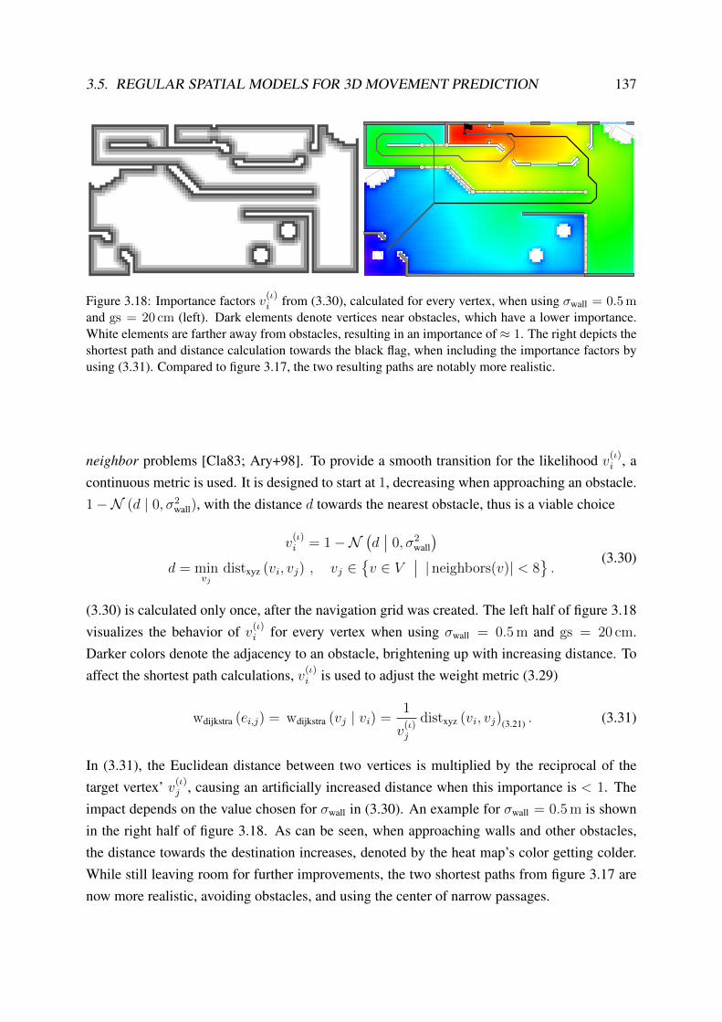
3.5. REGULAR SPATIAL MODELS FOR 3D MOVEMENT PREDICTION 137
Figure 3.18: Importance factors v(ι)i from (3.30), calculated for every vertex, when using σwall = 0.5 m
and gs = 20 cm (left). Dark elements denote vertices near obstacles, which have a lower importance.White elements are farther away from obstacles, resulting in an importance of ≈ 1. The right depicts theshortest path and distance calculation towards the black flag, when including the importance factors byusing (3.31). Compared to figure 3.17, the two resulting paths are notably more realistic.
neighbor problems [Cla83; Ary+98]. To provide a smooth transition for the likelihood v(ι)i , a
continuous metric is used. It is designed to start at 1, decreasing when approaching an obstacle.1−N (d | 0, σ2
wall), with the distance d towards the nearest obstacle, thus is a viable choice
v(ι)i = 1−N
(d∣∣ 0, σ2
wall
)d = min
vjdistxyz (vi, vj) , vj ∈
v ∈ V
∣∣ | neighbors(v)| < 8.
(3.30)
(3.30) is calculated only once, after the navigation grid was created. The left half of figure 3.18visualizes the behavior of v(ι)
i for every vertex when using σwall = 0.5 m and gs = 20 cm.Darker colors denote the adjacency to an obstacle, brightening up with increasing distance. Toaffect the shortest path calculations, v(ι)
i is used to adjust the weight metric (3.29)
wdijkstra (ei,j) = wdijkstra (vj | vi) =1
v(ι)j
distxyz (vi, vj)(3.21) . (3.31)
In (3.31), the Euclidean distance between two vertices is multiplied by the reciprocal of thetarget vertex’ v(ι)
j , causing an artificially increased distance when this importance is < 1. Theimpact depends on the value chosen for σwall in (3.30). An example for σwall = 0.5 m is shownin the right half of figure 3.18. As can be seen, when approaching walls and other obstacles,the distance towards the destination increases, denoted by the heat map’s color getting colder.While still leaving room for further improvements, the two shortest paths from figure 3.17 arenow more realistic, avoiding obstacles, and using the center of narrow passages.
138 CHAPTER 3. PROBABILISTIC MOVEMENT MODELS
Finally, the modified weighting is used to favor all movements that approach the destination
pdest(ei,j | qt−1
)=
κdest dist∗xyz (vj, vdest) < dist∗xyz (vi, vdest)
(1− κdest) else .(3.32)
The heuristic κdest in (3.32) is used to adjust the importance of the destination. While lower val-ues allow for detours, 1.0 enforces every taken edge to approach the requested destination. Thisrepresents a tradeoff between prior knowledge, and the behavior of the pedestrian [Ebn+16].
Besides adjusting the weight metric (3.31) to yield more realistic walking paths, the vertexlikelihood (3.30) can also be used directly within the random process of algorithm 1, to proac-tively avoid approaching nearby obstacles. v(ι)
j can either be included using another thresholdheuristic, or directly as probability. Depending on the actually used metric, a normalization ηmight be required beforehand
pwall(ei,j | qt−1
)= ηv
(ι)j . (3.33)
Using (3.33) within algorithm 1 alongside with other probabilities will yield more natural walks,by avoiding obstacles whenever possible. Yet, it will not fully prevent the walk from gettingstuck near obstacles, when there is no other option.
3.5.4 Continuous Results
The main disadvantage of the navigation grid is its discrete nature. By randomly walking fromvertex to vertex, as shown in figure 3.19a, directions are limited to multiples of 45°, and dis-tances to multiples of gs. While impacts are mitigated by the two introduced error metrics, gs
must still be reasonably small for individual errors to remain reasonable.
With walks and results directly tied to vertex positions, the approximated density p(qt |qt−1) is also rather discrete. This can be mitigated by introducing additional noise. Instead ofusing the last vertex directly as prediction result, this position can be slightly modified, creatinga slightly more continuous output. One option is to e.g. use a location drawn uniformly from therectangle denoted by this vertex instead [Ebn+17]. This is shown in figure 3.19b, where startand end of the random walk are located somewhere within the rectangle around each vertex.When performing thousands of random walks, this technique does neither affect the walkingdistance, nor the heading, on average. The distance and heading of individual walks, however,can deviate significantly, depending on the chosen walking distance dwalk and vertex spacing gs.This approach thus represents only a minor improvement towards continuous results, and thediscussed KDE is a better, yet much more costly, alternative [Bul+18].

3.5. REGULAR SPATIAL MODELS FOR 3D MOVEMENT PREDICTION 139
(a) (b) (c) (d)
Figure 3.19: Different strategies for walking along a graph-based data structure. (a) matches the tra-ditional approach, walking from vertex to vertex. (b) reduces the discreteness by randomly scatteringaround the destination vertex. (c) completely omits edge probabilities, just picking the destination basedon given distance and heading, when such a location is reachable. (d) is a combination of all three,randomly moving between adjacent cells, without being bound to the vertices themselves.
A solution that satisfies each requested walking distance and heading exactly, but is stillcomputationally efficient and suited for smartphone use, is given by using the continuous wall-intersection approach from section 3.3, but replacing costly intersection tests with cheaperqueries on the graph data structure: Given a starting point qt−1, heading q
(Θ)t−1, and walking
distance dwalk, the destination is known directly. This case is shown in figure 3.19c. Whether itis actually reachable from the starting point, and not blocked by obstacles, can be determined byfollowing edges that approximately point into the requested direction, similar to the A∗ shortestpath algorithm [HNR68]. Compared to the intersection tests from section 3.3, the graph directlyallows for fast, locally constrained queries, considering only a few edges that reside within acertain direction and distance. Furthermore, as the query returns the vertex that the requesteddestination belongs to, if being reachable, it provides a 3D location with known z-component,which was impossible for the 2D intersection tests from section 3.3.
Compared to random walks, there is no uncertainty or variation when using the approach. Ifreachable, the destination is used directly as-is, based on the requested heading and distance. Toadd an uncertainty in walking speed and direction, q(Θ)
t−1 and dwalk must be modified beforehand,e.g. by adding zero mean random variables N (0, σ2
turn) and N (0, σ2walk). The navigation grid is
then solely used to replace the costly intersection test with a more efficient solution. Randomwalks are completely omitted, as well as any semantic information stored on vertices. Whendirectly approaching an obstacle, where random walks got stuck in front, this approach willdirectly indicate that the requested walk is impossible. As earlier, one of several options, likeomitting the current simulation, must be chosen, to address this case.
When modifying this setup, at least, the information whether a vertex belongs to a stair, canbe included, to dynamically adjust the walking distance. For that, the algorithm sequentiallydeparts from qt−1, into the direction indicated by the heading q(Θ)
t−1. Each step is chosen to reach

140 CHAPTER 3. PROBABILISTIC MOVEMENT MODELS
the rectangle of the next vertex, if any, shown in figure 3.19d. In doing so, every segment of thewalk knows its underlying surface, enabling dynamic walking distance adjustments. However,due to considering only vertices along the path defined by the requested heading, individualprobabilities assigned to edges can not be considered. As discussed in section 3.3, while such adirect walking technique yields a continuous result, it is only suited for smaller simulation time-frames, as it relies on line-of-sight connections, where walking around corners is impossible.For longer simulations, the random walk is more suited, supporting fine-grained probabilities,yet producing more discrete results.
Some issues with discreteness can be mitigated by decreasing gs. However, this has a nega-tive effect on computational requirements, as random walks have to follow more edges to reacha given distance, and memory requirements are increasing quadratically. For a 100 m by 100 m
sized single floor, where 80 % of the surface is actually walkable, and 20 % belong to walls andother obstacles, 200 000 vertices are required when using a vertex spacing of gs = 20 cm. As3D placement only occurs for stairs, escalators and elevators, this number scales approximatelylinear with the number of floors in a building
|V | ≈ 80 %
(width
gs
depthgs
)N , N = |floors| . (3.34)
For a five story building, this results in 1 M required vertices. To uniquely identify this manyvertices, a 24 bit integer is needed for the numbering index. As discussed earlier, vertices canstore their location (x, y, z) using e.g. three 16 bit integers. Besides location, every vertex hasto store a list of ten neighbor indices. All combined, each vertex requires at least 36 byte ofdata storage. While today’s smartphones carry enough memory to easily handle this example,the situation is different for much larger public buildings, such as airports or hospitals. Incase of multiple-compound buildings, connected by large outdoor areas, even more vertices arerequired, to model their interconnection. When additional semantic details are added to verticesand edges, memory consumption increases even further. At worst, a single map can requireseveral hundred megabytes, becoming impractical for use on smartphones.
According to (3.34), memory concerns can be addressed by increasing gs, at the cost ofaccuracy. However, starting at gs >≈ 60 cm, there is an increasing risk for overlooking partsof the building. When the regular placement pattern does not align with the walkable surface,doors or narrow passages can be missed, excluding everything behind from being added to thenavigation grid. Real-world setups thus require more dense grids, ranging near gs ≈ 25 cm toprovide accurate results [Ebn+15; Ebn+16]. To predict movements within floorplans of hugebuildings, or multiple compounds connected by large outdoor areas, simultaneously addressingthe issue of discreteness, other data structures are required [Ebn+17].

3.6. IRREGULAR SPATIAL MODELS FOR 3D MOVEMENT PREDICTION 141
(a) (b) (c)
5 m
Figure 3.20: Different irregular spatial models for an example floorplan (left). The navigation gridcan use irregular sizing and placements, to model the walkable surface using rectangles (a). Instead ofmodeling the whole walkable surface, only the walkable paths can be described (b). Polygons properlyadapt to the shape of surrounding architecture (c).
3.6 Irregular Spatial Models for 3D Movement Prediction
As shown in the surveys from Afyouni et al. [ARC12] and Yanbing [Yan06], irregular placementpatterns can address some of the aforementioned problems. They are more flexible, and adjust tolocal architectural details, allowing for a better representation with reduced memory footprint.Especially when compared against the navigation grid. Referring to the latter, its vertices coulde.g. be placed irregularly. Using many small ones to describe stairs, doors, and narrow passages,while approximating open spaces with a few larger ones saves memory, and adds details onlywhere required, shown in figure 3.20a. However, this causes the length of their connecting edgesto vary significantly. Likewise, walkable directions become more discrete, not allowing for therandom walks as discussed in section 3.5. Also, it is not directly clear how to correctly describeneighborhoods, when a single vertex describes a large region and connects to many verticeswith smaller rectangles. Furthermore, rectangular shapes only work well with axis-alignedarchitecture, like shown in the figure. For buildings with a complex interior, the rectangularprimitive suffers from several drawbacks, not representing an ideal data structure [Fet+18].
Besides modeling the walkable surface, some irregular approaches model only the walkablepaths within a building, shown in figure 3.20b. An often used representative, are minimumspanning trees [Kru56] of a 2D Voronoi diagram [Lej50; Vor08]. First, the Voronoi diagramtessellates the walkable surface into smaller sections, adjusting to architectural details, suchas doors, walls, and other obstacles. This results in an irregular placement of sub-surfaces,represented by polygons (cf. figure 3.21b and 3.21d). The edges in between adjacent polygonscan hereafter be connected, forming a tree [Aur91]. A special variant of such a spanning treeis the generalized Voronoi graph (GVG) [CB95]. Applied to indoor scenarios, it describespotential routes through the building, similar to streets for car navigation, and can be used todescribe potential walks. It is often slightly modified, to remove some extends of the tree, which

142 CHAPTER 3. PROBABILISTIC MOVEMENT MODELS
(a) (b) (c) (d)
Figure 3.21: Delaunay triangulation and Voronoi diagram for an example floorplan. The corners ofwalls and other obstacles, shown as black dots, are connected by a Delaunay triangulation (a). Thisrepresentation can be converted to its dual, the Voronoi diagram (b). Using additional interpolationpoints along all wall segments increases the quality of both diagrams shown in (c) and (d). The GVG in(d) connects edges of the underlying Voronoi, describing walkable paths within the floorplan.
are considered unlikely, or unnecessary for modeling pedestrian walking behavior. This variantis referred to as reduced generalized Voronoi graph (RGVG) [NC99].
Mentioned earlier, another spatial representation are 3D meshes, describing the walkablesurface by triangles, or polygons in general, shown in figure 3.20c. A well known algorithmfor creating such meshes, based on a given set of edge-points, is the Delaunay triangulation
[Del34]. Aforementioned Voronoi graphs and Delaunay triangulation are closely related byduality. That is, one representation can be created from the other [DZM07]. Due to this duality,a 3D Voronoi graph can be derived from a triangulated 3D mesh, and vice versa. GVG andRGVG routes thus also work for 3D walking paths within buildings, along stairs, escalators andelevators, even though most of the aforementioned literature covered only 2D or 2.5D setups.
Depending on the way the floorplan is provided, the Voronoi diagram can e.g. be created byfirst performing a Delaunay triangulation, using the corner points of walls and other obstaclesas to-be-triangulated vertices. This is shown in figure 3.21a, where all corner points, shownas black dots, are connected by the Delaunay triangulation, which is hereafter converted to itsdual, the Voronoi diagram. This conversion can be performed by estimating a circle for eachtriangle, covering its three corners. For any two adjacent triangles, the centers of their circlesare connected, forming the Voronoi diagram [Joe99]. However, the result in 3.21b does notreveal any walkable paths. This is due to using only a few corners to perform the triangulation,not clearly separating between walkable areas and obstacles. By interpolating additional ver-tices along each wall segment, the Delaunay triangulation in 3.21c gets more dense. Now, thewalkable surfaces can clearly be separated from impassable areas. The latter is also describedby triangles, which must be deleted, as they reside within obstacles. Calculating the corre-sponding Voronoi diagram 3.21d, the GVG is now visible as the spanning tree along the edgesof the Voronoi cells [CB95]. The quality of the GVG thus directly depends on the number of

3.6. IRREGULAR SPATIAL MODELS FOR 3D MOVEMENT PREDICTION 143
interpolations along obstacle outlines. When the building’s floorplan is provided as 2D vectorgraphics, the Voronoi diagram can be created directly, using individual obstacle segments, givenas 2D lines [Kar04]. If the floorplan is provided as a triangulated 3D mesh, the correspondingVoronoi and GVG can also be created directly, using aforementioned translation.
The GVG in figure 3.21d denotes walkable routes within the map, which are centered be-tween walls and other obstacles [BJK05]. Resulting from an irregular tessellation, it can effi-ciently model complex architecture, and requires only a fraction of the memory demanded by anavigation grid. Similar to the latter, the GVG represents a walkable data structure, formed byconnecting several nodes. Yet, it models completely different movement predictions, as it doesnot cover large open spaces. Containing only a single path for traversing every region of thebuilding, it is mainly suited for narrow corridors, shown in figure 3.20b. To also cover scenarioswith pedestrians walking through large open spaces, adjustments are required. Hilsenbeck etal. [Hil+14] suggest a mitigation by placing a dense mesh of walkable nodes throughout largeopen areas. While the result hereafter covers the whole walkable surface, it suffers from thesame issues with discrete headings, previously discussed in section 3.5.
GVG und RGVG denote only a fraction of actually possible walks within the building. Thishas consequences for movement predictions p(qt | qt−1) and p(qt | qt−1,ot−1). In contrastto random walks along the graph, the risk of simulations getting stuck in front of obstacles isreduced, as there are less dead ends. On the other hand, only a fraction of all reachable lo-cations can be predicted by this setup. In theory, algorithm 1, used for the random walk, stillapplies to GVG. However, cumulative heading errors within (3.25) can not be compensated, asoften only two directions, back and forth, are possible. Similarly, the walking distance mightnot match with the distance between adjacent nodes of the GVG, which can be rather large. Asa workaround, the random walk could stop somewhere along an edge, to match the requesteddwalk exactly by interpolation. The strong limitations on allowed movements can be considereda benefit within narrow surroundings, such as hallways and stairwells. Getting stuck can be pre-vented, and the binary direction choice can suppress issues with sensor uncertainties. The GVGis also suited for navigation, supporting shortest path calculations, and adding constraints, likein (3.32). Yet, only affecting intersections, navigation constraints might be completely over-ruled by the heading. Furthermore, even after the adjustments from [Hil+14], the GVG suffersfrom drawbacks within large open environments, yielding similar issues with discreteness, asthe navigation grid. For such regions, another spatial data structure is more suited.

144 CHAPTER 3. PROBABILISTIC MOVEMENT MODELS
5 m
5 m
Figure 3.22: Three navigation mesh examples using triangles as primitives, including semantic informa-tion on indoor, outdoor, stairs and doors, shown in different colors. The segmentation algorithm ensuresthat primitives adjust to both, semantic boundaries and the surrounding architecture.
3.6.1 3D Navigation Meshes
Besides forming the dual of the Voronoi diagram, a Delaunay triangulation also represents a 2Dor 3D mesh of the building’s floorplan. It is created by triangulating the vertices interpolatedalong obstacle edges (cf. figure 3.21c). When omitting all triangles that would fully residewithin obstacles, all remaining ones denote the walkable surface. While this irregular result isnot viable for random walks, it can be used in the same way as discussed in section 3.5.4. Shownwithin the following, it can efficiently determine whether two locations within a building aredisconnected by an obstacle, and it allows reconstructing the z-coordinate when changing floors.Compared to the navigation grid, this irregular representation perfectly models surroundingarchitecture, as it closely adheres to obstacle borders. Simultaneously, it conserves memory, asthe triangles are significantly larger than aforementioned 20 cm by 20 cm grid cells [Fet+18].
When using a Delaunay triangulation, the average size of the triangles directly depends onthe distance between the to-be-connected vertices (see figure 3.21). As the triangulation onlyconsiders vertices, it is unable to distinguish between walkable surface and obstacles. Usinglarge distances thus increases the risk of triangles partially belonging to obstacles, shown infigure 3.21a. For the created mesh to be correct, the interpolated vertices are thus required tobe rather close, like shown in figure 3.21c. This aspect unnecessarily increases the number ofrequired triangles. Other algorithms besides Delaunay thus are more suited.
The general type of resulting data structure is referred to as navigation mesh, or meadow
map [Ark87]. It is e.g. used in computer games, to model the walkable areas, and to providenavigation [CS11]. While these meshes can be created from various data sources, a 3D modelof the building, containing floors, stairs, and objects combined with semantic information, isideal [Fet+18]. Literature provides various algorithms, such as watershed segmentation [VS91;RM00]. They generate primitives which accurately resemble the floorplan, including its se-mantic information, while trying to combine large regions into a single primitive. In general,

3.6. IRREGULAR SPATIAL MODELS FOR 3D MOVEMENT PREDICTION 145
the result describes the walkable surface using polygons. The algorithm ensures that adjacentpolygons share one of their edges, which is a crucial requirement for modeling adjacency.
As the result is used to represent the walkable surface, the same requirements as discussedfor the navigation grid (cf. section 3.5.1) apply. Walking below stairs or escalators is unlikely,and corresponding surfaces should be removed whenever the pedestrian has to crouch to fit be-neath. Similarly, walking close to walls and other obstacles is unlikely, and should therefore beprevented. This can be addressed by eroding the resulting mesh after its creation, thus shrinkingthe walkable surface by a given constant. To correctly determine pedestrian walking speeds fora certain surface of the floorplan, semantic information must be retained. The polygons thusmust be placed in a way that each one belongs to exactly one semantic group, like stairs, esca-lators or doors. Potential results are presented in figure 3.22. The depicted navigation meshesuse triangles as primitives, and adjust to semantic and architectural borders. The walkable re-gion was slightly eroded to ensure that regions directly adjacent to walls and other obstacles arenot considered walkable. Compared to the navigation grid, only a few primitives are needed toaccurately cover every nook and cranny of the floorplan.
The following focuses on movement predictions p(qt | qt−1) and p(qt | qt−1,ot−1), whenthe underlying spatial model is an irregular 3D navigation mesh of the walkable surface. Whilealso applying to polygons in general, the generated 3D mesh is assumed to contain only trian-gles. This is due to the triangle primitive offering unique characteristics, yielding a speed-upfor many of the required calculations, which is important for use on smartphones. Using trian-gles will slightly increase the required amount of memory, as more primitives and vertices areneeded. However, the result still consumes only a fraction of the navigation grid [Fet+18].
3.6.2 Movement Prediction
Similar to the navigation grid, the navigation mesh allows for several different approaches, topredict potential movements. It can e.g. be used as a fast look-up, to determine whether twolocations are connected, and reachable within a certain distance, providing a speed-up for thediscussions from section 3.3. Like in (3.12) and (3.8), potential whereabouts p(qt | qt−1) aredetermined by simulation, using a starting location, a walking direction, and distance, to predictnew whereabouts. In contrast to earlier, equations are described from another point of view,directly describing new whereabouts as the result from a random process. Again, the startingpoint for each simulation is given by posxyz
(qt−1
), combined with the walking direction q(Θ)
t−1,and distance dwalk. The latter can e.g. be set to the average of 1.4 m/s, or set to 0, to model the

146 CHAPTER 3. PROBABILISTIC MOVEMENT MODELS
case where the pedestrian is resting
q(x)t = q
(x)t−1 + d cos(q
(Θ)t−1)
q(y)t = q
(y)t−1 + d sin(q
(Θ)t−1)
d = dwalk + X walk
X walk ∼ N (0, σ2walk)
〈q〉t = 〈(x, y, z,Θ, . . .)〉t . (3.35)
(3.35) predicts new potential whereabouts in x and y by moving a distance d from the startingposition, into a given direction. For now, the z-coordinate q(z)
t is omitted, and will be discussedhereafter. Similar to (3.27), uncertainty in walking speed is given by a zero mean GaussianX walk, added to the requested distance. The heading is incorporated based on available priorknowledge. Like earlier, the initial walking direction often is completely unknown
q(Θ)0 ∼ U (0, 2π) . (3.36)
This heading is hereafter updated, depending on whether relative, absolute, or no heading ob-servations are available
q(Θ)t ∼ phead
(qt | qt−1,ot−1
)(3.13) . (3.37)
Again, due to the assumption of the pedestrian walking straight throughout a single simulation,this setup is only suited for small timeframes and short walking distances dwalk. As within (3.14),the result of (3.35) must only be accepted if posxyz (qt) can be reached from posxyz
(qt−1
). This
information, and the omitted z-coordinate, are both provided by the navigation mesh.
To determine whether two locations are reachable within a given distance, the trianglesand their adjacency are used. First, the triangle the starting position posxyz
(qt−1
)belongs
to is determined, shown in figure 3.23a. This is achieved by using barycentric coordinates[Vin17], describing the location of a point based on a triangle’s edges, hereby denoting whetherit resides within, or not. To prevent numerical issues, the z-component is allowed to vary, e.g.by working with 2D triangles in the (x, y) plane, and ensuring the point’s z is somewhere withinthe range of the original triangle’s z-coordinates. This is viable, as the created mesh ensuresthat there is at least a pedestrian’s height between triangles stacked along the z-axis. Findingthis initial triangle is costly when creating many samples, due to O(n), having to check everysingle triangle. This is addressed by caching, remembering the current triangle for every newlysampled qt, made clear within the following.
Having found the initial triangle, its adjacent neighborhood is examined. A fraction fromthe original navigation mesh is extracted, describing the reachable surface, when starting fromposxyz
(qt−1
), and walking for a certain distance. This surface is created by recursively adding
adjacent triangles using breadth-first search [GD18]. That is, first adding all directly adjacenttriangles, hereafter adding their adjacencies, ignoring duplicates. The recursion is terminatedas soon as a certain distance threshold has been reached, which depends on the to-be-simulated

3.6. IRREGULAR SPATIAL MODELS FOR 3D MOVEMENT PREDICTION 147
ρ3ρ1
ρ2
v
u
ρ
v
uρ′
ρ
(a) (b) (e)(c) (d)
Figure 3.23: Process for uniformly sampling a new location within the vicinity of a starting point (blackdot) when using navigation meshes as floorplan. First, the triangle the starting point belongs to is iden-tified (a). Second, a reachable fraction of the navigation mesh is extracted, based on some user-definedthreshold. One triangle within this fraction is chosen randomly, with respect to its size (b). Finally, arandom point within this triangle is created (c,d), hereafter denoting the destination (e).
walking distance dwalk. For short simulation distances dwalk, the extracted fraction of the navi-gation mesh contains only a few triangles, visualized in figure 3.23b.
For posxyz (qt) to be reachable from posxyz
(qt−1
), it must belong to one of the triangles
within the extracted fraction. As qt was calculated by (3.35), only x and y are valid for now.Whether the new (x, y) results in a change in z, depends on the floorplan. If start and end ofthe walk both belong to triangles that are part of the ground floor, the z-component remainsunchanged. If either of them e.g. belongs to a stair, the z-component is expected to be differ-ent. Thus, to determine whether posxyz (qt) is part of the extracted fraction of the navigationmesh, only (x, y) is used, examining whether this 2D location lies within any of the extractedtriangles, omitting their z-coordinate as well. If one triangle contains this 2D location, theomitted z-coordinate is re-calculated via barycentric interpolation [Vin17]. It reconstructs thez-coordinate based on (x, y), ensuring the resulting 3D coordinate resides on the triangle’s sur-face. Again, omitting z is valid, if the simulated walking distance dwalk is small, and triangles areensured to have a reasonable distance along the z-axis, which is a given for the described navi-gation mesh. To increase performance, the triangle that posxyz (qt) belongs to is remembered,preventing costly inclusion checks for subsequent simulations.
If the location determined by (3.35) does not belong to any of the extracted triangles, itis unreachable from the starting position posxyz
(qt−1
). Similarly to previous discussions for
other movement predictions, there are various options for dealing with such cases. Either byrunning the simulation again, yielding a slightly different location, due to the random noise forheading and distance, or by omitting this single simulation completely. Yet, a different strategycan be viable as well. Besides handling cases where the randomly determined location wasunreachable, it can serve as a complete walking prediction on its own, able to include arbitraryprobabilistic constraints, similar to the random walk from section 3.5.2.

148 CHAPTER 3. PROBABILISTIC MOVEMENT MODELS
According to section 3.2, a movement prediction model without prior knowledge just scat-ters potential new locations around the initial one. Not constraining the walking direction, andlimiting the walking distance within a broad, uniform range. The models in section 3.2 per-formed this kind of prediction, but were unable to consider the floorplan, and were only suitedfor 2D setups. Using the navigation mesh, aforementioned model can be constrained by thefloorplan, and supports 3D location predictions, by re-calculating the missing z-component.
A predicted posxyz (qt) is somewhere near its origin posxyz
(qt−1
). It can thus be generated
by determining the origins triangle, extracting a fraction of the mesh describing the walkablesurface around it, and randomly picking a destination that belongs to this walkable area. Thisyields a new location within the vicinity of posxyz
(qt−1
), constrained by the walkable surface,
including 3D location information. Here, p(qt | qt−1) is simulated by randomly picking a pointon the extracted fraction of the walkable surface. This is achieved by randomly choosing atriangle that is part of the extracted surface, shown in figure 3.23b, hereafter selecting a randompoint that resides within this triangle, visualized in figure 3.23c and 3.23d.
A random triangle is selected by drawing an uniformly distributed index, e.g. using a randomnumber generator. When performing an infinite number of simulations, this produces an equalnumber of samples from every triangle. However, as the size of all triangles is irregular, thisyields a non-uniform distribution of points with respect to the walkable surface, as sampleswill concentrate within smaller triangles. Thus, they must not be selected uniformly, but biasedbased on their surface area, where larger triangles are chosen more often than smaller ones.Each triangle’s probability is given by
p(trianglei) = η area(trianglei) , (3.38)
including a normalization constant η. Details on implementing biased random processes areomitted for now, and presented later in chapter 4. As shown within figure 3.23c, every point ρwithin a 2D or 3D triangle is then uniquely identified by a linear combination of two edges
ρ = ρ1 + u(ρ2 − ρ1) + v(ρ3 − ρ1) , 0 ≤ (u+ v) ≤ 1 . (3.39)
A random point within the triangle can be sampled by creating two uniformly distributed ran-dom numbers u, v ∼ U (0, 1). In case of (u + v) > 1, occurring for 50 % of the samples, theresulting point is outside of the triangle. Simply omitting those cases, and drawing a new one,can affect the output of poor (pseudo-)random number generators. The rejected result can beused when projecting the point back into the triangle, by mirroring it along the edge betweenρ2 and ρ3, visualized in figure 3.23d. Analytically this is achieved by
ρ = ρ1 + (1− u)(ρ2 − ρ1) + (1− v)(ρ3 − ρ1) , 1 < (u+ v) ≤ 2 . (3.40)

3.6. IRREGULAR SPATIAL MODELS FOR 3D MOVEMENT PREDICTION 149
When using the described approach, potential new whereabouts are given as samples, uniformlydistributed throughout the extracted fraction of the navigation mesh, shown in figure 3.24a. Thisyields a discrete drop to a probability of zero when leaving the fraction, not being realistic. Itcan be mitigated by applying a KDE to the samples, yielding a continuous probability densityfunction, slowly fading near the boundaries, shown in figure 3.24b.
In section 2.7, the KDE used on top of discrete fingerprints also included a weight for eachof them, based on their probability. That is, the weight favored some fingerprints over others,concentrating a larger part of the resulting density around fingerprints with higher weights. Thesame idea can be applied to the movement prediction. By calculating a weight w(qt) for eachsample qt, and applying a KDE afterwards, the uniform behavior is modified. Including weightsallows for creating arbitrary, non-uniform distributions, based on additional metrics, such as
w(qt) =
p(qt | qt−1) transition probability without observations
p(qt | qt−1,ot−1) transition probability with observation ,(3.41)
hereafter being as powerful as the random walks. The behavior of (3.35) can e.g. be approxi-mated by uniformly sampling multiple locations qt that are reachable from qt−1, and weightingeach one according to whether it matches the heading q(Θ)
t−1, and walking distance dwalk, includingan uncertainty
w(qt) = p(qt | qt−1,ot−1) = N(α∣∣ 0, σ2
turn
)N(d− dwalk
∣∣ 0, σ2walk
)α = ∠∆
(∠xy
(qt−1, qt
), q
(Θ)t−1
), d = distxy
(qt−1, qt
), 〈q〉t = 〈(x, y,Θ, . . .)〉t .
(3.42)
An example of random sampling with and without weights is shown in figure 3.24. The firsttwo figures depict the unweighted uniform sampling from a fraction of the navigation mesh,including a 3.5 m radius around the start qt−1. The corresponding KDE in figure 3.24b showsthe uniform probability, fading to zero towards the borders. When adding weights (3.42), allsamples with matching distance and heading are more important than others, visualized in fig-ure 3.24c. The corresponding KDE in figure 3.24d denotes a density, shaped as fraction of acircle, where both, the requested heading and distance, are correct. This solution matches with(3.12) and (3.14), yet, including the building’s floorplan, and supporting three dimensions.
Apart from the example (3.42), this approach yields room for an infinite number of met-rics. Almost all of the densities discussed in chapter 2 can be applied as well, to combine auniform floorplan-based movement prediction with sensor observations. By adjusting weights,an overall density is derived, that combines all individual viewpoints.

150 CHAPTER 3. PROBABILISTIC MOVEMENT MODELS
5 m
(a) (b) (c) (d)
Figure 3.24: 1000 unweighted (a) and weighted (c) random samples from a fraction of the floorplan’snavigation mesh, within a 3.5 m radius around the start qt−1 (black dot). The corresponding KDEs areshown as heat maps in (b) and (d). Weights used in (c) and (d) are based on (3.42), with dwalk = 2.8 m
and σturn = 0.3, assuming the pedestrian’s heading to be q(Θ)t−1 = 45°.
Besides being versatile, this approach is often impractical for use on smartphones. As shownin figure 3.24, numerous random samples are required, to derive new whereabouts, when start-ing from a single origin. In contrast, (3.42) requires just a few calculations to provide a move-ment prediction. As discussed earlier, if the uncertainties for σwalk and σturn are small, a singleprediction should be sufficient to approximate p(qt | qt−1).
However, this approach can e.g. be used for situations where the direct prediction (3.35)is unable to provide a result due to obstacles. A result is then obtained by requesting oneuniform sample with additional weighting, denoting how well the uniformly sampled locationmatches the initially requested heading and destination. Furthermore, the bottleneck solelystems from the required uniform sampling, to ensure some samples with a decent weight arepresent. The weighting process itself is efficient, and weights can e.g. be used to combine (3.35)with navigation information, favoring results that approach the pedestrian’s destination.
3.6.3 Navigation
As briefly mentioned for the GVG, irregular spatial models are also suited for navigation pur-poses. The internal data structure of a car navigation system is similar to the way the GVGmodels walkable routes within the building. It describes streets and intersections by edges andvertices, placed at arbitrary, irregular positions. As streets are rather narrow, they are well-approximated by edges with a certain thickness. However, for large open spaces, often encoun-tered indoors, a single edge does not provide a viable representation. It reduces the walkablesurfaces to a narrow channel, preventing the pedestrian from reaching any arbitrary location (cf.figure 3.20). The previously presented navigation grid suffers from the same issue, but mitigatedit, by placing numerous vertices and edges throughout the whole walkable area. The irregularnavigation mesh models the same surface, but requires only a few triangles. However, shortest

3.6. IRREGULAR SPATIAL MODELS FOR 3D MOVEMENT PREDICTION 151
5 m
Figure 3.25: Synthetic (left) and real-world example for shortest paths on navigation meshes when usinga graph created by connecting edge-midpoints for Dijkstra’s algorithm. Resulting paths avoid obstaclesbut often suffer from abrupt heading changes or zig-zag patterns. The heat map visualizes the walkingdistance towards the destination for every location within the building, where warm colors (red) are near,and cold colors (blue) are farther away. The heat map is created by searching for the nearest edge-midpoint, and using its known distance towards the destination.
path algorithms, like Dijkstra or A∗, rely on a graph-based data structure. Here, the navigationmesh’s representation is disadvantageous. While adjacent triangles always share two vertices,and thus also denote a graph-like structure, suited for Dijkstra or A∗, it is too sparse to provideviable results. Furthermore, this representation tends to favor exterior edges, as they providethe shortest possible connection [Kal10a], yielding the same unnatural walking patterns as thegraph without an obstacle-avoiding metric (see figure 3.17 and section 3.5.3).
A slight improvement is given when deriving a graph by connecting the edge-midpoints ofeach triangle, instead of the their corner vertices. This avoids movements along outer edges[Kal05; Cha82]. The results for a synthetic and a real-world example are shown in figure 3.25.Except for some minor issues with abrupt heading changes, the overall result for the syntheticfloorplan is viable. Within the real-world example, large open spaces clearly suffer from the dis-cussed drawbacks, indicated by zig-zag connections. The quality of the routing graph stronglydepends on the size and placement of the triangles, which in turn depend on the segmentationalgorithm used for deriving the navigation mesh. A shortest path calculation based on this resultthus represents an approximation of the actually required walking distance.
A corresponding distance-to-destination heat map is shown in the right of figure 3.25. Forevery location, it depicts the nearest edge-midpoint’s known distance towards the destination.The lower left of this heat map indicates major changes in distance between adjacent trian-gles. Their size and placement is unfavorable for the shortest path calculation. While there aremany variations of this strategy, like connecting triangle-centers instead of edge-midpoints, ora combination of both, they all suffer from similar drawbacks [Kal05].
Results can be improved by subdividing large triangles, before deriving the temporal graph.This is similar to the evenly-sized tessellation of the walkable surface, presented by [Hil+14].Yet, this causes new issues, as it increases memory requirements, which were originally meant

152 CHAPTER 3. PROBABILISTIC MOVEMENT MODELS
5 m
Figure 3.26: Synthetic (left) and real-world example for shortest paths on navigation meshes when usingthe funnel algorithm. Resulting paths are straight and realistic, but stick to obstacles (bold lines). Theextended version of the algorithm adds additional clearance, avoiding obstacles, being more realistic (thinlines). The heat map (center) visualizes the walking distance towards the destination for every locationwithin the building, is smooth, but computationally expensive. It can be approximated by barycentricinterpolation (right), and differs only slightly from the original.
to be decreased by using the navigation mesh. Similarly, the complexity of all required compu-tations increases as well, while still yielding inferior results.
A robust solution is given by the (extended) funnel algorithm [Kal10b; HS94]. Instead ofstrictly walking along edges, it also allows for straight movements through primitives. Thisis achieved by first calculating the shortest path like earlier, hereafter refining the result, bywalking directly through primitives whenever possible. That is, the algorithm analyzes thewalkable surface itself, instead of only the approximation. Its output is often superior to theone derived from the navigation mesh in section 3.5.3. Results for a synthetic and a real-worldexample are shown in figure 3.26. Compared to the one from figure 3.25, the path resulting fromthe funnel algorithm is smooth and straight. However, it sticks unnaturally close to obstacles.This is addressed by an extensions to the algorithm, adding margins, to walk around obstacles.Hereafter, resulting paths resemble actual pedestrian walking behavior. Both algorithms are alsoshown for the real-world floorplan. As earlier, when obstacles are not avoided, the upper-leftstairs denote the shortest path towards the destination. When adding a safety margin to avoidobstacles, the shortest path uses the stairs on the right, and looks more natural.
While the algorithm provides realistic walking paths, it requires complex calculations forevery single location in question. Compared to the graph-based solution from section 3.5.3,pre-calculating and storing the shortest path from every single location towards the destination,is impossible. However, as mentioned within the discussions on movement predictions, the ac-tual path is irrelevant. The only information required is whether a new prediction posxyz (qt)
is nearer to the destination than the previous one posxyz
(qt−1
). To perform this comparison,
every location within the navigation mesh must know its distance towards the chosen destina-tion. When using triangles as primitives, this information can be approximated by barycentricinterpolation. After choosing a destination, the funnel algorithm is used to calculate the dis-

3.7. SUMMARY 153
tance towards the destination for every vertex of the mesh’s triangles, once. This hereafterallows estimating the approximate distance towards the destination for every location withinthe triangles, using the barycentric interpolation. While results will be slightly different thanperforming an actual calculation of the funnel algorithm, they are close enough. The inter-polation is computationally inexpensive, and additional memory requirements for storing thedistance information are negligible, thus well-suited for smartphone use. Figure 3.26 shows thecorresponding heat maps, denoting the distance towards the destination within the small roomon the second floor. The left uses exactly calculated distances from the funnel algorithm, theright is based on barycentric interpolation. As can be seen, there is only a minor differencebetween both. The result can be used in a similar way as earlier for the navigation grid (3.32),weighting movements on whether they approach the destination ρdest, or depart from it
w(qt) = pdest(qt | qt−1
), 〈q〉t = 〈(x, y, z, . . .)〉t
=
κdest dist∗xyz
(posxyz (qt) ,ρdest
)< dist∗xyz
(posxyz
(qt−1
),ρdest
)(1− κdest) else .
(3.43)
3.7 Summary
Within this chapter, the likelihood for certain pedestrian movements and their probabilistic pre-diction, based on a floorplan, was discussed. Similar to car navigation systems, this informationcan be used to restrict certain movements, addressing sensor faults and uncertainties. Presentedmodels ranged from simple analytical 2D setups, to highly discontinuous 3D variants, consid-ering the floorplan and sensor observations. The latter require spatial data structures, where tworepresentatives were introduced. Based on them, various new probabilistic movement predic-tions were derived. Finally, the aspect of navigation was discussed, developing new algorithmsfor realistic routing within buildings, and corresponding movement predictions.
For an initial impression, the first movement predictions were completely unconstrained,analytical 2D variants. They visualized the drawbacks of not including the floorplan, and otherprior knowledge. Denoting large homogeneous shapes for new potential whereabouts, they areviable for a few use cases only. As pointed out, especially the current walking direction iscrucial for the quality of the estimated predictions. However, including this information alreadyreached the limitations of analytical approaches. While possible in general, the result representsonly an approximation of actual likelihood.
Therefore, the concept of simulation was briefly introduced. Instead of analytical calcula-tions, densities were represented by multiple samples. When applying a KDE on top of these

154 CHAPTER 3. PROBABILISTIC MOVEMENT MODELS
samples, a continuous and calculable density is derived. These simulations also enable consid-ering the building’s floorplan. Each sampled movement can be examined whether it is blockedby an obstacle, e.g. by using intersection tests. However, all discussed approaches referred totwo dimensional setups only. To efficiently predict 3D pedestrian movements, spatial floorplanmodels are required, describing the walkable surface.
The first examined data structure was a graph with vertices and edges. Its vertices wereplaced regularly throughout the whole walkable area of a building, covering ground floor, stairsand similar. When two adjacent vertices are physically reachable from one another, they gotconnected by an edge. The result describes the building’s walkable surface, referred to as nav-igation grid. Hereafter, an algorithm to estimate new potential whereabouts based on randomwalks along this graph was developed. A potential destination is created by starting from agiven origin, and randomly following adjacent edges. For derived destinations to be meaning-ful, edges are chosen based on probability metrics, denoting their likelihood, for example basedon a known heading. Thus, all resulting samples are distributed based on the likelihood of theedges they followed. The navigation grid allows for an efficient 3D movement prediction, basedon available knowledge. With graphs well suited for shortest path estimations, this strategy alsoenabled navigation. By introducing some adjustments, the calculated paths became realistic, de-noting potential routes through the building, and avoiding nearby obstacles. Yet, the navigationgrid requires large amounts of memory, and shows a rather discrete behavior.
Therefore, the navigation mesh was discussed as an alternative, also providing a spatial rep-resentation, yet, requiring less memory. It describes a building’s interior by triangles of varyingsize and location. As adjacent triangles share one of their edges, they closely resemble thewalkable surface. This data structure does not allow for random walks, and new probabilis-tic predictions had to be developed. One was similar to an initial analytic variant, calculatingpotential destinations based on walking speed, direction and uncertainty, yet, accepting it onlyif physically reachable. In contrast to earlier, the navigation mesh determines the reachabilityefficiently, and allows for a 3D estimation of the destination, impossible for the analytic variant.However, including additional probabilistic constraints besides distance and heading is limited.Therefore, the concept of uniform sampling and weighting was briefly introduced, equippingeach sample with a weight, which denotes the sample’s likelihood. These weights also allowedfor including navigational knowledge, indicating whether a potential movement approaches thedestination. The required routing was calculated by the extended funnel algorithm. It derivesrealistic walking paths, by avoiding obstacles. To prevent costly calculations, an efficient inter-polation strategy was developed that only needs to be calculated once.
The presented approaches allow an efficient prediction of potential movements, usable toconstrain sensor uncertainties. Combining both aspects is the topic of the following chapter.

Chapter 4
Recursive Density Estimation
As discussed within the two previous chapters, just using sensor observations to perform loca-tion estimations will yield results that are unstable, due to noise and uncertainty present withinthe readings. If the unknown state is observed by a single sensor only, and estimated solely byits noisy measurement, the resulting estimation directly depends on this measurement’s quality.By using additional information on surroundings, like a road map or the building’s floorplan,impossible movements indicated by some sensor can be addressed and compensated. However,there remains a discrepancy, when sensor readings are erroneous, but the indicated movement ispossible based on the map, yielding unstable and jumping location estimations. As discussed inchapter 2, averaging is able to compensate sensor noise, especially when it is of the zero meanGaussian type, by using more than one reading to perform the estimation. However, the pre-sented types of low-pass filters resulted in increased delays of the output. While delays are not aproblem for static measurands, like a moored ship, or a resting pedestrian, they are cumbersomefor dynamic systems with moving objects, which represent the main topic of this work.
The effect of using the moving average of sensor data to perform an estimation, is analyzedby an example. Assuming the one dimensional problem, to determine the position of a staticobject. Its current 1D position is observed within ot, by a noisy location sensor. For now, its realposition qt is constant, at 10 m, and the location sensor’s uncertainty is a zero mean Gaussian:
qt = 10 m , ot = qt +N (0, σ2) , σ = 3 . (4.1)
To improve the location estimation, the incoming sensor data ot is filtered by a moving averagelow-pass filter. It is implemented using a continuous equation, similar to simple IIR filters andthe complementary filter discussed in section 2.4.1 and 2.4.2:
qt = κ qt−1 + (1− κ)ot , κ = 0.9 , q0 = 0 . (4.2)
155

156 CHAPTER 4. RECURSIVE DENSITY ESTIMATION
In (4.2) the incoming observations o slowly contribute to the new state variable qt, linearlymixed with the previous one qt−1, representing the low-pass. Due to the mixing, the estimatedresult will experience a delay, as new observations are slowly faded in, depending on the valueof (1 − κ). This effect is depicted in figure 4.1a. After the sensor provides its first readings, ittakes some time for the estimation qt to move from q0 = 0 towards the real location. As thelatter belongs to a non-moving object, the system is stable after the low-pass filter converges.
If the underlying measurand is dynamic, e.g. a to be localized moving object, aforemen-tioned delays remain present at any instant in time. For a corresponding example of a dynamiccase, the state of an object’s position is assumed to start at q0 = 10 m, and hereafter increase by0.5 m/s. The behavior of the observation remains as for the static variant in (4.1):
qt = 10 m + t 0.5 m/s , ot = qt +N (0, σ2) , σ = 3 . (4.3)
The results are shown in figure 4.1b. While the output of (4.2) starts to approach the unknownstate of (4.3) based on the value chosen for κ, the state has already changed to a new value.Thus, the filter’s output constantly lacks behind the real value. However, when the behavior ofthe dynamic entity, like a car, ship or pedestrian, is known, assumptions on potential changescan be made. This is where the dynamic transition models from chapter 3 come in to play.When e.g. the speed of a moving object is known, future locations can be predicted, dependingon the elapsed amount of time. The delay in (4.2) results from the old estimation κqt−1 beingfavored over new sensor readings, and qt is unable to catch up. This can be addressed whenthe dynamic behavior is known. Instead of solely using κqt−1 as starting value for the nextestimation qt, the system’s behavior is included as well, predicting expected changes since qt−1.If this prediction ∆qt is added to the previous estimation qt−1, the delay induced by the filter iscompensated by the known behavior. The resulting filter is written as follows:
qt = κ(qt−1 + ∆qt
)+ (1− κ)ot , 0.5 < κ < 1.0 , q0 = 0 , (4.4)
where ∆qt defines the system’s dynamic behavior from (4.3), in this case thus given by
∆qt!
= qt − qt−1 = t 0.5 m/s . (4.5)
(4.4) equals the complementary filter (2.43), except that its gyroscope sensor is replaced by aprediction ∆qt of the system’s behavior. Figure 4.1c shows the resulting estimation when using(4.4) and (4.5) with κ = 0.9, instead of (4.2). Due to the known system dynamics, the prediction∆qt is able to compensate the introduced delay, and the filtered output converges similar to thestatic version shown in figure 4.1a.

157
05
10152025
5 s 10 s 15 s 20 s
(a) (4.1) with (4.2)
5 s 10 s 15 s 20 s
(b) (4.3) with (4.2)
5 s 10 s 15 s 20 s
(c) (4.3) with (4.4)+(4.5)
posi
tion
realsensor
estimated
Figure 4.1: Behavior of a state estimation for (4.1) and (4.3), using the filters (4.2) or (4.4)+(4.5) onsensor observations. When the measurand is static (a), the estimation stabilizes after several seconds. Fordynamic measurands, the estimation is a delayed version of the real value (b). This can be compensatedwhen the system’s behavior is known and can be predicted (c).
Figure 4.2 depicts the results for another dynamic system, where the unknown state performsa sinusoidal oscillation, observed by a sensor within an uncertainty of σ = 1
qt = sin(0.125 t) 4 m/s , ot = qt +N (0, σ2) , σ = 1 . (4.6)
The prediction ∆qt used within (4.4) is adjusted accordingly:
∆qt = qt − qt−1 = 4 m/s(
sin(0.125 t)− sin(0.125 (t− 1)
))≈ ∆t
((sin(0.125 (t− 0.5)
)4 m/s
) d
dt
)= ∆t
1
2cos(0.125 (t− 0.5)
).
(4.7)
As earlier, ∆qt within (4.7) describes the system’s dynamic change within a timeframe. Insteadof using the difference between qt and qt−1, this change can also be described by the derivativeof the underlying process, times the timeframe. While the latter is an approximation, it isdesirable for some situations, discussed later. As can be seen within figure 4.2a, when not usinga prediction, the filtered output quickly starts to deviate from the real underlying value. Thefilter not only introduces a delay, the amplitude of the oscillation is changed as well. This is dueto its design, using (1 − κ) to slowly introduce new observations. As soon as qt gets near theoscillation’s maximum amplitude, actual sensor values already started to decrease, preventingthe estimation from reaching it. For lower frequencies in (4.6), or smaller values of κ, the effectof the changed amplitude becomes less pronounced. A smaller κ, however, increases the impactof sensor noise, as it changes the low-pass filter’s cut-off frequency. When including the knownsystem behavior as prediction in figure 4.2b, filtered results become viable.
In the presented examples, κ was an empiric, constant choice, which will not suit real-worldscenarios. While lower values of κ introduce less delay, they pass more sensor noise, andvice versa. κ thus depends on the amount of noise present within the sensor readings, whichmight be dynamic as well. If noise is minor, (1 − κ) should be large, to favor the currentobservation ot, and vice versa. Within previous examples, the system’s behavior was well-

158 CHAPTER 4. RECURSIVE DENSITY ESTIMATION
−6
−3
0
3
6
10 s 20 s 30 s 40 s 50 s 60 s 70 s
(a) (4.6) with (4.2)
10 s 20 s 30 s 40 s 50 s 60 s 70 s
(b) (4.6) with (4.4)+(4.7)
posi
tion
realsensor
estimated
Figure 4.2: Behavior of a state estimation for (4.6) using the filters (4.2) or (4.4)+(4.7) on sensor ob-servations. When no prediction is available (a) the estimation constantly lacks behind the real location.With prediction (b), estimation and real value are almost identical.
known, and the prediction was expected to be exact without errors. For real-world use cases,however, the prediction is uncertain as well. The dynamics often are not fully known, can notdirectly be inferred for absolute points in time, and are as uncertain as the observed sensor data[Jaz70; GSS93]. The movement behavior of a ship, for example, depends on the current speedand rudder position, which are subject to changes, and can only be estimated based on sensorreadings. Furthermore, speed and current location are influenced by unknown external factors,such as wind, waves and ocean current. Just as the unknown state, a prediction can be dependenton sensor observations, and is subject to unknown external influences. This also leads to thequestion of how trustworthy the prediction currently is.
While (4.4) already contains a concept for either favoring the prediction or the sensor, givenby κ, it supports only a single sensor. More could be added as (1 − κ)o terms – one for everysensor, each using a different κ – but determining the correct value for each is cumbersome.Furthermore, the presented example described the unknown state as a single scalar. For in-door localization, however, the state contains the pedestrian’s 3D position and heading. Also,not every sensor contributes to all four values (cf. chapter 2 and chapter 3). Additionally, thepresented prediction is unable to include prior information, e.g. given by a floorplan. Finally,while (4.4)’s result was more realistic than the unfiltered observation, the quality of this result isunknown. Also, it is unable to include known uncertainties in a probabilistic way, representinga drawback, discussed in the two previous chapters.
This chapter thus focuses on methods and algorithms that can be used to combine multiplesensor inputs, to optimally estimate an unknown state. Algorithms must be able to include un-certainties present within both, sensor readings, and the dynamic prediction process. Referringto indoor localization and navigation, the sensor readings from the smartphone, discussed inchapter 2, are combined with potential movements of the pedestrian, discussed in chapter 3.The unknown state, that is, the pedestrian’s whereabouts and heading, is determined based on aprobabilistic fusion of the evaluations and transitions, described within both previous chapters.

4.1. PROBABILISTIC INFORMATION FUSION 159
p(q)p(q | o) = η p(o | q) p(q)
p(o | q)
Figure 4.3: Combining a prior estimation (left) with current sensor observations (right) to determine thecurrent posterior (center) via multiplication and normalization. Even though both probabilities (left/right)seem near zero, normalization yields another Gaussian distribution.
4.1 Probabilistic Information Fusion
As discussed, to determine the unknown state of a dynamic system, such as a moving vehicle,ship or pedestrian, information available by sensors and models should be combined in a prob-abilistic manner. Doing so includes known uncertainties, and provides a result that is optimal
for the given values, including an accuracy indication for the output. Referring to the simple 1Dlocalization example from earlier, a probabilistic combination based on uncertainties is brieflyexamined. Assuming the 1D location of the object to be known, including some uncertainty,given by p(q) with q = x, referred to as prior. At the current location of the object, a sensorreading o = x is observed, yielding a hint on the current location, as seen from the sensor,called measurement p(o | q). According to Bayes’ rule, the object’s most likely whereabouts qgiven the sensor reading o and initial guess p(q), is called posterior p(q | o) and defined as
posterior︷ ︸︸ ︷p(q | o) =
measurement︷ ︸︸ ︷p(o | q)
prior︷︸︸︷p(q)
p(o)︸︷︷︸normalization
= η p(o | q) p(q) =
p(o | q) p(q)∑q′ p(o | q′) p(q′)
discrete
p(o | q) p(q)∫∞−∞ p(o | q′) p(q′) dq′
continuous .(4.8)
Shown within (4.8), the posterior is given by the product of the initial expectations and currentsensor observations, including a normalization, to ensure the integral of the result yields 1, andthus describes a PDF as well. For readability, the normalization is abbreviated as η. Figure 4.3depicts a corresponding example of the posterior resulting from prior and observation. Eventhough both distributions barely overlap, and the result of their product is near zero, the normal-ization η yields a new PDF. When both, prior and observation, are distributed normally, such aswithin the figure, the normalized posterior denotes a normal distribution as well [Smi11]
ηN(x∣∣ µ1, σ
21
)N(x∣∣ µ2, σ
22
)= N
(x∣∣ µ1,2, σ
21,2
). (4.9)

160 CHAPTER 4. RECURSIVE DENSITY ESTIMATION
The new µ1,2 and σ21,2 of the resulting distribution are given by
µ1,2 =µ1σ
22 + µ2σ
21
σ21 + σ2
2
, σ21,2 =
σ21σ
22
σ21 + σ2
2
. (4.10)
For the following discussions, a slightly different notation is used for µ1,2 and σ21,2, where a
part of the equations is shared, and denotes how the two PDFs are combined. By adding thesubstitution term +(σ4
1 − σ41), σ1,2 can be rewritten as
σ21,2 =
σ21σ
22
σ21 + σ2
2
=σ2
1σ22 + σ4
1 − σ41
σ21 + σ2
2
=σ2
1σ22 + σ4
1
σ21 + σ2
2
− σ41
σ21 + σ2
2
= σ21 −
σ41
σ21 + σ2
2
. (4.11)
µ1,2 is adjusted similarly, by adding +(µ1σ21)− (µ1σ
21)
µ1,2 =µ1σ
22 + µ2σ
21
σ21 + σ2
2
=(µ1σ
21) + µ1σ
22 + µ2σ
21 − (µ1σ
21)
σ21 + σ2
2
=µ1σ
21 + µ1σ
22
σ21 + σ2
2
+µ2σ
21 − µ1σ
21
σ21 + σ2
2
=µ1(σ2
1 + σ22)
σ21 + σ2
2
+σ2
1(µ2 − µ1)
σ21 + σ2
2
= µ1 +σ2
1
σ21 + σ2
2
(µ2 − µ1) .
(4.12)Finally, (4.10) can be condensed to
µ1,2 = µ1 + k(µ2 − µ1)
σ21,2 = σ2
1 − k σ21
with k =σ2
1
σ21 + σ2
2
= σ21
(σ2
1 + σ22
)−1. (4.13)
According to (4.13), the new mean and variance are combined by a scalar value k, which solelydepends on the uncertainty of the to-be-combined distributions: the prior and the measurement.Due to the fraction, 0 ≤ k ≤ 1 with k = 0 for σ1 = 0, and k = 1 for σ2 = 0. The new mean µ1,2
depends on the prior’s mean plus k times the difference between the prior and measurement. Inother words, for k = 0, the new mean equals the prior’s mean, for k = 1 the new mean equalsthe measurement’s mean. For 0 < k < 1 it is somewhere in between. k thus works exactlyas κ within (4.2)/(4.4), deciding how to mix the prediction and the measurement. Yet, k is notempirically chosen, but depends on uncertainties. If the σ1 of the prior is smaller than the σ2
of the measurement, k < 0.5, and the posterior is nearer to the prior than to the measurement.If σ2 is the smaller one, k > 0.5, and the posterior shifts towards the measurement. In otherwords, k decides whether the prediction or the measurement is to be trusted more.
As (4.13) points out, the new uncertainty σ1,2 is also affected by k. However, no mixingbetween both uncertainties σ1 and σ2 is applied here. The new uncertainty equals the one ofthe prior, minus a fraction of the same value. Thus, the uncertainty of the posterior is unable togrow, but can only decrease. Put another way, the posterior will always be more accurate thanthe prior, independent of the uncertainty of the measurement.
4.2. BAYES FILTER 161
The discussed concept also allows for adding observations from more than one sensor, thatoccurred at the same instant in time. Assuming statistical independence of all sensors, thecombined probability of all currently available sensor readings o, given the current unknownstate q, is determined by the product of the individual probabilities
p(o | q) =N∏i=1
p(oi | q) , o = (o1, . . . , oN) . (4.14)
Again, if all observations are distributed normally
p(oi | q) = N(oi∣∣ µi, σ2
i
), (4.15)
the result of (4.14) is given by applying (4.13) N − 1 times, to combine all N sensor readingsinto a single normal distribution. If some sensor was faulty and did not provide an observation,it can simply be omitted. Due to (4.13), every additional sensor yields a decrease in uncertainty,rendering the result more accurate. However, (4.15) only holds true for independent sensors,providing their observations at the same instant in time. For subsequent observations, a differentapproach is required, as it is still unclear how the time component, and e.g. older observations,contribute to the overall result. Within the previously presented example of the IIR filter, newsensor readings yielded a contribution as they occurred, stabilizing the location estimation ofan object over time, refining the previous estimation. Furthermore, a prediction was added, todescribe the system’s dynamic behavior and thus compensate delays introduced by the filteringprocess. Both aforementioned aspects must be included within the probabilistic variant as well.
4.2 Bayes Filter
This leads to the question of how a probabilistic estimation can be improved when there aresubsequent observations from sensors at different points in time, that is, a history of observa-tions, and when a system and its unknown state are dynamic. The answer to both is providedby making the posterior p(q | o) from (4.8) dependent on the current time t, and conditioningit not only on the current observation o, but on the complete history of observations o1:t sincethe beginning up until t, as defined in (2.3). The dynamic behavior is added by conditioning theposterior on all internal and external influences u1:t, that affect the state
〈u〉t = u1:t = u1, . . . ,ut−1,ut with 〈u〉t = 〈(. . .)〉t . (4.16)

162 CHAPTER 4. RECURSIVE DENSITY ESTIMATION
For localization problems, ut might e.g. be given by a ship’s rudder angle, but is also affectedby environmental influences, such as wind and ocean current. In other words, influences thatsomehow affect the whereabouts over time. The discussed adjustments result in
p(q | o)(4.8) → p(qt | o1:t, u1:t) = bel(qt) , (4.17)
which, in literature [TBF05; Jaz70; Aru+01], is also referred to as belief, how the unknown stateqt might currently look like, based on the complete history of observations o1:t, and influencesu1:t. The notation for the history of previous values is equivalent to
p(qt | o1:t, u1:t) = p(qt | ot, . . . , o1 , ut, . . . , u1) . (4.18)
To rewrite the conditional probability (4.18) just like earlier in (4.8), a modified version ofBayes’ rule, conditioned on more than one variable, can be used
p(a | b, c, . . .) =p(a, b, c, . . .)
p(b, c, . . .)| reorder, p(a, b) = p(b,a)
=p(b,a, c, . . .)
p(b, c, . . .)| apply p(a, b) = p(a | b) p(b)
=p(b | a, c, . . .) p(a, c, . . .)
p(b | c, . . .) p(c, . . .)| apply p(a, b) = p(a | b) p(b)
=p(b | a, c, . . .) p(a | c, . . .) p(c | . . .) p(. . .)p(b | c, . . .) p(c | . . .) p(. . .)
=p(b | a, c, . . .) p(a | c, . . .)p(b | c, . . .)
| move denominator to η
= η p(b | a, c, . . .) p(a | c, . . .) .
(4.19)
Applying (4.19) to (4.18) then yields:
bel(qt) = p(qt | ot, . . . , o1 , ut, . . . , u1)
= η p(ot | qt , ot−1, . . . , o1 , ut, . . . , u1) p(qt | ot−1, . . . , o1 , ut, . . . , u1)
= η p(ot | qt, o1:t−1, u1:t)︸ ︷︷ ︸measurement probability
p(qt | o1:t−1, u1:t)︸ ︷︷ ︸prior
,(4.20)
which is still similar to (4.8), yet uses the discussed conditioning variables. However, (4.20)can be simplified when introducing a new assumption: The overall problem formulation of es-timating the current location of an object, based on sensor observations, influences, and priorknowledge, can be described as a continuous (hidden) Markov model (HMM). Hidden refers toobservations that only provide implicit hints on the current state, as they denote only relative in-formation, like speed and heading change, and/or are erroneous (cf. chapter 2) [BP66; TBF05].

4.2. BAYES FILTER 163
Such models satisfy the so called Markov property [Mar51]. Here, this property states that thenext state qt can be predicted solely by the previously estimated state qt−1, and the current ob-servations ot, and influences ut, respectively. In other words, when the Markov property holdstrue, past observations and influences provide no additional information. They are implicitlycontained within every state q. Thus, neither the history of estimated states, nor the observa-tions and influences that lead to those estimations, are required. When the Markov propertyholds true, the measurement probability from (4.20) can be simplified to
p(ot | qt, o1:t−1, u1:t) = p(ot | qt) . (4.21)
This is possible, because (4.21) is conditioned on qt, which fully contains all observations andinfluences up to time t, when the Markov property holds true.
This simplification does not work for the prior given in (4.20), as it is not conditioned onthe state q. To also utilize the Markov property for the prior, the previous state has to be addedto the equation. This is achieved using the law of total probability [BC12]
p(a) =
∫p(a | b) p(b) db
p(a | . . .) =
∫p(a | b, . . .) p(b | . . .) db .
(4.22)
By applying (4.22), the prior from (4.20) can be conditioned on some new arbitrary variable.This allows for conditioning the prior on the state q, required for utilizing the Markov property.In this case, qt−1 is used as conditioning variable, for reasons yet to discuss
p(qt | o1:t−1, u1:t) =
∫p(qt | qt−1, o1:t−1, u1:t) p(qt−1 | o1:t−1, u1:t) dqt−1 . (4.23)
As (4.23) is conditioned on qt−1, all information that lead to this state can be omitted. Thatis, the history of observations o1:t−1, and the influences u1:t−1, except the most recent one ut.Within the second parentheses, ut is removed, as this is future information regarding qt−1, andcan thus safely be omitted. The discussed changes result in
p(qt | o1:t−1, u1:t) =
∫p(qt | qt−1, ut) p(qt−1 | o1:t−1, u1:t−1) dqt−1 . (4.24)
Examining (4.17), the second parentheses within (4.24) clearly denotes the previous believe, attime t− 1. The resulting equation uses this previous believe, and combines ut with a transitionprobability qt−1 → qt, to convert it into a new believe. For the localization problem this reads:“Assuming the last believe was correct, given the current influences and some transition proba-
bility, where might the dynamic object have moved to?”. In literature, this equation is therefore
164 CHAPTER 4. RECURSIVE DENSITY ESTIMATION
often referred to as predicted believe or prediction [GSS93; KB61; TBF05], written as
bel(qt) = p(qt | o1:t−1, u1:t) =
∫p(qt | qt−1, ut)︸ ︷︷ ︸
prediction
bel(qt−1)︸ ︷︷ ︸previous believe
dqt−1 . (4.25)
The predicted believe bel(qt) is given by the previous believe bel(qt−1) and a transition proba-bility, modeling the object’s dynamics. As can be seen in (4.25), the prediction describes how asingle state qt−1 is converted into some new state, which is due to utilizing the law of total prob-ability. As the old state represents a distribution as well, every potential value has to undergothe prediction of what it might be hereafter, denoted by the integral. This can be interpreted as aconvolution between the prior and the prediction model. Applying the presented simplificationsfrom (4.21) and (4.24) to the initial equation (4.20), the posterior can be written as
bel(qt) = p(qt | o1:t, u1:t)
= η p(ot | qt, o1:t−1, u1:t) p(qt | o1:t−1, u1:t)
= η p(ot | qt) bel(qt)
= η p(ot | qt)︸ ︷︷ ︸measurement
∫p(qt | qt−1, ut)︸ ︷︷ ︸
prediction
bel(qt−1)︸ ︷︷ ︸recursion
dqt−1 ,
(4.26)
representing the final equation. It infers the posterior, that is, the believe, or probability distri-bution, of the unknown state qt at some point in time t, based on the current sensor observationsot, the qt predicted from the influences ut, and the previous state qt−1. For clarification, it distin-guishes between the predicted state qt, and the posterior qt. Due to the dependency on qt−1, theequation represents a recursive process, which is often referred to as recursive state estimation,recursive Bayesian estimation, Bayesian filtering, or, in short, Bayes filter [Sar13; TBF05]. Forit to work, the distribution of the first state q0 at time t = 0 must be provided. However, justdistributing it uniformly over the whole state space is a valid decision.
The behavior of the presented filter is depicted using a simple one-dimensional example,similar to (4.3), yet utilizing probability distributions instead of scalar values. The unknownstate qt solely contains the object’s 1D location. Again, the object’s actual dynamic movementis assumed with 0.5 m/s, however, now also including a zero mean Gaussian uncertainty
qt = 10 m + t (0.5 m/s + X ) , X ∼ N (0, . . .) . (4.27)
The initial believe bel(q0) at time t = 0 is the object’s initial location, if known, with somedegree of uncertainty. Here, it is expressed by the following distribution
bel(q0) = N (10, 0.22) . (4.28)

4.2. BAYES FILTER 165
The prediction also addresses the movement uncertaintyX from (4.27), by using another normaldistribution to introduce a similar uncertainty when predicting the object’s movement
bel(qt) = qt−1 +N(ut, σ
2), σ = 0.1 , ut = 0.5 . (4.29)
Shown in (4.29), the new state qt depends on the previous state qt−1, plus the expected move-ment of 0.5 m/s, including an uncertainty σ. As (4.29) resulted from the law of total proba-bilities, it denotes the transition from one explicit starting state qt−1. It thus has to be appliedto every potential prior state qt−1 (cf. integral (4.26)), which is somewhat similar to a convolu-tion between the prior believe bel(qt−1), and each transition probability (4.29). The predictedbelieve bel(qt) will thus become more uncertain. This effect is depicted in the left half offigure 4.4, where the prediction is shifted by 0.5 to the right, and is slightly wider than the prior.
The increased uncertainty after the prediction is addressed by sensor observations. Withinthis example, a sensor measures the object’s absolute position with a small uncertainty σ = 0.5.This uncertainty is included by assigning a probability to the difference between the observa-tions and the prediction bel(qt), that exactly resembles the expected sensor noise σ = 0.5
p(ot | qt) = N(ot∣∣ qt, σ2
)= N
(∆∣∣ 0, σ2
), σ = 0.5 , ∆ = ot − qt︸ ︷︷ ︸
∆sensor↔prediction
. (4.30)
Results after two prediction and measurement update iterations are depicted in figure 4.4. Thepredictions, shown in the left half, clearly denote an increase in uncertainty whenever the ob-ject’s dynamics are predicted. The resulting distribution is moved by 0.5 to the right, and getsslightly wider. This is intuitive behavior, as estimating a moving object’s location, e.g. a carpassing a tunnel, will become increasingly inaccurate over time. Hereafter, the following mea-surement update compares the current sensor observations ot against the prediction qt includingthe known sensor noise. This step refines the prediction, and results in the posterior, which ismore accurate (figure 4.4, right half). If sensor observations are currently unavailable, the poste-rior is equal to the predicted believe. The prediction ensures that the unknown state is adjusted,even without observations, yielding an increasing uncertainty over time. Again, this is similarto a car, passing a tunnel, and being tracked solely based on driving speed. This estimationbecomes increasingly uncertain. As soon as it exits the tunnel, observations are available, andthe cumulated uncertainty is decreased by the observations. Following previous discussions on(4.13), observations decrease uncertainty, while the newly introduced prediction increases it.
The presented equations for prediction and measurement update clearly resemble the prob-abilistic sensor and transition models discussed in chapter 2 and 3. Yet, it is unclear how toactually calculate the densities for the prediction bel(qt) and posterior bel(qt). While some of

166 CHAPTER 4. RECURSIVE DENSITY ESTIMATION
9 10 11 12 9 10 11 12
prediction
bel(q0)
bel(q1)
measurement update
bel(q1)
p(o1 | q1)
bel(q1)
bel(q1)
bel(q2)
bel(q2)
p(o2 | q2)
bel(q2)
Figure 4.4: Two prediction/update steps using the Bayes filter (4.26) on the presented example (4.27).The left half denotes the prediction of the object’s dynamics (4.29). Due to uncertainties, the predictedbelieve becomes wider than the prior. The right half shows the measurement update (4.30), where theprediction is refined by the current sensor observations, yielding a slightly more certain posterior.
the models from the previous chapters are given as simple normal distributions, just like thepresented 1D example, others required multivariate normal distributions, or represent mixturedistributions. Dependent on the to-be-solved problem formulation, analytical versions for cal-culating those densities exist. However, they often come at certain limitations. The same holdstrue for more complex algorithms, with support for arbitrary distributions. While often beingmore flexible, they suffer from other to-be-discussed drawbacks. The following sections willfocus on real-world implementations for applying the presented Bayes filter to actual problems,and address potential advantages and disadvantages of specific implementations.
4.3 Kalman Filter
The Bayes filter is not limited to specific density functions, and supports arbitrary distributionsfor believe, prediction and sensor noise. The way actual results are calculated within (4.26)depend on the chosen models, and thus the used density functions. For both, simplicity andcorrectness, analytical solutions to (4.26) are preferred. However, the analytical product andsummation of two densities is only available for a few representatives. The same holds truefor the prediction step, affecting the believe density, where analytical solutions are often onlyavailable for simple, linear models [TBF05], also shown in chapter 3.
This section focuses on analytical solutions for the Bayes filter. It covers problems that cansolely be modeled using normal distributions for the believe, prediction and the measurementupdate step, and where both, prediction and update, denote a linear system,Ax = b. Wheneverthose constraints can be satisfied, the Kalman filter [Kal60; KB61] can be used as analyticalimplementation of the Bayes filter. Even though normal distributions limit the applicability tounimodal problems, and the requirement for linear systems restricts potential predictions and

4.3. KALMAN FILTER 167
measurement updates, it is still applicable to many real-world scenarios. Applications rangefrom general object tracking [CHP79], over inertial navigation [Meh70], and satellite localiza-tion [Fit71], towards medical applications, such as tracking retinal blood vessels [CZK98].
The Kalman filter is based on the principles discussed in section 4.1 and 4.2. First, the priordensity is adjusted by a prediction step, hereafter being refined by a measurement update, re-sulting in the posterior. Here, both steps solely refer to the adjustment of normal distributions.Section 4.1 has already shown that the second step, of deriving the posterior, can be solved ana-lytically, as the product of two normal distributions denotes another normal distribution. (4.13)calculated the new µ and σ for the one dimensional case. However, it is yet unclear how tohandle the convolution required by the prediction within section 4.2, when using normal distri-butions. Furthermore, for arbitrary problems, a single dimension is insufficient, and multipledimensions are required. 3D localization, for example, requires at least 3 dimension’s for thewhereabouts (x, y, z). The Kalman filter thus uses multivariate normal distributions, to describebelieve, prediction and sensor noise:
p(x) =1√
(2π)d det (Σ)exp
(−1
2(x− µ)TΣ−1(x− µ)
). (4.31)
The distribution’s mean is given by the vector µ, and its uncertainty by the covariance matrixΣ. The latter not only models the variance for every component, e.g. a position in x, y and z,but also influences between the components, if any. For example, while the three position coor-dinates might be statistically independent, yielding zeros beside the diagonal of the matrix, anobject’s speed or direction influence its position, creating a dependency and thus a covariance.Likewise, the distribution’s center is given by the vector µ, holding the mean value for everysingle component. Within the Kalman filter, the distribution’s µ represents the mean value ofthe believe. The most likely estimation of the unknown state is thus directly given by this vector.While the typical notation in literature uses x for the state, and either y or z for the observations[TBF05; GA01; Kal60], to consent with the previous sections, within the following the state’smean is referred to as q, the observation as o, and the influences as u.
Following (4.26), the dynamics of the underlying model are defined within the predictionstep, where the prediction qt incorporates a set of known update rules based on the prior qt−1,known internal influences ut, and unknown external influences, which represents a convolu-tion of two distributions. Regarding normal distributions, a convolution of two yields anotherone, which is due to the following facts: A convolution in sample space equals a multiplicationin frequency space [Smi99, p. 180], the Fourier transform of a Gaussian equals another Gaus-sian [Smi99, p. 216], and the product of two Gaussians yields another Gaussian, as previouslyshown in section 4.1. As a consequence, the convolution of the prediction step yields a new
168 CHAPTER 4. RECURSIVE DENSITY ESTIMATION
normal distribution with different mean and covariance. For the Kalman filter, this adjustmentis described by a linear transformation. As will be shown shortly, a linear system applied to aGaussian will yield another Gaussian as well. The transformation is split into two steps, one forthe distribution’s mean and one for the covariance. The first is given by
qt = Aqt−1 +But (+X ) , X ∼ N (0,Σ) . (4.32)
(4.32) derives the new predicted state qt based on the previous state qt−1, adjusted by a matrixA. Additionally, known influences ut, adjusted by a matrix B, and unknown external influ-ences X , are included as well. The matrix A describes the change in state, when no additionalinfluences are given. The matrix B denotes the mapping from the influences u onto the stateq. This mapping is necessary, as the influences might be expressed using different units, do notaffect every component of the state, or affect more than one component. The zero mean Gaus-sian noise X has no impact on the calculation of qt, but is assumed to be present. It describesexpected uncertainties and systematic errors, increasing the uncertainty of the predicted stateqt, which is subject to an additional equation.
The essence of (4.32) can be explained using an example, often found in literature [Jaz70],where an object’s location x and velocity x represent the unknown state, which is affected by aknown acceleration x and unknown influences, such as wind, ocean current or similar
xt =
previous position︷︸︸︷xt−1 +
previous speed︷ ︸︸ ︷xt−1∆t +
known acceleration︷ ︸︸ ︷0.5xt(∆t)
2
xt = xt−1︸︷︷︸previous speed
+ xt∆t︸︷︷︸known acceleration
.(4.33)
To use (4.33) with the Kalman filter, it is rewritten according to (4.32)
qt =
(1 ∆t
0 1
)︸ ︷︷ ︸
A
(xt−1
xt−1
)︸ ︷︷ ︸qt−1
+
(0.5(∆t)2
∆t
)︸ ︷︷ ︸
B
(xt
)︸ ︷︷ ︸ut
(+X )
〈q〉t = 〈(x, x)T 〉t , 〈u〉t = 〈(x)〉t .
(4.34)
Within (4.34), the matrixA derives the new predicted location and speed qt, based on the priorqt−1. Likewise, B incorporates the current influences ut, containing the known acceleration,mapping the influences onto the state. As the state represents a normal distribution, this stepadjusts its mean, which can be thought of the average of a random variable X
E(X ) =1
N
N∑i=1
xi . (4.35)

4.3. KALMAN FILTER 169
As can be seen, this value is linearly affected by multiplication and addition. The result of (4.32)thus shifts the distribution’s mean, yielding the new center of the predicted state. Furthermore,adding a zero mean random variable X does not affect the mean itself, but only its covariance,referred to as P t. This value is also affected by the multiplication ofA, yet, in a different way.In general, the covariance of a multidimensional random variable X is defined as
Cov(X ) = E((
X − E(X )) (
X − E(X ))T)
. (4.36)
According to (4.32), the covariance P t−1 belonging to qt−1 is affected byAqt−1, and +X . Theterm +But has no impact, as adding a constant value does not affect the covariance, but onlythe mean. According to (4.36), the zero mean Gaussian noise X from (4.32) is incorporated bysimply adding it to P t−1. The impact of the productAqt−1 on P t−1 is given by
Cov(AX ) = E((AX − E(AX )
) (AX − E(AX )
)T)= E
((AX −AE(X )
) (AX −AE(X )
)T)= E
(A(X − E(X )
) (A(X − E(X )
))T)= E
(A(X − E(X )
) (X − E(X )
)TAT)
= AE((
X − E(X )) (
X − E(X ))T)
AT
= ACov(X )AT .
(4.37)
Combining all aspects yields the Kalman filter’s equation for the predicted covariance P t
P t = AP t−1AT +Q , (4.38)
that belongs to qt from (4.32). It is based on AP t−1AT , to match the product Aqt−1, and
the matrix Q includes the impact of the previously excluded random variable X . Similar tofigure 4.3, (4.32) and (4.38) adjust the center, size, and orientation of a normal distribution.Their combination thus resembles the Bayes filter’s convolution step.
After predicting the next state based on known behavior, sensor observations are used torefine the believe, denoting the posterior. The combination of the prediction with the currentmeasurements is performed in the same way as discussed in (4.13). If the prediction’s covari-ance P t is more certain than the measurement’s covariance Rt, it is preferred, and vice versa.The linear mixing of both covariances is given by the Kalman gainK, describing the ratio
K = P t
(P t +Rt
)−1. (4.39)
K is hereafter used to infer the new mean, by interpolating between prediction and measure-ment, and its covariance, by reducing the uncertainty based on the amount of mixing
qt = qt +K(ot − qt) , P t = P t −KP t . (4.40)

170 CHAPTER 4. RECURSIVE DENSITY ESTIMATION
For now, (4.39) and (4.40) strictly used the same calculations as the one dimensional case (4.13).However, just like the influences ut, the observations ot might use different units than the state,refer only to some parts of it, or more than one part of it. Therefore, a translation between bothis required. This adjustment is provided by another matrix, in literature often named C or H ,translating the predicted state qt into potential observations:
ot = Cqt (+X ) , X ∼ N (0,Σobs) . (4.41)
Again, the relationship denoted by (4.41) reads as “assuming the object’s current state is qt,
what should the sensors observe?”. It is given by the mapping C, converting from the state tothe observations, including a known zero mean Gaussian sensor noise X . Again, the latter isonly given to denote the presence of noise, but is not included within the calculation. Actualuncertainties of the current observation are denoted by the matrix Rt from (4.39). (4.39) and(4.40) thus are only correct for the special case ofC = I , where the observations can be directlymapped onto the state, without adjustments. For a general solution, qt must be converted tomeasurement space using Cqt, before it can be compared against the observations. The sameholds true for their covariances. According to (4.37), the covariance P t from the state space isconverted to the measurement space usingCP tC
T . The Kalman gain (4.39) hereafter reads as
K ′ = CP tCT(CP tC
T +R)−1
. (4.42)
Due to the impact ofC, the result of (4.42) uses the coordinate system of the measurements, andthus the measurement space. As the Kalman gain is used to adjust the state, and its covariance,the result must be mapped from the measurement space back to the state space using C−1:
qt = qt +
state space︷ ︸︸ ︷C−1K ′(ot −Cqt)︸ ︷︷ ︸
measurement space
, P t = P t −
state space︷ ︸︸ ︷C−1
(K ′(CP tC
T)︸ ︷︷ ︸
measurement space
)C−1T
= P t −C−1K ′CP t .
(4.43)
However, when C is not a square matrix, e.g. when only some of the attributes are observedby sensors, C−1 is undefined. While this can be addressed e.g. by using the Moore-Penrose
inverse [Pen55] instead, this introduces unnecessary roundoff errors. Therefore, the problemis addressed by moving C−1 into the calculation of the Kalman gain K ′ from (4.42), whichcancels with the firstC . This step finally yields the well-known Kalman filter equations for themeasurement update step, where the Kalman gain is given by
K = C−1K ′ = C−1(CP tC
T(CP tC
T +R)−1)
= P tCT(CP tC
T +R)−1
, (4.44)

4.3. KALMAN FILTER 171
and is used to derive the posterior’s mean and covariance
qt = qt +K(ot −Cqt) , P t = P t −K(CP t) = (I −KC)P t . (4.45)
Just like for the 1D case, the posterior’s mean ranges somewhere in between the predictionand the measurement, depending on the ratio K of the uncertainties. Similarly, the overalluncertainty is reduced based on this ratio, refining the posterior over time.
Reverting to the example (4.34) of estimating an object’s 1D location and velocity, theKalman filter requires the initial believe bel(q0) as a starting point. In case it is unknown, it isassumed to be distributed uniformly throughout the whole state space, which is approximatedby N (0,∞), or, in practice, some large numbers. Assuming that the initial location x of theexample object is approximately known, but its velocity x is not
q0 =
(0
0
), P 0 =
(1 0
0 100
), (4.46)
and there are no known or unknown influences. That is, the prediction only depends on theestimated state itself, and is assumed to be exact:
ut =(
0), Q =
(0 0
0 0
). (4.47)
The first prediction after ∆t = 1 s will not affect the mean, as the currently estimated velocityx is still 0, causing no change in position. The state’s covariance, however, is updated:
P 1 = AP 0AT +Q =
(1 ∆t
0 1
)(1 0
0 100
)(1 0
∆t 1
)+
(0 0
0 0
)=
(101 100
100 100
). (4.48)
As can be seen in (4.48), the uncertainty in velocity directly creates an uncertainty in location,as the location depends on the current velocity, and thus its variance. Now, the object is actuallymoving at 5 m/s, and a single sensor observes the current location x, at a variance of 2 m. Thefirst observation takes place after ∆t = 1 s, where the object resides at x = 5 m, and is relatedto the predicted state q1 via C
o1 =(
5), R =
(2), C =
(1 0
). (4.49)
The Kalman gainK denotes the ratio between predicted covariance and measurement noise
K1 = P 1CT(CP 1C
T +R)−1 ≈
(0.98
0.97
), (4.50)

172 CHAPTER 4. RECURSIVE DENSITY ESTIMATION
that is, the ratio between 101 and 101 + 2 for the location x, but in state space, including thecovariance between location and velocity. UsingK to estimate the posterior then yields
q1 = q1 +K (o1 −Cq1) ≈
(4.90
4.85
), P 1 = P 1 −KCP 1 ≈
(1.96 1.94
1.94 2.91
). (4.51)
(4.51) depicts two important aspects of the Kalman filter. Even though the initial velocity xwas unknown, assumed 0, and not observed by any sensor, the filter was able to estimate thecurrent velocity based on the covariance between location and velocity. Furthermore, eventhough the initial variance estimation for the velocity was 100, it dropped to 2.91 after a singlemeasurement update, which did not measure the velocity itself.
While the Kalman filter provides a robust estimation of the unknown state after only a fewmeasurement updates, it only supports for linear predictions and measurement updates. Whenangles and trigonometric functions come into play, the Kalman filter can not be used as is, dueto their nonlinear behavior. Regarding the localization context, this relates to predictions wherean angular heading is involved, or measurement updates that contain angular information, suchas radar and LIDAR [SCI13; TBF05]. For those cases, adjustments are required.
4.4 Extended Kalman Filter
As discussed within the previous section, linear transformations of a normal distribution gener-ate another normal distribution, which is scaled and shifted by constants. However, not all pre-dictions and measurement updates can be described using linear systems. As soon as functionslike sine and cosine are involved, the system becomes nonlinear. For most navigation purposes,however, those functions are mandatory, e.g. to adjust an object’s current whereabouts based onthe estimated heading and speed, as mentioned within chapter 3
xt = xt−1 + vt−1 cos(Θt−1)
yt = yt−1 + vt−1 sin(Θt−1) .(4.52)
When such nonlinear predictions are applied to a Gaussian prior, the resulting predicted believewill rarely be distributed normally around the mean value [TBF05]. This behavior is depictedin figure 4.5, where the Gaussian prior from the upper left is adjusted by three different trans-formation functions for comparison
fa(x) = 2x+ 2 fb(x) =
x |x| < 1
4x− 3 sgn(x) elsefc(x) = x+
3
4cos(x) . (4.53)

4.4. EXTENDED KALMAN FILTER 173
(a) linear (b) nonlinear (c) nonlinear
−6
−3
0
3
6
−6 −3 0 3 6 −6 −3 0 3 6 −6 −3 0 3 6
Figure 4.5: Linear and nonlinear modification of a Gaussian prior (upper left). If the density is modifiedby a linear transformation (a), the resulting distribution is another Gaussian. The nonlinear transforma-tions of (b) and (c) yield a non Gaussian result. Here, a Gaussian can be approximated (dashed curves)by linearizing the transformation (dashed lines). Adapted from [TBF05, p. 57] figure 3.4.
When the linear transformation fa(x), shown in figure 4.5a, is applied to the Gaussian prior, itis shifted and stretched by a factor of 2, and the result represents another Gaussian. The trans-formation fb(x) from figure 4.5b uses a conditional combination of two linear transformations,thus being discontinuous. While each of the two just stretches the prior, the overall result is nonGaussian. The same holds true for fc(x), shown in figure 4.5c. The impact of cos(x) moves thedensity’s mass towards one direction, producing a non Gaussian result. Transformations suchas fb(x) and fc(x) thus can not be used within the Kalman filter.
This drawback is addressed by the extended Kalman filter (EKF) [SSM62; Jaz70]. Com-pared to the regular Kalman filter, it allows for arbitrary prediction and measurement updatefunctions, but still relies on Gaussian distributions. Switching from linear to arbitrary func-tions within the prediction and measurement update step is achieved by replacing the matrixmultiplications with two functions, often referred to as g() and h():
qt =
linear︷ ︸︸ ︷Aqt−1 +But (+X ) ⇒ qt =
nonlinear︷ ︸︸ ︷g(qt−1,ut) (+X )
ot = Cqt (+X ) ⇒ ot = h(qt) (+X ) .
(4.54)
The new mean qt is the result of a prediction function g(), and is directly mapped onto theobservations using a translation h(). By replacing the linear matrix equations with functions, ageneral solution for arbitrary models becomes available. However, with the underlying distribu-tion still being a multivariate normal distribution, the previous calculations of P t (4.38) andK(4.44) are no longer valid. With the linear matricesA andC replaced by nonlinear adjustments,the uncertainty becomes distorted, and is no longer a Gaussian (cf. figure 4.5).
The main idea behind the EKF is to approximate the two matrices A and C, based on thefunctions g() and h(), at the drawback of accuracy [Do+09; SSM62]. Both matrices denote

174 CHAPTER 4. RECURSIVE DENSITY ESTIMATION
how a covariance is changed, when an underlying random variable is transformed by them. Sodo the two newly introduced functions g() and h(). Except that their change is not necessarilylinear (cf. figure 4.5). However, by assuming them to behave linearly throughout the wholerange, that is, enforcing linearization, A and C can be approximated. As the covariance isunaffected by addition of constants, the approximation is given by the partial derivative of g()
and h(), with respect to each output, that is, their Jacobian matrix [BC12]
J =
∂f1(x)∂x1
+ . . .+ ∂f1(x)∂xj
...∂fi(x)∂x1
+ . . .+ ∂fi(x)∂xj
,∂f(x)
∂xj= lim
∆→0
f(x1, . . . , xj + ∆, . . .)− f(x)
∆(4.55)
Like A and C, their Jacobian describes each dimension’s change in output depending on achange in input. Similar to a linear tangent around a center point, known from the Taylorseries [Tay15]. Regarding the prediction and measurement update of the EKF, the smaller theadjustments made by g(qt−1,ut) and h(qt), the more accurate the assumption of the linearbehavior is. The same holds true for the size of the covariances, det(P t) and det(R), yieldingmore accurate approximations for smaller values. As can be seen in (4.55), even if the partialderivative can not be determined analytically, it can be approximated numerically [TBF05].
For the EKF, the two matricesA and C from the Kalman filter are thus replaced by
A =
∂g1(qt−1,ut)
∂q1
· · ·∂g1(qt−1,ut)
∂qj... . . . ...
∂gi(qt−1,ut)
∂q1
· · ·∂gi(qt−1,ut)
∂qj
, C =
∂h1(qt)
∂q1
· · · ∂h1(qt)
∂qj... . . . ...
∂hi(qt)
∂q1
· · · ∂hi(qt)
∂qj
, (4.56)
which are then often referred to as F andH , respectively [GA01; Sar13]. For linear models g()
and h(), such as the presented example from (4.33) and (4.34), the content of the two Jacobiansis identical to the Kalman filter’s original matrices:
∂xt∂xt−1
= 1 ,∂xt∂xt−1
= ∆t ,∂xt∂xt−1
= 0 ,∂xt∂xt−1
= 1 ⇒ A =
(1 ∆t
0 1
). (4.57)
The extended Kalman filter allows for combining multiple sensors and prediction models withnonlinear behavior, while still maintaining the benefits of fast, analytical calculations. This putsthe filter to a broad use, from electronic battery impedance observing [Do+09], to multicopterlocation estimation [Gar+16]. Especially for the latter, the EKF presents an ideal candidate, aspotential movements oudoors are unlimited by surroundings. Here, the assumption of unimodal

4.5. PARTICLE FILTER 175
normal distributions provides an efficient analytical solution, to combine multiple sensors withpredictable behavior. Indoors, however, potential movements are constrained by architecture,often yielding multimodalities and discontinuities, discussed in chapter 3. Furthermore, com-pared to controlled vehicles, the movement of pedestrians is much more uncertain, requiring theprediction to predict all potential variants. For such use cases, Kalman filters are too restrictedin terms of predictions and density modeling, requiring for different approaches.
4.5 Particle Filter
Working based on a single, multivariate normal distribution is the (extended) Kalman filter’skey for fast, analytical calculations. Yet, this also represents its strongest drawback. For manyreal-world scenarios, the state space is constrained, requiring multimodal, arbitrarily shapeddistributions. Referring to the models discussed in chapter 2 and 3, it becomes clear that thecombination of a building’s architecture, and human walking behavior, often can not be repre-sented by such simple distributions. The predicted density must not propagate through impass-able objects, such as walls, and must be able to divide itself, when e.g. more than one walkingdirection is likely. The Kalman filter and its variants thus can not be used for most of the proba-bilistic prediction and measurement update models discussed in chapter 2 and chapter 3, as theyrely on more complex density functions than a single normal distribution.
Besides the Kalman filter as analytical implementation of the Bayes filter, there are other,sometimes non-analytical, representatives, allowing for arbitrary density functions. One pool ofapproaches is given by the so called Monte Carlo algorithms, named and described by StanislawUlam, John von Neumann and Nicholas Metropolis [Met87] in the mid 1940s. The method wasdeveloped during World War II, to solve problems related to thermonuclear reactions, wheremany calculations either could not be formulated in an analytical manner, or were too cum-bersome to calculate. Due to the advent of the first electronic computers, such as the ENIAC,simulations of physical circumstances, such as the behavior of particles, like neutrons, becamepossible. The results of the simulations were used to gather details on processes that couldnot be described in an analytical way. Here, a particle was a single entity with some state andbehavior, stored on a punched card [MU49]. The simulation used multiple particles, stored onseveral punched cards, representing a sort of initial state. The cards were fed into the compu-tation unit, applying known physical models based on the parameters stored for each particle,to derive a new set of particles. To estimate the result after a certain amount of time, this stepwas repeated. Seeming slow at first glance, as described by Metropolis and Ulam, this type ofsimulation can be highly parallelized. Every particle can be simulated on its own, whenever theproblem formulation assumes independence. This, however, is not always a given [Del98].

176 CHAPTER 4. RECURSIVE DENSITY ESTIMATION
(a) (b) (c)
Figure 4.6: Approximation of a Gaussian (dashed line) using 50 discrete samples (dots). Samples can beplaced according to the underlying probabilities, yielding a concentration based on the distribution (a).Alternatively, samples can be distributed uniformly throughout the whole state space, and are hereafterweighted (dot size) based on the underlying probability, shown in (b) and (c). A continuous representa-tion (solid line) is provided by applying a kernel density estimation.
Before simulating complex physical behavior, Ulam used the Monte Carlo method for astatistical analysis on the probability of winning the Canfiled solitaire card game. While think-ing about a combinatorial solution to the problem, he envisioned a more practical approach. Itwas given by simulating multiple games based on random moves, and counting the number ofpositive outcomes, using the power of the first computers [Eck87]. As postulated by the centrallimit theorem, for an infinite number of repetitions, such random experiments will yield an al-most exact result. For a limited number of runs, the quality of the approximated result dependson both, the number of runs, and the complexity of the simulated problem. The Monte Carlomethod thus allows for an approximation of various types of problems, and the name relates tothe eponymous casino, gambling, effects of randomness, simulation and approximation.
Besides simulating experimental results, this approach can also be used to approximate ar-bitrary density functions. Similarly to estimating the chance of winning the Canfield Solitaire,a density can be approximated by a limited number of random samples from it [Neu51]. Thisis depicted in figure 4.6. Explained in detail later, a set of equally important random samplesis distributed based on the probability of the density. That is, more likely regions receive moresamples, and vice versa (cf. figure 4.6a). Assuming a sufficiently large number of samples, theirhistogram resembles the underlying distribution. For a continuous solution, the discrete samplescan be applied to a KDE (cf. section 2.7) which can be thought of as a smoothed, interpolatedhistogram. As discussed, this approximation requires the random samples to follow the behav-ior of the to-be-approximated density. While describing a uniform distribution by generatinguniformly distributed samples within a certain range is trivial, generating non uniform samplesbased on an arbitrary PDF is not [Neu51].
A solution is given by drawing samples uniformly throughout the whole domain of the PDF,but hereafter weighting them based on the PDF’s probability, at each drawn location. When us-ing the weighted samples within the histogram or the KDE, the same result is achieved, shownin figure 4.6b and 4.6c. However, this approach usually requires more samples, as the whole

4.5. PARTICLE FILTER 177
(a) (b) (c)
Figure 4.7: Approximation of a multivariate Gaussian (ellipse = 2σ) using 325 discrete samples (dots).Samples can be placed according to the underlying probabilities, yielding a concentration based on thedistribution (a). Alternatively, samples can be distributed uniformly throughout the whole state space,hereafter weighted (dot size) based on the underlying probability, shown in (b) and (c). A continuousrepresentation is provided by applying a kernel density estimation, shown as gray background.
state space of the distribution, even unlikely regions, must be covered. This is especially cum-bersome for unbounded PDFs, such as the normal distribution, ranging between ±∞. Uniformsamples can be created either in a random pattern (see figure 4.6b), or using an ordered, equidis-tant spacing, shown in 4.6c. For both, the size of the samples depicted as dots represents theirweight. It is given by the to-be-approximated PDF, shown as dashed line. As can be seen withinfigure 4.6b and 4.6c, many of the samples are located within unlikely areas, receiving infinites-imally small weights. For 4.6a, where samples are equally important, and drawn based on thedistribution, this effect does not occur. While 4.6c yields a smooth symmetric result for the un-derlying density, equidistant spacing is rather inflexible, especially for large, high-dimensionalstate spaces. Yet, the same holds true for 4.6b. Uniform sampling of high-dimensional prob-lems with large domain ranges will yield many samples belonging to insignificant regions, asthe probability mass often concentrates within a small area. Regarding indoor localization,the state space is e.g. given by all possible 3D locations within a building. Depending on itssize, numerous samples are required, even though pedestrian whereabouts are expected to befocused on a small region. This drawback can already be observed for two dimensions, de-picted in figure 4.7. For the uniformly distributed and weighted samples in 4.7b and 4.7c, only≈ 16 % belong to the 2σ region of the underlying multivariate normal distribution, indicated byan ellipse. Whereas, by definition, 95 % of the samples from 4.7a reside within the 2σ contour.
Within the following discussions on a Monte Carlo-based implementation of the Bayes filter,the mentioned approaches are used to derive the results of prediction, measurement update, andthus the posterior. One state of the art representative for nonlinear and non Gaussian estimationbased on Monte Carlo methods is the particle filter [Del96], also referred to as sequential Monte
Carlo method [LC98]. It uses a set of weighted samples to approximate the Bayes filter’s PDFof the unknown state, based on the history of all observations and influences
p(qt | o1:t−1,u1:t) →(qt,[i], wt,[i]
)Ni=1
. (4.58)

178 CHAPTER 4. RECURSIVE DENSITY ESTIMATION
In (4.58), qt,[i] represents one potential state at time t including its weight wt,[i]. The overalldensity is approximated by N of such weighted samples, referred to as particles. For thisrepresentation to denote a proper PDF, the constraint
∫ +∞
−∞p(qt | o1:t−1,u1:t) dqt
!= 1 →
N∑i=1
wt,[i]!
= 1 . (4.59)
must be satisfied. Like earlier with fingerprinting (cf. section 2.7), given this discrete approxi-mation of several weighted samples, a continuous representation can be derived, e.g. by apply-ing a multivariate KDE, adding a small uncertainty around every individual sample
p(qt′ | o1:t−1,u1:t) ≈ kde
(qt′,(qt,[i], wt,[i]
)Ni=1
)=
1
N
N∑i=1
wt,[i]exp
(−1
2
(qt,[i] − qt′
)TΣ−1
(qt,[i] − qt′
))√(2π)dim det(Σ)
.
(4.60)
Σ adds a certain probability around each individual sample. The multivariate distribution alsofits the individual ranges of the state parameters, like location (x, y, z) and heading Θ. Anexample result is shown in figure 4.7, with the KDE as dark background. As can be seen, theKDE of all three presented sampling approaches is almost identical.
To implement the Bayes filter, the particle filter must approximate the density presented in(4.26). Ideally, the algorithm uses an existing set of weighted samples, the prior, and, for everystep, derives a new set, with its samples distributed according to (4.26), including the predictionand measurement update. However, analytical solutions to draw from such a mixture of distri-butions rarely exist [RC01]. While they can be approximated, e.g. by using a KDE on the priorset of samples, and randomly creating new samples based on the prediction and measurementprobability, this involves sampling from the whole state space and thus is inefficient.
Literature suggests a solution to this problem, which is similar to figure 4.7b. If samplingdirectly from the Bayes filter’s posterior is impossible, samples are taken from another distri-bution, referred to as proposal, and hereafter weighted based on the posterior. While using auniform distribution as proposal is possible, just like shown in previous figures, this yields manysamples within areas of low probabilities, thus requiring more samples. Therefore, the proposalshould be close to the posterior, to yield many samples within areas of high probabilities.
For uniformly distributed proposals, the samples are weighted solely by the probability ofthe posterior, just as shown within the figures. For all other cases, the proposal is biased, andthe weights can not be used directly, as the bias has to be removed beforehand. In general, whensamples are drawn according to pb(qt,[i]) but should be distributed based on pa(qt,[i]), the bias

4.5. PARTICLE FILTER 179
of pb(qt,[i]) can be removed by division [RC01; GSS93; Aru+01; TBF05]
wt,[i] =pa(qt,[i])
pb(qt,[i])=
posterior
proposal. (4.61)
While Doucet et al. [DGK01] have shown that an optimal proposal distribution exists, andis given by the one that minimizes the variance among all wt,[i] from (4.61), this approachis not efficient for most real-world scenarios [Aru+01]. Therefore, many different proposaldistributions are discussed in literature, ranging from simple approaches towards combinationswith the Kalman filter, and hybrid techniques, often dependent on explicit use cases [RC01;Wan+11a]. An important aspect regarding this choice is given by the way the proposal andposterior are used during the calculation: It must be possible to draw random samples from theproposal. Also, both, proposal and posterior, must be evaluable, to calculate (4.61).
One common choice for the proposal distribution thus uses the prediction model [RC01;Wan+11a; Aru+01]. Regarding (4.61), this yields the following weight update function:
w =posterior
proposal=
bel(qt)
bel(qt)
=ηp(ot | qt)
∫p(qt | qt−1,ut)bel(qt−1) dqt−1∫
p(qt | qt−1,ut)bel(qt−1) dqt−1
= ηp(ot | qt) .(4.62)
As the filter works with discrete samples from those distributions, it is rewritten as
wt,[i] = ηp(ot | qt,[i]
). (4.63)
By using the prediction as proposal, only the measurement probability is required to be evalu-able. The prediction is not evaluated, but must support for drawing random samples from it. Ascan be seen, the resulting setup works similar to the Kalman filter, but with discrete samples.Based on a set of weighted samples, denoting the prior, a new set of samples is created, repre-senting potential states after the prediction step, increasing uncertainty. This set is reweighted,based on the current sensor observations, decreasing uncertainty. The combination of drawingand weighing creates the posterior, as shown within previous figures.
This setup is often referred to as bootstrap filter [GSS93] or CONDENSATION algorithm
[IB98]. The movement models discussed in chapter 3 were designed with this kind of setup inmind: All of them support drawing random samples, but most of them can not be evaluated,as their results are also created by some Monte Carlo-like random process, such as the randomwalks along a grid. While using the prediction as proposal is a convenient solution, it representsone important drawback: Random samples are drawn solely based on the prediction, without

180 CHAPTER 4. RECURSIVE DENSITY ESTIMATION
considering the current measurements, yielding samples only in regions where the predictionis likely. As long as the prediction is certain, samples are placed ideally. If, however, theprediction is uncertain, and does not match with the sensor observations, samples are placedinefficiently within unlikely regions, resulting in a poor sampling of the posterior [RC01]. Dueto its analytical nature, the Kalman filter does not suffer from such problems. All followingdiscussions are focused on a particle filter using the prediction as proposal distribution.
In particle filter literature, the prediction and measurement update steps are also referredto as sampling/transition and weight-update/evaluation [Del96; LC98; GSS93; TBF05]. Theirimplementation is explained best by using an example: Assuming a dynamic object, moving in adirection Θ in 2D space (x, y), with the unknown state given by (x, y,Θ). When the initial stateq0 is known, the Kalman filter uses the known attributes as mean, and assigns correspondingvariances, depending on the expected accuracy. If the initial state is unknown, a zero meanGaussian with infinite variances approximates a uniform likelihood of all potential whereabouts.Within the particle filter, unknown initial states are modeled by uniformly distributing randomsamples throughout the whole state space, all with the same weight
p(q0)→(q0,[i], w0,[i]
)Ni=1
, 〈q〉t,[ ] = 〈(x, y,Θ)〉t,[ ]
q(x)0,[i] ∼ U (. . . , . . .) , q
(y)0,[i] ∼ U (. . . , . . .) , q
(Θ)0,[i] ∼ U (0, 2π) , w0,[i] =
1
N.
(4.64)
As can be seen in (4.64), compared to the Kalman filter, the particle filter requires discretebounds for the two uniform distributions for x and y. Furthermore, depending on this range,more samples might be needed, to accurately cover the whole state space (cf. figure 4.7). If theinitial state is well known, all samples can be initialized with the known value instead.
This set of weighted samples serves as an approximation of the unknown state’s initialdistribution, which is then subject to the prediction step. The Bayes filter’s prediction (4.25) de-noted something similar to a convolution, where every potential prior is adjusted by a predictionmodel. For the particle filter, (4.25) is reinterpreted as
bel(qt) =1
N
N∑i=1
p(qt | qt−1,[i],ut)wt−1,[i] , (4.65)
where every weighted sample (qt−1,[i], wt−1,[i]) from the prior contributes to the prediction, de-pendent on its weight wt−1,[i] and transition probability p(qt | qt−1,[i],ut). As discussed, thisdensity is approximated using a new set of random samples, which are drawn based on thislikelihood, therefore referred to as importance sampling [LC98; TBF05]. Regarding discreteconvolutions, this is similar to creatingN new samples per input qt−1,[i], based on a convolutionkernel given by p(qt | qt−1,[i],ut). This, however, increases the number of samples after every

4.5. PARTICLE FILTER 181
prediction, which is inconvenient for practical use. Due to required memory and computationtime, the number of new samples must be reduced. As described previously, a density is approx-imated by N samples, with quality increasing for larger N . Thus, 1 new sample for every of theN input samples is an approximation, but a valid decision. That is, every sample qt−1,[i] yieldsexactly one predicted sample qt,[i], distributed according to p(qt,[i] | qt−1,[i],ut). All resultingsamples combined denote the proposal distribution.
4.5.1 Random Sampling
In general, there are various ways to sample from a distribution. Most of which start with auniformly distributed value, as this is well-researched and can be provided by dedicated hard-ware components [HD62; SMV15]. This uniform value is hereafter adjusted in some nonlinearway that the distribution of several repetitions approximates the underlying PDF. In general,this effect can be achieved by using a function’s inverse [Met87]. Regarding distributions, thisonly applies to the exponential distribution [Kne18], where the inverse function can be usedto convert a uniformly distributed random variable Y ∼ U (0,maxx f(x, λ)), into a randomvariable X , that represents the exponential PDF. This is due to the exponential distribution’ssimilarity between its PDF and cumulative distribution function (CDF)
P (x) =
∫ x
−∞p(x′) dx′ with P (∞)
!= 1 . (4.66)
The CDF represents a general solution for sampling analytical densities, as its codomain stayswithin [0, 1], and the function is unique. Using a uniform random variable Y ∼ U (0, 1), theinverse P−1() can be used to create X , which resembles the behavior of the correspondingPDF [Neu51]. This technique is referred to as inverse transform sampling [Kne18]. As thecorresponding output of the CDF is unique, this approach also works for symmetric PDFs.However, for many distributions, like the normal distribution and discontinuous representatives,the CDF can not be described analytically, and/or the inverse is undefined due to non-invertiblefunctions, such as the factorial n!. To achieve invertibility, additional approximations, such asStirling’s equation for the factorial [Moi56], would be required.
While this drawback can be addressed by using a discrete, precomputed lookup table (LUT)to draw from, doing so imposes new drawbacks: Within the LUT, the keys are usually placedequidistant, and the input range [0, 1] is divided linearly into equally sized chunks. The outputrange, following the sampled distribution, almost always follows a nonlinear behavior. Regard-ing the inverse CDF of a normal distribution, a change around x≈ 0.5 yields almost no changein the output of y = P−1(x). Near x≈ 0 and x≈ 1, however, y = P−1(x) changes dramat-

182 CHAPTER 4. RECURSIVE DENSITY ESTIMATION
(a) (b) (c)
Figure 4.8: Rejection sampling for three probability density functions. The histogram of all acceptedsamples (large dots) resembles the underlying PDF. While this works for arbitrary distributions, thecomputation time depends on the number of outliers (small dots) during the sampling.
ically, converging towards ±∞. Within those regions, the LUT suffers from two aspects: Forsmall changes in x, which should yield fairly large changes in y, the LUT will often providethe same output. Furthermore, the contents of the LUT are limited to a discrete range. Thevalues provided for P−1(0) and P−1(1) are thus discretely limited, not resembling the infinitebehavior of a real normal distribution. While these drawbacks can somewhat be mitigated usinginterpolation and adding explicit entries for x = 0→ −∞ and x = 1→∞, such adjustmentsstrongly depend on the underlying distribution, and are not generally valid.
A practical solution, inspired by Monte Carlo methods, is rejection sampling [Neu51]. Itworks for every density where the PDF can be evaluated, even if the function is multivariate, dis-continuous, or not given analytically. For the one dimensional case, two uniformly distributedrandom variables are drawn, and compared against each other using the PDF
X ∼ U (−∞,+∞)
Y ∼ U (0, 1)⇒
Z = x ∈ X | y ∈ Y ≤ η p(x)
Z ∼ p(x) ,(4.67)
where η is used as a scaling factor, to ensure that PDF is mapped to the [0, 1] interval of therandom variable Y , enforcing η p(x) ≤ 1∀x. Usually, only a fraction [minx,maxx] of thePDF holds meaningful results. When this range is known, above equation is approximated by
X ∼ U (minx,maxx)
Y ∼ U(
0,maxx
p(x)) ⇒
Z = x ∈ X | y ∈ Y ≤ p(x)
Z ∼ p(x) .(4.68)
(4.68) leads to a visual representation of rejection sampling, shown in figure 4.8. x is drawnfrom the PDF’s domain, and y from its codomain. Accepted are all samples that reside belowthe curve described by the PDF. Just requiring the latter to be calculable, this allows for sam-pling from arbitrary, discontinuous, multivariate PDFs. The drawback is required computationtime. Most of the drawn pairs will reside outside of the curve, and thus are rejected. Fur-thermore, unbounded intervals between ±∞ can not be used practically, requiring for discretelimits.

4.5. PARTICLE FILTER 183
All of above approaches exhibit considerable drawbacks. Actual solutions are thus oftentailored directly to the distribution to sample from, such as the Box-Muller transform [BM58],to draw from a standard normal distribution. However, this is not possible for all distributions.The random walks along the navigation grid (cf. section 3.5.2), for example, were already basedon samples, and can be used as they are. Other variants, such as some from section 3.3, and thenavigation mesh-based movement models from section 3.6, however, can not. On a first glance,predictions such as (3.12), can only be sampled by rejection sampling, which is unsuitable foruse on smartphones. However, the prediction model can be reformulated, significantly reducingthe sampling complexity
q(Θ)t,[i] = α
q(x)t,[i] = q
(x)t−1,[i] + v cos (Θ)
q(y)t,[i] = q
(y)t−1,[i] + v sin (Θ)
wt,[i] = wt−1,[i]
α = q(Θ)t−1,[i] +N (0, σ2
turn)
v = u(v)t +N (0, σ2
step)
〈q〉t,[ ] = 〈(x, y,Θ)〉t,[ ] , 〈u〉t = 〈(v)〉t .
(4.69)
Despite seeming completely different, (4.69) describes the same behavior as (3.12), yet, froma sample-based perspective. For each transition qt−1,[i] → qt,[i], the new heading is given bythe heading of the input sample qt−1,[i], plus an uncertainty, that is drawn from a zero meannormal distribution. The location of qt,[i] is then given by the location from qt−1,[i], adjustedby this heading and the known velocity, which is also modified by a zero mean Gaussian, toincorporate its uncertainty. As can be seen, this prediction denotes a nonlinear movement,including uncertainties for velocity and direction changes, clearly representing a non Gaussian.However, only two Gaussians are required to perform this prediction. The complex problem(3.12) is reduced to updating discrete states, by drawing random samples from two Gaussiandistributions. Mentioned earlier, this is well-captured by the Box-Muller transform. As theresulting prediction is based on sample locations, all weights remain as they are.
(4.69) yields a new sample set with more variance than before, as discussed for the Kalmanfilter. When this prediction is used as proposal, the increased uncertainty is reduced by thesensor observations, similar to the Bayes filter’s measurement update (4.26)
bel(qt) = p(ot | qt) bel(qt) with bel(qt)→(qt,[i], wt,[i]
)Ni=1
. (4.70)
For 1D and multivariate normal distributions, (4.70) was solved analytically in section 4.1 and4.3. For sample-based density representations, the set of weighted samples denoting bel(qt) issimply reweighted based on (4.63), also including the previous weight
wt,[i] = p(ot | qt,[i])wt,[i] . (4.71)

184 CHAPTER 4. RECURSIVE DENSITY ESTIMATION
(a) initial (b) transition (c) evaluation (d) transition (e) evaluation
Figure 4.9: Two transition and evaluation steps for example (4.69) with prediction parameters (4.72), andobservation (4.73), starting from a well known location using a particle filter with 50 samples. Ellipsesdenote the observation’s 95 % confidence. The density resulting from a KDE is shown as black shading.
That is, every sample(qt,[i], wt,[i]
)from the prediction is reweighted based on its likelihood
p(ot | qt,[i]) of matching the current sensor observations ot. If a sample does not resemblethe measurements, its weight is decreased, thus affecting the histogram or KDE of all samples.Afterwards, all new weights are normalized, to satisfy (4.59).
To depict (4.69), the initial state is assumed to be well known, with the velocity and headingupdate as follows
q0,[i] = (0, 0, 0°)∀i , u(v)t = 0.7 , σwalk = 0.1 , σturn =
π
8. (4.72)
Current whereabouts are observed by a sensor, measuring the location (x, y), with its uncer-tainty given by a multivariate zero mean Gaussian
Σ =
(0.16 0
0 0.01
). (4.73)
Results when approximating this setup by 50 samples are depicted in figure 4.9. The initialstate is shown in 4.9a, where all samples share the same location and heading. After the firsttransition, the samples in 4.9b are spread according to the uncertain heading and velocity (4.72).Hereafter, their individual weights wt,[i] are adjusted based on the sensor observation. The de-picted ellipse denotes the 95 % contour of the sensor’s uncertainty. The dot size and arrowintensity in 4.9c depict the resulting weights. As can be seen, the KDE, shown as dark back-ground, concentrates where prediction and observation match. After the next transition in 4.9d,the samples are spread again, hereafter refined by an observation in 4.9e. This setup is referredto as sequential importance sampling [DGK01].
The example depicts a previously discussed issue. While 33 of the 50 samples reside withinthe 95 % contour of the observation 4.9c, only 22 reside within the observation of 4.9e. Overtime, most of the samples receive a low observation probability, and the important parts of theposterior are described by only a few samples. This aspect requires adequate countermeasures.

4.5. PARTICLE FILTER 185
4.5.2 Resampling
The particle filter uses a limited number of samples to approximate the density of the unknownstate. Therefore, as many samples as possible should reside within probable areas, to ensure aviable approximation. Figure 4.7a represents the ideal situation, where the unweighted samplesare distributed according to a PDF, and most of them reside within likely regions. When usingthe transition as proposal, it creates such a set of samples. Afterwards, they are weighted basedon the observation. When not matching with the observation, a sample’s weight is reduced. Se-quentially repeating those two steps, an increasing number of samples will obtain infinitesimallysmall weights, and the approximation of the density suffers, known as degeneracy problem orsample impoverishment [RC01; Wan+11a; DGK01; Fet+17].
By resampling, the weighted representation is converted back to an unweighted one, wheresamples are placed based on probabilities. For this, unlikely samples are removed, and replacedby likely ones. The purpose is to redistribute samples according to the posterior. Thereby,the actual density must not be altered, within the limits of an approximation. By omittingunlikely samples and adding more important ones, the problem of degeneracy is addressed. Thecombination of using the transition as proposal, weighting this result based on the observation,and (occasionally) applying resampling, addresses aforementioned issue. Due to the additionalresampling step, this setup is referred to as sequential importance resampling [RC01; Sar13].
The most common resampling technique is based on previously discussed inverse transformsampling [GSS93]. Here, the set of samples is converted into a CDF, by cumulating weights.Then, a uniformly drawn random variable X ∼ U (0, 1) is used to randomly pick elements
(qt,[i],W t,[i]
)Ni=1
with W t,[i] =i∑
j=1
wt,[j] . (4.74)
For discrete samples, drawing random elements can easily be accomplished. Instead of cal-culating P−1() for some random variable X , to determine the probability that lead to it, thesample that lead to the corresponding W t,[i] is chosen. As the cumulative weights are strictlyordered W t,[i] ≥ W t,[i−1], this sample is determined by a binary search that yields the firstsample satisfying W t,[i] ≥ X [IB98], resulting in the overall complexity of O(n log n). AllN newly generated samples are assigned the same normalized importance weight wt,[i] = 1/N.As samples with high initial weights occupy a larger segment of the cumulative [0, 1] interval,they are drawn more often than samples with lower weights. Unlikely samples thus often areremoved, slightly affecting the overall density approximation. This implementation is referredto as multinomial resampling [DC05].

186 CHAPTER 4. RECURSIVE DENSITY ESTIMATION
With minor adjustments, the complexity can be reduced to O(n). Instead of drawing oneuniformly distributed random number per output sample, the [0, 1] range of the CDF can besampled linearly, as shown in 4.6c and figure 4.7c. Pseudo random numbers are generated bystarting at e.g. x0 = 0, and using a fixed increment xj = xj−1 + 1/N. This also producesuniformly distributed samples ∈ [0, 1], but in a linear way. As xj is strictly increasing, exactlyas the cumulative weights W t,[i], the binary search can be omitted. Dependent on its weightinterval [W t,[i−1],W t,[i][, and 1/N, a sample is skipped, or added more than once to the output.Due to sampling evenly from the CDF, this is referred to as systematic resampling [BDH04].
Bolic et al. [BDH04] provide an overview on resampling techniques, comparing their com-putational and memory performances, important for smartphone use. They also provide anadjustment named residual-systematic resampling, where the cumulative weights (4.74) arenot required, further reducing the complexity. Another overview is given by Douc and Cappe[DC05], yet focusing on probabilistic differences, such as the variance of the result.
Aforementioned approaches only use existing samples, and each input sample might becontained more than once within the resulting sample set. While this still increases the numberof meaningful samples approximating the posterior, the variance of the state space is slightlyreduced. A more correct resampling is given by a continuous approach. First, the discretesamples are converted to a continuous density, using the KDE (4.60). This creates a calcu-lable PDF, which closely approximates the posterior. Hereafter, the presented rejection sam-pling can be used to randomly draw samples from this PDF. For each dimension of the state,a random sample is drawn within the range of its domain. For the current example, the co-ordinates (x, y) might e.g. be constrained by the building, and Θ ∈ [0, 2π[. These randomlysampled parameters denote a potential state q. It is accepted, when the corresponding KDEkde (q, . . .) yields a probability that is higher or equal than an uniformly drawn random vari-able X ∼ U (0,maxq kde (q, . . .)). This approach produces a completely new set of distinctsamples from the posterior, at the expense of significantly increased computational costs, dueto both, the KDE and the rejection sampling. While the KDE estimation can be acceleratedby approximations, the overhead is still notable. In practice, determining the upper boundmaxq kde (q, . . .), is non trivial as well [Ebn+17; Bul+18]. Furthermore, the KDE from (4.60)is unconstrained. That is, regarding localization problems, if several samples are located nearphysical obstacles, the KDE also assigns a non-zero probability to nearby locations behind theobstacle. This potentially yields resampled samples moving through walls, and other obstacles.
The difference between discrete and continuous resampling is shown in figure 4.10. Simplycopying samples based on their probability reduces variation, as some appear more than once.The KDE-based resampling, however, increases the variation. Within the depicted example, aGaussian with σx = σy = 0.05, σΘ = 0.03, and no covariance was used as KDE-kernel.

4.5. PARTICLE FILTER 187
(a) input (b) simple (c) KDE-based (d) input (e) simple (f) KDE-based
Figure 4.10: Comparison of two resampling strategies, for two weighted posteriors (a) and (d). Thesimple approach in (b) and (e) uses direct copies from (a) and (d), based on their likelihood. Here,some samples appear more than once. The KDE-based resampling in (c) and (f) draws new samples byrejection sampling. The latter clearly shows more variation than the simple variant.
Independent of the strategy, resampling slightly affects the approximation of the posterior.Therefore, it is often only applied when needed. That is, when an insufficient number of sampleshas a significant weight assigned to them. This number is referred to as the effective sample size
[KLW94], depends on the variance among sample weights, and can be approximated [Aru+01]
Neff =
(N∑i=1
(wt,[i]
)2
)−1
withN∑i=1
wt,[i]!
= 1 . (4.75)
Whenever this number falls below a threshold heuristic, resampling is applied. However, withresampling, one initially mentioned drawback of using the transition as proposal remains, andgets even more pronounced. In case of an erroneous measurement, the approximated densitycan end up with only a few samples with high weights, rendering the majority of samples unim-portant. After resampling, unimportant samples are likely to be removed from the set. The nexttransition is solely based on the samples that matched the erroneous measurement. Analyticalsolutions, like the Kalman filter, are able to compensate such single faulty measurements. Theparticle filter, however, entails the risk of not recovering from the faulty measurement, due toinsufficient samples belonging to actually more correct state representations [Fet+17].
4.5.3 Estimation
Yet unanswered is the question of how to infer the unknown state. For the Kalman filter, themean of the posterior denotes the most likely estimate of the unknown state, usable as-is. Forthe particle filter, a similar estimation is given by the weighted average of all samples [CGM07]
qt∗ =
N∑i=1
qt,[i]wt,[i] whenN∑i=1
wt,[i]!
= 1 . (4.76)
Due to aforementioned effects, this estimation should be conducted before applying the resam-pling step [LC98; CGM07]. When the sample set denotes a Gaussian, or at least an unimodal

188 CHAPTER 4. RECURSIVE DENSITY ESTIMATION
(a) (b) (c) (d)
Figure 4.11: Estimation of the unknown state using either the (weighted) average of all samples (square)or the location of the highest probability within the KDE (circle). For densities such as (a), both ap-proaches provide similar results. For densities like (b) and (c), often encountered in indoor localization,the KDE is able to provide more plausible results by focusing on the actual maximum. Especially for(c), where the weighted average is located directly between two modes. In case of many regions withequal probability (d), the KDE can not provide a stable result, as there is no clear maximum value.
distribution, the weighted average yields a viable, single estimation of the unknown state. Formultimodal distributions, however, this approach will often yield incorrect results. Assuming asample set with two modes, similar in probability. Here, the weighted average resides betweenboth modes, where the probability will, most likely, be rather small, as shown in figure 4.11c.
Literature suggests various other estimation techniques, often dependent on the use case andresulting posterior. A broad overview on available discrete and continuous techniques is givenby Deng and Wickham, discussing limitations and applicability of several algorithms [DW11].
Due to its simplicity, a common approach is to just use the sample that corresponds tothe highest individual weight wt,[i], therefore named best particle [Nis+09]. However, this isanalytically incorrect for the presented filter setup. When the transition is used as proposal,the weights only denote the likelihood of the observation. The probability of the predictedprior is modeled solely by the placement of samples, and thus completely discarded when onlyconsidering sample weights [CGM07]. A compromise is given by a spatially limited weightedaverage, only considering the samples within some vicinity around the one with the highestweight. Whether a sample belongs to this vicinity, is determined by a heuristic. For correctness,the weights of all samples belonging to this region must be normalized to sum up to 1.
Adaptive clustering techniques are similar to this approach, approximating the density usinga reduced number of new samples based on their probabilities, referred to as vector quantization
[UN94]. They are especially useful when regional estimations are preferred over single scalarresults. Also, they can be considered within the resampling process, or to strategically decreasethe number of samples, to reduce computational requirements without affecting the quality.
Besides discrete approaches, other techniques derive a continuous representation of the sam-ple set. Regression-based methods can e.g. be used to infer a nonlinear function that approxi-mates the weighted samples. Type and degree of the function strongly depend on the underlying

4.5. PARTICLE FILTER 189
problem, as well as resulting samples [Loa99]. The derived function then serves as basis forfurther evaluations. Similar to the KDE, this derives a continuous representation of the density,approximated by the sample set. However, neither of both directly indicates the most likelystate, as given by the Kalman filter’s mean. Such a single value is given by finding the maxi-mum within the continuous representation
qt∗ = arg max
qkde
(q,(qt,[i], wt,[i]
)Ni=1
), qt
∗ = arg maxq
freg (q) . (4.77)
When the fitted freg (q) allows for calculating extrema, qt∗ can be determined analytically. Forthe KDE-based variant, however, optimization algorithms are required for estimating qt∗. Thesealgorithms suffer from the risk of not converging, or getting stuck within a local maximum (seesection 2.7). Furthermore, the complexity of KDE calculations depends on the number of sam-ples, and the chosen kernel. Discrete approximations can address this problem, simultaneouslyproviding the global maximum that was encountered during the discrete calculations [Bul+18].Figure 4.11 depicts a comparison between the weighted average, and KDE-maximum estima-tion techniques. In case of multimodalities, or oddly shaped densities, the KDE can circumventissues encountered with the weighted average (cf. 4.11b and figure 4.11c). For densities likefigure 4.11d, where many regions share a similar probability, the KDE can provide unstableresults. Additionally, small changes within the underlying sample set can shift the global maxi-mum to some completely different state, yielding noisy estimations over time. This effect is notconfined solely the KDE, but affects others as well.
All aforementioned estimations derive the most likely state solely based on the current pos-terior sample set. For many real-world use cases, like localization and navigation problems,there is a strong temporal dependency between the sets. It thus makes sense to relate the cur-rent, and previous estimations. This aspect is addressed by smoothing techniques, consideringnot only the current but also previous sample sets, similar to a trajectory [GDW01].
By including the history of sample sets, temporal ambiguities can be addressed. A densitythat is split in half by an obstacle yields potential issues within the estimation. If one of thetwo modes gets unlikely over time, e.g. due to architectural constraints or sensor observations,smoothing can be used to refine previous estimations, preventing splitting from the start. Whilethis is mainly suitable for offline use, where pre-recorded datasets are analyzed and refined,online use is also possible. By slightly delaying the result presented to the user, future observa-tions and predictions become available, and can be considered when deriving the delayed result.This is referred to as fixed lag smoothing [PW09; Fet+16].
As shown, in contrast to the Kalman filter, the particle filter is more versatile, but comes atthe cost of being more discrete, and having increased computational requirements.

190 CHAPTER 4. RECURSIVE DENSITY ESTIMATION
4.6 Summary
Within this chapter, the theoretical background of sensor fusion was discussed. It is used tocombine the information from sensors (chapter 2) with the pedestrian walking models, and thefloorplan (chapter 3). The presented fusion uses the Bayes filter. It describes the most likelystate of a problem, based on the history of all sensor observations, and predictions. Therepossible implementations for the Bayes filter were introduced: The Kalman filter, the extendedKalman filter and the particle filter. During discussions, the benefits and drawbacks of eachimplementation were pointed out.
After briefly describing the limitations of simple filtering, such as the moving average, theconcept of the probabilistic Bayes filter was introduced. It derives the likelihood of an unknownstate, based on sensor observations and predictions. That is, instead of using scalar values only,it considers uncertainties, to derive both, the globally best result, and its quality. It also allowscombining multiple sensors, all contributing to the same result. A prediction step is used todescribe the behavior of the unknown state, and to include external influences.
The Kalman filter was introduced as an analytical implementation of the Bayes filter. Ituses matrices and vectors, to describe the unknown state, and its behavior, from the viewpointof multivariate normal distributions. While being analytical and optimal, it is limited in termsof supported problems, which are required to be linear and Gaussian. The extended Kalmanfilter mitigates some of these limitations, supporting nonlinear problems, but is still bound tomultivariate normal distributions. Thus, both filters are unsuitable for floorplan-based indoorlocalization and navigation, as discrete influences, such as walls, can not be considered.
To handle the complex probability densities from chapter 2 and 3, the particle filter wasintroduced. It also implements the Bayes filter, but uses discrete samples to approximate allrequired probability densities. While this is more versatile, it introduces discreteness, and in-creases computational overhead, dependent on the number of samples used. Furthermore, theprocess requires drawing random samples from the densities described in 3. Therefore, theconcept of random sampling was introduced theoretically, including brief modifications, to re-duce computational complexity. Hereafter, sensor observations are included by weighting allresulting samples. To ensure that they remain representative, the concept of resampling wasdiscussed. Finally, the most likely state is inferred by one of several estimation techniques.
Focusing solely on the theoretical backgrounds, several problem-dependent aspects are stillunresolved. The following chapter will thus focus on the practical aspects concerning sensorfusion in smartphone-based pedestrian indoor localization and navigation.

Chapter 5
Indoor Navigation
Previous sections examined the individual components, which are required for a smartphone-based indoor localization and navigation system, as shown in figure 1.3. Observations from sen-sors were used to evaluate potential movements or whereabouts, and models predicted pedes-trian walking behavior, utilizing the building’s floorplan to restrict movements by known archi-tecture. Hereafter, both parts were combined on a probabilistic basis, using recursive densityestimation to derive potential whereabouts after a certain amount of time, based on all sensorobservations, movement predictions and the building’s floorplan. However, many minor, yetimportant, aspects are still vague or unclear. Such as the way observations and predictions arefused within the recursive density estimation. While the general approach was discussed indetail, it e.g. remains unclear whether sensors should be considered within the prediction orevaluation step. Furthermore, while the necessity for an update interval was briefly discussed,its actual timing, and whether it depends on the pedestrian currently walking or resting, is notyet defined. Similarly, the semantic floorplan, used to derive the navigation grid or mesh fromchapter 3, was assumed to be a given. Actual strategies for deriving it, e.g. based on existingfloorplans, with support for later modifications, are yet to be discussed. Depending on the ar-chitectural complexity of the building, and the resulting floorplan, certain issues might arise,affecting the quality of the localization, eventually causing errors, yielding the recursive den-sity estimation to get stuck. Potential issues, and how to address them, also require furtherexamination.
This section provides missing details, briefly describing requirements for editing and deriv-ing indoor floorplans. How to actually fuse sensors on a smartphone, providing visual feedbackin realtime, without requiring large amounts of computational power and memory. Preventingpotential issues, and how to set up the system from scratch, with later experiments in mind.
191

192 CHAPTER 5. INDOOR NAVIGATION
(a) (b) (c) (d)
wid
th
1
23
4 1
23
4
1’
2’3’
4’
Figure 5.1: Representing walls using either a line between two points and a certain width, or a quad offour points (a), and potential intersections between them (b). If one wall ends within another, two of itsfour points are replaced by intersections (c). Two connected walls (same from/to) are either joined bycalculating an inner and outer intersection (d), or by cutting one and enlarging the other (dashed/dotted).
5.1 Complex Indoor Maps
Besides providing a visualization to the pedestrian, previous discussions on sensor and move-ment models clearly indicated that a floorplan with semantic information yields substantialimprovements for the localization process. The following thus gives a brief overview on theway floorplans are modeled, to be usable within the overall localization and navigation system.Especially, not requiring large amounts of data, allowing for adding semantic information, andmaintenance [ARC12]. Omitting minor exceptions [Fet+18], most buildings are composed ofstacked floors with a constant height, connected by stairs, elevators or escalators, and their wallsstarting at the bottom, up to the ceiling, using the complete height. Floors and walls can thusbe modeled in the 2D plane, e.g. by using 2D polygons, or other suitable primitives. For a 3Drepresentation, walls are extruded, e.g. based on the current floor’s height, reaching the ceiling.
For the presented system, all walls are modeled as 2D line-segments, defined by two points,and a certain thickness, denoting a quadrilateral. The latter is extrudable up to the floor’s height,to form a 3D obstacle. When using this representation, adjacent or intersecting walls do notshare a smooth interconnection. As depicted in figure 5.1, when the angle between both is nota multiple of 90°, they overlap in one of the shown ways. While issues could be mitigated byplacing walls only at multiples of 90°, many buildings will not satisfy this requirement [Fet+18].Incorrect intersections are only a minor problem for calculating the navigation grid/mesh, butthey impose issues when using the resulting model for 3D ray tracing, or within a 3D visual-ization presented to the user. Depending on the type of overlapping, z-Fighting can e.g. causevisual artifacts [VF13]. Also, 3D ray tracing approaches require clear entry and exit points forthe rays when traversing obstacles, such as walls. This requirement is not satisfied when onewall ends within another. When wall thickness is considered, as depicted in figure 5.1, 2D raytracing is affected as well.

5.1. COMPLEX INDOOR MAPS 193
(a) (b) (c) (d)
Figure 5.2: Typical wall with cutouts for doors and windows (a). An optimal triangulation of the wall’sfront face requires 10 triangles (b). The discussed simple triangulation algorithm requires 12 triangles(c). The final 3D result, including lateral surface and window frame, requires 48 triangles (d).
There are multiple options to address intersecting 3D elements. One of the most commonare Boolean operations on 3D meshes. However, depending on input geometry and Booleanoperation, related approaches often produce suboptimal results due to numerical issues [JHS98;Wan11]. As all walls will be modeled in 2D, their intersection problem can also be solved2D, using quadrilateral intersections, followed by extruding the modified quad by a predefinedheight, to create the 3D obstacle. The two most common wall intersections within floorplans arewalls ending within another, and walls directly connected to each other, shown in figure 5.1b.
To detect walls ending within other walls, each of the four corner points from figure 5.1a istested, whether it is contained within the quad of another wall. This point-in-polygon problemcan e.g. be solved using the even-odd rule or by calculating the winding number [HA01]. If apoint is identified to end within another wall, its line segment is intersected with the ones fromthe other wall, using simple line-line intersections.
Similarly, walls are connected to each other if they share one of their defining points. Tosmoothly connect them by creating a corner, two intersection points are identified, and segmentsare adjusted accordingly (cf. figure 5.1d). While this does not create realistic wall endings, asboth are joined via a shared edge, it works reasonably well for both, 3D visualization and raytracing. For a realistic joining, one of the two walls must be marked explicitly as the longer outerone, and the other as the shorter inner one, depicted as dashed and dotted lines in figure 5.1d.Here, it is not directly clear which of both variants is correct.
Additionally, cutouts for doors, and optionally windows, are required. Again, Boolean meshoperations could create them by subtraction. However, assuming that all walls, doors and win-dows are defined as extruded 2D quads, and doors/windows can not be placed above but onlybeneath each other, the problem is reduced to a simple triangulation, shown in figure 5.2. Divid-ing the wall into vertical slices, a window cutout is created by placing a 3D quad (two triangles)above and below it. Likewise, doors are created by placing a 3D quad above. The remainingempty parts right and left of the doors and windows are also filled by quads. This triangula-tion scheme is depicted in figure 5.2c. While the result uses more than the optimal number oftriangles, shown in figure 5.2b calculated by 2D polygon Boolean operation [JHS98; MK89],

194 CHAPTER 5. INDOOR NAVIGATION
Figure 5.3: Stairs are defined by multiple adjacent quads (left), each given by two 3D points and a width.When configuring adjacent quads to be joined by intersection (similar to figure 5.1), this method alsoallows for approximating circular stairs. Quads can easily be converted into a 3D representation usingtriangulation (right). The approximated circular stair differs only slightly from the correct representation.
the approach does not require costly intersection operations [HNU99], and is numerically sta-ble. After triangulating the front and back of the wall, its lateral surface and window frame arecreated by zig-zag connecting the front and the back face vertices, e.g. using a triangle strip
[KSS17]. Figure 5.2d shows the final 3D result for a wall with one door and one window.
Due to numerous architectural options, stairs require increased modeling effort. Yet, mostof them can be divided into several adjacent 3D quadrilaterals, defining both, the stair’s shapeand slope. To allow for 2D modeling, each quad is defined similarly to walls, using two points,and a thickness. The required 3D component is included by assigning both points an altitudeabove ground. A stair directly connecting two floors is thus expressed as a single quad, startingat the current floor, and ending at some altitude above it. For typical stairs, three quadrilateralsare used. One for the first slope, up to half the floor’s height, one for the plateau in between,and one for the second slope, up to the next floor. This requires quads to be directly adjacent,gapless, sharing one edge, and can be addressed similarly to walls, by intersecting adjacentquads, adjusting their edge-points for a smooth intersection. All cases are shown in the leftof figure 5.3. As before, the quad-based definition is used to derive a 3D representation, bylinearly interpolating along each quad’s edges, dividing it into several treads, based on averagetread sizes. The interpolated points are then duplicated, and adjusted in altitude to denote theedge-points of each tread’s upper and lower side. Pairs of eight vertices are then connected bytriangles, similarly to a cube. Resulting 3D representations are shown in the right of figure 5.3.
Similarly to stairs and walls, floors are modeled as 2D polygons, containing cutouts for stair-wells, escalators and elevators. Each polygon is equipped with semantic information, whetherit belongs to an indoor or outdoor area, e.g. to disable or enable the GPS component. Includingcutouts directly when drawing a new polygon is often cumbersome. Therefore, the floor canbe modeled without cutouts first, hereafter defining additional cutout-polygons, and subtractingthem from the base using Boolean operations [Vat92]. To determine the polygon’s 3D repre-sentation for visualizing or ray tracing, it is converted to triangles, using algorithms supportingpolygons with holes [Hel98].

5.2. FUSING ALL COMPONENTS 195
Figure 5.4: Screenshot of the developed Map-Editor, and a realistic rendering of the edited 3D map.
Maps discussed and presented within this work were created using a developed map-editor(see figure 5.4), allowing for fast editing, and including semantic information. Its 2D definitionsare used to derive a 2D visualization for the pedestrian, and to generate the navigation gridfrom section 3.4. Similarly, the derived 3D representation serves as 3D visualization, and isrequired to build the navigation mesh from section 3.6. Even though it describes architecture in2D and per-floor, instead of using real 3D modeling, all encountered buildings were editable,representing a viable tool for the indoor localization and navigation system.
5.2 Fusing All Components
The two main approaches for fusing available sensors with potential pedestrian movements,discussed in chapter 4, were the Kalman filter, and the particle filter. Both combined a move-ment prediction with an evaluation based on current sensor observations, that is, a recursive,periodic update routine, visualized in figure 5.5. While previous discussions focused mainly onthe mathematical background, they did not consider all aspects required for a smartphone-basedpedestrian indoor localization and navigation, examined within the following.
As pointed out, the Kalman filter is an analytical implementation of the Bayes filter. Whileresults can be calculated quickly without requiring large amounts of memory, it is limited tolinear Gaussian problems. This is mitigated by the extended Kalman filter with support for non-linearity, yet, still limited to Gaussian formulations, neither supporting multimodalities, oftenencountered with lateration (see section 2.7), nor offering capabilities for including floorplans.The Kalman filter’s use concerning smartphone-based indoor localization and navigation is thusrather limited. While there are constellations where analytical filters are sufficient, or can beused additionally, the particle filter is a better suited implementation of the Bayes filter for anindoor localization system. Its sample-based density representation allows for multimodalities,encountered within observations from Wi-Fi, walks splitting into multiple directions, and non-linear problems, like the heading-based movement required for most prediction models from

196 CHAPTER 5. INDOOR NAVIGATION
Acceleromter Gyroscope Magnetometer
IMU
Wi-Fi GPS Barometer
SensorsR
ecur
sive
Den
sity
Est
imat
ion
3D MapMovement Prediction
Evaluation
Location Estimation
Navigation Grid
Navigation Mesh
Floorplan
Editor
Rec
ursi
on
Figure 5.5: Overview of the overall system. Used as visual reference for the following discussions.
chapter 3. By using individual samples, it is also possible to evaluate intersections with thefloorplan, for each potential movement. Furthermore, the sample-based representation directlyresembles the concept of simulation, introduced and required for the random walks in sec-tion 3.5. Likewise, this filter matches both concepts for representing a sample-based density,discussed for predictions on the navigation mesh in section 3.6: Either by the distribution ofsamples with identical importance, or by assuming a uniform distribution, and applying weights
to them. As the particle filter is well suited for solving the overall problem formulation, thissection focuses solely on this type of filter, mentioning the Kalman filter only for reference, orwhen explicitly applicable. Yet, the particle filter comes at the cost of significantly increasedcomputational requirements, already discussed for the simulations of statistical processes, asthe approximation quality strongly depends on the number of samples, that is, used particles.Repercussions and potential workarounds will also be addressed by the following remarks.
For a first impression on the system’s behavior, figure 5.6 depicts a 2D example, using step-detection, turn-detection, and an absolute evaluation, similar to the one provided by Wi-Fi orGPS. The unknown state is defined as 〈q〉t = 〈(x, y,Θ)〉t . At t = 0, location and heading areunknown. As discussed, this is modeled by uniformly placing particles (dots) throughout thewalkable area, each with a random heading (thin lines). When this initial density is updated, allparticles walk ≈ 0.7 m (1.4 m/s) into the direction of their currently assigned heading, causingsome of them to encounter impassable walls, indicated by gray dots for t = 1. With everysubsequent update, the heading q(Θ)
t is adjusted based on turn-detection, before moving another≈ 0.7 m. The absolute evaluation at t = 3 favors all particles within the circle, denoting the1σ contour. Most particles outside of this range are unlikely hereafter, indicated in gray. Afterseveral updates, only a fraction of all initial particles remained likely, and the system convergeswith the pedestrian’s actual walking path, indicated as thick line. Within the following, allomitted details, on when to perform a filter update, which observations to include, how to handleparticles encountering an obstacle, which resampling and estimation to use, will be discussed.

5.2. FUSING ALL COMPONENTS 197
t = 0 t = 1 t = 3 t = 5 t = 9
Figure 5.6: Example behavior, ignoring implementation details. At t = 0 all particles (dots) are uni-formly distributed. After one filter update (t = 1), many of them described impossible walks (gray dots).The evaluation at t = 3 favors all particles within a small area (circle). Hereafter, the density convergeswith the actual path (thick gray line). Estimations are based on the weighted average (black line).
5.2.1 Update Frequency
One major aspect of Bayes filters, also concerning system performance, is the time period be-tween consecutive updates t−1→ t. That is, how often a prediction is performed and evaluatedagainst current sensor observations. It is indicated by the loop within the left of figure 5.5. Thistime period influences how often new location estimations are available, and thus how often theycan be presented to the pedestrian holding the smartphone. In terms of user experience, fasterupdates are preferred, as the pedestrian receives an immediate feedback on current whereabouts.As discussed, the same holds true for most movement prediction models, being more suited forshorter walks, that is, faster update rates (see chapter 3). Especially the navigation mesh, notusing shortest path calculations but simple reachability tests, is more accurate for smaller walk-ing distances. On the other hand, faster updates require more computations, affecting batterylife. Many indoor localization systems refer to a constant update rate around 500 ms [Jim+12;Hel+13; Ndz+17; Ebn+17]. This value is potentially inspired by aforementioned pedestrianwalking speeds, of approximately two steps per second. However, when assuming a constantupdate rate, predictions and evaluations are also performed when the pedestrian is currentlyresting, draining the smartphone’s battery unnecessarily. To provide instant visual feedback,still conserving energy, it therefore makes sense to couple updates with the step detection pro-cess, only updating when a step was detected [Fet+18]. This strategy represents the basis for allfollowing discussions, and is shown in figure 5.7, giving an overview on time and data behavior,that is, individual sensor contributions, intended as visual reference.
When using a step-detection-based update strategy, the current location of every particle isfirst used to determine whether it belongs to a leveled ground floor, or a sloped part of a stair.This information is then used to adjust the step length µstep, that is, the walking distance for theprediction, discussed in chapter 3. When the pedestrian is currently resting, the necessity forupdates depends on the visualized information. If solely the current whereabouts are presented,

198 CHAPTER 5. INDOOR NAVIGATION
Gyroscope
Accelerometer
Wi-Fi / GPS
Predict
Evaluate
Resample
Estimate
Figure 5.7: Overview on the system’s time and data behavior. A prediction occurs when a step is indi-cated by the accelerometer (big dot), and includes the cumulated change in heading from the gyroscope.When Wi-Fi or GPS observations are available, the prediction is evaluated before conducting the estima-tion and resampling. The barometer and magnetometer, not shown within this setup, are applicable toboth, prediction and evaluation. Theoretical backgrounds are discussed within the text.
no visual updates are required, as they remain constant. When the currently estimated headingis visualized, updates might be required, e.g. by triggering them not only after every detectedstep, but also after some timeout, when no steps were detected. In case of no steps, the walkinglength for the prediction model can then be set to µstep = 0, with an uncertainty σstep > 0,allowing for slight deviations [Ebn+15].
The step-based update also covers probabilistic step-detection variants, like (2.29). Here, afilter update is performed for every peak detected within the accelerometer’s magnitude. De-pending on its likelihood to denote a step, a fraction of the particles uses the estimated steplength. The remaining part uses a walking distance of zero with a small uncertainty. By con-figuring the number of particles for each of the two fractions based on the step-probability, theresulting prediction directly follows previous discussions on (2.29) and (2.31).
Shown in figure 5.5, independent of the chosen movement model, and the spatial modelused for representing the floorplan, the first action of the filter update performs a movementprediction, by adjusting every single particle, e.g. based on a step length and heading. Here-after, the evaluation fuses this intermediate result with current sensor observations to derive theposterior. For this second step, it is not directly clear which values may be considered, andwhich must not, as (4.21) includes only the most recent observations. Due to the sensors notsharing a common update rate, there might be recent observations for sensor A, but none forsensor B. When performing filter updates based on detected steps, that is, approximately every500 ms, all IMU Sensors and the barometer can be expected to have provided new observationssince the last filter update. Their readings can always be included within the evaluation to refinethe prediction. GPS and Wi-Fi, however, might not have provided new observations, as theirupdate rates are much slower, or they even might have failed completely. It is thus unclear howto proceed during the evaluation, when no recent sensor observations are available.

5.2. FUSING ALL COMPONENTS 199
When referring to the GPS, the last received reading could be re-used, when its error in-dication is adjusted depending on its age. That is, σgps increasing with the age of the sensorobservation. However, when using a Gaussian within (2.17), this yields an evaluation wherethe last sensor indication still denotes the most likely whereabouts, but nearby locations nowbeing more similar in terms of likelihood, due to the increased uncertainty. When the regionaldistribution (2.22) is used instead, the behavior is different, and more as intended, as the regionof potential whereabouts is increased, without favoring a single location. The correctness ofre-using old observations by increasing their uncertainty thus strongly depends on the chosenprobabilistic comparison. Similar rules hold true for Wi-Fi evaluations. However, as there aremultiple observations, one per access point, multiple uncertainties must be adjusted, dependingon the age of each measurement. After a certain amount of time, uncertainties become too largefor observations to be valuable. In such cases, simply omitting missing observations is a betterchoice [TBF05]. The same holds true for normal distribution-based comparisons of old obser-vations, as they can affect the result negatively. Thus, Wi-Fi and GPS are only included whenrecent sensor readings are available. All other sensors provide a decent refresh rate, for observa-tions to be available at every single filter update. This allows for including the current compassheading, the latest absolute or change in atmospheric pressure, or the currently detected activitywithin every single evaluation.
5.2.2 Including Observations
Mentioned within chapter 2 and figure 5.7, sensor observations can be applied to either theprediction or the evaluation step. An example, denoting the difference between both, is shownin figure 5.8. Here, a particle filter is combined with two movement prediction models, step-detection and turn-detection, with the initial location and heading well known. The prediction inthe top and center row uses a walking distance of µstep = 70 cm with σstep = 10 cm, but does notconstrain the heading, proceeding into an unknown direction. This is similar to figure 3.6 and(3.11), but omitting the case of the pedestrian currently resting. The evaluation then includesheading and turn-detection from the gyroscope, with σturn = 3°. Hereafter, only the particlesmoving to the right are likely, matching with the estimated pedestrian movement. During theresampling step (center row), all unlikely particles are replaced by more likely ones. Due toevaluation and resampling, the predicted density is refined from a circular shape into a singlespot, denoting the starting point for the next iteration. Compared to figure 3.6, this preventsconsecutive predictions from creating an unusual mixture of circles. If the resampling step isomitted (top row), the system fails to converge, as no particle remained likely after three update
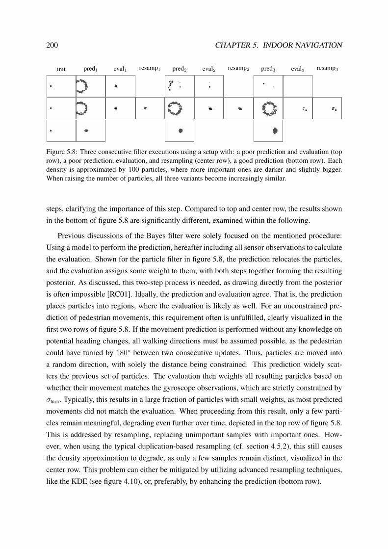
200 CHAPTER 5. INDOOR NAVIGATION
init pred1 eval1 resamp1 pred2 eval2 resamp2 pred3 eval3 resamp3
Figure 5.8: Three consecutive filter executions using a setup with: a poor prediction and evaluation (toprow), a poor prediction, evaluation, and resampling (center row), a good prediction (bottom row). Eachdensity is approximated by 100 particles, where more important ones are darker and slightly bigger.When raising the number of particles, all three variants become increasingly similar.
steps, clarifying the importance of this step. Compared to top and center row, the results shownin the bottom of figure 5.8 are significantly different, examined within the following.
Previous discussions of the Bayes filter were solely focused on the mentioned procedure:Using a model to perform the prediction, hereafter including all sensor observations to calculatethe evaluation. Shown for the particle filter in figure 5.8, the prediction relocates the particles,and the evaluation assigns some weight to them, with both steps together forming the resultingposterior. As discussed, this two-step process is needed, as drawing directly from the posterioris often impossible [RC01]. Ideally, the prediction and evaluation agree. That is, the predictionplaces particles into regions, where the evaluation is likely as well. For an unconstrained pre-diction of pedestrian movements, this requirement often is unfulfilled, clearly visualized in thefirst two rows of figure 5.8. If the movement prediction is performed without any knowledge onpotential heading changes, all walking directions must be assumed possible, as the pedestriancould have turned by 180° between two consecutive updates. Thus, particles are moved intoa random direction, with solely the distance being constrained. This prediction widely scat-ters the previous set of particles. The evaluation then weights all resulting particles based onwhether their movement matches the gyroscope observations, which are strictly constrained byσturn. Typically, this results in a large fraction of particles with small weights, as most predictedmovements did not match the evaluation. When proceeding from this result, only a few parti-cles remain meaningful, degrading even further over time, depicted in the top row of figure 5.8.This is addressed by resampling, replacing unimportant samples with important ones. How-ever, when using the typical duplication-based resampling (cf. section 4.5.2), this still causesthe density approximation to degrade, as only a few samples remain distinct, visualized in thecenter row. This problem can either be mitigated by utilizing advanced resampling techniques,like the KDE (see figure 4.10), or, preferably, by enhancing the prediction (bottom row).
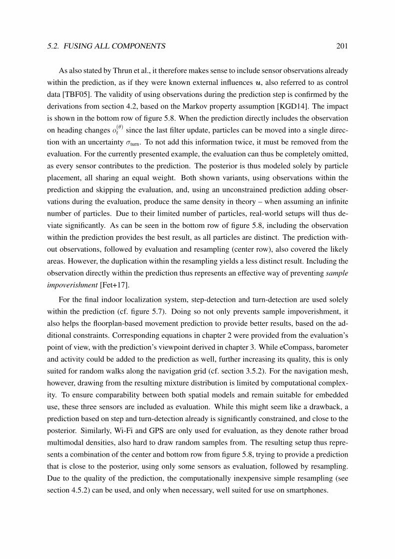
5.2. FUSING ALL COMPONENTS 201
As also stated by Thrun et al., it therefore makes sense to include sensor observations alreadywithin the prediction, as if they were known external influences u, also referred to as controldata [TBF05]. The validity of using observations during the prediction step is confirmed by thederivations from section 4.2, based on the Markov property assumption [KGD14]. The impactis shown in the bottom row of figure 5.8. When the prediction directly includes the observationon heading changes o(θ)
t since the last filter update, particles can be moved into a single direc-tion with an uncertainty σturn. To not add this information twice, it must be removed from theevaluation. For the currently presented example, the evaluation can thus be completely omitted,as every sensor contributes to the prediction. The posterior is thus modeled solely by particleplacement, all sharing an equal weight. Both shown variants, using observations within theprediction and skipping the evaluation, and, using an unconstrained prediction adding obser-vations during the evaluation, produce the same density in theory – when assuming an infinitenumber of particles. Due to their limited number of particles, real-world setups will thus de-viate significantly. As can be seen in the bottom row of figure 5.8, including the observationwithin the prediction provides the best result, as all particles are distinct. The prediction with-out observations, followed by evaluation and resampling (center row), also covered the likelyareas. However, the duplication within the resampling yields a less distinct result. Including theobservation directly within the prediction thus represents an effective way of preventing sample
impoverishment [Fet+17].
For the final indoor localization system, step-detection and turn-detection are used solelywithin the prediction (cf. figure 5.7). Doing so not only prevents sample impoverishment, italso helps the floorplan-based movement prediction to provide better results, based on the ad-ditional constraints. Corresponding equations in chapter 2 were provided from the evaluation’spoint of view, with the prediction’s viewpoint derived in chapter 3. While eCompass, barometerand activity could be added to the prediction as well, further increasing its quality, this is onlysuited for random walks along the navigation grid (cf. section 3.5.2). For the navigation mesh,however, drawing from the resulting mixture distribution is limited by computational complex-ity. To ensure comparability between both spatial models and remain suitable for embeddeduse, these three sensors are included as evaluation. While this might seem like a drawback, aprediction based on step and turn-detection already is significantly constrained, and close to theposterior. Similarly, Wi-Fi and GPS are only used for evaluation, as they denote rather broadmultimodal densities, also hard to draw random samples from. The resulting setup thus repre-sents a combination of the center and bottom row from figure 5.8, trying to provide a predictionthat is close to the posterior, using only some sensors as evaluation, followed by resampling.Due to the quality of the prediction, the computationally inexpensive simple resampling (seesection 4.5.2) can be used, and only when necessary, well suited for use on smartphones.

202 CHAPTER 5. INDOOR NAVIGATION
Figure 5.9: When particles (dots) are stopped in front of encountered obstacles, without taking furthermeasures, they eventually get stuck. This not only reduces the quality of the density approximation, butalso negatively affects the weighted average estimation (line), clearly lagging behind.
Furthermore, as this results in a tendentially more concentrated posterior with many distinctparticles, the number of particles required to provide a stable approximation is significantlyreduced. This matches with earlier discussions on the number of samples required for approx-imating statistical processes in general, conducted in section 3.2. When including the obser-vation within the prediction, and focusing on shorter update intervals, the number of particlescan be reduced, and it is sufficient to predict only a single qt,[i] for every qt−1,[i], instead ofmultiples. The number of required particles thus remains constant throughout subsequent filterupdates, instead of constantly rising, again increasing suitability for smartphone use.
5.2.3 Handling Impossible Movements
When using an observation-based prediction and the building’s floorplan, some peculiaritiesmust be considered. The floorplan can yield negative side effects, independent of whetherintersection tests, random walks, or the navigation mesh are used (cf. chapter 3). An example isshown in figure 5.9, where the prediction proceeds to the right, with a large heading uncertaintyof σturn = 7° for visualization. Here, all movements intersecting with a wall are stopped directlyin front of it, similar to the random walks, discussed in section 3.4, stopping in front of obstacles,due to the unavailability of walkable edges with high probabilities (cf. figure 3.16). Withoutfurther measures, this yields and increasing number of particles to get stuck and ineffective overtime, and also affects the estimation negatively. Figure 5.9 uses the common estimation, basedon the weighted average of all particles (see section 4.5.3), shown as a black line. Includingcaught particles causes incorrect results, shifting the estimated whereabouts. The weightedaverage clearly starts to stay behind the meaningful particles, as soon as the door is reached.This issue is mitigated when using a particle filter and absolute location estimations (e.g. Wi-Fi),which eventually re-weight unlikely particles. Yet, the problem can be prevented beforehand.
One discussed solution was to repeat impossible movements, randomly drawing new valuesfor distance and heading, eventually encountering a possible solution. However, for most cases,the probability of finding a valid solution within a few retries is rather low, especially whendirectly facing an obstacle. Another approach from literature simply deletes each particle thatbelongs to an invalid movement [EBS16]. Yet, this causes their number to deteriorate over time,

5.2. FUSING ALL COMPONENTS 203
Figure 5.10: Particles (dots) encountering an obstacle are assigned a weight of zero (gray, cf. (3.14)), andthus replaced during resampling. This suppresses impossible walks, and still ensures that the majority ofparticles remains effective. Compared to (5.9), the estimation (line) is now as desired.
e.g. requiring a prediction that increases the number of particles. Alternatively, the transitionitself should directly mark each sample that causes an impossible movement as unlikely, byassigning it a weight of (near) zero (3.14) [Ebn+14]. Within the evaluation, such particles are(almost) nonexistent, and the overall number remains constant. During the resampling step,low-weight particles are replaced by duplicating more likely ones, restoring the number ofeffective ones. While the duplication reduces distinctiveness, it is viable, as it typically affectsonly a small fraction of all particles, and is computationally efficient. The result for this strategyis shown in figure 5.10, where zero-weight particles are drawn in gray, directly before they areremoved by the particle filter’s resampling. The estimation lag present in figure 5.9 (black line)is corrected, all particles define a homogeneous density, and the estimation is located correctly.This strategy was also applied for creating the initial example, shown in figure 5.6.
While down-voting particles that denoted impossible movements was able to address theprevious problem, there are constellations where it is unable to, or causes new problems: Whenreceiving erroneous sensor observations, like invalid heading changes due to the pedestrianshaking the smartphone, or invalid Wi-Fi location estimations due to poor signal strength pre-dictions, particles might e.g. be forced into some corner of the floorplan. Depending on how thepedestrian continues to walk, that is, upcoming observations, these particles are either able toleave the corner, or get caught within. An example is shown in figure 5.11, again, solely basedon step-detection and turn-detection. Between the first and second prediction, the pedestrianshakes the phone, causing a sensor fault. This yields an incorrect relative heading observation,changing it by approximately 30° to the left (counter clockwise). Instead of moving along thecorridor, almost all particles are forced into the adjacent room. The following observations areaccurate again, representing the pedestrian’s walk along the corridor. That is, three steps with-out change in heading, followed by a 90° turn to the left, hereafter walking straight again. Ascan be seen, this causes all particles to get trapped within the room, unable to leave.
Again, there are various options for addressing this type of error. When using analytical den-sities, the problem is mitigated, as the room’s exterior still remains likely, even if infinitesimallysmall. However, most analytical approaches are unable to accurately model discontinuous prob-lems, as discussed for the Kalman filter. This type of issue thus represents a compromise thatcomes with the advantages of the sample-based particle filter. One solution is to (significantly)

204 CHAPTER 5. INDOOR NAVIGATION
Figure 5.11: Example with a sensor fault between the first and the second prediction. Instead of movingalong the corridor, most particles (dots) are forced inside a room, unable to leave. This behavior occursfor all three variants: predicting movements into all directions followed by evaluation and resampling(top row), observation-based prediction and stopping in front of obstacles (center row), and observa-tion-based prediction, down-weighting invalid movements (gray) and removing them during resampling(bottom row). For the latter, the last step contains only particles with a weight of zero, thus having failed.
increase the number of particles, enhancing the quality of the approximation, hopefully causingsome particles to remain outside of the room, eventually recovering. Working in theory, thisclearly represents a bottleneck for realtime use on smartphones. Alternatively, the uncertainty(here: σturn) could be increased, ensuring that a decent number of particles remains within thecorridor. However, when increasing uncertainties for all predictions, the ones with valid sensorobservations are rendered unnecessarily uncertain, causing a broad and growing density. Ide-ally, the false reading is detectable in some way, increasing uncertainties only when needed.For the presented example, where the fault is caused by the pedestrian shaking the phone, theuncertainty could be adjusted as described in the end of section 2.4.2. A corresponding exampleis shown in figure 5.12, where the false reading between the first two predictions is detected,and addressed by increasing σturn. In comparison to figure 5.11, the particles after the secondprediction now form a much wider density, including many particles with the correct walkingdirection. As the following sensor observations are accurate again, all subsequent steps continuefrom this broader density using a smaller σturn. Even though some particles enter the room, themajority uses the correct path along the corridor. While all three variants – stopping in frontof obstacles, using zero-weights and resampling, using a coarse prediction followed by evalu-ation and resampling – have improved, only the zero-weights method (bottom row) producesa desirable result. Here, all trapped particles are eventually removed, as they do not matchwith subsequent observations. The evaluation-based approach (top row), which does not useobservations within the prediction, provides almost the same estimation result, but with a lessdistinct particle set. The variant with the particles stopping in front of obstacles (center row)suffers from the same drawbacks as already indicated by figure 5.9, thus being impractical.

5.2. FUSING ALL COMPONENTS 205
Figure 5.12: Example with a sensor fault between the first and the second prediction. If this fault can bedetected, and the sensor-uncertainty is adjusted accordingly (compare against figure 5.11), getting stuckcan be mitigated for all three cases: predicting movements into all directions followed by evaluation andresampling (top row), predicting based on the observation and stopping in front of obstacles (center row),and predicting based on the observation, down-weighting invalid movements (gray) and removing themduring resampling (bottom row).
5.2.4 Detecting and Handling Deadlocks
However, as already mentioned briefly, not all types of sensor faults are detectable. Especiallyfor the Wi-Fi component, which is the only sensor providing absolute location information in-doors, potential error sources are numerous. The pedestrian, holding the phone, might attenuatesignals due to the shadowing of the body. Depending on the type of antenna installed withinthe smartphone, tilting it might alter receivable signal strengths as well. When signal strengthprediction models are used, they can differ significantly from real-world readings. For all thosecases, there is no clear indication whether some observation is suitable or erroneous. Withoutadjusting uncertainties accordingly, particles can easily get stuck, depending on their surround-ings, requiring other mitigation approaches [Fet+17; Ebn+17].
One option is to detect such deadlock situations, e.g. when the random walk indicates thatmany unlikely edges were taken, too many particle movements triggered a positive intersectiontest, or the largest weights after an evaluation are below a certain threshold. The most simplesolution is then given by restarting the particle filter. That is, uniformly distributing all particlesthroughout the walkable area, assigning each one a uniform random heading q(Θ)
0 ∼ U (0, 2π).Restarting is basically the same as for every starting situation, where the current whereaboutsare unknown. This was shown in figure 5.6, starting with a uniform distribution at t = 0, scatter-ing all particles throughout the walkable area, using an unknown heading. Restarting addressesthe deadlock, but causes the next few estimations to be unusable. Yet, as within figure 5.6, afterseveral steps, impossible movements will cause many particles to be replaced during resam-pling. As soon as new Wi-Fi observations are available (as for t = 3 in figure 5.6), additional

206 CHAPTER 5. INDOOR NAVIGATION
locations can be ruled out, assuming the sensor works as expected. Until t = 5 the densitybecame compact, and starts to resemble the actual ground truth. While taking some time torecover, the deadlock is addressed. When absolute location observations are unavailable, recov-ery strongly depends on the size and complexity of the floorplan, and the number of particlesused. For a large multistory building it is unlikely that a uniform distribution of a few hundredparticles contains the actual whereabouts, thus requiring better solutions.
To reduce the time needed for the system to stabilize, and prevent invalid estimations aftera restart, a heuristic could be applied. It is unlikely for the pedestrian to have moved acrossthe whole building or several floors within a short timeframe. Thus, instead of distributing allparticles uniformly, the stuck density could be scattered within a certain radius. Alternatively,only a fraction of the stuck density could be replaced by uniform samples, approximately keep-ing the last whereabouts, but allowing for other locations as well. Although, for this case, it isunclear how to weight the old and the new samples, and neither of the two methods representsan analytically profound solution.
One solution is the Interacting Multiple Model Particle Filter (IMMPF) [DB05], where asecond, less restrictive, filter is added besides the particle filter with floorplan-knowledge. Thatis, e.g. a particle filter without floorplan considerations. With the second filter being less restric-tive, it can not get stuck, but the quality of its estimation is reduced. The intention is to use bothfilters in parallel, based on the same input data. When a major difference between both filters isdetected, the restrictive version might be stuck. This difference is determined analytically, e.g.by the Kullback-Leibler divergence [KL51], estimating the dissimilarity of two densities. Forevery filter update, a new set of particles is derived by mixing both based on their divergence.The one with floorplan knowledge is dominant, and therefore preferred. When the divergenceis large, and the dominant one got stuck, the second, or support, is preferred instead. This isachieved by placing an exponential distribution on top of the Kullback-Leibler divergence dKL
pdom (dKL) = e−λdKL , psup (dKL) = 1− pdom (dKL) , λ > 0 , (5.1)
defining the probability for drawing a particle from either of the filters. This implements previ-ous discussions on filter restarts, and how to prevent them from being too strict. The IMMPF canbe thought of as providing an alternative density with tolerable quality that can be referred to,when the, usually better, dominant density got stuck. This provides a concept similar to restart-ing, without scattering particles within an unnecessarily large region. Compared to previousheuristic ideas, this variant is based on the well-researched Kullback-Leibler divergence, andrequires only a single empiric value λ, deciding when to mistrust the dominant filter [Fet+17].

5.3. REAL-WORLD CONSIDERATIONS 207
5.3 Real-World Considerations
Besides filter and sensor related issues, other aspects, affecting the system’s estimation qual-ity and computational performance based on a building’s actual architecture, available infras-tructure and similar, must be considered as well. Within the following, common pitfalls andpotential workarounds are briefly examined.
5.3.1 Sensitive Locations
As discussed in section 2.7, most buildings will contain locations, where the estimations fromsignal strength prediction models are significantly erroneous. In such places, the evaluation ofthe Wi-Fi component will not provide viable results, yielding aforementioned drawbacks, of thesystem potentially getting stuck. Using special signal strength prediction models, limited to thesensitive region, can address such issues by explicitly modeling local signal strength behavior(cf. section 2.7.6). This, however, might yield new problems, in areas where two regionalmodels are adjacent to each other. Due to completely different signal strength estimationswithin both regions, the evaluation for one of both will often be very unlikely compared to itsneighbor. The discontinuity between both models can cause particles to wait within one of thetwo regions, until the smartphone’s readings eventually agree. This yields new problems, whennot matching with other sensor observations, such as step-detection or turn-detection [Ebn+17].
Stairwells often represent a sensitive area, with their steel-reinforced concrete significantlyattenuating access points. As Wi-Fi reception is not required in stairwells, installing transmitterswithin is unreasonable. For indoor localization, battery powered supplementary devices, such asBluetooth beacons, are a viable alternative, providing signal strength-based localization withinareas of the building, where Wi-Fi is too weak, or model predictions inaccurate. Yet, theydemand for additional maintenance, and can suffer from signal strength depletion based ontheir battery level. Installing them within the whole building is thus not advisable. For sensitiveareas, however, they provide valuable additional localization information [Ebn+15].
Nevertheless, the observations from supplementary transmitters compete with the divergentWi-Fi-readings, potentially still causing localization errors. If so, Wi-Fi should be consideredunstable, relying solely on the supplement, such as aforementioned Bluetooth beacons. Often,more than one access point is affected by local effects within sensitive areas, e.g. yielding gen-erally weak RSSIs, except for a few transmitters. Whenever this constellation is encountered,the Wi-Fi component can be assumed unstable, and temporally excluded from the evaluation.

208 CHAPTER 5. INDOOR NAVIGATION
Situations, where disabling is advisable, can be detected by a quality heuristic [Ebn+17]
quality(s) = max
(min
(E(s)− τwMin
τwMax − τwMin, 1
), 0
). (5.2)
(5.2) maps the mean signal strength of all currently visible transmitters to a range of 0 ≤quality(s) ≤ 1, by using two empiric thresholds τwMax and τwMin. If its result drops below acertain value, Wi-Fi is disabled. The three thresholds can e.g. be determined by using empir-ically chosen values, or by estimating them within the model optimization process, letting themetric produce low outputs, whenever the model estimations are especially erroneous [Ebn+17].A more profound, yet more complex approach is e.g. given by training an artificial neural net-work, converting RSSI readings into a quality indication. Training data is e.g. given by theerror between reference measurements and model estimations (2.112), or by evaluating the po-sition of the reference measurement against the optimized model (2.111). Again, invisible andnon-permanent transmitters must be considered to provide viable results.
Besides completely disabling the Wi-Fi sensor, its impact can be limited. The uncertaintywithin the evaluation pwifi (ot | qt) can e.g. be increased, to address expected errors. Wheneverthe Wi-Fi component yields erroneous evaluations, there is a risk of the particle density gettingstuck within the building, due to the restricting floorplan. Another alternative is thus givenby temporarily disabling obstacles within the transition process, when a low Wi-Fi quality isdetected. As the metric is not binary but continuous, both variants, with and without obstacles,can be mixed continuously. Whenever the metric indicates viable Wi-Fi readings, obstaclesprovide additional localization quality. For weak Wi-Fi signals, they are omitted, ensuringthe localization process does not fail by getting stuck. That is, the Wi-Fi quality serves as anadditional mixing constraint to the IMMPF, deciding which filter to trust [Fet+17].
5.3.2 Data Acquisition
Another aspect is data acquisition. While this relates mainly to using the system for localizing ornavigating with a smartphone, it also concerns the setup phase, e.g. conducting Wi-Fi referencemeasurements (see section 2.7.6) within a building, where the phone can be used as well.
Sensor sample rates, like for the IMU and barometer, can be controlled to some extend, byselecting from a few pre-defined options (Android). Yet, actual rates can vary, and are hardwaredependent. Requesting the fastest sample rate often is a safe choice. The associated arithmeticoperations are either inexpensive, or downsampling is easily possible, e.g. by cumulating con-secutive readings (gyroscope), or simply discarding some observations (accelerometer, magne-tometer). The barometer typically uses low sample rates, not requiring adjustments [Bos15].

5.3. REAL-WORLD CONSIDERATIONS 209
For Bluetooth beacons, behavior is slightly different, as the detection is usually performedpassively. That is, the smartphone scans without actively requesting data, and beacons activelysend advertisements, without being asked for them. With each beacon controlling its own ad-vertisement interval, their sample rate can not be controlled by the phone, and varies amongtransmitters. Common rates are somewhere near 2 Hz, representing a tradeoff between batterylife, accuracy, and not polluting the radio channel [Lin15; Mic18].
As discussed, scanning for nearby Wi-Fi transmitters is performed actively, requesting aresponse from access points on every supported channel. Achievable sample rates thus stronglydepend on the number of channels to scan. While using both, 2.4 GHz and 5 GHz, providesmore readings, and thus a potentially better location estimation, including the 5 GHz-band sig-nificantly increases scanning times [Ebn+15; Ebn+17]. For some Android devices, 5 GHz canbe disabled within the Wi-Fi settings, to increase the sample rate. If this option is unavailable,there is a chance it is still available as hidden API, accessible via reflection. However, for moremodern devices, both options tend to be unavailable. Also, starting with Android 9, the Wi-Fiscanning rate is limited to a few times per minute, considerably reducing usefulness. Thiscan be addressed by reverting to Bluetooth beacons, not affected by this limitation, and sup-ported by most devices, or by using the upcoming FTM (cf. section 2.7.7), if supported by usedsmartphones and existing infrastructure. Android version 9 thus faces an important restriction,limiting the use of already installed infrastructure, requiring for new hardware, unnecessarilyincreasing the price, rendering indoor localization less pervasive and affordable. As of today,manual scanning for Wi-Fi transmitters is not allowed by the iOS operating system. Similarlyto Android version 9, Bluetooth beacons can be used instead, with future versions of hardwareand operating system eventually supporting Wi-Fi FTM as well.
Reference measurements, required for training signal strength prediction models (cf. sec-tion 2.7.6), can be conducted similarly, using commodity smartphones. For an adequate sampleof real-world behavior, the whole walkable area of a building should be covered [Ebn+17]. Byusing the semantic floorplan described earlier, actual locations can be added to the map, ensur-ing the position stored within a database matches with the location in the building. To ensurea stable signal strength estimation, several measurements are conducted at every such location,similar to fingerprinting [BP00; Shu+15; Men+11]. Effects of the phone’s antenna can be com-pensated by using different poses while measuring, e.g. by slowly turning, holding the phoneupfront. The resulting database can hereafter be used to estimate the parameters required fora chosen signal strength prediction model. Being used for all upcoming experiments and eval-uations, this approach was also applied for participating in the IPIN 2016 Indoor Localization
Competition, taking around 60 minutes of recording time within the competition building, withthe presented system providing the best results among all competitors [EvA16].

210 CHAPTER 5. INDOOR NAVIGATION
5.4 Performance Considerations
The goal is to provide an indoor localization and navigation system that is accurate, easy to setup, inexpensive, and suited for smartphone use. Memory and performance aspects thus playan important role besides financial considerations for required infrastructure, setup and main-tenance times. Fingerprints, for example, generally provide the most accurate Wi-Fi results,due to real-world measurements (cf. section 2.7.5). If conducted for every square meter of abuilding, with an average of ten access points visible at every fingerprint, and only their averagesignal strength stored as a single byte, a floor of 100 m by 100 m in size requires ≈ 100 KiB
of memory. Thus, the amount of data is manageable for most buildings, even when decimalnumbers, Gaussian distributions or histograms are stored (cf. section 2.7). Yet, a major issue,besides the time required for conducting fingerprints, are computational requirements within theevaluation, when e.g. a KDE is used to determine the probability for every particle, dependingon the likelihood of surrounding fingerprints. Based on the number of fingerprints and particles,the computational complexity can easily exceed the abilities of embedded devices.
5.4.1 Precomputed Model Predictions
When replacing fingerprinting with e.g. the log-distance model from section 2.7.6, computationtimes to predict the signal strength at the location of each particle, for every currently visibleaccess point, are minimized to a few arithmetic operations. This comes at the cost of reducedlocalization quality, with the log-distance model being less accurate than fingerprints. A mit-igation is given by using the extended log-distance model instead. However, its complexitydepends on the number of obstacles included within the prediction process (cf. section 2.7.6).When solely floors and ceilings are considered, there is only a slight overhead compared to thelog-distance model. Yet, including all types of walls within each floor significantly increasescomputation time, requiring intersection tests for all obstacles along the line of sight from eachparticle towards every visible access point. Depending on the complexity of the floorplan, andthe number of particles, embedded devices might fail to perform required computations in time.
Similar to solving the problem of costly shortest path calculations, the spatial models fromsection 3.4 can also be used to store precomputed signal strengths, at the cost of memory. Withinthe navigation grid, the result from a signal strength prediction model can be stored directly ontoeach vertex. The evaluation is then reduced to inexpensive lookups and comparisons, denotedin figure 5.13a. However, the amount of required memory can be significant. When verticesare placed every 25 cm, the 100 m by 100 m wide example floor, with ten access points visibleper location, already requires ≈ 1.5 MiB, when storing a single byte per transmitter. However,

5.4. PERFORMANCE CONSIDERATIONS 211
(a) (b) (c) (d) (e)
Figure 5.13: Varying strategies for precomputed signal strengths. Storing a value every few centimeters,e.g. directly on grid vertices (a). Using larger distances between predictions, still providing fast lookups(b). Grouping similar predictions, storing references to them on grid vertices (c). Attaching values totriangle edges of the navigation mesh followed by barycentric interpolation (d) and (e).
to maintain the signal strength prediction model’s ability to estimate a signal strength for every
transmitter and location, all access points within a building would have to be stored on everysingle vertex. This is unfeasible for larger buildings with many transmitters.
Typically, only a few transmitters are actually visible at any location within a building (cf.figure 2.27). One option to address memory consumption is thus given by storing only meaning-ful transmitters, with a prediction above some threshold. That is, if a transmitter’s predicted sig-nal strength for the location of some vertex is below this threshold, it is not stored, but assumedconstant, using the value of the threshold. This significantly reduces memory requirements. Theerror that results from using a constant instead of actual predictions can be limited by choosingthis constant to be near typical receiver sensitivity, where signals often are unrecognized by thehardware anyway.
Also, signal strengths do not change substantially within 25 cm, at least when no obstaclesare nearby. A less dense data-structure can thus be sufficient, e.g. storing predictions within aseparate 1 m by 1 m grid. However, this introduces the risk of not aligning with obstacles. Indi-cated within figure 5.13b, there are many locations where the same signal strength is predictedin front of and behind a wall, potentially causing errors within the evaluation.
Ideally, locations are only grouped together when they share similar signal strength predic-tions for all transmitters, yielding an irregular data structure. While being feasible for a singletransmitter, shown in 5.13c, there is no memory benefit. To the contrary, additional memory isrequired to store both, each group, and a reference to it for every lookup location. The size ofthis reference depends on the number of distinct groups, which in turn depends on the number ofinstalled transmitters. The chance for two nearby locations to have a similar signal strength pre-diction decreases with an increasing number of transmitters, due to physical effects discussedin section 2.7. This potentially causes many small groups, not saving memory at all. Besides,while grouping can reduce the required amount of memory, it introduces discreteness. Witheach prediction belonging to a larger area, discontinuous jumps between adjacent groups aregenerated, clearly visible within figure 5.13b and 5.13c, which negatively affect the evaluation.

212 CHAPTER 5. INDOOR NAVIGATION
When the navigation mesh is used as spatial data structure, recuperations are different. Simi-lar to vertices, precomputed RSSIs can be stored onto each triangle-corner within the mesh. Dueto using only a few triangles, in contrast to many grid vertices, memory savings are significant.Furthermore, this also reduces the effect of discontinuity, as signal strengths can be estimated bybarycentric interpolation within the triangle a particle belongs to, increasing evaluation quality.A corresponding example is shown in figure 5.13d and 5.13e. However, interpolated predictionscan still be significantly different from actual model values. As RSSIs are calculated only fortriangle-corners, results strongly depend on their placement. This can be verified by comparingfigure 5.13d and 5.13e, where the lower and upper right side clearly differs. While larger trian-gles reduce the memory footprint, they also diminish quality, not aligning with or resemblingthe actual signal strength behavior. When enforcing smaller triangles, this strategy is viable formost locations within a building, well-aligning with obstacles. This type of interpolation canalso be used for making fingerprints continuous, without requiring a costly KDE. Yet, conductedfingerprints can not be assumed to align with an algorithm’s triangle placement, thus being un-clear which RSSIs to assign to every triangle corner. One approach is e.g. given by inversedistance weighting [AC16], estimating the RSSIs for a triangle corner based on nearby finger-prints and their distance. Here, obstacles can be considered, ignoring all fingerprints where theline of sight is occluded. Besides its computational efficiency due to being precomputed, con-sidering obstacles denotes another advantage to the KDE-based approach, which is not directlyable to consider walls and other obstacles (cf. section 2.7.5).
As can be seen, the strategy for including the Wi-Fi component strongly depends on re-quired quality, size of the floorplan, number of installed access points, and available compu-tation power. For buildings with many drywalls, signal strength behavior is rather continuousand an extended log-distance model just considering floors and ceilings, is fast and sufficient[Ebn+17]. Besides improving model predictions in surroundings with complex architecture,reference measurements can also be used to determine, whether more complex models andprecomputation can provide a benefit.
5.4.2 Code Optimization
Besides engineering or deciding on appropriate algorithms and data structures to perform re-quired calculations, their actual implementation also plays an important role, affecting both,performance and memory requirement, briefly discussed within the following.
Programming Language One aspect is the programming language used for implementingall previously discussed models and calculations for smartphones. Especially when referringto Android-based smartphones, mainly programmed using Java or Kotlin [Lin+11]. Perfor-

5.5. SUMMARY 213
mance impact is often workload dependent, subjective, and thus hard to argue scientifically andin general [LZQ15]. Therefore, the following is mainly based on experience, gathered whiledeveloping the overall system. The implementation was solely based on native C++ code. A de-cision also made for portability reason, supporting Linux, Android and iOS. This also allowedfor operator overloading, simplifying the code for statistics, filtering, and estimation. Perfor-mance and memory considerations were also part of this decision. For Android and Java, earlysetups indicated significant overheads, especially related to the particle filter. This was also dueto the unavailability of plain memory objects, such as C structs, and not being able to storescalar types, like int or float, within lists or similar data structures.
Particles and Multithreading Besides programming language, the number of particles rep-resents a critical aspect, affecting overall system performance. As prediction, evaluation, andestimation are performed per-particle, their number has a direct influence. While using lessparticles enhances battery life, it negatively affects the quality of the recursive density estima-tion. As shown within previous figures, a decent number is required for a proper initialization,and to capture all likely whereabouts. It thus represents a tradeoff between quality, battery life,and available computational power. The presented system used between 5000 and 10 000 par-ticles, which is way more than used by competitors [NRP16; KS18; Gui+16; Shu+15]. Thiswas achieved by optimized C++ code, and by leveraging the previously mentioned fact, that theparticle filter is parallelizable (cf. section 4.5). Both, the prediction and evaluation step processparticles in parallel, using multiple threads, well suited for today’s multi-core smartphones.
5.5 Summary
This chapter provided the missing links between the required theory, presented within the threeprevious chapters. Therefore it concentrated on less scientific and more technical aspects, re-lated to the overall system implementation.
The first section was related to modeling a building’s floorplan, suitable for deriving one ofthe spatial data structures discussed for the movement models in chapter 3. Main focus was ona fast creation process with support for later modifications. It thus referred to 2D drawings perfloor. Yet, the result is still suitable to derive accurate 3D representations, including doors andwindows, for both, visualization and e.g. ray tracing. Furthermore, it allows including semanticinformation, like the type of ground, required for movement predictions.
Hereafter, the overall system was assembled, choosing the particle filter as implementationof the Bayes filter for the recursive density estimation process. This part described the way sen-sors are included within the overall system, using the step-detection as pacemaker, triggering the

214 CHAPTER 5. INDOOR NAVIGATION
filter update procedure. In contrast to typical convention, turn-detection was also used directlywithin the transition process, providing more robust movement predictions, and suppressingsample impoverishment. To reduce computational complexity, eCompass, activity-detection,Wi-Fi, Bluetooth beacons, and GPS were used within the evaluation step, well suited for result-ing multimodalities. While this decision seems like a drawback in terms of density accuracy,this represents a viable tradeoff between quality and required computational complexity.
Furthermore, due to the floorplan, the system’s prediction already is rather restrictive. Po-tential ways for handling impossible movements were discussed. Especially sensor faults, suchas an invalid turn-detection, can easily cause all particles to get stuck within a room. Whenthis situation occurs, recovery often is unlikely. Techniques for handling such situations werebriefly introduced, including their advantages and disadvantages. While a simple uniform restartis possible, it suffers from various drawbacks, and should thus be avoided.
The next part concentrated on real-world aspects, and how to ensure a decent absolute lo-cation estimation from radio transmitters, even within sensitive areas of a building. This wasachieved by either adding additional transmitters within those areas, or by adjusting the usedsignal strength prediction models, using regional limitations or more advanced variants. Thisalso lead to the question of data acquisition on smartphones. The topic was related to both,recording prior reference measurements, and actual observations when the pedestrian uses thelocalization and navigation system. Both aspects were briefly described, explaining how refer-ence measurements were conducted, and how sensor observations are sampled, adjusted, andincluded within the filter.
With the quality of the particle filters approximation depending on the number of parti-cles, this lead to the final question on how to handle a decent number of particles on today’ssmartphones. By using precomputations where applicable, a suitable programming language,and multithreading, several thousand particles are manageable, sufficient for approximating thecomplex behavior of pedestrians walking indoors.

Chapter 6
Experiments
Previous chapters examined smartphone-based pedestrian indoor localization and navigationfrom different points of view.
First, individual sensor components and their contribution were discussed in chapter 2. Theirobservations were used within a probabilistic relation. Either to evaluate potential pedestrianwhereabouts, or their changes, based on analytical constraints. Hereafter, pedestrian movementpredictions based on a building’s floorplan were examined in chapter 3. They were used toestimate the likelihood of certain movements, based on obstacles and the walkable surface.This also allowed for a continuous 3D estimation, when utilizing appropriate spatial models.The link between both viewpoints is recursive density estimation, introduced in chapter 4. Here,several potential variants, as well as their advantages and disadvantages, were discussed. Whileanalytical implementations are computationally inexpensive, they are too restrictive, unable toconsider the floorplan. Therefore, the particle filter was introduced, approximating probabilitydensities using multiple samples, well-suited for considering the floorplan. However, at thecost of increased computational complexity. Afterwards, chapter 5 presented several real-worldconsiderations. This concerned the 2D/3D setup of floorplans, and how to handle their obstaclesin a probabilistic and computationally efficient manner. Therefore, the filter’s update interval,and the inclusion of sensor observations were discussed in detail. Closed by remarks on theprogramming language’s impact of achievable performance.
Finally, this chapter provides an experimental viewpoint of all previous aspects. First, thetestbed is described in detail, covering used devices, examined buildings, data acquisition, andground truth estimation. Following the preceding structure, sensors and movement modelsare hereafter evaluated separately, estimating individual contributions, and limitations, beforeexamining their combination.
215

216 CHAPTER 6. EXPERIMENTS
All tests also refer to synthetic and constrained setups, minimizing external influences whilefocusing only on the aspects that are essential for a component. Additionally, actual real-worldscenarios are examined, and, if applicable, compared against the findings from their syntheticcounterparts. Hereafter, the overall indoor localization and navigation system is examined,backed by all initial findings. These tests are based on actual pedestrian walks, conductedwithin multiple buildings, where indoor localization and navigation provide a benefit. To ensurerepresentative results, all experiments were performed with multiple smartphones that vary inprice and age, and actual pedestrian walks were conducted by different persons.
6.1 Testbeds and Data Acquisition
This section provides an overview on used devices, and synthetic/real-world scenarios, requiredfor examining all system components. Missing details are provided later, for each test setup.
Devices In terms of pervasiveness and price, as of today, Android-based smartphones repre-sent the most desirable platform to support initially. Disallowing scanning for nearby Wi-Fitransmitters, iOS-based smartphones lack an important sensor, which is crucial for indoor lo-calization and navigation. Even though supporting Bluetooth beacons, also usable for inferringabsolute whereabouts, most buildings are not equipped with the additionally required infras-tructure. Thus, iOS-based smartphones were not considered within this work. Based on theirrelatively low market share, the same holds true for phones using a Microsoft operating system.Without loss of generality, all tests are based on several different Android smartphones, of allbrands, prices and ages. The diversity of phone vendors brings varying sensor brands, differentinternal assemblies, and various operating system versions. The chosen devices thus providea broad spectrum for the system to deal with, enforcing general solutions, preventing overfit-ting. Table 6.1 lists all smartphones used within evaluations, their initial date of release, usedoperating system version, and a brief overview on supported sensors. In general, recent modelssupport Wi-Fi in all relevant frequency ranges, Bluetooth Low Energy – required for Blue-tooth beacons to be detected – and a gyroscope for fine-grained heading estimations. Solely thebarometer is rarely found. Accuracy and precision of these sensors will be examined later.
Syntehtic and Constrained Testbeds To examine components individually, special setupswere constructed, minimizing external influences, focusing only on important aspects, and pro-viding a well-known ground truth for error estimations. For step-detection, this covers pedes-trian walks following a defined pattern, with a known number of steps. For turn-detection by thegyroscope, and absolute heading estimation from the magnetometer, a turntable is used, allow-ing for exact angular movements, providing an ideal ground truth. Additional pedestrian walks

6.1. TESTBEDS AND DATA ACQUISITION 217
Vendor Model Manufacturer Year Android Acc Gyr Mag Bar 2.4 5 BLE
Motorola Milestone 2 Motorola 2010 4.4.4 1 X - X - X - -Motorola Milestone 4 Motorola 2012 7.1.2 2 X - X - X - -Samsung Galaxy S3 mini Samsung 2012 5.1.1 3 X X X - X X XGoogle Nexus 6 Motorola 2014 7.1.1 X X X X X X XSamsung Galaxy S5 Neo Samsung 2015 6.0.1 X X X - X X XMotorola Moto Z Motorola 2016 9.0.0 4 X X X - X X XLG G6 LG 2017 8.0.0 X X X X X X XGoogle Pixel 2 XL LG 2017 9.0.0 X X X X X X XBlackBerry KEY2 TCL 2018 8.1.0 X X X - X X X
Table 6.1: Overview on examined smartphones, their date of initial release, currently running operat-ing system version, and supported sensors: accelerometer, gyroscope, magnetometer, barometer, Wi-Fi2.4 GHz/5 GHz and Bluetooth Low Energy (BLE), required for Bluetooth beacons.1 CyanogenMod 11, 2 LineageOS 14.1, 3 CyanogenMod 12.1, 4 LineageOS 16.0
allow for a visual impression on the corresponding behavior under real-world conditions. Forthe barometer, walks through a stairwell with known altitudes provide the ground truth for errorestimation. Similarly, activity-detection was performed based on walks annotated with labels,describing the pedestrian’s current activity. For Wi-Fi, brief constrained tests were performed,as external influences can not fully be prevented. These tests refer to general signal strengthbehavior, providing an insight on the quality of prediction models. For actual model optimiza-tion and error estimation, real-world setups are required. Movement prediction and navigationare examined based on synthetic floorplans. While not always being realistic, they provide avisualization of the model’s behavior, translatable to real-world scenarios.
Real-World Testbeds Besides synthetic and constrained testbeds, Wi-Fi predictions, absolutelocation estimation, and the overall system are examined within real-world scenarios, coveringthree completely different buildings, varying in age, materials, floor layout, and infrastructure.
The SHL, shown in figure 6.1, is a modern university complex, completed in 2011. It isdivided into a main building, with four stacked floors, and a two story annex. While the firstfloor is directly connected, the 2nd floor is separated by a small outdoor area, shown in theupper right of the figure. The walkable area covers ≈ 12 000 m2 when including outdoor areas,and ≈ 8500 m2 without. Walls are mainly made of drywall, using steel-reinforced concreteonly for stairwells, and in places where structural stability is required. The whole complex isequipped with 34 access points, using both, the 2.4 GHz and 5 GHz range. Due to legal issues,their locations must not be disclosed, and are therefore omitted within the figures.
The Museum 1 (cf. figure 6.2) was built in 1908, with three floors, each split into two halves.That is, there is a small change in altitude between both halves, requiring short stairs. Besidesbeing separated, the building is characterized by a predominant concrete structure, using only a

218 CHAPTER 6. EXPERIMENTS
few drywalls. The walkable area is≈ 3200 m2. While a partial Wi-Fi-infrastructure is available,it does not cover the whole walkable area. Therefore, additional Wi-Fi-beacons, based on theESP8266, were installed, yielding 41 transmitters for the absolute location estimation.
The Museum 2 in figure 6.3 was built as a convent in the 13th century, and serves as a museumsince 1936. Besides one main floor, there is no clear structure, and the seven annexes are placedat various altitudes and locations. Being directly attached to the old town wall, the building ischaracterized by massive concrete walls, using only a few drywalls. When including the garden,≈ 3000 m2 are walkable, and ≈ 2400 m2 without. As there is no existing Wi-Fi infrastructureat all, 45 ESP8266 Wi-Fi-beacons were installed to provide absolute location estimation.
Required Wi-Fi reference measurements were recorded by a pedestrian, residing at well-known positions, holding the smartphone upfront, slowly turning around in a circle, while thedevice scans for nearby transmitters. This yields multiple measurements for each single loca-tion, reducing the influence of the antenna and the human body. The number and locations ofthese measurements are presented, when examining the Wi-Fi component.
Within the shown buildings, various walks (see figure 6.4, 6.5 and 6.6) were conducted byseveral pedestrians, using different smartphones. The ground truth required for error estimationis provided by the pedestrian: All walks are defined by points with exactly known location, con-nected to a path. Whenever reaching such a point, the pedestrian added a label to the recording.Assuming a constant walking speed, this allows for interpolating a position along the path, forany point in time. Even though being inexact, accuracy is sufficient for the intended use.
Shown in figure 6.4, 6.5 and 6.6, the conducted walks cover completely different scenarios.Four of the five walks within SHL are close to a shortest path from A to B scenario. Only walk A4,a two-story loop using a stairwell, is mainly synthetic. While some walks within Museum 1
and Museum 2 resemble a shortest path, most of them were conducted with exhibition watching
behavior in mind. That is, the pedestrian carrying the smartphone behaved like a normal visitor,sometimes resting in front of exhibits. The vertical lines within Museum 1 are due to using anelevator to change the current floor. Thus, all examined walks represent various real-worldscenarios for an indoor localization and navigation system, examined within the following.

6.1. TESTBEDS AND DATA ACQUISITION 219
Figure 6.1: SHL – University of Applied Sciences Wurzburg-Schweinfurt. Modern building completed in2011, with four stacked floors, surrounded by a facade of metallized glass, approximately 75 × 50 m insize (upper left). Via an outdoor area, the main building is connected to a two story annex (lower right),with an overall size of approximately 110×60 m. The walkable area spans≈ 12 000 m2 when includingoutdoor areas, and ≈ 8500 m2 when not. The right half shows an increased distance between floors.
Figure 6.2: Museum 1 – Gaubodenmuseum Straubinga. A museum built in 1908, with three floors, eachsplit into two halves (see right figure). Between the two halves, there is a small offset in altitude, yieldingan uneven distribution of the floors. The museum’s overall size is approximately 55 × 40 m, with thewalkable area being ≈ 3700 m2. The right half shows an increased distance between floors.
Figure 6.3: Museum 2 – RothenburgMuseumb. A museum since 1936, but initially built as a 13th centuryconvent. Floors are arranged in various shapes, sizes, and altitudes, yielding a chaotic layout, with onemain area, and seven annexes. Being directly attached to the old town wall, the building is characterizedby massive concrete structures. The overall size is approximately 70× 50 m, covering ≈ 3000 m2 whenincluding the garden, and≈ 2400 m2 without. The right half shows an increased distance between floors.
ahttp://www.gaeubodenmuseum.de/bhttps://www.rothenburgmuseum.de/
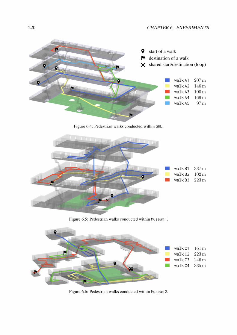
220 CHAPTER 6. EXPERIMENTS
start of a walkdestination of a walkshared start/destination (loop)
walk A1 207 mwalk A2 146 mwalk A3 100 mwalk A4 169 mwalk A5 97 m
Figure 6.4: Pedestrian walks conducted within SHL.
walk B1 337 mwalk B2 102 mwalk B3 223 m
Figure 6.5: Pedestrian walks conducted within Museum 1.
walk C1 161 mwalk C2 223 mwalk C3 246 mwalk C4 335 m
Figure 6.6: Pedestrian walks conducted within Museum 2.

6.2. EVALUATION OF SENSOR COMPONENTS 221
Model accelerometer gyroscope magnetometer barometer
Motorola Milestone 2 107.3 33.5 - - 9.7 0.8 - -Motorola Milestone 4 48.0 52.1 - - 95.2 15.5 - -Samsung Galaxy S3 Mini 101.2 17.5 101.4 17.6 49.3 4.5 - -Google Nexus 6 227.0 3.5 227.0 3.5 75.7 1.0 32.4 0.1Samsung Galaxy S5 Neo 200.6 0.6 200.6 0.6 102.1 20.4 - -Motorola Moto Z 198.1 0.8 198.1 0.8 49.5 0.1 - -LG G6 398.3 2.2 398.3 2.2 99.7 5.5 26.0 0.5Google Pixel 2 417.2 2.6 417.2 2.6 52.2 0.5 26.0 0.3BlackBerry KEY2 208.0 0.7 208.0 0.7 50.0 0.2 - -
Table 6.2: Mean sample rate (in Hz) and standard deviation of each IMU-sensor and the barometer, forall devices listed in table 6.1. A dash indicates a phone’s lack of support for a given sensor.
6.2 Evaluation of Sensor Components
All sensor components are examined, following the preceding structure. As the GPS is al-ready well-researched, and only of minor importance for indoor localization, no additional testswere performed. The focus is solely on IMU, barometer and Wi-Fi. As influences on the IMUsensors are numerous, synthetic benchmarks are conducted beforehand, analyzing the generalquality of accelerometers, gyroscopes and magnetometers installed within smartphones. Theseexaminations provide an impression on issues concerning accuracy and precision of relativeand absolute heading estimations. After evaluating each sensor on its own, combined tests arepresented, estimating the quality of pedestrian dead reckoning (PDR), when omitting sensorfusion, and absolute location indications. For Wi-Fi, the first step estimates the model predic-tion quality, when training them based on real-world reference measurements. Hereafter, theaccuracy of location estimation is examined, when using these trained models.
6.2.1 Sensor Overview
Before presenting results for step-detection, turn-detection, eCompass, barometer and activity-detection, general parameters of smartphone sensors are briefly examined. For now, the Wi-Ficomponent is omitted. Table 6.2 provides an overview on sensor sample rates and the estimatedstandard deviations for various smartphones, when requesting the fastest rate possible. As canbe seen, there are notable differences among the listed devices, concerning both, sample rate andstandard deviation. Especially older phones tend to suffer from rather aperiodic sensor readings,potentially causing issues, e.g. within frequency-based filters, relying on fixed sample rates.While the examined modern smartphones provided stable sample rates, individual frequenciesvaried significantly. To ensure that results among different devices are identical, this must beconsidered for filters, such as the moving average or complementary filter (see section 2.4).
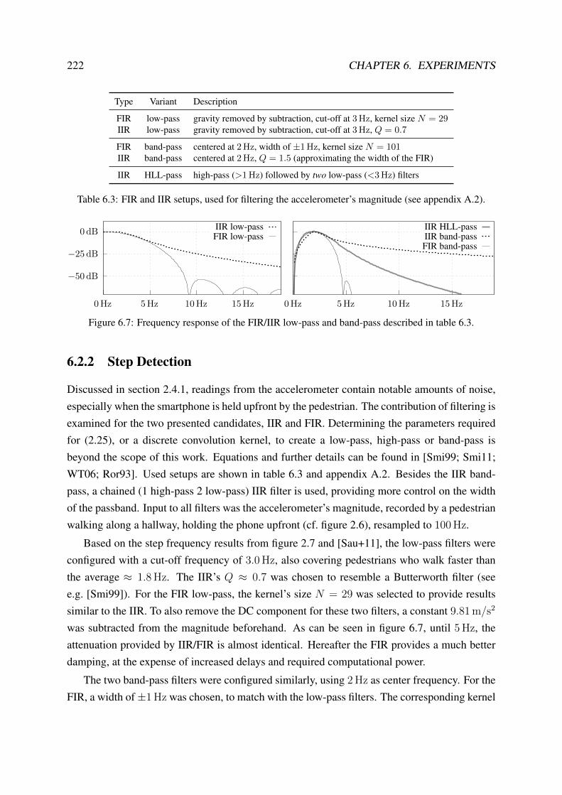
222 CHAPTER 6. EXPERIMENTS
Type Variant Description
FIR low-pass gravity removed by subtraction, cut-off at 3 Hz, kernel size N = 29IIR low-pass gravity removed by subtraction, cut-off at 3 Hz, Q = 0.7
FIR band-pass centered at 2 Hz, width of ±1 Hz, kernel size N = 101IIR band-pass centered at 2 Hz, Q = 1.5 (approximating the width of the FIR)
IIR HLL-pass high-pass (>1 Hz) followed by two low-pass (<3 Hz) filters
Table 6.3: FIR and IIR setups, used for filtering the accelerometer’s magnitude (see appendix A.2).
−50 dB
−25 dB
0 dB
0 Hz 5 Hz 10 Hz 15 Hz 0 Hz 5 Hz 10 Hz 15 Hz
IIR low-passFIR low-pass
IIR HLL-passIIR band-passFIR band-pass
Figure 6.7: Frequency response of the FIR/IIR low-pass and band-pass described in table 6.3.
6.2.2 Step Detection
Discussed in section 2.4.1, readings from the accelerometer contain notable amounts of noise,especially when the smartphone is held upfront by the pedestrian. The contribution of filtering isexamined for the two presented candidates, IIR and FIR. Determining the parameters requiredfor (2.25), or a discrete convolution kernel, to create a low-pass, high-pass or band-pass isbeyond the scope of this work. Equations and further details can be found in [Smi99; Smi11;WT06; Ror93]. Used setups are shown in table 6.3 and appendix A.2. Besides the IIR band-pass, a chained (1 high-pass 2 low-pass) IIR filter is used, providing more control on the widthof the passband. Input to all filters was the accelerometer’s magnitude, recorded by a pedestrianwalking along a hallway, holding the phone upfront (cf. figure 2.6), resampled to 100 Hz.
Based on the step frequency results from figure 2.7 and [Sau+11], the low-pass filters wereconfigured with a cut-off frequency of 3.0 Hz, also covering pedestrians who walk faster thanthe average ≈ 1.8 Hz. The IIR’s Q ≈ 0.7 was chosen to resemble a Butterworth filter (seee.g. [Smi99]). For the FIR low-pass, the kernel’s size N = 29 was selected to provide resultssimilar to the IIR. To also remove the DC component for these two filters, a constant 9.81 m/s2
was subtracted from the magnitude beforehand. As can be seen in figure 6.7, until 5 Hz, theattenuation provided by IIR/FIR is almost identical. Hereafter the FIR provides a much betterdamping, at the expense of increased delays and required computational power.
The two band-pass filters were configured similarly, using 2 Hz as center frequency. For theFIR, a width of±1 Hz was chosen, to match with the low-pass filters. The corresponding kernel

6.2. EVALUATION OF SENSOR COMPONENTS 223
7.49.4
11.413.4 unfiltered
−2024 IIR low-pass
−2
0
2
4
5 s 10 s 15 s
FIR low-pass
−2024 IIR band-pass
−2024 IIR HLL-pass
−2
0
2
4
5 s 10 s 15 s
FIR band-passampl
itude
(m/s
2)
Figure 6.8: Impact of applying the filters from table 6.3 to the accelerometer’s magnitude. The verticalline and a rectangle visually indicate each filter’s delay. All band-pass-like setups suffer from an initialpeak, resulting from the constant gravity contained within the signal. While the FIR band-pass providesthe smoothest result, its delay is clearly notable. Circles denote issues, explained within the text.
required N = 101 entries, to correctly remove the DC component from the accelerometer’smagnitude. With the sample rate of 100 Hz, this causes a delay of≈ 500 ms. The IIR’s Q = 1.5
was configured to match the ±1 Hz bandwidth of the FIR. Due to the large kernel size, the FIRprovides a good attenuation, and fast cut-offs. The IIR shows a viable cut-off only for the lowerfrequencies, with the attenuation of higher ones being less pronounced (cf. figure 6.7). Whilethis can be mitigated by further increasingQ, it also reduces the width of the passband, allowingonly for walks at a well known step frequency, affecting the filter’s general purpose.
This is addressed by chaining three IIR filters to approximate the FIR band-pass: A high-pass removes frequencies below 1 Hz, and two low-pass filters attenuate everything above 3 Hz.This combination, referred to as HLL-pass, creates a filter similar to a (2± 1) Hz band-pass,and is stronger than a single IIR. Shown in figure 6.7, this compromise between the IIR and FIRband-pass provides more control on passband and cut-offs, while retaining viable delay times.
Figure 6.8 shows the results when applying these filters to the magnitude of accelerometerreadings for a normally paced walk, sampled at 100 Hz. While peaks are distinguishable for allshown contestants, the FIR band-pass provides the smoothest result. However, as can be seenby comparing the vertical lines, both FIR filters, especially the band-pass with its larger kernel,introduce a significant delay. All three band-pass-like setups need some time to recognize andremove the gravity as DC component from the signal, rendering the first few seconds of outputunusable. This can be addressed by pre-feeding the filters with several constant readings of≈ 9.81 m/s2. Another aspect that divides low-pass and band-pass is the positive/negative peakratio. As mentioned in section 2.4.1, the step pattern usually consists of one positive, and onenegative peak, where the positive one is slightly more pronounced. This ratio is kept by the low-

224 CHAPTER 6. EXPERIMENTS
−3
−1
1
3
5
5 s 10 s 15 s 20 s 25 s 30 s
mag
nitu
de(m/s
2)
−3
−1
1
3
5
5 s 10 s 15 s 20 s 25 s 30 s
straight stair up straight+turn stair down straight
Figure 6.9: Magnitude of the accelerometer, filtered by the IIR low-pass from table 6.3. The device washeld upfront while walking 10 steps along a hallway, climbing a stair with 10 treads, making 10 stepsincluding a 180° turn, hereafter walking the same way back again.
Name Input Filtering Detection Scheme Name Filtering
SD1 magnitude - peak + dead timeSD2a magnitude IIR low-pass local maxima SD2b IIR HLL-passSD3a magnitude IIR low-pass zero crossing SD3b IIR HLL-passSD4a tilt compensated z IIR low-pass zero crossing SD4b IIR HLL-pass
Table 6.4: Examined step detectors and their configuration according to section 2.4.1.
pass filters, but removed by the band-passes, as it denotes a low frequency. When the desiredstep detection method relies on this ratio, band-pass filters can not be used.
Despite their abilities, FIR filters are overstated for the step detection problem. Due to both,delay and computational requirements, the following experiments omit the FIR filters, focusingonly on IIR versions. For the shown example, the IIR HLL-pass performed slightly better thanthe IIR band-pass, at a similar delay. However, for faster walks (see figure 6.10), the latter fails,due to aforementioned limitations, while the HLL-pass yields viable results. Being limited to anarrow range of walking speeds, the IIR band-pass is omitted as well. Actual step-detection isperformed using the IIR low-pass, the IIR HLL-pass, and no filtering for comparison.
Figure 6.9 depicts the accelerometer’s magnitude for a walk of 50 steps in length, includ-ing a stair, and one 180° turn, filtered by the IIR low-pass from table 6.3. During the turn, ataround 17 s, several zero crossings appear within the filtered signal, causing potential issues,depending on the chosen pattern detector. While the magnitude’s fluctuation is approximatelyconstant throughout the walk, the steps at 17 s, 26 s and 28 s are barely pronounced. In contrast,walking downstairs, between 20 s to 25 s, peaks increase in both directions. Besides this diver-sified walk, a simple 50-steps-straight setup is examined as well. To estimate the quality of thestep pattern detection algorithms discussed in section 2.4.1, both walks were conducted severaltimes, by multiple persons with varying footwear, using different devices. Table 6.4 lists all ex-amined contestants, including their detection and filtering strategy. Within recordings, the step

6.2. EVALUATION OF SENSOR COMPONENTS 225
−3−2−1
0123
10 s 15 s 10 s 15 s 20 s 10 s 15 s 20 s
mag
nitu
de(m/s
2)
Figure 6.10: Accelerometer’s magnitude for a fast paced walk. The raw data (left) contains significantamounts of noise, and does not allow for a robust step detection. Applying the IIR low-pass (middle)yields a noticeable improvement, but indicates several issues (filled circles), due to the present low andhigh frequency noise. Using the HLL-pass instead (right), enhances the overall result.
Dataset Walks SD1 SD2a SD2b SD3a SD3b SD4a SD4b
straight only 22 50.0 51.7 51.8 50.0 50.6 50.0 50.6straight only, fast 12 49.8 52.5 50.6 49.9 50.6 49.8 50.7
typical mix 25 47.1 48.9 52.8 49.4 50.1 49.1 49.9typical mix, fast 20 40.0 41.2 48.5 44.8 48.8 43.9 48.5
overall 79 46.5 48.3 51.1 48.5 50.0 48.2 49.9
Table 6.5: Number of detected steps for all detectors presented in table 6.4, averaged by dataset. Thecorrect number of steps is 50 for all cases.
frequency resided somewhere around ≈ 1.8 Hz. For this input, all strategies provided viableresults. Even when no filtering was used (SD1), deviations were only marginal.
Additionally, faster walking speeds were examined as well. When increasing the step fre-quency beyond 2.2 Hz, most detection schemes started to fail, missing up to 15 % of the takensteps. While the IIR low-pass used within SD2a-SD4a mitigated this problem, the overall num-ber of detected steps remained too low. Analyzing the raw accelerometer magnitude for thosewalks (see figure 6.10) reveals that the amount of noise increased significantly for both, high andlow frequencies. The low-pass filtered signal (middle) thus fluctuates at a very low frequency,removing some zero crossings. An IIR band-pass (not shown in the figure) provided slightlybetter results and reduced the number of missed steps, still with room for improvements, dueto its slow cut-off. The IIR HLL-pass addresses this issue with its two chained low-pass filters,and one high-pass, effectively removing all noise components from the raw signal (right).
Table 6.5 contains detailed results for all presented detectors and datasets. For normallypaced walks, all detectors provided viable results. As expected, the straight walks yielded thebest overall results. When variations, like stairs, are introduced, the risk for missing steps duringthe detection process increases. For highly paced walks, the HLL-pass, used in SD2b, SD3b andSD4b, provides better detection rates than the single low-pass used in other setups.

226 CHAPTER 6. EXPERIMENTS
bracket
turntable
motor
mount
79
142
45°
50
110
Figure 6.11: Layout of the turntable used for synthetic IMU tests. The direct-drive stepper motor ensuresa valuable ground truth. The bracket is used to place the smartphone into portrait and landscape mode,with a constant 45° tilt, required for tilt estimation tests. All distance units are given in mm.
6.2.3 Relative and Absolute Heading Estimation
The suitability of a smartphone’s IMU for turn-detection with the gyroscope, or absolute head-ing estimation by the eCompass, is examined synthetically, using a 3D-printed turntable (cf.figure 6.11). It is driven by a 17MH5417 stepper motor, with a physical resolution of 0.9 °/step,and executes requested rotations with accuracy and precision down to 1°. The resolution is fur-ther increased by a TMC2100 stepper driver, configured for 1/16 microstep interpolation, with afull 360° turn thus requiring 6400 steps. To ensure that the motor does not skip any steps, andthe smartphone keeps its enforced alignment, an acceleration and deceleration phase is used.
Tests examine three aspects, under controlled conditions: estimating accuracy and drift ofthe gyroscope, testing the magnetometers suitability for absolute heading estimation, and de-termining whether tilt compensation works as expected. Thus, experiments used three differentdevice orientations: The first places the phone flat onto the turntable, with its z-axis pointingupwards, and a rubber mat in between ensuring the device remains in place. To examine tiltcompensation, the phone is also placed in portrait and landscape mode, both with a 45° tilt an-gle, similar to a pedestrian holding the device upfront, fixed by a bracket shown in figure 6.11.
While the turntable is aligned parallel to the earth’s surface, a phone placed on top can notbe ensured to read an exact 0° angle, due to slight misalignments. All devices were manuallyaligned, ensuring that accelerometer readings match 0° as closely as possible. Angular valuesshown within the following experiments will thus vary slightly.
Results - Overview To determine the quality of tilt compensation and turn-detection, all threeposes were examined using three different turning rates: 62.7 °/s, 122.5 °/s and 234.0 °/s. Ta-ble 6.6 shows the results for measuring this turning rate, by using the median of the gyroscope’smagnitude (see (2.38)), and the results for the placement angle, determined by the average dotproduct between normalized accelerometer readings and (0, 0, 1)T (see (2.46)).

6.2. EVALUATION OF SENSOR COMPONENTS 227
0° flat landscape at 45° portrait at 45°62.7 °/s 122.5 °/s 234.0 °/s 62.7 °/s 122.5 °/s 234.0 °/s 62.7 °/s 122.5 °/s 234.0 °/s
S3 Mini 1.7° 1.4° 1.7° 45.8° 46.2° 47.5° 45.0° 44.7° 45.1°57.9 °/s 112.9 °/s 215.5 °/s 57.9 °/s 112.9 °/s 215.2 °/s 58.4 °/s 114.1 °/s 217.8 °/s
Nexus 6 0.9° 0.9° 1.6° 47.3° 47.1° 48.0° 46.5° 46.2° 45.3°62.4 °/s 121.9 °/s 232.7 °/s 62.2 °/s 121.4 °/s 231.9 °/s 62.0 °/s 121.4 °/s 232.1 °/s
Moto Z 1.5° 2.0° 3.4° 44.9° 44.9° 44.6° 45.1° 44.8° 43.5°62.6 °/s 122.2 °/s 233.4 °/s 63.0 °/s 123.1 °/s 234.8 °/s 62.0 °/s 121.5 °/s 233.0 °/s
LG G6 1.3° 1.5° 3.2° 45.7° 46.3° 48.1° 45.4° 45.5° 45.8°63.0 °/s 123.2 °/s 235.3 °/s 63.2 °/s 123.2 °/s 235.0 °/s 62.5 °/s 122.8 °/s 235.7 °/s
Pixel 2 1.9° 1.5° 3.1° 45.3° 45.9° 47.7° 45.9° 45.6° 45.8°62.6 °/s 122.3 °/s 233.6 °/s 62.6 °/s 122.3 °/s 233.6 °/s 63.7 °/s 124.5 °/s 237.7 °/s
KEY2 0.9° 1.4° 2.9° 45.4° 45.5° 45.9° 44.9° 44.2° 42.2°62.6 °/s 122.5 °/s 233.8 °/s 62.6 °/s 122.1 °/s 233.0 °/s 62.9 °/s 123.0 °/s 235.6 °/s
Table 6.6: Results of a turntable experiment, using three different device placements, each with threeturning speeds. For every phone, the first row shows the tilt angle, estimated by the average dot productbetween (0, 0, 1)T and the normalized readings from the accelerometer (see (2.46)). The second rowcontains the measured angular velocity, estimated by the median of the gyroscope’s magnitude.
For all devices, except the S3 Mini, turn rates are viable, and, due to using the magnitude,independent of the phone’s orientation. The S3 Mini is one of the first containing an IMU withgyroscope (see table 6.1). Besides comparatively poor sensor resolution, neither its accelerom-eter nor its gyroscope seemed to be correctly calibrated. Within all tests, the accelerometer’sz-axis was off by a constant +0.13 g, and the gyroscope’s x and z were off by +0.015 rad/s
and +0.005 rad/s, respectively. While the latter seems small, it denotes a drift of 17.19 °/min,significantly affecting turn-detection. The same holds true for tilt compensation. Dependingon the way this device is held, the tilt-vector deviates, due to the constant z-offset. While theaccelerometer of the Milestone 2 behaved similarly, all other examined smartphones did notshow major offsets for their accelerometers or gyroscopes. Yet, for all contestants, the estimatedangle indicated a dependency on the current turning rate, examined within the following.
Results - Pose Estimation Discussed in section 2.4.2 and 2.4.3, readings from gyroscope andmagnetometer are orientation dependent. The following examines the required tilt compensa-tion, using the turntable as controllable testbed, before evaluating actual pedestrian walks.
Figure 6.12 shows a setup, with the LG G6 placed flat onto the turntable, examining the influ-ence of the rotation axis, by moving it into six different positions: Centered within the turntablewhere the rotation axis matches the phone’s center, aligned with the left or right boundary of theturntable, moved to the top or bottom, and with the rotation axis matching the actual locationof the IMU. This location, shown for the LG G6, is model dependent, was determined by hard-ware teardown, and confirmed by experiments. The turntable was configured to perform tenturns counterclockwise (CCW), a short break, and ten turns clockwise (CW). The ten turns are
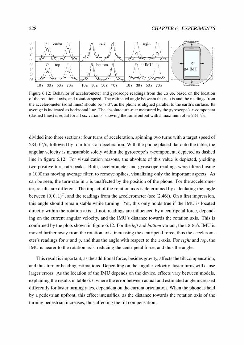
228 CHAPTER 6. EXPERIMENTS
0°2°4°6°
0°2°4°6°
10 s 30 s 50 s 70 s 10 s 30 s 50 s 70 s 10 s 30 s 50 s 70 s
center left right
top bottom at IMUIMU
Figure 6.12: Behavior of accelerometer and gyroscope readings from the LG G6, based on the locationof the rotational axis, and rotation speed. The estimated angle between the z-axis and the readings fromthe accelerometer (solid lines) should be ≈ 0°, as the phone is aligned parallel to the earth’s surface. Itsaverage is indicated as horizontal line. The absolute turn-rate measured by the gyroscope’s z-component(dashed lines) is equal for all six variants, showing the same output with a maximum of ≈ 234 °/s.
divided into three sections: four turns of acceleration, spinning two turns with a target speed of234.0 °/s, followed by four turns of deceleration. With the phone placed flat onto the table, theangular velocity is measurable solely within the gyroscope’s z-component, depicted as dashedline in figure 6.12. For visualization reasons, the absolute of this value is depicted, yieldingtwo positive turn-rate-peaks. Both, accelerometer and gyroscope readings were filtered usinga 1000 ms moving average filter, to remove spikes, visualizing only the important aspects. Ascan be seen, the turn-rate in z is unaffected by the position of the phone. For the accelerome-ter, results are different. The impact of the rotation axis is determined by calculating the anglebetween (0, 0, 1)T , and the readings from the accelerometer (see (2.46)). On a first impression,this angle should remain stable while turning. Yet, this only holds true if the IMU is locateddirectly within the rotation axis. If not, readings are influenced by a centripetal force, depend-ing on the current angular velocity, and the IMU’s distance towards the rotation axis. This isconfirmed by the plots shown in figure 6.12. For the left and bottom variant, the LG G6’s IMU ismoved farther away from the rotation axis, increasing the centripetal force, thus the accelerom-eter’s readings for x and y, and thus the angle with respect to the z-axis. For right and top, theIMU is nearer to the rotation axis, reducing the centripetal force, and thus the angle.
This result is important, as the additional force, besides gravity, affects the tilt compensation,and thus turn or heading estimations. Depending on the angular velocity, faster turns will causelarger errors. As the location of the IMU depends on the device, effects vary between models,explaining the results in table 6.7, where the error between actual and estimated angle increaseddifferently for faster turning rates, dependent on the current orientation. When the phone is heldby a pedestrian upfront, this effect intensifies, as the distance towards the rotation axis of theturning pedestrian increases, thus affecting the tilt compensation.

6.2. EVALUATION OF SENSOR COMPONENTS 229
27°30°33°36°
−4°0°4°
2 s 4 s 6 s 76 s 78 s 80 s 152 s 154 s 156 s
Figure 6.13: Consecutive ±15° CCW and CW rotation of a turntable tilted by 15°, with the phone in45° portrait mode. The two rows denote the tilt angles in x (top) and y (bottom), estimated from theaccelerometer (gray), gyroscope (dashed black) and complementary filter with κ = 0.998 (solid black).By combining both, the filter compensates noise from the accelerometer, and drift of the gyroscope.
The complementary filter (cf. section 2.4.2) provides a partial solution. By applying a low-pass filter to the accelerometer, temporal anomalies are compensated. Yet, this only addressessmall timeframes, unsuitable for longer turns, or the synthetic tests on the turntable. While thecomplementary filter can be configured to rely even more on the gyroscope, when increasingthe timeframe of compensation, drift becomes notable, causing new issues. These effects, andthe impact of the filter, are shown in figure 6.13, where the LG G6 was placed in 45° portraitmode, onto the turntable, which was tilted backwards by 15°, causing a 30° angle betweenphone and ground. The turntable was configured to perform ±15° turns around this initialposition, that is, 15° CCW once, followed by a repetition of 30° CW and 30° CCW, alternatingaround the initial center. This results in a shaking movement, similar to a walking pedestrian,holding the smartphone upfront. Figure 6.13 shows the estimated rotation for the phone, aroundits x and y axis (see (2.39) and (2.49)). As the gyroscope measures only relative changes, itscumulation was initialized using the first few estimations from the accelerometer. As can beseen, the accelerometer provides an absolute estimation, but contains significant amounts ofnoise. While the gyroscope does not show notable noise, it suffers from cumulating drifts, withthe 30° angle reaching 36° after ≈ 130 s. This is addressed by a complementary filter withan empiric κ = 0.998, combining accelerometer and gyroscope, deriving a stable, noise-freeestimation, suited for tilt compensation. While results were depicted and discussed for a singlephone, all other devices showed similar behavior, yet, dependent on the location of their IMU.
Results - Turn Angles The quality of gyroscope-based turn-detection is examined by theturntable performing ten turns CCW, followed by ten turns CW, using the three mentionedspeeds and orientations. Ground truth is the cumulated angle after the first ten, and all 20 turns,which should read 3600° and 0°, respectively. It is estimated using four different strategies:Integrating the gyroscope’s z-component (2.36), using the gyroscope’s signed magnitude (2.38),

230 CHAPTER 6. EXPERIMENTS
performing tilt compensation solely by the accelerometer using (2.49) with κ = 0, and, applyingtilt compensation by the complementary filter using (2.49) with an empiric κ = 0.998.
Results are listed in table 6.7. As expected, just integrating the gyroscope’s z-component(each 1st row) provides valid results only when the smartphone is placed parallel to the earth’ssurface. The 45° landscape and portrait modes should read approximately sin(45°) 3600° ≈2546°. While using the gyroscope’s signed magnitude (each 2nd row) addresses this issue, thisis only valid for the presented turntable tests, where the induced rotation has a single sourceaxis. When a pedestrian holds the smartphone while walking, shaking additionally affects themagnitude, invalidating the cumulated angle. For pedestrian walks, tilt compensation (each3rd and 4th row) should be applied to the gyroscope measurements, prior to the integrationstep. While the accelerometer is able to provide this compensation on its own (each 3rd row)previous experiments indicated that using a complementary filter (each 4th row) is advisable.
This is again confirmed by the values of the 45° portrait setup in table 6.7. When thebracket holds the smartphone in portrait mode (see figure 6.11), each device picks up a notableamount of noise, resulting from a disadvantageous center of mass. When using solely theaccelerometer for tilt compensation (3rd row), this noise affects the estimated tilt, and thus theresulting cumulated angle, clearly indicated by the divergent results. The complementary filteris able to address this issue by filtering the accelerometer, and including the gyroscope.
Counterintuitively, the KEY2 and Moto Z show larger errors for the flat placement, than forthe other two orientations. Analyzing the raw readings from the gyroscope indicated that thesensor within these devices provides slightly divergent turning rates for CCW and CW rotation,at least, for readings of the z-axis. Even though this difference is marginally, it cumulates overtime, causing notable deviations after the 20 turns. As it is less pronounced for faster turningrates, that is, shorter test-runs, it might be caused by a minor, constant calibration offset.
While repeatability is good for most devices, all absolute readings are slightly off. That is,the measured turn-rate (see table 6.6) does not match with the actual one, yielding the cumula-tions (see table 6.7) to be off as well. Especially the Pixel 2 in portrait mode deviates more than1 % from the actual turn-rate. Yet, for all examined devices, results were viable with relativelysmall errors for shorter timeframes, well suited for assisting coarse absolute headings.
Results - ECompass Even though the results for gyroscope-based turn-detection are promis-ing, they remain relative. When not knowing the pedestrian’s initial heading, and/or sufferingfrom cumulating drift, absolute indications are helpful, even if they are less accurate.
To ensure the magnetometer points towards geomagnetic north, a brief test compared theestimated angle (2.60) with the one from an analog compass, when placing each device flatonto the ground. Being inexact, results are not provided as actual angular values. Nevertheless,

6.2. EVALUATION OF SENSOR COMPONENTS 2310
°fla
tla
ndsc
ape
at45
°po
rtra
itat
45°
62.7
°/s
122.
5°/
s23
4.0
°/s
62.7
°/s
122.5
°/s
234.0
°/s
62.7
°/s
122.5
°/s
234.
0°/
s
S3Mini
3337
.037
.933
28.4
21.1
3322
.510
.821
14.2
36.5
2103
.515
.821
02.5
11.4
2193
.633
.821
96.2
15.0
2191
.711
.533
47.0
44.3
3335
.127
.033
27.6
15.1
3378
.510
7.9
3350
.356
.033
39.5
33.8
3372
.233
.533
69.2
18.3
3362
.114
.633
34.4
35.1
3327
.720
.133
22.6
10.4
3358
.010
3.5
3339
.355
.133
34.4
33.3
3355
.830
.733
45.4
7.9
3348
.19.
533
35.9
36.0
3327
.920
.033
22.0
10.2
3361
.410
3.9
3339
.355
.533
31.4
32.2
3358
.830
.433
50.0
8.1
3350
.910
.1
Nexus6
3579
.7-4
.535
82.9
-1.4
3579
.9-1
.924
37.1
10.9
2450
.9-0
.524
50.1
-0.4
2466
.5-2
.624
69.3
-3.7
2473
.6-1
.335
79.9
-4.8
3583
.2-1
.435
80.1
-1.9
3569
.60.
935
69.6
0.8
3568
.50.
035
83.1
-2.6
3569
.7-2
.135
71.6
-1.5
3579
.5-4
.535
82.6
-1.4
3578
.3-0
.935
67.2
4.7
3568
.40.
435
65.9
0.2
3557
.1-1
1.4
3566
.1-3
.835
69.0
-1.4
3579
.6-4
.635
82.7
-1.4
3579
.4-1
.735
68.7
2.6
3568
.80.
635
66.9
-0.2
3569
.70.
335
68.5
-1.9
3570
.7-0
.4
MotoZ
3598
.814
.135
94.7
5.8
3593
.23.
125
31.7
11.4
2530
.37.
725
29.2
4.5
2509
.39.
025
07.9
4.9
2507
.62.
435
99.6
14.4
3595
.46.
035
94.0
3.3
3619
.18.
036
17.7
5.9
3615
.83.
335
99.8
12.9
3591
.15.
735
87.6
2.6
3598
.814
.235
93.7
5.7
3586
.83.
336
15.7
6.9
3614
.24.
736
10.3
1.8
3543
.4-3
1.8
3555
.5-1
3.7
3573
.20.
535
99.0
14.2
3594
.45.
835
89.9
3.9
3617
.17.
436
15.4
5.0
3613
.42.
835
90.3
10.1
3587
.65.
335
81.6
3.7
LGG6
3619
.7-0
.036
19.8
-0.3
3620
.0-0
.125
57.3
0.2
2558
.6-0
.225
57.3
-0.1
2553
.9-0
.725
54.8
-0.4
2555
.9-0
.236
19.9
-0.1
3619
.9-0
.336
20.1
-0.2
3617
.70.
136
17.1
-0.2
3617
.1-0
.536
33.5
-0.3
3626
.6-1
.236
25.7
-0.3
3618
.5-0
.336
18.1
-0.1
3609
.4-0
.636
11.8
-0.8
3612
.3-0
.536
02.0
-0.9
3567
.1-4
0.4
3593
.0-9
.136
12.5
-2.2
3619
.5-0
.036
19.2
-0.3
3612
.40.
136
16.1
0.1
3615
.2-0
.236
06.5
0.3
3624
.0-0
.736
24.2
-0.4
3619
.9-0
.0
Pixel2
3594
.4-0
.235
94.5
-0.1
3594
.1-0
.125
25.5
-0.8
2527
.2-0
.625
28.2
0.2
2527
.9-0
.625
29.8
0.0
2530
.9-0
.335
94.6
-0.2
3594
.6-0
.135
94.2
-0.0
3595
.0-1
.235
93.9
-1.6
3594
.1-1
.036
65.5
-5.9
3657
.4-0
.836
57.0
-1.2
3591
.60.
135
92.7
0.3
3584
.60.
335
90.1
-2.4
3591
.8-1
.535
83.1
0.2
3622
.5-2
.436
44.8
-0.9
3644
.21.
935
94.2
-0.2
3593
.6-0
.135
86.4
0.2
3593
.5-1
.235
92.9
-1.6
3586
.8-0
.536
55.2
-1.1
3654
.4-0
.336
48.1
0.0
KEY2
3590
.6-1
1.6
3593
.4-6
.035
95.1
-3.4
2503
.7-0
.125
04.8
0.5
2504
.7-0
.025
32.7
-0.7
2525
.4-0
.525
26.4
-0.4
3591
.1-1
2.1
3594
.0-6
.435
95.7
-3.7
3591
.89.
935
89.2
6.0
3587
.42.
036
31.7
-10.
736
23.6
-5.0
3624
.3-2
.735
90.3
-11.
035
90.8
-6.0
3582
.7-3
.735
87.7
11.4
3586
.77.
235
77.4
3.6
3595
.0-2
2.4
3617
.5-5
.836
09.0
-3.2
3590
.7-1
1.4
3592
.3-5
.935
87.4
-1.2
3591
.411
.235
88.2
7.1
3580
.34.
636
19.7
-10.
336
20.9
-4.8
3615
.91.
3
Tabl
e6.
7:R
esul
tsof
the
turn
tabl
eex
peri
men
ts,p
erfo
rmin
gte
nC
CW
turn
s,fo
llow
edby
ten
CW
turn
s,us
ing
thre
edi
ffer
ents
mar
tpho
nepl
acem
ents
,ea
chw
ithth
ree
turn
ing
spee
ds.
For
ever
yph
one,
the
cum
ulat
edhe
adin
gch
ange
afte
rth
efir
stte
nC
CW
turn
s(l
eft
valu
e,sh
ould
be36
00°)
and
afte
radd
ition
alte
nC
Wtu
rns
(rig
htva
lue,
shou
ldbe
0°)i
sde
term
ined
usin
gfo
urdi
ffer
ents
trat
egie
s:In
tegr
atin
gth
egy
rosc
ope’
sz
-com
pone
ntas
-is
(2.3
6)(1
stro
w),
usin
gth
egy
rosc
ope’
ssi
gned
mag
nitu
de(2
.38)
(2nd
row
),pe
rfor
min
gtil
tcom
pens
atio
nso
lely
byth
eac
cele
rom
eter
usin
g(2
.49)
with
κ=
0(3
rdro
w),
and
appl
ying
tiltc
ompe
nsat
ion
byth
eco
mpl
emen
tary
filte
rusi
ng(2
.49)
with
κ=
0.99
8(4
thro
w).

232 CHAPTER 6. EXPERIMENTS
0°
180°240°300°360°
10 s 20 s 30 s 40 s 50 s
354°
357°
360°
363°
366°
11 s 12 s 13 s 14 s
60°
120°
180°
49 s 50 s 51 s 52 s
Figure 6.14: Angle estimated by (2.60) for the LG G6, after offset-removal and unwrapping for visualiza-tion reasons. The gray line denotes the angle derived from the raw sensor data, the black line resultedfrom prior low-pass filtering. Shown in the left, the unfiltered result contains significant amounts ofnoise, mitigated by the filter. The right denotes a minor nonlinearity throughout the rotation.
all examined errors remained within ±20°, and the majority within ±10°. While not ideal, thisis still suited for a probabilistic absolute heading, backed by a fine relative turn-detection.
Potential accuracy, precision, and lag were examined by placing each device flat onto theturntable, using a spacer of approximately 250 mm in between, to prevent the motor from in-fluencing sensor readings. The turntable’s pattern is changed to three repetitions of, 360° CCWfollowed by 360° CW, matching the value range of the magnetometer. Acceleration and de-celeration were disabled, to visualize the linearity of the sensor. However, this limits testingto the slowest speed of 62.7 °/s, ensuring the phone stays in place, and the motor not skippingsteps. To allow comparing against a known ground truth, all angles calculated from magnetome-ter readings are adjusted to be relative to the initial one, eliminating offsets towards magneticnorth. The result is unwrapped to remove jumps, e.g. between 0° and 360°, allowing for contin-uous drawing in figures. Additionally, a 250 ms moving average filter is applied to each of thethree magnetometer axes, before estimating the angle (2.60). Filtered and raw results are shownin figure 6.14. As can be seen, without filtering, a significant amount of noise is present withinthe estimated angle (left). Independent of filtering, the behavior while turning indicates a mi-nor nonlinearity, deviating from a straight line (right), observable for all tested devices. Whilesources for this behavior are numerous, it is most likely related to minor calibration issues.
Mentioned earlier, the magnetometer is affected by hard iron and soft iron effects, requir-ing (re)-calibration. For all examined devices (see table 6.1) except the Milestone 4, themagnetometer calibrated itself when being active, and the smartphone rotated several timesaround all three axes. The quality of this calibration is examined by fitting an ellipse ontothe (x, y) readings, which, for the conducted test, should form a circle around (0, 0). Thefitting is performed by solving an over-determined set of linear equations, determining sixellipse-parameters to match with all measured samples, based on the general ellipse equationax2 + bxy + cy2 + dx + ey + f = 0. It is hereafter converted to the geometric form, with a

6.2. EVALUATION OF SENSOR COMPONENTS 233
−20
0
20
−20 0 20
−42
−38
−20 0 20
−42
−38
x/y (µH)
y/z (µH)
x/z (µH)
Figure 6.15: Raw (gray) and filtered (black) magnetometer readings for the LG G6, that lead to figure 6.14.The fitted ellipse (dotted white) indicates an offset from (0, 0), including a minor unroundness. Similarly,both plots on the right reveal a minor sensor-tilt, affecting the roundness as well.
center, length of major/minor axis, and rotation [WGN15; Ber17]. The result for the LG G6 isshown in figure 6.15, containing the raw and filtered readings for all three magnetometer axes.As can be seen, the fitted ellipse is slightly off-center, and shows a minor unroundness, affectingthe linearity, as depicted earlier in figure 6.14. While this can be addressed using the presentedcalibration (2.62), differences in accuracy were negligible for most devices.
Table 6.8 presents an average out of several repetitions, for each examined smartphone. Thequality of automatic calibration is given by the average magnitude of the magnetometer readings(1st column), and the center of the estimated ellipse (2nd and 3rd column), which should be(0, 0). While not being ideal, automatic calibration is sufficient for absolute heading estimation.Only for the Milestone 4, the calibration was performed manually using (2.62). Besides thecenter of the ellipse, the ratio between the size of its minor and major axis (see figure 6.15)is calculated (4th column), indicating the roundness of the sensor readings, which should be1.0 for an ideal circle. While some of the devices show a tendency towards an ellipsoid, theirsensor readings are still viable for heading estimations. Sensor-tilt (5th column) also affects theroundness and angular results. The listed value denotes the angle between the x-axis, and a linedefined by the range of the magnetometer’s z-readings. For the presented turntable pattern, thelatter should also yield a horizontal line, and thus an angle of 0° (see figure 6.15 right). Whilesome devices indicated a slight tilt, results remained within a viable range, with no significantimpact on the estimated angles.
The right half of table 6.8 shows the angles estimated in between the turntable’s actions.They are based on the same values, as have been used for figure 6.14. That is, filtered, offset-corrected, and unwrapped. Entries are derived by searching for a minimum/maximum at eachof the 0°/360° plateaus. As can be seen, while the angles do not exactly conform with analternating pattern of 0° and 360°, they are well within range, even for older smartphone models.

234 CHAPTER 6. EXPERIMENTS
Magnitude/Center (µH) Roundness Angular Values (°)mag x y ratio tilt (°)
Milestone 2 46.41 0.54 2.13 0.98 0.93 -2.3 363.5 -2.3 362.6 -0.9 361.9 -2.4Milestone 4 - - - 0.95 0.24 -2.0 360.4 -1.2 360.0 -1.6 360.1 -2.2S3 Mini 42.63 0.37 -0.68 0.92 2.31 -2.0 359.8 -2.5 359.5 -3.0 357.9 -3.6Nexus 6 44.46 0.62 0.58 0.99 0.37 -1.4 361.5 -0.7 361.5 -0.8 361.0 -0.7S5 Neo 42.38 1.84 3.07 0.97 0.90 -0.3 361.0 -0.6 360.0 -2.1 360.4 0.5Moto Z 45.88 0.10 -1.87 0.98 1.74 -2.2 360.7 -3.5 361.3 -0.9 361.9 -2.1LG G6 44.14 0.12 2.44 0.95 1.43 -2.1 362.9 -0.0 362.1 -0.1 362.2 0.9Pixel 2 43.90 1.07 -1.13 0.96 0.61 -1.0 360.8 -0.8 360.6 -0.8 360.5 -0.7KEY2 46.19 -0.54 2.33 0.94 0.65 -0.6 362.3 -0.9 361.1 0.1 361.6 -1.2
Table 6.8: Results of the turntable experiments, performing three times a sequence of: 360° CCW and360° CW at 62.7 °/s, with the smartphone placed flat onto the turntable. Besides the seven estimatedangles (right), calibration-related metrics are shown (left), covering the average magnitude, offset from(0, 0), and the result’s roundness, explained within the text.
Tests requiring tilt compensation are presented only briefly, for two reasons. On the onehand, the turntable setup is not suited for a 45° portrait/landscape alignment with enough spacebetween the device and the motor, without introducing misalignment and shaking. On the otherhand, previous results for the gyroscope have already shown the validity of the tilt compensa-tion. Yet, examinations conducted with additional spacing indicated results similar to the onesfrom the gyroscope, with tilt compensation working as expected.
Not shown within figures, the angle estimated from the magnetometer was also comparedagainst the one determined from the gyroscope, indicating no significant delay between both,when using the raw magnetometer data. Even for devices where the sensor seems to performinternal filtering (S3 Mini, S5 Neo and Moto Z), lag was moderate, as low as a few milliseconds.Especially for the S3 Mini, the magnetometer was significantly more stable than its gyroscope,which suffered from aforementioned drifts. Thus, the conducted synthetic tests indicate thatabsolute heading from the magnetometer is suited for supporting the gyroscope.
6.2.4 Pedestrian Dead Reckoning
The actual quality of IMU-based turn-detection, and absolute heading estimation is determinedby a pedestrian walking while holding the smartphone upfront. For an impression of the esti-mation results, the previously examined step-detection is included as well, yielding a pedestriandead reckoning setup, depicting individual aspects for each of the two heading methods. It alsoprovides an impression on the capabilities of smartphone-based PDR. That is, expected local-ization quality, when not using sensors for absolute location estimations, omitting probabilisticapproaches, recursive density estimation, and constraints from an underlying floorplan.
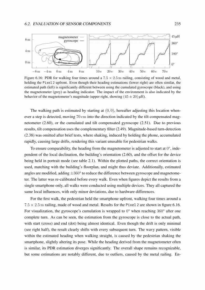
6.2. EVALUATION OF SENSOR COMPONENTS 235
0 m
4 m
8 m
−8 m −4 m 0 m 4 m 8 m 10 s 20 s 30 s 40 s 50 s 60 s 70 s
0°
180°
360°
45 µHgyroscope
magnetometer
Figure 6.16: PDR for walking four times around a 7.5 × 2.5 m railing, consisting of wood and metal,holding the Pixel 2 upfront. Even though their heading estimations (lower right) are often similar, theestimated path (left) is significantly different between using the cumulated gyroscope (black), and usingthe magnetometer (grey) as heading indicator. The impact of the environment is also indicated by thebehavior of the magnetometer’s magnitude (upper right, showing (45± 20) µH).
The walking path is estimated by starting at (0, 0), hereafter adjusting this location when-ever a step is detected, moving 70 cm into the direction indicated by the tilt compensated mag-netometer (2.60), or the cumulated and tilt compensated gyroscope (2.51). Due to previousresults, tilt compensation uses the complementary filter (2.49). Magnitude-based turn-detection(2.38) was omitted after brief tests, where shaking, induced by holding the phone, accumulatedrapidly, causing large drifts, rendering this variant unusable for pedestrian walks.
To ensure comparability, the heading from the magnetometer is adjusted to start at 0°, inde-pendent of the local declination, the building’s orientation (2.60), and the offset for the devicebeing held in portrait mode (see table 2.1). Within the plotted paths, the correct orientation isused, matching with the building’s floorplan, and might thus deviate. Additionally, estimatedangles are modified, adding±360° to reduce the difference between gyroscope and magnetome-ter. The latter was re-calibrated before every walk. Even when figures depict the results from asingle smartphone only, all walks were conducted using multiple devices. They all captured thesame local influences, with only minor deviations, due to hardware differences.
For the first walk, the pedestrian held the smartphone upfront, walking four times around a7.5× 2.5 m railing, made of wood and metal. Results for the Pixel 2 are shown in figure 6.16.For visualization, the gyroscope’s cumulation is wrapped to 0° when reaching 360° after onecomplete turn. As can be seen, the estimation from the gyroscope is close to the actual path,with start (cross) and end (dot) being almost identical. Even though the drift is only minimal(see right half), the result clearly shifts with every subsequent turn. The wavy pattern, visiblewithin the estimated heading when walking straight, is caused by the pedestrian shaking thesmartphone, slightly altering its pose. While the heading derived from the magnetometer oftenis similar, its PDR estimation diverges significantly. The overall shape remains recognizable,but some estimations are notably different, due to outliers, caused by the metal railing. En-

236 CHAPTER 6. EXPERIMENTS
−8 m
−4 m
0 m
4 m
−12 m−8 m −4 m 0 m 4 m 10 s 20 s 30 s 40 s 50 s
−540°
−360°
−180°
0°
180°45 µH
gyroscopemagnetometer
downwards, CW
180
°,C
CW
upwards, CCW
Figure 6.17: PDR for holding the Pixel 2 upfront, walking two floors downwards in CW direction,turning by 180° CCW in place, walking two floors upwards in CCW direction, reaching the origin.The stairwell’s environment affects the magnetometer significantly, indicated by changes in magnitude(upper right, showing (45± 20) µH), causing heading inversions in some locations (lower right plot).Consequently, the path estimated from the magnetometer’s heading (left plot) is rendered unusable.
vironmental influences are also notable within the sensor’s magnitude, depicted in the upperright plot, showing a range of (45± 20) µH. While the presented example seems like an idealcandidate for the complementary filter, compensating gyroscope drift with a low-pass filteredmagnetometer, this does not hold true in general. Temporal environmental effects can yieldheading offsets with unknown duration and impact, uncorrectable by the complementary filter.
This can be seen within a second setup, with a pedestrian walking two floors downwardsin CW direction, performing a 180° turn in place, walking back to the origin, shown in fig-ure 6.17. The environment is characterized by steel-reinforced concrete, a facade made of glassand metal-bars, and large radiators for heating the stairwell. Shown within the plots, local influ-ences, like the radiators, can cause the indicated heading to be the opposite of the real direction,uncorrectable by initial calibration. The magnitude of the magnetometer readings, shown withinthe upper right plot, also indicates the effect of surrounding metal objects. However, for the de-picted walk, there is no direct temporal correspondence between changes in magnitude, andheading errors. Besides heading, the estimated distance also unveils important results. Whilethe plot indicates a walking distance in x-direction of ≈ 8 m, the actually walked length mea-sures only ≈ 4 m. This is due to assuming a constant step length of 70 cm, which is incorrectwhile taking stairs. Here, the step length is given by the size of the stair’s treads, which was≈ 30 cm. As mentioned in chapter 3, this will be addressed later, by including the building’sfloorplan, adjusting the step length, whenever the underlying ground denotes treads of a stair.
A third walk is used to determine the long-term stability of step-detection, gyroscope andmagnetometer, when walking mainly straight forward. For this setup, the pedestrian held thesmartphone upfront, walking ≈ 60 m straight through the building, taking one 90° CCW turn,proceeding straight for ≈ 40 m. Results are depicted in figure 6.18, for two different devices,the Pixel 2 (solid lines), and the LG G6 (dashed lines). For both, the estimated walking distance

6.2. EVALUATION OF SENSOR COMPONENTS 237
magnetometergyroscope
50 m
10 s 20 s 30 s 40 s 50 s 60 s 70 s
0°
90°
45 µH
Figure 6.18: PDR for holding the Pixel 2 upfront, walking ≈ 100 m straight, with one 90° CCW turnin between. The magnetometer’s magnitude (upper right, showing (45± 20) µH) changes significantlythroughout the walk, so does its estimated heading (lower right). The result for both smartphones – thePixel 2 (solid), and the LG G6 (dashed) – slightly overshoots the actual destination (lower left). Whilethe gyroscope-based PDR diverges between both, the magnetometer-based variant is notably similar.
is slightly larger than the actual value, overshooting by approximately 2 m, due to an incorrectstep length constant. Concerning turn-detection, the two devices seem slightly biased, visibleas individual bending of their estimated paths. For the magnetometer’s estimation, both resultsare notably similar, showing the same local effects along the walking path, even though bothwere recorded one after another. Yet, besides being notably similar, and the overall shaperecognizable, there are major drawbacks for the magnetometer heading’s accuracy. The firsthalf of both walks is off by ≈ 15° from the horizontal ground truth. Within the second half,this error increases to ≈ 25° from the vertical ground truth. The difference between the halvesclearly indicates that this can not be addressed by a constant angular calibration offset.
The examined walks thus yield several conclusions. Similar to previous experiments, step-detection is accurate, but walking distance estimations can vary, especially when invalid as-sumptions on the pedestrian’s step length are made. In some cases, like the depicted overshoot-ing, this can be mitigated by including the building’s floorplan, preventing impossible walks.
The gyroscope-based turn-detection is almost free of noise, accurate within shorter time-frames, but suffers from cumulating drifts, notably affecting PDR-based location estimation.Furthermore, the amount of drift, and its direction, vary between the tested devices. Again,these issues can be mitigated by including a floorplan, limiting impossible walks.
The magnetometer can provide a coarse absolute heading, at least in some parts of the build-ing, but might suffer from unpredictable, large errors in other regions. As there was no directcorrespondence between changes in magnitude and observed errors, predicting outliers seemsdifficult. Only within measurements belonging to straight walks, or when compared againstturn-detection, assumptions on potential outliers can be made. Even after outlier filtering, theaccuracy of the estimated heading remains unclear (see (6.18)), influenced by the surroundingenvironment. However, based on the presented results, including the magnetometer probabilis-

238 CHAPTER 6. EXPERIMENTS
994.9
995.1
995.3
995.5
995.7
0 s 20 s 40 s 60 s 80 s 100 s 120 s
147148149150151152153154 994
994.2
994.4
994.6
994.8
0 s 10 s 20 s 30 s 40 s 50 s 60 s
154155156157158159160161
pres
sure
(hP
a) ground truth
measured
altit
ude
(m)
ground truthmeasured
Figure 6.19: Measured pressure over time, for a pedestrian walking upstairs by two stories, then down-stairs again, using the LG G6. At each plateau, the pedestrian either rested shortly (left), or kept walking(right). Solid lines denote the first walk, dashed lines all repetitions, made within a ten minute timeframe.Between the five walks on the left, and the ones on the right, one hour has passed. The ground truth wasdetermined by (2.71), based on the building’s altitude, a measured reference pressure, and the stair.
tically for a coarse heading estimation, seems feasible (cf. section 2.4.3). Corresponding resultswill be discussed when examining the overall system, including sensor fusion by recursive den-sity estimation, and constraints imposed by the building’s floorplan.
6.2.5 Altitude Estimation
To evaluate the contribution of smartphone barometers, discussed approaches, and issues, sev-eral walks with varying hardware, location, and ambient conditions were conducted. The ex-periments focus on accuracy, precision, delays, environmental influences, and consequences.
Repeatability of measurements was examined by conducting a two story walk (first up, thendown) several times, within a timeframe of ten minutes, using the LG G6, during cloudy weatherconditions. The difference in altitude between both stories was estimated using a plumb bob andis ≈ 5.54 m. While walking, four stairs, each ≈ 1.38 m in height, and five plateaus (includingstart and end) were taken. Figure 6.19 shows the results for five consecutive first-up-then-downwalks. At each plateau, the pedestrian rested either ≈ 10 s (left half) or kept walking (righthalf). The solid lines describe the first of five repetitions, all others are denoted by dashed lines.Between both variants, with and without resting at plateaus, one hour has passed, and, as can beseen, the atmospheric pressure changed by about 1 hPa, equal to 8 m in altitude. Even betweenthe repetitions, there is a difference in altitude of up to 1.0 m, and the atmospheric pressurereading varies notably. This clearly indicates a major drawback when using absolute pressureindications. Besides, figure 6.19 also indicates a poor repeatability during each single walk, asthere is no symmetry between both halves (walking upstairs/downstairs). However, comparedwith the 1 hPa difference, deviations throughout the walk were less severe.
As can also be seen, sensor readings appear unnaturally smooth, most probably due to fil-tering inside the sensor or operating system. This causes the plateaus, where the pedestrian

6.2. EVALUATION OF SENSOR COMPONENTS 239
Altitude Change Seconds per Stair Steps/Treads per Secondµ σ µ σ µ σ
stair↑ 31.5 cm/s 3.99 cm/s 4.38 0.66 1.85 0.23stair↓ 36.2 cm/s 3.78 cm/s 3.84 0.47 2.09 0.22
Table 6.9: Average stair walking speeds among several pedestrians for the staircase from figure 6.19.
was standing still, to barely appear as a flat line. For the non-resting walk, they are completelyunrecognizable. That is, all measurements appear like a low-pass filtered version of the groundtruth, yielding a curved and delayed output. This delay was first estimated visually, by movingthe measurements to the left until they match the ground truth, indicating ≈ 3 s. Likewise, thedelay was determined mathematically via numerical optimization of an error function, given bythe vertical distance between measurements and ground truth, indicating a delay of ≈ 3.4 s.
To estimate the impact of this delay, the pedestrian’s average change in altitude per second,and the time needed for climbing the examined staircase, are determined. For this, severalpedestrians walked within the staircase from figure 6.19, while taking the exact time at thebeginning and end of each individual stair. Results of this analysis are shown in table 6.9. Ascan be seen, delays presented by the LG G6’s barometer are almost equal to the average time ittakes a pedestrian to climb each stair, that is, half a floor. Even though the barometer indicatesthe first changes in atmospheric pressure slightly before the estimated delay, this still causesissues when evaluating the probability for potential pedestrian movements.
Figure 6.20 depicts the resulting evaluation, comparing barometer readings and ground truthprobabilistically. For the absolute variant (2.73), the current atmospheric pressure and altitudeabove mean sea level are required for the examined stairwell. Both values together are usedto convert the readings from the barometer into an expected altitude. This result is comparableagainst the walk’s ground truth, using (2.73) with σalt = 1 m. The uncertainty was determinedempirically, based on previous evaluations. It implies that > 99 % of all sensor readings areexpected to stay within a ±3 m boundary, or approximately one floor level. When using therelative approach (2.75), by using the first barometer reading as 0-reference, no absolute valuesare required, comparing solely relative pressure and altitude changes.
Figure 6.20 compares both variants. The absolute approach shows a poor repeatability. Dueto changing ambient conditions, the conducted repetitions are significantly different. Thus, theabsolute evaluation of barometer readings does not provide a viable solution to estimate thepedestrian’s altitude. This is effectively addressed by the relative strategy, where all repetitionsstart with the same likelihood, due to the initial pressure reference. However, even the relativevariant suffers from changing weather conditions, as they invalidate the initial reference even-

240 CHAPTER 6. EXPERIMENTS
0.1
0.2
0.3
0.4
20 s 40 s 60 s 80 s 100 s 120 s
off by 1.5 m
off by 2.0 m
0.1
0.2
0.3
0.4
10 s 20 s 30 s 40 s 50 s 60 s
(2.7
5)[r
elat
ive]
(2.7
3)[a
bsol
ute]
Figure 6.20: Absolute (2.73) and relative (2.75) evaluation of barometer readings for the data fromfigure 6.19. The absolute variant clearly lacks repeatability, due to the ambient pressure slightly changingbetween the conducted walks. Spikes within all results are caused by the sensor’s delay. For the walkswhere the pedestrian rested at each plateau (left) the probability is able to recover. For the non-restingwalks (right), the delay becomes even more apparent, with more and wider spikes.
tually. It is thus advisable, to use a time-limited approach, comparing the pressure and altitudechange during the last few seconds, instead of since start.
For both variants, the sensor delay yields noticeable drops in likelihood whenever taking astair, with spikes similar to being off by half a floor. When resting for 10 s at each plateau, theprobability is able to recover. For the non-resting variant, however, additional spikes appearand blend together, causing a period of reduced probability. Not shown within the figure, whencompensating the sensor delay manually, the spikes are significantly reduced, yielding almost ahorizontal line, that is, a constant probability, indicating the general viability of the sensor.
Both, the presented delays and repeatability, are sensor dependent attributes. Conductinga similar walk with a Google Nexus 6, equipped with a barometer from Invensense, yieldsthe results shown in figure 6.21. While the direct output of the sensor is less smooth, due to adecreased number of significant digits, delays are smaller, repeatability is better, and responseis more direct. Even when the pedestrian is not resting at the plateaus, they are visible withinthe data provided by this sensor. Furthermore, starting and ending pressure are almost identical,yielding a good repeatability of the measurements. Finally, the delay between ground truth andindicated readings is notably smaller, compared to the LG G6 with a Bosch BMP280 barometer.Optical and numerical analysis of the delay indicated ≈ 2.1 s. Thus, even though the outputfrom the Nexus 6 looks less pleasing, it is more useful for indoor localization and navigation.
Experiments also indicated a phenomenon, concerning the initial readings of the barome-ter. Shown in figure 6.21, in the beginning, the readings change rapidly by about one completefloor, stabilizing hereafter. While not being present within all recordings and/or hardware com-ponents, it was observed several times. Likewise, neither the direction nor the amount of change

6.2. EVALUATION OF SENSOR COMPONENTS 241
990.4
990.6
990.8
991
0 s 20 s 40 s 60 s 80 s 100 s 120 s 140 s 160 s 180 s
186187188189190191192193
pres
sure
(hP
a)
altit
ude
(m)ground truth
measured
Figure 6.21: Measurements from the barometer installed within the Google Nexus 6, held upfront by apedestrian, while walking a staircase up and down, twice.
were the same throughout tests. Even the timeframe the effect occurred for was varying, butranged somewhere around 5 s. While the source for this behavior is unknown, it might be relatedto filters, installed within the sensors [Bos15; Bos18]. As this phenomenon strongly affects therelative evaluation (2.75), it must be addressed by omitting the initial readings of the barometer,until they are assumed stable, e.g. by using the first reading after several seconds as reference.
To summarize, while the barometer is able to provide hints on the current altitude, these areonly stable when referring to smaller timeframes, which reduce the impact of environmentalchanges. The sensor is thus unsuited for absolute altitude estimations, but e.g. well suited fordetermining whether the pedestrian is currently taking stairs, that is, activity-detection.
6.2.6 Activity Detection
To determine the potential and accuracy of activity recognition, a tagged dataset containing allactivities was recorded for several pedestrian walks with varying devices. 10 % of this datasetwas used as training data, to estimate one 2D normal distribution per activity, based on theaccelerometer’s variance (2.77), and the barometer’s delta (2.78), both within a certain time-frame. A new 2D feature pair consisting of those two values is calculated for every incomingbarometer reading. Aforementioned distributions are estimated using the mean and covarianceof all pairs belonging to the same activity. While smaller timeframes introduce less delays,they are expected to be less accurate due to sensor noise. Corresponding results can be seen infigure 6.22, where three different timeframes, 250 ms, 500 ms and 1000 ms, are depicted. Thefocus of the figure is on separability. Actual values are thus omitted, and listed in table 6.11.For each activity, the estimated distribution is visualized using one ellipse for 1σ, and one for2σ around the mean, containing ≈ 68 % and ≈ 95 % of all samples, respectively.
As can be seen, a timeframe of 250 ms is too narrow to provide a viable separation betweenactivities. Unexpectedly, however, this is not only due to the barometer, but also the accelerom-eter. The pedestrian slightly shaking the phone while holding it changes the short term variance

242 CHAPTER 6. EXPERIMENTS(2
.78)
[bar
omet
er]
(2.77) [accelerometer]
250 ms
(2.77) [accelerometer]
500 ms
(2.77) [accelerometer]
1000 ms
stair↑
stair↓
standing walking
Figure 6.22: Estimated normal distributions for activity detection using the accelerometer’s variance(2.77), and the barometer’s delta (2.78) within three different timeframes. Dark and light gray ellipsesdenote the 1σ and 2σ region around the mean. For visibility, scales are omitted, and listed in table 6.11.
realΩ
standing walking stair↑ stair↓
standing 95.8 % 4.2 % 0.0 % 0.0 %walking 4.2 % 91.7 % 2.2 % 1.8 %stair↑ 0.0 % 3.1 % 95.1 % 1.8 %stair↓ 0.0 % 1.4 % 0.0 % 98.6 %
realΩ
standing walking stair↑ stair↓
standing 97.4 % 1.5 % 1.1 % 0.0 %walking 0.0 % 97.0 % 1.4 % 1.6 %stair↑ 0.0 % 3.1 % 95.6 % 1.3 %stair↓ 0.0 % 0.4 % 0.0 % 99.6 %
Table 6.10: Accuracy of activity recognition using one normal distribution for each activity Ω based on(2.77) and (2.78) with a 250 ms (left) and 500 ms (right) data window. The class Ω is determined by thedistribution with the highest probability (2.82).
of the magnitude in a similar way the step pattern does. Therefore, standing and walking
can not be well distinguished. Using 500 ms timeframes increases the separability. While the2σ regions (light gray ellipses) of the distributions are still overlapping, the 1σ regions (darkgray ellipses) are clearly separated. Increasing the timeframe even further to 1000 ms providesonly marginal improvements compared to 500 ms, and addresses the impact of noise as wellas other effects on the barometer. For older barometer sensors with a lower sample rate andhigher noise levels, the larger timeframe will yield improved results, at the cost of increaseddelays. However, as the sensors themselves also introduce lag (see section 6.2.5), additionaldelays introduced by the recognition step should be as short as possible.
The actual accuracy is determined by the amount of misclassifications. Therefore, eachfeature pair not used for training is compared against the estimated distributions, to determinethe best matching one, based on the highest probability (2.82). The number of classifications foreach class is then converted to a percentage. Results for the 250 ms and 500 ms timeframe arelisted in table 6.10. Values for the 1000 ms timeframe are almost identical to 500 ms, and thusomitted. Similar to the overlapping seen in figure 6.22, misclassifications between standing
and walking are notable for the 250 ms timeframe. As the 500 ms timeframe provides a viabletradeoff between delay and misclassifications, further examinations focus only on this setup.

6.2. EVALUATION OF SENSOR COMPONENTS 243
−0.03
−0.02
−0.01
0
0.01
0.02
0 0.5 1 1.5 2
(2.7
8)[b
arom
eter
]
(2.77) [accelerometer]
500 ms
stair↑
stair↓
standing walking
Figure 6.23: Heuristic thresholds τ accel and τ baro (solid lines) for the decision tree classifier. Ideally, thevertical split should be diagonal (dashed), to correctly distinguish between stair↑ and standing.
Ω(2.77) (2.78)µ σ µ ×10−2 σ ×10−3
standing 0.28 0.12 −0.10 1.86walking 1.60 0.39 −0.08 2.54stair↑ 1.29 0.60 −1.51 6.16stair↓ 1.67 0.48 1.62 4.23
realΩ
standing walking stair↑ stair↓
standing 97.0 % 3.0 % 0.0 % 0.0 %walking 0.1 % 98.1 % 0.4 % 1.4 %stair↑ 3.2 % 3.4 % 92.1 % 1.3 %stair↓ 0.5 % 1.7 % 0.0 % 97.8 %
Table 6.11: Mean and standard deviation of the estimated distributions for the 500 ms window (left), andcorresponding classification results when using a decision tree derived from these values (right).
In the following, the two thresholds τ accel and τ baro for the decision tree are estimated. Thiscan be done visually, by dividing the distributions in figure 6.22, or mathematically, using meanand covariance of the distributions. The discussed decision tree (cf. figure 2.17) only allowsfor horizontal (barometer) and vertical (accelerometer) splits. When deriving τ accel and τ baro
mathematically, only the center diagonal of each covariance matrix needs to be considered. Thecorresponding µ and σ for each activity are listed in table 6.11. Figure 6.23 shows the splits τ accel
and ±τ baro, placed by optically separating the distributions. The resulting values, τ accel = 0.61
and τ baro = 0.0065, are similar to using ≈ µ ± 2.5σ for the values from table 6.11. Thelisted average pressure change of 0.016 hPa per 500 ms, when walking upstairs or downstairs,equals a change in altitude of approximately 0.25 m/s, and depends on the pedestrian’s walkingspeed, and the height of the stair’s treads. Also shown in figure 6.23, the decision tree willcause classification errors between standing and stair↑, as a correct split would require adiagonal (dashed line). The results, using the 500 ms window with the decision tree are listedin table 6.11, clearly denoting the mentioned classification error.
In some cases, the mentioned numeric precision errors (cf. section 2.6), that can e.g. occurwhen estimating the average value of many sensor readings within a certain timeframe, were en-countered. Even though all errors were relatively small, they did affect results when being usedwithin (2.77) to determine the variance. Without compensated summation, this often resultedin E(X 2)− (E(X )2) < 0, and thus an invalid square root for the standard deviation.

244 CHAPTER 6. EXPERIMENTS
2.4 GHz only 2.4 GHz & 5 GHzModel Connected Disconnected Connected Disconnected
Motorola Milestone 2 0.46 0.011 0.53 0.004 - - - -Motorola Milestone 4 1.35 0.055 1.85 0.450 - - - -Samsung Galaxy S3 Mini 1.06 0.042 0.85 0.015 0.25 0.003 0.28 0.001Google Nexus 6 2.74 0.131 1.84 0.066 0.44 0.769 0.34 0.001Samsung Galaxy S5 Neo 1.11 0.027 0.88 0.039 0.25 0.002 0.29 0.002Motorola Moto Z* - - - - 0.07 0.042 0.07 0.042LG G6 1.11 0.081 0.97 0.072 0.25 0.041 0.30 0.024Google Pixel 2* - - - - 0.07 0.036 0.07 0.036BlackBerry KEY2 - - - - 0.19 0.031 0.45 0.013
Table 6.12: Mean sample rate (in Hz) and standard deviation of the Wi-Fi component within each phonelisted in table 6.1. Data was collected with both, a currently active Wi-Fi connection, and a disconnectedcomponent. Scanning was conducted using the 2.4 GHz range only, and 2.4 GHz & 5 GHz combined, ifpossible. Dashes indicate that some mode is unsupported by the phone’s hardware or operating system.
To summarize, activity-detection based on accelerometer and barometer provides a viableaccuracy for a smartphone held upfront, independent of using a Bayes classifier, or a decisiontree. Additional delays, besides the ones from the sensors themselves, can be as low as 500 ms.While even lower values are possible, they affect accuracy, and are thus not recommended.
6.2.7 Wi-Fi Location Estimation
Within the following, the quality of Wi-Fi-based absolute location estimation is examined. Thiscovers a brief overview on Wi-Fi hardware installed within smartphones, to determine dataacquisition speed, crucial for instantaneous system behavior. Hereafter, signal strength pre-diction accuracy is examined, by optimizing the discussed signal strength prediction models,using reference measurements recorded within the buildings from section 6.1. Based on thetrained prediction models, a Wi-Fi-only absolute location estimation is performed, determiningits accuracy, potential drawbacks within real-world scenarios, and how to address them.
Data Acquisition Mentioned in section 2.7, one potential drawback of the Wi-Fi-componentis the time required to scan for nearby transmitters. It depends on the actual implementationwithin the hardware component and its driver, whether the smartphone is currently connectedto some transmitter, and the to-be-scanned frequency range. For some devices, the latter canbe limited by software, scanning only the 2.4 GHz band, ignoring the 5 GHz range, providingfaster scanning times, but reducing the number of visible transmitters. Table 6.12 lists a briefcomparison for all examined smartphones, testing both, the connected and disconnected state,and, when supported, a scan limited to the 2.4 GHz range.
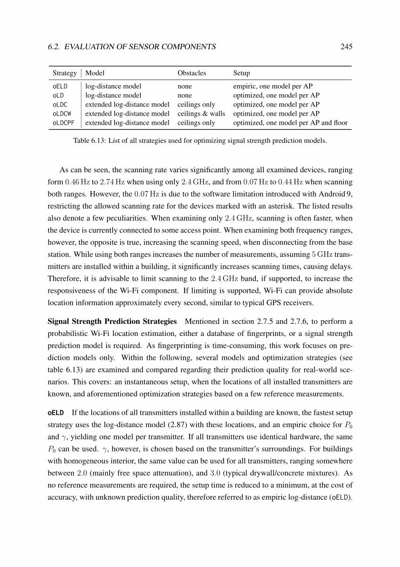
6.2. EVALUATION OF SENSOR COMPONENTS 245
Strategy Model Obstacles Setup
oELD log-distance model none empiric, one model per APoLD log-distance model none optimized, one model per APoLDC extended log-distance model ceilings only optimized, one model per APoLDCW extended log-distance model ceilings & walls optimized, one model per APoLDCPF extended log-distance model ceilings only optimized, one model per AP and floor
Table 6.13: List of all strategies used for optimizing signal strength prediction models.
As can be seen, the scanning rate varies significantly among all examined devices, rangingform 0.46 Hz to 2.74 Hz when using only 2.4 GHz, and from 0.07 Hz to 0.44 Hz when scanningboth ranges. However, the 0.07 Hz is due to the software limitation introduced with Android 9,restricting the allowed scanning rate for the devices marked with an asterisk. The listed resultsalso denote a few peculiarities. When examining only 2.4 GHz, scanning is often faster, whenthe device is currently connected to some access point. When examining both frequency ranges,however, the opposite is true, increasing the scanning speed, when disconnecting from the basestation. While using both ranges increases the number of measurements, assuming 5 GHz trans-mitters are installed within a building, it significantly increases scanning times, causing delays.Therefore, it is advisable to limit scanning to the 2.4 GHz band, if supported, to increase theresponsiveness of the Wi-Fi component. If limiting is supported, Wi-Fi can provide absolutelocation information approximately every second, similar to typical GPS receivers.
Signal Strength Prediction Strategies Mentioned in section 2.7.5 and 2.7.6, to perform aprobabilistic Wi-Fi location estimation, either a database of fingerprints, or a signal strengthprediction model is required. As fingerprinting is time-consuming, this work focuses on pre-diction models only. Within the following, several models and optimization strategies (seetable 6.13) are examined and compared regarding their prediction quality for real-world sce-narios. This covers: an instantaneous setup, when the locations of all installed transmitters areknown, and aforementioned optimization strategies based on a few reference measurements.
oELD If the locations of all transmitters installed within a building are known, the fastest setupstrategy uses the log-distance model (2.87) with these locations, and an empiric choice for P0
and γ, yielding one model per transmitter. If all transmitters use identical hardware, the sameP0 can be used. γ, however, is chosen based on the transmitter’s surroundings. For buildingswith homogeneous interior, the same value can be used for all transmitters, ranging somewherebetween 2.0 (mainly free space attenuation), and 3.0 (typical drywall/concrete mixtures). Asno reference measurements are required, the setup time is reduced to a minimum, at the cost ofaccuracy, with unknown prediction quality, therefore referred to as empiric log-distance (oELD).

246 CHAPTER 6. EXPERIMENTS
22
2APs: 34
24
4APs: 41
194
APs: 45
Figure 6.24: Location of reference measurements within the three buildings from figure 6.1-6.3, indicat-ing the number of visible transmitters by sized dots, and their total number in the lower left.
oLD For some buildings, the locations of installed transmitters might be unavailable, or undis-closed. Here, reference measurements can be used, to optimize the log-distance model (2.87),estimating each transmitter’s location, P0 and γ. For single-floors and drywalled interior, thisstrategy can provide sufficient accuracy, and will be referred to as log-distance (oLD).
oLDC As steel-reinforced concrete strongly attenuates radio signals (cf. section 2.7.1), floorsand ceilings should be considered within multistory buildings, when estimating signal strengthsfor transmitters installed within adjacent floors. Similar to oLD, this strategy uses referencemeasurements, but trains the extended log-distance model (2.88). It includes an additional at-tenuation factor for each transmitter’s model, to consider the impact of floor/ceiling attenuation,based on the building’s floorplan, therefore referred to as log-distance with ceilings (oLDC).
oLDCW When the building’s interior relies on a mixture of materials, such as drywalls, glassand concrete, including all individual obstacles can be required. Here, reference measurementsare used to train an extended log-distance model (2.88), not only including floors/ceilings, butalso all wall-obstacles, using an individual attenuation factor for every material. As mentionedearlier, while this offers an improved prediction quality, it significantly affects performance,requiring numerous intersection tests to estimate a single signal strength. Within the following,this strategy is referred to as log-distance with ceilings and walls (oLDCW).
oLDCPF The complexity of oLDCW can be reduced by a tradeoff, where only floors/ceilings areconsidered, and the model for each transmitter is not trained for the whole building, but forindividual regions within it, e.g. on a per-floor basis. Based on the reference measurements forone floor, one extended log-distance model (2.88) including only floors/ceilings is trained forevery visible transmitter, referred to as log-distance with ceilings, per floor (oLDCPF).
Within the following, all discussed strategies are applied to the buildings introduced in sec-tion 6.1, providing a detailed examination of achievable results. The empiric oELD is providedonly for SHL and Museum 2, as the required transmitter locations were unknown for Museum 1.Mentioned earlier, reference measurements, required for the other strategies, were recorded by

6.2. EVALUATION OF SENSOR COMPONENTS 247
Building APs FPs oELD oLD oLDC oLDCW oLDCPF
SHL 34 121 8.7 dB 6.3 dB 4.7 dB 4.0 dB 3.1 dBMuseum 1 41 139 - 4.8 dB 4.2 dB 3.6 dB 2.6 dBMuseum 2 45 130 11.2 dB 5.4 dB 4.3 dB 3.3 dB 2.7 dB
Table 6.14: RMSE (2.113), but among all access points of each examined building (see section 6.1 andfigure 6.24), and chosen optimization strategy (cf. table 6.13).
holding a smartphone upfront, slowly turning around in a circle, while scanning, yielding mul-tiple measurements for each transmitter visible at a location. Here, only static transmitters,belonging to the building’s Wi-Fi infrastructure, were considered. That is, all dynamic accesspoints, such as smartphone hot spots, smart presenters, Wi-Fi-equipped televisions, and similar,were omitted. Figure 6.24 depicts all reference measurements, with their dot-size representingthe number of distinct transmitters visible at each location. While this number is not a directindicator for prediction and localization quality, it can provide hints on sensitive areas, wherethe number of visible transmitters is too low to provide a stable localization.
The quality of the trained models is quantified by the RMSE among all transmitters, similarto (2.113). That is, the square root of the average squared difference between model predictionand reference measurement, for all fingerprints, access points, and repetitions. While this metricdoes not indicate outliers or regionally limited issues, it yields a brief quality estimator, shownin table 6.14. A corresponding probabilistic evaluation is provided by a cumulative distributionfunction, indicating the percentage of estimations that stay below a certain absolute error value
P (X < x) , with X =
absolute differences between all predictions and measurements︷ ︸︸ ︷∣∣Pmdl(posxyz (fp) ,ψap
)− ςfp,ap,n
∣∣ | ∀fp, ap, n, (6.1)
shown in figure 6.25. As can be seen in table 6.14 and figure 6.25, an empiric choice, using thesame P0 and γ for all transmitters, yields the highest RMSE. Here, the same P0 = −40 dBm
and γ = 3 were used for Museum 2 and SHL, with significantly varying error results. This is dueto the number of transmitters installed within Museum 2 being more dense, and the architectureof both buildings being completely different, requiring smaller values for γ.
For all examined cases, the RMSE and the corresponding CDF fully agree. Smaller RMSEsare due to improvements throughout the whole error spectrum (see figure 6.25). The quality ofthe optimization strategies follows the order they were presented in. As expected, optimizingone log-distance model per transmitter based on reference measurements (oLD) yields a lowerRMSE than a pure empiric choice, using the same P0 and γ for all access points (oELD). Addi-tionally including floors/ceilings (oLDC) further increases the prediction quality, especially for

248 CHAPTER 6. EXPERIMENTS
0.0
0.2
0.4
0.6
0.8
1.0
2 dB 5 dB 8 dB 11 dB 2 dB 5 dB 8 dB 11 dB 2 dB 5 dB 8 dB 11 dB
SHL Museum 1 Museum 2
oELDoLDoLDCoLDCW
oLDCPF
Figure 6.25: Result of the cumulative distribution function (6.1), for the absolute difference between allreference measurements and corresponding model predictions, based on the examined building, chosenmodel, and optimization strategy. As expected, the empiric variant oELD yields the largest errors.
the SHL and Museum 2. Intuitively, the amount of potential improvements strongly depends onthe building’s architecture. This can be seen by additionally including wall obstacles (oLDCW),where Museum 2 gained the most improvements, due to its massive concrete walls. Intended asa compromise, the per-floor optimization without wall-knowledge (oLDCPF) provided the bestresults for all examined buildings. This is due to the complex nature of radio signals, beingaffected by far more influences than are addressed by the presented models, such as reflectionand refraction. By regionally limiting the signal strength prediction model, the number of ef-fects to be dealt with is reduced, thus increasing the chance for better predictions. While usingeven smaller regions than per-floor is possible, it is not always advisable. Mentioned withinthe theoretical discussion, training requires a decent amount of reference measurements to bestable and converge. With smaller regions, the chance for potential issues, and poorly optimizedmodels for some transmitters, increases.
Locally limited issues, e.g. within concrete stairwells, can be visualized by calculating theaverage signed, and the maximum absolute error, for every location where reference measure-ments were conducted. That is, at every such location, each received RSSI for every knowntransmitter is compared against the corresponding model prediction for the same location
εavg (fp) = E(X )
εmax (fp) = max(|X |)with X =
differences between predictions and measurements, for one fp︷ ︸︸ ︷Pmdl
(posxyz (fp) ,ψap
)− ςfp,ap,n | ∀ap, n
. (6.2)
The average signed error provides an impression whether a model tends to predict too weakor too strong signal strengths for a location. Similarly, the maximum absolute error yields anoverview on the model’s worst-case behavior. The results for both metrics, and all examinedbuildings are shown in figure 6.26, 6.27, and 6.28.
As can be seen, while the behavior of the maximum absolute error is approximately com-parable between the buildings, the signed average behaves differently. The SHL (cf. figure 6.26)

6.2. EVALUATION OF SENSOR COMPONENTS 249
+7.9-8.7
+6.9-5.2
-3.9
+6.4+5.6
-3.3
23.8
16.5
21.0
15.3
−8.7 dB 7.9 dB 0 dB 23.8 dB
Figure 6.26: SHL (cf. figure 6.1) – average signed (top) and maximum absolute (bottom) deviation be-tween model predictions and reference measurements, when using oLD, oLDC, oLDCW, oLDCPF (left toright). Within the top row, blue indicates too weak, and red too strong model predictions.
+4.4
-3.6
-4.3
+3.2
-3.8+3.1
-2.2+2.3
25.5 24.3 21.8
11.0
−4.3 dB 4.4 dB 0 dB 25.5 dB
Figure 6.27: Museum 1 (cf. figure 6.2) – average signed (top) and maximum absolute (bottom) deviationbetween model predictions and reference measurements, when using oLD, oLDC, oLDCW, oLDCPF (left toright). Within the top row, blue indicates too weak, and red too strong model predictions.
-4.6+4.7 +3.9
-4.0+3.0-3.5 +3.7
-2.8
23.2
21.2 18.7
13.3
−4.6 dB 4.7 dB 0 dB 23.2 dB
Figure 6.28: Museum 2 (cf. figure 6.3) – average signed (top) and maximum absolute (bottom) deviationbetween model predictions and reference measurements, when using oLD, oLDC, oLDCW, oLDCPF (left toright). Within the top row, blue indicates too weak, and red too strong model predictions.

250 CHAPTER 6. EXPERIMENTS
denotes the highest errors, which is due to a lower number of transmitters per building size. WithMuseum 1 (figure 6.27) and Museum 2 (figure 6.28) being smaller, regional effects become morepronounced, visualized by red and blue alternating within several areas. Yet, for all buildings,regional errors follow previous findings, decreasing in the order of the examined optimizationstrategies. Similar to the RMSE, including wall-obstacles improves only some regions of theSHL, while using oLDCPF enhances predictions throughout the whole building, indicated by lesssaturated colors for both, signed average, and absolute maximum. Museum 1 is similar, show-ing most improvements for oLDCPF. Within Museum 2, however, including wall-obstacles clearlyenhances prediction quality, by considering the building’s massive concrete exterior.
Effects of certain materials on radio signal propagation is best explained within SHL, wherethe indoor and outdoor areas of the first floor (cf. figure 6.1) are separated by a facade of met-allized glass. This causes attenuations of 10 dB and above, visible within the average signederrors of figure 6.26, where the outdoor area is predicted too strong (red), and indoor areas tooweak (blue). While this can be mitigated by considering such obstacles (oLDCW), required inter-section tests are costly. Thus, the prediction from oLDCPF, with an average error of ≈ 3 dB isan ideal candidate for a computationally efficient, model-based location estimation.
Concerning the number of reference measurements required for a stable model estimation,there is no rule of thumb. For simple models, like oLD, half of the shown reference measure-ments can be removed, without significantly affecting the prediction quality of the resultingmodels. For more complex variants, especially oLDCW, a decent number of reference measure-ments is mandatory for a stable optimization. This number thus represents a tradeoff betweenaccuracy and setup time. Ideally, the whole walkable area is covered uniformly with measure-ments, to prevent regional overfitting. Similarly, neuralgic regions, like stairwells, should beincluded as well, to provide a general signal strength prediction solution.
Location Estimation Based on the optimized prediction models, Wi-Fi location estimationcan be performed. Within the following experiments, the whereabouts are estimated for everyWi-Fi scan s from the recorded walks, and compared with the corresponding ground truth (cf.figure 6.4, 6.5 and 6.6). Whereabouts are determined by two different strategies:
lBest The first strategy estimates the current location by numerically optimizing (2.111) withσrssi = 8, determining the best matching result. To increase the chance of finding a globalmaximum, the optimization process is repeated 10 000 times, each starting from a differentrandom location, which belongs to the walkable area of each building.
lFilter The second strategy is based on the particle filter, and starts by uniformly samplingthe walkable area, using 5000 particles. Each particle is evaluated, assigning a weight givenby (2.111) with σrssi = 8. The weighted average of all particles represents the first location

6.2. EVALUATION OF SENSOR COMPONENTS 251
estimation (see section 4.5). For every new Wi-Fi scan, the process continues from the previousset of particles, after scattering it by (3.10), with µwalk = 2.5 m and σwalk = 1.0 m. In otherwords, potential whereabouts are modeled by random samples. Between two Wi-Fi scans, thesesamples are relocated, but only within aforementioned constraints. After this spreading, theyare re-weighted by the current Wi-Fi observation. Afterwards, their weighted average denotesthe next location estimation. Eventually, resampling is applied, to ensure a decent amount ofparticles remain efficient. For the next Wi-Fi scan, the process starts all over. The resultingbehavior is similar to (3.8), prevents the Wi-Fi estimation from causing large jumps in location,and supports multimodalities unsupported by the Kalman filter.
While the first strategy (lBest) returns estimations that are independent of the previousones, the particle filter, used for the second strategy (lFilter), implicitly includes previousmeasurements, mitigating the impact of outliers, and regionally poor signal strength predictions.As no floorplan is included for now, its behavior is continuous, similar to a Kalman filter.
An example for one repetition of walk A1 is shown in figure 6.29. Even if examining only asingle walk, this is without loss of generality, as all others indicate similar effects. Comparingthe shown setups, the benefits of the particle filter (lFilter) become visible. Without filtering(lBest), the location estimations based on the oLD optimization strategy are noisy, with largeregional errors. The particle filter suppresses outliers by restricting location changes betweentwo measurements via (3.10). This yields smoother results, with reduced errors. Yet, filteringonly improves temporal effects, but is unable to address long-term issues, e.g. based on invalidsignal strength predictions, occurring around 10 s and 20 s.
These errors can be addressed by using more complex signal strength prediction models,like the depicted oLDC. Shown within the figure, this reduces the error between 10 s and 20 s
from 30 m to 12 m, as the model provides better predictions. Also shown within the figure,oLDC significantly improves the location estimation in z, when compared with oLD. Mentionedearlier, oLDC considers floors and ceilings within signal strength predictions, by including dis-crete attenuations. Predicted signal strengths will thus vary notably between adjacent floors,which matches with the actual real-world behavior. This also holds true for oLDCW and oLDCPF,not shown within the figure. Most of the time, their predictions match best with the correct floor,rendering adjacent floors unlikely, as shown within the figure. However, for all presented in-stances, the upper right outdoor area, labeled as (3), clearly causes significant problems. Theseerrors are examined by using another visualization of potential whereabouts.
Figure 6.30 depicts a probability heat map (2.111) for two points in time of walk A1. It de-notes the likelihood for residing at any location within the building, for the Wi-Fi measurementsreceived at t = 14 s directly after the start (top row), and at t = 97 s having reached the outdoorarea (bottom row). For the latter, all examined signal strength prediction models fail. Several

252 CHAPTER 6. EXPERIMENTS
oLD + lBest
oLD + lFilter
oLDC + lFilter
F3F2F1F0
F3F2F1F0
(1)
(2) (3)
(4)
(5)
0 m
10 m
20 m
30 m
40 m
20 s 40 s 60 s 80 s 100 s 120 s 140 s 160 s 180 s
oLD - lBestoLD - lFilteroLDC - lFilter
(1) (2) (3) (4) (5)
Figure 6.29: Location Estimation (top) and 3D error over time (bottom), for one repetition of walk A1(see figure 6.4), when using oLD + lBest, oLD + lFilter, and oLDC + lFilter. The three columns showthe side-view (left), perspective (center), and top-view (right) of each estimation result.
areas within the building are more likely than the actual ground truth (black dot). This is dueto the building’s facade made of metallized glass, attenuating radio signals, thus leaving a blindspot. In such situations, even the accurate fingerprinting can fail, as the number of receivabletransmitters is low, and their RSSIs are all rather similar.
Figure 6.30 also denotes the impact of including attenuating ceilings and obstacles. For oLD,the predictions for adjacent floors are similar, as they are only a few meters apart, not causingmajor free space attenuation. Not being able to provide floor estimations is a major drawback ofoLD’s simplicity. For all other methods, the floor estimation is mostly accurate. However, withinunusual buildings like Museum 2, the estimation can fail, due to their irregular floor layout.
Besides the shown benefits, including obstacles causes unwanted discontinuous behavior ofthe signal strength prediction. As soon as an obstacle intersects the line of sight, it causes a dropin signal strength. Due to physical effects like reflection and diffraction, the real-world behaviordeviates, is smoother, and less discontinuous. However, these effects are not considered by most

6.2. EVALUATION OF SENSOR COMPONENTS 253
oLD oLDC oLDCW oLDCPFi
Figure 6.30: Probability heat map (2.111), from warm (likely) to cold (unlikely), showing potentialwhereabouts for walk A1 at t = 14 s (top) and t = 97 s (bottom), based on the chosen optimizationstrategy. The ground truth is indicated by a dot. The additional oLDCPFi is explained within the text.
prediction models. This aspect also influences the probability for residing at certain locations,which will show the same discontinuous drops. For oLDC, this behavior is expected between ad-jacent floors only, where ceilings are considered. For oLDCW, the impact is also expected alongeach floor, as walls are considered as well. However, shown in the magnified region of fig-ure 6.30, oLDC also shows discontinuous behavior along floors, which is unexpected. The effectis caused by the optimization, which sometimes places access points outside of the building.This affects the behavior of ceiling intersection tests. When transmitters reside outside of thebuilding, there is not necessarily a ceiling along the line of sight, even when the transmitter is onanother floor. This is addressed by oLDCPFi, a modified version of oLDCPF – which is similar tooLDC concerning this behavior – forcing AP positions to remain inside the building, by addinga penalty to the target function. As can be seen, this mitigates discontinuous behavior. Eventhough the resulting signal strength prediction resulted in slightly increased errors (0.2 dB), thelocation estimation is less erroneous, as the density is more continuous. Yet, this is not a com-plete fix, as irregular building shapes, as in SHL and Museum 2, can still contain constellationswith no ceiling along the line of sight from a transmitter to a location on another floor.
Figure 6.31 depicts one cumulative distribution function (CDF) per building, containing thelocalization errors of all walks. These are given by the 3D distance between each position esti-mated from a Wi-Fi scan s, using either lBest and lFilter, and the ground truth interpolatedfor the scan’s timestamp (see section 6.1). Additionally, the error in z is determined separately,as correctly indicating the current floor is a significant benefit. Matching with previous discus-sions, the three buildings behave differently, due to architectural and infrastructural differences.

254 CHAPTER 6. EXPERIMENTS
0.25
0.50
0.750.90
0.25
0.50
0.750.90
3 m 6 m 9 m 12 m 15 m 3 m 6 m 9 m 12 m 15 m 3 m 6 m 9 m 12 m 15 m
SHL Museum 1
3D-l
Best
Museum 2
3D-l
Filter
oELD oLD oLDC oLDCW oLDCPF oLDCPFi
0.000.250.500.751.00
1 m 2 m 3 m 4 m 5 m 6 m 1 m 2 m 3 m 4 m 5 m 6 m 1 m 2 m 3 m 4 m 5 m 6 m
z-l
Filter
Figure 6.31: CDF of the 3D/z localization error, for the walks from section 6.1, based on the previouslyintroduced optimization strategies, plus one additional variant, described within the text. The differencebetween the lBest (top) and lFilter (center) location estimation strategy is clearly visible.
The top row of figure 6.31 shows the CDFs based on all walks within each building, whenusing the lBest localization strategy. As can be seen, SHL causes the largest errors, with 50 %
of them being worse than ≈ 6.6 m. This is due to a comparatively low number of installedtransmitters, covering approximately 350 m2 per AP. For Museum 1 and Museum 2, this value is90 m2 and 67 m2, respectively, thus yielding better results. Furthermore, some of the walksconducted within SHL used the outdoor area, which is not well-covered by radio signals, dueto the facade made of metallized glass. These outdoor parts yield large localization errors (seefigure 6.29), and cause 10 % of all 3D location estimation errors to be greater than ≈ 20 m. Forthe two other buildings, this value is as low as ≈ 7 m and ≈ 10 m, respectively.
The center row of figure 6.31 depicts the CDFs when using lFilter as location estimation.Compared with lBest, the resulting errors are notably reduced, which matches earlier findings.While the lower 50 % of all errors remain almost unaffected, the last 25 % and 10 % denotesignificant enhancements. This behavior is as expected, with the recursive density estimationmainly suppressing outliers, by preventing major jumps within the estimated location, basedon the described movement restriction. The depicted improvements, especially for SHL, clearlyindicate the possibilities offered by recursive density estimation.
The bottom row of figure 6.31 depicts the CDFs for the error in z, when using lFilter aslocation estimation. For SHL, the results are as expected. As soon as ceilings are consideredby the model, z-estimations become viable. For the other two buildings, however, z-errors are

6.2. EVALUATION OF SENSOR COMPONENTS 255
0.25
0.50
0.750.901.00 SHL Museum 1 Museum 2
oELDoLDoLDCoLDCW
oLDCPFoLDCPFi
Figure 6.32: CDF of the Kullback-Leibler divergence (KLD), for the walks from section 6.1, based onthe previously introduced optimization strategies, plus one additional variant, described within the text.As the KLD’s value does not convey a quantifiable meaning, the x-axis is unlabeled.
moderate even when ceilings remain unconsidered. This is due to the number of densely packedtransmitters, generally providing a higher accuracy, also affecting z.
When comparing figure 6.25 and 6.31, it becomes clear that better signal strength predic-tion models do not necessarily yield better location estimations, and that location errors arerelatively similar among most models. While oLDCPF provides the best estimations for SHL andMuseum 1, it does not for Museum 2, where 20 % of the results denote larger errors than the onesprovided by the simple oLD. While this is mitigated by lFilter, it still remains present. Forcingall estimated transmitter positions to remain inside the building (oLDCPFi) not only addressesdiscontinuities, but also suppresses additional outliers, yielding the best overall results.
Location Probability Figure 6.31 determined Wi-Fi localization quality by comparing themost likely whereabouts against the ground truth. While this is a common strategy for error es-timation, it is not ideal for the intended use case. Within the overall localization and navigationsystem, Wi-Fi is meant to weight particles on whether their state (location) is likely, or unlikely,based on the current signal strength readings from the smartphone. In other words, Wi-Fi is notused to directly infer a location (x, y, z), but to derive probabilities for arbitrary whereabouts.When used like this, two aspects are implied: Ideally, the location of the current ground truth,and its vicinity, should be as likely as possible, whereas all other locations should be unlikely.
Besides visually inspecting figure 6.30, both requirements can be quantified by the Kullback-Leibler divergence (KLD), measuring the (dis)similarity between the Wi-Fi density (2.111), andground truth. For the latter, any empiric distribution, modeling the likelihood of the groundtruth and its vicinity, can be chosen. For experiments, a multivariate normal distribution with42, 42, 0.752 along the diagonal of Σ was used, to favor floor accuracy over (x, y). Both den-sities are compared by generating 50 000 random samples throughout the whole walkable areaof each building. Similar to an error distance, the KLD yields a single scalar result, describ-ing the dissimilarity between the density around the ground truth, and the density of potentialwhereabouts, based on the current Wi-Fi measurements. All resulting scalars are combined into

256 CHAPTER 6. EXPERIMENTS
a CDF, containing all walks within a building, shown in figure 6.32. As can be seen, resultsare similar to figure 6.31, which depicted the CDF for the error in m. However, as the densitychosen for the ground truth enforces a higher z-accuracy, oELD and oLD yield inferior results.Again, among all examined walks and buildings, oLDCPFi provided the best estimation, wellsuited for a computationally efficient evaluation within the recursive density estimation process.
6.3 Evaluation of Movement Models
After examining all sensors for the overall indoor localization and navigation system, and pro-viding a first PDR example, the impact of adding a floorplan in combination with probabilisticmovement prediction is examined. The discussions from chapter 3 and 5.2 already includedsynthetic examples for the propagation of each movement prediction density. Therefore, thissection focuses on real-world setups, the amount of memory required for storing a spatial floor-plan model, its probabilistic aspect, the capability of performing 3D estimations based on 2Dsensor data, and including additional knowledge/sensors, using semantic information providedby the floorplan. As discussed in section 5.2, to perform probabilistic predictions on a navi-gation grid with random walks (cf. section 3.5.2), or on a navigation mesh (cf. section 3.6.2),sampling is required. All experiments thus focus on a recursive density estimation using theparticle filter (see section 4.5), including transition, evaluation, estimation and resampling.
6.3.1 Spatial Floorplan Representation
Before evaluating the advantages of a floorplan-based probabilistic movement prediction, thequality of the two discussed spatial representations, the navigation grid and the navigation mesh,is briefly examined. The focus is on spatial accuracy for real-world scenarios, and requiredmemory consumption, essential for use on embedded devices.
Memory Consumption To determine memory consumptions for both models based on theirconfigurable parameters, the three floorplans from section 6.1 are used, supplemented by fouradditional buildings, not examined in terms of conducted walks, but concerning their floorplan:
UAH – is the University of Alcala de Henares’ polytechnic building, with four floors and130 m to 130 m in size, where the presented system participated in the IPIN 2016 Indoor Local-
ization Competition, which required the floorplan. One of its floors is shown in figure A.1.
CAR – also belongs to the University of Alcala de Henares, was part of the IPIN 2016 Indoor
Localization Competition, and has one floor, 65 m to 40 m in size, surrounded by a large outdoorarea, shown in figure A.2.

6.3. EVALUATION OF MOVEMENT MODELS 257
Navigation Grid Navigation Mesh20 cm 30 cm 40 cm 50 cm Triangles Quads Pentagons Hexagons
SHL 518 k 228 k 128 k 82 k 4164 2527 2187 2035Museum 1 96 k 42 k 23 k 14 k 1852 1155 980 903Museum 2 83 k 33 k 17 k 11 k 857 531 448 411UAH 955 k 424 k 238 k 152 k 3206 2035 1788 1662CAR 105 k 46 k 25 k 16 k 801 479 424 387Townhall 182 k 80 k 45 k 28 k 2876 1806 1542 1425Museum 3 76 k 34 k 19 k 12 k 1223 748 633 581
Table 6.15: Number of vertices/primitives required to describe building floorplans, when using a naviga-tion grid with varying grid size gs, or a navigation mesh with different primitives.
Navigation Grid Navigation Mesh20 cm 30 cm 40 cm 50 cm Triangles Quads Pentagons Hexagons
SHL 30 MiB 13 MiB 7 MiB 5 MiB 248 KiB 191 KiB 172 KiB 164 KiBMuseum 2 5 MiB 2 MiB 1 MiB 636 KiB 51 KiB 40 KiB 35 KiB 33 KiBMuseum 1 5 MiB 2 MiB 1 MiB 811 KiB 110 KiB 87 KiB 77 KiB 73 KiBUAH 55 MiB 24 MiB 14 MiB 9 MiB 191 KiB 155 KiB 141 KiB 134 KiBCAR 6 MiB 3 MiB 1 MiB 930 KiB 48 KiB 36 KiB 33 KiB 31 KiBTownhall 10 MiB 5 MiB 3 MiB 2 MiB 171 KiB 136 KiB 121 KiB 115 KiBMuseum 3 4 MiB 2 MiB 1 MiB 687 KiB 73 KiB 57 KiB 51 KiB 48 KiB
Table 6.16: Memory required to store building floorplans, when using a navigation grid with varyinggrid size gs, or a navigation mesh with different primitives.
Townhall – is the townhall of Wurzburg, with four floors, but only two of them were mod-eled, approximately 60 m to 100 m in size, including a large courtyard for the first floor.
Museum 3 – models the Deutsches Hutmuseum in Lindenberg, which is a museum with fivefloors, approximately 40 m to 20 m in size, shown in figure A.3.
For the navigation grid, the memory consumption directly depends on the number of verticesand edges needed to model the building’s floorplan, which in turn depend on its size and numberof floors, and the chosen grid size, where smaller values yield a better spatial quality at the costof memory. For the navigation mesh, there is no direct correspondence between the size of eachfloor and required memory, as the data structure is irregular, able to model large areas with asingle primitive. The number of primitives depends on the architectural obstacles found withineach floor, dividing larger primitives into multiple smaller ones. Similarly, the type of primitive(triangle, quad, ...) also affects the required number, and thus memory.
Setting-dependent results for both models are shown in table 6.15 and table 6.16. The largestamong all examined buildings, UAH, requires most vertices for the navigation grid, yielding amemory requirement of 55 MiB for gs = 20 cm. When using the navigation mesh, the smallerSHL requires more primitives and memory. This is due to architectural differences, with SHL

258 CHAPTER 6. EXPERIMENTS
Figure 6.33: Comparison of navigation grid (gs = 40 cm) and navigation mesh, for advanced floorplans.While both produce viable results for complex circular stairs (left), elements not aligned to multiples of45°, like two of the three stairs in the right setup, indicate potential drawbacks of the navigation grid.
consisting of many small rooms, whereas UAH has larger rooms, thus requiring less primitives.Independent of such differences, the navigation mesh consumed less than 1 MiB for all exam-ined buildings. For the navigation grid, this is only possible when using large grid sizes of50 cm and above, providing only a coarse representation of the building. Nevertheless, even ags = 20 cm navigation grid of a large building is still manageable by a modern smartphone.
However, the numbers from table 6.16 refer to the smallest possible amount, storing onlyvertices and edges, and in a very dense manner. As soon as additional attributes are involved,such as shortest path estimations (see section 3.5.3 and 3.6.3), or pre-computed Wi-Fi sig-nal strengths (cf. section 5.4), numbers might exceed the manageable range: Storing the 20
strongest access points for each vertex would require at least 40 byte per vertex (id and RSSI),adding additional 40 MiB to the UAH. Which model is applicable for a specific use case, thusstrongly depends on the building’s architecture, and additional performance/quality require-ments.
Even though triangles require slightly more memory than other primitives (cf. table 6.16),they allow for interpolation and fast inclusion checks, and thus are preferred.
Spatial Quality Besides differences in memory consumption, the spatial representations alsovary in quality. While the navigation mesh is considered general purpose, the navigation grid’sregular structure is mainly suited for axis-aligned floorplans, with obstacles oriented in multi-ples of 45° or, even better, 90°, discussed in section 3.5.1. While this requirement holds true formany modern buildings, like SHL, it does not for older ones, or more complex architecture.
Figure 6.33 used complex architecture to compare a navigation grid with gs = 40 cm againsta navigation mesh with triangles, constructed by the algorithms discussed in section 3.5.1 and3.6.1, respectively. For a wide circular stair (left), both produce results that appear viable. Eventhough the navigation grid’s exterior is more discrete, compared to the navigation mesh, this isstill within limits, and the stair is covered by a multitude of walkable nodes and edges, evenwhen using gs = 40 cm. The semantic information, indicated by different colors (gray, black,blue), e.g. required for reducing the pedestrian’s step length throughout the stair, also works forboth spatial models. However, one of the three doors is not correctly labeled for the navigation

6.3. EVALUATION OF MOVEMENT MODELS 259
grid. This is due to the chosen spacing not yielding vertices within the door’s center, but onlydirectly before and behind it. This can be mitigated by using a smaller grid size.
Within the right half, three stairs with varying orientation and adjacent doors are shown.While the axis-aligned stair in the center is well suited for the regular navigation grid, the twoothers are not. Even though visually fine, the direction of edges is not ideal for predictingmovements along the stair, potentially yielding the depicted zig-zag pattern. The same appliesto the circular stair on the left, often not providing edges that follow the ideal path. Such cases,where the to-be-predicted walking direction does not match with the direction of edges, can notbe addressed by using smaller grid sizes, and are a general problem of the navigation grid.
Furthermore, figure 6.33 indicates a significant number of nodes and edges required for thenavigation grid, even when using a large grid size of gs = 40 cm. In contrast, the naviga-tion mesh is able to model fine details, adjusts to different alignments, while combining largeconnected areas into a few primitives. From the viewpoint of both, memory consumption andspatial quality, the navigation mesh thus is more promising than the navigation grid.
6.3.2 Navigation
One benefit of including a floorplan, discussed in section 3.5.3, is navigation. Not only for guid-ing the pedestrian towards a desired destination, but also to favor movements approaching thislocation, increasing the quality of the overall system. The impact is examined using simulationsof random walks along a navigation grid, using algorithm 1. It is started at a given location, andexecuted until the given destination is reached. The algorithm is thus executed with an unlim-ited walking distance dwalk. Only the destination-approaching metric (3.32) is used to determinethe probability for each edge, that is, the heading is completely unconstrained. Thus, edges aresolely chosen on whether they approach the destination, or not. The weight of the edges usedwithin Dijkstra’s algorithm is given by either (3.29) or (3.31), depending on whether walls areto be avoided, or not. For a robust estimation of the random walk’s behavior, this simulation isrepeated 5000 times. Results are visualized using a heat map, indicating how often every vertexof the graph was visited among all repetitions. Cold colors (blue) denote fewer visits than warmcolors (red). In case of no color, the vertex has not been visited at all.
Figure 6.34 shows the impact of different values for κdest, indicated by the heatmap of 5000
random walks through a synthetic maze. κdest affects the probability of favoring edges ap-proaching the destination over edges that depart from it. A value of κdest = 0.50, shown inthe left of figure 6.34, implies that all edges are equally important, and the destination doesnot affect the probability for taking an edge at all. Such a truly random walk will require asignificant amount of time, until the requested destination is reached by chance. As can be

260 CHAPTER 6. EXPERIMENTS
κdest = 0.50 κdest = 0.55 κdest = 0.70 κdest = 1.00
Figure 6.34: Impact of κdest on random walks approaching the destination via (3.32), weighted by (3.29)running simulation algorithm 1 along a gs = 20 cm grid. The heatmap denotes how often each vertexof the grid was visited during 5000 random walks, starting from the upper center, each running withoutdistance limitation, until reaching the destination in the lower center.
seen, the first few meters of the walk share the same color, indicating a similar number of visits.As soon as the maze allows for more than one walking direction, the colors get colder, andthe random walks split into several directions. Approaching the destination, colors are gettingwarmer again, as all random walks have to reach the destination. Being accessible from twosides, and the option to walk backwards, colors surrounding the destination are colder than theones around the origin. When the heuristic is slightly increased to κdest = 0.55, the effect offavoring destination-approaching edges is already significant. Most locations within the mazeare rarely visited (blue), or not visited at all (white). Furthermore, when the maze splits intothree potential walking directions, only two of them are considered, as the third one is a deadend. The impact is even more pronounced for κdest = 0.70, where most regions remain unvis-ited, and the left of the two valid paths is frequented more often, as it is slightly shorter thanthe alternative on the right. For κdest = 1.00, the simulation ignores all edges departing fromthe destination, leaving very narrow trails, with some vertices visited during almost every of the5000 repetitions, shown as red spots. While higher values for κdest yield a more direct approachof the destination, they allow for less deviations from the shortest path, ignoring alternatives,and the pedestrian not following the system’s recommendation. Estimating the correct value isthus an empiric choice, as tradeoff between a closely directed route, and allowed variation.
As can be seen in figure 6.34, all routes closely adhere to walls, slightly reducing the distanceof the shortest path. Discussed in section 3.5.3, this is atypical for pedestrian walking behavior.By artificially increasing the distance for edges near obstacles, the shortest path becomes morerealistic. The impact of this adjustment is shown in figure 6.35. When obstacles are not con-sidered, the result is unnaturally close to all obstacles, and only the left of two potential routesis used, as it is several meters shorter than using the stair on the right. Artificially adjusting thedistance between edges using (3.31), the second route along the right stair is more attractive,

6.3. EVALUATION OF MOVEMENT MODELS 261
κdest = 0.75, not avoiding walls (3.29) κdest = 0.75, avoiding walls via (3.31)
Figure 6.35: Impact of the wall avoiding metric (3.30) on random walks approaching the destinationvia (3.32), weighted by (3.31) running simulation algorithm 1 along a gs = 20 cm grid. The heatmapdenotes how often each vertex of the grid was visited during 20 000 random walks starting in the lowerleft, each running without distance limitation, until reaching the destination in the upper center.
being a few centimeters shorter. Furthermore, both routes are more natural, keeping some dis-tance towards obstacles, walking through the centers of doors and narrow passages. Yet, thenegative impact of the discrete regular grid is clearly visible. For segments of the shortest path,that have a direction which is not a multiple of 45°, there often is no single best choice thatyields the shortest path, and several equidistant ways connect the segment’s ending points. Thisis highlighted in figure 6.35, where dashed lines denote equidistant connections between twopoints. The heatmap around such segments appears much wider, covering all potential paths,indicated by larger cold (blue) regions. When the direction is a multiple of 45°, a single shortestconnection exists, shown by all narrow warm (green/red) streams within the figure. This effectcould be addressed by using more than eight adjacent neighbors, also considering vertices fur-ther away to introduce new walking directions, such as 22.5°. However, as those edges are evenlonger than
√2 gs, the distance error discussed in section 3.5.3 becomes more pronounced, and
memory requirements are increasing, potentially imposing issues on embedded use.
While the navigation mesh does not suffer from these discrete limitations, it potentiallyrequires more computations to include the destination information correctly. Discussed in sec-tion 3.6, the most efficient movement prediction for the mesh directly calculates a potentialtransition based on distance and heading from the origin, including some noise (3.35). In con-trast to probabilistic random walks along a navigation grid, the only way to also include anavigation likelihood, is by using particles, and adjusting their weight accordingly. However, asthe result of (3.35) is very constrained, covering only a small area, the resulting density mightlack particles in areas that are likely in terms of navigation. This is a typical limitation of theparticle filter, discussed in section 4.5. The posterior is modeled by both, placement and weightof the particles. If the placement (proposal distribution) does not cover areas likely in terms

262 CHAPTER 6. EXPERIMENTSun
corr
ecte
dco
rrec
ted
grid, gs = 20 cm grid, gs = 30 cm grid, gs = 40 cm navigation mesh
Figure 6.36: Comparison of navigation grid and navigation mesh, for one of the PDR examples fromsection 6.2.4 (see figure 6.16). For the navigation grid, different grid sizes gs were used, also examiningthe impact of distance and heading error compensation (cf. algorithm 1).
of weight, the result is not optimal. This can be mitigated by using the full sampling approachshown in figure 3.24, covering large areas with samples, hereafter weighting them based on all
metrics, that is, matching distance, heading, and navigation. While this variant ensures that thewhole area of importance is sampled, it requires more samples and thus computations to do so,unsuited for use on embedded devices. When navigation is the only prediction constraint, as infigure 6.35, full sampling is the only option, as no limiting heading information is available. Ascan be seen, in terms of flexibility, the navigation mesh is thus more constrained than randomwalks along a navigation grid.
6.3.3 Floorplan-Based Probabilistic Pedestrian Dead Reckoning
Advantages and disadvantages of including a building’s floorplan and probabilistic movementprediction are examined for the pedestrian dead reckoning setups from section 6.2.4. Althoughregionally limited, they include every essential behavior, and allow for focusing on the impor-tant aspects, without loss of generality. The floorplan not only prevents impossible walks, italso allows for 3D estimations, and its semantic information enables including probabilisticassumptions, additional prior knowledge, as well as new smartphone sensors. Besides step-detection, turn-detection, and absolute headings, which are typical for PDR, activity-detectionand navigational knowledge can now be considered as well. Additionally, differences betweenthe two presented spatial models are examined, emphasizing distinctions between discrete ran-dom walks along a navigation grid and continuous estimations on the navigation mesh. All ofthe following experiments refer to a probabilistic simulation using the particle filter.

6.3. EVALUATION OF MOVEMENT MODELS 263
Graph and Navigation Mesh A comparison, of the navigation grid’s and navigation mesh’sbehavior, is shown in figure 6.36. Its results are based on one of the previous PDR examples (seesection 6.2.4), walking four times around an obstacle. Similar to earlier, initial whereabouts andheading are well-known. A transition is performed whenever a step was detected, and proceedswith µstep = 70 cm into the direction of the heading updated by the gyroscope. In contrast toearlier, navigation grid and navigation mesh now allow for a probabilistic transition, each using1000 particles to include an uncertainty in step length σstep = 10 cm and turning σturn = 1°,both applied for every filter update, also preventing impossible movements, by down-weightingparticles that encountered an obstacle, or would represent an impossible transition.
For both models, the fastest calculable transition, well-suited for smartphone use, was cho-sen: Within the navigation mesh, each transition is determined by directly calculating the des-tination based on walking distance and estimated heading (3.35), including some uncertaintyfor both (3.37). If a calculated destination is reachable (contained within an adjacent triangle),it is accepted, otherwise the particle’s weight is reduced to zero (see section 5.2.3). Within thenavigation grid, edges are weighted based on whether their direction matches with the estimatedheading (3.25), and drawn randomly, until the walking distance of dwalk is reached. Discussedin section 3.5.2, this approach causes discretization errors based on the graph’s grid size, andmultiples of 45° for walkable edges, requiring compensation, introduced in algorithm 1.
Figure 6.36 depicts the necessity for this error compensation. Without it, walking distancesare longer than requested, dependent on the underlying grid size, visible as increased radiuswithin the three depicted results. Likewise, the 45°-structure becomes apparent, with the esti-mated path resembling an octagon. Yet, the overall results, when not using error compensation,appear consistent in their size and shape. This is due to the discretization, preventing minor an-gular changes. When all conducted turns are multiples of 45°, this can be considered a benefit.In general, however, this suppresses minor changes, or discretizes them into larger ones, causingissues for walks and buildings not aligned to multiples of 45°. Also visualized in figure 6.36,compensation from algorithm 1 addresses this issue, reducing the size of the estimated path, andproducing correctly rounded turns, even for larger grid sizes. The right shows the same resultwhen using the navigation mesh. It is similar to the navigation grid with error compensation,but shows slightly more variation, due to its continuous approach.
Discussed in section 5.2.3, detecting impossible walks is one important aspect the floorplanmodel must provide. For the navigation mesh this is identified when the calculated destinationis not covered by a triangle, or its triangle is too far from the starting point. For random walksalong the navigation grid, however, this is more complex (see section 3.5.2). As random walksfollow adjacent edges, drawn by weighted random sampling, they always produce a prediction,reachable from the starting point. To prevent particles from getting stuck in front of an obstacle,

264 CHAPTER 6. EXPERIMENTS
Figure 6.37: PDR with step and turn-detection, for the data from figure 6.17, now using a probabilisticestimation, including the building’s floorplan based on navigation grid (top) and navigation mesh (bot-tom). The result for both spatial models is similar, corrects gyroscope drift, and enables 3D estimations.
they must be identified. For the depicted example this was addressed by the obstacle-prevention(3.30). All nodes with less than eight neighbors are flagged, and particles residing at such nodesare down-weighted. In figure 6.36, those nodes are shown in black for gs = 20 cm. The particledown-weighting is indicated by their color, shown for t = 54 s, where blue indicates a low, andred a high weight. As can be seen for both, navigation grid and navigation mesh, particles nearobstacles are unlikely, compared to others in their vicinity. This prevents impossible movementsfrom affecting the estimation, and resampling eventually replaces such particles by more likelyones, ensuring stability throughout the walk. Comparing the depicted results against the rawPDR from figure 6.16, the advantages of including a floorplan become apparent.
3D Component Another benefit of including the floorplan is the ability to allow 3D walks,modeling the walkable surface by some spatial structure, which not only prevents impossiblewalks, but also introduces possible movements in z. This is shown for another result from theprevious PDR examples (figure 6.17), walking downwards by two stories within a stairwell, andthen upwards again. As can be seen in figure 6.36, both, navigation grid and navigation mesh,allow for 3D walks, even when only relative 2D sensors (step and turn-detection) are used. Forthe navigation mesh, each particle, not shown within the figure, is moved in the 2D plane, bycalculating a potential destination, hereafter determining its z-component based on barycentricinterpolation (cf. section 3.6.2). For the navigation grid, the random walk follows adjacentedges, updating the particles z-component with every edge. The result of both spatial models issimilar. Shown in the 2D top view on the right, the floorplan not only adds the z-component, italso addresses drifts, discussed and shown previously for the raw PDR in figure 6.17.
Including Additional Knowledge Discussed in chapter 3 and 5, the quality of movementprediction increases with every added information (origin, step length, heading, activity, des-

6.3. EVALUATION OF MOVEMENT MODELS 265
t = 0 s t = 13 s t = 26 s t = 39 s
Figure 6.38: Probabilistic PDR based on the building’s floorplan, with location and heading of the initialstate q0 well known, hereafter using step and turn-detection with the navigation mesh.
t = 0 s t = 13 s t = 26 s t = 39 s
Figure 6.39: Probabilistic PDR based on the building’s floorplan, with location and heading of the initialstate q0 unknown, modeled by a uniform distribution, hereafter using step and turn-detection.
tination). Predictions without distance and heading information are barely useful, especiallywhen performed several times in sequence. Therefore, step-detection and turn-detection areassumed to be available, provided by the accelerometer and gyroscope installed within everymodern smartphone. The impact of including additional knowledge besides these two, is exam-ined using another short walk, conducted with the LG G6. It consists of walking along a hallway,opening the door into a stairwell, moving up by one floor, leaving the stairwell through anotherdoor, walking along the hallway. This setup examines the impact of including a known origin,activity-detection, and navigation, as the walk represents a shortest path towards the destination.To improve 2D visualizations, floors and stairwell are separated by a blue glass facade.
Figure 6.38 shows the result when using only step-detection and turn-detection based onthe navigation mesh, with the initial whereabouts and heading well known. As can be seen,the floorplan allows for an almost ideal result, entering the stairwell, walking along the stair’scenter, reaching the next floor, and the destination. The result for the navigation grid is similar.
Figure 6.39 depicts the same experiment, but with the initial whereabouts and heading un-known, modeled by a uniform distribution. As the shown floorplan is very limited, most of theinitial particles eventually yield incorrect movements, removed by resampling, leaving only afew likely spots after 13 s. This effect increases when the pedestrian starts to walk along thestair, causing impossible turns for many of the particles. Having reached the end of the stair, thedensity converges, concentrating most of the particles near the actual whereabouts. The chancefor converging strongly depends on the conducted walk, as well as the layout of the floorplan.Yet, it can be increased by adding other sensors besides step and turn-detection.

266 CHAPTER 6. EXPERIMENTS
t = 0 s t = 13 s t = 26 s t = 39 s
standingwalkingstair↑stair↓
−0.02 hPa
0 hPa
5 s 10 s 15 s 20 s 25 s 30 s 35 s
Figure 6.40: Probabilistic PDR based on the building’s floorplan, with location and heading of the initialstate q0 unknown, modeled by a uniform distribution, hereafter using step, turn, and activity-detectionby the Bayes classifier (see section 2.6 and 6.2.6), to distinguish between walking and taking stairs. Thestair↑ at 12 s is a false positive, caused by opening the door into the stairwell. After some delay, theactivity is correct at 15 s, removing all non-stair particles until 26 s. At 34 s, another false positive occurs,again caused by opening the door. The change in atmospheric pressure within 500 ms is shown below.
Mentioned in section 2.6, activity-detection is one component, providing some sort of ab-solute location information, e.g. by focusing solely on stairs, when the corresponding activitywas detected. Figure 6.40 shows the result for unknown initial whereabouts, when includingactivity-detection based on the Bayes classifier (cf. section 2.6 and 6.2.6), using the semanticinformation from the navigation mesh and (2.80) with κmatch = 0.6, slightly favoring all transi-tions matching with the currently detected activity. At 9 s, the pedestrian rests to open the doorinto the stairwell, detected as standing. Opening causes a change in atmospheric pressure,which yields an incorrect stair↑ at 12 s, instead of walking. After some delay, at 15 s, theactivity is correct, and the density slowly starts to concentrate along the stair. When leaving thestairwell at 30 s, there is another false detection, again caused by opening a door to leave thestairwell. For this example, including the activity causes the density to converge a few secondsafter taking the stairs, representing a major benefit. As can be seen from the incorrectly detectedactivities, and the underlying change in atmospheric pressure within a 500 ms window (see sec-tion 6.2.6), the barometer itself is rather erroneous, affected by opening the door into or out ofthe stairwell. When Wi-Fi is used as well, providing an absolute z-estimation, it is advisableto omit the barometer as z-indicator, and refer to activity detection, to prevent negative side ef-fects. While the barometer is useful for a coarse z-estimation in buildings with numerous floors,Wi-Fi provides a similar quality (cf. section 6.2.7), and is available within far more devices.
In contrast to Wi-Fi, activity, or the barometer, knowledge on the pedestrian’s desired des-tination does not directly exclude locations within the building, but is able to favor some of the

6.3. EVALUATION OF MOVEMENT MODELS 267
t = 0 s t = 13 s t = 26 s t = 39 s
Figure 6.41: Probabilistic PDR based on the building’s floorplan, with location and heading of the initialstate q0 unknown, modeled by a uniform distribution, hereafter using step-detection, turn-detection, andthe pedestrian’s desired destination, evaluating all potential moves using the navigation grid with (3.32)(top), and the navigation mesh (bottom), both with κdest = 0.7. The distance of each location towardsthe destination is shown in the left (far: blue, near: red). For both spatial models, at t = 13 s particlesconcentrate along or near the stairwell, quickly converging hereafter.
potential movements. For the example shown in figure 6.41, the destination is assumed on thesecond floor. The distance towards it is calculated once for every location within the building,as shown in the left. Starting from a uniform distribution, the same step and turn-detection asearlier is applied, but all movements approaching the destination are slightly favored by (3.32)with κdest = 0.7. While this still allows for movements departing from the destination, thedensity starts to concentrate, where several consecutive transitions approached the destination.For the examined walk, the result of the navigation grid (top) and navigation mesh (bottom)is similar. As can be seen, assuming the pedestrian to use the shortest path towards a desireddestination can improve movement predictions, helping the density to converge.
Similar to navigation is the eCompass (see section 2.4.3), limiting potential walking direc-tions, based on the absolute heading estimated from the magnetometer. Shown in section 6.2.4,architectural influences prevent using the compass directly as sole heading indicator. However,when working with relative heading adjustments based on the gyroscope, as earlier, and in-cluding the eCompass as a coarse heading evaluation, it can provide an additional benefit. Inthe following example, the eCompass is included by (2.66), with a width of ±30°. That is, allparticles with a heading deviating less than 30° from the eCompass’ indication receive the sameweight, diminishing when the difference is above 30°. In doing so, the eCompass limits onlymovements deviating significantly. While (2.21) does not sum to 1 for the range of [0, 2π], theerror is marginal and re-normalized by the particle filter. An example is depicted in figure 6.42,re-using the data from figure 6.16, walking four times around an obstacle, where the compassindicated only minor outliers. Starting from a uniform distribution with random heading, theevaluation removes all particles pointing in the opposite direction. Even though the final den-

268 CHAPTER 6. EXPERIMENTS
Figure 6.42: Probabilistic PDR based on the building’s floorplan, with location and heading of the initialstate q0 unknown, modeled by a uniform distribution, hereafter using step-detection, turn-detection andabsolute heading from the eCompass based on (2.64).
sity did not fully converge, showing a second mode (lower left particles), and thus an invalidweighted-average estimation, the ground truth is covered by the majority of the density.
Figure 6.43 depicts another result of probabilistic PDR, including the building’s floorplanfor the data from figure 6.18. Seen on the left, when the origin is known, the floorplan correctsthe drift of the gyroscope and yields an almost ideal result. Additionally including the eCompassas evaluation ((2.64) or (2.66)), is shown by two additional estimations: One using a normaldistribution (ND) with σcomp = 45°, and one using the distribution from (2.21) (RD) at a widthof ±30°. The normal distribution keeps the mean of the eCompass, which was erroneous forthis walk (see figure 6.18), forcing the density towards the right, corrected by the floorplan,preventing some impossible walks. When using (2.21) as distribution, there is no clear mean, asall particles with approximately matching heading receive the same weight, mitigating the dragonto the mean. The right half of the figure shows the result for an unknown origin, modeledby a uniform distribution. When the eCompass is unavailable, the density converged a fewseconds before reaching the destination (lower left). With the eCompass enabled, convergenceis improved, although it still mistakenly enters the room in the upper left. The effect of usinga normal distribution for evaluating the eCompass is similar to the left half. Since the mean ispreserved, the estimation is dragged to the right. This is partly compensated by the floorplan,which prevents resulting impossible walks.
While the previous results were viable, to prevent negative effects of architectural influences(cf. figure 6.17), further increasing σ or temporally disabling the eCompass can be required.
6.3.4 Limitations
One main limitation of the presented movement predictions is convergence. This not solelyrelates to the prediction model or the underlying floorplan, but also stems from the requiredsimulation: As discussed earlier, both, the navigation grid and the navigation mesh, do notdirectly provide densities, but approximate one based on samples. Therefore, multiple samplesare required, with the quality directly proportional to their number (cf. section 4.5). Indicated

6.3. EVALUATION OF MOVEMENT MODELS 269
origin known origin unknown
step/turnstep/turn/compass (ND)step/turn/compass (RD)
Figure 6.43: Probabilistic PDR based on the building’s floorplan, combined with step-detection, turn-detection and absolute heading from the eCompass using (2.64) with a normal distribution (ND), andusing (2.66) with (2.21) (RD). Once with a known origin (left), and with an unknown origin (right).
by previous experiments, the floorplan, and additionally available information also affect thisquality. Especially when starting from a uniform prior, the chance for a limited sample-set tocontain the correct origin and heading strongly depends on the size of the floorplan.
The impact of certain aspects is analyzed by executing a walk-simulation multiple times,using pseudo-random numbers based on a seed. For each of the repetitions, a different seed isused, ensuring a varying pseudo-random process, and thus another result. Likewise, consecutivetests may refer to the same seed, to produce the same random numbers, e.g. for testing solelythe influence of the number of particles, keeping all other random decisions.
An example is visualized in the left of figure 6.44. When starting from a uniform priorwith 1000 particles, the chance for convergence is poor, depicted by the results for two differentseeds, shown in black and red. While the black one walked in the opposite direction, the redone was closer to the actual solution, but did still not converge. When increasing the number ofparticles, the results (blue and green) converged, reaching the actual destination.
A similar problem arises from invalid assumptions made during the movement prediction.As discussed in section 2.4.1, while detecting pedestrian steps is easy, estimating their sizeis not, especially when the phone is held upfront. Thus, apart from stairs, where the tread-size is known, a constant step length of µstep ≈ 70 cm is assumed, including σstep = 10 cm
for uncertainty. The impact of adjusting this assumption, which is similar to the pedestrianchanging the step length, is shown in the right of figure 6.44. While the larger step length (red)converges eventually, the shorter one (blue) does not, as all particles get trapped within a room.
A related problem occurs for many of the real-world walks, conducted in Museum 1 orMuseum 2. Here, the pedestrian often rested in front of exhibits, slowly turning to watch multipleitems. This looking-around typically involves minor foot movement, to turn the body, misclas-sified as steps, causing the movement prediction to update the estimated location. Depending on

270 CHAPTER 6. EXPERIMENTS
1000 particles (seed 1)1000 particles (seed 2)
10 000 particles (seed 2)100 000 particles (seed 2)
µstep = 63 cm
µstep = 70 cm
µstep = 77 cm
origin unknown origin known
Figure 6.44: Limitations of probabilistic PDR based on the building’s floorplan. When using only stepand turn-detection, starting from a uniform distribution (left), the chance for convergence is poor. For1000 particles, most results are like the black and the red path. For ≥ 10 000 particles (blue,green),the chance is increased. When starting from a known origin (right), invalid sensor readings, or falseassumptions, can lead to similar problems, depicted by using three different step sizes for the same walk.
the surrounding architecture, and the pedestrian’s behavior, this can lead to the whole densitygetting trapped, walking against obstacles. This e.g. happens within walk C2. After walkinga few seconds, the pedestrian watches exhibits, slowly turning, with the detected steps caus-ing the density to approach a corner, unable to move any further, indicated by the red path infigure 6.45e. This can often be mitigated by using the probabilistic step-detection (2.9) and(2.31), instead, as the magntitude of the accelerometer is significantly smaller when turning onthe spot. While the binary yes/no step-detection got stuck after a few seconds of walking, theprobabilistic variant (blue path) converged, with an average error of ≈ 1.5 m.
A similar problem occurs for walk A4, after finishing most of the walk without issues. Dur-ing climbing stairs, the step-detection indicates a false positive, yielding almost the whole den-sity to leave the stairwell through an adjacent door, shown in figure 6.45c and 6.45d. While afew particles remained on the stair, taking the correct path, they collided with the stair’s bound-ary, caused by a slight drift of the gyroscope, and were lost during resampling.
For walk A1, shown in figure 6.45a, the density does not get stuck, but does not convergeeither. When re-entering the building, some of the (red) particles use the correct path, whileothers refer to an adjacent stair. The density then splits into two modes, and remains like this fora few seconds (green particles). With the following right turn, many of the particles within thebuilding collide with the floorplan, while the outdoor-ones can freely proceed without obstacles.Even though a few (cyan) reached the actual destination, the majority remained outside, causingthe weighted average estimation to indicate an incorrect path.
For walk A2, shown in figure 6.45b, obstacles within the outdoor area caused the red densityto split into two modes. Without other obstacles nearby, this yields a large and growing uncer-

6.3. EVALUATION OF MOVEMENT MODELS 271
(a) walk A1 - top (b) walk A2 - top
(c) walk A4 - 3D(d) walk A4 - top
(e) walk C2 - top
Figure 6.45: Issues of probabilistic PDR, for some of the real-world scenarios from section 6.1. Blackand blue lines denote ground truth and estimation. Detailed descriptions are provided within the text.
tainty. The upper mode eventually vanishes, colliding with the building’s exterior. The lowerone enters the building through two doors, one of them connected to the destination.
Thus, matching with prior discussions (cf. section 5.2), the floorplan yields both, advantagesand disadvantages. Without, 3D estimations can not be performed, at least, not when using only2D sensors. Similarly, when not limiting impossible walks, a uniform prior can not convergewithout additional absolute sensors, such as Wi-Fi. However, when assumptions or sensor dataare invalid, these benefits become a drawback and the overall density might get stuck, unable torecover, requiring for a restart or similar techniques (see section 5.2).
To get an impression on actual numbers, two of the previously discussed PDR walks weresimulated 100 times, for each of which two metrics were determined: The first denotes if thedensity got stuck, which is the case when all particles received a weight of 0, denoting theywere unable to move. The second identifies whether the final location estimation was valid,matching with the ground truth, determined using a threshold of 1.5 m. Results for the walk,using a stairwell to change the floor, are shown in table 6.17. The longer walk along a floor’shallway is listed in table 6.18. By comparing both, various aspects can be recognized. Asexpected, the number of particles is important, affecting whether getting stuck, or yielding avalid estimation. In all cases, the resulting quality was directly proportional to the number

272 CHAPTER 6. EXPERIMENTS
100 particles 250 particles 500 particles 1000 particlesvalid stuck valid stuck valid stuck valid stuck
known origin 100 % 0 %uniform 13 % 66 % 28 % 31 % 41 % 8 % 67 % 1 %uniform, activity 15 % 69 % 34 % 28 % 47 % 6 % 70 % 1 %uniform, navigation 22 % 65 % 47 % 30 % 80 % 5 % 91 % 1 %
Table 6.17: Convergence results for the data from figures 6.38, 6.39, 6.40, 6.41 using 100 simulations.The metrics stuck and valid are explained within the text.
1000 particles 2500 particles 5000 particles 10000 particlesvalid stuck valid stuck valid stuck valid stuck
known origin 100 % 0 %known origin, compass 100 % 0 %uniform 5 % 95 % 10 % 90 % 33 % 67 % 50 % 50 %uniform, compass 41 % 59 % 73 % 27 % 96 % 4 % 100 % 0 %uniform, navigation 61 % 39 % 89 % 11 % 98 % 2 % 100 % 0 %
Table 6.18: Convergence results for the data from figure 6.43, using 100 simulations.
of particles used. Also as expected, the larger floorplan requires more particles, at least, whenstarting from an uniform prior. The listed values also denote the impact of additional informa-tion, like a known origin, activity, eCompass or known destination. In all cases, this informationincreased the correctness of the final result, and reduced the risk of getting stuck.
Between both walks, there is a noteworthy difference. For the longer one (table 6.18), allsimulations that did not get stuck, actually returned the correct location estimation for the finalposition, which is not the case for the shorter walk (table 6.17). This behavior is induced by thefloorplan: For the shorter walk, the destination on the upper floor is surrounded by free space,for the longer walk, it represents a dead end. Thus, the floorplan concentrates the density aroundthe desired destination, increasing the chance for matching with the ground truth.
As denoted by the presented results, probabilistic floorplan-based PDR is powerful. Whenthe pedestrian’s origin and initial heading are known, assumed step lengths are correct, andsensors do not suffer from major errors, the result converges, yielding an average accuracy of≈ 1.5 m for most parts of a walk. However, in case of sensor errors or invalid assumptions, thedensity easily gets stuck, unable to recover. Furthermore, origin and initial heading are unknownfor most use cases, and, if entered manually by the pedestrian, too inaccurate to converge.
Both can be addressed by additionally including sensors that provide absolute location esti-mations, like Wi-Fi or Bluetooth beacons, examined within the following, final experiments.

6.4. EVALUATION OF THE OVERALL SYSTEM 273
6.4 Evaluation of the Overall System
As indicated by previous experiments, Wi-Fi can provide a coarse absolute location estima-tion indoors, with the quality dependent on the available infrastructure and the chosen signalstrength prediction model. When initial heading and whereabouts are known, and a spatial floor-plan model is available, PDR can provide accurate results, at the risk of getting stuck, increasingwith time, and within large open spaces. When both components are combined, knowledge oninitial whereabouts is not required, as they are provided by Wi-Fi, whereas accurate probabilis-tic movement predictions are included by the floorplan-based PDR, yielding the final indoorlocalization and navigation system.
The performance of this final system is analyzed using the walks from section 6.1. Eachtransition is performed using the probabilistic PDR based on the navigation mesh, as it is moresuited for embedded use, requiring less memory than the navigation grid. Potential movementsare predicted whenever a pedestrian step is detected, moving into the direction given by eachparticle’s heading, adjusted by the cumulated turn rate and some uncertainty (see (3.35) and(3.37)). If a destination is not reachable, the particle remains in place, and is assigned a weightof zero. As some of the walks also include standing and turning in front of exhibits, periodicupdates are forced every 1000 ms, when no steps were detected.
For the final system, all individual uncertainties are slightly increased, to prevent eithercomponent from being too strict, reducing the risk of getting stuck. The chosen walking dis-tances were µstep = 70 cm with σstep = 15 cm when a step was detected, and µstep = 0 cm withσstep = 5 cm for forced periodic updates every 1000 ms, when no step occurred. Along stairs,their known tread-size is used with σstep = 10 cm. The heading is updated with an uncertaintyof σturn = 3°, applied when a step is detected, or a forced update is issued, thus equal to either3 °/s or 6 °/s. The Wi-Fi component uses oLDCPFi as optimization strategy and signal strengthprediction model (see section 6.2.7), which is evaluated against the smartphone’s RSSI read-ings using (2.111) and σrssi = 10 dB as uncertainty for every single transmitter. As earlier, theactivity-detection (2.80) is included using κmatch = 0.6, slightly favoring movements matchingthe detected activity. That is, the barometer is not included individually, but only as part of theactivity-detection, serving the same purpose, with a reduced risk for temporal environmental in-fluences. Based on previous findings, the eCompass is included using (2.21) with a large widthof 60°, but only if the last 3 s provided an almost stable reading, hopefully catching outliersheuristically. The only walk covering an outdoor area, where GPS could be used, is walk A2.However, the actual time outdoors was too short for most smartphone GPS sensors to reach astable fix, thus not providing a benefit. Including navigational knowledge is only possible for
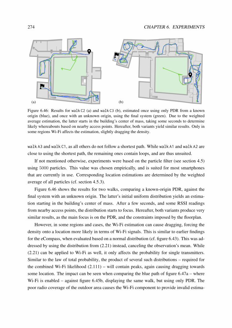
274 CHAPTER 6. EXPERIMENTS
(a) (b)
Figure 6.46: Results for walk C2 (a) and walk C3 (b), estimated once using only PDR from a knownorigin (blue), and once with an unknown origin, using the final system (green). Due to the weightedaverage estimation, the latter starts in the building’s center of mass, taking some seconds to determinelikely whereabouts based on nearby access points. Hereafter, both variants yield similar results. Only insome regions Wi-Fi affects the estimation, slightly dragging the density.
walk A3 and walk C1, as all others do not follow a shortest path. While walk A1 and walk A2 areclose to using the shortest path, the remaining ones contain loops, and are thus unsuited.
If not mentioned otherwise, experiments were based on the particle filter (see section 4.5)using 5000 particles. This value was chosen empirically, and is suited for most smartphonesthat are currently in use. Corresponding location estimations are determined by the weightedaverage of all particles (cf. section 4.5.3).
Figure 6.46 shows the results for two walks, comparing a known-origin PDR, against thefinal system with an unknown origin. The latter’s initial uniform distribution yields an estima-tion starting in the building’s center of mass. After a few seconds, and some RSSI readingsfrom nearby access points, the distribution starts to focus. Hereafter, both variants produce verysimilar results, as the main focus is on the PDR, and the constraints imposed by the floorplan.
However, in some regions and cases, the Wi-Fi estimation can cause dragging, forcing thedensity onto a location more likely in terms of Wi-Fi signals. This is similar to earlier findingsfor the eCompass, when evaluated based on a normal distribution (cf. figure 6.43). This was ad-dressed by using the distribution from (2.21) instead, canceling the observation’s mean. While(2.21) can be applied to Wi-Fi as well, it only affects the probability for single transmitters.Similar to the law of total probability, the product of several such distributions – required forthe combined Wi-Fi likelihood (2.111) – will contain peaks, again causing dragging towardssome location. The impact can be seen when comparing the blue path of figure 6.47a – whereWi-Fi is enabled – against figure 6.45b, displaying the same walk, but using only PDR. Thepoor radio coverage of the outdoor area causes the Wi-Fi component to provide invalid estima-

6.4. EVALUATION OF THE OVERALL SYSTEM 275
(a) (b)
Figure 6.47: Results for walk A2 and walk A3, estimated by the final system. In contrast to the blueresult, green also included navigational knowledge in the evaluation, based on κdest = 0.7. For (a), thisenhances the last segment of the walk, straightening the outdoor area. Within (b), the initial uncertaintyof using the stair is addressed, yielding a faster convergence.
tions, dragging the density. When additionally including navigational knowledge for this walk(green path of figure 6.47a), the effect is mitigated, as walking straight towards the destinationin the lower right is more likely. For figure 6.47b the effect of including navigational knowledge(green path) is similar, correctly using stairs instead of staying on the starting floor (blue).
The impact of using other Wi-Fi optimization strategies is shown in figure 6.48. oELD wasnot further examined, as it requires the locations of the transmitters to be known and addedmanually to the floorplan. This information often is unavailable, and conducting a few referencemeasurements takes similar amounts of time, but offers improved accuracy (cf. section 6.2.7).Likewise, oLDCW is omitted, as it provided only minor improvements compared to oLDC, butcomes with a computational overhead, exceeding the capabilities of commodity smartphones.While the results for oLDCPFi, oLDCPF and oLDC were very similar, oLD suffers from previouslyindicated z-estimation problems: By not considering ceilings, adjacent floors receive a similarlikelihood from the Wi-Fi component. With the initial density thus splitting onto multiple floors,a decent number of particles is required to converge and prevent the estimation from settlingon the wrong floor. This is visualized in figure 6.48b and 6.48c, where the latter used only1000 particles, causing the recursive density estimation to settle for the wrong floor (yellowparticles), unable to converge, eventually getting stuck. When using oLDCPFi, oLDCPF or oLDC,Wi-Fi provides an accurate floor-preference, shown in figure 6.48a. While the estimations in xand y are similar between the depicted models, the error in z is significantly different.
The stability of the final system is also analyzed based on the pedestrian walks from sec-tion 6.1. Each of the 12 paths was conducted by various pedestrians and smartphones. Allresulting recordings are simulated by the final system 50 times, each of which using a differentseed, to adjust underlying pseudo random processes. For all results it is determined, whetherthe estimation converged, and reached the path’s destination. The resulting chances for not

276 CHAPTER 6. EXPERIMENTS
(a) (b) (c)
Figure 6.48: Results for walk A1, estimated by the final system. When using oLDCPFi, oLDCPF or oLDCas Wi-Fi model (a), results are almost optimal. For oLD, however, the z-estimation is not ideal: For 5000particles (b), the estimation eventually converges. For 1000 particles (c), it also starts on all four floors(blue), but settles on the wrong one after a few seconds (yellow), finally getting stuck.
reaching the destination are listed in table 6.19. For most walks, this risk ranged well below10 %. Only walk A2 suffered from a much higher chance, stemming from the walk itself: Itstarts within a region with viable Wi-Fi location estimation, but after a few steps the pedestrianenters an adjacent stairwell, with poor Wi-Fi-coverage, due to massive concrete walls. Eventhough a few particles follow into the stairwell, take the stair, matching with the detected activ-ity, the majority remains outside, within areas much more likely in terms of Wi-Fi. That is, theinitial uniform distribution did not have enough time to settle on a stable mode, thus failing toconverge after a few seconds. This can be mitigated by disabling the Wi-Fi sensor as soon asthe stairwell is entered, e.g. by using the Wi-Fi quality metric (5.2). As all measurable RSSIsare rather low throughout the stairwell, the quality metric approaches zero, indicating that theobservations are unlikely to be valid. When including this technique within the final system,the number of failed results was reduced from 25 % to 15 %. Still being higher than for theother examined walks, this is due to the outdoor area, directly before this walk’s destination.Previous experiments have shown that the Wi-Fi-coverage outdoors is poor for this building,and signal strength predictions are rather erroneous in this area. Thus, many of the seeded sim-ulations entered through a wrong door, or got stuck shortly before the destination. This couldnot be mitigated by the GPS either, as the time outdoors was too short for the GPS to estimate aviable fix on most smartphones. Both issues could be addressed by installing additional trans-mitters throughout such regions. Especially within stairwells, one or two Bluetooth beacons aresufficient to significantly increase localization accuracy, and prevent potential issues.
The localization accuracy of the final system is calculated based on all simulations thatconverged, reaching the correct destination. For error visualization, the 3D Euclidean distancebetween estimation and ground truth was determined every 500 ms. Individual results for ev-ery walk are shown in figure A.7 to A.15. The corresponding overall results are provided ascumulative distribution functions, grouped by building, shown in figure 6.49. When comparedagainst the Wi-Fi-only location estimation from figure 6.31, the benefit of including additional

6.4. EVALUATION OF THE OVERALL SYSTEM 277
SHL Museum 1 Museum 2A1 A2 A3 A4 A5 B1 B2 B3 C1 C2 C3 C4
4 % 25 % 0 % 8 % 9 % 8 % 9 % 6 % 6 % 6 % 8 % 7 %
Table 6.19: Number of results that got stuck or did not reach the correct destination, determined byapplying the final system – 5000 particles, activity-detection, Wi-Fi – 50 times with 50 different seeds,to the conducted pedestrian walks from section 6.1.
0.25
0.50
0.750.901.00
2 m 4 m 6 m 8 m 10 m 2 m 4 m 6 m 8 m 10 m 2 m 4 m 6 m 8 m 10 m
SHL
walk A2 omitted
Museum 1 Museum 2
Figure 6.49: Cumulative distribution function after simulating all walks from section 6.1 using the finalsystem, showing the 3D distance error between estimations and ground truth, grouped by building.
sensors and the building’s floorplan becomes evident. As earlier, the two museums yield moreaccurate results, which is mainly due to an increased number of available Wi-Fi transmitters,with respect to each building’s size. However, when omitting the results for walk A2 (dashedline), suffering from the mentioned outdoor errors, the results for SHL become similar.
As can be seen from the final experiments, for most cases, the presented final system pro-vides viable results with a median error somewhere around 2 m to 3 m. While the floorplan al-lows for 3D location estimation and navigation, preventing impossible movements is not alwaysa benefit. Based on the values listed in table 6.19, there still is a notable risk of the recursivedensity estimation getting stuck, like for PDR-only approaches. While Wi-Fi was intended toaddress this risk, it can also be its root cause, when predicted signal strengths do not match withreal-world behavior, dragging the density to some location. The presented quality metric (5.2)can mitigate the problem, but does not provide a general solution, as it estimates potential issuessolely on low signal strengths. To address these remaining cases, more complex prevention andreset strategies will be required (cf. section 5.2.4), to further enhance the stability in the future.

278 CHAPTER 6. EXPERIMENTS
6.5 Summary
This chapter provided experimental results for all previously introduced techniques. The testbedwas based on synthetic tests using a turntable and confined scenarios, as well as real-worldwalks of several pedestrians within multiple buildings. First, the probabilistic sensor modelsfrom chapter 2 were examined, using both, synthetic and real-world setups. Second, the proba-bilistic movement models from chapter 3 were tested, using synthetic and real-world floorplans,with and without recursive density estimation. Finally, the overall indoor localization and navi-gation system was evaluated, applying it to multiple walks within actual buildings.
Section 6.1 briefly described the testbed used for all experiments. To allow focused exami-nations of sensors and effects, synthetic tests were included alongside real-world scenarios. Thesynthetic variants were based on smartphones placed on a turntable, as well as walks conductedunder constrained conditions. Additionally, three different buildings were examined, varyingin architecture, size and age. All tests were conducted using Android smartphones of differentprice classes and ages, carried by several pedestrians in case of real-world walks.
Section 6.2 gave a brief overview on sensors available within various smartphone models.Most of today’s devices contain an IMU with accelerometer, gyroscope and magnetometer.While Wi-Fi was available within all examined phones, the barometer is rather rare.
Then, section 6.2.2 examined the accelerometer-based step-detection from section 2.4.1. Allconducted tests indicated the benefits of filtering, and the differences between the two discussedimplementations, FIR and IIR. The latter is computationally efficient, and, when chained, suf-ficient for filtering noise, without introducing large delays. A simple peak detection within thefiltered accelerometer magnitude was sufficient to provide a robust step-detection. Solely forfast paced walks, the detection rate was reduced, which is due to increasing amounts of noise.
In section 6.2.3, relative turn-detection and absolute heading (section 2.4.2 and 2.4.3) es-timation were examined. First, each smartphone was mounted onto a turntable, providing theground truth for angular changes. This allowed determining the accuracy of the gyroscope, themagnetometer, and the required tilt compensation (see section 2.4.2). For all examined casesand devices, results were promising. Both, turn-detection and eCompass, were off by onlya few degrees, indicating that both, sensors and algorithms, are viable. However, real-worldexperiments conducted in section 6.2.4 denoted several issues. The gyroscope’s drift cumu-lates significantly over time, and the magnetometer is often notably influenced by the buildingsarchitecture.
Shown in section 6.2.5, readings from the barometer (see section 2.5) are also stronglydependent on the current ambient conditions. Absolute altitude estimations thus require somesort of reference. Using changes in altitude since starting to walk thus significantly improved

6.5. SUMMARY 279
the probabilistic evaluations. Yet, after walking several minutes, the initial reference is expectedto be invalid, due to constantly changing ambient conditions.
An alternative was examined in section 6.2.6. The barometer’s change in pressure and theaccelerometer’s standard deviation within a short timeframe are used for pedestrian activity-detection (cf. section 2.6). While not providing actual altitude estimations, this allows distin-guishing between standing, walking and taking stairs, and remains stable even for longer walks.Yet, the detection suffered from notable delays, mainly caused by the barometer sensor itself.
In section 6.2.7, absolute location estimation was examined, provided by the smartphone’ssignal strength indications for nearby access points (section 2.7). First, signal strength predic-tion models were trained, based on a few reference measurements conducted within a building.As shown, the quality of the resulting predictions is strongly dependent on the trained model,and the building’s architecture. While simple prediction models can be sufficient for some build-ings, others require more complex variants, also considering architecture details. Experimentsindicated that at least floors and ceilings should be considered to provide viable predictions.Then, based on the trained models, location estimations were performed. While more accurateprediction models tendentially provided better location estimations, the difference between allexamined models was less significant. Yet again, the model should at least consider floors andceilings, as this notably improved floor-level estimations. Independent of the chosen model,often more than one location is likely based on the current readings from the smartphone. Fur-thermore, Wi-Fi location estimations are noisy, often encountering large jumps. Due to both,filtering is strongly recommended. Results when applying a simple particle filter with an uncon-strained prediction yielded notably improved results, by suppressing major outliers. However,even with filtering Wi-Fi on its own is insufficient to solve the problem of indoor localization.
Section 6.3 examined the benefits of including the building’s floorplan by using the twospatial models introduced in chapter 3, with and without additional recursive density estima-tion and sensor fusion. First, the navigation grid and the navigation mesh were utilized tomodel various real-world buildings, which pointed out major differences. The navigation gridis rather discrete, more suited for axis-aligned architecture, and can require extensive amountsof memory. The navigation mesh adapts to the local architecture, and requires significantly lessmemory, due to the irregular triangle (primitive) placement. Concerning movement prediction,random walks (see section 3.5.2) are more versatile than the approaches supported by the nav-igation mesh, as they allow for efficient random sampling based on arbitrary metrics. Yet, forreal scenarios and short simulation timeframes, this aspect was less critical than its limitations,producing rather discrete results, and requiring large amounts of memory.
Nevertheless, both spatial models allowed for realistic 3D movement predictions, examinedby a pedestrian dead reckoning setup. Here, step-detection and turn-detection were combined

280 CHAPTER 6. EXPERIMENTS
with a known starting position, which was hereafter adjusted based on sensor observations andthe floorplan. As shown, this enabled 3D location estimations, even though sensors provideonly 2D data. Yet, the impact of cumulating drifts and sensor errors became clear. Probabilisticsetups based on the particle filter, including additional knowledge, are thus advisable.
Section 6.3.2 examined the impact of including navigational knowledge, supported by boththe navigation grid and navigation mesh. First, both variants required adjustments to prevent theestimated shortest paths from adhering unnaturally close to obstacles. Hereafter, both spatialmodels provided routes that match with typical pedestrian walking behavior. When includedwithin the probabilistic process, the desired destination can be used to rule out unlikely move-ments. This often helped the density to converge, especially when starting from a uniform prior.
Likewise, when currently taking stairs, activity-detection reduces the likely whereabouts toa few regions. Shown in section 6.3.3, this often presented major improvements concerningconvergence. While the magnetometer’s compass can be included in a similar way, to limitpotential headings, results strongly depend on ambient conditions. Nearby metal objects oftenaffected observations negatively. Therefore, uncertainty ranges and influences were examinedas well, e.g. comparing a normal distribution against the modified version from section 2.3.By not using a clear mean value, the adjusted distribution can prevent negative impacts frombiased sensors, such as the magnetometer. The section concluded by examining the contributionof individual components, by calculating the amount of random simulations that got stuck ordid not fully converge towards the destination. When the origin is well-known, floorplan-basedprobabilistic PDR without Wi-Fi provides viable results, as long as no major sensor faults occur.When including Wi-Fi, initial whereabouts need not be known, and faults from other sensors canbe compensated. However, poor signal strength readings can also cause the density estimationprocess to get stuck, sometimes unable to recover.
Finally, section 6.4 examined the overall system behavior for multiple long real-world walkswithin three buildings, conducted by several pedestrians. The results notably varied betweenthe three buildings, but also among walks within the same building. This is mainly due tocertain regions, where Wi-Fi reception is poor, causing significant temporal errors. These errorscan also cause the estimation to get stuck, unable to recover. Except for one walk, this riskwas similar between all examined walks and buildings. The building with the poorest resultsamong the three was equipped with significantly less wireless transmitters than the other two.While Wi-Fi can compensate gyroscope drift, and drops the requirement for knowing the initialorigin, its uncertainty is significant, and often reduces the overall localization result, whichcould be better when referring to the remaining sensors. Thus indicating the necessity forfurther improvements.

Chapter 7
Summary
In contrast to navigation outdoors, which has been well established during the last two decades,indoor localization and navigation still remains a niche existence. However, due to the everexpanding need and wish to travel, it becomes of increasing importance. Locating the terminalat an unknown airport, finding the correct ward within a large hospital, or receiving additionalinformation on nearby exhibits within a museum, denote just a few of the numerous use cases.For this new technique to be successful, it should be cheap, easy to set up, and be based onreadily available components. These requirements are not limited solely to the system’s user, butalso apply to its vendors, and the owners of each specific building where the system is installed.Leaving industrial use cases and special hardware components aside, this work focused onpedestrian indoor localization and navigation only. With smartphones being almost always athand, and containing a variety of sensors, these devices represent a desirable target platform.
The first chapter thus presented various smartphone sensors as well as their contributiontowards pedestrian indoor localization and navigation. As the observations from every sen-sor are noisy or in some way uncertain, they are examined on a probabilistic basis, where theexpected amount of noise is included as uncertainty. Throughout the chapter, a relation be-tween sensor readings and potential pedestrian whereabouts or movements within the buildingwas established. After introducing required preprocessing steps, probabilistic evaluations weredeveloped, assigning a quantified likelihood to all potential whereabouts and movements, de-pendent on expected sensor errors. Based on the well-known global positioning system, a briefexample was provided. However, with this localization component unavailable indoors, othersmartphone sensors are required. An alternative to the GPS that can be used indoors, and isalready available within many public buildings, is Wi-Fi. The smartphone’s signal strengthreadings from nearby transmitters can be used to infer the distance towards them, e.g. allowingmultilateration. However, as radio signals are notably affected by walls and other obstacles,
281

282 CHAPTER 7. SUMMARY
multilateration is too coarse within most buildings. Thus, Wi-Fi is often combined with fin-gerprinting, performing hundreds of signal strength measurements throughout the building todetermine the behavior of the radio signals. Each smartphone observation for nearby trans-mitters can then be compared with the recorded fingerprints, determining the one that matchesbest. While offering the best accuracy, the setup process is time consuming. This work thuspresented a compromise based on signal strength prediction models that are able to includeobstacles within their calculations. These models were trained based on a few reference mea-surements, hereafter providing signal strength estimations for every transmitter, throughout thewhole building. The trained models enable probabilistic location estimations, determining thelikelihood for certain whereabouts by comparing their corresponding signal strength predictionswith the smartphone’s observations. Yet, sometimes being inaccurate, this component is unableto solve the localization problem on its own. If the smartphone contains a barometer sensor, itcan be used in a similar way, determining the most likely floor, based on the current ambientpressure readings. Though, with these observations dependent on the weather and changingover time, they require some sort of calibrated reference. Thus, the concept of relative pres-sure readings was introduced. However, dependent on the duration of the walk and the age ofthe reference, it eventually becomes invalid, requiring for another approach. This was givenby activity-detection, combining the accelerometer and barometer readings within a short time-frame to determine the likelihood of the pedestrian to be currently resting, walking or takingstairs. While it does not provide absolute floor estimations, this approach is unaffected by slowchanges in ambient pressure and limits potential whereabouts when taking stairs is detected.Also based on the accelerometer, step-detection was used to infer individual steps made by thepedestrian. Combined with an assumption on the average step size, and including an uncer-tainty, this provides information on potential movements within a certain timeframe. Besidesthis velocity, the current walking direction is of similar importance. The magnetometer installedwithin smartphones was therefore used as a compass, to estimate the heading with respect to ge-omagnetic north. Yet, indoor environments significantly affect its readings, causing the sensorto often be unstable. More stable and unaffected by surroundings is the gyroscope, which wasused to infer changes in heading, referred to as turn-detection. However, as this sensor requiresmathematical integration, it suffers from cumulating drifts. The uncertainty thus cumulates overtime, and eventually reaches a level where the sensor can not provide a contribution.
Similar to navigation outdoors, mapping information can not only be used to estimate theshortest path to a desired destination. It can also be considered to limit impossible movements,and thus to reduce cumulating uncertainties. For this, two spatial models were introduced, mod-eling the walkable surface: A graph with vertices and edges, referred to as navigation grid, andthe navigation mesh, using adjacent and irregularly sized triangles. Both spatial models allow

283
for movement predictions based on the building’s floorplan. The presented random walks alongthe graph, for example, estimate all pedestrian movements that are possible within a certaintimeframe. The intention is similar to the approaches used within car navigation systems. Acar’s last known velocity, heading, and road can be used to provide predictions, even when theGPS is temporarily unavailable, like within a tunnel. Furthermore, this approach can also beused to suppress outliers, when the GPS indicates a faulty reading that does not conform withthe last known heading and velocity. Yet, in contrast to car navigation, pedestrian movementbehavior is significantly less restricted, and usually not limited to certain paths or directions.Unlike cars, a pedestrian can stop, accelerate, or turn at any given instant. This aspect wasexamined based on movement prediction models with and without knowledge of the build-ing’s floorplan. As pointed out, the quality of movement predictions depends on the availableprior knowledge. When assumptions on velocity, heading, and surrounding obstacles can bemade, results are significantly more realistic than without. Including the information from step-detection, turn-detection is thus strongly advisable, notably limiting potential movements. Thisalso concerns navigational knowledge. When the pedestrian’s desired destination is known, theshortest route for reaching it can be estimated. For this, common routing algorithms were used,with a modification to create realistic walking paths through the building, while avoiding nearbyobstacles. The system then assumes that the user follows the presented routing. While deviatingfrom it is still possible, it is typically less likely.
The combination of both aspects, sensor observations and floorplan-based movement pre-diction, was provided by recursive density estimation, using the Bayes filter. It enables a prob-abilistic fusion of multiple individual aspects, including their expected uncertainties, hereafterderiving the most likely result. Applied to localization indoors, the Bayes filter estimates thepedestrian’s most likely whereabouts based on the history of all sensor observations, and con-straints given by the floorplan. This also increases the usefulness of relative sensors, like step-detection and turn-detection, as their whole series of observations is considered, and matchedagainst the floorplan. While the Bayes filter can be implemented analytically using the (ex-tended) Kalman filter, this variant is too restricted for indoor localization, as it does not supportthe discontinuous constraints from the floorplan. This was addressed by using the particle filterinstead, which approximates all required densities based on several discrete samples, referredto as particles. Each of the particles represents one potential location the pedestrian might cur-rently reside at, including an estimated walking direction. The particles can directly be used tosimulate potential movements, e.g. by relocation based on an assumed walking speed, hereafterdetermining whether the resulting movement is possible by the floorplan.
For an efficient, yet flexible, implementation of the overall system, floorplan design choiceswere briefly discussed. A manually modeled floorplan is hereafter used to automatically derive

284 CHAPTER 7. SUMMARY
a navigation grid or navigation mesh for movement predictions. When using the particle filteras implementation, particles can denote impossible movements, if they collide with a wall oranother obstacle. These impossible movements must be addressed, to prevent negative influ-ences, and to ensure that all particles remain likely. For this, several strategies were discussed,such as assigning corresponding particles an infinitesimally small weight, which causes them tobe replaced during the particle filter’s resampling step.
Shown by experiments, all examined smartphone sensors provide a viable contribution to-wards indoor localization. Their general suitability was examined by synthetic tests, suppress-ing unwanted influences, and focusing on individual sensors only. A turntable provided an ac-curate ground truth to inspect turn-detection and absolute heading estimations, indicating viableresults among all examined smartphones. Likewise, step-detection applied to constrained walkswas accurate, as long as the pedestrians used typical pace. While both sensors combined alreadyenable indoor localization via pedestrian dead reckoning, this setup requires initial whereaboutsto be well known, and is likely to fail eventually, due to cumulating sensor errors. While Wi-Fiprovides absolute location estimations, its estimated whereabouts can notably deviate from theground truth. Corresponding estimations were performed within three buildings, based on sig-nal strength prediction models, trained by a few reference measurements. Comparing the re-sults, the limitations of the examined prediction models became clear. Simple line of sightmodels are too inaccurate to provide viable estimations, and at least floors and ceilings shouldbe considered. Using multiple models, each focusing on a fraction of the building, further in-creased the prediction quality. Matching with these findings, the probabilistic setup, based onthe particle filter, has proven to be notably more robust. Triggering updates whenever a step isdetected, each particle’s heading estimation is updated based on turn-detection and the associ-ated uncertainty. This relocates all particles to new whereabouts, if the floorplan conforms witha potential movement. If not, the movement is unlikely and thus suppressed. Similarly, move-ments not matching with the currently detected activity are suppressed as well. Additionally,Wi-Fi weights all particles based on whether the signal strength prediction for their locationmatches with the smartphone’s current observations. Over time, this combination of multiplesensors, movement prediction, and the building floorplan yields a robust probabilistic locationestimation. When assumptions on sensor noise and errors are correct, every additional compo-nent increases the quality of the particle filter’s estimation. Yet, sensor faults, like poor Wi-Fiobservations, or magnetometer readings affected by nearby metal objects, can cause the densityapproximation to destabilize. When encountered for longer timeframes, the particles can e.g.get stuck within a room, unable to leave. While several techniques for mitigation exist, whichstrategy and combination serves best, is one of several topics to be examined in the future.

Chapter 8
Future Work
Discussed within previous chapters and confirmed by experiments, the presented indoor local-ization and navigation system provided an accuracy that is sufficient for localization and routingwithin most buildings. However, indicated by the examined real-world walks, some caveats re-main and should be addressed in the future to further improve accuracy and stability.
The used step-detection e.g. relies on an empiric choice for the pedestrian’s step length andits uncertainty. While this was sufficient for most of the examined cases, it is not a genericsolution. To improve this part of the system, a dynamic step length estimation should be con-sidered, such as the ones provided by [Goy+11] or [Yu+19]. In doing so, varying walkingpatterns, like hectically pacing towards a gate in an airport, can be supported as well. While thepresented turn-detection itself does not rely on such constants, its uncertainty assumed withinevaluations also is a rather empiric heuristic. Here, additional research should examine meth-ods to determine the sensor’s current uncertainty on a profound basis [Cla+17]. This allowsdetecting sensor errors, and situations where the turn-detection is unstable. As shown withinexperiments, while the magnetometer can generally provide a stable heading, the influenceswithin indoor environments significantly limit its applicability. Here, further research shouldbe conducted to determine whether environmental influences can be detected from the observa-tions themselves. If so, the magnetometer should only be considered when it is expected stable.Besides, due to these influences being region-dependent, this opens room for absolute locationestimations based on magnetic fingerprinting [Shu+15; KS18]. Just like Wi-Fi fingerprinting,this compares the current sensor observations against a database of several localized measure-ments. Somewhat similar, critical areas of a building could also be equipped with devices thattransmit unique magnetic patterns, to provide additional location estimations by detecting thesepatterns within observations [EBS16]. To further improve accuracy, these techniques shouldbe examined and integrated if they match with the requirement of being cheap and easy to set
285

286 CHAPTER 8. FUTURE WORK
up. While the barometer also indicated room for further improvements, its limited availabilitywithin recent smartphones does not suggest that further research is advisable. To the contrary,this indicates the need for modifying the activity-detection to work without this sensor. Morecomplex estimators, additionally including the gyroscope and magnetometer, could be used todistinguish between the presented activities, without requiring a barometer [Cil+14; Li+18].However, indicated by sensor data gathered during experiments, when the smartphone is heldupfront, the difference between walking and taking stairs is minimal, and thus potentially hardto classify. This indicates the need for additional research concerning smartphone-only pedes-trian activity-detection. Wi-Fi signal strength prediction and location estimation also yield roomfor further improvements. The used reference measurements already provided setup times thatare notably faster than the ones required for fingerprinting. Yet, these times could further be re-duced by modifying their acquisition. Instead of resting and measuring at predefined locations,the pedestrian could walk consistently through the building, following a defined path. Based onthe recorded data, the exact location belonging to each received measurement can be interpo-lated along the path, similar to the ground truth estimations discussed in section 6.1. Just likestep-detection and turn-detection, the uncertainty assumed for measured Wi-Fi signal strengthsalso relies on an empiric choice, and research on potential dynamic estimations for this valueshould be conducted. Furthermore, shown within experiments, sometimes Wi-Fi estimationsare completely invalid, which indicates a non zero mean error. To prevent corresponding obser-vations from causing localization errors, circumstances should be further examined, to derive amore robust metric for sensor fault detection.
Like the sensors, indoor maps and corresponding pedestrian movement predictions alsohold room for further improvements. Discussed only briefly, escalators and elevators shouldbe modeled, and considered within predictions. However, while supported by the navigationgrid, elevators represent a problem for the navigation mesh. The mesh describes the walkablesurface, but vertical surfaces are neither supported by the mesh, nor by the movement predictionalgorithms presented for it, thus requiring future work on potential solutions. Besides, bothpresented spatial models, navigation grid and navigation mesh, are derived from a manuallycreated indoor map. Depending on the size of the building, the time needed for creating thisfloorplan can be significant. Therefore, further research should be conducted, examining thesuitability of other means for creating them, such as using scanned blueprints, cameras, laser-scanners, SLAM, robots, or similar [Cel+09; Hes+16; SCI13; Zha+15; Liu+17; CF14].
When examining the results from the overall system, a few caveats can be detected as well.Even though the floorplan prevents walking through walls, many of the displayed paths, esti-mated from the particle filter, did directly cross obstacles. While this is not an issue in general,as the pedestrian is only interested in the current whereabouts and not their history, it leads to

287
related future work. The reason for the issue lies, among others, within the used weighted av-erage estimation, which, for multimodal densities, often resides in between all modes, and thusanywhere on the map, independent of obstacles. This can e.g. be addressed by using the maxi-mum of a KDE instead, at the cost of computational complexity [Bul+18]. On the other hand,the discussed behavior also results from the path being constructed by simply connecting con-secutive estimations, not considering obstacles in between. Briefly mentioned earlier, this canbe improved by introducing a slight delay on the results presented to the user, thereby makingfuture observations available to the estimation process. Doing so allows for retrospective resultsmoothing, which yields better paths, but, more importantly, also stabilizes the estimations pre-sented to the pedestrian, at the cost of a slight delay [Fet+16]. Another floorplan-related issueis the risk of the recursive density estimation process to get stuck. Poor Wi-Fi estimations, orother sensor faults, can cause the density to get dragged into some room, unable to leave. De-scribed only briefly, these situations should be detected and handled, e.g. by running multipleparticle filters (IMMPF), one with floorplan and one without, mixing both based on error esti-mations [Fet+17]. Besides causing the density to get stuck, Wi-Fi can also yield more subtleissues. Shown in experiments, when the pedestrian’s origin is known, particle filter-based PDRprovides viable results. When including Wi-Fi, a known origin is not required, and its abso-lute indications can correct gyroscope-drift. However, Wi-Fi often showed a negative effect,increasing the localization error unnecessarily. Here, further research should be conducted, e.g.using the IMMPF to mix between PDR and Wi-Fi only when necessary, using the best of bothestimation results.
Concerning an indoor navigation product, additional aspects not discussed within this workshould be considered. One of which are viable visualization strategies. Potential options are topresent the pedestrian a 2D top view of the current floor, a 3D view in first person perspective, oran augmented reality, where routing information is displayed on top of the smartphone’s cameraimage [HB08]. Here, further research should be conducted, examining which variant providesthe best usability. Also, due to the large variety of different smartphones and correspondingsensors, localization accuracy will vary between different brands and models. Especially when asensor component is unavailable, or provides erroneous observations. These and similar aspectsshould be taken into account as well, examining the impact on an even broader range of devices.

288 CHAPTER 8. FUTURE WORK

List of Figures
1.1 Complex Single-Floor Indoor Map Example . . . . . . . . . . . . . . . . . . . 51.2 Complex Multi-Floor Indoor Map Example . . . . . . . . . . . . . . . . . . . 61.3 Overview of the Overall System . . . . . . . . . . . . . . . . . . . . . . . . . 8
2.1 Synthetic Velocity Sensor Readings . . . . . . . . . . . . . . . . . . . . . . . 162.2 Types of Measurement Errors . . . . . . . . . . . . . . . . . . . . . . . . . . . 172.3 GPS Localization Deviation for Good Reception Conditions . . . . . . . . . . 252.4 Modified Normal Distribution . . . . . . . . . . . . . . . . . . . . . . . . . . 262.5 IMU and World Coordinate System . . . . . . . . . . . . . . . . . . . . . . . 292.6 Accelerometer Readings When Walking . . . . . . . . . . . . . . . . . . . . . 312.7 Accelerometer Magnitude and Frequency Spectrum When Walking . . . . . . 332.8 Step Detection from Accelerometer Magnitude . . . . . . . . . . . . . . . . . 342.9 Probabilistic Step Detection from Accelerometer Magnitude . . . . . . . . . . 362.10 Impact of the Smartphone’s Pose on Gyoroscope Readings . . . . . . . . . . . 402.11 Impact of the Smartphone’s Pose on Accelerometer Readings . . . . . . . . . . 412.12 Complementary Filter Layout . . . . . . . . . . . . . . . . . . . . . . . . . . . 432.13 Local Declination and Average Intensity of the Earth’s Magnetic Field . . . . . 472.14 Magnetic Field and Magnetometer Coordinate System . . . . . . . . . . . . . 482.15 Relation Between Atmospheric Pressure and Height Above Sea Level . . . . . 552.16 Barometer Readings at a Fixed Location . . . . . . . . . . . . . . . . . . . . . 562.17 Activity Recognition Using a Binary Decision Tree . . . . . . . . . . . . . . . 592.18 Influences on RSSI by Various Components . . . . . . . . . . . . . . . . . . . 632.19 Simplified Dipole Antenna Radiation Pattern . . . . . . . . . . . . . . . . . . 642.20 Effects on Radio Signals . . . . . . . . . . . . . . . . . . . . . . . . . . . . . 662.21 Behavior of Measurable Signal Strength . . . . . . . . . . . . . . . . . . . . . 672.22 Log-Distance Signal Strength Prediction Model . . . . . . . . . . . . . . . . . 692.23 Extended Log-Distance Signal Strength Prediction Model . . . . . . . . . . . . 722.24 Ray-Tracing Signal Strength Prediction Model . . . . . . . . . . . . . . . . . . 73
289

290 LIST OF FIGURES
2.25 Discrete Lateration Examples . . . . . . . . . . . . . . . . . . . . . . . . . . . 77
2.26 Continuous Lateration Examples . . . . . . . . . . . . . . . . . . . . . . . . . 78
2.27 Real-World Fingerprint Example . . . . . . . . . . . . . . . . . . . . . . . . . 79
2.28 Signal Strength Uncertainty Distributions . . . . . . . . . . . . . . . . . . . . 82
2.29 Optimization Example for the Log-Distance Model (1) . . . . . . . . . . . . . 89
2.30 Optimization Example for the Log-Distance Model (2) . . . . . . . . . . . . . 90
2.31 Optimization Example for the Extended Log-Distance Model . . . . . . . . . . 92
2.32 Potential Encounters with Floors and Ceilings in Multi-Level Buildings . . . . 93
2.33 Regional Signal Strength Prediction Model Separation . . . . . . . . . . . . . 94
3.1 Potential Combinations of Sensor Readings and Mapping Data . . . . . . . . . 102
3.2 Example of Several 1D Transitions from a Known Origin . . . . . . . . . . . . 103
3.3 Comparison Between Analytical and Simulated Densities . . . . . . . . . . . . 105
3.4 Example Single-Floor Floorplan . . . . . . . . . . . . . . . . . . . . . . . . . 106
3.5 Behavior of Uncertainty for Potential Whereabouts . . . . . . . . . . . . . . . 109
3.6 Walk Simulation Using Walking and Resting without Heading Constraints . . . 110
3.7 Walk Simulation Using Walking and Resting with Heading Constraints . . . . 111
3.8 Walk Simulation Using Walking, Resting and Turning . . . . . . . . . . . . . . 112
3.9 Walk Simulation Including a Floorplan . . . . . . . . . . . . . . . . . . . . . . 113
3.10 Walk Simulation Using Shortest Paths . . . . . . . . . . . . . . . . . . . . . . 116
3.11 Overview on Different Spatial Floorplan Representations . . . . . . . . . . . . 119
3.12 Comparing Two Regular Spatial Models . . . . . . . . . . . . . . . . . . . . . 122
3.13 3D Navigation Grid Creation Steps . . . . . . . . . . . . . . . . . . . . . . . . 124
3.14 Discrete Behavior of Random Walks . . . . . . . . . . . . . . . . . . . . . . . 132
3.15 Random Walk Heading Error Compensation . . . . . . . . . . . . . . . . . . . 133
3.16 Random Walk Example . . . . . . . . . . . . . . . . . . . . . . . . . . . . . . 134
3.17 Shortest Path Example (1) . . . . . . . . . . . . . . . . . . . . . . . . . . . . 136
3.18 Shortest Path Example (2) . . . . . . . . . . . . . . . . . . . . . . . . . . . . 137
3.19 Strategies for Walking Along a Graph-Based Data Structure . . . . . . . . . . 139
3.20 Various Irregular Spatial Models . . . . . . . . . . . . . . . . . . . . . . . . . 141
3.21 Delaunay Triangulation and Voronoi Diagram for a Floorplan . . . . . . . . . . 142
3.22 Navigation Mesh Examples . . . . . . . . . . . . . . . . . . . . . . . . . . . . 144
3.23 Random Sampling on a Navigation Mesh (1) . . . . . . . . . . . . . . . . . . 147
3.24 Random Sampling on a Navigation Mesh (2) . . . . . . . . . . . . . . . . . . 150
3.25 Shortest Path on Navigation Meshes Using Edge-Midpoints . . . . . . . . . . . 151
3.26 Shortest Path on Navigation Meshes Using the Funnel Algorithm . . . . . . . . 152

LIST OF FIGURES 291
4.1 Behavior of a State Estimation Using a Low-Pass Filter (1) . . . . . . . . . . . 1574.2 Behavior of a State Estimation Using a Low-Pass Filter (2) . . . . . . . . . . . 1584.3 Combining a Prior Estimation with an Observation to Create a Posterior . . . . 1594.4 Bayes Filter Example . . . . . . . . . . . . . . . . . . . . . . . . . . . . . . . 1664.5 Linear and Nonlinear Density Modifications . . . . . . . . . . . . . . . . . . . 1734.6 Sampled Gaussian and KDE . . . . . . . . . . . . . . . . . . . . . . . . . . . 1764.7 Sampled Multivariate Gaussian and KDE . . . . . . . . . . . . . . . . . . . . 1774.8 Rejection Sampling for Three Probability Density Functions . . . . . . . . . . 1824.9 Particle Filter - Process Example . . . . . . . . . . . . . . . . . . . . . . . . . 1844.10 Particle Filter - Comparing Discrete and Continuous Resampling . . . . . . . . 1874.11 Particle Filter - Estimation Example . . . . . . . . . . . . . . . . . . . . . . . 188
5.1 Complex Indoor Maps - Wall Intersections . . . . . . . . . . . . . . . . . . . . 1925.2 Complex Indoor Maps - 3D Walls with Doors and Windows . . . . . . . . . . 1935.3 Complex Indoor Maps - Defining Stairs . . . . . . . . . . . . . . . . . . . . . 1945.4 Complex Indoor Maps - Map-Editor and Realistic Rendering of a Map . . . . . 1955.5 System - Overview . . . . . . . . . . . . . . . . . . . . . . . . . . . . . . . . 1965.6 System - Behavior over Time . . . . . . . . . . . . . . . . . . . . . . . . . . . 1975.7 System - Time and Data Diagram . . . . . . . . . . . . . . . . . . . . . . . . . 1985.8 Comparison of Filter Update Strategies . . . . . . . . . . . . . . . . . . . . . 2005.9 Handling of Colliding Transitions - Issues . . . . . . . . . . . . . . . . . . . . 2025.10 Handling of Colliding Transitions - Fix . . . . . . . . . . . . . . . . . . . . . 2035.11 Prediction Example with Sensor Fault - Issue . . . . . . . . . . . . . . . . . . 2045.12 Prediction Example with Sensor Fault - Fix . . . . . . . . . . . . . . . . . . . 2055.13 Strategies for Precomputed Signal Strength Lookups . . . . . . . . . . . . . . 211
6.1 Floorplan of SHL . . . . . . . . . . . . . . . . . . . . . . . . . . . . . . . . . 2196.2 Floorplan of Museum 1 . . . . . . . . . . . . . . . . . . . . . . . . . . . . . . 2196.3 Floorplan of Museum 2 . . . . . . . . . . . . . . . . . . . . . . . . . . . . . . 2196.4 Pedestrian Walks Conducted within SHL . . . . . . . . . . . . . . . . . . . . . 2206.5 Pedestrian Walks Conducted within Museum 1 . . . . . . . . . . . . . . . . . 2206.6 Pedestrian Walks Conducted within Museum 2 . . . . . . . . . . . . . . . . . 2206.7 Frequency Response of FIR and IIR Filters for Step Detection . . . . . . . . . 2226.8 Filtered Accelerometer Magnitude . . . . . . . . . . . . . . . . . . . . . . . . 2236.9 Accelerometer Magnitude for a Walking Pedestrian (1) . . . . . . . . . . . . . 2246.10 Accelerometer Magnitude for a Walking Pedestrian (2) . . . . . . . . . . . . . 2256.11 Layout of the Turntable Used for Synthetic IMU Tests . . . . . . . . . . . . . 226

292 LIST OF FIGURES
6.12 Impact of the Rotation Axis on Accelerometer and Gyroscope . . . . . . . . . 228
6.13 Turntable Tilt Estimation and Complementary Filter . . . . . . . . . . . . . . . 229
6.14 Turntable Results - Estimated Magnetometer Angle . . . . . . . . . . . . . . . 232
6.15 Turntable Results - Raw Magnetometer Data . . . . . . . . . . . . . . . . . . . 233
6.16 Comparing Magnetometer and Gyroscope for PDR (1) . . . . . . . . . . . . . 235
6.17 Comparing Magnetometer and Gyroscope for PDR (2) . . . . . . . . . . . . . 236
6.18 Comparing Magnetometer and Gyroscope for PDR (3) . . . . . . . . . . . . . 237
6.19 Repeatability of Barometer Measurements . . . . . . . . . . . . . . . . . . . . 238
6.20 Comparison of Absolute and Relative Barometer Evaluation . . . . . . . . . . 240
6.21 Barometer Measurement and Corresponding Ground Truth . . . . . . . . . . . 241
6.22 Activity Classification Based on Normal Distributions . . . . . . . . . . . . . . 242
6.23 Estimating a Decision Tree for Activity Detection . . . . . . . . . . . . . . . . 243
6.24 Location of Reference Measurements Conducted within Three Public Buildings 246
6.25 CDF of Wi-Fi Signal Strength Prediction Errors . . . . . . . . . . . . . . . . . 248
6.26 Signal Strength Prediction Errors within SHL . . . . . . . . . . . . . . . . . . 249
6.27 Signal Strength Prediction Errors within Museum 1 . . . . . . . . . . . . . . . 249
6.28 Signal Strength Prediction Errors within Museum 2 . . . . . . . . . . . . . . . 249
6.29 Wi-Fi Location Estimation for a Real Walk . . . . . . . . . . . . . . . . . . . 252
6.30 Wi-Fi Probability Heat Map for a Real Walk . . . . . . . . . . . . . . . . . . . 253
6.31 CDF of Wi-Fi Localization Errors . . . . . . . . . . . . . . . . . . . . . . . . 254
6.32 CDF of the Kullback-Leibler Divergence Between Estimation and Ground Truth 255
6.33 Spatial Comparison of Graph and Navigation Mesh . . . . . . . . . . . . . . . 258
6.34 Impact of the Shortest Path Likelihood Heuristic . . . . . . . . . . . . . . . . . 260
6.35 Impact of Wall Avoidance on the Shortest Path Likelihood . . . . . . . . . . . 261
6.36 Comparison of Grid and Navigation Mesh . . . . . . . . . . . . . . . . . . . . 262
6.38 Floorplan-Based PDR with Known Initial Whereabouts . . . . . . . . . . . . . 265
6.39 Floorplan-Based PDR with Unknown Initial Whereabouts . . . . . . . . . . . 265
6.40 Floorplan-Based PDR, Including Activity Detection . . . . . . . . . . . . . . . 266
6.41 Floorplan-Based PDR, Including Navigational Knowledge . . . . . . . . . . . 267
6.42 Floorplan-Based PDR, Including the eCompass (1) . . . . . . . . . . . . . . . 268
6.43 Floorplan-Based PDR, Including the eCompass (2) . . . . . . . . . . . . . . . 269
6.44 Limitations of Movement Prediction . . . . . . . . . . . . . . . . . . . . . . . 270
6.45 Potential Issues of Real-World Probabilistic PDR . . . . . . . . . . . . . . . . 271
6.46 Comparison of PDR and the Final System . . . . . . . . . . . . . . . . . . . . 274
6.47 Impact of Navigational Knowledge within the Final System . . . . . . . . . . . 275
6.48 Impact of Wi-Fi Model and Number of Particles within the Final System . . . . 276

LIST OF FIGURES 293
6.49 CDF of Errors Resulting from the Final System . . . . . . . . . . . . . . . . . 277
A.1 First Floor of UAH . . . . . . . . . . . . . . . . . . . . . . . . . . . . . . . . 332A.2 Floorplan of CAR . . . . . . . . . . . . . . . . . . . . . . . . . . . . . . . . . 333A.3 Floorplan of Museum 3 . . . . . . . . . . . . . . . . . . . . . . . . . . . . . . 333A.4 Final Result for walk B1 . . . . . . . . . . . . . . . . . . . . . . . . . . . . . . 334A.5 Final Result for walk B2 . . . . . . . . . . . . . . . . . . . . . . . . . . . . . . 334A.6 Final Result for walk B3 . . . . . . . . . . . . . . . . . . . . . . . . . . . . . . 334A.7 Final Result for walk A1 . . . . . . . . . . . . . . . . . . . . . . . . . . . . . . 335A.8 Final Result for walk A2 . . . . . . . . . . . . . . . . . . . . . . . . . . . . . . 335A.9 Final Result for walk A3 . . . . . . . . . . . . . . . . . . . . . . . . . . . . . . 335A.10 Final Result for walk A4 . . . . . . . . . . . . . . . . . . . . . . . . . . . . . . 335A.11 Final Result for walk A5 . . . . . . . . . . . . . . . . . . . . . . . . . . . . . . 335A.12 Final Result for walk C1 . . . . . . . . . . . . . . . . . . . . . . . . . . . . . . 336A.13 Final Result for walk C2 . . . . . . . . . . . . . . . . . . . . . . . . . . . . . . 336A.14 Final Result for walk C3 . . . . . . . . . . . . . . . . . . . . . . . . . . . . . . 336A.15 Final Result for walk C4 . . . . . . . . . . . . . . . . . . . . . . . . . . . . . . 336

294 LIST OF FIGURES

List of Tables
2.1 Smartphone Orientations . . . . . . . . . . . . . . . . . . . . . . . . . . . . . 492.2 Constants Relating Atmospheric Pressure and Altitude . . . . . . . . . . . . . 542.3 Absolute and Relative Pressure Dependent on Altitude . . . . . . . . . . . . . 572.4 Typical Radio Signal Attenuation Factors . . . . . . . . . . . . . . . . . . . . 682.5 Attenuation Factors for Typical Building Materials . . . . . . . . . . . . . . . 71
6.1 Overview on Examined Smartphones . . . . . . . . . . . . . . . . . . . . . . . 2176.2 Mean Sensor Sample Rates of the Examined Smartphones . . . . . . . . . . . 2216.3 FIR and IIR Filter Setups Used for Step-Detection . . . . . . . . . . . . . . . . 2226.4 Overview on Examined Step Detectors . . . . . . . . . . . . . . . . . . . . . . 2246.5 Step Detection Results . . . . . . . . . . . . . . . . . . . . . . . . . . . . . . 2256.6 Turntable Results - Estimated Speed and Angle . . . . . . . . . . . . . . . . . 2276.7 Turntable Results - Cumulative Angles Based on Strategy . . . . . . . . . . . . 2316.8 Turntable Results - Magnetometer Angular Values . . . . . . . . . . . . . . . . 2346.9 Average Stair Walking Speeds . . . . . . . . . . . . . . . . . . . . . . . . . . 2396.10 Accuracy of Activity Recognition When Using Normal Distributions . . . . . . 2426.11 Accuracy of Activity Recognition When Using a Decision Tree . . . . . . . . . 2436.12 Mean Wi-Fi Sample Rates of the Examined Smartphones . . . . . . . . . . . . 2446.13 Examined Wi-Fi Model Optimization Strategies . . . . . . . . . . . . . . . . . 2456.14 Wi-Fi Model RMSE Based on Building and Setup . . . . . . . . . . . . . . . . 2476.15 Floorplan Model - Number of Required Primitives . . . . . . . . . . . . . . . . 2576.16 Floorplan Model - Memory Requirements . . . . . . . . . . . . . . . . . . . . 2576.17 Convergence of Probabilistic Movement Prediction (1) . . . . . . . . . . . . . 2726.18 Convergence of Probabilistic Movement Prediction (2) . . . . . . . . . . . . . 2726.19 Chance for a Walk to Get Stuck within the Final System . . . . . . . . . . . . 277
A.1 IIR Filter Parameters for Step-Detection . . . . . . . . . . . . . . . . . . . . . 331A.2 FIR Low-Pass Kernel for Step-Detection . . . . . . . . . . . . . . . . . . . . . 331A.3 FIR Band-Pass Kernel for Step-Detection . . . . . . . . . . . . . . . . . . . . 331
295

296 LIST OF TABLES

LIST OF SYMBOLS 297
List of Symbols
Sign Descriptionα, β general purpose anglesd general purpose scalar distance valueκ general purpose scalar value used for mixing κ and (1− κ)
η general prupose normalization constantτ general purpose threshold valueu,v general purpose vectorsv general purpose velocity valueε general purpose error valueE general purpose cumulative error valueρ general purpose 3D pointρ(x), ρ(y), ρ(z) components of a 3D pointX ,Y ,Z general purpose random variables
ρdest the pedestrian’s desired destinationQ quaternionbw KDE bandwidth
q unknown state vectorq
(x)t , q
(y)t , . . . attributes of the unknown state at time t
q(Θ)t unknown state heading at time tq
(εhead)t−1 unknown state cumulated heading error at time t− 1
q(εdist)t−1 unknown state distance error at time t− 1
o observation vectoro
(Θ)t , o
(s)t , . . . attributes of the observation at time t
w probabilistic weightW cumulated probabilistic weight
G = (V,E) graph with vertices and edgesvi vertex within a graph Gv
(x)i , v
(y)i , . . . attributes of vertex i

298 LIST OF SYMBOLS
Sign Descriptionei,j edge between vertex vi and vjvdest vertex for the pedestrian’s desired destinationgs distance between adjacent graph vertices in x and ygsz distance between adjacent graph vertices in zp(ei,j | qt−1) probability to walk the given edge
g GPS observation (lon, lat, alt, err)
a accelerometer observation (x, y, z)
ω′ gyroscope observation, turn rate (x, y, z)
θ′ cumulative gyroscope turn ratesQω
′, Qθ
′, Qa, Q quaternions for: gyro turn rates, cumulative gyro turn rates, pose
from accelerometer, filtered poseR smartphone pose rotation matrixR−1 tilt compensation matrixω the pedestrian’s turn rateθ relative heading indication (cumulated within a timeframe)Θ absolute heading indication (cumulated since start)
B′ magnetometer observation, magnetic flux density (x, y, z)
B magnetic flux density vector, after tilt compensationΘNmag angle towards geomagnetic northΘNgeo angle towards geographic northΘdec local declination correctionΘbldg local declination correction, including building orientation
% barometer observation, atmospheric pressureh altitudehbldg building’s first floor’s altitude, above mean sea level
Ω activity class
s observed Wi-Fi signal strengthssap observed Wi-Fi signal strength for one transmitter

LIST OF SYMBOLS 299
Sign Descriptionς offline RSSI database (fingerprints/reference measurements)ςfp,ap,n n-th measurement for transmitter ap at location fpλ wavelengthρ• 3D position of a model predictionρ,ρ 3D position of a transmitter/receiverP , P signal power at a transmitter/receiverG ,G Wi-Fi antenna gain for a transmitter/receiverγ Wi-Fi path-loss exponentφ attenuation factor for a materialψ signal strength prediction model parametersψap signal strength prediction model parameters for one AP
κdest empiric value for favoring the shortest pathκact empiric value for favoring the same activityκw/s empiric value to mix standing and walking

300 LIST OF SYMBOLS

Bibliography
[AP99] E. Abbott and D. Powell. “Land-Vehicle Navigation Using GPS”. In: Proceedings
of the IEEE 87.1, 1999.
[ARC12] Imad Afyouni, Cyril Ray, and Christophe Claramunt. “Spatial Models for IndoorContext-Aware Navigation Systems: A Survey”. In: Journal of Spatial Informa-
tion Science 4, 2012.
[Aig15] Martin Aigner. Graphentheorie : Eine Einfuhrung aus dem 4-Farben Problem.Wiesbaden: Springer Spektrum, 2015.
[AY12] Moustafa Alzantot and Moustafa Youssef. “CrowdInside: Automatic Construc-tion of Indoor Floorplans”. In: International Conference on Advances in Geo-
graphic Information Systems. 2012.
[ARY95] Jørgen Bach Andersen, Theodore S. Rappaport, and Susumu Yoshida. “Propa-gation Measurements and Models for Wireless Communications Channels”. In:IEEE Communications Magazine, 1995.
[ABA11] J. Andreu, R. D. Baruah, and P. Angelov. “Real Time Recognition of Human Ac-tivities from Wearable Sensors by Evolving Classifiers”. In: IEEE International
Conference on Fuzzy Systems (FUZZ-IEEE). 2011.
[App] Apple. Documentation - Core Motion - Getting Raw Accelerometer Events.https://developer.apple.com/documentation/coremotion/getting raw accelerometer
events. Accessed: 2020-01-04.
[AAO11] A. A. B. Ariffin, N. H. A. Aziz, and K. A. Othman. “Implementation of GPS forLocation Tacking”. In: IEEE Control and System Graduate Research Colloquium.2011.
[Ark87] Ronald Craig Arkin. “Towards Cosmopolitan Robots : Intelligent Navigation inExtended Man-made Environments”. PhD thesis. University of Massachusetts,1987.
301

302 BIBLIOGRAPHY
[Aru+01] Sanjeev Arulampalam et al. “A Tutorial on Particle Filters for On-line Non-linear/ Non-Gaussian Bayesian Tracking”. In: IEEE Transactions on Signal Processing
50, 2001.
[Ary+98] Sunil Arya et al. “An Optimal Algorithm for Approximate Nearest NeighborSearching Fixed Dimensions”. In: Journal of the ACM (JACM) 45.6, 1998.
[Aur91] Franz Aurenhammer. “Voronoi Diagrams - A Survey of a Fundamental GeometricData Structure”. In: ACM Computing Surveys (CSUR) 23.3, 1991.
[AC16] J. Azevedo and S. Crisostomo. “Weather Stations-Assisted Barometric Altimeterfor Android: Interpolation Techniques for Improved Accuracy”. In: IEEE Sensors
Applications Symposium (SAS). 2016.
[BP00] Paramvir Bahl and Venkata N. Padmanabhan. “RADAR: An In-Building RF-based User Location and Tracking System”. In: Annual Joint Conference of the
IEEE Computer and Communications Societies. Vol. 2. 2000.
[BSA16] Leor Banin, Uri Schatzberg, and Yuval Amizur. “WiFi FTM and Map Informa-tion Fusion for Accurate Positioning”. In: International Conference on Indoor
Positioning and Indoor Navigation (IPIN). 2016.
[BP66] Leonard E. Baum and Ted Petrie. In: The Annals of Mathematical Statistics 37,1966.
[Baw+15] B. Bawazeer et al. “Reducing Scanning Delay for WiFi-to-WhiteFi Handovers”.In: Fifth International Conference on Digital Information and Communication
Technology and its Applications (DICTAP). 2015.
[BJK05] P. Beeson, N. K. Jong, and B. Kuipers. “Towards Autonomous Topological PlaceDetection Using the Extended Voronoi Graph”. In: IEEE International Confer-
ence on Robotics and Automation. 2005.
[Ben75] Jon Louis Bentley. “Multidimensional Binary Search Trees Used for AssociativeSearching”. In: Communications ACM 18.9, 1975.
[Ber17] Florian Berchtold. Geometrie : von Euklid bis zur hyperbolischen Geometrie mit
Ausblick auf angrenzende Gebiete. Springer Spektrum, 2017.
[Ber+08] Mark de Berg et al. Computational Geometry: Algorithms and Applications.Springer, 2008.
[BD13] Gerard Blanchet and Bertrand Dupouy. Computer Architecture. Iste Wiley, 2013.
[Blo83] Jacques-Francois Blondel. Cours d’architecture. 1683.

BIBLIOGRAPHY 303
[BDH04] Miodrag Bolic, Petar M. Djuric, and Sangjin Hong. “Resampling Algorithms forParticle Filters: A Computational Complexity Perspective”. In: Journal on Ad-
vances in Signal Processing (EURASIP) 15, 2004.
[BC12] William Bolstad and James Curran. Introduction to Bayesian Statistics. Wiley,2012.
[Bon+01] P. Bonnifait et al. “Data Fusion of Four ABS Sensors and GPS for an EnhancedLocalization of Car-like Vehicles”. In: IEEE International Conference on Robotics
and Automation (ICRA). Vol. 2. 2001.
[BN09] A. G. Bors and N. Nasios. “Kernel Bandwidth Estimation for NonparametricModeling”. In: IEEE Transactions on Systems, Man, and Cybernetics, Part B (Cy-
bernetics) 39.6, 2009.
[Bos14] Bosch Sensortec. BMC156 - 6-axis eCompass. BST-BMC156-DS000-01. 2014.
[Bos15] Bosch Sensortec. BMP180 - Digital pressure sensor. BST-BMP180-DS000-12.2015.
[Bos18] Bosch Sensortec. BMP280 - Digital pressure sensor. BST-BMP280-DS001-19.2018.
[Bou13] M. Bouhedda. “Neuro-Fuzzy Sensor’s Linearization Based FPGA”. In: IEEE In-
ternational Conference on Intelligent Data Acquisition and Advanced Computing
Systems (IDAACS). Vol. 1. 2013.
[BM58] George Edward Pelham Box and Mervin Edgar Muller. “A Note on the Genera-tion of Random Normal Deviates”. In: The Annals of Mathematical Statistics 29,1958.
[Bra+05] D. Braganza et al. “Tracking Control for Robot Manipulators with Kinematic andDynamic Uncertainty”. In: IEEE Conference on Decision and Control. 2005.
[Bre65] J. E. Bresenham. “Algorithm for computer control of a digital plotter”. In: IBM
Systems Journal 4.1, 1965.
[Bro+06] Raymond C. Browning et al. “Effects of obesity and sex on the energetic cost andpreferred speed of walking”. In: Journal of Applied Physiology 100.2, 2006.
[Bul+18] Markus Bullmann et al. “Fast Kernel Density Estimation using Gaussian FilterApproximation”. In: International Conference on Information Fusion (FUSION).2018.
304 BIBLIOGRAPHY
[BS12] M. Butta and I. Sasada. “Sources of Noise in a Magnetometer Based on Orthog-onal Fluxgate Operated in Fundamental Mode”. In: IEEE Transactions on Mag-
netics 48.4, 2012.
[CF14] R. Cabral and Y. Furukawa. “Piecewise Planar and Compact Floorplan Recon-struction from Images”. In: IEEE Conference on Computer Vision and Pattern
Recognition (CVPR). 2014.
[CGM07] O. Cappe, S. J. Godsill, and E. Moulines. “An Overview of Existing Methods andRecent Advances in Sequential Monte Carlo”. In: Proceedings of the IEEE 95.5,2007.
[Cap+17] N. Capurso et al. “An Android-Based Mechanism for Energy Efficient Localiza-tion Depending on Indoor/Outdoor Context”. In: IEEE Internet of Things Journal
4.2, 2017.
[CB07] Tom Carpenter and Joel Barrett. CWNA Certified Wireless Network Administra-
tor Official Study Guide (Exam PW0-100). 4th ed. McGraw-Hill Osborne Media,2007.
[Cas+14] D. Caspari et al. “Smartphone Sensor Based Algorithms for Dead Reckoning Us-ing Magnetic Field Sensor and Accelerometer for Localization Purposes”. In: In-
ternational Symposium on Wireless Systems within the Conferences on Intelligent
Data Acquisition and Advanced Computing Systems. 2014.
[Cel+09] Koray Celik et al. “Monocular Vision SLAM for Indoor Aerial Vehicles”. In:IEEE/RSJ International Conference on Intelligent Robots and Systems (IROS).2009.
[CHP79] Y. T. Chan, A. G. C. Hu, and J. B. Plant. “A Kalman Filter Based Tracking Schemewith Input Estimation”. In: IEEE Transactions on Aerospace and Electronic Sys-
tems 2, 1979.
[Cha82] B. Chazelle. “A Theorem on Polygon Cutting with Applications”. In: Annual
Symposium on Foundations of Computer Science (SFCS). 1982.
[CYJ15] Y. Chen, J. Yang, and S. Jiang. “Data Validation and Dynamic Uncertainty Es-timation of Self-validating Sensor”. In: IEEE International Instrumentation and
Measurement Technology Conference (I2MTC). 2015.
[Che+05] Yu-Chung Cheng et al. “Accuracy Characterization for Metropolitan-scale Wi-FiLocalization”. In: International Conference on Mobile Systems, Applications, and
Services. 2005.
BIBLIOGRAPHY 305
[Che+12] Yan-Ming Cheng et al. “Analysis on Interference Impact of WiFi on DTV”. In:World Automation Congress. 2012.
[CHP16] C. Chesneau, M. Hillion, and C. Prieur. “Motion estimation of a Rigid Body withan EKF using Magneto-Inertial Measurements”. In: International Conference on
Indoor Positioning and Indoor Navigation (IPIN). 2016.
[CPP10] Krishna Chintalapudi, Anand Padmanabha Iyer, and Venkata N. Padmanabhan.“Indoor Localization Without the Pain”. In: Annual International Conference on
Mobile Computing and Networking (MobiCom). ACM, 2010.
[Cho+12] I. N. Cholakova et al. “Temperature Influence on Hall Effect Sensors Character-istics”. In: Telecommunications Forum (TELFOR). 2012.
[CB95] H. Choset and J. Burdick. “Sensor Based Planning, Part I. The Generalized VoronoiGraph”. In: IEEE International Conference on Robotics and Automation. Vol. 2.1995.
[CZK98] O. Chutatape, Liu Zheng, and S. M. Krishnan. “Retinal blood vessel detection andtracking by matched Gaussian and Kalman filters”. In: International Conference
of the IEEE Engineering in Medicine and Biology Society. Vol. 6. 1998.
[Cil+14] F. De Cillis et al. “Indoor Positioning System using Walking Pattern Classifica-tion”. In: Mediterranean Conference on Control and Automation. 2014.
[Cla83] K. L. Clarkson. “Fast Algorithms for the All Nearest Neighbors Problem”. In:Annual Symposium on Foundations of Computer Science (SFCS). 1983.
[Cla+17] P. Clausen et al. “An Overview of a New Sensor Calibration Platform”. In: IEEE
International Workshop on Metrology for AeroSpace (MetroAeroSpace). 2017.
[Cla16] Christoph Clauser. Einfuhrung in die Geophysik : globale physikalische Felder
und Prozesse in der Erde. Springer Spektrum, 2016.
[Cor09] Thomas Cormen. Introduction to Algorithms. MIT Press, 2009.
[CK08] Erhard Cramer and Udo Kamps. Grundlagen der Wahrscheinlichkeitsrechnung
und Statistik. Springer, 2008.
[CS11] Xiao Cui and Hao Shi. “A*-based Pathfinding in Modern Computer Games”. In:International Journal of Computer Science and Network Security (IJCSNS) 11.1,2011.
[Cul56] E. G. Cullwick. “Electromagnetic Momentum and Electron Inertia in a CurrentCircuit”. In: Proceedings of the IEE - Part C: Monographs 103.3, 1956.

306 BIBLIOGRAPHY
[DH03] Winnie Daamen and Serge Hoogendoorn. “Experimental Research of PedestrianWalking Behavior”. In: Transportation Research Record Journal of the Trans-
portation Research Board 1828, 2003.
[DT05] N. Dalal and B. Triggs. “Histograms of Oriented Gradients for Human Detec-tion”. In: IEEE Computer Society Conference on Computer Vision and Pattern
Recognition (CVPR). Vol. 1. 2005.
[Del98] Pierre Del Moral. “Measure Valued Processes and Interacting Particle Systems.Application to Non Linear Filtering Problems”. In: The Annals of Applied Proba-
bility 8, 1998.
[Del96] Pierre Del Moral. “Nonlinear Filtering: Interacting Particle Solution”. In: Markov
Processes and Related Fields 2, 1996.
[Del34] B. N. Delaunay. “Sur la sphere vide”. In: Bulletin de l’Academie des Sciences de
l’URSS 1934.6, 1934.
[DLK07] Nikos Deligiannis, Spiros Louvros, and Stavros Kotsopoulos. “Optimizing Loca-tion Positioning Using Hybrid TOA-AOA Techniques in Mobile Cellular Net-works”. In: International Conference on Mobile Multimedia Communications.2007.
[DW11] Henry Deng and Hadley Wickham. Density estimation in R. Tech. rep. 2011.
[Deu10] Deutsche Akkreditierungsstelle. DAkkS-DKD-5 - Anleitung zum Erstellen eines
Kalibrierscheines. 1st ed. Version 2. 2010.
[Die06] James Diebel. “Representing Attitude: Euler Angles, Unit Quaternions, and Ro-tation Vectors”. In: Matrix 58, 2006.
[Dij59] E. W. Dijkstra. “A Note on Two Problems in Connexion with Graphs”. In: Nu-
merische Mathematik 1.1, 1959.
[Do+09] D. V. Do et al. “Impedance Observer for a Li-Ion Battery Using Kalman Filter”.In: IEEE Transactions on Vehicular Technology 58.8, 2009.
[DH10] Hans Dodel and Dieter Haupler. Satellitennavigation. 2nd ed. Springer, 2010.
[DC05] Randal Douc and O Cappe. In: 2005.
[DGK01] A. Doucet, N. J. Gordon, and V. Krishnamurthy. “Particle Filters for State Esti-mation of Jump Markov Linear Systems”. In: IEEE Transactions on Signal Pro-
cessing 49.3, 2001.
[DS84] Peter Doyle and James Snell. Random Walks and Electric Networks. AmericanMathematical Society, 1984.

BIBLIOGRAPHY 307
[DB05] H. Driessen and Y. Boers. “Efficient particle filter for jump Markov nonlinearsystems”. In: IEE Proceedings - Radar, Sonar and Navigation 152.5, 2005.
[DMX10] I. Dryanovski, W. Morris, and J. Xiao. “Multi-Volume Occupancy Grids: An Effi-cient Probabilistic 3D Mapping Model for Micro Aerial Vehicles”. In: IEEE/RSJ
International Conference on Intelligent Robots and Systems. 2010.
[Dvo+19] Nir Dvorecki et al. “A Machine Learning Approach for Wi-Fi RTT Ranging”. In:International Technical Meeting of The Institute of Navigation. 2019.
[DZM07] Ramsay Dyer, Hao Zhang, and Torsten Moller. “Voronoi-Delaunay Duality andDelaunay Meshes”. In: ACM Symposium on Solid and Physical Modeling (SPM).2007.
[Ebn+15] Frank Ebner et al. “Multi Sensor 3D Indoor Localisation”. In: International Con-
ference on Indoor Positioning and Indoor Navigation (IPIN). 2015.
[Ebn+16] Frank Ebner et al. “On Prior Navigation Knowledge in Multi Sensor Indoor Lo-calisation”. In: International Conference on Information Fusion (FUSION). 2016.
[Ebn+17] Frank Ebner et al. “On Wi-Fi Model Optimizations for Smartphone-Based IndoorLocalization”. In: International Journal of Geo-Information (ISPRS) 6.8, 2017.
[Ebn+14] Frank Ebner et al. “Robust Self-Localization using Wi-Fi, Step/Turn-Detectionand Recursive Density Estimation”. In: International Conference on Indoor Posi-
tioning and Indoor Navigation (IPIN). 2014.
[Eck87] Roger Eckhardt. “Stan Ulam, John Von Neumann, Monte Carlo Method”. In: Los
Alamos Science, 1987.
[EBS16] C. R. Ehrlich, J. Blankenbach, and A. Sieprath. “Towards a Robust Smartphone-based 2.5D Pedestrian Localization”. In: International Conference on Indoor Po-
sitioning and Indoor Navigation (IPIN). 2016.
[Elf89] A. Elfes. “Using Occupancy Grids for Mobile Robot Perception and Navigation”.In: Computer 22.6, 1989.
[Elh+14] M. Elhoushi et al. “Using Portable Device Sensors to Recognize Height Chang-ing Modes of Motion”. In: IEEE International Instrumentation and Measurement
Technology Conference (I2MTC). 2014.
[ETS12] ETSI. Broadband Radio Access Networks (BRAN); 5 GHz high performance RLAN;
Harmonized EN covering the essential requirements of article 3.2 of the R&TTE
Directive. 2012.
[Eur04] Eurocontrol. Guidance Material for Transition Altitude Change. 2004.

308 BIBLIOGRAPHY
[EvA16] EvAAL. IPIN 2016 Indoor Localization Competition - Results.http://evaal.aaloa.org/2016/competition-results. Accessed: 2020-01-04. 2016.
[Fan+11] J. Fang et al. “A Novel Calibration Method of Magnetic Compass Based on Ellip-soid Fitting”. In: IEEE Transactions on Instrumentation and Measurement 60.6,2011.
[Fed16] Federal Aviation Administration (FAA). Pilot’s Handbook of Aeronautical Knowl-
edge. Aviation Supplies and Academics, 2016.
[Fet+16] Toni Fetzer et al. “On Monte Carlo Smoothing in Multi Sensor Indoor Localisa-tion”. In: International Conference on Indoor Positioning and Indoor Navigation
(IPIN). 2016.
[Fet+17] Toni Fetzer et al. “Recovering from Sample Impoverishment in Context of In-door Localisation”. In: International Conference on Indoor Positioning and In-
door Navigation (IPIN). 2017.
[Fet+18] Toni Fetzer et al. “Smartphone-Based Indoor Localization within a 13th CenturyHistoric Building”. In: Sensors 18, 2018.
[FB81] Martin A. Fischler and Robert C. Bolles. “Random Sample Consensus: A Paradigmfor Model Fitting with Applications to Image Analysis and Automated Cartogra-phy”. In: Communications of the ACM 24.6, 1981.
[Fit71] R. Fitzgerald. “Divergence of the Kalman Filter”. In: IEEE Transactions on Au-
tomatic Control 16.6, 1971.
[Flu99] Fluke Corporation. Dual Display Multimeter - Service Manual. PN 609203. 1999.
[FG02] R. J. Fontana and S. J. Gunderson. “Ultra-wideband precision asset location sys-tem”. In: IEEE Conference on Ultra Wideband Systems and Technologies. 2002.
[For+10] Catherine Forbes et al. Statistical Distributions. 4th ed. Wiley, 2010.
[FM63] S. M. Forman and M. J. Minneman. “A Magnetic Induction Gyroscope”. In: IEEE
Transactions on Military Electronics MIL-7.1, 1963.
[Fri46] Harald T. Friis. “A Note on a Simple Transmission Formula”. In: Proceedings of
the IRE 34.5, 1946.
[Fri71] Harald T. Friis. “Introduction to Radio and Radio Antennas”. In: Spectrum, IEEE
8.4, 1971.
[Fro+13] M. Froehle et al. “Cooperative Multipath-Assisted Indoor Navigation and Track-ing (Co-MINT) Using UWB Signals”. In: IEEE International Conference on
Communications Workshops (ICC). 2013.

BIBLIOGRAPHY 309
[FT04] Taku Fujiyama and Nick Tyler. “An Explicit Study on Walking Speeds of Pedes-trians on Stairs”. In: International Conference on Mobility and Transport for El-
derly and Disabled People. 2004.
[Gar+16] S. Garcıa et al. “Indoor SLAM for Micro Aerial Vehicles Control Using Monoc-ular Camera and Sensor Fusion”. In: International Conference on Autonomous
Robot Systems and Competitions (ICARSC). 2016.
[GCC12] Shima Gerani, Mark Carman, and Fabio Crestani. “Aggregation Methods for Prox-imity-Based Opinion Retrieval”. In: ACM Transactions on Information Systems
30.4, 2012.
[GY15] M. Ghanbari and M. J. Yazdanpanah. “Delay Compensation of Tilt Sensors Basedon MEMS Accelerometer Using Data Fusion Technique”. In: IEEE Sensors Jour-
nal 15.3, 2015.
[GI10] T. Glasmachers and C. Igel. “Maximum Likelihood Model Selection for 1-NormSoft Margin SVMs with Multiple Parameters”. In: IEEE Transactions on Pattern
Analysis and Machine Intelligence 32.8, 2010.
[Gla90] Andrew Glassner. Graphics Gems. Academic Press, 1990.
[GDW01] S.J. Godsill, Arnaud Doucet, and Mike West. “Maximum a Posteriori SequenceEstimation Using Monte Carlo Particle Filters”. In: Annals of the Institute of Sta-
tistical Mathematics 53, 2001.
[GV13] Gene Golub and Charles Van Loan. Matrix Computations. Johns Hopkins Uni-versity Press, 2013.
[Gooa] Google. Android Developers - android.net.wifi.rtt.https://developer.android.com/reference/android/net/wifi/rtt/package-summary.Accessed: 2020-01-04.
[Goob] Google. Android Developers - Sensors Overview.https://developer.android.com/guide/topics/sensors/sensors overview. Accessed:2020-01-04.
[GSS93] N. J. Gordon, D. J. Salmond, and A. F. M. Smith. “Novel approach to nonlinear/non-Gaussian Bayesian state estimation”. In: IEE Proceedings F - Radar and Signal
Processing 140.2, 1993.
[Goy+11] P. Goyal et al. “Strap-Down Pedestrian Dead-Reckoning System”. In: Interna-
tional Conference on Indoor Positioning and Indoor Navigation (IPIN). 2011.

310 BIBLIOGRAPHY
[Goz+11] B. Gozick et al. “Magnetic Maps for Indoor Navigation”. In: IEEE Transactions
on Instrumentation and Measurement 60.12, 2011.
[Gra+11] Ben Graham et al. “Analysis of the Effect of Human Presence on a Wireless Sen-sor Network”. In: International Journal of Ambient Computing and Intelligence
(IJACI) 3.1, 2011.
[GA01] Mohinder Grewal and Angus Andrews. Kalman filtering : theory and practice
using MATLAB. 2nd ed. Wiley, 2001.
[Gri18] Geoffrey Grimmett. Probability on Graphs : Random Processes on Graphs and
Lattices. Cambridge University Press, 2018.
[GS97] Charles Grinstead and James Snell. Introduction to Probability. 2nd ed. AmericanMathematical Society, 1997.
[GSB05] G. Grisettiyz, C. Stachniss, and W. Burgard. “Improving Grid-based SLAM withRao-Blackwellized Particle Filters by Adaptive Proposals and Selective Resam-pling”. In: IEEE International Conference on Robotics and Automation. 2005.
[GGB12] S. Grzonka, G. Grisetti, and W. Burgard. “A Fully Autonomous Indoor Quadro-tor”. In: IEEE Transactions on Robotics 28.1, 2012.
[GB15] Frederico Gualberto and Heloisa Barbosa. “Factors That Influence PedestriansBehaviour at Crossings”. In: International Conference on Mobility and Transport
for Elderly and Disabled Persons. 2015.
[Gui+16] V. Guimaraes et al. “A Motion Tracking Solution for Indoor Localization UsingSmartphones”. In: International Conference on Indoor Positioning and Indoor
Navigation (IPIN). 2016.
[GH05] Andre Gunther and Christian Hoene. “Measuring Round Trip Times to Determinethe Distance between WLAN Nodes”. In: International Conference on Research
in Networking. 2005.
[GF06] W. Guo and N. P. Filer. “2.5D Indoor Mapping and Location-Sensing using an Im-pulse Radio Network”. In: IET Seminar on Ultra Wideband Systems, Technologies
and Applications. 2006.
[Gus10] F. Gustafsson. “Particle Filter Theory and Practice with Positioning Applications”.In: IEEE Aerospace and Electronic Systems Magazine 25.7, 2010.
[GD18] Ralf Guting and Stefan Dieker. Datenstrukturen und Algorithmen. 4th ed. Springer,2018.
BIBLIOGRAPHY 311
[Har+03] T. Harada et al. “Portable Orientation Estimation Device Based on Accelerom-eters, Magnetometers and Gyroscope Sensors for Sensor Network”. In: IEEE
International Conference on Multisensor Fusion and Integration for Intelligent
Systems. 2003.
[Har+13] F. Harris et al. “An Extension of the Linkwitz-Riley Crossover Filters for AudioSystems and Their Sampled Data Implementation”. In: International Conference
on Systems, Signals and Image Processing (IWSSIP). 2013.
[HNR68] P. E. Hart, N. J. Nilsson, and B. Raphael. “A Formal Basis for the Heuristic De-termination of Minimum Cost Paths”. In: IEEE Transactions on Systems Science
and Cybernetics 4.2, 1968.
[HTF09] Trevor Hastie, Robert Tibshirani, and Jerome Friedman. The Elements of Statisti-
cal Learning - Data Mining, Inference, and Prediction. Springer, 2009.
[Hee+11] F. Heereman et al. “Development of path loss model for 802.11n in large confer-ence rooms”. In: IEEE International Symposium on Antennas and Propagation
(APSURSI). 2011.
[Hel98] M. Held. “Efficient and Reliable Triangulation of Polygons”. In: Computer Graph-
ics International. 1998.
[Hel+13] H. Hellmers et al. “An IMU/magnetometer-based Indoor positioning system usingKalman filtering”. In: International Conference on Indoor Positioning and Indoor
Navigation (IPIN). 2013.
[HS94] John Hershberger and Jack Snoeyink. “Computing minimum length paths of agiven homotopy class”. In: Computational Geometry 4.2, 1994.
[Hes+16] W. Hess et al. “Real-time Loop Closure in 2D LIDAR SLAM”. In: IEEE Interna-
tional Conference on Robotics and Automation (ICRA). 2016.
[Hig02] Nicholas Higham. Accuracy and Stability of Numerical Algorithms. Society forIndustrial and Applied Mathematics, 2002.
[HB08] H. Hile and G. Borriello. “Positioning and Orientation in Indoor EnvironmentsUsing Camera Phones”. In: IEEE Computer Graphics and Applications 28.4,2008.
[Hil+14] Sebastian Hilsenbeck et al. “Graph-based Data Fusion of Pedometer and WiFiMeasurements for Mobile Indoor Positioning”. In: International Conference on
Ubiquitous Computing (UbiComp). 2014.

312 BIBLIOGRAPHY
[HA01] Kai Hormann and Alexander Agathos. “The Point in Polygon Problem for Arbi-trary Polygons”. In: Computational Geometry 20, 2001.
[HNG94] J. Horn, N. Nafpliotis, and D. E. Goldberg. “A Niched Pareto Genetic Algorithmfor Multiobjective Optimization”. In: IEEE Conference on Evolutionary Compu-
tation. IEEE World Congress on Computational Intelligence. 1994.
[HBS09] Xu Huang, Mark Barralet, and Dharmendra Sharma. “Accuracy of Location Iden-tification with Antenna Polarization on RSSI”. In: International MultiConference
of Engineers and Computer Scientists. Vol. 1. 2009.
[HS06] Thomas Huckle and Stefan Schneider. Numerische Methoden: Eine Einfuhrung
fur Informatiker, Naturwissenschaftler, Ingenieure und Mathematiker. 2nd ed.Springer, 2006.
[HD62] T. Hull and A. Dobell. “Random Number Generators”. In: SIAM Review 4.3,1962.
[HNU99] F. Hurtado, M. Noy, and J. Urrutia. “Flipping Edges in Triangulations”. In: Dis-
crete & Computational Geometry 22.3, 1999.
[Hut+16] D. P. Hutabarat et al. “Human Tracking in Certain Indoor and Outdoor Area byCombining the use of RFID and GPS”. In: IEEE Asia Pacific Conference on Wire-
less and Mobile (APWiMob). 2016.
[Ibr+18] Mohamed Ibrahim et al. “Verification: Accuracy Evaluation of WiFi Fine TimeMeasurements on an Open Platform”. In: Annual International Conference on
Mobile Computing and Networking (MobiCom). 2018.
[IEE07] IEEE. Wireless LAN Medium Access Control (MAC) and Physical Layer (PHY)
Specifications. Institute of Electrical and Electronics Engineers, Inc. IEEE Com-puter Society, 2007.
[IEE12] IEEE. Wireless LAN Medium Access Control (MAC) and Physical Layer (PHY)
Specifications. Institute of Electrical and Electronics Engineers,f Inc. IEEE Com-puter Society, 2012.
[IEE16] IEEE. Wireless LAN Medium Access Control (MAC) and Physical Layer (PHY)
Specifications. Institute of Electrical and Electronics Engineers, Inc. IEEE Com-puter Society, 2016.
[IB98] Michael Isard and Andrew Blake. “CONDENSATION - Conditional Density Prop-agation for Visual Tracking”. In: International Journal of Computer Vision 29,1998.

BIBLIOGRAPHY 313
[Isl+16] M. S. Islam et al. “A Low Cost MEMS and Complementary Filter Based AttitudeHeading Reference System (AHRS) for Low Speed Aircraft”. In: International
Conference on Electrical Engineering and Information Communication Technol-
ogy (ICEEICT). 2016.
[JHS98] Matthew J. Katz, Mark H. Overmars, and Micha Sharir. “Efficient Hidden SurfaceRemoval for Objects with Small Union Size”. In: Computational Geometry 2,1998.
[JSZ04] G. R. Jagadeesh, T. Srikanthan, and X. D. Zhang. “A Map Matching Method forGPS Based Real-Time Vehicle Location”. In: Journal of Navigation 57.3, 2004.
[Jan+15] Ales Janota et al. “Improving the Precision and Speed of Euler Angles Computa-tion from Low-Cost Rotation Sensor Data”. In: Sensors 15.3, 2015.
[Jaz70] A.H. Jazwinski. Stochastic Processes and Filtering Theory. Mathematics in Sci-ence and Engineering. Elsevier Science, 1970.
[JGB14] J. Jessup, S. N. Givigi, and A. Beaulieu. “Merging of Octree Based 3D OccupancyGrid Maps”. In: IEEE International Systems Conference Proceedings. 2014.
[Jim+12] A. R. Jimenez Ruiz et al. “Accurate Pedestrian Indoor Navigation by Tightly Cou-pling Foot-Mounted IMU and RFID Measurements”. In: IEEE Transactions on
Instrumentation and Measurement 61.1, 2012.
[Joe99] Nigel P. Weatherill Joe F. Thompson Bharat K. Soni. Handbook of Grid Genera-
tion. CRC Press, 1999.
[JP04] J. Jordana and R. Pallas-Areny. “Optimal Two-point Static Calibration of Mea-surement Systems with Quadratic Response”. In: IEEE Instrumentation and Mea-
surement Technology Conference (I2MTC). Vol. 1. 2004.
[JPP18] H. Ju, S. Y. Park, and C. G. Park. “A Smartphone-Based Pedestrian Dead Reck-oning System With Multiple Virtual Tracking for Indoor Navigation”. In: IEEE
Sensors Journal 18.16, 2018.
[JLH11] Sukhoon Jung, Choon-oh Lee, and Dongsoo Han. “Wi-Fi Fingerprint-based Ap-proaches Following Log-Distance Path Loss Model for Indoor Positioning”. In:IEEE MTT-S International Microwave Workshop Series on Intelligent Radio for
Future Personal Terminals. 2011.
[Jun+12] Wook Rak Jung et al. “Potential Risks of WiFi-based Indoor Positioning andProgress on Improving Localization Functionality”. In: ACM International Work-
shop on Indoor Spatial Awareness (SIGSPATIAL). 2012.

314 BIBLIOGRAPHY
[ElK+10] Kareem El-Kafrawy et al. “Propagation Modeling for Accurate Indoor WLANRSS-Based Localization”. In: Vehicular Technology Conference (VTC). 2010.
[Kal10a] Marcelo Kallmann. “Navigation Queries from Triangular Meshes”. In: Motion in
Games. 2010.
[Kal05] Marcelo Kallmann. “Path Planning in Triangulations”. In: Workshop on Reason-
ing, Representation, and Learning in Computer Games, International Joint Con-
ference on Artificial Intelligence (IJCAI). 2005.
[Kal10b] Marcelo Kallmann. “Shortest Paths with Arbitrary Clearance from NavigationMeshes”. In: Eurographics / SIGGRAPH Symposium on Computer Animation
(SCA). 2010.
[Kal60] R. E. Kalman. “A New Approach To Linear Filtering and Prediction Problems”.In: Journal of Basic Engineering (ASME) 82D, 1960.
[KB61] R. E. Kalman and R. S. Bucy. “New Results in Linear Filtering and PredictionTheory”. In: Journal of Basic Engineering 83, 1961.
[Kar+17] A. Karaagac et al. “Evaluation of Accurate Indoor Localization Systems in Indus-trial Environments”. In: IEEE International Conference on Emerging Technolo-
gies and Factory Automation (ETFA). 2017.
[Kar04] Menelaos Karavelas. “A robust and efficient implementation for the segmentVoronoi diagram”. In: International Symposium on Voronoi Diagrams in Science
and Engineering, 2004.
[KC15] L. Kau and C. Chen. “A Smart Phone-Based Pocket Fall Accident Detection,Positioning, and Rescue System”. In: IEEE Journal of Biomedical and Health
Informatics 19.1, 2015.
[KWS12] F. Keller, T. Willemsen, and H. Sternberg. “Calibration of Smartphones for the usein indoor navigation”. In: 2012 International Conference on Indoor Positioning
and Indoor Navigation (IPIN). 2012.
[KSS17] John Kessenich, Graham Sellers, and Dave Shreiner. OpenGL programming guide
: the official guide to learning OpenGL, version 4.5 with SPIR-V. Addison-Wesley,2017.
[KAO08] T. J. S. Khanzada, A.R. Ali, and A.S. Omar. “Time Difference of Arrival Estima-tion using Super Resolution Algorithms to Minimize Distance Measurement Errorfor Indoor Positioning Systems”. In: IEEE International Multitopic Conference.2008.

BIBLIOGRAPHY 315
[Kir+18] M. P. R. S. Kiran et al. “A Novel System Architecture for Real-time, Robust andAccurate Step Detection for PDR based Indoor Localization”. In: World Forum
on Internet of Things (WF-IoT). 2018.
[KGV83] S. Kirkpatrick, C. D. Gelatt, and M. P. Vecchi. “Optimization by Simulated An-nealing”. In: SCIENCE 220.4598, 1983.
[Kit06] Thenu Kittappa. Virtual Access Points. Tech. rep. Aruba Networks, 2006.
[Kna17] S. Knauth. “Smartphone PDR Positioning in Large Environments Employing WiFi,Particle Filter, and Backward Optimization”. In: International Conference on In-
door Positioning and Indoor Navigation (IPIN). 2017.
[Kne18] Ronald Kneusel. Random Numbers and Computers. Springer, 2018.
[KPN96] Richard Knoblauch, Martin Pietrucha, and Marsha Nitzburg. “Field Studies ofPedestrian Walking Speed and Start-Up Time”. In: Transportation Research
Record 1538, 1996.
[KS18] Manon Kok and Arno Solin. “Scalable Magnetic Field SLAM in 3D Using Gaus-sian Process Maps”. In: International Conference on Information Fusion (FU-
SION). 2018.
[KLW94] Augustine Kong, Jun S. Liu, and Wing Hung Wong. “Sequential Imputations andBayesian Missing Data Problems”. In: Journal of the American Statistical Asso-
ciation 89.425, 1994.
[Kon09] C Konvalin. Compensating for Tilt, Hard-Iron, and Soft-Iron Effects. Tech. rep.FierceElectronics, 2009.
[KGD14] Lukas Koping, Marcin Grzegorzek, and Frank Deinzer. “Probabilistic Step andTurn Detection in Indoor Localization”. In: Conference on Data Fusion and Tar-
get Tracking: Algorithms and Applications (DFTT). 2014.
[KSG18] Lukas Koping, Kimiaki Shirahama, and Marcin Grzegorzek. “A general frame-work for sensor-based human activity recognition”. In: Computers in Biology and
Medicine 95, 2018.
[Kop+14] Lukas Koping et al. “Indoor Localization Using Step and Turn Detection Togetherwith Floor Map Information”. In: FHWS Science Journal, 2014.
[Kop+12] Lukas Koping et al. “Indoor Navigation Using Particle Filter and Sensor Fusion”.In: Annual of Navigation 19, 2012.
[KU94] Arnold R. Krommer and Christoph W. Ueberhuber. Numerical Integration on Ad-
vanced Computer Systems. Springer, 1994.

316 BIBLIOGRAPHY
[Kru56] Joseph B. Kruskal. “On the Shortest Spanning Subtree of a Graph and the Travel-ing Salesman Problem”. In: American Mathematical Society 7.1, 1956.
[KL51] S. Kullback and R. A. Leibler. “On Information and Sufficiency”. In: Annals of
Mathematical Statistics 22.1, 1951.
[Kus+15] R. Kusber et al. “Direction Detection of Users Independent of Smartphone Orien-tations”. In: Vehicular Technology Conference (VTC2015-Fall). 2015.
[Led06] Hugo Ledoux. “Modelling Three-dimensional Fields in Geoscience with the Vo-ronoi Diagram and its Dual”. PhD thesis. University of Glamorgan, 2006.
[Lee+14] S. J. Lee et al. “Autonomous Tour Guide Robot by using Ultrasonic Range Sen-sors and QR code Recognition in Indoor Environment”. In: IEEE International
Conference on Electro/Information Technology. 2014.
[Lej50] G. Lejeune Dirichlet. “Uber die Reduction der positiven quadratischen Formenmit drei unbestimmten ganzen Zahlen”. In: Journal fur die reine und angewandte
Mathematik 40, 1850.
[Li+12] Fan Li et al. “A Reliable and Accurate Indoor Localization Method Using PhoneInertial Sensors”. In: International Conference on Ubiquitous Computing (Ubi-
Comp). 2012.
[Li+18] Frederic Li et al. “Comparison of Feature Learning Methods for Human ActivityRecognition Using Wearable Sensors”. In: Sensors 18.2, 2018.
[LJ14] J. Li and M. Johnson-Roberson. “Multi-altitude Multi-sensor Fusion Frameworkfor AUV Exploration and Survey”. In: Oceans - St. John’s. 2014.
[Li+05] Zang Li et al. “Robust Statistical Methods for Securing Wireless Localizationin Sensor Networks”. In: International Symposium on Information Processing in
Sensor Networks. IEEE Press, 2005.
[Lin+11] C. Lin et al. “Benchmark Dalvik and Native Code for Android System”. In: Inter-
national Conference on Innovations in Bio-inspired Computing and Applications.2011.
[Lin15] Joakim Lindh. Bluetooth® low energy Beacons. Texas Instruments. 2015.
[Liu+17] Chen Liu et al. “Raster-To-Vector: Revisiting Floorplan Transformation”. In: IEEE
International Conference on Computer Vision (ICCV). 2017.
[Liu+12] Hongbo Liu et al. “Push the Limit of WiFi based Localization for Smartphones”.In: International Conference on Mobile Computing and Networking. 2012.

BIBLIOGRAPHY 317
[LC98] Jun Liu and Rong Chen. “Sequential Monte Carlo Methods for Dynamic Sys-tems”. In: Journal of the American Statistical Association 93, 1998.
[Liu+07] Shih-Ping Liu et al. “Miniaturized WiFi System Module Using SiP/IPD for Hand-held Device Applications”. In: International Microsystems, Packaging, Assembly
and Circuits Technology. 2007.
[LZQ15] Y. Liu, P. Zhang, and M. Qiu. “Fast Numerical Evaluation for Symbolic Expres-sions in Java”. In: International Conference on High Performance Computing and
Communications. 2015.
[Loa99] Clive Loader. Local Regression and Likelihood. Springer, 1999.
[LC13] A. J. Lopez-Martin and A. Carlosena. “Sensor Signal Linearization Techniques:A Comparative Analysis”. In: IEEE Latin American Symposium on Circuits and
Systems (LASCAS). 2013.
[Lu+94] G. Lu et al. “Performance Analysis of A Shipborne Gyrocompass With A Multi-Antenna GPS system”. In: IEEE Position, Location and Navigation Symposium
(PLANS). 1994.
[Lui+11] Gough Lui et al. “Differences in RSSI Readings Made by Different Wi-Fi Chipsets:A Limitation of WLAN Localization”. In: International Conference on Localiza-
tion and GNSS. 2011.
[MK89] Avraham Margalit and Gary D. Knott. “An algorithm for computing the union, in-tersection or difference of two polygons”. In: Computers & Graphics 13.2, 1989.
[Mar51] A. A. Markov. “The theory of algorithms”. In: Trudy Mat. Inst. Steklov. Vol. 38.1951.
[McC86] Robert K. McConnell. “Method of and apparatus for pattern recognition”. US4567610A. 1986.
[McC+00] Dennis D. McCrady et al. “Mobile Ranging Using Low-Accuracy Clocks”. In:IEEE Transactions on Microwave Theory and Techniques 48.6, 2000.
[Mea80] Donald Meagher. Octree Encoding: A New Technique for the Representation, Ma-
nipulation and Display of Arbitrary 3-D Objects by Computer. Tech. rep. ImageProcessing Laboratory, 1980.
[Meh70] R. Mehra. “On the Identification of Variances and Adaptive Kalman Filtering”.In: IEEE Transactions on Automatic Control 15.2, 1970.

318 BIBLIOGRAPHY
[Men+11] Wei Meng et al. “Secure and Robust Wi-Fi Fingerprinting Indoor Localization”.In: International Conference on Indoor Positioning and Indoor Navigation (IPIN).2011.
[MMM96] Ronald Merrill, Michael McElhinny, and Phillip McFadden. The Magnetic Field
of the Earth : Paleomagnetism, the Core, and the Deep Mantle. Academic Press,1996.
[Met87] Nicholas Metropolis. “The Beginning of the Monte Carlo Method”. In: Los Alamos
Science 15, 1987.
[MU49] Nicholas Metropolis and Stanislaw Ulam. “The Monte Carlo Method”. In: Jour-
nal of the American Statistical Association 44.247, 1949.
[Mic18] EM Microelectronic. Bluetooth® Low-Energy Proximity Beacon With Accelerom-
eter - EMBC22. 2018.
[Mis18] R von Mises. “Uber die Ganzzahligkeit der Atomgewichte und verwandte Fra-gen”. In: Physikalische Zeitschrift 19, 1918.
[Moi56] Abraham de Moivre. The Doctrine of Chances: Or, A Method of Calculating the
Probability of Events in Play. 3rd ed. A. Millar, 1756.
[ME85] H. Moravec and A. Elfes. “High Resolution Maps from Wide Angle Sonar”. In:IEEE International Conference on Robotics and Automation. Vol. 2. 1985.
[Mor88] Hans P. Moravec. “Sensor fusion in certainty grids for mobile robots”. In: AI
Magazine 9, 1988.
[Mou+15] Quentin Mourcou et al. “Performance Evaluation of Smartphone Inertial SensorsMeasurement for Range of Motion”. In: Sensors 15.9, 2015.
[Mur+14] Kartik Muralidharan et al. “Barometric Phone Sensors – More Hype Than Hope!”In: ACM HotMobile. 2014.
[MS10] C. Murphy and H. Singh. “Rectilinear Coordinate Frames for Deep Sea Naviga-tion”. In: IEEE/OES Autonomous Underwater Vehicles. 2010.
[NC99] K. Nagatani and H. Choset. “Toward Robust Sensor Based Exploration by Con-structing Reduced Generalized Voronoi Graph”. In: IEEE/RSJ International Con-
ference on Intelligent Robots and Systems. Vol. 3. 1999.
[Ndz+17] S. G. Ndzukula et al. “A Bluetooth Low Energy based system for personnel track-ing”. In: Conference of the IEEE Industrial Electronics Society (IECON). 2017.

BIBLIOGRAPHY 319
[ND97] E. Nebot and H. Durrant-Whyte. “Initial calibration and alignment of an inertialnavigation”. In: Conference on Mechatronics and Machine Vision in Practice.1997.
[NM65] John A. Nelder and Roger Mead. “A Simplex Method for Function Minimiza-tion”. In: The Computer Journal 7.4, 1965.
[NPM13] P. Neto, J. N. Pires, and A. P. Moreira. “3-D Position Estimation from InertialSensing: Minimizing the Error from the Process of Double Integration of Ac-celerations”. In: Conference of the IEEE Industrial Electronics Society (IECON).2013.
[Neu51] John von Neumann. “Various Techniques Used in Connection With Random Dig-its”. In: National Bureau of Standards, 1951. Summary by G. E. Forsythe.
[NS80] Martin Newell and Carlo Sequin. “The Inside Story on Self-Intersecting Poly-gons”. In: Lambda 1.2, 1980.
[New67] Isaac Newton. “Methodus fluxionum et serierum infinitarum, 1671”. In: The
method of fluxions and infinite series, 1967.
[Ngu+16] Phong Nguyen et al. “User-Friendly Heading Estimation for Arbitrary Smart-phone Orientations”. In: International Conference on Indoor Positioning and In-
door Navigation (IPIN). 2016.
[Nie83] Heinrich Niemann. Klassifikation von Mustern. Springer, 1983.
[Nis+09] T. Nishida et al. “Dynamic State Estimation Using Particle Filter and AdaptiveVector Quantizer”. In: IEEE International Symposium on Computational Intelli-
gence in Robotics and Automation (CIRA). 2009.
[NOA] NOAA/NCEI/CIRES. World Magnetic Model 2019.https://www.ngdc.noaa.gov/geomag/WMM/. Accessed: 2020-01-04.
[Nuc+04] A. Nuchter et al. “6D SLAM with an Application in Autonomous Mine Mapping”.In: IEEE International Conference on Robotics and Automation (ICRA). Vol. 2.2004.
[NRP16] Henri Nurminen, Matti Raitoharju, and Robert Piche. “An efficient indoor posi-tioning particle filter using a floor-plan based proposal distribution”. In: Interna-
tional Conference on Information Fusion (FUSION). 2016.
[OAS76] National Oceanic, National Aeronautics Atmospheric Administration, and UnitedStates Air Force Space Administration. U.S. Standard Atmosphere. 1976.

320 BIBLIOGRAPHY
[Och+14] M. Ochiai et al. “A study on indoor position estimation based on fingerprinting us-ing GPS signals”. In: International Conference on Indoor Positioning and Indoor
Navigation (IPIN). 2014.
[Oga11] Clement Ogaja. Applied GPS for Engineers and Project Managers. American So-ciety of Civil Engineers, 2011.
[OCV12] U. Olgun, C. Chen, and J. L. Volakis. “Efficient Ambient WiFi Energy HarvestingTechnology and its Applications”. In: IEEE International Symposium on Anten-
nas and Propagation. 2012.
[Ols+16] F. Olsson et al. “Accelerometer calibration using sensor fusion with a gyroscope”.In: IEEE Statistical Signal Processing Workshop (SSP). 2016.
[Ope] OpenStreetMap. Indoor Mapping.https://wiki.openstreetmap.org/wiki/Indoor Mapping. Accessed: 2020-01-04.
[Pac+95] Scott Pace et al. The Global Positioning System : Assessing National Policies.RAND, 1995.
[Pal+11] Ravishankar Palaniappan et al. “Autonomous RF Surveying Robot for Indoor Lo-calization and Tracking”. In: International Conference on Indoor Positioning and
Indoor Navigation (IPIN). 2011.
[PHU09] Ambili T. Parameswaran, Mohammad I. Husain, and Shambhu Upadhyaya. “IsRSSI a Reliable Parameter in Sensor Localization Algorithms: An ExperimentalStudy”. In: Field Failure Data Analysis Workshop (F2DA). 2009.
[PHP17] S. Y. Park, S. J. Heo, and C. G. Park. “Accelerometer-based Smartphone StepDetection Using Machine Learning Technique”. In: International Electrical En-
gineering Congress (iEECON). 2017.
[Par+06] D. L. Partin et al. “Temperature Stable Hall Effect Sensors”. In: IEEE Sensors
Journal 6.1, 2006.
[Par62] Emanuel Parzen. “On Estimation of a Probability Density Function and Mode”.In: The Annals of Mathematical Statistics 33.3, 1962.
[PW09] Anindya Paul and Eric Wan. “RSSI-Based Indoor Localization and Tracking Us-ing Sigma-Point Kalman Smoothers”. In: Selected Topics in Signal Processing 3,2009.
[Pea95] Karl Pearson. “Contributions to the Mathematical Theory of Evolution II. SkewVariation in Homogeneous Material”. In: Philosophical Transactions of the Royal
Society of London 186, 1895.

BIBLIOGRAPHY 321
[Pen55] R. Penrose. “A generalized inverse for matrices”. In: Mathematical Proceedings
of the Cambridge Philosophical Society 51.3, 1955.
[PPG05] J. M. Dias Pereira, O. Postolache, and P. Silva Girao. “Adaptive Self-CalibrationAlgorithm for Smart Sensors Linearization”. In: IEEE Instrumentationand Mea-
surement Technology Conference Proceedings. Vol. 1. 2005.
[Pit32] Henri Pitot. “Description d’une Machine pour mesurer la vitesse des Eauxcourantes, et le sillage des Vaisseaux”. In: Histoire de l’Academie royale des sci-
ences, 1732.
[PC94] D. S. Polydorou and C. N. Capsalis. “A new path loss prediction statistical modelfor indoor wireless communications”. In: International Journal of Infrared and
Millimeter Waves 15.1, 1994.
[Pop+07] D. R. Popovic et al. “Three-Axis Teslameter With Integrated Hall Probe”. In:IEEE Transactions on Instrumentation and Measurement 56.4, 2007.
[Pow62] Michael J. D. Powell. “An iterative method for finding stationary values of a func-tion of several variables”. In: The Computer Journal 5.2, 1962.
[Rac07] Steve Rackley. Wireless Networking Technology: From Principles to Successful
Implementation. Elsevier, Newnes, 2007.
[Raj+96] A. Rajkumar et al. “Predicting RF coverage in large environments using ray-beamtracing and partitioning tree represented geometry”. In: Wireless Networks 2.2,1996.
[Rap02] Theodore S. Rappaport. Wireless Communications: Principles and Practice. Pren-tice Hall PTR, 2002.
[Rec73] Ingo Rechenberg. Evolutionsstrategie; Optimierung technischer Systeme nach
Prinzipien der biologischen Evolution. Frommann-Holzboog, 1973.
[RHG13] Rudiger Reinhardt, Armin Hoffmann, and Tobias Gerlach. Nichtlineare Opti-
mierung: Theorie, Numerik und Experimente. Springer, 2013.
[Ric+00] Elodie Richalot et al. “Electromagnetic Propagation into Reinforced-ConcreteWalls”. In: Microwave Theory and Techniques 48.3, 2000.
[RRF02] Robert Riener, Marco Rabuffetti, and Carlo Frigo. “Stair ascent and descent atdifferent inclinations”. In: Gait & Posture 15.1, 2002.
[RM00] Roerdink and Meijster. “The Watershed Transform: Definitions, Algorithms andParallelization Strategies”. In: Fundamenta Informatica (FUNDINF) 41, 2000.

322 BIBLIOGRAPHY
[Roo+02] Teemu Roos et al. “A Probabilistic Approach to WLAN User Location Estima-tion”. In: International Journal of Wireless Information Networks 9.3, 2002.
[Ror93] C Rorabaugh. Digital Filter Designer’s Handbook : Featuring C Routines. NewYork: McGraw-Hill, 1993.
[Ros56] Murray Rosenblatt. “Remarks on Some Non-Parametric Estimates of a DensityFunction”. In: The Annals of Mathematical Statistics 27, 1956.
[RC01] Yong Rui and Yunqiang Chen. “Better Proposal Distributions: Object TrackingUsing Unscented Particle Filter”. In: IEEE Computer Society Conference on Com-
puter Vision and Pattern Recognition (CVPR). Vol. 2. 2001.
[Sar13] Simo Sarkka. Bayesian Filtering and Smoothing. Cambridge University Press,2013.
[Sau+11] Nicolas Saunier et al. “Estimation of Frequency and Length of Pedestrian Stridein Urban Environments with Video Sensors”. In: Transportation Research Record
2264.1, 2011.
[Sch17] Harald Scheid. Elemente der Geometrie. Springer, 2017.
[Sch+12] S. Schmitt et al. “A Reference System for Indoor Localization Testbeds”. In:International Conference on Indoor Positioning and Indoor Navigation (IPIN).2012.
[SBW12] Felix Scholkmann, Jens Boss, and Martin Wolf. “An Efficient Algorithm for Au-tomatic Peak Detection in Noisy Periodic and Quasi-Periodic Signals”. In: Algo-
rithms 5.4, 2012.
[Sch77] Hans-Paul Schwefel. Numerische Optimierung von Computor-Modellen mittels
der Evolutionsstrategie. Birkhauser, 1977.
[SR92] Scott Y. Seidel and Theodore S. Rappaport. “914 MHz Path Loss Prediction Mod-els for Indoor Wireless Communications in Multifloored Buildings”. In: IEEE
Transactions on Antennas and Propagation 40.2, 1992.
[Sen+12] Souvik Sen et al. “You are facing the Mona Lisa: spot localization using PHYlayer information”. In: International Conference on Mobile Systems, Applica-
tions, and Services. ACM, 2012.
[Ser28] J. H. Service. “Radio Acoustic Position Finding in Hydrography”. In: Journal of
the A.I.E.E. 47.9, 1928.
[Sey05] John S. Seybold. Introduction to RF Propagation. Wiley-Interscience, 2005.

BIBLIOGRAPHY 323
[SJP13] Jiten Shah, G.J. Joshi, and Purnima Parida. “Behavioral Characteristics of Pedes-trian Flow on Stairway at Railway Station”. In: Procedia - Social and Behavioral
Sciences 104, 2013.
[SA11] A. Shahzada and K. Askar. “Dynamic Vehicle Navigation: An A* AlgorithmBased Approach Using Traffic and Road Information”. In: IEEE International
Conference on Computer Applications and Industrial Electronics (ICCAIE). 2011.
[SCI13] W Shane Grant, Randolph C. Voorhies, and Laurent Itti. “Finding Planes in Li-DAR Point Clouds for Real-Time Registration”. In: International Conference on
Intelligent Robots and Systems (IEEE/RSJ). 2013.
[She+09] A. Sheinker et al. “Magnetic Anomaly Detection Using a Three-Axis Magne-tometer”. In: IEEE Transactions on Magnetics 45.1, 2009.
[SS09] Hideaki Shimazaki and Shigeru Shinomoto. “Kernel bandwidth optimization inspike rate estimation”. In: Computational Neuroscience 29, 2009.
[Shi03] Peter Shirley. Realistic Ray Tracing. 2nd ed. AK Peters, 2003.
[Shu+15] Y. Shu et al. “Magicol: Indoor Localization Using Pervasive Magnetic Field andOpportunistic WiFi Sensing”. In: IEEE Journal on Selected Areas in Communi-
cations 33.7, 2015.
[Sie04] Roland Siegwart. Introduction to Autonomous Mobile Robots. MIT Press, 2004.
[Sil86] B. W. Silverman. Density Estimation for Statistics and Data Analysis. Chapmanand Hall, 1986.
[SSM62] Gerald L. Smith, Stanley F. Schmidt, and Leonard A. McGee. Application of sta-
tistical filter theory to the optimal estimation of position and velocity on board a
circumlunar vehicle. Tech. rep. National Aeronautics and Space Administration,1962.
[SGM14] I. M. Smith, D.V. Griffiths, and L. Margetts. Programming the Finite Element
Method. Wiley, 2014.
[Smi11] Julius Smith. Spectral Audio Signal Processing. W3K, 2011.
[Smi99] Steven W. Smith. The Scientist and Engineer’s Guide to Digital Signal Process-
ing. 2nd ed. California Technical Publishing, 1999.
[SD16] C. Soaz and K. Diepold. “Step Detection and Parameterization for Gait Assess-ment Using a Single Waist-Worn Accelerometer”. In: IEEE Transactions on Bio-
medical Engineering 63.5, 2016.

324 BIBLIOGRAPHY
[SB13] D. Sonowal and M. Bhuyan. “Linearizing Thermistor Characteristics by Piece-wise Linear Interpolation in Real Time FPGA”. In: International Conference on
Advances in Computing, Communications and Informatics (ICACCI). 2013.
[SMV15] R. Soorat, K. Madhuri, and A. Vudayagiri. “Hardware Random number Generatorfor cryptography”. In: arXiv e-prints, 2015.
[ST14] Sara Stancin and Saso Tomazic. “Time- and Computation-Efficient Calibration ofMEMS 3D Accelerometers and Gyroscopes”. In: Sensors 14.8, 2014.
[Stu15] Roland Stull. Practical Meteorology - An Algebra-based Survey of Atmospheric
Science. University of British Columbia, 2015.
[SND99] S. Sukkarieh, E. M. Nebot, and H. F. Durrant-Whyte. “A High Integrity IMU/GPSNavigation Loop for Autonomous Land Vehicle Applications”. In: IEEE Trans-
actions on Robotics and Automation 15.3, 1999.
[TY09] Tomoji Takasu and Akio Yasuda. “Development of the low-cost RTK-GPS re-ceiver with an open source program package RTKLIB”. In: International Sympo-
sium on GPS/GNSS, Jan. 2009.
[TG91] Yordphol Tanaboriboon and Jocelyn Guyano. “Analysis of Pedestrian Movementsin Bangkok”. In: Transportation Research Record 1294, 1991.
[TT08] Barry N. Taylor and Ambler Thompson, eds. The International System of Units
(SI). National Institute of Standards and Technology, 2008.
[Tay15] Brook Taylor. Methodus incrementorum directa et inversa. Londini, 1715.
[Thr03] Sebastian Thrun. “Learning Occupancy Grid Maps With Forward Sensor Mod-els”. In: Autonomous Robots 15, 2003.
[TBF05] Sebastian Thrun, Wolfram Burgard, and Dieter Fox. Probabilistic Robotics. TheMIT Press, 2005.
[Tia+02] Jing Tian et al. “Graph-Based Mobility Model for Mobile Ad Hoc Network Sim-ulation”. In: Annual Simulation Symposium. 2002.
[Tia+15] Qinglin Tian et al. “A Hybrid Indoor Localization and Navigation System withMap Matching for Pedestrians Using Smartphones”. In: Sensors 15.12, 2015.
[Tim82] John Timbs. Wonderful Inventions: From the Mariner’s Compass to the Electric
Telegraph Cable. G. Routledge and Sons, 1882.
[Tit11] Peter Tittmann. Graphentheorie : Eine anwendungsorientierte Einfuhrung.Hanser, 2011.

BIBLIOGRAPHY 325
[Tor+17] Joaquın Torres-Sospedra et al. “The Smartphone-Based Offline Indoor LocationCompetition at IPIN 2016: Analysis and Future Work”. In: Sensors 17.3, 2017.
[Tor44] Evangelista Torricelli. Opera geometrica. Typis Amatoris Massæ & Laurentij deLandis, 1644.
[TS12] K. Tumkur and S. Subbiah. “Modeling Human Walking for Step Detection andStride Determination by 3-Axis Accelerometer Readings in Pedometer”. In: Inter-
national Conference on Computational Intelligence, Modelling and Simulation.2012.
[UN94] Naonori Ueda and Ryohei Nakano. “A new competitive learning approach basedon an equidistortion principle for designing optimal vector quantizers”. In: Neural
Networks 7.8, 1994.
[VF13] A. A. Vasilakis and I. Fudos. “Depth-Fighting Aware Methods for MultifragmentRendering”. In: IEEE Transactions on Visualization and Computer Graphics 19.6,2013.
[Vat92] Bala R. Vatti. “A Generic Solution to Polygon Clipping”. In: Commun. ACM 35.7,1992.
[VDIa] VDI/VDE/DGQ/DKD 2622. Kalibrieren von Messmitteln fur elektrische Großen.
[VDIb] VDI/VDE/DGQ/DKD 2622 Blatt 2. Kalibrieren von Messmitteln fur elektrische
Großen - Methoden zur Ermittlung der Messunsicherheit.
[Vin17] John Vince. Mathematics for Computer Graphics. Springer, 2017.
[VS91] Lee Vincent and Pierre Soille. “Watersheds in Digital Spaces: An Efficient Algo-rithm Based on Immersion Simulations”. In: IEEE PAMI 13.6, 1991.
[Vin75] T. Vincenty. “Direct and Inverse Solutions of Geodesics on the Ellipsoid withapplication of nested equations”. In: Survey Review 23.176, 1975.
[Vor08] Georges Voronoi. “Nouvelles applications des parametres continus a la theoriedes formes quadratiques”. In: Journal fur die reine und angewandte Mathematik
134, 1908.
[WGN15] A. Wahdan, J. Georgy, and A. Noureldin. “Three-Dimensional MagnetometerCalibration With Small Space Coverage for Pedestrians”. In: IEEE Sensors Jour-
nal 15.1, 2015.
[Wan11] C. C. L. Wang. “Approximate Boolean Operations on Large Polyhedral Solidswith Partial Mesh Reconstruction”. In: IEEE Transactions on Visualization and
Computer Graphics 17.6, 2011.

326 BIBLIOGRAPHY
[Wan+11a] Fasheng Wang et al. “Particle Filter with Hybrid Proposal Distribution for Non-linear State Estimation”. In: Journal of Computers 6, 2011.
[Wan+11b] Jie Wang et al. “Differential radio map-based robust indoor localization”. In:EURASIP Journal on Wireless Communications and Networking, 2011.
[Wes50] G. P. De Westfelt. “Motor Design for a High-Speed Electrically-Driven Gyro-scope”. In: Electrical Engineering 69.5, 1950.
[WT06] Arthur Williams and Fred Taylor. Electronic Filter Design Handbook. McGraw-Hill, 2006.
[Wil02] Robert Wilson. Propagation Losses Through Common Building Materials 2.4
GHz vs 5 GHz. 2002.
[Wit19] Alexandra Witze. “Earth’s magnetic field is acting up”. In: Nature 565, 2019.
[WH08] Oliver Woodman and Robert Harle. “Pedestrian Localisation for Indoor Envi-ronments”. In: International Conference on Ubiquitous Computing (UbiComp).2008.
[Wu10] H. Wu. “Survey on three-dimensional spatial data models in GIS”. In: Conference
on Environmental Science and Information Application Technology. Vol. 2. 2010.
[XYH09] Wang Xiaoling, Zhao Yan, and Wang Hong. “Non-conduct Steering Sensor forElectric Power Steering”. In: International Conference on Information and Au-
tomation. 2009.
[Xu+13] C. Xu et al. “SCPL: Indoor Device-Free Multi-Subject Counting and Localiza-tion Using Radio Signal Strength”. In: International Conference on Information
Processing in Sensor Networks (IPSN). 2013.
[Yan06] W. Yanbing. “3D GIS Spatial Modeling for City Surface and Subsurface Inte-gration”. In: IEEE International Symposium on Geoscience and Remote Sensing.2006.
[YWL12] Zheng Yang, Chenshu Wu, and Yunhao Liu. “Locating in Fingerprint Space:Wireless Indoor Localization with Little Human Intervention”. In: International
Conference on Mobile Computing and Networking. 2012.
[Ye+14] H. Ye et al. “B-Loc: Scalable Floor Localization Using Barometer on Smart-phone”. In: International Conference on Mobile Ad Hoc and Sensor Systems.2014.
[YN01] S. You and U. Neumann. “Fusion of Vision and Gyro Tracking for Robust Aug-mented Reality Registration”. In: IEEE Virtual Reality. 2001.
BIBLIOGRAPHY 327
[YAS03] Moustafa A. Youssef, Ashok Agrawala, and A. Udaya Shankar. “WLAN Loca-tion Determination via Clustering and Probability Distributions”. In: IEEE Inter-
national Conference on Pervasive Computing and Communications. 2003.
[YAA05] Moustafa Youssef, Mohamed Abdallah, and Ashok Agrawala. Multivariate Anal-
ysis for Probabilistic WLAN Location Determination Systems. 2005.
[YA05] Moustafa Youssef and Ashok Agrawala. “The Horus WLAN Location Determi-nation System”. In: International Conference on Mobile Systems, Applications,
and Services (MobiSys). 2005.
[YMA07] Moustafa Youssef, Matthew Mah, and Ashok Agrawala. “Challenges: Device-free Passive Localization for Wireless Environments”. In: Annual International
Conference on Mobile Computing and Networking (MobiCom). 2007.
[Yu+19] Yue Yu et al. “A Robust Dead Reckoning Algorithm Based on Wi-Fi FTM andMultiple Sensors”. In: Remote Sensing 11.5, 2019.
[Zha+18a] J. Zhang et al. “A Complex User Activity Recognition Algorithm based on Con-volutional Neural Networks”. In: Ubiquitous Positioning, Indoor Navigation and
Location-Based Services (UPINLBS). 2018.
[Zha+18b] S. Zhang et al. “Indoor 2.5D Positioning of WiFi Based on SVM”. In: Ubiquitous
Positioning, Indoor Navigation and Location-Based Services (UPINLBS). 2018.
[Zha+15] Yizhong Zhang et al. “Online Structure Analysis for Real-Time Indoor SceneReconstruction”. In: ACM Trans. Graph. 34.5, 2015.
[ZY15] Z. Zhang and G. Yang. “Micromagnetometer Calibration for Accurate OrientationEstimation”. In: IEEE Transactions on Biomedical Engineering 62.2, 2015.
[Zha+11] Zengbin Zhang et al. “I Am the Antenna: Accurate Outdoor AP Location usingSmartphones”. In: International Conference on Mobile Computing and Network-
ing. 2011.
[Zho+15] B. Zhou et al. “Activity Sequence-Based Indoor Pedestrian Localization UsingSmartphones”. In: IEEE Transactions on Human-Machine Systems 45.5, 2015.
[Zho+12] Pengfei Zhou et al. “IODetector: A Generic Service for Indoor Outdoor Detec-tion”. In: ACM Conference on Embedded Network Sensor Systems (SenSys). 2012.

328 BIBLIOGRAPHY

Appendix
A.1 Tilt Compensation Example
The following example describes the tilt compensation process, based on the complementaryfilter, introduced in section 2.4.2. The smartphone is assumed to be held upfront in landscapemode, at an angle of 30° (see figure 2.5). Readings from the accelerometer are assumed as
a[0] = (0.10, 4.90, 8.40)T .
According to (2.46), the corresponding quaternion Qa[0] is
α = cos−1
((0.10, 4.90, 8.40)T
‖(0.10, 4.90, 8.40)T‖• (0, 0, 1)T
)≈ cos−1 (0.8637) ≈ 30.26° ,
u = (0.10, 4.90, 8.40)T × (0, 0, 1)T = (4.90,−0.10, 0.00)T ,
Qa[0] ≈(
30.26°,(4.90,−0.10, 0.00)T
‖(4.90,−0.10, 0.00)T‖
)≈(30.26°, (1.00,−0.02, 0.00)T
)≈(
cos(15.13°) + sin(15.13°)(1.00i− 0.02j + 0.00k))
≈ (0.965 + 0.261i− 0.005j + 0.000k) .
For visualization, this quaternion is used to initialize the complementary filter (2.49), and thusQ[0] = Qa[0] . The pedestrian now increases the tilt angle, rotating with ≈ 10 °/s around thedevice’s x-axis. Assuming a sample rate of 2 Hz, new (noisy) accelerometer and (more robust)gyroscope readings are observed after 500 ms, denoting the change of the device’s pose
a[1] = (0.98, 5.89, 7.85)T , ω′[1] = (0.17, 0.01, 0.02)T , ∆t = 500 ms .
The new quaternion for the accelerometer is thus as follows
Qa[1] ≈(37.26°, (0.99,−0.16, 0.00)T
)≈ (0.948 + 0.315i− 0.052j + 0.000k) .
329

330 BIBLIOGRAPHY
According to (2.47), the quaternion for the gyroscope’s turn-rate is given by
Qω′
[1] ≈(4.91°, (0.99, 0.06, 0.12)T
)≈(
cos(2.46°) + sin(2.46°)(0.99i + 0.06j + 0.12k))
≈ (0.999 + 0.042i + 0.002j + 0.005k) .
All quaternions can now be fused by the complementary filter (2.49). For the presented exam-ple, a mixing rate of κ = 0.9 is used
Q[1] ≈ 0.9(Qω
′
[1]Q[0]
)+ 0.1Qa[1]
≈ 0.9(
(0.999 + 0.042i + 0.002j + 0.005k) (0.965 + 0.261i− 0.005j + 0.000k))
+ 0.1Qa[1]
≈ 0.9(
(0.953 + 0.302i− 0.004j + 0.006k))
+ 0.1 (0.948 + 0.315i− 0.052j + 0.000k)
≈ (0.858 + 0.272i− 0.004j + 0.005k) + (0.095 + 0.032i− 0.005j + 0.000k)
≈ (0.953 + 0.303i− 0.009j + 0.005k)
≈(35.35°, (1.00,−0.03, 0.02)T
).
As can be seen, the gyroscope corrected the noisy observation from the accelerometer, and theestimated angle is close to the actual 35° (30° + 10 °/s · 500 ms). The complementary filter’squaternion Q[1] is then converted into the tilt compensation matrix [Die06]
R−1 ≈
1.00 −0.02 −0.01
0.00 0.82 −0.58
0.02 0.58 0.82
.
If the pedestrian now turns with ≈ 35 °/s while holding the smartphone in the aforementionedpose, the gyroscope readings are approximately
ω′ = (0.02, 0.36, 0.50)T ,
where the 35 °/s are divided into y and z. When transformed byR−1, this yields
R−1ω′ ≈ (0.01, 0.01, 0.62)T ≈ (0.43°, 0.29°, 35.32°)T ,
where solely the z-axis contains the pedestrian’s turn rate.

A.2. STEP-DETECTION FILTERS 331
A.2 Step-Detection Filters
IIR parameters and FIR kernels used for the filters applied to the accelerometer’s magnitude,before performing step-detection (see section 2.4.1).
a0 a1 a2 b0 b1 b2
IIR low-pass 1.0000 −1.7347 0.7660 0.0078 0.0156 0.0078IIR band-pass 1.0000 −1.9047 0.9198 0.0401 0.0000 −0.0401
IIR HLL-pass (low) 1.0000 −1.7347 0.7660 0.0078 0.0156 0.0078IIR HLL-pass (high) 1.0000 −1.9112 0.9150 0.9565 −1.9131 0.9565
Table A.1: IIR filter parameters for step-detection (see (2.25) and table 6.3)
k = (0.0012, 0.0019, 0.0034, 0.0060, 0.0101, 0.0157, 0.0229, 0.0313,0.0406, 0.0501, 0.0592, 0.0673, 0.0735, 0.0775, 0.0789, 0.0775,0.0735, 0.0673, 0.0592, 0.0501, 0.0406, 0.0313, 0.0229, 0.0157,0.0101, 0.0060, 0.0034, 0.0019, 0.0012)
Table A.2: FIR low-pass kernel for step-detection (see table 6.3)
k = (0.0000, 0.0000, 0.0000, 0.0001, 0.0002, 0.0003, 0.0005, 0.0007,0.0010, 0.0014, 0.0018, 0.0022, 0.0028, 0.0033, 0.0039, 0.0045,0.0050, 0.0054, 0.0057, 0.0057, 0.0056, 0.0052, 0.0044, 0.0033,0.0019, 0.0000, −0.0022, −0.0048, −0.0078, −0.0110, −0.0144, −0.0179,−0.0215, −0.0250, −0.0283, −0.0314, −0.0340, −0.0361, −0.0376, −0.0384,−0.0385, −0.0377, −0.0362, −0.0338, −0.0307, −0.0268, −0.0223, −0.0172,−0.0117, −0.0059, −0.0000, 0.0059, 0.0117, 0.0172, 0.0223, 0.0268,
0.0307, 0.0338, 0.0362, 0.0377, 0.0385, 0.0384, 0.0376, 0.0361,0.0340, 0.0314, 0.0283, 0.0250, 0.0215, 0.0179, 0.0144, 0.0110,0.0078, 0.0048, 0.0022, 0.0000, −0.0019, −0.0033, −0.0044, −0.0052,−0.0056, −0.0057, −0.0057, −0.0054, −0.0050, −0.0045, −0.0039, −0.0033,−0.0028, −0.0022, −0.0018, −0.0014, −0.0010, −0.0007, −0.0005, −0.0003,−0.0002, −0.0001, −0.0000, −0.0000, −0.0000)
Table A.3: FIR band-pass kernel for step-detection (see table 6.3)

332 BIBLIOGRAPHY
A.3 Additionally Used Maps
Overview on maps that were used additionally (see table 6.15 and 6.16), besides the threebuildings introduced in section 6.1. The two maps from figure A.1 and A.2 were modeledfor attending the IPIN 2016 Indoor Localization Competition, and belong to the University
of Alcala de Henares. The one from figure A.3 was modeled for an upcoming experimentaldeployment within the Hutmuseum in Lindenberg.
20 m
Figure A.1: UAH – Building of the University of Alcala de Henares, first floor.

A.3. ADDITIONALLY USED MAPS 333
10 m
Figure A.2: CAR – Building of the University of Alcala de Henares.
Figure A.3: Museum 3 – Hutmuseum in Lindenberg.
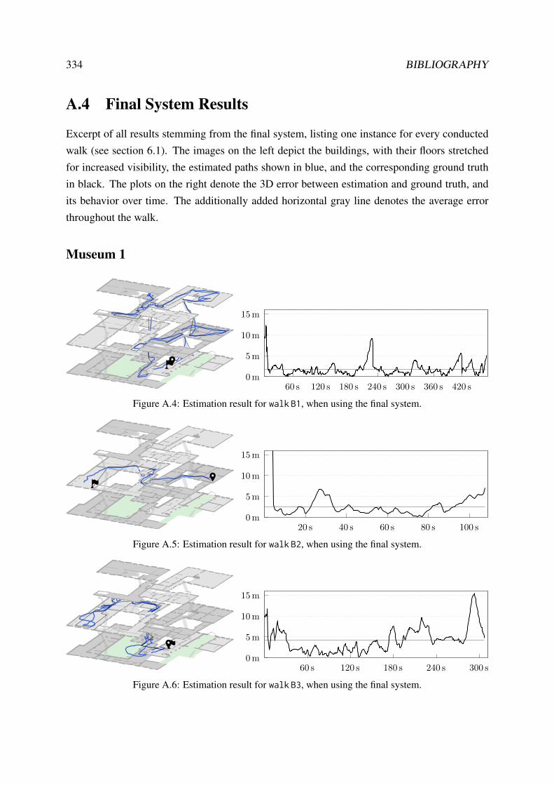
334 BIBLIOGRAPHY
A.4 Final System Results
Excerpt of all results stemming from the final system, listing one instance for every conductedwalk (see section 6.1). The images on the left depict the buildings, with their floors stretchedfor increased visibility, the estimated paths shown in blue, and the corresponding ground truthin black. The plots on the right denote the 3D error between estimation and ground truth, andits behavior over time. The additionally added horizontal gray line denotes the average errorthroughout the walk.
Museum 1
0 m
5 m
10 m
15 m
60 s 120 s 180 s 240 s 300 s 360 s 420 s
Figure A.4: Estimation result for walk B1, when using the final system.
0 m
5 m
10 m
15 m
20 s 40 s 60 s 80 s 100 s
Figure A.5: Estimation result for walk B2, when using the final system.
0 m
5 m
10 m
15 m
60 s 120 s 180 s 240 s 300 s
Figure A.6: Estimation result for walk B3, when using the final system.

A.4. FINAL SYSTEM RESULTS 335
SHL
0 m
5 m
10 m
15 m
30 s 60 s 90 s 120 s 150 s 180 s
Figure A.7: Estimation result for walk A1, when using the final system.
0 m
5 m
10 m
15 m
20 s 40 s 60 s 80 s 100 s 120 s 140 s
Figure A.8: Estimation result for walk A2, when using the final system.
0 m
5 m
10 m
15 m
15 s 30 s 45 s 60 s 75 s 90 s
Figure A.9: Estimation result for walk A3, when using the final system.
0 m
5 m
10 m
15 m
40 s 80 s 120 s 160 s
Figure A.10: Estimation result for walk A4, when using the final system.
0 m
5 m
10 m
15 m
15 s 30 s 45 s 60 s 75 s 90 s
Figure A.11: Estimation result for walk A5, when using the final system.

336 BIBLIOGRAPHY
Museum 2
0 m
5 m
10 m
15 m
20 s 40 s 60 s 80 s 100 s 120 s
Figure A.12: Estimation result for walk C1, when using the final system.
0 m
5 m
10 m
15 m
60 s 120 s 180 s 240 s 300 s
Figure A.13: Estimation result for walk C2, when using the final system.
0 m
5 m
10 m
15 m
120 s 240 s 360 s 480 s 600 s 720 s
Figure A.14: Estimation result for walk C3, when using the final system.
0 m
5 m
10 m
15 m
90 s 180 s 270 s 360 s 450 s 540 s
Figure A.15: Estimation result for walk C4, when using the final system.

Index
A*, 115, 117, 139, 151
accelerometer, 4, 27, 198, 217, 221, 331
activity, 12, 58–60, 201, 217
adjacency matrix, 127
angular velocity, 39, 43, 227, 228
antenna gain, 95
barometer, 4, 5, 53, 118, 198, 216
atmospheric pressure, 53, 238
barycentric, 146, 211, 212, 264
Bayes filter, 164, 166, 195
Bayes’ rule, 75, 159, 162
Bluetooth
beacon, 94, 207, 216
Low Energy, 216, 217
body frame, 43
bootstrap filter, 179
Box-Muller transform, 183
calibration, 16, 29, 232, 233, 237
central limit theorem, 19, 176
compass, 38, 230
declination, 38, 47, 48, 235
eCompass, 28, 104, 201, 221
geographic north, 38, 47–49
geomagnetic north, 47, 48, 230
hard iron, 51, 52, 232
inclination, 48, 49
magnetic north pole, 232magnetic south pole, 48soft iron, 51, 232
compensated summation, 59, 243complementary filter, 42–44, 101, 155, 221CONDENSATION algorithm, 179
dead reckoning, 4, 27, 221pedestrian dead reckoning, 27, 221
decision tree, 59, 243Delaunay, 142, 144Dijkstra, 115, 117, 151distribution
covariance, 60, 107, 167, 241cumulative distribution function, 181,
247exponential distribution, 35, 181, 206gamma distribution, 36mixture distribution, 37, 166, 201multimodal, 76, 81, 175, 195, 251multivariate, 107, 166, 255normal distribution, 19, 106, 161, 199,
241standard deviation, 77, 221uniform distribution, 19, 25, 178,
265–267unimodal, 166, 174, 187variance, 29, 160, 179, 187
337

338 INDEX
von Mises distribution, 46, 110, 130
Euler angle rates, 43Euler angles, 43, 44
filteringButterworth, 222convolution, 19, 165, 222FIR, 32, 222IIR, 32, 155, 222Linkwitz-Riley, 42
fingerprint, 50, 178, 210, 245Fourier transform, 34, 167funnel algorithm, 152–154
Gimbal lock, 43GPS, 1, 15, 102, 194, 221ground truth, 97, 206, 215, 334gyrocompass, 38, 39, 47gyroscope, 4, 18, 156, 198, 199, 216
Hall effect, 17, 48histogram, 82–84, 86, 176, 184, 210
IMMPF, 206, 208, 287importance sampling, 180IMU, 27, 198, 221inertial frame, 43inverse transform sampling, 181, 185
Jacobian matrix, 174
Kalman filter, 166, 167, 195, 251extended Kalman filter, 173, 195Kalman gain, 169
kernel density estimation, 82, 105, 176, 200bandwidth, 82–84Gaussian kernel, 83
Kullback-Leibler divergence, 206, 255
latitude, 23, 24, 49law of total probability, 108, 163, 274linear system, 168, 172localization
fine timing measurement, 98, 209lateration, 21, 195multilateration, 21TDOA, 21, 22, 98time of flight, 98TOA, 98
log-distance, 72, 88, 245extended log-distance model, 72, 210,
245, 246log-distance model, 68, 70, 210, 245log-normal shadowing model, 68
longitude, 23, 24lookup
k-d tree, 114, 122octree, 114, 122
MAC address, 74, 75, 96, 97magnetometer, 4, 5, 17, 198, 208, 216, 217Markov property, 163, 201Monte Carlo, 175–177, 179, 182
Naive Bayes, 61navigation grid, 124, 183, 191, 256navigation mesh, 144, 145, 183, 195, 256NFC, 55numerical optimization, 12, 76, 239
converge, 91, 94convex, 22, 51, 88–91downhill simplex, 22, 51genetic algorithm, 91gradient descent, 22, 51Moore–Penrose inverse, 23, 170Nelder-Mead, 22

INDEX 339
Newton’s method, 22overfitting, 87, 90, 94, 97, 216, 250simulated annealing, 91target function, 87, 88, 91, 93, 97, 253
occupancy grid, 113, 119, 121–123
partial derivative, 174particle filter, 4, 177, 178, 195, 215path loss, 64, 65, 90path loss exponent, 68PCA, 41
quantization noise, 19quaternion, 43, 44
radio signalsabsorption, 65, 66, 71attenuation, 65, 70, 246diffraction, 65, 66, 71, 252free space attenuation, 90, 245, 252free space loss, 65, 66multipath, 68multipath propagation, 66, 81reflection, 65, 66, 71, 248refraction, 65, 66, 71, 248scattering, 65, 66, 68shadowing, 65, 66, 71, 205
random walk, 132, 183, 201, 256RANSAC, 52ray tracing, 72, 114, 192reference measurement, 12, 56, 212, 218rejection sampling, 182, 183, 186, 187resampling, 185, 196, 251RFID, 55root mean square error, 87–92, 247, 250rotation axis, 44, 227, 228rotation matrix, 40, 41, 44RSSI, 62, 207, 248
sensor fusion, 13, 42, 45, 238signal strength, 4, 62, 203, 217
prediction model, 12, 67, 205, 244step-detection, 4, 11, 30, 196, 216SVM, 31, 61
Taylor series, 174tilt compensation, 49, 59, 224, 226transmission power, 64, 74, 90, 94turn-detection, 4, 28, 30, 104, 196, 216turn-rate, 37, 228
virtual access point, 96Voronoi, 141–144
zero mean, 19, 110, 155

340 INDEX

Lebenslauf
03/1986 Geboren in Werneck
09/1992 – 07/1996 Volksschule Am Wehrbusch, Grafenrheinfeld
09/1996 – 12/2004 Alexander-von-Humboldt-Gymnasium, SchweinfurtAbschluss: Mittlerer Schulabschluss
09/2005 – 07/2007 Friedrich-Fischer-Schule, SchweinfurtAbschluss: Fachabitur
09/2007 – 05/2008 Zivildienst imJugendhilfezentrum Maria Schutz, Grafenrheinfeld
10/2008 – 03/2012 Bachelor Studium Informatik an derFachhochschule Wurzburg-SchweinfurtAbschluss: Bachelor of Engineering
03/2012 – 02/2014 Master Studium Informationssysteme an derHochschule fur angewandte Wissenschaften Wurzburg-SchweinfurtAbschluss: Master of Science
02/2014 – 03/2020 Wissenschaftlicher Mitarbeiter an derHochschule fur angewandte Wissenschaften Wurzburg-SchweinfurtAufgabenschwerpunkt: Softwareentwicklung, Forschung und Lehre


Logos Verlag Berlin ISBN 978-3-8325-5232-9
ISSN 2701-9446
Technical innovation results in an enormous amount of data and information
that can be used for the description and analysis of individual humans andwho-
le populations. In this context, methods combining dierent sensor modalities
using suitable models are investigated to advance the understanding of the
human physical and mental state. This book series is dedicated to this broad
eld of research.
During the last century, navigation systems have become ubiquitous and guide
drivers, cyclists, and pedestrians towards their desired destinations. While
operating worldwide, they rely on line-of-sight conditions towards satellites
and are thus limited to outdoor areas. However, nding a gate within an
airport, a ward within a hospital, or a university’s auditorium also represent
navigation problems. To provide navigation within such indoor environments,
new approaches are required.
This thesis examines pedestrian 3D indoor localization and navigation using
commodity smartphones: A desirable target platform, always at hand and
equipped with a multitude of sensors. The IMU (accelerometer, gyroscope,
magnetometer) and barometer allow for pedestrian dead reckoning, that is,
estimating relative location changes. Absolute whereabouts can be determined
via Wi-Fi, an infrastructure present within most public buildings, or by using
Bluetooth Low Energy Beacons as inexpensive supplement. The building’s
3D floorplan not only enables navigation, but also increases accuracy by
preventing impossible movements, and serves as a visual reference for the
pedestrian. All aforementioned information is fused by recursive density
estimation based on a particle lter.
The conducted experiments cover both, theoretical backgrounds and real-world
use-cases. All discussed approaches utilize the infrastructure found within
most public buildings, are easy to set up, and maintain. Overall, this thesis
results in an indoor localization and navigation system that can be easily
deployed, without requiring any special hardware components.
Copyright © 2022 FDOKUMEN