1

Copyright Notice

This is the authors version of a work that was accepted for

publication in Pattern Recognition Letters.

Cristoforis, Nitsche, Krajnik, Pire, Mejail: Hybrid vision-

based navigation for mobile robots in mixed indoor/outdoor en-

vironments, Pattern Recognition Letters, 2014.

Changes resulting from the publishing process, such as

peer review, editing, corrections, structural formatting, and

other quality control mechanisms may not be reflected in

this document. Changes may have been made to this work

since it was submitted for publication. The full version

of the article is available on Elsevier’s sites with DOI:

10.1016/j.patrec.2014.10.010.

2

Pattern Recognition Lettersjournal homepage: www.elsevier.com

Hybrid vision-based navigation for mobile robots in mixed indoor/outdoor environments

Pablo De Cristoforisa,∗∗, Matias Nitschea, Tomas Krajnıkb,c, Taihu Pirea, Marta Mejaila

aLaboratory of Robotics and Embedded Systems, Faculty of Exact and Natural Sciences, University of Buenos Aires, ArgentinabLincoln Centre for Autonomous Systems, School of Computer Science, University of Lincoln, United KingdomcDepartment of Cybernetics, Faculty of Electrical Engineering, Czech Technical University in Prague, Czech republic

ARTICLE INFO ABSTRACT

Article history:

2000 MSC:

41A05

41A10

65D05

65D17

Keywords:

Vison-based navigation

Mixed indoor/outdoor environmets

Mobile robotics

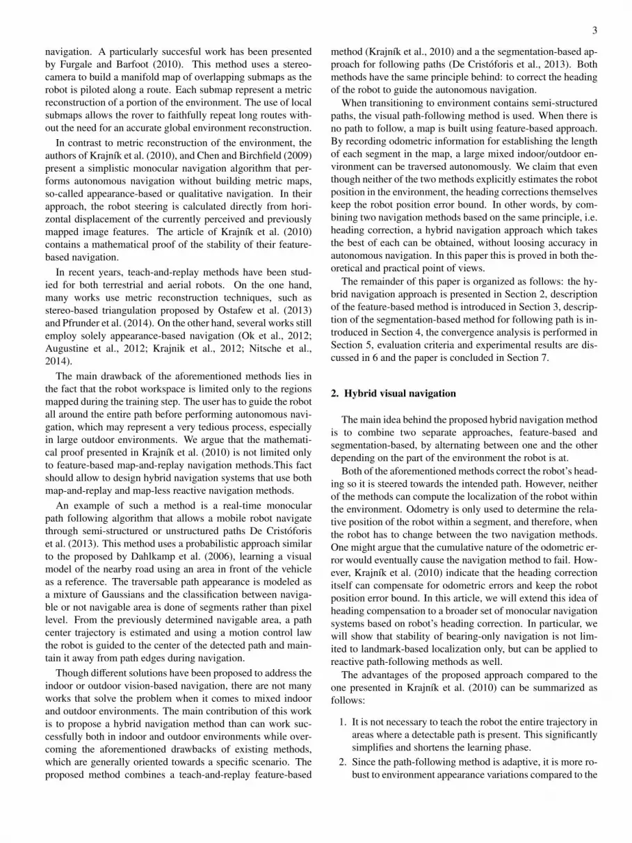
In this paper we present a vision-based navigation system for mobile robots

equipped with a single, off-the-shelf camera in mixed indoor/outdoor environ-

ments. A hybrid approach is proposed, based on the teach-and-replay tech-

nique, which combines a path-following and a feature-based navigation al-

gorithm. We describe the navigation algorithms and show that both of them

correct the robot’s lateral displacement from the intended path. After that, we

claim that even though neither of the methods explicitly estimates the robot po-

sition, the heading corrections themselves keep the robot position error bound.

We show that combination of the methods outperforms the pure feature-based

approach in terms of localization precision and that this combination reduces

map size and simplifies the learning phase. Experiments in mixed indoor/out-

door environments were carried out with a wheeled and a tracked mobile robots

in order to demonstrate the validity and the benefits of the hybrid approach.

c© 2014 Elsevier Ltd. All rights reserved.

1. Introduction

Autonomous navigation can be roughly described as the pro-

cess of moving safely along a path between a starting and a final

point. In mobile robotics, different sensors have been used for

this purpose, which has led to a varied spectrum of solutions.

Active sensors such as sonars (Borenstein and Koren, 1988),

laser range finders (Surmann et al., 2001) and radars (Kaliyape-

rumal et al., 2001) have been used in autonomous navigation

methods. These sensors are inherently suited for the task of

obstacle detection and can be used easily because they directly

measure the distances from obstacles to the robot.

Other sensors that are becoming a standard part in mobile

robotic systems, particularly in field robotics, are visual sen-

sors. Quality cameras have become increasingly affordable,

they are small and can provide high resolution data in real time.

They are passive and therefore do not interfere with other sen-

sors. Unlike range sensors, they can not only be used to de-

∗∗Corresponding author:

e-mail: pdecris@dc.uba.ar (Pablo De Cristoforis)

tect obstacles, but also to identify forbidden areas and navi-

gate mobile robots using human-defined rules (i.e. keep off the

grass). Such forbidden areas are not obstacles, since they are

in the same plane as the path, but should be considered as non-

traversable. Moreover, and probably more important, nowadays

computational power required by image processing techniques

is readily available in consumer hardware. For these reasons, in

recent years vision-based navigation for mobile robots has been

a widely studied topic.

Many visual navigation methods generally rely on the ex-

traction of salient visual features, using algorithms such as

well-known SIFT (Scale Invariant Feature Transform) or SURF

(Speeded Up Robust Features), among others. These are then

used as external references from which information about the

structure of the surrounding environment and/or the ego-motion

of the robot is estimated.

A classical approach to visual navigation is known as teach-

and-replay. This technique is closely related to visual servo-

ing (Chaumette and Hutchinson, 2006; F. Chaumette and S.

Hutchinson, 2007), where the task is to reach a desired pose us-

ing vision for control feedback. Several teach-and-replay works

employ visual features as landmarks to guide the autonomous

3

navigation. A particularly succesful work has been presented

by Furgale and Barfoot (2010). This method uses a stereo-

camera to build a manifold map of overlapping submaps as the

robot is piloted along a route. Each submap represent a metric

reconstruction of a portion of the environment. The use of local

submaps allows the rover to faithfully repeat long routes with-

out the need for an accurate global environment reconstruction.

In contrast to metric reconstruction of the environment, the

authors of Krajnık et al. (2010), and Chen and Birchfield (2009)

present a simplistic monocular navigation algorithm that per-

forms autonomous navigation without building metric maps,

so-called appearance-based or qualitative navigation. In their

approach, the robot steering is calculated directly from hori-

zontal displacement of the currently perceived and previously

mapped image features. The article of Krajnık et al. (2010)

contains a mathematical proof of the stability of their feature-

based navigation.

In recent years, teach-and-replay methods have been stud-

ied for both terrestrial and aerial robots. On the one hand,

many works use metric reconstruction techniques, such as

stereo-based triangulation proposed by Ostafew et al. (2013)

and Pfrunder et al. (2014). On the other hand, several works still

employ solely appearance-based navigation (Ok et al., 2012;

Augustine et al., 2012; Krajnik et al., 2012; Nitsche et al.,

2014).

The main drawback of the aforementioned methods lies in

the fact that the robot workspace is limited only to the regions

mapped during the training step. The user has to guide the robot

all around the entire path before performing autonomous navi-

gation, which may represent a very tedious process, especially

in large outdoor environments. We argue that the mathemati-

cal proof presented in Krajnık et al. (2010) is not limited only

to feature-based map-and-replay navigation methods.This fact

should allow to design hybrid navigation systems that use both

map-and-replay and map-less reactive navigation methods.

An example of such a method is a real-time monocular

path following algorithm that allows a mobile robot navigate

through semi-structured or unstructured paths De Cristoforis

et al. (2013). This method uses a probabilistic approach similar

to the proposed by Dahlkamp et al. (2006), learning a visual

model of the nearby road using an area in front of the vehicle

as a reference. The traversable path appearance is modeled as

a mixture of Gaussians and the classification between naviga-

ble or not navigable area is done of segments rather than pixel

level. From the previously determined navigable area, a path

center trajectory is estimated and using a motion control law

the robot is guided to the center of the detected path and main-

tain it away from path edges during navigation.

Though different solutions have been proposed to address the

indoor or outdoor vision-based navigation, there are not many

works that solve the problem when it comes to mixed indoor

and outdoor environments. The main contribution of this work

is to propose a hybrid navigation method than can work suc-

cessfully both in indoor and outdoor environments while over-

coming the aforementioned drawbacks of existing methods,

which are generally oriented towards a specific scenario. The

proposed method combines a teach-and-replay feature-based

method (Krajnık et al., 2010) and a the segmentation-based ap-

proach for following paths (De Cristoforis et al., 2013). Both

methods have the same principle behind: to correct the heading

of the robot to guide the autonomous navigation.

When transitioning to environment contains semi-structured

paths, the visual path-following method is used. When there is

no path to follow, a map is built using feature-based approach.

By recording odometric information for establishing the length

of each segment in the map, a large mixed indoor/outdoor en-

vironment can be traversed autonomously. We claim that even

though neither of the two methods explicitly estimates the robot

position in the environment, the heading corrections themselves

keep the robot position error bound. In other words, by com-

bining two navigation methods based on the same principle, i.e.

heading correction, a hybrid navigation approach which takes

the best of each can be obtained, without loosing accuracy in

autonomous navigation. In this paper this is proved in both the-

oretical and practical point of views.

The remainder of this paper is organized as follows: the hy-

brid navigation approach is presented in Section 2, description

of the feature-based method is introduced in Section 3, descrip-

tion of the segmentation-based method for following path is in-

troduced in Section 4, the convergence analysis is performed in

Section 5, evaluation criteria and experimental results are dis-

cussed in 6 and the paper is concluded in Section 7.

2. Hybrid visual navigation

The main idea behind the proposed hybrid navigation method

is to combine two separate approaches, feature-based and

segmentation-based, by alternating between one and the other

depending on the part of the environment the robot is at.

Both of the aforementioned methods correct the robot’s head-

ing so it is steered towards the intended path. However, neither

of the methods can compute the localization of the robot within

the environment. Odometry is only used to determine the rela-

tive position of the robot within a segment, and therefore, when

the robot has to change between the two navigation methods.

One might argue that the cumulative nature of the odometric er-

ror would eventually cause the navigation method to fail. How-

ever, Krajnık et al. (2010) indicate that the heading correction

itself can compensate for odometric errors and keep the robot

position error bound. In this article, we will extend this idea of

heading compensation to a broader set of monocular navigation

systems based on robot’s heading correction. In particular, we

will show that stability of bearing-only navigation is not lim-

ited to landmark-based localization only, but can be applied to

reactive path-following methods as well.

The advantages of the proposed approach compared to the

one presented in Krajnık et al. (2010) can be summarized as

follows:

1. It is not necessary to teach the robot the entire trajectory in

areas where a detectable path is present. This significantly

simplifies and shortens the learning phase.

2. Since the path-following method is adaptive, it is more ro-

bust to environment appearance variations compared to the

4

feature-based method. This increases the overall reliabil-

ity of the navigation.

3. The path following method reduces robot positioning error

faster than the feature-based approach. Thus, combination

of both methods allows for a more precise navigation.

4. The path following method does not need to store infor-

mation about the entire edge that is to be traversed. Rather

than that, it just need information about the path texture,

which dramatically reduces spatial requirements for stor-

age of the topological map especially when traversing long

outdoor paths.

2.1. Method overview

The topological map that the method uses is a graph where

nodes represent places in the environment and edges represent

the navigation methods that can be used to move between these

places. While the nodes are associated with azimuths indicating

directions of the outgoing edges, the edges contain information

that allows the robot to traverse between the individual places.

In other words, an edge of the hybrid topological map repre-

sents an action that the robot should take during its length in

different parts of the route: i.e. either the path-following or the

feature-based navigation.

The environment map is created during a training phase

where the user builds a topological map by driving a semi-

autonomously moving robot through the environment. During

the training, the robot either moves forwards while creating an

image-feature based map or it follows a pathway of the environ-

ment. Whenever the user terminates the current behaviour, the

robot records the length of the edge and creates a topological

node. Then, the user can manually set the robot orientation and

start path following or feature mapping again. It is important to

note that if the length of the path-following edge is known (e.g.

from an overhead map), there is no need to traverse the edge

during the learning phase.

Fig. 1. Schematic of an example map of the hybrid method for a given

indoor/outdoor scenario. Lines marked in blue consist of the portions of

the map which are traversed using the path-following method, while lines

marked in red, portions which are traversed using the feature-based ap-

proach.

In the autonomous navigation or “replay” phase, the robot

traverses a sequence of edges by either one of the two move-

ment primitives. Note that neither or the methods performs lo-

calization of the robot. Both methods simply keep the robot

close to the trained paths while using odometric reading to de-

cide whether the particular edge has been traversed or not. In

Section 5 we will show that despite of simplicity of the ap-

proach, the robot position error does not diverge over time.

In the next sections we will describe each navigation move-

ment primitive: feature-based for open areas (indoor or out-

door) where there is not bounded path to go through, or cross in-

tersection of two or more paths, and image segmentation based

method conceived to follow structured or semi-structured paths.

3. Feature-based visual navigation

The feature-based navigation method used as a motion prim-

itive of the proposed approach is based on Krajnık et al. (2010).

This method uses the map-and-replay technique which is de-

scribed in this section. This method allows a robot to follow a

given path by performing an initial learning phase where fea-

tures extracted from the camera images are stored. In a sec-

ond replay phase, the robot autonomously navigates through

the learned path while correcting its heading by comparing cur-

rently seen and previously stored features.

3.1. Image Features

Since image features are considered as visual landmarks, the

feature detector and descriptor algorithms are a critical compo-

nent of the navigation method. Image features must provide

enough information to steer the robot in a correct direction.

Furthermore, they should be robust to real world conditions,

i.e. changing illumination, scale, viewpoint and partial occlu-

sions and of course its performance must allow real-time op-

eration. In the original version of the method, Krajnık et al.

used SURF (Speeded Up Robust Feature) algorithm proposed

by Bay et al. (2008) to identify visual landmarks in the im-

age. The SURF method is reported to perform better than most

SIFT (Lowe, 2004) implementations in terms of speed and ro-

bustness to viewpoint and illumination change.

For this work, further evaluation of a variety of extractor

and descriptor algorithms, in the context of visual navigation,

was performed. The goal of these off-line experiments was to

determine which algorithm combination is the best choice for

visual navigation in terms of performance, robustness and re-

peatability (Krajnık et al., 2013). As a result of this evaluation,

we conclude that the combination of STAR based on CenSurE

(Center Surround Extremas) algorithm (Agrawal et al., 2008)

to detect image features and BRIEF (Binary Robust Indepen-

dent Elementary Features) algorithm (Calonder et al., 2010) to

build the descriptor of the feature outperforms the other image

feature extraction algorithms. The STAR extractor gives bet-

ter results to detect landmarks than SURF, because keypoints

extracted with STAR are more salient and thus, also more sta-

ble than keypoints extracted with SURF. The BRIEF descrip-

tor uses a simpler coding scheme to describe a feature, this re-

duces storage requirements and increases matching speed. The

SURF use 64 (or 128 in the extended version) double-precision

floating-point values to describe a keypoint, this results in 512

5

bytes (or 1024) of data for each descriptor. In contrast, BRIEF

uses a string of bits that can be packed in 32 bytes. Taking

into account the high number of features present in the map,

this can amount to hundreds of megabytes which are saved in

large-scale maps. Furthermore, in terms of speed, instead of us-

ing the Euclidean distance to compare descriptors as it is done

with SURF, BRIEF descriptors can be compared using Ham-

ming distance, which can be implemented extremely fast using

SSE instructions.

3.2. Learning Phase

In the initial learning phase, the robot is manually guided

through the environment while the map is built. The operator

can either let the robot go forward or stop it and turn it in a de-

sired direction. A map can therefore be built, which will have

the shape of a series of segments of certain length as computed

by the robots odometry. During forward movement, the robot

tracks features extracted from the robot’s camera images. For

each feature, its position in the image is saved along its descrip-

tor. Also, initial and final distances (as measured by the robot’s

odometry) along the segment where the feature was first and

last seen are also saved. Tracking is performed by extracting

features for the present frame and comparing these to others

that were continously seen in previous frames. While features

remain in the set of tracked landmarks, their information can be

updated. When features are not seen anymore, they are added

to the map and removed from this set. Matching is performed

by comparing descriptors.

The procedure which creates a map of one segment is as fol-

lows in the listing 1. Each landmark has an associated descrip-

tor ldesc, pixel position lpos0, lpos1

and robot relative distance

ld0, ld1

, for when the landmark was first and last seen, respec-

tively.

The map obtained by this approach is thus composed of a

series of straight segments, each described by its length s, az-

imuth φ0 and a set of detected landmarks L. A landmark l ∈ L

is described by a tuple (e, k,u, v, f , g), where e is its BRIEF

descriptor and k indicates the number of images, in which the

feature was detected. Vectors u and v denote positions of the

feature in the captured image at the moment of its first and last

detection and f and g are distances of the robot from the seg-

ment start at these moments.

3.3. Autonomous Navigation Phase

In order to navigate the environment using this method, the

robot is initially placed near the starting position of a known

segment. Then, the robot moves forward at constant speed

while correcting its heading. This is performed by retrieving

the set of relevant landmarks from the map at each moment and

to estimate their position in the current camera image. These

landmarks are paired with the currently detected ones and the

differences between the estimated and real positions are calcu-

lated. As these differences in image coordinates are related to a

displacement of the robot in the world, it is possible to actively

minimize these by moving the robot accordingly, and thus the

previously learnt path is replayed.

Algorithm 1: Learning Phase

Input: ϕ: initial robot orientation

Output: L: landmarks learned for the current segment,

s: segment length, ϕ0: segment orientation

ϕ0 ← ϕ read robot orientation from gyro or compass

L← ∅; /* clear the learned landmark set */

T ← ∅; /* clear the tracked landmark set */

repeatF ←features extracted from the current camera image

foreach l ∈ T dof ← find match(l,F)

if no match then

T ← T − { l } ; /* stop tracking */

L← L ∪ { l } ; /* add to segment */

elseF ← F − { f }

l← (ldesc, lpos0, fpos, ld0

, d) /* update image

coordinates & robot position */

foreach f ∈ F do

T ← T ∪ { ( fdesc, fpos0, fpos0

, d, d) } ; /* start

tracking new landmark */

until operator terminates learning mode

L← L ∪ T ; /* save tracked landmarks */

s← d ; /* remember the segment’s length */

Algorithm 2: Navigation Phase

Input: L: landmarks of the current segment s: current

segment length

Output: ω: angular robot speed v: forward robot speed

v← v0 ; /* start moving forwards */

while d < s do

H ← ∅ ; /* pixel-position differences */

T ← ∅ ; /* tracked landmarks */

foreach l ∈ L do

if ld0< d < ld1

then

T ← T ∪ { l } ; /* get expected

landmarks according to d */

F ←features extracted from the current camera image

while T not empty dof ← find match(l,F)

if matched then

/* compare feature position to

estimated current landmark

position by interpolation */

h← fpos −

(

(lpos1− lpos0

)d − ld0

ld1− ld0

+ lpos0

)

H ← H ∪ { h }

T ← T − { l }

ω← γ mode(H)

v, ω← 0 ; /* segment completed, stop moving */

6

More formally, the replay phase is as follows. Each time a

new image is captured, the robot updates the estimated traveled

distance d from the start of the segment and builds the set T by

retrieving landmarks in L that were visible at distance d during

learning. Then, features are extracted from the current camera

image and put in the set F. A pairing between the sets F and

T is established as in the learning phase. After establishing

these correspondences, for each pair of matching features their

image position is compared. The expected image position of

landmarks in T is obtained by linearly interpolating according

to d, since only initial and last image positions of landmarks

are stored during mapping to reduce map size. By taking the

horizontal difference in image positions a heading correction

for the robot can be established. To obtain a single correction

value, the most likely horizontal position needs to be obtained

since the matching process may produce outliers. Thus, this

single deviation value is obtained by sampling all horizontal

differences in a histogram and taking its mode.

While the robot moves forward at constant speed, this head-

ing correction is performed for each frame until d equals the

segment length stored in the map. The listing 2 presents the

algorithm used to traverse or ‘replay’ one segment.

4. Segmentation-based path-following

The path-following method used as motion primitive

of the proposed approach is based on a previous work

by De Cristoforis et al. (2013). Here, a mobile robot is au-

tonomously steered in order to remain inside a semi-structured

path by means of image processing alone.

The method works by first dividing the image into regions

or segments of similar appearance and then classifying these as

belonging to traversable or non-traversable areas. It does not

require a learning phase since it uses the area immediately in

front of the robot in order to obtain a sample of traversable ter-

rain. A gaussian-mixture model is used to describe this sample

(using the Hue, Saturation and Value components) and compare

to the rest of the regions in the image. After classification, the

most likely group of interconnected image segments is used to

obtain a contour of traversable path. With this contour a sim-

ple control law which infers the path middle line and steers the

robot to follow it is used.

Since the method only requires the area of the image below

the horizon level (i.e. the ground) to steer the robot, an initial

horizon detection method can be used to infer this area and re-

strict processing to the meaninful portion of the image. Figure

2 shows the image processing pipeline.

4.1. Image Segmentation

In outdoor semi-structured or unstructured environments, the

traversable area is often cluttered by small objects with a color

of the forbidden area, for example grass, tree leaves, water or

even snow in the middle of the road. In this case, most classifi-

cation methods working at a pixel level, like the one proposed

by Dahlkamp et al. (2006), would perform worse than methods

which first segment the image to several areas with similar tex-

ture or color. Thus, the initial step in the path-detection process

(a) Input image (b) Cropped &

blured

(c) Segment Map

(d) Hue per pixel (e) Mean hue per

super-pixel

(f) Value per pixel

(g) Mean value per

super-pixel

(h) Saturation per

pixel

(i) Mean saturation

per super-pixel

(j) Super-pixel clas-

sification as binary

mask

(k) Filtered binary

mask

(l) Path contour

Fig. 2. Pipeline description: (a) input image as acquired from the cam-

era, (b) cropped image below automatically detected horizon, (c) segment

map. For each segment, mean and covariance are computed:(e), (i) and (g)

show segment hue, saturation and value means respectively (d), (h) and(f)

show pixel hue, saturation and value for reference. (j) binary mask ob-

tained from classification using ground models from ROI. (k) morpholog-

ical opening filter is applied in order to ‘close’ small gaps in the binary

mask. (l) path contour extracted from processed binary mask and middle

points computed, on top-left linear and angular speeds values obtained by

control law.

is to segment the image into a set of super-pixels. After the im-

age is cropped to contain the region below the horizon (either

automatically or manually), the result is initially filtered to re-

duce noise (using a median-blur, which preserves edge contrast)

and then segmented. The segmentation algorithm used is the

graph-based approach proposed by Felzenszwalb and Hutten-

locher (2004). The algorithm first constructs a fully connected

graph where each node corresponds to a pixel in the image.

Pixel intensities between neighbors are analyzed and edges are

broken whenever a threshold is exceeded. The resulting uncon-

nected sub-graphs define the segments (or super-pixels).

4.2. Classification

To achieve a robust classification of the segments, a proba-

bilistic approach is used, based on Dahlkamp et al. (2006). This

step determines if a population sample (a segment), modeled

by a Gaussian probability distribution N(µ,Σ), with mean vec-

tor µ and covariance matrix Σ, represents an instance of a more

general model of the ‘navigable path’ class or not. This naviga-

ble path class is represented in turn by a Mixture-of-Gaussians

7

(MoG) model. The steps involved in the classification task are

as follows:

1. Segment model computation: each segment is modeled by

its mean µ and covariance Σ of HSV color values.

2. Navigable class computation: a rectangular ROI (Region

Of Interest) in the lower part of the image is used as a refer-

ence of navigable path (see Fig. 2). All models contained

in this ROI are merged by similarity (using Mahalanobis

distace). The resulting models which cover the ROI area

by more than a defined percentage are used as references

for navigable regions in the image.

3. Classification of all segments: All segments in the image

are compared to the reference models for navigable path

using the Mahalanobis distance. A binary mask for all

pixels is created indicating the membership to this class.

4. Contour extraction: the binary mask is post-processed by

a morphological opening operation to reduce artifacts and

from all regions classified as navigable path, the area in-

tersecting the ROI region is chosen. The contour of this

region is computed.

4.3. Motion control

The goal of the motion control is to correct the heading of

the robot to keep it in the middle of the road. From the previ-

ously determined contour, a path center trajectory is estimated

in order to guide the robot to the center of the detected path

and maintain it away from path edges. First, by going row-

by-row in the image, the middle point for the current row is

obtained from the leftmost and rightmost pixel’s horizontal po-

sitions of the path contour. The list of middle points is then used

to compute angular and linear speeds with a simple yet effective

control-law as follows. From the list of n horizontal values ui of

the i-th middle point of the detected path region, angular speed

ω and forward speed v are computed as follows:

ω = α

n∑

i

(

xi −w

2

)

, v = βn − |ω| (1)

where w is the width of the image and α and β are constants

specific to the robot’s speed controllers.

The effects of this control law are such that the robot will

turn in the direction where there is the highest deviation, in av-

erage, from middle points with respect to a vertical line passing

through the image center. This line can be assumed to be the

position of the camera, which is mounted centered on the robot.

Therefore, whenever a turn in the path or an obstacle is present,

the robot will turn to remain inside the path and avoid the obsta-

cle. The linear speed of the robot is reduced accordingly to the

angular speed determined by the previous computation. This

has the effect of slowing down the robot whenever it has to take

a sharp turn.

5. Robot position error analysis

In this section we show that despite the fact that the robot

localization is based on odometry, the robot position error does

not diverge over time due to the heading corrections caused by

the two movement primitives. Our analysis assumes that a mo-

bile robot moves through a sequence of n waypoints by using

reactive navigation algorithms (or motion primitives) that steer

the robot towards the waypoint’s connecting lines. We describe

robot position at each waypoint in the waypoint’s coordinate

frame and show that the robot’s relative position to a particular

waypoint can be calculated by a recursive formula xk+1 = Mk xk,

where the matrix Mk eigenvalues are 1 and mk. First, we show

that mk is lower than 1 because of the heading corrections in-

troduced by the motion primitive used to navigate between kth

and (k + 1)th waypoint. Finally, we show that if all the path

waypoints do not lie on a straight line, M =∏

k = 0n−1Mk

dominant eigenvalue is lower than one, meaning that the robot

position error is reduced as it travels the entire path.

5.1. Robot movement model

Let us assume that the robot moves on a plane and its position

and heading is x, y, ϕ respectively. Assume that the edge to be

traversed starts at coordinate origin and leads in the direction of

the x-axis.

The path following method presented in Section 4.1 calcu-

lates the robot’s steering speed ω directly from image coor-

dinates of the segmented path center. These coordinates are

affected by both robot heading φ and lateral displacement y.

Larger robot displacement and larger heading deviation cause

larger values of the steering speed, i.e.

ω ∼ −c0y − c1ϕ. (2)

Given that the robot’s speed v is much lower compared to the

maximal rotation speed ω, the robot can change its heading

much faster than its horizontal displacement y. Thus, a robot

steered by the method presented in Section 4 will quickly stabi-

lize its heading and reach a state when its rotation speed ω will

be close to zero. This allows to rewrite Equation 2 to

0 ≈ −c0y − c1ϕ. (3)

Thus, heading ϕ of a robot following the path can be expressed

as

ϕ ≈ −k0y, (4)

where k0 is a positive constant.

The case of the feature-based method is similar. If the robot

is displaced in a lateral direction from the path, i.e. in the direc-

tion of the y-axis, the perceived features will not be visible at

the expected positions, but will be shifted to the right for y > 0

and to the left y < 0.

Since the feature-based method steers the robot in a direction

that minimizes the difference (in horizontal coordinates) of the

expected and detected features, the robot heading will be stabi-

lized at a value that is proportional to its lateral displacement.

In other words, the robot heading ϕ satisfies a similar constrain

as in the previous case:

ϕ ≈ −k1y, (5)

where k1 is a positive constant.

8

Thus, both of the motion primitives of the hybrid method

adjust the robot heading ϕ proportionally to its lateral displace-

ment from the path, i.e. ϕ ≈ −ky, where k > 0. Both meth-

ods move the robot along the edge until the robots odometric

counter reports that the distance travelled exceeded the length

of the edge stored in the map. Assuming that the robot heading

ϕ is small, we can state that

dy

dx= ϕ = −ky. (6)

Let the initial position of the robot be (ax, ay), where the val-

ues of (ax, ay) are significantly smaller than the segment length.

Solving this differential equation with boundary conditions

ay = f (ax) allows us to compute the robot position:

y = aye−kx. (7)

Considering a segment of length s, we can calculate the robot

position (bx, by) after it traverses the entire segment as:

bx=ax + s

by=aye−ks.(8)

Equation (8) would hold for an error-less odometry and noise-

less camera. Considering the camera and odometry noise,

Equation (8) will be rewritten to

(

bx

by

)

=

(

1 0

0 e−sk

) (

ax

ay

)

+

(

sυ

ξ

)

, (9)

where υ and ξ are normally distributed random variables,

µ(υ) = 1, σ(υ) = ǫ, µ(ξ) = 0 and σ(ξ) = τ. A compact form of

(9) is

b =Ma + s. (10)

For a segment with an arbitrary azimuth, one can rotate the co-

ordinate system by the rotation matrix R, apply (10) and rotate

the result back by RT. Thus, Equation (10) would become

b = RT (MRa + s) = RTMRa + RTs. (11)

Using (11), the robot position b at the end of the segment can be

computed from its starting position a. Equations (11) allow to

calculate robot position as it traverses along the intended path.

5.2. Position error

Let the robot initial position a be a random variable drawn

from a two-dimensional normal distribution with the mean a.

Since Equation (11) has only linear and absolute terms, the final

robot position b will have a normal distribution as well. Let

a = a+a, where a is a random normal variable with zero mean.

Assuming the same notation for b and s, Equation (11) can be

rewritten as

b = RTMR(a + a) + RT(s + s) − b. (12)

Substituting RTMRa + RTs for b, Equation (12) becomes

b = RTMRa + RTs, (13)

where a, b, s are Gaussian random variables with zero mean.

The a and b represent the robot position error at the start and

end of the traversed segment.

5.3. Traversing multiple segments

Let the robot path is a closed chain of n linear segments de-

noted by numbers from 0 to n − 1. Let a segment i be oriented

in the direction αi and its length be si. Let the robot positions

at the start and end of the ith segment are ai and bi respectively.

Since the segments are joined, bi = ai+1 and Equation (13) for

the ith traveled segment is

ai+1 = Niai + RTi si, (14)

where Ni = RTi

MiRi. Thus, the robot position after traversing

the entire path consisting of the n segments will be

an = Na0 + t, (15)

where

N =

0∏

j=n−1

Nj and t =

n−1∑

i=0

n−1∏

j=i+1

Nj

RTi si. (16)

If the robot traverses the entire path k-times, its position can be

calculated in a recursive way by

a(k+1)n = Nakn + t. (17)

Since the mean of every si is equal to zero and si have normal

distribution, t, that is a linear combination of si, has a normal

distribution with zero mean as well. Therefore, Equation (17)

describes a linear discrete stochastic system, where the vector t

represents a disturbance vector. If the system characterized by

(17) is stable, then the position deviation of the robot from the

intended path ai does not diverge for k → +∞. The system is

stable if all eigenvalues of N lie within a unit circle.

As every Ni equals to RTi

MiRi, its eigenvalues lie on the

diagonal of Mi and its eigenvectors constitute columns of Ri.

Therefore, each matrix Ni is positive-definite and symmetric.

Since the dominant eigenvalue of every Ni equals to one, eigen-

values of N are smaller or equal to one. Since the dominant

eigenvalue of N is equal to one if and only if the dominant

eigenvalues of products Ni+1Ni are equal 1 for all i. However,

dominant eigenvalue of a product Ni+1Ni equals 1 only if the

dominant eigenvectors of both Ni and Ni+1 are linearly depen-

dent, which corresponds to collinearity of ith and (i + 1)th seg-

ment. Thus, a dominant eigenvalue n of the matrix N equals 1

if and only if all path segments are collinear, i.e. the entire path

is just a straight line. For any other case, the spectral radius

of N is lower than one, meaning that the system described by

(17) is stable. This means that if the robot travels the trajectory

repeatably, its position error akn does not diverge.

6. Experimental results

The proposed hybrid vision-based navigation system was im-

plemented in C/C++within the ROS (Robot Operating System)

framework as a set of separate ROS modules1. The perfor-

mance of the navigation system has been evaluated in an in-

door/outdoor environment. The experiments were performed

1We will plan to release an open version of the software if the paper is

accepted.

9

outside and inside of the Pabellon 1 building, Ciudad Universi-

taria, Buenos Aires, Argentina. Two sets of experiments were

performed with two different robots. Two robotic platforms

were used for experiments: a small differential caterpillar-

tracked robot called ExaBot (Pedre et al., 2014) and a four-

wheeled P3-AT from MobileRobots. Both platforms were

equipped with a single off-the-shelf camera and a Core i5 laptop

as the sensing and processing elements, respectively.

Additionally, the motion model correctness was also demon-

strated in practice, by teaching and repeating a single straight

segment in an outdoor scenario, using both methods. Finally,

the computational efficiency of the method was measured.

6.1. Motion model correctness

The first scenario was aimed at verification of the assump-

tions given in Section 5.1. In particular, we wanted to calculate

if the robot motion model established by equations 7 conforms

to real robot motion along one straight segment. To verify the

motion model, we have taught the robot to traverse a 5.6 m

long straight path. Then, we executed the autonomous naviga-

tion system in order to repeat the path 5 times, with an initial

lateral displacement of about 0.5 m from the original starting

point. The robot motion was tracked using an external localiza-

tion system Krajnık et al. (2014). We used both segmentation-

and feature-based methods for this test.The recovered trajecto-

ries, compared with an expected exponential shape given by 7,

are presented on Figure 3, where the stability of the system is

appreciated. The trajectories described by both methods corre-

spond to the exponential model presented in equation 7.

As can be seen, both navigation methods converge. How-

ever, it can be easily noted that in this outdoor scenario, the

segmentation-based path following method converges much

faster and with less error. Since the scene is comprised mostly

of distant elements, the feature-based method aligns its view

and converges much slower. On the other hand, on indoor sce-

narios, the convergence of the feature-based method is much

faster. Thus, it makes much more sense to use a faster con-

verging method such as path-following when the robot has to

navigate outdoors through a structured or semi-structured path.

6.2. Algorithm computational efficiency

During the aforementioned experiment, we have also mea-

sured the real-time performance of both navigation algorithms.

Typically, one cycle of the feature-based navigation algorithm

takes approximately 30 ms, out of which one half is spent with

the image features extraction and the other with the frame-

to-map matching. Segmentation of one image into superpix-

els typically takes 150 ms of a total of 215 ms that takes the

whole algorithm. Thus, the feature- and segmentation-based

algorithms issue about 30 and 4 steering commands per second

respectively, which allows to quickly stabilize the robot at the

heading desired.

6.3. Large-scale experiments

The purpose of the large-scale experiments was to test the

robot in realistic outdoor conditions. However, it was not

technically possible to cover the entire operation area by the

0.3

0.4

0.5

0.6

0.7

0.8

0.9

1

0 1 2 3 4 5 6

y [m

]

x [m]

trainingreplay #1replay #2replay #3replay #4replay #5

exponential fit

(a)

0.3

0.4

0.5

0.6

0.7

0.8

0.9

1

0 1 2 3 4 5 6

y [m

]

x [m]

trainingreplay #1replay #2replay #3replay #4replay #5

exponential fit

(b)

Fig. 3. Robot trajectory along a straight segment path. 3(a) shows the re-

sults using the feature-based method and 3(b) using the path following

method. Five replays were performed for each case. The data points of

the recorded trajectories are fitted using the equation y = aye−kx to verify

the motion model used in the navigation method.

localization system. Therefore, the algorithm precision has

been assessed in the same way as Chen and Birchfield (2009)

and Krajnık et al. (2010), i.e. the relative robot position has

been measured each time the robot traversed an entire path.

In both cases, a closed path was first taught during a tele-

operated run, traversing an open area around the entrance of

the building and a square path inside the building hall. On the

outdoor portion, when a path was available, the path-detection

method was used. Otherwise, the feature-based navigation

method was selected. During this training phase, a hybrid map

was built, which was later used during autonomous navigation.

For the P3-AT, the outdoor portion was considerably longer, of

a total of 150 m (see Figure 4), while for the ExaBot, the path

length was of 68 m. Two sets of experiments were performed

with the P3-AT on different days using different mappings of

the environment.

In order to test the robustness of the approach, a series of au-

tonomous replays of the previously taught path were performed.

While this type of navigation has been theoretically proved to

reduce odometric errors by means of processing visual infor-

mation, during the experiments the aim was to test this aspect

in practice. To this end, the position of the robot at the end

of each replay was measured and compared to the ending po-

sition. Furthermore, in order to better appreciate the previous

10

error reduction effect, during the experiments performed with

the ExaBot, the robot was laterally displaced by 0.6 m before

the first repetition while still remaining inside the bounds of the

path. This was possible due to the reduced size of the ExaBot.

On the other hand, due to its larger size, the P3-AT was only

displaced about 0.3 m. However, given such a long path, the

expected errors of odometry alone (generally around of 10%)

would be higher than this amount and what is of importance is

that after several repetitions the robot always reaches the ex-

pected position without significant error.

For the first set of experiments with the ExaBot, the positions

differences were measured by marking the final robot positions

on the floor and measuring by hand. In contrast, for the second

set of experiments performed with the P3-AT, an external visual

localization system, WhyCon (Krajnık et al., 2014), was used

as ground-truth data of the robot position. The localization sys-

tem allows obtaining the pose of the robot within its 2D plane

of motion, with respect to a user set coordinate system, by de-

tecting a circular pattern attached to the robot by means of an

external fixed camera. This localization system has been shown

to have around 1% relative error (in relation to the measurement

area).

The results for both sets can be seen in Table 1, correspond-

ing to five repeats for the case of the P3-AT and three for the

ExaBot (due to limited autonomy). As can be seen, the sec-

ond set of repeats with the P3-AT (second column) gave better

results than the first one (first column). This may be because

in the first case the learning phase was made in one day and

the autonomous navigation phase in another, while the weather

changed from cloudy/light rain to partly cloudy/sunny, affecting

the learned map of the environment. In the second set of repeats

with the P3-AT the whole experiment (both learning and replay

phase) was done in the same day. In total, using the presented

hybrid method, the P3-AT robot was able to autonomously nav-

igate 1.5 km. Example images corresponding to the robot views

during navigation can be seen in Figure 5.

P3-AT ExaBot

replay abs. err. [m ] rel. err. [% ] abs. err. [m ] rel. err. [% ]

1 0.40 0.09 0.27 0.06 0.12 0.12

2 0.58 0.19 0.39 0.12 0.07 0.10

3 0.90 0.20 0.60 0.13 0.03 0.05

4 0.86 0.21 0.57 0.13 - -

5 0.80 0.25 0.53 0.16 - -

avg. 0.71 0.19 0.47 0.12 0.07 0.09

Table 1. Position errors of the indoor/outdoor experiment with the hybrid

method, for each robot. Errors were measured after each repetition with

respect to the ending positions reached after training.

6.4. Performace comparison

To compare the algorithm precision with other teach-and-

repeat systems, we have decided to use accuracy εacc and the

repeatability εrep measures as introduced in Chen and Birch-

field (2009). The εacc and εrep are computed as the RMS of

Euclidean distance or a standard deviation of the robot’s final

(a) (b) (c)

(d)

(e) (f) (g)

Fig. 4. Images of the experiments and of the path traversed by the robot

around and inside the Pabellon 1 building, Ciudad Universitaria, Buenos

Aires, Argentina. 4(a), 4(b)and 4(c) shows the autonomous navigation

phase with the ExaBot, 4(e), 4(f) and 4(e) with the Pioneer 3P-AT, and 4(d)

shows the environment where the experiments took place and the traversed

path, taken from Google Maps.

positions from the path start by equations

εacc =

√

1n

∑ni=1 ‖xi − xf‖

2 εrep =

√

1n

∑ni=1 ‖xi − µ‖

2,

(18)

where xi is the robot position after completing the i-th loop, xf

the final position after training and µ =∑n

i=1 ci/n.

Table 2 compares repeatability and accuracy of the our re-

sults to the ones presented in Krajnık et al. (2010) and Chen

and Birchfield (2009). For this analysis the second experiment

with the P3-AT was taken.

Our method Other methods

P3-AT Krajnik Chen

Accuracy [m] 0.19 0.26 0.66

Repeatability [m] 0.08 0.14 1.47

Path length [m] 150 1040 40

Table 2. Comparison of the method’s accuracy and repeatability to other

works.

This summary indicates that the navigation accuracy of our

11

(a) (b) (c)

(d) (e) (f)

(g) (h) (i)

Fig. 5. Screenshots extracted from the ExaBot robot: 5(a), 5(b) and 5(i)

during the segmentation-based navigation and 5(c), 5(d), 5(e), 5(f), 5(g)

and 5(h) during the landmark-based navigation.

method is comparable with the closely related methods pre-

sented in articles Krajnık et al. (2010); Chen and Birchfield

(2009), showing better results for both accuracy and repeata-

bility analysis.

7. Conclusion

In this paper we propose a hybrid visual navigation system

for mobile robots in indoor/outdoor environments. The method

enables to use both segmentation-based and feature-based nav-

igation as elementary movement primitives for the entire sys-

tem. A topological map of the environment is defined that can

be thought as a graph, where the edges are navigable paths and

the nodes are open areas. As we already saw segmentation-

based navigation fits very well to path following (edges) and

landmark-based navigation is suitable for open areas (nodes).

The presented method is robust and easy to implement and

does not require sensor calibration or structured environment,

and its computational complexity is independent of the envi-

ronment size. We also present a convergence analysis showing

that despite the robot localization within a segment is based on

odometry, the robot position error does not diverge over time

due to the heading corrections caused by the properties of the

two movement primitives. We proved both theoretically and

empirically that if the robot traverses a closed path repeatedly,

its position error does not diverge. The aforementioned prop-

erties of the method allow even low-cost robots equipped only

with a single, off-the-shelf camera to effectively act in large in

mixed indoor/outdoor environments.

Acknowledgements

The research was supported by EU-ICT project 600623

STRANDS and CZ-ARG project 7AMB14ARo15.

References

Agrawal, M., Konolige, K., Blas, M., 2008. Censure: Center surround ex-

tremas for realtime feature detection and matching. Computer Vision–

ECCV 2008 , 102–115.

Augustine, M., Ortmeier, F., Mair, E., Burschka, D., Stelzer, A., Suppa,

M., 2012. Landmark-Tree map: A biologically inspired topological map

for long-distance robot navigation, in: Int. Conference on Robotics and

Biomimetics (ROBIO), pp. 128–135.

Bay, H., Ess, A., Tuytelaars, T., Van Gool, L., 2008. Speeded-up robust features

(SURF). Computer vision and image understanding 110, 346–359.

Borenstein, J., Koren, Y., 1988. Obstacle avoidance with ultrasonic sensors.

Robotics and Automation, IEEE Journal of 4, 213–218.

Calonder, M., Lepetit, V., Strecha, C., Fua, P., 2010. Brief: Binary robust

independent elementary features. Computer Vision–ECCV 2010 , 778–792.

Chaumette, F., Hutchinson, S., 2006. Visual servo control. i. basic approaches.

Robotics & Automation Magazine, IEEE 13, 82–90.

Chen, Z., Birchfield, S., 2009. Qualitative vision-based path following.

Robotics, IEEE Transactions on 25, 749–754.

Dahlkamp, H., Kaehler, A., Stavens, D., Thrun, S., Bradski, G., 2006. Self-

supervised monocular road detection in desert terrain, in: Proc. of Robotics:

Science and Systems (RSS).

De Cristoforis, P., Nitsche, M.A., Krajnık, T., Mejail, M., 2013. Real-time

monocular image-based path detection. Journal of Real-Time Image Pro-

cessing .

F. Chaumette and S. Hutchinson, 2007. Visual servo control. ii. advanced ap-

proaches [tutorial]. Robotics & Automation Magazine, IEEE 14, 109–118.

Felzenszwalb, P., Huttenlocher, D., 2004. Efficient graph-based image segmen-

tation. International Journal of Computer Vision 59, 167–181.

Furgale, P., Barfoot, T.D., 2010. Visual teach and repeat for long-range rover

autonomy. Journal of Field Robotics 27, 534–560.

Kaliyaperumal, K., Lakshmanan, S., Kluge, K., 2001. An algorithm for de-

tecting roads and obstacles in radar images. Vehicular Technology, IEEE

Transactions on 50, 170–182.

Krajnık, T., De Cristoforis, P., Faigl, J., Szucsova, H., Nitsche, M., Preucil, L.,

Mejail, M., 2013. Image features for long-term mobile robot autonomy, in:

ICRA 2013, Workshop on Long-Term Autonomy.

Krajnık, T., Faigl, J., Vonasek, V., Kosnar, K., Kulich, M., Preucil, L., 2010.

Simple yet stable bearing-only navigation. Journal of Field Robotics 27,

511–533.

Krajnık, T., Nitsche, M., Faigl, J., Vanek, P., Saska, M., Preucil, L., Duckett,

T., Mejail, M., 2014. A practical multirobot localization system. Journal of

Intelligent Robotic Systems , 1–24.

Krajnik, T., Nitsche, M., Pedre, S., Preucil, L., Mejail, M.E., 2012. A sim-

ple visual navigation system for an uav, in: Systems, Signals and De-

vices (SSD), 2012 9th International Multi-Conference on, IEEE. pp. 1–6.

doi:10.1109/SSD.2012.6198031.

Lowe, D., 2004. Distinctive image features from scale-invariant keypoints.

International journal of computer vision 60, 91–110.

Nitsche, M., Pire, T., Krajnk, T., Kulich, M., Mejail, M., 2014. Monte

carlo localization for teach-and-repeat feature-based navigation, in: Mistry,

M., Leonardis, A., Witkowski, M., Melhuish, C. (Eds.), Advances in Au-

tonomous Robotics Systems, Springer International Publishing. pp. 13–24.

doi:10.1007/978-3-319-10401-0_2.

Ok, K., Ta, D., Dellaert, F., 2012. Vistas and wall-floor intersection features-

enabling autonomous flight in man-made environments. Workshop on Vi-

sual Control of Mobile Robots (ViCoMoR): IEEE/RSJ International Con-

ference on Intelligent Robots and Systems .

Ostafew, C.J., Schoellig, A.P., Barfoot, T.D., 2013. Visual teach and repeat, re-

peat, repeat: Iterative Learning Control to improve mobile robot path track-

ing in challenging outdoor environments. 2013 IEEE/RSJ International Con-

ference on Intelligent Robots and Systems , 176–181doi:10.1109/IROS.

2013.6696350.

Pedre, S., Nitsche, M., Pessacg, F., Caccavelli, J., De Cristoforis, P., 2014.

Design of a multi-purpose low-cost mobile robot for research and education,

in: Towards Autonomous Robotic Systems, Springer.

Pfrunder, A., Schoellig, A.P., Barfoot, T.D., 2014. A proof-of-concept demon-

stration of visual teach and repeat on a quadrocopter using an altitude sen-

sor and a monocular camera, in: Computer and Robot Vision (CRV), 2014

Canadian Conference on, IEEE. pp. 238–245.

Surmann, H., Lingemann, K., Nuchter, A., Hertzberg, J., 2001. A 3d laser

range finder for autonomous mobile robots, in: Proceedings of the 32nd ISR

(International Symposium on Robotics), pp. 153–158.