Synopsis of Current Three- dimensional Geological Mapping ...
104
Synopsis of Current Three- dimensional Geological Mapping and Modeling in Geological Survey Organizations Editors Richard C. Berg 1 , Stephen J. Mathers 2 , Holger Kessler 2 , and Donald A. Keefer 1 1 Illinois State Geological Survey and 2 British Geological Survey Circular 578 2011
-
Upload
khangminh22 -
Category
Documents
-
view
0 -
download
0
Transcript of Synopsis of Current Three- dimensional Geological Mapping ...

Synopsis of Current Three-dimensional Geological Mapping and Modeling in Geological Survey OrganizationsEditorsRichard C. Berg1, Stephen J. Mathers2, Holger Kessler2,and Donald A. Keefer1
1Illinois State Geological Survey and 2British Geological Survey
Circular 578 2011

© 2011 University of Illinois Board of Trustees. All rights reserved. For permissions information, contact the Illinois State Geological Survey.
Front Cover: GCS_WGS_ 1984 projection of the world.
DISCLAIMER: Use of trade names is for descriptive purposes only and does not imply endorsement.
Acknowledgments
We thank the many contributors to this document, all of whom provided insights regarding three-dimensional geological mapping and modeling from around the globe. We thank Aki Artimo from Turun Seuden Vesi Oy (Regional Water Ltd.), Turku, Finland, and Jason Thomason from the Illinois State Geological Survey for their thoughtful review comments; Cheryl K. Nimz for technical editing; and Michael W. Knapp for graphics support and layout.

Circular 578 2011
ILLINOIS STATE GEOLOGICAL SURVEYPrairie Research Institute University of Illinois at Urbana-Champaign615 East Peabody DriveChampaign, Illinois 61820-6964217-333-4747www.isgs.illinois.edu
Synopsis of Current Three-dimensional Geological Mapping and Modeling in Geological Survey OrganizationsEditorsRichard C. Berg1, Stephen J. Mathers2, Holger Kessler2,and Donald A. Keefer1
1Illinois State Geological Survey and 2British Geological Survey

BGSBritish Geological Survey Kingsley Dunham Centre Keyworth NG12 5GG United Kingdom
BRGMBRGM (French Geological Survey) 3, avenue Claude-Guillemin B.P. 300 45060 Orléans cedex 2, France
CSMColorado School of Mines 1500 Illinois Street Golden, Colorado 80401 USA
DPIDepartment of Primary Industries 1 Spring Street Melbourne VIC 3000, Victoria, Australia
GAGeoscience Australia Cnr Jerrabomberra Avenue and Hindmarsh Drive Symonston ACT 2609, Canberra, Australia
GSCGeological Survey of Canada/Commission géologique du Canada Natural Resources Canada/Ressources naturelles Canada 601 Booth Street/rue Booth Ottawa, Ontario, Canada K1A 0E8
GSVGeoScience Victoria 1 Spring Street Melbourne VIC 3000, Victoria, Australia
Contributing OrganizationsINSIGHT GmbHHochstadenstrasse 1-3 50674, Cologne, Germany
ISGSIllinois State Geological Survey Institute of Natural Resource Sustainability 615 East Peabody Drive Champaign, Illinois 61820 USA
LfUBayerische Landesamt fur Umwelt (Bavarian Environment Ministry) Lazarettstrasse 67 80636 Munich, Germany
MGSManitoba Geological Survey 360-1395 Ellice Avenue Winnipeg, Manitoba, Canada R3G 3P2
MSGSMinnesota Geological Survey 2642 University Avenue West St Paul, Minnesota 55114-1057 USA
TNONederlandse Organisatie voor Toegepast Natuurwetenschap-pelijk Onderzoek (Geological Survey of the Netherlands) Princetonlaan 6 PO Box 85467 3508 AL Utrecht, The Netherlands
USGSU.S. Geological Survey USGS National Center 12201 Sunrise Valley Drive Reston, Virginia 20192 USA
Gerald W. Bawden (USGS), Richard C. Berg (ISGS), Eric Boisvert (GSC), Bernard Bourgoine (BRGM), Freek Busschers (TNO), Claire Castagnac (BRGM), Mark Cave (BGS), Don Cherry (DPI), Gabrielle Courioux (BRGM), Gerold Diepolder (LfU), Pierre D. Glynn (USGS), V.J.S. Grauch (USGS), Bruce Gill (DPI), Jan Gunnink (TNO), Linda J. Jacobsen (USGS), Greg Keller (MGS), Donald A. Keefer (ISGS), Holger Kessler (BGS), Charles Logan (GSC), Gaywood Matile (MGS), Denise Maljers (TNO), Stephen J. Mathers (BGS), Bruce Napier (BGS), Randall C. Orndorff (USGS), Robert Pamer (LfU), Tony Pack (GA), Serge J. Paradis (GSC), Geoff Phelps (USGS), Tim Rawling (GSV), Martin Ross (University of Waterloo), Hazen Russell (GSC), David Sharpe (GSC), Alex Smirnoff (GSC), Hans-Georg Sobisch (INSIGHT GmbH), Jan Stafleu (TNO), Harvey Thorleifson (MSGS), Catherine Truffert (BRGM), Keith Turner (Colorado School of Mines), Ronald Vernes (TNO)
Contributors

CONTENTS
PART 1: BACKGROUND, ISSUES, AND SOFTWARE 1
Chapter 1: Background and Purpose 3 Introduction 3 What Is a GSO? 3 Geological Mapping: A Brief History 3 Applications Benefiting from 3-D Geologic Maps 4
Chapter 2: Major Mapping and Modeling Issues 6 An Overview of Major 3-D Geological Mapping and Modeling Methods 6 Scale and Resolution 7 Uncertainty in Modeling 7
Chapter 3: Logistical Considerations Prior to Migrating to 3-D Geological Modeling and Mapping 11 Commingling Initial Mapping Strategies with Eventual Outcomes 11 Resource Allocation Strategies 11 Data Management Standardization 11 Necessary Data Sets 11 Digital Terrain Models 12 Borehole Drilling Logs 12 Lithologic Dictionaries and Stratigraphic Lexicons 12 Color Ramps 12 Optional Data Sets 12
Chapter 4: Common 3-D Mapping and Modeling Software Packages 13 3-D Geomodeller 13 ArcGIS 13 EarthVision 14 Cocad 14 GSI3D 14 Multilayer-GDM 15 Other Software 15 GeoVisionary 15 Isatis 15 Move 15 Petrel 15 Rockworks 15 SKUA 15 Surfer 15 Surpac 16 Vulcan 16
PART 2: MAPPING AND MODELING AT THE GEOLOGICAL SURVEY ORGANIZATIONS 17
Chapter 5: Geoscience Australia and GeoScience Victoria: 3-D Geological Modeling Developments in Australia 19 Introduction to 3-D Geology in Australia 19 Geoscience Australia 19 GeoScience Victoria 20 Modeling Workflow 21 Value-Added 3-D Geological Models 24 3-D Hydrogeology in Victoria 24
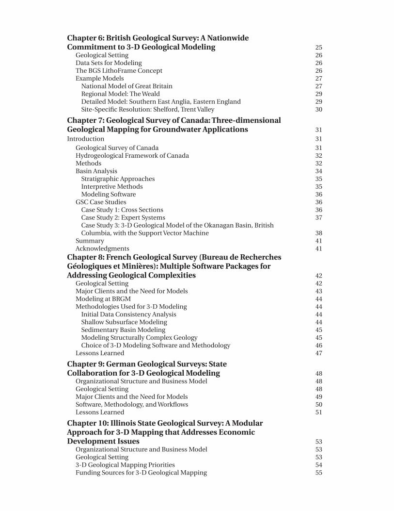
Chapter 6: British Geological Survey: A Nationwide Commitment to 3-D Geological Modeling 25 Geological Setting 26 Data Sets for Modeling 26 The BGS LithoFrame Concept 26 Example Models 27 National Model of Great Britain 27 Regional Model: The Weald 29 Detailed Model: Southern East Anglia, Eastern England 29 Site-Specific Resolution: Shelford, Trent Valley 30
Chapter 7: Geological Survey of Canada: Three-dimensional Geological Mapping for Groundwater Applications 31Introduction 31 Geological Survey of Canada 31 Hydrogeological Framework of Canada 32 Methods 32 Basin Analysis 34 Stratigraphic Approaches 35 Interpretive Methods 35 Modeling Software 36 GSC Case Studies 36 Case Study 1: Cross Sections 36 Case Study 2: Expert Systems 37 Case Study 3: 3-D Geological Model of the Okanagan Basin, British Columbia, with the Support Vector Machine 38 Summary 41 Acknowledgments 41Chapter 8: French Geological Survey (Bureau de Recherches Géologiques et Minières): Multiple Software Packages for Addressing Geological Complexities 42 Geological Setting 42 Major Clients and the Need for Models 43 Modeling at BRGM 44 Methodologies Used for 3-D Modeling 44 Initial Data Consistency Analysis 44 Shallow Subsurface Modeling 44 Sedimentary Basin Modeling 45 Modeling Structurally Complex Geology 45 Choice of 3-D Modeling Software and Methodology 46 Lessons Learned 47
Chapter 9: German Geological Surveys: State Collaboration for 3-D Geological Modeling 48 Organizational Structure and Business Model 48 Geological Setting 48 Major Clients and the Need for Models 49 Software, Methodology, and Workflows 50 Lessons Learned 51
Chapter 10: Illinois State Geological Survey: A Modular Approach for 3-D Mapping that Addresses Economic Development Issues 53 Organizational Structure and Business Model 53 Geological Setting 53 3-D Geological Mapping Priorities 54 Funding Sources for 3-D Geological Mapping 55

3-D Mapping Methods 56 Mapping Software and Staffing Strategy 57 Data Collection and Organization 58 Interpretation, Correlation, and Interpolation 58 Basic and Interpretive Map Production 59 Lessons Learned 59Chapter 11: Manitoba Geological Survey: Multi-scaled 3-D Geological Modeling with a Single Software Solution and Low Costs 60 Organizational Structure, Business Model, and Mission 60 Geological Setting 60 Major Clients and the Need for Models 60 Model Methodology 60 Cross Section Method (Quaternary to Precambrian Surface for Southeastern Manitoba) 61 Direct Data Modeling Method (Phanerozoic to Precambrian Surface) 61 Digitization Modeling Method (Chronostratigraphic Rock Units to Precambrian Surface) 62 Advantages of the MGS 3-D Mapping Approach 62 Lessons Learned 62Chapter 12: TNO–Geological Survey of the Netherlands: 3-D Geological Modeling of the Upper 500 to 1,000 Meters of the Dutch Subsurface 64 Organizational Structure, Business Model, and Mission 64 Geological Setting 64 Three Nationwide Models 65 DGM: The Digital Geological Model 65 REGIS II: The Regional Geohydrological Information System 65 GeoTOP: A 3-D Volume Model of the Upper 30 Meters 65 Major Clients and the Need for Models 65 Software 65 Workflow for Digital Geological Modeling 66 Data Selection 66 Stratigraphic Interpretation 66 Fault Mapping 66 Interpolation 66 Stacking the Units 67 Workflow for GeoTOP 67 Boreholes 67 Stratigraphic Interpolation 67 2-D Interpolation of Stratigraphic Units 68 3-D interpolation of Lithology Classes 68 Physical and Chemical Parameters 68
Chapter 13: U.S. Geological Survey: A Synopsis of Three-dimensional Modeling 69 Mission and Organizational Needs 69 Business Model 69 Geological Setting 69 Major Clients and the Need for Models 71 3-D/4-D Visualization for Geological Assessments 71 3-D/4-D Analyses and Use of LiDAR Imagery in Geological Modeling 73 Case Study: The Hayward Fault—An Example of a 3-D Geological Information Framework 73 Model Construction Methodology 74 Output 75

Observations, Suggestions, and Best Practices 75 Case Study: Santa Fe, New Mexico, 3-D Modeling as a Data Integrator 75 3-D/4-D Visualization and Geological Modeling for Hydrologic and Biologic Assessments 76 Lessons Learned 78 Workshops 78 User Survey 79 3-D Systems Database 79
PART 3: INFORMATION DELIVERY AND RECOMMENDATIONS 81
Chapter 14: Methods of Delivery and Outputs 83 INSIGHT GmbH Sub-surface Viewer 83 GeoScience Victoria Storage and Delivery of Information 84 Web Delivery at Geoscience Australia 84 ISGS 3-D Geologic Map Products 85
Chapter 15: Conclusions and Recommendations 86
References 87
Figures 2-1 Uncertainty drape on a model of central Glasgow, United Kingdom 7 2-2 Example of data density uncertainty plot for geological unit WITI using an influence distance of 200 m 8 2-3 Uncertainty assessment showing drill locations and drill type, and a grid of the average assumed error for geological surfaces 9 2-4 Cross section through a tidal channel in Zeeland, the Netherlands, showing the probability that a grid cell belongs to the tidal channel lithofacies 9 2-5 Probability that the Ashmore Member sand and gravel is greater than 10 feet thick in Kane County, Illinois, USA 10 4-1 Arc modeling in Lake County, Illinois, USA, showing data, cross sections, and surficial and 3-D geology 13 4-2 The GSI3D workflow 14 5-1 Australia’s Land and Marine Jurisdictions 20 5-2 Gawler Craton 3-D crustal VRML model 21 5-3 Mt. Warning, New South Wales, from Geoscience Australia’s 3-D Data Viewer showing surface geology (lithostratigraphy) with contacts and terrain hill shading 21 5-4 Three-dimensional geological model of Victoria incorporating Paleozoic and older basement as well as younger onshore and offshore basin fill and overlying volcanic cover 22 5-5 Numerical simulation results from 3-D Victoria modeling program. (a) Fluid flow associated with orogenic gold mineralization within an accreted Cambrian ocean basin; (b) strain partitioning around a Proterozoic basement block accreted during the same event 22 5-6 Four 3-D block diagrams of a study area in central Victoria (Spring Hill groundwater management area) 23 6-1 Bedrock geology of Great Britain 25 6-2 Superficial geology of Great Britain 25 6-3 Schematic section showing effective depth of modeling and definition across the LithoFrame 250, LithoFrame 50, and LithoFrame 10 resolutions 27 6-4 The LithoFrame 1M resolution onshore model of Great Britain 29 6-5 Example LithoFrame 250 model covering the Weald and adjacent parts of the English Channel 29 6-6 Scheduled availability of LithoFrame 250 resolution regional models for England and Wales 29

6-7 The LithoFrame 50 resolution southern East Anglia model of the Ipswich-Sudbury area covering 1,200 km2 30 6-8 The site-specific Shelford model 30 6-9 Current LithoFrame 10 and LithoFrame 50 coverage for Great Britain 30 7-1 Hydrogeological regions of Canada and key Canadian aquifers 33 7-2 Simplified basin analysis approach used in regional hydrogeological analysis of key Canadian aquifers 34 7-3 Example of an event stratigraphic model and integration of existing lithostratigraphic framework for the Oak Ridges Moraine Area 35 7-4 Example of the geological framework model for the Mirabel area 36 7-5 An isopach map and thickness histogram for the Newmarket Till unit 38 7-6 South Nation Conservation Authority model area showing a glaciofluvial isopach (eskers) draped over topographic digital elevation model 38 7-7 Input and output of support vector machine (SVM) modeling: (a) Geological coded input data set imported in Gocad; (b) the SVM classification result as a Gocad voxel object with local water bodies added on top of geological units 40 8-1 Geological map of the geology of France 42 8-2 Simplified map of the geology of France 43 8-3 Three-dimensional model of the Tertiary strata of the Aquitain Basin 44 8-4 Three-dimensional lithofacies model of Middle Eocene formations in Essonne Department 45 8-5 Location of two projects modeling the Trias and Dogger Formations of the Paris Basin 45 8-6 Three-dimensional static model of the Trias Formation in the southern Paris Basin for geothermal studies 46 8-7 Three-dimensional structural and petrophysical properties models of the Dogger Formation in the southern Paris Basin for CO
2 sequestration 46
8-8 Three-dimensional producer facies and porosity model of the Oolitic unit of the Dogger Formation (southeastern Paris Basin) 46 8-9 Estimation of the thermal resources in syn-sedimentary faulted deposits of the Limagne graben in central France 46 8-10 A 3-D model of a coal basin based on a cartography field trip (Alès, South-East of France) and building of the model from field observations 47 8-11 Geotechnical studies for a tunnel through the Alps between Turin (Italy) and Lyon (Alps) 47 9-1 Geological map of Germany 49 9-2 State of 3-D geological modeling in Germany 50 9-3 Part of a Gocad model depicting folded Carboniferous, coal-bearing strata of the Ruhr area 51 9-4 Structural model for monitoring an abandoned mining area underneath the city of Zwickau 51 9-5 Volume grid of Bavaria subdivided into four layers (crystalline basement, Mesozoic sediments, Upper Jurassic aquifer; omitted: Tertiary sediments of the Molasse) 52 10-1 Quaternary deposits map of Illinois 53 10-2 Kane County aquifer sensitivity map 54 10-3 Examples of 3-D maps and models of the Mahomet Bedrock Valley 55 10-4 GeoVisionary rendering of standardized lithologic borehole logs with a 1-m LiDAR-based digital elevation model 56 10-5 Kane County major Quaternary aquifer map 57 10-6 Visualization laboratory image on screen on GeoVisionary 58 11-1 Index map outlining the location of the various 3-D geological modeling activities in and around Manitoba 61

11-2 Three-dimensional geological Gocad model of southeast Manitoba including the Winnipeg region 61 11-3 Three-dimensional geological Gocad model of the TGI Williston Basin project area 62 11-4 Three-dimensional geological Gocad model of the Western Canada Sedimentary Basin spanning Manitoba, Saskatchewan, and Alberta 62 12-1 Location and schematic geological map of the Netherlands 64 12-2 Fault data stored in GIS and extracted for modeling 66 12-3 Schematic representation of two ways to assist interpolation: channel incision and thinning out near the limit of extent 67 12-4 Cross sections through the nationwide digital geological model 67 12-5 Part of the 3-D model of the central part of Zeeland, southwestern Netherlands 68 13-1 Simplified version of the geologic map of the conterminous United States 70 13-2 Map showing the location of the San Francisco Bay region 74 13-3 (a) Three-dimensional geologic map of the Hayward fault zone and (b) the Hayward fault surface with accompanying earthquake hypocenters 74 13-4 Work flow that uses 3-D modeling to integrate and synthesize diverse types of geological and geophysical information for a basin study near Santa Fe, New Mexico, USA 76 13-5 Perspective view of the greater Los Angeles region with InSAR imagery showing greater than 6 cm of groundwater pumping-induced subsidence 77 13-6 Three-dimensional images from seismic surveys of the speed of shock waves through sediment 13-7 Fracture model of the Äspö Hard Rock Laboratory 78 14-1 Options for delivery of British Geological Survey models 83 14-2 The Subsurface Viewer Interface showing the Southern East Anglia Model in the Subsurface Viewer with stratigraphic and permeability attribution 84 14-3 Villa Grove 7.5-minute Quadrangle map sheet 85
Tables 6-1 Main features of the LithoFrame resolutions 27 6-2 Geological detail possible at the various LithoFrame resolutions 28 7-1 Key Canadian aquifers grouped according to hydrogeological regions 32 7-2 Grouping of key Canadian aquifers according to host geology 33 7-3 Input data set statistics and support vector machine (SVM) classification results 41 13-1 The 3-D modeling and visualization software programs used by the USGS 72

PART 1BACKGROUND, ISSUES, AND SOFTWARE


Illinois State Geological Survey Circular 578 3
Chapter 1: Background and PurposeStephen J. Mathers1, Holger Kessler1, Richard C. Berg2, Donald A. Keefer2, and Keith A. Turner3
1British Geological Survey, 2Illinois State Geological Survey, 3Colorado School of Mines, Golden, Colorado
IntroductionSince 2001, six workshops on three-dimensional (3-D) geological mapping have been conducted in association with meetings of the Geological Society of America (GSA) and the Geological Association of Canada. The workshops have documented progress and estab-lished working relationships among an international group of geologists who have been developing new meth-ods for geological mapping largely to address the transition from traditional two-dimensional (2-D) to 3-D geologi-cal mapping (also referred to as 3-D geological modeling). This transition has been the direct result of increased societal need for a more detailed, improved understanding of the subsur-face to address critical land- and water-use issues (Thorleifson et al. 2010), coupled with significant technological advancements in Geographic Informa-tion Systems (GIS), digital cartography, data storage and analysis, and visual-ization techniques (Whitmeyer et al. 2010).
The October 2009 workshop in Port-land, Oregon (Berg et al. 2009), was sig-nificant because of the unprecedented representation from the world’s leading geological survey organizations (GSOs) in 3-D geological mapping. During the workshop it became very apparent that, although these GSOs share the same visions for the use of 3-D geologic maps, the methodologies, software tools, underlying mapping and model-ing strategies, and business models are highly varied.
Discussions at the workshop suggested that the time was right to produce a report documenting the current state-of-the-art for 3-D geological mapping in GSOs. Part of the motivation for this report was the need for advice to GSOs that are beginning to migrate from a
2-D to a 3-D mapping and modeling culture.
A similar workshop held in July 2009 in Madrid involved key players from GSOs of seven European countries (France, Germany, Italy, Netherlands, Poland, Spain, and United Kingdom). The goal of that workshop was to take the first steps toward establishing agreement and standardization of 3-D geological modeling approaches in Europe. The conclusions from that workshop were similar to those reached at Portland, and many of the Madrid workshop par-ticipants contributed material for this present report.
In this report, we have tried to capture the state-of-the-art of 3-D geological mapping in these participating GSOs. Throughout this document the terms “mapping” and “modeling” will be used interchangeably to recognize the strong institutional preferences of the participating GSOs. Each approach (see Chapters 5 through 13) is unique and reflects geological aspects of the nation or state, the drivers for geosci-ence information, the stakeholders commissioning maps and models, the external and internal organization of GSOs within the nation or state, the available data resources, and funding. This document is intended to help others learn from our successes and mistakes and to help them make the transition into the world of 3-D geolog-ical modeling. Growth of this commu-nity may eventually lead to stabiliza-tion of methods and the development and international use of geoscience data exchange standards.
This report has benefited from the excellent contributions received from staff serving in GSOs and allied bodies in Australia, Canada, France, Germany, the Netherlands, Great Britain, and the United States (USA).
What Is a GSO?A GSO is a not-for-profit government organization responsible for a range of tasks that generally include
• geologicalsurveying(mapping)ofthe nation, state, or province;
• conductinggeologicalresearchtosupport economic development, public health, and environmental protection;
• distributinggeoscienceinformation;and
• advisinggovernmentatvariouslevels regarding water, mineral and energy resources, environmental issues, and earth hazards.
Each country has its own governmental structure of ministries, departments, and bureaus. Although not all of the organizations involved in public sector 3-D geological modeling worldwide are geological surveys, these non-survey organizations are still responsible for overseeing national or state geological modeling.
Some nations have a single national geological survey (for example BRGM in France and the BGS in Great Brit-ain); in other countries, responsibilities are shared by both state/provincial and federal organizations (USA, Canada, Australia, and Germany).
Geological Mapping: A Brief HistoryGeological mapping has been a funda-mental activity of GSOs since the early 1800s, when governments began a sys-tematic search for mineral resources to fuel economic growth and industrial-ization. Beginning with William Smith’s 1815 map, A Geological Map of England and Wales and Part of Scotland, and its included cross section showing subsur-

4 Circular 578 Illinois State Geological Survey
face rock layers, geologists have sought ways to best portray geological infor-mation on 2-D maps.
The most conventional technique for portraying successions of geologi-cal strata in the subsurface has been through the use of cross sections and maps of the top or bottom surfaces of strata. Although cross sections provide a sense of geological structure and the continuity of geological units in the third dimension, they only provide information for a single plane cut through the Earth, and they do not provide a clear sense of the 3-D nature of the geology. Even with multiple cross sections, there are significant voids in information that the user must infer. In addition, top and bottom surface maps provide insight only on the distribution of individual deposits and do not give a clear sense of the full succession.
Stack-unit maps improved the under-standing of the three-dimensionality of geological information by using alpha-numeric codes or colors and patterns to represent the vertical succession of geological units to a specified depth. This mapping was termed “three-dimensional mapping” because of the extensive and detailed subsurface information that could be displayed.
The Dutch (e.g., Rijks Geologische Dienst 1925) pioneered the stack-unit technique beginning in the 1920s by mapping the geology in the upper 1 or 2 m. This technique was enhanced considerably between the early 1970s and the mid 1990s (e.g., Berg et al. 1984), as vertical successions com-monly were extended to depths of 6, 15, or 30 m at large scale (1:24,000 to 1:100,000). This mapping activity, mainly done by GSOs, was in response to requirements for detailed mapping in support of land- and water-use deci-sion making. Most of the stack-unit mapping was accomplished before computers were widely applied to geological mapping. The primary limi-tation of stack-unit mapping was that map depth was generally restricted because map unit labeling could be overly complex. However, with improvements in digital mapping tech-nology, sophisticated stack-unit maps to any depth now can be constructed
that serve the client community well, as shown by maps from the Ohio Geo-logical Survey in the USA (Shrake et al. 2009).
The availability of personal computers (PCs) in the 1980s and the rapid evolu-tion of hardware and software led to a revolution in geological mapping. Currently, several software applica-tions are available for PCs that allow for the development and visualization of maps for geological surfaces from land surface to any depth (Whitmeyer et al. 2010). Geological modeling and map-ping, as discussed in this publication, refers to the use of PCs and software to build, visualize, and analyze the subsurface geology in 3-D. This use has resulted in a wide range of mapping and modeling approaches, many of which are documented in this report.
Applications Benefiting from 3-D Geologic MapsThree-dimensional geologic maps are an extension of traditional 2-D geo-logical maps into the third dimension. These maps can portray subsurface stacked layers showing depths, thick-nesses, and material properties within a 3-D volumetric space. The output is a fully attributed and digital 3-D model created by geological interpretation and rigorous use of raw data geological knowledge and statistical methods.
Both 2-D and 3-D outputs are pro-duced using a similar classification of geological units and are presented at a range of scales or resolutions aimed at specific uses and stakeholder groups. The North American 3-D mapping workshops have targeted hydrogeo-logical applications, but 3-D geological models are finding receptive clients who need information about a range of earth science issues because (1) result-ing 3-D geologic maps can explain and portray complex geology with numerous map views in understand-able formats, (2) various derivative or interpretive maps can be produced and updated as new information becomes available, and (3) all can be released on demand and customized for clients with specific needs for earth resource information.
Many of the 3-D geological models constructed at GSOs have been com-missioned by industrial and govern-ment clients. In those situations, the mapping units and resolution are dictated by their needs. Such models generally require considerable modi-fication to be used for other purposes and for other users. For example, when shifting from regional to local site-specific 3-D mapping and modeling efforts, powerful data management tools are a prerequisite for integrating databases with 3-D modeling (Artimo et al. 2008).
Regional 3-D geological models pro-vide the context and framework for detailed investigations by various clients interested in different aspects of earth resource assessments. These more detailed investigations generally provide the best examples of economic benefits of 3-D mapping and modeling (Curry et al. 1994, Artimo et al. 2003), and, perhaps more significantly, they increase the awareness of the impor-tance of 3-D mapping investigations to local decision makers and politicians.
Two detailed economic assessments, as examples, highlight various site-specific applications derived from geological mapping. Bhagwat and Ipe (2000) conducted a cost:benefit study of a statewide 2-D mapping program in Kentucky (USA). The study was based on a detailed questionnaire to hundreds of map users following more than 20 years of geologic map use in that state. Those researchers estimated that project costs increased by up to 40% if geologic maps are not avail-able. Using very conservative assump-tions, they also reported a return of $25 to $39 for each government dollar invested in geological mapping. Fur-thermore, the Kentucky maps, com-pleted originally to boost the mineral and energy industries at a cost of more than $112 million (year 2010 dollars), have been used primarily to address water supply and protection issues, growth and development, environ-mental problems, and mitigation of a variety of natural hazards. A similarly designed benefit:cost assessment was performed by the Instituto Geológico y Minero de España (Geological and Mining Institute of Spain) by Garcia-
Illinois State Geological Survey Circular 578 5
Cortes et al. (2005). That study reported that an initial investment of ¡122 mil-lion for geological maps produced a savings to the Spanish economy of ¡2.2 billion (18:1 benefit:cost ratio). The greatest uses of geologic maps were for evaluating groundwater resources and industrial minerals, building and foun-dation construction projects, landslide assessments, and waste site locations.
The main sectors currently request-ing 3-D geological models from GSOs include those dealing with the follow-ing issues:
Water• Delineatingthedistributionand
thickness of aquifers and non-aquifers for input to groundwater flow models or for developing inter-pretive maps to support decisions relating to groundwater manage-ment, withdrawal, protection, and recharge.
• Conductingmorelocalizedstudiesfor groundwater flooding, river flood protection, contaminant transport, and wetland construction, protec-tion, and maintenance.
Waste Disposal, Management, and Contamination• Characterizingshallowanddeep
groundwater systems to assess risks associated with long-term disposal of nuclear wastes and the disposal and storage of municipal and haz-ardous wastes.
• Evaluatingthecontaminationpotential of shallow groundwater from construction refuse sites, underground storage tanks contain-ing gasoline and other chemicals, septic systems, large animal con-finement facilities and associated waste lagoons, chemical spills, use of road salts and other deicers on
paved surfaces, and over-applica-tion of fertilizers, sewage sludge, and chemicals onto agricultural fields.
Hydrocarbon, Energy, and Carbon Capture and Storage• Characterizingandmappingofoil
and gas reservoirs.
• Modelingforevaluationofthicknessand quality of coal resources.
• Evaluatinggeothermalpotential.
• Modelingofreservoircapacityand suitability for sequestration of carbon dioxide.
Land-Use Planning and Local Decision Making• Characterizingthesurfaceandnear-
surface to aid land-use planning in urban, suburban, and rural areas by helping to balance economic development with wise use of water and mineral resources and ensuring their protection.
• Protectingshallowgroundwaterthrough green planning restrictions, protecting vulnerable shallow aqui-fers, and providing unbiased infor-mation for industrial permitting, property tax assessments, and land acquisitions.
• Evaluatingsitesforcityzoningandestablishment of building codes.
Civil Engineering and Infrastructure• Conductingsite-specificinvestiga-
tions for construction projects such as highways, tunnels, sewers, rail-roads, pipelines, dams, dikes, locks, building foundations, linear route alignments for communications and utility infrastructure, and large transportation infrastructure proj-ects (mega sites).
• Providinggeologicalinformationtohelp determine risks from natural hazards and impacts on the natural
environment as a result of construc-tion projects (e.g., environmental impact assessments).
Archaeology• Characterizingshallowdepositsto
evaluate preservation potential and ground conditions.
• Establishingandmappingarchaeo-logical stratigraphy.
Mineral Resources• Conductingregionalandsite-scale
appraisals of mineral resources and reserves, including long-term impacts on the environment.
• Findingawell-balancedapproachto mining and land use ensuring that nearby economically available mineral resources are not made unavailable because of competing land uses.
Research• Conductingresearchandscientific
discovery in earth sciences (e.g., stratigraphy, tectonics, Quaternary evolution, and soil science).
• Conceptualizingandportrayingallsurfaces, depths, thicknesses, and geological processes over broad geographic areas in ways that were previously not possible and, in so doing, predicting the distribution of materials into regions of sparse data and visually analyzing and interpret-ing the geology and its history.
Education and Outreach• Visualizingthe“fullcubeofgeology.”
• Communicatingtheexistenceandrelevance of specific geological fea-tures.
• Increasingpublicunderstandingofgeoscience-related issues, and using geological information for teaching endeavors at all levels.

6 Circular 578 Illinois State Geological Survey
Chapter 2: Major Mapping and Modeling IssuesDonald A. Keefer1 , Holger Kessler2, Mark Cave2, and Stephen J. Mathers2
1Illinois State Geological Survey, 2British Geological Survey
An Overview of Major 3-D Geological Mapping and Modeling MethodsA wide range of software applications can be used for 3-D geological mod-eling. Some methods use common interpolation routines to make geologi-cal surfaces; others use sophisticated statistical methods; and still others use methods more akin to traditional geo-logical mapping. These applications do not fully constrain the user in how they are used; therefore, the range of work-flows for conducting a 3-D geological modeling project is almost as large as the number of practitioners who are conducting the mapping and modeling exercises.
Using software to map geology requires geologists to explicitly define consid-erations that were traditionally part of the intuitive science of geological mapping. It is generally very difficult for most geologists to understand how to translate their geological knowledge into the parameters con-tained in most mapping software. If a mapper loads data into a common interpolation package and relies on the software to “know” how the data should be mapped, little real geological knowledge is being used in the map-ping because only the information contained in the data is used, and the information is limited to the locations where the data reside. Statistical meth-ods of interpolation capture additional information on spatial variation, but alone do not naturally portray the complete spatial structure of specific depositional environments or the effects of certain faulting, and so the value of this information is limited. These more automated approaches to mapping seem to be most common in academia, where students and faculty are exploring insights gained by new methods and not necessarily trying to produce the most geologically accurate map.
The other common type of 3-D model delineates deposit boundaries and explicitly defines the potential distri-bution of material properties within these deposits. Typically, these models include plausible distributions of pet-rophysical properties (e.g., porosity, permeability) and are used as input to flow simulation models. Alternatively, any property can be simulated in this manner. The methods for developing these property models typically involve geostatistical tools and require signifi-cant expertise to apply them reliably. It is important to note that these prop-erty models should be developed using the same significant involvement by geologists familiar with the basic unit distributions and also with the likely characteristics of the modeled proper-ties. It is also important to understand that property models involve much more inference in the interpolation stage and should be expected to be much more uncertain than the maps showing the distribution of basic units. The TNO–Netherlands Geological Survey GeoTOP model, discussed in Chapter 12, is a good example of 3-D property modeling based on extensive databases of measured physical prop-erties in numerous well-distributed boreholes.
Finally, the importance of geologists being able to visualize their data at various stages of the mapping and modeling process is key for better understanding of the conceptual geo-logical framework, resolving multiple working hypotheses regarding geologi-cal process responsible for depositing various sediments, and for advancing applications of software packages. Particularly, the 3-D visualization of raw data early in the modeling process allows the geologist to immediately “see” data trends and to begin the process of evaluating data quality and distribution.
In GSOs, it is generally important for geologists to constrain geological mapping software by insight gained through years of training and from work that assimilates intangible aspects regarding the distribution and character of deposits. The editors and authors of this report feel strongly that any individual or organization involved with 3-D geological modeling needs to choose software and methods that allow them to provide significant geological control on the distribution and character of the deposits they are portraying. Although not always easy, it is increasingly possible to find software that simplifies the use of geological constraints on 3-D geological mapping. The discussions from the individual GSOs provide a diverse guide to differ-ent ways to model in this context.
The specific approaches to geological modeling at GSOs largely have been driven by the need to develop 3-D maps of geological successions for various areas. The terms used for these 3-D products vary by organization and sometimes by individuals within an organization. The use of the terms modeling and mapping are used inter-changeably in this document because of a recognition that conventions are already established in various groups, and it is not the objective of this docu-ment to propose standards in termi-nology or method.
It is important to recognize that there are two basic types of 3-D geologic maps or models. The most common type involves only the delineation of the distribution of specific map units. These models do not explicitly define any distribution of material properties within their boundaries. Sometimes, within this type of 3-D model, the mapped deposits can be divided into broad zones where each zone has dis-tinct patterns in the variability of tex-ture, porosity, or some other important characteristic.

Illinois State Geological Survey Circular 578 7
Scale and ResolutionAs with geologic maps of the land sur-face, maps and models of subsurface geological units can be constructed to show features of a certain minimum size. In traditional geological mapping, map scale is the parameter that dic-tates the minimum feature size, or level of detail, expected on a map. The scale of a geologic map is originally derived from the scale of its base map.
The concept of scale has always had limitations in geological mapping because the distribution of data is always irregular, which is particularly a problem for mapping subsurface geological units where data density generally decreases with depth. Maps in areas with a high data density typi-cally contain more detail than expected for the scale, whereas areas of low data density have much less detail than expected. Map scale also is a concept that is difficult for non-geologists to understand. The term “resolution” has been used increasingly in the digital world, often in the context of digital images or photographs. The reference to the resolution of a geologic map or model is increasingly common, as it can accommodate the fuzziness, or variation, in detail across a map better than just referring to differences in map scale. Reference to resolution of geological models, although more flex-ible in connotation than the concept of map scale, does not change the fact that geological models are limited in the resolution they capture and cannot reliably predict the distribution of higher (more detailed) resolution map features.
The physical, static nature of printed maps makes them difficult to use at scales beyond their publication. Unlike printed maps, digital maps and models are not physically bound or static in how they are used. Therefore, it is important when models and model data are distributed that a clear indi-cation be made of the reliable level of detail and the limits of reliability within the models and also that recom-mended map uses be clearly defined to discourage misuse.
Three-dimensional maps and models, because of their digital nature, can be
interactive, and if appropriate software is available, users can zoom in and out, effectively redefining the scale of the viewing window. In these situations, it is possible for digital 3-D geologi-cal models to be enlarged and used at resolutions beyond their limits of reli-ability.
Uncertainty in ModelingWith the increasing use of 3-D geologi-cal models, it is generally helpful to assess the uncertainty of the modeled deposits and their properties to ensure that end users can better understand the major limitations of the models and map products that are developed from them. The uncertainty of 3-D geo-logical models is not only restricted to the algorithms and data of the model, but also involves the geological infer-ences and interpretations that are used for the final models. Tradition-ally, modeling uncertainty in geologic maps relied rigorously on geostatistical models and assumptions that were often violated when the real sediment successions became complex. These uncertainty assessments were com-monly applied in the mineral extrac-tion and petroleum industries. Special-ized statistical expertise is required to apply these methods reliably. Although some GSOs are exploring the use of geostatistical methods of uncertainty
assessment, increasingly new methods are being used that are based less on statistical methods and more on geolo-gist insight about the reliability of data and interpretations. These uncertainty assessments are being used to help GSOs convey the mapper’s sense of confidence with the data or interpreta-tions in any mapping project.
This section provides examples of uncertainty assessments that have been developed and applied by GSOs. They illustrate various issues being addressed in these assessments and the ways uncertainty are being charac-terized for various mapping applica-tions. These examples do not represent an exhaustive list of applicable meth-ods, but they can be used as a starting point for future studies.
A simple depiction of uncertainty can be produced as a color ramped layer for a model. Figure 2-1 is an example of a 5-km × 5-km part of the Glasgow urban area in the United Kingdom (UK) where the reddish areas indicate high uncertainty (low data density), and the green areas indicate low uncertainty (high data density). This scheme tends to reflect the distribu-tion of boreholes, but the locations here are buffered or blurred to take into account the use of confidential borehole logs in the modeling exercise
NW
Figure 2-1 Uncertainty drape on a model of central Glasgow, United Kingdom.

8 Circular 578 Illinois State Geological Survey
because precise locations could not be divulged.
A more sophisticated approach has been applied to the modeling of the Glasgow urban area using the proce-dure described by Lelliot et al. (2009). Full details of the method are given in that publication, but, in summary, the method combines the 2-D spatial den-sity of the boreholes used to construct the surface with the geological com-plexity of the surface, where geological complexity refers to the relative change in curvature of the surface or the “tor-tuosity” of the surface. That is, if the data density is high, then the uncer-tainty is lower (or vice versa), and if the geological complexity is low, then the uncertainty is lower (or vice versa). The empirical uncertainty obtained from this approach is then calibrated into either an estimated absolute uncer-tainty or a relative scale using expert judgment. To calibrate the uncertainty the expert provides three pieces of information: the estimated absolute uncertainty of the surface at the bore-hole (i.e., the uncertainty in depth in the borehole log); the estimated worse case uncertainty on the surface where least information is available; and the distance from the borehole that the expert has confidence to predict the surface (the radius of influence of the borehole). In the examples shown here, the uncertainty has been expressed on a relative scale of 0 to 100 with 0 being very low uncertainty and 100 being very high (Figure 2-2).
The majority of the available boreholes were evaluated in the data selection process, and the deepest, best-logged bores were used to construct the model. A total of 1,852 boreholes (of 13,000) were specifically selected to construct the cross sections on which the surficial model was based. In addi-tion, many more boreholes not directly lying on specific cross section align-ments were also considered during the construction of the cross sections so that the overall construction of the model is based on an assessment of approximately 8,000 boreholes.
The uncertainty for the WITI geologi-cal unit for the Glasgow urban area was calculated using the procedure outlined by Lelliot et al. (2009) using
the order of ±10 m in XYZ (e.g., those blue areas of the WITI uncertainty sur-face on Figure 2-2).
Average uncertainty (average confi-dence) areas = 3 are those areas that are constrained by some geological data and where the geology is moder-ately complex (e.g., faulted or folded). In these areas, the error on the model might be considered to be on the order of ±30 m in XYZ (e.g., the green to tur-quoise areas on Figure 2-2).
Highest uncertainty (lowest confi-dence) areas = 5 are those areas that are not constrained by any geological data and where the geology is complex (e.g., faulted or folded). In these areas, the error on the model might be con-sidered to be on the order of ±70 m in XYZ (e.g., those red to orange areas of the uncertainty surface on Figure 2-2).
The surficial deposits uncertainty layers are supplied as ArcGIS 9.2 raster grid format and in the subsurface viewer.
Figure 2-2 Example of data density uncertainty plot for geological unit WITI using an influence distance of 200 m. Blue crosses indicate data points.
customized BGS software developed in Matlab programming language to mea-sure data density and geological com-plexity. The output is a grid file ranked from relatively low (0) to relatively high uncertainty (100). A 200-m radius of influence and a lowest to highest rela-tive uncertainty of 0.5 to 100 were used to calibrate the output (Figure 2-2).
The combined uncertainty scale (Figure 2-2) must be translated by the user into uncertainty categories; the lowest number represents the lowest uncertainty and the highest number the highest uncertainty. For the Clyde Gateway model, five categories could be considered. In ArcGIS this would be easy to achieve on the uncertainty raster grid by symbolizing using five classes.
Lowest uncertainty (highest confi-dence) areas = 1 are those areas that are well constrained by geological data and where the geology is relatively simple. In these areas, the error on the model might be considered to be on

Illinois State Geological Survey Circular 578 9
Lelliott et al. (2009) provides example outputs (Figure 2-3) for the use of this method for assessing a 3-D geologi-cal model of shallow surficial depos-its, where a sequence of river terrace gravels and alluvial deposits overlie mudstone bedrock. Values in red show a wide range of calculated elevations (high uncertainty); values in blue show the most consistent values (low uncertainty). The study concluded that the results agreed with intuitive expectations for the uncertainty, but that drilling should be undertaken to validate the uncertainty assessment of the model.
The TNO–Netherlands Geological Survey GeoTOP model, discussed in Chapter 12, uses stochastic techniques during model construction to compute the probability for each grid cell to belong to a specific lithostratigraphic unit and lithofacies. These probabili-ties provide a geostatistically based measure of model uncertainty. Figure 2-4 shows the results for a tidal channel in the province of Zeeland. The colors indicate the probability that a grid cell contains the sandy tidal channel litho-facies. At the center of the channel, this probability is high (100%). In the upper part of the channel, the green and yellow colors reveal much smaller probabilities. In this upper part, more clayey tidal flat deposits are expected. Similarly, probabilities are lower at the bottom of the channel where shells and shell-rich sand deposits are expected.
A study at the Illinois State Geological Survey (ISGS) recognized the difficulty of traditional geostatistical approaches to adequately capture geological knowledge of the data, deposits, and interpretations that are particularly relevant to making accurate uncer-tainty assessments. The ISGS recog-nized the impact of four factors that contribute to uncertainty in geologic maps: (1) variations in data quality, (2) variations in data density, (3) general-izations in texture, and (4) generaliza-tions in thickness (Dey et al. 2007d). The contributions of these factors to map uncertainty were evaluated with respect to terms of their likely impact on the predictive accuracy of a regional groundwater flow model that would use the 3-D geologic map.
Figure 2-4 Cross section through a tidal channel in Zeeland, the Netherlands, show-ing the probability that a grid cell belongs to the tidal channel lithofacies.
Figure 2-3 Uncertainty assessment showing drill locations and drill type, and a grid of the average assumed error for geological surfaces (Lelliott et al. 2009).

10 Circular 578 Illinois State Geological Survey
The evaluation of variations in data quality mirrored results from other studies (Russell et al. 2001): water well drillers tended to make system-atic errors in reporting the textures they encountered, and locational coordinates of boreholes were com-monly incorrect. Errors in locations
result in errors in elevation, which translates to errors in deposit depth and in correlation. To address loca-tion errors, the ISGS study committed significant resources to verifying and correcting the locational coordinates of every borehole used in mapping,
Figure 2-5 Probability that the Ashmore Member sand and gravel is greater than 10 feet thick in Kane County, Illinois, USA.
significantly improving the reliability of resultant maps. Analysis of data errors showed that, after sediment texture reporting errors were accounted for, the reporting errors remaining within the well logs had little impact on the reliability of identifying and correlating unconsolidated deposits more than 5 feet thick and generally more than 0.5 miles wide and several miles long, and in correlating bedrock units.
Dey et al (2009d) recognized that errors in thickness interpretations were dependent on data density, data accu-racy, and the underlying complexity of the geologic deposit being mapped. To evaluate the potential error in thick-ness estimates, they used a novel appli-cation of geostatistical methods. In the first stage of analysis, the isopach maps for each map unit were taken from the completed 3-D model and used as best estimates of the geologist’s conceptual models. Semivariograms modeled directly from the isopach grid values showed a relatively small variation in thickness for each map unit. These semivariograms were used in a stochastic simulation to estimate the amount and location of errors in the isopach maps. In the second stage of analysis, semivariograms modeled using the thickness values from the borehole data showed relatively large thickness variations for each unit. These semivariograms were used in a stochastic simulation to produce alter-native estimates of the amount and location of error in the isopach maps. These sets of simulations allowed for calculations of the probability that map units were less than or greater than various thickness thresholds. For example, maps were created to esti-mate the probability of a unit being thicker than 10 feet or thinner than 1 foot. These paired simulations pro-vided more insight on the likely uncer-tainty in the occurrence of mapped units than would be found under tradi-tional geostatistical evaluations.
Figure 2-5 from that study illustrates the probability that one sand and gravel deposit, the Ashmore Member of the Henry Formation, is greater than 10 feet (3.0 m) thick.

Illinois State Geological Survey Circular 578 11
Chapter 3: Logistical Considerations Prior to Migrating to 3-D Geological Modeling and MappingHolger Kessler1, Stephen J. Mathers2, and Donald A. Keefer2
1British Geological Survey, 2Illinois State Geological Survey
The migration from 2-D to 3-D geo-logical modeling or mapping for any GSO will benefit from consideration of several important issues. This sec-tion briefly discusses these issues and provides some insight on the conse-quences of different decisions.
Commingling Initial Mapping Strategies with Eventual OutcomesRegardless of scale, 3-D geological mapping and modeling investiga-tions should be integrated with other activities of a project at an early stage so project outcomes and deliverables reflect a client’s needs and are accom-plished within the capacity of those producing the information. Artimo et al. (2008) stated the importance of new and updated geological information that can be instantaneously integrated into the daily planning and guiding of a project, which underscores that “geological studies should not be con-sidered as single linear project events that are separated from the technical and legislative planning resulting from the geological investigations.” Having a robust database and allowing for integration of other contributing scien-tific information (e.g., hydrogeological modeling, geophysical investigations, and geochemical data) help shape and refine 3-D geological interpretations at various stages of geological under-standing and 3-D model development.
Resource Allocation StrategiesThree-dimensional geological mod-eling and mapping require different allocations of human, hardware, and software resources than does 2-D geo-logical mapping. The exact differences depend both on how 2-D mapping is currently accomplished at a GSO and
how the 3-D mapping will be con-ducted. As this report highlights, the software for the various approaches to 3-D geological mapping and modeling needs to be specialized. Centralization of various components of mapping (e.g., data management, data analy-sis, mapping, and visualization) can simplify efforts for the mappers, but often requires a larger investment in software and specialists in these areas. Less standardization in these compo-nents creates a more flexible environ-ment for the mappers, but can result in fragmentation of staff expertise, data requirements, and output file formats. These various consequences can be positive or negative, depending on how they are accommodated by the GSO. It takes time to research the costs and benefits of various options. However, without careful research, GSOs can meander through combinations of the various options until they find some-thing that satisfies their needs. Pilot studies (e.g., Lasemi and Berg 2001, Barnhardt et al. 2005) can be help-ful for developing new 3-D methods, testing new software, and helping to identify the issues involved with spe-cific changes to a mapping workflow. It also can be helpful for those wanting to initiate 3-D modeling programs to contact colleagues in other GSOs to inquire how they addressed specific issues. This document is designed to help describe the pros and cons of vari-ous approaches.
Data Management StandardizationAn issue that needs particular atten-tion is the development of various data management standards throughout the mapping workflow. Data management issues need to be identified relatively early in the organizational shift to 3-D mapping to prevent unexpected incompatibilities or development of
products that cannot be easily incor-porated into existing product lines or centralized database systems. Whether a GSO uses a fully standardized and centrally managed suite of software and data or a more flexible or modular approach to mapping, the organiza-tion needs to develop a consistent approach to (1) ensure interoperability between software packages and dif-ferent mapping projects; (2) ensure long-term accessibility to raw data, interpretations, and final products; and (3) promote effective communication and workflow between staff working on various aspects of mapping and modeling projects. One standard that needs to be established for each 3-D mapping project is map projection. In general, all data, maps, grids, sections, etc., should have the same coordinate system to ensure positional accuracy throughout a project. Although some software applications can reproject data on the fly, care should be taken when using data with different projec-tions, as errors have been known to occur, and subtle differences may not always be readily identifiable.
The solution to interoperability is unique to each GSO and, like the approach to determine resource allocation strategies, can benefit from a cost:benefit analysis of the various options. The individual GSO discussions in Chapters 5 through 13 highlight various options that are being used to manage the data, maps, models, and products at these organi-zations.
Necessary Data SetsThere is a suite of data sets that ranges between obligatory and helpful for the development of a sound 3-D geologic map or model. The determination of whether a specific data set is obligatory or optional can be somewhat subjec-tive and is dictated by the specific

12 Circular 578 Illinois State Geological Survey
software and workflow or the perspec-tives of the geologists involved with the mapping.
Digital Terrain ModelsA digital terrain model (DTM) of the proper resolution and extent for the map area, also known as a digital elevation model (DEM), is probably the most necessary data set for any 3-D mapping project. Because some 2-D mapping workflows still rely on hand drawing contacts on topographic maps, a given GSO may not be familiar with the requirements of acquisition and management of DTMs that meet the needs of specific 3-D mapping projects. Depending on the country, province, or state, acquisition of the necessary DTMs can range from easy to impossible and from free to prohibi-tively expensive.
Borehole Drilling LogsAfter acquisition of a suitable DTM, the availability of digital borehole driller’s descriptions is probably the next most important data set. Data quality issues associated with borehole logs must be evaluated, because these data, depending on their location or quality, might not meet the needs of the project or mappers. The quality of these data must be evaluated early, as unidentified errors can result in bore-holes being mislocated by significant distances. The referenced land-surface elevation of the borehole data must also be given consideration. Common practices suggest that the borehole elevations should be taken from the most detailed elevation source, regard-less of the resolution of DTM used.
Additionally, the quality of the geologi-cal descriptions can vary dramatically between individual records, which can significantly affect the value of these data for any mapping project. Finally, when potentially thousands of raw borehole data points are being visualized in 3-D, many points at vari-ous sites can be in the same general location. This creates a problem when creating associated databases, and, to ensure data quality, the “best” data point should be selected to represent the site.
Lithologic Dictionaries and Stratigraphic LexiconsLithologic dictionaries and strati-graphic lexicons are two additional geological data sets that should be considered when beginning the move to 3-D geological modeling. Although a dictionary that assigns standard lithologies to borehole driller’s descrip-tions may not be required for a given software package or workflow, every project needs to define the formal mapping units that are included in the map area. The format of these data sets is wholly dependent on the software used for modeling.
Color RampsOne of the last required data sets for any mapping project is the definition of a consistent color scale for all mod-eled units and properties. Develop-ment of internal standards can be worthwhile, but must be recognized as another option that each GSO must consider based on its resource base, timeline, and mapping project priori-ties.
Optional Data SetsSeveral optional data sets are com-monly used in 2-D and 3-D mapping that are worth considering:
• Collectionandcompilationofdigitalversions of additional borehole data, outcrop descriptions, additional field observations, geophysical bore-hole logs, and geophysical profile data can all be helpful in providing additional insights on the distribu-tion and character of the mapped deposits.
• Surficialgeologicmapsoftenareavailable for an area before 3-D modeling efforts begin. These maps can be very helpful in expedit-ing a subsurface mapping effort, regardless of the software used. It is common, however, for the surficial maps to be generated during the 3-D mapping effort, so these maps may not be available at the onset of a project.
• Accesstodigitaltopographicmapscan be of significant value, depend-ing on the products to be generated from the 3-D mapping effort. These topographic map layers should be appropriate in scale to the resolu-tion of mapping and to the desired scale of final map products.
• Finally,availablecrosssectionsandother profile data can be scanned and georeferenced for position and used in many mapping software applications. The value of including these types of images needs to be weighed against the mapping objec-tives, timeline, and expense (time and staffing) of digitizing and geore-ferencing these data.

Illinois State Geological Survey Circular 578 13
Chapter 4: Common 3-D Mapping and Modeling Software PackagesHolger Kessler1, Stephen J. Mathers1, Donald A. Keefer2, and Richard C. Berg2
1British Geological Survey, 2Illinois State Geological Survey
The most common software packages used for building 3-D geologic maps and models in many GSOs include ArcGIS, Gocad, EarthVision, 3-D Geo-Modeller, GSI3D, Multilayer-GDM, and Isatis. Of these, GSI3D, 3-D GeoMod-eller, and Multilayer-GDM have been developed by GSOs to meet custom-ized geological mapping and modeling needs of their organizations. Many other software packages are also used in GSOs worldwide as part of modeling workflows, and these include software for GIS, geostatistical analysis, seismic depth conversion, visualization, and property modeling.
3-D Geomodeller3-D Geomodeller was developed as a result of a requirement by the French Geological Survey (BRGM) to create a “geological editor” instead of using CAD or GIS techniques. The BRGM thought it was unnatural to force geologists to think in a way that was contrary to their training in order to create a 3-D model. A research and development project, known as GeoFrance 3-D, was established and ran for six years developing the prototype 3-DWEG (3-D Web Edit-eur Geologique) tool, which was the precursor to 3-D GeoModeller. At the same time, Intrepid Geophysics was optimizing the use of modern airborne geological data sets to aid geological interpretations. A joint venture was formed between BRGM and Intrepid to commercialize and further develop 3-DWEG under the 3-D Geomodeller brand name.
3-D Geomodeller is based on an implicit modeling of surfaces where each horizon is built by a 3-D inter-polation function (potential field co-kriging) that simultaneously takes into account
• datapointsonhorizonlocations(isopotential values),
• generalorientationsandpolaritiesof structures (gradients), and
• existenceofdiscontinuities(faults).
This method is actually very close to “geological thinking.” A geological model comprises a set of different hori-zons that are assembled with respect to their chronology and relationships. In addition, full tensor inversion gravity and magnetic modeling is an integral part of the software, which makes it an original environment in which to com-bine geological modeling and valida-tion through geophysical inversion.
3-D Geomodeller has been used extensively at BRGM and in public and private sector organizations, particularly in Australia and Canada. (More information about 3-D Geo-Modeller can be found at http://www.geomodeller.com/geo/index.php?lang=EN&menu=homepage/.)
ArcGISThe ArcGIS suite of products by ESRI is currently the global leader in GIS soft-
ware and is widely used within work-flows at GSOs for assembling and visu-alizing 2-D maps and, increasingly, for developing and visualizing 3-D geolog-ical models. Even though much of the ArcGIS data structure and functionality are focused on 2-D spatial data, ArcGIS is gradually increasing its capability for analyzing and rendering 3-D spatial data. The ArcScene module allows for the 3-D visualization of a wide range of geological data sets that are used in 3-D geological modeling (Figure 4-1). ESRI also allows customization and extension through VBA (Visual Basic for Applications) and the .net environ-ment, and custom tools and toolbars are being used to extend 3-D geological modeling capability. At the ISGS, for example, workflows have developed around custom tools to create cross sections, make stratigraphic picks on 3-D boreholes, and generate surface maps of the tops or bottoms of map units, all as part of a robust 3-D geo-logical modeling program.
Figure 4-1 ArcScene modeling in Lake County, Illinois, USA, showing data, cross sections, and surficial and 3-D geology (Illinois State Geological Survey screen capture).
14 Circular 578 Illinois State Geological Survey
a Geological mapb Correlated section
f thickness grid
d Unit distribution
c Fence diagram
e Calculated block model
SB 2 (84.07)
loftgsgb1
80.6778.07
56.84 cfb
43.44 tham
27.82 llte
g Synthetic borehole h Ground sliced at 20 m OD
Figure 4-2 The GSI3D workflow. Abbreviation: OD, outside diameter.
EarthVisionEarthVision by Dynamic Graphics is a high-end 3-D geological modeling and visualization application that was developed to support a range of geo-logical modeling applications. Earth-Vision is well suited to modeling for oil and gas resources, mining applications, and surficial and near-surface geologi-cal mapping and modeling projects (Soller et al. 1999, Artimo et al. 2003).
GocadGocad (Geological Object Computer Aided Design) software was developed out of a project started in 1989 by Pro-fessor Jean-Laurent Mallet at Nancy Université in France that evolved into a Gocad Research Group. Most new technology created in the Gocad Research Group was made available through plug-ins to the core Gocad software. The software is now owned and marketed by Paradigm Geophysi-cal. Gocad has been in use for model construction by specialized 3-D mod-elers within many GSOs and the hydro-carbon industry for at least a decade. As its name suggests, Gocad is a CAD system, requiring the input of data and then the application of complex, proprietary interpolation and surface fitting algorithms. (More information is available at http://www.pdgm.com/products/gocad.aspx/.) Gocad is prob-ably the most extensively used model-ing package in GSOs worldwide. It has been deployed successfully in most of the organizations contributing to this report.
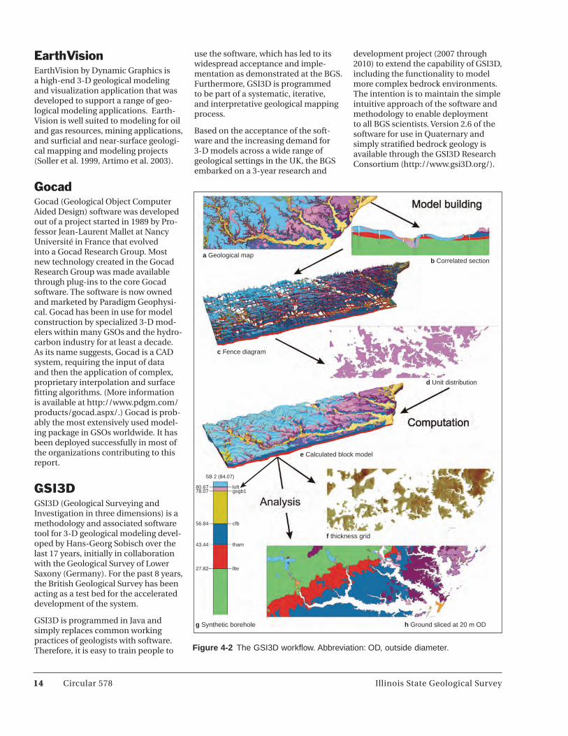
GSI3DGSI3D (Geological Surveying and Investigation in three dimensions) is a methodology and associated software tool for 3-D geological modeling devel-oped by Hans-Georg Sobisch over the last 17 years, initially in collaboration with the Geological Survey of Lower Saxony (Germany). For the past 8 years, the British Geological Survey has been acting as a test bed for the accelerated development of the system.
GSI3D is programmed in Java and simply replaces common working practices of geologists with software. Therefore, it is easy to train people to
use the software, which has led to its widespread acceptance and imple-mentation as demonstrated at the BGS. Furthermore, GSI3D is programmed to be part of a systematic, iterative, and interpretative geological mapping process.
Based on the acceptance of the soft-ware and the increasing demand for 3-D models across a wide range of geological settings in the UK, the BGS embarked on a 3-year research and
development project (2007 through 2010) to extend the capability of GSI3D, including the functionality to model more complex bedrock environments. The intention is to maintain the simple intuitive approach of the software and methodology to enable deployment to all BGS scientists. Version 2.6 of the software for use in Quaternary and simply stratified bedrock geology is available through the GSI3D Research Consortium (http://www.gsi3D.org/).

Illinois State Geological Survey Circular 578 15
The GSI3D methodology and workflow (Figure 4-2) requires the geologist to conduct five tasks:
• definethestratigraphicsuccession(topology rules),
• surveytheareatoproduceageo-logical map (if none exists already),
• codeandclassifyavailablelogsofboreholes,
• drawcrosssections,and
• drawmapsofthedistribution(out-crop and/or subcrop) of each geo-logical unit.
The model cap is formed by a DTM. The 3-D spatial model is calculated by triangulation that interpolates between the correlation line nodes in sections and along geological boundaries (Kes-sler and Mathers 2004).
Multilayer-GDMMultilayer-GDM, developed by BRGM, is especially suited for data control and for layered models with vertical faults where traditional geostatistics are particularly applicable. The Mul-tilayer-GDM software utilizes BRGM’s borehole and geological map data sets including fault traces, outcrop infor-mation, existing cross sections and outcrop-subcrop distributions, and a DEM. The software performs con-sistency checks between these varied sources. The model is controlled by a stratigraphic sequence file with rules concerning the nature of bounding surfaces (e.g., erosional, onlap). Once the data are internally consistent, geo-statistical techniques, including the Isatis package, are used to calculate the model. The produced model then can be used to generate automated maps and sections and then deliver the information using a viewer. There are many similarities in approach between GSI3D and Multilayer-GDM. (More details can be found at http://gdm.BRGM.fr/?lang=fr/.)
Other SoftwareOther 3-D geological modeling and geostatistical packages in use in GSOs include many that have their roots in the hydrocarbon and mining indus-
tries. An alphabetical listing of the most prominent of these follows.
GeoVisionaryGeoVisionary by Virtalis, in partner-ship with the BGS, is a high-resolution 3-D and stereo-visualization pack-age enabling the visualization and analysis of landforms, surficial and subsurface geologic maps, boreholes, cross sections, and geophysical data. GeoVisionary specializes in the man-agement and rendering of very large data structures and can accommodate elevation and imagery files covering entire countries. Although GeoVision-ary has limited data editing capabili-ties, it interfaces directly with ArcGIS to facilitate interactive map creation and editing. (More details can be found at http://www.virtalis.com/systems-a-services/geovisionary.)
IsatisIsatis by Geovariance is an advanced spatial analysis and geostatistical pack-age that can be used for sophisticated spatial data analysis, geostatistical modeling and simulation, statistically based assessments of uncertainty, and 3-D visualization. It is widely used in GSOs where it is a common tool for modeling porosity and permeability distributions and for modeling the uncertainty in the distribution of strati-graphic map units. (More details can be found at http://www.geovariances.com/en/isatis-ru324.)
MoveMove by Midland Valley Software focuses on structural geology and asso-ciated analytical geological modeling tools built upon tested geological algo-rithms. Geological models are designed to evolve both forward and backward through time, allowing geologists to check assumptions and verify data. The software can help geologists cap-ture data, build models, and field test interpretations. Move has been used to build and test 3-D subsurface models for major geotechnical and civil engi-neering projects. (More details can be found at http://www.mve.com/.)
PetrelPetrel by Schlumberger is a high-end 3-D geological framework and prop-erty modeling package designed for the petroleum industry. It has very sophisticated tools for integration of a wide range of data types, including 3-D seismic, but does not work easily with surficial and near-surface geological modeling. (More details can be found at http://www.slb.com/content/ser-vices/software/geo/petrel/geomodel-ing.asp.)
RockworksRockworks by Rockware is a PC-based system supporting a wide range of 2-D and 3-D geological mapping and mod-eling techniques for visualizing, inter-preting, and portraying surficial and subsurface information. It interpolates surface and solid models, computes reserve and overburden volumes, and can display maps, logs, cross sections, fence diagrams, solid models, reports, and animations. (More details can be found at http://www.rockware.com/product/overview.php?id=164.)
SKUASKUA by Paradigm Geophysics is a 3-D modeling package that is designed primarily for the petroleum indus-try. However, because its methodol-ogy embeds a full 3-D description of faulted volumes, it has application for GSOs mapping in structurally complex geological settings where modelers can create grids consistent with true stra-tigraphy and structure while honoring data and geological rules. (More details can be found at http://www.pdgm.com/products/skua.aspx.)
SurferSurfer by Golden Software is limited to the interpolation and visualiza-tion of 2-D surface models. Surfer has the capability to simultaneously view stacked sets of independent surfaces in 3-D space. (More details can be found at http://www.goldensoftware.com/products/surfer/surfer.shtml.)

16 Circular 578 Illinois State Geological Survey
SurpacSurpac by GemCom is used to support open pit and underground mining operations and exploration projects. The software employs 3-D graphics and workflow automation that can accommodate a client’s specific pro-cesses and data flows. (More details
can be found at http://www.gemcom-software.com/products/surpac/.)
VulcanVulcan by Maptec is designed specifi-cally for the mining industry to validate and transform raw mining data into 3-D models by providing 3-D software
tools that allow geologists to access and view drill hole data, define the geology, and accurately model ore bodies and deposits. Vulcan includes database management and geophysi-cal modules, and resource, geotechni-cal, and ore control tools. (More details can be found at http://www.maptek.com/products/vulcan/.)

PART 2MAPPING AND MODELING AT THE GEOLOGICAL SURVEY ORGANIZATIONS


Illinois State Geological Survey Circular 578 19
Chapter 5: Geoscience Australia and GeoScience Victoria: 3-D Geological Modeling Developments in AustraliaDon Cherry1, Bruce Gill1, Tony Pack2, and Tim Rawling3
1Departmant of Primary Industries, Melbourne, Victoria, Australia, 2Geoscience Australia, Canberra, Australia, and 3GeoScience Victoria, Melbourne, Victoria, Australia
Introduction to 3-D Geology in AustraliaAustralia is similar to the USA, Canada, and Germany in that the country is a federation of states held together under a national government. For the geosciences, this results in each state having a jurisdictional geological survey or geoscience department and the federal government also having a nationally focused department, known as Geoscience Australia.
In the development and use of 3-D geology, Geoscience Australia and Geo-science Victoria have been the most active GSOs in Australia. The use of 3-D geological methods for hydrogeologi-cal purposes has been a more recent development, with the study carried out by Cherry and Gill in Victoria, which is summarized in this article. An Australian national 3-D hydrogeol-ogy workshop held in September 2009 brought together a range of govern-ment and university researchers to present their work and discuss the development of national objectives for 3-D geology-based groundwater map-ping. The workshop extended abstracts can be found at http://www.ga.gov.au/image_cache/GA15507.pdf
Geoscience AustraliaGeoscience Australia (GA) was estab-lished in 1946 as the Bureau of Mineral Resources, Geology and Geophysics (BMR) to provide geological and geo-physical maps of Australia to underpin mineral exploration.
Today, GA’s role has expanded to pro-viding geoscientific information and knowledge to enable government and the community to make informed decisions about
• theexploitationofresources,
• themanagementoftheenviron-ment,
• thesafetyofcriticalinfrastructure,and
• theresultantwell-beingofallAus-tralians.
Excluding the Australian Antarctic Ter-ritory, GA’s activities cover a land area of 7.7 million km2 (the world’s sixth largest country and smallest continent) and a marine jurisdiction of 11.38 million km2 (the world’s third largest) including 2.56 million km2 of extended continental shelf confirmed by the United Nations Convention on the Law of the Sea (UNCLOS) in April 2008 (http://www.ga.gov.au/ausgeonews/ausgeonews200903/limits.jsp).
The onshore activities of GA focus on enhancing mineral exploration and environmental land-use planning by producing geological maps, databases, and information systems and conduct-ing regional geological and mineral systems research. Activities also con-tribute to safer communities and criti-cal infrastructure and the maintenance of fundamental gravity, geomagnetic, and seismic networks.
Offshore activities focus on providing pre-competitive data and information to assist in identifying new areas for petroleum exploration and the geologi-cal storage of carbon dioxide. Addi-tional activities also include mapping and documentation of Australia’s mari-time boundaries, studies of the marine environment, and sea floor mapping.
Spatial information activities focus on providing key spatial informa-tion of Australia with an emphasis on response to rapid and slow onset haz-ards, the detection of change, emer-
gency management requirements, natural risk assessment, and marine zone management. Australia’s Land and Marine Jurisdictions are shown in Figure 5-1.
Geoscience Australia uses a range of different 2-D and 3-D modeling appli-cations including Gocad, ArcGIS, ER Mapper, and PetroMod, depending on the professional subject area, the type of data being processed, and the desired output.
Most 3-D geological models are cre-ated using specialized and expensive software and have fairly large stor-age requirements. As a result, online publishing of 3-D models has been restricted. Model data are being dis-tributed via CD, DVD, portable hard drives, and restricted and constrained downloads.
In an effort to improve access to its 3-D models, GA has been converting 3-D geological models into Web-viewable formats for distribution and publica-tion online.
Initially, models were converted to VRML (Virtual Reality Modeling Lan-guage) and, since 2007, to X3D (Exten-sible 3-D), the XML-based successor to VRML. Both these formats are open source ISO standards for 3-D graphics on the Web developed and supported by the Web3D Consortium (http://www.web3d.org).
Both X3D and VRML allow interaction with the 3-D data using a Web browser plug-in; hence, 3-D Web mapping. Both VRML and X3D have proven to be very effective methods for communi-cating large amounts of complex 3-D geoscientific and geospatial informa-tion to a wide audience. Since 2000, over 40 unique 3-D Web models have

20 Circular 578 Illinois State Geological Survey
been produced, some of which are available online (Figure 5-2).
Since 2008, GA has been exploring the use of NASA’s World Wind software development kit to allow the public to explore and compare Australia’s continental data sets, such as radioele-ments, surface-related uranium, grav-ity and magnetic anomalies, and other mapping layers and to show the data draped over the Australian terrain in three dimensions. For example, Figure 5-3 shows Mt. Warning, New South
Wales, with surface geology from the 3D Data Viewer at 1:1,000,000 scale. Subsurface data such as seismic lines, earthquakes at depth, and 3-D geology are being explored for future releases. (http://www.ga.gov.au/resources/mul-timedia/world-wind.jsp and http://worldwind.arc.nasa.gov/java/)
GeoScience VictoriaGeoScience Victoria (GSV) is the mining and geology branch within the Victorian Department of Primary
Industries, the Australian state govern-ment agency responsible for mapping the geology of Victoria. It originally was founded in 1852 during the Victorian gold rush era. In 2004, its name was changed from the Geological Survey of Victoria after it merged with the Petro-leum Development Branch.
The Earth Resources Division (ERD) of the Department of Primary Industries has about 130 staff in four branches across Victoria. The key responsibilities of GSV are
• managinggeoscienceinformationon behalf of the State,
• assessingandpromotingthemin-erals and petroleum exploration potential to investors and govern-ment,
• providingregionalgeologicalframe-works for mineral exploration enti-ties and other stakeholders, and
• providinggeoscienceadvicetogov-ernment and industry.
Key stakeholders of the GSV are Vic-toria’s government ministers; local, state, territory, and commonwealth government organizations; extractive, geothermal, mineral, and petroleum industries and industry bodies; explor-ers and producers and their agents; and the broad community including recreational prospectors, community, environment, special interest groups, and students. The minerals, petroleum, geothermal, and extractive industries make a major contribution to Victo-ria, generating some A$5.4 billion per annum for the economy.
For decades, exploration geologists in the coal, oil, and gas industries and, more recently, in the minerals industry have been using 3-D modeling soft-ware to collate, visualize, and analyse their data sets. Generally, this effort has been focused at the reservoir/field or deposit/camp scale, and few regional, full-crustal 3-D geological models have been developed.
In 2002, GSV recognized the need to provide regional-scale 3-D models of Victoria’s geology. Soon after, the Victorian government committed to providing to industry the next gen-eration of exploration tools for the mineral resources of Victoria. After
Figure 5-1 Australia’s Land and Marine Jurisdictions.

Illinois State Geological Survey Circular 578 21
consulting with numerous exploration geologists, researchers, and govern-ment geologists, it was recognized that 3-D geological models would provide critical tools to explorers interested in understanding not only the distribu-tion and history of mineral deposits as well as energy and water resources, but also the entire Earth system that was responsible for their development. To that end, GSV established a 3-D model-ing program in 2004, and a well-funded 3-D geological modeling project began in 2007. This project was designed to develop a sophisticated, fully attrib-uted 1:250,000-scale 3-D model of the whole crust incorporating the onshore and offshore geology of the state.
MtWarning
ByronBay
Figure 5-3 Mt. Warning, New South Wales, from Geoscience Australia’s 3-D Data Viewer showing surface geology (lithostratigraphy) with contacts and terrain hill shading. 1:1,000,000.
Figure 5-2 Gawler Craton 3-D crustal VRML model.
Gawler Craton 3-D crustal model snapshots
Model interface, with DEM andcoastline
Modelled cross sections
Magnetite isosurface withprospect sites
Gradient points for susceptibility
Interactive volume slices
As a result of taking this “Moho to the sky” approach (e.g., Figure 5-4), that the modeling workflows needed to be flexible and allow incorporation of numerous geophysical data sets and their derivatives to aid in the interpre-tation of the 3-D structure of the Earth at depths beyond the scope of drilling control (as much as 40 km in places).
Modeling WorkflowGeoScience Victoria’s 3-D modeling team developed a model-building workflow that is applicable to both onshore and offshore settings and includes integration modeling between basement and basin blocks. The work-flow is based on the following steps:
• Integrateallavailablesurfacemap-ping, drilling constraints, poten-tial field data sets, 3-D inversion models, seismic data, and other 2-D and 3-D data sets into a 3-D storage and visualization environment.
• Defineanagreeduponstratigraphyfor the model region.
• Constructserialcrosssectionsbasedon surface geology and geophysical constraints perpendicular to major

22 Circular 578 Illinois State Geological Survey
structural trends with some tie sec-tions parallel to trend if there is sufficient structure to constrain the geometry in this direction.
• Digitizeserialcrosssectionsintoa2-D/3-D⁄4-D potential field forward modeling package such as Model-Vision or GMsys. These programs allow the measured potential field response of the section to be com-pared with the calculated response for the interpreted section based on the geometry and rock properties assigned. Although the cross sec-tions are essentially 2-D, the 2-D/3-D/4-D forward modeling algorithms allow the strike of the geology to be at an angle to the section (i.e., not perpendicular) and allow bodies that terminate out of the plane of the model to be included and con-tribute to the calculated signal. For-ward modeling of this type allows a first-order assessment of the validity of the starting geometry.
• Useacombinationofimplicitandexplicit modeling methodolo-gies (primarily SKUA, Gocad, and Geomodeller). Implicit modeling (e.g., SKUA, Geomodeller) requires that contacts and observations are assigned geological types and are placed within a defined strati-graphic column. The model is then constructed from the constraining data by the software and respects the defined relationships. This approach is ideal for organizations such as GSV because (1) models can be regenerated easily if new data become available, (2) higher resolu-tion models for smaller project areas can be derived from the same set of constraint data, and (3) the model surfaces match exactly, which is important if the outputs are to be used for subsequent finite element analysis. The implicit approach is data driven, so where there is a vast amount of available data, the regional models can contain com-plex overprinting relationships, and the implicit algorithm can be slow or unstable. As a result, GSV typically combines this approach with a tra-ditional CAD-based explicit model-ing approach using Gocad. Models are also refined and visualized in Gocad.
ba
Figure 5-5 Numerical simulation results from 3-D Victoria modeling program. (a) Fluid flow associated with orogenic gold mineralization within an accreted Cambrian ocean basin; (b) strain partitioning around a Proterozoic basement block accreted during the same event. Abbreviation: Ma, million years ago.
Figure 5-4 Three-dimensional geological model of Victoria incorporating Paleozoic and older basement as well as younger onshore and offshore basin fill and overly-ing volcanic cover. 1:1,000,000.

Illinois State Geological Survey Circular 578 23
Figure 5-6 Four 3-D block diagrams of a study area in central Victoria (Spring Hill ground-water management area). The top two diagrams show aerial photography and geology draped on the digital terrain model; the lower two are voxel models of the area. The second bottom image is colored according to water salinity range. The lowermost voxel image con-tains a water table change surface that shows the decline in level over the period 2000 to 2009 (the water table in the orange area has declined as much as 20 m).

24 Circular 578 Illinois State Geological Survey
• Run3-Dpotentialfieldinversionson the model (or its individual parts), ensuring that the 3-D geo-logical model is consistent with the available geophysical data sets. These inversions can highlight regions where the model’s predicted potential field response varies from the measured data. Here, the rock properties (such as density or mag-netic susceptibility) can be modi-fied within a rock volume to better match the measured response, thus potentially indicating zones of alter-ation associated with mineraliza-tion, or the shape of model surfaces or volumes can be modified again to better match measured responses. The results of these inversions are fed back into the modeling work-flow, further enhancing the model.
• Visualizethemodeling,primarilydone using Gocad, where the model constrains serial and seismic sec-tions, and any other appropriate data sets and surfaces are visualized and analyzed.
Value-Added 3-D Geological Models3-D models are useful visualization and analysis aids that provide the third dimension to traditional 2-D map-based approaches. However, using them in this way underutilizes their true power, which is unlocked when the 3-D model outputs are used to constrain numerical simulation models using finite element or particle model-ing codes to investigate Earth system behavior in 3-D or 4-D.
The outputs of the 3-D Victoria model-ing program (Figure 5-5) have been used to develop finite element models that predict the behavior, throughout the crust, of gold-bearing fluids associ-ated with mineralizing events. These models are tested in regions of known geology and then are used predictively in greenfield regions where the major elements of the geology are understood (e.g., from geophysics under shallow cover), but few deposits have yet been discovered. Numerical simulation of geodynamic processes, also based on regional 3-D control, has also allowed investigation into the nature of strain partitioning around Proterozoic crustal
blocks entrained in accretionary envi-ronments. This simulation has allowed investigation into the controls of basin formation during subsequent rifting and has direct application to hydro-carbon exploration, geological storage of carbon, geothermal energy, and groundwater resource investigations.
Finally, derivative 2-D data sets from the 3-D models have been produced to allow stakeholders who do not have access to sophisticated 3-D applica-tions to take advantage of the model outputs. These include depth surfaces for major stratigraphic contacts, depth to basement surfaces, granite thick-ness maps, fault maps, and inflection point layers. All of these can be loaded into a traditional 2-D GIS application and used as inputs to area selection mapping or weights of evidence style predictive analysis.
3-D Hydrogeology in VictoriaWithin the Victorian Department of Primary Industries, the Groundwater Research Group developed an interest in using 3-D geological mapping meth-ods for hydrogeological investigations when Mintern (2004) wrote a paper on the potential of the techniques for a Murray Darling Basin Groundwater Conference. The paper was inspired by developments at the Alberta Provincial Geological Survey in Canada following a study tour in 2003.
Cherry (2006) undertook a review of software platforms suitable for 3-D hydrogeology applications to establish the foundations for a more substantial study into 3-D hydrogeology appli-cations for Victorian groundwater resource management needs. During this review, the value of workshops sponsored by the Illinois State Geo-logical Survey, Geological Survey of Canada, and Minnesota Geological Survey became apparent (e.g., Berg et al. 2009). The experiences of others around the globe in utilizing these new methods helped establish the validity of the emerging technology and brought sufficient evidence of the potential of the techniques for a more substantial project to be developed in 2006. Although the hydrogeology appli-
cation research project arose inde-pendently of the GSV work, the 3-D hydrogeology project gained support from the larger GSV initiative in terms of in-principle support, expertise, and experience in the use of Gocad, data sharing, and use of a 3-D visualization facility.
The Victorian 3-D hydrogeology project has focused on three areas of interest to develop, test, and demon-strate the new methods: two intensely developed groundwater resource man-agement areas and an area of surface water–groundwater interest. Progress to date has been to assemble the avail-able geological data into suitable 3-D geology databases; explore the use of Gocad to model the main aquifers, faults, groundwater data; and develop visualizations of the data (Figure 5-6). The virtual models of the main aqui-fers have greatly improved conceptual models of the groundwater system in each area to be developed. An immedi-ate benefit has been the ability to iden-tify more logical boundaries for the groundwater resource management area as well as to identify flow constric-tions in the aquifers.
Using query tools in Gocad, the aquifer volumes have been calculated. A cru-cial step for calculating groundwater movement into and out of each area was to use the software to measure aquifer cross sectional areas at key points in the aquifer flows paths. Mass balance models were then constructed on the basis of the virtual model calcu-lations, allowing groundwater resource estimates to be made. Reducing the uncertainty in the physical dimensions of the aquifers also reduces uncer-tainty in mass balance modeling of the groundwater resource. The aquifer sur-faces are also able to be exported into numerical modeling packages (such as MODFLOW) to simulate the dynamic behavior of the aquifer system. For groundwater resource assessment purposes, the use of 3-D geology shows great promise in improving the tech-nical understanding of groundwater resources and in allowing groundwater users and administrators new ways of developing a shared understanding of the resource.

Illinois State Geological Survey Circular 578 25
Chapter 6: British Geological Survey: A Nationwide Commitment to 3-D Geological ModelingStephen J. Mathers, Holger Kessler, and Bruce NapierBritish Geological Survey
Figure 6-1 Bedrock geology of Great Britain.Figure 6-2 Superficial geology of Great Britain.
Upland peat
Glaciated uplands
Glaciolacustrinedeposits
Washembayment
Lowlandtill sheets
Glaciofluvialoutwash
Maximum extentof glaciation
Periglacialdeposits
Glaciateduplands
The British Geological Survey (BGS), founded in 1835, is the national geo-logical survey for Great Britain (includ-ing England, Scotland, and Wales). In addition to its government core fund-ing, the BGS earns around 50% of its income through commercially funded projects, services and sales. Its total annual turnover is around £55 million.
The BGS undertakes an integrated core program of geological mapping and modeling with an annual budget of about £5 million, and commercial contracts raise an additional £1 million per year for these activities. The BGS program produces digital geological maps (DigMap) and attributed 3-D geological models (LithoFrame) as its primary outputs.
Of the 500 BGS scientific staff, about 30% have been trained to use 3-D geo-logical modeling techniques and to employ these tools in primary surveys; coastal, urban, and engineering site remediation; and groundwater stud-ies. Approximately 20 scientists are engaged in 3-D modeling on a daily basis. The modeling community is supported by a help desk and training courses.

26 Circular 578 Illinois State Geological Survey
Geological SettingGreat Britain is the largest of the Brit-ish Isles lying in northwest Europe and covering an onshore area of about 210,000 km2. The island is geologi-cally diverse; the oldest rocks occur in the north and west and progressively younger rocks occur to the south and east toward the still subsiding southern North Sea Basin (Figure 6-1).
Archean gneissose rocks of the Lewis-ian Complex are found in northwestern Scotland and belong to the Laurentian craton of North America. Elsewhere in northern Scotland, deformed Neo-Pro-terozoic metasediments of the Moine and Dalradian supergroups are wide-spread together with Lower Palaeozoic sediments and volcanics in southern Scotland, Wales, and the Lake Dis-trict of England. These rocks were all deformed during the Caledonian Orog-eny at the end of the Silurian Period and are divided into a series of distinct structural terranes by major northeast-southwest aligned faults. Numerous granitic plutons were intruded into these sediments during the orogeny.
The largely terrestrial Devonian red bed rocks accumulated in fault-con-trolled basins within this Caledonian structural framework, and the overly-ing initially marine Carboniferous shelf carbonates gradually gave way to extensive fluviatile and deltaic sedi-mentation leading to the accumula-tion of major coal resources during the Pennsylvanian. These have subse-quently acted as source rocks for the oil and gas reserves that are trapped in the overlying sediments. The Variscan (Hercynian) Orogeny at the close of the Carboniferous is well recorded by the deformation of the Devonian-Carboniferous sediments of south-western England, where a large granitic batholith at depth is evidenced at the surface by a string of granite bosses. Elsewhere in southern England the rocks deformed by the Variscan Orog-eny lie buried beneath Mesozoic and Tertiary cover.
The succeeding Permian deposits of northeastern England fringe the large Zechstein continental basin that devel-oped across northwestern Europe in which thick evaporate sequences were
hole logs, geological map linework cap-tured as a series of themes (or layers), and key national geophysical data sets and seismic lines.
Additionally, digitally georectified nationwide topographic maps includ-ing historic versions, aerial photo-graphs, satellite imagery, and DEMs were licensed or purchased, and the availability of such data sets has been maintained and upgraded where new and improved products have become available.
The BGS LithoFrame ConceptThe BGS models are branded under the name LithoFrame. They represent the extension of the 2-D geological map into 3-D (Tables 6-1 and 6-2).
Central to the LithoFrame concept is that varied resolutions are consis-tent with one another so that collec-tively they form a seamless transition from the general national model to a detailed site-specific one. Figure 6-3 shows that the highest-order strati-graphic units (regionally extensive and well defined) shown in dashed red lines should be defined first and be included in all models of a higher (more detailed) resolution. Here the major stratigraphic boundaries selected at LithoFrame 250 are applied to the higher resolution 50 and 10 models. At LithoFrame 50, more detail is applied, showing seven rather than two units, but this detail is likely to be observed and depicted to a shallower depth. These units then extend through the more detailed LithoFrame 10 model, and more detail (here 17 units) is nested within them in the shallow sub-surface. Similar simplification of fault networks is shown on the right side of Figure 6-3.
The depth of modeling reflects the available data and the importance of seismic lines and deep boreholes to provide information when building low definition models, whereas the detailed LithoFrame 50 and 10 reso-lutions rely more heavily on surface geological mapping and shallow bore-holes. Hence, deeply buried surfaces constructed at LithoFrame 250 resolu-tion in some areas can be constructed
deposited. The succeeding Triassic sequences are almost exclusively ter-restrial red beds recording a diverse history of independent basin evolu-tion in the post orogenic extensional tectonic regime. They include the important Sherwood Sandstone Group that is widely exposed in the English Midlands and comprises both a major aquifer and a hydrocarbon reservoir. The succeeding Jurassic and Creta-ceous sediments record sedimentation in epeiric shelf seas culminating in the globally high sea levels and sedi-mentation of the Chalk Group across much of western Europe in the Upper Cretaceous. Due to subsequent ero-sion, the Chalk is now only exposed in southeastern England where it also constitutes a major aquifer.
Initial rifting associated with the open-ing of the North Atlantic resulted in the volcanic rocks of the Hebrides in northwestern Scotland; in southeast-ern England, terrestrial and marine Palaeogene sediments accumulated. These sediments were then folded during the Miocene-Oligocene in response to reactivation of underly-ing Variscan basement structures in southern England during the Alpine Orogeny.
Most of Great Britain has been glaci-ated several times during the Qua-ternary, resulting in the deposition of extensive sheets of till in lowland areas (shown in blue in Figure 6-2) and glaciated uplands in Wales and Scotland. These deposits are associated with large spreads of glaciofluvial sand and gravel (pink) and glaciolacustrine sediments (brown) in proglacial and ice-marginal settings. The extreme southern part of England remained ice-free throughout, and there peri-glacial mass movement and aeolian sediments and permafrost structures are widespread. Holocene deposits are located along major river courses and in coastal plains (yellow) including the large Wash embayment.
Data Sets for ModelingIn the 1990s, BGS converted its key national data sets into digital form and produced supporting dictionaries and lexicons for these databases. The data sets include borehole index and down-

Illinois State Geological Survey Circular 578 27
Table 6-1 Main features of the LithoFrame resolutions.1
LithoFrame 1M LithoFrame 250 LithoFrame 50 LithoFrame 10 Feature (National) (Regional) (Detailed) (Site-specific)
Proposed Entire onshore and UK Entire onshore and Onshore UK Major urban and coverage continental shelf UK continental shelf development areas; (long-term) areas of complex and classic near-surface geology
Tile size Single tile 100 x 100 km 20 x 20 km 5–10 km x 5–10 km
Resolution of 1 km 500 m 100–200 m 50–100 m grid output
Depth 50 km 5–10 km 1–2 m 100–200 m or base of surficial deposits if deeper
Uses Visualization, national Visualization, popular Analysis, the Detailed analysis and and international science, overviews for standard output, problem solving; site- collaboration, public the energy and water hydrocarbons, specific and detailed understanding of sectors, deep aggregates, bulk studies of all kinds science, education structural studies minerals, aquifers, planning, major infrastructure
Key data sets Geological linework Geological linework Geological linework Geological linework Digmap 625 deep Digmap 250 seismic Digmap 50 seismic Digmap10 all seismic lines, national lines and regional lines, boreholes, boreholes and mining and regional magnetic magnetic and gravity deep mining data data and gravity data, very data, deep boreholes deep boreholes
Commercial Low; popular Modest; contextual Moderate to high; Very high, custom potential publications, atlases models for energy, the standard product models to resolve water sectors for geoscientists and problems and deliver allied professions geoscience solutions at a detailed site- specific level
1LithoFrame scales: 1M, 1:1,000,000; 250, 1:250,000; 50, 1:50,000; 10, 1:10,000.
Figure 6-3 Schematic section showing effective depth of modeling and definition across the LithoFrame 250, LithoFrame 50, and LithoFrame 10 resolutions.
considering all the available data, and therefore they can be magnified to form the deeper parts of the higher res-olution, LithoFrame 50 and 10 models if required. This concept reinforces the suggestion that key surfaces should be first defined for low-resolution models and then used to form the framework for nested detail at higher definition for more detailed models.
Example ModelsNational Model of Great BritainAn onshore LithoFrame 1 M model (1:1,000,000 scale) (Tables 6-1 and 6-2) has been produced for Great Britain. The model is principally derived from
STRATIGRAPHIC UNITS FAULTS
INFORMATION
17
7
2
Mapping and lotsof boreholes
Seimic somedeep boreholesonly guesswork
Someboreholesprojection of crop
Site-specific1:10,000
Detailed1:50,000
Regional1:250,000

28 Circular 578 Illinois State Geological Survey
Table 6-2 Geological detail possible at the various LithoFrame resolutions.1
LithoFrame 1M LithoFrame 250 LithoFrame 50 LithoFrame 10 Detail (National) (Regional) (Detailed) (Site-specific)
Stratigraphic Major stratigraphic Group level likely to Formation level likely Members and resolution systems and deep be the most to be the most scientifically or (bedrock) crustal layers to the commonly applied commonly applied economically Moho picking out level, especially for level, especially for important beds down overall structure concealed strata concealed strata to 1-m-thick lenses
Stratigraphic Not depicted Superficial undivided Major units modeled Detailed modeling of resolution beds, lenses, etc. as (superficial) required
Unconformities Delineated at major Major unconformities Unconformities Minor unconformities system boundaries delineated by delineated by revealed by detailed stratigraphic stratigraphic stratigraphic units boundaries boundaries
Folding Depicted by overall Depicted by overall Detailed form Very detailed form form of major form of major depicted using depicted by thin sedimentary packets sedimentary packets structural sedimentary packets observations in and structural Digmap 50 observations at Digmap 10 scale
Faulting Major faults Those with throws of Faults with throws of Faults with throws of bounding domains of hundreds meters or more than 50 m; also more than 10 to 15 m; British geology, e.g., lateral displacement slightly smaller faults also slightly smaller Great Glen, Highland of several kilometers where these are faults where laterally Boundary faults; likely to be included laterally persistent or persistent or strongly vertical displacements in the model strongly influence the influencing the outcrop of kilometers and/or outcrop pattern; pattern; subparallel significant lateral subparallel faults faults amalgamated displacements of amalgamated where where their spacing 100 km spacing is <200 m is <50 m
Intrusions Major plutons such Plutons with Plutons with Plutons with and lavas as the southwestern outcrops-subcrops outcrops-subcrops of outcrops-subcrops of England and Lake of at least 10 km2 at least 5 km2 should at least 1 km2 sheet District batholiths should be included; be included; thick intrusions at least 5 m covering several major lava piles lava sequences and thick; individual lava hundred square major sheet intrusions flows and sheet kilometers in extent intrusions
Artificial ground Not shown Not shown Large pits and Quarries worked quarries worked and/or infilled, and and/or infilled, and large mappable extensive thick areas areas of made of made ground ground
1LithoFrame scales: 1M, 1:1,000,000; 250, 1:250,000; 50, 1:50,000; 10, 1:10,000.
the compilation of contoured strati-graphic surfaces, deep boreholes, seis-mic profiles, and regional geophysical interpretations (Whittaker 1985). The model (Figure 6-4) was constructed in Gocad by the BGS and shows the base of major geological units as 2-D surfaces (”flying carpets”). Also shown are the foci of significant earthquakes, major faults, and igneous plutons. The
model extends to a depth of about 30 km; the lowest, purple surface repre-sents the base of the crust (Moho). The model is mainly used for educational purposes, visualizations of the nation’s geology, and a basic spatial framework for more detailed modeling exercises. (For more information, see http://www.bgs.ac.uk/science/3dModeling/lithoframe1m.html.)
Surfaces modeled include these bases:
• Palaeogene
• Cretaceous
• Jurassic
• Triassic
• Permian
• Carboniferous

Illinois State Geological Survey Circular 578 29
• Devonian
• LowerPalaeozoic
• Precambrian
• Crust(Moho)
Regional Model: The WealdAt the next level of detail, regional LithoFrame 250 resolution models (1:250,000 scale) (Tables 6-1 and 6-2) are being constructed for the whole of England and Wales. An example from
Figure 6-4 The LithoFrame 1M resolution onshore model of Great Britain.
Figure 6-5 Example LithoFrame 250 model covering the Weald and adjacent parts of the English Channel.
2007
2008
2009
2010–2012
Figure 6-6 Scheduled availability of LithoFrame 250 resolution regional models for England and Wales.
the Weald-English Channel model is shown in Figure 6-5. This model was developed in Gocad and is based on extensive depth-converted seismic interpretations, deep boreholes with downhole geophysics, and surface geology. The progress toward regional LithoFrame 250K coverage is shown in Figure 6-6.
Detailed Model: Southern East Anglia, Eastern EnglandA systematic LithoFrame 50 (1:50,000 scale) detailed model (Tables 6-1 and 6-2) has been built for 1,200 km2 of southern East Anglia in the Ipswich-Sudbury area. Modeling was carried out in conjunction with a primary geo-logical survey of much of the area. The model was constructed as the survey progressed in 10-km × 10-km tiles, and then the various tiles were merged (Figure 6-7).
The model contains the major artificial deposits, about 25 superficial layers, including a complex, interleaved, Anglian glacial succession and bed-rock. The glacial succession includes a widespread till sheet (in blue) in the
north and west and extensive perigla-cial and ice-marginal glaciofluvial sand and gravel deposits (pink) underlying the till and exposed in the south and west of the area. The geometry of the latter deposits is especially important as they constitute a major aggregate resource. The bedrock comprises Plio-Pleistocene shallow marine sediments (Crags in deep purple) and Palaeogene marine and marginal sediments domi-nated by clays (blue and red). The dis-tribution of these clay-rich Palaeogene strata is crucial as they act as a protec-tive seal for the underlying Upper Cre-taceous Chalk Group aquifer (green). The model extends to the base of the Chalk Group at an average depth of about 300 m. The Chalk is one of Brit-ain’s principal aquifers, and this model has been licensed to the Environment Agency of England and Wales for use by the hydrogeological consultants to investigate issues of aquifer protection, recharge, and groundwater manage-ment. The model is also used to gener-ate borehole prognoses for site-specific inquiries and has improved scientific understanding of the complex glacial succession of the area.

30 Circular 578 Illinois State Geological Survey
Sudbury
Ipswich
10 km300 m
N
Figure 6-7 The LithoFrame 50 resolution southern East Anglia model of the Ipswich-Sudbury area covering 1,200 km2.
Site-Specific Resolution: Shelford, Trent ValleyAn integrated geological, geophysical, and remote sensing survey was under-taken to construct a high resolution 3-D LithoFrame 10 (1:10,000 scale) site-specific model (Tables 6-1 and 6-2) of the shallow subsurface geology of part of the Trent Valley in Nottingham-shire, UK. The 3-D model (Figure 6-8) was created using the GSI3D software package to evaluate the 1:10,000-scale geological survey, borehole data, and remote sensing images, plus verti-cal and horizontal profiles derived from geophysical techniques such as ground-penetrating radar (GPR), elec-
Figure 6-8 The site-specific Shelford model.
Figure 6-9 Current LithoFrame 10 and LithoFrame 50 coverage for Great Britain.
trical resistivity tomography (ERT), and automated resistivity profiling (ARP). The site covers about 2 km2 and con-sists of a Triassic mudstone overlain by Quaternary sand and gravel river terrace deposits and the modern flood-plain deposits of the River Trent. Addi-tionally, soil horizons were modeled together with areas of artificial deposits (Whitaker 1985, Tye et al. 2010).
The combined investigations enabled several advances in the understanding of the area including
• delineationofaburiedrivercliffforming the southern limit of the incised Trent valley,
• precisepositioningofhardthinsilt stone beds (skerries) within the bed-rock Gunthorpe Member of the Mercia Mudstone Group, and
• resolutionofthelithologicvariabil- ity of the sediments within the river terrace deposits.
This study demonstrates the potential for combining many and varied data sets within a single spatial reference system (GSI3D) to maximize the inter-pretation of subsurface conditions. Such investigations are very well-suited to ground investigations for major civil engineering and infrastructure proj-ects, together with site-based evalua-tion for environmental problems such as evaluating and tracking of pollution plumes. Similar resolution models have also been constructed for archae-ological investigations and to model the chronology of artificial deposits.
The distribution of detailed and site-specific models produced by the BGS is shown in Figure 6-9.

Illinois State Geological Survey Circular 578 31
Chapter 7: Geological Survey of Canada: Three-dimensional Geological Mapping for Groundwater ApplicationsH.A.J. Russell1, E. Boisvert2, C. Logan1, S.J. Paradis2, M. Ross3, D.R. Sharpe1, and A. Smirnoff2
1Geological Survey of Canada, 601 Booth St., Ottawa, Ontario, Canada, 2Geological Survey of Canada, Québec City, Québec, Canada, 3University of Waterloo, Department of Earth Sciences, Waterloo, Ontario, Canada
The Geological Survey of Canada (GSC) is a federal agency that operates col-laboratively with multiple provincial and territorial agencies that have direct responsibility for natural resource and groundwater management. Three-dimensional geological mapping has been embraced at the GSC during the past 20 years as data collection, analysis, interpolation, visualiza-tion, and presentation modes have evolved with the advent of increased computer processing capacity, graphic user interfaces, and 2-D and 3-D GIS (Geographic Information Systems). Nevertheless, for groundwater stud-ies the fundamental requirements for 3-D geological mapping have not changed radically from traditional geo-logical investigations. Basin analysis concepts provide the cornerstone of 3-D mapping at the GSC. Within this framework, emphasis is placed on data collection and understanding of the geological history of the basin. This knowledge base provides a framework for interpretation and correlation of disparate data sets necessary for input to interpolation algorithms for the construction of 3-D models. Basin analysis has been adapted across the groundwater program as a common methodology for 3-D studies. Subse-quent data processing, interpolation, and visualization within GIS software remain discretionary depending upon geographic and geological complex-ity, study objectives, and partnership requirements.
This paper highlights work completed in the past 17 years within the GSC’s Groundwater Geoscience Program (and its predecessor activities) toward mapping key Canadian aquifers, spe-
cifically 3-D subsurface geological model construction. Modeling tech-niques and underlying philosophi-cal approaches (basin analysis) are reviewed, and three case studies are presented to illustrate variations in study approaches.
IntroductionPrior to the widespread use of desktop computing and advanced GIS, text descriptions, geological maps, cross sections, and attached stratigraphic legends were the only way to com-municate a 3-D conceptualization of complex geological structures and their interrelationships. This 3-D concep-tualization was illustrated using struc-tural measurements (e.g., strike and dip), cross sections, isosurface maps (e.g., isopach maps), stratigraphic con-cepts (e.g., lithostratigraphy, allo- stratigraphy), and depositional facies concepts (Wather’s Law). Because paper maps are highly subjective and based on the skill and experience of the author, they convey a unique inter-pretation of the available information (e.g., aerial photographs, field observa-tions). Moreover, correct interpretation of the map also relies on the ability of the end user to understand the 2-D map components and correctly visual-ize the implied 3-D structure. Digital 3-D modeling techniques that take advantage of innovations in hardware and software (e.g., Thorleifson et al. 2010) are a logical extension of hand-drafted geological maps that have for decades been the norm at the GSC. Like hand-drafted geological maps, digital models are realizations of 3-D geology based on extrapolating discreet and often sparse observations or mea-
surements. Unlike hand-drafted maps, digital 3-D models provide a readily understandable means of visualizing geology and estimating geological unit volumes and also permitting advanced hydrogeological study by supporting quantitative flow modeling. Conceptu-ally the differences between the 3-D modeling techniques presented here are primarily in the amount of expert input utilized. Techniques range from largely automated and data-driven to 3-D CAD techniques that rely heavily on an expert to interpret and construct 3-D contacts.
Within the new paradigm of 3-D geo-logical mapping, various groups at the GSC have pursued 3-D modeling and visualization for mineral resource development (e.g., Hughes 1993, Mossop and Shetsen 1994, de Kemp 2007) and for groundwater issues (e.g., Logan et al. 2002, 2006; Ross et al. 2005; Sharpe et al. 2007; Smirnoff et al. 2008).
Geological Survey of CanadaFounded in 1842, the GSC is the oldest government research agency in Canada. It is part of the Earth Science Sector of the Department of Natural Resources along with the Canadian Centre of Remote Sensing and Geo-matics Canada. The GSC has tradi-tionally focused on the production of geoscience knowledge. More recently its mandate has expanded to include issues pertaining to geological hazards, groundwater, the environment, and climate change. The GSC operates in all 10 provinces and three territories on a cooperative basis with respective pro-

32 Circular 578 Illinois State Geological Survey
Table 7-1 Key Canadian aquifers grouped according to hydrogeological regions. No currently designated key Canadian aquifers are identified in the Maritime and Permafrost regions.
Cordillera 1. Gulf Islands 2. Nanaimo Lowland 3. Fraser Valley 4. Okanagan Valley 5. Shushwap Highlands
Western Canadian Sedimentary Basin 6. Paskapoo 7. Buried Valleys 8. Upper Cretaceous Sand 9. Milk River 10. Judith River 11. Eastend - Ravenscrag 12. Intertill 13. Manitoba Carbonate Rock 14. Manitoba Basal Clastic unit 15 Odanah Shale 16. Sandilands 17. Assiniboine Delta
Southern Ontario Lowlands 18. Oak Ridges Moraine 19. Grand River Basin 20. Credit River 21. Waterloo Moraine 22. Upper Thames River
Appalachians 23. Annapolis–Cornwallis valleys 24. Carboniferous Bain
St. Lawrence Platform 25. Mirabel 26. Châteauguay 27 Richelieu 28 Chaudière 29. Maurice 30. Portneuf
vincial and territorial agencies to fulfill a requirement of the Resources and Technical Surveys Act of 1949 and 1994 that the Minister of Natural Resources “make a full and scientific examination of the geological structure and miner-alogy of Canada.” Provinces are vested with the primary mandate for natural resource and groundwater manage-ment, whereas the GSC has particular interest in areas of federal jurisdiction such as trans-boundary aquifers (Table 7-1; e.g., Richelieu, Milk River) and federal lands within provinces (military and First Nations reserves). To respond
to federal government mandates and objectives, the GSC maintains a suite of programs that are funded on a 5-year cycle. To fulfill this mandate, the GSC has seven offices across Canada: a cen-tral office in Ottawa and six regional offices. The GSC maintains an applied research staff of 184 technical staff of which a group of 20 to 25 work on groundwater. The annual operating budget for the Groundwater Program in 2009 was 2.8 million dollars (ESS 2006) of which more than two-thirds was allocated to salaries. Study teams commonly consist of fewer than 10 staff members, most of whom are engaged in multiple projects. To sup-plement this limited capacity, the GSC actively develops partnerships with provincial, territorial, and other federal government agencies, industry, uni-versities, and other state and national geological surveys.
Groundwater resource investigations and research at the GSC date back to 1875 (Brown 1967). In 1972, however, the mandate for water resource man-agement (including groundwater) was passed to the newly formed Environ-ment Canada, and the GSC ceased to be active in groundwater studies. During the late 1980s and early 1990s, client surveys indicated that there was a demand for increased geological input to regional water supply studies (e.g., Canadian Geoscience Council 1993). Following an absence from regional groundwater studies of more than 20 years, the GSC reinitiated work on regional hydrogeology in a series of projects in the early 1990s (e.g., Sharpe et al. 1996, Parent et al. 1998, Ricketts 2000, Thorleifson et al. 2002). Within a decade, these early studies evolved into a national groundwater program at the GSC. A collaborative document between the provinces, territories, and the federal government established a framework for progress on ground-water studies in Canada (Rivera et al. 2003). Subsequently, the groundwater program of the GSC developed a strat-egy to map and assess 30 key aquifers across the country (Table 7-1; Figure 7-1).
These 30 key aquifers consist of bed-rock and glacial sediment aquifers involving fracture media and porous
media flow systems, and they range in size up to 60,000 km2 and up to sev-eral hundred meters in depth (Tables 7-1 and 7-2). In a country considered to have abundant surface water, the groundwater resources were largely ignored prior to the 1990s. The focus of groundwater research during the 1970s and 1980s shifted to groundwater contamination (e.g., Cherry 1996) and remediation. Nevertheless, groundwa-ter use in Canada is significant; 30% of Canadians, and 80% of rural Canada, depend on aquifers for potable water supply (Environment Canada). As might be anticipated in a country of almost 10,000,000 km2 with a rather modest population (35,000,000) con-centrated in urban areas, enormous challenges are presented for the devel-opment of a comprehensive under-standing of groundwater resources.
Hydrogeological Framework of CanadaThe geology, groundwater regimes, and hydrology of Canada are complex. The major hydrogeological domains of Canada have been assigned to nine hydrogeological regions (Sharpe et al. 2008). This classification is built on previous work by Brown (1967) and Heath (1988). The delineation of these regions is based on geological prov-inces and rock formations, surficial geology, topography, and the extent of permafrost. The 30 key Canadian aqui-fers form local elements within these regions and can be assigned to one of two principal classes: bedrock aquifers and surficial sediment aquifers. Within each of these two categories, the key aquifers can be classified based on geological environments (Table 7-2).
MethodsReflecting a long history of encour-aging creative problem-solving and methods development at the GSC, study teams working on 3-D geological modeling for groundwater are permit-ted latitude in how they approach 3-D geological mapping and the tools used for model construction and visualiza-tion. This approach also implicitly recognizes differences and prefer-ences within provincial agencies and the need to maximize collaboration

Illinois State Geological Survey Circular 578 33
Table 7-2 Grouping of key Canadian aquifers according to host geology.
Index to Style Figure 7-1 Comment
Bedrock 1, 2, 5, 8, 15 Areas of fractured bedrock aquifers and secondary porosity (undefined)
Fluvial 6, 10, 11, 24 Predominantly braided fluvial systems
Carbonate 13, 14 Paleozoic carbonate systems
Deltaic-coastal 9 Cretaceous bedrock system
Bedrock/surficial 19, 20, 22, 23, Large regional, commonly watershed scale aquifer complexes; contains fracture flow mixed 25, 26, 28 bedrock and porous media in eskers, moraines, and outwash
Surficial 3 Likely fluvial (undefined)
Moraine 16, 18, 21 Sand and gravel bodies up to 200 m thick overlying erosional unconformities with tunnel channels
Esker 27 Linear sand and gravel ridges in clay basins and moraines
Buried valley 4, 7, 12 Bedrock and sediment hosted valleys of tens of kilometers scale
Delta 17, 29, 30 Kilometer-scale glaciofluvial deltas constructed into paleo-glaciolacustrine and glacio-marine environments
Outwash 12 Relatively thin, spatially extensive sand and gravel deposits of braided outwash and valley trains
Cordillera
Western Canada Sedimentary Basin
Canadian Shield
Hudson Bay Lowlands
Southern Ontario Lowlands
St. Lawerence Platform
Appalachian Mountains
Maritimes Basin
Permafrost
Dry Climate Regions
Moist Climate Regions
Figure 7-1 Hydrogeological regions of Canada and key Canadian aquifers (base from Sharpe et al. 2009). (http://ess.nrcan.gc.ca/gm-ces/aquifer_map_e.php.) Case studies are 4, 18, and 25.

34 Circular 578 Illinois State Geological Survey
Figure 7-2 Simplified basin analysis approach used in regional hydrogeological analysis of key Canadian aquifers. The approach leads progressively from data-base development to quantitative understanding of the groundwater flow system as the study matures (Sharpe et al. 2002).
and post project utilization of models. Regardless of the methodology, how-ever, a concept common to 3-D model construction is the importance of inte-grating geological knowledge to ensure appropriate geological conceptualiza-tion and subsequent model construc-tion. Basin analysis provides a frame-work that supports this approach.
Basin AnalysisBasin analysis is a methodological framework for regional hydrogeo-logical analyses that integrates data from a variety of sources and scales of investigations (Miall 2000, Sharpe et al. 2002). The strength of this approach is its emphasis on geological analy-sis leading to the development of an understanding of basin history and, hence, a knowledge base that permits development of a predictive frame-work for understanding the textural, stratigraphic, and structural controls on groundwater flow at a hierarchy of scales within the basin. It is particularly appropriate for groundwater studies
in geological environments where geo-logical heterogeneity and flow systems occur at a hierarchy of scales.
The basin analysis approach used for studies of most key Canadian aquifers follows a progression of data compila-tion, conceptualization, model devel-opment, and quantitative analysis of flow systems (Figure 7-2; Sharpe et al. 2002) with feedback/interactions among components allowing continu-ous improvement of the database and models as the study progresses. By directly linking geological setting and basin history to aquifer properties, the basin analysis approach strives to develop more plausible hydrogeologi-cal models and supports development of numeric GIS rendering of data-driven models (e.g., Anderson 1989; LeGrand and Rosen 1998, 2000). Geo-logical model development for basins falls into two distinct styles: (1) predic-tive, process-based models, such as depositional models (e.g., Russell et al. 2003) and event stratigraphic models (Figure 7-3; Sharpe et al. 2002); and (2) GIS-based, data-driven models. The
development of process-based models assists geological interpretation and development of GIS-based models. In GIS-based modeling, stratigraphic interpretations developed in the basin analysis approach are used to help interpret more abundant, lower-quality archival data such as from water-well records (Bolduc et al. 2005, Ross et al. 2005, Logan et al. 2006, Paradis et al. 2010).
To support basin analysis, the GSC employs a multi-disciplinary approach to data collection that follows a sys-tematic progression. Initial data collec-tion and analysis consist of procuring published data and collating archival data. Surface data such as geological mapping (Sharpe et al. 1997), evapo-transpiration mapping (Fernandes et al. 2007) and DEMs are common exam-ples (Kenny et al. 1999). A key data set in Canada is the provincially admin-istered water-well records. All of the provinces maintain digital databases with a variety of attributes (Sharpe et al. 2009), and, in a number of cases (e.g., Ontario and Manitoba), the GSC has worked collaboratively with the provinces to assess the integrity and utility of the water-well databases (e.g., Russell et al. 1998). In the oil-produc-ing regions of the Western Canada Sed-imentary Basin, petroleum boreholes and associated geophysical logs are an important data set (Chen et al. 2007). To handle the wealth of data collated from archival and published sources, a variety of database approaches have been adopted at a project level from the use of relational databases (e.g., Boisvert and Michaud 1998, Russell et al. 1998, Knight et al. 2008) to the use of distributed database and Web ser-vices technologies (Sharpe et al. 2009). Depending on the location and scale of the study area, the number of water wells can range from the thousands to the tens of thousands (Bolduc et al. 2005, Logan et al. 2006). Subsequent data collection commonly focuses on geological mapping (e.g., Paradis et al. 2010), the collection of geophysical data (Pugin et al. 1999) for subsurface definition of the stratigraphic archi-tecture, and high-quality boreholes (Sharpe et al. 2002).
Geophysical methods have focused on 2-D seismic profiling techniques
QUANTITATIVEUNDERSTANDING
GROUNDWATER FLOWMODELS
HYDROSTRATIGRAPHIC MODELS
GEOLOGICAL MODELS
DATABASE DEVELOPMENT
of groundwater flow system
-flow and chemical characterization-quantitative analysis (e.g. water balance)
-numerical flow modelling
e.g. -conceptual models-definition and characterization of aquifers and aquitards
e.g. -conceptual models-landform and terrain models
-stratigraphic, architectural, and depositional models
e.g. -compilation of archival data; new data collection and integrataion

Illinois State Geological Survey Circular 578 35
that have evolved from labor-intensive planting and drilling of individual geo-phone and shot holes (e.g., Pugin et al. 1999) to semi-continuous data collec-tion with a landstreamer system of S- and P-waves (Pugin et al. 2009). More recently, airborne electromagnetic surveys are being employed in the prairies of Manitoba to map conduc-tivity contrasts for aquifer delineation (Oldenborger et al. 2011). Geophysical interpretations are commonly verified by drilling of continuously cored bore-holes (Knight et al. 2008) and down-hole geophysics (Pullan et al. 2002). Supplementary data commonly used to further constrain and refine basin understanding include piezometric, stream flow (Hinton et al. 1998), and hydrochemistry data (e.g., Cloutier et al. 2006).
Data standardization has been accom-plished on an ad hoc basis within respective projects, collaboratively with provincial agencies (e.g., Russell et al. 1998), and through participation in distributed database development (Sharpe et al. 2009) and developments of GroundWater Markup Language (GWML) (Boisvert and Broderic, unpublished data) and participation in GeoSciML (http://www.geosciml.org).
An objective common in many model-ing approaches has been to establish a standard basin (regional) stratigraphic framework for both regional and site-specific hydrogeological applications. In part because modeling activities have generally been completed in basins with no previous regional sub-surface model, each project has devel-oped an approach that is most suited to the specific situation (i.e., geological setting, available data, available tech-nology and expertise, and partnership mandates). As a result, a number of approaches have evolved at the GSC that can be categorized according to stratigraphic approach, interpola-tion choices, and modeling software selection. In some cases, the geologi-cal model is constructed with direct consideration of subsequent numerical flow modeling (Rivera et al. 2003). In other cases, the model has been devel-oped as a stratigraphic repository that could be used for various applications by extracting the needed (simplified) information (e.g., Ross et al. 2005).
Stratigraphic ApproachesThe standard stratigraphic approach in surficial (glacial) basins remains lithostratigraphy (Paradis et al. 2010).
However, event stratigraphy (allo- stratigraphy, sequence stratigraphy; Walker 1992) has been adapted in a number of studies. In common with sequence stratigraphy, regional uncon-formities forming bounding surfaces are a key element of this approach (Figure 7-3; e.g., Sharpe et al. 2002; Cummings et al. 2011).
Interpretive MethodsTwo approaches have generally been followed by GSC for rendering 3-D models: cross section methodology and stratigraphic database method. Both approaches rely heavily on bore-hole log data for subsurface model control.
The cross section approach provides a direct method of simplifying the geo-logical heterogeneity by allowing the geologist to interpret the data as strati-graphic correlations are made (Thor-leifson et al. 2002, Bolduc et al. 2005). Interpretations are deterministic in nature, and because the model’s integ-rity depends largely on the geologist’s ability to apply a set of correlation rules throughout the model area, there is potential for inconsistent stratigraphic correlations from section to section and across model iterations.
Alternatively, the stratigraphic data-base method relies on a well-structured database of coded borehole logs that contains contact information on all potential stratigraphic units, including those that have a zero thickness in por-tions of the study area (Hughes 1993). Although the ability of humans to recognize patterns and eliminate data “noise” helps the cross section model appear more geologically plausible, the level of expert input is variable from place to place throughout the model. The stratigraphic assignments in a stratigraphic database are also deter-ministic in nature, but once made and vetted, they can be combined with new data and reinterpolated without having to repeat the borehole interpretation and stratigraphic coding process. The data-driven stratigraphic database model can, however, display unlikely geological structures due to interpola-tion of sparse data coverage or poor data.
Age~ka Lithostratigraphy Chrono-
stratigraphy
~13
14
20
Halton Till
Oak Ridges Moraineand
Channel sediment
regional unc onform
ity
22
Newmarket Till
UpperThorncliffe Fm
Meadowcliffe Till
MiddleThorncliffe Fm
Seminary TillLower
Thorncliffe Fm
Sunnybrook TillPottery Road Till
Scarborough Fm
40
60
115
>135
Bedrock
Don Fm
York Till
Qua
tern
ary
Paleozoic
LateWisconsin
MiddleWisconsin
EarlyWisconsin
Sangamonian
Illinoian
Oak RidgesMoraine sediment
HaltonTill
Channelsediment
NewmarketTill
Lowersediment
Bedrock
Unconformity
Unconformity
Figure 7-3 Example of an event stratigraphic model and integration of existing lithostratigraphic framework for the Oak Ridges Moraine Area (Sharpe et al. 2002).
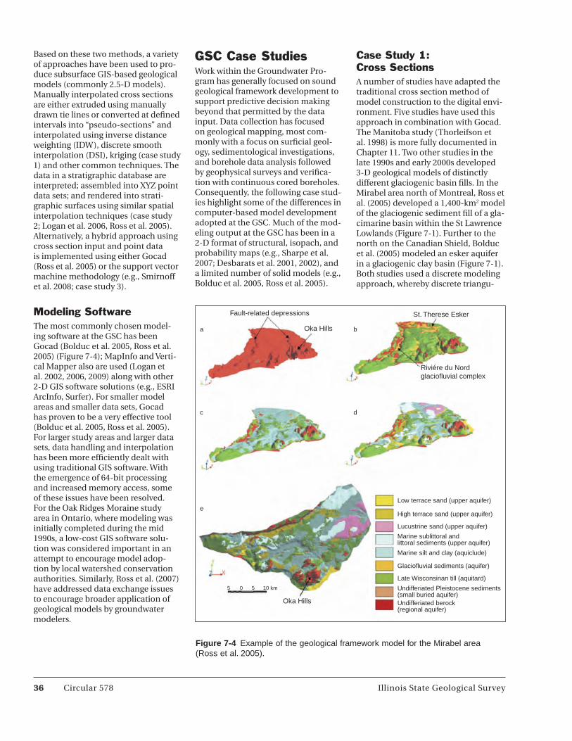
36 Circular 578 Illinois State Geological Survey
Figure 7-4 Example of the geological framework model for the Mirabel area (Ross et al. 2005).
Based on these two methods, a variety of approaches have been used to pro-duce subsurface GIS-based geological models (commonly 2.5-D models). Manually interpolated cross sections are either extruded using manually drawn tie lines or converted at defined intervals into “pseudo-sections” and interpolated using inverse distance weighting (IDW), discrete smooth interpolation (DSI), kriging (case study 1) and other common techniques. The data in a stratigraphic database are interpreted; assembled into XYZ point data sets; and rendered into strati-graphic surfaces using similar spatial interpolation techniques (case study 2; Logan et al. 2006, Ross et al. 2005). Alternatively, a hybrid approach using cross section input and point data is implemented using either Gocad (Ross et al. 2005) or the support vector machine methodology (e.g., Smirnoff et al. 2008; case study 3).
Modeling SoftwareThe most commonly chosen model-ing software at the GSC has been Gocad (Bolduc et al. 2005, Ross et al. 2005) (Figure 7-4); MapInfo and Verti-cal Mapper also are used (Logan et al. 2002, 2006, 2009) along with other 2-D GIS software solutions (e.g., ESRI ArcInfo, Surfer). For smaller model areas and smaller data sets, Gocad has proven to be a very effective tool (Bolduc et al. 2005, Ross et al. 2005). For larger study areas and larger data sets, data handling and interpolation has been more efficiently dealt with using traditional GIS software. With the emergence of 64-bit processing and increased memory access, some of these issues have been resolved. For the Oak Ridges Moraine study area in Ontario, where modeling was initially completed during the mid 1990s, a low-cost GIS software solu-tion was considered important in an attempt to encourage model adop-tion by local watershed conservation authorities. Similarly, Ross et al. (2007) have addressed data exchange issues to encourage broader application of geological models by groundwater modelers.
GSC Case StudiesWork within the Groundwater Pro-gram has generally focused on sound geological framework development to support predictive decision making beyond that permitted by the data input. Data collection has focused on geological mapping, most com-monly with a focus on surficial geol-ogy, sedimentological investigations, and borehole data analysis followed by geophysical surveys and verifica-tion with continuous cored boreholes. Consequently, the following case stud-ies highlight some of the differences in computer-based model development adopted at the GSC. Much of the mod-eling output at the GSC has been in a 2-D format of structural, isopach, and probability maps (e.g., Sharpe et al. 2007; Desbarats et al. 2001, 2002), and a limited number of solid models (e.g., Bolduc et al. 2005, Ross et al. 2005).
Case Study 1: Cross SectionsA number of studies have adapted the traditional cross section method of model construction to the digital envi-ronment. Five studies have used this approach in combination with Gocad. The Manitoba study (Thorleifson et al. 1998) is more fully documented in Chapter 11. Two other studies in the late 1990s and early 2000s developed 3-D geological models of distinctly different glaciogenic basin fills. In the Mirabel area north of Montreal, Ross et al. (2005) developed a 1,400-km2 model of the glaciogenic sediment fill of a gla-cimarine basin within the St Lawrence Lowlands (Figure 7-1). Further to the north on the Canadian Shield, Bolduc et al. (2005) modeled an esker aquifer in a glaciogenic clay basin (Figure 7-1). Both studies used a discrete modeling approach, whereby discrete triangu-
Fault-related depressions
Oka Hills
St. Therese Esker
Riviére du Nordglaciofluvial complex
Oka Hills
Low terrace sand (upper aquifer)
High terrace sand (upper aquifer)
Lucustrine sand (upper aquifer)
Glaciofluvial sediments (aquifer)
Late Wisconsinan till (aquitard)
Undifferiated Pleistocene sediments(small buried aquifer)Undifferiated berock (regional aquifer)
Marine sublittoral andlittoral sediments (upper aquifer)
Marine silt and clay (aquiclude)
a b
c d
e
05 5 10 km

Illinois State Geological Survey Circular 578 37
lated surfaces were constructed from points and open and closed curves and then modified by applying the DSI algorithm, which minimizes the rough-ness while honoring linear hard and soft constraints. Hard constraint refers to cases where the surface honors the data and does not move at that loca-tion during subsequent interpolation. By contrast, soft constraint refers to areas where the surface only tries to approach the data while keeping the roughness low. Data management was completed in Microsoft Access.
The initial data correlation and inter-polation were completed in 2-D as it was easier for the geologist to under-stand data relationships in this envi-ronment. Geological cross sections were built directly in the 3-D graphic, geo-referenced environment using ver-tical 2-D working planes and data buf-fers to select data for correlation along specific planes and to help reduce data transfers. It also exploited the 3-D visu-alization capabilities that were used to interactively test the consistency of a newly built cross section with other data in the system. For the Mirabel model, more than 40 cross sections were constructed as the basis of the 3-D framework.
To ensure stratigraphic consistency away from the input cross sections, an increased mesh density and minimum thickness constraint were applied locally to reduce inconsistencies between structural surfaces. Remain-ing crossovers were removed manually by adjusting triangle nodes, but this can result in discontinuities within the model. To exploit the data set to the maximum degree possible, shal-low boreholes that do not penetrate to bedrock were incorporated in order to respect minimum thickness con-straints. Crossovers and other thick-ness problems were thus corrected locally using an interactive approach.
A compilation of data and their asso-ciated reliability factor (training data versus low quality data) indicated that only 40% of the database was used for constructing the groundwater flow model. However, this did not mean that 60% of the boreholes were unreliable. In fact, many consistent data (training) were not integrated in the modeling
exercise due to data clustering in site-specific areas.
Case Study 2: Expert SystemsAn expert systems approach has been applied in two study areas in south-ern Ontario, the Oak Ridges Moraine (ORM) (Logan et al. 2006) and the South Nation River watershed (Logan et al. 2009). For each of these studies, a 3-D model of the regional stratigraphy was produced to visualize the archi-tecture of the aquifers and support quantitative hydrogeological model-ing. A combination of basin analysis and event stratigraphy was used to provide a sound geological basis for modeling. The stratigraphy of the two basins provided modeling challenges due to stacked and nested erosional valley systems (tunnel valleys) in the ORM and to buried esker systems in the South Nation study. In both stud-ies, and particularly the ORM study, strata are laterally discontinuous, and multiple stratigraphic units may be absent locally due to erosion or non-deposition. Early, in 1994, in the ORM study, a decision was made to use a fully data-driven, semi-automated approach in conventional GIS software with a relational database for support. This methodology evolved into the final expert model system approach that was implemented for the 10,000-km2 area of the ORM (Logan et al. 2002, 2006).
Based on data analysis and new data collection, a new stratigraphic model for the ORM was proposed based on allostratigraphic principals and a rec-ognition of regional unconformities characterized by drumlins and large buried valleys (Figure 7-3). The high quality of the data collection permitted iterative improvements to the geo-logical model. Similar improvement in understanding the South Nation stratigraphy was achieved from analy-sis of integrated sedimentological and geophysical data sets. The ORM 3-D model is data-driven, without subjec-tive surface editing or corrections, resulting in a variety of interpolative artifacts in areas of buried valleys. The South Nation Conservation Authority (SNCA) regional model is also largely
data-driven, except for one intensively studied esker near Vars, Ontario, for which a series of parallel seismic sec-tions were extrapolated to produce a soft data set to enforce a more realistic shape of the esker.
The stratigraphic models are based on extending surficial geological mapping into the subsurface, which comprises the most reliable and spatially exten-sive data set. Boreholes and seismic profiles provide subsurface control, and DEMs provide a common eleva-tion reference for all data. In Ontario, the most commonly used source of borehole data is the Ontario Ministry of the Environment water-well records. Ontario water-well data, however, is typically fraught with both location errors (Kenny et al. 1997) and non-rig-orous material/depth logging (Russell et al. 1998).
Interpreting material/depth logs in water-well records using expert system rules within a geospatial framework of more reliable data is the central concept of the modeling technique (Logan et al. 2006). Initial data assem-bly involved processing geological map data, topographic data, water-well data, geotechnical borehole data, and geophysical data. These data were checked for location and geological errors and standardized to a common geological coding system. Data were classified as either training data or low-quality data (water wells). For training data, stratigraphic coding was completed interactively by geologists. Subsequently, the DEM, surficial map polygons, and training data were used to help interpret less-reliable water-well data. The water-well record mate-rial descriptions were assigned strati-graphic codes using a system of expert rules developed from surface mapping, seismic data, and sedimentological and stratigraphic studies. Because the stratigraphy is subhorizontal and undeformed, propagating stratigraphic coding with depth was straightforward. To ensure stratigraphic integrity, miss-ing strata were recorded with a zero thickness interval in a comprehensive stratigraphic data table. Following the initial stratigraphic coding of the water-well records, the codes were checked against neighboring training

38 Circular 578 Illinois State Geological Survey
data to ensure consistent stratigraphic assignments.
With a complete stratigraphic data-base, the model was built by inter-polating a series of surfaces from extracted stratigraphic contact eleva-tions. Surfaces were further enhanced by identifying and incorporating well intervals that ended within, and not fully penetrating, a stratigraphic unit. Called “push-down” points, these elevations were only utilized if they were below the elevation of a pre-liminary model surface that had been interpolated without them. The model surfaces were forced to conform to the surficial geology mapping, and strati-graphic integrity was ensured for each of the five stratigraphic surfaces. The model consists of a series of structural and derived isopach DEM surfaces built on a 100-m grid (e.g., Logan et al. 2006, 2009; Sharpe et al. 2007).
Aquifer thickness maps (isopachs) generated from the ORM model (Figure 7-5) and the SNCA model (Figure 7-6) accurately depict the available data support and are regarded as geo-logically plausible at a regional scale. Locally, unrealistic discontinuities in channel fill and eskers reflect sporadic data coverage. As was done for the Vars esker, more targeted hydrogeological modeling should use expert-derived synthetic data, extrapolations, and cor-rections based on these regional, data-driven models for guidance.
Case Study 3: 3-D Geological Model of the Okanagan Basin, British Columbia, with the Support Vector MachineOne of the most robust and best-performing classification algorithms known to date is the support vector machine (SVM) (e.g., Cristianini and Shawe-Taylor 2000). This algorithm is based on statistical learning theory (Vapnik 1995) and uses a set of samples with known class information to build a plane that separates samples of dif-ferent classes. The initial data set is known as the training set, and every sample within it is characterized by features upon which the classification is based. In nonlinear cases, the task
Figure 7-6 South Nation Conservation Authority (SNCA) model area showing a glaciofluvial isopach (eskers) draped over a topographic digital elevation model. Esker volumes are more accurate to the west where data support is high. The large, thin volumes in the east reflect overestimated interpolation due to poor data coverage (Logan et al. 2009).
Figure 7-5 An isopach map and thickness histogram for the Newmarket Till unit. Pale areas indicate areas of no Newmaket Till. These areas represent areas of inferred erosion of the till unit, commonly along northeast-southwest–trending tun-nel valleys (Sharpe et al. 2007).

Illinois State Geological Survey Circular 578 39
of discovering the optimal separa-tor is turned into a linear problem by transferring input data into a higher-dimensional space known as the fea-ture space. The solution takes a non-linear form when projected back in the original data space. Once the equation for the optimal classifier is found, new data with unknown class information can be classified based on their posi-tion with regard to the plane.
The use of the SVM for data interpola-tion at the GSC was first tested using the Esker/Abitibi project (Bolduc et al. 2005) as a test case (Smirnoff et al. 2008). This area provided a Gocad-gen-erated model developed using numer-ous cross sections as a benchmark model against which to compare a SVM-generated model. The successful demonstration of the SVM-generated model provided the confidence for the application of this modeling approach in the Okanagan Valley of British Columbia for an area of 8,200 km2. The three-year project (2006 to 2009) included surficial geological mapping, borehole drilling, seismic profiling, and other activities (Paradis et al. 2010). All data were stored in a relational data-base for further analysis and general-ization. One of the major objectives of the data analysis was to produce a 3-D model reflecting the surficial geology of the study area.
As in the other two case studies, data originating from surficial geology map-ping (Paradis 2009) provided the most spatially continuous and reliable data for constraining all subsurface units with surface expression. The subsur-face stratigraphic information was mainly provided by a small number of borehole logs (about 6,800) and seis-mic profiles. These data cover an insig-nificant portion of the target model volume (<10%). Therefore, the data needed to be further analyzed, inter-preted, and generalized to increase the number of points controlling strati-graphic interpolation. This generaliza-tion was accomplished by creating a series of mutually consistent cross sec-tions that were then subsampled, and the resulting data set was combined with the surficial information to pro-duce the input point data set.
To make the labor-intensive process of building cross sections more efficient and reliable, a software tool was devel-oped (Paradis et al. 2010) to extract the relevant geological information from the log database and DEM along an arbitrary traverse of the study area. The logs are integrated into a traverse when they occur within a specified buffer distance. The closest logs are marked as being of primary importance. The traverse does not have to be straight and can change direction to maximize the proximity of available boreholes. The tool also reports when the traverse crosses other traverses to increase interpretation accuracy and minimize redundancy.
To facilitate initial data viewing and interpretation, linear maps were gen-erated along transects with selected boreholes within a 300-m buffer. Cross sections were generated as a series of scalable vector graphics (SVG) files, imported to CorelDraw, and printed. Stratigraphic correlations were then completed on paper by a geologist and digitized back in CorelDraw, where unit codes were assigned. The data from seismic surveys were handled similarly.
The resulting stratigraphic data set was reprojected from the cross section coordinate system to a real 3-D coordi-nate system and formatted as a Gocad vertex set containing unit-type code as the single property. For approximately 300,000 points (24%), the stratigraphic unit was identified from cross section and DEM sampling. For the remain-ing points, the stratigraphic unit was not coded, and the property value was set to zero. This value was determined later, during the modeling phase.
The input data set was loaded in Gocad 3-D GIS software for verification and analysis (Figure 7-7a). The modeling task was then to identify the strati-graphic units for previously unclassi-fied points (shown in white in Figure 7-7). The latter can be treated as a pure classification problem.
Being a boundary classification method, the SVM is not sensitive to data clustering. Therefore, the variable density of sampling points does not influence the final solution. Although
the classical SVM task is binary (two-class) classification, a number of meth-ods have been developed to support multi-class problems (see references in Hsu and Lin 2002). More detailed descriptions of the SVM algorithm are available from a number of sources (e.g., Cristianini and Shawe-Taylor 2000, Abe 2005).
Previous experiments demonstrated that the SVM can be an efficient tool in geological modeling (Smirnoff et al. 2008). For this project, the SVM classi-fier was built using sample coordinates as classification features and samples with known geology as a training set (for details, Paradis et al. 2010).Then, the rest of the data set points were clas-sified into eight geological units based on their coordinates (Table 7-3; Figure 7-7b).
For final visualization and analysis, the classification results were presented in Gocad as a high resolution voxel model (volume element, representing a value on a regular grid in 3-D space; Figure 7-7a). The stratigraphic succession is controlled by the bedrock valley topog-raphy and depositional environments. Along its axis, the valley is overlain by undifferentiated old sediments. The Rutland Formation represented by sand and gravel is also aligned with the valley trends and fines stratigraphically upward. A thick layer of Fraser Till blankets elevated areas in the east; in the west, till distribution is discontinu-ous. Glacial ice-contact sediments are generally observed at lower elevations and somewhat closer to the valley bottom except for the southeastern part of the basin where they are inter-spaced with till. These are overlain by lacustrine (Penticton) and fluvial sedi-ments centered directly in the valley. Finally, two small areas of unclassified and/or organic deposits are visible in the central and northwestern parts of the basin.
This project confirmed that the SVM can be efficiently applied in modeling surficial geology from data of various origins. With SVM, surface geology, borehole logs, and geophysics data were combined to produce a single input set for the algorithm. To increase the number of control points, the origi-

40 Circular 578 Illinois State Geological Survey
a
b
Figure 7-7 Input and output of support vector machine (SVM) modeling: (a) Geological coded input data set imported in Gocad. The white points are unclassified and will be classified by the support vector model (SVM); (b) the SVM classification result as a Gocad voxel object with local water bodies added on top of geological units. From south to north, the water bodies are lakes Okanagan, Ellison, Wood, and Kalamalka. Ellison Lake is about 800 m wide.

Illinois State Geological Survey Circular 578 41
Table 7-3 Input data set statistics and support vector machine (SVM) classification results. Units with codes 3 and 4 were merged with code 2 prior to SVM analysis and are missing from the table.
SVM SVM Known Known classified classified Unit Geological points (no.) points (%) points (no.) points (%)
Bedrock 1 86,038 6.84 780,233 81.67
Old sediments 2 12,820 1.02 14,609 1.53
Rutland (sand 5 20,280 1.61 33,986 3.56 and gravel)
Fraser Till 6 48,111 3.82 34,526 3.61
Glacial (ice) 7 33,625 2.67 21,345 2.23 contact
Penticton 8 44,292 3.52 39,778 4.16 (lacustrine)
Fluvial 9 56,374 4.48 30,728 3.22 sediments
Other 10 1,500 0.12 121 0.01 sediments
All units - 303,040 24.08 955,326 100.00
nal data were pre-processed, the data were validated, and geological exper-tise was integrated.
SummaryThree-dimensional geological map-ping has undergone a transformation in 20 years from traditional approaches of cross sections and planar maps with structural measurements and embedded stratigraphic relation-ships to fully interpolated structural surfaces and volume models that can be manipulated in 3-D visualization software (Thorleifson et al. 2010).
Within the Groundwater Program of the GSC this new technology has been embraced to bridge the gap between data needed with traditional geologi-cal products and the input required for numeric groundwater flow modeling. Nevertheless, the emphasis remains on high-quality data collection within a basin analysis framework that will provide a knowledge framework for understanding the geological history of the basin. This understanding pro-vides the means to interpolate between sparse data and make predictions on the spatial extent and heterogeneity of sedimentary units forming aqui-
fers. This basin analysis approach is common across aquifer studies within the groundwater program, whereas the choice of modeling and visualization software and model construction algo-rithms remains discretionary, provid-ing individual studies with the flexibil-ity to respond to a host of geographic, geological, data availability, political, and funding variables. Distributed database technologies and Web-based delivery mechanisms are being used to encourage improved data delivery to clients and improved infrastructure for collaborative analysis of key aquifers, both at the GSC and externally.
The mandate of the GSC is to pursue regional studies and develop an improved geological knowledge base for the country. Systematic mapping is not necessarily a component of that mandate, and, consequently, studies focus on methods development, appli-cation of emerging methods to Cana-dian geological settings, and improved geological models.
AcknowledgmentsThe clarity of this chapter was improved by internal reviews at the GSC by R. Knight and M. Hinton. This paper would never have been sub-mitted without the ongoing encour-agement by R. C. Berg. This paper is completed as part of the Groundwater Program of the Geological Survey of Canada, Earth Science Sector, Natural Resources Canada. It is contribution 20100285 of the Earth Science Sector.

42 Circular 578 Illinois State Geological Survey
Figure 8-1 Geological map of the geology of France (http://infoterre.BRGM.fr/).
Chapter 8: French Geological Survey (Bureau de Recherches Géologiques et Minières): Multiple Software Packages for Addressing Geological ComplexitiesClaire Castagnac, Catherine Truffert, Bernard Bourgine, and Gabriel CourriouxFrench Geological Survey, Orléans, France
The French Geological Survey is the Bureau de Recherches Géologiques et Minières (BRGM). It was founded in 1959 as a public corporation closely aligned with commercial and industrial interests. However, the roots of the organization go back to 1941 when it was called the Bureau de recherches géologiques et géophysiques (BRGG) within the Ministry of Industry.
BRGM research focuses on increas-ing the knowledge of the geosciences through the development and valida-tion of models, processes, instruments, and software. By developing new tech-niques and methodologies and dis-tributing high-quality information, the BRGM provides public agencies with the geological information needed to manage surface and subsurface issues for regional economic development and planning, including evaluating and mitigating natural hazards and con-tamination problem areas.
The BRGM has 22 regional centers in France and 7 centers in French over-seas territories. Its 2005 budget was over ¡84 million, and BRGM had about 850 employees. Internationally, the BRGM works either as part of a cooper-ative effort or as a commercial institu-tion in over 40 countries with govern-ments, public-sector firms, industry, and international funding institutions. The BRGM offers technology transfer in all earth science subdisciplines via geological investigations, support pro-grams, various types of technical sup-port, and training. (An overview of the BRGM scientific missions can be found at http://www.brgm.fr/inc/bloc/apro-pos/mission.jsp.)
Six departments in the BRGM utilize geological mapping and modeling: Geology, Mineral Resources, Hydro-geology, Environment, Geothermy,
and Natural Risk Assessments. The core staffing expertise for geological mapping and modeling lies within the Geology Department where 3-D geo-modeling in the shallow subsurface and regolith is a principal activity that is solely managed by the department. Work is done on a wide variety of dif-ferent projects in collaboration with other departments:
• 3-Dgeomodelingofdeepsedimen-tary basins is managed in collabora-tion with the Hydrogeology Depart-
ment and Geothermy Department;
• 3-Dgeomodelingofbedrockterrainfor mineral and energy resources is managed in collaboration with the Mineral Resources Department.
Geological SettingFigure 8-1 shows the diversity of the geology of France; however, there are three main structural settings:
1. The Palaeozoic and Hercynian Ter-ranes, shown in orange on Figure

Illinois State Geological Survey Circular 578 43
8-2, include the Armorican and Massif Central Mountains together with small parts of the Vosges Massif and Ardennes Massif. The Armorican Massif, which covers a large area in northwestern France, is composed of metamorphic and magmatic rocks affected by the Hercynian or (Variscan) earlier Cadomian Orogeny. The region was uplifted when the Bay of Biscay opened during the Cretaceous Period. The geological evolution of Massif Central started in the late Neoproterozoic and continues to this day. Massif Central has been shaped mainly by the Caledonian and Variscan Orogenies. Structur-ally it consists mainly of stacked metamorphic basement rocks with recumbent folds.
2. The Ceno-Mesozoic basins, shown in yellow on Figure 8-2, include the Paris Flandres Basin and the Aqui-taine Basin. The Paris Basin is the largest Mesozoic and Cenozoic sedi-mentary basin in France. It overlies geological strata disturbed by the Variscan Orogeny and forms a broad shallow bowl in which successive marine deposits have accumulated from the Triassic to the Pliocene. The borders of the Paris Basin lean on the Armorican Mountains to
the west, on the Massif Central Mountains to the south, and on the Ardennes and the Vosges Mountains to the east-northeast. To the north, its strata can be readily correlated with those beneath the English Channel and in southeastern Eng-land. The Aquitaine Basin is the second largest Mesozoic and Ceno-zoic sedimentary basin, occupying a large part of the country’s south-western quadrant. The sedimentary process in the Aquitaine Basin began in the Lower Triassic over the Variscan basement and close to the North Pyrenean Thrust. From here it slowly started spreading farther to the north.
3. The Ceno-Mesozoic orogenic belts are shown in blue on Figure 8-2. These include the Alps, Pyrenees, and Jura Mountains; the Rhine and Rodanien horsts; and the Massif Central volcanics.
The Alps form an extensive Tertiary orogenic belt that extends through southern Europe and Asia all the way to the Himalayas. The Alps were pro-duced as a result of the collision of the African and European tectonic plates, in which the western part of the Tethys Ocean closed. Enormous stress was exerted on the Mesozoic and early
Cenozoic sedimentary strata of the Tethys, and these were pushed against the stable Eurasian landmass by the northward-moving African landmass. Most of this deformation occurred during the Oligocene and Miocene Epochs. The collision formed great recumbent folds and gigantic thrust faults with the underlying crystalline basement rocks becoming exposed in the higher central regions. The Alpine Orogeny is also responsible for the important outbreak of Cenozoic volca-nism in the Massif Central.
The Pyrenees are older than the Alps. Their sediments were first deposited in coastal basins during the Paleozoic and Mesozoic Eras. During the Lower Cretaceous Period, the Bay of Biscay opened up and pushed present-day Spain against France causing compres-sion. The intense pressure and uplift-ing first affected the eastern part of the Pyrenees and then stretched progres-sively to the entire chain, culminating during the Eocene Epoch. The eastern part of the Pyrenees consists largely of granite and gneissose rocks; in the western parts, the granite peaks are flanked by layers of limestone.
Major Clients and the Need for Models The BRGM works on 3-D modeling projects in three main areas: public services, international projects, and research activities in collaboration with many partners and clients:
• Publicservices:theEuropeanUnion, the French State, regional government, and town authorities;
• Internationalprojects:privatesectorcompanies and foreign govern-ments;
• Research:laboratoryanduniversitycollaborations.
The major applications of BRGM’s 3-D modeling activities are geological surveying, aquifer protection and man-agement, urban geology, seismic risk evaluation, civil engineering, carbon capture and storage research, geother-mal potential, mineral resource extrac-tion, and post-mining evaluations.Figure 8-2 Simplified map of the geology of France (http://en.wikipedia.org/wiki/
File:Domaines_geologiques_france.png).

44 Circular 578 Illinois State Geological Survey
Figure 8-3 Three-dimensional of the Tertiary strata of the Aquitain Basin [EarthVision (Dynamic Graphics) and MultiLayer/GDM (BRGM)].
Modeling at BRGMAbout 10 geologists in the Geology Department regularly work on 3-D modeling. Ten additional staff are involved with modeling activities from other departments (e.g., Water, Geo-thermy, and Mineral Resources).
In serving its customers and meeting international standards, the BRGM uses these commercial software pack-ages:
1. Petrel (Schlumberger) and EarthVi-sion (Dynamic Graphics) for simple geology and basin analysis;
2. Isatis (Geovariance) for studies that need geostatistical analysis and quantification of uncertainty to assess resources;
3. Surpac (GemCom) for mining proj-ects that require construction of 3-D geological models for assessment of resources;
4. 3D GeoModeller (BRGM-Intrepid Geophysics) for helping to define complex 3-D geology based on implicit modeling of surfaces; and
5. MultiLayer/GDM (BRGM), which is specially suited for data control and for layered models where traditional geostatistics is particularly efficient.
In addition to these software packages, the BRGM has developed two in-house tools that are adapted to model the geometry in different geological settings.
Methodologies Used for 3-D Modeling
Initial Data Consistency AnalysisThis stage is the key to success for 3-D modeling. To build 3-D models of the subsurface, sedimentary basins, and regions of complex geology, large data sets have been compiled originating from geological maps, shallow and deep boreholes, and geophysical mea-surements, and all these data have been validated (true coordinates, accu-rate geological description, good geo-referencing, etc.). This part of the pro-cess represents about 30% of the 3-D geomodeling process. Data managers then check the data accuracy during
the compilation of the databases, and geostatisticians use statistical methods (e.g., histograms, scattergrams, and variance and covariance values) to discriminate the abnormal data before beginning the actual 3-D geomodeling process.
Shallow Subsurface ModelingThe purpose of 3-D modeling is to provide the public and geoscientists with a homogenous digital geologi-cal data set of the model. These 3-D models are built with Multilayer-GDM or EarthVision and take into account published geological maps (CHARM database) and boreholes (LOGISO database). In building 3-D models, the BRGM defines a lithostratigraphic table (stratigraphy) and specifies the type of contacts between various units (e.g., conformable, onlap, or eroded), and faults are always considered as vertical objects. Kriging methods are used to calculate 2-D lithologic surfaces (top, base, and thickness) using geological
maps, borehole information, and verti-cal faults system. By considering litho-logic relationships, 2-D surfaces are organized so that they build 3-D lay-ered geological models. An example of this process and a typical output is the 3-D layered model of the Tertiary strata of the Aquitain Basin (Figure 8-3).
To populate such models with material properties, stratigraphically interpreted boreholes are used to perform the final 3-D stochastic simulations and to fill the model with lithologic (limestone, sandstone, clay, and marl) and pet-rophysical properties. The stochastic geostatistical techniques usually used to fill 3-D models are sequential Gauss-ian simulations (SGS) and sequential indicator simulations (SIS) (Goovaerts 1997). Many simulations are done to compute the probability for each grid cell of the various lithofacies and pet-rophysical properties. These probabili-ties quantify the uncertainty of the 3-D volume model.
This methodology is also becoming more popular for hydrogeological and

Illinois State Geological Survey Circular 578 45
geotechnical applications to provide a better description of the shallow sub-surface (0 to 100 m). Figure 8-4 shows examples of 3-D volume models filled with lithologic and petrophysical prop-erties.
Sedimentary Basin ModelingThe BRGM is dealing with new chal-lenges related to climate change. Cur-rent projects are underway for gas and carbon sequestration and geothermal production. To meet these challenges, the BRGM has developed new meth-odologies, based on approaches from the oil and gas industry, to provide 3-D volume models populated with petro-physical properties. The 3-D geological model is constructed from geophysical surveys, well logs, and stratigraphic interpretations of sedimentary basins. The model is then filled with facies and petrophysical properties by taking into account models of the sedimentology-facies, and the geostatistical methods described. The goal is to model hetero-geneities at multiple scales for gas and fluid flow simulations.
Simulation examples include
• geothermalassessmentofthether-mal resource in the deep Triassic aquifer of the Paris Basin (Figures 8-5 and 8-6);
• carbonsequestrationstudytoassessthe deep aquifer reservoir and to model the heterogeneities of the Dogger Formation in the Paris Basin (Figures 8-7 and 8-8);
• furtherdetailedgassequestrationstudies in the Dogger Formation of the Paris Basin to model more pre-cisely the heterogeneities in the res-ervoir using permeability and poros-ity simulations (Figure 8-9); and
• estimationofthegeothermalpoten-tial of syn-sedimentary faulted deposits of the Limagne graben in central France. After the structural 3-D model was complete, it was meshed with a 3-D grid. Each cell of the 3-D grid was filled with geologi-cal information, and hydrodynamic and thermic properties. Then, simulations in this 3-D grid were performed to assess the thermal potential (Figure 8-10).
Modeling Structurally Complex GeologyMany projects that have cartographic and geotechnical issues deal with the complex structural geology of France and require 3-D geological models to better understand and visualize com-
plexities as well as to improve knowl-edge and assess risk. Two examples follow:
• InsoutheasternFrance,a3-Dmodelof a coal basin (Alès, France) was constructed. The complexity of this coal basin is the consequence
Figure 8-4 Three-dimensional lithofacies model of Middle Eocene formations in Essonne Department (south of Paris Basin) [Isatis (Geovariance) and MultiLayer/Gdm (BRGM)]. The model area is 10 km x 15 km x 100 m, and the grid cell size is 50 m x 50 m x 1m. Lithologies are limestone (blue), sandstone (yellow), clay (brown), and marl (green).
Figure 8-5 Location of two projects modeling the Trias and Dogger Formations of the Paris Basin.

46 Circular 578 Illinois State Geological Survey
of different phases of structural deformation over time. This exercise provided an opportunity to apply unique cartographic techniques in the field and to build a complex 3-D model based on field observa-tions. The final 3-D geological model (Figure 8-10) was built by master’s degree students during a field trip with the BRGM.
• AtunnelroutethroughtheAlpsto connect Turin (Italy) with Lyon (France) relied on geotechnical investigations based on a 3-D geo-logical model. The goal was to pro-duce cross sections through the 3-D model and then predict and assess
the probabil-ity of thick-ness, top, and base for each geological formation likely to be encountered during tunneling (Figure 8-11).
Choice of 3-D Modeling Software and MethodologyThe choice of 3-D modeling software and methodology used by the BRGM depends on many parameters:
• requireddepthofthemodels;
• typeofgeologicalsetting;
• geologicalcontextanddegreeofcomplexity of the geological objects (e.g., karst, fault networks, dolerite intrusions, buried channels);
• needtomeshmodelsforsimulation;
• methodtopopulatethemodelsandthe kind of properties needed for population;
• requirementforquantificationofuncertainty.
Figure 8-6 Three-dimensional static model of the Trias Formation in the southern Paris Basin for geothermal stud-ies [Petrel (Schlumberger)]. The model area is 100 km x 120 km x 1 km.
Figure 8-7 Three-dimensional structural and petrophysical properties models of the Dogger Formation in the southern Paris Basin for CO2 sequestration [Petrel (Schlumberger)]. The model area is 100 km x 120 km x 1 km.
Figure 8-8 Three-dimensional producer facies (top) and porosity (below) model of the Oolitic unit of the Dogger Formation (southeastern Paris Basin) [Isatis (Geovariance)]. Model area size is 15 km x 10 km x 3 km; grid cells are 100 m x 100 m x 10 m. In the facies model, the blue zones are per-meable, and the yellow zones are impermeable.
Figure 8-9 Estimation of the thermal resources in syn-sed-imentary faulted deposits of the Limagne graben in central France [3D GeoModeller (BRGM–Intrepid Geophysics)]. The model area size is 30 km x 30 km x 3 km.
Impermeable
Producer
Other
N/A

Illinois State Geological Survey Circular 578 47
Lessons LearnedThe BRGM has been involved in 3-D geological mapping and modeling for 10 years. The program began with 3-D geological mapping and now includes 3-D reservoir modeling. Lessons learned during BRGM’s 3-D mapping and modeling program are
• 3-Dmodelingisimportantforimproved understanding of geol-ogy and for new applications, such as groundwater evaluations, risk assessment, land use, mineral and
energy resources, CO2 storage, and
geothermal resources.
• Dataconsistencyisthekeytosuc-cess for 3-D modeling.
• Different3-Dmodelingsoftwarepackages are used to address dif-ferent geological conditions and to satisfy other requirements such as quality and complexity of the initial data set and the final purpose of the model.
• Theremustbethecapacityfordetermining uncertainty to best
assess portions of the map or model that are most reliable.
• The3-Dmodelingprocessshouldbehighly integrated as the BRGM has had to enhance links between mod-eling software packages, databases, GIS simulation software, and 3-D viewers.
• Researchprojectsarecurrentlyongoing to improve methodologies and tools for the 3-D modeling pro-cess.
Figure 8-10 A 3-D model of a coal basin based on a cartography field trip (Alès, southeast of France) and building of the model from field observations [3D GeoModeller (BRGM–Intrepid Geophysics)].
Figure 8-11 Geotechnical studies for a tunnel through the Alps between Turin (Italy) and Lyon (Alps) [3D GeoModeller (BRGM-Intrepid Geophysics)].

48 Circular 578 Illinois State Geological Survey
Chapter 9: German Geological Surveys: Federal- State Collaboration for 3-D Geological ModelingGerold W. DiepolderBavarian Environment Agency–Geological Survey, Munich, Germany on behalf of the Study Group 3-D Modelling (Kommunikationsforum 3D) of the German GSOs
Organizational Structure and Business ModelGermany manifests itself in an aggre-gation of 16 independent regional GSOs (cf. InfoGEO 2009), plus the federal institutes for Geosciences and Natural Resources (BGR) and the Leib-niz Institute for Applied Geophysics (LIAG), all of which vary considerably in regional competence, responsibili-ties, and organizational structures. Of the 16 German regional GSOs, 8 cur-rently are actively engaged in 3-D modeling, and 2 have assigned 3-D modeling to local universities. Ter-ritories covered range from 325 km2 (Bremen) to 70,550 km2 (Bavaria). The BGR is involved with project-based geoscientific issues of international and national interest, whereas LIAG is a research institution engaged in the application of geophysical methods to geoscientific problems.
Accordingly, organizational structures within the surveys are very diverse. Staffs range from one-person enter-prises to well-staffed sophisticated sec-tions comprising several geoscientists and information technology specialists implementing elaborate workflows for all steps of modeling and the pre- and post-processing of information.
Diversity and multi-faceted GSOs offer many options for cooperation and aug-mentation of geological perspectives and technological tools to best assess, model, and display the geology. The core of the multilateral cooperation is the Study Group 3-D Modelling (Kom-munikationsforum 3D) of the German GSOs. At present it comprises the two federal agencies (BGR and LIAG) and 10 regional GSOs actively engaged in 3-D geological modeling. The main objective of the group is to exchange
these structures are a particular focus of 3-D modeling at present.
In the Central German Uplands, low-grade metamorphic rocks of the Rhenohercynian Zone, predominantly Devonian and Carboniferous shales, are exposed in the Rhenish Massif, which also includes the productive Upper Carboniferous coal-bearing strata of the Ruhr area at its northern edge (Figure 9-1). The western part features the embayment of the Nieder-rhein Basin filled with Tertiary sedi-ments and large lignite deposits. In the northeastern continuation of the Rhenish Massif, the Harz Mountains, low-grade metamorphic rocks are studded with plutonic bodies. Permian volcanoclastic fillings of channels and basins and lower Triassic red sandstone (Bundsandstein) successions cover the large central parts of the Rhenohercyn-ian Zone and continue far to the south (Figure 9-1).
In southern Germany, Triassic and Jurassic sedimentary rocks are tilted, forming an arch-shaped scarpland. The youngest cuest-forming unit, Jurassic limestone, is partially covered by Creta-ceous sediments and features the 14.5 million-year-old Ries impact crater. Below the Mesozoic successions are the crystalline rocks of the Saxothuringian and Moldanubian Zone. These middle- to high-grade metamorphic sediments and embedded granitoid intrusions are exposed in the mountain ranges of the Black Forest and Odenwald in the southwest and in the Bohemian Massif (Erzgebirge and Bavarian Forest) in the east and southeast. Crystalline rock suites and their Triassic cover are sharply cut off along the Oberrhein-Graben, a part of the West-European rift zone filled with Tertiary sediments and volcanic complexes in its southern part and northern offshoot.
knowledge and information about workflows and best practices and to define modern, consistent standards for data and data access that facilitate data exchange and enable cross-border modeling with the aim of producing a unified 3-D model of Germany.
Another focus of the Study Group is to enhance software development, especially for Gocad and plug-ins, as this software is used by all Study Group members.
Dealing with the more technical issues of 3-D modeling is the core function of the German Gocad user work-shop, which is jointly organized by the Mining Academy of Freiberg and the Geological Survey of Saxony. The Gocad user workshop offers a discus-sion forum once a year to the model-ers focused on technical aspects. For minor agencies with only a few people involved in modeling, this forum is essential as it gives them the opportu-nity to benefit technically from other agencies that have more advanced 3-D capability.
Geological SettingThe complex geology of Germany (Figure 9-1) shows an overall tripartite arrangement with expansive central uplands separating the Northern German Basin from the Alpine Orogen and its adjacent Molasse Basin. Within the northern basin, Permian and Meso-zoic successions greater than 2 km thick are covered by Tertiary sands and clays reaching thicknesses greater than 3 km and overlain by up to 500 m of Quaternary deposits. Salt tectonics and related structures involving late Perm-ian (Zechstein) evaporites are wide-spread. Salt beds and diapirs are suit-able structures for deep repositories for carbon capture and storage (CCS) as

Illinois State Geological Survey Circular 578 49
South of the Danube, the northward thrust of the Alpine Orogen front caused a downdip of the Mesozoic suc-cessions including the karstified Upper Jurassic. Beneath the Molasse Basin filled with Alpine debris predominantly of the mid-Tertiary, the Jurassic aqui-fer reaches depths of more than 5 km, forming one of the highest potential hydrogeothermal systems in Ger-many. Structural modeling for efficient
utilization of this aquifer is another emphasis of present 3-D activities, including modeling of Tertiary sedi-mentary successions, which are host to minor but presently exploited oil and gas accumulations.
The folded Molasse along the north-ern margin of the Alps is part of the alpine nappe structures that emerged during the Cretaceous and Tertiary
while the Adriatic Plate was thrust over the southern margin of Europe. Thick layers of predominantly Mesozoic car-bonate rocks characterize the Northern Calcareous Alps, whereas sediments of the European shelf and the deep-sea trough are wedged in at the orogenic front.
Major Clients and the Need for ModelsAll German regional GSOs are indepen-dent scientific advisors to their territo-rial governments regarding all geologi-cal issues. Similarly, the BGR assists the federal government of Germany and German industry. The core func-tion of all German GSOs is to make the best existing geological information accessible to their clients. As geology is inherently a 3-D science, 3-D geo-logical models are crucial to transform abstract geoscientific information into tangible products and to communicate geological findings and benefits to non-geoscientists and policy makers. Nevertheless, territorial governments and ministries or subordinate agencies are only indirectly the principal cus-tomers of 3-D models.
Figure 9-2 shows the current status of 3-D modeling in Germany. Only in a few cases have deliverables con-sisted of 3-D models. However, GSOs increasingly employ advances in 3-D technology to better visualize and understand natural systems, and many tasks assigned to regional GSOs can be performed only, or more easily and precisely, by utilization of 3-D models. For instance, the Geothermal Informa-tion System for Germany (Schulz et al. 2007, Schulz 2009, Pester et al. 2010), developed by the LIAG in collaboration with the regional GSOs, extracts 2-D views of geological structures from 3-D models. The 2-D views comprise geo-logical profiles and maps that are gen-erated and retrieved via the Internet (GeotIS[Geothermisches Informations-system fur Deutschland 2010; http://www.geotis.de/).
Due to the ongoing discussion of options for the mitigation of climate change, 3-D activities of German GSOs are focused on the deeper subsur-face (e.g., for CCS) especially in the
Bundesanstalt fürGeowissenschaftenund Rohsto�e
G E O Z E N T R U M H A N N O V E R
©
Holozän
Pleistozän
Ter�är
Kreide
Jura
Trias
Perm
Karbon
Devon
Prädevon
Kristallin
Känozoische Vulkanite
PaläozoischeVulkanitePlutonite
Kiel
HamburgGüstrow
Bremen
Hannover BERLIN
Potsdam
Magdeburg
Halle
Erfurt Dresden
FreibergWeimar
Krefeld
Düsseldorf
Bonn
Saarbrücken
Wiesbaden
Stu�gart
Mainz
Freiburg München
Sitz einer geologischenLandes- oder Bundesbehörde
Hof
Figure 9-1 Geological map of Germany (BGR 1995). Locations of the state geo-logical surveys (effective 1995) are indicated by hammer and pick symbols.

50 Circular 578 Illinois State Geological Survey
northern German Basin, including the 41,540 km2 of the German North Sea sector (accomplished by Lower Saxony’s LBEG) as well as northeastern Germany, the Rhine-Ruhr area, the Oberrhein-Graben, and the Molasse Basin. The models are mainly gen-eral lithostratigraphic and structural overviews aimed at a multi-purpose utilization of the underground and for geothermal energy and its sustainable exploitation. These 3-D models are
a possible preliminary tool for sub-surface spatial planning. To promote the economic usability of the under-ground, subsurface management will become inevitable very soon. Compe-tition for available subsurface space will strongly increase among those wanting to develop the subsurface for geothermal energy, natural gas storage, waste storage including CO
2 (CCS), and
pressure reservoirs as buffer storage for wind energy generation.
Another major application of geologi-cal 3-D models is Web services that provide local information on the effi-ciency (and possible restrictions) of shallow geothermal energy facilities as presently realized for greater parts of Baden-Württemberg (LGRB 2009). Other German GSOs are dealing with the same issue. Further applications of subsurface 3-D modeling range from small-scale, high-resolution models (e.g., for infrastructure planning), to topical or general regional models (e.g., Görne 2009, Sattler and Pamer 2009), to statewide models covering areas up to 36,000 km2 (LGRB 2008).
Software, Methodology, and WorkflowsThe most widespread 3-D modeling software used at German regional GSOs is Paradigm’s Gocad. Every GSO actively engaged in geological 3-D modeling owns at least one Gocad base module, and larger surveys utilize sev-eral-set bundles plus add-on modules for different purposes. Because Gocad initially was designed for the exploi-tation of digital seismic mass data existing in the hydrocarbon industry, it lacks many geological rules and con-straints, and it is not always capable of reproducing a geologist’s way of 3-D modeling, which is highly itera-tive, conceptual, and usually implicit. Consequently, some of the GSOs are considering the purchase of additional software packages for particular needs. For pre-processing spatial data, calcu-lating grids, or triangulating unevenly distributed data, (1) GIS tools (mainly ESRI products), (2) CAD programs such as MicroStation, or (3) interpolation software such as Surfer are applied.
Because the organizational structures, data storage, and data management protocols of German geological surveys are very diverse, there are no common standards or script-based routines for data extraction and data processing prior to data import. Methods applied depend completely on the objective and scope of the projects and are very different, for example, digitizing analog maps, contour maps, and data such as the Geotectonic Atlas of Lower Saxony (Baldschuhn et al. 2001) versus com-
Model released or published
Model unpublished or under preparation
Figure 9-2 State of 3-D geological modeling in Germany including the German sector of the North Sea as of December 2009.

Illinois State Geological Survey Circular 578 51
pilation of old paper plots and new 3-D seismic profiling for the Molasse Basin in Bavaria. Generally, geological modeling is very specific to each area of interest, and normally several mod-eling procedures must be combined to achieve plausible results (Jessell 2001).
Nevertheless, using the same standard modeling software at most regional GSOs enables the sharing of model outputs independent of routines or workflows and the ability to customize them to local databases. Also, concep-tual parts of workflows and routines covering more general steps of pre- or post-processing are exchanged on demand. Several examples of 3-D sub-surface modeling at a German GSO and methodologies implemented are described and illustrated by Pamer and Diepolder (2010).
Lessons LearnedEven though it is generally accepted that geological 3-D modeling improves geological data visualization and inter-pretation, very few people at German GSOs are engaged in this essential task, because—despite substantial advances in computer technology—model build-ing is still a toilsome task feasible for skilled specialists only. Thus, the accel-eration of model building is a major challenge for surveys with limited staff-ing and limited 3-D modeling exper-tise. Figures 9-3, 9-4, and 9-5 show examples of 3-D modeling in Germany.
One option for increasing the use of 3-D modeling among more practitin- ers is to provide easy-to-use modeling software to field geologists. Integrating basic 3-D modeling into the GIS-based digital field data capture toolkits not only facilitates cross-validation of field data and communication of tacit knowledge, but it also ensures that only models that are checked for plausibility by local experts will be imported into a central modeling database. However, stepwise model preparation conducted by more than one person requires mandatory workflows for all geological settings and extensive documentation of each step. Implementation of a fully digital workflow for 3-D geological modeling (Smith 2005) should be a key objective for all German GSOs.
Figure 9-3 Part of a Gocad model depicting folded Carboniferous, coal-bearing strata of the Ruhr area (GD Nordrhine-Westphalia)
Figure 9-4 Structural model for monitoring an abandoned mining area underneath the city of Zwickau (LfULG Saxony)

52 Circular 578 Illinois State Geological Survey
Current plans by German GSOs also point at the development of a technol-ogy that supports storage and manage-ment of 3-D data in database manage-ment systems. The objective of these joint efforts is to overcome constraints in model size and/or resolution due to hardware or software limitations.
Building a model is just one part of a whole cascade of pre- and post-processing steps; many different processes have to be understood, and various software packages have to be handled in different ways. To stay up-to-date in all aspects is not possible for a GSO employing only a few modelers. Therefore, constant mutual knowledge
exchange—as successfully practiced by the German 3-D Study Group on a national level for several years—as well as sharing software developments and best practices, is crucial particularly for small surveys with a limited budget. The Madrid ‘09 workshop on 3-D modeling organized by the Geo3EU-initiative clearly revealed that even the major 3-D modeling agencies in Europe can strongly benefit from inter-agency and cross-border information exchange and cooperation.
The technical capabilities of agen-cies, however, are only one aspect of a successful 3-D modeling program. To ensure interoperability, common standards and subject-specific harmo-nization is necessary. Furthermore, as geology and the resources and risks connected with it do not respect politi-cal boundaries, common principles in line with national and international requirements are beneficial for cross-border modeling. Thus, to operate a complex and continuously evolving technology such as 3-D modeling and to ensure its success and orienta-tion toward the future, cooperation and exchange must continue to be strengthened.
Figure 9-5 Volume grid of Bavaria subdivided into four layers (crystalline base-ment, Mesozoic sediments, Upper Jurassic aquifer; omitted: Tertiary sediments of the Molasse). Left: Upper Jurassic aquifer gridded with the temperature field derived from deep boreholes throughout the Molasse basin. Right: Volume grids of seismic velocities within the entire Molasse basin based on deep borehole data and a detailed velocity model of the Greater Munich area including stacking veloci-ties of seismic sections (LfU Bavaria).

Illinois State Geological Survey Circular 578 53
Chapter 10: Illinois State Geological Survey: A Modular Approach for 3-D Mapping That Addresses Economic Development IssuesDonald A. KeeferIllinois State Geological Survey, Champaign, Illinois, USA
Organizational Structure and Business ModelThe Illinois State Geological Survey (ISGS) was created in its modern form in 1905, but dates back to the 1850s. The ISGS mission is to provide objec-tive scientific information to govern-ment, business, and the public (1) to improve the quality of life for Illinois citizens by providing the scientific information and interpretations needed for developing sound environ-mental policies and practices, and (2) to strengthen the Illinois economy by promoting wise development of the state’s abundant mineral resources. The ISGS is a division (since 2008) of the University of Illinois’ Praire Research Institute and has an annual appropriated budget (2009) of about US$6 million and total expenditures of more than US$13.2 million. It employs a staff of 185.
Geological mapping at the ISGS is a major programmatic priority and one way in which the Survey meets its larger statutory responsibilities of defining the geological framework of Illinois and supporting economic development and public and environ-mental health. Much of the research at the ISGS is not focused on production of 3-D maps and models, although geological mapping and some 3-D mapping and modeling is still a large part of the research program. Three-dimensional geological mapping and modeling at the ISGS is being used to address current problems related to groundwater availability or quality, carbon capture and storage, support for energy-sector needs, environmental health, and geological characterization for infrastructure development. The dimension and resolution of the map-ping projects are determined by the objectives of the funding agents, avail-
bedrock reservoirs. This modeling is being done by staff of the Advanced Energy Technology Initiative as part of a large project evaluating the viability of storing large quantities of CO
2 in
these reservoirs.
Geological SettingThe 3-D geological mapping program is currently focused on describing the distribution and character of Quater-nary glacial and postglacial deposits throughout Illinois (Figure 10-1). The Quaternary deposits in Illinois have been characterized by numerous researchers. Key stratigraphic delinea-tions are provided by Willman and Frye (1970) and Hansel and Johnson (1996).
able funds, and the complexity of the geological succession being mapped.
Currently, the staff working on 3-D geological mapping of Quaternary deposits at the ISGS are housed within the Quaternary and hydrology sec-tions. There are approximately 25 full-time staff and 12 students involved with geological mapping, including Quaternary geologists, hydrogeolo-gists, geophysicists, geochemists, GIS specialists, and data managers. The 3-D geological framework modeling and geostatistical simulation of rock properties is being conducted within the carbon capture and storage pro-gram, and that work focuses on model-ing the geometry and petrophysics of
5
2015 10
5
20
10
10
20
10
15
20
20
2015
10
5
5
HUDSON EPISODE
WISCONSIN EPISODE
ILLINOIS EPISODE
PRE-ILLINOIS EPISODE
Cahokia Fm; river sand, gravel, and silt
Thickness of Peoria and Roxana Silts; silt deposited as loess (5-ft contour interval)
Equality Fm; silt and clay deposited in lakes Henry Fm; sand and gravel deposited in glacial rivers, outwash fans, beaches, and dunes
End moraine
Till plain
Teneriffe Silt; silt and clay deposited in lakes
Pearl Fm; sand and gravel deposited in glacial rivers and outwash fans, and Hagarstown Mbr; ice-contact sand and gravel deposited in ridges
Glasford Fm; diamicton deposited as till and ice-marginal sediment
End moraine
Till plain
Wolf Creek Fm; predominantly diamicton deposited as till and ice-marginal sediment
Unglaciated
Winnebago Fm; diamicton deposited as till and ice-marginal sediment
Mason Group
Wedron Group(Tiskilwa, Lemont, and Wadsworth Fms) and Trafalgar Fm; diamicton deposited as till and ice-marginal sediment
Till plain
10
0 20 40 60 mi
0 100 km50
Figure 10-1 Quaternary deposits map of Illinois.

54 Circular 578 Illinois State Geological Survey
Quaternary deposits in Illinois are up to 150 m thick and average about 50 m thick. The areas with the thickest sucessions of Quaternary deposits are located in areas with terminal moraines from the late Wisconsin age and areas overlying preglacial buried bedrock valleys. Most Quaternary deposits in Illinois are glaciogenic diamictons (poorly sorted deposits, often rich in clay and silt) or sorted gla-ciofluvial or glaciolacustrine deposits (Lineback 1979). Glaciofluvial sands and gravels can be important aquifers and are often the main targets in map-ping of these deposits. Correlation and mapping of diamictons are compli-
cated because many of the glacially originated diamictons are similar in color, texture, and mineralogy. In the subsurface, the correlation of diamic-tons is further complicated by the wide variability in the thickness and occur-rence of glaciogenic sand and gravel deposits. Correlation and mapping of the glaciofluvial sands and gravels are complicated by the prevalence of mul-tiple, thin deposits within proglacial sequences proximal to moraines and because of the tendency for episodic scour and local redeposition of thicker sequences of sand and gravel, which creates overlapping textural and min-eralogical characteristics.
3-D Geological Mapping PrioritiesThe 3-D Quaternary mapping prior-ity areas in Illinois include the major population and industrial centers of Illinois:
• an11-countyareathatincludesmetropolitan Chicago,
• a15-countyareaofeast-centralIllinois that overlies the Mahomet Bedrock Valley, and
• largeportionsoftheIllinoisRivercorridor in central Illinois.
The metropolitan Chicago area is the focus of most of the current ISGS 3-D mapping and modeling pro-gram because of the area’s growing population (currently about 8 million people). The metropolitan Chicago area is experiencing local limitations in sand, gravel, and limestone aggregate resources, and there are significant regional stresses on groundwater sup-plies from both shallow and deep aqui-fers. Increasingly, county and city plan-ners are developing plans that encour-age recharge to shallow aquifers and protect the quality of these resources. Three-dimensional geological mapping is being used to delineate the extent, character, and potential interconnec-tions between the sand and gravel deposits as well as the depth to the surficial bedrock aquifer. The 3-D map-ping has resulted in the development of various 2-D maps (e.g., Figure 10-2) developed to assist decision makers in addressing these problems (Dey et al. 2007a, 2007b, 2007c).
The Mahomet Bedrock Valley in east-central Illinois contains thick sand and gravel deposits, including the Mahomet aquifer that fills the valley and is the main regional aquifer in downstate Illinois (Figure 10-3; Soller et al. 1999). Local groundwater extrac-tions for municipal, industrial, and agricultural supplies have produced significant drawdowns in the piezo-metric surface, indicating locally significant stress on the aquifer. Three-dimensional geological mapping is being used to delineate the thickness, character, and extent of the sand and gravel within the valley, the distribu-
Released by the authority of the State of Illinois: 2007
1 10 KILOMETERS0 1 2 43 5 6 7 8 9
SCALE 1:100,0001 8 MILES10 2 3 4 5 6 7
Aquifer Sensitivity Classification
A1
A2
A3
A4
B1
B2
C1
C2
C3
D1
D2
D3
E1
Map Unit A: High Potential for Aquifer ContaminationThe upper surface of the aquifer is within 20 feet of the land surface and the aquifer is greater than 20 feet thick.
Aquifers are greater than 50 feet thick and are within 5 feet of the land surface.
Aquifers are greater than 50 feet thick and are between 5 and 20 feet below the land surface.
Aquifers are between 20 and 50 feet thick and are within 5 feet of the land surface.
Aquifers are between 20 and 50 feet thick and are between 5 and 20 feet below the land surface.
Map Unit B: Moderately High Potential for Aquifer ContaminationThe upper surface of the aquifer is within 20 feet of the land surface and the aquifer is less than 20 feet thick.
Sand and gravel aquifers are between 5 and 20 feet thick, or high-permeability bedrock aquifers are between 15 and 20 feet thick, and either aquifer type is within 5 feet of the land surface.
Sand and gravel aquifers are between 5 and 20 feet thick, or high-permeability bedrock aquifers are between 15 and 20 feet thick, and either aquifer type is between 5 and 20 feet below the land surface.
Map Unit C: Moderate Potential for Aquifer ContaminationAquifers are between 20 and 50 feet below the land surface, and the overlying material is fine grained.
Aquifers are greater than 50 feet thick and are between 20 and 50 feet below the land surface.
Aquifers are between 20 and 50 feet thick and are between 20 and 50 feet below the land surface.
Sand and gravel aquifers are between 5 and 20 feet thick, or high-permeability bedrock aquifers are between 15 and 20 feet thick, and either aquifer type is between 20 and 50 feet below the land surface.
Map Unit D: Moderately Low Potential for Aquifer ContaminationUpper surfaces of sand and gravel or high-permeability bedrock aquifers are between 50 and 100 feet below the land surface, and the overlying material is fine grained.
Aquifers are greater than 50 feet thick and are between 50 and 100 feet below the land surface.
Aquifers are between 20 and 50 feet thick and are between 50 and 100 feet below the land surface.
Sand and gravel or high-permeability bedrock aquifers are not present within 100 feet of the land surface.
Sand and gravel aquifers are between 5 and 20 feet thick or high-permeability bedrock aquifers are between 15 and 20 feet thick and either aquifer type is between 50 and 100 feet below the land surface.
Haeger diamicton at the land surface
Map Unit E: Low Potential for Aquifer ContaminationAquifers are greater than 100 feet below the land surface, and the overlying material is fine grained.
Haeger Diamicton at the Land SurfaceThe overprint pattern indicates areas where the Haeger diamicton is at the land surface. Diamicton of the Haeger Member of the Lemont Formation is a sandy loam and contains abundant, discontinuous lenses of sand and gravel. The presence of this diamicton over an aquifer does not offer the same potential protection from contamination as an equal thickness of finer-grained diamicton. Areas with the pattern have higher sensitivity to contamination than areas without the pattern.
2520
88
Municipal boundaries
Rivers and lakes
Interstate highways
U.S. and state routes
Other roads
Railroads
Rive
rFo
x
90
88
90
88
20
20
30
47
31
38
56
47
47
72 7272
62
68
31
31
31
64
64
64
25
25
38
25
BigRock
Sugar Grove
Montgomery
Batavia
NorthAurora
Aurora
Virgil
Elburn
WestDundee
SleepyHollow
East Dundee
Elgin
SouthElgin
St. Charles
MaplePark
BarringtonHills
Carpentersville
Lily Lake
AlgonquinHuntley
Gilberts
Pingree Grove
Hampshire
Burlington
Geneva
T. 38 N.T. 39 N.
T. 39 N.T. 40 N.
T. 40 N.T. 41 N.
T. 41 N.T. 42 N.
R. 7 E. R. 8 E.
R. 8 E.R. 7 E.R. 7 E.R. 6 E.
41° 43' 28"
88° 15' 41"88° 36' 7"
42° 9' 15"
R. 7 E.R. 6 E.
T. 41 N.T. 42 N.
T. 40 N.T. 41 N.
T. 39 N.T. 40 N.
T. 38 N.T. 39 N.
88° 14' 19"
Figure 10-2 Kane County aquifer sensitivity map (Dey 2007a).
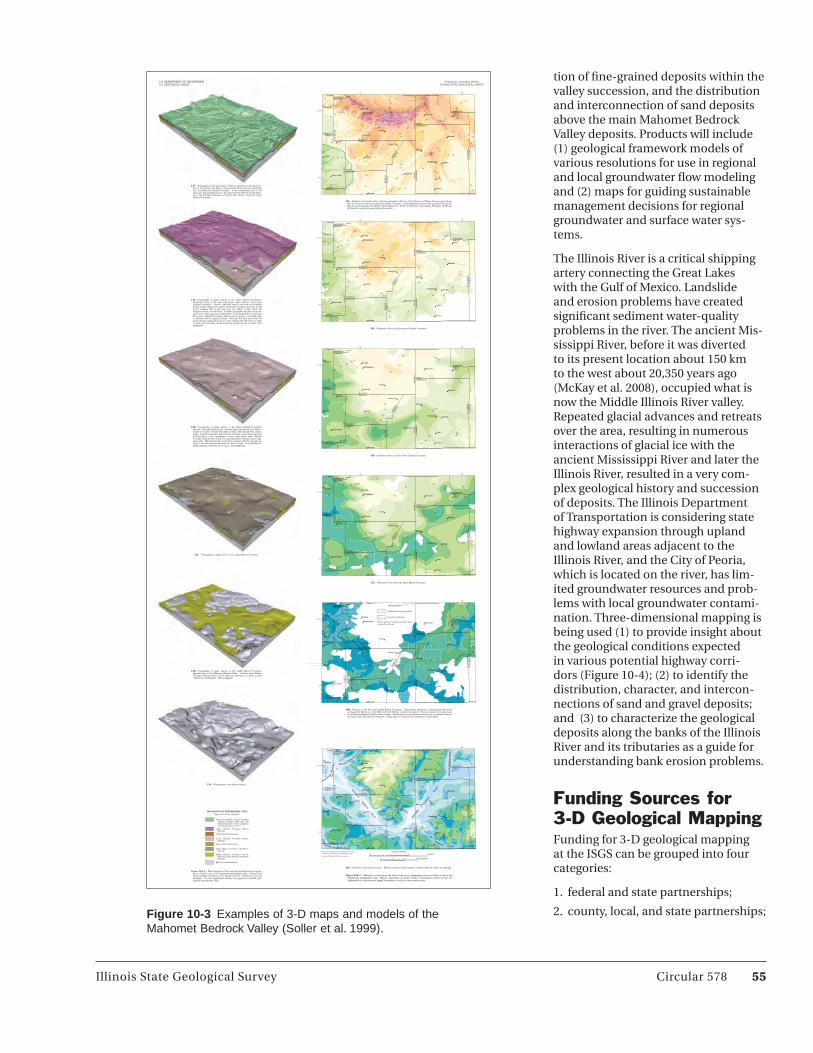
Illinois State Geological Survey Circular 578 55
tion of fine-grained deposits within the valley succession, and the distribution and interconnection of sand deposits above the main Mahomet Bedrock Valley deposits. Products will include (1) geological framework models of various resolutions for use in regional and local groundwater flow modeling and (2) maps for guiding sustainable management decisions for regional groundwater and surface water sys-tems.
The Illinois River is a critical shipping artery connecting the Great Lakes with the Gulf of Mexico. Landslide and erosion problems have created significant sediment water-quality problems in the river. The ancient Mis-sissippi River, before it was diverted to its present location about 150 km to the west about 20,350 years ago (McKay et al. 2008), occupied what is now the Middle Illinois River valley. Repeated glacial advances and retreats over the area, resulting in numerous interactions of glacial ice with the ancient Mississippi River and later the Illinois River, resulted in a very com-plex geological history and succession of deposits. The Illinois Department of Transportation is considering state highway expansion through upland and lowland areas adjacent to the Illinois River, and the City of Peoria, which is located on the river, has lim-ited groundwater resources and prob-lems with local groundwater contami-nation. Three-dimensional mapping is being used (1) to provide insight about the geological conditions expected in various potential highway corri-dors (Figure 10-4); (2) to identify the distribution, character, and intercon-nections of sand and gravel deposits; and (3) to characterize the geological deposits along the banks of the Illinois River and its tributaries as a guide for understanding bank erosion problems.
Funding Sources for 3-D Geological MappingFunding for 3-D geological mapping at the ISGS can be grouped into four categories:
1. federal and state partnerships;
2. county, local, and state partnerships;
Normal
BloomingtonGibson City
Paxton
Le Roy
Mackinaw
Heyworth
Atlanta
Farmer City
Mahomet
Lincoln Clinton
Champaign Urbana
Rantoul
Monticello
Pesotum
Tolono
Mount Pulaski
Decatur
WOODFORD CO.
MC LEAN CO.
TAZEWELL CO.
LOGAN CO.
LOGAN CO.
SANGAMON CO.
DE WITT CO.
MACON CO.
MA
CO
N C
O.
PIA
TT
CO
.
CH
AM
PA
I GN
CO
.
PIA
TT
CO
.
VER
MIL
ION
CO
.
CH
AM
PA
IGN
CO
.
DE
WIT
T CO
.
PIATT
CO
.
MC LEAN CO.
DE WITT CO.
FORD CO.
CHAMPAIGN CO.
IROQUOIS CO.
FORD CO.
MC
LEA
N C
O.
LO
GA
N C
O.
MC
L EA
NC
O.
Normal
BloomingtonGibson City
Paxton
Le Roy
Mackinaw
Heyworth
Atlanta
Farmer City
Mahomet
Lincoln Clinton
Champaign Urbana
Rantoul
Monticello
Pesotum
Tolono
Mount Pulaski
Decatur
WOODFORD CO.
MC LEAN CO.
TAZEWELL CO.
LOGAN CO.
LOGAN CO.
SANGAMON CO.
DE WITT CO.
MACON CO.
MA
CO
N C
O.
PIA
TT
CO
.
CH
AM
PA
IGN
CO
.
PIA
TT
CO
.
VER
MIL
ION
CO
.
CH
AM
PA
IGN
CO
.
DE
WIT
T CO
.
PIATT
CO
.
MC LEAN CO.
DE WITT CO.
FORD CO.
CHAMPAIGN CO.
IROQUOIS CO.
FORD CO.
MC
LEA
N C
O.
LO
GA
N C
O.
MC
LEA
NC
O.
Normal
BloomingtonGibson City
Paxton
Le Roy
Mackinaw
Heyworth
Atlanta
Farmer City
Mahomet
Lincoln Clinton
Champaign Urbana
Rantoul
Monticello
Pesotum
Tolono
Mount Pulaski
Decatur
WOODFORD CO.
MC LEAN CO.
TAZEWELL CO.
LOGAN CO.
LOGAN CO.
SANGAMON CO.
DE WITT CO.
MACON CO.
MA
CO
N C
O.
PI A
TT
CO
.
CH
AM
PA
I GN
CO
.
PIA
TT
CO
.
VER
MIL
ION
CO
.
CH
AM
PA
IGN
CO
.
DE
WIT
T CO
.
PIATT
CO
.
MC LEAN CO.
DE WITT CO.
FORD CO.
CHAMPAIGN CO.
IROQUOIS CO.
FORD CO.
MC
LEA
N C
O.
LO
GA
N C
O.
MC
L EA
NC
O.
600
625 650
650
650
675
700
675
675
675
700
700
700
700
700
725
725
725
725750
825800775
775
750
725
725
700
675
675
675700
725
750
750750
775
775
775
800
825850
800
800
675
675
700
72575
0
700
750
725
750
750
750800
800
800
800
775
775
600
600
675
700
650
625
600
575
550
550
575
550
650
650
675
650
650625600
600
575550
525
525
625600575
575
575
550
550
525
500
500
500
500
375
375
400
425450
475
350
350
500
550
550
525500
475
450
450475
500
500
525550
550
575
600
52550
0
500525
475450
450
450
450475500525550
575
600
625
650
450475500
425
425
425
425
400400
475450425400
50052555
0
400
400425450
475
500
525
550
375
350
400
550575600
625650
525
550 525
525
500
425400
475450
450425
400375
375 375400425
350
475
350
400
500
500
500
525
525
550
550
575
500
525
525
475
500
500
500
525
525
475
475
475
475
525
525
550
575
550
575
600
600 575 550
525
550
575
575
600
625
600
625
550
525
525
550
500
625
625
625
625
625650
650
625
625650
600
675600
600
675
675
650675
575
600
625
600
575
575
575
600
625
625
650
650
650
650
650
650675
675
675
650625
700
700
700
700
725
650
625
625
625
625
625
675
700
725
750
650
675
700
725
725
750
750
725
775
775
750
725
825
825
850
850
875
900
750
600
700
575
U.S. DEPARTMENT OF THE INTERIORU.S. GEOLOGICAL SURVEY
Prepared in cooperation with theILLINOIS STATE GEOLOGICAL SURVEY
EXPLANATION OF STRATIGRAPHIC UNITSFigures 13A–F and 16C and F
Wedron and Mason Groups, includingCahokia Formation (Wisconsin andHudson Episodes). Unit is assigned aminimum thickness of 15 ft
Upper Glasford Formation (IllinoisEpisode)
Upper Glasford basal sand
Lower Glasford Formation (IllinoisEpisode)
Lower Glasford basal sand
Upper Banner Formation (pre-IllinoisEpisode)
Middle Banner Formation—mostlyMahomet Sand Member (pre-IllinoisEpisode)
Bedrock (undifferentiated)
Figure 13A–F.—Block diagrams of the map area showing surface topogra-phy of bedrock and of five Quaternary stratigraphic units. Vertical facesshow variability in thickness of the Quaternary units. Viewpoint is from thesoutheast. To show topographic features, the images are vertically exag-gerated approximately 30x.
13A.—Topography of the bedrock surface.
13B.—Topography of upper surface of the middle Banner Formationdeposits lying in the Mahomet Bedrock Valley. Includes lower BannerFormation deposits where in the valley (see discussion on sheet 1 under“Quaternary stratigraphy,” fifth paragraph).
13C.—Topography of upper surface of the upper Banner Formation.
13D.—Topography of upper surface of the lower Glasford Formation.Sinuous, high-relief areas in the southwest and southeast are the result ofincision by modern streams (the valleys of Salt Creek and Salt Fork, respec-tively). A small topographic high near the southeast corner of the map areais attributed to a key stratigraphic control point where lower GlasfordFormation deposits were found at a noticeably higher elevation than in adja-cent points. Although this data point does not agree with the regional maptrend, it was retained (see discussion on sheet 1 under “An internally con-sistent geologic model and set of maps,” first paragraph).
13E.—Topography of upper surface of the upper Glasford Formation.Southeast corner of the map area shows upper surface of the lowerGlasford Formation. Sinuous, high-relief areas in the west and southeastare the result of incision by modern streams (for example, from west to eastin the southern half of the map area, the valleys of Salt Creek, theSangamon River, and Salt Fork). A small topographic high near the south-east corner of the map area is attributed to a key stratigraphic control pointwhere lower Glasford Formation deposits were found at a noticeably high-er elevation than in adjacent points. Although this data point does notagree with the regional map trend, it was retained (see discussion on sheet1 under “An internally consistent geologic model and set of maps,” firstparagraph).
13F.—Topography of the land surface, which is equivalent to the upper sur-face of the Wedron and Mason Groups except where they are covered bythin, discontinuous Cahokia Formation. In the southwestern part of themap area, beyond the limit of ice that deposited the Wedron Group diamic-tons, thin Cahokia Formation and Peoria Silt directly overlie the upperGlasford Formation.
40° 30'
89°
40°
88°
40° 30'
89°
40°
88°
40° 30'
89°
40°
88°
40° 30'
89°
40°
88°
EXPLANATION
Fluvial (sand and gravel) facies
Lacustrine (silt) facies
Where patterns coincide, lacustrine faciesoverlies fluvial facies
40° 30'
89°
40°
88°
40° 30'
89°
40°
88°
MAHOM
ET
B
EDRO
CK
VALL
EY
MAHO
MET BEDRO
CK VALLEY
PESOTUM
BEDROCKVALLEY
ON
AR
GA
B ED
RO
CKVA
LLEY
KE
NN
EY
BEDROCK
VALLEY
DANVERS BEDROCKVA
LLEY
MACKINAW
BE D
RO
CK
VAL L
E Y
MID
DLETOWN BEDROCK VALLEY
10 0 10 20 KILOMETERS
SCALE 1:500 00001001 20 MILES
Figure 14A–F.—Elevation, in feet above sea level, of the top or uppermost surface of bedrock and of fiveQuaternary stratigraphic units. Refer to discussion on sheet 1 under “Converting to raster format” forexplanation of characteristic jagged boundaries of units on these raster maps.
14A.—Elevation of the bedrock surface. Bedrock units are undifferentiated. Selected bedrock valleys are identified.
14B.—Elevation of the top of the middle Banner Formation. Approximate distribution of fluvial (sand and gravel)and lacustrine (silt) facies of the Mahomet Sand Member is shown by patterns. Sand and gravel commonly occurin the Mahomet Bedrock Valley’s main channel. Silt and clay occur in tributaries because ice or sediment dams inthe main channel blocked the tributaries, causing water to pond and fine sediment to be deposited.
14C.—Elevation of the top of the upper Banner Formation.
14D.—Elevation of the top of the lower Glasford Formation.
14E.—Elevation of the top of the upper Glasford Formation.
14F.—Elevation of the land surface, which is equivalent to the top of the Wedron and Mason Groups except wherethey are covered by thin, discontinuous Cahokia Formation. In the southwestern part of the map area (beyond thelimit of ice that deposited the Wedron Group diamictons, shown by black line), thin Cahokia Formation and PeoriaSilt directly overlie the upper Glasford Formation.
Base from ISGS data that was digitized from USGS1:24,000- and 1:62,500-scale topographic maps
Universal Transverse Mercator projection
Figure 10-3 Examples of 3-D maps and models of the Mahomet Bedrock Valley (Soller et al. 1999).

56 Circular 578 Illinois State Geological Survey
3. federal, county, state partnerships; and
4. private corporation and state part-nerships.
Within the federal and state partner-ship category and the federal, county, state partnership categories, the longest continually funded mapping program at the ISGS is the Great Lakes Geologic Mapping Coalition (GLGMC) (http://www.greatlakesgeology.org). At the ISGS, the GLGMC supports high-resolution 3-D mapping consis-tent with the detail generally found in 1:24,000-scale maps of surficial deposits. To date, the GLGMC efforts at the ISGS have focused on mapping the Quaternary deposits of extreme northeastern Illinois. Historically, the federal-state partnerships also have paid for medium-resolution mapping of a multi-county portion of the Qua-ternary deposits above the Mahomet Bedrock Valley in east-central Illinois (Figure 10-3)(Soller et al. 1999).
Partnerships of county and local gov-ernment agencies matched with state funding from the ISGS have typically supported 3-D geological mapping at a medium resolution that is compat-ible with geological characterization in support of regional groundwater flow modeling. These efforts have been conducted in central and northeastern Illinois.
Partnerships between private corpo-rations and the state to support 3-D geological mapping have been rare, but important. Currently, a high-resolution 3-D geological mapping program is in progress in and around Champaign County in east-central Illinois. The geological mapping for this project is being funded by the local water utility and is designed to support subsequent groundwater flow modeling and long-term sustainable management of the groundwater resources.
3-D Mapping MethodsWhile 3-D geological mapping projects are not required to follow a standard-ized mapping protocol at the ISGS, the basic mapping workflow is fairly consistent:
• datacollectionandorganization;
• interpretation,correlation,andinterpolation; and
• productionofbasicandinterpretivemaps.
The first phase of any ISGS mapping project is compilation of existing data within the mapping area. Most of these data are driller’s logs from water wells. Other, more reliable data used in map-ping projects include stratigraphic bor-ings and core descriptions collected by ISGS geologists, geophysical borehole logs from water supply or observation wells, previously published maps or reports, and existing field and outcrop descriptions. Water-well driller’s logs (about 450,000 in Illinois) are generally in their original form and include basic lithologic descriptions of the materi-als that were encountered. To simplify the interpretation and correlation of water-well data, the driller’s lithologic descriptions are matched with a set of standard lithotypes. This process is accomplished using a custom Micro-soft Access database and user inter-face that facilitates the assignment of standard lithotypes. Visualizing this lithologically standardized borehole data has become an important element of the ISGS mapping protocol, as it provides a first glimpse of data distri-bution and quality in 3-D space (Figure 10-4).
A significant amount of time in this phase of a mapping project also is spent verifying the location of the data points. This step is important because many of the map units can be very thin to discontinuous, and errors in location can result in vertical shifts in the reported elevation of individual deposits and can introduce errors into correlations and the final map. Finally, priorities for new data collection are typically identified at this phase of the project. When funds allow, new data are collected during various parts of the project cycle (e.g., from test drill-ing).
The second phase of each 3-D geo-logical mapping project involves the iterative processes of interpretation, correlation, and interpolation. Early steps are the identification of the map-ping objectives, the determination of the detail required in final products, and the identification of the main mapping units. As part of this process, the selected data are reviewed, and the mapping team examines available core samples to identify the likely deposi-tional environments and then delin-eates the map-unit framework for the area. Cross sections are made, either by hand or via computer, alternate conceptual models are explored, and initial map unit assignments are made. From these initial interpretations, geologists use one of two approaches
Figure 10-4 GeoVisionary rendering of standardized lithologic borehole logs with a 1-m LiDAR-based digital elevation model.

Illinois State Geological Survey Circular 578 57
to mapping. In the more traditional approach, structure and isopach maps are generated to evaluate the distri-bution and thickness of key marker horizons or important map units. Typically these maps are generated using computer interpolation software and then stored as uniformly gridded data sets. Each surface is evaluated against both the data and the set of other surfaces that constitute the 3-D map. When a surface map does not fit the conceptual model, the data, or the other surfaces, that map is corrected
to express the desired geometry. The conceptual model is used to determine the order and relationships between the various map units. Erosional and onlap relationships are identified, and grid-to-grid mathematical routines are used to create the correct relationships between pairs of surfaces. This process is repeated until the entire set of sur-face maps meets the interpretations of the mapping team. Depending on data quality and geological complexity, this can be a very slow process.
Alternatively, ISGS geologists have been intergrating GSI3D into their mapping projects. GSI3D creates 3-D maps through interpolation fron a large set of cross sections.
The third and final phase of the map-ping project includes the production of basic and interpretive map layers. During this phase, the mapping objec-tives and the list of contracted deliv-erables are revisited to determine the list of 2-D map sheets that will be pro-duced. This list always includes both structure and isopach maps for each map unit. Interpretive maps are devel-oped to address specific issues that are important to the decision makers within the map region. Maps showing the occurrence, depth, and thickness of major aquifers are commonly gener-ated interpretive maps (Figure 10-5). Other interpretive maps can highlight construction-related issues; predict land shaking for specific earthquake scenarios, or address specific shallow groundwater flow issues. Often, the set of surface grids that form the 3-D geologic map are exported for use in groundwater flow models. This process does not involve the creation of new published map products; it typically involves only the reformatting of the surface map files into a form that can be easily input to software used by col-laborating groundwater flow modelers. Depending on the software available, 3-D block models and animations can be generated to highlight important geological features that were identi-fied during mapping and that highlight critical mapping objectives.
Mapping Software and Staffing StrategyOver the past 5 years, the ISGS has explored various software options to support 3-D geological mapping over a range of spatial scales, from site-spe-cific to thousands of square kilometers. The ISGS evaluated high-cost pack-ages developed to support petroleum and mining applications and mid- to low-cost packages developed to sup-port the environmental consulting and regulatory industries. The cost and value of developing custom software for 3-D mapping and visualization
Released by the authority of the State of Illinois: 2007
1 10 KILOMETERS0 1 2 43 5 6 7 8 9
SCALE 1:100,0001 8 MILES10 2 3 4 5 6 7
Gilberts
>100
Major Aquifers (thickness in feet)
>100
50–100
20–50
>100
50–100
20–50
>100
50–100
20–50
>100
50–100
20–50
50–100
20–50
50–100
20–50
St. Charles
Hampshire
Virgil
Carpentersville
Unnamed
750
2520
88 Interstate highways
U.S. and state routes
Other roads
Railroads
Municipal boundaries
Rivers and lakes
Bedrock surface elevationContour interval 50 feet (above mean sea level)
Rive
rFo
x
700
700
750
800
800
750
750
700
700
700
650
650
600
700
650
700
650
700
750
700
700
700
750
750
750
750
700
700
650
600
650
600
750
700
750
700
700
700
700 700
550
500
650
600
650
600
550
550
600
600
650
650
600
650
700
650
600
550
65055
0
600
650
650
650
700
600
550
550
650
600
650
600
600
600
600
650
600
700
600
650
700
650
650
600
700
700
600
650
500
650
650
650
90
88
90
88
20
20
30
47
31
38
56
47
47
72 7272
62
68
31
31
31
64
64
64
25
25
38
25
BigRock
Sugar Grove
Montgomery
Batavia
NorthAurora
Aurora
Virgil
Elburn
WestDundee
SleepyHollow
East Dundee
Elgin
SouthElgin
St. Charles
MaplePark
BarringtonHills
Carpentersville
Lily Lake
AlgonquinHuntley
Gilberts
Pingree Grove
Hampshire
Burlington
Geneva
ST. CHARLES BEDROCK VALLEY
ELGIN
BEDROCKVALLEY
ELBURNBED
RO
CK
VALL
EY
T. 38 N.T. 39 N.
T. 39 N.T. 40 N.
T. 40 N.T. 41 N.
T. 41 N.T. 42 N.
R. 7 E. R. 8 E.
R. 8 E.R. 7 E.R. 7 E.R. 6 E.
41° 43' 28"
88° 15' 41"88° 36' 7"
42° 9' 15"
R. 7 E.R. 6 E.
T. 41 N.T. 42 N.
T. 40 N.T. 41 N.
T. 39 N.T. 40 N.
T. 38 N.T. 39 N.
88° 14' 19"
Figure 10-5 Kane County major Quaternary aquifer map (Dey et al. 2007c).

58 Circular 578 Illinois State Geological Survey
staff while allowing the geophysicists to manage, update, and interpret these files at any time.
Interpretation, Correlation, and InterpolationSoftware used for data analysis includes ArcGIS, Excel, and Isatis. Custom programs also have been developed to work with ArcScene to visualize 3-D borehole data. These in-house programs also allow for bore-hole data interpretations, assigning mapping unit interpretations to the underlying database, and simplifying the construction of cross sections and surface maps.
Three-dimensional visualization is currently being handled by three soft-ware packages, GeoVisionary (Figures 10-4 and 10-6), ArcScene, and GSI3D. The ISGS is in the early stages of com-bining these two applications into an integrated workflow. These three packages are expected to allow for the integration of all data types into a high-resolution 3-D environment and allow for interpretations in this 3-D space. Visualization of 3-D voxel models of facies and petrophysical properties are
were explored as was the feasibility of using modular, ad hoc combinations of desktop software to generate 3-D geo-logic maps.
After years of evaluation and discus-sion, the ISGS selected the modular, ad hoc combination of software for creat-ing 3-D geologic maps. This modular approach allows mappers the flexibility of efficiently improving their map-ping approach as software evolves to improve its support of various parts of the mapping workflow. This approach allows for continual use of the enter-prise database of wells, borings, and outcrops and for utilization of a stan-dardized, open data structure for man-aging geophysical data types, as well as images, cross sections, surface map grid files, animations, etc. Custom pro-grams and scripts can be easily inte-grated to provide desired functionality, and there is no need to completely revise the suite of programs, workflow, or data structure if the underlying software changes dramatically. This modular approach also permits the integration of routinely used soft-ware products (e.g., ArcGIS, Oracle, Microsoft Access, MAPublisher), and it accommodates new applications for any aspect of the workflow (e.g., visualization or surface interpolation) as they become available. Finally, this approach allows for the inclusion of software and custom scripts that are user-friendly enough for the tech-savvy field geologists to use and that do not require significant training or time for the mapping technicians or support specialists.
The current strategy for ISGS staff-ing on 3-D mapping projects is fluid and is based on the size of mapping areas, timeframes of projects, budget flexibilities, geological complexities, and technological capabilities of field geologists. Most projects have the assistance of support staff for data management, and all mapping proj-ects receive technical support in the production of map products. Most field geologists are able to manage ArcGIS and surface interpolation software and, for smaller projects, do not require the assistance of support staff in these areas. Larger projects and projects with more geological complexity often have
assistance from support staff in GIS and surface interpolation to help con-struct the structure and isopach maps, and to build and cross-check the vari-ous surfaces as 3-D maps and models are built.
Currently, the 3-D mapping program relies on a suite of software for the fol-lowing phases and tasks in the ISGS mapping workflow.
Data Collection and OrganizationWell logs, core and sample descrip-tions, and outcrop descriptions are managed using both Oracle and Micro-soft Access. The ISGS is moving to cen-tralization within the enterprise data-base under Oracle and reliance on vari-ous user interfaces, some via Microsoft Access. New Web-based interfaces to basic data access are expected to be developed over the next year.
The directory and file structure are standardized for the management of the various geophysical borehole logs and geophysical profile data sets. This standardization allows the data sets to be efficiently located and queried by all
Figure 10-6 Visualization laboratory image on screen on GeoVisionary.
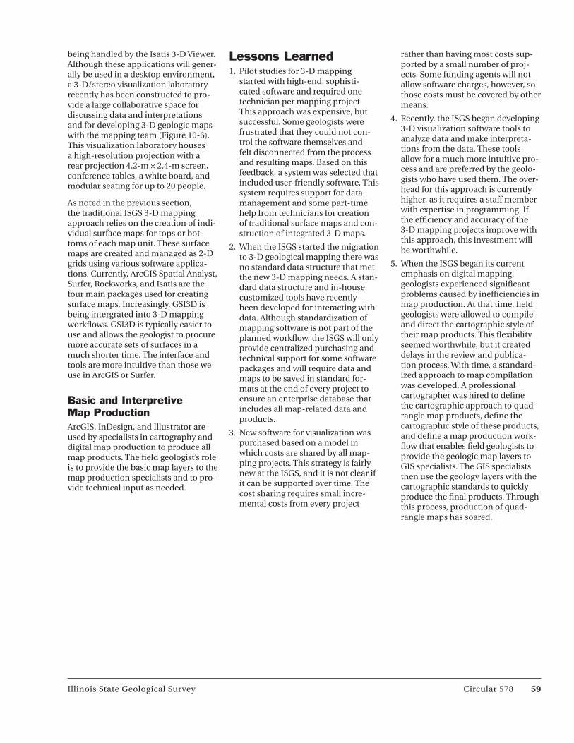
Illinois State Geological Survey Circular 578 59
being handled by the Isatis 3-D Viewer. Although these applications will gener-ally be used in a desktop environment, a 3-D/stereo visualization laboratory recently has been constructed to pro-vide a large collaborative space for discussing data and interpretations and for developing 3-D geologic maps with the mapping team (Figure 10-6). This visualization laboratory houses a high-resolution projection with a rear projection 4.2-m × 2.4-m screen, conference tables, a white board, and modular seating for up to 20 people.
As noted in the previous section, the traditional ISGS 3-D mapping approach relies on the creation of indi-vidual surface maps for tops or bot-toms of each map unit. These surface maps are created and managed as 2-D grids using various software applica-tions. Currently, ArcGIS Spatial Analyst, Surfer, Rockworks, and Isatis are the four main packages used for creating surface maps. Increasingly, GSI3D is being intergrated into 3-D mapping workflows. GSI3D is typically easier to use and allows the geologist to procure more accurate sets of surfaces in a much shorter time. The interface and tools are more intuitive than those we use in ArcGIS or Surfer.
Basic and Interpretive Map ProductionArcGIS, InDesign, and Illustrator are used by specialists in cartography and digital map production to produce all map products. The field geologist’s role is to provide the basic map layers to the map production specialists and to pro-vide technical input as needed.
Lessons Learned1. Pilot studies for 3-D mapping
started with high-end, sophisti-cated software and required one technician per mapping project. This approach was expensive, but successful. Some geologists were frustrated that they could not con-trol the software themselves and felt disconnected from the process and resulting maps. Based on this feedback, a system was selected that included user-friendly software. This system requires support for data management and some part-time help from technicians for creation of traditional surface maps and con-struction of integrated 3-D maps.
2. When the ISGS started the migration to 3-D geological mapping there was no standard data structure that met the new 3-D mapping needs. A stan-dard data structure and in-house customized tools have recently been developed for interacting with data. Although standardization of mapping software is not part of the planned workflow, the ISGS will only provide centralized purchasing and technical support for some software packages and will require data and maps to be saved in standard for-mats at the end of every project to ensure an enterprise database that includes all map-related data and products.
3. New software for visualization was purchased based on a model in which costs are shared by all map-ping projects. This strategy is fairly new at the ISGS, and it is not clear if it can be supported over time. The cost sharing requires small incre-mental costs from every project
rather than having most costs sup-ported by a small number of proj-ects. Some funding agents will not allow software charges, however, so those costs must be covered by other means.
4. Recently, the ISGS began developing 3-D visualization software tools to analyze data and make interpreta-tions from the data. These tools allow for a much more intuitive pro-cess and are preferred by the geolo-gists who have used them. The over-head for this approach is currently higher, as it requires a staff member with expertise in programming. If the efficiency and accuracy of the 3-D mapping projects improve with this approach, this investment will be worthwhile.
5. When the ISGS began its current emphasis on digital mapping, geologists experienced significant problems caused by inefficiencies in map production. At that time, field geologists were allowed to compile and direct the cartographic style of their map products. This flexibility seemed worthwhile, but it created delays in the review and publica-tion process. With time, a standard-ized approach to map compilation was developed. A professional cartographer was hired to define the cartographic approach to quad-rangle map products, define the cartographic style of these products, and define a map production work-flow that enables field geologists to provide the geologic map layers to GIS specialists. The GIS specialists then use the geology layers with the cartographic standards to quickly produce the final products. Through this process, production of quad-rangle maps has soared.

60 Circular 578 Illinois State Geological Survey
Chapter 11: Manitoba Geological Survey: Multi-scaled 3-D Geological Modeling with a Single Software Solution and Low CostsGreg Keller1, Gaywood Matile2, and Harvey Thorleifson2
1Manitoba Geological Survey, Winnipeg, Manitoba, Canada, and 2Minnesota Geological Survey, St. Paul, Minnesota, USA
Organizational Structure, Business Model, and MissionThe Manitoba Geological Survey (MGS) was founded in 1928. Its mission is to conduct investigations of the province’s Precambrian Shield, Western Canada Sedimentary Basin, and Hudson Bay Basin to improve the understanding of Manitoba’s geology and geological processes and, in so doing, encourage mineral exploration opportunities and contribute to wise land-use manage-ment. Investigations conducted by the MGS include those of exposed bed-rock, subsurface materials, and surfi-cial sediments including sand, gravel, and peat. The MGS provides data and products such as geological maps and reports, metallic and industrial mineral deposit reports and databases, mineral resource assessments, targeted geosci-ence research, development of explora-tion models, and maintenance of data inventories.
The MGS is within Manitoba’s Mineral Resources Division along with the Min-erals Policy and Business Development Section and the Mines and Petroleum Branches, which are regulatory bodies. Only the geological survey is con-cerned with 3-D modeling.
Until fairly recently, three-dimensional geological modeling was seen as more of a novelty than a business require-ment for the MGS. Beginning as a suc-cessful offshoot of the prairie portion of the Canadian National Geoscience Mapping Program (NATMAP), through the 2003 Lake Winnipeg Basin model, the 2008 Western Canada Sedimentary Basin (WCSB) model (Keller and Matile 2009), and the recently completed 2009 Targeted Geoscience Initiative (TGI)
Williston Basin model (TGI II Working Group 2009), the MGS’s commitment to 3-D modeling has grown to include mapping all of the Phanerozoic ter-rane of Manitoba in 3-D. Future plans include cooperation of the MGS with the Minnesota and North Dakota Geological Surveys to produce a cross-border Red River valley 3-D geologi-cal model. This model will combine the existing North Dakota/Minnesota Fargo-Moorhead regional models (Thorleifson et al. 2005) with Manito-ba’s 3-D data. Figure 11-1 summarizes 3-D mapping activities.
Geological SettingManitoba was completely engulfed in ice during the last glacial period, and most of Manitoba is covered with gla-cial sediments up to 300 m thick. The bedrock geology is composed of 60% Precambrian terrane, which is covered by the eastern edge of the Phanerozoic Williston Basin in the southwestern portion of the province and the west-ern edge of the Phanerozoic Hudson Bay Basin in the northeastern portion of the province. The Precambrian ter-rane, otherwise known as the Canadian Shield, has a discontinuous cover of glacial sediment and is made up of deformed crystalline rocks of the Archean Superior Province in the south and east and the Proterozoic Churchill Province in the north and west. The two Phanerozoic basins have a more continuous cover of glacial sediment and are composed of a stratified suite of gently dipping, primarily unde-formed, Paleozoic carbonate rocks that in the Williston Basin progress upward to Mesozoic shale. The surface of the Williston Basin comprises a set of eastward-facing bedrock escarpments that step up onto younger rocks in a westward direction.
Major Clients and the Need for ModelsTo date, 3-D models of the MGS have been used by other government branches, university students, and industry to assist in the planning stages of new pipeline construction, con-struction of groundwater models and chemical flow through these models, and in groundwater exploration drill holes. The ability to visualize in 3-D is an extremely useful educational tool for the public, the mineral exploration industry, and for students interested in a better understanding of Manitoba’s geological landscape.
Model MethodologyAlthough more than 25 geologists work at the MGS, only two are responsible for 3-D modeling, a geologist and a GIS/3-D modeling specialist, who work as a team. This synergy works very well, allowing each scientist to concentrate on his or her field of expertise. Models are created using data gleaned from a variety of disparate data sets. The bulk of the modeling is based upon well data (water wells, geoscientific and academic wells, and oil and gas wells); however, large lake bathymetry, seis-mic, digital elevation data, and surficial and bedrock geology are also used to refine the model. The software pack-ages utilized in the modeling workflow include ArcGIS (ESRI), MapInfo (Pitney Bowes), Access (Microsoft), and Gocad (Paradigm). Several different modeling methodologies have been employed at the MGS depending on the type of data available.

Illinois State Geological Survey Circular 578 61
Cross Section Method (Quaternary to Precambrian Surface for Southeastern Manitoba)• Water-welldata(over80,000holes),
along with surficial geology, bedrock geology, and digital elevation data are collected for the study area.
• Thesedataarethenformattedandplotted onto 54-inch cross section traces depicting a 5-km-wide west-east swath through the study area.
• Eachcrosssectiontraceisthenhand-interpreted to define unit tops, which filters data of variable quality based on local trends.
• Theinterpretationiscapturedevery5 km along the cross section trace and recorded as “virtual drill holes” or predicted stratigraphic points (PSP), which provides a 5-km grid of PSPs for the project area; these data are then imported into Microsoft Access and formatted.
• TheformattedPSPsarethenimported into Gocad 3 modeling software and combined with unit edges to create a model surface.
• Modelsurfacesarethenusedto“erode” Gocad stratigraphic grids (Sgrid) to create a filled volume or “solid” for each modeled unit (Figure 11-2).
Direct Data Modeling Method (Phanerozoic to Precambrian Surface)• Fivetoeightstratigraphicallysig-
nificant deep, detailed drill holes (“golden spikes”) per township (10 km × 10 km) are selected, and for-mation tops are re-picked for con-sistency at a high level of detail by stratigraphers over the study area.
• Theresultingdatasetofformationtops and a data set of formation edges form the basis of the model.
• ThesedataareimportedintoGocadand, because this data has been filtered by stratigraphers, can be directly modeled (Figure 11-3).
Figure 11-1 Index map outlining the location of the various 3-D geological mod-eling activities in and around Manitoba. The southwestern Manitoba model is in progress. Yellow blocks indicate areas of higher detail within the Fargo-Moorhead model.
Figure 11-2 Three-dimensional geological Gocad model of southeast Manitoba including the Winnipeg region.

62 Circular 578 Illinois State Geological Survey
Digitization Modeling Method (Chronostratigraphic Rock Units to Precambrian Surface)• Toconverttheexistingpaper3-D
model in the atlas of the WCSB into a digital 3-D model (Figure 11-4), structural contours and formation edges for each of the geological peri-ods were scanned from the WCSB (Mossop and Shetsen 1994) and digitized.
• Thedigitizedcontoursweretaggedfor elevation and, along with the edges, were exported into Gocad and directly modeled.
In each of these methodologies, the size of the data cells and/or triangles in the TIN of the resultant model are dependant on data quality and distri-bution, model size, and available com-puting power.
Advantages of the MGS 3-D Mapping ApproachUsing well-established, fairly inex-pensive software for the background work (Microsoft Access, MapInfo GIS, text editors), and a single 3-D software solution (Gocad) keeps costs and work-flow manageable.
The cross section methodology brings all of the available data together to use in interpreting the stratigraphy. Some data are lost in data-rich areas using this cross section method, but the method allows trends to be projected into data-poor areas.
A free data viewer (Geocando) is avail-able for Gocad that allows clients and the general public free access to the models (3-D visualization, rotation, and simple querying).
Lessons Learned• Althoughwater-welldataarehighly
variable in quality, they are very useful to fill in data gaps between the “golden spikes,” and data can be filtered by looking for trends using the cross section method just described.
Figure 11-3 Three-dimensional geological Gocad model of the TGI Williston Basin project area.
Figure 11-4 Three-dimensional geological Gocad model of the Western Canada Sedimentary Basin spanning Manitoba, Saskatchewan, and Alberta.
• Modeluncertaintycanbecalculatedsimply by observing the data den-sity and geological complexity of an area.
• Inareaswithalargenumberofdrill
holes, compressing all of the drill hole data from a 5-km north-south swath to a single cross section trace can make interpretation difficult. This difficulty is due to the scale
Illinois State Geological Survey Circular 578 63
of the cross section; holes begin to obscure one another as numbers increase, which is particularly sig-nificant in areas with increased local relief.
• Wheredataaresparse,thecrosssec-tion methodology can generate par-allel ridges on the final surface due to variations in isolated drill data from cross section to cross section,
much like steps can be generated when using contoured data. The lack of drill holes makes it difficult to visualize the trend of the data.
• Unitedgesthathavebeendrawninplan view without being cognizant of local relief can lead to flattened bedrock escarpments. Updated edges drawn with shaded relief pro-
vided by a digital elevation model will rectify this issue.
• Althoughburiedvalleysinsouth-ern Manitoba are only recogniz-able on the cross sections when they intersect a cross section at an angle approaching perpendicular, the cross section method will still be useful for targeting exploration water wells in buried valleys.

64 Circular 578 Illinois State Geological Survey
Chapter 12: TNO–Geological Survey of the Netherlands: 3-D Geological Modeling of the Upper 500 to 1,000 Meters of the Dutch SubsurfaceJan Stafleu, Denise Maljers, Freek Busschers, Jan Gunnink, and Ronald VernesTNO–Geological Survey of the Netherlands, Utrecht, The Netherlands
Organizational Structure, Business Model, and MissionThe present TNO–Geological Survey of the Netherlands was founded in 1997 by merging the governmental organization Rijks Geologische Dienst (literally State Geological Survey) and the TNO Institute for Groundwater and Geo-Energy. The origin of the State Geological Survey dates back to 1903; the TNO Institute for Groundwater started its work in 1948. Both institutes have always paid considerable atten-tion to applied geoscientific research. The mission of TNO–Geological Survey of the Netherlands is to provide the society with customized geoscientific knowledge, data, and information based on a thorough knowledge of the subsurface. The Institute employs over 300 geoscientists and has a turnover of about ¡35 million. The Geological Survey of the Netherlands forms part of the Netherlands Organisation for Applied Scientific Research (TNO), which was established in 1932.
The geomodeling department of the TNO–Geological Survey of the Neth-erlands focuses on the sustainable use and management of the upper 500 to 1,000 m of the Dutch subsurface. The department’s most important task is the characterization and modeling of geological deposits. It develops and maintains three models: DGM (digital geological model), REGIS II (Regional Geohydrological Information System), and GeoTOP (3-D model of the upper 30 m). REGIS II emerged from separate mapping tasks commissioned by the 12 Dutch provinces in collaboration with the Directorate-General for Public Works and Water Management and with TNO.
Geological SettingIntroductions to the Quaternary geol-ogy of the Netherlands can be found in publications by Zagwijn (1989) and De Gans (2007) among others. The follow-ing summary is largely adapted from descriptions by Rondeel et al. (1996).
The Netherlands are located on the southeastern rim of the North Sea Basin (Figure 12-1), and the edges of this basin are close to the country’s
The annual budget for geologists and modelers at TNO–Geological Survey of the Netherlands is about ¡3 million. There are approximately 10 geologists, 5 geohydrologists, 4 geomodelers, 4 geochemists, and 4 part-time GIS experts working on various modeling projects. From this staff there are 3 modelers and 1 to 2 geologists working more or less full-time only on the 3-D geological modeling of the subsurface of the Netherlands.
Figure 12-1 Location and schematic geological map of the Netherlands.

Illinois State Geological Survey Circular 578 65
eastern and southern borders. The sed-iments at the surface are almost exclu-sively Quaternary. The thickest Qua-ternary succession (600 m) occurs in the northwest. Tertiary and older sedi-ments are only exposed in the extreme east and south of the country, where the edges of the North Sea Basin were uplifted and eroded. The southeastern portion of the Netherlands is affected by a southeast-northwest string fault system, which formed a number of horst and graben blocks during the Tertiary and Quaternary. These faults are still active.
The Dutch landscape essentially con-sists of a Holocene coastal barrier and coastal plain and an interior with Pleistocene deposits cut by a Holocene fluvial system. The coastal barrier is interrupted on the south by the estuary of the Rhine, Meuse, and Scheldt Rivers and on the north by the tidal inlets of the Wadden Sea. The barrier is char-acterized by dunes and is locally up to 10 km wide. In places the barriers were reinforced with dikes.
The coastal plain covers the western half of the country and consists mainly of clay and peat. Much of the plain would be flooded in the absence of dikes. The distribution of land and water has been strongly influenced by humans, and the present-day limited extent of peat, for instance, is artificial. Because peat was historically exploited as fuel both in the coastal plain and further inland, moors partially cover the Pleistocene deposits.
The Rhine and Meuse Rivers enter the country from the east and south, respectively. Throughout the Holocene these rivers formed a thick succession of fluvio-deltaic sediments covering the Pleistocene deposits. In many places, the rivers are straightened arti-ficially, and virtually everywhere they are confined by dikes.
At the surface, the Pleistocene is largely sandy and of glacial, fluvial, and aeo-lian origin. Ice-pushed ridges locally reach heights of 100 m, but most of the Pleistocene occurs as flat-lying land. Pre-Pleistocene sediments are only exposed near the borders of the coun-
try. In the east, these sediments include various Mesozoic and Tertiary forma-tions, whereas those to the southwest are of Pliocene age. In one particular valley in the hills of the southernmost province, Tertiary sands, clays, lignites, and Cretaceous chalk are eroded down to their Carboniferous substratum.
Three Nationwide ModelsDGM: The Digital Geological ModelModern digital mapping of the Dutch subsurface started in 1999 with the development of the so-called Digital Geological Model (DGM; Van Gessel et al. unpublished.). This model, which is available to both professionals and the general public (www.dinoloket.nl), is a 3-D lithostratigraphic frame-work model of onshore Netherlands. The DGM consists of a series of raster layers. Each lithostratigraphic unit is represented by rasters for the top, bottom, and thickness of the unit. Raster layers are stored in the raster format of ESRI (ArcGIS). The lithostratigraphic units are at the for-mation level; Holocene deposits are represented as a single layer.
REGIS II: The Regional Geohydrological Information SystemA second important step in digital mapping was the development of the Regional Geohydrological Informa-tion System (REGIS II; Vernes and Van Doorn 2005), which further subdivides the lithostratigraphic units of the DGM into aquifers and aquitards. Represen-tative values for hydrological param-eters (e.g., hydraulic conductivity and effective porosity) are calculated and assigned to the model, making it suit-able for groundwater modeling on a regional scale. Like DGM, REGIS II models the Holocene deposits as a single cover layer. REGIS II is down-loadable from the TNO Web site (www.dinoloket.nl) and is widely used by regional authorities and water supply companies for groundwater modeling studies.
GeoTOP: A 3-D Volume Model of the Upper 30 MetersGeoTOP expresses the shallow subsur-face schematically in millions of grid cells (blocks), each measuring 100 × 100 m in the horizontal direction and 0.5 m in the vertical direction. Sev-eral parameter values are estimated for each grid cell. These parameters include geological characteristics, such as lithostratigraphic and lithofacies units, as well as physical and chemical parameters, such as hydraulic conduc-tivity and chloride content. The cell-based nature of the model allows for modeling of the internal heterogeneity of lithostratigraphic units in terms of lithofacies and other parameters.
Major Clients and the Need for ModelsREGIS II is widely used by regional authorities (i.e., provinces and water management agencies) and water supply companies for groundwater modeling studies.
The lithologic detail that is character-istic for the GeoTOP models is used in several areas:
• explorationforaggregateresources(sand, clay, and shells);
• detailedgroundwaterandcontami-nation studies;
• detailedstudiesofsaltpenetrationfrom seawater;
• landsubsidencestudies;and
• planningoflarge-scaleinfrastruc-tural works such as tunnels and rail-roads
SoftwareTNO uses a toolbox consisting of sev-eral components:
• ThegeostatisticalsoftwarepackageIsatis by Geovariance is the main modeling platform by which sta-tistical data analysis is performed, semi-variograms are constructed, and interpolation procedures are conducted.

66 Circular 578 Illinois State Geological Survey
• ESRI’sArcGISisusedtocreateaddi-tional input data for the modeling, including fault patterns, maps show-ing the extent of lithostratigraphic units, and geological features such as channel belts.
• Allsurfacesthatresultfromthe2-Dinterpolations in DGM, REGIS II, and GeoTOP are stored and pre-sented in ESRI’s raster format.
• Gocadisusedforvisualizationof3-D models and inspection of 2-D surfaces in 3-D displays.
• ThereisextensiveuseofthePythonprogramming/scripting language to create specific programs that perform many tasks, for example: (a) converting data from one data format to another; (b) extracting borehole information from the DINO database and preparing it for input to Isatis; and (c) automating lithostratigraphic interpretation of boreholes.
Workflow for Digital Geological ModelingData SelectionThe DGM is primarily based on litho-logic descriptions of a selection of 16,500 boreholes. This selection aims at an even distribution of good-quality borehole data including key strati-graphic borehole data derived from the Quaternary and Upper Tertiary deposits.
Stratigraphic InterpretationThe selected boreholes are stratigraph-ically interpreted by assigning the revised lithostratigraphic classification (Weerts et al. 2000) to the individual sample intervals. The base of each of the lithostratigraphic units in the bore-holes is subsequently used for interpo-lation and modeling. The basic strategy for lithostratigraphic interpretation is to work from nationwide cross sections to regional-scale cross sections that constitute the geological framework for the final interpretation of individual boreholes. For the interpolation, these individual interpreted boreholes are used.
Fault MappingA tectonic map showing all known major faults in the Tertiary and Qua-ternary deposits was constructed (Figure 12-2). The map is a thorough revision of fault patterns from earlier publications, including maps based on seismic data acquired for oil and gas exploration. Additional seismic data came from high-resolution surveys in the Roer Valley Graben, which is the most prominent tectonic feature in the Netherlands. For every lithostrati-graphic unit, the faults that have influ-enced the base of the unit are selected and used as “barriers” in the interpola-tion process.
InterpolationThe depths of the base of each lithostratigraphic unit, as derived from the borehole data, are interpolated to raster surfaces using the “block-krig-ing” algorithm (Isaaks and Srivastava 1989, Goovaerts 1997). The top surface follows indirectly from the joined basal surfaces of overlying units when all units are stacked (see section on stack-ing the units). The base surface was chosen because this surface is formed by depositional processes that are linked to the unit itself, whereas the top surface is often the result of mul-tiple geological processes (e.g., erosion and incision).
Figure 12-2 Fault data stored in GIS and extracted for modeling.
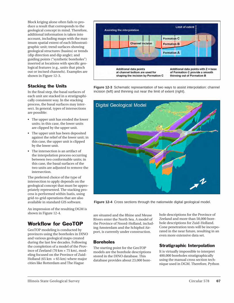
Illinois State Geological Survey Circular 578 67
Block kriging alone often fails to pro-duce a result that corresponds to the geological concept in mind. Therefore, additional information is taken into account, including maps with the max-imum spatial extent of each lithostrati-graphic unit; trend surfaces showing geological structures (basins) or trends (dip direction and dip angle); and guiding points (“synthetic boreholes”) inserted at locations with specific geo-logical features (e.g., units that pinch out or incised channels). Examples are shown in Figure 12-3.
Stacking the UnitsIn the final step, the basal surfaces of each unit are stacked in a stratigraphi-cally consistent way. In the stacking process, the basal surfaces may inter-sect. In general, types of intersections are possible:
• Theupperunithaserodedthelowerunits; in this case, the lower units are clipped by the upper unit.
• Theupperunithasbeendepositedagainst the relief of the lower unit; in this case, the upper unit is clipped by the lower unit.
• Theintersectionisanartifactofthe interpolation process occurring between two conformable units; in this case, the basal surfaces of the two units are adjusted to remove the intersection.
The preferred choice of the type of intersection to apply depends on the geological concept that must be appro-priately represented. The stacking pro-cess is performed within Isatis, using grid-to-grid operations that are also available in standard GIS software.
An impression of the resulting DGM is shown in Figure 12-4.
Workflow for GeoTOPGeoTOP modeling is conducted by provinces using the boreholes in DINO and various geological maps created during the last few decades. Following the completion of a model of the Prov-ince of Zeeland (70 km × 75 km), mod-eling focused on the Province of Zuid-Holland (65 km × 65 km) where major cities like Rotterdam and The Hague
Figure 12-3 Schematic representation of two ways to assist interpolation: channel incision (left) and thinning out near the limit of extent (right).
Figure 12-4 Cross sections through the nationwide digital geological model.
are situated and the Rhine and Meuse Rivers enter the North Sea. A model of the Province of Noord-Holland, includ-ing Amsterdam and the Schiphol Air-port, is currently under construction.
BoreholesThe starting point for the GeoTOP models are the borehole descriptions stored in the DINO database. This database provides about 23,000 bore-
hole descriptions for the Province of Zeeland and more than 50,000 bore-hole descriptions for Zuid-Holland. Cone penetration tests will be incorpo-rated in the near future, resulting in an even more extensive data set.
Stratigraphic InterpolationIt is virtually impossible to interpret 400,000 boreholes stratigraphically using the manual cross section tech-nique used in DGM. Therefore, Python

68 Circular 578 Illinois State Geological Survey
scripts were developed that use litho-logic borehole descriptions within a context of digitized geological maps to assign lithostratigraphic labels to the borehole intervals.
2-D Interpolation of Stratigraphic Units
During the second modeling step, 2-D bounding surfaces are constructed. These surfaces represent the top and base of the lithostratigraphic units and are used to place each 3-D grid cell in the model within the correct lithostratigraphic unit. The procedure used to construct 2-D bounding sur-faces is basically the same as the one used in DGM. However, in contrast to DGM, a stochastic interpolation technique is used (sequential Gauss-ian simulation; Goovaerts 1997), which allows for uncertainty to be estimated.
3-D Interpolation of Lithology Classes
The lithologic units in the boreholes are used to perform a final 3-D sto-chastic interpolation of lithology (e.g., clay, sand, peat) and, if applicable, sand-grain size class data within each lithostratigraphic unit. After this step, a cell-based (100 × 100 × 0.5 m) 3-D geological model is obtained. The 3-D interpolation is conducted for each lithostratigraphic unit separately using a stochastic interpolation technique called sequential indicator simulation (Goovaerts 1997). An example of a 3-D model is shown as Figure 12-5.
Physical and Chemical ParametersIn addition to the modeling just described, physical and chemical parameters are collected and mea-sured. The sampling strategy is such that measured values can be assigned to lithostratigraphic and lithofacies units, making it possible to obtain insights into the spatial variability of physical and chemical properties in
three dimensions. Examples of physi-cal and chemical parameters include (1) horizontal and vertical hydrau-lic conductivity, which is crucial in groundwater models, and (2) the reac-tivity of sediments, which is used in the modeling of contaminant plumes. The choice of parameters to include in the models is based on the needs of researchers at Deltares, TNO, and other organizations.
Figure 12-5 Part of the 3-D model of the central part of Zeeland, southwestern Netherlands.

Illinois State Geological Survey Circular 578 69
Chapter 13: U.S. Geological Survey: A Synopsis of Three-dimensional ModelingLinda J. Jacobsen1, Pierre D. Glynn1, Geoff A. Phelps2, Randall C. Orndorff1, Gerald W. Bawden2, and V.J.S. Grauch3
U.S. Geological Survey: 1Virginia, 2California, 3Colorado
Mission and Organizational NeedsThe U.S. Geological Survey (USGS) is a multidisciplinary agency that pro-vides assessments of natural resources (geological, hydrological, biological), the disturbances that affect those resources, and the disturbances that affect the built environment, natural landscapes, and human society. Until now, USGS map products have been generated and distributed primarily as 2-D maps, occasionally providing cross sections or overlays, but rarely allowing the ability to characterize and under-stand 3-D systems, how they change over time (4-D), and how they inter-act. And yet, technological advances in monitoring natural resources and the environment, the ever-increasing diversity of information needed for holistic assessments, and the intrinsic 3-D/4-D nature of the information obtained increases our need to gener-ate, verify, analyze, interpret, confirm, store, and distribute its scientific infor-mation and products using 3-D/4-D visualization, analysis, modeling tools, and information frameworks.
Today, USGS scientists use 3-D/4-D tools to (1) visualize and interpret geo-logical information, (2) verify the data, and (3) verify their interpretations and models. 3-D/4-D visualization can be a powerful quality control tool in the analysis of large, multidimensional data sets. USGS scientists use 3-D/4-D technology for 3-D surface (i.e., 2.5-D) visualization as well as for 3-D volu-metric analyses. Examples of geological mapping in 3-D include characteriza-tion of the subsurface for resource assessments, such as aquifer character-ization in the central United States, and for input into process models, such as seismic hazards in the western United States.
The USGS seeks to expand its 3-D/4-D capabilities in monitoring, interpret-ing, and distributing natural resource information, both by adopting and/or developing new 3-D/4-D tools and frameworks and by promoting and enabling greater use of available tech-nology.
Everything that shapes the Earth or affects its functions does so in 3-D space: water flowing over rocks, through aquifers, or as ice in glaciers; plants growing up into the atmosphere and down into the soil; the move-ment of animal life and pathogens within ecosystems; the movement of tectonic plates driven by deep con-vection beneath the crust; volcanic eruptions, floods, debris flows, and fires; the extraction, sequestration or migration of carbon, nutrients, con-taminants, biota, minerals, energy, and other resources. Until recently, the computational and visualization power necessary to understand these complex systems was limited to a handful of supercomputing centers or industrious scientists. This situation has now changed: personal computers equipped with fast video cards and vast storage allow wide access to 3-D/4-D tools and visualization.
Business ModelThe annual USGS budget is approxi-mately US$1 billion from federal appropriations. The bureau also receives about US$500 million from outside entities such as other federal agencies, foreign governments, inter-national agencies, U.S. states, and local government sources. More than half of the outside funding supports collab-orative work in water resources across the country, and the balance of the funding supports work in the geologi-cal, biological, and geographic sciences and information delivery.
The USGS has a workforce of approxi-mately 9,000 distributed in three large centers (Reston, Virginia; Denver, Colorado; Menlo Park, California) and in numerous smaller science centers across the 50 states. Scientific work is organized into “projects” run by principal investigators (PIs) who have significant latitude in planning and conducting research, including acqui-sition of the resources (e.g., equipment, computers, software) needed to carry out their studies. Due to the distributed nature of management and personnel and due to the independence of the PIs, finding common organizational solutions is often a challenge. For example, concerns regarding optimal use of 3-D/4-D technology within the USGS include these:
• Manytoolsandsolutionsareexpen-sive.
• Theusercommunityisnotwellcoordinated and sometimes does not buy or share software licenses as a group. Buying power is not cur-rently maximized.
• Pocketsofspecialistsareemerging,but there are few forums for sharing ideas and expertise.
• Stayingabreastofrapidlyevolvingtechnologies is difficult.
Geological SettingThe United States has a large variety of geological terranes that record more than 2 billion years of geological his-tory (Figure 13-1). The complexity of U.S. geology ranges from horizontal stacking of sediments in the Great Plains, Colorado Plateau, and Coastal Plain Physiographic Provinces to over-printing of compressional, extensional, and transform tectonics of the Pacific Border Province of the western United States (Figure 13-1). These varied geo-logical terranes present a challenge to

70 Circular 578 Illinois State Geological Survey
3-D modeling of divergent and con-vergent plate boundaries, strike-slip fault zones, and the stable craton. Also, surficial geological processes of the last several million years have left variable unconsolidated deposits, including the voluminous deposition of glacial mate-
rials in New England and the northern conterminous United States.
The oldest rocks of the United States are igneous and metamorphic rocks that occur in the Adirondacks of New York and the Superior Uplands of Min-
nesota. These rocks contain complex fracture systems that can be modeled for water and mineral resources, but also have metamorphic fabrics inher-ent from high heat and pressures that occurred over many millions of years.
The United States contains fold and thrust belts that record several con-tinental plate collisions. Examples of these are the Valley and Ridge, Blue Ridge, and Piedmont Provinces in the eastern United States where rocks were folded and faulted during four plate collision events between 1 billion years ago and 300 million years ago. The Rocky Mountains Province in the western United States records a colli-sion event from about 40 million years ago. Along with overprinting of several tectonic events, these terranes include complex fold relationships and zones of intense faulting that must be taken into account in models. Linear trends of folds and faults are characteristics of these provinces.
Strike-slip fault systems, such as the San Andreas fault system of the Pacific Border Province in California, are regions of particularly complicated geology. As continental plates or struc-tural blocks move past one another in a horizontal direction, complex compression and extensional struc-tures occur. In this setting, rocks are translated great distances horizon-tally. These offsets are superimposed on a Mesozoic to Paleogene history of subduction, accretion, batholith formation, and extensive extensional attenuation. Understanding structural control and associated seismic hazards along strike-slip fault zones such as the San Andreas fault system requires the fusion of traditional geological map-ping, geophysical measurements, seis-mology, structural geology, and state-of-the-art visualization and modeling techniques to produce detailed 3-D and 4-D geologic maps.
Extensional tectonic events are recorded in Triassic and Jurassic basin sediments within the Piedmont Prov-ince of the eastern United States and the Basin and Range Province of the western United States. In both regions, compressional tectonics resulted in folded and faulted rocks that were later
1. Superior Upland 10. Adirondack 19. Northern Rocky Mtns 2. Continental Shelf 11. Interior Low Plateaus 20. Columbia Plateau 3. Coastal Plain 12. Central Lowland 21. Colorado Plateau 4. Piedmont 13. Great Plains 22. Basin And Range 5. Blue Ridge 14. Ozark Plateaus 23. Cascade – Sierra Mtns 6. Valley and Ridge 15. Ouachita 24. Pacific Border 7. St. Lawrence Valley 16. Southern Rocky Mtns 25. Lower California 8. Appalachian Plateau 17. Wyoming Basin 9. New England 18. Middle Rocky Mtns
Figure 13-1 Simplified version of the King and Beikman (1974) geologic map of the conterminous United States. Colors indicate age of rock formations. Detailed explanation and digital versions are available at http://tapestry.usgs.gov and http://mrdata.usgs.gov/geology/kb.html.

Illinois State Geological Survey Circular 578 71
torn apart and that developed basins that were filled with sediments shed off highlands. In the Piedmont of the eastern United States, this extension was associated with the opening of the Atlantic Ocean. For the Basin and Range Province, extension is related to back-arc spreading behind the Coast Range and Cascades Provinces.
Volcanic terranes occur in the western U.S. Cascades and Sierra Nevada Prov-inces. Large masses of intrusive igne-ous rock represent the deeply eroded roots of a Mesozoic volcanic arc and its Mesozoic and Paleozoic country rock in the Sierra Nevada and an active volcanic arc in the Cascades where the Juan de Fuca plate in the Pacific Ocean is being subducted beneath North America.
The sedimentary rocks of the Interior Plains and Atlantic and Gulf Coastal Plains reflect numerous periods of transgressing and regressing seas. These provinces are generally flat lying to gently dipping marine sediments that show complex facies changes over time. The Atlantic and Gulf Coastal Plain contains marine and terrestrial sediments that span more than 100 million years. In some areas, terrestrial river systems have also deposited sedi-ments within these provinces, such as the Mississippi River in the Gulf Coastal Plain.
Several major glacial advances covered New England and the northern United States from 2.6 million years ago to about 11,000 years ago. The deposits that the melting glaciers left behind are quite variable and include silt, clay, sand, and till. These sediments have complex intertonguing relations that make 3-D modeling a challenge.
Major Clients and the Need for ModelsBased on the needs of its clients and of the U.S. public, the USGS has iden-tified seven major science strategy directions: ecosystems, wildlife and human health, climate change, energy and minerals, natural hazards, water availability, and data integration (U.S. Geological Survey 2007). Major users of USGS data and information include federal and state agencies, foreign gov-
ernments, multinational agencies (e.g., International Atomic Energy Agency, World Meteorological Organization, Food and Agriculture Organization), and national and international non-governmental organizations.
Because of its long-term monitoring data and resource assessments and the national and international scope of its science, resource and land man-agement agencies use USGS science in developing policies that help them meet their stewardship responsibili-ties. For example, agencies in the U.S. Department of the Interior and the U.S. Department of Agriculture rely on USGS science to manage federal lands and resources. Other agencies, such as the U.S. Environmental Protection Agency, rely on USGS assessments of anthropogenic contaminants across the landscape to develop and enforce regulations. The USGS provides infor-mation that helps other agencies develop policy and provide warnings or mitigation strategies relating to haz-ards such as volcanoes, fire, floods, and earthquakes. The USGS is developing an ecosystem and global change (cli-mate variability and land-use change) framework that will provide a context for its science and for its clients, such as regulatory and resource manage-ment agencies and public safety agen-cies.
Within the USGS, the greatest needs and applications of 3-D modeling and visualization have been emerging in geological, hydrogeologic, and biologic modeling and visualization. Specific needs include
• displaying,checkingrawscientificdata collected in multi-dimensional frameworks, and performing math-ematical and statistical operation on the data, often all in real time;
• displayingtemporalchangesinprimary scientific information in an “animated” 4-D framework (e.g., energy or material fluxes, disrup-tions in 3-D structures or boundar-ies, or changes in the intensities of given distributed characteristic properties);
• integratingdiversetypes(e.g.,point,line, areal, volumetric) of primary spatial-temporal information for
any given property (e.g., porosity, permeability, or any physiochemical property) in a 3-D/4-D visual envi-ronment that can display not only the information but also the associ-ated uncertainties;
• inverse,statistical,geostatistical,stochastic, or other types of model-ing to create 3-D/4-D realizations of natural phenomena;
• interpolatingandextrapolatingspa-tial and temporal values from data using a variety of methods and using interpreted and modeled informa-tion to build 3-D/4-D information frameworks, such as geological mapping frameworks, that maxi-mize the use of the knowledge avail-able for a given issue or given spatial system;
• maximizingourabilitytousetheinformation for given interpretive or predictive studies, simulations, and assessments; and
• usinganimations,fly-throughs,and data-discovery tools that help researchers individually or collab-oratively conduct science and com-municate results and their implica-tions to each other, decision makers, and the public.
• providingexamplemodels.
Currently, the USGS employs a myriad of 3-D modeling and visualization pro-grams (Table 13-1).
3-D/4-D Visualization for Geological AssessmentsThe USGS 3-D geological mapping efforts occur on a project-by-project basis. In addition to geological knowl-edge, at least one member of the staff has expertise in GIS and 3-D software. Others may have expertise in software specific to their discipline. The primary software packages used for, or in sup-port of, 3-D geological mapping in the USGS are EarthVision, 3-D GeoMod-eller, Move, RockWorks, ArcMap, Oasis montaj, SGeMS, Encom PA, and in-house software for geophysical model-ing. Recently published 3-D geologic maps (Faith et al. 2010, Pantea et al. 2008, Phelps et al. 2008) at the USGS incorporate new methods and proper-

72 Circular 578 Illinois State Geological Survey
ties that go beyond the traditional 2-D geologic map:
• completingdescriptionsofcharac-teristics of all significant geological features in a map (e.g., units, faults unconformities, structures, physi-cal, and chemical properties), and the methods and techniques used to map them (Descriptions are neces-sary because 3-D geological map-ping relies on a variety of unique
mapping methods, whereas 2-D geological mapping uses a standard set of mapping techniques defined from more than a century of prior work.);
• definingsomemapfeaturessolelyon the basis of geophysical expres-sion;
• includingadiscussionofthedatamodel used to construct the map;
• publishingthe3-Dmapinanopensource format in addition to an encrypted proprietary format; and
• publishinggeologicalfeaturessuch that they can be individually extracted from the map for general use as stand-alone features.
3-D geological framework applications in the USGS include these examples:
• geologicalmodelsforearthquakeassessments and assessments of
Table 13-1 The 3-D modeling and visualization software programs used by the USGS.1
Software Developer URL
3D GeoModeller Intrepid-BRGM http://www.geomodeller.com/geo/index.php
3DMove TM Midland Valley http://www.mve.com/Move/advanced-structural-modelling-software- move.html
ArcGIS© ESRI http://www.esri.com/software/arcgis/index.html
ArcHydro© AquaVeo TM http://www.aquaveo.com/archydro-groundwater
ArcView, ArcMap Rockware http://www.rockware.com/product/overviewSection. php?id=189§ion=54
Argus ONE Argus Holdings, Ltd. http://www.argusint.com/
COMSOL TM COMSOL http://www.comsol.com/
EarthVision® Dynamic Graphics, http://www.dgi.com/earthvision/evmain.html Inc.
Encom PA Encom http://www.encom.com.au/template2.asp?pageid=16
Erdas Imagine Erdas http://www.erdas.com/
Fledermaus IVS 3D http://www.ivs3d.com/products/fledermaus/
IDL/ENVI ITT Visual http://www.ittvis.com/ Information Solutions
LiDAR Viewer University of http://www.keckcaves.org/software/lidar/index.html California Davis
Model Viewer USGS http://water.usgs.gov/nrp/gwsoftware/modelviewer/ModelViewer.html
MODFLOW, GWT, USGS http://water.usgs.gov/software/lists/groundwater/ SUTRA, PHAST, http://en.wikipedia.org/wiki/MODFLOW MODELMUSE,USGS groundwater codes and visual interfaces
Oasis montaj GeoSoft http://www.geosoft.com/pinfo/oasismontaj/keyfeatures.asp
PolyWorks® InnovMetric http://www.innovmetric.com/ Software, Inc
Quick Terrain Applied Imagery http://www.appliedimagery.com/ Modeler
Rockworks TM RockWare http://www.rockware.com/product/overview.php?id=165
SGeMS Stanford University http://sgems.sourceforge.net/?q=node/20
Voxler®, Surfer® Golden Software http://www.goldensoftware.com/products/products.shtml
1Use of trade names is for descriptive purposes only and does not imply endorsement by the U.S. Government.

Illinois State Geological Survey Circular 578 73
past tectonic displacements and predictive modeling of the potential impacts of given fault-slip scenarios;
• geologicalmodelingforresourceassessments (oil and gas, minerals, geological sequestration of carbon);
• inversemodelingofanomalousgeo-physical properties;
• visualizationofmagmaticallydrivenbulging in volcanic areas and pre-dictive modeling of eruption types and timing; and
• visualizationanddetectionofsurface structures and landscape changes, such as faults, landslides and debris flows, paleofloods, gla-ciers, and impact craters.
3-D/4-D Analyses and Use of LiDAR Imagery in Geological ModelingGeomorphic and surface structure analyses are commonly conducted during mapping and modeling exer-cises. Indeed, 3-D/4-D analyses of earthquakes can provide valuable insights into the types of events that occurred, their impacts in modifying the land surface, and the likely stabil-ity or potential for post-event slip in the near future. For example, 3-D/4-D imagery analysis of precisely relocated earthquakes following the San Simeon earthquake in central California helped characterize the post-seismic slip and fault kinematics of the complex double blind thrust fault system (McLaren et al. 2008). Through 3-D surface con-touring of time-varied earthquakes, common earthquake features were identified, mapped, and visualized, revealing the migration and rotation of the transient post-seismic strain migra-tion as a function of time and depth. In another example, repeat ultra-high res-olution (sub-centimeter) 3-D ground-based LiDAR imagery was collected in the days and months following the magnitude 6.0 Parkfield earthquake in central California. Immersive virtual reality 4-D analysis (Kreylos et al. 2006, Kellogg et al. 2008) of the land surface and engineered structural features illuminated small active tectonic geo-morphic features that would have been overlooked in 2-D analysis. Further-
more, mathematical surface models of a bridge crossing the San Andreas fault near the epicenter showed over 7 cm of post-seismic slip in the 10 weeks after the main shock and bending of the steel support beams holding up the deck of the bridge.
Airborne and ground-based LiDAR have also contributed significantly to 3-D (and sometimes 4-D) geological mapping, particularly of potentially hazardous faults. Airborne LiDAR bare-earth models are especially helpful in heavily vegetated areas with little bed-rock exposure. For example, large-scale LiDAR imaging and vegetation removal in the Puget Sound region of Washing-ton state illuminated previously hidden faults and geomorphic expressions of past glacial epochs (Haugerud et al. 2003, Haugerud 2008). Similarly, a 37-km-long active fault was identified north of Lake Tahoe (California) within 500 m of a reservoir dam. The 4-D analysis of high-resolution T-LiDAR imagery determined that the fault was active and slipping at a rate of 0.5 mm/yr, which necessitated a reevaluation and reengineering of the reservoir con-struction (Hunter et al. 2010, Howle et al. 2009). Similarly, the 3-D/4-D fusion of ground-based and airborne LiDAR was used to measure offset in faulted glacier moraines in the eastern Sierra Nevada. Immersive virtual reality tools were then used to assess the quality of the merged products of the two dif-ferent data types, allowing for detailed analysis and understanding of the seismic hazards of the newly identified fault system. 3-D/4-D hazard response analysis has also been used to assess structure and surface stability after landslides (e.g., the 2005 Laguna Beach landslide in southern California), rock slides, and debris flows (e.g., following major fires in steep terrain). Detailed 3-D/4-D analyses are used to charac-terize these events, understand their driving mechanisms, and provide rapid situation awareness to local authorities regarding the post-event stability of the land surface. Immersive 3-D/4-D virtual reality analyses often allow sci-entists to evaluate hazards in areas that are inaccessible because of ongoing safety concerns.
Case Study: The Hayward Fault—An Example of a 3-D Geological Information FrameworkThe 3-D geologic map of the Hayward fault in California was constructed to support modeling of earthquake haz-ards. Models that attempted to predict potential damage from various earth-quake scenarios have until recently treated faults as vertical planes in semi-infinite half-spaces, primarily because of technological limitations. The 3-D geologic map of the Hayward fault was one of the first attempts to move away from simplified models and toward incorporating geology into the hazard scenarios. This change allows research-ers to study the effect of fault curvature and rheology on fault movement and the resulting energy waves that travel across the landscape. Current research, based on this mapping effort, indicates that both fault curvature and changes in rheology across the fault can signifi-cantly affect its behavior (Barall et al. 2008).
The Hayward fault is considered to be the most dangerous fault in the San Francisco Bay region, located in central California (Figure 13-2). There is a 27% chance of a magnitude 6.7 or greater earthquake on this fault over the next 30 years (Working Group on California Earthquake Probabilities 2003). The Hayward fault cuts through several cities that form a densely populated urban area, making it even more dan-gerous than the nearby, better known San Andreas fault. Earthquakes gener-ated along the fault threaten structures and critical lifelines that include con-duits for transportation, power, and water.
A team of geologists and geophysicists explored various approaches of com-bining geologic map data with subsur-face data to develop a 3-D earthquake hazard model of the Hayward fault. The team addressed geological questions regarding tectonics, structure, stratig-raphy, and history of the region. The team also addressed broader issues related to mapping in 3-D in general,

74 Circular 578 Illinois State Geological Survey
such as new mapping methods, reso-lution, uncertainty, database design, and publication options. The resulting 3-D map can be downloaded at http://pubs.usgs.gov/sim/3045. Correlations with fault behavior are discussed by Graymer et al. (2005).
The 3-D geologic map of the Hayward fault includes a volume of 100 × 20 × 14 km3, with the fault approximately bisecting the long dimension (Figure 13-3). The Hayward fault is an oblique right-lateral strike-slip fault with a compressive component of about 10%. The mapped volume is geologically complex, formed of two contrasting amalgamated suites of Mesozoic ter-ranes and overlying Cenozoic strata that have been juxtaposed by late Miocene and younger right-lateral offset of as much as 175 km. Consistent stratigraphy can usually be determined within the fault-bounded blocks but cannot be traced between them. The terranes themselves are fault-bounded packages of rocks emplaced, folded, faulted, and partially exhumed during subduction and subsequent exten-
Figure 13-2 Map showing the location of the San Francisco Bay region (inset). The red line demarcates the surface trace of the Hayward fault, and the blue rectangle shows the planimetric bound-ary of the 3-D map of the Hayward fault zone.
sional unroofing and faulted and trans-lated during strike-slip faulting.
The structural style imposed by the complex tectonics of the San Fran-cisco Bay region disallows the regular use of standard geological mapping tools, such as stratigraphic position and down-dip projection. In order to map geological units in 3-D, research-ers had to define simplified mappable units, for the most part corresponding to entire terranes. The region lacked relevant well data, so ample use was made of geophysical data to define the subsurface shape of the critical geo-logical features.
Model Construction MethodologySeveral somewhat independent model-ing efforts mapped individual geologi-cal features. The Hayward fault itself was mapped as a single surface using a combination of seismic data and cross sections. Several of the other faults in the model were mapped at the surface and projected downward based on the grain of local and regional geology. Two basins within the model were defined on the basis of their gravitational sig-nature. A subsurface unit, thought to be volcanic, was defined on the basis of its magnetic signature. Geological ter-ranes were mapped at the surface and
constrained at depth by faults, their magnetic signature, and other modeled geological features.
These individually modeled features were combined into a unified 3-D geo-logic map in the proprietary software EarthVision. In the EarthVision data model, faults are surfaces that have precedence over (truncate) all other surfaces. Faults are specified in a hier-archy to determine which faults cut which other surfaces. Unconformities are surfaces that truncate other non-fault surfaces, and depositional sur-faces onlap onto other surfaces. Mod-eled geological features were defined in EarthVision by their bounding surfaces according to the data model. Property information for geological unit vol-umes, such as formation name, are stored internally but can be queried interactively by modifying the unit volume color based on a property or by interactively clicking on a volume to retrieve the properties.
Once the model was constructed, it was evaluated by project members and received two scientific reviews external to the project. The reviewers interactively explored the map itself and examined the accompanying map pamphlet to look for geological inconsistencies in a manner similar to the review process for printed USGS geologic maps. Review comments were
Figure 13-3 (a) Three-dimensional geologic map of the Hayward fault zone and (b) the Hayward fault surface extracted from the map, shown with accompanying earthquake hypocenters.
a b

Illinois State Geological Survey Circular 578 75
resolved through further collaborative modeling and mapping.
OutputThe final publication contains a digital 3-D geologic map, an accompanying informational pamphlet, and a map plate that displays various views of the 3-D map. The map is published in two formats. The first is available in a free version of the 3-D viewer from the proprietary software EarthVision. The map can be viewed in a variety of ways but cannot be modified. The second format makes the fault surfaces and boundaries of the geological units available as a series of files stored in the open-source t-surf format. A user can reconstruct part or all of the fea-tures in the Hayward map from the surfaces, and this format has a lifespan longer than the free 3-D EarthVision viewer, which will become increas-ingly out of sync with newer operating systems. It is also expected that these geological features will be integrated with other data sets including lifeline and infrastructure data.
The pamphlet includes a discussion of the geological setting and history, a description of map features, includ-ing map units, map structures, and the data and modeling methods used to generate each feature in the model (feature-level metadata).
Observations, Suggestions, and Best Practices
The diminishing amount of data with depth has several implications:
• Resolutiondecreasesdramaticallywith depth, geological units in 3-D may be simplified compared with units mapped at the Earth’s surface, geophysics is important for model-ing and constraining geology at depth, and a range of expertise is needed to process and model vari-ous data types.
• Geologicalmappingcanbeexpanded to include mapping based on geophysical models of geological features in the subsurface. Rather than a description of the rock’s appearance in outcrop, a descrip-
Case Study: Santa Fe, New Mexico, 3-D Modeling as a Data IntegratorMany geological mapping projects at the USGS involve the development of regional geological frameworks to serve as the basis for understanding groundwater, geological hazards, and natural resources. Project goals focus on extrapolating geological mapping from the surface to depths greater than 1 km over large areas where little bore-hole information exists. To extrapolate below ground, we acquire airborne geophysics, fill in existing gravity cov-erage, and collect ground-based geo-physics in critical areas. Each of these geophysical data sets provides infor-mation on diverse aspects of different physical properties of the Earth, which then must be interpreted in the context of the geology of the area.
In a study near Santa Fe, New Mexico, USA, Grauch et al. (2009) found that 3D GeoModeller was well suited to inte-grating such diverse types of input in a 3-D world (Figure 13-4). An important objective of the study was to model the position of the surface represent-ing the bottom of the sedimentary section. This surface was needed to assess the aquifer and for groundwater modeling. Using a mixed data-driven and expert-controlled 3-D modeling approach, 3D GeoModeller allowed simultaneous data integration, syn-thesis, and geological interpretation of geophysical data in conjunction with 3-D geological mapping. Advan-tages to 3D GeoModeller are that it (1) directly incorporates geological field and borehole data, such as mapped contacts, borehole lithologic contacts, and strike and dip measurements, (2) ensures that the model follows known geological relationships in the area in 3-D, (3) allows indirect input of deriva-tive geophysical products and geologi-cal concepts as guides to the geological modeling, (4) provides geophysical forward and inverse modeling to check for geophysical validity, and (5) allows an individual to work in either a 2-D (cross section) or 3-D (points-in-space) environment.
tion of the geophysical characteris-tics and geological and geophysical context is provided.
• Featuresinthegeologicalmapareoften themselves the result of an individual modeling effort; the 3-D geological map is an amalgamation of models brought together to form a coherent geological map.
• Whenconstructingthemap,criticalfeatures (faults and unconformities) that will form the framework of the map need to be identified and built in first to allow the structural and topological relationships to be more easily seen, corrected, and verified early in the mapping process.
• Themapshouldmaintainbothgeological and database integrity; that is, geological rules should not be violated, topological rules should not be violated, and any associated tables should maintain database integrity.
• Puttingthe“bestavailabledata”intoa 3-D map is not always practical. Although in theory digital geologic maps can accommodate scales from the microscopic to continental, in practice current software limitations prevent a wide range of resolutions within a map. For example, LiDAR could not have been used as the model of the Earth’s surface in the 3-D geologic map of the Hayward fault zone because the data volume could not be supported.
• The3-Dmapcanexistinitsentiretyonly on a computer; as such, a 3-D viewing tool that can spin, slice, take apart, and query features in the map is a necessity.
Several steps can be taken to alleviate dependence on a particular software package:
• Describethedatamodelinthetext.
• Publishanopen-sourceversionofthe 3-D map.
• Ensurethateatureswithinthemapcan be extracted so that they can be studied independent of the map.
• Ensurethatthesoftwarecanaccom-modate complex structures that have multiple z-values, including oblique-slip faults, overturned folds, and diapirs.

76 Circular 578 Illinois State Geological Survey
3-D/4-D Visualization and Geological Modeling for Hydrologic and Biologic AssessmentsThe need to display and integrate increasingly large data sets and the need to analyze, often collaboratively,
a wide variety of multidisciplinary information necessitates using the most advanced visualization tools available, such as 4-D immersive vir-tual reality systems. Traditional 2-D analyses and rudimentary 3-D analyses (e.g., stereoimages on ordinary 2-D computer screens) are inefficient and
do not measure up to the complexity of the interdisciplinary analyses and interpretations that are required. Col-laboration among scientists, who often do not have the same scientific disci-plinary backgrounds and therefore lack a common scientific language, can be made significantly easier through the use of advanced 4-D immersive visual-ization systems. These systems utilize the spatial-temporal skills innately developed in people as they interact with their environment and help sci-entists communicate with each other. This section provides a “walkthrough” of example applications of 3-D/4-D technology in the hydrologic and bio-logic sciences, from the atmosphere to the subsurface.
Visualizing and representing atmo-spheric hydrologic processes are essential to the USGS mission. The USGS must be able to understand how orographic processes can affect precipitation, specifically types of pre-cipitation (rain, hail, snow) as well as duration and intensity, over a spectrum of spatial and temporal scales. Visual-izing, understanding, and predict-ing the focusing of precipitation and consequent impacts can help mitigate the damages caused by flooding, landslides, or debris flows. Visualiza-tion tools, coupled with “before and after” landscape surveys (e.g., through remote sensing or LiDAR), are being used to benchmark current landscape conditions and to help characterize and model the magnitude and extent of atmospheric events in terms of natu-ral hazards, water availability, ecosys-tem response, and long-term climatic variability.
The interrelationship of temperature and topography affects our landscapes, their associated ecosystems, and their evolution in time. For example, visual-izing and predicting temperature dis-tributions across a mountainous land-scape or watershed helps understand-ing of biologic habitats and how they may change. Understanding and visu-alizing topographic and climatic driv-ers can help predict the movement and intensity of fires, the spread of pests or invasive species, and/or the migration or extinction of species. USGS scien-tists also routinely collect high-resolu-
Santa FeSanta Fe
N2
0
ELEV
ATIO
N,
KM
0 20 40 60DISTANCE, KM
Vertical Exaggeration=4x
Santa FeSanta Fe
Santa FeSanta Fe
Santa FeSanta Fe
Santa FeSanta Fe
3D MODELLING
& SYNTHESIS
Visualize Geology; Compare ComputedGeophysical Fields
Input is Interpolated Following Geologic Rules
Create GeologicRules Input Used as Guides to
Extrapolate Geology
Data-Driven Modelling
Expert-ControlledModelling
Feedback Loop
EXPORT SURFACES
Mapped faults
Strike/dip
& contacts
estimates
2D magnetic m
odels
Interpreted faultsDepth
Interpreted faults
& co
ntac
ts
inve
rsio
n
2D gravity m
odels
3D basinStratigraphic contacts at depth
Mapped contacts
Minimum thickness of aquifer
Seism
ic in
terp
reta
tionResistivity m
odels
Geologic conceptualization
Stratigraphy &Fault Framework
Santa FeSanta Fe
Deep wellShallow well
Santa FeSanta Fe
Geologic Mapping
Aeromagnetic Data
Digital Elevation Model (Raised)
Base of Aquifers (without faults)
Gravity DataDrillhole Data Seismic-Re�ection
and MT Data
0 10
km
N
N
Figure 13-4 Work flow that uses 3-D modeling to integrate and synthesize diverse types of geological and geophysical information for a basin study near Santa Fe, New Mexico, USA (Grauch et al. 2009). Although 3D GeoModeller (BRGM-Intrepid Geophysics) was used for the synthesis (yellow workflow steps), a variety of other software packages were used to analyze geophysical data beforehand, including Oasis montaj and GM-SYS (Geosoft), Geotools MT (AOA Geophysics, Inc.), and methods and software developed by the USGS (Jachens and Moring 1990, Phillips 1997). 3-D visualization is from Oasis montaj.

Illinois State Geological Survey Circular 578 77
tion 4-D snow depth change data and combine the data with climate models to estimate daily snow melt runoff as a function of solar radiation and incident angle at various elevations. Climate forecast models using 4-D climate data and different global warming scenarios help us understand how ecosystems and water availability might change in the future.
Visualization in 4-D is needed to plan and manage water resources, their availability, and their quality and to plan the investments needed for their sustainable and balanced use and protection. Visualization is needed to understand the effects of (1) climate change on the storage and release of water at higher elevations, (2) land-use change on groundwater recharge, particularly at lower elevations, and (3) climate, land-use, and anthropogenic changes and natural system dynam-ics on the timing and intensity of the water cycle and its spatial distribution. Groundwater withdrawals not only impact water sustainability in arid or semi-arid environments but can also produce substantial land subsidence, damage infrastructure, and irreversibly decrease an aquifer’s ability to store water (Figure 13-5). Repeat satellite InSAR (Synthetic Aperture Radar Inter-ferometery) imagery of active hydro-carbon fields can show how the land surface responds over time to hydro-carbon pumping and CO
2 and water
injection. The 3-D/4-D visualization can help show what areas are at the greatest risk and can be used in opti-mization modeling to more efficiently manage and distribute pumping and recharge in a given area.
The USGS also conducts work visual-izing and predicting the impacts of sea level rise and salinity intrusion on coastal habitats (human and natural). Although fixed-level 3-D flooding maps are useful as a first cut interpreta-tion of the consequences of floods or sea level rise, the USGS also uses 4-D dynamic visualization of flood waves, storm surges, tsunamis, tidal surges, and outflows. Deterministic, predic-tive models, based on mathematical descriptions of both the operative physical processes and mass and energy conservation relations, are
often displayed using advanced visu-alization systems to enhance dynamic patterns that would not otherwise be apparent.
The USGS extensively uses 3-D/4-D visualization tools (non-stereo) in the representation and modeling of sub-surface flow and contaminant trans-port. In these studies, 3-D/4-D visual-ization is essential in
• representingandcheckingtheavail-able data and information in a geo-logical context;
• assessingrelevantgeologicalstruc-tures, as well as the spatial distribu-tion and temporal evolution of the hydrogeological (Figure 13-6) and chemical properties of those struc-tures, i.e., the porosity, permeability, mineralogy, and chemistry associ-ated with various geological units, their matrix, and structural features (open, closed, or partially filled), such as active faults, fractures, joints, channels, and macropores;
• usingintegrativehydrologic,chemi-cal, or geophysical response infor-mation to help determine, through “inverse modeling” numerical simu-lations, the spatial distribution of hydrogeological or geological prop-erties in various subsurface zones; and
• usingpredictiveor“forward”modeling to numerically simulate the potential movement of water, solutes, contaminants, colloids, viruses, or bacteria in the subsurface and the coupled evolution of the hydrogeological environment.
Hydrogeological studies have focused primarily on the shallow subsurface, which is usually the primary pro-vider of groundwater resources for irrigation or drinking water. Most groundwater contamination stud-ies have also focused on the shallow subsurface because of the importance of its human use and because of its high vulnerability to contamination. Hydrogeological studies and visual-ization of deeper environments have until recently been mainly confined to studies of sites that might be suit-able for the disposal of nuclear wastes (Figure 13-7) or the injection of other industrial wastes. The potential for using geological formations, specifi-cally former oil and gas reservoirs, coal seams, and saline aquifers for the geo-logical sequestration of supercritical CO
2, will likely result in a much greater
number of hydrogeological studies investigating the deeper regions of the subsurface. If geological sequestration of CO
2 becomes widely implemented,
we expect an exponential increase in
Figure 13-5 Perspective view of the greater Los Angeles region with InSAR imag-ery showing greater than 6 cm of groundwater pumping-induced subsidence over a region 40 km x 20 km in extent (Bawden et al. 2001).

78 Circular 578 Illinois State Geological Survey
studies and geological and hydrologic information obtained for subsurface environments. Once again, having ready access to 3-D/4-D visualization and information frameworks and inter-pretive tools will be key in making well-informed assessments and decisions based on clearly represented, under-stood, and quality-controlled data and information.
Lessons LearnedIn 2010, a small group of USGS man-agers and scientists recognized that individual researchers and teams were acquiring 3-D technologies across the USGS with little to no knowledge of other similar efforts. The group also observed that thousands of dollars were being spent on individual licenses across the bureau with no coordina-tion, and, although many scientists were adding 3-D applications as analy-sis tools, there were few forums for sharing ideas and knowledge of emerg-ing technologies. These findings led to efforts to endeavor to increase commu-nication and coordination across the bureau via workshops; a user-survey; development of a database of 3-D sys-tems, requirements, and users; and use of community-of-practice tools, such as a wiki.
WorkshopsA workshop called “3D Visualizations of Geological and Hydrogeological Systems,” held during an annual USGS Modeling Conference, drew almost 50 participants primarily from federal agencies and academia. The purpose of the workshop was to preview state-of-the-art 3-D characterization software and hardware to expand the reach of geological and hydrogeological assess-ments. Vendors were invited to demon-strate 3-D visualization products, and participants contributed their require-ments and knowledge of 3-D visualiza-tion tools. Also, a diverse cross section of USGS researchers who are experi-enced users of 3-D systems was con-vened to discuss USGS requirements and share knowledge. The result of the meeting was an action plan to better coordinate future purchases, stay in step with technological advances,
Figure 13-6 Three-dimensional images from seismic surveys of the speed of shock waves through sediment (Hyndman et al. 2000). The speed of waves is con-trolled partly by the compressibility of the sediment, which is related to the hydrau-lic conductivity. Therefore, it may be possible to use seismic images to better map heterogeneity in unconsolidated aquifers (from Sanford et al. 2006).
Figure 13-7 Fracture model of the Äspö Hard Rock Laboratory (SKI SITE-94 1997, Glynn and Voss 1999).

Illinois State Geological Survey Circular 578 79
define and increase opportunities for data integration, and champion com-munities of practice.
User SurveyThe USGS will conduct a Web-based survey of staff identified as using or having an interest in using 3-D appli-cations. The goal of the survey is (1) to identify the areas of scientific study that employ 3-D/4-D technologies, how the technologies are applied in research, what barriers might exist pre-venting scientists from applying these technologies, and (2) to raise aware-
ness of a new community designed to broaden the availability of 3-D/4-D technology and the knowledge sur-rounding it. The survey results will also be used to construct the 3-D systems database.
3-D Systems DatabaseThe USGS is developing a Web-based database to serve as a shared resource for exploring the various 3-D visual-ization systems used throughout the bureau. This storehouse will contain detailed information regarding hard-ware configurations, visualization sys-
tems, software packages, costs, avail-able licenses and/or available hard-ware, and requirements for use. Points of contact are provided along with any relevant videos that help convey the types of applications that have been developed using 3-D technology. Additional information is provided in the form of documents, Web sites, and slide presentations. Users will be encouraged to add comments, opin-ions, and observations to help make the 3-D resources useful to both new and experienced users to enhance their knowledge and help them research new software and hardware platforms.

INFORMATION DELIVERY AND RECOMMENDATIONS
PART 3


Illinois State Geological Survey Circular 578 83
Chapter 14: Methods of Delivery and OutputsStephen J. Mathers1, Holger Kessler1, Donald A. Keefer2, Don Cherry3, Bruce Gill3, Tony Pack4, and Tim Rawling5
1British Geological Survey, 2Illinois State Geological Survey, 3Department of Primary Industries, 4Geoscience Australia, 5Geoscience Victoria
After 3-D models are complete, the information they contain must be made available to various user com-munities (e.g., planners, regulators, and consultants). Analytical tools (including those for data management) and delivery mechanisms, if designed correctly, can assist both map produc-ers and users deal with scale issues and updating of 3-D models. So far most of these user groups still prefer 3-D model outputs to be presented in traditional 2-D forms such as paper maps and reports and digitally as shapefiles for integration in their GIS systems. It is important to recognize that for the foreseeable future, specific land-use decisions based on geologi-cal data, particularly those by planners and regulators, will need to be made using 2-D map products. However, although these products allow users to specifically evaluate the predicted geological succession at any place on the landscape, complex successions of geological deposits are not easily understood using the 2-D map prod-ucts. Three-dimensional geological block models and various views of a 3-D geological model drawn in 3-D space are extremely effective in com-municating how the geological depos-its are distributed and can be powerful aids to explain the distribution of lines on any resultant 2-D geologic map. Due to the relatively immature nature of 3-D geological mapping, software for effectively communicating 3-D geology in 3-D space is still evolving.
To overcome the difficulties of com-municating 3-D geological map inter-pretations, model producers such as GSOs have to be innovative and make use of existing technologies such as Google Earth and 3-D PDF. The advan-tage of these technologies is that they are available globally at no cost to the end user and are relatively simple and intuitive to use. An example of a 3-D
http://www.dinoloket.nl/nl/down load/sobisch.html). The functional-ity of the Subsurface Viewer includes maps of the buried geology, synthetic boreholes and slices, synthetic sec-tions, views of single geological objects and block models, exploded views, and the ability to switch between different properties of geological models (Figure 14-2). A small demonstration model accompanied by a user manual is served at http://www.bgs.ac.uk/down-loads/start.cfm?id=536.
All modeling projects are usually accompanied by a text report that gives details about the geological background, data, and software used and a summary of the results. It is envisaged that in the future these reports will be delivered online as PDFs. Three-dimensional geological
PDF can be downloaded from the BGS Web site (http://www.bgs.ac.uk/).
Several examples of outputs and meth-ods of delivery of geological informa-tion are provided in the following examples from GSOs.
INSIGHT GmbH Subsurface ViewerTo deliver the full richness of geological models (Figure 14-1) and provide users with fully interactive models, it is nec-essary to develop entirely new software systems. The BGS Subsurface Viewer is a stand-alone product for the delivery and analysis of geoscience models, partly fulfilling this requirement. It is being developed by INSIGHT GmbH, Cologne, Germany and is used by BGS and at TNO for this purpose (see
Figure 14-1 Options for delivery of British Geological Survey models.

84 Circular 578 Illinois State Geological Survey
models can also be exported to 3-D PDFs, and development of embed-ded 3-D animations is being planned to better illustrate a report for a given area (Figure 14-2). In addition, a con-sideration when making 3-D maps or models is creating and using geological databases that are constantly being updated, which provides the means to update accompanying 3-D maps and models, thereby creating “living models.”
GeoScience Victoria Storage and Delivery of InformationModel outputs are stored in GSV’s 3-D Model Management System (3DMMS), which is a geospatially aware database developed for the GSV by Runge Ltd. (see Chapter 5). This system allows models to be stored with associated metadata and searched or queried accordingly. Importantly, the 3-DMMS also provides a visualization and deliv-
ery mechanism by which exploration geologists can visit GSV’s office, upload their own 3-D data into a secure and confidential part of the database, and then visualize (in stereo in GSV’s 3-D visualization room) the data with the GSV model objects they choose.
The format of company data (e.g., Vulcan, Surpac, Minesight), the map or model projection, and coordinate system are inconsequential (AMG, MGA, local), as all of these conver-sions are handled ex tempore by the 3-DMMS. Users are able to look at any of the stored (open file) data, select useful objects, and then download them in whatever format and projec-tion they choose.
A Web interface is available for deliv-ery of 3-D models directly from the 3-DMMS, but at present, models are also provided in 3-D PDF, DXF, and Gocad format to allow non-specialists to utilize and better understand model
outputs. Stakeholders are also encour-aged to utilize the open source and free ParaviewGeo software package, which allows visualization and analysis of Gocad data sets with many common mining data types supported as well.
GeoScience Victoria’s long-term vision is to develop a statewide 3-D “living” earth resource model by 2016 (at 1:250,000 scale by 2011). For more information, go to www.3dvictoria.dpi.vic.gov.au/.
Web Delivery at Geoscience AustraliaInitially, 3-D geology projects were created using VRML (Virtual Reality Modeling Language), an open source standard for 3-D graphics on the Web, developed by the Web3D Consortium (http://www.web3D.org). Geological models were created using VRML to allow interaction with the 3-D data using a Web browser plug-in; hence, the term “3-D Web mapping.” From 2000 to 2005, Geoscience Australia (GA) produced nearly 40 unique 3-D VRML models, some of which are avail-able for online viewing from the GA Web site (http://www.ga.gov.au/map/web3D/)
In 2006, GA switched from VRML to X3D (Extensible 3D), the XML succes-sor to VRML, for creating 3-D models for the Web. X3D is the new open stan-dard for 3-D Web content and is sup-ported by the Web3D Consortium, the same group that supports VRML.
X3D has a number of advantages:
• ItsXMLformat(extensiblemarkuplanguage) allows easier interaction with other XML formats.
• ItisafreeISOstandardfor3-Donthe Web.
• Itsupportsalargerangeof3-Dgeometries.
• Itcanrepresentobjectsintrue3-Dspace including subsurface, surface, and above-ground features.
Geoscience Australias 3-D Web map-ping development is unique and has
Figure 14-2 The Subsurface Viewer Interface showing the Southern East Anglia Model in the Subsurface Viewer with stratigraphic (top) and permeability attribution (bottom).

Illinois State Geological Survey Circular 578 85
proved to be a very effective method for communicating large amounts of complex 3-D geoscientific and geospa-tial information to a wide audience. Originally, a significant driver for 3-D Web mapping was to help communi-cate the geological and geophysical data held in specialist applications such as Gocad. It did so by converting the 3-D models to a file size and format that were more widely viewable over the Internet. More recently, as Internet
speed has increased dramatically, and with the availability of online viewers for specialized geological modeling applications, GA has been reviewing how it publishes 3-D geological models and is looking at other technologies such as 3-D PDF and open source vir-tual worlds, in addition to X3D.
As an example, GA’s 3-D Data Viewer (http://www.ga.gov.au/map/web3d/world-wind/) is an application devel-
oped using NASA’s World Wind Java (http://worldwind.arc.nasa.gov/) to display Australia’s continental data sets. The viewer allows for comparisons between layers such as radio-elements, gravity and magnetic anomalies, and other mapping layers and allows the data to be draped over the Australian terrain in three dimensions. The viewer currently displays the radiometric map, gravity anomaly map, and the magnetic anomaly maps of Australia. Subsurface data, such as earthquakes at depth, have also been incorporated into the viewer and will be available online in future releases.
In the past year, a National Priority to improve water resource management has highlighted the need to develop data management and mapping sys-tems at the continental scale. The Bureau of Meteorology is currently investing in the development of a national water information system, of which groundwater will be a part. To this end, the development of a national scale “geofabric” upon which hydrol-ogy and hydrogeology can be incor-porated, is being investigated. The groundwater component will undoubt-edly utilize 3-D geological data as the framework for this development.
ISGS 3-D Geologic Map ProductsThe ISGS currently produces three dif-ferent types of products from 3-D geo-logical mapping efforts. Traditional 2-D map sheets are still the most common product produced. These sheets include the full range of map types, from surficial materials maps, to struc-ture and isopach contour maps, to a range of interpretive maps (i.e., poten-tial for aquifer contamination). In addi-tion to standard 2-D map sheets, the ISGS produces map sheets that provide exploded views of the 3-D map, high-lighting the distribution of the succes-sion of mapped units (Lasemi and Berg 2001, Abert et al. 2007). Additionally, GIS-compatible shapefiles of published geologic map layers are distributed free of charge.
Figure 14-3 Villa Grove 7.5-minute Quadrangle map sheet (Abert 1999).

86 Circular 578 Illinois State Geological Survey
Chapter 15: Conclusions and RecommendationsRichard C. Berg1, Stephen J. Mathers2, Holger Kessler2, and Donald A. Keefer1
1Illinois State Geological Survey and 2British Geological Survey
Three-dimensional geological map-ping and modeling is becoming an established technique for portraying geological information. The organi-zations that have begun using this technique find that it transforms their approach to geology and to a wider understanding of often complex geo-logical settings.
Three-dimensional geological models and maps at regional scales provide the framework for more detailed investi-gations by industry and local govern-ments. Robust data management tools are essential when transitioning from regional to more site-specific investiga-tions.
The 3-D geological mapping commu-nity is actively exploring a wide range of tools and techniques specifically designed to meet their mapping and information dissemination needs, and needs of their user community. The mappers are willing to share expertise and insights to individuals and orga-nizations and are helping to address societal issues related to environmen-tal protection, public health, water and mineral resources, and economic development.
The software and hardware that sup-ports geological mapping have been in a state of continual evolution, which has required that the workflows and strategies governing 3-D mapping at GSOs periodically evolve as well.
Approaches to geological modeling are different to suit the needs of indi-vidual GSOs (partly as a reflection of their customer base), which will likely remain the case in the foreseeable future. Convergence or streamlining of software use might occur over time, but it is impossible at present to envis-
age a standard piece of software, as this will intrude into individual organiza-tional policies and culture, as well as the possible capabilities of clients.
There is a benefit for individual GSOs to document various aspects of 3-D geological mapping projects, including choices of stratigraphic and rock clas-sification schemes, scales and resolu-tions of models, and projections. The GSOs also should be encouraged to publish their workflows and method-ologies for 3-D geological mapping and modeling.
The GSOs should be encouraged to publish geological models on the Web, and make them as interactive as pos-sible, so that differences and common-alities between geological products from various organizations can be evaluated.
Communications among the 3-D map-ping and modeling community must be maintained and formalized through the use of mailing lists, Web technol-ogy, and via various national and inter-national workshops, symposia, and other meetings. See, for example, the ISGS-hosted Web site with expanded abstracts and many Power Point presentations from six international workshops conducted since 2001 titled Three-dimensional Geological Map-ping for Groundwater Applications Workshops (http://www.isgs.illinois.edu/research/3DWorkshop/). See also the extended abstracts from the 2009 First Australian 3D Hydrogeol-ogy Workshop (http://www.ga.gov.au/image_cache/GA15507.pdf).
An ultimate long-term aim of some GSOs is to provide a collective joined up model of the Earth system. Geology
does not stop at political boundaries and many of the emerging resource (water and mineral), environmental, and energy issues require global solu-tions. The authors are aware that this is an ambitious aim given the disparities between the financial resources and priorities for the various GSOs world-wide, and yet, significant advances towards collective seamless 3-D models are being made at a national level in several countries, even though international cross-boundary model-ing efforts are rare.
We think that it would be worthwhile to initiate an international dialogue on the value of standards for 3-D geologi-cal mapping and modeling. There is a need to (1) evaluate the perceived benefits of various standards, (2) pri-oritize the standards seen as necessary, and (3) engage 3-D geological mapping and modeling software vendors in this dialogue. Over time, common data formats and relevant standards should emerge, leading to increased interoper-ability and exchange, perhaps follow-ing the lead from OneGeology.
The GSOs should consider participa-tion in initiatives such as GeoSciML and in organizations such as the Open Geospatial Consortium (OGC) and the International Organization for Stan-dardization (ISO). This participation will help involve the 3-D geological mapping community in standards being developed for the larger geosci-ence community.
In Europe, legal frameworks such as the INSPIRE directive (http://inspire.jrc.ec.europa.eu/) are beginning to set spatial standards. Wider participation from the geoscience community would help lead to more robust standards.

Illinois State Geological Survey Circular 578 87
Abe, S., 2005, Support vector machines for pattern classification: Springer-Verlag, London, 343 p.
Abert, C.C., 1999, Multi-dimensional geologic mapping of the Villa Grove Quadrangle, Douglas County, Illi-nois: Illinois State Geological Survey, geological mapping poster.
Abert, C.C., W.S. Dey, A.M. Davis, and B.B. Curry, 2007, Three-dimensional geologic model, Kane County, Illi-nois: Illinois State Geological Survey, ICGM Kane-3D.
Anderson, M.P., 1989, Hydrogeologic facies models to delineate large-scale spatial trends in glacial and glaciofluvial sediments: Geological Society of America Bulletin, v. 101, p. 501–511.
Artimo, A., R.C. Berg, C.C. Abert, and J. Mäkinen, 2003, Constructing a three-dimensional geological model of the Virttaankangas aquifer, south-western Finland: Methods applica-ble to Illinois: Illinois State Geologi-cal Survey, Circular 562, 9 p.
Artimo, A., S. Saraperä, and I. Ylander, 2008, Methods for integrating an extensive geodatabase with 3D modeling and data management tools for the Virttaankangas Artificial Recharge Project, southwestern Fin-land: Water Resources Management, v. 22, p. 1723–1739.
Baldschuhn, R., F. Binot, S. Fleig, and F. Kockel, (conv.), 2001, Geo-tektonischer Atlas von Nordwest-Deutschland und dem deutschen Nordsee-Sektor – Strukturen, Struk-turentwicklung, Paläogeographie, Geologisches Jahrbuch A 153: Stutt-gart (E. Schweizerbartsche Verlags-buchhandlung), 88 p.
Barall, M., R.A. Harris, and R.W. Simp-son, 2008, 3D spontaneous rupture models of large earthquakes on the Hayward fault, California: Hayward, California, Third Conference on Earthquake Hazards in the Eastern San Francisco Bay Area, October 22–24.
Barnhardt, M.L., R.C. Berg, A.K. Hansel, A.J. Stumpf, A. Dixon-Warren, C.J. Stohr, D.E. Luman, B.J. Stiff, A.J.M. Pugin, D.R. Larson, T.H. Larson, M.E. Barrett, and V.J. Amacher, 2005, Methods and standards develop-ment for three-dimensional geologic mapping of the Antioch Quadrangle, Lake County, Illinois: A pilot study: Illinois State Geological Survey, Open File Series 2005-12, 42 p.
Bawden, G.W., W. Thatcher, R.S. Stein, K.W. Hudnut, and G. Peltzer, 2001, Tectonic contraction across Los Angeles after removal of groundwa-ter pumping effects: Nature, v. 412, p. 812–815.
Berg, R.C., and C.C. Abert, 1999, Gen-eral aquifer sensitivity map: Villa Grove Quadrangle, Douglas County, Illinois: Illinois State Geological Survey, IGQ Villa Grove-AS, 1:24,000.
Berg, R.C., J.P. Kempton, and A.N. Stecyk, 1984, Geology for planning in Boone and Winnebago Counties: Illinois State Geological Survey, Cir-cular 531, 69 p.
Berg, R.C., H.A.J. Russell, H.A.J., and L.H. Thorleifson, 2009. Three-dimensional geological mapping: Illinois State Geological Survey, Open File Series 2009-4, 74 p.
BGR [Bundesanstalt für Geowis-senschaften und Rohstoffe], 1995. http://www.bgr.bund.de/cln_151/nn_326696/DE/Themen/GG_geol_Info/Bilder/Deutschland/geolo-gie_deutschland_g.html
Bhagwat, S.B., and V.C. Ipe, 2000, Eco-nomic benefits of detailed geologic mapping to Kentucky: Illinois State Geological Survey, Special Report 3, 39 p.
Boisvert, E., and Y. Michaud, 1998 Gestion des donnees de forage l’aide d’une approche topologique: Application au projet de cartogra-phie hydrogeologique du piemont laurentien, Québec (Managing borehole data using a topologic approach): Geological Survey of
Canada, Current Research 1998-E, p. 117–124. (In French.)
Bolduc, A.M., S.J. Paradis, M.-N. Riv-erin, T. Lefebvre, and Y. Michaud, 2005, A 3D esker geomodel for groundwater research: The case of the Saint-Mathieu–Berry esker, Abitibi, Quebec, Canada, in H. Rus-sell, R.C. Berg, and L.H. Thorleifson, eds., Three-dimensional geological mapping for groundwater applica-tions, Workshop extended abstracts: Geological Survey of Canada, Open File 5048, p. 17–20.
Brown, I.C., ed., 1967, Groundwater in Canada: Geological Survey of Canada, Economic Geology Report No. 24, Department of Energy, Mines and Resources, Ottawa, ON, Canada, 228 p.
Canadian Geoscience Council, 1993, Groundwater issues and research in Canada, in A.V. Morgan, ed., A report prepared for the Canadian Geoscience Council by the Task Force on Groundwater Resources Research: Waterloo, Ontario, Canada, Canadian Geoscience Council, 16 p.
Chang, C-C., and C.-J. Lin, 2001, LIBSVM: A Library for Support Vector Machines. http://www.csie.ntu.edu.tw/~cjlin/papers/libsvm.pdf. Accessed August 24, 2009.
Chen, Z., S.E. Grasby, T. Hamblin, T., and S. Xiu, S., 2007, Paskapoo Groundwater Study, Part II: Sand-stone thickness and porosity esti-mations using well log data for the aquifer system in the Tertiary Paska-poo Formation, Alberta: Geological Survey of Canada, Open File 5445, 14 p.
Cherry, D., 2006, A review of new approaches to groundwater resource and salinity assessment using mining and oil industry 3D visu-alization and quantification tools: Department of Primary Industry, Victoria, Australia, 20 p. http://www.dpi.vic.gov.au/dpi/vro/vrosite.nsf/pages/water_hydrogeology_review-
References

88 Circular 578 Illinois State Geological Survey
groundwater-resource-salinity-assessment
Cherry, J.A., 1996, Politics and econom-ics: geological research bridging the gulf—The near-term future–Part 2; Perspective 5: From site investiga-tions to site remediation: Implica-tions for hydrogeology: GSA Today, v. 6, no. 4, p. 13–15.
Cloutier, V., R. Lefebvre, M.M. Savard, E. Bourque, and R. Therrien, R., 2006, Hydrogeochemistry and groundwa-ter origin of the Basses-Laurentides sedimentary rock aquifer system, St. Lawrence Lowlands, Québec, Canada: Hydrogeology Journal, v. 14, p. 573–590.
Cristianini, N., and J. Shawe-Taylor, 2000, Support vector machines: Cambridge University Press, 189 p.
Cummings, D.I., G. Gorrell, J.-P. Guil-bault, J.A. Hunter, C. Logan, D. Ponomarenko, A. Pugin, S. Pullan, H.A.J. Russell, and D.R. Sharpe, 2011, Sequence stratigraphy of a muddy glaciated basin fill, with a focus on esker sedimentation: Geological Society of America Bulletin: doi: 10.1130/B30273.
Curry, B.B., K.G. Troost, and R.C. Berg, 1994, Quaternary geology of the Martinsville alternative site, Clark County, Illinois, A proposed low level radioactive waste disposal site: Illinois State Geological Survey, Cir-cular 556, 83 p.
De Gans, W., 2007, Quaternary geology of the Netherlands, in Th. E. Wong, D.A.J. Batjes, and J. De Jager, eds., Geology of the Netherlands: Royal Netherlands Academy of Art and Sciences, p. 173–195.
de Kemp, E, 2007, Mineral deposits of Canada: A synthesis of major deposit-types, district metallogeny, the evolution of geological prov-inces, and exploration methods, in W.D. Goodfellow, ed.: Geological Association of Canada, Mineral Deposits Division, Special Publica-tion no. 5, p. 1051–1061.
Desbarats, A.J., M.J. Hinton, C.E. Logan, and D.R. Sharpe, 2001, Geo-statistical mapping of leakance in
a regional aquitard, Oak Ridges Moraine area, Ontario, Canada: Hydrogeology Journal, v. 9, p. 79–96.
Desbarats, A.J., C.E. Logan, M.J. Hinton, and D.R. Sharpe, 2002, On the kriging of water table elevations using collateral information from a digital elevation model: Journal of Hydrology, v 255, no. 1–4, p. 25–38.
Dey, W.S., A.M. Davis, and B.B. Curry, 2007a, Aquifer sensitivity to con-tamination, Kane County, Illinois: Illinois State Geological Survey, ICGM Kane-AS, 1:100,000. http://library.isgs.uiuc.edu/maps/pdfs/icgm/kane/icgm-kane-as.pdf.
Dey, W.S., A.M. Davis, and B.B. Curry, 2007b, Bedrock geology, Kane County, Illinois: Illinois State Geo-logical Survey, ICGM Kane-BG, 1:100,000. http://library.isgs.uiuc.edu/Maps/pdfs/icgm/kane/icgm-kane-bg.pdf.
Dey, W.S., A.M. Davis, and B.B. Curry, 2007c, Major Quaternary aquifers, Kane County, Illinois: Illinois State Geological Survey, ICGM Kane-QA, 1:100,000. http://library.isgs.uiuc.edu/maps/pdfs/icgm/kane/icgm-kane-qa.pdf.
Dey, W.S., A.M. Davis, B.B. Curry, B.B., D.A. Keefer, and C.C. Abert, 2007d, Kane County water resources inves-tigations: Final report on geologic investigations: Illinois State Geologi-cal Survey, Open File Series 2007-7, 114 p. http://library.isgs.uiuc.edu/Pubs/pdfs/ofs/2007/ofs2007-07.pdf.
Dyke, L., D.R. Sharpe, I. Ross, and M. Hinton, 1997, Potential springs in the Oak Ridges Moraine, southern Ontario: Mapping from aerial ther-mography: Geological Survey of Canada and Ontario Ministry of Nat-ural Resources, Geological Survey of Canada, Open File 3374, 1:200,000.
ESS, 2006, Sciences sector business plan 2006–2009: Natural Resources Canada, Ottawa, Canada, 48 p.
Faith, J.R., C.C. Blome, M.P. Pantea, J.O. Puckeete, N. Osborn, S. Christenson, S. Pack, and T. Halihan, 2010, Three-dimensional geologic model of the
Arbuckle-Simpson aquifer, south-central Oklahoma: Reston, Virginia, U.S. Geological Survey, Open-File Report 2010-1123, Version 1.0, data storage CD.
Fernandes, R., V. Korolevych, and S. Wang, 2007, Trends in land evapo-transpiration over Canada for the period 1960–2000 based on in situ climate observations and a land sur-face model: Journal of Hydrometeo-rology, v. 8, p. 1016–1030.
Garcia-Cortes, A., J. Vivancos, and J. Fernandez-Giancotti, 2005, Economic and social value of the MAGNA Plan–Geological map of Spain at a scale of 1:50,000: Insti-tuto Geológico y Minero de España (Geological and Mining Institute of Spain), Boletín Geológico y Minero, v. 116, no. 4. [Q: How many pages?]
GeotIS [Geothermisches Informations-system für Deutschland], 2010: http://www.geotis.de/
Glynn, P.D., and C.I. Voss, 1999, Geo-chemical characterization of Sim-pevarp ground waters near the Äspö Hard Rock Laboratory: Swedish Nuclear Power Inspectorate (SKI), SKI report 96:29, 210 p.
Goovaerts, P., 1997, Geostatistics for natural resources evaluation: Oxford University Press, New York, 483 p.
Görne, S., 2009, Geologische 3D-Mod-ellierung auf unterschiedlicher Datengrundlage – eine Fallstudie im Raum Mügeln: Wissenschaftliche Mitteilungen TU Bergakademie H40, Freiberg, p. 31–36.
Grauch, V.J.S., J.D. Phillips, D.J. Koning, P.S. Johnson, and V. Bankey, 2009, Geophysical interpretations of the southern Española basin, New Mexico, that contribute to under-standing its hydrogeologic frame-work: U.S. Geological Survey, Profes-sional Paper 1761, 88 p. http://pubs.usgs.gov/pp/1761/.
Graymer, R.W., D.A. Ponce, R.C. Jachens, R.W. Simpson, and C.M. Wentworth, 2005, 3D geologic map of the Hayward fault, northern Cali-fornia; correlation of rock units with variations in seismicity, creep rate,

Illinois State Geological Survey Circular 578 89
and fault dip: Geology, v. 33, no. 6, p. 521–524.
Hansel, A.K., and W.H. Johnson, 1996, Wedron and Mason Groups: Lithostratigraphic reclassification of deposits of the Wisconsin Episode, Lake Michigan Lobe area: Illinois State Geological Survey, Bulletin 104, 116 p.
Haugerud, R.A., 2008, A model speci-fication for LiDAR surveys in the Pacific Northwest: Western Forester, v. 53, no. 2, p. 6–7.
Haugerud, R.A., D.J. Harding, S.Y. John-son, J.L. Harless, C.S. Weaver, and B.L. Sherrod, 2003, High-resolution LiDAR topography of the Puget Low-land, Washington— A bonanza for earth science: GSA Today, v. 13, no. 6, p. 4–10.
Heath, R.C., 1988, Hydrogeological setting of regions, in W. Back, J.S. Rosenshein, and P.R. Seaber, eds., Hydrogeology: Geological Society of America, The Geology of North America, v. 2, p. 15–25.
Hinton, M.J., H.A.J. Russell, G.S. Bowen, J.M.E. Ahad, 1998, Ground-water discharge in the Humber River watershed, in A.R. Piggot, ed.: Proceedings of the Groundwater in a Watershed Context Sympo-sium, Burlington, Ontario, Canada, December 2–4, 1998, p. 213–220.
Howle, J.F., G.W. Bawden, L.E. Hunter, and R.S. Rose, 2009, Modeling right-lateral offset of a Late Pleistocene terrace riser along the Polaris fault using ground based LiDAR imagery: Eos Transactions American Geo-physical Union, v. 90, no. 52, fall meeting suppl., abs.G51B-0661.
Hsu, C.-W., and C.-J. Lin, 2002, A com-parison of methods for multi-class support vector machines: IEEE Transactions on Neural Networks, v. 13, no. 2, p. 415–425.
Hughes, J.D., 1993, GEOMODEL: An expert system for modelling layered geological sequences applied to the assessment of coalfields, in R.V. Kirkham, W.D. Sinclair, R.I. Thorpe, and J.M Duke, eds., Mineral deposit
modelling: Geological Associa-tion of Canada, Special Paper 40, p. 707–734.
Hunter, L.E., J.F. Howle, R.S. Rose, and G.W. Bawden, 2010, LiDAR assisted identification of an active fault near Truckee, California: Bulletin of the Seismological Society of America, 100-5A, October, v. 101, no. 3, in press.
Hyndman, D.W., J.M. Harris, and S.M. Gorelick, 2000, Inferring the relationship between seismic slow-ness and hydraulic conductivity in heterogeneous aquifers: Water Resources Research, v. 36, no. 8, p. 2121–2132.
InfoGEO, 2009. http://www.infogeo.de/adressen
Isaaks, E.H., and R.M. Srivastava, 1989, An introduction to applied geosta-tistics: New York, Oxford University Press, New York, 561 p.
Jachens, R.C., and B.C. Moring, 1990, Maps of the thickness of Cenozoic deposits and the isostatic residual gravity over basement for Nevada: U.S. Geological Survey, Open-File Report 90-404, 15 p. http://pubs.er.usgs.gov/usgspubs/ofr/ofr90404.
Jessell, M., 2001, Three-dimensional geological modeling of potential-field data: Computers & Geosci-ences, v. 27, p. 455–465.
Keller, G.R., and G.L.D. Matile, 2009, Progress in 3D geological mapping in the eastern prairies of Canada and the USA, in R.C. Berg, L.H. Thorleifson, and H.A.J. Russell, eds., Three-dimensional geological map-ping, Workshop extended abstracts: Illinois State Geological Survey, Open File Series 2009-4, p. 17–23.
Kellogg, L.H., G.W. Bawden, T. Ber-nardin, M. Ballen, E. Cowgill, B. Hamann, M. Jadamec, O. Kreylos, O. Staadt, and D. Sumner, 2008, Interactive visualization to advance earthquake simulation: ACES Spe-cial Issue of Pure and Applied Geo-physics, v. 165, no. 3/4.
Kenny, F.M., P. Chan, and G. Hunter, 1997, Quality control of the posi-
tional accuracy of records in Ontario’s water well database using automated GIS techniques: Ottawa, Ontario, Canada, Conference Pro-ceedings Geomatics in the Era of RADARSAT GER 97, Ottawa, May 24-30, 1997.
Kenny, F.M., J. Paquette, H.A.J. Rus-sell, A.M. Moore, and M.J. Hinton, 1999, A digital elevation model of the Greater Toronto area, south-ern Ontario and Lake Ontario bathymetry: Geological Survey of Canada, Ontario Ministry of Natural Resources, and Canadian Hydro-graphic Service: Ottawa, Ontario, Geological Survey of Canada, Open File D3678, CD-ROM.
Kessler, H., and S.J. Mathers, 2004, Maps to models: Geoscientist, v. 14/10, p. 4–6.
King, P.B., and H.M. Beikman, 1974, The geologic map of the United States: U.S. Geological Survey, Pro-fessional Paper 901, 1:2,500,000.
Knight, R D, H.A.J. Russell, C. Logan, M.J. Hinton, D.R. Sharpe, S.E. Pullan, and H.L. Crow, H L. 2008, Regional hydrogeological studies: The value of data collected from continu-ously cored boreholes, in GeoEd-monton08/GéoEdmonto2008: 61st Canadian Geotechnical Conference and the 9th Joint CGS/IAH-CNC Groundwater Conference, Proceed-ings, p. 1484–1491
Kreylos, O., G.W. Bawden, T. Bernardin, M.I. Billen, E.S. Cowgill, R.D. Gold, B. Hamann, M. Jadamec, L.H. Kellogg, O.G. Staadt, and D.Y. Sumner, 2006, Enabling scientific workflows in virtual reality, in K. Hong Wong and G. Baciu, eds., Proceedings of ACM International Conference on Virtual Reality Continuum and its Applica-tions (VRCIA 2006): ACM Press, New York, p.155–162.
Lasemi, Z., and R.C. Berg, 2001, Three-dimensional geologic mapping: A pilot program for resource and envi-ronmental assessment in the Villa Grove Quadrangle, Douglas County, Illinois: Illinois State Geological Survey, Bulletin 106, 117 p.

90 Circular 578 Illinois State Geological Survey
LeGrand, H.E., and L. Rosen, 1998, Putting hydrogeological site stud-ies on track: Ground Water, v. 36, p. 193–194.
LeGrand, H.E., and L. Rosen, 2000, Systematic makings of early stage hydrogeological conceptual models: Ground Water, v. 38, p. 887–893.
Lelliott, M. R., M.R. Cave, and G.P. Wealthall, 2009, A structured approach to the measurement of uncertainty in 3D geological models: Quarterly Journal of Engineering Geology and Hydrogeology, v. 42, p. 95–106.
Lineback, J.A., 1979, Quaternary depos-its of Illinois. Illinois State Geologi-cal Survey, statewide map, 1:500,000.
LGRB [RP Freiburg, Landesamt für Geologie, Rohstoffe und Bergbau], ed., 2008, Das Geologische Landes-modell von Baden-Württemberg: Datengrundlagen, technische Umsetzung und erste geologische Ergebnisse; bearbeitet von Isabel Rupf & Edgar Nitsch, LGRB-Infor-mationen 21, Freiburg, 82 p.
LGRB [RP Freiburg, Landesamt für Geologie, Rohstoffe und Bergbau], 2009. http://www1.lgrb.uni-freiburg.de/isong/application/index.php?action=GoToStartMap
Logan, C., D.I. Cummings, S. Pullan, A. Pugin, H.A.J. Russell, and D.R. Sharpe, 2009, Hydrostratigraphic model of the South Nation water-shed region, south-eastern Ontario: Geological Survey of Canada, Open File 6206, 17 p. DVD.
Logan, C., H.A.J. Russell, D.R. Sharpe, and F. Kenny, 2006, The Role of GIS and expert knowledge in 3-D model-ling, Oak Ridges Moraine, southern Ontario, in J. Harris, ed., GIS for the Earth Sciences, Chapter 23: Geologi-cal Association of Canada, Special Publication 44, p. 519–542.
Logan, C., D.R. Sharpe, and H.A.J. Rus-sell, 2002, Regional 3D structural model of the Oak Ridges Moraine and Greater Toronto area, southern Ontario: version 1.0: Geological Survey of Canada, Open File 4329, CD-ROM.
McKay, E.D., R.C. Berg, A.K. Hansel, T.J. Kemmis, and A.J. Stumpf, 2008, Quaternary deposits and history of the ancient Mississippi River valley, north-central Illinois: Illinois State Geological Survey, Guidebook 35, 98 p.
McLaren, M.K., J.L. Hardebeck, N. van der Elst, J.R. Unruh, G.W. Bawden, and J. Luke Blair, 2008, Complex faulting associated with the 22 December 2003 Mw 6.5 San Simeon, California, earthquake, aftershocks, and post seismic surface deforma-tion: Bulletin of the Seismological Society of America, v. 98, p.1659–1680.
Miall, A.D., 2000, Principles of sedi-mentary basin analysis: New York, Springer-Verlag, 616 p.
Mintern, C., 2004, Water resource management using 3D catch-ment geology visual models, in 9th Murray Darling Basin Groundwater Workshop—‘Balancing the Basin’, Latrobe University, Bendigo, 4 p. http://www.dpi.vic.gov.au/dpi/vro/vrosite.nsf/pages/water_hydrogeol-ogy_using3d-catchment-geology-visual-models
Mossop, G.D., and I. Shetsen (compil-ers), 1994, Geological atlas of the Western Canada Sedimentary Basin: Canadian Society of Petroleum Geologists and Alberta Research Council, Calgary, 509 p.
Oldenborger, A.J.-M. Pugin, M.J. Hinton, S.E. Pullan, H.A.J. Russell, and D.R. Sharpe, 2011, Airborne time-domain electromagnetic data for mapping and characterization of the Spiritwood Valley aquifer, Mani-toba, Canada: Geological Survey of Canada, Current Research, no. 2010–11, 16 p.
Pamer, R., and G.W. Diepolder, 2010, 3D geological modelling in Bavaria—Objectives and setting of a state geological survey: Zeitschrift der Deutschen Gesellschaft für Geowissenschaften, v. 161, no. 2, p. 189–203.
Pantea, M.P., J.C. Cole, B.D. Smith, J.R. Faith, C.D. Blome, and D.D. Smith, 2008, Three-dimensional geologic
model of complex fault structures in the Upper Seco Creek area, Medina and Uvalde Counties, south-central Texas: U.S. Geological Survey, Sci-entific Investigations Report 2008-5131, Version 1.0. DVD.
Paradis, S.J., 2009, Surficial geology, Kelowna, British Columbia: Geo-logical Survey of Canada, Open File 6146, 1:50,000.
Paradis, S.J., E. Boisvert, A. Smirnoff, C. Deblonde, S. Grasby, A. Telka, A. Pugin, S. Pullan, and S. Thomson, 2010, Surficial geology, geochemistry and 3D modeling of the Kelowna-Westbank-Mission Creek area: Geo-logical Survey of Canada, Open File 6507, CD-ROM.
Parent, M., Y. Michaud, and E. Boisvert, 1998, Cartographie hydrogeologique regionale du pi_mont laurentien dans la MRC de Portneuf: Geolo-gie et stratigraphie des formations superficielles. (Regional hydrogeo-logic mapping of the Laurentian Piedmont in the Portneuf County municipality: Geology and stratig-raphy of the surficial formations): Geological Survey of Canada, Open File 3664-a, 1 sheet. (In French.)
Pester, S., T. Agemar, J.-A. Alten, J. Kuder, K. Kühne, A.-A. Maul, and R. Schulz, 2010, GeotIS—The Geother-mal Information System for Ger-many: Bali, Indonesia, Proceedings World Geothermal Congress 2010, 6 p.
Phelps, G.A., R.W. Graymer, R.C. Jachens, D.A. Ponce, R.W. Simpson, and C.M. Wentworth, C.M., 2008, Three-dimensional geologic map of the Hayward fault zone, San Fran-cisco Bay region, California: U.S. Geological Survey, Scientific Investi-gations Map 3045, 31 p.
Phillips, J.D., 1997, Potential-field geo-physical software for the PC, version 2.2: U.S. Geological Survey, Open-File Report 97–725. http://pubs.usgs.gov/of/1997/ofr-97-0725/.
Pugin, A.J.M., S.E. Pullan, and J.A. Hunter, 2009, Multicomponent high-resolution seismic reflection profiling: The Leading Edge, v. 28, no. 10, p. 1248–1261.

Illinois State Geological Survey Circular 578 91
Pugin, A., S.E. Pullan, and D.R. Sharpe, 1999, Seismic facies and regional architecture of the Oak Ridges Moraine area, southern Ontario: Canadian Journal of Earth Sciences, v. 36, p. 409–432.
Pullan, S.E., J.A. Hunter, and R.L. Good, 2002, Using downhole geophysical logs to provide detailed lithology and stratigraphic assignment, Oak Ridges Moraine, southern Ontario: Current Research 2202-E8: Geologi-cal Survey of Canada, p. 1–12.
Ricketts B. D., ed., 2000, Mapping, geo-physics, and groundwater modelling in aquifer delineation, Fraser Low-land and Delta, British Columbia: Geological Survey of Canada, Bul-letin 552, 131 p.
Rijks Geologische Dienst, 1925, Geolo-gische Kaart Van Nederland, Rotter-dam, 1:50,000.
Rivera, A., A. Crowe, A. Kohut, D. Rudolph, C. Baker, D. Pupek, N. Sha-heen, M. Lewis, and K. Parks, 2003, Canadian framework for collabora-tion on groundwater: Geological Survey of Canada, Contribution Series, 55 p.
Rondeel, H.E., D.A.J. Batjes, and W.H. Nieuwenhuijs, 1996, Synopsis: Petroleum geology of the Nether-lands—1993, in H.E. Rondeel, D.A.J. Batjes, and W.H. Nieuwenhuijs, eds., Geology of gas and oil under the Netherlands: The Royal Geological and Mining Society of The Nether-lands, p. S3–S20.
Ross, M., R. Martel, G. Parent, and A. Smirnoff, 2007, Geomodels as a key component of environmental impact assessments of military training ranges in Canada, in L.H. Thorleifson, R.C. Berg, and H.A.J. Russell, eds.,Three-dimensional geological mapping for groundwater applications, Workshop Extended abstracts: Minnesota Geological Survey, Open-File Report 07-4, p. 59–62.
Ross, M., M. Parent, and R. Lefebvre, 2005, 3D geologic framework models for regional hydrogeology and land-use management: A case study from
a Quaternary basin of southwestern Quebec, Canada: Hydrogeology Journal, v. 13, p. 690–707.
Russell, H.A.J., D.R. Sharpe, C. Logan, and T.A. Brennand, 2001, Not without sedimentology: Guiding groundwater studies in the Oak Ridges Moraine, southern Ontario, in R.C. Berg and L.H. Thorleifson, conveners, Geological Groundwater Flow Modeling Workshop extended abstracts: Illinois State Geological Survey, Open File Series 2001-1, 62 p.
Russell, H.A.J., R.W.C. Arnott, and D.R. Sharpe, 2003, Evidence for rapid sedimentation in a tunnel chan-nel, Oak Ridges Moraine, southern Ontario, Canada: Sedimentary Geol-ogy, v. 160, p. 33–55.
Russell, H.A.J., T.A. Brennand, C. Logan, and D.R. Sharpe, 1998, Standardization and assessment of geological descriptions from water well records: Greater Toronto and Oak Ridges Moraine areas, southern Ontario: Current Research 1998-E: Geological Survey of Canada, p. 89–102.
Sanford, W.E., J.S. Caine, D.A. Wilcox, H.C. McWreath, and J.R. Nicholas, 2006, Research opportunities in interdisciplinary ground-water sci-ence in the U.S. Geologic Survey: U.S. Geological Survey, Circular 1293, 21 p.
Sattler, S., and R. Pamer, 2009, A 3D structural model of the Bavarian basement: Munich, 6th European Congress on Regional Geoscien-tific Cartography and Information Systems (EUREGEO), Proceedings I, München (Landesamt für Ver-messung und Geoinformation), p. 202–203.
Schulz, R., 2009, Aufbau eines geother-mischen Informationssystems für Deutschland— Endbericht. LIAG-Bericht 128 452, Hannover.
Schulz, R., T. Agemar, A.-J. Alten, K. Kühne, A.-A. Maul, S. Pester, and W. Wirth, 2007, Aufbau eines geother-mischen Informationssystems für Deutschland: Erdöl Erdgas Kohle,
v. 123, no. 2, p. 76–81. http://www.geotis.de/homepage/Ergebnisse/EEK2_123.pdf
Sharpe, D.R., P.J. Barnett, T.A. Bren-nand, D. Finley, G. Gorrell, H.A.J. Russell, and P. Stacey, 1997, Surficial geology of the Greater Toronto and Oak Ridges Moraine area, south-ern Ontario: Geological Survey of Canada, Open File 3062, 1: 200,000.
Sharpe, D.R., B. Brodaric, E. Boisvert C. Logan, and H.A.J. Russell, 2009, Online access, visualization, and analysis of Canadian groundwater data, in R.C. Berg, L.H. Thorlei-fson, H.A.J. Russell, eds., Three-dimensional geological mapping for groundwater applications: Work-shop extended abstracts: Illinois Geological Survey, Open File 2009-4 p. 40–46.
Sharpe, D.R., L.D. Dyke, M.J. Hinton, S.E. Pullan, H.A.J. Russell, T.A. Bren-nand, P.J. Barnett, and A. Pugin, 1996, Groundwater prospects in the Oak Ridges Moraine area, southern Ontario: Application of regional geological models: Current Research 1996-E: Geological Survey of Canada, p. 181–190.
Sharpe, D.R., M.J. Hinton, H.A.J. Rus-sell, and A.J. Desbarats, 2002, The need for basin analysis in regional hydrogeological studies: Oak Ridges Moraine, southern Ontario: Geosci-ence Canada, v. 29, no. 1, p. 3–20.
Sharpe, D.R., H.A.J. Russell, S.E. Grasby, and P.R.J. Wozniak, 2008, Hydrogeological regions of Canada: Data release: Geological Survey of Canada, Open File 5893, 20 p.
Sharpe, D.R., H.A.J. Russell, and C. Logan, 2007, A 3-dimensional geo-logical model of the Oak Ridges Moraine area, Ontario, Canada: Journal of Maps, v. 2007, p. 239–253.
Shrake, D.L., E.R. Venteris, G.E. Larsen, M.P. Angle, and R.R. Pavey, 2009, Surficial geology map of the Findlay 30 × 60 minute quadrangle: The Ohio Journal of Science, v. 109, p. A-012.
SKI SITE-94, 1997, Deep Repository Performance Assessment Project:

92 Circular 578 Illinois State Geological Survey
Swedish Nuclear Power Inspector-ate (SKI), SKI Report 96:36 (2 vols.), 660 p.
Smirnoff, A., E. Boisvert, and S.J. Para-dis, 2008, Support vector machine for 3D modeling from sparse geolog-ical information of various origins: Computers & Geosciences, v. 34, p. 127–143.
Smith, I.F., ed., 2005, Digital spatial model project final report: British Geological Survey, Occasional Publi-cations 9, 56 p.
Soller, D.R., S.D. Price, J.P. Kempton, and R.C. Berg, 1999. Three-dimen-sional geologic maps of Quaternary sediments in east-central Illinois: U.S. Geological Survey, Geological Investigations Series, Map I-2669, 1:250,000.
TGI II Working Group, 2009, Williston Basin TGI: Manitoba Geological Survey and Saskatchewan Geologi-cal Survey, http://www.willistontgi.com Accessed September 2009.
Thorleifson, L.H., R.C. Berg, and H.A.J. Russell, 2010, Geological mapping goes 3-D in response to societal needs: GSA Today, v. 20, no. 8, p. 27–29.
Thorleifson, L.H., K. Harris, J. Berg, R. Tipping, Z. Malolepszy, B. Lusardi, D. Setterholm, and F. Anderson, 2005, Geological mapping and 3D model of deposits that host ground-water systems in the Fargo-Moorhead region, Minnesota and North Dakota: Minnesota Geological Survey, 155 p.
Thorleifson, L.H., R. Betcher, J. Birks, D. Boyle, A. Cherry, I. Clark, A.J.
Debarats, T. Edwards, D. Farrell, S. Grasby, M. Hinton, C. Kaszycki, P. Kennedy, M. Leybourne, W. McDou-gall, D. McRitchie, K. Osadetz, V. Remenda, E. Render, S. Ryan, and A. Woodbury, 1998, Hydrogeology and hydrogeochemistry of the Red River valley/interlake region of Manitoba: Manitoba Energy and Mines, Miner-als Division, Report of Activities, p. 172–185.
Thorleifson, L.H., G.L.D. Matile, G.R. Keller, and D.M. Pyne, 2002, Con-struction of a geological model for southern Manitoba for groundwater modelling, in L.H. Thorleifson, and R.C.Berg, eds., Three-dimensional geological mapping for groundwater applications: Workshop extended abstracts: Geological Survey of Canada, Open File 1449, p. 75–78.
Tye, A.M., H. Kessler, K. Ambrose, J.D.O. Williams, A. Scheib, M. Raines, and O. Kurus, 2010, Using integrated near-surface geophysical surveys to aid the mapping and interpretation of geology in a Trent landscape with a 3D geological framework: Near Surface Geophysics, v. 9, no. 1, p. 1531. http://nsg.eage.org/details.php?pubid=41958
U.S. Geological Survey, 2007, Facing tomorrow’s challenges—U.S. Geo-logical Survey science in the decade 2007–2017: U.S. Geological Survey, Circular 1309, 70 p.
Vapnik, V., 1995, The nature of statisti-cal learning theory: Springer-Verlag, New York, 311 p.
Vernes, R.W., and Th.H.M. Van Doorn, 2005, Van Gidslaag naar Hydroge-ologische Eenheid—Toelichting op de totstandkoming van de data set
REGIS II: Netherlands Institute of Applied Geosciences TNO, Report 05-038-B, 105 p.
Walker, R.G., 1992, Facies, facies models and modern stratigraphic concepts, in R.G. Walker and N.J. James, eds., Facies models: Response to sea level changes: Geo-logical Association of Canada, St. Johns, Newfoundland, p. 1–14.
Weerts, H.J.T., P. Cleveringa, J.H.J. Ebbing, F.D. De Lang, and W.E. Westerhoff, 2000, De lithostratigraf-ische indeling van Nederland– For-maties uit het Tertiair en Kwartair: Netherlands Institute of Applied Geosciences TNO, Report 00-095-A, 38 p.
Whitmeyer, S.J., J. Nicoletti, and D.G. DePaor, 2010, The digital revolution in geologic mapping: GSA Today, v. 20, no. 4/5, p. 4–10.
Whittaker, A., ed., 1985, Atlas of onshore sedimentary basins in Eng-land and Wales: Post Carboniferous tectonics and stratigraphy: Glasgow, Blackie, 71 p.
Willman, H.B., and J.C. Frye, 1970, Pleistocene stratigraphy of Illinois: Illinois State Geological Survey, Bul-letin 94, 204 p.
Working Group on California Earth-quake Probabilities, 2003, Earth-quake probabilities in the San Fran-cisco Bay region: 2002–2031: U.S. Geological Survey, Open-File Report 03-214, 235 p.
Zagwijn, W.H., 1989. The Netherlands during the Tertiary and the Qua-ternary: A case history of Coastal Lowland evolution: Geologie en Mijnbouw, v. 68, p. 107–120.