
Gear shift strategies for automotive transmissions
203
Gear shift strategies for automotive transmissions Citation for published version (APA): Ngo, D. V. (2012). Gear shift strategies for automotive transmissions. [Phd Thesis 1 (Research TU/e / Graduation TU/e), Mechanical Engineering]. Technische Universiteit Eindhoven. https://doi.org/10.6100/IR735458 DOI: 10.6100/IR735458 Document status and date: Published: 01/01/2012 Document Version: Publisher’s PDF, also known as Version of Record (includes final page, issue and volume numbers) Please check the document version of this publication: • A submitted manuscript is the version of the article upon submission and before peer-review. There can be important differences between the submitted version and the official published version of record. People interested in the research are advised to contact the author for the final version of the publication, or visit the DOI to the publisher's website. • The final author version and the galley proof are versions of the publication after peer review. • The final published version features the final layout of the paper including the volume, issue and page numbers. Link to publication General rights Copyright and moral rights for the publications made accessible in the public portal are retained by the authors and/or other copyright owners and it is a condition of accessing publications that users recognise and abide by the legal requirements associated with these rights. • Users may download and print one copy of any publication from the public portal for the purpose of private study or research. • You may not further distribute the material or use it for any profit-making activity or commercial gain • You may freely distribute the URL identifying the publication in the public portal. If the publication is distributed under the terms of Article 25fa of the Dutch Copyright Act, indicated by the “Taverne” license above, please follow below link for the End User Agreement: www.tue.nl/taverne Take down policy If you believe that this document breaches copyright please contact us at: [email protected] providing details and we will investigate your claim. Download date: 27. Sep. 2022
-
Upload
khangminh22 -
Category
Documents
-
view
1 -
download
0
Transcript of Gear shift strategies for automotive transmissions

Gear shift strategies for automotive transmissions
Citation for published version (APA):Ngo, D. V. (2012). Gear shift strategies for automotive transmissions. [Phd Thesis 1 (Research TU/e /Graduation TU/e), Mechanical Engineering]. Technische Universiteit Eindhoven.https://doi.org/10.6100/IR735458
DOI:10.6100/IR735458
Document status and date:Published: 01/01/2012
Document Version:Publisher’s PDF, also known as Version of Record (includes final page, issue and volume numbers)
Please check the document version of this publication:
• A submitted manuscript is the version of the article upon submission and before peer-review. There can beimportant differences between the submitted version and the official published version of record. Peopleinterested in the research are advised to contact the author for the final version of the publication, or visit theDOI to the publisher's website.• The final author version and the galley proof are versions of the publication after peer review.• The final published version features the final layout of the paper including the volume, issue and pagenumbers.Link to publication
General rightsCopyright and moral rights for the publications made accessible in the public portal are retained by the authors and/or other copyright ownersand it is a condition of accessing publications that users recognise and abide by the legal requirements associated with these rights.
• Users may download and print one copy of any publication from the public portal for the purpose of private study or research. • You may not further distribute the material or use it for any profit-making activity or commercial gain • You may freely distribute the URL identifying the publication in the public portal.
If the publication is distributed under the terms of Article 25fa of the Dutch Copyright Act, indicated by the “Taverne” license above, pleasefollow below link for the End User Agreement:www.tue.nl/taverne
Take down policyIf you believe that this document breaches copyright please contact us at:[email protected] details and we will investigate your claim.
Download date: 27. Sep. 2022

Gear Shift Strategies
for
Automotive Transmissions
Ngo Dac Viet

Doctoral committee:
prof.dr. L.P.H. de Goey (chairman)
prof.dr.ir. M. Steinbuch (supervisor)
dr.ir. T. Hofman (co-supervisor)
prof. Hyunsoo Kim, PhD (Sungkyunkwan University)
prof. Huei Peng, PhD (University of Michigan)
prof.dr.ir. P.P.J. van den Bosch (Eindhoven University of Technology)
dr.ir. A.F.A. Serrarens (Drivetrain Innovations B.V.)
dr.ir. P.A. Veenhuizen (HAN University of Applied Sciences)
The research leading to this dissertation is part of the project ‘Euro Hybrid’, which is aresearch project of Drivetrain Innovations B.V., together with Eindhoven University ofTechnology, The Netherlands. The project is financially supported by Dutch governmentthrough AgentschapNL.
Gear Shift Strategies for Automotive Transmissions / by Ngo Dac Viet – EindhovenUniversity of Technology, 2012 – PhD dissertation.
A catalogue record is available from the Eindhoven University of Technology Library.ISBN: 978-90-386-3222-3
Copyright c© 2012 by Ngo Dac Viet. All rights reserved.
This dissertation was prepared with the PDFLATEX documentation system.Cover design: Oranje Vormgevers, Eindhoven, The Netherlands.Reproduction: Ipskamp Drukkers B.V., Enschede, The Netherlands.

Gear Shift Strategies
for
Automotive Transmissions
PROEFSCHRIFT
ter verkrijging van de graad van doctor
aan de Technische Universiteit Eindhoven,
op gezag van de rector magnificus, prof.dr.ir. C.J. van Duijn,
voor een commissie aangewezen door het College voor Promoties
in het openbaar te verdedigen
op woensdag 26 september 2012 om 16.00 uur
door
Ngo Dac Viet
geboren te Thua Thien Hue, Vietnam

Dit proefschrift is goedgekeurd door de promotor:
prof.dr.ir. M. Steinbuch
Copromotor:
dr.ir. T. Hofman
Summary
Gear Shift Strategies for Automotive Transmissions
The development history of automotive engineering has shown the essential role of
transmissions in road vehicles primarily powered by internal combustion engines. The
engine with its physical constraints on the torque and speed requires a transmission to
have its power converted to the drive power demand at the wheels. Under dynamic
driving conditions, the transmission is required to shift in order to match the engine
power with the changing drive power. Furthermore, a gear shift decision is expected
to be consistent such that the vehicle can remain in the next gear for a period of time
without deteriorating the acceleration capability. Therefore, an optimal conversion of
the engine power plays a key role in improving the fuel economy and driveability. More-
over, the consequences of assumptions related to the discrete state variable-dependent
losses, e.g. gear shift, clutch slippage and engine start, and their effect on the gear shift
control strategies are necessary to be analyzed to yield insights into the fuel usage.
The first part of the dissertation deals with the design of gear shift strategies for
electronically controlled discrete ratio transmissions used in both conventional vehicles
and Hybrid Electric Vehicles (HEVs). For conventional vehicles, together with the fuel
economy, the driveability is systematically addressed in a Dynamic Programming (DP)
based optimal gear shift strategy by three methods: i) the weighted inverse of power
reserve, ii) the constant power reserve, and iii) the variable power reserve. In addition, a
Stochastic Dynamic Programming (SDP) algorithm is utilized to optimize the gear shift
strategy, subject to a stochastic distribution of the power request, in order to minimize
the expected fuel consumption over an infinite horizon. Hence, the SDP-based gear shift
strategy intrinsically respects the driveability and is realtime implementable. By per-
forming a comparative analysis of all proposed gear shift methods, it is shown that the
variable power reserve method achieves the highest fuel economy without deteriorating
the driveability. Moreover, for HEVs, a novel fuel-optimal control algorithm, consist-
ing of the continuous power split and discrete gear shift, engine on-off problems, based
on a combination of DP and Pontryagin’s Minimum Principle (PMP) is developed for
the corresponding hybrid dynamical system. This so-called DP-PMP gear shift control
approach benchmarks the development of an online implementable control strategy in
v
vi Summary
terms of the optimal tradeoff between calculation accuracy and computational efficiency.
Driven by an ultimate goal of realizing an online gear shift strategy, a gear shift map
design methodology for discrete ratio transmissions is developed, which is applied for
both conventional vehicles and HEVs. The design methodology uses an optimal gear
shift algorithm as a basis to derive the optimal gear shift patterns. Accordingly, statis-
tical theory is applied to analyze the optimal gear shift patterns in order to extract the
time-invariant shift rules. This alternative two-step design procedure makes the gear
shift map: i) improve the fuel economy and driveability, ii) be consistent and robust
with respect to shift busyness, and iii) be realtime implementable. The design process
is flexible and time efficient such that an applicability to various powertrain systems
configured with discrete ratio transmissions is possible. Furthermore, the study in this
dissertation addresses the trend of utilizing route information in the powertrain control
system by proposing an integrated predictive gear shift strategy concept, consisting of a
velocity algorithm and a predictive algorithm. The velocity algorithm improves the fuel
economy considerably (in simulation) by proposing a fuel-optimal velocity trajectory
over a certain driving horizon for the vehicle to follow. The predictive algorithm suc-
cessfully utilizes a predefined velocity profile over a certain horizon in order to realize a
fuel economy improvement very close to that of the globally optimal algorithm (DP).
In the second part of the dissertation, the energetic losses, involved with the gear
shift and engine start events in automated manual transmission-based HEVs, are mod-
eled. The effect of these losses on the control strategies and fuel consumption for (non-
)powershift transmission technologies is investigated. Regarding the gear shift loss, the
study discloses a perception of a fuel-efficient advantage of the powershift transmissions
over the non-powershift ones applied for passenger HEVs. It is also shown that the
engine start loss can not be ignored in seeking a fair evaluation of the fuel economy.
Moreover, the sensitivity study of the fuel consumption with respect to the prediction
horizon reveals that a predictive energy management strategy can realize the highest
achievable fuel economy with a horizon of a few seconds ahead. The last part of the
dissertation focuses on investigating the sensitivity of an optimal gear shift strategy to
the relevant control design objectives, i.e. fuel economy, driveability and comfort. A
singular value decomposition based method is introduced to analyze the possible cor-
relations and interdependencies among the design objectives. This allows that some
of the possible dependent design objective(s) can be removed from the objective func-
tion of the corresponding optimal control problem, hence thereby reducing the design
complexity.
Contents
Summary v
1 Introduction 1
1.1 Automotive Transmissions . . . . . . . . . . . . . . . . . . . . . . . . . . 1
1.1.1 History . . . . . . . . . . . . . . . . . . . . . . . . . . . . . . . . . 1
1.1.2 Technology Trends . . . . . . . . . . . . . . . . . . . . . . . . . . 3
1.2 Background . . . . . . . . . . . . . . . . . . . . . . . . . . . . . . . . . . 4
1.3 Challenges . . . . . . . . . . . . . . . . . . . . . . . . . . . . . . . . . . . 6
1.4 Objectives and Contributions . . . . . . . . . . . . . . . . . . . . . . . . 10
1.5 Outline of The Dissertation . . . . . . . . . . . . . . . . . . . . . . . . . 12
2 Optimal Gear Shift Strategies for Conventional Vehicles 17
2.1 Introduction . . . . . . . . . . . . . . . . . . . . . . . . . . . . . . . . . . 17
2.1.1 Literature Review . . . . . . . . . . . . . . . . . . . . . . . . . . . 18
2.1.2 Research Objectives . . . . . . . . . . . . . . . . . . . . . . . . . 19
2.2 Fuel-Optimal Gear Shift Strategy . . . . . . . . . . . . . . . . . . . . . . 20
2.2.1 Powertrain Model . . . . . . . . . . . . . . . . . . . . . . . . . . . 20
2.2.2 Powertrain System Dynamics . . . . . . . . . . . . . . . . . . . . 22
2.2.3 Optimal Gear Shift Control Problem . . . . . . . . . . . . . . . . 23
2.2.4 Simulation Results . . . . . . . . . . . . . . . . . . . . . . . . . . 24
2.3 Driveability-Optimal Gear Shift Strategy . . . . . . . . . . . . . . . . . . 26
2.3.1 Driveability Definition . . . . . . . . . . . . . . . . . . . . . . . . 26
2.3.2 Method 1: The Weighted Inverse of Power Reserve . . . . . . . . 27
2.3.3 Method 2: The Constant Power Reserve . . . . . . . . . . . . . . 28
2.3.4 Method 3: The Variable Power Reserve . . . . . . . . . . . . . . . 29
2.3.5 Comparison of Three Methods . . . . . . . . . . . . . . . . . . . . 35
2.4 Stochastic Gear Shift Strategy . . . . . . . . . . . . . . . . . . . . . . . . 37
2.4.1 Stochastic Modeling of Power Request . . . . . . . . . . . . . . . 37
2.4.2 Stochastic Gear Shift Algorithm . . . . . . . . . . . . . . . . . . . 40
2.4.3 Simulation Results and Discussions . . . . . . . . . . . . . . . . . 41
2.5 Conclusions . . . . . . . . . . . . . . . . . . . . . . . . . . . . . . . . . . 43
vii
viii Summary
3 Optimal Gear Shift Strategies for Hybrid Electric Vehicles 45
3.1 Introduction . . . . . . . . . . . . . . . . . . . . . . . . . . . . . . . . . . 45
3.2 Powertrain Modeling and Dynamics . . . . . . . . . . . . . . . . . . . . . 47
3.2.1 Powertrain Model . . . . . . . . . . . . . . . . . . . . . . . . . . . 48
3.2.2 Powertrain System Dynamics . . . . . . . . . . . . . . . . . . . . 50
3.3 Optimal Gear Shift Strategy without Start-Stop Functionality . . . . . . 51
3.3.1 Dynamic Programming . . . . . . . . . . . . . . . . . . . . . . . . 52
3.3.2 Dynamic Programming-Pontryagin’s Minimum Principle . . . . . 53
3.4 Optimal Gear Shift Strategy with Start-Stop Functionality . . . . . . . . 57
3.4.1 Dynamic Programming . . . . . . . . . . . . . . . . . . . . . . . . 58
3.4.2 Dynamic Programming-Pontryagin’s Minimum Principle . . . . . 58
3.5 Simulation Results and Discussions . . . . . . . . . . . . . . . . . . . . . 60
3.5.1 Baseline Vehicles . . . . . . . . . . . . . . . . . . . . . . . . . . . 60
3.5.2 HEV without the Start-Stop Functionality . . . . . . . . . . . . . 63
3.5.3 HEV with the Start-Stop Functionality . . . . . . . . . . . . . . . 65
3.5.4 Simulation Results on FTP75 . . . . . . . . . . . . . . . . . . . . 66
3.6 Conclusions . . . . . . . . . . . . . . . . . . . . . . . . . . . . . . . . . . 66
4 Gear Shift Map Design Methodology 67
4.1 Introduction . . . . . . . . . . . . . . . . . . . . . . . . . . . . . . . . . . 67
4.2 Powertrain Modeling and Dynamics . . . . . . . . . . . . . . . . . . . . . 70
4.2.1 Powertrain Model . . . . . . . . . . . . . . . . . . . . . . . . . . . 70
4.2.2 Powertrain System Dynamics . . . . . . . . . . . . . . . . . . . . 72
4.3 Analysis of Gear Shift Contribution to Fuel Economy . . . . . . . . . . . 73
4.3.1 Conventional Vehicle . . . . . . . . . . . . . . . . . . . . . . . . . 73
4.3.2 Hybrid Electric Vehicle . . . . . . . . . . . . . . . . . . . . . . . . 74
4.4 Gear Shift Map Design for Conventional Vehicles . . . . . . . . . . . . . 77
4.4.1 Acquisition of Optimal Gear Shift Data . . . . . . . . . . . . . . 78
4.4.2 Analysis of Shift Data . . . . . . . . . . . . . . . . . . . . . . . . 79
4.4.3 Shift Map Verification . . . . . . . . . . . . . . . . . . . . . . . . 82
4.5 Gear Shift Map Design for Hybrid Electric Vehicles . . . . . . . . . . . . 83
4.5.1 Gear Shift Map for Hybrid Mode . . . . . . . . . . . . . . . . . . 84
4.5.2 Gear Shift Map for E Mode . . . . . . . . . . . . . . . . . . . . . 86
4.5.3 Gear Downshift Map for Regenerative Mode . . . . . . . . . . . . 87
4.5.4 Shift Map Verification . . . . . . . . . . . . . . . . . . . . . . . . 87
4.6 Experimental Validation on Conventional Vehicle . . . . . . . . . . . . . 89
4.6.1 Gear Shift Map Generation . . . . . . . . . . . . . . . . . . . . . 90
4.6.2 Description of Gear Shift Pattern . . . . . . . . . . . . . . . . . . 90
4.6.3 Validation in Simulation Environment . . . . . . . . . . . . . . . 92
4.6.4 Experimental Results . . . . . . . . . . . . . . . . . . . . . . . . . 95
4.7 Conclusions . . . . . . . . . . . . . . . . . . . . . . . . . . . . . . . . . . 96
Contents ix
5 Integrated Predictive Gear Shift Strategy 97
5.1 Benefits of The Preview Route Information . . . . . . . . . . . . . . . . . 97
5.2 Powertrain Modeling and Dynamics . . . . . . . . . . . . . . . . . . . . . 99
5.2.1 Powertrain Modeling . . . . . . . . . . . . . . . . . . . . . . . . . 100
5.2.2 Powertrain System Dynamics . . . . . . . . . . . . . . . . . . . . 102
5.3 Predictive Algorithm . . . . . . . . . . . . . . . . . . . . . . . . . . . . . 102
5.3.1 Model Predictive Control . . . . . . . . . . . . . . . . . . . . . . . 102
5.3.2 Predictive Gear Shift Problem . . . . . . . . . . . . . . . . . . . . 103
5.3.3 Simulation Results . . . . . . . . . . . . . . . . . . . . . . . . . . 104
5.4 Velocity Algorithm . . . . . . . . . . . . . . . . . . . . . . . . . . . . . . 106
5.4.1 Travel Requirements on a Preview Route Segment . . . . . . . . . 107
5.4.2 Optimal Velocity Problem . . . . . . . . . . . . . . . . . . . . . . 107
5.5 Implementation of the Velocity Algorithm . . . . . . . . . . . . . . . . . 109
5.5.1 Discretization of Vehicle Longitudinal Dynamics . . . . . . . . . . 109
5.5.2 Decoupling of Velocity Algorithm . . . . . . . . . . . . . . . . . . 110
5.5.3 Driving Horizon . . . . . . . . . . . . . . . . . . . . . . . . . . . . 111
5.5.4 Simulation Results . . . . . . . . . . . . . . . . . . . . . . . . . . 112
5.6 Integrated Predictive Gear Shift Strategy . . . . . . . . . . . . . . . . . . 114
5.7 Conclusions . . . . . . . . . . . . . . . . . . . . . . . . . . . . . . . . . . 115
6 Effect of Gear Shift and Engine Start Losses 117
6.1 Introduction . . . . . . . . . . . . . . . . . . . . . . . . . . . . . . . . . . 117
6.2 Hybrid Powertrain Model . . . . . . . . . . . . . . . . . . . . . . . . . . 119
6.3 Hybrid Powertrain Control Algorithm . . . . . . . . . . . . . . . . . . . . 121
6.3.1 Optimal Control Problem Formulation . . . . . . . . . . . . . . . 121
6.3.2 Gear Shift Command Sensitivity . . . . . . . . . . . . . . . . . . 123
6.3.3 Gear Shift Hysteresis . . . . . . . . . . . . . . . . . . . . . . . . . 123
6.4 Gear Shift Loss Model and Control Problem . . . . . . . . . . . . . . . . 125
6.4.1 Gear Shift Loss Model . . . . . . . . . . . . . . . . . . . . . . . . 125
6.4.2 Optimal Control Problem with Gear Shift Loss . . . . . . . . . . 128
6.4.3 Simulation Results . . . . . . . . . . . . . . . . . . . . . . . . . . 129
6.5 Engine Start Loss Model and Control Problem . . . . . . . . . . . . . . . 131
6.5.1 Engine Start Loss Model . . . . . . . . . . . . . . . . . . . . . . . 131
6.5.2 Simulation Results . . . . . . . . . . . . . . . . . . . . . . . . . . 133
6.6 Prediction Horizon Sensitivity Study . . . . . . . . . . . . . . . . . . . . 134
6.6.1 Predictive Control Algorithm . . . . . . . . . . . . . . . . . . . . 134
6.6.2 Simulation Results and Discussions . . . . . . . . . . . . . . . . . 135
6.7 Conclusions . . . . . . . . . . . . . . . . . . . . . . . . . . . . . . . . . . 135

x Summary
7 Structural Analysis of the Control Design Objectives 139
7.1 Introduction . . . . . . . . . . . . . . . . . . . . . . . . . . . . . . . . . . 139
7.2 Review of Design Objectives . . . . . . . . . . . . . . . . . . . . . . . . . 140
7.3 Powertrain Modeling and Dynamics . . . . . . . . . . . . . . . . . . . . . 142
7.3.1 Powertrain Modeling . . . . . . . . . . . . . . . . . . . . . . . . . 143
7.3.2 Powertrain System Dynamics . . . . . . . . . . . . . . . . . . . . 144
7.4 Optimal Control Problem . . . . . . . . . . . . . . . . . . . . . . . . . . 145
7.4.1 Vehicular Propulsion Systems . . . . . . . . . . . . . . . . . . . . 145
7.4.2 Multi-Objective Function . . . . . . . . . . . . . . . . . . . . . . . 146
7.4.3 Optimal Control Algorithm . . . . . . . . . . . . . . . . . . . . . 147
7.5 SVD-based Structural Analysis . . . . . . . . . . . . . . . . . . . . . . . 148
7.5.1 Singular Value Decomposition . . . . . . . . . . . . . . . . . . . . 148
7.5.2 Structural Analysis . . . . . . . . . . . . . . . . . . . . . . . . . . 149
7.6 Results and Discussions . . . . . . . . . . . . . . . . . . . . . . . . . . . 150
7.6.1 Application of SVD-based Structural Analysis . . . . . . . . . . . 150
7.6.2 Simulation Results for Conventional Vehicles . . . . . . . . . . . . 151
7.6.3 Simulation Results for Hybrid Electric Vehicles . . . . . . . . . . 154
7.7 Conclusions . . . . . . . . . . . . . . . . . . . . . . . . . . . . . . . . . . 155
8 Conclusions and Recommendations 157
8.1 Conclusions . . . . . . . . . . . . . . . . . . . . . . . . . . . . . . . . . . 157
8.2 Recommendations . . . . . . . . . . . . . . . . . . . . . . . . . . . . . . . 162
A Optimal Power Split Control of HEVs 165
B State Constrained Optimal Control of the Power Split for HEVs 169
C Drive Cycles 173
Bibliography 176
Acknowledgements 187
Curriculum Vitae 191
Chapter 1
Introduction
Abstract - In this chapter, some historical and technological trends of automotive transmis-sions used in road vehicles are briefly presented. Moreover, the background and scope of thedissertation are presented. In addition, the challenges related to the gear shift strategy designare discussed, which motivates the research objectives and scientific contributions. Finally, anoutline of the dissertation is given.
1.1 Automotive Transmissions
1.1.1 History
Invention of the automobile and utilizing it as a means of transportation have made a
great contribution to the growth of society. Automotive engineering and technology have
always been subject to evolution. The current state of the art in vehicular propulsion
systems is characterized by the following hierarchical interrelations:
environment ↔ traffic ↔ vehicle ↔ engine/transmission.
Since the early phase of the automotive development, the interaction between the en-
vironment and the traffic has been represented by an ever increasing number of legal
standards related to reducing the exhaust gas pollutants, noise emissions, hazardous
substances and waste, etc. The increasingly high traffic density, high demand of mobil-
ity and transportation adversely have a significant impact on the environment, causing
the large societal problems such as a rapid depleting petroleum resources, an increasing
air pollution and global warming. Meanwhile, the traffic and vehicles have been closely
connected and have affected each other in a way to meet the required human mobility
and transportation needs such as accessability, destination attainability, maximum fuel
economy, maximum driveability and comfort, etc. Hence, vehicular propulsion systems
have been designed to satisfy the various human needs, and to match the public and
1

2 1 Introduction
traffic situations, which have resulted in a strong segmentation of the vehicle classes.
Vehicles powered by internal combustion engines require a transmission to transmit the
engine power to the drive power at the wheels in accordance with a wide range of oper-
ating speeds. Therefore, in the last three decades, many different transmission designs
have been developed with competing concepts in terms of the cost, packaging, overall
gear ratio, the number of gears, efficiency, comfort and the ease of operation, etc.
Briefly, the development history of automotive transmissions can be roughly split into
two stages [89].
• Until 1980’s
In 1784, James Watt stipulated that the torque and speed of steam or internal
combustion engines must be adapted to the load by means of a transmission in
order to obtain the maximum drive power at the wheels. From 1884 till 1914,
the correct principle for the torque-speed conversion was verified. From 1914 till
the 1980’s, the geared transmissions, automatic transmissions and continuously
variable transmissions were developed. Later, the geared transmissions were more
accepted because of their high power-weight ratio. The notion of standardized
gearboxes was established. The development had continued until the 1980’s in
terms of service life, reliability, noise level and the ease of operation. The number
of speeds and the overall gear ratio constantly increased.
• 1980’s to present
The transmission research and development have been focused on the individual
solutions tailored to a particular usage. Alternative transmissions for passenger
cars are competing with each other, e.g. Manual Transmission (MT), Automated
Manual Transmission (AMT), Dual Clutch Transmission (DCT), PowerShift-
Automated Manual Transmission (PS-AMT) [130], Automatic Transmission (AT),
Continuously Variable Transmission (CVT) and Hybrid Transmission1 (HT), elec-
trically variable transmissions, etc. The number of gears increased up to eight
speeds [122] or even nine speeds [36]. In the case of commercial vehicles, the
transmissions have 6-16 speeds and cover large overall gear ratios. There are also
important developments in integrating the subsystems in both passenger and com-
mercial transmission technologies such as electronics, embedded software, function
development, as well as in system and information networking, e.g. CAN bus, ap-
plied in vehicles.
1The electric motor(s), clutch, torsional vibration damper, and hydraulics etc., of a hybrid con-cept are fitted in the geared transmission in a space-saving and efficient manner to create a HybridTransmission (HT).
1.1 Automotive Transmissions 3
1.1.2 Technology Trends
The rapid technology developments in electronics and electro-mechanical components
and their application in the powertrain system are shaping the future of automotive
transmission towards improving the fuel economy, driveability and gear shift comfort.
Growth in the vehicle market driven by the increasingly stringent emission norms will
create opportunities for the more advanced fuel-efficient transmission technologies such
as AMT, PS-AMT, DCT, and CVT, HT, etc., to reach the end consumers.
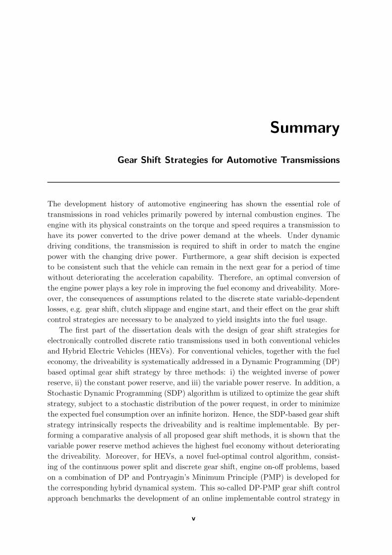
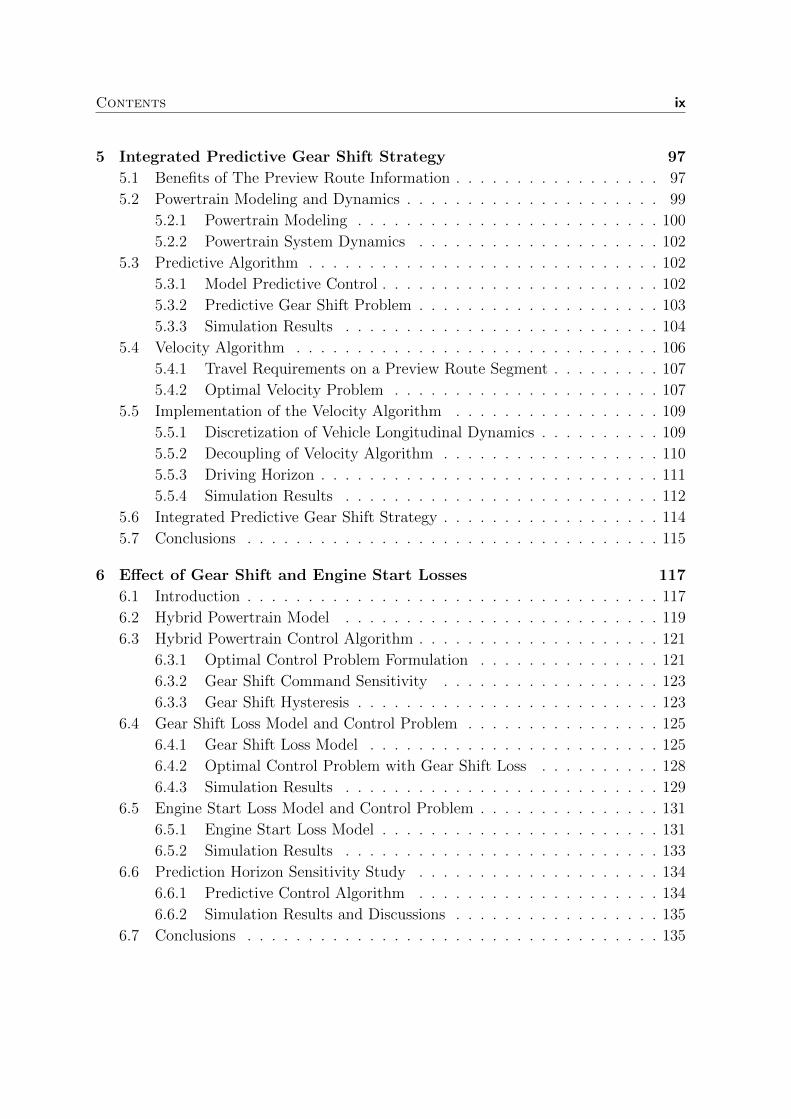
Figure 1.1: Passenger car transmissions: market share and prediction [89](NAFTA stands for the North American Free Trade Agreement area).
4 1 Introduction
Figure 1.1 illustrates the market share and prediction of the future market share of pas-
senger car transmissions from 2000 till 2015 [89]. From this figure, it can be observed
that the market share differs from region to region. Towards the future, it is expected
that the diversification in transmission types is increasing. Moreover, the market share
related to the automated transmissions is globally expanding, in particular for trans-
mission types with discrete ratio. However, the predicted market share for the CVT
and HT is also increasing rapidly. Furthermore, in the China and India markets of
automotive transmissions, there is also a strong shift towards the AMT and DCT tech-
nologies [109] (not shown in Figure 1.1). Electronic control of the gear shift process
in combination with an optimal shift strategy provides a means to further improve the
fuel economy, driveability and the reduction of pollutant emissions.
Improvement of the fuel economy has always been an ongoing process of the automobile
industry. Hybridization and electrification of powertrains have gained an impressive
momentum and will become a leading technological trend for future vehicles. A signifi-
cant market share of hybrid vehicles of up to 10% of the total vehicle market is expected
within 10 to 15 years [37]. Even the full-electric vehicles may benefit from a transmission
technology [1]. Currently, two-speed AMT/DCT or even three-speed DCT are being
developed. For example, the first gear provides the required acceleration torque from
standstill in order to reduce the battery current, which improves the battery lifetime
and efficiency. Meanwhile the second gear provides the required operation speed such
that the power is constant for a relatively large speed range.
1.2 Background
Every vehicle needs a transmission [89].
An automotive transmission is an inevitable system for a vehicle (even for electric
vehicles). From the analysis of the transmission technology trends, the above statement
of every vehicle needs a transmission [89] can be reaffirmed. To further elaborate on the
necessity of a transmission for road vehicles and thereby contributing to the automotive
transmission control and design, the research presented in this dissertation focuses on:
• vehicles primarily powered by internal combustion engines; and,
• designing the gear shift strategy for electronically controlled discrete ratio trans-
missions.
To realize the advantages of the electronically controlled discrete ratio transmissions,
such as a high fuel economy, an acceptable driveability, and a shifting automation, a
1.2 Background 5
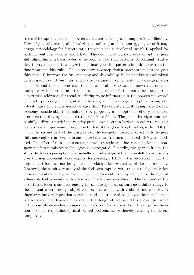
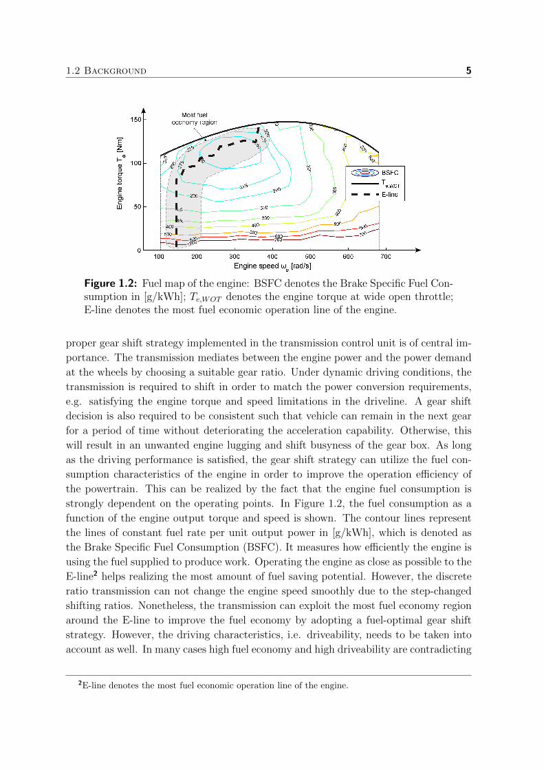
Figure 1.2: Fuel map of the engine: BSFC denotes the Brake Specific Fuel Con-sumption in [g/kWh]; Te,WOT denotes the engine torque at wide open throttle;E-line denotes the most fuel economic operation line of the engine.
proper gear shift strategy implemented in the transmission control unit is of central im-
portance. The transmission mediates between the engine power and the power demand
at the wheels by choosing a suitable gear ratio. Under dynamic driving conditions, the
transmission is required to shift in order to match the power conversion requirements,
e.g. satisfying the engine torque and speed limitations in the driveline. A gear shift
decision is also required to be consistent such that vehicle can remain in the next gear
for a period of time without deteriorating the acceleration capability. Otherwise, this
will result in an unwanted engine lugging and shift busyness of the gear box. As long
as the driving performance is satisfied, the gear shift strategy can utilize the fuel con-
sumption characteristics of the engine in order to improve the operation efficiency of
the powertrain. This can be realized by the fact that the engine fuel consumption is
strongly dependent on the operating points. In Figure 1.2, the fuel consumption as a
function of the engine output torque and speed is shown. The contour lines represent
the lines of constant fuel rate per unit output power in [g/kWh], which is denoted as
the Brake Specific Fuel Consumption (BSFC). It measures how efficiently the engine is
using the fuel supplied to produce work. Operating the engine as close as possible to the
E-line2 helps realizing the most amount of fuel saving potential. However, the discrete
ratio transmission can not change the engine speed smoothly due to the step-changed
shifting ratios. Nonetheless, the transmission can exploit the most fuel economy region
around the E-line to improve the fuel economy by adopting a fuel-optimal gear shift
strategy. However, the driving characteristics, i.e. driveability, needs to be taken into
account as well. In many cases high fuel economy and high driveability are contradicting
2E-line denotes the most fuel economic operation line of the engine.
6 1 Introduction
attributes.
Therefore, in the next section, the challenges related to the gear shift problem of discrete
ratio transmissions used in conventional and hybrid electric vehicles will be addressed,
which motivates the research in this dissertation.
1.3 Challenges
The gear shift strategy for discrete ratio transmissions is a part of the supervisory
control algorithm. The supervisory control algorithm generates for example the set
points for the gear shift command based on the current powertrain states to improve
the operation performance of the powertrain system. In this section, the basic dynamics
of the powertrain system is briefly introduced, and some control design challenges are
formulated based on, but not limited to:
• the level of which the drive power request is known; and,
• the particular application (i.e., conventional or hybrid vehicle); and,
• the assumptions related to the development of an online strategy; and finally,
• the assumptions related to discrete state variable-dependent losses, such as gear
shift and engine start stop losses.
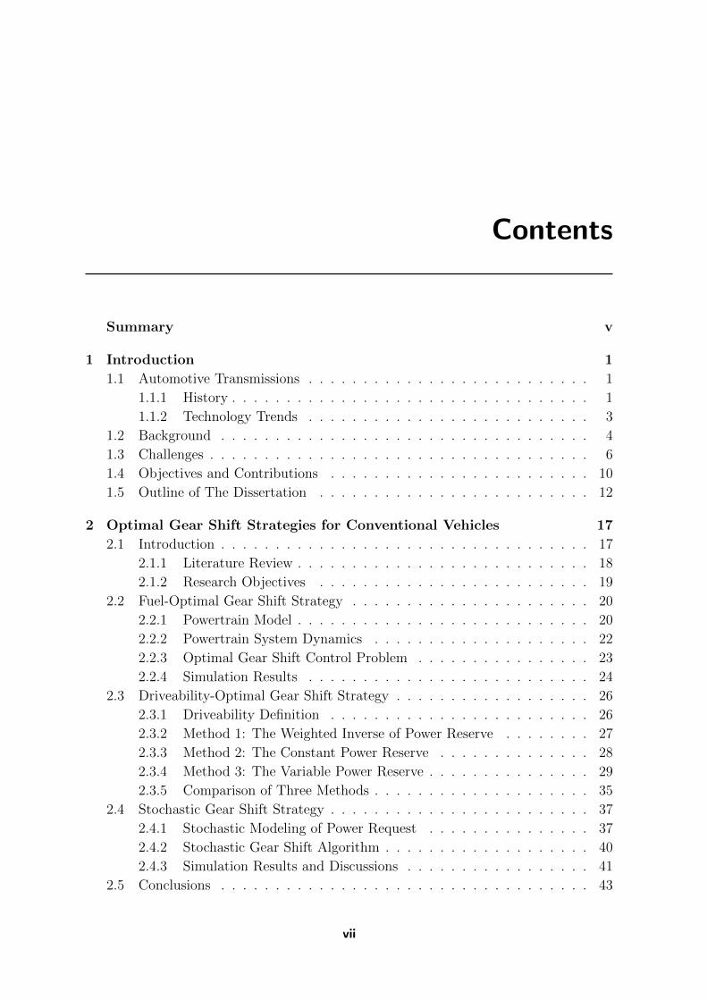
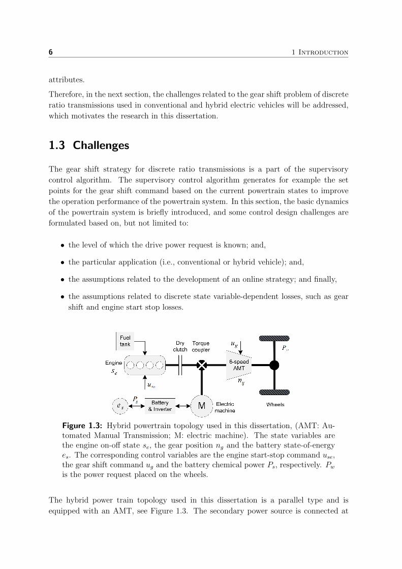
Figure 1.3: Hybrid powertrain topology used in this dissertation, (AMT: Au-tomated Manual Transmission; M: electric machine). The state variables arethe engine on-off state se, the gear position ng and the battery state-of-energyes. The corresponding control variables are the engine start-stop command use,the gear shift command ug and the battery chemical power Ps, respectively. Pwis the power request placed on the wheels.
The hybrid power train topology used in this dissertation is a parallel type and is
equipped with an AMT, see Figure 1.3. The secondary power source is connected at

1.3 Challenges 7
the primary side of the transmission. The quasi static modeling approach [42] is adopted
in this dissertation to model the main powertrain components. This approach is very
suitable for developing the supervisory control algorithm. Due to the discrete nature
of the transmission ratio, the discrete-time dynamics of the powertrain system can be
expressed in a generic form by,
x(k + 1) = f(x(k), u(k), z(k)
), (1.1)
Ceq(x(k), u(k), z(k)
)= 0, (1.2)
Cin(x(k), u(k), z(k)
)< 0, (1.3)
wherein: k is the fixed discrete-time step, x(k) and u(k) are the state and control
variable vectors, respectively; z(k) is the disturbance vector imposed on the vehicle; f
is the function describing the dynamics of the system state. The matrices Ceq and Cindescribe the equality and inequality constraints of the powertrain system, respectively.
From a control point of view, the power request at the wheels Pw is ordinarily referred
as the disturbance. In the optimal control problem for the powertrain system, the
disturbance can arise from the external disturbing forces acting on the system due to
changes of road conditions, traffic conditions, driver behaviors, etc. In general, the
power request can be classified into three levels.
1. The power request is known a priori for the whole driving profile.
2. The power request is totally unknown. This case mostly describes a real-life drive
mission.
3. The power request is known over a certain preview horizon. This is achieved by
means of a prediction technique and onboard route information systems.
Accordingly, the supervisory control algorithm, for example, including the gear shift
strategy, is designed such that the disturbance is expectedly attenuated in order to
improve the operation performance of the powertrain. The foreseen challenges related
to the gear shift strategy design for conventional and hybrid vehicles are discussed
next. Moreover, the consequences of the assumptions related to discrete state variable-
dependent losses, i.e. gear shift, clutch slippage and engine start, and their effect on
the control strategies are addressed in the subsequent sections.
Optimal gear shift strategy for conventional vehicles
The conventional powertrain control consists of one state variable, which is the gear
position ng(k). Hence, an optimal gear shift strategy, allowing the engine to operate in
the region closely to the E-line, will reduce the fuel consumption. Consequently, this will

8 1 Introduction
result in a lower speed and a higher torque of the engine, hence reducing the acceleration
capability, represented by the power reserve, denoted by ∆Pe = (Te,WOT − Te) ωe.
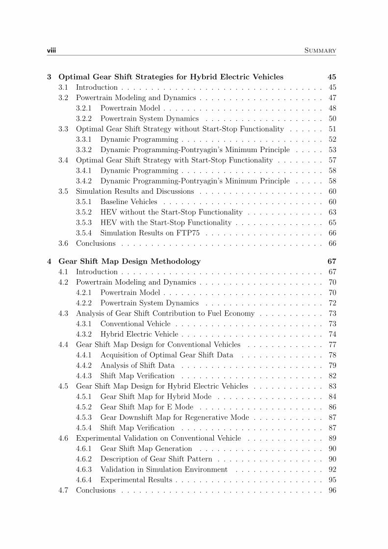
Figure 1.4 demonstrates a tradeoff between a fuel economy improvement potential and
a reduction of driveability at three indicated points 1, 2 and 3, with ∆Pe,1 < ∆Pe,2 <
∆Pe,3, respectively. A decision to choose the operating point among three of them should
be made on the basis of the ability to remain in the next gear for an acceptable period
of time. Therefore, a gear shift strategy needs to be designed such that an optimal
tradeoff between the fuel economy and driveability can be realized for the vehicle.
Figure 1.4: Tradeoff between the fuel economy and driveability for a conven-tional vehicle.
So far, addressing the driveability in the powertrain control can be found in a relatively
limited amount of published literature, which mostly focus on satisfying a certain con-
stant power request by cooperatively control the gear shift and throttle opening [66],
or satisfying a constraint on a change in the engine power reserve for a given change
in the throttle angle by controlling the CVT ratio [135]. Nonetheless, under the effect
of the disturbance (changing driver behavior, changing road condition, etc.) the power
request varies from time to time, which requires the driveability to be addressed in an
optimal gear shift strategy for the whole drive cycle. Therefore, in this dissertation, the
focus is on developing a systematic method to analyze and define the optimal tradeoff
between the fuel economy and driveability.
Optimal gear shift strategy for HEVs
For the hybrid electric powertrain as shown in Figure 1.3, the dynamical system consists
of three state variables: the discrete engine on-off state se(k), the continuous battery
state-of-energy es(k), and the discrete gear position ng(k). The corresponding control
variables are the engine start-stop command use(k) (discrete), the battery power Ps(k)

1.3 Challenges 9
(continuous), and the gear shift command ug(k) (discrete). Due to the co-existence
of the continuous and discrete variables, the dynamical system is a hybrid dynamical
system as well. In general, the design of an optimal control algorithm for a hybrid
dynamical system with constraints on the state and control variables encounters complex
design challenges in terms of optimality, for example, due to the non-smoothness of the
objective function [23]. Therefore, the advantages of a HEV could be deteriorated if
the gear shift and engine on-off strategies are insufficiently optimized. Moreover, the
gear shift command ug(k) is constrained due to a practical comfort aspect, e.g. not
allowing the gear box to shift from the first gear to the highest gear at the next time
instant. Besides, the multi-objective character of the problem imposes further control
design challenges. The gear shift problem in principle can be solved by discretizing the
continuous variables (se(k) and Ps(k)) and using deterministic Dynamic Programming
(DP) [83], yet can result in a computational burden due to the ‘curse of dimensionality’.
Apparently, the tradeoff among optimality, accuracy and the computational efficiency is
seen as one of the main challenges for the design of a gear shift control algorithm
for HEVs. In addition, a computationally efficient and optimal Energy Management
Strategy (EMS) is very beneficial for accelerating the design process of a HEV at the
initial development phase, thus reducing valuable development time and cost.
Realtime gear shift strategy for automotive transmissions
In order to drive the vehicle on road, a real time implementable gear strategy for the
transmission is required. When the drive power request is totally unknown, a map-
based gear shift strategy is a solution for determining when to shift gears online. A
static gear shift map generates the shifting points, defined as a point-wise function of
the vehicle speed and the drive power request observed at the transmission input, which
determines how to shift gears correspondingly.
For conventional vehicles, the design of a gear shift map is traditionally based on know-
how, experience of the calibration engineers and tuning in a heuristic manner [87].
Hence, the gear shift map becomes consistent and relatively robust after a huge effort
and relative time-consuming trial-and-error are performed. This experience-based gear
shift strategy does not exploit the inherent potential of the powertrain system suffi-
ciently to improve the overall performance of the vehicle, and hence coming with a
lower confidence on the optimality with respect to the fuel economy and driveability. A
method in order to improve the shift rules can be found in [66]. Therefore, developing
a map-based gear shift strategy which makes the optimal tradeoff between the fuel econ-
omy and driveability in a systematic manner is seen as one of the additional research
challenges in this dissertation.
For HEVs, the design of a static gear shift map is more complex compared to conven-
tional vehicles, given that the acceleration capability can be obtained by the hybrid

10 1 Introduction
powertrain system. Therefore, developing an implementable gear shift strategy based
on a static map, which is adapted to different operation modes of the hybrid system,
would require a rigorous design and analysis.
Recently, using route information is seen as a possibility to significantly further improve
the fuel economy for HEVs, for example see, [2,10,57,152]. However, utilizing route in-
formation to predict the power request over a certain horizon will increase complexity of
the optimization problem by one more state variable, the to-be-optimized vehicle speed.
Hence, an optimized map-based gear shift strategy appears as a well-compromised solu-
tion for the velocity trajectory optimization problem. When the prediction of the power
request over a certain horizon is available, a gear shift strategy incorporated in a pre-
dictive EMS will allow the HEV to boost the fuel saving level. Again, this emphasizes
on the necessity of a computation-efficient and optimal gear shift strategy such that the
predictive EMS can be realtime implementable.
Consequences with respect to the gear shift and engine start events
Incorporation of the gear shift and engine start-stop strategies into an EMS for an AMT-
based HEV in order to maximize the fuel economy benefit can result in: i) an earlier
upshift pattern and a higher shifting frequency, and ii) a frequent stop and start of the
engine. However, it should be noted that the gear shift or engine start-stop induces
additional energy losses. For example, the vehicle speed reduces during shifting due to
a torque interruption, and higher drive power is needed from the engine to compensate
for these dynamic losses later on. Moreover, a certain amount of energy is consumed
through cranking the engine from rest. However, in literature, these losses and their
effect on the control strategy and fuel consumption are often neglected. This can finally
end up with an unfair evaluation on the fuel benefit of HEVs with respect to the gear
shift and engine start-stop strategies. Hence, it is necessary to model these losses and
analyze their effect on the control strategies for HEVs.
Moreover, analysis of the correlation among the design objectives (fuel economy, emis-
sions, driveability, etc.) and investigation of the sensitivity of an optimal control algo-
rithm to the relevant design objectives are essential. The result of this analysis can be
used to simplify the multi-objective function. A systematic method, based on Singular
Value Decomposition (SVD), for such an analysis is investigated in this dissertation.
1.4 Objectives and Contributions
Motivated by the research challenges related to the gear shift problem for discrete ratio
transmissions, used in conventional and hybrid electric vehicles as addressed in Section
1.3, the following six research objectives (O1 −O6) are specifically defined:
1.4 Objectives and Contributions 11
• O1: define and address the driveability in a fuel-optimal gear shift strategy for
conventional vehicles on drive cycles known a priori.
• O2: design a fuel-optimal control algorithm, including the gear shift strategy, for
the hybrid dynamical system of HEVs on drive cycles known a priori.
• O3: develop an online gear shift strategy for conventional and hybrid electric
vehicles equipped with discrete ratio transmissions. The strategy improves the
fuel economy meanwhile still satisfying an acceptable driveability.
• O4: propose a gear shift strategy for a HEV to further improve the fuel economy
by exploiting route information from the GPS-based onboard navigation system.
• O5: analyze the effect of the gear shift and engine start losses on the control
strategy and fuel consumption.
• O6: investigate the sensitivity of an optimal gear shift strategy to the relevant
control design objectives, such as fuel economy, driveability, comfort, etc.
By fulfilling all the defined research objectives, the work presented in this dissertation
systematically tackles all the discussed challenges related to the gear shift problem,
thereby making a fundamental contribution in the field of the automotive transmission
control design and analysis. Explicitly, the following main contributions (C1 −C6) are
obtained:
• C1: various optimal gear shift strategies with respect to the fuel economy and
driveability are proposed for conventional vehicles. A novel concept of variable
power reserve is developed to properly address the driveability, meanwhile guar-
anteeing the highest achievable fuel economy (Chapter 2).
• C2: a novel gear shift control algorithm based on a combination of DP and Pon-
tryagin’s Minimum Principle (PMP) is developed for the hybrid dynamical system
(consisting of continuous and discrete variables) of HEVs. This so-called DP-PMP
algorithm benchmarks the gear shift problem in terms of optimality and compu-
tational efficiency (Chapter 3).
• C3: a gear shift map design methodology aiming at a realtime solution for discrete
ratio transmissions is developed. The methodology exploits the fuel economy and
driveability potential of the optimal gear shift strategies (proposed in Chapters 2
and 3) in order to realize an online gear shift strategy for conventional and hybrid
electric vehicles (Chapter 4).
• C4: a concept of integrated predictive gear shift strategy for HEVs, utilizing
route information to further explore fuel economy potential, is demonstrated in
simulation (Chapter 5).

12 1 Introduction
• C5: an analysis of the effect of gear shift and engine start losses on control strate-
gies for AMT-based HEVs. By taking the gear shift loss into account, this study
reveals a perception of a fuel-efficient advantage of powershift transmissions (DCT,
PS-AMT) over non-powershift transmissions (MT, AMT) applied for passenger
HEVs. Furthermore, the effect of the engine start loss can not be ignored in seek-
ing a fair evaluation of the fuel economy for parallel HEVs. A prediction horizon
of few seconds can help a predictive EMS to realize the highest achievable fuel
economy (Chapter 6).
• C6: a Singular Value Decomposition-based technique is introduced to analyze
the correlation among the design objectives of an optimal gear shift problem for
conventional and hybrid electric vehicles (Chapter 7).
1.5 Outline of The Dissertation
The dissertation consists of six self-contained research chapters, i.e. from Chapter 2
till Chapter 7. The work presented in the dissertation can be categorized into two
main parts. The first four chapters together form the first part, related to the gear shift
strategy design for automotive transmissions corresponding with three transparent levels
of the power request. This is shown in Figure 1.5. Meanwhile the last two chapters
form the second part, involved with the analysis of the consequences on the control
design objectives with respect to a gear shift strategy and an engine start-stop strategy,
see Figure 1.6. On both figures, the arrowed lines indicate the linkage among chapters,
meaning that the outcome of a certain chapter is used as input to another chapter. For
example, the DP-PMP control approach developed in Chapter 3 is utilized in Chapters
4 and 5 as the corresponding input. The six contributions (C1 - C6) for six chapters
are also shown in the output arrowed lines. Within the context of defining the optimal
gear shift points for automotive transmissions, the dissertation is unified by hierarchical
interconnections among the chapters. The outline of the dissertation is given next.
In relation to the first part, Chapter 2 deals with the optimal gear shift problem for
conventional vehicles. The driveability is systematically analyzed in a DP-based fuel-
optimal gear shift strategy by three methods: i) the weighted inverse of power reserve,
ii) the constant power reserve, and iii) the variable power reserve. A Stochastic Dy-
namic Programming (SDP) algorithm optimizes the gear shift strategy, subject to a
stochastic distribution of the power request, to minimize the expected fuel consumption
over an infinite horizon, hence making the obtained solution intrinsically respect the
driveability and be realtime implementable. A comparative analysis of all proposed
gear shift methods is given in terms of the fuel economy and driveability improvement.
The variable power reserve method achieves the highest fuel economy meaning without
sacrificing the driveability. Chapter 3 focuses on a fuel-optimal gear shift strategy for

1.5 Outline of The Dissertation 13
Figure 1.5: Overview of linkage among Chapters 2, 3, 4 and 5 with contribu-tions.
HEVs, wherein a novel control algorithm based on a combination of DP and PMP is
developed. The EMS based on DP-PMP control approach benchmarks the develop-
ment of an online control strategy in terms of the tradeoff between calculation accuracy
and computational efficiency. The gear shift strategies proposed in Chapters 2 and 3
are not realtime implementable, yet result in a globally optimal solution on a priori
drive cycle. Aiming at a real time implementable solution, Chapter 4 develops a gear
shift map design methodology for discrete ratio transmissions, used in conventional and
hybrid electric vehicles. The optimal gear shift strategy proposed in Chapters 2 and
3 are utilized as the bases to derive the optimal gear shift patterns. Then statistical
theory is applied to analyze the optimal gear shift patterns in order to extract the
shift rules. Hence this alternative two-step design procedure makes the gear shift map
respect the fuel economy and driveability, consistent and robust with respect to shift
busyness. In Chapter 5, a concept of an integrated predictive gear shift strategy for
HEVs is demonstrated in simulation environment. The control strategy utilizes route
information obtained from a GPS-based onboard navigation system to further explore
the fuel economy potential.
In connection with the second part, Chapter 6 addresses the energetic losses, involving
with the gear shift and engine start events, in an AMT-based HEV. The effect of these
losses on the control strategies and fuel consumption for (non-)powershift transmission
technologies is investigated. Moreover, the sensitivity of prediction horizon on the fuel
consumption is analyzed. Chapter 7 defines the relevant control design objectives, i.e.
fuel economy, driveability and comfort, with respect to an optimal gear shift problem
of vehicular propulsion systems. A SVD-based method is introduced to analyze the
possible correlations and interdependencies among the design objectives.

14 1 Introduction
Figure 1.6: Overview of linkage among Chapters 6 and 7 with contributions.
Finally, the conclusions and recommendations of the dissertation are given in Chapter
8.
Publications
In the research leading to this dissertation, the following journals and conference papers
have been publishing.
Refereed journal publications
• V. Ngo, J. A. Colin Navarrete, T. Hofman, M. Steinbuch, and A. Serrarens. Op-
timal Gear Shift Strategies for Conventional Vehicles. In preparation for journal
publication, 2012. (Chapter 2).
• V. Ngo, T. Hofman, M. Steinbuch, and A. Serrarens. Optimal Control of the Gear
Shift Command for Hybrid Electric Vehicles. IEEE Transactions on Vehicular
Technology, vol. 61, issue 8, 2012. (Chapter 3).
• V. Ngo, T. Hofman, M. Steinbuch, and A. Serrarens. Gear Shift Map Design
Methodology for Automotive Transmissions. In preparation for journal publica-
tion, 2012. (Chapter 4).
• V. Ngo, T. Hofman, M. Steinbuch, and A. Serrarens. Integrated Predictive Gear
Shift Strategy for Hybrid Electric Vehicles. In preparation for journal publication,
2012. (Chapter 5).
• V. Ngo, T. Hofman, M. Steinbuch, and A. Serrarens. Effect of Gear Shift and
Engine Start Losses on Control Strategies for Hybrid Electric Vehicles. In prepa-
ration for journal publication, 2012. (Chapter 6).

1.5 Outline of The Dissertation 15
• V. Ngo, T. Hofman, M. Steinbuch, and A. Serrarens. Structural Analysis of
Control Design Objectives for Vehicular Propulsion Systems. In preparation for
journal publication, 2012. (Chapter 7).
Refereed conference publications
• A. Serrarens, R. van Druten, W. van Liempt, N. Weel, P. Kumar, L. Romers,
V. Ngo. Light Hybridization of Diesel Powertrains: the most cost-effective route
towards 120g/km CO2 and below. VDI2008 Innovative Powertrain Systems, Nov,
2008, Germany.
• V. Ngo, T. Hofman, M. Steinbuch, and A. Serrarens. Shifting Strategy for
Stepped-Gear Transmission Vehicle - A Comparative Study and Design Method.
The 24th International Battery, Hybrid and Fuel Cell Electric Vehicle Symposium
- EVS24, Stavanger, Norway, May 2009.
• V. Ngo, T. Hofman, M. Steinbuch, and A. Serrarens. Performance Indices for
Vehicular Propulsion Systems. The 15th Asia Pacific Automotive Engineering
Conference - APAC15, Hanoi, Vietnam, October 2009.
• V. Ngo, T. Hofman, M. Steinbuch, and A. Serrarens. An Optimal Control-Based
Algorithm for Hybrid Electric Vehicle Using Preview Route Information. 2010
American Control Conference - ACC2010, Maryland, USA, June 2010.
• V. Ngo, T. Hofman, M. Steinbuch, and A. Serrarens, L. Merkx. Improvement
of Fuel Economy in Power-Shift Automated Manual Transmission through Shift
Strategy Optimization - An Experimental Study. Vehicle Power and Propulsion
Conference 2010 - IEEE-VPPC 2010, Lille, France, September 2010.
• V. Ngo, T. Hofman, M. Steinbuch, and A. Serrarens. Optimal Shifting Strategy for
a Parallel Hybrid Electric Vehicle. The 25th World Battery, Hybrid and Fuel Cell
Electric Vehicle Symposium and Exhibition - EVS25, Shenzhen, China, November
2010.
• V. Ngo, T. Hofman, M. Steinbuch, and A. Serrarens. Analyses of the Perfor-
mance Index for a Hybrid Electric Vehicle. 2011 American Control Conference -
ACC2011, San Francisco - CA, USA, June 2011.
• V. Ngo, T. Hofman, M. Steinbuch, and A. Serrarens. Predictive Gear Shift Con-
trol for a Parallel Hybrid Electric Vehicle. 2011 Vehicle Power and Propulsion
Conference - IEEE-VPPC 2011, Chicago, USA, September 2011.

16 1 Introduction
• V. Ngo, T. Hofman, M. Steinbuch, and A. Serrarens. Effect of Gear Shift and
Engine Start Losses on Control Strategies for Hybrid Electric Vehicles. The 26th
Electric Vehicle Symposium - EVS26, Los Angeles - California, USA, May 2012.

Chapter 2
Optimal Gear Shift Strategies forConventional Vehicles1
Abstract - This chapter aims at designing optimal gear shift strategies for conventional pas-senger vehicles equipped with discrete ratio transmissions. The fuel economy and driveabilityare selected as the design objectives. Three methods of addressing the vehicle driveabilityare proposed for a fuel-optimal gear shift algorithm based on Dynamic Programming (DP)to quantitatively study the tradeoff between the fuel economy and driveability. Furthermore,another method based on Stochastic Dynamic Programming (SDP) is proposed to derive anoptimal gear shift strategy over a number of drive cycles in an average sense, hence makingit respect the vehicle driveability. In contrast with the DP-based strategy, the obtained gearshift strategy based on SDP is realtime implementable. A comparative analysis of all proposedgear shift methods is given in terms of the fuel economy and driveability improvements.
2.1 Introduction
For conventional vehicles equipped with discrete ratio transmissions, e.g. automatic,
dual clutch, automated (manual) transmissions, etc., a decision on selecting a different
gear leads to a sudden change of the engine operating point due to a stepped change
of the transmission ratio. With highly nonlinear characteristics of the engine fuel con-
sumption and maximum torque, a change of the engine operating point due to a gear
shift can result in a deficient fuel operation state, and/or a low driveability condition
for the vehicle thereafter. Hence, an optimal gear shift strategy for a discrete ratio
transmission plays an important role in achieving a high performance for the vehicle.
In literature, there does not exist a systematic method to quantitatively investigate the
1This chapter has been prepared for a journal submission in the form as: V. Ngo, J. A. ColinNavarrete, T. Hofman, M. Steinbuch, A. Serrarens. Optimal Gear Shift Strategies for ConventionalVehicles. 2012.
17

18 2 Optimal Gear Shift Strategies for Conventional Vehicles
tradeoff between the fuel economy and driveability with respect to an optimal gear shift
strategy. Hence, in this chapter, various methods, taking the driveability into account,
are proposed for the design of the optimal gear shift strategy. They are comparatively
analyzed in terms of the fuel economy and driveability improvements, towards achieving
the most optimal method.
2.1.1 Literature Review
In literature, a substantial amount of published research can be found, addressing the
design of the ratio control strategy for automotive transmissions. With respect to a
fuel economy improvement, the control strategies aim at moving the engine operating
points as close as possible to the most fuel economy region. For a push belt Continuously
Variable Transmission (CVT), a sequence quadratic programming-based optimization
algorithm for an offline optimal ratio strategy, and an online suboptimal feed-forward
ratio controller can be found in [105]. For discrete ratio transmissions, a ratio control
strategy can be alternatively interpreted as a gear shift strategy. Due to the discrete
nature of the ratio, discrete optimization techniques, e.g. Dynamic Programming (DP),
can be efficiently utilized to derive an optimal gear shift schedule over a given drive
cycle. In addition, the suboptimal gear shift strategy revolves around the methods
based on heuristic rules, e.g. genetic algorithm, fuzzy logic, know-how of calibration
engineers or from empirical experiments, etc., for example see [18, 99]. The globally
optimal gear shift strategy is used to benchmark the fuel economy on a certain drive
cycle, and therefore not realtime implementable. Meanwhile the rule-based strategy is
less fuel economic, yet realtime implementable.
Improvement of the vehicle driveability, represented by the driver’s power demand satis-
faction, while simultaneously optimizing the fuel economy is the main challenging aspect
for the gear shift strategy design. For a CVT-based vehicle, the authors in [129] suggest
that a ratio control strategy with a fuel consumption increase by 15%-20% compared
to the E-line (indicating the most fuel-efficient line of the engine) can lead to a good
driveability acceptance. The authors in [135] propose a method for choosing the opti-
mum ratio trajectory for a CVT-based passenger vehicle. An optimization problem is
formulated focusing on maximizing the fuel economy and driveability, which is defined
by a change in the engine power reserve for a given change in the throttle angle. This
driveability definition creates a consistent and desirable vehicle response under different
road load conditions. The authors claim a good, or improved driveability, while still
achieving a fuel economy benefit compared with other ratio control schedules.
For a vehicle equipped with a discrete ratio transmission, the driveability can be im-
proved by an integrated powertrain control approach. In [87], a two-layer fuzzy gear
shift strategy for an Automatic Transmission (AT), considering the engine working con-
2.1 Introduction 19
ditions and the driver’s intention, can eliminate unnecessary shifts occurring when the
driver’s intention is overlooked or unclear. The authors state a better acceleration per-
formance. In [166], a gear shift method, based on pattern recognition and a learning
algorithm, is proposed. By utilizing three different dynamic parameters, i.e. the throt-
tle position, vehicle speed and acceleration, the method improves the fuel economy and
acceleration capability as claimed by the authors. Another method of combined time-
optimal and fuzzy-logic strategies to control the engine during a gear shift process of an
Automated Manual Transmission (AMT) is proposed in [167]. By decreasing the engine
speed deviation between the controlled target and actual output, and shortening the
gear shift time, the proposed control algorithm is claimed to be capable of reducing fuel
consumption, engine noise, shift jerk and the clutch friction loss. An integrated pow-
ertrain control approach based on an optimization technique to improve the driver’s
power demand satisfaction for an AT vehicle can be found in [7, 66]. DP is used to
solve a fuel-optimal gear shift and throttle control problem over a number of different
acceleration profiles. Then, the optimized gear shift map and the throttle open map
for the vehicle are extracted to govern the operation of the integrated powertrain. The
method is found to be promising in improving the fuel economy without compromis-
ing the driveability. Also for an AT, the authors in [6] propose an adaptive gearshift
strategy that compensates for variations in the vehicle and road conditions, e.g. the
load, trailering, grade, and the curvature. The method utilizes two shift maps: a fuel
economy map and a sportive map, in order to dynamically generates the shifting points
adapted to the current vehicle and road conditions in achieving the optimal tradeoff
between the fuel economy and the driveability.
2.1.2 Research Objectives
For discrete ratio transmissions, it can be observed that improving the fuel economy
while not compromising the driveability is still a challenging research problem. There
is lack of a proper method to analyze the correlation, and hence not able to define an
optimal tradeoff between the fuel economy and driveability through an optimal gear
shift strategy. Therefore, in this chapter a systematic approach will be developed con-
sisting of: i) designing a fuel-optimal gear shift strategy, ii) defining the driveability and
taking it into the fuel-optimal gear shift problem, and iii) quantitatively evaluating and
comparing the fuel economy and driveability among the proposed gear shift strategies.
Firstly, a fuel-optimal gear shift control problem is formulated and solved by using DP
to obtain a baseline fuel economy. Secondly, the vehicle driveability represented for
an acceleration capability and defined by the power reserve, is addressed in the fuel-
optimal gear shift problem by three methods. In the first method, the power reserve
is incorporated in the objective function by a weight factor. In the second method,
the driveability is respected by imposing an inequality constraint on the power reserve,

20 2 Optimal Gear Shift Strategies for Conventional Vehicles
which is equal to or larger than a constant threshold value. In the third method, a
variable power reserve concept, as a function of the vehicle speed being predefined
over a wide range of driving scenarios, is constructed and respected by an inequality
constraint to ensure an acceptable driveability. And finally, an optimal tradeoff between
the fuel economy and driveability is derived from a comparative analysis of the three
methods.
The DP-based gear shift algorithm requires the whole drive cycle to be known a priori.
It optimizes the powertrain’s operational performance by identifying an optimal gear
shift schedule over the given drive cycle. Hence, the obtained gear shift strategy can
not be implemented in realtime. Towards an online solution for a gear shift problem, a
design method based on Stochastic Dynamic Programming (SDP) is proposed for that
purpose. The SDP algorithm formulates and solves an infinite-horizon optimization
problem over a probabilistic distribution of the power request from many drive cycles
rather than a single drive cycle. The vehicle speed is also considered as a state variable.
Hence, the obtained gear shift strategy, in the form of a set of shift maps, is time-
invariant and feedback with respect to the state variables (the gear position and the
vehicle speed), such that it can be implemented in realtime. The SDP optimization
problem, subject to the power request from many drive cycles, renders the stochastic
gear shift strategy a driveability satisfaction.
This chapter is organized as follows. The fuel-optimal gear shift problem is formulated
and solved in Section 2.2. The driveability-optimal gear shift problem is discussed in
Section 2.3. The stochastic gear shift strategy is addressed in Section 2.4. And finally,
conclusions and recommendations are given in Section 2.5.
2.2 Fuel-Optimal Gear Shift Strategy
2.2.1 Powertrain Model
In order to derive a supervisory control strategy, the quasi static modeling approach is
used to model the main powertrain components. A fixed time step ∆t of one second
is chosen to simulate the powertrain system. Hence, the powertrain system dynamics
faster than 1Hz are ignored [42]. The component models in discrete time domain k are
described as follows.
• Engine: the engine fuel consumption is modeled by a static fuel efficiency map,
see Figure 2.2. It indicates the contour lines of constant Brake Specific Fuel
Consumption (BSFC), which a static point-wise function of the speed ωe(k) and
the torque Te(k). The BSFC describes the fuel rate mf (k) per unit output power
of the engine. The engine torque obtained at wide open throttle for the whole
2.2 Fuel-Optimal Gear Shift Strategy 21
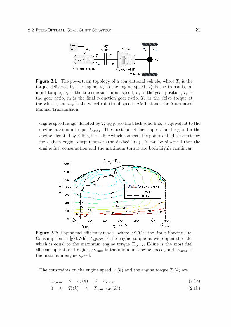
Figure 2.1: The powertrain topology of a conventional vehicle, where Te is thetorque delivered by the engine, ωe is the engine speed, Tg is the transmissioninput torque, ωg is the transmission input speed, ng is the gear position, rg isthe gear ratio, rd is the final reduction gear ratio, Tw is the drive torque atthe wheels, and ωw is the wheel rotational speed. AMT stands for AutomatedManual Transmission.
engine speed range, denoted by Te,WOT , see the black solid line, is equivalent to the
engine maximum torque Te,max. The most fuel efficient operational region for the
engine, denoted by E-line, is the line which connects the points of highest efficiency
for a given engine output power (the dashed line). It can be observed that the
engine fuel consumption and the maximum torque are both highly nonlinear.
Figure 2.2: Engine fuel efficiency model, where BSFC is the Brake Specific FuelConsumption in [g/kWh], Te,WOT is the engine torque at wide open throttle,which is equal to the maximum engine torque Te,max, E-line is the most fuelefficient operational region, ωe,min is the minimum engine speed, and ωe,max isthe maximum engine speed.
The constraints on the engine speed ωe(k) and the engine torque Te(k) are,
ωe,min ≤ ωe(k) ≤ ωe,max, (2.1a)
0 ≤ Te(k) ≤ Te,max(ωe(k)
), (2.1b)
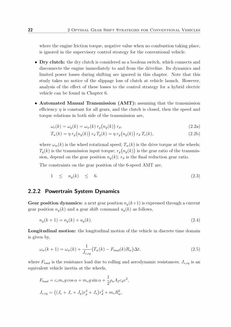
22 2 Optimal Gear Shift Strategies for Conventional Vehicles
where the engine friction torque, negative value when no combustion taking place,
is ignored in the supervisory control strategy for the conventional vehicle.
• Dry clutch: the dry clutch is considered as a boolean switch, which connects and
disconnects the engine immediately to and from the driveline. Its dynamics and
limited power losses during shifting are ignored in this chapter. Note that this
study takes no notice of the slippage loss of clutch at vehicle launch. However,
analysis of the effect of these losses to the control strategy for a hybrid electric
vehicle can be found in Chapter 6.
• Automated Manual Transmission (AMT): assuming that the transmission
efficiency η is constant for all gears, and the clutch is closed, then the speed and
torque relations in both side of the transmission are,
ωe(k) = ωg(k) = ωw(k) rg(ng(k)
)rd, (2.2a)
Tw(k) = η rg(ng(k)
)rd Tg(k) = η rg
(ng(k)
)rd Te(k), (2.2b)
where ωw(k) is the wheel rotational speed; Tw(k) is the drive torque at the wheels;
Tg(k) is the transmission input torque; rg(ng(k)
)is the gear ratio of the transmis-
sion, depend on the gear position ng(k); rd is the final reduction gear ratio.
The constraints on the gear position of the 6-speed AMT are,
1 ≤ ng(k) ≤ 6. (2.3)
2.2.2 Powertrain System Dynamics
Gear position dynamics: a next gear position ng(k+1) is expressed through a current
gear position ng(k) and a gear shift command ug(k) as follows,
ng(k + 1) = ng(k) + ug(k). (2.4)
Longitudinal motion: the longitudinal motion of the vehicle in discrete time domain
is given by,
ωw(k + 1) = ωw(k) +1
Jv,eq
(Tw(k)− Fload(k)Rw
)∆t, (2.5)
where Fload is the resistance load due to rolling and aerodynamic resistances; Jv,eq is an
equivalent vehicle inertia at the wheels,
Fload = crmvg cosα +mvg sinα +1
2ρaAfcdv
2,
Jv,eq =((Je + Jc + Jp)r
2g + Js
)r2d +mvR
2w,

2.2 Fuel-Optimal Gear Shift Strategy 23
and mv is the vehicle weight; Rw is the wheel radius; Je is the engine inertia; Jc is the
clutch inertia; Jp is the transmission primary inertia; Js is the transmission secondary
inertia; ρa is the air density; Af is the frontal area of vehicle; cd is the aerodynamic
drag coefficient; cr is the rolling friction coefficient; g is the gravity coefficient; v is the
vehicle velocity; and α is the road slope. It should be noted that the vehicle wheel slip
is ignored.
2.2.3 Optimal Gear Shift Control Problem
The powertrain system dynamics, described by (2.1)-(2.5), can be expressed in a generic
form by,
x(k + 1) = f(x(k), u(k)
), (2.6)
Ceq(x(k), u(k)
)= 0, (2.7)
Cin(x(k), u(k)
)< 0, (2.8)
where x(k) = [ng(k), ωv(k)]T and u(k) = [ug(k), Tw(k)]T are the vectors of state and
control variables,respectively; f is the function describing the dynamic system; Ceq and
Cin are the matrices of equality and inequality constraints of the system, respectively.
Imposing a bound on the discrete gear shift command ug(k) will influence the gear shift
dynamics (2.4), and affect to the optimality. For a 6-speed AMT, ug(k) belongs to the
set {−5, · · · ,−1, 0, 1, · · · , 5}. With a reason for an acceptable driveability, the gear
shift command is chosen as,
ug(k) =
−1 downshift,
0 sustaining,
1 upshift,
(2.9)
to avoid a large variation of the engine speed under a certain shift. One gear upshift
(ug(k) = 1) or one gear downshift (ug(k) = −1) for each time step of one second
is reasonable, since the average shifting time for an AMT is typically less than one
second.
Problem 2.1. Given a drive cycle v(k) with time length N , implying that the vehicle
longitudinal motion (2.5) is deterministic, find an optimal control law u∗(k) = u∗g(k) to
minimize a cost function of fuel consumption over the drive cycle, that is
u∗(k) = arg minu(k)
J =N−1∑k=0
mf (k)∆t, (2.10)
subject to the constraints (2.6)-(2.9).

24 2 Optimal Gear Shift Strategies for Conventional Vehicles
Dynamic Programming (DP) [11] is well known as a powerful method to solve a non-
linear, non-convex optimization problem with mixed constraints while obtaining a glob-
ally optimal time-variant, state-feedback solution. In order to apply DP to the proposed
optimal control problem, we need to
• grid the state variables x(k);
• grid the corresponding control variables u(k); and,
• calculate mf (k) for the whole drive cycle for every grid point;
Then, the optimal cost-to-go function at any time step k, denoted as J ∗k , is defined as,
• step k = N :
J ∗N = 0, (2.11)
• step k ∈ [0, 1, . . . , N − 1]:
J ∗k(x(k)
)= min
u(k)
[mf (k)∆t+ J ∗k+1
(x(k + 1)
)]. (2.12)
The optimal cost-to-go function J ∗k is defined backwards from k = N until k = 0.
The optimal solution u∗(k) is obtained correspondingly with a specific value for the end
constraint x(N).
2.2.4 Simulation Results
Table 2.1: Relative fuel efficiency improvement of the optimal gear shift strat-egy compared with the prescribed gear shift schedule.
Drive cycle NEDC FTP75Relative fuel efficiency improvement [%] 14.2 25.4
In order to investigate the fuel-efficient potential of the optimal gear shift strategy, the
prescribed gear shift schedules accompanied with the test cycles NEDC and FTP75
(see, Appendix C) are chosen as the baseline shift schedules. These prescribed gear
shift schedules, denoted by Pres. and shown by the dashed lines in Figure 2.3, define
the shift points for the transmission on NEDC and FTP75 for the standardized test

2.2 Fuel-Optimal Gear Shift Strategy 25
0 200 400 600 800 1000 12000
2
4
6
Time [s]
n g [−]
NEDC
Pres.
DP
0 200 400 600 800 1000 1200 1400 1600 1800 20000
2
4
6
Time [s]
n g [−]
FTP75
Pres.
DP
Figure 2.3: Prescribed (Pres.) and the optimal gear positions (DP) over theNEDC and FTP75 cycles.
100 200 300 400 500 600 7000
20
40
60
80
100
120
140260
260
260
260
260
260
275
275
275
275
275
275
275
275
290
290
290290
290
290290
290
320
320
320320
320
320
320
360360
360
360
360
400400
400
400
400
500 500
500
500
600600
600
700 700700
ωe [rad/s]
Te [N
m]
BSFC [g/kWh]
Te,WOT
E−line
Pres.
DP
Figure 2.4: Engine operating points corresponding with the prescribed gearshift strategy (Pres.) and the optimal gear shift strategy (DP).
procedure2. The optimal gear shift schedule, denoted by DP, is shown by the solid
lines in Figure 2.3. It can be observed that, the transmission is shifted at higher rate
and to higher values than the prescribed strategy. Obviously, the engine operating
points resulted from the optimal gear shift strategy gather around the E-line as much
as possible. Meanwhile for the prescribed shift schedules, the engine operating points
are more far from the E-line, see Figure 2.4. The relative fuel efficiency improvement of
the optimal gear shift strategy compared with the prescribed schedule is of 14.2% and
2NEDC is the standard emission test cycle in Europe, thus the prescribed gear shift schedule isaccompanied to give shift signals for geared transmission vehicles. Meanwhile the prescribed gear shiftschedule for the standard emission test cycle FTP75 is given by ADVISOR.

26 2 Optimal Gear Shift Strategies for Conventional Vehicles
25.4% on NEDC and FTP75, respectively, see Table 2.1. Therefore, it can be concluded
that by optimizing the gear shift strategy, the fuel economy of conventional vehicles can
be improved significantly.
2.3 Driveability-Optimal Gear Shift Strategy
2.3.1 Driveability Definition
The fuel-optimal gear shift strategy, proposed in Section 2.2, yields an early and frequent
upshift pattern for the transmission. It renders the engine, on average, to operate at a
lower speed and high torque region, and hence improving the fuel economy. As a result,
the so-called torque reserve ∆Te, defined by a difference between the maximum engine
torque and the actual engine torque (∆Te = Te,max− Te), tends to decrease. Therefore,
if the driver demands a higher acceleration, the engine torque reserve might not be
able to fulfil the acceleration surplus. Obviously, this will deteriorate the acceleration
capability of the vehicle under certain driving situations. In other words, the fuel
economy improvement is gained at a penalty of driveability deterioration. Therefore,
in this section, a study on the tradeoff between the fuel economy and the driveability
with respect to an optimal gear shift strategy is presented. An appropriate method to
address the driveability of conventional vehicles is well defined.
The driveability in general has a broad inference, such as vehicle responsiveness, oper-
ating smoothness, driving comfort, vibration, jerk, tip-in tip-out, etc., [158]. Regarding
to the gear shift strategy, the engine operating point is changed in a stepwise manner.
So, a relevant term for determining the driveability is the acceleration capability, i.e.
how much acceleration potential is available for the vehicle after a certain gear shift.
Since the power reserve, denoted as ∆Pe (2.13) and defined by the product of the engine
speed and the torque reserve, represents an instant availability of power for accelera-
tion, it can also be used as a measurement for driveability [92, 135]. Furthermore, the
study in [145] also indicates the engine power to be the best parameter representing the
driver’s demand.
∆Pe = (Te,max − Te) ωe. (2.13)
In this chapter, three different methods are proposed to address driveability of the
vehicle,
• Method 1: incorporating the inverse of power reserve with a certain weight factor
in the objective function of a fuel-optimal gear shift control problem.
• Method 2: adding an inequality constraint for the power reserve level in a fuel-
optimal gear shift control problem in order to ensure that the vehicle actual power

2.3 Driveability-Optimal Gear Shift Strategy 27
reserve is always above a certain constant threshold.
• Method 3: adding an inequality constraint for the power reserve in a fuel-optimal
gear shift control problem. The bound of the power reserve is varied with the
vehicle speed.
2.3.2 Method 1: The Weighted Inverse of Power Reserve
Aiming at maximizing the fuel economy and driveability, and then analyzing a tradeoff
between them with respect to an optimal gear shift strategy, a corresponding cost
function is constructed as,
J =N−1∑k=0
[mf (k) + ν ∆P−1
e (k)]∆t, (2.14)
where ν is a weight factor imposed on an inverse of the power reserve. The corresponding
driveability optimal gear shift control problem is similar to Problem 2.1. Hence, DP is
used to solve this control problem.
The fuel consumption, denoted by FC, and the accumulative power reserve, denoted
by APR, calculated for the whole drive cycle, are used to quantify the tradeoff between
the fuel economy and driveability.
FC =N−1∑k=0
mf (k)∆t, (2.15a)
APR =N−1∑k=0
∆Pe(k)∆t. (2.15b)
The weight factor ν is varied as in (2.16) to study a sensitivity of the tradeoff between
the fuel economy and driveability to the gear shift strategy.
ν ∈ {0, 1, 2, 3, 4, 6, 8, 10, 12, 14} · 500 [g ·Ws−1]. (2.16)
The drive cycles used for simulation are NEDC, FTP75, LA92, CADC-urban and
CADC-road (see, Appendix C). A sensitivity analysis of FC and APR with respect
to the weight factor ν is depicted in Figure 2.5a. It can be seen that both FC and
APR increase corresponding to an increase of the weight factor for all drive cycles.
This means that the vehicle driveability can only be improved at a cost of fuel economy
reduction. Figure 2.5b shows a translation of FC and APR to the coordinate origin for
a better understanding of the correlation. Basically, a positive linear relation between
FC and APR can be seen for almost all selected drive cycles.
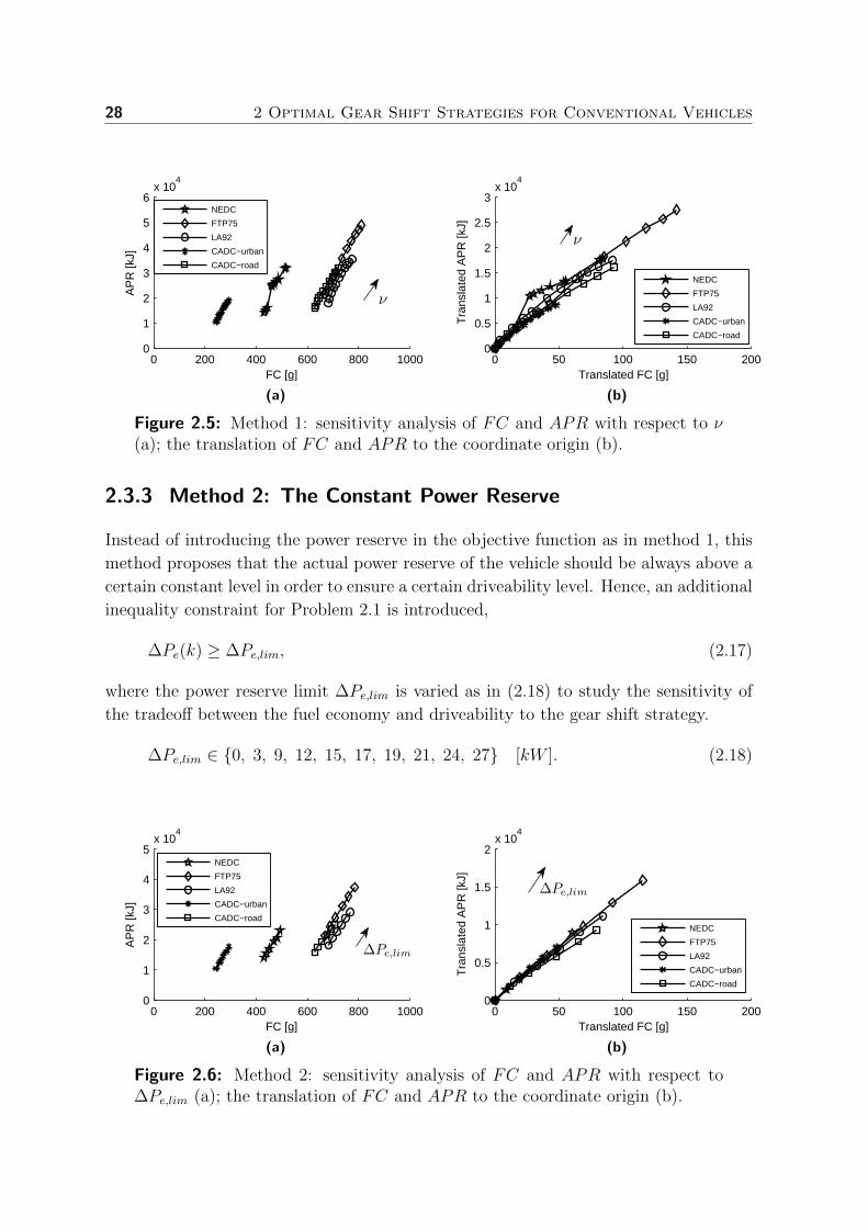
28 2 Optimal Gear Shift Strategies for Conventional Vehicles
0 200 400 600 800 10000
1
2
3
4
5
6x 10
4
FC [g]
AP
R [k
J]
ν
NEDC
FTP75
LA92
CADC−urban
CADC−road
(a)
0 50 100 150 2000
0.5
1
1.5
2
2.5
3x 10
4
Translated FC [g]
Tra
nsla
ted
AP
R [k
J]
ν
NEDC
FTP75
LA92
CADC−urban
CADC−road
(b)
Figure 2.5: Method 1: sensitivity analysis of FC and APR with respect to ν(a); the translation of FC and APR to the coordinate origin (b).
2.3.3 Method 2: The Constant Power Reserve
Instead of introducing the power reserve in the objective function as in method 1, this
method proposes that the actual power reserve of the vehicle should be always above a
certain constant level in order to ensure a certain driveability level. Hence, an additional
inequality constraint for Problem 2.1 is introduced,
∆Pe(k) ≥ ∆Pe,lim, (2.17)
where the power reserve limit ∆Pe,lim is varied as in (2.18) to study the sensitivity of
the tradeoff between the fuel economy and driveability to the gear shift strategy.
∆Pe,lim ∈ {0, 3, 9, 12, 15, 17, 19, 21, 24, 27} [kW ]. (2.18)
0 200 400 600 800 10000
1
2
3
4
5x 10
4
FC [g]
AP
R [k
J]
∆Pe,lim
NEDC
FTP75
LA92
CADC−urban
CADC−road
(a)
0 50 100 150 2000
0.5
1
1.5
2x 10
4
Translated FC [g]
Tra
nsla
ted
AP
R [k
J]
∆Pe,lim
NEDC
FTP75
LA92
CADC−urban
CADC−road
(b)
Figure 2.6: Method 2: sensitivity analysis of FC and APR with respect to∆Pe,lim (a); the translation of FC and APR to the coordinate origin (b).

2.3 Driveability-Optimal Gear Shift Strategy 29
Simulation results of FC and APR, defined in (2.15), are shown in Figure 2.6a. A
translation of FC and APR to the coordinate origin are depicted in Figure 2.6b. It can
be observed that an increase of ∆Pe,lim leads to a decrease of the fuel economy. For this
method, the higher the value of ∆Pe,lim, the better the driveability comes at a cost of
fuel economy reduction. Furthermore, it can be concluded that an increase of APR is
proportional with an increase of FC with respect to ∆Pe,lim.
2.3.4 Method 3: The Variable Power Reserve
Both Methods 1 and 2 show that, the optimal gear shift strategy is sensitive to the weight
factor ν and the power reserve limit ∆Pe,lim, respectively. These design parameters are
kept being constant for the whole drive cycle, and hence making the obtained gear shift
strategy become more conservative. To overcome this drawback, the weight factor or the
power reserve limit needs to be adapted to the changing driving conditions. Therefore,
defining a rule for such an adaptation is a key factor for a fuel-optimal gear shift control
strategy to further improve the fuel economy and driveability potentially at the same
time. In this section, a method based on a concept of variable power reserve is proposed
to address the driveability as put in a fuel-optimal gear shift strategy. The power reserve
required for a certain acceleration capability of the vehicle is varied in accordance with
its actual speed. In other words, the variable power reserve is a function of the vehicle
speed, denoted as ∆Pe,var(v(k)
). Hence, the gear shift control problem needs to respect
the variable power reserve by an inequality constraint as,
∆Pe(k) ≥ ∆Pe,var. (2.19)
A novel approach is developed to define the variable power reserve ∆Pe,var(v(k)
). This
approach is based on a statistical analysis of the vehicle acceleration characteristics on
various drive cycles. The details are presented next.
Vehicle performance characteristics
In this section, the discrete time variable k is left out of the variables for brevity. For
the functional variables, the independent variable is omitted to improve the readability,
for example rg := rg(ng(k)
). Then, if the engine output torque is Te, the propulsion
force available at the wheels is given by,
Fw = ηrg rd TeRw
. (2.20)
Under the influence of road material and driving conditions, e.g. dry, wet, snow, etc.,
the tractive force at the wheels induced by friction is approximated by
Ffr =µ mv g
(lb + cr (hg −Rw)
)l + µ hg
, (2.21)

30 2 Optimal Gear Shift Strategies for Conventional Vehicles
where l is the wheelbase length of the vehicle; lb is the horizontal distance from the
vehicle gravity center to the rear tire; hg is the height of the vehicle gravity center; µ is
the friction coefficient between the tire and road surface.
If we assume that the standard road material of asphalt is used under a dry condition,
the corresponding peak friction coefficient µp is chosen to calculate a maximum friction
force Ffr,max at the wheels. The maximum propulsion force at the wheels, denoted as
Fw,max, is calculated by (2.20) with the engine torque at wide open throttle. So, the
vehicle maximum acceleration is derived as,
amax =min
(Fw,max, Ffr,max
)− Fload
mv,eq
, (2.22)
where mv,eq is the equivalent vehicle mass at the wheels,
mv,eq =
((Je + Jc + Jp) r
2g + Js
)r2d
R2w
+mv.
Figure 2.7 depicts the maximum acceleration characteristic vs. the vehicle velocity cor-
responding with each gear position ng (see, the solid lines). So, the actual accelerations
of the vehicle in real-life driving are always inside these bounds. Here, the decelerations
are irrelevant for the design method, and therefore neglected.
Variable power reserve
In order to define the variable power reserve ∆Pe,var, a statistical analysis of vehicle
acceleration characteristics on various drive cycles is performed. Depend on the regions,
the driving styles, the driving purposes, etc., the drive cycles are differed from each
other. Therefore, the selected drive cycles must encompass a representative driving
profile of the vehicle, giving quantitative information of the acceleration level a driver
would normally require at every vehicle speed. In this study, to ensure objectiveness, the
drive cycles chosen are the standardized ones: ARB02, CADC, FTP75, Hurk, HWFET,
JN1015, LA92, NEDC, NYCC, and US06 (see, Appendix C).
The velocity is discretized into a finite number of values Nv with an equal discretized
step, thus giving a velocity set,
V = {v1, v2, · · · , vNv}. (2.23)
For a given drive cycle, at a certain velocity v(k) the corresponding acceleration is
approximated as,
a(k)|v(k) =v(k + 1)− v(k)
∆t. (2.24)

2.3 Driveability-Optimal Gear Shift Strategy 31
Sampling the velocity and computing the corresponding acceleration on all chosen drive
cycles to create the velocity data. Then clustering the velocity data in accordance with
all elements of the velocity set (2.23) to form the corresponding acceleration data. The
velocity data and the acceleration data together create the statistical data of the chosen
drive cycles. Mapping the statistical data onto the vehicle performance characteristics
to realize the representative acceleration characteristics for the vehicle, see, the light
blue circles in Figure 2.7. The statistical data falling outside the acceleration bounds
are cut off due to infeasible driving situations.
0 50 100 150 2000
0.5
1
1.5
2
2.5
3
3.5
4
v [km/h]
a [m
/s2 ]
a
max (n
g=1)
amax
(ng=2)
amax
(ng=3)
amax
(ng=4)
amax
(ng=5)
amax
(ng=6)
statistical data
Figure 2.7: Performance characteristics of the vehicle, indicated by the sixsolid lines corresponding with six gear positions. The representative accelerationcharacteristics are indicated by the light blue circles. v is the vehicle velocity, ais the vehicle acceleration.
0 0.5 1 1.5 2 2.5 30
0.2
0.4
0.6
0.8
1
a [m/s2]
Pro
babi
lity
dens
ity acc. data
GEV fit
(a)
0 0.5 1 1.5 2 2.5 30
0.2
0.4
0.6
0.8
1
a [m/s2]
Cum
ulat
ive
prob
abili
ty
acc. data
GEV fit
(b)
Figure 2.8: Analysis of the acceleration data at the velocity cluster vl =30 [km/h]. a is the acceleration. Legends: acc. stands for acceleration; GEVstands for generalized extreme value.
The acceleration data is clustered in accordance with vl ∈ V , l = 1, 2, . . . , Nv. There-

32 2 Optimal Gear Shift Strategies for Conventional Vehicles
fore, analyzing this cluster can give an insight of a driveability level for the vehicle at the
corresponding velocity. The acceleration data at each cluster of velocity is considered
as a random variable. In statistics and probability theory [85, 113], probability density
function is a function that describes the relative likelihood for a random variable to take
on a given value. Hence, probability density function is an appropriate tool to analyze
the acceleration data.
As a demonstration, an analysis for the acceleration data at the velocity cluster
vl = 30 [km/h] is given in Figure 2.8: a probability density distribution in (a), and
a corresponding cumulative probability in (b). The acceleration data can be fitted by
the generalized extreme value distribution having a cumulative distribution function,
FCD(a;κ, σ, ξ) = exp
{−[1 + ξ
(a− κσ
)]−1/ξ},
where a is the vehicle acceleration; κ is the location parameter; σ is the scale parameter;
and ξ is the shape parameter.
The fits are shown by the red solid lines. It demonstrates that the acceleration range of
[0.3, 0.9] [m/s2] has the highest probability density, meaning that this acceleration range
is where the vehicle acceleration is most likely occurred. Nonetheless, the maximum
vehicle acceleration is at 3.1[m/s2], occurring at very small probability. Whereas, the
cumulative probability defines a probability of the vehicle acceleration a to be smaller
or equal to a certain value areq, described by,
Prob[a ≤ areq
∣∣vl ∈ V] = pa, (2.25)
where Prob is a probability of a certain event. Apparently, in order to have pa = 1,
areq must be equal to 3.1[m/s2].
It is observed that, a definition of an acceptable driveability level for the vehicle over the
whole velocity range is equivalent to a definition of pa for each velocity cluster vl ∈ V .
Drivers would always expect the vehicle to fully meet the acceleration request, which
means that pa = 1 ∀ vl ∈ V . This would require a gear shift strategy, resulting in
a high power reserve, ready for a possible maximum acceleration. Such a high power
reserve level will induce a sportive driving behavior, however, it decreases the fuel saving
potential considerably. Hence, defining an appropriate value for pa can improve the fuel
economy meanwhile ensuring an acceptable vehicle driveability.
Regarding to the accumulative probability, statistical and probability theories point
out that a confidence level associated with a certain pa is commonly chosen at 90%, or
95%, or 99% [85, 113]. In this study, a confidence level is chosen at 90%. Therefore,
if drivers would expect the vehicle to always satisfy the acceleration demand, it’s very
likely that the vehicle can only meet 90% of the driving demand. Hence, pa = 0.9 is
chosen for a fairly acceptable driveability level. In other words, the vehicle can follow

2.3 Driveability-Optimal Gear Shift Strategy 33
up to 90% of the occurring acceleration situations. Note that 10% excluded represents
the very hard, sudden acceleration situations, which are not specifically matched with
the powertrain capability at the current gear. Hence, the transmission is required to
shift gears (downshift) such that the powertrain can accommodate the high acceleration
demand.
Once, the acceptance driveability level represented by pa has been defined, the required
acceleration areq(vl), ∀ vl ∈ V is obtained by solving a reverse problem, defined corre-
spondingly with (2.25). So, a polynomial fit areq,fit(v), as a function of the velocity, can
be achieved,
areq,fit(v) = p1v6 + p2v
5 + p3v4 + p4v
3 + p5v2 + p6v + p7, (2.26)
where p1, p2, p3, p4, p5, p6 and p7 are the coefficients of the polynomial fit.
0 50 100 150 2000
0.5
1
1.5
2
2.5
3
3.5
4
v [km/h]
a [m
/s2 ]
a
max (n
g=1)
amax
(ng=2)
amax
(ng=3)
amax
(ng=4)
amax
(ng=5)
amax
(ng=6)
areq
areq,fit
Figure 2.9: Acceleration capability characteristics required to ensure an ac-ceptable driveability level. v is the vehicle speed, a is the vehicle acceleration.
0 50 100 150 2000
1
2
3
4
5
6
7
v [km/h]
n g [−]
Figure 2.10: Feasible operating regions corresponding with the gear positionsfor a satisfaction of the vehicle driveability. v is the vehicle speed, ng is the gearposition.
Figure 2.9 depicts the required accelerations areq(vl) and the corresponding fit polyno-

34 2 Optimal Gear Shift Strategies for Conventional Vehicles
mial areq,fit(v). It represents the acceleration capability characteristics, as a function
of the vehicle speed, to ensure that the vehicle can confidently cover 90% of the actual
driving situations.
Intersections of areq,fit(v) with the vehicle performance characteristics at a certain gear
create the correspondingly feasible operating region for the powertrain at that gear
position. Hence, the intersection among the feasible operating regions yields a com-
mon operating area for optimally shifting gears meanwhile still ensuring the acceptable
driveability level, see Figure 2.10.
Finally, from (2.26), the variable power reserve is derived as,
∆Pe,var(v) = mv,eq areq,fit(v) v. (2.27)
Control problem formulation
A fuel-optimal gear shift control problem, taking into account the variable power reserve
(2.27) to respect a certain driveability requirement, is formulated as follows.
Problem 2.2. Given a drive cycle v(k) with time length N , thus making the vehicle
longitudinal motion (2.5) deterministic, find an optimal gear shift strategy u∗(k) = u∗g(k)
to minimize the cost function of fuel consumption over the drive cycle, that is,
u∗(k) = arg minu(k)
J =N−1∑k=0
mf (k)∆t, (2.28)
subject to the constraints (2.6)-(2.9), and
∆Pe(k) ≥ max{
0, ∆Pe,var(v(k)
)− Pe,req(k)
}, (2.29)
where Pe,req(k) is the required power to follow the given drive cycle v(k).
Note that (2.19) refers to a general constraint for meeting the driveability requirement.
Therefore, the power Pe,req(k), required to follow a given drive cycle, has to be subtracted
from ∆Pe,var(v(k)
)as in (2.29). If Pe,req(k) ≥ ∆Pe,var
(v(k)
)holds, the constraint (2.29)
becomes inactive because the real power reserve ∆Pe(k) is always larger than zero. For
this problem, DP is also used to derive the optimal solution.
Simulation results
Simulation results of Method 3 are given in Table 2.2. The fuel-optimal gear shift strat-
egy, described in Section 2.2, is chosen as a reference. It shows that Method 3 degrades
the fuel economy compared to the reference, but benefiting a significant improvement
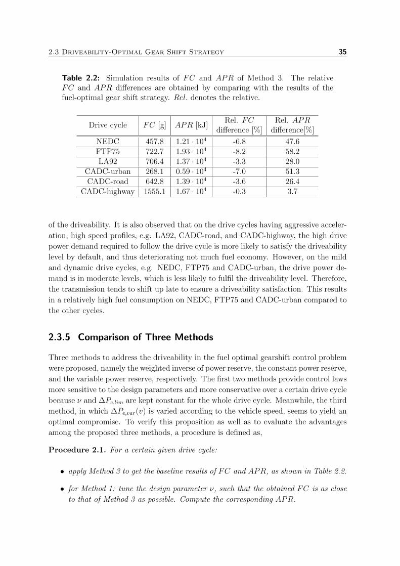
2.3 Driveability-Optimal Gear Shift Strategy 35
Table 2.2: Simulation results of FC and APR of Method 3. The relativeFC and APR differences are obtained by comparing with the results of thefuel-optimal gear shift strategy. Rel. denotes the relative.
Drive cycle FC [g] APR [kJ]Rel. FC Rel. APR
difference [%] difference[%]
NEDC 457.8 1.21 · 104 -6.8 47.6FTP75 722.7 1.93 · 104 -8.2 58.2LA92 706.4 1.37 · 104 -3.3 28.0
CADC-urban 268.1 0.59 · 104 -7.0 51.3CADC-road 642.8 1.39 · 104 -3.6 26.4
CADC-highway 1555.1 1.67 · 104 -0.3 3.7
of the driveability. It is also observed that on the drive cycles having aggressive acceler-
ation, high speed profiles, e.g. LA92, CADC-road, and CADC-highway, the high drive
power demand required to follow the drive cycle is more likely to satisfy the driveability
level by default, and thus deteriorating not much fuel economy. However, on the mild
and dynamic drive cycles, e.g. NEDC, FTP75 and CADC-urban, the drive power de-
mand is in moderate levels, which is less likely to fulfil the driveability level. Therefore,
the transmission tends to shift up late to ensure a driveability satisfaction. This results
in a relatively high fuel consumption on NEDC, FTP75 and CADC-urban compared to
the other cycles.
2.3.5 Comparison of Three Methods
Three methods to address the driveability in the fuel optimal gearshift control problem
were proposed, namely the weighted inverse of power reserve, the constant power reserve,
and the variable power reserve, respectively. The first two methods provide control laws
more sensitive to the design parameters and more conservative over a certain drive cycle
because ν and ∆Pe,lim are kept constant for the whole drive cycle. Meanwhile, the third
method, in which ∆Pe,var(v) is varied according to the vehicle speed, seems to yield an
optimal compromise. To verify this proposition as well as to evaluate the advantages
among the proposed three methods, a procedure is defined as,
Procedure 2.1. For a certain given drive cycle:
• apply Method 3 to get the baseline results of FC and APR, as shown in Table 2.2.
• for Method 1: tune the design parameter ν, such that the obtained FC is as close
to that of Method 3 as possible. Compute the corresponding APR.
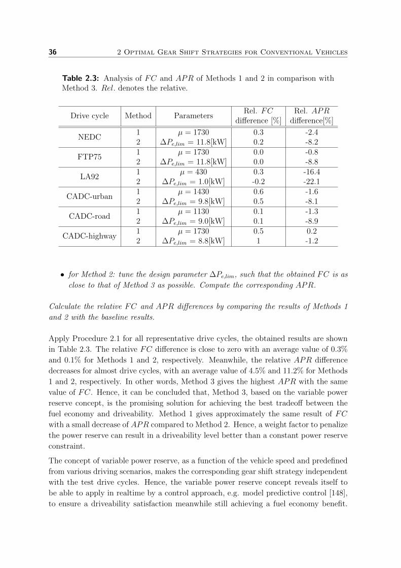
36 2 Optimal Gear Shift Strategies for Conventional Vehicles
Table 2.3: Analysis of FC and APR of Methods 1 and 2 in comparison withMethod 3. Rel. denotes the relative.
Drive cycle Method ParametersRel. FC Rel. APR
difference [%] difference[%]
NEDC1 µ = 1730 0.3 -2.42 ∆Pe,lim = 11.8[kW] 0.2 -8.2
FTP751 µ = 1730 0.0 -0.82 ∆Pe,lim = 11.8[kW] 0.0 -8.8
LA921 µ = 430 0.3 -16.42 ∆Pe,lim = 1.0[kW] -0.2 -22.1
CADC-urban1 µ = 1430 0.6 -1.62 ∆Pe,lim = 9.8[kW] 0.5 -8.1
CADC-road1 µ = 1130 0.1 -1.32 ∆Pe,lim = 9.0[kW] 0.1 -8.9
CADC-highway1 µ = 1730 0.5 0.22 ∆Pe,lim = 8.8[kW] 1 -1.2
• for Method 2: tune the design parameter ∆Pe,lim, such that the obtained FC is as
close to that of Method 3 as possible. Compute the corresponding APR.
Calculate the relative FC and APR differences by comparing the results of Methods 1
and 2 with the baseline results.
Apply Procedure 2.1 for all representative drive cycles, the obtained results are shown
in Table 2.3. The relative FC difference is close to zero with an average value of 0.3%
and 0.1% for Methods 1 and 2, respectively. Meanwhile, the relative APR difference
decreases for almost drive cycles, with an average value of 4.5% and 11.2% for Methods
1 and 2, respectively. In other words, Method 3 gives the highest APR with the same
value of FC. Hence, it can be concluded that, Method 3, based on the variable power
reserve concept, is the promising solution for achieving the best tradeoff between the
fuel economy and driveability. Method 1 gives approximately the same result of FC
with a small decrease of APR compared to Method 2. Hence, a weight factor to penalize
the power reserve can result in a driveability level better than a constant power reserve
constraint.
The concept of variable power reserve, as a function of the vehicle speed and predefined
from various driving scenarios, makes the corresponding gear shift strategy independent
with the test drive cycles. Hence, the variable power reserve concept reveals itself to
be able to apply in realtime by a control approach, e.g. model predictive control [148],
to ensure a driveability satisfaction meanwhile still achieving a fuel economy benefit.

2.4 Stochastic Gear Shift Strategy 37
Apparently, Methods 1 and 2, yielding solutions sensitive to the design parameters and
conservative to a drive cycle, are hard to implement in a realtime controller.
2.4 Stochastic Gear Shift Strategy
A gear shift strategy based on DP requires a knowledge of the whole drive cycle to
obtain a globally optimal solution, thus making it not a realtime solution. Meanwhile a
realtime implementable gear shift strategy can be achieved by utilizing Model Predictive
Control (MPC) or Stochastic Dynamic Programming [11]. The MPC-based algorithm
solves the optimal problem over a prediction horizon. Utilizing knowledge of the driving
profile over the prediction horizon, and applying the receding principle, the MPC-based
strategy is realtime implementable, but yielding a suboptimal solution. Meanwhile
SDP-based algorithm formulates and solves an infinite-horizon optimization problem
over a probabilistic distribution of the power demand obtained from many drive cycles
rather than a single drive cycle. This means that the SDP-based strategy is optimal
on an average sense, time-invariant and state variable feedback such that it can be
implemented in realtime.
The vehicle driveability can be addressed in a MPC-based gear shift strategy by utilizing
the variable power reserve concept (Method 3). Due to suboptimal characteristics, the
MPC-based strategy will result in a decrease of the driveability capability compared
to the DP-based gear shift strategy. Whereas, the SDP-based gear shift strategy is
optimized over many drive cycles on an average sense, which implies that the driveabil-
ity is intrinsically respected. To compare with Method 3 in terms of the driveability
improvement, details and results of the SDP-based gear shift problem are given in the
following sections.
2.4.1 Stochastic Modeling of Power Request
Markov model of power request dynamics
In real-life driving, the driver controls the vehicle speed by pressing the throttle and
brake pedals. In general, these command signals are interpreted as a power request
at the wheels to be satisfied by the powertrain. Hence, the power request, positive
or negative, is considered as an input to the powertrain controller. In this section,
a model of the power request, as a stochastic dynamic process based on the Markov
chain [70,82], is chosen to generate the power request. Assuming that, the power request
Preq is discretized to create a set,
Preq = {z1, z2, · · · , zNp}, (2.30)
38 2 Optimal Gear Shift Strategies for Conventional Vehicles
wherein Np approximates the actual continuum of values of the power request.
The vehicle speed is discretized into a finite number Nv of values, thus giving a set,
V = {v1, v2, · · · , vNv}.
The Markov chain defines a dynamics of the power request Preq by a transition proba-
bility matrix TM ∈ RNp×Np×Nv , whose elements are defined as,
tij,l = Prob[Preq(k + 1) = zj
∣∣∣Preq(k) = zi, v(k) = vl
]with i, j = 1, 2, . . . , Np; l = 1, 2, . . . , Nv
(2.31)
where tij,l is the (i, j, l)th element of TM representing one-step transition probability
from the current states of Preq(k) and v(k) at current time step k to state Preq(k + 1)
at next time step k + 1.
Note that for a given power request, the vehicle longitudinal dynamics is deterministic.
Hence, specifying drive cycle characteristics is equivalent to specifying the transition
probability tij,l, which can be estimated from the known drive cycles or the past driv-
ing records. In this study, standard drive cycles are used to determine the transition
probability matrix TM. The maximum likelihood algorithm, a suitable candidate for
dealing with the discrete data, is used to derive TM.
Algorithm 2.1. Maximum likelihood estimation
1. Chose the drive cycles that represent for actual driving profiles, e.g. suburban,
urban, and highway, etc.
2. Sample the vehicle speed v(k), then calculate the corresponding power request at
current time step Preq(k), and at next time step Preq(k+1) by using the quasi-static
powertrain model.
3. Cluster v(k) in accordance with all elements of V to create the velocity cluster at
vl, and collecting the corresponding power request data.
4. For each velocity cluster vl, cluster the power request Preq(k) in accordance with
all elements of Preq to create the power request data at cluster zi, and collecting
the corresponding next power request Preq(k + 1).
5. Then, cluster the corresponding Preq(k+1) in accordance with all elements of Preq.
6. Define the transition probability by the maximum likelihood estimator, which
counts the observation data as,
tij,l =nij,lnil
if nil 6= 0,

2.4 Stochastic Gear Shift Strategy 39
where nij,l is the number of occurrences of the transition from zi to zj at the
velocity cluster vl; nil is the total number of times that zi has occurred at the
velocity cluster vl. Apparently,
nil =
Np∑j=1
nij,l and
Np∑j=1
tij,l = 1.
It is worthwhile to mention that if the observation data are not rich enough to cover the
whole state space, nil may be zero for a specific case of the velocity cluster vl. There-
fore, a fuzzy smoothing algorithm [22] is used to estimate the corresponding transition
probabilities.
Algorithm 2.2. Fuzzy smoothing estimation
1. If denote the elements vl ∈ V , l = 1, 2, . . . , Nv as the velocity clusters. Then,
assume at a certain velocity cluster vl, there exists Nobs observations of the cor-
responding current and next power requests, obtained from the given drive cy-
cles. Denote a pair of observations of the power request as x = [xk, xk+1] ,[Preq(k), Preq(k + 1)] giving,
xn , {x1, x2, . . . , xNobs}, with n = 1, 2, . . . , Nobs.
2. If denote the elements zi ∈ Preq, i = 1, 2, . . . , Np as the power request clusters.
Then, a membership function of any observed power request xk with respect to a
certain power request cluster zi is defined as,
mi(xk) =
{Np∑m=1
[d(xk, zi)/d(xk, zm)
]1/(F−1)}−1
,
where d(xk, zi) denotes the Euclidean distance between xk and zi; F is a suitable
chosen constant greater than one.
3. Use the membership function mi(xk), the smoothed transition probabilities of the
Markov chain model is estimated as,
tij,l =
∑Nobs
n=1
[mi(x
nk)mj(x
nk+1)
]∑Nobs
n=1 mi(xnk), i, j = 1, 2, . . . , Np.
It is apparent that when F tends to one, the fuzzy smooth estimation approaches
the maximum likelihood estimation. Figure 2.11 shows an example of the estimated
transition probabilities at a velocity cluster vl = 80 [km/h]. The diagonally dominant
structure of the transition probabilities reveals a high correlation of the power request
separated by one time step. This can be explained that if the vehicle is experiencing
some power request level at the current time step, it’s likely to experience a similar
power request level at the next time step.

40 2 Optimal Gear Shift Strategies for Conventional Vehicles
510
1520
250
10
20
0
0.5
1
Preq (k+ 1) = zj
vl = 80[km/h]
Preq (k) = zi
t ij,l
Figure 2.11: Transition probability matrix at a quantized vehicle speed80[km/h].
Define the stochastic power request
Given a Markov model of the power request, the inverse transform method [26] can
be used to define the actual vehicle power request evolution. Given a vehicle speed
clustered to vl and a current power request clustered to zi at time k, by generating
a positive random number urand with a uniform distribution, ranged [0, 1], the next
power request Preq(k + 1) can be defined as,
Preq(k + 1) =
z1, if 0 ≤ urand < ti1,l,z2, if ti1,l ≤ urand < ti1,l + ti2,l,· · ·
zj, if∑j−1
q=1 tiq,l ≤ urand <∑j
q=1 tiq,l.
(2.32)
2.4.2 Stochastic Gear Shift Algorithm
Gear shift problem formulation
Problem 2.3. Given the powertrain model and a Markov model of the power request
evolution, the objective is to define an optimal gear shift strategy u∗ = u∗g that maps the
observed states to control decisions to minimize the expected total fuel consumption over
an infinite horizon,
J = limN→inf
EPreq
{N−1∑k=0
γk mf (k) ∆t
}, (2.33)
subject to the constraints (2.6)-(2.9) and (2.31).

2.4 Stochastic Gear Shift Strategy 41
The objective function consists of the instantaneous fuel consumption mf (k)∆t, accu-
mulated over time, discounted by a factor γ (0 < γ < 1), averaged over a stochastic
distribution of the power request. N is the horizon which approaches infinity for this
stochastic algorithm. E{. . .} denotes the expectation with respect to the considered
prediction model defined by the time-invariant Markov chain.
Applying the optimality principle of Bellman [11], the stochastic gear shift control prob-
lem is solved by a two-step algorithm, namely policy evaluation and policy improvement.
• Policy evaluation
In this policy, for each possible state vector value x, given a control policy u(x),
the cost-to-go J (x) is computed recursively as,
J s+1(x) = mf ∆t+ EPreq
[γ J s
(f(x, u(x)
))]∀x ∈ X. (2.34)
where s represents an iteration index; X is the set of admissible state value.
The recurrence relation is evaluated iteratively for all state vector values in the
discretized set of admissible states.
• Policy improvement
The optimality principle [11] indicates that an optimal control policy for the
stochastic gear shift control problem is also the control policy that minimizes
the cost-to-go function J (x) in (2.34). Hence, the optimal control policy u∗ = u∗gfor each state vector value x is defined as,
u∗(x) = arg minu∈U(x)
{mf ∆t+ E
Preq
[γ J
(f(x, u))]}
∀x ∈ X, (2.35)
where U(x) is the set of admissible control value corresponding to the state value
x.
After both policies are completed, the optimal control policy is feedback to the policy
evaluation step, and then the entire procedure is repeated iteratively until the optimal
cost function converges. In this study, the discount factor is chosen as γ = 0.9; and the
terminate condition for the iteration process is set with ‖J s+1(x)− J s(x)‖∞ < 1%.
2.4.3 Simulation Results and Discussions
The gear shift strategy obtained from the stochastic control algorithm is a set of shift
maps. Each shift map, corresponding to each velocity cluster vl, generates the shift
points for the transmission based on the current gear position and the current power

42 2 Optimal Gear Shift Strategies for Conventional Vehicles
request. Therefore the SDP-based gear shift strategy can be directly implemented in
simulation or in realtime.
The stochastic gear shift problem is formulated and solved, subject to a probabilistic
distribution of the power request in an average sense. For the stochastic gear shift prob-
lem, the power request is considered as a dynamic process, represented by a probability
transition. Various drive cycles are used to construct the probability transition matrix
TM for the power request evolution. Therefore, the stochastic-based gear shift strategy
by default respects the power request dynamics, meaning that vehicle driveability is
taken into account. Therefore the diversity of driving scenarios in the drive cycles will
determine a driveability coverage level.
Table 2.4: Simulation results of the SDP method. The relative FC and APRdifferences are obtained by comparing with Method 3. Rel. denotes the relative.
Drive cycle FC [g] APR [kJ]Rel. FC Rel. APR
difference [%] difference[%]
NEDC 450.9 1.02 · 104 -1.5 -15.7FTP75 700.2 1.35 · 104 -3.1 -30.1LA92 715.8 1.10 · 104 1.3 -19.7
CADC-urban 285.1 0.46 · 104 6.3 -22.0CADC-road 629.1 1.09 · 104 -2.1 -21.6
CADC-highway 1555.9 1.58 · 104 0.1 -5.4
Method 3 (see, Section 2.3) gives an optimal tradeoff between the fuel economy and
driveability. This method is based on the variable power reserve concept, which is
extracted from a statistical analysis of the power request over various drive cycles.
As analyzed, the stochastic gear shift strategy intrinsically respects the driveability.
Hence, it is necessary to compare the stochastic gear shift strategy with Method 3
for approaching the insight on the driveability aspect among the proposed gear shift
strategies.
To do so and to ensure a fair comparison, the standard drive cycles, utilized for building
the probability transition matrix of the SDP algorithm, are chosen the same as Method
3, which are ARB02, CADC, FTP75, Hurk, HWFET, JN1015, LA92, NEDC, NYCC,
and US06 (see, Appendix C). The stochastic gear shift strategy is tested on the repre-
sentative drive cycles (also the same as Method 3). Simulation results are displayed in
Table 2.4. Compared with the results of Method 3, the stochastic gear shift strategy
gives a better fuel economy on NEDC, FTP75 and CADC-road. Meanwhile on LA92,
CADC-urdan and CADC-highway it reveals a fuel deficiency. On average, the relative
FC difference of the stochastic method compared with Method 3 is 0.2%, which renders

2.5 Conclusions 43
the two methods to be nearly equal on the fuel economy aspect. However, the nega-
tive relative APR differences on all the tested drive cycles mean that the SDP method
results in a less acceleration capability compared with Method 3. In conclusion, the
variable power reserve concept introduced in Method 3 offers the best way to improve
the fuel economy while still satisfying an acceptable driveability level.
2.5 Conclusions
In this chapter, the fuel economy potential of a conventional vehicle equipped with an
AMT is explored by a fuel-optimal gear shift strategy based on DP. Simulation results
over the standard drive cycles shows a substantial improvement of the fuel economy.
The tradeoff between the fuel economy and driveability with respect to an optimal gear
shift strategy is addressed systematically by three methods. In Method 1, the driveabil-
ity is considered by proposing an objective function consisting of the fuel consumption
and the weighted inverse of power reserve. In Method 2, the driveability is respected by
imposing an inequality constraint on a constant power reserve level. And in Method 3,
the variable power reserve concept, varied with the vehicle speed, is utilized to respect
an acceptable driveability level. Simulation results show that Methods 1 and 2 improve
the driveability at a cost of a fuel economy reduction in a linear manner. Meanwhile,
Method 3 achieves an optimal tradeoff between the fuel economy and driveability com-
pared with Methods 1 and 2. In other words, if applying the concept of variable power
reserve in the design of a fuel-optimal gear shift strategy, the fuel economy can be
improved without sacrificing the vehicle driveability.
Furthermore, the gear shift strategy based on SDP is capable of handling the vehicle
driveability meanwhile improving the fuel economy on an average sense. However, it
is not able to compete with the variable power reserve concept proposed in Method 3
for an acceleration capability. Conversely, the SDP method is realtime implementable,
which is not held for Method 3. Nonetheless, the variable power reserve concept can
be applied in a realtime gear shift approach, e.g. a predictive gear shift strategy, or an
optimization-based gear shift map extraction.
The design framework proposed in this study can be applied to other powertrain systems
equipped with discrete ratio transmissions to address the driveability in an optimal gear
shift strategy.

44

Chapter 3
Optimal Gear Shift Strategies forHybrid Electric Vehicles1
Abstract - This chapter proposes a control algorithm for the Energy Management Strategyto explore the potential fuel saving of Hybrid Electric Vehicles (HEVs) equipped with anAutomated Manual Transmission. The control algorithm is developed based on a combinationof Dynamic Programming (DP) and Pontryagin’s Minimum Principle (PMP) to optimallycontrol the discrete gear shift command, in addition to the continuous power split betweenthe internal combustion engine and electric machine. The proposed algorithm outperformsthe DP algorithm in terms of computational efficiency without loss of accuracy. Simulationresults for the DP-PMP algorithm show that by further optimizing the gear shift strategy,additional fuel savings of 20.3% and 31.6% can be reached compared to the prescribed gearshift strategies on the drive cycles NEDC and FTP75, respectively.Furthermore, with the start-stop functionality available, it is shown that the two-point bound-ary value problem following from the PMP can not be solved with sufficient accuracy withoutloss of optimality. This means that the finding of a constant value for the Lagrange multiplierwhile satisfying the battery state-of-energy at the terminal time is not always guaranteed.Therefore an alternative approach of state-of-energy feedback control to adapt the Lagrangemultiplier is adopted. The obtained results are very close to the globally optimal solution ofthe DP algorithm. Simulation results show the relative fuel savings can be up to 26.8% and36.4% compared to the prescribed gear shift strategies on NEDC and FTP75, respectively.
3.1 Introduction
Design of the Energy Management Strategies (EMSs) for Hybrid Electric Vehicles
(HEVs) to improve vehicle performance, such as fuel economy, driveability, comfort
and emissions has received considerable attentions in literature [126]. Regardless the
1This chapter has been accepted for a journal publication in the form of a paper as [98]: V. Ngo,T. Hofman, M. Steinbuch, A. Serrarens. Optimal Control of Gear Shift Command for Hybrid ElectricVehicles. IEEE Transactions on Vehicular Technology, vol. 61, issue 8, 2012.
45

46 3 Optimal Gear Shift Strategies for Hybrid Electric Vehicles
powertrain topology, the EMS controls the power flow of the powertrain system to
satisfy the driver’s power request while minimizing a certain cost function over a
drive cycle under system constraints. For example, the control strategy aims at op-
timally choosing the power split between the internal combustion engine and electric
machine in order to minimize fuel consumption. Many control solutions have been
proposed for the EMSs in literature, such as heuristic controllers based on predefined
rules, fuzzy logics, neural networks; optimal controllers based on deterministic Dy-
namic Programming (DP) or optimal control, such as Pontryagin’s Minimum Principle
(PMP) [3, 50,51,63,67,73,118,125–127,134].
For HEVs equipped with discrete ratio transmissions, such as an Automated Manual
Transmission (AMT), the instantaneous operating points of the hybrid driveline are not
only defined by the power split but also defined by the gear position of the transmission.
Therefore, a control algorithm including an optimized gear shift strategy would result
in a fuel economy improvement. In [107], a heuristic gear shift strategy is proposed
by selecting the highest possible gear position capable of delivering the required power
from the engine given a vehicle speed. In [83], the authors use DP to derive optimal
trajectories of the power split and gear shift sequence to minimize the weighted cost
function of fuel consumption and pollution emissions for a hybrid electric truck. In [25],
the authors utilize optimal control to derive the combined optimal torque distribution
and gear position to minimize fuel consumption for a parallel HEV. In this way, the
optimal solution can be computed very fast. However, the control algorithm allows the
transmission to freely shift within the admissible set of gear positions. This shift strategy
is not realistic and unreasonable in terms of the vehicle driveability. The authors in
[156] propose an EMS for a parallel HEV to optimize the torque distribution and gear
shift separately. Given the optimal torque distribution, pre-defined for minimizing the
powertrain equivalent specific fuel consumption, the gear shift strategy is designed to
maximize the powertrain efficiency. By doing so, the authors acknowledge the designed
EMS to be suboptimal despite a claim of significant fuel economy improvement.
Nevertheless, none of the mentioned research papers has discussed a systematic method
to optimize the gear shift strategy for HEVs in order to address its potential fuel saving
compared to the case of a standard gear shift strategy. Moreover, the constraints on the
gear shift command, affecting to the vehicle driveability [98], are not taken into account
in synthesizing the control algorithm. Another issue related to the shift strategy is
how fast such a control algorithm can compute the optimal solution when comparing
with the DP. Therefore, in this study, a framework of designing the optimal control
algorithm for the gear shift problem and analyzing its contribution to the fuel economy
of a parallel HEV is presented. Firstly, DP is used to obtain the globally optimal
solution of the gear shift position and power split despite the fact that it requires a
heavy computation. Secondly, a control algorithm based on a combination of DP and
PMP is proposed to achieve fast computation meanwhile attaining the globally optimal

3.2 Powertrain Modeling and Dynamics 47
solution. This so-called DP-PMP control algorithm is a novel method for the gear shift
problem of HEVs equipped with discrete ratio transmissions. It is seen as a suitable
alternative applied for a realtime implementable control algorithm, such as a model
predictive control algorithm.
Furthermore, HEVs can utilize a start-stop functionality to stop and re-start the engine
during the driving mission. This functionality enables further fuel consumption reduc-
tion by turning off the engine when needed. When the drive power request is beyond
the electric machine capacity, the engine is assumed to be re-started immediately and
supplies propulsive power to the wheels. Incorporating the start-stop functionality into
the synthesis of an optimal control algorithm can be found in published studies, for
example see [3, 63, 67, 118, 134]. The PMP method is commonly chosen for the control
algorithm to achieve the global optimal solution with fast computation. However, in the
mentioned research works, there are two points which have not been addressed fully and
sufficiently: i) the gear shift problem is not taken into account; ii) the constant Lagrange
multiplier (or the costate or the equivalent factor between the fuel energy cost and the
battery energy cost) is assumed to exist which is not always correct. Therefore, the gear
shift control problem will be extended to the hybrid powertrain including the start-stop
functionality to explore the potential fuel saving. The DP-PMP control algorithm is
still applied to achieve the solution at fast computing manner. The followed two-point
boundary value problem from PMP will be addressed explicitly in terms of the start-
stop functionality (through the engine on-off state variable). Consequently, the design
rule for finding the (constant) Lagrange multiplier to satisfy the battery state-of-energy
at the terminal time will be achieved.
This chapter is organized as follows. The powertrain modeling and dynamics are given
in Section 3.2. The optimal gear shift strategy for the HEV without the start-stop
functionality is designed in Section 3.3. Meanwhile the optimal gear shift strategy for
the HEV with the start-stop functionality is proposed in Section 3.4. Simulation results
and discussions are given in Section 3.5. And finally, conclusions are given in Section
3.6.
3.2 Powertrain Modeling and Dynamics
The hybrid powertrain topology is shown in Figure 3.1. The main parameters of the
powertrain components are given in Table 3.1. Aiming at deriving an EMS, the quasi-
static models of the powertrain components are used and simulated with a fixed time
step of one second. The system dynamics faster than 1Hz are ignored [42]. The
clutch system is considered as a discrete switch to connect and disconnect the engine
immediately to and from the driveline. Its dynamics and limited power losses during a
gear shift or an engine start are ignored. Notice of the slippage loss of clutch at vehicle

48 3 Optimal Gear Shift Strategies for Hybrid Electric Vehicles
launch is also not taken into account. However, analysis of the effect of these losses to
the control strategy can be found in Chapter 6.
Figure 3.1: A parallel hybrid electric vehicle topology, (AMT: Automated Man-ual Transmission; M: Electric machine).
Table 3.1: Prototype HEV specifications.
Item Description/Quantity
Enginetype: diesel,maximum torque of 200Nm,maximum power of 68kW.
Electric machinemaximum torque of 40Nm,maximum power of 6kW.
Battery Lithium-ion, capacity of 6Ah, 110V.
Transmission6-speed automated manual transmission,rg = [3.817, 2.053, 1.302, 0.959, 0.744, 0.614].
Vehicle mass 1320kg.
3.2.1 Powertrain Model
• Engine: the engine fuel consumption model used in this study is based on the
static fuel rate map as shown in Figure 3.2. For a certain engine speed ωe(k), the
fuel mass flow mf (k) is approximated as an affine piece-wise second order function
of the power as expressed in (3.1),
mf (k) ≈ a0(k)P 2e (k) + a1(k)Pe(k) + a2(k). (3.1)
in which the coefficients a0(k), a1(k) and a2(k) are functions of the engine speed.
If assume during braking, the engine is switched off and decoupled from the drive-
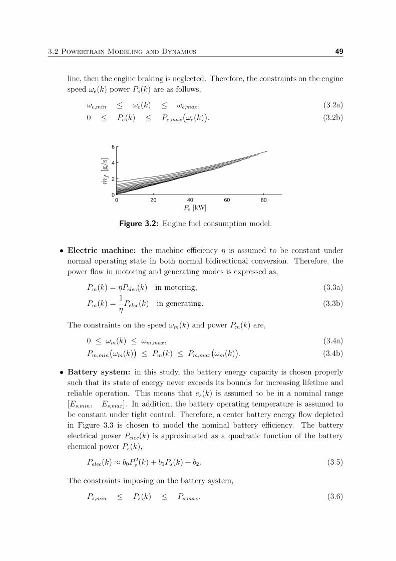
3.2 Powertrain Modeling and Dynamics 49
line, then the engine braking is neglected. Therefore, the constraints on the engine
speed ωe(k) power Pe(k) are as follows,
ωe,min ≤ ωe(k) ≤ ωe,max, (3.2a)
0 ≤ Pe(k) ≤ Pe,max(ωe(k)
). (3.2b)
0 20 40 60 800
2
4
6
Pe [kW]
mf[g/s]
Figure 3.2: Engine fuel consumption model.
• Electric machine: the machine efficiency η is assumed to be constant under
normal operating state in both normal bidirectional conversion. Therefore, the
power flow in motoring and generating modes is expressed as,
Pm(k) = ηPelec(k) in motoring, (3.3a)
Pm(k) =1
ηPelec(k) in generating. (3.3b)
The constraints on the speed ωm(k) and power Pm(k) are,
0 ≤ ωm(k) ≤ ωm,max, (3.4a)
Pm,min(ωm(k)
)≤ Pm(k) ≤ Pm,max
(ωm(k)
). (3.4b)
• Battery system: in this study, the battery energy capacity is chosen properly
such that its state of energy never exceeds its bounds for increasing lifetime and
reliable operation. This means that es(k) is assumed to be in a nominal range
[Es,min, Es,max]. In addition, the battery operating temperature is assumed to
be constant under tight control. Therefore, a center battery energy flow depicted
in Figure 3.3 is chosen to model the nominal battery efficiency. The battery
electrical power Pelec(k) is approximated as a quadratic function of the battery
chemical power Ps(k),
Pelec(k) ≈ b0P2s (k) + b1Ps(k) + b2. (3.5)
The constraints imposing on the battery system,
Ps,min ≤ Ps(k) ≤ Ps,max. (3.6)
50 3 Optimal Gear Shift Strategies for Hybrid Electric Vehicles
−6 −4 −2 0 2 4 6
−5
0
5
Ps [kW]
Pel
ec [
kW]
Figure 3.3: Battery efficiency model.
• Automated Manual Transmission (AMT): the transmission efficiency η is
assumed to be constant for all gears, the speed and torque relations in both side
of transmission when the clutch closed are,
ωe(k) = ωg(k) = ωw(k)rg(k), (3.7a)
Tw(k) = η rg(k) Tg(k) = η rg(k) Te(k). (3.7b)
wherein: ωw(k) is the wheel rotational speed; Tw(k) is the drive torque at the
wheels; Tg(k) is the transmission input torque; rg(k) denotes the gear ratio. The
final reduction gear ratio is merged into the transmission ratio for a simplification.
The constraints on the gear position of the 6-speed transmission are,
1 ≤ ng(k) ≤ 6. (3.8)
• Power flow model: the power flow equilibrium at the transmission input of the
powertrain is expressed as,
Pe(k) = Pg(k) + Pm(k). (3.9)
3.2.2 Powertrain System Dynamics
The powertrain system consists of the continuous battery state-of-energy es(k), and the
discrete gear position ng(k). Their dynamics are governed by the two corresponding
control variables Ps(k) and ug(k) as,
es(k + 1) = es(k) + Ps(k)∆t, (3.10)
ng(k + 1) = ng(k) + ug(k). (3.11)
Apparently, due to co-existence of the continuous and discrete variables, the powertrain
system is a hybrid dynamical system as well.
Vehicle longitudinal dynamics: the longitudinal motion of the vehicle in discrete
time domain is given by,
ωw(k + 1) = ωw(k) +1
Jv,eq
(Tw(k)− Fload(k)Rw
)∆t, (3.12)

3.3 Optimal Gear Shift Strategy without Start-Stop Functionality 51
where Fload is the resistance loads due to rolling and aerodynamic resistances; Jv,eq is
an equivalent vehicle inertia at the wheel,
Jv,eq =((Je + Jc + Jp)r
2g + Js
)r2d +mvR
2w,
Fload = crmvg cosα +mvg sinα +1
2ρaAfcdv
2,
and mv is the vehicle weight; Rw is the wheel radius; Je is the engine inertia; Jc is the
clutch inertia; Jp is the transmission primary inertia; Js is the transmission secondary
inertia; ρa is the air density; Af is the frontal area of vehicle; cd is the aerodynamic
drag coefficient; cr is the rolling friction coefficient; g is the gravity coefficient; v is the
vehicle speed; α is the slope of the road.
3.3 Optimal Gear Shift Strategy without Start-StopFunctionality
Initially, the start-stop functionality is assumed to be not available. The operating
points of the hybrid powertrain are governed by the power split between the engine
and electric machine, and the gear position. The power split is alternatively controlled
by the continuous engine power which varies in the boundary interval determined by
(3.2b), (3.4b), (3.6) and (3.9). Detail of the power split control is given in Section 3.3.2.
The gear position is controlled by the discrete gear shift command through the gear
shift dynamics expressed by (3.11). The discrete gear shift command ug(k) belongs to
the set {ug,min, · · · ,−1, 0, 1, · · · , ug,max}. Under the constraints (3.11) and (3.8), for a
6-speed AMT, [ug,min, ug,max] = [−5, 5].
From a control point of view, the bounds ug,min and ug,max have effect on the optimality.
However, defining the optimum bounds for the gear shift command ug(k) is out of the
scope of this study. For reasons of an acceptable driveability, the gear shift command
is chosen as,
ug(k) =
−1, downshift,
0, sustaining,
1, upshift,
(3.13)
to avoid a large variation of the engine speed under a certain shift at a certain time step
k. One gear upshift (ug(k) = 1) or downshift (ug(k) = −1) for each time step of one
second is reasonable, because the average shift time for an AMT is typically less than
one second.
Note that the gear shift event will lead to a change of the engine torque due to a changed
engine speed, which may cost additional fuel affecting the optimal control solution. In

52 3 Optimal Gear Shift Strategies for Hybrid Electric Vehicles
this study, this phenomenon is ignored as well. This effect will be investigated in
Chapter 6.
The optimization problem is formulated as follows.
Problem 3.1. Given a priori drive cycle v(k) with a time length of N , implying that
the vehicle longitudinal dynamics (3.12) is deterministic, find an optimal control law
u∗(k) =[P ∗s (k), u∗g(k)
], that minimize the cost function of fuel consumption over the
entire drive cycle, defined as,
J =N−1∑k=0
mf
(Pe(k), ωe(k), k
)∆t , (3.14)
subject to the constraints (3.12) - (3.9) and
es(N) = es(0) , (3.15)
ng(N) = ng(0) . (3.16)
In the next section, two optimization solvers for Problem 3.1 will be presented. The
first one is based on DP. The second one is based on a combination of DP and PMP.
3.3.1 Dynamic Programming
DP [11, 14] is well known as a powerful numerical method on optimal state feedback
control to solve a non-linear, non-convex optimization problem with constraints while
obtaining a globally optimal time-variant solution. To apply DP to Problem 3.1, we
need,
• to grid the state variables x(k) =[es(k), ng(k)
];
• to grid the corresponding control variables u(k) =[Ps(k), ug(k)
];
• to calculate the instantaneous cost mf
(Pe(k), ωe(k), k
)∆t for the whole drive cycle;
The states x(k) ∈ X(k), the control inputs u(k) ∈ U(k) are discrete variables both in
time (index k) and value. Exactly, the subset U(k) depends on the states x(k), i.e.
u(k) ∈ U(x(k)
). Then, the optimal cost-to-go function is defined backwards as the
following steps.
Step k = N :
J ∗N = 0; (3.17)

3.3 Optimal Gear Shift Strategy without Start-Stop Functionality 53
Step k, 0 ≤ k < N :
J ∗k(x(k)
)= min
u(k)∈U(x(k))[mf
(Pe(k), ωe(k), k
)∆t+ J ∗k+1
(x(k + 1)
)]; (3.18)
Solving the above procedure backward until k = 0, the optimal solution u∗(k) is obtained
correspondingly with a specific end constraint on x(N).
3.3.2 Dynamic Programming-Pontryagin’s Minimum Principle
It is noticed that solving Problem 3.1 by discretizing the continuous variables, se(k)
and Ps(k), and using deterministic DP can lead to a computational burden due to the
‘curse of dimensionality’. Applying optimal control theory (PMP method) to Problem
3.1 is possible if a continuously variable ratio model for the AMT can be obtained, such
that the cost function is differentiable with respect to the transmission ratio. Then, the
continuous optimal solution will be derived in a fast computational manner. However,
rounding off the continuous optimal ratio to the corresponding gear ratio for the AMT
will definitely lead to a sub-optimality. Furthermore, respecting the constraints on the
ratio variation speed is another factor affecting the rounded-off solution. Apparently,
the tradeoff between optimality, accuracy and the computational efficiency is seen as
one of the main challenges for the design of a gear shift control algorithm for HEVs.
Respecting the discrete nature of ratio of the AMT, and taking into account the ad-
vantages of the DP and PMP, a control algorithm based on a combination of DP and
PMP is proposed for the gear shift problem of HEVs. The globally optimal solutions
of P ∗s (k) (or P ∗e (k) alternatively) and u∗g(k) are obtained and the computational time
is significantly reduced. The control method consists of: deriving the optimal engine
power based on the PMP in the inner loop, meanwhile the gear position dynamics,
under the mixed-constraints (3.8) and (3.13) is optimally controlled by using DP in the
outer loop. The structure of the DP-PMP control algorithm is illustrated in Figure 3.4.
The optimal control problem is formulated and solved in the form of a power flow based
model for consistency. This algorithm is presented next.
PMP for an optimal power split
Assume at a certain time step k, given the vehicle speed v(k), the required power Pw(k)
at the wheels is computed from (3.12). With a given admissible gear position ng(k),
assume that the constraints on engine speed and electric machine speed, (3.2a) and
(3.4a), are satisfied and Pw(k) can be produced by the powertrain, i.e., by both the
engine and electric machine. The lower and upper bounds of the electric machine power
and battery power can be incorporated with the bounds of engine power to create the

54 3 Optimal Gear Shift Strategies for Hybrid Electric Vehicles
Figure 3.4: The DP-PMP control algorithm.
new bounds for the control variable Pe(k),
P′
e,min(k) ≤ Pe(k) ≤ P′
e,max(k) . (3.19)
The new lower bound and upper bound of the engine power are defined as follows,
P′
e,min(k) = max{0; Pg(k) + PEM,min(k)} , (3.20)
P′
e,max(k) = min{Pe,max(k); Pg(k) + PEM,max(k)} , (3.21)
wherein:
PEM,min(k) = max{Pm,min(k); η
(b0P
2s,min + b1Ps,min + b2
)}, (3.22)
PEM,max(k) = min{ηPm,max(k);
(b0P
2s,max + b1Ps,max + b2
)}. (3.23)
For compact notation, let us denote the engine fuel rate Fr(Pe(k), k
):=
mf
(Pe(k), ωe(k), k
)and the chemical battery power Ps
(Pe(k), k
):= Ps(k) as functions
of the engine power.
The optimal control problem is reformulated as follows.
Problem 3.2. Given a prior drive cycle with a time length N , with a given admissible
gear sequence ng(k) along the drive cycle, find an optimal engine power P ∗e (k) that
minimizes the cost function J1 of fuel consumption over the entire drive cycle, defined

3.3 Optimal Gear Shift Strategy without Start-Stop Functionality 55
as,
J1 =N−1∑k=0
Fr(Pe(k), k
)∆t, (3.24)
subject to constraints:
es(k + 1) = es(k) + Ps(Pe(k), k
)∆t,
P′
e,min(k) ≤ Pe(k) ≤ P′
e,max(k).
In this study, the upper and lower bounds of state variable es(k) are ignored by assuming
that the battery capacity is chosen properly such that it never exceeds its bounds. The
Lagrange multiplier is used to take into account the dynamics of battery. This leads to
the Hamiltonian function (3.25) at each time step needs to be minimized, see Appendix
A for the proof.
H(Pe(k), λopt, k
)=[
Fr(Pe(k), k
)+ λoptPs
(Pe(k), k
)]∆t. (3.25)
From the model approximations of engine fuel rate and battery efficiency model,
Fr(Pe(k), k
)and Ps
(Pe(k), k
)can be approximated as affine piecewise second-order
functions of engine power at a certain engine speed. Therefore, if the constant opti-
mal Lagrange multiplier λopt is known, the globally instantaneous optimal engine power
P ∗e (k) can be obtained analytically. Therefore, the globally instantaneous equivalent
optimal cost value is defined correspondingly by
Ceq(k) =[
Fr(P ∗e (k), k
)+ λoptPs
(P ∗e (k), k
)]. (3.26)
However, it should be noticed that for the gear shift control problem with constraints
on the battery state-of-energy es(k), a derivation of the optimal solution can be found
in Appendix B. It is observed that when the battery state-of-energy reaches its bounds,
then the Lagrange multiplier changes its value. Between the two consecutive points of
reaching the bounds of the state of energy, the Lagrange multiplier is kept constant.
DP for an optimal gear shift strategy
The PMP proposed in Section 3.3.2 solves only the globally optimal power split along a
drive cycle with any certain gear shift sequence by choosing a proper Lagrange multiplier
λopt, satisfying the constraint (3.15) on the battery energy at the terminal time. This
means that the optimal solution of the power split is independent with the gear position
if λopt is known in advance. Therefore the gear shift sequence can be optimized along
the drive cycle to further improve the fuel economy. Due to the characteristic of discrete
ratio of the AMT, a DP-based control algorithm applied to define the optimal gear shift
strategy is presented as follows.
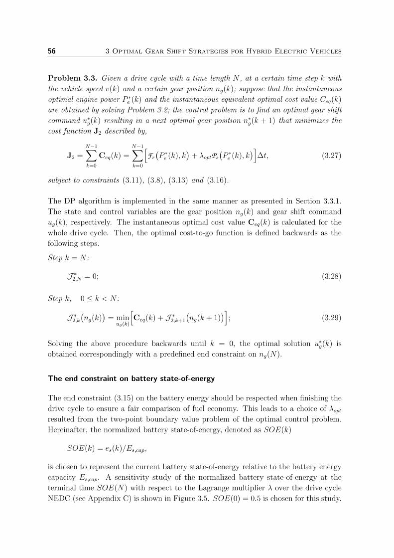
56 3 Optimal Gear Shift Strategies for Hybrid Electric Vehicles
Problem 3.3. Given a drive cycle with a time length N , at a certain time step k with
the vehicle speed v(k) and a certain gear position ng(k); suppose that the instantaneous
optimal engine power P ∗e (k) and the instantaneous equivalent optimal cost value Ceq(k)
are obtained by solving Problem 3.2; the control problem is to find an optimal gear shift
command u∗g(k) resulting in a next optimal gear position n∗g(k + 1) that minimizes the
cost function J2 described by,
J2 =N−1∑k=0
Ceq(k) =N−1∑k=0
[Fr(P ∗e (k), k
)+ λoptPs
(P ∗e (k), k
)]∆t, (3.27)
subject to constraints (3.11), (3.8), (3.13) and (3.16).
The DP algorithm is implemented in the same manner as presented in Section 3.3.1.
The state and control variables are the gear position ng(k) and gear shift command
ug(k), respectively. The instantaneous optimal cost value Ceq(k) is calculated for the
whole drive cycle. Then, the optimal cost-to-go function is defined backwards as the
following steps.
Step k = N :
J ∗2,N = 0; (3.28)
Step k, 0 ≤ k < N :
J ∗2,k(ng(k)
)= min
ug(k)
[Ceq(k) + J ∗2,k+1
(ng(k + 1)
)]; (3.29)
Solving the above procedure backwards until k = 0, the optimal solution u∗g(k) is
obtained correspondingly with a predefined end constraint on ng(N).
The end constraint on battery state-of-energy
The end constraint (3.15) on the battery energy should be respected when finishing the
drive cycle to ensure a fair comparison of fuel economy. This leads to a choice of λoptresulted from the two-point boundary value problem of the optimal control problem.
Hereinafter, the normalized battery state-of-energy, denoted as SOE(k)
SOE(k) = es(k)/Es,cap,
is chosen to represent the current battery state-of-energy relative to the battery energy
capacity Es,cap. A sensitivity study of the normalized battery state-of-energy at the
terminal time SOE(N) with respect to the Lagrange multiplier λ over the drive cycle
NEDC (see Appendix C) is shown in Figure 3.5. SOE(0) = 0.5 is chosen for this study.

3.4 Optimal Gear Shift Strategy with Start-Stop Functionality 57
−5.5 −5 −4.5 −4 −3.5 −3
x 10−5
0
0.2
0.4
0.6
0.8
1
SOE(N
)
λ [g/J]
λopt
Figure 3.5: SOE(N) vs. λ of the HEV without start-stop functionality.
We can see that SOE(N) monotonously decreases with λ. At λ > λopt, the powertrain
tends to use more electrical power that leads to a battery discharge. Vice versa, at
λ < λopt, the vehicle tends to generate electrical power that leads to a battery charge.
Therefore a search method (bisection search method) is utilized in this study to find the
optimal Lagrange multiplier λopt to satisfy the end constraint (3.15) at SOE(N) = 0.5.
The search condition is stopped at |∆SOE| = |SOE(N) − SOE(0)| < ξ with ξ is a
predefined positive small number.
3.4 Optimal Gear Shift Strategy with Start-Stop Func-tionality
One of the advantages of HEVs is the availability of the start-stop functionality to
further reduce the fuel consumption by shutting down the engine whenever feasible.
The start-stop functionality describes the engine on-off state by a state variable se(k),
se(k) =
{1, engine on,
0, engine off.(3.30)
with the state dynamics and the constraints on the control variable are correspondingly
given by,
se(k + 1) = se(k) + use(k), (3.31)
use(k) =
{[0, 1] if se(k) = 0,
[−1, 0] if se(k) = 1.(3.32)
When the engine is on, the fuel rate at a certain engine speed is defined by (3.1) and
the engine power is larger than zero. When engine is off, the fuel rate is zero and the
engine power is zero. Therefore the fuel rate model of the engine at a certain engine
speed ωe(k) is expressed as
mf
(Pe(k), k
)=
{a0P
2e (k) + a1Pe(k) + a2, if se(k) = 1,
0, if se(k) = 0,(3.33)
58 3 Optimal Gear Shift Strategies for Hybrid Electric Vehicles
Figure 3.6: Cost functional L(Pe)
−6.8 −6.6 −6.4 −6.2 −6 −5.8 −5.6 −5.4 −5.2 −5
x 10−5
0
0.2
0.4
0.6
0.8
1
SOE(N
)
λ [g/J]
λs
Figure 3.7: SOE(N) vs. λ of the HEV with start-stop functionality.
or equivalently
mf
(Pe(k), k
)=
{a0P
2e (k) + a1Pe(k) + a2, if 0 < Pe(k) ≤ Pe,max(k),
0, if Pe(k) = 0,(3.34)
which clearly shows that there is a discontinuous point of fuel rate model at Pe(k) = 0.
3.4.1 Dynamic Programming
Designing the EMS to optimize the gear shift command for the HEV with the start-
stop functionality can be done by using the DP method despite the fact that intensively
computational demand is required due to the presence of one more state variable se(k).
The dynamic system consists of three state variables, x(k) =[se(k), es(k), ng(k)
],
and three corresponding control variables u(k) =[use(k), Ps(k), ug(k)
]. The same
procedure as in Section 3.3.1 is used to implement the DP-based control algorithm in
simulation.
3.4.2 Dynamic Programming-Pontryagin’s Minimum Principle
The computational burden due to the curse of dimensionality of DP can be reduced
significantly by using the DP-PMP control algorithm as presented in Section 3.3.2.
Utilizing the PMP method in designing the EMS is followed by solving the two-point

3.4 Optimal Gear Shift Strategy with Start-Stop Functionality 59
boundary value problem to find an initial value of the Lagrange multiplier such that the
end constraint of the battery state of energy is respected. This issue is analyzed next.
At a certain time step k, assuming that the power demand from the wheels is Pw,
then the admissible range of engine power can be defined as 0 ≤ Pe ≤ Pe,max by using
(3.20)-(3.21). Let L(Pe)
denote the augmented Lagrange cost functional as
L(Pe)
=
{Fr(Pe)
+ λPs(Pe)
if 0 < Pe ≤ Pe,max,
λPs(Pe)
if Pe = 0,(3.35)
which is discontinuous at Pe = 0 due to the characteristic of fuel rate model as described
by (3.34). Apparently, L(Pe)
is non-differentiable at Pe = 0. However, the PMP method
is still applicable to define the global optimal solution regardless the discontinuity of
the cost functional. Figure 3.6 gives a demonstration for the augmented cost functional
L(Pe)
at a certain λ. There are two local minima for the cost functional L(Pe): one is
at Pe,min1 = 0 and the other is assumed at Pe,min2 ∈ (0, Pe,max]. The minimum one is
chosen by comparing the L(Pe,min1
)and L
(Pe,min2
). It can be either at Pe,min1 = 0 or
at Pe,min2 such that the augmented Lagrange cost functional is global minimum.
Due to the discontinuous characteristic, the optimal solution depends on the value of
Lagrange multiplier λ. There exists a switching point of Lagrange multiplier denoted
as λs whereby L(Pe,min1
)= L
(Pe,min2
)occurs. In other words, such a λs does not exist
with respect to the optimal solution. Therefore, for a variation of λ around the point
λs, there is a jump in optimal solution of Pe by an amount of Pe,min2 − Pe,min1, thus
Pe,min2s. As a result, the same consequence holds for the optimal solution of the battery
power Ps which yields a jump in the normalized battery energy SOE.
Figure 3.7 shows the sensitivity of the normalized battery state-of-energy at the terminal
time SOE(N) with respect to the λ over the NEDC. The SOE(N) is discontinuous at
λs. Therefore, a constant optimal Lagrange multiplier λopt does not exist if the end
constraint on the normalized battery state-of-energy SOE(N) = 0.5 is required at the
terminal time.
The DP-PMP control algorithm is used in the same manner as described in Section
3.3.2 for the gear shift control problem. The PMP is used in the inner loop to define
the instantaneous optimal power split. The DP is used in the outer loop to define the
optimal gear position and the engine on-off state from the beginning until the end of
the drive cycle. Due to the non-existence of a constant Lagrange multiplier, to respect
the end constraint on battery state-of-energy (3.15), the costate λ(k) is controlled by
using an integral regulator (I controller) as in (3.36). This leads to the fact that the
obtained solution is not globally optimal.
λ(k + 1) = λ(k) +KI
(es(k)− es(0)
). (3.36)

60 3 Optimal Gear Shift Strategies for Hybrid Electric Vehicles
3.5 Simulation Results and Discussions
0 200 400 600 800 1000 12000
50
100
150
Spe
ed [k
m/h
]
0 200 400 600 800 1000 12000
2
4
6
Time [s]
Gea
r [−
]
Figure 3.8: NEDC cycle (top) and a prescribed gear shift schedule (bottom).
0 200 400 600 800 1000 12000
2
4
6
n g [−]
0 200 400 600 800 1000 1200
0
20
40
Pe,
Ps [
kW]
Ps
Pe
0 200 400 600 800 1000 12000.30.40.50.60.7
SO
E [−
]
Time [s]
Figure 3.9: Test 1: DP algorithm for only the power split optimization.
3.5.1 Baseline Vehicles
The drive cycle NEDC is chosen for simulation, see Figure 3.8. This drive cycle is a
standardized emission test cycle in Europe. There is a prescribed gear shift schedule
accompanied along with this cycle to signal the gear shift for vehicles with manual
transmission [42].

3.5 Simulation Results and Discussions 61
0 200 400 600 800 1000 12000
2
4
6
n g [−]
0 200 400 600 800 1000 1200
0
20
40
Pe,
Ps [
kW]
P
e
Ps
0 200 400 600 800 1000 12000.30.40.50.60.7
SO
E [−
]
Time [s]
Figure 3.10: Test 2: DP algorithm for the power split and gear shift optimiza-tion.
0 200 400 600 800 1000 12000
2
4
6
n g [−]
0 200 400 600 800 1000 1200
0
20
40
Pe,
Ps [
kW]
P
e
Ps
0 200 400 600 800 1000 12000.30.40.50.60.7
SO
E [−
]
Time [s]
Figure 3.11: Test 3: DP-PMP algorithm for the power split and gear shiftoptimization.
One of the purposes of this study is to evaluate the contribution of the gear shift strategy
to a fuel economy improvement of HEVs. Therefore, two baseline vehicles are defined:
1) a baseline-conventional vehicle with the same parameters of the hybrid vehicle except
for the secondary power source; 2) a baseline-HEV is simulated whereby the EMS is
designed by DP to optimize only the power split. The prescribed gear shift schedule

62 3 Optimal Gear Shift Strategies for Hybrid Electric Vehicles
0 200 400 600 800 1000 12000
2
4
6
n g [−]
0 200 400 600 800 1000 12000.3
0.4
0.5
0.6
0.7
SO
E [−
]
Time [s]
DP
DP−PMP
Figure 3.12: Comparison of Tests 2 and 3.
0 200 400 600 800 1000 12000246
n g [−]
0 200 400 600 800 1000 1200−1
012
s e [−]
0 200 400 600 800 1000 1200
0
20
40
Pe,
Ps [
kW]
Ps
Pe
0 200 400 600 800 1000 12000.30.40.50.60.7
SO
E [−
]
Time [s]
Figure 3.13: Test 4: DP algorithm for the power split, gear shift and start-stopfunctionality optimization.
(accompanied along with drive cycle) is used to shift gears in both baseline vehicles. The
start-stop functionality is assumed to be not available for the baseline-HEV. This is only
theoretical because the start-stop functionality is always available in HEVs. Simulation
results of the baseline-HEV are shown in Figure 3.9. The battery state-of-energy at
the end of drive cycle satisfies its end constraint. The fuel economy improvement is of
12.2% compared to the baseline-conventional vehicle, see Table 3.2.

3.5 Simulation Results and Discussions 63
0 200 400 600 800 1000 12000246
n g [−]
0 200 400 600 800 1000 1200−1
012
s e [−]
0 200 400 600 800 1000 1200
0
20
40
Pe,
Ps [
kW]
Ps
Pe
0 200 400 600 800 1000 12000.30.40.50.60.7
SO
E [−
]
Time [s]
Figure 3.14: Test 5: DP-PMP algorithm for the power split, gear shift andstart-stop functionality optimization.
0 200 400 600 800 1000 1200
−6
−5.995
−5.99
x 10−5
Time [s]
λ[g/J
]
Figure 3.15: λ(k) of the DP-PMP algorithm for Test 5.
3.5.2 HEV without the Start-Stop Functionality
Simulation results of two algorithms, the DP and DP-PMP, are illustrated in Figures
3.10 and 3.11, respectively. The gear shift patterns of both approaches are totally
different from the prescribed gear shift schedule. The proposed control algorithms
allow the vehicle to shift to higher gear and earlier which contribute to fuel economy
improvement. Figure 3.12 shows a comparison of the gear position and the battery
state-of-energy of both approaches. The obtained optimal solutions are almost the
same. The state of energy in both cases satisfies the end constraint to ensure the fair
comparisons of fuel economy.
From Table 3.2, we see that fuel economy for both approaches are improved up to 30%
relatively to the case of the baseline conventional vehicle. By optimally shifting the gear,
potential fuel savings can be obtained up to 20.3% compared to the case of baseline-
HEV. There is a small difference in the fuel economy between these two methods. This

64 3 Optimal Gear Shift Strategies for Hybrid Electric Vehicles
is due to the numerical errors of gridding the control variables in the DP algorithm.
Meanwhile, the DP-PMP algorithm improves the computation efficiency significantly
by a factor of 171 compared with the DP algorithm.
It appears that an optimal gear shift strategy for the hybrid vehicle can improve the
fuel economy substantially, up to 20.3% and 30% compared to the baseline-HEV and
baseline conventional vehicle, respectively. The optimal gear shift strategy owns its fuel
efficiency to: i) much motor assist during acceleration, and ii) lowering the engine speed
during constant speed phase. Furthermore, it should be emphasized that the baseline
gear shift strategy (the prescribed gear shift schedule) is less efficient due to its late-
upshift strategy. During acceleration or cruising (constant speed), the optimal gear shift
strategy triggers the upshift to occur earlier, more frequent and to higher values, which
will allow the engine to operate at low speed region for more fuel efficient. Another
issue contributing to the significant values of fuel economy improvement is a chosen
minimum engine speed. In this study, the minimum engine speed is set at 800[rpm] to
provide theoretical value of fuel saving.
In real-life driving, the minimum engine speed for passenger cars during driving can be
somewhere between 800[rpm]-1200[rpm], which will result in a less fuel saving compared
to the obtained theoretical value. For example, in previous experimental research work
for an AMT conventional vehicle [99], it showed that 11.2% fuel economy improvement
on the ECE cycle (urban part of NEDC) can be realized by using an optimized shifting
strategy. The 11.2% fuel economy improvement is compared with the baseline gear shift
strategy (the prescribed gear shift schedule).
Table 3.2: Comparison of simulation results on NEDC.
Test AlgorithmsFuel Improvement Time[g] [%] [s]2
0 Baseline-conventional vehicle 468.7 - 1
1Baseline-HEV: optimizing only thepower split by DP algorithm
411.7 12.2 - 460
2HEV: optimizing the power split andgear shift by DP algorithm
328.0 30.0 20.3 1540
3HEV: optimizing the power split andgear shift by DP-PMP algorithm
328.1 30.0 20.3 9
4HEV: optimizing the power split, gearshift and start-stop functionality by DPalgorithm
300.2 35.9 27.1 3964
5HEV: optimizing the power split, gearshift and start-stop functionality byDP-PMP algorithm
301.3 35.7 26.8 9
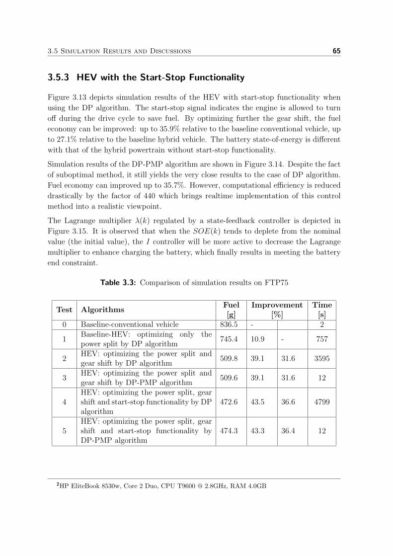
3.5 Simulation Results and Discussions 65
3.5.3 HEV with the Start-Stop Functionality
Figure 3.13 depicts simulation results of the HEV with start-stop functionality when
using the DP algorithm. The start-stop signal indicates the engine is allowed to turn
off during the drive cycle to save fuel. By optimizing further the gear shift, the fuel
economy can be improved: up to 35.9% relative to the baseline conventional vehicle, up
to 27.1% relative to the baseline hybrid vehicle. The battery state-of-energy is different
with that of the hybrid powertrain without start-stop functionality.
Simulation results of the DP-PMP algorithm are shown in Figure 3.14. Despite the fact
of suboptimal method, it still yields the very close results to the case of DP algorithm.
Fuel economy can improved up to 35.7%. However, computational efficiency is reduced
drastically by the factor of 440 which brings realtime implementation of this control
method into a realistic viewpoint.
The Lagrange multiplier λ(k) regulated by a state-feedback controller is depicted in
Figure 3.15. It is observed that when the SOE(k) tends to deplete from the nominal
value (the initial value), the I controller will be more active to decrease the Lagrange
multiplier to enhance charging the battery, which finally results in meeting the battery
end constraint.
Table 3.3: Comparison of simulation results on FTP75
Test AlgorithmsFuel Improvement Time[g] [%] [s]
0 Baseline-conventional vehicle 836.5 - 2
1Baseline-HEV: optimizing only thepower split by DP algorithm
745.4 10.9 - 757
2HEV: optimizing the power split andgear shift by DP algorithm
509.8 39.1 31.6 3595
3HEV: optimizing the power split andgear shift by DP-PMP algorithm
509.6 39.1 31.6 12
4HEV: optimizing the power split, gearshift and start-stop functionality by DPalgorithm
472.6 43.5 36.6 4799
5HEV: optimizing the power split, gearshift and start-stop functionality byDP-PMP algorithm
474.3 43.3 36.4 12
2HP EliteBook 8530w, Core 2 Duo, CPU T9600 @ 2.8GHz, RAM 4.0GB

66 3 Optimal Gear Shift Strategies for Hybrid Electric Vehicles
3.5.4 Simulation Results on FTP75
FTP75, representing a more realistic drive cycle, is also chosen for testing on simulation
platform. The results are shown in Table 3.3. It can be seen from Tests 2 and 4 that,
by optimally shifting gears, potential fuel savings can be achieved up to 31.6% and
36.6% (compared with the baseline HEV) for the HEV without and with the start-
stop functionality, respectively. From Tests 3 and 5, it also shows that the DP-PMP
algorithm improves the same fuel economy with the DP algorithm. Meanwhile the DP-
PMP algorithm reduces computational burden significantly by the factors of 300 and
415 compared with the DP algorithm for the HEV without and with the start-stop
functionality, respectively.
3.6 Conclusions
This chapter presented a control algorithm based on a combination of DP and PMP
for HEVs to further optimize the gear shift command. The proposed control algorithm
reduces the computation time significantly compared with the DP algorithm. It shows
that by further optimally controlling the gear shift command, the potential fuel saving
can be increased significantly.
Applying the DP-PMP control algorithm for the HEV was addressed explicitly in terms
of the start-stop functionality. For the hybrid powertrain without the start-stop func-
tionality, it is found that a unique constant Lagrange multiplier exists such that the end
constraint of the battery state-of-energy is respected, and the globally optimal solution
is guaranteed. For the hybrid powertrain with the start-stop functionality, the constant
Lagrange multiplier for the optimal control problem does not always exist. Therefore,
the obtained results of the proposed control algorithm are suboptimal, despite the fact
that they are very close to the globally optimal results obtained from the DP algorithm.
The DP-PMP control algorithm is considered as a novel control algorithm for the op-
timal gear shift problem of HEVs. From an engineering point of view, the DP-PMP
algorithm can be considered as a globally optimal method applied for HEVs. The algo-
rithm is executed fast enough such that it can be seen as a potential candidate applied
in a realtime implementable control algorithm, such as a model predictive control.

Chapter 4
Gear Shift Map Design Methodology1
Abstract - In this chapter, a design methodology is developed to build the gear shift map forautomotive transmissions used in conventional and hybrid electric vehicles. The methodologyutilizes an optimal gear shift strategy to derive the optimal gear shift patterns over a widerange of driving profiles. Then, statistical theory is applied to analyze the obtained gear shiftpatterns towards a gear shift map. The designed gear shift map improves the fuel economyand driveability. It is consistent, robust to shift busyness, and realtime implementable. Thedesign process is flexible and time-efficient such that an applicability to various powertrainsystems configured with discrete ratio transmissions is possible. Validation on a test vehicleproves the effectiveness of the design methodology.
4.1 Introduction
Gear shift strategy has been proved to be crucial for vehicles to improve the fuel econ-
omy, driveability, etc. A supervisory control algorithm, including an optimal gear shift
strategy, based on optimal control algorithms, such as Dynamic Programming (DP),
Pontryagin’s Minimum Principle (PMP), Dynamic Programming-Pontryagin’s Mini-
mum Principle (DP-PMP), Model Predictive Control (MPC), etc., can guarantee an
optimal operation of the powertrain system over a priori drive cycle. Therefore, the
obtained gear shift strategy is not optimal, consistent and robust for other drive cycles.
Furthermore, disturbances involved with the powertrain system, e.g. driving conditions
and driver behaviors, etc., are not considered and addressed in the algorithm, thus
making the corresponding gear shift strategy hard to be reliably realtime implemented.
Hence, a gear shift strategy based on a static shift map has been widely adopted as a
standard solution for shifting gears online. A static shift map defines the shift points
based on the current vehicle speed and the engine torque (sensing via the acceleration
1This chapter has been prepared for a journal publication in the form as: V. Ngo, T. Hofman, M.Steinbuch, A. Serrarens. Gear Shift Map Design Methodology for Automotive Transmissions. 2012.
67

68 4 Gear Shift Map Design Methodology
pedal position, throttle opening, etc.). Design of a gear shift map is traditionally based
on know-how, experience of the calibration engineers and tunings in heuristic maner.
Hence, the gear shift map is consistent and robust after a huge trial-and-error effort.
This so-called experience-based gear shift strategy does not exploit the inherent po-
tential of the powertrain system sufficiently to improve the overall performance of the
vehicle, and thus coming with a lower confidence on optimality with respect to the
fuel economy and driveability. In this research, a gear shift map design methodology
is developed for discrete ratio transmissions used in road vehicles. The methodology
takes advantages of: i) the optimal-based gear shift strategy, and ii) the statistical
theory, to build an optimized gear shift map, which is consistent, robust and realtime
implementable.
In literature, there is a small number of studies addressing about the gear shift map
design methods for conventional vehicles. Besides an essential requirement on fuel
economy improvement, ensuring an acceptable driveability level is also an important
index for the design of a map-based gear shift strategy. The study in [168] analyzes
the influence of different vehicle weights on the gear shift point control. In order to
ensure the driveability, the authors adopt a policy of maintaining the same acceleration
level after shifting, which requires an unchanged throttle position right after shifting.
The most fuel economy points are derived to create a gear shift map. Also focusing
on the driveability, the authors in [55] present an approach based on DP to define
an optimal gear shift sequence. The optimization criterion aims at minimizing the
acceleration time of the vehicle. Meanwhile the authors in [66] also put the driveability
into consideration when designing a gear shift map for an automatic transmission. An
optimization problem for the gear shift and throttle opening strategies is formulated
on a prescribed launch profile with a constant engine power, representing a driveability
constraint. DP is used to obtain the optimal results at different constant engine power
levels, which are then combined to form the gear shift and throttle opening maps. These
two maps will govern the operation of the integrated powertrain. The authors claim
an improved fuel economy for the designed gear shift map meanwhile still meeting a
sufficient driveability level.
Regarding Hybrid Electric Vehicles (HEVs), where a certain driveability level can be
satisfied by an assistance from the secondary power source, the gear shift strategy in
general can aim at further improving the fuel economy. However, there is not much
published research dedicating on the design of a map-based gear shift strategy for dis-
crete ratio transmissions. Due to the availability of the secondary power source, the
gear shift map for HEVs should be composed from the different gear shift strategies in
different driving modes, as discussed in [78]. However that paper does not describe the
design of such a gear shift strategy. In [157], the authors propose a method to design
a gear shift map for an Automated Manual Transmission (AMT). A gear shift problem
is formulated and solved by using static programming to derive the most fuel-economic

4.1 Introduction 69
shift points corresponding with a prescribed constant acceleration profile. The method
takes the vehicle speed, engine torque (or mechanical braking torque), and motor torque
into account to form a three-dimension gear shift map, which is designed correspond-
ingly with the driving modes. The authors claim a fuel economy improvement compared
to a traditional shift map of a conventional vehicle. However the optimization prob-
lem is not well formulated in terms of the system constraints to guarantee optimality.
Furthermore, an optimization-based gear shift map extraction for HEVs can be found
in [75, 83]. The authors utilize DP to design an optimal Energy Management Strategy
(EMS) to derive the optimal gear shift solution. Then, a near optimal map-based gear
shift strategy is built by observation and extraction. An improvement of the driveability
for the designed gear shift map compared to an original, intuitive algorithm-based shift
map is claimed by the authors.
Through literature review, it is observed that the gear shift map design methods pro-
posed in the published studies have not taken a wide range of driving scenarios, i.e. the
driving behavior dynamics and road dynamics, into account. For conventional vehicles,
the driveability is not systematically addressed in the gear shift map due to lack of a
driveability-optimal gear shift strategy design method. For HEVs, coupling among the
operating modes and the resulted dominant gear shift pattern(s) have not been analyzed
in order to achieve an overall, consistent, robust and optimized gear shift map over a
wide range of driving scenarios. Furthermore, there is lack of an approach to properly
analyze the optimal gear shift data towards extracting the representative optimal gear
shift lines of the gear shift map. In this study, a gear shift map design methodology
for discrete ratio transmissions used in conventional and hybrid electric vehicles is de-
veloped. Aiming at designing a gear shift map improving both the fuel economy and
driveability, the methodology utilizes an optimal gear shift strategy to derive the opti-
mal gear shift patterns over a wide range of driving profiles. Statistical theory is then
applied to analyse the optimal gear shift patterns, towards extracting the optimal gear
shift lines of the gear shift map. Robustness and consistency of the gear shift map are
considered in the step of statistical analysis and shifting line extraction. The design
methodology is described and demonstrated by applying for the prototype conventional
and hybrid electric vehicles. Experimental validation on a test conventional vehicle, dif-
ferent from the prototype vehicle, is performed to verify the applicability and flexibility
of the design method.
This chapter is organized as follows. The powertrain modeling and dynamics are given
in Section 4.2. An analysis of gear shift contribution to the fuel economy of conventional
and hybrid electric vehicles is given in Section 4.3. Gear shift map design methodology
applied for conventional vehicles is described in Section 4.4. Meanwhile application
of the gear shift map design methodology for HEVs is discussed in Section 4.5. An
experimental validation of the design methodology on a test conventional vehicle is
presented in Section 4.6. And finally, conclusions are given in Section 4.7.

70 4 Gear Shift Map Design Methodology
4.2 Powertrain Modeling and Dynamics
4.2.1 Powertrain Model
The hybrid powertrain topology is shown in Figure 4.1. This study focuses on both
conventional and hybrid electric vehicle, so a conventional powertrain topology can be
realized by removing or deactivating the battery, inverter and electric machine from the
hybrid driveline. The main parameters of the powertrain components are given in Table
4.1.
Figure 4.1: The hybrid powertrain topology, (AMT: Automated Manual Trans-mission; M: Electric machine).
Table 4.1: Specifications of the prototype vehicle.
Item Description/Quantity
Enginediesel type,maximum torque of 200Nm,maximum power of 68kW.
Electric machinemaximum torque of 40Nm,maximum power of 6kW.
Battery lithium-ion; capacity of 6Ah, 110V.
Transmission6-speed automated manual transmission,rg = [3.817, 2.053, 1.302, 0.959, 0.744, 0.614].
Vehicle mass 1320kg.
Aiming at designing an EMS, the quasi static modeling approach is used to model
the main powertrain components. Hence, a time step ∆t of one second is chosen to
simulate the powertrain system, thus ignoring the system dynamics faster than 1Hz [42].
The clutch is modeled as a boolean switch to connect and to disconnect the engine

4.2 Powertrain Modeling and Dynamics 71
immediately to and from the driveline. Its dynamics and limited power losses during a
gear shift or an engine start are ignored. Notice of the slippage loss of clutch at vehicle
launch is also not taken into account. However, analysis of the effect of these losses to
the control strategy can be found in Chapter 6.
• Start-stop system: the start-stop system can be modeled by a decision variable
se(k) to control the engine on-off state.
se(k) =
{1 if engine on,
0 if engine off.(4.1)
• Engine: for a certain engine speed ωe(k), the fuel mass flow mf (k) is modeled
as an affine piece-wise second order function of the engine power, as expressed in
(4.2),
mf (k) ≈(a0(k)P 2
e (k) + a1(k)Pe(k) + a2(k))se(k). (4.2)
in which the coefficients a0(k), a1(k) and a2(k) are functions of the engine speed.
When the engine is off, no fuel is consumed. If assume during braking, the engine is
switched off and decoupled from the driveline, then the engine braking is neglected.
Therefore, the constraints on the speed ωe(k) and the power Pe(k) are as follows,
ωe,min ≤ ωe(k) ≤ ωe,max, (4.3a)
0 ≤ Pe(k) ≤ Pe,max(ωe(k)
). (4.3b)
• Electric machine: the machine efficiency η is assumed to be constant in a normal
operating state. Therefore, the power flow in motoring and generating modes is
expressed as,
Pm(k) = ηPelec(k) in motoring, (4.4a)
Pm(k) =1
ηPelec(k) in generating. (4.4b)
The constraints on the speed ωm(k) and the power Pm(k) are,
0 ≤ ωm(k) ≤ ωm,max, (4.5a)
Pm,min(ωm(k)
)≤ Pm(k) ≤ Pm,max
(ωm(k)
). (4.5b)
• Battery system: the electrical power Pelec(k) is modeled as a quadratic function
of the storage power Ps(k),
Pelec(k) ≈ b0P2s (k) + b1Ps(k) + b2. (4.6)

72 4 Gear Shift Map Design Methodology
The constraints on the battery storage power,
Ps,min ≤ Ps(k) ≤ Ps,max. (4.7)
Notice that the battery capacity is chosen properly such that its state never ex-
ceeds the predefined upper and lower bounds for increasing lifetime and reliable
operation. Battery operating temperature is assumed to be under tight control.
• Automated Manual Transmission (AMT): transmission efficiency η is as-
sumed to be constant for all gears. The speed and torque relations in both side
of transmission when the clutch closed are,
ωe(k) = ωg(k) = ωw(k)rg(k), (4.8a)
Tw(k) = η rg(k) Tg(k) = η rg(k) Te(k). (4.8b)
wherein: ωw(k) is the wheel rotational speed; Tw(k) is the drive torque at the
wheels; Tg(k) is the transmission input torque; rg(k) denotes the gear ratio. The
final reduction gear ratio is merged into the transmission ratio for a simplification.
The constraints on the gear position of the 6-speed transmission are,
1 ≤ ng(k) ≤ 6. (4.9)
• Power flow model: the power flow equilibrium at the transmission input of the
powertrain is expressed as,
Pe(k) = Pg(k) + Pm(k). (4.10)
where Pm(k) = 0 if the conventional powertrain is under consideration.
4.2.2 Powertrain System Dynamics
The powertrain dynamic system consist of three state variables: the start-stop state
se(k), battery state-of-energy es(k) and gear position ng(k). Their dynamics are gov-
erned by three corresponding control variables use(k), Ps(k) and ug(k) as,
se(k + 1) = se(k) + use(k), (4.11)
es(k + 1) = es(k) + Ps(k)∆t, (4.12)
ng(k + 1) = ng(k) + ug(k). (4.13)
Vehicle longitudinal dynamics: the discrete longitudinal motion of the vehicle is
given by,
ωw(k + 1) = ωw(k) +1
Jv,eq
(Tw(k)− Fload(k)Rw
)∆t, (4.14)

4.3 Analysis of Gear Shift Contribution to Fuel Economy 73
where Fload is the resistant loads due to rolling and aerodynamic resistances; Jv,eq is an
equivalent vehicle inertia at the wheels,
Jv,eq =((Je + Jc + Jp)r
2g + Js
)r2d +mvR
2w,
Fload = crmvg cosα +mvg sinα +1
2ρaAfcdv
2,
and mv is the vehicle weight; Rw is the wheel radius; Je is the engine inertia; Jc is the
clutch inertia; Jp is the transmission primary inertia; Js is the transmission secondary
inertia; ρa is the air density; Af is the frontal area of vehicle; cd is the aerodynamic
drag coefficient; cr is the rolling friction coefficient; g is the gravity coefficient; v is the
vehicle speed; α is the slope of the road.
4.3 Analysis of Gear Shift Contribution to Fuel Economy
Under an optimal EMS, the engine tends to operate at low speed and high torque
areas for a fuel economy improvement, see Chapters 2 and 3. A gear shift decision
can only be made if the engine speed at the next gear is above the minimum engine
speed ωe,min(k), as imposed by the inequality constraint (4.3a). This lower bound will
definitely influence a gear shift decision, and thus considerably affect the fuel economy
improvement. Raising this threshold will render the engine to operate at higher speed
than it would do for a lower value, which will result in an inefficient operation state
of the engine. Hence, a design methodology, which is based on the optimal shift data
to analyze and extract the gear shift lines, is influenced by the lower bound of the
engine speed. Therefore, its sensitivity study on fuel economy is necessary within the
framework of developing a gear shift map design methodology.
4.3.1 Conventional Vehicle
For a supervisory control algorithm over a given drive cycle, the gear shift command
is the only control variable for the conventional powertrain system. Hence, an analysis
of the fuel economy improvement is straightforward, which can be done by an optimal
gear shift strategy.
Problem 4.1. Given a drive cycle v(k) with time length N , find an optimal control
law of the gear shift command u∗(k) = u∗g(k) to minimize the cost function of fuel
consumption over the entire drive cycle, defined as,
JCV =N−1∑k=0
mf (k)∆t, (4.15)
subject to the system dynamics and constraints (4.2), (4.3), (4.8), (4.9), (4.10) and
(4.13),
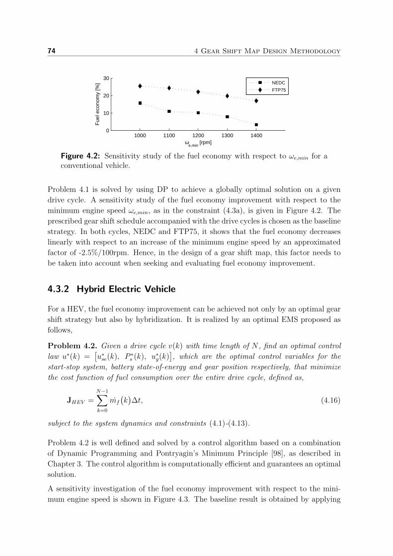
74 4 Gear Shift Map Design Methodology
1000 1100 1200 1300 14000
10
20
30
ωe,min
[rpm]
Fue
l eco
nom
y [%
]
NEDC
FTP75
Figure 4.2: Sensitivity study of the fuel economy with respect to ωe,min for aconventional vehicle.
Problem 4.1 is solved by using DP to achieve a globally optimal solution on a given
drive cycle. A sensitivity study of the fuel economy improvement with respect to the
minimum engine speed ωe,min, as in the constraint (4.3a), is given in Figure 4.2. The
prescribed gear shift schedule accompanied with the drive cycles is chosen as the baseline
strategy. In both cycles, NEDC and FTP75, it shows that the fuel economy decreases
linearly with respect to an increase of the minimum engine speed by an approximated
factor of -2.5%/100rpm. Hence, in the design of a gear shift map, this factor needs to
be taken into account when seeking and evaluating fuel economy improvement.
4.3.2 Hybrid Electric Vehicle
For a HEV, the fuel economy improvement can be achieved not only by an optimal gear
shift strategy but also by hybridization. It is realized by an optimal EMS proposed as
follows,
Problem 4.2. Given a drive cycle v(k) with time length of N , find an optimal control
law u∗(k) =[u∗se(k), P ∗s (k), u∗g(k)
], which are the optimal control variables for the
start-stop system, battery state-of-energy and gear position respectively, that minimize
the cost function of fuel consumption over the entire drive cycle, defined as,
JHEV =N−1∑k=0
mf
(k)∆t, (4.16)
subject to the system dynamics and constraints (4.1)-(4.13).
Problem 4.2 is well defined and solved by a control algorithm based on a combination
of Dynamic Programming and Pontryagin’s Minimum Principle [98], as described in
Chapter 3. The control algorithm is computationally efficient and guarantees an optimal
solution.
A sensitivity investigation of the fuel economy improvement with respect to the mini-
mum engine speed is shown in Figure 4.3. The baseline result is obtained by applying

4.3 Analysis of Gear Shift Contribution to Fuel Economy 75
1000 1100 1200 1300 14000
10
20
30
40
50
ωe,min
[rpm]
Fue
l eco
nom
y [%
]
NEDC
FTP75
Figure 4.3: Sensitivity study of the fuel economy with respect to ωe,min for aHEV.
the prescribed gear shift schedule accompanied with the drive cycles on a corresponding
conventional vehicle. An increase of the minimum engine speed will result in a decrease
of the relative fuel economy with an approximated factor of -1.0%/100rpm. Comparing
to the conventional vehicle, the fuel economy improvement of the hybrid electric vehicle
is less sensitive to the minimum engine speed. Assuming that the start-stop function-
ality in the hybrid powertrain can be done by using the electric machine to crank up
the engine from rest, the corresponding fuel benefit can be appointed to the hybridiza-
tion factor. This implies that there are two factors contributing to the fuel economy
improvement of HEVs: the gear shift and the hybridization. In order to investigate the
share of these two factors in the fuel economy improvement, an algorithm is proposed
for this purpose.
Algorithm 4.1. Given a drive cycle, Problem 4.2 is formulated and solved. Then at
every time step k,
• compute the instantaneous optimal fuel rate m∗f (k);
• given the optimal gear position n∗g(k), compute the required engine power without
hybridization,
Pe,gs(k)∣∣n∗g(k);
• compute the corresponding fuel rate without hybridization, given n∗g(k) and
Pe,gs(k),
mf,gs(k)∣∣Pe,gs(k), n∗g(k).
Define the fuel consumption for two powertrain systems:
• the hybrid powertrain, mf =∑N−1
0 m∗f (k)∆t;
• the conventional powertrain utilizing the corresponding optimal gear shift strategy
obtained from the EMS of the hybrid powertrain, mf,gs =∑N−1
0 mf,gs(k)∆t.

76 4 Gear Shift Map Design Methodology
Here mf,base denotes fuel consumption of the baseline vehicle. Then, contributions of
the gear shift and hybridization to the total fuel economy are defined as,
• the fuel economy improvement due to the gear shift: mf,base −mf,gs;
• the fuel economy improvement due to the hybridization: mf,gs −mf ;
• the total fuel economy improvement: mf,base −mf .
Figure 4.4: Contributions of the gear shift and hybridization to the fuel econ-omy.
Algorithm 4.1 can be graphically explained through a demonstration shown in Figure
4.4. Under a certain power request at the wheels, a corresponding power at the transmis-
sion input can be expressed in the form of a hyperbolic torque-speed curve, the dashed
dotted black line. For the conventional powertrain, if a prescribed gear schedule is used
for shifting, the engine operating point is positioned at the red dot. Hybridization of
the powertrain with an optimal EMS allows i) the engine operating point to move to
the green dot due to an optimal gear shift strategy, ii) a further load balance sharing
(power split) between the engine and electric machine to move the engine operating
point as close to the E-line as possible, see the corresponding battery charged or motor
assist point due to a certain power split strategy. Factors i) and ii) help improving the
hybrid powertrain efficiency compared to the conventional one.
Calculation results of Algorithm 4.1 on NEDC and FTP75 are shown in Figure 4.5.
Therein, the fuel economy improvement of the optimal gear shift strategy for the con-
ventional vehicle, as discussed in Section 4.3.1, is also plotted for reference, see the
marked dotted lines. The dark grey bars indicate contribution of the gear shift; mean-
while the light grey bars indicate contribution of the hybridization. It can be seen that
contribution of the gear shift in the hybrid vehicle is almost equal to the optimal gear
shift strategy for the conventional vehicle. Hence, from an engineering point of view, it
can be inferred that the gear shift factor is independent from the hybridization factor

4.4 Gear Shift Map Design for Conventional Vehicles 77
1000 1100 1200 1300 14000
10
20
30
40
50
ωe,min
[rpm]
Fue
l eco
nom
y [%
]NEDC
GearshiftHybridizationConventional
(a)
1000 1100 1200 1300 14000
10
20
30
40
50
ωe,min
[rpm]
Fue
l eco
nom
y [%
]
FTP75
GearshiftHybridizationConventional
(b)
Figure 4.5: Contributions of the gear shift and hybridization to the fuel econ-omy of the HEV. Simulation results on NEDC and FTP75 are shown in (a) and(b), respectively.
for the HEV. Furthermore, when raising the minimum engine speed, contribution of the
gear shift factor is reduced but the hybridization factor is more active to maintain the
fuel economy level. This helps neutralizing the fuel economy sensitivity to ωe,min for
the hybrid vehicle compared to the conventional vehicle.
4.4 Gear Shift Map Design for Conventional Vehicles
The optimal gear shift strategies for the conventional vehicle, proposed in Chapter
2, are benchmark solutions rather than realtime implementable ones. Despite the fact
that the stochastic-based strategy is realtime implementable, a rigorous implementation
approach is required to deal with the uncertainties and disturbances of the powertrain
system to ensure a robust and fuel-efficient gear shift pattern. Therefore, a map-based
gear shift strategy, which can be implemented directly to the production vehicles and
ensures optimality, appears as a promising solution. This section describes a novel
methodology which is used to generate an optimized gear shift map for conventional
vehicles equipped with discrete ratio transmissions.

78 4 Gear Shift Map Design Methodology
4.4.1 Acquisition of Optimal Gear Shift Data
This is the first step of the design methodology. The fuel optimal gear shift problem,
see Problem 4.1, is formulated and solved to obtain the optimal gear shift points on
various drive cycles. The higher the number of drive cycles used to acquire the optimal
gear shift points, the higher level of optimality the designed gear shift map is. In this
study, the standard test drive cycles in Europe, Japan and United States, e.g. ARB02,
CADC, FTP75, HWFET, Hurk, JN1015, LA92, NEDC, NYCC, and US06, are chosen
to objectively represent the drive profiles of vehicles. Note that the driveability optimal
gear shift problem, see Problem 2.2 in Chapter 2, is applied if a driveability-optimal
gear shift map is required. The optimal shift points, as point-wise functions of the
engine torque and vehicle speed, for all gear upshift patterns are shown in Figure 4.6.
The optimal shift points, hereafter called the shift data, scatter around a specific area
for a certain upshift pattern. With the upshift patterns of 1→ 2, 2→ 3 and 3→ 4, the
scatter areas are less dispersed than that of the upshift patterns of 4 → 5 and 5 → 6.
Nonetheless, an inference of a shift pattern characteristic based on a rigorous analysis
of the corresponding shift data is necessary, such that representative shift lines can be
extracted.
0 20 400
50
100
150
200
Te [N
m]
v [km/h]
1 → 2
(a)
20 40 60 800
50
100
150
200
Te [N
m]
v [km/h]
2 → 3
(b)
20 40 60 80 100 1200
50
100
150
200
Te [N
m]
v [km/h]
3 → 4
(c)
40 60 80 100 120 1400
50
100
150
200
Te [N
m]
v [km/h]
4 → 5
(d)
50 100 1500
50
100
150
200
Te [N
m]
v [km/h]
5 → 6
(e)
Figure 4.6: Optimal upshift points of the conventional vehicle, wherein thex-mark points denote the outliers.
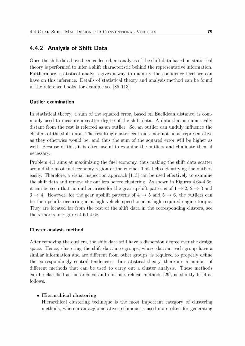
4.4 Gear Shift Map Design for Conventional Vehicles 79
4.4.2 Analysis of Shift Data
Once the shift data have been collected, an analysis of the shift data based on statistical
theory is performed to infer a shift characteristic behind the representative information.
Furthermore, statistical analysis gives a way to quantify the confidence level we can
have on this inference. Details of statistical theory and analysis method can be found
in the reference books, for example see [85, 113].
Outlier examination
In statistical theory, a sum of the squared error, based on Euclidean distance, is com-
monly used to measure a scatter degree of the shift data. A data that is numerically
distant from the rest is referred as an outlier. So, an outlier can unduly influence the
clusters of the shift data. The resulting cluster centroids may not be as representative
as they otherwise would be, and thus the sum of the squared error will be higher as
well. Because of this, it is often useful to examine the outliers and eliminate them if
necessary.
Problem 4.1 aims at maximizing the fuel economy, thus making the shift data scatter
around the most fuel economy region of the engine. This helps identifying the outliers
easily. Therefore, a visual inspection approach [113] can be used effectively to examine
the shift data and remove the outliers before clustering. As shown in Figures 4.6a-4.6c,
it can be seen that no outlier arises for the gear upshift patterns of 1 → 2, 2 → 3 and
3 → 4. However, for the gear upshift patterns of 4 → 5 and 5 → 6, the outliers can
be the upshifts occurring at a high vehicle speed or at a high required engine torque.
They are located far from the rest of the shift data in the corresponding clusters, see
the x-marks in Figures 4.6d-4.6e.
Cluster analysis method
After removing the outliers, the shift data still have a dispersion degree over the design
space. Hence, clustering the shift data into groups, whose data in each group have a
similar information and are different from other groups, is required to properly define
the correspondingly central tendencies. In statistical theory, there are a number of
different methods that can be used to carry out a cluster analysis. These methods
can be classified as hierarchical and non-hierarchical methods [29], as shortly brief as
follows.
• Hierarchical clustering
Hierarchical clustering technique is the most important category of clustering
methods, wherein an agglomerative technique is used more often for generating

80 4 Gear Shift Map Design Methodology
clusters. The working principle of this technique is to start with individual points
as clusters, then successively merge the two closest clusters until only one cluster
remains. This clustering technique is basically described in Algorithm 4.2.
Algorithm 4.2. Agglomerative clustering method
define the cluster proximity matrix, if necessary;repeat
- merge the two closest clusters,- update the cluster proximity matrix to reflect the proximity be-tween the new clusters and the original clusters,
until only one cluster remains.
• Non-hierarchical clustering
This clustering technique is most often known as a K-means clustering method.
The K-means method defines the data prototype in terms of a centroid, which
is usually a mean of a group of points. The K-means clustering technique is
described by Algorithm 4.3.
Algorithm 4.3. K-means clustering method
select K points as initial centroids;repeat
- form K clusters by assigning each point to its closest centroid,- recompute the centroid of each cluster,
until the centroids do not change.
In this study, an effective approach of combining two clustering methods is used to
analyze the shift data [29]. The hierarchical agglomerative method is used to define
the optimum number of clusters. Then the non-hierarchical K-means method is used to
compute the centroid of each cluster. All cluster centroids will form a central tendency
of the gear shift pattern. Figures 4.7a-4.7b show an exemplary cluster analysis for a
gear upshift pattern from 2→ 3. There are seven clusters resulting in seven centroids,
indicated by the blue circled x-marks. The centroids create a basis for building a shift
line by a curve best fitting these points.
Shift line extraction
For a conventional vehicle, a gear shift map consists of the upshift lines and the corre-
sponding downshift lines.
• Upshift: the upshift line is built from the centroids of the corresponding upshift
patterns by a best fitting curve. Figure 4.7c typically depicts an upshift line from
2→ 3.

4.4 Gear Shift Map Design for Conventional Vehicles 81
20 40 60 800
50
100
150
200
Te [N
m]
v [km/h]
(a)
20 40 60 800
50
100
150
200
Te [N
m]
v [km/h]
(b)
20 40 60 800
50
100
150
200
Te [N
m]
v [km/h]
(c)
20 40 60 800
50
100
150
200
v [km/h]
Te [N
m]
(d)
2 → 3
3 → 2
Te,WOT
Figure 4.7: Exemplary analysis of the shift data of the conventional vehicle:the shift data of 2→ 3 in (a); cluster analysis in (b); an extraction of the upshiftline in (c), a corresponding downshift line of 3 → 2 in (d).
0 20 40 60 80 100 1200
50
100
150
200
v [km/h]
Te [N
m]
Upshift
1 → 2
2 → 3
3 → 4
4 → 5
5 → 6
0 20 40 60 80 100 1200
50
100
150
200
v [km/h]
Te [N
m]
Downshift
2 → 1
3 → 2
4 → 3
5 → 4
6 → 5
Figure 4.8: A gear shift map for the conventional vehicle.
• Downshift: a downshift line is built by considering two cases: i) a normal down-
shift occurs to avoid engine stalling due to a reduction of the vehicle speed; ii)

82 4 Gear Shift Map Design Methodology
a power downshift, called kick-downshift, is required to meet a high torque de-
mand at the wheels, which is not fulfilled by the powertrain at the current gear
position. Taking these two factors into account, a downshift pattern, for example
from 3→ 2, is built, see Figure 4.7d.
Figure 4.7d depicts the upshift pattern 2→ 3, and the corresponding downshift pattern
3→ 2. At a certain engine torque, there always exists a difference in the vehicle speed
at the upshift and downshift lines. This results in a shifting hysteresis phenomenon,
required for a consistent and robust shifting pattern.
4.4.3 Shift Map Verification
Applying the procedure described in Section 4.4.2 for the other shift patterns to extract
the shift lines, a gear shift map is obtained and shown in Figure 4.8. Detail description
of the typical upshift and downshift lines is given in Section 4.6.2. This gear shift map
can be implemented directly in simulation or realtime environment.
ARB02 CADC FTP75 JN1015 LA92 NEDC US060
2
4
6
8
Fue
l def
icie
ncy
[%]
Drive cycleAverage
Figure 4.9: Fuel deficiency of the gear shift map compared to the DP-basedoptimal shift strategy for the conventional vehicle.
The obtained gear shift map is implemented in a simulation model of the conventional
vehicle to verify a fuel economy improvement. The drive cycles are chosen to consist of
the urban, suburban and highway parts, which represent the typical driving missions for
the vehicle. By comparing with a globally optimal result (DP result), a fuel deficiency
of the gear shift map is realized, as shown in Figure 4.9. Depend on the drive cycles,
the fuel deficiency varies from 0.9% to 3.9%. On average, the gear shift map, which
is consistent, robust and realtime implementable, degrades the fuel economy of 2.3%
compared with a globally optimal gear shift algorithm based on DP.
4.5 Gear Shift Map Design for Hybrid Electric Vehicles 83
4.5 Gear Shift Map Design for Hybrid Electric Vehicles
HEVs, having a secondary power source offer, more operation modes, e.g. engine mode,
assisting mode, charging mode, electrically driving mode and regenerative mode, to im-
prove the fuel economy, driveability, etc., compared to conventional vehicles. Therefore,
a gear shift strategy for HEVs is required to match with all operation modes. This
can be achieved by an advanced EMS to optimally govern the operation of the hybrid
powertrain. The EMS proposed in [98] is computationally efficient and guarantees an
optimal solution. Hence, it is highly suitable for the gear shift design methodology for
HEVs. The obtained optimal gear shift data will ensure an optimality of the gear shift
map, compatible with all operation modes of the hybrid vehicle. The design process is
highly accelerated due to a computationally efficient property of the EMS.
Gear shift map characteristics
• Shift map coordinate: the gear shift map coordinate for a conventional vehicle is
based on the vehicle speed and engine torque. However, for a HEV, the equilibrium
point of the power flow is at the transmission input. Hence it is reasonable to define
a gear shift map coordinate based on the vehicle speed and the transmission input
torque.
• Hybrid mode: this mode in general can be referred to an engine mode or an
assisting mode or a charging mode. Basically, in hybrid mode, the engine primarily
supplies the propulsive power for the vehicle. Hence, the design of gear shift map
in hybrid mode is thus similar to that of a conventional vehicle.
• E mode: this mode refers to a situation of electrically driving the vehicle. The
electric machine is placed in front of the transmission. Therefore, a gear shift
strategy in E mode can expand the operating range for the electric machine with
respect to the vehicle speed range, and thus gaining a fuel benefit.
• Regenerative mode: in this mode the electric machine functions as a generator
to recuperate the vehicle kinetic energy. A gear shift strategy in this mode can
increase the energy conversion efficiency of the generator and thus further con-
tributing for a fuel benefit.
Note that the transition among the operating modes in the HEV is assumed to be well
defined and properly controlled. In addition, this kind of mode shifting is irrelevant to
a gear shift map design, and thus ignored in this study.
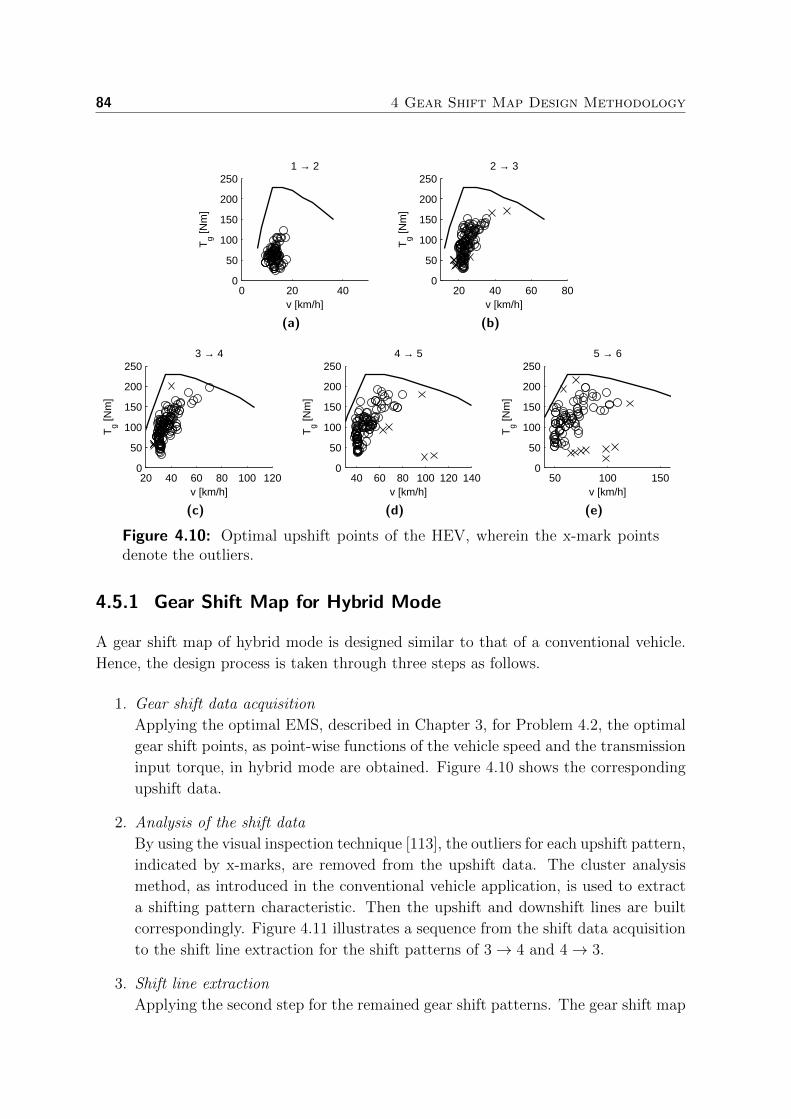
84 4 Gear Shift Map Design Methodology
0 20 400
50
100
150
200
250
Tg [N
m]
v [km/h]
1 → 2
(a)
20 40 60 800
50
100
150
200
250
Tg [N
m]
v [km/h]
2 → 3
(b)
20 40 60 80 100 1200
50
100
150
200
250
Tg [N
m]
v [km/h]
3 → 4
(c)
40 60 80 100 120 1400
50
100
150
200
250
Tg [N
m]
v [km/h]
4 → 5
(d)
50 100 1500
50
100
150
200
250
Tg [N
m]
v [km/h]
5 → 6
(e)
Figure 4.10: Optimal upshift points of the HEV, wherein the x-mark pointsdenote the outliers.
4.5.1 Gear Shift Map for Hybrid Mode
A gear shift map of hybrid mode is designed similar to that of a conventional vehicle.
Hence, the design process is taken through three steps as follows.
1. Gear shift data acquisition
Applying the optimal EMS, described in Chapter 3, for Problem 4.2, the optimal
gear shift points, as point-wise functions of the vehicle speed and the transmission
input torque, in hybrid mode are obtained. Figure 4.10 shows the corresponding
upshift data.
2. Analysis of the shift data
By using the visual inspection technique [113], the outliers for each upshift pattern,
indicated by x-marks, are removed from the upshift data. The cluster analysis
method, as introduced in the conventional vehicle application, is used to extract
a shifting pattern characteristic. Then the upshift and downshift lines are built
correspondingly. Figure 4.11 illustrates a sequence from the shift data acquisition
to the shift line extraction for the shift patterns of 3→ 4 and 4→ 3.
3. Shift line extraction
Applying the second step for the remained gear shift patterns. The gear shift map

4.5 Gear Shift Map Design for Hybrid Electric Vehicles 85
20 40 60 80 1000
50
100
150
200
250
Tg [N
m]
v [km/h]
(a)
20 40 60 80 1000
50
100
150
200
250
Tg [N
m]
v [km/h]
(b)
20 40 60 80 1000
50
100
150
200
250
Tg [N
m]
v [km/h]
(c)
20 40 60 80 1000
50
100
150
200
250
v [km/h]
Tg [N
m]
(d)
3 → 4
4 → 3
TTR,max
Figure 4.11: Exemplary analysis of the shift data of the HEV: the shift dataof 3 → 4 in (a); cluster analysis in (b); an extraction of the upshift line in (c),a corresponding downshift line of 4 → 3 in (d).
0 20 40 60 80 100 1200
50
100
150
200
250
v [km/h]
Tg [N
m]
Upshift of the hybrid mode
1 → 2
2 → 3
3 → 4
4 → 5
5 → 6
0 20 40 60 80 100 1200
50
100
150
200
250
v [km/h]
Tg [N
m]
Downshift of the hybrid mode
2 → 1
3 → 2
4 → 3
5 → 4
6 → 5
Figure 4.12: A gear shift map for hybrid mode of the HEV.
in hybrid mode is obtained and depicted in Figure 4.12.

86 4 Gear Shift Map Design Methodology
4.5.2 Gear Shift Map for E Mode
A gear shift strategy in E mode helps expanding the electric machine operating range
with respect to the vehicle speed range. The proposed EMS for the HEV does not
derive the optimal gear shift strategy separated from the engine on-off and power split
strategies. Furthermore, the gear shift patterns in all operation modes are coupled
together to create an optimal gear shift strategy for the whole drive cycle.
For a HEV where the engine is the main traction source, E mode occurs if a low drive
power is required. When a high drive power is needed, the vehicle transits to hybrid
mode to meet the high demand traction. In this situation, a gear shift is occurred in
hybrid mode instead of E mode. Therefore the electric machine can take advantage of
the gear shift strategy in hybrid mode to expand its operating range. Apparently, the
relative size of the electric machine, compared to the engine size, is a decisive factor
for a coupling between the gear shift patterns in E mode and hybrid mode. Taking
the mentioned issues into account, the design of gear shift map of E mode should be
considered in the light of the gear shift map of hybrid mode.
Hence, a gear shift map of E mode is built in accordance with a procedure given as
follows.
1. E mode data
Collect the transition data (from E mode to hybrid mode) and the gear shift data
(occurring within E mode). Figure 4.13 shows the obtained data separating in
each gear position. The transition data creates a boundary between E mode and
hybrid mode, indicated by the dashed line. Meanwhile the upshift data is not
rich enough to clearly define the shift patterns within E mode. This implies that
a gear shift in E mode would not further improve the fuel economy rather than
an operation in E mode would do. However, the operating region of the electric
machine, corresponding with each gear position, can yield the possible gear shift
patterns in E mode, indicated by vertical solid lines.
2. Upshift patterns
By comparing with the upshift lines of hybrid mode, there are identical upshift
patterns for E mode. This reveals that hybrid mode dominates E mode. In
other words, an improvement of the combustion efficiency is much more important
than an improvement of the electro-mechanical conversion efficiency of the electric
machine with respect to an optimal gear shift strategy. Therefore, the electric
machine can take advantage of the upshift strategy occurred in hybrid mode to
expand its operating range, thus increasing the portion of the traveled distance in
E mode.
3. Downshift patterns

4.5 Gear Shift Map Design for Hybrid Electric Vehicles 87
The downshift patterns in E mode can be defined as the corresponding upshift
patterns, due to the fact that there is no clutch operation in a shift process in E
mode. However, the downshift patterns of E mode are chosen as the downshift
patterns of hybrid mode to respect a gear shift hysteresis.
4.5.3 Gear Downshift Map for Regenerative Mode
Figure 4.14 shows the obtained downshift data in regenerative mode. For each down-
shift pattern, the corresponding downshift points create an optimal downshift region.
Basically, the downshift line can be extracted by using the cluster analysis technique
applied for the conventional vehicle. However, to approach a downshift pattern robust
to driving uncertainties, e.g. an upshift request induced right after a regenerative down-
shift, a left boundary linear line of each downshift region is defined for a corresponding
downshift pattern, see the circled-mark solid lines.
It can be seen that the downshift lines are not vertical, meaning that a downshift point is
a function of the vehicle speed and the brake torque. A higher a brake torque requires at
the wheels, an earlier a regenerative downshift would occur to exploit the high efficient
region of the electric machine. Crossing points of the downshift lines with the vehicle
speed axis nearly coincide with that of the upshift lines in hybrid mode. This discloses
that the downshift points in regenerative mode occur earlier than that of hybrid mode.
Actually, an earlier downshift in regenerative mode will rapidly raise up the speed of
electric machine, thus avoiding operating at the power limit region (at low speed) and
approach an efficient operating region. Hence, a gear downshift strategy in regenerative
mode can further improve the fuel economy of hybrid vehicles.
4.5.4 Shift Map Verification
A gear shift map of the HEV, consisting of all gear shift maps corresponding with all
operating modes, is constructed as shown in Figure 4.15. As analyzed, the shift map of
E mode is considered as a lower part of hybrid mode shift map (at a low transmission
torque area). Therefore, hybrid mode shift map governs the gear shift when the driving
torque is positive; the shift map of regenerative mode governs the gear downshift when
the driving torque is negative (regenerative braking). When the driving torque is zero,
e.g. the vehicle coasts down smoothly by the aerodynamic drag and rolling friction
resistances, the shift strategy of hybrid mode at zero torque will govern a downshift for
the transmission.
The gear shift map is verified by implementing it in a simulation model of the HEV.
The DP-PMP approach [98] is applied to control the engine start-stop and power split.
Compared to the optimal gear shift strategy, the gear shift map reduces the fuel economy

88 4 Gear Shift Map Design Methodology
0 20 40 60 80 100 1200
10
20
30
40
50Hybrid mode area
v [km/h]
Tg [N
m]
1 → 2
2 → 3
3 → 4
4 → 5
5 → 6
Figure 4.13: A gear shift map for E mode.
Figure 4.14: A gear downshift map for regenerative mode.
0 20 40 60 80 100 120−500
−400
−300
−200
−100
0
100
200
E mode area
Hybrid mode area
Regenerative mode area
Tg [N
m]
v [km/h]
1 → 2
2 → 3
3 → 4
4 → 5
5 → 6
2 → 1
3 → 2
4 → 3
5 → 4
6 → 5
2 → 1
3 → 2
4 → 3
5 → 4
6 → 5
Figure 4.15: A gear shift map for the HEV.
from 2.5% to 5.9% on all simulated drive cycles, see Figure 4.16. On average, a fuel
deficiency of 4.1% is obtained in return for a consistent, robust and realtime map-based
gear shift strategy for the HEV.

4.6 Experimental Validation on Conventional Vehicle 89
ARB02 CADC FTP75 JN1015 LA92 NEDC US060
2
4
6
8F
uel d
efic
ienc
y [%
]
Drive cycleAverage
Figure 4.16: Fuel deficiency of the gear shift map compared with the DP-PMPgear shift strategy for the HEV.
4.6 Experimental Validation on Conventional Vehicle
The gear shift map design methodology is applied to produce a gear shift map for a
test conventional vehicle. The test vehicle is different from the prototype vehicle, used
for demonstrating the development of in the design methodology. The test vehicle is
powered by a gasoline engine, meanwhile the prototype vehicle is diesel-based pow-
ered. Two gear shift maps, based on the fuel-optimal and driveability-optimal gear
shift strategies, are produced and tested to verify the fuel economy and driveability
improvements. This helps to validate the applicability of the design methodology on
various vehicle propulsion technologies.
Figure 4.17 shows the test vehicle for which the designed gear shift maps will be im-
plemented for an experimental validation. In the right is the original gear shift map
implemented on the vehicle at production. This map, denoted as a ‘BASE’ map, is used
to obtain the baseline results for a comparative analysis with the designed gear shift
maps. The parameters of the test vehicle are given in Table 4.2. Note that the equipped
6-speed AMT has a powershift module activated for all gear shift patterns among the
first four gears [132], thus avoiding the torque interruption at the corresponding gear
shift.
Table 4.2: Main parameters of the test vehicle.
Item Description/Quantity
Enginetype: gasoline,maximum torque of 140Nm,maximum power of 70kW.
Transmission6-speed PowerShift (PS) AMT,rg = [3.071, 1.913, 1.258, 0.943, 0.763, 0.643].
Vehicle mass 1120kg.

90 4 Gear Shift Map Design Methodology
Figure 4.17: The test vehicle (left). The gear shift map at production (right),denoted as ‘BASE’ map.
4.6.1 Gear Shift Map Generation
Two gear shift maps are built for the test vehicle.
• ECO map: this map refers to a gear shift strategy, aiming at improving the fuel
economy. Therefore, the whole procedure introduced in Section 4.4 is applied to
generate ECO map.
• ECOS map: this map refers to a gear shift strategy aiming at improving the fuel
economy meanwhile still satisfying an acceptable driveability level. The method to
address the driveability, based on the variable power reserve concept (see Section
2.3 of Chapter 2), is utilized in the gear shift design methodology to generate
ECOS map.
Figures 4.18 and 4.19 illustrate ECO and ECOS maps, respectively. Note that the
vertical axis of the shift map denotes the accelerator pedal position Ap, ranged 0%-100%,
instead of the engine torque. A conversion from the engine torque to the accelerator
pedal position is done by using two conversion maps: i) the first map describes the
engine torque as a function of the engine speed and throttle position, ii) the second
map describes the throttle position as a function of the accelerator pedal position.
Hence, a gear shift point for the test vehicle is generated based on the vehicle speed and
accelerator pedal position.
4.6.2 Description of Gear Shift Pattern
The gear shift patterns are extracted from ECO and ECOS maps, called ECO and
ECOS shift patterns, and shown in Figure 4.20. It can be seen that ECO shift pattern

4.6 Experimental Validation on Conventional Vehicle 91
0 50 100 150 2000
50
100
v [km/h]
Ap [%
]
1 → 22 → 33 → 44 → 55 → 6
0 50 100 150 2000
50
100
v [km/h]
Ap [%
]
2 → 13 → 24 → 35 → 46 → 5
Figure 4.18: ECO map, aiming at a fuel economy improvement.
0 50 100 150 2000
50
100
v [km/h]
Ap [%
]
1 → 22 → 33 → 44 → 55 → 6
0 50 100 150 2000
50
100
v [km/h]
Ap [%
]
2 → 13 → 24 → 35 → 46 → 5
Figure 4.19: ECOS map, aiming at improving the fuel economy meanwhilesatisfying an acceptable driveability level.
Figure 4.20: Description of the gearshift patterns in ECO map (left) and ECOS
map (right).
92 4 Gear Shift Map Design Methodology
occurs earlier than ECOS shift pattern with respect to the vehicle speed. Hence, the
engine will operate at lower engine speed region under ECO map compared to ECOS
map. In general, a shift pattern can be divided into three parts: lower, middle and
upper.
• Lower part is an area where the shift patterns are parallel with the Y-axis. It
represents shift conditions for the vehicle independent of the acceleration pedal
input. In this area, a gear shift takes place depending on the current vehicle speed.
Under mild driving situations, e.g. maintaining the vehicle speed, following a
traffic stream, etc., an upshift is triggered when the vehicle speed is larger than
the upshift threshold. Under a coasting down, when the vehicle speed is smaller
than a downshift threshold, a downshift is triggered to sustain the engine speed
above a limit.
• Upper part defines an area where the gearshift patterns are relative steep with
respect to the X-axis. In this area, the driver requests a high or full engine power
to satisfy its driving styles. An upshift can occur if the engine satisfies the power
request and the vehicle speed is higher than a shift threshold. If the power request
is high at the current gear, a kick-downshift is performed such that the engine can
meet this high power request at the lower gear.
• Middle part where the lower and upper parts are linked together. The obtained
gearshift patterns in this area depict an optimal tradeoff among the design objec-
tives, e.g. fuel economy, driveability, etc. It can be seen that the upshift pattern of
ECOS map is less steep than that of ECO map to improve the vehicle performance.
4.6.3 Validation in Simulation Environment
Fuel economy test
ECO and ECOS maps are implemented on a forward facing simulation model of the
test vehicle, built in Matlab/Simulink, to test the fuel economy. Compared to BASE
map, a fuel economy improvement is achieved for both designed gear shift maps on the
drive cycles NEDC and JN1015, see Table 4.3. As expected, ECO map gains more fuel
benefit than ECOS map.
Driveability test
Forward facing simulation results of the relative fuel economy improvement show a
very promising prospect for the gear shift map design methodology in generating the
gear shift map, especially for ECOS map with a considerable improvement of the fuel

4.6 Experimental Validation on Conventional Vehicle 93
Table 4.3: Simulation results of the relative fuel economy improvement.
Shift Map NEDC JN1015
BASE (manufacturer) - -ECO 7.3 % 9.9 %ECOS 4.3 % 3.7 %
50 55 60 65
20
30
40
50
Time [s]
v [k
m/h
]
Ref.
ECO
ECOS
BASE
50 55 60 650
2
4
6
Time [s]
n g [−]
ECO
ECOS
BASE
(a)
50 55 60 65
50
60
70
80
Time [s]
v [k
m/h
]
Ref.
ECO
ECOS
BASE
50 55 60 650
2
4
6
Time [s]
n g [−]
ECO
ECOS
BASE
(b)
Figure 4.21: Mild acceleration tests.
45 50 55 60 65
50
60
70
80
Time [s]
v [k
m/h
]
Ref.
ECO
ECOS
BASE
45 50 55 60 650
2
4
6
Time [s]
n g [−]
ECO
ECOS
BASE
(a)
0 5 10 15 200
20
40
60
Time [s]
v [k
m/h
]
Ref.
ECO
ECOS
BASE
0 5 10 15 200
2
4
6
Time [s]
n g [−]
ECO
ECOS
BASE
(b)
Figure 4.22: High acceleration tests.

94 4 Gear Shift Map Design Methodology
economy. In order to evaluate the driveability characteristic of ECOS map, several
acceleration profiles are tested with three gear shift maps.
• Mild acceleration profiles consist of two tests, as shown in Figure 4.21.
For the first test, see Figure 4.21a, ECOS map gives a better acceleration response.
ECO map triggers earlier upshift to higher gear. Therefore, there is a torque
interruption at the shifts 4 → 5 and 5 → 6, which causes a velocity tracking
loss. Meanwhile BASE map reveals a latest upshift compared to the other two.
The PS-AMT maintains at the second gear for a long period, thus bringing the
engine speed to a high revolution. Therefore, at high engine speed, the reduced
maximum engine torque could not continue to accommodate the vehicle with
velocity tracking until an upshift to the third gear occurs.
For the second test, see Figure 4.21b, due to a high power demand, the three maps
require a kick-downshift for the transmission to improve the engine traction capa-
bility by raising the engine speed. However, ECO map triggers a kick-downshift
two times from the sixth gear to the fourth gear, thus resulting in a velocity loss
due to a torque interruption in the PS-AMT. It is observed that when nearly ap-
proaching 80[km/h], ECOS map allows an upshift pattern earlier than BASE map,
thus improving the fuel economy. BASE map keeps the transmission at the third
gear longer, thus bringing the engine speed to a high revolution. Therefore the
reduced maximum torque degrades the vehicle acceleration capability compared
to ECOS map.
• High acceleration profiles consist of two tests, as shown in Figure 4.22.
For the first test, see Figure 4.22a, ECOS and BASE maps result in a nearly
equal velocity response. Meanwhile ECO map reveals a poor driveability followed
by a torque interruption due to a two-gear kick-downshift occurrence, from the
sixth gear to the fourth gear. Right after reaching the setpoint velocity, ECOS
map produces upshifts earlier than BASE map to contribute to a fuel economy
improvement.
For the second test, see Figure 4.22b, ECOS map possesses a good driveability
property compared to the other maps. The results also show an earlier upshift,
at higher rate to higher gear position, is held for ECO map. Meanwhile, ECOS
map is better than BASE map in terms of an upshift trigger.
In summary, the driveability tests reveal that ECOS map is better than BASE map
in fulfilling the vehicle performance. Furthermore, ECOS map yields an earlier upshift
pattern compared to BASE map, thus coming with a considerable gain in the fuel
economy. Meanwhile a superior fuel economy property of ECO map is penalized by a
low driveability capability.

4.6 Experimental Validation on Conventional Vehicle 95
4.6.4 Experimental Results
0 200 400 600 800 1000 12000
50
100
t [s]
v[km/h]
0 200 400 600 800 1000 12000
2
4
6
t [s]
ng[-]
0 200 400 600 800 1000 12000
1
2
t [s]
mf[g/s]
ECO
ECOS
BASE
Figure 4.23: Experimental test results on NEDC.
Table 4.4: Experimental results of the relative fuel economy improvement.
Shift Map NEDC JN1015
BASE (manufacturer) - -ECO 7.4 % 8.7 %ECOS 4.8 % 3.9 %
Experimental tests of the vehicle are performed on the roller bench for the drive cycles
NEDC and JN1015. The gear position and fuel rate on NEDC, corresponding with the
three gear shift maps, are illustrated in Figure 4.23. ECO map yields a highest upshift
frequency and allows the transmission to go to a highest gear. ECOS map triggers an
upshift earlier and stays longer at the same gear position compared to BASE map. The
relative fuel economy improvement on NEDC and JN1015 are given in Table 4.4. ECO
map possesses a highest fuel economy property compared to the other two. ECOS map
also improves the fuel economy considerably compared to BASE map.

96 4 Gear Shift Map Design Methodology
By comparing the simulation results (in Table 4.3) with the experimental results (in
Table 4.4), the relative fuel economy improvement on NEDC is almost equal together for
both cases. The biggest difference between the simulation and experiment is realized at
ECO map on JN1015, with absolute difference of 1.2%. In general, it can be observed
that there is not much difference of the relative fuel economy improvement between
the two validation approaches. Hence, the match between simulation and experimental
results validates the effectiveness of the gear shift map design methodology.
4.7 Conclusions
In this chapter, a gear shift map design methodology for road vehicles equipped with
discrete ratio transmissions was developed. The fuel economy, driveability, consistency
and robustness of the designed gear shift map are guaranteed by combining an opti-
mal gear shift strategy with a statistical gear shift pattern extraction method in the
design process. The design methodology is model-based, thus giving a flexibility with
changes, modifications of the powertrain specifications, and being time-efficient for the
design process. Therefore, the design methodology is applicable to various powertrain
configurations.
Furthermore, it is found that the minimum operable engine speed considerably affects
to the fuel economy. Due to the hybridization factor, HEVs diminish the sensitivity
of fuel economy to the minimum engine speed compared to conventional vehicles. The
early downshift strategy in regenerative mode of HEVs will boost the energy conversion
efficiency of the electric machine in generation mode, and thus further improving the
fuel economy.

Chapter 5
Integrated Predictive Gear ShiftStrategy1
Abstract - This study focuses on utilizing route information obtained from an onboard navi-gation system and a Global Positioning System (GPS) in the design of an Energy ManagementStrategy (EMS) to improve the fuel economy of Hybrid Electric Vehicles (HEVs). Given apriori driving profile over a horizon, assumed as an output of the onboard navigation system,a predictive algorithm is proposed to control the gear shift command, besides the power splitand engine start-stop decision, to further improve the fuel economy. Given route informationover a driving horizon in the form of road characteristics, speed limits, average speed, traveleddistance, etc., a velocity algorithm is proposed to derive a fuel-optimal vehicle speed as afunction of time. The two algorithms supplement each other to create a so-called integratedpredictive gear shift strategy to explore the fuel saving potential of HEVs.
5.1 Benefits of The Preview Route Information
An onboard navigation system combined with a Global Positioning System (GPS) helps
gaining route information, such as road characteristics, speed limits, etc., over a certain
driving horizon, thus making this information available as an extra input to the Energy
Management Strategy (EMS) of Hybrid Electric Vehicles (HEVs). Hence, by exploiting
this route information in the design of an EMS, a further significant fuel economy
improvement can be realized.
Depending on the built-in technology of the onboard navigation system, the obtained
route information can be classified into two categories. In the first category, the route
information is processed to yield a driving profile in terms of the vehicle speed and time
within a certain horizon, which becomes a priori cycle information for the EMS. At this
1This chapter has been prepared for a journal publication in the form as: V. Ngo, T. Hofman, M.Steinbuch, A. Serrarens. Integrated Predictive Gear Shift Strategy for Hybrid Electric Vehicles. 2012.
97

98 5 Integrated Predictive Gear Shift Strategy
level, the onboard navigation system supplies a velocity setpoint for the vehicle to follow.
In the second category, the route information is not well processed. It is characterized
in the form of the speed limits, average speed, traveling time, etc., within a certain
driving horizon. Corresponding to the first category, a so-called predictive algorithm
is proposed for the EMS to anticipate the gear shift command, besides the power split
and engine start-stop decisions, to further improve the fuel economy. Regarding the
second category, a so-called velocity algorithm is proposed to derive a fuel-optimal
velocity profile over a driving horizon. This algorithm is seen as a promising solution
to be implemented in the onboard navigation system to yield a fuel-optimal velocity
trajectory, which is a priori to the predictive algorithm. The two algorithms supplement
each other for realizing an integrated predictive gear shift strategy achieving the highest
possible fuel economy for HEVs in real-life driving.
In the literature, there is an increasing amount of studies utilizing preview route infor-
mation to improve the fuel economy for HEVs. In [5, 10], the authors assume that the
velocity profile over a preview route segment is available for a formulation of a predictive
power split control problem. Meanwhile in [2], the authors exploit route information
in the form of topographic profiles and average traveling speed to predict a reference
signal for battery state of charge. This predicted battery state of charge is then used
to maximize the recuperated energy despite the constraints on battery state of charge,
thus improving the fuel economy. At another aspect, utilizing route information to pre-
dict the velocity trajectory over a preview route segment has increasingly gained much
attention. A fuzzy-based control algorithm to compute a weighted average velocity over
a look-ahead zone is seen in [111]. Markov chain is also used to model a stochastic
process of the vehicle speed on a specific traveling route [57]. The authors divide this
specific route into a number of intervals and define the vehicle speed at the end of each
interval by a predefined Markov model. The authors in [152] formulate a velocity trajec-
tory optimization problem for a truck application. A simple non-smooth cost function
together with assumptions of constant acceleration and deceleration rates, and speed
limits for every consecutive route segment, are used to derive a velocity profile over
a route segment. Furthermore, in [61], the authors propose a method for building a
velocity profile along the preview route cycle by dividing it into a series of segments.
The speed for each segment is defined from statistical features, e.g. mean, variance,
etc. Accordingly, a path forecasting-based control algorithm is proposed to optimize
the battery charging and discharging for a fuel economy improvement. Nonetheless,
for all mentioned studies, the obtained velocity profile along a preview route cycle or
segment is not optimal in terms of fuel consumption and traveling time.
In this study, firstly, it is assumed that a prediction of the velocity profile over a certain
horizon is available thanks to a GPS-based onboard navigation system. This facilitates
a study of designing a predictive algorithm [96], based on Model Predictive Control
(MPC), to anticipate the gear shift command besides the start-stop decision and power
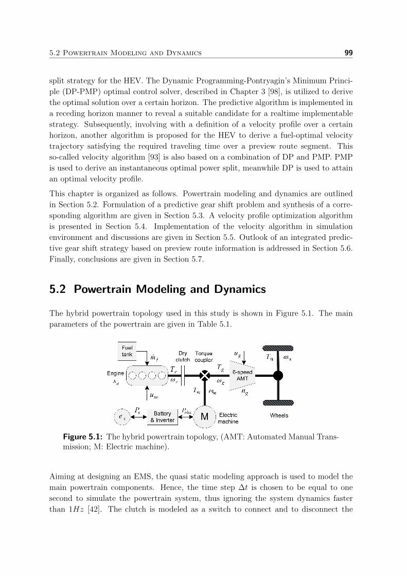
5.2 Powertrain Modeling and Dynamics 99
split strategy for the HEV. The Dynamic Programming-Pontryagin’s Minimum Princi-
ple (DP-PMP) optimal control solver, described in Chapter 3 [98], is utilized to derive
the optimal solution over a certain horizon. The predictive algorithm is implemented in
a receding horizon manner to reveal a suitable candidate for a realtime implementable
strategy. Subsequently, involving with a definition of a velocity profile over a certain
horizon, another algorithm is proposed for the HEV to derive a fuel-optimal velocity
trajectory satisfying the required traveling time over a preview route segment. This
so-called velocity algorithm [93] is also based on a combination of DP and PMP. PMP
is used to derive an instantaneous optimal power split, meanwhile DP is used to attain
an optimal velocity profile.
This chapter is organized as follows. Powertrain modeling and dynamics are outlined
in Section 5.2. Formulation of a predictive gear shift problem and synthesis of a corre-
sponding algorithm are given in Section 5.3. A velocity profile optimization algorithm
is presented in Section 5.4. Implementation of the velocity algorithm in simulation
environment and discussions are given in Section 5.5. Outlook of an integrated predic-
tive gear shift strategy based on preview route information is addressed in Section 5.6.
Finally, conclusions are given in Section 5.7.
5.2 Powertrain Modeling and Dynamics
The hybrid powertrain topology used in this study is shown in Figure 5.1. The main
parameters of the powertrain are given in Table 5.1.
Figure 5.1: The hybrid powertrain topology, (AMT: Automated Manual Trans-mission; M: Electric machine).
Aiming at designing an EMS, the quasi static modeling approach is used to model the
main powertrain components. Hence, the time step ∆t is chosen to be equal to one
second to simulate the powertrain system, thus ignoring the system dynamics faster
than 1Hz [42]. The clutch is modeled as a switch to connect and to disconnect the

100 5 Integrated Predictive Gear Shift Strategy
Table 5.1: The prototype vehicle specifications.
Item Description/Quantity
Enginediesel type,maximum torque of 200Nm,maximum power of 68kW.
Electric machinemaximum torque of 40Nm,maximum power of 6kW.
Battery lithium-ion; capacity of 6Ah, 110V.
Transmission6-speed automated manual transmission,rg = [3.817, 2.053, 1.302, 0.959, 0.744, 0.614].
Vehicle mass 1320kg.
engine immediately to and from the driveline. Its dynamics and limited power losses
during a gear shift or an engine start are ignored in this chapter. Notice of the slippage
loss of clutch at vehicle launch is also not taken into account. However, analysis of the
effect of these losses to the control strategy can be found in Chapter 6.
5.2.1 Powertrain Modeling
• Start-stop system: the start-stop system can be modeled by a decision variable
se(k) to control the engine on-off state. When the engine is off, no fuel is consumed
by the engine.
se(k) =
{1 if engine on,
0 if engine off.(5.1)
• Engine: for a certain engine speed ωe(k), the fuel mass flow mf (k) is modeled as
an affine piece-wise second order function of the power as expressed in (5.2),
mf (k) ≈(a0(k)P 2
e (k) + a1(k)Pe(k) + a2(k))se(k). (5.2)
in which the coefficients a0(k), a1(k) and a2(k) are functions of the engine speed.
If assume during braking, the engine is switched off and decoupled from the drive-
line, then the engine braking is neglected. Therefore, the constraints on the engine
speed ωe(k) power Pe(k) are as follows,
ωe,min ≤ ωe(k) ≤ ωe,max, (5.3a)
0 ≤ Pe(k) ≤ Pe,max(ωe(k)
). (5.3b)
5.2 Powertrain Modeling and Dynamics 101
• Electric machine: the machine efficiency η is assumed to be constant in a normal
operating state. Therefore, the power flow in motoring and generating modes is
expressed as,
Pm(k) = ηPelec(k) in motoring, (5.4a)
Pm(k) =1
ηPelec(k) in generating. (5.4b)
The constraints on the speed ωm(k) and power Pm(k) are,
0 ≤ ωm(k) ≤ ωm,max, (5.5a)
Pm,min(ωm(k)
)≤ Pm(k) ≤ Pm,max
(ωm(k)
). (5.5b)
• Battery system: the electrical power Pelec(k) is modeled as a quadratic function
of the storage power Ps(k),
Pelec(k) ≈ b0P2s (k) + b1Ps(k) + b2. (5.6)
The constraints imposing on the battery system,
Ps,min ≤ Ps(k) ≤ Ps,max. (5.7)
Notice that the battery capacity is chosen properly such that its state never ex-
ceeds a predefined lower bound Es,min and a upper bound Es,max for increasing
lifetime and reliable operation. Battery operating temperature is assumed to be
under tight control.
• Automated Manual Transmission (AMT): the transmission efficiency η is
assumed to be constant for all gears. The speed and torque relations in the
driveline when the clutch closed are,
ωe(k) = ωg(k) = ωw(k)rg(k), (5.8a)
Tw(k) = η rg(k) Tg(k) = η rg(k) Te(k). (5.8b)
wherein: ωw(k) is the wheel rotational speed; Tw(k) is a drive torque at the wheels;
Tg(k) is a transmission input torque; rg(k) denotes a gear ratio, depend on the
gear position ng(k). The final reduction gear ratio is merged into the transmission
ratio for a simplification.
The constraints on the gear position of a 6-speed transmission are,
1 ≤ ng(k) ≤ 6. (5.9)
• Power flow model: the power flow equilibrium at the transmission input of the
powertrain is expressed as,
Pe(k) = Pg(k) + Pm(k). (5.10)

102 5 Integrated Predictive Gear Shift Strategy
5.2.2 Powertrain System Dynamics
The powertrain dynamic system consists of three state variables: the start-stop se(k),
the battery state-of-energy es(k) and the gear position ng(k). Their dynamics are
governed by three corresponding control variables use(k), Ps(k) and ug(k) as,
se(k + 1) = se(k) + use(k), (5.11)
es(k + 1) = es(k) + Ps(k)∆t, (5.12)
ng(k + 1) = ng(k) + ug(k). (5.13)
Longitudinal dynamics: it represents the motion of the vehicle, given by:
v(k + 1) = v(k) + a(k)∆t; (5.14)
wherein the vehicle acceleration a(k) is calculated by,
a(k) =1
Jv,eq
(Tw(k)
Rw
− Fload(k)),
where Fload is a resistance load due to rolling and aerodynamic resistances; Jv,eq is an
equivalent vehicle inertia at the wheel,
Jv,eq =((Je + Jc + Jp)r
2g + Js
)r2d +mvR
2w,
Fload = crmvg cosα +mvg sinα +1
2ρaAfcdv
2,
and mv is the vehicle weight; Rw is the wheel radius; Je is the engine inertia; Jc is the
clutch inertia; Jp is the transmission primary inertia; Js is the transmission secondary
inertia; ρa is the air density; Af is the frontal area of vehicle; cd is the aerodynamic
drag coefficient; cr is the rolling friction coefficient; g is the gravity coefficient; v is the
vehicle speed; α is the slope of the road. It should be noted that vehicle wheel slip is
ignored.
5.3 Predictive Algorithm
5.3.1 Model Predictive Control
The Model Predictive Control (MPC) methodology involves solving online an open-loop
finite horizon optimal control problem subject to input, state and/or output constraints.
At each discrete-time instant k, the measured variables and the process model (linear,
nonlinear or hybrid) are used to calculate (predict) a future behavior of the controlled
plant over a specified time horizon, which is usually called the prediction horizon and

5.3 Predictive Algorithm 103
is denoted by Np. This is achieved by considering a future control scenario as the input
sequence applied to the process model, which must be calculated such that certain
desired constraints and objectives are fulfilled. To do that, a cost function is minimized
subject to constraints, yielding an optimal sequence of control inputs over a specified
time horizon, which is usually called control horizon and is denoted by Nc. According to
the receding horizon control principle, only the first element of the computed optimal
sequence of control inputs is then applied to the plant and this sequence of steps is
repeated at the next discrete-time step, for the updated state [148].
5.3.2 Predictive Gear Shift Problem
To apply the MPC principle for a predictive gear shift problem in the HEV, the following
assumptions are made:
• the prediction horizon and the control horizon are assumed to be equal, and is
defined by the length of a preview route segment.
• a velocity profile over the horizon is assumed to be known a priori.
• a certain available drive cycle is utilized as a reference drive profile, which is
assumed to be constructed from consecutive preview route segments of the whole
drive mission.
The predictive gear shift problem based on MPC principle for the prototype HEV is
formulated as follows.
Problem 5.1. Assuming that at current time step k, a prediction of the vehicle speed
v(k) =[v(k+ 1|k), v(k+ 2|k), ..., v(k+Nc|k)
]Tis available over a horizon Nc, find an
optimal control law u∗(k) =[u∗se(k), P ∗s (k), u∗g(k)
], that minimize the fuel cost function
J(k) accumulated over the entire driving horizon,
J(k) =Nc−1∑i=0
mf
(se(k + i|k), Pe(k + i|k), ωe(k + i|k)
)∆t, (5.15)
subject to the constraints (5.1) - (5.13) and,
Es,min ≤ es(k +Nc|k) ≤ Es,max, (5.16)
wherein
es(k +Nc|k) = es(k) +Nc−1∑i=0
Ps(k + i|k)∆t (5.17)
denotes the prediction of battery state-of-energy at the end of horizon;
u∗se(k), P ∗s (k) and u∗g(k) denote the vectors of predictive optimal control sequences over
the horizon Nc at a time step k.
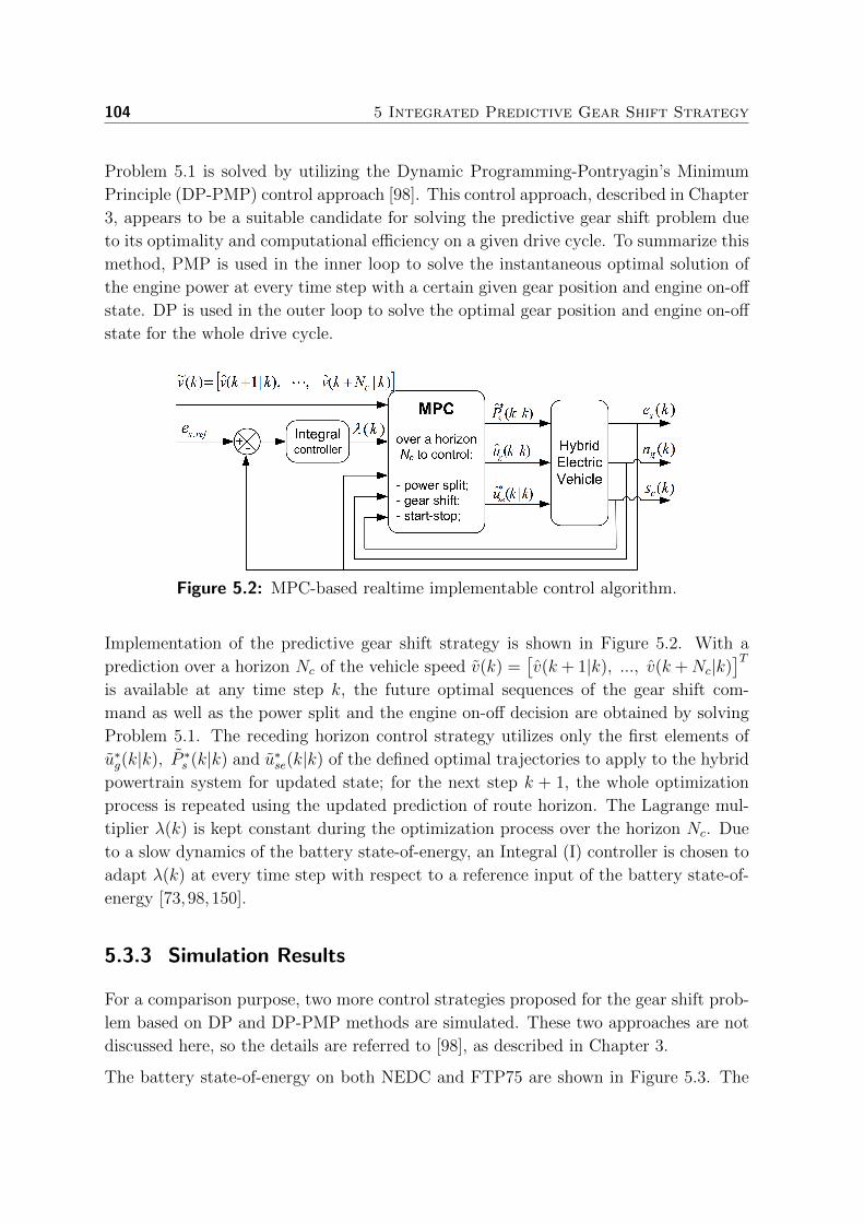
104 5 Integrated Predictive Gear Shift Strategy
Problem 5.1 is solved by utilizing the Dynamic Programming-Pontryagin’s Minimum
Principle (DP-PMP) control approach [98]. This control approach, described in Chapter
3, appears to be a suitable candidate for solving the predictive gear shift problem due
to its optimality and computational efficiency on a given drive cycle. To summarize this
method, PMP is used in the inner loop to solve the instantaneous optimal solution of
the engine power at every time step with a certain given gear position and engine on-off
state. DP is used in the outer loop to solve the optimal gear position and engine on-off
state for the whole drive cycle.
Figure 5.2: MPC-based realtime implementable control algorithm.
Implementation of the predictive gear shift strategy is shown in Figure 5.2. With a
prediction over a horizon Nc of the vehicle speed v(k) =[v(k + 1|k), ..., v(k +Nc|k)
]Tis available at any time step k, the future optimal sequences of the gear shift com-
mand as well as the power split and the engine on-off decision are obtained by solving
Problem 5.1. The receding horizon control strategy utilizes only the first elements of
u∗g(k|k), P ∗s (k|k) and u∗se(k|k) of the defined optimal trajectories to apply to the hybrid
powertrain system for updated state; for the next step k + 1, the whole optimization
process is repeated using the updated prediction of route horizon. The Lagrange mul-
tiplier λ(k) is kept constant during the optimization process over the horizon Nc. Due
to a slow dynamics of the battery state-of-energy, an Integral (I) controller is chosen to
adapt λ(k) at every time step with respect to a reference input of the battery state-of-
energy [73,98,150].
5.3.3 Simulation Results
For a comparison purpose, two more control strategies proposed for the gear shift prob-
lem based on DP and DP-PMP methods are simulated. These two approaches are not
discussed here, so the details are referred to [98], as described in Chapter 3.
The battery state-of-energy on both NEDC and FTP75 are shown in Figure 5.3. The

5.3 Predictive Algorithm 105
0 200 400 600 800 1000 12000.2
0.3
0.4
0.5
0.6
Time (s)
SO
ENEDC
DP
DP−PMP
MPC − Nc=1
MPC − Nc=5
0 200 400 600 800 1000 1200 1400 1600 1800 20000.2
0.3
0.4
0.5
0.6
Time (s)
SO
E
FTP75
Figure 5.3: Battery state-of-energy es(k) on NEDC and FTP75
0 10 20 30 40 50 600
1
2
3
Rel
. fue
l diff
eren
ce [%
]
Control horizon Nc [step−sec]
NEDC
FTP75
(a)
0 10 20 30 40 50 600
500
1000
Cal
cula
tion
time
[s]
Control horizon Nc [step−sec]
NEDC
FTP75
(b)
Figure 5.4: Relative fuel difference [%] and calculation time [s] vs. the controlhorizon Nc are shown in (a) and (b), respectively.
coefficient of the integral controller is properly tuned such that the battery state-of-
energy at the end of drive cycle is equal to its initial value to ensure fair comparisons
among the control approaches. The DP results (the solid lines) almost overlap the results
of the DP-PMP method (the dashed lines), which renders the DP-PMP almost globally
optimal from an engineering point of view. For the predictive gear shift strategy, two
cases of Nc = 1 and Nc = 5 are chosen for demonstration. For the case of Nc = 1 (the
dashed-dotted lines), es(k) is more different from the globally optimal result. Meanwhile

106 5 Integrated Predictive Gear Shift Strategy
for the case of Nc = 5 (the dotted lines), it is very close to the globally optimal result.
The MPC-based approach tends to use as much electric energy as possible to minimize
the fuel cost function over the driving horizon. This results in a more depletion of
SOE corresponding with a shorter horizon. The online-updated Lagrange multiplier
will allow the EMS to bring the battery state-of-energy back to its initial value at the
end of the drive mission.
Figure 5.4a depicts simulation results of the relative fuel difference vs. the control hori-
zon Nc on both NEDC and FTP75. The relative fuel difference is derived by comparing
to the fuel consumption of the predictive gear shift strategy with that of a globally
optimal strategy based on DP. With Nc = 1 (one time step ahead), the maximum rela-
tive fuel difference is 2% on the NEDC. It shows that with Nc ≥ 2, the predictive gear
shift strategy achieves a fuel consumption level almost close to the globally optimal
solution. This reveals that the MPC-based controller can use only the vehicle model
and accelerator pedal position to estimate the next vehicle speed in order to achieve a
significant fuel economy improvement. Moreover, a prediction of the vehicle speed over
a short horizon, for example with a horizon of 5s, is realistic with the current technology
of the onboard navigation firmware. This shows the possibility of implementing such a
controller in realtime without requirement of knowing (a large part of) the drive cycle
a priori.
Figure 5.4b indicates an increased calculation time vs. an increased control horizon Nc
for the predictive gear shift strategy. Nevertheless, the calculation time for all surveyed
cases of Nc is smaller than the time length of the driving profiles. Especially, with a
very short control horizon, e.g. Nc ≤ 10, the fuel consumption is steadily close to the
global optimal solution meanwhile the computation time is very small compared to the
length of the drive profiles. This reveals that the MPC-based gear shift strategy is seen
as a realtime implementable control algorithm from an execution time point of view.
5.4 Velocity Algorithm
Based on the onboard navigation system in combination with the GPS, the obtained
route information is given in the form of a route segment length L, a minimum allowable
speed vmin and a maximum allowable speed vmax. The objective is to propose an
algorithm to derive a fuel-optimal velocity profile over a preview route segment, such
that the vehicle can finish this preview route segment at a given traveling time Nc in
the most fuel efficient way.
5.4 Velocity Algorithm 107
5.4.1 Travel Requirements on a Preview Route Segment
Given the route information, the constraints imposed on the vehicle longitudinal dy-
namics is,
amin ≤ a(k) ≤ amax, (5.18a)
vmin ≤ v(k) ≤ vmax. (5.18b)
wherein amin stands for the highest deceleration rate due to safety condition, and amaxrepresents for the highest acceleration rate due to the powertrain traction capacity and
friction traction.
The traveled distance of the vehicle is defined as,
s(k + 1) = s(k) + v(k)∆t+a(k)
2∆t2,
wherein a(k) is assumed to be constant in the time interval k → k + 1. The end
constraint on traveled distance at the end of horizon is defined as,
s(Nc) = L. (5.19)
5.4.2 Optimal Velocity Problem
For an optimal velocity problem, the hybrid powertrain system are determined
by four state variables v(k), se(k), ng(k), es(k) which are controlled by
a(k), use(k), ug(k), Ps(k), respectively. The powertrain system consists of two contin-
uous and two discrete state variables which make the optimal velocity problem really
challenging for the design of a corresponding solver in terms of the optimality and
computational efficiency. By discretizing all the continuous state and corresponding
control variables and applying Dynamic Programming, the globally optimal solution
can be obtained. Apparently, for the powertrain dynamic system with four state vari-
ables, the ‘curse of dimensionality’ is still a remained issue for the DP algorithm whose
requirements on computational accuracy and efficiency are highly contradictory.
Inspired by the novel control algorithm for the hybrid dynamical system [98], described
in Chapter 3, the concept of combining DP and PMP is utilized to synthesize the solver
for the optimal velocity problem. However, aiming at demonstrating the generation of
an optimal velocity profile over a driving horizon, the engine start-stop and gear shift
strategies are excluded in the problem formulation to reduce the system dimension,
and thus reducing the computational burden for the DP-PMP algorithm. The engine
is assumed to stop and re-start immediately matching with driving conditions, e.g.
electrically driving at low vehicle speed or low power demand, regenerative braking,
engine stop idling, etc. A fuel-efficient gear shift map, discussed in Chapter 4, is applied

108 5 Integrated Predictive Gear Shift Strategy
to shift gears. Therefore, it will render the obtained solution of the corresponding
velocity algorithm suboptimal.
The optimal velocity algorithm is formulated as follows.
Problem 5.2. Given a driving horizon length L with a required traveling time not
longer than Nc, find an optimal control law u∗(k) = [a∗(k), P ∗e (k)], which are the
vehicle acceleration and engine power sequences over the time horizon Nc, that govern
the vehicle to finish the driving horizon in the most fuel economy way, or equivalently
minimize the fuel cost function,
J =N−1∑k=0
mf (k)∆t (5.20)
subject to the constraints (5.2)-(5.8), (5.10), (5.12), (5.14), (5.18) and (5.19).
Problem 5.2 is separated into two problems. The PMP is utilized in the first problem
to define an instantaneous optimal power split between the engine and electric machine.
The DP is applied in the second problem to define an optimal acceleration sequence
over the whole driving horizon.
PMP for optimal power split
Problem 5.3. At a certain time step k, under a certain engine on-off state se(k) and
gear position ng(k), given a possible vehicle speed from vi(k) to vj(k+1), find an optimal
control law of engine power P ∗e (k) that minimizes the instantaneous fuel cost function,
J1(k) = mf (k)∆t, (5.21)
subject to the dynamics and constraints described in (5.2)-(5.8),(5.10).
Assuming with a given admissible gear position ng(k) at any time step k, the constraints
on engine speed and electric machine speed, (5.3a) and (5.5a), are satisfied and the
required power at the wheel Pw(k) can be produced by the powertrain, i.e., by both
the engine and electric machine. The constraints on the electric machine and battery
power (5.5b), (5.7) can be incorporated with the constraints of the engine power (5.3b)
to create the new bounds for the control variable Pe(k), as follows,
P′
e min(k) ≤ Pe(k) ≤ P′
e max(k). (5.22)
The fuel rate (5.2) and battery efficiency model (5.6) can be approximated as affine
piecewise second-order functions of engine power at a certain engine speed, and thus
denoted as Fr(Pe(k), k
):= mf (k) and Ps
(Pe(k), k
):= Ps(k) for compact notations.

5.5 Implementation of the Velocity Algorithm 109
Applying the PMP method, the objective is to find an instantaneous optimal engine
power P ∗e (k) > 0 that minimizes an equivalent fuel cost functional Ceq(k),
Ceq(k) =[Fr(Pe(k), k
)+ λ(k) · Ps
(Pe(k), k
)]·∆t, (5.23)
Therefore, if the Lagrange multiplier λ(k) is known, the globally instantaneous optimal
engine power P ∗e (k) can be obtained analytically. The globally instantaneous equivalent
optimal cost value is defined correspondingly by
C∗eq(k) =[Fr(P ∗e (k), k
)+ λ(k) · Ps
(P ∗e (k), k
)]·∆t. (5.24)
DP for optimal acceleration sequence
Problem 5.4. Find an optimal acceleration profile a∗(k), resulting in an optimal ve-
locity profile v∗(k), along the driving horizon that minimizes the cost functional,
J2 =N−1∑k=0
C∗eq(k) (5.25)
subject to constraints: (5.12), (5.14), (5.18) and (5.19).
The implementation of the DP algorithm is performed by discretizing the state variable
v(k) and the corresponding control variable a(k), and then calculating the cost func-
tional J2 for the whole driving profile. The optimal cost-to-go path is solved backwards
as the following steps.
• Step k = Nc:
J ∗2 (Nc) = 0. (5.26)
• Step k, 0 ≤ k < N :
J ∗2(vi(k), k
)= min
aij(k)
[C∗eq(k) + J ∗2
(vj(k + 1), k + 1
)]. (5.27)
Solving the above procedure backward until k = 0, the optimal solutions of a∗(k) and
v∗(k) are obtained correspondingly with a specific end value of v(Nc).
5.5 Implementation of the Velocity Algorithm
5.5.1 Discretization of Vehicle Longitudinal Dynamics
To apply DP for Problem 5.4, the control variable for the vehicle dynamics is required
to be discretized. From the constraint (5.18a), the deceleration and acceleration grid

110 5 Integrated Predictive Gear Shift Strategy
vectors are defined with a grid step δa as,
Adec = {amin, amin + δa, . . . , −δa}, (5.28)
Aacc = {δa, . . . , amax − δa, amax}. (5.29)
For any pair of adec ∈ Adec and aacc ∈ Aacc, the grid space agrid of control variable a(k)
is formed
agrid = {adec, adec − δa, . . . , 0, . . . , aacc − δa, aacc}, (5.30)
If we define δv = δa∆t, taking into account the velocity constraint (5.18b), the grid
space of velocity vgrid is thus in the form,
vgrid = {vmin, vmin + δv, . . . , vmax − δv, vmax}. (5.31)
Furthermore, the velocity grid vgrid(k) at any time step k is reduced further by recon-
structing the minimum speed vmin(k) and maximum speed vmax(k) as follows,
vmin(k) = max{vmin(k − 1) + amin∆t, 0
}, (5.32)
vmax(k) = min{vmax(k − 1) + amax∆t, vmax
}. (5.33)
5.5.2 Decoupling of Velocity Algorithm
Due to a coupling of the vehicle acceleration and drive power demand, solving Problem
5.2 by separating it into Problems 5.3 and 5.4, and solving them by the PMP and DP
respectively, does not guarantee a globally optimal solution.
The vehicle acceleration determines the drive power demand, which influences the power
split and thus directly affecting the fuel consumption in (5.21). Meanwhile the vehicle
acceleration influences the longitudinal dynamics, as in (5.14). Therefore, to ensure
an optimality when decoupling Problem 5.2, an equivalent factor, denoting a rate of
change of the vehicle acceleration a(k) with respect to a change of the instantaneous
equivalent fuel cost functional C∗eq(k), must be defined. Furthermore, to satisfy the end
constraint on traveled distance (5.19), it requires the solver to know the rate of change
of the instantaneous equivalent fuel cost functional C∗eq(k) with respect to a change of
the vehicle speed v(k).
An alternative technique is introduced to deal with this coupling in the DP algorithm.
The lower and upper bounds on agrid are varied by changing the values of adec and
aacc. Then, construct a boundary region of the feasible traveled distance profiles along
the preview route segment, such that any traveled profile falling within this region will
meet the constraints (5.18) and (5.19). The upper bound is constructed based on the
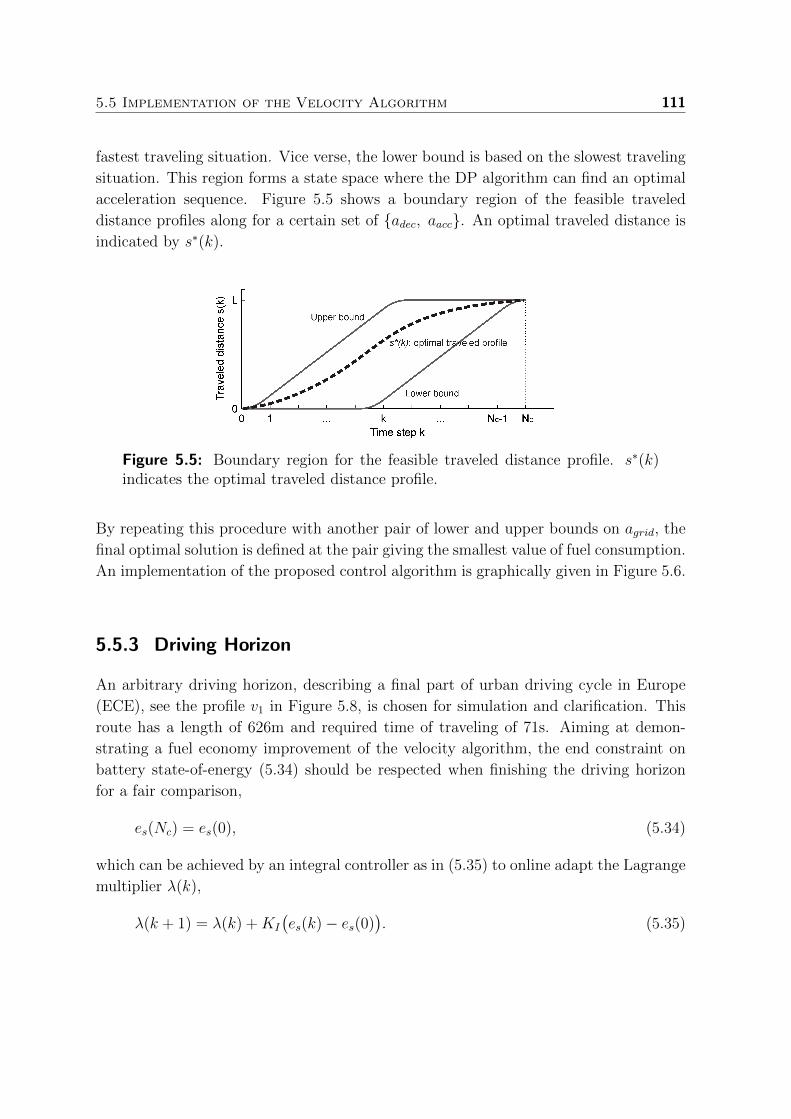
5.5 Implementation of the Velocity Algorithm 111
fastest traveling situation. Vice verse, the lower bound is based on the slowest traveling
situation. This region forms a state space where the DP algorithm can find an optimal
acceleration sequence. Figure 5.5 shows a boundary region of the feasible traveled
distance profiles along for a certain set of {adec, aacc}. An optimal traveled distance is
indicated by s∗(k).
Figure 5.5: Boundary region for the feasible traveled distance profile. s∗(k)indicates the optimal traveled distance profile.
By repeating this procedure with another pair of lower and upper bounds on agrid, the
final optimal solution is defined at the pair giving the smallest value of fuel consumption.
An implementation of the proposed control algorithm is graphically given in Figure 5.6.
5.5.3 Driving Horizon
An arbitrary driving horizon, describing a final part of urban driving cycle in Europe
(ECE), see the profile v1 in Figure 5.8, is chosen for simulation and clarification. This
route has a length of 626m and required time of traveling of 71s. Aiming at demon-
strating a fuel economy improvement of the velocity algorithm, the end constraint on
battery state-of-energy (5.34) should be respected when finishing the driving horizon
for a fair comparison,
es(Nc) = es(0), (5.34)
which can be achieved by an integral controller as in (5.35) to online adapt the Lagrange
multiplier λ(k),
λ(k + 1) = λ(k) +KI
(es(k)− es(0)
). (5.35)
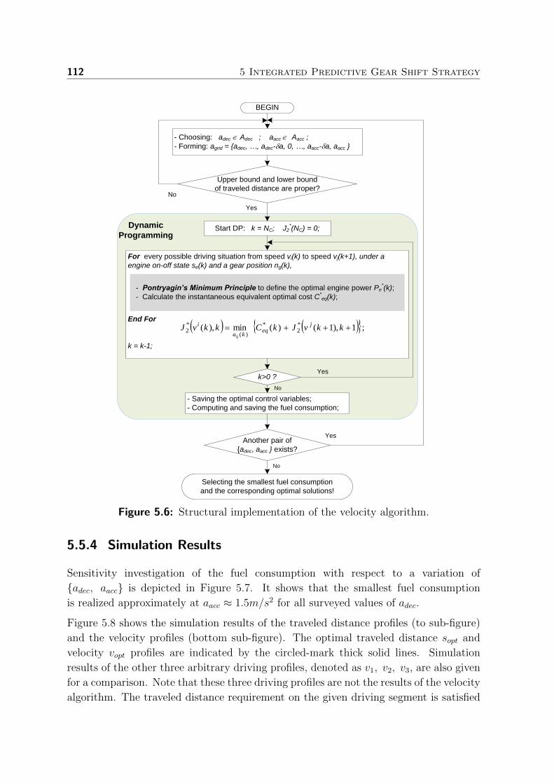
112 5 Integrated Predictive Gear Shift Strategy
BEGIN
- Choosing: adec Adec ; aacc Aacc ;
- Forming: agrid = {adec, …, adec-a, 0, …, aacc-a, aacc }
Upper bound and lower bound
of traveled distance are proper?
Dynamic
ProgrammingStart DP: k = NC; J2
*(NC) = 0;
k>0 ?Yes
For every possible driving situation from speed vi(k) to speed vj(k+1), under a
engine on-off state se(k) and a gear position ng(k),
End For
k = k-1;
;1),1()(min),( *2
*
)(
*2 kkvJkCkkvJ j
eqka
i
ij
Yes
- Saving the optimal control variables;
- Computing and saving the fuel consumption;
Another pair of
{adec, aacc } exists?
Selecting the smallest fuel consumption
and the corresponding optimal solutions!
Yes
No
No
No
- Pontryagin’s Minimum Principle to define the optimal engine power Pe*(k);
- Calculate the instantaneous equivalent optimal cost C*eq(k);
Figure 5.6: Structural implementation of the velocity algorithm.
5.5.4 Simulation Results
Sensitivity investigation of the fuel consumption with respect to a variation of
{adec, aacc} is depicted in Figure 5.7. It shows that the smallest fuel consumption
is realized approximately at aacc ≈ 1.5m/s2 for all surveyed values of adec.
Figure 5.8 shows the simulation results of the traveled distance profiles (to sub-figure)
and the velocity profiles (bottom sub-figure). The optimal traveled distance sopt and
velocity vopt profiles are indicated by the circled-mark thick solid lines. Simulation
results of the other three arbitrary driving profiles, denoted as v1, v2, v3, are also given
for a comparison. Note that these three driving profiles are not the results of the velocity
algorithm. The traveled distance requirement on the given driving segment is satisfied

5.5 Implementation of the Velocity Algorithm 113
0 0.5 1 1.5 2 2.5
−2.5−2−1.5−1−0.5013.5
14
14.5
15
15.5
aacc
[m/s2]adec
[m/s2]
Fue
l con
sum
ptio
n [g
]
Figure 5.7: Sensitivity study of the fuel consumption with respect to a variationof {adec, aacc}.
0 10 20 30 40 50 60 700
200
400
600
Tra
vele
d di
stan
ce [m
]
Time [s]
sopt
s1
s2
s3
0 10 20 30 40 50 60 700
5
10
15
Time [s]
Vel
ocity
[m/s
]
vopt
v1
v2
v3
Figure 5.8: Comparison of the optimal driving profile (circled-mark thick solidline) with other three profiles along the given route segment.
by the four driving profiles (top sub-figure). The optimal velocity profile possesses a
moderate acceleration and the smallest deceleration. Its deceleration phase lasts longer
than the other three to take advantage of regenerative braking.
As given in Table 5.2, the fuel economy of the driving profile v1 is 11.5% lower compared
with that of the optimal profile vopt. Meanwhile, for the other two arbitrary driving
profiles v2 and v3, a severe reduction in fuel economy is 15.1% and 16.5%, respectively.
The end constraint of the battery state-of-energy is guaranteed by the condition |∆es| =|es(Nc)−es(0)|/es(0)∗100 < 1%. Although, the optimal velocity problem is partly solved
using a surface response model to find an optimal setting for the bounds on agrid, and
creates a suboptimal solution, it shows a significant fuel economy improvement.

114 5 Integrated Predictive Gear Shift Strategy
Table 5.2: Fuel consumption of four driving profiles along the route segment.
Profile |∆es| [%] Fuel [g] Fuel economy [%]
vopt 0.5 14.14 baselinev1 (ECE) 0.6 15.76 -11.5
v2 0.6 16.28 -15.1v3 0.8 16.48 -16.6
5.6 Integrated Predictive Gear Shift Strategy
A concept of an integrated predictive gear shift strategy for the transmission equipped
in a HEV is created by i) embedding the velocity algorithm on an onboard navigation
system, ii) implementing the predictive algorithm for a corresponding EMS. Output
of the onboard navigation system is a prediction of the velocity profile over a driving
horizon. This prediction information is put into the EMS based on the predictive
algorithm controlling the gear shift besides the engine on-off decision and power split
strategy. Figure 5.9 graphically demonstrates this concept. Validated by a fuel economy
improvement for each separated algorithm, the concept is proved to work in principle.
Figure 5.9: Schematic diagram of the concept of integrated predictive gear shiftstrategy.
5.7 Conclusions 115
5.7 Conclusions
In this study, a concept of integrated predictive gear shift strategy for the transmission
equipped in a HEV was demonstrated and validated in simulation environment. Despite
the fact of being not globally optimal, the velocity algorithm significantly improves the
fuel economy for the HEV by proposing an optimized velocity profile for the vehicle to
follow. The predictive algorithm successfully utilizes a short preview horizon to realize a
fuel economy improvement very close to that of the globally optimal control algorithm.
Future work should focus on implementing the velocity algorithm on a preview route
segment with a relatively short horizon, e.g. an acceleration phase, a cruise phase or
a deceleration phase, etc., to analyze the effect of the horizon length on the optimal
solution. Upgrading the velocity algorithm such that it is able to handle with a free
final state of the vehicle speed and battery state-of-energy (at the end of each driving
horizon) is also required. This makes the upgraded velocity algorithm applicable for a
certain driving mission consisting of consecutive fuel-optimal driving segments, while
still achieving a desired finishing time.

116

Chapter 6
Effect of Gear Shift and Engine StartLosses1
Abstract - In this study, the energetic loss models involved with gear shift and engine start ina parallel Hybrid Electric Vehicle (HEV) equipped with an Automated Manual Transmission(AMT) will be introduced. An optimal control algorithm for the start-stop, power splitand gear shift problem based on the Dynamic Programming-Pontryagin’s Minimum Principlecontrol approach is utilized to evaluate the effect of the gear shift and engine start losseson the optimal solution. Furthermore, with preview route information available, a ModelPredictive Control (MPC) algorithm is applied to investigate an achievable fuel saving withrespect to the prediction horizon. Under the influence of the gear shift loss, simulation resultsof a passenger HEV disclose a superior fuel efficient property of the powershift-AMT over theAMT. It also shows that by reducing the interruption time in the gear shift process as muchas possible, the AMT vehicle can reduce the fuel consumption noticeably compared to thePS-AMT vehicle. The study also reveals a minimum prediction length of 5s required for thedesign of a MPC-based realtime implementable controller to get the possible maximum fueleconomy under the impact of the engine start loss.
6.1 Introduction
Design of the Energy Management Strategies (EMSs) for Hybrid Electric Vehicles
(HEVs) in general aims at optimally choosing the power split between the internal
combustion engine and electric machine to improve the fuel economy, for example
see, [3, 25, 50, 63, 67, 73, 83, 96, 98, 107, 118, 125, 126, 134, 156]. For HEVs equipped with
discrete ratio transmissions, e.g. an Automated Manual Transmission (AMT), the oper-
ating points of the hybrid powertrain are not only defined by the power split but also by
1This chapter has been prepared for a journal publication in the form as: V. Ngo, T. Hofman, M.Steinbuch, A. Serrarens. Effect of Gear Shift and Engine Start Losses on Control Strategies for HybridElectric Vehicles. 2012.
117

118 6 Effect of Gear Shift and Engine Start Losses
the start-stop state and gear position. Hence, by further optimizing the start-stop and
gear shift strategies, the fuel economy is improved substantially compared to the EMSs
optimizing only the power split. Consequently, the controller allows i) the transmission
to shift up earlier with higher frequency and to higher values, and ii) the engine to stop
and restart more frequently, for a fuel benefit [3,25,63,67,83,96,98,107,118,125,134,156].
At a gear shift or engine start event, an amount of energy related to clutch slippage,
vehicle velocity loss during shifting, and engine cranking, is lost. So, it is worthwhile to
concern these losses when the number of shifts and starts is at a considerable amount
for a certain drive cycle. However, none of the mentioned published papers has been
addressing the relevant gear shift and engine start losses, and thus analyzing their effect
on the control strategies and fuel consumption. Therefore, this study will focus on these
challenges.
Regarding to the gear shift, a shift decision will encounter a change of the engine rotating
dynamics, a possible clutch operation loss and a consequent vehicle velocity loss due to
an interrupted tractive torque. Hence, compensation for the gear shift loss might cost
additional fuel. For a decision of restarting the engine, apart from the tractive torque
required at the wheels, an extra torque from the electric machine is needed for cranking
up the engine from stand still and compensating the friction loss in the clutch. This
would consume an amount of electric energy which sometime later can cost fuel for
recharging. Engine combustion takeover after the cranking phase for each engine start
process should also be considered. In summary, on highly dynamic drive cycles with
frequent stop-go patterns, the number of gear shifts and engine restarts will increase.
Hence, the fuel consumption might increase.
Therefore, this study will bring the aforementioned aspects, regarding to the losses of
shifting gears and restarting engine, into the EMS [98] to analyze their influence on
the fuel economy. It’s worthwhile to mention that the proposed EMS for a parallel
HEV equipped with an AMT, optimally control not only the power split but also the
engine start-stop and gear shift. The control algorithm based on a combination of Dy-
namic Programming (DP) and Pontryagin’s Minimum Principle (PMP) guarantees an
optimality and is computationally efficient. First of all, a sensitivity study of the fuel
economy with respect to the gear shift command is conducted towards a gear shift hys-
teresis strategy implementation to get rid of the shift busyness and hunt. A gear shift
loss model capturing the main shifting characteristics is introduced and incorporated
in the EMS for a fuel economy evaluation. Then, a sensitivity study with respect to
the interruption time of tractive torque during a gear shift process reveals a perception
of a fuel-efficient advantage of the powershift transmissions (Dual Clutch Transmis-
sion (DCT), PowerShift-AMT (PS-AMT) [132], etc.) compared to non-powershift ones
(Manual Transmission (MT), AMT). In addition, an engine start loss model correspond-
ing to the prototype HEV is built and embedded in the EMS design to reflect its effect
on fuel consumption. Moreover, Model Predictive Control (MPC) for the HEV appears

6.2 Hybrid Powertrain Model 119
to be a possible candidate for a realtime implementation when using preview route in-
formation [96]. Therefore, the impact of the prediction horizon length on the achievable
fuel saving of the HEV with the engine start loss modeled will be investigated for this
realtime implementable control algorithm.
The content of this research work is organized as follows. The hybrid powertrain model
is given in Section 6.2. The optimal control problem for the engine start-stop decision,
power split and gear shift strategies is formulated in Section 6.3. Gear shift loss model
and its influence on the fuel economy will be discussed in Section 6.4. Engine start loss
model and the related optimal control problem are addressed in Section 6.5. Prediction
horizon length sensitivity study on the fuel economy resulted from the corresponding
predictive control algorithm under the impact of engine start loss is given in Section
6.6. Finally, conclusions are given in Section 6.7.
6.2 Hybrid Powertrain Model
Aiming at deriving an EMS, the quasi-static models of the powertrain components are
used and simulated with a time step of one second. The system dynamics faster than
1Hz are ignored [42]. The clutch system is considered as a discrete switch to connect
and to disconnect the engine immediately to and from the driveline. The energy losses
during the clutching process of the gear shift and engine start are addressed explicitly
in Sections 6.4 and 6.5, respectively.
Figure 6.1: A parallel hybrid electric vehicle topology, (AMT: Automated Man-ual Transmission; M: Electric machine).
The start-stop system can be modeled by using a discrete state variable se(k) to repre-
sent the engine on-off state,
se(k) =
{1 if engine on,
0 if engine off.(6.1)
We ignore the engine drag torque during deceleration phase due to a disconnection of

120 6 Effect of Gear Shift and Engine Start Losses
the engine from the driveline and the engine is shut down. For a certain engine speed
ωe(k), the fuel consumption model is approximated as an affine piece-wise second order
function of the engine power Pe(k). The fit coefficients a0, a1, and a2 are dependent on
the engine speed,
mf
(Pe(k), k
)≈(a0P
2e (k) + a1Pe(k) + a2
)se(k). (6.2)
The electric machine efficiency ηm is assumed to be constant. Therefore the power Pm(k)
flowing in and out of the electric machine in motoring mode and generating mode is
expressed as follows,
Pm(k) = ηm Pelec(k) (if motoring);
Pm(k) =1
ηmPelec(k) (generating).
(6.3)
We assume the battery state-of-energy es(k) to be in a nominal range [Es,min, Es,max]
such that its effect to the battery efficiency model can be ignored. Hence, the electrical
power Pelec(k) can be approximated as a quadratic function of the chemical power Ps(k)
as,
Pelec(k) ≈ b0P2s (k) + b1Ps(k) + b2. (6.4)
The gearbox efficiency model is assumed to be constant η for all gears. The torque and
speed relations in the driveline (the clutch is closed) are given by,
Tw(k) = Tg(k) rg(k) η, (6.5)
ωw(k) =ωm(k)
rg(k), ωm(k) = ωg(k), (6.6)
where Tw(k) is the transferred torque at the wheels (assumed equal to output torque
of the transmission); Tg(k) is the input torque of the transmission; rg(ng(k)
)denotes
the discrete gear ratio depending on the gear position ng(k); ωw(k) is the wheel speed;
ωm(k) is the electric machine speed and ωg(k) is the transmission input speed.
At any time step k, the power flow equilibrium in the parallel hybrid powertrain topology
is expressed as,
Pe(k) = Pg(k) + Pm(k), (6.7)
with Pg(k) is the power flow at the transmission input.
The vehicle longitudinal motion dynamics in discrete time domain is given by,
ωw(k + 1) = ωw(k) +1
Jv,eq
(Tw(k)− Fload(k)Rw
)∆t, (6.8)

6.3 Hybrid Powertrain Control Algorithm 121
where Fload is the resistance loads due to rolling and aerodynamic resistances; Jv,eq is
an equivalent vehicle inertia at the wheel,
Jv,eq =((Je + Jc + Jp)r
2g + Js
)r2d +mvR
2w,
Fload = crmvg cosα +mvg sinα +1
2ρaAfcdv
2,
and mv is the vehicle weight; Rw is the wheel radius; Je is the engine inertia; Jc is the
clutch inertia; Jp is the transmission primary inertia; Js is the transmission secondary
inertia; ρa is the air density; Af is the frontal area of vehicle; cd is the aerodynamic
drag coefficient; cr is the rolling friction coefficient; g is the gravity coefficient; v is the
vehicle speed; α is the slope of the road.
6.3 Hybrid Powertrain Control Algorithm
6.3.1 Optimal Control Problem Formulation
Problem 6.1. Given a drive cycle v(k) with a time length of N , implying that the
vehicle longitudinal dynamics (6.8) is deterministic, find an optimal control law u∗(k) =[u∗se(k), P ∗s (k), u∗g(k)
], which are the optimal control variables for the start-stop system,
battery state-of-energy, and gear shift, respectively, that minimize the fuel cost function
described by,
J =N−1∑k=0
mf
(Pe(k), ωe(k), k
)∆t, (6.9)
subject to:
1. the hybrid powertrain dynamics,
se(k + 1) = se(k) + use(k), (6.10)
es(k + 1) = es(k) + Ps(k)∆t, (6.11)
ng(k + 1) = ng(k) + ug(k), (6.12)
2. the constraints on the speeds of the drivetrain components,
ωe,min ≤ ωe(k) ≤ ωe,max, (6.13a)
0 ≤ ωm(k) ≤ ωm,max, (6.13b)

122 6 Effect of Gear Shift and Engine Start Losses
3. the constraints on the engine power Pe(k), electric machine power Pm(k) and
battery power Ps(k) are,
0 ≤ Pe(k) ≤ Pe,max(ωe(k)
), (6.14a)
Pm,min(ωm(k)
)≤ Pm(k) ≤ Pm,max
(ωm(k)
), (6.14b)
Ps,min ≤ Ps(k) ≤ Ps,max, (6.14c)
4. the constraints on the system states, which are the engine start-stop state and gear
position,
0 ≤ se(k) ≤ 1, (6.15)
1 ≤ ng(k) ≤ 6, (6.16)
here, note that the constraints on the engine on-off state are described by (6.1).
5. the end constraint of the battery state-of-energy,
es(N) = es(0) +N−1∑k=0
Ps(k)∆t = es(0), (6.17)
6. the constraints on the control variables,
use(k) =
{[0, 1] if se(k) = 0,
[−1, 0] if se(k) = 1;(6.18)
ug(k) ∈{ug,min, · · · ,−1, 0, 1, · · · , ug,max
}, (6.19)
wherein ∆t is the time step of the discrete system; ug,min and ug,max are the lower and
upper bounds for the gear shift command ug(k).
In this study, the upper and lower bounds of the state variable es(k) are ignored by
an assumption that the battery capacity Es,cap is chosen properly such that es(k) never
exceeds its bounds for increasing the battery lifetime and reliable operation. Battery
operating temperature is assumed to be under tight control.
Dynamic Programming-Pontryagin’s Minimum Principle (DP-PMP) control approach,
described in Chapter 3, appears to be a suitable candidate to solve the formulated
optimal control problem. For further details of this approach, interested readers are
referred to [98]. In summary, PMP is used in the inner loop to solve the instantaneous
optimal solution of the battery power (or the engine power alternatively) at every time
step with a certain gear position and engine on-off state. DP is used in the outer loop
to solve the optimal gear position and the engine on-off state for the whole drive cycle.
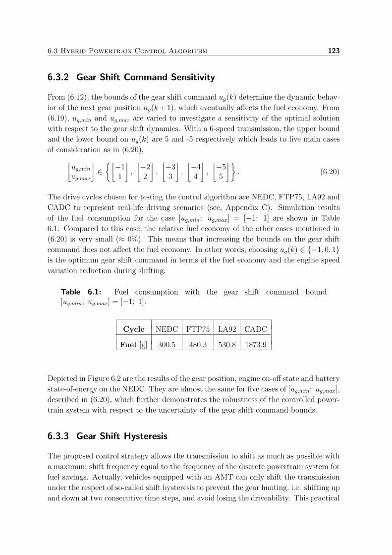
6.3 Hybrid Powertrain Control Algorithm 123
6.3.2 Gear Shift Command Sensitivity
From (6.12), the bounds of the gear shift command ug(k) determine the dynamic behav-
ior of the next gear position ng(k+ 1), which eventually affects the fuel economy. From
(6.19), ug,min and ug,max are varied to investigate a sensitivity of the optimal solution
with respect to the gear shift dynamics. With a 6-speed transmission, the upper bound
and the lower bound on ug(k) are 5 and -5 respectively which leads to five main cases
of consideration as in (6.20),[ug,minug,max
]∈{[−11
],
[−22
],
[−33
],
[−44
],
[−55
]}. (6.20)
The drive cycles chosen for testing the control algorithm are NEDC, FTP75, LA92 and
CADC to represent real-life driving scenarios (see, Appendix C). Simulation results
of the fuel consumption for the case [ug,min; ug,max] = [−1; 1] are shown in Table
6.1. Compared to this case, the relative fuel economy of the other cases mentioned in
(6.20) is very small (≈ 0%). This means that increasing the bounds on the gear shift
command does not affect the fuel economy. In other words, choosing ug(k) ∈ {−1, 0, 1}is the optimum gear shift command in terms of the fuel economy and the engine speed
variation reduction during shifting.
Table 6.1: Fuel consumption with the gear shift command bound[ug,min; ug,max] = [−1; 1].
Cycle NEDC FTP75 LA92 CADC
Fuel [g] 300.5 480.3 530.8 1873.9
Depicted in Figure 6.2 are the results of the gear position, engine on-off state and battery
state-of-energy on the NEDC. They are almost the same for five cases of [ug,min; ug,max],
described in (6.20), which further demonstrates the robustness of the controlled power-
train system with respect to the uncertainty of the gear shift command bounds.
6.3.3 Gear Shift Hysteresis
The proposed control strategy allows the transmission to shift as much as possible with
a maximum shift frequency equal to the frequency of the discrete powertrain system for
fuel savings. Actually, vehicles equipped with an AMT can only shift the transmission
under the respect of so-called shift hysteresis to prevent the gear hunting, i.e. shifting up
and down at two consecutive time steps, and avoid losing the driveability. This practical

124 6 Effect of Gear Shift and Engine Start Losses
0 200 400 600 800 1000 12000
2
4
6n g [−
]
0 200 400 600 800 1000 1200
0
1
s e [−]
0 200 400 600 800 1000 12000.2
0.3
0.4
0.5
0.6
Time [s]
SO
E [−
]
Figure 6.2: Simulation results on the NEDC for five cases of the gear shiftcommand bounds [ug,min; ug,max].
issue can be implemented into the EMS by imposing a constraint of not changing gear
within nhys time steps after each previous shifting, described by a general shift condition,
general shift condition
uhys = ug(k − nhys) + · · ·+ ug(k − 1);
if uhys == 0ug(k) ∈ {−1, 0, 1},
elseug(k) = 0,
end
This means that a gear shift decision can be only made when a hysteresis time nhys is
respected. The powertrain dynamic system for control will increase in dimension by an
order of nhys−1. Therefore, nhys > 1 will make the control system more complicated and
affect to the computation load of the control algorithm. Hence, in this study nhys = 1
is adopted for a reasonable compromise, which leads to a simplified shift hysteresis
condition as in (6.21),
ug(k − 1)ug(k) = 0. (6.21)
Simulation results are given in Table 6.2. The relative difference of the shift hysteresis
case compared to the baseline is indicated in the parenthesis. It depicts that the shift
hysteresis strategy reduces the number of shifts significantly, meanwhile the fuel econ-

6.4 Gear Shift Loss Model and Control Problem 125
Table 6.2: Simulation results corresponding with a study on the gear shifthysteresis. Relative difference is indicated in the parenthesis
CycleBaseline Shift hysteresis
Fuel [g] No. shift Fuel [g] No. shift
NEDC 300.5 73 301.8 (0.4%) 71 (-2.7%)
FTP75 480.3 423 481.5 (0.3%) 197 (-53.4%)
LA92 530.8 358 531.8 (0.2%) 179 (-50%)
CADC 1873.9 651 1876.2 (0.1%) 244 (-62.5%)
omy impact is small. The obtained results reveal an essential role of the shift hysteresis
in removing the unnecessary shifts not affecting the fuel economy considerably.
6.4 Gear Shift Loss Model and Control Problem
The gear shift process of an AMT-based vehicle includes three chronological phases:
1) disengaging the clutch and lowering the engine torque; 2) shifting to the expected
gear; and 3) engaging the clutch while increasing the engine torque again. The speed
and torque profiles of both clutch and engine during the shifting process are assumed
to be properly controlled in every phase to ensure quick shifting, more comfort and and
less friction losses, etc. [39, 132]. The energetic loss model involved with the gear shift
process is described next.
6.4.1 Gear Shift Loss Model
A decision of shifting gears is meaningful when the vehicle is in acceleration or cruising
modes, wherein the engine is used as a primary mover to meet the required positive
drive torque at the wheels. The transmission can: i) shift up to accommodate the
engine speed to the changing vehicle speed and improve the fuel economy, or ii) even
shift down, called kick-downshift, if a higher acceleration or driving uphill is required.
During electrically driving mode (the electric machine is used to solely propel the ve-
hicle) or deceleration mode (the electric machine operates as a generator to recuperate
the kinetic energy), the hybrid powertrain with a start-stop functionality can turn the
engine off and disconnect it from the driveline. The clutch is opened. Apparently, there
is no slippage phenomena in clutch which leads to no energy loss involved. The gear

126 6 Effect of Gear Shift and Engine Start Losses
shift during these driving modes can be assumed to occur immediately.
In summary, only upshift and kick-downshift events are considered for modeling the
gear shift loss which is described next.
Upshift
Figure 6.3a demonstrates the simplified uniform profiles of the speed and torque of the
engine and clutch in an upshift process. Three phases of the shifting process occurring in
the interval ∆tshift are indicated. In phases 1 (disengagement) and 3 (engagement), the
engine torque and clutch transferred torque are controlled to have a declined and inclined
patterns to allow a comfort disengagement and engagement, respectively. Hence, there
exists a slippage phenomena at the clutch to transfer the tractive torque to the wheels
during these phases. The speed difference between the engine and clutch during these
phases is small enough, thus assuming to be zero [34,39,132,165]. In phase 2, the clutch
is fully disengaged for shifting gears, and there is an interruption of the tractive torque
which finally results in a velocity loss for an interval ∆tint. Due to the engine drag
torque, the engine speed is assumed to reduce to a synchronization point corresponding
to the clutch speed at the next higher gear. Denoting the engine torque right before
and after shifting is Te, then the engine torque and tractive torque transferred to the
wheels during an upshift process can be modeled as,
• in phases 1, 2 and 3, the corresponding engine torque can be averaged as,
Te,1 =Te2,
Te,2 = 0,
Te,3 =Te2
;
(6.22)
• the average tractive torque transferred to the wheels during an upshift process
(due to a clutch slippage in phases 1 and 3),
Te,shift =Te2
∆tshift −∆tint2∆tshift
. (6.23)
Kick-downshift
Figure 6.3b shows the typical profiles of the engine and clutch torque for a kick-downshift
process [34, 39, 132,165]. It also consists of three phases. In phases 1 and 3, the engine
and clutch torque profiles are similar to an upshift. In phase 2, the clutch torque is
zero, meanwhile the engine torque is maintained above zero to increase the engine speed

6.4 Gear Shift Loss Model and Control Problem 127
(a) (b)
Figure 6.3: Simplified engine and clutch profiles during an upshift process (a),and a kick-downshift process (b).
up to the synchronization point corresponding to the clutch speed at next lower gear.
Hence the engine torque and tractive torque transferred to the wheels during an upshift
process can be modeled as,
• in phases 1, 2 and 3, the corresponding engine torque can be averaged as,
Te,1 =Te + Te,2
2,
Te,2 = Jeωe,3 − ωe,1
∆tint,
Te,3 =Te + Te,2
2,
(6.24)
where Je is the equivalent inertia on the engine side (seen from the clutch); ωe,1is the engine speed in phase 1 (right before shifting); ωe,3 is the engine speed in
phase 3 (right after shifting);
• the average tractive torque transferred to the wheels during a kick-downshift pro-
cess (due to a clutch slippage in phases 1 and 3),
Te,shift =Te + Te,2
2
∆tshift −∆tint∆tshift
. (6.25)
Note that the engine torque in phase 2 does not constitute the tractive torque, but it
still results in additional fuel consumption.
Velocity tracking loss
As analyzed in the upshift and kick-downshift and demonstrated in Figure 6.3, the
tractive torque is totally lost during phase 2 of the shifting process due to a clutch

128 6 Effect of Gear Shift and Engine Start Losses
opening. During phases 1 and 3, the tractive torque transferred to the wheels is defined
by (6.23) and (6.25). Taking all these tractive torque characteristics into account will
result in a velocity loss for each upshift or kick-downshift event. Therefore, the vehicle
needs to accelerate more, later in the driving mission, in order to compensate for the
loss in each gear shift. This will definitely influence the fuel economy of the vehicle.
Apparently, the length of the power interruption in phase 2, denoted by ∆tint, mainly
decide the effect level of the gear shift loss on the vehicle performance. In reality,
the interruption time ∆tint is varied according to the types of vehicles and the clutch
operation conditions [39,132]. Therefore, a sensitivity study with respect to ∆tint should
be done for a thorough analysis of the gear shift loss effect.
6.4.2 Optimal Control Problem with Gear Shift Loss
The design of EMSs for AMT-based HEVs always assumes the gear shift to occur
instantly, which means that there is no torque interruption at the wheels when shifting
and the vehicle keeps tracking the velocity and acceleration profiles. This is only true
when the transmission possesses a powershift technology, e.g. PS-AMT, DCT, AT, etc.,
to enable the tractive torque to be transferred to the wheels during shifting. As said
for AMTs, the consequence of a gear shift activity is loss of velocity tracking. To arrive
the final destination on time, the vehicle must accelerate more after each gear shift to
compensate for the velocity loss accumulated during shifting.
As shown in Section 6.3.3, the optimal control strategy for the HEV yields many shifts
for fuel economy improvement. Therefore, it’s a fair evaluation to include AMT gear
shift loss model to the fuel-optimal EMS. Note that, as a consequence of the velocity
tracking loss, the vehicle can not exactly follow a given drive cycle, and thus the next
vehicle speed is gear shift dependent. An EMS optimizing further the driving profile
(velocity, traveled time) [93,151] is an appropriate solution for the control problem with
the gear shift loss model involved. Such a control algorithm is complicated and out of
scope of this study. In order to cope with the velocity tracking loss, an appropriate
approach to investigate effect of the gear shift loss on fuel economy and evaluate power-
shift technology is introduced as follows.
PS-AMT : the EMS is designed with no gear shift loss model taken into account. This
means the AMT has a powershift technology to ensure a velocity tracking. The designed
EMS optimizes the engine on-off state, power split and gear shift.
AMT : the hybrid powertrain is equipped with an AMT. The gear shift loss model
is respected during the design process of the EMS. The optimal gear shift strategy
obtained from the PS-AMT is now used as a prescribed one for the AMT. To ensure
the same average speed with the PS-AMT in order to get a fair comparison on the fuel
economy, the next vehicle speed is controlled by an integral regulator. The powertrain

6.4 Gear Shift Loss Model and Control Problem 129
is simulated in a forward-facing manner and the EMS optimizes the engine on-off state
and power split.
6.4.3 Simulation Results
The gear shift hysteresis strategy is taken into account in the case of the PS-AMT to
avoid any gear shift hunting pattern. Figure 6.4 depicts a zoom-in of one part of the
simulation results on the NEDC. It can be seen that when an upshift occurs, the AMT
vehicle losses velocity tracking, represented by the corresponding flat vehicle speed (the
dotted line). Right after each upshift, the AMT vehicle accelerates higher than the PS-
AMT vehicle to compensate for the velocity tracking loss during the gear shift before.
48 52 56 60 640
2
4
6
n g [−]
48 52 56 60 640
20
40
Time [s]
v [k
m/h
]
PS−AMT
AMT
Figure 6.4: Zoom-in on the NEDC of the velocity tracking for the PS-AMT vs.the AMT.
Sensitivity study of the relative fuel difference (by comparing the fuel consumption
of the AMT vehicle with that of the PS-AMT vehicle) with respect to a variation
in interruption time ∆tint over the tested drive cycles is shown in Figure 6.5. The
interruption is varied as,
∆tint ∈ {0.3, 0.4, 0.5, 0.6, 0.7, 0.8, 0.9, 1}[s] (6.26)
to reflect the possible interruption time of the actual gear shift activity. Herein ∆tint =
0.3s represents the possible smallest time of actuating the synchronizer for a gear change.
Meanwhile ∆tint = 1s represents the longest interruption time for passenger cars. It
is noticed that the slopes of the torque profiles during disengagement and engagement
phases are unchanged for a comfort reason. In this study, the slope time for each phase
is chosen to equal to 0.2s. The AMT vehicle speed is controlled to finish the drive cycle

130 6 Effect of Gear Shift and Engine Start Losses
0.3 0.4 0.5 0.6 0.7 0.8 0.9 10
40
80
120
Fue
l diff
eren
ce [g
]
0.3 0.4 0.5 0.6 0.7 0.8 0.9 10
10
20
∆tint [s]
Rel
. fue
l diff
eren
ce [%
]
NEDC
FTP75
LA92
CADC
Figure 6.5: Sensitivity study of the fuel difference (comparing the AMT vehiclewith the PS-AMT vehicle) with respect to a variation in interruption time ∆tint.
on time to ensure a fair comparison with the PS-AMT vehicle.
• The results shown in Figure 6.5 reveal that, the longer the interruption time, the
more the AMT vehicle consumes fuel compared to the PS-AMT vehicle. The
results on the drive cycles FTP75, LA92 and CADC, representing real-life driving
missions, demonstrate a superior fuel economy property of the PS-AMT compared
to the AMT. Therefore, reducing the interruption time in the gear shift process
of the AMT would reduce the fuel consumption at a considerable amount.
• On NEDC, the relative fuel difference is very small and even equal to zero at
∆tint = 0.4. This means that the obtained driving profile from the AMT vehicle
is equivalent with the NEDC in terms of fuel consumption. This characteristic
discloses the possibility of further boosting the fuel economy for HEVs by optimiz-
ing the vehicle velocity profile while still satisfying the requirements on traveled
distance and time.
• In an attempt to find the rationale of fuel advantage of the PS-AMT vehicle over
the AMT one, dynamical analysis (mean and standard deviation) of acceleration
characteristics of the drive cycles is conducted and shown in Figure 6.6. It can
be seen that the NEDC is less dynamic, represented by the lowest mean and
standard deviation compared to the other drive cycles. This corresponds with the
lowest relative fuel difference on the NEDC. Meanwhile, the LA92 has the highest
dynamical property, represented by the highest mean and standard deviation.
This is matched with the highest relative fuel difference on the LA92, see Figure
6.5. An analogous correlation between the dynamical property of drive cycle and
the relative fuel difference is also held for FTP75 and CADC. Hence, it can be
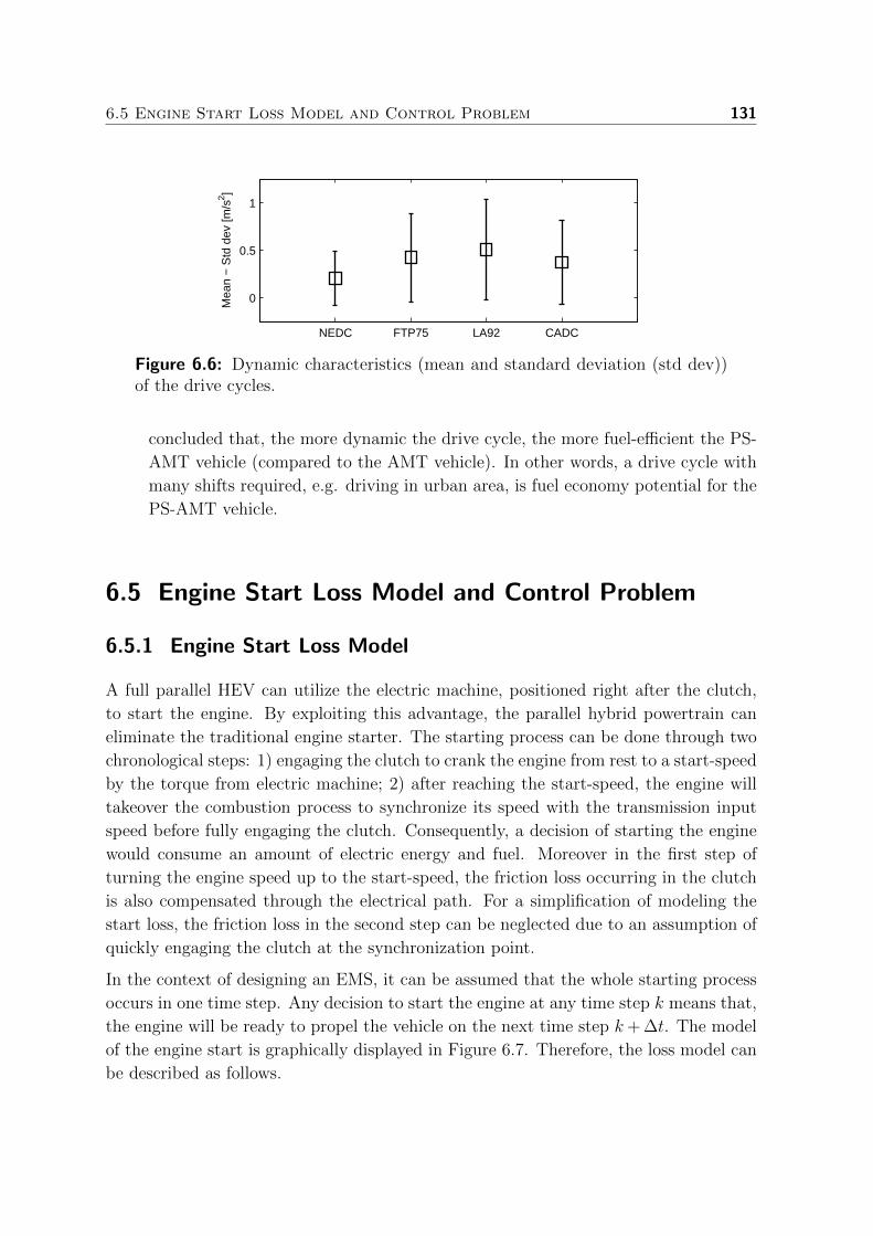
6.5 Engine Start Loss Model and Control Problem 131
NEDC FTP75 LA92 CADC
0
0.5
1
Mea
n −
Std
dev
[m/s
2 ]
Figure 6.6: Dynamic characteristics (mean and standard deviation (std dev))of the drive cycles.
concluded that, the more dynamic the drive cycle, the more fuel-efficient the PS-
AMT vehicle (compared to the AMT vehicle). In other words, a drive cycle with
many shifts required, e.g. driving in urban area, is fuel economy potential for the
PS-AMT vehicle.
6.5 Engine Start Loss Model and Control Problem
6.5.1 Engine Start Loss Model
A full parallel HEV can utilize the electric machine, positioned right after the clutch,
to start the engine. By exploiting this advantage, the parallel hybrid powertrain can
eliminate the traditional engine starter. The starting process can be done through two
chronological steps: 1) engaging the clutch to crank the engine from rest to a start-speed
by the torque from electric machine; 2) after reaching the start-speed, the engine will
takeover the combustion process to synchronize its speed with the transmission input
speed before fully engaging the clutch. Consequently, a decision of starting the engine
would consume an amount of electric energy and fuel. Moreover in the first step of
turning the engine speed up to the start-speed, the friction loss occurring in the clutch
is also compensated through the electrical path. For a simplification of modeling the
start loss, the friction loss in the second step can be neglected due to an assumption of
quickly engaging the clutch at the synchronization point.
In the context of designing an EMS, it can be assumed that the whole starting process
occurs in one time step. Any decision to start the engine at any time step k means that,
the engine will be ready to propel the vehicle on the next time step k+ ∆t. The model
of the engine start is graphically displayed in Figure 6.7. Therefore, the loss model can
be described as follows.
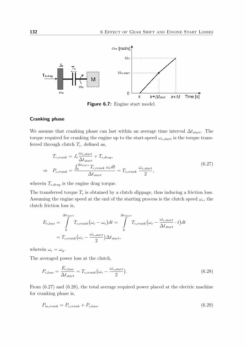
132 6 Effect of Gear Shift and Engine Start Losses
Figure 6.7: Engine start model.
Cranking phase
We assume that cranking phase can last within an average time interval ∆tstart. The
torque required for cranking the engine up to the start-speed ωe,start is the torque trans-
ferred through clutch Tc, defined as,
Tc,crank = Jeωe,start∆tstart
+ Te,drag,
⇒ Pc,crank =
∫ ∆tstart0
Tc,crank ωedt
∆tstart= Tc,crank
ωe,start2
,
(6.27)
wherein Te,drag is the engine drag torque.
The transferred torque Tc is obtained by a clutch slippage, thus inducing a friction loss.
Assuming the engine speed at the end of the starting process is the clutch speed ωc, the
clutch friction loss is,
Ec,loss =
∆tstart∫0
Tc,crank(ωc − ωe
)dt =
∆tstart∫0
Tc,crank(ωc −
ωe,start∆tstart
· t)dt
= Tc,crank(ωc −
ωe,start2
)∆tstart,
wherein ωc = ωg.
The averaged power loss at the clutch,
Pc,loss =Ec,loss∆tstart
= Tc,crank(ωc −
ωe,start2
). (6.28)
From (6.27) and (6.28), the total average required power placed at the electric machine
for cranking phase is,
Pm,crank = Pc,crank + Pc,loss. (6.29)
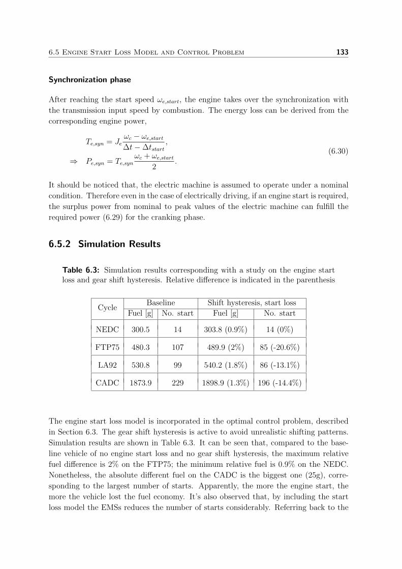
6.5 Engine Start Loss Model and Control Problem 133
Synchronization phase
After reaching the start speed ωe,start, the engine takes over the synchronization with
the transmission input speed by combustion. The energy loss can be derived from the
corresponding engine power,
Te,syn = Jeωc − ωe,start∆t−∆tstart
,
⇒ Pe,syn = Te,synωc + ωe,start
2.
(6.30)
It should be noticed that, the electric machine is assumed to operate under a nominal
condition. Therefore even in the case of electrically driving, if an engine start is required,
the surplus power from nominal to peak values of the electric machine can fulfill the
required power (6.29) for the cranking phase.
6.5.2 Simulation Results
Table 6.3: Simulation results corresponding with a study on the engine startloss and gear shift hysteresis. Relative difference is indicated in the parenthesis
CycleBaseline Shift hysteresis, start loss
Fuel [g] No. start Fuel [g] No. start
NEDC 300.5 14 303.8 (0.9%) 14 (0%)
FTP75 480.3 107 489.9 (2%) 85 (-20.6%)
LA92 530.8 99 540.2 (1.8%) 86 (-13.1%)
CADC 1873.9 229 1898.9 (1.3%) 196 (-14.4%)
The engine start loss model is incorporated in the optimal control problem, described
in Section 6.3. The gear shift hysteresis is active to avoid unrealistic shifting patterns.
Simulation results are shown in Table 6.3. It can be seen that, compared to the base-
line vehicle of no engine start loss and no gear shift hysteresis, the maximum relative
fuel difference is 2% on the FTP75; the minimum relative fuel is 0.9% on the NEDC.
Nonetheless, the absolute different fuel on the CADC is the biggest one (25g), corre-
sponding to the largest number of starts. Apparently, the more the engine start, the
more the vehicle lost the fuel economy. It’s also observed that, by including the start
loss model the EMSs reduces the number of starts considerably. Referring back to the

134 6 Effect of Gear Shift and Engine Start Losses
simulation results of the study on gear shift hysteresis shown in Table 6.2, it can be
recognized that, the engine start loss deteriorates the fuel economy more than the gear
shift hysteresis. In summary, the effect of engine start loss can not be ignored in seeking
a fair evaluation of the fuel economy for hybrid vehicles.
6.6 Prediction Horizon Sensitivity Study
Losses involved with a discrete decision of either shifting gears or starting engine have
been considered in the design of an EMS to find out a theoretical value of the fuel saving.
However, knowledge of the whole drive cycle, required for the EMS design, is almost
impossible to obtain in advance. In reality, only a driving profile over a certain horizon
can be known by a prediction technique. Therefore, with a preview route information
available, a predictive control algorithm for hybrid powertrain systems appears to be
a suitable candidate to realize a highest fuel saving as much close as possible to the
theoretical value (see, Chapter 5).
6.6.1 Predictive Control Algorithm
We use a certain available drive cycle as a reference driving profile which is assumed
to be constructed from the consecutive preview route segments of the whole driving
mission. Model Predictive Control (MPC) problem for the prototype parallel HEV is
formulated as follows.
Problem 6.2. Assuming that at current time step k, a prediction of the vehicle speed
v(k) =[v(k + 1|k), v(k + 2|k), ..., v(k + Nc|k)
]Tis known over a certain horizon Nc,
find an optimal control law u∗(k) =[u∗se(k), P ∗s (k), u∗g(k)
], that minimize the fuel cost
functional J(k) over the entire prediction horizon,
J(k) =Nc−1∑i=0
mf
(se(k + i|k), Pe(k + i|k), ωe(k + i|k)
)∆t, (6.31)
subject to the constraints (6.10) - (6.19) and,
Es min ≤ es(k +Nc|k) ≤ Es max, (6.32)
with
es(k +Nc|k) = es(k) +Nc−1∑i=0
Ps(k + i|k)∆t, (6.33)
wherein: u∗se(k), P ∗s (k) and u∗g(k) denote the vectors of predictive optimal control se-
quences over the horizon Nc at time step k.
6.7 Conclusions 135
The MPC problem is solved by using the DP-PMP algorithm, described Chapter 3.
The predictive control approach is implemented in a receding horizon control manner
to realize a real-time implementable algorithm when utilizing the route information.
Only the first element of the defined optimal trajectories of u∗se(k), P ∗s (k) and u∗g(k) is
applied to the hybrid powertrain system; for the next step k+1, the whole optimization
process is repeated with the updated system states and new prediction of the route
horizon.
The gear shift loss model can not be incorporated in the MPC due to the velocity loss at
each gear shift, resulting in the next vehicle speed to be dependent on the gear position.
Hence, we assume that the PS-AMT is used in the hybrid powertrain. The gear shift
hysteresis and the engine start loss model are respected under the control algorithm.
6.6.2 Simulation Results and Discussions
Sensitivity study of the relative fuel difference with respect to the prediction horizon
Nc is shown in Figure 6.8. The relative fuel difference is obtained by comparing the
result of the MPC approach with that of an optimal approach (based on the DP-
PMP algorithm). The MPC without the gear shift hysteresis and engine start loss
model included (see, the upper plot) indicates that with a short horizon of Nc = 2, the
predictive controller realizes a result very close to the optimal solution. The relative
fuel difference steadily approaches a small value around 0.2% from Nc ≥ 2. However,
for the case of the MPC with the gear shift hysteresis and the engine start loss model
included (see, the lower plot), from the horizons Nc ≥ 4, the relative fuel difference is
steady, ranged from 1% (NEDC) until 3% (FTP75). The obtained results reveal that
at least a prediction horizon of 5s ahead the vehicle is necessary to achieve the most
possible fuel economy. Fortunately a prediction of the velocity profile over a preview
route segment of 5s is almost possible for current technology of the vehicle onboard
navigation system nowadays.
Sensitivity study of the calculation time with respect to the prediction horizon for the
MPC strategy, including the gear shift hysteresis and the engine start loss, is shown in
Figure 6.9. The calculation time is almost linear with the prediction horizon and smaller
than the drive cycle length itself. This brings a realtime implementation possibility to
the MPC-based control algorithm.
6.7 Conclusions
Design of the EMSs for passenger HEVs equipped with discrete ratio transmissions
requires an optimal gear shift strategy for a fuel economy benefit. One gear up or down
per shift is the most optimum gear shift command in terms of the fuel economy and

136 6 Effect of Gear Shift and Engine Start Losses
0 5 10 15 20 25 30
0
1
2
Rel
. fue
l diff
eren
ce (
%)
Prediction horizon Nc [s]
MPC
0 5 10 15 20 25 300
2
4
Rel
. fue
l diff
eren
ce (
%)
Prediction horizon Nc [s]
MPC with a shift hystersis and an engine start loss
NEDC
FTP75
LA92
CADC
Figure 6.8: Sensitivity result of the relative fuel difference with respect to theprediction horizon Nc of the MPC approach.
0 5 10 15 20 25 300
200
400
600
800
Cal
cula
tion
time
[s]
Prediction horizon Nc [s]
NEDC
FTP75
LA92
CADC
Figure 6.9: Sensitivity result of the calculation time for the MPC, includingthe gear shift hysteresis and engine start loss, with respect to the predictionhorizon Nc.
engine operation comfort. Gear shift hysteresis strategy plays a crucial role in reducing
the shift busyness and hunt in a way not deteriorating the fuel economy.
Regarding the loss involved with the gear shift, it is found by simulation that a per-
ception of a fuel-efficient advantage of powershift transmissions (DCT, PS-AMT) over
non-powershift transmissions (MT, AMT) is realized for passenger HEVs.
Any discrete decision of starting the engine in a parallel HEV will induce an energy loss
which finally affects the optimal solution. This loss can not be ignored in a proper EMS
to ensure a fair evaluation of the fuel economy. The model predictive control algorithm
utilizes the engine start loss model effectively in yielding the possible shortest prediction
horizon (five seconds) such that the highest possible fuel economy level can be realized.
Prospects of future research continued from this study are very diverse. An investigation
of the effect of gear shift and engine start losses on the control strategies for commercial

6.7 Conclusions 137
vehicles equipped with an AT or a DCT is an example. This helps verifying whether
the fuel benefit of powershift transmissions compared to non-powershift ones is held for
the commercial vehicle class.

138

Chapter 7
Structural Analysis of the ControlDesign Objectives1
Abstract - In the optimal control design for vehicular propulsion systems, the objective func-tion describing the design objectives (fuel economy, driveability, comfort, emissions, batteryoperation, battery aging, etc.) plays an important role in defining the optimal solution. How-ever, the definition of the objective function is not often analyzed explicitly and thoroughly.In this study, a method of objectively analyzing and evaluating the objective function is in-troduced. The method uses the Singular Value Decomposition (SVD) technique to analyzethe correlations among the design objectives and investigate their sensitivity to an optimalcontrol algorithm. Accordingly, the dependent design objective(s) will be omitted such thatthe objective function can be simplified. This will reduce the complexity of the control design.The method is then applied to the optimal control design for a conventional vehicle and a hy-brid electric vehicle. It is found that, instead of introducing an objective function including thefuel consumption, comfort (the weighted gear shift frequency), and driveability (the weightedinverse of power reserve), a simplified objective function consisting of the fuel consumptionand comfort can be proposed for the control design, such that the driveability is not sacrificednoticeably at the obtained optimal solution.
7.1 Introduction
Design of vehicular propulsion systems boils down to choices of topology, technology,
size of the components (in terms of power or energy) and control strategy to achieve
the design objectives, such as fuel economy, driveability, comfort, emissions, battery
operation, battery aging, etc. Regarding the control strategy which governs the oper-
ations of individual components of vehicular propulsion systems at each time instant,
1This chapter has been prepared for a journal publication in the form as: V. Ngo, T. Hofman, M.Steinbuch, A. Serrarens. Structural Analysis of the Control Design Objectives for Vehicular PropulsionSystems. 2012.
139

140 7 Structural Analysis of the Control Design Objectives
optimal control [42, 49] is widely used to achieve the optimal solution with respect to
the specified control design objectives. Therefore, the starting point of formulating a
certain optimal control problem is to define an objective function, which consists of
a single or multiple design objectives. For the case of a multi-objective problem, the
objective function can be created by summing the relevant objectives multiplied by the
corresponding weight factors defining the relative importance. However, defining an ap-
propriate objective function with suitable weight factors for a specific propulsion system
is an ambiguous task. This is due to the fact that there might be strong interdepen-
dencies of the design parameters, unknown sensitivities of the design parameters to the
design objectives, and the possibility of finding multiple sets of weight factors resulting
in an equal overall design performance [49]. Hence, an objective function is appropriate
when it can diminish the interdependent design objective(s), and finally, it can balance
the tradeoff(s) among the design objectives of the design process [49, 91,121,158].
In literature, the objective function is generally defined based upon the powertrain
configurations (conventional, hybrid, etc.), the control strategy, and the subjective rea-
sonings of the designers about relative impacts among the design objectives. In this
research work, a method of objectively analyzing the design objectives for the con-
trol design of vehicular propulsion systems (conventional and hybrid powertrains) is
proposed. The method uses the Singular Value Decomposition (SVD) technique to
analyze: i) the sensitivity of the design objectives with respect to an optimal control
problem, and ii) the correlation among the design objectives. Herein the optimal control
problem also takes the gear shift problem into account. Then, the dependent design
objective(s) will be omitted such that the objective function for the optimal control
problem can be simplified in order to reduce the design complexity.
This study is organized as follows. In Section 7.2, the design objectives for the optimal
control problem of vehicular propulsion systems are reviewed. In Section 7.3, the quasi
static models of the main components of conventional and hybrid powertrain systems
are given. In Section 7.4, a multi-objective optimal control problem is formulated for
the powertrain systems. In Section 7.5, a SVD-based structural analysis method is
introduced. Analysis of the interdependencies among the design objectives is also pre-
sented. Simulation results together with discussion are given in Section 7.6. Finally,
conclusions and future research can be found in Section 7.7.
7.2 Review of Design Objectives
The design objectives for the control design of vehicular propulsion systems can be,
e.g. fuel economy, driveability, comfort, emission, battery operation, battery aging,
etc. Table 7.1 shows the possible design objectives, denoted by DO1 − DO6, and the
corresponding performance metrics.

7.2 Review of Design Objectives 141
• DO1 - fuel economy is evaluated by the amount of fuel consumed over a given
drive cycle.
• DO2 - driveability is a comprehensive terminology for vehicle responsiveness. It
can be determined as the instant power reserve, or the instant torque reserve, or
vehicle acceleration, or velocity tracking of the vehicle, etc.
• DO3 - the main comfort metrics can be listed as jerk, gear shift time or gear shift
frequency, etc.
• DO4 - emission standard have been increasingly tightened due to the environ-
mental problem. Hence, Carbon Dioxide (CO2), mono-Nitrogen Oxides (NOx),
Carbon Monoxide (CO), Particulate Matter (PM) and Hydro Carbons (HC),
etc., can be used as metrics for engine emissions.
• DO5 - regarding hybrid electric vehicles, to ensure the reliable operation of battery,
its state of charge needs to stay within a predefined operating range to avoid any
damage.
• DO6 - battery aging (battery wear) represents the overall reduction of battery life.
Table 7.1: Design objectives and the corresponding metrics.
Design objective Metric
DO1 - Fuel economy fuel consumption.DO2 - Driveability power reserve, acceleration, velocity tracking.DO3 - Comfort jerk, shifting time, shifting frequency.DO4 - Emissions CO2, NOx, CO, PM,HC.DO5 - Battery operation state of charge.DO6 - Battery aging effective Ah-throughput.
Table 7.2 shows how an objective function has been composed in literature. The first
column indicates which design objective(s) is (are) utilized in building a certain ob-
jective function. The second column gives a literature overview of objective functions
proposed for Conventional Vehicle (CV); meanwhile the third column indicates the ref-
erences wherein objective functions are proposed for Hybrid Electric Vehicle (HEV).
The objective functions vary according to the types of powertrain configurations, de-
sign method, control algorithms, etc. However fuel economy and driveability are the
most concerned design objectives.

142 7 Structural Analysis of the Control Design Objectives
Table 7.2: Literature review of the design objective composition. CV denotesConventional Vehicle; HEV represents Hybrid Electric Vehicle.
Objective composition CV HEV
DO1[60, 92,105] [8, 41,73,88,136,144,169–171][12,48,135] [3, 25,67,76,98,107,126,156,164]
DO1 +DO2 [47, 135] [158]DO1 +DO3 [133] -DO1 +DO4 [12, 60] [19,52,53,112,147]DO1 +DO5 - [4, 69,159,163]DO1 +DO6 - [128]DO1 +DO2 +DO3 [92] -DO1 +DO2 +DO5 - [21]DO1 +DO4 +DO5 - [56, 81,82,162]DO1 +DO2 +DO3 +DO5 - [158]DO1 +DO3 +DO4 +DO5 - [17, 80,83,106,172]
7.3 Powertrain Modeling and Dynamics
The hybrid powertrain topology used in this study is shown in Figure 7.1. This study
focuses on both conventional and hybrid electric vehicle, so a conventional powertrain
topology can be realized by removing the battery, the inverter and the electric machine
from the driveline.
Figure 7.1: The hybrid powertrain topology, (AMT: Automated Manual Trans-mission; M: Electric machine).
With aiming at deriving the appropriate Energy Management Strategy (EMS), quasi
static models of the main powertrain components are used. The length of time step ∆t
of one second is chosen to simulate the powertrain, hence the dynamics faster than 1Hz
are ignored [42]. The clutch system is considered as a boolean switch to connect and to
7.3 Powertrain Modeling and Dynamics 143
disconnect the engine immediately to and from the driveline. Its dynamics and limited
power losses during a gear shift or an engine start are ignored in this chapter.
7.3.1 Powertrain Modeling
• Start-stop system: the start-stop system can be modeled by a decision variable
se(k) to control the engine on-off state. When the engine is off, no fuel is consumed
by the engine.
se(k) =
{1 if engine on,
0 if engine off.(7.1)
• Engine: for a certain engine speed ωe(k), the fuel mass flow mf (k) is modeled as
an affine piece-wise second order function of the power as expressed in (7.2),
mf (k) ≈(a0(k)P 2
e (k) + a1(k)Pe(k) + a2(k))se(k). (7.2)
in which the coefficients a0(k), a1(k) and a2(k) are functions of the engine speed.
When the engine is off, no fuel is consumed. If assume during braking, the engine is
switched off and decoupled from the driveline, then the engine braking is neglected.
Therefore, the constraints on the engine speed ωe(k) power Pe(k) are as follows,
ωe,min ≤ ωe(k) ≤ ωe,max, (7.3a)
0 ≤ Pe(k) ≤ Pe,max(ωe(k)
). (7.3b)
• Electric machine: the machine efficiency η is assumed to be constant in a normal
operating state. Therefore, the power flow in motoring and generating modes is
expressed as,
Pm(k) = ηPelec(k) in motoring, (7.4a)
Pm(k) =1
ηPelec(k) in generating. (7.4b)
The constraints on the speed ωm(k) and power Pm(k) are,
0 ≤ ωm(k) ≤ ωm,max, (7.5a)
Pm,min(ωm(k)
)≤ Pm(k) ≤ Pm,max
(ωm(k)
). (7.5b)
• Battery system: the electrical power Pelec(k) is modeled as a quadratic function
of the storage power Ps(k),
Pelec(k) ≈ b0P2s (k) + b1Ps(k) + b2. (7.6)

144 7 Structural Analysis of the Control Design Objectives
The constraints imposing on the battery system,
Ps,min ≤ Ps(k) ≤ Ps,max, (7.7a)
Es,min ≤ es(k) ≤ Es,max. (7.7b)
• Automated Manual Transmission (AMT): the transmission efficiency η is
assumed to be constant for all gears, the speed and torque relations in both side
of transmission are (when clutch is closed),
ωe(k) = ωg(k) = ωw(k)rg(k), (7.8a)
Tw(k) = η rg(k) Tg(k) = η rg(k) Te(k). (7.8b)
wherein: ωw(k) is the wheel rotational speed; Tw(k) is the drive torque at the
wheels; Tg(k) is the transmission input torque; rg(k) denotes the gear ratio. The
final reduction gear ratio is merged into the transmission ratio for a simplification.
The constraints on the gear position of the 6-speed transmission are,
1 ≤ ng(k) ≤ 6. (7.9)
• Power flow model: the power flow equilibrium at the transmission input of the
powertrain is expressed as,
Pe(k) = Pg(k) + Pm(k). (7.10)
where Pm(k) = 0 if the conventional powertrain is considered.
7.3.2 Powertrain System Dynamics
The powertrain dynamic system consists of three state variables: the start-stop se(k),
the battery state-of-energy es(k) and the gear position ng(k). Their dynamics are
governed by three corresponding control variables use(k), Ps(k) and ug(k) as,
se(k + 1) = se(k) + use(k), (7.11)
es(k + 1) = es(k) + Ps(k)∆t, (7.12)
ng(k + 1) = ng(k) + ug(k). (7.13)
Vehicle longitudinal dynamics: the longitudinal motion of the vehicle in discrete
time domain is given by,
ωw(k + 1) = ωw(k) +1
Jv,eq
(Tw(k)− Fload(k)Rw
)∆t, (7.14)

7.4 Optimal Control Problem 145
where Fload is the resistance loads due to rolling and aerodynamic resistances; Jv,eq is
an equivalent vehicle inertia at the wheel,
Jv,eq =((Je + Jc + Jp)r
2g + Js
)r2d +mvR
2w,
Fload = crmvg cosα +mvg sinα +1
2ρaAfcdv
2,
and mv is the vehicle weight; Rw is the wheel radius; Je is the engine inertia; Jc is the
clutch inertia; Jp is the transmission primary inertia; Js is the transmission secondary
inertia; ρa is the air density; Af is the frontal area of vehicle; cd is the aerodynamic
drag coefficient; cr is the rolling friction coefficient; g is the gravity coefficient; v is the
vehicle speed; α is the slope of the road.
7.4 Optimal Control Problem
7.4.1 Vehicular Propulsion Systems
The dynamic behavior of the vehicular propulsion systems for conventional and hybrid
vehicles can be expressed in a generic form by
x(k + 1) = f(x(k), u(k), z(k)
), (7.15)
Ceq(x(k), u(k), z(k)
)= 0, (7.16)
Cin(x(k), u(k), z(k)
)< 0, (7.17)
wherein x(k) and u(k) are the state variable vector and control variable vector, respec-
tively; z(k) is the disturbance to the powertrain system which is defined by a priori
drive cycle. f is the function describing the dynamics of the system state. Ceq and Cinare the functions describing the equality and inequality constraints of the systems.
The conventional powertrain system is described by, (7.2)-(7.3),(7.8)-(7.10), (7.13),
(7.14). The state and control variables are,
x(k) =[ng(k)
],
u(k) =[ug(k)
].
The hybrid powertrain system is described by (7.1)-(7.14). The state and control vari-
ables are,
x(k) =[se(k), es(k), ng(k)
],
u(k) =[use(k), Ps(k), ug(k)
].
From (7.13), the constraints on the discrete gear shift command ug(k) influence the gear
shift dynamics and have effect on the optimality. Under the constraints (7.9), with a

146 7 Structural Analysis of the Control Design Objectives
6-speed AMT, ug(k) belongs to the set {−5, · · · ,−1, 0, 1, · · · , 5}. For reasons of an
acceptable driveability, the gear shift command is chosen as,
ug(k) =
−1 downshift,
0 sustaining,
1 upshift,
(7.18)
to avoid a large variation of the engine speed under a certain shifting at a certain time
step k. One gear upshift (ug(k) = 1) or downshift (ug(k) = −1) for each time step of
one second are reasonably, since the average shifting time for an AMT is typically less
than one second.
7.4.2 Multi-Objective Function
0 100 200 300 400 500 600
0
10
20
30
40
50
60
70
80
Speed [rad/s]
Po
we
r[k
W]
Pe,max
Pm,max
P + Pe,max m,max
*2 gear
Power reserve
Operating point*1 gear
*3 gear
Figure 7.2: Demonstration of the power reserve in relation with the gear posi-tion for the hybrid powertrain.
Within the context of design an optimal control problem including the gear shift strat-
egy, the relevant design objectives are required to be well-defined. Figure 7.2 graphically
shows the correlation between the gear position and the power reserve of the hybrid
powertrain. It can be seen that the power reserve is decreased when the transmission
performs an upshift and vice versa. Intuitively, when the controller allows more up-
shifts, the engine operating points will be moved to a region of higher nominal torque
and lower speed, which results in a lower power reserve. Furthermore, the fuel mass flow
is a function of the engine power. Therefore, the engine power reserve has a correlation
with the fuel consumption. It can be seen that changing the operating points by further
optimizing the gear shift would affect the driveability (power reserve) and comfort (shift
frequency or number of shifts) of the hybrid powertrain system. This reasoning holds
also for the conventional powertrain system.

7.4 Optimal Control Problem 147
Therefore, an objective function is proposed by the weighted sum of the fuel consump-
tion, comfort and driveability, as follows,
J =N−1∑k=0
L(k) =N−1∑k=0
[mf (k) + w1|ug(k)|+ w2
(∆Pe(k) + ∆Pm(k)
)−1]∆t, (7.19)
in which, N is the length of the drive cycle; w1 and w2 are the weight factors; ∆Pe(k) and
∆Pm(k) are the power reserve of the engine and electric machine, respectively; w1|ug(k)|represents the comfort cost related to the gear shift frequency; w2
(∆Pe(k)+∆Pm(k)
)−1
stands for the driveability cost related to the power reserve.
7.4.3 Optimal Control Algorithm
Problem 7.1. Given a drive cycle with a time length N , implying that the vehicle
longitudinal dynamics (7.14) is deterministic, find an optimal control law u∗(k) that
minimizes the objective function (7.19):
u∗(k) = arg minu(k)
J =N−1∑k=0
L(k)
subject to the constraints (7.15)-(7.18) and
x(N) = x(0). (7.20)
Dynamic Programming (DP) [14] is well known as a powerful method to solve a non-
linear, non convex optimization problem with mixed constraints while obtaining a glob-
ally optimal time-variant, state feedback solution. To apply DP to the proposed optimal
control problem, we need to
• grid the state variables x(k);
• grid the corresponding control variables u(k);
• calculate L(k) in (7.19) for the whole drive cycle for every grid point;
Then, the optimal cost-to-go function is defined as,
• step k = N :
J ∗N = 0, (7.21)
• step k ∈ [0, 1, . . . , N − 1]:
J ∗k(x(k)
)= min
u(k)
[L(k) + J ∗k+1
(x(k + 1)
)]. (7.22)
148 7 Structural Analysis of the Control Design Objectives
By solving the optimal cost-to-go function backwards until k = 0, the optimal solution
u∗(k) is obtained correspondingly with a specific value for the end constraint x(N).
Reducing the objective function to a simple form so that the weight factors can be
tuned easily meanwhile the control algorithm can achieve the desired performances is
the ultimate goal. In order to do so, we need to study the correlations and dependencies
among the design objectives of the objective function. Then the dependent ones can be
eliminated so that a simplified objective function can be obtained. Clearly, this boils
down to a rank analysis which will be introduced next.
7.5 SVD-based Structural Analysis
SVD is a widely used method in the structural and rank analysis of the dynamic system.
A similar usage of rank conditions using the SVD is to measure the interactions between
the inputs and the outputs of the dynamic system [103, 117, 143]. Furthermore, a
special application of the SVD method is that it can be used to evaluate the system’s
performances by doing the data-based structural analysis [43]. A brief introduction of
the SVD-based structural analysis is given next.
7.5.1 Singular Value Decomposition
Consider a linear algebraic equation as,
Ax = b; A ∈ RN×M . (7.23)
SVD of the matrix A is given
A = UΣV T
wherein:
U =[u1, u2, · · ·uN
]∈ RN×N ,
V =[v1, v2, · · · vM
]∈ RM×M ,
Σ = diag(σi|0) ∈ RN×M .
(7.24)
The column vectors vi of V and ui of U are known as the right input singular vectors
and left output singular vectors of matrix A, respectively. They hold an important
relation:
Avi = σiui . (7.25)
This equation states that each right input singular vector is mapped by the system A
onto the corresponding left output singular vector with the magnification factor being

7.5 SVD-based Structural Analysis 149
the corresponding singular value. From (7.25), if σi = 0, then Avi = 0, i.e., vi forms the
null space of A. Thus any change made in the direction corresponding to the singular
value σi = 0 maps into the zero vector in the output space. In other words, any input
in that direction is not reflected in the output space.
By using (7.24), the solution x to (7.23) is directly obtained as linear combination of
the scaled right input singular vectors,
x =
rank(A)∑i
uTi · bσi
vi =
rank(A)∑i
qivi . (7.26)
Any target vector b can be achieved by a linear combination of the scaled left output
singular vectors as
b =
rank(A)∑i
σiqiui =
rank(A)∑i
(uTi · b)ui . (7.27)
7.5.2 Structural Analysis
In the structural analysis of this study, vi is called the input mode vector, and ui is called
the output mode vector. From (7.26) the control input vector x is a linear combination
of the input mode vectors vi multiplied by the corresponding input weight factors qi.
So, the designer can assess the control input distribution pattern through the input
weight factors qi. Similarity, we can use the output mode vectors ui to assess tradeoffs
among the contributions of them to the target vector b as in (7.27).
For example, consider the input weight factor q1 in (7.27) to be much larger than the
other weight factors in the linear combination. Since σ1 is the largest singular value,
q1σ1 is dominant among the coefficients of the linear combination, then the actual target
vector b will be largely dependent on the first output mode vector u1.
The input mode vectors vi and output mode vectors ui obtained from SVD are paired by
the corresponding singular values σi. Thus, truncating any input mode vector vi would
affect the corresponding output mode vector ui, and vice versa. Truncating the output
mode vector ui that is part of the linear combination of the target vector b would degrade
the total performance. If, however, the truncated output mode vector contributes little
to the target vector b, then there would be little performance degradation and it would
be possible to save control effort equal in size to the weighted input mode vector that
is paired with the truncated output mode vector.
Cutting off any input mode vector vi that consumes a large control input, i.e., one with
a large weight factor qi, but contributes little to the total performance of the target
vector b, will reduce the design complexity at a little performance degradation.

150 7 Structural Analysis of the Control Design Objectives
From (7.27), it is clear that the output mode vector ui that lines up more towards the
target vector b will contribute more to b. Therefore, the value of inner product of two
vector ui and b, which is called the collinearity and denoted by coli , (uTi · b), can
be used to measure the performance dependency of the target vector b on each output
mode vector ui. Using this indicator, we can identify which output mode vector ui is
dominant in achieving the target vector b and which output mode vector ui contributes
little. Furthermore, the normalized target vector b should be used to compare the
collinearities for simplicity since they span from 0 to 1.
7.6 Results and Discussions
7.6.1 Application of SVD-based Structural Analysis
The structural analysis for the powertrain systems will be carried out by using the
SVD technique. The analysis is not based on the system model, but is based on data
obtained from simulating the system model governed by the optimal control algorithm,
as described in Section 7.4. The concerned data is the discrete optimal cost values along
the drive cycle.
Objective function analysis: the optimal objective function (7.19) is rewritten as follows.
J∗ =N−1∑k=0
L∗(k) =N−1∑k=0
[m∗fe(k) +m∗sh(k) +m∗pr(k)
], (7.28)
wherein the asterisk (*) denotes the optimal solution and
m∗fe(k) , m∗f (k)∆t,
m∗sh(k) , w1|u∗g(k)|∆t,
m∗pr(k) , w2
(∆P ∗e (k) + ∆P ∗m(k)
)−1∆t.
The discrete optimal cost values of (7.28) are stacked along the discrete time dimension
of the drive cycle to create the linear algebraic equation Ax = b, with
A =
m∗fe(0) m∗sh(0) m∗pr(0)m∗fe(1) m∗sh(1) m∗pr(1)
......
...m∗fe(N − 1) m∗sh(N − 1) m∗pr(N − 1)
, b =
L∗(0)L∗(1)
...L∗(N − 1)
,x =
[1 1 1
]T.
(7.29)
In (7.29), the vector x acts as the control vector imposed on the weighted objectives,
so it is chosen as x = [1 1 1]T to respect the original optimal values of the objectives.
7.6 Results and Discussions 151
The target vector b contains the instantaneous optimal values of the objective function
at every time step. SVD-based structural analysis method is applied to study the
sensitivity of the design objectives to the weight factors w1 and w2.
7.6.2 Simulation Results for Conventional Vehicles
The main parameters of a prototype conventional vehicle are given in Table 7.3.
Table 7.3: Main parameters of a prototype conventional vehicle.
Item Description/Quantity
Enginetype: gasoline,maximum torque of 140Nm,maximum power of 70kW.
Transmission6-speed automated manual transmission,rg = [3.071, 1.913, 1.258, 0.943, 0.763, 0.643].
Vehicle mass 1120kg.
• The NEDC cycle: the weight factors w1 and w2 are chosen as,
w1 ∈ {0.6, 1, 1.5, 2, 3}, (7.30)
w2 ∈ {250, 500, 750, 1000, 1500, 2000}. (7.31)
Computational results of SVD analyses for the input weight factors qi and the
normalized collinearities coli for all combinations of w1 and w2 are shown in Figure
7.3.
In Figure 7.3a, q1 varies from 0.89→ 0.99, q2 varies from 0.72→ 0.94 and q3 varies
from 0.48 → 0.87. By looking at the normalized collinearities in Figure 7.3b, we
can recognize that the values of coli are totally different from each other. col1approximately varies from 0.90 → 0.99; col2 approximately varies from 0.13 →0.44 whereas col3 roughly varies from 0.02→ 0.09.
From col2 and col3, it is observed that the maximum contributions of the output
mode vectors u2 and u3 to the target vector b are 19.4% (= 0.442 ∗ 100%) and
0.8% (= 0.092 ∗ 100%) respectively. Meanwhile, the maximum contributions of
input mode vectors v2 and v3 to the control input vector x are almost equivalent
to that of v1 (observed from q1, q2 and q3). This is an important observation on
the fact that the output mode vector u3 pays only a very small contribution to

152 7 Structural Analysis of the Control Design Objectives
02
4 01000
20000
0.5
1
w2w
1
q 1
02
4 01000
20000
0.5
1
w2w
1
q 2
02
4 01000
20000
0.5
1
w2w
1
q 3
(a)
02
4 01000
20000
0.5
1
w2w
1
col 1
02
4 01000
20000
0.5
1
w2w
1
col 2
02
4 01000
20000
0.5
1
w2w
1
col 3
(b)
02
4 01000
20000
0.5
1
w2w
1
x 1
02
4 01000
20000
0.5
1
w2w
1
x 3
02
4 01000
20000
0.5
1
w2w
1
x 3
(c)
Figure 7.3: Results of the conventional powertrain on NEDC: the input weightfactors qi in (a); the collinearities coli in (b); the three directions x1, x2 and x3
of the reconstructed x in (c).
the target vector b. Therefore, truncating the input mode vector v3 will save a
large amount of control effort without seriously degrading the performance.
From the observations and analyses above, we can come up with a design decision
to truncate the input mode vector v3 out of the control input vector x. Therefore,
x can be approximated as,
x ≈ q1 · v1 + q2 · v2 ,[x1 x2 x3
]T. (7.32)
Using the obtained simulation results, the reconstructed control input vector x is
depicted in Figure 7.3c. We can see that x1 varies from 0.84 → 0.96; x2 varies
from 0.8 → 0.96. Meanwhile, x3 varies from 0.02 → 0.18. Or the control input
vector x can be re-designed as,
x ≈[1 1 0
]T. (7.33)
• The FTP75 cycle: the weight factors w1 and w2 are chosen as,
w1 ∈ {1, 2, 3, 4, 5}, (7.34)
w2 ∈ {250, 500, 750, 1000, 1250, 1500}. (7.35)

7.6 Results and Discussions 153
0
5 01000
20000
0.5
1
w2w
1
q 1
0
5 01000
20000
0.5
1
w2w
1
q 2
0
5 01000
20000
0.5
1
w2w
1
q 3
(a)
0
5 01000
20000
0.5
1
w2w
1
col 1
0
5 01000
20000
0.5
1
w2w
1
col 2
0
5 01000
20000
0.5
1
w2w
1
col 3
(b)
0
5 01000
20000
0.5
1
w2w
1
x 1
0
5 01000
20000
0.5
1
w2w
1
x 3
0
5 01000
20000
0.5
1
w2w
1
x 3
(c)
Figure 7.4: Results of the conventional powertrain on FTP75: the input weightfactors qi in (a); the collinearities coli in (b); three directions x1, x2 and x3 ofthe reconstructed x in (c).
Computational results of SVD analyses for the input weight factors qi and the
normalized collinearities coli are shown in Figure 7.4. By using the same analysis
technique applied on the NEDC cycle, the control input vector x is reconstructed
and depicted in Figure 7.4c. Or the control input vector x can be approximately
re-designed as
x ≈[1 1 0
]T. (7.36)
From (7.33) and (7.36), it can be concluded that the third design objective, i.e. the
power reserve term, can be eliminated from the objective function (7.28) due to its small
contribution to the objective function. In other words, the objective function for the
optimal control problem can be simplified as,
JCV =N−1∑k=0
[mf (k) + w1|ug(k)|
]∆t. (7.37)
Therefore, it would be easy to tune only one weight factor w1 such that the Pareto
optimal solution is achieved to satisfy the expected design objectives.

154 7 Structural Analysis of the Control Design Objectives
7.6.3 Simulation Results for Hybrid Electric Vehicles
Another case study of the SVD-based structural analysis is applied for a prototype
HEV, see Table 7.4 for the main parameters, to investigate the correlations among of
the design objectives. NEDC and FTP75 are still used to test the analysis approach.
Table 7.4: Main parameters of a prototype HEV.
Item Description/Quantity
Enginediesel type,maximum torque of 200Nm,maximum power of 68kW.
Electric machinemaximum torque of 40Nm,maximum power of 6kW.
Battery lithium-ion; capacity of 6Ah, 110V.
Transmission6-speed automated manual transmission,rg = [3.817, 2.053, 1.302, 0.959, 0.744, 0.614].
Vehicle mass 1320kg.
Table 7.5: The weight factors w1 and w2 for the HEV optimal control problemon NEDC and FTP75.
Cycle w1 w2
NEDC ∈ {1, 2, 3, 4} ∈ 100 ∗ {2, 4, 6, 8, 10}FTP75 ∈ {2, 6, 10, 14, 20} ∈ 1000 ∗ {1, 3, 5, 8, 10}
The results of SVD analyses on the NEDC and FTP75 are shown in Figure 7.5 and
Figure 7.6 respectively. Using the same analysis technique applied for the conventional
vehicle, it’s still able to achieve the reconstructed control input vector x as depicted
in Figure 7.5c and Figure 7.6c for the NEDC and FTP75 respectively. Notice the
reconstructed control input vector x for the case of FTP75, in which, x1 varies from
0.74 → 1.08; x2 varies from 0.6 → 0.95; and x3 varies from 0.04 → 0.35. In this case
study, x3 is not approximated to zero for the whole ranges of w1 and w2. Therefore, the
three directions are normalized by the ‖x‖2 to evaluate their relative contributions to
the input vector x. The maximum relative contribution of x3 is 10% which is relative
small compared to the contributions of x1 and x2, such that x3 can be ignored from an
engineering point of view. Meaning that, the control input vector x can be re-designed

7.7 Conclusions 155
02
4 0500
10000
0.5
1
w2w
1
q 1
02
4 0500
10000
0.5
1
w2w
1
q 2
02
4 0500
10000
0.5
1
w2w
1
q 2
(a)
02
4 0500
10000
0.5
1
w2w
1
col 1
02
4 0500
10000
0.5
1
w2w
1
col 2
02
4 0500
10000
0.5
1
w2w
1
col 3
(b)
02
4 0500
10000
0.5
1
w2w
1
x 1
02
4 0500
10000
0.5
1
w2w
1
x 2
02
4 0500
10000
0.5
1
w2w
1
x 3
(c)
Figure 7.5: Results of the hybrid powertrain on NEDC: the input weight factorsqi in (a); the collinearities coli in (b); three directions x1, x2 and x3 of thereconstructed x in (c).
as follows,
x ≈[1 1 0
]T. (7.38)
So, it is observed that for the optimal control problem of HEVs, the driveability, defined
by the weighted inverse of power reserve, pays a very small contribution to the objective
function. Therefore, the objective function is simplified as,
JHEV =N−1∑k=0
[mf (k) + w1|ug(k)|
]∆t. (7.39)
7.7 Conclusions
A method of objectively analyzing and evaluating the objective function of an optimal
control problem for vehicular propulsion systems was proposed. The method utilizes
the SVD-based structural analysis approach to study the correlations among the design
objectives and investigate their sensitivity to the optimal control algorithm of vehicular
propulsion systems. It helps identifying the possibly dependent design objective(s)
among the originally concerned ones, such that an objective function can be properly
156 7 Structural Analysis of the Control Design Objectives
010
20 05000
100000
0.5
1
w2w
1
q 1
010
20 05000
100000
0.5
1
w2w
1
q 2
010
20 05000
100000
0.5
1
w2w
1
q 2
(a)
010
20 05000
100000
0.5
1
w2w
1
col 1
010
20 05000
100000
0.5
1
w2w
1
col 2
010
20 05000
100000
0.5
1
w2w
1
col 3
(b)
010
20 05000
100000
0.5
1
w2w
1
x 1
010
20 05000
100000
0.5
1
w2w
1
x 2
010
20 05000
100000
0.5
1
w2w
1
x 3
(c)
Figure 7.6: Results of the hybrid powertrain on FTP75: the input weightfactors qi in (a); the collinearity coli in (b); three directions x1, x2 and x3 of thereconstructed x in (c).
defined in terms of reducing the complexity of the optimal control design. From the
simulation results of the two case-studies, one for conventional vehicle with a gasoline
engine, and the other for hybrid electric vehicle with a diesel engine, it can be concluded
that the driveability (the weighted inverse of power reserve) is the dependent design
objective and has a very small influence on the objective function in defining the optimal
solution. Therefore, the objective function consisting of the fuel economy (the fuel
consumption) and the comfort (the weighted gear shift frequency) can be proposed for
the control design of both powertrain systems.
The proposed method shows itself as an effective method to be able to analyze the ob-
jective function. The proposed method is not limited to a specific powertrain topology.
In principle, it can be extended to other types of vehicle configurations.

Chapter 8
Conclusions and Recommendations
Abstract - In this chapter, the main conclusions following from the previous chapters aredrawn and the recommendations for future research are also given.
8.1 Conclusions
The research presented in this dissertation deals with the gear shift control strategy
for conventional and hybrid electric vehicles equipped with discrete ratio transmissions.
This resulted in the six research objectives (O1 −O6) as presented in Chapter 1.
• O1: define and address the driveability in a fuel-optimal gear shift strategy for
conventional vehicles on drive cycles known a priori.
• O2: design a fuel-optimal control algorithm, including the gear shift strategy, for
the hybrid dynamical system of HEVs on drive cycles known a priori.
• O3: develop an online gear shift strategy for conventional and hybrid electric
vehicles equipped with discrete ratio transmissions. The strategy improves the
fuel economy meanwhile still satisfying an acceptable driveability.
• O4: propose a gear shift strategy for a HEV to further improve the fuel economy by
exploiting the route information from the GPS-based onboard navigation system.
• O5: analyze the effect of the gear shift and engine start losses on the control
strategy and fuel consumption.
• O6: investigate the sensitivity of an optimal gear shift strategy to the relevant
control design objectives, such as fuel economy, driveability, comfort, etc.
157
158 8 Conclusions and Recommendations
The six research objectives were addressed in six research chapters, from Chapter 2 till
Chapter 7, respectively. The first four objectives were fulfilled by developing various
gear shift strategies for automotive transmission. The last two objectives focussed on i)
investigating the effect of the discrete state variable-dependent losses (gear shift, clutch
losses and engine start) on the control strategy, and ii) analyzing the consequences on
the control design objectives (fuel economy, driveability, comfort) with respect to the
optimal gear shift strategy. In summary, the research presented in this dissertation
made a fundamental contribution in the field of the automotive transmission control
design and analysis, with six explicit contributions (C1 −C6):
• C1: various optimal gear shift strategies with respect to the fuel economy and
driveability are proposed for conventional vehicles. A novel concept of variable
power reserve is developed to properly address the driveability, meanwhile guar-
anteeing the highest achievable fuel economy (Chapter 2).
• C2: a novel gear shift control algorithm based on a combination of DP and Pon-
tryagin’s Minimum Principle (PMP) is developed for the hybrid dynamical system
(consisting of continuous and discrete variables) of HEVs. This so-called DP-PMP
algorithm benchmarks the gear shift problem in terms of optimality and compu-
tational efficiency (Chapter 3).
• C3: a gear shift map design methodology aiming at a realtime solution for discrete
ratio transmissions is developed. The methodology exploits the fuel economy and
driveability potential of the optimal gear shift strategies (proposed in Chapters 2
and 3) in order to realize an online gear shift strategy for conventional and hybrid
electric vehicles (Chapter 4).
• C4: a concept of integrated predictive gear shift strategy for HEVs, utilizing
route information to further explore fuel economy potential, is demonstrated in
simulation (Chapter 5).
• C5: an analysis of the effect of gear shift and engine start losses on control strate-
gies for AMT-based HEVs. By taking the gear shift loss into account, this study
reveals a perception of a fuel-efficient advantage of powershift transmissions (DCT,
PS-AMT) over non-powershift transmissions (MT, AMT) applied for passenger
HEVs. Furthermore, the effect of the engine start loss can not be ignored in seek-
ing a fair evaluation of the fuel economy for parallel HEVs. A prediction horizon
of few seconds can help a predictive EMS to realize the highest achievable fuel
economy (Chapter 6).
• C6: a Singular Value Decomposition-based technique is introduced to analyze
the correlation among the design objectives of an optimal gear shift problem for
conventional and hybrid electric vehicles (Chapter 7).

8.1 Conclusions 159
The main results and conclusions are summarized in the following subsections.
Optimal gear shift strategies for conventional vehicles
In Chapter 2, a systematic approach in order to address the fuel economy and driveabil-
ity in an optimal gear shift strategy for conventional vehicles equipped with an AMT
was proposed.
The fuel-optimal gear shift strategy based on DP benchmarks the fuel economy on
a certain drive cycle. The driveability, defined by the power reserve and represented
for an acceleration capability, is systematically addressed in the fuel-optimal gear shift
problem. The tradeoff between the fuel economy and driveability is investigated by three
methods: i) the weighted inverse of power reserve, ii) the constant power reserve, and iii)
the variable power reserve. The first two methods provide control laws more sensitive
to the design parameters, and the obtained solutions are too conservative on a certain
drive cycle. The third method outperforms the first two methods in terms of the fuel
economy and driveability improvements, which is explained by a variable characteristic
of the power reserve to the vehicle speed such that the gear shift strategy is adapted
accordingly. The advantages of the variable power reserve method is reaffirmed through
a comparative analysis with a Stochastic Dynamic Programming (SDP)-based gear shift
strategy. The SDP algorithm optimizes the gear shift strategy, subject to a stochastic
distribution of the power request, to minimize the expected fuel consumption over an
infinite horizon. Hence the obtained solution intrinsically respects the driveability and
is realtime implementable. The SDP-based strategy nearly results in the same fuel
economy, yet in a lower acceleration capability compared to the results obtained from
the variable power reserve method.
The variable power reserve method possesses a superior character in dealing with the
driveability effectively and adaptively over a wide range of driving profiles, meanwhile
still improving the fuel economy. Hence, it is highly suitable for a realtime application,
e.g. a predictive gear shift strategy, or an optimization-based gear shift map design.
Optimal gear shift strategies for HEVs
For HEVs, a DP-based EMS, including the gear shift strategy, is proved to be only
useful for benchmarking a globally optimal solution, yet requires an intensive compu-
tation. Therefore, the DP-PMP control algorithm is considered as a novel method for
the constrained optimal control problem of the hybrid dynamical system in terms of
optimality and computational efficiency. PMP is used in the inner loop of the control
algorithm to obtain the instantaneous optimal solution for the continuous control vari-
able. Meanwhile, DP is applied in the outer loop of the control algorithm to define the
optimal solution for the discrete control variable(s). The main insights related to the

160 8 Conclusions and Recommendations
application of this novel method for the hybrid powertrain system are given next.
• For the hybrid powertrain without a start-stop functionality, the DP-PMP ap-
proach optimizes the power split and gear shift command. It is found that a
unique constant Lagrange multiplier exists, such that the end constraint of the
battery state-of-energy is respected and a globally optimal solution is guaranteed.
• For the hybrid powertrain with a start-stop functionality, the DP-PMP approach
optimizes the engine start-stop command, power split and gear shift command.
It reveals that finding a constant Lagrange multiplier is not possible for this non-
smooth optimization problem. A battery state-of-energy feedback controller, e.g.
proportional integral controller, is used to adapt the Lagrange multiplier over
time. Therefore the obtained solution is in principle suboptimal, despite the fact
that it is very close to the globally optimal solution based on DP.
From an engineering point of view, the DP-PMP algorithm can be considered as a glob-
ally optimal method applied for HEVs. The algorithm is executed fast enough such that
it can be seen as a potential candidate, which can be used in a realtime implementable
control algorithm, e.g. a predictive gear shift strategy, or an optimization-based gear
shift map design method.
Gear shift map design methodology
Chapter 4 developed a gear shift map design methodology for conventional and hybrid
electric vehicles equipped with discrete ratio transmissions. By applying the two-step
design procedure: i) utilize an optimal gear shift strategy to derive the optimal gear
shift patterns; and ii) use statistical theory to analyse the optimal gear shift patterns
and extract the shift lines; the gear shift map is obtained. Through various application
and validation in both simulation and experimental environments, it is proved that the
obtained gear shift map is acceptably optimized with respect to maximizing the fuel
economy and driveability. Furthermore, the obtained gear shift pattern is guaranteed
to be consistent and robust. More importantly, the design methodology is:
• flexible (easy adaptable) with changes and modifications during the design process;
• time-efficient for the design process;
• applicable to various powertrain configurations with discrete ratio transmissions.
In summary, the design methodology forms a theoretical and quantified way to generate
the commonly used gear shift map for automotive transmissions based on the powertrain
system modeling and control and statistical analysis.

8.1 Conclusions 161
Integrated predictive gear shift strategy
Chapter 5 presented an integrated predictive gear shift strategy concept for HEVs. It
consists of two algorithms exploiting route information and complementing each other:
i) a predictive algorithm controls the gear shift command, beside the power split and
engine on-off decision by utilizing route information given in the form of a priori ve-
locity profile; ii) the velocity algorithm derives a fuel-optimal velocity trajectory by
utilizing route information given in the form of the road characteristics, speed limits,
and average traveling time, etc. The concept has been demonstrated and validated in
a simulation environment. The velocity algorithm improves the fuel economy consider-
ably by proposing a fuel-optimal velocity trajectory over a certain driving horizon for
the vehicle to follow. The predictive algorithm successfully utilizes a predefined velocity
profile over a certain horizon to realize a fuel economy improvement very close to that
of the globally optimal algorithm.
Hence, the velocity algorithm is seen as a promising solution to be implemented on
the onboard navigation system to yield a velocity profile over a horizon, which is se-
quentially fed to the predictive algorithm implemented on an EMS. The two algorithms
complement each other to create an integrated predictive gear shift strategy realizing
the highest fuel economy potential for HEVs.
Effect of gear shift and engine start losses
In Chapter 6, the energy losses involved with the gear shift and engine start processes of
an AMT-based HEV were modeled and incorporated in the design of an EMS in order
to analyze their influences on the fuel economy, respectively.
Design of the EMSs for passenger HEVs equipped with discrete ratio transmissions
requires an optimal gear shift strategy for a fuel economy benefit. One gear up or down
per shift is the most optimum gear shift command in terms of the fuel economy and
engine operation comfort. Gear shift hysteresis strategy plays a crucial role in reducing
the shift busyness and hunt in a way not deteriorating the fuel economy.
Regarding the loss involved with the gear shift, it is found by simulation that a per-
ception of a fuel-efficient advantage of powershift transmissions (DCT, PS-AMT) over
non-powershift transmissions (MT, AMT) is realized for passenger HEVs.
In relation with the engine start, it is found that the induced energy loss can not be
ignored in a proper design of the EMS to guarantee a fair evaluation on the fuel economy
of parallel HEVs. Furthermore, the model predictive control algorithm utilized the
engine start loss model effectively in yielding the possible shortest prediction horizon of
5s such that the highest fuel economy can be realized.

162 8 Conclusions and Recommendations
Structural analysis of the control design objectives
Chapter 7 discussed a method to analyze the sensitivity of an optimal gear shift strategy
to the control design objectives. The method utilizes the Singular Value Decomposition-
based structural analysis approach to objectively and quantitatively study the possible
correlations among the control design objectives. It is found that the objective function,
originally comprised of the fuel consumption, driveability (the weighted inverse of power
reserve), and comfort (the weighted gear shift frequency), can be simplified to the one
consisting of only the fuel consumption and comfort. The analysis results show that
the driveability is interdependent with the comfort. The SVD-based method is able to
identify the possible dependent control design objective(s). Hence, a design decision to
omit the dependent design objective(s) can be realized. This will allow to build a proper
objective function for the optimal control problem, thus reducing the design complexity.
8.2 Recommendations
In light of the findings of the study presented in this dissertation, directions for future
research are given next.
1. Powertrain component size study
Within the context of designing discrete ratio transmissions for road vehicles pri-
marily powered by internal combustion engines, the gear shift strategy has a vital
position in improving the fuel economy, see Chapters 2 and 3. Furthermore, the
gear number together with the ratios are also a decisive factor in defining the
optimal shift points. The greater the gear number, the better the engine will
exploit its efficiency by adhering to the ideal tractive effort. Nonetheless, the fuel
economy potential comes at a price of a possible high shifting frequency, an in-
crease of weight and size of the gearbox. From a powertrain system design point
of view, there are: i) a possibly strong interdependency among the design param-
eters (the supervisory control strategy and component size), and ii) an unknown
sensitivity of the design parameters to the design objectives (fuel economy and
driveability) [49]. Hence, in pursuit of the advantages offered by an optimal gear
shift strategy, the follow-up research is defined as follows:
• search for an optimum design of the gear number, ratios and ratio coverage for
the transmission used in conventional vehicles to improve the fuel economy
and/or driveability;
• study the optimal power specifications (sizes) of the engine, electric machine
and transmission parameters (the number of gears, step value and ratio cov-
erage) for HEVs to improve the fuel economy.

8.2 Recommendations 163
2. Gear shift map generation tool
As stated in Chapter 1, a strong segmentation of the vehicle classes has led to a
variety of the transmission technologies and applications. Furthermore, it is nec-
essary to assess the impact of different powertrain systems and the corresponding
control strategies, including the gear shift strategy, on the design objectives at a
very early stage of the development process. Therefore, an optimized gear shift
map in terms of the fuel economy and driveability for automotive transmissions is
highly fitted for the purpose of accelerating the development process and applica-
tion. Motivated by the very positive outcomes and insights of the gear shift map
design methodology, presented in Chapter 4, development of a tool to formally
generate the gear shift map for a given powertrain system is seen as a promising
prospect in terms of practical applicability.
3. Towards preview route-based driving
Recently, the trend in automotive control technology development is to utilize
route information obtained from the GPS-based onboard navigation system in
order to improve the fuel economy [2, 93, 96, 151]. In line with this, Chapter 5
demonstrated an integrated predictive gear shift strategy which also exploits route
information to realize the fuel benefit for HEVs. Ultimately, this trend will result
in autonomous driving, wherein the vehicle can brake, accelerate and steer by its
own to obtain the maximum possible fuel saving, while even improving (lowering)
trip time. This represents an ideal situation where a pre-computed optimal veloc-
ity trajectory is exactly followed by the vehicle, wherein the powertrain system is
governed by an optimal supervisory control algorithm accordingly. However, in
real-life traffic situations, it might not be possible to track the optimal profile due
to the upcoming traffic disturbances. Therefore, driving the vehicle with a preview
route horizon and cooperating (using communication systems) with the vehicle(s)
in front are seen as a solution for this problem. The vehicle will switch from a
velocity tracking mode to a vehicle following mode, thus making the optimal al-
gorithm in former mode is not optimal for later mode. Moreover, implementation
of the control algorithm on a relatively short driving horizon, e.g. an accelera-
tion horizon, a cruise horizon, and a deceleration horizon, etc., is also required
to point out the practical relevance, such as the horizon length, constraints on
the battery state-of-energy, and estimation of the Lagrange multiplier on various
driving profiles, etc. These challenges are recommended for future research.
4. Powershift transmissions vs. non-powershift transmissions
The research in this dissertation has demonstrated by simulation that powershift
transmissions (DCT, PS-AMT) are more fuel-efficient than non-powershift trans-
missions (MT, AMT) applied for passenger HEVs, see Chapter 6. This is proved
by modeling and incorporating the gear shift loss into the design of an optimal

164 8 Conclusions and Recommendations
EMS. From the large margin of relative fuel difference of powershift transmissions
over non-powershift ones, it can set preliminary inferences of:
• a fuel benefit property of the AT over the MT or AMT;
• a fuel benefit of powershift transmissions (AT, DCT, PS-AMT) over non-
powershift transmissions (MT, AMT) applied for commercial vehicles,
wherein the large drivetrain component inertias and reliable operation of
transmissions usually require the interruption time of shifting to be in the
order of 0.5-1.0s and longer.
Apparently, these preliminary inferences are contrary to the fact that, for example
the AT is considered to have a moderate efficiency compared to the MT or AMT.
Therefore, to reinforce the hypothesis, a simulation study for the intended vehicle
classes equipped with powershift transmissions is required. Experimental study is
also needed to prove the hypothesis.

Appendix A
Optimal Power Split Control of HEVs
Problem A.1. Given a drive cycle v(k) with time length N , with a given certain
admissible gear sequence ng(k) along this drive cycle, find an instantaneous optimal
engine power P ∗e (k) that minimizes the cost function of fuel consumption over the entire
drive cycle,
J =N−1∑k=0
Fr(Pe(k), k
)∆t, (A.1)
subject to constraints:
es(k + 1) = es(k) + Ps(Pe(k), k
)∆t, (A.2)
P′
e,min(k) ≤ Pe(k) ≤ P′
e,max(k). (A.3)
To apply Pontryagin’s minimum principle to solve this optimal control problem, the
constraint on engine power is rewritten as an equality constraint by introducing a pa-
rameter p(k),
P 2e (k) + A(k) · Pe(k) + B(k) + p2(k) = 0, (A.4)
wherein:
A(k) = −(P′
e,min(k) + P′
e,max(k)),
B(k) = P′
e,min(k) · P ′e,max(k).
The augmented cost function J′
is constructed by using Lagrange multipliers λ(k) and
γ(k) to take into account the constraints, thus giving,
J′=
N−1∑k=0
Fr(Pe(k), k)∆t
−λ(k)(es(k + 1)− es(k)− Ps
(Pe(k), k
)∆t)
−γ(k)(P 2e (k) + A(k)Pe(k) + B(k) + p2(k)
) . (A.5)
165

166 A Optimal Power Split Control of HEVs
Optimality condition with respect to the constraint on engine power is defined as,
∂J′
∂p(k)= 0 ⇔ 2γ(k)p(k) = 0 ⇔
{γ(k) = 0,
p(k) = 0.(A.6)
According to (A.6), we have two cases needed to be considered as follows:
• case 1: p(k) = 0,
P ∗e,1(k) ∈ {P ′e,min(k), P′
e,max(k)}. (A.7)
In this case the optimal engine power is at its bounds, either at the lower bound
or at the upper bound.
• case 2: γ(k) = 0,
the inequalities described by (A.3) are inactive. Therefore, we have the Hamilto-
nian function as,
H(Pe(k), λ(k), k
)=[
Fr(Pe(k), k
)+ λ(k)Ps
(Pe(k), k
)]∆t. (A.8)
According to the Pontryagin’s minimum principle, the necessary optimality con-
ditions are defined by the followings:
λ(k)− λ(k + 1) =∂H(Pe(k), λ(k), k
)∂es(k)
= 0
⇔ λ(k) , λopt, ∀k ∈ [0, 1, . . . , N − 1],
(A.9)
∂H(Pe(k), λ(k), k
)∂Pe(k)
= 0
⇔∂Fr(Pe(k), k
)∂Pe(k)
+ λ(k)∂Ps(Pe(k), k
)∂Pe(k)
= 0.
(A.10)
From approximations of the engine fuel rate (3.1) and the battery efficiency
model (3.5), Fr(Pe(k), k
)and Ps
(Pe(k), k
)can be approximated as affine piecewise
second-order functions of the engine power at a certain engine speed [25, 73]. So,
the Hamiltonian function at each time step is continuous and quadratic. There-
fore, there exists such a constant Lagrange multiplier denoted as λopt (see, [149]),
such that the final state of es(N) meets a specifically predefined value. The glob-
ally optimal solution of the engine power P ∗e,2(k) is derived analytically. The
two-point boundary value problem is solved.

167
For both cases 1 and 2, by using (A.9), the cost function (A.5) can be rewritten as,
J′=
N−1∑k=0
[Fr(Pe(k), k
)+ λoptPs
(Pe(k), k
)]∆t− λopt
(es(N)− es(0)
)∆t. (A.11)
Therefore, the globally instantaneous optimal solution of engine power is defined as,
P ∗e (k) = arg min
Pe(k)∈{P ∗e,1(k)
P ∗e,2(k)
}[
Fr(Pe(k), k
)+ λoptPs
(Pe(k), k
)]. (A.12)

168

Appendix B
State Constrained Optimal Control ofthe Power Split for HEVs
Under optimally controlled, the EMS will drive the battery state-of-energy around its
initial value and ensure its end constraint to be respected. This appendix reformulates
the optimization problem described in Appendix A if the bounds on the battery state-
of-energy are taken into account in the control design.
Problem B.1. Given a drive cycle v(k) with time length of N , with a given certain
admissible gear sequence ng(k) along this drive cycle, find an instantaneous optimal
engine power P ∗e (k) that minimizes the cost function of fuel consumption over the entire
drive cycle,
J =N−1∑k=0
Fr(Pe(k), k
)∆t, (B.1)
subject to constraints:
es(k + 1) = es(k) + Ps(Pe(k), k
)∆t, (B.2)
Es,min ≤ es(k) ≤ Es,max, (B.3)
P′
e,min(k) ≤ Pe(k) ≤ P′
e,max(k). (B.4)
The constraint on engine power Pe(k) must be rewritten as an equality constraint by
introducing a parameter p(k),
P 2e (k) + A(k) · Pe(k) + B(k) + p2(k) = 0, (B.5)
wherein:
A(k) = −(P′
e,min(k) + P′
e,max(k)),
B(k) = P′
e,min(k) · P ′e,max(k).
169

170 B State Constrained Optimal Control of the Power Split for HEVs
The constraint on battery state of energy es(k) must be rewritten as an equality con-
straint by introducing a parameter q(k),
e2s(k) + C · es(k) + D + q2(k) = 0, (B.6)
wherein:
C = −(Es,min + Es,max
),
D = Es,min · Es,max.
The new cost function J′
is constructed by using Lagrange multipliers λ(k), γ(k) and
β(k) to take into account the constraints, thus giving,
J′=
N−1∑k=0
Fr(Pe(k), k)∆t−
−λ(k)(es(k + 1)− es(k)− Ps
(Pe(k), k
)∆t)
−γ(k)(P 2e (k) + A(k)Pe(k) + B(k) + p2(k)
)−β(k)
(e2s(k) + C · es(k) + D + q2(k)
)
. (B.7)
Optimality conditions are defined as,
∂J′
∂p(k)= 0⇔ 2γ(k)p(k) = 0⇔
{p(k) = 0,
γ(k) = 0.(B.8)
∂J′
∂q(k)= 0⇔ 2β(k)q(k) = 0⇔
{q(k) = 0,
β(k) = 0,(B.9)
∂J′
∂es(k)= 0 ⇔ λ(k + 1) = λ(k)− β(k)
(2es(k) + C
), (B.10)
∂J′
∂Pe(k)= 0
⇔∂Fr(Pe(k), k
)∂Pe(k)
+ λ(k)∂Ps(Pe(k), k
)∂Pe(k)
− γ(k)(2Pe(k) + A(k)
)= 0,
(B.11)
and the second derivative,
∂2J′1
∂P 2e (k)
≥ 0 ⇔∂2Fr
(Pe(k), k
)∂P 2
e (k)+ λ(k)
∂2Ps(Pe(k), k
)∂P 2
e (k)− 2γ(k) ≥ 0. (B.12)
According to (B.8) and (B.9), we have four cases needed to be considered as follows:
• case 1: q(k) = 0 & p(k) = 0,
with condition q(k) = 0 we have,
e∗s,1(k) ∈ {Es,min, Es,max}. (B.13)
171
- if e∗s,1(k) = Es,min, from (B.10) we have:
λ(k + 1) = λ(k)− β(k)(Es,min − Es,max
), (B.14)
es(k + 1) ≥ Es,min ⇔ Ps(Pe(k), k
)≥ 0. (B.15)
- if e∗s,1(k) = Es,max, from (B.10) we have:
λ(k + 1) = λ(k)− β(k)(Es,max − Es,min
), (B.16)
es(k + 1) ≤ Es,max ⇔ Ps(Pe(k), k
)≤ 0. (B.17)
with condition p(k) = 0, we have the optimal engine power P ∗e,1(k)
P ∗e,1(k) ∈ {P ′e,min(k), P′
e,max(k)}, (B.18)
and the optimal battery power defined correspondingly with respect to (B.15) and
(B.17).
• case 2: q(k) = 0 & γ(k) = 0,
with condition q(k) = 0 we have still approach the conditions of next values of
λ(k + 1) and Ps(Pe(k), k
)as in (B.14)-(B.17) of case 1.
with condition γ(k) = 0, the engine power Pe(k) is in its boundary. The optimal
engine power P ∗e,2(k) is obtained by solving,
∂Fr(Pe(k), k
)∂Pe(k)
+ λ(k)∂Ps(Pe(k), k
)∂Pe(k)
= 0,
∂2Fr(Pe(k), k
)∂P 2
e (k)+ λ(k)
∂2Ps(Pe(k), k
)∂P 2
e (k)≥ 0,
and the optimal battery power defined correspondingly with respect to conditions
(B.15) and (B.17).
• case 3: β(k) = 0 & p(k) = 0,
for this case, the optimal control problem now returns to problem described in
Appendix A. Therefore the same procedure is applied to define the optimal engine
power P ∗e,3(k) and P ∗e,4(k) correspondingly.
• case 4: β(k) = 0 & γ(k) = 0,
this case is similar to case 3.
For cases 1, 2, 3 and 4, the cost function (B.7) becomes,
J′=
N−1∑k=0
Fr(Pe(k), k
)∆t− λ(k)
(es(k + 1)−
−es(k)− Ps(Pe(k), k
)∆t) , (B.19)

172 B State Constrained Optimal Control of the Power Split for HEVs
or
J′=
N−1∑k=0
[Fr(Pe(k), k
)+ λ(k)Ps
(Pe(k), k
)]∆t−
−N−1∑k=0
λ(k)(es(k + 1)− es(k)
)∆t.
(B.20)
In (B.20), the first summation term is the augmented Lagrange cost functional which
is continuous at every time step; the second summation term describes the demand
constraint on the state variable. In this study, this demand constraint denotes the
variation of battery state of energy at the beginning and the end of the drive cycle.
Therefore, the globally instantaneous optimal solution of engine power is defined as,
P ∗e (k) = arg min
Pe(k)∈
P ∗e,1(k),
P ∗e,2(k),
P ∗e,3(k),
P ∗e,4(k)
{Fr(Pe(k), k
)+ λ(k)Ps
(Pe(k), k
)}. (B.21)
Apparently, from (B.14) and (B.16) it is observed that when the battery state of energy
reaches its bounds, then the Lagrange multiplier λ(k) changes its value. Between the two
consecutive points of reaching the bounds of the battery state-of-energy, the Lagrange
multiplier λ(k) is kept constant.
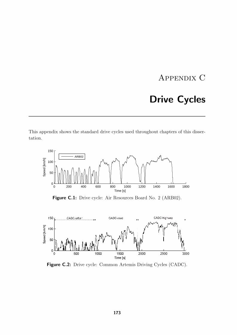
Appendix C
Drive Cycles
This appendix shows the standard drive cycles used throughout chapters of this disser-
tation.
0 200 400 600 800 1000 1200 1400 1600 18000
50
100
150
Time [s]
Spe
ed [k
m/h
]
ARB02
Figure C.1: Drive cycle: Air Resources Board No. 2 (ARB02).
Figure C.2: Drive cycle: Common Artemis Driving Cycles (CADC).
173

174 C Drive Cycles
0 200 400 600 800 1000 1200 1400 1600 1800 20000
50
100
150
Time [s]
Spe
ed [k
m/h
]
FTP75
Figure C.3: Drive cycle: Federal Test Procedure 75 (FTP75).
0 100 200 300 400 500 600 700 800 9000
50
100
150
Time [s]
Spe
ed [k
m/h
]
HURK
Figure C.4: Drive cycle: Hurk (in Eindhoven, The Netherlands).
0 100 200 300 400 500 600 700 8000
50
100
150
Time [s]
Spe
ed [k
m/h
]
HWFET
Figure C.5: Drive cycle: Highway Fuel Economy Driving Cycle (HWFET).
0 100 200 300 400 500 600 7000
50
100
150
Time [s]
Spe
ed [k
m/h
]
JN1015
Figure C.6: Drive cycle: Japan 1015 (JN1015).

175
0 500 1000 15000
50
100
150
Time [s]
Spe
ed [k
m/h
]
LA92
Figure C.7: Drive cycle: Los Angeles 92 (LA92).
0 200 400 600 800 1000 12000
50
100
150
Time [s]
Spe
ed [k
m/h
]
NEDC
Figure C.8: Drive cycle: New European Drive Cycle (NEDC).
0 100 200 300 400 500 6000
50
100
150
Time [s]
Spe
ed [k
m/h
]
NYCC
Figure C.9: Drive cycle: New York City Cycle (NYCC).
0 100 200 300 400 500 6000
50
100
150
Time [s]
Spe
ed [k
m/h
]
US06
Figure C.10: Drive cycle: US06.

176

Bibliography
[1] F. Alkhalisi. Are automotive suppliers prepared for a new era in transmission technology? InElectric & Hybrid Vehicle Technology International. UKIP Media & Event Ltd, 2012.
[2] D. Ambuhl and L. Guzzella. Predictive reference signal generator for hybrid electric vehicles.IEEE Transactions on Vehicular Technology, 58(9):4730–4740, 2009.
[3] D. Ambuhl, O. Sundstrom, A. Sciarretta, and L. Guzzella. Explicit optimal control policy and itspractical application for hybrid electric powertrains. Control Engineering Practice, 18:1429–1439,2010.
[4] I. Arsie, M. Graziosi, C. Pianese, and M. Rizzo, G.and Sorrentino. Optimization of supervisorycontrol strategy for parallel hybrid vehicle with provisional load estimate. In Proceedings of the7th International Symposium on Advanced Vehicle Control - AVEC04, 2004.
[5] M. Back, M. Simons, F. Kirschbaum, and V. Krebs. Predictive control of drivetrains. In Pro-ceedings of the 15th IFAC World Congress, 2002.
[6] S. Bai, K. V. Hebbale, and C. J. Lee. Automatic transmission shift point control system andmethod of use, 2008.
[7] S. Bai, J. Maguire, D. K. Kim, and H. Peng. Dynamic programming based motor vehicle shiftmap generation. In Proceedings of the world automotive congress 2006 - FISITA 2006, 2006.
[8] S. Barsali, C. Miulli, and A. Possenti. A control strategy to minimize fuel consumption of serieshybrid electric vehicles. IEEE Transactions on Energy Conversion, 19(1):187–195, 2004.
[9] R. Bartholomaeus, M. Klingner, and M. Lehnert. Prediction of power demand for hybrid vehiclesoperating in fixed-route service. In Proceedings of the 17th IFAC World Congress, pages 5640–5645, Seoul, Korea, 2008.
[10] R. Beck, A. Bollig, and D. Abel. Comparison of two real-time predictive strategies for the optimalenergy management of a hybrid electric vehicle. Oil and Gas Science and Technology–Rev. IFP,62:635–643, 2007.
[11] R.E. Bellman. Dynamic Programming. Princeton University Press, Princeton, USA, 1957.
[12] A. Bemporad, P. Borodani, and M. Mannelli. Hybrid control of an automotive robotized gearboxfor reduction of consumptions and emissions. Springer Berlin -Heidelberg, 2623:81–96, 2003.
[13] J. Bernard, S. Delprat, T. M. Guerra, and F. N. Buchi. Fuel efficient power management strategyfor fuel cell hybrid powertrains. Control Engineering Practice, 18:408–417, 2010.
[14] D. P. Bertsekas. Dynamic Programming and Optimal Control. Athena Scientific, Belmont, USA,2000.
[15] I. J. M. Besselink, P. F. Van Oorschot, E. Meinders, and H. Nijmeijer. Design of an efficient,low weight battery electric vehicle based on a VW Lupo 3L. In Proceedings of the 25th ElectricVehicle Symposium, Shenzhen, China, 2010. 10 pages.
177

178
[16] H. A. Borhan, A. Vahidi, A. M. Phillips, M. L. Kuang, and I. V. Kolmanovsky. Predictive energymanagement of a power-split hybrid electric vehicle. In Proceedings of 2009 American ControlConference, pages 3970–3976, St. Louis, MO., USA, 2009.
[17] L. Buie, M. Fry, P. Fussey, and C. Mitts. An application of cost-based power management controlstrategies to hybrid fuel cell vehicles. In Proceedings of 2004 SAE International, 2004.
[18] A. Casavola, G. Prodi, and G. Rocca. Efficient gear shifting strategies for green driving policies.In Proceedings of 2010 American Control Conference, pages 4331–4336, 2010.
[19] M. Ceraolo, A. di Donato, and G. Franceschi. A general approach to energy optimization ofhybrid electric vehicles. IEEE Transactions on Vehicular Technology, 57(3):1433–1441, 2008.
[20] F. H. Clarke. Necessary Conditions in Dynamic Optimization. Vol. 173, Nr 816. AmericanMathematical Society, Providence, Rhode Island, USA, 2005.
[21] R. Cook, A. M. Cristobal, G. Parks, C. O. Correa, and P. J. Clarkson. Multi-objective opti-mization of a hybrid electric vehicle - drive train and driving strategy. Springer Berlin, 4403,2007.
[22] J. Dai. Isolated word recognition using Markov chain models. IEEE Transactions on Speech andAudio Processing, 3(6):458–463, 1995.
[23] B. de Schutter and W. P. M. H. Heemels. Modeling and Control of Hybrid Systems. LectureNotes of the DISC Course, 2008. DISC: Dutch Institute of Systems and Control.
[24] S. Delprat, T. M. Guerra, and J. Rimaux. Optimal control of a parallel powertrain: From globaloptimization to real time control strategy. In Proceedings of 2002 IEEE Vehicular TechnologyConference, pages 2082–2088, Birmingham, Al., USA, 2002.
[25] S. Delprat, J. Lauber, T. M. Guerra, and J. Rimaux. Control of a parallel hybrid powertrain:Optimal control. IEEE Transactions on Vehicular Technology, 53:872–881, 2004.
[26] Luc Devroye. Non-Uniform Random Variate Generation. Springer-Verlag, 1986.
[27] R. Edwards, J. F. Larive, V. Mahieu, and P. Rouveirolles. Well-to-wheels analysis of futureautomotive fuels and powertrains in the European context, WELL-TO-TANK report version2b. European Commission Joint Research Centre, Institute for Environment and Sustainability,2006.
[28] M. Ehsani, Y. Gao, and A. Emadi. Modern Electric, Hybrid Electric, and Fuel Cell Vehicles -Fundamentals, Theory, and Design. CRC Press, September 2009.
[29] B. S. Everitt, S. Landau, and M. Leese. Cluster Analysis. Arnold, 4th edition, 2001.
[30] B. C. Fabien. Numerical solution of constrained optimal control problems with parameters.Applied Mathematics and Computation, 80:43–62, 1996.
[31] S. A. Fayazi, S. Farhangi, and B. Asaei. Power delivery co-ordination to meet driver’s demandin a mild hybrid vehicle with automated manual transmission. In Proceedings of the 34th AnnualConference of IEEE Industrial Electronics, pages 327–332, 2008.
[32] Z. Filipi and Y.J. Kim. Hydraulic hybrid propulsion for heavy vehicles: Combining the simulationand engine-in-the-loop techniques to maximize the fuel economy and emission benefits. Oil andGas Science and Technology–Rev. IFP, 65:155–178, 2009.
[33] Z. Filipi, L. Louca, B. Daran, C. C. Lin, U. Yildir, B. Wu, M. Kokkolaras, D. Assanis, H. Peng,P. Papalambros, J. Stein, D. Szkubiel, and R. Chapp. Combined optimisation of design and powermanagement of the hydraulic hybrid propulsion system for the 6x6 medium truck. InternationalJournal of Heavy Vehicle Systems, 11:372–402, 2004.
[34] D. G. Florencio, E. R. Assis, and C. H. F. Amendola. The manual transmission automated -gearshift quality comparison to a similar manual system. In Proceedings of 2004 SAE Interna-tional, 2004.

Bibliography 179
[35] D. Foster, R. Cloudt, and F. Willems. Towards integrated powertrain control: exploiting synergybetween a diesel hybrid and aftertreatment system in a distribution truck. In Proceedings of IEEEIntelligent Vehicles Symposium, pages 1021–1026, Eindhoven, the Netherlands, 2008.
[36] ZF Friedrichshafen. ZF develops 9-speed automatic transmission for passenger cars. Press Infor-mation, 11 2011.
[37] T. Gassman and C. Gasch. Transmission technology for hybrid and electric vehicle. In Proceedingsof 2012 SAE International, 2012.
[38] H.P. Geering. Optimal Control with Engineering Applications. Springer-Verlag, Berlin, Heidel-berg, Germany, 2007.
[39] L. Glielmo, L. Iannelli, V. Vacca, and F. Vasca. Gearshift control for automated manual trans-missions. IEEE/ASME Transactions on Mechatronics, 11(1):17–26, 2006.
[40] Q. Gong, Y. Li, and Z.R. Peng. Trip-based optimal power management of plug-in hybrid electricvehicles. IEEE Transactions on Vehicular Technology, 57:3393–3401, 2008.
[41] Qiuming Gong, Yaoyu Li, and Zhong-Ren Peng. Optimal power management of plug-in HEVwith intelligent transportation system. In Proceedings of IEEE/ASME international conferenceon advanced intelligent mechatronics, pages 1–6, 2007.
[42] L. Guzzella and A. Sciarretta. Vehicle Propulsion Systems: Introduction to Modeling and Opti-mization. Springer-Verlag, Berlin, Heidelberg, Germany, 2007.
[43] K. W. Gwak and G. Y. Masada. Structural analysis and optimization of nonlinear control systemsusing singular value decomposition. Journal of Dynamic Systems, Measurement, and Control,127, 2005.
[44] R. F. Hartl, S. P. Sethi, and R. G. Vickson. A survey of the maximum principles for optimalcontrol problems with state constraints. SIAM Review, 37:181–218, 1995.
[45] K. Hayashi, Y. Shimizu, Y. Dote, A. Takayama, and A. Hirako. Neuro fuzzy transmission controlfor automobile with variable loads. IEEE Transactions on Control Systems Technology, 3(1):49–53, 1995.
[46] R. P. G. Heath and A. J. Child. Zeroshift - a seamless automated manual transmission with notorque interrupt. In Proceedings of 2007 SAE International, 2007.
[47] E. Hellstrom. Look-ahead Control of Heavy Vehicles. PhD thesis, Linkoping University Instituteof Technology, Linkoping, Sweden, 2010.
[48] E. Hellstrom, J. Aslund, and L. Nielsen. Management of kinetic and electric energy in heavytrucks. SAE International Journal of Engines, 3:1152–1163, 2010.
[49] T. Hofman. Framework for Combined control and design optimization of hybrid vehicle propulsionsystems. PhD thesis, Technische Universiteit Eindhoven, The Netherlands, 2007.
[50] T. Hofman, M. Steinbuch, R. Van Druten, and A. Serrarens. Rule-based energy managementstrategies for hybrid vehicles. International Journal of Electric and Hybrid Vehicles, 1:71–94,2007.
[51] T. Hofman, M. Steinbuch, R. van Druten, and A. Serrarens. Design of CVT-based hybridpassenger cars. IEEE Transactions on Vehicular Technology, 58(2):572–587, 2009.
[52] X. L. Hu, Z. F. Wang, and L. Y. Liao. Multi-objective optimization of HEV fuel economy andemissions using evolutionary computation. In Proceedings of 2004 SAE International, 2004.
[53] M. Huang. Optimal multilevel hierarchical control strategy for parallel hybrid electric vehicle.In Proceedings of 2006 IEEE Vehicle Power and Propulsion Conference, pages 1–4, 2006.
[54] International Energy Agency. Hybrid and electric vehicles - the electric drive plugs in. Technicalreport, International Energy Agency, 2011.
180
[55] B. Jacobson and M. Spickenreuther. Gearshift sequence optimisation for vehicles with automatednon-powershifting transmissions. International Journal of Vehicle Design, 32:187–207, 2003.
[56] S. I. Jeon, S. T. Jo, Y. I. Park, and J. M. Lee. Multi-mode driving control of a parallel hybridelectric vehicle using driving pattern recognition. Journal of Dynamic Systems, Measurement,and Control, 124:141–149, 2002.
[57] L. Johannesson, M. Asbogard, and B. Egardt. Assessing the potential of predictive controlfor hybrid vehicle powertrains using stochastic dynamic programming. IEEE Transactions onIntelligent Transportation Systems, 8:71 – 83, 2007.
[58] V. H. Johnson, K. Wipke, and D. Rausen. HEV control strategy for real-time optimization offuel economy and emissions. In Proceedings of 2000 SAE International, 2000.
[59] R. Johri, S. Baseley, and Z. Filipi. Simultaneous optimization of supervisory control and gearshift logic for a parallel hydraulic hybrid refuse truck using stochastic dynamic programming. InProceeding of the 4th Annual Dynamic Systems and Control Conference, VA, USA, 2011.
[60] J. M. Kang, I. Kolmanovsky, and J. W. Grizzle. Dynamic optimization of lean burn engineaftertreatment. Journal of Dynamic Systems, Measurement, and Control, 123:153–160, 2001.
[61] G. E. Katsargyri, I. V. Kolmanovsky, J. Michelini, M. L. Kuang, A. M. Phillips, M. Rinehart,and M. A. Dahleh. Optimally controlling hybrid electric vehicles using path forecasting. InProceedings of 2009 American Control Conference, pages 4613–4617, 2009.
[62] J. T. B. A. Kessels. Energy Management for Automotive Power Nets. PhD thesis, EindhovenUniversity of Technology, The Netherlands, 2007.
[63] J. T. B. A. Kessels, M. W. T. Koot, P. P. J. van den Bosch, and D. B. Kok. Online energy manage-ment for hybrid electric vehicles. IEEE Transactions on Vehicular Technology, 57(6):3428–3440,2008.
[64] J. T. B. A. Kessels and P. Van den Bosch. Electronic horizon: Road information used by energymanagement strategies. Journal of Intelligent Information and Database Systems, 2:187–203,2008.
[65] H. K. Khalil. Nonlinear Systems. Third edition. Prentice-Hall, Inc., New Jersey, USA, 2002.
[66] D. K. Kim, H. Peng, S. Bai, and J. M. Maguire. Control of integrated powertrain with elec-tronic throttle and automatic transmission. IEEE Transactions on Control Systems Technology,15(3):474–482, 2007.
[67] N. Kim, S. Cha, and H. Peng. Optimal control of hybrid electric vehicles based on Pontryagin’sminimum principle. IEEE Transactions on Control Systems Technology, 19(5):1279–1287, 2011.
[68] F. Kirschbaum, M. Back, and M. Hart. Determination of the fuel-optimal trajectory for a vehiclealong a known route. In Proceedings of the 15th IFAC Triennial World Congress, Barcelona,Spain, 2002. 5 pages.
[69] A. Kleimaier and D. Schroder. An approach for the online optimized control of a hybrid power-train. In Proceeding of the 7th International Advanced Motion Control Workshop, pages 215–220,2002.
[70] I. Kolmanovsky, I. Siverguina, and B. Lygoe. Optimization of powertrain operating policy forfeasibility assessment and calibration: stochastic dynamic programming approach. In Proceedingsof 2002 American Control Conference, volume 2, pages 1425–1430, 2002.
[71] I. V. Kolmanovsky and V. Winstead. A receding horizon optimal control approach to activestate and parameter estimation in automotive systems. In Proceedings of 2006 IEEE Conferenceon Control Applications, pages 2796–2801, Munich, Germany, 2006.
[72] M. Koot. Energy Management for Vehicular Electric Power Systems. PhD thesis, TechnischeUniversiteit Eindhoven, The Netherlands, 2006.

Bibliography 181
[73] M. Koot, J. T. B. A. Kessels, B. de Jager, W. Heemels, P. van den Bosch, and M. Steinbuch.Energy management strategies for vehicular electric power systems. IEEE Transactions on Ve-hicular Technology, 54:771–782, 2005.
[74] M. Koot, J.T.B.A. Kessels, and B. De Jager. Fuel reduction of parallel hybrid electric vehicles.In Proceedings of 2005 IEEE Vehicle Power and Propulsion Conference, pages 26–31, Chicago,IL, USA, 2005.
[75] D. S. Kum, H. Peng, and N. K. Bucknor. Supervisory control of parallel hybrid electric vehicles forfuel and emission reduction. Journal of Dynamic Systems, Measurement, and Control, 133(6):10,2011.
[76] O. Kyoungcheol, J. H. Min, D. H. Choi, and H. S. Kim. Optimization of control strategyfor a single-shaft parallel hybrid electric vehicle. Proceedings of the Institution of MechanicalEngineers, Part D - Journal of Automobile Engineering, 221:555–565, 2007.
[77] D. le Guen, T. Weck, A. Balihe, and B. Verbeke. Definition of gearshift pattern: Innovativeoptimization procedures using system simulation. SAE International Journal of Engines, 4:412–431, 04 2011.
[78] H. D. Lee, S. K. Sul, H. S. Cho, and J. M. Lee. Advanced gear-shifting and clutching strategyfor a parallel-hybrid vehicle. IEEE Industry Applications Magazine, 6(6):26–32, 2000.
[79] Robert D. Leopold. A new definition of ‘fuel efficiency ’ in commercial vehicles. In Proceedingsof 2009 SAE International, 2009.
[80] W. Li, G. Xu, Z. Wang, and Y. Xu. Dynamic energy management for hybrid electric vehiclebased on adaptive dynamic programming. In Proceeding of 2008 IEEE International Conferenceon Industrial Technology, pages 1–6, 2008.
[81] C. C. Lin, S. Jeon, H. Peng, and J. M. Lee. Driving pattern recognition for control of hybridelectric trucks. Vehicle System Dynamics, 42:41–58, 2004.
[82] C. C. Lin, H. Peng, and J. W. Grizzle. A stochastic control strategy for hybrid electric vehicles.In Proceedings of 2004 American Control Conference, volume 5, pages 4710–4715, 2004.
[83] C. C. Lin, H. Peng, J. W. Grizzle, and J. M. Kang. Power management strategy for a parallelhybrid electric truck. IEEE Transactions on Control Systems Technology, 11:839–849, 2003.
[84] S. Lin, S. Chang, and B. Li. Gearshift system design for automated manual transmission basedon an electromagnetic actuator. In Proceedings of 2011 International Electrical and ControlEngineering Conference, pages 2250–2253, 2011.
[85] B. W. Lindgren. Statistical theory. Chapman & Hall, 4th edition, 1993.
[86] S. M. Lukic and A. Emadi. Effects of drivetrain hybridization on fuel economy and dynamicperformance of parallel hybrid electric vehicles. IEEE Transactions on Vehicular Technology,53:385–389, 2004.
[87] B. Mashadi, A. Kazemkhani, and R. B. Lakeh. An automatic gear-shifting strategy for manualtransmissions. Proceedings of the Institution of Mechanical Engineers, Part I - Journal of Systemsand Control Engineering, 221:757–768, 2007.
[88] C. Musardo, G. Rizzoni, and B. Staccia. A-ECMS : An adaptive algorithm for hybrid electric ve-hicle energy management. In Proceedings of the 2005 IEEE Conference on Decision and Control,and the European Control Conference, pages 1816–1823, Seville, Spain, 2005.
[89] H. Naunheimer, B. Bertsche, J. Ryborz, and W. Novak. Automotive Transmissions: Fundamen-tals, Selection, Design and Application. Springer, 2 edition, 2011.
[90] G. J. L. Naus, R. P. A. Vugts, J. Ploeg, M. J. G. Van de Molengraft, and M. Steinbuch.String-stable CACC design and experimental validation, a frequency-domain approach. IEEETransactions on Vehicular Technology, 59:4268–4279, 2010.

182
[91] V. Ngo, T. Hofman, M. Steinbuch, and A. Serrarens. Performance indices for vehicular propulsionsystems. In Proceedings of the 15th Asia Pacific Automotive Engineering Conference, 2009.
[92] V. Ngo, T. Hofman, M. Steinbuch, and A. Serrarens. Shifting strategy for step change transmis-sion vehicle a comparative study and design method. In Proceedings of the 24th InternationalBattery, Hybrid and Fuel Cell Electric Vehicle Symposium, 2009.
[93] V. Ngo, T. Hofman, M. Steinbuch, and A. Serrarens. An optimal control-based algorithm forhybrid electric vehicle using preview route information. In Proceedings of 2010 American ControlConference, 2010.
[94] V. Ngo, T. Hofman, M. Steinbuch, and A. Serrarens. Optimal shifting strategy for a parallelhybrid electric vehicle. In Proceedings of the 25th World Battery, Hybrid and Fuel Cell ElectricVehicle Symposium and Exhibition - EVS25, 2010.
[95] V. Ngo, T. Hofman, M. Steinbuch, and A. Serrarens. Analyses of the performance index for ahybrid electric vehicle. In Proceedings of 2011 American Control Conference, 2011.
[96] V. Ngo, T. Hofman, M. Steinbuch, and A. Serrarens. Predictive gear shift control for a parallelhybrid electric vehicle. In Proceedings of 2011 IEEE Vehicle Power and Propulsion Conference,pages 1–6, 2011.
[97] V. Ngo, T. Hofman, M. Steinbuch, and A. Serrarens. Effect of gear shift and engine start losseson control strategies for hybrid electric vehicles. In Proceedings of the 26th Electric VehicleSymposium - EVS26, 2012.
[98] V. Ngo, T. Hofman, M. Steinbuch, and A. Serrarens. Optimal control of the gear shift commandfor hybrid electric vehicles. IEEE Transactions on Vehicular Technology, 61, 2012.
[99] V. Ngo, T. Hofman, M. Steinbuch, A. Serrarens, and L. Merkx. Improvement of fuel economy inpower-shift automated manual transmission through shift strategy optimization - an experimentalstudy. In Proceedings of 2010 IEEE Vehicle Power and Propulsion Conference, pages 1–5, 2010.
[100] D. F. Opila, D. Aswani, R. McGee, J. A Cook, and J. W. Grizzle. Incorporating drivabilitymetrics into optimal energy management strategies for hybrid vehicles. In Proceedings of the47th IEEE Conference on Decision and Control, pages 4382–4389. IEEE, 2008.
[101] G. Paganelli, G. Ercole, A. Brahma, Y. Guezennec, and G. Rizzoni. General supervisory controlpolicy for the energy optimization of charge-sustaining hybrid electric vehicles. JSAE Review,22:511–518, 2001.
[102] G. Paganelli, T.M. Guerra, S. Delprat, Y. Guezennec, and G. Rizzoni. Optimal control theoryapplied to hybrid fuel cell powered vehicle. In Proceedings of the 15th IFAC Triennial WorldCongress, Barcelona, Spain, 2002. 6 pages.
[103] M. F. Pan and C. C. Ku. Application of singular value decomposition for structural modalanalysis. The Japanese Journal of Applied Physics, 30:2626–2635, 1991.
[104] B. Passenberg, P. Kock, and O. Stursberg. Combined time and fuel optimal driving of trucksbased on a hybrid model. In Proceedings of 2009 European Control Conference, pages 4955–4960,Budapest, Hungary, 2009.
[105] R. Pfiffner and L. Guzzella. Optimal operation of CVT-based powertrains. International Journalof Robust and Nonlinear Control, 11(11):1003–1021, 2001.
[106] P. Pisu, K. Koprubasi, and G. Rizzoni. Energy management and drivability control problemsfor hybrid electric vehicles. In Proceedings of the 44th IEEE European Control Conference onDecision and Control, pages 1824–1830, 2005.
[107] P. Pisu and G. Rizzoni. A comparative study of supervisory control strategies for hybrid electricvehicles. IEEE Transactions on Control Systems Technology, 15:506–518, 2007.
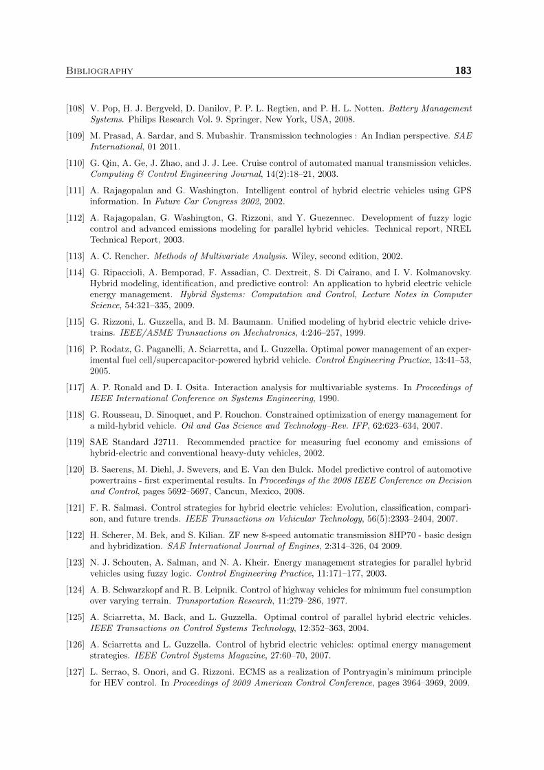
Bibliography 183
[108] V. Pop, H. J. Bergveld, D. Danilov, P. P. L. Regtien, and P. H. L. Notten. Battery ManagementSystems. Philips Research Vol. 9. Springer, New York, USA, 2008.
[109] M. Prasad, A. Sardar, and S. Mubashir. Transmission technologies : An Indian perspective. SAEInternational, 01 2011.
[110] G. Qin, A. Ge, J. Zhao, and J. J. Lee. Cruise control of automated manual transmission vehicles.Computing & Control Engineering Journal, 14(2):18–21, 2003.
[111] A. Rajagopalan and G. Washington. Intelligent control of hybrid electric vehicles using GPSinformation. In Future Car Congress 2002, 2002.
[112] A. Rajagopalan, G. Washington, G. Rizzoni, and Y. Guezennec. Development of fuzzy logiccontrol and advanced emissions modeling for parallel hybrid vehicles. Technical report, NRELTechnical Report, 2003.
[113] A. C. Rencher. Methods of Multivariate Analysis. Wiley, second edition, 2002.
[114] G. Ripaccioli, A. Bemporad, F. Assadian, C. Dextreit, S. Di Cairano, and I. V. Kolmanovsky.Hybrid modeling, identification, and predictive control: An application to hybrid electric vehicleenergy management. Hybrid Systems: Computation and Control, Lecture Notes in ComputerScience, 54:321–335, 2009.
[115] G. Rizzoni, L. Guzzella, and B. M. Baumann. Unified modeling of hybrid electric vehicle drive-trains. IEEE/ASME Transactions on Mechatronics, 4:246–257, 1999.
[116] P. Rodatz, G. Paganelli, A. Sciarretta, and L. Guzzella. Optimal power management of an exper-imental fuel cell/supercapacitor-powered hybrid vehicle. Control Engineering Practice, 13:41–53,2005.
[117] A. P. Ronald and D. I. Osita. Interaction analysis for multivariable systems. In Proceedings ofIEEE International Conference on Systems Engineering, 1990.
[118] G. Rousseau, D. Sinoquet, and P. Rouchon. Constrained optimization of energy management fora mild-hybrid vehicle. Oil and Gas Science and Technology–Rev. IFP, 62:623–634, 2007.
[119] SAE Standard J2711. Recommended practice for measuring fuel economy and emissions ofhybrid-electric and conventional heavy-duty vehicles, 2002.
[120] B. Saerens, M. Diehl, J. Swevers, and E. Van den Bulck. Model predictive control of automotivepowertrains - first experimental results. In Proceedings of the 2008 IEEE Conference on Decisionand Control, pages 5692–5697, Cancun, Mexico, 2008.
[121] F. R. Salmasi. Control strategies for hybrid electric vehicles: Evolution, classification, compari-son, and future trends. IEEE Transactions on Vehicular Technology, 56(5):2393–2404, 2007.
[122] H. Scherer, M. Bek, and S. Kilian. ZF new 8-speed automatic transmission 8HP70 - basic designand hybridization. SAE International Journal of Engines, 2:314–326, 04 2009.
[123] N. J. Schouten, A. Salman, and N. A. Kheir. Energy management strategies for parallel hybridvehicles using fuzzy logic. Control Engineering Practice, 11:171–177, 2003.
[124] A. B. Schwarzkopf and R. B. Leipnik. Control of highway vehicles for minimum fuel consumptionover varying terrain. Transportation Research, 11:279–286, 1977.
[125] A. Sciarretta, M. Back, and L. Guzzella. Optimal control of parallel hybrid electric vehicles.IEEE Transactions on Control Systems Technology, 12:352–363, 2004.
[126] A. Sciarretta and L. Guzzella. Control of hybrid electric vehicles: optimal energy managementstrategies. IEEE Control Systems Magazine, 27:60–70, 2007.
[127] L. Serrao, S. Onori, and G. Rizzoni. ECMS as a realization of Pontryagin’s minimum principlefor HEV control. In Proceedings of 2009 American Control Conference, pages 3964–3969, 2009.
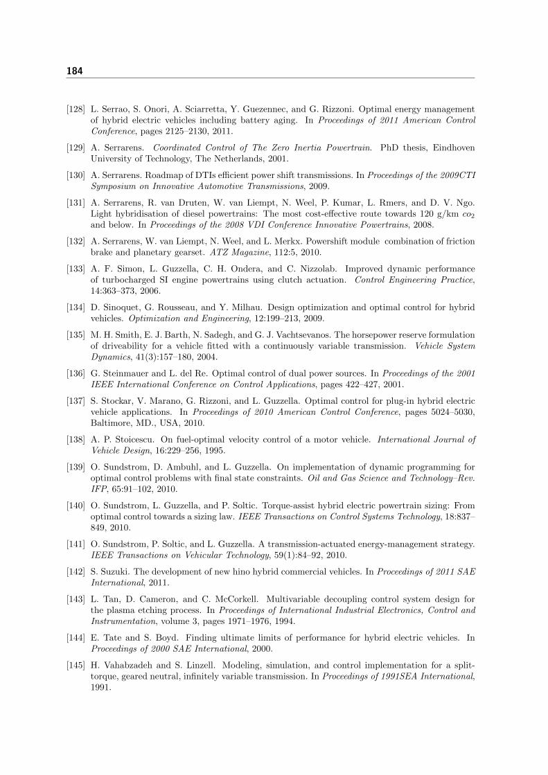
184
[128] L. Serrao, S. Onori, A. Sciarretta, Y. Guezennec, and G. Rizzoni. Optimal energy managementof hybrid electric vehicles including battery aging. In Proceedings of 2011 American ControlConference, pages 2125–2130, 2011.
[129] A. Serrarens. Coordinated Control of The Zero Inertia Powertrain. PhD thesis, EindhovenUniversity of Technology, The Netherlands, 2001.
[130] A. Serrarens. Roadmap of DTIs efficient power shift transmissions. In Proceedings of the 2009CTISymposium on Innovative Automotive Transmissions, 2009.
[131] A. Serrarens, R. van Druten, W. van Liempt, N. Weel, P. Kumar, L. Rmers, and D. V. Ngo.Light hybridisation of diesel powertrains: The most cost-effective route towards 120 g/km co2and below. In Proceedings of the 2008 VDI Conference Innovative Powertrains, 2008.
[132] A. Serrarens, W. van Liempt, N. Weel, and L. Merkx. Powershift module combination of frictionbrake and planetary gearset. ATZ Magazine, 112:5, 2010.
[133] A. F. Simon, L. Guzzella, C. H. Ondera, and C. Nizzolab. Improved dynamic performanceof turbocharged SI engine powertrains using clutch actuation. Control Engineering Practice,14:363–373, 2006.
[134] D. Sinoquet, G. Rousseau, and Y. Milhau. Design optimization and optimal control for hybridvehicles. Optimization and Engineering, 12:199–213, 2009.
[135] M. H. Smith, E. J. Barth, N. Sadegh, and G. J. Vachtsevanos. The horsepower reserve formulationof driveability for a vehicle fitted with a continuously variable transmission. Vehicle SystemDynamics, 41(3):157–180, 2004.
[136] G. Steinmauer and L. del Re. Optimal control of dual power sources. In Proceedings of the 2001IEEE International Conference on Control Applications, pages 422–427, 2001.
[137] S. Stockar, V. Marano, G. Rizzoni, and L. Guzzella. Optimal control for plug-in hybrid electricvehicle applications. In Proceedings of 2010 American Control Conference, pages 5024–5030,Baltimore, MD., USA, 2010.
[138] A. P. Stoicescu. On fuel-optimal velocity control of a motor vehicle. International Journal ofVehicle Design, 16:229–256, 1995.
[139] O. Sundstrom, D. Ambuhl, and L. Guzzella. On implementation of dynamic programming foroptimal control problems with final state constraints. Oil and Gas Science and Technology–Rev.IFP, 65:91–102, 2010.
[140] O. Sundstrom, L. Guzzella, and P. Soltic. Torque-assist hybrid electric powertrain sizing: Fromoptimal control towards a sizing law. IEEE Transactions on Control Systems Technology, 18:837–849, 2010.
[141] O. Sundstrom, P. Soltic, and L. Guzzella. A transmission-actuated energy-management strategy.IEEE Transactions on Vehicular Technology, 59(1):84–92, 2010.
[142] S. Suzuki. The development of new hino hybrid commercial vehicles. In Proceedings of 2011 SAEInternational, 2011.
[143] L. Tan, D. Cameron, and C. McCorkell. Multivariable decoupling control system design forthe plasma etching process. In Proceedings of International Industrial Electronics, Control andInstrumentation, volume 3, pages 1971–1976, 1994.
[144] E. Tate and S. Boyd. Finding ultimate limits of performance for hybrid electric vehicles. InProceedings of 2000 SAE International, 2000.
[145] H. Vahabzadeh and S. Linzell. Modeling, simulation, and control implementation for a split-torque, geared neutral, infinitely variable transmission. In Proceedings of 1991SEA International,1991.

Bibliography 185
[146] A. Vahidi, A. Stefanopoulou, and H. Peng. Recursive least squares with forgetting for onlineestimation of vehicle mass and road grade. Vehicle System Dynamics, 43:31–55, 2005.
[147] H. J. Valeri, B. W. Keith, and J. R. David. HEV control strategy for real-time optimization offuel economy and emissions. In Proceedings of 2000 SAE International, 2000.
[148] T. J. J. van den Boom and A. A. Stoorvogel. Model Predictive Control. DISC Course-LectureNotes, 2010.
[149] P. P. J. van den Bosch and F. A. Lootsma. Scheduling of power generation via large-scalenonlinear optimization. Journal of Optimization Theory and Applications, 55:313–326, 1987.
[150] T. van Keulen. Fuel Optimal Control of Hybrid Vehicles. PhD thesis, Eindhoven University ofTechnology, The Netherlands, The Netherlands, 2011.
[151] T. van Keulen, B. de Jager, and M. Steinbuch. Optimal trajectories for vehicles with energyrecovery options. In Proceedings of the 18th IFAC World Congress, volume 18, 2011.
[152] T.A.C. van Keulen, A.G. de Jager, A.F.A. Serrarens, and M. Steinbuch. Optimal energy manage-ment in hybrid electric trucks using route information. Oil and Gas Science and Technology–Rev.IFP, 65:103 – 113, 2010.
[153] P. Varaiya. Lecture notes on optimization. Technical report, University of California at Berkeley,1998.
[154] M. Vasak, M. Baotic, N. Peric, and M. Bago. Optimal rail route energy management underconstraints and fixed arrival time. In Proceedings of 2009 European Control Conference, pages2972–2977, Budapest, Hungary, 2009.
[155] F. Vasca, L. Iannelli, A. Senatore, and M. T. Scafati. Modeling torque transmissibility forautomotive dry clutch engagement. In Proceedings of 2008 American Control Conference, pages306–311, 2008.
[156] F. Wang, X. J. Mao, B. Zhuo, H. Zhong, and Z. L. Ma. Parallel hybrid electric system energyoptimization control with automated mechanical transmission. Proceedings of the Institution ofMechanical Engineers, Part D - Journal of Automobile Engineering, 222:499–513, 2008.
[157] W. Wang, Q. Wang, and X. Zeng. Automated manual transmission shift strategy for parallelhybrid electric vehicle. In Proceedings of 2009 SAE International, 2009.
[158] X. Wei. Modeling and Control of a Hybrid Electric Drivetrain for Optimum Fuel Economy,Performance and Driveability. PhD thesis, Ohio State University, US, 2004.
[159] X. Wei, L. Guzzella, V. I. Utkin, and G. Rizzoni. Model-based fuel optimal control of hybrid elec-tric vehicle using variable structure control systems. Journal of Dynamic Systems, Measurement,and Control, 129:13–19, 2007.
[160] F. Willems and R. Cloudt. Experimental demonstration of a new model-based SCR control strat-egy for cleaner heavy-duty diesel engines. IEEE Transactions on Control Systems Technology,19:1305–1313, 2011.
[161] S. S. Williamson and A. Emadi. Comparative assessment of hybrid electric and fuel cell vehi-cles based on comprehensive well-to-wheels efficiency analysis. IEEE Transactions on VehicularTechnology, 54:856–862, 2005.
[162] J. S. Won and R. Langari. Intelligent energy management agent for a parallel hybrid vehicle-partii: torque distribution, charge sustenance strategies, and performance results. IEEE Transactionson Vehicular Technology, 54(3):935–953, 2005.
[163] J. S. Won, R. Langari, and M. Ehsani. An energy management and charge sustaining strategyfor a parallel hybrid vehicle with CVT. IEEE Transactions on Control Systems Technology,13(2):313–320, 2005.

186 Bibliography
[164] W. Xiong, Y. Zhang, and C. Yin. Optimal energy management for a series-parallel hybrid electricbus. Journal of Energy Conversion and Management, 50:1730–1738, 2009.
[165] M. Yamasaki, H. Konno, H. Kuroiwa, and N. Ozaki. Automated manual transmission with torqueassist mechanism for reducing shift shock. In Proceedings of 2005 SAE International, 2005.
[166] Z. G Yang, C. X Cao, and Y. Su. A method of optimal shift control based on pattern recogni-tion and learning algorithm. In Proceedings of the 4th World Congress Intelligent Control andAutomation, volume 2, pages 955–959, 2002.
[167] X. Yin, D. Xue, and Y. Cai. Application of time-optimal strategy and fuzzy logic to the enginespeed control during the gear-shifting process of AMT. In Proceedings of the 4th InternationalConferrence of Fuzzy Systems and Knowledge Discovery, volume 4, pages 468–472, 2007.
[168] Z. Yong, S. Jian, W. Di, and Xu C. Automatic transmission shift point control under differentdriving vehicle mass. In Proceedings of 2002 SAE International, 2002.
[169] H. J. Yoon and C. J. Lee. An optimized control strategy for parallel hybrid electric vehicle. InProceedings of 2003 SAE International, 2003.
[170] R. Zhang and Y. Chen. Control of hybrid dynamical systems for electric vehicles. In Proceedingsof 2001 American Control Conference, volume 4, pages 2884–2889, 2001.
[171] Y. Zhang, H. Lin, B. Zhang, and Mi C. Performance modeling and optimization of a novelmulti-mode hybrid powertrain. Journal Mechanical Design, 128:79–89, 2006.
[172] Y. Zhu, Y. Chen, Z. H. Wu, and A. H. Wang. Optimization design of an energy managementstrategy for hybrid vehicles. International Journal of Alternative Propulsion, 1:47–62, 2006.

Acknowledgements
It has been a great privilege for me to be with the Control Systems Technology Group
at Mechanical Engineering Department, Eindhoven University of Technology, as a PhD
candidate. The PhD journey is probably the most challenging one with which I have
ever been. By organizing the study, planing the project, doing research, and realizing
fruitful results, a dissertation has finally come up. The research as presented in this
dissertation has been made possible by the contributions of numerous people to whom
I would like to acknowledge.
First of all, I would like to express my deep gratitude to my supervisor Prof. Maarten
Steinbuch, for offering me the opportunity to work on such an interesting project as a
PhD candidate. He has patiently provided the vision, encouragement and advise nec-
essary for me to proceed through the doctoral program and complete my dissertation.
I am totaly delighted with his efficient, pragmatic, direct and honest guidance and su-
pervising approach. He has always given me a freedom to do research in the academic
environment. I have learnt a lot from him, not only the knowledge but also the commu-
nication, organization and management skills, which will definitely benefit my future
career.
I am very much grateful to my co-supervisor Dr. Theo Hofman, with whom I work
closely during my PhD candidacy. He has guided me openly and critically and motivated
me to pursue independent, innovative research. I am much indebted to him for his
valuable advice in my work, spending his precious times at regular meetings, reading
papers and dissertation. I am totally undoubted to say that he is a strong and supportive
advisor, very enthusiastic and energetic. Beside the academic world, we have shared
together a lot of fun, life, conference time, etc. I am very happy of having had the
opportunity to work with him.
The research project is proposed by Drivetrain Innovations B.V. (DTI) together with
Eindhoven University of Technology. Herewith, I would like to send special thanks to
DTI in general, and to Dr. Alex Serrarens in particular. The guidance, support, helpful
suggestions and critical comments for papers and dissertation from him has served me
well throughout my PhD. He was the source of inspiration in the early days of my PhD.
187
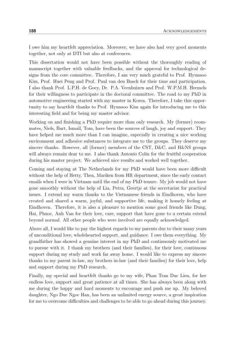
188 Acknowledgements
I owe him my heartfelt appreciation. Moreover, we have also had very good moments
together, not only at DTI but also at conferences.
This dissertation would not have been possible without the thoroughly reading of
manuscript together with valuable feedbacks, and the approval for technological de-
signs from the core committee. Therefore, I am very much grateful to Prof. Hyunsoo
Kim, Prof. Huei Peng and Prof. Paul van den Bosch for their time and participation.
I also thank Prof. L.P.H. de Goey, Dr. P.A. Veenhuizen and Prof. W.P.M.H. Heemels
for their willingness to participate in the doctoral committee. The road to my PhD in
automotive engineering started with my master in Korea. Therefore, I take this oppor-
tunity to say heartfelt thanks to Prof. Hyunsoo Kim again for introducing me to this
interesting field and for being my master advisor.
Working on and finishing a PhD require more than only research. My (former) room-
mates, Niels, Bart, Ismail, Tom, have been the sources of laugh, joy and support. They
have helped me much more than I can imagine, especially in creating a nice working
environment and adhesive substances to integrate me to the groups. They deserve my
sincere thanks. However, all (former) members of the CST, D&C, and H&NS groups
will always remain dear to me. I also thank Antonio Colin for the fruitful cooperation
during his master project. We achieved nice results and worked well together.
Coming and staying at The Netherlands for my PhD would have been more difficult
without the help of Hetty, Thea, Mariken from HR department, since the early contact
emails when I were in Vietnam until the end of my PhD tenure. My job would not have
gone smoothly without the help of Lia, Petra, Geertje at the secretariat for practical
issues. I extend my warm thanks to the Vietnamese friends in Eindhoven, who have
created and shared a warm, joyful, and supportive life, making it homely feeling at
Eindhoven. Therefore, it is also a pleasure to mention some good friends like Dung,
Hai, Phuoc, Anh Van for their love, care, support that have gone to a certain extend
beyond normal. All other people who were involved are equally acknowledged.
Above all, I would like to pay the highest regards to my parents due to their many years
of unconditional love, wholehearted support, and guidance. I owe them everything. My
grandfather has showed a genuine interest in my PhD and continuously motivated me
to pursue with it. I thank my brothers (and their families), for their love, continuous
support during my study and work far away home. I would like to express my sincere
thanks to my parent in-law, my brothers in-law (and their families) for their love, help
and support during my PhD research.
Finally, my special and heartfelt thanks go to my wife, Phan Tran Duc Lien, for her
endless love, support and great patience at all times. She has always been along with
me during the happy and hard moments to encourage and push me up. My beloved
daughter, Ngo Duc Ngoc Han, has been an unlimited energy source, a great inspiration
for me to overcome difficulties and challenges to be able to go ahead during this journey.

Acknowledgements 189
Việc tiếp tục học tập nâng cao chuyên môn, nghiên cứu tiến sĩ sẽ không suôn sẻ nếu thiếu sự giúp
đỡ, tạo điều kiện thuận lợi của TS. Lê Vinh Danh ở Đại học Tôn Đức Thắng. Tôi xin chân thành cảm
ơn sự quan tâm, và những động viên quý báu của Thầy trong thời gian vừa qua. Tôi cũng xin cảm
ơn sự giúp đỡ của các đồng nghiệp ở phòng KHCN-HT-SĐH và khoa Điện-Điện tử. Nhân đây, tôi
cũng xin gởi lời cảm ơn đến PGS. TS. Phạm Xuân Mai (ĐHBK Tp.HCM) vì những trao đổi hữu ích,
các hoạt động chuyên môn, sự quan tâm, và chia sẻ chân thành trong nhiều năm qua, góp thêm
gia vị cuộc sống cho việc nghiên cứu.
Đạt được thành quả hôm nay, trước tiên tôi xin bày tỏ lòng biết ơn đến ông nội. Mặt dù tuổi đã
trên 80, nhưng ông nội luôn luôn son sắt động viên, khích lệ và bày tỏ sự mong đợi thành công
trên con đường nghiên cứu của tôi. Mong ông luôn luôn mạnh khỏe và minh mẫn. Bằng cả tấm
lòng, điều mà khó diễn tả thành lời, tôi xin gởi lời tri ân đến ba mẹ, vì tình yêu thương vô bờ, sự
nuôi nấng, dạy dỗ, hỗ trợ vô điều kiện, sự tận tâm hướng dẫn và động viên không ngừng. Bên cạnh
đó, tôi xin gởi lời cảm ơn đến anh Thủy (và gia đình) và em Triều, vì những thương yêu, tin tưởng
và hỗ trợ vai trò trong quá trình tôi học tập và làm việc xa nhà, xa quê hương. Tôi cũng xin chân
thành biết ơn ba mẹ vợ, anh Đức Anh (và gia đình) và em Hiếu (và gia đình), đã luôn quan tâm,
động viên, giúp đỡ với sự yêu thương, tạo thuận lợi cho quá trình nghiên cứu này.
Cuối cùng là những lời cảm ơn đặc biệt dành cho vợ tôi, Đức Liên, vì sự yêu thương không điều
kiện, hỗ trợ, lo lắng và kiên nhẫn trong mọi thời gian, đồng hành và động viên trong mọi khó khăn.
Con gái yêu quý, Ngọc Hân, thật sự là nguồn năng lượng vô tận, là sự động viên lớn lao để tôi có
thể vượt qua những khó khăn, thách thức và tiến lên phía trước trong suốt chặng đường nghiên
cứu tiến sĩ.
Ngo Dac Viet
Eindhoven, The Netherlands.
July, 2012.

190
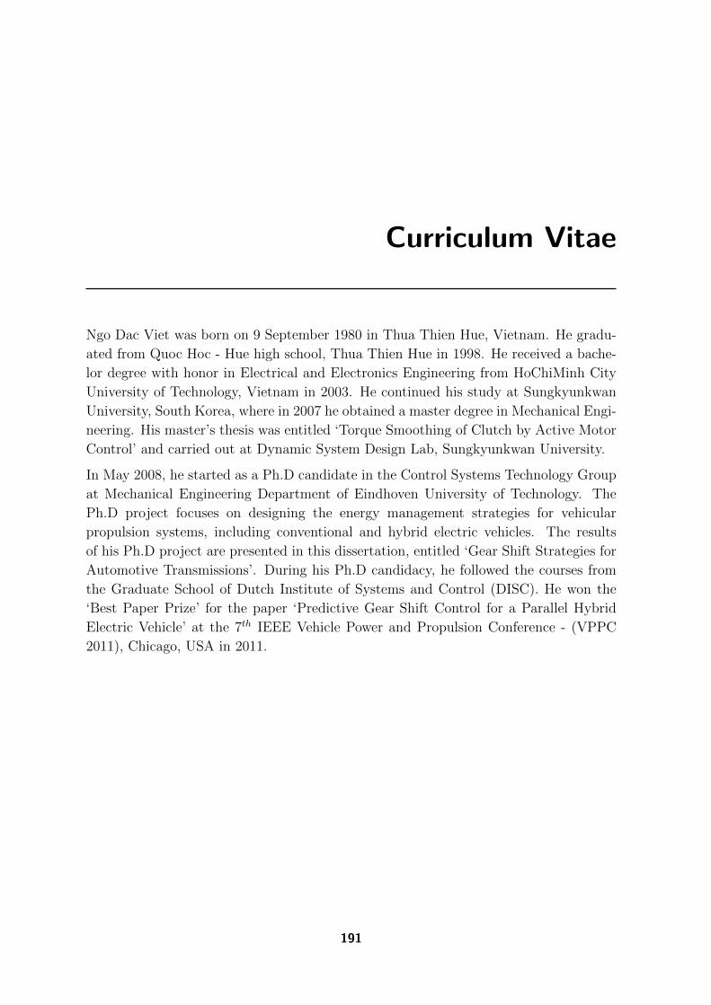
Curriculum Vitae
Ngo Dac Viet was born on 9 September 1980 in Thua Thien Hue, Vietnam. He gradu-
ated from Quoc Hoc - Hue high school, Thua Thien Hue in 1998. He received a bache-
lor degree with honor in Electrical and Electronics Engineering from HoChiMinh City
University of Technology, Vietnam in 2003. He continued his study at Sungkyunkwan
University, South Korea, where in 2007 he obtained a master degree in Mechanical Engi-
neering. His master’s thesis was entitled ‘Torque Smoothing of Clutch by Active Motor
Control’ and carried out at Dynamic System Design Lab, Sungkyunkwan University.
In May 2008, he started as a Ph.D candidate in the Control Systems Technology Group
at Mechanical Engineering Department of Eindhoven University of Technology. The
Ph.D project focuses on designing the energy management strategies for vehicular
propulsion systems, including conventional and hybrid electric vehicles. The results
of his Ph.D project are presented in this dissertation, entitled ‘Gear Shift Strategies for
Automotive Transmissions’. During his Ph.D candidacy, he followed the courses from
the Graduate School of Dutch Institute of Systems and Control (DISC). He won the
‘Best Paper Prize’ for the paper ‘Predictive Gear Shift Control for a Parallel Hybrid
Electric Vehicle’ at the 7th IEEE Vehicle Power and Propulsion Conference - (VPPC
2011), Chicago, USA in 2011.
191

192