Gear-Shift Schedule for Electric Vehicleswith Multi-Speed Transmissions

TRCIM20180115-1 January, 2018

Yuhanes Dedy Setiawan Liauw and Jorge Angeles

C e n t r e f o r

McGill

IntelligentMachines

Centre for Intelligent Machines, Department of Mechanical Engineering

McGill University, Montreal, Canada

Abstract

In this report we propose a gear-shift schedule for electric vehicles with multi-speed transmis-sions. A case study is provided whereby the gear-shift schedule for the GM EV1 with a two-speednovel modular transmission is devised. First, the efficiency map of the electric vehicle is gen-erated. A number of ways are described with a greater detail given to a map generation usingMATLAB/Simulink. Second, the gear-shift time is determined based on an established procedure.Finally, the gear-shift schedule is generated and explained in depth. Detailed procedures are ex-plained along with the code description. Several technical problems are documented together withthe solutions.

Keywords: Gear-shift schedule; Electric Vehicles; Multi-speed transmissions

1 Introduction

Vehicles with automatic transmissions perform gear-shifting according to a gear-shift schedule,which determines when the gear should be shifted to achieve optimal performance with minimumenergy consumption. A recent development in electric vehicles includes multi-speed transmissions,where a gear-shift schedule needs to be devised for electric vehicles with automatic transmissions.However, the schedule-devising procedures for conventional vehicles are not applicable to elec-tric vehicles because electric motors and engines have different efficiency maps. A procedure todevise gear-shift schedules for electric vehicles with multi-speed transmissions was proposed byZhu et al. [1]. In this report, the procedure is utilized to devise a gear-shift schedule for theGM EV1 with a two-speed transmission. The practical details on performing the procedure usingMATLAB/Simulink are reported along with the code description. In addition, several technicalproblems are documented together with the solutions.

2 The Gear-shift Schedule

A gear-shift schedule is designed for the GM EV1 with a two-speed transmission in this report.The details of the generation of the gear-shifting schedule are available in a paper by Zhu et al. [1].To begin with, the efficiency map of the EV motor was reproduced to determine the characteristicsof the motor for the Simplified Federal Urban Drive Schedule (SFUDS) driving cycle. The efficiencymap is accessible either from the motor manufacturer or from commercial motor software, such asMotorSolve, from Infolytica. This package has the capability to generate the efficiency map of amotor under design, as exemplified in Fig. 1. Although MotorSolve can yield an accurate efficiencymap, extensive details of the motor design that may not be available for public are mandatoryto generate the map. Alternatively, the efficiency map can be produced by means of Larminieand Lowry’s efficiency map model [2]. Some motor parameters are necessary, such as the motorcopper, iron, windage and motor constant losses, which are available from the motor catalogue,measured, or requested from the manufacturer. Furthermore, the efficiency map can be measuredusing dynamometers. For the purposes of this study, the GM EV1 motor efficiency map wasproduced by means of Larminie and Lowry’s model, as displayed in Fig. 2. The numbers on thelines account for the efficiency. The MATLAB script to design the gear-shift schedule is providedin Appendix A for reference.

After the efficiency map of the GM EV1 motor was generated, the efficiency map for thevehicle taking the two-speed transmission into account was created. This was simply done bymanipulating the motor efficiency map, namely, the maximum speed and torque of the map aredivided and multiplied by the transmission gear ratio, respectively. The maximum torque of thevehicle efficiency map for gear 1 is the maximum torque of the motor efficiency map times 4, whichis the first gear ratio. Likewise, the vehicle efficiency map for the second gear ratio was obtainedby multiplying the motor efficiency map by 2.67. In other words, the vertical axis is turned intothe transmission output torque.

In order to devise a gear-shifting schedule, the horizontal axis of the vehicle efficiency mapswas converted to the vehicle speed, as opposed to the motor speed. The relationship between the

2

Figure 1: Efficiency map generated by MotorSolve [3]

motor speed and vehicle speed is given by [2]:

ω = γv

rrad s−1 (1)

where ω is the motor speed, γ the gear ratio, v the vehicle speed, and r the wheel radius.

After adjusting the motor efficiency map with the corresponding gear ratio, the vehicle efficiencymap for that particular gear ratio was generated. The maximum torques and speeds of the GMEV1 motor with and without the transmission are listed in Table 1. The vehicle efficiency maps forgears 1 and 2 are depicted in Fig. 3. The vertical and horizontal axes were intentionally set to themaximum to clearly express the modification of the efficiency maps due to the application of ourMST. As illustrated in the figure, the EVs with MSTs have multiple efficiency maps correspondingto the gear ratios of the MST that can be advantageous for particular cases. The consecutiveefficiency map is indicated in Fig 4. Please note that the efficiency values in the vehicle efficiencymap have to be converted back to the values in the motor efficiency map when the efficiency iscalculated to design the gear-shift schedule.

3

0.5

0.5

0.5 0.5

0.5

5

0.5

5

0.55 0.55

0.6

0.6

0.6 0.6

0.6

5

0.6

5

0.65 0.65

0.7

0.7

0.7 0.7

0.7

5

0.7

5

0.750.75

0.8

0.8

0.80.8

0.8

5

0.850.85

100 200 300 400 500 600 700

20

40

60

80

100

120

Figure 2: The GM EV1 motor efficiency map

Table 1: Adjusted GM EV1 performance

Gear ratio 1:1 4:1 2.67:1

T (N.m) 139 556 371.13ω (rad/s) 733 183.25 274.53v (km/h) - 117.29 175.72

The next step was to draw a constant-traction-torque line on the consecutive map. Utilizing theefficiency map MATLAB script by Larminie’s and Lowry’s [2], this step posed a challenge becausethe efficiency map data of the first gear does not carry the same interval as that of the second gear.The solution was to retrieve the torque data that have the minimum difference between gear 1and gear 2. Gear 2 has a lower torque than gear 1; therefore, the data interval in gear 2 is smallerthan that in gear 1. The technique exploited the MATLAB function meshgrid for torque 1 andtorque 2, as in line 78 of the MATLAB script in Appendix A. Subsequently, the difference wasobtained in line 79 and the minimum in line 80. The for loop in lines 88–98 locate the minimumdifference and determine the best pair.

The efficiency was calculated when efficiency maps were generated. Therefore, we only neededto locate the data row at hand in MATLAB workspace. First, a particular torque that is to becompared between gear 1 and gear 2 was selected. Then, the efficiency of the torque in questionfor both gear ratios was located. Second, the line intersection between the two efficiency lines wasdetected. The efficiency lines can be drawn but it is not necessary. We only need to detect the

4

0.5

0.50.5

0.5

7

0.57

0.57

0.6

4

0.6

4

0.64

0.7

1

0.7

1

0.71

0.7

8

0.7

8

0.78

0.8

5

0.8

5

0.85

0 20 40 60 80 100 120 140 160 180 200

0

100

200

300

400

500

600

(a) Gear 1

0.5

0.5 0.5

0.5

7

0.57 0.57

0.6

4

0.64 0.64

0.7

1

0.71 0.71

0.7

8

0.78 0.78

0.8

5

0.850.85

0 20 40 60 80 100 120 140 160 180 200

0

100

200

300

400

500

600

(b) Gear 2

Figure 3: Two-speed GM EV1 efficiency maps

0.5

0.5

0.5

0.5

7

0.5

7

0.57

0.6

4

0.6

4

0.64

0.7

1

0.7

1

0.71

0.7

8

0.7

8

0.78

0.8

5

0.8

5

0.85

0.5

0.5 0.5

0.5

7

0.57 0.57

0.6

4

0.64 0.64

0.7

1

0.71 0.71

0.7

8

0.78 0.78

0.8

5

0.85 0.85

0 20 40 60 80 100 120 140 160 180 200

0

100

200

300

400

500

600

Figure 4: The consecutive GM EV1 efficiency map

intersection point that indicates the vehicle speed in which it is efficient to shift the gear. Thecode lines 100-116 are intended to find the efficiency and, in turn, the point of equal efficiency forthe two gear ratios. The previous meshgrid technique was reused. The exact intersection point

5

0 50 100 150

0

20

40

60

80

100

Figure 5: Gear-shift schedule for the GM EV1 with a two-speed transmission

cannot be detected because the two vector arrays speed 1 and 2 have different data intervals.Therefore, meshgrid was employed to find the pairs with minimum difference, as indicated in line108. Finally, the two closest speed arrays were found, then averaged to obtain the speed of interest.

The next step was to find the throttle (accelerator pedal position) of the foregoing speed intwo different gear ratios with an input-to-output power ratio as

% =Pout

ηPin

=Tω

ηPin

(2)

where % is the throttle, Pin the maximum power (around 2535 W), T the maximum motor torque,ω the maximum motor speed, and η the motor efficiency.

It should be noted that the torques and speeds were retrieved from the vehicle efficiency map(as opposed to the motor efficiency map); therefore, these values must be converted to the motorefficiency map before being inputted to Eq. (2). The script is given in lines 118–145. Two gear-shifting schedules for upshift and downshift were generated, as displayed in Fig. 5. The lines weretoo close, but this was expected. A solution is provided where the proper downshift shifting lineis computed as suggested by Zhu et al. [1], namely,

Vdown = (1− An)Vup (3)

where Vdown is the downshifting vehicle speed, An the offset coefficient (0.4–0.45), and Vup the

6

0 50 100 150

0

20

40

60

80

100

Figure 6: Modified gear-shift schedule

upshifting vehicle speed. The offset coefficient An of 0.4 is selected for the purposes of this study.

The MATLAB script to modify the downshifting line is given in lines 146–154 and the modifiedgear-shift schedule is included in Fig. 6. The horizontal axis is the vehicle speed, whereas thevertical axis the throttle or accelerator pedal position. The two plots pertain to the upshift anddownshift lines. When the vehicle speed and throttle passes these lines, the gear ratio will shiftaccordingly.

3 Range Simulation

Range simulation was conducted by modifying Larminie and Lowry’s MATLAB code [2] thatwas written for a range-prediction of the standard (single-speed) GM EV1. The gear-shift time forthe drive cycle SFUDS is included in Fig. 7, where the time history of the gear ratio throughoutSFUDS drive cycle is plotted over the SFUDS cycle to indicate when the gear-shifting occurs.Apparently, the second gear ratio is more efficient for the SFUDS cycle.

The MATLAB script to generate the gear-ratio shifting is included in Appendix B. First,on lines 8–14, a relationship between throttle and acceleration was determined. In this case, asimple linear relationship between throttle and acceleration, where the acceleration is divided bythe maximum value of acceleration in the drive cycle, was employed. Please note that this is

7

0 100 200 300

Time (s)

0

20

40

60

80Speed(kph)

Gear ratioSFUDS

Figure 7: Gear-shift time

Figure 8: Shifting thresholds in Simulink

true when the acceleration is positive. In contrast, when the motor operates as a generator forregenerative braking, the driver supposedly will not press the throttle. Hence, a dummy value0.015 is employed in that case. Three succeeding lines in the code are included to plot the throttleand the acceleration to verify their relationship.

Lines 19–28 specify the velocity thresholds for the upshift and downshift in Simulink. The

8

Simulink file utilized to perform this task is displayed in Fig. 8. Essentially, the acceleration wasconverted to throttle and multiplied by 100 in line 24. This is intended to assign the upshift anddownshift thresholds for different throttle values. Two look-up tables (up th and down th) in theSimulink file comprise data from the gear-shift schedule, one for the upshift, the other for thedownshift. On the Table and Breakpoints section of the look-up tables, the speed data of thegear-shift schedule can be inputed in the Table Section, and the throttle data in the Breakpoints-1Section. The whole data were simply copied and pasted into the box within the square brackets.The procedure was repeated for the downshift line of the gear-shift schedule.

Because this simulation procedure takes time and it is inconvenient to wait every time thesimulation is executed, the data of throttle are saved, as expressed in line 30. The plot commandson lines 31 and 32 are included only for verification. After the speed thresholds were prescribed,the gear-shift time was detected according to the gear-shift schedule for the SFUDS. Lines 35–45impose the condition that the gear will shift (simulation starts from gear 1) if the current velocityexceeds the threshold both for upshift and downshift. The gear-shift time with SFUDS on thebackground is plotted on lines 47–58, as depicted in Fig. 7. The gear ratio is defined in the finalline 61.

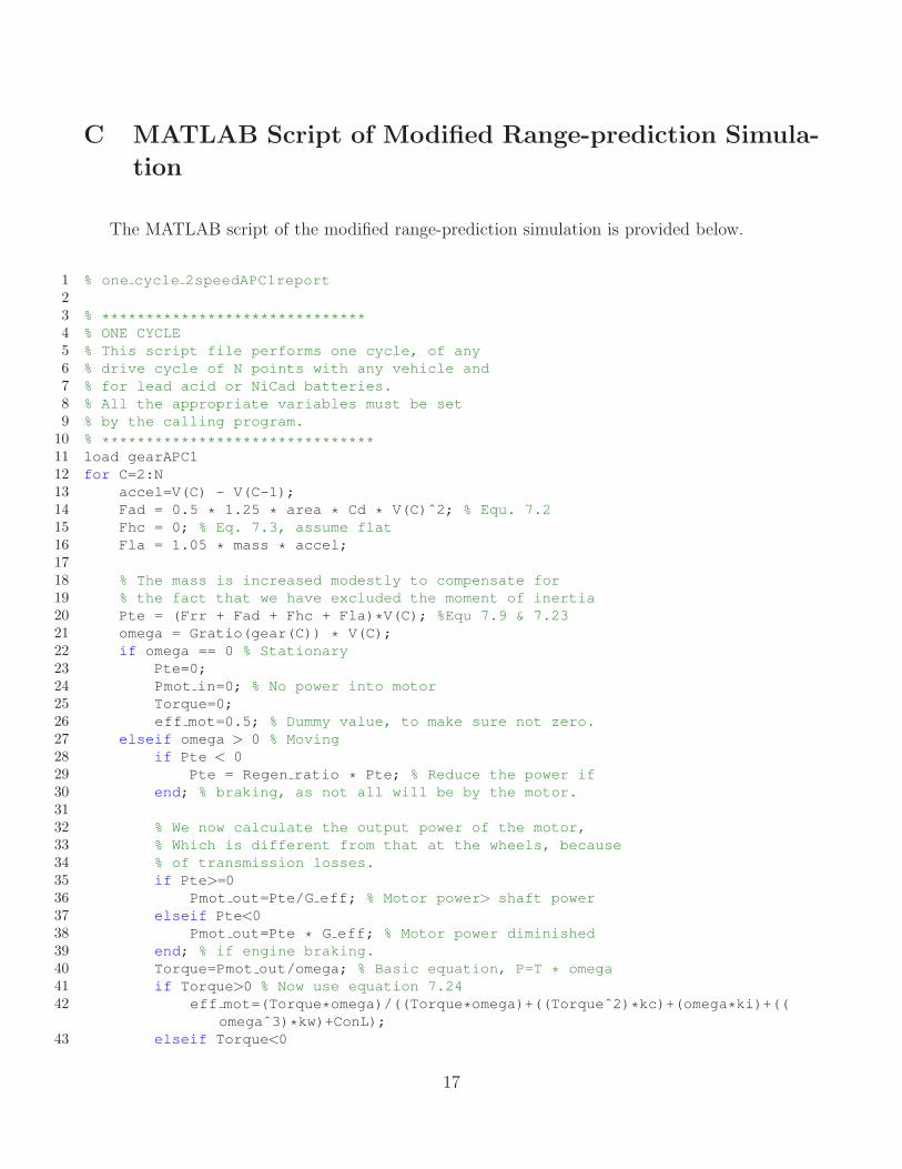
The final step is to modify the one cycle code in Larminie and Lowry’s range model. Ap-parently, this code was written for the range-prediction of EVs with a single speed. Therefore,the gear changes according to the gear-shift time illustrated in Fig. 7 must be incorporated in therange simulation of GM EV1 with a two-speed transmission. The modified code of one cycle isprovided in Appendix C, with only a few lines of the code modified. Therefore, only lines added ormodified will be explained. First, line 11 incorporates the gear-shift time in the simulation cycle.Then, line 21 provides the data of the gear ratio of the MST. The gear ratio is determined bythese inputted data because the simulation happened every second, which is the sample time ofthe SFUDS. Lastly, the final lines 87–89 are modified to check the tractive power Pte and velocitiesfor each sample.

4 Conclusions

We reported here on the details of the devising of gear-shift schedules for electric vehicles withmulti-speed transmissions. A case study is included whereby the schedule for the GM EV1 witha two-speed transmission was devised. The design was conducted in MATLAB/Simulink, theprocedure documented along with the code description.

References

[1] B. Zhu, N. Zhang, P. Walker, X. Zhou, W. Zhan, Y. Wei, and N. Ke, “Gear shift scheduledesign for multi-speed pure electric vehicles,” Proc. IMechE, part D: Journal of Automobile

Engineering, vol. 229, no. 1, pp. 70 – 82, 2015.

[2] J. Larminie and J. Lowry, Electric Vehicle Technology Explained, Second Edition. John Wileyand Sons, West Sussex, England, 2012.

9

[3] Infolytica Press Release, “Infolytica corporation releases MotorSolve v5 for immediate distri-bution1.” Accessed: 2017-12-20.

1http://www.infolytica.com/news/infolytica-corporation-releases-motorsolve-v5/

10

A MATLAB Script to Devise the Gear-shifting Schedule

The MATLAB script to design gear-shift schedule is as follows:

1 close all;clear all;clc;

23 %% efficiency map for gear 1

4 r = 0.2159; % in m, wheel radius for 235/45R17 taken from Zhu's

5 G1 = 4; % first gear ratio

6 max torque = 8.03; % Nm

7 max speed = 315; % rad/s

8 max output torque1 = G1*max torque;

9 a1 = G1/r/3.6; % \omega rad/s = a1 * vehicle speed km/h, 3.6 converts m/s to km/h

10 max vehicle speed1 = max speed/a1;

11 x=linspace(1,max vehicle speed1); % N.B. km/h, not rpm

12 y=linspace(1,max output torque1);

13 % Allocate motor loss constants.

14 kc=0.2; % For copper losses

15 ki=0.08; % For iron losses

16 kw=1e-7; % For windage losses

17 ConL=60; % For constant motor losses

18 [X,Y]=meshgrid(x,y);

19 Output power=((a1*X).*(Y/G1)); % Torque x speed = power

20 B=((Y/G1).ˆ2)*kc; % Copper losses

21 % Appendices: MATLAB? Examples 291

22 C=(a1*X)*ki; % Iron losses

23 D=((a1*X).ˆ3)*kw; % Windage losses

24 Input power = Output power + B + C + D + ConL;

25 Z = Output power./Input power;

26 % We now set the efficiencies for which a contour

27 % will be plotted.

28 % V=[0.7,0.8,0.85,0.9,0.91,0.92,0.925,0.93];

29 V=[0.5:0.07:0.87];

30 box off

31 grid off

32 [C,h] = contour(X,Y,Z,V);

33 xlabel('Speed/km.hˆ-ˆ1'), ylabel('Torque/N.m');

34 clabel(C,h)

35 hold on

36 V=[0,550];

37 [C] = contour(X,Y,Output power,V, 'red', 'linewidth', 2);

38 clabel(C)

3940 %% efficiency map for gear 2

41 G2 = 2.67; % second gear ratio

42 a2 = G2/r/3.6; % constant for motor speed rad/s to vehicle speed km/h, 3.6 converts

m/s to km/h

43 max output torque2 = G2*max torque;

44 max vehicle speed2 = max speed/a2;

45 x2=linspace(1,max vehicle speed2); % N.B. km/h, not rpm

46 y2=linspace(1,max output torque2);

11

4748 % Allocate motor loss constants.

49 kc=0.2; % For copper losses

50 ki=0.08; % For iron losses

51 kw=1e-7; % For windage losses

52 ConL=60; % For constant motor losses

53 [X2,Y2]=meshgrid(x2,y2);

5455 Output power=((a2*X2).*(Y2/G2)); % Torque x speed = power

56 B2=((Y2/G2).ˆ2)*kc; % Copper losses

57 % Appendices: MATLAB? Examples 291

58 C2=(a2*X2)*ki; % Iron losses

59 D2=((a2*X2).ˆ3)*kw; % Windage losses

60 Input power = Output power + B2 + C2 + D2 + ConL;

61 Z2 = Output power./Input power;

62 % We now set the efficiencies for which a contour

63 % will be plotted.

64 % V=[0.7,0.8,0.85,0.9,0.91,0.92,0.925,0.93];

65 V2=[0.5:0.07:0.87];

66 box off

67 grid off

68 [C,h] = contour(X2,Y2,Z2,V2);

69 xlabel('Speed/km.hˆ-ˆ1'), ylabel('Torque/N.m');

70 clabel(C,h)

71 hold on

72 V=[0,550];

73 [C] = contour(X2,Y2,Output power,V, 'red', 'linewidth', 2);

74 clabel(C)

7576 %% step 2 a constant-traction-torque line

77 format long

78 [X3,Y3] = meshgrid(Y(:,1),Y2(:,1));

79 A=abs(X3-Y3);

80 c=min(A);

81 l=zeros(length(c),5);

8283 % find the minimum torque difference because

84 % I dont have the exact torque for two

85 % different gear ratio due to two different

86 % linspace

8788 for i=1:length(c)

89 % position = find(A==c(i));

90 [row,col,v]=find(A==c(i));

91 % [m,n] = size(A);

92 % [Q,R]=quorem(sym(position),sym(m));

93 l(i,1)=Y(col,1);

94 l(i,2)=Y2(row,1);

95 l(i,3)=c(i);

96 l(i,4)=col; % the column of Y that has minimum difference

97 l(i,5)=row; % the column of Y2 that has minimum difference

98 end

12

99100 %% step 3 calculate the motor efficiency but

101 % only until 66 which is around 21 Nm

102 n=65; % number of points to compare

103 speed=zeros(n,1);

104 Eff=zeros(n,4);

105 for j=2:n+1;

106 [X4,Y4] = meshgrid(Z(:,l(j,4)),Z2(:,l(j,5)));

107 A2=abs(X4-Y4);

108 c2=min(min(A2));

109 [row,col,v]=find(A2==c2);

110 speed(j,1) = (X(1,col)+X2(1,row))/2;

111 Eff(j,1) = Z(col,l(j,4)); % efficiency in gear 1

112 Eff(j,2) = Z2(row,l(j,5)); % efficiency in gear 2

113 Eff(j,3) = c2; % efficiency difference

114 Eff(j,4) = Z(col,l(j,4))-Z2(row,l(j,5)); % double check

115 end

116 sorted speed = sort(speed);

117118 %% step 4-5 throttle values

119120 max power = 2535.79;

121 throttle gear=zeros(n,2);

122 for k=2:n+1;

123 eff = Eff(k,1);

124 % first gear 4:1

125 T = l(k,1)/G1;

126 omega=speed(k,1)*a1;

127 throttle gear(k,1) = 100*T*omega/max power/eff;

128 % throttle gear(k,1) = 100*sqrt(T*omega/max power/eff);

129 % throttle gear(k,1) = 100*nthroot(T*omega/max power/eff,4);

130131132 % second gear 4:1

133 T2 = l(k,1)/G2;

134 omega2=speed(k,1)*a2;

135 throttle gear(k,2) = 100*T2*omega2/max power/eff;

136 % throttle gear(k,2) = 100*sqrt(T2*omega2/max power/eff);

137 % throttle gear(k,2) = 100*nthroot(T2*omega2/max power/eff,4);

138 end

139 sorted throttle = sort(throttle gear);

140 figure(2);

141 plot(sorted speed(:,1),sorted throttle(:,1));

142 hold on;

143 grid on;

144 plot(sorted speed(:,1),sorted throttle(:,2));

145 xlabel('Speed/km.hˆ-ˆ1'), ylabel('Throttle/%');

146 %% adjusting the downshift curves

147 figure(3)

148 An = 0.4;

149 new downshift = (1-An)*sorted speed(:,1);

150 plot(sorted speed(:,1),sorted throttle(:,1));

13

151 hold on;

152 grid on;

153 plot(new downshift(:,1),sorted throttle(:,2))

154 xlabel('Speed/km.hˆ-ˆ1'), ylabel('Throttle/%');

14

B MATLAB Script to Compute the Gear-shifting Time

The MATLAB script to create the gear-shift time is given below.

1 %% shiftTime5report.m

23 close all;clear all;clc;

4 load shiftData; % accel in m/sˆ2 and XDATA

5 sfuds; % kph

6 N=length(V); % Find out how many readings

78 for c=1:N

9 if accel(c) > 0

10 throttle(c) = accel(c)/1.8465;

11 else

12 throttle(c) = 0.015;

13 end

14 end

15 % plot(XDATA,accel)

16 % hold on

17 % plot(XDATA,throttle,'r')

1819 %% velocity threshold

20 % Up th = zeros(1,N);

21 % Down th = zeros(1,N);

22 % for c=1:N

23 % clear up th

24 % thr=100*throttle(c);

25 % sim('thresholdGMEV1');

26 % Up th(c) = up th(1,1);

27 % Down th(c) = down th(1,1);

28 % end

2930 load speedThresholdGMEV1; % Up th and Down th in kph

31 % plot(XDATA,Up th);hold on;

32 % plot(XDATA,Down th);

3334 %% gear shift time

35 gear = zeros(1,N);

36 for c=2:N

37 gear(1) = 1;

38 if V(c)>Up th(c) && gear(c-1) == 1

39 gear(c) = gear(c-1)+1;

40 elseif V(c)<Down th(c) && gear(c-1) == 2

41 gear(c) = gear(c-1)-1;

42 else

43 gear(c)=gear(c-1);

44 end

45 end

46 % yyaxis left;

47 plot(XDATA,5*gear, '-k', 'LineWidth', 2);

15

48 hold on;

49 % yyaxis right;

50 plot(XDATA,V, '--r', 'LineWidth', 2)

51 grid on;

52 ylim([0 90]);xlim([0 365]);

53 set(legend('Gear ratio','SFUDS'), 'interpreter','latex')

54 ylabel('Speed (kph)','interpreter','latex','FontSize',13)

55 xlabel('Time~(s)','interpreter','latex','FontSize',13)

56 % annotation('textbox','String','1st gear ratio','interpreter','latex','FontSize

',12)

57 % annotation('textbox','String','2nd gear ratio','interpreter','latex','FontSize

',12)

58 set(gca,'FontSize',15);

596061 Gratio=[34 15];

16

C MATLAB Script of Modified Range-prediction Simula-

tion

The MATLAB script of the modified range-prediction simulation is provided below.

1 % one cycle 2speedAPC1report

23 % ******************************4 % ONE CYCLE

5 % This script file performs one cycle, of any

6 % drive cycle of N points with any vehicle and

7 % for lead acid or NiCad batteries.

8 % All the appropriate variables must be set

9 % by the calling program.

10 % *******************************11 load gearAPC1

12 for C=2:N

13 accel=V(C) - V(C-1);

14 Fad = 0.5 * 1.25 * area * Cd * V(C)ˆ2; % Equ. 7.2

15 Fhc = 0; % Eq. 7.3, assume flat

16 Fla = 1.05 * mass * accel;

1718 % The mass is increased modestly to compensate for

19 % the fact that we have excluded the moment of inertia

20 Pte = (Frr + Fad + Fhc + Fla)*V(C); %Equ 7.9 & 7.23

21 omega = Gratio(gear(C)) * V(C);

22 if omega == 0 % Stationary

23 Pte=0;

24 Pmot in=0; % No power into motor

25 Torque=0;

26 eff mot=0.5; % Dummy value, to make sure not zero.

27 elseif omega > 0 % Moving

28 if Pte < 0

29 Pte = Regen ratio * Pte; % Reduce the power if

30 end; % braking, as not all will be by the motor.

3132 % We now calculate the output power of the motor,

33 % Which is different from that at the wheels, because

34 % of transmission losses.

35 if Pte>=0

36 Pmot out=Pte/G eff; % Motor power> shaft power

37 elseif Pte<0

38 Pmot out=Pte * G eff; % Motor power diminished

39 end; % if engine braking.

40 Torque=Pmot out/omega; % Basic equation, P=T * omega

41 if Torque>0 % Now use equation 7.24

42 eff mot=(Torque*omega)/((Torque*omega)+((Torqueˆ2)*kc)+(omega*ki)+((

omegaˆ3)*kw)+ConL);

43 elseif Torque<0

17

44 eff mot=(-Torque*omega)/((-Torque*omega) + ((Torqueˆ2)*kc)+(omega*ki)

+((omegaˆ3)*kw)+ConL);

45 end;

46 if Pmot out >= 0

47 Pmot in = Pmot out/eff mot; % Equ 7.25

48 elseif Pmot out < 0

49 Pmot in = Pmot out * eff mot;

50 end;

51 end;

5253 Pbat = Pmot in + Pac; % Equation 7.27

5455 if bat type=='NC'

56 E=open circuit voltage NC(DoD(C-1),NoCells);

57 elseif bat type=='LA'

58 E=open circuit voltage LA(DoD(C-1),NoCells);

59 else

60 error('Invalid battery type');

61 end;

6263 if Pbat > 0 % Use Equ. 2.20

64 I = (E - ((E*E) - (4*Rin*Pbat))ˆ0.5)/(2*Rin);

65 CR(C) = CR(C-1) +((Iˆk)/3600); %Equation 2.18

66 elseif Pbat==0

67 I=0;

68 elseif Pbat <0

69 % Regenerative braking. Use Equ. 2.22, and

70 % double the internal resistance.

71 Pbat = - 1 * Pbat;

72 I = (-E + (E*E + (4*2*Rin*Pbat))ˆ0.5)/(2*2*Rin);

73 CR(C) = CR(C-1) - (I/3600); %Equation 2.23

74 end;

7576 DoD(C) = CR(C)/PeuCap; %Equation 2.19

7778 if DoD(C)>1

79 DoD(C) =1;

80 end

8182 % Since we are taking one second time intervals,

83 % the distance traveled in metres is the same

84 % as the velocity. Divide by 1000 for km.

85 D(C) = D(C-1) + (V(C)/1000);

86 XDATA(C)=C; % See Section 7.4.4 for the use

87 YDATA(1,C)=Pte;

88 YDATA(2,C) = V(C)./.3556; % omega output, .3556m is the wheel radius

89 YDATA(3,C) = YDATA(1,C)./YDATA(2,C);

90 end;

91 % Now return to calling program.

18