Gear Selection Strategy Development - TUGraz DIGITAL Library
110
Gear Selection Strategy Development Dzheylan S. Myumyun Master thesis Institute of Automotive Engineering Graz University of Technology Supervisors DI(FH) Thomas Frühwirth Assoc.Prof.Dipl.-Ing.Dr.techn. Mario Hirz 2018
-
Upload
khangminh22 -
Category
Documents
-
view
0 -
download
0
Transcript of Gear Selection Strategy Development - TUGraz DIGITAL Library

Gear Selection Strategy Development
Dzheylan S. Myumyun
Master thesisInstitute of Automotive Engineering
Graz University of Technology
Supervisors
DI(FH) Thomas Frühwirth Assoc.Prof.Dipl.-Ing.Dr.techn. Mario Hirz
2018


Contents
Table of Content II
Abstract III
Kurzfassung IV
1 Introduction 11.1 Description . . . . . . . . . . . . . . . . . . . . . . . . . . . . . . . . . 11.2 Objective . . . . . . . . . . . . . . . . . . . . . . . . . . . . . . . . . . 1
2 Method Description 32.1 Current Technology . . . . . . . . . . . . . . . . . . . . . . . . . . . . . 32.2 Ideas of Concept . . . . . . . . . . . . . . . . . . . . . . . . . . . . . . 52.3 Architecture . . . . . . . . . . . . . . . . . . . . . . . . . . . . . . . . . 7
2.3.1 Inputs . . . . . . . . . . . . . . . . . . . . . . . . . . . . . . . . 82.3.2 Velocity Profile/Predicted . . . . . . . . . . . . . . . . . . . . . 112.3.3 Dynamic Changes Evaluation . . . . . . . . . . . . . . . . . . . 122.3.4 Engine Torque/Speed Profile . . . . . . . . . . . . . . . . . . . . 142.3.5 Allowed Gear Calculation . . . . . . . . . . . . . . . . . . . . . 17
3 Software Description 243.1 0_Inputs . . . . . . . . . . . . . . . . . . . . . . . . . . . . . . . . . . . 25
3.1.1 0_VVeh/AVeh . . . . . . . . . . . . . . . . . . . . . . . . . . . 273.1.2 1_EngineRelatedCalculations . . . . . . . . . . . . . . . . . . . 28
3.2 1_DynamicChangesEvaluation . . . . . . . . . . . . . . . . . . . . . . . 293.2.1 0_HeavyBrakeFlag . . . . . . . . . . . . . . . . . . . . . . . . . 303.2.2 1_FastOffFlag . . . . . . . . . . . . . . . . . . . . . . . . . . . . 313.2.3 2_ABS/ESPFlag . . . . . . . . . . . . . . . . . . . . . . . . . . 323.2.4 3_KickDownFlag . . . . . . . . . . . . . . . . . . . . . . . . . . 32
3.3 3_EngineTorque/SpeedProfile . . . . . . . . . . . . . . . . . . . . . . . 333.4 4_AllowedGearCalculation . . . . . . . . . . . . . . . . . . . . . . . . . 44
3.4.1 0_SelectionoftheDesiredGear . . . . . . . . . . . . . . . . . . . 443.4.2 1_EvaluationofthePossibleGear . . . . . . . . . . . . . . . . . . 46
3.4.2.1 0_UpshiftProhibition . . . . . . . . . . . . . . . . . . 473.4.2.1.1 0_ABS/ESPEvaluation . . . . . . . . . . . . 483.4.2.1.2 1_FastOffEvaluation . . . . . . . . . . . . . . 493.4.2.1.3 2_KickdownEvaluation . . . . . . . . . . . . 503.4.2.1.4 3_HeavyBrakeEvaluation . . . . . . . . . . . 503.4.2.1.5 4_EngineSpeedPredCheck . . . . . . . . . . . 52
II

3.4.2.2 1_DownshiftProhibition . . . . . . . . . . . . . . . . . 533.4.2.3 2_NVH . . . . . . . . . . . . . . . . . . . . . . . . . . 543.4.2.4 3_EngineEfficiencyCheck . . . . . . . . . . . . . . . . 563.4.2.5 4_ClutchHeatDissipationCheck . . . . . . . . . . . . . 603.4.2.6 5_FutureGearTrendCheck . . . . . . . . . . . . . . . . 62
3.4.3 2_DesiredGearSelection . . . . . . . . . . . . . . . . . . . . . . 67
4 Simulation and Testing Environment 694.1 Testing Environment . . . . . . . . . . . . . . . . . . . . . . . . . . . . 694.2 Test Results . . . . . . . . . . . . . . . . . . . . . . . . . . . . . . . . . 72
5 Conclusion and Future Work 78
Symbols 81
Acronyms 82
A Legend for the Simulink Blocks 83
B Legend for the Simulink Libraries 86B.1 S-RFlipFlop . . . . . . . . . . . . . . . . . . . . . . . . . . . . . . . . . 86B.2 ResetTimer . . . . . . . . . . . . . . . . . . . . . . . . . . . . . . . . . 87B.3 LowPassFilterReset . . . . . . . . . . . . . . . . . . . . . . . . . . . . . 87B.4 ArrangeMatrix . . . . . . . . . . . . . . . . . . . . . . . . . . . . . . . 88
C Test Results Extension 89
List of Figures 91
List of Tables 93
References 94


Abstract
Day by day, the car manufacturers try to improve fuel consumption levels to be ableto achieve emission regulations. In this thesis, predictive road data information isintegrated to the gear selection algorithm to be able to achieve better fuel consumptionlevels. Similar designs were already used in heavy duty vehicles.
Sensors in the vehicle can observe the coming conditions and controllers can adaptvehicle reactions more efficiently with the predictive road data information. Additionally,since gear selection effects engine operation points, proper selection of the gears inthe transmission has a significant impact on the fuel consumption levels. Moreover,with the enhancement of transmisson hardware architecture of the Dedicated HybridTransmissions (DHT) area and hybrid vehicles, it will not be possible anymore to usethe conventional shift maps in gear selection strategies. That’s why a different approachfor gear selection strategy with the consideration of inertia forces, transmission lossesand engine efficiencies should be developed that is able to consider the predictive roaddata information.
The proposed gear selection strategy architecture, which is the main goal of thisthesis, will be designed for different kinds of powertrain and transmission designs.Since predictive road data information will be also considered during the design of thearchitecture, this can then also be used in autonomous vehicles.
Engine torque and speed targets will be calculated with respect to predictive vehiclevelocity profile and with the consideration of powertrain losses. Gear selection will beperformed according to engine efficiency and predictive clutch losses during the gearshift. During selection of the desired gear, predictive engine efficiencies and predictiveengine limitations will be also taken into consideration. Designed architecture will beimplemented in Simulink for Dual Clutch Transmission (DCT) conventional vehicle andsimulated in AVL VSM™. The results will be compared with the currently developedDCT software project. The expected results will show that with the proposed gearselection strategy, it is possible to achieve less fuel consumption levels.
III


Kurzfassung
Tag für Tag versuchen die Automobilhersteller den Kraftstoffverbrauch zu verbessern,um die neu aufkommenden Emissionsvorschriften einzuhalten. In dieser Arbeit werdenprädiktive Streckendateninformationen in den Gangwahlalgorithmus integriert, umbessere Kraftstoffverbrauchswerte zu erreichen. Ähnliche Konzepte finden bereits inLastkraftfahrzeugen Anwendung.
Durch prädiktive Streckendaten kann die Gangwahl effizienter gestalltet werden, indemdie Sensoren im Fahrzeug die aufkommenden Straßenbedingungen erfassen und daraufreagieren. Da auch die Gangwahl den Motorbetriebspunkt beeinflusst, hat die richtigeWahl der Gänge einen wesentlichen Einfluss auf die Kraftstoffverbrauchswerte. Darüberhinaus wird es durch die Erweiterung von Fahrzeugen, mit Dedicated Hybrid Transmis-sions (DHT) und Hybridisierung, nicht mehr möglich sein, die bis jetzt genutzenSchaltkennfelder in den aktuellen Gangauswahlstrategien zu verwenden. Aus diesemGrund sollte eine neue Gangauswahlstrategie unter Berücksichtigung von Trägheitskräft-en, Übertragungsverlusten und Motorwirkungsgraden unter Einbeziehung der prädiktiv-en Streckendaten entwickelt werden.
Durch den vorgeschlagenen Gangwahlalgorithmus sollte für verschiedene Arten vonAntriebssträngen und Getrieben eine Funktionsarchitektur entwickelt werden. Daprädiktive Streckendateninformationen auch beim Entwickeln der Funktionsarchitekturberücksichtigt werden, können diese dann auch in autonomen Fahrzeugen verwendetwerden.
Motordrehmoment- und -drehzahl werden in Bezug auf das voraussichtliche Fahrzeug-geschwindigkeitsprofil und unter Berücksichtigung von Antriebsstrangverlusten berech-net. Die Gangwahl sollte entsprechend demMotorwirkungsgrad und den vorhergesagtenKupplungsverlusten während des Schaltvorgangs durchgeführt werden. Bei der Auswahldes gewünschten Ganges werden auch prädiktiv der Motorwirkungsgrad und dieEinschränkungen berücksichtigt. Die daraus entworfene Funktionsarchitektur sollte inSimulink für konventionelle Fahrzeuge mit Doppelkupplungsgetriebe (DCT) implemen-tiert und in AVL VSM™ simuliert werden. Die Ergebnisse werden mit dem aktuelllaufenden DCT-Softwareprojekt verglichen. Die erwarteten Werte zeigen, dass mitder vorgeschlagenen Gangauswahlstrategie eine Reduktion des Kraftstoffverbrauchserzielbar ist.
IV


Acknowledgment
First of all, I would like to thank my manager Muammer Yolga for giving me theopportunity working with AVL and supporting me while my supervisor ThomasFrühwirth was not available. Thanks to my professor Mario Hirz for accepting meas a master student. I want to thank also my supervisor Thomas Frühwirth for thereviews and solving my problems in his lack of time.
Finally, special thanks go my family for supporting me every moment in my life andmy best friend Emrah Erdoğan for encouraging me from far away in my whole studytime in Graz. The last thanks to love of my life Daniel Reiterer as a first reviewer ofmy thesis, supporting me morally and technically.
V


1 Introduction
1.1 Description
Mankind always try to predict the future in their social life, in economy, in socialsciences, etc. It plays important role in engineering life as well. In these days, engineerstry to predict the conditions coming in the future and adapt the systems accordingly. Ifcontrollers in the vehicle are able to know driver needs, upcoming road, vehicle velocityin the future, they can calculate the most efficient control strategy to satisfy driversintent. It would also make the gear selection more effective. The idea of this thesis iscoming up from this point.
In the future, the emission regulations will become more strict because of legislation. Asan illustrate, the EU6d Emission Regulation implements Real Driving Emissions (RDE)as an additional type approval requirement within the 2017-2020 timeframe. [3]. TheRDE legislation requires engines to be clean under all operating conditions. Becauseof this reason, car manufacturers try to improve emission levels of the production carsby hybrid architecture, efficient engine operations or reducing losses in overall vehicle.Moreover, people are willing to buy environment-friendly vehicles, which exhaust lessemissions. To be able to achieve optimal engine efficiency, gear selection strategies playan important role, since gear selection provides engine operation in optimal points.
According to today’s developments, gear selection in non manual transmissions ishandled by parameterizable maps, so called shift maps, based on the accelerator pedalposition and vehicle speed. There are different shift maps for different conditions,like uphill, downhill, sport mode, cold start, etc. There are big calibration effortsnot only because of the number of shift maps, but also switching between shift mapsand interpolation during switching. Frühwirth [13], interpreted the accelerator pedalposition by changing hierarchy, which helps in reducing calibration effort by not usingconventional shift strategies so called shift maps. Moreover, with more complex hybridtransmissions such as AVL Future Hybrid 7 and 8 Mode [2], shift maps are not usableanymore, because of ECVT (Electronic Continuously Variable Transmission) drivingmodes. ECVT driving modes have to be used in conjunction with pure electric drivinggears as well as parallel hybrid driving gears, which need to be considered by futuregear selection/ mode selection systems.
1.2 Objective
In this thesis, in addition to Frühwirth’s [13] development, new approach for thegear selection strategy with predictive road data will be suggested. By the usage
1

of predictive road data, the controller can predict/ calculate future conditions, likeuphill, downhill, curve, traffic lights, etc. The presented architecture can be used forhybrid and conventional vehicles, future development can also be included easily.
In addition to the design of the architecture, software model will be implemented forconventional 7 speed DCT (Dual Clutch Transmission) for SUV (Sport Utility Vehicle).The developed software will be tested in the simulation environment and results will becompared with the gear selection strategy of currently developed project. The proposedsoftware architecture, which will be explained in detail in 2.Method Description section,is not implemented completely. Namely, predictive road data is not processed, whichis not the scope of this thesis, but the proccessed data will be taken as an input.
2

2 Method Description
2.1 Current Technology
In the current production cars, predictive road data information is used in adaptivedriver assistant systems, for example Audi introduced this in the Q7 model [6]. Itslows down based on the speed limits on the road by detecting the traffic signs, as wellas when curve or downhill is detected in the coming road. Moreover, it is also usedin gear selection algorithms in heavy duty vehicles. Banerjee et.al. [8] showed in thedevelopment in ZF Friedrichshafen AG, by including GPS (Global Positioning System)data information in gear selection algorithm, that heavy duty vehicles can react betterfor road gradient changes. By recognizing road gradient before it comes, controllerin the heavy duty vehicle can prepare engine acceleration capacity for driving on theuphill in advanced. There are more research topics about predictive road data usagein gear selection strategies for heavy duty vehicles. To illustrate, Reghunath et.al. [20]developed a gear shift strategy for heavy duty vehicles to be able to overcome to cominghill conditions by using predictive road data information. Additionally, Schuler [21] andTerwen [22] analyzed road slope, vehicle mass, vehicle movement and driver wish fortrucks in their PhD studies and used these information during the gear selection.
The challenging part in the proccessing of predictive road data is calculating the roadtrajectories out of processed GPS data. Road trajectory calculation depends on notonly GPS data, it also depends on psychological conditions of the driver, such as driverthinking, driver behaviors in the specific traffic situations, driving style, like aggressive,or relax. In the literature, there are several researches made to be able to calculate roadtrajectories. Panahandeh [19] suggested route and destination prediction by analyzingthe history of driving for individuals. Lorenzo et.al. [10] used the sensors providedinformation about the driver’s mood, attention span, as well as interaction with thecar. For example, in addition to the navigation data, acceleration and braking, climatecontrol and seat position are used during the prediction of trajectories. Tran et.al. [23]suggested a prediction of a driver behavior by foot gesturing, namely they analyzed afoot movement by using vision-based foot behavior analysis. Wang et.al. [24] analyzeddriver distraction based on brain activity patterns. Mabuchi et.al. [17] tried to predictdrivers stop or go at yellow traffic signal from vehicle behavior. Keller et.al. [16]studied the pedestrian movements to be able to predict moving behaviors.
As can be understood from all these papers, there are so many researches going on aboutproccessing the predictive road data, like studies of Banerjee et.al. [8], Reghunath [20].This information should be also included in gear selection strategies, since there is stillroom for improvement related to fuel efficiency/emissions but also driver satisfaction.
3

If autonomous vehicles are brought into consideration, which might even communicatewith their environment, this will open up even more prediction strategies. For example,cars might be able to plan their stay at electric charging stations or battery exchanges.Therefore, these information can be also used in their driving and gear selectionstrategy.
Currently, gear selection in vehicles with automatic transmissions are calculated witha conventional shift maps. Figure 2.1 shows a state of the art shift map with upshiftand downshift lines with constraints of vehicle velocity and accelerator pedal. Whensolid lines are crossed, upshift is performed. In the same way, when the dashed linesare crossed, downshift is performed, as it is shown in the figure. There is a hysteresisbetween upshift and downshift. There are various parameterizable maps possible formore efficient drive and required drivability, which brings too much calibration effortnot only because of the several number of shift maps for the different situations likesport, uphill, downhill, cold start,etc. but also because of switching between them.
Figure 2.1: Conventional shift map with upshift and downshift lines [11]
In literature, there are several researches for improving these conventional shift maps.As Fofana et.al. [12] stated in their research, a gear shift map is designed in two stages.First, initial shift point is obtained by using analytical methods. Calibration is thenused to refine the initial shift points and generate a set of gear shift maps based onexpected driving conditions and vehicle uses. They aimed to automate this processby using dynamic programming to obtain first shift point based on driveability, thenapplied a statistical analysis to define the final shift point. Ngo et.al. [18] developed agear shift map design methodology, which takes advantage of the optimal-based gearshift strategy and the statistical theory to construct an optimized gear shift map, whichis consistent, robust and real time implementable. Ha et.al. [14] designed a flexible
4
gear shift pattern instead of static gear shift maps. They used normalized radial basisfunction neural network for generating flexible shift maps to satisfy the driver demandsincluding comfort and fuel consumption.
Vehicle developments progress through hybrid architectures, where electric motor isused in addition to the engine. DHTs (Dedicated Hybrid Transmission) are one type ofthese hybrid architectures. Figure 2.2 shows a DHT type gearbox, where electric motoris mounted inside transmission. Engine can be separated with C0 clutch completelyfrom the transmission and pure electric drive with two different discrete gear ratios arepossible. Additionally, ECVT (Electronic Continuously Variable Transmission) modesprovide variable gear ratio instead of fixed gear ratio, with planetary gear structure.With the variable gear ratio flexibility, engine can be operated at its most efficientload point to either propel the car or charge the battery. If engine is not needed,it is also possible to shut down the engine and drive only with electric motor. Oneof the drawback of state of the art shift maps is usability in DHTs. DHTs open upnew areas for optimization also considering battery state with ECVT modes. Velocityand accelerator pedal are not the only constraints in gear selection in DHTs. Torquesplit between engine and electric motor, as well as battery charging level should bealso considered. Different gears can be selected for the same velocity and acceleratorpedal position, since torque splits may differ in every time. With variable gear ratio inECVT modes, it is even harder to decide correct gear ratio just by considering thesetwo constraints.
Figure 2.2: DHT type Gearbox [2]
2.2 Ideas of Concept
In this study, new architecture will be suggested for the gear selection strategy. Thisarchitecture includes the usage of predictive road data for the passenger cars. The
5

architecture is applicable for both hybrid and conventional passenger cars. Gearselection will be calculated based on the vehicle velocity profile. Vehicle velocityprofile calculation highly depends on predictive road data information. Additionally,dynamic driver behavior and road changes will be analyzed and considered in the gearselection like fast off, heavy brake, NVH, ABS/ESP activations. This part of thearchitecture is taken from thesis of Frühwirth [13] and extended by the predictive roaddata information.
The perfect conditions for these calculations would be provided by autonomous vehicles,where the route is calculated in the beginning of the drive. Prediction of the driverbehaviors, road planning algorithms, learning algorithms are still in development ascan be seen from the research papers, which are provided in the chapter above. In thecurrent technology, it is possible to read the road information for the coming road likeuphill, downhill and curve, which are important factors in gear selections. Road datainformation is collected and processed by some companies like Continental [1]. eHorizonproject of Continental integrates topographical and digital map data with sensor data,namely GPS receivers for predictive control of vehicle systems. Future events, such asthe uphill inclination after the next corner, are exploited at an early stage in order tooptimize the vehicle’s response. eHorizon interprets map and sensor data, which canbe adapted to the vehicle control easily. Additionally, this system provides weather-,vehicle and time dependent speed instructions, which are not identified by the camerasystems.
Figure 2.3: A schematic of a segmentational splitting of predictive data
These information is combined with the map and sensor data, then proccessed datais provided as segments, see Figure 2.3. Segment is defined as the part of the road,which has same characteristics, such as weather, road gradient, velocity limits, etc. Itsupplies also dynamic data via cloud, like traffic information or changes on the route.
The other aim of this thesis is designing a new software for the gear selection by notusing conventional shift maps. There is a thesis about a different gear selection strategywithout using of conventional shift maps, as it was mentioned before [13]. In additionto this, aim of this thesis is to improve this approach by considering predictive road
6
data information, transmission efficiency and inertia losses. Therefore, gear selectionis done with physical model by considering efficiencies and losses instead of velocityand acceleration pedal dependency.
2.3 Architecture
Figure 2.4: The architecture of the software
Self proposed architecture can be seen in Figure 2.4. Figure shows relevant subsystemsof Gear Selection, which will be described in detail in the coming sections. Signal flowsare represented by the arrows. The subsystems are placed according to calculationorder, where Inputs is the first executed subsystem, which is followed by Vehicle velocityprofile/predicted and so on. In this figure, only Gear Selection part is implemented,where Experience and Learning systems will not be treated in this thesis but mightbe an improvement suggestion. As discussed in chapter C. Simulation and TestingEnvironment, pure gear selection part is already showing acceptable results.
In this thesis, Gear Selection itself is called as system, whereas the other blocks aresubsystems of Gear Selection system or subsystems of other systems. Gear SelectionSystem consists of the following subsystems, which will be discussed in the followingsubsections in detail.
• Inputs
• Velocity Profile/Predicted
• Dynamic Changes Evaluation
• Engine Torque/Speed Profile
• Allowed Gear Calculation
• Experience
7

2.3.1 Inputs
In this subsystem of Gear Selection, required input data will be taken from ECU(Engine Control Unit), Hardware, ESP (Electronic Stability Program), HCU (HybridControl Unit) and HMI (Human Machine Interface). These signals will be processedto be used inside the gear selection software.
Inputs from HCU:
HCU is the main control component of hybrid vehicles. According to the input signalssuch as accelerator pedal position, requested gear and brake pedal position, the HCUcan calculate the engine, electric motor driving and generation torque.
If this system is applied for the hybrid vehicles, HCU should give some efficiencycalculations to the TCU (Transmission Control Unit). TCU is the control unit for theautomatic transmission, which uses sensors from the vehicle as well as data provided byECU (Engine Control Unit) to calculate how and when to change gears in the vehiclefor optimum performance, fuel economy and shift quality. Gear shifting, hydraulicand clutch controls are also performed by TCU. When it is a hybrid vehicle, HCU isthe master of engine control. HCU decides the possible hybrid mode and accordinglyengine speed and torque requests are sent to the ECU. Afterwards ECU controls theengine to be able to fulfill the HCU requests. Because of this reason, HCU is ableto calculate overall efficiency more effectively, since HCU can calculate which electricmotor/engine speed and torque are possible according to possible hybrid mode. Out ofthis information, HCU can select the optimum HCU driving mode such as boosting orgeneration and provide efficiencies accordingly to TCU. By designing this architecture,it is assumed that HCU will influence overall vehicle efficiency according to hybrid modeand engine requests. Additionally, in hybrid vehicles, torque split is an important factorfor deciding the desired gear since it effects the engine and electric motor efficienciesand in parallel fuel consumptions. To be able to get desired output shaft request,torque source can be partially engine, partially electric motor or only electric motoror only engine. Proportional torque between engine and electric motor is defined astorque split. SOC (State of Charge) level of the battery and hybrid modes are factorsthat torque split depends on, that’s why torque splits should be calculated in HCU.With the predictive road data information, it is possible to simulate recuperation anddrive capabilites for future conditions and battery management system can be plannedmore efficiently. For example, driver goes in flat road, battery needs to be chargedand downhill road is coming. There is no need to find another strategy for chargingthe battery but braking during the downhill drive can easily be used for charging thebattery.
8

Hardware:
Following signals will be taken from hardware interface from the sensors to be able tocalculate desired gear.
• Output shaft speed is read from sensor as a unit of rad/s.
• Output shaft direction is read from sensor and sensor delivers the informationabout forward or backward turning of the output shaft.
HMI:
HMI can be defined as interface between controller and a user. It provides a graphicbased visualization of a controllers. User can influence the controllers in the vehiclewith HMI or vehicle controllers can also communicate with the user by showingmalfunctioning in the car or delivering some informations such as fuel consumption,vehicle velocity, current gear, etc. Following input signals are delivered by driver viaHMI.
• Gear lever position is influenced by a driver and sent through the HMI. Typicalgear lever positions are Park, Neutral, Drive, Manual and Sport. When Drive isengaged, possible gear is defined by the gear selection system in the TCU. WhenManual is selected, desired gear is defined by the user by Tip Up/Down buttonsand gear shifting is performed by TCU. Sport mode is like Drive mode but inthis mode, sportive drive can be performed, namely acceleration capacity is muchmore according to Drive mode.
• Vehicle mode can be also influenced by driver via HMI, where Comfort, Sport,Economy, etc. modes can be selected.
Prediction related:
Static and dynamic route data is delivered via this module. Following inputs are usedin gear selection strategy.
• Processed static route data, namely segment matrix is delivered via this module.
• Processed dynamic data, like traffic information, constraction on the way, etc.are delivered via this module.
ESP controller:
ESP controller provides vehicle stability incase of loss of steering control and appliesbrakes in the wheels individually for bringing the driver the steering that driver intents.
9
In case of ESP is activated, following signals are taken as an input and processed insidethe gear selection.
• In loss of steering detection, ABS/ESP Flags are raised.
• When ESP is activated, wheel speeds are controlled by ESP system.
• Wheel dynamic radius is also provided by ESP system.
• When ESP is activated, it applies brakes to the wheels individually, so that brakepedal pressure is also provided by this system.
ECU:
ECU controls the actuators inside the combustion engine and optimizes the engineperformance. Following signals are provided via ECU to the TCU.
• Acceleration pedal position in percentage
• Engine torque in Nm
• Engine idle speed in rpm
• Engine speed in rpm
Moreover, vehicle speed will be calculated from output shaft speed. Vehicle accelerationwill be calculated by taking the derivative of the vehicle speed. Engine synchronizedspeed for each gear will be calculated by multiplication of gear ratio with output shaftspeed. Engine torque limitations will be calculated based on parameterizable mapswith respect to engine synchronized speed. Parameterizable maps used for enginelimitations are static maps, where influencing factors like ambient temperature orengine temperature are not considered. Actual gear will be calculated in other part ofthe TCU software based on rail states or clutch conditions.
Experience:
This system should be implemented separately from the gear selection strategy. This isa different system for observing the behavior of vehicle according to output of the gearselection strategy. The idea of Experience system is to generate data and behavior ofthe vehicle according to these data can be monitored easily. Out of this information,parameter fitting can be implemented by using the input information against the actualoutputs. In the end, weight factor should be generated and given as a feedback to theInput subsystem of Gear Selection. Afterwards, this information will be evaluatedunder ’Evaluation of the selected gears’ subsystem of ’Allowed Gear Calculation’. Bythe information coming from Experience system, gear selection strategy can be adaptedand improved overtime.
10

2.3.2 Velocity Profile/Predicted
Figure 2.5: The subsystem of Velocity Profile/Predicted Calculation
Velocity and acceleration profile prediction will be calculated in this subsystem of GearSelection, which can be seen in the Figure 2.5. Subsystems are shown in the figure in thecalculation orders, where Prediction will be processed first, then Profile is calculated.Implementation of this subsystem is not the scope of this thesis. During the testingof the software, predicted velocity profile will be given as an input to the output shafttorque profile calculation.
Driver behavior prediction subsystem is used for predicting the driver needs. Thereare different kind of researches going on. Some of them was also mentioned in theprevious sections. For example, Lorenzo et.al. [10] tried to predict drivers mood, Tranet.al. [23] analyzed foot gesturing or Wang et.al. [24] analyzed brain activity pattern.All those information can be used for predicting the driver needs and adapting vehiclevelocity profile accordingly.
Predictive road data subsystem of Prediction analyze the static data like uphill,downhill, curve, velocit limits, etc. Route information comes as segments, which wasexplained in the Figure 2.3.
Predictive traffic data subsystem of Prediction contains the traffic information, whichchanges dynamically. Such as car behavior in front, pedestrian, traffic lights, constructionarea. Predictive traffic data can overwrite the predictive road data by generatingemergency changes flag and distance to the object, such as sudden brake in front ofthe car. It is possible to add any predicted information coming in the future here.
11

During the velocity profile calculation, vehicle mode has a big effect, which is implementedas a subsystem of Profile calculation. It contains the driver mode request informationlike sport, comfort, economy, etc. Vehicle mode information comes from HMI as driverchoice and is combined with driver behavior prediction from the Prediction subsystembefore. According to the vehicle mode, different parameterizable parameters should beassigned to be used in the coming subsystems during vehicle velocity and accelerationcalculations.
Calculating the predictive velocity profile requires quite a lot calculation works, whichwill not be done in this thesis. The perfect condition for this calculation might bepossible in an autonomous car such that the road is known in advance and velocityprofile is calculated in a most efficient way. The most challenging part here is predictingthe driver behavior. It is like to procast the drivers wishes: whether driver prefers slowor aggressive drive, whether driver prefers press accelerator pedal more to be able toovercome traffic lights, when it is blinking or just stop. What is the behavior of thedriver? Is it more impulsive or relaxed? Does the driver like to go high speeds orlow speeds generally? They are all constraints in the prediction. It is possible touse learning algorithm to be able to analyze and adapt software according to driverbehavior over time, introduced e.g. in the research of Panahandeh [19].
2.3.3 Dynamic Changes Evaluation
Dynamic changes during the drive, which effect gear selection, will be evaluated andflags will be calculated out of this information to be used afterwards during AllowedGear Calculation subsystem of Gear Selection, which can be seen in the Figure 2.6.Subsystems are shown in the calculation order, where Emergency changes will beprocessed first, then it is further evaluated under Heavy Brake, Fast Off and Kickdownsubsystems. The other subsystems are calculated in paralel and send their own outputinformation seperately from the Dynamic changes evaluation to the other subsystemsin the Gear Selection system.
• Heavy Brake: Heavy brake is a state, which pressing the brake pedal suddenlyand hard. Brake pedal pressure will be checked against a parameterizable mapwith vehicle velocity input. If it is greater than a parameter, Heavy brake flagwill be activated. Heavy brake flag will be reseted after a parameterizable time,if Heavy Brake flag is disabled.
• Fast Off: Fast off is a state, which removing foot from the acceleration pedal.Accelerator pedal position will be checked with a parameterizable map. If it isreleased too fast, Fast off flag will be activated. Fast off flag will be reseted aftera parameterizable time, if Fast off flag is disabled.
12

Figure 2.6: The Subsystem of Dynamic Changes Evaluation.
• ABS/ESP: If ABS/ESP is triggered, which comes from ABS/ESP directly, thisflag will be activated. This flag information may change depending on ESPsystem. ESP can completely disable gear shift or request upshift for reducingthe output shaft speed or request clutch separation. Required action will beevaluated in the coming subsystem, Evaluation of the selected gears.
• Kickdown: Kickdown is a state, which pressing the accelerator pedal suddenlyand hard. If accelerator pedal position gradient is higher than a parameterizablemaps value according to accelerator pedal position, Kickdown flag will beactivated. Kickdown flag will be reseted after a parameterizable time, if Kickdownflag is disabled. For the hybrid vehicles, this information will come from HCUdirectly.
• Emergency Changes: This information comes from ‘Prediction Traffic Data’ asa flag and a distance to the object. Object can be car, which makes emergencybrake or a pedestrian, who jumps to the road unexpectedly or traffic lights thatturn on red. Following actions can be taken during this condition:
– For stopping before crashing to the object, heavy brake can be applied. Inthat case, Heavy Brake flag will be activated.
– When vehicle speed is low and distance to the object is not that short, justremoving foot from accelerator pedal can be enough. In that case, Fast offaction can be enough for overcoming the target and Fast off flag will beactivated.
– When front car applies brake and side road is available, take over can beperformed. In this time, Kickdown flag will be activated.
– If vehicle velocity is low, normal brake can be enough, in this case none ofthe flag will be activated and normal drive will be performed.
13
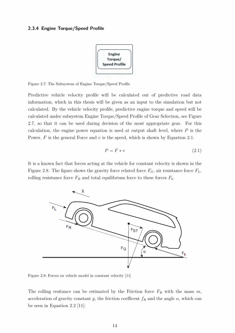
2.3.4 Engine Torque/Speed Profile
Figure 2.7: The Subsystem of Engine Torque/Speed Profile
Predictive vehicle velocity profile will be calculated out of predictive road datainformation, which in this thesis will be given as an input to the simulation but notcalculated. By the vehicle velocity profile, predictive engine torque and speed will becalculated under subsystem Engine Torque/Speed Profile of Gear Selection, see Figure2.7, so that it can be used during decision of the most appropriate gear. For thiscalculation, the engine power equation is used at output shaft level, where P is thePower, F is the general Force and v is the speed, which is shown by Equation 2.1.
P = F ∗ v (2.1)
It is a known fact that forces acting at the vehicle for constant velocity is shown in theFigure 2.8. The figure shows the gravity force related force FG, air resistance force FL,rolling resistance force FR and total equilibrium force to these forces Fk.
Figure 2.8: Forces on vehicle model in constant velocity [11]
The rolling resitance can be estimated by the Friction force FR with the mass m,acceleration of gravity constant g, the friction coefficent fR and the angle α, which canbe seen in Equation 2.2 [11]:
14

FR = m ∗ g ∗ fR ∗ cosα (2.2)
The air resistance against the vehicle will be concluded by air resistance force FL withair drag force cD, air density ρA, cross sectional area of the vehicle AF and vehiclevelocity v, which can be seen in Equation 2.3 [11]:
FL = 12 ∗ cD ∗ ρA ∗ AF ∗ v ∗ |v| (2.3)
Climbing resistance force FST where road gradient will be inclueded in the calculationsis calculated by Equation 2.4 [11]:
FST = m ∗ g ∗ sinα (2.4)
Forces Fk to keep the vehicle in the constant velocity calculation can be seen in Equation2.5 [11]:
Fk = FR + FL + FST (2.5)
For an overall forces F on the vehicle, engine acceleration effect will be also includedwith vehicle mass mveh, vehicle acceleration a, which is shown in Equation 2.6.
F = mveh ∗ a+ Fk (2.6)
There is inertia losses in the vehicle, which will be taken into consideration duringengine torque profile calculation from engine power in output shaft level. In this thesisFWD (Front Wheel Drive) vehicle will be used during implementation of the software,whose inertias can be seen in Figure 2.9.
Where IE refers to inertia of engine, IG refers to inertia of transmission, iA refers toaxle drive ratio, iG refers to discrete gear ratio, IAF refers to inertia of front axles, IAR
refers to inertia of rear axles.
Total inertia in front axles IF will be calculated with the Equation 2.7 [15]:
IF = IAF + i2A ∗ (IG + i2G ∗ IE) (2.7)
Total inertia in rear axles IR will be calculated with the Equation 2.8 [15]:
IR = IAR (2.8)
In the end, overall torque loss MJout because of inertias with acceleration a and wheel
15

Figure 2.9: Moments of Inertias for a FWD Vehicle [15]
dynamic radius r will be calculated with the Equation 2.9 [15]:
MJout = a ∗ IF + IR
r2 (2.9)
Power loss because of inertias will be calculated with the Equation 2.10:
PJout = MJout ∗ ωEng (2.10)
Engine speed in gear ωEng is a function of vehicle velocity v, dynamic tire radius r andtotal gear ratio i, as can be seen in Equation 2.11:
ωEng = v
r∗ i; (2.11)
Transmission losses was measured in the testbed under different conditions withthe following steady state conditions: torque and load, rotational speed or velocity,temperature, time or duration of operation, engaged gear. Depending on the variationof load and speed, the propotional amounts of losses vary. While in low speed andtorque situations the base losses are predominant, the torque and speed dependentlosses are significant for the description of the efficiency at high speed or load condition.By permutation of the testing parameters, an efficiency map was formed with respectto input speed and input torque in percentage of the maximum input torque thatdescribes losses over all conditions.
16

All in all, engine torque target for each gearMEng will be calculated by engine power P ,engine speed in gear ωEng, transmission efficiency η and power loss because of inertiasPJout with the following Equation: 2.12
MEng = P + PJout
ωEng ∗ η(2.12)
2.3.5 Allowed Gear Calculation
Figure 2.10: The Subsystem of Allowed Gear Calculation
This is the final step of the Gear Selection strategy, which is shown in Figure 2.10. Thefigure shows subsystems in the calculation order where Selection of the desired gearwill be executed first, then Evaluation of the selected gears and in the end Calculationof allowed gear. The subsystem under Evaluation of the selected gears are calculatedin paralel. The subsystems, which are colored grey are processed further in Evaluationfuture gear trends. These grey subsystems do not send any output to from Evaluationof the selected gears to Calculation of allowed gear. That’s the reason why thesesubsystems are placed back from the other subsystems under Evaluation of the selectedgears.
First of all, desired gear/s will be selected according to engine allowances. Afterwards,selected gears will be evaluated with respect to engine and powertrain efficiencies. Inthis stage clutch heat dissipation during shift will be also considered. Moreover, future
17

gear trends will be evaluated with respect to efficiencies. Dynamic changes flags willbe evaluated under Upshift, Downshift prohibition subsystems of Evaluation of theselected gears. All in all evaluations will be finalized and the most desired gear will beselected in Calculation of Allowed Gear subsystem of Allowed gear calculation.
Selection of the Desired Gear:
In this subsystem of Allowed gear calculation, desired gear will be selected with respectto engine and electric motor limitations. For the current thesis, where a conventionalcar is simulated, following strategy will be implemented:
Engine speed synchronization for each gear calculation will be taken from ’Input’subsystem. Engine target torque and speed will be taken from ’Engine Torque/SpeedProfile’ subsystem of Gear Selection. Synchronized engine speeds will be checked,whether they are in engine parameterized speed limitations. If they are in the limits,they will be assigned as allowed gear/s. Engine torque limits will be calculated in’Inputs’ subsystem with respect to engine synchronized speed, which will be used forchecking whether engine torque targets are in these limits. If engine target torques arewithin these limits, it will be assigned as allowed gear/s. In the end, selected desiredgear will be the common gear/s from these limitation checks. There can be a conditionwhere none of the gear is sufficient for the engine target torque. In this case, the gearwhich gives the highest engine torque within the engine speed limits will be selectedas an allowed gear.
For the hybrid drive, where both engine and electric motor is running, both engineand electric motor limitations should be considered. If it is hybrid architecture, torquesplits will be also an important variant.
For the hybrid drive, when only electric motor is running, logic can be updatedaccording to both electric motor limitations and hydraulic needs. Logic would bechanged according to hydraulic architecture. For example, if mechanical pump ispositioned in the input shaft and it turns with the input shaft speed, followingconditions can be considered:
• If flow request increases above the actual flow, minimum input shaft speed willnot be interfered.
• If pressure request increases above available pressure, minimum input shaft speedwill not be interfered.
• Otherwise; current gear will be kept during electric drive.
18

Evaluation of the selected gears:
Selected desired gear under subsystem ’Selection of the Desired Gear’ will be evaluatedunder this subsystem.
Upshift prohibition: In this subsystem of Evaluation of the selected gears, dynamicflags which were calculated under ’Dynamic Changes Evaluation’ will be evaluatedwith respect to upshift prohibition.
• If ABS/ESP flag is activated, necessary action will change according to ESP signalcontent. Some ESP systems inhibit gear shifts, whereas some ESP systems mightrequest upshift to reduce output torque.
• If Fast off flag is activated, action will be taken according to synchronized enginespeed. If synchronized engine speed is exceeded, gears until the last desiredone plus one upper gear will be allowed. So that higher engine speed will beprevented. Otherwise; gears until the last desired one will be allowed.
• If Kickdown flag is activated, gears higher than the last desired gear and lastdesired gear will be disabled, to be able to force vehicle to downshift. Thereason behind, when downshift is performed, there will be more engine speedand requested acceleration performance will be achieved.
• If Heavy brake flag is activated, new engine speed for each gear to be able to getduring brake actions should be calculated. If this new engine speed for each gearis greater than a synchronized engine speed for each gear, then relevant gear willbe disabled. The idea behind is triggering the shift earlier, so that having higheracceleration capabilites afterwards.
Additionally, current gear will be evaluated, according to future engine speed limitations.Current selected gear/s which were calculated under ’Selection of the Desired Gear’will be evaluated according to predicted engine speed. UpShift duration is estimatedaccording to current engine speed. Current selected gears will be checked with respectto future maximum engine speed limitations. If after a parameterizable shiftingduration, this gear is not under maximum engine speed limit, then it should be disabled.
Downshift prohibition: current gear will be evaluated according to future enginespeed limitations. Current desired gear/s which were calculated under ’Selection ofthe Desired Gear’ will be evaluated according to predicted engine speed. Downshiftduration is estimated according to current engine speed. Current selected gears willbe checked with respect to future minimum engine speed limitations. If after aparameterizable shifting duration, this gear is not above minimum engine speed limit,then it should be disabled.
19

NVH evaluation: NVH behavior will be considered in gear selection with a parameterizablemap with engine speed and mean pressure according to engine torque target at enginelevel constraints. Output of this maps will indicate good or bad NVH behavior. Thesemaps can be gear dependent. There can be specific gears, in specific conditions thatcause specific bad noises in specific engine speed/torque areas. Observing of NVH willbe more challenging for DHTs as powerflow through the transmission is continuouslyvariable. In this case, torque splits and ECVT gears should be also constraints forNVH evaluation.
Engine efficiency: Engine efficiency for interfered, as well as for predicted engineefficiency values will be evaluated by a map with respect to average mean pressureand engine speed. Output of this map will be a fuel consumption in g/kWh.
Results of this map will be processed further in Evaluation of future gear trends.
Clutch heat dissipation [11]: The temperature increase in the clutch is determinedby the power loss. The power loss in the clutch is a result of clutch torque and speeddifferences between the clutch sides. The greatest power loss occurs in the beginning ofa shift and drops to zero toward the end of the synchronization phase. Clutch torquein the engine side is applied by the engine, which can be reduced by engine torqueintervention control. The other side of the torque decelerates because of the rotatingmasses. At constant torque during shift, the heat loss is determined by a work loss.Figure 2.11 shows the curve of the dissipated power (PV ) for a powershift and theassociated integral that equals the energy converted into heat namely work loss (WV ).
As can be understood from the upper explanations, heat dissipation in clutch occursduring the shifting phase, namely where clutch slip occurs. In slipping phase, frictionbetween the clutches results in heat dissipation, respectively power loss. This valuehighly depends on the torque handover functionality in the transmission software,where shifting from one gear to an other gear is performed. This makes clutchheat dissipation, in other words, power losses estimation, a complicated task. In thissoftware, parameterizable map will be constructed with respect to clutch slip, clutchtorque and shift time. Power losses during shifting is estimated as a power unit of kW.In the future, this functionality can be improved with the interface connection withtorque handover, such as torque handover can deliver an estimated time during speedand torque phase and these maps can be constructed dynamically.
Power losses during shifting will be processed further in Evaluation of future geartrends.
20

Figure 2.11: Power and energy losses during torque speed sequence shift [11]
Powertrain efficiency check with respect to hybrid mode: In HCU, powertrain efficiencywas calculated for each gear with respect to selected hybrid mode. During thecalculation of the losses, electric motor and inverter efficiencies should be considered.There will be also losses during the transformation of kinetic energy into chemicalenergy for charging the battery and during using the stored energy. For the predictiveselection, powertrain efficiency should also be predicted according to engine and electricmotor torque/speed distributions with the consideration of torque splits.
Output of this subsystem of Evaluation of the selected gears will be processed furtherin Evaluation of future gear trends.
Since conventional vehicle is used for the validation of the architecture, this subsystemwill not be implemented in the software.
Evaluation of future gear trends: Under this subsystem of Evaluation of the selectedgears, evaluation of engine efficiency, clutch heat dissipation and powertrain efficiencieswith respect to hybrid mode will be processed further. First of all, some gears will beinhibited by checking the engine efficiency for the predicted gears. If predicted mostefficient gear is different than the current gear, engine efficiency improvement will bechecked. If engine efficiency is not changed more than a parameterizable value, currentgear will be kept in this time step.
21

The second evaluation will consider shift losses because of clutch heat dissipation.When predictive calculation gives the scenario in the Figure 2.12, two possibility willbe evaluated. First scenario calculates the power losses during shifting. For example,calculation of power losses during shifting from gear 2 to gear 3, engine losses duringdriving in gear 3 and power losses during shifting from gear 3 to gear 2 will be added.Second scenario calculates engine losses during driving in the actual gear, in this figuregear 2. For the same time interval, losses are compared and most efficient scenario isselected.
Figure 2.12: Possible Shift Scenario, change of a target gear
Feedback processed data: The idea behind treats the question, if it is possible tomonitor the data that is generated, and according to generated data, responses willbe monitored. In the end of the Gear Selection, under ’Experience’ system, see Figure2.4, gear request and efficiency of the responses will be monitored. In the end, weightfactor will be generated and evaluated here. This is a curve fitting or so called learningalgorithm. As an example, after the desired gear is engaged, driver torque demandwill be checked whether it is fulfilled. How was the behavior? Was it the correct gear?In the end weighting factor will be calculated and used during evaluation of the gearafterwards under this subsystem. The other example can be, if early shift was occuredseveral times, weighting factor will be changed, so that there will not be early shiftnext time.
Calculation of allowed gear:
After the evaluation of the possible factors in Gear Selection in the transmissionsoftware, last calculation will be done under this subsystem of Calculation of allowedgear for defining the desired gear and sending as an output from the Gear selectionstrategy.
Calculated desired gear will be combined here with the gear lever position and dynamicflags. Transmissions have general 5 gear lever conditions, which are manual, drive,reverse, park and neutral. If park or neutral gear lever is engaged, neutral gear will be
22

selected. If reverse gear lever is engaged, reverse gear will be selected. If manual gearlever mode is requested, calculated gear in the before subsystems will be disabled andgear selection will be done according to driver manual gear selection. Finally, if drivemode is selected, evaluated gears according to predicted values as well as current valueswill be combined under this subsystem and sent as a desired gear. Dynamic changeshave always priority over the other factors. If there is upshift/downshift prohibitionor selected gear is not valid under NVH point of view, calculated gear with respect toefficiencies, driver requests will be cancelled. In this time, gear selection will be doneaccording to dynamic changes limits.
23

Figure 3.1: 5 speed DCT Architecture [5]
3 Software Description
The proposed architecture in chapter: 2.Method Description is applicable for thedifferent kinds of powertrain architecture and transmission types like conventional,hybrid, AT (Automatic Transmission), DHT, whereas in the present work, softwareis implemented for 1.2 liter inline 3 TGDI (Turbocharged Gasoline Direct Injection)engine with a wet clutch 7 speed DCT in SUV. An example of a DCT transmissioncan be seen in Figure 3.1. DCT has two separate shafts, where even and odd gearsare separated onto these shafts. One clutch is used just for engaging odd gears andother clutch is used just for engaging even gears. With this two shaft architecture,it is possible to preselect the coming gear. For example, when the vehicle speeds up,controller in the car automatically detect the gear change point and will preselect theupper gear. In the same way, when the vehicle speeds down, controller will preselecta lower gear. When gear change is requested, currently engaged clutch disengages andthe other preselected clutch engages.
Software implementation is done in Matlab/Simulink environment [4]. Simulink,developed by MathWorks, is a graphical programming environment for modeling,simulating and analyzing multidomain dynamical systems. It’s primary interface isa graphical block diagramming tool and a customizable set of block libraries.
Implemented software according to explained architecture in section 2. MethodDescription can be seen in Figure 3.2. Under this section, software implementation willbe explained. Moreover, it should be noted down that 2_Velocity/ProfilePrediction isan empty subsystem where predicted vehicle velocity is calculated. For the validation
24

of the software, vehicle velocity profile vector is given as an input to the system andprocessed in subsystem 3_EngineTorque/SpeedProfile.
Figure 3.2: Implemented Software in Matlab/Simulink Environment
The figure 3.2 shows the subsystems in execution order from left to right. The arrowsrepresent signal flows. Input port TSI takes the required interfaces from AVL VSM andoutput port GSel sends required outputs from gear selection system to the AVL VSM.Integration with AVL VSM will be explained more in the coming section C.Simulationand Testing Environment.
Please see Appendix A.Legend for the Simulink Blocks for the functionalities of thesimulink blocks.
3.1 0_Inputs
Inputs are processed and gathered to the software from this subsystem, which can beseen in Figure 3.3. Signal naming is done according to names in the project to becompared. Explanations of the input signals can be seen in Table 3.1.
25

Figure 3.3: Input subsystem implementation in Matlab/Simulink Environment
Table 3.1: Input list of the sofwareSignal name Description
Signal name DescriptionVSDM_SpdVeh Vehicle velocity in km/h
TSI_TqInsft0Act Engine torque in Nm
SigPC_NOutsft Output shaft speed in rpm
TSI_PctgAcerPedlPosn Acceleration pedal position in percentageRlSC_ValGearDrv Actual gear valueTSI_bAcvBrkLockAnti ABS activation flagTSI_PBrkCyl Brake cylinder pressure in barTSI_bAcvEspGearHldReq ESP activation that indicates actual gear shall be holdPctgRoadGrdt Road gradient input as a percentageGSel_IdxGearDesrdOld One sampled delayed value of the requested gear
26

3.1.1 0_VVeh/AVeh
Figure 3.4: Calculation of Vehicle Acceleration in Matlab/Simulink Environment
Figure 3.4 shows the calculation of the vehicle acceleration from the vehicle velocityinput under subsystem ’0_VVeh/AVeh’.
Input and Output signals description can be seen in Table 3.1 and 3.3 respectively.Parameter descriptions can be seen in Table 3.2.
Vehicle velocity is feed through with changing the signal name. For the vehicleacceleration calculation: first of all unit conversion from km/h to m/s is appliedby division with parameter, afterwards derivative operation is applied. Since thesimulation step is 10 ms, subtraction is divided to the 10 ms for getting accelerationunit as m/s. In the end of the calculation, Lowpass filter is implemented by library,incase of noises in the vehicle velocity information. Please see Appendix Figure B.3 fordetailed implementation and description of the low pass filter.
Table 3.2: Calibrateable parameters used in 0_Inputs subsystemParameter name Description ValueGlob_FacVCnvn_P Unit conversion factor from km/h to m/s 3,6GSel_TcFilForAVeh_P Vehicle acceleration filtering, low pass filter
time constant0,01
Ts10ms_P Sample time in sec 0,01
Table 3.3: Output list of subsystem 0_VVeh/AVehSignal name DescriptionGSel_VVeh Vehicle velocity in m/sGSel_AVeh Vehicle acceleration in m/s2
27

3.1.2 1_EngineRelatedCalculations
Figure 3.5: Calculation of synchronized engine speeds in Matlab/Simulink Environment
Figure 3.5 shows the synchronized engine speed calculation out of output shaft speedwith respect to gear ratios. Gear ratios are defined from engine level to outputshaft level. Input and output signals explanation can be seen in Table 3.1 and 3.4respectively. Please note that final drive ratio is also included in these parameters,where detailed explanations can be seen in Table 3.5.
Table 3.4: Output list of subsystem 0_EngineRelatedCalculationsSignal name DescriptionGSel_TqEng Engine torque in NmGSel_NEngGearXSync Engine synchronized speed for gear X in rpm
28

Table 3.5: Calibrateable parameters used in 1_EngineRelatedCalculations subsystemParameter name Description ValueGlob_RatTqEngToTq-OutG1_P
Gear ratio of gear 1, final drive ratio isincluded
16,800
Glob_RatTqEngToTq-OutG2_P
Gear ratio of gear 2, final drive ratio isincluded
9,444
Glob_RatTqEngToTq-OutG3_P
Gear ratio of gear 3, final drive ratio isincluded
6,323
Glob_RatTqEngToTq-OutG4_P
Gear ratio of gear 4, final drive ratio isincluded
4,718
Glob_RatTqEngToTq-OutG5_P
Gear ratio of gear 5, final drive ratio isincluded
3,498
Glob_RatTqEngToTq-OutG6_P
Gear ratio of gear 6, final drive ratio isincluded
2,776
Glob_RatTqEngToTq-OutG7_P
Gear ratio of gear 7, final drive ratio isincluded
2,386
3.2 1_DynamicChangesEvaluation
Figure 3.6: Calculation of Dynamic Changes Flags in Matlab/Simulink Environment
Dynamic changes are evaluated under this subsystem, where dynamic change typesare grouped under different subsystems. Detailed explanations will be presented in thecoming pages.
• 0_HeavyBrakeFlag: Heavy brake detection flag calculation
• 1_FastOffFlag: Fast off detection flag calculation
• 2_ABS/ESPFlag: ABS/ESP flag detection
• 3_KickDownFlag: Kickdown detection flag calculation
29

3.2.1 0_HeavyBrakeFlag
Figure 3.7: Calculation of Heavy Brake Flag in Matlab/Simulink Environment
Inputs/Outputs description can be seen in Table 3.6. Parameter descriptions can beseen in Table 3.7.
Brake pedal pressure is compared against a parameterizable map, which depends on avehicle velocity. If brake pedal pressure is greater than a parameterizable map output,heavy brake flag is set(S-R-FlipFlop library block, see Figure B.1). When brake pedalpressure is not greater anymore from the output of the parameterizable map, timer isstarted (ResetTimer library block, see Figure B.2). After a parameterizable time, flagis reseted.
Table 3.6: Input/Output signals used in 0_HeavyBrakeFlag subsystemSignal name DescriptionGSel_PBrk Brake pedal pressure in bar comes from simulation environmentGSel_VVeh Vehicle velocity in km/h comes from simulation environmentGSel_bAcvHvyBrk Output signal of heavy brake flag calculation. Flag is raised,
when heavy brake is detected.
Table 3.7: Calibrateable parameters used in 0_HeavyBrakeFlag subsystemParameter name Description ValueTiMax_P Maximum timer count value in 10 ms 1000Ts10ms_P Sample time in sec 0,01GSel_VVehForBrkP_A Axes for determining the heavy brake with
the GSel_PBrk_M[0 5 25 50 70 100]
GSel_PBrk_M Brake pressure threshold value in bar withrespect to vehicle velocity to be able todetermine heavy brake
[150 150 50 80100 150]
GSel_TiHvyBrkThd_P In heavy brake flag calculation, timercounter output comparison threshold in sec
0.5
30

Figure 3.8: Calculation of Fast off Flag in Matlab/Simulink Environment
3.2.2 1_FastOffFlag
Inputs/Outputs description can be seen in Table 3.8. Parameter descriptions can beseen in Table 3.9.
If accelerator pedal position change is lower or equal to the parameterizable mapdepends on accelerator pedal, Fast off flag is set(S-R-FlipFlop block, see Figure B.1).When this comparison is not correct anymore, timer is started (ResetTimer block, seeFigure B.2). After a parameterizable time, flag is reseted.
Table 3.8: Input/Output signals used in 1_FastOffFlag subsystemSignal name DescriptionGSel_PosnAcerPedl Accelerator pedal position in pct comes from simulation
environmentGSel_bAcvFastOff Output signal of fast off flag calculation. Flag is raised, when
fast off is detected.
Table 3.9: Calibrateable parameters used in 1_FastOffFlag subsystemParameter name Description ValueTiMax_P Maximum timer count value in 10 ms 1000Ts10ms_P Sample time in sec 0,01GSel_PosnAcerPedlGrdt-FastOff_M
Acceleration pedal gradient threshold valuein pct/10ms with respect to accelerationpedal position to be able to determine fastoff
[ -12,5 -17,5 -22,5-27,5 -32,5 -37,5 -40]
GSel_PosnAcerPedlFast-Off_A
Axes for determining the fast off withGSel_PosnAcerpedlGrdtFastOff_M
[0 20 35 50 70 85101]
GSel_TiFastOffThd_P In fast off flag calculation, timer counteroutput comparison threshold in sec
0,5
31

3.2.3 2_ABS/ESPFlag
Figure 3.9: Calculation of ABS/ESP Flag in Matlab/Simulink Environment
Inputs/Outputs description can be seen in Table 3.10.
If ABS is activated or ESP gear hold request is activated, ABS/ESP activation flag isactivated as well. This implementation can be vary depending on ESP interfaces. Inthe current project, ESP gives a gear hold request, but there may be also situation,that ESP can request upshift for reducing the output shaft torque. In that time, thispart should be updated.
Table 3.10: Input/Output signals used in 2_ABS/ESPFlag subsystemSignal name DescriptionTSI_bAcvEspGearHldReq ESP activation flag that indicates actual gear shall be hold,
comes from simulation environmentTSI_bAcvBrkLockAnti ABS activation flag comes from simulation environmentGSel_bAcvAbsEsp Output signal of ABS/ESP flag calculation. Flag is raised,
when ABS or ESP is activated.
3.2.4 3_KickDownFlag
Figure 3.10: Calculation of Kickdown Flag in Matlab/Simulink Environment
Inputs/Outputs description can be seen in Table 3.11. Parameter descriptions can beseen in Table 3.12.
If accelerator pedal position change is higher than the parameterizable map depends onaccelerator pedal position and accelerator pedal position is greater than a parameterizable
32

value, Kickdown flag is set (S-R-FlipFlop block, see Figure B.1). When this comparisonis not correct anymore, timer is started (ResetTimer block, see Figure B.2). After aparameterizable time, flag is reseted. Kickdown flag calculation logic can be overwrittenby a multiport switch. If it is as seen in the Figure 3.10, first input is one, third inputis given as output of the multiport switch.
Table 3.11: Input/Output signals used in 3_KickDownFlag subsystemSignal name DescriptionGSel_PosnAcerPedl Accelerator pedal position in pct comes from simulation
environmentGSel_bAcvKickdown Output signal of Kickdown flag calculation. Flag is raised, when
kickdown is detected.
Table 3.12: Calibrateable parameters used in 3_KickDownFlag subsystemParameter name Description ValueTiMax_P Maximum timer count value in 10 ms 1000Ts10ms_P Sample time in sec 0,01GSel_PosnAcerPedlGrdt-Kickdw_M
Acceleration pedal gradient threshold valuein pct/10ms with respect to accelerationpedal position to be able to determine kickdown
[7 7 15 25 50]
GSel_PosnAcerPedl-Kickdw_A
Axes for determining the kick down withGSel_PosnAcerPedlGrdtKickdw_M
[5 15 35 55 85]
GSel_PosnAcerPedl-Kickdw_P
Accelerator pedal position threshold forkickdown determination in percentage
90
3.3 3_EngineTorque/SpeedProfile
Under this subsystem, engine profile calculation is implemented by matlab functionblock, see Figure 3.11. In each sample time, 10 ms, vehicle velocity and accelerationvector are updated. Number of elements of these vectors depend on predicted timespan, which can be parameterized for this simulation.
The other input is road gradient in percentage. For the simulation, road gradient istaken as a constant value. That’s the reason, it is not implemented as a vector likevehicle velocity and acceleration. When road gradient is calculated from predictiveroad data properly, this value should be also taken as a vector, since it can change inthe defined time span.
Inputs/Outputs description can be seen in Table 3.13. All parameters used in thissubsystem are summarized in Table 3.18
33

(a) Prediction Road Data Evaluation Subsystem
(b) Prediction Road Data Evaluation shown with Matlab function
Figure 3.11: Calculation of Engine Torque and Speed Profile in Matlab/Simulink Environment
34

Table 3.13: Input/Output signals used in 3_EngineTorque/SpeedProfile subsystemSignal name DescriptionVVeh_fcn Predicted vehicle velocity profile given to the software as an
input in m/sAVeh_fcn Predicted vehicle acceleration profile given to the software as
an input in m/s2
GSel_PctgRoadGrdt Road gradient given to the software as an input in pctgPred_PwrEngPrfl Engine power profile in the parameterizable time interval in
Watt. It is a vector, which elements represent the value foreach sample time
Pred_NOutSft Output shaft speed profile in the parameterizable time intervalrpm. It is a vector, which elements represent the value for eachsample time
Pred_NEngSync Synchronized engine speed profile matrix in rpm, which eachcolumn represents gear id and rows are value for each sampletime
Pred_TqEngMin Minimum engine torque profile matrix in Nm, which eachcolumn represents gear id and rows are value for each sampletime
Pred_TqEngMax Maximum engine torque profile matrix in Nm, which eachcolumn represents gear id and rows are value for each sampletime
Pred_TqEngTgtForGear Engine torque target profile for each gear in parameterizabletime interval in Nm. It is a matrix , which each columnrepresents gear id and rows are value for each sample time
Pred_TqEngTgtCur Engine torque target for each gear in present sample time inNm
Pred_TqEngTgtToSw Engine torque target profile in parameterizable time interval inNm. It is a vector, which elements represent the value for eachtime
Figure 3.12: Calculation of Engine Power by Matlab Function
In 2. Method Description part, related formulas were introduced for calculation of theengine power. In Figure 3.12, engine power calculation for the defined prediction spancan be seen. Descriptions of the calculated values are summarized in the Table 3.14.
35

Table 3.14: Calculated values in Figure 3.12Signal name DescriptionIN_VVehProfile Predicted vehicle velocity to be used in script in m/salpha road gradient angle in radIN_AVehProfile Predicted vehicle acceleration to the used in script in m/s2
Rd Air resistance force N .Rc Climbing resistance force rpm.Rr Rolling resistance force rpm.IN_PwrEngPrfl Engine power profile in the parameterizable time interval to be
used in script in Watt. It is a vector by [redictiontimespan]
Figure 3.13: Calculation of Synchronized Engine Speed by Matlab function
In Figure 3.13, output shaft and engine synchronized speed for each gear for thedefined predicted time span is calculated. IN_NEngSync is a matrix, which eachcolumn represents gear id and rows are value for each sample time. Descriptions of thecalculated values are summarized in the Table 3.15
Table 3.15: Calculated values in Figure 3.13Signal name DescriptionIN_NOutSft Calculated output shaft speed vector in rpm, which elements
represent the value for each sample timeIN_NEngGearXSync Engine synchronized speed vector for gear X rpm, which
elements represent the value for each sample timeIN_NEngSync Calculated engine synchronized speed matrix
[predictiontimespan,7] in rpm
36

Figure 3.14: Calculation of Engine Torque Target and Engine Limitation by Matlab Function
In Figure 3.14, engine torque related calculations in matlab function can be seen.Descriptions of the calculated values are summarized in the Table 3.16. Equations,transmission efficiency calculations that are implemented in this code, were explainedin 2. Method Description part.
37

In the first lines, inertia loss as torque in output shaft level is calculated. Calculatedinertia losses are converted to the power for each gear.
Afterwards, engine torque target is calculated from engine power and output shaftspeed. Percentage engine torque is calculated to be used in transmission efficiency mapsfrom this engine torque target. It should be noted down that, percentage engine torquecalculation is not accurate. Since calculated engine torque target does not include anylosses. But in this calculation it is necessary for transmission efficiency calculation,since percentage engine torque is one input of transmission efficiency maps. Then,transmission efficiency calculation for each engaged gear by maps are implemented byinterp(...) matlab function. This is interpolation function, where related output of thetransmission efficiency map is calculated by linear interpolation according to axes.
Finally, engine target torque is calculated with the effects of transmission and inertialosses. Inertia losses as power is added to the engine power value, whereas transmissionefficiency value is divided. In this stage, engine target torque is limited by a parameter’PwrEngMinThdForDecel’. This parameter represents engine power minimum fordeceleration, which has a default 0 value. The reason is engine efficiency maps areapplicable just for the positive engine torque. For the deceleration, namely negativeengine torques, different engine maps should be used for gear selection, which isevaluated in the coming parts of the software. Engine target torque is a matrix, whicheach column represents gear id and rows are value for each sample time.
Table 3.16: Calculated values in Figure 3.14Signal name DescriptionGSel_TqJLossTotForGX Calculated inertia loss vector, which elements represent the
value for each sample time, as torque in output shaft level forgear X in Nm.
IN_TqEngTgt Engine target torque vector, which elements represent the valuefor each sample time in Nm.
IN_PctgEngTqGearX Calculated percentage engine torque vector, which elementsrepresent the value for each sample time for gear X in pct
GSel_EffTrsmGearX Calculated transmission efficiency vector, which elementsrepresent the value for each sample time for gear X
IN_TqEngGearXTgt Calculated engine target torque vector, which elementsrepresent the value for each sample time for gear X in Nm.
IN_TqEngTgtPrfl Calculated engine target torque matrix [predictiontimespan,7]in Nm
38

Figure 3.15: Sending the related outputs from Matlab Function to Simulink Environment
Figure 3.15 shows engine torque limitation calculations and assignment of relatedoutput values to be sent to the Simulink environment. Descriptions of the calculatedvalues are summarized in the Table 3.17.
Engine minimum and maximum torques are calculated for each gear. They areimplemented by a parameterizable maps according to engine characteristics, dependson synchronized engine speed. Engine torque minimum and maximum limitations area matrix, which each column represents gear id and rows are value for each sampletime.
39

Table 3.17: Calculated values in Figure 3.15Signal name DescriptionIN_TqEngGearXMax Calculated maximum engine torque vector [predictiontimespan]
for gear X in Nm.IN_TqEngMax Calculated maximum engine torque matrix
[predictiontimespan,7] in NmIN_TqEngGearXMin Calculated minimum engine torque vector [predictiontimespan],
which elements represent the value for each sample time for gearX in Nm.
IN_TqEngMin Calculated minimum engine torque matrix[predictiontimespan,7] in Nm
IN_PwrEngPrflToSw Engine power profile in the parameterizable time interval to beused in script in Watt. It is a vector by [redictiontimespan]
IN_NEngSyncPredToSw Calculated engine synchronized speed matrix in rpm, whicheach column represents gear id and rows are value for eachsample time
IN_NOutSftToSw Calculated output shaft speed vector, which elements representthe value for each sample time in rpm.
IN_TqEngMaxPredToSw Calculated maximum engine torque matrix in Nm, which eachcolumn represents gear id and rows are value for each sampletime
IN_TqEngMinPredToSw Calculated minimum engine torque matrix in Nm, which eachcolumn represents gear id and rows are value for each sampletime
IN_TqEngTgtToSw Engine target torque vector, which elements represent the valuefor each sample time in Nm.
IN_TqEngTgtPrflCurrent Calculated engine target for each gear in current time in NmIN_TqEngTgtPrflFor...GearToSw
Calculated engine target torque matrix in Nm, which eachcolumn represents gear id and rows are value for each sampletime
Table 3.18: Calibrateable parameters used in 3_EngineTorque/SpeedProfile subsystemParameter name Description Value
Glob_AGrv_P Gravitationalacceleration onearth in m/s2
9,81
Glob_CoeffRRollFric_P Rolling resistancefriction coefficient
0,009
Glob_RdVehWhlDyn_P vehicle dynamicwheel radius in m
0,335
Glob_CoeffAirDrag_P Air drag coefficient 0,3Glob_ArVehRef_P Reference vehicle
area to be used inair drag calculationin m2
2,35
Continued on next page
40

Table 3.18 – continued from previous pageParameter name Description Value
Glob_RhoAir_P Air density kg/m3 1,225Glob_ValPi_P Value pi 3,141592654GSel_MVehDrvtr_P Vehicle weight in kg 1582GSel_NEngMax_A Maximum engine
rotational speedin rpm axes formaximum enginetorque calculation
[0 750 1000 1500 2000 2500 3000 3500 4000 45004650 5000 5500 6000]
GSel_TqEngMax_M Maximum enginetorque in Nm
table value formaximum enginetorque calculation
[0 75 120 210 210 210 210 210 210 210 210 194 177120]
GSel_NEngMin_A Minimum enginerotational speedin rpm axes forminimum enginetorque calculation
[750 1000 1500 2000 2500 3000 3500 4000 4500 46505000 5500 6000]
GSel_TqEngMin_M Minimum enginetorque in Nm
table value forminimum enginetorque calculation
[-10,7 -11 -12.2 -12.8 -14.3 -16.1 -18 -20,7 -23,8 -24,73 -26,9 -30,1 -33,55]
Moment of Inertia related parametersGSel_JEng_P Engine inertia in
kgm20,173
GSel_JTrsmG1Out_P Moment of inertia intransmission outputfor gear 1 in kgm2
0,127680228
GSel_JTrsmG2Out_P Moment of inertia intransmission outputfor gear 2 in kgm2
0,045754253
GSel_JTrsmG3Out_P Moment of inertia intransmission outputfor gear 3 in kgm2
0,018090944
GSel_JTrsmG4Out_P Moment of inertia intransmission outputfor gear 4 in kgm2
0,005309165
GSel_JTrsmG5Out_P Moment of inertia intransmission outputfor gear 5 in kgm2
0,011912576
GSel_JTrsmG6Out_P Moment of inertia intransmission outputfor gear 6 in kgm2
0,003950731
Continued on next page
41
Table 3.18 – continued from previous pageParameter name Description Value
GSel_JTrsmG7Out_P Moment of inertia intransmission outputfor gear 7 in kgm2
0,00554048
GSel_JWhl_P Moment of inertia inwheel in kgm2
1,1
Transmission efficiency related parametersGSel_PctgEngTqForTrsm-Eff_A
Engine load inpercentage withrespect to maximumload
[10 20 30 40 50 60 70 80 90 100]
GSel_NEngForTrsmEff_A Engine speed in rpm [1000 1250 1500 1750 2000 2250 2500 2750 30003500]
GSel_EffTrsmGear1_M Transmissionefficiency for gear 1
[91.9 94.4 95.3 95.6 95.6 95.7 95.6 0.0 0.0 0.091.0 94.1 95.0 95.4 95.5 95.6 95.6 95.7 95.6 0.090.5 93.8 94.8 95.3 95.5 95.6 95.6 95.6 95.6 95.689.4 93.3 94.5 95.0 95.4 95.5 95.6 95.6 95.7 95.788.4 93.0 94.3 94.7 95.5 95.3 95.7 95.5 95.7 95.787.5 92.4 94.0 94.7 95.0 95.3 95.5 95.5 95.6 95.686.3 91.9 93.8 94.5 94.8 95.2 95.4 95.5 95.6 95.584.8 91.3 93.3 94.2 94.7 95.0 95.2 95.4 95.4 95.584.2 90.7 92.9 93.9 94.5 94.9 95.1 95.3 95.4 95.581.7 89.5 92.3 93.5 94.3 94.7 94.9 95.2 95.3 95.3]
GSel_EffTrsmGear2_M Transmissionefficiency for gear 2
[92.7 94.8 95.4 96.0 96.0 96.2 96.2 0.0 0.0 0.091.3 94.2 95.4 95.8 96.1 96.1 96.2 96.3 96.3 0.090.6 94.0 95.2 95.7 96.0 96.2 96.3 96.3 96.4 96.390.1 93.8 95.0 95.6 95.9 96.0 96.2 96.2 96.3 96.388.1 93.6 94.9 95.1 95.6 96.1 96.1 96.1 96.3 96.488.1 92.9 94.4 95.2 95.6 95.9 96.0 96.1 96.2 96.387.1 92.3 94.1 95.0 95.4 95.7 95.9 96.0 96.1 96.286.0 91.8 93.8 94.7 95.3 95.6 95.8 96.0 96.1 96.284.7 91.3 93.4 94.5 95.0 95.4 95.7 95.8 96.1 96.183.1 90.3 92.9 94.1 94.8 95.3 95.6 95.8 95.9 96.0]
GSel_EffTrsmGear3_M Transmissionefficiency for gear 3
[93.0 95.5 96.1 96.3 96.4 96.4 96.6 0.0 0.0 0.092.1 94.8 95.7 96.2 96.4 96.5 96.5 96.6 96.7 0.091.6 94.6 95.5 95.9 96.2 96.4 96.5 96.6 96.6 96.690.8 94.1 95.3 95.8 96.2 96.4 96.5 96.6 96.6 96.690.5 94.4 95.5 96.0 96.3 96.5 96.6 96.7 96.8 96.889.3 93.4 94.8 95.6 96.0 96.2 96.4 96.5 96.6 96.688.3 92.9 94.5 95.3 95.8 96.1 96.3 96.5 96.5 96.687.1 92.3 94.1 95.1 95.6 96.0 96.2 96.3 96.5 96.685.8 91.9 93.9 94.9 95.5 95.8 96.1 96.4 96.5 96.584.1 91.1 93.5 94.6 95.3 95.7 96.0 96.2 96.3 96.4]
Continued on next page
42

Table 3.18 – continued from previous pageParameter name Description Value
GSel_EffTrsmGear4_M Transmissionefficiency for gear 4
[92.5 95.0 95.9 96.4 96.6 96.7 96.9 0.0 0.0 0.091.2 94.5 95.6 96.2 96.5 96.7 96.9 96.9 97.0 0.090.3 94.1 95.5 96.1 96.4 96.7 96.8 97.0 97.0 97.089.8 93.8 95.3 95.9 96.3 96.5 96.7 96.9 96.9 97.089.3 93.4 94.7 95.7 96.3 96.4 96.5 96.8 97.0 96.987.6 93.0 94.7 95.5 96.0 96.3 96.6 96.7 96.8 96.986.4 92.3 94.2 95.2 95.9 96.2 96.4 96.6 96.7 96.885.3 91.8 93.9 95.0 95.6 96.0 96.3 96.5 96.7 96.884.6 91.4 93.6 94.7 95.5 95.9 96.2 96.5 96.7 96.882.5 90.4 93.1 94.4 95.2 95.7 96.1 96.3 96.5 96.6]
GSel_EffTrsmGear5_M Transmissionefficiency for gear 5
[91.5 95.1 95.9 96.5 96.8 96.9 97.0 0.0 0.0 0.090.7 94.5 95.6 96.3 96.7 96.9 97.0 97.1 97.1 0.089.5 94.0 95.5 96.1 96.5 96.8 96.9 97.1 97.1 97.288.9 93.6 95.1 95.9 96.4 96.7 97.0 97.1 97.1 97.288.2 93.4 94.7 95.7 96.5 96.6 96.7 97.0 97.2 97.286.1 92.5 94.5 95.5 96.1 96.4 96.7 96.8 97.0 97.085.6 92.1 94.3 95.3 95.9 96.4 96.6 96.8 96.9 97.084.3 91.6 93.8 95.1 95.7 96.2 96.5 96.7 96.8 97.083.2 91.1 93.5 94.8 95.5 96.0 96.4 96.6 96.8 96.981.5 90.0 93.0 94.4 95.2 95.8 96.2 96.4 96.6 96.8]
GSel_EffTrsmGear6_M Transmissionefficiency for gear 6
[89.8 94.0 95.3 96.1 96.5 96.7 96.9 0.0 0.0 0.088.4 93.4 95.0 95.8 96.3 96.6 96.8 97.0 97.1 0.087.5 93.0 94.8 95.7 96.3 96.6 96.9 97.0 97.1 97.286.7 92.6 94.5 95.5 96.1 96.4 96.7 96.9 97.0 97.183.4 92.2 93.9 95.4 95.8 96.3 96.6 96.7 97.0 97.084.1 90.6 93.8 95.0 95.7 96.2 96.5 96.7 96.8 96.983.2 90.8 93.4 94.7 95.5 96.0 96.3 96.6 96.7 96.981.9 90.2 93.0 94.4 95.3 95.8 96.2 96.5 96.7 96.880.7 89.6 92.7 94.2 95.1 95.7 96.2 96.4 96.7 96.878.8 88.7 92.1 93.8 94.8 95.5 95.9 96.2 96.5 96.6]
GSel_EffTrsmGear7_M Transmissionefficiency for gear 7
[89.4 93.4 95.3 96.1 96.6 96.9 97.0 0.0 0.0 0.088.4 93.1 95.0 95.8 96.4 96.6 96.8 97.0 97.1 0.087.2 92.8 94.7 95.6 96.1 96.5 96.8 96.9 97.0 97.185.8 92.1 94.2 95.3 96.0 96.4 96.7 96.9 97.1 97.284.0 88.7 93.0 94.8 95.5 96.1 96.4 96.7 96.8 96.983.5 90.7 93.4 94.8 95.5 96.0 96.4 96.6 96.7 96.982.3 90.2 93.1 94.5 95.4 95.8 96.2 96.5 96.8 96.980.7 89.7 92.7 94.1 95.1 95.7 96.1 96.4 96.6 96.879.4 88.8 92.2 93.9 94.9 95.5 96.0 96.3 96.5 96.7]
43

Figure 3.16: Calculation of Allowed Gear in Matlab/Simulink Environment
3.4 4_AllowedGearCalculation
After the definiton of engine torque and speed according to vehicle velocity andacceleration profile, allowed gear according to these values are calculated under thissubsystem. First selection will be done in subsystem 0_SelectionoftheDesiredGearaccording to engine limitations. Then, in subsystem 1_EvaluationofthePossibleGear,selected gears are evaluated. Finally, desired gear is defined under subsystem2_DesiredGearSelection.
3.4.1 0_SelectionoftheDesiredGear
First selection of the desired gear/s are evaluated under this subsystem by matlabfunction, Figure 3.17. Inputs/Outputs description can be seen in Table 3.20. Parameterdescriptions can be seen in Table 3.19.
Firstly, synchronized engine speed matrix for each gear is evaluated with respect toengine speed limitations and ’bEnaEngSpeed’ boolean matrix, which each columnsrepresent gear id and rows are value for each sample time. If 4. gear is allowed, 1 isassigned to fourth column in respective row. The same operation is repeated for theengine torques and ’bEnaEngTq’ boolean matrix is calculated. Selection gear will bethe intersection of these matrix.
44

Figure 3.17: Calculation of Desired Gear Selection in Matlab/Simulink Environment
It should be highlighted that bEnaEngSpeed assigns at least one gear for the calculatedengine synchronized speeds, in other words, there will be always at least one gearselected. But this is not valid for bEnaEngTq. Since engine torque target can becalculated such that it is not possible to fulfill the output shaft torque request. Sothat, bEnaEngTq matrix row/s may all results as 0. In this case, the gear which givesthe highest engine torque within the engine speed limits will be selected as an allowedgear.
In the end, selected gear matrix for each time step, for each gear ’bEnaGear’ is assignedto the output signal IN_IdGearAllowed.
Table 3.19: Calibrateable parameters used in 0_SelectionoftheDesiredGear subsystemGSel_NEngMaxInGear_P Maximum engine speed for each gear in
rpm[6300 6300 63006300 6300 63006300]
GSel_NEngMinInGear_P Minimum engine speed for each gear in rpm [-1000 1200 12001200 1200 12001200]
45

Table 3.20: Input/Output signals used in 0_SelectionoftheDesiredGear subsystemSignal name Descriptionsimtime simulation time in 10 msGSel_NEngSyncPrfl Synchronized engine speed profile for each gear in
parameterizable time interval in rpm. It is a matrix,which each column represents gear id and rows are value foreach sample time
GSel_TqEngMin Minimum engine torque profile for each gear in parameterizabletime interval in Nm. It is a matrix, which each columnrepresents gear id and rows are value for each sample time
GSel_TqEngMax Maximum engine torque profile for each gear in parameterizabletime interval in Nm, It is a matrix, which each columnrepresents gear id and rows are value for each sample time
GSel_TqEngTgtPrfl Engine torque target profile for each gear in parameterizabletime interval in Nm. It is a matrix, which each columnrepresents gear id and rows are value for each sample time
GSel_IdGearAllwdPred Allowed gear with respect to engine allowances inparameterizable time interval. It is a matrix, which eachcolumn represents gear id and rows are value for each sampletime
3.4.2 1_EvaluationofthePossibleGear
Under this subsystem, Figure 3.18, selected gears are evaluated.
• 0_UpshiftProhibition: Dynamic changes flags are evaluated according to upshiftallowances.
• 1_DownshiftProhibition: Dynamic changes flags are evaluated according todownshift allowances.
• 2_NVH: NVH behavior of the engine is evaluated with respect to gear.
• 3_EngineEfficiencyCheck: Engine efficiency is evaluated with respect to gear.
• 4_ClutchHeatDissipationCheck: Clutch heat dissipation during the possibleshifts are evaluated.
• 5_FutureGearTrendCheck: Future gear trend is evaluated and selected gear isoptimized accordingly.
46
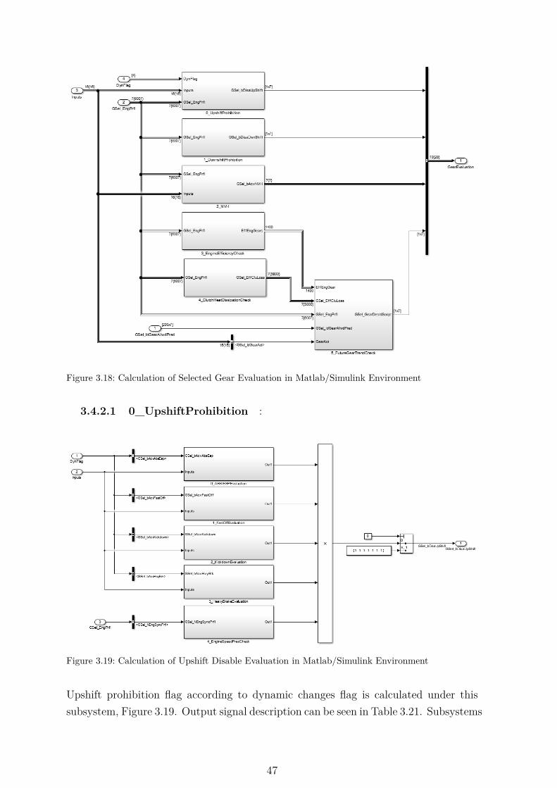
Figure 3.18: Calculation of Selected Gear Evaluation in Matlab/Simulink Environment
3.4.2.1 0_UpshiftProhibition :
Figure 3.19: Calculation of Upshift Disable Evaluation in Matlab/Simulink Environment
Upshift prohibition flag according to dynamic changes flag is calculated under thissubsystem, Figure 3.19. Output signal description can be seen in Table 3.21. Subsystems
47

can be descriped shortly as the following. Detailed explanations will be provided inthe coming pages.
• 0_ABS/ESPEvaluation: ABS/ESP dynamic flag is evaluated according to upshiftallowances.
• 1_FastOffEvaluation: Fast off dynamic flag is evaluated according to upshiftallowances.
• 2_KickdownEvaluation: Kickdown dynamic flag is evaluated according to upshiftallowances.
• 3_HeavyBrakeEvaluation: Heavy brake dynamic flag is evaluated according toupshift allowances.
• 4_EngineSpeedPredCheck: Engine predicted speed allowances is evaluated accordingto upshift allowances.
Table 3.21: Input/Output signals used in 0_UpshiftProhibition subsystemSignal name DescriptionGSel_bDisaUpShift Enabled/Disabled gears with respect to upshift prohibition. If
1 is assigned, gear is allowed, otherwise not allowed.
3.4.2.1.1 0_ABS/ESPEvaluation
Figure 3.20: Evaluation of the ABS/ESP Flag
If ABS/ESP dynamic changes flag is activated, upshift is not allowed and gears fromthe current desired gear are disabled until 7.gear. This logic may change dependingon ESP interfaces. In the current simulation, ESP interfaces deactivates the upshift,that’s why, it is implemented like this. Inputs description can be seen in Table 3.22
48
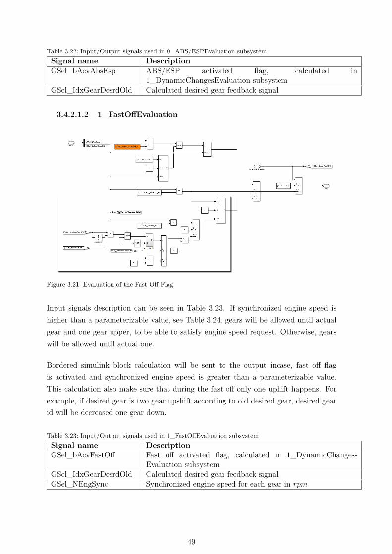
Table 3.22: Input/Output signals used in 0_ABS/ESPEvaluation subsystemSignal name DescriptionGSel_bAcvAbsEsp ABS/ESP activated flag, calculated in
1_DynamicChangesEvaluation subsystemGSel_IdxGearDesrdOld Calculated desired gear feedback signal
3.4.2.1.2 1_FastOffEvaluation
Figure 3.21: Evaluation of the Fast Off Flag
Input signals description can be seen in Table 3.23. If synchronized engine speed ishigher than a parameterizable value, see Table 3.24, gears will be allowed until actualgear and one gear upper, to be able to satisfy engine speed request. Otherwise, gearswill be allowed until actual one.
Bordered simulink block calculation will be sent to the output incase, fast off flagis activated and synchronized engine speed is greater than a parameterizable value.This calculation also make sure that during the fast off only one uphift happens. Forexample, if desired gear is two gear upshift according to old desired gear, desired gearid will be decreased one gear down.
Table 3.23: Input/Output signals used in 1_FastOffEvaluation subsystemSignal name DescriptionGSel_bAcvFastOff Fast off activated flag, calculated in 1_DynamicChanges-
Evaluation subsystemGSel_IdxGearDesrdOld Calculated desired gear feedback signalGSel_NEngSync Synchronized engine speed for each gear in rpm
49

Table 3.24: Calibrateable parameters used in 1_FastOffEvaluation subsystemParameter name Description ValueGSel_NEngOfsFastOff_P Engine speed offset for fast of evaluation in
rpm3500
3.4.2.1.3 2_KickdownEvaluation
Figure 3.22: Evaluation of the Kickdown Flag
Under this logic, upper gears with actual gear are disabled to force the softwaredownshift. Since in the high torque demands, engine speed should be kept high with alow gear selection. There is also precaution incase of an old desired gear is 1. In thiscase, ’>’ relational operation will be false for all gears, then output of the Assignmentblock [0 0 0 0 0 0 0] will be replaced by a vector [1 0 0 0 0 0 0], which means, only 1is allowed.
Inputs description can be seen in Table 3.25
Table 3.25: Input/Output signals used in 2_KickdownEvaluation subsystemSignal name DescriptionGSel_bAcvKickdown Kickdown activated flag, calculated in 1_DynamicChanges-
Evaluation subsystemGSel_IdxGearDesrdOld Calculated desired gear feedback signal
3.4.2.1.4 3_HeavyBrakeEvaluation
Figure 3.23: Evaluation of the Heavy Brake Flag
50

Heavy brake pedal state evaluation is handled under this component, see Figure 3.23.Firstly minimum engine offset speed is calculated by a parameterizable map withrespect to vehicle velocity and deceleration of a vehicle. The map and axes valuescan be seen in Table 3.26. This offset is summed by the parameterizable values forengine minimum speed for shifting and for driving. Element, which id is old desiredgear in vector goes to Y0 input is replaced by a value of U, which is the minimumengine value for the driven gear. The updated engine minimum parameterizable vectoris compared with synchronized engine speed. If the parameterizable vector element islarger than a synchronized engine speed, the gear, which has this element id is disabled.Since it means, synchronized engine speed cannot satisfy the driving with these gears.If heavy brake flag is not activated, all the gears are allowed by giving all 1, 7 elementvector to the output.
Table 3.26: Calibrateable parameters used in 3_HeavyBrakeEvaluation subsystemParameter name Description ValueGSel_VVehHvyBrk_A Vehicle velocity supporting points for heavy
brake situation evaluation in km/h[0 20 35 50 70 85100 110 130 145160 190 220 250]
GSel_AVehHvyBrk_A Vehicle acceleration supporting points forheavy brake situation evaluation
[1 1.5 2 2.5 3 3.54 5 6 7 8 10 12 14]
GSel_NEngOfsHvyBrk_M Minimum engine speed offset over absolutevehicle deceleration and vehicle velocitywhen brake is applied
-
GSel_NEngMinOfsRamp-RateHvyBrk_P
Ramp of minimum engine speed offset overabsolute vehicle deceleration and vehiclevelocity when brake is released:ramp ofengine rotational speed offset in rpm
25
GSel_NEngMinOfsRamp-LimnHvyBrk_P
Ramp of minimum engine speed offset overabsolute vehicle deceleration and vehiclevelocity when brake is released:ramp ofengine rotational speed offset in rpm
10000
GSel_NEngMinInGear-HvyBrk_M
Heavy brake minimum engine rotationalspeed in each gear in rpm
[1400 1400 14401600 1650 17001700]
GSel_NEngMinForShift-HvyBrk_M
Heavy brake minimum engine rotationalspeed to shift into gear in rpm
[1200 1300 14001450 1500 15501600]
51

Table 3.27: Input/Output signals used in 3_HeavyBrakeEvaluation subsystemSignal name DescriptionGSel_bAcvHvyBrk Heavy Brake activated flag, calculated in 1_DynamicChanges-
Evaluation subsystemGSel_IdxGearDesrdOld Calculated desired gear feedback signalGSel_NEngSync Synchronized engine speed for each gear in rpmGSel_AVeh Vehicle acceleration in m/s2
GSel_VVeh Vehicle velocity in m/s
3.4.2.1.5 4_EngineSpeedPredCheck
Figure 3.24: Evaluation of the Engine Speed Prediction for Upshift Prohibition
Engine speed limit are checked for the current gear after a parameterizable shiftingtime, see Figure 3.24. If after a parameterizable shifting time, engine speed will stillallow the gear/s that are selected in present, there will not be change in the selectedgears. If engine speed does not allow after a parameterizable shifting time the currentselected gear/s, since engine maximum limit is violated, then the violating gear shouldbe disabled.
This check is executed, when actual gear is not equal to 7, since otherwise it will notbe logical. There is not a higher gear than 7.
Used parameters and input/output signals can be seen from the Table 3.29 and Table3.28
Table 3.28: Calibrateable parameters used in 4_EngineSpeedPredCheck subsystemParameter name Description ValueGSel_NEngMaxInGear_P Maximum engine speed in each gear in rpm [6300 6300 6300
6300 6300 63006300]
GSel_TiUpShift_P Calibrateable upshift time 10ms 30
52

Table 3.29: Input/Output signals used in 4_EngineSpeedPredCheck subsystemSignal name DescriptionGSel_NEngSync Synchronized engine speed profile for each gear in
parameterizable time interval in rpm. It is a matrix ,which each column represents gear id and rows are value foreach sample time
IN_bEnaEngSpdUp-ShiftChkToSw
Engine speed check after a parameterizable upshift time forchecking, if the selected gear is still in the engine speedlimitations. It is a matrix by [1,7]
3.4.2.2 1_DownshiftProhibition :
Figure 3.25: Calculation of Downshift Disable Evaluation in Matlab/Simulink Environment
Engine speed limit are checked for the current gear after a parameterizable shiftingtime is evaluated, see Figure 3.25. If after a parameterizable shifting time, enginespeed will still allow the gear/s that are selected in present, there will not be change inthe selected gears. If engine speed does not allow after a parameterizable shifting timethe current selected gear/s, since engine minimum limit is violated, then the violatinggear should be disabled.
This check is executed, when actual gear is not equal to 1, since otherwise it will notbe logical. There is not a lower gear than 1.
Used input/output signals and parameters can be seen from the Table 3.29 and Table3.31
53

Table 3.30: Input/Output signals used in 1_DownshiftProhibition subsystemSignal name DescriptionGSel_NEngSync Synchronized engine speed profile for each gear in
parameterizable time interval in rpm. It is a matrix,which each column represents gear id and rows are value foreach time
IN_bEnaEngSpdDown-ShiftChkToSw
Engine speed check after a parameterizable upshift time forchecking if the selected gear is still allowed in engine speedallowances point of view. It is a matrix by [1,7]
GSel_bDisaDwnShift Enabled/Disabled gears with respect to downshift prohibition,calculated in 1_DownshiftProhibition subsystem
Table 3.31: Calibrateable parameters used in 1_DownshiftProhibition subsystemParameter name Description ValueGSel_NEngMinInGear_P Minimum engine speed in each gear in rpm [-1000 1200 1200
1200 1200 12001200]
GSel_TiDownShift_P Calibrateable upshift time 10ms 30
3.4.2.3 2_NVH :
Figure 3.26: Calculation of NVH in Matlab/Simulink Environment
54

Figure 3.27: Calculation of Mean Effective Pressure in Matlab/Simulink Environment
Under this subsystem, NVH behavior of the engine is calculated for each gear andcurrent data by a parameterizable map. The output 1 of the map means gear is allowedfor the current mean effective pressure and engine synchronized speed. The output 0 ofthe map means gear is not allowed for the current mean effective pressure and enginesynchronized speed. Inputs definitions can be seen in Table 3.32. Parameter valuesand explanations can be seen in Table 3.33.
Mean effective pressure calculation to be sent to the first input of the map can beseen in Figure 3.27. Calculation was implemented based on the following equation 3.1,where Pm is mean effective pressure, MEng is engine torque, Vcyl is volume of a pistoncylinder.
Pm = 4 ∗MEng ∗ π3 ∗ Vcyl
(3.1)
This calculation handled by a vector, which each element represents value for one gear.In first operation, engine target torque vector is divided by value 3 in vector formwhich is the number of cylinder in the engine and it is multiplied with 4 since it is afour stroke engine. By the parameter ’Glob_FacPCnvn_P’, unit conversion from bar
to N/m2 is implemented. In the end, vector is splitted to his elements by ’Demux’simulink block. Namely, calculated values for each gear is sent seperately to be able toevaluated in the maps.
It should be highlighted that related NVH data cannot be found for the current project,thats why all maps are parameterized by value 1, namely all gears are allowed.
55

Table 3.32: Input/Output signals used in 2_NVH subsystemSignal name DescriptionGSel_NEngGearXSync Engine synchronized speed for gear X in rpmGSel_PGearXMean Mean effective pressure for gear X in barGSel_TqEngTgtCur Engine torque target for the current data for each gear in Nm.
Table 3.33: Calibrateable parameters used in 2_NVH subsystemParameter name Description ValueGlob_ValPi_P Value pi in vector form for each gear value 3,141592654Glob_FacPCnvn_P Conversion factor from bar to N/m2 in
vector form for each gear value1e5
Glob_VolCylEngSum_P Engine cylinder capacity in vector form foreach gear value in m3
0,00039942
GSel_PEngForNVH_A Mean effective pressure supporting pointsfor NVH table in bar
[...]
GSel_NEngForNVH_A Engine rotational speed supporting pointsfor NVH table in rpm
[...]
GSel_StEngGearX-NVH_M
Possible areas of mean effective pressureand rotational speed according to NVHbehavior for gear X
[...]
3.4.2.4 3_EngineEfficiencyCheck :
Figure 3.28: Calculation of Engine Efficiencies in Matlab/Simulink Environment
56

Figure 3.29: Calculation of Mean Effective Pressure in Matlab/Simulink Environment
Under this subsystem, engine efficiency for each gear is calculated, see Figure 3.28.Inputs definitions can be seen in Table 3.34. Parameter values and explanations canbe seen in Table 3.35.
Calibrateable engine efficiency map is used with constraints engine speed and meaneffective pressure in the piston cylinder. Maps output is a fuel consumption in g/kWh.Mean effective pressure calculation to be sent to the first input of the map can beseen in Figure 3.29. Calculation was implemented based on the following equation 3.2,where Pm is mean effective pressure, MEng is engine torque, Vcyl is volume of a pistoncylinder..
Pm = 4 ∗MEng ∗ π3 ∗ Vcyl
(3.2)
This calculation handled by a matrix, which each column represents gear id and rowsare value for each sample time. In first operation, engine target torque matrix ismultiplied by value 4 in matrix form which is the engine stroke and it is divided by3, which is the number of cylinder. By the parameter ’Glob_FacPCnvn_M’, unitconversion from bar to N/m2 is implemented. Afterwards, matrix is splitted to hiscolumns by a library ’ArrangeMatrix, Figure B.4’. Namely, calculated values for eachgear is sent as a vector seperately, to be able to evaluated in the maps. From Figure3.28, same split operation can be seen for the synchronized engine speeds as well.
GSel_EffEngLowPwr_M map is used for the low engine power and when enginedecelerates, namely when engine torque has a negative value. In this time, only enginespeed is used as a map input.
57

Table 3.34: Input/Output signals used in 3_EngineEfficiencyCheck subsystemSignal name DescriptionGSel_NEngSyncPrfl Synchronized engine speed profile for each gear in
parameterizable time interval in rpm. It is a matrix,which each column represents gear id and rows are value foreach sample time
GSel_TqEngTgtPrfl Engine torque target profile for each gear in parameterizabletime interval in Nm. It is a matrix, which each columnrepresents gear id and rows are value for each sample time
Table 3.35: Calibrateable parameters used in 3_EngineEfficiencyCheck subsystemParameter name Description ValueGlob_ValPi_M Value pi in matrix
form3,141592654
Glob_VolCylEng-Sum_M
Engine cylindercapacity in matrixform in m3
3,141592654
Glob_FacPCnvn_M Conversion factorfrom bar to N/m2
in matrix form
1e5
GSel_PEngForEng-Eff_A
Mean effectivepressure for engineefficiency map inbar
[1 2 3 4 5 6 7 8 9 10 11 12 13 14 15 16 17 18 19 20 21 22]
GSel_NEngForEng-Eff_A
Engine speed forengine efficiencymap in rpm
[800 1000 1250 1500 1750 2000 2400 2800 3200 3600 4000 4500 50005500]
GSel_EffEngLow-Pwr_M
Engine BSFCefficiency map ing/kWh in lowpower
[560 562 565 575 580 582 585 587 600 620 640 655 675 700]
Continued on next page
58
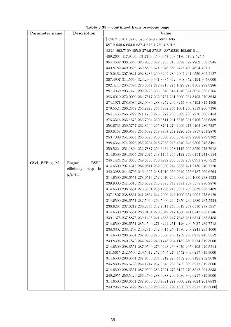
Table 3.35 – continued from previous pageParameter name Description Value
GSel_EffEng_M Engine BSFCefficiency map ing/kWh
[ 628.2 594.1 574.8 578.2 549.7 582.1 635.1 ...587.2 640.6 653.6 637.4 672.1 730.4 801.8423.1 402.7109 405.0 374.6 378.81 387.9228 402.6616 ...409.2663 417.9404 431.7763 450.0657 468.5180 473.2 525.5354.4682 338.5840 328.9000 322.3233 318.3098 322.7262 332.3945 ...339.8782 349.9596 359.8806 371.6048 385.2477 400.4624 421.1319.0462 307.0821 292.8286 290.3292 289.2902 291.9550 302.2127 ...307.4907 314.5663 323.2909 331.8385 342.6308 352.9194 367.0000292.4143 285.7394 276.8647 272.9913 274.1029 275.4505 282.8286 ...287.4059 293.7475 299.9228 305.6846 314.1546 324.6025 336.8165283.6010 272.0000 264.7317 262.0757 261.5000 264.8495 270.3643 ...274.1971 278.8086 282.9930 288.3252 294.3245 303.5192 315.4509279.5524 266.2857 255.7973 254.5982 254.1604 256.7519 260.7396 ...264.1453 266.5229 271.1750 275.5272 280.5509 288.7270 300.5453276.3316 265.4673 255.7064 250.5811 251.3676 251.9406 255.6389 ...258.6736 259.5757 262.8696 265.8761 270.4990 277.9162 286.7257280.0158 266.9583 255.5082 248.8807 247.7220 248.9857 251.2870 ...253.7000 254.6854 256.5623 258.0000 263.6578 269.2288 279.9382298.6364 274.2226 255.2204 248.7053 246.4340 245.9306 248.3491 ...250.5224 251.1894 252.7887 254.3434 258.1115 265.3550 273.7618314.6500 294.3965 267.2075 248.1165 245.2122 243.6154 244.6154 ...246.1424 247.8333 249.3385 250.4292 253.6538 259.0991 270.7212314.6500 297.4315 264.9811 252.0000 244.0835 241.2130 240.7170 ...242.3288 244.6796 246.4325 248.1019 250.2649 255.6187 269.6264314.6500 298.6551 278.0513 252.2970 243.9000 239.1600 238.1532 ...239.9000 241.5315 243.6392 245.9925 248.2981 257.3375 270.2876314.6500 298.6551 276.3991 258.1296 245.0321 239.3839 236.7489 ...237.1807 238.8661 241.2864 244.2000 246.1000 254.9992 273.6129314.6500 298.6551 282.5040 263.5000 244.7350 239.2380 237.5554 ...236.6263 237.6217 239.2845 242.7014 246.3019 257.0510 278.5957314.6500 298.6551 286.9164 270.9042 247.1066 241.0747 238.6146 ...239.1375 237.8875 239.1495 241.4685 247.7648 261.6514 285.5485314.6500 298.6551 285.4500 271.3244 251.9126 246.5037 239.7718 ...238.3302 238.4708 240.2870 242.0614 250.1980 268.2245 295.4000314.6500 298.6551 287.9500 275.5000 263.1739 256.0975 245.5552 ...239.8396 240.7870 244.9472 245.1748 254.1182 280.6774 319.3000314.6500 298.6551 287.9500 276.9443 266.8979 265.9195 249.5214 ...241.5615 242.5500 249.5072 252.6505 270.4552 309.6217 319.3000314.6500 298.6551 287.9500 284.8212 270.4452 266.9125 252.9638 ...245.8306 245.6733 254.1217 267.0545 286.3752 309.6217 319.3000314.6500 298.6551 287.9500 286.7621 275.3122 270.8512 261.8833 ...249.2955 256.5429 266.4539 288.9988 299.4636 309.6217 319.3000314.6500 298.6551 287.9500 286.7621 277.0000 272.8024 261.8833 ...249.2955 256.5429 266.4539 288.9988 299.4636 309.6217 319.3000]
59

3.4.2.5 4_ClutchHeatDissipationCheck :
Figure 3.30: Calculation of Clutch Heat Dissipation in Matlab/Simulink Environment
Figure 3.31: Calculation of power loss in clutches during shift in Matlab/Simulink Environment
Theoretical background was introduced in chapter ’2.Method Description’ for the powerlosses in the clutch during the shift. In this subsystem, according to this theoretical
60

background some assumptions were made and maps were created. Maps are linear,where minimum and maximum clutch torques are taken as 50 and 350Nm, minimumand maximum clutch slips are taken as 50 and 1000rpm and shifting time is taken as500ms. Clutch slip is defined by the speed difference between each side of the clutch.As it can be seen in Figure 3.31, clutch slip shifting from gear 1 to gear 2 is calculatedby the engine synchronized speed difference. This figure shows only one calculation forshifting from gear 1 to gear 2. This calculation is repeated for the each possible shifts.In this software, upshift is allowed sequentially, where downshift can be handled byskipping the gears. For example, upshift from gear 5 will be allowed only to gear 6,whereas downshift from gear 5 can be allowed to 4. gear as well as 3, 2 or 1. Odd gearto odd gear or even gear to even gear shift is harder than odd to even or vice versashift according to control point of view. Although shifting takes longer and hard tocontrolling clutches and rails, it is possible.
During driving, there will be no clutch slip, namely speed differences between the eachside of the clutch will be zero. If the shift is requested, engine speed should be changedfrom engine synchronized speed at 1. gear to engine synchronized speed at 2. gear,which creates clutch slip. In Figure 3.31, input engine synchronized matrix is splittedto its column to get the value for each gear seperately by library ArrangeMatrix, seeFigure B.4. After the calculation of clutch slip by substraction the speeds, absolutevalue is taken. Since negative or positive sign in the clutch slip just represents, whichside has the highest speed value. But this information is not required during powerloss calculation. The important thing is magnitude of speed difference in each side ofthe clutch.
Output of the map in Figure 3.31 is in unit Watt. To be able to compare this resultwith engine efficiencies in g/kWh in the coming subsystem 5_FutureGearTrendCheck,the parameterizable conversion factor is implemented by a map before sending tothe output, which can be seen in Figure 3.30. This map is calibrated according tosimulation measurements. Fuel consumption is measured for a specific engine powerand approximate value is assigned to the map.
Detailed explanations of the each signals and parameters used in this subsystem canbe seen in Table 3.36 and 3.37 respectively.
61

Table 3.36: Input/Output signals used in 4_ClutchHeatDissipationCheck subsystemSignal name DescriptionGSel_NEngSyncPrfl Synchronized engine speed profile for each gear in
parameterizable time interval in rpm. It is a matrix,which each column represents gear id and rows are value foreach sample time
GSel_TqSftInpPrfl Engine torque target profile in parameterizable time interval inNm. It is a vector, which elements represent the value for eachsample time
GSel_EffCluLossGearX Clutch calculated power loss during shifting from gear X toother 7 gears, it is a vector with a number of gear, 7 timespredicted time span.
Table 3.37: Calibrateable parameters used in 4_ClutchHeatDissipationCheck subsystemParameter name Description ValueGSel_DifSyncdEngSpd_A Synchronized engine speed difference axis
between current gear and allowed shiftinggear in rpm
[50 2000]
GSel_TqSftInp_A Current input shaft torque axes for clutchheat loss in Nm
[50 350]
GSel_PwrCluHeatLoss_M Factor for comparing the power loss inthe clutch during shift because of the heatdissipation in Watt
[65,4498458,1489 2618,018326]
GSel_PwrCluLoss_A Clutch heat dissipation power to engineefficiency conversion factor axes of the map
[5 10 20 30 40 50]
GSel_EffCluLoss_M Clutch heat dissipation power to engineefficiency conversion factor map
[280 268 340 245275 275]
GSel_NrGear_P number of gear parameter 7
3.4.2.6 5_FutureGearTrendCheck :
Desired gear will be calculated according to predictive road data. Backgroundinformation was explained in chapter 2.Method Description. The input signals weretaken from 3_EngineEfficiencyCheck and 4_ClutchHeatDissipationCheck subsystemsand these values are evaluated with the matlab function block, as can be seen in Figure3.32.
Engine efficiency and clutch heat dissipation signals are initialized inside the matlabfunction as can be seen in Figure 3.33. Clutch heat dissipation signals GSel_EffCluLoss-GearX are a vector, which can be divided 7 equal layers. First layer represents powerloss during shifting from 1 to 1, second layer represents shift from 1 to 2, and so on.The X in the name represents the actual gear. In the Figure 3.33, in first lines, clutchheat dissipation signals are structured to be able to use in the script.
62

Figure 3.32: Calculation of Future Gear Trend in Matlab/Simulink Environment
Figure 3.33: Initialization of the used signals in the future gear trend evaluation script.
Out of clutch heat dissipation signals, 3 dimensional matrix is created, where columnrepresents to be shifted gear, row represents time span and 3. dimension representsactual gear. The part ’Arrange Engine Efficiency’ assigns the engine efficiency signalsto variable GSel_EffEng and to variable GSel_EffEngLowPwr for low engine power to
63

be used inside the script. This variable is a matrix, where each column represents thedesired gear and rows represents each sample time.
In the Figure 3.34, engine efficiency evaluation for the coming gears are implemented.By the engine efficiency map, fuel consumption in g/kWh is calculated. This mapoutput is multiplied with an engine power to be able to get fuel consumption in g/h,which is used for the selection of the most efficient gear. If gear is not selected, engineefficiency of this gear will be zero. Adding the high value like 70000, keeps these notselected gears out of evaluation. In the gear efficiency evaluation, minimum valuemeans minimum fuel consumption, that’s why value with a minimum engine efficiencywill be selected as the most desired gear. The same calculation is done one time forthe general gear efficiency and one time for the gear efficiency in low engine power.
Figure 3.34: Evaluation of the engine efficiency. If engine efficiency does not change more than aparameterizable value after the new desired gear, keep the old desired gear.
Afterwards, used variables in the for loop is initialized. For loop turn in number ofsample time in defined times span. Explanation of these variables are presented inTable 3.38.
In the for loop, there are two main conditions; firstly low engine power is checked. Ifengine power is lower than a threshold, engine efficiency map for low engine power isused for gear selection. This condition includes low engine power condition as well as
64
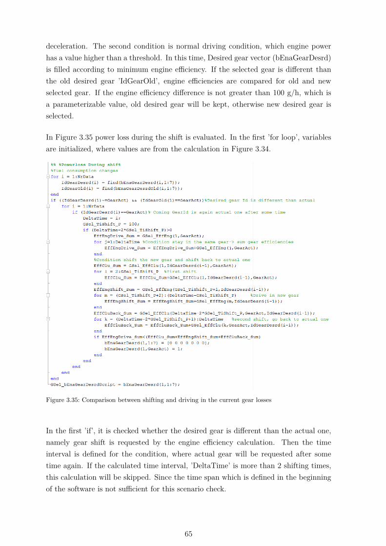
deceleration. The second condition is normal driving condition, which engine powerhas a value higher than a threshold. In this time, Desired gear vector (bEnaGearDesrd)is filled according to minimum engine efficiency. If the selected gear is different thanthe old desired gear ’IdGearOld’, engine efficiencies are compared for old and newselected gear. If the engine efficiency difference is not greater than 100 g/h, which isa parameterizable value, old desired gear will be kept, otherwise new desired gear isselected.
In Figure 3.35 power loss during the shift is evaluated. In the first ’for loop’, variablesare initialized, where values are from the calculation in Figure 3.34.
Figure 3.35: Comparison between shifting and driving in the current gear losses
In the first ’if’, it is checked whether the desired gear is different than the actual one,namely gear shift is requested by the engine efficiency calculation. Then the timeinterval is defined for the condition, where actual gear will be requested after sometime again. If the calculated time interval, ’DeltaTime’ is more than 2 shifting times,this calculation will be skipped. Since the time span which is defined in the beginningof the software is not sufficient for this scenario check.
65

If the prediction time span is enough, following calculations will be done. Overall engineefficiency is calculated for the condition keeping the actual gear. Result is written tothe variable ’EffEngDrive_Sum’. Then, shifting to the desired gear, driving in desiredgear and come back to the actual gear losses are calculated and written to the variablesEffClu_Sum, EffEngShift_Sum and EffCluBack_Sum respectively. In the end, thesescenarios are compared in the losses point of view. If the driving in the actual gearhas less fuel consumption compare to the shifting scenario, actual gear will be kept.Namely, element id, which has the actual gear is set in the vector bEnaGearDesrd.Otherwise, bEnaGearDesrd vector is kept same and desired gear is updated with thenew gear id, like calculated in Figure 3.34. In the end of the line, output from scriptassignment is implemented.
Table 3.38: Input/Output signals and variables used in 5_FutureGearTrendCheck subsystem andinside the matlab function.
Signal name DescriptionPwrEng Engine power profile in the parameterizable time interval in
Watt. It is a vector by [redictiontimespan]GSel_IdGearAllwdPred Allowed gear with respect to engine allowances in
parameterizable time interval. It is a matrix, which eachcolumn represents gear id and rows are value for each sampletime
EffEngGear Engine gear efficiencies for each gear, calculated in3_EngineEfficiencyCheck subsystem
GSel_IdGearAct Actual gear valueGSel_EffCluLossGearX Clutch power loss calculated during shifting from gear X to
other 7 gears in 4_ClutchHeatDissipationCheck subsystem,itis a vector with a number of element 7 times predicted timespan.
GSel_GearDesrdScript Desired gear, calculated in 5_FutureGearTrendChecksubsystem
GearEval_min minimum engine efficiency value for the specified time betweenselected gears
bEnaGearDesrd this is a 7 element vector. When X gear is selected, X. elementof a vector assigned 1
IdGearOld Old desired gear IdIdGearDesrd Desired gear IdEffEngDrive_Sum Overall engine efficiency in g/h, for the scenario, come back to
actual gear after some timeEffClu_Sum First shifting power loss in the clutch in g/kWh, for the
scenario, come back to actual gear after some timeEffEngShift_Sum Engine efficiency in g/h between two shifts, for the scenario,
come back to actual gear after some timeEffCluBack_Sum Second shifting power loss in the clutch in g/h, for the scenario,
come back to actual gear after some time
66

3.4.3 2_DesiredGearSelection
(a) Desired Gear Calculation Subsystem
(b) Combination of Evaluated Gears from 1_EvaluationofthePossibleGear Subsystem
Figure 3.36: Calculation of Desired Gear in Matlab/Simulink Environment
Under this subsystem, evaluated gear values from 1_EvaluationofthePossibleGearsubsystem is combined. All input signals are vector, which has 7 element whichrepresents one gear value. If the value is 1, it means, this gear is allowed. If the valueis 0, it means, this gear is not allowed. Combined form of input signals can be seen inFigure 3.36.b. Within all this signals Upshift prohibition flag ’GSel_bDisaUpShift’ hasthe highest priority. Then in a sequence, Downshift prohibition flag ’GSel_bDisaDwn-Shift’, NVH evaluation flag ’GSel_bAcvNVH’ and gear id calculated in 5_FutureGear-TrendCheck subsystem GSel_GearDesrdScript has a higher priority. Which means, ifone of the upshift prohibition flag is raised, the other inputs are not considered but gearis selected according to ’GSel_bDisaUpShift’ flag. If none of the flags are activated,gear selection will be done with calculation under 5_FutureGearTrendCheck script.
Afterwards, the selected gear Id will be defined, see Figure 3.36.a. The gear has ahigher id will be selected. Ideally, in this level of the component, only one gear shouldbe requested. Vector elements going as an input to the max block, has one valuebetween 1 to 7 and other values are all zero. In the end of the calculation, precautionis taken, incase, there will be no gear selected. In this case, old desired gear is kept.
67

Table 3.39: Input/Output signals used in 2_DesiredGearSelection subsystemSignal name DescriptionGSel_bDisaUpShift Enabled/Disabled gears with respect to upshift prohibition
in vector for each gear, calculated in 0_UpshiftProhibitionsubsystem
GSel_bDisaDwnShift Enabled/Disabled gears with respect to downshift prohibitionin vector for each gear, calculated in 1_DownshiftProhibitionsubsystem
GSel_bAcvNVH Enabled/Disabled gears information with respect to NVHbehavior in vector for each gear, calculated in 2_NVHsubsystem
GSel_GearDesrdScript Desired gear in vector for each gear, calculated in5_FutureGearTrendCheck subsystem
GSel_IdxGearDesrd Desired gear which is sent as an output from Gear SelectionStrategy component to other components in the TCU
68

4 Simulation and Testing Environment
Under this section, simulation environment and test results will be presented. AVLVSM™ is used for creating the simulation environment for functional testing. AVLVSM™ is a simulation package of tools that supports engineers in the field of conceptdevelopment, calibration and functional validation [7]. By this tool it is possible tosimulate longitudinal and lateral dynamic behaviors of the vehicle.
4.1 Testing Environment
VSM provides to set drivetrain, engine, tyre, suspension, etc. characteristics. Thereare also different kinds of transmission models like AT, MT (Manual Transmission),CVT (Continuously Variable Transmission).
VSM uses Matlab Simulink environment for the execution of the tests. For eachrequired part of the vehicle such as Drivetrain, ECU Module, Engine Module, SteeringModule, etc. and road, there are S-functions. S-function is a computer languagedescription of a Simulink block written in Matlab, C, C++ or Fortran. Signal flowbetween VSM and gear selection strategy is represented in Figure 4.1. VSM is theinput generator and provides all required interfaces to the Gear Selection Strategy.Gear selection strategy executes the inputs and provides desired gear to the VSM.
Figure 4.1: Communication between Gear Selection Strategy and AVL VSM™
Figure 4.2 shows intefaces between VSM and gear selection strategy in SimulinkEnvironment. The yellow subsystem in the Figure 4.2 is a function call for initializationof the parameters and objects used in software. The green subsystem is the developedsoftware within this thesis. AVL VSM requires desired gear which is provided by firstoutput Gear. When gear change is active, which is an information coming from AVLVSM, desired gear is not updated, when shifting is not active, calculated desired gear issent. The second output is requested by AVL VSM is Gear Change, which is providedby second output. This signal contains information whether upshift or downshift isrequested. When upshift is requested, 1 is sent. When downshift is requested, -1 issent. When desired gear is the same with the current gear, namely no shift is requested,0 is sent.
69

Figure 4.2: Interface connections between developed gear selection strategy and AVL VSM™
Parameter settings for the drivetrain, engine, vehicle geometry are parameterizedthrough the VSM GUI , see Figure 4.3. Front differential configuration is selectedas drivetrain configuration.
Engine torque map, fuel consumption map, transmission efficiency map, inertias,aerodynamic constans are assigned via the VSM GUI according to project vehiclespecifications. For a driver, brakes, clutches, suspension, pedal maps typical mid-sizevehicle default values are used, which is already exist in VSM. For the both simulation,same VSM GUI parameterization is used.
Vehicle velocity and road gradient vectors are also given from there.
Figure 4.3: AVL VSM™ GUI
70

4.2 Test Results
Functional tests were run with the initial calibration of the project, which has beencalibrated at a test track. This means, gear selection strategy works in normalconditions properly on a flat road test track and the project is close to finishing phase.Project uses state of the art shift maps as a gear selection strategy, which was explainedunder 2.1 Current Technology section. Software developed in this study is calibratedaccording to simulation model in VSM.
Same parameterization is used for both project and thesis simulation environment inVSM GUI. Overall, 3 different testcases were created for functional testing. In firsttest, NEDC (New European Driving Cycle) [9] is given as a vehicle velocity profilefor the flat road and simulated for the gear selection developed in project and in thisstudy. NEDC is a driving cycle, designed to assess the emission levels of engines andfuel economy in passenger cars. The results can be seen from Figure 4.4. For the bettervisibility, first repeated part of the test results were cutted and results are shown after600 seconds. Results until 600. seconds can be seen from Appendix C.
As it is indicated in legend of the graphs, black lines are the results for the componentdeveloped in project and red lines are the results for the component developed inthis study. Absolute fuel consumption levels are slightly different, see Figure 4.4.b.Differences in emissions can be seen better from specific fuel consumption graph.Project gear selection selects the gears according to vehicle velocity and acceleratorpedal position. Calibration engineers calibrated these maps to be able to get better fuelconsumption levels. Whereas gear selection developed in this study decides desired gearaccording to engine efficiency maps with the consideration of drivetrain losses. Around640. second, while project gear selection demands second gear, thesis gear selectionstays in the same gear. In this part, project gear selection efficiency performanceis better with respect to specific fuel consumption. Around 775. seconds, from 880.seconds to 937. seconds and from 1020. seconds to 1072. seconds according to differentgear demands better specific fuel consumption is reached by developed gear selection.As it was expected in the beginning of the study, better fuel consumption levels werenot reached completely but in some parts in the simulation better fuel consumptionlevels can be observed. In the end of the test cycle, absolute fuel consumption levelsdifference is around 1 g/h.
It should be noted down that, during the standstill, requesting the neutral gear logicwas not implemented, that’s the reason in this time first gear is demanded and specificfuel consumption has a highest value.
71

(a) Vehicle velocity, gear demand, engine torque and speed results
(b) Fuel consumption levels
Figure 4.4: Test Results for NEDC test cyle in flat road after 600 seconds
72

In second test, cold start phase of FTP-75 [9] driving cycle is given as a vehicle velocityprofile for the flat road and simulated for the gear selection developed in project andin this study. FTP-75 (United States Environmental Protection Agency Federal TestProcedure) is a city driving cycle to measure tailpipe emissions and fuel economy ofpassenger cars. The results can be seen in Figure 4.5.
Velocity profile in this cycle is more aggressive than the NEDC cycle. In this case,clutch heat dissipation checks calculation, which is explained under section 3.4.2.65_FutureGearTrendCheck, plays an important role. When there is velocity changeoccurs just a short time, maybe there is no need to demand gear change but keeping thesame gear is more efficient. This logic is needed, since gear selection is done in this studybased on output shaft torque. In FTP-75, vehicle velocity changes aggressively and thisresults also aggressive changes in output shaft torque, namely engine torque. Withoutthis logic, gear demand would be changed always according to engine torque changes.Aggresive vehicle velocity changes are overcome with the hysteresis implementationin the shift maps in project gear selection, which was explained under 2.1 CurrentTechnology section.
In this study, it was possible to get improvement in some parts of the cycle in specificfuel consumption, which can be seen in Figure 4.5.b. After 415. seconds, it is clearlyseen that absolute fuel consumption levels are also better in developed gear selectionresults. The other remark about the results are around 410. seconds, project is notable to follow vehicle velocity, namely it cannot fulfill the driver demand, which is alsoan important requirements that should be fulfilled during the vehicle development.
As expected in the beginning of the study, better fuel consumption levels were not ableto reached completely but improvements can be seen in some parts of the simulation.In the end, absolute fuel consumption level difference is measured as 3 g/h. Gearselection for the future can be improved more with the preselection logic for DCTs.In this way, coming gear can be preengaged before the selection. This strategy canprovide better shift quality and less losses during shifting and this results in a betterfuel consumption levels.
It should be noted down that, during the standstill, requesting the neutral gear logicwas not implemented, that’s the reason in this time first gear is demanded and specificfuel consumption has a highest value.
73

(a) Vehicle velocity, gear demand, engine torque and speed results
(b) Fuel consumption levels
Figure 4.5: Test Results for FTP-75 test cyle in flat road
74

In third test, gear selection strategy developed in this study was compared flat road vs5� road gradient condition by giving the last cycle of the NEDC as a velocity profile.The aim of this test, showing how software works for road gradient conditions. Theresults can be seen from Figure 4.6.
Figure 4.6: Test results for NEDC in 5� road gradient
As it is indicated in the legend of the graph, black lines show results in flat road,and red lines show results in 5� road gradient. When road gradient was 5�, shiftingshappened later than flat road tests, which was an expected result. During uphilldriving, more torque is needed in the wheels, that’s why to be able to get this highertorque, it is required to stay in lower gear longer to be able to get higher engine speed.Around 230.sec, when velocity start to increase from around 70 km/h to 100 km/h,one downshift is requested in 5� road gradient testing. The reason is engine does nothave enough torque to be able to deliver this desired torque to output shaft. That’swhy one downshift is performed, engine accelerates and afterwards, previous gear isengaged again. This can be improved by including torque reserve logic. While outputshaft torque is calculated, torque reserve can be added to the output shaft. Torquereserve represents the power reserve of the vehicle for the coming situatons. Gearselection is done according to updated output shaft torque, in other words, engineoperation points are evaluated with the updated output shaft torque. In this way, itmay be possible to drive without downshifting, since current gear can already deliver
75

required acceleration levels. As an improvement to the current implementation, driveracceleration request in the future can be predicted and this value can be reserved duringoutput shaft torque calculation. In this way, when acceleration is requested, there isno need to fulfill this request by downshifting, since this torque is already available inengine.
For fuel consumption point, fuel consumption is higher when it is driven in uphill road.Since more torque is needed in output shaft and engine torque is higher in this timefor giving the higher torque to the wheels.
76

5 Conclusion and Future Work
As can be seen from test results, it was possible to get better fuel consumption levelspartially with the developed gear selection strategy. In the end of the test cycles,absolute fuel consumption levels were calculated quite same. It should be noted downthat, developed software requires less calibration work compared to the gear selectionstrategy developed in the project, since during the gear selection, engine efficiency mapsare used instead of several conventional shift maps. For 7 gears transmission, each shiftmap contains 6 upshift and 6 downshift lines, 14 supporting points per line, 20 shiftmaps for different conditions. Totally, there is 12*14*20 = 3360 parameters. Insteadof 3360 parameters, gear selection in this study uses engine efficiency map, which has308 parameter inside. Moreover, developed gear selection requires less implementationeffort, since instead of 20 shift maps, there is just one engine efficiency map. There isalso not extra implementation effort for selection of the proper shift map.
By the third test cases, it was also shown that developed gear selection strategy isapplicable for the road gradient conditions. Unfortunately, performance could not becompared with the project gear selection strategy, since calibration was not completedfor driving uphill and downhill conditions.
There is still room for improvement in the developed gear selection strategy. Shiftsequencing can be considered, which depends on the applied transmission type. Sinceit is possible to get the coming road conditions and velocity, shift sequencing can becalculated in advance. During deciding shift sequencing, efficiency as well as driverfeeling can be considered. Maybe shifting from 7 to 1 gear is the most efficient option,however how driver will feel during this shift is also important. Moreover, for theDHT transmission, there will be several kinds of shift possibilities in considerationof torque splits. This shift sequencing is considered partially in this thesis. Theimplementation can be seen under section 3.4.2.6. 5_FutureGearTrendCheck. Thislogic can be improved further for hybrid and different kinds of transmission types.
Technology is developed more in hybrid drive, since the strict emission regulations.Transmission types are also improved through the DHT. In DHT, it is not possibleto use conventional shift maps, since there is ECVT drives. ECVT driving modes areused in conjunction with pure electric driving gears as well as parallel hybrid drivinggears, which makes gear selection with shift maps almost impossible. Hybrid vehiclearchitecture and ECVT driving modes bring torque splits into account, which shouldbe also considered, during developing the gear selection for hybrid vehicles.
In the future, sailing function can be included, which is an energy efficient drivingoperating mode, that turning off the engine during vehicle is still moving. In the
77

same way, coasting can be also included. Coasting is defined as decoupling the enginefrom the vehicle and running engine in idle mode. These modes can be used duringdecelerating for the standstill position. For example, since vehicle velocity profile isknown by prediction calculations, when vehicle is decelerating, and it is seen thatvehicle has enough power to be able to come to the predicted standstill position, sailingor coasting can be activated.
Torque reserve calculation can be also included as it is mentioned in the results ofdriving in uphill road. With the torque reserve logic, it is possible to get sportive drivewithout downshift.
In DCT, even and odd gears are separated onto two separate shafts. One clutch is usedjust for engaging odd gears and other clutch is used just for engaging even gears. Withthis two shaft architecture, it is possible to preselect the coming gear. For example,when the vehicle speeds up, controller in the car automatically detect the gear changepoint and will preselect the upper gear. In the same way, when the vehicle speedsdown, controller will preselect a lower gear. When gear change is requested, currentlyengaged clutch disengages and the other preselected clutch engages. Currently, thislogic is not implemented in the thesis software. This logic should be also includedfor DCT control software. When this is introduced in the current architecture, thereshould be one more output for preselect gear, namely future gear. This gear is alreadycalculated under 3.4.2.6. 5_FutureGearTrendCheck subsystem but not given to theoutput. With the improvement of gear sequencing calculation, this logic can be alsoimproved.
Power losses during the shifting in clutches can be also improved. In this calculation,shifting time is given as a constant value. This value highly depends on torque handoverfunctionality, which handles the torque shifting from one clutch to other. In the future,torque handover part of the software can send shifting time according to the hardwarelimitations. By this, it is possible to get more accurate shifting loss values. For this,additional research should be done for analyzing the clutch losses during shift. Theeffect of the developed gear selection strategy would not be too much. After the outputof the clutch losses simulation, current clutch losses parameters used in the softwareshould be updated according to research output.
As it was described in the architecture description of the software, learning algorithmcan be added after the gear selection strategy system. This algorithm can improve gearselection overtime also it helps learning the driver needs. This system can be parameterfitting approach, so that it can update parameter used in the software overtime, forbetter gear selection quality.
78

Instead of considering NVH just for the current data, it can be considered as furtherdevelopment during the prediction calculation. Since engine speed and torque canbe calculated for future, NVH bahavior can be checked for the future conditions.In this way, even the selected gear is the best gear in efficiency point of view, itcan result a bad noises or jerks, which is not desirable by the driver. The effectof the software would be using the same parameterizable map implementation withvector, namely predicted engine torque and speed inputs. Afterwards, the output ofthe maps should be evaluated under subsystem 3.4.2.6. 5_FutureGearTrendCheck inthe software, which was explained under 3. Software Description chapter.
79

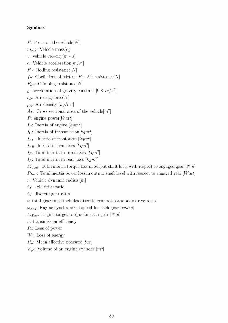
Symbols
F : Force on the vehicle[N ]mveh: Vehicle mass[kg]v: vehicle velocity[m ∗ s]a: Vehicle acceleration[m/s2]FR: Rolling resistance[N ]fR: Coefficient of friction FL: Air resistance[N ]FST : Climbing resistance[N ]g: acceleration of gravity constant [9.81m/s2]cD: Air drag force[N ]ρA: Air density [kg/m3]AF : Cross sectional area of the vehicle[m2]P : engine power[Watt]IE: Inertia of engine [kgm2]IG: Inertia of transmission[kgm2]IAF : Inertia of front axes [kgm2]IAR: Inertia of rear axes [kgm2]IF : Total inertia in front axes [kgm2]IR: Total inertia in rear axes [kgm2]MJout: Total inertia torque loss in output shaft level with respect to engaged gear [Nm]PJout: Total inertia power loss in output shaft level with respect to engaged gear [Watt]r: Vehicle dynamic radius [m]iA: axle drive ratioiG: discrete gear ratioi: total gear ratio includes discrete gear ratio and axle drive ratioωEng: Engine synchronized speed for each gear [rad/s]MEng: Engine target torque for each gear [Nm]η: transmission efficiencyPv: Loss of powerWv: Loss of energyPm: Mean effective pressure [bar]Vcyl: Volume of an engine cylinder [m3]
80


Acronyms
ABS: Anti-lock Braking SystemAT: Automatic TransmissionBMEP: Brake mean effective pressure in engin piston cylinderBSFC: Brake Specific Fuel ConsumptionCAN: Controller Area NetworkCVT: Continuously Variable Transmission DCT: Dual Clutch TransmissionDHT: Dedicated Hybrid TransmissionECVT: Electronic Continuously Variable Transmission ECU: Engine Contol UnitESP: Electronic Stability ProgramFWD: Front Wheel DriveFTP75: US Environmental Protection Agency Federal Test ProcedureGPS: Global Positioning SystemGUI: Graphical User InterfaceHCU: Hybrid Control UnitHMI: Human Machine InterfaceMT: Manual TransmissionNEDC: New European Driving CycleNVH: Noise, Vibration and HarshnessRDE: Real Driving EmissionsSOC: State of ChargeSUV: Sport Utility VehicleTCU: Transmission Control UnitTGDI: Turbocharged Gasoline Direct Injection
81

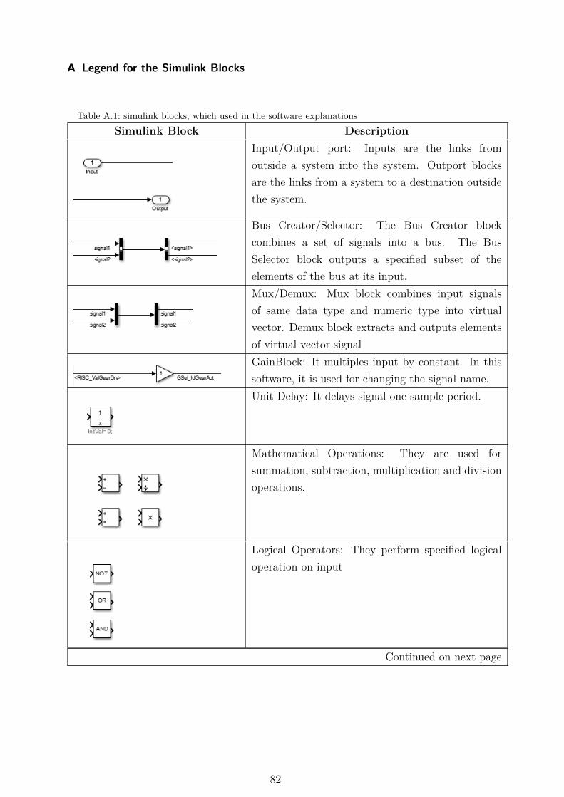
A Legend for the Simulink Blocks
Table A.1: simulink blocks, which used in the software explanationsSimulink Block Description
Input/Output port: Inputs are the links fromoutside a system into the system. Outport blocksare the links from a system to a destination outsidethe system.
Bus Creator/Selector: The Bus Creator blockcombines a set of signals into a bus. The BusSelector block outputs a specified subset of theelements of the bus at its input.Mux/Demux: Mux block combines input signalsof same data type and numeric type into virtualvector. Demux block extracts and outputs elementsof virtual vector signalGainBlock: It multiples input by constant. In thissoftware, it is used for changing the signal name.Unit Delay: It delays signal one sample period.
Mathematical Operations: They are used forsummation, subtraction, multiplication and divisionoperations.
Logical Operators: They perform specified logicaloperation on input
Continued on next page
82

Table A.1 – continued from previous pageSimulink Block Description
Relational Operations: They perform specifiedrelational operation on inputs.
Min/Max Block: They output minimum ormaximum input value.
Constant Block: They generate constant value.When this constant value such as ’Parameter’, isdefined in workspace, it is colored orange in thissoftware to show, it is a parameter, which can beparameterized from workspace.Lookup Tables: LookUp table approximatesone/two-dimensional function. Direct Lookup Tableindex into n-dimensional table to retrieve element,vector, or 2-D matrix.
Multiport Switch: it chooses between multiple blockinputs. In this picture, first input is the controlinput, when it is 0, second input is given as anoutput, otherwise, third input is given as an output.
Goto/From: Goto block passes block input to Fromblocks. From block accept input from Goto block.
Continued on next page
83

Table A.1 – continued from previous pageSimulink Block Description
Assignment: It assigns values to specified elementsof signal. Input Y0 is a vector. Input Idx1 is the Idof a vector Y0. Y0 element value, where id is definedfrom Idx1 input is replaced by U.
Selector: It selects input elements from vector,matrix, or multidimensional signal, where U is thevector input, Idx1 is the Id of a vector element.
Matlab Function: It is a function defined withSimulink block, where you can write matlab scriptinside as a function and this function is called inevery sample time.
84

B Legend for the Simulink Libraries
In Simulink, library is defined as reusable libraries of blocks and subsystems. Somelibraries were created to be used during the implementation, where logic is repeatedseveral times.
B.1 S-RFlipFlop
Figure B.1: S-RFlipFlop library subsystem in Matlab/Simulink Environment
SR Flip Flop holds the flag Set ’S’ until it is reseted by input Reset ’R’. For the truthtable, please see TableB.1
Table B.1: Truth table of SR Flip FlopS R Q1 0 10 0 1 (after S=1, R=0)0 1 00 0 0 (after S=0, R=1)1 1 1
85

B.2 ResetTimer
Figure B.2: ResetTimer library subsystem in Matlab/Simulink Environment
ResetTimer library counts the time by adding the Increment ’Inc’ to the last value ofTime Elapsed ’TiElpd’ in every calculation time step, when it is triggered by EnableTimer ’TmrEna’. Limitation by Maximum time ’TiMax’ can be also set for not countingto the infinity.
B.3 LowPassFilterReset
Figure B.3: LowPassFilterReset library subsystem in Matlab/Simulink Environment
LowPassFilterReset library is a filter that passes signals with a frequency lower thana certain cutoff frequency ’TcFil’, and attenuates signals ’SigFilInp’ with frequencieshigher than the cutoff frequency ’TcFil’. Filter is initialized by Reset Value ’RstVal’ inthe first time sample of the simulation. This filter can be reseted by the input TriggerReset ’RstTrig’ in any time during the simulation.
86

B.4 ArrangeMatrix
Figure B.4: ArrangeMatrix library subsystem in Matlab/Simulink Environment
ArrangeMatrix library is split the columns of a matrix which has 7 columns. In thesoftware, it is used for splitting the prediction value matrix to its column and get thevalues for each gear as a vector. For example, ’ValGear1’ is the calculated predictionvalue for the Gear 1.
87

C Test Results Extension
(a) Vehicle velocity, gear demand, engine torque and speed results
(b) Fuel consumption levels
Figure C.1: Test Results for NEDC test cyle in flat road before 600 seconds
88


List of Figures
2.1 Conventional shift map with upshift and downshift lines [11] . . . . . . 42.2 DHT type Gearbox [2] . . . . . . . . . . . . . . . . . . . . . . . . . . . 52.3 A schematic of a segmentational splitting of predictive data . . . . . . . 62.4 The architecture of the software . . . . . . . . . . . . . . . . . . . . . . 72.5 The subsystem of Velocity Profile/Predicted Calculation . . . . . . . . 112.6 The Subsystem of Dynamic Changes Evaluation. . . . . . . . . . . . . . 132.7 The Subsystem of Engine Torque/Speed Profile . . . . . . . . . . . . . 142.8 Forces on vehicle model in constant velocity [11] . . . . . . . . . . . . . 142.9 Moments of Inertias for a FWD Vehicle [15] . . . . . . . . . . . . . . . 162.10 The Subsystem of Allowed Gear Calculation . . . . . . . . . . . . . . . 172.11 Power and energy losses during torque speed sequence shift [11] . . . . 212.12 Possible Shift Scenario, change of a target gear . . . . . . . . . . . . . . 223.1 5 speed DCT Architecture [5] . . . . . . . . . . . . . . . . . . . . . . . 243.2 Implemented Software in Matlab/Simulink Environment . . . . . . . . 253.3 Input subsystem implementation in Matlab/Simulink Environment . . 263.4 Calculation of Vehicle Acceleration in Matlab/Simulink Environment . 273.5 Calculation of synchronized engine speeds in Matlab/Simulink Environment 283.6 Calculation of Dynamic Changes Flags in Matlab/Simulink Environment 293.7 Calculation of Heavy Brake Flag in Matlab/Simulink Environment . . . 303.8 Calculation of Fast off Flag in Matlab/Simulink Environment . . . . . 313.9 Calculation of ABS/ESP Flag in Matlab/Simulink Environment . . . . 323.10 Calculation of Kickdown Flag in Matlab/Simulink Environment . . . . 323.11 Calculation of Engine Torque and Speed Profile in Matlab/Simulink
Environment . . . . . . . . . . . . . . . . . . . . . . . . . . . . . . . . . 343.12 Calculation of Engine Power by Matlab Function . . . . . . . . . . . . 353.13 Calculation of Synchronized Engine Speed by Matlab function . . . . . 363.14 Calculation of Engine Torque Target and Engine Limitation by Matlab
Function . . . . . . . . . . . . . . . . . . . . . . . . . . . . . . . . . . . 373.15 Sending the related outputs fromMatlab Function to Simulink Environment 393.16 Calculation of Allowed Gear in Matlab/Simulink Environment . . . . . 443.17 Calculation of Desired Gear Selection in Matlab/Simulink Environment 453.18 Calculation of Selected Gear Evaluation in Matlab/Simulink Environment 473.19 Calculation of Upshift Disable Evaluation in Matlab/Simulink Environment 473.20 Evaluation of the ABS/ESP Flag . . . . . . . . . . . . . . . . . . . . . 483.21 Evaluation of the Fast Off Flag . . . . . . . . . . . . . . . . . . . . . . 493.22 Evaluation of the Kickdown Flag . . . . . . . . . . . . . . . . . . . . . 503.23 Evaluation of the Heavy Brake Flag . . . . . . . . . . . . . . . . . . . . 50
89
3.24 Evaluation of the Engine Speed Prediction for Upshift Prohibition . . . 523.25 Calculation of Downshift Disable Evaluation in Matlab/Simulink Environment 533.26 Calculation of NVH in Matlab/Simulink Environment . . . . . . . . . . 543.27 Calculation of Mean Effective Pressure in Matlab/Simulink Environment 553.28 Calculation of Engine Efficiencies in Matlab/Simulink Environment . . 563.29 Calculation of Mean Effective Pressure in Matlab/Simulink Environment 573.30 Calculation of Clutch Heat Dissipation in Matlab/Simulink Environment 603.31 Calculation of power loss in clutches during shift in Matlab/Simulink
Environment . . . . . . . . . . . . . . . . . . . . . . . . . . . . . . . . . 603.32 Calculation of Future Gear Trend in Matlab/Simulink Environment . . 633.33 Initialization of the used signals in the future gear trend evaluation script. 633.34 Evaluation of the engine efficiency. If engine efficiency does not change
more than a parameterizable value after the new desired gear, keep theold desired gear. . . . . . . . . . . . . . . . . . . . . . . . . . . . . . . . 64
3.35 Comparison between shifting and driving in the current gear losses . . . 653.36 Calculation of Desired Gear in Matlab/Simulink Environment . . . . . 674.1 Communication between Gear Selection Strategy and AVL VSM™ . . 694.2 Interface connections between developed gear selection strategy and
AVL VSM™ . . . . . . . . . . . . . . . . . . . . . . . . . . . . . . . . 714.3 AVL VSM™ GUI . . . . . . . . . . . . . . . . . . . . . . . . . . . . . . 714.4 Test Results for NEDC test cyle in flat road after 600 seconds . . . . . 734.5 Test Results for FTP-75 test cyle in flat road . . . . . . . . . . . . . . . 754.6 Test results for NEDC in 5� road gradient . . . . . . . . . . . . . . . . 76B.1 S-RFlipFlop library subsystem in Matlab/Simulink Environment . . . . 86B.2 ResetTimer library subsystem in Matlab/Simulink Environment . . . . 87B.3 LowPassFilterReset library subsystem in Matlab/Simulink Environment 87B.4 ArrangeMatrix library subsystem in Matlab/Simulink Environment . . 88C.1 Test Results for NEDC test cyle in flat road before 600 seconds . . . . 89
90
List of Tables
3.1 Input list of the sofware . . . . . . . . . . . . . . . . . . . . . . . . . . 263.2 Calibrateable parameters used in 0_Inputs subsystem . . . . . . . . . . 273.3 Output list of subsystem 0_VVeh/AVeh . . . . . . . . . . . . . . . . . 273.4 Output list of subsystem 0_EngineRelatedCalculations . . . . . . . . . 283.5 Calibrateable parameters used in 1_EngineRelatedCalculations subsystem 293.6 Input/Output signals used in 0_HeavyBrakeFlag subsystem . . . . . . 303.7 Calibrateable parameters used in 0_HeavyBrakeFlag subsystem . . . . 303.8 Input/Output signals used in 1_FastOffFlag subsystem . . . . . . . . . 313.9 Calibrateable parameters used in 1_FastOffFlag subsystem . . . . . . . 313.10 Input/Output signals used in 2_ABS/ESPFlag subsystem . . . . . . . 323.11 Input/Output signals used in 3_KickDownFlag subsystem . . . . . . . 333.12 Calibrateable parameters used in 3_KickDownFlag subsystem . . . . . 333.13 Input/Output signals used in 3_EngineTorque/SpeedProfile subsystem 353.14 Calculated values in Figure 3.12 . . . . . . . . . . . . . . . . . . . . . . 363.15 Calculated values in Figure 3.13 . . . . . . . . . . . . . . . . . . . . . . 363.16 Calculated values in Figure 3.14 . . . . . . . . . . . . . . . . . . . . . . 383.17 Calculated values in Figure 3.15 . . . . . . . . . . . . . . . . . . . . . . 403.18 Calibrateable parameters used in 3_EngineTorque/SpeedProfile subsystem 403.19 Calibrateable parameters used in 0_SelectionoftheDesiredGear subsystem 453.20 Input/Output signals used in 0_SelectionoftheDesiredGear subsystem . 463.21 Input/Output signals used in 0_UpshiftProhibition subsystem . . . . . 483.22 Input/Output signals used in 0_ABS/ESPEvaluation subsystem . . . . 493.23 Input/Output signals used in 1_FastOffEvaluation subsystem . . . . . 493.24 Calibrateable parameters used in 1_FastOffEvaluation subsystem . . . 503.25 Input/Output signals used in 2_KickdownEvaluation subsystem . . . . 503.26 Calibrateable parameters used in 3_HeavyBrakeEvaluation subsystem . 513.27 Input/Output signals used in 3_HeavyBrakeEvaluation subsystem . . . 523.28 Calibrateable parameters used in 4_EngineSpeedPredCheck subsystem 523.29 Input/Output signals used in 4_EngineSpeedPredCheck subsystem . . 533.30 Input/Output signals used in 1_DownshiftProhibition subsystem . . . 543.31 Calibrateable parameters used in 1_DownshiftProhibition subsystem . 543.32 Input/Output signals used in 2_NVH subsystem . . . . . . . . . . . . 563.33 Calibrateable parameters used in 2_NVH subsystem . . . . . . . . . . 563.34 Input/Output signals used in 3_EngineEfficiencyCheck subsystem . . . 583.35 Calibrateable parameters used in 3_EngineEfficiencyCheck subsystem . 583.36 Input/Output signals used in 4_ClutchHeatDissipationCheck subsystem 623.37 Calibrateable parameters used in 4_ClutchHeatDissipationCheck subsystem 62
91

3.38 Input/Output signals and variables used in 5_FutureGearTrendChecksubsystem and inside the matlab function. . . . . . . . . . . . . . . . . 66
3.39 Input/Output signals used in 2_DesiredGearSelection subsystem . . . . 68A.1 Simulink blocks, which are used in the software . . . . . . . . . . . . . 83B.1 Truth table of SR Flip Flop . . . . . . . . . . . . . . . . . . . . . . . . 86
92

References
[1] Dynamic eHorizon, 2017 (accessed Aprily 20, 2018). https://www.continental-automotive.com/en-gl/Passenger-Cars/Interior/Software-Solutions-and-Services/eHorizon/Dynamic-eHorizon.
[2] AVL Future Hybrid 7 and 8 Mode, 2018 (accessed April 22, 2018). https://www.avl.com/documents/10138/2699442/Solution+Sheet+Future+Hybrid.
[3] Real Driving Emissions (RDE), 2018 (accessed Aprily 22, 2018). https://www.avl.com/-/real-driving-emissions-rde-.
[4] Matlab Homepage, 2018 (accessed August 24, 2018). https://de.mathworks.com/?s_tid=gn_logo.
[5] How Dual-clutch Transmissions Work, 2018 (accessed July 15, 2018). https://s.hswstatic.com/gif/dual-clutch-transmission-12.gif.
[6] Audi Q7 predictive efficiency assistant, 2018 (accessed July 8, 2018).https://www.audi-technology-portal.de/en/electrics-electronics/driver-assistant-systems/audi-q7-predictive-efficiency-assistant.
[7] AVL VSM 4, 2018 (accessed July 8, 2018). https://www.avl.com/-/avl-vsm-4-.
[8] Alexander Banerjee, Maik Würthner, and Cosmin Tudosie. Prevision gpsdie schaltstrategie für das getriebesystem traxon. ATZ-AutomobiltechnischeZeitschrift, 115(6):490–493, 2013.
[9] Tim J BARLOW, S Latham, IS McCrae, and PG Boulter. A reference book ofdriving cycles for use in the measurement of road vehicle emissions. TRL PublishedProject Report, 2009.
[10] Giusy Di Lorenzo, Fabio Pinelli, Francisco C Pereira, Assaf Biderman, Carlo Ratti,Charles Lee, and Chuhee Lee. An affective intelligent driving agent: Driver’strajectory and activities prediction. In Vehicular Technology Conference Fall(VTC 2009-Fall), 2009 IEEE 70th, pages 1–4. IEEE, 2009.
[11] Robert Fischer, Ferit Küçükay, Gunter Jürgens, Rolf Najork, and BurkhardPollak. The Automotive Transmission Book. Springer, 2015.
[12] Adama Fofana, Olivier Haas, Vince Ersanilli, Keith Burnham, Joe Mahtani, ChrisWoolley, and Karen Vithanage. Multi-objective genetic algorithm for an automatictransmission gear shift map. IFAC-PapersOnLine, 49(3):123–128, 2016.
[13] Thomas Frühwirth. Entwicklung einer schaltstrategie zur reduktion deskalibrationsaufwandes, January 2014.
93

[14] Sang-Hyung Ha and Hong-Tae Jeon. Development of intelligent gear-shifting mapbased on radial basis function neural networks. International Journal of FuzzyLogic and Intelligent Systems, 13(2):116–123, 2013.
[15] Wolfgang Hirschberg. Script for the lecture automotive engineering, February2014.
[16] Christoph G Keller and Dariu M Gavrila. Will the pedestrian cross? a studyon pedestrian path prediction. IEEE Transactions on Intelligent TransportationSystems, 15(2):494–506, 2014.
[17] Ryuki Mabuchi and Keiichi Yamada. Prediction of driver’s stop or go at yellowtraffic signal from vehicle behavior. In Intelligent Vehicles Symposium (IV), 2013IEEE, pages 1161–1166. IEEE, 2013.
[18] Viet Dac Ngo, Theo Hofman, Maarten Steinbuch, and Alex Serrarens. Gearshift map design methodology for automotive transmissions. Proceedings of theInstitution of Mechanical Engineers, Part D: Journal of Automobile Engineering,228(1):50–72, 2014.
[19] Ghazaleh Panahandeh. Driver route and destination prediction. In IntelligentVehicles Symposium (IV), 2017 IEEE, pages 895–900. IEEE, 2017.
[20] Sreenath K Reghunath, Deepak Sharma, and Ashwini S Athreya. Optimalgearshift strategy using predictive algorithm for fuel economy improvement.Technical report, SAE Technical Paper, 2014.
[21] Ralf Schuler. Situationsadaptive Gangwahl in Nutzfahrzeugen mitautomatisiertem Schaltgetriebe, volume 34. expert verlag, 2007.
[22] Stephan Terwen. Vorausschauende längsregelung schwerer lastkraftwagen,volume 6. KIT Scientific Publishing, 2010.
[23] Cuong Tran, Anup Doshi, and Mohan Manubhai Trivedi. Modeling and predictionof driver behavior by foot gesture analysis. Computer Vision and ImageUnderstanding, 116(3):435–445, 2012.
[24] Shouyi Wang, Yiqi Zhang, Changxu Wu, Felix Darvas, and Wanpracha ArtChaovalitwongse. Online prediction of driver distraction based on brain activitypatterns. IEEE Transactions on Intelligent Transportation Systems, 16(1):136–150, 2015.
94