remote sensing

Technical Note

Galileo E5 AltBOC Signals: Application for Single-FrequencyTotal Electron Content Estimations

Artem M. Padokhin 1,2 , Anna A. Mylnikova 1,3, Yury V. Yasyukevich 3,* , Yury V. Morozov 4,Gregory A. Kurbatov 1 and Artem M. Vesnin 3

�����������������

Citation: Padokhin, A.M.;

Mylnikova, A.A.; Yasyukevich, Y.V.;

Morozov, Y.V.; Kurbatov, G.A.; Vesnin,

A.M. Galileo E5 AltBOC Signals:

Application for Single-Frequency

Total Electron Content Estimations.

Remote Sens. 2021, 13, 3973. https://

doi.org/10.3390/rs13193973

Academic Editors: Jean-Paul Boy,

Umberto Riccardi and

Umberto Tammaro

Received: 23 August 2021

Accepted: 1 October 2021

Published: 4 October 2021

Publisher’s Note: MDPI stays neutral

with regard to jurisdictional claims in

published maps and institutional affil-

iations.

Copyright: © 2021 by the authors.

Licensee MDPI, Basel, Switzerland.

This article is an open access article

distributed under the terms and

conditions of the Creative Commons

Attribution (CC BY) license (https://

creativecommons.org/licenses/by/

4.0/).

1 Faculty of Physics, Lomonosov Moscow State University, 119991 Moscow, Russia;padokhin@physics.msu.ru (A.M.P.); manna@iszf.irk.ru (A.A.M.); kurbatov_ga@physics.msu.ru (G.A.K.)

2 Pushkov Institute of Terrestrial Magnetism, Ionosphere and Radio Wave Propagation RAS,108840 Troitsk, Russia

3 Department of Near-Earth Space Physics, Institute of Solar-Terrestrial Physics SB RAS, 664033 Irkutsk, Russia;artem_vesnin@iszf.irk.ru

4 Trapeznikov Institute of Control Sciences RAS, 117997 Moscow, Russia; y.morozov@javad.com* Correspondence: yasukevich@iszf.irk.ru; Tel.: +7-3952-564554

Abstract: Global navigation satellite system signals are known to be an efficient tool to monitor theEarth ionosphere. We suggest Galileo E5 AltBOC phase and pseudorange observables—a single-frequency combination—to estimate the ionospheric total electron content (TEC). We performed aone-month campaign in September 2020 to compare the noise level for different TEC estimationsbased on single-frequency and dual-frequency data. Unlike GPS, GLONASS, or Galileo E5a and E5bsingle-frequency TEC estimations (involving signals with binary and quadrature phase-shift keying,such as BPSK and QPSK, or binary offset carrier (BOC) modulation), an extra wideband Galileo E5AltBOC signal provided the smallest noise level, comparable to that of dual-frequency GPS. Forelevation higher than 60 degrees, the 100 s root-mean-square (RMS) of TEC, an estimated TEC noiseproxy, was as follows for different signals: ~0.05 TECU for Galileo E5 AltBOC, 0.09 TECU for GPS L5,~0.1TECU for Galileo E5a/E5b BPSK, and 0.85 TECU for Galileo E1 CBOC. Dual-frequency phasecombinations provided RMS values of 0.03 TECU for Galileo E1/E5, 0.03 and 0.07 TECU for GPSL1/L2 and L1/L5. At low elevations, E5 AltBOC provided at least twice less single-frequency TECnoise as compared with data obtained from E5a or E5b. The short dataset of our study could limit theobtained estimates; however, we expect that the AltBOC single-frequency TEC will still surpass theBPSK analogue in noise parameters when the solar cycle evolves and geomagnetic activity increases.Therefore, AltBOC signals could advance geoscience.

Keywords: Galileo; total electron content; AltBOC; single-frequency TEC; ionosphere

1. Introduction

Many scientific problems and practical applications (involving transionospheric prop-agation) require reliable monitoring of the ionospheric variability at different spatial andtemporal scales. For some applications, engineers need 3D electron density distribution,but often they need only total electron content (TEC)—an integral parameter.

To estimate TEC, scientists have suggested radio beacons which provide data on theFaraday rotation of the signal polarization plane [1] or the signal phase and pseudorange(group delay) [2,3]. The first approach requires geomagnetic field data along the line of sightand linearly polarized signals. This makes the second approach more usable for low Earthorbit (LEO) [4], medium Earth orbit (MEO) [5], and geostationary Earth orbit (GEO) [6–8]satellite data. Global navigation satellite systems (GNSS)—such as GPS, GLONASS, Galileoand BeiDou—include MEO and GEO (BeiDou) satellites which provide global coverage ofstable signals at multiple coherent operating frequencies. Thus, global navigation satellitesystem signals have become an efficient tool to monitor the Earth ionosphere.

Remote Sens. 2021, 13, 3973. https://doi.org/10.3390/rs13193973 https://www.mdpi.com/journal/remotesensing

Remote Sens. 2021, 13, 3973 2 of 14

GNSS TEC provides a basis for different techniques: GNSS radio tomography [9–11],GNSS radio interferometry of travelling ionospheric disturbances (TID) [12], ionospheremapping [13,14], absolute TEC estimation [15], and ionospheric perturbation indices esti-mation [16–18]. Scientists use these techniques and data to study space weather, to createempirical or first principal ionospheric models [19,20], to estimate the quality of differentmodels [21,22], and to update ionospheric models [23].

Most of the above studies involve dual-frequency phase and pseudorange observa-tions. The dual-frequency approach exploits frequency dependence of the ionosphericdelay. The single-frequency approach exploits opposite dependence of ionosphere effectson phase and pseudorange observations. For binary-phase shift keying (BPSK) and binaryoffset carrier (BOC) [24] modulation, noises of pseudorange observations exceed those ofphase observations. This results in high amounts of noise in dual-frequency pseudorangeTEC or single-frequency TEC. The high noise limits the applications of single-frequencyTEC, though exceptions are some data from geostationary satellites [7] and from low-endGNSS receivers in legacy smartphones [25].

Satellites’ clock stability and the coherency of the two operating frequencies affect thedual-frequency TEC estimates. Thus, EGNOS dual-frequency phase TEC noises exceedthose in GPS/GLONASS single-frequency TEC [6]. However, advances in GNSS signalshave allowed the signal to noise ratio (SNR) to be increased and the noise in observables(and subsequently in TEC) to be decreased, mostly by implementing advanced signalcoding. Among those advanced signal coding methods is AltBOC (alternative BOC),described in detail in [26]. The AltBOC signal features an extra wideband within twice abandwidth of QPSK signals and provides a very steep autocorrelation function.

Following [27], we considered the properties of an AltBOC signal, which can affectnoises in TEC estimates. The upper panel in Figure 1 shows autocorrelation functions ofBPSK and AltBOC(15,10) signals. Integers (m,n) and (n) in brackets stand for multipliers forsubcarrier frequency fs = m × f0 and chip rate frequency fchip = n × f0, with f0 = 1.023 MHz,a value typical for GNSS; Tchip is chip length. The main correlation peak of the AltBOCsignal is steeper than the peak of the BPSK signal.

Because code tracking noise is inversely proportional to the steepness of the autocorre-lation function, we expect a decrease in pseudorange noise for the AltBOC signal comparedto the BPSK signal. The middle panel in Figure 1 shows pseudorange noise (σcode) vs.the carrier-to-noise ratio (C/N0) for AltBOC(15,10), BPSK(10) and BPSK(1) signals. Forcalculations we used the following parameters: a delay-locked loop filter bandwidth of1Hz, delay-locked loop correlator spacing of 1/12 chips for BPSK(1) and 1/5 chips forBPSK(10) and AltBOC(15,10), and a correlation time of 20 ms for BPSK(1) and 100 ms forBPSK(10) and AltBOC(15,10).

The AltBOC signal outperforms both BPSK(1) and BPSK(10), with a noise below 5 cmdown to a C/N0 of 35dB-Hz. The bottom panel in Figure 1 describes signals’ resistanceagainst multipath (code multipath envelopes) for BPSK and AltBOC signals assuming anearly-late power discriminator with the above-mentioned spacing and one reflected raywith a signal over multipath ratio SMR = 2.

The AltBOC modulation provides much higher multipath resistance compared to theBPSK(1) modulation. AltBOC signals surpass BPSK(10) signals for long delays to mitigatemultipath, while the signals have comparable characteristics for short multipath delays.Such an improvement in both pseudorange noise and multipath resistance should improvenoise in TEC estimates if they rely on pseudorange observables.

Recently, Galileo started to exploit extra wideband E5 AltBOC signals [26] availablewith modern geodetic receivers. The current article studies the potential of Galileo E5AltBOC signals for TEC estimates. For that, we compare TEC noises when differentobservables are used, and analyze the rate of the TEC index deduced from AltBOC signals.

Remote Sens. 2021, 13, 3973 3 of 14Remote Sens. 2021, 13, 3973 3 of 14

Figure 1. Autocorrelation functions (top), pseudorange noises (middle) and code multipath enve-lopes for BPSK and AltBOC signals. Blue lines stand for BPSK(1), the green line represents BPSK(10), and the red line is for AltBOC(15, 10).

2. Galileo E5 AltBOC Signal The Galileo satellites transmit E5 signals in the [1164 MHz - 1215 MHz] band, which

is the largest radionavigation satellite system (RNSS) band. It is also a highly protected aeronautical radio navigation services (ARNS) radio band, but it is not exclusive to RNSS. That means that Galileo E5 signals share this band with other GNSS signals, as well as with non-RNSS services. In particular, GPS L5 and L2C, QZSS L5S and L2, SBAS L5, IRNSS L5, BeiDou B2a/B2b, as well as future GLONASS L3 all fall within this band.

Figure 2 compares the spectrum of the Galileo E5 signal with the spectra of GPS L5 and L2C. These spectra were obtained from the MSU test site equipped with a JAVAD Delta3 receiver according to the procedure described in [28]. (Section 4 provides infor-mation about the MSU test site.) The Galileo E5a signal overlaps with the GPS L5 signal, which has similar signal characteristics (see Figure 2), as well as with the BeiDou B2a sig-nal. The Galileo E5b signal does not interfere with any of the GPS signals, but it has the same frequency and modulation as the BeiDou B2b signal and is very close to the future

Figure 1. Autocorrelation functions (top), pseudorange noises (middle) and code multipath en-velopes (bottom) for BPSK and AltBOC signals. Blue lines stand for BPSK(1), the green line representsBPSK(10), and the red line is for AltBOC(15,10).

2. Galileo E5 AltBOC Signal

The Galileo satellites transmit E5 signals in the [1164–1215 MHz] band, which isthe largest radionavigation satellite system (RNSS) band. It is also a highly protectedaeronautical radio navigation services (ARNS) radio band, but it is not exclusive to RNSS.That means that Galileo E5 signals share this band with other GNSS signals, as well as withnon-RNSS services. In particular, GPS L5 and L2C, QZSS L5S and L2, SBAS L5, IRNSS L5,BeiDou B2a/B2b, as well as future GLONASS L3 all fall within this band.

Figure 2 compares the spectrum of the Galileo E5 signal with the spectra of GPS L5 andL2C. These spectra were obtained from the MSU test site equipped with a JAVAD Delta3receiver according to the procedure described in [28]. (Section 4 provides information aboutthe MSU test site.) The Galileo E5a signal overlaps with the GPS L5 signal, which has similarsignal characteristics (see Figure 2), as well as with the BeiDou B2a signal. The GalileoE5b signal does not interfere with any of the GPS signals, but it has the same frequencyand modulation as the BeiDou B2b signal and is very close to the future GLONASS L3

Remote Sens. 2021, 13, 3973 4 of 14

signal. Figure 2 shows that the spectrum of the E5 AltBOC signal has twice a bandwidthcompared to those of GPS L5 and L2C. That fact, together with the steeper autocorrelationfunction of the AltBOC modulated signal [29], should lead to significant improvements inpositioning and multipath mitigation, and, thus, to a decrease in noise for single-frequencyTEC estimation.

Remote Sens. 2021, 13, 3973 4 of 14

GLONASS L3 signal. Figure 2 shows that the spectrum of the E5 AltBOC signal has twice a bandwidth compared to those of GPS L5 and L2C. That fact, together with the steeper autocorrelation function of the AltBOC modulated signal [29], should lead to significant improvements in positioning and multipath mitigation, and, thus, to a decrease in noise for single-frequency TEC estimation.

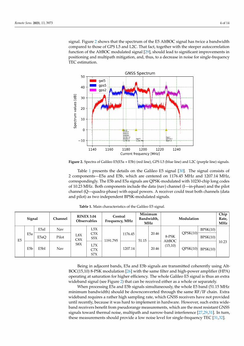
Table 1 presents the details on the Galileo E5 signal [30]. The signal consists of 2 com-ponents – E5a and E5b, which are centered on 1176.45 MHz and 1207.14 MHz, correspond-ingly. The E5b and E5a signals are QPSK-modulated with 10230-chip long codes of 10.23 MHz. Both components include the data (nav) channel (I—in-phase) and the pilot channel (Q—quadra-phase) with equal powers. A receiver could treat both channels (data and pilot) as two independent BPSK-modulated signals.

Being in adjacent bands, E5a and E5b signals are transmitted coherently using Alt-BOC(15,10) 8-PSK modulation [26] with the same filter and high-power amplifier (HPA) operating at saturation for higher efficiency. The whole Galileo E5 signal is thus an extra wideband signal (see Figure 2) that can be received either as a whole or separately.

Figure 2. Spectra of Galileo E5(E5a+E5b) (red line), GPS L5 (blue line) and L2C (purple line) sig-nals.

Table 1. Main characteristics of the Galileo E5 signal.

Signal Chan-nel

RINEX 3.04

Observa-bles

Central Frequency,

MHz

Minimum Bandwidth,

MHz Modulation

Chip Rate, MHz

E5 E5a

E5aI Nav

L8X C8X S8X

L5X C5X S5X

1191.795 1176.45

51.15 20.46

8-PSK AltBOC (15,10)

QPSK(10) BPSK(10)

10.23 E5aQ Pilot BPSK(10)

E5b E5bI Nav L7X C7X S7X

1207.14 20.46 QPSK(10) BPSK(10)

When processing E5a and E5b signals simultaneously, the whole E5 band (51.15MHz

minimum bandwidth) should be downconverted through the same RF/IF chain. Extra wideband requires a rather high sampling rate, which GNSS receivers have not provided until recently, because it was hard to implement in hardware. However, such extra wide-band receivers benefit from pseudorange measurements, which are the most resistant

Figure 2. Spectra of Galileo E5(E5a + E5b) (red line), GPS L5 (blue line) and L2C (purple line) signals.

Table 1 presents the details on the Galileo E5 signal [30]. The signal consists of2 components—E5a and E5b, which are centered on 1176.45 MHz and 1207.14 MHz,correspondingly. The E5b and E5a signals are QPSK-modulated with 10230-chip long codesof 10.23 MHz. Both components include the data (nav) channel (I—in-phase) and the pilotchannel (Q—quadra-phase) with equal powers. A receiver could treat both channels (dataand pilot) as two independent BPSK-modulated signals.

Table 1. Main characteristics of the Galileo E5 signal.

Signal Channel RINEX 3.04Observables

CentralFrequency, MHz

MinimumBandwidth,

MHzModulation

ChipRate,MHz

E5

E5aE5aI Nav

L8XC8XS8X

L5XC5XS5X

1191.795

1176.45

51.15

20.468-PSK

AltBOC(15,10)

QPSK(10)BPSK(10)

10.23E5aQ Pilot BPSK(10)

E5b E5bI NavL7XC7XS7X

1207.14 20.46 QPSK(10) BPSK(10)

Being in adjacent bands, E5a and E5b signals are transmitted coherently using Alt-BOC(15,10) 8-PSK modulation [26] with the same filter and high-power amplifier (HPA)operating at saturation for higher efficiency. The whole Galileo E5 signal is thus an extrawideband signal (see Figure 2) that can be received either as a whole or separately.

When processing E5a and E5b signals simultaneously, the whole E5 band (51.15 MHzminimum bandwidth) should be downconverted through the same RF/IF chain. Extrawideband requires a rather high sampling rate, which GNSS receivers have not provideduntil recently, because it was hard to implement in hardware. However, such extra wide-band receivers benefit from pseudorange measurements, which are the most resistant GNSSsignals toward thermal noise, multipath and narrow-band interference [27,29,31]. In turn,these measurements should provide a low noise level for single-frequency TEC [31,32].

Remote Sens. 2021, 13, 3973 5 of 14

Processing E5a and E5b signals separately as two independent QPSK-coded signalsdoes not require an extra-wide bandwidth receiver, thus reducing its complexity. This isexactly the way the majority of current-generation professional GNSS receivers operate.In this case, low-noise TEC estimates can be obtained only with dual-frequency E5a/E5bphase measurements, while range measurements contain significant noise due to narrowerbandwidth and less sophisticated coding.

Note also that the minimal receiving power of both Galileo E5a and E5b signalsexceeds those of the Galileo E1 signal by 2 dB [30]. Therefore, using E5a/E5b, we couldassume a better performance (as compared with Galileo E1) in case of signal obstruction.

3. Ionospheric TEC Estimation with GNSS Signals

As mentioned above, TEC can be estimated using either dual- or single-frequencypseudorange and carrier phase measurements. In the first case, the linear combinationsof phase (Li and Lj) or pseudorange (Pi and Pj) measurements at two frequencies f i andf j give the slant TEC estimate along the receiver–satellite line of sight via the followingwell-known relations [33]:

sTEC =cK

(Lifi−

Lj

f j

)f 2

i f 2j

f 2i − f 2

j+ const, (1)

sTEC =1K(

Pj − Pi) f 2

i f 2j

f 2i − f 2

j+ DCB, (2)

where K = 40.308 m3/s2, c is the speed of light in a vacuum, const represents undefinedcarrier-phase ambiguities, and DCB stands for the sum of differential code biases in satel-lites transmitting and receivers receiving chains. For Galileo, (Li, Lj) and (Pi, Pj) correspondto phase and code measurements for any pair of signals. Combination (2) proved to bevery noisy compared to (1) when applied to BPSK- and BOC-coded signals. We useddual-frequency combination (1) as a reference in the comparative TEC noise analysis.

A single-frequency pseudorange / carrier phase combination for slant TEC estimationcan be also constructed by exploiting the fact that ionospheric contribution enters phaseand group refractivity index with the opposite sign [34]:

sTEC =fi

2

2K

(Pi −

Licfi

)+ const, (3)

where the same notations apply and const once again stands for unknown carrier-phaseambiguities. When one uses combination (3), a significant noise appears when appliedto BPSK- and BOC-coded signals due to pseudorange measurements. Moreover, likecombination (1), it provides only relative estimates of slant TEC due to an unknown initialphase. This is the reason that single-frequency combination (3) is not widely applied inionospheric studies. New extra wideband GNSS signals (i.e. Galileo E5 AltBOC) couldresolve some issues arising with single-frequency combinations, especially the TEC noiseproblem: the wider spectral occupancy and steeper main peak of autocorrelation functionof such signals results in lower noise and higher multipath robustness. Below, we providethe comparison of noise characteristics for slant TEC estimated via (3) with BPSK-, BOC-and AltBOC-coded signals, assuming dual-frequency combination (1) as a reference.

We corrected raw data to mitigate cycle slip effects. If two consecutive TEC valuesexceed (in absolute value) the previous values by more than 4 TECU, cycle slips occur. TheTEC jump provides a correction constant for the TEC values after the slip.

Following [6], we used the TEC root-mean-square within 100 s (or 100 s TEC RMS) asa proxy for TEC noise throughout this work:

TEC RMS =√< TEC2 >100s −〈TEC〉2100s (4)

Remote Sens. 2021, 13, 3973 6 of 14

The 100 s interval was selected for two reasons: on the one hand, it is reasonably longenough to provide a statistically significant amount of TEC data, and on the other hand,it is reasonably short enough to limit the influence of the ionospheric variability (whichusually has larger timescales) on the obtained results.

Note that assuming DCBs are known/calibrated carrier leveling or code smoothingprocedures can be applied to (1) and (2), providing absolute values of TEC, while due tounknown phase ambiguities, single-frequency combination (3) seems to be suitable formonitoring TEC changes rather than absolute TEC values. Nevertheless, the approach forresolving unknown constants in (3), which is quite similar to DCB estimation [34], could beadopted, making single-frequency relative TEC estimates quite useful for applications thatrequire absolute TEC data.

4. Experimental Setup

Currently, there are 24 Galileo satellites continuously transmitting wideband E5 Al-tBOC signals, which can be used to estimate the ionospheric TEC via single-frequencycombination (3). The number of receiving sites capable of working with that type of signalis also increasing. To analyze the noise level of TEC estimation with E5 AltBOC signals, weperformed a one-month campaign in September 2020. The test receiver MSU was locatedat the roof of the Faculty of Physics, Lomonosov Moscow State University, Russia. Table 2shows the coordinates and technical characteristics of the receiver.

Table 2. Characteristics of the MSU receiving site used for studying the TEC noise level.

Parameter Value

Station name MSUCoordinates 55.75◦ N, 37.62◦ E

Receiver #1 type JAVAD Delta3

Signals tracked by Receiver #1GPS L1/L1C/L2/L5; GLONASS L1/L2; Galileo

E1/E6/E5a/E5b/E5; SBAS L1/L5; QZSS L1/L2/L5/L6;BeiDou B1/B2/B3; IRNSS L5

Receiver #2 type JAVAD Sigma

Signals tracked by Receiver #2 GPS L1/L1C/L2/L5; GLONASS L1/L2; GalileoE1/E6/E5a/E5b; SBAS L1/L5

Antenna type JAVAD RingAnt-G3T (Choke Ring)Data rate 1 Hz

We performed our campaign in the early ascending phase in solar cycle 25; themonthly average F10.7 was 71 s.f.u. The studied equinox period covers mostly undisturbedconditions, except 2 geomagnetic storms (Kp indices reached 50 on September 28, and5+ on September 27). However, we do not expect significant effects on GNSS signals atmid-latitudes for these minor storms.

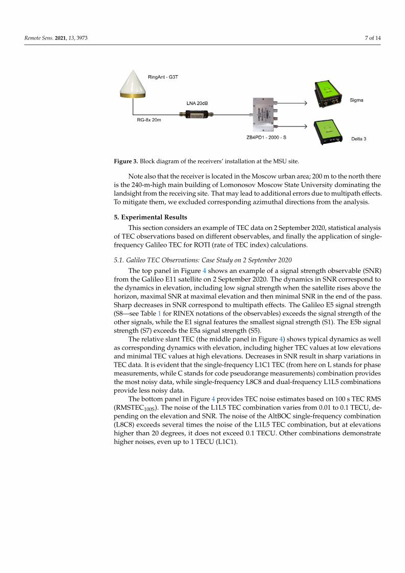
Experimental facilities included two receivers (Sigma and Delta3), but only one(Delta3) treated extra wideband E5 signals, while the other (Sigma) processed E5a/E5bsignals separately. In the current study, we show only the Delta3 receiver data. However,both receivers used the same RingAnt antenna connected by a 20 m RG-8x cable throughthe Mini-Circuits ZB4PD1-2000-s splitter (6 dB loss). To adjust the input signal (which issplit between two receivers), the chain included a 20 dB low-noise amplifier (LNA) witha bandpass of 1.1–1.65 GHz (see Figure 3). The amplifier resulted in comparatively highvalues of SNR for all GNSS signals observed at this site.

Remote Sens. 2021, 13, 3973 7 of 14Remote Sens. 2021, 13, 3973 7 of 14

Figure 3. Block diagram of the receivers’ installation at the MSU site.

5. Experimental Results This section considers an example of TEC data on 2 September 2020, statistical analy-

sis of TEC observations based on different observables, and finally the application of sin-gle-frequency Galileo TEC for ROTI (rate of TEC index) calculations.

5.1. Galileo TEC Observations: Case Study on 2 September 2020 The top panel in Figure 4 shows an example of a signal strength observable (SNR)

from the Galileo E11 satellite on 2 September 2020. The dynamics in SNR correspond to the dynamics in elevation, including low signal strength when the satellite rises above the horizon, maximal SNR at maximal elevation and then minimal SNR in the end of the pass. Sharp decreases in SNR correspond to multipath effects. The Galileo E5 signal strength (S8—see Table 1 for RINEX notations of the observables) exceeds the signal strength of the other signals, while the E1 signal features the smallest signal strength (S1). The E5b signal strength (S7) exceeds the E5a signal strength (S5).

The relative slant TEC (the middle panel in Figure 4) shows typical dynamics as well as corresponding dynamics with elevation, including higher TEC values at low elevations and minimal TEC values at high elevations. Decreases in SNR result in sharp variations in TEC data. It is evident that the single-frequency L1C1 TEC (from here on L stands for phase measurements, while C stands for code pseudorange measurements) combination provides the most noisy data, while single-frequency L8C8 and dual-frequency L1L5 com-binations provide less noisy data.

Figure 3. Block diagram of the receivers’ installation at the MSU site.

Note also that the receiver is located in the Moscow urban area; 200 m to the north thereis the 240-m-high main building of Lomonosov Moscow State University dominating thelandsight from the receiving site. That may lead to additional errors due to multipath effects.To mitigate them, we excluded corresponding azimuthal directions from the analysis.

5. Experimental Results

This section considers an example of TEC data on 2 September 2020, statistical analysisof TEC observations based on different observables, and finally the application of single-frequency Galileo TEC for ROTI (rate of TEC index) calculations.

5.1. Galileo TEC Observations: Case Study on 2 September 2020

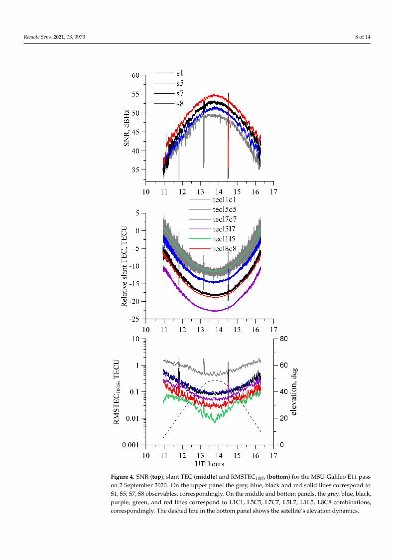
The top panel in Figure 4 shows an example of a signal strength observable (SNR)from the Galileo E11 satellite on 2 September 2020. The dynamics in SNR correspond tothe dynamics in elevation, including low signal strength when the satellite rises above thehorizon, maximal SNR at maximal elevation and then minimal SNR in the end of the pass.Sharp decreases in SNR correspond to multipath effects. The Galileo E5 signal strength(S8—see Table 1 for RINEX notations of the observables) exceeds the signal strength of theother signals, while the E1 signal features the smallest signal strength (S1). The E5b signalstrength (S7) exceeds the E5a signal strength (S5).

The relative slant TEC (the middle panel in Figure 4) shows typical dynamics as wellas corresponding dynamics with elevation, including higher TEC values at low elevationsand minimal TEC values at high elevations. Decreases in SNR result in sharp variations inTEC data. It is evident that the single-frequency L1C1 TEC (from here on L stands for phasemeasurements, while C stands for code pseudorange measurements) combination providesthe most noisy data, while single-frequency L8C8 and dual-frequency L1L5 combinationsprovide less noisy data.

The bottom panel in Figure 4 provides TEC noise estimates based on 100 s TEC RMS(RMSTEC100S). The noise of the L1L5 TEC combination varies from 0.01 to 0.1 TECU, de-pending on the elevation and SNR. The noise of the AltBOC single-frequency combination(L8C8) exceeds several times the noise of the L1L5 TEC combination, but at elevationshigher than 20 degrees, it does not exceed 0.1 TECU. Other combinations demonstratehigher noises, even up to 1 TECU (L1C1).

Remote Sens. 2021, 13, 3973 8 of 14Remote Sens. 2021, 13, 3973 8 of 14

Figure 4. SNR (top), slant TEC (middle) and RMSTEC100S (bottom) for the MSU-Galileo E11 pass on 2 September 2020. On the upper panel the grey, blue, black and red solid lines correspond to S1, S5, S7, S8 observables, correspondingly. On the middle and bottom panels, the grey, blue, black, purple, green, and red lines correspond to L1C1, L5C5, L7C7, L5L7, L1L5, L8C8 combina-tions, correspondingly. The dashed line in the bottom panel shows the satellite's elevation dynam-ics.

Figure 4. SNR (top), slant TEC (middle) and RMSTEC100S (bottom) for the MSU-Galileo E11 passon 2 September 2020. On the upper panel the grey, blue, black and red solid lines correspond toS1, S5, S7, S8 observables, correspondingly. On the middle and bottom panels, the grey, blue, black,purple, green, and red lines correspond to L1C1, L5C5, L7C7, L5L7, L1L5, L8C8 combinations,correspondingly. The dashed line in the bottom panel shows the satellite’s elevation dynamics.

Remote Sens. 2021, 13, 3973 9 of 14

5.2. Galileo TEC: Statistical Analysis

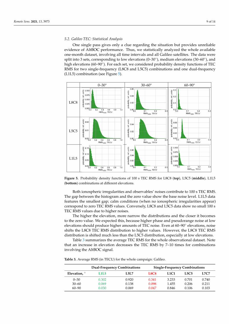
One single pass gives only a clue regarding the situation but provides unreliableevidence of AltBOC performance. Thus, we statistically analyzed the whole availableone-month dataset, involving all time intervals and all Galileo satellites. The data weresplit into 3 sets, corresponding to low elevations (0–30◦), medium elevations (30–60◦), andhigh elevations (60–90◦). For each set, we considered probability density functions of TECRMS for two single-frequency (L8C8 and L5C5) combinations and one dual-frequency(L1L5) combination (see Figure 5).

Remote Sens. 2021, 13, 3973 9 of 14

The bottom panel in Figure 4 provides TEC noise estimates based on 100 sec TEC RMS (RMSTEC100S). The noise of the L1L5 TEC combination varies from 0.01 to 0.1 TECU, depending on the elevation and SNR. The noise of the AltBOC single-frequency combina-tion (L8C8) exceeds several times the noise of the L1L5 TEC combination, but at elevations higher than 20 degrees, it does not exceed 0.1 TECU. Other combinations demonstrate higher noises, even up to 1 TECU (L1C1).

5.2. Galileo TEC: Statistical Analysis One single pass gives only a clue regarding the situation but provides unreliable ev-

idence of AltBOC performance. Thus, we statistically analyzed the whole available one-month dataset, involving all time intervals and all Galileo satellites. The data were split into 3 sets, corresponding to low elevations (0-30°), medium elevations (30-60°), and high elevations (60-90°). For each set, we considered probability density functions of TEC RMS for two single-frequency (L8C8 and L5C5) combinations and one dual-frequency (L1L5) combination (see Figure 5).

Both ionospheric irregularities and observables’ noises contribute to 100-sec TEC RMS. The gap between the histogram and the zero value show the base noise level. L1L5 data features the smallest gap; calm conditions (when no ionospheric irregularities ap-pear) correspond to zero TEC RMS values. Conversely, L8C8 and L5C5 data show no small 100-sec TEC RMS values due to higher noises.

The higher the elevation, more narrow the distributions and the closer it becomes to the zero value. We expected this, because higher phase and pseudorange noise at low elevations should produce higher amounts of TEC noise. Even at 60-90° elevations, noise shifts the L8C8 TEC RMS distribution to higher values. However, the L8C8 TEC RMS dis-tribution is shifted much less than the L5C5 distribution, especially at low elevations.

Table 3 summarizes the average TEC RMS for the whole observational dataset. Note that an increase in elevation decreases the TEC RMS by 7-10 times for combinations in-volving the AltBOC signal.

0–30° 30–60° 60–90°

L8C8

L5C5

L1L5

Figure 5. Probability density functions of 100-sec TEC RMS for L8C8 (top), L5C5 (middle), L1L5 (bottom) combinations at different elevations.

Figure 5. Probability density functions of 100 s TEC RMS for L8C8 (top), L5C5 (middle), L1L5(bottom) combinations at different elevations.

Both ionospheric irregularities and observables’ noises contribute to 100 s TEC RMS.The gap between the histogram and the zero value show the base noise level. L1L5 datafeatures the smallest gap; calm conditions (when no ionospheric irregularities appear)correspond to zero TEC RMS values. Conversely, L8C8 and L5C5 data show no small 100 sTEC RMS values due to higher noises.

The higher the elevation, more narrow the distributions and the closer it becomesto the zero value. We expected this, because higher phase and pseudorange noise at lowelevations should produce higher amounts of TEC noise. Even at 60–90◦ elevations, noiseshifts the L8C8 TEC RMS distribution to higher values. However, the L8C8 TEC RMSdistribution is shifted much less than the L5C5 distribution, especially at low elevations.

Table 3 summarizes the average TEC RMS for the whole observational dataset. Notethat an increase in elevation decreases the TEC RMS by 7–10 times for combinationsinvolving the AltBOC signal.

Table 3. Average RMS (in TECU) for the whole campaign: Galileo.

Dual-Frequency Combinations Single-Frequency Combinations

Elevation, ◦ L1L5 L5L7 L8C8 L1C1 L5C5 L7C7

0–30 0.302 0.920 0.341 3.233 0.701 0.74030–60 0.069 0.138 0.098 1.455 0.206 0.21160–90 0.030 0.069 0.047 0.846 0.106 0.103

Remote Sens. 2021, 13, 3973 10 of 14

The Galileo E5 AltBOC signal provides the smallest noise of single-frequency TEC(L8C8), which is comparable to that of the L1L5 dual-frequency combination. At lowelevations, L1L5 and L8C8 TEC RMS are almost the same; at higher elevations, L8C8TEC RMS exceeds L1L5 ones by 1.5 times. Other combinations feature ~1.5–20 timeshigher values of TEC noise against Galileo L8C8. The worst results correspond to thesingle-frequency L1C1 combination.

At low elevations, E5 AltBOC provides at least twice less noise as compared withE5a/E5b combinations (both single- and dual-frequency). The E5a/E5b dual-frequencycombination provides almost no advantage over the single-frequency E5 AltBOC com-bination, probably due to the closeness of their frequencies. Nevertheless, the noise insingle-frequency E5a or E5b combinations exceeds those of the dual-frequency E5a/E5bphase combination by ~1.5 times.

We also compared obtained Galileo TEC noise with those from GPS. Table 4 providesresults on 100 s RMS for L1L5, L5C5 and L1L2 GPS TEC. Except at low elevations, theGalileo E5 AltBOC single-frequency combination features less noise as compared with theGPS L1L2 and L1L5 (and, of course, the GPS L5C5) combinations.

Table 4. Average RMS (in TECU) for the whole campaign: GPS.

Dual-Frequency Combinations Single-Frequency Combination

Elevation, ◦ L1L5 L1L2 L5C5

0–30 0.430 0.367 0.70830–60 0.145 0.110 0.15760–90 0.068 0.033 0.088

At high elevations, the 100 s single-frequency TEC root-mean-squares were (fromlow to high values): ~0.05 TECU for Galileo E5 AltBOC, 0.09 TECU for GPS L5, 0.1TECUfor Galileo E5a/E5b BPSK, and 0.85 TECU for Galileo E1 CBOC. At the same elevations,dual-frequency combinations provided: 0.03 TECU for Galileo E1/E5 TEC, 0.03 TECUand 0.07 TECU for GPS L1L2 and L1L5. Therefore, the Galileo E5 AltBOC signal providedthe smallest amount of noise for TEC among single-frequency combinations, which iscomparable to that of the dual-frequency TEC of both GPS and Galileo.

5.3. Galileo Single-Frequency Data for ROTI Calculations

Many scientists use the ROTI index [16] to study small-scale ionospheric irregulari-ties [35]. A higher noise level in the single-frequency TEC data (against dual-frequencydata) results in higher ROTI values. However, we expect that such data could also beuseful to estimate the effects of ionospheric irregularities. To estimate this, we analyzedROTI quality from Galileo AltBOC data (L8C8) against ROTI quality from dual-frequencydata (we chose L1L5 as a reference).

Figure 6 shows how the ROTI values from single-frequency Galileo AltBOC data(L8C8) corresponds to those from L1L5. We compare the data for the same satellite-receiverset, but for different observables. L1L5 provides a reference to find a discrepancy forAltBOC single-frequency data.

We expect a noise-multiplying effect for ROTI. Figure 6a provides the ROTIL8C8-to-ROTIL1L5 ratio. ROTIL8C8 values 3 times (maximum of the distribution) exceed ROTIL1L5.Outliers in ROTI estimations provide an increase in distribution at 20 (we chose this valueas a limit). ROTIL1L5 values could exceed ROTIL8C8 values due to L1/L5 noises.

Scattering diagrams (Figure 6b) also show (for low ROTI) a positive correlation be-tween ROTIL8C8 and ROTIL1L5, but the coefficient between them differs from 1. Thispositive correlation gives hope that scientists could use the single-frequency AltBOC ROTIas an additional indicator for the ionosphere state.

Remote Sens. 2021, 13, 3973 11 of 14

Remote Sens. 2021, 13, 3973 11 of 14

Outliers in ROTI estimations provide an increase in distribution at 20 (we chose this value as a limit). ROTIL1L5 values could exceed ROTIL8C8 values due to L1/L5 noises.

Scattering diagrams (Figure 6b) also show (for low ROTI) a positive correlation be-tween ROTIL8C8 and ROTIL1L5, but the coefficient between them differs from 1. This positive correlation gives hope that scientists could use the single-frequency AltBOC ROTI as an additional indicator for the ionosphere state.

(a) (b)

Figure 6. ROTI quality from Galileo AltBOC data. (a), ROTIL8C8/ROTIL1L5; (b), ROTIL8C8 vs. ROTIL1L5.

6. Discussion and Conclusions Different factors affect TEC measurements: the intrinsic thermal noise of the receiver,

the stability of the disciplined oscillator, the coherence of the operating frequencies, mul-tipath, etc. [36]. Increase in the satellite transmitter power [37], application of choke ring antennas, or advanced signal coding (providing a steeper and narrower main maximum of the autocorrelation function) could, to some extent, compensate for such negative fac-tors.

Our results (involving Galileo as an example) show a one-order decrease in single-frequency TEC noises when a system uses AltBOC signals instead of BPSK signals. The estimated TEC noise proxies (for elevation higher 60 deg.)—100-sec root-mean-square (RMS) of TEC—were: ~ 0.05 TECU for Galileo E5 AltBOC, 0.09 TECU for GPS L5, ~0.1TECU for Galileo E5a/E5b BPSK, and 0.85 TECU for Galileo E1 CBOC. Dual-frequency combinations provide RMS values of 0.03 TECU for Galileo E1E5 and 0.03/0.07 TECU for GPS L1L2/L1L5. At low elevations, E5 AltBOC provides at least twice less single-fre-quency TEC noise as compared with the data obtained from E5a or E5b.

The obtained results indicate that AltBOC signals level down the noise in TEC from a single-frequency phase-code combination to the noise in TEC from the reference phase dual-frequency signals encoded in BPSK.

Note that our comparison used data obtained simultaneously on the same receiver and antenna, which guarantees the same level of thermal noise. We installed a choke ring antenna, which itself suppresses multipath effects. We could expect that the single-fre-quency AltBOC TEC has even more of an advantage over single-frequency BPSK TEC when standard antennas are used, especially at low elevations. However, this requires a separate study.

The short dataset during mostly undisturbed geomagnetic conditions could limit ob-tained estimates. Mid-latitude observations also could limit our study, since no intense small-scale ionospheric irregularities (which appear at mid-latitudes usually during strong or severe storms [38]) affected the GNSS signals. It would be important for future studies to verify our results in the presence of small-scale irregularities at high-, mid- and low-latitudes under intense geomagnetic storms and plasma bubble conditions. We ex-pect that, qualitatively, results will hold as the solar cycle evolves and geomagnetic

Figure 6. ROTI quality from Galileo AltBOC data. (a) ROTIL8C8/ROTIL1L5; (b) ROTIL8C8 vs.ROTIL1L5.

6. Discussion and Conclusions

Different factors affect TEC measurements: the intrinsic thermal noise of the receiver,the stability of the disciplined oscillator, the coherence of the operating frequencies, mul-tipath, etc. [36]. Increase in the satellite transmitter power [37], application of choke ringantennas, or advanced signal coding (providing a steeper and narrower main maximum ofthe autocorrelation function) could, to some extent, compensate for such negative factors.

Our results (involving Galileo as an example) show a one-order decrease in single-frequency TEC noises when a system uses AltBOC signals instead of BPSK signals. Theestimated TEC noise proxies (for elevation higher 60 deg.)—100 s root-mean-square (RMS)of TEC—were: ~0.05 TECU for Galileo E5 AltBOC, 0.09 TECU for GPS L5, ~0.1TECU forGalileo E5a/E5b BPSK, and 0.85 TECU for Galileo E1 CBOC. Dual-frequency combinationsprovide RMS values of 0.03 TECU for Galileo E1E5 and 0.03/0.07 TECU for GPS L1L2/L1L5.At low elevations, E5 AltBOC provides at least twice less single-frequency TEC noise ascompared with the data obtained from E5a or E5b.

The obtained results indicate that AltBOC signals level down the noise in TEC froma single-frequency phase-code combination to the noise in TEC from the reference phasedual-frequency signals encoded in BPSK.

Note that our comparison used data obtained simultaneously on the same receiverand antenna, which guarantees the same level of thermal noise. We installed a chokering antenna, which itself suppresses multipath effects. We could expect that the single-frequency AltBOC TEC has even more of an advantage over single-frequency BPSK TECwhen standard antennas are used, especially at low elevations. However, this requires aseparate study.

The short dataset during mostly undisturbed geomagnetic conditions could limitobtained estimates. Mid-latitude observations also could limit our study, since no intensesmall-scale ionospheric irregularities (which appear at mid-latitudes usually during strongor severe storms [38]) affected the GNSS signals. It would be important for future studiesto verify our results in the presence of small-scale irregularities at high-, mid- and low-latitudes under intense geomagnetic storms and plasma bubble conditions. We expectthat, qualitatively, results will hold as the solar cycle evolves and geomagnetic activityincreases, such that the AltBOC single-frequency TEC will still surpass BPSK analogue innoise parameters.

The obtained TEC noise estimates contain contributions from the intrinsic noisespecific to each individual receiver. Therefore, we cannot consider the obtained estimatesas universal estimates. However, we suppose similar features for other receivers: a foldreduction in TEC noise when using AltBOC signals could be expected, but the TEC noiselevel should agree with a receiver’s intrinsic and multipath noise. To verify, one can usethe approach by Demyanov et al. [36].

Remote Sens. 2021, 13, 3973 12 of 14

We also analyzed the ROTI index based on single-frequency AltBOC TEC. The positivecorrelation observed with dual-frequency data gives hope that scientists could use thesingle-frequency AltBOC ROTI as an additional indicator for the state of the ionosphere.

Note that assuming DCBs are known/calibrated dual-frequency combinations to-gether provide absolute values of TEC, while single-frequency combinations seem to besuitable for monitoring TEC changes rather than absolute TEC values. Nevertheless, theapproach for resolving unknown constants through LxCx combinations, which is quite sim-ilar to DCB estimation [34], could be adopted, making this data quite useful for problemsthat require absolute TEC.

We expect similar features (a fold decrease in the single-frequency TEC noise) forBeiDou B2 AltBOC signals. Unfortunately, Galileo and BeiDou use AltBOC coding onlyon one operating frequency. We could also expect a decrease in dual-frequency TEC noisewhen both frequencies use AltBOC coding. That would make it possible to record TECdisturbances of low amplitude from such important events as, for example, the effectsof artificial high-frequency heating [39], the response of the ionosphere to C-class solarflares [40] and low-magnitude earthquakes [41], which can produce effects at levels typicalof the current GNSS TEC estimates. Therefore, AltBOC signals could advance geoscience.

Author Contributions: Conceptualization, A.M.P.; methodology, A.M.P., A.A.M., Y.V.Y.; software,A.A.M., A.M.V., Y.V.M.; validation, A.M.P., A.A.M., Y.V.Y.; formal analysis, A.A.M., Y.V.M.; investiga-tion, A.M.P., A.A.M., Y.V.Y., Y.V.M.; data curation, Y.V.M., G.A.K.; writing—original draft preparation,A.M.P., A.A.M., Y.V.Y., Y.V.M.; writing—review and editing, A.M.P., A.A.M., Y.V.Y.; visualization,A.A.M.; supervision, A.M.P.; project administration, A.M.P.; funding acquisition, Y.V.Y. All authorshave read and agreed to the published version of the manuscript.

Funding: Data processing and Galileo AltBOC signal property investigation performed under theRussian Science Foundation Grant No. 17-77-20005. Experimental Galileo data at the MSU test sitewere obtained with the support of the Russian Foundation for Basic Research (project #19-05-00941).The APC was funded by the above-mentioned foundations.

Institutional Review Board Statement: Not applicable.

Informed Consent Statement: Not applicable.

Data Availability Statement: Data available by request from MSU and ISTP SB RAS.

Acknowledgments: The authors acknowledge V.V. Demyanov for the fruitful discussions, JavadGNSS for providing technical support under GNSS data acquisition, and the anonymous reviewersfor their suggestions to improve the paper.

Conflicts of Interest: The authors declare no conflict of interest.

References1. Davies, K. Recent progress in satellite radio beacon studies with particular emphasis on the ATS-6 radio beacon experiment. Space

Sci. Rev. 1980, 25, 357–430. [CrossRef]2. Aitchison, G.J.; Weekes, K. Some deductions of ionospheric information from the observations of emissions from satellite

1957-alpha-2.1. The theory of the analysis. J. Atmos. Terr. Phys. 1959, 144, 236–243. [CrossRef]3. Alpert, I.L. On Ionospheric Investigations by Coherent Radiowaves Emitted from Artificial Earth Satellites. Space Sci. Rev. 1976,

18, 551–602. [CrossRef]4. Bernhardt, P.A.; Siefring, C.L.; Galysh, I.J.; Koch, D.E. A new technique for absolute total electron content determination using the

CITRIS instrument on STPSat1 and the CERTO beacons on COSMIC. Radio Sci. 2010, 45, RS3006. [CrossRef]5. Royden, H.N.; Miller, R.B.; Buennagel, L.A. Comparison NAVSTAR satellite L band ionospheric calibrations with Faraday

rotation measurements. Radio Sci. 1984, 19, 798–804. [CrossRef]6. Kunitsyn, V.E.; Padokhin, A.M.; Kurbatov, G.A.; Yasyukevich, Y.V.; Morozov, Y.V. Ionospheric TEC estimation with the signals of

various geostationary navigational satellites. GPS Solut. 2016, 20, 877–884. [CrossRef]7. Cooper, C.; Mitchell, C.N.; Wright, C.J.; Jackson, D.R.; Witvliet, B.A. Measurement of ionospheric total electron content using

single-frequency geostationary satellite observations. Radio Sci. 2019, 54, 10–19. [CrossRef]8. Savastano, G.; Komjathy, A.; Shume, E.; Vergados, P.; Ravanelli, M.; Verkhoglyadova, O.; Meng, X.; Crespi, M. Advantages of

Geostationary Satellites for Ionospheric Anomaly Studies: Ionospheric Plasma Depletion Following a Rocket Launch. RemoteSens. 2019, 11, 1734. [CrossRef]

Remote Sens. 2021, 13, 3973 13 of 14

9. Bust, G.S.; Crowley, G.; Garner, T.W.; Gaussiran, T.L.; Meggs, R.W.; Mitchell, C.N.; Spencer, P.S.J.; Yin, P.; Zapfe, B. Four-dimensional GPS imaging of space weather storms. Space Weather 2007, 5, S02003. [CrossRef]

10. Kunitsyn, V.E.; Nesterov, I.A.; Padokhin, A.M.; Tumanova, Y.S. Ionospheric radio tomography based on the GPS/GLONASSnavigation systems. J. Commun. Technol. Electron. 2011, 56, 1269–1281. [CrossRef]

11. Nesterov, I.A.; Kunitsyn, V.E. GNSS radio tomography of the ionosphere: The problem with essentially incomplete data. Adv.Space Res. 2011, 47, 1789–1803. [CrossRef]

12. Afraimovich, E.L.; Palamartchouk, K.S.; Perevalova, N.P. Statistical Angle-of-arrival and Doppler Method for GPS radiointerferometry of TIDs. Adv. Space Res. 2000, 26, 1001–1004. [CrossRef]

13. Hernández-Pajares, M.; Juan, J.M.; Sanz, J.; Orus, R.; Garcia-Rigo, A.; Feltens, J.; Komjathy, A.; Schaer, S.C.; Krankowski, A. TheIGS VTEC maps: A reliable source of ionospheric information since 1998. J. Geophys. 2009, 83, 263–275. [CrossRef]

14. Mannucci, A.J.; Wilson, B.D.; Yuan, D.N.; Ho, C.H.; Lindqwister, U.J.; Runge, T.F. A global mapping technique for GPS derivedionospheric TEC measurements. Radio Sci. 1998, 33, 565–582. [CrossRef]

15. Yasyukevich, Y.; Mylnikova, A.; Vesnin, A. GNSS-Based Non-Negative Absolute Ionosphere Total Electron Content, its SpatialGradients, Time Derivatives and Differential Code Biases: Bounded-Variable Least-Squares and Taylor Series. Sensors 2020,20, 5702. [CrossRef]

16. Pi, X.; Mannucci, A.J.; Lindqwister, U.J.; Ho, C.M. Monitoring of global ionospheric irregularities using the worldwide GPSnetwork. Geophys. Res. Lett. 1997, 24, 2283–2286. [CrossRef]

17. Nesterov, I.A.; Andreeva, E.S.; Padokhin, A.M.; Tumanova, Y.S.; Nazarenko, M.O. Ionospheric perturbation indices based on thelow- and high-orbiting satellite radio tomography data. GPS Solut. 2017, 21, 1679–1694. [CrossRef]

18. Wilken, V.; Kriegel, M.; Jakowski, N.; Berdermann, J. An ionospheric index suitable for estimating the degree of ionosphericperturbations. J. Space Weather Space Clim. 2018, 8, A19. [CrossRef]

19. Ivanov, V.; Gefan, G.; Gorbachev, O. Global empirical modelling of the total electron content of the ionosphere for satellite radionavigation systems. J Atmos. Sol.-Terr. Phys. 2011, 73, 1703–1707. [CrossRef]

20. Zhukov, A.V.; Yasyukevich, Y.V.; Bykov, A.E. GIMLi: Global Ionospheric total electron content model based on machine learning.GPS Solut. 2021, 25, 19. [CrossRef]

21. Ephishov, I.I.; Baran, L.W.; Shagimuratov, I.I.; Yakimova, G.A. Comparison of total electron content obtained from GPS with IRI.Phys. Chem. Earth Part C Sol. Terr. Planet. Sci. 2000, 25, 339–342. [CrossRef]

22. Feltens, J.; Angling, M.; Jackson-Booth, N.; Jakowski, N.; Hoque, M.; Hernández-Pajares, M.; Aragón-Àngel, A.; Orús, R.;Zandbergen, R. Comparative testing of four ionospheric models driven with GPS measurements. Radio Sci. 2011, 46, RS0D12.[CrossRef]

23. Kotova, D.S.; Ovodenko, V.B.; Yasyukevich, Y.V.; Klimenko, M.V.; Ratovsky, K.G.; Mylnikova, A.A.; Andreeva, E.S.; Kozlovsky,A.E.; Korenkova, N.A.; Nesterov, I.A.; et al. Efficiency of updating the ionospheric models using total electron content at mid-and sub-auroral latitudes. GPS Solut. 2020, 24, 25. [CrossRef]

24. Kaplan, E.D.; Hegarty, C.J.B. Understand GPS/GNSS Principles and Applications, 2nd ed.; Artech House: Norwood, MA, USA, 2017;p. 703.

25. Hernández-Pajares, M.; Roma-Dollase, D.; Garcia-Fernàndez, M.; Orus-Perez, R.; García-Rigo, A. Precise Ionospheric ElectronContent Monitoring from Single-Frequency GPS Receivers. GPS Solut. 2018, 22, 102. [CrossRef]

26. Lestarquit, L.; Artaud, G.; Issler, J.-L. AltBOC for Dummies or Everything You Always Wanted to Know About AltBOC. InProceedings of the 21st International Technical Meeting of the Satellite Division of The Institute of Navigation (ION GNSS 2008),Savannah, GA, USA, 16–19 September 2008; pp. 961–970.

27. Sleewaegen, J.M.; De Wilde, W.; Hollreiser, M. Galileo AltBOC Receiver. In Proceedings of the ION GNSS 2004, Rotterdam, TheNetherlands, 16–19 May 2004.

28. JAVAD GNSS Receiver External Interface Specification. Available online: http://download.javad.com/manuals/GREIS/GREIS_Reference_Guide.pdf (accessed on 22 August 2021).

29. Silva, P.F.; Silva, J.S.; Peres, T.R.; Fernández, A.; Palomo, J.M.; Andreotti, M.; Hill, C.; Colomina, I.; Miranda, C.; Parés, M.E. Resultsof Galileo AltBOC for precise positioning. In Proceedings of the in 6th ESA Workshop on Satellite Navigation Technologies(Navitec 2012) & European Workshop on GNSS Signals and Signal Processing, Noordwijk, The Netherlands, 5–12 December 2012;pp. 1–9. [CrossRef]

30. Galileo—Open Service—Signal in Space Interface Control Document (OS SIS ICD V1.3). Available online: https://www.gsc-europa.eu/sites/default/files/sites/all/files/Galileo-OS-SIS-ICD.pdf (accessed on 22 August 2021).

31. Diessongo, H.; Bock, H.; Schueler, T.; Junker, S.; Kiroe, A. Exploiting the Galileo E5 Wideband Signal for Improved Single-Frequency Precise Positioning. Inside GNSS 2012, 7, 64–73.

32. Julien, O.; Macabiau, C.; Issler, J.-L. Ionospheric delay estimation strategies using Galileo E5 signals only. In Proceedings of the inGNSS 2009, 22nd International Technical Meeting of The Satellite Division of the Institute of Navigation, Savannah, GA, USA,22–25 September 2009; pp. 3128–3141.

33. Hoffmann-Wellenhof, B.; Lichtenegger, H.; Collins, J. Global Positioning System: Theory and Practice, 5th ed.; Springer: New York,NY, USA, 2001; p. 313.

34. Yasyukevich, Y.V.; Mylnikova, A.A.; Ivanov, V.B. Estimating the absolute total electron content based on single-frequency satelliteradio navigation GPS/GLONASS data. Sol.-Terr. Phys. 2017, 3, 128–137. [CrossRef]

Remote Sens. 2021, 13, 3973 14 of 14

35. Basu, S.; Groves, K.M.; Quinn, J.M.; Doherty, P. A comparison of TEC fluctuations and scintillations at Ascension Island. J. Atmos.Sol.-Terr. Physics. 1999, 61, 1219–1226. [CrossRef]

36. Demyanov, V.; Sergeeva, M.; Fedorov, M.; Ishina, T.; Gatica-Acevedo, V.J.; Cabral-Cano, E. Comparison of TEC Calculations Basedon Trimble, Javad, Leica, and Septentrio GNSS Receiver Data. Remote Sens. 2020, 12, 3268. [CrossRef]

37. Yasyukevich, Y.V.; Yasyukevich, A.S.; Astafyeva, E.I. How modernized and strengthened GPS signals enhance the systemperformance during solar radio bursts. GPS Solut. 2021, 25, 46. [CrossRef]

38. Astafyeva, E.I.; Afraimovich, E.L.; Voeykov, S.V. Generation of secondary waves due to intensive large-scale AGW traveling. Adv.Space Res. 2008, 41, 1459–1462. [CrossRef]

39. Kunitsyn, V.E.; Andreeva, E.S.; Frolov, V.L.; Komrakov, G.P.; Nazarenko, M.O.; Padokhin, A.M. Sounding of HF heating-inducedartificial ionospheric disturbances by navigational satellite radio transmissions. Radio Sci. 2012, 47, RS0L15. [CrossRef]

40. Yasyukevich, Y.V.; Voeykov, S.V.; Zhivetiev, I.V.; Kosogorov, E.A. Ionospheric response to solar flares of C and M classes inJanuary–February 2010. Cosm. Res. 2013, 51, 114–123. [CrossRef]

41. Perevalova, N.P.; Sankov, V.A.; Astafyeva, E.I.; Zhupityaeva, A.S. Threshold magnitude for Ionospheric TEC response toearthquakes. J. Atmos. Sol.-Terr. Phys. 2014, 108, 77–90. [CrossRef]