
galilei - EU Agency for the Space Programme (EUSPA)
337
GALILEI REF : DATE : GALI-GMV-DD044 07/02/2003 Generic Local Element Performance Validation ISSUE : Issue 1.2 PAGE: 1 Sustainable Mobility and Intermodality Promoting Competitive and Sustainable Growth GALILEI Generic Local Element Performance Validation Written by Responsibility - Company Date Signature A. Catalina JI. Herrero C. Barredo R. Dávila J. Fernández-de-Velasco GMV Sistemas 07/02/03 Verified by JA. March GMV Sistemas 07/02/03 Certified by WBS Code : C.3.G Classification : PP
-
Upload
khangminh22 -
Category
Documents
-
view
0 -
download
0
Transcript of galilei - EU Agency for the Space Programme (EUSPA)

GALILEI REF :
DATE :
GALI-GMV-DD044
07/02/2003
Generic Local Element Performance Validation ISSUE : Issue 1.2 PAGE: 1
Sustainable Mobility and Intermodality Promoting Competitive and Sustainable Growth
GALILEI
Generic Local Element Performance Validation
Written by Responsibility - Company Date Signature
A. Catalina
JI. Herrero
C. Barredo
R. Dávila
J. Fernández-de-Velasco
GMV Sistemas 07/02/03
Verified by
JA. March GMV Sistemas 07/02/03
Certified by
WBS Code : C.3.G Classification : PP

GALILEI REF :
DATE :
GALI-GMV-DD044
07/02/2003
Generic Local Element Performance Validation ISSUE : Issue 1.2 PAGE: 2
THE INFORMATION IN THIS DOCUMENT IS PROVIDED AS IS AND NO GUARANTEE OR WARRANTY IS GIVEN THAT THE
INFORMATION IS FIT FOR ANY PURPOSE. THE USER THEREOF USES THE INFORMATION AT ITS SOLE RISK AND LIABILITY.
FURTHERMORE, DATA, CONCLUSIONS OR RECOMMENDATIONS IN THIS REPORT ARE PROVIDED ON THE
BASIS THAT SUCH INFORMATION IS SUBSEQUENTLY, AND PRIOR TO USE, VERIFIED BY THE PARTY WISHING TO USE
THAT INFORMATION.
GALILEI REF :
DATE :
GALI-GMV-DD044
07/02/2003
Generic Local Element Performance Validation ISSUE : Issue 1.2 PAGE: 3
CHANGE RECORDS
ISSUE DATE § : CHANGE RECORD AUTHOR
Draft 01 3/06/2002 Initial draft José Ignacio Herrero, Alfredo Catalina, Javier Fernández-de-Velasco
Issue 01 16/07/2002 Issue 01 A. Catalina,
JI Herrero,
R. Dávila
C. Barredo
Issue 01.1 29/07/2002 Issue 01.1 A. Catalina,
C. Barredo
R. Dávila
JI Herrero
Issue 1.2 7/02/2003 Updated Simulation Results with a Preliminary Modified version of Polaris.
Number of Minimum Number of Sub-elements needed.
Estimation of Communication Delays.
JI Herrero

GALILEI REF :
DATE :
GALI-GMV-DD044
07/02/2003
Generic Local Element Performance Validation ISSUE : Issue 1.2 PAGE: 4
TABLE OF CONTENTS 1 EXECUTIVE SUMMARY........................................................................................................... 20
2 OVERVIEW.................................................................................................................................. 22
2.1 INTRODUCTION...................................................................................................................... 22 2.2 OBJECTIVE............................................................................................................................... 23 2.3 SCOPE OF THE DOCUMENT................................................................................................ 23 2.4 APPLICABLE DOCUMENTS................................................................................................. 25 2.5 REFERENCE DOCUMENTS .................................................................................................. 25 2.5.1 Phase 3 Simulation References .............................................................................................. 25 2.5.2 Galileo Constellation References ........................................................................................... 25 2.5.3 DRS – Differential Reference Station References ................................................................ 26 2.5.4 PL – Pseudolite References .................................................................................................... 27 2.5.5 LIM – Local Integrity Monitor References .......................................................................... 28 2.5.6 GPS References ....................................................................................................................... 28 2.5.7 GLONASS References............................................................................................................ 29 2.5.8 EGNOS References ................................................................................................................. 29 2.5.9 LORAN / CHAYKA / EUROFIX References ...................................................................... 29 2.5.10 Ground Based Communication Networks References ........................................................ 29 2.6 ACRONYMS .............................................................................................................................. 30 3 VALIDATION BASIS .................................................................................................................. 33
3.1 BASIC CONCEPTS................................................................................................................... 33 3.2 WHAT IS VALIDATION? ....................................................................................................... 33 3.3 PERFORMANCE REQUIREMENTS .................................................................................... 34 3.4 VALIDATION TECHNIQUES ................................................................................................ 34 4 BOTTOM-UP VALIDATION APPROACH ............................................................................. 36
4.1 INTRODUCTION...................................................................................................................... 36 4.2 TOP-DOWN AND BOTTOM-UP STRATEGIES.................................................................. 37 4.3 REFERENCE ARCHITECTURE ........................................................................................... 37 4.4 SUB-ELEMENTS AND EXTERNAL SYSTEMS ANALYSIS............................................. 40 5 GENERIC VALIDATION PROCEDURE................................................................................. 43
5.1.1 Introduction............................................................................................................................. 43 5.2 PRELIMINARY GENERAL ASSUMPTIONS ...................................................................... 44 5.2.1 Navigation Assumptions ......................................................................................................... 45 5.2.2 Communication Assumptions ................................................................................................ 46 5.3 IMPACT OF THE GENERAL ASSUMPTIONS................................................................... 47

GALILEI REF :
DATE :
GALI-GMV-DD044
07/02/2003
Generic Local Element Performance Validation ISSUE : Issue 1.2 PAGE: 5
5.4 LIMITATIONS OF THE GENERAL ASSUMPTIONS........................................................ 48 5.5 PARAMETERS TO BE ANALYSED...................................................................................... 49 5.6 ENVIRONMENTAL RESTRICTIONS .................................................................................. 50 5.7 VALIDATION METHOD......................................................................................................... 51 5.7.1 Phase One: Local..................................................................................................................... 51 5.7.2 Phase Two: Global Interoperability ...................................................................................... 56 5.7.3 Phase Three: Simulation Assessment of Phase 2.................................................................. 57 6 LISP #1 PERFORMANCE VALIDATION ............................................................................... 67
6.1 PERFORMANCE REQUIREMENTS .................................................................................... 67 6.2 LISP#1 GENERIC ARCHITECTURE.................................................................................... 67 6.3 LISP#1 PHASE I LOCAL ANALYSIS.................................................................................... 68 6.3.1 Sub-element and external system influence .......................................................................... 68 6.3.2 Environmental Constraint Impact ........................................................................................ 69 6.3.3 Sub-Element and External System Contribution................................................................. 70 6.4 LISP#1 PHASE II. INTEROPERABILITY............................................................................ 71 6.5 LISP#1 PHASE III. UPDATED SIMULATION RESULTS ................................................. 71 6.5.1 Procedure and Variable Parameters Included In the LISP1 Analysis............................... 71 6.5.2 Tables of Results...................................................................................................................... 72 6.5.3 Review Of Sub-Element Election and Minimum Number of Sub-elements Needed 74 7 LISP #2 PERFORMANCE VALIDATION ............................................................................... 76
7.1 PERFORMANCE REQUIREMENTS .................................................................................... 76 7.2 LISP#2 GENERIC ARCHITECTURE.................................................................................... 76 7.3 LISP#2 PHASE I LOCAL ANALYSIS.................................................................................... 77 7.3.1 Sub-element and External System Influence ........................................................................ 77 7.3.2 Environmental Constraint Impact ........................................................................................ 78 7.3.3 Sub-Element and External System Contribution................................................................. 79 7.4 LISP#2 PHASE II. INTEROPERABILITY............................................................................ 80 7.5 LISP#2 PHASE III. UPDATED SIMULATION RESULTS ................................................. 80 7.5.1 Procedure and Variable Parameters Included In the LISP2 Analysis............................... 80 7.5.2 Tables of Results...................................................................................................................... 81 7.5.3 Review Of Sub-Element Election and Minimum Number of Sub-elements Needed 82 8 LISP #3 PERFORMANCE VALIDATION ............................................................................... 85
8.1 LISP#3A PERFORMANCE REQUIREMENTS.................................................................... 85 8.2 LISP#3A GENERIC ARCHITECTURE................................................................................. 85 8.3 LISP#3B PERFORMANCE REQUIREMENTS.................................................................... 86 8.4 LISP#3B GENERIC ARCHITECTURE................................................................................. 86
GALILEI REF :
DATE :
GALI-GMV-DD044
07/02/2003
Generic Local Element Performance Validation ISSUE : Issue 1.2 PAGE: 6
8.5 LISP#3A PHASE I LOCAL ANALYSIS................................................................................. 87 8.5.1 Sub-Element and External System Influence ....................................................................... 87 8.5.2 Environmental Constraint Impact ........................................................................................ 88 8.5.3 Sub-Element and External System Contribution................................................................. 89 8.6 LISP#3B PHASE I LOCAL ANALYSIS................................................................................. 90 8.6.1 Sub-Element and External System Influence ....................................................................... 90 8.6.2 Environmental Constraint Impact ........................................................................................ 91 8.6.3 Sub-element and external system contribution .................................................................... 92 8.7 LISP#3A#3B PHASE II. INTEROPERABILITY .................................................................. 93 8.8 LISP#3A PHASE III. UPDATED SIMULATION RESULTS .............................................. 93 8.8.1 Procedure and Variable Parameters Included In the LISP3a Analysis............................. 93 8.8.2 Tables of Results...................................................................................................................... 94 8.8.3 Review Of Sub-Element Election and Minimum Number of Sub-elements Needed 95 8.9 LISP#3B PHASE III. UPDATED SIMULATION RESULTS............................................... 96 8.9.1 Procedure and Variable Parameters Included In the LISP3b Analysis ............................ 96 8.9.2 Tables of Results...................................................................................................................... 96 8.9.3 Review Of Sub-Element Election and Minimum Number of Sub-elements Needed 98 9 LISP #4 PERFORMANCE VALIDATION ............................................................................... 99
9.1 LISP#4A PERFORMANCE REQUIREMENTS.................................................................... 99 9.2 LISP#4B PERFORMANCE REQUIREMENTS.................................................................... 99 9.3 LISP#4A#4B GENERIC ARCHITECTURE ........................................................................ 100 9.4 LISP#4A#4B PHASE I LOCAL ANALYSIS ........................................................................ 100 9.4.1 Sub-element and external system influence ........................................................................ 100 9.5 ENVIRONMENTAL CONSTRAINT IMPACT................................................................... 102 9.5.1 LISP#4A Sub-Element and External System Contribution.............................................. 102 9.5.2 LISP#4B Sub-Element and External System Contribution .............................................. 103 9.6 LISP#4A#4B PHASE II. INTEROPERABILITY ................................................................ 103 9.7 LISP#4A PHASE III. UPDATED SIMULATION RESULTS ............................................ 103 9.7.1 Procedure and Variable Parameters Included In the LISP4a Analysis........................... 104 9.7.2 Tables of Results.................................................................................................................... 104 9.7.3 Review Of Sub-Element Election and Minimum Number of Sub-elements Needed 106 9.8 LISP#4B PHASE III. UPDATED SIMULATION RESULTS............................................. 106 9.8.1 Procedure and Variable Parameters Included In the LISP4b Analysis .......................... 106 9.8.2 Tables of Results.................................................................................................................... 107 9.8.3 Review Of Sub-Element Election and Minimum Number of Sub-elements Needed 108
GALILEI REF :
DATE :
GALI-GMV-DD044
07/02/2003
Generic Local Element Performance Validation ISSUE : Issue 1.2 PAGE: 7
10 ESTIMATION FIGURES OF DELAYED RECEPTION OF CORRECTIONS AND TTA ........................................................................................................................................... 109
10.1 TECHNOLOGIES USED ...................................................................................................... 109 10.2 COMMUNICATION SERVICE VOLUME ........................................................................ 109 10.3 DATA RATES FOR EACH LISP ......................................................................................... 110 10.4 DATA FRAMES...................................................................................................................... 111 10.5 ANALYSIS OF DELAY FIGURES ...................................................................................... 111 10.6 CONCLUSIONS ..................................................................................................................... 113 11 VALIDATION CONCLUSIONS AND REMARKS ............................................................. 114
12 RECOMMENDATIONS.......................................................................................................... 117
12.1 RECOMMENDATIONS FOR THE GALILEO LOCAL ELEMENT MRD AND FOR THE GALILEO LOCAL ELEMENT SRD .......................................................................... 117 ANNEX 1 GALILEO ........................................................................................................................ 118
1 INTRODUCTION....................................................................................................................... 119
2 POSITIONING SERVICES....................................................................................................... 120
3 GALILEO SYSTEM MAIN FEATURES ................................................................................ 122
3.1 EXTRACT OF GLOBAL REQUIREMENTS OF GALILEO SPACE SEGMENT......... 122 3.2 ORBITAL FEATURES AND PARAMETERS .................................................................... 123 3.3 SPACECRAFT DESIGN PARAMETERS............................................................................ 123 3.4 GALILEO FREQUENCY PLAN........................................................................................... 124 4 GALILEO SYSTEM ARCHITECTURE:................................................................................ 125
5 GALILEO PERFORMANCES VALIDATION ...................................................................... 126
6 UERE BUDGET.......................................................................................................................... 128
6.1 TROPOSPHERIC BUDGET, ORBIT DETERMINATION AND TIME SYNCHRONISATION ..................................................................................................................... 128 6.2 IONOSPHERIC EFFECT....................................................................................................... 129 6.3 ENVIRONMENT INFLUENCE ............................................................................................ 130 7 DUAL-FREQUENCY UERE BUDGET................................................................................... 131
7.1 GALILEO ACCURACY PERFORMANCE (OPEN SKY)................................................. 132 7.2 PDOP ANALYSIS AND AVAILABILITY ........................................................................... 134 7.3 COMPARATIVE ANALYSIS BETWEEN COMBINATION OF CONSTELLATIONS........................................................................................................................ 137 8 REFERENCES............................................................................................................................ 139
ANNEX 2 DIFFERENTIAL REFERENCE STATION ................................................................ 141
GALILEI REF :
DATE :
GALI-GMV-DD044
07/02/2003
Generic Local Element Performance Validation ISSUE : Issue 1.2 PAGE: 8
1 INTRODUCTION TO DGPS .................................................................................................... 142
1.1 GROUNDWAVE SYSTEMS.................................................................................................. 142 2 LOCAL COMPONENT DIFFERENTIAL GALILEO REFERENCE STATION.............. 143
3 DRS AND ACCURACY............................................................................................................. 145
4 DRS AND GALILEO SIGNAL TESTBED.............................................................................. 147
5 STANDARDS FOR REFERENCE STATIONS ...................................................................... 148
5.1 LOCAL COMPONENT FOR MARITIME APPLICATIONS........................................... 148 5.2 RTCM RECOMMENDED STANDARDS FOR REFERENCE STATIONS.................... 148 5.3 LOCAL COMPONENT FOR AERONAUTICAL APLICATIONS .................................. 149 5.4 AVIATION SYSTEM PERFORMANCE STANDARDS DGNSS...................................... 150 6 MULTIPLE REFENCE STATION .......................................................................................... 151
7 DRS AND IONOSPHERIC INTERFERENCE....................................................................... 152
8 DGPS PERFORMANCE CONCLUSIONS ............................................................................. 153
8.1 SUMMARY OF RESIDUAL DIFFERENTIAL GPS PSEUDORANGES ERRORS....... 153 8.2 DIFFERENTIAL GPS ERROR BUDGET FOR USERS WITHIN 50 KM OF THE REFERENCE STATION ................................................................................................................. 154 9 CARRIER PHASE DIFFRENTIAL GPS ................................................................................ 155
9.1 RT-2 PERFORMANCE .......................................................................................................... 155 9.2 RT-20 PERFORMANCE ........................................................................................................ 157 9.3 PERFORMANCE CONCLUSIONS - CDGPS..................................................................... 158 10 REFERENCES.......................................................................................................................... 160
ANNEX 3 PSEUDOLITE ................................................................................................................. 161
1 INTRODUCTION....................................................................................................................... 162
2 PSEUDOLITE HARDWARE.................................................................................................... 164
3 THE NEAR-FAR PROBLEM ................................................................................................... 165
4 MULTIPATH PROPAGATION ............................................................................................... 168
5 AVAILABILITY AND PSEUDOLITES .................................................................................. 169
6 APPLICATIONS ........................................................................................................................ 171
7 CONCLUSIONS ......................................................................................................................... 172
7.1 ACCURACY PERFORMANCE ............................................................................................ 172 7.2 NAVIGATION IMPROVEMENTS....................................................................................... 172

GALILEI REF :
DATE :
GALI-GMV-DD044
07/02/2003
Generic Local Element Performance Validation ISSUE : Issue 1.2 PAGE: 9
8 REFERENCES............................................................................................................................ 178
ANNEX 4 LOCAL INTEGRITY MONITOR................................................................................ 179
1 INTRODUCTION....................................................................................................................... 180
2 LIMS AND INTEGRITY........................................................................................................... 181
3 INTEGRITY AND AIR NAVIGATION SYSTEMS............................................................... 183
4 SYSTEM INTEGRITY .............................................................................................................. 184
4.1 INTEGRITY OF DATA GENERATED BY GROUND REFERENCE STATIONS........ 184 5 DATA LINK INTEGRITY ........................................................................................................ 185
5.1 RTCM MARITIME STANDARD INTEGRITY MONITOR............................................. 185 5.2 PERFORMANCE SPECIFICATIONS ................................................................................. 185 6 REFERENCES............................................................................................................................ 186
ANNEX 5 SPACE BASED EXTERNAL NAVIGATION SYSTEM............................................ 187
1 GPS............................................................................................................................................... 189
1.1 INTRODUCTION TO GPS .................................................................................................... 189 1.2 CARRIERS............................................................................................................................... 189 1.3 CODES...................................................................................................................................... 189 1.4 PERFORMANCE OBJECTIVES.......................................................................................... 190 1.5 ASSESSMENT OF GPS VULNERABILITIES.................................................................... 191 1.5.1 Ionospheric Interference ...................................................................................................... 191 1.5.2 Unintentional Radio Frequency (RF) Interference............................................................ 191 1.5.3 GPS Vulnerabilities To Intentional Disruption.................................................................. 193 1.6 ERROR BUDGET ................................................................................................................... 195 1.6.1 Standard Error Model Without SA..................................................................................... 195 1.6.2 GPS Errors With SA for SPS............................................................................................... 196 1.6.3 Precise Error Model, Dual Frequency ................................................................................ 196 1.7 REFERENCES......................................................................................................................... 197 2 GLONASS.................................................................................................................................... 198
3 PERFORMANCE MEASUREMENTS .................................................................................... 200
3.1 ACCURACY............................................................................................................................. 200 3.2 AVAILABILITY...................................................................................................................... 200 3.3 REFERENCES......................................................................................................................... 201 4 EUROPEAN GEOSTATIONARY NAVIGATION OVERLAY SYSTEM (EGNOS)......... 202
4.1 WAD (WIDE AREA DIFFERENTIAL) CONCEPT ........................................................... 202
GALILEI REF :
DATE :
GALI-GMV-DD044
07/02/2003
Generic Local Element Performance Validation ISSUE : Issue 1.2 PAGE: 10
4.2 WIDE AREA DIFFERENTIAL GPS ARCHITECTURE................................................... 203 4.3 INTRODUCTION TO WAAS................................................................................................ 203 4.4 INTRODUCTION TO EGNOS.............................................................................................. 204 4.5 EGNOS PERFORMANCE .................................................................................................... 206 4.6 PHASES /SCHEDULE. ........................................................................................................... 207 4.7 INDUSTRIAL CONSORTIUM.............................................................................................. 208 4.8 EGNOS TRANSITION INTO GALILEO............................................................................. 208 4.9 THE EGNOS TO GALILEO TRANSITION OBJECTIVES ............................................. 209 4.10 EGNOS+ MISSION CONCEPT: SERVICES & BROADCAST ....................................... 209 4.11 THE EGNOS+ CONCEPT PROPOSES AN OPTIMAL TRANSITION FROM EGNOS TO GALILEO: ................................................................................................................... 210 4.12 EGNOS PERFORMANCE REQUIREMENTS (SARPS V7) ............................................ 211 4.13 ERROR BUDGET .................................................................................................................. 212 4.14 REFERENCES........................................................................................................................ 212 ANNEX 6 GROUND BASED EXTERNAL NAVIGATION SYSTEM....................................... 213
1 LORAN ........................................................................................................................................ 215
1.1 LORAN-C SYSTEM DESCRIPTION................................................................................... 215 1.2 LORAN-C SERVICE INTEGRITY ...................................................................................... 218 1.3 SKY WAVE REJECTION AND ASF.................................................................................... 218 1.3.1 Propagation Anomalies......................................................................................................... 219 1.4 LORAN-C RECEIVER........................................................................................................... 219 1.5 CHAYKA.................................................................................................................................. 221 1.5.1 LORAN-C and CHAYKA Compatibility ........................................................................... 221 2 EUROFIX .................................................................................................................................... 222
2.1.1 EUROFIX System Overview................................................................................................ 222 2.2 EUROFIX MODULATION.................................................................................................... 223 2.3 EUROFIX COVERAGE ......................................................................................................... 224 2.4 EUROFIX PERFORMANCE................................................................................................. 225 2.5 EUROFIX DATALINK........................................................................................................... 226 2.6 EUROFIX/GPS RECEIVER .................................................................................................. 227 3 LORAN-C/EUROFIX/EGNOS INTEGRATION.................................................................... 228
3.1 ADVANTAGES OF LORAN-C/EUROFIX/EGNOS........................................................... 228 3.2 SCOPE OF LOREG T&V....................................................................................................... 228 4 CONCLUSIONS ......................................................................................................................... 230
4.1 REFERENCES......................................................................................................................... 230 ANNEX 7 SPACE BASED COMMUNICATION NETWORK .................................................. 231
1 VSAT NETWORKS ................................................................................................................... 233
GALILEI REF :
DATE :
GALI-GMV-DD044
07/02/2003
Generic Local Element Performance Validation ISSUE : Issue 1.2 PAGE: 11
1.1 OVERVIEW............................................................................................................................. 233 1.2 VSAT COMPONENTS ........................................................................................................... 234 1.3 VSAT NETWORKS ................................................................................................................ 235 1.3.1 Multipoint Network .............................................................................................................. 235 1.3.2 Full-Meshed Network ........................................................................................................... 235 1.3.3 Hybrid Voice and Data Network ......................................................................................... 235 1.3.4 Single Channel Per Carrier (SCPC) - Point-to-Point ........................................................ 236 1.3.5 Broadcast Networks.............................................................................................................. 236 1.4 VSAT ACCESS ........................................................................................................................ 236 1.4.1 Time Division Multiple Access (TDMA) ............................................................................. 236 1.4.2 Frequency Division Multiple Access (FDMA).................................................................... 237 1.4.3 Code Division Multiple Access (CDMA)............................................................................. 238 1.5 BENEFITS OF VSATS ........................................................................................................... 238 2 REFERENCES............................................................................................................................ 240
ANNEX 8 GROUND BASED COMMUNICATION NETWORK............................................... 241
1 2G – GSM .................................................................................................................................... 243
1.1 HISTORY ................................................................................................................................. 243 1.2 CELLULAR SYSTEMS.......................................................................................................... 245 1.3 ARCHITECTURE OF THE GSM NETWORK................................................................... 247 1.4 GSM RADIO INTERFACE.................................................................................................... 248 1.4.1 Discontinuous Transmission/Reception (DTX/DRX) ....................................................... 249 1.4.2 Timing Advance .................................................................................................................... 250 1.4.3 Power Control ....................................................................................................................... 250 1.4.4 Multipath and Equalisation ................................................................................................. 250 1.5 FREQUENCY HOPPING....................................................................................................... 251 1.5.1 GSM Services......................................................................................................................... 251 2 2.5G – GPRS & E-GPRS............................................................................................................ 254
3 3G – UMTS.................................................................................................................................. 257
3.1 UMTS SERVICES ................................................................................................................... 258 3.2 UMTS ARCHITECTURE....................................................................................................... 259 3.2.1 UMTS Core Network............................................................................................................ 260 3.2.2 UMTS Terrestrial Radio Access Network .......................................................................... 260 3.3 UMTS SPECTRUM & RADIO ACCESS ............................................................................. 264 4 TETRA......................................................................................................................................... 266
4.1 OVERVIEW............................................................................................................................. 266 4.2 PERFORMANCE .................................................................................................................... 267 4.3 FUTURE DEVELOPMENTS................................................................................................. 268
GALILEI REF :
DATE :
GALI-GMV-DD044
07/02/2003
Generic Local Element Performance Validation ISSUE : Issue 1.2 PAGE: 12
4.4 CRITICAL ENVIRONMENTS.............................................................................................. 269 5 RDS............................................................................................................................................... 270
5.1 OVERVIEW............................................................................................................................. 270 5.2 PERFORMANCE .................................................................................................................... 271 5.3 CRITICAL ENVIRONMENTS.............................................................................................. 271 6 DAB AND DRM.......................................................................................................................... 272
6.1 OVERVIEW............................................................................................................................. 272 6.2 EUREKA 147............................................................................................................................ 273 6.2.1 Generation of the DAB signal .............................................................................................. 273 6.3 CRITICAL ENVIRONMENTS.............................................................................................. 274 7 DECT ........................................................................................................................................... 275
7.1 OVERVIEW............................................................................................................................. 275 7.2 RADIO ACCESS...................................................................................................................... 276 7.3 CRITICAL ENVIRONMENTS.............................................................................................. 276 8 BLUETOOTH ............................................................................................................................. 277
8.1 OVERVIEW............................................................................................................................. 277 8.2 BLUETOOTH ARCHITECTURE AND OPERATION...................................................... 278 8.2.1 Bluetooth Radio..................................................................................................................... 279 8.3 CRITICAL ENVIRONMENTS.............................................................................................. 279 9 IRDA ............................................................................................................................................ 280
9.1 OVERVIEW............................................................................................................................. 280 9.1.1 Characteristics of Physical IrDA Data Signaling ............................................................... 282 9.1.2 Characteristics of IrDA Link Access Protocol (IrLAP) .................................................... 282 9.1.3 Characteristics of IrDA Link Management Protocol (IrLMP)......................................... 282 9.2 CRITICAL ENVIRONMENTS.............................................................................................. 283 10 HOMERF 2.0............................................................................................................................. 284
10.1 OVERVIEW ............................................................................................................................ 284 10.2 INTERFERENCE IMMUNITY ............................................................................................ 285 10.3 CRITICAL ENVIRONMENTS............................................................................................. 286 11 WIRELESS MAN (WMAN) IEEE 802.16.............................................................................. 287
11.1 OVERVIEW ............................................................................................................................ 287 11.2 MEDIUM ACCESS CONTROL (MAC) .............................................................................. 287 11.3 PHYSICAL LAYER ............................................................................................................... 288 11.4 CRITICAL ENVIRONMENTS............................................................................................. 288 12 REFERENCES.......................................................................................................................... 289
GALILEI REF :
DATE :
GALI-GMV-DD044
07/02/2003
Generic Local Element Performance Validation ISSUE : Issue 1.2 PAGE: 13
ANNEX 9 ELCANO CONFIGURATION FILES FOR SIMULATION..................................... 290
1 ANNEXED FILES FOR SIMULATIONS................................................................................ 291
1.1 CONSTELLATIONS............................................................................................................... 291 1.1.1 EGNOS Constellation ........................................................................................................... 291 1.1.2 GALILEO Constellation ...................................................................................................... 291 1.1.3 GPS Constellation ................................................................................................................. 296 1.2 FAILURE STATISTICS ......................................................................................................... 301 1.2.1 GALILEO Failure Statistics ................................................................................................ 301 1.2.2 GALILEO+GPS Failure Statistics ...................................................................................... 301 1.2.3 GALILEO+GPS+EGNOS Failure Statistics ...................................................................... 301 1.3 CONSTELLATION UERE BUDGET................................................................................... 301 ANNEX 10 PHASE II: INTEROPERABILITY ANALYSIS FOR DD027 V1.0 ........................ 302
1 INTEROPERABILITY ANALYSIS FOR LISP#1.................................................................. 303
1.1 CONCLUSIONS ...................................................................................................................... 308 2 INTEROPERABILITY ANALYSIS FOR LISP#2.................................................................. 310
2.1 CONCLUSIONS ...................................................................................................................... 315 3 INTEROPERABILITY ANALYSIS FOR LISP#3.................................................................. 316
3.1 LISP#3A-PHASE 2: INTEROPERABILITY ....................................................................... 316 3.2 LISP#3BPHASE 2: INTEROPERABILITY......................................................................... 321 3.3 CONCLUSIONS ...................................................................................................................... 325 4 INTEROPERABILITY ANALYSIS FOR LISP#4.................................................................. 327
4.1 LISP#4A PHASE II. INTEROPERABILITY....................................................................... 327 4.2 LISP#4B PHASE II. INTEROPERABILITY ....................................................................... 330 4.3 CONCLUSIONS ...................................................................................................................... 333 5 VALIDATION SUMMARY ...................................................................................................... 335

GALILEI REF :
DATE :
GALI-GMV-DD044
07/02/2003
Generic Local Element Performance Validation ISSUE : Issue 1.2 PAGE: 14
LIST OF FIGURES Fig. 2.1: Inputs to the DD044 document. ................................................................................ 23 Fig. 4.1: Validation procedure, Top-Down approach.............................................................. 36 Fig. 4.2: Validation procedure. Bottom-Up approach. ............................................................ 37 Fig. 4.3: Generic LE Reference Architecture. ......................................................................... 38 Fig. 4.4: Study scenario. .......................................................................................................... 41 Fig. 4.5: LISP performances merging process. ....................................................................... 41 Fig. 4.6: Sub-Element or External System – Block Characterization. .................................... 42 Fig. 5.1:Validation procedure.................................................................................................. 43 Fig. 5.2: Validation Methodology. .......................................................................................... 57 Fig. 2.1: Levels of Service Used For Constellation Design In an Early Study. .................... 120 Fig. 2.2: SAS Navigation Service Requirements For the Definition Phase. ......................... 120 Fig. 2.3: Performance parameters for the OAS for different system configurations. OAS-G1x
are single-frequency receiver based, OAS-G2x are dual-frequency receiver based and OAS-GSx are dual-frequency receiver based in combination with GPS (L1+L5)........ 121
Fig. 2.4: Performance parameters for the CAS2-SAS for different system configurations. CAS2-SAS-G is based on the global component of Galileo. CAS2-SAS-R adn CAS2-SAS-L are based on global and regional and global and local components of Galileo respectively and CAS2-SAS-RS is based on the global and regional component of Galileo in combination with GPS (L1+L5). .................................................................. 121
Fig. 3.1: Parameters of GALILEO Constellation. ................................................................. 123 Fig. 3.2: Navigation Signal Main Features Consider in the Definition Study....................... 124 Fig. 3.3: Galileo Frequency Plan........................................................................................... 124 Fig. 5.1: Validation Methodology. ........................................................................................ 126 Fig. 5.2: Validation Tools...................................................................................................... 127 Fig. 6.1: Galileo Navigation Data: Broadcasting Requirements. .......................................... 128 Fig. 7.1: Contributions to UERE with dual-frequency (“E1”/”E5”) reception. .................... 131 Fig. 7.2: UERE with and without Multipath of a ionospheric free dual-frequency
measurement.................................................................................................................. 131 Fig. 7.3: Worst Vertical Accuracy with Elevations over 10º................................................. 132 Fig. 7.4: Worst Vertical Accuracy of GALILEO MEO constellation augmented with GEO’s
in EGNOS positions. ..................................................................................................... 133 Fig. 7.5: Worst Vertical Accuracy Performances of a GPS+GALILEO constellation.......... 133 Fig. 7.6: PDOP for Galileo Constellation (1 satellite failure) ............................................... 134 Fig. 7.7: PDOP for the GPS Constellation (1 satellite failure).............................................. 135 Fig. 7.8: PDOP for Galileo+GPS Constellation (1 satellite failure)...................................... 135 Fig. 7.9: Average PDOP for different number of satellite failures........................................ 135 Fig. 7.10: Vertical Accuracy of a 30 MEO Constellation. (10% Masking Angle, 99%
availability).................................................................................................................... 136
GALILEI REF :
DATE :
GALI-GMV-DD044
07/02/2003
Generic Local Element Performance Validation ISSUE : Issue 1.2 PAGE: 15
Fig. 7.11: Horizontal Accuracy of a 30 MEO Constellation. (25% Masking Angle, 99% availability).................................................................................................................... 136
Fig. 7.12: Performance Options............................................................................................. 137 Fig. 7.13: User Impacts of GPS Modernisation..................................................................... 137 Fig. 7.14: Modernised GPS and Galileo UERE Budgets. ..................................................... 137 Fig. 7.15: Horizontal Vertical Accuracy. .............................................................................. 138 Fig. 7.16: RAIM Availability (Percentage). .......................................................................... 138 Fig. 4.1: Galileo Signal Testbed Architecture. ...................................................................... 147 Fig. 9.1: Typical RT-2 Horizontal convergence – Static mode............................................. 156 Fig. 9.2: Typical RT-2 horizontal convergence. Kinematic mode. ....................................... 157 Fig. 9.3: Typical RT-20 Convergence. Static mode. ............................................................. 158 Fig. 9.4: Typical RT-20 Convergence. Kinematic mode. ..................................................... 158 Fig. 2.1: Pseudolite Transmitter Block Diagram................................................................... 164 Fig. 3.1: Near-Far Problem for different applications. .......................................................... 165 Fig. 3.2: Microstrip patch antenna with choke ring............................................................... 167 Fig. 4.1: Basic Reflection Model........................................................................................... 168 Fig. 6.1: Application: availability improvement by using pseudolites. ................................. 171 Fig. 7.1: HDOP and VDOP without Pseudolite (simulation, mask angle 15º)...................... 173 Fig. 7.2: HDOP and VDOP with pseudolite (simulation, mask angle 15º)........................... 173 Fig. 7.3: Simulation Performance LSAST (Least squares Ambiguity Search Procedure). ... 174 Fig. 7.4: Simulation Performance MAPAS (Maximu a posteriori Ambiguity Search)......... 175 Fig. 7.5: Simulation Performance FASF (Fast Ambiguity Search Filter). ............................ 176 Fig. 7.6: Simulation Performance DIAS (Direct Integer Ambiguity search). ....................... 177 Fig. 3.1: Pseudorange-Derived Clock/Ephemeris Accuracy. ................................................ 200 Fig. 3.2: Number of Useable GLONASS satellites and navigation solution availability in LA.
....................................................................................................................................... 201 Fig. 4.1: Limitations of DGPS............................................................................................... 202 Fig. 4.2: Wide Area Augmentation System........................................................................... 203 Fig. 4.3: Overview of EGNOS system. ................................................................................. 205 Fig. 4.4: EGNOS Coverage. .................................................................................................. 207 Fig. 4.5: EGNOS Schedule.................................................................................................... 207 Fig. 4.6: Phases...................................................................................................................... 208 Fig. 4.7: EGNOS-GALILEO services integration................................................................. 210 Fig. 4.8: EGNOS+ Baseline Architecture. ............................................................................ 210 Fig. 1.1: LORAN-C pulse shape. .......................................................................................... 215 Fig. 1.2: LORAN-C pulse measurement points. ................................................................... 216 Fig. 1.3: Coverage of LORAN-C. ......................................................................................... 217 Fig. 1.4: LORAN-C receiver architecture. ............................................................................ 219 Fig. 2.1: EUROFIX coverage (current status)....................................................................... 224 Fig. 2.2: European EUROFIX coverage (extension to SELS and CHAYKA). .................... 224
GALILEI REF :
DATE :
GALI-GMV-DD044
07/02/2003
Generic Local Element Performance Validation ISSUE : Issue 1.2 PAGE: 16
Fig. 2.3: EUROFIX performances......................................................................................... 225 Fig. 1.1: Number of GSM subscribers per year..................................................................... 244 Fig. 1.2: GSM market share by world region (July 2001)..................................................... 245 Fig. 1.3: Hexagonal cell structure with frequency reuse. ...................................................... 245 Fig. 1.4: Architecture of the GSM network........................................................................... 248 Fig. 2.1:GPRS protocol stack. ............................................................................................... 255 Fig. 2.2: GPRS & E-GPRS data communications performances – throughput versus distance
to BTS in Urban environment. ...................................................................................... 255 Fig. 2.3: GPRS & E-GPRS data communications performances – throughput versus distance
to BTS in Rural environment. ....................................................................................... 256 Fig. 3.1: Data rate versus mobility for UMTS in comparison with fixed networks and other
mobile communication systems. ................................................................................... 259 Fig. 3.2:Transmission rates.................................................................................................... 260 Fig. 3.3: UMTS phase 1; UTRAN......................................................................................... 261 Fig. 3.4: RNC functions. ....................................................................................................... 263 Fig. 3.5: Node-B overview. ................................................................................................... 264 Fig. 3.6: UMTS frequency bands. ......................................................................................... 264 Fig. 4.1: Typical TETRA network. ....................................................................................... 267 Fig. 6.1: Generation of the DAB signal................................................................................. 273 Fig. 8.1: A Bluetooth piconet. ............................................................................................... 277 Fig. 8.2: Bluetooth stack protocols........................................................................................ 278 Fig. 9.1: IrDA protocol stack................................................................................................. 280 Fig. 9.2: Optical port geometry ............................................................................................. 281 Fig. 9.3: IR transducer module .............................................................................................. 281 Fig. 10.1: Spectrum use by FHSS (left) and DSSS (right) technologies................................ 285
GALILEI REF :
DATE :
GALI-GMV-DD044
07/02/2003
Generic Local Element Performance Validation ISSUE : Issue 1.2 PAGE: 17
LIST OF TABLES Table 2.1: Applicable documents ............................................................................................ 25 Table 4-1 Generic Local Element Reference Architecture Sub-Elements .............................. 38 Table 4-2 External systems, which have an interface with the Generic Local Element.......... 39 Table 4-3 Internal Interfaces of the Generic Local Element Reference Architecture ............. 39 Table 4-4 External Interfaces of the Generic Local Element Reference Architecture ............ 40 Table 5.1: Risk on Assumptions initially made....................................................................... 48 Table 5.2: LISP Performance requirements. ........................................................................... 49 Table 5.3: Sub-element and external system influence on local performances....................... 52 Table 5.4: Sub-element and external system influence on local performances....................... 53 Table 5.5: Sub-element and external system influence on local performances....................... 54 Table 5.6: Environment impact on local performances........................................................... 55 Table 5.7: Sub-Element and External System contribution. ................................................... 56 Table 5.8: Simulation Abilities included in Phase 3 ............................................................... 59 Table 5.9: GPS and GALILEO Simulated Constellations ...................................................... 62 Table 5.10: Mono-frequency UERE Budget for Modernised GPS and GALILEO
Constellations for UE2 and UE4 environments .............................................................. 62 Table 5.11: Bi-frequency L1/E5b UERE Budget for GALILEO Constellation for UE2 and
UE4 environments ........................................................................................................... 62 Table 5.12: Bi-frequency L1/L5 UERE Budget for GPS Constellation.................................. 62 Table 5.13: UERE Budget of Galileo Plus Local Service for UE2 and UE4 environments ... 63 Table 5.14: Summary of Residual UT UERE Models When Using DGNSS Stations ........... 63 Table 5.15: Summary of Residual Errors of RT-20 When Using CDGNSS Stations............. 64 Table 5.16: Summary of Residual Errors of local TCAR Service .......................................... 64 Table 5.17: Summary of Pseudolite Error Influence............................................................... 65 Table 5.18: Summary of Pseudolite Error Budget .................................................................. 65 Table 5.19: UERE Budget of Galileo Plus Local Service....................................................... 66 Table 5.20: UERE Budget of Galileo Plus Local Service....................................................... 66 Table 6.1: LISP#1 Validation Parameters. .............................................................................. 67 Table 6.2: LISP 1 Systems influence on navigation................................................................ 68 Table 6.3: LISP1 Systems influence on communication......................................................... 68 Table 6.4: LISP 1 systems contribution. ................................................................................. 70 Table 6.5: LISP 1 Initial Results.On variation of coordinates................................................. 72 Table 6.6: LISP 1 Behaviour with Variation of LE Coordinates. ........................................... 73 Table 6.7: LISP 1 Behaviour with Variation Of Delayed Corrections.................................... 73 Table 6.8: LISP 1 Behaviour with Variation With Satellite Failures. ..................................... 73 Table 7.1: LISP#2 Validation Parameters. .............................................................................. 76 Table 7.2: LISP 2 system influences on navigation performances.......................................... 77
GALILEI REF :
DATE :
GALI-GMV-DD044
07/02/2003
Generic Local Element Performance Validation ISSUE : Issue 1.2 PAGE: 18
Table 7.3: LISP 2 system influences on communication performances.................................. 78 Table 7.4: LISP 2 Sub-element and external system contribution. ......................................... 79 Table 7.5: LISP 2 Initial Results. ............................................................................................ 81 Table 7.6: LISP 2 Behaviour with Variation of LE Coordinates. ........................................... 82 Table 7.7: LISP 2 Behaviour with Variation Of Delayed Corrections.................................... 82 Table 7.8: LISP 2 Behaviour with Variation With Satellite Failures. ..................................... 82 Table 8.1: LISP#3a Validation Parameters. ............................................................................ 85 Table 8.2: LISP#3b Validation Parameters. ............................................................................ 86 Table 8.3: LISP 3A Systems Influence on Navigation............................................................ 87 Table 8.4: LISP 3a Systems Influence on Communication..................................................... 88 Table 8.5: LISP 3A Sub-Element and External System Contribution..................................... 89 Table 8.6: LISP 3B Systems Influence on Navigation Performances. .................................... 90 Table 8.7: LISP 3B Systems Influence on Communication.................................................... 91 Table 8.8: LISP 3b Sub-element and external system contribution. ....................................... 92 Table 8.9: LISP 3a Initial Results............................................................................................ 94 Table 8.10: LISP 3a Behaviour with Variation of LE Coordinates......................................... 95 Table 8.11: LISP 3a Behaviour with Variation Of Delayed Corrections. ............................... 95 Table 8.12: LISP 3a Behaviour with Variation With Satellite Failures. ................................. 95 Table 8.13: LISP 3b Initial Results. ........................................................................................ 97 Table 8.14: LISP 3b Behaviour with Variation of LE Coordinates. ....................................... 97 Table 8.15: LISP 3b Behaviour with Variation With Satellite Failures. ................................. 97 Table 9.1: LISP#4a Validation Parameters. ............................................................................ 99 Table 9.2: LISP#4b Validation Parameters. ............................................................................ 99 Table 9.3: LISP 4 system influences on navigation performances........................................ 100 Table 9.4: LISP 4 system influences on communication performances................................ 101 Table 9.5: LISP 4A Sub-Element and External System Contribution................................... 102 Table 9.6: LISP 4B Sub-Element and External System Contribution................................... 103 Table 9.7: LISP 4a Initial Results.......................................................................................... 104 Table 9.8: LISP 4a Behaviour with Variation of LE Coordinates......................................... 105 Table 9.9: LISP 4a Behaviour with Variation Of Delayed Corrections. ............................... 105 Table 9.10: LISP 4a Behaviour with Variation With Satellite Failures. ............................... 106 Table 9.11: LISP 4b Initial Results. ...................................................................................... 107 Table 9.12: LISP 4b Behaviour with Variation of LE Coordinates. ..................................... 107 Table 9.13: LISP 4b Behaviour with Variation Of Delayed Corrections.............................. 108 Table 9.14: LISP 4b Behaviour with Variation With Satellite Failures. ............................... 108 Table 10.1: Cell Communication Service Volume Related to each Technology .................. 110 Table 10.2: Cell Service Volume Related to each LISP........................................................ 110 Table 3.1: Accuracy requirements......................................................................................... 146 Table 8.1: DGPS Pseudorange errors. ................................................................................... 153
GALILEI REF :
DATE :
GALI-GMV-DD044
07/02/2003
Generic Local Element Performance Validation ISSUE : Issue 1.2 PAGE: 19
Table 8.2: DGPS error budget. .............................................................................................. 154 Table 9.1: Real Time Kinematic Software - Comparison. .................................................... 155 Table 9.2: RT-2 Performance: Static mode. .......................................................................... 155 Table 9.3: RT-2 Performance Kinematic mode..................................................................... 156 Table 9.4: RT-20 Performance. ............................................................................................. 157 Table 5.1: Availability requirements. .................................................................................... 170 Table 2.1: Integrity requirements. ......................................................................................... 182 Table 1.1: Standard Error Model Without SA....................................................................... 195 Table 1.2: GPS errors with SA for SPS................................................................................. 196 Table 1.3: Precise error model, Dual Frequency. .................................................................. 196 Table 2.1: System specifications for GLONASS. ................................................................. 198 Table 2.2: GLONASS Constellations Status. September 1900 and 2000. ............................ 199 Table 4.1: System Specifications for EGNOS....................................................................... 205 Table 4.2: EGNOS Performance Requirements. ................................................................... 211 Table 4.3: Wide Area Differential GPS Error Budget........................................................... 212 Table 1.1: LORAN-C Performances (U.S. FRP, 1996). ....................................................... 217 Table 2.1: EUROFIX Performances...................................................................................... 225 Table 2.2: EUROFIX message format (based on RTCM Type-9 correction)....................... 226 Table 4.1: Timing results....................................................................................................... 230 Table 4.2: Accuracy and Availability results. ....................................................................... 230 Table 1.1: Most important events in GSM’s development.................................................... 244 Table 1.2: Main characteristics of the GMS standard. .......................................................... 249 Table 3.1: UMTS capacity in a dense urban environment. ................................................... 257 Table 3.2: UMTS capacity in a rural environment. ............................................................... 258 Table 4.1: TETRA performance summary. ........................................................................... 268 Table 5.1: RDS performance summary. ................................................................................ 271 Table 9.1: Signalling rate and pulse duration specifications. ................................................ 282 Table 3.1: Potentials for availability to Indoor approach. ..................................................... 323 Table 5.1: Validation Summary. ........................................................................................... 335

GALILEI REF :
DATE :
GALI-GMV-DD044
07/02/2003
Generic Local Element Performance Validation ISSUE : Issue 1.2 PAGE: 20
1 EXECUTIVE SUMMARY
In this document the Generic Local Element Performance Validation is derived. The overall objective is to verify the navigation and communication performances of the future Local Elements (LE). Once the Reference Architecture is fixed and the set of LISP architectures are given the definition of the generic approach of the performance validation can be carried out. The main restriction throughout the validation procedure is the unavailability of a real physical environment where to test and verify final performances of the LE. In this sense, additional engineering is needed to perform a generic validation. Generic Validation is a complex task. Different validation strategies and techniques could lead to different approaches and different results, and in order to achieve concrete validation results some assumptions are previously needed. Along the present document, objectivity has been the first priority. Optimistic assumptions have been mainly avoided and conservative criteria related with current achievements in satellite navigation performances have been followed. This conservative assumption must be understood as a realistic-pessimistic approach along the validation procedure. Due to the high level definition of the LE architecture, a bottom-up approach has been employed in this phase. The following techniques have been applied along the validation procedure:
• Formal studies: For the sub-element and sub-block analysis of parameters and performances. As well as the environmental conditions. This phase concludes with the definition of error budgets for each sub-element of the LISP architecture.
• Simulations: For the Navigation performances of the constellation segment in conjunction with DRS and PL sub-elements.
• Extrapolation: To assess the interoperability phase. • Demonstrations: Left to the future physical LE implementation.
LISP sub-element and external system analysis lead to the identification of the working of the system and outcomes the set of parameters needed to characterize the whole Local Element performances. A detailed study of the several sub-elements and external systems is given in this document. Further analyses based upon these studies reveal how the system performances could be affected when environmental constraints are applied. By fixing the set of LISP required performances and giving the environment constraints the validation process is carried out in three phases:
Phase 1: Local.

GALILEI REF :
DATE :
GALI-GMV-DD044
07/02/2003
Generic Local Element Performance Validation ISSUE : Issue 1.2 PAGE: 21
Phase 2: Interoperability made for DD027 v1.0. Phase 3: Simulation assessment made for DD027 v1.2.
The former local phase, consist on the study and analysis in a separate way of Sub-elements and Sub-blocks included in the LE architecture definition. As a conclusion of this analysis, parameter extraction affecting to the Navigation and Communication performances are extracted. Also a magnitude of influence can be extracted from this analysis. The second phase, consist on each LISP analysis as was defined in DD027 v1.0. Preliminary interaction effects are analysed isolating main influence of sub-elements and final expected behaviour. Final interoperability conclusions are made for each LISP. Extrapolation techniques will be mainly used for this second phase, in which only a functional analysis is made according with the information provided in the LISP architecture definition. This phase is provided in annex 10 for information purposes. Last updated simulation results are provided in Phase 3. The third phase, is an additional effort from GMV Sistemas PTM SA whose target was to nearly completely assess navigation performances of the LE architectures defined in DD027v1.2 with simulations. In this third phase, due to the lack of budget information to be used for the LE, GMV has defined in addition the UERE budgets of the simulated sub-elements, and has extracted from this error budgets, the final results for each LISP. The objective of this task is to assess: 1st) The maximum radius where are met all navigation requirements for each LISP. 2nd) According to the obtained radius, check if service volume is met. In contrary case, then determine the number of sub-elements needed to meet the service volume for each LISP. 3rd) Additionally, an estimation of realistic figures for the communication delays will be provided, in concrete the delay of the differential corrections reception and of status messages will be computed. A status message example is an alarm message from the CPS, hence, the status message delay, is an estimation of the expected TTA parameter, also defined for each LISP.
GALILEI REF :
DATE :
GALI-GMV-DD044
07/02/2003
Generic Local Element Performance Validation ISSUE : Issue 1.2 PAGE: 22
2 OVERVIEW
2.1 INTRODUCTION
In this document a validation procedure is introduced to achieve the Generic Local Performance Validation. The main scheme considered is based upon the use of two possible validation strategies by taking into account the LISP architectures and the set of navigation and communication parameters in order to achieve the validation process. The main purposes of the DD-044 document are:
• To define the generic approach of the performance validation (navigation and communication including user terminal)
• To validate the generic LE performance (navigation and communication including user terminal)
This validation process is written upon the outcomes of the following documents:
• DD-021: Complementary System: Function/Performances This document summarizes the activities performed along WP C.2.B where a large set of Complementary system / sensors classes are identified including: GNSS / SBAS / GBAS, Loran-C / Eurofix, Sensors, RTK / TCAR, UWB, Other positioning techniques, Mobiles and Other communications means.
• DD-027: Generic LE Architecture Definition
This document provides a detailed specification for each LE architecture. Starting point is the Generic LE Reference Architecture and it results in the synthesis of documents coming from the following tasks:
o Architecture definition. o User terminal definition. o Interface definition. o Security architecture definition. o Safety architecture definition. o Service Centre architecture definition.
The Generic LE Reference architecture, derived from DD-027 contents provides with Generic LE Architecture for each Local Integrated Service Package (LISP), to be specified at the following work packages:
• WP C.3.C.1.A, LISP1 • WP C.3.C.1.B, LISP2 • WP C.3.C.1.C, LISP3

GALILEI REF :
DATE :
GALI-GMV-DD044
07/02/2003
Generic Local Element Performance Validation ISSUE : Issue 1.2 PAGE: 23
• WP C.3.C.1.D, LISP4
Fig. 2.1: Inputs to the DD044 document.
A detailed study of the several sub-elements and external systems is given in this document. As a result from this a complete analysis of the system working and performances is derived. First the validation concepts are introduced. Then several points are considered in order to make a decision regarding different validation strategies (top-down or bottom-up). Bottom-up approach is finally chosen and a detailed validation procedure is established considering two stages.
2.2 OBJECTIVE
The overall objective is to state a validation procedure and verify the navigation and communication performances of the Local Element.
2.3 SCOPE OF THE DOCUMENT
This section points to the basic structure of the DD044 document (Generic Local Element Performance Validation). The document includes two parts:
Part A: contains a presentation of the validation concepts, introduces the validation procedure and the validation of each LISP. Conclusions, remarks and recommendations are given at the end of this part. Following, a brief description of each section is provided:
Section 1, includes the general executive summary of the document. Section 2, includes a detailed overview of objectives, references and quick description of all sections in the document. Section 3, introduces the validation basic concepts, and validation techniques.
DD-021Complementary System Function/Performances
DD-027Generic LE Architecture
Definition
DD-044Generic LE
Performance Validation
GALILEI REF :
DATE :
GALI-GMV-DD044
07/02/2003
Generic Local Element Performance Validation ISSUE : Issue 1.2 PAGE: 24
Section 4, describes the bottom-up validation approach chosen throughout the current analysis. Section 5, contains a complete description of the validation procedure used for DD044, including the three phases of the validation work. All assumptions taken, models and budgets used in simulations will be included. Section 6, includes LISP#1 performance validation, according with section 5 description. Section 7, includes LISP#2 performance validation, according with section 5 description. Section 8, includes LISP#3a and LISP#3b performance validation, according with section 5 descriptions. Section 9, includes LISP#4a and LISP#4b performance validation, according with section 5 descriptions. Section 10, includes the delay budget estimation for differential corrections and status messages. Conclusions of these figures will be presented if any. Section 11, overviews the validation conclusions. Section 12, concludes Part A with recommendations to the Galileo LE MRD and SRD.
Part B: consists of the needed reference information to carry out the validation procedures for each LISP. Part B is a reference part compounded of several annexes:
Annex 1, includes Galileo reference information. Annex 2, includes Differential Reference Stations reference information. Annex 3, includes Pseudolites reference information. Annex 4, includes Local Integrity Monitor reference information. Annex 5, includes Space Based Navigation Systems reference information. Annex 6, includes Ground Based Navigation Systems reference information. Annex 7, includes Space Based Communication Network reference information. Annex 8, includes Ground Based Communication Network reference information. Annex 9, includes Elcano Configuration Files for Simulation. Annex 10, includes interoperability phase 2 analysis provided for DD027 v1.0.
Part A analysis and reasoning are based upon the contents of the technical annexes of Part B. The skeleton of each annex has an introductory part covering an introduction to the system and a summarized explanation of the working of the system, and a conclusion or performances part which introduces the main parameters and performances needed to achieve the validation procedure. For this reason, it is recommended a quick review to Part B before reading part A in order to have a clear idea of the several sub-elements and external system that take part on the LISP architecture.

GALILEI REF :
DATE :
GALI-GMV-DD044
07/02/2003
Generic Local Element Performance Validation ISSUE : Issue 1.2 PAGE: 25
2.4 APPLICABLE DOCUMENTS
DD-022 LISP Definitions and Specifications DD-021 Complementary System: Function/Performances DD-027 Generic LE Architecture Definition
Table 2.1: Applicable documents
2.5 REFERENCE DOCUMENTS
2.5.1 PHASE 3 SIMULATION REFERENCES
[1] “UERE Budget Results”, Galileo Phase B2. Ref GB2/SE/TNO/0001 Issue 5, Date 11/07/2002.
2.5.2 GALILEO CONSTELLATION REFERENCES
[1] Web page: http://www.esa.int/export/esaSA/GGGMX650NDC_navigation_0.html [2] “Galileo: Satellite System Design and Technology Developments”, J. Benedicto, S.E. Dinwiddy, G. Gatti, R. Lucas, M. Lugert (Nov-2000). [3] “Galileo Navigation Control & Constellation Management”, Manfred Lugert, Ian Brighton, Yves Capelle, Roger Thompson. GNSS 2001, V International Symposium. (Sevilla, May-2001). [4] “Galileo Spacecraft and Payload Design”,Ludwig Laux, Giuliano Gatti and others. GNSS 2001, V International Symposium. (Sevilla, May-2001). [5] “Galileo Constellation: Optimisation Criteria and Achievements”, Rafael Lucas, Alberto García, Steve Abbondanza, Guillermo Salgado. GNSS 2001, V International Symposium. (Sevilla, May-2001). [6] “GalileoSAT: System Architecture and Design Status”, R. Dellago, F. luongo, M. Marinelli, J.Hahn, R. Lucas. GNSS 2001, V International Symposium. (Sevilla, May-2001). [7] “Galileo System Architecture and Services”, Javier Benedicto, Daniel Ludwig. GNSS 2001, V International Symposium. (Sevilla, May-2001). [8] “Does Ionospheric Irregularitites Affect GALILEO System Integrity?”, S. Schlüter, N.Jakowski, E.Engler. GNSS 2001, V International Symposium. (Sevilla, May-2001). [9] “The Regional Component in the Galileo Architecture”, U. Guida, F. Martinino, S. Scarda. GNSS 2001, V International Symposium. (Sevilla, May-2001). [10] “Information Data Within the Galileo Message”, M. Leonardi, F.Martinino, M. Romay Merino, S. Schlueter and others. GNSS 2001, V International Symposium. (Sevilla, May-2001).
GALILEI REF :
DATE :
GALI-GMV-DD044
07/02/2003
Generic Local Element Performance Validation ISSUE : Issue 1.2 PAGE: 26
[11] “The Local Component In the Galileo Architecture”, H. Birli, U. Guida. GNSS 2001, V International Symposium. (Sevilla, May-2001). [12] “GALILEO System Architecture”, Ch. Schäfer, T. Weber. GNSS 2001, V International Symposium. (Sevilla, May-2001). [13] “GALA, the definition of GALILEO overall Architecture”, A. Masson, Ch. Schäfer, I. Casewell, M. Romay and others. GNSS 2001, V International Symposium. (Sevilla, May-2001). [14] “Ambiguity Resolution Using Three Carriers- Performance Analysis using “Real” Data”, U. Vollath, E. Roy. GNSS 2001, V International Symposium. (Sevilla, May-2001). [15] “New Integrity Concept at User Level for a Future Galileo and GPS Environment”, A.B.Martín, A. Mozo, A. Águeda, M. Romay. GNSS 2001, V International Symposium. (Sevilla, May-2001). [16] “Galileo Plus GPS - Oportunities”, J. Spiller, T. Tapsell, R. Peckham. GNSS 2001, V International Symposium. (Sevilla, May-2001). [17] “Galileo System Time and Orbitography Performances Studied at Alcatel Space Industries”, P. Rozanès, B. Deguine. GNSS 2001, V International Symposium. (Sevilla, May-2001). [18] “Galileo Performance at High Latitudes”, B. Forssell. GNSS 2001, V International Symposium. (Sevilla, May-2001). [19] “Performance Potential of a Combined Galileo/GPS Navigation System”, K. Sheridan, P. Cross, S Lannelongue and others. GNSS 2001, V International Symposium. (Sevilla, May-2001). [20] “Comparative Study of Positioning Algorithms for Galileo”, JC. De Mateo, A. García-Rodriguez, M. Martín-Neira. GNSS 2001, V International Symposium. (Sevilla, May-2001). [21] “Exploration of the Guaranteed achievable OD&TS Accuracy of the current and future GNSS by using robust Minimax estimate Approach”, V. Bobrov, L. Mazzini, and others. GNSS 2001, V International Symposium. (Sevilla, May-2001).
2.5.3 DRS – DIFFERENTIAL REFERENCE STATION REFERENCES [1] Theory and applications. Volume II. Parkinson and Spilker, Eds/. Axelrad and Enge, Assoc.Eds [2] Galileo Signal Validation Development R. De Gaudenzi, European Space Agency, N.Hoult, A Batchelor, G. Burden, M. Quinlan, Thales Research Ltd, United Kingdom [3] Dual frequency DGPS service for combating ionospheric interference. Ole Orpen. Henk Zwaan. Fugro Seastar AS. [4] RTCM recommended standards for differential navstar GPS reference stations and integrity monitors. Developed by RTCM special committee nº104. [5] GALILEI Annex 1 “Description of work” 19/07/2001 [6] The Local component in Galileo Architecture. Hans Birli Thales ATM. Umberto Guida alenia Spazio.
GALILEI REF :
DATE :
GALI-GMV-DD044
07/02/2003
Generic Local Element Performance Validation ISSUE : Issue 1.2 PAGE: 27
[7] Analysis of the Three Carrier Ambiguity Resolution (TCAR) Technique for Precise Relative Positioning in GNSS-2, Vollath U., et al, Proceedings of the ION GPS-98, 1998. [8] Dynamic-free Bias-free Differential GPS: Application to Landing, Martin-Neira M., Lucas R., Proceeedings of the AAS Conference, Durango, 1991, AAS-91-413. [9] GALA, the definition of GALILEO overall architecture. Arnaud Masson. Jean Chenebault, Nicolas Vicent, Alcatel Spaces Industries, Christof Shäfer, Mark Stevens, Astrium, Francesco Martinino, Alenia Spazio, Ian Casewell, Nicole Duchenne, Christian Legras, THALES, Miguel Romay, GMV,Luigi Gortan, CRF. [10] Recommendations on Differential GNSS Mr. Joseph W. Spalding USCG Research & Development Center Dr. Jacques Beser 3S Navigation Inc. Dr. Frank van Diggelen Ashtech, Inc.
2.5.4 PL – PSEUDOLITE REFERENCES [1] Global Positioning System: Theory and applications. Volumen II. Parkinson and Spilker, Eds/. Axelrad and Enge, Assoc.Eds [2] Antenna Diagram Shaping for Pseudolite Transmitter Antennas. A solution to the near-far problem. Sven Martin. Institute of flight Guidance and Control. Technical Universiuty of Braunschwaeig, Germany. [3] GPS Pseudolite Transceivers and ther aplications. Jonathan Mstone, Edward A. Le Master, Prof J. David Powell, Prof Stephen Rock, Standford University. [4] Galileo Signal Validation Development R. De Gaudenzi, European Space Agency, N. Hoult, A Batchelor, G. Burden, M. Quinlan, Thales Research Ltd, United Kingdom [5]Recommendations on Differential GNSS Mr. Joseph W. Spalding USCG Research & Development Center Dr. Jacques Beser 3S Navigation Inc. Dr. Frank van Diggelen Ashtech, Inc. [6] Dual frequency DGPS service for combating ionospheric interference. Ole Orpen. Henk Zwaan. Fugro Seastar AS. [7] RTCM recommended standards for differential navstar GPS reference stations and integrity monitors. Developed by RTCM special committee nº104. [8] GALILEI Annex 1 “Description of work” 19/07/2001 [9] The Local component in Galileo Architecture. Hans Birli Thales ATM. Umberto Guida alenia Spazio. [10] Analysis of the Three Carrier Ambiguity Resolution (TCAR) Technique for Precise Relative Positioning in GNSS-2, Vollath U., et al,Proceedings of the ION GPS-98, 1998. [11] Dynamic-free Bias-free Differential GPS: Application to Landing, Martin-Neira M., Lucas R., Proceeedings of the AAS Conference, Durango, 1991, AAS-91-413. [12] GALA, the definition of GALILEO overall architecture. Arnaud Masson. Jean Chenebault, Nicolas Vicent, Alcatel Spaces Industries, Christof Shäfer, Mark Stevens, Astrium, Francesco Martinino, Alenia Spazio, Ian Casewell, Nicole Duchenne, Christian Legras, THALES, Miguel Romay, GMV,Luigi Gortan, CRF. [13] “HAPPI – a High Accuracy Pseudolite/GPS Position Integration”, Ford, Tom, et al, Proceedings of ION-GPS-97, Kansas City, MO, Sept. 1997, pp.1719-1728. [14] “Precise Positioning with GPS near Obstructions by Augmentation with Pseudolites”, Stone, J.M. Powell, J.D. Proceedings of IEEE PLANS 1998, Palm Spring, CA. pp. 562-569.

GALILEI REF :
DATE :
GALI-GMV-DD044
07/02/2003
Generic Local Element Performance Validation ISSUE : Issue 1.2 PAGE: 28
[15] “Experimental demonstration of GPS for rendezvous between two prototype space vehicles”, Zimmerma, Kurt et al., Proceedings of ION-GPS-95, Palm Springs CA, v 2 1995, pp. 1905-1913. [16] “Pseudolite Augmented DGPS for Land Applications”, Holden, T. and Morley, T. Proceedings ION-GPS-97, Kansas City, MO, Sep. 1997, pp. 1397-1404. [17] ”Proposed Airport Pseudolite Signal Specification for GPS Precision Approach Local Area Augmmentation Systems”, Van Dierendonck, AJ. Fenton, P.Hegarty, C. proceedings of ION-GPS-97, Kansas City, MO, Sept. 1997, pp. 1603-1612.
2.5.5 LIM – LOCAL INTEGRITY MONITOR REFERENCES
[1] GALILEO Integrity Performance assessment (GIPA). Wolfgang Werner, Theodor Zink, Erwin Löhnert, Jürgen Pielmeier. IfEN Gessellshaft für Satellitennavigation mbH. [2] Theory and applications. Volume II. Parkinson and Spilker, Eds/. Axelrad and Enge, Assoc.Eds [3] RTCM Recommended standards for differential navstar GPS reference stations and integrity monitors. (RSIM). Developed by RTCM special committee nº104
2.5.6 GPS REFERENCES
[1] GPS Theory and Applications. Volume I. Bradford W.Parkinson [2] Statistical Reliability Measures for GPS. G. Lachapell and S.Ryan. Department of Geomatics Engineering, The university of Calgary. [3] Vulnerability assessment of the transportation infrastructure relying on the GPS. Final report. John A.Volpe National Transportation Systems Center. Office of the assistant secretary for transportation policy U.S. Department of transportation. [4] “GPS RF Interference via a TV signal”. Buck,T , and Sellick, G., Proceedings of the 10th International Technical Meeting of the Satellite Division of the Institute of Navigation GPS-97, Kansas City, Sept. 1997 [5] “GPS Risk Assessment Study- Final Report”, Johns Hopkins University Applied Physics Laboratory, January 1999. [6] “The role of the GNSS in supporting airport surface operations”. RTCA DO-247, January 7, 1999. [7] “Assessment of radio frequency interference relevant to the GNSS”, RTCA DO.235, January 27, 1997. [8] “History of Ultra Wideband Communications and Radar: Part 1, UWB Communications”, Barrett, Terence, Microwave Journal, Vol 44 Nº1, January 2001. [9] Report of the commission to address United States National Security Space Management and Organization, January 11, 2001. [10] Gps/Galileo Radio Frequency Compatibility Analisys, J. Godet, ECGASTeam/CNES. Ion GPS’2000.
GALILEI REF :
DATE :
GALI-GMV-DD044
07/02/2003
Generic Local Element Performance Validation ISSUE : Issue 1.2 PAGE: 29
2.5.7 GLONASS REFERENCES
[1] GLONASS: http://mx.iki.rssi.ru/SFCSIC/english.html [2] GALI-ASPI-DD-021 [3] GLONASS Operations, 1999-2000. Gerald L. Cook and Elie Accad. Sequoia Research Corporation.
2.5.8 EGNOS REFERENCES
[1] Theory and applications. Volume II. Parkinson and Spilker, Eds/. Axelrad and Enge, Assoc.Eds [2] EGNOS Transition into GALILEO. JM. Pièplu, P.Gouni, JL.Kaced, C.Tabard. ALCATEL Space Industries.
2.5.9 LORAN / CHAYKA / EUROFIX REFERENCES
[1] http://www.nels.org/ [2] NELS Booklet 971031.doc [3] http://www.eurofix.tudelft.nl/ [4] “LORAN-C/EUROFIX Activities in Europe: Status and Future
Developments”,Wolfgang Lechner, Stefan Baumann, ION GPS 2000, 19-22 September 2000, Salt Lake City.
[5] “LORAN/EUROFIX/EGNOS Integration Test& Validation Programme (LOREG)- Concept and First Results” Wolfgang Lechner, Stefan Baumann, Gunn Marit Hernes, Terje Jörgensen, (http://www.telematica.de/LOREG)
2.5.10 GROUND BASED COMMUNICATION NETWORKS REFERENCES
[1] http://www.comms.eee.strath.ac.uk/~gozalvez/gsm/gsm.html [2] http://www.gsmworld.com/news/statistics/index.html [3] http://www.umtsworld.com/technology/gprs.htm [4] http://www.iec.org/online/tutorials/umts/ [5] http://www.umtsworld.com/technology/overview.htm [6] http://www.nt.tuwien.ac.at/mobile/projects/UMTS/en/ [7] http://www.tetramou.com [8] http://www.etsi.org/frameset/home.htm?/technicalactiv/TETRA/tetra.htm [9] http://www.rds.org.uk

GALILEI REF :
DATE :
GALI-GMV-DD044
07/02/2003
Generic Local Element Performance Validation ISSUE : Issue 1.2 PAGE: 30
[10] http://www.eurekadab.org/frame.htm [11] http://www.etsi.org/frameset/home.htm?/technicalactiv/DECT/dect.htm [12] http://www.dectweb.com [13] http://www.bluetooth.com [14] http://www.palowireless.com/bluearticles [15] http://www.irda.org [16] http://www.nwfusion.com/news/tech/2001/0903tech.html [17] http://www.homerf.org [18] http://grouper.ieee.org/groups/802/16/index.html [19] “IEEE Standard 802.16: A technical overview of the wirelessMANTM air interface
for broadband wireless access”, Carl Eklund, Roger B. Marks, Kenneth L. Stanwood, Stanley Wang, IEEE Communications Magazine, June 2002, pp98-107.
2.6 ACRONYMS
ADAS Advanced Driver Assistance System AUTS Additional User Terminal Sensor CPS Central Processing Station CS Commercial Service DGRS Differential Galileo Reference Station DGS Data Gathering Station DJF Design Justification File DRS Differential Galileo Reference Station EC European Commission ECN External Communication Network EGNOS European Geostationary Navigation Overlay Service ESA European Space Agency G(S)BCN Ground (or Space) Baced Communication Netwok GBCN Ground Based Communication Network GBEN Ground Based External Navigation system GIM Ground Integrity Monitoring GISS Galileo Interim Support Structure GLE Generic Local Element GLESOC Galileo Local Element Service & Operating Centre GPRS General Packet Radio Service GPS Global Positioning System GSM Global System for Mobile communications GSPF Galileo Service Product Facility GUS GALILEO Uplink Station

GALILEI REF :
DATE :
GALI-GMV-DD044
07/02/2003
Generic Local Element Performance Validation ISSUE : Issue 1.2 PAGE: 31
HLD High Level Mission Document ICD Interface Control Document IF Interface INS Inertial Navigation System IRB Indoor Reference Beacon IWAN Internal Wide Area Network KMF Key Management Facility LE n Local Element for the LISP n LE Local Element LE-MRD Local Element Mission Requirements Document LE-SRD Local Element System Requirements Document LEUT Local Element User Terminal LIM Local Integrity Monitor LISP Local Integrated Services Packages LUF Local Uplink Facility MEO Medium Earth Orbit MMCU Monitoring and Maintenance Control Unit MRD Mission Requirements Document PL Pseudolite PL-T Pseudolite Transceiver PRS Public Regulated Services PVT Position, Velocity, Time QoS Quality of Service RAIM Receiver Autonomous Integrity Monitoring RIM Receiver Integrity Monitoring RTCM Radio Technical Commission for Maritime Services RTK Real Time Kinematic SAS Safety of Life Services SBCN Space Based Communication Network SBEN Space Based External Navigation system SC Service Centre SIS Signal In Space SISA Signal In Space Accuracy SISA-IF Signal In Space Alert – Integrity Flag SNIF Substitutive, Necessary, Improve, Inefficient SOL Safety Of Life SP Service Provider SRD System Requirements Document SV Satellite Vehicle
GALILEI REF :
DATE :
GALI-GMV-DD044
07/02/2003
Generic Local Element Performance Validation ISSUE : Issue 1.2 PAGE: 32
TCAR Three Carrier Ambiguity Resolution TTA Time To Alarm UMTS Universal Mobile Telecommunications System UT User Terminal UTS User Terminal Sensor VPN Virtual Private Network VRS Virtual Reference Station WAN Wide Area Network
GALILEI REF :
DATE :
GALI-GMV-DD044
07/02/2003
Generic Local Element Performance Validation ISSUE : Issue 1.2 PAGE: 33
3 VALIDATION BASIS
3.1 BASIC CONCEPTS
Due to the use of the different terminology and in order to understand the main idea of a validation procedure some concepts must be clarified:
Qualification. This procedure is related to hardware issues and the design of a system. Is defined in an early stage to meet some specifications of working quality.
Certification. The aim of this procedure is to deal with some standards. Validation. Gives an answer whether the system is able to deal with the previously
defined performances in the operational environment or not. Acceptance. Leads to the final achievement of the planned objectives.
Validation is a complex process. The goal is to know if the system is able to deal with the required performances in the operational environment. To do this, the following items must be considered:
Involved standards. Definition of the operational environment. Applicability of hypothesis, models, methods and study scenarios.
3.2 WHAT IS VALIDATION?
Validation can be defined as the set of activities that lead to the demonstration of navigation and communication performances in a certain operational scenario. Considering navigation and communication topics, the operational scenario includes the following:
Navigation: Signal-In-Space, User Receiver Validation, Real Environment conditions (iono, tropo, multipath, interference).
Communication: bandwidth, transmission rate, error rate, latency time, modulation scheme.
GALILEI REF :
DATE :
GALI-GMV-DD044
07/02/2003
Generic Local Element Performance Validation ISSUE : Issue 1.2 PAGE: 34
3.3 PERFORMANCE REQUIREMENTS
Performance requirements are inputs to the validation procedure. The complete set of performance requirements and environment constraints is derived from the document DD-022 (Lisp Definition and Specifications). Definition of the generic architecture is given in DD-027 “Generic Local Element Reference Architecture”. In this document the Generic Local Element Architectures are stated for each Local Integrated Service Package (LISP). In a general way, we can consider a set of typical parameters of study to be validated:
Navigation: Accuracy, Availability, Continuity, Integrity, Time to Alarm. Communication: Voice/Data, Half/Full duplex, broadcast/broadcatch, modulation
scheme, bandwidth, transmission rate, error rate, integrity. Other: interoperability.
However, GALILEI key parameters to be validated are summarized in the following table:
Navigation: Accuracy, Time to Alarm, Availability. Communication: Voice/Data, 1 way/2 way, broadcast/broadcatch. Other: interoperability.
By considering this, the validation process must be carried out for each LISP, taking into account the environment constraints that define them and the interconnection of the different subsystems.
3.4 VALIDATION TECHNIQUES
In order to be able to achieve a validation procedure several techniques must be applied. The need for these techniques arises upon the idea that some parts of the system do not exist at the moment or they are simply ideas. Usually only simulations or mathematical models are available. Sometimes validation can be carried out through performance extrapolation or by inspection or study of an existing physical implementation of the system. The validation process described further on this document remains on several validation techniques summarized in the following paragraphs:
Analysis. Related to a formal (math) study. Simulation. The developing of a software tool to validate the system Demonstration. Through a physical implementation of the system. Performance extrapolation. This is to go from a set of known performances to other
set of desired performances by means of extrapolation techniques. Inspection or study of an existing physical implementation of the system (partial).

GALILEI REF :
DATE :
GALI-GMV-DD044
07/02/2003
Generic Local Element Performance Validation ISSUE : Issue 1.2 PAGE: 35
Throughout DD044 the following techniques have been applied: • Formal studies: For the sub-element and sub-block analysis of parameters and
performances. As well as the environmental conditions. This phase concludes with the definition of error budgets for each sub-element of the LISP architecture.
• Simulations: For the Navigation performances of the constellation segment in conjunction with DRS and PL sub-elements.
• Extrapolation: To assess the interoperability phase. • Demonstrations: Left to the future physical LE implementation.
•
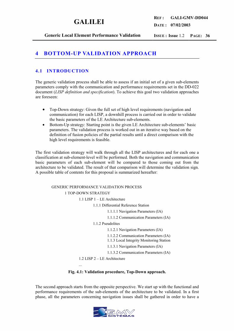
GALILEI REF :
DATE :
GALI-GMV-DD044
07/02/2003
Generic Local Element Performance Validation ISSUE : Issue 1.2 PAGE: 36
4 BOTTOM-UP VALIDATION APPROACH
4.1 INTRODUCTION
The generic validation process shall be able to assess if an initial set of a given sub-elements parameters comply with the communication and performance requirements set in the DD-022 document (LISP definition and specification). To achieve this goal two validation approaches are foreseen:
• Top-Down strategy: Given the full set of high level requirements (navigation and communication) for each LISP, a downhill process is carried out in order to validate the basic parameters of the LE Architecture sub-elements.
• Bottom-Up strategy: Starting point is the given LE Architecture sub-elements’ basic parameters. The validation process is worked out in an iterative way based on the definition of fusion policies of the partial results until a direct comparison with the high level requirements is feasible.
The first validation strategy will walk through all the LISP architectures and for each one a classification at sub-element-level will be performed. Both the navigation and communication basic parameters of each sub-element will be compared to those coming out from the architecture to be validated. The result of that comparison will determine the validation sign. A possible table of contents for this proposal is summarized hereafter:
Fig. 4.1: Validation procedure, Top-Down approach.
The second approach starts from the opposite perspective. We start up with the functional and performance requirements of the sub-elements of the architecture to be validated. In a first phase, all the parameters concerning navigation issues shall be gathered in order to have a
GENERIC PERFORMANCE VALIDATION PROCESS 1 TOP-DOWN STRATEGY 1.1 LISP 1 – LE Architecture 1.1.1 Differential Reference Station 1.1.1.1 Navigation Parameters (IA) 1.1.1.2 Communication Parameters (IA) 1.1.2 Pseudolites 1.1.2.1 Navigation Parameters (IA) 1.1.2.2 Communication Parameters (IA) 1.1.3 Local Integrity Monitoring Station 1.1.3.1 Navigation Parameters (IA) 1.1.3.2 Communication Parameters (IA) 1.2 LISP 2 – LE Architecture ...

GALILEI REF :
DATE :
GALI-GMV-DD044
07/02/2003
Generic Local Element Performance Validation ISSUE : Issue 1.2 PAGE: 37
high level navigation requirements description of the architecture to be validated. Then, the same process shall be worked out for the communication parameters. Finally, the results achieved will be used to find out whether the validating architecture addresses the technical specifications defined for the given LISP architecture in the DD-22 document. As done in the former point, this process might be described in the following table of contents:
Fig. 4.2: Validation procedure. Bottom-Up approach.
4.2 TOP-DOWN AND BOTTOM-UP STRATEGIES
Bottom-Up strategies are more convenient compared with Top-Down approaches depending on the level of detail or level of description of the system. As well as the validation process remains on the LISP architectures and these are described in a functional way it seems like if a bottom-up strategy will suit better than a top-down strategy. Regarding the chosen parameters of study it can be foreseen that a top-down strategy leads to multiple and possible designs. For this reason and having a high level of detail of the LISP architectures a bottom-up approach was selected to achieve the validation process.
4.3 REFERENCE ARCHITECTURE
Reference architecture is a functional architecture that can be found on DD027 document. It is presented here for information purposes, with the information about sub-elements, boxes and interfaces pinpointed in the architecture figure. In case of further clarifications regarding this architecture, refer directly to DD027.
GENERIC PERFORMANCE VALIDATION PROCESS
2 BOTTOM-UP STRATEGY
2.1 LISP 1 – LE Architecture 2.1.1 NAVIGATION PARAMETERS 2.1.1.1 Differential Reference Station - Nav. Parameters (IA) 2.1.1.2 Pseudolites – Nav. Parameters (IA) 2.1.1.3 ... 2.1.1.X High-level Navigation parameters fusion 2.1.2 COMMUNICATION PARAMETERS 2.1.2.1 Differential Reference Station - Comm. Parameters (IA) 2.1.2.2 Pseudolites – Comm. Parameters (IA) 2.1.2.3 ... 2.1.2.X High-level Comm. parameters fusion 3.1 LISP 2 – LE Architecture ...
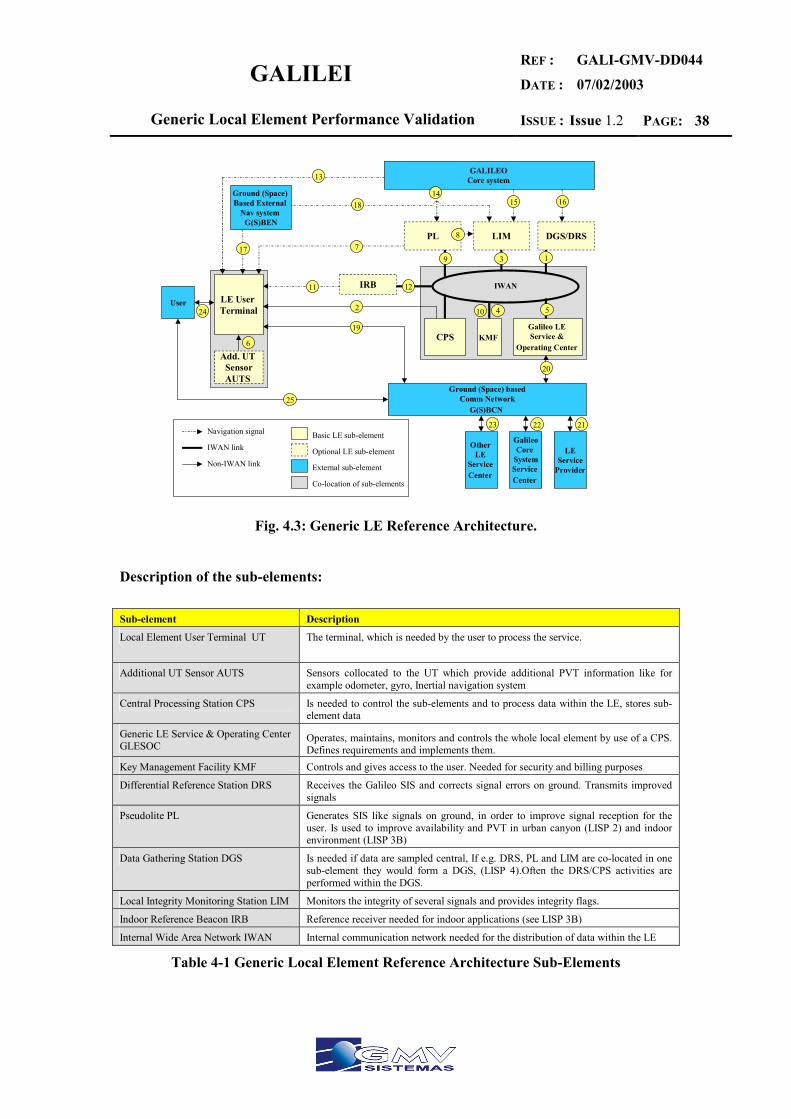
GALILEI REF :
DATE :
GALI-GMV-DD044
07/02/2003
Generic Local Element Performance Validation ISSUE : Issue 1.2 PAGE: 38
LIMPL
LE User Terminal
KMF CPSGalileo LE Service &
Operating Center
IRB
Ground (Space) basedComm Network
G(S)BCN
GalileoCore
SystemService Center
Other LE
Service Center
LEService
Provider
GALILEO Core system
Ground (Space) Based External
Nav system G(S)BEN
Add. UT SensorAUTS
DGS/DRS
Navigation signal
Non-IWAN link
Basic LE sub-element
Optional LE sub-element
External sub-element
Co-location of sub-elements
IWAN link
IWAN
6
10 4
17
13
14 15 16
7 8
18
9 3 1
11 12
2 5
19
20
23 22 21
User 24
25
Fig. 4.3: Generic LE Reference Architecture.
Description of the sub-elements: Sub-element Description
Local Element User Terminal UT The terminal, which is needed by the user to process the service.
Additional UT Sensor AUTS Sensors collocated to the UT which provide additional PVT information like for example odometer, gyro, Inertial navigation system
Central Processing Station CPS Is needed to control the sub-elements and to process data within the LE, stores sub-element data
Generic LE Service & Operating Center GLESOC
Operates, maintains, monitors and controls the whole local element by use of a CPS. Defines requirements and implements them.
Key Management Facility KMF Controls and gives access to the user. Needed for security and billing purposes
Differential Reference Station DRS Receives the Galileo SIS and corrects signal errors on ground. Transmits improved signals
Pseudolite PL Generates SIS like signals on ground, in order to improve signal reception for the user. Is used to improve availability and PVT in urban canyon (LISP 2) and indoor environment (LISP 3B)
Data Gathering Station DGS Is needed if data are sampled central, If e.g. DRS, PL and LIM are co-located in one sub-element they would form a DGS, (LISP 4).Often the DRS/CPS activities are performed within the DGS.
Local Integrity Monitoring Station LIM Monitors the integrity of several signals and provides integrity flags.
Indoor Reference Beacon IRB Reference receiver needed for indoor applications (see LISP 3B)
Internal Wide Area Network IWAN Internal communication network needed for the distribution of data within the LE
Table 4-1 Generic Local Element Reference Architecture Sub-Elements
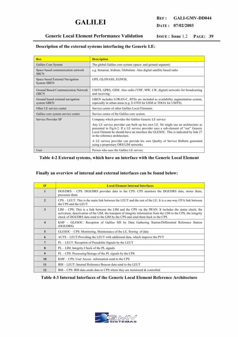
GALILEI REF :
DATE :
GALI-GMV-DD044
07/02/2003
Generic Local Element Performance Validation ISSUE : Issue 1.2 PAGE: 39
Description of the external systems interfacing the Generic LE: Box Description
Galileo Core System The global Galileo core system (space- and ground segment)
Space based communication network SBCN
e.g. Inmarsat, Iridium, Globalstar. Also digital satellite based radio
Space based External Navigation System SBEN
GPS, GLONASS, EGNOS,
Ground Based Communication Network GBCN
UMTS, GPRS, GSM. Also radio (VHF, MW, LW, digital) networks for broadcasting and receiving
Ground based external navigation system GBEN
GBEN includes LORAN-C, BTSs are included as availability augmentation system, especially in urban areas (e.g. E-OTD for GSM or TDOA for UMTS).
Other LE service center Service center of other Galileo Local Elements.
Galileo core system service center Service center of the Galileo core system.
Service Provider SP Company which provides the Galileo Generic LE service Any LE service provider can built up his own LE. He might use an architecture as presented in Fig.6-2. If a LE service provider uses a sub-element of “our” Generic Local Element he should have an interface the GLESOC. This is indicated by link 27 in the reference architecture. A LE service provider can provide his own Quality of Service Bulletin generated using a proprietary DRS/LIM networks
User Person who uses the Galileo LE service
Table 4-2 External systems, which have an interface with the Generic Local Element
Finally an overview of internal and external interfaces can be found below:
IF Local Element Internal Interfaces
1 DGS/DRS – CPS: DGS/DRS provides data to the CPS: CPS monitors the DGS/DRS data, stores them, processes them
2 CPS – LEUT: This is the main link between the LEUT and the rest of the LE. It is a one-way OTA link between the CPS and the LEUT
3 LIM – CPS: This is a link between the LIM and the CPS via the IWAN. It includes the status check, the activation, deactivation of the LIM, the transport of integrity information from the LIM to the CPS, the integrity check of DGS/DRS data send to the LIM by the CPS and send them back to the CPS
4 KMF – GLESOC: Reception of Galileo SIS by Data Gathering Station/Differential Reference Station (DGS/DRS)
5 GLESOC – CPS: Monitoring, Maintenance of the LE, Storing of data
6 AUTS – LEUT:Providing the LEUT with additional data, which improve the PVT
7 PL – LEUT: Reception of Pseudolite Signals by the LEUT
8 PL – LIM: Integrity Check of the PL signals
9 PL – CPS: Processing/Storage of the PL signals by the CPS
10 KMF – CPS: User Access information send to the CPS
11 IRB – LEUT: Internal Reference Beacon data send to the LEUT
12 IRB – CPS: IRB data sends data to CPS where they are monitored & controlled
Table 4-3 Internal Interfaces of the Generic Local Element Reference Architecture

GALILEI REF :
DATE :
GALI-GMV-DD044
07/02/2003
Generic Local Element Performance Validation ISSUE : Issue 1.2 PAGE: 40
IF External Interfaces
13 Reception of Galileo SIS by the Local Element User Terminal (LEUT)
14 Reception of Galileo SIS by Pseudolites (PL)
15 Reception of Galileo SIS by Local Integrity Monitoring Station (LIM)
16 Reception of Galileo SIS by Data Gathering Station/Differential Reference Station (DGS/DRS)
17 Reception of Signals of Ground or Space Based External Navigation Systems (G(S)BEN) by the LEUT
18 Reception of G(S)BCN signals data by the LIM
19 Interface between the Ground or Space Based Communication Network (G(S)BCN) and the LEUT
20 Interface between the G(S)BCN and the Galileo LE Service and Operating Center GLESOC
21 Interface between the G(S)BCN and the Galileo LE Service and the LE Service Provider
22 Interface between the G(S)BCN and the Galileo LE Service and the Galileo Service Product Facility (SPF), this is the Galileo Core System Service Center
23 Interface between the G(S)BCN and the Galileo LE Service and other LE Service Centers
24 Interface between User and LEUT
25 Interface between User and G(S)BCN
Table 4-4 External Interfaces of the Generic Local Element Reference Architecture
4.4 SUB-ELEMENTS AND EXTERNAL SYSTEMS ANALYSIS
A closer look at the Reference Architecture and the LISP architecture yields that its components can be grouped as internal sub-elements and external systems to the architecture. So the following sub-elements are internal to the LISP architectures: Differential Reference Station (DRS), Local Integrity Monitor (LIM) and Pseudolite (PL). By the way, external systems are:
Space Based External Navigation System, SBEN. Including GPS, EGNOS and GLONASS.
Space Based Communication Network, SBCN. These are Inmarsat, Iridium, GlobalStar and Digital Satellite Based Radio.
Ground Based External Navigation System, GBEN. E.g. LORAN, EUROFIX and others.
Ground Based Communication Network, GBCN: UMTS, GPRS, GSM, Radio…

GALILEI REF :
DATE :
GALI-GMV-DD044
07/02/2003
Generic Local Element Performance Validation ISSUE : Issue 1.2 PAGE: 41
Fig. 4.4: Study scenario.
A severe analysis must be done in order to weigh up how the sub-elements and external systems contribute to the achievement of the required performances. For this reason, every block in the LISP architectures has been studied. As a result of this analysis a set of working parameters and its impact on the performance parameters has been stated. A complete description of these parameters can be found in the annexes and summarized in several tables.
Fig. 4.5: LISP performances merging process.
Generic LE Reference Architecture
LISP 1
LISP 2
LISP 3a
LISP 3b
LISP 4a
LISP 4b
Generic LE Architecture 1Generic LE Architecture 1
Generic LE Architecture 2Generic LE Architecture 2
Generic LE Architecture 3aGeneric LE Architecture 3a
Generic LE Architecture 3bGeneric LE Architecture 3b
Generic LE Architecture 4aGeneric LE Architecture 4a
Generic LE Architecture 4bGeneric LE Architecture 4b
Sub ElementsSub Elements
Ext. SystemsExt. Systems
DRSLIM
PL LEUT
SBCNSBEN
GBCN GBEN
Performances
DRSLIM
PL LEUT
SBCNSBEN
GBCN GBEN
Performances
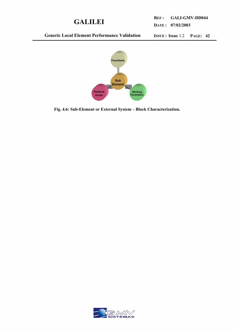
GALILEI REF :
DATE :
GALI-GMV-DD044
07/02/2003
Generic Local Element Performance Validation ISSUE : Issue 1.2 PAGE: 42
Fig. 4.6: Sub-Element or External System – Block Characterization.
Performances
WorkingParameters
Functions
SubElement
Performances
WorkingParameters
Functions
SubElement

GALILEI REF :
DATE :
GALI-GMV-DD044
07/02/2003
Generic Local Element Performance Validation ISSUE : Issue 1.2 PAGE: 43
5 GENERIC VALIDATION PROCEDURE
5.1.1 INTRODUCTION
Once the LISP architectures, performance requirements and the set of sub-elements are stated the validation procedure takes place. It is carried out in three phases. In the first phase an isolated analysis of the LISP architecture sub-elements and external systems is performed. The objective of this analysis is to weigh up the contribution of each sub-element or system to achieve the system performances. In the second phase the impact of the several components of the system on the whole performances is assessed.
Fig. 5.1:Validation procedure.
The third phase not represent in Fig. 5.1, is an additional effort from GMV Sistemas PTM SA whose target was to nearly completely assess navigation performances of the LE architecture with simulations. In this third phase, due to the lack of budget information to be used for the LE, GMV has defined in addition the UERE budgets of the simulated sub-elements, and has extracted from this error budgets, the final results for each LISP. This third phase, is the simulation update of phase 2 for DD027 v1.2. Validation is made in advance to check if the conditions are met to achieve the expected navigation and communication performances of each LISP. To complete the validation procedure, formerly is needed to fix some preliminary general assumptions, continuing with a description of the parameters to be analysed and its values on each LISP. After identifying the targets of the validation procedure, environmental restrictions are described and their influence along the validation procedure. With these previous sub-tasks a complete description of the followed general method is given. Finally, this method will be applied to each LISP concluding the validation phase.
Conclusions
Interoperability
Env. constraints
Local Validation
External Inputs
BlockCharacterization
Generic LEArchitecture
Nav&Comm perfos
LISP
Remarks & Recommd.
Phase 1
Phase 2
GALILEI REF :
DATE :
GALI-GMV-DD044
07/02/2003
Generic Local Element Performance Validation ISSUE : Issue 1.2 PAGE: 44
A final summary table will simply conclude if the validation procedure has reached the expected performances. When the validation procedure meet expected performances no additional remarks will be needed, but in most of cases, references to concrete aspects to take into account will be given. Some conclusions, remarks and recommendations will be additionally given at the end of the document. In annexes, additional technical concrete information has been grouped mainly to give a fast description and overview of local performances of each sub-element (grouped or not with other sub-elements) present on the LE architecture. In some of cases, may the user know this information, but we consider it necessary as a reference of error magnitudes and an added value of the document in terms of being self-contained.
5.2 PRELIMINARY GENERAL ASSUMPTIONS
To understand the present validation work some preliminary assumptions needs to be fixed. It is important from the point of view of reusing this document to agree previously with these generic points:
- The main objective of this document is to provide the Generic Validation of LE Architectures defined for LISP#1#2#3ab#4ab. Navigation and communication parameters to be validated are fixed.
- LE defined architectures have been defined according to a high-level description procedure. Black boxes shall represent each sub-element within the LE, and physical links are indicated and numbered in DD027.
- Within this general approach, only general working parameters are defined: Navigation parameters considered are Availability, Accuracy and TTA. Communication parameters considered are: Type of Communication (1W/2W, Voice/Data, Broadcast/Broadcatch).
- The low LE description procedure followed is thought to allow future particular solutions to each concrete application and the validation procedure is intended to avoid particular cases and be also general. In spite of this, the third phase concretes the error budgets for DRS, DGS, PL and GNSS sub-elements and sub-components, to allow a complete simulation task of each LISP. The simulation results of this phase are related to the error budgets assumed.
- Initially are defined three different kinds of environments to be used for the validation phase: Clear-Sky, Urban canyon and indoor scenarios. The Clear-Sky case, shall lead to the best possible performances of the system, while the rest of them are successive degradation of the external conditions. For each environment, generic approaches are given for the validation phase. For the simulation phase 3, clear-sky is assumed to have a constant masking angle of 10º, urban and indoor cases are assumed to have a constant masking angle of 25º. The difference between them is stressed on the error budget models.
GALILEI REF :
DATE :
GALI-GMV-DD044
07/02/2003
Generic Local Element Performance Validation ISSUE : Issue 1.2 PAGE: 45
- Due to this generic definition approach, valid for a great deal of applications, final expected performances are according the most restrictive applications intended to be covered for each LISP. The validation phase will cover this most restrictive parameters extracted from each particular LISP.
- Within the validation approach for phase 1 and 2, Navigation validation is initially isolated from the Communication validation. Validation of Navigation parameters is mainly leading to confirm the global performances of the LE architecture, while validation of Communication parameters mainly should warranty the final service of the LE architecture. In phase 3, concrete error budgets are related to the delayed communications hence this effect is studied.
5.2.1 NAVIGATION ASSUMPTIONS
- Validation of Navigation parameters is leading to confirm the achievable of the global Availability, Accuracy and TTA performances within LE architectures proposed.
- If these performances are clearly reached after validation study, architectural model should be considered validated and no additional remarks should be needed.
- If these performances are not clearly reached after validation study, architectural model should be considered potentially risky and additional remarks will be given to achieve navigation performances.
- Due to the general presence of nearly all the principal Sub-Elements within the LE architectures chosen, when required, additional optimisation remarks will be presented leading to avoiding a costly architecture regarding the application needs. In this optimisation phase, mainly a relaxation of final performances will be required.
- GPS previous experience will be the reference point to fix the minimum future expected performances, and know-how of static and dynamic algorithms are expected to be successfully re-used achieving similar levels of accuracy.
- From a general point of view it is assumed that Near Sub-metric (1m level) accuracy can be obtained through the usage of Differential Reference Stations by using only Code (pseudo-range) corrections provided by the Reference Stations. This approach will be considered valid for static and low dynamic cases.
- From a general point of view it is assumed that Sub-metric (0.5 m level) accuracy can be obtained through the usage of Differential Reference Stations by using Code and Phase corrections provided by the Reference Stations and applying differential corrections smoothed with the received phase. This approach will be considered valid for static and low dynamic cases.
- From a general point of view it is assumed that Centimetric (0.020m level) accuracy can be obtained through de usage of Kinematic techniques based on integer ambiguity resolution and algorithms of multipath reduction, in receivers with very high performances. This approach will be considered valid for static and low dynamic cases.
- From a general point of view it is assumed that Millimetric (0.005 m level) accuracy can be obtained through de usage of Kinematic techniques based on integer ambiguity resolution, algorithms of multipath reduction, in receivers with very high performances. This approach will be considered statistically valid after a successful post-processing analysis.
GALILEI REF :
DATE :
GALI-GMV-DD044
07/02/2003
Generic Local Element Performance Validation ISSUE : Issue 1.2 PAGE: 46
- For each accuracy level, we consider that if some preliminary conditions are met within the scope of the area considered, LE range performances will apply along the scope of the area.
- Availability conditions shall depend mainly on constellations considered, including constellation failures and masking angles obscuring SIS. In annexes some interference problems are considered, but can be technically solved, so in the current analysis we will consider no additional interference phenomena applies.
- Accuracy conditions shall depend on the availability of having enough incoming information to achieve the solution. Certain restrictions shall apply to the incoming information.
- TTA conditions shall depend mainly on having some redundancy information of the constellation to allow the detection of integrity risks.
- In terms of usable constellations for applications, it has made the assumption that Galileo constellation shall be used as a minimum, with the addition of SBEN (Space Based External Navigation Systems) in case of availability necessity. Within SBEN considered for the validation phase shall be included GPS and EGNOS as best potentials systems.
- Galileo future constellation shall be at least technologically similar (conservative criteria) in terms of performances to other current constellations like GPS. And will be usable along with them to provide an enhanced result.
- Galileo LE Sub-Elements are foreseen to achieve at least the performances obtained by current GPS techniques and algorithms. With this approach, previous experience with Pseudolites and Reference Stations can be re-used.
- The most immediate source of benefit of the Galileo Navigation System is its optimised constellation configuration allowing the enhancement of provided availability around the world. This availability parameter will be the starting point of the validation procedure.
- The local area covered by the LE architecture will be restricted to the coverage area in which the algorithms can be applied to reach expected LE performances. Along the validation procedure it is assumed that if algorithms are applied and incoming information is good enough, performances are warranted.
- Throughout the validation phase, the definition of additional parameters within the LE architectures should be avoided (to be as general as possible), but in some cases extrapolation of real cases should serve as useful examples.
- These assumptions are considered general for the validation phase, acceptable from the point of view of given defined parameters, and should lead to a general validation procedure.
- For the third simulation phase, concrete navigation error budgets are provided at the end of this section (see 5.7.3.5) to achieve concrete significant results.
5.2.2 COMMUNICATION ASSUMPTIONS
- Validation of Communication parameters is leading to confirm the achievable of the global Level of Service intended within LE architectures proposed, in terms of features requested.
- If the expected Level of Service is clearly reached after validation study, architectural model should be considered validated and no additional remarks should be needed.
GALILEI REF :
DATE :
GALI-GMV-DD044
07/02/2003
Generic Local Element Performance Validation ISSUE : Issue 1.2 PAGE: 47
- If the expected Level of Service is not clearly reached after validation study, architectural model should be considered potentially risky and additional remarks will be given to achieve communication Level of Service.
- Existing Communication technologies and previous experience will be the reference point to fix the minimum future expected Level of Service.
- All the communication links are specified through a high-level definition of the LE architecture corresponding to each LISP.
- The local area covered by the LE architecture (in which applies the LE performances) will be restricted to the coverage area in which all defined links work properly. Along the validation procedure no coverage failures are considered.
- Throughout the validation phase, the definition of additional parameters within the LE architectures should be avoided (to be as general as possible), but in some cases extrapolation of real cases should serve as useful examples.
- These assumptions are considered general for the validation phase, acceptable from the point of view of given defined parameters, and should lead to a general validation procedure.
- For the third simulation phase, communication delays are considered in the simulations according to concrete communication error budgets provided at the end of this section (see 5.7.3.5).
5.3 IMPACT OF THE GENERAL ASSUMPTIONS
The main purpose of the general assumptions is to be as general as possible in the definition of properties for the validation of the LE architectures. These previous considerations are needed to start from the same point and to have homogeneous criteria along the validation procedure. As no concrete particular parameters are given, some preliminary considerations in terms of behaviour are needed to make the validation with a minimum of warranties to be possible. As stated at the end of each preliminary navigation and communication assumptions, these assumptions are taken acceptable and generic enough to achieve a generic validation procedure. In case one or more than one assumption is not acceptable from the point of view of any concrete application, validation procedure should be revised and the final impact of this change needs to be checked, but is out of the scope of the current document. So the main impact of the previous general assumptions is to validate four General Cases. The followed procedure applies for any other general or particular case but analysing all the possibilities is not affordable along this document. In this line, the general procedure can be followed in case of newer particular cases, but any particularisation will have surely additional performance values to be taken into account in the validation task and will probably have the chance to be physically validated. However some guidelines can be extracted from the present validation study to check in advance what the conclusions should be, this is one of the benefits of this approach. After describing the validation method and LISP analysis some guidelines will be extracted, but will be reviewed for direct applications into new particularisations of each LISP to concrete applications. It will be shown that any feature and environment particularisation should lead mainly to a variation study of the Local Area of Applicability (To Be Defined) of the given performances for that LISP.
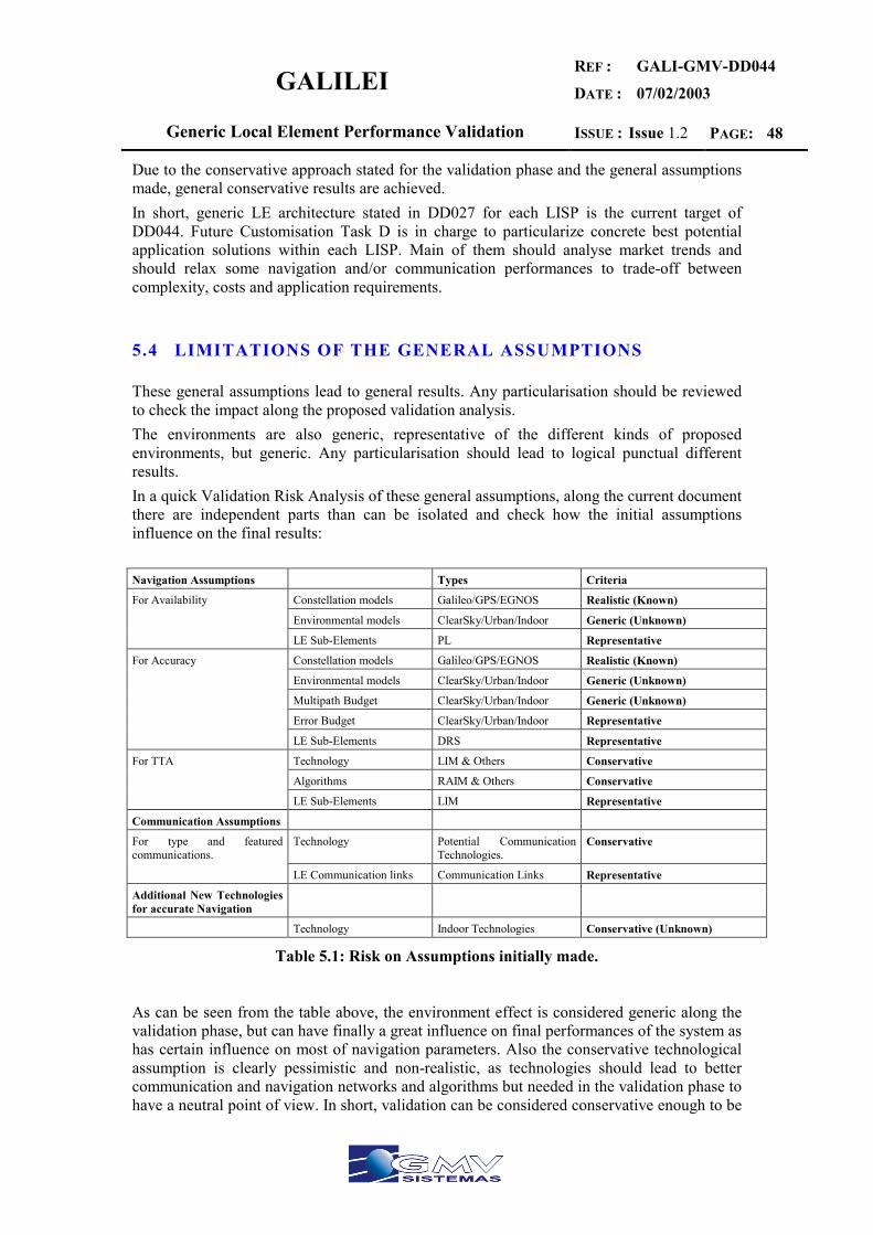
GALILEI REF :
DATE :
GALI-GMV-DD044
07/02/2003
Generic Local Element Performance Validation ISSUE : Issue 1.2 PAGE: 48
Due to the conservative approach stated for the validation phase and the general assumptions made, general conservative results are achieved. In short, generic LE architecture stated in DD027 for each LISP is the current target of DD044. Future Customisation Task D is in charge to particularize concrete best potential application solutions within each LISP. Main of them should analyse market trends and should relax some navigation and/or communication performances to trade-off between complexity, costs and application requirements.
5.4 LIMITATIONS OF THE GENERAL ASSUMPTIONS
These general assumptions lead to general results. Any particularisation should be reviewed to check the impact along the proposed validation analysis. The environments are also generic, representative of the different kinds of proposed environments, but generic. Any particularisation should lead to logical punctual different results. In a quick Validation Risk Analysis of these general assumptions, along the current document there are independent parts than can be isolated and check how the initial assumptions influence on the final results: Navigation Assumptions Types Criteria
Constellation models Galileo/GPS/EGNOS Realistic (Known)
Environmental models ClearSky/Urban/Indoor Generic (Unknown)
For Availability
LE Sub-Elements PL Representative
Constellation models Galileo/GPS/EGNOS Realistic (Known)
Environmental models ClearSky/Urban/Indoor Generic (Unknown)
Multipath Budget ClearSky/Urban/Indoor Generic (Unknown)
Error Budget ClearSky/Urban/Indoor Representative
For Accuracy
LE Sub-Elements DRS Representative
Technology LIM & Others Conservative
Algorithms RAIM & Others Conservative
For TTA
LE Sub-Elements LIM Representative
Communication Assumptions
Technology Potential Communication Technologies.
Conservative For type and featured communications.
LE Communication links Communication Links Representative
Additional New Technologies for accurate Navigation
Technology Indoor Technologies Conservative (Unknown)
Table 5.1: Risk on Assumptions initially made.
As can be seen from the table above, the environment effect is considered generic along the validation phase, but can have finally a great influence on final performances of the system as has certain influence on most of navigation parameters. Also the conservative technological assumption is clearly pessimistic and non-realistic, as technologies should lead to better communication and navigation networks and algorithms but needed in the validation phase to have a neutral point of view. In short, validation can be considered conservative enough to be
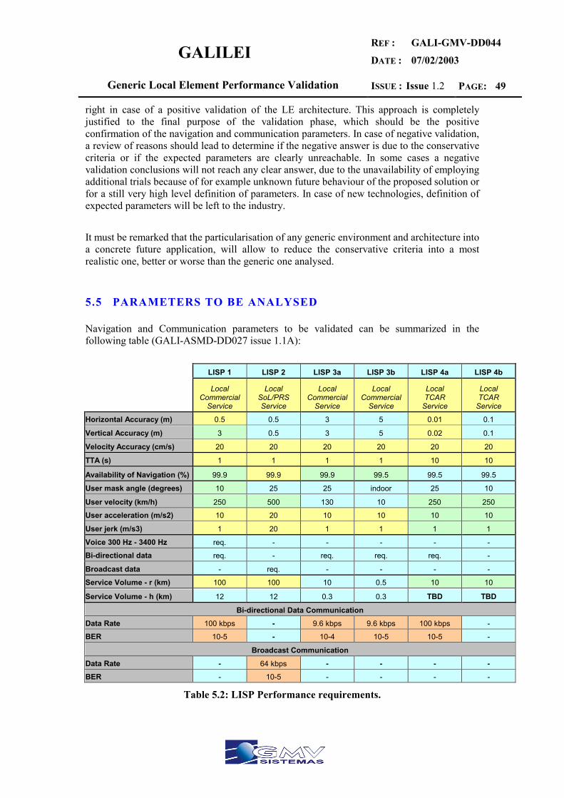
GALILEI REF :
DATE :
GALI-GMV-DD044
07/02/2003
Generic Local Element Performance Validation ISSUE : Issue 1.2 PAGE: 49
right in case of a positive validation of the LE architecture. This approach is completely justified to the final purpose of the validation phase, which should be the positive confirmation of the navigation and communication parameters. In case of negative validation, a review of reasons should lead to determine if the negative answer is due to the conservative criteria or if the expected parameters are clearly unreachable. In some cases a negative validation conclusions will not reach any clear answer, due to the unavailability of employing additional trials because of for example unknown future behaviour of the proposed solution or for a still very high level definition of parameters. In case of new technologies, definition of expected parameters will be left to the industry. It must be remarked that the particularisation of any generic environment and architecture into a concrete future application, will allow to reduce the conservative criteria into a most realistic one, better or worse than the generic one analysed.
5.5 PARAMETERS TO BE ANALYSED
Navigation and Communication parameters to be validated can be summarized in the following table (GALI-ASMD-DD027 issue 1.1A):
LISP 1 LISP 2 LISP 3a LISP 3b LISP 4a LISP 4b
Local Commercial
Service
Local SoL/PRS Service
Local Commercial
Service
Local Commercial
Service
Local TCAR
Service
Local TCAR
Service
Horizontal Accuracy (m) 0.5 0.5 3 5 0.01 0.1
Vertical Accuracy (m) 3 0.5 3 5 0.02 0.1
Velocity Accuracy (cm/s) 20 20 20 20 20 20
TTA (s) 1 1 1 1 10 10
Availability of Navigation (%) 99.9 99.9 99.9 99.5 99.5 99.5
User mask angle (degrees) 10 25 25 indoor 25 10
User velocity (km/h) 250 500 130 10 250 250
User acceleration (m/s2) 10 20 10 10 10 10
User jerk (m/s3) 1 20 1 1 1 1
Voice 300 Hz - 3400 Hz req. - - - - -
Bi-directional data req. - req. req. req. -
Broadcast data - req. - - - -
Service Volume - r (km) 100 100 10 0.5 10 10
Service Volume - h (km) 12 12 0.3 0.3 TBD TBD
Bi-directional Data Communication Data Rate 100 kbps - 9.6 kbps 9.6 kbps 100 kbps -
BER 10-5 - 10-4 10-5 10-5 -
Broadcast Communication
Data Rate - 64 kbps - - - - BER - 10-5 - - - -
Table 5.2: LISP Performance requirements.
GALILEI REF :
DATE :
GALI-GMV-DD044
07/02/2003
Generic Local Element Performance Validation ISSUE : Issue 1.2 PAGE: 50
5.6 ENVIRONMENTAL RESTRICTIONS
In order to unify the environmental restrictions along this title, main particularities are explained justifying the three scenarios considered along the current validation document. Clear Sky scenario will get the best possible profit from the available constellations. This means that the highest level of performances should be achieved through the clear sky environment. To simulate Clear Sky environment it has been set a maximum masking angle of 10º. The study of 5º can be added to study differences on constellation availability. Multipath can be minimised with the wise use of installation requirements, token ring antennas and software correlation techniques. Urban Canyon scenario will act as a more restrictive environment in which the availability of the constellation will decrease due to major presence of additional obstacles and multipath effect will increase its mean value. Contrary to clear sky scenario in which the study of it should lead to a general clear sky performance achievement, an urban canyon environment can have a great number of different environments in which particular performances will depend highly on each concrete situation studied. From the generic validation point of view it has been fixed the urban canyon scenario as one clear sky scenario with higher masking angles up to 25º. As Multipath effect will depend greatly on the final real scenario, to check the best achievable performances, it may be omitted, but finally it has to be included to impact final accuracy value. Indoor scenario will be the next level of constellation signal degradation. For this case, high sensitivity receivers shall be needed, as in a general case no direct line of sight exists from the receivers to the received constellation. Again in this case availability of the constellation will decrease and a considerable multipath value will be introduced on the final solution. This poor Navigability should lead to the introduction of additional indoor techniques to improve accuracy. Also indoor scenario lead to a lower C/No signal strength and so additional losses of SIS should happen. Like in Urban Canyon a masking angle of 25º will be used, and if no additional signal augmentation systems (like Pseudolites acting as transceivers) are used, a penalization of 2 less received satellites will apply. For phase 3, 25º will apply with a corrected error budget defined at the end of this section (see 5.7.3.5). All scenario definition will include both Clear Sky and Urban Canyon environments. In this case, Urban Canyon represents the most restrictive case to be validated. High Dynamics restriction is thought for direct applicability to aircraft navigation solutions. In this case, the main restriction is the working data rate of the constellation receivers to warranty the achievable solution on time and to check integrity failures. 10Hz receivers should be needed. Radial Range Scope determines the circle range of scope within each LISP in which defined performances do have to be met. This radial scope is defined to have a realistic value for market purpose. From the validation point of view, this parameter will not be verified as it depends strongly on the real environment. In Clear Sky case, a positive validation will lead to an immediate positive Radial Range Scope validation if incoming information is achievable within all the radial scope and accuracy is maintained along radial distance. In Urban Canyon
GALILEI REF :
DATE :
GALI-GMV-DD044
07/02/2003
Generic Local Element Performance Validation ISSUE : Issue 1.2 PAGE: 51
or Indoor applications, a local positive validation will lead also to an immediate positive Radial Range Scope validation, but probably additional items (Sub-elements) needs to be added to maintain LE parameters within specifications along Radial Scope.
5.7 VALIDATION METHOD
5.7.1 PHASE ONE: LOCAL
The following procedure is established: 1- For each LISP a table summarizes the performance requirements. These include the
following: a. Navigation: Time to Alarm, Accuracy and Availability. b. Communication: voice/data, 1 way/2 ways and broadcast/broadcatch.
2- For each LISP the influence of every sub-element and external system on the performance parameters is analyzed and a table titled “sub-element and external system influence on local performances” is given.
5.7.1.1 Sub-Element and External System Influence on Local Performances
In this section navigation and communication performances must be seen as sub-element or external system performances instead of service performances. For this reason a “communication performances” section for navigation systems can be seen on each table.
5.7.1.1.1 Navigation
The following table summarizes the impact on several navigation and communication performances. Communication performances might be seen as “communication performances for navigation”. Only the main effect of every sub-element or external system on the performances is considered.

GALILEI REF :
DATE :
GALI-GMV-DD044
07/02/2003
Generic Local Element Performance Validation ISSUE : Issue 1.2 PAGE: 52
Table 5.3: Sub-element and external system influence on local performances.
(1) Pseudolite impact on accuracy: by means of having a good geometry (as a result of the introduction of an additional satellite) or a precise calculation of the pseudolite position. (2) Transmission of DGPS or EGNOS corrections through LORAN carrier. Remarks:
Only direct pseudolites are considered (this excludes the use of inverse pseudolites).
Broadcast services transmit information from the sub-element or external system side to the user.
Communications are always considered from the sub-element or external system side to the user side.
Data communication only.
5.7.1.1.2 Communication
The table below summarizes the Ground Based Communication Systems parameters for navigation and communication purposes.
Navigation Communication Acc. TTA Avai. Voice
/Data 1 W/2 W Brdcast Brdcatch
DRS √ D 1W √ PL (1) √ D 1W √ LIM- √ D 1W √ GALILEO EGNOS √ √ D 1W √ GPS √ √ D 1W √ GLONASS √ √ D 1W √ LORAN-C √ D 1W √ CHAYKA √ D 1W √ EUROFIX(2) √ D 1W √

GALILEI REF :
DATE :
GALI-GMV-DD044
07/02/2003
Generic Local Element Performance Validation ISSUE : Issue 1.2 PAGE: 53
Table 5.4: Sub-element and external system influence on local performances.
[×××] Mobile cellular systems. [×××] Long range and medium range communication systems. [×××] Short range communication systems. Remarks (4) Impact on availability when used as a cellular localization system (by means of measuring the signal power or similar). (5) Semi-duplex (6) Multicast transmission
5.7.1.1.3 Environmental Constraint Impact
In this section an analysis of the environmental constraint impact on the sub-elements and external system performances is carried out. The contents of this section are basically a summary of the “Performance Section” of the analyzed sub-elements and external systems:
DRS
Navigation Communication Acc. TTA Avai. Voice
/Data 1 W/2 W Brdcast Brdcatch
GSM (4) √ D/V 2W GPRS √ D/V 2W √(6) UMTS √ D/V 2W √(6) TETRA D/V 2W √(6) RDS D 1W √ DAB/DRM D 1W √ DECT V/D 2W BLUETOOTH V/D 2W √(6) IRDA D 2W (5) HOME RF D 2W √(6) WMAN (802.16) D 2W
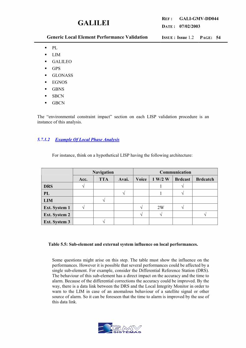
GALILEI REF :
DATE :
GALI-GMV-DD044
07/02/2003
Generic Local Element Performance Validation ISSUE : Issue 1.2 PAGE: 54
PL LIM GALILEO GPS GLONASS EGNOS GBNS SBCN GBCN
The “environmental constraint impact” section on each LISP validation procedure is an instance of this analysis.
5.7.1.2 Example Of Local Phase Analysis
For instance, think on a hypothetical LISP having the following architecture:
Table 5.5: Sub-element and external system influence on local performances.
Some questions might arise on this step. The table must show the influence on the performances. However it is possible that several performances could be affected by a single sub-element. For example, consider the Differential Reference Station (DRS). The behaviour of this sub-element has a direct impact on the accuracy and the time to alarm. Because of the differential corrections the accuracy could be improved. By the way, there is a data link between the DRS and the Local Integrity Monitor in order to warn to the LIM in case of an anomalous behaviour of a satellite signal or other source of alarm. So it can be foreseen that the time to alarm is improved by the use of this data link.
Navigation Communication Acc. TTA Avai. Voice 1 W/2 W Brdcast Brdcatch
DRS √ 1 √ PL √ 1 √ LIM √ Ext. System 1 √ √ 2W √ Ext. System 2 √ √ √ Ext. System 3 √
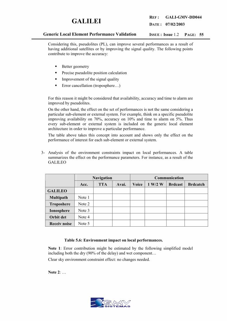
GALILEI REF :
DATE :
GALI-GMV-DD044
07/02/2003
Generic Local Element Performance Validation ISSUE : Issue 1.2 PAGE: 55
Considering this, pseudolites (PL), can improve several performances as a result of having additional satellites or by improving the signal quality. The following points contribute to improve the accuracy:
Better geometry Precise pseudolite position calculation Improvement of the signal quality Error cancellation (troposphere…)
For this reason it might be considered that availability, accuracy and time to alarm are improved by pseudolites. On the other hand, the effect on the set of performances is not the same considering a particular sub-element or external system. For example, think on a specific pseudolite improving availability on 70%, accuracy on 10% and time to alarm on 5%. Thus every sub-element or external system is included on the generic local element architecture in order to improve a particular performance. The table above takes this concept into account and shows only the effect on the performance of interest for each sub-element or external system.
3- Analysis of the environment constraints impact on local performances. A table summarizes the effect on the performance parameters. For instance, as a result of the GALILEO
Table 5.6: Environment impact on local performances.
Note 1: Error contribution might be estimated by the following simplified model including both the dry (90% of the delay) and wet component… Clear sky environment constraint effect: no changes needed. Note 2: …
Navigation Communication Acc. TTA Avai. Voice 1 W/2 W Brdcast Brdcatch
GALILEO Multipath Note 1 Troposhere Note 2 Ionosphere Note 3 Orbit det Note 4 Receiv noise Note 5
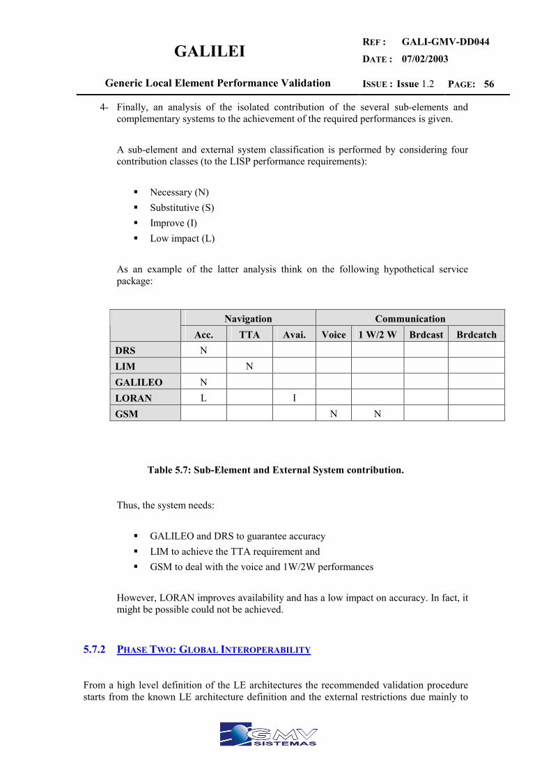
GALILEI REF :
DATE :
GALI-GMV-DD044
07/02/2003
Generic Local Element Performance Validation ISSUE : Issue 1.2 PAGE: 56
4- Finally, an analysis of the isolated contribution of the several sub-elements and complementary systems to the achievement of the required performances is given.
A sub-element and external system classification is performed by considering four contribution classes (to the LISP performance requirements):
Necessary (N) Substitutive (S) Improve (I) Low impact (L)
As an example of the latter analysis think on the following hypothetical service package:
Table 5.7: Sub-Element and External System contribution.
Thus, the system needs:
GALILEO and DRS to guarantee accuracy LIM to achieve the TTA requirement and GSM to deal with the voice and 1W/2W performances
However, LORAN improves availability and has a low impact on accuracy. In fact, it might be possible could not be achieved.
5.7.2 PHASE TWO: GLOBAL INTEROPERABILITY
From a high level definition of the LE architectures the recommended validation procedure starts from the known LE architecture definition and the external restrictions due mainly to
Navigation Communication Acc. TTA Avai. Voice 1 W/2 W Brdcast Brdcatch
DRS N LIM N GALILEO N LORAN L I GSM N N
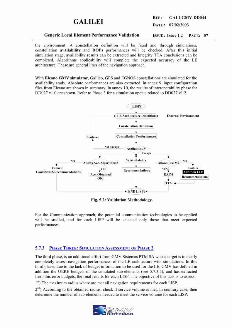
GALILEI REF :
DATE :
GALI-GMV-DD044
07/02/2003
Generic Local Element Performance Validation ISSUE : Issue 1.2 PAGE: 57
the environment. A constellation definition will be fixed and through simulations, constellation availability and DOPs performances will be checked. After this initial simulation stage, availability results can be extracted and Integrity TTA conclusions can be completed. Algorithms applicability will complete the expected accuracy of the LE architecture. These are general lines of the navigation approach. With Elcano GMV simulator, Galileo, GPS and EGNOS constellations are simulated for the availability study. Absolute performances are also extracted. In annex 9, input configuration files from Elcano are shown in summary. In annex 10, the results of interoperability phase for DD027 v1.0 are shown. Refer to Phase 3 for a simulation update related to DD027 v1.2.
External Environment
Enough
Constellation Definition
Constellation Performances
% Availability
Recommendations
Failure
Failure
Acc. ObtainedOK
Conditions&RecommendationsRAIM
Failure
TTA
Not Enough
NO
YES
NO
YES
Recommendations
Fig. 5.2: Validation Methodology.
For the Communication approach, the potential communication technologies to be applied will be studied, and for each LISP will be selected only those that meet expected performances.
5.7.3 PHASE THREE: SIMULATION ASSESSMENT OF PHASE 2
The third phase, is an additional effort from GMV Sistemas PTM SA whose target is to nearly completely assess navigation performances of the LE architecture with simulations. In this third phase, due to the lack of budget information to be used for the LE, GMV has defined in addition the UERE budgets of the simulated sub-elements (see 5.7.3.5), and has extracted from this error budgets, the final results for each LISP. The objective of this task is to assess: 1st) The maximum radius where are met all navigation requirements for each LISP. 2nd) According to the obtained radius, check if service volume is met. In contrary case, then determine the number of sub-elements needed to meet the service volume for each LISP.
GALILEI REF :
DATE :
GALI-GMV-DD044
07/02/2003
Generic Local Element Performance Validation ISSUE : Issue 1.2 PAGE: 58
3rd) Additionally, an estimation of realistic figures for the communication delays will be provided, in concrete the delay of the differential corrections reception and of status messages will be computed. A status message example is an alarm message from the CPS, hence, the status message delay, is an estimation of the expected TTA parameter, also defined for each LISP. The results of this third point are provided in section 10 of DD044.
5.7.3.1 Description of Polaris Tool for Simulations
For phase 3, we have used a non-public preliminary version of Polaris simulation tool, with additional modifications to include the proposed error budgets for DRS and PL sub-elements. With this preliminary version, different GNSS constellations can be simulated in conjunction with a LE composed with DRS/DGS stations and PL sub-elements. Polaris simulation tool is an enhancement of Elcano tool and will be completely available at the end of 2003 (Polaris v2.0). One first version of the Polaris simulation tool will be available at July of 2003. In respect to current simulations performed in DD044, this preliminary and locally modified version of Polaris simulation tool gives the following facilities:
• Includes a Keplerian Constellation propagator of GNSS orbits. • Includes POLARIS ability to simulate DRS and PL sub-elements. • Includes modifications to DGNSS modules allowing the inclusion of delays on
differential corrections and distance budgets degradation. • Includes implementation of New Algorithms structure for proposed UERE
Budget definitions.
This non-public preliminary version of Polaris simulation tool is a constellation design tool fully developed at GMV. The final purpose of this tool is not only to design constellations but also to assess performances and to analyse the stability of the performances with time. Is composed of a main module that generates and simulates the target satellites constellation with DRS and PL sub-elements, and is capable of generate the FOM (Figures of Merit) requested.
5.7.3.2 Objectives of Phase 3 Performance Assessment
The overall objective of phase 3 is to assess performance obtained for all defined LISP architectures in DD027. In concrete the following navigation and communication parameters will be assessed: • Preliminary simulation study to confirm each LISP architecture configuration. Presence
of one or several GNSS constellations, and usage of code or phase techniques. • Availability of Accuracy of results for the LISP architectures with only one sub-element
of each type included. With this approach, the convergence radius where both parameters (accuracy and availability) are met will be extracted. Hence we will obtain the preliminary volume of service achieved. Additionally, different effects of changes on local coordinates and delays of differential corrections will be pinpointed for information purposes.
• Finally, if the achieved volume of service is smaller than the LISP specified one, new addition of sub-elements will be required to reach the specified volume of service, hence, a final computation of expected needed sub-elements will be made to this purpose. The
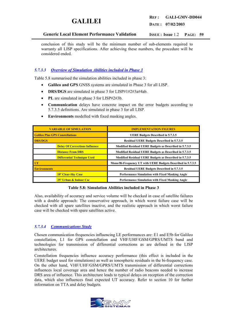
GALILEI REF :
DATE :
GALI-GMV-DD044
07/02/2003
Generic Local Element Performance Validation ISSUE : Issue 1.2 PAGE: 59
conclusion of this study will be the minimum number of sub-elements required to warranty all LISP specifications. After achieving these numbers, the procedure will be considered ended.
5.7.3.3 Overview of Simulation Abilities included in Phase 3
Table 5.8 summarised the simulation abilities included in phase 3: • Galileo and GPS GNSS systems are simulated in Phase 3 for all LISP. • DRS/DGS are simulated in phase 3 for LISP#1#2#3a#4ab. • PL are simulated in phase 3 for LISP#2#3b. • Communication delays have concrete impact on the error budgets according to
5.7.3.5 definitions. Are simulated in phase 3 for all LISP. • Environments modelled with fixed masking angles.
VARIABLE OF SIMULATION IMPLEMENTATION FIGURES
Galileo Plus GPS Constellations UERE Budgets Described in 5.7.3.5
DRS/DGS Residual UERE Budgets Described in 5.7.3.5
Delay Of Corrections Influence Modified Residual UERE Budgets as Described in 5.7.3.5
Distance From DRS Modified Residual UERE Budgets as Described in 5.7.3.5
Differential Technique Used Modified Residual UERE Budgets as Described in 5.7.3.5
UT Mono/Bi-Frequency UT with UERE Budgets Described in 5.7.3.5
Environments Residual UERE Budgets Described in 5.7.3.5
10º Clear-Sky Case Performance Simulation with Fixed Masking Angle
25º Urban & Indoor Cse Performance Simulation with Fixed Masking Angle
Table 5.8: Simulation Abilities included in Phase 3
Also, availability of accuracy and service volume will be checked in case of satellite failures with a double approach: The conservative approach, in which worst failure case will be checked with all spare satellites inactive, and the realistic approach in which worst failure case will be checked with spare satellites active.
5.7.3.4 Communications Study
Chosen communication frequencies influencing LE performances are: E1 and E5b for Galileo constellation, L1 for GPS constellation and VHF/UHF/GSM/GPRS/UMTS band and technologies for transmission of differential corrections as are defined in the LISP architectures. Constellation frequencies influence accuracy performance (this effect is included in the UERE budget used for simulations) as well as ionospheric residuals in the bi-frequency case. On the other hand, VHF/UHF/GSM/GPRS/UMTS transmission of differential corrections influences local coverage area and hence the number of radio beacons needed to increase DRS area of influence. This architecture leads to typical delays on reception of the correction data, which also influences final expected UT accuracy. Refer to section 10 for further information on TTA and delay budgets.
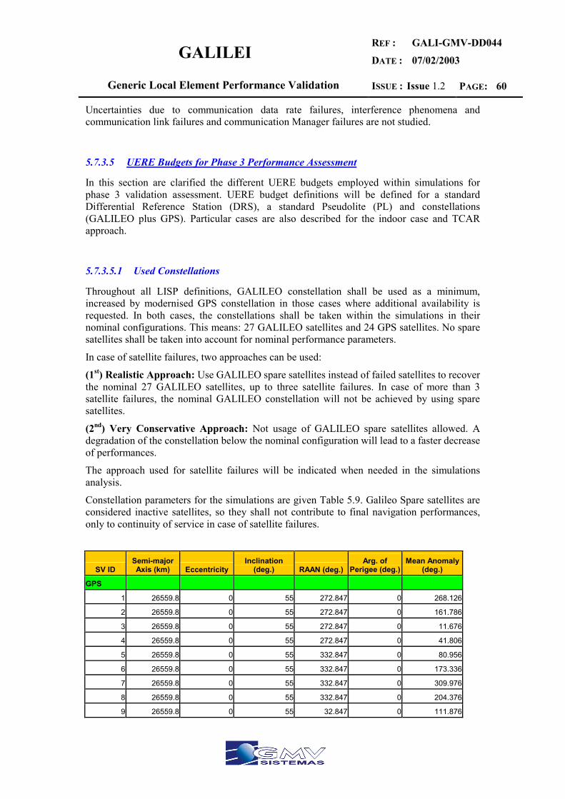
GALILEI REF :
DATE :
GALI-GMV-DD044
07/02/2003
Generic Local Element Performance Validation ISSUE : Issue 1.2 PAGE: 60
Uncertainties due to communication data rate failures, interference phenomena and communication link failures and communication Manager failures are not studied.
5.7.3.5 UERE Budgets for Phase 3 Performance Assessment
In this section are clarified the different UERE budgets employed within simulations for phase 3 validation assessment. UERE budget definitions will be defined for a standard Differential Reference Station (DRS), a standard Pseudolite (PL) and constellations (GALILEO plus GPS). Particular cases are also described for the indoor case and TCAR approach.
5.7.3.5.1 Used Constellations
Throughout all LISP definitions, GALILEO constellation shall be used as a minimum, increased by modernised GPS constellation in those cases where additional availability is requested. In both cases, the constellations shall be taken within the simulations in their nominal configurations. This means: 27 GALILEO satellites and 24 GPS satellites. No spare satellites shall be taken into account for nominal performance parameters.
In case of satellite failures, two approaches can be used:
(1st) Realistic Approach: Use GALILEO spare satellites instead of failed satellites to recover the nominal 27 GALILEO satellites, up to three satellite failures. In case of more than 3 satellite failures, the nominal GALILEO constellation will not be achieved by using spare satellites.
(2nd) Very Conservative Approach: Not usage of GALILEO spare satellites allowed. A degradation of the constellation below the nominal configuration will lead to a faster decrease of performances.
The approach used for satellite failures will be indicated when needed in the simulations analysis.
Constellation parameters for the simulations are given Table 5.9. Galileo Spare satellites are considered inactive satellites, so they shall not contribute to final navigation performances, only to continuity of service in case of satellite failures.
SV ID Semi-major Axis (km) Eccentricity
Inclination (deg.) RAAN (deg.)
Arg. of Perigee (deg.)
Mean Anomaly (deg.)
GPS
1 26559.8 0 55 272.847 0 268.126
2 26559.8 0 55 272.847 0 161.786
3 26559.8 0 55 272.847 0 11.676
4 26559.8 0 55 272.847 0 41.806
5 26559.8 0 55 332.847 0 80.956
6 26559.8 0 55 332.847 0 173.336
7 26559.8 0 55 332.847 0 309.976
8 26559.8 0 55 332.847 0 204.376
9 26559.8 0 55 32.847 0 111.876

GALILEI REF :
DATE :
GALI-GMV-DD044
07/02/2003
Generic Local Element Performance Validation ISSUE : Issue 1.2 PAGE: 61
10 26559.8 0 55 32.847 0 11.796
11 26559.8 0 55 32.847 0 339.666
12 26559.8 0 55 32.847 0 241.556
13 26559.8 0 55 92.847 0 135.226
14 26559.8 0 55 92.847 0 265.446
15 26559.8 0 55 92.847 0 35.156
16 26559.8 0 55 92.847 0 167.356
17 26559.8 0 55 152.847 0 197.046
18 26559.8 0 55 152.847 0 302.596
19 26559.8 0 55 152.847 0 333.686
20 26559.8 0 55 152.847 0 66.066
21 26559.8 0 55 212.847 0 238.886
22 26559.8 0 55 212.847 0 345.226
23 26559.8 0 55 212.847 0 105.206
24 26559.8 0 55 212.847 0 135.346
Galileo
1 29993.707 0 56 0 0 0
2 29993.707 0 56 0 0 40
3 29993.707 0 56 0 0 80
4 29993.707 0 56 0 0 120
5 29993.707 0 56 0 0 160
6 29993.707 0 56 0 0 200
7 29993.707 0 56 0 0 240
8 29993.707 0 56 0 0 280
9 29993.707 0 56 0 0 320
10 29993.707 0 56 120 0 13.33
11 29993.707 0 56 120 0 53.33
12 29993.707 0 56 120 0 93.33
13 29993.707 0 56 120 0 133.33
14 29993.707 0 56 120 0 173.33
15 29993.707 0 56 120 0 213.33
16 29993.707 0 56 120 0 253.33
17 29993.707 0 56 120 0 293.33
18 29993.707 0 56 120 0 333.33
19 29993.707 0 56 240 0 26.66
20 29993.707 0 56 240 0 66.66
21 29993.707 0 56 240 0 106.66
22 29993.707 0 56 240 0 146.66
23 29993.707 0 56 240 0 186.66
24 29993.707 0 56 240 0 226.66
25 29993.707 0 56 240 0 266.66
26 29993.707 0 56 240 0 306.66
27 29993.707 0 56 240 0 346.66
(Spare) 28 29993.707 0 56 0 0 (Inactive) 20

GALILEI REF :
DATE :
GALI-GMV-DD044
07/02/2003
Generic Local Element Performance Validation ISSUE : Issue 1.2 PAGE: 62
(Spare) 29 29993.707 0 56 120 0 (Inactive) 20
(Spare) 30 29993.707 0 56 240 0 (Inactive) 20
Table 5.9: GPS and GALILEO Simulated Constellations
5.7.3.5.2 Constellations UERE Budget
Assessed by GPS SIS and expected GALILEO SIS information extracted from DD044, Annex 1, and with UERE Budget Results (Ref: GB2/SE/TNO/0001) from Galileo Phase B2, following UERE budgets are extracted for mono and bi-frequency cases. S/A is considered always disabled along the current validation assessment. For Rural Vehicle Environment (UE2) and Safety-of-life Services (Satellite-only, SS6) the UERE ID for Galileo constellation is P-UERE 7 for bi-frequency receivers and P-UERE2 for mono-frequency receivers (SS1). Due to expected GPS modernisation, we consider the same values for mono-frequency receivers for both constellations. GPS bi-frequency UERE budget is extracted from DD044, Annex 1. For Aeronautical en Route environments (UE4) and Safety-of-life Services (Satellite-only, SS6) the UERE ID for Galileo constellation is P-UERE 9. Due to expected GPS modernisation, we consider the same values for mono-frequency receivers for both constellations. GPS bi-frequency UERE budget is extracted from DD044, Annex 1.
ELEVATION (º)
Service/Environment 5 10 15 20 30 40 50 60 90
P-UERE 2/ Degraded P-UERE 7+Margin (L1) cm 826 733 656 589 480 400 345 309 278
P-UERE 9 Degraded L1 SAS+Margin cm 2168 1939 1736 1557 1266 1051 901 805 719
Table 5.10: Mono-frequency UERE Budget for Modernised GPS and GALILEO Constellations for UE2 and UE4 environments
ELEVATION (º)
Service/Environment 5 10 15 20 30 40 50 60 90
P-UERE 7 + Margin cm 157 105 90 83 78 76 75 75 74
P-UERE 9 + Margin cm 158 106 91 84 79 78 77 76 75
Table 5.11: Bi-frequency L1/E5b UERE Budget for GALILEO Constellation for UE2 and UE4 environments
ELEVATION (º)
Service/Environment 5 10 15 20 30 40 50 60 90
GPS UERE +Margin cm 605 363 -- 219 193 166 -- -- 158
Table 5.12: Bi-frequency L1/L5 UERE Budget for GPS Constellation
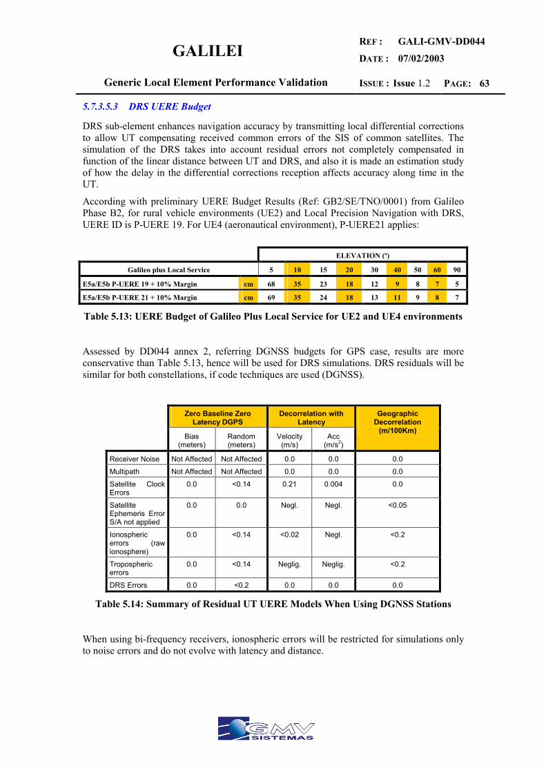
GALILEI REF :
DATE :
GALI-GMV-DD044
07/02/2003
Generic Local Element Performance Validation ISSUE : Issue 1.2 PAGE: 63
5.7.3.5.3 DRS UERE Budget
DRS sub-element enhances navigation accuracy by transmitting local differential corrections to allow UT compensating received common errors of the SIS of common satellites. The simulation of the DRS takes into account residual errors not completely compensated in function of the linear distance between UT and DRS, and also it is made an estimation study of how the delay in the differential corrections reception affects accuracy along time in the UT.
According with preliminary UERE Budget Results (Ref: GB2/SE/TNO/0001) from Galileo Phase B2, for rural vehicle environments (UE2) and Local Precision Navigation with DRS, UERE ID is P-UERE 19. For UE4 (aeronautical environment), P-UERE21 applies:
ELEVATION (º)
Galileo plus Local Service 5 10 15 20 30 40 50 60 90
E5a/E5b P-UERE 19 + 10% Margin cm 68 35 23 18 12 9 8 7 5
E5a/E5b P-UERE 21 + 10% Margin cm 69 35 24 18 13 11 9 8 7
Table 5.13: UERE Budget of Galileo Plus Local Service for UE2 and UE4 environments
Assessed by DD044 annex 2, referring DGNSS budgets for GPS case, results are more conservative than Table 5.13, hence will be used for DRS simulations. DRS residuals will be similar for both constellations, if code techniques are used (DGNSS).
Table 5.14: Summary of Residual UT UERE Models When Using DGNSS Stations
When using bi-frequency receivers, ionospheric errors will be restricted for simulations only to noise errors and do not evolve with latency and distance.
Zero Baseline Zero Latency DGPS
Decorrelation with Latency
Bias (meters)
Random (meters)
Velocity (m/s)
Acc (m/s2)
Geographic Decorrelation
(m/100Km)
Receiver Noise Not Affected Not Affected 0.0 0.0 0.0
Multipath Not Affected Not Affected 0.0 0.0 0.0
Satellite Clock Errors
0.0 <0.14 0.21 0.004 0.0
Satellite Ephemeris Error S/A not applied
0.0 0.0 Negl. Negl. <0.05
Ionospheric errors (raw ionosphere)
0.0 <0.14 <0.02 Negl. <0.2
Tropospheric errors
0.0 <0.14 Neglig. Neglig. <0.2
DRS Errors 0.0 <0.2 0.0 0.0 0.0
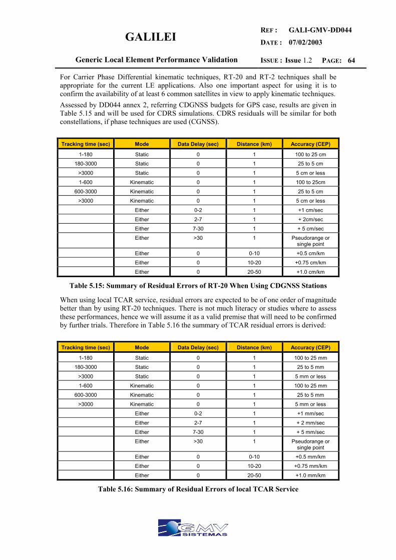
GALILEI REF :
DATE :
GALI-GMV-DD044
07/02/2003
Generic Local Element Performance Validation ISSUE : Issue 1.2 PAGE: 64
For Carrier Phase Differential kinematic techniques, RT-20 and RT-2 techniques shall be appropriate for the current LE applications. Also one important aspect for using it is to confirm the availability of at least 6 common satellites in view to apply kinematic techniques. Assessed by DD044 annex 2, referring CDGNSS budgets for GPS case, results are given in Table 5.15 and will be used for CDRS simulations. CDRS residuals will be similar for both constellations, if phase techniques are used (CGNSS). Tracking time (sec) Mode Data Delay (sec) Distance (km) Accuracy (CEP)
1-180 Static 0 1 100 to 25 cm
180-3000 Static 0 1 25 to 5 cm
>3000 Static 0 1 5 cm or less
1-600 Kinematic 0 1 100 to 25cm
600-3000 Kinematic 0 1 25 to 5 cm
>3000 Kinematic 0 1 5 cm or less
Either 0-2 1 +1 cm/sec
Either 2-7 1 + 2cm/sec
Either 7-30 1 + 5 cm/sec
Either >30 1 Pseudorange or single point
Either 0 0-10 +0.5 cm/km
Either 0 10-20 +0.75 cm/km
Either 0 20-50 +1.0 cm/km
Table 5.15: Summary of Residual Errors of RT-20 When Using CDGNSS Stations
When using local TCAR service, residual errors are expected to be of one order of magnitude better than by using RT-20 techniques. There is not much literacy or studies where to assess these performances, hence we will assume it as a valid premise that will need to be confirmed by further trials. Therefore in Table 5.16 the summary of TCAR residual errors is derived: Tracking time (sec) Mode Data Delay (sec) Distance (km) Accuracy (CEP)
1-180 Static 0 1 100 to 25 mm
180-3000 Static 0 1 25 to 5 mm
>3000 Static 0 1 5 mm or less
1-600 Kinematic 0 1 100 to 25 mm
600-3000 Kinematic 0 1 25 to 5 mm
>3000 Kinematic 0 1 5 mm or less
Either 0-2 1 +1 mm/sec
Either 2-7 1 + 2 mm/sec
Either 7-30 1 + 5 mm/sec
Either >30 1 Pseudorange or single point
Either 0 0-10 +0.5 mm/km
Either 0 10-20 +0.75 mm/km
Either 0 20-50 +1.0 mm/km
Table 5.16: Summary of Residual Errors of local TCAR Service
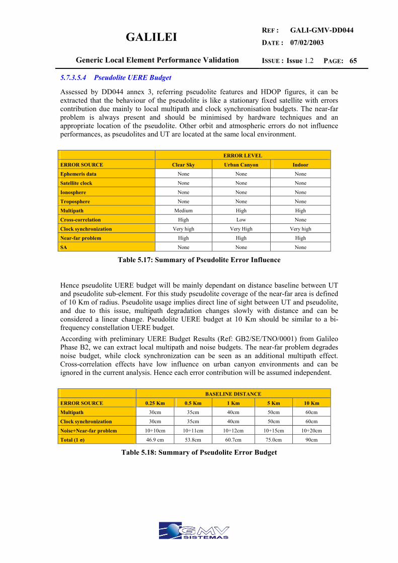
GALILEI REF :
DATE :
GALI-GMV-DD044
07/02/2003
Generic Local Element Performance Validation ISSUE : Issue 1.2 PAGE: 65
5.7.3.5.4 Pseudolite UERE Budget
Assessed by DD044 annex 3, referring pseudolite features and HDOP figures, it can be extracted that the behaviour of the pseudolite is like a stationary fixed satellite with errors contribution due mainly to local multipath and clock synchronisation budgets. The near-far problem is always present and should be minimised by hardware techniques and an appropriate location of the pseudolite. Other orbit and atmospheric errors do not influence performances, as pseudolites and UT are located at the same local environment. ERROR LEVEL
ERROR SOURCE Clear Sky Urban Canyon Indoor
Ephemeris data None None None
Satellite clock None None None
Ionosphere None None None
Troposphere None None None
Multipath Medium High High
Cross-correlation High Low None
Clock synchronization Very high Very High Very high
Near-far problem High High High
SA None None None
Table 5.17: Summary of Pseudolite Error Influence
Hence pseudolite UERE budget will be mainly dependant on distance baseline between UT and pseudolite sub-element. For this study pseudolite coverage of the near-far area is defined of 10 Km of radius. Pseudolite usage implies direct line of sight between UT and pseudolite, and due to this issue, multipath degradation changes slowly with distance and can be considered a linear change. Pseudolite UERE budget at 10 Km should be similar to a bi-frequency constellation UERE budget. According with preliminary UERE Budget Results (Ref: GB2/SE/TNO/0001) from Galileo Phase B2, we can extract local multipath and noise budgets. The near-far problem degrades noise budget, while clock synchronization can be seen as an additional multipath effect. Cross-correlation effects have low influence on urban canyon environments and can be ignored in the current analysis. Hence each error contribution will be assumed independent. BASELINE DISTANCE
ERROR SOURCE 0.25 Km 0.5 Km 1 Km 5 Km 10 Km
Multipath 30cm 35cm 40cm 50cm 60cm
Clock synchronization 30cm 35cm 40cm 50cm 60cm
Noise+Near-far problem 10+10cm 10+11cm 10+12cm 10+15cm 10+20cm
Total (1 σ) 46.9 cm 53.8cm 60.7cm 75.0cm 90cm
Table 5.18: Summary of Pseudolite Error Budget
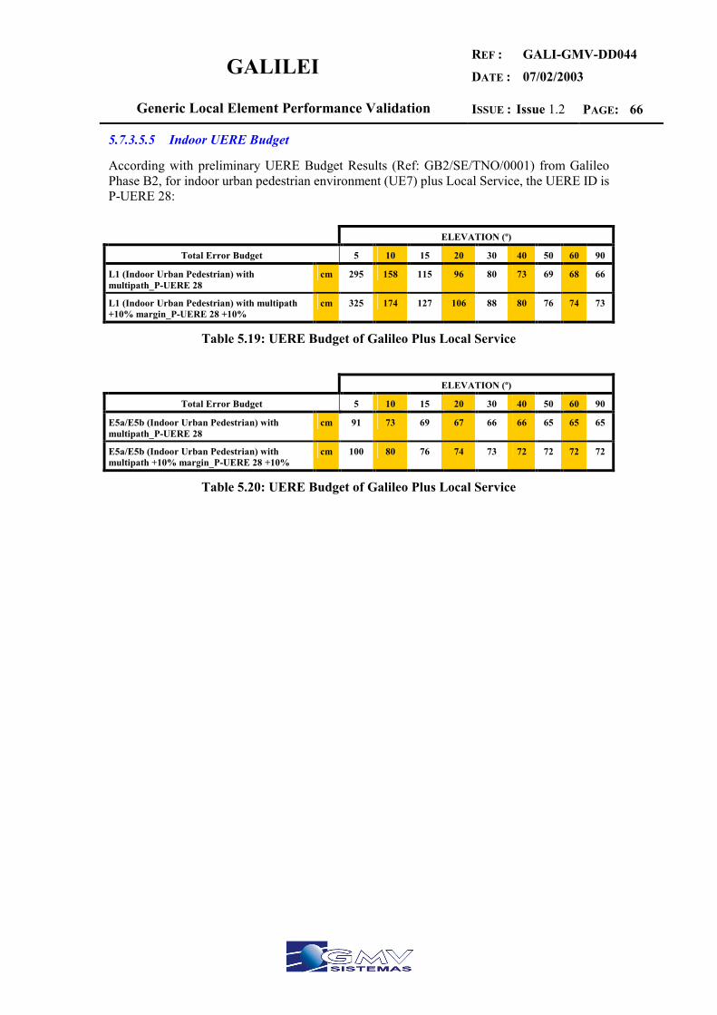
GALILEI REF :
DATE :
GALI-GMV-DD044
07/02/2003
Generic Local Element Performance Validation ISSUE : Issue 1.2 PAGE: 66
5.7.3.5.5 Indoor UERE Budget
According with preliminary UERE Budget Results (Ref: GB2/SE/TNO/0001) from Galileo Phase B2, for indoor urban pedestrian environment (UE7) plus Local Service, the UERE ID is P-UERE 28:
ELEVATION (º)
Total Error Budget 5 10 15 20 30 40 50 60 90
L1 (Indoor Urban Pedestrian) with multipath_P-UERE 28
cm 295 158 115 96 80 73 69 68 66
L1 (Indoor Urban Pedestrian) with multipath +10% margin_P-UERE 28 +10%
cm 325 174 127 106 88 80 76 74 73
Table 5.19: UERE Budget of Galileo Plus Local Service
ELEVATION (º)
Total Error Budget 5 10 15 20 30 40 50 60 90
E5a/E5b (Indoor Urban Pedestrian) with multipath_P-UERE 28
cm 91 73 69 67 66 66 65 65 65
E5a/E5b (Indoor Urban Pedestrian) with multipath +10% margin_P-UERE 28 +10%
cm 100 80 76 74 73 72 72 72 72
Table 5.20: UERE Budget of Galileo Plus Local Service

GALILEI REF :
DATE :
GALI-GMV-DD044
07/02/2003
Generic Local Element Performance Validation ISSUE : Issue 1.2 PAGE: 67
6 LISP #1 PERFORMANCE VALIDATION
In this section the validation process is carried out in order to validate the LISP 1 architecture. LISP #1 provides services on the Professional Market; sector Oil & Gas, Precision Agriculture and Environment, Clear Sky Environment, Accuracy is better or equal 0.5 m, Voice and Bi-directional communication capabilities.
6.1 PERFORMANCE REQUIREMENTS
Table 6.1 summarizes the performance requirements. Generic LISP parameters to be validated are: LISP # Navigation Communication
Accuracy (H/V) m Availability (%) TTA (sec) Voice 1-way 2-way Broadcast
1 0.5/3 99.9 1 Req. Req.
LISP # User Masking Angle Service Volume (r/h) Km UT Data Rate
1 10º 100/12 Rural Vehicle 100 kbps
Table 6.1: LISP#1 Validation Parameters.
6.2 LISP#1 GENERIC ARCHITECTURE
LIM
LE User Terminal
KMF CPSGalileo LE Service &
Operating Center
Ground (Space) basedComm Network
G(S)BCN
GalileoCore
SystemService Center
Other LE
Service Center
LEService
Provider
GALILEO Core system
Ground (Space) Based External
Nav system G(S)BEN
Add. UT SensorAUTS
DRS
Navigation signal
Non-IWAN link
Basic LE sub-element
Optional LE sub-element
External sub-element
Co-location of sub-elements
IWAN link
IWAN
6
10 4
17
13
14 15 16 18
3 1
2 5
19
20
23 22 21
User 24
25
Figure 6-1 Generic Local Element Architecture for LISP 1
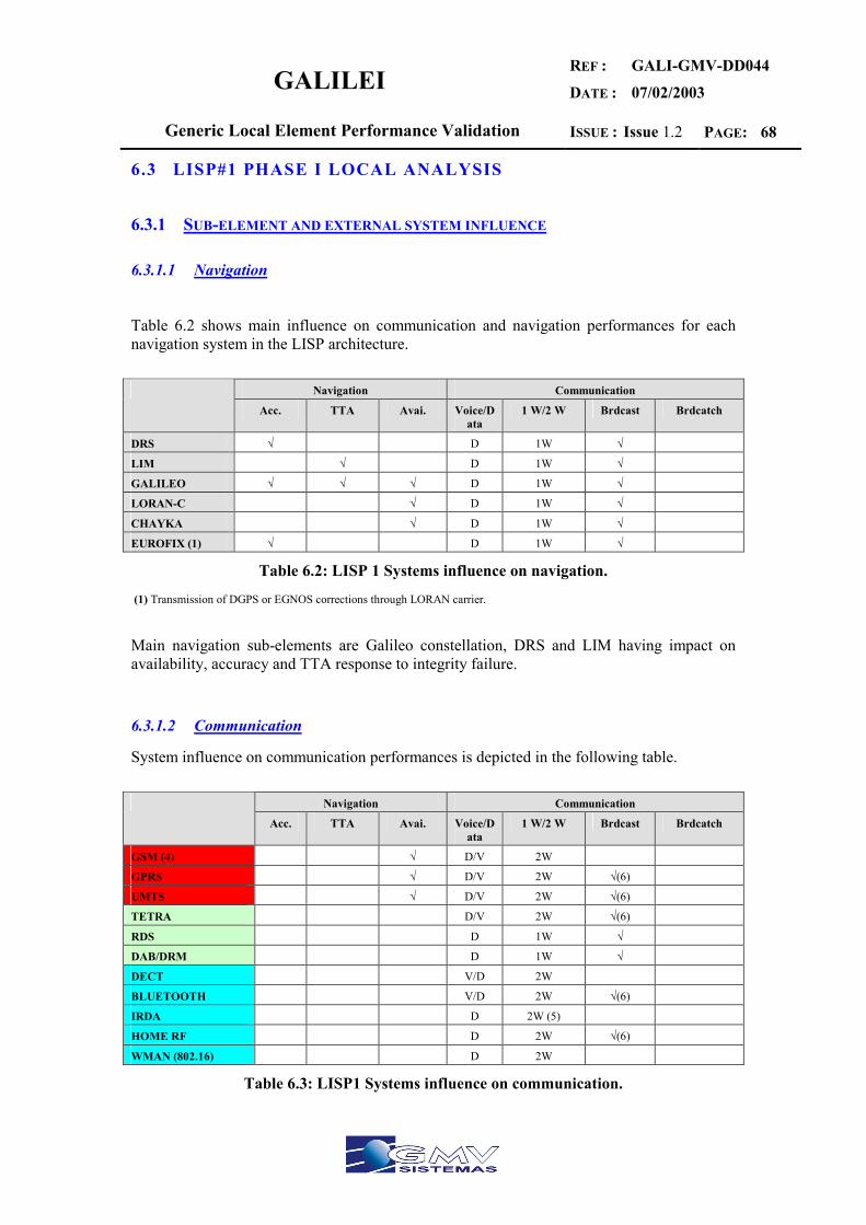
GALILEI REF :
DATE :
GALI-GMV-DD044
07/02/2003
Generic Local Element Performance Validation ISSUE : Issue 1.2 PAGE: 68
6.3 LISP#1 PHASE I LOCAL ANALYSIS
6.3.1 SUB-ELEMENT AND EXTERNAL SYSTEM INFLUENCE
6.3.1.1 Navigation
Table 6.2 shows main influence on communication and navigation performances for each navigation system in the LISP architecture.
Navigation Communication
Acc. TTA Avai. Voice/Data
1 W/2 W Brdcast Brdcatch
DRS √ D 1W √
LIM √ D 1W √
GALILEO √ √ √ D 1W √
LORAN-C √ D 1W √
CHAYKA √ D 1W √
EUROFIX (1) √ D 1W √
Table 6.2: LISP 1 Systems influence on navigation.
(1) Transmission of DGPS or EGNOS corrections through LORAN carrier.
Main navigation sub-elements are Galileo constellation, DRS and LIM having impact on availability, accuracy and TTA response to integrity failure.
6.3.1.2 Communication
System influence on communication performances is depicted in the following table.
Navigation Communication
Acc. TTA Avai. Voice/Data
1 W/2 W Brdcast Brdcatch
GSM (4) √ D/V 2W
GPRS √ D/V 2W √(6)
UMTS √ D/V 2W √(6)
TETRA D/V 2W √(6)
RDS D 1W √
DAB/DRM D 1W √
DECT V/D 2W
BLUETOOTH V/D 2W √(6)
IRDA D 2W (5)
HOME RF D 2W √(6)
WMAN (802.16) D 2W
Table 6.3: LISP1 Systems influence on communication.
GALILEI REF :
DATE :
GALI-GMV-DD044
07/02/2003
Generic Local Element Performance Validation ISSUE : Issue 1.2 PAGE: 69
[×××] Mobile cellular systems. [×××] Long range and medium range communication systems. [×××] Short range communication systems. Remarks (4) Impact on availability when used as a cellular localization system (by means of measuring the signal power or similar). (5) Semi-duplex (6) Multicast transmission
Voice and 2-Way requirements can be met by several different communication services. The chosen of one concrete solution should depend on final coverage area and communication purpose.
6.3.2 ENVIRONMENTAL CONSTRAINT IMPACT
Clear Sky scenario will get the best possible profit from the available constellations. This means that the highest level of performances should be achieved through the clear sky environment. To simulate Clear Sky environment it has been set a maximum masking angle of 10º. In this case with low performance degradation we can expect to have optimum navigation performances from the sub-elements and external systems, including: - High Availability: We consider a typical masking angle of 10 degrees. Availability and
Geometric values will be completely due to the satellite constellations configuration. - Minimum Multipath effect. - TTA: Not applicable. References for performances results in Open Sky case can be found on the annexes: - GALILEO: see the following section on annex 1:
o Section 5.5: GALILEO Accuracy Performances (Open Sky). - Differential Reference Station (DRS): see the following sections on annex 2
o Section 8: Performance Conclusions DGPS. o Section 9: Performance Conclusions CDGPS.
- Pseudolite (PL): see the following sections on annex 3 o Section 7: Conclusions.
- Space Based External Navigation System (SBEN): see the following sections on annex 5
o GPS: Section 1.6, Error Budget. o GLONASS: Section 3, Performance Measures. o EGNOS:
Section 4.11: EGNOS Performance Requirements (SARPSV7). Section 4.12: Error Budget.
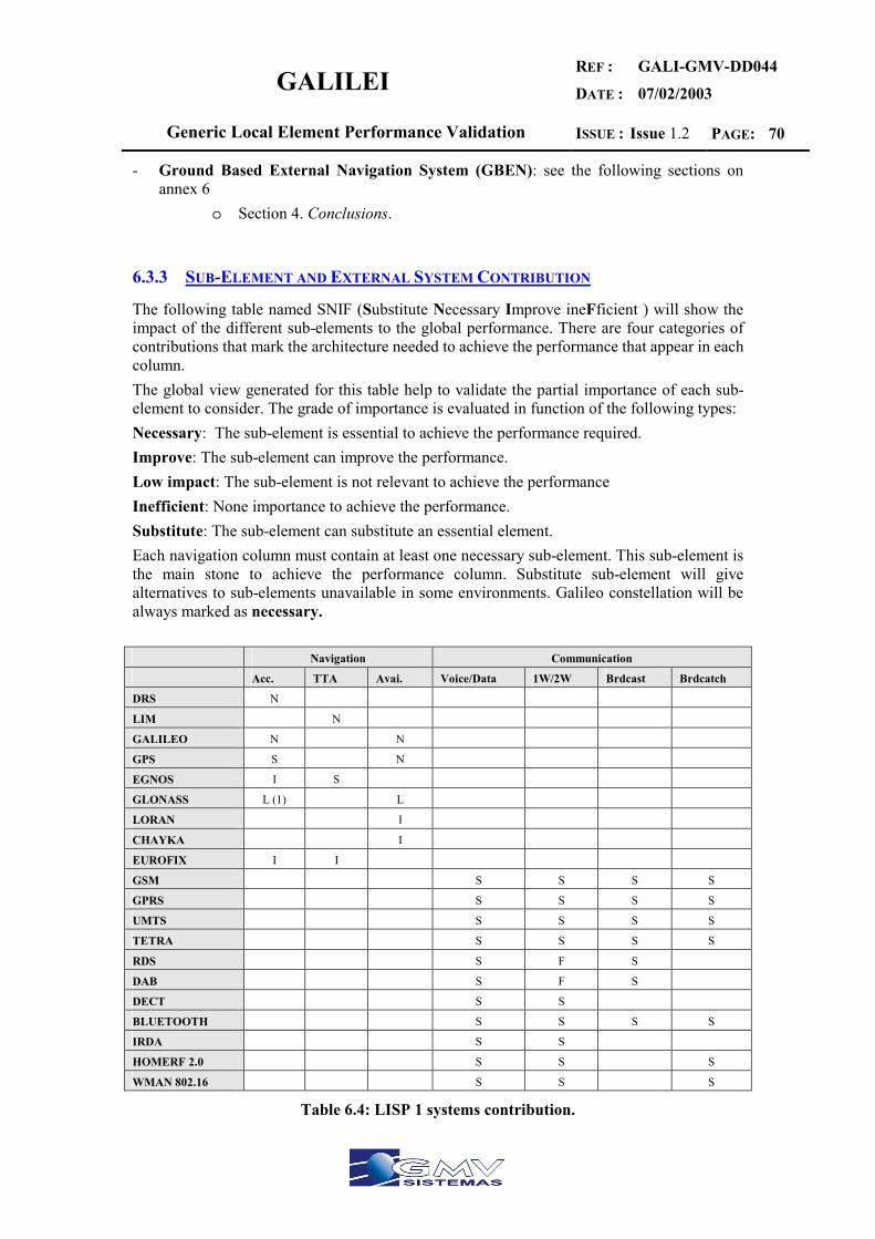
GALILEI REF :
DATE :
GALI-GMV-DD044
07/02/2003
Generic Local Element Performance Validation ISSUE : Issue 1.2 PAGE: 70
- Ground Based External Navigation System (GBEN): see the following sections on annex 6
o Section 4. Conclusions.
6.3.3 SUB-ELEMENT AND EXTERNAL SYSTEM CONTRIBUTION
The following table named SNIF (Substitute Necessary Improve ineFficient ) will show the impact of the different sub-elements to the global performance. There are four categories of contributions that mark the architecture needed to achieve the performance that appear in each column. The global view generated for this table help to validate the partial importance of each sub-element to consider. The grade of importance is evaluated in function of the following types: Necessary: The sub-element is essential to achieve the performance required. Improve: The sub-element can improve the performance. Low impact: The sub-element is not relevant to achieve the performance Inefficient: None importance to achieve the performance. Substitute: The sub-element can substitute an essential element. Each navigation column must contain at least one necessary sub-element. This sub-element is the main stone to achieve the performance column. Substitute sub-element will give alternatives to sub-elements unavailable in some environments. Galileo constellation will be always marked as necessary. Navigation Communication
Acc. TTA Avai. Voice/Data 1W/2W Brdcast Brdcatch
DRS N
LIM N
GALILEO N N
GPS S N
EGNOS I S
GLONASS L (1) L
LORAN I
CHAYKA I
EUROFIX I I
GSM S S S S
GPRS S S S S
UMTS S S S S
TETRA S S S S
RDS S F S
DAB S F S
DECT S S
BLUETOOTH S S S S
IRDA S S
HOMERF 2.0 S S S
WMAN 802.16 S S S
Table 6.4: LISP 1 systems contribution.

GALILEI REF :
DATE :
GALI-GMV-DD044
07/02/2003
Generic Local Element Performance Validation ISSUE : Issue 1.2 PAGE: 71
N = Necessary L = Low impact I = Improve F = Inefficient
S = Substitute (1) System availability is not guaranteed.
The key sub-elements to achieve accuracy performance are DRS and GALILEO. GPS can be a backup to GALILEO. This duality introduces the compatibility of DRS between GPS and GALILEO signal. The 0.5 m vertical accuracy is a requirement that can be achieved with a high performance DRS. LIM is a single sub-element that can obtain integrity performance. Only GALILEO will not reach the value required for TTA. Available performance must be obtained with GALILEO constellation. An availability study is presented in phase 2 of interoperability.
6.4 LISP#1 PHASE II. INTEROPERABILITY
The interoperability analysis is related with DD027 v1.0. Refer to annex 10 for further checks of this analysis. Phase 3 is the simulation update of phase 2 for last DD027 v1.2 version. Hence refer to LISP#1 phase 3 to check updated simulation results.
6.5 LISP#1 PHASE III. UPDATED SIMULATION RESULTS
These updated simulation results have been computed for each LISP by using a preliminary non-public version of Polaris simulation tool. This preliminary SW version has been modified by GMV Sistemas PTM SA to allow the simulation of proposed UERE budgets for the GALILEI project.
6.5.1 PROCEDURE AND VARIABLE PARAMETERS INCLUDED IN THE LISP1 ANALYSIS
Throughout this section availability of accuracy performances of LISP1 architecture is presented. Following cases have been simulated to check the recommended LISP1 architecture configuration:
1) Galileo vs Galileo plus GPS. 2) Code vs Phase RT-2 Techniques. 3) Dual vs Non-Dual Techniques (for the Galileo constellation).
The simulation has been made for horizontal accuracy of 0.5 meters and a vertical accuracy of 3 meters. Valid results are met when 99.9% of accuracy availability is reached. Throughout the preliminary study the number of satellite failures is always fixed to cero and differential corrections are perfectly synchronized with GNSS information (0 seconds of delay for reception of corrections). Also, the simulation area is 120x120 Km2 always centered

GALILEI REF :
DATE :
GALI-GMV-DD044
07/02/2003
Generic Local Element Performance Validation ISSUE : Issue 1.2 PAGE: 72
in the point (40, -5) in latitude and longitude coordinates in which is located the DRS antenna. A fixed masking angle of 10º is considered along LISP1 simulations. The main purpose of these simulations is to fix LISP1 features needed to achieve availability of 0.5 meters of Haccuracy (NSE 95%) and 3 meters of Vaccuracy (NSE 95%) with more than 99.9% of availability. When the availability of accuracy is met, the radius of availability around LE center will be extracted as an output. This radius will be the expected radius of coverage of the LE. After the final election of LISP1 architecture, to complete LISP1 simulations, the following cases are studied only for the chosen LISP1 architecture:
1) Satellite failures. 2) Delayed reception of DGNSS/CDGNSS information. 3) Coordinates variation of LE.
6.5.2 TABLES OF RESULTS
The initial results of LISP1 lead to the election of both constellations Galileo plus GPS in a dual configuration with phase techniques to achieve a radius of 69 Km for the LE with one DRS. Constellations Environment UT Technique UT Phase Sat. Failures/Delay LE Radius Coordinates (Lon, Lat)
Galileo 10º Code L1 0/0 0 (-5, 40)
Galileo 10º Code L1/E5b 0/0 0 (-5, 40)
Galileo 10º Kinematic L1 0/0 35 Km (-5, 40)
Galileo 10º Kinematic L1/E5b 0/0 55 Km (-5, 40)
Galileo +GPS 10º Code L1 0/0 5 Km (-5, 40)
Galileo +GPS 10º Code L1/E5b 0/0 8Km (-5, 40)
Galileo +GPS 10º Kinematic L1 0/0 50 Km (-5, 40)
Galileo +GPS 10º Kinematic L1/E5b 0/0 69Km (-5, 40)
Table 6.5: LISP 1 Initial Results.On variation of coordinates
The main influence on availability is due to better DOP behaviour. Constellations Environment UT Technique UT Phase Sat. Failures/Delay LE Radius Coordinates (Lon, Lat)
Galileo +GPS 10º Kinematic L1/E5b 0/0 69 Km (-5, 40)
Galileo +GPS 10º Kinematic L1/E5b 0/0 75 Km (0, 40)
Galileo +GPS 10º Kinematic L1/E5b 0/0 70 Km (5, 40)
Galileo +GPS 10º Kinematic L1/E5b 0/0 70 Km (10, 40)
Galileo +GPS 10º Kinematic L1/E5b 0/0 73 Km (-5, 45)
Galileo +GPS 10º Kinematic L1/E5b 0/0 74 Km (0, 45)
Galileo +GPS 10º Kinematic L1/E5b 0/0 73 Km (5, 45)
Galileo +GPS 10º Kinematic L1/E5b 0/0 74 Km (10, 45)
Galileo +GPS 10º Kinematic L1/E5b 0/0 74 Km (-5, 50)
Galileo +GPS 10º Kinematic L1/E5b 0/0 73 Km (0, 50)
Galileo +GPS 10º Kinematic L1/E5b 0/0 74 Km (5, 50)
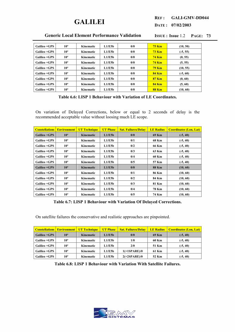
GALILEI REF :
DATE :
GALI-GMV-DD044
07/02/2003
Generic Local Element Performance Validation ISSUE : Issue 1.2 PAGE: 73
Galileo +GPS 10º Kinematic L1/E5b 0/0 75 Km (10, 50)
Galileo +GPS 10º Kinematic L1/E5b 0/0 73 Km (-5, 55)
Galileo +GPS 10º Kinematic L1/E5b 0/0 74 Km (0, 55)
Galileo +GPS 10º Kinematic L1/E5b 0/0 74 Km (5, 55)
Galileo +GPS 10º Kinematic L1/E5b 0/0 79 Km (10, 55)
Galileo +GPS 10º Kinematic L1/E5b 0/0 84 Km (-5, 60)
Galileo +GPS 10º Kinematic L1/E5b 0/0 87 Km (0, 60)
Galileo +GPS 10º Kinematic L1/E5b 0/0 84 Km (5, 60)
Galileo +GPS 10º Kinematic L1/E5b 0/0 88 Km (10, 60)
Table 6.6: LISP 1 Behaviour with Variation of LE Coordinates.
On variation of Delayed Corrections, below or equal to 2 seconds of delay is the recommended acceptable value without loosing much LE scope. Constellations Environment UT Technique UT Phase Sat. Failures/Delay LE Radius Coordinates (Lon, Lat)
Galileo +GPS 10º Kinematic L1/E5b 0/0 69 Km (-5, 40)
Galileo +GPS 10º Kinematic L1/E5b 0/1 68 Km (-5, 40)
Galileo +GPS 10º Kinematic L1/E5b 0/2 66 Km (-5, 40)
Galileo +GPS 10º Kinematic L1/E5b 0/3 63 Km (-5, 40)
Galileo +GPS 10º Kinematic L1/E5b 0/4 60 Km (-5, 40)
Galileo +GPS 10º Kinematic L1/E5b 0/5 57 Km (-5, 40)
Galileo +GPS 10º Kinematic L1/E5b 0/0 88 Km (10, 60)
Galileo +GPS 10º Kinematic L1/E5b 0/1 86 Km (10, 60)
Galileo +GPS 10º Kinematic L1/E5b 0/2 84 Km (10, 60)
Galileo +GPS 10º Kinematic L1/E5b 0/3 81 Km (10, 60)
Galileo +GPS 10º Kinematic L1/E5b 0/4 78 Km (10, 60)
Galileo +GPS 10º Kinematic L1/E5b 0/5 74 Km (10, 60)
Table 6.7: LISP 1 Behaviour with Variation Of Delayed Corrections.
On satellite failures the conservative and realistic approaches are pinpointed. Constellations Environment UT Technique UT Phase Sat. Failures/Delay LE Radius Coordinates (Lon, Lat)
Galileo +GPS 10º Kinematic L1/E5b 0/0 69 Km (-5, 40)
Galileo +GPS 10º Kinematic L1/E5b 1/0 60 Km (-5, 40)
Galileo +GPS 10º Kinematic L1/E5b 2/0 51 Km (-5, 40)
Galileo +GPS 10º Kinematic L1/E5b 1(+1SPARE)/0 61 Km (-5, 40)
Galileo +GPS 10º Kinematic L1/E5b 2(+2SPARE)/0 52 Km (-5, 40)
Table 6.8: LISP 1 Behaviour with Variation With Satellite Failures.
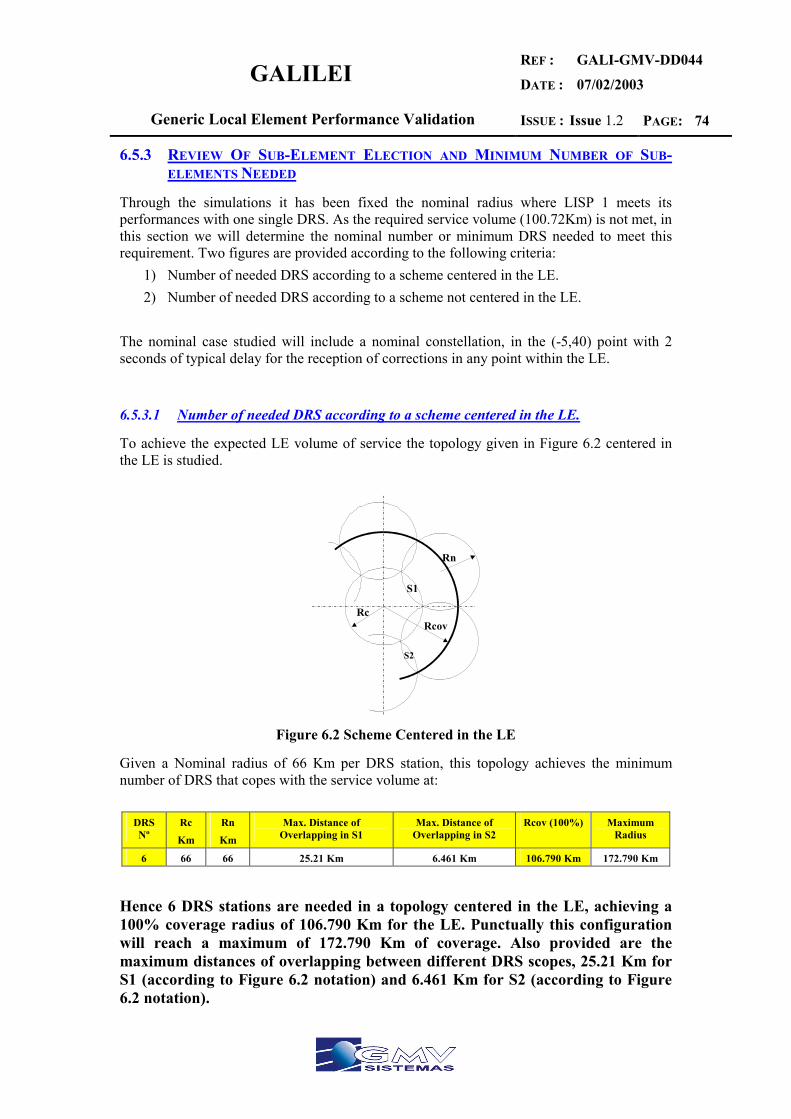
GALILEI REF :
DATE :
GALI-GMV-DD044
07/02/2003
Generic Local Element Performance Validation ISSUE : Issue 1.2 PAGE: 74
6.5.3 REVIEW OF SUB-ELEMENT ELECTION AND MINIMUM NUMBER OF SUB-ELEMENTS NEEDED
Through the simulations it has been fixed the nominal radius where LISP 1 meets its performances with one single DRS. As the required service volume (100.72Km) is not met, in this section we will determine the nominal number or minimum DRS needed to meet this requirement. Two figures are provided according to the following criteria:
1) Number of needed DRS according to a scheme centered in the LE. 2) Number of needed DRS according to a scheme not centered in the LE.
The nominal case studied will include a nominal constellation, in the (-5,40) point with 2 seconds of typical delay for the reception of corrections in any point within the LE.
6.5.3.1 Number of needed DRS according to a scheme centered in the LE.
To achieve the expected LE volume of service the topology given in Figure 6.2 centered in the LE is studied.
Rn
RcRcov
S1
S2
Figure 6.2 Scheme Centered in the LE
Given a Nominal radius of 66 Km per DRS station, this topology achieves the minimum number of DRS that copes with the service volume at:
DRS Nº
Rc Km
Rn Km
Max. Distance of Overlapping in S1
Max. Distance of Overlapping in S2
Rcov (100%) Maximum Radius
6 66 66 25.21 Km 6.461 Km 106.790 Km 172.790 Km
Hence 6 DRS stations are needed in a topology centered in the LE, achieving a 100% coverage radius of 106.790 Km for the LE. Punctually this configuration will reach a maximum of 172.790 Km of coverage. Also provided are the maximum distances of overlapping between different DRS scopes, 25.21 Km for S1 (according to Figure 6.2 notation) and 6.461 Km for S2 (according to Figure 6.2 notation).

GALILEI REF :
DATE :
GALI-GMV-DD044
07/02/2003
Generic Local Element Performance Validation ISSUE : Issue 1.2 PAGE: 75
6.5.3.2 Number of needed DRS according to a scheme not centered in the LE.
To achieve the expected LE volume of service the topology given in Figure 6.3 not centered in the LE is studied. Given a Nominal radius of 66 Km per DRS station, this topology achieves the following service volume:
DRS Nº
Rc Km
Rn Km
Max. Distance of Overlapping in S1
Max. Distance of Overlapping in S2
Rcov (100%) Maximum Radius
4 -- 66 -- 38.661 Km 93.338 Km 132 Km
Is clear that with only 2 more DRS, this topology is not achieving a 100% of service volume in 100.72Km, hence this topology does not reduce the number of DRS to achieve a service volume of 100.72 Km. This topology is therefore discarded for LISP1.
Rn
Rcov
S2
Figure 6.3 Scheme Not Centered in the LE
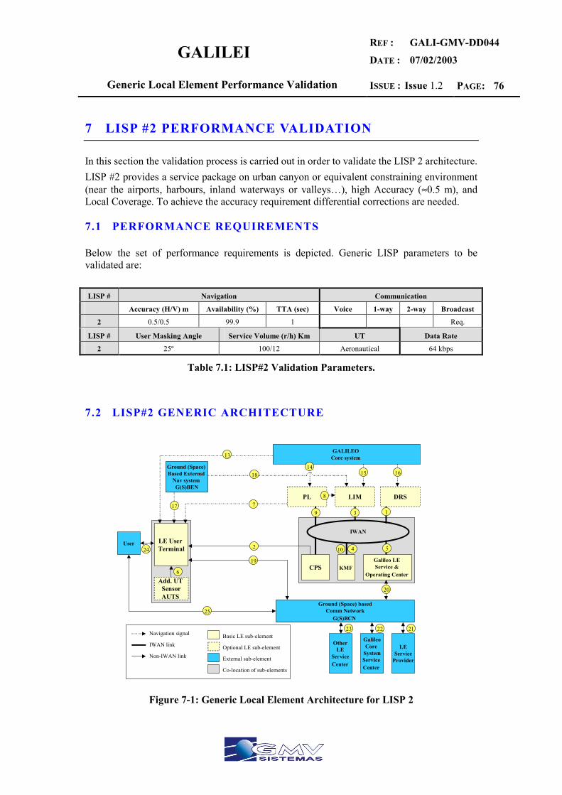
GALILEI REF :
DATE :
GALI-GMV-DD044
07/02/2003
Generic Local Element Performance Validation ISSUE : Issue 1.2 PAGE: 76
7 LISP #2 PERFORMANCE VALIDATION
In this section the validation process is carried out in order to validate the LISP 2 architecture. LISP #2 provides a service package on urban canyon or equivalent constraining environment (near the airports, harbours, inland waterways or valleys…), high Accuracy (≈0.5 m), and Local Coverage. To achieve the accuracy requirement differential corrections are needed.
7.1 PERFORMANCE REQUIREMENTS
Below the set of performance requirements is depicted. Generic LISP parameters to be validated are: LISP # Navigation Communication
Accuracy (H/V) m Availability (%) TTA (sec) Voice 1-way 2-way Broadcast
2 0.5/0.5 99.9 1 Req.
LISP # User Masking Angle Service Volume (r/h) Km UT Data Rate
2 25º 100/12 Aeronautical 64 kbps
Table 7.1: LISP#2 Validation Parameters.
7.2 LISP#2 GENERIC ARCHITECTURE
LIMPL
LE User Terminal
KMF CPSGalileo LE Service &
Operating Center
Ground (Space) basedComm Network
G(S)BCN
GalileoCore
SystemService Center
Other LE
Service Center
LEService
Provider
GALILEO Core system
Ground (Space) Based External
Nav system G(S)BEN
Add. UT SensorAUTS
DRS
Navigation signal
Non-IWAN link
Basic LE sub-element
Optional LE sub-element
External sub-element
Co-location of sub-elements
IWAN link
IWAN
6
10 4
17
13
14 15 16
7 8
18
9 3 1
2 5
19
20
23 22 21
User 24
25
Figure 7-1: Generic Local Element Architecture for LISP 2
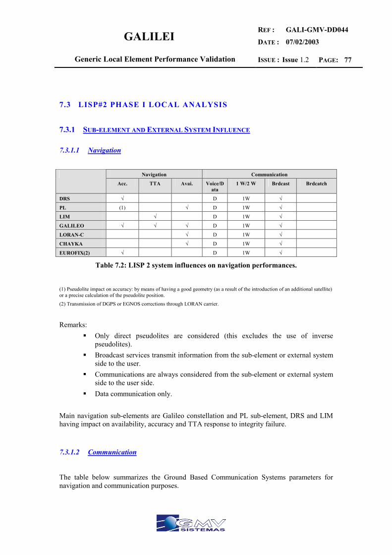
GALILEI REF :
DATE :
GALI-GMV-DD044
07/02/2003
Generic Local Element Performance Validation ISSUE : Issue 1.2 PAGE: 77
7.3 LISP#2 PHASE I LOCAL ANALYSIS
7.3.1 SUB-ELEMENT AND EXTERNAL SYSTEM INFLUENCE
7.3.1.1 Navigation
Navigation Communication
Acc. TTA Avai. Voice/Data
1 W/2 W Brdcast Brdcatch
DRS √ D 1W √
PL (1) √ D 1W √
LIM √ D 1W √
GALILEO √ √ √ D 1W √
LORAN-C √ D 1W √
CHAYKA √ D 1W √
EUROFIX(2) √ D 1W √
Table 7.2: LISP 2 system influences on navigation performances.
(1) Pseudolite impact on accuracy: by means of having a good geometry (as a result of the introduction of an additional satellite) or a precise calculation of the pseudolite position. (2) Transmission of DGPS or EGNOS corrections through LORAN carrier.
Remarks:
Only direct pseudolites are considered (this excludes the use of inverse pseudolites).
Broadcast services transmit information from the sub-element or external system side to the user.
Communications are always considered from the sub-element or external system side to the user side.
Data communication only. Main navigation sub-elements are Galileo constellation and PL sub-element, DRS and LIM having impact on availability, accuracy and TTA response to integrity failure.
7.3.1.2 Communication
The table below summarizes the Ground Based Communication Systems parameters for navigation and communication purposes.
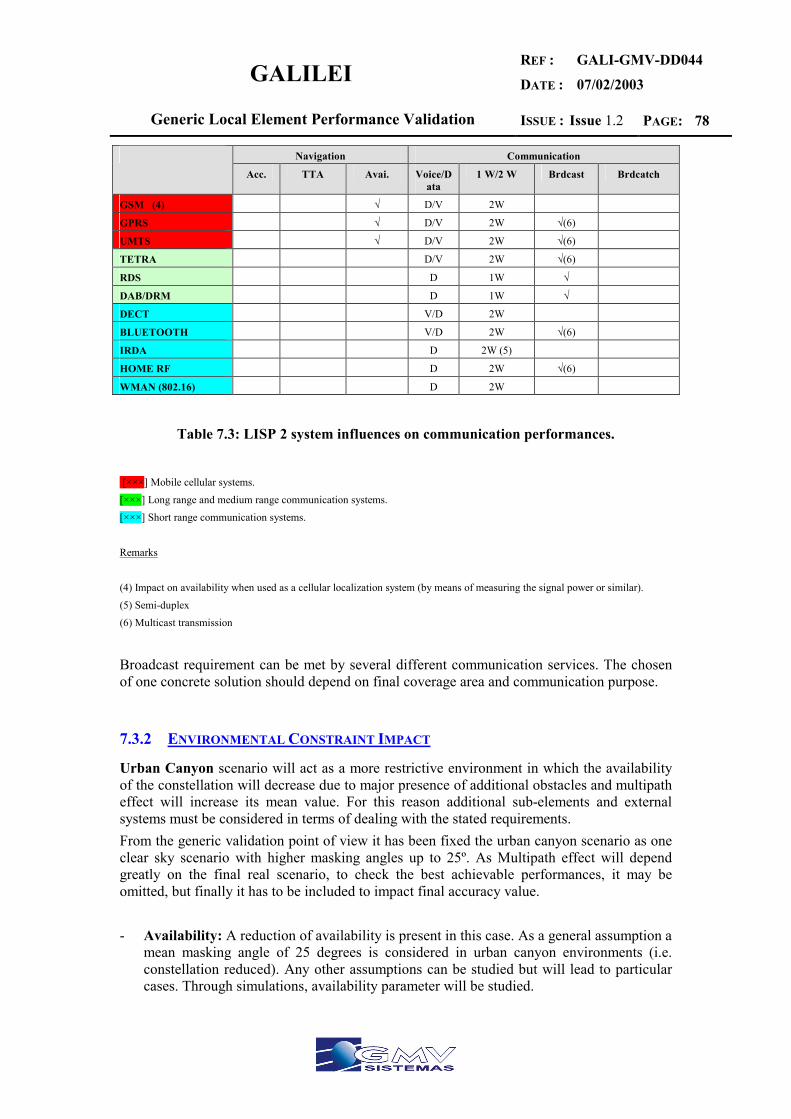
GALILEI REF :
DATE :
GALI-GMV-DD044
07/02/2003
Generic Local Element Performance Validation ISSUE : Issue 1.2 PAGE: 78
Navigation Communication
Acc. TTA Avai. Voice/Data
1 W/2 W Brdcast Brdcatch
GSM (4) √ D/V 2W
GPRS √ D/V 2W √(6)
UMTS √ D/V 2W √(6)
TETRA D/V 2W √(6)
RDS D 1W √
DAB/DRM D 1W √
DECT V/D 2W
BLUETOOTH V/D 2W √(6)
IRDA D 2W (5)
HOME RF D 2W √(6)
WMAN (802.16) D 2W
Table 7.3: LISP 2 system influences on communication performances.
[×××] Mobile cellular systems. [×××] Long range and medium range communication systems. [×××] Short range communication systems. Remarks (4) Impact on availability when used as a cellular localization system (by means of measuring the signal power or similar). (5) Semi-duplex (6) Multicast transmission
Broadcast requirement can be met by several different communication services. The chosen of one concrete solution should depend on final coverage area and communication purpose.
7.3.2 ENVIRONMENTAL CONSTRAINT IMPACT
Urban Canyon scenario will act as a more restrictive environment in which the availability of the constellation will decrease due to major presence of additional obstacles and multipath effect will increase its mean value. For this reason additional sub-elements and external systems must be considered in terms of dealing with the stated requirements. From the generic validation point of view it has been fixed the urban canyon scenario as one clear sky scenario with higher masking angles up to 25º. As Multipath effect will depend greatly on the final real scenario, to check the best achievable performances, it may be omitted, but finally it has to be included to impact final accuracy value. - Availability: A reduction of availability is present in this case. As a general assumption a
mean masking angle of 25 degrees is considered in urban canyon environments (i.e. constellation reduced). Any other assumptions can be studied but will lead to particular cases. Through simulations, availability parameter will be studied.

GALILEI REF :
DATE :
GALI-GMV-DD044
07/02/2003
Generic Local Element Performance Validation ISSUE : Issue 1.2 PAGE: 79
- Multipath effect: substantially increased as a result of signal propagation through obstacles (buildings) but is highly dependent on each particular case.
- TTA: Not applicable (only signal interference effects might be considered for this item in a local environment).
References for performances results in this case can be extrapolated from the annexes: - GALILEO: see the following section on annex 1:
o Section 2: Positioning Services (A1) o Section 7.2: PDOP Analysis and Availability.
- Differential Reference Station (DRS): see the following sections on annex 2 o Section 8: Performance Conclusions DGPS. o Section 9: Performance Conclusions CDGPS.
- Pseudolite (PL): see the following sections on annex 3 o Section 7: Conclusions.
7.3.3 SUB-ELEMENT AND EXTERNAL SYSTEM CONTRIBUTION
Navigation Communication
Acc. TTA Avai. Voice/Data 1W/2W Brdcast Brdcatch
DRS N
PL I N
LIM N
GALILEO N N
GPS S I
EGNOS I L
GLONASS L (1) L
LORAN I
CHAYKA I
EUROFIX I I
GSM S S S S
GPRS S S S S
UMTS S S S S
TETRA S S S S
RDS F F S
DAB F F S
DECT S S
BLUETOOTH S S S S
IRDA F S
HOMERF 2.0 S S S
WMAN 802.16 S S S
Table 7.4: LISP 2 Sub-element and external system contribution.

GALILEI REF :
DATE :
GALI-GMV-DD044
07/02/2003
Generic Local Element Performance Validation ISSUE : Issue 1.2 PAGE: 80
N = Necessary L = Low impact I = Improve F = Inefficient
S = Substitute (1) System Availability is not guaranteed.
EGNOS availability is highly reduced on urban environments. As it is a geostationary satellite visibility is highly determined by the street orientation. An applicable solution on this situations might be solved by the use of additional communication means to transmit EGNOS corrections. ESA’s SISNeT project is an example of this: EGNOS corrections are available at the User Terminal by including a GPRS modem and a data link to ESA’s Internet Server. The key sub-elements to achieve accuracy performance are DRS and GALILEO. GPS can be a backup to GALILEO. The 0.5 m vertical accuracy is a requirement that can be achieved with a high performance DRS. LIM is an only sub-element that can obtain integrity performance. Only GALILEO will not get the value required for TTA. Available performance should be obtained with GALILEO constellation, and PL. These elements are necessary in function of high available required. Hence PL element is the key to achieve the available performance. An availability study is presented in phase 2 of interoperability.
7.4 LISP#2 PHASE II. INTEROPERABILITY
The interoperability analysis is related with DD027 v1.0. Refer to annex 10 for further checks of this analysis. Phase 3 is the simulation update of phase 2 for last DD027 v1.2 version. Hence refer to LISP#2 phase 3 to check updated simulation results.
7.5 LISP#2 PHASE III. UPDATED SIMULATION RESULTS
These updated simulation results have been computed for each LISP by using a preliminary non-public version of Polaris simulation tool. This preliminary SW version has been modified by GMV Sistemas PTM SA to allow the simulation of proposed UERE budgets for the GALILEI project.
7.5.1 PROCEDURE AND VARIABLE PARAMETERS INCLUDED IN THE LISP2 ANALYSIS
Derived from LISP2 requirements and previous LISP 1 simulations, initially only Galileo constellation is being used for simulations. Dual Phase techniques are requested for the sub-metric accuracy on the hugest possible radius. The simulation has been made for horizontal accuracy of 0.5 meters and a vertical accuracy of 0.5 meters. Valid results are met when 99.9% of accuracy availability is reached. Throughout the preliminary study the number of satellite failures is always fixed to cero and differential corrections are perfectly synchronized with GNSS information (0 seconds of delay for reception of corrections). Also, the simulation area is 120x120 Km2 always centered
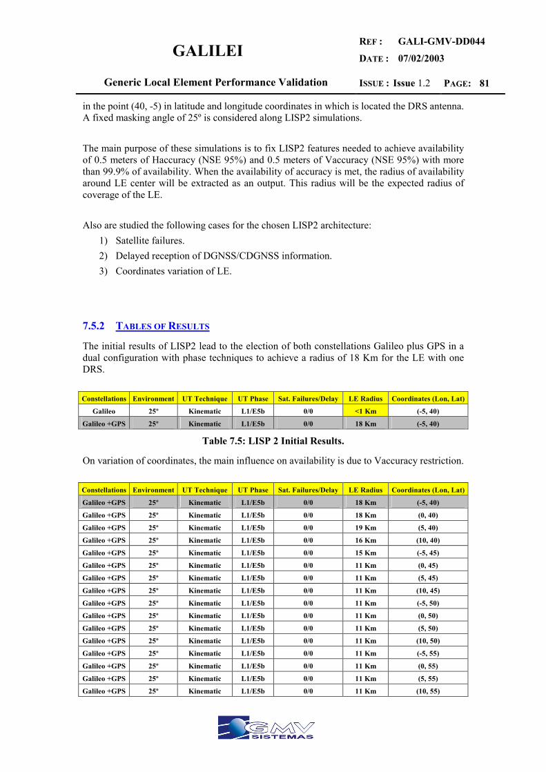
GALILEI REF :
DATE :
GALI-GMV-DD044
07/02/2003
Generic Local Element Performance Validation ISSUE : Issue 1.2 PAGE: 81
in the point (40, -5) in latitude and longitude coordinates in which is located the DRS antenna. A fixed masking angle of 25º is considered along LISP2 simulations. The main purpose of these simulations is to fix LISP2 features needed to achieve availability of 0.5 meters of Haccuracy (NSE 95%) and 0.5 meters of Vaccuracy (NSE 95%) with more than 99.9% of availability. When the availability of accuracy is met, the radius of availability around LE center will be extracted as an output. This radius will be the expected radius of coverage of the LE. Also are studied the following cases for the chosen LISP2 architecture:
1) Satellite failures. 2) Delayed reception of DGNSS/CDGNSS information. 3) Coordinates variation of LE.
7.5.2 TABLES OF RESULTS
The initial results of LISP2 lead to the election of both constellations Galileo plus GPS in a dual configuration with phase techniques to achieve a radius of 18 Km for the LE with one DRS. Constellations Environment UT Technique UT Phase Sat. Failures/Delay LE Radius Coordinates (Lon, Lat)
Galileo 25º Kinematic L1/E5b 0/0 <1 Km (-5, 40)
Galileo +GPS 25º Kinematic L1/E5b 0/0 18 Km (-5, 40)
Table 7.5: LISP 2 Initial Results.
On variation of coordinates, the main influence on availability is due to Vaccuracy restriction. Constellations Environment UT Technique UT Phase Sat. Failures/Delay LE Radius Coordinates (Lon, Lat)
Galileo +GPS 25º Kinematic L1/E5b 0/0 18 Km (-5, 40)
Galileo +GPS 25º Kinematic L1/E5b 0/0 18 Km (0, 40)
Galileo +GPS 25º Kinematic L1/E5b 0/0 19 Km (5, 40)
Galileo +GPS 25º Kinematic L1/E5b 0/0 16 Km (10, 40)
Galileo +GPS 25º Kinematic L1/E5b 0/0 15 Km (-5, 45)
Galileo +GPS 25º Kinematic L1/E5b 0/0 11 Km (0, 45)
Galileo +GPS 25º Kinematic L1/E5b 0/0 11 Km (5, 45)
Galileo +GPS 25º Kinematic L1/E5b 0/0 11 Km (10, 45)
Galileo +GPS 25º Kinematic L1/E5b 0/0 11 Km (-5, 50)
Galileo +GPS 25º Kinematic L1/E5b 0/0 11 Km (0, 50)
Galileo +GPS 25º Kinematic L1/E5b 0/0 11 Km (5, 50)
Galileo +GPS 25º Kinematic L1/E5b 0/0 11 Km (10, 50)
Galileo +GPS 25º Kinematic L1/E5b 0/0 11 Km (-5, 55)
Galileo +GPS 25º Kinematic L1/E5b 0/0 11 Km (0, 55)
Galileo +GPS 25º Kinematic L1/E5b 0/0 11 Km (5, 55)
Galileo +GPS 25º Kinematic L1/E5b 0/0 11 Km (10, 55)
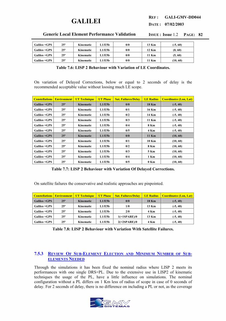
GALILEI REF :
DATE :
GALI-GMV-DD044
07/02/2003
Generic Local Element Performance Validation ISSUE : Issue 1.2 PAGE: 82
Galileo +GPS 25º Kinematic L1/E5b 0/0 13 Km (-5, 60)
Galileo +GPS 25º Kinematic L1/E5b 0/0 12 Km (0, 60)
Galileo +GPS 25º Kinematic L1/E5b 0/0 11 Km (5, 60)
Galileo +GPS 25º Kinematic L1/E5b 0/0 11 Km (10, 60)
Table 7.6: LISP 2 Behaviour with Variation of LE Coordinates.
On variation of Delayed Corrections, below or equal to 2 seconds of delay is the recommended acceptable value without loosing much LE scope. Constellations Environment UT Technique UT Phase Sat. Failures/Delay LE Radius Coordinates (Lon, Lat)
Galileo +GPS 25º Kinematic L1/E5b 0/0 18 Km (-5, 40)
Galileo +GPS 25º Kinematic L1/E5b 0/1 16 Km (-5, 40)
Galileo +GPS 25º Kinematic L1/E5b 0/2 14 Km (-5, 40)
Galileo +GPS 25º Kinematic L1/E5b 0/3 11 Km (-5, 40)
Galileo +GPS 25º Kinematic L1/E5b 0/4 8 Km (-5, 40)
Galileo +GPS 25º Kinematic L1/E5b 0/5 4 Km (-5, 40)
Galileo +GPS 25º Kinematic L1/E5b 0/0 11 Km (10, 60)
Galileo +GPS 25º Kinematic L1/E5b 0/1 10 Km (10, 60)
Galileo +GPS 25º Kinematic L1/E5b 0/2 8 Km (10, 60)
Galileo +GPS 25º Kinematic L1/E5b 0/3 5 Km (10, 60)
Galileo +GPS 25º Kinematic L1/E5b 0/4 1 Km (10, 60)
Galileo +GPS 25º Kinematic L1/E5b 0/5 0 Km (10, 60)
Table 7.7: LISP 2 Behaviour with Variation Of Delayed Corrections.
On satellite failures the conservative and realistic approaches are pinpointed. Constellations Environment UT Technique UT Phase Sat. Failures/Delay LE Radius Coordinates (Lon, Lat)
Galileo +GPS 25º Kinematic L1/E5b 0/0 18 Km (-5, 40)
Galileo +GPS 25º Kinematic L1/E5b 1/0 13 Km (-5, 40)
Galileo +GPS 25º Kinematic L1/E5b 2/0 4 Km (-5, 40)
Galileo +GPS 25º Kinematic L1/E5b 1(+1SPARE)/0 13 Km (-5, 40)
Galileo +GPS 25º Kinematic L1/E5b 2(+2SPARE)/0 4 Km (-5, 40)
Table 7.8: LISP 2 Behaviour with Variation With Satellite Failures.
7.5.3 REVIEW OF SUB-ELEMENT ELECTION AND MINIMUM NUMBER OF SUB-ELEMENTS NEEDED
Through the simulations it has been fixed the nominal radius where LISP 2 meets its performances with one single DRS+PL. Due to the extensive use in LISP2 of kinematic techniques the usage of the PL, have a little influence on simulations. The nominal configuration without a PL differs on 1 Km less of radius of scope in case of 0 seconds of delay. For 2 seconds of delay, there is no difference on including a PL or not, as the coverage

GALILEI REF :
DATE :
GALI-GMV-DD044
07/02/2003
Generic Local Element Performance Validation ISSUE : Issue 1.2 PAGE: 83
area remains the same. Hence it is recommended to omit the PL within this LISP2 configuration, according with obtained simulations. From now on, we will include only DRS stations for LISP2. As the required service volume (100.72 Km) is not met, in this section we will determine the nominal number or minimum DRS needed to meet this requirement. Two figures are provided according to the following criteria:
1) Number of needed DRS according to a scheme centered in the LE. 2) Number of needed DRS according to a scheme not centered in the LE.
The nominal case studied will include a nominal constellation, in the (-5,40) point with 2 seconds of typical delay for the reception of corrections in any point within the LE.
7.5.3.1 Number of needed DRS according to a scheme centered in the LE.
To achieve the expected LE volume of service the topology centered in the LE is studied. This model will be propagated until achieve the volume of service radius. Given a Nominal radius of 14 Km per DRS station, this topology achieves the minimum number of DRS that copes with the service volume at:
DRS Nº Rc Km
Rn Km
Max. Distance of Overlapping in S1
Max. Distance of Overlapping in S2
Rcov (100%) Maximum Radius
Level0: 11 14 14 1.370 Km 11.542 Km 36.652 Km 40.630 Km
Level1: 18 36.652 14 2.087 Km 11.133 Km 59.002 Km 62.565 Km
Level2: 24 59.002 14 2.813 Km 9.677 Km 80.175 Km 84.189 Km
Level3: 30 80.175 14 3.225 Km 8.986 Km 100.729 Km 104.950 Km
Total: 83 -- -- -- -- 100.729 Km 104.950 Km
Hence 83 DRS stations are needed in a topology centered in the LE, achieving a 100% coverage radius of 100.729 Km for the LE. Punctually this configuration will reach a maximum of 104.950 Km of coverage.
7.5.3.2 Number of needed DRS according to a scheme not centered in the LE.
To achieve the expected LE volume of service the topology not centered in the LE is studied. Given a Nominal radius of 14 Km per DRS station, this topology achieves the following service volume:
DRS Nº Rc Km
Rn Km
Max. Distance of Overlapping in S1
Max. Distance of Overlapping in S2
Rcov (100%) Maximum Radius
Level0: 4 14 14 -- 8.201 Km 19.799 Km 28 Km
Level1: 12 19.799 14 1.646 Km 11.356 Km 42.316 Km 46.153 Km
Level2: 18 42.316 14 2.726 Km 9.389 Km 63.235 Km 67.589 Km
Level3: 23 63.235 14 3.550 Km 7.933 Km 82.762 Km 87.685 Km
Level4: 27 82.762 14 4.377 Km 6.549 Km 100.759 Km 106.385 Km

GALILEI REF :
DATE :
GALI-GMV-DD044
07/02/2003
Generic Local Element Performance Validation ISSUE : Issue 1.2 PAGE: 84
Total: 84 -- -- -- -- 100.759 Km 106.385 Km
Hence this topology does not reduce the number of DRS to achieve a service volume of 100.72 Km. This topology is therefore discarded for LISP2.
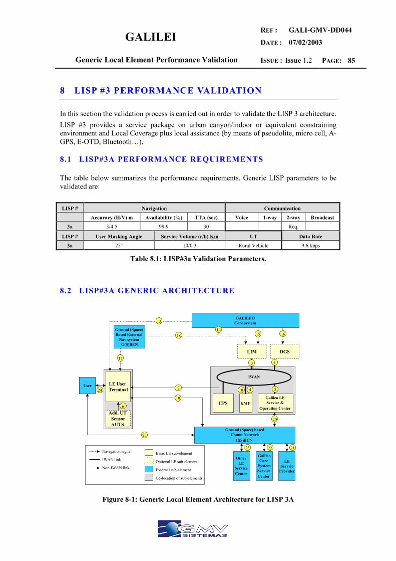
GALILEI REF :
DATE :
GALI-GMV-DD044
07/02/2003
Generic Local Element Performance Validation ISSUE : Issue 1.2 PAGE: 85
8 LISP #3 PERFORMANCE VALIDATION
In this section the validation process is carried out in order to validate the LISP 3 architecture. LISP #3 provides a service package on urban canyon/indoor or equivalent constraining environment and Local Coverage plus local assistance (by means of pseudolite, micro cell, A-GPS, E-OTD, Bluetooth…).
8.1 LISP#3A PERFORMANCE REQUIREMENTS
The table below summarizes the performance requirements. Generic LISP parameters to be validated are: LISP # Navigation Communication
Accuracy (H/V) m Availability (%) TTA (sec) Voice 1-way 2-way Broadcast
3a 3/4.5 99.9 30 Req.
LISP # User Masking Angle Service Volume (r/h) Km UT Data Rate
3a 25º 10/0.3 Rural Vehicle 9.6 kbps
Table 8.1: LISP#3a Validation Parameters.
8.2 LISP#3A GENERIC ARCHITECTURE
LIM
LE User Terminal
KMF CPSGalileo LE Service &
Operating Center
Ground (Space) basedComm Network
G(S)BCN
GalileoCore
SystemService Center
Other LE
Service Center
LEService
Provider
GALILEO Core system
Ground (Space) Based External
Nav system G(S)BEN
Add. UT SensorAUTS
DGS
Navigation signal
Non-IWAN link
Basic LE sub-element
Optional LE sub-element
External sub-element
Co-location of sub-elements
IWAN link
IWAN
6
10 4
17
13
14 15 16 18
3 1
2 5
19
20
23 22 21
User 24
25
Figure 8-1: Generic Local Element Architecture for LISP 3A
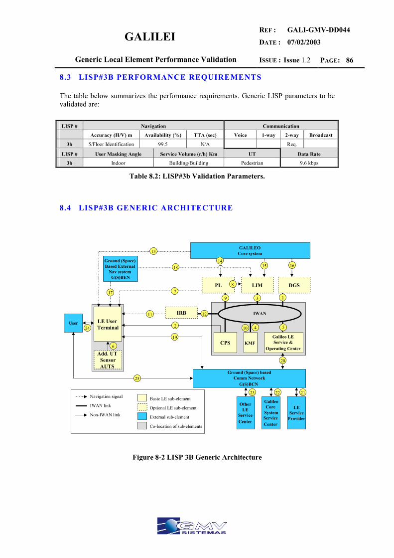
GALILEI REF :
DATE :
GALI-GMV-DD044
07/02/2003
Generic Local Element Performance Validation ISSUE : Issue 1.2 PAGE: 86
8.3 LISP#3B PERFORMANCE REQUIREMENTS
The table below summarizes the performance requirements. Generic LISP parameters to be validated are: LISP # Navigation Communication
Accuracy (H/V) m Availability (%) TTA (sec) Voice 1-way 2-way Broadcast
3b 5/Floor Identification 99.5 N/A Req.
LISP # User Masking Angle Service Volume (r/h) Km UT Data Rate
3b Indoor Building/Building Pedestrian 9.6 kbps
Table 8.2: LISP#3b Validation Parameters.
8.4 LISP#3B GENERIC ARCHITECTURE
LIMPL
LE User Terminal
KMF CPSGalileo LE Service &
Operating Center
IRB
Ground (Space) basedComm Network
G(S)BCN
GalileoCore
SystemService Center
Other LE
Service Center
LEService
Provider
GALILEO Core system
Ground (Space) Based External
Nav system G(S)BEN
Add. UT SensorAUTS
DGS
Navigation signal
Non-IWAN link
Basic LE sub-element
Optional LE sub-element
External sub-element
Co-location of sub-elements
IWAN link
IWAN
6
10 4
17
13
14 15 16
7 8
18
9 3 1
11 12
2 5
19
20
23 22 21
User 24
25
Figure 8-2 LISP 3B Generic Architecture

GALILEI REF :
DATE :
GALI-GMV-DD044
07/02/2003
Generic Local Element Performance Validation ISSUE : Issue 1.2 PAGE: 87
8.5 LISP#3A PHASE I LOCAL ANALYSIS
8.5.1 SUB-ELEMENT AND EXTERNAL SYSTEM INFLUENCE
8.5.1.1 Navigation
The table below shows the influence on communication and navigation performances for each navigation system in the LISP 3A architecture.
Navigation Communication
Acc. TTA Avai. Voice/Data
1 W/2 W Brdcast Brdcatch
DGS √ D 1W √
LIM √ D 1W √
GALILEO √ √ √ D 1W √
EGNOS √ √ D 1W √
GPS √ √ D 1W √
GLONASS √ √ D 1W √
LORAN-C √ D 1W √
CHAYKA √ D 1W √
EUROFIX(2) √ D 1W √
Table 8.3: LISP 3A Systems Influence on Navigation.
(1) See note regarding accuracy improvement by pseudolites on previous paragraphs. (2) Transmission of DGPS or EGNOS corrections through LORAN carrier.
Main navigation sub-elements are Galileo+SBEN constellations, DGS and LIM having impact on availability, accuracy and TTA response to integrity failure.
8.5.1.2 Communication
System influence on communication performances is depicted in the following table.
Navigation Communication
Acc. TTA Avai. Voice/Data
1 W/2 W Brdcast Brdcatch
GSM (4) √ D/V 2W
GPRS √ D/V 2W √(6)
UMTS √ D/V 2W √(6)
TETRA D/V 2W √(6)
RDS D 1W √
DAB/DRM D 1W √
DECT V/D 2W
BLUETOOTH V/D 2W √(6)
IRDA D 2W (5)
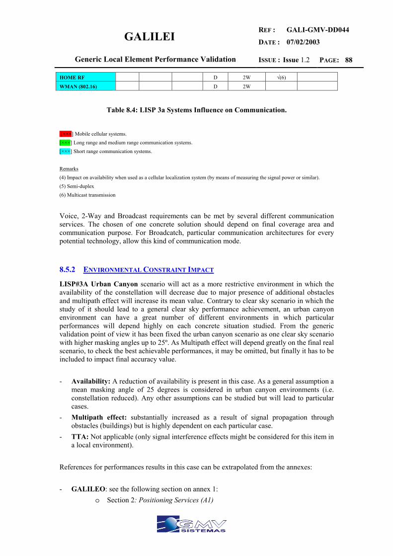
GALILEI REF :
DATE :
GALI-GMV-DD044
07/02/2003
Generic Local Element Performance Validation ISSUE : Issue 1.2 PAGE: 88
HOME RF D 2W √(6)
WMAN (802.16) D 2W
Table 8.4: LISP 3a Systems Influence on Communication.
[×××] Mobile cellular systems. [×××] Long range and medium range communication systems. [×××] Short range communication systems. Remarks (4) Impact on availability when used as a cellular localization system (by means of measuring the signal power or similar). (5) Semi-duplex (6) Multicast transmission
Voice, 2-Way and Broadcast requirements can be met by several different communication services. The chosen of one concrete solution should depend on final coverage area and communication purpose. For Broadcatch, particular communication architectures for every potential technology, allow this kind of communication mode.
8.5.2 ENVIRONMENTAL CONSTRAINT IMPACT
LISP#3A Urban Canyon scenario will act as a more restrictive environment in which the availability of the constellation will decrease due to major presence of additional obstacles and multipath effect will increase its mean value. Contrary to clear sky scenario in which the study of it should lead to a general clear sky performance achievement, an urban canyon environment can have a great number of different environments in which particular performances will depend highly on each concrete situation studied. From the generic validation point of view it has been fixed the urban canyon scenario as one clear sky scenario with higher masking angles up to 25º. As Multipath effect will depend greatly on the final real scenario, to check the best achievable performances, it may be omitted, but finally it has to be included to impact final accuracy value. - Availability: A reduction of availability is present in this case. As a general assumption a
mean masking angle of 25 degrees is considered in urban canyon environments (i.e. constellation reduced). Any other assumptions can be studied but will lead to particular cases.
- Multipath effect: substantially increased as a result of signal propagation through obstacles (buildings) but is highly dependent on each particular case.
- TTA: Not applicable (only signal interference effects might be considered for this item in a local environment).
References for performances results in this case can be extrapolated from the annexes: - GALILEO: see the following section on annex 1:
o Section 2: Positioning Services (A1)

GALILEI REF :
DATE :
GALI-GMV-DD044
07/02/2003
Generic Local Element Performance Validation ISSUE : Issue 1.2 PAGE: 89
o Section 7.2: PDOP Analysis and Availability. - Differential Reference Station (DRS): see the following sections on annex 2
o Section 8: Performance Conclusions DGPS. o Section 9: Performance Conclusions CDGPS.
- Pseudolite (PL): see the following sections on annex 3 o Section 7: Conclusions.
8.5.3 SUB-ELEMENT AND EXTERNAL SYSTEM CONTRIBUTION
Navigation Communication
Acc. TTA Avai. Voice/Data 1W/2W Brdcast Brdcatch
DGS N
LIM N
GALILEO N N
GPS S N
EGNOS I S
GLONASS L (1) L
LORAN I
CHAYKA I
EUROFIX I I
GSM S S S S
GPRS S S S S
UMTS S S S S
TETRA S S S S
RDS S F S
DAB S F S
DECT S S
BLUETOOTH S S S S
IRDA S S
HOMERF 2.0 S S S
WMAN 802.16 S S S
Table 8.5: LISP 3A Sub-Element and External System Contribution.
N = Necessary L = Low impact I = Improve F = Inefficient
S = Substitute (1) System Availability is not guaranteed.
The key sub-elements to achieve accuracy performance are DGS and GALILEO. GPS can be a backup to GALILEO. This introduces the compatibility of DGS between GPS and GALILEO signal. The 1.0 m vertical accuracy is a requirement that can be achieved with DGS and GALILEO.
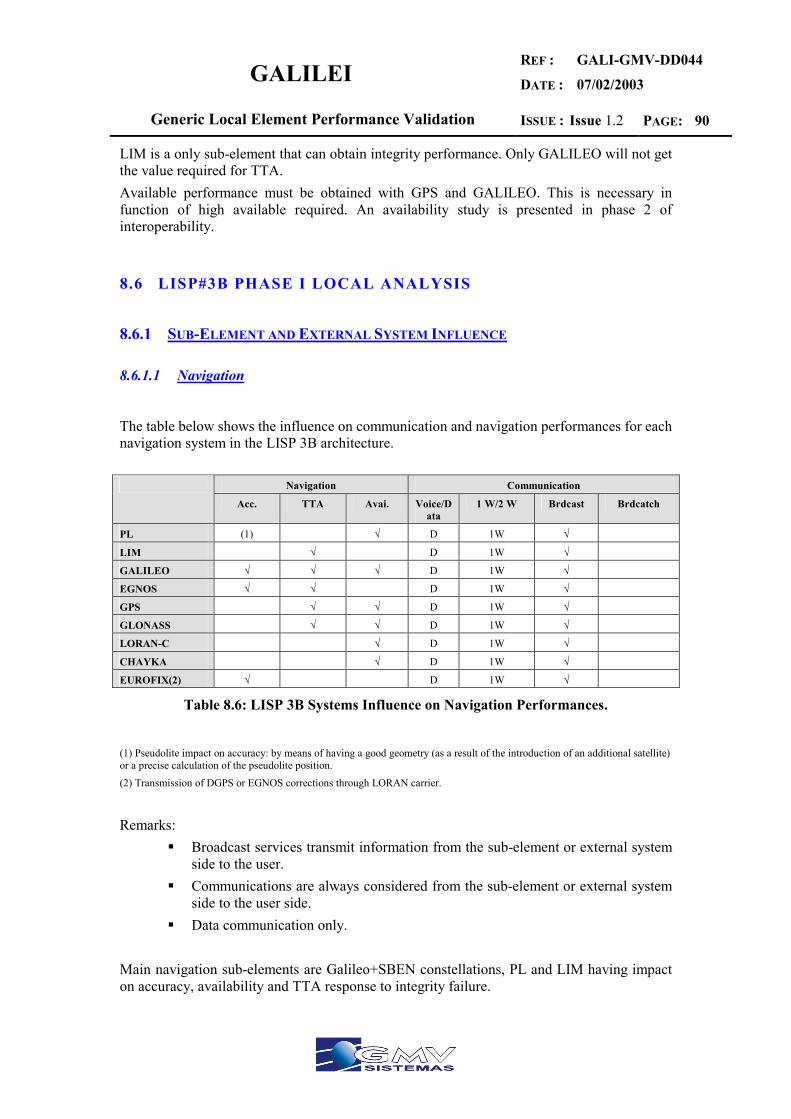
GALILEI REF :
DATE :
GALI-GMV-DD044
07/02/2003
Generic Local Element Performance Validation ISSUE : Issue 1.2 PAGE: 90
LIM is a only sub-element that can obtain integrity performance. Only GALILEO will not get the value required for TTA. Available performance must be obtained with GPS and GALILEO. This is necessary in function of high available required. An availability study is presented in phase 2 of interoperability.
8.6 LISP#3B PHASE I LOCAL ANALYSIS
8.6.1 SUB-ELEMENT AND EXTERNAL SYSTEM INFLUENCE
8.6.1.1 Navigation
The table below shows the influence on communication and navigation performances for each navigation system in the LISP 3B architecture.
Navigation Communication
Acc. TTA Avai. Voice/Data
1 W/2 W Brdcast Brdcatch
PL (1) √ D 1W √
LIM √ D 1W √
GALILEO √ √ √ D 1W √
EGNOS √ √ D 1W √
GPS √ √ D 1W √
GLONASS √ √ D 1W √
LORAN-C √ D 1W √
CHAYKA √ D 1W √
EUROFIX(2) √ D 1W √
Table 8.6: LISP 3B Systems Influence on Navigation Performances.
(1) Pseudolite impact on accuracy: by means of having a good geometry (as a result of the introduction of an additional satellite) or a precise calculation of the pseudolite position. (2) Transmission of DGPS or EGNOS corrections through LORAN carrier.
Remarks:
Broadcast services transmit information from the sub-element or external system side to the user.
Communications are always considered from the sub-element or external system side to the user side.
Data communication only. Main navigation sub-elements are Galileo+SBEN constellations, PL and LIM having impact on accuracy, availability and TTA response to integrity failure.
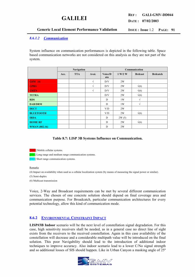
GALILEI REF :
DATE :
GALI-GMV-DD044
07/02/2003
Generic Local Element Performance Validation ISSUE : Issue 1.2 PAGE: 91
8.6.1.2 Communication
System influence on communication performances is depicted in the following table. Space based communication networks are not considered on this analysis as they are not part of the system.
Navigation Communication
Acc. TTA Avai. Voice/Data
1 W/2 W Brdcast Brdcatch
GSM (4) √ D/V 2W
GPRS √ D/V 2W √(6)
UMTS √ D/V 2W √(6)
TETRA D/V 2W √(6)
RDS D 1W √
DAB/DRM D 1W √
DECT V/D 2W
BLUETOOTH V/D 2W √(6)
IRDA D 2W (5)
HOME RF D 2W √(6)
WMAN (802.16) D 2W
Table 8.7: LISP 3B Systems Influence on Communication.
[×××] Mobile cellular systems. [×××] Long range and medium range communication systems. [×××] Short range communication systems. Remarks (4) Impact on availability when used as a cellular localization system (by means of measuring the signal power or similar). (5) Semi-duplex (6) Multicast transmission
Voice, 2-Way and Broadcast requirements can be met by several different communication services. The chosen of one concrete solution should depend on final coverage area and communication purpose. For Broadcatch, particular communication architectures for every potential technology, allow this kind of communication mode.
8.6.2 ENVIRONMENTAL CONSTRAINT IMPACT
LISP#3B Indoor scenario will be the next level of constellation signal degradation. For this case, high sensitivity receivers shall be needed, as in a general case no direct line of sight exists from the receivers to the received constellation. Again in this case availability of the constellation will decrease and a considerable multipath value will be introduced on the final solution. This poor Navigability should lead to the introduction of additional indoor techniques to improve accuracy. Also indoor scenario lead to a lower C/No signal strength and so additional losses of SIS should happen. Like in Urban Canyon a masking angle of 25º

GALILEI REF :
DATE :
GALI-GMV-DD044
07/02/2003
Generic Local Element Performance Validation ISSUE : Issue 1.2 PAGE: 92
will be used, and if no additional signal augmentation systems (like Pseudolites acting as transceivers) are used, a penalization of 2 less received satellites will apply. - Availability: A reduction of availability is present in this case. As a general assumption a
minimum masking angle of 25 degrees is considered for indoor environments (i.e. constellation reduced). Any other assumptions can be studied but will lead to particular cases.
- Multipath effect: substantially increased as a result of signal propagation through obstacles (buildings) but is highly dependent on each particular case.
- TTA: Not applicable (only signal interference effects might be considered for this item in a local environment).
8.6.3 SUB-ELEMENT AND EXTERNAL SYSTEM CONTRIBUTION Navigation Communication
Acc. TTA Avai. Voice/Data 1W/2W Brdcast Brdcatch
PL I N
LIM I
GALILEO N N N
GPS S N
EGNOS I I
GLONASS L (1) L
LORAN I
CHAYKA I
EUROFIX I I
GSM S S S S
GPRS S S S S
UMTS S S S S
TETRA S S S S
RDS S F S
DAB S F S
DECT S S
BLUETOOTH S S S S
IRDA S S
HOMERF 2.0 S S S
WMAN 802.16 S S S
Table 8.8: LISP 3b Sub-element and external system contribution.
N = Necessary L = Low impact I = Improve F = Inefficient
S = Substitute
(1) System Availability is not guaranteed.
GALILEI REF :
DATE :
GALI-GMV-DD044
07/02/2003
Generic Local Element Performance Validation ISSUE : Issue 1.2 PAGE: 93
EGNOS availability is highly reduced on urban environments. As geostationary satellite visibility is highly determined by the street orientation. An applicable solution on this situations might be solved by the use of additional communication means to transmit EGNOS corrections. ESA’s SISNeT project is an example of this: EGNOS corrections are available at the User Terminal by including a GPRS modem and a data link to ESA’s Internet Server. The key sub-element to achieve accuracy performance is GALILEO. GPS can be a backup to GALILEO. The 5 m vertical accuracy is a requirement that can be achieved without a DRS. LIM is an only sub-element that can obtain integrity performance. Only GALILEO will not get the value required for TTA. Available performance must be obtained with GPS and GALILEO, and PL. There elements are necessary in function of high available required. PL element is the key to achieve the available performance. An availability study is presented in phase 2 of interoperability.
8.7 LISP#3A#3B PHASE II. INTEROPERABILITY
The interoperability analysis is related with DD027 v1.0. Refer to annex 10 for further checks of this analysis. Phase 3 is the simulation update of phase 2 for last DD027 v1.2 version. Hence refer to LISP#3a#3b phase 3 to check updated simulation results.
8.8 LISP#3A PHASE III. UPDATED SIMULATION RESULTS
These updated simulation results have been computed for each LISP by using a preliminary non-public version of Polaris simulation tool. This preliminary SW version has been modified by GMV Sistemas PTM SA to allow the simulation of proposed UERE budgets for the GALILEI project.
8.8.1 PROCEDURE AND VARIABLE PARAMETERS INCLUDED IN THE LISP3A ANALYSIS
Throughout this section availability of accuracy performances of LISP3a architecture is presented. Following cases have been simulated to check the recommended LISP3a architecture configuration:
1) Galileo vs Galileo plus GPS. 2) Code vs Phase RT-2 Techniques. 3) Dual vs NoDual Techniques (for the Galileo constellation).
The simulation has been made for an horizontal accuracy of 3 meters and a vertical accuracy of 4.5 meters. Valid results are met when 99.9% of accuracy availability is reached. Throughout the preliminary study the number of satellite failures is always fixed to cero and differential corrections are perfectly synchronized with GNSS information (0 seconds of delay for reception of corrections). Also, the simulation area is 120x120 Km2 always centered in the point (40, -5) in latitude and longitude coordinates in which is located the DRS antenna. A fixed masking angle of 25º is considered along LISP3a simulations.

GALILEI REF :
DATE :
GALI-GMV-DD044
07/02/2003
Generic Local Element Performance Validation ISSUE : Issue 1.2 PAGE: 94
The main purpose of these simulations is to fix LISP3a features needed to achieve availability of 3 meters of Haccuracy (NSE 95%) and 4.5 meters of Vaccuracy (NSE 95%) with more than 99.9% of availability. When the availability of accuracy is met, the radius of availability around LE center will be extracted as an output. This radius will be the expected radius of coverage of the LE. After the final election of LISP3a architecture, to complete LISP3a simulations, the following cases are studied only for the chosen LISP3a architecture:
1) Satellite failures. 2) Delayed reception of DGNSS/CDGNSS information. 3) Coordinates variation of LE.
8.8.2 TABLES OF RESULTS
The initial results of LISP3a lead to the election of both constellations Galileo plus GPS in a single frequency configuration with code techniques to achieve a radius far over 100 Km for the LE with one DRS. Constellations Environment UT Technique UT Phase Sat. Failures/Delay LE Radius Coordinates (Lon, Lat)
Galileo 25º Code L1 0/0 0 (-5, 40)
Galileo 25º Code L1/E5b 0/0 0 (-5, 40)
Galileo 25º Kinematic L1 0/0 0 (-5, 40)
Galileo 25º Kinematic L1/E5b 0/0 0 (-5, 40)
Galileo +GPS 25º Code L1 0/0 >100 Km (-5, 40)
Galileo +GPS 25º Code L1/E5b 0/0 >100 Km (-5, 40)
Galileo +GPS 25º Kinematic L1 0/0 >100 Km (-5, 40)
Galileo +GPS 25º Kinematic L1/E5b 0/0 >100 Km (-5, 40)
Table 8.9: LISP 3a Initial Results.
On variation of coordinates, the main influence on availability is due to better DOP behaviour. Constellations Environment UT Technique UT Phase Sat. Failures/Delay LE Radius Coordinates (Lon, Lat)
Galileo +GPS 25º Code L1 0/0 >100 Km (-5, 40)
Galileo +GPS 25º Code L1 0/0 >100 Km (0, 40)
Galileo +GPS 25º Code L1 0/0 >100 Km (5, 40)
Galileo +GPS 25º Code L1 0/0 >100 Km (10, 40)
Galileo +GPS 25º Code L1 0/0 >100 Km (-5, 45)
Galileo +GPS 25º Code L1 0/0 >100 Km (0, 45)
Galileo +GPS 25º Code L1 0/0 >100 Km (5, 45)
Galileo +GPS 25º Code L1 0/0 >100 Km (10, 45)
Galileo +GPS 25º Code L1 0/0 >100 Km (-5, 50)
Galileo +GPS 25º Code L1 0/0 >100 Km (0, 50)
Galileo +GPS 25º Code L1 0/0 >100 Km (5, 50)
Galileo +GPS 25º Code L1 0/0 >100 Km (10, 50)
Galileo +GPS 25º Code L1 0/0 >100 Km (-5, 55)

GALILEI REF :
DATE :
GALI-GMV-DD044
07/02/2003
Generic Local Element Performance Validation ISSUE : Issue 1.2 PAGE: 95
Galileo +GPS 25º Code L1 0/0 >100 Km (0, 55)
Galileo +GPS 25º Code L1 0/0 >100 Km (5, 55)
Galileo +GPS 25º Code L1 0/0 >100 Km (10, 55)
Galileo +GPS 25º Code L1 0/0 >100 Km (-5, 60)
Galileo +GPS 25º Code L1 0/0 >100 Km (0, 60)
Galileo +GPS 25º Code L1 0/0 >100 Km (5, 60)
Galileo +GPS 25º Code L1 0/0 >100 Km (10, 60)
Table 8.10: LISP 3a Behaviour with Variation of LE Coordinates.
On variation of Delayed Corrections, below or equal to 1 seconds of delay is the recommended acceptable value without loosing much LE scope.
Constellations Environment UT Technique UT Phase Sat. Failures/Delay LE Radius Coordinates (Lon, Lat)
Galileo +GPS 25º Code L1 0/0 >100 Km (-5, 40)
Galileo +GPS 25º Code L1 0/1 >100 Km (-5, 40)
Galileo +GPS 25º Code L1 0/2 >100 Km (-5, 40)
Galileo +GPS 25º Code L1 0/3 16Km (95%)0 (-5, 40)
Galileo +GPS 25º Code L1 0/4 0 (-5, 40)
Galileo +GPS 25º Code L1 0/5 0 (-5, 40)
Galileo +GPS 25º Code L1 0/0 >100 Km (10, 60)
Galileo +GPS 25º Code L1 0/1 >100 Km (10, 60)
Galileo +GPS 25º Code L1 0/2 0 (10, 60)
Galileo +GPS 25º Code L1 0/3 0 (10, 60)
Galileo +GPS 25º Code L1 0/4 0 (10, 60)
Galileo +GPS 25º Code L1 0/5 0 (10, 60)
Table 8.11: LISP 3a Behaviour with Variation Of Delayed Corrections.
On satellite failures the conservative and realistic approaches are pinpointed. Constellations Environment UT Technique UT Phase Sat. Failures/Delay LE Radius Coordinates (Lon, Lat)
Galileo +GPS 25º Code L1 0/0 >100 Km (-5, 40)
Galileo +GPS 25º Code L1 1/0 >100 Km (-5, 40)
Galileo +GPS 25º Code L1 2/0 30 Km (-5, 40)
Galileo +GPS 25º Code L1 1(+1SPARE)/0 >100 Km (-5, 40)
Galileo +GPS 25º Code L1 2(+2SPARE)/0 45 Km (-5, 40)
Table 8.12: LISP 3a Behaviour with Variation With Satellite Failures.
8.8.3 REVIEW OF SUB-ELEMENT ELECTION AND MINIMUM NUMBER OF SUB-ELEMENTS NEEDED
Through the simulations it has been fixed the nominal radius where LISP 3a meets its performances with one single DRS. The nominal case studied will include a nominal
GALILEI REF :
DATE :
GALI-GMV-DD044
07/02/2003
Generic Local Element Performance Validation ISSUE : Issue 1.2 PAGE: 96
constellation, in the (-5,40) point with 1 seconds of typical delay (short baselines) for the reception of corrections in any point within the LE (Service Volume fixed at 10.0045 Km). Simulations indicate that volume service is over 100Km, hence, the minimum number of DRS to be included are 1DRS.
8.9 LISP#3B PHASE III. UPDATED SIMULATION RESULTS
These updated simulation results have been computed for each LISP by using a preliminary non-public version of Polaris simulation tool. This preliminary SW version has been modified by GMV Sistemas PTM SA to allow the simulation of proposed UERE budgets for the GALILEI project.
8.9.1 PROCEDURE AND VARIABLE PARAMETERS INCLUDED IN THE LISP3B ANALYSIS
Throughout this section availability of accuracy performances of LISP3b architecture is presented. Following cases have been simulated to check the recommended LISP3b architecture configuration:
1) Galileo vs Galileo plus GPS. 2) IndoorL1 vs. Indoor E5b/E5a.
The simulation has been made for an horizontal accuracy of 5 meters. Valid results are met when 99.5% of accuracy availability is reached. Also, the simulation area is 10x10 Km2 always centered in the point (40, -5) in latitude and longitude coordinates. A fixed masking angle of 25 (indoor) is considered along LISP3b simulations. The main purpose of these simulations is to fix LISP3b features needed to achieve availability of 5 meters of Haccuracy (NSE 95%) with more than 99.5% of availability. When the availability of accuracy is met, the radius of availability around LE center will be extracted as an output. This radius will be the expected radius of coverage of the LE. After the final election of LISP3b architecture, to complete LISP3b simulations, the following cases are studied only for the chosen LISP3b architecture:
1) Satellite failures. 2) Coordinates variation of LE.
8.9.2 TABLES OF RESULTS
The initial results of LISP3b lead to the election of both constellations Galileo plus GPS in a indoor E5a/E5b configuration to achieve a radius of over 100Km for the LE with the proposed indoor UERE model.
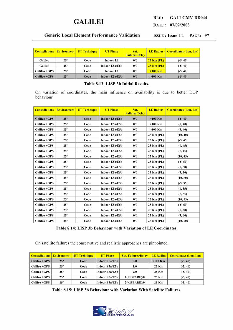
GALILEI REF :
DATE :
GALI-GMV-DD044
07/02/2003
Generic Local Element Performance Validation ISSUE : Issue 1.2 PAGE: 97
Constellations Environment UT Technique UT Phase Sat.
Failures/DelayLE Radius Coordinates (Lon, Lat)
Galileo 25º Code Indoor L1 0/0 25 Km (PL) (-5, 40)
Galileo 25º Code Indoor E5a/E5b 0/0 25 Km (PL) (-5, 40)
Galileo +GPS 25º Code Indoor L1 0/0 >100 Km (-5, 40)
Galileo +GPS 25º Code Indoor E5a/E5b 0/0 >100 Km (-5, 40)
Table 8.13: LISP 3b Initial Results.
On variation of coordinates, the main influence on availability is due to better DOP behaviour. Constellations Environment UT Technique UT Phase Sat.
Failures/DelayLE Radius Coordinates (Lon, Lat)
Galileo +GPS 25º Code Indoor E5a/E5b 0/0 >100 Km (-5, 40)
Galileo +GPS 25º Code Indoor E5a/E5b 0/0 >100 Km (0, 40)
Galileo +GPS 25º Code Indoor E5a/E5b 0/0 >100 Km (5, 40)
Galileo +GPS 25º Code Indoor E5a/E5b 0/0 25 Km (PL) (10, 40)
Galileo +GPS 25º Code Indoor E5a/E5b 0/0 25 Km (PL) (-5, 45)
Galileo +GPS 25º Code Indoor E5a/E5b 0/0 25 Km (PL) (0, 45)
Galileo +GPS 25º Code Indoor E5a/E5b 0/0 25 Km (PL) (5, 45)
Galileo +GPS 25º Code Indoor E5a/E5b 0/0 25 Km (PL) (10, 45)
Galileo +GPS 25º Code Indoor E5a/E5b 0/0 25 Km (PL) (-5, 50)
Galileo +GPS 25º Code Indoor E5a/E5b 0/0 25 Km (PL) (0, 50)
Galileo +GPS 25º Code Indoor E5a/E5b 0/0 25 Km (PL) (5, 50)
Galileo +GPS 25º Code Indoor E5a/E5b 0/0 25 Km (PL) (10, 50)
Galileo +GPS 25º Code Indoor E5a/E5b 0/0 25 Km (PL) (-5, 55)
Galileo +GPS 25º Code Indoor E5a/E5b 0/0 25 Km (PL) (0, 55)
Galileo +GPS 25º Code Indoor E5a/E5b 0/0 25 Km (PL) (5, 55)
Galileo +GPS 25º Code Indoor E5a/E5b 0/0 25 Km (PL) (10, 55)
Galileo +GPS 25º Code Indoor E5a/E5b 0/0 25 Km (PL) (-5, 60)
Galileo +GPS 25º Code Indoor E5a/E5b 0/0 25 Km (PL) (0, 60)
Galileo +GPS 25º Code Indoor E5a/E5b 0/0 25 Km (PL) (5, 60)
Galileo +GPS 25º Code Indoor E5a/E5b 0/0 25 Km (PL) (10, 60)
Table 8.14: LISP 3b Behaviour with Variation of LE Coordinates.
On satellite failures the conservative and realistic approaches are pinpointed.
Constellations Environment UT Technique UT Phase Sat. Failures/Delay LE Radius Coordinates (Lon, Lat)
Galileo +GPS 25º Code Indoor E5a/E5b 0/0 >100 Km (-5, 40)
Galileo +GPS 25º Code Indoor E5a/E5b 1/0 25 Km (-5, 40)
Galileo +GPS 25º Code Indoor E5a/E5b 2/0 25 Km (-5, 40)
Galileo +GPS 25º Code Indoor E5a/E5b 1(+1SPARE)/0 25 Km (-5, 40)
Galileo +GPS 25º Code Indoor E5a/E5b 2(+2SPARE)/0 25 Km (-5, 40)
Table 8.15: LISP 3b Behaviour with Variation With Satellite Failures.
GALILEI REF :
DATE :
GALI-GMV-DD044
07/02/2003
Generic Local Element Performance Validation ISSUE : Issue 1.2 PAGE: 98
8.9.3 REVIEW OF SUB-ELEMENT ELECTION AND MINIMUM NUMBER OF SUB-ELEMENTS NEEDED
Through the simulations it has been fixed the nominal radius where LISP 3b meets its performances with indoor technology and one single PL. It can be seen that the influence of the PL makes final performances to meet the requirements when PL is available, hence is mandatory the presence of the PL element. In the simulations, the volume service is the same as the PL coverage (direct line of sight), which has been set to 25 Km according to the UERE model. This preliminary radius meets the expected service volume (building volume). The only restriction, is of course availability of PL element. Hence, the minimum number of PL to be included are 1PL.

GALILEI REF :
DATE :
GALI-GMV-DD044
07/02/2003
Generic Local Element Performance Validation ISSUE : Issue 1.2 PAGE: 99
9 LISP #4 PERFORMANCE VALIDATION
In this section the validation process is carried out in order to validate the LISP 4 architecture. LISP#4 provides a service within High to Very High Accuracy (5 mm to 0.1 m) for Professional market for Scientific Real Time and Non Real Time applications (mainly). This LISP could be share in two LISP:
LISP #4A with communication and LISP #4B without communication.
9.1 LISP#4A PERFORMANCE REQUIREMENTS
The table shows the performance requirements. Generic LISP parameters to be validated are: LISP # Navigation Communication
Accuracy (H/V) m Availability (%) TTA (sec) Voice 1-way 2-way Broadcast
4a 0.01/0.02 99.5 10 Req.
LISP # User Masking Angle Service Volume (r/h) Km UT Data Rate
4a 25º N/A Urban Vehicle 100 kbps
Table 9.1: LISP#4a Validation Parameters.
9.2 LISP#4B PERFORMANCE REQUIREMENTS
The table shows the performance requirements. Generic LISP parameters to be validated are: LISP # Navigation Communication
Accuracy (H/V) m Availability (%) TTA (sec) Voice 1-way 2-way Broadcast
4b 0.1/0.1 99.5 10
LISP # User Masking Angle Service Volume (r/h) Km UT Data Rate
4b 10º N/A Rural Vehicle
Table 9.2: LISP#4b Validation Parameters.
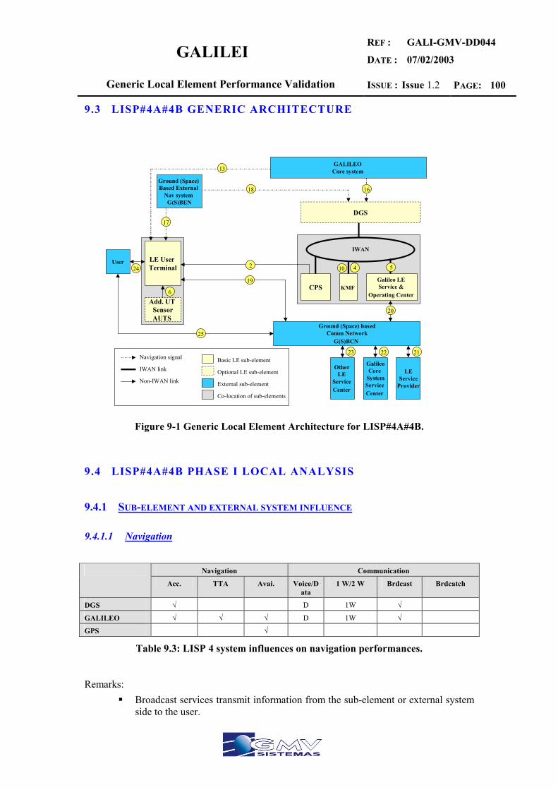
GALILEI REF :
DATE :
GALI-GMV-DD044
07/02/2003
Generic Local Element Performance Validation ISSUE : Issue 1.2 PAGE: 100
9.3 LISP#4A#4B GENERIC ARCHITECTURE
LE User Terminal
KMF CPSGalileo LE Service &
Operating Center
Ground (Space) basedComm Network
G(S)BCN
GalileoCore
SystemService Center
Other LE
Service Center
LEService
Provider
GALILEO Core system
Ground (Space) Based External
Nav system G(S)BEN
Add. UT SensorAUTS
DGS
Navigation signal
Non-IWAN link
Basic LE sub-element
Optional LE sub-element
External sub-element
Co-location of sub-elements
IWAN link
IWAN
6
10 4
17
13
16 18
2 5
19
20
23 22 21
User 24
25
Figure 9-1 Generic Local Element Architecture for LISP#4A#4B.
9.4 LISP#4A#4B PHASE I LOCAL ANALYSIS
9.4.1 SUB-ELEMENT AND EXTERNAL SYSTEM INFLUENCE
9.4.1.1 Navigation
Navigation Communication
Acc. TTA Avai. Voice/Data
1 W/2 W Brdcast Brdcatch
DGS √ D 1W √
GALILEO √ √ √ D 1W √
GPS √
Table 9.3: LISP 4 system influences on navigation performances.
Remarks:
Broadcast services transmit information from the sub-element or external system side to the user.

GALILEI REF :
DATE :
GALI-GMV-DD044
07/02/2003
Generic Local Element Performance Validation ISSUE : Issue 1.2 PAGE: 101
Communications are always considered from the sub-element or external system side to the user side.
Data communication only. Main navigation sub-elements are Galileo+SBEN constellations and DGS having impact on availability and accuracy.
9.4.1.2 Communication
The table below summarizes the Ground Based Communication Systems parameters for navigation and communication purposes.
Navigation Communication
Acc. TTA Avai. Voice/Data
1 W/2 W Brdcast Brdcatch
GSM (4) √ D/V 2W
GPRS √ D/V 2W √(6)
UMTS √ D/V 2W √(6)
TETRA D/V 2W √(6)
RDS D 1W √
DAB/DRM D 1W √
DECT V/D 2W
BLUETOOTH V/D 2W √(6)
IRDA D 2W (5)
HOME RF D 2W √(6)
WMAN (802.16) D 2W
Table 9.4: LISP 4 system influences on communication performances.
[×××] Mobile cellular systems. [×××] Long range and medium range communication systems. [×××] Short range communication systems.
Remarks (4) Impact on availability when used as a cellular localization system (by means of measuring the signal power or similar). (5) Semi-duplex (6) Multicast transmission
Voice and 2-Way requirements can be met by several different communication services. The chosen of one concrete solution should depend on final coverage area and communication purpose.
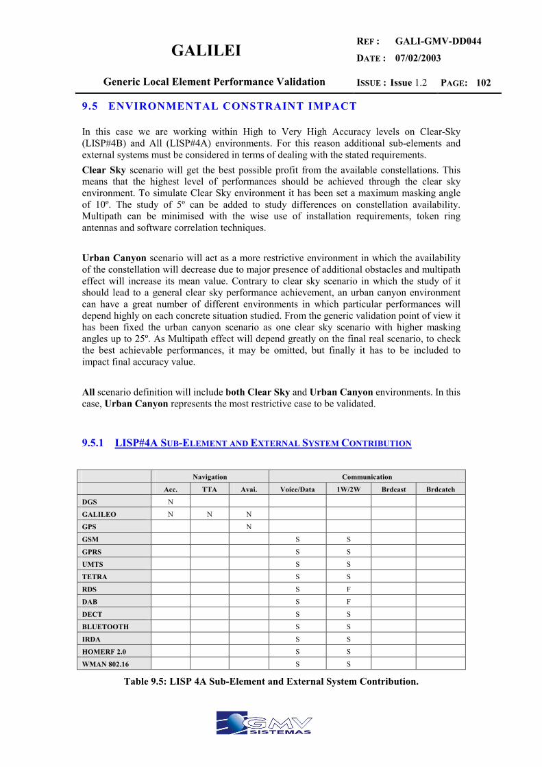
GALILEI REF :
DATE :
GALI-GMV-DD044
07/02/2003
Generic Local Element Performance Validation ISSUE : Issue 1.2 PAGE: 102
9.5 ENVIRONMENTAL CONSTRAINT IMPACT
In this case we are working within High to Very High Accuracy levels on Clear-Sky (LISP#4B) and All (LISP#4A) environments. For this reason additional sub-elements and external systems must be considered in terms of dealing with the stated requirements. Clear Sky scenario will get the best possible profit from the available constellations. This means that the highest level of performances should be achieved through the clear sky environment. To simulate Clear Sky environment it has been set a maximum masking angle of 10º. The study of 5º can be added to study differences on constellation availability. Multipath can be minimised with the wise use of installation requirements, token ring antennas and software correlation techniques. Urban Canyon scenario will act as a more restrictive environment in which the availability of the constellation will decrease due to major presence of additional obstacles and multipath effect will increase its mean value. Contrary to clear sky scenario in which the study of it should lead to a general clear sky performance achievement, an urban canyon environment can have a great number of different environments in which particular performances will depend highly on each concrete situation studied. From the generic validation point of view it has been fixed the urban canyon scenario as one clear sky scenario with higher masking angles up to 25º. As Multipath effect will depend greatly on the final real scenario, to check the best achievable performances, it may be omitted, but finally it has to be included to impact final accuracy value. All scenario definition will include both Clear Sky and Urban Canyon environments. In this case, Urban Canyon represents the most restrictive case to be validated.
9.5.1 LISP#4A SUB-ELEMENT AND EXTERNAL SYSTEM CONTRIBUTION
Navigation Communication
Acc. TTA Avai. Voice/Data 1W/2W Brdcast Brdcatch
DGS N
GALILEO N N N
GPS N
GSM S S
GPRS S S
UMTS S S
TETRA S S
RDS S F
DAB S F
DECT S S
BLUETOOTH S S
IRDA S S
HOMERF 2.0 S S
WMAN 802.16 S S
Table 9.5: LISP 4A Sub-Element and External System Contribution.

GALILEI REF :
DATE :
GALI-GMV-DD044
07/02/2003
Generic Local Element Performance Validation ISSUE : Issue 1.2 PAGE: 103
N = Necessary L = Low impact I = Improve F = Inefficient
S = Substitute
The key sub-elements to achieve accuracy performance are DGS and GALILEO. GPS can be a backup to GALILEO. Available performance must be obtained with GALILEO+GPS constellations. An availability study is presented in phase 2 of interoperability.
9.5.2 LISP#4B SUB-ELEMENT AND EXTERNAL SYSTEM CONTRIBUTION
Navigation Communication
Acc. TTA Avai. Voice/Data 1W/2W Brdcast Brdcatch
DGS N
GALILEO N N N
GPS N
Table 9.6: LISP 4B Sub-Element and External System Contribution.
N = Necessary L = Low impact I = Improve F = Inefficient
S = Substitute
The key sub-elements to achieve accuracy performance are DGS and GALILEO. GPS can be a backup to GALILEO. Available performance must be obtained with GALILEO+GPS constellations. An availability study is presented in phase 2 of interoperability.
9.6 LISP#4A#4B PHASE II. INTEROPERABILITY
The interoperability analysis is related with DD027 v1.0. Refer to annex 10 for further checks of this analysis. Phase 3 is the simulation update of phase 2 for last DD027 v1.2 version. Hence refer to LISP#4a#4b phase 3 to check updated simulation results.
9.7 LISP#4A PHASE III. UPDATED SIMULATION RESULTS
These updated simulation results have been computed for each LISP by using a preliminary non-public version of Polaris simulation tool. This preliminary SW version has been modified by GMV Sistemas PTM SA to allow the simulation of proposed UERE budgets for the GALILEI project.

GALILEI REF :
DATE :
GALI-GMV-DD044
07/02/2003
Generic Local Element Performance Validation ISSUE : Issue 1.2 PAGE: 104
9.7.1 PROCEDURE AND VARIABLE PARAMETERS INCLUDED IN THE LISP4A ANALYSIS
Throughout this section availability of accuracy performances of LISP4a architecture is presented. Following cases have been simulated to check the recommended LISP4a architecture configuration:
1) Galileo vs Galileo plus GPS. 2) Dual vs NoDual Techniques (for the Galileo constellation).
The simulation has been made for an horizontal accuracy of 0.01 meters and a vertical accuracy of 0.02 meters. Valid results are met when 99.5% of accuracy availability is reached. Throughout the preliminary study the number of satellite failures is always fixed to cero and differential corrections are perfectly synchronized with GNSS information (0 seconds of delay for reception of corrections). Also, the simulation area is 120x120 Km2 always centered in the point (40, -5) in latitude and longitude coordinates in which is located the DGS antenna. A fixed masking angle of 25º is considered along LISP4a simulations. The main purpose of these simulations is to fix LISP4a features needed to achieve availability of 0.01 meters of Haccuracy (NSE 95%) and 0.02 meters of Vaccuracy (NSE 95%) with more than 99.5% of availability. When the availability of accuracy is met, the radius of availability around LE center will be extracted as an output. This radius will be the expected radius of coverage of the LE. After the final election of LISP4a architecture, to complete LISP4a simulations, the following cases are studied only for the chosen LISP4a architecture:
1) Satellite failures. 2) Delayed reception of DGNSS/CDGNSS information. 3) Coordinates variation of LE.
9.7.2 TABLES OF RESULTS
The initial results of LISP4a lead to the election of both constellations Galileo plus GPS in a single frequency configuration with TCAR techniques to achieve a radius of 2 Km for the LE with one DGS. Constellations Environment UT Technique UT Phase Sat. Failures/Delay LE Radius Coordinates (Lon, Lat)
Galileo 25º TCAR L1 0/0 0 Km (-5, 40)
Galileo 25º TCAR L1/E5b 0/0 0 Km (-5, 40)
Galileo +GPS 25º TCAR L1 0/0 2 Km (-5, 40)
Galileo +GPS 25º TCAR L1/E5b 0/0 2 Km (-5, 40)
Table 9.7: LISP 4a Initial Results.
On variation of coordinates, the main influence on availability is due to better DOP behaviour.
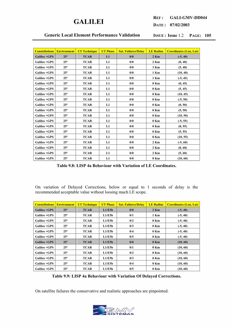
GALILEI REF :
DATE :
GALI-GMV-DD044
07/02/2003
Generic Local Element Performance Validation ISSUE : Issue 1.2 PAGE: 105
Constellations Environment UT Technique UT Phase Sat. Failures/Delay LE Radius Coordinates (Lon, Lat)
Galileo +GPS 25º TCAR L1 0/0 2 Km (-5, 40)
Galileo +GPS 25º TCAR L1 0/0 2 Km (0, 40)
Galileo +GPS 25º TCAR L1 0/0 3 Km (5, 40)
Galileo +GPS 25º TCAR L1 0/0 1 Km (10, 40)
Galileo +GPS 25º TCAR L1 0/0 1 Km (-5, 45)
Galileo +GPS 25º TCAR L1 0/0 0 Km (0, 45)
Galileo +GPS 25º TCAR L1 0/0 0 Km (5, 45)
Galileo +GPS 25º TCAR L1 0/0 0 Km (10, 45)
Galileo +GPS 25º TCAR L1 0/0 0 Km (-5, 50)
Galileo +GPS 25º TCAR L1 0/0 0 Km (0, 50)
Galileo +GPS 25º TCAR L1 0/0 0 Km (5, 50)
Galileo +GPS 25º TCAR L1 0/0 0 Km (10, 50)
Galileo +GPS 25º TCAR L1 0/0 0 Km (-5, 55)
Galileo +GPS 25º TCAR L1 0/0 0 Km (0, 55)
Galileo +GPS 25º TCAR L1 0/0 0 Km (5, 55)
Galileo +GPS 25º TCAR L1 0/0 0 Km (10, 55)
Galileo +GPS 25º TCAR L1 0/0 2 Km (-5, 60)
Galileo +GPS 25º TCAR L1 0/0 2 Km (0, 60)
Galileo +GPS 25º TCAR L1 0/0 2 Km (5, 60)
Galileo +GPS 25º TCAR L1 0/0 0 Km (10, 60)
Table 9.8: LISP 4a Behaviour with Variation of LE Coordinates.
On variation of Delayed Corrections, below or equal to 1 seconds of delay is the recommended acceptable value without loosing much LE scope. Constellations Environment UT Technique UT Phase Sat. Failures/Delay LE Radius Coordinates (Lon, Lat)
Galileo +GPS 25º TCAR L1/E5b 0/0 2 Km (-5, 40)
Galileo +GPS 25º TCAR L1/E5b 0/1 1 Km (-5, 40)
Galileo +GPS 25º TCAR L1/E5b 0/2 0 Km (-5, 40)
Galileo +GPS 25º TCAR L1/E5b 0/3 0 Km (-5, 40)
Galileo +GPS 25º TCAR L1/E5b 0/4 0 Km (-5, 40)
Galileo +GPS 25º TCAR L1/E5b 0/5 0 Km (-5, 40)
Galileo +GPS 25º TCAR L1/E5b 0/0 0 Km (10, 60)
Galileo +GPS 25º TCAR L1/E5b 0/1 0 Km (10, 60)
Galileo +GPS 25º TCAR L1/E5b 0/2 0 Km (10, 60)
Galileo +GPS 25º TCAR L1/E5b 0/3 0 Km (10, 60)
Galileo +GPS 25º TCAR L1/E5b 0/4 0 Km (10, 60)
Galileo +GPS 25º TCAR L1/E5b 0/5 0 Km (10, 60)
Table 9.9: LISP 4a Behaviour with Variation Of Delayed Corrections.
On satellite failures the conservative and realistic approaches are pinpointed.

GALILEI REF :
DATE :
GALI-GMV-DD044
07/02/2003
Generic Local Element Performance Validation ISSUE : Issue 1.2 PAGE: 106
Constellations Environment UT Technique UT Phase Sat. Failures/Delay LE Radius Coordinates (Lon, Lat)
Galileo +GPS 25º TCAR L1/E5b 0/0 2 Km (-5, 40)
Galileo +GPS 25º TCAR L1/E5b 1/0 0 Km (-5, 40)
Galileo +GPS 25º TCAR L1/E5b 2/0 0 Km (-5, 40)
Galileo +GPS 25º TCAR L1/E5b 1(+1SPARE)/0 0 Km (-5, 40)
Galileo +GPS 25º TCAR L1/E5b 2(+2SPARE)/0 0 Km (-5, 40)
Table 9.10: LISP 4a Behaviour with Variation With Satellite Failures.
9.7.3 REVIEW OF SUB-ELEMENT ELECTION AND MINIMUM NUMBER OF SUB-ELEMENTS NEEDED
Not applicable as there is no service volume defined. Typical coverage radius per DGS station is 1 to 2 Km at a maximum.
9.8 LISP#4B PHASE III. UPDATED SIMULATION RESULTS
These updated simulation results have been computed for each LISP by using a preliminary non-public version of Polaris simulation tool. This preliminary SW version has been modified by GMV Sistemas PTM SA to allow the simulation of proposed UERE budgets for the GALILEI project.
9.8.1 PROCEDURE AND VARIABLE PARAMETERS INCLUDED IN THE LISP4B ANALYSIS
Throughout this section availability of accuracy performances of LISP4b architecture is presented. Following cases have been simulated to check the recommended LISP4b architecture configuration:
1) Galileo vs Galileo plus GPS. 2) Dual vs NoDual Techniques (for the Galileo constellation).
The simulation has been made for an horizontal accuracy of 0.1 meters and a vertical accuracy of 0.1 meters. Valid results are met when 99.5% of accuracy availability is reached. Throughout the preliminary study the number of satellite failures is always fixed to cero and differential corrections are perfectly synchronized with GNSS information (0 seconds of delay for reception of corrections). Also, the simulation area is 120x120 Km2 always centered in the point (40, -5) in latitude and longitude coordinates in which is located the DRS antenna. A fixed masking angle of 10º is considered along LISP4b simulations. The main purpose of these simulations is to fix LISP4b features needed to achieve availability of 0.1 meters of Haccuracy (NSE 95%) and 0.1 meters of Vaccuracy (NSE 95%) with more than 99.5% of availability. When the availability of accuracy is met, the radius of availability around LE center will be extracted as an output. This radius will be the expected radius of coverage of the LE.
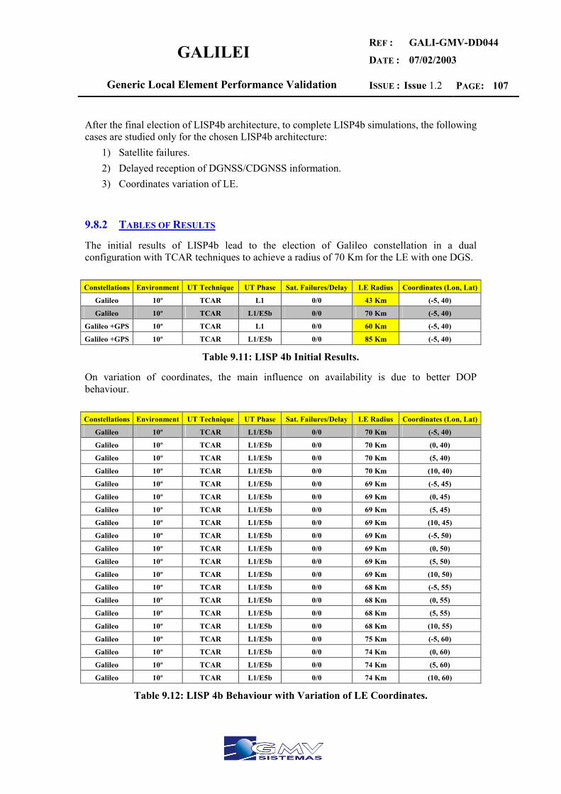
GALILEI REF :
DATE :
GALI-GMV-DD044
07/02/2003
Generic Local Element Performance Validation ISSUE : Issue 1.2 PAGE: 107
After the final election of LISP4b architecture, to complete LISP4b simulations, the following cases are studied only for the chosen LISP4b architecture:
1) Satellite failures. 2) Delayed reception of DGNSS/CDGNSS information. 3) Coordinates variation of LE.
9.8.2 TABLES OF RESULTS
The initial results of LISP4b lead to the election of Galileo constellation in a dual configuration with TCAR techniques to achieve a radius of 70 Km for the LE with one DGS. Constellations Environment UT Technique UT Phase Sat. Failures/Delay LE Radius Coordinates (Lon, Lat)
Galileo 10º TCAR L1 0/0 43 Km (-5, 40)
Galileo 10º TCAR L1/E5b 0/0 70 Km (-5, 40)
Galileo +GPS 10º TCAR L1 0/0 60 Km (-5, 40)
Galileo +GPS 10º TCAR L1/E5b 0/0 85 Km (-5, 40)
Table 9.11: LISP 4b Initial Results.
On variation of coordinates, the main influence on availability is due to better DOP behaviour. Constellations Environment UT Technique UT Phase Sat. Failures/Delay LE Radius Coordinates (Lon, Lat)
Galileo 10º TCAR L1/E5b 0/0 70 Km (-5, 40)
Galileo 10º TCAR L1/E5b 0/0 70 Km (0, 40)
Galileo 10º TCAR L1/E5b 0/0 70 Km (5, 40)
Galileo 10º TCAR L1/E5b 0/0 70 Km (10, 40)
Galileo 10º TCAR L1/E5b 0/0 69 Km (-5, 45)
Galileo 10º TCAR L1/E5b 0/0 69 Km (0, 45)
Galileo 10º TCAR L1/E5b 0/0 69 Km (5, 45)
Galileo 10º TCAR L1/E5b 0/0 69 Km (10, 45)
Galileo 10º TCAR L1/E5b 0/0 69 Km (-5, 50)
Galileo 10º TCAR L1/E5b 0/0 69 Km (0, 50)
Galileo 10º TCAR L1/E5b 0/0 69 Km (5, 50)
Galileo 10º TCAR L1/E5b 0/0 69 Km (10, 50)
Galileo 10º TCAR L1/E5b 0/0 68 Km (-5, 55)
Galileo 10º TCAR L1/E5b 0/0 68 Km (0, 55)
Galileo 10º TCAR L1/E5b 0/0 68 Km (5, 55)
Galileo 10º TCAR L1/E5b 0/0 68 Km (10, 55)
Galileo 10º TCAR L1/E5b 0/0 75 Km (-5, 60)
Galileo 10º TCAR L1/E5b 0/0 74 Km (0, 60)
Galileo 10º TCAR L1/E5b 0/0 74 Km (5, 60)
Galileo 10º TCAR L1/E5b 0/0 74 Km (10, 60)
Table 9.12: LISP 4b Behaviour with Variation of LE Coordinates.

GALILEI REF :
DATE :
GALI-GMV-DD044
07/02/2003
Generic Local Element Performance Validation ISSUE : Issue 1.2 PAGE: 108
On variation of Delayed Corrections, below or equal to 2 seconds of delay is the recommended acceptable value without loosing much LE scope. Constellations Environment UT Technique UT Phase Sat. Failures/Delay LE Radius Coordinates (Lon, Lat)
Galileo 10º TCAR L1/E5b 0/0 70 Km (-5, 40)
Galileo 10º TCAR L1/E5b 0/1 68 Km (-5, 40)
Galileo 10º TCAR L1/E5b 0/2 66 Km (-5, 40)
Galileo 10º TCAR L1/E5b 0/3 62 Km (-5, 40)
Galileo 10º TCAR L1/E5b 0/4 58 Km (-5, 40)
Galileo 10º TCAR L1/E5b 0/5 54 Km (-5, 40)
Galileo 10º TCAR L1/E5b 0/0 74 Km (10, 60)
Galileo 10º TCAR L1/E5b 0/1 72 Km (10, 60)
Galileo 10º TCAR L1/E5b 0/2 70 Km (10, 60)
Galileo 10º TCAR L1/E5b 0/3 66 Km (10, 60)
Galileo 10º TCAR L1/E5b 0/4 62 Km (10, 60)
Galileo 10º TCAR L1/E5b 0/5 58 Km (10, 60)
Table 9.13: LISP 4b Behaviour with Variation Of Delayed Corrections.
On satellite failures the conservative and realistic approaches are pinpointed. Constellations Environment UT Technique UT Phase Sat. Failures/Delay LE Radius Coordinates (Lon, Lat)
Galileo 10º TCAR L1/E5b 0/0 70 Km (-5, 40)
Galileo 10º TCAR L1/E5b 1/0 42 Km (-5, 40)
Galileo 10º TCAR L1/E5b 2/0 0 Km (-5, 40)
Galileo 10º TCAR L1/E5b 1(+1SPARE)/0 43 Km (-5, 40)
Galileo 10º TCAR L1/E5b 2(+2SPARE)/0 0 Km (-5, 40)
Table 9.14: LISP 4b Behaviour with Variation With Satellite Failures.
9.8.3 REVIEW OF SUB-ELEMENT ELECTION AND MINIMUM NUMBER OF SUB-ELEMENTS NEEDED
Not applicable as there is no service volume defined. Typical coverage radius per DGS station is about 66 Km as can be extracted for the nominal case, with 2 seconds of delayed differential corrections.

GALILEI REF :
DATE :
GALI-GMV-DD044
07/02/2003
Generic Local Element Performance Validation ISSUE : Issue 1.2 PAGE: 109
10 ESTIMATION FIGURES OF DELAYED RECEPTION OF CORRECTIONS AND TTA
10.1 TECHNOLOGIES USED
To completely define the figures of delayed reception, the main issue to consider is the communication architecture and technology chosen to broadcast Differential Corrections and Status Messages to the UT. Mainly, in DD027 are pinpointed typical radio-mobile technologies like GSM, GPRS and UTMS apart from usage of VHF and UHF bands. We will focus our study in this technological classification. As there is not a single association between one technology and one LISP, we will make this estimation from a general POW valid for most of LISP architectures. Hence, results will be more or less self-dependent on the type of technology employed, but not in the LISP architecture, that can be adapted to any of the communication technologies considered. Of course, a mandatory parameter will be the expected service volume of each LISP.
• Hence, Technologies used are VHF, UHF, GSM, GPRS and UTMS.
10.2 COMMUNICATION SERVICE VOLUME
The theory of Radio Transmissions provides accurate equations to compute expected distance of coverage of the signal after knowing the main link parameters (Frequency, propagation conditions, transmitter power, transmitter terminal losses, transmitter antenna’s gain, receptor antenna’s gain, receptor terminal losses, receiver system noise factor, transmission width-band, fading margin and threshold reception power), but at the level of communication description provided in DD027, we assume as a right approach to take typical coverage distances for each communication technology for a preliminary study of delays on communications, and this approach will be used for the current analysis. Each typical figure, will determine the communication-cell coverage. Additionally, we will determine how many communication cells are needed to achieve each LISP service volume. The communication topology chosen will be an overlapped one and centered in the first transmission cell. Further assessment for typical values can be found in Radio Communication Literacy1 and 2. Results are summarised in Fig. 5.1.
• Hence, chosen Cell Radius Coverage for VHF and UHF is 40 Km. • Hence, chosen Cell Radius Coverage for GSM, GPRS and UMTS is 15 Km.
1 See “Transmisión por Radio”, José Mª Hernando Rábanos, Colección E.T.S.I. de Telecomunicación (U.P.M). 2 See “Comunicaciones Móviles”, José Manuel Huidobro Moya, Ed. Paraninfo, 2002.

GALILEI REF :
DATE :
GALI-GMV-DD044
07/02/2003
Generic Local Element Performance Validation ISSUE : Issue 1.2 PAGE: 110
Technology Frequency Range Propagation Methods Typical Radius
Coverage Chosen Cell
Coverage
VHF 30 to 300 MHz Spatial Tropospheric waves Ionospheric Dispersion.
50 to 2000 Km 40 Km
UHF 300 to 3000MHz Spatial Tropospheric waves Tropospheric Dispersion.
40 to 600 Km 40 Km
GSM 900,1800 MHz UHF like Tropospheric Dispersion.
UHF like Cell: 15 to 35 Km
15 Km
GPRS 900,1800 MHz UHF like Tropospheric Dispersion.
UHF like Cell: 15 to 35 Km
15 Km
UMTS 1800 to 2200 MHz UHF like Tropospheric Dispersion.
UHF like Cell: 15 Km
15 Km
Table 10.1: Cell Communication Service Volume Related to each Technology
According with the proposed cell radius coverage, the number of communication cells needed are summarised below. The maximum number of levels is 4, this is, to reach any UT within the LE, a maximum of 4+1(Central Cell) =5 cells are used for communication: LISP Technology Levels & Number of
Cells per Level Partial
Coverage Technology Levels & Number of
Cells per Level Partial
Coverage
LISP1 VHF/UHF 10 Cells
Level 1: 10 Cells 101.284 Km GSM/GPRS/UMTS 72 Cells
Level 1: 11 Cells Level 2: 15 Cells Level 3: 21 Cells Level 4: 25 Cells
39.271 Km 60.492 Km 81.513 Km
100.745 Km
LISP2 VHF/UHF 10 Cells
Level 1: 10 Cells 101.284 Km GSM/GPRS/UMTS 72 Cells
Level 1: 11 Cells Level 2: 15 Cells Level 3: 21 Cells Level 4: 25 Cells
39.271 Km 60.492 Km 81.513 Km
100.745 Km
LISP3a VHF/UHF Level 1: 1 Cells 40 Km GSM/GPRS/UMTS Level 1: 1 Cells 15 Km
LISP3b VHF/UHF Level 1: 1 Cells 40 Km GSM/GPRS/UMTS Level 1: 1 Cells 15 Km
LISP4a VHF/UHF Level 1: 1 Cells 40 Km GSM/GPRS/UMTS Level 1: 1 Cells 15 Km
LISP4b VHF/UHF Level 1: 1 Cells 40 Km GSM/GPRS/UMTS Level 1: 1 Cells 15 Km
Table 10.2: Cell Service Volume Related to each LISP
Taken into account the number of DRS stations for each LISP, it is highly recommended the following configuration:
• LISP#1: VHF/UHF configuration, tending to 6 Cells, one for each DRS station. • LISP#2: GSM/GPRS/UMTS configuration, tending to 83 Cells, one for each DRS
station. • LISP#3a/3b/4a/4b: Both configurations are possible.
10.3 DATA RATES FOR EACH LISP
Regarding expected data rates, according with DD027, we will consider always a broadcast communication (broadcast of differential corrections and Alarm Messages) of 9.6kbps for LISP#3a and LISP#3b, 100 kbps for LISP#1, LISP#4a and LISP#4b, and 64kbps for LISP#2.

GALILEI REF :
DATE :
GALI-GMV-DD044
07/02/2003
Generic Local Element Performance Validation ISSUE : Issue 1.2 PAGE: 111
10.4 DATA FRAMES
• Differential Corrections:
In a general case, data transmission includes GALILEO+GPS differential corrections (20 bytes per satellite in view) and GALILEO Integrity messages (10 bytes per satellite in view). With a maximum of 30 satellites in view, means 900 bytes. Additionally a 10% is added to complete the transmission communication protocol, making finally 990 bytes.
• Alarm Message (Status Message):
Can be as short as needed. A recommended maximum number of bytes is to have between 20 and 30 bytes of information, protocol and CRCs included. 30 bytes will be taken for the current analysis.
10.5 ANALYSIS OF DELAY FIGURES
The minimum time-delay needed to receive a complete set of data frames (differential corrections or Status Message) is estimated below. The communication architecture is cell-based according with the number of cells estimated before. Each cell, will act as an autonomous radio beacon, being all of them interconnected through the GBCN included in each LISP architecture. Let us check in a quick review, the global communication path followed by one data frame:
1) Differential Correction Data Frame: Is created in one concrete DRS station. This DRS station has associated one broadcast communication cell, hence through one local CPS the data frame accesses to the GBCN reaching finally the cell-node centre where the information is transmitted to the UT. Basically, communication delays are due to HW&SW cable communication delays and HW&SW broadcast delays due to only one radio beacon. 2) Status Message Data Frame: In this case, a status message to be notified to the UT is created in the CPS as is the case of an alarm message. This message has associated one or more (even all) broadcast communication cells, hence through the Galileo LE Service & Operating Centre the data frame accesses to the GBCN reaching finally the cell-nodes where the information is transmitted to the UT. Again, basically, communication delays are due to HW&SW cable communication delays and HW&SW broadcast delays due to only one radio beacon (all broadcast beacons transmits approximately at the same time).
The global delay figure can be expressed according to the following equation:
UTnextMeasUTacqBeaconDRS
onTransmissiBeaconDRS
sMediaAccesBeaconDRS
SWprocessBeaconDRS
HWacqDELAY TTTTTTT +++++= ∑∑∑∑++++ 1111
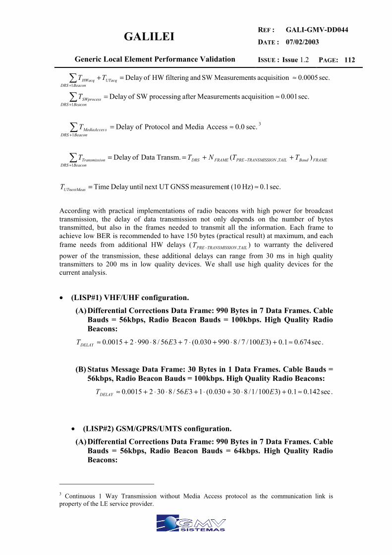
GALILEI REF :
DATE :
GALI-GMV-DD044
07/02/2003
Generic Local Element Performance Validation ISSUE : Issue 1.2 PAGE: 112
sec. 0.0005n acquisitio tsMeasuremenSW and filteringHW ofDelay 1
≈=+∑+
UTacqBeaconDRS
HWacq TT
sec. 0.001 n acquisitio tsMeasuremenafter processingSW ofDelay 1
≈=∑+ BeaconDRS
SWprocessT
sec. 0.0 Access Media and Protocol ofDelay 1
≈=∑+ BeaconDRS
sMediaAccesT 3
FRAMEBaudTAILONTRANSMISSIPREFRAMEDRSBeaconDRS
onTransmissi TTNTT )(Transm. Data ofDelay ,1
++== −+∑
sec. 0.1 Hz) (10t measuremen GNSS next UT untilDelay Time ≈=UTnextMeasT
According with practical implementations of radio beacons with high power for broadcast transmission, the delay of data transmission not only depends on the number of bytes transmitted, but also in the frames needed to transmit all the information. Each frame to achieve low BER is recommended to have 150 bytes (practical result) at maximum, and each frame needs from additional HW delays ( TAILONTRANSMISSIPRET ,− ) to warranty the delivered power of the transmission, these additional delays can range from 30 ms in high quality transmitters to 200 ms in low quality devices. We shall use high quality devices for the current analysis.
• (LISP#1) VHF/UHF configuration. (A) Differential Corrections Data Frame: 990 Bytes in 7 Data Frames. Cable
Bauds = 56kbps, Radio Beacon Bauds = 100kbps. High Quality Radio Beacons:
.sec674.01.0)3100/7/8990030.0(7356/899020015.0 ≈+⋅+⋅+⋅⋅+≈ EETDELAY
(B) Status Message Data Frame: 30 Bytes in 1 Data Frames. Cable Bauds =
56kbps, Radio Beacon Bauds = 100kbps. High Quality Radio Beacons: .sec142.01.0)3100/1/830030.0(1356/83020015.0 ≈+⋅+⋅+⋅⋅+≈ EETDELAY
• (LISP#2) GSM/GPRS/UMTS configuration. (A) Differential Corrections Data Frame: 990 Bytes in 7 Data Frames. Cable
Bauds = 56kbps, Radio Beacon Bauds = 64kbps. High Quality Radio Beacons:
3 Continuous 1 Way Transmission without Media Access protocol as the communication link is property of the LE service provider.

GALILEI REF :
DATE :
GALI-GMV-DD044
07/02/2003
Generic Local Element Performance Validation ISSUE : Issue 1.2 PAGE: 113
.sec718.01.0)364/7/8990030.0(7356/899020015.0 ≈+⋅+⋅+⋅⋅+≈ EETDELAY
(B) Status Message Data Frame: 30 Bytes in 1 Data Frames. Cable Bauds =
56kbps, Radio Beacon Bauds = 64kbps. High Quality Radio Beacons: .sec144.01.0)364/1/830030.0(1356/83020015.0 ≈+⋅+⋅+⋅⋅+≈ EETDELAY
• (LISP#3ab) Any configuration. (A) Differential Corrections Data Frame: 990 Bytes in 7 Data Frames. Cable
Bauds = 56kbps, Radio Beacon Bauds = 9.6kbps. High Quality Radio Beacons:
.sec419.11.0)36.9/7/8990030.0(7356/899020015.0 ≈+⋅+⋅+⋅⋅+≈ EETDELAY
(B) Status Message Data Frame: 30 Bytes in 1 Data Frames. Cable Bauds =
56kbps, Radio Beacon Bauds = 9.6kbps. High Quality Radio Beacons: .sec165.01.0)36.9/1/830030.0(1356/83020015.0 ≈+⋅+⋅+⋅⋅+≈ EETDELAY
• (LISP#4ab) Any configuration. (A) Differential Corrections Data Frame: 990 Bytes in 7 Data Frames. Cable
Bauds = 56kbps, Radio Beacon Bauds = 100kbps. High Quality Radio Beacons:
.sec674.01.0)3100/7/8990030.0(7356/899020015.0 ≈+⋅+⋅+⋅⋅+≈ EETDELAY
(B) Status Message Data Frame: 30 Bytes in 1 Data Frames. Cable Bauds =
56kbps, Radio Beacon Bauds = 100kbps. High Quality Radio Beacons: .sec142.01.0)3100/1/830030.0(1356/83020015.0 ≈+⋅+⋅+⋅⋅+≈ EETDELAY
10.6 CONCLUSIONS
With the given architecture and given data rates, transmission can cope with RT (Real Time) tasks; having for LISP#1,#2,#4ab below one second of maximum synchronisation delay, and for LISP#3ab below two seconds of maximum synchronisation delay. For LISP#3ab, each two seconds is provided a complete set of corrections. In all LISP cases, TTA has turned out to be further below 1 second (0.165 sec), hence TTA requirement is met through the chosen architecture.

GALILEI REF :
DATE :
GALI-GMV-DD044
07/02/2003
Generic Local Element Performance Validation ISSUE : Issue 1.2 PAGE: 114
11 VALIDATION CONCLUSIONS AND REMARKS
• Validation has been completed from a high level definition of the LE architecture. Extrapolation techniques and criteria based on availability and performance simulations have been used to check validation results of proposed LE architectures.
• A conservative criterion has been applied leading to avoid optimistic results. Even more due to the high restrictive parameters given focused on applications with the best possible performances.
• LISP#1 simulations recommend using both GNSS constellations, bi-frequency UT due to long service volume and kinematic algorithms to achieve accuracy restrictions. In spite of it, 6 DRS are needed to meet service volume requirement.
• LISP#2 simulations recommend using both GNSS constellations (in urban areas 99.9% accuracy availability cannot be met with the usage of only one GNSS constellation), bi frequency UT due to long service volume and kinematic algorithms to achieve accuracy restrictions. PL increases final service volume, but its influence is low-noticed because of the kinematic techniques employed, that enhance horizontal and vertical accuracy. In spite of this, with one DRS, a typical service volume of 14 Km is only met, hence it has been estimated about 83 DRS stations to meet LISP requirements.
• LISP#3a simulations recommend using both GNSS constellations, mono-frequency UT and code algorithms to achieve LISP requirements. In this case, simulations confirm that LISP#3a service volume is reached.
• LISP#3b simulations remark the importance of the PL role. Service volume is limited mainly by PL coverage. When PL is not available, accuracy requirements are not met.
• LISP#4a simulations recommend using both GNSS constellations to increase availability in urban environments. Due to the very restrictive accuracy conditions only 1-2 Km of service volume is reached.
• LISP#4b has been simulated for only GALILEO constellation. Performances are met, but satellite failures have a great impact on final service volume due to a decrease on satellite availability. The difference on using mono-frequency and bi-frequency receivers has true impact on final service volume (40 vs 70 Km).
• It is expected that the dual presence of Galileo and GPS constellations would lead to discover new useful features used to minimize (or estimate) sources of errors like receiver noise and multipath or using both to provide an enhanced solution. In any case the foreseen benefits has not been taken into account (apart from the increase on availability) along the validation procedure.
• The interoperability effect of the dual presence of Galileo and GPS signal frequencies has to be considered (not used in simulations). See Annex 5, Section1.5 Assessment of GPS Vulnerabilities. Extrapolation of results can be made in the Galileo case. Also refer to [10] document within GPS reference index.
• The present validation document assumes the communication links are working properly. Any disturbance or lack of communication shall lead to a decrease on Navigation Performances, even to not accomplish the expected LISP performance Requirements.
GALILEI REF :
DATE :
GALI-GMV-DD044
07/02/2003
Generic Local Element Performance Validation ISSUE : Issue 1.2 PAGE: 115
• The highest performance requirements in LISP#4A are only expected for static cases (or very low dynamics) and mainly in post-processed statistical results. To Warranty millimetric level of accuracy some measurements redundancy should be needed with low DOP values (conservative criteria of 9 satellites (TBD) in view have been stated as needed for enough redundancy of the solution). Also Local Area scope should be constrained.
• PL transceivers can be an effective way to expand the capability of positioning system, eliminating DRS, allowing pseudolites to self-survey their own locations.
• GALILEO constellation is always used as a premise. • All communication links for each particular LISP are feasible. With the only
restriction of having the technology ready to one particular implementation (i.e. UMTS is still not ready to be used, instead GSM or GPRS can be already used)
• Industry validates communication services and Standards. • Final LE architecture case should have to minimize the number of sub-elements and
to simplify the UT communication system. • LIM should be avoided in most of cases due to the inherent presence of the integrity
message in the Galileo SIS. Also RAIM algorithms can be used thanks to the increase of satellite availability in those cases Galileo+GPS constellations are employed. LIM only should be justified in most demanding applications for redundancy.
• For most of Clear-Sky applications it is recommended only use the Galileo Constellation system. Provided availability is foreseen enough to meet many of the typical navigation applications.
• One interesting accessible way of simplifying the LE architecture is by means of
using the Pseudolites as transceivers of the GPS SIS. • Performance requirements are highly restrictive and lead, as a general rule, to a very
complex architectures containing, in most cases, hardly all the possible sub-elements or external system of the generic LE architecture. Depending on the target applications and foreseen market, this may give unaffordable architectures.
• A cost study of the final service must be carried out regarding this point in order to have a realistic and affordable system.
• Interoperability between sub-elements and external system should be taken into account as a general rule during the design of the particular services.
• UT Validation: Still in an early stage to be completely validated. At the current
definition phase of the LE, most of complexity goes to the UT. Heterogeneity of systems leads to a considerable increase of costs due to the great amount of different communication links and to the non-relaxation of LISP parameters.
• Due to the importance given to most restrictive millimetric applications, a generic homologation should be requested to the UT to meet expected specifications.
• Communication Validation: In the SNIF Tables are presented the potentials to meet the communication requirements. At this level of architecture definition no much more can be provided in terms of validation. Any of the proposed substitutives can be used. A proper installation should lead to a successful implementation of the

GALILEI REF :
DATE :
GALI-GMV-DD044
07/02/2003
Generic Local Element Performance Validation ISSUE : Issue 1.2 PAGE: 116
communication system. Industry and Market are the starting point of the communication system. Performances are fixed by Industry on concrete solutions. And the use of one of the communication links is dependent on Market trends.
• Typical acceptable delays on communications goes from 0 to 2 seconds for differential corrections. Status messages are expected to be received in 1 second.
• Continuity (Validation Parameter for Safety Critical Systems Applications): (Not taken into account along the current validation phase) Through the continuity definition (GALI-ASPI-DD025) LE service is left open, with the only restriction of having a robust Integrity detection to allow the user to recognize this situation. This parameter is a point to take into account in concrete applications.
• Cost Assessment Validation Remark: Three general costs needs to be analyzed: Development Costs, LE Maintenance Costs and UT Development and Maintenance costs. These costs are directly related with the Complexity of the LE architecture.
• UT complexity has to be checked to avoid new devices with compatibility problems between different manufacturers.

GALILEI REF :
DATE :
GALI-GMV-DD044
07/02/2003
Generic Local Element Performance Validation ISSUE : Issue 1.2 PAGE: 117
12 RECOMMENDATIONS
The presence of an IM from is recommended but should be avoided in most of non-critical applications. Mainly on those applications with more than one constellation for availability reasons: In this case, RAIM algorithms can be near 100% applicable allowing TTA parameter to be met within the UT equipment. Also, the IM uplink communication should not be available to the applications sector, as are expected an increase of false failure reports. The Galileo core system should not well-interpret the real sources of the received problem that could lead to inefficient management of the incoming information. The Ground segment of the Galileo core system should detect all these cases. The number of UT links should be minimised for efficiency. Mainly those links received from the LE architecture. Only one radio link is recommended for integrity and information interchange.
12.1 RECOMMENDATIONS FOR THE GALILEO LOCAL ELEMENT MRD AND FOR THE GALILEO LOCAL ELEMENT SRD
• LISP#1 simulations recommend using both GNSS constellations, bi-frequency UT due to long service volume and kinematic algorithms to achieve accuracy restrictions. In spite of it, 6 DRS are needed to meet service volume requirement.
• LISP#2 simulations recommend using both GNSS constellations (in urban areas 99.9% accuracy availability cannot be met with the usage of only one GNSS constellation), bi frequency UT due to long service volume and kinematic algorithms to achieve accuracy restrictions. PL increases final service volume, but its influence is low-noticed because of the kinematic techniques employed, that enhance horizontal and vertical accuracy. In spite of this, with one DRS, a typical service volume of 14 Km is only met, hence it has been estimated about 83 DRS stations to meet LISP requirements.
• LISP#3a simulations recommend using both GNSS constellations, mono-frequency UT and code algorithms to achieve LISP requirements. In this case, simulations confirm that LISP#3a service volume is reached.
• LISP#3b simulations remark the importance of the PL role. Service volume is limited mainly by PL coverage. When PL is not available, accuracy requirements are not met.
• LISP#4a simulations recommend using both GNSS constellations to increase availability in urban environments. Due to the very restrictive accuracy conditions only 1-2 Km of service volume is reached.
• LISP#4b has been simulated for only GALILEO constellation. Performances are met, but satellite failures have a great impact on final service volume due to a decrease on satellite availability. The difference on using mono-frequency and bi-frequency receivers has true impact on final service volume (40 vs 70 Km).

GALILEI REF :
DATE :
GALI-GMV-DD044
07/02/2003
Generic Local Element Performance Validation ISSUE : Issue 1.2 PAGE: 118
ANNEX 1 GALILEO

GALILEI REF :
DATE :
GALI-GMV-DD044
07/02/2003
Generic Local Element Performance Validation ISSUE : Issue 1.2 PAGE: 119
1 INTRODUCTION
Galileo will be Europe’s own global navigation satellite system, providing a highly accurate, guaranteed global positioning service under civilian control. In general lines, it will be inter-operable with GPS and GLONASS, the two other global satellite navigation systems. By offering dual frequencies as standard, Galileo will deliver real-time positioning accuracy down to the metre range. It will also guarantee availability of the service under all but the most extreme circumstances and will inform users within seconds of a failure of any satellite. This integrity reports will make GALILEO suitable for applications where safety is crucial. The first experimental GALILEO satellite will be launched in late 2004. The objective of this experimental satellite is to characterize the critical technologies, which are already under development under ESA contracts. Thereafter up to four operational satellites will be launched in the timeframe 2005-2006 to validate the basic Galileo space and related ground segment. Once this In-Orbit Validation (IOV) phase has been completed, the remaining satellites will be installed to reach the Full Operational Capability (FOC) in 2008. The fully deployed Galileo system consists of 30 satellites (27 operational + 3 active spares), positioned in three circular Medium Earth Orbit (MEO) planes in 23616 km altitude above the Earth, and at an inclination of the orbital planes of 56 degrees with reference to the equatorial plane. Once this is achieved, the Galileo navigation signals will provide a good coverage even at latitudes up to 75 degrees north, which corresponds to the North Cape, and beyond. The large number of satellites together with the optimisation of the constellation, and the availability of the three active spare satellites, will ensure that the loss of one satellite has no discernible effect on the user. Two Galileo Control Centres (GCC) will be implemented on European ground to provide for the control of the satellites and to perform the navigation mission management. The data provided by a global network of twenty Galileo Sensor Stations (GSS) will be sent to the Galileo Control Centres through a redundant communications network. The GCC’s will use the data of the Sensor Stations to compute the integrity information and to synchronize the time signal of all satellites and of the ground station clocks. The exchange of the data between the Control Centres and the satellites will be performed through so-called up-link stations. Five S-band up-link stations and 10 C-band up-link stations will be installed around the globe for this purpose. As a further feature, Galileo will provide a global Search and Rescue (SAR) function, based on the operational Cospas-Sarsat system. To do so, each satellite will be equipped with a transponder, which is able to transfer the distress signals from the user transmitters to the Rescue Co-ordination Centre, which will then initiate the rescue operation. At the same time, the system will provide a signal to the user, informing him that his situation has been detected and that help is under way. The justification of the GALILEO system is offering one European independent alternative for satellite navigation to guaranty an uninterrupted service to the growing market sector of navigation and fleet location, and to allow the applications sector to look into new innovative ideas leading to global navigation and safety solutions.
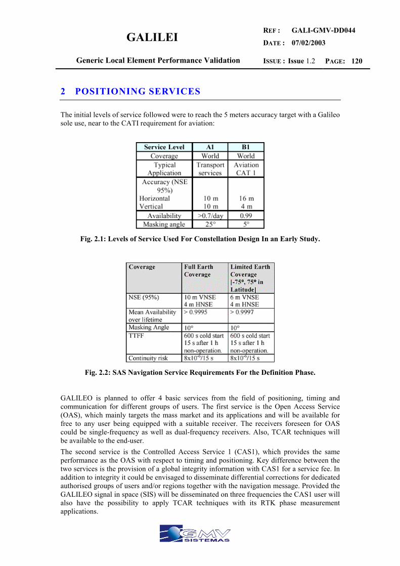
GALILEI REF :
DATE :
GALI-GMV-DD044
07/02/2003
Generic Local Element Performance Validation ISSUE : Issue 1.2 PAGE: 120
2 POSITIONING SERVICES
The initial levels of service followed were to reach the 5 meters accuracy target with a Galileo sole use, near to the CATI requirement for aviation:
Fig. 2.1: Levels of Service Used For Constellation Design In an Early Study.
Fig. 2.2: SAS Navigation Service Requirements For the Definition Phase.
GALILEO is planned to offer 4 basic services from the field of positioning, timing and communication for different groups of users. The first service is the Open Access Service (OAS), which mainly targets the mass market and its applications and will be available for free to any user being equipped with a suitable receiver. The receivers foreseen for OAS could be single-frequency as well as dual-frequency receivers. Also, TCAR techniques will be available to the end-user. The second service is the Controlled Access Service 1 (CAS1), which provides the same performance as the OAS with respect to timing and positioning. Key difference between the two services is the provision of a global integrity information with CAS1 for a service fee. In addition to integrity it could be envisaged to disseminate differential corrections for dedicated authorised groups of users and/or regions together with the navigation message. Provided the GALILEO signal in space (SIS) will be disseminated on three frequencies the CAS1 user will also have the possibility to apply TCAR techniques with its RTK phase measurement applications.

GALILEI REF :
DATE :
GALI-GMV-DD044
07/02/2003
Generic Local Element Performance Validation ISSUE : Issue 1.2 PAGE: 121
The third service is the Controlled Access Service 2 (CAS2) for safety critical applications (CAS2-SAS). Compared with CAS1, it provides higher positioning accuracy in combination with higher availability and additional regional integrity information.
Fig. 2.3: Performance parameters for the OAS for different system configurations. OAS-G1x are single-frequency receiver based, OAS-G2x are dual-frequency receiver based and OAS-GSx are dual-frequency receiver based in combination with GPS (L1+L5).
Fig. 2.4: Performance parameters for the CAS2-SAS for different system configurations. CAS2-SAS-G is based on the global component of Galileo. CAS2-SAS-R adn CAS2-SAS-L are based on global and regional and global and local components of Galileo respectively and CAS2-SAS-RS is based on the global and regional component of Galileo in combination with GPS (L1+L5).
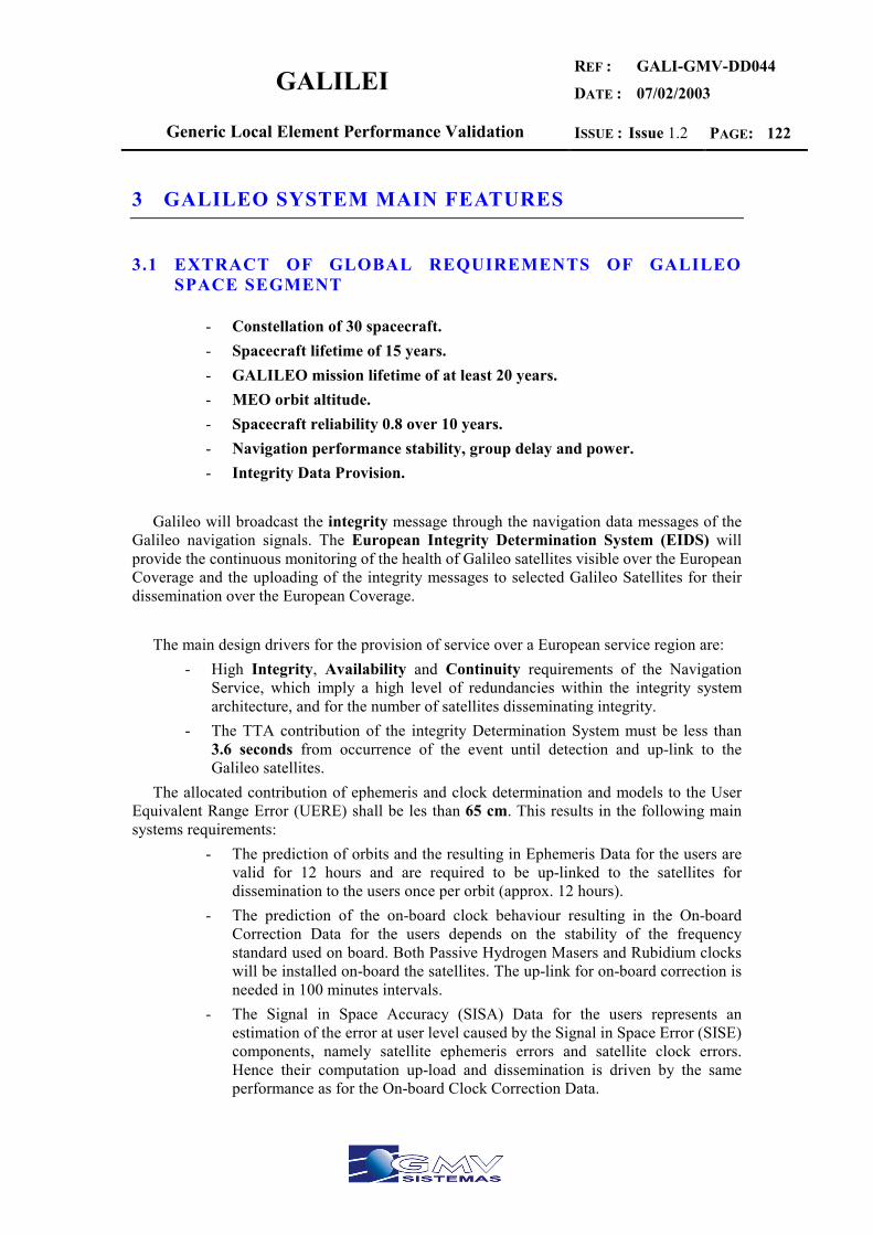
GALILEI REF :
DATE :
GALI-GMV-DD044
07/02/2003
Generic Local Element Performance Validation ISSUE : Issue 1.2 PAGE: 122
3 GALILEO SYSTEM MAIN FEATURES
3.1 EXTRACT OF GLOBAL REQUIREMENTS OF GALILEO SPACE SEGMENT
- Constellation of 30 spacecraft. - Spacecraft lifetime of 15 years. - GALILEO mission lifetime of at least 20 years. - MEO orbit altitude. - Spacecraft reliability 0.8 over 10 years. - Navigation performance stability, group delay and power. - Integrity Data Provision.
Galileo will broadcast the integrity message through the navigation data messages of the Galileo navigation signals. The European Integrity Determination System (EIDS) will provide the continuous monitoring of the health of Galileo satellites visible over the European Coverage and the uploading of the integrity messages to selected Galileo Satellites for their dissemination over the European Coverage.
The main design drivers for the provision of service over a European service region are:
- High Integrity, Availability and Continuity requirements of the Navigation Service, which imply a high level of redundancies within the integrity system architecture, and for the number of satellites disseminating integrity.
- The TTA contribution of the integrity Determination System must be less than 3.6 seconds from occurrence of the event until detection and up-link to the Galileo satellites.
The allocated contribution of ephemeris and clock determination and models to the User Equivalent Range Error (UERE) shall be les than 65 cm. This results in the following main systems requirements:
- The prediction of orbits and the resulting in Ephemeris Data for the users are valid for 12 hours and are required to be up-linked to the satellites for dissemination to the users once per orbit (approx. 12 hours).
- The prediction of the on-board clock behaviour resulting in the On-board Correction Data for the users depends on the stability of the frequency standard used on board. Both Passive Hydrogen Masers and Rubidium clocks will be installed on-board the satellites. The up-link for on-board correction is needed in 100 minutes intervals.
- The Signal in Space Accuracy (SISA) Data for the users represents an estimation of the error at user level caused by the Signal in Space Error (SISE) components, namely satellite ephemeris errors and satellite clock errors. Hence their computation up-load and dissemination is driven by the same performance as for the On-board Clock Correction Data.
GALILEI REF :
DATE :
GALI-GMV-DD044
07/02/2003
Generic Local Element Performance Validation ISSUE : Issue 1.2 PAGE: 123
3.2 ORBITAL FEATURES AND PARAMETERS
The MEO (Medium Earth Orbit) orbit type, for the baseline constellation is a Walker 27/3/1 orbit (i.e. 9 operational spacecraft in each of 3 orbital planes, with the orbital planes uniformly distributed round the equator at intervals of 120 degrees). However, in addition to the operational configuration of 27 spacecraft, a total of 3 active, in-orbit spares are foreseen (one spacecraft per orbit plane), each spare being placed in the nominal orbit and, if required being configured to take place of any failed spacecraft during the operational phase. The initial constellation therefore comprises 30 active spacecraft in three orbit planes with the following orbital parameters.
Semi-Major Axis (Km) 29993.707 Inclination (degrees) 56
Fig. 3.1: Parameters of GALILEO Constellation.
3.3 SPACECRAFT DESIGN PARAMETERS
Extract of the Overall Spacecraft payload: Mass at Launch Time 625 Kg. Power Consumption: 1.5 Kg Dimensions 2700x1200x1100 mm Length: 13 m solar arrays deployed Lifetime: 15 years. Reliability: 0.85 over 10 years. Attitude Profile: Geocentric and yaw steered.
Extract of Navigation Payload:
Mass: 113 Kg. Power: 808 W.

GALILEI REF :
DATE :
GALI-GMV-DD044
07/02/2003
Generic Local Element Performance Validation ISSUE : Issue 1.2 PAGE: 124
3.4 GALILEO FREQUENCY PLAN
Provided Galileo will disseminate its signal in space (SIS) on three freely accessible frequencies on 1200 MHz and 1500 MHz bands, the user will have the possibility to use three carrier ambiguity resolution (TCAR) techniques for the ambiguity resolution in connection with its phase measurement based real-time kinematic (RTK) applications. In order to limit the degrading effect due to multipath, the frequency diversity has been found to be a convenient solution, which greatly simplifies the system complexity. Frequency plan is described below:
Fig. 3.2: Navigation Signal Main Features Consider in the Definition Study.
Fig. 3.3: Galileo Frequency Plan.

GALILEI REF :
DATE :
GALI-GMV-DD044
07/02/2003
Generic Local Element Performance Validation ISSUE : Issue 1.2 PAGE: 125
4 GALILEO SYSTEM ARCHITECTURE:
GALILEO System is divided into several components, which themselves consist of different segments. These segments are formed by a set of elements necessary to fulfil the tasks of the respective segment. The Galileo system consists of:
- A global component with the space segment, the global mission ground segment, a support segment, a management segment, and an operating segment and includes the integration of the European EGNOS system.
- Potentially one or several regional components outside Europe with a regional mission ground segment each, and
- Potentially several local components with a local mission ground segment each.
Local area requirements are more demanding than those that will be available from the global system /accuracy, integrity TTA, signal acquisition/reacquisition, etc.) These special services will be met through the use of augmentations provided by local components. Local components providing differential corrections for single frequency users would reach positioning accuracy better than 1 meter. Those stations could report also integrity with a time to alarm of 1 second. It is expected that local service providers will adapt the signal format to accommodate additional data. The exploitation of the TCAR technique with local components allows users to determine their position with errors below 10 centimetres. The pilot signal, provided with the open signals, enhances the performance of wireless telecommunications networks (GSM/UMTS) assisted position determination applications in difficult environments ( urban canyon and indoor applications). Local stations broadcasting satellite-like signals (pseudolites) are used for increasing the availability of GALILEO service in a defined local area.

GALILEI REF :
DATE :
GALI-GMV-DD044
07/02/2003
Generic Local Element Performance Validation ISSUE : Issue 1.2 PAGE: 126
5 GALILEO PERFORMANCES VALIDATION
For the study of statistic performances of the future Galileo system the typical validation methodology presented below is not possible due to the unavailability of the physical platform to be validated. So alternative validation techniques are requested.
Fig. 5.1: Validation Methodology.
Depending on the simulation case, a general case should include a mixture between parameters extraction, operational working models, simulation and extrapolation techniques. GMV has available Elcano tool allowing to simulate statistic performances of Keplerian propagated constellation models through simple starting definition models. Also simple urban environments performances (straight streets) can be simulated. The only requirement needed for the simulation tools is to previously compute error parameters (UERE budget), and to introduce the constellation expected parameter definition. Some results of the Galileo and Galileo+GPS constellations will be shown from previous studies. An upgrade to Elcano tool mainly thought for constellation simulations is GMV Polaris simulator tool (still not available) whose aim is including within the simulation additional Local Sub-elements (like DGPS stations, Pseudolites, sensors,…) to compute local performances over an area.
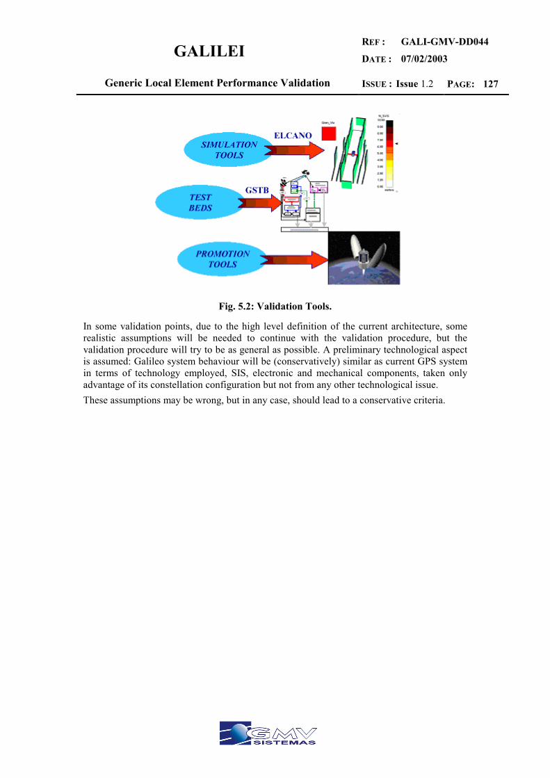
GALILEI REF :
DATE :
GALI-GMV-DD044
07/02/2003
Generic Local Element Performance Validation ISSUE : Issue 1.2 PAGE: 127
Fig. 5.2: Validation Tools.
In some validation points, due to the high level definition of the current architecture, some realistic assumptions will be needed to continue with the validation procedure, but the validation procedure will try to be as general as possible. A preliminary technological aspect is assumed: Galileo system behaviour will be (conservatively) similar as current GPS system in terms of technology employed, SIS, electronic and mechanical components, taken only advantage of its constellation configuration but not from any other technological issue. These assumptions may be wrong, but in any case, should lead to a conservative criteria.
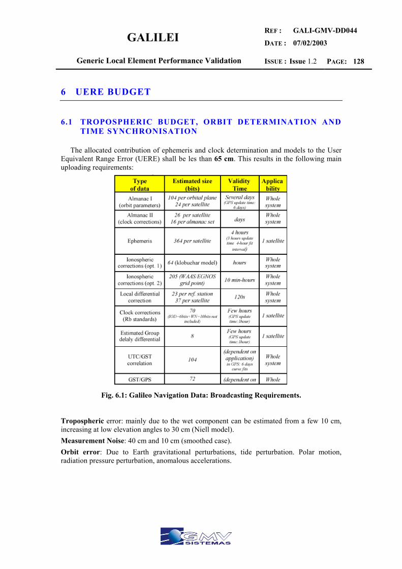
GALILEI REF :
DATE :
GALI-GMV-DD044
07/02/2003
Generic Local Element Performance Validation ISSUE : Issue 1.2 PAGE: 128
6 UERE BUDGET
6.1 TROPOSPHERIC BUDGET, ORBIT DETERMINATION AND TIME SYNCHRONISATION
The allocated contribution of ephemeris and clock determination and models to the User Equivalent Range Error (UERE) shall be les than 65 cm. This results in the following main uploading requirements:
Fig. 6.1: Galileo Navigation Data: Broadcasting Requirements.
Tropospheric error: mainly due to the wet component can be estimated from a few 10 cm, increasing at low elevation angles to 30 cm (Niell model). Measurement Noise: 40 cm and 10 cm (smoothed case). Orbit error: Due to Earth gravitational perturbations, tide perturbation. Polar motion, radiation pressure perturbation, anomalous accelerations.
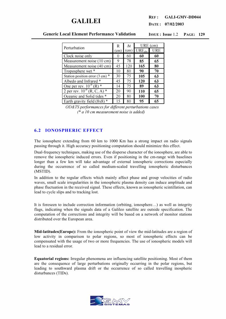
GALILEI REF :
DATE :
GALI-GMV-DD044
07/02/2003
Generic Local Element Performance Validation ISSUE : Issue 1.2 PAGE: 129
6.2 IONOSPHERIC EFFECT
The ionosphere extending from 60 km to 1000 Km has a strong impact on radio signals passing through it. High accuracy positioning computation should minimize this effect. Dual-frequency techniques, making use of the disperse character of the ionosphere, are able to remove the ionospheric induced errors. Even if positioning in the cm-range with baselines longer than a few km will take advantage of external ionospheric corrections especially during the occurrence of so called medium-scaled travelling ionospheric disturbances (MSTID). In addition to the regular effects which mainly affect phase and group velocities of radio waves, small scale irregularities in the ionospheric plasma density can induce amplitude and phase fluctuation in the received signal. These effects, known as ionospheric scintillation, can lead to cycle slips and to tracking lost. It is foreseen to include correction information (orbiting, ionosphere…) as well as integrity flags, indicating when the signals data of a Galileo satellite are outside specification. The computation of the corrections and integrity will be based on a network of monitor stations distributed over the European area. Mid-latitudes(Europe): From the ionospheric point of view the mid-latitudes are a region of low activity in comparison to polar regions, so most of ionospheric effects can be compensated with the usage of two or more frequencies. The use of ionospheric models will lead to a residual error. Equatorial regions: Irregular phenomena are influencing satellite positioning. Most of them are the consequence of large perturbations originally occurring in the polar regions, but leading to southward plasma drift or the occurrence of so called travelling inospheric disturbances (TIDs).
GALILEI REF :
DATE :
GALI-GMV-DD044
07/02/2003
Generic Local Element Performance Validation ISSUE : Issue 1.2 PAGE: 130
6.3 ENVIRONMENT INFLUENCE
Open Sky case: Will lead to the highest performances of the system. Elcano tool will serve as a statistic tool for this open sky case. Previous studies of Galileo constellation show the performances of the system. Most of UERE assumptions will be made for this case. Masking angles will not exceed 10º. Multipath can be avoided in this case. Urban Canyon: A reduction of availability is present in this case. Extrapolation techniques will be needed. A generic approach can be given for this environment by considering a constant masking angle of 25º in urban canyons (constellation reduced). Any other assumptions can be studied but will lead to particular cases. Multipath effect also will increase but is highly dependent on each particular case, so usually will not be considered (to achieve highest possible performances) or considered constant. Local augmentation systems will be added to meet required performances. Indoor: In this case, satellite constellation is clearly insufficient and new radio techniques needs to apply as complementary systems. Accuracy will obviously decrease.
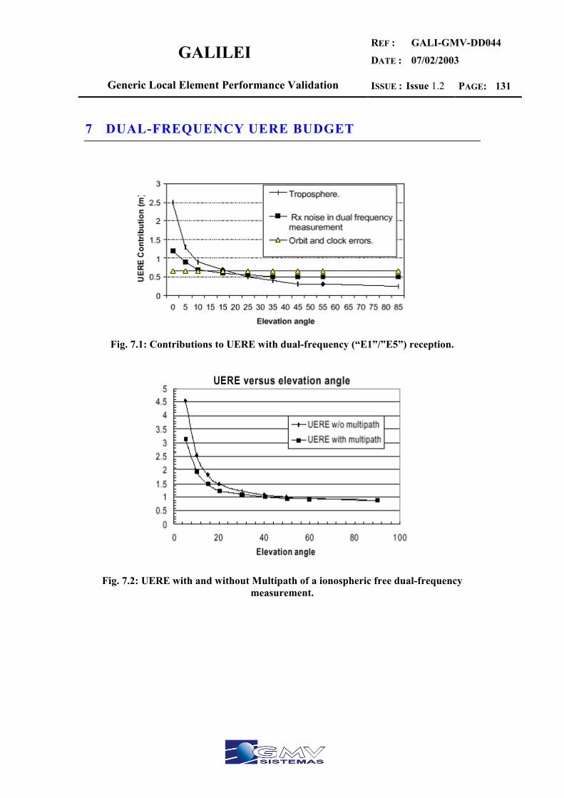
GALILEI REF :
DATE :
GALI-GMV-DD044
07/02/2003
Generic Local Element Performance Validation ISSUE : Issue 1.2 PAGE: 131
7 DUAL-FREQUENCY UERE BUDGET
Fig. 7.1: Contributions to UERE with dual-frequency (“E1”/”E5”) reception.
Fig. 7.2: UERE with and without Multipath of a ionospheric free dual-frequency
measurement.

GALILEI REF :
DATE :
GALI-GMV-DD044
07/02/2003
Generic Local Element Performance Validation ISSUE : Issue 1.2 PAGE: 132
7.1 GALILEO ACCURACY PERFORMANCE (OPEN SKY)
Fig. 7.3: Worst Vertical Accuracy with Elevations over 10º.
Vertical accuracy in European (Mid-Latitude) regions is between 4 to 6 m. The results for a 5 degrees minimum masking angle would be better: for the nominal configuration, a vertical error of 6.5m and a horizontal error of 3.9 meters. When the UERE without multipaht effects is considered, the vertical error for 10 degrees becomes 7.2 meters while for 5 degrees becomes 5.7 meters.
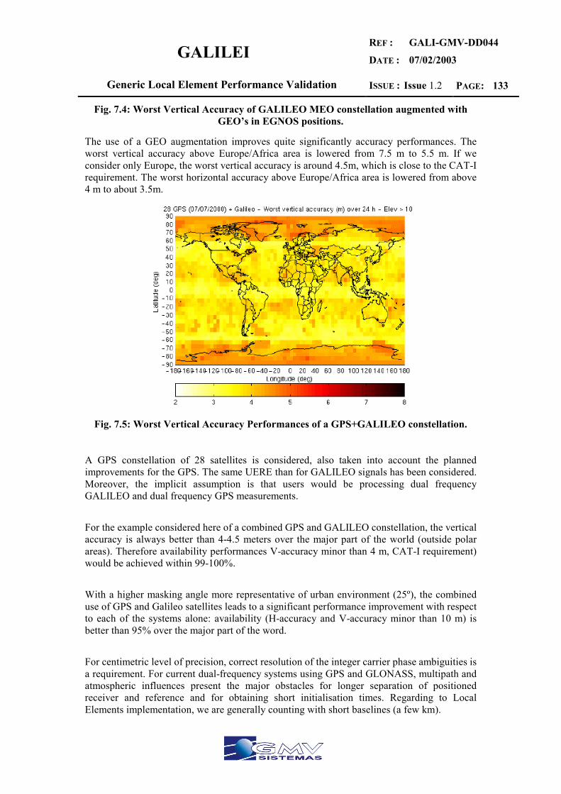
GALILEI REF :
DATE :
GALI-GMV-DD044
07/02/2003
Generic Local Element Performance Validation ISSUE : Issue 1.2 PAGE: 133
Fig. 7.4: Worst Vertical Accuracy of GALILEO MEO constellation augmented with GEO’s in EGNOS positions.
The use of a GEO augmentation improves quite significantly accuracy performances. The worst vertical accuracy above Europe/Africa area is lowered from 7.5 m to 5.5 m. If we consider only Europe, the worst vertical accuracy is around 4.5m, which is close to the CAT-I requirement. The worst horizontal accuracy above Europe/Africa area is lowered from above 4 m to about 3.5m.
Fig. 7.5: Worst Vertical Accuracy Performances of a GPS+GALILEO constellation.
A GPS constellation of 28 satellites is considered, also taken into account the planned improvements for the GPS. The same UERE than for GALILEO signals has been considered. Moreover, the implicit assumption is that users would be processing dual frequency GALILEO and dual frequency GPS measurements. For the example considered here of a combined GPS and GALILEO constellation, the vertical accuracy is always better than 4-4.5 meters over the major part of the world (outside polar areas). Therefore availability performances V-accuracy minor than 4 m, CAT-I requirement) would be achieved within 99-100%. With a higher masking angle more representative of urban environment (25º), the combined use of GPS and Galileo satellites leads to a significant performance improvement with respect to each of the systems alone: availability (H-accuracy and V-accuracy minor than 10 m) is better than 95% over the major part of the word. For centimetric level of precision, correct resolution of the integer carrier phase ambiguities is a requirement. For current dual-frequency systems using GPS and GLONASS, multipath and atmospheric influences present the major obstacles for longer separation of positioned receiver and reference and for obtaining short initialisation times. Regarding to Local Elements implementation, we are generally counting with short baselines (a few km).

GALILEI REF :
DATE :
GALI-GMV-DD044
07/02/2003
Generic Local Element Performance Validation ISSUE : Issue 1.2 PAGE: 134
7.2 PDOP ANALYSIS AND AVAILABILITY
The constellations used in the simulations are: Galileo Constellation: 30 MEO (Walker 30/3/1) satellites (3 orbital planes) 56 deg. Inclination. 29994 km semi-major axis. Nominal GPS constellation 24 MEO satellites (6 orbital planes) 55 deg. Inclination. 26561.75 km semi major axis. Galileo+GPS. In terms of visibility, with a GPS constellation a mean of 6 satellites are in view along time, Galileo constellation optimises the mean to 9 satellites. So, with a GPS+Galileo constellation, a mean of 14 satellites are in view, this allows the user to perform RAIM algorithms near 100% of times. The global distribution of the satellites in the new scenario, with GPS and Galileo constellations, leads to obtain better geometric performances. The 3 constellations were propagated during 1 day and PDOP was computed every 30 minutes. The following pictures show the worst PDOP values for Galileo, GPS and both. 100% availability level is reached when considering the worst case of 1 satellite failure.
Fig. 7.6: PDOP for Galileo Constellation (1 satellite failure)
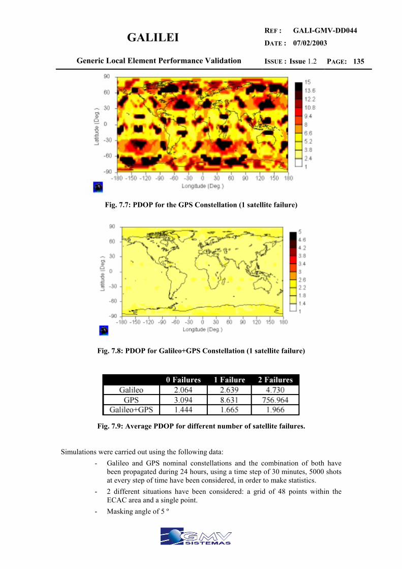
GALILEI REF :
DATE :
GALI-GMV-DD044
07/02/2003
Generic Local Element Performance Validation ISSUE : Issue 1.2 PAGE: 135
Fig. 7.7: PDOP for the GPS Constellation (1 satellite failure)
Fig. 7.8: PDOP for Galileo+GPS Constellation (1 satellite failure)
Fig. 7.9: Average PDOP for different number of satellite failures.
Simulations were carried out using the following data:
- Galileo and GPS nominal constellations and the combination of both have been propagated during 24 hours, using a time step of 30 minutes, 5000 shots at every step of time have been considered, in order to make statistics.
- 2 different situations have been considered: a grid of 48 points within the ECAC area and a single point.
- Masking angle of 5 º
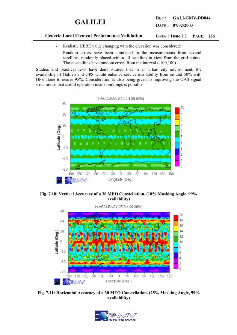
GALILEI REF :
DATE :
GALI-GMV-DD044
07/02/2003
Generic Local Element Performance Validation ISSUE : Issue 1.2 PAGE: 136
- Realistic UERE value changing with the elevation was considered: - Random errors have been simulated in the measurements from several
satellites, randomly placed within all satellites in view from the grid points. These satellites have random errors from the interval (-100,100).
Studies and practical tests have demonstrated that in an urban city environment, the availability of Galileo and GPS would enhance service availability from around 50% with GPS alone to nearer 95%. Consideration is also being given to improving the OAS signal structure so that useful operation inside buildings is possible.
Fig. 7.10: Vertical Accuracy of a 30 MEO Constellation. (10% Masking Angle, 99% availability)
Fig. 7.11: Horizontal Accuracy of a 30 MEO Constellation. (25% Masking Angle, 99%
availability)
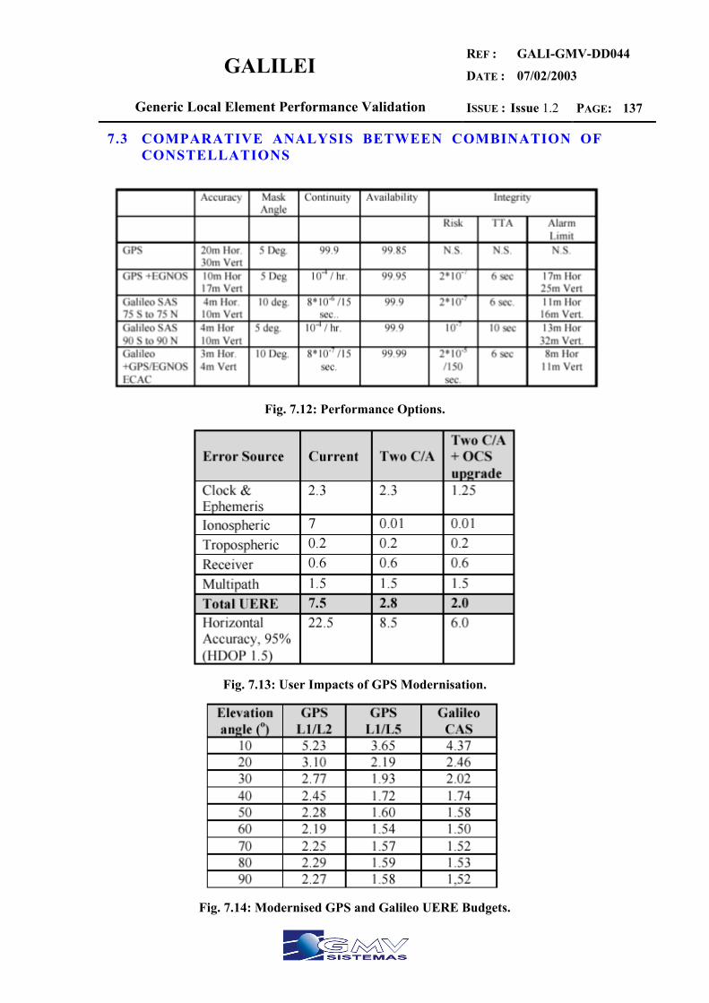
GALILEI REF :
DATE :
GALI-GMV-DD044
07/02/2003
Generic Local Element Performance Validation ISSUE : Issue 1.2 PAGE: 137
7.3 COMPARATIVE ANALYSIS BETWEEN COMBINATION OF CONSTELLATIONS
Fig. 7.12: Performance Options.
Fig. 7.13: User Impacts of GPS Modernisation.
Fig. 7.14: Modernised GPS and Galileo UERE Budgets.

GALILEI REF :
DATE :
GALI-GMV-DD044
07/02/2003
Generic Local Element Performance Validation ISSUE : Issue 1.2 PAGE: 138
Fig. 7.15: Horizontal Vertical Accuracy.
Fig. 7.16: RAIM Availability (Percentage).
GALILEI REF :
DATE :
GALI-GMV-DD044
07/02/2003
Generic Local Element Performance Validation ISSUE : Issue 1.2 PAGE: 139
8 REFERENCES
[1] Web page: http://www.esa.int/export/esaSA/GGGMX650NDC_navigation_0.html [2] “Galileo: Satellite System Design and Technology Developments”, J. Benedicto, S.E. Dinwiddy, G. Gatti, R. Lucas, M. Lugert (Nov-2000). [3] “Galileo Navigation Control & Constellation Management”, Manfred Lugert, Ian Brighton, Yves Capelle, Roger Thompson. GNSS 2001, V International Symposium. (Sevilla, May-2001). [4] “Galileo Spacecraft and Payload Design”,Ludwig Laux, Giuliano Gatti and others. GNSS 2001, V International Symposium. (Sevilla, May-2001). [5] “Galileo Constellation: Optimisation Criteria and Achievements”, Rafael Lucas, Alberto García, Steve Abbondanza, Guillermo Salgado. GNSS 2001, V International Symposium. (Sevilla, May-2001). [6] “GalileoSAT: System Architecture and Design Status”, R. Dellago, F. luongo, M. Marinelli, J.Hahn, R. Lucas. GNSS 2001, V International Symposium. (Sevilla, May-2001). [7] “Galileo System Architecture and Services”, Javier Benedicto, Daniel Ludwig. GNSS 2001, V International Symposium. (Sevilla, May-2001). [8] “Does Ionospheric Irregularitites Affect GALILEO System Integrity?”, S. Schlüter, N.Jakowski, E.Engler. GNSS 2001, V International Symposium. (Sevilla, May-2001). [9] “The Regional Component in the Galileo Architecture”, U. Guida, F. Martinino, S. Scarda. GNSS 2001, V International Symposium. (Sevilla, May-2001). [10] “Information Data Within the Galileo Message”, M. Leonardi, F.Martinino, M. Romay Merino, S. Schlueter and others. GNSS 2001, V International Symposium. (Sevilla, May-2001). [11] “The Local Component In the Galileo Architecture”, H. Birli, U. Guida. GNSS 2001, V International Symposium. (Sevilla, May-2001). [12] “GALILEO System Architecture”, Ch. Schäfer, T. Weber. GNSS 2001, V International Symposium. (Sevilla, May-2001). [13] “GALA, the definition of GALILEO overall Architecture”, A. Masson, Ch. Schäfer, I. Casewell, M. Romay and others. GNSS 2001, V International Symposium. (Sevilla, May-2001). [14] “Ambiguity Resolution Using Three Carriers- Performance Analysis using “Real” Data”, U. Vollath, E. Roy. GNSS 2001, V International Symposium. (Sevilla, May-2001). [15] “New Integrity Concept at User Level for a Future Galileo and GPS Environment”, A.B.Martín, A. Mozo, A. Águeda, M. Romay. GNSS 2001, V International Symposium. (Sevilla, May-2001). [16] “Galileo Plus GPS - Oportunities”, J. Spiller, T. Tapsell, R. Peckham.
GALILEI REF :
DATE :
GALI-GMV-DD044
07/02/2003
Generic Local Element Performance Validation ISSUE : Issue 1.2 PAGE: 140
GNSS 2001, V International Symposium. (Sevilla, May-2001). [17] “Galileo System Time and Orbitography Performances Studied at Alcatel Space Industries”, P. Rozanès, B. Deguine. GNSS 2001, V International Symposium. (Sevilla, May-2001). [18] “Galileo Performance at High Latitudes”, B. Forssell. GNSS 2001, V International Symposium. (Sevilla, May-2001). [19] “Performance Potential of a Combined Galileo/GPS Navigation System”, K. Sheridan, P. Cross, S Lannelongue and others. GNSS 2001, V International Symposium. (Sevilla, May-2001). [20] “Comparative Study of Positioning Algorithms for Galileo”, JC. De Mateo, A. García-Rodriguez, M. Martín-Neira. GNSS 2001, V International Symposium. (Sevilla, May-2001). [21] “Exploration of the Guaranteed achievable OD&TS Accuracy of the current and future GNSS by using robust Minimax estimate Approach”, V. Bobrov, L. Mazzini, and others. GNSS 2001, V International Symposium. (Sevilla, May-2001).
GALILEI REF :
DATE :
GALI-GMV-DD044
07/02/2003
Generic Local Element Performance Validation ISSUE : Issue 1.2 PAGE: 141
ANNEX 2 DIFFERENTIAL REFERENCE STATION
GALILEI REF :
DATE :
GALI-GMV-DD044
07/02/2003
Generic Local Element Performance Validation ISSUE : Issue 1.2 PAGE: 142
1 INTRODUCTION TO DGPS
With assumption that differential techniques and concepts with GALILEO are similar to differential technical and concepts with GPS, models and theories to GALILEO reference station will be based in DGPS.
Differential GPS (DGPS) is a technique that significantly improves both the accuracy and the integrity of the GPS. DGPS requires high-quality GPS “reference receivers” at known, surveyed locations. The reference station estimates the slowly varying error components of each satellite range measurement and forms a correction for each GPS satellite in view. This correction is broadcast to all DGPS users on a convenient communications link. Typical ranges for a local area differential GPS (LADGPS) station are up to 150Km Within this operating range, the differential correction greatly improves accuracy for all users.[1]
This improvement arises because the largest GPS errors vary slowly with time and
strongly correlated over distance. Differential DGPS also significantly improves the integrity because it reduces the probability that a GPS user would suffer from an unacceptable position error attributable to an undetected system fault.[1]
In DGPS broadcast techniques alternatives may be categorized as follow:
1. Low and medium frequency (LF and MF) ground systems 2. VHF and UHF networks 3. Mobile satellite communications
1.1 GROUNDWAVE SYSTEMS
Low frequency, medium frequency, and high-frequency (HF)designate the bands from 30-300 KHz, 300-3000 KHz, and 3-30 MHz, respectively. These band are formed by ground wave and sky wave propagation, where the ground wave follows the surface of the Earth and the sky wave reflects off the ionosphere. Low-frequency and medium frequency ground wave propagation have been utilized to broadcast DGPS data. Coverage radio horizon is adequate to where the DGPS corrections themselves are still valid. High frequency broadcast of DGPS corrections is not commonplace for a number of reasons. First, the HF ground wave is rapidly attenuated by propagation over land or over any significant land segments. Second, sky wave system suffer from a “skip zone”, so the transmitter must be located outside of the coverage area. Third, multiple sky waves can destructively interference and cause signal fades. Indeed, a reliable sky wave broadcast would be require frequency diversity, and multiple frequencies are difficult to license in active HF band.[1]
GALILEI REF :
DATE :
GALI-GMV-DD044
07/02/2003
Generic Local Element Performance Validation ISSUE : Issue 1.2 PAGE: 143
2 LOCAL COMPONENT DIFFERENTIAL GALILEO REFERENCE STATION
The Local Component is not only devoted to the improvement of the services provided by the GALILEO global component (that is to say the constellation) but more generally to satisfy the market needs in terms of navigation and value added services. The GALILEO local component should provide one or several of the following generic functions :
Improvement of Positioning/Velocity/Time (PVT) performance : considering the
LAAS, differential corrections are computed by a reference station and broadcast to the user terminal for correction of local errors.
Improvement of Availability/Continuity: as an example, a pseudolite is a reference station that plays the role of an additional satellite and broadcasts a similar navigation signal but with a more favourable geometry.
Improvement of Integrity Performance: as an example, a reference station monitors
the integrity performance and then if needed broadcasts directly to the user an alarm in a reduced duration. Transmission of data: system information (such as ephemeris, clock correction, …),navigation related data (information linked with the position of the user : restaurants, …), value added data (maps, traffic information, ….) are various types of information to be broadcast by the operator if requested by the users; but there may be also a need for transmission of data from the user to the operator in case of an emergency call for example.
In addition to the above, another system based on Local Components is being
developed for aviation, called GRAS (Ground Based Regional Augmentation System). GRAS delivers a GBAS-like service for all phases of flight and is intended to cover large areas through networks of stations, where such coverage is needed. GALILEO and its’ potential Local Components may provide the navigation component delivering high precision and integrity service to the users. In aviation, this service will be utilized by the surveillance function to provide an accurate position with high integrity. The inter-relation between the navigation and surveillance services and systems is crucial and needs to be addressed in the GALILEO framework. ADS-B is a surveillance function that will use GALILEO and its’ Local Components and is generally seen as an enabler for true growth of capacity and increased safety in European airspace.
Maritime - WPD.2.E Harbour entrance, traffic monitoring and vessel docking are applications / needs currently addressed by different systems (regulated or not). Harbour entrance (together with coastal navigation) is making use of the IALA / AISM Differential GPS system based on radio beacon transmissions, traffic monitoring is currently based on radar as a primary sensor for VTS / VTMS while the IMO recommends the adoption of AIS in the near future, and docking systems, when available, are neither based on satellite positioning nor standardised. This work package will consequently try to achieve a GALILEO Local Component definition that could serve these different applications, taking into account the pre existing systems and the

GALILEI REF :
DATE :
GALI-GMV-DD044
07/02/2003
Generic Local Element Performance Validation ISSUE : Issue 1.2 PAGE: 144
international regulatory environment. Specifically for the docking harbour system and in order to get the centimeter precision the RTK/TCAR solution will be tackled.

GALILEI REF :
DATE :
GALI-GMV-DD044
07/02/2003
Generic Local Element Performance Validation ISSUE : Issue 1.2 PAGE: 145
3 DRS AND ACCURACY
Differential Reference Station (DRS) receives the Galileo SIS and corrects signal errors on ground. Transmits improved signals. DRS due to high position accuracy will be necessary. Accuracy is defined in dd025 as: The degree of conformance between the estimated or measured position and/or velocity of a platform at a given time and its true parameter at that time (Parameters in this context may be position co-ordinates, velocity, time, angle, etc.). Radionavigation system accuracy is usually presented as a statistical measure of system error and is specified as: • Predictable - The accuracy of a radionavigation system’s position solution with
respect to the charted solution. Both the position solution and the chart must be based upon the same geodetic datum. • Repeatable - The accuracy with which a user can return to a position whose co-
ordinates have been measured at a previous time with the same navigation system. • Relative - The accuracy with which a user can measure position relative to that of
another user of the same navigation system at the same time. Service Category
Horizontal Position Accuracy (NSE 95%)
Vertical Position Accuracy (NSE 95%)
Velocity Accuracy
Static Timing Accuracy
Dynamic Timing Accuracy
OAS-G1 16 m 36 m 50 cm/s 0.1 s 0.1 s OAS-G2 7 m 15 m 20 cm/s 0.1 s 0.1 s OAS-GS 4 m 10 m 20 cm/s 0.1 s 0.1 s CAS1-G 7 m 15 m 20 cm/s 10 to 20 ns 100 ns CAS1-GS 4 m 10 m NA 10 to 20 ns 100 ns CAS1-L1 0.8 m 1 m NA 10 to 20 ns 100 ns CAS1-L2 0.8 m 1 m NA 10 to 20 ns 100 ns CAS1-L3 tbd tbd Tbd tbd tbd SAS-G (En route)
100 m NA 20 cm/s 10 to 20 ns 100 ms
SAS-G (NPA)
100 m NA 20 cm/s 10 to 20 ns 100 ms
SAS-G (CAT1)
6 m 6 20 cm/s 10 to 20 ns 100 ms
SAS-GS 3 m 4 20 cm/s 10 to 20 ns 100 ms

GALILEI REF :
DATE :
GALI-GMV-DD044
07/02/2003
Generic Local Element Performance Validation ISSUE : Issue 1.2 PAGE: 146
(CAT1) SAS-R (CAT1)
6 m 6 20 cm/s 10 to 20 ns 100 ms
SAS-RM 3 m 4 m 20 cm/s 10 to 20 ns 100 ms SAS-L 1 m 1.5 m 20 cm/s 10 to 20 ns 100 ms GAS-G 6 m 6 m 20 cm/s 10 to 20 ns 100 ms GAS-GS 3 m 4 m 20 cm/s 10 to 20 ns 100 ms GAS-L 1 m 1.5 m 20 cm/s 10 to 20 ns 100 ms EGNOS-2 100 m - - 20 ns 20 ns EGNOS-3A 7.7 m 7.7 m - 20 ns 20 ns EGNOS-3B 4 m 4 m - 20 ns 20 ns EGNOS-3C 7.7 m 7.7 m - 20 ns 20 ns
Table 3.1: Accuracy requirements.
The Galileo SIS Receiver in the differential Galileo reference station (DGRS) measures the pseudorange to the Galileo satellites. Since the ground station location is precisely known the differential correction can be calculated and disseminated via the Local Transmission Chain (LTC) together with the relevant local integrity information to the user terminal where it will be applied to the navigation solution. The dissemination method depends on the service and the application. Basically 3 different ways are distinguished: • Direct broadcast via digital radio data links (DL) incorporated in the local component. • Broadcast via infrastructure of other systems external to Galileo. • Broadcast via Galileo satellites. In the last method is treated as an option where the local navigation data will be transmitted via terrestrial networks to the global ground segment, up-linked to the Galileo satellites and broadcast via the SIS navigation message. In case the direct broadcast via local data links will be to the user. The implementation of local data link subsystems for broadcast of differential correction and integrity warnings depends is application specific. In general, most broadcast alternatives may be categorized as follow in:
• VHF and UHF data links or networks. • Low/medium frequency (LF,MF) ground wave systems. • Mobile satellite satellites • Mobile phone systems.

GALILEI REF :
DATE :
GALI-GMV-DD044
07/02/2003
Generic Local Element Performance Validation ISSUE : Issue 1.2 PAGE: 147
4 DRS AND GALILEO SIGNAL TESTBED
Galileo Signal Validation Development besides providing the capability to evaluate signal structures, the testbed is also required to support the assessment of specific navigation algorithms, including, for example, the Three Carrier Ambiguity Resolution (TCAR) method [7], dynamic-free absolute and relative navigation filtering [8], and various ionospheric models. A differential capability is essential to support the TCAR and relative navigation capabilities. Also shown in the figure is an optional additional receiver, which can be used to represent a reference station for use in differential navigation mode. In this configuration, the signal simulator generates signals for both the reference receiver and the user receiver at each of the three frequencies (a total of 72 signals).
Fig. 4.1: Galileo Signal Testbed Architecture.
GALILEI REF :
DATE :
GALI-GMV-DD044
07/02/2003
Generic Local Element Performance Validation ISSUE : Issue 1.2 PAGE: 148
5 STANDARDS FOR REFERENCE STATIONS
5.1 LOCAL COMPONENT FOR MARITIME APPLICATIONS
GALILEO local components will provide improvements in key maritime areas, • Harbour • High traffic port • Major Port
Particularly in three representative local component configurations for maritime applications: For these application areas three representative configurations are identified which are based on Differential GALILEO Reference Stations complemented by Local Integrity Monitor Stations and Pseudolite Stations depending on the maritime site and type or category of the application and will significantly contribute to on-board positioning and navigation tasks as well as shored-board services of ship tracking and identification respectively.
5.2 RTCM RECOMMENDED STANDARDS FOR REFERENCE STATIONS
The reference station defined to include the Reference receiver and the modulator. The primary function of the RS is to compute the �seudorange corrections for satellite above the elevation mask angle. When possible, the RS may track satellites below the mask angle on available channels, even though it is not broadcasting any �seudorange corrections for them. Performance specifications fixed by RTCM recommended standard for DGPS are given for two types of services, marine navigation and Multi-use services. The marine navigation specifications would be applicable for a DGPS service providing 5 meters (2drms) accuracy in the presence of SA for separations up to 300 Km. The multi-use reference station is capable of providing meter level performance. A multi-use services serves other marine operations in addition to navigation such as dredging operations, charting activities, and environment assessment. Service providers should select specifications required by application. Pseudorange Measurement and correction specifications, modulated output to marine navigation band, environmental parameters can be found in [4]. In maritime DGPS service the reference station uses a reference receiver and an MSK modulator to generate the RTCM messages for broadcasting. The MSK modulator can be considered an intrinsic part of the RS. Sending code and carrier phase data to a recorder and/or a dedicated line is optional, depending on the service provider’s requirements. Providing RTCM messages through an additional RS data port for Radio Frequency (RF)
GALILEI REF :
DATE :
GALI-GMV-DD044
07/02/2003
Generic Local Element Performance Validation ISSUE : Issue 1.2 PAGE: 149
modulation or data recording is an option that the service provider can consider, but this capability may affect data latency. The RS can be located at local broadcast transmitter site, or not. However, using a remotely located RS introduces additional communication link costs and failure mechanisms.
5.3 LOCAL COMPONENT FOR AERONAUTICAL APLICATIONS
The following Aeronautical applications have been identified for the use of Galileo local components:
• Precision approach CAT I/II/III • ADS-B (Automated Dependdent Surveillance-Broadcast) • SMGCS (Surface Movement Guidance and Control)
Due to their safety critically aeronautical applications have the most stringent requirements with respect to accuracy, integrity, availability and continuity of service. They need sophisticated systems of most recent technology and highest reliability and quality. Compared to Local Components for the other applications those systems are characterized by safety measures and redundancy down to subsystem level to fulfill he advanced requirements. The configurations are based on Differential GALILEO Reference Stations complemented by Local Integrity Monitors and Airport Pseudolites depending on the airport environmental conditions and the type or category of application (NPV, CAT I , CATTII, CATIII). Configuration may be specific to the site and environmental conditions of an individual airport. Data Broadcast will be done via local VHF data links. The concepts of Galileo Local Components for aeronautical applications are based on the CAT I GBAS/LAAS concepts currently under �seudorange�ion for GPS. They have to be extended for Galileo ranging sources into account the advance characteristics of the Galileo satellite constellation and the Galileo SIS. In contrast to current GPS, GALILEO will provide a second frequency with high chip rate for civil use. Therefore GALILEO local components may provide better performance than current GPS and may have the potential for CAT /II/II precision approach. In the GALA study the highest GALILEO service level defined for aeronautical applications is SAS-L which covers CAT I precision approach. Performance budget simulations have proven the feasibility of CAT I for normal environmental conditions. CAT II operations would require a 20% lower continuity risk. To reach the advanced

GALILEI REF :
DATE :
GALI-GMV-DD044
07/02/2003
Generic Local Element Performance Validation ISSUE : Issue 1.2 PAGE: 150
CAT II/III requirements it is proposed to use additional Pseudolites to improve accuracy and continuity of service.
5.4 AVIATION SYSTEM PERFORMANCE STANDARDS DGNSS
RTCA/DO-217 Minimum aviation system performance standards DGNSS instrument approach system can be found in RTCA/DO-217. Initial application of this system are anticipated to support special category I (SCAT-I) precision approaches, which are specially authorized approaches made to MLS/ILS category I minima with DGNSS used to provide navigation guidance. DGNSS Instrument Approach Systems (DIAS) ground subsystem provides monitored differential corrections and high accuracy three-dimensional precision approach waypoints to the airborne subsystem via the data link subsystem. The subsystem consists of a DGNSS Reference Receiver function, which receives the GNSS satellite signals and generates the necessary differential information through use of the surveyed, known position of reference receiver antenna. A DGNSS Data processing function performs the necessary calculations to format the differential correction message. The ground subsystem also contains a DIAS Data Transmitting Function, which broadcasts the differential correction and waypoint messages to aircraft in the vicinity of the DIAS ground system. The ground-based DGNSS reference receiver function will provide time-tagged differential correction information referenced to the satellites coordinate system(s) and, when appropriate, satellite integrity information to the DGNSS Data Processing Function. The DGNSS data Transmitter transmits differential and high-accuracy precision approach waypoint information to the DIAS airborne subsystem in order to support highly accurate and reliable GNSS navigation. This data is transmitted via an aeronautical data link. SCAT-I system accuracy is one element of the Total system Error (TSE) budget used within the tunnel concept. The SCAT-I system shall demonstrably support a TSE (95%) commensurate with the inner tunnel dimensions at the decision altitude (height). To promote interoperability, the ground subsystems of different implementations must satisfy a common set of minimum performance specifications. SCAT-I systems shall therefore satisfy the ground station �seudorange accuracy of 1.1 meters (defined as RMS value of the satellite �seudorange errors) at reference station, frequent updates to limit nominal �seudorange error growth to 0.5 meters, and 95% TSE of 9.76 meters vertically and 33.54 meters horizontally.
GALILEI REF :
DATE :
GALI-GMV-DD044
07/02/2003
Generic Local Element Performance Validation ISSUE : Issue 1.2 PAGE: 151
6 MULTIPLE REFENCE STATION
Over the past few years, the concept of using reference station networks for real-time kinematic GPS positioning has been promoted strongly by several investigator groups. The basic idea is that, with the pre-determined coordinates of reference stations and fixed GPS carrier phase ambiguities, the so-called ‘correction terms’ for the �seudorange biases and orbit errors can be generated to support carrier phase-based medium RTK positioning. See, for example, Gao et al. (1997), Han & Rizos (1996); Raquet (1997); Wanninger (1995); Wubbena et al. (1996). A detailed review of the various multi-reference station network approachs can be found in Fotopoulos & Cannon (2001). After the double-differenced ambiguities associated with the reference receivers have been fixed to their correct values (for more details concerning this issue see, e.g.Gao et al., 1997; Schaer et al., 1999; Colombo et al.,1999; Chen et al., 2000; Dai et al., 2001a), the double-differenced GPS/GLONASS residuals can be generated. The spatially correlated errors to be interpolated could be the pseudo-range and carrier phase residuals for the L1,L2 frequencies, or other linear combinations.

GALILEI REF :
DATE :
GALI-GMV-DD044
07/02/2003
Generic Local Element Performance Validation ISSUE : Issue 1.2 PAGE: 152
7 DRS AND IONOSPHERIC INTERFERENCE
Incidents of navigation and positioning problems have been increased using GPS system. L band differential GPS communications equipment has lost “lock” on the satellite signals and consequently stopped receiving differential correction data or even the GPS signals. [3] These problems are consequences of increased solar activity. Solar activity depend on 11-year solar sunspot cycle. Rays and particles from the sun affect to ionosphere which is created by the solar x-rays and extreme ultraviolet rays. These rays pass into magnetosphere, causing photo ionization of upper atmosphere, creating free electrons. The measure of number of free electrons in the ionosphere is called Total electron Content (TEC). Activity solar affect to GPS satellite in two ways. • Ionospheric delay errors ( proportional to TEC) • Scintillations. Ways to combat problems due to Ionospheric interference include:
• Combating Ionospheric Delay errors Improved Ionospheric modeling Dual frequency GPS measurements
• Combating Scintillations No direct guaranteed solution for this as even GPS signals are affected Some GPS receivers and antenna perform better than others Indirectly dealt with by using reference station further a field which are unaffected, thus increasing availability. (all sites not affected at the same time). Experience in West Africa shows that vessels tend to be less affected than reference station, due to higher noise level and lower margins on land than at sea. The errors in differential GPS system can be removed by using dual frequency GPS receivers both at reference station and the mobile. Errors of 10-20 m can be reduced to about 3 m o less even on up to 2000Km baselines. The effect of scintillations will also be reduced, as reference station s at longer distances, that may not be affected, can be used. Fugro has introduced an enhanced real time DGPS service utilizing dual frequency GPS called Starfix-Plus in selected areas. The Ionospheric delay is calculated at the DGPS reference station. In order to reduce the noise on the Ionospheric measurements, carrier phase smoothing of the delay is applied. An RTCM type 15 message is generated and broadcast with the standard RTCM type I message. The type 15 message contains the Ionospheric delay to each satellite at reference station, while the type I contains the �seudorange correction to each satellite.
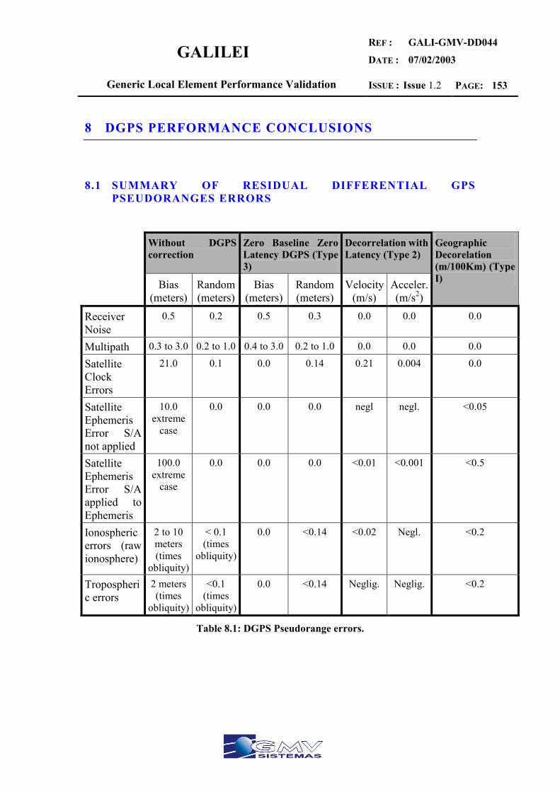
GALILEI REF :
DATE :
GALI-GMV-DD044
07/02/2003
Generic Local Element Performance Validation ISSUE : Issue 1.2 PAGE: 153
8 DGPS PERFORMANCE CONCLUSIONS
8.1 SUMMARY OF RESIDUAL DIFFERENTIAL GPS PSEUDORANGES ERRORS
Without DGPS correction
Zero Baseline Zero Latency DGPS (Type 3)
Decorrelation with Latency (Type 2)
Bias (meters)
Random (meters)
Bias (meters)
Random (meters)
Velocity (m/s)
Acceler. (m/s2)
Geographic Decorelation (m/100Km) (Type I)
Receiver Noise
0.5 0.2 0.5 0.3 0.0 0.0 0.0
Multipath 0.3 to 3.0 0.2 to 1.0 0.4 to 3.0 0.2 to 1.0 0.0 0.0 0.0
Satellite Clock Errors
21.0 0.1 0.0 0.14 0.21 0.004 0.0
Satellite Ephemeris Error S/A not applied
10.0 extreme
case
0.0 0.0 0.0 negl negl. <0.05
Satellite Ephemeris Error S/A applied to Ephemeris
100.0 extreme
case
0.0 0.0 0.0 <0.01 <0.001 <0.5
Ionospheric errors (raw ionosphere)
2 to 10 meters (times
obliquity)
< 0.1 (times
obliquity)
0.0 <0.14 <0.02 Negl. <0.2
Tropospheric errors
2 meters (times
obliquity)
<0.1 (times
obliquity)
0.0 <0.14 Neglig. Neglig. <0.2
Table 8.1: DGPS Pseudorange errors.
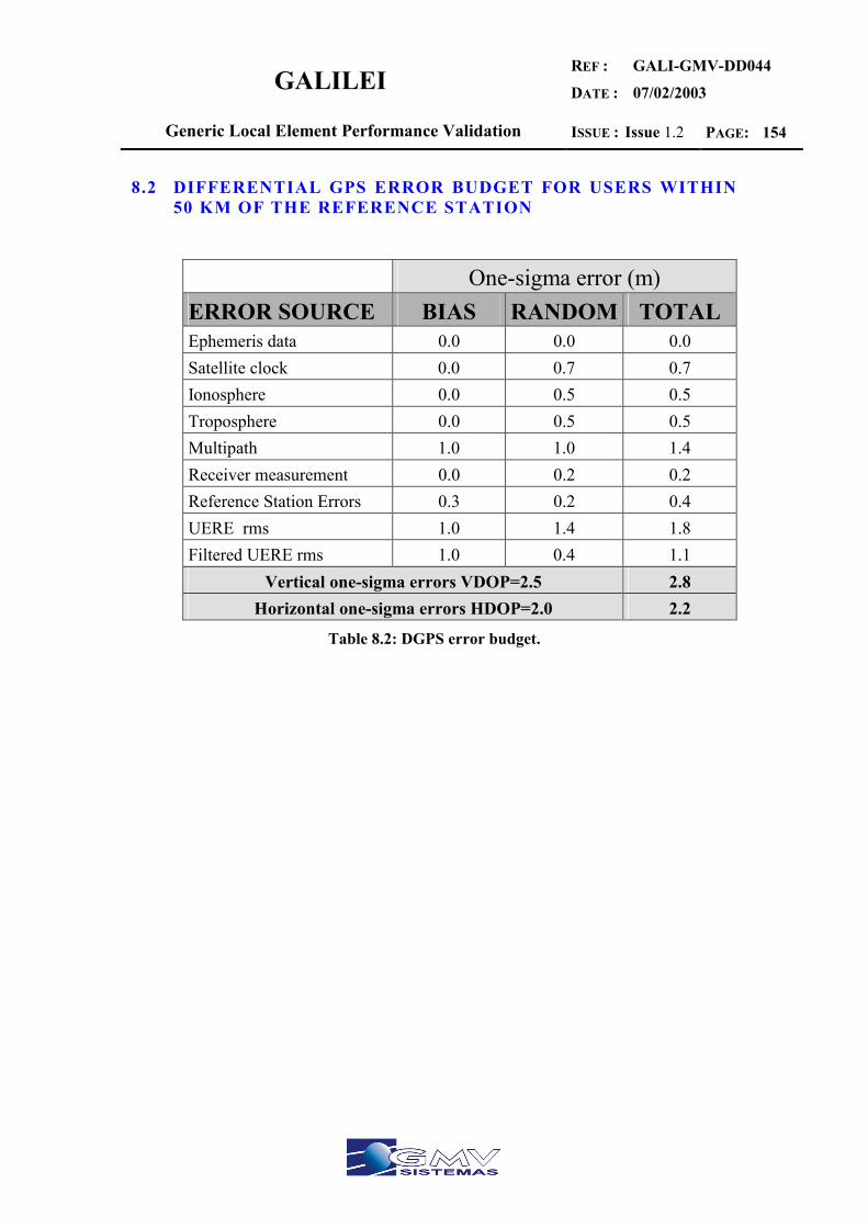
GALILEI REF :
DATE :
GALI-GMV-DD044
07/02/2003
Generic Local Element Performance Validation ISSUE : Issue 1.2 PAGE: 154
8.2 DIFFERENTIAL GPS ERROR BUDGET FOR USERS WITHIN 50 KM OF THE REFERENCE STATION
One-sigma error (m) ERROR SOURCE BIAS RANDOM TOTAL Ephemeris data 0.0 0.0 0.0 Satellite clock 0.0 0.7 0.7 Ionosphere 0.0 0.5 0.5 Troposphere 0.0 0.5 0.5 Multipath 1.0 1.0 1.4 Receiver measurement 0.0 0.2 0.2 Reference Station Errors 0.3 0.2 0.4 UERE rms 1.0 1.4 1.8 Filtered UERE rms 1.0 0.4 1.1
Vertical one-sigma errors VDOP=2.5 2.8 Horizontal one-sigma errors HDOP=2.0 2.2
Table 8.2: DGPS error budget.
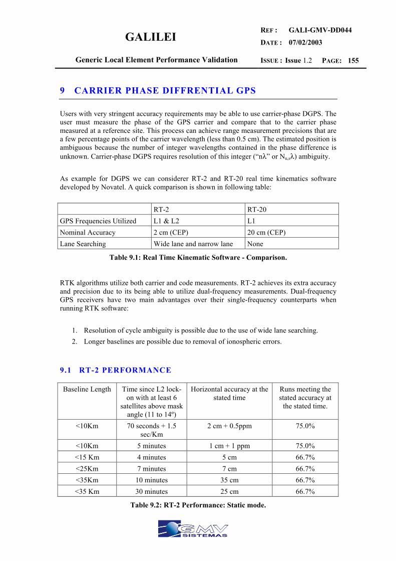
GALILEI REF :
DATE :
GALI-GMV-DD044
07/02/2003
Generic Local Element Performance Validation ISSUE : Issue 1.2 PAGE: 155
9 CARRIER PHASE DIFFRENTIAL GPS
Users with very stringent accuracy requirements may be able to use carrier-phase DGPS. The user must measure the phase of the GPS carrier and compare that to the carrier phase measured at a reference site. This process can achieve range measurement precisions that are a few percentage points of the carrier wavelength (less than 0.5 cm). The estimated position is ambiguous because the number of integer wavelengths contained in the phase difference is unknown. Carrier-phase DGPS requires resolution of this integer (“nλ” or Nu,sλ) ambiguity. As example for DGPS we can considerer RT-2 and RT-20 real time kinematics software developed by Novatel. A quick comparison is shown in following table: RT-2 RT-20 GPS Frequencies Utilized L1 & L2 L1 Nominal Accuracy 2 cm (CEP) 20 cm (CEP) Lane Searching Wide lane and narrow lane None
Table 9.1: Real Time Kinematic Software - Comparison.
RTK algorithms utilize both carrier and code measurements. RT-2 achieves its extra accuracy and precision due to its being able to utilize dual-frequency measurements. Dual-frequency GPS receivers have two main advantages over their single-frequency counterparts when running RTK software:
1. Resolution of cycle ambiguity is possible due to the use of wide lane searching. 2. Longer baselines are possible due to removal of ionospheric errors.
9.1 RT-2 PERFORMANCE
Baseline Length Time since L2 lock-on with at least 6
satellites above mask angle (11 to 14º)
Horizontal accuracy at the stated time
Runs meeting the stated accuracy at
the stated time.
<10Km 70 seconds + 1.5 sec/Km
2 cm + 0.5ppm 75.0%
<10Km 5 minutes 1 cm + 1 ppm 75.0% <15 Km 4 minutes 5 cm 66.7% <25Km 7 minutes 7 cm 66.7% <35Km 10 minutes 35 cm 66.7% <35 Km 30 minutes 25 cm 66.7%
Table 9.2: RT-2 Performance: Static mode.

GALILEI REF :
DATE :
GALI-GMV-DD044
07/02/2003
Generic Local Element Performance Validation ISSUE : Issue 1.2 PAGE: 156
Baseline Length Time since L2 lock-on with at least 6
satellites above mask angle (11 to 14º)
Horizontal accuracy at the stated time
Runs meeting the stated accuracy at
the stated time.
< 10 Km 120 seconds + 1.5 sec/km
2 cm + 0.5 ppm 75.0%
< 15 Km 8 minutes 8 cm 66.7% < 25 Km 14 minutes 10 cm 66.7% < 35 Km 20 minutes 40 cm 66.7% < 35 Km 60 minutes 25 cm 66.7%
Table 9.3: RT-2 Performance Kinematic mode.
Fig. 9.1: Typical RT-2 Horizontal convergence – Static mode.
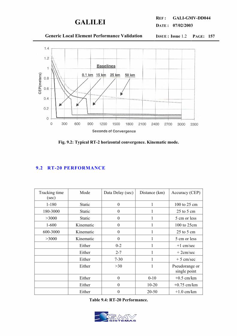
GALILEI REF :
DATE :
GALI-GMV-DD044
07/02/2003
Generic Local Element Performance Validation ISSUE : Issue 1.2 PAGE: 157
Fig. 9.2: Typical RT-2 horizontal convergence. Kinematic mode.
9.2 RT-20 PERFORMANCE
Tracking time (sec)
Mode Data Delay (sec) Distance (km) Accuracy (CEP)
1-180 Static 0 1 100 to 25 cm 180-3000 Static 0 1 25 to 5 cm
>3000 Static 0 1 5 cm or less 1-600 Kinematic 0 1 100 to 25cm
600-3000 Kinematic 0 1 25 to 5 cm >3000 Kinematic 0 1 5 cm or less
Either 0-2 1 +1 cm/sec Either 2-7 1 + 2cm/sec Either 7-30 1 + 5 cm/sec Either >30 1 Pseudorange or
single point Either 0 0-10 +0.5 cm/km Either 0 10-20 +0.75 cm/km Either 0 20-50 +1.0 cm/km
Table 9.4: RT-20 Performance.
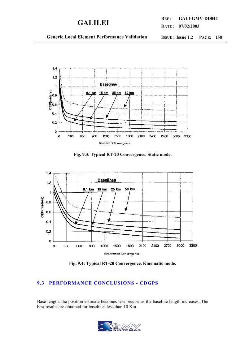
GALILEI REF :
DATE :
GALI-GMV-DD044
07/02/2003
Generic Local Element Performance Validation ISSUE : Issue 1.2 PAGE: 158
Fig. 9.3: Typical RT-20 Convergence. Static mode.
Fig. 9.4: Typical RT-20 Convergence. Kinematic mode.
9.3 PERFORMANCE CONCLUSIONS - CDGPS
Base length: the position estimate becomes less precise as the baseline length increases. The best results are obtained for baselines less than 10 Km.
GALILEI REF :
DATE :
GALI-GMV-DD044
07/02/2003
Generic Local Element Performance Validation ISSUE : Issue 1.2 PAGE: 159
• Ephemeris errors: typical position errors of 0.75 cm per 10 Km of baseline length • Ionospheric effects: Error dominant for single-frequency GPS receivers on baselines
exceeding 10 Km. Differential ionospheric effects reach their peak at dusk and dawn, being at a minimum during hours of darkness. Ionospheric effects can be estimated and removed on dual-frequency GPS receivers, increasing the permissible baseline length, but at the cost of introducing additional noise to the solution. Therefore this type of compensation is only used increases where the ionosphere error is much larger the noise and multipath error.
• Tropospheric effects. Typical position errors of approximately 1 cm per 10 Km of baseline length. This error increases if there is a significant height difference between the reference and remote stations, as well as if there are significantly different weather conditions between the two sites.
• Multipath interference: is the dominant error on short differential baselines. • Convergence time: the position estimate becomes more accurate and more precise
with time. Convergence time is affected by the number of satellites and baseline length.

GALILEI REF :
DATE :
GALI-GMV-DD044
07/02/2003
Generic Local Element Performance Validation ISSUE : Issue 1.2 PAGE: 160
10 REFERENCES
[1] Theory and applications. Volume II. Parkinson and Spilker, Eds/. Axelrad and Enge, Assoc.Eds [2] Galileo Signal Validation Development R. De Gaudenzi, European Space Agency, N.Hoult, A Batchelor, G. Burden, M. Quinlan, Thales Research Ltd, United Kingdom [3] Dual frequency DGPS service for combating ionospheric interference. Ole Orpen. Henk Zwaan. Fugro Seastar AS. [4] RTCM recommended standards for differential navstar GPS reference stations and integrity monitors. Developed by RTCM special committee nº104. [5] GALILEI Annex 1 “Description of work” 19/07/2001 [6] The Local component in Galileo Architecture. Hans Birli Thales ATM. Umberto Guida alenia Spazio. [7] Analysis of the Three Carrier Ambiguity Resolution (TCAR) Technique for Precise Relative Positioning in GNSS-2, Vollath U., et al, Proceedings of the ION GPS-98, 1998. [8] Dynamic-free Bias-free Differential GPS: Application to Landing, Martin-Neira M., Lucas R., Proceeedings of the AAS Conference, Durango, 1991, AAS-91-413. [9] GALA, the definition of GALILEO overall architecture. Arnaud Masson. Jean Chenebault, Nicolas Vicent, Alcatel Spaces Industries, Christof Shäfer, Mark Stevens, Astrium, Francesco Martinino, Alenia Spazio, Ian Casewell, Nicole Duchenne, Christian Legras, THALES, Miguel Romay, GMV,Luigi Gortan, CRF. [10] Recommendations on Differential GNSS Mr. Joseph W. Spalding USCG Research & Development Center Dr. Jacques Beser 3S Navigation Inc. Dr. Frank van Diggelen Ashtech, Inc.

GALILEI REF :
DATE :
GALI-GMV-DD044
07/02/2003
Generic Local Element Performance Validation ISSUE : Issue 1.2 PAGE: 161
ANNEX 3 PSEUDOLITE
GALILEI REF :
DATE :
GALI-GMV-DD044
07/02/2003
Generic Local Element Performance Validation ISSUE : Issue 1.2 PAGE: 162
1 INTRODUCTION
Pseudolites (PLs) are ground based transmitters that can be configured to emit GALILEO-like signals for enhancing GALILEO navigation performances by providing increased accuracy, integrity and availability.
Accuracy improvement can occur because of better local geometry, as measured by a lower vertical dilution of precision (VDOP), which is important in aircraft precision approach and landing applications. Accuracy and integrity enhancement can also be achieved by employing a PL´s integral data link to support differential modes of operation ant timely transmittal of integrity warning information. Availability is increased because a PL provides an additional ranging source to augment the GALILEO constellation.[1]. Pseudolites use a CDMA signal structure similar to the satellites and operate within the same frequency bands of the navigation satellite system they augment, even if their pseudo-satellite signals are characterized by different gold codes and data messages. The introduction of pseudolites has two key objectives:
• signal augmentation • data link enhancement.
Signal augmentation increase the number of available signals and improve or
maintain the geometrical quality for user position determination. Data link enhancement provide an integrated capacity for supplying key data to users for the navigation system and the pseudolites integrity warning and differential corrections to improve positioning accuracy via code-based local differential techniques (LDGPS) and potentially carrier phase-based kinematics differential techniques. The big advantage of a pseudolite configuration compared to a stand-alone navigation satellite system is their exact known location. These performance enhancements are deeply dependent on the synchronization between the local pseudolite-based system clock and the navigation system time. Pseudolite transmitters that contain an atomic clock synchronized to GPS time may be used as an additional stand-alone ranging source just like the GPS satellites. By using a GPS receiver to solve for the clock offset from GPS time very accurately, this form of a pseudolite transceiver may synchronize its transmitted signal when sufficient GPS satellites are in view. This allows the transmitted signal to be utilized by the user independently of any GPS satellite or reference station. However, very stable clocks and time-synchronization equipment make this option expensive [3]. This synchronization can be achieved in the other two ways, according to the architecture of the pseudolites configuration.
• If the employment of only one pseudolite is envisaged, the more attractive architecture is based on the pseudolite collocated with a LDGPS reference receiver.

GALILEI REF :
DATE :
GALI-GMV-DD044
07/02/2003
Generic Local Element Performance Validation ISSUE : Issue 1.2 PAGE: 163
According to this approach, only one TX/RX antenna allowing also self-calibration, is employed by the pseudolite, especially if LOS (Line Of Sight) visibility to the reference receiver might be a problem.
• If more than one pseudolite is required, the remote approach with a common
reference receiver for synchronization is more desirable. In this case, the reference receiver sends corrections to the remote “slave” pseudolites to correct itself and also sends message data to be transmitted.
Pseudolites can be configured to serve a limited area with a power level low enough to
preclude appreciable interference to standard navigation signals coming from the space-based Constellation.
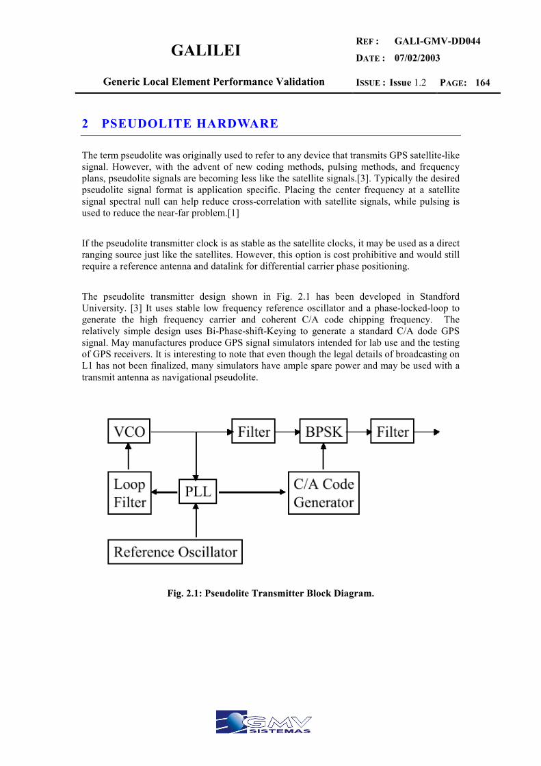
GALILEI REF :
DATE :
GALI-GMV-DD044
07/02/2003
Generic Local Element Performance Validation ISSUE : Issue 1.2 PAGE: 164
2 PSEUDOLITE HARDWARE
The term pseudolite was originally used to refer to any device that transmits GPS satellite-like signal. However, with the advent of new coding methods, pulsing methods, and frequency plans, pseudolite signals are becoming less like the satellite signals.[3]. Typically the desired pseudolite signal format is application specific. Placing the center frequency at a satellite signal spectral null can help reduce cross-correlation with satellite signals, while pulsing is used to reduce the near-far problem.[1] If the pseudolite transmitter clock is as stable as the satellite clocks, it may be used as a direct ranging source just like the satellites. However, this option is cost prohibitive and would still require a reference antenna and datalink for differential carrier phase positioning. The pseudolite transmitter design shown in Fig. 2.1 has been developed in Standford University. [3] It uses stable low frequency reference oscillator and a phase-locked-loop to generate the high frequency carrier and coherent C/A code chipping frequency. The relatively simple design uses Bi-Phase-shift-Keying to generate a standard C/A dode GPS signal. May manufactures produce GPS signal simulators intended for lab use and the testing of GPS receivers. It is interesting to note that even though the legal details of broadcasting on L1 has not been finalized, many simulators have ample spare power and may be used with a transmit antenna as navigational pseudolite.
Fig. 2.1: Pseudolite Transmitter Block Diagram.
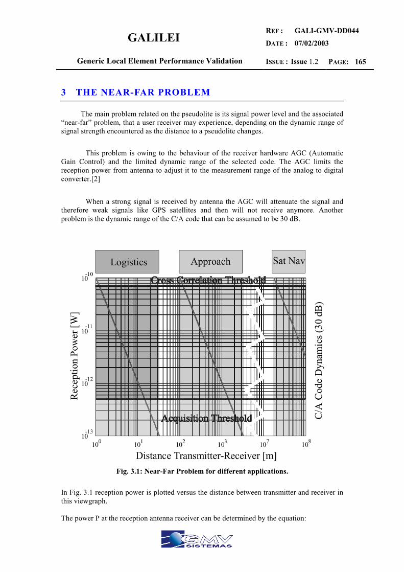
GALILEI REF :
DATE :
GALI-GMV-DD044
07/02/2003
Generic Local Element Performance Validation ISSUE : Issue 1.2 PAGE: 165
3 THE NEAR-FAR PROBLEM
The main problem related on the pseudolite is its signal power level and the associated “near-far” problem, that a user receiver may experience, depending on the dynamic range of signal strength encountered as the distance to a pseudolite changes.
This problem is owing to the behaviour of the receiver hardware AGC (Automatic Gain Control) and the limited dynamic range of the selected code. The AGC limits the reception power from antenna to adjust it to the measurement range of the analog to digital converter.[2]
When a strong signal is received by antenna the AGC will attenuate the signal and therefore weak signals like GPS satellites and then will not receive anymore. Another problem is the dynamic range of the C/A code that can be assumed to be 30 dB.
Fig. 3.1: Near-Far Problem for different applications.
In Fig. 3.1 reception power is plotted versus the distance between transmitter and receiver in this viewgraph. The power P at the reception antenna receiver can be determined by the equation:
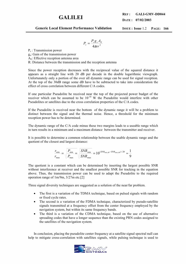
GALILEI REF :
DATE :
GALI-GMV-DD044
07/02/2003
Generic Local Element Performance Validation ISSUE : Issue 1.2 PAGE: 166
24 rrAgPP Ess
s π=
Ps : Transmission power ga: Gain of the transmission power AE: Effective reception antenna area R: Distance between the transmission and the reception antenna Since the power reception decreases with the reciprocal value of the squared distance it appears as a straight line with 20 dB per decade in the double logarithmic viewgraph. Unfortunately only a portion of the over all dynamic range can be used for signal reception. At the top of the 30dB range some dB have to be subtracted to take into consideration the effect of cross correlation between different C/A codes. If one particular Pseudolite be received near the top of the projected power budget of the receiver which can be assumed to be 10-10 W the Pseudolite would interfere with other Pseudolites or satellites due to the cross correlation properties of the C/A codes. If the Pseudolite is received near the bottom of the dynamic range it will be a problem to distinct between the signal and the thermal noise. Hence, a threshold for the minimum reception power has to be determined. The dynamic range of the C/A code minus these two margins leads to a useable range which in turn results in a minimum and a maximum distance between the transmitter and receiver. It is possible to determine a common relationship between the usable dynamic range and the quotient of the closest and largest distance:
9110 20/)(
max
min
max
min
max
min max,min, ≈=== − dBdB SNRSNR
SNRSNR
PP
rr
The quotient is a constant which can be determined by inserting the largest possible SNR without interference at receiver and the smallest possible SNR for tracking in the equation above. Thus, the transmission power can be used to adapt the Pseudolite to the required operation range of 1m/9m, 3/27m etc.[2] Three signal diversity techniques are suggested as a solution of the near/far problem.
• The first is a variation of the TDMA technique, based on pulsed signals with random or fixed cycle rates.
• The second is a variation of the FDMA technique, characterized by pseudo-satellite signals transmitted at a frequency offset from the center frequency employed by the navigation system, but within its same frequency bands.
• The third is a variation of the CDMA technique, based on the use of alternative spreading codes that have a longer sequence than the existing PRN codes assigned to the satellites of the navigation system.
In conclusion, placing the pseudolite center frequency at a satellite signal spectral null can help to mitigate cross-correlation with satellites signals, while pulsing technique is used to
GALILEI REF :
DATE :
GALI-GMV-DD044
07/02/2003
Generic Local Element Performance Validation ISSUE : Issue 1.2 PAGE: 167
reduce the near/far problem. Further, increasing the data rate can allow the transfer of differential corrections, eliminating the need for additional data-links.
In the case of GPS system, the power received from the GPS satellites is nearly
independent of user location, since received signal power typically decreases by only 10 dB as the satellites move from zenith to within 5 degrees of the horizon. In contrast, the power received from a pseudolite changes by 60 dB from an acquisition range of 10 km to a point of closest approach on the runway of 10 m.
The pseudolite signal is pulsed to reduce interference with GPS receivers. The pulsing duty cycle may be 10% with pulse duration of 100 µs. Such a short pulse has a little effect on most GPS receivers.
Nevertheless, pulsing alone may not guarantee non-interference. In this case, the pseudolite could use a 10 MHz chipping rate rather than the 1 MHz chipping rate used by SPS.
Alternatively, the pseudolite signal could be offset in frequency relative to the GPS L1 frequency. Offset of 8 MHz or more would be reassuring, because the filters in the receiver front end would partially attenuate the pseudolite signal.
In summary, near/far problem is probably best solved by pulsing and using a higher chipping rate.
Other alternative [2] to overcome the limitations of the Near-Far problem as well as
the large error budget due to multipath propagation is the adaptation of the antenna diagram to the pseudolite´s environment. The type of antenna used would depend upon the application and environment. Microstrip path antennas (Fig. 3.2) provide a uniform spherical pattern which is optimal for small areas, e.g. indoor usage. Whereas high-gain parabolic or helix antennas are suitable for long-range coverage. Possible reflectors can be excluded by notches in the antenna pattern or by beam shaping using different kinds of ground planes. Site planning for pseudolite transmitter antennas has to be done carefully, depending on the geometry and user requirements.
Fig. 3.2: Microstrip patch antenna with choke ring.

GALILEI REF :
DATE :
GALI-GMV-DD044
07/02/2003
Generic Local Element Performance Validation ISSUE : Issue 1.2 PAGE: 168
4 MULTIPATH PROPAGATION
Multipath propagation is caused by reflection of the original signal which interfere with the signal itself. Possible reflectors are any kind of surfaces. Metallic reflectors work like mirrors for electromagnetic waves in the particular frequency band. Depending on the reflection angle α and the material of the reflector the orientation of the polarization may be changed. The models which represent this behavior are usually very complex. Besides this, some basic conclusions can be drawn from a very simple reflection model. Fig. 4.1 shows a basic reflection model taking into account two way propagation of the electromagnetic wave. The reflected signal which superimposes the direct wave reach from below the reception antenna.[2]
Fig. 4.1: Basic Reflection Model.
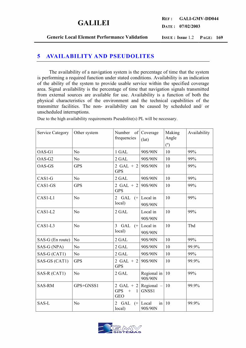
GALILEI REF :
DATE :
GALI-GMV-DD044
07/02/2003
Generic Local Element Performance Validation ISSUE : Issue 1.2 PAGE: 169
5 AVAILABILITY AND PSEUDOLITES
The availability of a navigation system is the percentage of time that the system is performing a required function under stated conditions. Availability is an indication of the ability of the system to provide usable service within the specified coverage area. Signal availability is the percentage of time that navigation signals transmitted from external sources are available for use. Availability is a function of both the physical characteristics of the environment and the technical capabilities of the transmitter facilities. The non- availability can be caused by scheduled and/ or unscheduled interruptions. Due to the high availability requirements Pseudolite(s) PL will be necessary. Service Category Other system Number of
frequencies Coverage (lat)
Making Angle (º)
Availability
OAS-G1 No 1 GAL 90S/90N 10 99% OAS-G2 No 2 GAL 90S/90N 10 99% OAS-GS GPS 2 GAL + 2
GPS 90S/90N 10 99%
CAS1-G No 2 GAL 90S/90N 10 99% CAS1-GS GPS 2 GAL + 2
GPS 90S/90N 10 99%
CAS1-L1 No 2 GAL (+ local)
Local in 90S/90N
10 99%
CAS1-L2 No 2 GAL Local in 90S/90N
10 99%
CAS1-L3 No 3 GAL (+ local)
Local in 90S/90N
10 Tbd
SAS-G (En route) No 2 GAL 90S/90N 10 99% SAS-G (NPA) No 2 GAL 90S/90N 10 99.9% SAS-G (CAT1) No 2 GAL 90S/90N 10 99% SAS-GS (CAT1) GPS 2 GAL + 2
GPS 90S/90N 10 99.9%
SAS-R (CAT1) No 2 GAL Regional in 90S/90N
10 99%
SAS-RM GPS+GNSS1 2 GAL + 2 GPS + 1 GEO
Regional – GNSS1
10 99.9%
SAS-L No 2 GAL (+ local)
Local in 90S/90N
10 99.9%
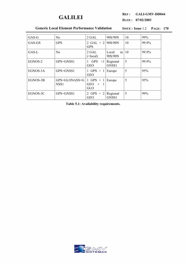
GALILEI REF :
DATE :
GALI-GMV-DD044
07/02/2003
Generic Local Element Performance Validation ISSUE : Issue 1.2 PAGE: 170
GAS-G No 2 GAL 90S/90N 10 99% GAS-GS GPS 2 GAL + 2
GPS 90S/90N 10 99.9%
GAS-L No 2 GAL (+local)
Local in 90S/90N
10 99.9%
EGNOS-2 GPS+GNSS1 1 GPS +1 GEO
Regional GNSS1
5 99.9%
EGNOS-3A GPS+GNSS1 1 GPS + 1 GEO
Europe 5 95%
EGNOS-3B GPS+GLONASS+GNSS1
1 GPS + 1 GEO + 1 GLO
Europe 5 95%
EGNOS-3C GPS+GNSS1 2 GPS + 2 GEO
Regional GNSS1
5 99%
Table 5.1: Availability requirements.
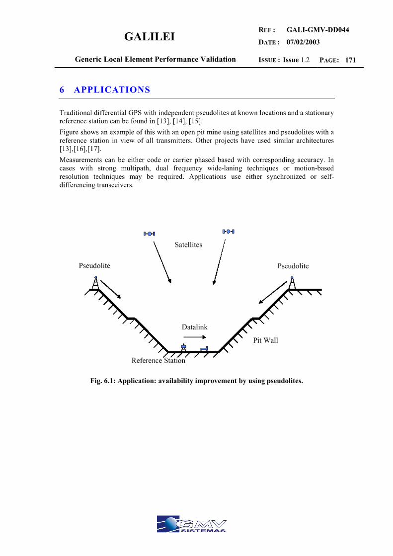
GALILEI REF :
DATE :
GALI-GMV-DD044
07/02/2003
Generic Local Element Performance Validation ISSUE : Issue 1.2 PAGE: 171
6 APPLICATIONS
Traditional differential GPS with independent pseudolites at known locations and a stationary reference station can be found in [13], [14], [15]. Figure shows an example of this with an open pit mine using satellites and pseudolites with a reference station in view of all transmitters. Other projects have used similar architectures [13],[16],[17]. Measurements can be either code or carrier phased based with corresponding accuracy. In cases with strong multipath, dual frequency wide-laning techniques or motion-based resolution techniques may be required. Applications use either synchronized or self-differencing transceivers.
Fig. 6.1: Application: availability improvement by using pseudolites.
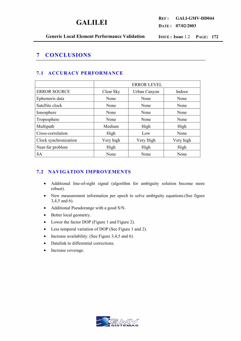
GALILEI REF :
DATE :
GALI-GMV-DD044
07/02/2003
Generic Local Element Performance Validation ISSUE : Issue 1.2 PAGE: 172
7 CONCLUSIONS
7.1 ACCURACY PERFORMANCE
ERROR LEVEL ERROR SOURCE Clear Sky Urban Canyon Indoor Ephemeris data None None None Satellite clock None None None Ionosphere None None None Troposphere None None None Multipath Medium High High Cross-correlation High Low None Clock synchronization Very high Very High Very high Near-far problem High High High SA None None None
7.2 NAVIGATION IMPROVEMENTS
• Additional line-of-sight signal (algorithm for ambiguity solution become more robust).
• New measurement information per epoch to solve ambiguity equations.(See figure 3,4,5 and 6).
• Additional Pseudorange with a good S/N. • Better local geometry. • Lower the factor DOP (Figure 1 and Figure 2). • Less temporal variation of DOP (See Figure 1 and 2). • Increase availability. (See Figure 3,4,5 and 6). • Datalink to differential corrections. • Increase coverage.
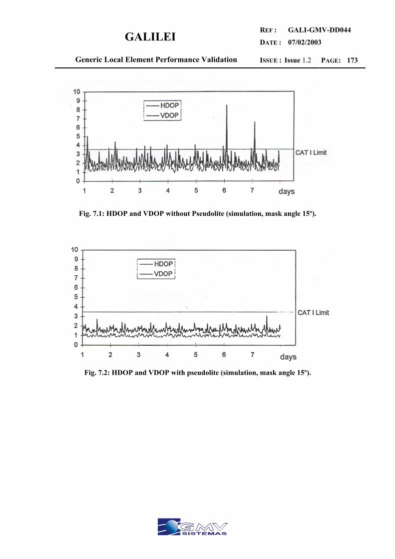
GALILEI REF :
DATE :
GALI-GMV-DD044
07/02/2003
Generic Local Element Performance Validation ISSUE : Issue 1.2 PAGE: 173
Fig. 7.1: HDOP and VDOP without Pseudolite (simulation, mask angle 15º).
Fig. 7.2: HDOP and VDOP with pseudolite (simulation, mask angle 15º).
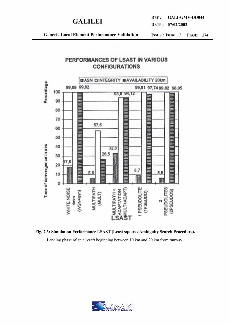
GALILEI REF :
DATE :
GALI-GMV-DD044
07/02/2003
Generic Local Element Performance Validation ISSUE : Issue 1.2 PAGE: 174
Fig. 7.3: Simulation Performance LSAST (Least squares Ambiguity Search Procedure).
Landing phase of an aircraft beginning between 10 km and 20 km from runway.
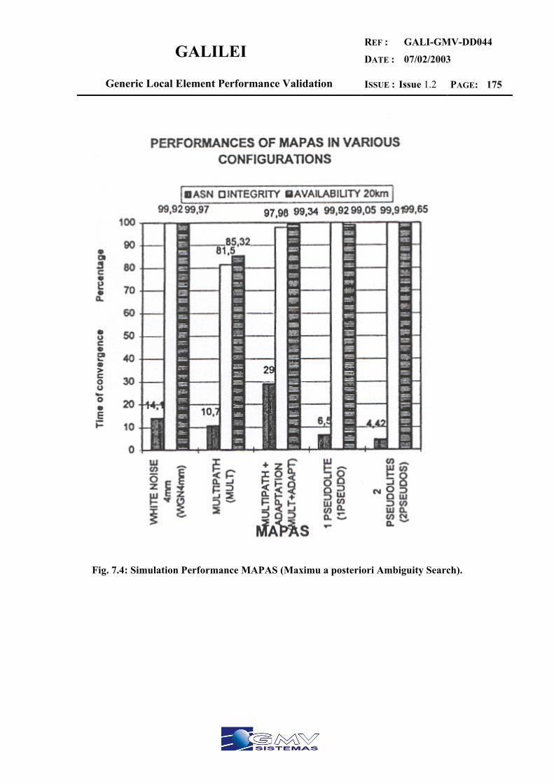
GALILEI REF :
DATE :
GALI-GMV-DD044
07/02/2003
Generic Local Element Performance Validation ISSUE : Issue 1.2 PAGE: 175
Fig. 7.4: Simulation Performance MAPAS (Maximu a posteriori Ambiguity Search).

GALILEI REF :
DATE :
GALI-GMV-DD044
07/02/2003
Generic Local Element Performance Validation ISSUE : Issue 1.2 PAGE: 176
Fig. 7.5: Simulation Performance FASF (Fast Ambiguity Search Filter).

GALILEI REF :
DATE :
GALI-GMV-DD044
07/02/2003
Generic Local Element Performance Validation ISSUE : Issue 1.2 PAGE: 177
Fig. 7.6: Simulation Performance DIAS (Direct Integer Ambiguity search).
GALILEI REF :
DATE :
GALI-GMV-DD044
07/02/2003
Generic Local Element Performance Validation ISSUE : Issue 1.2 PAGE: 178
8 REFERENCES
[1] Global Positioning System: Theory and applications. Volumen II. Parkinson and Spilker, Eds/. Axelrad and Enge, Assoc.Eds [2] Antenna Diagram Shaping for Pseudolite Transmitter Antennas. A solution to the near-far problem. Sven Martin. Institute of flight Guidance and Control. Technical Universiuty of Braunschwaeig, Germany. [3] GPS Pseudolite Transceivers and ther aplications. Jonathan Mstone, Edward A. Le Master, Prof J. David Powell, Prof Stephen Rock, Standford University. [4] Galileo Signal Validation Development R. De Gaudenzi, European Space Agency, N. Hoult, A Batchelor, G. Burden, M. Quinlan, Thales Research Ltd, United Kingdom [5]Recommendations on Differential GNSS Mr. Joseph W. Spalding USCG Research & Development Center Dr. Jacques Beser 3S Navigation Inc. Dr. Frank van Diggelen Ashtech, Inc. [6] Dual frequency DGPS service for combating ionospheric interference. Ole Orpen. Henk Zwaan. Fugro Seastar AS. [7] RTCM recommended standards for differential navstar GPS reference stations and integrity monitors. Developed by RTCM special committee nº104. [8] GALILEI Annex 1 “Description of work” 19/07/2001 [9] The Local component in Galileo Architecture. Hans Birli Thales ATM. Umberto Guida alenia Spazio. [10] Analysis of the Three Carrier Ambiguity Resolution (TCAR) Technique for Precise Relative Positioning in GNSS-2, Vollath U., et al,Proceedings of the ION GPS-98, 1998. [11] Dynamic-free Bias-free Differential GPS: Application to Landing, Martin-Neira M., Lucas R., Proceeedings of the AAS Conference, Durango, 1991, AAS-91-413. [12] GALA, the definition of GALILEO overall architecture. Arnaud Masson. Jean Chenebault, Nicolas Vicent, Alcatel Spaces Industries, Christof Shäfer, Mark Stevens, Astrium, Francesco Martinino, Alenia Spazio, Ian Casewell, Nicole Duchenne, Christian Legras, THALES, Miguel Romay, GMV,Luigi Gortan, CRF. [13] “HAPPI – a High Accuracy Pseudolite/GPS Position Integration”, Ford, Tom, et al, Proceedings of ION-GPS-97, Kansas City, MO, Sept. 1997, pp.1719-1728. [14] “Precise Positioning with GPS near Obstructions by Augmentation with Pseudolites”, Stone, J.M. Powell, J.D. Proceedings of IEEE PLANS 1998, Palm Spring, CA. pp. 562-569. [15] “Experimental demonstration of GPS for rendezvous between two prototype space vehicles”, Zimmerma, Kurt et al., Proceedings of ION-GPS-95, Palm Springs CA, v 2 1995, pp. 1905-1913. [16] “Pseudolite Augmented DGPS for Land Applications”, Holden, T. and Morley, T. Proceedings ION-GPS-97, Kansas City, MO, Sep. 1997, pp. 1397-1404. [17] ”Proposed Airport Pseudolite Signal Specification for GPS Precision Approach Local Area Augmmentation Systems”, Van Dierendonck, AJ. Fenton, P.Hegarty, C. proceedings of ION-GPS-97, Kansas City, MO, Sept. 1997, pp. 1603-1612.

GALILEI REF :
DATE :
GALI-GMV-DD044
07/02/2003
Generic Local Element Performance Validation ISSUE : Issue 1.2 PAGE: 179
ANNEX 4 LOCAL INTEGRITY MONITOR

GALILEI REF :
DATE :
GALI-GMV-DD044
07/02/2003
Generic Local Element Performance Validation ISSUE : Issue 1.2 PAGE: 180
1 INTRODUCTION
One objective of the system GALILEO will be the provision of integrity information in form of an integrity flag (IF) to he user. The purpose of this is that each satellite individual has a integrity flag to inform the user about the correctness of the accuracy information contained in the signal-in-space accuracy (SISA) value. [1] Considering the basic integrity architecture, there are still unresolved key issues remaining that will drive the GALILEO performance. Critical use cases will be covered by the GIPA (GALILEO Integrity Performance Assessment) project [1]. The following GIPA use cases (GUC) are considered by GIPA project [1]:
• GUC-01 SISA representation. • GUC-02 SISA Refresh Rate. • GUC-03 SISA Margin Assumption. • GUC-04 If Spatial Concept. • GUC-05 IMS (Integrity monitor Station) Netwok. • GUC-06 IMS Measurement Quality. • GUC-07 Navigation signal. • GUC-08 Feared Events. • GUC-09 Elevation Mask Angle at User. • GUC-10 Elevation Mask at IMS.
GIPA project conclusions to GUC can be consulted in reference [1]

GALILEI REF :
DATE :
GALI-GMV-DD044
07/02/2003
Generic Local Element Performance Validation ISSUE : Issue 1.2 PAGE: 181
2 LIMS AND INTEGRITY
Local Integrity Monitoring Stations (LIMS) improve local integrity for the user. The LIMS calculates its position from the satellite constellation, compares it with its true position and checks whether it is in the tolerated limit and sends an integrity flag to the user in case one satellite cannot be used. LIMS become necessary, when the time-to alarm of a local application is shorter than being provided by the Galileo core system. The integrity monitor (LIM) receives all the SIS including the data link and pseudolite signal and checks independently the function of the reference station and of the pseudolite stations. The monitoring functions ensure that reference station broadcasts no hazardous misleading information and no bad signal in space is transmitted by the pseudolite.
A user shall received a timely warning when a failure exists, i. e. when a position error exceeds the Alarm Limit. TTA requirements demand Local Integrity monitoring stations LIM. Service Category Integrity risk Time to
alarm Horizontal alarm limit
Vertical alarm limit
Level of Guarantee
OAS-G1 NA NA NA NA None OAS-G2 NA NA NA NA None OAS-GS NA NA NA NA None CAS1-G 2.10-7 hour 10 s 20 m 45 m High CAS1-GS 2.10-7 hour 10 s 13 m 32 m Medium CAS1-L1 2.10-7 hour 1 s 2 m 3.5 m High CAS1-L2 2.10-7 hour 10 s tbc 2 m 3.5 m High CAS1-L3 tbd Tbd Tbd Tbd High SAS-G (En route) 2.10-7 hour 15 s 556 m NA High SAS-G (NPA) 2.10-7 hour 10 s 556 m NA High SAS-G (CAT1) 3.5.10-7 /150s 6 s 11 m 15 m High SAS-GS (CAT1) 3.5.10-7 /150s 6 s 8 m 10 m Medium SAS-R (CAT1) 3.5.10-7 /150s 6 s 11 m 15 m High SAS-RM 3.5.10-7 /150s 6 s 8 m 10 m Medium SAS-L 2.10-8 /150s 1 s 3 m 5.5 m High GAS-G 3.5.10-7 /150 s 6 s 11 m 15 m High GAS-GS 3.5.10-7 /150 s 6 s 8 m 10 m Medium GAS-L 2.10-8 / 150 s 1 s 3 m 5.5 m High
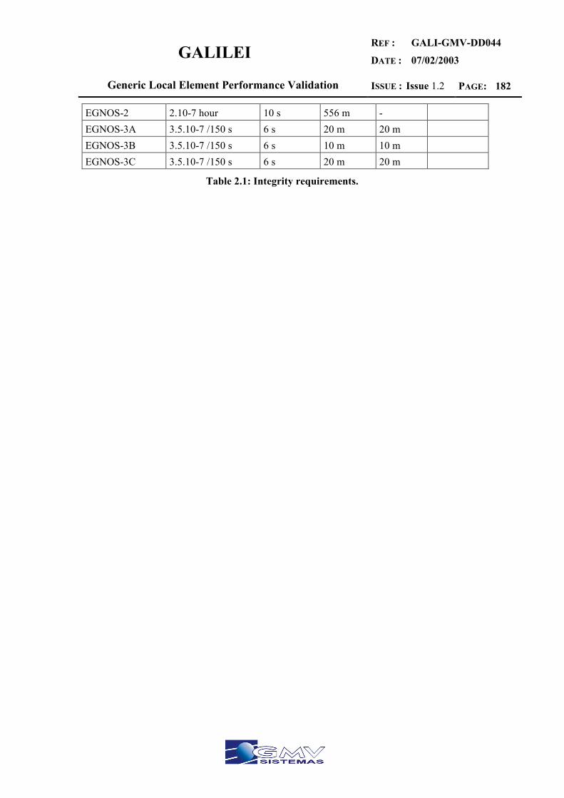
GALILEI REF :
DATE :
GALI-GMV-DD044
07/02/2003
Generic Local Element Performance Validation ISSUE : Issue 1.2 PAGE: 182
EGNOS-2 2.10-7 hour 10 s 556 m - EGNOS-3A 3.5.10-7 /150 s 6 s 20 m 20 m EGNOS-3B 3.5.10-7 /150 s 6 s 10 m 10 m EGNOS-3C 3.5.10-7 /150 s 6 s 20 m 20 m
Table 2.1: Integrity requirements.
GALILEI REF :
DATE :
GALI-GMV-DD044
07/02/2003
Generic Local Element Performance Validation ISSUE : Issue 1.2 PAGE: 183
3 INTEGRITY AND AIR NAVIGATION SYSTEMS
Integrity is the measure of trust that can be placed on the correctness of the navigation system output. Landing aircraft in poor visibility imposes the very highest standards of performance for a navigation system. The requirement for Category III (lowest visibility) integrity is given as probability of missed failure detection per approach of 5x10⁻⁹. GPS augmented use Integrity Beacon Landing System (IBLS) to achieve the requirements necessaries to highest performance. Integrity beacons are situated in pairs or either side of the approach path to a runway. The power is set low so that broadcast signal is measurable only inside of the bubble around of the aircraft . The benefit provided by Integrity beacon is the capacity for RAIM during precision approach and landing. A precision approach position solution based on GPS Integrity Beacons is overdetermined. Because of redundancy of information and the centimeter-level precision of the measurements, tight thresholds on the solution rms residual can be set for the detection of anomalous conditions. The IBLS provides both ground monitoring integrity and RAIM is immune to anomalies and failures because it employs the GPS carrier to solve explicitly for all ranges biases. An integrity detection scheme that emphasizes RAIM enables the ultimate integrity decision to be made by the aircraft, not the ground. This autonomous decision capability ensures that, regardless of the state of the system ground components , there is always more than enough information for the aircraft to make independent assessment integrity.[2]
GALILEI REF :
DATE :
GALI-GMV-DD044
07/02/2003
Generic Local Element Performance Validation ISSUE : Issue 1.2 PAGE: 184
4 SYSTEM INTEGRITY
As an example of standard system integrity we are going to consider the standard defined in document RTCA/DO-217 Minimum aviation system performance standards DGSS instrument approach system: Special Category SCAT-I. Position determination accuracy shall be protected by ground-based and airborne integrity monitoring function(s). These functions ensure high confidence in the navigation solution and the data upon which it is based. The SCAT-I system shall be designed such that the probability of undetected violation of the outer tunnel containment surface, constructed around the flight path defined by the waypoints known to the airborne subsystem, is no greater than 1x10⁻⁷ per approach. (or 2.4x10⁻⁶ per hour of flight on the FAS). Expected handling characteristics of specific aircraft may be used as part of the demonstration that this requirement is met.
4.1 INTEGRITY OF DATA GENERATED BY GROUND REFERENCE STATIONS
A ground based integrity monitoring function shall be used to validate the accuracy of the data generated by the ground reference station and transmitted to airborne users. It shall be possible to demonstrate that integrity monitoring function is functionally separate from ground reference station function. The ground reference station and ground integrity monitoring function shall employ independent antenna, or otherwise address multipath errors. The monitoring function shall validate data prepared for transmission. This validation shall be performed priot to RF transmission. The ground integrity monitoring function shall validate continued acceptable performance of the SCAT-I data link.
GALILEI REF :
DATE :
GALI-GMV-DD044
07/02/2003
Generic Local Element Performance Validation ISSUE : Issue 1.2 PAGE: 185
5 DATA LINK INTEGRITY
As an example of data link integrity we can consider the standard defined in document RTCA/DO-217 Minimum aviation system performance standards DGSS instrument approach system: Special Category SCAT-I. The probability of data link integrity failure, defined as the probability that an airborne system validates data which was corrupted after being validated by ground-based DGNSS signal monitoring function, shall be less than 1x10⁻⁸ per approach. This integrity requirements applies to the data link, the ground transmitter, and the airborne receiver. The required 24-bit CRC provides end-to-end protection of 6x10⁻⁸ on each message. The additional integrity can be obtained by establishing that probability of a data link error is sufficiently small such that the integrity over an approach is less than 1x10⁻⁸, or by establishing additional means of validating data (such as verification of IOD, satellite ID, etc).
5.1 RTCM MARITIME STANDARD INTEGRITY MONITOR
The integrity monitor is intended to provide a measure of the integrity of the DGPS signal broadcast and the content of the DGPS corrections. The integrity monitor consists of monitoring processes and integrity processes. Quantities monitored consist of characteristics of the radio beacon MSK signal, the RTCM SC-104 messages stream, accuracy of the DGPS corrected pseudoranges and the resulting positioning using these ranges. Integrity functions consist of ensuring than data quality factors in the RTCM SC-104 data are internally consistent with the accuracy of the data. An integrity monitor can be configured to either report alarms for a particular reference station ID or report alarms for whatever broadcast is being received. When programmed to monitor a particular Reference Station ID, and that is not the ID being received, the IM will continue to monitor the DGPS broadcast, will not report alarms, or store any archive data.[3]
5.2 PERFORMANCE SPECIFICATIONS
The specifications contained in [3] are met under the following conditions.
• A minimum L1 C/A Code signal power level incident upon the antenna of –160dBW at an elevation angle of greater than 7.5 degrees.
• A minimum tracking time of 120 seconds for a given satellite after initial acquisition under the aforementioned minimum incident power level.
• A minimum of 4 and maximum of 12 satellites in view.

GALILEI REF :
DATE :
GALI-GMV-DD044
07/02/2003
Generic Local Element Performance Validation ISSUE : Issue 1.2 PAGE: 186
6 REFERENCES
[1] GALILEO Integrity Performance assessment (GIPA). Wolfgang Werner, Theodor Zink, Erwin Löhnert, Jürgen Pielmeier. IfEN Gessellshaft für Satellitennavigation mbH. [2] Theory and applications. Volume II. Parkinson and Spilker, Eds/. Axelrad and Enge, Assoc.Eds [3] RTCM Recommended standards for differential navstar GPS reference stations and integrity monitors. (RSIM). Developed by RTCM special committee nº104
GALILEI REF :
DATE :
GALI-GMV-DD044
07/02/2003
Generic Local Element Performance Validation ISSUE : Issue 1.2 PAGE: 187
ANNEX 5 SPACE BASED EXTERNAL NAVIGATION SYSTEM

GALILEI REF :
DATE :
GALI-GMV-DD044
07/02/2003
Generic Local Element Performance Validation ISSUE : Issue 1.2 PAGE: 188
In this annex an analysis of the following Space Based External Navigation Systems (SBEN) is given:
GPS GLONASS EGNOS

GALILEI REF :
DATE :
GALI-GMV-DD044
07/02/2003
Generic Local Element Performance Validation ISSUE : Issue 1.2 PAGE: 189
1 GPS
1.1 INTRODUCTION TO GPS
The Global Positioning System (GPS) consists of three segments: the space segment, the control segment, and the user segment. The control segment tracks each satellite and periodically uploads to the satellite its prediction of future satellite positions and satellite clock time corrections. These predictions are then continuously transmitted by the satellite to the user as a part of the navigation message. The space segment consists of 24 satellites, each of which continuously transmits a ranging signal that includes the navigation message stating current position and time correction. The user receiver tracks the ranging signal of selected satellites and calculates three-dimensional position and local time.[1]
1.2 CARRIERS
Each GPS satellite transmits signals centred on two microwave radio frequency 1575.42 MHz, referred to as L1, and 1227.60 MHz referred to as L2. These channels lie in a band of frequencies known as the L-band, which start just above the frequencies used by cellular telephones. The international Telecommunications Union, has set aside special subbands within the L-band for satellite-based positioning systems. GPS signals must provide a means for determining not only high-accuracy positions in real time, but also velocities. Velocities are determined by measuring the slight shift in the frequency of the received signals due to the Doppler effect. In order to measure velocities with centimetre per second accuracy, centimetre wavelength signal are required.
1.3 CODES
For a user to obtain positions independently in real time, the signals must be modulated; that is, the pure sinusoid must be altered in such a fashion that time-delay measurements can be made. This is achieved by modulating the carriers with pseudorandom noise (PRN) codes. The PRN codes consist of sequences of binary values (zeros and ones) that, at first sight, appear to have a been randomly chosen. But a truly random sequence can only arise from unpredictable causes over which, and which we could not duplicate. However, using a mathematical algorithm or special hardware devices called tapped feedback registers, we can generate sequences that do not repeat until after some chosen interval of time. Such sequences are termed pseudorandom. Two different PRN codes are transmitted by each satellite: the C/A or coarse/acquisition, code, and the P, or precision, code. The C/A code is a sequence of 1023 binary digits, or chips, which is repeated every millisecond. This means that the chips are generated at rate of 1023 million per second and that one chip has duration of about one microsecond. Because
GALILEI REF :
DATE :
GALI-GMV-DD044
07/02/2003
Generic Local Element Performance Validation ISSUE : Issue 1.2 PAGE: 190
the C/A code is repeated every millisecond, a GPS receiver can quickly lock onto signal and begin matching the received code with the one generated by the receiver. The precision of a range measurement is determined in part by the wavelength of the chips in the PRN code. Higher precision can be obtained with shorter wavelengths. The wave length of the P-code chips is only 30 m, one tenth the wavelength of the C/A code chips; the rate at which the chips are generated is correspondingly 10 times as fast: 10.23 million per second. The P-code is an extremely long sequence. The pattern of chips does not repeat until after 266 days, or about 2.35x10¹⁴ chips. Each satellite is assigned a unique one-week segment of this code, which is initialized at Saturday/Sunday midnight each week. The C/A code is modulated onto L1 carrier, whereas the P-code is transmitted on both L1 and L2. Access to the lower accuracy C/A-code is provided in the GPS Standard Positioning Service (SPS), the level of service authorized for civilian users. The precision positioning service (PPS) provides access to both the C/A code and the P-code and I designed primarily for military users.
1.4 PERFORMANCE OBJECTIVES
The key performance objectives of the GPS system can be summarized as follows: 1. High-accuracy, real-time position, velocity, and time for military users on a variety of
platform, some of which have high dynamics; e.g. a high performance aircraft, high accuracy translates into 10 m three dimensional rms position accuracy or better; velocity accuracy < 0.1m/s.
2. Good accuracy for civil users, the real-time civil user accuracy objective is considered to be 100m (at about the 95th percentile) or better in three dimensions. This accuracy is improved eliminating the deliberate degradation of the ranging signal.
3. World-wide, all weather operation 24 h a day. 4. Resistance to intentional (jamming) or unintentional interference for all users,
enhanced resistance to jamming for military users. 5. Capability for highly accurate geodetic survey to centimetre levels using radio
frequency carrier measurements, capability for high accuracy time transfer to 100 ns or better.
6. Affordable, reliable user equipment, users cannot be required to carry high-accuracy clocks, e.g. atomic frequency standards, or sophisticated arrays of directional antennas that must be pointed at the satellites.

GALILEI REF :
DATE :
GALI-GMV-DD044
07/02/2003
Generic Local Element Performance Validation ISSUE : Issue 1.2 PAGE: 191
1.5 ASSESSMENT OF GPS VULNERABILITIES
There are numerous causes for unintentional interference or disruption of GPS. These are briefly discussed below, followed by an assessment of the GPS vulnerabilities in the aviation, maritime, and surface environments.[3] The primary signal characteristic that makes GPS vulnerable is the low power of the signal. A receiver can lose lock on a satellite due to an interfering signal that is only a few orders of magnitude stronger than the minimum received GPS signal strength ( 10-16 watt, equivalently –160 dBw, at the Earth’s surface for the L1 C/A code). In addition, a receiver attempting to acquire lock on a GPS signal requires 6 to 10 dB more carrier-to-noise margin than is required for tracking.
1.5.1 IONOSPHERIC INTERFERENCE
The ionosphere surrounding the earth at approximately 350 Km altitude (F layer) can refract the L band signals of GPS. Small-scale electron density fluctuations can diffract the signal into a pattern of amplitude and phase variations that moves across the surface of the earth. This effect is called scintillation. The resulting group delay is a very important factor in ionospheric GPS interference. Because group delay is, to first order, inversely proportional to frequency squared, it can be virtually eliminated with a dual-frequency receiver such as one that processes either L2 or L5 in additional a L1. The range errors can be up to 20 meters for single frequency receivers during solar events such as flares but dual frequency receivers (L2 semi-codeless tracking) can measure and remove these errors. In susceptible areas near the poles and equator, differential correction accuracy may be reduced due to the rapid fluctuation in the ionosphere. In addition, the ionosphere can form small scale diffraction gratings that cause signal fading and phase changes, which have their worst effects at the poles and near the 15º degree latitudes. Fading is particularly a problem for L2 semi-codeless tracking because it does not get the full gain from code correlation in the receiver so its tracking is more tenuous. Scintillation can cause rapid changes in signal phase that can be exceed the receiver’s tracking loop dynamic capability causing loss of lock. This can affect both L1 and L2 tracking in the susceptible regions mentioned above and is worse in the evening hours before midnight.
1.5.2 UNINTENTIONAL RADIO FREQUENCY (RF) INTERFERENCE
There are concerns about interference from RF transmitters that may produce unwanted signal power in the L1 band. The current systems of concern have been distilled down to mobile end fixed VHF, television channels 23, 66, and 67, the mobile satellite service (MSS), and Ultra Wide band (UWB) communications, over-the-horizon (OTH) radar and personal electronic devices (PEDs) such as cell phones carried on board vehicles and vessels. L2 may experience
GALILEI REF :
DATE :
GALI-GMV-DD044
07/02/2003
Generic Local Element Performance Validation ISSUE : Issue 1.2 PAGE: 192
more interference because the frequency is in a band where radar systems have co-primary allocation, and does not enjoy the same protection for aeronautical safety-of-life applications as the L1 and L5 bands. The extent of L2 vulnerability vis-à-vis L1 and L5, which are allocated to the Aeronautical Radionavegation Service (ARNS), may depend on the degree the bands are monitored and protected for their primary uses by ITU member nations. Satnav systems, such as Galileo System may generate unwanted RFI if desired coordination with the GPS policy makers fails to materialize. Broadcast television. Interference from TV signals has been observed in at least one case [4]. The best option for minimizing occurrences would appear to be through tightened FCC harmonic/spurius radiation limits, education of TV engineers to maximize voluntary compliance, and enhanced enforcement. Also, all users should be encouraged and instructed to report interference incidents. The FCC has imposed spurius and harmonics limits on DTV which should, it enforced, protect that use of GPS in aircraft. VHF Interference. A study conducted by Johns Hopkins University (JHU) [5] indicated that mobile and fixed transmitters might interference with GPS receivers at ground level as far away as 3.5 and 5.5 nautical miles, respectively. Although there have been reports of interfering signals that have not been identified, there are no confirmed reports of VHF interference from ground-based transmitters to be found in the literature, despite the use of VHF transmitters and GPS for a decade. This observation does not apply to on-board aircraft equipment. Transmission from on-board VHF communications equipment have caused significant interference with GPS signal reception. During development of RTCA document DO-247 [6], RTCA SC-159 examined the potential effects of radio frequency interference (RFI) on use of GPS for airport surface applications. The committee first examined those systems tahat are unique to airport surface environment and were not included in the previous RTCA SC-159 evaluation of GPS interference described in RTCA DO-235 [7]. The results of the RTCA analysis indicate that there are no RFI concerns from these systems. Airport surveillance radar, mode S, and DME do not have harmonic at GPS L1 frequency and therefore do not present an interference concern to GPS. Airport operational service vehicles carry at least one VHF radio for ground control purposes. Emergency vehicles also may carry FM transceivers to monitor the frequencies of local police and fire departaments. This equipment can operate near or on the 9th and 10th subharmonics of L1. Personal Electronics Devices. PEDs include devices such as cellular telephones and two-way pagers, that can cause disruption of GPS signal reception. Over the Horizon Radar. The JHU report also suggested that more study be done on OTH radar because of the limited public information on such systems. They suggest the threat is minimal due to the small number of these radars and their small beam widths. Mobile Satellite Service (MSS). MSS communications systems pose two distinct interference threats to the GPS L1 signal. Handheld MSS mobile earth stations (MESs), transmitting in the 1610-1660.5 MHz band, can introduce wideband power in the GPS band, raising the noise
GALILEI REF :
DATE :
GALI-GMV-DD044
07/02/2003
Generic Local Element Performance Validation ISSUE : Issue 1.2 PAGE: 193
level. A compromise has been reached whereby the emissions of a single MSS MES device are limited so that they cannot disrupt GPS aviation receivers. However, concern remains that multiple MSS MESs could cluster in an area (for example, on a highway beneath the approach to a runway or on a beach) and disrupt GPS in aviation, marine and surface vehicles. Another potential source of GPS interference are the spurious and harmonic emissions from geostationary satellites that transmit in the 1525-1559 MHz band. To date, these emissions are unregulated by the ITU. The two leading U.S. MSS vendors, Iridium and Global Star, are having financial difficulties and their future is in doubt. However, market conditions may change and other vendors may enter the market. A recent proposal to place MSS space-to-earth transmissions in the 1559-1567 MHz band adjacent to L1 presented a potential threat to GPS signals and significant threat to its growth. Satellite emissions could interfere with the WAAS geostationary signal which has a 1dB weaker signal than GPS satellites. This proposal was defeated at the June 2000 World Radiocommunication Conference (WRC). Ultra Wideband Radar and Communications. Ultra wideband (UWB) radar and communications systems generate extremely short pulses that produces a low power signal with a very wide bandwidth (0-3 GHz according to one vendor). If the pulse transmit are not sufficiently randomized, there may also be spikes in UWB device out spectra. For many narrowband systems, the average amount of power in their spectrum from a wideband system is negligible. Because the GPS signal power is so small, however, GPS operation may be affected. Initial tests sponsored by the DOT and NTIA have shown that UWB can disrupt GPS and cause loss of lock. NTIA currently is performing additional UWB-GPS testing to quantify the effects of many different UWB system characteristics (duration, repetition rate, etc.) produced by different electronic designs and antennas [8]. The FCC has yet to rule on whether to establish criteria that permit the operation of low-power UWB devices without license or need for frequency coordination, pending a review of the upcoming test results.
1.5.3 GPS VULNERABILITIES TO INTENTIONAL DISRUPTION
The accelerating military dependence on GPS worldwide makes mechanisms to disrupt the signals potent weapons that many militarily sophisticated countries are actively developing. The U.S. and its allies can use the encrypted P(Y) code for better accuracy and integrity, but to acquire that code, most military receivers still must track the C/A code first. Potential adversaries and the global civil community have access only to the C/A code. Y-code jammers typically would also effective against C/A code. Some jamming devices/techniques are available on the Internet and proliferation will continue, because a single device that could disrupt military and civil operations worldwide would be attractive to malicious governments and groups. Civil GPS applications may be either innocent bystanders or the intended target. In either case, the mechanisms, potential effects, detection observables, and available mitigation equipment and techniques must be completely known to the civilian community, so that vital and safety-of-life applications can be prepared properly. Most if not all of the severe consequences of deliberate disruption of
GALILEI REF :
DATE :
GALI-GMV-DD044
07/02/2003
Generic Local Element Performance Validation ISSUE : Issue 1.2 PAGE: 194
the GPS service can be offset by judicious planning. This will include use of backup systems and/or procedures in critical applications. Shutdown. The Rumsfeld report publicly recognizes the potential for a significant attack against the U.S. military technology infrastructure in space, that includes intelligence, communications, and GPS navigation satellites. The report states that “An attack on elements of US space systems during a crisis or conflict should not be considered an improbable act”.[9] Although the likelihood that these events actually will occur is very small, the severe consequences merit an awareness of the potential threat. In addition, this threat will increase in importance over the next several years as critical modal applications such as aviation are expected ti replace current navigation aids with augmented GPS as primary navigation system. This future critical role will add to the desirability of GPS as a traget for hostile action. Jamming. Intentional interference or jamming of GPS is the emission of radio frequency energy of sufficient power and with the proper characteristics to prevent receivers in the target area from tracking the GPS signals. It is well known within the military GPS community that the SPS can be jammed over a significant area by an airborne, low power jammer (1 watt). It is estimated that a 1 w spoofer could result in the loss of GPS signal acquisition for all satellites to the horizon (approximately 350 Km). If jammers are made with some sophistication, so that the jamming signal has the same type of spread spectrum as GPS, the same power results in a dramatically increased denial range. A one watt GPS-like signal can prevent C/A code acquisition to more than 620 miles. The vulnerability of the GPS system to this type of “GPS-like” spread spectrum de-spreading processing gain, and will be extremely difficult to detect by conventional methods such as spectrum analysis. Spoofing and Meaconing. Spoofing is a technique that has long been used to deceive a radar´s target-ranging operation. In the case of GPS, the intent is to cause an active GPS receiver to lock onto legitimate-appearing false signals and then be slowly walked off the desired path such that sufficient time passes prior to the discovery of the deception, thereby precluding satisfactory corrective measures. Spoofing can be more difficult to achieve than jamming, and it is less likely to be used as it is often targeted to an individual user. Spoofing, however, can achieve the widespread disruption of jamming, because, while a spoofer can inject misleading data within a localized area, the PRN signal will act as highly effective jammer over large distances. A spoofer also can defeat nearly all anti-jamming equipment. Meaconing is the reception, delay, and rebroadcast of radio navigation signals to confuse a navigation system or user.
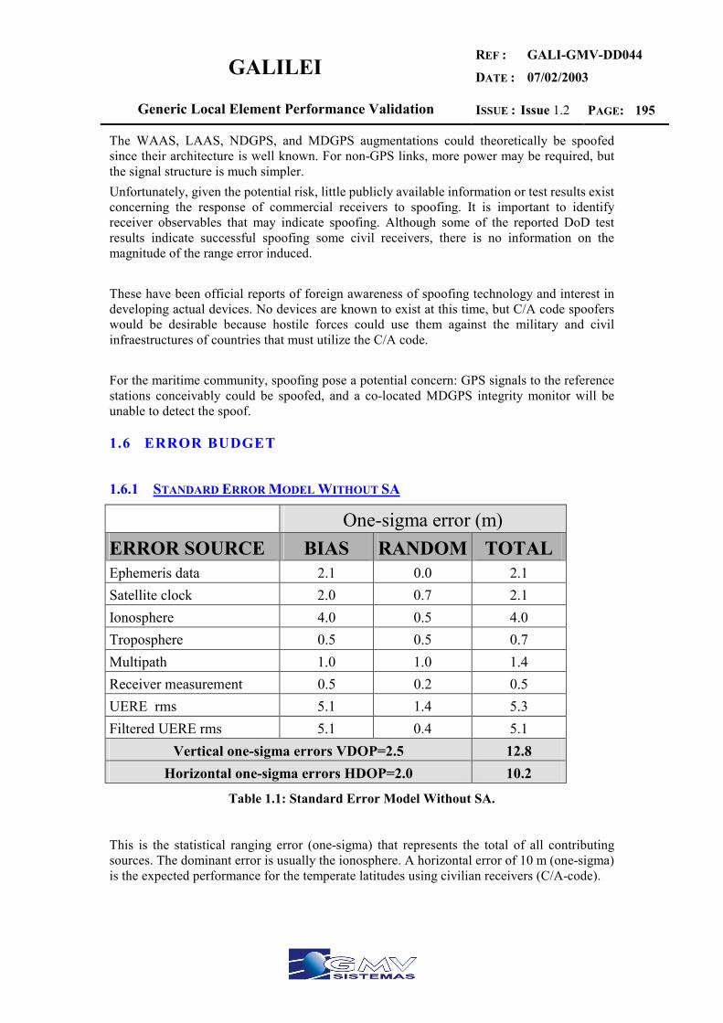
GALILEI REF :
DATE :
GALI-GMV-DD044
07/02/2003
Generic Local Element Performance Validation ISSUE : Issue 1.2 PAGE: 195
The WAAS, LAAS, NDGPS, and MDGPS augmentations could theoretically be spoofed since their architecture is well known. For non-GPS links, more power may be required, but the signal structure is much simpler. Unfortunately, given the potential risk, little publicly available information or test results exist concerning the response of commercial receivers to spoofing. It is important to identify receiver observables that may indicate spoofing. Although some of the reported DoD test results indicate successful spoofing some civil receivers, there is no information on the magnitude of the range error induced. These have been official reports of foreign awareness of spoofing technology and interest in developing actual devices. No devices are known to exist at this time, but C/A code spoofers would be desirable because hostile forces could use them against the military and civil infraestructures of countries that must utilize the C/A code. For the maritime community, spoofing pose a potential concern: GPS signals to the reference stations conceivably could be spoofed, and a co-located MDGPS integrity monitor will be unable to detect the spoof.
1.6 ERROR BUDGET
1.6.1 STANDARD ERROR MODEL WITHOUT SA
One-sigma error (m) ERROR SOURCE BIAS RANDOM TOTAL Ephemeris data 2.1 0.0 2.1 Satellite clock 2.0 0.7 2.1 Ionosphere 4.0 0.5 4.0 Troposphere 0.5 0.5 0.7 Multipath 1.0 1.0 1.4 Receiver measurement 0.5 0.2 0.5 UERE rms 5.1 1.4 5.3 Filtered UERE rms 5.1 0.4 5.1
Vertical one-sigma errors VDOP=2.5 12.8 Horizontal one-sigma errors HDOP=2.0 10.2
Table 1.1: Standard Error Model Without SA.
This is the statistical ranging error (one-sigma) that represents the total of all contributing sources. The dominant error is usually the ionosphere. A horizontal error of 10 m (one-sigma) is the expected performance for the temperate latitudes using civilian receivers (C/A-code).

GALILEI REF :
DATE :
GALI-GMV-DD044
07/02/2003
Generic Local Element Performance Validation ISSUE : Issue 1.2 PAGE: 196
1.6.2 GPS ERRORS WITH SA FOR SPS
One-sigma error (m) ERROR SOURCE BIAS RANDOM TOTAL Ephemeris data 2.1 0.0 2.1 Satellite clock 20.0 0.7 20.0 Ionosphere 4.0 0.5 4.0 Troposphere 0.5 0.5 0.7 Multipath 1.0 1.0 1.4 Receiver measurement 0.5 0.5 0.5 UERE rms 20.5 1.4 20.6 Filtered UERE rms 20.5 0.4 20.5
Total Vertical one-sigma errors VDOP=2.5 51.4 Total Horizontal one-sigma errors HDOP=2.0 41.4
Table 1.2: GPS errors with SA for SPS.
1.6.3 PRECISE ERROR MODEL, DUAL FREQUENCY
One-sigma error (m) ERROR SOURCE BIAS RANDOM TOTAL Ephemeris data 2.1 0.0 2.1 Satellite clock 2.0 0.7 2.1 Ionosphere 1.0 0.7 1.2 Troposphere 0.5 0.5 0.7 Multipath 1.0 1.0 1.4 Receiver measurement 0.5 0.2 0.5 UERE rms 3.3 1.5 3.6 Filtered UERE rms 3.3 0.4 3.3
Vertical one-sigma errors VDOP=2.5 8.3 Horizontal one-sigma errors HDOP=2.0 6.6
Table 1.3: Precise error model, Dual Frequency.
GALILEI REF :
DATE :
GALI-GMV-DD044
07/02/2003
Generic Local Element Performance Validation ISSUE : Issue 1.2 PAGE: 197
1.7 REFERENCES
[1] GPS Theory and Applications. Volume I. Bradford W.Parkinson [2] Statistical Reliability Measures for GPS. G. Lachapell and S.Ryan. Department of Geomatics Engineering, The university of Calgary. [3] Vulnerability assessment of the transportation infrastructure relying on the GPS. Final report. John A.Volpe National Transportation Systems Center. Office of the assistant secretary for transportation policy U.S. Department of transportation. [4] “GPS RF Interference via a TV signal”. Buck,T , and Sellick, G., Proceedings of the 10th International Technical Meeting of the Satellite Division of the Institute of Navigation GPS-97, Kansas City, Sept. 1997 [5] “GPS Risk Assessment Study- Final Report”, Johns Hopkins University Applied Physics Laboratory, January 1999. [6] “The role of the GNSS in supporting airport surface operations”. RTCA DO-247, January 7, 1999. [7] “Assessment of radio frequency interference relevant to the GNSS”, RTCA DO.235, January 27, 1997. [8] “History of Ultra Wideband Communications and Radar: Part 1, UWB Communications”, Barrett, Terence, Microwave Journal, Vol 44 Nº1, January 2001. [9] Report of the commission to address United States National Security Space Management and Organization, January 11, 2001. [10] Gps/Galileo Radio Frequency Compatibility Analisys, J. Godet, ECGASTeam/CNES. Ion GPS’2000.
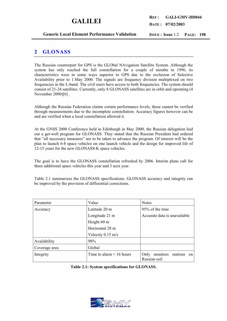
GALILEI REF :
DATE :
GALI-GMV-DD044
07/02/2003
Generic Local Element Performance Validation ISSUE : Issue 1.2 PAGE: 198
2 GLONASS
The Russian counterpart for GPS is the GLObal NAvigation Satellite System. Although the system has only reached the full constellation for a couple of months in 1996, its characteristics were in some ways superior to GPS due to the exclusion of Selective Availability prior to 1.May 2000. The signals are frequency division multiplexed on two frequencies in the L-band. The civil users have access to both frequencies. The system should consist of 21-24 satellites. Currently, only 8 GLONASS satellites are in orbit and operating (4 November 2000)[6] . Although the Russian Federation claims certain performance levels, these cannot be verified through measurements due to the incomplete constellation. Accuracy figures however can be and are verified when a local constellation allowed it. At the GNSS 2000 Conference held in Edinburgh in May 2000, the Russian delegation laid out a get-well program for GLONASS. They stated that the Russian President had ordered that “all necessary measures” are to be taken to advance the program. Of interest will be the plan to launch 6-8 space vehicles on one launch vehicle and the design for improved life of 12-15 years for the new GLONASS-K space vehicles. The goal is to have the GLONASS constellation refreshed by 2006. Interim plans call for three additional space vehicles this year and 3 next year. Table 2.1 summarizes the GLONASS specifications. GLONASS accuracy and integrity can be improved by the provision of differential corrections. Parameter Value Notes Accuracy Latitude 20 m
Longitude 21 m Height 60 m Horizontal 28 m Velocity 0.15 m/s
95% of the time Accurate data is unavailable
Availability 98% Coverage area Global Integrity Time to alarm < 16 hours Only monitors stations on
Russian soil
Table 2.1: System specifications for GLONASS.
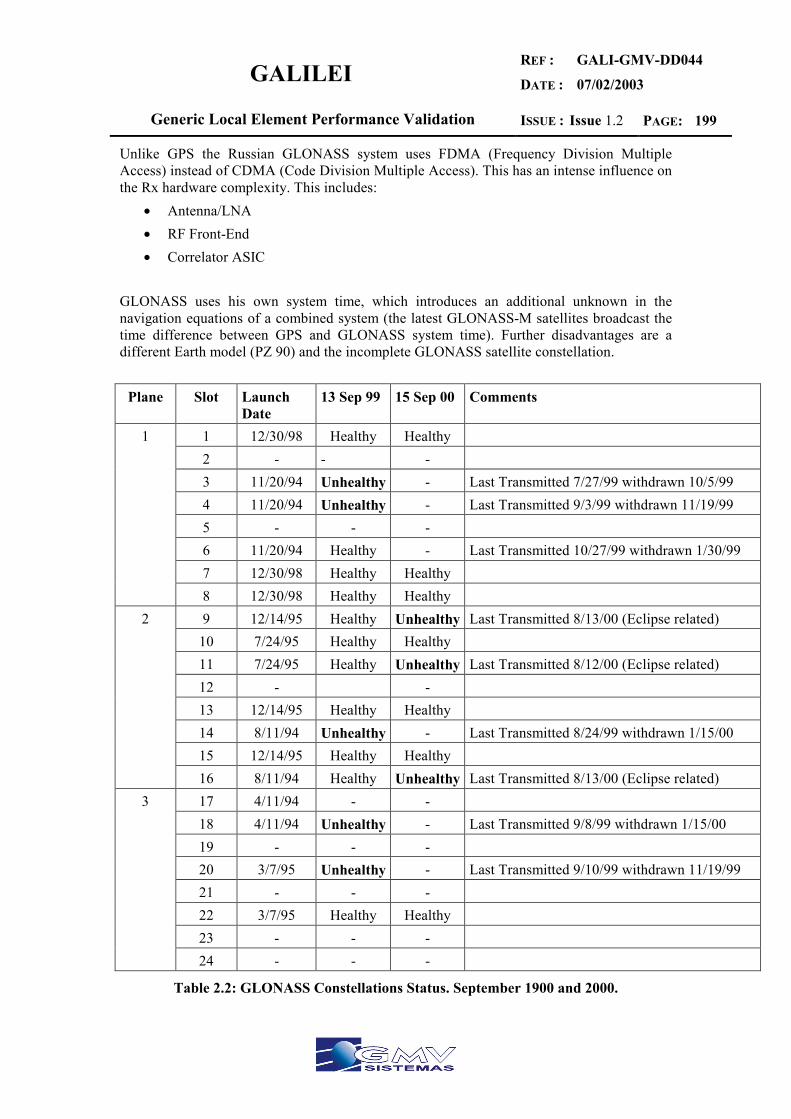
GALILEI REF :
DATE :
GALI-GMV-DD044
07/02/2003
Generic Local Element Performance Validation ISSUE : Issue 1.2 PAGE: 199
Unlike GPS the Russian GLONASS system uses FDMA (Frequency Division Multiple Access) instead of CDMA (Code Division Multiple Access). This has an intense influence on the Rx hardware complexity. This includes:
• Antenna/LNA • RF Front-End • Correlator ASIC
GLONASS uses his own system time, which introduces an additional unknown in the navigation equations of a combined system (the latest GLONASS-M satellites broadcast the time difference between GPS and GLONASS system time). Further disadvantages are a different Earth model (PZ 90) and the incomplete GLONASS satellite constellation.
Plane Slot Launch Date
13 Sep 99 15 Sep 00 Comments
1 12/30/98 Healthy Healthy 2 - - - 3 11/20/94 Unhealthy - Last Transmitted 7/27/99 withdrawn 10/5/99 4 11/20/94 Unhealthy - Last Transmitted 9/3/99 withdrawn 11/19/99 5 - - - 6 11/20/94 Healthy - Last Transmitted 10/27/99 withdrawn 1/30/99 7 12/30/98 Healthy Healthy
1
8 12/30/98 Healthy Healthy 9 12/14/95 Healthy Unhealthy Last Transmitted 8/13/00 (Eclipse related)
10 7/24/95 Healthy Healthy 11 7/24/95 Healthy Unhealthy Last Transmitted 8/12/00 (Eclipse related) 12 - - 13 12/14/95 Healthy Healthy 14 8/11/94 Unhealthy - Last Transmitted 8/24/99 withdrawn 1/15/00 15 12/14/95 Healthy Healthy
2
16 8/11/94 Healthy Unhealthy Last Transmitted 8/13/00 (Eclipse related) 17 4/11/94 - - 18 4/11/94 Unhealthy - Last Transmitted 9/8/99 withdrawn 1/15/00 19 - - - 20 3/7/95 Unhealthy - Last Transmitted 9/10/99 withdrawn 11/19/99 21 - - - 22 3/7/95 Healthy Healthy 23 - - -
3
24 - - -
Table 2.2: GLONASS Constellations Status. September 1900 and 2000.
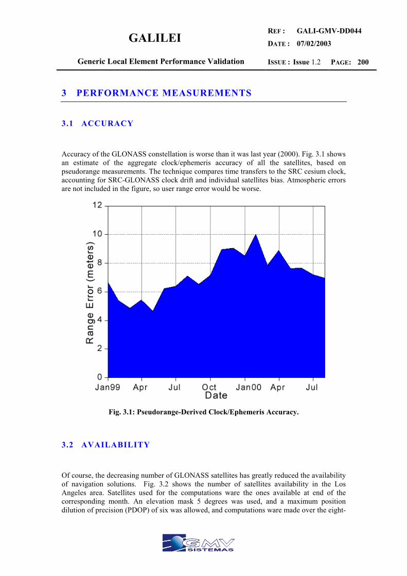
GALILEI REF :
DATE :
GALI-GMV-DD044
07/02/2003
Generic Local Element Performance Validation ISSUE : Issue 1.2 PAGE: 200
3 PERFORMANCE MEASUREMENTS
3.1 ACCURACY
Accuracy of the GLONASS constellation is worse than it was last year (2000). Fig. 3.1 shows an estimate of the aggregate clock/ephemeris accuracy of all the satellites, based on pseudorange measurements. The technique compares time transfers to the SRC cesium clock, accounting for SRC-GLONASS clock drift and individual satellites bias. Atmospheric errors are not included in the figure, so user range error would be worse.
Fig. 3.1: Pseudorange-Derived Clock/Ephemeris Accuracy.
3.2 AVAILABILITY
Of course, the decreasing number of GLONASS satellites has greatly reduced the availability of navigation solutions. Fig. 3.2 shows the number of satellites availability in the Los Angeles area. Satellites used for the computations ware the ones available at end of the corresponding month. An elevation mask 5 degrees was used, and a maximum position dilution of precision (PDOP) of six was allowed, and computations ware made over the eight-
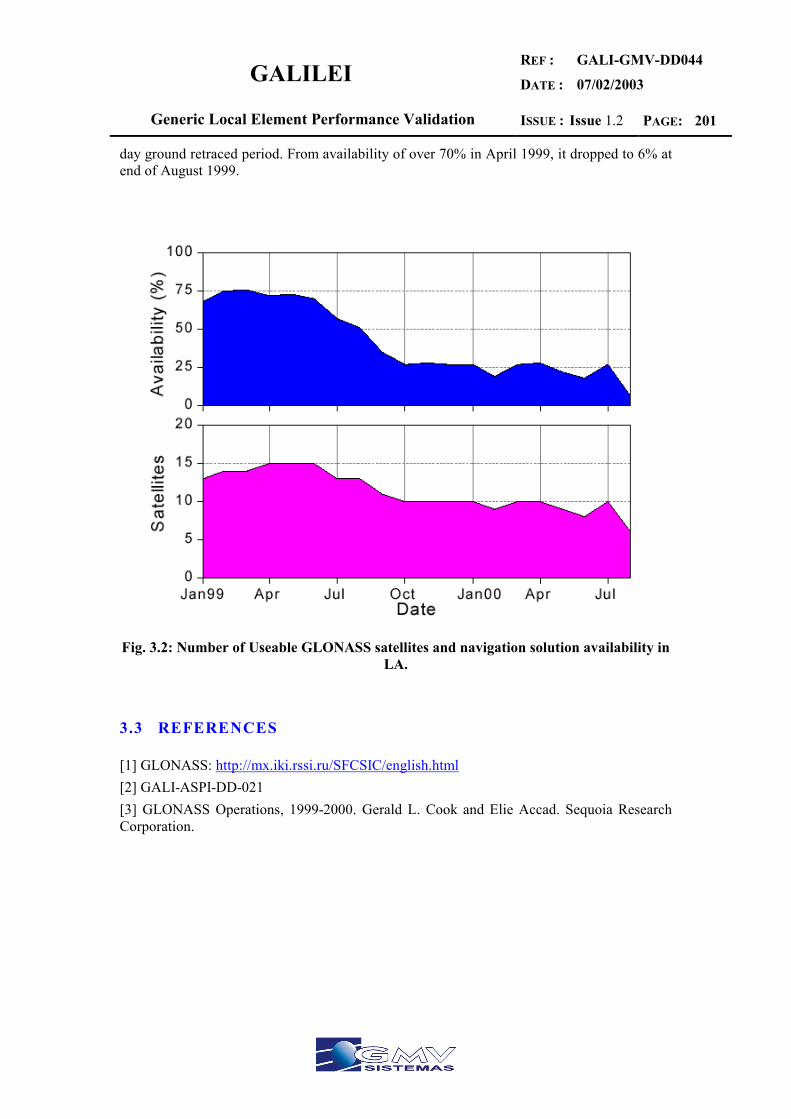
GALILEI REF :
DATE :
GALI-GMV-DD044
07/02/2003
Generic Local Element Performance Validation ISSUE : Issue 1.2 PAGE: 201
day ground retraced period. From availability of over 70% in April 1999, it dropped to 6% at end of August 1999.
Fig. 3.2: Number of Useable GLONASS satellites and navigation solution availability in
LA.
3.3 REFERENCES
[1] GLONASS: http://mx.iki.rssi.ru/SFCSIC/english.html [2] GALI-ASPI-DD-021 [3] GLONASS Operations, 1999-2000. Gerald L. Cook and Elie Accad. Sequoia Research Corporation.

GALILEI REF :
DATE :
GALI-GMV-DD044
07/02/2003
Generic Local Element Performance Validation ISSUE : Issue 1.2 PAGE: 202
4 EUROPEAN GEOSTATIONARY NAVIGATION OVERLAY SYSTEM (EGNOS)
4.1 WAD (WIDE AREA DIFFERENTIAL) CONCEPT
DGPS have several limitations. DGPS corrects all error sources with a unique scalar for each satellite, and his validity is limited to the surroundings of the differential station (correlated errors). WAD (Wide area differential) is a concept to provide differential corrections in a wide area For that purpose it is necessary to separate the differential error sources:
• Satellite clock (scalar) + Satellite Ephemeris corrections (vector). • Ionospheric corrections (scalar for different grid points).
Additional information on the quality of those corrections (estimation of a bounding for the residual errors) as the basis for providing integrity, however this involve a major complexity of the system.
Fig. 4.1: Limitations of DGPS.

GALILEI REF :
DATE :
GALI-GMV-DD044
07/02/2003
Generic Local Element Performance Validation ISSUE : Issue 1.2 PAGE: 203
4.2 WIDE AREA DIFFERENTIAL GPS ARCHITECTURE
The WADGPS network includes at least one master station, a number of monitor stations, and communication links. Each monitor station is equipped with a high-quality clock and a high-quality GPS receiver capable of tracking all satellites within the field of view. The GPS measurements are taken at each monitor station and sent to the master station. The master station computes GPS error components, based on the known monitor station locations and the information collected. The computed error corrections are transmitted to the users via any convenient communication link, such as satellite, telephone, or radio. The process can be summarized as follows:
1. Monitor stations at known locations collect GPS pseudoranges from all satellites in view.
2. Pseudoranges and dual-frequency ionospheric delay measurements (if available) are sent to the master station.
3. Master station computes an error correction vector. 4. Error correction vector is transmitted to users. 5. Users apply error corrections to their measured pseudoranges and collected ephemeris
data to improve navigation accuracy.
4.3 INTRODUCTION TO WAAS
The wide area augmentation system (WAAS) is a safety-critical system consisting of a signal-in-space and ground network to support enroute through precision approach air navigation. It is designed to augment GPS so that it can be used as the primary navigation sensor. The WAAS augments GPS with the following three services: a ranging function, which improves availability and reliability,; differential GPS corrections, which improve accuracy; and integrity monitoring, which improves safety.[1]
Fig. 4.2: Wide Area Augmentation System.
GALILEI REF :
DATE :
GALI-GMV-DD044
07/02/2003
Generic Local Element Performance Validation ISSUE : Issue 1.2 PAGE: 204
As shown in Fig. 4.2, the WAAS broadcasts GPS integrity and correction data to GPS users and also provides a ranging signal that augments GPS. The WAAS ranging signal is GPS-like modulated with a spread spectrum code from the same family as the GPS C/A codes. The code phase and carrier frequency of the signal will be controlled so that the WASS satellites provide additional range measurements to the GPS user. The WAAS signal also carry data that contain differential corrections and integrity information for all GPS satellites as well as the geostationary satellites. A ground network develops the differential corrections and integrity data broadcast to the users. Wide area reference stations (WRS) are widely dispersed data collections sites that receive and process signals received from the GPS and geostationary satellites. The WRS forward their data to data-processing sites referred to as wide area master stations (WMS or central processing facilities). The WMS process the raw data to determine integrity, differential corrections, residual errors, and ionospheric delay information for each monitored satellite. They also develop ephemeris and clock information for the geostationary satellites. All these data are packed into the WASS message, which is sent to navigation Earth stations (NES). The NES uplink this message to the geostationary satellites, which broadcast the GPS-like signal described earlier. The differential corrections and the improved geometry provided by the geostationary satellites will improved accuracy to better than 10 m (2drms) in the vertical, which is adequate for aircraft Category I precision approach.
4.4 INTRODUCTION TO EGNOS
EGNOS is the European Satellite Based Augmentation System (SBAS). It will be interoperable with the American WAAS (Wide Area Augmentation System) and Japanese MTSAT. EGNOS is intended to provide three different augmentations to GNSS (Global Navigation Satellite System).
• Integrity information • Additional ranging signal compatible with GPS/GLONASS • Wide Area Differential corrections for GNSS.
The system, currently being deployed, consists of some 30 Ranging and Integrity Monitoring Stations (RIMS) on European soil collecting data on the satellite systems GPS and GLONASS. This data is sent to a Master Control Center, which calculates integrity and differential correction data. The differential corrections are divided into separate parameters for clock errors, Ionospheric errors etc. A geostationary satellite broadcasts this data in the coverage area. EGNOS is not a navigation system in itself. Although it provides a ranging function, it needs To be used in conjunction with GPS/GLONASS.
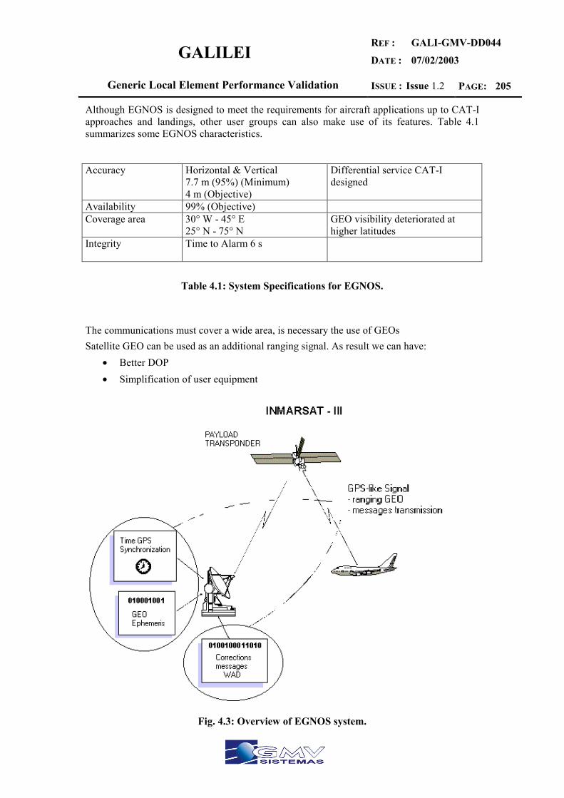
GALILEI REF :
DATE :
GALI-GMV-DD044
07/02/2003
Generic Local Element Performance Validation ISSUE : Issue 1.2 PAGE: 205
Although EGNOS is designed to meet the requirements for aircraft applications up to CAT-I approaches and landings, other user groups can also make use of its features. Table 4.1 summarizes some EGNOS characteristics.
Accuracy Horizontal & Vertical
7.7 m (95%) (Minimum) 4 m (Objective)
Differential service CAT-I designed
Availability 99% (Objective) Coverage area 30° W - 45° E
25° N - 75° N GEO visibility deteriorated at higher latitudes
Integrity Time to Alarm 6 s
Table 4.1: System Specifications for EGNOS. The communications must cover a wide area, is necessary the use of GEOs Satellite GEO can be used as an additional ranging signal. As result we can have:
• Better DOP • Simplification of user equipment
Fig. 4.3: Overview of EGNOS system.
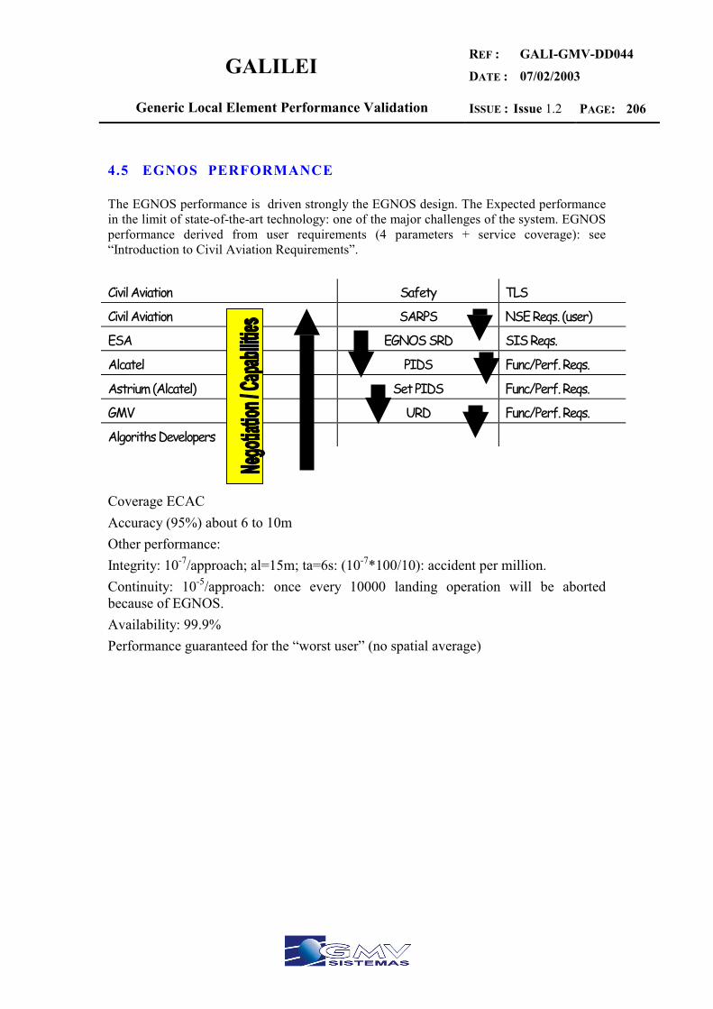
GALILEI REF :
DATE :
GALI-GMV-DD044
07/02/2003
Generic Local Element Performance Validation ISSUE : Issue 1.2 PAGE: 206
4.5 EGNOS PERFORMANCE
The EGNOS performance is driven strongly the EGNOS design. The Expected performance in the limit of state-of-the-art technology: one of the major challenges of the system. EGNOS performance derived from user requirements (4 parameters + service coverage): see “Introduction to Civil Aviation Requirements”.
Civil Aviation Safety TLS
Civil Aviation SARPS NSE Reqs. (user)
ESA EGNOS SRD SIS Reqs.
Alcatel PIDS Func/Perf. Reqs.
Astrium (Alcatel) Set PIDS Func/Perf. Reqs.
GMV URD Func/Perf. Reqs.
Algoriths Developers Coverage ECAC Accuracy (95%) about 6 to 10m Other performance: Integrity: 10-7/approach; al=15m; ta=6s: (10-7*100/10): accident per million. Continuity: 10-5/approach: once every 10000 landing operation will be aborted because of EGNOS. Availability: 99.9% Performance guaranteed for the “worst user” (no spatial average)
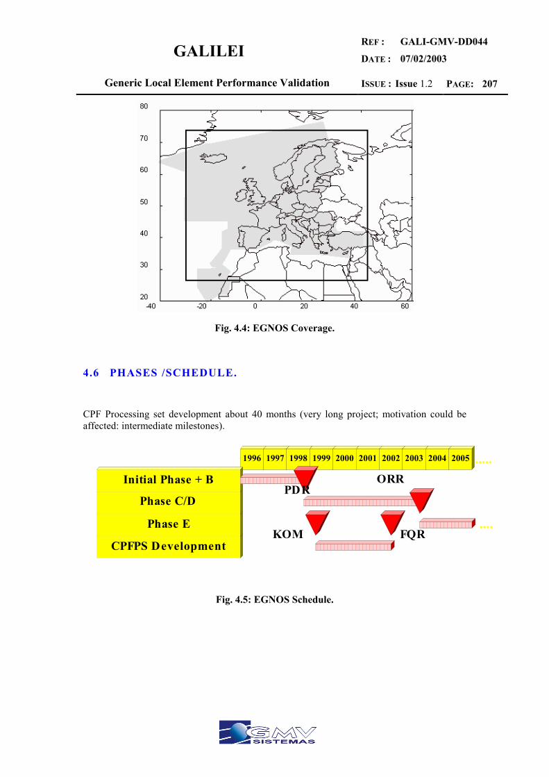
GALILEI REF :
DATE :
GALI-GMV-DD044
07/02/2003
Generic Local Element Performance Validation ISSUE : Issue 1.2 PAGE: 207
Fig. 4.4: EGNOS Coverage.
4.6 PHASES /SCHEDULE.
CPF Processing set development about 40 months (very long project; motivation could be affected: intermediate milestones).
CPFPS Development
Phase E
Phase C/D
1996 1997 1998 1999 2000 2001 2002 2003 2004 2005
Initial Phase + B.....
....KOM FQR
ORRPDR
Fig. 4.5: EGNOS Schedule.
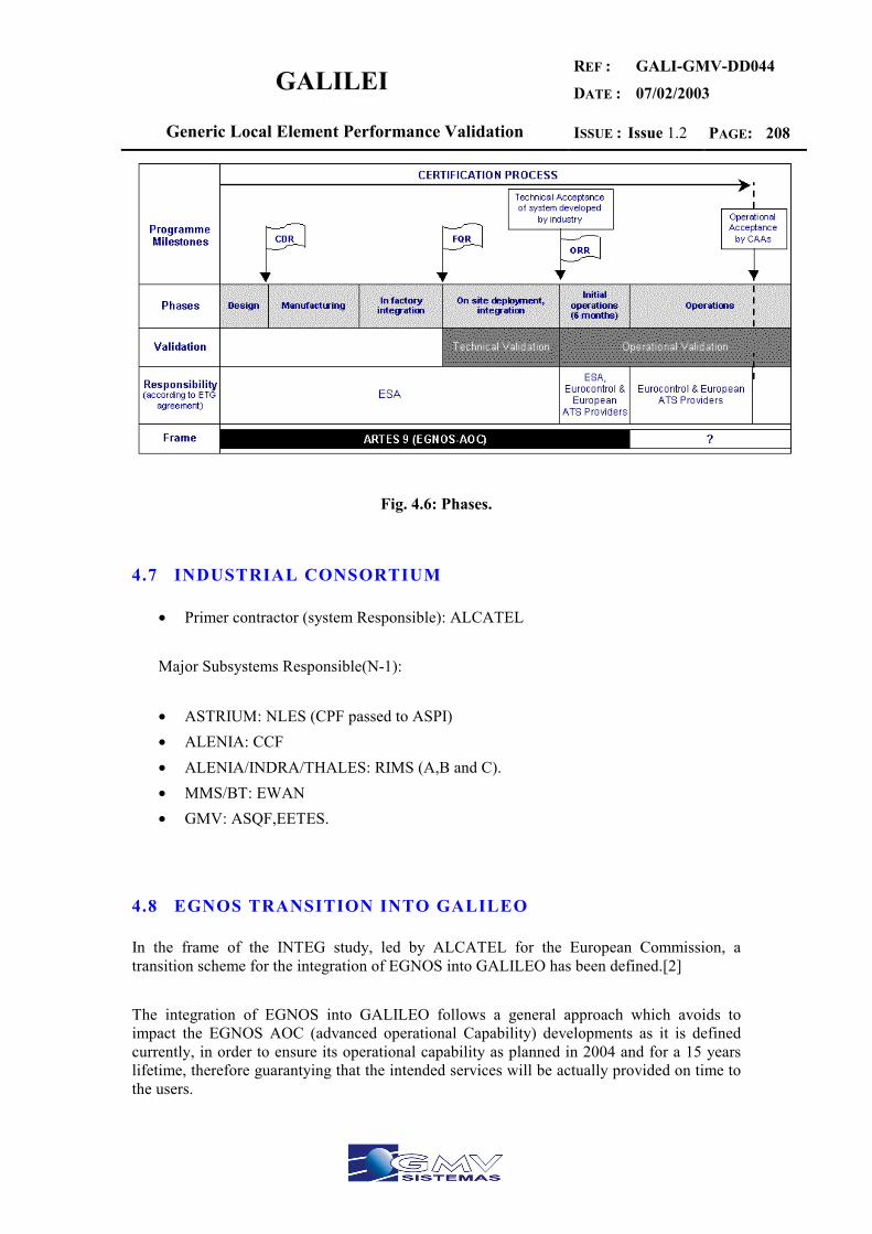
GALILEI REF :
DATE :
GALI-GMV-DD044
07/02/2003
Generic Local Element Performance Validation ISSUE : Issue 1.2 PAGE: 208
Fig. 4.6: Phases.
4.7 INDUSTRIAL CONSORTIUM
• Primer contractor (system Responsible): ALCATEL Major Subsystems Responsible(N-1): • ASTRIUM: NLES (CPF passed to ASPI) • ALENIA: CCF • ALENIA/INDRA/THALES: RIMS (A,B and C). • MMS/BT: EWAN • GMV: ASQF,EETES.
4.8 EGNOS TRANSITION INTO GALILEO
In the frame of the INTEG study, led by ALCATEL for the European Commission, a transition scheme for the integration of EGNOS into GALILEO has been defined.[2] The integration of EGNOS into GALILEO follows a general approach which avoids to impact the EGNOS AOC (advanced operational Capability) developments as it is defined currently, in order to ensure its operational capability as planned in 2004 and for a 15 years lifetime, therefore guarantying that the intended services will be actually provided on time to the users.

GALILEI REF :
DATE :
GALI-GMV-DD044
07/02/2003
Generic Local Element Performance Validation ISSUE : Issue 1.2 PAGE: 209
The necessary evolutions of EGNOS within GALILEO need also to accommodate the GPS evolutions (provision of the modernized GPS) will occur in a similar time frame than GALILEO.
4.9 THE EGNOS TO GALILEO TRANSITION OBJECTIVES
EGNOS shall offer the GPS augmentation service up to the end of its required lifetime which is 15 years, i.e. until 2018 with the total respect of international standards and associated evolutions (RTCA, EUROCAE, SARPS).
• During the transition period, the EGNOS service shall not be interrupted. • The integration of EGNOS and GALILEO shall avoid any impact on EGNOS AOC
ORR schedule (Operational Readiness Review). • The integration of EGNOS and GALILEO shall protect returns on EGNOS
investments (EOIG, final users). • EGNOS shall provide a back-up independent Navigation Service to GALILEO
Navigation Services through an augmentation service to GPS or GPS and GLONASS in Europe with WAAS and MSAS SBAS systems.
• EGNOS shall become the European integrity component of GALILEO (i.e. provision of GALILEO satellites integrity in addition to augmentation to GPS and GLONASS).
• The GALILEO architecture shall maximize the re-use of qualified elements of EGNOS.
4.10 EGNOS+ MISSION CONCEPT: SERVICES & BROADCAST
EGNOS+ system would provide its services through both EGNOS GEO+ payloads and GALILEO MEO satellites. The two following diagrams illustrate the different broadcast channels and associated services for the overlay/integrity data from two different perspectives:
1. from user perspective 2. from the EGNOS+ subsystems perspective.
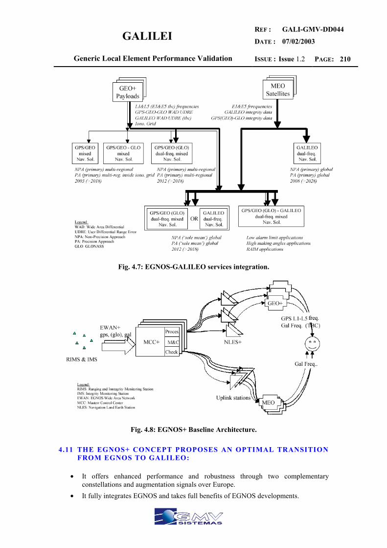
GALILEI REF :
DATE :
GALI-GMV-DD044
07/02/2003
Generic Local Element Performance Validation ISSUE : Issue 1.2 PAGE: 210
Fig. 4.7: EGNOS-GALILEO services integration.
Fig. 4.8: EGNOS+ Baseline Architecture.
4.11 THE EGNOS+ CONCEPT PROPOSES AN OPTIMAL TRANSITION FROM EGNOS TO GALILEO:
• It offers enhanced performance and robustness through two complementary constellations and augmentation signals over Europe.
• It fully integrates EGNOS and takes full benefits of EGNOS developments.
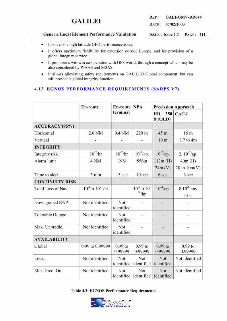
GALILEI REF :
DATE :
GALI-GMV-DD044
07/02/2003
Generic Local Element Performance Validation ISSUE : Issue 1.2 PAGE: 211
• It solves the high latitude GEO performance issue. • It offers maximum flexibility for extension outside Europe, and for provision of a
global integrity service. • It proposes a win-win co-operation with GPS world, through a concept which may be
also considered by WAAS and MSAS. • It allows alleviating safety requirements on GALILEO Global component, but can
still provide a global integrity function.
4.12 EGNOS PERFORMANCE REQUIREMENTS (SARPS V7)
Precission Approach En-route En-route
terminalNPA
HD 350 ft (OLD)
CAT-I
ACCURACY (95%) Horizontal 2.0 NM 0.4 NM 220 m 45 m 16 m Vertical - - - 10 m 7.7 to 4m INTEGRITY Integrity risk 10-7/hr 10-7/hr 10-7/ap. 10-7/ap. 2. 10-7/ap. Alarm limit 4 NM 1NM 556m 112m (H)
24m (V) 40m (H)
20 to 10m(V)Time to alert 5 min 15 sec 10 sec 6 sec 6 sec CONTINUITY RISK Total Loss of Nav. 10-4to 10-8 /hr 10-4to 10-
8 /hr 10-4/ap. 8.10-8 any
15 s. Downgraded RNP Not identified Not
identified- - -
Tolerable Outage Not identified Not identified
- - -
Max. Unpredic. Not identified Not identified
- - -
AVAILABILITY Global 0.99 to 0.99999 0.99 to
0.99999 0.99 to 0.99999
0.99 to 0.99999
0.99 to 0.99999
Local Not identified Not identified
Not identified
Not identified
Not identified
Max. Pred. Out Not identified Not identified
Not identified
Not identified
Not identified
Table 4.2: EGNOS Performance Requirements.
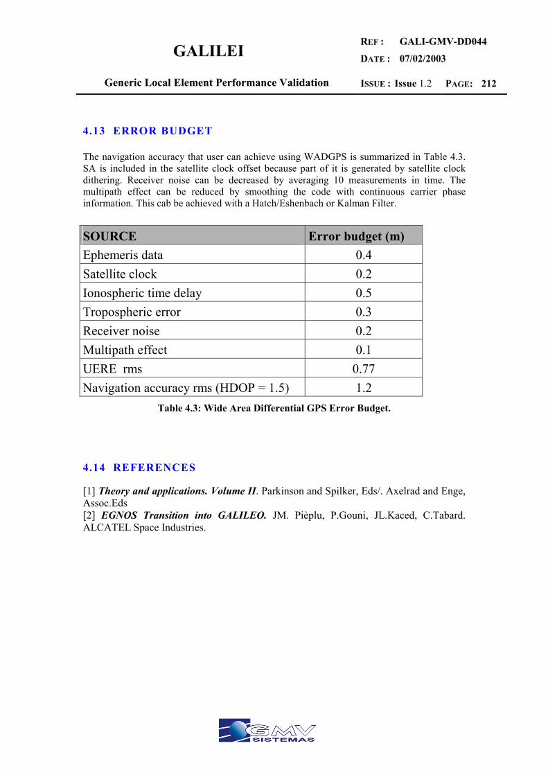
GALILEI REF :
DATE :
GALI-GMV-DD044
07/02/2003
Generic Local Element Performance Validation ISSUE : Issue 1.2 PAGE: 212
4.13 ERROR BUDGET
The navigation accuracy that user can achieve using WADGPS is summarized in Table 4.3. SA is included in the satellite clock offset because part of it is generated by satellite clock dithering. Receiver noise can be decreased by averaging 10 measurements in time. The multipath effect can be reduced by smoothing the code with continuous carrier phase information. This cab be achieved with a Hatch/Eshenbach or Kalman Filter.
SOURCE Error budget (m) Ephemeris data 0.4 Satellite clock 0.2 Ionospheric time delay 0.5 Tropospheric error 0.3 Receiver noise 0.2 Multipath effect 0.1 UERE rms 0.77 Navigation accuracy rms (HDOP = 1.5) 1.2
Table 4.3: Wide Area Differential GPS Error Budget.
4.14 REFERENCES
[1] Theory and applications. Volume II. Parkinson and Spilker, Eds/. Axelrad and Enge, Assoc.Eds [2] EGNOS Transition into GALILEO. JM. Pièplu, P.Gouni, JL.Kaced, C.Tabard. ALCATEL Space Industries.
GALILEI REF :
DATE :
GALI-GMV-DD044
07/02/2003
Generic Local Element Performance Validation ISSUE : Issue 1.2 PAGE: 213
ANNEX 6 GROUND BASED EXTERNAL NAVIGATION SYSTEM

GALILEI REF :
DATE :
GALI-GMV-DD044
07/02/2003
Generic Local Element Performance Validation ISSUE : Issue 1.2 PAGE: 214
In this section an overview of the Ground Based External Navigation Systems (GBEN) is given. The following GBEN systems are considered:
LORAN CHAYKA EUROFIX
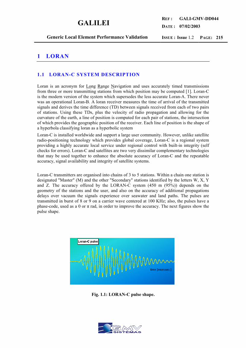
GALILEI REF :
DATE :
GALI-GMV-DD044
07/02/2003
Generic Local Element Performance Validation ISSUE : Issue 1.2 PAGE: 215
1 LORAN
1.1 LORAN-C SYSTEM DESCRIPTION
Loran is an acronym for Long Range Navigation and uses accurately timed transmissions from three or more transmitting stations from which position may be computed [1]. Loran-C is the modern version of the system which supersedes the less accurate Loran-A. There never was an operational Loran-B. A loran receiver measures the time of arrival of the transmitted signals and derives the time difference (TD) between signals received from each of two pairs of stations. Using these TDs, plus the velocity of radio propagation and allowing for the curvature of the earth, a line of position is computed for each pair of stations, the intersection of which provides the geographic position of the receiver. Each line of position is the shape of a hyperbola classifying loran as a hyperbolic system Loran-C is installed worldwide and support a large user community. However, unlike satellite radio-positioning technology which provides global coverage, Loran-C is a regional system providing a highly accurate local service under regional control with built-in integrity (self checks for errors). Loran-C and satellites are two very dissimilar complementary technologies that may be used together to enhance the absolute accuracy of Loran-C and the repeatable accuracy, signal availability and integrity of satellite systems. Loran-C transmitters are organised into chains of 3 to 5 stations. Within a chain one station is designated "Master" (M) and the other "Secondary" stations identified by the letters W, X, Y and Z. The accuracy offered by the LORAN-C system (450 m (95%)) depends on the geometry of the stations and the user, and also on the accuracy of additional propagations delays over vacuum the signals experience over seawater and land paths. The pulses are transmitted in burst of 8 or 9 on a carrier wave centered at 100 KHz; also, the pulses have a phase-code, used as a 0 or π rad, in order to improve the accuracy. The next figures show the pulse shape.
Fig. 1.1: LORAN-C pulse shape.
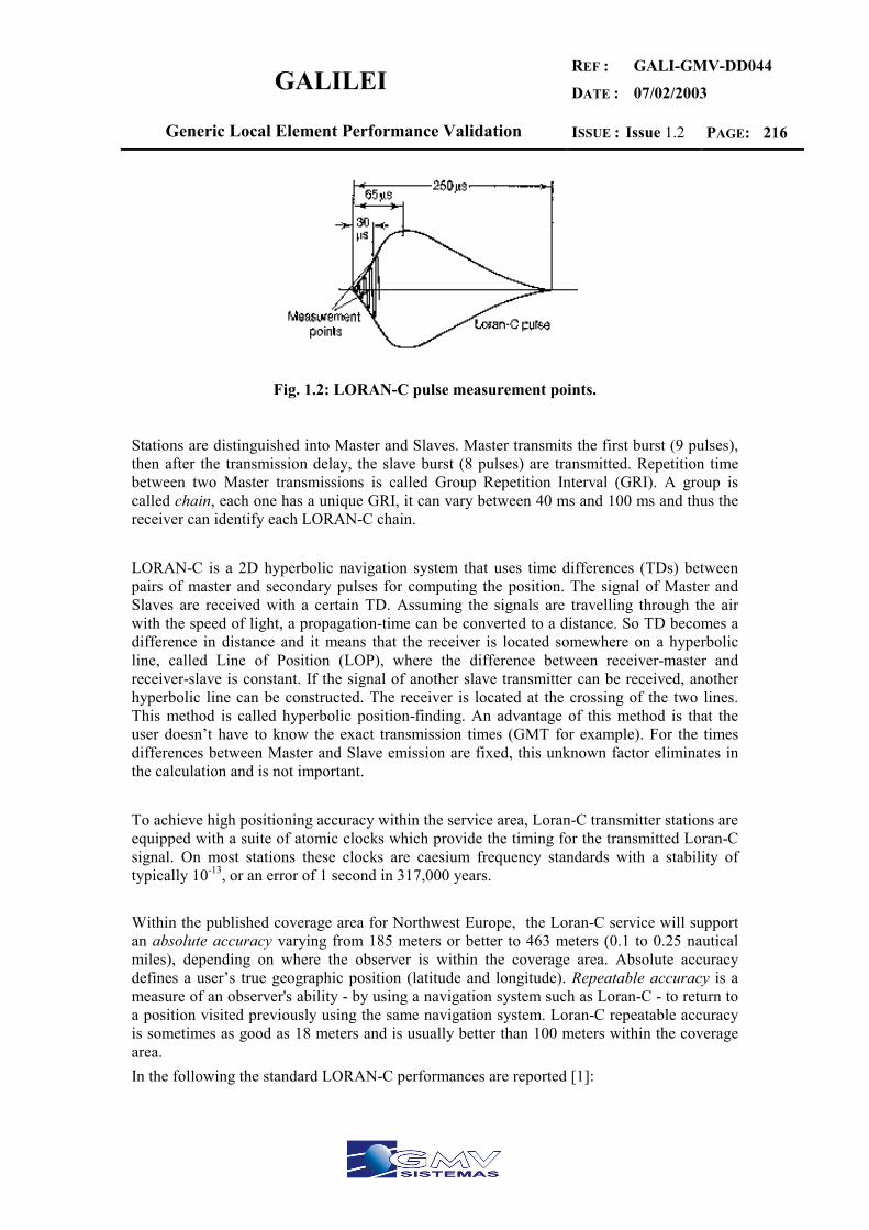
GALILEI REF :
DATE :
GALI-GMV-DD044
07/02/2003
Generic Local Element Performance Validation ISSUE : Issue 1.2 PAGE: 216
Fig. 1.2: LORAN-C pulse measurement points.
Stations are distinguished into Master and Slaves. Master transmits the first burst (9 pulses), then after the transmission delay, the slave burst (8 pulses) are transmitted. Repetition time between two Master transmissions is called Group Repetition Interval (GRI). A group is called chain, each one has a unique GRI, it can vary between 40 ms and 100 ms and thus the receiver can identify each LORAN-C chain. LORAN-C is a 2D hyperbolic navigation system that uses time differences (TDs) between pairs of master and secondary pulses for computing the position. The signal of Master and Slaves are received with a certain TD. Assuming the signals are travelling through the air with the speed of light, a propagation-time can be converted to a distance. So TD becomes a difference in distance and it means that the receiver is located somewhere on a hyperbolic line, called Line of Position (LOP), where the difference between receiver-master and receiver-slave is constant. If the signal of another slave transmitter can be received, another hyperbolic line can be constructed. The receiver is located at the crossing of the two lines. This method is called hyperbolic position-finding. An advantage of this method is that the user doesn’t have to know the exact transmission times (GMT for example). For the times differences between Master and Slave emission are fixed, this unknown factor eliminates in the calculation and is not important. To achieve high positioning accuracy within the service area, Loran-C transmitter stations are equipped with a suite of atomic clocks which provide the timing for the transmitted Loran-C signal. On most stations these clocks are caesium frequency standards with a stability of typically 10-13, or an error of 1 second in 317,000 years.
Within the published coverage area for Northwest Europe, the Loran-C service will support an absolute accuracy varying from 185 meters or better to 463 meters (0.1 to 0.25 nautical miles), depending on where the observer is within the coverage area. Absolute accuracy defines a user’s true geographic position (latitude and longitude). Repeatable accuracy is a measure of an observer's ability - by using a navigation system such as Loran-C - to return to a position visited previously using the same navigation system. Loran-C repeatable accuracy is sometimes as good as 18 meters and is usually better than 100 meters within the coverage area. In the following the standard LORAN-C performances are reported [1]:

GALILEI REF :
DATE :
GALI-GMV-DD044
07/02/2003
Generic Local Element Performance Validation ISSUE : Issue 1.2 PAGE: 217
Absolute accuracy 185-463 m Repeatable accuracy 18-90 m Availability 99.6% Reliability 99.6% Integrity LORAN-C signals are constantly monitored.
A “blink” is manually initiated immediately upon detection of an abnormality
Coverage Regional Fix rate 1 fix/sec Fix dimension 2D + Time Uniqueness of solutions4 No, but easily resolvable System capacity Unlimited
Table 1.1: LORAN-C Performances (U.S. FRP, 1996).
An imaginary line drawn between the Master and each secondary station (Slave) is called the baseline [1]. The continuation of the baseline in either direction is called a baseline extension. Typical baselines are from 1200 to 1900 Km. Chain coverage is determined by the power transmitted from each transmitter in the chain, the distance between them and the geometry of the chain (how the different transmitters are oriented in relation to each other). Fig. 1.3 shows the coverage of the system around the world.
Fig. 1.3: Coverage of LORAN-C.
The number of transmitters are distributed in the following way:
4 In hyperbolic mode, i.e., the position solution is ambiguous due to the presence of a second point of intersection of the two hyperbolas.
GALILEI REF :
DATE :
GALI-GMV-DD044
07/02/2003
Generic Local Element Performance Validation ISSUE : Issue 1.2 PAGE: 218
• 14 transmitters in Europe
• 24 transmitters in USA
• 23 transmitters in Asia
Today’s state-of-the-art, solid state Loran-C transmitters are adapted for automatic operation; that is to say all vital transmitter functions are duplicated or designed for graceful degradation so that the result of a defect is minimised. These vital functions are further monitored at the Control Centre which has the capability of initiating corrective action using data communications. As a consequence, the transmitters may be operated as unmanned stations except for caretakers.
1.2 LORAN-C SERVICE INTEGRITY
Loran-C stations are constantly monitored to detect signal abnormalities which would render the system unusable for navigation. "Blink" is the prime means by which the user is notified that the transmitted Loran-C signal does not comply with the system specifications. Blink also indicates that the Control Centre cannot ensure that the signal complies with these specifications, for instance, as a result of discontinuation of data communications linking the Control Centre to the stations. Blink is a distinctive change in the group of eight Loran-C pulses that can be recognised automatically by a receiver so the user is notified instantly that the Loran-C chain blinking should not be used for navigation. Blink starts at a maximum of 60 seconds after detection of an abnormality. Automatic blink initiated within 10 seconds of a timing abnormality may be added where Loran-C is extensively used for aviation purposes. The blink signal will cause most receivers to indicate, by an alarm, that the navigation data displayed may be in error
1.3 SKY WAVE REJECTION AND ASF
LORAN-C low carrier frequency of 100 KHz was chosen to take advantage of propagation of the stable ground wave to long distances [1]. However, the presence of delayed sky waves, reflected from the ionosphere, cause distortions of the pulse shape and change the carrier phase within the pulses of the received signal. To avoid sky wave contamination, the Loran-C receiver selects a zero crossing of a specified carrier cycle at the front end of the pulses transmitted by master and secondary stations. Making the cycle selection early in the ground wave pulse - usually the third cycle is employed - ensures that the time interval measurement is made using the uncontaminated part of the pulse. Precise control over the pulse shape at the transmitter ensures that the selected zero crossing can be identified reliably by the receiver. Limited conductivity of water and soil introduces additional propagation delays on the signal. The delay due to seawater (high conductivity) is known and can easily be taken into account in LORAN-C positioning. Dry soil, mountains and ice generally have low conductivity and the introduced delay is higher. Considering the importance of radiowave propagation, delays introduce errors for the determination of TD and hence of the absolute positioning position accuracy. These
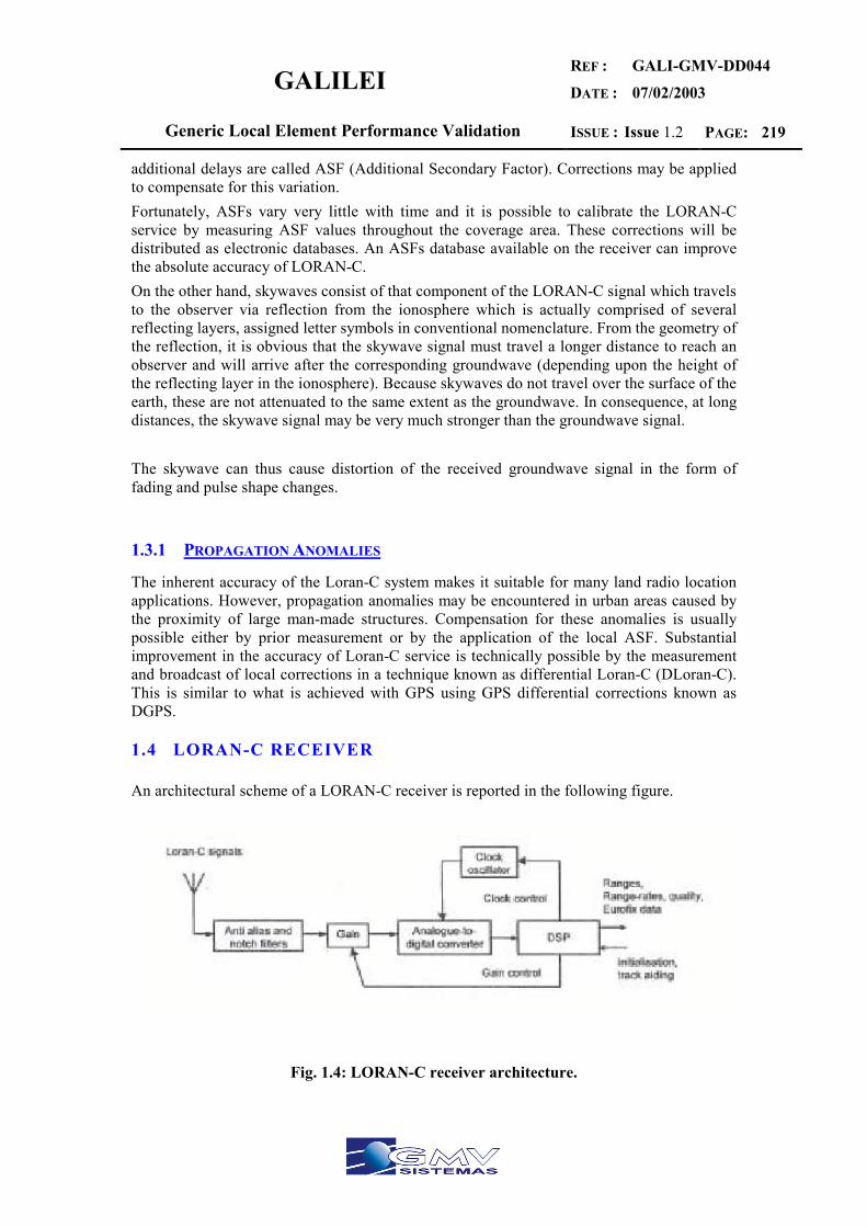
GALILEI REF :
DATE :
GALI-GMV-DD044
07/02/2003
Generic Local Element Performance Validation ISSUE : Issue 1.2 PAGE: 219
additional delays are called ASF (Additional Secondary Factor). Corrections may be applied to compensate for this variation. Fortunately, ASFs vary very little with time and it is possible to calibrate the LORAN-C service by measuring ASF values throughout the coverage area. These corrections will be distributed as electronic databases. An ASFs database available on the receiver can improve the absolute accuracy of LORAN-C. On the other hand, skywaves consist of that component of the LORAN-C signal which travels to the observer via reflection from the ionosphere which is actually comprised of several reflecting layers, assigned letter symbols in conventional nomenclature. From the geometry of the reflection, it is obvious that the skywave signal must travel a longer distance to reach an observer and will arrive after the corresponding groundwave (depending upon the height of the reflecting layer in the ionosphere). Because skywaves do not travel over the surface of the earth, these are not attenuated to the same extent as the groundwave. In consequence, at long distances, the skywave signal may be very much stronger than the groundwave signal. The skywave can thus cause distortion of the received groundwave signal in the form of fading and pulse shape changes.
1.3.1 PROPAGATION ANOMALIES
The inherent accuracy of the Loran-C system makes it suitable for many land radio location applications. However, propagation anomalies may be encountered in urban areas caused by the proximity of large man-made structures. Compensation for these anomalies is usually possible either by prior measurement or by the application of the local ASF. Substantial improvement in the accuracy of Loran-C service is technically possible by the measurement and broadcast of local corrections in a technique known as differential Loran-C (DLoran-C). This is similar to what is achieved with GPS using GPS differential corrections known as DGPS.
1.4 LORAN-C RECEIVER
An architectural scheme of a LORAN-C receiver is reported in the following figure.
Fig. 1.4: LORAN-C receiver architecture.

GALILEI REF :
DATE :
GALI-GMV-DD044
07/02/2003
Generic Local Element Performance Validation ISSUE : Issue 1.2 PAGE: 220
The LORAN-C signal received either by an E-field or H-field antenna is modified by anti alias and notch filters and amplified to improve the signal quality. The modified signal is processed by an ADC, which receives information from a clock oscillator. The digital signal is converted afterwards by a Digital Signal Processing (which also controls the clock oscillator) into range, range rate, quality and Eurofix data.
GALILEI REF :
DATE :
GALI-GMV-DD044
07/02/2003
Generic Local Element Performance Validation ISSUE : Issue 1.2 PAGE: 221
1.5 CHAYKA
Chayka is a Russian military system equivalent to LORAN-C. Two chains in the former Soviet Union, called Chayka, exists. One chain provides coverage in European Russia, Ukraine and Byelorussia; a second one provides coverage to the Pacific approaches to Siberia. Chayka is slightly different than LORAN-C: it is a hyperbolic system that uses the same frequency (100 KHz), a slightly different pulse signal, and a significantly different control regime. The main difference between both systems is the used time reference. Related to the future operation of Chayka, the Russian Federation introduced their radionavigation plans and it was confirmed that all members were of the opinion that LORAN-C and Chayka services should not be discontinued until a next generation satellite system was in full operation and had been proved to meet all operational requirements. The Russian Federation-controlled Chayka networks will not be considered for phasing out until at least the year 2010. Chayka signal can be received in Western Europe.
1.5.1 LORAN-C AND CHAYKA COMPATIBILITY
Loran-C and Chayka operate on the same frequency and transmit similar navigation signals using the same time reference. In this respect the systems are interchangeable and their use, either alone or in combination, is transparent to receiving equipment. The area covered by the combined systems is significantly extended over what each system alone can provide. The system compatibility and extended coverage of the combined systems is the basis for close cooperation with the CIS [2]. Currently, fourteen Chayka stations are in operation in the CIS area forming the following four chains:
1. The European chain, comprising five stations located near the towns of Bryansk (Master), Pertozavodsk, Slonim, Simferopol and Syzran (secondaries); 2. The Eastern chain, having four stations located near Aleksandrovsk-Sakhalinsky (Master), Ussuriysk and Okhotsk (secondaries); 3. The Northern chain, comprising four stations located in the vicinity of the town of Dudinka (Master), Taimalyr, Inta and the isle of Pankratiev (secondaries); 4. The Northwest chain, which comprises three stations located near the town of Inta (Master), on the isle of Pankratiev and in Tumanny (secondaries).

GALILEI REF :
DATE :
GALI-GMV-DD044
07/02/2003
Generic Local Element Performance Validation ISSUE : Issue 1.2 PAGE: 222
2 EUROFIX
2.1.1 EUROFIX SYSTEM OVERVIEW
Eurofix is an integrated navigation system which combines LORAN-C and Differential GNSS. By additional time-modulation of the LORAN-C signals information can be sent to users. In the current set-up this datalink is used to broadcast differential GPS corrections. The datalink is also used to simultaneously transmit differential GLONASS corrections and integrity information on the satellite systems. Emergency broadcast short messages or other broadcast data can be implemented if needed. The effective data rate of this communications channel ranges from 47-19 bits per second, depending on the Group Repetition Interval (GRI) of the LORAN-C station [1]. Obviously, Eurofix can equally well be used on sea, land or in the air. The user has the choice to either use Eurofix as a Local Area Augmentation System (LAAS) or as a Regional Area Augmentation System (RAAS) [1]. The first mode requires the reception of just one single Eurofix LORAN-C station. This type of operation is identical to e.g. the IALA DGPS beacon system. The more advanced RAAS mode requires two or more Eurofix stations within range. The user may then operate in a quasi network mode by applying the weighted average of the received corrections from the multiple stations. This technique resembles e.g. Starfix, although the costly data network at the Starfix provider side is not needed at all. In the Eurofix system the networking is entirely accomplished at the user side, just by combining data from a number of Eurofix stations. RAAS is very interesting as it offers even better accuracy and reliability than the single-station LAAS mode of operation. As the spatial decorrelation effects of the DGPS corrections are in the RAAS mode largely cancelled the accuracy improves. The Eurofix station redundancy makes the DGPS service more reliable.
External integrity is provided by the Eurofix stations. In case of detected range or range-rate correction values exceeding certain thresholds, the user will be alerted within 10 seconds. This external integrity service is not replacing RAIM in the user’s GNSS receiver. It just comes on top of RAIM as an added security measure.
As many LORAN-C stations are dual-rated, an improved data-rate can be achieved by using both rates for the transmission of data. This higher data rate offers a further improvement in DGNSS accuracy or can e.g. be used to increase the transmission capacity of short messages.
EUROFIX was developed by Delft University of Technology. LORAN-C or Chayka stations are upgraded to broadcast low-speed data reliable over ranges up to 1000 km. Data are separated into 8 channels which are assigned to DGPS, DGLONASS, DLORAN-C/DChayka, navigation integrity messages and short message services (SMS). Three channels are reserved for future applications. The capacity of the SMS capability depends on the load on the EUROFIX data link (data are characterised by different levels of priority, e.g. integrity data have higher priority). A single dual rated LORAN-C station has in Europe a minimum datalink bandwidth of 57 bps. Due to the datalink limitations, RTCM #9 is transmitted as DGPS corrections by the EUROFIX system.

GALILEI REF :
DATE :
GALI-GMV-DD044
07/02/2003
Generic Local Element Performance Validation ISSUE : Issue 1.2 PAGE: 223
The implementation and maintenance of the current four EUROFIX transmitters in Europe is financed by the operator of the European LORAN-C system NELS. NELS is funded by public sources from the six member states.
2.2 EUROFIX MODULATION
As LORAN-C is a navigation system in itself, the additional transmission of information is restricted by the LORAN-C navigation requirements and parameters. The additional data modulation onto the LORAN-C signal shall not influence normal LORAN-C operation. Therefore, the following restrictions are imposed on the use of the Eurofix datalink:
• The blinking service must be preserved, which excludes the first two pulses of each LORAN-C group from Eurofix modulation.
• The modulation is not allowed to induce tracking biases, which requires a balanced type of modulation.
• The modulation index must be kept small in order to prevent an undesirable loss in tracking signal power.
Based on these requirements, a 3-level pulse position modulation with a 1 µs modulation index is chosen. Only the last 6 out of the 8 pulses per GRI are modulated and the modulation is always balanced on a per GRI basis. The application of 3-level modulation (a 1 µs advance, a prompt, or a 1 µs delay) leaves a possible 7 bit of information per GRI [10]. With LORAN-C GRI's varying between 40 ms and 100 ms, the raw bit rate available for data transmission ranges consequently from 175 to 70 bit/s.
Normal LORAN-C users only experience a slight signal loss of 0.79 dB [10, + input CC Brest]. Future LORAN-C receivers, which have knowledge of the Eurofix modulation, can compensate for the applied modulation, once the pulses are demodulated. This re-modulation will cancel the signal loss completely. Note that the influences of Cross-Rate interference and blanking, phenomena inherent to the choice of the LORAN-C signal structure, cause much larger signal degradation than the Eurofix modulation. As LORAN signals at large distances can be heavily disturbed by Cross-Rate Interference, Continuous Wave Interference and Atmospheric Noise, the transmitted information is protected by Reed-Solomon Forward Error Correcting codes (FEC). Currently, information data protection is provided in three stages:
• A Cyclic Redundancy Check (CRC) is added to the information data to provide datalink integrity.
• The balanced modulation scheme provides a simple parity check to validate the received data per GRI.
• The Reed-Solomon code (RS) enables correction of corrupted pulses or groups of pulses.
Obviously, the application of FEC increases datalink availability and integrity at the cost of a reduced effective data rate. The final effective data rate depends on the combination of applied error correction and the Group Repetition Interval of the LORAN-C transmitter. In the present set-up, 56 bits of information, protected by a 14-bit CRC, are packed into a 30-GRI message.
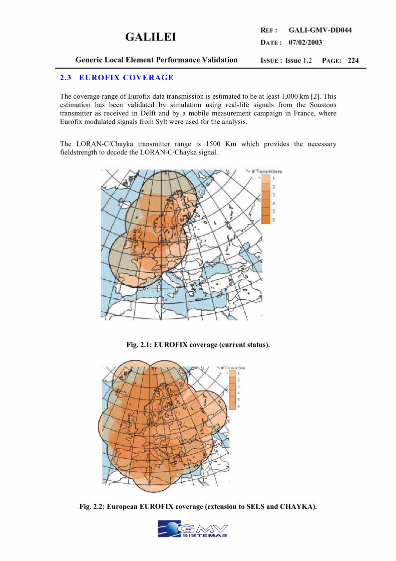
GALILEI REF :
DATE :
GALI-GMV-DD044
07/02/2003
Generic Local Element Performance Validation ISSUE : Issue 1.2 PAGE: 224
2.3 EUROFIX COVERAGE
The coverage range of Eurofix data transmission is estimated to be at least 1,000 km [2]. This estimation has been validated by simulation using real-life signals from the Soustons transmitter as received in Delft and by a mobile measurement campaign in France, where Eurofix modulated signals from Sylt were used for the analysis. The LORAN-C/Chayka transmitter range is 1500 Km which provides the necessary fieldstrength to decode the LORAN-C/Chayka signal.
Fig. 2.1: EUROFIX coverage (current status).
Fig. 2.2: European EUROFIX coverage (extension to SELS and CHAYKA).
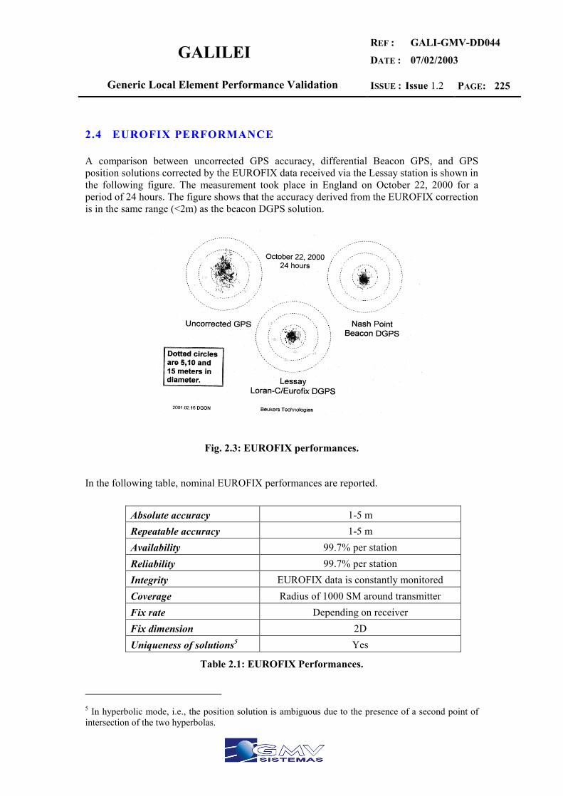
GALILEI REF :
DATE :
GALI-GMV-DD044
07/02/2003
Generic Local Element Performance Validation ISSUE : Issue 1.2 PAGE: 225
2.4 EUROFIX PERFORMANCE
A comparison between uncorrected GPS accuracy, differential Beacon GPS, and GPS position solutions corrected by the EUROFIX data received via the Lessay station is shown in the following figure. The measurement took place in England on October 22, 2000 for a period of 24 hours. The figure shows that the accuracy derived from the EUROFIX correction is in the same range (<2m) as the beacon DGPS solution.
Fig. 2.3: EUROFIX performances.
In the following table, nominal EUROFIX performances are reported.
Absolute accuracy 1-5 m Repeatable accuracy 1-5 m Availability 99.7% per station Reliability 99.7% per station Integrity EUROFIX data is constantly monitored Coverage Radius of 1000 SM around transmitter Fix rate Depending on receiver Fix dimension 2D Uniqueness of solutions5 Yes
Table 2.1: EUROFIX Performances.
5 In hyperbolic mode, i.e., the position solution is ambiguous due to the presence of a second point of intersection of the two hyperbolas.
GALILEI REF :
DATE :
GALI-GMV-DD044
07/02/2003
Generic Local Element Performance Validation ISSUE : Issue 1.2 PAGE: 226
2.5 EUROFIX DATALINK
The Eurofix datalink is presently used to transmit differential GPS corrections, integrity messages and also short messages. The transmitted DGPS correction data should remain compatible with existing DGPS receivers. The current data format (table 3) is, therefore, derived from the RTCM SC-104 format for Differential GPS data broadcasts. At the receiving end, the Eurofix correction messages which are optimised for low-data rate transmission, are reformatted into standard RTCM message formats without loss of resolution or compatibility.
Due to the rather low data rate the LORAN-C system can provide, the corrections are transmitted asynchronously, which means that every message contains a correction for one satellite only (comparable with RTCM type-9 messages). When corrections for more satellites were broadcast in a single message, it would simply take too much time before the message was fully received and corrections could be applied to the GPS receiver. By that time the information would have aged and lost validity. Table 2 shows the Eurofix data format derived from the RTCM correction messages. As can be seen from the table, room for 8 possible messages is reserved. Currently, only DGPS correction data, satellite integrity messages and Short Message Service broadcast are implemented.
The DGPS reference station will be located at the LORAN-C transmitter site. It calculates and monitors range and range-rate corrections for all satellites in view. In this set-up the reference station provides a Local Area Augmentation Service over a large coverage area (3 million square kilometres per Eurofix station). Large parts of Europe are covered by two or more LORAN stations. By receiving corrections from multiple reference stations the user can calculate a weighted average and generate in this way a Networked DGPS correction. This correction then better resembles the situation at his position.
The EUROFIX data is based on the RTCM #9 message and is reported in the following table.
Function Bits Resolution Range Message type 3 8 types of messages Modified Z-Count 13 0.6 s 0-3599.4 Scale factor 1 UDRE 2 4 Satellite ID 5 32 satellites Pseudo-Range Correction 16 0.02 or 0.32 m ±655.34 or ±10485.44 m Range Rate Correction 8 0.002 or 0.032 m/s ±0.254 m/s or ±4064 m/s Issue of Data 8
TOTAL 56
Table 2.2: EUROFIX message format (based on RTCM Type-9 correction).
As reported, 8 types of messages are possible. At the moment, only three types of messages are implemented:

GALILEI REF :
DATE :
GALI-GMV-DD044
07/02/2003
Generic Local Element Performance Validation ISSUE : Issue 1.2 PAGE: 227
• DGPS correction
• Satellite integrity
• SMS service It has to be further remembered that RTCM #9 is used in low data rate link to transmit in time sharing corrections for each satellite (e.g. in USCG American network). This introduces errors due to the age of the corrections received by the user receiver. With LORAN-C GRI varying between 40 ms and 100 ms, the raw bit rate available ranges from 175 bps to 70 bps.
2.6 EUROFIX/GPS RECEIVER
In the following, an architectural scheme of an integrated EUROFIX/GPS receiver is reported. The integration of GALILEO is also taken into account. An integrated EUROFIX/GALILEO/GPS receiver is basically constituted by the integration of the different satellite and terrestrial receivers. A sensor data combinatory system able to integrate different measurements and to produce positioning and navigation data is through a data fusion process is the core of the receiver.
A PC-based EUROFIX receiver implemented at the Sylt LORAN-C transmitter in February 1997 by the Delft University [1]. The reference station set-up is located in the office building on the Sylt transmitter site and consists of an industrial-type PC, a NovAtel GPS receiver and communication modules. The PC contains software to calculate and to monitor corrections for all satellites in view, to apply Forward Error Correction and it communicates with the transmitter in a building at about 200 m distance. At the transmitter building Megapulse, Inc. modified the LORAN Timing Unit (LTU) to be able to modulate the messages onto the LORAN-C pulses. The DGPS reference antenna is placed on the roof of the office building. This site was carefully chosen to minimise range and range-rate errors due to multipath and masking of the satellite signals by the LORAN-C transmitter antenna. The location of the antenna was accurately surveyed by the German Department of Transportation. To allow maximum flexibility in the test scheme, the reference station can be remotely controlled from the monitor station at Delft University via a modem connection.
Besides antenna and bandpass filter the datalink receiver is basically a software receiver. After being bandpass filtered the signals are A/D converted and processed in a computer. In software the signals are demodulated and decoded, and the resulting RTCM corrections are fed into a standard DGPS receiver, which outputs the corrected position fix. Integrity information and short messages are shown on the PC monitor. The processing power requirements needed for demodulation and decoding of the LORAN-C pulses are low, which allows a cost effective implementation of Eurofix datalink capabilities in existing or newly designed receivers.

GALILEI REF :
DATE :
GALI-GMV-DD044
07/02/2003
Generic Local Element Performance Validation ISSUE : Issue 1.2 PAGE: 228
3 LORAN-C/EUROFIX/EGNOS INTEGRATION
The basic concept for the integration of EGNOS into EUROFIX is related to the possibility to transmit EGNOS messages through LORAN-C. The possibility to integrate EGNOS into the current EUROFIX concept is leading to the chance to provide enhanced GPS augmentation messages through the LORAN-C transmitters. Today only RTCM message 9 is transmitted for augmentation purposes. The architectural impacts on the EUROFIX architecture for the introduction of EGNOS into the EUROFIX concept are:
• Installation of EGNOS reference receivers at the LORAN-C transmitters or datalink from the EGNOS MCC
• Conversion of EGNOS message into RTCM format • To achieve full EGNOS performance => enhancement of the EUROFIX datalink
capacity • Software update in the user receiver to process EGNOS data
At the receiver side, the implementation of an integrated EUROFIX/EGNOS receiver does not lead to major modifications with respect to the typical EUROFIX receiver, being the EGNOS message transmitted on a LORAN-C carrier. The major update is a software/firmware update required to process the EGNOS data with an EUROFIX receiver.
3.1 ADVANTAGES OF LORAN-C/EUROFIX/EGNOS
Here is presented some a list of benefits of the joined use of the systems [3]: • Good signal availability in “shadowed environment” (to some extend even indoor) • Robust system (High transmission power ~250 KW) • “Low-cost” infrastructure (operating costs for European wide system <<5% of
GALILEO costs) • DGNSS correction data • Integrity information for GNSS through LORAN-C data link (civil system) • Growing “timing” community • Increasing number of receiver manufacturers • Combined use of LORAN-C in TOE-mode with GNSS
3.2 SCOPE OF LOREG T&V
A test and validation programme was initiated by NELS in co-operation with Telematica e. K. to demonstrate the potential benefits of a combined use of LORAN-C/EUROFIX and

GALILEI REF :
DATE :
GALI-GMV-DD044
07/02/2003
Generic Local Element Performance Validation ISSUE : Issue 1.2 PAGE: 229
EGNOS [4] within different fields of applications. The LOREG T&V programme is structured into different phases:
• Phase 1 develops the overall T&V concept and the software for data collection, analysis and visualisation
• Phase 2.1 is the realisation of the measurement campaigns in a first version • Phase 2.2 is the realisation of the measurement campaigns in a complete version
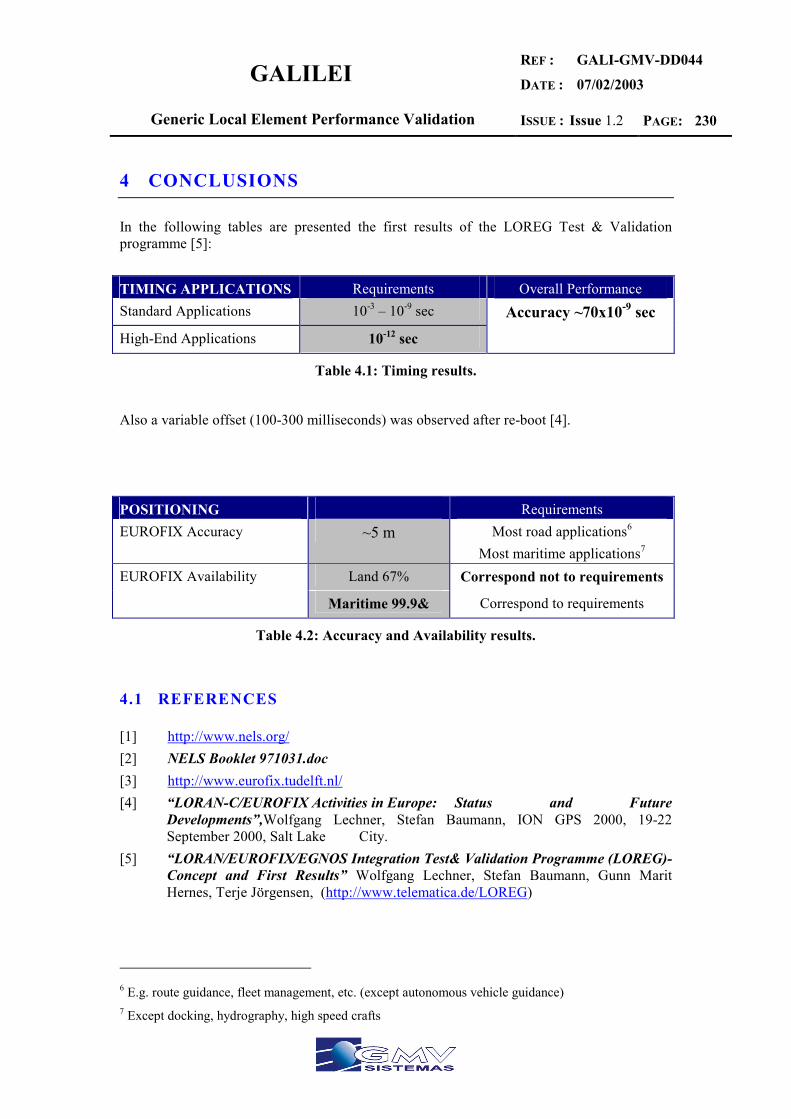
GALILEI REF :
DATE :
GALI-GMV-DD044
07/02/2003
Generic Local Element Performance Validation ISSUE : Issue 1.2 PAGE: 230
4 CONCLUSIONS
In the following tables are presented the first results of the LOREG Test & Validation programme [5]: TIMING APPLICATIONS Requirements Overall Performance Standard Applications 10-3 – 10-9 sec Accuracy ~70x10-9 sec High-End Applications 10-12 sec
Table 4.1: Timing results.
Also a variable offset (100-300 milliseconds) was observed after re-boot [4]. POSITIONING Requirements EUROFIX Accuracy ~5 m Most road applications6
Most maritime applications7 EUROFIX Availability Land 67% Correspond not to requirements
Maritime 99.9& Correspond to requirements
Table 4.2: Accuracy and Availability results.
4.1 REFERENCES
[1] http://www.nels.org/ [2] NELS Booklet 971031.doc [3] http://www.eurofix.tudelft.nl/ [4] “LORAN-C/EUROFIX Activities in Europe: Status and Future
Developments”,Wolfgang Lechner, Stefan Baumann, ION GPS 2000, 19-22 September 2000, Salt Lake City.
[5] “LORAN/EUROFIX/EGNOS Integration Test& Validation Programme (LOREG)- Concept and First Results” Wolfgang Lechner, Stefan Baumann, Gunn Marit Hernes, Terje Jörgensen, (http://www.telematica.de/LOREG)
6 E.g. route guidance, fleet management, etc. (except autonomous vehicle guidance) 7 Except docking, hydrography, high speed crafts
GALILEI REF :
DATE :
GALI-GMV-DD044
07/02/2003
Generic Local Element Performance Validation ISSUE : Issue 1.2 PAGE: 231
ANNEX 7 SPACE BASED COMMUNICATION NETWORK

GALILEI REF :
DATE :
GALI-GMV-DD044
07/02/2003
Generic Local Element Performance Validation ISSUE : Issue 1.2 PAGE: 232
This annex introduces an analysis of the Space Based Communication Network (SBCN). The following communication systems are considered:
Inmarsat Iridium Globalstar Digital satellite based radio

GALILEI REF :
DATE :
GALI-GMV-DD044
07/02/2003
Generic Local Element Performance Validation ISSUE : Issue 1.2 PAGE: 233
1 VSAT NETWORKS
1.1 OVERVIEW
VSAT stands for “Very Small Aperture Terminal” and refers to receive/transmit terminals installed at dispersed sites connecting to a central hub via satellite using small diameter antenna dishes (0.6 to 3.8 meter), used for the reliable transmission of data, video or voice via geostationary satellites. Generally, these systems operate in the:
• Ku-band (10.7 - 12.75 GHz): this band are used primarily in Europe and North America.
• C-band8 (3.4 – 4.8 GHz): used extensively in Asia, Africa and Latin America. There is one major drawback to satellites downlinking signals at frequencies greater than 10 gigahertz: the length of these microwaves is so short that rain, snow or even rain-filled clouds passing overhead can reduce the intensity of the incoming signals. At these higher frequencies, the length of the falling rain droplets are close to a resonant sub-multiple of the signal's wave length; the droplets therefore are able to absorb and de-polarize the microwaves passing through the Earth's atmosphere. In places such as Southeast Asia or the Caribbean, torrential downpours can lower the level of the incoming Ku-band satellite signal by 20 dB or more; this may severely degrade the quality of the signals or even interrupt reception entirely [2]. So in these areas C-band antennas are preferred. VSATs use a star network with the use of satellite earth stations that rely on a large central hub. Alternatively the use of mesh (hubless) VSAT networks can provide communication between VSAT terminals directly. Most VSAT terminals utilize satellite dishes in the 1 to 2.4 meter range, though both smaller and larger dish configurations are available. The selection of satellite, terminal size and configuration is based on the specific requirements of the applications for which VSAT will be utilized. There are two types of operation:
• Bi-directional operation: the dish both transmits (uplink) and receives (downlink) information.
• Receive-only operation: The dish receives (downlink) information only. VSAT is growth compatible, allowing the user to make incremental increases in its network. The use of VSAT provides the ability to expand capacity and system growth, while maintaining a handle on costs which are closely associated with the increase in capacity or system growth. 8 C-band requires a larger diameter antenna than Ku-band.
GALILEI REF :
DATE :
GALI-GMV-DD044
07/02/2003
Generic Local Element Performance Validation ISSUE : Issue 1.2 PAGE: 234
1.2 VSAT COMPONENTS
A VSAT network consists of two major components, a ground segment and a space segment: • The space segment: it consists of the satellite and its on-board transponders. The
satellites used are exclusively in the Geo-stationary orbit, located on an arc 36,000 km above the equator.
• The ground segment: it consists of a central hub station and a family of remote terminals (satellite earth stations) generally referred to as remote VSATs.
A VSAT terminal can typically divided into two parts-an outdoor unit and an indoor unit:
• Outdoor Unit: This comprises of an antenna and transceiver. In the transmit direction the IF/L-Band carrier is frequency converted to C or Ku band and then amplified via an SSPA; 2W – 240W depending on the data rate, required BER, satellite and VSAT network configuration. In the receive direction the carriers received by the antenna are amplified and down converted to either 70/140MHz IF or L-Band by the transceiver. After which they pass to the indoor demodulator via the cross site cables. The antenna system consists of a reflector, feedhorn and a mount. The size of the antenna varies from 1.8 metres to 3.8 metres. The feedhorn is mounted on the antenna frame at its focal point by support arms. The feedhorn directs the transmitted power towards the antenna dish or collects the received power from it.
The VSAT terminal transceiver is of the high stability, low phase noise type, meeting the mandatory specification of Intelsat and Eutelsat. Redundant configuration can be provided for higher levels of service availability. These include Low Noise Amplifiers (LNA) and down converters for amplification and down conversion of the received signal respectively. LNAs are designed to minimise the noise added to the signal during this first stage of the converter as the noise performance of this stage determines the overall noise performance of the converter unit. The noise temperature is the parameter used to describe the performance of a LNA Up converters and High Powered Amplifiers (HPA) are also part of the transceiver and are used for up converting and amplifying the signal before transmitting to the feedhorn. The Up/Down converters convert frequencies between intermediate frequency (Usually IF level 70 MHz) and radio frequency. For Extended C band, the down converter receives the signal at 4.500 to 4.800 GHz and the up converter converts it to 6.725 to 7.025 GHz. Interfacility Link: The outdoor unit is connected through a low loss co-axial cable to the indoor unit. The typical limit of an IFL cable is about 300 feet.
• Indoor Unit: This comprises of a multiplexer/FRAD and PSK modem. Modems are supplied with BPSK, QPSK or 8PSK modulation schemes and options compliant with IDR, IBS or SMS international standards.
GALILEI REF :
DATE :
GALI-GMV-DD044
07/02/2003
Generic Local Element Performance Validation ISSUE : Issue 1.2 PAGE: 235
1.3 VSAT NETWORKS
There are basically five types of networks employed in VSAT operations, explained below [1].
1.3.1 MULTIPOINT NETWORK
The Multipoint Network Structure is used in data oriented networks that require voice. The network structure provides for two-way data, voice and multi-media operations. The network configuration is a star type network that connects one or more main sites to various remote sites. It employs a central hub station and a communication satellite. Each main site uplinks and downlinks from the central hub through terrestrial (land) links. Each remote site can only uplink to the hub. If a remote site has data to send to any other location, it must first pass the information to the hub, and then it can be routed to its final destination. This type of network is very flexible, supporting multiple interfaces available for LAN, Voice and Data connections and can support numerous transport protocols. The network employs TDMA (Time Division Multiple Access) as the means to send data to each remote site. This provides a secure means of transporting data, as each data packet contains the specific address of the station that it is addressed to and only that station can receive the data and pass it on to its network.
1.3.2 FULL-MESHED NETWORK
For Voice oriented networks a Full-Meshed Designed Network is utilized. In a Full-Meshed there is no central hub and each site can communicate directly with all network nodes. It employs single satellite hops between each network nodes, which enables superior voice quality, and efficient fast-response data connections. Since the network does not employ a central hub, each station requires increased processing and transmission power. Each remote must uplink and downlink with other remote sites with exactly the same size antenna over the same radio frequency. In this network one site on the network must provide a Network Control System. It is responsible for setting up calls between the sites and monitors the traffic and bandwidth use. From this site all operating statistics are generated and billing information is produced. The Network Control System established the allocation of bandwidth as each connection is established through bandwidth-on-demand, that is as one node initiates a call to another node, the Network Control System demands a certain amount of bandwidth from the bandwidth pool and then assigns it to the two nodes for the duration of the communication . Once a call is terminated, the bandwidth is then free, and is back available from the bandwidth pool. This type of network is capable of providing interconnection of dissimilar communication devices. It provides the capability of providing connections between must all currently available communication devices. The system can provide a connection for an individual handset, PBX (Public Branch Exchange) or can provide a gateway system.
1.3.3 HYBRID VOICE AND DATA NETWORK
This type of network is a hybrid between the Multipoint and Full-Meshed network. Like the Full-Meshed Network it does not contain a central hub, though it provides all remote sites
GALILEI REF :
DATE :
GALI-GMV-DD044
07/02/2003
Generic Local Element Performance Validation ISSUE : Issue 1.2 PAGE: 236
with the capability to communicate direct with all other sites . It provides the ability to offer voice, fax, and videoconferencing opportunities between the sites. Data and video can be broadcast is bi-directional between the central hub and the remote site. This system takes separate voice and data interfaces at the remote site and then processes this and combines them onto a single cable connecting to the antenna. The remote HES VSAT acts as a switch routing all connections to their appropriate destination. The system is capable of a wide-range of advance telephony and PBX voice services and provides an efficient LAN/WAN network service.
1.3.4 SINGLE CHANNEL PER CARRIER (SCPC) - POINT-TO-POINT
SCPC circuits are point-to-point circuits that provide two-way communication between VSAT terminals located at two sites. It is a very flexible system and has the capability to handle multiple data types over multiple protocols. The system can handle voice, fax, and video application. the data rates range from 9.6 kbps up to 8.4 Mbs. It is ideally suited for bringing Internet to remote ISP sites. Internet access is provided through one satellite dish connected to the Internet through a point-to-point line and transmission is accomplished between it and another terminal at the remote ISP through the use of a satellite. This system is capable of both asymmetric and well as symmetric connections.
1.3.5 BROADCAST NETWORKS
Broadcast Networks provide for the transmission of data, video and audio files to any number of users. The system "broadcasts" from the central site to the end user remote sites. This one-way system provides an uplink from the central site and each remote site downlinks (receives) only. It provides high speed channel that is capable of up to 24 Mbs up linked, providing this information to numerous units.
1.4 VSAT ACCESS
The primary objective and advantage of these networks is to maximise the usage of common satellite and other resources amongst all VSAT sites [3]. The method by which these networks optimise the use of satellite capacity, and spectrum utilisation in a flexible and cost-effective manner are referred to as satellite access schemes and are detailed below.
1.4.1 TIME DIVISION MULTIPLE ACCESS (TDMA)
In a TDMA network, all VSATs share satellite resource on a time slot basis. Remote VSATs use TDMA channels or in-routes for communicating with the hub. There are several in-routes associated with one out-route. Several VSATs share one in-route thereby sharing the bandwidth. Typical in-routes operate at 64 or 128 Kbps. Generally systems with star topology use a Time Division Multiplexed/ Time Division Multiple Access (TDM/TDMA) transmission technique.
GALILEI REF :
DATE :
GALI-GMV-DD044
07/02/2003
Generic Local Element Performance Validation ISSUE : Issue 1.2 PAGE: 237
Critical to all TDMA schemes is the function of clock synchronisation which is performed by the TDMA hub or Master Earth Station.
1.4.1.1 Fixed assigned TDMA
The VSATs may access the in-route on a fixed assigned TDMA mode, wherein each VSAT is allocated a specific time slot or slots. In Slotted ALOHA case each VSAT can access any slot at any time with the remote sites randomly transmitting messages on the inbound transmission path. Most of the time this allows messages an instant access to the in-route data stream making it to be the fastest method of transmitting messages to the hub. However, when two or more sites transmit packets simultaneously a collision occurs where the hub station will not receive any of the affected packets. On detecting a collision, remote sites undergo a random transmission delay and re-transmit the packet in another time-slot before the transaction is complete. Slotted ALOHA helps in most efficient use of bandwidth in situations where multiple sites are randomly transmitting short bursty messages back to the hub. TDMA networks are ideally suited for medium to large networks with medium data rates. As an intermediate refinement, techniques have been developed to toggle the operation of a VSAT from a Slotted ALOHA mode to a Fixed Assigned mode. This is referred to as Dynamic Reservation. As the traffic grows, the VSAT senses the same and switches over to a fixed assigned TDMA mode, wherein it has an assured amount of slots. This switchover between Slotted Aloha and Fixed Assigned TDMA is done dynamically dependent on the traffic profile. This allows optimum usage of satellite resources.
1.4.2 FREQUENCY DIVISION MULTIPLE ACCESS (FDMA)
Here all VSATs share the satellite resource on the frequency domain only. Typically implemented in a mesh or single satellite-hop topology, FDMA has the following variants.
1.4.2.1 Pre-Assigned Multiple Access (PAMA)
It implies that the VSATs are pre-allocated a designated frequency. Equivalent of the terrestrial leased line solutions, PAMA solutions use the satellite resources constantly. Consequently there is no call up delay which makes them most suited for interactive data applications or high traffic volumes . As such PAMA connects high data traffic sites within an organisation. SCPC (Single Channel Per Carrier) refers to the usage of a single satellite carrier for carrying a single channel of user traffic. The frequency is allocated on a pre-assigned basis in case of SCPC VSATs. The term SCPC VSAT is often used interchangeably with PAMA VSAT. Thus a permanently assigned frequency channel provides dedicated bandwidth, through which you can send data, voice or video. This illustrates the concept of Dedicated Resource in Shared Environment. Here the frequency channel is dedicated to you but the basic Satellite resource is shared by many. Now the assigned frequency carrier in PAMA can either be used for voice or for data. Also it is possible the use of one carrier for data and voice, however it calls for the use of a call of
GALILEI REF :
DATE :
GALI-GMV-DD044
07/02/2003
Generic Local Element Performance Validation ISSUE : Issue 1.2 PAGE: 238
device named Voice Data Multiplexer (VDM) which combines or aggregates several data and voice channels into one trunk line which in turn is interfaced to the VSAT equipment.
1.4.2.2 Demand Assigned Multiple Access (DAMA)
Network uses a pool of satellite channels, which are available for use by any station in that network. On demand a pair of available channels are assigned so that a call can be established. Once the call is completed, the channels are returned to the pool for an assignment to another call. Since the satellite resource is used only in proportion to the active circuits and their holding times, this is ideally suited for voice traffic and data traffic in batch mode. DAMA offers point to point voice, fax, and data requirements and supports video conferencing.
1.4.3 CODE DIVISION MULTIPLE ACCESS (CDMA)
Under this a central network monitoring system allocates a unique code to each of the VSATs enabling multiple VSATs to transmit simultaneously and share a common frequency band. The data signal is combined with a high bit rate code signal which is independent of the data. Reception at the end of the link is accomplished by mixing the incoming composite data/code signal with a locally generated and correctly synchronised replica of the code. Since this network requires that the central NMS coordinates code management and clock synchronisation of all remote VSATs, Star is by default the best topology. Although this is ideally suited for very large networks with low data requirements there are practical restrictions in the use of spread spectrum.
1.5 BENEFITS OF VSATS
VSATs have multiple advantage over terrestrial lines, not only the ease of installation. Below are described the main benefits:
1. Last mile problem: VSATs located at your premises guarantee seamless communication even across the last mile.
2. Reliability: Uptime of up to 99.5 percent is achievable on a VSAT network. This is significantly higher than the typical leased line uptime of approximately 80 to 85 percent.
3. Time: VSAT deployment takes no more than 4-6 weeks as compared to 4 to 6 months for leased lines
4. Network management: Network monitoring and control of the entire VSAT network is much simpler than a network of leased lines, involving multiple carriers at multiple locations. A much smaller number of elements needs to be monitored in case of a VSAT network and also the number of vendors and carriers involved in between any two user terminals in a VSAT network is typically one. A VSAT NMS easily
GALILEI REF :
DATE :
GALI-GMV-DD044
07/02/2003
Generic Local Element Performance Validation ISSUE : Issue 1.2 PAGE: 239
integrates end-to-end monitoring and configuration control for all network subsystems.
5. Flexibility: VSAT networks offer enormous expansion capabilities. This feature factors in changes in the business environment and traffic loads that can be easily accommodated on a technology migration path. Additional VSATs can be rapidly installed to support the network expansion to any site, no matter however remote.
6. Cost: A comparison of costs between a VSAT network and a leased line network reveals that a VSAT network offers significant savings over a two to three years timeframe. This does not take into account the cost of downtime, inclusion of which would result in the VSAT network being much more cost-effective. Additionally, in case of VSATs, the service charges depend on the bandwidth which is allocated to your network in line with your requirements. Whereas with a leased line you get a dedicated circuit in multiples of 64Kbps whether you need that amount of bandwidth or not.

GALILEI REF :
DATE :
GALI-GMV-DD044
07/02/2003
Generic Local Element Performance Validation ISSUE : Issue 1.2 PAGE: 240
2 REFERENCES
[1] http://www.donegal-holdings.com/vsat.htm [2] http://www.mlesat.com/Article9.html [3] http://www.zdnetindia.com/biztech/services/whitepapers/stories/22257.html

GALILEI REF :
DATE :
GALI-GMV-DD044
07/02/2003
Generic Local Element Performance Validation ISSUE : Issue 1.2 PAGE: 241
ANNEX 8 GROUND BASED COMMUNICATION NETWORK
GALILEI REF :
DATE :
GALI-GMV-DD044
07/02/2003
Generic Local Element Performance Validation ISSUE : Issue 1.2 PAGE: 242
Ground Based Communication Network (GBCN) systems are covered in this annex. GBCN can be grouped as:
Mobile Long and medium range Short range
These include systems like GSM, GPRS, UMTS, TETRA, DECT, RDS, BLUETOOH, IRDA, RFHOME, and WMAN among others.
GALILEI REF :
DATE :
GALI-GMV-DD044
07/02/2003
Generic Local Element Performance Validation ISSUE : Issue 1.2 PAGE: 243
1 2G – GSM
1.1 HISTORY
The Global System for Mobile communications is a digital cellular communications system. It was developed in order to create a common European mobile telephone standard but it has been rapidly accepted worldwide. GSM was designed to be compatible with ISDN services [1].
The idea of cell-based mobile radio systems appeared at Bell Laboratories (in USA) in the early 1970s. However, mobile cellular systems were not introduced for commercial use until the 1980s. During the early 1980s, analog cellular telephone systems experienced a very rapid growth in Europe, particularly in Scandinavia and the United Kingdom. Today cellular systems still represent one of the fastest growing telecommunications systems.
But in the beginnings of cellular systems, each country developed its own system, which was an undesirable situation for the following reasons:
• The equipment was limited to operate only within the boundaries of each country.
• The market for each mobile equipment was limited.
In order to overcome these problems, the Conference of European Posts and Telecommunications (CEPT) formed, in 1982, the Groupe Spécial Mobile (GSM) in order to develop a pan-European mobile cellular radio system (the GSM acronym became later the acronym for Global System for Mobile communications). The standardized system had to meet certain criteria:
• Spectrum efficiency
• International roaming
• Low mobile and base stations costs
• Good subjective voice quality
• Compatibility with other systems such as ISDN (Integrated Services Digital Network)
• Ability to support new services
In 1989 the responsability for the GSM specifications passed from the CEPT to the European Telecommunications Standards Institute (ETSI). The aim of the GSM specifications is to describe the functionality and the interface for each component of the system, and to provide guidance on the design of the system. These specifications will then standardize the system in order to guarantee the proper interworking between the different elements of the GSM system. In 1990, the phase I of the GSM specifications were published but the commercial use of GSM did not start until mid-1991.

GALILEI REF :
DATE :
GALI-GMV-DD044
07/02/2003
Generic Local Element Performance Validation ISSUE : Issue 1.2 PAGE: 244
The most important events in the development of the GSM system are presented in the next table (¡Error! No se encuentra el origen de la referencia.).
YEAR EVENT 1982 CEPT establishes a GSM group in order to develop the standards for a pan-
European cellular mobile system 1985 Adoption of a list of recommendations to be generated by the group 1986 Field tests were performed in order to test the different radio techniques
proposed for the air interface 1987 TDMA is chosen as access method (in fact, it will be used with FDMA)
Initial Memorandum of Understanding (MoU) signed by telecommunication operators (representing 12 countries)
1988 Validation of the GSM system 1989 The responsability of the GSM specifications is passed to the ETSI 1990 Appearance of the phase 1 of the GSM specifications 1991 Commercial launch of the GSM service 1992 Enlargement of the countries that signed the GSM- MoU> Coverage of
larger cities/airports 1993 Coverage of main roads GSM services start outside Europe 1995 Phase 2 of the GSM specifications Coverage of rural areas
Table 1.1: Most important events in GSM’s development.
Fig. 1.1 represents the evolution of the total number of GSM; it reached 684.2 millions in May 2002 [2].
Fig. 1.1: Number of GSM subscribers per year.
Fig. 1.2 shows the repartition of GSM subscribers on July 2001. In July 2001, 153 countries were using GSM standard for cellular telecommunication. Europe and Asia have the most important number of subscribers. In May 2002, 179 the number of countries using GSM standard growth to 179.
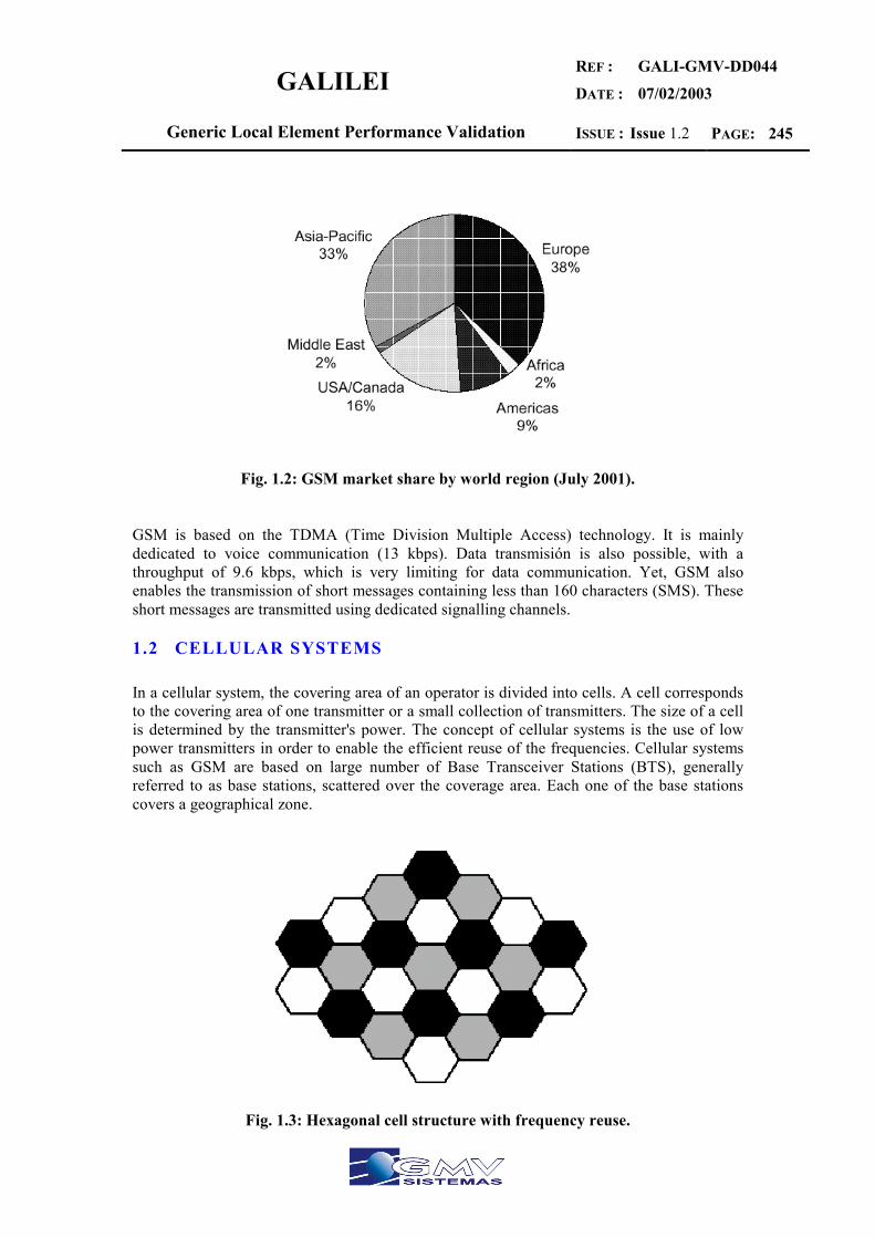
GALILEI REF :
DATE :
GALI-GMV-DD044
07/02/2003
Generic Local Element Performance Validation ISSUE : Issue 1.2 PAGE: 245
Fig. 1.2: GSM market share by world region (July 2001).
GSM is based on the TDMA (Time Division Multiple Access) technology. It is mainly dedicated to voice communication (13 kbps). Data transmisión is also possible, with a throughput of 9.6 kbps, which is very limiting for data communication. Yet, GSM also enables the transmission of short messages containing less than 160 characters (SMS). These short messages are transmitted using dedicated signalling channels.
1.2 CELLULAR SYSTEMS
In a cellular system, the covering area of an operator is divided into cells. A cell corresponds to the covering area of one transmitter or a small collection of transmitters. The size of a cell is determined by the transmitter's power. The concept of cellular systems is the use of low power transmitters in order to enable the efficient reuse of the frequencies. Cellular systems such as GSM are based on large number of Base Transceiver Stations (BTS), generally referred to as base stations, scattered over the coverage area. Each one of the base stations covers a geographical zone.
Fig. 1.3: Hexagonal cell structure with frequency reuse.
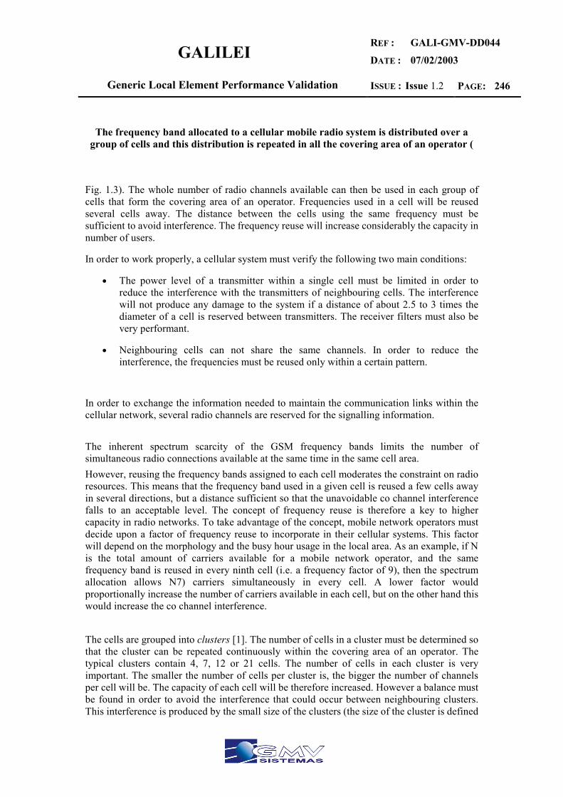
GALILEI REF :
DATE :
GALI-GMV-DD044
07/02/2003
Generic Local Element Performance Validation ISSUE : Issue 1.2 PAGE: 246
The frequency band allocated to a cellular mobile radio system is distributed over a group of cells and this distribution is repeated in all the covering area of an operator (
Fig. 1.3). The whole number of radio channels available can then be used in each group of cells that form the covering area of an operator. Frequencies used in a cell will be reused several cells away. The distance between the cells using the same frequency must be sufficient to avoid interference. The frequency reuse will increase considerably the capacity in number of users.
In order to work properly, a cellular system must verify the following two main conditions:
• The power level of a transmitter within a single cell must be limited in order to reduce the interference with the transmitters of neighbouring cells. The interference will not produce any damage to the system if a distance of about 2.5 to 3 times the diameter of a cell is reserved between transmitters. The receiver filters must also be very performant.
• Neighbouring cells can not share the same channels. In order to reduce the interference, the frequencies must be reused only within a certain pattern.
In order to exchange the information needed to maintain the communication links within the cellular network, several radio channels are reserved for the signalling information. The inherent spectrum scarcity of the GSM frequency bands limits the number of simultaneous radio connections available at the same time in the same cell area. However, reusing the frequency bands assigned to each cell moderates the constraint on radio resources. This means that the frequency band used in a given cell is reused a few cells away in several directions, but a distance sufficient so that the unavoidable co channel interference falls to an acceptable level. The concept of frequency reuse is therefore a key to higher capacity in radio networks. To take advantage of the concept, mobile network operators must decide upon a factor of frequency reuse to incorporate in their cellular systems. This factor will depend on the morphology and the busy hour usage in the local area. As an example, if N is the total amount of carriers available for a mobile network operator, and the same frequency band is reused in every ninth cell (i.e. a frequency factor of 9), then the spectrum allocation allows N7) carriers simultaneously in every cell. A lower factor would proportionally increase the number of carriers available in each cell, but on the other hand this would increase the co channel interference.
The cells are grouped into clusters [1]. The number of cells in a cluster must be determined so that the cluster can be repeated continuously within the covering area of an operator. The typical clusters contain 4, 7, 12 or 21 cells. The number of cells in each cluster is very important. The smaller the number of cells per cluster is, the bigger the number of channels per cell will be. The capacity of each cell will be therefore increased. However a balance must be found in order to avoid the interference that could occur between neighbouring clusters. This interference is produced by the small size of the clusters (the size of the cluster is defined
GALILEI REF :
DATE :
GALI-GMV-DD044
07/02/2003
Generic Local Element Performance Validation ISSUE : Issue 1.2 PAGE: 247
by the number of cells per cluster). The total number of channels per cell depends on the number of available channels and the type of cluster used.
The density of population in a country is so varied that different types of cells are used [1]:
• Macrocells: the macrocells are large cells for remote and sparsely populated areas
• Microcells: these cells are used for densely populated areas. By splitting the existing areas into smaller cells, the number of channels available is increased as well as the capacity of the cells. The power level of the transmitters used in these cells is then decreased, reducing the possibility of interference between neighbouring cells.
• Selective cells: it is not always useful to define a cell with a full coverage of 360 degrees. In some cases, cells with a particular shape and coverage are needed. These cells are called selective cells. A typical example of these cells are the cells that may be located at the entrances of tunnels where a coverage of 360 degrees is not needed; in this case, a selective cell with coverage of 120 degrees is used.
• Umbrella cells: A freeway crossing very small cells produces an important number of handovers among the different small neighbouring cells. In order to solve this problem, the concept of umbrella cells is introduced. An umbrella cell covers several microcells. The power level inside an umbrella cell is increased comparing to the power levels used in the microcells that form the umbrella cell. When the speed of the mobile is too high, the mobile is handed off to the umbrella cell. The mobile will then stay longer in the same cell (in this case the umbrella cell). This will reduce the number of handovers and the work of the network.
A too important number of handover demands and the propagation characteristics of a mobile can help to detect its high speed.
1.3 ARCHITECTURE OF THE GSM NETWORK
The GSM technical specifications define the different entities that form the GSM network by defining their functions and interface requirements.
The GSM network can be divided into four main parts:
• The Mobile Station (MS): a Mobile Station consist of two main elements:
o The mobile equipment or terminal
o The subscriber Identity Module (SIM)
• The Base Station Subsystem (BSS): The BSS connects the Mobile Station and the NSS. It is in charge of the transmission and reception. The BSS can be divided into two parts:
o The Base Transceiver Station (BTS) or Base Station.
o The Base Station Controller (BSC).
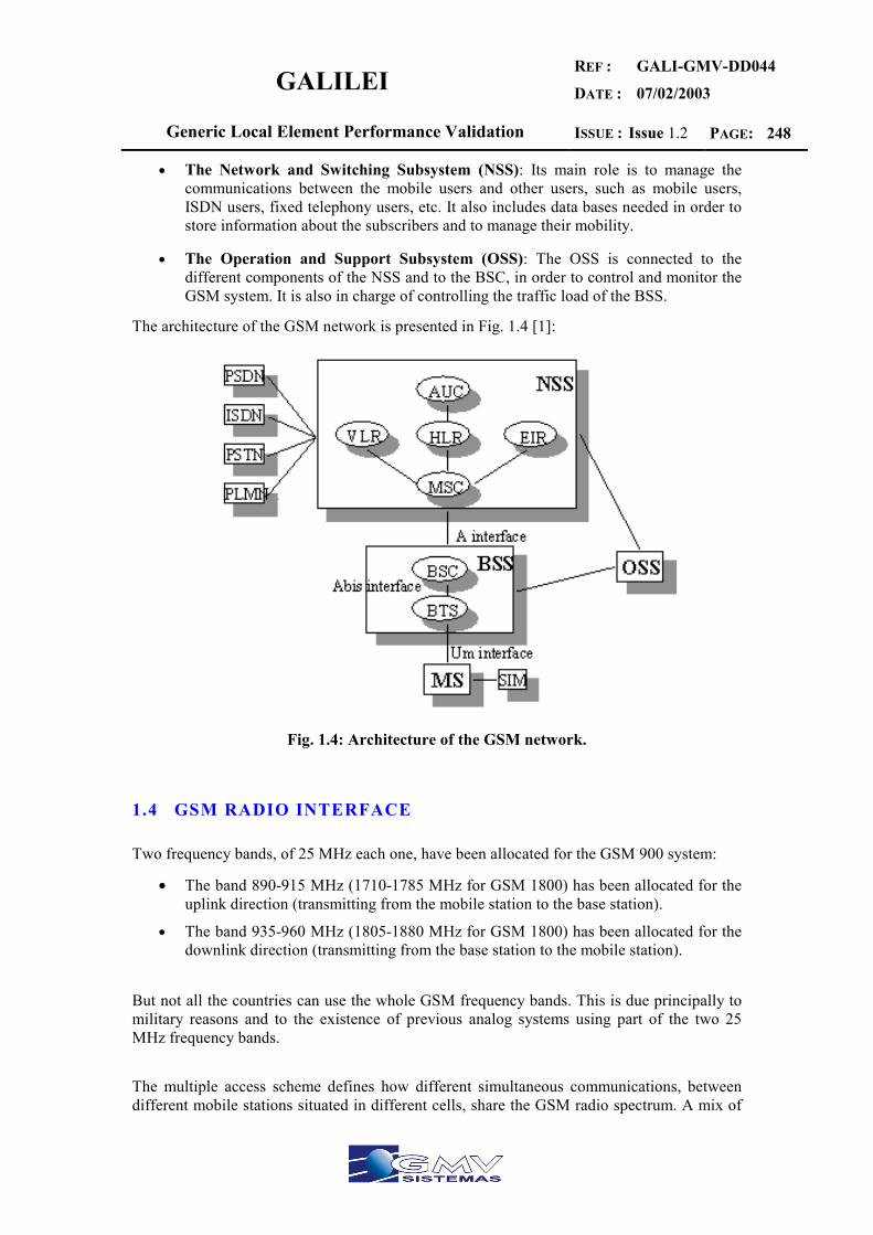
GALILEI REF :
DATE :
GALI-GMV-DD044
07/02/2003
Generic Local Element Performance Validation ISSUE : Issue 1.2 PAGE: 248
• The Network and Switching Subsystem (NSS): Its main role is to manage the communications between the mobile users and other users, such as mobile users, ISDN users, fixed telephony users, etc. It also includes data bases needed in order to store information about the subscribers and to manage their mobility.
• The Operation and Support Subsystem (OSS): The OSS is connected to the different components of the NSS and to the BSC, in order to control and monitor the GSM system. It is also in charge of controlling the traffic load of the BSS.
The architecture of the GSM network is presented in Fig. 1.4 [1]:
Fig. 1.4: Architecture of the GSM network.
1.4 GSM RADIO INTERFACE
Two frequency bands, of 25 MHz each one, have been allocated for the GSM 900 system:
• The band 890-915 MHz (1710-1785 MHz for GSM 1800) has been allocated for the uplink direction (transmitting from the mobile station to the base station).
• The band 935-960 MHz (1805-1880 MHz for GSM 1800) has been allocated for the downlink direction (transmitting from the base station to the mobile station).
But not all the countries can use the whole GSM frequency bands. This is due principally to military reasons and to the existence of previous analog systems using part of the two 25 MHz frequency bands. The multiple access scheme defines how different simultaneous communications, between different mobile stations situated in different cells, share the GSM radio spectrum. A mix of
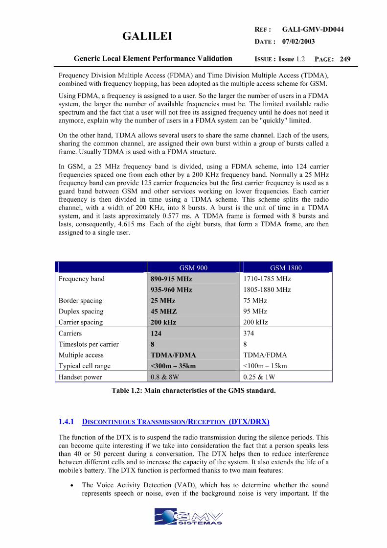
GALILEI REF :
DATE :
GALI-GMV-DD044
07/02/2003
Generic Local Element Performance Validation ISSUE : Issue 1.2 PAGE: 249
Frequency Division Multiple Access (FDMA) and Time Division Multiple Access (TDMA), combined with frequency hopping, has been adopted as the multiple access scheme for GSM.
Using FDMA, a frequency is assigned to a user. So the larger the number of users in a FDMA system, the larger the number of available frequencies must be. The limited available radio spectrum and the fact that a user will not free its assigned frequency until he does not need it anymore, explain why the number of users in a FDMA system can be "quickly" limited.
On the other hand, TDMA allows several users to share the same channel. Each of the users, sharing the common channel, are assigned their own burst within a group of bursts called a frame. Usually TDMA is used with a FDMA structure.
In GSM, a 25 MHz frequency band is divided, using a FDMA scheme, into 124 carrier frequencies spaced one from each other by a 200 KHz frequency band. Normally a 25 MHz frequency band can provide 125 carrier frequencies but the first carrier frequency is used as a guard band between GSM and other services working on lower frequencies. Each carrier frequency is then divided in time using a TDMA scheme. This scheme splits the radio channel, with a width of 200 KHz, into 8 bursts. A burst is the unit of time in a TDMA system, and it lasts approximately 0.577 ms. A TDMA frame is formed with 8 bursts and lasts, consequently, 4.615 ms. Each of the eight bursts, that form a TDMA frame, are then assigned to a single user.
GSM 900 GSM 1800 Frequency band 890-915 MHz
935-960 MHz 1710-1785 MHz 1805-1880 MHz
Border spacing 25 MHz 75 MHz Duplex spacing 45 MHZ 95 MHz Carrier spacing 200 kHz 200 kHz Carriers 124 374 Timeslots per carrier 8 8 Multiple access TDMA/FDMA TDMA/FDMA Typical cell range <300m – 35km <100m – 15km Handset power 0.8 & 8W 0.25 & 1W
Table 1.2: Main characteristics of the GMS standard.
1.4.1 DISCONTINUOUS TRANSMISSION/RECEPTION (DTX/DRX)
The function of the DTX is to suspend the radio transmission during the silence periods. This can become quite interesting if we take into consideration the fact that a person speaks less than 40 or 50 percent during a conversation. The DTX helps then to reduce interference between different cells and to increase the capacity of the system. It also extends the life of a mobile's battery. The DTX function is performed thanks to two main features:
• The Voice Activity Detection (VAD), which has to determine whether the sound represents speech or noise, even if the background noise is very important. If the
GALILEI REF :
DATE :
GALI-GMV-DD044
07/02/2003
Generic Local Element Performance Validation ISSUE : Issue 1.2 PAGE: 250
voice signal is considered as noise, the transmitter is turned off producing then, an unpleasant effect called clipping.
• The comfort noise. An inconvenient of the DTX function is that when the signal is considered as noise, the transmitter is turned off and therefore, a total silence is heard at the receiver. This can be very annoying to the user at the reception because it seems that the connection is dead. In order to overcome this problem, the receiver creates a minimum of background noise called comfort noise. The comfort noise eliminates the impression that the connection is dead.
Discontinuous reception (DRX) is a method used to conserve the mobile station’s power. The paging channel is divided into subchannels corresponding to single mobile stations. Each mobile station will then only 'listen' to its subchannel and will stay in the sleep mode during the other subchannels of the paging channel.
1.4.2 TIMING ADVANCE
The timing of the bursts transmissions is very important. Mobiles are at different distances from the base stations. Their delay depends, consequently, on their distance. The aim of the timing advance is that the signals coming from the different mobile stations arrive to the base station at the right time. The base station measures the timing delay of the mobile stations. If the bursts corresponding to a mobile station arrive too late and overlap with other bursts, the base station tells, this mobile, to advance the transmission of its bursts.
1.4.3 POWER CONTROL
At the same time the base stations perform the timing measurements, they also perform measurements on the power level of the different mobile stations. These power levels are adjusted so that the power is nearly the same for each burst.
A base station also controls its power level. The mobile station measures the strength and the quality of the signal between itself and the base station. If the mobile station does not receive correctly the signal, the base station changes its power level.
1.4.4 MULTIPATH AND EQUALISATION
At the GSM frequency bands, radio waves reflect from buildings, cars, hills, etc. So not only the 'right' signal (the output signal of the emitter) is received by an antenna, but also many reflected signals, which corrupt the information, with different phases. This is known as multipath and it is an important degradation factor
An equaliser is in charge of extracting the 'right' signal from the received signal. It estimates the channel impulse response of the GSM system and then constructs an inverse filter. The receiver knows which training sequence it must wait for. The equaliser will then, comparing the received training sequence with the training sequence it was expecting, compute the coefficients of the channel impulse response. In order to extract the 'right' signal, the received signal is passed through the inverse filter.

GALILEI REF :
DATE :
GALI-GMV-DD044
07/02/2003
Generic Local Element Performance Validation ISSUE : Issue 1.2 PAGE: 251
1.5 FREQUENCY HOPPING
The propagation conditions and therefore the multipath fading depend on the radio frequency. In order to avoid important differences in the quality of the channels, the slow frequency hopping is introduced. The slow frequency hopping changes the frequency with every TDMA frame. A fast frequency hopping changes the frequency many times per frame but it is not used in GSM. The frequency hopping also reduces the effects of co-channel interference. Since frequencies fade independently, short bursts of data spread around the frequency spectrum will preserve the content more efficiently. Another advantage of frequency hopping is that it reduces the likelihood of co-channel interference. This is due top the fact that adjacent cells reusing the same frequency statistically interfere less if they are randomly spread around the available frequency band of the carrier. In other words, cells using the same frequency band interfere less if the hopping sequences within the bands are different.
There are different types of frequency hopping algorithms. The algorithm selected is sent through the Broadcast Control Channels.
Even if frequency hopping can be very useful for the system, a base station does not have to support it necessarily On the other hand, a mobile station has to accept frequency hopping when a base station decides to use it.
1.5.1 GSM SERVICES
It is important to note that all the GSM services were not introduced since the appearance of GSM but they have been introduced in a regular way. The GSM Memorandum of Understanding (MoU) defined four classes for the introduction of the different GSM services:
• E1: introduced at the start of the service.
• E2: introduced at the end of 1991.
• Eh: introduced on availability of half-rate channels.
• A: these services are optional. Three categories of services can be distinguished:
• Teleservices.
• Bearer services.
• Supplementary Services.
GALILEI REF :
DATE :
GALI-GMV-DD044
07/02/2003
Generic Local Element Performance Validation ISSUE : Issue 1.2 PAGE: 252
1.5.1.1 Teleservices
The next are considered teleservices:
• Telephony (E1® Eh)
• Facsmile group 3 (E1)
• Emergency calls (E1® Eh)
• Teletex
• Short Message Services (E1, E2, A). Using these services, a message of a maximum of 160 alphanumeric characters can be sent to or from a mobile station. If the mobile is powered off, the message is stored. With the SMS Cell Broadcast (SMS-CB), a message of a maximum of 93 characters can be broadcast to all mobiles in a certain geographical area.
• Fax mail. Thanks to this service, the subscriber can receive fax messages at any fax machine.
• Voice mail. This service corresponds to an answering machine.
1.5.1.2 Bearer Services
A bearer service is used for transporting user data. Some of the bearer services are listed below:
• Asynchronous and synchronous data, 300-9600 bps (E1)
• Alternate speech and data, 300-9600 bps (E1)
• Asynchronous PAD (packet-switched, packet assembler/disassembler) access, 300-9600 bps (E1)
• Synchronous dedicated packet data access, 2400-9600 bps (E2)
1.5.1.3 Supplementary Services
The next services are considered supplementary services:
• Call Forwarding (E1). The subscriber can forward incoming calls to another number if the called mobile is busy (CFB), unreachable (CFNRc) or if there is no reply (CFNRy). Call forwarding can also be applied unconditionally (CFU).
• Call Barring. There are different types of `call barring' services:
• Barring of All Outgoing Calls, BAOC (E1).
• Barring of Outgoing International Calls, BOIC (E1).
GALILEI REF :
DATE :
GALI-GMV-DD044
07/02/2003
Generic Local Element Performance Validation ISSUE : Issue 1.2 PAGE: 253
• Barring of Outgoing International Calls except those directed toward the Home PLMN Country, BOIC-exHC (E1)
• Barring of All Incoming Calls, BAIC (E1)
• Barring of incoming calls when roaming (A)
• Call hold (E2). Puts an active call on hold
• Call Waiting, CW (E2). Informs the user, during a conversation, about another incoming call. The user can answer, reject or ignore this incoming call.
• Advice of Charge, AoC (E2). Provides the user with an online charge information.
• Multiparty service (E2). Possibility of establishing a multiparty conversation.
• Closed User Group, CUG (A). It corresponds to a group of users with limited possibilities of calling (only the people of the group and certain numbers).
• Calling Line Identification Presentation, CLIP (A). It supplies the called user with the ISDN of the calling user.
• Calling Line Identification Restriction, CLIR (A). It enables the calling user to restrict the presentation.
• Connected Line identification Presentation, CoLP (A). It supplies the calling user with the directory number he gets if his call is forwarded.
• Connected Line identification Restriction, CoLR (A). It enables the called user to restrict the presentation.
• Operator determined barring (A). Restriction of different services and call types by the operator.

GALILEI REF :
DATE :
GALI-GMV-DD044
07/02/2003
Generic Local Element Performance Validation ISSUE : Issue 1.2 PAGE: 254
2 2.5G – GPRS & E-GPRS
General Packet Radio Service (GPRS) is a data service designed for second generation GSM and PCS networks [3]. It uses a packet radio principle to carry end user's packet data protocol like IP or X.25 information from mobiles to external packet data networks and visa versa. GPRS optimises the use of radio and network resources. Separation between the base station subsystem and network subsystem is maintained and the network subsystem can be reused with other services. GPRS radio channel reservation and allocation is done flexible from 1 to 8 radio interface timeslots per TDMA frame and timeslots are shared by all the active users. Up and downlink are allocated separately. The radio interface resources are shared dynamically between data and speech services according to operator’s preference and base station load. Several radio channel coding schemes are specified to allow data rates from 9 kbits/s up to 171 kbits/s and eventually 384 kbits/s per user. The available bandwidth per channel depends upon which coding scheme is used. CS1 provides connectivity under "all conditions" and delivers a user throughput of up to 9.05 kbits/s, While CS4 requires excellent radio signal (Carrier to Interference ratio of 27 dB) and delivers a user throughput of up to 21.4 kbits/s. GPRS end its enhanced version (E-GPRS) makes use of a modified physical layer (8PSK instead of GMSK modulation when the radio link conditions are favourable, which significantly increases the throughput). GPRS and E-GPRS provide both unidirectional and bi-directional data communications in a packet mode, using symmetric or asymmetric links. GPRS is an end to end packet transmission system. GPRS and E-GPRS will have Broadcast Multicast capability in the future. GPRS is designed to support intermittent and bursty data transfers and occasional transmission of large volumes of data, and point-to-point and point-to-multipoint services are also supported. GSM network requires two new network elements for GPRS. The Serving GPRS Support Node (SGSN), which performs security functions, mobility management and access control (Fig. 2.1). Frame Relay connects the SGSN the base station system. The Gateway GSN (GGSN) is used for interworking with external packet-switched networks. GPRS is standardised in ETSI (European Telecommunications Standards Institute).
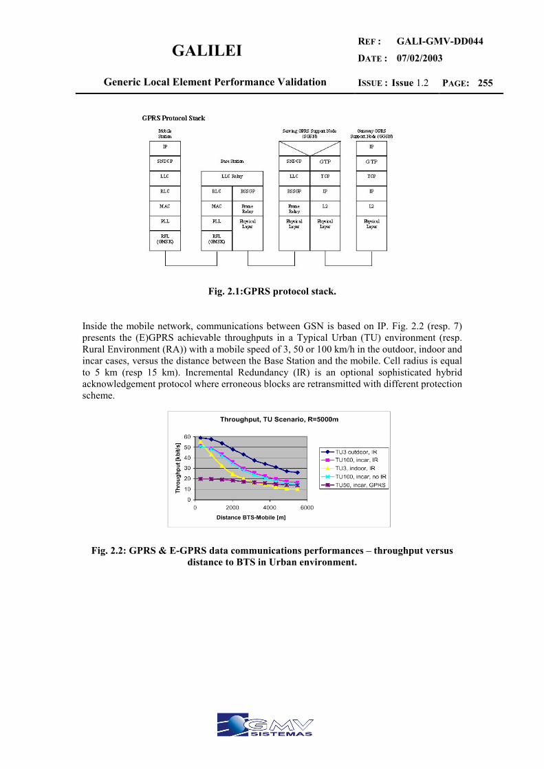
GALILEI REF :
DATE :
GALI-GMV-DD044
07/02/2003
Generic Local Element Performance Validation ISSUE : Issue 1.2 PAGE: 255
Fig. 2.1:GPRS protocol stack.
Inside the mobile network, communications between GSN is based on IP. Fig. 2.2 (resp. 7) presents the (E)GPRS achievable throughputs in a Typical Urban (TU) environment (resp. Rural Environment (RA)) with a mobile speed of 3, 50 or 100 km/h in the outdoor, indoor and incar cases, versus the distance between the Base Station and the mobile. Cell radius is equal to 5 km (resp 15 km). Incremental Redundancy (IR) is an optional sophisticated hybrid acknowledgement protocol where erroneous blocks are retransmitted with different protection scheme.
Fig. 2.2: GPRS & E-GPRS data communications performances – throughput versus distance to BTS in Urban environment.

GALILEI REF :
DATE :
GALI-GMV-DD044
07/02/2003
Generic Local Element Performance Validation ISSUE : Issue 1.2 PAGE: 256
Fig. 2.3: GPRS & E-GPRS data communications performances – throughput versus distance to BTS in Rural environment.
In the Urban case, GPRS enables a data throughput superior to 10 kbps on one physical channel, which makes a throughput of 30 to 40 kbps when using 3 or 4 physical channel per user (packet mode). E-GPRS throughput on one physical channel ranges from 60 kbps (mobile closed to the antenna) to around 20 kbps (mobile at the boundary of the cell). As in GPRS, one user total useful throughput can be increased by multiplying the number of used physical channels. Typical Mobile Stations have the ability to receive four physical channels in parallel.

GALILEI REF :
DATE :
GALI-GMV-DD044
07/02/2003
Generic Local Element Performance Validation ISSUE : Issue 1.2 PAGE: 257
3 3G – UMTS
Universal Mobile Telecommunications System (UMTS) is envisioned as the successor to Global System for Mobile Communications (GSM). UMTS signals the move into the third generation (3G) of mobile networks [4]. UMTS also addresses the growing demand of mobile and Internet applications for new capacity in the overcrowded mobile communications sky. The new network increases transmission speed to 2 Mbps per mobile user and establishes a global roaming standard.
UMTS provides both voice and bi-directional data communication. Speech service maximal throughput is 12.2 kbps. Different data services require different useful throughput and different block error rate (BLER). Contrary to GSM, GPRS and E-GPRS, UMTS is an interference limited system: performance mainly depend on the number of users in the cell, their useful throughputs and the Base Station power. In opposition with TDMA systems, UMTS performances for one user (for a given configuration) does not really depend on the position of this user in the cell. Each user which is actually served by one Node-B receives almost the same quality thanks to sophisticated power control algorithm. Following Table 3.1 and Table 3.2 present system simulation results giving UMTS capacity in a Dense Urban Environment (resp Rural Environment) with a sector area of 0.08 km2 (resp 4 km2), for different types of service (voice, real time data, non real time data) with different throughput and required block error rate. Uplink and Downlink transmission are presented. In those tables, all the users are assumed to use the same service (throughput, BLER) with an activity factor of 100%.
Table 3.1: UMTS capacity in a dense urban environment9.
9 *-Simulation results not available
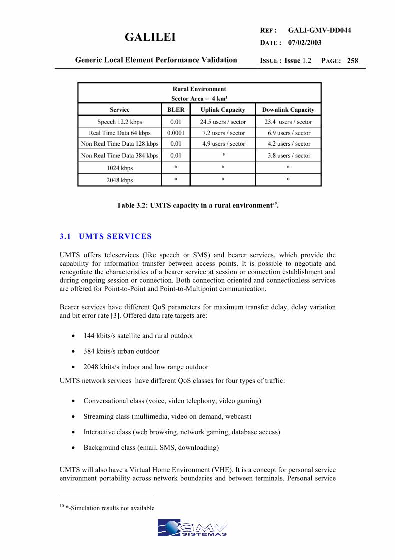
GALILEI REF :
DATE :
GALI-GMV-DD044
07/02/2003
Generic Local Element Performance Validation ISSUE : Issue 1.2 PAGE: 258
Table 3.2: UMTS capacity in a rural environment10.
3.1 UMTS SERVICES
UMTS offers teleservices (like speech or SMS) and bearer services, which provide the capability for information transfer between access points. It is possible to negotiate and renegotiate the characteristics of a bearer service at session or connection establishment and during ongoing session or connection. Both connection oriented and connectionless services are offered for Point-to-Point and Point-to-Multipoint communication.
Bearer services have different QoS parameters for maximum transfer delay, delay variation and bit error rate [3]. Offered data rate targets are:
• 144 kbits/s satellite and rural outdoor
• 384 kbits/s urban outdoor
• 2048 kbits/s indoor and low range outdoor
UMTS network services have different QoS classes for four types of traffic:
• Conversational class (voice, video telephony, video gaming)
• Streaming class (multimedia, video on demand, webcast)
• Interactive class (web browsing, network gaming, database access)
• Background class (email, SMS, downloading)
UMTS will also have a Virtual Home Environment (VHE). It is a concept for personal service environment portability across network boundaries and between terminals. Personal service
10 *-Simulation results not available
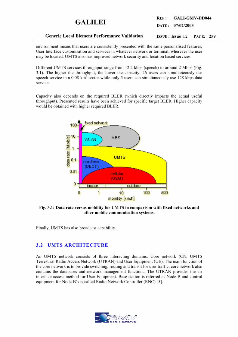
GALILEI REF :
DATE :
GALI-GMV-DD044
07/02/2003
Generic Local Element Performance Validation ISSUE : Issue 1.2 PAGE: 259
environment means that users are consistently presented with the same personalised features, User Interface customisation and services in whatever network or terminal, wherever the user may be located. UMTS also has improved network security and location based services.
Different UMTS services throughput range from 12.2 kbps (speech) to around 2 Mbps (Fig. 3.1). The higher the throughput, the lower the capacity: 26 users can simultaneously use speech service in a 0.08 km2 sector while only 5 users can simultaneously use 128 kbps data service. Capacity also depends on the required BLER (which directly impacts the actual useful throughput). Presented results have been achieved for specific target BLER. Higher capacity would be obtained with higher required BLER.
Fig. 3.1: Data rate versus mobility for UMTS in comparison with fixed networks and other mobile communication systems.
Finally, UMTS has also broadcast capability.
3.2 UMTS ARCHITECTURE
An UMTS network consists of three interacting domains: Core network (CN, UMTS Terrestrial Radio Access Network (UTRAN) and User Equipment (UE). The main function of the core network is to provide switching, routing and transit for user traffic; core network also contains the databases and network management functions. The UTRAN provides the air interface access method for User Equipment. Base station is referred as Node-B and control equipment for Node-B’s is called Radio Network Controller (RNC) [5].
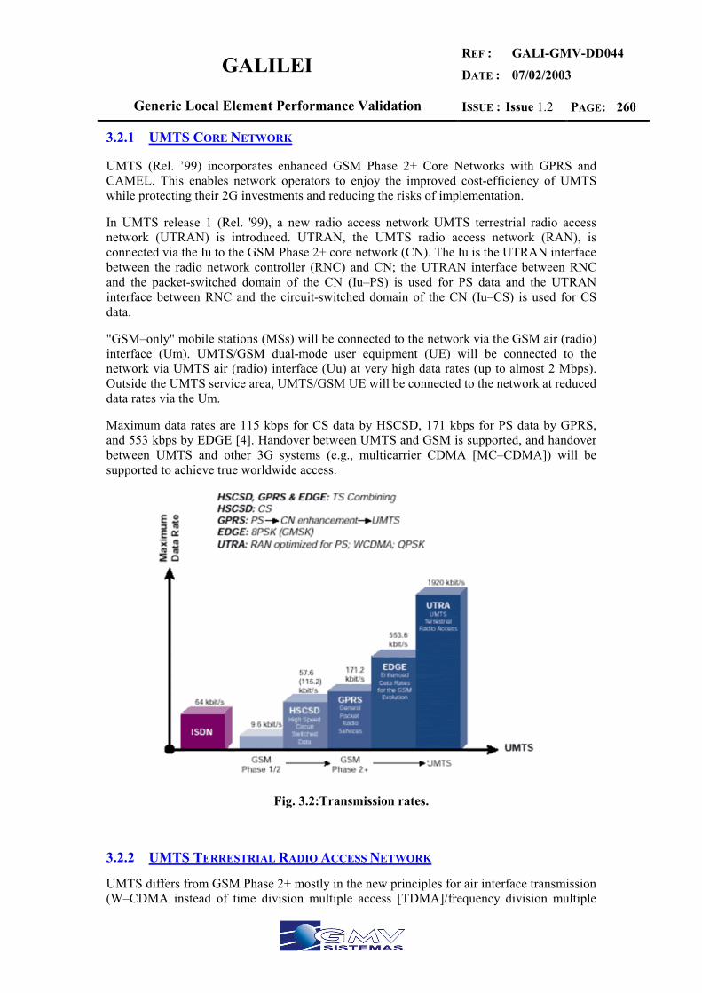
GALILEI REF :
DATE :
GALI-GMV-DD044
07/02/2003
Generic Local Element Performance Validation ISSUE : Issue 1.2 PAGE: 260
3.2.1 UMTS CORE NETWORK
UMTS (Rel. ’99) incorporates enhanced GSM Phase 2+ Core Networks with GPRS and CAMEL. This enables network operators to enjoy the improved cost-efficiency of UMTS while protecting their 2G investments and reducing the risks of implementation.
In UMTS release 1 (Rel. '99), a new radio access network UMTS terrestrial radio access network (UTRAN) is introduced. UTRAN, the UMTS radio access network (RAN), is connected via the Iu to the GSM Phase 2+ core network (CN). The Iu is the UTRAN interface between the radio network controller (RNC) and CN; the UTRAN interface between RNC and the packet-switched domain of the CN (Iu–PS) is used for PS data and the UTRAN interface between RNC and the circuit-switched domain of the CN (Iu–CS) is used for CS data.
"GSM–only" mobile stations (MSs) will be connected to the network via the GSM air (radio) interface (Um). UMTS/GSM dual-mode user equipment (UE) will be connected to the network via UMTS air (radio) interface (Uu) at very high data rates (up to almost 2 Mbps). Outside the UMTS service area, UMTS/GSM UE will be connected to the network at reduced data rates via the Um.
Maximum data rates are 115 kbps for CS data by HSCSD, 171 kbps for PS data by GPRS, and 553 kbps by EDGE [4]. Handover between UMTS and GSM is supported, and handover between UMTS and other 3G systems (e.g., multicarrier CDMA [MC–CDMA]) will be supported to achieve true worldwide access.
Fig. 3.2:Transmission rates.
3.2.2 UMTS TERRESTRIAL RADIO ACCESS NETWORK
UMTS differs from GSM Phase 2+ mostly in the new principles for air interface transmission (W–CDMA instead of time division multiple access [TDMA]/frequency division multiple
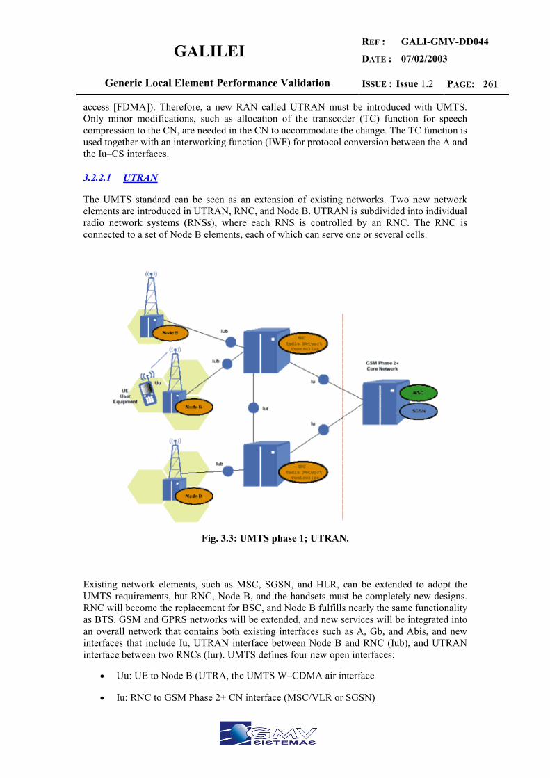
GALILEI REF :
DATE :
GALI-GMV-DD044
07/02/2003
Generic Local Element Performance Validation ISSUE : Issue 1.2 PAGE: 261
access [FDMA]). Therefore, a new RAN called UTRAN must be introduced with UMTS. Only minor modifications, such as allocation of the transcoder (TC) function for speech compression to the CN, are needed in the CN to accommodate the change. The TC function is used together with an interworking function (IWF) for protocol conversion between the A and the Iu–CS interfaces.
3.2.2.1 UTRAN
The UMTS standard can be seen as an extension of existing networks. Two new network elements are introduced in UTRAN, RNC, and Node B. UTRAN is subdivided into individual radio network systems (RNSs), where each RNS is controlled by an RNC. The RNC is connected to a set of Node B elements, each of which can serve one or several cells.
Fig. 3.3: UMTS phase 1; UTRAN.
Existing network elements, such as MSC, SGSN, and HLR, can be extended to adopt the UMTS requirements, but RNC, Node B, and the handsets must be completely new designs. RNC will become the replacement for BSC, and Node B fulfills nearly the same functionality as BTS. GSM and GPRS networks will be extended, and new services will be integrated into an overall network that contains both existing interfaces such as A, Gb, and Abis, and new interfaces that include Iu, UTRAN interface between Node B and RNC (Iub), and UTRAN interface between two RNCs (Iur). UMTS defines four new open interfaces:
• Uu: UE to Node B (UTRA, the UMTS W–CDMA air interface
• Iu: RNC to GSM Phase 2+ CN interface (MSC/VLR or SGSN)
GALILEI REF :
DATE :
GALI-GMV-DD044
07/02/2003
Generic Local Element Performance Validation ISSUE : Issue 1.2 PAGE: 262
o Iu-CS for circuit-switched data
o Iu-PS for packet-switched data
• Iub: RNC to Node B interface
• Iur: RNC to RNC interface, not comparable to any interface in GSM
The Iu, Iub, and Iur interfaces are based on ATM transmission principles. ATM Adaptation Layer type 2 (AAL2) handles circuit switched connection and packet connection protocol AAL5 is designed for data delivery.
3.2.2.2 RNC Functions
The RNC enables autonomous radio resource management (RRM) by UTRAN. It performs the same functions as the GSM BSC, providing central control for the RNS elements (RNC and Node Bs).
The RNC handles protocol exchanges between Iu, Iur, and Iub interfaces and is responsible for centralized operation and maintenance (O&M) of the entire RNS with access to the OSS. Because the interfaces are ATM–based, the RNC switches ATM cells between them. The user’s circuit-switched and packet-switched data coming from Iu–CS and Iu–PS interfaces are multiplexed together for multimedia transmission via Iur, Iub, and Uu interfaces to and from the UE.
The RNC uses the Iur interface, which has no equivalent in GSM BSS, to autonomously handle 100 percent of the RRM, eliminating that burden from the CN. Serving control functions such as admission, RRC connection to the UE, congestion and handover/macro diversity are managed entirely by a single serving RNC (SRNC).
If another RNC is involved in the active connection through an inter–RNC soft handover, it is declared a drift RNC (DRNC). The DRNC is only responsible for the allocation of code resources. A reallocation of the SRNC functionality to the former DRNC is possible (serving radio network subsystem [SRNS] relocation). The term controlling RNC (CRNC) is used to define the RNC that controls the logical resources of its UTRAN access points.
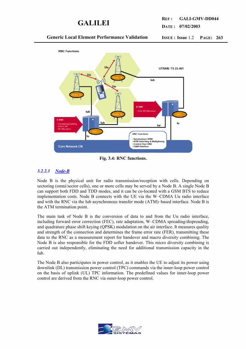
GALILEI REF :
DATE :
GALI-GMV-DD044
07/02/2003
Generic Local Element Performance Validation ISSUE : Issue 1.2 PAGE: 263
Fig. 3.4: RNC functions.
3.2.2.3 Node-B
Node B is the physical unit for radio transmission/reception with cells. Depending on sectoring (omni/sector cells), one or more cells may be served by a Node B. A single Node B can support both FDD and TDD modes, and it can be co-located with a GSM BTS to reduce implementation costs. Node B connects with the UE via the W–CDMA Uu radio interface and with the RNC via the Iub asynchronous transfer mode (ATM)–based interface. Node B is the ATM termination point.
The main task of Node B is the conversion of data to and from the Uu radio interface, including forward error correction (FEC), rate adaptation, W–CDMA spreading/dispreading, and quadrature phase shift keying (QPSK) modulation on the air interface. It measures quality and strength of the connection and determines the frame error rate (FER), transmitting these data to the RNC as a measurement report for handover and macro diversity combining. The Node B is also responsible for the FDD softer handover. This micro diversity combining is carried out independently, eliminating the need for additional transmission capacity in the Iub.
The Node B also participates in power control, as it enables the UE to adjust its power using downlink (DL) transmission power control (TPC) commands via the inner-loop power control on the basis of uplink (UL) TPC information. The predefined values for inner-loop power control are derived from the RNC via outer-loop power control.
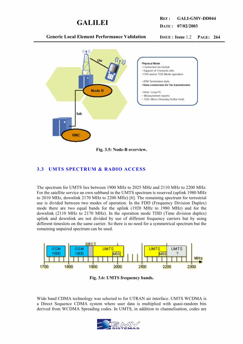
GALILEI REF :
DATE :
GALI-GMV-DD044
07/02/2003
Generic Local Element Performance Validation ISSUE : Issue 1.2 PAGE: 264
Fig. 3.5: Node-B overview.
3.3 UMTS SPECTRUM & RADIO ACCESS
The spectrum for UMTS lies between 1900 MHz to 2025 MHz and 2110 MHz to 2200 MHz. For the satellite service an own subband in the UMTS spectrum is reserved (uplink 1980 MHz to 2010 MHz, downlink 2170 MHz to 2200 MHz) [6]. The remaining spectrum for terrestrial use is divided between two modes of operation. In the FDD (Frequency Division Duplex) mode there are two equal bands for the uplink (1920 MHz to 1980 MHz) and for the downlink (2110 MHz to 2170 MHz). In the operation mode TDD (Time division duplex) uplink and downlink are not divided by use of different frequency carriers but by using different timeslots on the same carrier. So there is no need for a symmetrical spectrum but the remaining unpaired spectrum can be used.
Fig. 3.6: UMTS frequency bands.
Wide band CDMA technology was selected to for UTRAN air interface. UMTS WCDMA is a Direct Sequence CDMA system where user data is multiplied with quasi-random bits derived from WCDMA Spreading codes. In UMTS, in addition to channelisation, codes are
GALILEI REF :
DATE :
GALI-GMV-DD044
07/02/2003
Generic Local Element Performance Validation ISSUE : Issue 1.2 PAGE: 265
used for synchronisation and scrambling. WCDMA has two basic modes of operation: Frequency Division Duplex (FDD) and Time Division Duplex (TDD) [5]. One of the main advantages of CDMA systems is the capability of using signals that arrive in the receivers with different time delays. This phenomenon is called multipath. FDMA and TDMA, which are narrow band systems, cannot discriminate between the multipath arrivals, and resort to equalization to mitigate the negative effects of multipath. Due to its wide bandwidth and rake receivers, CDMA uses the multipath signals and combines them to make an even stronger signal at the receivers. CDMA subscriber units use rake receivers. This is essentially a set of several receivers. One of the receivers (fingers) constantly searches for different multipaths and feeds the information to the other three fingers. Each finger then demodulates the signal corresponding to a strong multipath. The results are then combined together to make the signal stronger.
GALILEI REF :
DATE :
GALI-GMV-DD044
07/02/2003
Generic Local Element Performance Validation ISSUE : Issue 1.2 PAGE: 266
4 TETRA
4.1 OVERVIEW
TErrestrial Trunked RAdio (TETRA) is the modern digital Private Mobile Radio (PMR) and Public Access Mobile Radio (PAMR) technology for police, ambulance and fire services, security services, utilities, military, public access, fleet management, transport services, closed user groups, factory site services, mining, etc [8].
With support of the European Commission and the ETSI members, the TETRA standard has been developed over a number of years by the co-operation of manufacturers, users, operators and other experts, with emphasis on ensuring the standard will support the needs of emergency services throughout Europe and beyond. The standard builds upon the lessons and techniques of previous analogue Trunked radio systems and the successful development of GSM during the 1980s. The work started in 1990 and the first standards were ready in 1995.
TETRA offers fast call set-up time, addressing the critical needs of many user segments, excellent group communication support, Direct mode operation between radios, packet data and circuit data transfer services, frequency economy and excellent security features. TETRA uses Time Division Multiple Access (TDMA) technology with 4 user channels on one radio carrier and 25 kHz spacing between carriers. This makes it inherently efficient in the way that it uses the frequency spectrum. For emergency systems in Europe the frequency bands 380-383 MHz and 390-393 MHz have been allocated for use by a single harmonized digital land mobile systems by the ERC Decision (96)01. Additionally, whole or appropriate parts of the bands 383-395 MHz and 393-395 MHz can be utilized should the bandwidth be required.
For civil systems in Europe the frequency bands 410-430 MHz, 870-876 MHz / 915-921 MHz, 450-470 MHz, 385-390 MHz / 395-399,9 MHz, have been allocated for TETRA by the ERC Decision (96)04.
TETRA trunking facility provides a pooling of all radio channels which are then allocated on demand to individual users, in both voice and data modes. By the provision of national and multi-national networks, national and international roaming can be supported, the user being in constant seamless communications with his colleagues. TETRA supports point-to-point, and point-to-multipoint bidirectional communications for single cell (with cell diameters up to 50 km) both by the use of the TETRA infrastructure and by the use of Direct Mode without infrastructure.
TETRAPOL is a digital mobile radio platform developed by MATRA-NORTEL Communications. It is aimed purely to the public safety and utilities sector of the market. It has not been approved by ETSI that feels that Europe only needs one standard for digital trunked mobile radio [7]. Both packet-switched and circuit-switched services are supported; the choice among the two is made in relation with final application. A utility company that uses data for meter readings, for instance, will use packet switched transmission with low bit rates, while police users need circuit switched transmission with higher bit rates.
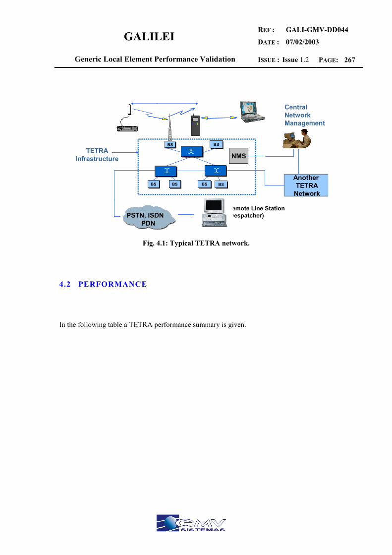
GALILEI REF :
DATE :
GALI-GMV-DD044
07/02/2003
Generic Local Element Performance Validation ISSUE : Issue 1.2 PAGE: 267
Fig. 4.1: Typical TETRA network.
4.2 PERFORMANCE
In the following table a TETRA performance summary is given.
TETRAInfrastructure
.
Remote Line Station (Despatcher)
BSBS BSBS
BSBS BSBS BSBSBSBSAnother TETRA
Network
NMS
CentralNetworkManagement
PSTN, ISDNPDN

GALILEI REF :
DATE :
GALI-GMV-DD044
07/02/2003
Generic Local Element Performance Validation ISSUE : Issue 1.2 PAGE: 268
Transfer mode
Circuit switched data (28.8 Kbit/sec max bit rate) Circuit switched protected data (18.2 Kbit/sec max bit rate) Circuit switched strongly protected data (9.6 Kbit/sec) Connection oriented packet switched data Connectionless packet switched data
Multiple Access TDMA Modulation П/4 DQPSK
Frequency Band 150 MHz-900 MHz (Europe) Carrier spacing 25 KHz 4 channels per carrier
Bit Rate
Max data transfer rate 28.8 Kbit/sec Video images can be transmitted at 19.2 Kbit/sec Transmission speeds can vary and can be set according to the specific needs
Latency Time Real time Call set-up time: 300 msec
Coverage Local Urban and suburban areas with low to medium user densities and cell sizes of tens of kilometres (large cells)
Services
Full duplex person-to-person, group calls (with or without ACK) Broadcast calls within the TETRA network Calls to any fixed or mobile phone via the PSTN interface Terminals can communicate with each other on an one-to-one basis independent of the TETRA infrastructure IP-based packet data User-originated text messaging Direct Mode: allows direct operation between terminals without use of trunking infrastructure
Applications Voice and data communications organizations that need access to voice and data services also when out of touch with the infrastructure
Table 4.1: TETRA performance summary.
4.3 FUTURE DEVELOPMENTS
TETRA standardization has reached a mature state. The major future developments are the continuation, by standardizing the next generation in TETRA Release 2 and by the maintenance of existing TETRA standards.
GALILEI REF :
DATE :
GALI-GMV-DD044
07/02/2003
Generic Local Element Performance Validation ISSUE : Issue 1.2 PAGE: 269
The objective of TETRA Release 2 is that EP TETRA produces an additional set of ETSI deliverables (and maintenance thereafter) in order to enhance TETRA in accordance with the following requirements:
a) Evolution of TETRA to provide packet data at much higher speeds than are available in the current standard. This is to support multimedia and other high speed data applications required by existing and future TETRA users.
b) Selection and standardisation of additional speech codec(s) for TETRA, to enable intercommunication between TETRA and other 3G networks without transcoding, and to provide enhanced voice quality for TETRA by using the latest low bit rate voice codec technology.
c) Further enhancements of the TETRA air interface standard in order to provide increased benefits and optimisation in terms of spectrum efficiency, network capacity, system performance, quality of service, size and cost of terminals, battery life, and other relevant parameters.
d) Production and/or adoption of standards to provide improved interworking and roaming between TETRA and public mobile networks such as GSM, GPRS and UMTS.
e) Evolution of the TETRA SIM, with the aim of convergence with USIM, to meet the needs for TETRA specific services whilst gaining the benefits of interworking and roaming with public mobile networks such as GSM, GPRS and UMTS.
f) Extension of the operating range of TETRA, to provide increased coverage and low cost deployments for applications such as airborne public safety, maritime, rural telephony and ’linear utilities’ (eg pipelines).
g) Provision of new ETSI deliverables in order to support further user/market driven requirements that may be identified during study work in the early stages of the work programme.
h) Ensure full backward compatibility and integration of the new services with existing TETRA standards, in order to future proof existing and future investments by TETRA users.
These requirements are in addition to the user requirements for PMR/PAMR that are already satisfied by existing TETRA standards. The work will include completion and formal approval of outstanding work related to these existing requirements. The work will build upon the unique combination of services and facilities already included within existing TETRA
4.4 CRITICAL ENVIRONMENTS
TETRA radio signal coming from the outside can be seriously attenuated (e.g. 60 dB) in deep fading indoor, subways or similar scenarios. New enhancements proposed for TETRA standards include frequency hoping that could give further immunity in indoor environments. Also, auxiliary relay stations and radiating cable could be necessary locally in critical environments as mentioned above.

GALILEI REF :
DATE :
GALI-GMV-DD044
07/02/2003
Generic Local Element Performance Validation ISSUE : Issue 1.2 PAGE: 270
5 RDS
5.1 OVERVIEW
The RDS (Radio Data System) is a data broadcast system for FM stations that opens conventional FM receivers a new range of features like programme identification, alternative frequency list, programme type identification, traffic announcement signal, etc. The RDS was specified by the EBU (European Broadcasting Union) in 1984, and adopted by the CENELEC as a European standard in 1990, having been adopted by most European FM stations. In the USA, a slightly different specification, called RBDS, has also been deployed [9]. The developers aimed at making radio receivers very user-friendly, especially car radios when these are used where a transmitter network with a number of alternative frequencies (AF) are present. In addition listeners should be enabled to see the programme service name (PS) on an eight character alpha-numerical display and the transmitter frequency information, displayed on non-RDS radios, is then only used, in the background, by an RDS radio. All this has become possible by the using, for many years, microprocessor controlled PLL tuner technology, permitting a radio to be retuned within milliseconds. During this process the audio signal is muted which because of the short time is usually not detected by the ear. Thus, the radio is able to choose the transmitter frequency, among a number of alternatives, that gives the best quality reception. It is also sure that the switch-over is made to exactly the same programme service by performing a kind of identity check using the programme identity (PI) code. Travel information with RDS is possible using the Travel Programme (TP) and Travel Announcement (TA) flags. Information is broadcast for motorists, identified in parallel with the ARI system with the corresponding RDS features TP/TA. But ARI is being replaced on a European scale, so it will cease after the year 2005. A more recent development of RDS is the digitally coded Traffic Message Channel (TMC) which is now planned to be introduced all over Europe, within projects funded by the European Union. However, present RDS radios are not yet suitable for RDS-TMC. A new revision of the RDS specification released on 1997, increased the potential applications supported by RDS systems. Among these new applications, Differential GPS correction data services (DGPS) allow distributing in real-time correction information of the GPS signals received locally. These corrections are computed by reference stations and distributed to final users using RDS broadcasting stations. With this system, current deployments in some European regions and countries allow to improve locally GPS positioning with accuracy better than 10 m. Differential data is broadcast using RTCM format, accepted by most commercial GPS receivers, allowing a direct integration with OEM RDS receivers. RDS is absolutely future proof and will not be replaced by DAB, at least until such time as when FM broadcasting ceases to exist and this, for sure, is not going to happen within the next 20 years, in spite of the breathtaking developments of the new era of digital broadcasting.
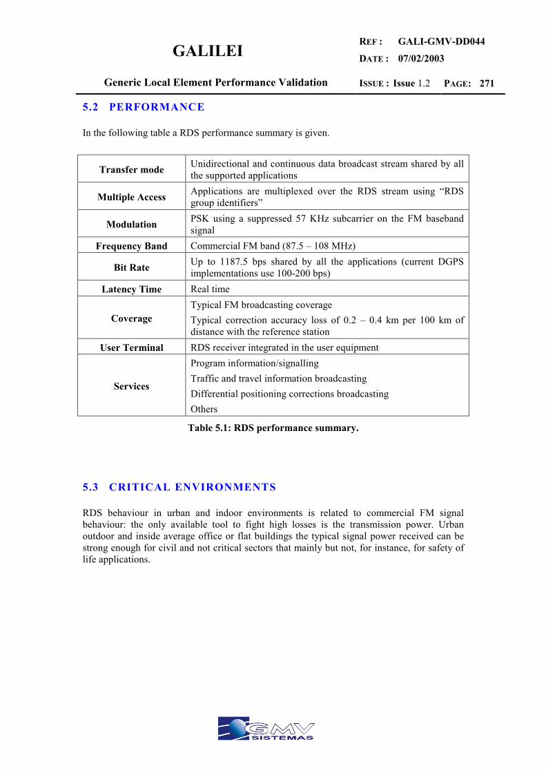
GALILEI REF :
DATE :
GALI-GMV-DD044
07/02/2003
Generic Local Element Performance Validation ISSUE : Issue 1.2 PAGE: 271
5.2 PERFORMANCE
In the following table a RDS performance summary is given.
Transfer mode Unidirectional and continuous data broadcast stream shared by all the supported applications
Multiple Access Applications are multiplexed over the RDS stream using “RDS group identifiers”
Modulation PSK using a suppressed 57 KHz subcarrier on the FM baseband signal
Frequency Band Commercial FM band (87.5 – 108 MHz)
Bit Rate Up to 1187.5 bps shared by all the applications (current DGPS implementations use 100-200 bps)
Latency Time Real time
Coverage Typical FM broadcasting coverage Typical correction accuracy loss of 0.2 – 0.4 km per 100 km of distance with the reference station
User Terminal RDS receiver integrated in the user equipment
Services
Program information/signalling Traffic and travel information broadcasting Differential positioning corrections broadcasting Others
Table 5.1: RDS performance summary.
5.3 CRITICAL ENVIRONMENTS
RDS behaviour in urban and indoor environments is related to commercial FM signal behaviour: the only available tool to fight high losses is the transmission power. Urban outdoor and inside average office or flat buildings the typical signal power received can be strong enough for civil and not critical sectors that mainly but not, for instance, for safety of life applications.

GALILEI REF :
DATE :
GALI-GMV-DD044
07/02/2003
Generic Local Element Performance Validation ISSUE : Issue 1.2 PAGE: 272
6 DAB AND DRM
6.1 OVERVIEW
Digital Audio Broadcasting, DAB, is the most fundamental advance in radio technology since the introduction of FM Stereo radio. It gives listeners interference free reception or high-quality sound, easy to use receivers, and an unlimited potential for wider listening through many additional stations, services and developments [10]. DAB is broadcast on terrestrial networks, with prospects for Satellite broadcasting in the future. You are able to receive the terrestrial Digital Audio Broadcasting programs using solely a tiny non-directional stub antenna. You can receive CD-like quality radio programmes even in the car without any annoying interference and signal distortion. DAB radio is designed for the multimedia age: DAB can carry not only audio, but also text pictures, data and even videos. In short, DAB fully complies with the tough requirements of the Digital Age, which is emerging before us. Apart from receiving audio entertainment via the radio, programmes can also be accompanied by text, such as Lyrics. Weather forecasts can be accompanied by a satellite map of the area you are in and of course there is a facility to determine very precisely where you are. Just imagine, no more map-reading for the co-pilot! Emergency Vehicles will be able to find their way to a fire or an accident, immediately, because the transmitted maps are regularly updated, displaying traffic-jams and road works and can therefore suggest diversion routes. Other travel, traffic or transportation information is accessible to a DAB listener, in terms of car parking or even bus and train schedules. It is possible to receive business news, stock exchange rates and even fax messages on the road. Apart from all this, Tourist/City Information, File Transfer/Software download are also possible with DAB radio. Digital Audio Broadcasting (DAB) has been the first digital terrestrial broadcast technology introduced in Europe with the purpose to replace in some future current analogue FM technology. It has been standardised by the ITU in 1994 for terrestrial and satellite broadcasting and it is an European standard adopted by the ETSI in 1997. Similarly, the Digital Radio Mondiale (DRM) specification has been developed to replace analogue AM technologies using frequency bands below 30 MHz. The DAB is a highly spectrum and power efficient broadcast system thanks to:
• MPEG-1 and MPEG-2 audio compression techniques
• Coding redundancy to provide error protection
• Information spreading over time and frequency domains improving behaviour in front of fading and multipath propagation
• Single Frequency Network allowing frequency reuse in adjacent broadcasting stations of the same network.
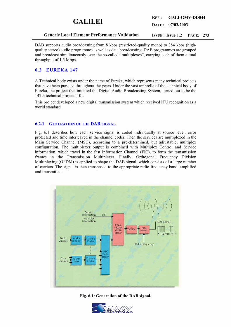
GALILEI REF :
DATE :
GALI-GMV-DD044
07/02/2003
Generic Local Element Performance Validation ISSUE : Issue 1.2 PAGE: 273
DAB supports audio broadcasting from 8 kbps (restricted-quality mono) to 384 kbps (high-quality stereo) audio programmes as well as data broadcasting. DAB programmes are grouped and broadcast simultaneously over the so-called “multiplexes”, carrying each of them a total throughput of 1.5 Mbps.
6.2 EUREKA 147
A Technical body exists under the name of Eureka, which represents many technical projects that have been pursued throughout the years. Under the vast umbrella of the technical body of Eureka, the project that initiated the Digital Audio Broadcasting System, turned out to be the 147th technical project [10]. This project developed a new digital transmission system which received ITU recognition as a world standard.
6.2.1 GENERATION OF THE DAB SIGNAL
Fig. 6.1 describes how each service signal is coded individually at source level, error protected and time interleaved in the channel coder. Then the services are multiplexed in the Main Service Channel (MSC), according to a pre-determined, but adjustable, multiplex configuration. The multiplexer output is combined with Multiplex Control and Service information, which travel in the fast Information Channel (FIC), to form the transmission frames in the Transmission Multiplexer. Finally, Orthogonal Frequency Division Multiplexing (OFDM) is applied to shape the DAB signal, which consists of a large number of carriers. The signal is then transposed to the appropriate radio frequency band, amplified and transmitted.
Fig. 6.1: Generation of the DAB signal.

GALILEI REF :
DATE :
GALI-GMV-DD044
07/02/2003
Generic Local Element Performance Validation ISSUE : Issue 1.2 PAGE: 274
6.3 CRITICAL ENVIRONMENTS
DAB and DRM suffer from similar problems as RDS in urban canyon and indoor environments. Nevertheless, DAB and DRM have a much better behaviour in front of multipath propagation thanks to OFDM modulation and coding protection. This mainly improves its performance in urban environments and inside buildings but the same criteria applies when subway or similar strong attenuation environments: auxiliary relay stations are required if local coverage inside a certain e.g. subway station is desired.

GALILEI REF :
DATE :
GALI-GMV-DD044
07/02/2003
Generic Local Element Performance Validation ISSUE : Issue 1.2 PAGE: 275
7 DECT
7.1 OVERVIEW
DECT (Digital Enhanced Cordless Telecommunications) is a flexible digital radio access technology for cordless communications in residential, business and public environments [11]. Designed for short-range use as an access mechanism to the main networks, DECT offers cordless voice, fax, high speed data and multimedia communications, wireless local area networks and wireless PBX. It is a high capacity digital technology for cell radii ranging from 25-50 meters (indoor mobile use) to 250 meters (outdoor mobile use) and up to 15 km for fixed wireless use. Mobile coverage is not guaranteed over 45 km/h relative velocity [12]. It thus has applications in the factory, office, home and public areas. For network operators DECT is also a cost-effective and flexible alternative to conventional cable/fibre connections into customers' premises, by providing "Wireless Local Loop". Frequency bands have been made available for DECT in more than 100 countries worldwide. DECT services are compatible with GSM and ISDN and dual-mode DECT/GSM handsets are available. In a large number of countries DECT operates in a protected band, i.e. no interference from other technologies. ETSI DECT is one of the technologies the IMT-2000 specification. The ETSI Project DECT is responsible for the development and maintenance of standards on this technology. All DECT systems are based on a main standard that is the Common Interface (CI), which is often used in association with the Generic Access Profile (GAP). Built upon these base standards are a large number of Type Approval, Testing, Interworking and Data Services specifications produced up to now. A recent important step for the development of DECT data application was the achievement of DECT Packet Radio Service (DPRS) introducing the flexibility and resources optimisation of packet technology, opening the field to further developments in terms of speed and profiles. The Project responds to the growing demand for the support of data services and the continuous desire to increase available data rates by adding high bit rate modes to DECT, current support of data applications up to more than 2 Mbit/s. Work on the third version of DPRS is ongoing. This supports the transmission of broadband data up to more than 10 Mbit/s. In addition to this basic DPRS standards, a group of standards called Application Specific Access Profiles (ASAPs) has been also created. These are industry-driven standards intended to enhance interoperability. Each of them identifies a specific application scenario and selects a specific subset of DPRS services plus a voice service for particular applications. DMAP (DECT Multimedia Access Profile), developed for residential/SOHO applications, allows design of low-cost domestic devices for local data interconnection and Internet connection via PSTN/ISDN. DECT standards can be reused in a general spectrum allocation band, and provide technical requirements to be applied for DECT approval in countries outside Europe which have a different spectrum allocation for DECT. A standard was created specifically for the use of the DECT radio access technology in the 2,45 GHz ISM Band.
GALILEI REF :
DATE :
GALI-GMV-DD044
07/02/2003
Generic Local Element Performance Validation ISSUE : Issue 1.2 PAGE: 276
DECT supports also mobile internet technology, specifying the additional requirements for DECT IP applications
7.2 RADIO ACCESS
DECT use two possible transfer modes: circuit-switched and packet-switched, using MS-TDMA technology for multiple access (24 timeslots/frame on each of the 10 carriers) and GPSK modulation.. DECT frequency band is free-of-charge, using 10 carriers with 1,728 MHz spacing in 1880 MHZ, 1900 MHZ and 3,5 GHz. This technology guarantees high-quality speech; DECT bit rate is 32 Kbit/sec ADPCM with echo control, but up to V.90 Kbit/sec is possible in more recent developments. In the near future DPRS will support data applications up to more than 2 Mbit/sec.
7.3 CRITICAL ENVIRONMENTS
Since designed for home, office and urban environments DECT is able to provide services at nominal performance if adequate considerations are taken into account during system deployment (more strong requirements will require a more detailed study of local propagation behaviour case by case). The most important restriction of DECT technology is the limited mobility between terminals and base stations (i.e. 45 km/h). For quasi stationary users moving at below 45 km/h the Doppler effect and multipath propagation can degrade the performance of the radio link. To reduce this effect, DECT can take advantage of apace and frequency diversity mechanisms. Using two or more antenna combined at distance about half of the wavelength inside the terminal, the impact can be compensated and link performance improved. Furthermore, in multicell systems space diversity is alternatively supported by means intercell handover. Finally, frequency diversity is implemented using dynamic carrier selection. These two last diversity mechanisms also give protection in the case the user enters in a fading dip while moving. For stationary users in urban outdoor environment, amplitude, phase and arrival angle of beams (the principal and all the reflected) are constant, this produces fading that distorts signal amplitude and phase. To mitigate this effect, space and frequency diversity are also used.
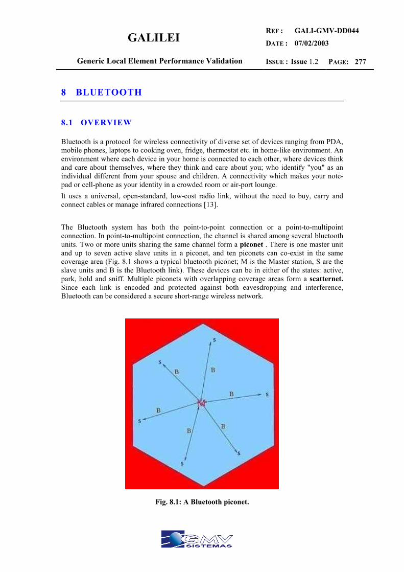
GALILEI REF :
DATE :
GALI-GMV-DD044
07/02/2003
Generic Local Element Performance Validation ISSUE : Issue 1.2 PAGE: 277
8 BLUETOOTH
8.1 OVERVIEW
Bluetooth is a protocol for wireless connectivity of diverse set of devices ranging from PDA, mobile phones, laptops to cooking oven, fridge, thermostat etc. in home-like environment. An environment where each device in your home is connected to each other, where devices think and care about themselves, where they think and care about you; who identify "you" as an individual different from your spouse and children. A connectivity which makes your note-pad or cell-phone as your identity in a crowded room or air-port lounge. It uses a universal, open-standard, low-cost radio link, without the need to buy, carry and connect cables or manage infrared connections [13]. The Bluetooth system has both the point-to-point connection or a point-to-multipoint connection. In point-to-multipoint connection, the channel is shared among several bluetooth units. Two or more units sharing the same channel form a piconet . There is one master unit and up to seven active slave units in a piconet, and ten piconets can co-exist in the same coverage area (Fig. 8.1 shows a typical bluetooth piconet; M is the Master station, S are the slave units and B is the Bluetooth link). These devices can be in either of the states: active, park, hold and sniff. Multiple piconets with overlapping coverage areas form a scatternet. Since each link is encoded and protected against both eavesdropping and interference, Bluetooth can be considered a secure short-range wireless network.
Fig. 8.1: A Bluetooth piconet.
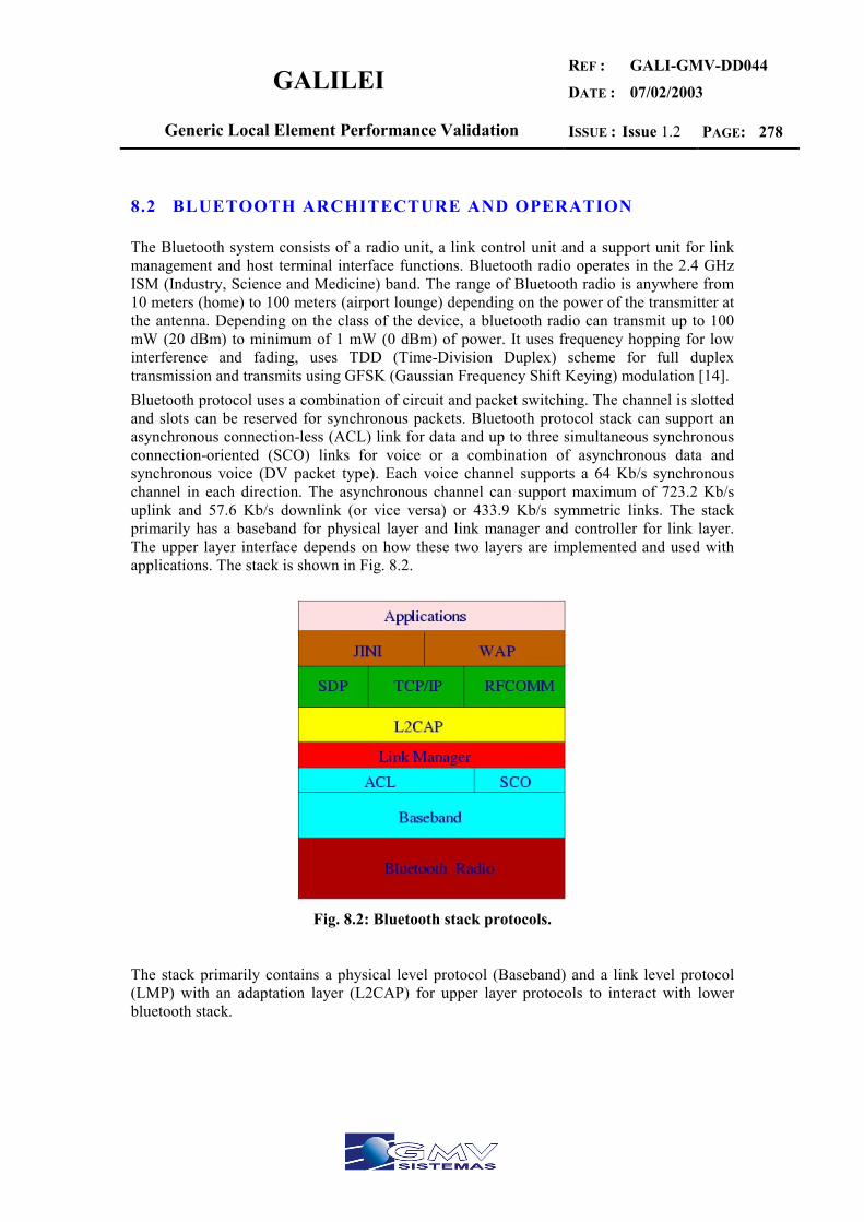
GALILEI REF :
DATE :
GALI-GMV-DD044
07/02/2003
Generic Local Element Performance Validation ISSUE : Issue 1.2 PAGE: 278
8.2 BLUETOOTH ARCHITECTURE AND OPERATION
The Bluetooth system consists of a radio unit, a link control unit and a support unit for link management and host terminal interface functions. Bluetooth radio operates in the 2.4 GHz ISM (Industry, Science and Medicine) band. The range of Bluetooth radio is anywhere from 10 meters (home) to 100 meters (airport lounge) depending on the power of the transmitter at the antenna. Depending on the class of the device, a bluetooth radio can transmit up to 100 mW (20 dBm) to minimum of 1 mW (0 dBm) of power. It uses frequency hopping for low interference and fading, uses TDD (Time-Division Duplex) scheme for full duplex transmission and transmits using GFSK (Gaussian Frequency Shift Keying) modulation [14]. Bluetooth protocol uses a combination of circuit and packet switching. The channel is slotted and slots can be reserved for synchronous packets. Bluetooth protocol stack can support an asynchronous connection-less (ACL) link for data and up to three simultaneous synchronous connection-oriented (SCO) links for voice or a combination of asynchronous data and synchronous voice (DV packet type). Each voice channel supports a 64 Kb/s synchronous channel in each direction. The asynchronous channel can support maximum of 723.2 Kb/s uplink and 57.6 Kb/s downlink (or vice versa) or 433.9 Kb/s symmetric links. The stack primarily has a baseband for physical layer and link manager and controller for link layer. The upper layer interface depends on how these two layers are implemented and used with applications. The stack is shown in Fig. 8.2.
Fig. 8.2: Bluetooth stack protocols.
The stack primarily contains a physical level protocol (Baseband) and a link level protocol (LMP) with an adaptation layer (L2CAP) for upper layer protocols to interact with lower bluetooth stack.
GALILEI REF :
DATE :
GALI-GMV-DD044
07/02/2003
Generic Local Element Performance Validation ISSUE : Issue 1.2 PAGE: 279
8.2.1 BLUETOOTH RADIO
Bluetooth radio is an integral part of a Bluetooth device as it provides an electrical interface for transfer of packets on a modulated carrier frequency using wireless bearer services (CDMA, GSM, DECT). The radio operates in the 2.4 GHz ISM (Industrial Scientific Medicine) band which requires a very small and efficient antenna (smart antenna), a good RF front end (LNA, Up-converter, down-converter) on chip, power controller, GFSK modulator and a transmit/receive switch for it work as a transceiver [14]. In the US and Europe, a band of 83.5 MHz is available; in this band, 79 RF channels spaced 1 MHz apart are defined. Japan, Spain and France use only 23 RF channels spaced 1 MHz apart. The channel is represented by a pseudo-random hopping sequence hopping the 79 or 23 RF channels. The hopping sequence is unique for the piconet and is determined by the Bluetooth device address of the master; the phase in the hopping sequence is determined by the Bluetooth clock of the master. The channel is divided into time slots, each 625 microsec in length, where each slot corresponds to an RF hop frequency. The nominal hop rate is 1600 hops/s. All bluetooth units participating in the piconet are time and hop-synchronized to the channel.
8.3 CRITICAL ENVIRONMENTS
Due to absorption of its signal (f = 2.4 GHz) it cannot penetrate massive concrete walls. Bluetooth can transport voice and data information only within a limited distance of about 10 metres. But in combination with other communication links (e.g. telephone, fax, PC, laptop, Galileo receiver) it is very useful for short distance voice and data exchange and value-adding of information without using cables.
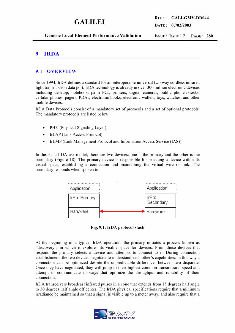
GALILEI REF :
DATE :
GALI-GMV-DD044
07/02/2003
Generic Local Element Performance Validation ISSUE : Issue 1.2 PAGE: 280
9 IRDA
9.1 OVERVIEW
Since 1994, IrDA defines a standard for an interoperable universal two way cordless infrared light transmission data port. IrDA technology is already in over 300 million electronic devices including desktop, notebook, palm PCs, printers, digital cameras, public phones/kiosks, cellular phones, pagers, PDAs, electronic books, electronic wallets, toys, watches, and other mobile devices. IrDA Data Protocols consist of a mandatory set of protocols and a set of optional protocols. The mandatory protocols are listed below:
• PHY (Physical Signaling Layer) • IrLAP (Link Access Protocol) • IrLMP (Link Management Protocol and Information Access Service (IAS))
In the basic IrDA use model, there are two devices: one is the primary and the other is the secondary (Figure 18). The primary device is responsible for selecting a device within its visual space, establishing a connection and maintaining the virtual wire or link. The secondary responds when spoken to.
Fig. 9.1: IrDA protocol stack
At the beginning of a typical IrDA operation, the primary initiates a process known as “discovery”, in which it explores its visible space for devices. From those devices that respond the primary selects a device and attempts to connect to it. During connection establishment, the two devices negotiate to understand each other’s capabilities. In this way a connection can be optimized despite the unpredictable differences between two disparate. Once they have negotiated, they will jump to their highest common transmission speed and attempt to communicate in ways that optimize the throughput and reliability of their connection. IrDA transceivers broadcast infrared pulses in a cone that extends from 15 degrees half angle to 30 degrees half angle off center. The IrDA physical specifications require that a minimum irradiance be maintained so that a signal is visible up to a meter away, and also require that a
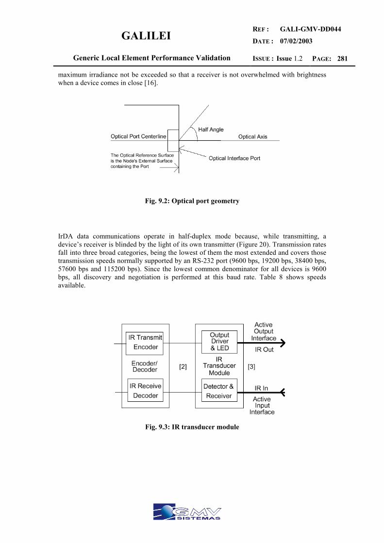
GALILEI REF :
DATE :
GALI-GMV-DD044
07/02/2003
Generic Local Element Performance Validation ISSUE : Issue 1.2 PAGE: 281
maximum irradiance not be exceeded so that a receiver is not overwhelmed with brightness when a device comes in close [16].
Fig. 9.2: Optical port geometry
IrDA data communications operate in half-duplex mode because, while transmitting, a device’s receiver is blinded by the light of its own transmitter (Figure 20). Transmission rates fall into three broad categories, being the lowest of them the most extended and covers those transmission speeds normally supported by an RS-232 port (9600 bps, 19200 bps, 38400 bps, 57600 bps and 115200 bps). Since the lowest common denominator for all devices is 9600 bps, all discovery and negotiation is performed at this baud rate. Table 8 shows speeds available.
Fig. 9.3: IR transducer module
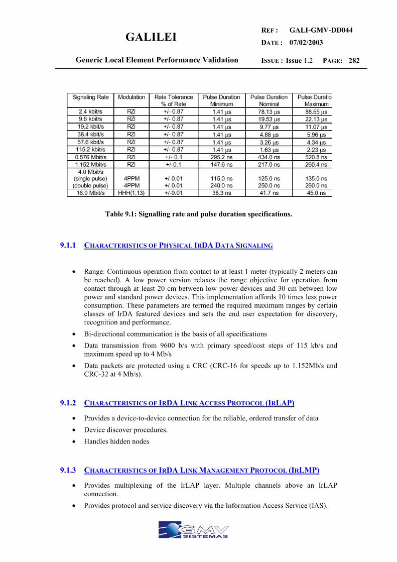
GALILEI REF :
DATE :
GALI-GMV-DD044
07/02/2003
Generic Local Element Performance Validation ISSUE : Issue 1.2 PAGE: 282
Table 9.1: Signalling rate and pulse duration specifications.
9.1.1 CHARACTERISTICS OF PHYSICAL IRDA DATA SIGNALING
• Range: Continuous operation from contact to at least 1 meter (typically 2 meters can
be reached). A low power version relaxes the range objective for operation from contact through at least 20 cm between low power devices and 30 cm between low power and standard power devices. This implementation affords 10 times less power consumption. These parameters are termed the required maximum ranges by certain classes of IrDA featured devices and sets the end user expectation for discovery, recognition and performance.
• Bi-directional communication is the basis of all specifications • Data transmission from 9600 b/s with primary speed/cost steps of 115 kb/s and
maximum speed up to 4 Mb/s • Data packets are protected using a CRC (CRC-16 for speeds up to 1.152Mb/s and
CRC-32 at 4 Mb/s).
9.1.2 CHARACTERISTICS OF IRDA LINK ACCESS PROTOCOL (IRLAP)
• Provides a device-to-device connection for the reliable, ordered transfer of data • Device discover procedures. • Handles hidden nodes
9.1.3 CHARACTERISTICS OF IRDA LINK MANAGEMENT PROTOCOL (IRLMP)
• Provides multiplexing of the IrLAP layer. Multiple channels above an IrLAP connection.
• Provides protocol and service discovery via the Information Access Service (IAS).

GALILEI REF :
DATE :
GALI-GMV-DD044
07/02/2003
Generic Local Element Performance Validation ISSUE : Issue 1.2 PAGE: 283
9.2 CRITICAL ENVIRONMENTS
IrDA behaviour is independent of indoor/outdoor environment context due to its very short line-of-sight coverage.

GALILEI REF :
DATE :
GALI-GMV-DD044
07/02/2003
Generic Local Element Performance Validation ISSUE : Issue 1.2 PAGE: 284
10 HOMERF 2.0
10.1 OVERVIEW
HomeRF is an open industry specification that defines how devices as PCs, peripherals, cordless phones, and many other consumer electronic devices share and communicate voice, data and streaming media in and around the home. HomeRF-compliant products operate in the license-free 2.4 GHz frequency band and utilize frequency-hopping spread spectrum RF technology for secure and robust wireless communications [17]. HomeRF blends technologies from several worldwide standards since none of them alone could meet the market requirements. Data networking technologies based on CSMA/CA protocols (essentially wireless Ethernet) were derived from the Open-Air and IEEE 802.11 standards, and cordless phone technologies based on TDMA are adapted from DECT. HomeRF was developed by the Home Radio Frequency Working Group (WG), which initially included five leading computer companies but has since expanded to over 50 companies made up of leaders across the PC, consumer electronics, networking, peripherals, communications, software, retail channel, home control, and semiconductor industries worldwide. This group was launched in March 1998 to promote the mass deployment of interoperable consumer devices that share and communicate voice, data and streaming media in and around the home without the complication and expense associated with running new wires. The HomeRF WG is dedicated to developing wireless home networking products that are simple, secure, reliable and affordable to the consumer. At the beginning of 2001, it announced organizational changes to allow increased transmission speeds and support additional device types, applications and services. And in the autumn of 2001, it announced for formation of a HomeRF European WG to focus on the European marketplace. The HomeRF MAC layer [17] provides three distinct service flow categories:
• An asynchronous, connectionless packet data service (or “wireless Ethernet”) typically used for TCP/IP traffic
• A prioritised and repetitive connection-oriented data service typically used for streaming media sessions using UDP/IP flows
• An isochronous, full-duplex, symmetric, two-way voice service typically used to map multiple toll-quality voice connections as defined by the DECT protocol
The HomeRF MAC layer operates in a TDMA-like scheme: within each repeating frame, either 10 or 20 ms long depending on the presence of active voice calls, the bulk of the time (or bandwidth) is typically available for asynchronous data. However, within this asynchronous data period the first available opportunities to send packets are reserved sequentially for the prioritised streaming media sessions. Up to 8 sequentially prioritised simultaneous sessions are allowed but if fewer than 8 are present, the reservations are cancelled and the time (or bandwidth) is fully available for asynchronous data services.
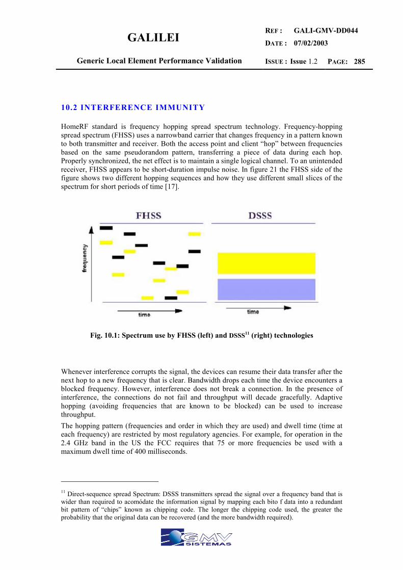
GALILEI REF :
DATE :
GALI-GMV-DD044
07/02/2003
Generic Local Element Performance Validation ISSUE : Issue 1.2 PAGE: 285
10.2 INTERFERENCE IMMUNITY
HomeRF standard is frequency hopping spread spectrum technology. Frequency-hopping spread spectrum (FHSS) uses a narrowband carrier that changes frequency in a pattern known to both transmitter and receiver. Both the access point and client “hop” between frequencies based on the same pseudorandom pattern, transferring a piece of data during each hop. Properly synchronized, the net effect is to maintain a single logical channel. To an unintended receiver, FHSS appears to be short-duration impulse noise. In figure 21 the FHSS side of the figure shows two different hopping sequences and how they use different small slices of the spectrum for short periods of time [17].
Fig. 10.1: Spectrum use by FHSS (left) and DSSS11 (right) technologies
Whenever interference corrupts the signal, the devices can resume their data transfer after the next hop to a new frequency that is clear. Bandwidth drops each time the device encounters a blocked frequency. However, interference does not break a connection. In the presence of interference, the connections do not fail and throughput will decade gracefully. Adaptive hopping (avoiding frequencies that are known to be blocked) can be used to increase throughput. The hopping pattern (frequencies and order in which they are used) and dwell time (time at each frequency) are restricted by most regulatory agencies. For example, for operation in the 2.4 GHz band in the US the FCC requires that 75 or more frequencies be used with a maximum dwell time of 400 milliseconds.
11 Direct-sequence spread Spectrum: DSSS transmitters spread the signal over a frequency band that is wider than required to acomódate the information signal by mapping each bito f data into a redundant bit pattern of “chips” known as chipping code. The longer the chipping code used, the greater the probability that the original data can be recovered (and the more bandwidth required).
GALILEI REF :
DATE :
GALI-GMV-DD044
07/02/2003
Generic Local Element Performance Validation ISSUE : Issue 1.2 PAGE: 286
All FHSS products on the market allow users to deploy more than one logical channel in the same area. They accomplish this by implementing separate channels on different, pseudorandom, hopping sequences. Because there are a large number of possible sequences in the 2.4 GHz band, FHSS allows many non-overlapping channels to be deployed in the same space.
10.3 CRITICAL ENVIRONMENTS
As with other wireless technologies operating in the ISM unlicensed 2.4 GHz frequency band (2.4000-2.4835 GHz), the devices must accept all interference from other authorized (either primary or secondary) users of the band, and also they cannot penetrate massive concrete buildings. Nevertheless, inside them its nominal coverage HomeRF can work in typical home and office indoor environments. In front of other technologies operating in this band, HomeRF seems to be more interference immune thanks to spread spectrum and time/frequency diversity (FHSS, as explained above) than DSSS-based technologies.
GALILEI REF :
DATE :
GALI-GMV-DD044
07/02/2003
Generic Local Element Performance Validation ISSUE : Issue 1.2 PAGE: 287
11 WIRELESS MAN (WMAN) IEEE 802.16
11.1 OVERVIEW
IEEE Standard 802.16 , which defines WirelessMANTM air interface specifications for wireless metropolitan area networks (MANs), was completed in October 2001 and published on 8 April 2002 [18]. A wireless MAN provides network access to buildings through exterior antennas communicating with central radio base stations (BSs). The wireless Man offers an alternative to cabled access networks, such as fiber optic links, coaxial systems using cable modems, and digital subscriber lines (DSL) links. Because wireless systems have the capacity to address broad geographic areas without the costly infrastructure development required in deploying cable links to individual sites, the technology may prove less expensive to deploy and may lead to more ubiquitous broadband access. In this scenario, with WirelessMAN technology bringing the network to a building, users inside the building will connect to it with conventional in-building networks such as, for data, Ethernet (IEEE 802.3) or wireless LANs (IEEE 802.11). IEEE Standard 802.16 was designed to evolve as a set of air interfaces based on a common MAC protocol but with physical layer specifications dependent on the spectrum of use and the associated regulations. The standard addresses frequencies from 10 to 66 GHz, where extensive spectrum is currently available worldwide but at which the short wavelengths introduce significant deployment challenges. Development of the IEEE Standard 802.16 and the included WirelessMANTM air interface is the responsibility of IEEE Working Group 802.16 on Broadband Wireless Access (BWA) Standards. The working group’s initial interest was the 10-66 GHz range. The 2-11 GHz amendment project that led to IEEE 802.16a was approved in March 2000 and primarily involves the development of new physical layer specifications, with supporting enhancements to the basic MAC. In addition, the working group has completed IEEE Standard 802.16.2 to address 10-66 GHz coexistence and, through the amendment project 802.16.2a, is expanding its recommendations to include licensed bands from 2-11 GHz. The work of 802.16.1 (“Air interface for 10 to 66 GHz”) is the farthest along, and it’s likely that will generate the most interest in the industry, as it is targeted at available frequency bands. Figure 22 shows an overview of the 802.16.1 architecture.
11.2 MEDIUM ACCESS CONTROL (MAC)
The IEEE 802.16 MAC protocol was designed for point-to-multipoint broadband wireless access applications. It addresses the need for very high bit rates, both uplink (to the BS) and downlink (from the BS). Access and bandwidth allocation algorithms must accommodate hundreds of terminals that may be shared by multiple end users. The services required by these end users are varied in their nature and include legacy time-division multiplex (TDM) voice and data, Internet Protocol (IP) connectivity, and packetized voice over IP (VoIP). To support this variety of services, the 802.16 MAC must accommodate both continuous and bursty traffic [19].
GALILEI REF :
DATE :
GALI-GMV-DD044
07/02/2003
Generic Local Element Performance Validation ISSUE : Issue 1.2 PAGE: 288
The 802.16 MAC protocol must also support a variety of backhaul requirements, including both asynchronous transfer mode (ATM) and packet-based protocols.. The sequence of time slots across multiple TDMA frames that is dedicated to one subscriber forms a logical channel, and MAC frames are transmitted over that logical channel. IEEE 802.16.1 is intended to support individual channel data rates of from 2 Mbps to 155 Mbps.
11.3 PHYSICAL LAYER
Because of the point-to-multipoint architecture, the BS basically transmits a TDM signal, with individual subscriber stations allocated time slots serially. Access in the uplink direction is by time-division multiple access (TDMA) [19]. The physical layer specifications defined for 10-66 GHz uses burst single carrier modulation with adaptive burst profiling in which transmission parameters, including the modulation and coding schemes, may be adjusted individually to each Subscriber Station (SS) on a frame-by-frame basis. Both TDD12 and burst FDD13 variants are defined. Channel bandwidths of 20-25 MHz (typical US allocation) or 28 MHz /typical European allocation) are specified, along with Nyquist square-root raised-cosine pulse shaping with a rolloff factor of 0.25. Randomization is performed for spectral shaping and to ensure bit transitions for clock recovery. The forward error correction (FEC) used is Reed-Solomon GF(256), with variable block size and error correction capabilities. This is paired with an inner block convolutional code to robustly transmit critical data, such as frame control and initial accesses. The FEC options are paired with quadrature phase shift keying (QPSK), 16-state quadrature amplitude modulation (16-QAM), and 64-state QAM (64-QAM) to form burst profiles of varying robustness and efficiency.
11.4 CRITICAL ENVIRONMENTS
Even in critical environment (urban canyons) WMAN together with other local elements WMAN seems to be an ideal network for transportation of information, which need high data rates.
12 Time Division Duplexing: The uplink and downlink share a channel but do not transmit simultaneously. 13 Frequency Division Duplexing: The uplink and downlink operate on separate channels, sometimos simultaneously.

GALILEI REF :
DATE :
GALI-GMV-DD044
07/02/2003
Generic Local Element Performance Validation ISSUE : Issue 1.2 PAGE: 289
12 REFERENCES
[1] http://www.comms.eee.strath.ac.uk/~gozalvez/gsm/gsm.html [2] http://www.gsmworld.com/news/statistics/index.html [3] http://www.umtsworld.com/technology/gprs.htm [4] http://www.iec.org/online/tutorials/umts/ [5] http://www.umtsworld.com/technology/overview.htm [6] http://www.nt.tuwien.ac.at/mobile/projects/UMTS/en/ [7] http://www.tetramou.com [8] http://www.etsi.org/frameset/home.htm?/technicalactiv/TETRA/tetra.htm [9] http://www.rds.org.uk [10] http://www.eurekadab.org/frame.htm [11] http://www.etsi.org/frameset/home.htm?/technicalactiv/DECT/dect.htm [12] http://www.dectweb.com [13] http://www.bluetooth.com [14] http://www.palowireless.com/bluearticles [15] http://www.irda.org [16] http://www.nwfusion.com/news/tech/2001/0903tech.html [17] http://www.homerf.org [18] http://grouper.ieee.org/groups/802/16/index.html [19] “IEEE Standard 802.16: A technical overview of the wirelessMANTM air interface
for broadband wireless access”, Carl Eklund, Roger B. Marks, Kenneth L. Stanwood, Stanley Wang, IEEE Communications Magazine, June 2002, pp98-107.

GALILEI REF :
DATE :
GALI-GMV-DD044
07/02/2003
Generic Local Element Performance Validation ISSUE : Issue 1.2 PAGE: 290
ANNEX 9 ELCANO CONFIGURATION FILES FOR SIMULATION
GALILEI REF :
DATE :
GALI-GMV-DD044
07/02/2003
Generic Local Element Performance Validation ISSUE : Issue 1.2 PAGE: 291
1 ANNEXED FILES FOR SIMULATIONS
1.1 CONSTELLATIONS
1.1.1 EGNOS CONSTELLATION 0 42164.180 0.0000 0.0000 0 #-Sat 1-#Semi-major Axis (Km.) 0 0.000 0.0000 0.0000 0 #Eccentricity 0 0.000 0.0000 0.0000 0 #Inclination 0 0.000 0.0000 0.0000 0 #RAAN (DEG.) 0 0.000 0.0000 0.0000 0 #Arg. of Perigee (DEG.) 0 0.000 -20.0000 20.0000 0 #Mean Anomaly (DEG.) 1.3670000 #Failure Probability 1 #UERE Budget Model Constellation Communication Constellation GNSS 0 42164.180 0.0000 0.0000 0 #-Sat 2-#Semi-major Axis (Km.) 0 0.000 0.0000 0.0000 0 #Eccentricity 0 0.000 0.0000 0.0000 0 #Inclination 0 0.000 0.0000 0.0000 0 #RAAN (DEG.) 0 0.000 0.0000 0.0000 0 #Arg. of Perigee (DEG.) 0 120.000 -20.0000 20.0000 0 #Mean Anomaly (DEG.) 1.3670000 #Failure Probability 1 #UERE Budget Model Constellation Communication Constellation GNSS 0 42164.180 0.0000 0.0000 0 #-Sat 3-#Semi-major Axis (Km.) 0 0.000 0.0000 0.0000 0 #Eccentricity 0 0.000 0.0000 0.0000 0 #Inclination 0 0.000 0.0000 0.0000 0 #RAAN (DEG.) 0 0.000 0.0000 0.0000 0 #Arg. of Perigee (DEG.) 0 240.000 -20.0000 20.0000 0 #Mean Anomaly (DEG.) 1.3670000 #Failure Probability 1 #UERE Budget Model Constellation Communication Constellation GNSS
1.1.2 GALILEO CONSTELLATION 0 29994.000 -1000.0000 1000.0000 0 #-Sat 4-#Semi-major Axis (Km.) 0 0.000 0.0000 0.0000 0 #Eccentricity 0 56.000 -5.0000 5.0000 0 #Inclination 0 0.000 0.0000 0.0000 0 #RAAN (DEG.) 0 0.000 0.0000 0.0000 0 #Arg. of Perigee (DEG.) 0 0.000 -20.0000 20.0000 1 #Mean Anomaly (DEG.) 1.0000000 #Failure Probability 1 #UERE Budget Model Constellation Galileo Constellation Galileo_GPS Constellation GNSS 0 29994.000 -1000.0000 1000.0000 0 #-Sat 5-#Semi-major Axis (Km.) 0 0.000 0.0000 0.0000 0 #Eccentricity 0 56.000 -5.0000 5.0000 0 #Inclination 0 0.000 0.0000 0.0000 0 #RAAN (DEG.) 0 0.000 0.0000 0.0000 0 #Arg. of Perigee (DEG.) 0 40.000 -20.0000 20.0000 1 #Mean Anomaly (DEG.) 1.0000000 #Failure Probability 1 #UERE Budget Model Constellation Galileo Constellation Galileo_GPS Constellation GNSS 0 29994.000 -1000.0000 1000.0000 0 #-Sat 6-#Semi-major Axis (Km.)

GALILEI REF :
DATE :
GALI-GMV-DD044
07/02/2003
Generic Local Element Performance Validation ISSUE : Issue 1.2 PAGE: 292
0 0.000 0.0000 0.0000 0 #Eccentricity 0 56.000 -5.0000 5.0000 0 #Inclination 0 0.000 0.0000 0.0000 0 #RAAN (DEG.) 0 0.000 0.0000 0.0000 0 #Arg. of Perigee (DEG.) 0 80.000 -20.0000 20.0000 1 #Mean Anomaly (DEG.) 1.0000000 #Failure Probability 1 #UERE Budget Model Constellation Galileo Constellation Galileo_GPS Constellation GNSS 0 29994.000 -1000.0000 1000.0000 0 #-Sat 7-#Semi-major Axis (Km.) 0 0.000 0.0000 0.0000 0 #Eccentricity 0 56.000 -5.0000 5.0000 0 #Inclination 0 0.000 0.0000 0.0000 0 #RAAN (DEG.) 0 0.000 0.0000 0.0000 0 #Arg. of Perigee (DEG.) 0 120.000 -20.0000 20.0000 1 #Mean Anomaly (DEG.) 1.0000000 #Failure Probability 1 #UERE Budget Model Constellation Galileo Constellation Galileo_GPS Constellation GNSS 0 29994.000 -1000.0000 1000.0000 0 #-Sat 8-#Semi-major Axis (Km.) 0 0.000 0.0000 0.0000 0 #Eccentricity 0 56.000 -5.0000 5.0000 0 #Inclination 0 0.000 0.0000 0.0000 0 #RAAN (DEG.) 0 0.000 0.0000 0.0000 0 #Arg. of Perigee (DEG.) 0 160.000 -20.0000 20.0000 1 #Mean Anomaly (DEG.) 1.0000000 #Failure Probability 1 #UERE Budget Model Constellation Galileo Constellation Galileo_GPS Constellation GNSS 0 29994.000 -1000.0000 1000.0000 0 #-Sat 9-#Semi-major Axis (Km.) 0 0.000 0.0000 0.0000 0 #Eccentricity 0 56.000 -5.0000 5.0000 0 #Inclination 0 0.000 0.0000 0.0000 0 #RAAN (DEG.) 0 0.000 0.0000 0.0000 0 #Arg. of Perigee (DEG.) 0 200.000 -20.0000 20.0000 1 #Mean Anomaly (DEG.) 1.0000000 #Failure Probability 1 #UERE Budget Model Constellation Galileo Constellation Galileo_GPS Constellation GNSS 0 29994.000 -1000.0000 1000.0000 0 #-Sat10-#Semi-major Axis (Km.) 0 0.000 0.0000 0.0000 0 #Eccentricity 0 56.000 -5.0000 5.0000 0 #Inclination 0 0.000 0.0000 0.0000 0 #RAAN (DEG.) 0 0.000 0.0000 0.0000 0 #Arg. of Perigee (DEG.) 0 240.000 -20.0000 20.0000 1 #Mean Anomaly (DEG.) 1.0000000 #Failure Probability 1 #UERE Budget Model Constellation Galileo Constellation Galileo_GPS Constellation GNSS 0 29994.000 -1000.0000 1000.0000 0 #-Sat11-#Semi-major Axis (Km.) 0 0.000 0.0000 0.0000 0 #Eccentricity 0 56.000 -5.0000 5.0000 0 #Inclination 0 0.000 0.0000 0.0000 0 #RAAN (DEG.) 0 0.000 0.0000 0.0000 0 #Arg. of Perigee (DEG.) 0 280.000 -20.0000 20.0000 1 #Mean Anomaly (DEG.) 1.0000000 #Failure Probability 1 #UERE Budget Model Constellation Galileo Constellation Galileo_GPS Constellation GNSS 0 29994.000 -1000.0000 1000.0000 0 #-Sat12-#Semi-major Axis (Km.) 0 0.000 0.0000 0.0000 0 #Eccentricity 0 56.000 -5.0000 5.0000 0 #Inclination 0 0.000 0.0000 0.0000 0 #RAAN (DEG.) 0 0.000 0.0000 0.0000 0 #Arg. of Perigee (DEG.) 0 320.000 -20.0000 20.0000 1 #Mean Anomaly (DEG.) 1.0000000 #Failure Probability
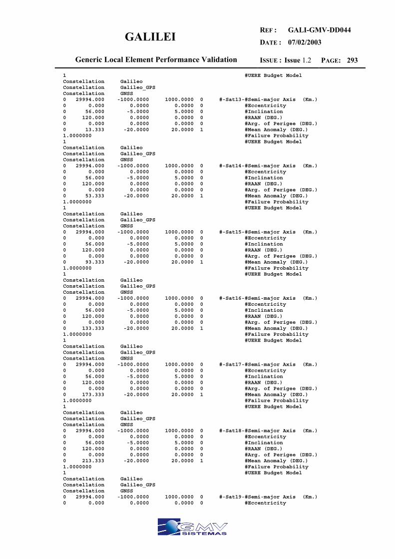
GALILEI REF :
DATE :
GALI-GMV-DD044
07/02/2003
Generic Local Element Performance Validation ISSUE : Issue 1.2 PAGE: 293
1 #UERE Budget Model Constellation Galileo Constellation Galileo_GPS Constellation GNSS 0 29994.000 -1000.0000 1000.0000 0 #-Sat13-#Semi-major Axis (Km.) 0 0.000 0.0000 0.0000 0 #Eccentricity 0 56.000 -5.0000 5.0000 0 #Inclination 0 120.000 0.0000 0.0000 0 #RAAN (DEG.) 0 0.000 0.0000 0.0000 0 #Arg. of Perigee (DEG.) 0 13.333 -20.0000 20.0000 1 #Mean Anomaly (DEG.) 1.0000000 #Failure Probability 1 #UERE Budget Model Constellation Galileo Constellation Galileo_GPS Constellation GNSS 0 29994.000 -1000.0000 1000.0000 0 #-Sat14-#Semi-major Axis (Km.) 0 0.000 0.0000 0.0000 0 #Eccentricity 0 56.000 -5.0000 5.0000 0 #Inclination 0 120.000 0.0000 0.0000 0 #RAAN (DEG.) 0 0.000 0.0000 0.0000 0 #Arg. of Perigee (DEG.) 0 53.333 -20.0000 20.0000 1 #Mean Anomaly (DEG.) 1.0000000 #Failure Probability 1 #UERE Budget Model Constellation Galileo Constellation Galileo_GPS Constellation GNSS 0 29994.000 -1000.0000 1000.0000 0 #-Sat15-#Semi-major Axis (Km.) 0 0.000 0.0000 0.0000 0 #Eccentricity 0 56.000 -5.0000 5.0000 0 #Inclination 0 120.000 0.0000 0.0000 0 #RAAN (DEG.) 0 0.000 0.0000 0.0000 0 #Arg. of Perigee (DEG.) 0 93.333 -20.0000 20.0000 1 #Mean Anomaly (DEG.) 1.0000000 #Failure Probability 1 #UERE Budget Model Constellation Galileo Constellation Galileo_GPS Constellation GNSS 0 29994.000 -1000.0000 1000.0000 0 #-Sat16-#Semi-major Axis (Km.) 0 0.000 0.0000 0.0000 0 #Eccentricity 0 56.000 -5.0000 5.0000 0 #Inclination 0 120.000 0.0000 0.0000 0 #RAAN (DEG.) 0 0.000 0.0000 0.0000 0 #Arg. of Perigee (DEG.) 0 133.333 -20.0000 20.0000 1 #Mean Anomaly (DEG.) 1.0000000 #Failure Probability 1 #UERE Budget Model Constellation Galileo Constellation Galileo_GPS Constellation GNSS 0 29994.000 -1000.0000 1000.0000 0 #-Sat17-#Semi-major Axis (Km.) 0 0.000 0.0000 0.0000 0 #Eccentricity 0 56.000 -5.0000 5.0000 0 #Inclination 0 120.000 0.0000 0.0000 0 #RAAN (DEG.) 0 0.000 0.0000 0.0000 0 #Arg. of Perigee (DEG.) 0 173.333 -20.0000 20.0000 1 #Mean Anomaly (DEG.) 1.0000000 #Failure Probability 1 #UERE Budget Model Constellation Galileo Constellation Galileo_GPS Constellation GNSS 0 29994.000 -1000.0000 1000.0000 0 #-Sat18-#Semi-major Axis (Km.) 0 0.000 0.0000 0.0000 0 #Eccentricity 0 56.000 -5.0000 5.0000 0 #Inclination 0 120.000 0.0000 0.0000 0 #RAAN (DEG.) 0 0.000 0.0000 0.0000 0 #Arg. of Perigee (DEG.) 0 213.333 -20.0000 20.0000 1 #Mean Anomaly (DEG.) 1.0000000 #Failure Probability 1 #UERE Budget Model Constellation Galileo Constellation Galileo_GPS Constellation GNSS 0 29994.000 -1000.0000 1000.0000 0 #-Sat19-#Semi-major Axis (Km.) 0 0.000 0.0000 0.0000 0 #Eccentricity
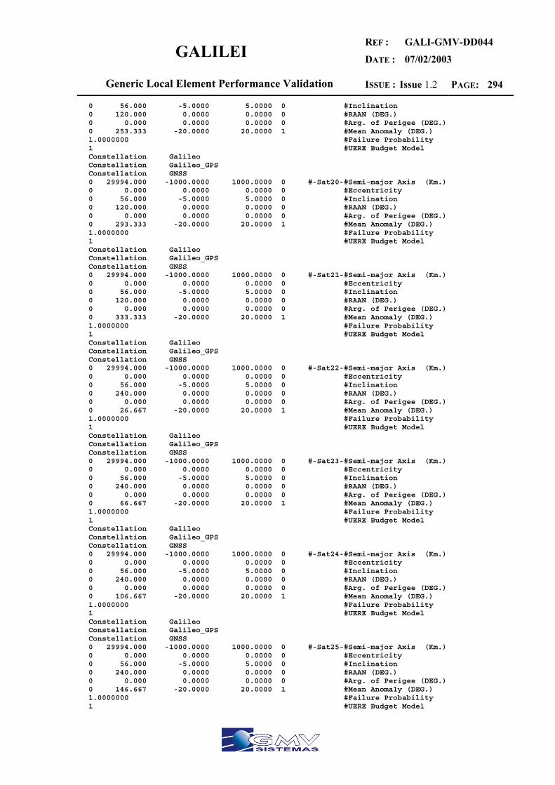
GALILEI REF :
DATE :
GALI-GMV-DD044
07/02/2003
Generic Local Element Performance Validation ISSUE : Issue 1.2 PAGE: 294
0 56.000 -5.0000 5.0000 0 #Inclination 0 120.000 0.0000 0.0000 0 #RAAN (DEG.) 0 0.000 0.0000 0.0000 0 #Arg. of Perigee (DEG.) 0 253.333 -20.0000 20.0000 1 #Mean Anomaly (DEG.) 1.0000000 #Failure Probability 1 #UERE Budget Model Constellation Galileo Constellation Galileo_GPS Constellation GNSS 0 29994.000 -1000.0000 1000.0000 0 #-Sat20-#Semi-major Axis (Km.) 0 0.000 0.0000 0.0000 0 #Eccentricity 0 56.000 -5.0000 5.0000 0 #Inclination 0 120.000 0.0000 0.0000 0 #RAAN (DEG.) 0 0.000 0.0000 0.0000 0 #Arg. of Perigee (DEG.) 0 293.333 -20.0000 20.0000 1 #Mean Anomaly (DEG.) 1.0000000 #Failure Probability 1 #UERE Budget Model Constellation Galileo Constellation Galileo_GPS Constellation GNSS 0 29994.000 -1000.0000 1000.0000 0 #-Sat21-#Semi-major Axis (Km.) 0 0.000 0.0000 0.0000 0 #Eccentricity 0 56.000 -5.0000 5.0000 0 #Inclination 0 120.000 0.0000 0.0000 0 #RAAN (DEG.) 0 0.000 0.0000 0.0000 0 #Arg. of Perigee (DEG.) 0 333.333 -20.0000 20.0000 1 #Mean Anomaly (DEG.) 1.0000000 #Failure Probability 1 #UERE Budget Model Constellation Galileo Constellation Galileo_GPS Constellation GNSS 0 29994.000 -1000.0000 1000.0000 0 #-Sat22-#Semi-major Axis (Km.) 0 0.000 0.0000 0.0000 0 #Eccentricity 0 56.000 -5.0000 5.0000 0 #Inclination 0 240.000 0.0000 0.0000 0 #RAAN (DEG.) 0 0.000 0.0000 0.0000 0 #Arg. of Perigee (DEG.) 0 26.667 -20.0000 20.0000 1 #Mean Anomaly (DEG.) 1.0000000 #Failure Probability 1 #UERE Budget Model Constellation Galileo Constellation Galileo_GPS Constellation GNSS 0 29994.000 -1000.0000 1000.0000 0 #-Sat23-#Semi-major Axis (Km.) 0 0.000 0.0000 0.0000 0 #Eccentricity 0 56.000 -5.0000 5.0000 0 #Inclination 0 240.000 0.0000 0.0000 0 #RAAN (DEG.) 0 0.000 0.0000 0.0000 0 #Arg. of Perigee (DEG.) 0 66.667 -20.0000 20.0000 1 #Mean Anomaly (DEG.) 1.0000000 #Failure Probability 1 #UERE Budget Model Constellation Galileo Constellation Galileo_GPS Constellation GNSS 0 29994.000 -1000.0000 1000.0000 0 #-Sat24-#Semi-major Axis (Km.) 0 0.000 0.0000 0.0000 0 #Eccentricity 0 56.000 -5.0000 5.0000 0 #Inclination 0 240.000 0.0000 0.0000 0 #RAAN (DEG.) 0 0.000 0.0000 0.0000 0 #Arg. of Perigee (DEG.) 0 106.667 -20.0000 20.0000 1 #Mean Anomaly (DEG.) 1.0000000 #Failure Probability 1 #UERE Budget Model Constellation Galileo Constellation Galileo_GPS Constellation GNSS 0 29994.000 -1000.0000 1000.0000 0 #-Sat25-#Semi-major Axis (Km.) 0 0.000 0.0000 0.0000 0 #Eccentricity 0 56.000 -5.0000 5.0000 0 #Inclination 0 240.000 0.0000 0.0000 0 #RAAN (DEG.) 0 0.000 0.0000 0.0000 0 #Arg. of Perigee (DEG.) 0 146.667 -20.0000 20.0000 1 #Mean Anomaly (DEG.) 1.0000000 #Failure Probability 1 #UERE Budget Model
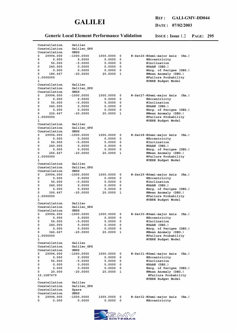
GALILEI REF :
DATE :
GALI-GMV-DD044
07/02/2003
Generic Local Element Performance Validation ISSUE : Issue 1.2 PAGE: 295
Constellation Galileo Constellation Galileo_GPS Constellation GNSS 0 29994.000 -1000.0000 1000.0000 0 #-Sat26-#Semi-major Axis (Km.) 0 0.000 0.0000 0.0000 0 #Eccentricity 0 56.000 -5.0000 5.0000 0 #Inclination 0 240.000 0.0000 0.0000 0 #RAAN (DEG.) 0 0.000 0.0000 0.0000 0 #Arg. of Perigee (DEG.) 0 186.667 -20.0000 20.0000 1 #Mean Anomaly (DEG.) 1.0000000 #Failure Probability 1 #UERE Budget Model Constellation Galileo Constellation Galileo_GPS Constellation GNSS 0 29994.000 -1000.0000 1000.0000 0 #-Sat27-#Semi-major Axis (Km.) 0 0.000 0.0000 0.0000 0 #Eccentricity 0 56.000 -5.0000 5.0000 0 #Inclination 0 240.000 0.0000 0.0000 0 #RAAN (DEG.) 0 0.000 0.0000 0.0000 0 #Arg. of Perigee (DEG.) 0 226.667 -20.0000 20.0000 1 #Mean Anomaly (DEG.) 1.0000000 #Failure Probability 1 #UERE Budget Model Constellation Galileo Constellation Galileo_GPS Constellation GNSS 0 29994.000 -1000.0000 1000.0000 0 #-Sat28-#Semi-major Axis (Km.) 0 0.000 0.0000 0.0000 0 #Eccentricity 0 56.000 -5.0000 5.0000 0 #Inclination 0 240.000 0.0000 0.0000 0 #RAAN (DEG.) 0 0.000 0.0000 0.0000 0 #Arg. of Perigee (DEG.) 0 266.667 -20.0000 20.0000 1 #Mean Anomaly (DEG.) 1.0000000 #Failure Probability 1 #UERE Budget Model Constellation Galileo Constellation Galileo_GPS Constellation GNSS 0 29994.000 -1000.0000 1000.0000 0 #-Sat29-#Semi-major Axis (Km.) 0 0.000 0.0000 0.0000 0 #Eccentricity 0 56.000 -5.0000 5.0000 0 #Inclination 0 240.000 0.0000 0.0000 0 #RAAN (DEG.) 0 0.000 0.0000 0.0000 0 #Arg. of Perigee (DEG.) 0 306.667 -20.0000 20.0000 1 #Mean Anomaly (DEG.) 1.0000000 #Failure Probability 1 #UERE Budget Model Constellation Galileo Constellation Galileo_GPS Constellation GNSS 0 29994.000 -1000.0000 1000.0000 0 #-Sat30-#Semi-major Axis (Km.) 0 0.000 0.0000 0.0000 0 #Eccentricity 0 56.000 -5.0000 5.0000 0 #Inclination 0 240.000 0.0000 0.0000 0 #RAAN (DEG.) 0 0.000 0.0000 0.0000 0 #Arg. of Perigee (DEG.) 0 346.667 -20.0000 20.0000 1 #Mean Anomaly (DEG.) 1.0000000 #Failure Probability 1 #UERE Budget Model Constellation Galileo Constellation Galileo_GPS Constellation GNSS 0 29994.000 -1000.0000 1000.0000 0 #-Sat31-#Semi-major Axis (Km.) 0 0.000 0.0000 0.0000 0 #Eccentricity 0 56.000 -5.0000 5.0000 0 #Inclination 0 0.000 0.0000 0.0000 0 #RAAN (DEG.) 0 0.000 0.0000 0.0000 0 #Arg. of Perigee (DEG.) 0 20.000 -20.0000 20.0000 1 #Mean Anomaly (DEG.) 15.1087679 #Failure Probability 1 #UERE Budget Model Constellation Galileo Constellation Galileo_GPS Constellation Spare Constellation GNSS 0 29994.000 -1000.0000 1000.0000 0 #-Sat32-#Semi-major Axis (Km.) 0 0.000 0.0000 0.0000 0 #Eccentricity

GALILEI REF :
DATE :
GALI-GMV-DD044
07/02/2003
Generic Local Element Performance Validation ISSUE : Issue 1.2 PAGE: 296
0 56.000 -5.0000 5.0000 0 #Inclination 0 120.000 0.0000 0.0000 0 #RAAN (DEG.) 0 0.000 0.0000 0.0000 0 #Arg. of Perigee (DEG.) 0 20.000 -20.0000 20.0000 1 #Mean Anomaly (DEG.) 15.1087679 #Failure Probability 1 #UERE Budget Model Constellation Galileo Constellation Galileo_GPS Constellation Spare Constellation GNSS 0 29994.000 -1000.0000 1000.0000 0 #-Sat33-#Semi-major Axis (Km.) 0 0.000 0.0000 0.0000 0 #Eccentricity 0 56.000 -5.0000 5.0000 0 #Inclination 0 240.000 0.0000 0.0000 0 #RAAN (DEG.) 0 0.000 0.0000 0.0000 0 #Arg. of Perigee (DEG.) 0 20.000 -20.0000 20.0000 1 #Mean Anomaly (DEG.) 15.1087679 #Failure Probability 1 #UERE Budget Model Constellation Galileo Constellation Galileo_GPS Constellation Spare Constellation GNSS
1.1.3 GPS CONSTELLATION 25th June 2002 (Source extracted from web page: http://gibs.leipzig.ifag.de/cgi-bin/gps_almanac.cgi?de)
0 26559.403 -1000.0000 1000.0000 0 #-Sat1-#Semi-major Axis (Km.) 0 0.005 0.0000 0.0000 0 #Eccentricity 0 55.567 -5.0000 5.0000 0 #Inclination 0 170.719 0.0000 0.0000 0 #RAAN (DEG.) 0 -97.104 0.0000 0.0000 0 #Arg. of Perigee (DEG.) 0 -90.743 -20.0000 20.0000 1 #Mean Anomaly (DEG.) 1.0000000 #Failure Probability 1 #UERE Budget Model Constellation GNSS Constellation Galileo_GPS Constellation GPS 0 26558.542 -1000.0000 1000.0000 0 #-Sat2-#Semi-major Axis (Km.) 0 0.022 0.0000 0.0000 0 #Eccentricity 0 53.400 -5.0000 5.0000 0 #Inclination 0 -75.364 0.0000 0.0000 0 #RAAN (DEG.) 0 -110.643 0.0000 0.0000 0 #Arg. of Perigee (DEG.) 0 -143.676 -20.0000 20.0000 1 #Mean Anomaly (DEG.) 1.0000000 #Failure Probability 1 #UERE Budget Model Constellation GNSS Constellation Galileo_GPS Constellation GPS 0 26560.183 -1000.0000 1000.0000 0 #-Sat3-#Semi-major Axis (Km.) 0 0.003 0.0000 0.0000 0 #Eccentricity 0 53.475 -5.0000 5.0000 0 #Inclination 0 -13.676 0.0000 0.0000 0 #RAAN (DEG.) 0 29.448 0.0000 0.0000 0 #Arg. of Perigee (DEG.) 0 24.128 -20.0000 20.0000 1 #Mean Anomaly (DEG.) 1.0000000 #Failure Probability 1 #UERE Budget Model Constellation GNSS Constellation Galileo_GPS Constellation GPS 0 26560.233 -1000.0000 1000.0000 0 #-Sat4-#Semi-major Axis (Km.) 0 0.006 0.0000 0.0000 0 #Eccentricity 0 55.558 -5.0000 5.0000 0 #Inclination 0 50.923 0.0000 0.0000 0 #RAAN (DEG.) 0 -16.959 0.0000 0.0000 0 #Arg. of Perigee (DEG.) 0 -133.144 -20.0000 20.0000 1 #Mean Anomaly (DEG.) 1.0000000 #Failure Probability 1 #UERE Budget Model Constellation GNSS

GALILEI REF :
DATE :
GALI-GMV-DD044
07/02/2003
Generic Local Element Performance Validation ISSUE : Issue 1.2 PAGE: 297
Constellation Galileo_GPS Constellation GPS 0 26559.825 -1000.0000 1000.0000 0 #-Sat5-#Semi-major Axis (Km.) 0 0.004 0.0000 0.0000 0 #Eccentricity 0 53.581 -5.0000 5.0000 0 #Inclination 0 -74.091 0.0000 0.0000 0 #RAAN (DEG.) 0 30.966 0.0000 0.0000 0 #Arg. of Perigee (DEG.) 0 -150.094 -20.0000 20.0000 1 #Mean Anomaly (DEG.) 1.0000000 #Failure Probability 1 #UERE Budget Model Constellation GNSS Constellation Galileo_GPS Constellation GPS 0 26560.570 -1000.0000 1000.0000 0 #-Sat6-#Semi-major Axis (Km.) 0 0.007 0.0000 0.0000 0 #Eccentricity 0 53.909 -5.0000 5.0000 0 #Inclination 0 -10.935 0.0000 0.0000 0 #RAAN (DEG.) 0 -126.145 0.0000 0.0000 0 #Arg. of Perigee (DEG.) 0 -84.965 -20.0000 20.0000 1 #Mean Anomaly (DEG.) 1.0000000 #Failure Probability 1 #UERE Budget Model Constellation GNSS Constellation Galileo_GPS Constellation GPS 0 26559.956 -1000.0000 1000.0000 0 #-Sat7-#Semi-major Axis (Km.) 0 0.012 0.0000 0.0000 0 #Eccentricity 0 54.007 -5.0000 5.0000 0 #Inclination 0 -12.619 0.0000 0.0000 0 #RAAN (DEG.) 0 -111.799 0.0000 0.0000 0 #Arg. of Perigee (DEG.) 0 33.973 -20.0000 20.0000 1 #Mean Anomaly (DEG.) 1.0000000 #Failure Probability 1 #UERE Budget Model Constellation GNSS Constellation Galileo_GPS Constellation GPS 0 26559.956 -1000.0000 1000.0000 0 #-Sat8-#Semi-major Axis (Km.) 0 0.008 0.0000 0.0000 0 #Eccentricity 0 55.001 -5.0000 5.0000 0 #Inclination 0 -128.710 0.0000 0.0000 0 #RAAN (DEG.) 0 123.753 0.0000 0.0000 0 #Arg. of Perigee (DEG.) 0 -73.058 -20.0000 20.0000 1 #Mean Anomaly (DEG.) 1.0000000 #Failure Probability 1 #UERE Budget Model Constellation GNSS Constellation Galileo_GPS Constellation GPS 0 26559.690 -1000.0000 1000.0000 0 #-Sat9-#Semi-major Axis (Km.) 0 0.013 0.0000 0.0000 0 #Eccentricity 0 54.221 -5.0000 5.0000 0 #Inclination 0 -132.031 0.0000 0.0000 0 #RAAN (DEG.) 0 47.455 0.0000 0.0000 0 #Arg. of Perigee (DEG.) 0 -102.122 -20.0000 20.0000 1 #Mean Anomaly (DEG.) 1.0000000 #Failure Probability 1 #UERE Budget Model Constellation GNSS Constellation Galileo_GPS Constellation GPS 0 26558.628 -1000.0000 1000.0000 0 #-Sat10-#Semi-major Axis (Km.) 0 0.005 0.0000 0.0000 0 #Eccentricity 0 56.164 -5.0000 5.0000 0 #Inclination 0 109.785 0.0000 0.0000 0 #RAAN (DEG.) 0 8.505 0.0000 0.0000 0 #Arg. of Perigee (DEG.) 0 96.384 -20.0000 20.0000 1 #Mean Anomaly (DEG.) 1.0000000 #Failure Probability 1 #UERE Budget Model Constellation GNSS Constellation Galileo_GPS Constellation GPS 0 26559.740 -1000.0000 1000.0000 0 #-Sat11-#Semi-major Axis (Km.) 0 0.001 0.0000 0.0000 0 #Eccentricity 0 52.556 -5.0000 5.0000 0 #Inclination 0 45.686 0.0000 0.0000 0 #RAAN (DEG.)
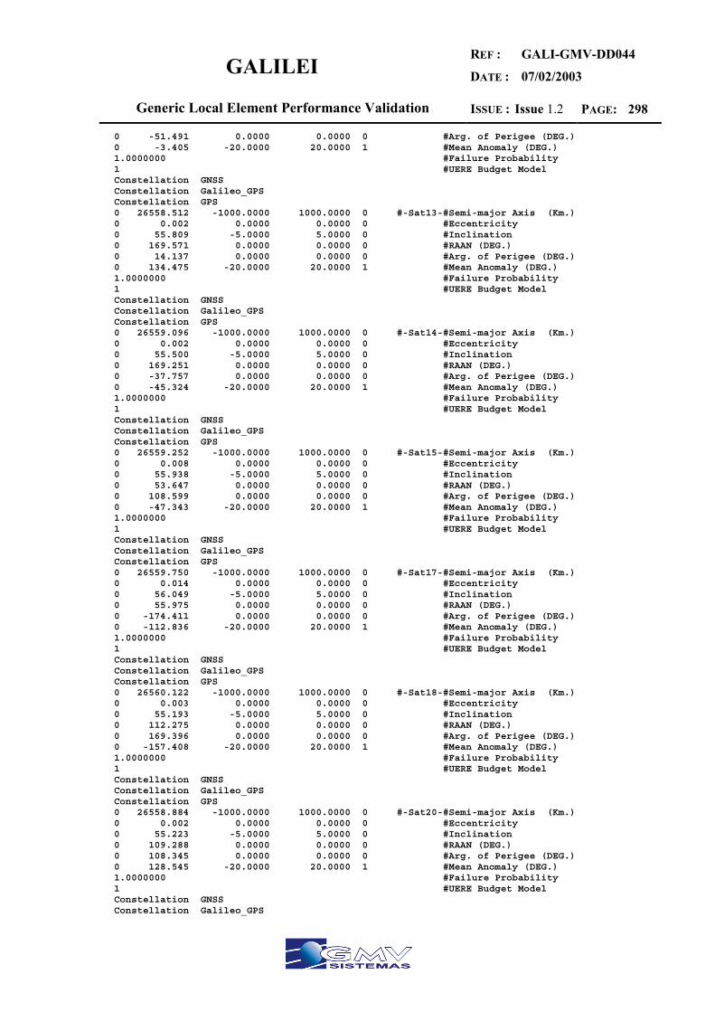
GALILEI REF :
DATE :
GALI-GMV-DD044
07/02/2003
Generic Local Element Performance Validation ISSUE : Issue 1.2 PAGE: 298
0 -51.491 0.0000 0.0000 0 #Arg. of Perigee (DEG.) 0 -3.405 -20.0000 20.0000 1 #Mean Anomaly (DEG.) 1.0000000 #Failure Probability 1 #UERE Budget Model Constellation GNSS Constellation Galileo_GPS Constellation GPS 0 26558.512 -1000.0000 1000.0000 0 #-Sat13-#Semi-major Axis (Km.) 0 0.002 0.0000 0.0000 0 #Eccentricity 0 55.809 -5.0000 5.0000 0 #Inclination 0 169.571 0.0000 0.0000 0 #RAAN (DEG.) 0 14.137 0.0000 0.0000 0 #Arg. of Perigee (DEG.) 0 134.475 -20.0000 20.0000 1 #Mean Anomaly (DEG.) 1.0000000 #Failure Probability 1 #UERE Budget Model Constellation GNSS Constellation Galileo_GPS Constellation GPS 0 26559.096 -1000.0000 1000.0000 0 #-Sat14-#Semi-major Axis (Km.) 0 0.002 0.0000 0.0000 0 #Eccentricity 0 55.500 -5.0000 5.0000 0 #Inclination 0 169.251 0.0000 0.0000 0 #RAAN (DEG.) 0 -37.757 0.0000 0.0000 0 #Arg. of Perigee (DEG.) 0 -45.324 -20.0000 20.0000 1 #Mean Anomaly (DEG.) 1.0000000 #Failure Probability 1 #UERE Budget Model Constellation GNSS Constellation Galileo_GPS Constellation GPS 0 26559.252 -1000.0000 1000.0000 0 #-Sat15-#Semi-major Axis (Km.) 0 0.008 0.0000 0.0000 0 #Eccentricity 0 55.938 -5.0000 5.0000 0 #Inclination 0 53.647 0.0000 0.0000 0 #RAAN (DEG.) 0 108.599 0.0000 0.0000 0 #Arg. of Perigee (DEG.) 0 -47.343 -20.0000 20.0000 1 #Mean Anomaly (DEG.) 1.0000000 #Failure Probability 1 #UERE Budget Model Constellation GNSS Constellation Galileo_GPS Constellation GPS 0 26559.750 -1000.0000 1000.0000 0 #-Sat17-#Semi-major Axis (Km.) 0 0.014 0.0000 0.0000 0 #Eccentricity 0 56.049 -5.0000 5.0000 0 #Inclination 0 55.975 0.0000 0.0000 0 #RAAN (DEG.) 0 -174.411 0.0000 0.0000 0 #Arg. of Perigee (DEG.) 0 -112.836 -20.0000 20.0000 1 #Mean Anomaly (DEG.) 1.0000000 #Failure Probability 1 #UERE Budget Model Constellation GNSS Constellation Galileo_GPS Constellation GPS 0 26560.122 -1000.0000 1000.0000 0 #-Sat18-#Semi-major Axis (Km.) 0 0.003 0.0000 0.0000 0 #Eccentricity 0 55.193 -5.0000 5.0000 0 #Inclination 0 112.275 0.0000 0.0000 0 #RAAN (DEG.) 0 169.396 0.0000 0.0000 0 #Arg. of Perigee (DEG.) 0 -157.408 -20.0000 20.0000 1 #Mean Anomaly (DEG.) 1.0000000 #Failure Probability 1 #UERE Budget Model Constellation GNSS Constellation Galileo_GPS Constellation GPS 0 26558.884 -1000.0000 1000.0000 0 #-Sat20-#Semi-major Axis (Km.) 0 0.002 0.0000 0.0000 0 #Eccentricity 0 55.223 -5.0000 5.0000 0 #Inclination 0 109.288 0.0000 0.0000 0 #RAAN (DEG.) 0 108.345 0.0000 0.0000 0 #Arg. of Perigee (DEG.) 0 128.545 -20.0000 20.0000 1 #Mean Anomaly (DEG.) 1.0000000 #Failure Probability 1 #UERE Budget Model Constellation GNSS Constellation Galileo_GPS
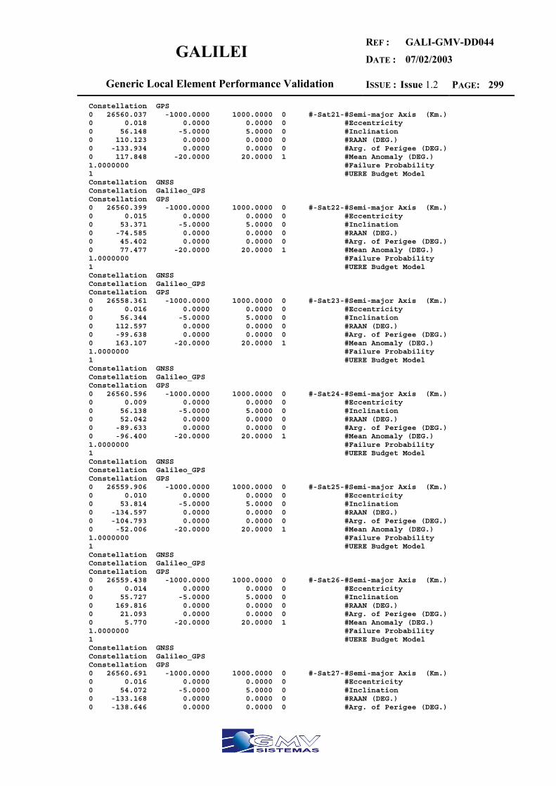
GALILEI REF :
DATE :
GALI-GMV-DD044
07/02/2003
Generic Local Element Performance Validation ISSUE : Issue 1.2 PAGE: 299
Constellation GPS 0 26560.037 -1000.0000 1000.0000 0 #-Sat21-#Semi-major Axis (Km.) 0 0.018 0.0000 0.0000 0 #Eccentricity 0 56.148 -5.0000 5.0000 0 #Inclination 0 110.123 0.0000 0.0000 0 #RAAN (DEG.) 0 -133.934 0.0000 0.0000 0 #Arg. of Perigee (DEG.) 0 117.848 -20.0000 20.0000 1 #Mean Anomaly (DEG.) 1.0000000 #Failure Probability 1 #UERE Budget Model Constellation GNSS Constellation Galileo_GPS Constellation GPS 0 26560.399 -1000.0000 1000.0000 0 #-Sat22-#Semi-major Axis (Km.) 0 0.015 0.0000 0.0000 0 #Eccentricity 0 53.371 -5.0000 5.0000 0 #Inclination 0 -74.585 0.0000 0.0000 0 #RAAN (DEG.) 0 45.402 0.0000 0.0000 0 #Arg. of Perigee (DEG.) 0 77.477 -20.0000 20.0000 1 #Mean Anomaly (DEG.) 1.0000000 #Failure Probability 1 #UERE Budget Model Constellation GNSS Constellation Galileo_GPS Constellation GPS 0 26558.361 -1000.0000 1000.0000 0 #-Sat23-#Semi-major Axis (Km.) 0 0.016 0.0000 0.0000 0 #Eccentricity 0 56.344 -5.0000 5.0000 0 #Inclination 0 112.597 0.0000 0.0000 0 #RAAN (DEG.) 0 -99.638 0.0000 0.0000 0 #Arg. of Perigee (DEG.) 0 163.107 -20.0000 20.0000 1 #Mean Anomaly (DEG.) 1.0000000 #Failure Probability 1 #UERE Budget Model Constellation GNSS Constellation Galileo_GPS Constellation GPS 0 26560.596 -1000.0000 1000.0000 0 #-Sat24-#Semi-major Axis (Km.) 0 0.009 0.0000 0.0000 0 #Eccentricity 0 56.138 -5.0000 5.0000 0 #Inclination 0 52.042 0.0000 0.0000 0 #RAAN (DEG.) 0 -89.633 0.0000 0.0000 0 #Arg. of Perigee (DEG.) 0 -96.400 -20.0000 20.0000 1 #Mean Anomaly (DEG.) 1.0000000 #Failure Probability 1 #UERE Budget Model Constellation GNSS Constellation Galileo_GPS Constellation GPS 0 26559.906 -1000.0000 1000.0000 0 #-Sat25-#Semi-major Axis (Km.) 0 0.010 0.0000 0.0000 0 #Eccentricity 0 53.814 -5.0000 5.0000 0 #Inclination 0 -134.597 0.0000 0.0000 0 #RAAN (DEG.) 0 -104.793 0.0000 0.0000 0 #Arg. of Perigee (DEG.) 0 -52.006 -20.0000 20.0000 1 #Mean Anomaly (DEG.) 1.0000000 #Failure Probability 1 #UERE Budget Model Constellation GNSS Constellation Galileo_GPS Constellation GPS 0 26559.438 -1000.0000 1000.0000 0 #-Sat26-#Semi-major Axis (Km.) 0 0.014 0.0000 0.0000 0 #Eccentricity 0 55.727 -5.0000 5.0000 0 #Inclination 0 169.816 0.0000 0.0000 0 #RAAN (DEG.) 0 21.093 0.0000 0.0000 0 #Arg. of Perigee (DEG.) 0 5.770 -20.0000 20.0000 1 #Mean Anomaly (DEG.) 1.0000000 #Failure Probability 1 #UERE Budget Model Constellation GNSS Constellation Galileo_GPS Constellation GPS 0 26560.691 -1000.0000 1000.0000 0 #-Sat27-#Semi-major Axis (Km.) 0 0.016 0.0000 0.0000 0 #Eccentricity 0 54.072 -5.0000 5.0000 0 #Inclination 0 -133.168 0.0000 0.0000 0 #RAAN (DEG.) 0 -138.646 0.0000 0.0000 0 #Arg. of Perigee (DEG.)
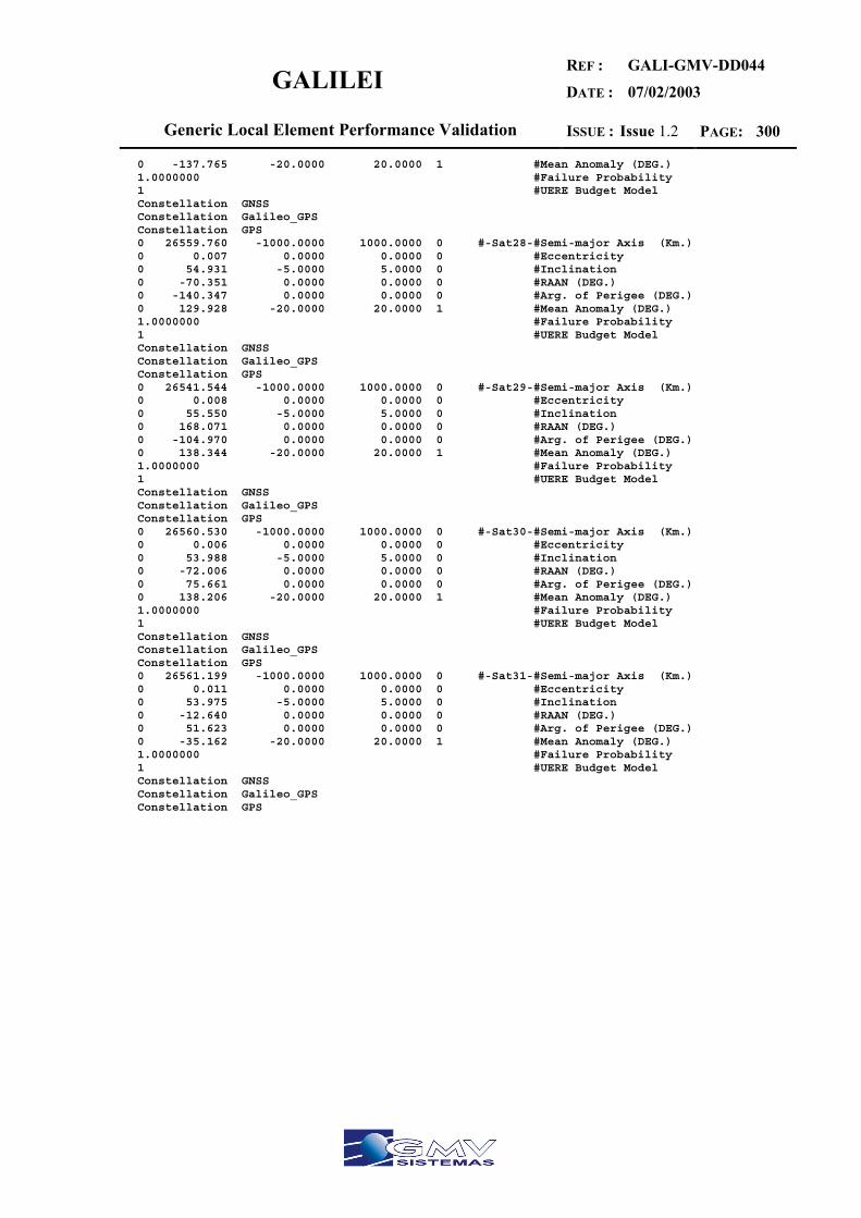
GALILEI REF :
DATE :
GALI-GMV-DD044
07/02/2003
Generic Local Element Performance Validation ISSUE : Issue 1.2 PAGE: 300
0 -137.765 -20.0000 20.0000 1 #Mean Anomaly (DEG.) 1.0000000 #Failure Probability 1 #UERE Budget Model Constellation GNSS Constellation Galileo_GPS Constellation GPS 0 26559.760 -1000.0000 1000.0000 0 #-Sat28-#Semi-major Axis (Km.) 0 0.007 0.0000 0.0000 0 #Eccentricity 0 54.931 -5.0000 5.0000 0 #Inclination 0 -70.351 0.0000 0.0000 0 #RAAN (DEG.) 0 -140.347 0.0000 0.0000 0 #Arg. of Perigee (DEG.) 0 129.928 -20.0000 20.0000 1 #Mean Anomaly (DEG.) 1.0000000 #Failure Probability 1 #UERE Budget Model Constellation GNSS Constellation Galileo_GPS Constellation GPS 0 26541.544 -1000.0000 1000.0000 0 #-Sat29-#Semi-major Axis (Km.) 0 0.008 0.0000 0.0000 0 #Eccentricity 0 55.550 -5.0000 5.0000 0 #Inclination 0 168.071 0.0000 0.0000 0 #RAAN (DEG.) 0 -104.970 0.0000 0.0000 0 #Arg. of Perigee (DEG.) 0 138.344 -20.0000 20.0000 1 #Mean Anomaly (DEG.) 1.0000000 #Failure Probability 1 #UERE Budget Model Constellation GNSS Constellation Galileo_GPS Constellation GPS 0 26560.530 -1000.0000 1000.0000 0 #-Sat30-#Semi-major Axis (Km.) 0 0.006 0.0000 0.0000 0 #Eccentricity 0 53.988 -5.0000 5.0000 0 #Inclination 0 -72.006 0.0000 0.0000 0 #RAAN (DEG.) 0 75.661 0.0000 0.0000 0 #Arg. of Perigee (DEG.) 0 138.206 -20.0000 20.0000 1 #Mean Anomaly (DEG.) 1.0000000 #Failure Probability 1 #UERE Budget Model Constellation GNSS Constellation Galileo_GPS Constellation GPS 0 26561.199 -1000.0000 1000.0000 0 #-Sat31-#Semi-major Axis (Km.) 0 0.011 0.0000 0.0000 0 #Eccentricity 0 53.975 -5.0000 5.0000 0 #Inclination 0 -12.640 0.0000 0.0000 0 #RAAN (DEG.) 0 51.623 0.0000 0.0000 0 #Arg. of Perigee (DEG.) 0 -35.162 -20.0000 20.0000 1 #Mean Anomaly (DEG.) 1.0000000 #Failure Probability 1 #UERE Budget Model Constellation GNSS Constellation Galileo_GPS Constellation GPS
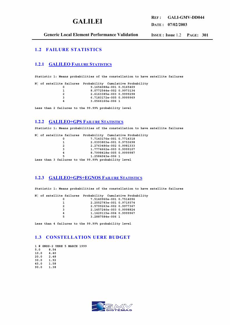
GALILEI REF :
DATE :
GALI-GMV-DD044
07/02/2003
Generic Local Element Performance Validation ISSUE : Issue 1.2 PAGE: 301
1.2 FAILURE STATISTICS
1.2.1 GALILEO FAILURE STATISTICS
Statistic 1: Means probabilities of the constellation to have satellite failures N¦ of satellite failures Probability Cumulative Probability 0 9.1654088e-001 0.9165409 1 8.0772544e-002 0.9973134 2 2.6163385e-003 0.9999298 3 6.7183172e-005 0.9999969 4 3.0566160e-006 1 Less than 2 failures to the 99.99% probability level
1.2.2 GALILEO+GPS FAILURE STATISTICS Statistic 1: Means probabilities of the constellation to have satellite failures N¦ of satellite failures Probability Cumulative Probability 0 7.7143176e-001 0.7714318 1 2.0393803e-001 0.9753698 2 2.2763486e-002 0.9981333 3 1.7774662e-003 0.9999107 4 8.7998418e-005 0.9999987 5 1.2584043e-006 1 Less than 3 failures to the 99.99% probability level
1.2.3 GALILEO+GPS+EGNOS FAILURE STATISTICS Statistic 1: Means probabilities of the constellation to have satellite failures N¦ of satellite failures Probability Cumulative Probability 0 7.5140960e-001 0.7514096 1 2.2052783e-001 0.9719374 2 2.5799263e-002 0.9977367 3 2.1457246e-003 0.9998824 4 1.1429115e-004 0.9999967 5 3.2887584e-006 1 Less than 4 failures to the 99.99% probability level
1.3 CONSTELLATION UERE BUDGET
1 # GNSS-2 UERE 5 MARCH 1999 5.0 8.54 10.0 4.40 20.0 2.48 30.0 1.92 45.0 1.58 90.0 1.38

GALILEI REF :
DATE :
GALI-GMV-DD044
07/02/2003
Generic Local Element Performance Validation ISSUE : Issue 1.2 PAGE: 302
ANNEX 10 PHASE II: INTEROPERABILITY ANALYSIS FOR DD027 v1.0
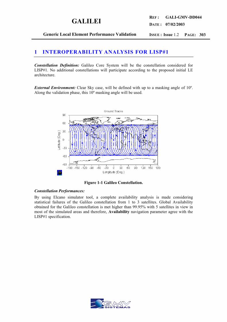
GALILEI REF :
DATE :
GALI-GMV-DD044
07/02/2003
Generic Local Element Performance Validation ISSUE : Issue 1.2 PAGE: 303
1 INTEROPERABILITY ANALYSIS FOR LISP#1
Constellation Definition: Galileo Core System will be the constellation considered for LISP#1. No additional constellations will participate according to the proposed initial LE architecture. External Environment: Clear Sky case, will be defined with up to a masking angle of 10º. Along the validation phase, this 10º masking angle will be used.
Figure 1-1 Galileo Constellation.
Constellation Performances: By using Elcano simulator tool, a complete availability analysis is made considering statistical failures of the Galileo constellation from 1 to 3 satellites. Global Availability obtained for the Galileo constellation is met higher than 99.95% with 5 satellites in view in most of the simulated areas and therefore, Availability navigation parameter agree with the LISP#1 specification.
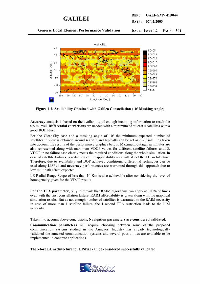
GALILEI REF :
DATE :
GALI-GMV-DD044
07/02/2003
Generic Local Element Performance Validation ISSUE : Issue 1.2 PAGE: 304
Figure 1-2. Availability Obtained with Galileo Constellation (10º Masking Angle)
Accuracy analysis is based on the availability of enough incoming information to reach the 0.5 m level. Differential corrections are needed with a minimum of at least 4 satellites with a good DOP level. For the Clear-Sky case and a masking angle of 10º the minimum expected number of satellites in view is obtained around 4 and 5 and typically can be set as 6 - 7 satellites taken into account the results of the performance graphics below. Maximum outages in minutes are also represented along with maximum VDOP values for different satellite failures until 3. VDOP in no failure case clearly meets the required conditions along the whole simulation. In case of satellite failures, a reduction of the applicability area will affect the LE architecture. Therefore, due to availability and DOP achieved conditions, differential techniques can be used along LISP#1 and accuracy performances are warranted through this approach due to low multipath effect expected. LE Radial Range Scope of less than 10 Km is also achievable after considering the level of homogeneity given for the VDOP results. For the TTA parameter, only to remark that RAIM algorithms can apply at 100% of times even with the first constellation failure. RAIM affordability is given along with the graphical simulation results. But as not enough number of satellites is warranted to the RAIM necessity in case of more than 1 satellite failure, the 1-second TTA restriction leads to the LIM necessity. Taken into account above conclusions, Navigation parameters are considered validated. Communication parameters will require choosing between some of the proposed communication systems studied in the Annexes. Industry has already technologically validated the annexed communication systems and several possibilities are available to be implemented in concrete applications. Therefore LE architecture for LISP#1 can be considered successfully validated.
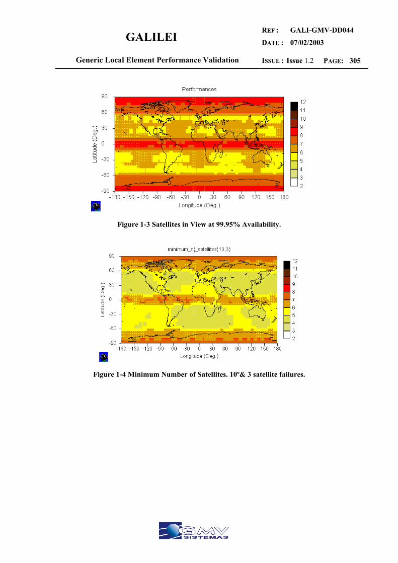
GALILEI REF :
DATE :
GALI-GMV-DD044
07/02/2003
Generic Local Element Performance Validation ISSUE : Issue 1.2 PAGE: 305
Figure 1-3 Satellites in View at 99.95% Availability.
Figure 1-4 Minimum Number of Satellites. 10º& 3 satellite failures.

GALILEI REF :
DATE :
GALI-GMV-DD044
07/02/2003
Generic Local Element Performance Validation ISSUE : Issue 1.2 PAGE: 306
Figure 1-5 Maximum Outage in minutes.
Figure 1-6 Maximum VDOP for 0 satellite failure case (10º&99.95 Avail.)
Figure 1-7 Maximum VDOP for 1 satellite failure case (10º&99.95 Avail.)
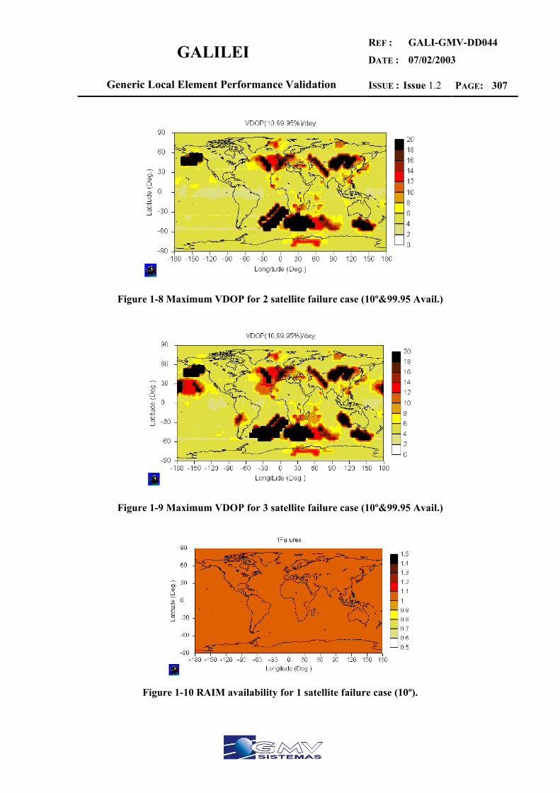
GALILEI REF :
DATE :
GALI-GMV-DD044
07/02/2003
Generic Local Element Performance Validation ISSUE : Issue 1.2 PAGE: 307
Figure 1-8 Maximum VDOP for 2 satellite failure case (10º&99.95 Avail.)
Figure 1-9 Maximum VDOP for 3 satellite failure case (10º&99.95 Avail.)
Figure 1-10 RAIM availability for 1 satellite failure case (10º).

GALILEI REF :
DATE :
GALI-GMV-DD044
07/02/2003
Generic Local Element Performance Validation ISSUE : Issue 1.2 PAGE: 308
Figure 1-11 RAIM availability for 2 satellite failure case (10º).
Figure 1-12 RAIM availability for 3 satellite failure case (10º).
1.1 CONCLUSIONS
Local performances were introduced on the previous section (Environmental Constraint impact). As can be seen, the achievement of the required performances is guaranteed by using the elements on table 6.4. Necessary elements are highlighted on the table. Substitutive elements help to the improvement of the performances.
Availability: refer to the mentioned section for further details. According to the GALILEO service definition (section 2, Positioning Services) the mean availability over lifetime is defined to be greater than 99.95% -full earth coverage. Improvement on this parameter can be obtained by means of considering additional SBEN systems like GPS but they are not strictly necessary. Simulations agree with availability parameter. Accuracy: in order to deal with the accuracy performance a DRS is needed. Differential phase-smoothing techniques might be applied. To reach high level
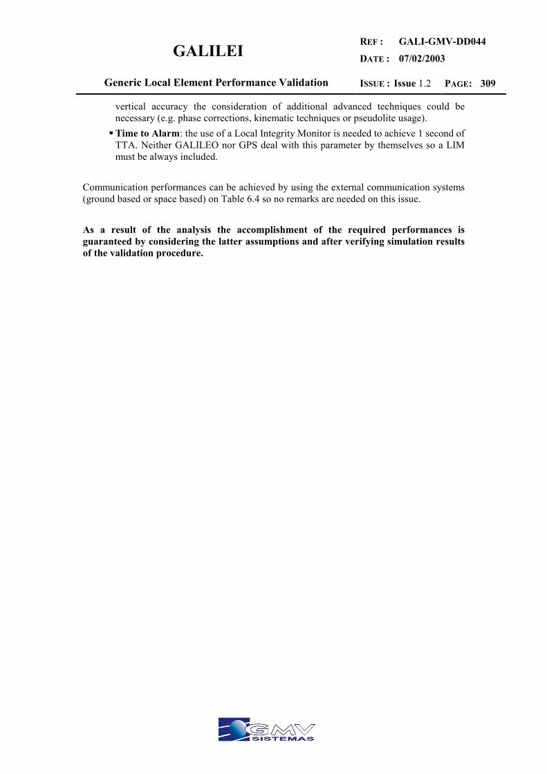
GALILEI REF :
DATE :
GALI-GMV-DD044
07/02/2003
Generic Local Element Performance Validation ISSUE : Issue 1.2 PAGE: 309
vertical accuracy the consideration of additional advanced techniques could be necessary (e.g. phase corrections, kinematic techniques or pseudolite usage). Time to Alarm: the use of a Local Integrity Monitor is needed to achieve 1 second of TTA. Neither GALILEO nor GPS deal with this parameter by themselves so a LIM must be always included.
Communication performances can be achieved by using the external communication systems (ground based or space based) on Table 6.4 so no remarks are needed on this issue. As a result of the analysis the accomplishment of the required performances is guaranteed by considering the latter assumptions and after verifying simulation results of the validation procedure.
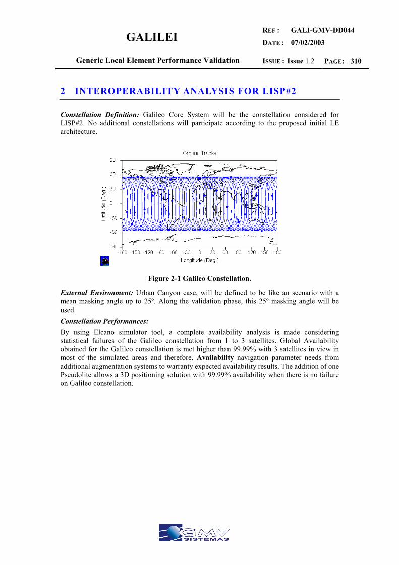
GALILEI REF :
DATE :
GALI-GMV-DD044
07/02/2003
Generic Local Element Performance Validation ISSUE : Issue 1.2 PAGE: 310
2 INTEROPERABILITY ANALYSIS FOR LISP#2
Constellation Definition: Galileo Core System will be the constellation considered for LISP#2. No additional constellations will participate according to the proposed initial LE architecture.
Figure 2-1 Galileo Constellation.
External Environment: Urban Canyon case, will be defined to be like an scenario with a mean masking angle up to 25º. Along the validation phase, this 25º masking angle will be used. Constellation Performances: By using Elcano simulator tool, a complete availability analysis is made considering statistical failures of the Galileo constellation from 1 to 3 satellites. Global Availability obtained for the Galileo constellation is met higher than 99.99% with 3 satellites in view in most of the simulated areas and therefore, Availability navigation parameter needs from additional augmentation systems to warranty expected availability results. The addition of one Pseudolite allows a 3D positioning solution with 99.99% availability when there is no failure on Galileo constellation.
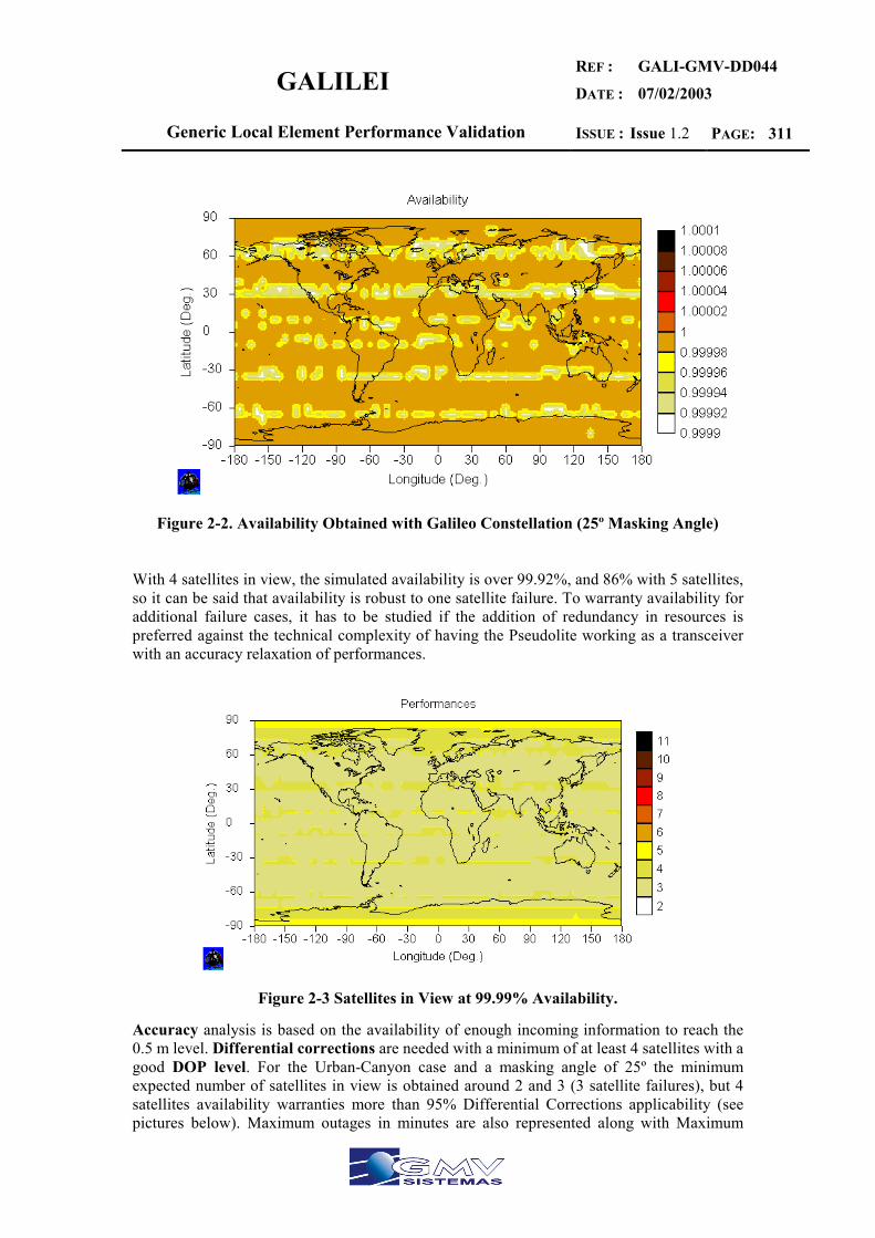
GALILEI REF :
DATE :
GALI-GMV-DD044
07/02/2003
Generic Local Element Performance Validation ISSUE : Issue 1.2 PAGE: 311
Figure 2-2. Availability Obtained with Galileo Constellation (25º Masking Angle)
With 4 satellites in view, the simulated availability is over 99.92%, and 86% with 5 satellites, so it can be said that availability is robust to one satellite failure. To warranty availability for additional failure cases, it has to be studied if the addition of redundancy in resources is preferred against the technical complexity of having the Pseudolite working as a transceiver with an accuracy relaxation of performances.
Figure 2-3 Satellites in View at 99.99% Availability.
Accuracy analysis is based on the availability of enough incoming information to reach the 0.5 m level. Differential corrections are needed with a minimum of at least 4 satellites with a good DOP level. For the Urban-Canyon case and a masking angle of 25º the minimum expected number of satellites in view is obtained around 2 and 3 (3 satellite failures), but 4 satellites availability warranties more than 95% Differential Corrections applicability (see pictures below). Maximum outages in minutes are also represented along with Maximum
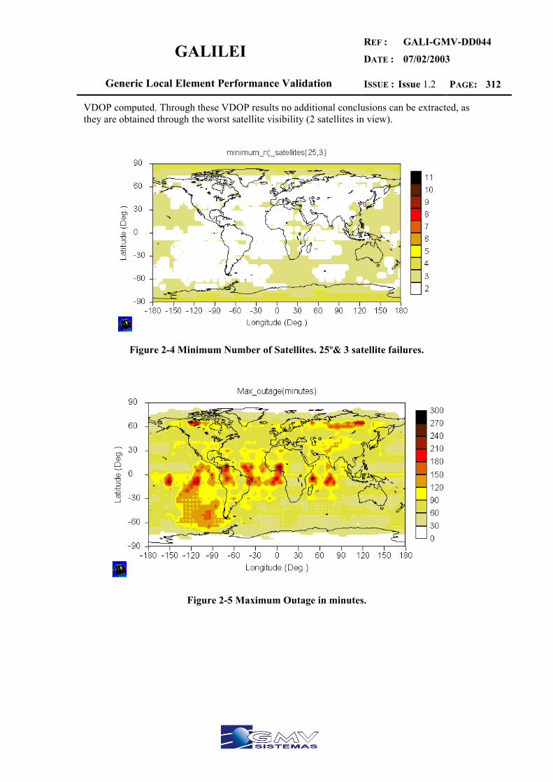
GALILEI REF :
DATE :
GALI-GMV-DD044
07/02/2003
Generic Local Element Performance Validation ISSUE : Issue 1.2 PAGE: 312
VDOP computed. Through these VDOP results no additional conclusions can be extracted, as they are obtained through the worst satellite visibility (2 satellites in view).
Figure 2-4 Minimum Number of Satellites. 25º& 3 satellite failures.
Figure 2-5 Maximum Outage in minutes.

GALILEI REF :
DATE :
GALI-GMV-DD044
07/02/2003
Generic Local Element Performance Validation ISSUE : Issue 1.2 PAGE: 313
Figure 2-6 Maximum VDOP for 0 satellite failure case (25º&99.99 Avail.)
In short two main effects should be considered to: Satellite geometry and Multipath effect. The Pseudolite sub-element provided in the LE architecture, has an immediate benefit to the geometry of the constellation, and should lead to achieve the 0.5 m level of accuracy in the horizontal and vertical planes by using phase smoothing techniques. Multipath reduction techniques have to be used. LE Radial Range Scope is dependant on the final application environment and on the final affordable costs. For Urban Canyon environment distances of applicability of 10 Km can be achieved as said along the current validation document if constellation availability is maintained. For complex environment geometries particular studies can determine i.e. the minimum number of Pseudolites needed in each local area scope. LISP#2 tolerance to multipath is really low due to low constellation availability, so LE Radial Range Scope should depend on this restriction. For the TTA parameter, only to remark that RAIM algorithms cannot be applied due to the low satellite constellation visibility for LISP#2. Because of this and the 1-second TTA restriction, LIM module is strictly needed.

GALILEI REF :
DATE :
GALI-GMV-DD044
07/02/2003
Generic Local Element Performance Validation ISSUE : Issue 1.2 PAGE: 314
Figure 2-7 RAIM availability for 0 satellite failure case (25º).
Figure 2-8 RAIM availability for 1 satellite failure case (25º).
Taken into account above conclusions, Navigation parameters are considered validated. Communication parameters will require choosing between some of the proposed communication systems studied in the Annexes. Industry has already technologically validated the annexed communication systems and several possibilities are available to be implemented in concrete applications. Therefore LE architecture for LISP#2 can be considered successfully validated.

GALILEI REF :
DATE :
GALI-GMV-DD044
07/02/2003
Generic Local Element Performance Validation ISSUE : Issue 1.2 PAGE: 315
2.1 CONCLUSIONS
Local performances were introduced on the previous section (Environmental Constraint impact). As can be seen, the achievement of the required performances is guaranteed by using the elements on table 7.4. Necessary elements are highlighted on the table. Substitutive elements help to the improvement of the performances.
Availability: Simulations performed agree with availability parameter through the addition of new sources of SIS availability like Pseudolites or the inclusion of GPS constellation. In LISP#2, pseudolite is preferred to enhance final geometry of the received constellation and warranty a 100% of availability of pseudolite signal in the local area.
Accuracy: in order to deal with the accuracy performance DRS and PL sub-elements are needed. The number of pseudolites needed have a direct dependency with the geometry problem in terms of availability to process accurate algorithms.
Time To Alarm: the use of a Local Integrity Monitor is needed to achieve 1 second of TTA. Neither GALILEO nor GPS deal with this parameter by themselves so a LIM must be always included.
Communication performances can be achieved by using the external communication systems (ground based or space based) on Table 7.4 so no remarks are needed on this issue. As a result of the analysis the accomplishment of the required performances is guaranteed by considering the latter assumptions and after verifying simulation results of the validation procedure.
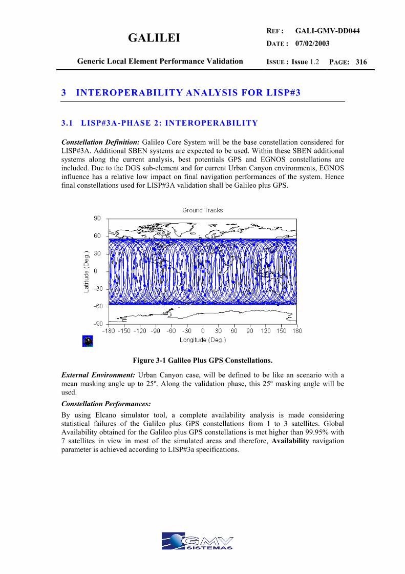
GALILEI REF :
DATE :
GALI-GMV-DD044
07/02/2003
Generic Local Element Performance Validation ISSUE : Issue 1.2 PAGE: 316
3 INTEROPERABILITY ANALYSIS FOR LISP#3
3.1 LISP#3A-PHASE 2: INTEROPERABILITY
Constellation Definition: Galileo Core System will be the base constellation considered for LISP#3A. Additional SBEN systems are expected to be used. Within these SBEN additional systems along the current analysis, best potentials GPS and EGNOS constellations are included. Due to the DGS sub-element and for current Urban Canyon environments, EGNOS influence has a relative low impact on final navigation performances of the system. Hence final constellations used for LISP#3A validation shall be Galileo plus GPS.
Figure 3-1 Galileo Plus GPS Constellations.
External Environment: Urban Canyon case, will be defined to be like an scenario with a mean masking angle up to 25º. Along the validation phase, this 25º masking angle will be used. Constellation Performances: By using Elcano simulator tool, a complete availability analysis is made considering statistical failures of the Galileo plus GPS constellations from 1 to 3 satellites. Global Availability obtained for the Galileo plus GPS constellations is met higher than 99.95% with 7 satellites in view in most of the simulated areas and therefore, Availability navigation parameter is achieved according to LISP#3a specifications.
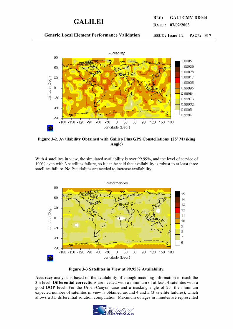
GALILEI REF :
DATE :
GALI-GMV-DD044
07/02/2003
Generic Local Element Performance Validation ISSUE : Issue 1.2 PAGE: 317
Figure 3-2. Availability Obtained with Galileo Plus GPS Constellations (25º Masking
Angle)
With 4 satellites in view, the simulated availability is over 99.99%, and the level of service of 100% even with 3 satellites failure, so it can be said that availability is robust to at least three satellites failure. No Pseudolites are needed to increase availability.
Figure 3-3 Satellites in View at 99.95% Availability.
Accuracy analysis is based on the availability of enough incoming information to reach the 3m level. Differential corrections are needed with a minimum of at least 4 satellites with a good DOP level. For the Urban-Canyon case and a masking angle of 25º the minimum expected number of satellites in view is obtained around 4 and 5 (3 satellite failures), which allows a 3D differential solution computation. Maximum outages in minutes are represented
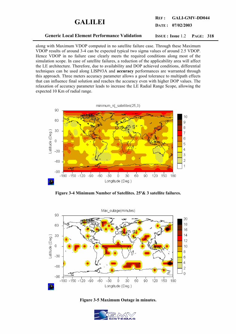
GALILEI REF :
DATE :
GALI-GMV-DD044
07/02/2003
Generic Local Element Performance Validation ISSUE : Issue 1.2 PAGE: 318
along with Maximum VDOP computed in no satellite failure case. Through these Maximum VDOP results of around 3-4 can be expected typical two sigma values of around 2.5 VDOP. Hence VDOP in no failure case clearly meets the required conditions along most of the simulation scope. In case of satellite failures, a reduction of the applicability area will affect the LE architecture. Therefore, due to availability and DOP achieved conditions, differential techniques can be used along LISP#3A and accuracy performances are warranted through this approach. Three meters accuracy parameter allows a good tolerance to multipath effects that can influence final solution and reaches the accuracy even with higher DOP values. The relaxation of accuracy parameter leads to increase the LE Radial Range Scope, allowing the expected 10 Km of radial range.
Figure 3-4 Minimum Number of Satellites. 25º& 3 satellite failures.
Figure 3-5 Maximum Outage in minutes.
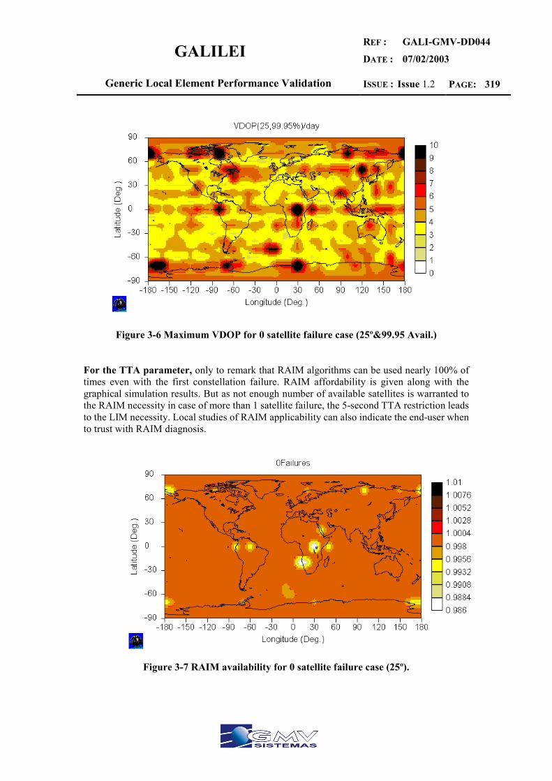
GALILEI REF :
DATE :
GALI-GMV-DD044
07/02/2003
Generic Local Element Performance Validation ISSUE : Issue 1.2 PAGE: 319
Figure 3-6 Maximum VDOP for 0 satellite failure case (25º&99.95 Avail.)
For the TTA parameter, only to remark that RAIM algorithms can be used nearly 100% of times even with the first constellation failure. RAIM affordability is given along with the graphical simulation results. But as not enough number of available satellites is warranted to the RAIM necessity in case of more than 1 satellite failure, the 5-second TTA restriction leads to the LIM necessity. Local studies of RAIM applicability can also indicate the end-user when to trust with RAIM diagnosis.
Figure 3-7 RAIM availability for 0 satellite failure case (25º).

GALILEI REF :
DATE :
GALI-GMV-DD044
07/02/2003
Generic Local Element Performance Validation ISSUE : Issue 1.2 PAGE: 320
Figure 3-8 RAIM availability for 1 satellite failure case (25º).
Figure 3-9 RAIM availability for 2 satellite failure case (25º).
Taken into account above conclusions, Navigation parameters are considered validated. Communication parameters will require choosing between some of the proposed communication systems studied in the Annexes. Industry has already technologically validated the annexed communication systems and several possibilities are available to be implemented in concrete applications. Therefore LE architecture for LISP#3A can be considered successfully validated.

GALILEI REF :
DATE :
GALI-GMV-DD044
07/02/2003
Generic Local Element Performance Validation ISSUE : Issue 1.2 PAGE: 321
3.2 LISP#3BPHASE 2: INTEROPERABILITY
Constellation Definition: Galileo Core System will be the base constellation considered for LISP#3B. Additional SBEN systems are expected to be used. Within these SBEN additional systems along the current analysis, best potentials GPS and EGNOS constellations are included. Due to the high probability of EGNOS SIS obstruction for Indoor environments, EGNOS influence has a relative low impact on final navigation performances of the system. Hence final constellations used for LISP#3B validation shall be Galileo plus GPS.
Figure 3-10 Galileo Plus GPS Constellations.
External Environment: Indoor case, is a newer potential environment for applications. Initially is defined in GALI-ASMUK-DD024, issue 1.1 from a general point of view to meet the requested performances for users having a masking angle better than 25º (same as Urban Canyon). From this point of view, by using 25º restriction LISP#3B, availability is the same than LISP#3A case and where DRS sub-element is changed with a Pseudolite acting as a reference station. This restriction is general but not realistic enough. Along this validation procedure, it is needed to define some additional restrictions, to extract availability values, and then proceed with the accuracy analysis. This analysis will be at a functional level as Indoor technologies are being currently investigated and Indoor environments depends strongly on each particular case. Indoor Study Case: Starting from the scratch, indoor environments are considered more restrictive than Urban Canyons. At a general level of description, it can be said that SIS will be received at lower C/No dB with a very important multipath component, as no direct line of sight is normally possible. Technology needs from very sensitive constellation receivers and at the same time capable to avoid the near-far effect of possible transmission sources (Pseudolites and others…). In short, the received constellation for an indoor environment should be at best like the Urban Canyon case (25º Masking Angle) but with some additional satellite losses. A quick availability study should help to determine an availability model for indoor scenarios. Making use of Elcano tool the following results have been obtained of number of satellites in
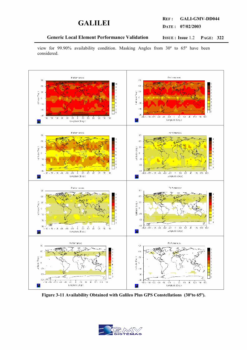
GALILEI REF :
DATE :
GALI-GMV-DD044
07/02/2003
Generic Local Element Performance Validation ISSUE : Issue 1.2 PAGE: 322
view for 99.90% availability condition. Masking Angles from 30º to 65º have been considered.
Figure 3-11 Availability Obtained with Galileo Plus GPS Constellations (30ºto 65º).

GALILEI REF :
DATE :
GALI-GMV-DD044
07/02/2003
Generic Local Element Performance Validation ISSUE : Issue 1.2 PAGE: 323
Masking Angle Mean of Satellites In View European & USA Potential
30 6-7 7 Optimistic 35 5-6 6 Optimistic 40 3-4 4 Potential 45 2-3 3 Best 50 1-2 2 No 55 0-1 1 No 60 0-1 0 No 65 0 0 No
Table 3.1: Potentials for availability to Indoor approach.
In the table above can be extracted the mean of satellites in View for each masking angle simulation. Mean of satellites for the European and USA areas are also shown. Potentials to Indoor approach are pinpointed at 40-45º condition of masking angle. So we will consider Indoor approach to the environment whose masking angle could range from 25º in an optimistic case similar to Urban Canyon approach, but in general with additional signal losses due to presence of obstacles, that leads us to a mean masking angle of 45º (TBD) at a maximum. Environments with greater masking angles will be considered not satellite navigable, and other techniques will be needed to achieve navigation. Constellation Performances: By using Elcano simulator tool, the availability analysis is made considering statistical failures of the Galileo plus GPS constellations from 1 to 3 satellites. Global Availability obtained for the Galileo plus GPS constellations is met higher than 99.90% with 2-3 satellites in view in most of the simulated areas even with 1 satellite failure.
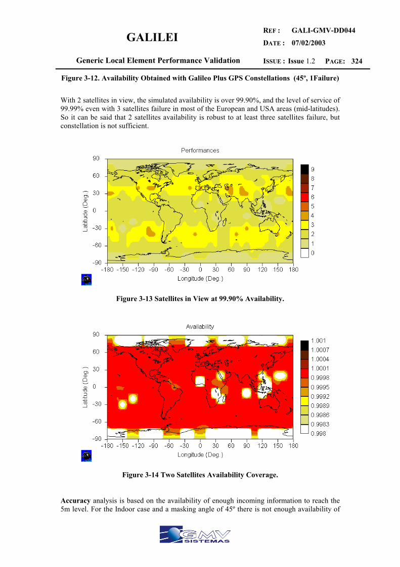
GALILEI REF :
DATE :
GALI-GMV-DD044
07/02/2003
Generic Local Element Performance Validation ISSUE : Issue 1.2 PAGE: 324
Figure 3-12. Availability Obtained with Galileo Plus GPS Constellations (45º, 1Failure)
With 2 satellites in view, the simulated availability is over 99.90%, and the level of service of 99.99% even with 3 satellites failure in most of the European and USA areas (mid-latitudes). So it can be said that 2 satellites availability is robust to at least three satellites failure, but constellation is not sufficient.
Figure 3-13 Satellites in View at 99.90% Availability.
Figure 3-14 Two Satellites Availability Coverage.
Accuracy analysis is based on the availability of enough incoming information to reach the 5m level. For the Indoor case and a masking angle of 45º there is not enough availability of
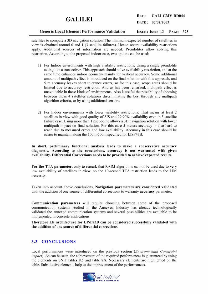
GALILEI REF :
DATE :
GALI-GMV-DD044
07/02/2003
Generic Local Element Performance Validation ISSUE : Issue 1.2 PAGE: 325
satellites to compute a 3D navigation solution. The minimum expected number of satellites in view is obtained around 0 and 1 (3 satellite failures). Hence severe availability restrictions apply. Additional sources of information are needed: Pseudolites allow solving this restriction. According to the proposed indoor case, two options can be used:
1) For Indoor environments with high visibility restrictions: Using a single pseudolite acting like a transceiver. This approach should solve availability restriction, and at the same time enhances indoor geometry mainly for vertical accuracy. Some additional amount of multipath effect is introduced on the final solution with this approach, and 5 m accuracy leaves short tolerance errors, so for this case, scope areas should be limited due to accuracy restriction. And as has been remarked, multipath effect is unavoidable in these kinds of environments. Also is useful the possibility of choosing between those 4 satellites solutions discriminating the best through any multipath algorithm criteria, or by using additional sensors.
2) For Indoor environments with lower visibility restrictions: That means at least 2
satellites in view with good quality of SIS and 99.90% availability even in 5 satellite failure case. Using more than 1 pseudolite allows a 3D navigation solution with lower multipath impact on final solution. For this case 5 meters accuracy is also hard to reach due to measured errors and low availability. Accuracy in this case should be easier to maintain along the 100m-500m specified for LISP#3B.
In short, preliminary functional analysis leads to make a conservative accuracy diagnostic. According to the conclusions, accuracy is not warranted with given availability. Differential Corrections needs to be provided to achieve expected results. For the TTA parameter, only to remark that RAIM algorithms cannot be used due to very low availability of satellites in view, so the 10-second TTA restriction leads to the LIM necessity. Taken into account above conclusions, Navigation parameters are considered validated with the addition of one source of differential corrections to warranty accuracy parameter. Communication parameters will require choosing between some of the proposed communication systems studied in the Annexes. Industry has already technologically validated the annexed communication systems and several possibilities are available to be implemented in concrete applications. Therefore LE architecture for LISP#3B can be considered successfully validated with the addition of one source of differential corrections.
3.3 CONCLUSIONS
Local performances were introduced on the previous section (Environmental Constraint impact). As can be seen, the achievement of the required performances is guaranteed by using the elements on SNIF tables 8.5 and table 8.8. Necessary elements are highlighted on the table. Substitutive elements help to the improvement of the performances.
GALILEI REF :
DATE :
GALI-GMV-DD044
07/02/2003
Generic Local Element Performance Validation ISSUE : Issue 1.2 PAGE: 326
Availability: LISP#3A reaches availability with both Galileo+GPS constellations. LISP#3B needs from additional sources (like PL sub-elements) to reach availability condition. Accuracy: in order to deal with the accuracy performance DGS/DRS sub-elements are needed. Also the introduction of PL in LISP#3B enhances geometry problem mainly in terms of vertical accuracy. Time To Alarm: the use of a Local Integrity Monitor is needed to achieve 5 and 10 second of TTA.
Communication performances can be achieved by using the external communication systems (ground based or space based) on Table 8.5 and Table 8.8 so no remarks are needed on this issue. As a result of the analysis the accomplishment of the required performances is guaranteed for LISP#3A and LISP#3B by considering the latter assumptions and corrections and after verifying simulation results of the validation procedure.
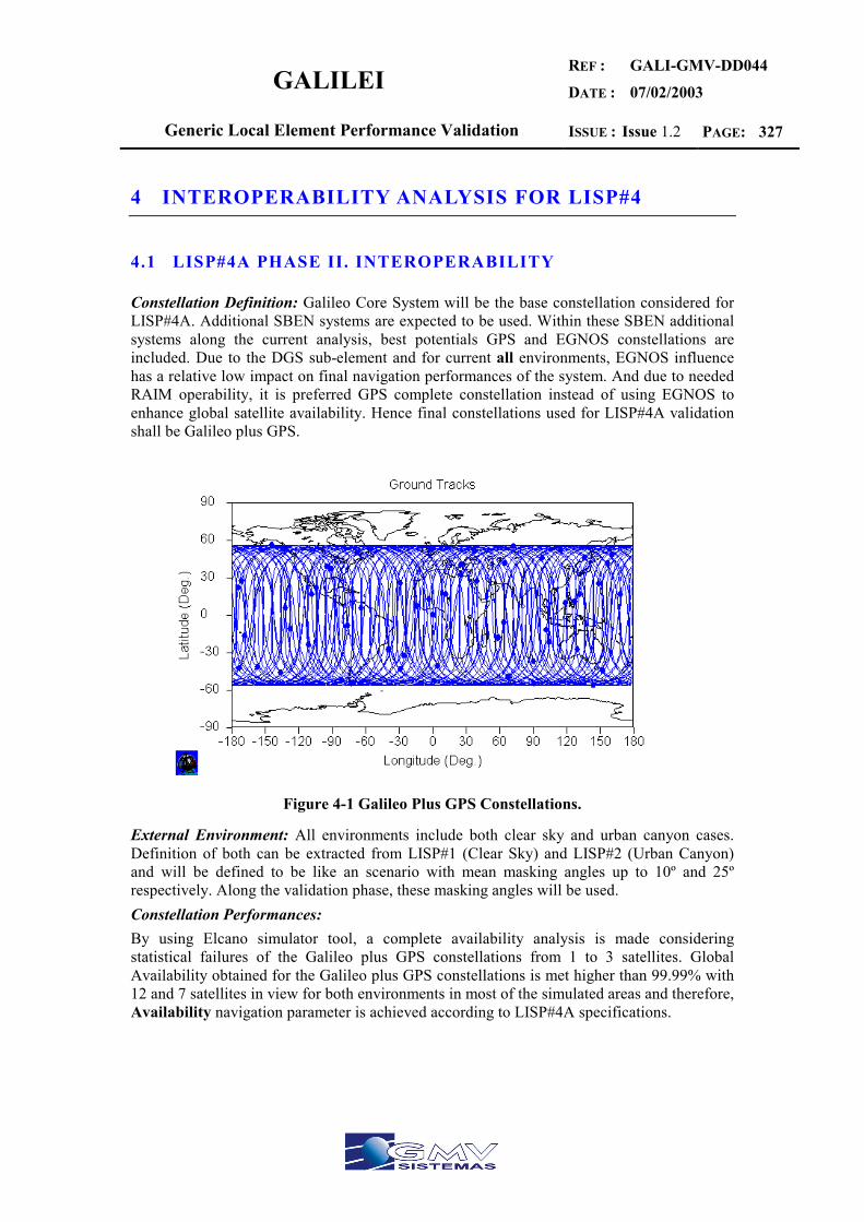
GALILEI REF :
DATE :
GALI-GMV-DD044
07/02/2003
Generic Local Element Performance Validation ISSUE : Issue 1.2 PAGE: 327
4 INTEROPERABILITY ANALYSIS FOR LISP#4
4.1 LISP#4A PHASE II. INTEROPERABILITY
Constellation Definition: Galileo Core System will be the base constellation considered for LISP#4A. Additional SBEN systems are expected to be used. Within these SBEN additional systems along the current analysis, best potentials GPS and EGNOS constellations are included. Due to the DGS sub-element and for current all environments, EGNOS influence has a relative low impact on final navigation performances of the system. And due to needed RAIM operability, it is preferred GPS complete constellation instead of using EGNOS to enhance global satellite availability. Hence final constellations used for LISP#4A validation shall be Galileo plus GPS.
Figure 4-1 Galileo Plus GPS Constellations.
External Environment: All environments include both clear sky and urban canyon cases. Definition of both can be extracted from LISP#1 (Clear Sky) and LISP#2 (Urban Canyon) and will be defined to be like an scenario with mean masking angles up to 10º and 25º respectively. Along the validation phase, these masking angles will be used. Constellation Performances: By using Elcano simulator tool, a complete availability analysis is made considering statistical failures of the Galileo plus GPS constellations from 1 to 3 satellites. Global Availability obtained for the Galileo plus GPS constellations is met higher than 99.99% with 12 and 7 satellites in view for both environments in most of the simulated areas and therefore, Availability navigation parameter is achieved according to LISP#4A specifications.

GALILEI REF :
DATE :
GALI-GMV-DD044
07/02/2003
Generic Local Element Performance Validation ISSUE : Issue 1.2 PAGE: 328
Figure 4-2. Availability Obtained with Galileo Plus GPS Constellations (10º-25º)
With 4 satellites in view, the simulated availability is over 99.99%, and the level of service of near 99.90% even with 3 satellites failure, so it can be said that availability is robust to at least three satellites failure.
Figure 4-3 Satellites in View at 99.99% Availability (10º-25º).
Accuracy analysis is based on the availability of enough incoming information to reach the 0.005m level. It is stated for this Millimetric approach, than can be achieved through the use of the Galileo Global TCAR service. Phase correction techniques and such a high accuracy should require enough satellite availability and very good DOP values. Redundancy on satellite constellation will be needed, and only 4 satellites in view are insufficient. Applying the conservative criteria of having 8+1=9 satellites (TBD) (2x3D solutions+1spare) will lead to have enough redundant information to potentially achieve final accuracy parameter. For the Clear Sky case and a masking angle of 10º the minimum expected number of satellites in view is obtained around 7 and 8 (3 satellite failures), which allows apply these high performance techniques. Simulated VDOP maximum values are around 2-3. Hence VDOP in 3 satellites failure case meets the required conditions along most of the simulation scope. Therefore, due to availability and DOP achieved conditions, LISP#4A accuracy parameters are potentially feasible to be reached. For the Urban Canyon case and a masking angle of 25º the minimum expected number of satellites in view is obtained around 4 and 5 (3 satellite failures), which does not allow applying these high performance techniques. Therefore, due to limited availability LISP#4A should need from additional availability sources to work in Urban Canyon environments. In terms of navigation solution, LISP#4A accuracy parameters are potentially not feasible to be reached for the urban canyon case with the proposed architecture.

GALILEI REF :
DATE :
GALI-GMV-DD044
07/02/2003
Generic Local Element Performance Validation ISSUE : Issue 1.2 PAGE: 329
Figure 4-4 Minimum Number of Satellites. 10º-25º& 3 satellite failures.
For the TTA parameter, only to remark that RAIM algorithms can be used nearly 100% of times for the Clear Sky case even with three constellation failures. RAIM affordability is given along with the graphical simulation results. Even with 5 satellite failures RAIM it is expected to be near 100% of usability. With this information LIM could be avoided and the 5-second TTA restriction is covered along with RAIM availability. For the Urban Canyon case RAIM algorithms can be used nearly 100% of times even with the first constellation failure. But as not enough number of available satellites is warranted to the RAIM necessity in case of more than 1 satellite failure, the 5-second TTA restriction leads to the LIM necessity.
Figure 4-5 RAIM availability for 3-2 satellite failure case (10º-25º).
Taken into account above conclusions, Navigation parameters are considered validated for the Clear Sky case. Urban Canyon case should need from additional sources of availability to have redundancy on the information to be processed. Communication parameters will require choosing between some of the proposed communication systems studied in the Annexes. Industry has already technologically validated the annexed communication systems and several possibilities are available to be implemented in concrete applications. Therefore LE architecture for LISP#4A can be considered successfully validated for the Clear Sky case.

GALILEI REF :
DATE :
GALI-GMV-DD044
07/02/2003
Generic Local Element Performance Validation ISSUE : Issue 1.2 PAGE: 330
4.2 LISP#4B PHASE II. INTEROPERABILITY
Constellation Definition: Galileo Core System will be the base constellation considered for LISP#4B. Additional SBEN systems are expected to be used. Within these SBEN additional systems along the current analysis, best potentials GPS and EGNOS constellations are included. Due to the DGS sub-element and for current Clear Sky environments, EGNOS influence has a relative low impact on final navigation accuracy performances of the system. And due to needed RAIM operability, it is preferred GPS complete constellation instead of using EGNOS to enhance global satellite availability. Hence final constellations used for LISP#4B validation shall be Galileo plus GPS.
Figure 4-6 Galileo Plus GPS Constellations.
External Environment: Clear Sky case, will be defined to be like an scenario with a mean masking angle up to 10º. Along the validation phase, this 10º masking angle will be used. Constellation Performances: By using Elcano simulator tool, a complete availability analysis is made considering statistical failures of the Galileo plus GPS constellations from 1 to 3 satellites. Global Availability obtained for the Galileo plus GPS constellations is met higher than 99.90% with 12-13 satellites in view in most of the simulated areas and therefore, Availability navigation parameter is achieved according to LISP#4B specifications.
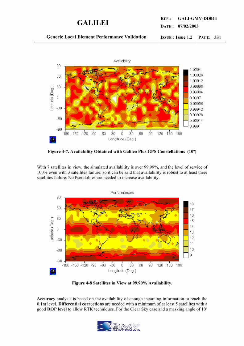
GALILEI REF :
DATE :
GALI-GMV-DD044
07/02/2003
Generic Local Element Performance Validation ISSUE : Issue 1.2 PAGE: 331
Figure 4-7. Availability Obtained with Galileo Plus GPS Constellations (10º)
With 7 satellites in view, the simulated availability is over 99.99%, and the level of service of 100% even with 3 satellites failure, so it can be said that availability is robust to at least three satellites failure. No Pseudolites are needed to increase availability.
Figure 4-8 Satellites in View at 99.90% Availability.
Accuracy analysis is based on the availability of enough incoming information to reach the 0.1m level. Differential corrections are needed with a minimum of at least 5 satellites with a good DOP level to allow RTK techniques. For the Clear Sky case and a masking angle of 10º
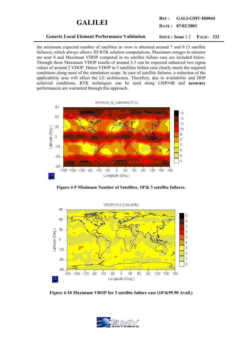
GALILEI REF :
DATE :
GALI-GMV-DD044
07/02/2003
Generic Local Element Performance Validation ISSUE : Issue 1.2 PAGE: 332
the minimum expected number of satellites in view is obtained around 7 and 8 (3 satellite failures), which always allows 3D RTK solution computations. Maximum outages in minutes are near 0 and Maximum VDOP computed in no satellite failure case are included below. Through these Maximum VDOP results of around 2-3 can be expected enhanced two sigma values of around 2 VDOP. Hence VDOP in 3 satellites failure case clearly meets the required conditions along most of the simulation scope. In case of satellite failures, a reduction of the applicability area will affect the LE architecture. Therefore, due to availability and DOP achieved conditions, RTK techniques can be used along LISP#4B and accuracy performances are warranted through this approach.
Figure 4-9 Minimum Number of Satellites. 10º& 3 satellite failures.
Figure 4-10 Maximum VDOP for 3 satellite failure case (10º&99.90 Avail.)
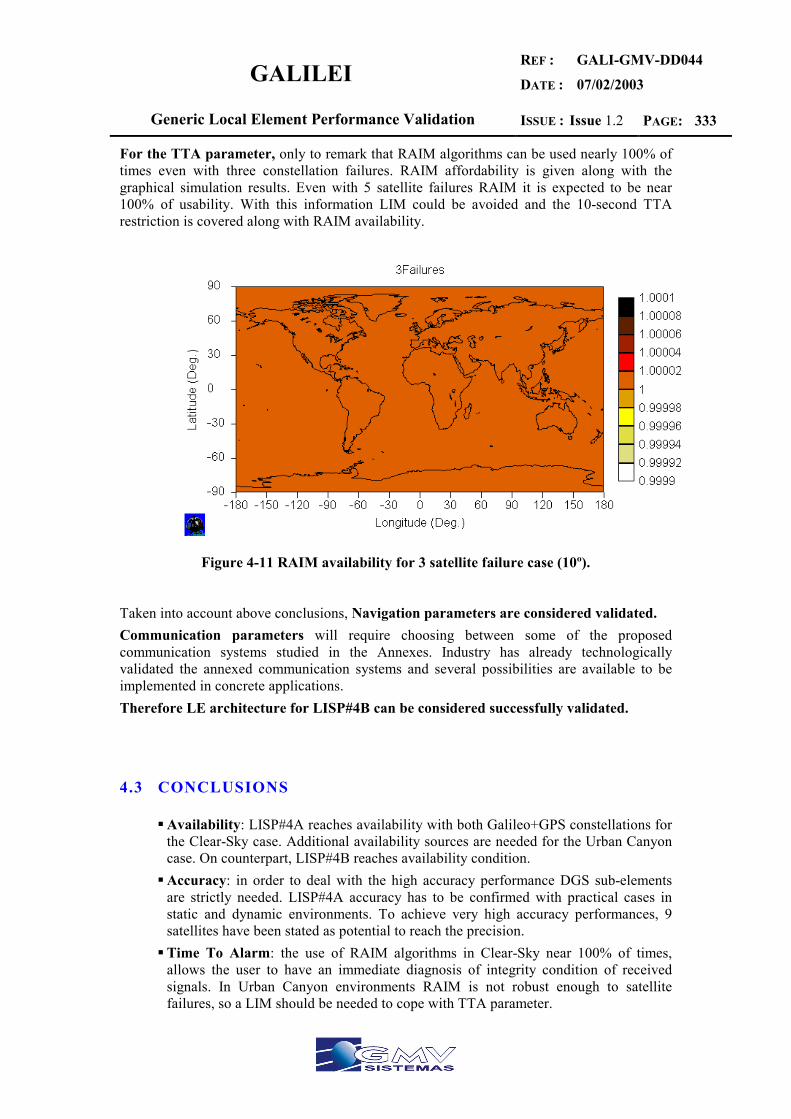
GALILEI REF :
DATE :
GALI-GMV-DD044
07/02/2003
Generic Local Element Performance Validation ISSUE : Issue 1.2 PAGE: 333
For the TTA parameter, only to remark that RAIM algorithms can be used nearly 100% of times even with three constellation failures. RAIM affordability is given along with the graphical simulation results. Even with 5 satellite failures RAIM it is expected to be near 100% of usability. With this information LIM could be avoided and the 10-second TTA restriction is covered along with RAIM availability.
Figure 4-11 RAIM availability for 3 satellite failure case (10º).
Taken into account above conclusions, Navigation parameters are considered validated. Communication parameters will require choosing between some of the proposed communication systems studied in the Annexes. Industry has already technologically validated the annexed communication systems and several possibilities are available to be implemented in concrete applications. Therefore LE architecture for LISP#4B can be considered successfully validated.
4.3 CONCLUSIONS
Availability: LISP#4A reaches availability with both Galileo+GPS constellations for the Clear-Sky case. Additional availability sources are needed for the Urban Canyon case. On counterpart, LISP#4B reaches availability condition. Accuracy: in order to deal with the high accuracy performance DGS sub-elements are strictly needed. LISP#4A accuracy has to be confirmed with practical cases in static and dynamic environments. To achieve very high accuracy performances, 9 satellites have been stated as potential to reach the precision. Time To Alarm: the use of RAIM algorithms in Clear-Sky near 100% of times, allows the user to have an immediate diagnosis of integrity condition of received signals. In Urban Canyon environments RAIM is not robust enough to satellite failures, so a LIM should be needed to cope with TTA parameter.

GALILEI REF :
DATE :
GALI-GMV-DD044
07/02/2003
Generic Local Element Performance Validation ISSUE : Issue 1.2 PAGE: 334
As a result of the analysis the accomplishment of the required performances is guaranteed for LISP#4A and LISP#4B by considering the latter assumptions and corrections and after verifying simulation results of the validation procedure.
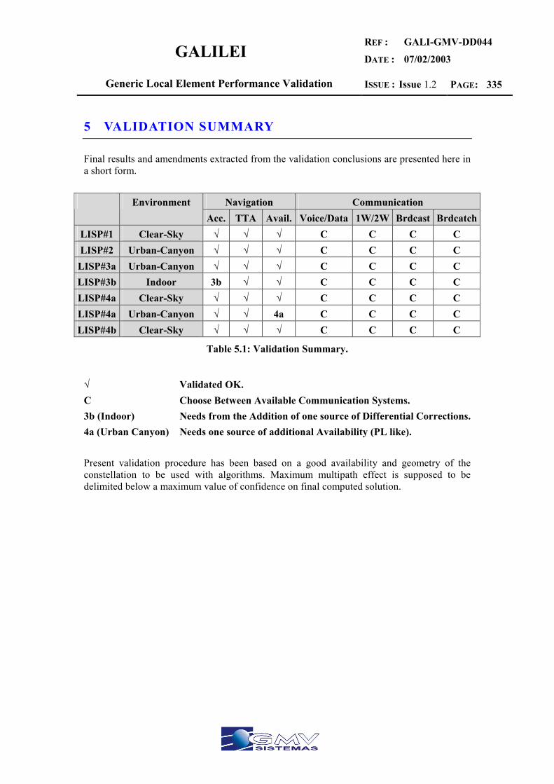
GALILEI REF :
DATE :
GALI-GMV-DD044
07/02/2003
Generic Local Element Performance Validation ISSUE : Issue 1.2 PAGE: 335
5 VALIDATION SUMMARY
Final results and amendments extracted from the validation conclusions are presented here in a short form.
Navigation Communication Environment Acc. TTA Avail. Voice/Data 1W/2W Brdcast Brdcatch
LISP#1 Clear-Sky √ √ √ C C C C LISP#2 Urban-Canyon √ √ √ C C C C
LISP#3a Urban-Canyon √ √ √ C C C C LISP#3b Indoor 3b √ √ C C C C LISP#4a Clear-Sky √ √ √ C C C C LISP#4a Urban-Canyon √ √ 4a C C C C LISP#4b Clear-Sky √ √ √ C C C C
Table 5.1: Validation Summary.
√ Validated OK. C Choose Between Available Communication Systems. 3b (Indoor) Needs from the Addition of one source of Differential Corrections.4a (Urban Canyon) Needs one source of additional Availability (PL like). Present validation procedure has been based on a good availability and geometry of the constellation to be used with algorithms. Maximum multipath effect is supposed to be delimited below a maximum value of confidence on final computed solution.

GALILEI REF :
DATE :
GALI-GMV-DD044
07/02/2003
Generic Local Element Performance Validation ISSUE : Issue 1.2 PAGE: 336
END OF DOCUMENT

GALILEI REF :
DATE :
GALI-GMV-DD044
07/02/2003
Generic Local Element Performance Validation ISSUE : Issue 1.2 PAGE: i
DOCUMENT DISTRIBUTION From : Alfredo Catalina
Project Acronym : GALILEI Project Name : Galileo System Analysis Title : Generic Local Element Performance Validation Issue : Issue 1.2 Reference/identification : GALI-GMV-DD044 Date : 07/02/2003 Page Number : 337 File : DD044v20.doc Classification : PP WBS : C.3.G Contract : Type of Document : DD Template Name : Task C.3 DD.dot
To :
Distribution
Company Name N° Ex. Company Name N° Ex.