FY 2010-FY 2011 Biennium Economic Report of the Governor
155
FY 2010-FY 2011 Biennium Economic Report of the Governor This publication, as required by Section 4-74a of the Connecticut General Statutes, is prepared by the Office of Policy and Management. Office of the Secretary Robert L. Genuario, Secretary Michael J. Cicchetti, Deputy Secretary Budget and Financial Management Division John Bacewicz, Executive Budget Officer Barry Sullivan, Assistant Executive Budget Officer Economics, Capital, and Revenue Forecasting Thomas J. Fiore, Section Director Daniel Colter, Principal Budget Specialist Lisa M. DuBois, Budget Analyst Steven Kitowicz, Principal Budget Specialist Andrew Pels, Intern Kristin M. Wirtanen, Principal Budget Specialist Ming J. Wu, Principal Budget Specialist For information on data or analysis provided in this document or any questions or comments, please contact the Budget and Financial Management Division at (860) 418-6265. February 4, 2009 Office of Policy and Management 450 Capitol Avenue Hartford, Connecticut 06106
-
Upload
khangminh22 -
Category
Documents
-
view
0 -
download
0
Transcript of FY 2010-FY 2011 Biennium Economic Report of the Governor

FY 2010-FY 2011 Biennium Economic Report of the Governor
This publication, as required by Section 4-74a of the Connecticut General Statutes, is prepared by the Office of Policy and Management.
Office of the Secretary Robert L. Genuario, Secretary
Michael J. Cicchetti, Deputy Secretary
Budget and Financial Management Division John Bacewicz, Executive Budget Officer
Barry Sullivan, Assistant Executive Budget Officer
Economics, Capital, and Revenue Forecasting Thomas J. Fiore, Section Director
Daniel Colter, Principal Budget Specialist Lisa M. DuBois, Budget Analyst
Steven Kitowicz, Principal Budget Specialist Andrew Pels, Intern
Kristin M. Wirtanen, Principal Budget Specialist Ming J. Wu, Principal Budget Specialist
For information on data or analysis provided in this document or any questions or comments, please contact the Budget and Financial Management Division at (860) 418-6265.
February 4, 2009
Office of Policy and Management 450 Capitol Avenue
Hartford, Connecticut 06106

TABLE OF CONTENTS Page INTRODUCTION....................................................................................................................... 2 GENERAL CHARACTERISTICS ............................................................................................ 3-17 Census Information............................................................................................................... 3 Population Projections.......................................................................................................... 8 Housing................................................................................................................................... 11 EMPLOYMENT PROFILE ........................................................................................................ 18-30 Employment Estimates......................................................................................................... 18 Nonagricultural Employment ............................................................................................. 19 Manufacturing Employment ............................................................................................... 22 Nonmanufacturing Employment........................................................................................ 25 Unemployment Rate ............................................................................................................. 29 SECTOR ANALYSIS.................................................................................................................. 31-74 Energy ..................................................................................................................................... 31 Gasoline Consumption and Automotive Fuel Economy................................................. 41 Export Sector .......................................................................................................................... 45 Connecticut’s Defense Industry .......................................................................................... 53 Retail Trade in Connecticut.................................................................................................. 58 Small Business in Connecticut............................................................................................. 63 Nonfinancial Debt ................................................................................................................. 66 Savings by U.S. Households ................................................................................................ 70 PERFORMANCE INDICATORS............................................................................................. 75-93 Gross Product......................................................................................................................... 75 Productivity and Unit Labor Cost....................................................................................... 78 Value Added .......................................................................................................................... 79 Capital Expenditures ............................................................................................................ 81 Total Personal Income .......................................................................................................... 81 Per Capita Personal Income................................................................................................. 84 Per Capita Disposable Personal Income............................................................................. 87 Inflation and Its Effects on Personal Income ..................................................................... 88 Real Personal Income............................................................................................................ 89 Real Per Capita Personal Income ........................................................................................ 90 Cost of Living Index.............................................................................................................. 92 MAJOR REVENUE RAISING TAXES.................................................................................... 94-111 Personal Income Tax ............................................................................................................. 94 Sales and Use Tax .................................................................................................................. 100 Corporation Business Tax .................................................................................................... 103 Motor Fuels Tax ..................................................................................................................... 105 Other Sources ......................................................................................................................... 107 ECONOMIC ASSUMPTIONS OF THE GOVERNOR'S BUDGET .................................. 112-123 Foreign Sector ........................................................................................................................ 112 United States’ Economy........................................................................................................ 114 Connecticut's Economy ........................................................................................................ 116 REVENUE FORECAST.............................................................................................................. 124-129 IMPACT OF THE GOVERNOR'S BUDGET ON THE STATE'S ECONOMY ............... 130-135 APPENDIX ................................................................................................................................... A1-A16
i

APPENDIX Page Connecticut Resident Population Census Counts by Town.................................................. A1–A4 Major U.S. and Connecticut Economic Indicators................................................................... A5-A16 1. U.S. Economic Variables.................................................................................................... A5 2. U.S. Personal Income ......................................................................................................... A6 3. U.S. Personal Income and its Disposition....................................................................... A7 4. U.S. Employment and the Labor Force ........................................................................... A8 5. U.S. Consumer Price Indexes ........................................................................................... A9 6. Connecticut Personal Income ........................................................................................... A10 7. Connecticut Deflated Personal Income........................................................................... A11 8. Connecticut Manufacturing Employment...................................................................... A12 9. Connecticut Nonmanufacturing Employment .............................................................. A13 10. Connecticut Labor Force & Other Economic Indicators ............................................... A14 11. Connecticut Analytics........................................................................................................ A15 12. Regional Economic Indicators- Personal Income & Wages ......................................... A16
ii

E C O N O M I C R E P O R T O F T H E G O V E R N O R
2 0 0 9 - 2 0 11

Economic Report of the Governor
- 2 -
INTRODUCTION
This report fulfills the requirements of Section 4-74a of the General Statutes which stipulates that:
"Part IV of the Budget Document shall consist of the recommendations of the Governor concerning the economy and shall include an analysis of the impact of both proposed spending and proposed revenue programs on the employment, production and purchasing power of the people and industries within the State".
This report is also designed to provide a brief profile of the State of Connecticut, the economy of the State, revenues and economic assumptions that support the Governor's Budget, and an analysis of the impact of both proposed spending and proposed revenue programs on the economy of the State of Connecticut. The report will focus on eight areas including: (1) the general characteristics of the State; (2) the profile of employment in the State; (3) an in depth analysis of important Connecticut Sectors; (4) the performance indicators of three differing entities (the United States, the New England Region, and Connecticut); (5) a discussion of some of the important revenue raising taxes; (6) the economic assumptions of the Governor's Budget, including narratives on the foreign sector, the U.S. economy and the Connecticut economy, and a numerical comparison of some of the important indicators used in the preparation of the Governor's Budget; (7) the revenue forecasts of the General Fund and the Special Transportation Fund; and (8) the expected impact of the Governor's Budget on the economy of the State of Connecticut.
Economic Report of the Governor
- 3 -
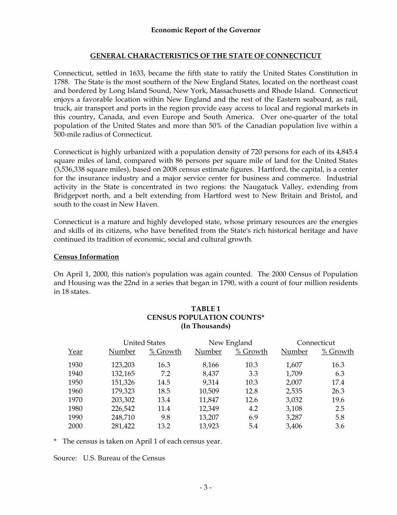
GENERAL CHARACTERISTICS OF THE STATE OF CONNECTICUT Connecticut, settled in 1633, became the fifth state to ratify the United States Constitution in 1788. The State is the most southern of the New England States, located on the northeast coast and bordered by Long Island Sound, New York, Massachusetts and Rhode Island. Connecticut enjoys a favorable location within New England and the rest of the Eastern seaboard, as rail, truck, air transport and ports in the region provide easy access to local and regional markets in this country, Canada, and even Europe and South America. Over one-quarter of the total population of the United States and more than 50% of the Canadian population live within a 500-mile radius of Connecticut. Connecticut is highly urbanized with a population density of 720 persons for each of its 4,845.4 square miles of land, compared with 86 persons per square mile of land for the United States (3,536,338 square miles), based on 2008 census estimate figures. Hartford, the capital, is a center for the insurance industry and a major service center for business and commerce. Industrial activity in the State is concentrated in two regions: the Naugatuck Valley, extending from Bridgeport north, and a belt extending from Hartford west to New Britain and Bristol, and south to the coast in New Haven. Connecticut is a mature and highly developed state, whose primary resources are the energies and skills of its citizens, who have benefited from the State's rich historical heritage and have continued its tradition of economic, social and cultural growth. Census Information On April 1, 2000, this nation's population was again counted. The 2000 Census of Population and Housing was the 22nd in a series that began in 1790, with a count of four million residents in 18 states.
TABLE 1 CENSUS POPULATION COUNTS*
(In Thousands)
United States New England Connecticut Year Number % Growth Number % Growth Number % Growth
1930 123,203 16.3 8,166 10.3 1,607 16.3 1940 132,165 7.2 8,437 3.3 1,709 6.3 1950 151,326 14.5 9,314 10.3 2,007 17.4 1960 179,323 18.5 10,509 12.8 2,535 26.3 1970 203,302 13.4 11,847 12.6 3,032 19.6 1980 226,542 11.4 12,349 4.2 3,108 2.5 1990 248,710 9.8 13,207 6.9 3,287 5.8 2000 281,422 13.2 13,923 5.4 3,406 3.6
* The census is taken on April 1 of each census year. Source: U.S. Bureau of the Census

Economic Report of the Governor
- 4 -
In 2000, the population totaled 281.4 million people in the 50 states and the District of Columbia. Since 1930, the population has risen in all three data series for all decades. However, during the 1970s, 1980s and 1990s, the population growth in Connecticut and New England was significantly lower than the prior three decades and lower than the nation for the recent periods. In the United States, the resident population, which excludes Armed Forces Overseas, increased from 248,709,873 in 1990 to 281,421,906 in 2000, an increase of 13.2% for the 1990s, and the greatest increase since the 1960s. New England's population increased 5.4% from 1990 to 2000, experiencing slower growth. Within New England, only Vermont and New Hampshire experienced growth significantly higher than the region. This trend is likely to continue. During the last few decades, the heavily populated states experienced a slowdown in the growth of their populations. This phenomenon was common in New England, the Middle Atlantic, the East North Central and the West North Central Regions. The fastest growing states were those in the West, the South, the Pacific and the southern portion of the Mountain regions. The apportionment of seats in the U.S. House of Representatives changed as a result of both the 1990 Census and the 2000 Census. Also, Connecticut’s federal aid levels for various grants will continue to fall as the state’s estimated population size, relative to the nation’s, decreases each year. Resident population in Connecticut, according to figures from the 2000 census, was 3,405,565 an increase of 118,449 from the 3,287,116 figure of 1990. This represented a growth of 3.6% for the decade, slower growth than was experienced by either the New England Region or the nation as a whole, for the third consecutive decade. In fact, between 1990 and 2000, the state’s growth rate was the fourth lowest in the nation. During the recession of the early 1990s, Connecticut’s population started declining as a result of the state’s weak economy, the high relative cost of living, and a softened job market which collectively made the state less attractive. The minor population losses in the early 1990s were the result of small in-migration compared to a much larger out-migration. This net out-migration is not to be confused with overall population declines, because a surplus of births and an influx of foreign migration have offset domestic out-migration in most years. The migration of population to and from Connecticut during the late 1980s and 1990s parallels the performance of the state’s economy, rising during the expansion, declining at the time of the recession, and rising again during the last few years of the 1990s. Connecticut counties experiencing faster growth during the 1990s generally were those not dominated by large urban areas. The national population is estimated monthly by the United States Bureau of the Census for total population which includes Armed Forces Overseas, resident population and civilian population. Population growth is a primary long-run determinant of the potential expansion path of the economy from both the supply and demand sides of the economy. The growth of the population and its composition have profound impacts on the labor force, education, housing, and the demand for consumer goods and services.

Economic Report of the Governor
- 5 -
TABLE 2 COUNTY POPULATION IN CONNECTICUT
1990 1990 2000 2000 Percent County Census Percent Census Percent Change Fairfield 827,645 25.2 882,567 25.9 6.6 Hartford 851,783 25.9 857,183 25.2 0.6 Litchfield 174,092 5.3 182,193 5.3 4.7 Middlesex 143,196 4.4 155,071 4.6 8.3 New Haven 804,219 24.5 824,008 24.2 2.5 New London 254,957 7.7 259,088 7.6 1.6 Tolland 128,699 3.9 136,364 4.0 6.0 Windham 102,525 3.1 109,091 3.2 6.4
TOTAL 3,287,116 100.0 3,405,565 100.0 3.6
Source: U.S. Bureau of the Census, U.S. Department of Commerce Annual estimates of population as of mid-calendar year for each state are vital for comparing standards of living through per capita income, productivity through per capita Gross State Product, or a state's private activity bond limitation which, under federal law, is capped at a level dependent upon the size of the population. Estimates are prepared by the U.S. Bureau of the Census based on the number of births and deaths as well as a variety of factors to approximate net migration changes. These factors can include Medicare enrollees, motor vehicle registrations, building permits, licensed drivers, school enrollments, etc. To comply with the Connecticut General Statutes concerning state aid to municipalities, the Department of Public Health also prepares an annual mid-year estimate of population based on the number of births, deaths and school age population.
TABLE 3 MID-YEAR POPULATION
(In Thousands)
Mid United States New England Connecticut Year Number % Growth Number % Growth Number % Growth 1999 279,040 1.2 13,838 0.8 3,386 0.6 2000 282,172 1.1 13,952 0.8 3,412 0.8 2001 285,040 1.0 14,047 0.7 3,428 0.5 2002 287,727 0.9 14,127 0.6 3,448 0.6 2003 290,211 0.9 14,181 0.4 3,468 0.6 2004 292,892 0.9 14,202 0.1 3,475 0.2 2005 295,561 0.9 14,208 0.0 3,479 0.1 2006 298,363 0.9 14,233 0.2 3,488 0.3 2007 301,290 1.0 14,259 0.2 3,490 0.1 2008 304,060 0.9 14,304 0.3 3,501 0.3
Source: U.S. Bureau of the Census, U.S. Department of Commerce
Economic Report of the Governor
- 6 -
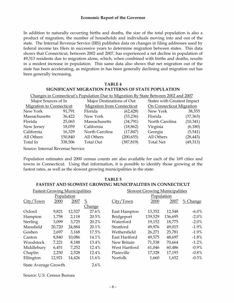
In addition to naturally occurring births and deaths, the size of the total population is also a product of migration, the number of households and individuals moving into and out of the state. The Internal Revenue Service (IRS) publishes data on changes in filing addresses used by federal income tax filers in successive years to determine migration between states. This data shows that Connecticut, between 2002 and 2007, has experienced a net decline in population of 49,313 residents due to migration alone, which, when combined with births and deaths, results in a modest increase in population. This same data also shows that net migration out of the state has been accelerating, as migration in has been generally declining and migration out has been generally increasing.
TABLE 4 SIGNIFICANT MIGRATION PATTERNS OF STATE POPULATION
Changes in Connecticut’s Population Due to Migration By State Between 2002 and 2007 Major Sources of In Major Destinations of Out States with Greatest Impact
Migration to Connecticut Migration from Connecticut On Connecticut Migration New York 91,791 Florida (62,428) New York 38,555 Massachusetts 36,422 New York (53,236) Florida (37,363) Florida 25,065 Massachusetts (34,791) North Carolina (10,341) New Jersey 18,059 California (18,862) Virginia (6,180) California 16,329 North Carolina (17,847) Georgia (5,541) All Others 150,840 All Others (200,655) All Others (28,443) Total In 338,506 Total Out (387,819) Total Net (49,313)
Source: Internal Revenue Service Population estimates and 2000 census counts are also available for each of the 169 cities and towns in Connecticut. Using that information, it is possible to identify those growing at the fastest rates, as well as the slowest growing municipalities in the state:
TABLE 5 FASTEST AND SLOWEST GROWING MUNICIPALITIES IN CONNECTICUT
Fastest Growing Municipalities Slowest Growing Municipalities Population Population City/Town 2000 2007 %
Change City/Town 2000 2007 % Change
Oxford 9,821 12,527 27.6% East Hampton 13,352 12,548 -6.0% Hampton 1,758 2,118 20.5% Bridgeport 139,529 136,695 -2.0% Sterling 3,099 3,725 20.2% Waterford 19,152 18,775 -2.0% Mansfield 20,720 24,884 20.1% Stratford 49,976 49,015 -1.9% Goshen 2,697 3,168 17.5% Wethersfield 26,271 25,781 -1.9% Canton 8,840 10,086 14.1% East Hartford 49,575 48,697 -1.8% Woodstock 7,221 8,188 13.4% New Britain 71,538 70,664 -1.2% Middlebury 6,451 7,252 12.4% West Hartford 61,046 60,486 -0.9% Chaplin 2,250 2,528 12.4% Plainville 17,328 17,193 -0.8% Ellington 12,921 14,426 11.6% Norfolk 1,660 1,652 -0.5%
State Average Growth 2.6% Source: U.S. Census Bureau

Economic Report of the Governor
- 7 -
Households Demand for goods and services depends upon the level of household income and the total number of households. The number of households is a function of household size and population: for example, for a given population, as the size of the household declines, the number of households increases, which causes higher demand for housing and automobiles as well as household goods and services. The number of households in Connecticut, in 2005, was 1,323,838, up 8.3% from the 1995 count, but up only 1.7% from the 2000 Census estimate. This is not unexpected in that it reflects the slow growth in Connecticut’s population over the last several years. Family households include a householder and one or more other persons living in the same household who are related by birth, marriage or adoption. Non-family households include a householder living alone or with non-relatives.
TABLE 6 HOUSEHOLDS (In Thousands)
Households % Change Calendar Year US Connecticut During Period US Connecticut
1995 98,990 1,222 1995-2000 6.6% 6.5% 2000 105,480 1,302 2000-2005 5.3% 1.7% 2005 111,091 1,324 1995-2005 12.2% 8.3%
Source: U.S. Bureau of the Census Source: U.S. Bureau of the Census
PERSONS PER HOUSEHOLD1930 - 2000
3.893.67
3.37 3.333.14
2.752.63 2.59
3.923.70
3.463.27
3.16
2.762.59 2.53
0
1
2
3
4
5
1930 1940 1950 1960 1970 1980 1990 2000
CALENDAR YEAR
FAM
ILY
SIZ
E
United States
Connecticut

Economic Report of the Governor
- 8 -
Between 1990 and 2000, the relatively stable population, the increasing number of households, and the changing mix in the types of households in Connecticut resulted in a decrease in average population per household in the state. The declines in household size can be considered indicators of social change. Society is adjusting its mores to fit the demands of new generations including: delaying marriage, both delaying and having fewer children and the establishment of one or two person households by career minded men and women. Other social changes that result in smaller households are the increase in the elderly population and the increasing numbers of one parent families that are the consequence of the general rise in the number of divorces. Age Cohorts According to the latest data available, the distribution of Connecticut’s population between age cohorts is somewhat different from that of the U.S. average. The state has a lower concentration of persons aged 18 to 44 years than either New England or the Nation as a whole, and a higher concentration of persons aged 65 and over (especially 85 and over) than the Nation as a whole. Growth in this older age cohort in Connecticut will accelerate as baby boomers age. The aging population will put pressure on state spending requirements, which could be exacerbated by state revenues which may not grow at the same rate as during the late 1990s. The National Center for Health Statistics estimated average life expectancy at birth to be 77.8 years in 2005, up from 73.7 years in 1980, 75.4 years in 1990, and 77.0 years in 2000. As life spans continue to increase nationally, this trend is expected to impact retirement, social security, pension systems, health care, etc.
TABLE 7 POPULATION DISTRIBUTION BY AGE IN 2007
(In Thousands)
17 & Less 18 to 24 25 to 44 45 to 64 65 + 85 + Total United States 73,821 29,460 83,660 76,503 37,846 5,506 301,290 % of Total 24.5 9.8 27.8 25.4 12.6 1.8 100.0 New England 3,194 1,370 3,860 3,912 1,923 307 14,259 % of Total 22.4 9.6 27.1 27.4 13.5 2.2 100.0 Connecticut 817 322 928 953 471 77 3,490 % of Total 23.4 9.2 26.6 27.3 13.5 2.2 100.0 Source: U.S. Bureau of the Census Population Projections The U.S. Department of Commerce, Bureau of the Census, has published population projections for the United States and the 50 states. Based on these projections, the elderly population (defined as those 65 years and over) continues to grow substantially. For every person over the age of 65, the number of workers, aged 18 to 64, is expected to decrease 41.5 percent, from 4.5 workers in 2000 to 2.6 workers in 2030. The size of this cohort is not only growing rapidly, the average age is also increasing. The

Economic Report of the Governor
- 9 -
most senior subset, which are those aged 85 and older, is increasing at a faster rate than the total elderly population in Connecticut. This significant growth will impact both the size and complexity of the demand for services required by this segment of Connecticut’s population. There will be increased demand for health care facilities, public transportation, elderly housing, etc. The burden of caring for the elderly may become much greater as the baby boom generation begin to reach the age of sixty-five in the year 2011.
TABLE 8
PROJECTIONS OF THE POPULATION IN CONNECTICUT (Mid-Year Resident Population In Thousands)
Source: U.S. Department of Commerce, Bureau of the Census, April 2005 More specifically, the following three Tables call attention to some significant trends with particular implications to be considered as resource allocation decisions are made for the future. First, as shown in the following Table, Connecticut is and will remain a very densely populated state in a very densely populated region of the country. This has implications for housing, transportation, law enforcement and natural resources, as well as other areas.
TABLE 9 POPULATION DENSITY BY YEAR
(Persons per Square Mile)
1990 Census
2000 Census
2008 Estimate
2010 Projection
2020 Projection
2030 Projection
United States 70.3 79.6 86.0 87.4 95.0 102.8 Northeast 313.1 330.3 338.5 343.8 352.1 355.4 Connecticut 678.4 702.8 722.6 738.3 758.6 761.3
Source: U.S. Bureau of the Census In addition, a change is occurring in the age distribution of the population. As shown below, not only are the elderly increasing in number, but the non-elderly, on a relative scale, are
1990 2000 Projections % Change Age Group Census Census 2010 2020 2030 2000-2030
Total 3,287.1 3,405.6 3,577.5 3,675.7 3,688.6 8.3% 0-17 737.6 841.7 814.0 816.3 823.4 (2.2%) 18-44 1,452.3 1,304.3 1,257.5 1,258.5 1,217.9 (6.6%) 45-64 651.3 789.4 990.4 958.2 852.9 8.0% 65 & Over 445.9 470.2 515.6 642.5 794.4 68.9% 85 & Over 47.1 64.3 93.7 105.6 132.4 105.9% Ratio
18-64/65+ 4.7 4.5 4.4 3.5 2.6 (41.5%)
Median Age 34.4 37.4 39.6 39.7 41.1 9.9%

Economic Report of the Governor
- 10 -
decreasing, with the young and very young remaining a relatively stable portion of the total. This means that increasing pressure will be brought upon those between the ages of 18 and 65 to provide social and support services for the young and the elderly, particularly for the elderly.
TABLE 10 DEPENDENCY RATIOS*
(Number of Dependent Population per 100 Provider Population)
* The Dependency Ratio is the number of the target dependent population (i.e., the aged or youth or the two groups combined) divided by the segment of the population which has traditionally provided for the dependent population, through taxes for health and social programs, volunteer activities, etc. The provider group is generally considered to be those older than 17 and less than 65 years of age.
Source: U.S. Bureau of the Census, Population Distribution Branch
TABLE 11 POPULATION DISTRIBUTION BY RACE AND YEAR
(Percent of Total Population Based On Each Census)
United States Northeast Region Connecticut 1980 1990 2000 1980 1990 2000 1980 1990 2000
White 86.0 83.9 77.0 88.5 85.6 79.3 92.0 89.6 83.5 African-American 11.8 12.3 12.6 10.1 11.4 11.6 7.1 8.6 9.3 Asian 1.6 3.0 3.7 1.2 2.7 4.0 0.7 1.6 2.5 American Indian 0.6 0.8 0.9 0.2 0.3 0.3 0.2 0.2 0.3 Other - - 5.8 - - 4.8 - - 4.4
Total 100.0 100.0 100.0 100.0 100.0 100.0 100.0 100.0 100.0 Hispanic Origin 6.4 9.0 12.5 5.4 7.6 9.8 4.1 6.5 9.4 Note: The method of counting by race changed in 2000. Definitions of various race categories
were changed and, for the first time, a respondent could check off more than one race. Source: U.S. Bureau of the Census Finally, cultural implications might be suggested by the racial distribution of the population in the state. The white population is decreasing as a percentage of the total, as both the African-
Dependency Ratio 1980 1990 2000 2010 2020 2030 United States 65.1 61.5 61.6 59.0 67.2 76.1 Connecticut 61.9 57.0 62.7 59.2 65.8 78.1
Youth Dependency United States 46.5 41.3 41.5 38.3 40.0 41.5 Connecticut 42.9 35.8 40.2 36.2 36.8 39.8
Aged Dependency United States 18.6 20.2 20.1 20.7 27.2 34.6 Connecticut 19.0 21.2 22.5 22.9 29.0 38.4
Aged Female Dependency Ratio United States 11.1 12.1 11.8 12.0 15.4 19.4 Connecticut 11.5 12.8 13.4 13.6 17.0 22.5

Economic Report of the Governor
- 11 -
American and Hispanic groups increase as a percentage of the total population, with the Hispanic growth rate outpacing the African-American growth rate. Although Asians make up a very small percentage of the total population, Asians comprise the fastest growing group, while the American Indian population remains fairly stable. These same trends are occurring in the nation and the region. Housing The United States financial systems have been in turmoil for over a year. The housing sector, which just a few years ago was one of the strongest pillars of the economy, played a vital role in precipitating the current financial crisis and economic downturn. Record foreclosures due to the resetting of variable rate and subprime mortgages shocked the housing market and mortgage lenders, leading to the demise of some of the nation’s largest financial institutions. In the past year, homeowners have watched the equity in their homes decline or disappear. Homes are not selling quickly, and when they do sell they are selling for less than they would have two years ago. Some homeowners have responded to declining home values by cutting back their spending, and residential construction remains subdued. The weakness in the housing market has proved to be a serious drag on overall economic activity within the nation. A slowing economy has in turn reduced the demand for houses, implying a further weakening of conditions in the mortgage and housing markets. With the public apprehensive of entering into the housing market during the economic recession, the housing sector has, and will continue to, realize record breaking declines. Housing starts have fallen to record lows. During fiscal year 2008, housing starts in the U.S. fell 26.8% with 1.1 million starts being recorded nationally. In Connecticut, starts for new dwelling units decreased in fiscal 2008 to an annual rate of 6,700 units, far below any level realized in the recent past. The declining housing starts have negatively impacted homebuilders, among others in the construction sector, and have undoubtedly contributed to the increasing unemployment rate nationwide. As families have lost and continue to lose one or more of their incomes, the likelihood of mortgage defaults rises thereby creating additional foreclosures, and further negatively impacting the housing market. The severity of the situation has prompted action by the Federal Government as well as individual states who have initiated new housing programs to try to keep families in their homes. In addition, the Federal Open Market Committee has approved lowering key interest rates to record lows in an attempt to spur lending, encourage spending, and also guard against deflation. The Federal Reserve has also vowed to take all steps necessary to promote the recommencement of sustainable economic growth and to preserve price stability. The effect of these measures on the housing market is not yet known. The Table and chart on the following page provides a ten year historical profile of housing starts in the United States, the New England Region, and Connecticut.

Economic Report of the Governor
- 12 -
TABLE 12 HOUSING STARTS
(In Thousands)
Fiscal United States New England Connecticut Year Number % Growth Number % Growth Number % Growth
1998-99 1,659.3 8.4 46.3 5.6 11.1 12.4 1999-00 1,637.8 (1.3) 44.6 (3.7) 9.6 (14.2) 2000-01 1,570.7 (4.1) 41.8 (6.2) 8.6 (10.0) 2001-02 1,645.9 4.8 44.7 6.8 9.2 7.2 2002-03 1,729.2 5.1 43.8 (2.0) 8.5 (7.2) 2003-04 1,945.3 12.5 50.8 16.0 9.8 15.2 2004-05 2,016.3 3.7 56.1 10.5 11.6 18.1 2005-06 2,036.0 1.0 55.6 (0.9) 11.1 (4.2) 2006-07 1,546.5 (24.0) 43.3 (22.1) 8.5 (23.7) 2007-08 1,131.8 (26.8) 31.6 (26.9) 6.7 (21.4)
Source: U.S. Department of Commerce, Bureau of the Census
HOUSING STARTSBY FISCAL YEAR
0
500
1,000
1,500
2,000
2,500
3,000
1998 1999 2000 2001 2002 2003 2004 2005 2006 2007FISCAL YEAR
1,00
0's O
F U
NIT
S, U
.S.
-5
5
15
25
35
45
55
65
1,00
0's O
F U
NIT
S, N
.E. &
CT
United StatesNew EnglandConnecticut
Source: U.S. Department of Commerce, Bureau of the Census Of the 6,700 housing starts that the State of Connecticut realized in fiscal year 2008, 72% or approximately 4,818 units were single-family dwellings with the remaining 28% or approximately 1,872 units constructed as multi-family units. The starts for single-family

Economic Report of the Governor
- 13 -
housing units were down 21.4% from the number of single-family residences that were started in fiscal year 2007. A major indicator of housing activity is the number of building permits authorizing construction issued by local authorities. The Connecticut Department of Economic & Community Development (DECD), the lead agency for all matters relating to housing, tabulates this information and presents it in its annual report “Connecticut Housing Production & Permit Authorized Construction”. It should be noted that construction is ultimately undertaken for all but a very small percentage of housing units authorized by permits. A major portion typically gets under way during the month of permit issuance and most of the remainder begins within the three following months. Because of this lag, housing permits reported do not represent the number of units actually put into construction for the period shown and should therefore not be interpreted as housing starts. The Table below shows the Connecticut counties in which privately owned housing permits were issued in calendar 2007, indicating the geographic distribution of housing construction activity. According to the report, calendar 2007 registered a 16.1% decrease in housing permit activity. Permit activity totaling 7,746 units, down from 9,236 in 2006 and 11,885 in 2005, was authorized. Fairfield County led Connecticut counties with 2,290 permits issued, 29.6% of the total permits issued in calendar 2007.
TABLE 13 CONNECTICUT HOUSING PERMIT ACTIVITY
Calendar Year 2007
Total Units % Growth County Authorized % of Total Over CY 2006 Fairfield 2,290 29.6 18.1 Hartford 1,711 22.1 (25.8) Litchfield 384 5.0 (29.0) Middlesex 558 7.2 (12.0) New Haven 1,256 16.2 (24.1) New London 718 9.3 (28.6) Tolland 526 6.8 (24.7) Windham 303 3.9 (33.8) State Total 7,746 100.0 (16.1)
Source: Connecticut State Department of Economic and Community Development In addition, residential demolition permits issued during calendar 2007 totaled 1,285. Greenwich issued the most demolition permits with 177, followed by Westport and New Haven. These three cities accounted for 28.2% of all demolition permits. As a result, the net gain to Connecticut’s housing inventory totaled 6,461 units in calendar 2007. This was a decrease of 15.6% from 2006’s net gain of 7,652 units. At the end of 2007, an estimated 1,445,682 housing units existed in Connecticut. The following Table shows changes in Connecticut’s housing unit inventory on a calendar basis from 2006 to 2007.

Economic Report of the Governor
- 14 -
TABLE 14 CONNECTICUT HOUSING INVENTORY
Inventory % of Inventory % of Net Growth Structure Type 2006 Total 2007 Total Gain Rate One-Unit 932,000 64.7 936,376 64.8 4,376 0.5% Two-Units 120,115 8.4 120,285 8.3 170 0.1% Three & Four Units 126,882 8.8 126,931 8.8 49 0.0% Five Or More Units 248,039 17.2 249,924 17.3 1,885 0.8% Other 12,185 0.9 12,166 0.8 (19) (0.2%) Total Inventory 1,439,221 100.0 1,445,682 100.0 6,461 0.4%
Source: Connecticut State Department of Economic and Community Development Median Sales Price Of Housing Median sales price is the sales price at which half of the sales are above and half below the price. The median sales price data is for the sale of single-family homes. As shown in the Table below, the median sales price in Connecticut in 2007 was $321,410, up 42.9% since 2002. The increase however, was only 2.3% in calendar year 2007 significantly lower than the 9.8% growth that was realized in calendar year 2005 or the 13.7% growth which occurred between calendar year 2002 and 2003. With the modest 2.3% growth in the median sales price of homes, the State of Connecticut fared better than the national average as the U.S. median sales price dropped 2.6% in calendar year 2007 to $211,010.
TABLE 15 SALES PRICE OF HOMES IN CONNECTICUT AND THE UNITED STATES
(By Calendar Year)
2002
2003
2004
2005
2006
2007
2002-07 (Change)
CT Median Price $224,880 $255,750 $279,650 $307,110 $314,310 $321,410 $96,530 % Change 1.8% 13.7% 9.3% 9.8% 2.3% 2.3% 42.9% U.S. Median Price $159,090 $172,270 $192,230 $214,880 $216,690 $211,010 $51,920 % Change 1.2% 8.3% 11.6% 11.8% 0.8% (2.6%) 32.6% CT as a % of U.S. 141 148 145 143 145 152 CT Affordability
Index
125.80
120.75
117.60
109.57
104.69
107.63
(18.17) % Change (0.5%) (4.0%) (2.6%) (6.8%) (4.5%) 2.8% (14.4%) U.S. Affordability
Index
145.49
149.71
141.87
131.28
125.71 135.29
(18.19) % Change 0.5% 2.9% (5.2%) (7.5%) (4.2%) 7.6% (10.2%)
Source: Moody’s Economy.com

Economic Report of the Governor
- 15 -
To interpret the housing affordability index, a value of 100 means that a family with the median income has exactly enough income to qualify for a mortgage on a median-priced home. An index above 100 signifies that a family earning the median income has more than enough income to qualify for a mortgage loan on a median-priced home, assuming a 20% down payment. The chart on the previous page indicates that overall housing affordability has fallen in the U.S. and Connecticut over the past 6 years, indicating that housing prices are outpacing income increases, which also contributed to the current correction in the housing market. Age of Buyer or Renter As Table 8 demonstrates, current population projections anticipate a decline in the 18-44 year old age group of 3.6% between 2000 and 2010, a decline of 3.2% between 2010 and 2030, and an overall decline of 6.6% between the years 2000 and 2030. This is significant for the housing market for two reasons. First, this age group is the prime source of household formation. Consequently, a declining population of this age group, similar to what occurred in Connecticut during the 1990s, will slow the formation of new households, thus reducing the demand for starter homes. Moreover, weak demand for starter homes makes it harder for maturing families who already own starter homes to move up, thus reducing demand and appreciation throughout the housing market. Table 8 also illustrates that the age group of citizens 65 and older grew during the 1990s, at a healthy rate of 5.6%. This age group is projected to grow rapidly during the next twenty-five years. Projected growth rates of the 65 and older age group are: 9.7% from 2000 to 2010, 24.6% from 2010 to 2020, and 68.9% between the years 2000 and 2030. With the growth in this demographic, the housing market will see a shift in the type of housing units that are sought after. As more baby-boomers turn into empty-nesters, they will trade-down their large homes for smaller, easier to maintain condos and second homes. Demand for easier to maintain rental or condo units, particularly those targeted toward the elderly, will accelerate and boost the state’s housing market, but at a cost. As the elderly population expands, additional benefits and services to care for this group will be required. How society will pay for these ever-expanding needs has yet to be determined. Changes in the Mortgage Market Fiscal year 2008 began with averages for the thirty-year fixed and one-year adjustable rate mortgages of 6.7% and 5.7% respectively. Throughout fiscal year 2008, thirty-year fixed rates fell to a low of 5.8% in January 2008 and then rose again. By fiscal year end, rates averaged 6.2%, a half a percent lower than the previous June. Refinancing as a percentage of total mortgage applications has dropped from a high of 80.5% in March of 2003 to 69.1% in November 2008. The reduction in the number of refinancing applications suggests that a majority of consumers who could benefit from lower interest rates have already refinanced. Recent efforts by the federal government to lower interest rates and implement measures to provide credit to the mortgage markets will likely increase refinancing activity over the next several months. As the economic climate continues to deteriorate and job losses ensue, the housing crisis is not anticipated to alleviate in the near future. Some figures suggest that the worst is yet to come.

Economic Report of the Governor
- 16 -
For instance, the number of homeowners who fell behind in their mortgages hit a record 6.99% in the third quarter of calendar year 2008, up from 5.59% a year ago, according to the Mortgage Bankers Association. A December 8, 2008 report from the Office of Comptroller of the Currency states that more than half of the borrowers who had their mortgages modified in the first half of 2008 are already delinquent again. It is expected that many of these delinquencies will turn to foreclosures in the coming months. In addition, the Credit Suisse Group is forecasting that there will 8.1 million foreclosures by the end of 2012, accounting for 16% of all U.S. mortgages. Effects of Subprime in the Mortgage Market In days when our financial system was less complicated, before the era of mortgage brokers and securitizations, the subprime crisis would never have come close to happening. When someone wanted to purchase a home, unless they had the funds to pay in cash, that person would go to their local bank to take out a mortgage. The banker reviewed the applicant’s credit history and, if the loan in question met the bank’s risk tolerance criteria, the mortgage was approved. The bank had a clear incentive not to lend to those unable to repay, as the bank would bear the financial pain in the case of a default. In the recent subprime crisis that simple incentive structure broke down, as the risks of subprime borrowers were passed on from one party to the next through securitization and other innovations in the financial markets. The majority of subprime loans start with non-banks, namely mortgage brokers. Responding in large part to their compensation structure (these brokers did not get paid unless they said yes to loans), brokers were rewarded for putting borrowers into mortgages whether they could afford them or not. A common practice was to issue mortgages with small monthly payments in the first couple of years that would jump when the interest rate reset further down the line. In the past, traditional banks would have refused to purchase loans from mortgage brokers with high-risk borrowers. However, the ability to sell pools of mortgages to investment banks, leaving the lender’s balance sheet to be repackaged as securities, destroyed the incentive the lender had to screen its borrowers. This practice created a world in which those who originated the loans did not have a financial stake in whether or not the loan was eventually paid off. In turn, these mortgage-backed securities, whose underlying value rested in the streams of monthly mortgage payments, generated huge upfront fees and commissions for investment banks. The large payout as soon as a deal was closed created an incentive for investment banks to overlook the long-term implications of these transactions. Even the ratings agencies, such as Moody’s and Standard & Poor’s, did not properly assess the risk of these securities until it was too late. This system functioned as long as housing prices rose. With housing prices on the rise, a subprime borrower having trouble making his monthly payments could either sell the home for more than he paid for it or take out a home equity loan. But once the housing market began to decline and homes decreased in value, these options were no longer available. The result was a glut of borrowers faced with mortgage payments they could no longer afford and no easy way to get out of those mortgages. We are now seeing the effects, with a sharp rise in home mortgage delinquencies and foreclosures. In turn, these foreclosures flood the supply side of the housing market, further lowering home prices and continuing the vicious cycle.

Economic Report of the Governor
- 17 -
Many parties played their part in creating the subprime crisis. From the mortgage brokers and lenders who knew that many subprime borrowers did not meet prudent credit standards, to investment banks blinded by the huge, up-front commissions generated by securitizations, to ratings agencies who failed to adequately measure the risk of mortgage-backed securities, all had a hand in creating the housing bubble and subsequent collapse. Even the borrowers themselves, many of whom knew that they were entering into mortgages they could not afford, were complicit in creating the subprime crisis that is now affecting our housing market. Currently, subprime loans are approximately 11.0% of all mortgage loans outstanding in Connecticut, down from 13.0% in the first quarter of 2006. Comparatively, subprime loans are approximately 12.2% of all mortgage loans in the nation, down from a peak of 14.0%. In addition to subprime loans, there is another category of mortgages called ALT-A loans. Alt-A (Alternative-Documentation) loans are primarily credit-score driven, because the candidates for these loans tend to lack proof of income from traditional employment. Commissioned employees are usually good candidates for ALT-A loans due to the inconsistency in their income each month. Alt A might even be considered a short-term solution, entered into with the understanding that the borrower will refinance later. There are considerably fewer ALT-A loans than subprime loans in Connecticut, and the timing of their resets is later. While we are starting to see the tailing off of subprime resets, with many foreclosures expected to follow those resets, Alt-A resets are not expected to peak until mid-2012 before tailing off, with more foreclosures likely to follow.

Economic Report of the Governor
- 18 -
EMPLOYMENT PROFILE Employment Estimates The employment estimates for most of the tables included in this section are obtained through the U.S. Bureau of Labor Statistics and the Connecticut State Labor Department. They are developed as part of the federal-state cooperative Current Employment Statistics (CES) Program. The estimates for the state and the labor market areas are based on the responses to surveys of 5,000 Connecticut employers registered with the Unemployment Insurance Program. Companies are chosen to participate based on specifications from the U.S. Bureau of Labor Statistics. As a general rule, all large establishments are included in the survey as well as a sample of smaller employers. It should be noted, however, that this method of estimating employment may result in under counting jobs created by agricultural and private household employees, the self-employed and unpaid family workers who are not included in the sample. The survey only counts total business payroll employment in the economy. In an effort to provide a broader employment picture, the following Table, based on residential employment, was developed. Total residential employment is estimated based on household surveys which include individuals excluded from establishment employment figures such as self employed and workers in the agricultural sector. By that measure, residential employment in fiscal 2008 increased by 18,600 jobs. Likewise, the level of establishment employment based on the survey response increased by 13,200 jobs in fiscal 2008. The following Table provides a ten fiscal year historical profile of residential and establishment employment in Connecticut.
TABLE 16 CONNECTICUT SURVEY EMPLOYMENT COMPARISONS
(In Thousands)
Fiscal Residential Establishment Year Employment % Growth Employment % Growth
1998-99 1,691.0 0.64 1,657.4 1.98 1999-00 1,697.4 0.38 1,682.0 1.49 2000-01 1,698.4 0.06 1,690.4 0.49 2001-02 1,700.5 0.12 1,675.1 (0.90) 2002-03 1,699.0 (0.09) 1,652.4 (1.36) 2003-04 1,700.1 0.07 1,643.7 (0.52) 2004-05 1,713.0 0.76 1,657.0 0.81 2005-06 1,739.4 1.54 1,670.1 0.79 2006-07 1,768.8 1.69 1,689.1 1.13 2007-08 1,787.4 1.05 1,702.3 0.78
Source: U.S. Bureau of Labor Statistics, Connecticut State Labor Department

Economic Report of the Governor
- 19 -
Nonagricultural Employment Nonagricultural employment includes all persons employed except federal military personnel, the self-employed, proprietors, unpaid family workers, farm and household domestic workers. Nonagricultural employment is comprised of the broad manufacturing sector and the nonmanufacturing sector. These two components of nonagricultural employment are discussed in detail in the following sections. The following Table shows a ten year historical profile of nonagricultural employment in the United States, the New England Region, and Connecticut.
TABLE 17 NONAGRICULTURAL EMPLOYMENT
(In Thousands) Fiscal United States New England Connecticut Year Number % Growth Number % Growth Number % Growth
1998-99 127,426 2.45 6,792.7 2.10 1,657.4 1.98 1999-00 130,597 2.49 6,943.3 2.22 1,682.0 1.49 2000-01 132,252 1.27 7,067.4 1.79 1,690.4 0.49 2001-02 130,876 (1.04) 6,971.4 (1.36) 1,675.1 (0.90) 2002-03 130,116 (0.58) 6,881.0 (1.30) 1,652.4 (1.36) 2003-04 130,463 0.27 6,853.6 (0.40) 1,643.7 (0.52) 2004-05 132,468 1.54 6,897.5 0.64 1,657.0 0.81 2005-06 135,001 1.91 6,948.9 0.75 1,670.1 0.79 2006-07 136,957 1.45 7,015.7 0.96 1,689.1 1.13 2007-08 137,851 0.65 7,057.6 0.60 1,702.3 0.78 Source: U.S. Bureau of Labor Statistics, Connecticut State Labor Department In Connecticut, approximately 52% of total personal income is derived from wages earned by workers classified in the nonagricultural employment sector. Thus, increases in employment in this sector lead to increases in personal income growth and consumer demand. In addition, nonagricultural employment can be used to compare similarities and differences between economies, whether state or regional, and to observe structural changes within. These factors make nonagricultural employment figures a valuable indicator of economic activity. The positive growth in nonagricultural employment continued through fiscal 2008 with an increase of approximately 13,200 jobs. The following Chart provides a graphic presentation of the growth rates in nonagricultural employment for the three entities for a ten fiscal year period.

Economic Report of the Governor
- 20 -
NONAGRICULTURAL EMPLOYMENTFISCAL YEAR GROWTH BY PERCENT
-2
-1
0
1
2
3
4
1999 2000 2001 2002 2003 2004 2005 2006 2007 2008
FISCAL YEAR
PERC
ENT
United States
New England
Connecticut
Source: U.S. Bureau of Labor Statistics, Connecticut State Labor Department
TABLE 18 NONAGRICULTURAL EMPLOYMENT
LONG-TERM GROWTH RATES Growth Rates Cumulative Growth Rates Fiscal Year United States Connecticut United States Connecticut 1950-1960 23.4% 24.6% 23.4% 24.6% 1960-1970 31.6% 31.9% 62.4% 64.4% 1970-1980 27.3% 17.8% 106.7% 93.6% 1980-1990 20.4% 16.0% 148.8% 124.5% 1990-2000 19.8% 2.3% 198.2% 129.7% 2000-2008 5.6% 1.2% 214.7% 132.4% The previous Table shows employment growth rates for the United States and the State of Connecticut over five decades beginning in state fiscal year 1950. This table highlights the robust growth in nonagricultural employment for Connecticut prior to 1990 as emphasized by the modest 2.3% growth between 1990 and 2000 and the even more limited 1.2% growth during the 2000-2008 time period. While the United States did not show the same decline in growth in that period, the U.S. growth did slow in the 2000-2008 period with only a 5.6% growth rate. Throughout the last two decades, while manufacturing employment in Connecticut has been steadily declining, employment growth in nonmanufacturing industries has surged. Relatively rapid growth in the nonmanufacturing sector is a trend that is in evidence nationwide and

Economic Report of the Governor
- 21 -
Manufacturing, 11.2%
Trade, Trans. & Utilit ies, 18.3%
Finance (FIRE), 8.4%
Education and Health Services, 17.1%
Professional and Business Services,
12.1%
Other Services, 11.8%
Government, 14.8%
Other Nonmanufacturing,
6.3%
Fiscal Year 2008 Connecticut Employment
reflects the increased importance of the service industry. This shift in employment provides for relatively more stable economic growth in the long run through the moderation of the peaks and troughs of economic cycles. In fiscal 2008, approximately 89% of the state’s workforce was employed in nonmanufacturing jobs, up from roughly 50% in the early 1950s. The following Table depicts the decrease in the ratio of manufacturing employment to total employment in Connecticut over the last five decades.
TABLE 19 CONNECTICUT RATIO OF MANUFACTURING EMPLOYMENT
TO TOTAL EMPLOYMENT (In Thousands)
Ratio of Mfg. Fiscal Total Manufacturing NonMfg. Employment to Year Employment Employment Employment Total Employment 1950 766.1 379.9 386.2 49.6 1955 874.7 423.2 451.6 48.4 1960 915.2 407.1 508.1 44.5 1965 1,033.0 436.2 596.8 42.2 1970 1,198.1 441.8 756.3 36.9 1975 1,224.6 389.8 834.8 31.8 1980 1,428.4 440.8 987.6 30.9 1985 1,558.2 408.0 1,150.2 26.2 1990 1,623.5 341.0 1,282.5 21.0 1995 1,561.6 248.5 1,313.1 15.9 2000 1,682.0 236.7 1,445.4 14.1 2008 1,702.3 190.4 1,511.9 11.2
The pie chart on the right provides a breakdown of Connecticut employment in fiscal year 2008. As evident in the pie, Connecticut employment is highly concentrated in nonmanufacturing employment sectors with only 11.2 % of Connecticut laborers employed in the manufacturing sector. The services sector, which includes the professional and business, education and health, and leisure and hospitality segments, is clearly the leading sector in fiscal year 2008 with 41.0% of those working employed in that classification.
Economic Report of the Governor
- 22 -
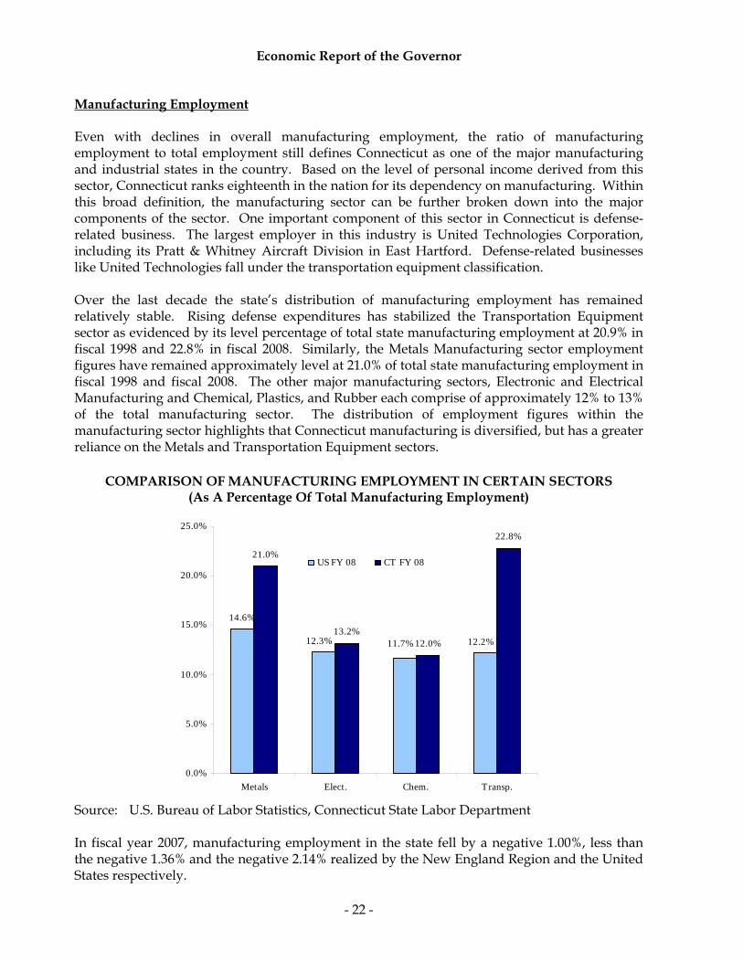
Manufacturing Employment Even with declines in overall manufacturing employment, the ratio of manufacturing employment to total employment still defines Connecticut as one of the major manufacturing and industrial states in the country. Based on the level of personal income derived from this sector, Connecticut ranks eighteenth in the nation for its dependency on manufacturing. Within this broad definition, the manufacturing sector can be further broken down into the major components of the sector. One important component of this sector in Connecticut is defense-related business. The largest employer in this industry is United Technologies Corporation, including its Pratt & Whitney Aircraft Division in East Hartford. Defense-related businesses like United Technologies fall under the transportation equipment classification. Over the last decade the state’s distribution of manufacturing employment has remained relatively stable. Rising defense expenditures has stabilized the Transportation Equipment sector as evidenced by its level percentage of total state manufacturing employment at 20.9% in fiscal 1998 and 22.8% in fiscal 2008. Similarly, the Metals Manufacturing sector employment figures have remained approximately level at 21.0% of total state manufacturing employment in fiscal 1998 and fiscal 2008. The other major manufacturing sectors, Electronic and Electrical Manufacturing and Chemical, Plastics, and Rubber each comprise of approximately 12% to 13% of the total manufacturing sector. The distribution of employment figures within the manufacturing sector highlights that Connecticut manufacturing is diversified, but has a greater reliance on the Metals and Transportation Equipment sectors.
COMPARISON OF MANUFACTURING EMPLOYMENT IN CERTAIN SECTORS (As A Percentage Of Total Manufacturing Employment)
14.6%
21.0%
13.2%12.0%
22.8%
12.3% 12.2%11.7%
0.0%
5.0%
10.0%
15.0%
20.0%
25.0%
Metals Elect. Chem. Transp.
US FY 08 CT FY 08
Source: U.S. Bureau of Labor Statistics, Connecticut State Labor Department In fiscal year 2007, manufacturing employment in the state fell by a negative 1.00%, less than the negative 1.36% and the negative 2.14% realized by the New England Region and the United States respectively.

Economic Report of the Governor
- 23 -
MANUFACTURING EMPLOYMENTFISCAL YEAR GROWTH BY PERCENT
-10
-8
-6
-4
-2
0
2
4
1998 1999 2000 2001 2002 2003 2004 2005 2006 2007 2008
FISCAL YEAR
PERC
ENT
United States
New England
Connecticut
TABLE 20
MANUFACTURING EMPLOYMENT (In Thousands)
Fiscal United States New England Connecticut Year Number % Growth Number % Growth Number % Growth
1999-00 17,288 (0.81) 936.4 (1.55) 236.7 (3.24) 2000-01 17,037 (1.45) 933.8 (0.28) 233.6 (1.30) 2001-02 15,736 (7.64) 851.6 (8.80) 218.3 (6.56) 2002-03 14,879 (5.45) 788.3 (7.44) 205.0 (6.13) 2003-04 14,328 (3.71) 751.2 (4.70) 197.6 (3.59) 2004-05 14,289 (0.27) 742.4 (1.18) 196.7 (0.48) 2005-06 14,203 (0.60) 726.0 (2.21) 194.0 (1.35) 2006-07 14,025 (1.25) 715.3 (1.46) 192.4 (0.82) 2007-08 13,725 (2.14) 705.6 (1.36) 190.4 (1.00)
Source: U.S. Bureau of Labor Statistics, Connecticut State Labor Department Historically, manufacturing employment closely parallels the business cycle, typically expanding when the economy is healthy and contracting during recessionary periods, as it did during the early 1980s. However, this phenomenon diverged in the latter part of the 1980s, as contractions in manufacturing employment were not initially accompanied by a recession. Other factors, such as heightened foreign competition, smaller defense budgets, and improved productivity, played a significant role in affecting the overall level of manufacturing employment in Connecticut.
Source: U.S. Bureau of Labor Statistics, Connecticut State Labor Department

Economic Report of the Governor
- 24 -
The erosion of the state’s manufacturing base reflects the national trend away from traditional industries, both durable and nondurable. More of U.S. demand is being satisfied by foreign producers who can manufacture goods more cheaply. The upward trend of higher productivity has enabled Connecticut manufacturers to make more with fewer workers. Even with the structural change, manufacturing employment in Connecticut still accounts for 11.2% of all nonfarm payroll jobs, compared to 10.0% in the U.S. through fiscal 2008. The sector still matters. Manufacturing jobs remain one of the best-paid segments of payroll, contributing more to personal income than the same number of service jobs. The following Table provides a breakdown of the state’s manufacturing employment by industry and indicates percentage changes for the year and over a ten year period for each of the manufacturing sectors. In fiscal 2008, total manufacturing employment in Connecticut remained relatively level with fiscal 2007 with a small 1.0% reduction in the manufacturing workforce. The manufacturing sector that experienced the largest decline in the number employed in fiscal 2008 was the metal manufacturing sector with an overall reduction of 2.0% from the fiscal year 2007 level. At 0.5% and 0.6% growth respectively, the transportation equipment and electronics and electrical products were the only two manufacturing sectors which experienced growth from fiscal 2007 to 2008. The percent change from fiscal 1998 to 2007 demonstrates the overall decline in manufacturing employment over the last ten years.
TABLE 21 CONNECTICUT MANUFACTURING EMPLOYMENT BY INDUSTRY
(In Thousands)
Percent Change F.Y. F.Y. F.Y. FY 2007 to FY 1999 to Industry 1998-99 2006-07 2007-08 FY 2008 FY 2008 Transportation Equipment 51.73 43.51 43.74 0.5 (15.4) Metal Manufacturing 51.56 40.79 40.08 (1.7) (22.2) Electronic & Electrical 36.39 25.04 25.30 1.1 (30.5) Chemical, Plastics & Rubber 28.08 23.60 22.74 (3.7) (19.0) Printing, Publishing & Textile 26.03 17.27 16.97 (1.8) (34.8) Industrial Machinery 24.69 18.14 18.11 (0.2) (26.7) Food, Beverage & Tobacco 8.76 8.48 8.17 (3.6) (6.7) Miscellaneous 17.41 15.58 15.32 (1.7) (12.0) Total Mfg. Employment 244.65 192.41 190.42 (1.0) (22.2)
Source: U.S. Bureau of Economic Analysis, Connecticut State Labor Department The following Table ranks the 50 states in terms of their relative dependence on manufacturing wages as a percentage of total personal income.

Economic Report of the Governor
- 25 -
TABLE 22 MANUFACTURING WAGES AS A PERCENT OF PERSONAL INCOME BY STATE
Fiscal Year 2008 (In Millions of Dollars)
Personal Mfg. Personal Mfg.
State Income Wages % Rank State Income Wages % Rank Indiana $214,599 $29,126 13.5 1 Texas $915,429 $56,730 6.20 26 Wisconsin 206,810 24,847 12.0 2 Massachusett 324,971 20,016 6.16 27 Michigan 350,273 36,538 10.4 3 Maine 45,727 2,801 6.13 28 Iowa 107,231 11,052 10.3 4 Nebraska 65,987 4,005 6.07 29 Ohio 402,142 38,981 9.69 5 Georgia 325,377 19,717 6.06 30 New Hampshire 55,546 5,298 9.54 6 Rhode Island 42,714 2,489 5.83 31 Kansas 104,003 9,147 8.79 7 New Jersey 435,692 25,355 5.82 32 Kentucky 133,541 11,648 8.72 8 Louisiana 157,872 8,678 5.50 33 Alabama 153,959 13,350 8.67 9 South Dakota 29,416 1,585 5.39 34 Tennessee 210,253 17,581 8.36 10 West Virginia 54,430 2,825 5.19 35 South Carolina 140,320 11,635 8.29 11 Oklahoma 130,776 6,755 5.17 36 Minnesota 218,234 17,858 8.18 12 Arizona 212,442 10,757 5.06 37 North Carolina 312,123 25,415 8.14 13 Delaware 35,231 1,725 4.90 38 Arkansas 87,830 6,917 7.88 14 North Dakota 24,160 1,044 4.32 39 Mississippi 85,625 6,724 7.85 15 Virginia 327,020 13,985 4.28 40 Vermont 23,773 1,853 7.79 16 Colorado 205,179 8,548 4.17 41 Oregon 134,415 10,443 7.77 17 Maryland 267,409 9,524 3.56 42 Connecticut 195,773 14,224 7.27 18 New York 921,419 28,582 3.10 43 Utah 81,541 5,821 7.14 19 New Mexico 62,224 1,790 2.88 44 Pennsylvania 492,434 34,255 6.96 20 Florida 711,605 18,498 2.60 45 Illinois 538,025 37,299 6.93 21 Montana 32,590 832 2.55 46 Washington 272,974 18,393 6.74 22 Nevada 104,259 2,461 2.36 47 Missouri 204,736 13,605 6.65 23 Wyoming 25,636 476 1.86 48 Idaho 48,409 3,153 6.51 24 Alaska 28,435 468 1.65 49 California 1,550,470 97,001 6.26 25 Hawaii 51,409 585 1.14 50 U.S. Average 11,899,552 746,675 6.27
Source: U.S. Department of Commerce, Bureau of Economic Analysis Nonmanufacturing Employment The nonmanufacturing sector is comprised of industries that provide a service. Services differ significantly from manufactured goods in that the output is generally intangible, it is produced and consumed concurrently, and it cannot be inventoried. Connecticut’s nonmanufacturing sector consists of the industries listed in the following Table. Over the last three decades,
Economic Report of the Governor
- 26 -
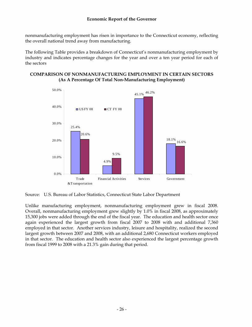
nonmanufacturing employment has risen in importance to the Connecticut economy, reflecting the overall national trend away from manufacturing. The following Table provides a breakdown of Connecticut’s nonmanufacturing employment by industry and indicates percentage changes for the year and over a ten year period for each of the sectors
COMPARISON OF NONMANUFACTURING EMPLOYMENT IN CERTAIN SECTORS (As A Percentage Of Total Non-Manufacturing Employment)
25.4%
4.9%
45.1%
18.1%
9.5%
46.2%
16.6%
20.6%
0.0%
10.0%
20.0%
30.0%
40.0%
50.0%
Trade&Transportation
Financial Activities Services Government
US FY 08 CT FY 08
Source: U.S. Bureau of Labor Statistics, Connecticut State Labor Department Unlike manufacturing employment, nonmanufacturing employment grew in fiscal 2008. Overall, nonmanufacturing employment grew slightly by 1.0% in fiscal 2008, as approximately 15,300 jobs were added through the end of the fiscal year. The education and health sector once again experienced the largest growth from fiscal 2007 to 2008 with and additional 7,360 employed in that sector. Another services industry, leisure and hospitality, realized the second largest growth between 2007 and 2008, with an additional 2,680 Connecticut workers employed in that sector. The education and health sector also experienced the largest percentage growth from fiscal 1999 to 2008 with a 21.3% gain during that period.

Economic Report of the Governor
- 27 -
TABLE 23 CONNECTICUT NONMANUFACTURING EMPLOYMENT BY INDUSTRY
(In Thousands)
Percent Change F.Y. F.Y. F.Y. FY 2007 to FY 1999 to Industry 1998-99 2006-07 2007-08 FY 2008 FY 2008 Construction & Mining 60.44 68.47 69.17 1.03 14.45 Information 44.23 38.02 38.82 2.13 (12.23) Transp., Trade & Utilities 310.30 310.79 311.38 0.19 0.35 Transp., & Warehousing 41.29 44.06 44.25 0.43 7.17 Utilities 9.80 8.14 8.21 0.85 (16.19) Wholesale 66.35 67.65 68.50 1.26 3.24 Retail 192.87 190.94 190.42 (0.27) (1.27) Finance (FIRE) 139.86 144.95 143.54 (0.97) 2.63 Finance & Insurance 119.16 123.81 122.94 (0.70) 3.18 Real Estate 20.70 21.14 20.60 2.13 (0.48) Services 626.17 687.26 697.77 1.53 11.43 Professional & Business 207.53 205.37 205.67 0.15 (0.90) Education & Health 240.09 283.74 291.10 2.59 21.25 Leisure & Hospitality 118.09 133.96 136.64 2.00 15.71 All Other Services 60.46 64.19 64.36 0.26 6.45 Government 231.71 247.16 251.20 1.64 8.41 Federal 22.47 19.63 19.44 (0.93) (13.50) State 65.64 67.11 69.77 3.96 6.28 Local 143.59 160.42 161.99 0.98 12.81 Total Nonmanufacturing Employment 1,412.72 1,496.64 1,511.89 1.02 7.02
Note: Totals may not agree with detail due to rounding. Source: U.S. Department of Commerce, Bureau of Economic Analysis

Economic Report of the Governor
- 28 -
The following Table and Chart provide a ten year profile of nonmanufacturing employment in the United States, the New England Region, and Connecticut.
TABLE 24
NONMANUFACTURING EMPLOYMENT (In Thousands)
Fiscal United States New England Connecticut Year Number % Growth Number % Growth Number % Growth
1998-99 109,999 2.98 5,841.6 2.74 1,412.7 2.51 1999-00 113,309 3.01 6,006.9 2.83 1,445.3 2.31 2000-01 115,211 1.68 6,133.5 2.11 1,456.7 0.79 2001-02 115,141 (0.06) 6,119.8 (0.22) 1,456.8 0.01 2002-03 115,240 0.09 6,092.5 (0.45) 1,447.5 (0.64) 2003-04 116,137 0.78 6,102.4 0.16 1,446.1 (0.09) 2004-05 118,179 1.76 6,155.1 0.86 1,460.4 0.98 2005-06 120,798 2.22 6,222.9 1.10 1,476.1 1.08 2006-07 122,929 1.76 6,300.3 1.24 1,496.6 1.39 2007-08 124,129 0.98 6,352.0 0.82 1,511.9 1.02
Source: U.S. Bureau of Labor Statistics, Connecticut State Labor Department
NONMANUFACTURING EMPLOYMENTFISCAL YEAR GROWTH BY PERCENT
-1
0
1
2
3
4
1999 2000 2001 2002 2003 2004 2005 2006 2007 2008
FISCAL YEAR
PERC
ENT
United States
New England
Connecticut
Source: U.S. Bureau of Labor Statistics, Connecticut State Labor Department
Economic Report of the Governor
- 29 -
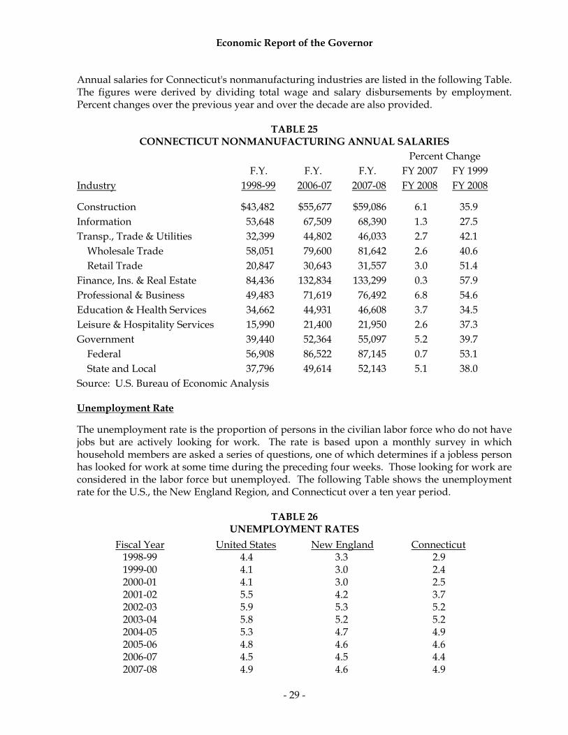
Annual salaries for Connecticut's nonmanufacturing industries are listed in the following Table. The figures were derived by dividing total wage and salary disbursements by employment. Percent changes over the previous year and over the decade are also provided.
TABLE 25
CONNECTICUT NONMANUFACTURING ANNUAL SALARIES
Percent Change F.Y. F.Y. F.Y. FY 2007 FY 1999 Industry 1998-99 2006-07 2007-08 FY 2008 FY 2008 Construction $43,482 $55,677 $59,086 6.1 35.9 Information 53,648 67,509 68,390 1.3 27.5 Transp., Trade & Utilities 32,399 44,802 46,033 2.7 42.1 Wholesale Trade 58,051 79,600 81,642 2.6 40.6 Retail Trade 20,847 30,643 31,557 3.0 51.4 Finance, Ins. & Real Estate 84,436 132,834 133,299 0.3 57.9 Professional & Business 49,483 71,619 76,492 6.8 54.6 Education & Health Services 34,662 44,931 46,608 3.7 34.5 Leisure & Hospitality Services 15,990 21,400 21,950 2.6 37.3 Government 39,440 52,364 55,097 5.2 39.7 Federal 56,908 86,522 87,145 0.7 53.1 State and Local 37,796 49,614 52,143 5.1 38.0 Source: U.S. Bureau of Economic Analysis Unemployment Rate The unemployment rate is the proportion of persons in the civilian labor force who do not have jobs but are actively looking for work. The rate is based upon a monthly survey in which household members are asked a series of questions, one of which determines if a jobless person has looked for work at some time during the preceding four weeks. Those looking for work are considered in the labor force but unemployed. The following Table shows the unemployment rate for the U.S., the New England Region, and Connecticut over a ten year period.
TABLE 26 UNEMPLOYMENT RATES
Fiscal Year United States New England Connecticut 1998-99 4.4 3.3 2.9 1999-00 4.1 3.0 2.4 2000-01 4.1 3.0 2.5 2001-02 5.5 4.2 3.7 2002-03 5.9 5.3 5.2 2003-04 5.8 5.2 5.2 2004-05 5.3 4.7 4.9 2005-06 4.8 4.6 4.6 2006-07 4.5 4.5 4.4 2007-08 4.9 4.6 4.9

Economic Report of the Governor
- 30 -
UNEMPLOYMENT RATESBY FISCAL YEAR
2
3
4
5
6
1999 2000 2001 2002 2003 2004 2005 2006 2007 2008
FISCAL YEAR
PERC
ENT
United States
New England
Connecticut
Source: U.S. Bureau of Labor Statistics, Connecticut State Labor Department

Economic Report of the Governor
- 31 -
SECTOR ANALYSIS Energy Over the past two hundred years, the history of energy supplies and the mode of energy use in the United States reflected the country’s industrialization, economic development, and social transformation. As the U.S. becomes more dependent on imported energy, economic activity hinges more upon the availability and stability of its supply in the world market. In the past 35 years, all of the nation’s five recessions were concurrent with the energy disruptions that occurred worldwide in 1991 (Iraq invaded Kuwait), in 1981 (Iran/Iraq war), in 1979 (Iranian Revolution), and in 1973 (Arab Oil Embargo). The March 2001 recession followed an energy supply disturbance that occurred in late 2000 when petroleum inventories remained relatively low and the price reached a then record high of $37.80 per barrel, the highest since the Gulf War of 1991. The current recession, which began in December 2007, was also presaged by a hike in oil prices and was accompanied by the joint crises in the housing and financial markets. Reaching a fresh record high above $94.62 a barrel in October 2007, domestic West Texas Intermediate crude oil in December 2007 averaged $92.95 a barrel, up 70% from a year earlier. The price rose to an all time monthly record of $133.93 a barrel in May 2008. The United States, like the rest of the industrialized world, relies heavily on three fossil fuels: crude oil, coal, and natural gas. The following three sections describe energy production and consumption for the world, the United States, and Connecticut. Worldwide In the world oil market, supply and demand among countries or regions is significantly imbalanced. The following Table illustrates the disparity between the world’s suppliers of oil and its users. Members of the Organization of Petroleum Exporting Countries (OPEC), for example, supplied 35.42 million barrels per day (MBPD) in 2007 and consumed 11.97 MBPD, leaving a 23.45 MBPD surplus. The Organization for Economic Cooperation and Development (OECD), on the other hand, consumed more than it supplied. In 2007, the OECD consumed 49.14 MBPD, while supplying only 21.46 MBPD, registering a 27.68 MBPD deficit. The United States consumed 20.68 MBPD in 2007, representing almost a quarter of total world demand, compared to a production of 8.46 MBPD, or 10% of world supply, reflecting a 60% dependency on foreign oil supplies. The deficit between supply and demand also exists in larger economies such as Japan, France, and Germany. Demand in China and India, Asia’s two most populous and fastest economically growing countries, continues its upward trend, accounting for some 10% in 2007, up from 5.5% in 1991. China, which switched from a net exporter of oil in 1995, began running an increasing oil deficit as its economy continued to grow at a brisk pace. In 2007, China consumed 7.58 MBPD while supplying 3.90 MBPD, leaving a 3.68 MBPD deficit. This reflects China’s approaching 50% dependency on foreign oil supplies. Faced with soaring demand and fierce competition for resources, China and India have teamed up to control oil and gas fields in Africa, Latin America, and elsewhere.

Economic Report of the Governor
- 32 -
TABLE 27 WORLD OIL SUPPLY AND DEMAND
Calendar 2007
Supply Demand Millions Millions of Barrels % of of Barrels % of Per Day Total Per Day Total Total OECD (a) 21.46 25.4% Total OECD 49.14 57.3% United States 8.46 10.0 United States 20.68 24.1 Canada 3.42 4.1 Canada 2.37 2.8 Mexico 3.50 4.1 Mexico 2.12 2.5 North Sea (b) 4.54 5.4 Japan 5.01 5.8 Other OECD 1.54 1.8 Germany 2.46 2.9 France 1.95 2.3 Total OPEC (c) 35.42 42.0 Italy 1.70 2.0 Saudi Arabia 8.72 10.3 United Kingdom 1.76 2.1 Iran 3.91 4.6 Other OECD 11.09 12.9 Iraq 2.09 2.5 Other OPEC 20.70 24.5 Total Non-OECD 36.67 42.7 Former USSR 4.28 5.0 Total Non-OECD 27.53 32.6 China 7.57 8.8 Former USSR 12.60 14.9 India 2.80 3.3 China 3.90 4.6 OPEC 11.97 13.9 Other 11.03 13.1 Other 10.05 11.7 Total Supply 84.41 100.0% Total Demand 85.81 100.0% Note: (a) The OECD includes the United States, Western European countries, Australia, Canada,
Japan, and New Zealand. (b) North Sea includes the United Kingdom Offshore, Norway, Denmark, Netherlands
Offshore, and Germany Offshore. (c) The OPEC includes Algeria, Gabon, Indonesia, Iran, Iraq, Kuwait, Libya, Nigeria, Qatar,
Saudi Arabia, the United Arab Emirates, and Venezuela.
Source: U.S. Department of Energy, Energy Information Administration, International Petroleum Monthly and International Energy Annual 2007
World energy reserves also mirror the same pattern of disparity as the oil supply market. The following Table shows world oil and natural gas reserves by country. The share of world oil reserves held by all OPEC countries is 75%. Of the total, the Middle East controls approximately 65% of world oil reserves with Saudi Arabia alone controlling approximately one-quarter of the total, followed by Iran’s 11.6% and Iraq’s 10.9%. The Middle East countries controlled 40.0% of natural gas reserves.

Economic Report of the Governor
- 33 -
TABLE 28 WORLD OIL & NATURAL GAS RESERVES
January 1, 2007
Oil Gas Billions of % of Trillions of % of Barrels Total Cubic Feet Total North America 58.2 5.1% 286.8 4.5% United States 21.0 1.8 211.1 3.3 Mexico 11.7 1.0 19.0 0.3 Canada 25.6 2.2 56.8 0.9 Central & South America 77.1 6.7 242.2 3.8 Venezuela 52.9 4.6 151.1 2.4 Western Europe 14.5 1.3 175.7 2.9 E. Europe & Former USSR 123.4 10.8 2,136.7 33.4 Middle East 722.5 63.2 2,555.1 40.0 Saudi Arabia 262.3 22.9 252.5 3.9 Iran 133.0 11.6 974.0 15.2 Iraq 125.1 10.9 90.0 1.4 Kuwait 100.1 8.8 56.2 0.9 Other Mid. East 102.0 8.9 1,182.4 18.5 Africa 111.7 9.8 500.7 7.8 Far East & Others 36.0 3.1 497.7 7.8 Total 1,143.4 100.0 6,395.1 100.0
Note: Totals may not add due to rounding.
Source: U.S. Department of Energy, Energy Information Administration, International Energy Annual
As the economy grows, the United States continues to deplete its energy reserves. U.S. crude oil and natural gas reserves in 2007 were estimated at 21.0 billion barrels and 211.1 trillion cubic feet, or 1.8% and 3.3%, respectively, of the world’s reserve. These were down about 30% and 20%, respectively, from 1977 levels, the year when the U.S. Department of Energy started assembling the reserve data. Oil or natural gas reserves are the estimated quantities that are recoverable in the future from known reservoirs under existing economic and operating conditions. United States The U.S. has the largest demand for world oil. While it counts for about 5% of world population and supplies 10% of world oil, it consumes 25% of world oil production and produces about 28% of the world’s GDP. The nation has long been a net energy importer. According to the Annual Energy Review, the U.S. consumed 101.64 quadrillion British Thermal Units (QBTU’s) of energy in 2007, 2.3 times the 1960 level. Whereas the U.S. produced only 71.71 QBTU’s and exported 5.36 QBTU’s in 2007, it required net imports of 29.24 QBTU’s, which represented 28.8% of total national energy consumption, up from 25.2% in 2000, 16.6% in 1990, and 6.0% in 1960.

Economic Report of the Governor
- 34 -
National energy consumption has increased at an average annual rate of 1.2% over the past two decades. Growth in energy consumption has trended along with economic conditions, up during periods of healthy economic growth and down during periods of sluggish growth. Growth in energy consumption also reflects the movement of prices, higher during periods of relatively low or stable prices and down during periods of price increases. The following Table illustrates the breakdown of energy usage in the U.S. in 2007 by fuel type and by economic sector. As can be seen, petroleum products are the most important energy source for the U.S. economy. The 39.82 quadrillion petroleum-generated BTU’s accounted for approximately 40.0% of U.S. fuel consumption, followed by natural gas at 23.64 QBTU’s and coal at 22.77 QBTU’s. These three fuel sources together accounted for approximately 85% of U.S. fuel consumption. Nuclear power and hydroelectric power were distant followers.
TABLE 29
U.S. ENERGY CONSUMPTION IN 2007 (Quadrillion BTU's)
Fuels
Resi -dential
Com- mercial
In- dustrial
Trans- portation
Electric Generation
Total
% of Total
Natural Gas 4.84 3.08 8.00 0.67 7.05 23.64 23.3% Petroleum 1.28 0.63 9.52 27.72 0.66 39.82 39.2% Coal 0.01 0.07 1.86 0.00 20.84 22.77 22.4% Nuclear 0.00 0.00 0.00 0.00 8.42 8.42 8.3% Hydroelectric 0.00 0.00 0.02 0.00 2.44 2.46 2.4% Other 0.56 0.12 2.03 0.63 1.06 4.39 4.3% Electricity 4.75 4.58 3.43 0.03 0.11 12.90 12.7% Electric Losses 10.32 9.95 7.45 0.06 (40.57) (12.79) (12.6)% Total Demand 21.75 18.43 32.32 29.10 0.00 101.59 100.0%
% of Total 21.9% 18.5% 32.5% 29.2% 0.0% 100.0%
Note: Totals may not add due to rounding.
Source: U.S. Department of Energy, Energy Information Administration, Annual Energy Review 2007
There are five energy-use sectors: residential, commercial, industrial, transportation, and electric power generation. The first four sectors are end-users while the last one is the intermediate-user that consists of all utility and non-utility facilities and equipment used in the electricity industry. Of the four end-users, the industrial sector was the largest energy consumer, consuming 32.32 QBTU’s in 2007, followed by transportation at 29.10 QBTU’s, residential at 21.75 QBTU’s, and commercial at 18.43 QBTU’s. In contrast to the relatively smooth trends in the other sectors, industrial consumption has showed the greatest fluctuation, dropping sharply in 1975, 1980-83, and 2001-03 in response to high oil prices and economic slowdown. The electric power generation sector consumes and also produces energy. Energy losses occur throughout the entire electrical system beginning with utility generation in fossil-fired, nuclear or hydroelectric power plants all the way to the end-users. Energy losses are approximately two-thirds of total energy input during the conversion process of heat energy into mechanical energy for turning electric generators. Of the electricity generated, about 5% is lost in plant use and 9% is lost in transmission and distribution.

Economic Report of the Governor
- 35 -
Crude Oil Prices Oil is a global commodity. Crude oil prices in the U.S. depend not only upon domestic market conditions, but also upon worldwide supply and demand. While long-term upward trending oil prices are fundamentally caused by the world’s tighter supply and increasing demand, short-term price fluctuations are basically caused by interruptions in supply due to geopolitical unrest, seasonal or unexpected damages to facilities in, for instance, the Gulf of Mexico, or other events. Mounting world consumption has directly brought price increases as spare production capacity is more limited now than it has been over the past 3 decades. As oil fields age with inadequate investment, productivity declines. Crude oil production in the U.S., for example, fell from the peak average of 18.6 barrels per day per well in 1972 to 10.0 barrels in 2007. Forecasts of future supply and inventory levels also affect short-run oil prices. As demand and supply are delicately in balance, crude oil inventory relative to its historical average and anticipated levels also play a critical role. The “risk premium” reflects the possibility of a supply shortage, creating the incentive to hoard bigger inventories, which leads to higher prices. The value of the U.S. dollar relative to other major currencies has become an important factor recently, as the dollar serves as the world standard unit of trade. The continued decline in the dollar contributed in driving oil prices to an all time high at $147 per barrel in July of 2008. To defend against the losses due to the deprecation of the dollar, oil producing countries and oil companies raised oil prices. Subsequently, the slowdown in the global economy combined with an appreciation in the dollar has helped send oil prices down more than 70% to hover around $40 per barrel in December 2008. Crude oil prices have a long history of large fluctuations that affect the world and U.S. economies as well as inflation levels. In 1973, the year of the Arab Oil Embargo, crude oil prices in the U.S. measured by the composite Refiners' Acquisition Cost averaged $4.15 per barrel. After two consecutive supply disturbances brought on by the Iranian Revolution in 1979 and the Iran-Iraq war in 1980, oil prices reached $35.28 per barrel in 1981. Since then, long-term prices had trended down to a low of $12.52 per barrel in 1998 and then stayed in the $20 range until mid-2003. Crude oil prices started to creep up above $30 per barrel in late 2003 and continued to soar to the upper $60s in 2007, and then rose up close to $110 per barrel in the first nine months of 2008. The world oil market becomes more vulnerable as inventory levels tighten, consumption from rapidly growing emerging markets expands, and the U.S. dollar depreciates. In real terms as adjusted for inflation, the 2008’s $100.96 per barrel price also surpassed the last annual peak of $78.21 per barrel registered in 1981.

Economic Report of the Governor
- 36 -
TABLE 30 CRUDE OIL PRICES AND U.S. CONSUMPTION
Refiners’ Crude Oil Acquisition Costs* Per Barrel
Year
Current $
In 2006$*
Year
Current $
In 2006$*
1973 4.15 18.83 2001 22.95 26.13 1975 10.37 38.84 2002 24.02 26.92 1980 28.22 69.05 2003 28.60 31.34 1981 35.28 78.21 2004 36.91 39.39 1985 26.75 50.11 2005 50.32 51.95 1990 22.34 34.47 2006 60.10 60.10 1995 17.23 22.79 2007 67.98 66.09 2000 28.24 33.06 2008* 108.20 100.96
Note: * Adjusted by 2006 CPI-U, where 1982-84=100.00 and 2006 = 201.58. ** The average for the first nine months.
Source: U.S. Department of Energy, Energy Information Administration Longer term oil prices are expected to trend up as world demand grows faster than the rate of discovery of new supplies. The following factors are driving prices higher: new oil fields are harder to find, crude oil is more costly to extract, underinvestment had been occurring for years in this industry, and mounting demand for oil in Asia, the Middle East, some industrialized countries, and elsewhere. As the world enters a recession, demand falls and so do prices. It is estimated that 70% of the existing oil fields are more than 30 years old. Oil reserves in the Middle East and Persian Gulf region may be nearing maturity or depletion. However, the world is expected to rely even more on OPEC’s current 42% share as potential production from non-OPEC countries decline. As the world economy continues to grow, the increasing demand will more than offset any savings gained from efficiency and conservation. The world rate of replenishment of oil reserves relative to their rate of supply, the so-called Reserve Replenishment Ratio (RRR), has been declining and is expected to move below the healthy ratio of 100% for the next five years. Although the discovery of Jack Field in the Gulf of Mexico and Tupi Field in Brazil may add tens of billion of barrels of crude oil reserves and help increase the RRR ratio, meaningful production may not happen for years to come. Capital investments on alternative renewable energy from solar, wind, biofuels and geothermal have increased drastically; nonetheless, their share of power production is still small. Operable nuclear plants, the major alternative resource for production, in the U.S. continue to decline to 104 units in 2007, down from a peak of 112 units in 1990. No new operating licenses have been granted since 1998. Efficiency Increasing efficiency has spearheaded the nation’s energy conservation policy. Energy regulatory agencies have been aggressively protecting the environment by promoting energy-efficient products over the past two decades. The National Appliance Energy Conservation Act of 1987 set minimum efficiency standards for 13 appliances and prohibited the sale if standards were not met. In 1992, the EPA embarked upon “Energy Star” as a voluntary labeling

Economic Report of the Governor
- 37 -
program to identify and promote energy-efficient products to reduce greenhouse gas emissions. The Energy Star label now covers more than 50 product categories from small battery chargers to central AC to big new homes. It includes appliances, electronics, heating and cooling equipment, office equipment, lighting, commercial food services, and new buildings with additional energy-saving features that are 20–30% more efficient than standard homes. To promote energy efficient buildings in the U.S., the Leadership in Energy and Environmental Design (LEED), a non-profit organization under the U.S. Green Building Council (USGBC), provides green building rating standards for environmentally sustainable construction and design. Other than energy conservation, increases in productivity also play a vital role in efficiency. Productivity, a crucial ingredient in the economy's long-term vitality, is a measure of economic efficiency which shows how effectively economic inputs are converted into output. Productivity is measured by comparing the amount of goods and services produced with the inputs that are used in production. A measure of efficiency is the amount of energy used to produce a dollar of Gross Domestic Product (GDP). The following Table compares U.S. consumption of fuel sources and illustrates the nation’s improvement in energy efficiency. Energy consumption per dollar of GDP has trended down at an average annual rate of 1.5% during the past 3 decades. In 1977, it required 16,420 BTU’s of energy to produce $1 of GDP measured in 2000 dollars; by 2007, it had fallen to 8,816 BTU’s, a 47% reduction in three decades. The decline in energy consumption per dollar of GDP resulted from efficiency improvements and a structural shift from energy intensive industries to those that consume less energy but create more valued added products such as finance, banking, and professional services. However, improvements in energy efficiency vary from period to period, depending upon energy prices, consumers’ consumption habits, and technology improvements, etc. Efficiency tends to stagnate when fuel prices decline. As oil prices fell, the incentive to conserve energy diminished. Oil Stability Program To protect against supply disruptions, the United States began to create a Strategic Petroleum Reserve (SPR) under the Energy Policy and Conservation Act of 1975 (EPCA). The SPR program was established as a 750 million barrel capacity crude oil reserve with the objective of achieving a maximum draw-down rate within 15 days of the notice to proceed. To maximize long-term protection against oil supply disruptions, President George W. Bush in late 2001 directed the Secretary of Energy to fill the SPR up to its 700 million barrel capacity.

Economic Report of the Governor
- 38 -
TABLE 31 U.S. PRIMARY ENERGY CONSUMPTION & ENERGY EFFICIENCY
U.S. Energy Consumption GDP BTU
Calendar Year
Total Quadrillion BTU’s
Percent Change
Billion (In 2000$)
Per $1 GDP (In 2000$)
Percent Change
1975 72.00 4,311.2 16,700 1980 78.12 8.5% 5,161.7 15,135 (9.4%) 1985 76.49 (2.1%) 6,053.7 12,635 (16.5%) 1990 84.65 10.7% 7,112.5 11,902 (5.8%) 1995 91.17 7.7% 8,031.7 11,352 (4.6%) 2000 98.98 2.2% 9,817.0 10,082 (11.2%) 2001 96.33 (2.7%) 9,890.7 9,756 (3.4%) 2002 97.86 1.6% 10,004.8 9,738 (0.0%) 2003 98.21 0.4% 10,301.0 9,534 (2.1%) 2004 100.35 2.2% 10,675.8 9,400 (1.4%) 2005 100.51 0.2% 10,989.5 9,146 (2.7%) 2006 99.86 (0.7%) 11,294.8 8,841 (3.3%) 2007 101.60 1.8% 11,523.9 8,816 (0.3%)
Source: U.S. Department of Energy, Energy Information Administration, Annual Energy Review 2007
U.S. Department of Labor, Bureau of Labor Statistics In early 2000, a shortage of home heating oil sent prices to a high of $2.45 per gallon from $1.00 per gallon a year earlier. To reduce such risk in the future, the U.S. Department of Energy established the Northeast Heating Oil Reserve under the SPR program. The maximum inventory of heating oil in the reserve is 2 million barrels, which will provide relief for approximately 10 days. This reserve program was permanently established in March of 2001 as a part of America's energy readiness effort, separating it from the Strategic Petroleum Reserve. Heating oil is the dominant fuel used for home heating in Connecticut with 52% of all homes in Connecticut using heating oil as the primary heating fuel. Connecticut Connecticut is ranked as one of the most efficient states in the nation in energy usage. Connecticut consumed 4,657 BTU’s per current dollar of Gross State Product in 2005, the latest available data, ranking the second most efficient state among the 50 states and 43% less than the national average of 8,129 BTU’s. When compared to the national per person consumption, Connecticut residents are moderate energy users. Connecticut consumed 258.2 million BTU’s of energy per person in 2005, ranking it 44th among the 50 states and 24% less than the national average of 339.2 million BTU's. These figures were far less than Alaska's consumption of 1,193.9 million BTU's, the largest consumer in the nation. Because the State lacks indigenous energy sources, it must import nearly all the energy that it consumes. This situation affects Connecticut consumers’ energy choices and results in prices that are approximately 25% higher
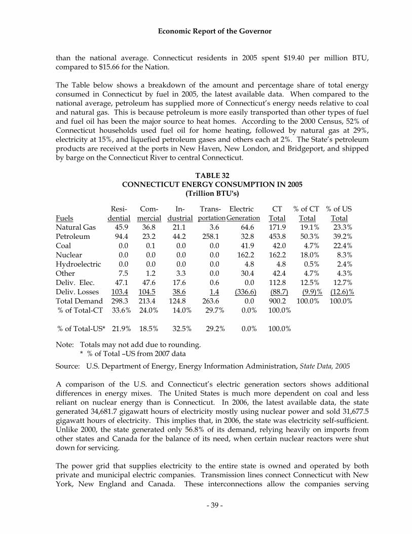
Economic Report of the Governor
- 39 -
than the national average. Connecticut residents in 2005 spent $19.40 per million BTU, compared to $15.66 for the Nation. The Table below shows a breakdown of the amount and percentage share of total energy consumed in Connecticut by fuel in 2005, the latest available data. When compared to the national average, petroleum has supplied more of Connecticut’s energy needs relative to coal and natural gas. This is because petroleum is more easily transported than other types of fuel and fuel oil has been the major source to heat homes. According to the 2000 Census, 52% of Connecticut households used fuel oil for home heating, followed by natural gas at 29%, electricity at 15%, and liquefied petroleum gases and others each at 2%. The State’s petroleum products are received at the ports in New Haven, New London, and Bridgeport, and shipped by barge on the Connecticut River to central Connecticut.
TABLE 32 CONNECTICUT ENERGY CONSUMPTION IN 2005
(Trillion BTU's)
Resi- Com- In- Trans- Electric CT % of CT % of US Fuels dential mercial dustrial portation Generation Total Total Total Natural Gas 45.9 36.8 21.1 3.6 64.6 171.9 19.1% 23.3% Petroleum 94.4 23.2 44.2 258.1 32.8 453.8 50.3% 39.2% Coal 0.0 0.1 0.0 0.0 41.9 42.0 4.7% 22.4% Nuclear 0.0 0.0 0.0 0.0 162.2 162.2 18.0% 8.3% Hydroelectric 0.0 0.0 0.0 0.0 4.8 4.8 0.5% 2.4% Other 7.5 1.2 3.3 0.0 30.4 42.4 4.7% 4.3% Deliv. Elec. 47.1 47.6 17.6 0.6 0.0 112.8 12.5% 12.7% Deliv. Losses 103.4 104.5 38.6 1.4 (336.6) (88.7) (9.9)% (12.6)%Total Demand 298.3 213.4 124.8 263.6 0.0 900.2 100.0% 100.0% % of Total-CT 33.6% 24.0% 14.0% 29.7% 0.0% 100.0%
% of Total-US* 21.9% 18.5% 32.5% 29.2% 0.0% 100.0% Note: Totals may not add due to rounding. * % of Total –US from 2007 data
Source: U.S. Department of Energy, Energy Information Administration, State Data, 2005 A comparison of the U.S. and Connecticut’s electric generation sectors shows additional differences in energy mixes. The United States is much more dependent on coal and less reliant on nuclear energy than is Connecticut. In 2006, the latest available data, the state generated 34,681.7 gigawatt hours of electricity mostly using nuclear power and sold 31,677.5 gigawatt hours of electricity. This implies that, in 2006, the state was electricity self-sufficient. Unlike 2000, the state generated only 56.8% of its demand, relying heavily on imports from other states and Canada for the balance of its need, when certain nuclear reactors were shut down for servicing. The power grid that supplies electricity to the entire state is owned and operated by both private and municipal electric companies. Transmission lines connect Connecticut with New York, New England and Canada. These interconnections allow the companies serving

Economic Report of the Governor
- 40 -
Connecticut to meet large or unexpected electric load requirements from resources located outside of Connecticut’s boundaries. All electric utilities in the State are members of the New England Power Pool and operate as part of the regional bulk power system. An independent system operator, ISO New England Inc., operates this regional system. In 2006, the latest available data, there were 1,596,183 electricity consumers in Connecticut, with residential units accounting for approximately 90%; commercial units, 9%; and 0.5% each for industrial units and others. Approximately 94% of the electricity was sold by two investor-owned companies: Connecticut Light & Power Company and United Illuminating Company. Not all energy prices in the state are higher than the national average. Only residential heating fuel is lower cost than the national average. The following Table compares various prices to the national average for natural gas, motor gasoline, residential heating oil, residential electricity, and total average energy paid by consumers. As electricity prices vary from state to state in the U.S., so do prices between districts within Connecticut, depending upon the rates charged by their electricity providers. The average retail price for electricity in 2006 in Connecticut was 14.83 cents per kilowatt hour, the fourth highest state in the nation. This trailed Hawaii’s 20.72 cents, Massachusetts’ 15.45 cents, and New York’s 15.27 cents. The national average was 8.90 cents.
TABLE 33
CONSUMER ENERGY PRICES IN THE UNITED STATES AND CONNECTICUT Nominal Dollars Per Million BTU in 2005
Natural
Gas Motor
Gasoline Residential Heating Fuel
All *
Petroleum Retail
Electricity
Total
Energy Connecticut $12.01 $18.16 $6.17 $15.90 $36.35 $19.40 United States $9.92 $17.83 $6.65 $15.49 $23.92 $15.66
CT as a % of the U.S. 121% 102% 93% 103% 152% 124% * Includes motor gasoline, residential and distillate fuel oil, liquefied petroleum gases, and jet
fuel, etc.
Source: U.S. Department of Energy, Energy Information Administration, State Data Natural gas is delivered to Connecticut through pipelines that terminate in Boston and New York from Canada and the Gulf of Mexico area. Connecticut also receives natural gas (LNG) through a pipeline from a terminal located in Boston which is supplied by LNG tanker ships. Since 1996, the DPUC has allowed some competitive market forces to enter the natural gas industry in the state. Commercial and industrial gas consumers can choose non-regulated suppliers for their natural gas requirements. Natural gas is delivered to consumers using the local distribution company’s mains and pipelines. Located at or near the end of pipelines, Connecticut’s distribution companies have to pay higher transportation cost and outbid other buyers in order to gain access rights to the gas wellhead.

Economic Report of the Governor
- 41 -
Gasoline Consumption and Automotive Fuel Economy
In the U.S., highway vehicles consume approximately 98% of all gasoline. Only about 2% is used for other purposes such as agriculture, aviation, construction and boating. During 2006, gasoline consumption in the U.S. totaled 140.3 billion gallons, the equivalent of 9.15 million barrels per day. In 2006, Connecticut had 1,475 gasoline stations, accounting for some 0.9% of the U.S. total. The Table below shows gasoline consumption during the past ten years for the U.S. and Connecticut.
TABLE 34 GASOLINE CONSUMPTION IN THE UNITED STATES & CONNECTICUT
Calendar U.S. Consumption Percent Connecticut Percent
Year Gallons (000's) Change Gallons (000's)* Change 1997 125,399,139 1.7% 1,400,016 0.7% 1998 127,977,505 2.1% 1,425,178 1.8% 1999 132,260,590 3.3% 1,551,446 8.9% 2000 132,279,950 0.0% 1,476,340 (4.8%) 2001 134,110,264 1.4% 1,496,469 1.4% 2002 137,664,309 2.7% 1,589,580 6.2% 2003 139,065,057 1.0% 1,645,268 3.5% 2004 141,700,177 1.9% 1,860,908 13.1% 2005 140,338,710 (1.0%) 1,614,697 (13.2%) 2006 140,320,089 0.0% 1,566,875 (3.0%)
* Given the unusually sharp rise in consumption in 2004, this federally reported data point is likely erroneous, making a subsequent sharp decline in 2005.
Source: U. S. Department of Transportation, Office of Highway Information Management, Highway Statistics
During 2006 in Connecticut, gasoline consumption totaled 1.57 billion gallons or 38.4 million barrels, accounting for 1.1% of the nation’s consumption. This converts to consumption of 462 gallons per Connecticut resident versus 470 gallons for the nation. Per capita consumption is attributable to several factors such as income level, traffic condition, averaged weight of vehicles and distance that residents drive to work or shop, the percentage of workers telecommuting and ride sharing. Connecticut, as one of the smallest states in the nation, residents generally commute shorter distances to work and shop. Emissions of carbon dioxide from motor vehicles represent 97% of the total greenhouse gas emissions in the U.S. In 1975, the U.S. Congress authorized the Department of Transportation to set automobile efficiency standards, known as Corporate Average Fuel Economy (CAFE). These regulations mandate that automobile makers achieve a fleet wide minimum for fuel efficiency. After the enactment of the law, the average miles per gallon (MPG) for automobiles and light trucks increased from 20.1 MPG in model year (MY) 1979 to 26.8 MPG in MY 2008, a 33.3% improvement in CAFE. The Table below shows automotive fuel economy for the past decade.

Economic Report of the Governor
- 42 -
TABLE 35 AUTOMOTIVE FUEL ECONOMY
Domestic vs. Imported Passenger Cars & Trucks (Model Year, Average Miles Per Gallon)
1999 2000 2001 2002 2003 2004 2005 2006 2007 2008** CAFE Standards Passenger Cars 27.5 27.5 27.5 27.5 27.5 27.5 27.5 27.5 27.5 27.5 Light Trucks* 20.7 20.7 20.7 20.7 20.7 20.7 21.0 21.6 22.2 22.5 Cars Produced 28.3 28.5 28.8 28.9 29.5 29.5 30.3 30.1 31.2 31.2 Domestic Cars 28.0 28.5 28.7 29.0 29.1 29.9 30.5 30.5 30.6 31.0 Import Cars 29.0 28.3 29.0 28.7 29.9 28.7 29.9 29.7 32.1 31.4 Light Truck (Up to 8,500 lbs) 20.9 21.3 20.9 21.4 21.7 21.5 22.1 22.5 23.0 23.4 Total Fleet 24.5 24.8 24.5 24.7 25.0 24.6 25.4 25.8 26.6 26.8 Light Truck Share of Fleet
48.5%
49.0%
50.8%
51.8%
54.2%
55.5%
54.8%
52.9%
52.8%
49.6%
* Light trucks weigh up to 10,000 pounds in gross vehicle weight and include pickups, vans, truck-based station wagons, and utility vehicles that are generally less efficient than cars ** 22.5 MPG for 2008 is the unreformed standard. In August of 2005, the U.S. Department of Transportation reformed the standard of the CAFE program for MY 2008-2011 light trucks. Source: U.S. Dept. of Transportation, National Highway Traffic Safety Administration
U.S. Department of Commerce, Bureau of Economic Analysis The increase in fuel efficiency varied over the past three decades, accelerating during the 1970s and 1980s, but having remained relatively constant since the mid 1990s. MY 2008 was a banner year that raised MPG to an historic high of 26.8 MPG. During the 1970s and 1980s, more efficient engines and smaller cars were produced. During the 1990s and into the early 2000s, light trucks gained market share while sales for high-powered, four-wheel drive cars, and larger, heavier, less fuel-efficient models increased, reducing the average MPG rating for new vehicles. In 1987, the total fleet fuel economy peaked at 26.2 MPG when light trucks made up 31.6% of the market. By 2008, light trucks made up 49.6% of market sales after peaking at 55.5% in 2004. The federal law sets forth a civil penalty of $5.50 for each tenth of an MPG by which a manufacturer’s CAFE level falls short of the standard, multiplied by the total number of passenger automobiles or light trucks produced by the manufacturer in that model year. CAFE standards in MY 2008 for passenger cars are 27.5 MPG, the same since 1990, and light trucks are 22.5 MPG. To further improve the air quality and fuel efficiency, the U.S. Department of Transportation in August of 2005 reformed the structure of the CAFE program for light trucks and established higher CAFE standards for MY 2008-2011 light trucks. Manufacturers may comply with CAFE standards established under the reformed structure (the reformed CAFE) or with standards established in the traditional way (the unreformed CAFE) during a transition period of MYs 2008-2010. In MY 2011, all manufacturers will be required to comply with a reformed CAFE standard.

Economic Report of the Governor
- 43 -
Fluctuations in Gasoline Prices The price of gasoline is one of the most closely watched items by consumers. The U.S. Bureau of Labor Statistics assigns a 4.303% relative weight to this single component to calculate the CPI-U index, the consumer price index for all urban consumers in 2007. Short-term gasoline prices have long been known for their drastic volatility, often rising and dropping markedly during short periods of time. The average retail gasoline price for all grades in the U.S. in October of 2008, for example, was $3.20 per gallon, compared to $2.84 a year earlier and down from its all time high of $4.14 in July of 2008. Monthly prices fluctuated 34% from $3.08 to $4.14 in 2008. Gasoline price fluctuations are determined basically by the cost of crude oil, the fundamental law of supply and demand of fuel, any disruption of refinery operations, inventory levels, seasonality and weather conditions, the regulation of environmental standards and geopolitical conditions, etc. The California’s October 2008 retail price of all grades branded gasoline of $3.39 per gallon, for example, can be broken down into four categories as follows: crude oil ($1.75, 51.6%), federal & state taxes ($0.61, 18.1%), refining costs & profits ($0.65, 19.0%), and distribution and marketing ($0.38, 11.3%) when domestic West Texas Intermediate crude oil averaged $76.65 per barrel. Since the tax portion is relatively stable, the three other categories were the major driving forces in gasoline prices. In July 2008, when average crude prices reached an all time high at $133.40 per barrel, crude oil cost accounted for 72% of gasoline prices.
TABLE 36 RETAIL MOTOR GASOLINE PRICES (Dollars per Gallon, Regular Gasoline)
Calendar Year Nominal Price Real Price*
Average Real Price (for the Decade of)
1950 $0.27 $1.62 $1.54 1960 0.31 1.48 1.40 1970 0.36 1.30 1.40 1980 1.25 2.20 1.70 1990 1.16 1.43 1.27 2000 1.51 1.51 1.69 2001 1.46 1.43 - 2002 1.36 1.31 - 2003 1.59 1.50 - 2004 1.88 1.72 - 2005 2.30 2.03 - 2006 2.59 2.22 - 2007 2.80 2.34 -
Average** 1.57
Note: Prices for 1950 to 1970 are leaded regular; 1980 and after are unleaded regular. * Real prices are in chained 2000 dollars, calculated by using GDP implicit price
deflators. ** Averaged from 1976 to 2007 Source: U.S. Dept. of Energy, Energy Information Administration

Economic Report of the Governor
- 44 -
The long run nominal price, however, shows a relatively stable upward trend except for sharp upticks in the early 1980s and the most recent three years. Gasoline prices averaged approximately 30 cents per gallon during the 1950s through the early 1970s. After the Arab oil embargo in 1973, gasoline prices gradually increased to $2.80 per gallon in 2007. To remove the effects of inflation, the use of inflation-adjusted prices for comparison can better reflect the real price changes. The Table below shows that the average real gasoline price for the past six decades was $1.57 per gallon. The average real price in 2007 reached a three-decade high at $2.34 per gallon; however, it was only 1 cent higher than the previous all-time high of $2.33 set in 1981. Gasoline Prices In Developed Countries Gasoline prices in the U.S. may rank among the lowest in the world for oil-importing countries, and even lower than some oil-exporting countries. Average gasoline prices in the European countries are approximately 2.5 times that of the U.S. In 2006, according to the “International Fuel Prices 2007” report for some 170 countries, the average retail fuel price in the U.S. was $2.38 per gallon, compared to $0.61 in Saudi Arabia, $2.80 in Mexico, $2.91 in Russia, $3.82 in India, $4.13 in Japan, $4.77 in Brazil, and $6.17 in the United Kingdom. Under heavy subsidies, fuel prices in most Middle Eastern countries are below the price for crude oil on the world market. In Europe, non-economic factors play the primary role in driving up gasoline prices. To conserve energy and prevent environmental damage, large gas taxes, in addition to steep taxes on car purchases and ownership, are levied to discourage car use and hence gasoline consumption. The following Table shows the retail price of gasoline among selected countries in October of 2008. The tax portion of the price of gasoline in the U.S. accounted for only 12.5% of the retail price, compared to 62.6% in the U.K. and 64.5% in Germany. Of the 40-cent excise tax in the U.S., 18.4 cents per gallon was the federal fuel tax with the remainder attributable to state taxes.
TABLE 37 END-USER GASOLINE PRICES AMONG DEVELOPED COUNTRIES
Unleaded Premium Gasoline, October 2008
Tax U.S. End-User Before End-User As a % of Price as a % of
Country Tax ($) Tax *($) Price ($) Price Other Country France 2.53 4.13 6.66 62.0% 47.6% Germany 2.40 4.37 6.77 64.5% 46.8% Italy 2.80 3.96 6.76 58.6% 46.9% United Kingdom 2.52 4.22 6.74 62.6% 47.0% Average of Above 2.56 4.25 6.73 63.1% 47.1% Japan 3.76 2.41 6.17 39.0% 51.4% Canada 2.45 1.04 3.49 29.9% 90.8% USA 2.77 0.40 3.17 12.5%
* Excise tax only
Source: U.S. Department of Energy, Energy Information Administration, International Energy Agency

Economic Report of the Governor
- 45 -
Export Sector Trade is playing an increasingly important role in the U.S. economy. U.S. real exports and imports accounted for 34.6% of Gross Domestic Product (GDP) in 2007, up from 32.5% in 2006, 25.7% in 2000, 16.3% in 1990, 12.3% in 1980, 9.9% in 1970, and 7.8% in 1960. The increase in 2007 is attributed to the growth in the U.S. and worldwide economies which accelerated export and import activities. Exports and a favorable balance of payments have traditionally been important to the growth of the U.S. affecting employment, production, and income. Real exports of goods and services have been significantly boosting economic growth over the past decades. Real exports grew 13.0% in 2007 while real imports grew by only 6.1%, down from double digit growth between 2004 and 2006.
U.S. TRADE BALANCEBY CALENDAR YEAR
-800
-400
0
400
800
1,200
1,600
2,000
2,400
2,800
3,200
1997 1998 1999 2000 2001 2002 2003 2004 2005 2006 2007
CALENDAR YEAR
BILL
ION
S O
F D
OLL
ARS
U.S. Exports
U.S. Imports
U.S. Trade Balance
Source: U.S. Department of Commerce, "Survey of Current Business”, July 2008 The previous graph illustrates the United States’ trade balance for the past ten years. In 2007, the deficit improved to $618.5 billion, down from $696.1 billion in 2006. The improvement in 2007 was due to a lessening of the U.S. trade deficit in merchandise trade coupled with increased surpluses in the investment income and service transaction categories. The United States trade balances in the past decade generally improved during recession years and deteriorated during recovery and expansionary periods. Trade deficits narrowed in 1991 and 2001 when the U.S. experienced an economic slowdown, whereas deficits widened during the boom years that were experienced during most of the 1990s. The U.S. price elasticity of demand for foreign goods and services is greater than our major trade partners’ elasticity of

Economic Report of the Governor
- 46 -
demand for U.S. goods and services resulting in unfavorable trade balances during U.S. economic recoveries. Merchandise Trade According to the U.S. Department of Commerce, international trade is classified into three categories: merchandise trade, service transactions, and investment income. There are six subcategories within merchandise trade including: foods and beverages; industrial supplies and materials; capital goods excluding autos; autos; consumer goods and others. The deficit in merchandise trade improved by 2.3% and registered $819.4 billion in 2007, down from $838.3 billion in 2006. United States merchandise imports have been concentrated among four categories: industrial supplies and materials, capital goods excluding autos, autos, and consumer goods. They accounted for more than 90% of total merchandise imports over the past decade. In contrast, U.S. exports have been concentrated in two categories: capital goods and industrial supplies and materials. These two categories accounted for approximately 67% of the country’s merchandise exports in 2007. The broad penetration of foreign imports indicates the difficulty the U.S. would have in improving its trade position. Of the total deficit of $618.5 billion, consumer goods and industrial supplies and materials accounted for the largest portions of the deficit, reaching $332.4 billion and $323.0 billion respectively in 2007. Consumer goods consist of durables and nondurables. Durable goods include household and kitchen appliances such as radio and stereo equipment, televisions and video receivers, bicycles, watches, toys and sporting goods. Nondurables include footwear, apparel, medical, dental and pharmaceutical preparations. The trade deficit in this category registered a 4.9% increase after growth of 7.3% in 2006 and 9.4% in 2005. The second largest portion of the deficit occurred in industrial supplies and materials which includes energy products, iron and steel, metal products, lumber and paper and chemicals excluding medicinals. In 2007, the U.S. imported $639.4 billion worth of these goods compared to the $316.4 billion that the U.S. exported. The industrial supplies and materials trade deficit at $323.0 billion represents a 1% decrease from 2006’s deficit of $326.4 billion. The third largest portion of the merchandise trade deficit occurred in the auto category at $137.9 billion, a 7.9% decrease from 2006’s deficit of $149.7 billion. Service Transactions The United States is highly competitive in the delivery of services. It is estimated that the U.S. is 20% more productive than our major foreign competitors in this area. The surplus in service transactions increased to $119.1 billion in 2007, up from a surplus of $85.0 billion in 2006. This category had previously witnessed a gradual decline in surpluses from a peak of $90.4 billion in 1997. Imports increased 8.4% to $378.1 billion while exports of services increased 14.6% to $497.2 billion. Of the $119.1 billion total surplus in 2007, $132.5 billion was attributable to royalty and license fees, which more than offset the deficit in other services.

Economic Report of the Governor
- 47 -
TABLE 38 U.S. TRADE DEFICIT BY CATEGORY
(In Billions of Dollars)
2006 2007 Exports Imports Balance Exports Imports Balance Total Trade 2,142.2 2,838.3 (696.1) 2,463.5 3,082.0 (618.5) Merchandise 1,023.1 1,861.4 (838.3) 1,148.5 1,967.9 (819.4) Foods/Beverages 66.0 75.0 (9.0) 84.3 81.7 2.6 Industrial Supplies & Materials 276.1 602.5 (326.4) 316.4 639.4 (323.0) Capital Goods, Excluding Autos 415.0 418.3 (3.3) 447.4 444.5 2.9 Autos 107.0 256.7 (149.7) 121.0 258.9 (137.9) Consumer Goods 129.1 446.1 (317.0) 146.1 478.5 (332.4) Others 30.0 62.8 (32.8) 33.3 64.9 (31.6) Services 433.9 348.9 85.0 497.2 378.1 119.1 Travel & Transportation 154.0 164.9 (10.9) 173.9 171.8 2.1 Royalties, License fees, etc. 261.3 149.0 112.3 306.1 173.6 132.5 Other Services 18.6 35.0 (16.4) 17.2 32.7 (15.5) Investment Income 685.2 628.0 57.2 817.8 736.0 81.8 Direct Investment 328.5 144.4 184.1 368.3 134.4 233.9 Other Private Investment 351.3 339.1 12.2 444.3 426.5 17.8 U.S. Gov’t Receipts/Payments 2.4 135.0 (132.6) 2.2 165.1 (162.9) Compensation of Employees 3.0 9.5 (6.5) 3.0 10.0 (7.0)
Percent Change From Previous Year
Total Trade 19.8 15.6 4.5 15.0 8.6 (11.1) Merchandise 14.4 10.7 6.5 12.3 5.7 (2.3) Foods/Beverages 11.9 10.1 (1.1) 27.7 8.9 (128.9) Industrial Supplies & Materials 18.4 14.9 12.0 14.6 6.1 (1.0) Capital Goods, Excluding Autos 14.5 10.3 (80.6) 7.8 6.3 (187.9) Autos 8.5 7.2 6.2 13.1 0.9 (7.9) Consumer Goods 11.2 8.4 7.3 13.2 7.3 4.9 Others 17.6 6.6 (1.8) 11.0 3.3 (3.7) Services 11.7 10.5 16.9 14.6 8.4 40.1 Travel & Transportation 7.0 5.0 (17.4) 12.9 4.2 (119.3) Royalties, License fees, etc. 16.8 19.7 13.2 17.1 16.5 18.0 Other Services (10.6) 2.6 23.3 (7.5) (6.6) (5.5) Investment Income 35.5 37.3 18.9 19.4 17.2 43.0 Direct Investment 22.0 23.6 20.7 12.1 (6.9) 27.1 Other Private Investment 52.4 49.1 293.5 26.5 25.8 45.9 U.S. Gov’t Receipts/Payments (11.1) 29.9 31.0 (8.3) 22.3 22.9 Compensation of Employees 0.0 2.2 3.2 0.0 5.3 7.7
Note: Percent changes were derived before rounding to billions.
Source: U.S. Department of Commerce, "Survey of Current Business”, July 2008

Economic Report of the Governor
- 48 -
Investment Income The balance in investment income registered a surplus of $81.8 billion, a 43.0% increase from 2006. Investment income contains two components: 1) receipts generated from U.S.-owned assets abroad including direct investments, other private securities such as the U.S. government-owned securities as well as corporate bonds and stocks, and 2) compensation receipts of workers employed abroad in international organizations and foreign embassies stationed in the U.S., including wages, salaries, and benefits. Payments are the counterpart of U.S. receipts; they are in contrast paid on foreign-owned assets invested in the U.S. There are six major types of foreign assets in the United States including: U.S. government securities held by foreign governments and the private sector, direct investments, and liabilities captured by private bonds, corporate stocks and U.S. banks. According to the U.S. Department of Commerce, in calendar 2007 foreign assets in the U.S., measured at current cost increased by $3,474.7 billion, or 20.9%, to $20,081.8 billion, compared to an increase of $3,258.7 billion, or 22.7%, to $17,640.0 billion for U.S. assets abroad. This placed U.S. international investment at a net negative of $2,441.8 billion. U.S. direct investment in assets abroad continues to exceed foreign direct investment in the U.S. In 2007, the U.S.’s direct investment abroad was $3,332.8 billion and foreign direct investment in the U.S. was $2,422.8 billion, registering $910.0 billion in net investment, up from $784.4 billon in 2006. Foreign assets in the United States are mostly in securities such as bonds and stocks issued by the U.S. Treasury and corporations.
NET INTERNATIONAL INVESTMENT POSITION OF THE U.S.
($2,500.00)
($2,000.00)
($1,500.00)
($1,000.00)
($500.00)
$0.00
$500.00
1977 1982 1987 1992 1997 2002 2007
CALENDAR YEAR
NET
INTE
RNA
TIO
NA
L IN
VES
TMEN
T PO
SITI
ON
AT YEAR-END(in Billions)
($2,441.8)
Source: U.S. Department of Commerce, "Survey of Current Business”, July 2008 The table on the following page shows U.S. trade transactions by area for 2007. The deficit on goods and services in 2007 was $618.5 billion, a decrease of $77.6 billion. The United States

Economic Report of the Governor
- 49 -
continues to import more from Europe, Canada, Japan, Latin America, Asia and Pacific, Africa, and the Middle East than it exports to those regions. The 2007 exports and imports to and from the European Union and Canada were record levels. In addition, the 2007 trade deficit with China and Japan were records.
TABLE 39 U.S. INTERNATIONAL TRANSACTIONS
(By Area, In Billions of Dollars)
----------- 2006 ----------- ----------- 2007 ----------- Exports Import Bal. Exports Import Bal. Total Trade 2,142.2 2,838.3 (696.1) 2,463.5 3,082.0 (618.5) Western Europe 718.9 837.4 (118.5) 895.7 937.1 (41.4) Canada 314.0 355.1 (41.1) 338.4 374.0 (35.6) Latin America (1) 436.4 517.9 (81.5) 513.5 567.0 (53.5) Asia & Pacific (2) 484.7 901.3 (416.6) 549.5 974.2 (424.7) Africa 34.9 87.2 (52.3) 41.4 99.8 (58.4) Middle East 63.0 101.8 (38.8) 73.6 110.5 (36.9) Others (3) 90.3 37.6 52.7 51.4 19.4 32.0
European Union (4) 626.2 730.5 (104.3) 779.9 817.6 (37.7) Australia 40.0 30.0 10.0 46.7 28.0 18.7 Japan 128.4 238.5 (110.1) 130.3 241.8 (111.5) China 72.1 328.2 (256.1) 88.1 375.4 (287.3)
Percent Change From Previous Year
----------- 2006 ----------- ----------- 2007 ----------- Exports Import Bal. Exports Import Bal. Total Trade 19.8 15.6 4.5 15.0 8.6 (11.1) Western Europe 26.4 16.5 (21.1) 24.6 11.9 (65.1) Canada 11.8 6.8 (20.3) 7.8 5.3 (13.4) Latin America (1) 23.5 20.0 4.1 17.7 9.5 (34.4) Asia & Pacific (2) 16.2 13.7 10.9 13.4 8.1 1.9 Africa 14.4 23.2 29.8 18.6 14.4 11.7 Middle East 13.9 16.2 20.1 16.8 8.5 (4.9) Others (3) 8.9 79.0 (14.9) (43.1) (48.4) (39.3)
European Union (4) 26.3 15.3 (24.3) 24.5 11.9 (63.9) Australia 22.7 59.6 (27.5) 16.8 (6.7) 87.0 Japan 8.2 9.4 10.8 1.5 1.4 1.3 China 30.9 20.1 17.4 22.2 14.4 12.2
(1) Includes Argentina, Brazil, Mexico, Venezuela, and other Western Hemisphere countries (2) Includes Australia, China, Hong Kong, India, Japan, Republic of Korea, Singapore, Taiwan,
and other Asia and Pacific countries (3) Includes figures for International Organizations and unallocated areas (4) Includes 27 member states: Austria, Belgium, Bulgaria, Cyprus, Czech Republic,
Denmark, Estonia, Finland, France, Germany, Greece, Hungary, Ireland, Italy, Latvia, Lithuania, Luxembourg, Malta, Poland, Portugal, Romania, Slovakia, Slovenia, Spain, Sweden, Netherlands, & United Kingdom
Source: U.S. Department of Commerce, "Survey of Current Business", July 2008

Economic Report of the Governor
- 50 -
In 2007, the United States imported $375.4 billion worth of goods and services from China while exporting only $88.1 billion to that country. The resulting trade deficit with China was $287.3 billion in 2007, 12.2% higher than the 2006 deficit of $256.1 billion. The 2007 negative trade balance of $287.3 billion was a record and the imbalance continues to grow at alarming rates. The top five U.S. imports from China in 2007 are electrical machinery and equipment at $76.7 billion, power generation equipment at $64.0 billion, toys and games at $26.1 billion, apparel at $24.0 billion, and furniture at $20.4 billion. To further illustrate the disparity in trade between the two countries; while the amount of electrical machinery and equipment imported into the U.S. from China is $76.7 billion in 2007, that same commodity was number one on the top U.S. exports to China at only $10.7 billion. Connecticut Exports In Connecticut, the export sector has assumed an important role in overall economic growth. State exports of goods abroad for the past five years averaged 5.44% of the Gross State Product (GSP). According to figures published by the United States Department of Commerce, which were adjusted and enhanced by the University of Massachusetts (MISER) to capture a greater percent of indirect exports, Connecticut exports of commodities totaled $13,719.0 million in 2007. The State's economy benefits from goods produced not only for direct shipment abroad but also from those that are ultimately exported from other states. These indirect exports are important in industries whose products require further processing such as primary metals, fabricated metal products and chemicals. In addition, indirect exports are important in industries whose products constitute components and parts for assembly into machinery, electrical equipment and transportation equipment. Exports of services of approximately $5.9 billion and income receipts of approximately $9.8 billion on Connecticut direct investment abroad also play a vital role in Connecticut. These bring Connecticut’s total export related receipts to approximately $29.4 billion, or approximately 13.6% of the State’s GSP. Exports of services include foreign transactions generated from travel, royalties and license fees, as well as private services including education and business services. Income receipts on Connecticut investment abroad include profits, interest, dividends and capital gains generated from direct investment and securities owned by the state’s citizens or companies. As a high-tech state with excellent institutes of higher education and growing entertainment attractions, along with superior expertise in finance and insurance, Connecticut’s service exports and investment income are estimated to be higher than the national average. Connecticut industries that rely most heavily on exports are Transportation Equipment (North American Industry Classification System (NAICS) 336), Chemicals (NAICS 325), Fabricated Metal (NAICS 332), Nonelectrical Machinery (NAICS 333), Computer & Electronic Equipment (NAICS 334), Electrical Equipment (NAICS 335), and Miscellaneous Manufacturing (NAICS 339). NAICS refers to the North American Industry Classification System, which replaced the Standard Industrial Classification (SIC) system and was implemented in 1997. The top seven industries accounted for 84.0% of Connecticut's foreign sales in 2007. The following table shows the breakdown of major products by NAICS code for the past five years. In 2006, transportation equipment, which includes aircraft engines and spare parts, gas turbines, and helicopters,

Economic Report of the Governor
- 51 -
spacecraft, etc. accounted for 41.7% of total exports down from 43.6% of exports in 2006. In terms of average annual growth from 2003 to 2007, primary metal manufacturing posted the strongest growth at 31.3%.
TABLE 40 COMMODITY EXPORTS ORIGINATING IN CONNECTICUT BY PRODUCT
(In Millions of Dollars)
% of Average 2007 Growth
NAICS Industry 2003 2004 2005 2006 2007 Total 03-07 322 Paper 188.6 165.8 219.8 230.3 147.8 1.1 (2.6%) 325 Chemicals 749.0 608.2 590.4 749.0 1,446.0 10.5 24.5% 326 Plastics & Rubber 137.6 179.6 178.4 203.1 211.8 1.5 12.0% 331 Primary Metal 203.1 275.7 325.9 639.7 480.1 3.5 31.3% 332 Fabricated Metal 440.5 406.5 408.2 540.1 584.3 4.3 8.3% 333 Machinery, exc. Elec. 784.4 1,106.8 1,129.2 1,387.4 1,615.7 11.8 20.6% 334 Computer & Electronic 789.5 803.6 885.4 1,077.0 1,311.0 9.6 13.8% 335 Electrical Equipment 336.1 469.7 433.0 551.3 606.4 4.4 17.3% 336 Transportation Equip. 3,298.1 3,177.8 3,936.7 5,339.1 5,726.5 41.7 15.8% 339 Miscellaneous MFG 486.4 606.2 562.1 285.8 228.8 1.7 (12.9%) Others 723.0 759.3 1,018.2 1,235.5 1,360.6 9.9 17.6% Total Commodity Exports 8,136.4 8,559.2 9,687.3 12,238.3 13,719.0 100% 14.2%
% Growth (2.1%) 5.2% 13.2% 26.3% 12.1% Gross State Product ($M) 169,885 182,112 193,281 204,964 216,266
% Growth 2.30% 7.20% 6.13% 6.04% 5.51% 6.2% Exports as a % of GSP 4.79% 4.70% 5.01% 5.97% 6.34%
Source: U.S. Department of Commerce, & University of Massachusetts (MISER) Overall growth in exports of commodities for the past five years averaged 14.2%. Exports of $13.7 billion are estimated to account for 6.34% of Connecticut Gross State Product (GSP), which is significantly higher than recently seen percentages between 4.79% and 5.97% for the past five years. The bulk of Connecticut's exports are shipped by air from Bradley International Airport and by sea from the port of New Haven. In 2007, exports originating from Connecticut totaled $13.7 billion, with 61.0% of the total being shipped by air, 20.4% being delivered by sea, and the remaining 18.6% being transported inland by railroad or truck to Canada, Mexico or other states for further shipment to other countries. This compares with 55.4% by air, 17.6% by sea, and 27.5% by land for exports totaling $4.5 billion in 1990. This reflects the demand for meeting just-in-time inventory requirements, as the majority of goods produced are transported by air as it provides more frequent departures and faster transit times. The following table shows the ten major foreign countries to which state firms export their products. In 2007 Canada remained the largest destination country at 13.1%, followed by Germany, France, the United Kingdom, and Mexico. These five countries accounted for 45.9% of

Economic Report of the Governor
- 52 -
total state exports in 2007. While exports to Canada decreased 6.8% to $1.8 billion in 2007, exports to Germany and France experienced double digit growth from 2006 to 2007. Germany increased 19.2% to $1.5 billion while France increased 16.4% to $1.4 billion. Another major partner, China, experienced 34.9% growth from 2006 purchasing $565.1 million of the state’s exports up from $419.0 million worth of goods in 2006. China also has the largest average growth from 2003-2007 at 54.7%.
TABLE 41 COMMODITY EXPORTS ORIGINATING IN CONNECTICUT BY COUNTRY
(In Millions of Dollars) Percent 2003-07 of Average 2007 2007 Growth Destination Rank 2003 2004 2005 2006 2007 Total Rate Canada 1 1,352.3 1,472.5 1,681.0 1,931.6 1,799.5 13.1 7.8 Germany 2 1,095.7 1,181.7 1,602.0 1,216.6 1,450.6 10.6 9.6 France 3 760.1 762.2 832.2 1,212.3 1,410.9 10.3 17.9 United Kingdom 4 512.8 547.8 697.0 857.0 854.7 6.2 14.2 Mexico 5 436.9 340.9 246.6 839.7 784.8 5.7 46.1 Singapore 6 478.0 586.3 559.8 707.0 748.9 5.5 12.6 Japan 7 639.0 501.5 436.8 702.8 622.5 4.5 3.8 China (mainland) 8 149.2 227.3 160.7 419.0 565.1 4.1 54.7 Korea, Republic of 9 198.6 270.1 364.5 412.1 555.5 4.0 29.7 Netherlands 10 282.9 195.7 170.9 379.5 470.7 3.4 25.6 Other Areas 2,230.9 2,473.2 2,935.8 3,560.7 4,455.8 32.5 19.0 TOTAL 8,136.4 8,559.2 9,687.3 12,238.3 13,719.0 100.0% 14.2
Source: Connecticut Department of Economic and Community Development In an effort to create jobs and investment, the Department of Economic and Community Development has been working with a number of foreign companies to establish branches in Connecticut. As a result of this work, foreign countries continually invest and own firms in Connecticut. This foreign investment is an important stimulant for Connecticut’s economic growth and future productivity as 7.1% of the state’s total private industry employment in 2006 was a result of foreign investment in Connecticut. In 2006, 104,900 Connecticut workers were employed by foreign-controlled companies. Major sources of foreign investment in Connecticut in 2006 included the Netherlands, the United Kingdom, Germany, France, and Switzerland. One quarter of these jobs, or 26,300 workers, were employed in the manufacturing sector.

Economic Report of the Governor
- 53 -
The International Division of the Department of Economic and Community Development continues to promote international trade to increase Connecticut’s global competitiveness. The methods employed to promote international trade includes providing export assistance to Connecticut companies as well as providing assistance to foreign companies interested in expanding or relocating in Connecticut. For further information regarding any assistance, services, or publications, please contact the following:
State of Connecticut Department of Economic and Community Development
505 Hudson Street Hartford, Connecticut 06106
(860) 270-8166, 270-8067, or 270-8068 Or visit their website, http://www.state.ct.us/ecd/ for more details. Connecticut's Defense Industry The defense industry is an integral part of Connecticut's manufacturing sector, and has been since the inception of the United States as a nation. The state's economy is still affected by the volume of defense contracts awarded or subcontracted to Connecticut firms. In FFY 2007, contractors in the state were awarded $8.6 billion worth of defense-related prime contracts, with the heaviest concentration in the state’s transportation equipment sector. This was up 10.5% from the $7.78 billion received in awards in FFY 2007. Of the total awarded, $7.54 billion, or 87.7%, went to the following five Connecticut companies listed below primarily for the described areas of work: 1. United Technologies Corp. $4,865,760,000 Aircraft, Engines & Turbines 2. General Dynamics Corp. $2,258,351,000 Submarines 3. Colt Defense LLC $215,084,000 Military Arms 4. DRS Technologies, Inc. $130,677,000 Power Transmission and Distribution Equipment 5. Goodrich Corporation $71,235,000 Engine Accessories The following Table shows the distribution of prime defense contracts in the state by program or type of work, with a heavy reliance on engines, turbines and ships, to be different from the national distribution of all contracts awarded. It is this concentration which plays a role in the volatility of state awards.

Economic Report of the Governor
- 54 -
TABLE 42
VALUE OF PRIME CONTRACT AWARDS BY PROGRAM IN FFY 2007 (In Thousands of Dollars)
United States Connecticut Program Value Percent Value Percent Engines, Turbines and Components $6,028,581 1.9% $2,532,959 29.4% Ships 8,615,722 2.7% 2,147,702 25.0% Research and Development 55,075,247 17.5% 1,291,105 15.0% Aircraft and Airframe Structural Components
26,967,009 8.5% 670,901 7.8%
Aircraft Components and Accessories 4,743,110 1.5% 302,431 3.5% Weapons 2,688,342 0.9% 219,352 2.6% All Other 211,413,717 67.0% 1,436,909 16.7% Total $315,531,728 100.0% $8,601,359 100.0%
Source: U.S. Department of Defense The following Table displays the geographic distribution of prime defense contracts within the state, with the majority of the work in New London, Fairfield and Hartford Counties.
TABLE 43 GEOGRAPHIC DISTRIBUTION OF CONNECTICUT PRIME CONTRACT AWARDS
(And Total Awards in Thousands of Dollars) County of Contractor FFY 2003 FFY 2004 FFY 2005 FFY 2006 FFY 2007 Fairfield 19.5% 26.6% 25.9% 32.7% 34.1% Hartford 38.7% 33.5% 29.8% 22.0% 17.6% Litchfield 0.5% 0.4% 0.5% 0.4% 0.9% Middlesex 4.4% 0.6% 12.2% 11.4% 1.5% New Haven 1.4% 1.1% 1.5% 1.8% 2.5% New London 35.2% 37.7% 29.4% 31.3% 43.0% Tolland 0.1% 0.1% 0.6% 0.3% 0.2% Windham 0.2% 0.1% 0.1% 0.1% 0.3% State Total 100.0% 100.0% 100.0% 100.0% 100.0% State Total $8,064,809 $8,959,424 $8,753,063 $7,780,793 $8,601,359
Source: U.S. Department of Defense Prime defense contracts have tended to be "leading" indicators of the state's economic activity. This means that changes in defense contract awards precede changes in employment. However, new defense contract awards cannot be directly converted into anticipated employment gains or losses because: a) contracts have different terms and different completion dates; b) subcontracting on prime awards may be done by firms in different states; c) research and development contracts are usually capital intensive rather than labor intensive; and d) there

Economic Report of the Governor
- 55 -
often exists a time lag between awarding the contract and having the necessary funding become available. Although employment is affected by the defense budget, the state’s economic activity is not immediately impacted by fluctuations in defense contracts. To compare the relative volatility of contract awards with employment, the coefficient of variation is used: the larger the number, the greater the volatility. It is derived by dividing the standard deviation of a variable by its mean. The coefficient of variation for the state's defense contract awards, over the past decade, was 0.435 compared with 0.069 for transportation equipment employment. This implies that the fluctuations in employment are milder than the fluctuations in defense contract awards. Because most defense contract awards are long-term projects, there is usually a backlog of unfinished orders in the pipeline, allowing continued employment even if new contracts are not received.
TABLE 44 CONNECTICUT DEFENSE CONTRACT AWARDS AND RELATED EMPLOYMENT
Federal Fiscal
Defense Contract Awards
%
Connecticut Transportation
Equipment Employment
%
Defense Contract
Awards in 2000 Dollars
% Year (000's) Growth (000's) Growth (000's) Growth
1997-98 3,408,719 34.4 52.28 1.5 3,601,113 32.4 1998-99 3,169,394 (7.0) 49.85 (4.6) 3,275,928 (9.0) 1999-00 2,177,465 (31.3) 46.92 (5.9) 2,177,465 (33.5) 2000-01 4,269,544 96.1 46.86 (0.1) 4,151,414 90.7 2001-02 5,638,585 32.1 45.32 (3.3) 5,397,245 30.0 2002-03 8,064,809 43.0 43.34 (4.4) 7,547,609 39.8 2003-04 8,959,424 11.1 43.17 (0.4) 8,167,352 8.2 2004-05 8,753,063 (2.3) 43.50 0.8 7,717,754 (5.5) 2005-06 7,780,793 (11.1) 43.59 0.2 6,646,094 (13.9) 2006-07 8,601,359 10.5 43.58 0.0 7,143,530 7.5
Coefficient of Variation 0.435 0.069 0.385
Sources: U.S. Department of Defense, Bureau of Labor Statistics, & Department of Labor It is also possible to look at real contract awards for the past decade by taking into account the erosion of the dollar by adjusting contracts for inflation. From $3.6 billion in FFY 1998, real defense contract awards increased to $7.1 billion in FFY 2007. This represents an average growth of 7.9% per year from FFY 1998 to FFY 2007, with virtually all of the growth occurring after 2000, spurred by the wars on terrorism and in Iraq. Connecticut’s defense contract awards have become extremely volatile since the late 1980s and are much less stable when compared with other states or the nation as a whole. The coefficient of variation for Connecticut, over the past decade, was 0.435, compared to 0.374 for the U.S., reflecting the fluctuations in the state’s annual levels of defense contract awards.

Economic Report of the Governor
- 56 -
TABLE 45 COMPARISON OF U.S. AND CONNECTICUT DEFENSE CONTRACT AWARDS
Connecticut U.S. Defense 3-year Defense 3-year
Federal Contract Moving Contract Moving Fiscal Awards % Average % Awards % Average % Year (Millions $) Growth (Millions $) Growth (Millions $) Growth (Millions $) Growth
1997-98 3,409 34.4 2,861 8.8 109,386 2.7 108,452 0.1 1998-99 3,169 (7.0) 3,038 6.2 114,875 5.0 110,274 1.7 1999-00 2,177 (31.3) 2,918 (3.9) 123,295 7.3 115,852 5.1 2000-01 4,270 96.1 3,205 9.8 135,225 9.7 124,465 7.4 2001-02 5,639 32.1 4,029 25.7 158,737 17.4 139,086 11.7 2002-03 8,065 43.0 5,991 48.7 191,221 20.5 161,728 16.3 2003-04 8,959 11.1 7,554 26.1 203,389 6.4 184,449 14.0 2004-05 8,753 (2.3) 8,592 13.7 236,986 16.5 210,532 14.1 2005-06 7,781 (11.1) 8,498 (1.1) 257,456 8.6 232,610 10.5 2006-07 8,601 10.5 8,378 (1.4) 315,532 22.6 269,991 16.1
Coefficient of Variation 0.435 0.374
Source: United States Department of Defense As defense contract awards normally take several years to complete, one can use the 3-year moving average method to better reflect actual production activities. Overall defense changes in Connecticut have been more severe and more volatile than the national average. Both of these factors had negative implications for the state’s economy. Volatility imposes difficulties for the industry in terms of long term planning, making future capital investment less likely and decreasing the dollars devoted to Research and Development. Connecticut's total defense awards, based on a three year moving average, have increased at an average annual rate of 12.7% during this time, compared to an average growth of 10.7% for the nation. Most of this growth has come between 2000 and 2005 because Connecticut has been much more dependent on contracts which include procurement of aircraft, engines and ships, than is the nation as a whole, and they declined through most of the 1990s, and are only recently rebounding. During the 1990s, defense policy strategies shifted from a focus on the threat of global conflict to regional contingencies. Procurement practices had shifted from an emphasis on full production of new systems to the development of prototypes; therefore, defense procurement had been falling at a faster rate than overall defense spending, although the war on terrorism has begun another shift in procurement strategy. Over the last ten years, the relative share of defense related production activities, measured by the size of the moving average of defense contract awards compared to Gross State Product (GSP), hovered around 2.0% and below in the late 1990s, came back up to 4.4% in FFY 2005 and declined to 3.9% in FFY 2007. (This was 9.8% in 1982.) The following Table provides a ten year history of U.S. and Connecticut defense awards and the proportion of state GSP such awards represent.

Economic Report of the Governor
- 57 -
TABLE 46 CONNECTICUT DEFENSE CONTRACT AWARDS AND GSP
Connecticut U.S. Cal. Year 3-year Defense Defense CT GSP Average CT
Federal Contract Contract Current CT Awards Fiscal Awards Awards CT as % Dollars Awards as % of Year (Millions) (Millions) of U.S. (Millions) (Millions) CT GSP
1997-98 3,409 109,386 3.1 145,373 2,861 2.0 1998-99 3,169 114,875 2.8 150,303 3,038 2.0 1999-00 2,177 123,295 1.8 160,436 2,918 1.8 2000-01 4,270 135,225 3.2 165,025 3,205 1.9 2001-02 5,639 158,737 3.6 166,073 4,029 2.4 2002-03 8,065 191,222 4.2 169,885 5,991 3.5 2003-04 8,959 203,389 4.4 182,112 7,554 4.1 2004-05 8,753 236,986 3.7 193,281 8,592 4.4 2005-06 7,781 257,456 3.0 204,964 8,498 4.1 2006-07 8,601 315,532 2.7 216,266 8,378 3.9
Coefficient of Variation 0.435 0.374
Source: United States Department of Defense and Department of Commerce In federal fiscal 2007, while Connecticut ranked ninth in total defense contracts awarded, it ranked third in per capita defense dollars awarded with a figure of $2,456. This figure was almost 2.4 times the national average of $1,046. In 2006, Connecticut ranked tenth in total defense contracts awarded and third in per capita defense dollars awarded with a figure of $2,220. This was more than 2.5 times the national average of $860 for that year. The wars in Afghanistan and Iraq and the war on terrorism have created a need for replacements for lost equipment and systems, spare parts, and new features on existing systems as new needs are identified in the ever-changing environment. Additionally, with previously awarded contracts and ongoing construction contracts for aircraft engines, helicopters and submarines, production activity in Connecticut will extend into the future. The primary defense systems of interest to Connecticut include:
1. The AH-64 Apache Helicopter 2. The CH-47 Chinook Helicopter 3. The UH-60 Utility Helicopter (Blackhawk) 4. The MH-60R Helicopter 5. The MH-60S Helicopter 6. The C-17 Globemaster Aircraft 7. The F-15E Eagle Multi-Mission Fighter Aircraft 8. The F-16 Falcon Multi-Mission Fighter Aircraft 9. The F-22 Raptor Fighter Aircraft
10. The F-35 Joint Strike Fighter (JSF) Aircraft 11. The RQ-4 Global Hawk Unmanned Aircraft 12. The Virginia Class Submarine

Economic Report of the Governor
- 58 -
TABLE 47 COMPARISON OF STATE PRIME CONTRACT AWARDS
Federal Fiscal Year 2007
State
Prime
Contract Awards $ (000)
Rank
$ Per Capita Prime
Contract Awards
Rank
State
Prime
Contract Awards $ (000)
Rank
$ Per Capita Prime
Contract Awards
Rank Virginia 40,851,321 1 5,297 1 Ohio 6,698,710 14 584 26 Alaska 2,520,956 27 3,688 2 Tennessee 3,389,920 22 551 27 Connecticut 8,601,359 9 2,456 3 Michigan 5,289,849 17 525 28 Maryland 13,121,392 5 2,335 4 Louisiana 2,252,431 28 525 29 Massachusetts 11,885,974 6 1,843 5 Kansas 1,442,650 35 520 30 Vermont 1,081,304 38 1,741 6 Washington 3,304,398 23 511 31 Missouri 10,105,630 8 1,719 7 Iowa 1,518,830 33 508 32 Alabama 7,842,960 12 1,695 8 Oklahoma 1,819,100 30 503 33 Texas 39,480,651 2 1,652 9 Georgia 4,718,932 19 494 34 Colorado 6,548,413 15 1,347 10 North Dakota 308,949 45 483 35 Mississippi 3,736,331 20 1,280 11 New York 7,947,143 11 412 36 Arizona 8,098,950 10 1,278 12 Illinois 5,133,561 18 399 37 New Hampsh. 1,596,747 32 1,213 13 Kentucky 1,630,708 31 384 38 Utah 2,979,799 26 1,126 14 South Dakota 269,135 46 338 39 California 38,914,099 3 1,065 15 Rhode Island 317,887 43 301 40 Maine 1,314,477 36 998 16 Idaho 450,156 42 300 41 Hawaii 1,246,134 37 971 17 Nebraska 515,546 41 291 42 Indiana 5,901,068 16 930 18 Oregon 1,038,562 39 277 43 Pennsylvania 10,949,831 7 881 19 Nevada 694,218 40 271 44 New Jersey 7,491,409 13 862 20 North Carolina 1,867,388 29 206 45 Florida 15,335,818 4 840 21 Montana 189,676 48 198 46 New Mexico 1,507,577 34 765 22 Delaware 114,932 49 133 47 South Carolina 3,182,574 24 722 23 Arkansas 310,451 44 110 48 Wisconsin 3,687,704 21 658 24 West Virginia 194,483 47 107 49 Minnesota 3,145,967 25 605 25 Wyoming 43,891 50 84 50
U.S. Total 315,531,728 1,046
Source: U.S. Department of Defense, U.S. Department of Commerce, Bureau of the Census Retail Trade in Connecticut Consumer spending on goods and services, ranging from pencils to refrigerators to haircuts to electricity, accounted for approximately seventy-three percent of the gross domestic product (GDP) in fiscal 2008. Over the past twenty-five years, retail sales as a percentage of GDP has consistently averaged around seventy-five percent, except during the 1991-1993 recession period where they fell to approximately seventy-two percent. During the last decade, variations in retail

Economic Report of the Governor
- 59 -
trade closely matched variations in GSP growth, making retail trade an important barometer of economic health. The North American Industry Classification, 1997 includes establishments that engage in selling merchandise for personal or household consumption and rendering services incidental to the sale of the goods in the retail trade industry. The North American Industry Classification System (NAICS) codes for retail trade are from NAICS 44 to NAICS 45. In general, retail establishments are classified in these codes according to the principal lines of commodities sold (apparel, groceries, etc.) or the usual trade designation (liquor store, drug store, etc.). The following Table shows the major group in each NAICS code as well as the state’s retail trade history for the past two fiscal years. Retail sales reflect the pulse of economic conditions: they perform strongly as the economy expands whereas they perform poorly during a recession. Connecticut retail trade in fiscal 2008 totaled $48.8 billion, a 5.2% increase over fiscal year 2007.
TABLE 48 RETAIL TRADE IN CONNECTICUT
(In Millions of Dollars)
NAICS Industry
FY 2007
% of Total
FY 2008
% of Total
% Change
441 Motor Vehicle and Parts Dealers $8,602 18.5% $8,197 16.8% (4.7)% 442 Furniture and Home Furnishings Stores 2,635 5.7% 1,993 4.1% (24.4)% 443 Electronics and Appliance Stores 1,627 3.5% 1,686 3.5% 3.6% 444 Building Material and Garden
Supply Stores 3,465 7.5% 3,243 6.6% (6.4)%
445 Food and Beverage Stores 6,472 13.9% 9,433 19.3% 45.8% 446 Health and Personal Care Stores 4,219 9.1% 3,905 8.0% (7.5)% 447 Gasoline Stations 3,073 6.6% 3,403 7.0% 10.8% 448 Clothing and Clothing Accessories Stores 2,838 6.1% 2,947 6.0% 3.8% 451 Sporting Goods, Hobby, Book and Music
Stores 1,155 2.5% 1,195 2.4% 3.4%
452 General Merchandise Stores 5,135 11.1% 5,193 10.6% 1.1% 453 Miscellaneous Store Retailers 3,998 8.6% 4,037 8.3% 1.0% 454 Nonstore Retailers 3,209 6.9% 3,616 7.4% 12.7% Total $46,428 100.0% $48,848 100.0% 5.2% Durables (NAICS 441,442, 443, 444) $16,329 35.2% $15,120 31.0% (7.4)% Nondurables (All Other NAICS) $30,099 64.8% $33,728 69.0% 12.1%
Source: Connecticut Department of Revenue Services Retail trade can be broken down into two major categories, durable and nondurable goods. Durable goods are items that presumably last three years or more and include such items as automobiles, furniture, and appliances. Nondurable goods have a shorter life span and include such items as food, gas, apparel, and other miscellaneous products. Durable goods are normally big-ticket items that are sensitive to interest rates and the overall economic climate. Purchases of durable goods drop off when interest rates increase or individuals encounter a slowdown in income growth or become concerned about future employment and income stream prospects.

Economic Report of the Governor
- 60 -
Sales of durable goods experience greater fluctuations during changing economic conditions. Growth in sales at retail stores that concentrate on durable goods tends to increase faster than the growth in gross state product during expansionary years and experience greater declines during recessionary years. Sales of nondurable goods are typically less volatile as most items are deemed “necessities” and relatively inelastic regardless of price variations. Necessities include such items as food, footwear, clothing, gasoline, as well as drugs. The above Table shows that Connecticut sales of nondurable goods had a significant increase of 12.1% in fiscal 2008. The strong growth seen in nondurable goods sales can be attributed to the higher energy prices that inflated gasoline and fuel sales and food prices. In addition to the traditional transactions occurring in Connecticut based "bricks and mortar" establishments, a significant amount of retail activity is also taking place within and beyond the state’s borders through mail and on-line order sales. U.S. Supreme Court rulings forbid states from forcing retailers to collect sales tax unless the seller has a physical presence in the state where the purchase is made (nexus). As retail sales via the Internet grew rapidly, the U.S. Department of Commerce started estimating e-commerce quarterly transactions in late 1999. In fiscal 2008 national retail e-commerce sales are estimated at $133.9 billion, accounting for 3.3% of total retail sales of $4,100.5 billion. Retail transactions through the Internet have increased much faster than traditional brick and mortar sales. E-commerce retail sales rose 7.3% in fiscal 2008 compared to a 3.1% increase for traditional retail sales. The estimate of e-commerce sales does not include travel agencies, financial services, manufacturers, and wholesalers. Connecticut has seen erosion of its tax base due to the Internet sales trend. In a study conducted by the University of Tennessee’s Center for Business and Economic Research, it was estimated that by 2008, Connecticut would lose between $320.5 and $501.2 million in state revenue due to e-commerce. Although the Office of Policy and Management believes that the revenue loss is significant, the exact amount is difficult to determine as more traditional “bricks and mortar” retailers with nexus in Connecticut establish internet sales channels and collect the state sales tax. The issue is compounded by the fact that in those instances where an internet retailer does not collect the tax, voluntary compliance by most residents to pay the use tax on such transactions has been low. Currently, state and local governments as well as the private sector have undertaken a joint effort referred to as the Streamlined Sales Tax Project (SSTP). The project’s aim is to fundamentally restructure the national sales tax system by creating a uniform taxable base, thereby simplifying tax administration among the states. The Streamlined Sales and Use Tax Agreement went into effect in October of 2005. As of July 2008, 19 of the 44 states who have authorized the participation in SSTP have enacted legislation to fully comply with the Agreement to become full-member states. The likelihood of Congressional action on the issue also increases as more states adopt the streamlined approach. Connecticut is currently one of the 44 states referred to as a participant state, as it has not enacted legislation to modify its sales tax. Public Act 07-4 of the June Special Legislative Session, established a Streamlined Sales Tax Commission which was charged with evaluating: (1) the changes necessary in the state sales tax

Economic Report of the Governor
- 61 -
in order for Connecticut to become a full member of the Streamlined Sales Tax Governing Board, and (2) the benefits to the state and to retailers if the state were to become a full member. The Commission published their report in January 2008 and made the following recommendations:
1. In order to move forward, Connecticut would have to deal with the prohibition of multiple rates and the prohibition of exemptions based on the value of an item. If it is decided that it is in Connecticut’s best interest to participate, the executive and legislative branches of government need to reach consensus on these issues.
2. If it is decided that it is in Connecticut’s best interest to participate, the state would need to develop a methodology to estimate what the revenue impact would be. Because the revenue impact will be based on the tax rate and base, it would be imperative that recommendation 1 be completed first.
3. The primary goal of the SSTP was to convince Congress to confer collection authority over remote sales on the states that enact the streamlined system on the theory that the system eliminates the burdens on interstate commerce that had been the justification for denying states that authority. That has not yet happened making the current system voluntary. Connecticut should postpone its decision on becoming a participating member until such time as federal legislation is enacted.
Retail trade as a percentage of disposable income in Connecticut decreased to 30.5% in fiscal 2008, from 30.9% in fiscal 2007. The decrease reflects a slower growth in the demand for goods, and to a lesser extent for services than disposable income. The state’s per capita disposable income of $45,611 in fiscal 2008 was 32.3% above the national average of $34,470. In FY 2008, Connecticut per capita retail trade was estimated at $13,930. With the highest per capita disposable income in the nation, continued long-term growth in retail sales is expected. In general, wealthier people tend to purchase more expensive cars and replace them more frequently. The same may be applicable for other durable goods such as computer equipment, appliances and furniture. Additional factors, which affect the level of expenditures, can include tax burden, consumer confidence, economic climate as well as the condition of a household’s balance sheet. According to the 2002 economic census on retail sales, a survey that is done once every 5 years by the U.S. Department of Commerce, Connecticut had $42.0 billion of retail sales, up from $34.9 billion in 1997. Retail sales varied among the state’s eight counties with most sales concentrated in Fairfield, Hartford, and New Haven. These three counties accounted for 79.7% of total sales, with the remaining 20.3% spread among the other five counties. Tables 53 and 54 provide detail on retail sales activity by county. Growth in sales also varied among counties. Between 1997 and 2002, Windham increased the fastest at 33.4%, followed by Litchfield at 29.8%, compared to a less than 20% growth for Hartford, Middlesex, and Tolland. Although the retail trade sector is one of the major sources of jobs in the Connecticut economy, the number of establishments has declined. In 2002, the sector had 13,861 establishments down from 14,574 in 1997 and 21,012 in 1992. The following Table compares retail sales with personal income growth and changes in population. Slower sales growth in Hartford reflected below average growth in income and

Economic Report of the Governor
- 62 -
population while the healthy sales growth in Windham reflected the 1.8% increase in the number of establishments rather than a marked increase in personal income or population.
TABLE 49 RETAIL SALES, INCOME AND POPULATION BY COUNTY
Retail Sales Personal Income ($B) Population (000’s) % Change % Change % Change '97 to '02 1997 2002 '97 to '02 1997 2002 '97 to '02
Fairfield 20.5% 40.62 53.78 32.4% 861.0 894.8 3.9% Hartford 15.8% 26.58 33.29 25.2% 846.0 867.1 2.5% Litchfield 29.8% 5.69 7.04 23.7% 179.8 186.4 3.7% Middlesex 19.5% 4.76 6.11 28.4% 150.4 159.6 6.1% New Haven 20.0% 23.90 29.76 24.5% 813.5 834.9 2.6% New London 25.2% 7.29 9.16 25.7% 258.7 262.7 1.5% Tolland 17.1% 3.70 4.76 28.6% 132.6 142.4 7.4% Windham 33.4% 2.58 3.18 23.3% 107.4 111.2 3.5%
Connecticut 20.1% 115.13 147.08 27.8% 3,349.3 3,459.1 3.3% Source: U.S. Department of Commerce, Bureau of Economic Analysis
TABLE 50 RETAIL SALES IN CONNECTICUT BY COUNTY
Per % Number Employee Employees Number Annual % Sales of of Sales Per of Payroll of
($M) Total Employees ($ 000’s) Establish. Establish. ($M) Total A. 1997 Economic Census Fairfield 11,563.9 33.1% 54,012 214.1 13.5 4,008 1,218.0 33.5% Hartford 8,829.0 25.3% 51,121 172.7 13.9 3,683 943.6 26.0% Litchfield 1,611.0 4.6% 8,193 196.6 10.0 816 158.0 4.3% Middlesex 1,345.0 3.8% 8,050 167.1 10.8 742 143.1 3.9% New Haven 7,725.2 22.1% 41,942 184.2 12.6 3,335 775.9 21.3% New London 2,405.0 6.9% 13,923 172.7 11.8 1,182 240.3 6.6% Tolland 763.9 2.2% 5,028 151.9 11.7 428 81.8 2.3% Windham 695.8 2.0% 4,666 149.1 12.3 380 73.6 2.0% Total 34,938.8 100.0% 186,935 186.9 12.8 14,574 3,634.3 100.0%
B. 2002 Economic Census Fairfield 13,931.1 33.2% 54,834 254.1 14.1 3,876 1,524.3 33.6%
Hartford 10,220.4 24.4% 50,872 200.9 15.2 3,347 1,101.7 24.3% Litchfield 2,090.3 5.0% 8,830 236.7 11.3 784 212.8 4.7% Middlesex 1,607.9 3.8% 8,346 192.7 11.2 743 187.2 4.1% New Haven 9,268.4 22.1% 44,627 207.7 13.9 3,218 985.8 21.8% New London 3,011.9 7.2% 14,752 204.2 13.2 1,119 319.4 7.0% Tolland 894.3 2.1% 4,522 197.8 11.7 387 98.1 2.2% Windham 928.4 2.2% 5,024 184.8 13.0 387 101.8 2.2% Total 41,952.7 100.0% 191,807 218.7 13.8 13,861 4,531.1 100.0%

Economic Report of the Governor
- 63 -
C. Growth (%) from 1997 to 2002 Fairfield 20.5 1.5 18.7 5.0 (3.3) 25.1 Hartford 15.8 (0.5) 16.3 9.5 (9.1) 16.8 Litchfield 29.8 7.8 20.4 12.2 (3.9) 34.7 Middlesex 19.5 3.7 15.3 3.5 0.1 30.8 New Haven 20.0 6.4 12.8 10.3 (3.5) 27.1 New London 25.2 6.0 18.2 11.9 (5.3) 32.9 Tolland 17.1 (10.1) 30.2 (0.5) (9.6) 19.9 Windham 33.4 7.7 23.9 5.7 1.8 38.3
Total 20.1 22.5 17.0 7.9 (4.9) 24.7
Source: U.S. Department of Commerce, "Census of Retail Trade, Connecticut" Small Business in Connecticut Small businesses in the nation, as well as in Connecticut, have been playing an increasingly important role in overall economic activity. Small businesses are often cited as the major labor generators, the important job providers, and the primary technological innovators. Studies have shown that small businesses contributed the majority of the scientific and technological advances and developments in the twentieth century. They tend to be externally efficient which leads to the creation of new products, new jobs, and new processes. On the other hand, large business firms tend to be internally efficient, which leads to substituting capital for labor and focusing on cutting operational costs. In addition, small businesses help develop the free enterprise system, deterring monopoly formation by providing competition. With greater innovation and product differentiation occurring within small businesses, large firms are forced to improve productivity in order to respond to marketplace competition, thereby increasing society’s social well-being and standard of living. Structurally, small business tends mostly to be sole proprietorships and partnerships, and, to a lesser extent, corporations. These organizations range from "mom & pop" stores to high-tech instrument laboratories. The definition of a small business, however, varies, and may even change over time. Theoretically, a small business firm is one that does not benefit from an economy of scale available to large firms. The U.S. Small Business Administration (SBA), in determining eligibility for loans and assistance, takes into account whether the entity concerned is dominant in its market. Other criteria include amount of annual receipts and number of employees, which may even vary by industry. The definition of small business varies from state to state based on comparative size in the regional economy, industrial structure, and policy emphasis. According to Connecticut General Statutes, Chapter 588r, a small business is a firm with an employee size of 500 or less. It includes employees in any subsidiary or affiliate of a corporation, partnership, or sole proprietorship, operating for profit. For entities focused on special innovative research programs, the size of a small business is based upon federal guidelines.

Economic Report of the Governor
- 64 -
According to the classification of the U.S. Department of Commerce, businesses can be broken down into several groups by employment size. Since the definition for small business is not generally agreed upon, the Department of Commerce, rather than identifying them by specific size, simply lists all employment classes for comparison. In 2005, the latest year for which complete, consistent and comparable data is available, among the total 93,561 establishments employing 1,662,000 persons in Connecticut, small businesses with fewer than 100 employees accounted for 97.5% of total establishments and 52.7% of the total labor force. The Table on the following page shows the breakdown of employment for manufacturing and non-manufacturing sectors and the distribution statistics for establishments and employment by business size in Connecticut. This Table demonstrates that small businesses constitute a major part of the state’s employment and have contributed to job growth during this period, especially between 2000 and 2005, when larger firms were experiencing a period of reductions in employment. The Table also shows that, in 2005, small business firms played an equally important role in the nonmanufacturing sector as in manufacturing. Businesses with more than 500 employees accounted for 20.7% of total employment in nonmanufacturing, compared to 28.5% in manufacturing. This lower percentage is indicative of the concentration of small business in service activities where substitutions are uncommon and services are inherently specialized while goods production occurs in larger firms with economies of scale in both labor and capital. This certainly fits the traditional economic production model. A breakdown of total employment into manufacturing and nonmanufacturing sectors reflects different growth patterns for various firm sizes. Between 1995 and 2005, the employment increase was solely in the nonmanufacturing sector which continually absorbed the outflow from the manufacturing sector, further shifting the economic activity of the state toward services. During this time, the percentage of manufacturing employment in manufacturing firms which had 500 or more employees fell from 50.4% in 1995 to 28.5% in 2005 (a fall of 43.5%), while the percentage of nonmanufacturing employment in nonmanufacturing firms which had 500 or more employees fell from 27.7% in 1995 to 20.7% in 2005 (a drop of only 25.3%). This more pronounced decrease in the employment in larger manufacturing firms could be explained by a move to permanent downsizing and outsourcing, thus becoming more productive. Small businesses are constantly facing operational difficulties and at the same time confronting competition from larger firms. To ensure constant growth for the economy, it is imperative that policy makers pay special attention to small businesses. Recognizing that small business is an important engine of economic growth, the State has aggressively created and provided a wide range of programs and services aimed to help expand or set-up new businesses. The Connecticut Department of Economic and Community Development (DECD) has partnered with the Connecticut Economic Resource Center, Inc. to provide programs such as counseling, training, financing, technical assistance, and trade information to assist this important sector.
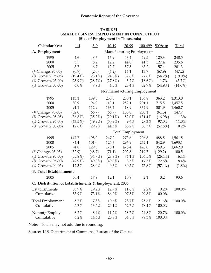
Economic Report of the Governor
- 65 -
TABLE 51 SMALL BUSINESS EMPLOYMENT IN CONNECTICUT
(Size of Employment in Thousands)
Calendar Year 1-4 5-9 10-19 20-99 100-499 500&up Total A. Employment Manufacturing Employment
1995 4.6 8.7 16.9 43.4 49.5 125.3 248.5 2000 3.5 6.2 12.2 44.8 41.3 127.4 235.6 2005 3.7 6.7 12.7 57.5 63.2 57.4 201.3
(# Change, 95-05) (0.9) (2.0) (4.2) 14.1 13.7 (67.9) (47.2) (% Growth, 95-05) (19.4%) (23.1%) (24.6%) 32.6% 27.6% (54.2%) (19.0%) (% Growth, 95-00) (23.9%) (28.7%) (27.8%) 3.2% (16.6%) 1.7% (5.2%) (% Growth, 00-05) 6.0% 7.9% 4.5% 28.4% 52.9% (54.9%) (14.6%) Nonmanufacturing Employment
1995 143.1 189.3 230.3 230.1 156.8 363.2 1,313.0 2000 80.9 94.9 113.1 252.1 201.1 715.5 1,457.5 2005 91.1 112.9 163.4 418.9 362.9 301.9 1,460.7
(# Change, 95-05) (52.0) (66.7) (66.9) 188.8 206.1 (61.3) 147.7 (% Growth, 95-05) (36.3%) (35.2%) (29.1%) 82.0% 131.4% (16.9%) 11.3% (% Growth, 95-00) (43.5%) (49.9%) (50.9%) 9.6% 28.3% 97.0% 11.0% (% Growth, 00-05) 12.6% 29.2% 44.5% 66.2% 80.5% (57.8%) 0.2% Total Employment
1995 147.7 198.0 247.2 273.6 206.3 488.5 1,561.5 2000 84.4 101.0 125.3 296.9 242.4 842.9 1,693.1 2005 94.8 129.3 176.1 476.4 426.0 359.3 1,662.0
(# Change, 95-05) (52.9) (68.7) (71.1) 202.8 219.7 (129.2) 100.5 (% Growth, 95-05) (35.8%) (34.7%) (28.8%) 74.1% 106.5% (26.4%) 6.4% (% Growth, 95-00) (42.9%) (49.0%) (49.3%) 8.5% 17.5% 72.5% 8.4% (% Growth, 00-05) 12.3% 28.0% 40.6% 60.5% 75.8% (57.4%) (1.8%) B. Total Establishments 2005 50.4 17.9 12.1 10.8 2.1 0.2 93.6 C. Distribution of Establishments & Employment, 2005 Establishments 53.9% 19.2% 12.9% 11.6% 2.2% 0.2% 100.0%
Cumulative 53.9% 73.1% 86.0% 97.5% 99.8% 100.0% Total Employment 5.7% 7.8% 10.6% 28.7% 25.6% 21.6% 100.0%
Cumulative 5.7% 13.5% 24.1% 52.7% 78.4% 100.0% Nonmfg Employ. 6.2% 8.4% 11.2% 28.7% 24.8% 20.7% 100.0%
Cumulative 6.2% 14.6% 25.8% 54.5% 79.3% 100.0%
Note: Totals may not add due to rounding.
Source: U.S. Department of Commerce, Bureau of the Census

Economic Report of the Governor
- 66 -
For more information, please write or contact the following:
Connecticut Economic Resource Center, Inc. 805 Brook Street
Rocky Hill, CT 06067 1-(860)-571-7136 1-(800)-392-2122
Connecticut Department of Economic & Community Development
Research Division 505 Hudson Street Hartford, CT 06106
1-(860)-270-8165 1-(860)-270-8000
Nonfinancial Debt For many years, national attention has been centering on the issue of the federal budget and trade deficits, as well as the level of indebtedness of domestic nonfinancial entities. Domestic Nonfinancial Debt (DNFD) is the aggregate net indebtedness of all nonfinancial borrowers in the United States. It includes the borrowings of all levels of government, business and households. It excludes the debt of foreigners and the liabilities of financial intermediaries such as commercial banks, thrift institutions and finance companies. As required by the Full Employment and Balanced Growth Act of 1978, DNFD is compiled quarterly by the Federal Reserve System. The following Table shows the 10-year history from 1998 to 2007 for total DNFD and each of its components. In 2007, the year-end total domestic nonfinancial debt outstanding was $31,723.4 billion. Total non-financial debt for the past decade has grown 95.5%, outpacing the growth in GDP of 56.7%. Among the four components, household debts grew the fastest at 133.9% while Federal indebtedness the slowest at 36.5%, with business and local government closely in line with total debt. Prior to 1990, household borrowings trailed those of businesses; however, faster growth since 1991 in home mortgages and consumer credit coupled with a steady increase in income helped catapult household borrowings to the top. Over the past decade, the private sector has increasingly played a more important role in the debt market. Debt growth in the private sector grew by 115.4% versus 49.4% for the public sector that includes the federal government as well as state and local government. Debt outstanding in the private sector accounted for 76.9% of the total in 2007, up from 69.8% in 1998. Following double digit growth over the past five years, households in 2007 continued to take on mortgages even though interest rates became less favorable and the housing market softened. While demand for housing and home related items such as furniture and building materials slowed, consumers spent more on non-housing related goods and services at gas stations, drinking establishments, mail order and food related services and warehouse clubs. Of the total $31.7 trillion nonfinancial debt outstanding, households accounted for 43.7%,

Economic Report of the Governor
- 67 -
followed by nonfinancial businesses at 33.3%, the federal government at 16.1%, and state and local governments at 6.9%.
TABLE 52 DOMESTIC NON-FINANCIAL DEBT (DNFD) OUTSTANDING BY SECTOR IN THE U.S.
In Billions of Dollars by Yearend
2007 Growth
1989 1998 2007 % of Total
(’89 to ’98)
(’98 to ’07)
1. Private Sector a. Households Home Mortgages $2,277.3 $4,057.5 $10,542.7 33.2% 78.2% 159.8% Consumer Credits 809.3 1,441.3 2,554.3 8.1% 78.1% 77.2% Other 250.3 421.5 751.5 2.4% 68.4% 78.3% Sub-Total $3,336.9 $5,920.3 $13,848.5 43.7% 77.4% 133.9% b. Business Mortgages $1,190.8 $1,382.2 $3,646.9 11.5% 16.1% 163.8% Corporate Bonds 961.1 1,881.2 3,559.1 11.2% 95.7% 89.2% Bank Loans 1,250.0 1,806.0 3,041.5 9.6% 44.5% 68.4% Other 222.5 340.9 313.3 1.0% 53.2% (8.2%) Sub-Total $3,624.4 $5,410.3 $10,560.6 33.3% 49.3% 95.2% Sub-Total - Private sector $6,961.3 $11,330.6 $24,409.1 76.9% 62.8% 115.4%
2. Public Sector Federal Government $2,251.2 $3,752.2 $5,122.3 16.1% 66.7% 36.5% State & Local Gov’t 940.4 1,143.8 2,191.9 6.9% 21.6% 91.6%
Sub-Total - Public Sector $3,191.6 $4,896.0 $7,314.2 23.1% 53.4% 49.4% Total DNFD $10,152.9 $16,226.6 $31,723.4 100.0% 59.8% 95.5% GDP, 4th Quarter $ 5,584.3 $8,953.8 $14,031.2 60.3% 56.7% DNFD as a % of GDP 181.8 181.2 226.1
Source: Board of Governors of the Federal Reserve System U.S. Department of Commerce
The DNFD-to-GDP ratio stood at 226.1% in 2007, up from 181.2% in 1998, implying a faster growth in nonfinancial debt than GDP in the past decade. The DNFD-to-GDP ratio gained speed in the late 1980s as a result of a combination of nearly double-digit increases in federal borrowings and the deregulation of the financial markets. During the 1980s, non-bank financial institutions funneled funds more freely between the suppliers of capital and its consumers, creating a more competitive and efficient market. The ratio declined in the 1990s as federal debt fell and the growth in borrowings by state and local governments slowed, which was also accompanied by more robust GDP growth. However, more recently the ratio rebounded rapidly, resulting from an accommodative monetary policy, less stringent financing standards on mortgages, and an economic recovery that stimulated borrowing and higher spending levels in both the household and business sectors.
Economic Report of the Governor
- 68 -
Household Borrowing Household borrowings, which include home mortgages, consumer credit, and other miscellaneous items, totaled $13.85 trillion and accounted for 43.7% of total non-financial debt. Growth in household borrowings had been accelerating, climbing at a double digit pace for five consecutive years between 2002 and 2006, but slowed to 6.8% in 2007, with a total growth of 133.9% for the past decade. Faster household borrowing is due fundamentally to the low, and at times negative, personal saving rate, leaving borrowing as the only available avenue for households. In the first half of the 1990s, growth in household borrowings averaged only 6.3% per year as sluggish income growth, the depressed value of real estate, and increased health insurance and educational costs made consumers more cautious. In the second half of the 1990s, average household borrowings climbed to 7.5% per year as a result of the continued healthy growth in income from wages, capital gains, and an appreciation in home values. During the most recent economic recovery between 2002 and 2006, growth in borrowings averaged 11.0% per year as a buildup of wealth generated by increases in income and an appreciation in real estate, favorably low interest rates, and loosened credit standards that fueled a borrowing and spending binge. U.S. saving rates, defined as personal saving as a percentage of disposable income, averaged only 1.4% since 2000, dropping from an average of 5.2% in the 1990s and 9.0% in the 1980s. They deteriorated further to range between a negative 0.7% and a positive 1.1% for the past 12 quarters ending in 2007. Net household asset levels also affected household borrowings. Household assets include home and financial equities. Net home equity (value of homes less mortgage liabilities) has been growing important to the economy. The net value of home equity grew more than 50% from 2001 to mid 2007, and then began declining. During this period, household financial assets grew even faster at 75.7% from mid 2002 to the third quarter of 2007. Overall, household assets gained 52.0% to $21.0 trillion during the same period. The share of net home equity of total family net assets has played important role on borrowings. Net home equity accounted for 47.1% of households’ total net assets in 2007, up from 37.5% in 2001. Research findings show that rising home prices have a bigger influence on credit creation and spending than that of rising equity prices. Home value appreciation is perceived more permanent and consistent with a higher propensity to consume by the public relative to gains in the stock market that are volatile and ephemeral in nature. Unlike capital gains on stocks, benefits realized through mortgage refinancing due to the appreciation of homes or lower mortgage rates can be cashed out without tax liability. Refinancing frees up more money for spending, paying off old debts or investments in a second home. The Tax Payer Relief Act of 1997 also allows a tax exemption of up to $500,000 of gain for joint filers or $250,000 for single filers. Among total household borrowings of $13.85 trillion in 2007, home mortgage loans accounted for $10.54 trillion, or 76.1% of household borrowings, followed by consumer credit at $2.55 trillion, or 18.4%, with the remainder in other miscellaneous items. After six consecutive years of rapid expansion, growth in home mortgages slowed in 2007 as a correction related to sub-prime and Alt-A mortgages engulfed consumers. As plunging housing prices were coupled with reset provisions on certain mortgages and a slowdown in the economy, delinquency rates

Economic Report of the Governor
- 69 -
on all residential real estate loans increased, up from 1.95% in 2006 to 3.04% in 2007 and deteriorated to 4.33% by mid-2008. The volume of resets on exotic mortgages to much higher rates of interest peaked between mid-2007 and mid-2008. Responding to rising foreclosure rates, lenders began tightening their lending policies, further limiting credit availability on the already retrenched financial market. At the same time, the economy was bearing the brunt of a severe oil price hike that surged close to $150 a barrel in July 2008. A prolonged and deeper recession in the housing sector will weigh on consumer spending and business investment, and has threatened the overall economy. Consumer credit not secured by real estate is comprised of non-revolving credit (such as automobile and personal loans) and revolving credit (which includes credit card debt and store charges). It registered $2.6 trillion in late 2007, with non-revolving credit accounting for approximately 65% of the total consumer credit. Consumer credit helped finance a large expansion in spending for consumer non-durables. Credit card debt continues to increase at a rapid pace as convenience and security continue to improve, and more consumers rely on credit cards for making purchases online or by telephone despite higher interest rate charges. Business Borrowing Business borrowings include debts owed by corporations, nonfarm corporations and farms. Total borrowings registered $10.56 trillion at the end of 2007. Borrowing instruments include corporate bonds, commercial paper, municipal securities, bank loans, mortgages, and others. Mortgages comprised the major portion of the total, accounting for 34.5% of business borrowings, followed by corporate bonds at 33.7% and bank loans at 28.8%. Businesses had benefited from a more accommodative lending environment as banks had eased both standards and terms on commercial and industrial loans, and mortgage rates remained favorably low. Government Borrowing The U.S. federal budget has long been operating under deficits since the early 1950s. The federal deficit started surging in the early 1980s from an expansionary fiscal policy and tax cuts, intending to sacrifice a short-term loss in revenue for a long-term gain through more rapid economic growth. This expectation, however, was not fully realized and deficits persisted into the late 1990s. After being saddled with deficits in most of the 1990s, the federal budget turned to a surplus in 1998 and reached a high of $236.5 billion in fiscal 2000. Federal operations, however, turned red in fiscal 2002 and continued to deteriorate with a deficit of $437.6 billion in fiscal 2008. The federal deficit for FY 2009 is expected to widen sharply as the growth in revenues slows while spending accelerates as the economy slows and federal bailout programs intended to rescue the financial industry and boost the economy come to fruition. As the federal operating budget continued to post a deficit, the national debt also increased. By the end of federal fiscal year 2008, gross debt outstanding registered $10,024 billion, up 11.3% from fiscal 2007 and accelerating from 5.9% in fiscal 2007, with per capita debt outstanding approximately $32,500. In fiscal 2008, the federal interest payments were $451.2 billion, which accounted for 15.2% of total federal outlays. The federal budget deficit in the U.S. in 2008 equates to -2.5% of its GDP, compared to +1.1% in Germany, -3.8% in Great Britain, -2.9% in France, and -2.5% in Japan.
Economic Report of the Governor
- 70 -
Of the 2008 total federal gross debt of $10.02 trillion, $5.81 trillion, or 58%, was held by the public and $4.22 billion, or 42%, by intra-governmental agencies. Public holders include individuals, corporations, state or local governments, foreign governments, and other entities outside of the United States while intra-governmental agencies hold federal securities in trust funds, revolving funds, and other special funds. The federal statutes authorize federal agencies such as the Federal Reserve Bank and various trust funds to invest in U.S. Treasury securities. Debt outstanding by state and local government, which includes states, counties, municipalities and other local entities, increased at a faster rate in 2007 due to a faster increase in expenditures than receipts. Interest payments grew by 4.5% in 2007 to $98.5 billion, accounting for 5.2% of total current expenditures. Interest payments in the next few years are expected to increase as the economy slows and credit contracts across the private and public sectors. According to the U.S. Department of Commerce’s “State Government Finances,” state government debt outstanding in Connecticut at the end of fiscal 2006, the latest available year, was $24.04 billion, up from $23.05 billion in 2005. Connecticut per capita state government debt was $6,876 in fiscal 2006, up from $6,584 in fiscal 2005 and compared with $2,915 for the nation, which was up from $2,693 in 2005. Connecticut's overall credit rating is determined by three major rating agencies: Moody's Investors Service, Standard & Poor's Corporation, and Fitch Investors Service, Inc. As of the end of 2008, Connecticut’s General Obligation bonds are rated Aa3 by Moody’s and AA by Standard & Poor's Corporation and Fitch Investors Service, Inc. The rating process provides information for investors about risk. Low ratings will generally result in higher borrowing costs. Savings by U.S. Households A low personal savings rate has been a concern for some time as it will negatively impact our economy and society. Consumers’ imprudent financing of consumption has created an unsustainable level of consumer debt, lowering potential economic growth, raising interest rates, and may result in social problems. We may be witnessing an unexpected reversal of consumer-financing behavior that has caused a sudden drop in consumption and resulted in economic instability. The lower national savings rate has not generated sufficient funds domestically to support the investment necessary to sustain long-run economic growth. This has created a situation requiring excessive reliance on foreign capital and an unfavorable current account balance. The solid line on the following chart shows the national savings rate for U.S. consumers from 1950 through 2007. After staying at an average of 8.7% between 1950 and 1980, U.S. saving rates have been trending down from a high of 12.2% in late 1981 to a low of negative 0.7% in late 2005 and an average of 0.4% in 2006. The savings rate is defined as personal savings divided by disposable personal income. Disposable personal income is defined as total personal income less personal tax and nontax payments to governments. Personal savings is defined as

Economic Report of the Governor
- 71 -
disposable personal income less consumption expenditures (including consumer durables), interest payments, and net transfer payments to the rest of the world.
SAVING BY U.S. HOUSEHOLDS
-2
0
2
4
6
8
10
12
14
1950 1960 1970 1980 1990 2000CALENDAR YEAR
Savi
ngs R
ate
(%)
400
450
500
550
600
650
Net
Wor
th A
s % o
f Dis
posa
ble
Pe
rson
al In
com
e
Savings RateNet Worth as % of DPI
Source: U.S. Bureau of Economic Analysis (BEA) The savings rate is often criticized because, by definition, personal incomes do not include the sales of existing assets. Realization of capital gains or losses from the appreciation or depreciation of assets such as stocks, bonds and antique collections, etc. are excluded in personal income, leading to under-/overvaluation of the income level. The definition of personal consumption outlay includes expenditures that might arguably be considered investments. For example, the purchase of a computer, a consumer durable, for education or training is treated as consumption. Mortgage payments also could be considered part of an investment. These expenditures are essentially “hidden savings”. In today’s economy, education and training, rather than physical capital, are the major inputs for economic growth. Education expenditures at all levels in the U.S. in 2001 accounted for approximately 7.5% of GDP, the highest among major industrialized nations, compared to 4.6% in Japan. Critics, therefore, conclude that our lower national savings rate may be due to an understated personal income with overstated consumption and there are some merits to this argument. The chart also shows how the savings rate is affected by economic conditions by depicting the net worth of consumers as a percentage of disposable personal income. After the mid 1970s, the “wealth effect” took hold as people began to spend more because they had more assets to leverage and finance their consumption. This relative net worth has generally moved inversely with the savings rate. Before 1980, the savings rate was trending upward, with the relative net

Economic Report of the Governor
- 72 -
worth generally decreasing. During this period, before various innovative and creative financing mechanisms were available to the middle class, people generally lived on cash. During hard times, they may have saved less, left existing savings untouched to grow as long as possible, and eventually lived on what they had saved. After the 1970s, when credit cards and home equity loans became available to more households, savings rates decreased but net worth as a percentage of disposable personal income generally increased due to the acceleration in capital gains. During generally good economic times, people believe they are wealthier and spend more, driving the savings rate down. People had been spending more because they had greater assets and the ability to obtain financing secured by these assets. Household Balance Sheet The Federal Reserve Bank’s “Flow of Funds Accounts” contains statistics on the assets, liabilities, and net worth for the household sector. The table below shows these three components that comprise a balance sheet for 1945, 1998, and 2007, to evaluate the financial position of the nation’s households.
TABLE 53
BALANCE SHEET OF HOUSEHOLDS AND NON-PROFIT ORGANIZATIONS In Billions of Dollars
1945 % of % of % of Average 1945 In 2007 $ Total 1998 Total 2007 Total Growth * A. Assets 1. Real Estate 134.8 1,558.1 18.2% 10,587.3 24.3% 22,302.2 30.8% 21.5% 2. Stock related 122.9 1,420.5 16.6% 18,320.7 42.0% 23,772.7 32.8% 25.4% 3. Other 483.9 5,593.0 65.3% 14,676.5 33.7% 26,404.2 36.4% 6.0% Total 741.6 8,571.6 100.0% 43,584.5 100.0% 72,479.1 100.0% 12.0% B. Liabilities 1. Home Mortgages 18.6 215.0 61.4% 4,057.5 65.3% 10,530.3 73.2% 77.4% 2. Consumer Credit 6.8 78.6 22.4% 1,441.3 23.2% 2,556.6 17.8% 50.9% 3. Other 4.9 56.6 16.2% 718.0 11.6% 1,302.4 9.1% 35.5% Total 30.3 350.2 100.0% 6,217.3 100.0% 14,389.3 100.0% 64.7% C. Net Worth 711.3 8,221.4 37,367.2 58,089.8 9.8% 1. Net Home Equity 116.2 1,343.1 6,529.8 11,771.9 12.5%
2. As a % of Net Worth 16.3
% 17.5% 20.5%
D. As a % of Total Assets 1. Home Mortgages 2.5% 9.3% 14.5% 2. Liabilities 4.1% 14.3% 19.9%
3. Net worth 95.9
% 85.7% 80.1% Note: * Average real growth from 1945 to 2007 Source: Board of Governors of the Federal Reserve System
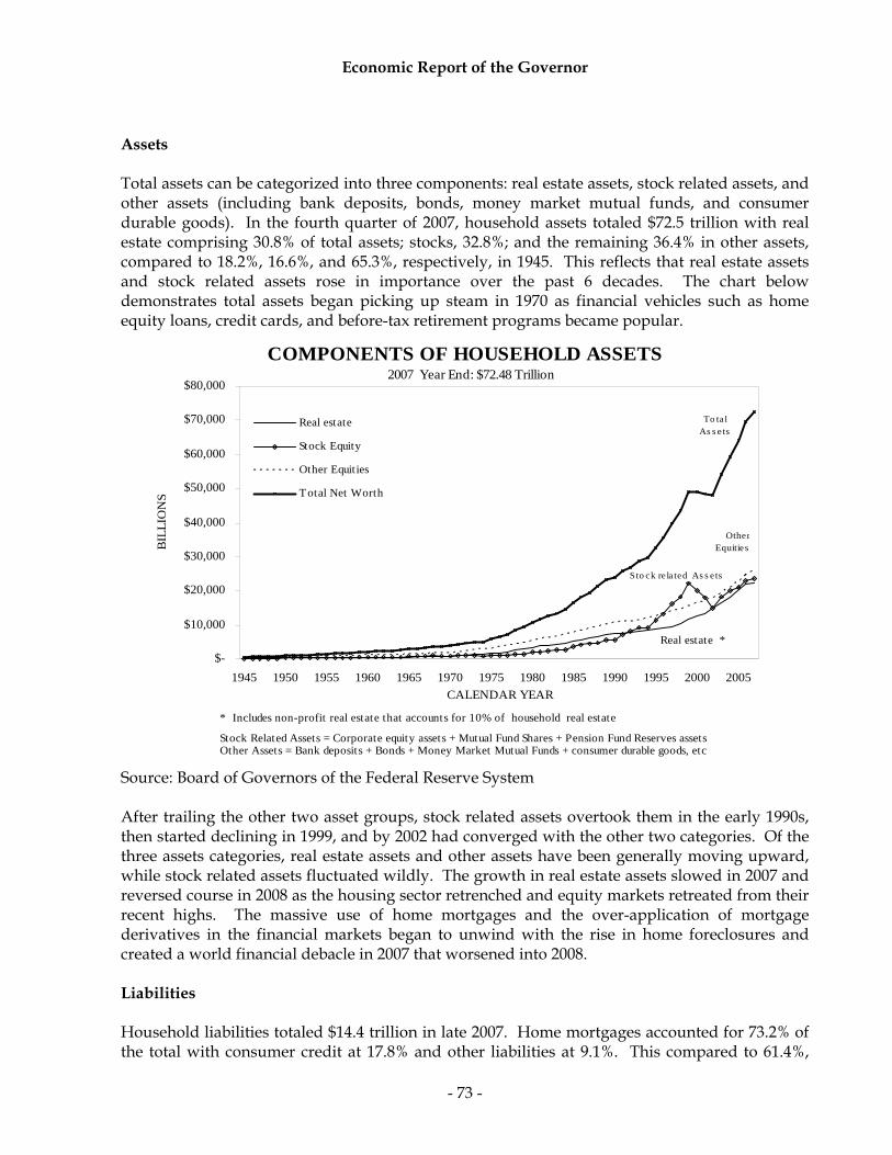
Economic Report of the Governor
- 73 -
Assets Total assets can be categorized into three components: real estate assets, stock related assets, and other assets (including bank deposits, bonds, money market mutual funds, and consumer durable goods). In the fourth quarter of 2007, household assets totaled $72.5 trillion with real estate comprising 30.8% of total assets; stocks, 32.8%; and the remaining 36.4% in other assets, compared to 18.2%, 16.6%, and 65.3%, respectively, in 1945. This reflects that real estate assets and stock related assets rose in importance over the past 6 decades. The chart below demonstrates total assets began picking up steam in 1970 as financial vehicles such as home equity loans, credit cards, and before-tax retirement programs became popular.
COMPONENTS OF HOUSEHOLD ASSETS
$-
$10,000
$20,000
$30,000
$40,000
$50,000
$60,000
$70,000
$80,000
1945 1950 1955 1960 1965 1970 1975 1980 1985 1990 1995 2000 2005CALENDAR YEAR
BIL
LIO
NS
Real estate
Stock Equity
Other Equities
Total Net Worth
Real estate *
Sto ck re la ted As s e ts
2007 Year End: $72.48 Trillion
* Includes non-profit real estate that accounts for 10% of household real estate
Stock Related Assets = Corporate equity assets + Mutual Fund Shares + Pension Fund Reserves assets
Other Equitie s
To ta l As s e ts
Other Assets = Bank deposits + Bonds + Money Market Mutual Funds + consumer durable goods, etc
Source: Board of Governors of the Federal Reserve System
After trailing the other two asset groups, stock related assets overtook them in the early 1990s, then started declining in 1999, and by 2002 had converged with the other two categories. Of the three assets categories, real estate assets and other assets have been generally moving upward, while stock related assets fluctuated wildly. The growth in real estate assets slowed in 2007 and reversed course in 2008 as the housing sector retrenched and equity markets retreated from their recent highs. The massive use of home mortgages and the over-application of mortgage derivatives in the financial markets began to unwind with the rise in home foreclosures and created a world financial debacle in 2007 that worsened into 2008.
Liabilities Household liabilities totaled $14.4 trillion in late 2007. Home mortgages accounted for 73.2% of the total with consumer credit at 17.8% and other liabilities at 9.1%. This compared to 61.4%,
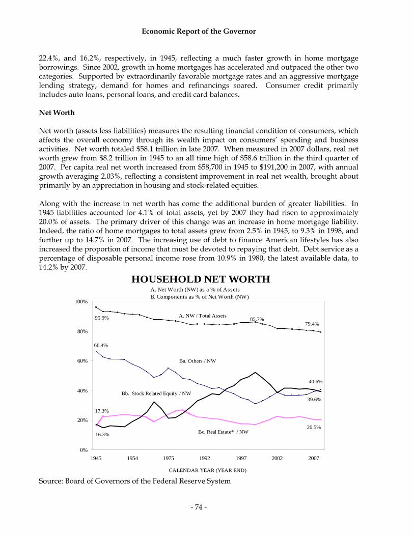
Economic Report of the Governor
- 74 -
22.4%, and 16.2%, respectively, in 1945, reflecting a much faster growth in home mortgage borrowings. Since 2002, growth in home mortgages has accelerated and outpaced the other two categories. Supported by extraordinarily favorable mortgage rates and an aggressive mortgage lending strategy, demand for homes and refinancings soared. Consumer credit primarily includes auto loans, personal loans, and credit card balances.
Net Worth Net worth (assets less liabilities) measures the resulting financial condition of consumers, which affects the overall economy through its wealth impact on consumers’ spending and business activities. Net worth totaled $58.1 trillion in late 2007. When measured in 2007 dollars, real net worth grew from $8.2 trillion in 1945 to an all time high of $58.6 trillion in the third quarter of 2007. Per capita real net worth increased from $58,700 in 1945 to $191,200 in 2007, with annual growth averaging 2.03%, reflecting a consistent improvement in real net wealth, brought about primarily by an appreciation in housing and stock-related equities. Along with the increase in net worth has come the additional burden of greater liabilities. In 1945 liabilities accounted for 4.1% of total assets, yet by 2007 they had risen to approximately 20.0% of assets. The primary driver of this change was an increase in home mortgage liability. Indeed, the ratio of home mortgages to total assets grew from 2.5% in 1945, to 9.3% in 1998, and further up to 14.7% in 2007. The increasing use of debt to finance American lifestyles has also increased the proportion of income that must be devoted to repaying that debt. Debt service as a percentage of disposable personal income rose from 10.9% in 1980, the latest available data, to 14.2% by 2007.
HOUSEHOLD NET WORTH
0%
20%
40%
60%
80%
100%
1945 1954 1975 1992 1997 2002 2007
CALENDAR YEAR (YEAR END)
Ba. Others / NW
Bc. Real Estate* / NW
Bb. Stock Related Equity / NW
17.3%
16.3%
66.4%
20.5%
39.6%
40.6%
A. NW / Total Assets95.9% 85.7%79.4%
A. Net Worth (NW) as a % of AssetsB. Components as % of Net Worth (NW)
Source: Board of Governors of the Federal Reserve System

Economic Report of the Governor
- 75 -
PERFORMANCE INDICATORS
This section is devoted to performance trends of various economic indicators for three entities; the United States, the New England Region and Connecticut. These statistics will indicate the relative economic performance of these entities showing both their strong and weak points. Gross Product Gross National Product (GNP) is defined as the aggregate current market value of final goods and services produced by a nation's citizens and capital, regardless of location, in a given period of time. GNP was generally used as a measure of a nation's economic performance to track the cyclical ups and downs of the economy, but GNP reflects more than domestic activity; products produced by citizens outside territorial borders are included, while products produced by foreign workers and capital located in the nation are excluded. As a result, Gross Domestic Product (GDP) which measures all economic activity within a territory, and is consistent with other economic indicators such as employment and shipments of manufactured goods, has been adopted as a better measure of economic activity within a territory. Because prices of goods and services change over time, both GNP and GDP may also change, even if there has been no change in physical output. Therefore, to measure changes in real output, they are adjusted by an index of the general price level and expressed in constant dollars. Other things being equal, when real gross product rises, the economy is experiencing an expansion; when real gross product falls the economy is experiencing a decline. In the past, a fixed-weighted inflation index, the GDP deflator, had been used to measure real output, but with the rapid change in technology, price movements for certain commodities actually grew less than the price for all goods on average. As such, the traditional measurement of real product had misstated the growth in output as it moved away from the base year, creating what is known as substitution bias. To correct for this bias, the U.S. Department of Commerce, Bureau of Economic Analysis, uses a chained-type inflation index based on calendar year 2000. One measure of a state's economic performance is Gross State Product (GSP). Like GDP, GSP is the current market value of all final goods and services produced by labor and property located in a state. In 2007, the State of Connecticut produced $216.3 billion worth of goods and services and $181.8 billion worth of goods and services in 2000 chained type dollars. Between 2002 and 2007, the output contribution of transportation, warehousing and utilities, information services and Finance, Insurance, and Real Estate (FIRE) increased, while construction and wholesale and retail trade fell, and most everything else remained fairly constant. The broadly defined services in the private sector, which includes industries in information, professional and technical services, health care and education, FIRE and other services have increased to 61.0% of total GSP in 2007 from 59.8% in 2002, with transportation, warehousing and utilities increasing from 3.14% in 2002 to 3.6% in 2007, or 16.6%. Information services increased from 3.9% to 4.2%, or 7.7%, and FIRE increased from 29.0% to 29.9%, or 3.1%. During this period, the shift toward services in Connecticut occurred at a slower rate than the rate for the nation as a whole. The share of service production increased 1.2 percentage points (2.0%) in Connecticut versus increasing 1.2 percentage points (2.4%) for the nation. An increasing share of service production could help smooth the business cycle, reducing the span and depth of recessions and prolonging the length of expansions. Normally, activities in service

Economic Report of the Governor
- 76 -
sectors relative to manufacturing are less susceptible to pent-up demand, less subject to inventory-induced swings, less intensive in capital requirements, and somewhat less vulnerable to foreign competition. Connecticut began moving toward services sooner than the nation as a whole, and continues to lead in that direction.
TABLE 54 GROSS PRODUCT
Calendar United States * New England * Connecticut
Year Dollars % Growth Dollars % Growth Dollars % Growth A. Millions of Current Dollars
2002 10,398,402 3.4 591,733 1.9 166,073 0.6 2003 10,886,172 4.7 612,006 3.4 169,885 2.3 2004 11,607,041 6.6 647,473 5.8 182,112 7.2 2005 12,346,871 6.4 674,562 4.2 193,281 6.1 2006 13,119,938 6.3 712,051 5.6 204,964 6.0 2007 13,743,021 4.7 744,672 4.6 216,266 5.5
% Increase (‘02 to ‘07) 32.2 25.8 30.2
B. Constant Dollars**
2002 9,981,850 1.5 568,750 (0.3) 158,628 (1.6) 2003 10,225,679 2.4 579,651 1.9 159,456 0.5 2004 10,580,223 3.5 597,196 3.0 165,828 4.0 2005 10,899,704 3.0 606,068 1.5 171,123 3.2 2006 11,240,107 3.1 623,136 2.8 176,900 3.4 2007 11,467,503 2.0 636,223 2.1 181,809 2.8
% Increase (‘02 to ‘07) 14.9 11.9 14.6 * Sum of State's Gross State Products. ** 2000 chained dollar series are calculated as the product of the chain-type quantity index and
the 2000 current-dollar value of the corresponding series, divided by 100. The system for these calculations was converted from SIC Codes to the NAICS system starting in 1998.
Source: U.S. Department of Commerce, Bureau of Economic Analysis The following Table, which displays gross state product by source in 2007, shows Connecticut’s production concentrated in two areas: finance, insurance and real estate (FIRE) and manufacturing (ignoring the broad category of services). Production in these two industries accounted for 42.5% of total production in Connecticut compared to 32.6% for the nation and was an increase from 41.6% in 2002. This demonstrates that Connecticut’s economy is more heavily concentrated in a few industries than the nation as a whole and this concentration has changed little in recent years. Additionally, Connecticut’s portion of U.S. total GSP has declined from 1.60% to 1.57%, a drop of 0.03 percentage points, or 1.9%.
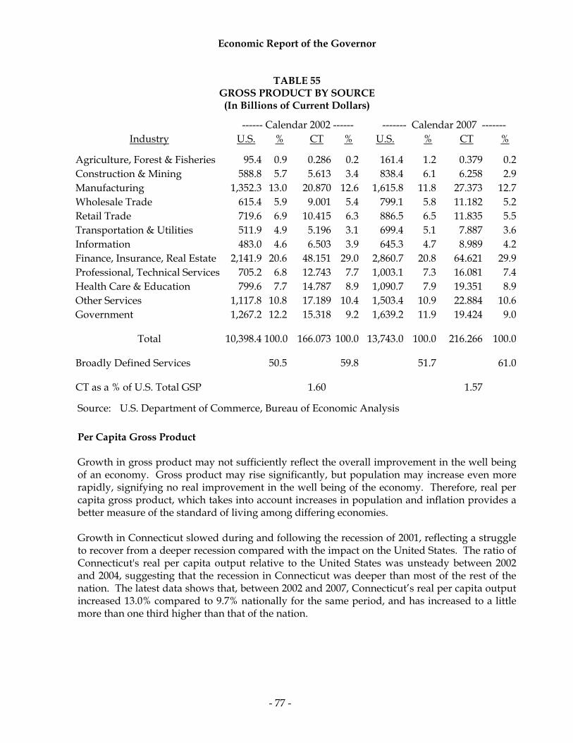
Economic Report of the Governor
- 77 -
TABLE 55 GROSS PRODUCT BY SOURCE (In Billions of Current Dollars)
------ Calendar 2002 ------ ------- Calendar 2007 ------- Industry U.S. % CT % U.S. % CT %
Agriculture, Forest & Fisheries 95.4 0.9 0.286 0.2 161.4 1.2 0.379 0.2 Construction & Mining 588.8 5.7 5.613 3.4 838.4 6.1 6.258 2.9 Manufacturing 1,352.3 13.0 20.870 12.6 1,615.8 11.8 27.373 12.7 Wholesale Trade 615.4 5.9 9.001 5.4 799.1 5.8 11.182 5.2 Retail Trade 719.6 6.9 10.415 6.3 886.5 6.5 11.835 5.5 Transportation & Utilities 511.9 4.9 5.196 3.1 699.4 5.1 7.887 3.6 Information 483.0 4.6 6.503 3.9 645.3 4.7 8.989 4.2 Finance, Insurance, Real Estate 2,141.9 20.6 48.151 29.0 2,860.7 20.8 64.621 29.9 Professional, Technical Services 705.2 6.8 12.743 7.7 1,003.1 7.3 16.081 7.4 Health Care & Education 799.6 7.7 14.787 8.9 1,090.7 7.9 19.351 8.9 Other Services 1,117.8 10.8 17.189 10.4 1,503.4 10.9 22.884 10.6 Government 1,267.2 12.2 15.318 9.2 1,639.2 11.9 19.424 9.0
Total 10,398.4 100.0 166.073 100.0 13,743.0 100.0 216.266 100.0
Broadly Defined Services 50.5 59.8 51.7 61.0
CT as a % of U.S. Total GSP 1.60 1.57
Source: U.S. Department of Commerce, Bureau of Economic Analysis Per Capita Gross Product Growth in gross product may not sufficiently reflect the overall improvement in the well being of an economy. Gross product may rise significantly, but population may increase even more rapidly, signifying no real improvement in the well being of the economy. Therefore, real per capita gross product, which takes into account increases in population and inflation provides a better measure of the standard of living among differing economies. Growth in Connecticut slowed during and following the recession of 2001, reflecting a struggle to recover from a deeper recession compared with the impact on the United States. The ratio of Connecticut's real per capita output relative to the United States was unsteady between 2002 and 2004, suggesting that the recession in Connecticut was deeper than most of the rest of the nation. The latest data shows that, between 2002 and 2007, Connecticut’s real per capita output increased 13.0% compared to 9.7% nationally for the same period, and has increased to a little more than one third higher than that of the nation.

Economic Report of the Governor
- 78 -
TABLE 56 PER CAPITA GROSS PRODUCT
A. In Current Dollars
Calendar United States New England Connecticut Year Dollars % Growth Dollars % Growth Dollars % Growth % of U.S.
2002 36,120 2.4 41,871 1.3 48,111 0.0 133 2003 37,481 3.8 43,137 3.0 48,916 1.7 131 2004 39,589 5.6 45,563 5.6 52,303 6.9 132 2005 41,727 5.4 47,446 4.1 55,437 6.0 133 2006 43,915 5.2 50,006 5.4 58,632 5.8 134 2007 45,563 3.8 52,206 4.4 61,750 5.3 136
% Increase (‘02 to ‘07) 26.1 24.7 28.3
B. In 2000 Chained Dollars
Calendar United States New England Connecticut Year Dollars % Growth Dollars % Growth Dollars % Growth % of U.S.
2002 34,673 0.5 40,245 (0.9) 45,954 (2.2) 133 2003 35,207 1.5 40,856 1.5 45,914 (0.1) 130 2004 36,086 2.5 42,025 2.9 47,626 3.7 132 2005 36,836 2.1 42,629 1.4 49,082 3.1 133 2006 37,623 2.1 43,762 2.7 50,604 3.1 135 2007 38,020 1.1 44,603 1.9 51,911 2.6 137
% Increase (‘02 to ‘07) 9.7 10.8 13.0
Source: U.S. Department of Commerce, Bureau of Economic Analysis & Bureau of the Census Productivity and Unit Labor Cost Gross State Product provides the information to gauge Connecticut’s efficiency in the use of labor, i.e., labor productivity. Rising productivity leads to an improved standard of living and curbs inflationary pressures. In the Table on the following page, the column entitled Hourly Production shows labor productivity as the ratio of total output to total workhours in Connecticut’s manufacturing sector. On an hourly basis, nominal output in the manufacturing sector increased from $67.1 in 1998 to $123.7 in 2007, an 84.4% increase in output per hour over the period compared to only a 27.2% increase in the Consumer Price Index over the same period. Another approach allows for the assessment of the labor cost for each $1 of product produced - the unit labor cost. Labor cost is one of the major input costs and is often cited as a critical indicator of competitiveness. The column entitled Unit Labor Cost shows the monetary cost which is equal to the average hourly wages of each worker divided by productivity. Connecticut continues to enjoy a downward trend in labor costs when the productivity factor is included. Per $1 of output costs, the unit labor cost has declined from 23.6 cents in 1998 to 16.7 cents in 2007, a 29.4% reduction over the period, even while production workers have enjoyed a 30.2% increase in average hourly wages. Overall, productivity depends upon a broad range of factors. Other than wages, the quality of management as well as the size of and quantity of capital stock invested in the form of plant,

Economic Report of the Governor
- 79 -
machinery and equipment, and the employment of new technologies impact productivity. Any increase in labor productivity is the combined result of all these factors.
TABLE 57 CONNECTICUT’S MANUFACTURING LABOR PRODUCTIVITY
Production Hourly Total Average
Cal. GSP Workhours Production Wages Hourly Unit Labor Cost Year (Million) (Million) (Output Per Hour) (Million) Wages (¢ Per $1 Output) 1998 $21,457 320.0 $67.1 $5,064.6 $15.8 23.6¢ 1999 $20,525 298.2 $68.8 $4,946.5 $16.6 24.1¢ 2000 $20,963 295.1 $71.0 $5,093.9 $17.3 24.3¢ 2001 $21,405 271.3 $78.9 $4,807.1 $17.7 22.5¢ 2002 $20,870 251.2 $83.1 $4,529.6 $18.0 21.7¢ 2003 $19,109 243.7 $78.4 $4,478.2 $18.4 23.4¢ 2004 $21,628 232.8 $92.9 $4,534.7 $19.5 21.0¢ 2005 $22,555 231.2 $97.6 $4,509.9 $19.5 20.0¢ 2006 $25,849 224.3 $115.3 $4,502.3 $20.1 17.4¢ 2007 $27,373 221.3 $123.7 $4,561.8 $20.6 16.7¢
% Increase (‘98-‘07) 84.4 30.2 (29.4) Source: U.S. Department of Commerce, Bureau of Economic Analysis U.S. Department of Commerce, Bureau of the Census, “Annual Survey of Manufactures” U.S. Department of Labor, Bureau of Labor Statistics Value Added In order to more accurately assess the performance of the manufacturing sector, one must look beyond employment figures. Employment figures provide only a one dimensional view of what is actually occurring in the manufacturing sector of the Connecticut economy. Although Connecticut has lost 176,000 manufacturing jobs (47.6%) between calendar year 1977 and 2006, this is being partially mitigated by a long-term increase in productivity per worker. Value added is the market value of a firm's output less the value of inputs which it purchased from other firms. Changes in productivity over time can be measured by dividing the value that is added to a product by the total number of production workers involved in producing that good. The following Table lists value added per production worker for Connecticut and the U.S. Connecticut's value added per production worker has steadily increased over every period covered in the table. Moreover, by 2006, Connecticut's value added per production worker was 120% of the national average, up from 100% in 1977.

Economic Report of the Governor
- 80 -
TABLE 58 VALUE ADDED PER PRODUCTION WORKER
(In Current Dollars)
% Change Cumulative % Ratio of Cal. United From Prior Period Change From 2002 CT Value Year Conn. States Conn. U.S. Conn. U.S. Added to U.S. 1977 42,828 42,741 61.9 63.3 1.002 1982 66,830 66,458 56.0 55.5 1.006 1987 103,228 94,927 54.5 42.8 1.087 1992 143,074 122,387 38.6 28.9 1.169 1997 179,595 151,317 25.5 23.6 1.187 2002 219,805 182,512 22.4 20.6 1.204 2003 220,268 194,966 0.2 6.8 0.2 6.8 1.130 2004 251,111 217,983 14.0 11.8 14.2 19.4 1.152 2005 267,644 239,329 6.6 9.8 21.8 31.1 1.118 2006 301,115 251,178 12.5 5.0 37.0 37.6 1.199
Note: Value Added Per Production Worker = Total Value Added by Manufacture Number of Production Workers
Source: U.S. Department of Commerce, “Annual Survey of Manufactures” Value added per production worker can vary greatly among manufacturing sectors. Factors which may contribute to this variance include the mix between labor and capital, the overall cost structure for an industry, the volume of production, and the prevailing markup or profit on a product. The following Table segments value added per production worker by industry in Connecticut for calendar year 2005 and 2006.
TABLE 59 VALUE ADDED PER PRODUCTION WORKER IN CONNECTICUT BY INDUSTRY
(In Current Dollars)
Industry 2005 2006 % Change Manufacturing 267,644 301,115 12.5 Food 406,478 410,804 1.1 Printing 137,317 142,283 3.6 Paper 255,824 257,636 0.7 Chemical 1,334,698 1,752,000 31.3 Plastics & Rubber 146,830 159,538 8.7 Primary Metals 160,667 216,360 34.7 Fabricated Metals 160,035 162,086 1.3 Machinery 229,717 249,050 8.4 Computer & Electronic 262,850 336,243 27.9 Electrical Equipment 205,483 210,983 2.7 Transportation Equipment 321,103 391,397 21.9 Note: Value Added Per Production Worker = Total Value Added by Manufacture Number of Production Workers Source: U.S. Department of Commerce, “Annual Survey of Manufactures”

Economic Report of the Governor
- 81 -
Capital Expenditures Connecticut's manufacturers have also been making substantial investments in capital equipment. Total capital expenditures are defined as outlays for permanent additions and major alterations to manufacturing establishments and investments in new machinery and equipment used for replacement and additions to plant capacity. Organizations undertake capital projects for various reasons including to reduce costs, improve efficiencies, upgrade product quality, develop new products and to implement environmental and safety technology. According to the Annual Survey of Manufactures, for the past 10 years, the level of capital expenditures within Connecticut has remained well above the one billion dollar figure. The following Table details capital expenditures in Connecticut. To further promote the expansion of manufacturing firms in Connecticut, the Legislature passed and the Governor signed into law, the Manufacturing Assistance Act of 1990 and the Manufacturing Recovery Act of 1992. These laws provide substantial incentives for manufacturers to make capital expenditures within Connecticut. The main tenet of the acts is a five year alleviation of local property taxes on all new or newly acquired machinery used in the production process. The machinery must be of the type classified by the Internal Revenue Service as five or seven year property. Beginning in fiscal 2002, towns are eligible to receive 80% reimbursement from the state for the property taxes foregone on such machinery. Municipalities must then abate the remaining 20% of property taxes on such machinery. Public Act 06-83 significantly enhanced this program by extending property tax relief beyond the initial five year exemption period by phasing out such taxation over a five fiscal year period. By assessment years commencing on and after October 1, 2011, all such equipment will be exempt from property taxation.
TABLE 60 TOTAL CAPITAL EXPENDITURES IN CONNECTICUT
(In Millions of Dollars)
Calendar Connecticut Percent Year Capital Expenditures Change 1997 1,867.8 5.6 1998 1,900.9 1.8 1999 1,715.9 (9.7) 2000 1,861.6 8.5 2001 1,783.2 (4.2) 2002 1,448.5 (18.8) 2003 1,242.7 (14.2) 2004 1,236.2 (0.5) 2005 1,201.6 (2.8) 2006 1,260.5 4.9 Source: U.S. Department of Commerce, “Annual Survey of Manufactures” Total Personal Income Total personal income, defined as current income received by persons from all sources including public and private transfer payments but excluding transfers among persons, is a good reliable measure of economic performance. Total personal income captures the

Economic Report of the Governor
- 82 -
manufacturing sector through manufacturing wages; the nonmanufacturing sector through wages in government, wholesale/retail trade, utilities, transportation, mining, personal services, etc.; the private sector through proprietor's income, etc.; and a part of agricultural activity via farm properties' income. Personal income is approximately 84% of Gross Domestic Product; hence, the two are well correlated. The U.S. Department of Commerce defines the various sources of personal income as the following: Wages and Salaries - the monetary remuneration of employees, including the compensation of corporate officers; commissions, tips and bonuses; and receipts in kind that represent income to the recipient. Wages and salaries are measured before deductions such as social security contributions and union dues. Other Labor Income - consists primarily of employer contributions for employee pension and insurance funds and employer contributions for government social insurance. Property Income - income from Dividends, Interest and Rents. Dividends are payments in cash or other assets, excluding stock, by corporations organized
for profit to non-corporate stockholders who are U.S. residents. Interest is the monetary and imputed interest income of persons from all sources. Imputed
interest represents the excess of income received by financial intermediaries from funds entrusted to them by persons, over income disbursed by these intermediaries to persons. Part of imputed interest reflects the value of financial services rendered without charge to persons by depository institutions. The remainder is property income held by life insurance companies and private non-insured pension funds on behalf of persons; one example is the additions to policyholder reserves held by life insurance companies.
Rental income is the monetary income of persons (except those primarily engaged in the
real estate business) from the rental of real property (including mobile homes); the imputed net rental income of owner-occupants of nonfarm dwellings; and the royalties received by persons from patents, copyrights, and rights to natural resources.
Proprietors' Income - the income, including income-in-kind, of sole proprietorships and partnerships and of tax-exempt cooperatives. The imputed net rental income of owner occupants of farm dwellings with certain adjustments is included. Transfer Payments - income payments to persons, generally in monetary form, for which they do not render current services. These include payments by the government and business to individuals and nonprofit institutions. Personal Contributions to Social Insurance - contributions made by individuals under the various social insurance programs. Payments by employees and the self-employed (farm and nonfarm) are included as well as contributions that are sometimes made by employers on behalf of their employees (i.e., those customarily paid by the employee but, under special arrangement, paid by the employer).

Economic Report of the Governor
- 83 -
The correlation between Gross Domestic Product and personal income provides another basis of comparison among individual states. A comparison of growth rates in personal income is a good indicator of a state’s present and future performance. According to figures provided by the U.S. Bureau of Economic Analysis, personal income to Connecticut residents during fiscal year 2008 was $195.77 billion, a 5.1% increase over fiscal 2007. Total personal income in Connecticut increased 54.4% from fiscal 1999 to 2008. For the United States, total personal income increased 56.4%, and in the New England Region, the increase for the identical period was 54.3 %. The following Table and Chart shows personal income for the United States, the New England Region, and Connecticut.
TABLE 61 PERSONAL INCOME
(In Millions)
Fiscal United States New England Connecticut Year Dollars % Growth Dollars % Growth Dollars % Growth
1998-99 7,607,013 6.27 446,176 6.44 126,769 6.15 1999-00 8,109,583 6.61 481,751 7.97 135,783 7.11 2000-01 8,613,913 6.22 518,388 7.61 145,744 7.34 2001-02 8,788,092 2.02 525,601 1.39 146,946 0.83 2002-03 8,974,062 2.12 530,090 0.85 146,983 0.03 2003-04 9,398,254 4.73 552,498 4.23 153,265 4.27 2004-05 9,992,970 6.33 580,695 5.10 163,149 6.45 2005-06 10,617,281 6.25 614,800 5.87 174,081 6.70 2006-07 11,309,119 6.52 654,315 6.43 186,240 6.98 2007-08 11,899,552 5.22 688,504 5.23 195,773 5.12
PERSONAL INCOME GROWTHFISCAL YEAR GROWTH BY PERCENT
0
1
2
3
4
5
6
7
8
1999 2000 2001 2002 2003 2004 2005 2006 2007 2008FISCAL YEAR
PERC
ENT
United States
New England
Connecticut
Source: U.S. Department of Commerce, Bureau of Economic Analysis

Economic Report of the Governor
- 84 -
The State of Connecticut's sources of personal income vary slightly from those of the United States, with wages and employee salaries accounting for approximately 55.2% of total personal income compared to 54.4% for the nation in fiscal 2008. The following Table shows a comparative study of the sources of personal income for the United States and Connecticut over a ten-year fiscal period. The table clearly shows a significant shift from manufacturing wages to other sources of income including property income and proprietors’ income.
TABLE 62 SOURCES OF PERSONAL INCOME
(In Billions of Dollars)
FISCAL YEAR 1998-99 FISCAL YEAR 2007-08 U.S. % CT % U.S. % CT % Manufacturing Salaries & Wages 689.2 9.1 13.3 10.5 746.8 6.3 14.2 7.3 Nonmanufacturing Salaries & Wages 3,634.1 47.8 63.1 49.8 5,719.3 48.1 93.8 47.9 Proprietors Income 655.5 8.6 10.4 8.2 1,071.6 9.0 18.3 9.4 Property Income 1,417.0 18.6 22.6 17.9 2,092.9 17.6 39.5 20.2 Other Labor Income 855.7 11.2 14.0 11.1 1,474.9 12.4 22.9 11.7 Transfer Payments Less Payments to 355.5 4.7 3.2 2.5 794.1 6.6 7.1 3.5 Social Insurance Total 7,607.0 100.0 126.8 100.0 11,899.6 100.0 195.8 100.0 Note: Totals may not agree with detail due to rounding. Source: U.S. Department of Commerce, Bureau of Economic Analysis Per Capita Personal Income One of the more important single indicators of a state's performance is the growth in per capita personal income. This is total personal income divided by the population. On a per capita basis, personal income growth in Connecticut increased 48.5% from fiscal 1999 to 2008, compared to a national increase of 43.2% and a New England Region increase of 48.8%. Per capita personal income in Connecticut, for the most recent fiscal year, was 15.8% higher than for the New England Region and 42.1% higher than for the United States. Connecticut's per capita personal income continues to be at a higher level than that of the nation and New England due to the concentration of manufacturing in relatively high paying manufacturing industries and major corporate headquarters within the state. The Table below shows the growth in per capita personal income for ten fiscal years for the United States, the New England Region and Connecticut. The Chart provides a graphic

Economic Report of the Governor
- 85 -
representation of the growth rates in per capita personal income for the three entities over a ten year fiscal period.
TABLE 63 PER CAPITA PERSONAL INCOME
Fiscal United States New England Connecticut Year Dollars % Growth Dollars % Growth Dollars % Growth
1998-99 27,379 5.05 32,338 5.68 37,528 5.55 1999-00 28,857 5.40 34,632 7.10 39,905 6.33 2000-01 30,327 5.09 36,987 6.80 42,573 6.69 2001-02 30,635 1.01 37,269 0.76 42,678 0.24 2002-03 31,000 1.19 37,411 0.38 42,411 (0.63) 2003-04 32,169 3.77 38,897 3.97 44,049 3.86 2004-05 33,888 5.35 40,850 5.02 46,818 6.29 2005-06 35,667 5.25 43,201 5.75 49,846 6.47 2006-07 37,629 5.50 45,911 6.27 53,222 6.77 2007-08 39,213 4.21 48,125 4.82 55,732 4.72
Source: U.S. Department of Commerce, Bureau of Economic Analysis
All figures derived by: Total Personal Income Population
PER CAPITA PERSONAL INCOME GROWTHFISCAL YEAR GROWTH BY PERCENT
-1
0
1
2
3
4
5
6
7
8
1999 2000 2001 2002 2003 2004 2005 2006 2007 2008
FISCAL YEAR
PERC
ENT
United States
New England
Connecticut
Source: U.S. Department of Commerce, Bureau of Economic Analysis The following Table shows per capita income for each of the fifty states with their corresponding ranking for fiscal year 2008. In 2008, Connecticut ranked number 1 in the nation

Economic Report of the Governor
- 86 -
based on per capita personal income. Connecticut’s figure of $55,732 for per capita personal income remained approximately 42.1% higher than the national average.
TABLE 64 PER CAPITA PERSONAL INCOME BY STATE
(Fiscal 2008)
Per Capita Per Capita State Income Rank State Income Rank Connecticut $55,732 1 South Dakota 36,829 26 Massachusetts 50,239 2 Wisconsin 36,762 27 New Jersey 49,953 3 Louisiana 36,676 28 Wyoming 48,817 4 Oklahoma 36,034 29 New York 47,670 5 Iowa 35,810 30 Maryland 47,278 6 Oregon 35,608 31 California 42,112 7 Ohio 35,018 32 Virginia 42,078 8 Missouri 34,693 33 New Hampshire 41,935 9 Michigan 34,681 34 Colorado 41,925 10 Maine 34,579 35 Washington 41,896 11 North Carolina 34,113 36 Illinois 41,746 12 Tennessee 33,941 37 Minnesota 41,726 13 Montana 33,840 38 Alaska 41,336 14 Georgia 33,759 39 Delaware 40,433 15 Indiana 33,705 40 Rhode Island 40,238 16 Alabama 33,182 41 Nevada 39,942 17 Arizona 32,984 42 Hawaii 39,805 18 Idaho 31,953 43 Pennsylvania 39,527 19 South Carolina 31,618 44 Florida 38,529 20 New Mexico 31,403 45 Vermont 38,098 21 Kentucky 31,368 46 Texas 37,893 22 Arkansas 30,832 47 North Dakota 37,733 23 Utah 30,523 48 Kansas 37,348 24 West Virginia 30,001 49 Nebraska 37,095 25 Mississippi 29,245 50 U.S. Average $39,213 Source: U.S. Department of Commerce, Bureau of Economic Analysis All figures derived by: Personal Income Population

Economic Report of the Governor
- 87 -
Per Capita Disposable Personal Income The following Table shows per capita disposable income for each of the fifty states with their corresponding ranking for fiscal year 2008. Per capita disposable income is defined as the income available to an individual for spending or saving. It is per capita personal income less personal tax and nontax payments. Personal taxes are composed of federal, state and local income taxes, as well as, personal property taxes and estate and gift taxes. Nontax payments are made up of fines and fees.
TABLE 65 PER CAPITA DISPOSABLE PERSONAL INCOME BY STATE
(Fiscal 2008)
Per Capita Per Capita Disposable Disposable State Income Rank State Income Rank Connecticut $45,535 1 Louisiana $32,545 26 New Jersey 42,981 2 South Dakota 32,359 27 Massachusetts 42,493 3 Iowa 32,337 28 New York 40,888 4 Wisconsin 32,058 29 Maryland 40,052 5 Michigan 31,912 30 Wyoming 39,019 6 Oklahoma 31,470 31 New Hampshire 37,419 7 Ohio 31,357 32 Alaska 37,236 8 Missouri 31,318 33 Washington 36,952 9 Oregon 31,024 34 Colorado 36,746 10 Tennessee 30,842 35 California 36,438 11 Indiana 30,618 36 Minnesota 36,381 12 Maine 30,497 37 Virginia 36,263 13 North Carolina 29,879 38 Illinois 35,996 14 Alabama 29,876 39 Delaware 35,845 15 Georgia 29,831 40 Nevada 35,560 16 Montana 29,675 41 Hawaii 35,443 17 Arizona 29,414 42 Rhode Island 35,260 18 New Mexico 29,117 43 Pennsylvania 34,744 19 Kentucky 28,335 44 Florida 34,362 20 South Carolina 28,183 45 Texas 34,249 21 Utah 28,014 46 Nebraska 33,574 22 Idaho 27,916 47 Kansas 33,329 23 Arkansas 27,425 48 Vermont 33,239 24 West Virginia 27,321 49 North Dakota 33,019 25 Mississippi 27,219 50 U.S. Average $34,446 Source: U.S. Department of Commerce, Bureau of Economic Analysis All figures derived by: Disposable Personal Income Population

Economic Report of the Governor
- 88 -
Inflation and Its Effect On Personal Income Inflation is defined as a rise in the general price level (or average level of prices) of all goods and services, or equivalently a decline in the purchasing power of a unit of money. The general price level varies inversely with the purchasing power of a unit of money. Hence, when prices increase purchasing power declines. To take into account the erosion of income due to increasing prices, income is deflated by a consumer price index. The Consumer Price Index (CPI) is a measure of the average change in prices over time for a fixed market basket of goods and services. The Bureau of Labor Statistics publishes CPI's for two population groups: a CPI for All Urban Consumers (CPI-U) which covers approximately 80 percent of the total population; and a CPI for Urban Wage Earners and Clerical Workers (CPI-W) which covers 32 percent of the total population. The CPI-U includes, in addition to wage earners and clerical workers, groups such as professional, managerial and technical workers, the self employed, short-term workers, the unemployed, retirees and others not in the labor force. The following Table shows the Consumer Price Index for All Urban Consumers and its growth over a ten fiscal year period.
TABLE 66 THE U.S. CONSUMER PRICE INDEX
(1982-84=100)
Fiscal Year C.P.I. % Growth
1998-99 164.5 1.73 1999-00 169.3 2.88 2000-01 175.1 3.41 2001-02 178.2 1.77 2002-03 182.1 2.20 2003-04 186.1 2.20 2004-05 191.7 3.00 2005-06 199.0 3.80 2006-07 204.1 2.58 2007-08 211.7 3.71
Source: U.S. Bureau of Labor Statistics The CPI is based on prices of food, clothing, shelter, fuels, transportation fares, and charges for doctors' and dentists' services, drugs, and the other goods that people buy for day-to-day living. In addition, all taxes directly associated with the purchase and use of items and services are included in the index. In calculating the index, price changes for the various items in 85 urban areas across the country are averaged together with weights which represent their importance in the spending of the appropriate population group. Local data is then combined to obtain a U.S. city average. Movements of the indexes from one month to another are usually expressed as percentage changes rather than changes in index points, because index point changes are effected by the level of the index in relation to its base period while percent changes are not.
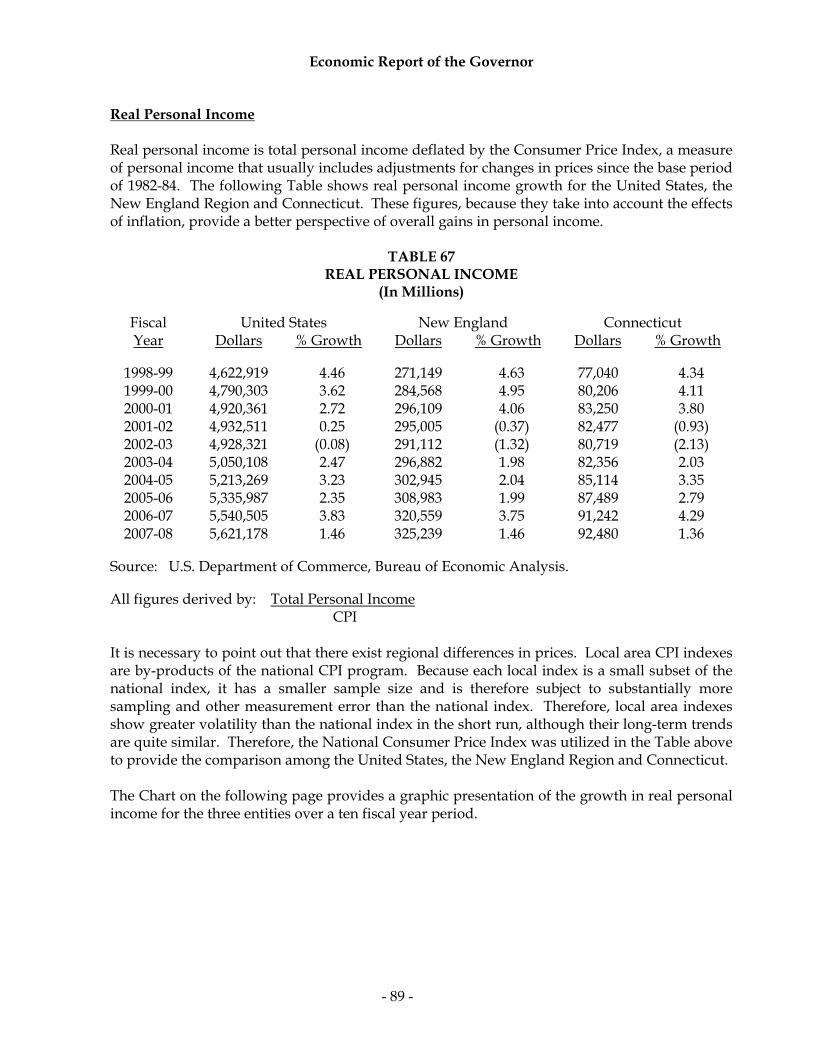
Economic Report of the Governor
- 89 -
Real Personal Income Real personal income is total personal income deflated by the Consumer Price Index, a measure of personal income that usually includes adjustments for changes in prices since the base period of 1982-84. The following Table shows real personal income growth for the United States, the New England Region and Connecticut. These figures, because they take into account the effects of inflation, provide a better perspective of overall gains in personal income.
TABLE 67 REAL PERSONAL INCOME
(In Millions)
Fiscal United States New England Connecticut Year Dollars % Growth Dollars % Growth Dollars % Growth
1998-99 4,622,919 4.46 271,149 4.63 77,040 4.34 1999-00 4,790,303 3.62 284,568 4.95 80,206 4.11 2000-01 4,920,361 2.72 296,109 4.06 83,250 3.80 2001-02 4,932,511 0.25 295,005 (0.37) 82,477 (0.93) 2002-03 4,928,321 (0.08) 291,112 (1.32) 80,719 (2.13) 2003-04 5,050,108 2.47 296,882 1.98 82,356 2.03 2004-05 5,213,269 3.23 302,945 2.04 85,114 3.35 2005-06 5,335,987 2.35 308,983 1.99 87,489 2.79 2006-07 5,540,505 3.83 320,559 3.75 91,242 4.29 2007-08 5,621,178 1.46 325,239 1.46 92,480 1.36
Source: U.S. Department of Commerce, Bureau of Economic Analysis. All figures derived by: Total Personal Income CPI It is necessary to point out that there exist regional differences in prices. Local area CPI indexes are by-products of the national CPI program. Because each local index is a small subset of the national index, it has a smaller sample size and is therefore subject to substantially more sampling and other measurement error than the national index. Therefore, local area indexes show greater volatility than the national index in the short run, although their long-term trends are quite similar. Therefore, the National Consumer Price Index was utilized in the Table above to provide the comparison among the United States, the New England Region and Connecticut. The Chart on the following page provides a graphic presentation of the growth in real personal income for the three entities over a ten fiscal year period.

Economic Report of the Governor
- 90 -
REAL PERSONAL INCOME GROWTHFISCAL YEAR GROWTH BY PERCENT
-3
-2
-1
0
1
2
3
4
5
6
1999 2000 2001 2002 2003 2004 2005 2006 2007 2008
FISCAL YEAR
PERC
ENT
United States
New England
Connecticut
Source: U.S. Department of Commerce, Bureau of Economic Analysis Real Per Capita Personal Income Real per capita personal income is per capita personal income deflated by the Consumer Price Index and shows how individuals comprising a geographical entity have fared after adjusting for the effects of inflation. A comparison of the growth rates measures the relative economic performance of each entity as it adjusts personal income growth by population changes.
TABLE 68 REAL PER CAPITA PERSONAL INCOME
Fiscal United States New England Connecticut Year Dollars % Growth Dollars % Growth Dollars % Growth
1998-99 16,639 3.26 19,652 3.88 22,807 3.76 1999-00 17,046 2.45 20,457 4.10 23,572 3.35 2000-01 17,323 1.63 21,127 3.28 24,318 3.17 2001-02 17,195 (0.74) 20,918 (0.99) 23,954 (1.50) 2002-03 17,024 (0.99) 20,545 (1.78) 23,291 (2.77) 2003-04 17,286 1.54 20,901 1.73 23,670 1.63 2004-05 17,679 2.28 21,311 1.96 24,425 3.19 2005-06 17,926 1.39 21,712 1.88 25,051 2.57 2006-07 18,435 2.84 22,492 3.60 26,074 4.08 2007-08 18,524 0.48 22,733 1.07 26,327 0.97
Source: U.S. Department of Commerce, Bureau of Economic Analysis All figures derived by: Total Personal Income CPI X Population

Economic Report of the Governor
- 91 -
The previous Table shows the growth in real per capita personal income for the United States, the New England Region, and Connecticut. The Chart below provides a graphic presentation of the growth in real per capita personal income for the three entities over a ten fiscal year period.
REAL PER CAPITA INCOME GROWTHFISCAL YEAR GROWTH BY PERCENT
-3
-2
-1
0
1
2
3
4
5
1999 2000 2001 2002 2003 2004 2005 2006 2007 2008
FISCAL YEAR
PERC
ENT
United States
New England
Connecticut
Source: U.S. Department of Commerce, Bureau of Economic Analysis
TABLE 69 GROWTH IN REAL PER CAPITA PERSONAL INCOME
(Base Year: 2007)
Fiscal % Growth % Cumulative Growth Year United States Connecticut United States Connecticut
1950-1960 27.7% 28.5% 27.7% 28.5% 1960-1970 37.2% 40.6% 75.2% 80.7% 1970-1980 17.9% 12.8% 106.5% 103.7% 1980-1990 21.6% 38.9% 151.0% 182.9% 1990-2000 13.5% 13.5% 184.9% 221.1% 2000-2007 8.5% 11.3% 209.2% 257.5%
Source: Moody’s Economy.com The above Table highlights the cumulative growth in real per capita personal income over the past fifty-seven years. Overall, Connecticut has enjoyed higher cumulative growth in real per capita personal income, exceeding the United States by 48.3 percentage points. In one decade alone, 1980 to 1990, Connecticut’s growth in real personal income was 17.3 percentage points

Economic Report of the Governor
- 92 -
higher than the United States’ growth. Even though job growth in the state has lagged that of the nation, Connecticut residents’ income growth has out-performed that of the nation’s over the long-term. Cost of Living Index Statistics regarding inflation and the cost of living for Connecticut are frequently requested by the public. The two indicators are not the same. The inflation index such as the CPI-U is used to measure purchasing power relative to its historical performance, while the cost of living index is used to measure purchasing power relative to one’s geographical peers. In other words, the cost of living index is produced to measure the relative price level of consumer goods and services for a specific area relative to other jurisdictions at a given time. A widely used index to measure cost of living differences among urban areas is ACCRA Cost of Living Index, which is produced by The Council for Community and Economic Research (C2ER). This report includes indices for approximately 320 Metropolitan Statistical Areas (MTAs), Metropolitan Statistical Divisions (MTDs), and Micropolitan Statistical Areas (MCAs) as defined by the U.S. Office of Management and Budget (OMB). In Connecticut, the C2ER survey includes the four urban areas from the following MTAs: Stamford in the Bridgeport-Stamford-Norwalk MTA, Hartford in the Hartford-West Hartford-East Hartford MTA, New Haven in the New Haven-Milford MTA, and New London in the Norwich-New London MTA. The following Table shows the cost of living comparison for three neighboring cities: Boston in the Boston-Quincy MTD, Hartford in the Hartford-West Hartford-East Hartford MTA, and New York (Manhattan) in the New York-White Plains-Wayne NY-NJ MTD in the second quarter of 2007.
TABLE 70 COMPARISON OF COST OF LIVING
2nd Quarter 2008 Composite Grocery Trans- Health
MTA/MTD Index Items Housing Utilities portation Care Misc.* Hartford, CT 122.2 113.4 140.4 135.8 106.3 114.8 111.0 Boston, MA 134.8 113.9 158.7 144.9 108.8 133.6 126.6 New York, NY 220.3 145.2 408.5 177.3 115.8 133.3 135.9 Index Weights 100% 12.49% 29.84% 9.94% 10.73% 4.07% 32.93%
* denotes miscellaneous goods and services Source: The Council for Community and Economic Research (C2ER), “ACCRA Cost of Living Index”, Second Quarter 2008
The Cost of Living Composite Index is weighted by a “market basket” of approximately 60 goods and services for the typical professional and executive household. It is further broken down into six categories including grocery items, housing, utilities, transportation, health care, and miscellaneous goods and services to reflect the different categories of consumer expenditures. The index for the Hartford area, for example, for the second quarter of 2008 was

Economic Report of the Governor
- 93 -
122.2 compared to the national average of 100. This index demonstrates that the overall living cost in the Hartford area was higher than the national average by 22.2%. Among the six categories, the cost of housing in the Hartford area was the most expensive item, a full 40.4% higher than the national average, followed by utilities at 35.8%, health care at 14.8%, grocery items at 13.4%, miscellaneous goods and services at 11.0%, and transportation at 6.3% higher than the national average. The index, updated quarterly, does not measure tax differentials. In the second quarter of 2008, numerous cities had a relatively higher cost of living than the Hartford area. These include, for example, New York City (Manhattan) at 220.3; San Francisco, California at 170.9; and Honolulu, Hawaii at 161.7. Living costs in most southern states’ cities are relatively low; for example, Pryor, Oklahoma at 82.4; Sequin, Texas at 84.5; and Baton Rouge, Louisiana at 88.2. The cost of living in the Hartford area was collectively on par with Boulder, Colorado; Philadelphia, Pennsylvania; and Providence, Rhode Island, which registered at 122.4, 123.5, and 123.5, respectively. The cost of living index can provide useful information for relocation decisions. If someone is contemplating a job offer in a certain area, he or she may use this index as a guide to evaluate the financial merits of the move. For example, if a Hartford resident is considering a move to New York City (Manhattan) and wants to maintain his or her current lifestyle, other things being equal, his or her after-tax income level has to increase by 80.3%, (220.3-122.2)/122.2, in order to compensate for the higher cost of living. On the contrary, if a New York City resident is contemplating a move to Hartford, his or her after-tax income level can be reduced by 44.5%, (122.2-220.3)/220.3, in order to sustain the same current life style. The cost of living for metropolitan statistical areas within Connecticut also varies. For the second quarter of 2008, the ACCRA cost of living Index for the Stamford area was at 148.5, New Haven at 123.9, and New London at 115.9, compared to 122.2 for Hartford. These four statistical areas accounted for 70% of the state’s total population. The following Table demonstrates the relative index of the components for these four Connecticut regions.
TABLE 71 COMPARISON OF COST OF LIVING IN CONNECTICUT Hartford, New Haven, New London, and Stamford MTAs
2nd Quarter 2008 Composite Grocery Trans- Health
MTA Index Items Housing Utilities portation Care Misc. Hartford 122.2 113.4 140.4 135.8 106.3 114.8 111.0 New Haven 123.9 119.4 141.8 144.6 101.9 113.5 111.6 New London 115.9 113.8 125.2 128.1 102.4 112.6 109.3 Stamford 148.5 109.5 220.1 127.4 115.2 114.5 119.8 Source: The Council for Community and Economic Research (C2ER), “ACCRA Cost of Living
Index”, Second Quarter 2008

Economic Report of the Governor
- 94 -
THE MAJOR REVENUE RAISING TAXES IN THE STATE OF CONNECTICUT In fiscal 2008, Connecticut’s General Fund derived 76 percent of its revenue from the collection of taxes. To provide an analysis of the overall tax burden on the individuals of each state, the following Table was prepared for fiscal 2007. The Table shows overall state tax collections as a percentage of personal income. In the Table, note that Connecticut ranks 27th, signifying that in 26 other states a greater percentage of an individual's income is going for state taxes than in Connecticut.
TABLE 72 STATE TAX COLLECTIONS AS A PERCENTAGE OF PERSONAL INCOME
Fiscal 2007
State Percentage Rank State Percentage Rank Alaska 12.91% 1 Washington 6.93% 26 Vermont 11.36% 2 Connecticut 6.90% 27 Hawaii 10.45% 3 Indiana 6.84% 28 West Virginia 8.99% 4 Massachusetts 6.72% 29 Arkansas 8.97% 5 Rhode Island 6.72% 30 New Mexico 8.89% 6 Nebraska 6.58% 31 Minnesota 8.62% 7 Pennsylvania 6.58% 32 Wyoming 8.61% 8 South Carolina 6.51% 33 Delaware 8.57% 9 Iowa 6.45% 34 North Dakota 8.24% 10 Ohio 6.40% 35 Maine 8.22% 11 Nevada 6.37% 36 Mississippi 7.93% 12 Alabama 6.07% 37 Kentucky 7.76% 13 Oregon 6.07% 38 California 7.74% 14 Arizona 6.06% 39 Idaho 7.68% 15 Virginia 6.05% 40 North Carolina 7.64% 16 Georgia 6.00% 41 Montana 7.58% 17 Maryland 5.93% 42 Utah 7.57% 18 Illinois 5.81% 43 Louisiana 7.43% 19 Tennessee 5.66% 44 Oklahoma 7.34% 20 Missouri 5.51% 45 Wisconsin 7.32% 21 Florida 5.21% 46 New York 7.22% 22 Colorado 4.76% 47 Michigan 7.03% 23 Texas 4.72% 48 Kansas 7.00% 24 South Dakota 4.68% 49 New Jersey 6.99% 25 New Hampshire 4.06% 50 U.S. Average 6.63%
Source: U.S. Department of Commerce, "State Government Finances, 2007" Following is a discussion of the major revenue raising taxes in the State of Connecticut.

Economic Report of the Governor
- 95 -
Personal Income Tax For income years commencing on or after January 1, 1991, a personal income tax was imposed upon income of residents of the State (including resident trusts and estates), part-year residents and certain non-residents who have taxable income derived from or connected with sources within Connecticut. For tax years commencing on or after January 1, 1991, and prior to January 1, 1992, the tax was imposed at the rate of 1.5% on Connecticut taxable income. For tax years commencing on or after January 1, 1992, the separate tax on capital gains, dividends and interest was repealed, and the tax was imposed at the rate of 4.5% of Connecticut taxable income. Beginning with tax years commencing on or after January 1, 1996, a second, lower tax rate of 3% was introduced for a certain portion of taxable income. Beginning with tax years commencing January 1, 2003 the 4.5% rate was increased to 5.0%. The amount of taxable income subject to the lower tax rate has been expanded as set forth in the Table below. Depending on federal income tax filing status and Connecticut adjusted gross income, personal exemptions ranging from $13,500 to $24,000 are available to taxpayers, with such exemptions phased out at certain higher income levels. Legislation enacted in 1999 increases the exemption amount for single filers over a certain number of years from $12,000 to $15,000. In addition, tax credits ranging from 75% to 1% of a taxpayer's Connecticut tax liability are also available, again dependent upon federal income tax filing status and Connecticut adjusted gross income (See Table 75 for more details). Neither the personal exemption nor the tax credit is available to a trust or an estate. Also commencing in income year 1996, personal income taxpayers were eligible for up to a $100 credit for property taxes paid on their primary residence or on their motor vehicle. This credit increased to $215 for income year 1997, $350 for income year 1998, $425 for income year 1999, and to $500 for income years 2000 through 2002, with amounts above the initial $100 phased-out at higher income levels. Beginning with income year 2003, the credit was reduced to $350, but rose to $500 in income year 2006. The Personal Income Tax generated $7,512.7 million in fiscal year 2007-08, $6,749.5 million in fiscal year 2006-07, and $6,156.4 million in fiscal year 2005-06. In fiscal year 2007-08, this tax accounted for 45.8% of total revenue and 56.1% of total tax collections, while in fiscal year 2006-07 it accounted for 42.8% of total revenue and 53.3% of total tax collections.
TABLE 73 TAXABLE INCOME AMOUNTS SUBJECT TO THE LOWER RATE
WITH THE REMAINDER SUBJECT TO THE HIGHER RATE
Amount At Low Rate By Filing Status Income Year Low Rate High Rate Single Joint Head of Household
1996 3.0% 4.5% $ 2,250 $ 4,500 $ 3,500 1997 3.0% 4.5% $ 6,250 $12,500 $10,000 1998 3.0% 4.5% $ 7,500 $15,000 $12,000
1999 - 2002 3.0% 4.5% $10,000 $20,000 $16,000 2003 & After 3.0% 5.0% $10,000 $20,000 $16,000
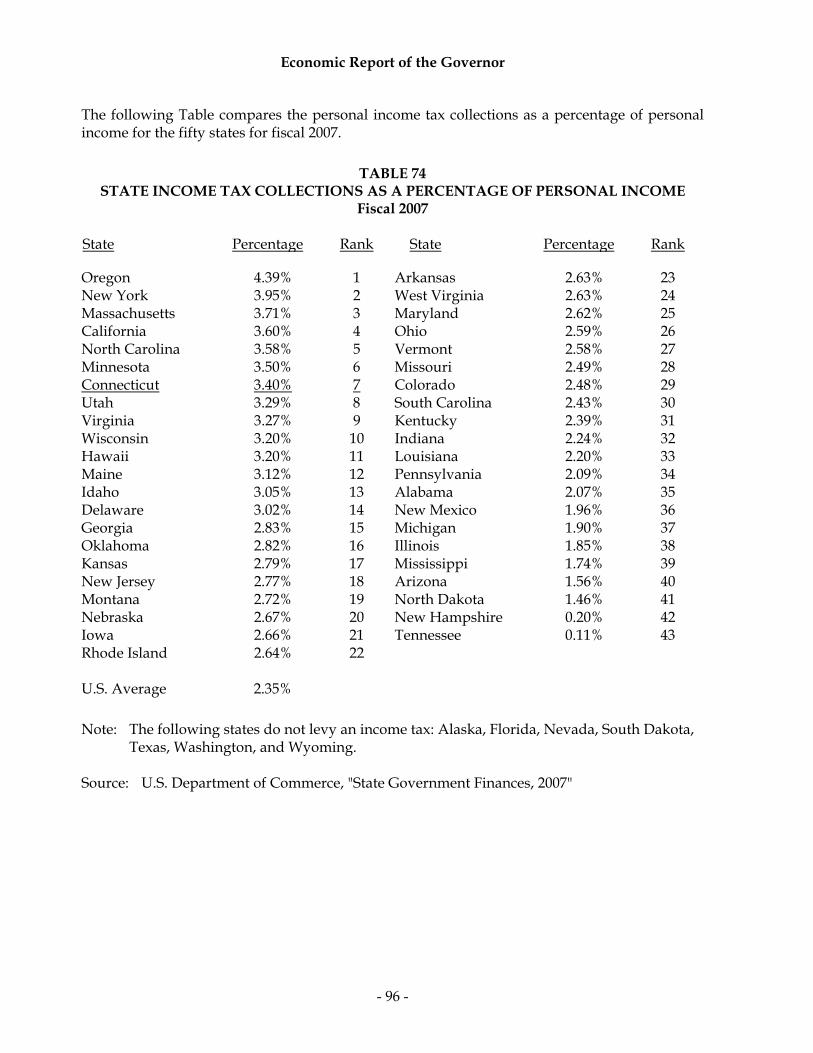
Economic Report of the Governor
- 96 -
The following Table compares the personal income tax collections as a percentage of personal income for the fifty states for fiscal 2007.
TABLE 74 STATE INCOME TAX COLLECTIONS AS A PERCENTAGE OF PERSONAL INCOME
Fiscal 2007
State Percentage Rank State Percentage Rank Oregon 4.39% 1 Arkansas 2.63% 23 New York 3.95% 2 West Virginia 2.63% 24 Massachusetts 3.71% 3 Maryland 2.62% 25 California 3.60% 4 Ohio 2.59% 26 North Carolina 3.58% 5 Vermont 2.58% 27 Minnesota 3.50% 6 Missouri 2.49% 28 Connecticut 3.40% 7 Colorado 2.48% 29 Utah 3.29% 8 South Carolina 2.43% 30 Virginia 3.27% 9 Kentucky 2.39% 31 Wisconsin 3.20% 10 Indiana 2.24% 32 Hawaii 3.20% 11 Louisiana 2.20% 33 Maine 3.12% 12 Pennsylvania 2.09% 34 Idaho 3.05% 13 Alabama 2.07% 35 Delaware 3.02% 14 New Mexico 1.96% 36 Georgia 2.83% 15 Michigan 1.90% 37 Oklahoma 2.82% 16 Illinois 1.85% 38 Kansas 2.79% 17 Mississippi 1.74% 39 New Jersey 2.77% 18 Arizona 1.56% 40 Montana 2.72% 19 North Dakota 1.46% 41 Nebraska 2.67% 20 New Hampshire 0.20% 42 Iowa 2.66% 21 Tennessee 0.11% 43 Rhode Island 2.64% 22 U.S. Average 2.35%
Note: The following states do not levy an income tax: Alaska, Florida, Nevada, South Dakota, Texas, Washington, and Wyoming.
Source: U.S. Department of Commerce, "State Government Finances, 2007"

Economic Report of the Governor
- 97 -
The following Table shows Connecticut personal income tax exemptions ranging from $13,000 to $24,000 including the phase out as income levels rise depending on adjusted gross income for each income tax filing status.
TABLE 75 CONNECTICUT PERSONAL INCOME TAX CREDITS & EXEMPTIONS
Income Year 2009
Single*
Married Filing Jointly
Head of Household Exemption: $13,500 Exemption: $24,000 Exemption: $19,000
Phase Out: $1K of exemption for Phase Out: $1K of exemption for Phase Out: $1K of exemption for each $1K from $27.0K to $39.0K each $1K from $48K to $72K each $1K from $38K to $57K
AGI AGI % of AGI AGI % of AGI AGI % of
From To Tax From To Tax From To Tax
$13,500 $16,900 75% $24,000 $30,000 75% $19,000 $24,000 75% $16,900 $17,400 70% $30,000 $30,500 70% $24,000 $24,500 70% $17,400 $17,900 65% $30,500 $31,000 65% $24,500 $25,000 65% $17,900 $18,400 60% $31,000 $31,500 60% $25,000 $25,500 60% $18,400 $18,900 55% $31,500 $32,000 55% $25,500 $26,000 55% $18,900 $19,400 50% $32,000 $32,500 50% $26,000 $26,500 50% $19,400 $19,900 45% $32,500 $33,000 45% $26,500 $27,000 45% $19,900 $20,400 40% $33,000 $33,500 40% $27,000 $27,500 40% $20,400 $22,500 35% $33,500 $40,000 35% $27,500 $34,000 35% $22,500 $23,000 30% $40,000 $40,500 30% $34,000 $34,500 30% $23,000 $23,500 25% $40,500 $41,000 25% $34,500 $35,000 25% $23,500 $24,000 20% $41,000 $41,500 20% $35,000 $35,500 20% $24,000 $28,100 15% $41,500 $50,000 15% $35,500 $44,000 15% $28,100 $28,600 14% $50,000 $50,500 14% $44,000 $44,500 14% $28,600 $29,100 13% $50,500 $51,000 13% $44,500 $45,000 13% $29,100 $29,600 12% $51,000 $51,500 12% $45,000 $45,500 12% $29,600 $30,100 11% $51,500 $52,000 11% $45,500 $46,000 11% $30,100 $54,000 10% $52,000 $96,000 10% $46,000 $74,000 10% $54,000 $54,500 9% $96,000 $96,500 9% $74,000 $74,500 9% $54,500 $55,000 8% $96,500 $97,000 8% $74,500 $75,000 8% $55,000 $55,500 7% $97,000 $97,500 7% $75,000 $75,500 7% $55,500 $56,000 6% $97,500 $98,000 6% $75,500 $76,000 6% $56,000 $56,500 5% $98,000 $98,500 5% $76,000 $76,500 5% $56,500 $57,000 4% $98,500 $99,000 4% $76,500 $77,000 4% $57,000 $57,500 3% $99,000 $99,500 3% $77,000 $77,500 3% $57,500 $58,000 2% $99,500 $100,000 2% $77,500 $78,000 2% $58,000 $58,500 1% $100,000 $100,500 1% $78,000 $78,500 1%
Source: General Statutes of the State of Connecticut * The Governor’s budget includes a proposal to delay the increase in the singles exemption from
the income year 2008 levels

Economic Report of the Governor
- 98 -
The following Table shows whether state and local governmental obligations are included in the definition of state income for tax purposes.
TABLE 76 STATE AND LOCAL GOVERNMENT OBLIGATIONS EXEMPTIONS
FOR DETERMINING INDIVIDUAL'S STATE INCOME
Other Other Own State's Own State's State Securities Securities State Securities Securities Alabama E T Montana E T Alaska (no tax) Nebraska E T Arizona E T Nevada (no tax) Arkansas E T New Hampshire E T California E T New Jersey E T Colorado E T New Mexico E T Connecticut E T New York E T Delaware E T North Carolina E T Florida (no tax) North Dakota E T Georgia E T Ohio E T Hawaii E T Oklahoma T (1) T Idaho E T Oregon E T Illinois T (1) T Pennsylvania E T Indiana E E Rhode Island E T Iowa T (1) T South Carolina E T Kansas E T South Dakota (no tax) Kentucky E T Tennessee E T Louisiana E T Texas (no tax) Maine E T Utah E E (2) Maryland E T Vermont E T Massachusetts E T Virginia E T Michigan E T Washington (no tax) Minnesota E T West Virginia E T Mississippi E T Wisconsin T (1) T Missouri E T Wyoming (no tax) T = Taxable / E = Exempt
(1) Interest earned from some qualified obligations is exempt from the tax. (2) Taxable for bonds acquired after 2002 if the other state or locality imposes an
income-based tax on Utah bonds. Source: Commerce Clearing House, Inc.
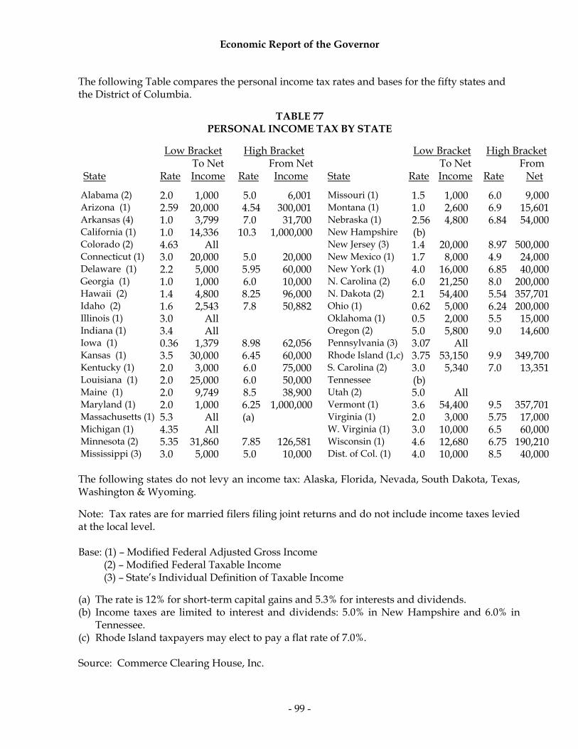
Economic Report of the Governor
- 99 -
The following Table compares the personal income tax rates and bases for the fifty states and the District of Columbia.
TABLE 77 PERSONAL INCOME TAX BY STATE
Low Bracket High Bracket Low Bracket High Bracket
State
Rate
To Net Income
Rate
From Net Income
State
Rate
To Net Income
Rate
From Net
Alabama (2) 2.0 1,000 5.0 6,001 Missouri (1) 1.5 1,000 6.0 9,000 Arizona (1) 2.59 20,000 4.54 300,001 Montana (1) 1.0 2,600 6.9 15,601 Arkansas (4) 1.0 3,799 7.0 31,700 Nebraska (1) 2.56 4,800 6.84 54,000 California (1) 1.0 14,336 10.3 1,000,000 New Hampshire (b) Colorado (2) 4.63 All New Jersey (3) 1.4 20,000 8.97 500,000 Connecticut (1) 3.0 20,000 5.0 20,000 New Mexico (1) 1.7 8,000 4.9 24,000 Delaware (1) 2.2 5,000 5.95 60,000 New York (1) 4.0 16,000 6.85 40,000 Georgia (1) 1.0 1,000 6.0 10,000 N. Carolina (2) 6.0 21,250 8.0 200,000 Hawaii (2) 1.4 4,800 8.25 96,000 N. Dakota (2) 2.1 54,400 5.54 357,701 Idaho (2) 1.6 2,543 7.8 50,882 Ohio (1) 0.62 5,000 6.24 200,000 Illinois (1) 3.0 All Oklahoma (1) 0.5 2,000 5.5 15,000 Indiana (1) 3.4 All Oregon (2) 5.0 5,800 9.0 14,600 Iowa (1) 0.36 1,379 8.98 62,056 Pennsylvania (3) 3.07 All Kansas (1) 3.5 30,000 6.45 60,000 Rhode Island (1,c) 3.75 53,150 9.9 349,700 Kentucky (1) 2.0 3,000 6.0 75,000 S. Carolina (2) 3.0 5,340 7.0 13,351 Louisiana (1) 2.0 25,000 6.0 50,000 Tennessee (b) Maine (1) 2.0 9,749 8.5 38,900 Utah (2) 5.0 All Maryland (1) 2.0 1,000 6.25 1,000,000 Vermont (1) 3.6 54,400 9.5 357,701 Massachusetts (1) 5.3 All (a) Virginia (1) 2.0 3,000 5.75 17,000 Michigan (1) 4.35 All W. Virginia (1) 3.0 10,000 6.5 60,000 Minnesota (2) 5.35 31,860 7.85 126,581 Wisconsin (1) 4.6 12,680 6.75 190,210 Mississippi (3) 3.0 5,000 5.0 10,000 Dist. of Col. (1) 4.0 10,000 8.5 40,000 The following states do not levy an income tax: Alaska, Florida, Nevada, South Dakota, Texas, Washington & Wyoming. Note: Tax rates are for married filers filing joint returns and do not include income taxes levied at the local level. Base: (1) – Modified Federal Adjusted Gross Income (2) – Modified Federal Taxable Income (3) – State’s Individual Definition of Taxable Income (a) The rate is 12% for short-term capital gains and 5.3% for interests and dividends. (b) Income taxes are limited to interest and dividends: 5.0% in New Hampshire and 6.0% in
Tennessee. (c) Rhode Island taxpayers may elect to pay a flat rate of 7.0%. Source: Commerce Clearing House, Inc.

Economic Report of the Governor
- 100 -
Sales and Use Tax The sales tax is imposed, subject to certain limitations, on the gross receipts from certain transactions within the State of persons engaged in business in the state including: 1) retail sales of tangible personal property; 2) the sale of certain services; 3) the leasing or rental of tangible personal property; 4) the producing, fabricating, processing, printing, or imprinting of tangible personal property to special order or with material furnished by the consumer; 5) the furnishing, preparing or serving of food, meals or drinks; and 6) the occupancy of hotels or lodging house rooms for a period not exceeding thirty consecutive calendar days. The use tax is imposed on the consideration paid for certain services or purchases or rentals of tangible personal property used within the state and not subject to the sales tax. Both the sales and use taxes are levied at a rate of six percent. Various exemptions from the tax are provided, based on the nature, use, or price of the property or services involved or the identity of the purchaser. Hotel rooms are taxed at 12%. The sales and use tax is an important source of revenue for the State of Connecticut. In fiscal 2007-08, sales and use taxes accounted for 21.8% of total revenue and 28.6% of total tax collections, compared to 22.2% and 29.4%, respectively, in fiscal 2006-07. When analyzing sales taxes, a simple comparison of rates is not an effective way to measure the tax burden imposed. An analysis of the tax base must be included to provide a more meaningful comparison. In an attempt to provide a more relevant comparison of the sales tax burden, two studies are presented. The first study shows sales tax collections as a percentage of personal income. The larger the percentage of personal income going to sales tax collections, the heavier the burden of that tax. The Table on the following page shows sales tax collections as a percentage of personal income and the corresponding ranking of the states. Note that Connecticut's tax burden is less than 35 other states. The comparison is based on fiscal year 2007 data. From fiscal 1991 to fiscal 2007, Connecticut's sales tax collections as a percentage of personal income dropped from 3.15% with a rank of ninth to 1.63% with a rank of 36th, and compared to the national average of 2.09%. This change was primarily due to the reduction in Connecticut's sales tax rate from 8% to 6% and an expansion of the exemptions on certain services and goods. The second study provides an analysis of major sales tax exemptions by state. Connecticut excludes from its sales tax such major items as food products for human consumption, drugs and medicines used by humans, clothing and footwear up to $50, machinery, professional services, residential utilities and motor fuels. Table Number 81 shows the comparison for major sales tax exemptions.

Economic Report of the Governor
- 101 -
TABLE 78 SALES TAX COLLECTIONS AS A PERCENTAGE OF PERSONAL INCOME
Fiscal 2007
Sales Sales Tax Tax State Rate (%) % Rank State Rate (%) % Rank Hawaii 4.0* 5.25 1 California 6.25* 2.20 24 Washington 6.5* 4.26 2 West Virginia 6.0 2.18 25 Mississippi 7.0 3.91 3 Minnesota 6.5* 2.17 26 Arkansas 6.0* 3.53 4 Rhode Island 7.0 2.13 27 Tennessee 7.0* 3.38 5 Wisconsin 5.0 2.10 28 Nevada 6.5* 3.25 6 Georgia 4.0* 2.05 29 Florida 6.0* 3.17 7 Ohio 5.5* 2.01 30 New Mexico 5.0 3.15 8 New Jersey 7.0 2.00 31 Wyoming 4.0* 2.97 9 Pennsylvania 6.0* 1.85 32 Arizona 5.6* 2.78 10 Iowa 5.0* 1.78 33 Idaho 6.0 2.77 11 North Carolina 4.5* 1.76 34 South Dakota 4.0* 2.65 12 Missouri 4.225* 1.68 35 Indiana 6.0 2.63 13 Connecticut 6.0 1.63 36 Utah 4.65* 2.51 14 Oklahoma 4.5* 1.62 37 South Carolina 6.0* 2.42 15 Alabama 4.0* 1.56 38 Maine 5.0 2.42 16 Illinois 6.25* 1.54 39 Nebraska 5.5* 2.40 17 Vermont 6.0 1.49 40 Texas 6.25* 2.39 18 Maryland 6.0 1.35 41 Louisiana 4.0 2.38 19 Massachusetts 5.0 1.33 42 Michigan 6.0 2.35 20 New York 4.0* 1.24 43 Kansas 5.3* 2.28 21 Colorado 2.9* 1.15 44 North Dakota 5.0* 2.24 22 Virginia 4.0* 1.13 45 Kentucky 6.0 2.21 23 U.S. Average 2.09 * Local tax rates are additional. Note: Alaska, Delaware, Montana, New Hampshire, and Oregon do not levy a sales tax. The
state of Delaware imposes a merchants’ and manufacturers’ license tax and a use tax on leases.
Source: Commerce Clearing House, Inc.; U.S. Department of Commerce, "State Government Finances”, 2006; U.S. Department of Commerce, Bureau of Economic Analysis
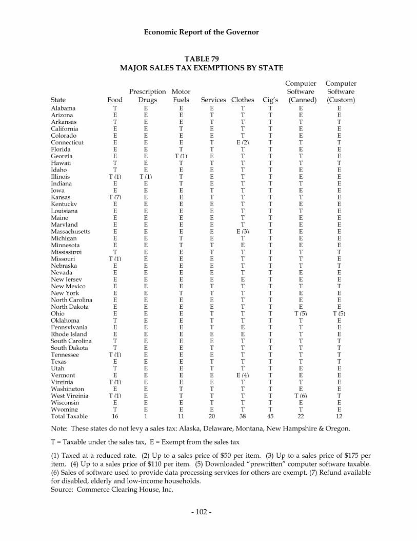
Economic Report of the Governor
- 102 -
TABLE 79 MAJOR SALES TAX EXEMPTIONS BY STATE
State
Food
Prescription Drugs
Motor Fuels
Services
Clothes
Cig’s
Computer Software (Canned)
Computer Software (Custom)
Alabama T E E E T T E E Arizona E E E T T T E E Arkansas T E E T T T T T California E E T E T T E E Colorado E E E E T T E E Connecticut E E E T E (2) T T T Florida E E T T T T E E Georgia E E T (1) E T T T E Hawaii T E T T T T T T Idaho T E E E T T E E Illinois T (1) T (1) T E T T E E Indiana E E T E T T T E Iowa E E E T T T E E Kansas T (7) E E T T T T E Kentucky E E E E T T E E Louisiana E E E E T T T E Maine E E E E T T E E Maryland E E E E T T E E Massachusetts E E E E E (3) T E E Michigan E E T E T T E E Minnesota E E T T E T E E Mississippi T E E T T T T T Missouri T (1) E E E T T T E Nebraska E E E E T T T T Nevada E E E E T T E E New Jersey E E E E E T E E New Mexico E E E T T T T T New York E E T T T T E E North Carolina E E E E T T E E North Dakota E E E E T T E E Ohio E E E T T T T (5) T (5) Oklahoma T E E T T T T E Pennsylvania E E E T E T T E Rhode Island E E E E E T T E South Carolina T E E E T T T T South Dakota T E E T T T T T Tennessee T (1) E E E T T T T Texas E E E T T T T T Utah T E E T T T E E Vermont E E E E E (4) T E E Virginia T (1) E E E T T T E Washington E E T T T T E E West Virginia T (1) E T T T T T (6) T Wisconsin E E E T T T E E Wyoming T E E E T T T E Total Taxable 16 1 11 20 38 45 22 12
Note: These states do not levy a sales tax: Alaska, Delaware, Montana, New Hampshire & Oregon.
T = Taxable under the sales tax, E = Exempt from the sales tax
(1) Taxed at a reduced rate. (2) Up to a sales price of $50 per item. (3) Up to a sales price of $175 per item. (4) Up to a sales price of $110 per item. (5) Downloaded “prewritten” computer software taxable. (6) Sales of software used to provide data processing services for others are exempt. (7) Refund available for disabled, elderly and low-income households. Source: Commerce Clearing House, Inc.

Economic Report of the Governor
- 103 -
Corporation Business Tax The Corporation Business Tax is imposed on any corporation, joint stock company or association or fiduciary of any of the foregoing which carries on or has the right to carry on business within the state or owns or leases property or maintains an office within the state. The Corporation Business Tax consists of three components. The taxpayer's liability is the greatest amount computed under any of the three components. The first is a tax measured by the net income of a taxpayer (the "Income-Base Tax"). Net income means federal gross income (with limited variations) less certain deductions, most of which correspond to the deductions allowed under the Internal Revenue Code of 1986, as amended from time to time. In fiscal 2007-08, the Corporation Business Tax accounted for 4.5% of total revenue and 5.5% of total tax collections, while in fiscal 2006-07 they were 5.7% and 7.0%, respectively. If a taxpayer is taxable solely within the state, the Income-Base Tax is measured by, and based upon, its entire net income. If a taxpayer is taxable in another state in which it conducts business, the base against which the Income-Base Tax is measured is the portion of the taxpayer's entire net income assigned to the state, pursuant to a statutory formula designed to identify the proportion of the taxpayer's trade or business conducted within the state. Currently, the Income-Base Tax is levied at the rate of seven and one half percent. The second part of the Corporation Business Tax is an additional tax on capital (the "Additional Tax"). The additional tax base is determined either as a specific maximum dollar amount or at a flat rate on a defined base, usually related in whole or part to its capital stock and balance sheet surplus, profit and deficit. If a taxpayer is also taxable in another state in which it conducts business, the defined base is apportioned most often to the value of certain assets having tax situs within the state. The third component of the Corporation Business Tax is the Minimum Tax, which is $250. Corporations must compute their tax under all three bases and then pay the tax under the highest computation. Numerous tax credits are also available to corporations including, but not limited to, research and development credits of 1% to 6%, credits for property taxes paid on electronic and data processing equipment, and a 5% credit for investments in fixed and human capital. The Table on the following page provides a comparison of the assessed rates for the corporation business tax for the fifty states and the District of Columbia.

Economic Report of the Governor
- 104 -
TABLE 80 CORPORATION TAX BY STATE
Low Bracket High Bracket Low Bracket High Bracket
State
% Rate
To Net Income
% Rate
From Net Income
State
% Rate
To Net Income
% Rate
From Net Income
Alabama 6.5 All Mississippi 3.0 5,000 5.0 10,000 Alaska 1.0 10,000 9.4 90,000 Missouri 6.25 All Arizona 6.97 All Montana 6.75 All Arkansas 1.0 3,000 6.5 100,000 Nebraska 5.58 50,000 7.81 50,000 California (1) 8.84 All New Hampshire 8.5 All Colorado 4.63 All New Jersey (7) 6.5 50,000 9.0 100,000 Connecticut 7.5 All New Mexico 4.8 500,000 7.6 1.0M Delaware 8.7 All New York 7.1 All Florida (2) 5.5 All N. Carolina 6.9 All Georgia 6.0 All N. Dakota 2.6 3,000 6.5 30,000 Hawaii 4.4 25,000 6.4 100,000 Ohio 5.1 50,000 8.5 50,000 Idaho 7.6 All Oklahoma 6.0 All Illinois (3) 4.8 All Oregon 6.6 All Indiana 8.5 All Pennsylvania 9.99 All Iowa 6.0 25,000 12.0 250,000 Rhode Island 9.0 All Kansas (4) 4.0 All S. Carolina 5.0 All Kentucky 4.0 50,000 6.0 100,000 Tennessee 6.5 All Louisiana 4.0 25,000 8.0 200,000 Utah 5.0 All Maine 3.5 25,000 8.93 250,000 Vermont 6.0 10,000 8.5 250,000 Maryland 8.3 All Virginia 6.0 All Massachusetts 9.5 All West Virginia 8.5 All Michigan (5) 4.95 All Wisconsin 7.9 All Minnesota (6) 9.8 All District of Col. 9.98 All
Note: The table does not include corporate income taxes levied at the local level. These states do not levy a corporate income tax: Nevada, South Dakota, Texas, Washington & Wyoming. The following states require a minimum tax: Arizona $50; California $800; Connecticut $250; Idaho $20; Kentucky $175; Massachusetts $456; Montana $50; New Jersey $500; New York $25; Oregon $10; Rhode Island $500; Utah $100; Vermont $250; District of Columbia $100
(1) Tax rate on financial S-corporations is 3.5%, and the tax rate all other S-corporations is 1.5%. Banks and financial corporations (except financial S-corporations) are subject to 10.84% An alternative minimum tax imposed is 6.65%.
(2) An alternative minimum tax imposed 3.3%, an exemption of $5,000 is allowed. (3) Additional personal property replacement tax is imposed at the rate of 2.5% of net income for corporations other than S-corporations. 1.5% for S corporations. (4) A surtax of 3.10% on taxable incomes in excess of $50,000 is imposed. (5) All taxpayers subject to a surcharge of 21.99% of tax liability before application of credits.
Plus, 0.8% of modified gross receipts on receipts of $350,000 or more. (6) A 5.8% tax is imposed on any alternative minimum taxable income over the base tax (7) A 4.0% surtax is imposed on the liability remaining after any credits allowed. Source: Commerce Clearing House, Inc. Rates Effective for IY 2008

Economic Report of the Governor
- 105 -
Motor Fuels Tax The state imposes a tax, subject to certain limitations, (1) on gasoline and certain other liquids which are prepared, advertised, offered for sale, sold for use as, or commonly and commercially used as, a fuel in internal combustion engines ("gasoline" or "gasohol") and (2) on all combustible gases and liquids which are suitable and used for generation of power to propel motor vehicles ("special fuels"). The distributors liable for these taxes are those entities which distribute fuel within the state, import fuel into the State for distribution within the State, or produce or refine fuels within the State. The Gasoline Tax is imposed on each gallon of gasoline or gasohol sold (other than to another distributor) or used within the state by a distributor. The tax on special fuels (the "Special Fuel Tax") is assessed on each gallon of special fuels used within the State in a motor vehicle licensed, or required to be licensed, to operate upon the public highways of the state. The Special Fuels Tax is paid by vehicle users, and is generally collected by retail dealers of special fuels (primarily diesel fuel). Various exemptions from both taxes are provided, among which are sales to, or use by the United States, the state or its municipalities. The Motor Carrier Road Tax is imposed upon gallons of fuel (again, primarily diesel fuel) used by business entities ("motor carriers") which operate any of the following vehicles in the State: (i) passenger vehicles seating more than nine persons; (ii) road tractors or tractor trucks; or (iii) trucks having a registered gross weight in excess of eighteen thousand pounds. Such motor carriers pay the tax on the gallons of fuel which they use while operating such vehicles in the state. The number of gallons subject to the tax is determined by multiplying the total number of gallons of fuel used by the motor carrier during each year by a fraction, the numerator of which is the total number of miles traveled by the motor carrier's vehicles within the state during the year, and the denominator of which is the total number of miles traveled by the motor carrier's vehicles both within and outside the state during the year. The Gasoline Tax is twenty-five cents per gallon. Effective July 1, 2008, the Special Fuels and Motor Carrier Taxes were raised from thirty-seven cents per gallon to 43.4 cents per gallon. The 1983 session of the General Assembly enacted a Special Transportation Fund for highway construction and maintenance and 1¢ per gallon of the motor fuels tax, or a total of $14.2 million, was dedicated to this fund. Beginning July 1, 1984, the Special Transportation Fund was expanded to include all collections from the motor fuels tax. The Table on the following page shows the comparative rates for Motor Fuel Taxes for the 50 states.

Economic Report of the Governor
- 106 -
TABLE 81 MOTOR FUEL TAXES BY STATE
Sales Sales Excise Tax Total Excise Tax Total State Tax Rate Tax* State Tax Rate Tax* Alabama 16.0¢ - 16.0¢ Montana 27.0¢ - 27.0¢ Alaska 8.0 - 8.0 Nebraska 26.0 - 26.0 Arizona 18.0 - 18.0 Nevada 24.0 - 24.0 Arkansas 21.5 - 21.5 New Hampshire 18.0 - 18.0 California 18.0 6.25 30.5 New Jersey 10.5 - 10.5 Colorado 22.0 - 22.0 New Mexico 17.0 - 17.0 Connecticut (a) 25.0 - 25.0 New York 8.0 4.25 16.5 Delaware 23.0 - 23.0 North Carolina (e) 29.9 - 29.9 Florida 15.3 6.00 27.3 North Dakota 23.0 - 23.0 Georgia (b) 18.5 - 18.5 Ohio 28.0 - 28.0 Hawaii (c) 29.7 - 29.7 Oklahoma 16.0 - 16.0 Idaho 25.0 - 25.0 Oregon 24.0 - 24.0 Illinois 19.0 6.25 31.5 Pennsylvania 31.2 - 31.2 Indiana (b) 37.4 - 37.4 Rhode Island 30.0 - 30.0 Iowa 21.0 - 21.0 South Carolina 16.0 - 16.0 Kansas 24.0 - 24.0 South Dakota 22.0 - 22.0 Kentucky (d) 21.1 - 21.1 Tennessee (f) 20.0 - 20.0 Louisiana 20.0 - 20.0 Texas 20.0 - 20.0 Maine 27.6 - 27.6 Utah 24.5 - 24.5 Maryland 23.5 - 23.5 Vermont 19.0 - 19.0 Massachusetts 21.0 - 21.0 Virginia 17.5 - 17.5 Michigan 19.0 6.00 31.0 Washington 37.5 6.50 50.5 Minnesota 20.0 6.50 33.0 West Virginia (g) 32.2 - 32.2 Mississippi 18.0 - 18.0 Wisconsin 30.9 - 30.9 Missouri 17.0 - 17.0 Wyoming 13.0 - 13.0 * The total column in the above table is the sum of the per gallon state tax and sales taxes or
additional taxes where applicable. The price used to estimate the effect of the sales tax, which excludes state taxes, was $2.00 per gallon.
(a) Plus a petroleum gross receipts tax of 7.0% effective 7/1/08, which equates to
approximately 12.2¢ per gallon assuming an average wholesale price of $1.75 per gallon. (b) Includes a pre-paid sales tax- converted to a cents per gallon rate of 11.0¢ in Georgia and
19.4¢ in Indiana (c) County taxes between 8.8¢ and 16.5¢ per gallon are levied in addition to the state tax of 17¢
per gallon. An average of 12.7¢ was used in calculating the excise tax. (d) Tax is 9% of the average wholesale price plus a highway user tax. (e) Includes an additional tax based on the average wholesale price of motor fuel. (f) Plus an optional one-cent-per-gallon special tax imposed by certain counties on petroleum
products and an environmental assurance fee at the rate of 0.4¢ per gallon. (g) Includes sales tax of 11.7¢ per gallon Source: Commerce Clearing House, Inc.

Economic Report of the Governor
- 107 -
Other Sources The following Tables show the most recent comparative rates or exemptions for some of the other taxes and fees collected by the states.
TABLE 82 CIGARETTE TAXES BY STATE
State Rate State Rate Alabama 42.5 ¢ Montana $1.70 Alaska $2.00 Nebraska 64.0 ¢ Arizona $2.00 Nevada 80.0 ¢ Arkansas 59.0 ¢ New Hampshire 80.0 ¢ California 87.0 ¢ New Jersey $2.575 Colorado 84.0 ¢ New Mexico 91.0 ¢ Connecticut $2.00 New York $2.75 Delaware $1.15 North Carolina 35.0 ¢ Florida 33.9 ¢ North Dakota 44.0 ¢ Georgia 37.0 ¢ Ohio $1.25 Hawaii $2.00 Oklahoma $1.03 Idaho 57.0 ¢ Oregon $1.18 Illinois 98.0 ¢ Pennsylvania $1.35 Indiana 99.5 ¢ Rhode Island $2.46 Iowa $1.36 South Carolina 7.0 ¢ Kansas 79.0 ¢ South Dakota 53.0 ¢ Kentucky (1) 30.0 ¢ Tennessee 62.0 ¢ Louisiana 36.0 ¢ Texas $1.41 Maine $2.00 Utah (2) 69.5 ¢ Maryland $2.00 Vermont $1.99 Massachusetts $1.51 Virginia 30.0 ¢ Michigan $2.00 Washington $2.025 Minnesota $1.23 West Virginia 55.0 ¢ Mississippi (2) 18.0 ¢ Wisconsin $1.77 Missouri 17.0 ¢ Wyoming 60.0 ¢
Note: The tax is based on a pack of 20 cigarettes. (1) Plus a 0.001¢ enforcement tax on each package of cigarettes. (2) The tax rate is increased by the same amount of any reduction in the federal excise tax. Source: Commerce Clearing House, Inc.

Economic Report of the Governor
- 108 -
TABLE 83 INSURANCE COMPANIES TAX BY STATE
Domestic Foreign Domestic Foreign Tax Tax Tax Tax State Rate % Rate % State Rate % Rate % Alabama (1) 0.50-3.60 0.50-3.60 Montana (1) 1.00-4.25 1.00-4.25 Alaska (1) 0.75-6.00 0.75-6.00 Nebraska (1,4) 0.50-1.75 0.50-1.75 Arizona (1,3) 0.66-3.00 0.66-3.00 Nevada 3.50 3.50 Arkansas (1) 0.75-4.00 0.75-4.00 New Hampshire (7) 1.00-4.00 1.00-4.00 California (1) 0.50-5.00 0.50-5.00 New Jersey (1) 1.05-5.00 1.05-5.00 Colorado (1,2) 0.50-3.00 0.50-3.00 New Mexico 3.003-4.003 3.003-4.003 Connecticut 1.75-4.00 1.75-4.00 New York (1,7) 0.80-4.30 0.80-4.30 Delaware (1,3) 1.75-5.00 1.75-5.00 North Carolina (1) 0.74-5.00 0.74-5.00 Florida (1,4) 0.75-5.00 0.75-5.00 North Dakota (1,7) 1.75-2.00 1.75-2.00 Georgia (1,2,4) 2.25-4.00 2.25-4.00 Ohio (1,4,7) 1.00-5.00 1.00-5.00 Hawaii (1) 0.88-4.27 0.88-4.27 Oklahoma (4) 2.25-6.00 2.25-6.00 Idaho (1,2) 1.50-1.70 1.50-1.70 Oregon (8) (8) Illinois (1,4) 3.50-5.00 3.50-5.00 Pennsylvania (1) 1.25-5.00 1.25-5.00 Indiana (1) 1.80-2.50 1.80-2.50 Rhode Island 1.75-3.00 1.75-3.00 Iowa 1.00 1.00 South Carolina (1) 0.75-4.50 0.75-4.50 Kansas (1,4) 2.00-6.00 2.00-6.00 South Dakota (1) 0.25-3.00 0.25-3.00 Kentucky (1,4,5) 2.00-3.00 2.00-3.00 Tennessee (1,2,7) 1.75-3.25 1.75-3.25 Louisiana (4) (6) (6) Texas (1) 1.37-4.85 1.37-4.85 Maine (1) 1.00-3.00 1.00-3.00 Utah 2.26-9.75 2.26-9.75 Maryland 2.00 2.00 Vermont 2.00-3.00 2.00-3.00 Massachusetts (1,3) 1.00-2.00 1.00-2.00 Virginia (1) 0.75-2.25 0.75-2.25 Michigan 1.25 1.25 Washington (1) 0.95-2.00 0.95-2.00 Minnesota (1,4) 0.50-3.00 0.50-3.00 W. Virginia (1,4,7) 3.00-5.00 3.00-5.00 Mississippi (1) 1.00-3.00 1.00-3.00 Wisconsin (1) 0.50-3.50 0.50-3.50 Missouri (1) 1.00-5.00 1.00-5.00 Wyoming (1) 0.75-3.00 0.75-3.00 Note: The tax is based on the net premiums of authorized insurers, excludes surplus line rates. (1) Depending upon the type of insurance issued or the type of organization formed. (2) Rate is reduced depending upon the percentage of premiums or assets invested in the State
or the State's securities. (3) Plus a surtax of 0.4312% on vehicles in Arizona, 0.25% in Delaware, and 14% of the tax
imposed in Massachusetts. (4) Plus a fire marshal's tax not to exceed 1%, 0.313% in Oklahoma, 0.75% in Kentucky and
Ohio, 0.80% in Kansas, 1.25% in Louisiana, 1.50% in Minnesota, 2.00% in West Virginia. (5) Plus a surcharge or $1.50 per $100 of premiums on Kentucky risks other than health & life. (6) Life and health related premiums of $7,000 or less, $140; over $7,000, $140 plus $225 per
$10,000; other premiums of $6,000 or less, $185; over $6,000, $185 plus $300 per $10,000. (7) With minimum tax of $200 in New Hampshire, North Dakota, & West Virginia, $150 in
Tennessee and $250 in New York and Ohio. (8) After 2001, foreign and alien insurers are no longer subject to gross premium tax, but are
subject to the corporate excise tax. Source: Commerce Clearing House, Inc., State Tax Guide

Economic Report of the Governor
- 109 -
TABLE 84 ALCOHOLIC BEVERAGE TAXES BY STATE
(Dollars Per Gallon)
State
Distilled Spirits
Wines 14%
or Less
Wines 14%
to 21%
Beer
State
Distilled Spirits
Wines 14%
or Less
Wines 14%
to 21%
Beer Alabama (1,2) 58% 1.70 58% .53 Montana (1,2) 16% 1.06 1.06 .14 Alaska 12.80 2.50 2.50 1.07 Nebraska 3.75 .95 .95 .31 Arizona 3.00 .84 .84 .16 Nevada 3.60 .70 1.30 .16 Arkansas 2.50 .75 .75 .23 New Hampshire (1) .30 .30 .30 .30 California 3.30 .20 .20 .20 New Jersey 4.40 .70 .70 .12 Colorado 2.28 .32 .32 .08 New Mexico 6.06 1.70 5.68 .41 Connecticut 4.50 .60 .60 .20 New York 6.44 .19 .19 .11 Delaware 5.46 .97 .97 .16 N. Carolina (1,2) 25% .79 .91 .53 Florida 9.53 2.25 3.00 .48 N. Dakota 2.50 .50 .60 .16 Georgia 4.54 1.51 2.54 .48 Ohio (1) 1.20 .30 .98 .18 Hawaii 5.98 1.38 1.38 .93 Oklahoma 5.56 .72 1.40 .40 Idaho (1,2) 2% .45 .45 .15 Oregon (1) .67 .77 .08 Illinois 4.50 .73 .73 .19 Pennsylvania (1,2) 1.00 .07 .11 .08 Indiana 2.68 .47 .47 .12 Rhode Island 3.75 .60 .75 .10 Iowa (1) 1.75 1.75 1.75 .19 S. Carolina (3) 2.72 .90 .90 .77 Kansas 2.50 .30 .75 .18 S. Dakota 3.93 .93 1.45 .27 Kentucky 1.92 .50 .50 .08 Tennessee (4) 4.40 1.21 1.21 .14 Louisiana 2.50 .11 .23 .32 Texas 2.40 .20 .41 .19 Maine (1) 1.25 .60 .60 .35 Utah (1,2) .41 13% 13% .41 Maryland 1.50 .40 .40 .09 Vermont (1,2) 25% .55 25% .27 Massachusetts 4.05 .55 .55 .11 Virginia (1,2,5) 20% 1.51 1.51 .26 Michigan (1,2) 9.9% .51 .76 .20 Washington (1) 8.08 .87 1.72 .26 Minnesota 5.03 .30 .95 .15 W. Virginia (2,6) 5% 1.00 1.00 .18 Mississippi (1) 2.50 .35 .35 .43 Wisconsin (7) 3.25 .25 .45 .06 Missouri 2.00 .30 .30 .06 Wyoming (1) 1.14 .95 .95 .02 (1) Monopoly state, receives most or all of revenue through markup. Tax rates shown are in
addition to any price markup. (2) Of the retail price. (3) Additional surtaxes of 5% on alcoholic beverages and 18¢ for wine are applied. (4) Tennessee levies a 17% surcharge on the wholesale price of malt beverages. (5) Additional tax of 4% of retail imposed on all wine. (6) A 5% tax is imposed on sales of liquor outside municipalities. (7) An administration fee of 3¢ per gallon is imposed on intoxicating liquors. Source: Commerce Clearing House, Inc., State Tax Guide The Tables on the next two pages list individual General Fund Revenue sources and Special Transportation Fund sources as a percentage of total collections for a five fiscal year period.

Economic Report of the Governor
- 110 -
TABLE 85 GENERAL FUND REVENUES
TAXES ($K) FY 2004 FY 2005 FY 2006 FY 2007 FY 2008* Personal Income $4,943,430 $5,570,724 $6,156,373 $6,749,462 $7,512,688 Sales and Use 3,133,888 3,290,366 3,401,966 3,496,110 3,582,317 Corporation 518,009 678,969 787,702 890,730 733,942 Public Service Corporation 193,643 196,819 225,263 235,502 237,113 Insurance Companies 233,412 257,152 269,902 253,016 227,221 Inheritance & Estate 147,614 253,907 196,258 179,922 170,618 Cigarettes 279,572 273,979 272,230 269,525 335,197 Oil Companies 106,894 143,548 212,091 144,404 205,483 Real Estate Conveyance 176,743 207,631 207,458 211,222 158,544 Alcoholic Beverages 44,044 44,236 45,998 46,006 47,077 Admissions, Dues, Cabaret 31,662 31,699 35,367 33,439 37,277 Miscellaneous 34,822 39,028 142,180 144,517 139,980 Total - Taxes 9,843,733 10,988,058 11,952,788 12,653,855 13,387,458 Less Refunds of Taxes (650,800) (681,279) (730,850) (746,539) (852,184) Less Refunds of R&D Credit (10,378) (8,850) (6,694) (5,982) (11,362) Total - Taxes Less Refunds 9,182,555 10,297,929 11,215,244 11,901,334 12,523,911 OTHER REVENUE Transfer-Special Revenue 286,699 273,894 289,946 283,808 287,604 Indian Gaming Payments 402,733 417,838 427,527 430,476 411,410 Licenses, Permits & Fees 154,585 143,250 157,400 151,738 171,739 Sales of Commodities & Services 40,991 35,148 34,612 35,528 30,066 Investment Income 1,779 15,293 53,702 83,610 63,943 Rents, Fines & Escheats 117,719 170,732 91,456 51,782 59,922 Miscellaneous 111,149 153,982 176,596 188,324 140,089 Less Refunds of Payments (574) (374) (438) (513) (501) Total - Other Revenue 1,115,081 1,209,764 1,230,801 1,224,753 1,164,272 OTHER SOURCES Federal Grants 2,564,256 2,497,670 2,549,577 2,602,774 2,701,603 Transfer from Special Funds 346,883 142,500 89,400 100,000 115,300 Transfer to Other Funds (85,000) (85,000) (86,300) (45,300) (102,300) Total - Other Sources 2,826,139 2,555,170 2,552,677 2,657,474 2,714,603
GRAND TOTAL $13,123,775 $14,062,863 $14,998,721 $15,783,561 $16,402,786
TAXES % of Total % of Total % of Total % of Total % of Total Personal Income 37.67% 39.61% 41.05% 42.76% 45.80% Sales and Use 23.88 23.40 22.68 22.15 21.84 Corporation 3.95 4.83 5.25 5.64 4.47 Public Service Corporation 1.48 1.40 1.50 1.49 1.45 Insurance Companies 1.78 1.83 1.80 1.60 1.39 Inheritance & Estate 1.12 1.81 1.31 1.14 1.04 Cigarettes 2.13 1.95 1.82 1.71 2.04 Oil Companies 0.81 1.02 1.41 0.91 1.25 Real Estate Conveyance 1.35 1.48 1.38 1.34 0.97 Alcoholic Beverages 0.34 0.31 0.31 0.29 0.29 Admissions, Dues, Cabaret 0.24 0.23 0.24 0.21 0.23 Miscellaneous 0.27 0.28 0.95 0.92 0.85 Total - Taxes 75.01 78.14 79.69 80.17 81.62 Less Refunds of Taxes (4.96) (4.84) (4.87) (4.73) (5.20) Less Refunds of R&D Credit (0.08) (0.06) (0.04) (0.04) (0.07) Total – Taxes Less Refunds 69.97 73.23 74.78 75.40 76.35 OTHER REVENUE Transfer-Special Revenue 2.18 1.95 1.93 1.80 1.75 Indian Gaming Payments 3.07 2.97 2.85 2.73 2.51 Licenses, Permits & Fees 1.18 1.02 1.05 0.96 1.05 Sales of Commodities & Services 0.31 0.25 0.23 0.23 0.18 Investment Income 0.01 0.11 0.36 0.53 0.39 Rents, Fines & Escheats 0.90 1.21 0.61 0.33 0.37 Miscellaneous 0.85 1.09 1.18 1.19 0.85 Less Refunds of Payments - - - - - Total - Other Revenue 8.50 8.60 8.20 7.76 7.10 OTHER SOURCES Federal Grants 19.50 17.76 17.00 16.49 16.47 Transfer from Special Funds 2.60 1.01 0.60 0.63 0.70 Transfer to Other Funds (0.60) (0.60) (0.58) (0.29) (0.62) Total - Other Sources 21.50 18.17 17.02 16.84 16.55
GRAND TOTAL 100.00% 100.00% 100.00% 100.00% 100.00%

Economic Report of the Governor
- 111 -
TABLE 86 SPECIAL TRANSPORTATION FUND REVENUES
FY 2004 FY 2005 FY 2006 FY 2007 FY 2008*TAXES ($K) Motor Fuels $464,472 $483,797 $480,868 $478,250 $495,123 Oil Companies 10,500 13,000 43,500 141,000 127,800 DMV Sales 70,412 69,720 68,419 67,889 64,863 Less Refunds of Taxes (10,096) (8,329) (8,853) (7,916) (6,999) Total - Taxes Less Refunds 535,288 558,188 583,934 679,223 680,787 OTHER REVENUE Motor Vehicle Receipts 219,159 233,852 227,261 224,678 225,524 Licenses, Permits & Fees 155,074 155,083 160,442 170,460 153,762 Interest Income 24,524 32,681 40,125 45,999 36,555 Transfer from Other Funds 3,730 - - 8,000 16,700 Transfer to Other Funds (8,500) (8,500) (4,600) (7,000) (9,500) Transfer to TSB (22,850) (28,727) (25,300) (20,300) (20,800) Less Refunds of Payments (2,507) (2,779) (2,666) (2,716) (2,719) Total – Other Revenue 368,630 381,610 395,262 419,121 399,517
GRAND TOTAL $903,918 $939,798 $979,196 $1,098,344 $1,080,304 % of Total % of Total % of Total % of Total % of Total
TAXES Motor Fuels 51.38% 51.48% 49.11% 43.54% 45.83% Oil Companies 1.16 1.38 4.44 12.84 11.83 DMV Sales 7.79 7.42 6.99 6.18 6.00 Less Refunds of Taxes (1.12) (0.89) (0.90) (0.72) (0.65) Total – Taxes Less Refunds 59.22 59.39 59.63 61.84 63.02 OTHER REVENUE Motor Vehicle Receipts 24.25 24.88 23.21 20.46 20.88 Licenses, Permits & Fees 17.16 16.50 16.39 15.52 14.23 Interest Income 2.71 3.48 4.10 4.19 3.38 Transfer from Other Funds 0.41 - - 0.73 1.55 Transfer to Other Funds (0.94) (0.90) (0.47) (0.64) (0.88) Transfer to TSB (2.53) (3.06) (2.58) (1.85) (1.93) Less Refunds of Payments (0.28) (0.30) (0.27) (0.25) (0.25) Total - Other Revenue 40.78 40.61 40.37 38.16 36.98
GRAND TOTAL 100.00% 100.00% 100.00% 100.00% 100.00% * Per the Comptroller’s Report dated September 2, 2008

Economic Report of the Governor
- 112 -
ECONOMIC ASSUMPTIONS OF THE GOVERNOR'S BUDGET The Foreign Sector As the world’s economy continues to become more globalized, the U.S. economy is impacted by the rest of the world through increasingly integrated flows of trade, finance, technology diffusion, information networking, and cross-cultural exchanges. During the past three decades, total U.S. imports and exports in both goods and services, as measured in 2000 dollars, have increased from $634.4 billion in 1980 to $3,398.4 billion in 2007, an increase of 423% versus only a 123% increase for real Gross Domestic Product (GDP). This shows that the growing interaction between the U.S. economy and the world economic system has been more than two times as fast as the growth in domestic economic activity. The U.S.’s exports are highly related to the prevailing economic condition of our major partners: generally growing faster during their recovery periods and slower during recessionary periods. As globalization continues, cooperation on trade treaties and coordination of financial and economic systems between countries or regions will help promote mutual trade and GDP growth as well as economic and price stability. Although the world and the U.S. economy is expected to slow in 2009, total real U.S. imports and exports are forecast to continue to grow faster than the overall U.S. economy, expanding 14.8% from 2008 to 2011 versus only 5.4% for real U.S. GDP. Like the Nation, Connecticut’s exports also hinge upon our trade partners’ economic conditions. When forecasting the U.S. and Connecticut economies, the worldwide economic condition must be taken into consideration. The weighted export growth index can be used as a reference to measure worldwide economic conditions and to predict Connecticut’s export potential. Connecticut's export growth index is constructed by weighing the state’s share of exports to each trade partner multiplied by the projected GDP growth for that partner. The following Table displays actual real growth in GDP for the past decade, as well as the estimated and projected growths for the G-7 countries (United States, Canada, the European Big Four, and Japan), Mexico, the Pacific Basin, and the overall world economy. Connecticut's export growth index increased to 4.0% in 2006 after reaching its last recession low of 1.7% registered in 2001. Most developed countries are currently in recession and once fast-growing countries are either on the verge of or at risk of recession. World GDP growth slowed to 2.0% in 2008 and is anticipated to decelerate to 0.6% in 2009 as slower international trade and capital flows spread into developing countries. The world economy is projected to revive to 2.7% in 2010 and 3.7% in 2011. Weaker 2008 economic growth in our major trade partners forced Connecticut’s weighted growth index to slow to 2.3%. As the worldwide economy is expected to deteriorate in 2009, Connecticut’s export-weighted growth index will only increase by a scant 0.9%, the lowest in the past decade. Connecticut’s export index is anticipated to rebound with growth of 3.0% in 2010 and 3.8% in 2011 as the world economy improves and global financial conditions become more favorable. Collectively, the G-7 nations, Mexico and the countries in the Pacific Basin area account for 69.9% of Connecticut’s total exports in 2007, down from 77.4% in 2001. This reflects that, while relying less on the G-7 countries and more on the Pacific Basin area, Connecticut has been diversifying its exports into other regions such as Eastern Europe and South America.

Economic Report of the Governor
- 113 -
TABLE 87 ECONOMIC GROWTH OF MAJOR TRADING PARTNERS
(GNP/GDP % Growth)
CT Export Calendar Germany Pacific World Weighted Year U.S. Canada Japan (a) U.K. France Italy Mexico Basin(b) (c) Growth(d)
1999 4.5 5.5 (0.0) 1.9 3.5 3.2 1.9 3.9 6.6 3.0 3.9 2000 3.7 5.2 2.8 3.5 3.9 4.1 3.8 6.6 7.6 4.0 4.8 2001 0.8 1.8 0.2 1.4 2.8 1.8 1.7 (0.2) 7.3 1.4 3.4 2002 1.6 2.9 0.3 0.0 2.5 1.1 0.3 0.8 3.6 1.5 1.7 2003 2.5 1.9 1.5 (0.2) 2.8 1.1 0.2 1.4 6.0 2.1 2.3 2004 3.6 3.1 2.7 0.7 2.8 2.2 1.4 4.0 7.3 3.4 3.4 2005 2.9 2.9 1.9 1.0 2.1 1.9 0.7 3.1 6.8 2.9 2.9 2006 2.8 3.1 2.1 3.2 2.8 2.4 1.9 4.9 7.5 3.6 4.0
2007 2.0 2.7 2.4 2.6 3.0 2.1 1.4 3.2 8.1 3.4 3.9 2008 (E) 1.2 0.9 0.2 1.3 0.8 1.0 (0.3) 2.4 6.1 2.0 2.3 2009 (P) (1.5) 1.1 (0.5) (1.2) (1.7) (0.5) (0.5) 2.0 4.4 0.6 0.9 2010 (P) 2.1 2.8 1.3 1.4 1.0 1.6 1.8 4.0 6.0 2.7 3.0 2011 (P) 4.8 3.0 1.8 2.2 6.0 2.0 1.5 4.6 6.3 3.7 3.8
% of CT’s Exports * Total 2003 16.6 7.9 9.3 6.3 13.5 1.8 5.9 15.9 77.2 2004 17.2 5.9 8.9 6.4 13.8 1.4 6.4 14.2 74.2 2005 17.3 4.5 8.6 7.2 16.5 1.5 5.8 12.7 74.1 2006 15.8 5.7 9.9 7.0 9.9 1.3 5.8 18.2 73.6 2007 13.1 4.5 10.6 6.2 10.3 1.0 5.7 18.5 69.9 * For 2008 to 2011, assumes the same percentage as in 2007. (a) The data reflects a united Germany. (b) Includes China, Hong Kong, Indonesia, Macao, Malaysia, Philippines, Singapore, South
Korea, Thailand, Taiwan and Vietnam. (c) World growth rate weighted by the size of economies and measured in Purchasing Power
Parity terms. (d) Economic growth rate weighted by Connecticut’s share of exports to trade partners. (E) Estimated (P) Projected Source: Moody’s Economy.com & U.S. Department of Commerce
University of Massachusetts (MISER)
Despite a lower growth outlook for trade in 2009, actual economic growth and trade performance rely more upon a smooth and orderly financial market and social conditions. Numerous risk factors may profoundly affect the world economy in a disorderly way and detrimentally hamper Connecticut exports, affecting the outcome in either direction. If concerns over the worldwide recession turn more pessimistic, financial markets may over-react and have a tumultuous impact on the world economy. An unexpected geopolitical or natural disturbance, either domestically or elsewhere, has the potential to disturb the international economic landscape, sending the world
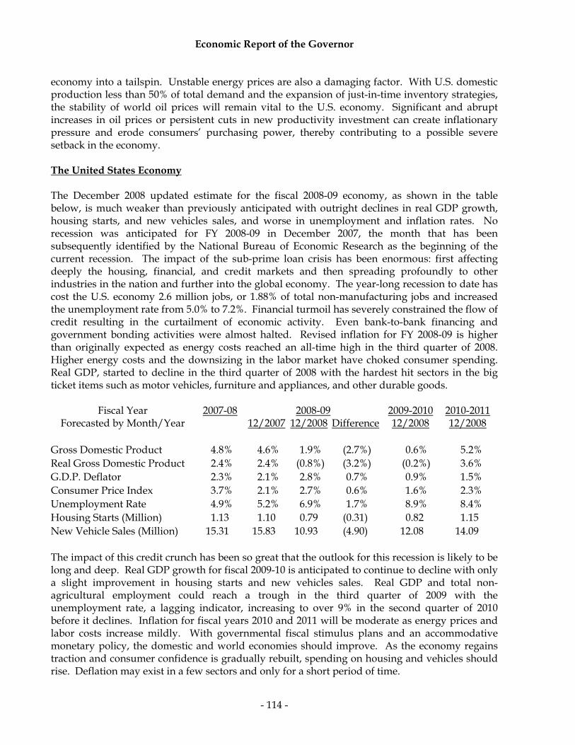
Economic Report of the Governor
- 114 -
economy into a tailspin. Unstable energy prices are also a damaging factor. With U.S. domestic production less than 50% of total demand and the expansion of just-in-time inventory strategies, the stability of world oil prices will remain vital to the U.S. economy. Significant and abrupt increases in oil prices or persistent cuts in new productivity investment can create inflationary pressure and erode consumers’ purchasing power, thereby contributing to a possible severe setback in the economy. The United States Economy The December 2008 updated estimate for the fiscal 2008-09 economy, as shown in the table below, is much weaker than previously anticipated with outright declines in real GDP growth, housing starts, and new vehicles sales, and worse in unemployment and inflation rates. No recession was anticipated for FY 2008-09 in December 2007, the month that has been subsequently identified by the National Bureau of Economic Research as the beginning of the current recession. The impact of the sub-prime loan crisis has been enormous: first affecting deeply the housing, financial, and credit markets and then spreading profoundly to other industries in the nation and further into the global economy. The year-long recession to date has cost the U.S. economy 2.6 million jobs, or 1.88% of total non-manufacturing jobs and increased the unemployment rate from 5.0% to 7.2%. Financial turmoil has severely constrained the flow of credit resulting in the curtailment of economic activity. Even bank-to-bank financing and government bonding activities were almost halted. Revised inflation for FY 2008-09 is higher than originally expected as energy costs reached an all-time high in the third quarter of 2008. Higher energy costs and the downsizing in the labor market have choked consumer spending. Real GDP, started to decline in the third quarter of 2008 with the hardest hit sectors in the big ticket items such as motor vehicles, furniture and appliances, and other durable goods.
Fiscal Year 2007-08 2008-09 2009-2010 2010-2011 Forecasted by Month/Year 12/2007 12/2008 Difference 12/2008 12/2008
Gross Domestic Product 4.8% 4.6% 1.9% (2.7%) 0.6% 5.2% Real Gross Domestic Product 2.4% 2.4% (0.8%) (3.2%) (0.2%) 3.6% G.D.P. Deflator 2.3% 2.1% 2.8% 0.7% 0.9% 1.5% Consumer Price Index 3.7% 2.1% 2.7% 0.6% 1.6% 2.3% Unemployment Rate 4.9% 5.2% 6.9% 1.7% 8.9% 8.4% Housing Starts (Million) 1.13 1.10 0.79 (0.31) 0.82 1.15 New Vehicle Sales (Million) 15.31 15.83 10.93 (4.90) 12.08 14.09 The impact of this credit crunch has been so great that the outlook for this recession is likely to be long and deep. Real GDP growth for fiscal 2009-10 is anticipated to continue to decline with only a slight improvement in housing starts and new vehicles sales. Real GDP and total non-agricultural employment could reach a trough in the third quarter of 2009 with the unemployment rate, a lagging indicator, increasing to over 9% in the second quarter of 2010 before it declines. Inflation for fiscal years 2010 and 2011 will be moderate as energy prices and labor costs increase mildly. With governmental fiscal stimulus plans and an accommodative monetary policy, the domestic and world economies should improve. As the economy regains traction and consumer confidence is gradually rebuilt, spending on housing and vehicles should rise. Deflation may exist in a few sectors and only for a short period of time.

Economic Report of the Governor
- 115 -
Forecast Caveats The projection of only a modest decline in real output growth in fiscal 2010 and a healthy rebound in fiscal 2011 with modest inflation assumes that there is improvement in the financial markets. Through government’s massive efforts, the financial market should respond and return to its fundamentally sound working state; therefore, the economy will enter a recovery path. However, these measures that include a series of programs (foreclosure mitigation, industry bailouts, tax cuts, infrastructure and local government spending and a zero interest rate policy, etc.) may take longer than expected to work. Any material increase in the level of toxic financial assets or a lengthy delay in the restoration of profitability to the banking systems may worsen the flow of credit and thereby delay economic recovery. The fiscal and monetary actions of governmental institutions are intended to counter the effects of a slowing economy and spur consumer spending. However, when households are already burdened with high debt levels, combined with job insecurity, a significant portion of any stimulus will be diverted to paying down debt (i.e., past consumption) or increase savings (i.e., future consumption), thus lessening any economic benefit. The Federal Reserve System’s zero interest rate policy (ZIRP) is intended to shore up the troubled housing market and boost business and investor confidence. However, the beneficial aspects of this policy may also be partially offset by negative side effects. Overseas governments have been heavy purchasers of U.S. Government debt and may be reluctant to increase such holdings when such low interest rates may not compensate for perceived risks of mounting U.S. debt levels and the potential for wide currency swings. Projections indicate that the federal budget deficit may reach an historic high of 7% of GDP. Moreover, those same governments may use their surplus of savings at home to stimulate their own domestic economy as opposed to investing in the U.S. An unexpectedly deeper slowdown in consumer spending would exacerbate the already weak economy. A further decline in the stock and housing markets will further destroy any remnants of the “wealth effect”, thereby affecting consumer behavior that impacts two-thirds of the national economy. The slumping housing market has brought a hefty loss in home values since its peak. During the same time, some 50% in U.S. equity value has been wiped out. Growth in consumption could be further curbed as consumers become more conscientious about boosting their inadequate level of savings. Energy prices, always the wildcard, will continue to exert significant influence over the economy. Any geopolitical tension, speculative disorder, or other unexpected event could drive the price higher, sending the economy into a tailspin. There are also a myriad of other factors that may impinge upon domestic growth and inflation projections, including an unexpected economic or financial shock in a major country, the unfavorable outcome of any regional conflict, unstable foreign geopolitical conditions, and even an unexpected natural disaster. Any major disturbance could steer the forecast in either direction.

Economic Report of the Governor
- 116 -
The Connecticut Economy (History) A comparison of the original forecasts for Connecticut’s personal income, nonagricultural employment and unemployment rates with actual figures for fiscal 2005-06 through 2007-08 and the current forecast for fiscal 2008-09 are presented in the following Table.
TABLE 88
HISTORICAL COMPARISON OF CONNECTICUT ECONOMIC INDICATORS
Nonagricultural Unemployment Fiscal Year Personal Income Employment Rate
2005-06 12/04 Forecast $168.7 Billion 1,665.6 Thousand 4.5% Actual $174.1 Billion 1,670.1 Thousand 4.6% Difference $5.4 Billion 4.5 Thousand 0.1%
2006-07 12/05 Forecast $184.5 Billion 1,691.5 Thousand 5.2% Actual $186.2 Billion 1,689.0 Thousand 4.4% Difference $1.7 Billion (2.5) Thousand (0.8%) 2007-08 12/06 Forecast $191.2 Billion 1,692.1 Thousand 4.4% Actual $195.8 Billion 1,702.3 Thousand 4.9% Difference $4.6 Billion 10.2 Thousand 0.5%
2008-09 12/07 Forecast $199.2 Billion 1,708.5 Thousand 4.8% Latest Forecast $198.5 Billion 1,677.7 Thousand 6.6% Difference ($0.7) Billion (30.8) Thousand 1.8%
After employment bottomed out in July of 2003 in Connecticut, the nation’s economic engine continued its positive growth, and Connecticut’s growth also continued. Employment, per-capita gross state product and personal income, and labor productivity all saw healthy growth for about the next three years, and the unemployment rate remained below the national rate. For more than two years, now, however, there have been subtle signs of softness, becoming more obvious in the last year, linked to national issues of subprime loans and credit tightening. The number employed finally reached the last pre-recession peak of July, 2000, in July of 2007, but the unemployment rate has generally been rising since reaching a low point in April of 2006. The following Table compares nonagricultural employment and its two major components for the U.S. and Connecticut: first, during the last recession, showing the peak at the beginning of the recession and the most current peak after coming out of the recession and, second, the most current situation, since the last peak in December of 2007, as the state entered the current recession. In the twelve months since employment peaked in December of 2007, the state has lost more than 29,000 jobs, or 1.8% of the total number of jobs existing at the peak. In comparison, in the last recession, the state lost a total of 61,000 jobs, or 3.5% of the July, 2000, peak, but lost 18,500 jobs, or only 1.1% in the first twelve months. However, Connecticut has, so far, lost fewer jobs as a percentage of the total workforce than the nation.

Economic Report of the Governor
- 117 -
TABLE 89
UNITED STATES & CONNECTICUT CHANGE IN EMPLOYMENT (In Thousands, Seasonally Adjusted)
Early 2000s Recession
United States Connecticut 2/01 12/07 Change % Chg. 7/00 12/07 Change % Chg. Mfg. Empl. 17,029 13,772 (3,257) (19.1%) 237 191 (46) (19.5%) NonMfg. Empl. 115,522 124,306 8,784 7.6% 1,463 1,516 53 3.6% NonAgr. Empl. 132,551 138,078 5,527 4.2% 1,700 1,707 7 0.4%
Recovery achieved February of 2005 Recovery achieved August of 2007
Current Recession United States Connecticut
12/07 12/08 Change % Chg. 12/07 12/08 Change % Chg.
Mfg. Empl. 13,772 12,981 (791) (5.7%) 191 186 (5) (2.6%)
NonMfg. Empl. 124,306 122,508 (1,798) (1.4%) 1,516 1,491 (25) (1.6%)
NonAgr. Empl. 138,078 135,489 (2,589) (1.9%) 1,707 1,677 (30) (1.8%)
The Tables below provide a breakdown of the employment totals and changes, in thousands of jobs, for each sector and the corresponding impact on the unemployment rate in state labor market areas (LMA), since employment last peaked in December of 2007.
Connecticut Employment Selected LMA Unemployment Rates (Seasonally Adjusted) (Not Seasonally Adjusted)
Sectors Dec. ‘07 Dec. ‘08 Chg. LMA Dec. ‘07 Dec. ‘08 Chg. Trade, Transp. & Utilities 313.1 301.2 (11.9) Waterbury 6.1% 8.6% 2.5% Manufacturing 190.7 185.7 (5.0) Brdgprt/Stmfrd 4.0% 6.0% 2.0% Construction & Mining 68.5 63.1 (5.4) Hartford 4.3% 6.7% 2.4% Fin., Ins. & Real Estate 143.2 141.5 (1.7) Danielson 5.6% 8.2% 2.6% Information 39.2 38.0 (1.2) Torrington 4.2% 6.3% 2.1% Services 700.6 696.3 (4.3) New London 4.3% 6.7% 2.4% Government * 251.2 251.4 0.2 New Haven 4.7% 6.6% 1.9%
Total 1,706.5 1,677.2 (29.3) Danbury 3.4% 5.1% 1.7% Enfield 4.7% 6.8% 2.1%
* Includes Native American tribal government employment, including casino employment, and federal, state and local government.

Economic Report of the Governor
- 118 -
CONNECTICUT EMPLOYMENT
Percent Change In Employment By Sector And Jobs Gained/(Lost) (From December 2007 to December 2008)
-7.9%
-3.8%
-3.1%
0.1%
-0.6%
-2.6%
-1.2%
-10.5% -8.5% -6.5% -4.5% -2.5% -0.5% 1.5% 3.5% 5.5%
Government*
Manufacturing
200
(4,300)
(1,700)
(5,000)
(11,900) Trade, Transp. & Utilities
(5,400)
(1,200)
Construction & Mining
Fin., Ins. & Real Estate
Information
Services
*Government includes employees of Sovereign Tribal Nations
in casinos and federal, state and local governments. Personal income in Connecticut grew by 5.1% in fiscal 2008, comparable to the rate for the nation. After adjusting for inflation, Connecticut’s real per capita personal income increased by 1.0%. Furthermore, Connecticut per capita personal income still remains well above the U.S. average by 42.1%. Mortgage rates have remained relatively low from an historical perspective. The Federal Reserve reduced rates seven times in 2008, by a total of 400 to 425 basis points, to an all-time low. The number of housing permits in calendar year 2007 was down 16.1% compared to the year before, with uneven changes geographically, as only Fairfield County saw positive growth. The number of housing starts in fiscal year 2008 was down 21.4% over fiscal 2007, following a drop of 23.7% in fiscal 2007. The median price of homes in the state increased 2.3% in calendar year 2007, a relatively minor increase compared to recent years. Moreover, for the first time in many years, the affordability of homes for Connecticut residents improved. Because housing construction and prices did not reach quite the frenzied levels of other parts of the country over the last few years, the impact of the subprime mortgage issue in Connecticut had been delayed, but the full impact of lower prices and reduced sales is now being felt and will continue for some time. Finally, Connecticut’s personal income tax revenues, after growing 9.6% the previous year, grew 11.3% in fiscal 2008, as estimated and final payments, which include capital gains, rose 19.8% compared to last year. When combined with changes in all the other taxes, total tax receipts grew year-over year by 5.8%. This, coupled with overall expenditure restraints, and the economy’s resiliency, were the key reasons the state entered this recession in a relatively strong financial position.

Economic Report of the Governor
- 119 -
The Connecticut Economy (Forecast) Any attempt to forecast the economic outlook for the state over the next few years must factor in certain other considerations which are not easily quantified, at least at this time: fuel prices have fallen significantly, and will probably remain lower than last year; borrowing costs are lower, which will help those who can get credit; and a new federal recovery plan initiative, still not defined, should bring financial help to consumers and workers, businesses, and state and local governments. On the other hand, Connecticut’s job mix is more heavily weighted towards the financial services industry than the nation as a whole. The state economy is significantly influenced by the fortunes of Wall Street which have performed poorly for more than a year, and state tax revenues depend heavily on capital gains and bonuses from those markets. Fiscal year 2008 was generally good for the state’s economy, although signs of weakness began to emerge late in fiscal 2008. Moving forward, the state is expected to experience difficult economic times, like the rest of the nation, which has been in recession since December of 2007. Although Connecticut’s economy has become more diversified, thus tempering the impact, employment, housing, and state revenue are still at grave risk as the biennium unfolds. Employment in the state is expected to contract for the first time since fiscal year 2004. Total nonagricultural employment is projected to decrease 1.4% and 2.6%, respectively, during fiscal years 2009 and 2010, and grow 1.0% in fiscal year 2011. Employment is projected to reach a low point early in calendar 2010. Not surprisingly, manufacturing employment, where the vast majority of job losses were concentrated during the last recession and subsequent weak recovery, is expected to continue its drag on employment growth that has prevailed since 1998. In fact, employment is not expected to see substantial improvement between fiscal years 2008 and 2011 in any sectors except health and education services (4.7%), with dramatic losses in construction (-12.8%), and professional and business services (-10.8%). While forecasts of productivity gains are respectable, corporate earnings are expected to decline. Housing values have declined, and household net worth has been reduced. While federal taxes have remained lower since being cut in 2001, the recipe of stagnant disposable income growth and tight credit are some of the factors that will prevent consumers from continuing their spending pace, as consumer confidence remains low. Personal income will grow by only 1.4% in both fiscal years 2009 and 2010. After adjusting for inflation, personal income will register declines. The unemployment rate in the state, which stood at 4.9% in fiscal year 2008, is expected to rise to 8.0% in fiscal year 2010 and then drop to 7.7% the next year. Connecticut’s population growth during the forecast period is estimated to be moderate, and remain below the national growth rate, based upon the trend of the last several years. In the next couple of years, the supply of labor should be more than adequate to meet demand. However, long-term demand for skilled workers will have to be met by a rise in the state’s trained labor force. Once economic growth resumes, the lack of skilled workers represents one of the biggest challenges the state will face in the future because many lack the skills to take the jobs that are or will be available. If the situation persists, this could impact economic growth in the long term.

Economic Report of the Governor
- 120 -
The forecast for the most widely used economic indicators for the Connecticut’s economy is shown below.
12/08 Forecast Fiscal Year 2009-10 Fiscal Year 2010-11 Personal Income $201.3 Billion $208.3 Billion Nonagricultural Employment 1,634.1 Thousand 1,650.5 Thousand Unemployment Rate 8.0% 7.7%
Many of the trends discussed last year have continued. Personal income will continue anemic growth, and housing sales and prices will continue to drop. Also, major risks facing the state and the nation discussed last year have also come to fruition: (1) We are now in recession; (2) The stock market has experienced a catastrophic downturn; (3) Job growth has been halted. The following Table shows the impact of prior recessionary periods on the state. This shows that the two most recent recoveries took longer than might have been expected.
RECESSIONS IMPACT ON CONNECTICUT’S LABOR MARKET
Employment Jobs Lost As A Months From Months From Peak To Trough Percent Of Total Jobs Peak To Trough Peak To Regaining Peak Feb. ‘70 - Jun. ‘71 4.0% 16 34 Aug. ‘74 - Sept. ‘75 4.4% 13 32 Mar. ’80- Aug. ‘80 1.4% 5 11 Oct. ’81 - Feb. ‘83 1.5% 16 21 Feb. ’89 - Dec. ‘92 9.4% 46 131 Jul. ‘00 - Jul. ‘03 3.5% 36 85 Average 4.0% 22 52
Dec. ‘07 – Dec ‘08 1.8% * * * Assumes that the latest peak of the labor market was reached in December of 2007, and the
impact of the current recession is yet to be determined. Based on all the cited risks, there are now reasons to be concerned about the continued decline in employment. We have passed a new employment peak and it will likely be some time before recovery is in sight, with projections showing employment not regaining previous peak levels until 2012. Unfortunately, the bulk of the projected job losses during this recession are still ahead of us. Putting the current situation into perspective, job losses are forecast to reach approximately 74,000 jobs, while approximately 160,000 jobs were lost between 1989 and 1992. On the other hand, the unemployment rate is projected to rise to 8.2% by early 2010, a level not seen since fiscal year 1977. The following tables provide historical and forecasted values for the major economic variables used in revenue forecasting for the United States and Connecticut.

Economic Report of the Governor
- 121 -
TABLE 90 UNEMPLOYMENT RATES
Seasonally Adjusted
Fiscal Year Quarters United States Connecticut 2006-07 1 4.6% 4.5%
2 4.4% 4.3% 3 4.5% 4.4% 4 4.5% 4.4% 2007-08 1 4.7% 4.6% 2 4.8% 4.8% 3 4.9% 5.0% 4 5.3% 5.2% 2008-09 1 6.0% 6.1% 2 6.5% 6.4% 3 7.3% 6.9% Start of Forecast 4 7.9% 7.2% 2009-10 1 8.5% 7.6% 2 8.9% 8.0% 3 9.1% 8.2% 4 9.1% 8.2%
2010-11 1 8.9% 8.0% 2 8.6% 7.8% 3 8.3% 7.6% 4 7.9% 7.2%
Source of Historical Data: U.S. Bureau of Labor Statistics, Connecticut State Labor Department
TABLE 91 Comparison of Connecticut's Personal Income Versus U.S. GDP and Personal Income
(Seasonally Adjusted in Billions of Dollars)
Connecticut United States United States Personal % Change Personal % Change % Change Fiscal Year Income Year Ago Income Year Ago GDP Year Ago 1999-00 135.783 7.1 8,109.6 6.6 9,571.3 6.4 2000-01 145.744 7.3 8,613.9 6.2 9,991.5 4.4 2001-02 146.946 0.8 8,788.1 2.0 10,280.3 2.9 2002-03 146.983 0.0 8,974.1 2.1 10,664.0 3.7 2003-04 153.265 4.3 9,398.3 4.7 11,330.4 6.2 2004-05 163.149 6.4 9,993.0 6.3 12,045.2 6.3 2005-06 174.081 6.7 10,617.3 6.2 12,832.1 6.5 2006-07 186.240 7.0 11,309.1 6.5 13,467.0 4.9 2007-08 195.773 5.1 11,899.6 5.2 14,106.8 4.8 2008-09 (E) 198.499 1.4 12,213.3 2.4 14,381.4 1.9 2009-10 (P) 201.251 1.4 12,551.8 2.8 14,472.9 0.6 2010-11 (P) 208.288 3.5 13,065.1 4.1 15,219.9 5.2
(E) = Estimated / (P) = Projected
Source of Historical Data: U.S. Bureau of Economic Analysis

Economic Report of the Governor
- 122 -
TABLE 92 STATE OF CONNECTICUT
Annualized Personal Income & Nonagricultural Employment (In Millions)
Personal % Change Nonagricultural % Change Fiscal Year Income Year Ago Employment Year Ago
2006-07 1 180,573 7.2 1,682.7 1.2 2 183,751 6.5 1,687.5 1.3 3 189,817 7.3 1,690.7 1.0 4 190,820 7.0 1,695.2 1.0 Average 186,240 7.0 1,689.1 1.1
2007-08 1 194,193 7.5 1,700.6 1.1 2 195,448 6.4 1,704.2 1.0 3 196,044 3.3 1,702.1 0.7 Start of Forecast 4 197,407 3.5 1,702.3 0.4 Average 195,773 5.1 1,702.3 0.8
2008-09 1 198,333 2.1 1,703.9 0.2 2 198,623 1.6 1,689.6 -0.9 3 198,413 1.2 1,666.7 -2.1 4 198,627 0.6 1,650.8 -3.0 Average 198,499 1.4 1,677.7 -1.4
2009-10 1 199,461 0.6 1,639.0 -3.8 2 200,417 0.9 1,632.7 -3.4 3 201,788 1.7 1,630.9 -2.1 4 203,340 2.4 1,634.0 -0.1 Average 201,251 1.4 1,634.1 -2.6
2010-11 1 205,257 2.9 1,639.8 0.1 2 207,245 3.4 1,646.7 0.9 3 209,325 3.7 1,653.7 1.4 4 211,324 3.9 1,661.7 1.7 Average 208,288 3.5 1,650.5 1.0

Economic Report of the Governor
- 123 -
TABLE 93 U.S. CONSUMER PRICE INDEX, SEASONALLY ADJUSTED
(1982-84 = 100)
Consumer % Change Fiscal Year Price Index Year Ago
2006-07 1 203.2 3.3 2 202.4 1.9 3 204.3 2.4 4 206.6 2.6 Average 204.1 2.6
2007-08 1 208.0 2.4 2 210.6 4.0 3 212.8 4.2 4 215.4 4.3 Average 211.7 3.7
2008-09 1 219.0 5.3 2 217.4 3.2 3 216.5 1.8 Start of Forecast 4 217.1 0.8 Average 217.5 2.7
2009-10 1 218.6 (0.2) 2 220.3 1.4 3 221.9 2.5 4 223.3 2.9 Average 221.0 1.6
2010-11 1 224.5 2.7 2 225.7 2.5 3 226.7 2.2 4 227.5 1.9 Average 226.1 2.3
Source of Historical Data: U.S. Bureau of Labor Statistics

Economic Report of the Governor
- 124 -
REVENUE FORECAST The following Table shows the actual General Fund Revenue collections for fiscal 2007-08, and estimated revenue collections for fiscal 2008-09 and projected revenue collections for fiscal 2009-10 and fiscal 2010-11 by major sources.
TABLE 94 STATE OF CONNECTICUT - GENERAL FUND REVENUES
(In Millions of Dollars)
Projected Revenue Proposed Net Actual Estimated At Current Revenue Projected Revenue Revenue Rates Changes Revenue
Taxes 2007-08 2008-09 2009-10 2009-10 2009-10 Personal Income Tax $ 7,512.7 $ 6,900.0 $ 6,741.0 $ 13.3 $ 6,754.3 Sales & Use Tax 3,582.3 3,499.7 3,577.5 4.2 3,581.7 Corporation Tax 733.9 607.6 597.2 35.0 632.2 Public Service Tax 237.1 247.3 250.4 - 250.4 Inheritance & Estate Tax 170.6 255.1 190.8 - 190.8 Insurance Companies Tax 227.2 192.2 188.2 - 188.2 Cigarette Tax 335.2 325.0 322.0 - 322.0 Real Estate Conveyance Tax 158.5 124.1 125.3 - 125.3 Oil Companies Tax 205.5 88.0 88.0 24.5 112.5 Alcoholic Beverages 47.1 47.5 48.0 - 48.0 Admissions and Dues 37.3 37.5 37.9 - 37.9 Miscellaneous 140.0 141.0 144.3 - 144.3 Total Taxes $ 13,387.5 $ 12,465.0 $ 12,310.6 $ 77.0 $ 12,387.6 Less Refunds of Taxes (852.2) (920.0) (950.0) - (950.0) Less R&D Credit Exchange (11.4) (11.9) (12.4) - (12.4) TOTAL - Taxes Less Refunds $ 12,523.9 $ 11,533.1 $ 11,348.2 $ 77.0 $ 11,425.2 Other Revenues Transfers Special Revenue $ 287.6 $ 289.0 $ 294.5 $ 10.0 $ 304.5 Indian Gaming Payments 411.4 375.0 417.1 5.0 422.1 License, Permits, Fees 171.7 156.7 178.5 137.2 315.7 Sales of Commodities & 30.1 31.5 33.3 - 33.3 Rents, Fines & Escheats 59.9 71.2 94.9 13.0 107.9 Investment Income 63.9 30.0 20.0 - 20.0 Miscellaneous 140.1 142.5 152.6 3.0 155.6 Less Refunds of Payments (0.5) (0.6) (0.6) - (0.6) TOTAL - Other Revenues $ 1,164.3 $ 1,095.3 $ 1,190.3 $ 168.2 $ 1,358.5 Other Sources Federal Grants $ 2,701.6 $ 3,189.5 $ 3,162.9 $ 851.2 $ 4,014.1 Transfer From Tobacco 115.3 115.8 112.8 - 112.8 Transfers From/(To) Other (102.3) 164.3 (136.0) 734.6 598.6 TOTAL - Other Sources $ 2,714.6 $ 3,469.6 $ 3,139.7 $ 1,585.8 4,725.5 TOTAL - General Fund $ 16,402.8 $ 16,098.0 $ 15,678.2 $ 1,831.0 17,509.2

Economic Report of the Governor
- 125 -
Projected Revenue Proposed Net At Current Revenue Projected Rates Changes Revenue 2010-11 2010-11 2010-11 $ 7,217.5 $ 16.8 $ 7,234.3 3,701.9 4.4 3,706.3 657.0 35.0 692.0 253.8 - 253.8 196.6 - 196.6 188.2 - 188.2 317.0 - 317.0 127.8 - 127.8 64.6 4.5 69.1 48.5 - 48.5 38.3 - 38.3 140.0 - 140.0 $ 12,951.2 $ 60.7 $ 13,011.9 (1,015.0) - (1,015.0) (12.9) - (12.9) $ 11,923.3 $ 60.7 $ 11,984.0 $ 295.9 $ 10.0 $ 305.9 394.7 5.0 399.7 163.3 109.2 272.5 34.1 - 34.1 96.9 13.0 109.9 20.0 - 20.0 153.1 5.0 158.1 (0.6) - (0.6) $ 1,157.4 $ 142.2 $ 1,299.6 $ 3,217.1 $ 536.2 $ 3,753.3 113.2 - 113.2 (136.0) 1,113.4 977.4 $ 3,194.3 $ 1,649.6 $ 4,843.9 $ 16,275.0 $ 1,852.5 $ 18,127.5
Explanation of Changes
Personal Income Tax Delay the increase in the singles exemption for 3 years. Sales and Use Tax Suspend the sales tax free week for 2 years. Corporation Tax Cap the Film Industry Tax Credit at $30 million/year. Suspend the Historic Homes and Historic Structures Tax Credits for 2 years. Oil Companies Tax Increase the transfer to the Special Transportation Fund by $20 million in FY 2011 and by $30 million annually thereafter. Eliminate Department of Environmental Protection Special Purpose Funds. Transfers Special Revenue Reduce lottery retailer commission from 5% to 4%. Indian Gaming Payments Reflects extended hours of alcoholic beverage sales. License, Permits, and Fees Increase various license, permits, and fees. Eliminate Department of Environmental Protection Special Purpose Funds. Rents, Fines, Escheats Extend the 5 cent deposit requirement to additional containers and escheat the unclaimed deposits to the state. Miscellaneous Revenue Increase the resident state trooper reimbursement rate to 100% over two years. Federal Grants Impact of Federal Stimulus monies for Medicaid and Education and recommended expenditure changes. Transfers-Other Various fund transfers. Use of the Budget Reserve Fund- $514.5 million in FY 2010 and $585.5 million in FY 2011. Securitization of the Energy Funds- $350 million. Level-fund the Mashantucket Pequot and Mohegan Grant.

Economic Report of the Governor
- 126 -
GENERAL FUND FISCAL YEAR 2009-10 – TOTAL $17,509.2 MILLION*
Sales & Use $3,581.7 19.3%
Corporation $632.2 3.4%
Federal Grants $4,014.1 21.6%
Other Revenues & Tobacco Settlement
$2,156.7 11.6%
Personal Income $6,754.3 36.4%
Other Taxes $1,419.4 7.7%
GENERAL FUND FISCAL YEAR 2010-11 – TOTAL $18,127.5 MILLION*
Other Taxes $1,379.3 7.2%
Personal Income $7,234.3 37.6%
Other Revenues & Tobacco Settlement
$2,477.0 12.9%Federal Grants $3,753.3 19.5%
Corporation $692.0 3.6%
Sales & Use $3,706.3 19.2%
* Refunds of Taxes are estimated at $950.0M for FY 2009-10 and $1,015.0M for FY 2010-11,
R&D Credit Exchange are estimated at $12.4M for FY 2009-10 and $12.9 M for FY 2010-11, Refunds of Payments are estimated at $0.6M for both FY 2009-10 and FY 2010-11, Transfers to Other Funds are $86.25M for both FY 2009-10 and FY 2010-11.

Economic Report of the Governor
- 127 -
This page has been intentionally left blank.

Economic Report of the Governor
- 128 -
TABLE 95 STATE OF CONNECTICUT
SPECIAL TRANSPORTATION FUND REVENUES (In Millions of Dollars)
Projected Revenue Proposed Net Actual Estimated Current Revenue Projected Revenue Revenue Rates Changes Revenue
Taxes 2007-08 2008-09 2009-10 2009-10 2009-10 Motor Fuels Tax $ 495.1 $ 499.7 $ 499.7 $ - $ 499.7 Oil Companies Tax 127.8 141.9 141.9 - 141.9 Sales Tax DMV 64.9 60.5 61.1 - 61.1 Less Refunds of Taxes (7.0) (7.4) (7.5) - (7.5) TOTAL - Taxes Less Refunds $ 680.8 $ 694.7 $ 695.2 $ - $ 695.2 Other Sources Motor Vehicle Receipts $ 225.5 $ 229.3 $ 233.2 $ 36.2 $ 269.4 Licenses, Permits & Fees 153.8 155.8 157.4 34.7 192.1 Interest Income 36.6 25.0 25.0 - 25.0 Transfers From (To) Other Funds 7.2 (8.0) (9.5) 3.0 (6.5) Transfer To TSB (20.8) (15.3) (15.3) - (15.3) Less Refunds of Payments (2.7) (3.0) (3.1) - (3.1) TOTAL - Other Sources $ 399.5 $ 383.8 $ 387.7 $ 73.9 $ 461.6 TOTAL – S.T.F. $ 1,080.3 $ 1,078.5 $ 1,082.9 $ 73.9 $ 1,156.8
FISCAL YEAR 2009-10 - TOTAL $ 1,156.8 MILLION*
Licenses, Permits, Fees $192.1 16.1%
Oil Companies & Sales Taxes $203.0 17.1%
Motor Vehicle Receipts $269.4 22.7%
Interest Income $25.0 2.1%
Motor Fuels Tax $499.7 42.0%
* Refunds of Taxes are estimated at $7.5M, Transfers to Other Funds are estimated at $6.5 M, Refunds of Payments are estimated at $3.1M and Transfers to Transportation Strategy Board are estimated at $15.3M in fiscal 2009-10.

Economic Report of the Governor
- 129 -
Projected Revenue Proposed Net Current Revenue Projected Rates Changes Revenue 2010-11 2010-11 2010-11
$ 494.7 $ - $ 494.7 165.3 20.0 185.3 61.7 - 61.7 (7.6) - (7.6)
$ 714.1 $ 20.0 $ 734.1
$ 237.1 $ 36.2 $ 273.3 159.0 57.4 216.4 25.0 - 25.0 (9.5) 3.0 (6.5) (15.3) - (15.3) (3.2) - (3.2)
$ 393.1 $ 96.6 $ 489.7
$ 1,107.2 $ 116.6 $ 1,223.8
FISCAL YEAR 2010-11 - TOTAL $ 1,223.8 MILLION*
Licenses, Permits, Fees $216.4 17.2%
Oil Companies & Sales Taxes $247.0 19.7%
Motor Vehicle Receipts $273.3 21.7%
Interest Income $25.0 2.0%
Motor Fuels Tax $494.7 39.4%
* Refunds of Taxes are estimated at $7.6M, Transfers to Other Funds are estimated at $6.5M,
Refunds of Payments are estimated at $3.2M and Transfers to Transportation Strategy Board are estimated at $15.3M in fiscal 2010-11.
Explanation of Changes Oil Companies Increase transfer from the General Fund by $20.0 million. Motor Vehicle Receipts Increase registration, driver’s license, and motor vehicle inspection fees. License, Permits, Fees Increase various motor vehicle and transportation related fines and fees. Enhance traffic enforcement. Establish a Driver Responsibility Program. Transfers-From/(To) Other Funds Eliminate the transfer to the Conservation Fund.

Economic Report of the Governor
- 130 -
IMPACT OF THE GOVERNOR'S BUDGET ON THE STATE'S ECONOMY The traditional purpose of a governmental budget is threefold: it outlines necessary and desirable public services; it estimates how much these services will cost; and it defines the resources that are required to provide these services. The budget is the fundamental policy document of every level of government. As proposed, enacted and implemented, it represents a consensus on what government realistically can and ought to do. The economic implications of governmental budgets are significant. The government sector including federal and local governments is an important dimension of the national economy, accounting for 19.4% of the Gross Domestic Product. The spending and tax policies of government profoundly influence the performance of the economy. Because the Governor's budget accounts for 7.8% of the Gross State Product, it is inevitable that state government's expenditure and revenue actions influence the State's economy. The economy has entered a severe recession that is expected to last many more months and claim many more jobs. The result is a budget recommendation that is severely constrained by these harsh economic realities, yet attempts to shield the most vulnerable citizens from the shock that threatens their social and economic wellbeing. Governor Rell believes this budget will preserve the most important aspects of our quality of life, and help the state live within its means. Expenditure Actions
Education and Workforce
Although our current economic outlook is bleak, we must not put off planning for our future. Human capital will drive our future economic prospects; if the state produces and retains a quality workforce, our economy will flourish. Connecticut’s labor market rewards those with both skills and education; even more importantly, for poor and often minority citizens, getting a college degree reduces the financial barriers created by poverty and economic disadvantage. For too many of the state’s citizens, however, the financial benefits of skilled jobs are beyond their reach. They do not have the training or education to compete for better paying jobs, jobs that will be needed in an increasingly competitive global economy. To accomplish this, Governor Rell is proposing a series of landmark initiatives to restructure our education system and strengthen its critical linkages to the state’s economy. Governor Rell is endorsing four major education and economic development restructurings. These include: 1) Merge the leadership and staffing of the state’s education agencies, creating a true
governing body for the kindergarten-to-graduate school (Pk-20) academic continuum; 2) Unite the leadership and staffing of the Connecticut Community Colleges(CCs), the
Technical High School System (THSS) and the Office for Workforce Competitiveness to provide a workforce-driven State system of Middle Colleges;
3) Combine the economic development tourism, arts, historical and film programs with the rest of the state’s General Fund economic development programs;

Economic Report of the Governor
- 131 -
4) Join the leadership and staffs of two quasi-public economic development agencies to improve the visibility and functionality of their programs.
Governor Rell’s expanded Board of Education, which includes higher education, sets the stage for a seamless, coordinated education system from preschool through graduate school. Additionally, the companion restructuring of two major public education systems, the Technical High Schools and the Community Colleges, expands learning opportunities for high school students, not only to take college courses while in high school, but it increases the possibility that students will be academically prepared for college. Selected workforce personnel and programs will guide the economic mission of the Middle College System. A stronger Department of Economic and Community Development (DECD), along with a merger of two economic development quasi-public agencies, will increase the visibility of the State’s jobs creation programs. DECD will take a central leadership role, including the utilization of the latest web-based technology to assist job creators find the right program for their specific needs. The jobs DECD helps create will be filled by an increasingly skilled workforce, prepared for work in Connecticut’s economy by an academically coordinated Pk-20 education system and the new Middle College System.
Health and Human Services Despite the difficult economic climate, this budget does not sacrifice the most critical supports that have been so carefully crafted over the years to assist Connecticut’s neediest residents. While there are proposals in the budget to reduce health and human services programs, many of those changes are in keeping with the Governor’s focus on streamlining state government and reorienting agency efforts toward core missions. . The commitment to maintaining the safety net is especially important during an economic downturn, when many residents are more likely to need services such as health care, income supports, and other social services. The Governor is not proposing across the board reductions in Medicaid provider rates or in nursing home rates. In fact, the funding for Medicaid rate increases that was added during the FY2007-09 biennium—totaling over $200 million annually—is preserved. In addition, the Governor is maintaining recent expansions in Medicaid eligibility: HUSKY A eligibility remains at 185% of the federal poverty level (FPL), and eligibility for pregnant women remains at 250% FPL. The Governor is also not proposing across-the-board reductions to private provider funding. This budget reflects a commitment to serving those in greatest need. The budget includes funding for caseload growth in many programs under the Department of Social Services (DSS), such as Medicaid, including HUSKY A, the Charter Oak Health Plan, State Administered General Assistance (SAGA), and community programming under the Money Follows the Person initiative. Funding for caseload growth is also proposed under the Department of Developmental Services (DDS) for persons with developmental disabilities who are graduating from high school or aging out of services provided by the Department of Children and Families (DCF) or local education agencies and into residential or day services provided under DDS’ adult service system; for forensic (court-involved) cases, and for the Birth to Three early

Economic Report of the Governor
- 132 -
intervention program. Funding is also provided for additional persons to be served through the General Assistance Behavioral Health program, the young adult services program, and the program for those with traumatic or acquired brain injuries under the Department of Mental Health and Addiction Services (DMHAS). In addition, funding for additional children and youth requiring foster care and adoption services is provided under the Department of Children and Families. This demonstrates an extraordinary commitment to increasing services to those in need, despite the challenges facing Connecticut’s economy. Some adjustments are proposed where necessary to reflect either new programs or funding available at the federal level. The availability and maturation of the Medicare Part D pharmacy benefit has allowed Connecticut to eliminate funding for the state’s Medicare Part D Supplemental Needs Fund, as prescription drug plans are required to cover those drugs that are medically necessary. Similarly, funding for the ConnPACE program will be targeted to those most in need. Other program reductions or eliminations are necessary to deal with the fiscal crisis. Adult dental benefits under the Medicaid and SAGA programs are scaled back to cover emergency services only. Co-payments and premiums are introduced or increased under Medicaid, including HUSKY A and B, as an alternative to reducing or eliminating eligibility. A number of grant-based programs in various agencies are scaled back or eliminated, particularly where they may not represent activities that are part of an agency’s core mission. As part of the Governor’s initiative to streamline government operations, two facilities are proposed for closure. The High Meadows residential facility operated by DCF will be closed and services shifted to Connecticut Children’s Place or to available community services. Cedarcrest Hospital, operated by DMHAS, is also slated for closure and Connecticut Valley Hospital and a variety of other inpatient and community service providers will be utilized to serve its clients. The closure will result in no loss of beds to the DMHAS system. The Governor is also proposing some additional efforts to ensure that those in the most need can be assisted during the economic downturn. In DSS, the Governor is proposing funding for additional food and nutrition assistance by increasing categorical eligibility through a state plan change under the federally-funded Supplemental Nutrition Assistance Program (formerly the Food Stamp program), expanding assistance to food pantries and food banks, and expanding meal services for the elderly. In addition, the Governor is proposing a reallocation of existing shelter resources to initiate a focus on “rapid rehousing,” with shelters offering financial and housing specialist support and intensive counseling to families experiencing a housing crisis. These efforts are expected to reduce shelter stays and expedite placement and restabilization in the community.
General Government In an effort to streamline state functions, Governor Rell has proposed to consolidate and eliminate a number of state commissions and agencies. Many of these entities are advisory in nature; many are duplicative of other state functions. Additionally, agencies that provide similar support functions to various boards and commissions have been consolidated into larger agencies that currently have the ability to provide these functions and thereby achieve efficiencies. In addition, the Governor has proposed that courthouses also be consolidated. There are currently 15 Judicial District Courts and 20 Geographical Area Courts in Connecticut. This proposal will reduce court locations by two courthouses, two Geographical Area Courts and

Economic Report of the Governor
- 133 -
one Judicial District Court, taking the total number from 35 to 32. The matters handled by these courts will be moved to the remaining jurisdictions. This streamlining will allow for more efficient court operations. Governor Rell has also made changes that will allow for more transparency within the Department of Environmental Protection. The agency receives revenue from many sources that are segregated into special fund accounts. These funds, in addition to the General Fund, are used to provide the full range of environmental protection activities. By requiring that all funding be deposited into, and that all activities be funded through, the General Fund, a total picture of the services provided by the agency will be demonstrated. The Governor is also proposing funding for a “civilian conservation corps” that will provide jobs to unemployed persons to assist in the maintenance of public facilities and properties. In order to increase the level of traffic enforcement, the Governor is redeploying state troopers to highway duty. Thirty-one troopers who have been serving in non-patrol functions and eighteen troopers stationed at Bradley Airport that are in excess of the required airport staffing level will be redeployed to highway patrol duty in order to provide additional enforcement and ensure that our highways become safer. In addition, the state intends to deploy the latest technology by using speed cameras to assist in the enforcement of traffic laws. Currently truck inspections in the State of Connecticut are conducted by both the Departments of Motor Vehicles and Public Safety. In order to standardize the functions and achieve more efficient operations, the staffing will be consolidated into the Department of Motor Vehicles, thereby making available an additional 21 sworn personnel to be redeployed to highway duties. This will also allow for more thorough inspections due to the need to comply with the Motor Carrier Safety Assistance Program (MCSAP). DMV is the lead agency for MCSAP a Federal grant program that provides financial assistance to States to reduce the number and severity of crashes and hazardous materials. There are numerous data collection and data reporting requirements; MCSAP must be performed strictly in accordance with federal regulations. This initiative would move costs from the General Fund to the Special Transportation Fund, a more appropriate funding source for truck inspections. The juvenile jurisdiction change is scheduled to go into effect January 1, 2010. Toward that end, the Juvenile Jurisdiction Policy Operations Coordinating Council has been meeting to determine the final implementation plan. In light of the State’s economic condition and the continuing effort to finalize the implementation plan, this initiative is being delayed for two years with a new effective date of January 1, 2012. The delay will also allow for the municipal impact to be analyzed and the necessary capital improvements to be completed. Finally, this has all been accomplished while still fully funding both the state employees’ pension fund and the teachers’ pension fund. The Capital Budget The Governor’s recommended capital budget for FY2010 and FY2011 provides funding for capital projects and programs that help to create and retain jobs in Connecticut. The recommended capital budget includes significant funds for local school construction, clean water projects and community college facilities.

Economic Report of the Governor
- 134 -
At the same time, the recommended capital budget recognizes the need to keep borrowing costs down during these difficult economic times by limiting new bond authorizations to only the most essential projects and programs that are in need of additional funds. The recommendations take into account that significant funds from prior years remain available for use before new bond authorizations are necessary. Finally, the Governor has recommended significant cancellations of prior year authorizations that are either no longer necessary or are for projects that are not essential. Revenue Actions During calendar year 2007, economic conditions in our country began to shift. Against the backdrop of already rising energy prices came the unfolding subprime mortgage meltdown. Almost overnight, interest rates rose dramatically particularly for individuals and businesses without the strongest of credit scores. This credit crunch and general economic downturn became a global issue in 2008. This immediately impacted the nation’s housing market which had expanded significantly this decade, fueled by cheap credit which had existed since the depths of the last recession. The ensuing credit crunch and financial market uncertainty devastated investors and led to a dramatic reduction in interest rates by the Federal Reserve combined with an economic stimulus package from the federal government. While some actions have been taken by the federal government, and more are expected, such as an economic recovery initiative from a recently-inaugurated President Obama, the next few years are expected to present a situation described as potentially the worst economic downturn since the Great Depression of the 1930s. As state revenues have begun to shrink, Governor Rell has already put forward two deficit mitigation plans in the last quarter of calendar year 2008. Within this economic environment, the Governor developed her revenue proposals for the new biennium. The Governor is proposing modest changes to the state’s revenue structure that avoids raising taxes while conserving the state’s resources as long as possible as the economic ill winds affecting the nation arrive at our doorstep. Within this framework, the Governor is proposing to cap the state’s liability under the film industry tax credit to no more than $30 million annually. This program, only enacted in 2006, has already risen to just over $100 million in tax credits awarded becoming far and away the state’s largest business tax credit. The proposed changes will deploy the state’s limited resources more effectively and are projected to save the state $25 million in each year of the biennium. Two relatively new business tax credits for historic homes and historic structures are also being suspended for a period of two years, yet are being retained long-term to encourage such investment. Those changes are expected to save $10 million in each year of the biennium. The Governor is also proposing numerous fee increases as most fees have not been raised since early in the last decade. In addition, several fund transfers have been proposed as numerous non-General Fund accounts have built up large balances or are programmed to receive additional General Fund dollars at a time when the state can least afford it and must prioritize those expenditures that are most essential. The Governor is proposing to delay a tax decrease that was scheduled to take effect this income year for single filers, yet retains those changes in the out-years, saving the state $13.3 million and $16.8 million in each year of the biennium. Finally, it is expected that an economic recovery program will be implemented at the federal level by spring of 2009. While the program is not yet well defined, there are indications of what

Economic Report of the Governor
- 135 -
that initiative will probably look like. Based on the information available, it is anticipated that the state will receive an additional $1.3 billion between fiscal year 2009 and fiscal year 2011 as enhanced federal matching funds for Medicaid and Title IV-E programs, and over $700 million for education aid during the biennium. This is an unprecedented increase in federal aid. Even with such largess, the state must rely on the resources on deposit in the Budget Reserve Fund. The Governor’s plan calls for fully utilizing those reserves totaling $1.38 billion over three fiscal years beginning in the current fiscal year 2009. It is by husbanding those resources the state can prevent draconian cuts to services while attempting to preserve the state’s cash position which should help the state weather the effects of this economic tsunami. Conclusion These proposals, taken all together, demonstrate Governor Rell’s recognition of the reality of an extremely challenging economic climate for the state. This budget also demonstrates a pragmatic response to this environment. The Governor has attempted to preserve the established fiscal stability of the state by making difficult but necessary decisions.

Economic Report of the Governor
A P P E N D I X

Economic Report of the Governor
- A 1 -
Connecticut Resident Population Census Counts Population Population 1990-2000 % 2007 1990 Rank 2000 Rank Change Chg. DPH* Est. Total 3,287,116 3,405,565 118,449 3.6 3,502,309
Andover 2,540 149 3,036 147 496 19.5 3,181 Ansonia 18,403 52 18,554 57 151 0.8 18,550 Ashford 3,765 138 4,098 135 333 8.8 4,453 Avon 13,937 72 15,832 68 1,895 13.6 17,333 Barkhamsted 3,369 140 3,494 143 125 3.7 3,665 Beacon Falls 5,083 124 5,246 125 163 3.2 5,770 Berlin 16,787 60 18,215 59 1,428 8.5 20,254 Bethany 4,608 128 5,040 126 432 9.4 5,566 Bethel 17,541 56 18,067 61 526 3.0 18,514 Bethlehem 3,071 144 3,422 144 351 11.4 3,549 Bloomfield 19,483 51 19,587 52 104 0.5 20,693 Bolton 4,575 129 5,017 127 442 9.7 5,116 Bozrah 2,297 152 2,357 153 60 2.6 2,444 Branford 27,603 35 28,683 32 1,080 3.9 28,984 Bridgeport 141,686 1 139,529 1 -2,157 -1.5 136,695 Bridgewater 1,654 161 1,824 160 170 10.3 1,884 Bristol 60,640 9 60,062 11 -578 -1.0 60,911 Brookfield 14,113 71 15,664 69 1,551 11.0 16,413 Brooklyn 6,681 110 7,173 113 492 7.4 7,886 Burlington 7,026 107 8,190 108 1,164 16.6 9,143 Canaan 1,057 168 1,081 168 24 2.3 1,094 Canterbury 4,467 131 4,692 130 225 5.0 5,100 Canton 8,268 101 8,840 101 572 6.9 10,086 Chaplin 2,048 155 2,250 156 202 9.9 2,528 Cheshire 25,684 37 28,543 33 2,859 11.1 28,833 Chester 3,417 139 3,743 141 326 9.5 3,834 Clinton 12,767 77 13,094 81 327 2.6 13,578 Colchester 10,980 87 14,551 74 3,571 32.5 15,495 Colebrook 1,365 164 1,471 165 106 7.8 1,529 Columbia 4,510 130 4,971 129 461 10.2 5,331 Cornwall 1,414 163 1,434 166 20 1.4 1,480 Coventry 10,063 91 11,504 87 1,441 14.3 12,192 Cromwell 12,286 79 12,871 83 585 4.8 13,552 Danbury 65,585 8 74,848 7 9,263 14.1 79,226 Darien 18,196 53 19,607 51 1,411 7.8 20,246 Deep River 4,332 132 4,610 133 278 6.4 4,673 Derby 12,199 80 12,391 84 192 1.6 12,434 Durham 5,732 120 6,627 116 895 15.6 7,397 East Granby 4,302 133 4,745 132 443 10.3 5,122 East Haddam 6,676 111 8,333 105 1,657 24.8 8,852 East Hampton 10,428 88 13,352 78 2,924 28.0 12,548 East Hartford 50,452 17 49,575 19 -877 -1.7 48,697 East Haven 26,144 36 28,189 35 2,045 7.8 28,632 East Lyme 15,340 67 18,118 60 2,778 18.1 18,690

Economic Report of the Governor
- A 2 -
Connecticut Resident Population Census Counts Population Population 1990-2000 % 2007 1990 Rank 2000 Rank Change Chg. DPH*Est.
East Windsor 10,081 90 9,818 94 -263 -2.6 10,617 Eastford 1,314 165 1,618 163 304 23.1 1,789 Easton 6,303 113 7,272 111 969 15.4 7,366 Ellington 11,197 84 12,921 82 1,724 15.4 14,426 Enfield 45,532 20 45,212 20 -320 -0.7 45,011 Essex 5,904 118 6,505 117 601 10.2 6,753 Fairfield 53,418 14 57,340 13 3,922 7.3 57,548 Farmington 20,608 48 23,641 45 3,033 14.7 25,084 Franklin 1,810 160 1,835 159 25 1.4 1,891 Glastonbury 27,901 33 31,876 29 3,975 14.2 33,169 Goshen 2,329 151 2,697 151 368 15.8 3,168 Granby 9,369 93 10,347 93 978 10.4 11,215 Greenwich 58,441 12 61,101 9 2,660 4.6 61,871 Griswold 10,384 89 10,807 89 423 4.1 11,390 Groton 45,144 21 39,907 23 -5,237 -11.6 42,324 Guilford 19,848 50 21,398 49 1,550 7.8 22,373 Haddam 6,769 109 7,157 114 388 5.7 7,800 Hamden 52,434 15 56,913 14 4,479 8.5 57,698 Hampton 1,578 162 1,758 161 180 11.4 2,118 Hartford 139,739 2 124,121 2 -15,618 -11.2 124,563 Hartland 1,866 158 2,012 158 146 7.8 2,077 Harwinton 5,228 123 5,283 124 55 1.1 5,564 Hebron 7,079 106 8,610 104 1,531 21.6 9,232 Kent 2,918 147 2,858 150 -60 -2.1 2,952 Killingly 15,889 64 16,472 67 583 3.7 17,710 Killingworth 4,814 127 6,018 121 1,204 25.0 6,443 Lebanon 6,041 115 6,907 115 866 14.3 7,354 Ledyard 14,913 68 14,687 72 -226 -1.5 15,097 Lisbon 3,790 137 4,069 136 279 7.4 4,205 Litchfield 8,365 100 8,316 106 -49 -0.6 8,671 Lyme 1,949 157 2,016 157 67 3.4 2,076 Madison 15,485 66 17,858 64 2,373 15.3 18,793 Manchester 51,618 16 54,740 15 3,122 6.0 55,857 Mansfield 21,103 45 20,720 50 -383 -1.8 24,884 Marlborough 5,535 121 5,709 123 174 3.1 6,351 Meriden 59,479 11 58,244 12 -1,235 -2.1 59,225 Middlebury 6,145 114 6,451 118 306 5.0 7,252 Middlefield 3,925 135 4,203 134 278 7.1 4,248 Middletown 42,762 22 43,167 21 405 0.9 47,778 Milford 49,938 18 52,305 17 2,367 4.7 55,445 Monroe 16,896 59 19,247 54 2,351 13.9 19,402 Montville 16,673 61 18,546 58 1,873 11.2 19,744 Morris 2,039 156 2,301 155 262 12.8 2,345 Naugatuck 30,625 29 30,989 30 364 1.2 31,931 New Britain 75,491 7 71,538 8 -3,953 -5.2 70,664 New Canaan 17,864 55 19,395 53 1,531 8.6 19,890
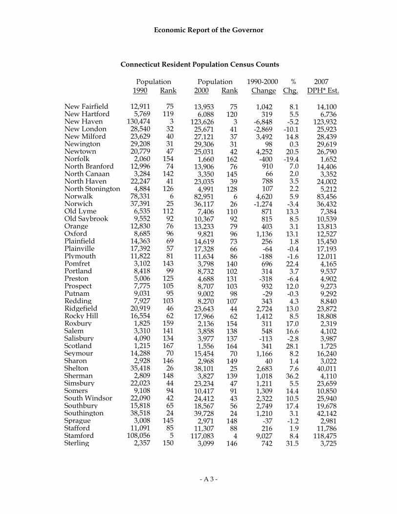
Economic Report of the Governor
- A 3 -
Connecticut Resident Population Census Counts
Population Population 1990-2000 % 2007 1990 Rank 2000 Rank Change Chg. DPH* Est.
New Fairfield 12,911 75 13,953 75 1,042 8.1 14,100 New Hartford 5,769 119 6,088 120 319 5.5 6,736 New Haven 130,474 3 123,626 3 -6,848 -5.2 123,932 New London 28,540 32 25,671 41 -2,869 -10.1 25,923 New Milford 23,629 40 27,121 37 3,492 14.8 28,439 Newington 29,208 31 29,306 31 98 0.3 29,619 Newtown 20,779 47 25,031 42 4,252 20.5 26,790 Norfolk 2,060 154 1,660 162 -400 -19.4 1,652 North Branford 12,996 74 13,906 76 910 7.0 14,406 North Canaan 3,284 142 3,350 145 66 2.0 3,352 North Haven 22,247 41 23,035 39 788 3.5 24,002 North Stonington 4,884 126 4,991 128 107 2.2 5,212 Norwalk 78,331 6 82,951 6 4,620 5.9 83,456 Norwich 37,391 25 36,117 26 -1,274 -3.4 36,432 Old Lyme 6,535 112 7,406 110 871 13.3 7,384 Old Saybrook 9,552 92 10,367 92 815 8.5 10,539 Orange 12,830 76 13,233 79 403 3.1 13,813 Oxford 8,685 96 9,821 96 1,136 13.1 12,527 Plainfield 14,363 69 14,619 73 256 1.8 15,450 Plainville 17,392 57 17,328 66 -64 -0.4 17,193 Plymouth 11,822 81 11,634 86 -188 -1.6 12,011 Pomfret 3,102 143 3,798 140 696 22.4 4,165 Portland 8,418 99 8,732 102 314 3.7 9,537 Preston 5,006 125 4,688 131 -318 -6.4 4,902 Prospect 7,775 105 8,707 103 932 12.0 9,273 Putnam 9,031 95 9,002 98 -29 -0.3 9,292 Redding 7,927 103 8,270 107 343 4.3 8,840 Ridgefield 20,919 46 23,643 44 2,724 13.0 23,872 Rocky Hill 16,554 62 17,966 62 1,412 8.5 18,808 Roxbury 1,825 159 2,136 154 311 17.0 2,319 Salem 3,310 141 3,858 138 548 16.6 4,102 Salisbury 4,090 134 3,977 137 -113 -2.8 3,987 Scotland 1,215 167 1,556 164 341 28.1 1,725 Seymour 14,288 70 15,454 70 1,166 8.2 16,240 Sharon 2,928 146 2,968 149 40 1.4 3,022 Shelton 35,418 26 38,101 25 2,683 7.6 40,011 Sherman 2,809 148 3,827 139 1,018 36.2 4,110 Simsbury 22,023 44 23,234 47 1,211 5.5 23,659 Somers 9,108 94 10,417 91 1,309 14.4 10,850 South Windsor 22,090 42 24,412 43 2,322 10.5 25,940 Southbury 15,818 65 18,567 56 2,749 17.4 19,678 Southington 38,518 24 39,728 24 1,210 3.1 42,142 Sprague 3,008 145 2,971 148 -37 -1.2 2,981 Stafford 11,091 85 11,307 88 216 1.9 11,786 Stamford 108,056 5 117,083 4 9,027 8.4 118,475 Sterling 2,357 150 3,099 146 742 31.5 3,725

Economic Report of the Governor
- A 4 -
Connecticut Resident Population Census Counts
Population Population 1990-2000 % 2007 1990 Rank 2000 Rank Change Chg. DPH* Est.
Stonington 16,919 58 17,906 63 987 5.8 18,343 Stratford 49,389 19 49,976 18 587 1.2 49,015 Suffield 11,427 83 13,552 77 2,125 18.6 15,104 Thomaston 6,947 108 7,503 109 556 8.0 7,818 Thompson 8,668 97 8,878 100 210 2.4 9,231 Tolland 11,001 86 13,146 80 2,145 19.5 14,631 Torrington 33,687 27 35,202 27 1,515 4.5 35,451 Trumbull 32,016 28 34,243 28 2,227 7.0 34,752 Union 612 169 693 169 81 13.2 751 Vernon 29,841 30 28,063 36 -1,778 -6.0 29,620 Voluntown 2,113 153 2,528 152 415 19.6 2,612 Wallingford 40,822 23 43,026 22 2,204 5.4 44,679 Warren 1,226 166 1,254 167 28 2.3 1,384 Washington 3,905 136 3,596 142 -309 -7.9 3,671 Waterbury 108,961 4 107,271 5 -1,690 -1.6 107,174 Waterford 17,930 54 19,152 55 1,222 6.8 18,775 Watertown 20,456 49 21,661 48 1,205 5.9 22,128 West Hartford 60,110 10 61,046 10 936 1.6 60,486 West Haven 54,021 13 52,360 16 -1,661 -3.1 52,676 Westbrook 5,414 122 6,292 119 878 16.2 6,618 Weston 8,648 98 10,037 95 1,389 16.1 10,200 Westport 24,410 39 25,749 40 1,339 5.5 26,508 Wethersfield 25,651 38 26,271 38 620 2.4 25,781 Willington 5,979 117 5,959 122 -20 -0.3 6,139 Wilton 15,989 63 17,633 65 1,644 10.3 17,715 Winchester 11,524 82 10,664 90 -860 -7.5 10,748 Windham 22,039 43 22,857 46 818 3.7 23,678 Windsor 27,817 34 28,237 34 420 1.5 12,491 Windsor Locks 12,358 78 12,043 85 -315 -2.5 28,754 Wolcott 13,700 73 15,215 71 1,515 11.1 16,407 Woodbridge 7,924 104 8,983 99 1,059 13.4 9,201 Woodbury 8,131 102 9,198 97 1,067 13.1 9,654 Woodstock 6,008 116 7,221 112 1,213 20.2 8,188
* DPH stands for the Connecticut Department of Public Health
Source: U.S. Bureau of the Census, April 1, 1990 & 2000 Department of Public Health, “Est. Population in Connecticut as of July 1, 2007”

Economic Report of the Governor
MAJOR U.S. ECONOMIC INDICATORS - FISCAL YEAR BASIS
TABLE 1U.S. ECONOMIC VARIABLES
1999 2000 2001 2002 2003 2004 2005 2006 2007 2008Gross DomesticProduct ($B) 8,996.0 9,571.3 9,991.5 10,280.3 10,664.0 11,330.4 12,045.2 12,832.1 13,467.0 14,106.8Percent Change 5.5% 6.4% 4.4% 2.9% 3.7% 6.2% 6.3% 6.5% 4.9% 4.8%
Real GDP 9,261.0 9,679.2 9,876.4 9,947.5 10,131.3 10,510.9 10,836.8 11,161.3 11,379.9 11,655.0Percent Change 4.2% 4.5% 2.0% 0.7% 1.8% 3.7% 3.1% 3.0% 2.0% 2.4%
GDP Deflator (2000=100) 97.1 98.9 101.2 103.3 105.3 107.8 111.1 115.0 118.3 121.0Percent Change 1.3% 1.8% 2.3% 2.2% 1.9% 2.4% 3.1% 3.4% 2.9% 2.3%
Housing Starts (K) 1,659.3 1,637.8 1,570.7 1,645.9 1,729.2 1,945.3 2,016.3 2,036.0 1,546.5 1,131.8Percent Change 8.4% -1.3% -4.1% 4.8% 5.1% 12.5% 3.7% 1.0% -24.0% -26.8%
Unemployment Rate 4.4% 4.1% 4.1% 5.5% 5.9% 5.8% 5.3% 4.8% 4.5% 4.9%
New Vehicle Sales (M) 16.06 17.54 16.89 16.96 16.64 16.81 17.04 16.76 16.31 15.31Percent Change 4.3% 9.2% -3.7% 0.4% -1.9% 1.0% 1.3% -1.6% -2.7% -6.1%
Consumer Price Index('82-'84=100) 164.5 169.3 175.1 178.2 182.1 186.1 191.7 199.0 204.1 211.7Percent Change 1.7% 2.9% 3.4% 1.8% 2.2% 2.2% 3.0% 3.8% 2.6% 3.7%
Industrial ProductionIndex ('02=100) 97.2 102.1 102.7 99.0 100.7 102.3 105.7 108.4 110.3 112.0Percent Change 4.2% 5.0% 0.6% -3.6% 1.7% 1.6% 3.3% 2.5% 1.8% 1.5%
Personal Income ($B) 7,607.0 8,109.6 8,613.9 8,788.1 8,974.1 9,398.3 9,993.0 10,617.3 11,309.1 11,899.6Percent Change 6.3% 6.6% 6.2% 2.0% 2.1% 4.7% 6.3% 6.2% 6.5% 5.2%
Real PersonalIncome ($B in 82-84=100) 4,622.9 4,790.3 4,920.4 4,932.5 4,928.3 5,050.1 5,213.3 5,336.0 5,540.5 5,621.2Percent Change 4.5% 3.6% 2.7% 0.2% -0.1% 2.5% 3.2% 2.4% 3.8% 1.5%
Disposable PersonalIncome ($B) 6,548.9 6,938.7 7,343.8 7,685.2 7,947.6 8,416.7 8,879.0 9,353.3 9,906.6 10,453.0Percent Change 5.8% 6.0% 5.8% 4.6% 3.4% 5.9% 5.5% 5.3% 5.9% 5.5%
Disposable PersonalIncome ($B in 1996$) 6,777.2 7,019.7 7,261.0 7,483.3 7,598.1 7,876.5 8,085.3 8,252.6 8,538.9 8,728.3Percent Change 4.6% 3.6% 3.4% 3.1% 1.5% 3.7% 2.7% 2.1% 3.5% 2.2%
- A 5 -

Economic Report of the Governor
MAJOR U.S. ECONOMIC INDICATORS - FISCAL YEAR BASIS
TABLE 2U.S. PERSONAL INCOME(BILLIONS OF DOLLARS)
1999 2000 2001 2002 2003 2004 2005 2006 2007 2008
Personal Income 7,607.0 8,109.6 8,613.9 8,788.1 8,974.1 9,398.3 9,993.0 10,617.3 11,309.1 11,899.6Percent Change 6.3% 6.6% 6.2% 2.0% 2.1% 4.7% 6.3% 6.2% 6.5% 5.2%
Wages & Salaries 4,323.3 4,651.3 4,917.4 4,948.8 5,014.9 5,233.6 5,526.3 5,852.1 6,193.7 6,466.2Percent Change 7.4% 7.6% 5.7% 0.6% 1.3% 4.4% 5.6% 5.9% 5.8% 4.4%
Manufacturing Income 689.2 729.2 737.5 682.0 667.8 673.3 698.1 719.7 738.6 746.8 Percent Change 3.7% 5.8% 1.1% -7.5% -2.1% 0.8% 3.7% 3.1% 2.6% 1.1%
Nonmanufacturing Inc. 3,634.1 3,922.1 4,180.0 4,266.8 4,347.1 4,560.3 4,828.2 5,132.4 5,455.1 5,719.3 Percent Change 8.1% 7.9% 6.6% 2.1% 1.9% 4.9% 5.9% 6.3% 6.3% 4.8%
Other Labor Income 855.7 914.2 973.2 1,040.7 1,152.5 1,229.1 1,309.4 1,373.8 1,421.9 1,474.9Percent Change 6.3% 6.8% 6.5% 6.9% 10.7% 6.7% 6.5% 4.9% 3.5% 3.7%
Proprietor’s Income 655.5 703.1 754.5 768.5 782.0 863.1 935.7 994.5 1,030.8 1,071.6Percent Change 9.6% 7.3% 7.3% 1.9% 1.8% 10.4% 8.4% 6.3% 3.7% 4.0%
Farm Income 31.1 24.3 21.2 12.7 20.4 36.1 35.3 23.0 29.8 43.5 Percent Change -0.6% -21.9% -12.8% -40.3% 61.5% 76.9% -2.4% -34.8% 29.6% 46.2%
Nonfarm Income 624.4 678.8 733.3 755.8 761.6 827.0 900.5 971.5 1,001.0 1,028.1 Percent Change 10.1% 8.7% 8.0% 3.1% 0.8% 8.6% 8.9% 7.9% 3.0% 2.7%
Rental Income 144.0 149.7 153.9 173.1 135.0 132.6 92.4 24.9 39.6 44.5Percent Change 10.3% 4.0% 2.8% 12.5% -22.0% -1.8% -30.3% -73.1% 59.1% 12.5%
Personal Dividend Inc. 342.6 351.6 379.0 376.3 409.7 459.0 571.9 631.5 749.1 820.3Percent Change -0.9% 2.6% 7.8% -0.7% 8.9% 12.0% 24.6% 10.4% 18.6% 9.5%
Personal Interest Income 930.4 970.3 1,020.8 976.4 920.3 897.8 943.7 1,082.0 1,167.9 1,228.1Percent Change 4.1% 4.3% 5.2% -4.3% -5.8% -2.4% 5.1% 14.7% 7.9% 5.2%
Transfer Payments 997.9 1,050.2 1,134.0 1,246.3 1,317.7 1,388.3 1,464.6 1,564.1 1,661.2 1,790.7Percent Change 3.5% 5.2% 8.0% 9.9% 5.7% 5.4% 5.5% 6.8% 6.2% 7.8%
- A 6 -

Economic Report of the Governor
MAJOR U.S. ECONOMIC INDICATORS - FISCAL YEAR BASIS
TABLE 3U.S. PERSONAL INCOME AND ITS DISPOSITION
(BILLIONS OF DOLLARS)
1999 2000 2001 2002 2003 2004 2005 2006 2007 2008Less:Contributions toSocial Insurance 643.7 682.0 719.9 740.5 760.6 801.9 852.0 901.6 946.2 982.2Percent Change 6.3% 5.9% 5.6% 2.9% 2.7% 5.4% 6.2% 5.8% 4.9% 3.8%
Equals:Personal Income 7,607.0 8,109.6 8,613.9 8,788.1 8,974.1 9,398.3 9,993.0 10,617.3 11,309.1 11,899.6Percent Change 6.3% 6.6% 6.2% 2.0% 2.1% 4.7% 6.3% 6.2% 6.5% 5.2%
Less:Personal Taxes 1,065.2 1,176.5 1,278.4 1,113.5 1,035.1 997.6 1,127.3 1,283.0 1,426.2 1,475.8Percent Change 9.0% 10.5% 8.7% -12.9% -7.0% -3.6% 13.0% 13.8% 11.2% 3.5%
Equals:Disposable Personal Inc. 6,548.9 6,938.7 7,343.8 7,685.2 7,947.6 8,416.7 8,879.0 9,353.3 9,906.6 10,453.0Percent Change 5.8% 6.0% 5.8% 4.6% 3.4% 5.9% 5.5% 5.3% 5.9% 5.5%
Less:Personal Outlays 6,319.0 6,792.0 7,204.2 7,498.1 7,793.7 8,235.7 8,754.6 9,313.3 9,838.0 10,358.6Percent Change 6.4% 7.5% 6.1% 4.1% 3.9% 5.7% 6.3% 6.4% 5.6% 5.3%
Equals:Personal Savings 229.9 146.8 139.7 187.2 153.8 181.0 124.4 40.0 68.6 94.4Percent Change -8.6% -36.1% -4.9% 34.0% -17.8% 17.6% -31.2% -67.8% 71.5% 37.5%
Personal Savings Rate 3.5% 2.1% 1.9% 2.4% 2.0% 2.1% 1.4% 0.4% 0.7% 0.9%
- A 7 -

Economic Report of the Governor
MAJOR U.S. ECONOMIC INDICATORS - FISCAL YEAR BASIS
TABLE 4U.S. EMPLOYMENT AND THE LABOR FORCE
(MILLIONS OF JOBS)
1999 2000 2001 2002 2003 2004 2005 2006 2007 2008
Establishment Employ. 127.4 130.6 132.3 130.9 130.1 130.5 132.5 135.0 137.0 137.9Percent Change 2.4% 2.5% 1.3% -1.0% -0.6% 0.3% 1.5% 1.9% 1.4% 0.7%
Manufacturing 17.4 17.3 17.0 15.7 14.9 14.3 14.3 14.2 14.0 13.7Percent Change -0.8% -0.8% -1.4% -7.7% -5.5% -3.7% -0.3% -0.6% -1.2% -2.2%
Nonmanufacturing 110.0 113.3 115.2 115.1 115.2 116.1 118.2 120.8 122.9 124.1Percent Change 3.0% 3.0% 1.7% -0.1% 0.1% 0.8% 1.8% 2.2% 1.8% 1.0%
Construction & Mining 7.0 7.3 7.4 7.4 7.3 7.4 7.7 8.2 8.4 8.2 Percent Change 5.5% 4.6% 1.8% -0.8% -1.3% 2.0% 4.3% 6.2% 2.1% -2.5%
Information 3.3 3.5 3.7 3.5 3.3 3.1 3.1 3.1 3.0 3.0 Percent Change 4.8% 7.1% 3.9% -4.6% -6.5% -4.0% -2.1% -0.9% -0.7% -0.5%
Public Utility, Trade & Transportation 25.5 26.1 26.2 25.7 25.4 25.4 25.7 26.1 26.5 26.6 Percent Change 2.1% 2.3% 0.6% -2.0% -1.2% -0.1% 1.5% 1.6% 1.2% 0.5%
Finance, Insurance & Real Estate 7.6 7.7 7.7 7.8 7.9 8.0 8.1 8.3 8.3 8.3 Percent Change 3.6% 1.2% 1.0% 1.0% 1.1% 1.2% 0.9% 2.2% 1.0% -1.0%
Services 46.6 48.1 49.3 49.4 49.8 50.7 51.8 53.3 54.6 55.8 Percent Change 3.4% 3.3% 2.3% 0.3% 0.8% 1.7% 2.3% 2.7% 2.6% 2.1%
Professional & Business 15.5 16.4 16.7 16.1 15.9 16.2 16.6 17.3 17.8 18.0 Percent Change 5.2% 5.3% 2.3% -3.6% -1.3% 1.4% 3.0% 3.9% 3.0% 1.3%
Education & Health 14.6 14.9 15.3 15.9 16.4 16.8 17.1 17.6 18.1 18.6 Percent Change 2.6% 2.1% 2.7% 3.8% 3.0% 2.0% 2.3% 2.7% 2.6% 3.0%
Leisure & Hospitality 11.4 11.7 12.0 12.0 12.1 12.3 12.7 12.9 13.3 13.6 Percent Change 2.5% 2.8% 2.3% 0.1% 0.6% 2.1% 2.6% 2.3% 2.6% 2.5%
Other Services 5.0 5.1 5.2 5.3 5.4 5.4 5.4 5.4 5.5 5.5 Percent Change 2.7% 2.0% 1.3% 2.5% 1.2% 0.3% -0.2% 0.3% 1.0% 0.8%
Government 20.1 20.6 20.9 21.4 21.6 21.6 21.7 21.9 22.1 22.3 Percent Change 1.7% 2.6% 1.3% 2.3% 1.1% -0.1% 0.7% 0.8% 1.0% 1.0%
Civilian Labor Force 138.6 141.1 143.2 144.3 145.7 146.8 148.2 150.4 152.4 153.7Percent Change 1.1% 1.8% 1.4% 0.8% 1.0% 0.7% 1.0% 1.4% 1.4% 0.8%
Unemployment Rate 4.4% 4.1% 4.1% 5.5% 5.9% 5.8% 5.3% 4.8% 4.5% 4.9%
- A 8 -

Economic Report of the Governor
MAJOR U.S. ECONOMIC INDICATORS - FISCAL YEAR BASIS
TABLE 5CONSUMER PRICE INDEXES
(1982-1984 = 100)
1999 2000 2001 2002 2003 2004 2005 2006 2007 2008All Items – UrbanConsumers 164.5 169.3 175.1 178.2 182.1 186.1 191.7 199.0 204.1 211.7Percent Change 1.7% 2.9% 3.4% 1.8% 2.2% 2.2% 3.0% 3.8% 2.6% 3.7%
Food & Beverages 162.9 166.2 170.9 175.6 178.1 183.7 189.1 193.4 198.9 208.1 Percent Change 2.2% 2.0% 2.8% 2.8% 1.4% 3.1% 3.0% 2.3% 2.9% 4.6%
Housing 162.1 166.4 173.4 178.2 182.6 186.9 192.4 199.6 206.5 212.8 Percent Change 2.2% 2.6% 4.2% 2.8% 2.5% 2.3% 3.0% 3.7% 3.5% 3.1%
Energy 102.0 115.9 131.5 121.0 130.3 142.0 159.7 194.2 198.7 226.7 Percent Change -5.2% 13.7% 13.4% -8.0% 7.7% 8.9% 12.5% 21.7% 2.3% 14.1%
Commodities 142.7 147.0 150.6 149.6 150.7 152.4 156.9 163.1 165.0 172.0 Percent Change 0.6% 3.0% 2.4% -0.6% 0.7% 1.1% 3.0% 3.9% 1.2% 4.2%
Apparel 132.2 130.6 128.9 125.3 122.1 120.7 120.2 119.2 119.5 118.6 Percent Change -0.5% -1.2% -1.4% -2.8% -2.5% -1.2% -0.4% -0.8% 0.3% -0.8%
Transportation 141.6 149.4 155.2 151.9 156.2 159.2 167.0 179.9 181.2 192.8 Percent Change -0.9% 5.5% 3.9% -2.1% 2.8% 2.0% 4.9% 7.7% 0.7% 6.4%
Services 186.4 191.7 199.6 206.5 213.2 219.5 226.2 234.6 242.9 251.0 Percent Change 2.5% 2.8% 4.1% 3.5% 3.3% 2.9% 3.0% 3.7% 3.6% 3.3%
Medical Care 246.3 255.4 266.7 278.9 291.6 303.5 316.7 329.8 343.0 358.7 Percent Change 3.5% 3.7% 4.4% 4.6% 4.5% 4.1% 4.3% 4.1% 4.0% 4.6%
Other Goods & Services 248.2 264.9 276.3 288.6 296.6 301.4 308.8 317.6 327.5 338.9 Percent Change 7.6% 6.7% 4.3% 4.5% 2.8% 1.6% 2.5% 2.8% 3.1% 3.5%
- A 9 -

Economic Report of the Governor
MAJOR CONNECTICUT ECONOMIC INDICATORS - FISCAL YEAR BASIS
TABLE 6PERSONAL INCOME
(BILLIONS OF DOLLARS)
1999 2000 2001 2002 2003 2004 2005 2006 2007 2008
Personal Income 126.77 135.78 145.74 146.95 146.98 153.27 163.15 174.08 186.24 195.77Percent Change 6.1% 7.1% 7.3% 0.8% 0.0% 4.3% 6.4% 6.7% 7.0% 5.1%
DisposablePersonal Income 103.29 109.75 116.64 121.57 124.47 130.96 138.04 143.68 150.76 159.95Percent Change 5.5% 6.3% 6.3% 4.2% 2.4% 5.2% 5.4% 4.1% 4.9% 6.1%
Total Wages 76.42 81.55 86.08 84.86 84.41 87.85 92.91 97.69 103.45 107.98Percent Change 7.0% 6.7% 5.6% -1.4% -0.5% 4.1% 5.8% 5.2% 5.9% 4.4%
Manufacturing Wages 13.31 13.45 14.08 12.75 12.28 12.50 12.92 13.18 13.66 14.22 Percent Change 5.1% 1.1% 4.7% -9.5% -3.6% 1.8% 3.4% 2.0% 3.7% 4.1%
Nonmanufacturing Wages 63.11 68.10 72.00 72.11 72.13 75.35 79.99 84.52 89.79 93.76 Percent Change 7.4% 7.9% 5.7% 0.2% 0.0% 4.5% 6.2% 5.7% 6.2% 4.4%
Other Labor Income 14.04 14.90 15.90 17.04 18.39 19.57 21.10 21.68 22.07 22.85Percent Change 5.7% 6.1% 6.7% 7.2% 7.9% 6.4% 7.8% 2.8% 1.8% 3.5%
Proprietor’s Income 10.44 12.18 14.37 15.18 14.93 15.69 16.70 17.83 18.09 18.32Percent Change 12.0% 16.7% 18.0% 5.6% -1.6% 5.1% 6.4% 6.8% 1.4% 1.3%
Property Income 22.64 23.91 25.83 25.49 24.33 24.94 27.04 31.07 36.19 39.49Percent Change 3.8% 5.6% 8.0% -1.3% -4.6% 2.5% 8.4% 14.9% 16.5% 9.1%
Transfer PaymentsLess Social Insurance 3.23 3.23 3.56 4.38 4.92 5.22 5.41 5.80 6.45 7.13Percent Change -9.9% 0.2% 10.3% 22.9% 12.4% 6.1% 3.6% 7.3% 11.1% 10.6%
Transfer Payments 13.96 14.47 15.27 16.39 17.17 17.90 18.66 19.57 20.79 21.97Percent Change 1.8% 3.7% 5.5% 7.4% 4.7% 4.2% 4.3% 4.9% 6.2% 5.7%
Social Insurance 10.73 11.24 11.70 12.01 12.25 12.67 13.25 13.77 14.34 14.84Percent Change 5.9% 4.7% 4.1% 2.7% 1.9% 3.5% 4.5% 3.9% 4.2% 3.5%
- A 10 -

Economic Report of the Governor
MAJOR CONNECTICUT ECONOMIC INDICATORS - FISCAL YEAR BASIS
TABLE 7DEFLATED PERSONAL INCOME
(BILLIONS OF DOLLARS)
1999 2000 2001 2002 2003 2004 2005 2006 2007 2008
Personal Income 130.51 137.33 144.07 142.19 139.64 142.19 146.79 151.43 157.38 161.75Percent Change 4.8% 5.2% 4.9% -1.3% -1.8% 1.8% 3.2% 3.2% 3.9% 2.8%
DisposablePersonal Income 106.34 111.00 115.30 117.64 118.26 121.49 124.20 124.98 127.40 132.15Percent Change 4.2% 4.4% 3.9% 2.0% 0.5% 2.7% 2.2% 0.6% 1.9% 3.7%
Total Wages 78.68 82.48 85.09 82.11 80.20 81.50 83.59 84.98 87.42 89.22Percent Change 5.7% 4.8% 3.2% -3.5% -2.3% 1.6% 2.6% 1.7% 2.9% 2.1%
Manufacturing Wages 13.70 13.60 13.92 12.33 11.67 11.60 11.63 11.46 11.55 11.75 Percent Change -0.6% -0.6% -0.6% -11.4% -5.4% -0.6% 0.2% -1.4% 0.7% 1.8%
Nonmanufacturing 64.98 68.88 71.17 69.78 68.53 69.90 71.97 73.52 75.87 77.47 Wages 6.0% 6.0% 3.3% -2.0% -1.8% 2.0% 3.0% 2.2% 3.2% 2.1% Percent Change
Other Labor Income 14.45 15.07 15.71 16.48 17.47 18.15 18.98 18.86 18.65 18.88Percent Change 4.4% 4.3% 4.3% 4.9% 6.0% 3.9% 4.6% -0.6% -1.1% 1.2%
Proprietor’s Income 10.75 12.32 14.21 14.69 14.19 14.56 15.02 15.51 15.28 15.14Percent Change 10.6% 14.6% 15.3% 3.4% -3.4% 2.6% 3.2% 3.2% -1.5% -0.9%
Property Income 23.30 24.19 25.53 24.67 23.11 23.13 24.33 27.03 30.58 32.63Percent Change 2.5% 3.8% 5.6% -3.4% -6.3% 0.1% 5.1% 11.1% 13.1% 6.7%
Transfer PaymentsLess Social Insurance 3.32 3.27 3.52 4.24 4.68 4.84 4.86 5.05 5.45 5.89Percent Change -11.0% -1.6% 7.8% 20.3% 10.4% 3.6% 0.4% 3.7% 7.9% 8.1%
Transfer Payments 14.37 14.63 15.09 15.86 16.31 16.60 16.79 17.02 17.57 18.15Percent Change 0.5% 1.8% 3.1% 5.1% 2.8% 1.8% 1.1% 1.4% 3.2% 3.3%
Social Insurance 11.05 11.37 11.57 11.62 11.63 11.76 11.92 11.98 12.12 12.26Percent Change 4.6% 2.9% 1.8% 0.5% 0.1% 1.1% 1.4% 0.5% 1.2% 1.2%
Note: All categories are deflated by GDP Price Index (2000 = 100).
- A 11 -

Economic Report of the Governor
MAJOR CONNECTICUT ECONOMIC INDICATORS - FISCAL YEAR BASIS
TABLE 8MANUFACTURING EMPLOYMENT
(THOUSANDS -SA)
1999 2000 2001 2002 2003 2004 2005 2006 2007 2008
Manufacturing 244.65 236.72 233.64 218.32 204.93 197.60 196.63 194.01 192.41 190.42Percent Change -1.0% -3.2% -1.3% -6.6% -6.1% -3.6% -0.5% -1.3% -0.8% -1.0%
Electronic & Electrical 36.39 35.05 35.40 31.33 27.73 25.95 25.75 25.05 25.04 25.30 Percent Change -4.1% -3.7% 1.0% -11.5% -11.5% -6.4% -0.8% -2.7% -0.1% 1.1%
Metals Manufacturing 51.56 50.01 49.10 44.76 41.87 40.71 41.27 41.02 40.79 40.08 Percent Change -0.5% -3.0% -1.8% -8.8% -6.5% -2.8% 1.4% -0.6% -0.6% -1.7%
Industrial Machinery 24.69 23.70 23.32 21.23 19.50 18.65 18.34 17.99 18.14 18.11 Percent Change -4.4% -4.0% -1.6% -9.0% -8.1% -4.4% -1.7% -1.9% 0.8% -0.2%
Transportation Equip. 51.73 47.93 46.95 46.34 44.18 43.06 43.31 43.60 43.51 43.74 Percent Change 0.2% -7.3% -2.1% -1.3% -4.7% -2.5% 0.6% 0.7% -0.2% 0.5%
Chemical, Plast. & Rub. 28.08 28.67 29.48 27.88 26.52 25.51 25.20 24.56 23.60 22.74 Percent Change 2.8% 2.1% 2.8% -5.4% -4.9% -3.8% -1.2% -2.6% -3.9% -3.7%
Printing, Publ. & Textile 26.03 25.14 23.99 21.82 19.94 19.29 18.53 17.61 17.27 16.97 Percent Change -3.2% -3.4% -4.6% -9.1% -8.6% -3.3% -3.9% -5.0% -1.9% -1.8%
Food, Bev. & Tobacco 8.76 8.89 8.48 8.56 8.76 8.41 8.40 8.55 8.48 8.17 Percent Change 1.4% 1.5% -4.7% 1.0% 2.2% -4.0% -0.1% 1.8% -0.8% -3.6%
Miscellaneous 17.41 17.32 16.93 16.41 16.43 16.02 15.83 15.63 15.58 15.32 Percent Change 2.4% -0.5% -2.3% -3.1% 0.2% -2.5% -1.2% -1.3% -0.3% -1.7%
- A 12 -

Economic Report of the Governor
MAJOR CONNECTICUT ECONOMIC INDICATORS - FISCAL YEAR BASIS
TABLE 9NONMANUFACTURING EMPLOYMENT
(THOUSANDS -SA)
1999 2000 2001 2002 2003 2004 2005 2006 2007 2008
Nonmanufacturing 1,412.7 1,445.3 1,456.7 1,456.8 1,447.5 1,446.1 1,460.4 1,476.1 1,496.6 1,511.9Percent Change 2.5% 2.3% 0.8% 0.0% -0.6% -0.1% 1.0% 1.1% 1.4% 1.0%
Construction & Mining 60.44 63.60 65.90 65.77 62.39 64.43 67.24 67.08 68.47 69.17 Percent Change 4.4% 5.2% 3.6% -0.2% -5.1% 3.3% 4.4% -0.2% 2.1% 1.0%
Information 44.23 45.36 46.43 42.64 40.09 39.19 38.65 37.82 38.02 38.82 Percent Change -0.4% 2.5% 2.4% -8.2% -6.0% -2.2% -1.4% -2.1% 0.5% 2.1%
Utilities 9.80 9.72 9.48 9.07 8.92 8.70 8.65 8.31 8.14 8.21 Percent Change 0.8% -0.8% -2.4% -4.3% -1.8% -2.4% -0.6% -4.0% -2.0% 0.9%
Transportation 41.29 41.73 41.97 40.31 39.84 40.41 42.77 43.98 44.06 44.25 Percent Change 3.3% 1.1% 0.6% -4.0% -1.2% 1.4% 5.8% 2.8% 0.2% 0.4%
Wholesale Trade 66.35 67.04 68.10 66.57 65.73 65.58 65.91 67.18 67.65 68.50 Percent Change 1.3% 1.0% 1.6% -2.2% -1.3% -0.2% 0.5% 1.9% 0.7% 1.3%
Retail Trade 192.87 196.59 195.63 195.12 192.43 191.26 192.74 191.27 190.94 190.42 Percent Change 0.9% 1.9% -0.5% -0.3% -1.4% -0.6% 0.8% -0.8% -0.2% -0.3%
Finance & Insurance 119.16 120.48 121.68 122.21 122.54 121.15 120.75 122.31 123.81 122.94 Percent Change 5.5% 1.1% 1.0% 0.4% 0.3% -1.1% -0.3% 1.3% 1.2% -0.7%
Real Estate 20.70 21.34 21.57 20.68 20.28 20.21 20.49 21.00 21.14 20.60 Percent Change 2.9% 3.1% 1.1% -4.1% -2.0% -0.3% 1.4% 2.5% 0.7% -2.6%
Professional & Business 207.53 214.33 214.08 205.81 199.02 196.47 197.92 202.53 205.37 205.67 Percent Change 4.2% 3.3% -0.1% -3.9% -3.3% -1.3% 0.7% 2.3% 1.4% 0.2%
Education & Health 240.09 244.47 247.76 256.59 262.14 266.24 270.96 275.99 283.74 291.10 Percent Change 1.9% 1.8% 1.3% 3.6% 2.2% 1.6% 1.8% 1.9% 2.8% 2.6%
Leisure & Hospitality 118.09 120.48 120.49 121.08 123.55 126.63 128.72 130.73 133.96 136.64 Percent Change 2.4% 2.0% 0.0% 0.5% 2.0% 2.5% 1.6% 1.6% 2.5% 2.0%
Other Services 60.46 60.68 61.52 62.84 62.35 62.30 62.68 63.03 64.19 64.36 Percent Change 0.1% 0.4% 1.4% 2.1% -0.8% -0.1% 0.6% 0.6% 1.8% 0.3%
Federal Government 22.47 23.38 22.07 21.37 21.14 20.39 19.98 19.78 19.63 19.44 Percent Change 0.5% 4.0% -5.6% -3.2% -1.1% -3.5% -2.0% -1.0% -0.8% -0.9%
State & Local Gov't. 209.23 216.14 220.01 226.74 227.04 223.17 222.91 225.10 227.53 231.76 Percent Change 2.8% 3.3% 1.8% 3.1% 0.1% -1.7% -0.1% 1.0% 1.1% 1.9%
- A 13 -

Economic Report of the Governor
MAJOR CONNECTICUT ECONOMIC INDICATORS - FISCAL YEAR BASIS
TABLE 10LABOR FORCE & OTHER ECONOMIC INDICATORS
(THOUSANDS -SA)
1999 2000 2001 2002 2003 2004 2005 2006 2007 2008
Labor Force 1,741.4 1,739.9 1,742.2 1,764.9 1,792.2 1,793.9 1,800.9 1,822.5 1,850.5 1,879.6Percent Change -0.5% -0.1% 0.1% 1.3% 1.5% 0.1% 0.4% 1.2% 1.5% 1.6%
NonagriculturalEmployment 1,657.4 1,682.0 1,690.4 1,675.1 1,652.4 1,643.7 1,657.0 1,670.1 1,689.0 1,702.3Percent Change 2.0% 1.5% 0.5% -0.9% -1.4% -0.5% 0.8% 0.8% 1.1% 0.8%
ResidentialEmployment 1,691.0 1,697.4 1,698.4 1,700.5 1,699.0 1,700.1 1,713.0 1,739.4 1,768.8 1,787.4Percent Change 0.6% 0.4% 0.1% 0.1% -0.1% 0.1% 0.8% 1.5% 1.7% 1.0%
Unemployed 50.4 42.5 43.7 64.4 93.2 93.7 87.9 83.1 81.7 92.2Percent Change -27.1% -15.8% 3.0% 47.2% 44.8% 0.5% -6.2% -5.4% -1.8% 12.9%
Unemployment Rate 2.9% 2.4% 2.5% 3.7% 5.2% 5.2% 4.9% 4.6% 4.4% 4.9%
Households 1,287.4 1,299.7 1,308.6 1,316.0 1,324.7 1,329.9 1,331.9 1,334.8 1,337.7 1,340.6Percent Change 0.8% 1.0% 0.7% 0.6% 0.7% 0.4% 0.2% 0.2% 0.2% 0.2%
Housing Starts 11,127.4 9,552.7 8,597.7 9,215.4 8,547.8 9,849.3 11,634.4 11,147.5 8,507.7 6,669.0Percent Change 11.8% -14.2% -10.0% 7.2% -7.2% 15.2% 18.1% -4.2% -23.7% -21.6%
Single Family 9,373.3 8,406.3 7,352.2 8,268.3 7,326.5 7,910.0 9,676.6 9,166.9 6,911.5 4,815.0 Percent Change 11.5% -10.3% -12.5% 12.5% -11.4% 8.0% 22.3% -5.3% -24.6% -30.3%
Multi Family 1,754.1 1,146.4 1,245.5 947.1 1,221.4 1,939.3 1,957.8 1,980.6 1,596.2 1,854.0 Percent Change 13.8% -34.6% 8.6% -24.0% 29.0% 58.8% 1.0% 1.2% -19.4% 16.2%
New Car Registrations 224.6 233.8 245.0 224.6 227.4 254.8 228.1 230.5 212.8 217.8Percent Change 20.0% 4.1% 4.8% -8.3% 1.2% 12.0% -10.5% 1.1% -7.7% 2.3%
Note: Connecticut housing starts are already in thousands.
- A 14 -

Economic Report of the Governor
MAJOR CONNECTICUT ECONOMIC INDICATORS - FISCAL YEAR BASIS
TABLE 11ANALYTICS
1999 2000 2001 2002 2003 2004 2005 2006 2007 2008
Wages/Total Income 60.29% 60.06% 59.06% 57.75% 57.43% 57.32% 56.95% 56.12% 55.55% 55.16%
Other Labor Income/Total Income 11.07% 10.97% 10.91% 11.59% 12.51% 12.77% 12.93% 12.46% 11.85% 11.67%
Social Insurance/Total Income 8.47% 8.28% 8.03% 8.17% 8.33% 8.27% 8.12% 7.91% 7.70% 7.58%
Transfer Payments/Total Income 11.01% 10.66% 10.47% 11.16% 11.68% 11.68% 11.44% 11.24% 11.16% 11.22%
Proprietor’s Income/Total Income 8.24% 8.97% 9.86% 10.33% 10.16% 10.24% 10.23% 10.24% 9.71% 9.36%
Property Income/Total Income 17.86% 17.61% 17.72% 17.35% 16.55% 16.27% 16.57% 17.85% 19.43% 20.17%
Average Wages(Thousands in 2000 $) 46.66 48.55 48.36 50.41 50.82 51.21 51.20 51.27 51.39 50.99
Average Mfg. Wages(Thousands in 2000 $) 56.01 57.47 59.58 56.49 56.94 58.69 59.12 59.07 60.01 61.72
Average Nonmfg. Wages(Thousands in 2000 $) 45.08 47.11 46.64 49.47 49.91 50.15 50.11 50.23 50.29 49.68
Manufacturing Shareof Employment 14.51% 13.93% 13.28% 13.40% 12.99% 12.42% 12.04% 11.70% 11.31% 10.88%
Residential Employment/Total Nonagricultural 1.003 0.999 0.965 1.044 1.077 1.068 1.049 1.049 1.040 1.022
- A 15 -

Economic Report of the Governor
MAJOR CONNECTICUT REGIONAL ECONOMIC INDICATORS - CALENDAR YEAR BASIS
TABLE 12PERSONAL INCOME (MILLIONS-SAAR)
BRIDGEPORT-STAMFORD-NORWALK
1998 1999 2000 2001 2002 2003 2004 2005 2006 2007
Personal Income 44,997.1 47,458.5 52,183.1 54,988.0 53,476.6 53,283.9 58,112.6 61,615.1 66,392.9 71,762.2Percent Change 10.8% 5.5% 10.0% 5.4% -2.7% -0.4% 9.1% 6.0% 7.8% 8.1%
Total Wages 23,671.5 25,465.1 27,952.1 28,579.2 27,269.9 27,979.1 29,736.3 31,504.7 33,688.2 36,415.6Percent Change 8.8% 7.6% 9.8% 2.2% -4.6% 2.6% 6.3% 5.9% 6.9% 8.1%
HARTFORD-WEST HARTFORD-EAST HARTFORD
1998 1999 2000 2001 2002 2003 2004 2005 2006 2007
Personal Income 37,298.7 38,896.5 42,563.3 43,991.5 44,296.7 45,181.4 48,151.8 50,518.3 53,139.4 56,641.1Percent Change 6.5% 4.3% 9.4% 3.4% 0.7% 2.0% 6.6% 4.9% 5.2% 6.6%
Total Wages 23,988.6 25,425.5 27,291.6 28,169.5 28,186.5 28,519.7 30,477.6 31,956.8 33,423.0 35,600.4Percent Change 6.4% 6.0% 7.3% 3.2% 0.1% 1.2% 6.9% 4.9% 4.6% 6.5%
NEW LONDON-NORWICH, CT-RI
1998 1999 2000 2001 2002 2003 2004 2005 2006 2007
Personal Income 7,716.3 8,010.8 8,512.8 8,921.3 9,215.7 9,542.4 10,120.1 10,402.2 10,807.4 11,385.1Percent Change 5.9% 3.8% 6.3% 4.8% 3.3% 3.5% 6.1% 2.8% 3.9% 5.3%Total Wages 4,632.5 4,786.1 4,992.3 5,308.8 5,511.2 5,677.5 5,894.9 6,094.6 6,301.0 6,639.1Percent Change 4.5% 3.3% 4.3% 6.3% 3.8% 3.0% 3.8% 3.4% 3.4% 5.4%
- A 16 -