
Fuzzy Approximate Reasoning toward Multi-Objective Optimization Policy: Deployment for Supply Chain...
6
Fuzzy Approximate Reasoning toward Multi-Objective Optimization Policy: Deployment for Supply Chain Programming M.H. Fazel Zarandi, Mosahar Tarimoradi, M.H. Alavidoost, Behnoush Shakeri Computational Intelligent Systems Laboratory Department of Industrial Engineering and Management Systems Amirkabir University of Technology Tehran, Iran [email protected], [email protected], [email protected], [email protected] Abstract— To make a policy and decision for an appropriate set of optimizer algorithms is an important and controversial issue. It is significant especially when we want to consider more than a single objective and have to use multi-objective applications. The aim of this paper is to consider procedural fuzzy approximate reasoning to infer which one of the Multi-Objective Evolutionary Algorithms (MOEAs) could play a role in the suitable set as prevalent tool. The proposed procedure is put into practice for an invented bi- objective programming in the supply chain and three numbers of similar applications from the same family, i.e. NSGA-II, NRGA, and PESA-II are deployed. Keywords— fuzzy approximate reasoning; optimization policy; supply chain; NSGA-II; NRGA; PESA-II. I. INTRODUCTION The MOEAs are useful for big and complicated problems with more than a single objective in which one cannot find optimal solutions by the exact method. While being encountered with more than a single objective the selection for suitable MOEAs is vague, and also since the meta-heuristics act randomly, it is better to use fuzzy approximate reasoning ([1], [2], [3]and etc. ) which is used by practitioners in many areas ([4], [5], [4], and etc.). The issue is considered in the proposed procedure in this paper so that the functionality measurements by a couple of linguistic variables [6], as Quality and Time are associated as input variables for the reasoning process ([7], [8], [9], [10], and etc.). The contributions in this paper are organized as though, first the proposed procedural fuzzy approximate reasoning is explained. A bi-objective problem in supply chain programming is invented, and three MOEAs from the same family are used. The NSGA-II is introduced by Deb [11] as one of most used and propounded GA-based algorithms for solving multi- objective problems [12], the NRGA is presented by Jadaan using transformation of the NSGA-II selection strategy from the Tournament selection to the Roulette Wheel selection[13], and the PESA-II is presented by Corne et al. to make NSGA-II faster and to mitigate its complexity [14]. II. PROCEDURAL APPROXIMATE REASONING As shown in Fig. 1, the approximate reasoning procedure in this paper consists of the actions to expand the meta-rule, and the inference based on the emerged fuzzy rule base. The premises and consequences of the rules need the documented experience of the MOEAs’ performance. Their performance approximation relying on indexes could be caught and also the membership functions parameters to have a fuzzy rule base by fuzzy arithmetic could be calculated. After these, the desires about the quality of results and the processing time determine which rules should be fired and what is an appropriate set of the MOEAs, and develop a control policy [15] Fig. 1 Policy making based on fuzzy approximate reasoning The fuzzy rule base is supposed that should be expanded using the Meta-Rule accordingly as follows: Meta-Rule: From: Type(Time, QPF ) Suitable Subset of {B,C,D}
Transcript of Fuzzy Approximate Reasoning toward Multi-Objective Optimization Policy: Deployment for Supply Chain...

Fuzzy Approximate Reasoning toward
Multi-Objective Optimization Policy:
Deployment for Supply Chain Programming
M.H. Fazel Zarandi, Mosahar Tarimoradi, M.H. Alavidoost, Behnoush Shakeri Computational Intelligent Systems Laboratory
Department of Industrial Engineering and Management Systems
Amirkabir University of Technology
Tehran, Iran
[email protected], [email protected], [email protected], [email protected]
Abstract— To make a policy and decision for an appropriate set of optimizer algorithms is an important and controversial issue. It is significant especially when we want to consider more than a single objective and have to use multi-objective applications. The aim of this paper is to consider procedural fuzzy approximate reasoning to infer which one of the Multi-Objective Evolutionary Algorithms (MOEAs) could play a role in the suitable set as prevalent tool. The proposed procedure is put into practice for an invented bi-objective programming in the supply chain and three numbers of similar applications from the same family, i.e. NSGA-II, NRGA, and PESA-II are deployed.
Keywords— fuzzy approximate reasoning; optimization policy; supply chain; NSGA-II; NRGA; PESA-II.
I. INTRODUCTION
The MOEAs are useful for big and complicated
problems with more than a single objective in which
one cannot find optimal solutions by the exact
method. While being encountered with more than a
single objective the selection for suitable MOEAs is
vague, and also since the meta-heuristics act
randomly, it is better to use fuzzy approximate
reasoning ([1], [2], [3]and etc. ) which is used by
practitioners in many areas ([4], [5], [4], and etc.).
The issue is considered in the proposed procedure in
this paper so that the functionality measurements by a
couple of linguistic variables [6], as Quality and
Time are associated as input variables for the
reasoning process ([7], [8], [9], [10], and etc.). The
contributions in this paper are organized as though,
first the proposed procedural fuzzy approximate
reasoning is explained. A bi-objective problem in
supply chain programming is invented, and three
MOEAs from the same family are used. The NSGA-II
is introduced by Deb [11] as one of most used and
propounded GA-based algorithms for solving multi-
objective problems [12], the NRGA is presented by
Jadaan using transformation of the NSGA-II selection
strategy from the Tournament selection to the
Roulette Wheel selection[13], and the PESA-II is
presented by Corne et al. to make NSGA-II faster and
to mitigate its complexity [14].
II. PROCEDURAL APPROXIMATE REASONING As shown in Fig. 1, the approximate reasoning
procedure in this paper consists of the actions to expand the meta-rule, and the inference based on the emerged fuzzy rule base. The premises and consequences of the rules need the documented experience of the MOEAs’ performance. Their performance approximation relying on indexes could be caught and also the membership functions parameters to have a fuzzy rule base by fuzzy arithmetic could be calculated. After these, the desires about the quality of results and the processing time determine which rules should be fired and what is an appropriate set of the MOEAs, and develop a control policy [15]
Fig. 1 Policy making based on fuzzy approximate reasoning
The fuzzy rule base is supposed that should be expanded using the Meta-Rule accordingly as follows:
Meta-Rule:
From: Type(Time, QPF) Suitable Subset of {B,C,D}

Where: A: {NSGA-II, NRGA, PESA-II} B: Subset of A that has excellent value for Time
C: Subset of A that has excellent value for 𝑄𝑃��
D: Subset of A that has good value for Time and also 𝑄𝑃�� Time, is linguistically valued as: Free, or Bounded, or Exigent
𝐐𝐏�� , is linguistically valued as: Average, or High, or Excellent
The Quality of Pareto Front (𝑄𝑃��) as a fuzzy operator which aggregates the values of multiple indexes, is one of the input variables in this meta-rule.
The values of 𝑄𝑃�� for each one of the evolutionary applications tend to the membership function parameters. Thus, the Triangular Fuzzy Number (TFN) and some criteria should be referred to. A TFN, as is graphically shown in Fig. 2, can be characterized
by three parameters�� = (𝐴1, 𝐴2, 𝐴3). TFN is used in this paper because of its computational simplicity in comparison with the other fuzzy numbers, as it is considered by Kaufmann [16], and more importantly that it matches with the semantics of the issue. The emerging results by each evolutionary application during the tuning and their value in each one of the indexes could be defined by a TFN. In other words, a TFN could be devoted to each index in each one of the MOEAs. To do so, the minimum value for each index is caught as𝐴1, mean value for each index as𝐴2, and finally, the maximum amount of each one as𝐴3.
Fig. 2 Schematic of a triangular fuzzy number
The 𝑄𝑃�� helps to aggregate the emerged results during the calib-ration relying on the quality/precision indexes. Based on the fuzzy arithmetic relations, as
mentioned formerly, the 𝑄𝑃�� which is based on the Yager Ordered Weighting Averaging (OWA) [17], could be calculated by (1) :
𝑄𝑃�� = ∑𝑤𝑖 . 𝑐𝑖
𝐿
𝑖=1
(1)
Where 𝑐𝑖 is ith index, and 𝑤𝑖 donates the weight or in better words, the priority of the ith index.
III. CASE PROBLEM As a test problem, a supply chain problem is
modeled. A couple of objectives are associated with the invented model. The first considers the total cost of SC and makes it minimum, whilst the second objective function maximizes the customer service level. As shown in Fig. 3, the minded SCN here is a three echelon one, consisting of suppliers to the left, distribution centers (DCs) in the middle, and retailer
nodes which are related to the customers to the right. The developed SC is axiomatized as follows: 1. It has an integrated structure consisting both of
potential supplier and potential DCs to procure retailer
demands for multitude commodities.
2. It has predefined numbers of suppliers and DCs with
identified capacities.
3. The number of its retailers and their demands
distribution are identified.
4. It operates in an uncertain circumstance, i.e. its main
interior parameters as demands, lead-time, procure and
transportation costs, and also holding costs of
inventory for commodities are all supposed to be
uniform random variables with identified average and
variance (Table I).
5. Its DCs and suppliers are all supposed to be potentially
operational at the beginning of the constructing
network.
6. Its suppliers and DCs do their procuring, shipment,
and holding duties perfectly.
7. Any retailer receives its demand for a specific
merchandize only from one of the DCs.
8. Shortage cannot occur at the retailer nodes in any
form.
9. More than one supplier can replete the demand of a
specific DC.
10. More than one DC can replete the demand of each
retailer.
In other words, it is a Balanced Supply Chain
Network (BSCN) in which the total capacity of all
suppliers is greater or equal to the total consumption
of all commodities, and the total procurement capacity
of all commodities are equal to the total consumption
of all end customers, and the total consumption of all
commodities is equal to the total procurement of all
commodities by suppliers.
Fig. 3 The considered network structure
The used notations in this model are listed in Table I, and the decision variables are also defined as shown in Table II.
Based on the stock theory, the jth warehouse daily demand distribution for the kth commodity
follows 𝑁(𝐷𝑗𝑘 , 𝜃𝑗
𝑘). Where 𝐷𝑗𝑘 delegates the average
daily demand of the jth warehouse for the kth
commodity and 𝜃𝑗𝑘 is the daily demand variance of the
jth warehouse for the kth commodity. The formulas for
𝑨𝟑 𝑨𝟏 𝑨𝟐
1.0

calculation of 𝐷𝑗𝑘 and 𝜃𝑗
𝑘 are as (2) while ∀ 𝑗 =1,2, . . , 𝐽 , 𝑘 = 1,2,… ,𝐾:
𝐷𝑗𝑘 =∑𝜇𝑖
𝑘 . 𝑥𝑗𝑖𝑘
𝐼
𝑖=1
, 𝜃𝑗𝑘 =∑𝜐𝑖
𝑘 . 𝑥𝑗𝑖𝑘
𝐼
𝑖=1
(2).
The expected value of the kth commodity lead-time delivery in the jth warehouse could be calculated by (3) while ∀ 𝑗 = 1,2, . . , 𝐽 , 𝑘 = 1,2, … , 𝐾:
𝐸𝑗𝑘 = ∑ 𝐿𝑚𝑗
𝑘 . 𝑦𝑚𝑗𝑘
𝑀
𝑚=1
(3).
The average and variance of the specific kth
commodity demand in lead-time for the jth warehouse are as (4)0 and (5), while ∀ 𝑗 = 1,2, . . , 𝐽 , 𝑘 = 1,2, … , 𝐾:
𝐷𝑗′𝑘 = 𝐸j
k. 𝐷𝑗𝑘 = 𝐸j
k.∑𝜇𝑖𝑘 . 𝑥𝑗𝑖
𝑘
𝐼
𝑖=1
(4).
𝜃𝑗′𝑘 = 𝐸𝑗
𝑘 . 𝜃𝑗𝑘 = 𝐸𝑗
𝑘 .∑𝜐𝑖𝑘 . 𝑥𝑗𝑖
𝑘
𝐼
𝑖=1
(5)
Then𝑆𝑆𝑗𝑘, the buffer quantity of the kth commodity
for the jth warehouse could be calculated by (6) while ∀ 𝑗 = 1,2, . . , 𝐽 , 𝑘 = 1,2,… , 𝐾:
𝑆𝑆jk = 𝑧1−𝛼 . [√𝜃𝑗
′𝑘] (6).
The order point and optimum quantity of the jth
warehouse (𝑄𝑗∗𝑘) are as (7) and (8) while ∀ 𝑗 =
1,2, . . , 𝐽 , 𝑘 = 1,2,… ,𝐾:
𝑟𝑗𝑘 = 𝐷𝑗
′𝑘 + 𝑆𝑆𝑗𝑘 .(7)
𝑄𝑗∗𝑘 = √
2. 𝐴𝑗𝑘. 𝛽 ∑ 𝜇𝑖
𝑘. 𝑥𝑗𝑖𝑘𝐼
𝑖=1
ℎ𝑗𝑘 (8)
Where the used indices: i : Number of Retailers j : Number of Warehouses (DCs) k : Number of Commodities
m : Number of Suppliers
The mathematical model is expressed as follows: 𝐎𝐛𝐣𝐞𝐜𝐭𝐢𝐯𝐞 𝟏: 𝑓1
= Min
{
∑ 𝑔𝑚. 𝑧𝑚
𝑀
𝑚=1
+ ∑𝐹𝑗 . 𝑢𝑗
𝐽
𝑗=1
+ 𝛽∑∑∑∑𝜇𝑖𝑘
𝐼
𝑖=1
. 𝑟𝑐𝑚𝑗𝑘 . 𝑥𝑗𝑖
𝑘 . 𝑦𝑚𝑗𝑘
𝐽
𝑗=1
𝑀
𝑚=1
𝐾
𝑘=1
+ 𝛽∑∑∑𝜇𝑖𝑘 . 𝑡𝑐𝑗𝑖
𝑘 . 𝑥𝑗𝑖𝑘
𝐼
𝑖=1
𝐽
𝑗=1
𝐾
𝑘=1
+∑∑√2.𝐴𝑗𝑘. ℎ𝑗
𝑘 . [∑𝜇𝑖𝑘 . 𝑥𝑗𝑖
𝑘
𝐼
𝑖=1
]
𝐽
𝑗=1
𝐾
𝑘=1
+∑∑ℎ𝑗𝑘 . 𝑧1−𝛼 . √∑∑𝐿𝑚𝑗
𝑘 . 𝜐𝑖𝑘 . 𝑥𝑗𝑖
𝑘 . 𝑦𝑚𝑗𝑘
𝐼
𝑖=1
𝑀
𝑚=1
𝐽
𝑗=1
𝐾
𝑘=1}
(9)
𝐎𝐛𝐣𝐞𝐜𝐭𝐢𝐯𝐞 𝟐: 𝑓2
= Max {∑ ∑ ∑ ∑ 𝜇𝑖
𝑘. 𝑥𝑗𝑖𝑘 . 𝑦𝑚𝑗
𝑘𝐼𝑖=1
𝐽𝑗=1
𝑀𝑚=1
𝐾𝑘=1
∑ ∑ 𝜇𝑖𝑘𝐼
𝑖=1𝐾𝑘=1
} (10)
Subject to:
∑𝑥𝑗𝑖𝑘
𝐽
𝑗=1
≤ 1,
∀ 𝑖 ∈ 𝑆𝐼, 𝑘 ∈ 𝑆𝐾 (11)
𝑥ijk ≤ uj,
∀ 𝑖 ∈ 𝑆𝐼, 𝑗 ∈ 𝑆𝐽, 𝑘 ∈ 𝑆𝐾 (12)
∑ 𝑦𝑚𝑗𝑘
𝑀
𝑚=1
≤ 1,
∀ 𝑗 ∈ 𝑆𝐽, 𝑘 ∈ 𝑆𝐾 (13)
𝑦𝑚𝑗𝑘 ≤ 𝑧𝑚,
∀ 𝑚 ∈ 𝑆𝑀, 𝑗 ∈ 𝑆𝐽, 𝑘 ∈ 𝑆𝐾 (14)
∑𝑢𝑗 ≤ 𝑁
𝐽
𝑗=1
(15)
∑ 𝑧𝑚
𝑀
𝑚=1
≤ 𝑅 (16)
∑𝜇𝑖𝑘
𝐼
𝑖=1
. 𝑥𝑗𝑖𝑘 + 𝑧1−𝛼.
[ √∑∑𝐿𝑚𝑗
𝑘 . 𝜐𝑖𝑘 . 𝑥𝑗𝑖
𝑘 . 𝑦𝑚𝑗𝑘
𝐼
𝑖=1
𝑀
𝑚=1]
≤ 𝑤𝑗. 𝑢𝑗 ,
∀ 𝑗 ∈ 𝑆𝐽 , 𝑘 ∈ 𝑆𝐾
(17)
∑[∑𝜇𝑖𝑘
𝐼
𝑖=1
. 𝑥𝑗𝑖𝑘]
𝐽
𝑗=1
. 𝑦mjk ≤ 𝑠m. zm,
∀ 𝑚 ∈ 𝑆𝑀, 𝑘 ∈ 𝑆𝐾 (18)
𝑥𝑗𝑖𝑘 ∈ [0 , 1] , 𝑦𝑚𝑗
𝑘 ∈ [0 , 1] , 𝑢𝑗 ∈ [0 , 1], 𝑧𝑚 ∈ [0 , 1] (19)
The objective function 1 (9) minimizes the total cost of setting up and operating the network, and the objective function 2 (10) maximizes the replenishing rate or service level. The constraint in (11) states that the ith retailer receives the kth commodity that could be satisfied just from one warehouse. The constraint in (12) specifies that the variables are bounded. The constraint in (13) enforces the kth commodity demand of the jth warehouse that could be procured just by one supplier. The constraint in (14) states that if the mth supplier is open, the jth warehouse will receive its demand from the mth supplier. The constraint in (15) indicates the maximum number of warehouses. The constraint in (16) specifies the maximum number of suppliers. The constraint in (17) ensures that the jth warehouse capacity is greater than the ith retailer demand and its buffer. The constraint in (18) enforces that the supplier capacity must be greater than the warehouse capacity. The constraint in (19) indicates that the variables are binary. Table I and Table II depict the used notations.
TABLE I. NOTATION USED IN FORMULATION
Nota
tio
n
Mea
nin
g
Dis
trib
uti
on
/
Valu
e
Dim
en
sio
n
μik
Average Daily Demand from ith Retailer for kth Commodity
U[70-120] unit
υik
Variance Daily Demand from ith Retailer for kth Commodity
U[10-25] unit
Fj jth Warehouse Opening Fixed Cost 650 $
hjk
jth Warehouse Holding Cost for kth Commodity
U[70-90] $
AJk
jth Warehouse ordering cost for kth Commodity
5$ $
wj Potential Capacity of jth Warehouse 750 unit
tcjik
Unit Cost of kth Commodity shipping from jth Warehouse to ith Retailer
U[10-15] $
gm mth Supplier Fixed Cost to be Selected/Accept to Procure
1500 $
rcmjk
Cost of Procuring, Stocking and Shipping kth Commodity from mth Supplier to jth Warehouse
U[65-80] $
sm Potential Capacity of mth Supplier 500 Monthly
lmjk
Lead-time for kth Commodity from mth Supplier to jth Warehouse
U[2-3] Day
R The Maximum Possible Number of Supplier
50 unit
N The Maximum Possible Number of Warehouses
25 unit
β The Number of Working-day Per Year 220 Day
TABLE II. DECISION VARIABLES USED IN FORMULATION
Variables Definition
𝑥𝑗𝑖𝑘 ∈ [0 , 1]
1, If the Demand of kth Commodity for ith Retailer is Satisfied by jth Warehouse, Else 0
𝑦𝑚𝑗𝑘 ∈ [0 , 1] 1, If the Stock of kth Commodity for jth Warehouse is Procured
by mth Supplier, Else 0.
𝑢𝑗 ∈ [0 , 1] 1, If jth Warehouse is Open/Active, Else 0.
𝑧𝑚 ∈ [0 , 1] 1, If mth Supplier is Selected for/Accept Procuring, Else 0.
𝑄𝑗𝑘 ≥ 0 Optimum Quantity of kth Commodity for jth Warehouse
𝑆𝑆jk ≥ 0 Buffer Quantity of kth Commodity for jth Warehouse
𝑟𝑗𝑘 ≥ 0 kth Commodity Order Point for jth Warehouse
IV. THE EXPERIMENTS To carry the proposed procedure of fuzzy
approximate reasoning for the test problem into practice, the authors deployed the three similar applications from the same family, NSGA-II, NRGA, and PESA-II. Note that the applications parameters are tuned as proposed by Alavidoost [18]. The performance approximation and fuzzy evaluation of MOEAs need some indexes that are used for fuzzy measurement as presented in Table III.
TABLE III PRIMED INDEX TOOLKIT
Index Equation Description
CPU Time (CPT)
Elapsed Time Needed Time for Processing
Ratio of
Non-dominated Individuals
(RNI)
𝑹𝑵𝑰 =𝑛
𝑛𝑃𝑜𝑝
While 𝒏𝑷𝒐𝒑 = Number of Population
Ratio of Non-Dominated Member Numbers to the Total Population [19]
Uniformly
Distribution
(UD)
𝑼𝑫 =1
1 + 𝑆𝑆
Where 𝑺𝑺 =
√1
𝑛−1∑ (�� − 𝑑𝑖)
2𝑛𝑖=1
Measures Pareto Fronts’ Uniformly Distribution [20]
Diversity (Di)
𝑫𝒊 = ∑ max𝑖,𝑗|𝑓𝑘𝑖 − 𝑓𝑘
𝑗|
𝑛𝑂𝑏𝑗
𝑘=1
;
∀ 𝒊, 𝒋 = 1,2,… , 𝑛
Measures Pareto Fronts’ Diversity
Quality Metric
(QM)
𝑸𝑴𝒍 =|𝑃𝑇𝑙 ∈ 𝑃𝑇
∗|
|𝑃𝑇𝑙|
Where 𝑷𝑻∗ = Global Non-Dominated Points
Quality of Emerged Results [21]
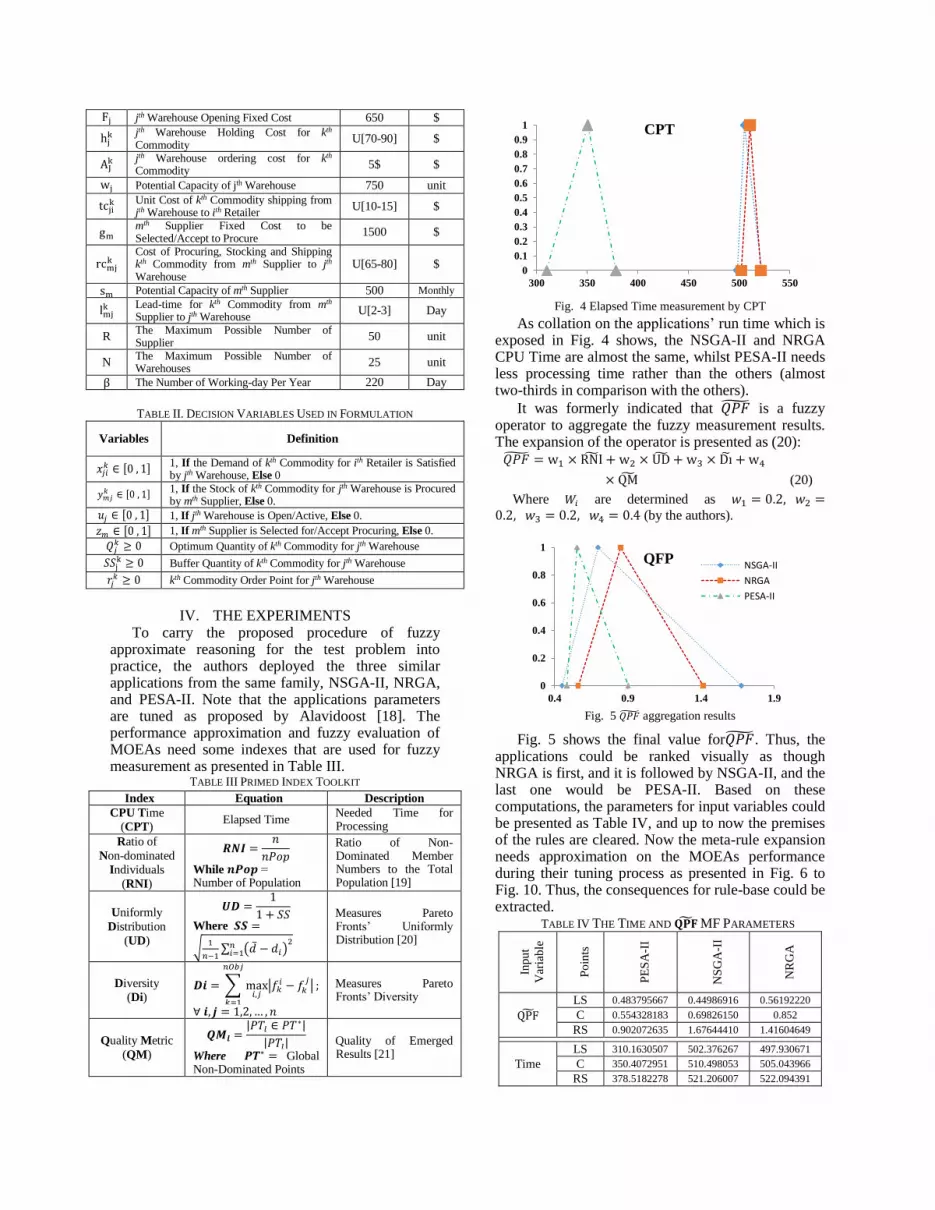
Fig. 4 Elapsed Time measurement by CPT
As collation on the applications’ run time which is exposed in Fig. 4 shows, the NSGA-II and NRGA CPU Time are almost the same, whilst PESA-II needs less processing time rather than the others (almost two-thirds in comparison with the others).
It was formerly indicated that 𝑄𝑃�� is a fuzzy operator to aggregate the fuzzy measurement results. The expansion of the operator is presented as (20): 𝑄𝑃�� = w1 × RNI + w2 × UD + w3 × Di + w4
× QM (20)
Where 𝑊𝑖 are determined as 𝑤1 = 0.2, 𝑤2 =0.2, 𝑤3 = 0.2, 𝑤4 = 0.4 (by the authors).
Fig. 5 𝑄𝑃�� aggregation results
Fig. 5 shows the final value for𝑄𝑃��. Thus, the applications could be ranked visually as though NRGA is first, and it is followed by NSGA-II, and the last one would be PESA-II. Based on these computations, the parameters for input variables could be presented as Table IV, and up to now the premises of the rules are cleared. Now the meta-rule expansion needs approximation on the MOEAs performance during their tuning process as presented in Fig. 6 to Fig. 10. Thus, the consequences for rule-base could be extracted.
TABLE IV THE TIME AND 𝐐𝐏�� MF PARAMETERS
Inpu
t
Var
iab
le
Po
ints
PE
SA
-II
NS
GA
-II
NR
GA
QPF
LS 0.483795667 0.44986916 0.56192220
C 0.554328183 0.69826150 0.852
RS 0.902072635 1.67644410 1.41604649
Time
LS 310.1630507 502.376267 497.930671
C 350.4072951 510.498053 505.043966
RS 378.5182278 521.206007 522.094391
0
0.1
0.2
0.3
0.4
0.5
0.6
0.7
0.8
0.9
1
300 350 400 450 500 550
CPT
0
0.2
0.4
0.6
0.8
1
0.4 0.9 1.4 1.9
QFP NSGA-II
NRGA
PESA-II

Fig. 6 Line plot and boxplot for CPU Time
Fig. 7 Line plot and boxplot for RNI
Fig. 8 Line plot and boxplot for UD
Fig. 9 Line plot and boxplot for Di
Fig. 10 Line plot and boxplot for QM
A comparison between MOEAs by processing time is exposed in Fig. 6. As it is resolved, the NSGA-II and NRGA processing times are almost equal and are twice that of PESA-II. The visualization in Fig. 7 compares the non-dominated result of all deployed MOEAs. As it is clear, the number of non-dominated ones for the NSGA-II and NRGA are almost the same
but less than those emerged by PESA-II. A UD-based comparison presented in Fig. 8, similar to the former comparison, shows no differentiation between NSGA-II and NRGA while PESA-II has better distribution smoothness in collation with the other two. Fig. 9 considers their differentiation in solution diversity in terms of Di. As it is clear, the NRGA diversity is more than NSGA-II, and NSGA-II is more than PESA-II. The non-dominated solution for three MOEAs are exposed in Fig. 10 which shows that the performances of both NSGA-II and NSGA-II from the Pareto Front quality point of view are the same, howbeit they are weaker than PESA-II.
Fig. 11 Fuzzy rule base
RULE 1: IF (Time is free) and (QPF is excellent) THEN (SuitableSet is PESA-II.&.NSGA-II.&.NRGA) (0.2)
RULE 2: IF (Time is free) and (QPF is excellent) THEN (SuitableSet is NSGA-II.&.NRGA) (0.8)
RULE 3: IF (Time is free) and (QPF is high) THEN (SuitableSet is PESA-II.&.NSGA-II.&.NRGA) (0.3)
RULE 4: IF (Time is free) and (QPF is high) THEN (SuitableSet is NSGA-II.&.NRGA) (0.3)
RULE 5: IF (Time is free) and (QPF is average) THEN (SuitableSet is PESA-II.&.NSGA-II) (0.4)
RULE 6: IF (Time is free) and (QPF is average) THEN (SuitableSet is PESA-II.&.NSGA-II.&.NRGA) (0.6)
RULE 7: IF (Time is bounded) and (QPF is excellent) THEN (SuitableSet is PESA-II.&.NSGA-II.&.NRGA) (0.4)
RULE 8: IF (Time is bounded) and (QPF is excellent) THEN (SuitableSet is NSGA-II.&.NRGA) (0.6)
RULE 9: IF (Time is bounded) and (QPF is high) THEN (SuitableSet is PESA-II.&.NSGA-II.&.NRGA) (0.6)
RULE 10: IF (Time is bounded) and (QPF is high) THEN (SuitableSet is NSGA-II.&.NRGA) (0.4)
RULE 11: IF (Time is bounded) and (QPF is average) THEN (SuitableSet is PESA-II.&.NSGA-II) (0.8)
RULE 12: IF (Time is bounded) and (QPF is average) THEN (SuitableSet is PESA-II.&.NSGA-II.&.NRGA) (0.2)
RULE 13: IF (Time is exigent) and (QPF is excellent) THEN (SuitableSet is PESA-II.&.NSGA-II) (0.6)
RULE 14: IF (Time is exigent) and (QPF is excellent) THEN (SuitableSet is PESA-II.&.NSGA-II.&.NRGA) (0.4)
RULE 15: IF (Time is exigent) and (QPF is high) THEN (SuitableSet is PESA-II.&.NSGA-II) (0.7)
RULE 16: IF (Time is exigent) and (QPF is high) THEN (SuitableSet is PESA-II.&.NSGA-II.&.NRGA) (0.3) RULE 17: IF (Time is exigent) and (QPF is average) THEN (SuitableSet is PESA-II.&.NSGA-II) (0.9) RULE 18: IF (Time is exigent) and (QPF is average) THEN (SuitableSet is PESA-II.&.NSGA-II.&.NRGA) (0.1)
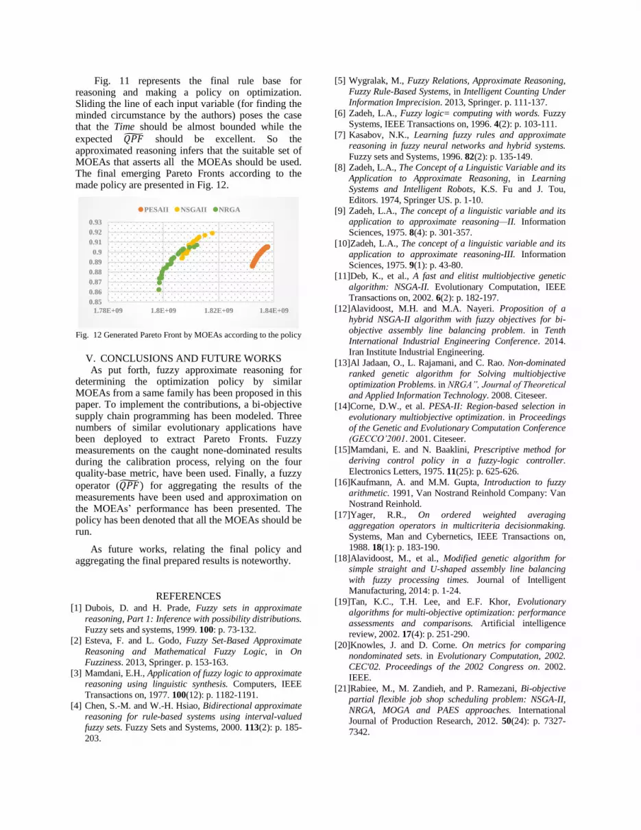
Fig. 11 represents the final rule base for reasoning and making a policy on optimization. Sliding the line of each input variable (for finding the minded circumstance by the authors) poses the case that the Time should be almost bounded while the
expected 𝑄𝑃�� should be excellent. So the approximated reasoning infers that the suitable set of MOEAs that asserts all the MOEAs should be used. The final emerging Pareto Fronts according to the made policy are presented in Fig. 12.
Fig. 12 Generated Pareto Front by MOEAs according to the policy
V. CONCLUSIONS AND FUTURE WORKS As put forth, fuzzy approximate reasoning for
determining the optimization policy by similar MOEAs from a same family has been proposed in this paper. To implement the contributions, a bi-objective supply chain programming has been modeled. Three numbers of similar evolutionary applications have been deployed to extract Pareto Fronts. Fuzzy measurements on the caught none-dominated results during the calibration process, relying on the four quality-base metric, have been used. Finally, a fuzzy
operator (𝑄𝑃��) for aggregating the results of the measurements have been used and approximation on the MOEAs’ performance has been presented. The policy has been denoted that all the MOEAs should be run.
As future works, relating the final policy and aggregating the final prepared results is noteworthy.
REFERENCES [1] Dubois, D. and H. Prade, Fuzzy sets in approximate
reasoning, Part 1: Inference with possibility distributions.
Fuzzy sets and systems, 1999. 100: p. 73-132.
[2] Esteva, F. and L. Godo, Fuzzy Set-Based Approximate
Reasoning and Mathematical Fuzzy Logic, in On
Fuzziness. 2013, Springer. p. 153-163.
[3] Mamdani, E.H., Application of fuzzy logic to approximate
reasoning using linguistic synthesis. Computers, IEEE
Transactions on, 1977. 100(12): p. 1182-1191.
[4] Chen, S.-M. and W.-H. Hsiao, Bidirectional approximate
reasoning for rule-based systems using interval-valued
fuzzy sets. Fuzzy Sets and Systems, 2000. 113(2): p. 185-
203.
[5] Wygralak, M., Fuzzy Relations, Approximate Reasoning,
Fuzzy Rule-Based Systems, in Intelligent Counting Under
Information Imprecision. 2013, Springer. p. 111-137.
[6] Zadeh, L.A., Fuzzy logic= computing with words. Fuzzy
Systems, IEEE Transactions on, 1996. 4(2): p. 103-111.
[7] Kasabov, N.K., Learning fuzzy rules and approximate
reasoning in fuzzy neural networks and hybrid systems.
Fuzzy sets and Systems, 1996. 82(2): p. 135-149.
[8] Zadeh, L.A., The Concept of a Linguistic Variable and its
Application to Approximate Reasoning, in Learning
Systems and Intelligent Robots, K.S. Fu and J. Tou,
Editors. 1974, Springer US. p. 1-10.
[9] Zadeh, L.A., The concept of a linguistic variable and its
application to approximate reasoning—II. Information
Sciences, 1975. 8(4): p. 301-357.
[10]Zadeh, L.A., The concept of a linguistic variable and its
application to approximate reasoning-III. Information
Sciences, 1975. 9(1): p. 43-80.
[11]Deb, K., et al., A fast and elitist multiobjective genetic
algorithm: NSGA-II. Evolutionary Computation, IEEE
Transactions on, 2002. 6(2): p. 182-197.
[12]Alavidoost, M.H. and M.A. Nayeri. Proposition of a
hybrid NSGA-II algorithm with fuzzy objectives for bi-
objective assembly line balancing problem. in Tenth
International Industrial Engineering Conference. 2014.
Iran Institute Industrial Engineering.
[13]Al Jadaan, O., L. Rajamani, and C. Rao. Non-dominated
ranked genetic algorithm for Solving multiobjective
optimization Problems. in NRGA”, Journal of Theoretical
and Applied Information Technology. 2008. Citeseer.
[14]Corne, D.W., et al. PESA-II: Region-based selection in
evolutionary multiobjective optimization. in Proceedings
of the Genetic and Evolutionary Computation Conference
(GECCO’2001. 2001. Citeseer.
[15]Mamdani, E. and N. Baaklini, Prescriptive method for
deriving control policy in a fuzzy-logic controller.
Electronics Letters, 1975. 11(25): p. 625-626.
[16]Kaufmann, A. and M.M. Gupta, Introduction to fuzzy
arithmetic. 1991, Van Nostrand Reinhold Company: Van
Nostrand Reinhold.
[17]Yager, R.R., On ordered weighted averaging
aggregation operators in multicriteria decisionmaking.
Systems, Man and Cybernetics, IEEE Transactions on,
1988. 18(1): p. 183-190.
[18]Alavidoost, M., et al., Modified genetic algorithm for
simple straight and U-shaped assembly line balancing
with fuzzy processing times. Journal of Intelligent
Manufacturing, 2014: p. 1-24.
[19]Tan, K.C., T.H. Lee, and E.F. Khor, Evolutionary
algorithms for multi-objective optimization: performance
assessments and comparisons. Artificial intelligence
review, 2002. 17(4): p. 251-290.
[20]Knowles, J. and D. Corne. On metrics for comparing
nondominated sets. in Evolutionary Computation, 2002.
CEC'02. Proceedings of the 2002 Congress on. 2002.
IEEE.
[21]Rabiee, M., M. Zandieh, and P. Ramezani, Bi-objective
partial flexible job shop scheduling problem: NSGA-II,
NRGA, MOGA and PAES approaches. International
Journal of Production Research, 2012. 50(24): p. 7327-
7342.
0.85
0.86
0.87
0.88
0.89
0.9
0.91
0.92
0.93
1.78E+09 1.8E+09 1.82E+09 1.84E+09
PESAII NSGAII NRGA