Fuzzy Algorithms for Maximum Lifetime Routing in Wireless Sensor Networks

Online Routing Algorithms for Maximum Lifetime in

Wireless Sensor Networks 1

Mahmood R. Minhas, Sathish Gopalakrishnan, Victor C. M. Leung

Department of Electrical & Computer Engineering,

University of British Columbia,

Vancouver, BC V6T1Z4, Canada

Email: {mrminhas,sathish,vleung} @ece.ubc.ca

Abstract

The importance of energy preservation in wireless sensor networks is long estab-

lished, and a number of maximum lifetime routing schemes exist in the literature. Many

of the existing online routing schemes are based on the use of some edge-weight func-

tions, but those schemes exhibit diverse performances in terms of the obtained lifetime

results. The major contribution of the present work is to critically analyze the existing

edge-weight functions in order to identify their shortcomings. We obtain an insight into

the desired behavior of weight functions, and design better functions that are employed

in the proposed approaches. We present two online routing schemes, namely the fuzzy

1This work was supported by the Natural Sciences and Engineering Research Council of Canada undergrant STPGP 322208-05.

1

maximum lifetime routing scheme (FML), and the fuzzy multiobjective routing scheme

(FMO). The former tries to maximize the lifetime objective, whereas the latter strives

to simultaneously optimize the lifetime as well as the energy consumption objective.

Simulation results obtained under a variety of network scenarios indicate the superior-

ity of the proposed schemes over a number of other online routing schemes in terms of

the lifetime as well as the energy consumption metric. For better scalability, we also

present a fully distributed implementation of the FML routing scheme. The overhead

analysis shows that the distributed scheme is successful in considerably reducing the

control overhead.

keywords: Wireless sensor networks, lifetime maximization, energy-aware routing, online

routing algorithms, distributed algorithms, multiobjective optimization, fuzzy functions and

operators.

1 Introduction

Wireless sensor networks (WSNs) have found a number of potential applications in various

fields [1,7]. WSN is usually comprised of battery-operated sensor devices capable of commu-

nication and processing. In many real-life applications, sensor nodes are deployed in remote

or hostile environments with a high node density, and the operational lifetime of a WSN

depends on the available battery energies in the nodes. Thus there is a compelling need for

energy-aware techniques and protocols at all the layers including the routing layer [7, 19].

The existing routing schemes can broadly be classified into online routing and offline

routing schemes (a brief review of the related energy-aware and maximum lifetime routing

schemes is given in Section 8). An online routing scheme needs to find a route for each routing

request without the knowledge of the future routing requests [18]. Section 2 describes the

online routing model in detail.

A number of online routing schemes are found in the literature [11, 13, 17, 18]. The two

closest, in working mechanism, to the present work are the online maximum lifetime routing

heuristic (OML) due to Park and Sahni [18], and the CMAX heuristic due to Kar et al. [11].

The core mechanism in both the schemes is the use of edge-weight functions. The function

computes a certain weight for each edge, depending on the residual energy value of its source

node (the transmitting sensor node). Followed by the weight assignment step, the maximum

lifetime path is found on the basis of the assigned weights. Thus the edge-weight function

has a decisive impact on the overall performance of these online routing schemes.

A major contribution of this work is an effort to investigate the shortcomings in the existing

weight functions of the OML and the CMAX schemes in order to obtain an insight into the

desired behavior and characteristics of a more effective weight function. The effort leads

to the design of improved fuzzy-logic based weight functions that are used in the proposed

routing algorithms. Section 4 presents a comparative analysis of the weight functions used

by the FML, OML, and CMAX schemes, and presents an investigative insight into the

improvement obtained. The results confirm our belief that the improved fuzzy-logic-based

weight functions provide an edge to the proposed schemes over the aforementioned two

existing online routing schemes.

We present two online routing algorithms, namely the fuzzy maximum lifetime routing

algorithm (FML), and the fuzzy multiobjective routing algorithm (FMO). Moreover, we also

present a distributed FML routing implementation. Sections 3 and 5, respectively, describe

algorithmic details of the FML and the FMO routing schemes, whereas a description of the

distributed FML algorithm is given in Section 6.

The motivation for resorting to fuzzy logic in designing the weight functions is that the

fuzzy sets and membership functions have proved to be an effective mean of expressing the

costs of the various objectives involved in an optimization problem [27, 29]. Secondly, in

case of the multiobjective routing, there is a need for designing a multiobjective aggrega-

tion function, and fuzzy logic offers a better alternative, namely ordered weighted operator

(OWA) to the other traditional aggregation approaches such as weighted sum [26,28]. A brief

introduction to fuzzy sets, membership functions, and operators is given in the appendix.

We conduct a performance comparison of the proposed routing algorithm to the OML

heuristic (OML) and the CMAX heuristic. Detailed simulation results and related discus-

sions are given in Section 7. An extensive set of simulation results obtained under various

network scenarios and parameters show that the proposed FML algorithm outperforms both

the OML as well as the CMAX heuristic, in terms of the network lifetime and the average

energy consumption metrics. It should be noted that Park and Sahni [18] have already

demonstrated the supremacy of the OML heuristic, not only over the CMAX heuristic,

but also over a number of other existing maximum lifetime routing algorithms including

MRPC [17] and z.Pmin [3]. In case of the distributed FML, the overhead analysis shows

that the distributed approach has a considerably lower overhead than that of the centralized

FML algorithm (see Section 7.4), and hence it may offer a viable online maximum lifetime

routing solution for real-life large-scale WSN deployments.

2 The System Model and the Problem Formulation

The system model used in this work is similar to the model used in our earlier work [16]. We

consider a static WSN deployment, and model it as a directed graph G(V,E), where V is the

set of nodes, and E is the set of edges. All the nodes have equal initial energy σ. The node

batteries are neither replaceable nor remotely rechargeable. Each node vi ∈ V , has a set of

neighbor nodes (denoted as neighborhood set Ni) that the node vi can reach by a single hop

transmission, using a certain maximum transmission radius rt. An edge e(vi, vj) between

the two nodes is defined to exist only if vi and vj are within the radio transmission range of

each other, i.e., if dij ≤ rt, where dij is the Euclidian distance between the two nodes.

The energy consumption model used in our simulations is based on the first order radio

propagation model, used by many other works in the context of WSN routing [4, 9, 10].

According to this model, the energy expended by a sensor node during transmission and

reception of a k-bit packet is given by Equations (1) and (2), respectively.

TXij = (A + B · dmij ) · k (1)

RXij = A · k (2)

In Equations (1) and (2), A is distance-independent and accounts for the energy consumed

by transmitter or receiver circuitry, B denotes the energy required by the transmitter’s

amplifier, whereas m is a field constant typically in the range [2,4] and depends on certain

characteristics of the wireless medium.

In the online routing model, a routing algorithm needs to find a route for each routing

request without the knowledge of the future routing requests. Further, there are no prefixed

source nodes, and also no assumptions are made about data generation rate. On the other

hand, an offline routing algorithm finds a route for a given routing request with the full

knowledge of the future routing requests (a routing request is initiated by a sensor node to

indicate its intention to send its sensed data to a sink node). Moreover, some offline routing

schemes assume that only a prefixed node (or a subset of nodes) in the entire network may

act as source node(s), and that the data generation rates are known a priori. Several offline

routing approaches based on analytical and heuristic solutions have been proposed [4,15,23].

We believe while an offline routing model may suit certain WSN applications, there are

numerous WSN scenarios, where an online routing model captures the characteristics of a

real-time event-driven WSN application more accurately, i.e., an event may occur anywhere

at any point in real-time, and any node that detects that event may need to act as a source

node. There are numerous examples of such applications including surveillance in a battle

or disaster field (person or object detection, target detection, fire outbreak), environmental

monitoring (temperature or humidity rise at a certain location, activity in a target space

such as a nest or a plant) [1, 7, 25].

We have a set of source nodes performing sensing task. At any time, a source node vm

may initiate a routing request rh(vm, vn), where h = {1, 2, · · ·}, for sending its sensed data

to a sink node vn. A routing request does not imply a single data message (packet), rather

it represents a sequence of data packets to be sent from the source node to a sink node. We

assume there are numerous routing requests {r1, r2, r3, . . .} during the lifetime of WSN. The

goal of the proposed online routing algorithms is to efficiently route each routing request rh,

without the knowledge of any future routing requests rq (where q > h), in such a manner

that maximizes the number of successful routing requests before the end of the WSN lifetime.

We employ a simple, but commonly used, WSN lifetime definition: The WSN lifetime

is equal to the minimum of the lifetimes of all the sensor nodes in the network, i.e., the

network lifetime ends as soon as any node in WSN runs out of its battery [4,6,15,23]. If the

lifetime of a WSN node is denoted by Tvi, the WSN lifetime may be expressed as given by

Equation (3).

T = mini

{Tvi} ∀ vi ∈ V (3)

3 The Fuzzy Maximum Lifetime Routing Algorithm

(FML)

The FML algorithm makes use of an edge-weight function like some other online routing

schemes, but as mentioned earlier, for the proposed FML algorithm, we explicitly formulate

the weight function based on a novel use of fuzzy sets and membership functions.

In order to apply fuzzy logic to the maximum lifetime routing problem, a linguistic vari-

able residual energy of a node vi ∈ V , and a fuzzy set high lifetime are defined. A fuzzy

membership function (depicted in Figure (1)) is designed to map a value of the residual

energy to its corresponding fuzzy lifetime membership value µijlt in the fuzzy set high lifetime.

As may be observed, the function assigns a high membership value to an edge having

a large amount of residual energy (re) at its starting node vi. Initially, when the residual

�

�

�

��α�σ��σ��

µ ��

��

γγγγ��

Figure 1: A depiction of the fuzzy membership function for lifetime.

energy of a node is equal to σ, each of its outgoing edges is assigned a membership value of

1.0. As the node residual energy decays, the corresponding membership value falls, initially

at a slow rate and then at a sharp rate. This behavior of the membership function strongly

discourages the inclusion, on the selected routing path, of those intermediate nodes that have

depleted their energy beyond a certain threshold value. The threshold point may be altered

by adjusting the value of α. An expression for the fuzzy lifetime membership function can

be derived using the equation of line, and is given by Equation (4).

µijlt =

1− ( 1−γ1−α

) · (1− re(vi)σ

) :

if α · σ < re(vi) ≤ σ

γα·σ−TXij

× (re(vi)− TXij) :

if TXij < re(vi) ≤ α · σ

0 : if re(vi) ≤ TXij

(4)

Here

re(vi) = ce(vi)− TXij (5)

where re(vi) and ce(vi) denote residual energy and current energy of node vi respectively,

and α ∈ [0, 1], γ ∈ [0, 1] are algorithmic parameters. Then a weight is assigned to each edge

e(vi, vj) using the following equation:

wij = 1− µijlt (6)

��

��

��

�� µ� ��µ� ��

��

��

�� !��"�

��

Figure 2: The fuzzy maximum lifetime (FML) routing algorithm.

The proposed fuzzy routing algorithm (shown in Figure (2)) works as follows: When a

routing request rh(vm, vn) is initiated, a fuzzy lifetime membership value is computed for

each edge in WSN using Equation (4), and hence a weight is assigned to each edge using

Equation (6). Following the weight assignments, the maximum lifetime path ph, between

vm and vn, is found using the Dijkstra’s shortest path algorithm [8]. It should be noted

that FML algorithm has a complexity advantage over the OML algorithm, since for each

routing request, the FML algorithm requires only one shortest path search whereas the OML

algorithm requires two.

4 A Comparative Analysis of the FML, OML and CMAX

Weight Functions

As mentioned earlier, the proposed fuzzy-logic-based weight function is the distinguishing

feature of the FML routing algorithm that contrasts it from the OML and the CMAX

heuristics. We believe that the above mentioned feature is the underlying reason for the

superiority of FML over the other two heuristics (see the simulation results and comparisons

given in Section 7). Therefore, it seems natural to investigate and comprehend the cause of

supremacy of FML. In this section, we follow this natural instinct, and make an effort to

identify the possible strength in FML mechanism.

Before presenting the comparative study, it is necessary to describe brief details of the

OML and the CMAX heuristics. CMAX [11] formulates an edge-weight function, which is

used to assign a weight to each edge in the network. The weight for an edge e(vi, vj) is

computed as TXij (λη(i)− 1), where η(i) = 1− ce(vi)/σ, and λ is an algorithmic parameter.

As can be seen, CMAX due to term ‘η(i)’, assigns a high weight to an edge e(vi, vj), if the

node vi has consumed a large amount of its initial energy. Then Dijkstra’s algorithm is

used to find the minimum cost path. CMAX algorithm needs only one shortest path search,

whereas zPmin requires two to find the maximum lifetime path.

Park and Sahni [18] presented an online maximum lifetime algorithm (OML) that is also

based on edge weight assignment like CMAX. The OML heuristic works as follows: Let

G(V,E) be the given graph, and G′(V, E ′) be the graph after removing all edges e(vi, vj)

such that ce(vi) < TXij. For a routing request to send data from a source vm to a sink vn,

the minimum energy path P ′ is found, and the minimum residual energy minRE along P ′

is computed. A second pruned graph G′′(V, E ′′) is obtained by removing all edges e′(vi, vj)

from G′ such that ce(vi) − TXij < minRE. The weight w′′ to be assigned to each edge in

G′′ is computed using the following equation.

w′′ = (TXij + ρ(vi)) · (λη(i) − 1) (7)

where λ is an algorithmic parameter of OML, and ρ(vi) is given by

ρ(vi) =

0 if ce(vi)− TXij > eMin(vi)

c otherwise

(8)

where eMin(vi) is the energy required by node vi to transmit to its closest neighbor and

‘c > 0’ is an algorithmic parameter.

��

��

��

��

��

��

��

��

��

��

��

��

��

��

��

��

� �

� �

� ��

��

��

Figure 3: A comparison of the proposed FML weight function to the OML and theCMAX weight functions. In our opinion, the CMAX weight assignment behavior is overly-pessimistic, whereas that of the OML is too optimistic (or too late) to have a timely effecton the lifetime objective.

A visible similarity in all the three heuristics is the use of edge weight functions, i.e., all

three schemes proceed by assigning a weight to each edge in the network and then finding

the minimum cost path. Therefore, a comparative study of these weight functions may lead

us to an insight into the performance difference among FML and the other heuristics.

The OML and the CMAX weight functions are formulated implicitly to attain a certain

behavior of the edge-weight corresponding to a given value of the residual energy. On the

other hand, the proposed weight functions are explicitly designed based on use of fuzzy

membership functions, which offer a flexible way of representing the cost of a given objective

as a fuzzy membership value [29].

The weight functions used by OML and CMAX seem very similar apparently, since both

use a common term λ, however λ is defined in different ways by both the approaches. A brief

discussion on the differences among these two is given by [18]. The FML weight function is

defined in an altogether different manner, i.e., the weight assigned to an edge is computed

based on fuzzy lifetime membership value of the edge that in turn ultimately is a function

of the residual energy level of the originating node. Figure (3) shows the weight assigned to

an edge as a function of the residual energy of the by each of the three heuristics.

As discussed by Park and Sahni in [18], it is relatively easier to explain the performance

lag of CMAX since based on its definition of λ term, it prematurely starts assigning a higher

weight to an edge that has depleted a large fraction of its initial battery power (notice the

rise in weight curve as soon as re falls below values of 0.5). The authors argued that this

behavior of CMAX weight function is premature, and therefore suggested that even though

a node may have depleted a large fraction of its energy, this should not imply its exclusion

from the route search process since it may rule out a number of good routing choices. In an

effort to rectify this behavior of CMAX, OML authors proposed that, for achieving a longer

lifetime, the edge weight should better be a function of the ratio of the residual energy of the

node to the minimum energy required to transmit to the closest neighbor. As a result, they

relaxed the constraint and obtained a weight function curve that starts rising only after the

residual energy decays beyond 5% of the initial energy level.

We argue that the above described threshold used in the OML scheme for raising the

weight is probably too late to have a considerable effect on the maximum lifetime routing

path search process: The OML weight function keeps assigning a negligible (almost zero)

weight to an edge until its originating node has depleted almost 95% of its battery power. The

FML weight function tries to attain a balance between the two extreme behaviors of CMAX

and OML, and strives to respond to the continuous decay of residual energy throughout

the network operation as described in following: The weight is increased from 0 to 0.1 at a

steady lower rate when the residual energy is in range [1.0, 0.2] (notice that OML assigns an

almost 0 weight at even re(vi) = 0.2). There is a breakpoint at re(vi) = 0.2, as beyond that

point, the weight increases at a much sharper rate.

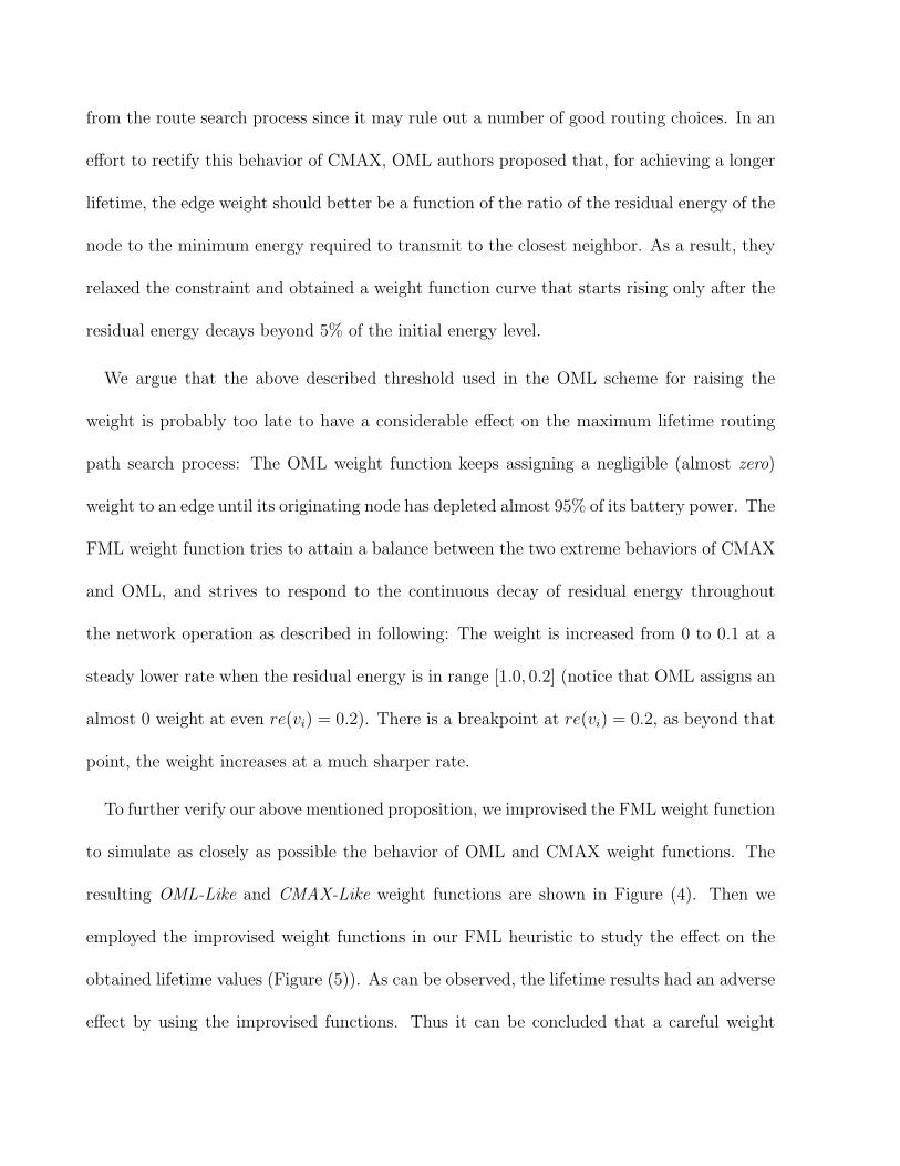
To further verify our above mentioned proposition, we improvised the FML weight function

to simulate as closely as possible the behavior of OML and CMAX weight functions. The

resulting OML-Like and CMAX-Like weight functions are shown in Figure (4). Then we

employed the improvised weight functions in our FML heuristic to study the effect on the

obtained lifetime values (Figure (5)). As can be observed, the lifetime results had an adverse

effect by using the improvised functions. Thus it can be concluded that a careful weight

��

��

��

��

��

��

��

��

��

��

��

��

��

��

��

��

� �

� �

� ��

� ��

� ��

��

��

Figure 4: A depiction of the improvised FML weight functions (named as the OML-like andthe CMAX-like) designed to roughly adopt into FML the weight assignment behavior ofOML and the CMAX heuristics.

�

��

��

��

��

��

��

��

��

��

��

�� !��

Figure 5: A comparison between the lifetime values obtained by using the original and theimprovised FML weight functions. The use of either of the improvised functions results indegradation the lifetime value.

function design for FML is one of its strengths that helped in achieving better lifetime.

5 The Fuzzy Multiobjective Routing Algorithm (FMO)

In order to incorporate the minimum energy consumption objective in our routing algorithm,

another linguistic variable required energy along an edge e(vi, vj), and a corresponding fuzzy

set low energy consumption are defined. A fuzzy membership function (Figure (6)) is pro-

posed to map a value of the variable required energy to its corresponding fuzzy minimum

energy membership value µijme. As may be seen, the function assigns the lowest (highest)

membership value to an edge requiring the maximum (minimum) transmission energy among

all the neighboring edges. This behavior of membership function encourages the selection

of such edges that require lesser transmission energy. The lowest membership value may

be altered by adjusting the value of algorithmic parameter ∆. An expression for the fuzzy

minimum energy membership function is given by Equation (9).

�

��

�

� ��

�

�

��µµ µµ� ��

Figure 6: A depiction of the fuzzy membership function for minimum energy.

µijme = 1 +

(∆− 1)× TXij

max(TXij)(9)

where

max(TXij) = maxj{TXij} ∀ j s.t. vj ∈ Ni (10)

min(TXij) = minj{TXij} ∀ j s.t. vj ∈ Ni (11)

In order to formulate a fuzzy multiobjective aggregation function for an edge, the following

fuzzy rule is proposed:

IF an edge

has start node with high lifetime AND

requires low energy consumption

THEN it is a good edge.

The above fuzzy rule translates to the following ‘and-like’ function by employing the OWA

operator:

µij = β ×min(µijlt , µ

ijme) + (1− β)× (

µijlt + µij

me

2) (12)

where µij is the fuzzy multiobjective membership value of the edge e(vi, vj), and β ∈ [0, 1]

is a constant. As can be observed, the above OWA function due to the term β×min(µijlt , µ

ijme),

asserts a preference on the objective having the least membership value. Also, it may be

noted that due to nature of our carefully designed membership functions, the minimum

value of µijlt is 0, whereas that of µij

me is ∆ > 0. Therefore it is easy to infer that if the

residual energy (and the corresponding lifetime membership value µijlt ) is high, a similar

preference level is given to both the objectives; otherwise if µijlt < ∆, the preference shifts

to the maximum lifetime objective. As a conclusion, the value of parameter ∆ affects the

relative preference of the two routing objectives.

The proposed fuzzy multiobjective routing algorithm (Figure (7)) operates as follows:

When a routing request rh(vm, vn) is initiated, a fuzzy lifetime membership value is com-

puted for each edge using Equation (4). Also, a fuzzy minimum energy membership value

for each edge is computed using Equation (9), followed by computation of a multiobjec-

tive membership value using Equation (12). Then a weight is assigned to each edge using

��

��

��

�� µµµµ�� µµµµ

��

��µµµµ��µµµµ�

��

��

��

��

��!�� "��

��

Figure 7: The fuzzy multiobjective (FMO) routing algorithm.

Equation (13).

wij = 1− µij (13)

Following the weight assignment, the multiobjective path ph between vm and vn is found

using Dijkstra’s shortest path algorithm [8].

6 The Distributed FML Algorithm

The proposed fuzzy routing algorithms described in the earlier sections are source-directed

in their working, and thus require a centralized implementation. This implies a considerable

protocol control overhead since, during each shortest path search phase, a possibly large

number of control packets need to be sent to the source node from each of the intermediate

nodes on the partially searched path. This fact results in poor scalability of the routing

algorithm which may hinder its practical application to large-scale WSNs. In addition, the

need for transmission and reception of a large number of control packets implies an implicit

energy consumption overhead that has a direct adverse effect on the energy conservation as

well as the lifetime maximization objectives. Therefore, for a better scalability and a lower

energy consumption overhead, we propose a distributed fuzzy maximum lifetime (FML)

algorithm shown in Figure (8).

��

��

��

�� µ� ��µ� ��

��

��!��"�� !��

��

#�� $��

�� "��

� � % ��

��"��

� � ��

��

&��!��

��

��"��!��

'�!��

��"��

��

"�� $��(�

��

Figure 8: The distributed FML routing algorithm.

The distributed FML algorithm works as follows: Each node in WSN computes its ‘fuzzy

membership value’ using the fuzzy maximum lifetime membership function given by Equa-

tion (4). For each routing request, a setup phase is triggered during which, a sink nodes

initiates by broadcasting a setup packet to its immediate neighbor nodes. On receiving the

said packet, each of the neighbor nodes registers itself as the sink’s neighbor and updates its

forwarding table (FT) by storing the route to the sink node along with an accumulated cost

of the route to the sink node. Then it broadcasts a setup packet containing the above stated

routing information to its following upstream neighbors that perform the similar updates in

their forwarding tables. This local broadcast process is carried out until the source node

(that initiated the routing request) is reached. As a result of the setup phase, each node

discovers a route as well as an accumulated cost to the sink node.

The setup phase is followed by the data transmission phase during which, starting from

the source node, each intermediate node makes a local forwarding decision based on its

forwarding table and thus forwards the data packet to the best downstream neighbor (the

one having the least accumulated cost to the sink). This forwarding scheme continues until

the sink node is reached. The route found is used for the entire duration of the routing

request (all source to sink packets in the routing request are routed along the same route).

7 Performance Evaluation and Discussions

We present a comprehensive evaluation of the proposed fuzzy routing algorithms. For the

comparison purpose, we implemented two other online routing heuristics namely, the online

maximum lifetime (OML) [18] and the CMAX [11] heuristics.

The performance metrics used for comparison are network lifetime and average energy

consumption. Network lifetime is computed as the number of successful sessions (end to

end, i.e., source to sink packet deliveries) before any sensor node in WSN runs out of its

battery (Recall from Section 2 that network lifetime ends as soon as the first node in WSN

dies). Average energy consumption is computed as the total energy expended during a routing

request divided by the number of sessions (source to sink packet deliveries) in the routing

request. Total energy expended during a routing request refers to the sum of transmission

energies and reception energies of all the intermediate nodes on the path selected for the

routing request. It is worth mentioning that even the transmission energy of the source node

is added to the above sum. However, the reception energy at the sink node is not included

since the sink node is usually a base station not powered by a battery.

Our simulation setup consists of 2-dimensional grid of size X × Y populated with n sensor

nodes randomly deployed within the region. In our simulations, sink nodes are assumed to

have infinite energy (usually the sink node is a base station powered by a fixed power source)

and predetermined locations, whereas all other nodes (including the source nodes) have an

equal level of initial residual energy equal to σ. A sample random WSN topology consisting

of 50 nodes with a single sink node spread in a 25m × 25m region is shown in Figure (9).

OO O

O O OO O O

OO O O O

O OO

OX O O O O

OO

O OO O O O O

O OO O O

O O OO O

O O OO O O

O O

Figure 9: A sample random topology of 50 nodes. An ‘o’ indicates a sensor node, whereas‘X’ shows a sink node.

In the scope of a routing algorithm, we assume a MAC layer with lower energy losses

due to bounded number of retransmission attempts (it may appear to be an optimistic

assumption considering typical wireless MAC protocols that offer a probabilistic nature of

contention-based channel access mechanism, but some recently proposed MAC protocols are

able to offer deterministic contention-free or lesser-than-typical contention channel access

guarantees [5, 21, 22]).

Our traffic model is online, where there are no known source nodes or predetermined traffic

flows; rather we assume that any of the non-sink nodes on detecting an event in its sensing

range is able to initiate a routing request in order to start sending its sensed data to a sink

node.

7.1 Finding Values for the Simulation Parameters

There are number of simulation parameters to which, we need to assign suitable values. For

wireless medium related parameters including A, B and m, we used typical values as were

used by many other works [4,10]. We randomly placed between 30 to 100 sensor nodes in a

fixed-size square region measuring (X × Y ) m2, whereas the transmission range of a sensor

node’s radio was varied from 7m to 15m. A list of the simulation parameters and their values

is given in Table 1.

Table 1: A list of values used for various simulation parameters.σ 1 JA 100 nJ/bitB 50 pJ/bit/m4

m 4

X 25Y 25n {30, 40, 50, . . . , 100}rt {7, 8, . . . , 15}

In addition, the FML scheme has two algorithmic parameters (α and γ), for which the best

values (e.g., those resulting in the maximum obtained lifetime) were determined empirically.

For this purpose, we experimented with all values for γ ∈ {0.1, 0.2, . . . , 0.9} using numerous

possible combinations of values for n and rt, and the best value found for γ was 0.9, and hence

we used this value in the rest of our simulations. Then, we conducted a series of experiments

to determine the best value for α. We tried 10 values for α ∈ {0.1, 0.2, . . . , 1.0}, and for

each value, we obtained the lifetime results using 10 random 50-node topologies, whereas 10

random routing sequences were generated for each topology. In other words, for each value

of α, we averaged our results over 100 runs. The results obtained are shown in Figure (10).

As can be seen, α = 0.2 obtained marginally best lifetime, and hence we set the value of

parameter α at 0.2 throughout our simulations. In our implementations of OML and CMAX,

we used the best value for the parameter λ = 1011, as reported by the OML authors in [18].

�

��

��

��

��

��

��

� ��

αααα

Figure 10: Effect of α on the lifetime metric obtained by FML routing algorithm. It may benoted that setting α = 0.2 results in the highest lifetime value.

7.2 Performance Comparison of the FML Scheme with the OML

and the CMAX Heuristics

We execute runs of FML and OML on 10 randomly generated 100-node topologies, and

performed a comparison in terms of lifetime metric. Table (2) lists the lifetime values ob-

tained by both approaches along with some statistical measures. Each row corresponds to

a topology and 10 random sequences of routing requests were generated for each topology.

The columns Average and SD respectively, show the average and the standard deviation of

lifetime values obtained over 10 sequences, whereas the last two columns respectively, show

the average and standard deviation of percentage improvement achieved by the FML over the

OML. It may be noted that the FML consistently outperforms the OML by a considerable

margin ranging from 10% to 20% (average is about 14%). In other words, this experiment,

carried out on a variety of topologies and routing request sequences, exhibits that the use of

FML prolongs the network lifetime by a allowing a considerable more number of sessions.

Table 2: A statistical comparison of lifetime results obtained by FML and OML for 10different topologies. The FML achieves lifetime values that are 10% to 20% better thanthose achieved by the OML.

Topology Average SD Avg. Imp. (%) SD Imp. (%)

1FML 8020 382.39

11.15 5.79OML 7220 229.98

2FML 9000 740.87

11.87 5.66OML 8050 596.75

3FML 8480 507.28

10.61 6.91OML 7670 188.86

4FML 9480 1018.50

10.67 15.16OML 8610 479.47

5FML 7670 271.01

13.30 6.34OML 6780 261.62

6FML 7870 371.33

14.34 8.33OML 6910 510.88

7FML 9260 400.56

15.01 6.11OML 8060 313.40

8FML 10930 992.25

16.85 8.51OML 9380 850.88

9FML 11190 636.75

20.45 7.91OML 9320 723.88

10FML 9380 385.28

14.45 7.93OML 8220 480.28

Now we include CMAX heuristic in our comparisons. Park and Sahni [18] have already

demonstrated the supremacy of OML over CMAX, but it would be interesting to study where

FML stands in comparison to CMAX as well. In case of each routing approach, all the results

reported are averaged over 100 runs – 10 random network topologies were generated, and 10

random request sequences were generated for each topology.

�

��

��

��

��

��

� � ��

��

��

��

��

��

��

��

��

��

��

� � ��

� ��

��

��

!�

"��#

(a) (b)

Figure 11: A comparison of FML to OML and CMAX in terms of (a) network lifetime and(b) average energy consumption for a varying transmission radius (rt = {7, 8, · · · , 15}) for a50-node WSN topology. The FML is able to achieve the highest lifetime values as well asthe least average energy consumption values.

�

��

��

��

��

��

� � � ��

��

��

��

��

��

��

��

��

��

��

� � ��

� ��

��

��

!�

"��#

(a) (b)

Figure 12: A comparison of FML to OML and CMAX in terms of (a) network lifetime and(b) average energy consumption for a varying transmission radius (rt = {7, 8, · · · , 15}) for a100-node WSN topology. The FML is able to achieve the highest lifetime values as well asthe least average energy consumption values.

7.2.1 The Effect of the Transmission Radius

We study the effect of transmission radius on the network lifetime obtained by FML and

the two other approaches. Figures (11) (a) and (b), respectively, show the lifetime and

�

��

��

��

��

��

��

��

��

��

��

��

��

��

��

��

��

��

��

� ��

��

�� !� "��#

(a) (b)

Figure 13: A comparison of FML to OML and CMAX in terms of (a) network lifetime and(b) average energy consumption for a varying node density (n = {30, 40, · · · , 100}) and afixed transmission radius rt = 12. The FML is able to obtain the highest lifetime values witha clearly increasing trend with an increasing node density. On the other hand, the energyconsumption in case of FML exhibits a decreasing trend with the increasing node density.

the average energy consumption obtained by all the three approaches in case of 50 nodes

for a range of transmission radius values. Again, it may clearly be seen that FML obtains

better lifetimes than both OML and CMAX. However, the lifetime obtained by FML and

OML increases until rt = 12 and then remains constant, whereas in case of CMAX, lifetime

reaches a maximum value at rt = 9 and then starts falling sharply. It should be noted that

very similar trends of OML and CMAX are reported by Park and Sahni [18]. The initial

increasing trend in the lifetime can be explained as follows: with the increase in transmission

radius rt, each node is able to communicate farther, and to discover more neighboring nodes,

and thus a higher network connectivity is resulted that offers more routing choices at each

node. As a result, a routing algorithm is able to find more cost-effective (maximal lifetime)

routes. However at the same time, energy consumption also rises because a node now may

transmit to a farther neighbor that requires more transmission energy. Also in terms of

energy consumption, it can be seen that for the entire range of transmission radius values

used in this experiment, routes found by FML consume considerably lesser energy than those

found by OML or CMAX.

Figures (12) (a) and (b), respectively, show the lifetime and the average energy consump-

tion obtained by all the approaches in case of 100 nodes for a range of transmission radius

values. The lifetime as well energy consumption trends here are similar to ones obtained for

50-node case discussed above. However, the worth mentioning fact is that the improvement

margin of FML over OML is even larger in case of 100-nodes. This is a healthy behavior that

FML performs even better with the increasing network density which is a typical feature of

real life WSNs.

7.2.2 The Effect of the Node Density

We study the effect of sensor node density on the results by randomly deploying n ∈ {30, 40, . . . , 100}

sensor nodes in a region of fixed size. Figures (13) (a) and (b), respectively, show the life-

time and the average energy consumption obtained for a varying node density in case of

rt = 12. It may be seen that FML was able to obtain higher lifetime values than the other

two approaches. Moreover, with the rising node density, FML shows a consistently sharper

increasing trend in the obtained lifetime. On the other hand, OML is not able to show a

similar competitive increasing trend at higher transmission radii, and thus the performance

difference grows to be higher. As far as the energy metric is concerned, FML clearly proved

to be more energy frugal than OML and CMAX approaches. It can be noted that FML

exhibits a relatively sharper decreasing trend in terms of energy consumption as the node

density grows.

0

4

8

12

16

20

0.1 0.2 0.3 0.4 0.5 0.6 0.7 0.8 0.9 1

Normalized Current Energy of a Node

Per

cen

tag

e o

f no

des

FML

OML

0

4

8

12

16

20

0.1 0.2 0.3 0.4 0.5 0.6 0.7 0.8 0.9 1

Normalized Current Energy of a Node

Per

cen

tag

e o

f no

des

FML

OML

(a) (b)

Figure 14: A comparison of FML and OML in terms of ‘current energy’ distribution at theend of network lifetime for (a) n=50 and (b) n=100. The results give an insight into thebetter performance of the FML: longer lifetimes are obtained by achieving a more uniformconsumption pattern across the network.

7.2.3 A comparison in Terms of Energy Consumption Distribution

Moreover, we conducted a set of experiments to obtain an insight into energy consumption

pattern across the nodes in a topology. Figures (14) (a) and (b) show a comparison of current

energy distribution at the end of WSN lifetime obtained by FML and OML for 50 and 100

node network, respectively. In both the figures, X-axis shows the normalized current energy

level of nodes, whereas Y-axis shows the percentage of total nodes having a certain level

of current energy at the end of network lifetime. For both topologies, we find that FML

behaves better than OML as in the FML case, at the end of network lifetime, the number

of nodes having lower current energy levels, i.e., in range [0.1, 0.3], is much larger than that

obtained in the OML case. For instance, in case of 50-node network, almost 40% of the

nodes have their remaining energy levels at 30% or below, whereas the same measure is just

around 20% in case of OML. This means that a considerably larger number of nodes have

depleted 70% of their battery power before reaching the point when a node in the network

runs fully out of its battery (which translates to end of lifetime as per the definition used in

this work). In other words, FML achieves a prolonged network lifetime by choosing a more

uniform distribution of routing paths (and thus a more uniform energy consumption pattern

across all the nodes in the network). On the other hand, OML reaches the end of lifetime

much earlier, i.e., a node runs out of battery as early as only 20% of the nodes have depleted

70% of their battery power.

Again as was observed in the previous comparisons discussed above in this section, FML

behaves relatively better for larger network sizes, the similar current-energy distribution plot

for a 100-node topology shows an even a bigger performance gap between FML and OML.

It is observed that in the FML case, at the end of network lifetime, a large portion (about

40%) of nodes have their current energy levels at 30% or lower, whereas in the OML case,

a only 12% on the nodes fall in this range. Moreover, it can be seen that a large portion

of nodes have current energy levels between 50% and 90% which is not a good sign at the

end of network lifetime since the routing algorithm should have tried to exploit the energy

reserve at those nodes to ensure a prolonged lifetime.

Another way of looking at the energy consumption pattern is to compare the average

current levels of the nodes obtained by FML and OML at the end of network lifetime as

depicted by Figure (15). The figure shows the values of the said metric for network sizes

ranging from 50 to 100 nodes. As can be observed, at the end of lifetime, FML consistently

achieves a considerably lower average energy level than the OML does. Again the difference

becomes wider with the increasing network size (from about 10% for 50-node network to

about 15% for 100-node network). This trend also supports our claim regarding the FML

mechanism that it exercises a more uniform energy consumption across the network nodes

and thus extracts its success from this fact and hence delays the time to the failure of first

node in the network.

0

0.1

0.2

0.3

0.4

0.5

0.6

0.7

0.8

50 60 70 80 90 100

Number of nodes (n)

Ave

rag

e cu

rren

t en

erg

y FML

OML

Figure 15: A comparison of FML and OML in terms of ‘average current energy’ at the endof network lifetime for a varying node density n = {30, 40, · · · , 100}. It may be seen in allthe cases that FML reaches the end of lifetime only when the average current energy of thenodes in WSN has fallen to a considerably lower level than that observed in the case of OML.

7.3 FMO Performance: Effect of Multiobjective Routing on the

Lifetime and the Energy Consumption

In this section, we present the results of FMO approach with a view of studying the effect

of incorporating the minimum energy consumption objective on the lifetime maximization

process. To start with, a series of experiments were conducted for determining suitable values

for the parameters ∆ and β using various combination values for the two parameters, and

the lifetime and the average energy consumption values obtained from FMO are shown in

Figures (16) (a) and (b), respectively. As may be observed, β = 0.2 results in the maximum

lifetime as well as the least energy consumption, hence we set its value at 0.2 in all the

subsequent runs. Also it may be noted that for smaller values of ∆, the preference of the

energy consumption objective is high, and as a consequence, the average energy consumption

is low, but at the same time, the network lifetime also falls. Hence, there is a visible tradeoff

between the two routing objectives, and the parameter ∆ can be used to achieve a desired

balance.

��

��

��

��

��

��

�� ∆

β

��

��

��

��

��

��

��

�� ∆

β

(a) (b)

Figure 16: The effect of choosing various possible combinations of the two FMO parameters,namely ∆ and β, on (a) Lifetime and (b) average energy consumption obtained by FMO.The FMO multiobjective framework is able to offer a flexible tradeoff between the twooptimization objectives (lifetime vs. energy consumption): Setting ∆ = 0.2 achieves theleast energy consumption values, but at the same time results in the worst lifetime values.

Next, we conduct experiments to study the effect of ∆ in a scenario of varying node

density. Figures (17) (a) and (b) show the lifetime and the average energy consumption,

respectively, obtained by FML and FMO (for ∆ ∈ {0.2, 0.4, 0.6, 0.8}) for a varying node

density n. Again a lifetime-energy consumption tradeoff is clearly visible in the results, i.e.,

for instance, FMO obtains the least energy consumption when ∆ = 0.2, but also obtains

the least lifetime in this case. Thus, FMO is able to offer a flexible control over choosing a

desired balance between the two routing objectives.

�

��

��

��

��

��

��

��

��

��

��

��

��

��

��

��

��

��

��

��

�� !��"

�� !��

�� !��

(a) (b)

Figure 17: A comparison with the FML, in terms of (a) Lifetime and (b) average energyconsumption, to the FMO for various values for the parameter ∆ for a varying node densityn. The results again show the flexible lifetime vs. energy consumption tradeoff offered bythe FMO.

7.4 Reducing Control Overhead: A Comparison with Distributed

FML

The major objective of designing the distributed FML algorithm is to reduce the control

overhead that is inherent in the proposed FML algorithm due to the use of centralized

Dijkstra’s shortest path search process. A high control overhead poses a scalability question

to algorithm, and thus may prohibit its application to large-scale WSNs. The proposed

distributed FML tries to counter the problem by cutting down the number of control packets

that need to be sent across the network.

In this section, we perform a quantitative study to assess performance gain of the dis-

tributed FML in terms of control traffic reduction. We conduct simulations to compute the

amount of control bits as well as data bits transmitted in case of centralized and distributed

FML algorithms. The computations were recorded over a range of sensor node density,

and the results are plotted in Figure (18). As expected, the centralized implementation

has a higher control overhead than the distributed scheme. Moreover, the centralized case

overhead rises much sharply with an increasing number of sensor nodes, whereas in the dis-

tributed case, the overhead increase is reasonable. As a result, the performance gap grows

to a significant amount for a 100-node network.

It should be noted that this large difference in the number of transmitted control bits

directly translates to a considerable performance difference in terms of the magnitude of

energy consumption, and thus the effect on lifetime objective. Therefore, the analysis in this

section shows that distributed FML algorithm is a strong candidate for maximum lifetime

routing in large scale WSNs.

��

��

��

��

��

��

� ��

��

��

� �

��

��

Figure 18: A comparison between the control overhead of the centralized and the distributedFML schemes in terms of the amount of the control traffic needed during the path searchphase. The distributed FML successfully lowers the control overhead by a considerablemargin.

8 Related Work

Comprehensive reviews of existing routing techniques for WSNs have been presented by

Perillo et al. [19] and Al-Karaki et al. [2]. Al-Karaki et al. classified the existing protocols

into many categories based on two criteria namely, network structure and protocol operation.

However the existing energy-aware routing schemes for WSNs can be broadly classified on

the criterion of routing objective into minimum energy (ME) routing and maximum lifetime

(ML) routing.

Most of the earlier reported attempts related to energy efficient routing in WSN fall in

the category of minimum energy routing. Minimum energy (ME) routing algorithms and

protocols focus on finding a ‘shortest’ or ‘minimum energy’ path between a source node

and the sink node. The main objective of such techniques is to minimize the total amount

of energy consumption for a given routing session. The biggest drawback of typical ME

routing schemes is that battery power of nodes on the favorite paths is quickly drained. As

a consequence, a WSN may prematurely suffer from a network partitioning or at least a

considerable degree of loss in sensing coverage. In other words, these schemes usually do not

cater for a balanced energy consumption pattern among sensor nodes of a WSN.

Maximum lifetime (ML) routing algorithms on the other hand strive to delay as much

as possible the time until sensor nodes runs out of battery. The basic philosophy of this

class of techniques is to favor routes consisting of nodes with higher residual energy, though

various ML routing algorithms may use different underlying path selection mechanisms. For

instance, a simple comparison of ME and ML routing algorithms is shown in Figure (19).

Three of the possible paths between source and sink nodes are shown with their total available

current energies (ce). The number shown along an edge is the energy required to transmit

along the edge. A ME routing scheme selects path2 as it results in minimum total energy

consumption, whereas a possible ML routing algorithm may select path3 depending on max-

min(ce) criterion, i.e., the path along which the minimum ‘ce’ is maximum among all the

paths.

E (ce=3)

A (ce=2)

B (ce=3)

ti

D (ce=2)

F (ce=4)

si

2

1

1

1

1

1

1 1

�� Path 1: S-A-B-T, total ce=5 Path 2: S-D-T, total ce=2 Path 3: S-E-F-T, total ce=7

Minimum Energy path: Path 2 Maximum Lifetime path: Path 3

Figure 19: A high-level comparison between mechanism of the minimum energy and themaximum lifetime routing techniques (adopted and modified from [1]).

We present a brief review of some of the related existing maximum lifetime routing schemes

for WSN. An online routing algorithm – namely CMAX – is presented in [11]. Park and

Sahni [18] presented an online maximum lifetime heuristic (OML).

Misra et al. [17] proposed MRPC, which is an online routing algorithm that selects the

path which has the maximum available lifetime whereas the lifetime of a path is computed

based on the minimum of the residual energies of the nodes that lie along that path. Max-

min z · Pmin [3] is another ML routing algorithm that first finds the minimum energy path

Pmin between a source and the sink. Then in an effort to balance the tradeoff between the

minimum energy and the maximum lifetime objective, it tries to search a path along which

the total energy consumption is no more than z · Pmin where z is an algorithmic parameter.

Sungwook et al. [12] present an online energy-efficient routing scheme that claims to take

real-time online route decisions for QoS-constrained WSN application scenarios.

A number of analytical solution approaches are also found where the WSN lifetime problem

is formulated as a liner program and then solved by using any of the LP solution techniques

such as gradient projection method and others [4, 15, 23]. These LP techniques require a

priori knowledge of the future routing requests and data rates. Cui et al. [6] present a utility

based scheme to solve ML routing problem.

Multipath routing approaches have also been a popular choice due to their underlying

philosophy of distributing the data flow among multiple paths for a single routing request

between a source and sink. A number of multipath algorithms have been developed [2]. The

energy-aware routing (EAR) protocol [20] is a distributed multipath protocol that discovers

and maintains multiple paths with their accumulated costs by local flooding. The best ML

path is chosen probabilistically based on the accumulated path cost. Lu et al. present an

energy-aware multipath routing protocol in [14]. Srinivasan et al. [24] proposed a data-centric

routing algorithm in which, a node decides to participate in packet forwarding only if it has

enough available energy.

9 Conclusions

A number of online routing scheme are presented for maximum lifetime routing in WSNs.

A critical effort is made for identifying the shortcomings of the edge cost functions used in

some of the existing online routing schemes. The comparative analysis of the weight functions

provides us an insight to the better operating regions in terms of the relation between the

residual energy and the edge weight, and hence leads to the design of more effective behavior

of the cost functions.

The role of the fuzzy membership functions and operators is to offer a flexible mean of

explicitly implementing the desired behavior of the cost functions, but in general, any non-

fuzzy approach may also be used as a tool for achieving the task. However, fuzzy logic may

be useful in formulating the cost of the objectives involved in many related optimization

problems in WSNs.

For the sake of giving a fine and complete view to the reader, some minor concluding

remarks are worth mentioning. We did not investigate the sensitivity of the performance

to the fine tuning of the proposed fuzzy membership functions – For instance what if two

or more breakpoints (threshold points) are introduced instead of one in the maximum life-

time membership function. We did not evaluate the effect of some simulation settings such

as varying the number of sink nodes in the network, placing the sink node(s) at various

geographic locations, varying the area of the sensor field, to name a few.

The multiobjective optimization framework can be easily extended to incorporate other

critical routing objectives. The fully distributed implementation approach presented for the

FML scheme can be similarly extended to the FMO scheme.

In the immediate future, we plan to extend our work on multiobjective routing to include

other crucial metrics such as latency and capacity. We shall also look into devising multipath

routing approaches for seeking further improvement in terms of the lifetime and energy

consumption metrics. Further, we will consider flow prioritization to determine schemes for

dropping certain requests when more important requests arrive. Other aspects of interest

include context-aware routing and co-design of energy-efficient routing and MAC protocols

using fuzzy functions. Last but not least, we plan on investigating for defining novel/atypical

but relatively realistic lifetime metrics with a view of measuring the WSN lifetime more

accurately.

A short introduction to fuzzy Logic

Fuzzy Logic is a mathematical discipline invented to express human reasoning in rigorous

mathematical notation. Unlike classical reasoning in which, a proposition is either true or

false, fuzzy logic establishes an approximate truth value of a proposition based on linguistic

variables and inference rules. The value of a linguistic variable is expressed as words or

sentences in a natural or an artificial language [29]. By using hedges like ‘more’, ‘many’,

‘few’, and connectors like AND, OR, and NOT with linguistic variables, an expert can form

rules, which govern the approximate reasoning.

.1 Fuzzy Membership Functions

In the context of crisp sets, a certain element is either a member or a nonmember of a set

(in other words, the membership value is either 1 or 0), whereas in fuzzy logic, a certain

element may have a partial membership in a set (membership value is in the range [0,1]).

A fuzzy membership function is used to compute the membership value corresponding to a

given value of the linguistic variable. The membership function can be designed in a flexible

way in order to reflect the desired goodness behavior of an objective. For instance, as can be

seen in Section 3, we design a fuzzy membership function for computing lifetime membership

value µlt corresponding to the residual energy value of a node, where a higher value of µlt

means a higher goodness level of the ‘lifetime’ objective.

.2 Fuzzy Ordered Weighted Averaging (OWA) Operator

As in the case of the proposed fuzzy multiobjective (FMO) routing algorithm, there are

multiple optimization goals that we want to optimize simultaneously, we need to formulate

a multiobjective cost aggregation function that may reflect the effect of all the objectives

collectively as a scalar value. A common approach is to use a weighted sum based cost

function. Generally, this type of cost function is not sufficient to reach the desired solution

due to certain reasons [26,28]: the formulation of multiobjective cost functions do not desire

pure ‘anding’ or ‘oring’ kind of aggregation operation. The formulation of multiobjective

decision function neither desires a pure ‘anding’ of t-norms, nor a pure ‘oring’ of s-norms.

Fuzzy logic offers a fuzzy aggregation operator, namely the Ordered Weighted Averaging

(OWA) [26], as an alternative to weighted sum, for designing a multiobjective cost function.

This operator allows easy adjustment of the degree of ‘anding’ and ‘oring’ embedded in

the aggregation. ‘Or-like’ and ‘And-like’ OWA operators for two fuzzy sets A and B are

implemented as given in Equations (14) and (15), respectively.

µA∪B(x) = β ×max(µA, µB) + (1− β)× 1

2(µA + µB) (14)

µA∩B(x) = β ×min(µA, µB) + (1− β)× 1

2(µA + µB) (15)

where µA and µB denote the fuzzy membership values in fuzzy sets A and B respectively,

whereas β is a parameter in the range [0, 1] that controls the degree to which OWA operator

resembles a pure ‘or’ or a pure ‘and’, respectively.

Acknowledgement

This work was supported by the Natural Sciences and Engineering Research Council of

Canada under grant STPGP 322208-05.

References

[1] Akyildiz, I., Su, W., Sankarasubramaniam, Y., and Cayirci, E. Wireless

Sensor Networks: A Survey. Elsevier Computer Networks 38 (March 2001), 393–422.

[2] Al-Karaki, J. N., and Kamal, A. E. Routing Techniques in Wireless Sensor

Networks: A Survey. IEEE Wireless Communications 11, 6 (2004), 6–28.

[3] Aslam, J., Li, Q., and Rus, D. Three Power-Aware Routing Algorithms for Sensor

Network. Wireless Comm. and Mobile Computing 3 (2003), 187–208.

[4] Chang, J.-H., and Tassiulas, L. Maximum Lifetime Routing in Wireless Sensor

Networks. IEEE/ACM Transactions on Networking 12, 4 (August 2004), 609–619.

[5] Crenshaw, T. L., Hoke, S., Tirumala, A., and Caccamo, M. Robust Implicit

EDF: A Wireless MAC Protocol for Collaborative Real-Time Systems. ACM Transac-

tions on Embedded Computing Systems 6, 4 (September 2007), 28/2–28/29.

[6] Cui, Y., Xue, Y., and Nahrstedt, K. A Utility-Based Distributed Maximum

Lifetime Routing Algorithm for Wireless Networks. IEEE Transactions on Vehicular

Technology 55, 3 (May 2006), 797–805.

[7] Culler, D., Estrin, D., and Srivastava, M. Overview of Sensor Networks. IEEE

Computer 37, 8 (August 2004), 41–49.

[8] Dijkstra, E. W. A Note on Two Problems in Connexion with Graphs. In Numerische

Mathematik 1 (1959), 269–271.

[9] Heinzelman, W., Chandrakasan, A., and Balakrishnan, H. Energy-Efficient

Communication Protocol for Wireless Microsensor Networks. In Proceedings of 33rd

Hawaii International Conference on Sys. Sci. (January 2000).

[10] Kalpakis, K., Dasgupta, K., and Namjoshi, P. Efficient Algorithms for Maximum

Lifetime Data Gathering and Aggregation in Wireless Sensor Networks. Computer

Networks 42, 6 (2003), 697–716.

[11] Kar, K., Kodialam, M., Lakshman, T., and Tassiulas, L. Routing for Network

Capacity Maximization in Energy-Constrained Ad-Hoc Networks. In Proceedings of

IEEE INFOCOM (2003).

[12] Kim, S., Park, S., Park, S., and Kim, S. Energy Efficient Online Routing Al-

gorithm for QoS-Sensitive Sensor Networks. IEICE Transactions on Communications

E91-B, 7 (2008), 2401–2404.

[13] Li, Q., Aslam, J., and Rus, D. Online Power-Aware Routing in Wireless Adhoc

Networks. In Proceedings of IEEE MobiComm (2001).

[14] Lu, Y., and Wong, V. W. An Energy-efficient Multipath Routing Protocol for

Wireless Sensor Networks. Wiley International Journal of Communication Systems 20,

7 (2007), 747–766.

[15] Madan, R., and Lall, S. Maximum Lifetime Routing in Wireless Sensor Networks.

IEEE Transactions on Wireless Communications 5, 8 (August 2006), 2185–2193.

[16] Minhas, M. R., Gopalakrishnan, S., and Leung, V. C. M. Fuzzy Algorithms

for Maximum Lifetime Routing in Wireless Sensor Networks. In Proceedings of IEEE

Global Telecommunications Conference (Globecom) (December 2008), pp. 1–6.

[17] Misra, A., and Banerjee, S. MRPC: Maximizing Network Lifetime for Reliable

Routing in Wireless Environments. In Proceedings of IEEE Wireless Communication

and Networking Conf (WCNC’02) (2002).

[18] Park, J., and Sahni, S. An Online Heuristic for Maximum Lifetime Routing in

Wireless Sensor Networks. IEEE Transactions on Computers 55 (August 2006), 1048–

1056.

[19] Perillo, M., and Heinzelman, W. Fundamental Algorithms and Protocols for

Wireless and Mobile Networks. CRC Hall, 2005, ch. Wireless Sensor Network Protocols.

[20] Rahul, C., and Rabaey, J. Energy Aware Routing for Low Energy Ad Hoc Sensor

Networks. In Proceedings of IEEE WCNC (March 2002), vol. 1, pp. 350–355.

[21] Rajendran, V., Obraczka, K., and Garcia-Luna-Aceves, J. J. Energy-

Efficient, Collision-Free Medium Access Control for Wireless Sensor Networks. Wireless

Networks 12, 1 (September 2006), 63–78.

[22] Roedig, U., Barroso, A., and Sreenan, C. J. F-MAC: A Deterministic Media

Access Control Protocol Without Time Synchronization. In Proceedings of the Third

IEEE European Workshop on Wireless Sensor Networks (EWSN2006) (February 2006),

IEEE Computer Society Press, pp. 276–291.

[23] Shah-Mansouri, V., and Wong, V. W. S. Distributed Maximum Lifetime Routing

in Wireless Sensor Networks Based on Regularization. In Proceedings of the IEEE Global

Telecommunications Conference (Globecom) (November 2007), pp. 598–603.

[24] Srinivasan, T., Chandrasekar, R., and Vijaykumar, V. A Fuzzy, Energy-

efficient Scheme for Data Centric Multipath Routing in Wireless Sensor Networks.

Wireless and Optical Communications Networks, 2006 IFIP International Conference

on (April 2006).

[25] Tubaishat, M., and Madria, S. Overview of Sensor Networks. IEEE Potentials 22,

2 (April/May 2003), 20–23.

[26] Yager, R. On Ordered Weighted Averaging Aggregation Operators in Multicriteria

Decision Making. IEEE Transaction on Systems, MAN, and Cybernetics 18, 1 (January

1988).

[27] Yager, R. Fuzzy Sets and Approximate Reasoning in Decision and Control. In Pro-

ceedings of the IEEE International Conference on Fuzzy Systems (1992), pp. 415–427.

[28] Yager, R. Second Order Structures in Multi-criteria Decision Making. International

Journal of Man-Machine Studies (1992), 36:553–570.

[29] Zimmerman, H. Fuzzy Set Theory and Its Applications, 3rd ed. Kluwer Academic

Publishers, 1996.

Fuzzy Algorithms for Maximum Lifetime Routing in Wireless Sensor Networks

Documents

Transcript of Fuzzy Algorithms for Maximum Lifetime Routing in Wireless Sensor Networks