FUNDAMENTALS OF PROBABILITY - Essay Writing Lebanon
672
THIRD EDITION FUNDAMENTALS OF PROBABILITY WITH STOCHASTIC PROCESSES SAEED GHAHRAMANI Western New England College Upper Saddle River, New Jersey 07458
-
Upload
khangminh22 -
Category
Documents
-
view
1 -
download
0
Transcript of FUNDAMENTALS OF PROBABILITY - Essay Writing Lebanon

THIRD EDITION
FUNDAMENTALS
OF PROBABILITYWITH STOCHASTIC PROCESSES
SAEED GHAHRAMANI
Western New England College
Upper Saddle River, New Jersey 07458

Library of Congress Cataloging-in-Publication Data
Ghahramani, Saeed.Fundamentals of probability with stochastic processes/ Saeed Ghahramani.—3rd edition.
p. cm.Includes Index.ISBN: 0-13-145340-81. Probabilities. I. Title.
QA273.G464 2005519.2—dc22 2004048541
Executive Editor: George LobellEditor-in-Chief: Sally YaganProduction Editor: Jeanne AudinoAssistant Managing Editor: Bayani Mendoza DeLeonSenior Managing Editor: Linda Mihatov BehrensExecutive Managing Editor: Kathleen SchiaparelliVice-President/Director of Production and Manufacturing: David W. RiccardiAssistant Manufacturing Manager/Buyer: Michael BellManufacturing Manager: Trudy PisciottiMarketing Manager: Halee DinseyMarketing Assistant: Rachel BeckmanArt Director: Jayne ConteCover Designer: Bruce KenselaarCover Image Specialist: Rita WenningCover Photo: PhotoLibrary.comBack Cover Photo: Benjamin Shear / Taxi / Getty Images, Inc.Compositor: Saeed GhahramaniComposition: AMS-LATEX
©2005, 2000, 1996 by Pearson Education, Inc.Pearson Prentice HallPearson Education, Inc.Upper Saddle River, NJ 07458
All rights reserved. No part of this book may be reproduced, in any formor by any means, without permission in writing from the publisher.
Pearson Prentice Hall® is a trademark of Pearson Education, Inc.
Printed in the United States of America
10 9 8 7 6 5 4 3 2 1
ISBN 0-13-145340-8
Pearson Education LTD., LondonPearson Education of Australia PTY, Limited, SydneyPearson Education Singapore, Pte. Ltd.Pearson Education North Asia Ltd, Hong KongPearson Education Canada, Ltd., TorontoPearson Educación de Mexico, S.A. de C.V.Pearson Education – Japan, TokyoPearson Education Malaysia, Pte. Ltd

To Lili, Adam, and Andrew


Contents
� Preface xi
� 1 Axioms of Probability 1
1.1 Introduction 11.2 Sample Space and Events 31.3 Axioms of Probability 111.4 Basic Theorems 181.5 Continuity of Probability Function 271.6 Probabilities 0 and 1 291.7 Random Selection of Points from Intervals 30
Review Problems 35
� 2 Combinatorial Methods 38
2.1 Introduction 382.2 Counting Principle 38
Number of Subsets of a Set 42Tree Diagrams 42
2.3 Permutations 472.4 Combinations 532.5 Stirling’s Formula 70
Review Problems 71
� 3 Conditional Probability and Independence 75
3.1 Conditional Probability 75Reduction of Sample Space 79
3.2 Law of Multiplication 853.3 Law of Total Probability 883.4 Bayes’ Formula 1003.5 Independence 107
v

vi Contents
3.6 Applications of Probability to Genetics 126Hardy-Weinberg Law 130Sex-Linked Genes 132
Review Problems 136
� 4 Distribution Functions andDiscrete Random Variables
139
4.1 Random Variables 1394.2 Distribution Functions 1434.3 Discrete Random Variables 1534.4 Expectations of Discrete Random Variables 1594.5 Variances and Moments of Discrete Random Variables 175
Moments 1814.6 Standardized Random Variables 184
Review Problems 185
� 5 Special Discrete Distributions 188
5.1 Bernoulli and Binomial Random Variables 188Expectations and Variances of Binomial Random Variables 194
5.2 Poisson Random Variable 201Poisson as an Approximation to Binomial 201Poisson Process 206
5.3 Other Discrete Random Variables 215Geometric Random Variable 215Negative Binomial Random Variable 218Hypergeometric Random Variable 220
Review Problems 228
� 6 Continuous Random Variables 231
6.1 Probability Density Functions 2316.2 Density Function of a Function of a Random Variable 2406.3 Expectations and Variances 246
Expectations of Continuous Random Variables 246Variances of Continuous Random Variables 252
Review Problems 258

Contents vii
� 7 Special Continuous Distributions 261
7.1 Uniform Random Variable 2617.2 Normal Random Variable 267
Correction for Continuity 2707.3 Exponential Random Variables 2847.4 Gamma Distribution 2927.5 Beta Distribution 2977.6 Survival Analysis and Hazard Function 303
Review Problems 308
� 8 Bivariate Distributions 311
8.1 Joint Distribution of Two Random Variables 311Joint Probability Mass Functions 311Joint Probability Density Functions 315
8.2 Independent Random Variables 330Independence of Discrete Random Variables 331Independence of Continuous Random Variables 334
8.3 Conditional Distributions 343Conditional Distributions: Discrete Case 343Conditional Distributions: Continuous Case 349
8.4 Transformations of Two Random Variables 356Review Problems 365
� 9 Multivariate Distributions 369
9.1 Joint Distribution of n > 2 Random Variables 369Joint Probability Mass Functions 369Joint Probability Density Functions 378Random Sample 382
9.2 Order Statistics 3879.3 Multinomial Distributions 394
Review Problems 398
� 10 More Expectations and Variances 400
10.1 Expected Values of Sums of Random Variables 400Pattern Appearance 407
10.2 Covariance 415

viii Contents
10.3 Correlation 42910.4 Conditioning on Random Variables 43410.5 Bivariate Normal Distribution 449
Review Problems 454
� 11 Sums of Independent RandomVariables and Limit Theorems
457
11.1 Moment-Generating Functions 45711.2 Sums of Independent Random Variables 46811.3 Markov and Chebyshev Inequalities 476
Chebyshev’s Inequality and Sample Mean 48011.4 Laws of Large Numbers 486
Proportion versus Difference in Coin Tossing 49511.5 Central Limit Theorem 498
Review Problems 507
� 12 Stochastic Processes 511
12.1 Introduction 51112.2 More on Poisson Processes 512
What Is a Queuing System? 523PASTA: Poisson Arrivals See Time Average 525
12.3 Markov Chains 528Classifications of States of Markov Chains 538Absorption Probability 549Period 552Steady-State Probabilities 554
12.4 Continuous-Time Markov Chains 566Steady-State Probabilities 572Birth and Death Processes 576
12.5 Brownian Motion 586First Passage Time Distribution 593The Maximum of a Brownian Motion 594The Zeros of Brownian Motion 594Brownian Motion with Drift 597Geometric Brownian Motion 598
Review Problems 602

Contents ix
� 13 Simulation 606
13.1 Introduction 60613.2 Simulation of Combinatorial Problems 61013.3 Simulation of Conditional Probabilities 61413.4 Simulation of Random Variables 61713.5 Monte Carlo Method 626
� Appendix Tables 630
� Answers to Odd-Numbered Exercises 634
� Index 645


Preface
This one- or two-term basic probability text is written for majors in mathematics, physicalsciences, engineering, statistics, actuarial science, business and finance, operations re-search, and computer science. It can also be used by students who have completed a basiccalculus course. Our aim is to present probability in a natural way: through interestingand instructive examples and exercises that motivate the theory, definitions, theorems, andmethodology. Examples and exercises have been carefully designed to arouse curiosityand hence encourage the students to delve into the theory with enthusiasm.
Authors are usually faced with two opposing impulses. One is a tendency to put toomuch into the book, because everything is important and everything has to be said theauthor’s way! On the other hand, authors must also keep in mind a clear definition of thefocus, the level, and the audience for the book, thereby choosing carefully what shouldbe “in” and what “out.” Hopefully, this book is an acceptable resolution of the tensiongenerated by these opposing forces.
Instructors should enjoy the versatility of this text. They can choose their favoriteproblems and exercises from a collection of 1558 and, if necessary, omit some sectionsand/or theorems to teach at an appropriate level.
Exercises for most sections are divided into two categories: A and B. Those incategoryA are routine, and those in category B are challenging. However, not all exercisesin category B are uniformly challenging. Some of those exercises are included becausestudents find them somewhat difficult.
I have tried to maintain an approach that is mathematically rigorous and, at the sametime, closely matches the historical development of probability. Whenever appropriate,I include historical remarks, and also include discussions of a number of probabilityproblems published in recent years in journals such as Mathematics Magazine and Amer-ican Mathematical Monthly. These are interesting and instructive problems that deservediscussion in classrooms.
Chapter 13 concerns computer simulation. That chapter is divided into several sec-tions, presenting algorithms that are used to find approximate solutions to complicatedprobabilistic problems. These sections can be discussed independently when relevantmaterials from earlier chapters are being taught, or they can be discussed concurrently,toward the end of the semester. Although I believe that the emphasis should remain onconcepts, methodology, and the mathematics of the subject, I also think that studentsshould be asked to read the material on simulation and perhaps do some projects. Com-puter simulation is an excellent means to acquire insight into the nature of a problem, itsfunctions, its magnitude, and the characteristics of the solution.
xi

xii Preface
Other Continuing Features
• The historical roots and applications of many of the theorems and definitions arepresented in detail, accompanied by suitable examples or counterexamples.
• As much as possible, examples and exercises for each section do not refer toexercises in other chapters or sections—a style that often frustrates students andinstructors.
• Whenever a new concept is introduced, its relationship to preceding concepts andtheorems is explained.
• Although the usual analytic proofs are given, simple probabilistic arguments arepresented to promote deeper understanding of the subject.
• The book begins with discussions on probability and its definition, rather than withcombinatorics. I believe that combinatorics should be taught after students havelearned the preliminary concepts of probability. The advantage of this approachis that the need for methods of counting will occur naturally to students, and theconnection between the two areas becomes clear from the beginning. Moreover,combinatorics becomes more interesting and enjoyable.
• Students beginning their study of probability have a tendency to think that samplespaces always have a finite number of sample points. To minimize this proclivity,the concept of random selection of a point from an interval is introduced in Chap-ter 1 and applied where appropriate throughout the book. Moreover, since thebasis of simulating indeterministic problems is selection of random points from(0, 1), in order to understand simulations, students need to be thoroughly familiarwith that concept.
• Often, when we think of a collection of events, we have a tendency to thinkabout them in either temporal or logical sequence. So, if, for example, a se-quence of events A1, A2, . . . , An occur in time or in some logical order, wecan usually immediately write down the probabilities P(A1), P
(A2 | A1
), . . . ,
P(An | A1A2 · · · An−1
)without much computation. However, we may be in-
terested in probabilities of the intersection of events, or probabilities of eventsunconditional on the rest, or probabilities of earlier events, given later events.These three questions motivated the need for the law of multiplication, the lawof total probability, and Bayes’ theorem. I have given the law of multiplication asection of its own so that each of these fundamental uses of conditional probabilitywould have its full share of attention and coverage.
• The concepts of expectation and variance are introduced early, because importantconcepts should be defined and used as soon as possible. One benefit of thispractice is that, when random variables such as Poisson and normal are studied,the associated parameters will be understood immediately rather than remainingambiguous until expectation and variance are introduced. Therefore, from thebeginning, students will develop a natural feeling about such parameters.

Preface xiii
• Special attention is paid to the Poisson distribution; it is made clear that thisdistribution is frequently applicable, for two reasons: first, because it approximatesthe binomial distribution and, second, it is the mathematical model for an enormousclass of phenomena. The comprehensive presentation of the Poisson process andits applications can be understood by junior- and senior-level students.
• Students often have difficulties understanding functions or quantities such as thedensity function of a continuous random variable and the formula for mathemat-ical expectation. For example, they may wonder why
∫xf (x) dx is the appro-
priate definition for E(X) and why correction for continuity is necessary. I haveexplained the reason behind such definitions, theorems, and concepts, and havedemonstrated why they are the natural extensions of discrete cases.
• The first six chapters include many examples and exercises concerning selectionof random points from intervals. Consequently, in Chapter 7, when discussinguniform random variables, I have been able to calculate the distribution and (bydifferentiation) the density function of X, a random point from an interval (a, b).In this way the concept of a uniform random variable and the definition of itsdensity function are readily motivated.
• In Chapters 7 and 8 the usefulness of uniform densities is shown by using manyexamples. In particular, applications of uniform density in geometric probabilitytheory are emphasized.
• Normal density, arguably the most important density function, is readily motivatedby De Moivre’s theorem. In Section 7.2, I introduce the standard normal density,the elementary version of the central limit theorem, and the normal density just asthey were developed historically. Experience shows this to be a good pedagogicalapproach. When teaching this approach, the normal density becomes natural anddoes not look like a strange function appearing out of the blue.
• Exponential random variables naturally occur as times between consecutive eventsof Poisson processes. The time of occurrence of the nth event of a Poisson processhas a gamma distribution. For these reasons I have motivated exponential andgamma distributions by Poisson processes. In this way we can obtain many ex-amples of exponential and gamma random variables from the abundant examplesof Poisson processes already known. Another advantage is that it helps us visu-alize memoryless random variables by looking at the interevent times of Poissonprocesses.
• Joint distributions and conditioning are often trouble areas for students. A detailedexplanation and many applications concerning these concepts and techniques makethese materials somewhat easier for students to understand.
• The concepts of covariance and correlation are motivated thoroughly.

xiv Preface
• A subsection on pattern appearance is presented in Section 10.1. Even though themethod discussed in this subsection is intuitive and probabilistic, it should helpthe students understand such paradoxical-looking results as the following. On theaverage, it takes almost twice as many flips of a fair coin to obtain a sequence offive successive heads as it does to obtain a tail followed by four heads.
• The answers to the odd-numbered exercises are included at the end of the book.
New To This Edition
Since 2000, when the second edition of this book was published, I have received muchadditional correspondence and feedback from faculty and students in this country andabroad. The comments, discussions, recommendations, and reviews helped me to im-prove the book in many ways. All detected errors were corrected, and the text has beenfine-tuned for accuracy. More explanations and clarifying comments have been addedto almost every section. In this edition, 278 new exercises and examples, mostly of anapplied nature, have been added. More insightful and better solutions are given for anumber of problems and exercises. For example, I have discussed Borel’s normal numbertheorem, and I have presented a version of a famous set which is not an event. If a faircoin is tossed a very large number of times, the general perception is that heads occursas often as tails. In a new subsection, in Section 11.4, I have explained what is meant by“heads occurs as often as tails.”
Some of the other features of the present revision are the following:
• An introductory chapter on stochastic processes is added. That chapter coversmore in-depth material on Poisson processes. It also presents the basics of Markovchains, continuous-time Markov chains, and Brownian motion. The topics are cov-ered in some depth. Therefore, the current edition has enough material for a secondcourse in probability as well. The level of difficulty of the chapter on stochasticprocesses is consistent with the rest of the book. I believe the explanations in thenew edition of the book make some challenging material more easily accessibleto undergraduate and beginning graduate students. We assume only calculus as aprerequisite. Throughout the chapter, as examples, certain important results fromsuch areas as queuing theory, random walks, branching processes, superpositionof Poisson processes, and compound Poisson processes are discussed. I have alsoexplained what the famous theorem, PASTA, Poisson Arrivals See Time Average,states. In short, the chapter on stochastic processes is laying the foundation onwhich students’ further pure and applied probability studies and work can build.
• Some practical, meaningful, nontrivial, and relevant applications of probability andstochastic processes in finance, economics, and actuarial sciences are presented.
• Ever since 1853, when Gregor Johann Mendel (1822–1884) began his breedingexperiments with the garden pea Pisum sativum, probability has played an impor-

Preface xv
tant role in the understanding of the principles of heredity. In this edition, I haveincluded more genetics examples to demonstrate the extent of that role.
• To study the risk or rate of “failure,” per unit of time of “lifetimes” that have alreadysurvived a certain length of time, I have added a new section, Survival Analysisand Hazard Functions, to Chapter 7.
• For random sums of random variables, I have discussed Wald’s equation and itsanalogous case for variance. Certain applications of Wald’s equation have beendiscussed in the exercises, as well as in Chapter 12, Stochastic Processes.
• To make the order of topics more natural, the previous editions’Chapter 8 is brokeninto two separate chapters, Bivariate Distributions and Multivariate Distributions.As a result, the section Transformations of Two Random Variables has been cov-ered earlier along with the material on bivariate distributions, and the convolutiontheorem has found a better home as an example of transformation methods. Thattheorem is now presented as a motivation for introducing moment-generating func-tions, since it cannot be extended so easily to many random variables.
Sample Syllabi
For a one-term course on probability, instructors have been able to omit many sectionswithout difficulty. The book is designed for students with different levels of ability, anda variety of probability courses, applied and/or pure, can be taught using this book. Atypical one-semester course on probability would cover Chapters 1 and 2; Sections 3.1–3.5; Chapters 4, 5, 6; Sections 7.1–7.4; Sections 8.1–8.3; Section 9.1; Sections 10.1–10.3;and Chapter 11.
A follow-up course on introductory stochastic processes, or on a more advanced prob-ability would cover the remaining material in the book with an emphasis on Sections 8.4,9.2–9.3, 10.4 and, especially, the entire Chapter 12.
A course on discrete probability would cover Sections 1.1–1.5; Chapters 2, 3, 4, and5; The subsections Joint Probability Mass Functions, Independence of Discrete RandomVariables, and Conditional Distributions: Discrete Case, from Chapter 8; the subsectionJoint Probability Mass Functions, from Chapter 9; Section 9.3; selected discrete topicsfrom Chapters 10 and 11; and Section 12.3.
Web Site
For the issues concerning this book, such as reviews and errata, the Web site
http://mars.wnec.edu/∼sghahram/probabilitybooks.html
is established. In this Web site, I may also post new examples, exercises, and topics thatI will write for future editions.
xvi Preface
Solutions Manual
I have written an Instructor’s Solutions Manual that gives detailed solutions to virtuallyall of the 1224 exercises of the book. This manual is available, directly from PrenticeHall, only for those instructors who teach their courses from this book.
Acknowledgments
While writing the manuscript, many people helped me either directly or indirectly. Lili,my beloved wife, deserves an accolade for her patience and encouragement; as do mywonderful children.
According to Ecclesiastes 12:12, “of the making of books, there is no end.” Improve-ments and advancement to different levels of excellence cannot possibly be achievedwithout the help, criticism, suggestions, and recommendations of others. I have beenblessed with so many colleagues, friends, and students who have contributed to the im-provement of this textbook. One reason I like writing books is the pleasure of receivingso many suggestions and so much help, support, and encouragement from colleaguesand students all over the world. My experience from writing the three editions of thisbook indicates that collaboration and camaraderie in the scientific community is trulyoverwhelming.
For the third edition of this book and its solutions manual, my brother, Dr. SoroushGhahramani, a professor of architecture from Sinclair College in Ohio, using AutoCad,with utmost patience and meticulosity, resketched each and every one of the figures. Asa result, the illustrations are more accurate and clearer than they were in the previouseditions. I am most indebted to my brother for his hard work.
For the third edition, I wrote many new AMS-LATEX files. My assistants, Ann Guyotteand Avril Couture, with utmost patience, keen eyes, positive attitude, and eagerness putthese hand-written files onto the computer. My colleague, Professor Ann Kizanis, who isknown for being a perfectionist, read, very carefully, these new files and made many goodsuggestions. While writing about the application of genetics to probability, I had severaldiscussions with Western New England’s distinguished geneticist, Dr. Lorraine Sartori.I learned a lot from Lorraine, who also read my material on genetics carefully and madevaluable suggestions. Dr. Michael Meeropol, the Chair of our Economics Department,read parts of my manuscripts on financial applications and mentioned some new ideas.Dr. David Mazur was teaching from my book even before we were colleagues. Over thepast four years, I have enjoyed hearing his comments and suggestions about my book. Itgives me a distinct pleasure to thank Ann Guyotte, Avril, Ann Kizanis, Lorraine, Michael,and Dave for their help.
Professor Jay Devore from California Polytechnic Institute—San Luis Obispo, madeexcellent comments that improved the manuscript substantially for the first edition. From

Preface xvii
Boston University, Professor Mark E. Glickman’s careful review and insightful sugges-tions and ideas helped me in writing the second edition. I was very lucky to receivethorough reviews of the third edition from Professor James Kuelbs of University of Wis-consin, Madison, Professor Robert Smits of New Mexico State University, and Ms. EllenGundlach from Purdue University. The thoughtful suggestions and ideas of these col-leagues improved the current edition of this book in several ways. I am most grateful toDrs. Devore, Glickman, Kuelbs, Smits, and Ms. Gundlach.
For the first two editions of the book, my colleagues and friends at Towson Universityread or taught from various revisions of the text and offered useful advice. In particular,I am grateful to Professors Mostafa Aminzadeh, Raouf Boules, Jerome Cohen, JamesP. Coughlin, Geoffrey Goodson, Sharon Jones, Ohoe Kim, Bill Rose, Martha Siegel,Houshang Sohrab, Eric Tissue, and my late dear friend Sayeed Kayvan. I want to thankmy colleagues Professors Coughlin and Sohrab, especially, for their kindness and thegenerosity with which they spent their time carefully reading the entire text every timeit was revised.
I am also grateful to the following professors for their valuable suggestions andconstructive criticisms: Todd Arbogast, The University of Texas at Austin; RobertB. Cooper, Florida Atlantic University; Richard DeVault, Northwestern State Universityof Louisiana; Bob Dillon, Aurora University; Dan Fitzgerald, Kansas Newman Univer-sity; Sergey Fomin, Massachusetts Institute of Technology; D. H. Frank, Indiana Uni-versity of Pennsylvania; James Frykman, Kent State University; M. Lawrence Glasser,Clarkson University; Moe Habib, George Mason University; Paul T. Holmes, Clem-son University; Edward Kao, University of Houston; Joe Kearney, Davenport College;Eric D. Kolaczyk, Boston University; Philippe Loustaunau, George Mason University;John Morrison, University of Delaware; Elizabeth Papousek, Fisk University; RichardJ. Rossi, California Polytechnic Institute—San Luis Obispo; James R. Schott, Universityof Central Florida; Siavash Shahshahani, Sharif University of Technology, Tehran, Iran;Yang Shangjun, Anhui University, Hefei, China; Kyle Siegrist, University of Alabama—Huntsville; Loren Spice, my former advisee, a prodigy who became a Ph.D. student atage 16 and a faculty member at the University of Michigan at age 21; Olaf Stackelberg,Kent State University; and Don D. Warren, Texas Legislative Council.
Special thanks are due to Prentice Hall’s visionary editor, George Lobell, for hisencouragement and assistance in seeing this effort through. I also appreciate the excellentjob Jeanne Audino has done as production editor for this edition.
Last, but not least, I want to express my gratitude for all the technical help I received,for 17 years, from my good friend and colleague Professor Howard Kaplon of TowsonUniversity, and all technical help I regularly receive from Kevin Gorman and John Wille-main, my friends and colleagues at Western New England College. I am also grateful toProfessor Nakhlé Asmar, from the University of Missouri, who generously shared withme his experiences in the professional typesetting of his own beautiful book.
Saeed [email protected]


Chapter 1
Axioms of Probability
1.1 INTRODUCTION
In search of natural laws that govern a phenomenon, science often faces “events” thatmay or may not occur. The event of disintegration of a given atom of radium is one suchexample because, in any given time interval, such an atom may or may not disintegrate.The event of finding no defect during inspection of a microwave oven is another example,since an inspector may or may not find defects in the microwave oven. The event that anorbital satellite in space is at a certain position is a third example. In any experiment,an event that may or may not occur is called random. If the occurrence of an eventis inevitable, it is called certain, and if it can never occur, it is called impossible. Forexample, the event that an object travels faster than light is impossible, and the event thatin a thunderstorm flashes of lightning precede any thunder echoes is certain.
Knowing that an event is random determines only that the existing conditions underwhich the experiment is being performed do not guarantee its occurrence. Therefore, theknowledge obtained from randomness itself is hardly decisive. It is highly desirable todetermine quantitatively the exact value, or an estimate, of the chance of the occurrenceof a random event . The theory of probability has emerged from attempts to deal with thisproblem. In many different fields of science and technology, it has been observed that,under a long series of experiments, the proportion of the time that an event occurs mayappear to approach a constant. It is these constants that probability theory (and statistics)aims at predicting and describing as quantitative measures of the chance of occurrenceof events. For example, if a fair coin is tossed repeatedly, the proportion of the headsapproaches 1/2. Hence probability theory postulates that the number 1/2 be assigned tothe event of getting heads in a toss of a fair coin.
Historically, from the dawn of civilization, humans have been interested in gamesof chance and gambling. However, the advent of probability as a mathematical disci-pline is relatively recent. Ancient Egyptians, about 3500 B.C., were using astragali, afour-sided die-shaped bone found in the heels of some animals, to play a game nowcalled hounds and jackals. The ordinary six-sided die was made about 1600 B.C. andsince then has been used in all kinds of games. The ordinary deck of playing cards,probably the most popular tool in games and gambling, is much more recent than dice.
1

2 Chapter 1 Axioms of Probability
Although it is not known where and when dice originated, there are reasons to believethat they were invented in China sometime between the seventh and tenth centuries.Clearly, through gambling and games of chance people have gained intuitive ideas aboutthe frequency of occurrence of certain events and, hence, about probabilities. But sur-prisingly, studies of the chances of events were not begun until the fifteenth century.The Italian scholars Luca Paccioli (1445–1514), Niccolò Tartaglia (1499–1557), Giro-lamo Cardano (1501–1576), and especially Galileo Galilei (1564–1642) were among thefirst prominent mathematicians who calculated probabilities concerning many differentgames of chance. They also tried to construct a mathematical foundation for probabil-ity. Cardano even published a handbook on gambling, with sections discussing methodsof cheating. Nevertheless, real progress started in France in 1654, when Blaise Pas-cal (1623–1662) and Pierre de Fermat (1601–1665) exchanged several letters in whichthey discussed general methods for the calculation of probabilities. In 1655, the Dutchscholar Christian Huygens (1629–1695) joined them. In 1657 Huygens published thefirst book on probability, De Ratiocinates in Aleae Ludo (On Calculations in Games ofChance). This book marked the birth of probability. Scholars who read it realized thatthey had encountered an important theory. Discussions of solved and unsolved problemsand these new ideas generated readers interested in this challenging new field.
After the work of Pascal, Fermat, and Huygens, the book written by James Bernoulli(1654–1705) and published in 1713 and that by Abraham de Moivre (1667–1754) in1730 were major breakthroughs. In the eighteenth century, studies by Pierre-SimonLaplace (1749–1827), Siméon Denis Poisson (1781–1840), and Karl FriedrichGauss (1777–1855) expanded the growth of probability and its applications very rapidlyand in many different directions. In the nineteenth century, prominent Russian mathe-maticians Pafnuty Chebyshev (1821–1894), Andrei Markov (1856–1922), andAleksandrLyapunov (1857–1918) advanced the works of Laplace, De Moivre, and Bernoulli con-siderably. By the early twentieth century, probability was already a developed theory,but its foundation was not firm. A major goal was to put it on firm mathematical grounds.Until then, among other interpretations perhaps the relative frequency interpretationof probability was the most satisfactory. According to this interpretation, to define p, theprobability of the occurrence of an event A of an experiment, we study a series of sequen-tial or simultaneous performances of the experiment and observe that the proportion oftimes that A occurs approaches a constant. Then we count n(A), the number of times thatA occurs during n performances of the experiment, and we define p = limn→∞ n(A)/n.This definition is mathematically problematic and cannot be the basis of a rigorous prob-ability theory. Some of the difficulties that this definition creates are as follows:
1. In practice, limn→∞ n(A)/n cannot be computed since it is impossible to repeat anexperiment infinitely many times. Moreover, if for a large n, n(A)/n is taken as anapproximation for the probability of A, there is no way to analyze the error.
2. There is no reason to believe that the limit of n(A)/n, as n → ∞, exists. Also, ifthe existence of this limit is accepted as an axiom, many dilemmas arise that cannot

Section 1.2 Sample Space and Events 3
be solved. For example, there is no reason to believe that, in a different series ofexperiments and for the same event A, this ratio approaches the same limit. Hencethe uniqueness of the probability of the event A is not guaranteed.
3. By this definition, probabilities that are based on our personal belief and knowledgeare not justifiable. Thus statements such as the following would be meaningless.
• The probability that the price of oil will be raised in the next six months is 60%.
• The probability that the 50,000th decimal figure of the number π is 7 exceeds10%.
• The probability that it will snow next Christmas is 30%.
• The probability that Mozart was poisoned by Salieri is 18%.
In 1900, at the International Congress of Mathematicians in Paris, David Hilbert(1862–1943) proposed 23 problems whose solutions were, in his opinion, crucial tothe advancement of mathematics. One of these problems was the axiomatic treatmentof the theory of probability. In his lecture, Hilbert quoted Weierstrass, who had said,“The final object, always to be kept in mind, is to arrive at a correct understandingof the foundations of the science.” Hilbert added that a thorough understanding ofspecial theories of a science is necessary for successful treatment of its foundation.Probability had reached that point and was studied enough to warrant the creation of afirm mathematical foundation. Some work toward this goal had been done by ÉmileBorel (1871–1956), Serge Bernstein (1880–1968), and Richard von Mises (1883–1953),but it was not until 1933 that Andrei Kolmogorov (1903–1987), a prominent Russianmathematician, successfully axiomatized the theory of probability. In Kolmogorov’swork, which is now universally accepted, three self-evident and indisputable propertiesof probability (discussed later) are taken as axioms, and the entire theory of probability isdeveloped and rigorously based on these axioms. In particular, the existence of a constantp, as the limit of the proportion of the number of times that the event A occurs when thenumber of experiments increases to ∞, in some sense, is shown. Subjective probabilitiesbased on our personal knowledge, feelings, and beliefs may also be modeled and studiedby this axiomatic approach.
In this book we study the mathematics of probability based on the axiomatic approach.Since in this approach the concepts of sample space and event play a central role, wenow explain these concepts in detail.
1.2 SAMPLE SPACE AND EVENTS
If the outcome of an experiment is not certain but all of its possible outcomes are pre-dictable in advance, then the set of all these possible outcomes is called the samplespace of the experiment and is usually denoted by S. Therefore, the sample space ofan experiment consists of all possible outcomes of the experiment. These outcomes are

4 Chapter 1 Axioms of Probability
sometimes called sample points, or simply points, of the sample space. In the languageof probability, certain subsets of S are referred to as events. So events are sets of pointsof the sample space. Some examples follow.
Example 1.1 For the experiment of tossing a coin once, the sample space S consistsof two points (outcomes), “heads” (H) and “tails” (T). Thus S = {H, T}. �
Example 1.2 Suppose that an experiment consists of two steps. First a coin is flipped.If the outcome is tails, a die is tossed. If the outcome is heads, the coin is flipped again.The sample space of this experiment is S = {T1, T2, T3, T4, T5, T6, HT, HH}. For thisexperiment, the event of heads in the first flip of the coin is E = {HT, HH}, and the eventof an odd outcome when the die is tossed is F = {T1, T3, T5}. �
Example 1.3 Consider measuring the lifetime of a light bulb. Since any nonnegativereal number can be considered as the lifetime of the light bulb (in hours), the samplespace is S = {x : x ≥ 0}. In this experiment, E = {x : x ≥ 100} is the event that thelight bulb lasts at least 100 hours, F = {x : x ≤ 1000} is the event that it lasts at most1000 hours, and G = {505.5} is the event that it lasts exactly 505.5 hours. �
Example 1.4 Suppose that a study is being done on all families with one, two, or threechildren. Let the outcomes of the study be the genders of the children in descending orderof their ages. Then
S = {b, g, bg, gb, bb, gg, bbb, bgb, bbg, bgg, ggg, gbg, ggb, gbb}.
Here the outcome b means that the child is a boy, and g means that it is a girl. The eventsF = {b, bg, bb, bbb, bgb, bbg, bgg} and G = {gg, bgg, gbg, ggb} represent familieswhere the eldest child is a boy and families with exactly two girls, respectively. �
Example 1.5 A bus with a capacity of 34 passengers stops at a station some timebetween 11:00 A.M. and 11:40 A.M. every day. The sample space of the experiment,consisting of counting the number of passengers on the bus and measuring the arrivaltime of the bus, is
S ={(i, t) : 0 ≤ i ≤ 34, 11 ≤ t ≤ 11
2
3
}, (1.1)
where i represents the number of passengers and t the arrival time of the bus in hoursand fractions of hours. The subset of S defined by F = {(27, t) : 11 1
3 < t < 11 23
}is the
event that the bus arrives between 11:20 A.M. and 11:40 A.M. with 27 passengers. �
Remark 1.1 Different manifestations of outcomes of an experiment might lead todifferent representations for the sample space of the same experiment. For instance, inExample 1.5, the outcome that the bus arrives at t with i passengers is represented by(i, t), where t is expressed in hours and fractions of hours. By this representation, (1.1)

Section 1.2 Sample Space and Events 5
is the sample space of the experiment. Now if the same outcome is denoted by (i, t),where t is the number of minutes after 11 A.M. that the bus arrives, then the sample spacetakes the form
S1 = {(i, t) : 0 ≤ i ≤ 34, 0 ≤ t ≤ 40}.
To the outcome that the bus arrives at 11:20 A.M. with 31 passengers, in S the correspond-ing point is
(31, 11 1
3
), while in S1 it is (31, 20). �
Example 1.6 (Round-Off Error) Suppose that each time Jay charges an item to hiscredit card, he will round the amount to the nearest dollar in his records. Therefore, theround-off error, which is the true value charged minus the amount recorded, is random,with the sample space
S = {0, 0.01, 0.02, . . . , 0.49, −0.50, −0.49, . . . ,−0.01},
where we have assumed that for any integer dollar amount a, Jay rounds a.50 to a + 1.The event of rounding off at most 3 cents in a random charge is given by{
0, 0.01, 0.02, 0.03, −0.01, −0.02, −0.03}. �
If the outcome of an experiment belongs to an event E, we say that the event E
has occurred. For example, if we draw two cards from an ordinary deck of 52 cardsand observe that one is a spade and the other a heart, all of the events {sh}, {sh, dd},{cc, dh, sh}, {hc, sh, ss, hh}, and {cc, hh, sh, dd} have occurred because sh, the out-come of the experiment, belongs to all of them. However, none of the events {dh, sc},{dd}, {ss, hh, cc}, and {hd, hc, dc, sc, sd} have occurred because sh does not belong toany of them.
In the study of probability theory the relations between different events of an experi-ment play a central role. In the remainder of this section we study these relations. In allof the following definitions the events belong to a fixed sample space S.
Subset An event E is said to be a subset of the event F if, whenever E occurs, Falso occurs. This means that all of the sample points of E are containedin F . Hence considering E and F solely as two sets, E is a subset ofF in the usual set-theoretic sense: that is, E ⊆ F .
Equality Events E and F are said to be equal if the occurrence of E implies theoccurrence of F , and vice versa; that is, if E ⊆ F and F ⊆ E, henceE = F .
Intersection An event is called the intersection of two events E and F if it occursonly whenever E and F occur simultaneously. In the language of setsthis event is denoted by EF or E ∩ F because it is the set containingexactly the common points of E and F .

6 Chapter 1 Axioms of Probability
Union An event is called the union of two events E and F if it occurs wheneverat least one of them occurs. This event is E ∪ F since all of its pointsare in E or F or both.
Complement An event is called the complement of the event E if it only occurswhenever E does not occur. The complement of E is denoted by Ec.
Difference An event is called the difference of two events E and F if it occurswhenever E occurs but F does not. The difference of the events E andF is denoted by E−F . It is clear that Ec = S−E and E−F = E∩Fc.
Certainty An event is called certain if its occurrence is inevitable. Thus thesample space is a certain event.
Impossibility An event is called impossible if there is certainty in its nonoccurrence.Therefore, the empty set ∅, which is Sc, is an impossible event.
Mutually Exclusiveness If the joint occurrence of two events E and F is impos-sible, we say that E and F are mutually exclusive. Thus E and F aremutually exclusive if the occurrence of E precludes the occurrence ofF , and vice versa. Since the event representing the joint occurrence ofE and F is EF , their intersection, E and F , are mutually exclusive ifEF = ∅. A set of events {E1, E2, . . . } is called mutually exclusive ifthe joint occurrence of any two of them is impossible, that is, if ∀i �= j ,EiEj = ∅. Thus {E1, E2, . . . } is mutually exclusive if and only ifevery pair of them is mutually exclusive.
The events⋃n
i=1 Ei ,⋂n
i=1 Ei ,⋃∞
i=1 Ei , and⋂∞
i=1 Ei are defined in a way similar toE1 ∪E2 and E1 ∩E2. For example, if {E1, E2, . . . , En} is a set of events, by
⋃ni=1 Ei we
mean the event in which at least one of the events Ei, 1 ≤ i ≤ n, occurs. By⋂n
i=1 Ei
we mean an event that occurs only when all of the events Ei, 1 ≤ i ≤ n, occur.Sometimes Venn diagrams are used to represent the relations among events of a
sample space. The sample space S of the experiment is usually shown as a large rectangleand, inside S, circles or other geometrical objects are drawn to indicate the events ofinterest. Figure 1.1 presents Venn diagrams for EF , E ∪ F , Ec, and (EcG) ∪ F . Theshaded regions are the indicated events.
Example 1.7 At a busy international airport, arriving planes land on a first-come,first-served basis. Let
E = there are at least five planes waiting to land,
F = there are at most three planes waiting to land,
H = there are exactly two planes waiting to land.

Section 1.2 Sample Space and Events 7
E F
(EcG) FE c
EF
E F
S
E F
E F
G
S
S S
E
Figure 1.1 Venn diagrams of the events specified.
Then
1. Ec is the event that at most four planes are waiting to land.
2. Fc is the event that at least four planes are waiting to land.
3. E is a subset of Fc; that is, if E occurs, then Fc occurs. Therefore, EFc = E.
4. H is a subset of F ; that is, if H occurs, then F occurs. Therefore, FH = H .
5. E and F are mutually exclusive; that is, EF = ∅. E and H are also mutuallyexclusive since EH = ∅.
6. FHc is the event that the number of planes waiting to land is zero, one, or three.�
Unions, intersections, and complementations satisfy many useful relations betweenevents. A few of these relations are as follows:
(Ec)c = E, E ∪ Ec = S, andEEc = ∅.

8 Chapter 1 Axioms of Probability
Commutative laws:E ∪ F = F ∪ E, EF = FE.
Associative laws:
E ∪ (F ∪ G) = (E ∪ F) ∪ G, E(FG) = (EF)G.
Distributive laws:
(EF) ∪ H = (E ∪ H)(F ∪ H), (E ∪ F)H = (EH) ∪ (FH).
De Morgan’s first law:
(E ∪ F)c = EcF c,( n⋃
i=1
Ei
)c =n⋂
i=1
Eci ,
( ∞⋃i=1
Ei
)c =∞⋂i=1
Eci .
De Morgan’s second law:
(EF)c = Ec ∪ Fc,( n⋂
i=1
Ei
)c =n⋃
i=1
Eci ,
( ∞⋂i=1
Ei
)c =∞⋃i=1
Eci .
Another useful relation between E and F , two arbitrary events of a sample space S, is
E = EF ∪ EFc.
This equality readily follows from E = ES and distributivity:
E = ES = E(F ∪ Fc) = EF ∪ EFc.
These and similar identities are usually proved by the elementwise method. The ideais to show that the events on both sides of the equation are formed of the same samplepoints. To use this method, we prove set inclusion in both directions. That is, samplepoints belonging to the event on the left also belong to the event on the right, and viceversa. An example follows.
Example 1.8 Prove De Morgan’s first law: For E and F , two events of a sample spaceS, (E ∪ F)c = EcF c.
Proof: First we show that (E ∪ F)c ⊆ EcF c; then we prove the reverse inclusionEcF c ⊆ (E ∪ F)c. To show that (E ∪ F)c ⊆ EcF c, let x be an outcome that belongsto (E ∪ F)c. Then x does not belong to E ∪ F , meaning that x is neither in E nor inF . So x belongs to both Ec and Fc and hence to EcF c. To prove the reverse inclusion,let x ∈ EcF c. Then x ∈ Ec and x ∈ Fc, implying that x �∈ E and x �∈ F . Therefore,x �∈ E ∪ F and thus x ∈ (E ∪ F)c. �
Section 1.2 Sample Space and Events 9
Note that Venn diagrams are an excellent way to give intuitive justification for thevalidity of relations or to create counterexamples and show invalidity of relations. How-ever, they are not appropriate to prove relations. This is because of the large numberof cases that must be considered (particularly if more than two events are involved).For example, suppose that by means of Venn diagrams, we want to prove the identity(EF)c = Ec ∪ Fc. First we must draw appropriate representations for all possible waysthat E and F can be related: cases such as EF = ∅, EF �= ∅, E = F , E = ∅, F = S,and so on. Then in each particular case we should find the regions that represent (EF)c
and Ec ∪ Fc and observe that they are the same. Even if these two sets have differentrepresentations in only one case, the identity would be false.
EXERCISES
A
1. A deck of six cards consists of three black cards numbered 1, 2, 3, and threered cards numbered 1, 2, 3. First, Vann draws a card at random and withoutreplacement. Then Paul draws a card at random and without replacement fromthe remaining cards. Let A be the event that Paul’s card has a larger number thanVann’s card. Let B be the event that Vann’s card has a larger number than Paul’scard.
(a) Are A and B mutually exclusive?
(b) Are A and B complements of one another?
2. A box contains three red and five blue balls. Define a sample space for the exper-iment of recording the colors of three balls that are drawn from the box, one byone, with replacement.
3. Define a sample space for the experiment of choosing a number from the interval(0, 20). Describe the event that such a number is an integer.
4. Define a sample space for the experiment of putting three different books on ashelf in random order. If two of these three books are a two-volume dictionary,describe the event that these volumes stand in increasing order side-by-side (i.e.,volume I precedes volume II).
5. Two dice are rolled. Let E be the event that the sum of the outcomes is odd andF be the event of at least one 1. Interpret the events EF , EcF , and EcF c.
6. Define a sample space for the experiment of drawing two coins from a purse thatcontains two quarters, three nickels, one dime, and four pennies. For the sameexperiment describe the following events:

10 Chapter 1 Axioms of Probability
(a) drawing 26 cents;
(b) drawing more than 9 but less than 25 cents;
(c) drawing 29 cents.
7. A telephone call from a certain person is received some time between 7:00 A.M. and9:10 A.M. every day. Define a sample space for this phenomenon, and describe theevent that the call arrives within 15 minutes of the hour.
8. LetE, F , andGbe three events; explain the meaning of the relationsE∪F∪G = G
and EFG = G.
9. A limousine that carries passengers from an airport to three different hotels justleft the airport with two passengers. Describe the sample space of the stops andthe event that both of the passengers get off at the same hotel.
10. Find the simplest possible expression for the following events.
(a) (E ∪ F)(F ∪ G).
(b) (E ∪ F)(Ec ∪ F)(E ∪ Fc).
11. At a certain university, every year eight to 12 professors are granted UniversityMerit Awards. This year among the nominated faculty are Drs. Jones, Smith, andBrown. Let A, B, and C denote the events, respectively, that these professors willbe given awards. In terms of A, B, and C, find an expression for the event thatthe award goes to (a) only Dr. Jones; (b) at least one of the three; (c) none of thethree; (d) exactly two of them; (e) exactly one of them; (f) Drs. Jones or Smith butnot both.
12. Prove that the event B is impossible if and only if for every event A,
A = (B ∩ Ac) ∪ (Bc ∩ A).
13. Let E, F , and G be three events. Determine which of the following statementsare correct and which are incorrect. Justify your answers.
(a) (E − EF) ∪ F = E ∪ F .
(b) FcG ∪ EcG = G(F ∪ E)c.
(c) (E ∪ F)cG = EcF cG.
(d) EF ∪ EG ∪ FG ⊂ E ∪ F ∪ G.
14. In an experiment, cards are drawn, one by one, at random and successively froman ordinary deck of 52 cards. Let An be the event that no face card or ace appearson the first n − 1 drawings, and the nth draw is an ace. In terms of An’s, find anexpression for the event that an ace appears before a face card, (a) if the cards aredrawn with replacement; (b) if they are drawn without replacement.

Section 1.3 Axioms of Probability 11
B
15. Prove De Morgan’s second law, (AB)c = Ac ∪ Bc, (a) by elementwise proof;(b) by applying De Morgan’s first law to Ac and Bc.
16. Let A and B be two events. Prove the following relations by the elementwisemethod.
(a) (A − AB) ∪ B = A ∪ B.
(b) (A ∪ B) − AB = ABc ∪ AcB.
17. Let {An}∞n=1 be a sequence of events. Prove that for every event B,
(a) B(⋃∞
i=1 Ai
) =⋃∞i=1 BAi .
(b) B⋃(⋂∞
i=1 Ai
) =⋂∞i=1(B ∪ Ai).
18. Define a sample space for the experiment of putting in a random order seven differ-ent books on a shelf. If three of these seven books are a three-volume dictionary,describe the event that these volumes stand in increasing order side by side (i.e.,volume I precedes volume II and volume II precedes volume III).
19. Let {A1, A2, A3, . . . } be a sequence of events. Find an expression for the eventthat infinitely many of the Ai’s occur.
20. Let {A1, A2, A3, . . . } be a sequence of events of a sample space S. Find a sequence{B1, B2, B3, . . . } of mutually exclusive events such that for all n ≥ 1,
⋃ni=1 Ai =⋃n
i=1 Bi .
1.3 AXIOMS OF PROBABILITY
In mathematics, the goals of researchers are to obtain new results and prove their correct-ness, create simple proofs for already established results, discover or create connectionsbetween different fields of mathematics, construct and solve mathematical models forreal-world problems, and so on. To discover new results, mathematicians use trial anderror, instinct and inspired guessing, inductive analysis, studies of special cases, and othermethods. But when a new result is discovered, its validity remains subject to skepticismuntil it is rigorously proven. Sometimes attempts to prove a result fail and contradictoryexamples are found. Such examples that invalidate a result are called counterexamples.No mathematical proposition is settled unless it is either proven or refuted by a coun-terexample. If a result is false, a counterexample exists to refute it. Similarly, if a resultis valid, a proof must be found for its validity, although in some cases it might take years,decades, or even centuries to find it.

12 Chapter 1 Axioms of Probability
Proofs in probability theory (and virtually any other theory) are done in the frameworkof the axiomatic method. By this method, if we want to convince any rational person, saySonya, that a statement L1 is correct, we will show her how L1 can be deduced logicallyfrom another statement L2 that might be acceptable to her. However, if Sonya doesnot accept L2, we should demonstrate how L2 can be deduced logically from a simplerstatement L3. If she disputes L3, we must continue this process until, somewhere alongthe way we reach a statement that, without further justification, is acceptable to her. Thisstatement will then become the basis of our argument. Its existence is necessary sinceotherwise the process continues ad infinitum without any conclusions. Therefore, in theaxiomatic method, first we adopt certain simple, indisputable, and consistent statementswithout justifications. These are axioms or postulates. Then we agree on how andwhen one statement is a logical consequence of another one and, finally, using the termsthat are already clearly understood, axioms and definitions, we obtain new results. Newresults found in this manner are called theorems. Theorems are statements that canbe proved. Upon establishment, they are used for discovery of new theorems, and theprocess continues and a theory evolves.
In this book, our approach is based on the axiomatic method. There are three axiomsupon which probability theory is based and, except for them, everything else needs to beproved. We will now explain these axioms.
Definition (Probability Axioms) Let S be the sample space of a random phe-nomenon. Suppose that to each event A of S, a number denoted by P(A) is associatedwith A. If P satisfies the following axioms, then it is called a probability and the numberP(A) is said to be the probability of A.
Axiom 1 P(A) ≥ 0.
Axiom 2 P(S) = 1.
Axiom 3 If {A1, A2, A3, . . . } is a sequence of mutually exclusive events (i.e., thejoint occurrence of every pair of them is impossible: AiAj = ∅ wheni �= j ), then
P( ∞⋃
i=1
Ai
)=
∞∑i=1
P(Ai).
Note that the axioms of probability are a set of rules that must be satisfied before S
and P can be considered a probability model.Axiom 1 states that the probability of the occurrence of an event is always nonnegative.
Axiom 2 guarantees that the probability of the occurrence of the event S that is certain is1. Axiom 3 states that for a sequence of mutually exclusive events the probability of theoccurrence of at least one of them is equal to the sum of their probabilities.
Axiom 2 is merely a convenience to make things definite. It would be equallyreasonable to have P(S) = 100 and interpret probabilities as percentages (which wefrequently do).

Section 1.3 Axioms of Probability 13
Let S be the sample space of an experiment. Let A and B be events of S. We saythat A and B are equally likely if P(A) = P(B). Let ω1 and ω2 be sample points of S.We say that ω1 and ω2 are equally likely if the events {ω1} and {ω2} are equally likely,that is, if P({ω1}) = P({ω2}).
We will now prove some immediate implications of the axioms of probability.
Theorem 1.1 The probability of the empty set ∅ is 0. That is, P(∅) = 0.
Proof: Let A1 = S and Ai = ∅ for i ≥ 2; then A1, A2, A3, . . . is a sequence ofmutually exclusive events. Thus, by Axiom 3,
P(S) = P( ∞⋃
i=1
Ai
)=
∞∑i=1
P(Ai) = P(S) +∞∑i=2
P(∅),
implying that∑∞
i=2 P(∅) = 0. This is possible only if P(∅) = 0. �
Axiom 3 is stated for a countably infinite collection of mutually exclusive events. Forthis reason, it is also called the axiom of countable additivity. We will now show that thesame property holds for a finite collection of mutually exclusive events as well. That is,P also satisfies finite additivity.
Theorem 1.2 Let {A1, A2, . . . , An} be a mutually exclusive set of events. Then
P( n⋃
i=1
Ai
)=
n∑i=1
P(Ai).
Proof: For i > n, let Ai = ∅. Then A1, A2, A3, . . . is a sequence of mutually exclusiveevents. From Axiom 3 and Theorem 1.1 we get
P( n⋃
i=1
Ai
)= P
( ∞⋃i=1
Ai
)=
∞∑i=1
P(Ai)
=n∑
i=1
P(Ai) +∞∑
i=n+1
P(Ai) =n∑
i=1
P(Ai) +∞∑
i=n+1
P(∅)
=n∑
i=1
P(Ai). �
Letting n = 2, Theorem 1.2 implies that if A1 and A2 are mutually exclusive, then
P(A1 ∪ A2) = P(A1) + P(A2). (1.2)
The intuitive meaning of (1.2) is that if an experiment can be repeated indefinitely, thenfor two mutually exclusive events A1 and A2, the proportion of times that A1 ∪A2 occurs

14 Chapter 1 Axioms of Probability
is equal to the sum of the proportion of times that A1 occurs and the proportion of timesthat A2 occurs. For example, for the experiment of tossing a fair die, S = {1, 2, 3, 4, 5, 6}is the sample space. Let A1 be the event that the outcome is 6, and A2 be the event thatthe outcome is odd. Then A1 = {6} and A2 = {1, 3, 5}. Since all sample points areequally likely to occur (by the definition of a fair die) and the number of sample points ofA1 is 1/6 of the number of sample points of S, we expect that P(A1) = 1/6. Similarly,we expect that P(A2) = 3/6. Now A1A2 = ∅ implies that the number of sample pointsof A1 ∪ A2 is (1/6 + 3/6)th of the number of sample points of S. Hence we shouldexpect that P(A1 ∪ A2) = 1/6 + 3/6, which is the same as P(A1) + P(A2). This andmany other examples suggest that (1.2) is a reasonable relation to be taken as Axiom 3.However, if we do this, difficulties arise when a sample space contains infinitely manysample points, that is, when the number of possible outcomes of an experiment is notfinite. For example, in successive throws of a die let An be the event that the first 6occurs on the nth throw. Then we would be unable to find the probability of
⋃∞n=1 An,
which represents the event that eventually a 6 occurs. For this reason, Axiom 3, which isthe infinite analog of (1.2), is required. It by no means contradicts our intuitive ideas ofprobability, and one of its great advantages is that Theorems 1.1 and 1.2 are its immediateconsequences.
A significant implication of (1.2) is that for any event A, P(A) ≤ 1. To see this, notethat
P(A ∪ Ac) = P(A) + P(Ac).
Now, by Axiom 2,P(A ∪ Ac) = P(S) = 1;
therefore, P(A) + P(Ac) = 1. This and Axiom 1 imply that P(A) ≤ 1. Hence
The probability of the occurrence of an event is always some numberbetween 0 and 1. That is,
0 ≤ P(A) ≤ 1.
� Remark 1.2† Let S be the sample space of an experiment. The set of all subsetsof S is denoted by P(S) and is called the power set of S. Since the aim of probabilitytheory is to associate a number between 0 and 1 to every subset of the sample space,probability is a function P from P(S) to [0, 1]. However, in theory, there is one exceptionto this: If the sample space S is not countable, not all of the elements of P(S) are events.There are elements of P(S) that are not (in a sense defined in more advanced probabilitytexts) measurable. These elements are not events (see Example 1.21). In other words,it is a curious mathematical fact that the Kolmogorov axioms are inconsistent with thenotion that every subset of every sample space has a probability. Since in real-worldproblems we are only dealing with those elements of P(S) that are measurable, we are
†Throughout the book, items that are optional and can be skipped are identified by �’s.

Section 1.3 Axioms of Probability 15
not concerned with these exceptions. We must also add that, in general, if the domainof a function is a collection of sets, it is called a set function. Hence probability is areal-valued, nonnegative, countably additive set function. �
Example 1.9 A coin is called unbiased or fair if, whenever it is flipped, the probabilityof obtaining heads equals that of obtaining tails. Suppose that in an experiment anunbiased coin is flipped. The sample space of such an experiment is S = {T, H}. Sincethe events {H} and {T} are equally likely to occur, P({T}) = P({H}), and since they aremutually exclusive,
P({T, H}) = P
({T})+ P({H}).
Hence Axioms 2 and 3 imply that
1 = P(S) = P({H, T}) = P
({H})+ P({T}) = P
({H})+ P({H}) = 2P
({H}).This gives that P
({H}) = 1/2 and P({T}) = 1/2. Now suppose that an experiment
consists of flipping a biased coin where the outcome of tails is twice as likely as heads;then P
({T}) = 2P({H}). Hence
1 = P(S) = P({H, T}) = P
({H})+ P({T}) = P
({H})+ 2P({H}) = 3P
({H}).This shows that P
({H}) = 1/3; thus P({T}) = 2/3. �
Example 1.10 Sharon has baked five loaves of bread that are identical except that oneof them is underweight. Sharon’s husband chooses one of these loaves at random. LetBi, 1 ≤ i ≤ 5, be the event that he chooses the ith loaf. Since all five loaves are equallylikely to be drawn, we have
P({B1}
) = P({B2}
) = P({B3}
) = P({B4}
) = P({B5}
).
But the events {B1}, {B2}, {B3}, {B4}, and {B5} are mutually exclusive, and the samplespace is S = {B1, B2, B3, B4, B5}. Therefore, by Axioms 2 and 3,
1 = P(S) = P({B1}
)+ P({B2}
)+ P({B3}
)+ P({B4}
)+ P({B5}
) = 5 · P({B1}
).
This gives P({B1}
) = 1/5 and hence P({Bi}
) = 1/5, 1 ≤ i ≤ 5. Therefore, theprobability that Sharon’s husband chooses the underweight loaf is 1/5. �
From Examples 1.9 and 1.10 it should be clear that if a sample space contains N
points that are equally likely to occur, then the probability of each outcome (samplepoint) is 1/N . In general, this can be shown as follows. Let S = {s1, s2, . . . , sN } bethe sample space of an experiment; then, if all of the sample points are equally likely tooccur, we have
P({s1}
) = P({s2}
) = · · · = P({sN }).

16 Chapter 1 Axioms of Probability
But P(S) = 1, and the events {s1}, {s2}, . . . , {sN } are mutually exclusive. Therefore,
1 = P(S) = P({s1, s2, . . . , sN })
= P({s1}
)+ P({s2}
)+ · · · + P({sN }) = NP
({s1}).
This shows that P({s1}
) = 1/N . Thus P({si}
) = 1/N for 1 ≤ i ≤ N .One simple consequence of the axioms of probability is that, if the sample space of
an experiment contains N points that are all equally likely to occur, then the probabilityof the occurrence of any event A is equal to the number of points of A, say N(A), dividedby N . Historically, until the introduction of the axiomatic method by A. N. Kolmogorovin 1933, this fact was taken as the definition of the probability of A. It is now calledthe classical definition of probability. The following theorem, which shows that theclassical definition is a simple result of the axiomatic approach, is also an important toolfor the computation of probabilities of events for experiments with finite sample spaces.
Theorem 1.3 Let S be the sample space of an experiment. If S has N points that areall equally likely to occur, then for any event A of S,
P(A) = N(A)
N,
where N(A) is the number of points of A.
Proof: Let S = {s1, s2, . . . , sN }, where each si is an outcome (a sample point) of theexperiment. Since the outcomes are equiprobable, P
({si}) = 1/N for all i, 1 ≤ i ≤ N .
Now let A = {si1, si2, . . . , siN(A)}, where sij ∈ S for all ij . Since {si1}, {si2}, . . . , {siN(A)
}are mutually exclusive, Axiom 3 implies that
P(A) = P({si1, si2, . . . , siN(A)
})= P
({si1})+ P
({si2})+ · · · + P
({siN(A)})
= 1
N+ 1
N+ · · · + 1
N︸ ︷︷ ︸N(A) terms
= N(A)
N. �
Example 1.11 Let S be the sample space of flipping a fair coin three times and A bethe event of at least two heads; then
S = {HHH, HTH, HHT, HTT, THH, THT, TTH, TTT}
and A = {HHH, HTH, HHT, THH}. So N = 8 and N(A) = 4. Therefore, the proba-bility of at least two heads in flipping a fair coin three times is N(A)/N = 4/8 = 1/2.
�

Section 1.3 Axioms of Probability 17
Example 1.12 An elevator with two passengers stops at the second, third, and fourthfloors. If it is equally likely that a passenger gets off at any of the three floors, what isthe probability that the passengers get off at different floors?
Solution: Let a and b denote the two passengers and a2b4 mean that a gets off at thesecond floor and b gets off at the fourth floor, with similar representations for other cases.Let A be the event that the passengers get off at different floors. Then
S = {a2b2, a2b3, a2b4, a3b2, a3b3, a3b4, a4b2, a4b3, a4b4}
and A = {a2b3, a2b4, a3b2, a3b4, a4b2, a4b3}. So N = 9 and N(A) = 6. Therefore, thedesired probability is N(A)/N = 6/9 = 2/3. �
Example 1.13 A number is selected at random from the set of integers{1, 2, . . . , 1000
}.
What is the probability that the number is divisible by 3?
Solution: Here the sample space contains 1000 points, so N = 1000. Let A be the set ofall numbers between 1 and 1000 that are divisible by 3. Then A = {3m : 1 ≤ m ≤ 333}.So N(A) = 333. Therefore, the probability that a random natural number between 1 and1000 is divisible by 3 is equal to 333/1000. �
Example 1.14 A number is selected at random from the set {1, 2, . . . , N}. What isthe probability that the number is divisible by k, 1 ≤ k ≤ N?
Solution: Here the sample space contains N points. Let A be the event that the outcomeis divisible by k. Then A = {km : 1 ≤ m ≤ [N/k]}, where [N/k] is the greatest integerless than or equal to N/k (to compute [N/k], just divide N by k and round down). SoN(A) = [N/k] and P(A) = [N/k]/N. �
Remark 1.3 As explained in Remark 1.1, different manifestations of outcomes ofan experiment may lead to different representations for the sample space of the sameexperiment. Because of this, different sample points of a representation might not havethe same probability of occurrence. For example, suppose that a study is being done onfamilies with three children. Let the outcomes of the study be the number of girls andthe number of boys in a randomly selected family. Then
S = {bbb, bgg, bgb, bbg, ggb, gbg, gbb, ggg}
and
� = {bbb, bbg, bgg, ggg}
are both reasonable sample spaces for the genders of the children of the family. In S, forexample, bgg means that the first child of the family is a boy, the second child is a girl,

18 Chapter 1 Axioms of Probability
and the third child is also a girl. In �, bgg means that the family has one boy and twogirls. Therefore, in S all sample points occur with the same probability, namely, 1/8. In�, however, probabilities associated to the sample points are not equal:
P({bbb}) = P
({ggg}) = 1/8,
but
P({bbg}) = P
({bgg}) = 3/8. �
Finally, we should note that for finite sample spaces, if nonnegative probabilities areassigned to sample points so that they sum to 1, then the probability axioms hold. LetS = {w1, w2, . . . , wn} be a sample space. Let p1, p2, . . . , pn be n nonnegative realnumbers with
∑ni=1 pi = 1. Let P be defined on subsets of S by P
({wi}) = pi , and
P({wi1, wi2, . . . , wi�}
) = pi1 + pi2 + · · · + pi�.
It is straightforward to verify that P satisfies the probability axioms. Hence P defines aprobability on the sample space S.
1.4 BASIC THEOREMS
Theorem 1.4 For any event A, P(Ac) = 1 − P(A).
Proof: Since AAc = ∅, A and Ac are mutually exclusive. Thus
P(A ∪ Ac) = P(A) + P(Ac).
But A ∪ Ac = S and P(S) = 1, so
1 = P(S) = P(A ∪ Ac) = P(A) + P(Ac).
Therefore, P(Ac) = 1 − P(A). �
This theorem states that the probability of nonoccurrence of the event A is 1 minus theprobability of its occurrence. For example, consider S = {
(i, j) : 1 ≤ i ≤ 6, 1 ≤ j ≤6}, the sample space of tossing two fair dice. If A is the event of getting a sum of 4, then
A = {(1, 3), (2, 2), (3, 1)
}and P(A) = 3/36. Theorem 1.4 states that the probability
of Ac, the event of not getting a sum of 4, which is harder to count, is 1 − 3/36 = 33/36.
As another example, consider the experiment of selecting a random number from theset {1, 2, 3, . . . , 1000}. By Example 1.13, the probability that the number selected isdivisible by 3 is 333/1000. Thus by Theorem 1.4, the probability that it is not divisibleby 3, a quantity harder to find directly, is 1 − 333/1000 = 667/1000.

Section 1.4 Basic Theorems 19
B _ AA
B
Figure 1.2 A ⊆ B implies that B = (B − A) ∪ A.
Theorem 1.5 If A ⊆ B, then
P(B − A) = P(BAc) = P(B) − P(A).
Proof: A ⊆ B implies that B = (B − A) ∪ A (see Figure 1.2). But (B − A)A = ∅.So the events B − A and A are mutually exclusive, and P(B) = P
((B − A) ∪ A
) =P(B − A) + P(A). This gives P(B − A) = P(B) − P(A). �
Corollary If A ⊆ B, then P(A) ≤ P(B).
Proof: By Theorem 1.5, P(B − A) = P(B) − P(A). Since P(B − A) ≥ 0, we havethat P(B) − P(A) ≥ 0. Hence P(B) ≥ P(A). �
This corollary says that, for instance, it is less likely that a computer has one defectthan it has at least one defect. Note that in Theorem 1.5, the condition of A ⊆ B isnecessary. The relation P(B − A) = P(B) − P(A) is not true in general. For example,in rolling a fair die, let B = {1, 2} and A = {3, 4, 5}, then B − A = {1, 2}. Therefore,P(B − A) = 1/3, P(B) = 1/3, and P(A) = 1/2. Hence P(B − A) �= P(B) − P(A).
Theorem 1.6 P(A ∪ B) = P(A) + P(B) − P(AB).
Proof: A∪B = A∪(B −AB) (see Figure 1.3) and A(B −AB) = ∅, so A and B −AB
are mutually exclusive events and
P(A ∪ B) = P(A ∪ (B − AB)
) = P(A) + P(B − AB). (1.3)
Now since AB ⊆ B, Theorem 1.5 implies that
P(B − AB) = P(B) − P(AB).
Therefore, (1.3) gives
P(A ∪ B) = P(A) + P(B) − P(AB). �
20 Chapter 1 Axioms of Probability
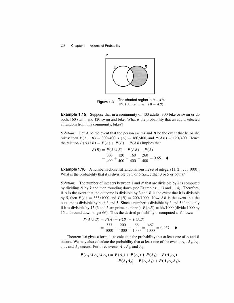
Figure 1.3 The shaded region is B −AB.Thus A ∪ B = A ∪ (B − AB).
Example 1.15 Suppose that in a community of 400 adults, 300 bike or swim or doboth, 160 swim, and 120 swim and bike. What is the probability that an adult, selectedat random from this community, bikes?
Solution: Let A be the event that the person swims and B be the event that he or shebikes; then P(A ∪ B) = 300/400, P(A) = 160/400, and P(AB) = 120/400. Hencethe relation P(A ∪ B) = P(A) + P(B) − P(AB) implies that
P(B) = P(A ∪ B) + P(AB) − P(A)
= 300
400+ 120
400− 160
400= 260
400= 0.65. �
Example 1.16 A number is chosen at random from the set of integers {1, 2, . . . , 1000}.What is the probability that it is divisible by 3 or 5 (i.e., either 3 or 5 or both)?
Solution: The number of integers between 1 and N that are divisible by k is computedby dividing N by k and then rounding down (see Examples 1.13 and 1.14). Therefore,if A is the event that the outcome is divisible by 3 and B is the event that it is divisibleby 5, then P(A) = 333/1000 and P(B) = 200/1000. Now AB is the event that theoutcome is divisible by both 3 and 5. Since a number is divisible by 3 and 5 if and onlyif it is divisible by 15 (3 and 5 are prime numbers), P(AB) = 66/1000 (divide 1000 by15 and round down to get 66). Thus the desired probability is computed as follows:
P(A ∪ B) = P(A) + P(B) − P(AB)
= 333
1000+ 200
1000− 66
1000= 467
1000= 0.467. �
Theorem 1.6 gives a formula to calculate the probability that at least one of A and B
occurs. We may also calculate the probability that at least one of the events A1, A2, A3,. . . , and An occurs. For three events A1, A2, and A3,
P(A1 ∪ A2 ∪ A3) = P(A1) + P(A2) + P(A3) − P(A1A2)
− P(A1A3) − P(A2A3) + P(A1A2A3).

Section 1.4 Basic Theorems 21
For four events,
P(A1 ∪ A2 ∪ A3 ∪ A4) = P(A1) + P(A2) + P(A3) + P(A4) − P(A1A2)
− P(A1A3) − P(A1A4) − P(A2A3) − P(A2A4)
− P(A3A4) + P(A1A2A3) + P(A1A2A4)
+ P(A1A3A4) + P(A2A3A4) − P(A1A2A3A4).
We now explain a procedure, which will enable us to find P(A1 ∪ A2 ∪ · · · ∪ An), theprobability that at least one of the events A1, A2, · · · , An occurs.
Inclusion-Exclusion Principle To calculate P(A1 ∪A2 ∪ · · · ∪An), first find all ofthe possible intersections of events from A1, A2, . . . , An and calculate their probabilities.Then add the probabilities of those intersections that are formed of an odd number ofevents, and subtract the probabilities of those formed of an even number of events.
The following formula is an expression for the principle of inclusion-exclusion. It followsby induction. (For an intuitive proof, see Example 2.29.)
P( n⋃
i=1
Ai
)=
n∑i=1
P(Ai) −n−1∑i=1
n∑j=i+1
P(AiAj ) +n−2∑i=1
n−1∑j=i+1
n∑k=j+1
P(AiAjAk)
− · · · + (−1)n−1P(A1A2 · · · An).
Example 1.17 Suppose that 25% of the population of a city read newspaper A, 20%read newspaper B, 13% read C, 10% read both A and B, 8% read both A and C, 5% readB and C, and 4% read all three. If a person from this city is selected at random, what isthe probability that he or she does not read any of these newspapers?
Solution: Let E, F , and G be the events that the person reads A, B, and C, respectively.The event that the person reads at least one of the newspapers A, B, or C is E ∪ F ∪ G.Therefore, 1 − P(E ∪ F ∪ G) is the probability that he or she reads none of them. Since
P(E ∪ F ∪ G) = P(E) + P(F) + P(G) − P(EF) − P(EG)
− P(FG) + P(EFG)
= 0.25 + 0.20 + 0.13 − 0.10 − 0.08 − 0.05 + 0.04 = 0.39,
the desired probability equals 1 − 0.39 = 0.61. �
Example 1.18 Dr. Grossman, an internist, has 520 patients, of which (1) 230 arehypertensive, (2) 185 are diabetic, (3) 35 are hypochondriac and diabetic, (4) 25 are allthree, (5) 150 are none, (6) 140 are only hypertensive, and finally, (7) 15 are hyper-tensive and hypochondriac but not diabetic. Find the probability that Dr. Grossman’snext appointment is hypochondriac but neither diabetic nor hypertensive. Assume that

22 Chapter 1 Axioms of Probability
appointments are all random. This implies that even hypochondriacs do not make morevisits than others.
Solution: Let T , C, and D denote the events that the next appointment of Dr. Gross-man is hypertensive, hypochondriac, and diabetic, respectively. The Venn diagram ofFigure 1.4 shows that the number of patients with only hypochondria is 30. Therefore,the desired probability is 30/520 ≈ 0.06. �
Figure 1.4 Venn diagram of Example 1.18.
Theorem 1.7 P(A) = P(AB) + P(ABc).
Proof: Clearly, A = AS = A(B ∪Bc) = AB ∪ABc. Since AB and ABc are mutuallyexclusive,
P(A) = P(AB ∪ ABc) = P(AB) + P(ABc). �
Example 1.19 In a community, 32% of the population are male smokers; 27% arefemale smokers. What percentage of the population of this community smoke?
Solution: Let A be the event that a randomly selected person from this communitysmokes. Let B be the event that the person is male. By Theorem 1.7,
P(A) = P(AB) + P(ABc) = 0.32 + 0.27 = 0.59.
Therefore, 59% of the population of this community smoke. �
Remark 1.4 In the real world, especially for games of chance, it is common to expressprobability in terms of odds. We say that the odds in favor of an event A are r to s ifP(A) = r/(r + s). Similarly, the odds against an event A are r to s if P(A) = s/(r + s).Therefore, if the odds in favor of an event A are r to s, then the odds against A are s
to r . For example, in drawing a card at random from an ordinary deck of 52 cards, theodds against drawing an ace are 48 to 4 or, equivalently, 12 to 1. The odds in favor of anace are 4 to 48 or, equivalently, 1 to 12. If for an event A, P(A) = p, then the odds infavor of A are p to 1 − p. Therefore, for example, in flipping a fair coin three times, byExample 1.11, the odds in favor of HHH are 1/8 to 7/8 or, equivalently, 1 to 7. �

Section 1.4 Basic Theorems 23
EXERCISES
A
1. Gottfried Wilhelm Leibniz (1646–1716), the German mathematician, philosopher,statesman, and one of the supreme intellects of the seventeenth century, believedthat in a throw of a pair of fair dice, the probability of obtaining the sum 11 isequal to that of obtaining the sum 12. Do you agree with Leibniz? Explain.
2. Suppose that 33% of the people have O+ blood and 7% have O−. What is theprobability that the next president of the United States has type O blood?
3. The probability that an earthquake will damage a certain structure during a yearis 0.015. The probability that a hurricane will damage the same structure duringa year is 0.025. If the probability that both an earthquake and a hurricane willdamage the structure during a year is 0.0073, what is the probability that next yearthe structure will not be damaged by a hurricane or an earthquake?
4. Suppose that the probability that a driver is a male, and has at least one motorvehicles accident during a one-year period, is 0.12. Suppose that the correspondingprobability for a female is 0.06. What is the probability of a randomly selecteddriver having at least one accident during the next 12 months?
5. Suppose that 75% of all investors invest in traditional annuities and 45% of theminvest in the stock market. If 85% invest in the stock market and/or traditionalannuities, what percentage invest in both?
6. In a horse race, the odds in favor of the first horse winning in an 8-horse race are 2to 5. The odds against the second horse winning are 7 to 3. What is the probabilitythat one of these horses will win?
7. Excerpt from the TV show The Rockford Files:
Rockford: There are only two doctors in town. The chances of bothautopsies being performed by the same doctor are 50–50.
Reporter: No, that is only for one autopsy. For two autopsies, thechances are 25–75.
Rockford: You’re right.
Was Rockford right to agree with the reporter? Explain why or why not?
8. A company has only one position with three highly qualified applicants: John,Barbara, and Marty. However, because the company has only a few women em-ployees, Barbara’s chance to be hired is 20% higher than John’s and 20% higherthan Marty’s. Find the probability that Barbara will be hired.
24 Chapter 1 Axioms of Probability
9. In a psychiatric hospital, the number of patients with schizophrenia is three timesthe number with psychoneurotic reactions, twice the number with alcohol addic-tions, and 10 times the number with involutional psychotic reaction. If a patient isselected randomly from the list of all patients with one of these four diseases, whatis the probability that he or she suffers from schizophrenia? Assume that none ofthese patients has more than one of these four diseases.
10. Let A and B be two events. Prove that
P(AB) ≥ P(A) + P(B) − 1.
11. A card is drawn at random from an ordinary deck of 52 cards. What is the proba-bility that it is (a) a black ace or a red queen; (b) a face or a black card; (c) neithera heart nor a queen?
12. Which of the following statements is true? If a statement is true, prove it. If it isfalse, give a counterexample.
(a) If P(A) + P(B) + P(C) = 1, then the events A, B, and C are mutuallyexclusive.
(b) If P(A ∪ B ∪ C) = 1, then A, B, and C are mutually exclusive events.
13. Suppose that in the Baltimore metropolitan area 25% of the crimes occur duringthe day and 80% of the crimes occur in the city. If only 10% of the crimes occuroutside the city during the day, what percent occur inside the city during the night?What percent occur outside the city during the night?
14. Let A, B, and C be three events. Prove that
P(A ∪ B ∪ C)
= P(A) + P(B) + P(C) − P(AB) − P(AC) − P(BC) + P(ABC).
15. Let A, B, and C be three events. Show that exactly two of these events will occurwith probability
P(AB) + P(AC) + P(BC) − 3P(ABC).
16. Eleven chairs are numbered 1 through 11. Four girls and seven boys sit on thesechairs at random. What is the probability that chair 5 is occupied by a boy?
17. A ball is thrown at a square that is divided into n2 identical squares. The prob-ability that the ball hits the square of the ith column and j th row is pij , where∑n
i=1
∑nj=1 pij = 1. In terms of pij ’s, find the probability that the ball hits the j th
horizontal strip.
18. Among 33 students in a class, 17 of them earned A’s on the midterm exam, 14earned A’s on the final exam, and 11 did not earn A’s on either examination. What

Section 1.4 Basic Theorems 25
is the probability that a randomly selected student from this class earned an A onboth exams?
19. From a small town 120 persons were selected at random and asked the followingquestion: Which of the three shampoos, A, B, or C, do you use? The followingresults were obtained: 20 use A and C, 10 use A and B but not C, 15 use all three,30 use only C, 35 use B but not C, 25 use B and C, and 10 use none of the three.If a person is selected at random from this group, what is the probability that heor she uses (a) only A; (b) only B; (c) A and B? (Draw a Venn diagram.)
20. The coefficients of the quadratic equation x2 + bx + c = 0 are determined bytossing a fair die twice (the first outcome is b, the second one is c). Find theprobability that the equation has real roots.
21. Two integers m and n are called relatively prime if 1 is their only common positivedivisor. Thus 8 and 5 are relatively prime, whereas 8 and 6 are not. A number isselected at random from the set {1, 2, 3, . . . , 63}. Find the probability that it isrelatively prime to 63.
22. A number is selected randomly from the set {1, 2, . . . , 1000}. What is the proba-bility that (a) it is divisible by 3 but not by 5; (b) it is divisible neither by 3 nor by5?
23. The secretary of a college has calculated that from the students who took calculus,physics, and chemistry last semester, 78% passed calculus, 80% physics, 84%chemistry, 60% calculus and physics, 65% physics and chemistry, 70% calculusand chemistry, and 55% all three. Show that these numbers are not consistent, andtherefore the secretary has made a mistake.
B
24. From an ordinary deck of 52 cards, we draw cards at random and without replace-ment until only cards of one suit are left. Find the probability that the cards leftare all spades.
25. A number is selected at random from the set of natural numbers {1, 2, . . . , 1000}.What is the probability that it is divisible by 4 but neither by 5 nor by 7 ?
26. For a Democratic candidate to win an election, she must win districts I, II, andIII. Polls have shown that the probability of winning I and III is 0.55, losing II butnot I is 0.34, and losing II and III but not I is 0.15. Find the probability that thiscandidate will win all three districts. (Draw a Venn diagram.)
27. Two numbers are successively selected at random and with replacement from theset {1, 2, . . . , 100}. What is the probability that the first one is greater than thesecond?
26 Chapter 1 Axioms of Probability
28. Let A1, A2, A3, . . . be a sequence of events of a sample space. Prove that
P( ∞⋃
n=1
An
)≤
∞∑n=1
P(An).
This is called Boole’s inequality.
29. Let A1, A2, A3, . . . be a sequence of events of an experiment. Prove that
P( ∞⋂
n=1
An
)≥ 1 −
∞∑n=1
P(Acn).
Hint: Use Boole’s inequality, discussed in Exercise 28.
30. In a certain country, the probability is 49/50 that a randomly selected fighter planereturns from a mission without mishap. Mia argues that this means there is onemission with a mishap in every 50 consecutive flights. She concludes that if afighter pilot returns safely from 49 consecutive missions, he should return homebefore his fiftieth mission. Is Mia right? Explain why or why not.
31. Let P be a probability defined on a sample space S. For events A of S defineQ(A) = [P(A)
]2and R(A) = P(A)/2. Is Q a probability on S? Is R a probability
on S? Why or why not?
In its general case, the following exercise has important applications in coding theory,telecommunications, and computer science.
32. (The Hat Problem) A game begins with a team of three players entering aroom one at a time. For each player, a fair coin is tossed. If the outcome is heads,a red hat is placed on the player’s head, and if it is tails, a blue hat is placed on theplayer’s head. The players are allowed to communicate before the game beginsto decide on a strategy. However, no communication is permitted after the gamebegins. Players cannot see their own hats. But each player can see the other twoplayers’ hats. Each player is given the option to guess the color of his or her hat orto pass. The game ends when the three players simultaneously make their choices.The team wins if no player’s guess is incorrect and at least one player’s guess iscorrect. Obviously, the team’s goal is to develop a strategy that maximizes theprobability of winning. A trivial strategy for the team would be for two of itsplayers to pass and the third player to guess red or blue as he or she wishes. Thisgives the team a 50% chance to win. Can you think of a strategy that improves thechances of the team winning?

Section 1.5 Continuity of Probability Function 27
1.5 CONTINUITY OF PROBABILITY FUNCTIONS
Let R denote(here and everywhere else throughout the book) the set of all real numbers.We know from calculus that a function f : R → R is called continuous at a point c ∈ Rif limx→c f (x) = f (c). It is called continuous on R if it is continuous at all points c ∈ R.We also know that this definition is equivalent to the sequential criterion f : R → R iscontinuous on R if and only if, for every convergent sequence {xn}∞n=1 in R,
limn→∞ f (xn) = f ( lim
n→∞ xn). (1.4)
This property, in some sense, is shared by the probability function. To explain this, weneed to introduce some definitions. But first recall that probability is a set function fromP(S), the set of all possible events of the sample space S, to [0, 1].
A sequence {En, n ≥ 1} of events of a sample space is called increasing if
E1 ⊆ E2 ⊆ E3 ⊆ · · · ⊆ En ⊆ En+1 · · · ;
it is called decreasing if
E1 ⊇ E2 ⊇ E3 ⊇ · · · ⊇ En ⊇ En+1 ⊇ · · · .
For an increasing sequence of events {En, n ≥ 1}, by limn→∞ En we mean the event thatat least one Ei, 1 ≤ i < ∞ occurs. Therefore,
limn→∞ En =
∞⋃n=1
En.
Similarly, for a decreasing sequence of events {En, n ≥ 1}, by limn→∞ En we mean theevent that every Ei occurs. Thus in this case
limn→∞ En =
∞⋂n=1
En.
The following theorem expresses the property of probability function that is analogousto (1.4).
Theorem 1.8 (Continuity of Probability Function) For any increasing ordecreasing sequence of events, {En, n ≥ 1},
limn→∞ P(En) = P( lim
n→∞ En).

28 Chapter 1 Axioms of Probability
Figure 1.5The circular disks are the Ei ’s and the shaded circular annuliare the Fi ’s, except for F1, which equals E1.
Proof: For the case where {En, n ≥ 1} is increasing, let F1 = E1, F2 = E2 − E1,F3 = E3 − E2, . . . , Fn = En − En−1, . . . . Clearly, {Fi, i ≥ 1} is a mutually exclusiveset of events that satisfies the following relations:
n⋃i=1
Fi =n⋃
i=1
Ei = En, n = 1, 2, 3, . . . ,
∞⋃i=1
Fi =∞⋃i=1
Ei
(see Figure 1.5). Hence
P( limn→∞ En) = P
( ∞⋃i=1
Ei
)= P
( ∞⋃i=1
Fi
)=
∞∑i=1
P(Fi) = limn→∞
n∑i=1
P(Fi)
= limn→∞ P
( n⋃i=1
Fi
)= lim
n→∞ P( n⋃
i=1
Ei
)= lim
n→∞ P(En),
where the last equality follows since {En, n ≥ 1} is increasing, and hence⋃n
i=1 Ei = En.
This establishes the theorem for increasing sequences.If {En, n ≥ 1} is decreasing, then En ⊇ En+1, ∀n, implies that Ec
n ⊆ Ecn+1, ∀n.
Therefore, the sequence {Ecn, n ≥ 1} is increasing and
P( limn→∞ En) = P
( ∞⋂i=1
Ei
)= 1 − P
[( ∞⋂i=1
Ei
)c ] = 1 − P( ∞⋃
i=1
Eci
)= 1 − P( lim
n→∞ Ecn) = 1 − lim
n→∞ P(Ecn) = 1 − lim
n→∞[1 − P(En)
]= 1 − 1 + lim
n→∞ P(En) = limn→∞ P(En). �
Example 1.20 Suppose that some individuals in a population produce offspring ofthe same kind. The offspring of the initial population are called second generation,

Section 1.6 Probabilities 0 and 1 29
the offspring of the second generation are called third generation, and so on. If withprobability exp
[− (2n2 +7)/(6n2)]
the entire population completely dies out by the nthgeneration before producing any offspring, what is the probability that such a populationsurvives forever?
Solution: Let En denote the event of extinction of the entire population by the nthgeneration; then
E1 ⊆ E2 ⊆ E3 ⊆ · · · ⊆ En ⊆ En+1 ⊆ · · ·because if En occurs, then En+1 also occurs. Hence, by Theorem 1.8,
P {population survives forever} = 1 − P {population eventually dies out}
= 1 − P( ∞⋃
i=1
Ei
)= 1 − lim
n→∞ P(En)
= 1 − limn→∞ exp
(− 2n2 + 7
6n2
)=1−e−1/3. �
1.6 PROBABILITIES 0 AND 1
Events with probabilities 1 and 0 should not be misinterpreted. If E and F are eventswith probabilities 1 and 0, respectively, it is not correct to say that E is the sample spaceS and F is the empty set ∅. In fact, there are experiments in which there exist infinitelymany events each with probability 1, and infinitely many events each with probability 0.An example follows.
Suppose that an experiment consists of selecting a random point from the interval(0, 1). Since every point in (0, 1) has a decimal representation such as
0.529387043219721 · · · ,
the experiment is equivalent to picking an endless decimal from (0, 1) at random (note thatif a decimal terminates, all of its digits from some point on are 0). In such an experimentwe want to compute the probability of selecting the point 1/3. In other words, we wantto compute the probability of choosing 0.333333 · · · in a random selection of an endlessdecimal. Let An be the event that the selected decimal has 3 as its first n digits; then
A1 ⊃ A2 ⊃ A3 ⊃ A4 ⊃ · · · ⊃ An ⊃ An+1 ⊃ · · · ,
since the occurrence of An+1 guarantees the occurrence of An. Now P(A1) = 1/10because there are 10 choices 0, 1, 2, . . . , 9 for the first digit, and we want only one ofthem, namely 3, to occur. P(A2) = 1/100 since there are 100 choices 00, 01, . . . , 09,10, 11, . . . , 19, 20, . . . , 99 for the first two digits, and we want only one of them, 33, tooccur. P(A3) = 1/1000 because there are 1000 choices 000, 001, . . . , 999 for the first

30 Chapter 1 Axioms of Probability
three digits, and we want only one of them, 333, to occur. Continuing this argument, wehave P(An) = (1/10)n. Since
⋂∞n=1 An = {1/3}, by Theorem 1.8,
P(1
3is selected
)= P
( ∞⋂n=1
An
)= lim
n→∞ P(An) = limn→∞
( 1
10
)n = 0.
Note that there is nothing special about the point 1/3. For any other point 0.α1α2α3α4 · · ·from (0, 1), the same argument could be used to show that the probability of its occur-rence is 0 (define An to be the event that the first n digits of the selected decimal areα1, α2, . . . , αn, respectively, and repeat the same argument). We have shown that in ran-dom selection of points from (0, 1), the probability of the occurrence of any particularpoint is 0. Now for t ∈ (0, 1), let Bt = (0, 1) − {t}. Then P
({t}) = 0 implies that
P(Bt) = P({t}c) = 1 − P
({t}) = 1.
Therefore, there are infinitely many events, Bt ’s, each with probability 1 and none equalto the sample space (0, 1).
1.7 RANDOM SELECTION OF POINTS FROM INTERVALS
In Section 1.6, we showed that the probability of the occurrence of any particular point ina random selection of points from an interval (a, b) is 0. This implies immediately that if[α, β] ⊆ (a, b), then the events that the point falls in [α, β], (α, β), [α, β), and (α, β] are
all equiprobable. Now consider the intervals(a,
a + b
2
)and
(a + b
2, b)
; sincea + b
2
is the midpoint of (a, b), it is reasonable to assume that
p1 = p2, (1.5)
where p1 is the probability that the point belongs to(a,
a + b
2
)and p2 is the probability
that it belongs to(a + b
2, b)
. The events that the random point belongs to(a,
a + b
2
)and
(a + b
2, b)
are mutually exclusive and
(a,
a + b
2
)∪[a + b
2, b)
= (a, b);therefore,
p1 + p2 = 1.
This relation and (1.5) imply that
p1 = p2 = 1/2.

Section 1.7 Random Selection of Points from Intervals 31
Hence the probability that a random point selected from (a, b) falls into the interval(a,
a + b
2
)is 1/2. The probability that it falls into
[a + b
2, b)
is also 1/2. Note that the
length of each of these intervals is 1/2 of the length of (a, b). Now consider the intervals
(a,
2a + b
3
],(2a + b
3,a + 2b
3
], and
(a + 2b
3, b)
. Since2a + b
3and
a + 2b
3are the
points that divide the interval (a, b) into three subintervals with equal lengths, we canassume that
p1 = p2 = p3, (1.6)
where p1, p2, and p3 are the probabilities that the point falls into(a,
2a + b
3
],(2a + b
3,a + 2b
3
], and
(a + 2b
3, b), respectively. On the other hand, these three
intervals are mutually disjoint and(a,
2a + b
3
]∪(2a + b
3,a + 2b
3
]∪(a + 2b
3, b)
= (a, b).
Hencep1 + p2 + p3 = 1.
This relation and (1.6) imply that
p1 = p2 = p3 = 1/3.
Therefore, the probability that a random point selected from (a, b) falls into the interval(a,
2a + b
3
]is 1/3. The probability that it falls into
(2a + b
3,a + 2b
3
]is 1/3, and the
probability that it falls into(a + 2b
3, b)
is 1/3. Note that the length of each of these
intervals is 1/3 of the length of (a, b). These and other similar observations indicate thatthe probability of the event that a random point from (a, b) falls into a subinterval (α, β)
is equal to (β − α)/(b − a).Note that in this discussion we have assumed that subintervals of equal lengths are
equiprobable. Even though two subintervals of equal lengths may differ by a finite or acountably infinite set (or even a set of measure zero), this assumption is still consistentwith our intuitive understanding of choosing random points from intervals. This isbecause in such an experiment, the probability of the occurrence of a finite or countablyinfinite set (or a set of measure zero) is 0.

32 Chapter 1 Axioms of Probability
Thus far, we have based our discussion of selecting random points from intervals onour intuitive understanding of this experiment and not on a mathematical definition. Suchdiscussions are often necessary for the creation of appropriate mathematical meaningsfor unclear concepts. The following definition, which is based on our intuitive analysis,gives an exact mathematical meaning to the experiment of random selection of pointsfrom intervals.
Definition A point is said to be randomly selected from an interval (a, b) if any twosubintervals of (a, b) that have the same length are equally likely to include the point.The probability associated with the event that the subinterval (α, β) contains the pointis defined to be (β − α)/(b − a).
As explained before, choosing a random number from (0, 1) is equivalent to choos-ing randomly all the decimal digits of the number successively. Since in practice thisis impossible, choosing exact random points or numbers from (0, 1) or any other in-terval is only a theoretical matter. Approximate random numbers, however, can begenerated by computers. Most of the computer languages, some scientific computersoftware, and some calculators are equipped with subroutines that generate approxi-mate random numbers from intervals. However, since it is difficult to construct goodrandom number generators, there are computer languages, software programs, and cal-culators that are equipped with poor random number generator algorithms. An excellentreference for construction of good random number generators is The Art of ComputerProgramming, Volume 2, Seminumerical Algorithms, third edition, by Donald E. Knuth(Addison Wesley, 1998). Simple mechanical tools can also be used to find such approx-imations. For example, consider a spinner mounted on a wheel of unit circumference(radius 1/2π ). Let A be a point on the perimeter of the wheel. Each time that we flickthe spinner, it stops, pointing toward some point B on the wheel’s circumference. Thelength of the arc AB (directed, say, counterclockwise) is an approximate random numberbetween 0 and 1 if the spinner does not have any “sticky” spots (see Figure 1.6).
Figure 1.6 Spinner, a model to generate random numbers.
Finally, when selecting a random point from an interval (a, b), we may think of anextremely large hypothetical box that contains infinitely many indistinguishable balls.

Section 1.7 Random Selection of Points from Intervals 33
Imagine that each ball is marked by a number from (a, b), each number of (a, b) ismarked on exactly one ball, and the balls are completely mixed up, so that in a randomselection of balls, any two of them have the same chance of being drawn. With thistranscendental model in mind, choosing a random number from (a, b) is then equivalentto drawing a random ball from such a box and looking at its number.
� Example 1.21 (A Set that Is Not an Event) Let an experiment consist ofselecting a point at random from the interval [−1, 2]. We will construct a set that isnot an event (i.e., it is impossible to associate a probability with the set). We begin bydefining an equivalence relation on [0, 1]: x ∼ y if x − y is a rational number. LetQ = {r1, r2, . . . } be the set of rational numbers in [−1, 1]. Clearly, x is equivalent to y
if x − y ∈ Q. The fact that this relation is reflexive, symmetric, and transitive is trivial.Therefore, being an equivalence relation, it partitions the interval [0, 1] into disjointequivalence classes (�α). These classes are such that if x and y ∈ �α for some α, thenx − y is rational. However, if x ∈ �α and y ∈ �β , and α �= β, then x − y is irrational.These observations imply that for each α, the equivalence class �α is countable. Since⋃
α �α = [0, 1] is uncountable, the number of equivalence classes is uncountable. LetE be a set consisting of exactly one point from each equivalence class �α. The existenceof such a set is guaranteed by the Axiom of Choice. We will show, by contradiction, thatE is not an event. Suppose that E is an event, and let p be the probability associatedwith E. For each positive integer n, let En = {rn + x : x ∈ E} ⊆ [−1, 2]. For eachrn ∈ Q, En is simply a translation of E. Thus, for all n, the set En is also an event, andP(En) = P(E) = p.
We now make two more observations: (1) For n �= m, En ∩ Em = ∅, (2) [0, 1] ⊂⋃∞n=1 En. To prove (1), let t ∈ En ∩ Em. We will show that En = Em. If t ∈ En ∩ Em,
then for some rn, rm ∈ Q, and x, y ∈ E, we have that t = rn + x = rm + y. That is,x − y = rm − rn is rational, and x − y belongs to the same equivalence class. Since E
has exactly one point from each equivalence class, we must have x = y, hence rn = rm,hence En = Em. To prove (2), let x ∈ [0, 1]. Then x ∼ y for some y ∈ E. This impliesthat x − y is a rational number in Q. That is, for some n, x − y = rn, or x = y + rn, orx ∈ En. Thus x ∈⋃∞
n=1 En.
Putting (1) and (2) together, we obtain
1/3 = P([0, 1]) ≤ P
( ∞⋃n=1
En
)≤ 1,
or
1/3 ≤∞∑
n=1
P(En) =∞∑
n=1
p ≤ 1.
This is a contradiction because∑∞
n=1 p is either 0 or ∞. Hence E is not an event, andwe cannot associate a probability with this set. �

34 Chapter 1 Axioms of Probability
EXERCISES
A
1. A bus arrives at a station every day at a random time between 1:00 P.M. and 1:30 P.M.
What is the probability that a person arriving at this station at 1:00 P.M. will haveto wait at least 10 minutes?
2. Past experience shows that every new book by a certain publisher captures ran-domly between 4 and 12% of the market. What is the probability that the nextbook by this publisher captures at most 6.35% of the market?
3. Which of the following statements are true? If a statement is true, prove it. If it isfalse, give a counterexample.
(a) If A is an event with probability 1, then A is the sample space.
(b) If B is an event with probability 0, then B = ∅.
4. Let A and B be two events. Show that if P(A) = 1 and P(B) = 1, thenP(AB) = 1.
5. A point is selected at random from the interval (0, 2000). What is the probabilitythat it is an integer?
6. Suppose that a point is randomly selected from the interval (0, 1). Using thedefinition in Section 1.7, show that all numerals are equally likely to appear as thefirst digit of the decimal representation of the selected point.
B
7. Is it possible to define a probability on a countably infinite sample space so thatthe outcomes are equally probable?
8. Let A1, A2, . . . , An be n events. Show that if
P(A1) = P(A2) = · · · = P(An) = 1,
then P(A1A2 · · · An) = 1.
9. (a) Prove that⋂∞
n=1(1/2 − 1/2n, 1/2 + 1/2n) = {1/2}.(b) Using part (a), show that the probability of selecting 1/2 in a random selec-
tion of a point from (0, 1) is 0.
10. A point is selected at random from the interval (0, 1). What is the probability thatit is rational? What is the probability that it is irrational?
Chapter 1 Review Problems 35
11. Suppose that a point is randomly selected from the interval (0, 1). Using thedefinition in Section 1.7, show that all numerals are equally likely to appear as thenth digit of the decimal representation of the selected point.
12. Let {A1, A2, A3, . . . } be a sequence of events. Prove that if the series∑∞
n=1 P(An)
converges, then P(⋂∞
m=1
⋃∞n=m An
)= 0. This is called the Borel-Cantelli
lemma. It says that if∑∞
n=1 P(An) < ∞, the probability that infinitely manyof the An’s occur is 0.Hint: Let Bm =⋃∞
n=m An and apply Theorem 1.8 to {Bm, m ≥ 1}.13. Show that the result of Exercise 8 is not true for an infinite number of events. That
is, show that if {Et : 0 < t < 1} is a collection of events for which P(Et) = 1, it
is not necessarily true that P( ⋂
t∈(0,1)
Et
)= 1.
14. Let A be the set of rational numbers in (0, 1). Since A is countable, it can be writtenas a sequence
(i.e.,A = {rn : n = 1, 2, 3, . . . }). Prove that for any ε > 0, A can
be covered by a sequence of open balls whose total length is less than ε. That is,∀ε > 0, there exists a sequence of open intervals (αn, βn) such that rn ∈ (αn, βn)
and∑∞
n=1(βn −αn) < ε. This important result explains why in a random selectionof points from (0, 1) the probability of choosing a rational is zero.Hint: Let αn = rn − ε/2n+2, βn = rn + ε/2n+2.
REVIEW PROBLEMS
1. The number of minutes it takes for a certain animal to react to a certain stimulusis a random number between 2 and 4.3. Find the probability that the reaction timeof such an animal to this stimulus is no longer than 3.25 minutes.
2. Let P be the set of all subsets of A = {1, 2}. We choose two distinct sets randomlyfrom P . Define a sample space for this experiment, and describe the followingevents:
(a) The intersection of the sets chosen at random is empty.
(b) The sets are complements of each other.
(c) One of the sets contains more elements than the other.
3. In a certain experiment, whenever the event A occurs, the event B also occurs.Which of the following statements is true and why?
(a) If we know that A has not occurred, we can be sure that B has not occurredas well.

36 Chapter 1 Axioms of Probability
(b) If we know that B has not occurred, we can be sure that A has not occurredas well.
4. The following relations are not always true. In each case give an example to refutethem.
(a) P(A ∪ B) = P(A) + P(B).
(b) P(AB) = P(A)P (B).
5. A coin is tossed until, for the first time, the same result appears twice in succession.Define a sample space for this experiment.
6. The number of the patients now in a hospital is 63. Of these 37 are male and 20are for surgery. If among those who are for surgery 12 are male, how many of the63 patients are neither male nor for surgery?
7. Let A, B, and C be three events. Prove that
P(A ∪ B ∪ C) ≤ P(A) + P(B) + P(C).
8. Let A, B, and C be three events. Show that
P(A ∪ B ∪ C) = P(A) + P(B) + P(C)
if and only if P(AB) = P(AC) = P(BC) = 0.
9. Suppose that 40% of the people in a community drink or serve white wine, 50%drink or serve red wine, and 70% drink or serve red or white wine. What percentageof the people in this community drink or serve both red and white wine?
10. Answer the following question, asked of Marilyn Vos Savant in the “Ask Marilyn”column of Parade Magazine, March 3, 1996.
My dad heard this story on the radio. At Duke University, two studentshad received A’s in chemistry all semester. But on the night beforethe final exam, they were partying in another state and didn’t get backto Duke until it was over. Their excuse to the professor was that theyhad a flat tire, and they asked if they could take a make-up test. Theprofessor agreed, wrote out a test and sent the two to separate roomsto take it. The first question (on one side of the paper) was worth 5points, and they answered it easily. Then they flipped the paper overand found the second question, worth 95 points: ‘Which tire was it?’What was the probability that both students would say the same thing?My dad and I think it’s 1 in 16. Is that right?
11. Let A and B be two events. Suppose that P(A), P(B), and P(AB) are given.What is the probability that neither A nor B will occur?

Chapter 1 Review Problems 37
12. Let A and B be two events. The event (A−B)∪ (B −A) is called the symmetricdifference of A and B and is denoted by A B. Clearly, A B is the event thatexactly one of the two events A and B occurs. Show that
P(A B) = P(A) + P(B) − 2P(AB).
13. A bookstore receives six boxes of books per month on six random days of eachmonth. Suppose that two of those boxes are from one publisher, two from anotherpublisher, and the remaining two from a third publisher. Define a sample spacefor the possible orders in which the boxes are received in a given month by thebookstore. Describe the event that the last two boxes of books received last monthare from the same publisher.
14. Suppose that in a certain town the number of people with blood type O and bloodtype A are approximately the same. The number of people with blood type B is1/10 of those with blood type A and twice the number of those with blood typeAB. Find the probability that the next baby born in the town has blood type AB.
15. A number is selected at random from the set of natural numbers {1, 2, 3, . . . , 1000}.What is the probability that it is not divisible by 4, 7, or 9?
16. A number is selected at random from the set {1, 2, 3, . . . , 150}. What is theprobability that it is relatively prime to 150? See Exercise 21, Section 1.4, for thedefinition of relatively prime numbers.
17. Suppose that each day the price of a stock moves up 1/8 of a point, moves down1/8 of a point, or remains unchanged. For i ≥ 1, let Ui and Di be the events thatthe price of the stock moves up and down on the ith trading day, respectively. Interms of Ui’s and Di’s, find an expression for the event that the price of the stock
(a) remains unchanged on the ith trading day;
(b) moves up every day of the next n trading days;
(c) remains unchanged on at least one of the next n trading days;
(d) is the same as today after three trading days;
(e) does not move down on any of the next n trading days.
18. A bus traveling from Baltimore to New York has breaks down at a random loca-tion. What is the probability that the breakdown occurred after passing throughPhiladelphia? The distances from New York and Philadelphia to Baltimore are,respectively, 199 and 96 miles.
19. The coefficient of the quadratic equation ax2 + bx + c = 0 are determined bytossing a fair die three times (the first outcome is a, the second one b, and the thirdone c). Find the probability that the equation has no real roots.

Chapter 2
Combinatorial Methods
2.1 INTRODUCTION
The study of probability includes many applications, such as games of chance, occupancyand order problems, and sampling procedures. In some of such applications, we deal withfinite sample spaces in which all sample points are equally likely to occur. Theorem 1.3shows that, in such cases, the probability of an event A is evaluated simply by dividing thenumber of points of A by the total number of sample points. Therefore, some probabilityproblems can be solved simply by counting the total number of sample points and thenumber of ways that an event can occur.
In this chapter we study a few rules that enable us to count systematically. Combi-natorial analysis deals with methods of counting: a very broad field with applications invirtually every branch of applied and pure mathematics. Besides probability and statistics,it is used in information theory, coding and decoding, linear programming, transporta-tion problems, industrial planning, scheduling production, group theory, foundations ofgeometry, and other fields. Combinatorial analysis, as a formal branch of mathematics,began with Tartaglia in the sixteenth century. After Tartaglia, Pascal, Fermat, ChevalierAntoine de Méré (1607–1684), James Bernoulli, Gottfried Leibniz, and Leonhard Eu-ler (1707–1783) made contributions to this field. The mathematical development of thetwentieth century accelerated development by combinatorial analysis.
2.2 COUNTING PRINCIPLES
Suppose that there are n routes from town A to town B, and m routes from B to a thirdtown, C. If we decide to go from A to C via B, then for each route that we choose fromA to B, we have m choices from B to C. Therefore, altogether we have nm choices togo from A to C via B. This simple example motivates the following principle, which isthe basis of this chapter.
Theorem 2.1 (Counting Principle) If the set E contains n elements and the setF contains m elements, there are nm ways in which we can choose, first, an element ofE and then an element of F .
38

Section 2.2 Counting Principle 39
Proof: Let E = {a1, a2, . . . , an} and F = {b1, b2, . . . , bm}; then the followingrectangular array, which consists of nm elements, contains all possible ways that we canchoose, first, an element of E and then an element of F .
(a1, b1), (a1, b2), . . . , (a1, bm)
(a2, b1), (a2, b2), . . . , (a2, bm)...
(an, b1), (an, b2), . . . , (an, bm) �
Now suppose that a fourth town, D, is connected to C by � routes. If we decide to gofrom A to D, passing through C after B, then for each pair of routes that we choose fromA to C, there are � possibilities from C to D. Therefore, by the counting principle, thetotal number of ways we can go from A to D via B and C is the number of ways we cango from A to C through B times �, that is, nm�. This concept motivates a generalizationof the counting principle.
Theorem 2.2 (Generalized Counting Principle) Let E1, E2, . . . , Ek be setswith n1, n2, . . . , nk elements, respectively. Then there are n1 × n2 × n3 × · · · × nk waysin which we can, first, choose an element of E1, then an element of E2, then an elementof E3, . . . , and finally an element of Ek.
In probability, this theorem is used whenever we want to compute the total number ofpossible outcomes when k experiments are performed. Suppose that the first experimenthas n1 possible outcomes, the second experiment has n2 possible outcomes, . . . , and thekth experiment has nk possible outcomes. If we define Ei to be the set of all possibleoutcomes of the ith experiment, then the total number of possible outcomes coincideswith the number of ways that we can, first, choose an element of E1, then an element ofE2, then an element of E3, . . . , and finally an element of Ek; that is, n1 × n2 × · · · × nk.
Example 2.1 How many outcomes are there if we throw five dice?
Solution: Let Ei , 1 ≤ i ≤ 5, be the set of all possible outcomes of the ith die. ThenEi = {1, 2, 3, 4, 5, 6}. The number of the outcomes of throwing five dice equals thenumber of ways we can, first, choose an element of E1, then an element of E2, . . . , andfinally an element of E5. Thus we get 6 × 6 × 6 × 6 × 6 = 65. �
Remark 2.1 Consider experiments such as flipping a fair coin several times, tossinga number of fair dice, drawing a number of cards from an ordinary deck of 52 cards atrandom and with replacement, and drawing a number of balls from an urn at random andwith replacement. In Section 3.5, discussing the concept of independence, we will showthat all the possible outcomes in such experiments are equiprobable. Until then, however,in all the problems dealing with these kinds of experiments, we assume, without explicitlyso stating in each case, that the sample points of the sample space of the experiment underconsideration are all equally likely. �

40 Chapter 2 Combinatorial Methods
Example 2.2 In tossing four fair dice, what is the probability of at least one 3?
Solution: Let A be the event of at least one 3. Then Ac is the event of no 3 in tossingthe four dice. N(Ac) and N , the number of sample points of Ac and the total number ofsample points, respectively, are given by 5 × 5 × 5 × 5 = 54 and 6 × 6 × 6 × 6 = 64.Therefore, P(Ac) = N(Ac)/N = 54/64. Hence P(A) = 1 −P(Ac) = 1 − 625/1296 =671/1296 ≈ 0.52. �
Example 2.3 Virginia wants to give her son, Brian, 14 different baseball cards withina 7-day period. If Virginia gives Brian cards no more than once a day, in how many wayscan this be done?
Solution: Each of the baseball cards can be given on 7 different days. Therefore, in7 × 7 × · · · × 7 = 714 ≈ 6.78 × 10¹¹ ways Virginia can give the cards to Brian. �
Example 2.4 Rose has invited n friends to her birthday party. If they all attend, andeach one shakes hands with everyone else at the party exactly once, what is the numberof handshakes?
Solution 1: There are n + 1 people at the party and each of them shakes hands withthe other n people. This is a total of (n + 1)n handshakes, but that is an overcount sinceit counts “A shakes hands with B” as one handshake and “B shakes hand with A” as asecond. Since each handshake is counted exactly twice, the actual number of handshakesis (n + 1)n/2.
Solution 2: Suppose that guests arrive one at a time. Rose will shake hands with all then guests. The first guest to appear will shake hands with Rose and all the remainingguests. Since we have already counted his or her handshake with Rose, there will ben − 1 additional handshakes. The second guest will also shake hands with n − 1 fellowguests and Rose. However, we have already counted his or her handshakes with Roseand the first guest. So this will add n − 2 additional handshakes. Similarly, the thirdguest will add n − 3 additional handshakes, and so on. Therefore, the total number ofhandshakes will be n + (n − 1) + (n − 2) + · · · + 3 + 2 + 1. Comparing solutions 1 and2, we have the well-known relation
1 + 2 + 3 · · · + (n − 2) + (n − 1) + n = n(n + 1)
2. �
Example 2.5 At a state university in Maryland, there is hardly enough space forstudents to park their cars in their own lots. Jack, a student who parks in the facultyparking lot every day, noticed that none of the last 10 tickets he got was issued on aMonday or on a Friday. Is it wise for Jack to conclude that the campus police do notpatrol the faculty parking lot on Mondays and on Fridays? Assume that police give notickets on weekends.

Section 2.2 Counting Principle 41
Solution: Suppose that the answer is negative and the campus police patrol the parkinglot randomly; that is, the parking lot is patrolled every day with the same probability. LetA be the event that out of 10 tickets given on random days, none is issued on a Mondayor on a Friday. If P(A) is very small, we can conclude that the campus police do notpatrol the parking lot on these two days. Otherwise, we conclude that what happened isaccidental and police patrol the parking lot randomly. To find P(A), note that since eachticket has five possible days of being issued, there are 510 possible ways for all ticketsto have been issued. Of these, in only 310 ways no ticket is issued on a Monday or ona Friday. Thus P(A) = 310/510 ≈ 0.006, a rather small probability. Therefore, it isreasonable to assume that the campus police do not patrol the parking lot on these twodays. �
Example 2.6 (Standard Birthday Problem) What is the probability that at leasttwo students of a class of size n have the same birthday? Compute the numerical valuesof such probabilities for n = 23, 30, 50, and 60. Assume that the birth rates are constantthroughout the year and that each year has 365 days.
Solution: There are 365 possibilities for the birthdays of each of the n students. There-fore, the sample space has 365n points. In 365×364×363×· · ·× [365− (n−1)
]ways
the birthdays of no two of the n students coincide. Hence P(n), the probability that notwo students have the same birthday, is
P(n) = 365 × 364 × 363 × · · · × [365 − (n − 1)]
365n,
and therefore the desired probability is 1−P(n). For n = 23, 30, 50, and 60 the answersare 0.507, 0.706, 0.970, and 0.995, respectively. �
Remark 2.2 In probability and statistics studies, birthday problems similar to Example2.6 have been very popular since 1939, when introduced by von Mises. This is probablybecause when solving such problems, numerical values obtained are often surprising.Persi Diaconis and Frederick Mosteller, two Harvard professors, have mentioned thatthey “find the utility of birthday problems impressive as a tool for thinking about coinci-dences.” Diaconis and Mosteller have illustrated basic statistical techniques for studyingthe fascinating, curious, and complicated “Theory of Coincidences” in the December1989 issue of the Journal of the American Statistical Association. In their study, theyhave used birthday problems “as examples which make the point that in many problemsour intuitive grasp of the odds is far off.” Throughout this book, where appropriate, wewill bring up some interesting versions of these problems, but now that we have cited“coincidence,” let us read a few sentences from the abstract of the aforementioned paperto get a better feeling for its meaning.

42 Chapter 2 Combinatorial Methods
Once we set aside coincidences having apparent causes, four principles ac-count for large numbers of remaining coincidences: hidden cause; psychol-ogy, including memory and perception; multiplicity of endpoints, includingthe counting of “close” or nearly alike events as if they were identical; andthe law of truly large numbers, which says that when enormous numbersof events and people and their interactions cumulate over time, almost anyoutrageous event is bound to occur. These sources account for much of theforce of synchronicity. �
Number of Subsets of a Set
Let A be a set. The set of all subsets of A is called the power set of A. As an importantapplication of the generalized counting principle, we now prove that the power set of aset with n elements has 2n elements. This important fact has lots of good applications.
Theorem 2.3 A set with n elements has 2n subsets.
Proof: Let A = {a1, a2, a3, . . . , an} be a set with n elements. Then there is a one-to-one correspondence between the subsets of A and the sequences of 0’s and 1’s of lengthn: To a subset B of A we associate a sequence b1b2b3 · · · bn, where bi = 0 if ai �∈ B,and bi = 1 if ai ∈ B. For example, if n = 3, we associate to the empty subset of A
the sequence 000, to {a2, a3} the sequence 011, and to {a1} the sequence 100. Now, bythe generalized counting principle, the number of sequences of 0’s and 1’s of length n is2 × 2 × 2 × · · · × 2 = 2n. Thus the number of subsets of A is also 2n. �
Example 2.7 A restaurant advertises that it offers over 1000 varieties of pizza. If, atthe restaurant, it is possible to have on a pizza any combination of pepperoni, mushrooms,sausage, green peppers, onions, anchovies, salami, bacon, olives, and ground beef, is therestaurant’s advertisement true?
Solution: Any combination of the 10 ingredients that the restaurant offers can be puton a pizza. Thus the number of different types of pizza that it is possible to make is equalto the number of subsets of the set {pepperoni, mushrooms, sausage, green peppers,onions, anchovies, salami, bacon, olives, ground beef}, which is 210 = 1024. Therefore,the restaurant’s advertisement is true. Note that the empty subset of the set of ingredientscorresponds to a plain cheese pizza. �
Tree Diagrams
Tree diagrams are useful pictorial representations that break down a complex countingproblem into smaller, more tractable ones. They are used in situations where the numberof possible ways an experiment can be performed is finite. The following examples

Section 2.2 Counting Principle 43
illustrate how tree diagrams are constructed and why they are useful. A great advantageof tree diagrams is that they systematically identify all possible cases.
Example 2.8 Bill and John keep playing chess until one of them wins two games ina row or three games altogether. In what percent of all possible cases does the game endbecause Bill wins three games without winning two in a row?
Figure 2.1 Tree diagram of Example 2.8.
Solution: The tree diagram of Figure 2.1 illustrates all possible cases. The total numberof possible cases is equal to the number of the endpoints of the branches, which is 10.The number of cases in which Bill wins three games without winning two in a row, asseen from the figure, is one. So the answer is 10%. Note that the probability of this eventis not 0.10 because not all of the branches of the tree are equiprobable. �
Example 2.9 Mark has $4. He decides to bet $1 on the flip of a fair coin four times.What is the probability that (a) he breaks even; (b) he wins money?
Solution: The tree diagram of the Figure 2.2 illustrates various possible outcomes forMark. The diagram has 16 endpoints, showing that the sample space has 16 elements. Insix of these 16 cases, Mark breaks even and in five cases he wins money, so the desiredprobabilities are 6/16 and 5/16, respectively. �

44 Chapter 2 Combinatorial Methods
Figure 2.2 Tree diagram of Example 2.9.
EXERCISES
A
1. How many six-digit numbers are there? How many of them contain the digit 5?Note that the first digit of an n-digit number is nonzero.
2. How many different five-letter codes can be made using a, b, c, d, and e? Howmany of them start with ab?
3. The population of a town is 20,000. If each resident has three initials, is it truethat at least two people have the same initials?
4. In how many different ways can 15 offices be painted with four different colors?
5. In flipping a fair coin 23 times, what is the probability of all heads or all tails?
6. In how many ways can we draw five cards from an ordinary deck of 52 cards(a) with replacement; (b) without replacement?
7. Two fair dice are thrown. What is the probability that the outcome is a 6 and anodd number?
8. Mr. Smith has 12 shirts, eight pairs of slacks, eight ties, and four jackets. Supposethat four shirts, three pairs of slacks, two ties, and two jackets are blue. (a) What isthe probability that an all-blue outfit is the result of a random selection? (b) Whatis the probability that he wears at least one blue item tomorrow?

Section 2.2 Counting Principle 45
9. A multiple-choice test has 15 questions, each having four possible answers, ofwhich only one is correct. If the questions are answered at random, what is theprobability of getting all of them right?
10. Suppose that in a state, license plates have three letters followed by three numbers,in a way that no letter or number is repeated in a single plate. Determine thenumber of possible license plates for this state.
11. A library has 800,000 books, and the librarian wants to encode each by using acode word consisting of three letters followed by two numbers. Are there enoughcode words to encode all of these books with different code words?
12. How many n × m arrays (matrices) with entries 0 or 1 are there?
13. How many divisors does 55,125 have?Hint: 55,125 = 325372.
14. A delicatessen has advertised that it offers over 500 varieties of sandwiches. If atthis deli it is possible to have any combination of salami, turkey, bologna, cornedbeef, ham, and cheese on French bread with the possible additions of lettuce,tomato, and mayonnaise, is the deli’s advertisement true? Assume that a sandwichnecessarily has bread and at least one type of meat or cheese.
15. How many four-digit numbers can be formed by using only the digits 2, 4, 6, 8,and 9? How many of these have some digit repeated?
16. In a mental health clinic there are 12 patients. A therapist invites all these patientsto join her for group therapy. How many possible groups could she get?
17. Suppose that four cards are drawn successively from an ordinary deck of 52 cards,with replacement and at random. What is the probability of drawing at least oneking?
18. A campus telephone extension has four digits. How many different extensions withno repeated digits exist? Of these, (a) how many do not start with a 0; (b) howmany do not have 01 as the first two digits?
19. There are N types of drugs sold to reduce acid indigestion. A random sample of n
drugs is taken with replacement. What is the probability that brand A is included?
20. Jenny, a probability student, having seen Example 2.6 and its solution, becomesconvinced that it is a nearly even bet that someone among the next 22 people shemeets randomly will have the same birthday as she does. What is the fallacy inJenny’s thinking? What is the minimum number of people that Jenny must meetbefore the chances are better than even that someone shares her birthday?
21. A salesperson covers islands A, B, . . . , I . These islands are connected by thebridges shown in the Figure 2.3. While on an island, the salesperson takes oneof the possible bridges at random and goes to another one. She does her business

46 Chapter 2 Combinatorial Methods
on this new island and then takes a bridge at random to go to the next one. Shecontinues this until she reaches an island for the second time on the same day. Shestays there overnight and then continues her trips the next day. If she starts hertrip from island I tomorrow, in what percent of all possible trips will she end upstaying overnight again at island I?
Figure 2.3 Islands and connecting bridges of Exercise 21.
B
22. In a large town, Kennedy Avenue is a long north-south avenue with many inter-sections. A drunken man is wandering along the avenue and does not really knowwhich way he is going. He is currently at an intersection O somewhere in themiddle of the avenue. Suppose that, at the end of each block, he either goes northwith probability 1/2, or he goes south with probability 1/2. Draw a tree diagramto find the probability that, after walking four blocks, (a) he is back at intersectionO; (b) he is only one block away from intersection O.
23. An integer is selected at random from the set {1, 2, . . . , 1, 000, 000}. What is theprobability that it contains the digit 5?
24. How many divisors does a natural number N have?Hint: A natural numberN can be written asp
n11 p
n22 · · · pnk
k , wherep1, p2, . . . , pk
are distinct primes.
25. In tossing four fair dice, what is the probability of tossing, at most, one 3?
26. A delicatessen advertises that it offers over 3000 varieties of sandwiches. If atthis deli it is possible to have any combination of salami, turkey, bologna, cornedbeef, and ham with or without Swiss and/or American cheese on French, white, orwhole wheat bread, and possible additions of lettuce, tomato, and mayonnaise, isthe deli’s advertisement true? Assume that a sandwich necessarily has bread andat least one type of meat or cheese.

Section 2.3 Permutations 47
27. One of the five elevators in a building leaves the basement with eight passengersand stops at all of the remaining 11 floors. If it is equally likely that a passengergets off at any of these 11 floors, what is the probability that no two of these eightpassengers will get off at the same floor?
28. The elevator of a four-floor building leaves the first floor with six passengers andstops at all of the remaining three floors. If it is equally likely that a passengergets off at any of these three floors, what is the probability that, at each stop of theelevator, at least one passenger departs?
29. A number is selected randomly from the set {0000, 0001, 0002, . . . , 9999}. Whatis the probability that the sum of the first two digits of the number selected is equalto the sum of its last two digits?
30. What is the probability that a random r-digit number (r ≥ 3) contains at least one0, at least one 1, and at least one 2?
2.3 PERMUTATIONS
To count the number of outcomes of an experiment or the number of possible ways anevent can occur, it is often useful to look for special patterns. Sometimes patterns help usdevelop techniques for counting. Two simple cases in which patterns enable us to counteasily are permutations and combinations. We study these two patterns in this sectionand the next.
Definition An ordered arrangement of r objects from a set A containing n objects(0 < r ≤ n) is called an r-element permutation of A, or a permutation of the elementsof A taken r at a time. The number of r-element permutations of a set containing n
objects is denoted by nPr .
By this definition, if three people, Brown, Smith, and Jones, are to be scheduled for jobinterviews, any possible order for the interviews is a three-element permutation of theset {Brown, Smith, Jones}.
If, for example, A = {a, b, c, d}, then ab is a two-element permutation of A, acd
is a three-element permutation of A, and adcb is a four-element permutation of A. Theorder in which objects are arranged is important. For example, ab and ba are considereddifferent two-element permutations, abc and cba are distinct three-element permutations,and abcd and cbad are different four-element permutations.
To compute nPr , the number of permutations of a set A containing n elements takenr at a time (1 ≤ r ≤ n), we use the generalized counting principle: Since A has n
elements, the number of choices for the first object in the r-element permutation is n.For the second object, the number of choices is the remaining n − 1 elements of A. For

48 Chapter 2 Combinatorial Methods
the third one, the number of choices is the remaining n − 2, . . . , and, finally, for the rthobject the number of choices is n − (r − 1) = n − r + 1. Hence
nPr = n(n − 1)(n − 2) · · · (n − r + 1). (2.1)
An n-element permutation of a set with n objects is simply called a permutation.The number of permutations of a set containing n elements, nPn, is evaluated from (2.1)by putting r = n.
nPn = n(n − 1)(n − 2) · · · (n − n + 1) = n!. (2.2)
The formula n! (the number of permutations of a set of n objects) has been wellknown for a long time. Although it first appeared in the works of Persian and Arabmathematicians in the twelfth century, there are indications that the mathematicians ofIndia were aware of this rule a few hundred years before Christ. However, the surprisenotation ! used for “factorial” was introduced by Christian Kramp in 1808. He chose thissymbol perhaps because n! gets surprisingly large even for small numbers. For example,we have that 18! ≈ 6.402373 × 10¹⁵, a number that, according to Karl Smith,† is greaterthan six times “the number of all words ever printed.”
There is a popular alternative for relation (2.1). It is obtained by multiplying bothsides of (2.1) by (n − r)! = (n − r)(n − r − 1) · · · 3 · 2 · 1. We get
nPr · (n − r)!= [n(n − 1)(n − 2) · · · (n − r + 1)
] · [(n − r)(n − r − 1) · · · 3 · 2 · 1].
This gives nPr · (n − r)! = n!. Therefore,
The number of r-element permutations of a set containing n objectsis given by
nPr = n!(n − r)! . (2.3)
Note that for r = n, this relation implies that nPn = n!/0!. But by (2.2), nPn = n!.Therefore, for r = n, to make (2.3) consistent with (2.2), we define 0! = 1.
Example 2.10 Three people, Brown, Smith, and Jones, must be scheduled for jobinterviews. In how many different orders can this be done?
Solution: The number of different orders is equal to the number of permutations of theset {Brown, Smith, Jones}. So there are 3! = 6 possible orders for the interviews. �
Example 2.11 Suppose that two anthropology, four computer science, three statistics,three biology, and five music books are put on a bookshelf with a random arrangement.What is the probability that the books of the same subject are together?
†Karl J. Smith, The Nature of Mathematics, 9th ed., Brooks/Cole, Pacific Grove, Calif., 2001, p. 39.

Section 2.3 Permutations 49
Solution: Let A be the event that all the books of the same subject are together. ThenP(A) = N(A)/N , where N(A) is the number of arrangements in which the books dealingwith the same subject are together and N is the total number of possible arrangements.Since there are 17 books and each of their arrangements is a permutation of the set ofthese books, N = 17!. To calculate N(A), note that there are 2! × 4! × 3! × 3! × 5!arrangements in which anthropology books are first, computer science books are next,then statistics books, after that biology, and finally, music. Also, there are the samenumber of arrangements for each possible ordering of the subjects. Since the subjectscan be ordered in 5! ways, N(A) = 5! × 2! × 4! × 3! × 3! × 5!. Hence
P(A) = 5! × 2! × 4! × 3! × 3! × 5!17! ≈ 6.996 × 10⁻⁸. �
Example 2.12 If five boys and five girls sit in a row in a random order, what is theprobability that no two children of the same sex sit together?
Solution: There are 10! ways for 10 persons to sit in a row. In order that no two of thesame sex sit together, boys must occupy positions 1, 3, 5, 7, 9, and girls positions 2, 4,6, 8, 10, or vice versa. In each case there are 5! × 5! possibilities. Therefore, the desiredprobability is equal to
2 × 5! × 5!10! ≈ 0.008. �
We showed that the number of permutations of a set of n objects is n!. This formula isvalid only if all of the objects of the set are distinguishable from each other. Otherwise, thenumber of permutations is different. For example, there are 8! permutations of the eightletters ST ANFORD because all of these letters are distinguishable from each other.But the number of permutations of the 8 letters BERKELEY is less than 8! since thesecond, the fifth, and the seventh letters in BERKELEY are indistinguishable. If in anypermutation of these letters we change the positions of these three indistinguishable E’swith each other, no new permutations would be generated. Let us calculate the numberof permutations of the letters BERKELEY . Suppose that there are x such permutationsand we consider any particular one of them, say BYERELEK . If we label the E’s:BYE1RE2LE3K so that all of the letters are distinguishable, then by arranging E’samong themselves we get 3! new permutations, namely,
BYE1RE2LE3K BYE2RE3LE1K
BYE1RE3LE2K BYE3RE1LE2K
BYE2RE1LE3K BYE3RE2LE1K
which are otherwise all the same. Therefore, if all the letters were different, then for eachone of the x permutations we would have 3! times as many. That is, the total number ofpermutations would have been x × 3!. But since eight different letters generate exactly

50 Chapter 2 Combinatorial Methods
8! permutations, we must have x × 3! = 8!. This gives x = 8!/3!. We have shown thatthe number of distinguishable permutations of the letters BERKELEY is 8!/3!. Thissort of reasoning leads us to the following general theorem.
Theorem 2.4 The number of distinguishable permutations of n objects of k differenttypes, where n1 are alike, n2 are alike, . . . , nk are alike and n = n1 + n2 + · · · + nk, is
n!n1! × n2! × · · · × nk! .
Example 2.13 How many different 10-letter codes can be made using three a’s, fourb’s, and three c’s?
Solution: By Theorem 2.4, the number of such codes is 10!/(3!× 4!× 3!) = 4200. �
Example 2.14 In how many ways can we paint 11 offices so that four of them will bepainted green, three yellow, two white, and the remaining two pink?
Solution: Let “ggypgwpygwy” represent the situation in which the first office is paintedgreen, the second office is painted green, the third one yellow, and so on, with similarrepresentations for other cases. Then the answer is equal to the number of distinguishablepermutations of “ggggyyywwpp,” which by Theorem 2.4 is 11!/(4! × 3! × 2! × 2!) =69, 300. �
Example 2.15 A fair coin is flipped 10 times. What is the probability of obtainingexactly three heads?
Solution: The set of all sequences of H (heads) and T (tails) of length 10 forms thesample space and contains 210 elements. Of all these, those with three H, and sevenT, are desirable. But the number of distinguishable sequences with three H’s andseven T’s is equal to 10!/(3! × 7!). Therefore, the probability of exactly three heads
is( 10!
3! × 7!)/
210 ≈ 0.12. �
EXERCISES
A
1. In the popular TV show Who Wants to Be a Millionaire, contestants are askedto sort four items in accordance with some norm: for example, landmarks ingeographical order, movies in the order of date of release, singers in the order ofdate of birth. What is the probability that a contestant can get the correct answersolely by guessing?

Section 2.3 Permutations 51
2. How many permutations of the set {a, b, c, d, e} begin with a and end with c?
3. How many different messages can be sent by five dashes and three dots?
4. Robert has eight guests, two of whom are Jim and John. If the guests will arrivein a random order, what is the probability that John will not arrive right after Jim?
5. Let A be the set of all sequences of 0’s, 1’s, and 2’s of length 12.
(a) How many elements are there in A?
(b) How many elements of A have exactly six 0’s and six 1’s?
(c) How many elements of A have exactly three 0’s, four 1’s, and five 2’s?
6. Professor Haste is somewhat familiar with six languages. To translate texts fromone language into another directly, how many one-way dictionaries does he need?
7. In an exhibition, 20 cars of the same style that are distinguishable only by theircolors, are to be parked in a row, all facing a certain window. If four of the carsare blue, three are black, five are yellow, and eight are white, how many choicesare there?
8. At various yard sales, a woman has acquired five forks, of which no two are alike.The same applies to her four knives and seven spoons. In how many differentways can three place settings be chosen if each place setting consists of exactlyone fork, one knife, and one spoon? Assume that the arrangement of the placesettings on the table is unimportant.
9. In a conference, Dr. Richman’s lecture is related to Dr. Chollet’s and should notprecede it. If there are six more speakers, how many schedules could be arranged?Warning: Dr. Richman’s lecture is not necessarily scheduled right after Dr. Chol-let’s lecture.
10. A dancing contest has 11 competitors, of whom three are Americans, two areMexicans, three are Russians, and three are Italians. If the contest result lists onlythe nationality of the dancers, how many outcomes are possible?
11. Six fair dice are tossed. What is the probability that at least two of them show thesame face?
12. (a) Find the number of distinguishable permutations of the lettersMISSISSIPPI .(b) In how many of these permutations P ’s are together? (c) In how many I ’s aretogether? (d) In how many P ’s are together, and I ’s are together? (e) In a ran-dom order of the letters MISSISSIPPI , what is the probability that all S’s aretogether?
13. A fair die is tossed eight times. What is the probability of exactly two 3’s, three1’s, and three 6’s?
14. In drawing nine cards with replacement from an ordinary deck of 52 cards, what

52 Chapter 2 Combinatorial Methods
is the probability of three aces of spades, three queens of hearts, and three kingsof clubs?
15. At a party, n men and m women put their drinks on a table and go out on the floorto dance. When they return, none of them recognizes his or her drink, so everyonetakes a drink at random. What is the probability that each man selects his owndrink?
16. There are 20 chairs in a room numbered 1 through 20. If eight girls and 12 boyssit on these chairs at random, what is the probability that the thirteenth chair isoccupied by a boy?
17. There are 12 students in a class. What is the probability that their birthdays fallin 12 different months? Assume that all months have the same probability ofincluding the birthday of a randomly selected person.
18. If we put five math, six biology, eight history, and three literature books on abookshelf at random, what is the probability that all the math books are together?
19. One of the five elevators in a building starts with seven passengers and stops atnine floors. Assuming that it is equally likely that a passenger gets off at any ofthese nine floors, find the probability that at least two of these passengers will getoff at the same floor.
20. Five boys and five girls sit at random in a row. What is the probability that theboys are together and the girls are together?
21. If n balls are randomly placed into n cells, what is the probability that each cellwill be occupied?
22. A town has six parks. On a Saturday, six classmates, who are unaware of eachother’s decision, choose a park at random and go there at the same time. What isthe probability that at least two of them go to the same park? Convince yourselfthat this exercise is the same as Exercise 11, only expressed in a different context.
23. A club of 136 members is in the process of choosing a president, a vice president,a secretary, and a treasurer. If two of the members are not on speaking terms anddo not serve together, in how many ways can these four people be chosen?
B
24. Let S and T be finite sets with n and m elements, respectively.
(a) How many functions f : S → T can be defined?
(b) If m ≥ n, how many injective (one-to-one) functions f : S → T can bedefined?
(c) If m = n, how many surjective (onto) functions f : S → T can be defined?

Section 2.4 Combinations 53
25. A fair die is tossed eight times. What is the probability of exactly two 3’s, exactlythree 1’s, and exactly two 6’s?
26. Suppose that 20 sticks are broken, each into one long and one short part. Bypairing them randomly, the 40 parts are then used to make 20 new sticks. (a) Whatis the probability that long parts are all paired with short ones? (b) What is theprobability that the new sticks are exactly the same as the old ones?
27. At a party, 15 married couples are seated at random at a round table. What isthe probability that all men are sitting next to their wives? Suppose that of thesemarried couples, five husbands and their wives are older than 50 and the remaininghusbands and wives are all younger than 50. What is the probability that all menover 50 are sitting next to their wives? Note that when people are sitting around around table, only their seats relative to each other matters. The exact position of aperson is not important.
28. A box contains five blue and eight red balls. Jim and Jack start drawing balls fromthe box, respectively, one at a time, at random, and without replacement until ablue ball is drawn. What is the probability that Jack draws the blue ball?
2.4 COMBINATIONS
In many combinatorial problems, unlike permutations, the order in which elements arearranged is immaterial. For example, suppose that in a contest there are 10 semifinalistsand we want to count the number of possible ways that three contestants enter the finals.If we argue that there are 10×9×8 such possibilities, we are wrong since the contestantscannot be ordered. If A, B, and C are three of the semifinalists, then ABC, BCA, ACB,BAC, CAB, and CBA are all the same event and have the same meaning: “A, B, andC are the finalists.” The technique known as combinations is used to deal with suchproblems.
Definition An unordered arrangement of r objects from a set A containing n objects(r ≤ n) is called an r-element combination of A, or a combination of the elements of A
taken r at a time.
Therefore, two combinations are different only if they differ in composition. Let x
be the number of r-element combinations of a set A of n objects. If all the permutationsof each r-element combination are found, then all the r-element permutations of A arefound. Since for each r-element combination of A there are r! permutations and the totalnumber of r-element permutations is nPr , we have
x · r! = nPr .

54 Chapter 2 Combinatorial Methods
Hence x · r! = n!/(n − r)!, so x = n!/[(n − r)! r!]. Therefore, we have shown that
The number of r-element combinations of n objects is given by
nCr = n!(n − r)! r! .
Historically, a formula equivalent to n!/[(n − r)! r!] turned up in the works of theIndian mathematician Bhaskara II (1114–1185) in the middle of the twelfth century.Bhaskara II used his formula to calculate the number of possible medicinal preparationsusing six ingredients. Therefore, the rule for calculation of the number of r-elementcombinations of n objects has been known for a long time.
It is worthwhile to observe that nCr is the number of subsets of size r that can beconstructed from a set of size n. By Theorem 2.3, a set with n elements has 2n subsets.Therefore, of these 2n subsets, the number of those that have exactly r elements is nCr .
Notation: By the symbol
(n
r
)(read: n choose r) we mean the number of all r-element
combinations of n objects. Therefore, for r ≤ n,(n
r
)= n!
r! (n − r)! .
Observe that
(n
0
)=(
n
n
)= 1 and
(n
1
)=(
n
n − 1
)= n. Also, for any 0 ≤ r ≤ n,
(n
r
)=(
n
n − r
)and (
n + 1
r
)=(
n
r
)+(
n
r − 1
). (2.4)
These relations can be proved algebraically or verified combinatorially. Let us prove(2.4) by a combinatorial argument. Consider a set of n+1 objects, {a1, a2, . . . , an, an+1}.There are
(n + 1
r
)r-element combinations of this set. Now we separate these r-element
combinations into two disjoint classes: one class consisting of all r-element combina-tions of {a1, a2, . . . , an} and another consisting of all (r − 1)-element combinations of
{a1, a2, . . . , an} attached to an+1. The latter class contains
(n
r − 1
)elements and the
former contains
(n
r
)elements, showing that (2.4) is valid.
Example 2.16 In how many ways can two mathematics and three biology books beselected from eight mathematics and six biology books?

Section 2.4 Combinations 55
Solution: There are
(8
2
)possible ways to select two mathematics books and
(6
3
)possible ways to select three biology books. Therefore, by the counting principle,(
8
2
)×(
6
3
)= 8!
6! 2! × 6!3! 3! = 560
is the total number of ways in which two mathematics and three biology books can beselected. �
Example 2.17 A random sample of 45 instructors from different state universitieswere selected randomly and asked whether they are happy with their teaching loads.The responses of 32 were negative. If Drs. Smith, Brown, and Jones were among thosequestioned, what is the probability that all three of them gave negative responses?
Solution: There are
(45
32
)different possible groups with negative responses. If three
of them are Drs. Smith, Brown, and Jones, the other 29 are from the remaining 42 facultymembers questioned. Hence the desired probability is(
42
29
)(
45
32
) ≈ 0.35. �
Example 2.18 In a small town, 11 of the 25 schoolteachers are against abortion, eightare for abortion, and the rest are indifferent. A random sample of five schoolteachers isselected for an interview. What is the probability that (a) all of them are for abortion;(b) all of them have the same opinion?
Solution:
(a) There are
(25
5
)different ways to select random samples of size 5 out of 25 teachers.
Of these, only
(8
5
)are all for abortion. Hence the desired probability is(
8
5
)(
25
5
) ≈ 0.0011.
(b) By an argument similar to part (a), the desired probability equals(11
5
)+(
8
5
)+(
6
5
)(
25
5
) ≈ 0.0099. �

56 Chapter 2 Combinatorial Methods
Example 2.19 In Maryland’s lottery, players pick six different integers between 1 and49, order of selection being irrelevant. The lottery commission then randomly selects sixof these as the winning numbers. A player wins the grand prize if all six numbers thathe or she has selected match the winning numbers. He or she wins the second prize ifexactly five, and the third prize if exactly four of the six numbers chosen match with thewinning ones. Find the probability that a certain choice of a bettor wins the grand, thesecond, and the third prizes, respectively.
Solution: The probability of winning the grand prize is
1(49
6
) = 1
13, 983, 816.
The probability of winning the second prize is(6
5
)(43
1
)(
49
6
) = 258
13, 983, 816≈ 1
54, 200,
and the probability of winning the third prize is(6
4
)(43
2
)(
49
6
) = 13, 545
13, 983, 816≈ 1
1032. �
Example 2.20 From an ordinary deck of 52 cards, seven cards are drawn at randomand without replacement. What is the probability that at least one of the cards is a king?
Solution: In
(52
7
)ways seven cards can be selected from an ordinary deck of 52 cards.
In
(48
7
)of these, none of the cards selected is a king. Therefore, the desired probability
is
P(at least one king) = 1 − P(no kings) = 1 −
(48
7
)(
52
7
) = 0.4496.
Warning: A common mistake is to calculate this and similar probabilities as follows:To make sure that there is at least one king among the seven cards drawn, we will first

Section 2.4 Combinations 57
choose a king; there are
(4
1
)possibilities. Then we choose the remaining six cards from
the remaining 51 cards; there are
(51
6
)possibilities for this. Thus the answer is
(4
1
)(51
6
)(
52
7
) = 0.5385.
This solution is wrong because it counts some of the possible outcomes several times.For example, the hand KH, 5C, 6D, 7H, KD, JC, and 9S is counted twice: once when KH isselected as the first card from the kings and 5C, 6D, 7H, KD, JC, and 9S from the remaining51, and once when KD is selected as the first card from the kings and KH, 5C, 6D, 7H, JC,and 9S from the remaining 51 cards. �
Example 2.21 What is the probability that a poker hand is a full house? A poker handconsists of five randomly selected cards from an ordinary deck of 52 cards. It is a fullhouse if three cards are of one denomination and two cards are of another denomination:for example, three queens and two 4’s.
Solution: The number of different poker hands is
(52
5
). To count the number of full
houses, let us call a hand of type (Q,4) if it has three queens and two 4’s, with similarrepresentations for other types of full houses. Observe that (Q,4) and (4,Q) are differentfull houses, and types such as (Q,Q) and (K,K) do not exist. Hence there are 13 × 12
different types of full houses. Since for every particular type, say (4,Q), there are
(4
3
)ways to select three 4’s and
(4
2
)ways to select two Q’s, the desired probability equals
13 × 12 ×(
4
3
)×(
4
2
)(
52
5
) ≈ 0.0014. �
Example 2.22 Show that the number of different ways n indistinguishable objectscan be placed into k distinguishable cells is(
n + k − 1
n
)=(
n + k − 1
k − 1
).
Solution: Let the n indistinguishable objects be represented by n identical oranges, andthe k distinguishable cells be represented by k people. We want to count the number of
58 Chapter 2 Combinatorial Methods
different ways that n identical oranges can be divided among k people. To do this, addk − 1 identical apples to the oranges. Then take the n + k − 1 apples and oranges andline them up in some random order. Give all of the oranges preceding the first appleto the first person, all of the oranges between the first and second apples to the secondperson, all of the oranges between the second and third apples to the third person, andso on. Note that if, for example, an apple appears in the beginning of the line, then thefirst person does not receive any oranges. Similarly, if two apples appear next to eachother, say, at the ith and (i + 1)st positions, then the (i + 1)st person does not receiveany oranges. This process establishes a one-to-one correspondence between the waysn identical oranges can be divided among k people, and the number of distinguishablepermutations of n + k − 1 apples and oranges, of which the n oranges are identical andthe k − 1 apples are identical. By Theorem 2.4, the answer to this problem is
(n + k − 1)!n! (k − 1)! =
(n + k − 1
n
)=(
n + k − 1
k − 1
). �
Example 2.23 Let n be a positive integer, and let x1 + x2 + · · · + xk = n be a givenequation. A vector (x1, x2, . . . , xk) satisfying x1 + x2 + · · · + xk = n is said to be anonnegative integer solution of the equation if for each i, 1 ≤ i ≤ k, xi is a nonnegativeinteger. It is said to be a positive integer solution of the equation if for each i, 1 ≤ i ≤ k,xi is a positive integer.
(a) How many distinct nonnegative integer solutions does the equation x1 +x2 +· · ·+xk = n have?
(b) How many distinct positive integer solutions does the equation x1+x2+· · ·+xk =n have?
Solution:
(a) If we think of x1, x2, . . . , xk as k cells, then the problem reduces to that of dividing n
identical objects (namely, n 1’s) into k cells. Hence, by Example 2.22, the answeris (
n + k − 1
n
)=(
n + k − 1
k − 1
).
(b) For 1 ≤ i ≤ k, let yi = xi − 1. Then, for each positive integer solution(x1, x2, . . . , xk) of x1 + x2 + · · · + xk = n, there is exactly one nonnegativeinteger solution (y1, y2, . . . , yk) of y1 + y2 + · · · + yk = n − k, and conversely.Therefore, the number of positive integer solutions of x1 + x2 + · · · + xk = n isequal to the number of nonnegative integer solutions of y1 +y2 +· · ·+yk = n−k,which, by part (a), is(
(n − k) + k − 1
n − k
)=(
n − 1
n − k
)=(
n − 1
k − 1
). �

Section 2.4 Combinations 59
Example 2.24 An absentminded professor wrote n letters and sealed them in en-velopes before writing the addresses on the envelopes. Then he wrote the n addresses onthe envelopes at random. What is the probability that at least one letter was addressedcorrectly?
Solution: The total number of ways that one can write n addresses on n envelopes is n!;thus the sample space contains n! points. Now we calculate the number of outcomes inwhich at least one envelope is addressed correctly. To do this, let Ei be the event that theith letter is addressed correctly; then E1 ∪E2 ∪· · ·∪En is the event that at least one letteris addressed correctly. To calculate P(E1∪E2∪· · ·∪En), we use the inclusion-exclusionprinciple. To do so we must calculate the probabilities of all possible intersections of theevents from E1, . . . , En, add the probabilities that are obtained by intersecting an oddnumber of the events, and subtract all the probabilities that are obtained by intersecting aneven number of the events. Therefore, we need to know the number of elements of Ei’s,Ei ∩ Ej ’s, Ei ∩ Ej ∩ Ek’s, and so on. Now Ei contains (n − 1)! points, because whenthe ith letter is addressed correctly, there are (n − 1)! ways to address the remainingn − 1 envelopes. So P(Ei) = (n − 1)!/n!. Similarly, Ei ∩ Ej contains (n − 2)!points, because if the ith and j th envelopes are addressed correctly, the remaining n − 2envelopes can be addressed in (n−2)! ways. Thus P(Ei ∩Ej) = (n−2)!/n!. Similarly,P(Ei ∩ Ej ∩ Ek) = (n − 3)!/n!, and so on. Now in computing P(E1 ∪ E2 ∪ · · · ∪ En),
there are n terms of the form P(Ei),
(n
2
)terms of the form P(Ei ∩ Ej),
(n
3
)terms of
the form P(Ei ∩ Ej ∩ Ek), and so on. Hence
P(E1 ∪ E2 ∪ · · · ∪ En) = n(n − 1)!
n! −(
n
2
)(n − 2)!
n! + · · · +
(−1)n−2
(n
n − 1
)[n − (n − 1)
]!n! + (−1)n−1
(n
n
)1
n! .
This expression simplifies to
P(E1 ∪ E2 ∪ · · · ∪ En) = 1 − 1
2! + 1
3! − 1
4! + · · · + (−1)n−1
n! .
Remark: Note that since ex =∑∞n=0(x
n/n!), if n → ∞, then
P( ∞⋃
i=1
Ei
)= 1 − 1
2! + 1
3! − 1
4! + · · · + (−1)n−1
n! + · · ·
= 1 −(
1 − 1 + 1
2! − 1
3! + 1
4! − · · · + (−1)n
n! + · · ·)
= 1 −∞∑
n=0
(−1)n
n! = 1 − 1
e≈ 0.632.

60 Chapter 2 Combinatorial Methods
Hence even if the number of the envelopes is very large, there is still a very good chancefor at least one envelope to be addressed correctly. �
One of the most important applications of combinatorics is that the formula for ther-element combinations of n objects enables us to find an algebraic expansion for (x+y)n.
Theorem 2.5 (Binomial Expansion) For any integer n ≥ 0,
(x + y)n =n∑
i=0
(n
i
)xn−iyi .
Proof: By looking at some special cases, such as
(x + y)2 = (x + y)(x + y) = x2 + xy + yx + y2
and
(x + y)3 = (x + y)(x + y)(x + y)
= x3 + x2y + yx2 + xy2 + yx2 + xy2 + y2x + y3,
it should become clear that when we carry out the multiplication
(x + y)n = (x + y)(x + y) · · · (x + y)︸ ︷︷ ︸n times
,
we obtain only terms of the form xn−iyi, 0 ≤ i ≤ n. Therefore, all we have to do isto find out how many times the term xn−iyi appears, 0 ≤ i ≤ n. This is seen to be(
n
n − i
)=(
n
i
)because xn−iyi emerges only whenever the x’s of n − i of the n factors
of (x + y) are multiplied by the y’s of the remaining i factors of (x + y). Hence
(x + y)n =(
n
0
)xn +
(n
1
)xn−1y +
(n
2
)xn−2y2 + · · ·
+(
n
n − 1
)xyn−1 +
(n
n
)yn. �
The binomial coefficients nCr have a long history. Chinese mathematicians wereusing them as early as the late eleventh century. The famous mathematician and poet ofPersia, Omar Khayyam, also rediscovered them (twelfth century), as did Nasir ad-DinTusi in the following century; they were rediscovered in Europe in the sixteenth centuryby the German mathematician Stifel as well as by the Italian mathematicians Tartagliaand Cardano. But perhaps the most exhaustive study of these numbers was made byPascal in the seventeenth century, and for that reason they are usually associated withhim.
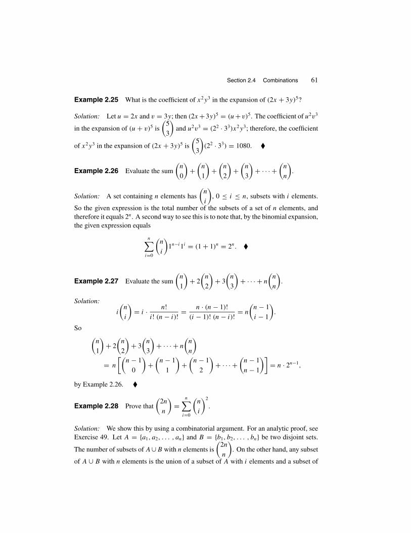
Section 2.4 Combinations 61
Example 2.25 What is the coefficient of x2y3 in the expansion of (2x + 3y)5?
Solution: Let u = 2x and v = 3y; then (2x +3y)5 = (u+v)5. The coefficient of u2v3
in the expansion of (u + v)5 is
(5
3
)and u2v3 = (22 · 33)x2y3; therefore, the coefficient
of x2y3 in the expansion of (2x + 3y)5 is
(5
3
)(22 · 33) = 1080. �
Example 2.26 Evaluate the sum
(n
0
)+(
n
1
)+(
n
2
)+(
n
3
)+ · · · +
(n
n
).
Solution: A set containing n elements has
(n
i
), 0 ≤ i ≤ n, subsets with i elements.
So the given expression is the total number of the subsets of a set of n elements, andtherefore it equals 2n. A second way to see this is to note that, by the binomial expansion,the given expression equals
n∑i=0
(n
i
)1n−i1i = (1 + 1)n = 2n. �
Example 2.27 Evaluate the sum
(n
1
)+ 2
(n
2
)+ 3
(n
3
)+ · · · + n
(n
n
).
Solution:
i
(n
i
)= i · n!
i! (n − i)! = n · (n − 1)!(i − 1)! (n − i)! = n
(n − 1
i − 1
).
So (n
1
)+ 2
(n
2
)+ 3
(n
3
)+ · · · + n
(n
n
)= n
[(n − 1
0
)+(
n − 1
1
)+(
n − 1
2
)+ · · · +
(n − 1
n − 1
)]= n · 2n−1,
by Example 2.26. �
Example 2.28 Prove that
(2n
n
)=
n∑i=0
(n
i
)2
.
Solution: We show this by using a combinatorial argument. For an analytic proof, seeExercise 49. Let A = {a1, a2, . . . , an} and B = {b1, b2, . . . , bn} be two disjoint sets.
The number of subsets of A∪B with n elements is
(2n
n
). On the other hand, any subset
of A ∪ B with n elements is the union of a subset of A with i elements and a subset of

62 Chapter 2 Combinatorial Methods
B with n − i elements for some 0 ≤ i ≤ n. Since for each i there are
(n
i
)(n
n − i
)such subsets, we have that the total number of subsets of A ∪ B with n elements is
n∑i=0
(n
i
)(n
n − i
). But since
(n
n − i
)=(
n
i
), we have the identity. �
Example 2.29 In this example, we present an intuitive proof for the inclusion-exclusionprinciple explained in Section 1.4:
P( n⋃
i=1
Ai
)=
n∑i=1
P(Ai) −n−1∑i=1
n∑j=i+1
P(AiAj ) +n−2∑i=1
n−1∑j=i+1
n∑k=j+1
P(AiAjAk)
− · · · + (−1)n−1P(A1A2 · · · An).
Let S be the sample space. If an outcome ω /∈ ⋃ni=1 Ai , then ω /∈ Ai, 1 ≤ i ≤ n.
Therefore, the probability of ω is not added to either side of the preceding equation.Suppose that ω ∈ ⋃n
i=1 Ai ; then ω belongs to k of the Ai’s for some k, 1 ≤ k ≤ n.
Now, to the left side of the equation the probability of ω is added exactly once. We willshow that the same is true on the right. Clearly, the first term on the right side contains
the probability of ω exactly k =(
k
1
)times. The second term subtracts this probability(
k
2
)times, the third term adds it back, this time
(k
3
)times, and so on until the kth
term. Depending on whether k is even or odd, the kth term either subtracts or adds the
probability of ω exactly
(k
k
)times. The remaining terms do not contain the probability
of ω. Therefore, the total number of times the probability of ω is added to the right sideis (
k
1
)−(
k
2
)+(
k
3
)− · · · (−1)k−1
(k
k
)= −
k∑i=1
(k
i
)1k−i(−1)i =
(k
0
)−
k∑i=0
(k
i
)1k−i(−1)i
= 1 − (1 − 1)k = 1,
where the next-to-the-last equation follows from the binomial expansion. This establishesthe inclusion-exclusion principle. �
Example 2.30 Suppose that we want to distribute n distinguishable balls into k dis-tinguishable cells so that n1 balls are distributed into the first cell, n2 balls into the secondcell, . . . , nk balls into the kth cell, where n1 + n2 + n3 + · · · + nk = n. To count the
number of ways that this is possible, note that we have
(n
n1
)choices to distribute n1

Section 2.4 Combinations 63
balls into the first cell; for each choice of n1 balls in the first cell, we then have
(n − n1
n2
)choices to distribute n2 balls into the second cell; for each choice of n1 balls in the first
cell and n2 balls in the second cell, we have
(n − n1 − n2
n3
)choices to distribute n3
balls into the third cell; and so on. Hence by the generalized counting principle the totalnumber of such distributions is(
n
n1
)(n − n1
n2
)(n − n1 − n2
n3
)· · ·(
n − n1 − n2 − · · · − nk−1
nk
)= n!
(n − n1)! n1! × (n − n1)!(n − n1 − n2)! n2! × (n − n1 − n2)!
(n − n1 − n2 − n3)! n3! × · · ·
× (n − n1 − n2 − n3 − · · · − nk−1)!(n − n1 − n2 − n3 − · · · − nk−1 − nk)! nk! = n!
n1! n2! n3! · · · nk!because n1 + n2 + n3 + · · · + nk = n and (n − n1 − n2 − · · · − nk)!= 0! = 1. �
As an application of Example 2.30, we state a generalization of the binomial expan-sion (Theorem 2.5) and leave its proof as an exercise (see Exercise 28).
Theorem 2.6 (Multinomial Expansion) In the expansion of
(x1 + x2 + · · · + xk)n,
the coefficient of the term xn11 x
n22 x
n33 · · · xnk
k , n1 + n2 + · · · + nk = n, is
n!n1! n2! · · · nk! .
Therefore,
(x1 + x2 + · · · + xk)n =
∑n1+n2+···+nk=n
n!n1! n2! · · · nk! x
n11 x
n22 x
n33 · · · xnk
k .
Note that the sum is taken over all nonnegative integers n1, n2, . . . , nk such thatn1 + n2 + · · · + nk = n.
EXERCISES
A
1. Jim has 20 friends. If he decides to invite six of them to his birthday party, howmany choices does he have?

64 Chapter 2 Combinatorial Methods
2. Each state of the 50 in the United States has two senators. In how many ways maya majority be achieved in the U.S. Senate? Ignore the possibility of absence orabstention. Assume that all senators are present and voting.
3. A panel consists of 20 men and 25 women. How many choices do we have toobtain a jury of six men and six women from this panel?
4. From an ordinary deck of 52 cards, five are drawn randomly. What is the probabilityof drawing exactly three face cards?
5. A random sample of n elements is taken from a population of size N withoutreplacement. What is the probability that a fixed element of the population isincluded? Simplify your answer.
6. Judy puts one piece of fruit in her child’s lunch bag every day. If she has threeoranges and two apples for the next five days, in how many ways can she do this?
7. Ann puts at most one piece of fruit in her child’s lunch bag every day. If she hasonly three oranges and two apples for the next eight lunches of her child, in howmany ways can she do this?
8. Lili has 20 friends. Among them are Kevin and Gerry, who are husband and wife.Lili wants to invite six of her friends to her birthday party. If neither Kevin norGerry will go to a party without the other, how many choices does Lili have?
9. In front of Jeff’s office there is a parking lot with 13 parking spots in a row. Whencars arrive at this lot, they park randomly at one of the empty spots. Jeff parks hiscar in the only empty spot that is left. Then he goes to his office. On his return hefinds that there are seven empty spots. If he has not parked his car at either endof the parking area, what is the probability that both of the parking spaces that arenext to Jeff’s car are empty?
10. Find the coefficient of x9 in the expansion of (2 + x)12.
11. Find the coefficient of x3y4 in the expansion of (2x − 4y)7.
12. A team consisting of three boys and four girls must be formed from a group ofnine boys and eight girls. If two of the girls are feuding and refuse to play on thesame team, how many possibilities do we have?
13. A fair coin is tossed 10 times. What is the probability of (a) five heads; (b) at leastfive heads?
14. If five numbers are selected at random from the set {1, 2, 3, . . . , 20}, what is theprobability that their minimum is larger than 5?
15. From a faculty of six professors, six associate professors, ten assistant professors,and twelve instructors, a committee of size six is formed randomly. What is theprobability that (a) there are exactly two professors on the committee; (b) allcommittee members are of the same rank?

Section 2.4 Combinations 65
16. A lake contains 200 trout; 50 of them are caught randomly, tagged, and returned.If, again, we catch 50 trout at random, what is the probability of getting exactlyfive tagged trout?
17. Find the values ofn∑
i=0
2i
(n
i
)and
n∑i=0
xi
(n
i
).
18. A fair die is tossed six times. What is the probability of getting exactly two 6’s?
19. Suppose that 12 married couples take part in a contest. If 12 persons each wina prize, what is the probability that from every couple one of them is a winner?
Assume that all of the
(24
12
)possible sets of winners are equally probable.
20. Poker hands are classified into the following 10 nonoverlapping categories inincreasing order of likelihood. Calculate the probability of the occurrence of eachclass separately. Recall that a poker hand consists of five cards selected randomlyfrom an ordinary deck of 52 cards.
Royal flush: The 10, jack, queen, king, and ace of the same suit.
Straight flush: All cards in the same suit, with consecutive denomi-nations except for the royal flush.
Four of a kind: Four cards of one denomination and one card of asecond denomination: for example, four 8’s and a jack.
Full house: Three cards of one denomination and two cards of asecond denomination: for example, three 4’s and two queens.
Flush: Five cards all in one suit but not a straight or royal flush.
Straight: Cards of distinct consecutive denominations, not all in onesuit: for example, 3 of hearts, 4 of hearts, 5 of spades, 6 of hearts, and7 of clubs.
Three of a kind: Three cards of one denomination, a fourth card ofa second denomination, and a fifth card of a third denomination.
Two pairs: Two cards from one denomination, another two from asecond denomination, and the fifth card from a third denomination.
One pair: Two cards from one denomination, with the third, fourth,and fifth cards from a second, third, and fourth denomination, respec-tively: for example, two 8’s, a king, a 5, and a 4.
None of the above.
21. There are 12 nuts and 12 bolts in a box. If the contents of the box are dividedbetween two handymen, what is the probability that each handyman will get sixnuts and six bolts?
22. A history professor who teaches three sections of the same course every semester

66 Chapter 2 Combinatorial Methods
decides to make several tests and use them for the next 10 years (20 semesters) asfinal exams. The professor has two policies: (1) not to give the same test to morethan one class in a semester, and (2) not to repeat the same combination of threetests for any two semesters. Determine the minimum number of different tests thatthe professor should prepare.
23. A four-digit number is selected at random. What is the probability that its onesplace is less than its tens place, its tens place is less than its hundreds place, andits hundreds place is less than its thousands place? Note that the first digit of ann-digit number is nonzero.
24. Using Theorem 2.6, expand (x + y + z)2.
25. What is the coefficient of x2y3z2 in the expansion of (2x − y + 3z)7?
26. What is the coefficient of x3y7 in the expansion of (2x − y + 3)13?
27. An ordinary deck of 52 cards is dealt, 13 each, to four players at random. What isthe probability that each player receives 13 cards of the same suit?
28. Using induction, binomial expansion, and the identity(n
n1
)(n − n1)!
n2! n3! · · · nk! = n!n1! n2! · · · nk! ,
prove the formula of multinomial expansion.
29. A staircase is to be constructed between M and N (see Figure 2.4). The distancesfrom M to L, and from L to N , are 5 and 2 meters, respectively. If the height of astep is 25 centimeters and its width can be any integer multiple of 50 centimeters,how many different choices do we have?
Figure 2.4 Staircase of Exercise 29.
30. Each state of the 50 in the United States has two senators. What is the probabilitythat in a random committee of 50 senators (a) Maryland is represented; (b) allstates are represented?

Section 2.4 Combinations 67
31. According to the 1998 edition of Encyclopedia Britannica, “there are at least15,000 to as many as 35,000 species of orchids.” These species have been foundnaturally and are distinct from each other. Suppose that hybrids can be created bycrossing any two existing species. Furthermore, suppose that hybrids themselvescan be continued to be hybridized with each other or with an original species.Orchid lovers develop thousands and thousands of hybrids for use as garden orgreenhouse ornamental and for the commercial flower trade. Suppose that allspecies are crossed, two at a time, to create the first generation of hybrids. Thenthe first generation of hybrids are crossed with each other and with the originalspecies, two at a time, to develop the second generation of hybrids. The secondgeneration of hybrids are crossed with each other, with the first generation hybrids,and with the original species, two at a time, to generate the third generation ofhybrids, and so on. Let n be the total number of original species of orchids. Letnk be the number of hybrids in the kth generation.
(a) Find nk in terms of n, n1, . . . , nk−1.
(b) For n = 25, 000, find the largest possible total number of all hybrids in thefirst four generations.
B
32. Prove the binomial expansion formula by induction.
Hint: Use the identity
(n
k − 1
)+(
n
k
)=(
n + 1
k
).
33. A class contains 30 students. What is the probability that there are six monthseach containing the birthdays of two students, and six months each containing thebirthdays of three students? Assume that all months have the same probability ofincluding the birthday of a randomly selected person.
34. In a closet there are 10 pairs of shoes. If six shoes are selected at random, what isthe probability of (a) no complete pairs; (b) exactly one complete pair; (c) exactlytwo complete pairs; (d) exactly three complete pairs?
35. An ordinary deck of 52 cards is divided into two equal sets randomly. What is theprobability that each set contains exactly 13 red cards?
36. In Maryland’s lottery, players pick six different integers between 1 and 49, theorder of selection being irrelevant. The lottery commission then randomly selectssix of these as the winning numbers. What is the probability that at least twoconsecutive integers are selected among the winning numbers?Hint: Let A be the set of all 6-element combinations of
{1, 2, . . . , 49
}with no
consecutive integers. LetB be the set of all 6-element combinations of{1, 2, . . . , 44
}.
Begin by showing that there is a one-to-one correspondence between A and B.
37. A train consists of n cars. Each of m passengers (m > n) will choose a car

68 Chapter 2 Combinatorial Methods
at random to ride in. What is the probability that (a) there will be at least onepassenger in each car; (b) exactly r (r < n) cars remain unoccupied?
38. Suppose that n indistinguishable balls are placed at random into n distinguishablecells. What is the probability that exactly one cell remains empty?
39. Prove that(n
0
)−(
n
1
)+(
n
2
)− · · · + (−1)k
(n
k
)+ · · · + (−1)n
(n
n
)= 0.
40. Show that (n
0
)+(
n + 1
1
)+ · · · +
(n + r
r
)=(
n + r + 1
r
).
Hint:
(n
r
)=(
n + 1
r
)−(
n
r − 1
).
41. By a combinatorial argument, prove that for r ≤ n and r ≤ m,(n + m
r
)=(
m
0
)(n
r
)+(
m
1
)(n
r − 1
)+ · · · +
(m
r
)(n
0
).
42. Evaluate the following sum:(n
0
)+ 1
2
(n
1
)+ 1
3
(n
2
)+ · · · + 1
n + 1
(n
n
).
43. Suppose that five points are selected at random from the interval (0, 1). What isthe probability that exactly two of them are between 0 and 1/4?Hint: For any point there are four equally likely possibilities: to fall into (0, 1/4),[1/4, 1/2), [1/2, 3/4), and [3/4, 1).
44. A lake has N trout, and t of them are caught at random, tagged, and returned. Wecatch n trout at a later time randomly and observe that m of them are tagged.
(a) Find PN , the probability of what we observed actually happen.
(b) To estimate the number of trout in the lake, statisticians find the value ofN that maximizes PN . Such a value is called the maximum likelihoodestimator of N . Show that the maximum of PN is [nt/m], where by [nt/m]we mean the greatest integer less than or equal to nt/m. That is, prove thatthe maximum likelihood estimator of the number of trout in the lake is[nt/m].
Hint: Investigate for what values of N the probability PN is increasing and forwhat values it is decreasing.

Section 2.4 Combinations 69
45. Let n be a positive integer. A random sample of four elements is taken from theset{0, 1, 2, . . . , n
}, one at a time and with replacement. What is the probability
that the sum of the first two elements is equal to the sum of the last two elements?
46. For a given position with n applicants, m applicants are equally qualified andn − m applicants are not qualified at all. Assume that a recruitment process isconsidered to be fair if the probability that a qualified applicant is hired is 1/m,and the probability that an unqualified applicant is hired is 0. One fair recruitmentprocess is to interview all applicants, identify the qualified ones, and then hireone of the m qualified applicants randomly. A second fair process, which is moreefficient, is to interview applicants in a random order and employ the first qualifiedapplicant encountered. For the fairness of the second recruitment process,
(a) present an intuitive argument;
(b) give a rigorous combinatorial proof.
47. In how many ways can 10 different photographs be placed in six different en-velopes, no envelope remaining empty?Hint: An easy way to do this problem is to use the following version of theinclusion-exclusion principle: Let A1, A2, . . . , An be n subsets of a finite set �
with N elements. Let N(Ai) be the number of elements of Ai , 1 ≤ i ≤ n, andN(Ac
i ) = N − N(Ai). Let Sk be the sum of the elements of all those intersectionsof A1, A2, . . . , An that are formed of exactly k sets. That is,
S1 = N(A1) + N(A2) + · · · + N(An),
S2 = N(A1A2) + N(A1A3) + · · · + N(An−1An),
and so on. Then
N(Ac1A
c2 · · ·Ac
n) = N − S1 + S2 − S3 + · · · + (−1)nSn.
To solve the problem, let N be the number of ways that 10 different photographscan be placed in six different envelopes, allowing for the possibility of emptyenvelopes. Let Ai be the set of all situations in which envelope i is empty. Thenthe desired quantity is N(Ac
1Ac2 · · · Ac
6).
48. We are given n (n > 5) points in space, no three of which lie on the same straightline. Let � be the family of planes defined by any three of these points. Supposethat the points are situated in a way that no four of them are coplanar, and no twoplanes of � are parallel. From the set of the lines of the intersections of the planesof �, a line is selected at random. What is the probability that it passes throughnone of the n points?Hint: For i = 0, 1, 2, let Ai be the set of all lines of the intersections that aredetermined by planes having i of the given n points in common. If |Ai | denotesthe number of elements of Ai , the answer is |A0|/
(|A0| + |A1| + |A2|).

70 Chapter 2 Combinatorial Methods
49. Using the binomial theorem, calculate the coefficient of xn in the expansion of(1 + x)2n = (1 + x)n(1 + x)n to prove that(
2n
n
)=
n∑i=0
(n
i
)2
.
For a combinatorial proof of this relation, see Example 2.28.
50. An absentminded professor wrote n letters and sealed them in envelopes withoutwriting the addresses on them. Then he wrote the n addresses on the envelopes atrandom. What is the probability that exactly k of the envelopes were addressedcorrectly?Hint: Consider a particular set of k letters. Let M be the total number of waysthat only these k letters can be addressed correctly. The desired probability is the
quantity
(n
k
)M/n!; using Example 2.24, argue that M satisfies
∑n−ki=2 (−1)i/i! =
M/(n − k)!.51. A fair coin is tossed n times. Calculate the probability of getting no successive
heads.Hint: Let xi be the number of sequences of H’s and T’s of length i with nosuccessive H’s. Show that xi satisfies xi = xi−1 + xi−2, i ≥ 2, where x0 = 1 andx1 = 2. The answer is xn/2n. Note that {xi}∞i=1 is a Fibonacci-type sequence.
52. What is the probability that the birthdays of at least two students of a class of sizen are at most k days apart? Assume that the birthrates are constants throughoutthe year and that each year has 365 days.
2.5 STIRLING’s FORMULA
To estimate n! for large values of n, the following formula is used. Discovered in 1730by James Stirling (1692–1770), it appeared in his book Methodus Differentialis (Bowyer,London, 1730). Also, independently, a slightly less general version of the formula wasdiscovered by De Moivre, who used it to prove the central limit theorem.
Theorem 2.7 (Stirling’s Formula)
n! ∼ √2πn nne−n,
where the sign ∼ means
limn→∞
n!√2πn nne−n
= 1.

Chapter 2 Review Problems 71
Stirling’s formula, which usually gives excellent approximations in numerical compu-tations, is also often used to prove theoretical problems. Note that although the ratioR(n) = n!/(√2πn nne−n) becomes 1 at ∞, it is still close to 1, even for very smallvalues of n. The following table shows this fact.
n n! √2πn nne−n R(n)
1 1 0.922 1.0842 2 1.919 1.0425 120 118.019 1.0178 40,320 39,902.396 1.010
10 3,628,800 3,598,695.618 1.00812 479,001,600 475,687,486.474 1.007
Be aware that, even though limn→∞ R(n) is 1, the difference between n! and√
2πn nne−n
increases as n gets larger. In fact, it goes to ∞ as n → ∞.
Example 2.31 Approximate the value of[2n (n!)2
]/(2n)! for large n.
Solution: By Stirling’s formula, we have
2n(n!)2
(2n)! ∼ 2n2πn(nn)2e−2n
√4πn (2n)2ne−2n
=√
πn
2n. �
EXERCISE
1. Use Stirling’s formula to approximate
(2n
n
)1
22nand
[(2n)!]3[
(4n)! (n!)2] for large n.
REVIEW PROBLEMS
1. Albert goes to the grocery store to buy fruit. There are seven different varieties offruit, and Albert is determined to buy no more than one of any variety. How manydifferent orders can he place?

72 Chapter 2 Combinatorial Methods
2. Virginia has 1 one-dollar bill, 1 two-dollar bill, 1 five-dollar bill, 1 ten-dollar bill,and 1 twenty-dollar bill. She decides to give some money to her son Brian withoutasking for change. How many choices does she have?
3. If four fair dice are tossed, what is the probability that they will show four differentfaces?
4. From the 10 points that are placed on a circumference, two are selected randomly.What is the probability that they are adjacent?
5. A father buys nine different toys for his four children. In how many ways can hegive one child three toys and the remaining three children two toys each?
6. A window dresser has decided to display five different dresses in a circular ar-rangement. How many choices does she have?
7. Judy has three sets of classics in literature, each set having four volumes. In howmany ways can she put them on a bookshelf so that books of each set are notseparated?
8. Suppose that 30 lawn mowers, of which seven have defects, are sold to a hardwarestore. If the store manager inspects six of the lawn mowers randomly, what is theprobability that he finds at least one defective lawn mower?
9. In how many ways can 23 identical refrigerators be allocated among four storesso that one store gets eight refrigerators, another four, a third store five, and thelast one six refrigerators?
10. In how many arrangements of the letters BERKELEY are all three E’s adjacent?
11. Bill and John play in a backgammon tournament. A player is the winner if he winsthree games in a row or four games altogether. In what percent of all possible casesdoes the tournament end because John wins four games without winning three ina row?
12. In a small town, both of the accidents that occurred during the week of June 8,1988, were on Friday the 13th. Is this a good excuse for a superstitious person toargue that Friday the 13th’s are inauspicious?
13. How many eight-digit numbers without two identical successive digits are there?
14. A palindrome is a sequence of characters that reads the same forward or backward.For example, rotator, madam, Hannah, the German name Otto, and an Indianlanguage, Malayalam, are palindromes. So are the following expressions: “Putup,” “Madam I’m Adam,” “Was it a cat I saw?” and these two sentences in Latinconcerning St. Martin, Bishop of Tours: “Signa te, signa; temere me tangis etangis. Roma tibi subito motibus ibit amor.” (Respectively: Cross, cross yourself;you annoy and vex me needlessly. Through my exertions, Rome, your desire, willsoon be near.) Determine the number of palindromes containing 11 characters that
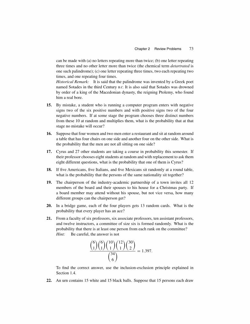
Chapter 2 Review Problems 73
can be made with (a) no letters repeating more than twice; (b) one letter repeatingthree times and no other letter more than twice (the chemical term detartrated isone such palindrome); (c) one letter repeating three times, two each repeating twotimes, and one repeating four times.Historical Remark: It is said that the palindrome was invented by a Greek poetnamed Sotades in the third Century B.C. It is also said that Sotades was drownedby order of a king of the Macedonian dynasty, the reigning Ptolemy, who foundhim a real bore.
15. By mistake, a student who is running a computer program enters with negativesigns two of the six positive numbers and with positive signs two of the fournegative numbers. If at some stage the program chooses three distinct numbersfrom these 10 at random and multiplies them, what is the probability that at thatstage no mistake will occur?
16. Suppose that four women and two men enter a restaurant and sit at random arounda table that has four chairs on one side and another four on the other side. What isthe probability that the men are not all sitting on one side?
17. Cyrus and 27 other students are taking a course in probability this semester. Iftheir professor chooses eight students at random and with replacement to ask themeight different questions, what is the probability that one of them is Cyrus?
18. If five Americans, five Italians, and five Mexicans sit randomly at a round table,what is the probability that the persons of the same nationality sit together?
19. The chairperson of the industry-academic partnership of a town invites all 12members of the board and their spouses to his house for a Christmas party. Ifa board member may attend without his spouse, but not vice versa, how manydifferent groups can the chairperson get?
20. In a bridge game, each of the four players gets 13 random cards. What is theprobability that every player has an ace?
21. From a faculty of six professors, six associate professors, ten assistant professors,and twelve instructors, a committee of size six is formed randomly. What is theprobability that there is at least one person from each rank on the committee?Hint: Be careful, the answer is not(
6
1
)(6
1
)(10
1
)(12
1
)(30
2
)(
34
6
) = 1.397.
To find the correct answer, use the inclusion-exclusion principle explained inSection 1.4.
22. An urn contains 15 white and 15 black balls. Suppose that 15 persons each draw

74 Chapter 2 Combinatorial Methods
two balls blindfolded from the urn without replacement. What is the probabilitythat each of them draws one white ball and one black ball?
23. In a lottery the tickets are numbered 1 through N . A person purchases n (1 ≤n ≤ N ) tickets at random. What is the probability that the ticket numbers areconsecutive? (This is a special case of a problem posed by Euler in 1763.)
24. An ordinary deck of 52 cards is dealt, 13 each, at random among A, B, C, and D.What is the probability that (a) A and B together get two aces; (b) A gets all theface cards; (c) A gets five hearts and B gets the remaining eight hearts?
25. To test if a computer program works properly, we run it with 12 different data sets,using four computers, each running three data sets. If the data sets are distributedrandomly among different computers, how many possibilities are there?
26. A fair die is tossed eight times. What is the probability that the eighth outcome isnot a repetition?
27. A four-digit number is selected at random. What is the probability that its onesplace is greater than its tens place, its tens place is greater than its hundreds place,and its hundreds place is greater than its thousands place? Note that the first digitof an n-digit number is nonzero.
28. From the set of integers{1, 2, 3, . . . , 100000
}a number is selected at random.
What is the probability that the sum of its digits is 8?Hint: Establish a one-to-one correspondence between the set of integers from{1, 2, . . . , 100000} the sum of whose digits is 8, and the set of possible ways 8identical objects can be placed into 5 distinguishable cells. Then use Example 2.22.

Chapter 3
Conditional Probability
and Independence
3.1 CONDITIONAL PROBABILITY
To introduce the notion of conditional probability, let us first examine the followingquestion: Suppose that all of the freshmen of an engineering college took calculus anddiscrete math last semester. Suppose that 70% of the students passed calculus, 55%passed discrete math, and 45% passed both. If a randomly selected freshman is foundto have passed calculus last semester, what is the probability that he or she also passeddiscrete math last semester? To answer this question, let A and B be the events that therandomly selected freshman passed discrete math and calculus last semester, respectively.Note that the quantity we are asked to find is not P(A), which is 0.55; it would have beenif we were not aware that B has occurred. Knowing that B has occurred changes thechances of the occurrence of A. To find the desired probability, denoted by the symbolP(A | B) [read: probability of A given B] and called the conditional probability ofA given B, let n be the number of all the freshmen in the engineering college. Then(0.7)n is the number of freshmen who passed calculus, and (0.45)n is the number ofthose who passed both calculus and discrete math. Therefore, of the (0.7)n freshmenwho passed calculus, (0.45)n of them passed discrete math as well. It is given that therandomly selected student is one of the (0.7)n who passed calculus; we also want to findthe probability that he or she is one of the (0.45)n who passed discrete math. This isobviously equal to (0.45)n/(0.7)n = 0.45/0.7. Hence
P(A | B) = 0.45
0.7.
But 0.45 is P(AB) and 0.7 is P(B). Therefore, this example suggests that
P(A | B) = P(AB)
P (B). (3.1)
As another example, suppose that a bus arrives at a station every day at a random
75

76 Chapter 3 Conditional Probability and Independence
time between 1:00 P.M. and 1:30 P.M. Suppose that at 1:10 the bus has not arrived and wewant to calculate the probability that it will arrive in not more than 10 minutes from now.Let A be the event that the bus will arrive between 1:10 and 1:20 and B be the event thatit will arrive between 1:10 and 1:30. Then the desired probability is
P(A | B) = 20 − 10
30 − 10=
20 − 10
30 − 030 − 10
30 − 0
= P(AB)
P (B). (3.2)
The relation P(A | B) = P(AB)/P (A) discovered in (3.1) and (3.2) can also beverified for other types of conditional probability problems. It is compatible with ourintuition and is a logical generalization of the existing relation between the conditionalrelative frequency of the event A with respect to the condition B and the ratio of therelative frequencies of AB and the relative frequency of B. For these reasons it is takenas a definition.
Definition If P(B) > 0, the conditional probability of A given B, denoted byP(A | B), is
P(A | B) = P(AB)
P (B). (3.3)
If P(B) = 0, formula (3.3) makes no sense, so the conditional probability is definedonly for P(B) > 0.This formula may be expressed in words by saying that the conditionalprobability of A given that B has occurred is the ratio of the probability of joint occurrenceof A and B and the probability of B. It is important to note that (3.3) is neither an axiomnor a theorem. It is a definition. As explained previously, this definition is fully justifiedand is not made arbitrarily. Indeed, historically, it was used implicitly even before it wasformally introduced by De Moivre in the book The Doctrine of Chance.
Example 3.1 In a certain region of Russia, the probability that a person lives at least80 years is 0.75, and the probability that he or she lives at least 90 years is 0.63. What isthe probability that a randomly selected 80-year-old person from this region will surviveto become 90?
Solution: Let A and B be the events that the person selected survives to become 90 and80 years old, respectively. We are interested in P(A | B). By definition,
P(A | B) = P(AB)
P (B).
Now, P(AB) = P(A) because “at least 80” and “at least 90” overlap with “at least 90,”which is A. Hence
P(A | B) = P(AB)
P (B)= P(A)
P (B)= 0.63
0.75= 0.84. �

Section 3.1 Conditional Probability 77
Example 3.2 From the set of all families with two children, a family is selected atrandom and is found to have a girl. What is the probability that the other child of thefamily is a girl? Assume that in a two-child family all sex distributions are equallyprobable.
Solution: Let B and A be the events that the family has a girl and the family has twogirls, respectively. We are interested in P(A | B). Now, in a family with two childrenthere are four equally likely possibilities: (boy, boy), (girl, girl), (boy, girl), (girl, boy),where by, say, (girl, boy), we mean that the older child is a girl and the younger is a boy.Thus P(B) = 3/4, P (AB) = 1/4. Hence
P(A | B) = P(AB)
P (B)= 1/4
3/4= 1
3. �
Example 3.3 From the set of all families with two children, a child is selected atrandom and is found to be a girl. What is the probability that the second child of thisgirl’s family is also a girl? Assume that in a two-child family all sex distributions areequally probable.
Solution: Let B be the event that the child selected at random is a girl, and let A be theevent that the second child of her family is also a girl. We want to calculate P(A | B).Now the set of all possibilities is as follows: The child is a girl with a sister, the child isa girl with a brother, the child is a boy with a sister, and the child is a boy with a brother.Thus P(B) = 2/4 and P(AB) = 1/4. Hence
P(A | B) = P(AB)
P (B)= 1/4
2/4= 1
2. �
Remark 3.1 There is a major difference between Examples 3.2 and 3.3. In Exam-ple 3.2, a family is selected and found to have a girl. Therefore, we have three equallylikely possibilities: (girl, girl), (boy, girl), and (girl, boy), of which only one is desirable:(girl, girl). So the required probability is 1/3. In Example 3.3, since a child rather thana family is selected, families with (girl, girl), (boy, girl), and (girl, boy) are not equallylikely to be chosen. In fact, the probability that a family with two girls is selected equalstwice the probability that a family with one girl is selected. That is,
P(girl, girl) = 2P(girl, boy) = 2P(boy, girl).
This and the fact that the sum of the probabilities of (girl, girl), (girl, boy), (boy, girl) is1 give
P(girl, girl) + 1
2P(girl, girl) + 1
2P(girl, girl) = 1,

78 Chapter 3 Conditional Probability and Independence
which implies that
P(girl, girl) = 1
2. �
Example 3.4 An English class consists of 10 Koreans, 5 Italians, and 15 Hispanics.A paper is found belonging to one of the students of this class. If the name on the paperis not Korean, what is the probability that it is Italian? Assume that names completelyidentify ethnic groups.
Solution: Let A be the event that the name on the paper is Italian, and let B be the eventthat it is not Korean. To calculate P(A | B), note that AB = A because “the name beingItalian,” and “the name not being Korean” overlap with “the name being Italian,” whichis A. Hence P(AB) = P(A) = 5/30. Therefore,
P(A | B) = P(AB)
P (B)= 5/30
20/30= 1
4. �
Example 3.5 We draw eight cards at random from an ordinary deck of 52 cards.Given that three of them are spades, what is the probability that the remaining five arealso spades?
Solution: Let B be the event that at least three of them are spades, and let A denotethe event that all of the eight cards selected are spades. Then P(A | B) is the desiredquantity and is calculated from P(A | B) = P(AB)/P (B) as follows:
P(AB) =
(13
8
)(
52
8
)since AB is the event that all eight cards selected are spades.
P(B) =8∑
x=3
(13
x
)(39
8 − x
)(
52
8
)because at least three of the cards selected are spades if exactly three of them are spades,

Section 3.1 Conditional Probability 79
or exactly four of them are spades, . . . , or all eight of them are spades. Hence
P(A | B) = P(AB)
P (B)=
(13
8
)(
52
8
)8∑
x=3
(13
x
)(39
8 − x
)(
52
8
)≈ 5.44 × 10⁻⁶. �
An important feature of conditional probabilities (stated in the following theorem) isthat they satisfy the same axioms that ordinary probabilities satisfy. This enables us touse the theorems that are true for probabilities for conditional probabilities as well.
Theorem 3.1 Let S be the sample space of an experiment, and let B be an event of S
with P(B) > 0. Then
(a) P(A | B) ≥ 0 for any event A of S.
(b) P(S | B) = 1.
(c) If A1, A2, . . . is a sequence of mutually exclusive events, then
P( ∞⋃
i=1
Ai | B)
=∞∑i=1
P(Ai | B).
The proof of this theorem is left as an exercise.
Reduction of Sample Space
Let B be an event of a sample space S with P(B) > 0. For a subset A of B, defineQ(A) = P(A | B). Then Q is a function from the set of subsets of B to [0, 1]. Clearly,Q(A) ≥ 0, Q(B) = P(B | B) = 1 and, by Theorem 3.1, if A1, A2, . . . is a sequence ofmutually exclusive subsets of B, then
Q( ∞⋃
i=1
Ai
)= P
( ∞⋃i=1
Ai | B)
=∞∑i=1
P(Ai | B) =∞∑i=1
Q(Ai).
Thus Q satisfies the axioms that probabilities do, and hence it is a probability function.Note that while P is defined for all subsets of S, the probability function Q is definedonly for subsets of B. Therefore, for Q, the sample space is reduced from S to B.This reduction of sample space is sometimes very helpful in calculating conditional

80 Chapter 3 Conditional Probability and Independence
probabilities. Suppose that we are interested in P(E | B), where E ⊆ S. One way tocalculate this quantity is to reduce S to B and find Q(EB). It is usually easier to computethe unconditional probability Q(EB) rather than the conditional probability P(E | B).Examples follow.
Example 3.6 A child mixes 10 good and three dead batteries. To find the deadbatteries, his father tests them one-by-one and without replacement. If the first fourbatteries tested are all good, what is the probability that the fifth one is dead?
Solution: Using the information that the first four batteries tested are all good, werephrase the problem in the reduced sample space: Six good and three dead batteriesare mixed. A battery is selected at random: What is the probability that it is dead? Thesolution to this trivial question is 3/9 = 1/3. Note that without reducing the sample space,the solution of this problem is not so easy. �
Example 3.7 A farmer decides to test four fertilizers for his soybean fields. He buys32 bags of fertilizers, eight bags from each kind, and tries them randomly on 32 plots,eight plots from each of fields A, B, C, and D, one bag per plot. If from type I fertilizerone bag is tried on field A and three on field B, what is the probability that two bags oftype I fertilizer are tried on field D?
Solution: Using the information that one and three bags of type I fertilizer are tried onfields A and B, respectively, we rephrase the problem in the reduced sample space: 16bags of fertilizers (of which four are type I) are tried randomly, eight on field C and eighton field D. What is the probability that two bags of type I fertilizer are tried on field D?The solution to this easier unconditional version of the problem is(
4
2
)(12
6
)(
16
8
) ≈ 0.43. �
Example 3.8 On a TV game show, there are three curtains. Behind two of the curtainsthere is nothing, but behind the third there is a prize that the player might win. Theprobability that the prize is behind a given curtain is 1/3. The game begins with thecontestant randomly guessing a curtain. The host of the show (master of ceremonies),who knows behind which curtain the prize is, will then pull back a curtain other than theone chosen by the player and reveal that the prize is not behind that curtain. The hostwill not pull back the curtain selected by the player, nor will he pull back the one withthe prize, if different from the player’s choice. At this point, the host gives the playerthe opportunity to change his choice of curtain and select the other one. The questionis whether the player should change his choice. That is, has the probability of the prizebeing behind the curtain chosen changed from 1/3 to 1/2 or it is still 1/3? If it is still 1/3,

Section 3.1 Conditional Probability 81
the contestant should definitely change his choice. Otherwise, there is no point in doingso.
Solution: We will show that the conditional probability that the contestant wins, giventhat he always changes his original choice is 2/3. Therefore, the contestant shoulddefinitely change his choice. To show this, suppose that the prize is behind curtain 1,and the contestant always changes his choice. These two assumptions reduce the samplespace. The elements of the reduced sample space can be described by 3-tuples (x, y, z),where x is the curtain the contestant guesses first, y is the curtain the master of ceremoniespulls back, and z is the curtain the contestant switches to. For example, (3, 2, 1) representsa game in which the contestant guesses curtain 3, the master of ceremonies pulls backcurtain 2, and the contestant switches to curtain 1. Therefore, given that the prize isbehind curtain 1 and the contestant changes his choice, the reduced sample space S is
S = {(1, 2, 3), (1, 3, 2), (2, 3, 1), (3, 2, 1)}.
Note that the event that the contestant guesses curtain 2 is{(2, 3, 1)
}, the event that he
guesses curtain 3 is{(3, 2, 1)
}, whereas the event that he guesses curtain 1 is{
(1, 2, 3), (1, 3, 2)}. Given that the prize is behind curtain 1 and the contestant always
switches his original choice, the event that the contestant wins is{(2, 3, 1), (3, 2, 1)
}.
Since the contestant guesses a curtain with probability 1/3,
P({
(2, 3, 1)}) = P
({(3, 2, 1)
}) = P({
(1, 2, 3), (1, 3, 2)}) = 1
3.
This shows that no matter what values are assigned to P({
(1, 2, 3)})
and P({
(1, 3, 2)})
,as long as their sum is 1/3, the conditional probability that the contestant wins, given thathe always changes his original choice, is
P({
(2, 3, 1)})+ P
({(3, 2, 1)
}) = 2
3. �
By Theorem 3.1, the function Q defined above by Q(A) = P(A | B) is a probabilityfunction. Therefore, Q(A) = P(A | B) satisfies the theorems stated for P . In particular,for all choices of B, P(B) > 0,
1. P(∅ | B) = 0.
2. P(Ac | B) = 1 − P(A | B).
3. If C ⊆ A, then P(AC c | B) = P(A − C | B) = P(A | B) − P(C | B).
4. If C ⊆ A, then P(C | B) ≤ P(A | B).
5. P(A ∪ C | B) = P(A | B) + P(C | B) − P(AC | B).
6. P(A | B) = P(AC | B) + P(AC c | B).

82 Chapter 3 Conditional Probability and Independence
7. To calculate P(A1 ∪A2 ∪A3 ∪· · ·∪An | B), we calculate conditional probabilitiesof all possible intersections of events from {A1, A2, . . . , An}, given B, add theconditional probabilities obtained by intersecting an odd number of the events,and subtract the conditional probabilities obtained by intersecting an even numberof events.
8. For any increasing or decreasing sequences of events {An, n ≥ 1},lim
n→∞ P(An | B) = P( limn→∞ An | B).
EXERCISES
A
1. Suppose that 15% of the population of a country are unemployed women, and atotal of 25% are unemployed. What percent of the unemployed are women?
2. Suppose that 41% of Americans have blood type A, and 4% have blood type AB.If in the blood of a randomly selected American soldier the A antigen is found,what is the probability that his blood type is A? The A antigen is found only inblood types A and AB.
3. In a technical college all students are required to take calculus and physics. Statis-tics show that 32% of the students of this college get A’s in calculus, and 20% ofthem get A’s in both calculus and physics. Gino, a randomly selected student ofthis college, has passed calculus with an A. What is the probability that he got anA in physics?
4. Suppose that two fair dice have been tossed and the total of their top faces is foundto be divisible by 5. What is the probability that both of them have landed 5?
5. A bus arrives at a station every day at a random time between 1:00 P.M. and 1:30 P.M.
A person arrives at this station at 1:00 and waits for the bus. If at 1:15 the bus hasnot yet arrived, what is the probability that the person will have to wait at least anadditional 5 minutes?
6. Prove that P(A | B) > P(A) if and only if P(B | A) > P(B). In probability, iffor two events A and B, P(A | B) > P(A), we say that A and B are positivelycorrelated. If P(A | B) < P(A), A and B are said to be negatively correlated.
7. A spinner is mounted on a wheel of unit circumference (radius 1/2π ). Arcs A, B,and C of lengths 1/3, 1/2, and 1/6, respectively, are marked off on the wheel’sperimeter (see Figure 3.1). The spinner is flicked and we know that it is not pointingtoward C. What is the probability that it points toward A?

Section 3.1 Conditional Probability 83
Figure 3.1 Spinner of Exercise 7.
8. In throwing two fair dice, what is the probability of a sum of 5 if they land ondifferent numbers?
9. In a small lake, it is estimated that there are approximately 105 fish, of which 40are trout and 65 are carp. A fisherman caught eight fish; what is the probabilitythat exactly two of them are trout if we know that at least three of them are not?
10. From 100 cards numbered 00, 01, . . . , 99, one card is drawn. Suppose that α
and β are the sum and the product, respectively, of the digits of the card selected.Calculate P
({α = i | β = 0}), i = 0, 1, 2, 3, . . . , 18.
11. From families with three children, a family is selected at random and found to havea boy. What is the probability that the boy has (a) an older brother and a youngersister; (b) an older brother; (c) a brother and a sister? Assume that in a three-childfamily all gender distributions have equal probabilities.
12. Show that if P(A) = 1, then P(B | A) = P(B).
13. Prove that if P(A) = a and P(B) = b, then P(A | B) ≥ (a + b − 1)/b.
14. Prove Theorem 3.1.
15. Prove that if P(E | F) ≥ P(G | F) and P(E | Fc) ≥ P(G | Fc), thenP(E) ≥ P(G).
16. The theaters of a town are showing seven comedies and nine dramas. Marlon hasseen five of the movies. If the first three movies he has seen are dramas, what isthe probability that the last two are comedies? Assume that Marlon chooses theshows at random and sees each movie at most once.
17. Suppose that 28 crayons, of which four are red, are divided randomly among Jack,Marty, Sharon, and Martha (seven each). If Sharon has exactly one red crayon,what is the probability that Marty has the remaining three?
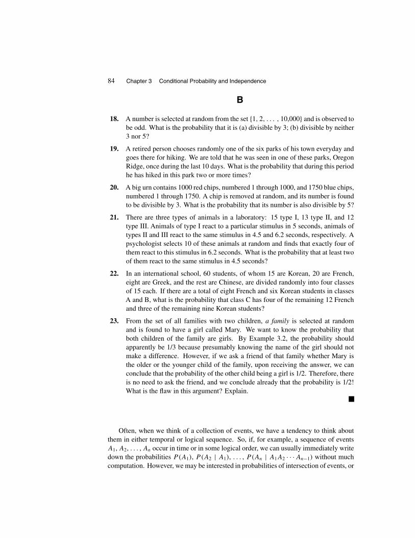
84 Chapter 3 Conditional Probability and Independence
B
18. A number is selected at random from the set {1, 2, . . . , 10,000} and is observed tobe odd. What is the probability that it is (a) divisible by 3; (b) divisible by neither3 nor 5?
19. A retired person chooses randomly one of the six parks of his town everyday andgoes there for hiking. We are told that he was seen in one of these parks, OregonRidge, once during the last 10 days. What is the probability that during this periodhe has hiked in this park two or more times?
20. A big urn contains 1000 red chips, numbered 1 through 1000, and 1750 blue chips,numbered 1 through 1750. A chip is removed at random, and its number is foundto be divisible by 3. What is the probability that its number is also divisible by 5?
21. There are three types of animals in a laboratory: 15 type I, 13 type II, and 12type III. Animals of type I react to a particular stimulus in 5 seconds, animals oftypes II and III react to the same stimulus in 4.5 and 6.2 seconds, respectively. Apsychologist selects 10 of these animals at random and finds that exactly four ofthem react to this stimulus in 6.2 seconds. What is the probability that at least twoof them react to the same stimulus in 4.5 seconds?
22. In an international school, 60 students, of whom 15 are Korean, 20 are French,eight are Greek, and the rest are Chinese, are divided randomly into four classesof 15 each. If there are a total of eight French and six Korean students in classesA and B, what is the probability that class C has four of the remaining 12 Frenchand three of the remaining nine Korean students?
23. From the set of all families with two children, a family is selected at randomand is found to have a girl called Mary. We want to know the probability thatboth children of the family are girls. By Example 3.2, the probability shouldapparently be 1/3 because presumably knowing the name of the girl should notmake a difference. However, if we ask a friend of that family whether Mary isthe older or the younger child of the family, upon receiving the answer, we canconclude that the probability of the other child being a girl is 1/2. Therefore, thereis no need to ask the friend, and we conclude already that the probability is 1/2!What is the flaw in this argument? Explain.
Often, when we think of a collection of events, we have a tendency to think aboutthem in either temporal or logical sequence. So, if, for example, a sequence of eventsA1, A2, . . . , An occur in time or in some logical order, we can usually immediately writedown the probabilities P(A1), P(A2 | A1), . . . , P(An | A1A2 · · · An−1) without muchcomputation. However, we may be interested in probabilities of intersection of events, or

Section 3.2 Law of Multiplication 85
probabilities of events unconditional on the rest, or probabilities of earlier events, givenlater events. In the next three sections, we will develop techniques for calculating suchprobabilities.
Suppose that, in a random phenomenon, events occur in either temporal or logicalsequence. In Section 3.2 (Law of Multiplication), we will discuss the probabilitiesof the intersection of events in terms of conditional probabilities of later events givenearlier events. In Section 3.3 (Law of Total Probability), we will find the probabilities ofunconditional events in terms of conditional probabilities of later events given the earlierones. In Section 3.4 (Bayes’ Formula), we will discuss a formula relating probabilitiesof earlier events, given later events, to the conditional probabilities of later events giventhe earlier ones.
3.2 LAW OF MULTIPLICATION
The relation
P(A | B) = P(AB)
P (B)
is also useful for calculating P(AB). If we multiply both sides of this relation by P(B)[note that P(B) > 0
], we get
P(AB) = P(B)P (A | B), (3.4)
which means that the probability of the joint occurrence of A and B is the product ofthe probability of B and the conditional probability of A given that B has occurred. IfP(A) > 0, then by letting A = B and B = A in (3.4), we obtain
P(BA) = P(A)P (B | A).
Since P(BA) = P(AB), this relation gives
P(AB) = P(A)P (B | A). (3.5)
Thus, to calculate P(AB), depending on which of the quantities P(A | B) and P(B | A)
is known, we may use (3.4) or (3.5), respectively. The following example clarifies theusefulness of these relations.
Example 3.9 Suppose that five good fuses and two defective ones have been mixed up.To find the defective fuses, we test them one-by-one, at random and without replacement.What is the probability that we are lucky and find both of the defective fuses in the firsttwo tests?
Solution: Let D1 and D2 be the events of finding a defective fuse in the first and secondtests, respectively. We are interested in P(D1D2). Using (3.5), we get
P(D1D2) = P(D1)P (D2 | D1) = 2
7× 1
6= 1
21. �

86 Chapter 3 Conditional Probability and Independence
Relation (3.5) can be generalized for calculating the probability of the joint occurrenceof several events. For example, if P(AB) > 0, then
P(ABC) = P(A)P (B | A)P (C | AB). (3.6)
To see this, note that P(AB) > 0 implies that P(A) > 0; therefore,
P(A)P (B | A)P (C | AB) = P(A)P (AB)
P (A)
P (ABC)
P (AB)= P(ABC).
The following theorem will generalize (3.5) and (3.6) to n events and can be shown inthe same way as (3.6) is shown.
Theorem 3.2 If P(A1A2A3 · · · An−1) > 0, then
P(A1A2A3 · · ·An−1An)
= P(A1)P (A2 | A1)P (A3 | A1A2) · · · P(An | A1A2A3 · · · An−1).
Example 3.10 A consulting firm is awarded 43% of the contracts it bids on. Supposethat Nordulf works for a division of the firm that gets to do 15% of the projects contractedfor. If Nordulf directs 35% of the projects submitted to his division, what percentage ofall bids submitted by the firm will result in contracts for projects directed by Nordulf?
Solution: Let A1 be the event that the firm is awarded a contract for some randomlyselected bid. Let A2 be the event that the contract will be sent to Nordulf’s division. LetA3 be the event that Nordulf will direct the project. The desired probability is calculatedas follows:
P(A1A2A3) = P(A1)P (A2 | A1)P (A3 | A1A2) = (0.43)(0.15)(0.35) = 0.0226.
Hence 2.26% of all bids submitted by the firm will be directed by Nordulf. �
Example 3.11 Suppose that five good and two defective fuses have been mixed up.To find the defective ones, we test them one by one, at random and without replacement.What is the probability that we find both of the defective fuses in exactly three tests?
Solution: Let D1, D2, and D3 be the events that the first, second, and third fuses testedare defective, respectively. Let G1, G2, and G3 be the events that the first, second, andthird fuses tested are good, respectively. We are interested in the probability of the eventG1D2D3 ∪ D1G2D3. We have
P(G1D2D3 ∪ D1G2D3)
= P(G1D2D3) + P(D1G2D3)
= P(G1)P (D2 | G1)P (D3 | G1D2) + P(D1)P (G2 | D1)P (D3 | D1G2)
= 5
7× 2
6× 1
5+ 2
7× 5
6× 1
5≈ 0.095. �

Section 3.2 Law of Multiplication 87
EXERCISES
A
1. In a trial, the judge is 65% sure that Susan has committed a crime. Robert isa witness who knows whether Susan is innocent or guilty. However, Robert isSusan’s friend and will lie with probability 0.25 if Susan is guilty. He will tell thetruth if she is innocent. What is the probability that Robert will commit perjury?
2. There are 14 marketing firms hiring new graduates. Kate randomly found therecruitment ads of six of these firms and sent them her resume. If three of thesemarketing firms are in Maryland, what is the probability that Kate did not applyto a marketing firm in Maryland?
3. In a game of cards, two cards of the same color and denomination form a pair.For example, 8 of hearts and 8 of diamonds is one pair, king of spades and kingof clubs is another. If six cards are selected at random and without replacement,what is the probability that there will be no pairs?
4. If eight defective and 12 nondefective items are inspected one by one, at random andwithout replacement, what is the probability that (a) the first four items inspectedare defective; (b) from the first three items at least two are defective?
5. There are five boys and six girls in a class. For an oral exam, their teacher callsthem one by one and randomly. (a) What is the probability that the boys and thegirls alternate? (b) What is the probability that the boys are called first? Comparethe answers to parts (a) and (b).
6. An urn contains five white and three red chips. Each time we draw a chip, welook at its color. If it is red, we replace it along with two new red chips, and if itis white, we replace it along with three new white chips. What is the probabilitythat, in successive drawing of chips, the colors of the first four chips alternate?
7. Solve the following problem, asked of Marilyn Vos Savant in the “Ask Marilyn”column of Parade Magazine, January 3, 1999.
You’re at a party with 199 other guests when robbers break in andannounce that they are going to rob one of you. They put 199 blankpieces of paper in a hat, plus one marked “you lose.” Each guest mustdraw, and the person who draws “you lose” will get robbed. The robbersoffer you the option of drawing first, last, or at any time in between.When would you take your turn?
Assume that those who draw earlier will not announce whether they drew the “youlose” paper.
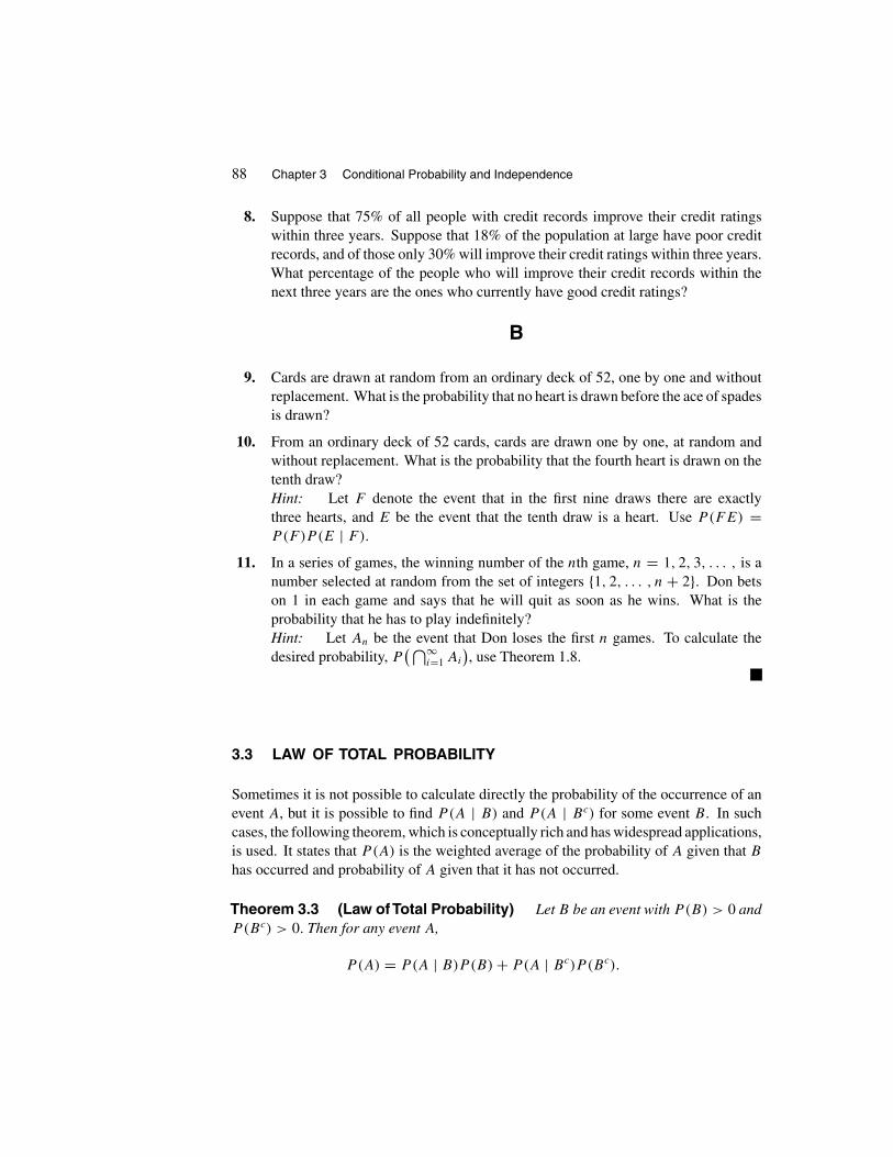
88 Chapter 3 Conditional Probability and Independence
8. Suppose that 75% of all people with credit records improve their credit ratingswithin three years. Suppose that 18% of the population at large have poor creditrecords, and of those only 30% will improve their credit ratings within three years.What percentage of the people who will improve their credit records within thenext three years are the ones who currently have good credit ratings?
B
9. Cards are drawn at random from an ordinary deck of 52, one by one and withoutreplacement. What is the probability that no heart is drawn before the ace of spadesis drawn?
10. From an ordinary deck of 52 cards, cards are drawn one by one, at random andwithout replacement. What is the probability that the fourth heart is drawn on thetenth draw?Hint: Let F denote the event that in the first nine draws there are exactlythree hearts, and E be the event that the tenth draw is a heart. Use P(FE) =P(F)P (E | F).
11. In a series of games, the winning number of the nth game, n = 1, 2, 3, . . . , is anumber selected at random from the set of integers {1, 2, . . . , n + 2}. Don betson 1 in each game and says that he will quit as soon as he wins. What is theprobability that he has to play indefinitely?Hint: Let An be the event that Don loses the first n games. To calculate thedesired probability, P
(⋂∞i=1 Ai
), use Theorem 1.8.
3.3 LAW OF TOTAL PROBABILITY
Sometimes it is not possible to calculate directly the probability of the occurrence of anevent A, but it is possible to find P(A | B) and P(A | Bc) for some event B. In suchcases, the following theorem, which is conceptually rich and has widespread applications,is used. It states that P(A) is the weighted average of the probability of A given that B
has occurred and probability of A given that it has not occurred.
Theorem 3.3 (Law of Total Probability) Let B be an event with P(B) > 0 andP(Bc) > 0. Then for any event A,
P(A) = P(A | B)P (B) + P(A | Bc)P (Bc).

Section 3.3 Law of Total Probability 89
Proof: By Theorem 1.7,
P(A) = P(AB) + P(ABc). (3.7)
Now P(B) > 0 and P(Bc) > 0. These imply that P(AB) = P(A | B)P (B) andP(ABc) = P(A | Bc)P (Bc). Putting these in (3.7), we have proved the theorem. �
Example 3.12 An insurance company rents 35% of the cars for its customers fromagency I and 65% from agency II. If 8% of the cars of agency I and 5% of the cars ofagency II break down during the rental periods, what is the probability that a car rentedby this insurance company breaks down?
c c
Figure 3.2 Tree diagram of Example 3.12.
Solution: Let A be the event that a car rented by this insurance company breaks down.Let I and II be the events that it is rented from agencies I and II, respectively. Then bythe law of total probability,
P(A) = P(A | I)P (I) + P(A | II)P (II)
= (0.08)(0.35) + (0.05)(0.65) = 0.0605.
Tree diagrams facilitate solutions to this kind of problem. Let B and Bc stand forbreakdown and not breakdown during the rental period, respectively. Then, as Figure 3.2shows, to find the probability that a car breaks down, all we need to do is to compute,by multiplication, the probability of each path that leads to a point B and then add themup. So, as seen from the tree, the probability that the car breaks down is (0.35)(0.08) +(0.65)(0.05) = 0.06, and the probability that it does not break down is (0.35)(0.92) +(0.65)(0.95) = 0.94. �
Example 3.13 In a trial, the judge is 65% sure that Susan has committed a crime. Julieand Robert are two witnesses who know whether Susan is innocent or guilty. However,

90 Chapter 3 Conditional Probability and Independence
Robert is Susan’s friend and will lie with probability 0.25 if Susan is guilty. He will tellthe truth if she is innocent. Julie is Susan’s enemy and will lie with probability 0.30 ifSusan is innocent. She will tell the truth if Susan is guilty. What is the probability that,in the course of the trial, Robert and Julie will give conflicting testimony?
Solution: Let I be the event that Susan is innocent. Let C be the event that Robert andJulie will give conflicting testimony. By the law of total probability,
P(C) = P(C | I )P (I) + P(C | I c)P (I c)
= (0.30)(.35) + (0.25)(.65) = 0.2675. �
Example 3.14 (Gambler’s Ruin Problem) Two gamblers play the game of “headsor tails,” in which each time a fair coin lands heads up player A wins $1 from B, andeach time it lands tails up, player B wins $1 from A. Suppose that player A initially hasa dollars and player B has b dollars. If they continue to play this game successively,what is the probability that (a) A will be ruined; (b) the game goes forever with nobodywinning?
Solution:
(a) Let E be the event that A will be ruined if he or she starts with i dollars, and letpi = P(E). Our aim is to calculate pa . To do so, we define F to be the event thatA wins the first game. Then
P(E) = P(E | F)P (F ) + P(E | Fc)P (F c).
In this formula, P(E | F) is the probability that A will be ruined, given that hewins the first game; so P(E | F) is the probability that A will be ruined if hiscapital is i + 1; that is, P(E | F) = pi+1. Similarly, P(E | Fc) = pi−1. Hence
pi = pi+1 · 1
2+ pi−1 · 1
2. (3.8)
Now p0 = 1 because if A starts with 0 dollars, he or she is already ruined. Also,if the capital of A reaches a + b, then B is ruined; thus pa+b = 0. Therefore,we have to solve the system of recursive equations (3.8), subject to the boundaryconditions p0 = 1 and pa+b = 0. To do so, note that (3.8) implies that
pi+1 − pi = pi − pi−1.
Hence, letting p1 − p0 = α, we get
pi − pi−1 = pi−1 − pi−2 = pi−2 − pi−3 = · · · = p2 − p1 = p1 − p0 = α.

Section 3.3 Law of Total Probability 91
Thus
p1 = p0 + α
p2 = p1 + α = p0 + α + α = p0 + 2α
p3 = p2 + α = p0 + 2α + α = p0 + 3α
...
pi = p0 + iα
...
Now p0 = 1 gives pi = 1 + iα. But pa+b = 0; thus 0 = 1 + (a + b)α. This givesα = −1/(a + b); therefore,
pi = 1 − i
a + b= a + b − i
a + b.
In particular, pa = b/(a + b). That is, the probability that A will be ruined isb/(a + b).
(b) The same method can be used with obvious modifications to calculate qi , theprobability that B is ruined if he or she starts with i dollars. The result is
qi = a + b − i
a + b.
Since B starts with b dollars, he or she will be ruined with probability qb =a/(a+b). Thus the probability that the game goes on forever with nobody winningis 1− (qb +pa). But 1− (qb +pa) = 1−a/(a+b)−b/(a+b) = 0. Therefore, ifthis game is played successively, eventually either A is ruined or B is ruined. �
Remark 3.2 If the game is not fair and on each play gambler A wins $1 from B withprobability p, 0 < p < 1, p �= 1/2, and loses $1 to B with probability q = 1 − p,relation (3.8) becomes
pi = ppi+1 + qpi−1,
but pi = (p + q)pi , so (p + q)pi = ppi+1 + qpi−1. This gives
q(pi − pi−1) = p(pi+1 − pi),
which reduces topi+1 − pi = q
p(pi − pi−1).
Using this relation and following the same line of argument lead us to
pi =[(q
p
)i−1 +(q
p
)i−2 + · · · +(q
p
)+ 1]α + p0,
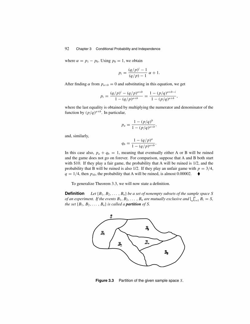
92 Chapter 3 Conditional Probability and Independence
where α = p1 − p0. Using p0 = 1, we obtain
pi = (q/p)i − 1
(q/p) − 1α + 1.
After finding α from pa+b = 0 and substituting in this equation, we get
pi = (q/p)i − (q/p)a+b
1 − (q/p)a+b= 1 − (p/q)a+b−i
1 − (p/q)a+b,
where the last equality is obtained by multiplying the numerator and denominator of thefunction by (p/q)a+b. In particular,
pa = 1 − (p/q)b
1 − (p/q)a+b,
and, similarly,
qb = 1 − (q/p)a
1 − (q/p)a+b.
In this case also, pa + qb = 1, meaning that eventually either A or B will be ruinedand the game does not go on forever. For comparison, suppose that A and B both startwith $10. If they play a fair game, the probability that A will be ruined is 1/2, and theprobability that B will be ruined is also 1/2. If they play an unfair game with p = 3/4,q = 1/4, then p10, the probability that A will be ruined, is almost 0.00002. �
To generalize Theorem 3.3, we will now state a definition.
Definition Let {B1, B2, . . . , Bn} be a set of nonempty subsets of the sample space S
of an experiment. If the events B1, B2, . . . , Bn are mutually exclusive and⋃n
i=1 Bi = S,the set {B1, B2, . . . , Bn} is called a partition of S.
Figure 3.3 Partition of the given sample space S.

Section 3.3 Law of Total Probability 93
For example, if S of Figure 3.3 is the sample space of an experiment, then B1, B2, B3,B4, and B5 of the same figure form a partition of S. As another example, consider theexperiment of drawing a card from an ordinary deck of 52 cards. Let B1, B2, B3, and B4
denote the events that the card is a spade, a club, a diamond, and a heart, respectively. Then{B1, B2, B3, B4} is a partition of the sample space of this experiment. If Ai , 1 ≤ i ≤ 10,denotes the event that the value of the card drawn is i, and A11, A12, and A13 are theevents of jack, queen, and king, respectively, then {A1, A2, . . . , A13} is another partitionof the same sample space. Note that
For an experiment with sample space S, for any event A, A and Ac
both nonempty, the set {A, Ac} is a partition.
As observed, Theorem 3.3 is used whenever it is not possible to calculate P(A)
directly, but it is possible to find P(A | B) and P(A | Bc) for some event B. In manysituations, it is neither possible to find P(A) directly, nor possible to find a single eventB that enables us to use
P(A) = P(A | B)P (B) + P(A | Bc)P (Bc).
In such situations Theorem 3.4, which is a generalization of Theorem 3.3 and is alsocalled the law of total probability, might be applicable.
Theorem 3.4 (Law ofTotal Probability) If {B1, B2, . . . , Bn} is a partition of thesample space of an experiment and P(Bi) > 0 for i = 1, 2, . . . , n, then for any event A
of S,
P(A) = P(A | B1)P (B1) + P(A | B2)P (B2) + · · · + P(A | Bn)P (Bn)
=n∑
i=1
P(A | Bi)P (Bi).
More generally, let {B1, B2, . . . } be a sequence of mutually exclusive events of S suchthat
⋃∞i=1 Bi = S. Suppose that, for all i ≥ 1, P(Bi) > 0. Then for any event A of S,
P(A) =∞∑i=1
P(A | Bi)P (Bi).
Proof: Since B1, B2, . . . , Bn are mutually exclusive, BiBj = ∅ for i �= j . Thus(ABi)(ABj) = ∅ for i �= j . Hence {AB1, AB2, . . . , ABn} is a set of mutually exclusiveevents. Now
S = B1 ∪ B2 ∪ · · · ∪ Bn
gives
A = AS = AB1 ∪ AB2 ∪ · · · ∪ ABn;

94 Chapter 3 Conditional Probability and Independence
therefore,
P(A) = P(AB1) + P(AB2) + · · · + P(ABn).
But P(ABi) = P(A | Bi)P (Bi) for i = 1, 2, . . . , n, so
P(A) = P(A | B1)P (B1) + P(A | B2)P (B2) + · · · + P(A | Bn)P (Bn).
The proof of the more general case is similar. �
When using this theorem, one should be very careful to choose B1, B2, B3, . . . , sothat they form a partition of the sample space.
Example 3.15 Suppose that 80% of the seniors, 70% of the juniors, 50% of thesophomores, and 30% of the freshmen of a college use the library of their campusfrequently. If 30% of all students are freshmen, 25% are sophomores, 25% are juniors,and 20% are seniors, what percent of all students use the library frequently?
Figure 3.4 Tree diagram of Example 3.15.
Solution: Let U be the event that a randomly selected student is using the libraryfrequently. Let F, O, J , and E be the events that he or she is a freshman, sophomore,junior, or senior, respectively. Then {F, O, J, E} is a partition of the sample space. Thus
P(U) = P(U | F)P (F ) + P(U | O)P (O) + P(U | J )P (J ) + P(U | E)P (E)
= (0.30)(0.30) + (0.50)(0.25) + (0.70)(0.25) + (0.80)(0.20) = 0.55.
Therefore, 55% of these students use the campus library frequently. The same calculationcan be carried out readily from the tree diagram of Figure 3.4, where U means they usethe library frequently and N means that they do not. �

Section 3.3 Law of Total Probability 95
Example 3.16 Suppose that 16% of an insurance company’s automobile policyhold-ers are male and under the age of 25, while 12% are female and under the age of 25.The following table lists the percentages of various groups of policyholders who wereinvolved in a car accident last a year.
Male Female BetweenGroup
Under 25 Under 25 25 and 65Over 65
Percentageof Accidents
20% 8% 5% 10%
Find the range of the percentages of this company’s policyholders who got involved in acar accident during the previous year.
Solution: Let M , F , B, and O be, respectively, the events that a randomly selectedautomobile policyholder of this company is a male and under the age of 25, a female andunder the age of 25, between the ages 25 and 65, and over the age of 65. Let A be theevent that he or she got involved in an accident last year. By the law of total probability,
P(A) = P(A | M)P(M) + P(A | F)P (F ) + P(A | B)P (B) + P(A | O)P (O)
= (0.20)(0.16) + (0.08)(0.12) + (0.05)P (B) + (0.10)P (O)
= 0.0416 + (0.05)P (B) + (0.10)P (O).
The lower bound of the range of percentages of all policyholders of this company who gotinvolved in a car accident last year is obtained, from this relation, by putting P(B) = 1and P(O) = 0. It gives P(A) = 0.0916. The upper bound of the range is obtained byputting P(B) = 0 and P(O) = 1, which gives P(A) = 0.1416. Therefore, the range ofthe percentages we are interested in is between 9.16% and 14.16%. �
Example 3.17 An urn contains 10 white and 12 red chips. Two chips are drawn atrandom and, without looking at their colors, are discarded. What is the probability thata third chip drawn is red?
Solution: For i ≥ 1, let Ri be the event that the ith chip drawn is red and Wi be theevent that it is white. Intuitively, it should be clear that the two discarded chips provideno information, so P(R3) = 12/22, the same as if it were the first chip drawn from theurn. To prove this mathematically, note that {R2W1, W2R1, R2R1, W2W1} is a partitionof the sample space; therefore,
P(R3) = P(R3 | R2W1)P (R2W1) + P(R3 | W2R1)P (W2R1)
+ P(R3 | R2R1)P (R2R1) + P(R3 | W2W1)P (W2W1). (3.9)

96 Chapter 3 Conditional Probability and Independence
Now
P(R2W1) = P(R2 | W1)P (W1) = 12
21× 10
22= 20
77,
P (W2R1) = P(W2 | R1)P (R1) = 10
21× 12
22= 20
77,
P (R2R1) = P(R2 | R1)P (R1) = 11
21× 12
22= 22
77,
and
P(W2W1) = P(W2 | W1)P (W1) = 9
21× 10
22= 15
77.
Substituting these values in (3.9), we get
P(R3) = 11
20× 20
77+ 11
20× 20
77+ 10
20× 22
77+ 12
20× 15
77= 12
22. �
EXERCISES
A
1. If 5% of men and 0.25% of women are color blind, what is the probability that arandomly selected person is color blind?
2. Suppose that 40% of the students of a campus are women. If 20% of the womenand 16% of the men of this campus are A students, what percent of all of them areA students?
3. Jim has three cars of different models: A, B, and C. The probabilities that modelsA, B, and C use over 3 gallons of gasoline from Jim’s house to his work are 0.25,0.32, and 0.53, respectively. On a certain day, all three of Jim’s cars have 3 gallonsof gasoline each. Jim chooses one of his cars at random, and without payingattention to the amount of gasoline in the car drives it toward his office. What isthe probability that he makes it to the office?
4. One of the cards of an ordinary deck of 52 cards is lost. What is the probabilitythat a random card drawn from this deck is a spade?
5. Two cards from an ordinary deck of 52 cards are missing. What is the probabilitythat a random card drawn from this deck is a spade?
Section 3.3 Law of Total Probability 97
6. Of the patients in a hospital, 20% of those with, and 35% of those without my-ocardial infarction have had strokes. If 40% of the patients have had myocardialinfarction, what percent of the patients have had strokes?
7. Suppose that 37% of a community are at least 45 years old. If 80% of the time aperson who is 45 or older tells the truth, and 65% of the time a person below 45tells the truth, what is the probability that a randomly selected person answers aquestion truthfully?
8. A person has six guns. The probability of hitting a target when these guns areproperly aimed and fired is 0.6, 0.5, 0.7, 0.9, 0.7, and 0.8, respectively. What isthe probability of hitting a target if a gun is selected at random, properly aimed,and fired?
9. A factory produces its entire output with three machines. Machines I, II, and IIIproduce 50%, 30%, and 20% of the output, but 4%, 2%, and 4% of their outputsare defective, respectively. What fraction of the total output is defective?
10. Solve the following problem, from the “Ask Marilyn” column of Parade Magazine,October 29, 2000.
I recently returned from a trip to China, where the government is so con-cerned about population growth that it has instituted strict laws aboutfamily size. In the cities, a couple is permitted to have only one child. Inthe countryside, where sons traditionally have been valued, if the firstchild is a son, the couple may have no more children. But if the firstchild is a daughter, the couple may have another child. Regardless ofthe sex of the second child, no more are permitted. How will this policyaffect the mix of males and females?
To pose the question mathematically, what is the probability that a randomly se-lected child from the countryside is a boy?
11. Suppose that five coins, of which exactly three are gold, are distributed among fivepersons, one each, at random, and one by one. Are the chances of getting a goldcoin equal for all participants? Why or why not?
12. In a town, 7/9th of the men and 3/5th of the women are married. In that town, whatfraction of the adults are married? Assume that all married adults are the residentsof the town.
13. A child gets lost in the Disneyland at the Epcot Center in Florida. The father of thechild believes that the probability of his being lost in the east wing of the centeris 0.75 and in the west wing is 0.25. The security department sends an officer tothe east and an officer to the west to look for the child. If the probability that asecurity officer who is looking in the correct wing finds the child is 0.4, find theprobability that the child is found.

98 Chapter 3 Conditional Probability and Independence
14. Suppose that there exist N families on the earth and that the maximum number ofchildren a family has is c. Let αj
(0 ≤ j ≤ c,
∑cj=0 αj = 1
)be the fraction of
families with j children. Find the fraction of all children in the world who are thekth born of their families (k = 1, 2, . . . , c).
15. Let B be an event of a sample space S with P(B) > 0. For a subset A of S, defineQ(A) = P(A | B). By Theorem 3.1 we know that Q is a probability function.For E and F , events of S
[P(FB) > 0
], show that Q(E | F) = P(E | FB).
B
16. Suppose that 40% of the students on a campus, who are married to students on thesame campus, are female. Moreover, suppose that 30% of those who are married,but not to students at this campus, are also female. If one-third of the marriedstudents on this campus are married to other students on this campus, what is theprobability that a randomly selected married student from this campus is a woman?Hint: Let M , C, and F denote the events that the random student is married,is married to a student on the same campus, and is female. For any event A,let Q(A) = P(A | M). Then, by Theorem 3.1, Q satisfies the same axiomsthat probabilities satisfy. Applying Theorem 3.3 to Q and, using the result ofExercise 15, we obtain
P(F | M) = P(F | MC)P (C | M) + P(F | MCc)P (Cc | M).
17. Suppose that the probability that a new seed planted in a specific farm germinates isequal to the proportion of all planted seeds that germinated in that farm previously.Suppose that the first seed planted in the farm germinated, but the second seedplanted did not germinate. For positive integers n and k (k < n), what is theprobability that of the first n seeds planted in the farm exactly k germinated?
18. Suppose that 10 good and three dead batteries are mixed up. Jack tests them oneby one, at random and without replacement. But before testing the fifth battery herealizes that he does not remember whether the first one tested is good or is dead.All he remembers is that the last three that were tested were all good. What is theprobability that the first one is also good?
19. A box contains 18 tennis balls, of which eight are new. Suppose that three balls areselected randomly, played with, and after play are returned to the box. If anotherthree balls are selected for play a second time, what is the probability that they areall new?
20. From families with three children, a child is selected at random and found to be agirl. What is the probability that she has an older sister? Assume that in a three-child family all sex distributions are equally probable.Hint: Let G be the event that the randomly selected child is a girl, A be the event

Section 3.3 Law of Total Probability 99
that she has an older sister, and O, M , and Y be the events that she is the oldest,the middle, and the youngest child of the family, respectively. For any subset B
of the sample space let Q(B) = P(B | G); then apply Theorem 3.3 to Q. (Seealso Exercises 15 and 16.)
21. Suppose that three numbers are selected one by one, at random and without re-placement from the set of numbers {1, 2, 3, . . . , n}. What is the probability thatthe third number falls between the first two if the first number is smaller than thesecond?
22. Avril has certain standards for selecting her future husband. She has n suitors andknows how to compare any two and rank them. She decides to date one suitor at atime randomly. When she knows a suitor well enough, she can marry or reject him.If she marries the suitor, she can never know the ones not dated. If she rejects thesuitor, she will not be able to reconsider him. In this process, Avril will not choosea suitor she ranks lower than at least one of the previous ones dated. Avril’s goal isto maximize the probability of selecting the best suitor. To achieve this, she adoptsthe following strategy: For some m, 0 ≤ m < n, she dumps the first m suitorsshe dates after knowing each of them well no matter how good they are. Then shemarries the first suitor she dates who is better than all those preceding him. Interms of n, find the value of m which maximizes the probability of selecting thebest suitor.Remark: This exercise is a model for many real-world problems in which wehave to reject “choices” or “offers” until the one we think is the “best.” Note thatit is quite possible that we reject the best “offer” or “choice” in the process. If thishappens, we will not be able to make a selection.
23. (Shrewd Prisoner’s Dilemma) Because of a prisoner’s constant supplication,the king grants him this favor: He is given 2N balls, which differ from each otheronly in that half of them are green and half are red. The king instructs the prisonerto divide the balls between two identical urns. One of the urns will then be selectedat random, and the prisoner will be asked to choose a ball at random from the urnchosen. If the ball turns out to be green, the prisoner will be freed. How shouldhe distribute the balls in the urn to maximize his chances of freedom?Hint: Let g be the number of green balls and r be the number of red balls inthe first urn. The corresponding numbers in the second urn are N − g and N − r .The probability that a green ball is drawn is f (g, r):
f (g, r) = 1
2
( g
g + r+ N − g
2N − g − r
).
Find the maximum of this function of two variables (r and g). Note that themaximum need not occur at an interior point of the domain.

100 Chapter 3 Conditional Probability and Independence
3.4 BAYES’ FORMULA
To introduce Bayes’ formula, let us first examine the following problem. In a bolt factory,30, 50, and 20% of production is manufactured by machines I, II, and III, respectively. If4, 5, and 3% of the output of these respective machines is defective, what is the probabilitythat a randomly selected bolt that is found to be defective is manufactured by machineIII? To solve this problem, let A be the event that a random bolt is defective and B3 bethe event that it is manufactured by machine III. We are asked to find P(B3 | A). Now
P(B3 | A) = P(B3A)
P (A), (3.10)
so we need to know the quantities P(B3A) and P(A). But neither of these is given. Tofind P(B3A), note that since P(A | B3) and P(B3) are known we can use the relation
P(B3A) = P(A | B3)P (B3). (3.11)
To calculate P(A), we must use the law of total probability. Let B1 and B2 be the eventsthat the bolt is manufactured by machines I and II, respectively. Then {B1, B2, B3} is apartition of the sample space; hence
P(A) = P(A | B1)P (B1) + P(A | B2)P (B2) + P(A | B3)P (B3). (3.12)
Substituting (3.11) and (3.12) in (3.10), we arrive at Bayes’ formula:
P(B3 | A) = P(B3A)
P (A)
= P(A | B3)P (B3)
P (A | B1)P (B1) + P(A | B2)P (B2) + P(A | B3)P (B3)(3.13)
= (0.03)(0.20)
(0.04)(0.30) + (0.05)(0.50) + (0.03)(0.20)≈ 0.14. (3.14)
Relation (3.13) is a particular case of Bayes’ formula (Theorem 3.5). We will nowexplain how a tree diagram is used to write relation (3.14). Figure 3.5, in which D standsfor “defective” and N for “not defective,” is a tree diagram for this problem. To findthe desired probability all we need do is find (by multiplication) the probability of therequired path, the path from III to D, and divide it by the sum of the probabilities of thepaths that lead to D’s.
In general, modifying the argument from which (3.13) was deduced, we arrive at thefollowing theorem.

Section 3.4 Bayes’ Formula 101
0.012 + 0.025 + 0.006 = 0.0430.006/0.043 = 0.14
Figure 3.5 Tree diagram for relation (3.14).
Theorem 3.5 (Bayes’ Theorem) Let {B1, B2, . . . , Bn} be a partition of thesample space S of an experiment. If for i = 1, 2, . . . , n, P (Bi) > 0, then for any eventA of S with P(A) > 0,
P(Bk | A) = P(A | Bk)P (Bk)
P (A | B1)P (B1) + P(A | B2)P (B2) + · · · + P(A | Bn)P (Bn).
In statistical applications of Bayes’ theorem, B1, B2, . . . , Bn are called hypotheses,P(Bi) is called the prior probability of Bi , and the conditional probability P(Bi | A) iscalled the posterior probability of Bi after the occurrence of A.
Note that, for any event B of S, B and Bc both nonempty, the set {B, Bc} is a partitionof S. Thus, by Theorem 3.5,
If P(B) > 0 and P(Bc) > 0, then for any event A of S with P(A) > 0,
P(B | A) = P(A | B)P (B)
P (A | B)P (B) + P(A | Bc)P (Bc).
Similarly,
P(Bc | A) = P(A | Bc)P (Bc)
P (A | B)P (B) + P(A | Bc)P (Bc).
These are the simplest forms of Bayes’ formula. They are used whenever the quantitiesP(A | B), P (A | Bc), and P(B) are given or can be calculated. The typical situationis that A happens logically or temporally after B, so that the probabilities P(B) andP(A | B) can be readily computed. Bayes’ formula is applicable when we know the

102 Chapter 3 Conditional Probability and Independence
probability of the more recent event, given that the earlier event has occurred, P(A | B),and we wish to calculate the probability of the earlier event, given that the more recentevent has occurred, P(B | A). In practice, Bayes’ formula is used when we know theeffect of a cause and we wish to make some inference about the cause.
Theorem 3.5, in its present form, is due to Laplace, who named it after ThomasBayes (1701–1761). Bayes, a prominent English philosopher and an ordained minister,did a comprehensive study of the calculation of P(B | A) in terms of P(A | B). Hiswork was continued by other mathematicians such as Laplace and Gauss.
We will now present several examples concerning Bayes’ theorem. To emphasize theconvenience of tree diagrams, in Example 3.21, we will use a tree diagram as well.
Example 3.18 In a study conducted three years ago, 82% of the people in a randomlyselected sample were found to have “good” financial credit ratings, while the remaining18% were found to have “bad” financial credit ratings. Current records of the peoplefrom that sample show that 30% of those with bad credit ratings have since improvedtheir ratings to good, while 15% of those with good credit ratings have since changed tohaving a bad credit rating. What percentage of people with good credit ratings now hadbad ratings three years ago?
Solution: Let G be the event that a randomly selected person from the sample has agood credit rating now. Let B be the event that he or she had a bad credit rating threeyears ago. The desired quantity is P(B | G). By Bayes’ formula,
P(B | G) = P(G | B)P (B)
P (G | B)P (B) + P(G | Bc)P (Bc)
= (0.30)(.18)
(0.30)(.18) + (.85)(.82)= 0.072,
where P(G | Bc) = 0.85, because the probability is 1 − 0.15 = 0.85 that a personwith good credit rating three years ago has a good credit rating now. Therefore, 7.2% ofpeople with good credit ratings now had bad ratings three years ago. �
Example 3.19 During a double homicide murder trial, based on circumstantial ev-idence alone, the jury becomes 15% certain that a suspect is guilty. DNA samplesrecovered from the murder scene are then compared with DNA samples extracted fromthe suspect. Given the size and conditions of the recovered samples, a forensic scientistestimates that the probability of the sample having come from someone other than thesuspect is 10−9.With this new information, how certain should the jury be of the suspect’sguilt?
Solution: Let G and I be the events that the suspect is guilty and innocent, respectively.Let D be the event that the recovered DNA samples from the murder scene match withthe DNA samples extracted from the suspect. Since {G, I } is a partition of the sample

Section 3.4 Bayes’ Formula 103
space, we can use Bayes’ formula to calculate P(G | D), the probability that the suspectis the murderer in view of the new evidence.
P(G | D) = P(D | G)P (G)
P (D | G)P (G) + P(D | I )P (I)
= 1(.15)
1(.15) + 10−9(.85)= 0.9999999943.
This shows that P(I | D) = 1 − P(G | D) is approximately 5.67 × 10⁻⁹, leaving noreasonable doubt for the innocence of the suspect.
In some trials, prosecutors have argued that if P(D | I ) is “small enough,” thenthere is no reasonable doubt for the guilt of the defendant. Such an argument, called theprosecutor’s fallacy, probably stems from confusing P(D | I ) for P(I | D). One shouldpay attention to the fact that P(D | I ) is infinitesimal regardless of the suspect’s guilt orinnocence. To elaborate this further, note that in this example, P(I | D) is approximately5.67 times larger than P(D | I ), which is 10−9. This is because even without the DNAevidence, there is a 15% chance that the suspect is guilty.
We will now present a situation, which clearly demonstrates that P(D | I ) shouldnot be viewed as the probability of guilt in evaluating reasonable doubt. Suppose that thedouble homicide in this example occurred in California, and there is no suspect identified.Suppose that a DNA data bank identifies a person in South Dakota whose DNA matcheswhat was recovered at the California crime scene. Furthermore, suppose that the forensicscientist estimates that the probability of the sample recovered at the crime scene havingcome from someone other than the person in South Dakota is still 10−9. If there is noevidence that this person ever traveled to California, or had any motive for committingthe double homicide, it is doubtful that he or she would be indicted. In such a caseP(D | I ) is still 10−9, but this quantity hardly constitutes the probability of guilt for theperson in South Dakota. The argument that since P(D | I ) is infinitesimal there is noreasonable doubt for the guilt of the person from South Dakota does not seem convincingat all. In such a case, the quantity P(I | D), which can be viewed as the probability ofguilt, cannot even be estimated if nothing beyond DNA evidence exists. �
Example 3.20 On the basis of reconnaissance reports, Colonel Smith decides thatthe probability of an enemy attack against the left is 0.20, against the center is 0.50,and against the right is 0.30. A flurry of enemy radio traffic occurs in preparation forthe attack. Since deception is normal as a prelude to battle, Colonel Brown, havingintercepted the radio traffic, tells General Quick that if the enemy wanted to attack on theleft, the probability is 0.20 that he would have sent this particular radio traffic. He tellsthe general that the corresponding probabilities for an attack on the center or the right are0.70 and 0.10, respectively. How should General Quick use these two equally reliablestaff members’ views to get the best probability profile for the forthcoming attack?
Solution: Let A be the event that the attack would be against the left, B be the event thatthe attack would be against the center, and C be the event that the attack would be against

104 Chapter 3 Conditional Probability and Independence
the right. Let be the event that this particular flurry of radio traffic occurs. ColonelBrown has provided information of conditional probabilities of a particular flurry ofradio traffic given that the enemy is preparing to attack against the left, the center, and theright. However, Colonel Smith has presented unconditional probabilities, on the basisof reconnaissance reports, for the enemy attacking against the left, the center, and theright. Because of these, the general should take the opinion of Colonel Smith as priorprobabilities for A, B, and C. That is, P(A) = 0.20, P(B) = 0.50, and P(C) = 0.30.Then he should calculate P(A | ), P(B | ), and P(C | ) based on Colonel Brown’sview, using Bayes’ theorem, as follows.
P(A | ) = P( | A)P (A)
P ( | A)P (A) + P( | B)P (B) + P( | C)P (C)
= (0.2)(0.2)
(0.2)(0.2) + (0.7)(0.5) + (0.1)(0.3)= (0.2)(0.2)
0.42≈ 0.095.
Similarly,
P(B | ) = (0.7)(0.5)
0.42≈ 0.83 and P(C | ) = (0.1)(0.3)
0.42≈ 0.071. �
Example 3.21 A box contains seven red and 13 blue balls. Two balls are selectedat random and are discarded without their colors being seen. If a third ball is drawnrandomly and observed to be red, what is the probability that both of the discarded ballswere blue?
Solution: Let BB, BR, and RR be the events that the discarded balls are blue and blue,blue and red, red and red, respectively. Also, let R be the event that the third ball drawnis red. Since {BB, BR, RR} is a partition of sample space, Bayes’ formula can be usedto calculate P(BB | R).
P(BB |R)= P(R |BB)P (BB)
P (R |BB)P (BB) + P(R |BR)P (BR) + P(R |RR)P (RR).
Now
P(BB) = 13
20× 12
19= 39
95, P (RR) = 7
20× 6
19= 21
190,
and
P(BR) = 13
20× 7
19+ 7
20× 13
19= 91
190,
where the last equation follows since BR is the union of two disjoint events: namely, thefirst ball discarded was blue, the second was red, and vice versa. Thus
P(BB | R) =7
18× 39
957
18× 39
95+ 6
18× 91
190+ 5
18× 21
190
≈ 0.46.

Section 3.4 Bayes’ Formula 105
This result can be found from the tree diagram of Figure 3.6 as well. Alternatively,reducing sample space, given that the third ball was red, there are 13 blue and six redballs which could have been discarded. Thus
P(BB | R) = 13
19× 12
18≈ 0.46. �
5
18· 21
190+ 6
18· 91
190+ 7
18· 39
95≈ 0.35,
7
18· 39
95≈ 0.16,
0.16
0.35≈ 0.46.
Figure 3.6 Tree diagram for Example 3.21.
EXERCISES
A
1. In transmitting dot and dash signals, a communication system changes 1/4 of thedots to dashes and 1/3 of the dashes to dots. If 40% of the signals transmitted aredots and 60% are dashes, what is the probability that a dot received was actuallya transmitted dot?
2. On a multiple-choice exam with four choices for each question, a student eitherknows the answer to a question or marks it at random. If the probability that heor she knows the answers is 2/3, what is the probability that an answer that wasmarked correctly was not marked randomly?

106 Chapter 3 Conditional Probability and Independence
3. A judge is 65% sure that a suspect has committed a crime. During the courseof the trial, a witness convinces the judge that there is an 85% chance that thecriminal is left-handed. If 23% of the population is left-handed and the suspectis also left-handed, with this new information, how certain should the judge be ofthe guilt of the suspect?
4. In a trial, the judge is 65% sure that Susan has committed a crime. Julie and Robertare two witnesses who know whether Susan is innocent or guilty. However, Robertis Susan’s friend and will lie with probability 0.25 if Susan is guilty. He will tellthe truth if she is innocent. Julie is Susan’s enemy and will lie with probability0.30 if Susan is innocent. She will tell the truth if Susan is guilty. What is theprobability that Susan is guilty if Robert and Julie give conflicting testimony?
5. Suppose that 5% of the men and 2% of the women working for a corporation makeover $120,000 a year. If 30% of the employees of the corporation are women, whatpercent of those who make over $120,000 a year are women?
6. A stack of cards consists of six red and five blue cards. A second stack of cardsconsists of nine red cards. A stack is selected at random and three of its cardsare drawn. If all of them are red, what is the probability that the first stack wasselected?
7. A certain cancer is found in one person in 5000. If a person does have the disease,in 92% of the cases the diagnostic procedure will show that he or she actually hasit. If a person does not have the disease, the diagnostic procedure in one out of 500cases gives a false positive result. Determine the probability that a person with apositive test result has the cancer.
8. Urns I, II, and III contain three pennies and four dimes, two pennies and five dimes,three pennies and one dime, respectively. One coin is selected at random fromeach urn. If two of the three coins are dimes, what is the probability that the coinselected from urn I is a dime?
9. In a study it was discovered that 25% of the paintings of a certain gallery are notoriginal. A collector in 15% of the cases makes a mistake in judging if a paintingis authentic or a copy. If she buys a piece thinking that it is original, what is theprobability that it is not?
10. There are three identical cards that differ only in color. Both sides of one are black,both sides of the second one are red, and one side of the third card is black and itsother side is red. These cards are mixed up and one of them is selected at random.If the upper side of this card is red, what is the probability that its other side isblack?
11. With probability of 1/6 there are i defective fuses among 1000 fuses (i = 0, 1, 2,3, 4, 5). If among 100 fuses selected at random, none was defective, what is theprobability of no defective fuses at all?

Section 3.5 Independence 107
12. Solve the following problem, asked of Marilyn Vos Savant in the “Ask Marilyn”column of Parade Magazine, February 18, 1996.
Say I have a wallet that contains either a $2 bill or a $20 bill (with equallikelihood), but I don’t know which one. I add a $2 bill. Later, I reachinto my wallet (without looking) and remove a bill. It’s a $2 bill. There’sone bill remaining in the wallet. What are the chances that it’s a $2 bill?
B
13. There are two stables on a farm, one that houses 20 horses and 13 mules, the otherwith 25 horses and eight mules. Without any pattern, animals occasionally leavetheir stables and then return to their stables. Suppose that during a period whenall the animals are in their stables, a horse comes out of a stable and then returns.What is the probability that the next animal coming out of the same stable willalso be a horse?
14. An urn contains five red and three blue chips. Suppose that four of these chips areselected at random and transferred to a second urn, which was originally empty.If a random chip from this second urn is blue, what is the probability that two redand two blue chips were transferred from the first urn to the second urn?
15. The advantage of a certain blood test is that 90% of the time it is positive forpatients having a certain disease. Its disadvantage is that 25% of the time it is alsopositive in healthy people. In a certain location 30% of the people have the disease,and anybody with a positive blood test is given a drug that cures the disease. If20% of the time the drug produces a characteristic rash, what is the probabilitythat a person from this location who has the rash had the disease in the first place?
3.5 INDEPENDENCE
Let A and B be two events of a sample space S, and assume that P(A) > 0 and P(B) > 0.
We have seen that, in general, the conditional probability of A given B is not equal tothe probability of A. However, if it is, that is, if P(A | B) = P(A), we say that A
is independent of B. This means that if A is independent of B, knowledge regardingthe occurrence of B does not change the chance of the occurrence of A. The relationP(A | B) = P(A) is equivalent to the relations P(AB)/P (B) = P(A), P (AB) =P(A)P (B), P (BA)/P (A) = P(B), and P(B | A) = P(B). The equivalence of thefirst and last of these relations implies that if A is independent of B, then B is independentof A. In other words, if knowledge regarding the occurrence of B does not change thechance of occurrence of A, then knowledge regarding the occurrence of A does not

108 Chapter 3 Conditional Probability and Independence
change the chance of occurrence of B. Hence independence is a symmetric relation onthe set of all events of a sample space. As a result of this property, instead of makingthe definitions “A is independent of B” and “B is independent of A,” we simply definethe concept of the “independence of A and B.” To do so, we take P(AB) = P(A)P (B)
as the definition. We do this because a symmetrical definition relating A and B doesnot readily follow from either of the other relations given
[i.e., P(A | B) = P(A)
or P(B | A) = P(B)]. Moreover, these relations require either that P(B) > 0 or
P(A) > 0, whereas our definition does not.
Definition Two events A and B are called independent if
P(AB) = P(A)P (B).
If two events are not independent, they are called dependent. If A and B are independent,we say that {A, B} is an independent set of events.
Note that in this definition we did not require P(A) or P(B) to be strictly positive.Hence by this definition any event A with P(A) = 0 or 1 is independent of every eventB (see Exercise 13).
Example 3.22 In the experiment of tossing a fair coin twice, let A and B be the eventsof getting heads on the first and second tosses, respectively. Intuitively, it is clear thatA and B are independent. To prove this mathematically, note that P(A) = 1/2 andP(B) = 1/2. But since the sample space of this experiment consists of the four equallyprobable events: HH, HT, TH, and TT, we have P(AB) = P(HH) = 1/4. HenceP(AB) = P(A)P (B) is valid, implying the independence of A and B. It is interestingto know that Jean Le Rond d’Alembert (1717–1783), a French mathematician, had arguedthat, since in the experiment of tossing a fair coin twice the possible number of heads is0, 1, and 2, the probability of no heads, one heads, and two heads, each is 1/3. �
Example 3.23 In the experiment of drawing a card from an ordinary deck of 52 cards,let A and B be the events of getting a heart and an ace, respectively. Whether A andB are independent cannot be answered easily on the basis of intuition alone. However,using the defining formula, P(AB) = P(A)P (B), this can be answered at once sinceP(AB) = 1/52, P(A) = 1/4, P(B) = 1/13, and 1/52 = 1/4 × 1/13. Hence A andB are independent events. �
Example 3.24 An urn contains five red and seven blue balls. Suppose that two ballsare selected at random and with replacement. Let A and B be the events that the firstand the second balls are red, respectively. Then, using the counting principle, we getP(AB) = (5 × 5)/(12 × 12). Now P(AB) = P(A)P (B) since P(A) = 5/12 andP(B) = 5/12. Thus A and B are independent. If we do the same experiment without

Section 3.5 Independence 109
replacement, then P(B | A) = 4/11 while
P(B) = P(B | A)P (A) + P(B | Ac)P (Ac)
= 4
11× 5
12+ 5
11× 7
12= 5
12,
which might be quite surprising to some. But it is true. If no information is given on theoutcome of the first draw, there is no reason for the probability of second ball being redto differ from 5/12. Thus P(B | A) �= P(B), implying that A and B are dependent. �
Example 3.25 In the experiment of selecting a random number from the set of nat-ural numbers {1, 2, 3, . . . , 100}, let A, B, and C denote the events that they are di-visible by 2, 3, and 5, respectively. Clearly, P(A) = 1/2, P (B) = 33/100, P (C) =1/5, P (AB) = 16/100, and P(AC) = 1/10. Hence A and B are dependent while A andC are independent. Note that if the random number is selected from {1, 2, 3, . . . , 300},then each of {A, B}, {A, C}, and {B, C} is an independent set of events. This is because300 is divisible by 2, 3, and 5, but 100 is not divisible by 3. �
Figure 3.7 Spinner of Example 3.26.
Example 3.26 A spinner is mounted on a wheel. Arcs A, B, and C, of equal length,are marked off on the wheel’s perimeter (see Figure 3.7). In a game of chance, thespinner is flicked, and depending on whether it stops on A, B, or C, the player wins1, 2, or 3 points, respectively. Suppose that a player plays this game twice. Let E
denote the event that he wins 1 point in the first game and any number of points inthe second. Let F be the event that he wins a total of 3 points in both games, and G
be the event that he wins a total of 4 points in both games. The sample space of thisexperiment has 3 × 3 = 9 elements, E = {
(1, 1), (1, 2), (1, 3)}, F = {
(1, 2), (2, 1)},
and G = {(1, 3), (2, 2), (3, 1)
}. Therefore, P(E) = 1/3, P(G) = 1/3, P(F) = 2/9,
P(FE) = 1/9, and P(GE) = 1/9. These show that E and G are independent, whereasE and F are not. To justify these intuitively, note that if we are interested in a total of 3points, then getting 1 point in the first game is good luck, since obtaining 3 points in thefirst game makes it impossible to win a sum of 3. However, if we are interested in a sum

110 Chapter 3 Conditional Probability and Independence
of 4 points, it does not matter what we win in the first game. We have the same chanceof obtaining a sum of 4 if the first game results in any of the numbers 1, 2, or 3. �
We now prove that if A and B are independent events, so are A and Bc.
Theorem 3.6 If A and B are independent, then A and Bc are independent as well.
Proof: By Theorem 1.7,
P(A) = P(AB) + P(ABc).
Therefore,
P(ABc) = P(A) − P(AB) = P(A) − P(A)P (B)
= P(A)[1 − P(B)
] = P(A)P (Bc). �
Corollary If A and B are independent, then Ac and Bc are independent as well.
Proof: A and B are independent, so by Theorem 3.6 the events A and Bc are inde-pendent. Now, using the same theorem again, we have that Ac and Bc are independent.
�
Thus, if A and B are independent, knowledge about the occurrence or nonoccurrenceof A does not change the chances of the occurrence or nonoccurrence of B, and viceversa.
Remark 3.3 If A and B are mutually exclusive events and P(A) > 0, P(B) > 0, thenthey are dependent. This is because, if we are given that one has occurred, the chance ofthe occurrence of the other one is zero. That is, the occurrence of one of them precludesthe occurrence of the other. For example, let A be the event that the next president of theUnited States is a Democrat and B be the event that he or she is a Republican. Then A
and B are mutually exclusive; hence they are dependent. If A occurs, that is, if the nextpresident is a Democrat, the probability that B occurs, that is, he or she is a Republicanis zero, and vice versa. �
The following example shows that if A is independent of B and if A is independentof C, then A is not necessarily independent of BC or of B ∪ C.
Example 3.27 Dennis arrives at his office every day at a random time between 8:00A.M.
and 9:00 A.M. Let A be the event that Dennis arrives at his office tomorrow between8:15 A.M. and 8:45 A.M. Let B be the event that he arrives between 8:30 A.M. and 9:00 A.M.,and let C be the event that he arrives either between 8:15 A.M. and 8:30 A.M. or between8:45 A.M. and 9:00 A.M. Then AB, AC, BC, and B ∪ C are the events that Dennis arrivesat his office between 8:30 and 8:45, 8:15 and 8:30, 8:45 and 9:00, and 8:15 and 9:00,

Section 3.5 Independence 111
respectively. Thus P(A) = P(B) = P(C) = 1/2 and P(AB) = P(AC) = 1/4. SoP(AB) = P(A)P (B) and P(AC) = P(A)P (C); that is, A is independent of B and it isindependent of C. However, since BC and A are mutually exclusive, they are dependent.Also, P(A | B ∪ C) = 2/3 �= P(A). Thus B ∪ C and A are dependent as well. �
Example 3.28 (Jailer’s Paradox) The jailer of a prison in which Alex, Ben, andTim are held is the only person, other than the judge, who knows which of these threeprisoners is condemned to death, and which two will be freed. The prisoners know thatexactly two of them will go free; they do not know which two. Alex has written a letterto his fiancée. Just in case he is not one of the two who will be freed, he wants to give theletter to a prisoner who goes free to deliver. So Alex asks the jailer to tell him the nameof one of the two prisoners who will go free. The jailer refuses to give that information toAlex. To begin with, he is not allowed to tell Alex whether Alex goes free or not. PuttingAlex aside, he argues that, if he reveals the name of a prisoner who will go free, then theprobability of Alex dying increases from 1/3 to 1/2. He does not want to do that.
As Zweifel notes in the June 1986 issue of Mathematics Magazine, page 156, “thisseems intuitively suspect, since the jailer is providing no new information toAlex, so whyshould his probability of dying change?” Zweifel is correct. Just revealing to Alex thatBen goes free, or just revealing to him that Tim goes free is not the type of informationthat changes the probability of Alex dying. What changes the probability of Alex dyingis telling him whether both Ben and Tim are going free or exactly one of them is goingfree.
To explain this paradox, we will show that, under suitable conditions, if the jailer tellsAlex that Tim goes free, still the probability is 1/3 that Alex dies. Telling Alex that Timis going free reveals to Alex that the probability of Ben dying is 2/3. Similarly, tellingAlex that Ben is going free reveals to Alex that the probability of Tim dying is 2/3. Toshow these facts, let A, B, and T be the events that “Alex dies,” “Ben dies,” and “Timdies.” Let
ω1 = Tim dies, and the jailer tells Alex that Ben goes free
ω2 = Ben dies, and the jailer tells Alex that Tim goes free
ω3 = Alex dies, and the jailer tells Alex that Ben goes free
ω4 = Alex dies, and the jailer tells Alex that Tim goes free.
The sample space of all possible episodes is S = {ω1, ω2, ω3, ω4}. Now, if Tim dies, withprobability 1, the jailer will tell Alex that Ben goes free. Therefore, ω1 occurs if and onlyif Tim dies. This implies that P(ω1) = 1/3. Similarly, if Ben dies, with probability 1,the jailer will tell Alex that Tim goes free. Therefore, ω2 occurs if and only if Ben dies.This shows that P(ω2) = 1/3. To assign probabilities to ω3 and ω4, we will make twoassumptions: (1) If Alex is the one who is scheduled to die, then the event that the jailerwill tell Alex that Ben goes free is independent of the event that the jailer will tell Alexthat Tim goes free, and (2) if Alex is the one who is scheduled to die, then the probabilitythat the jailer will tell Alex that Ben goes free is 1/2; hence the probability that he will tell
112 Chapter 3 Conditional Probability and Independence
Alex that Tim goes free is 1/2 as well. Under these conditions, P(ω3) = P(ω4) = 1/6.
Let J be the event that “the jailer tells Alex that Tim goes free;” then
P(A | J ) = P(AJ)
P (J )= P(ω4)
P (ω2) + P(ω4)=
1
61
3+ 1
6
= 1
3,
This shows that if the jailer reveals no information about the fate of Alex, telling Alexthe name of one prisoner who goes free does not change the probability of Alex dying;it remains to be 1/3.
Note that the decision as which of Ben, Tim, or Alex is condemned to death, andwhich two will be freed, has been made by the judge. The jailer has no option to controlAlex’s fate. With probability 1, the jailer knows which one of the three dies and whichtwo will go free. It is Alex who doesn’t know any of these probabilities. Alex can onlyanalyze these probabilities based on the information he receives from the jailer. If Alex isdying, and the jailer disobeys the conditions (1) and (2), then he could decide to tell Alex,with arbitrary probabilities, which of Ben or Tim goes free. In such a case, P(A | J ) willno longer equal 1/3. It will vary depending on the probabilities of J and J c. If the jailerinsists on not giving extra information to Alex, he should obey conditions (1) and (2).Furthermore, the jailer should tell Alex what his rules are when he reveals information.Alex can only analyze the probability of dying based on the full information he receivesfrom the jailer. If the jailer does not reveal his rules to Alex, there is no way for Alex toknow whether the probability that he is the unlucky prisoner has changed or not.
Zweifel analyzes this paradox by using Bayes’ formula:
P(A | J ) = P(J | A)P (A)
P (J | A)P (A) + P(J | B)P (B) + P(J | T )P (T )
=1
2× 1
31
2× 1
3+ 1 × 1
3+ 0 × 1
3
= 1
3.
Similarly, if D is the event that “the jailer tells Alex that Ben goes free,” then P(A |D) = 1/3. In his explanation of this paradox Zweifel writes
Aside from the formal application of Bayes’ theorem, one would like to under-stand this “paradox” from an intuitive point of view. The crucial point whichcan perhaps make the situation clear is the discrepancy between P(J | A)
and P(J | B) noted above. Bridge players call this the “Principle of Re-stricted Choice.” The probability of a restricted choice is obviously greaterthan that of a free choice, and a common error made by those who attemptto solve such problems intuitively is to overlook this point. In the case of thejailer’s paradox, if the jailer says “Tim will go free” this is twice as likely to

Section 3.5 Independence 113
occur when Ben is scheduled to die (restricted choice; jailer must say “Tim”)as when Alex is scheduled to die (free choice; jailer could say either “Tim”or “Ben”).
The jailer’s paradox and its solution have been around for a long time. Despite this,when the same problem in a different context came up in the “Ask Marilyn” column ofParade Magazine on September 9, 1990 (see Example 3.8) and Marilyn Vos Savant† gavethe correct answer to the problem in the December 2, 1990 issue, she was taken to taskby three mathematicians. By the time the February 17, 1991 issue of Parade Magazinewas published, Vos Savant had received 2000 letters on the problem, of which 92% ofgeneral respondents and 65% of university respondents opposed her answer. This storyreminds us of the statement of De Moivre in his dedication of The Doctrine of Chance:
Some of the Problems about Chance having a great appearance of Sim-plicity, the Mind is easily drawn into a belief, that their Solution may beattained by the mere Strength of natural good Sense; which generally prov-ing otherwise and the Mistakes occasioned thereby being not unfrequent,‘tis presumed that a Book of this Kind, which teaches to distinguish Truthfrom what seems so nearly to resemble it, will be looked upon as a help togood Reasoning. �
We now extend the concept of independence to three events: A, B, and C are calledindependent if knowledge about the occurrence of any of them, or the joint occurrenceof any two of them, does not change the chances of the occurrence of the remaining events.That is, A, B, and C are independent if {A, B}, {A, C}, {B, C}, {A, BC}, {B, AC}, and{C, AB} are all independent sets of events. Hence A, B, and C are independent if
P(AB) = P(A)P (B),
P (AC) = P(A)P (C),
P (BC) = P(B)P (C),
P(A(BC)
) = P(A)P (BC),
P(B(AC)
) = P(B)P (AC),
P(C(AB)
) = P(C)P (AB).
Now note that these relations can be reduced since the first three and the relationP(ABC) = P(A)P (B)P (C) imply the last three relations. Hence the definition ofthe independence of three events can be shortened as follows.
†Ms. Vos Savant is the writer of a reader-correspondence column and is listed in the Guinness Book ofRecords Hall of Fame for “highest IQ.”

114 Chapter 3 Conditional Probability and Independence
Definition The events A, B, and C are called independent if
P(AB) = P(A)P (B),
P (AC) = P(A)P (C),
P (BC) = P(B)P (C),
P (ABC) = P(A)P (B)P (C).
If A, B, and C are independent events, we say that {A, B, C} is an independent set ofevents.
The following example demonstrates that P(ABC) = P(A)P (B)P (C), in general,does not imply that {A, B, C} is a set of independent events.
Example 3.29 Let an experiment consist of throwing a die twice. Let A be theevent that in the second throw the die lands 1, 2, or 5; B the event that in the secondthrow it lands 4, 5 or 6; and C the event that the sum of the two outcomes is 9. ThenP(A) = P(B) = 1/2, P(C) = 1/9, and
P(AB) = 1
6�= 1
4= P(A)P (B),
P (AC) = 1
36�= 1
18= P(A)P (C),
P (BC) = 1
12�= 1
18= P(B)P (C),
while
P(ABC) = 1
36= P(A)P (B)P (C).
Thus the validity of P(ABC) = P(A)P (B)P (C) is not sufficient for the independenceof A, B, and C. �
If A, B, and C are three events and the occurrence of any of them does not change thechances of the occurrence of the remaining two, we say that A, B, and C are pairwiseindependent. Thus {A, B, C} forms a set of pairwise independent events if P(AB) =P(A)P (B), P(AC) = P(A)P (C), and P(BC) = P(B)P (C). The difference betweenpairwise independent events and independent events is that, in the former, knowledgeabout the joint occurrence of any two of them may change the chances of the occurrenceof the remaining one, but in the latter it would not. The following example illuminatesthe difference between pairwise independence and independence.
Example 3.30 A regular tetrahedron is a body that has four faces and, if it is tossed, theprobability that it lands on any face is 1/4. Suppose that one face of a regular tetrahedronhas three colors: red, green, and blue. The other three faces each have only one color:

Section 3.5 Independence 115
red, blue, and green, respectively. We throw the tetrahedron once and let R, G, and B bethe events that the face on which it lands contains red, green, and blue, respectively. ThenP(R | G) = 1/2 = P(R), P (R | B) = 1/2 = P(R), and P(B | G) = 1/2 = P(B).
Thus the events R, B, and G are pairwise independent. However, R, B, and G are notindependent events since P(R | GB) = 1 �= P(R). �
The independence of more than three events may be defined in a similar manner.A set of n events A1, A2, . . . , An is said to be independent if knowledge about theoccurrence of any of them or the joint occurrence of any number of them does not changethe chances of the occurrence of the remaining events. If we write this definition in termsof formulas, we get many equations. Similar to the case of three events, if we reduce thenumber of these equations to the minimum number that can be used to have all of theformulas satisfied, we reach the following definition.
Definition The set of events {A1, A2, . . . , An} is called independent if for everysubset {Ai1, Ai2, . . . , Aik }, k ≥ 2, of {A1, A2, . . . , An},
P(Ai1Ai2 · · · Aik ) = P(Ai1)P (Ai2) · · ·P(Aik ). (3.15)
This definition is not in fact limited to finite sets and is extended to infinite sets ofevents (countable or uncountable) in the obvious way. For example, the sequence ofevents
{Ai
}∞i=1 is called independent if for any of its subsets {Ai1, Ai2, . . . , Aik }, k ≥ 2,
(3.15) is valid.By definition, events A1, A2, . . . , An are independent if, for all combinations
1 ≤ i < j < k < · · · ≤ n, the relations
P(AiAj ) = P(Ai)P (Aj),
P (AiAjAk) = P(Ai)P (Aj)P (Ak),
...
P (A1A2 · · ·An) = P(A1)P (A2) · · ·P(An)
are valid. Now we see that the first line stands for
(n
2
)equations, the second line
stands for
(n
3
)equations, . . . , and the last line stands for
(n
n
)equations. Therefore,
A1, A2, . . . , An are independent if all of the above
(n
2
)+(
n
3
)+ · · · +
(n
n
)relations
are satisfied. Note that, by the binomial expansion (see Theorem 2.5 and Example 2.26),(n
2
)+(
n
3
)+ · · · +
(n
n
)= (1 + 1)n −
(n
1
)−(
n
0
)= 2n − n − 1.
Thus the number of these equations is 2n − n − 1. Although these equations seem tobe cumbersome to check, it usually turns out that they are obvious and checking is notnecessary.

116 Chapter 3 Conditional Probability and Independence
Example 3.31 We draw cards, one at a time, at random and successively from anordinary deck of 52 cards with replacement. What is the probability that an ace appearsbefore a face card?
Solution: We will explain two different techniques that may be used to solve this typeof problems. For a third technique, see Exercise 32, Section 12.3.
Technique 1: Let E be the event of an ace appearing before a face card. Let A, F ,and B be the events of ace, face card, and neither in the first experiment, respectively.Then, by the law of total probability,
P(E) = P(E | A)P (A) + P(E | F)P (F ) + P(E | B)P (B).
Thus
P(E) = 1 × 4
52+ 0 × 12
52+ P(E | B) × 36
52. (3.16)
Now note that since the outcomes of successive experiments are all independent of eachother, when the second experiment begins, the whole probability process starts all overagain. Therefore, if in the first experiment neither a face card nor an ace are drawn, theprobability of E before doing the first experiment and after it would be the same; that is,P(E | B) = P(E). Thus Equation (3.16) gives
P(E) = 4
52+ P(E) × 36
52.
Solving this equation for P(E), we obtain P(E) = 1/4, a quantity expected because thenumber of face cards is three times the number of aces (see also Exercise 36).
Technique 2: Let An be the event that no face card or ace appears on the first (n−1)
drawings, and the nth draw is an ace. Then the event of “an ace before a face card” is⋃∞n=1 An. Now {An, n ≥ 1} forms a sequence of mutually exclusive events because,
if n �= m, simultaneous occurrence of An and Am is the impossible event that an aceappears for the first time in the nth and mth draws. Hence
P( ∞⋃
n=1
An
)=
∞∑n=1
P(An).
To compute P(An), note that P(an ace on any draw) = 1/13 and P(no face card and noace in any trial) = 9/13. By the independence of trials we obtain
P(An) =( 9
13
)n−1( 1
13
).
Therefore,
P( ∞⋃
n=1
An
)=
∞∑n=1
( 9
13
)n−1( 1
13
)= 1
13
∞∑n=1
( 9
13
)n−1
= 1
13· 1
1 − 9/13= 1
4.

Section 3.5 Independence 117
Here∑
is calculated from the geometric series theorem: For a �= 0, |r| < 1, thegeometric series
∑∞n=m arn converges to arm/(1 − r).
It is interesting to observe that, in this problem, if cards are drawn without replace-ment, even though the trials are no longer independent, the answer would still be thesame. For 1 ≤ n ≤ 37, let En be the event that no face card or ace appears on the firstn − 1 drawings; let Fn be the event that the nth draw is an ace. Then the event of “anace appearing before a face card” is
⋃37n=1 EnFn. Clearly, {EnFn, 1 ≤ n ≤ 37} forms a
sequence of mutually exclusive events. Hence
P( 37⋃
n=1
EnFn
)=
37∑n=1
P(EnFn) =37∑
n=1
P(En)P (Fn | En)
=37∑
n=1
(36
n − 1
)(
52
n − 1
) × 4
52 − (n − 1)= 1
4. �
Example 3.32 Figure 3.8 shows an electric circuit in which each of the switcheslocated at 1, 2, 3, and 4 is independently closed or open with probabilities p and 1 − p,respectively. If a signal is fed to the input, what is the probability that it is transmitted tothe output?
Solution: Let Ei be the event that the switch at location i is closed, 1 ≤ i ≤ 4. A signalfed to the input will be transmitted to the output if at least one of the events E1E2 andE3E4 occurs. Hence the desired probability is
P(E1E2 ∪ E3E4) = P(E1E2) + P(E3E4) − P(E1E2E3E4)
= p2 + p2 − p4 = p2(2 − p2). �
Figure 3.8 Electric circuit of Example 3.32.
118 Chapter 3 Conditional Probability and Independence
Example 3.33 Adam tosses a fair coin n + 1 times, Andrew tosses the same coin n
times. What is the probability that Adam gets more heads than Andrew?
Solution: Let H1 and H2 be the number of heads obtained by Adam and Andrew,respectively. Also, let T1 and T2 be the number of tails obtained by Adam and Andrew,respectively. Since the coin is fair,
P(H1 > H2) = P(T1 > T2).
ButP(T1 > T2) = P(n + 1 − H1 > n − H2) = P(H1 ≤ H2).
Therefore, P(H1 > H2) = P(H1 ≤ H2). So
P(H1 > H2) + P(H1 ≤ H2) = 1
implies that
P(H1 > H2) = P(H1 ≤ H2) = 1
2.
Note that a combinatorial solution to this problem is neither elegant nor easy to handle:
P(H1 > H2) =n∑
i=0
P(H1 > H2 | H2 = i)P (H2 = i)
=n∑
i=0
n+1∑j=i+1
P(H1 = j)P (H2 = i)
=n∑
i=0
n+1∑j=i+1
(n + 1)!j ! (n + 1 − j)!
2n+1
n!i! (n − i)!
2n
= 1
22n+1
n∑i=0
n+1∑j=i+1
(n + 1
j
)(n
i
).
However, comparing these two solutions, we obtain the following interesting identity.
n∑i=0
n+1∑j=i+1
(n + 1
j
)(n
i
)= 22n. �

Section 3.5 Independence 119
EXERCISES
A
1. Jean le Rond d’Alembert, a French mathematician, believed that in successive flipsof a fair coin, after a long run of heads, a tail is more likely. Do you agree withd’Alembert on this? Explain.
2. Clark and Anthony are two old friends. Let A be the event that Clark will attendAnthony’s funeral. Let B be the event that Anthony will attend Clark’s funeral.Are A and B independent? Why or why not?
3. In a certain country, the probability that a fighter plane returns from a missionwithout mishap is 49/50, independent of other missions. In a conversation, Miaconcluded that any pilot who flew 49 consecutive missions without mishap shouldbe returned home before the fiftieth mission. But, on considering the matter, Jimconcluded that the probability of a randomly selected pilot being able to fly 49consecutive missions safely is (49/50)49 = 0.3716017. In other words, the oddsare almost two to one against an ordinary pilot performing the feat that this pilothas already performed. Hence the pilot would seem to be more skillful than mostand thus has a better chance of surviving the 50th mission. Who is right, Mia, Jim,or neither of them? Explain.
4. A fair die is rolled twice. Let A denote the event that the sum of the outcomesis odd, and B denote the event that it lands 2 on the first toss. Are A and B
independent? Why or why not?
5. An urn has three red and five blue balls. Suppose that eight balls are selected atrandom and with replacement. What is the probability that the first three are redand the rest are blue balls?
6. Suppose that two points are selected at random and independently from the interval(0, 1). What is the probability that the first one is less than 3/4, and the second oneis greater than 1/4?
7. According to a recent mortality table, the probability that a 35-year-old U.S. citizenwill live to age 65 is 0.725. (a) What is the probability that John and Jim, two35-year-old Americans who are not relatives, both live to age 65? (b) What is theprobability that neither John nor Jim lives to that age?
8. The Italian mathematician Giorlamo Cardano once wrote that if the odds in favorof an event are 3 to 1, then the odds in favor of the occurrence of that event in twoconsecutive independent experiments are 9 to 1. (He squared 3 and 1 to obtain 9to 1.) Was Cardano correct?

120 Chapter 3 Conditional Probability and Independence
9. Consider the four “unfolded” dice in Figure 3.9 designed by Stanford professorBradley Effron. Clearly, none of these dice is an ordinary die with sides numbered1 through 6. A game consists of two players each choosing one of these four diceand rolling it. The player rolling a larger number is the winner. Show that if allfour dice are fair, it is twice as likely for die A to beat die B, twice as likely for dieB to beat die C, twice as likely for die C to beat D, and surprisingly, it is twice aslikely for die D to beat die A.
Figure 3.9 Effron dice.
10. (Chevalier de Méré’s Paradox†) In the seventeenth century in France therewere two popular games, one to obtain at least one 6 in four throws of a fair dieand the other to bet on at least one double 6 in 24 throws of two fair dice. Frenchnobleman and mathematician Chevalier de Méré argued that the probabilities of a6 in one throw of a fair die and a double 6 in one throw of two fair dice are 1/6 and1/36, respectively. Therefore, the probability of at least one 6 in four throws of afair die and at least one double 6 in 24 throws of two fair dice are 4 × 1/6 = 2/3and 24×1/36 = 2/3, respectively. However, even then experience had convincedgamblers that the probability of winning the first game was higher than winningthe second game, a contradiction. Explain why de Méré’s argument is false, andcalculate the correct probabilities of winning in these two games.
11. In data communications, a message transmitted from one end is subject to varioussources of distortion and may be received erroneously at the other end. Supposethat a message of 64 bits (a bit is the smallest unit of information and is either1 or 0) is transmitted through a medium. If each bit is received incorrectly withprobability 0.0001 independently of the other bits, what is the probability that themessage received is free of error?
12. Find an example in which P(AB) < P(A)P (B).
13. (a) Show that if P(A) = 1, then P(AB) = P(B).
(b) Prove that any event A with P(A) = 0 or P(A) = 1 is independent of everyevent B.
†Some scholars consider this problem to be the inception of modern probability theory.

Section 3.5 Independence 121
14. Show that if an event A is independent of itself, then P(A) = 0 or 1.
15. Show that if A and B are independent and A ⊆ B, then either P(A) = 0 orP(B) = 1.
16. Suppose that 55% of the customers of a shoestore buy black shoes. Find theprobability that at least one of the next six customers who purchase a pair ofshoes from this store will buy black shoes. Assume that these customers decideindependently.
17. Three missiles are fired at a target and hit it independently, with probabilities 0.7,0.8, and 0.9, respectively. What is the probability that the target is hit?
18. In his book, Probability 1, published by Harcourt Brace and Company, 1998,Amir Aczel estimates that the probability of life for any one given star in theknown universe is 0.00000000000005 independently of life for any other star.Assuming that there are 100 billion galaxies in the universe and each galaxy has300 billion stars, what is the probability of life on at least one other star in theknown universe? How does this probability change if there were only a billiongalaxies, each having 10 billion stars?
19. In a tire factory, the quality control inspector examines a randomly chosen sampleof 15 tires. When more than one defective tire is found, production is halted, theexisting tires are recycled, and production is then resumed. The purpose of thisprocess is to ensure that the defect rate is no higher than 6%. Occasionally, bya stroke of bad luck, even if the defect rate is no higher than 6%, more than onedefective tire occurs among the 15 chosen. Determine the fraction of the time thatthis happens.
20. In a community of M men and W women, m men and w women smoke (m ≤M, w ≤ W). If a person is selected at random and A and B are the events thatthe person is a man and smokes, respectively, under what conditions are A and B
independent?
21. Prove that if A, B, and C are independent, then A and B ∪ C are independent.Also show that A − B and C are independent.
22. A fair die is rolled six times. If on the ith roll, 1 ≤ i ≤ 6, the outcome is i, we saythat a match has occurred. What is the probability that at least one match occurs?
23. There are n cards in a box numbered 1 through n. We draw cards successively andat random with replacement. If the ith draw is the card numbered i, we say that amatch has occurred. (a) What is the probability of at least one match in n trials?(b) What happens if n increases without bound?
24. In a certain county, 15% of patients suffering heart attacks are younger than 40,20% are between 40 and 50, 30% are between 50 and 60, and 35% are above 60.On a certain day, 10 unrelated patients suffering heart attacks are transferred to a

122 Chapter 3 Conditional Probability and Independence
county hospital. If among them there is at least one patient younger than 40, whatis the probability that there are two or more patients younger than 40?
25. If the events A and B are independent and the events B and C are independent, isit true that the events A and C are also independent? Why or why not?
26. From the set of all families with three children a family is selected at random. LetA be the event that “the family has children of both sexes” and B be the eventthat “there is at most one girl in the family.” Are A and B independent? Answerthe same question for families with two children and families with four children.Assume that for any family size all sex distributions have equal probabilities.
27. An event occurs at least once in four independent trials with probability 0.59. Whatis the probability of its occurrence in one trial?
28. Let {A1, A2, . . . , An} be an independent set of events and P(Ai) = pi, 1 ≤ i ≤n.
(a) What is the probability that at least one of the events A1, A2, . . . , An occurs?
(b) What is the probability that none of the events A1, A2, . . . , An occurs?
29. Figure 3.10 shows an electric circuit in which each of the switches located at1, 2, 3, 4, 5, and 6 is independently closed or open with probabilities p and1 − p, respectively. If a signal is fed to the input, what is the probability that it istransmitted to the output?
Figure 3.10 Electric circuit of Exercise 29.
B
30. An urn contains two red and four white balls. Balls are drawn from the urnsuccessively, at random and with replacement. What is the probability that exactlythree whites occur in the first five trials?
31. A fair coin is tossed n times. Show that the events “at least two heads” and “oneor two tails” are independent if n = 3 but dependent if n = 4.
32. A fair coin is flipped indefinitely. What is the probability of (a) at least one headin the first n flips; (b) exactly k heads in the first n flips; (c) getting heads in all ofthe flips indefinitely?

Section 3.5 Independence 123
33. If two fair dice are tossed six times, what is the probability that the sixth sumobtained is not a repetition?
34. Suppose that an airplane passenger whose itinerary requires a change of airplanesin Ankara, Turkey, has a 4% chance of losing each piece of his or her luggageindependently. Suppose that the probability of losing each piece of luggage in thisway is 5% at Da Vinci airport in Rome, 5% at Kennedy airport in New York, and4% at O’Hare airport in Chicago. Dr. May travels from Bombay to San Franciscowith one piece of luggage in the baggage compartment. He changes airplanes inAnkara, Rome, New York, and Chicago.
(a) What is the probability that his luggage does not reach his destination withhim?
(b) If the luggage does not reach his destination with him, what is the probabilitythat it was lost at Da Vinci airport in Rome?
35. An experiment consists of first tossing a fair coin and then drawing a card randomlyfrom an ordinary deck of 52 cards with replacement. If we perform this experimentsuccessively, what is the probability of obtaining heads on the coin before an acefrom the cards?Hint: See Example 3.31.
36. Let S be the sample space of a repeatable experiment. Let A and B be mutuallyexclusive events of S. Prove that, in independent trials of this experiment, theevent A occurs before the event B with probability P(A)/[P(A) + P(B)].Hint: See Example 3.31; this exercise can be done the same way.
37. In the experiment of rolling two fair dice successively, what is the probability thata sum of 5 appears before a sum of 7?Hint: See Exercise 36.
38. An urn contains nine red and one blue balls. A second urn contains one red and fiveblue balls. One ball is removed from each urn at random and without replacement,and all of the remaining balls are put into a third urn. If we draw two balls randomlyfrom the third urn, what is the probability that one of them is red and the other oneis blue?
39. Suppose that n ≥ 2 missiles are fired at a target and hit it independently. If theprobability that the ith missile hits it is pi, i = 1, 2, . . . , n, find the probabilitythat at least two missiles will hit the target.
40. From a population of people with unrelated birthdays, 30 people are selected atrandom. What is the probability that exactly four people of this group have thesame birthday and that all the others have different birthdays (exactly 27 birthdaysaltogether)? Assume that the birthrates are constant throughout the first 365 daysof a year but that on the 366th day it is one-fourth that of the other days.

124 Chapter 3 Conditional Probability and Independence
41. Figure 3.11 shows an electric circuit in which each of the switches located at 1, 2, 3,4, and 5 is independently closed or open with probabilities p and 1−p, respectively.If a signal is fed to the input, what is the probability that it is transmitted to theoutput?
Figure 3.11 Electric circuit of Exercise 41.
42. In a contest, contestants A, B, and C are each asked, in turn, a general scientificquestion. If a contestant gives a wrong answer to a question, he drops out ofthe game. The remaining two will continue to compete until one of them dropsout. The last person remaining is the winner. Suppose that a contestant knowsthe answer to a question independently of the other contestants, with probabilityp. Let CAB represent the event that C drops out first, A next, and B wins, withsimilar representations for other cases. Calculate and compare the probabilities ofABC, BCA, and CAB.
43. Hemophilia is a hereditary disease. If a mother has it, then with probability 1/2,any of her sons independently will inherit it. Otherwise, none of the sons becomeshemophilic. Julie is the mother of two sons, and from her family’s medical historyit is known that, with the probability 1/4, she is hemophilic. What is the probabilitythat (a) her first son is hemophilic; (b) her second son is hemophilic; (c) none ofher sons are hemophilic?Hint: Let H , H1, and H2 denote the events that the mother, the first son, and thesecond son are hemophilic, respectively. Note that H1 and H2 are conditionallyindependent given H . That is, if we are given that the mother is hemophilic,knowledge about one son being hemophilic does not change the chance of theother son being hemophilic. However, H1 and H2 are not independent. This isbecause if we know that one son is hemophilic, the mother is hemophilic andtherefore with probability 1/2 the other son is also hemophilic.
44. (Laplace’s Law of Succession) Suppose that n + 1 urns are numbered 0through n, and the ith urn contains i red and n − i white balls, 0 ≤ i ≤ n. An urnis selected at random, and then the balls it contains are removed one by one, at

Section 3.5 Independence 125
random, and with replacement. If the first m balls are all red, what is the probabilitythat the (m + 1)st ball is also red?Hint: Let Ui be the event that the ith urn is selected, Rm the event that the firstm balls drawn are all red, and R the event that the (m + 1)st ball drawn is red.Note that R and Rm are conditionally independent given Ui ; that is, given that theith urn is selected, R and Rm are independent. Hence
P(R | RmUi) = P(R | Ui) = i
n.
To find P(R | Rm), use
P(R | Rm) =n∑
i=0
P(R | RmUi)P (Ui | Rm),
where P(Ui | Rm) is obtained from Bayes’ theorem. The final answer is
P(R | Rm) =
n∑i=0
( i
n
)m+1
n∑k=0
(k
n
)m.
Note that if we consider the function f (x) = xm+1 on the interval [0, 1], the rightRiemann sum of this function on the partition 0 = x0 < x1 < x2 < · · · < xn =1, xi = i/n is
n∑i=1
f (xi)(xi − xi−1) =n∑
i=1
xm+1i
1
n= 1
n
n∑i=0
( i
n
)m+1.
Therefore, for largen, (1/n)∑n
i=0(i/n)m+1 is approximately equal to∫ 1
0 xm+1dx =1/(m+2). Similarly, (1/n)
∑nk=0(k/n)m is approximately
∫ 10 xmdx = 1/(m+1).
Hence
P(R | Rm) =
1
n
n∑i=0
( i
n
)m+1
1
n
n∑k=0
(k
n
)m≈ 1/(m + 2)
1/(m + 1)= m + 1
m + 2.
Laplace designed and solved this problem for philosophical reasons. He used it toargue that the sun will rise tomorrow with probability (m+1)/(m+2) if we knowthat it has risen in the m preceding days. Therefore, according to this, as timepasses by, the probability that the sun rises again becomes higher, and the event ofthe sun rising becomes more and more certain day after day. It is clear that, to arguethis way, we should accept the problematic assumption that the phenomenon of

126 Chapter 3 Conditional Probability and Independence
the sun rising is “random,” and the model of this problem is identical to its randombehavior.
In the following section, no prior knowledge of genetics is assumed. If it is skipped,then all exercises and examples in this and future chapters marked “(Genetics)” shouldbe skipped as well.
� 3.6 APPLICATIONS OF PROBABILITY TO GENETICS
In 1854, the Austrian monk Greger Johann Mendel (1822–1884) proposed a mechanismfor the inheritance of physical traits. Since then probability has played a central role inthe understanding of certain aspects of genetics. In this section, we will examine someelementary applications of probability in the foundations of modern genetics.
Biologists estimate that the human body contains approximately 60 trillion cells. Thewidth of a cell is approximately one-hundredth of a millimeter. Within each cell there isa large oval structure called the nucleus. In the nucleus, the control center of the cell,are threadlike bodies called chromosomes. Chromosomes contain genes. In the human,there are about 100,000 genes. A gene is the fundamental physical unit of heredity.Genes code for characteristics of the individual and are passed on from one generationto another. For example, a person with green eyes has genes that code for green eyes,and a person with a bent little finger has genes that code for that.
Human beings have 46 chromosomes (23 pairs) in each cell. This number is constantfor a particular species. For example, chickens have 36 and peas have 14 chromosomesin each of their cells, respectively. In humans, the reproductive cells are the egg andsperm cells. Except for the reproductive cells, in each human cell, 23 chromosomescome from the father and 23 from the mother. Each member of a pair, is the same lengthand has the same appearance. It is important to know that the genes that control a certaincharacteristic occupy the same location on the paired chromosomes. Of all the geneticmaterial on the chromosomes, there are between 20,000 and 50,000 genes that code forall characteristics of the individual. For nonreproductive cells, every cell carries everysingle gene. Therefore, all of the genetic material of individuals can be found in each andevery cell. In each nonreproductive cell, there is one pair of chromosomes called the sexchromosome, which determines a person’s gender. Unlike all other pairs of chromosomes,in males, the sex chromosomes do not look alike. One is called the X chromosome andone is called the Y . They differ in shape and size. Females have two X chromosomes.Furthermore, in males, the X chromosome has no corresponding genetic information onthe Y chromosome. The reproductive cells contain only 23 unpaired chromosomes. Thisis so that during fertilization each parent can contribute 23 chromosomes to the zygote orfertilized egg. We will discuss sex chromosomes and reproductive cells later. For now,we concentrate on nonreproductive cells and nonsex chromosomes.

Section 3.6 Applications of Probability to Genetics 127
Genes appear in alternate forms. For example, for seed color of the garden pea, thegene appears in one form for yellow and another form for green. Similarly, the gene forthe stem height of the garden pea has one form for “tall” and another form for “short.”Alternate forms of genes are called alleles. Therefore, the gene for the seed color of thegarden pea has two alleles, the allele for yellow and the allele for green. The gene forthe stem height of a garden pea has an allele for tall and an allele for short.
During fertilization, for each trait, each parent contributes only one of a pair of alleles.That is how the paired conditions of chromosomes and genes, discussed previously, aretransferred from one generation to another. The genes contributed by the parents may ormay not be the same allele. For the seed color of the garden pea, during reproduction, bothparents might contribute their yellow producing alleles, both might contribute their greenproducing alleles, or one might contribute its green and the other its yellow producingallele. In the former case, after reproduction, it does not matter which parent contributedthe yellow producing allele and which the green producing allele. The result is the same:The offspring has one yellow and one green producing allele. It often happens that whenthe genes contributed by the parents are different alleles, then, in the offspring, only oneallele is fully expressed and the other one is masked. That is, one allele is dominantover the other. In such cases, one can observe the full effect of the dominant allele, butno effect of other alleles can be detected. The allele that is masked is called recessive.
As Mendel did, suppose that a biologist takes a number of pea plants that haveinherited one dominant allele for purple flower color from father and one dominant allelefor purple flower color from mother. Suppose that the biologist crosses each of theseplants with a pea plant that has inherited two recessive alleles for white flower color, onefrom each parent. Then she will observe that the resulting first generation offspring allwill have purple flowers and, as a result of fertilization, the colors will not change to lighterpurple. This is an observation that proves that inheritance is not necessarily a blendingphenomenon. At this stage, one might think that the absence of white flowers among thefirst generation offspring indicates that its heritable factor is annihilated. However, if thebiologist continues her experiment and crosses the new generation of the plants betweeneach other, she will observe that approximately 1/4th of their offspring will have whiteflowers. This phenomenon demonstrates the presence of the recessive white flower allelein the first generation of the plants.
An observable characteristic such as physical appearance of an organism is called itsphenotype. The organism’s genetic constitution (makeup) is its genotype. To discussapplications of probability to genetics, we use uppercase letters to represent dominantalleles and lowercase to represent recessive alleles. For the pea plants, let A represent thedominant allele for purple flowers and a represent the recessive allele for white flowers.Then each of the pea plants in the experiment above belongs to one of the three genotypesAA, Aa, aa. Recall that Aa and aA are identical. They both mean that the pea plant hasinherited a dominant purple flower allele from one parent and a recessive white flowerallele from another parent. AA and aa are defined similarly.
Inheritance patterns usually involve exactly two alleles per gene. However, there are

128 Chapter 3 Conditional Probability and Independence
genes that have multiple alleles. It is important to know that even when, in a population,multiple alleles of a gene exist, still, for that gene, each individual carries at most twodifferent alleles. As an example, for blood groups in humans, there are three alleles: A,B, and O. Since each person inherits one of these alleles from each parent, there are sixgenotypes. Blood groups A and B are dominant to the O. Therefore, people who inherittype A from one parent and type O from another will have type A blood. Similarly,people who inherit type B blood from one parent and type O from another will havetype B blood. Obviously, inheriting type A blood from both parents results in type Ablood, inheriting type B blood from both parents results in type B blood, and inheritingtype O blood from both parents results in type O blood. Interestingly enough, neitherblood group A is dominant to blood group B nor vice versa. Individuals who inherittype A blood from one parent and type B blood from another have a blood type in whichboth A and B alleles are expressed. That blood type is called type AB blood. A and Bare said to be codominant to each other.
In general, during fertilization, for each characteristic, each parent contributes ran-domly one member of its alleles independently of other characteristics and independentlyof the reproduction of other offspring. Therefore, in the pea plant example discussed pre-viously, where A represents the dominant allele for purple flowers and a represents therecessive allele for white flowers, when the biologist crosses a pea plant of genotype AA
with a pea plant of genotype aa, the resulting plant is Aa with probability 1. However,when crossing a plant of genotype Aa with another plant of genotype Aa, the resultingplant is AA with probability 1/4, Aa with probability 1/2, and aa with probability 1/4.That is why, in the second generation, approximately 1/4th of the pea plants will havewhite flowers.
Example 3.34 In guinea pigs, having long hair is a recessive trait. Suppose that anoffspring of two short-haired guinea pigs has long hair. What is the probability that atleast one of the next three offspring of these two guinea pigs also has long hair?
Solution: LetA represent the dominant allele for short hair and a represent the recessiveallele for long hair. Since the offspring with long hair is aa, both parents must be Aa.Hence any other offspring is Aa with probability 1/2, is AA with probability 1/4, andis aa with probability 1/4. Therefore, the probability is 3/4 that any offspring is short-haired. The probability that the next three offspring are all short-haired is (3/4)3. Theprobability that at least one of them is long-haired is 1 − (3/4)3 = 37/64 = 0.578. �
Example 3.35 Consider the three alleles A, B, and O for blood types. Suppose thata man of genotype AB marries a woman of genotype AO. If they have six children, whatis the probability that none will have type AB blood?
Solution: The genotype of a child of these parents will be one of the following withequal probabilities: AA, AB, AO, BO. Since the alleles A and B are codominant toeach other and dominant to O, a child of these parents will have blood type A with

Section 3.6 Applications of Probability to Genetics 129
probability 1/2, blood type AB with probability 1/4, and blood type B with probability1/4. Therefore, by independence, the probability that none of the six children will haveblood type AB is (3/4)6 ≈ 0.178. �
Example 3.36 Consider the three alleles A, B, and O for the human blood types.Suppose that, in a certain population, the frequencies of these alleles are 0.45, 0.20, and0.35, respectively. Kim and John, two members of the population, are married and havea son named Dan. Kim and Dan both have blood types AB. John’s blood type is B. Whatis the probability that John’s genotype is BB?
Solution: Clearly, John’s genotype is either BB or BO. Let E be the event that it is BB.Then Ec is the event that John’s genotype is BO. Let F be the event that Dan’s genotypeis AB. By Bayes’ formula, the probability we are interested in is
P(E | F) = P(F | E)P (E)
P (F | E)P (E) + P(F | Ec)P (Ec)
= (1/2)(0.20)2
(1/2)(0.20)2 + (1/4)(0.20)(0.35)= 0.53.
Note that P(E) = (0.20)2 and P(Ec) = (0.20)(0.35) since for the two B alleles inJohn’s blood type, each is coming from one parent independently of the other parent.�
Certain characteristics such as human height or human skin color result from poly-genic inheritance. Unlike the color of the pea plant flowers, such characteristics are notcontrolled by a single gene. For example, it is the additive effect of several genes thatdetermines the level of darkness of human skin. Apart from the environmental factorssuch as nutrition and light, in humans, variation in darkness level of the skin is continuousmainly because, as a heritable character, skin color is controlled by several genes. Inhumans, the same is true for the height and most other quantitative inheritance. Supposethat human skin color is controlled by four genes independently inherited. For thosegenes, let A, B, C, and D represent the dominant alleles for dark skin. For the respectivegenes, let a, b, c, and d represent the recessive alleles for light skin. Then individu-als who are AABBCCDD are the darkest members of the population, and individualswho are aabbccdd are the lightest. Moreover, all the dominant alleles contribute to theskin color. For example, an individual who is AAbbccdd is darker than an individualwho is Aabbccdd, and those who are Aabbccdd are darker than those with genotypesaabbccdd. Depending on the degree to which each of the four genes contributes to thedarkness of the skin, there is a very wide range of skin colors among the members ofthe population. As an example, assuming that each gene contributes the same amountof darkness to the skin, people with the following genotypes are ordered from lightest todarkest:
Aabbccdd, aaBbCcdd, AABbccDd, AaBbCcDD,

130 Chapter 3 Conditional Probability and Independence
whereas people with the following genotypes are indistinguishable in skin color pheno-type:
AAbbCcDd, AaBbCcDd, aaBbCcDD, AABBccdd.
As another example, suppose that on an island, the zeroth generation is the entire pop-ulation, which consists of a male population all members having the lightest skin and afemale population all members having the darkest skin. Suppose that a member belongsto the second generation if all of his or her grandparents belong to the zeroth generation.To find the probability that a member of the second generation has the lightest possibleskin, of the four genes that control skin color, consider the gene whose dominant allelefor dark skin is denoted by A. In the zeroth generation, all females are AA and all malesare aa. Therefore, in the first generation, all members, regardless of gender, are Aa. Inthe second generation, a member is AA with probability 1/4, Aa with probability 1/2, andaa with probability 1/4. Similarly, the probability is 1/4 that in the second generationa member is bb, the probability is 1/4 that he or she is cc, and the probability is 1/4that he or she is dd. Since genes are independently inherited, the probability that, inthe second generation, a person has the lightest color (i.e., has genotype aabbccdd) is(1/4)4 = 1/256.
Hardy-Weinberg Law
In organisms having two sets of chromosomes, called diploid organisms, which we allare, each hereditary character of each individual is carried by a pair of genes. A genehas alternate alleles that usually are dominant A or recessive a, so that the possible pairsof genes are AA, Aa (same as aA), and aa. Under certain conditions, by the Hardy-Weinberg law, to be discussed later, the probabilities of AA, Aa, and Aa in all futuregenerations remain the same as those in the second generation. To show this importantfact, we will first discuss what is meant by natural selection, mutation, random mating,and migration.
Roughly speaking, natural selection is the process by which forms of life bestadapted to the environment are the most fit. They live longer and are most likely toreproduce and hence perpetuate the survival of their type. Lack of natural selectionimplies that, in a form of life, all types are equally adapted to the environment. There isno type that survives longer and produces in greater number.
A heritable change to the genetic material is called mutation. It can happen byradiation, chemicals, or any carcinogen. A mutagen is a substance or preparation thatcan cause mutation.
In certain populations, individuals choose mates on the basis of their own genotypes.For example, among humans, short and tall individuals may marry more often within theirown groups. In other situations, individuals might often choose to mate with individualsof different genotypes. In such cases, mating is not random. We say that, in a population,random mating occurs if mating between genotypes occur totally at random. Underrandom mating, between genotypes, mating will occur in proportion to the frequencies

Section 3.6 Applications of Probability to Genetics 131
of the genotypes. Therefore, the probability of a mating between any two genotypes isthe product of the frequencies of those genotypes in the population.
To prevent gene flow between populations of the same species, individuals should beprevented from migration. Clearly, immigrants and emigrants can change the balance ofthe frequencies of the genotypes. Existing alleles may be removed from the population byemigration. New alleles might be added by immigration. In both cases, the frequenciesof the remaining alleles might increase or decrease.
Let r be the probability that a randomly selected person in the population is AA. Lets be the probability that he or she is Aa, and let t be the probability that he or she is aa.Then r + s + t = 1. Let E be the event that a randomly selected father transmits A to achild. Then
P(E) = P(E | the father is AA)P (the father is AA)
+ P(E | the father is Aa)P (the father is Aa)
+ P(E | the father is aa)P (the father is aa)
= 1 · r + 1
2· s + 0 · t = r + s
2.
Similarly, the probability that the father transmits a is t + s/2, the probability thatthe mother transmits A is r + s/2, and the probability that the mother transmits a ist + s/2. Now suppose that we have a very large population in which natural selectiondoes not occur and is free from mutation and migration. Then, under random mating,the contributions of the parents to the genetic heritage of their offspring are independentof each other. Therefore, the probability that an offspring selected at random is AA isr1 = (r + s/2)2, the probability that he or she is Aa is s1 = 2(r + s/2)(t + s/2), andthe probability that he or she is aa is t1 = (t + s/2)2. These formulas imply that, r2, theprobability that a randomly selected offspring from the third generation is AA is givenby (r1 + s1/2)2, the probability that he or she is Aa is s2 = 2(r1 + s1/2)(t1 + s1/2), andthe probability that he or she is aa is t2 = (t1 + s1/2)2. Some algebra shows that r2 = r1,t2 = t1 and s2 = s1. For example,
r2 =(r1 + s1
2
)2 =[(
r + s
2
)2 +(r + s
2
)(t + s
2
)]2
=[(
r + s
2
)(r + s
2+ t + s
2
)]2
=[(
r + s
2
)(r + t + s)
]2 =(r + s
2
)2 = r1.
Therefore, the proportions of AA, Aa, and aa in the third generation are the same as
in the second generation. Let p = r + s
2and q = t + s
2. Then p is the frequency of
allele A and q is the frequency of allele a in the population. We have shown that, underthe conditions explained previously, when the population is in equilibrium, the genotypefrequencies of AA, Aa, and aa are p2, 2pq, and q2, respectively. Note that p + q = 1

132 Chapter 3 Conditional Probability and Independence
implies thatp2 + 2pq + q2 = (p + q)2 = 1,
as expected. We have established the following important law:
The Hardy-Weinberg Law: For a diploid organism with alternate dominant alleleA and recessive allele a, the possible pairs of genes are AA, Aa, and aa. Under randommating conditions, in a very large population of a diploid organism in which naturalselection does not occur and is free from mutation and migration, the proportions of AA,Aa, and aa in all future generations remain the same as those in the second generation.Moreover, if the gene frequency of A is p and the gene frequency of a is q, then, in allfuture generations, the genotype frequencies of AA, Aa, and aa remain in the proportionsp2, 2pq, and q2.
Example 3.37 Suppose that 64% of the sheep in a certain region have straight horn.If, for the sheep in that region, the allele for curly horn is dominant to the allele forstraight horn, under the conditions of Hardy-Weinberg law, find the percentage of sheepwho have two different alleles of the gene for horn shape.
Solution: Let the dominant allele for the curly horn be denoted by H and the recessiveallele for straight horn be h. Since the genotype of a sheep with straight horn is hh,applying the Hardy-Weinberg’s law, we have that q2 = 0.64, or q = 0.8. Therefore,p = 0.2, and the percentage of sheep who have Hh is 2pq = 2(0.2)(0.8) = 0.32. �
Sex-Linked Genes
In this subsection, we will discuss sex chromosomes and reproductive cells. Recallthat the reproductive cells are the egg and sperm cells, collectively called gametes.We know that except for gametes, in each of the human cells, 23 chromosomes comefrom the father and 23 from the mother. Among the 23 pairs of chromosomes in eachnongamete cell, there is one pair of chromosomes, called the sex chromosomes, whichdetermines a person’s gender. The pair of sex chromosomes in human females arecalled X chromosomes. Similar to other pairs of chromosomes, the pair of female sexchromosomes come one from each parent and look alike. The genes also appear in pairs,one from each parent, and those controlling the same characteristic occupy the sameposition on the paired X chromosomes inherited from father and mother. Concerningdominance and recessivity, the rules for the paired X chromosomes are the same asthose followed by the 22 pairs of nonsex chromosomes of nongametes. The pair of sexchromosomes in human males do not look alike. They differ in shape and size. Oneof the chromosomes, inherited from the mother, is an X chromosome. The other one,inherited from the father, is said to be a Y chromosome. For most genes lying on the X
chromosome, there is no corresponding gene on the Y chromosome. The only genes thatlie on the Y chromosomes are those that are important in determining the male structuresand organs. All genes on the X chromosome are called X-linked genes. Similarly, all

Section 3.6 Applications of Probability to Genetics 133
genes on the Y chromosome are called Y -linked genes. For X-linked genes in males,we do not have recessivity and dominance. This is because males have exactly one X
chromosome. Therefore, males carry only one allele of each X-linked gene. As a result,for example, if a male is color-blind, since the gene for color blindness is on the X
chromosome, he must have inherited it from the mother. Some people bleed excessivelywhen injured. They might have a genetic disease called hemophilia. If a male is ahemophiliac, he must have inherited it from his mother, since the genes for hemophilialie on the X chromosome. There are many other characteristics such as X-linked baldnesswhere a male inherits the characteristic from his mother.
Like humans, in all mammals, the sex chromosomes determine a mammal’s gender.Mammalian males have one X chromosome and one Y chromosome. Mammalian fe-males have two X chromosomes. In such cases, males are represented as XY , femalesas XX. It is important to know that the XY and XX patterns are not true for all malesand females of all species. For example, female birds carry two different chromosomes,whereas male birds carry two identical chromosomes.
We will now discuss gametes. Unlike nonproductive cells, which have 23 pairs ofchromosomes, gametes carry 23 single chromosomes. Therefore, no gamete containsany paired chromosomes. A gamete carries every single gene of the individual, but inonly one copy. When gametes are formed, with equal probabilities and independent ofother genes, only one of the alleles of each gene will end up in the gamete. Clearly, agamete has only one sex chromosome. In human females, the unique chromosome isnecessarily an X chromosome. However, in males, it is either an X chromosome or aY chromosome with equal probabilities. This follows because, in females, both of thesex chromosomes in nonreproductive cells are X and, in males, one of them is X andthe other one is Y . Therefore, an egg contains only one X chromosome, while a spermcell contains either an X chromosome or a Y chromosome with equal probability. If thesperm cell that fertilizes the egg carries an X chromosome, then the offspring is female.If it carries a Y chromosome, then the offspring is male. That explains why in humans itis equally likely that an offspring is a boy or a girl.
Example 3.38 What is the probability that 12 of the chromosomes in a randomlyselected human gamete are paternal and 11 are maternal?
Solution: There is a one-to-one correspondence between the set of all possible combi-nations of 23 chromosomes of which 12 are paternal (P ) and 11 are maternal (M) and theset of all distinguishable sequences of 12 P ’s and 11 M’s. By the generalized countingprinciple, the number of sequences of P and M of length 23 is 223. By Theorem 2.4, thenumber of distinguishable permutations of 23 letters of which 12 are P and 11 are M is
23!12! 11! . Therefore, the desired probability is
( 23!12! 11!
)/223 = 0.16. �
Example 3.39 Hemophilia is a sex-linked disease with normal allele H dominant tothe mutant allele h. Kim and John are married and their son, Dan, has hemophilia. If the

134 Chapter 3 Conditional Probability and Independence
frequencies of H and h are 0.98 and 0.02, respectively, what is the probability that Kimhas hemophilia?
Solution: Dan has inherited all of his sex-linked genes from his mother. Since Dan ishemophiliac, Kim is either Hh or hh. Let E be the event that she is hh. Then Ec is theevent that she is Hh. Let F be the event that Dan has hemophilia. By Bayes’ formula,the desired probability is
P(E | F) = P(F | E)P (E)
P (F | E)P (E) + P(F | Ec)P (Ec)
= 1 · (0.02)(0.02)
1 · (0.02)(0.02) + (1/2) · [2(0.98)(0.02)] = 0.02.
Hence the conditional probability that Kim has hemophilia given that her son, Dan, hashemophilia is 0.02. Note that the unconditional probability that Kim has hemophilia is(0.02)(0.02) = 0.0004. �
EXERCISES
A
1. Kim has blood type O and John has blood type A. The blood type of their son,Dan, is O. What is the probability that John’s genotype is AO?
2. Suppose that a gene has k (k > 2) alleles. For that gene, how many genotypes canan individual have?
3. For the shape of pea seed, the allele for round shape, denoted by R, is dominantto the allele for wrinkled shape, denoted by r . A pea plant with round seed shapeis crossed with a pea plant with wrinkled seed shape. If half of the offspring haveround seed shape and half have wrinkled seed shape, what were the genotypes ofthe parents?
4. In humans, the presence of freckles and having free earlobes are independentlyinherited dominant traits. Kim and John both have free earlobes and both havefreckles, but their son, Dan, has attached earlobes and no freckles. What is theprobability that Kim and John’s next child has free earlobes and no freckles?
5. For Drosophila (a kind of fruit fly), B, the gray body, is dominant over b, the blackbody, and V , the wild-type wing is dominant over v, vestigial (a very small wing).A geneticist, T. H. Morgan, when mating Drosophila of genotype BbV v withDrosophila of genotype bbvv, observed that 42% of the offspring were BbV v,41% were bbvv, 9% were Bbvv, and 8% were bbV v. Based on these results,

Section 3.6 Applications of Probability to Genetics 135
should we expect that the body color and wild-type genes of Drosophila are ondifferent chromosomes (that is, are unlinked and hence independent)? Why orwhy not?
6. In a population, 1% of the people suffer from hereditary genetic deafness. Thehearing allele is dominant and is denoted by D. The recessive allele for deafnessis denoted by d. Kim and John, from the population, are married and have a sonnamed Dan. If Kim and Dan are both deaf, what is the probability that John isalso deaf?
7. In the United States, among the Caucasian population, cystic fibrosis is a seriousgenetic disease. For cystic fibrosis, the normal allele is dominant to the mutantallele. Suppose that, in a certain region of the country, 5.29% of the people havecystic fibrosis. Under the Hardy-Weinberg conditions, determine the percentageof people in that region who carry at least one mutant allele of the disease.
8. Hemophilia is a sex-linked disease with normal allele H dominant to the mutantallele h. Kim and John are both phenotypically normal. If the frequencies of H
and h are 0.98 and 0.02, respectively, what is the probability that Dan, their son,has hemophilia?
9. Color blindness is a sex-linked hereditary disease with normal allele C dominantto the mutant allele c. Kim and John are married and their son, Dan, is color-blind.If, in the population, the frequencies of C and c are 0.83 and 0.17, respectively,what is the probability that Kim is color-blind?
10. Hemophilia is a sex-linked hereditary disease with normal allele H dominant to themutant allele h. Kim and John are married and their daughter,Ann, has hemophilia.If John has hemophilia, and the frequencies of H and h, in the population, are 0.98and 0.02, respectively, what is the probability that Kim does not have hemophiliabut she is a carrier for that disease?
B
11. In a certain country, all children with cystic fibrosis die before reaching adulthood.For this lethal disease, the normal allele, denoted by C, is dominant to the mutantallele, denoted by c. In that country, the probability is p that a person is only acarrier; that is, he or she is Cc. If Mr. J, a resident of the country had a brotherwho died of cystic fibrosis, what is the probability that Mr. J’s next child will havecystic fibrosis?
12. Let p and q be positive numbers with p + q = 1. For a gene with dominant alleleA and recessive allele a, let p2, 2pq, and q2 be the probabilities that a randomlyselected person has genotype AA, Aa, and aa, respectively. If a man is of genotypeAA, what is the probability that his brother is also of genotype AA?

136 Chapter 3 Conditional Probability and Independence
REVIEW PROBLEMS
1. Two persons arrive at a train station, independently of each other, at random timesbetween 1:00 P.M. and 1:30 P.M. What is the probability that one will arrive between1:00 P.M. and 1:12 P.M., and the other between 1:17 P.M. and 1:30 P.M.?
2. A polygraph operator detects innocent suspects as being guilty 3% of the time. Ifduring a crime investigation six innocent suspects are examined by the operator,what is the probability that at least one of them is detected as guilty?
3. In statistical surveys where individuals are selected randomly and are asked ques-tions, experience has shown that only 48% of those under 25 years of age, 67%between 25 and 50, and 89% above 50 will respond. A social scientist is about tosend a questionnaire to a group of randomly selected people. If 30% of the pop-ulation are younger than 25 and 17% are older than 50, what percent will answerher questionnaire?
4. Diseases D1, D2, and D3 cause symptom A with probabilities 0.5, 0.7, and 0.8,respectively. If 5% of a population have disease D1, 2% have disease D2, and3.5% have disease D3, what percent of the population have symptom A? Assumethat the only possible causes of symptom A are D1, D2, and D3 and that no onecarries more than one of these three diseases.
5. Professor Stern has three cars. The probability that on a given day car 1 is operativeis 0.95, that car 2 is operative is 0.97, and that car 3 is operative is 0.85. If ProfessorStern’s cars operate independently, find the probability that on next Thanksgivingday (a) all three of his cars are operative; (b) at least one of his cars is operative;(c) at most two of his cars are operative; (d) none of his cars is operative.
6. A bus traveling from Baltimore to New York breaks down at a random location.If the bus was seen running at Wilmington, what is the probability that the break-down occurred after passing through Philadelphia? The distances from NewYork,Philadelphia, and Wilmington to Baltimore are, respectively, 199, 96, and 67 miles.
7. Roads A, B, and C are the only escape routes from a state prison. Prison recordsshow that, of the prisoners who tried to escape, 30% used road A, 50% usedroad B, and 20% used road C. These records also show that 80% of those whotried to escape via A, 75% of those who tried to escape via B, and 92% of thosewho tried to escape via C were captured. What is the probability that a prisonerwho succeeded in escaping used road C?
8. From an ordinary deck of 52 cards, 10 cards are drawn at random. If exactly fourof them are hearts, what is the probability of at least one spade being among them?

Chapter 3 Review Problems 137
9. A fair die is thrown twice. If the second outcome is 6, what is the probability thatthe first one is 6 as well?
10. Suppose that 10 dice are thrown and we are told that among them at least one haslanded 6. What is the probability that there are two or more sixes?
11. Urns I and II contain three pennies and four dimes, and two pennies and five dimes,respectively. One coin is selected at random from each urn. If exactly one of themis a dime, what is the probability that the coin selected from urn I is the dime?
12. An experiment consists of first tossing an unbiased coin and then rolling a fair die.If we perform this experiment successively, what is the probability of obtaining aheads on the coin before a 1 or 2 on the die?
13. Six fair dice are tossed independently. Find the probability that the number of 1’sminus the number of 2’s will be 3.
14. Urn I contains 25 white and 20 black balls. Urn II contains 15 white and 10 blackballs. An urn is selected at random and one of its balls is drawn randomly andobserved to be black and then returned to the same urn. If a second ball is drawnat random from this urn, what is the probability that it is black?
15. An urn contains nine red and one blue balls. A second urn contains one red and fiveblue balls. One ball is removed from each urn at random and without replacement,and all of the remaining balls are put into a third urn. What is the probability thata ball drawn randomly from the third urn is blue?
16. A fair coin is tossed. If the outcome is heads, a red hat is placed on Lorna’s head.If it is tails, a blue hat is placed on her head. Lorna cannot see the hat. She is askedto guess the color of her hat. Is there a strategy that maximizes Lorna’s chancesof guessing correctly?Hint: Suppose that Lorna chooses the color red with probability α and blue withprobability 1 − α. Find the probability that she guesses correctly.
17. A child is lost at Epcot Center in Florida. The father of the child believes thatthe probability of his being lost in the east wing of the center is 0.75, and in thewest wing 0.25. The security department sends three officers to the east wing andtwo to the west to look for the child. Suppose that an officer who is looking inthe correct wing (east or west) finds the child, independently of the other officers,with probability 0.4. Find the probability that the child is found.
18. Solve the following problem, asked of Marilyn Vos Savant in the “Ask Marilyn”column of Parade Magazine, August 9, 1992.
Three of us couples are going to Lava Hot Springs next weekend. We’restaying two nights, and we’ve rented two studios, because each holdsa maximum of only four people. One couple will get their own studioon Friday, a different couple on Saturday, and one couple will be out of

138 Chapter 3 Conditional Probability and Independence
luck. We’ll draw straws to see which are the two lucky couples. I told mywife we should just draw once, and the loser would be the couple out ofluck both nights. I figure we’ll have a two-out-of-three (66 2
3 %) chanceof winning one of the nights to ourselves. But she contends that weshould draw straws twice—first on Friday and then, for the remainingtwo couples only, on Saturday—reasoning that a one-in-three (33 1
3 %)chance for Friday and a one-in-two (50%) chance for Saturday will giveus better odds. Which way should we go?
19. A student at a certain university will pass the oral Ph.D. qualifying examinationif at least two of the three examiners pass her or him. Past experience shows that(a) 15% of the students who take the qualifying exam are not prepared, and (b) eachexaminer will independently pass 85% of the prepared and 20% of the unpreparedstudents. Kevin took his Ph.D. qualifying exam with Professors Smith, Brown,and Rose. What is the probability that Professor Rose has passed Kevin if we knowthat neither Professor Brown nor Professor Smith has passed him? Let S, B, andR be the respective events that Professors Smith, Brown, and Rose have passedKevin. Are these three events independent? Are they conditionally independentgiven that Kevin is prepared? (See Exercises 43 and 44, Section 3.5.)
20. Adam and three of his friends are playing bridge. (a) If, holding a certain hand,Adam announces that he has a king, what is the probability that he has at least onemore king? (b) If, for some other hand, Adam announces that he has the king ofdiamonds, what is the probability that he has at least one more king? Compareparts (a) and (b) and explain why the answers are not the same.

Chapter 4
Distribution Functions and
Discrete Random Variables
4.1 RANDOM VARIABLES
In real-world problems we are often faced with one or more quantities that do not havefixed values. The values of such quantities depend on random actions, and they usuallychange from one experiment to another. For example, the number of babies born in acertain hospital each day is not a fixed quantity. It is a complicated function of manyrandom factors that vary from one day to another. So are the following quantities: thearrival time of a bus at a station, the sum of the outcomes of two dice when thrown, theamount of rainfall in Seattle during a given year, the number of earthquakes that occur inCalifornia per month, and the weight of grains of wheat grown on a certain plot of land(it varies from one grain to another). In probability, quantities introduced in these diverseexamples are called random variables. The numerical values of random variables areunknown. They depend on random elements occurring at the time of the experiment andover which we have no control. For example, if in rolling two fair dice, X is the sum,then X can only assume the values 2, 3, 4, . . . , 12 with the following probabilities:
P(X = 2) = P({
(1, 1)}) = 1/36,
P (X = 3) = P({
(1, 2), (2, 1)}) = 2/36,
P (X = 4) = P({
(1, 3), (2, 2), (3, 1)}) = 3/36,
and, similarly,
Sum, i 5 6 7 8 9 10 11 12
P(X = i) 4/36 5/36 6/36 5/36 4/36 3/36 2/36 1/36
139
140 Chapter 4 Distribution Functions and Discrete Random Variables
Clearly, {2, 3, 4, . . . , 12} is the set of possible values of X. Since X ∈ {2, 3, 4, . . . , 12},we should have
∑12i=2 P(X = i) = 1, which is readily verified. The numerical value
of a random variable depends on the outcome of the experiment. In this example, forinstance, if the outcome is (2, 3), then X is 5, and if it is (5, 6), then X is 11. X is notdefined for points that do not belong to S, the sample space of the experiment. Thus X isa real-valued function on S. However, not all real-valued functions on S are consideredto be random variables. For theoretical reasons, it is necessary that the inverse image ofan interval in R be an event of S, which motivates the following definition.
Definition Let S be the sample space of an experiment. A real-valued functionX : S → R is called a random variable of the experiment if, for each interval I ⊆ R ,{s : X(s) ∈ I
}is an event.
In probability, the set{s : X(s) ∈ I
}is often abbreviated as {X ∈ I }, or simply as
X ∈ I .
Example 4.1 Suppose that three cards are drawn from an ordinary deck of 52 cards,one by one, at random and with replacement. Let X be the number of spades drawn; thenX is a random variable. If an outcome of spades is denoted by s, and other outcomes arerepresented by t , then X is a real-valued function defined on the sample space
S = {(s, s, s), (t, s, s), (s, t, s), (s, s, t), (s, t, t), (t, s, t), (t, t, s), (t, t, t)},by X(s, s, s) = 3, X(s, t, s) = 2, X(s, s, t) = 2, X(s, t, t) = 1, and so on. Now wemust determine the values that X assumes and the probabilities that are associated withthem. Clearly, X can take the values 0, 1, 2, and 3. The probabilities associated withthese values are calculated as follows:
P(X = 0) = P({
(t, t, t)}) = 3
4× 3
4× 3
4= 27
64,
P (X = 1) = P({
(s, t, t), (t, s, t), (t, t, s)})
=(1
4× 3
4× 3
4
)+(3
4× 1
4× 3
4
)+(3
4× 3
4× 1
4
)= 27
64,
P (X = 2) = P({
(s, s, t), (s, t, s), (t, s, s)})
=(1
4× 1
4× 3
4
)+(1
4× 3
4× 1
4
)+(3
4× 1
4× 1
4
)= 9
64,
P (X = 3) = P({
(s, s, s)}) = 1
64.
If the cards are drawn without replacement, the probabilities associated with the values0, 1, 2, and 3 are

Section 4.1 Random Variables 141
P(X = 0) =
(39
3
)(
52
3
) , P (X = 1) =
(13
1
)(39
2
)(
52
3
) ,
P (X = 2) =
(13
2
)(39
1
)(
52
3
) , P (X = 3) =
(13
3
)(
52
3
) .
Therefore,
P(X = i) =
(13
i
)(39
3 − i
)(
52
3
) , i = 0, 1, 2, 3. �
Example 4.2 A bus stops at a station every day at some random time between 11:00A.M.
and 11:30 A.M. If X is the actual arrival time of the bus, X is a random variable. It is afunction defined on the sample space S = {t : 11 < t < 11 1
2
}by X(t) = t. As we know
from Section 1.7, P(X = t) = 0 for any t ∈ S, and P(X ∈ (α, β)
) = β − α
11 12 − 11
=2(β − α) for any subinterval (α, β) of (11, 11 1
2 ). �
Example 4.3 In the United States, the number of twin births is approximately 1 in90. Let X be the number of births in a certain hospital until the first twins are born.X is a random variable. Denote twin births by T and single births by N . Then X is areal-valued function defined on the sample space
S = {T , NT , NNT, NNNT, . . . } by X( NNN · · · N︸ ︷︷ ︸i−1
T ) = i.
The set of all possible values of X is {1, 2, 3, . . . } and
P(X = i) = P( NNN · · · N︸ ︷︷ ︸i−1
T ) =(89
90
)i−1( 1
90
). �
Example 4.4 In a certain country, the draft-status priorities of eligible men are de-termined according to their birthdays. Suppose that numbers 1 to 31 are assigned tomen with birthdays on January 1 to January 31, numbers 32 to 60 to men with birthdayson February 1 to February 29, numbers 61 to 91 to men with birthdays on March 1 to
142 Chapter 4 Distribution Functions and Discrete Random Variables
March 31, . . . , and finally, numbers 336 to 366 to those with birthdays on December 1to December 31. Then numbers are selected at random, one by one, and without replace-ment, from 1 to 366 until all of them are chosen. Those with birthdays corresponding tothe first number drawn would have the highest draft priority, those with birthdays corre-sponding to the second number drawn would have the second-highest priority, and so on.Let X be the largest of the first 10 numbers selected. Then X is a random variable thatassumes the values 10, 11, 12, . . . , 366. The event X = i occurs if the largest numberamong the first 10 is i, that is, if one of the first 10 numbers is i and the other 9 are from1 through i − 1. Thus
P(X = i) =
(i − 1
9
)(
366
10
) , i = 10, 11, 12, . . . , 366.
As an application, let us calculate P(X ≥ 336), the probability that, among individualshaving one of the 10 highest draft priorities, there are some with birthdays in December.We have that
P(X ≥ 336) =366∑
i=336
(i − 1
9
)(
366
10
) ≈ 0.592. �
Remark: On December 1, 1969 the Selective Service headquarters in Washington, D.C.determined the draft priorities of 19-year-old males by using a method very similar tothat of Example 4.4. �
We will now explain how, from given random variables, new ones can be formed.Let X and Y be two random variables over the same sample space S; then X : S → Rand Y : S → R are real-valued functions having the same domain. Therefore, we canform the functions X + Y ; X − Y ; aX + bY , where a and b are constants; XY ; andX/Y, where Y �= 0. Since the domain of these real-valued functions is S, they are alsorandom variables defined on S. Hence the sum, the difference, linear combinations, theproduct, and the quotients (if they exist) of random variables are themselves randomvariables. Similarly, if f : R → R is an ordinary real-valued function, the compositionof f and X, f ◦X : S → R, is also a random variable. For example, let f : R → R bedefined by f (x) = x2; then f ◦X : S → R is X2. Hence X2 is a random variable as well.Similarly, functions such as sin X, cos X2, eX, and X3 − 2X are random variables. Soare the following functions: X2 + Y 2; (X2 + Y 2)/(2Y + 1), Y �= −1/2; sin X + cos Y ;√
X2 + Y 2; and so on. Functions of random variables appear naturally in probabilityproblems. As an example, suppose that we choose a point at random from the unit diskin the plane. If X and Y are the x and the y coordinates of the point, X and Y are random

Section 4.2 Distribution Functions 143
variables. The distance of (X, Y ) from the origin is√
X2 + Y 2, a random variable thatis a function of both X and Y .
Example 4.5 The diameter of a flat metal disk manufactured by a factory is a randomnumber between 4 and 4.5. What is the probability that the area of such a flat disk chosenat random is at least 4.41π?
Solution: Let D be the diameter of the metal disk selected at random. D is a randomvariable, and the area of the metal disk, π(D/2)2, which is a function of D, is also arandom variable. We are interested in the probability of the event πD2/4 > 4.41π ,which is
P(πD2
4> 4.41π
)= P(D2 > 17.64) = P(D > 4.2).
Now to calculate P(D > 4.2), note that, since the length of D is a random num-ber in the interval (4, 4.5), the probability that it falls into the subinterval (4.2, 4.5) is(4.5 − 4.2)/(4.5 − 4) = 3/5. Hence P(πD2/4 > 4.41π) = 3/5. �
Example 4.6 A random number is selected from the interval (0, π/2). What is theprobability that its sine is greater than its cosine?
Solution: Let the number selected be X; then X is a random variable and thereforesin X and cos X, which are functions of X, are also random variables. We are interestedin the probability of the event sin X > cos X:
P(sin X > cos X) = P(tan X > 1) = P(X >
π
4
)=
π
2− π
4π
2− 0
= 1
2,
where the first equality holds since in the interval (0, π/2), cos X > 0, and the secondequality holds since, in this interval, tan X is strictly increasing. �
4.2 DISTRIBUTION FUNCTIONS
Random variables are often used for the calculation of the probabilities of events. Forexample, in the experiment of throwing two dice, if we are interested in a sum of atleast 8, we define X to be the sum and calculate P(X > 8). Other examples are thefollowing:
1. If a bus arrives at a random time between 10:00 A.M. and 10:30 A.M. at a station, andX is the arrival time, then X < 10 1
6 is the event that the bus arrives before 10:10 A.M.
2. If X is the price of gold per troy ounce on a random day, then X ≤ 400 is the eventthat the price of gold remains at or below $400 per troy ounce.

144 Chapter 4 Distribution Functions and Discrete Random Variables
3. If X is the number of votes that the next Democratic presidential candidate will get,then X ≥ 5 × 10⁷ is the event that he or she will get at least 50 million votes.
4. If X is the number of heads in 100 tosses of a coin, then 40 < X ≤ 60 is the eventthat the number of heads is at least 41 and at most 60.
Usually, when dealing with a random variable X, for constants a and b (b < a),computation of one or several of the probabilities P(X = a), P(X < a), P(X ≤ a),P(X > b), P(X ≥ b), P(b ≤ X ≤ a), P(b < X ≤ a), P(b ≤ X < a), andP(b < X < a) is our ultimate goal. For this reason we calculate P(X ≤ t) for allt ∈ (−∞, +∞). As we will show shortly, if P(X ≤ t) is known for all t ∈ R, then forany a and b, all of the probabilities that are mentioned above can be calculated. In fact,since the real-valued function P(X ≤ t) characterizes X, it tells us almost everythingabout X. This function is called the distribution function of X.
Definition If X is a random variable, then the function F defined on (−∞, +∞) byF(t) = P(X ≤ t) is called the distribution function of X.
Since F “accumulates” all of the probabilities of the values of X up to and includingt , sometimes it is called the cumulative distribution function of X. The most importantproperties of the distribution functions are as follows:
1. F is nondecreasing; that is, if t < u, then F(t) ≤ F(u). To see this, note that theoccurrence of the event {X ≤ t} implies the occurrence of the event {X ≤ u}. Thus{X ≤ t} ⊆ {X ≤ u} and hence P(X ≤ t) ≤ P(X ≤ u). That is, F(t) ≤ F(u).
2. limt→∞ F(t) = 1. To prove this, it suffices to show that for any increasing sequence{tn} of real numbers that converges to ∞, limn→∞ F(tn) = 1. This follows fromthe continuity property of the probability function (see Theorem 1.8). The events{X ≤ tn} form an increasing sequence that converges to the event
⋃∞n=1{X ≤ tn} =
{X < ∞}; that is, limn→∞{X ≤ tn} = {X < ∞}. Hence
limn→∞ P(X ≤ tn) = P
( ∞⋃n=1
{X ≤ tn})
= P(X < ∞) = 1,
which means that
limn→∞ F(t) = 1.
3. limt→−∞ F(t) = 0. The proof of this is similar to the proof that limt→∞ F(t) = 1.
4. F is right continuous. That is, for every t ∈ R , F (t+) = F(t). This means that iftn is a decreasing sequence of real numbers converging to t , then
limn→∞ F(tn) = F(t).

Section 4.2 Distribution Functions 145
To prove this, note that since tn decreases to t , the events {X ≤ tn} form a decreasingsequence that converges to the event
⋂∞n=1{X ≤ tn} = {X ≤ t}. Thus, by the
continuity property of the probability function,
limn→∞ P(X ≤ tn) = P
( ∞⋂n=1
{X ≤ tn})
= P(X ≤ t),
which means that
limn→∞ F(tn) = F(t).
As mentioned previously, by means of F , the distribution function of a randomvariable X, a wide range of probabilistic questions concerning X can be answered. Hereare some examples.
1. To calculate P(X > a), note that P(X > a) = 1 − P(X ≤ a), thus
P(X > a) = 1 − F(a).
2. To calculate P(a < X ≤ b), b > a, note that {a < X ≤ b} = {X ≤ b} − {X ≤ a}and {X ≤ a} ⊆ {X ≤ b}. Hence, by Theorem 1.5,
P(a < X ≤ b) = P(X ≤ b) − P(X ≤ a) = F(b) − F(a).
3. To calculate P(X < a), note that the sequence of the events {X ≤ a − 1/n} is anincreasing sequence that converges to
⋃∞n=1{X ≤ a − 1/n} = {X < a}. Therefore,
by the continuity property of the probability function (Theorem 1.8),
limn→∞ P
(X ≤ a − 1
n
)= P
( ∞⋃n=1
{X ≤ a − 1
n
})= P(X < a),
which means that
P(X < a) = limn→∞ F
(a − 1
n
).
Hence P(X < a) is the left-hand limit of the function F as x → a; that is,
P(X < a) = F(a−).
4. To calculate P(X ≥ a), note that P(X ≥ a) = 1 − P(X < a). Thus
P(X ≥ a) = 1 − F(a−).
5. Since {X = a} = {X ≤ a} − {X < a} and {X < a} ⊆ {X ≤ a}, we can write
P(X = a) = P(X ≤ a) − P(X < a) = F(a) − F(a−).

146 Chapter 4 Distribution Functions and Discrete Random Variables
Note that since F is right continuous, F(a) is the right-hand limit of F . This impliesthe following important fact:
Let F be the distribution function of a random variable X; P(X = a) isthe difference between the right- and left-hand limits of F at a. If thefunction F is continuous at a, these limits are the same and equal toF(a). Hence P(X = a) = 0. Otherwise, F has a jump at a, and themagnitude of the jump, F(a) − F(a−), is the probability that X = a.
As in cases 1 to 5, we can establish similar cases to obtain the following table.
Probability ProbabilityEvent of the event Event of the event
concerning X in terms of F concerning X in terms of F
X ≤ a F(a) a < X ≤ b F(b) − F(a)
X > a 1 − F(a) a < X < b F(b−) − F(a)
X < a F(a−) a ≤ X ≤ b F(b) − F(a−)
X ≥ a 1 − F(a−) a ≤ X < b F(b−) − F(a−)
X = a F(a) − F(a−)
Example 4.7 The distribution function of a random variable X is given by
F(x) =
⎧⎪⎪⎪⎪⎪⎪⎪⎪⎨⎪⎪⎪⎪⎪⎪⎪⎪⎩
0 x < 0
x/4 0 ≤ x < 1
1/2 1 ≤ x < 21
12x + 12 2 ≤ x < 3
1 x ≥ 3,
where the graph of F is shown in Figure 4.1. Compute the following quantities:
(a) P(X < 2); (b) P(X = 2); (c) P(1 ≤ X < 3);(d) P(X > 3/2); (e) P(X = 5/2); (f) P(2 < X ≤ 7).
Solution:
(a) P(X < 2) = F(2−) = 1/2.
(b) P(X = 2) = F(2) − F(2−) = (2/12 + 1/2) − 1/2 = 1/6.

Section 4.2 Distribution Functions 147
x
F(x)
0 1 2 3
1/4
1/2
2/33/4
1
Figure 4.1 Distribution function of Example 4.7.
(c) P(1 ≤ X < 3) = P(X < 3) − P(X < 1) = F(3−) − F(1−) =(3/12 + 1/2) − 1/4 = 1/2.
(d) P(X > 3/2) = 1 − F(3/2) = 1 − 1/2 = 1/2.
(e) P(X = 5/2) = 0 since F is continuous at 5/2 and has no jumps.
(f) P(2 < X ≤ 7) = F(7) − F(2) = 1 − (2/12 + 1/2) = 1/3. �
Example 4.8 For the experiment of flipping a fair coin twice, let X be the number oftails and calculate F(t), the distribution function of X, and then sketch its graph.
Solution: Since X assumes only the values 0, 1, and 2, we have F(t) = P(X ≤ t) = 0,if t < 0. If 0 ≤ t < 1, then
F(t) = P(X ≤ t) = P(X = 0) = P({HH}) = 1/4.
If 1 ≤ t < 2, then
F(t) = P(X ≤ t) = P(X = 0 or X = 1) = P({HH, HT, TH}) = 3/4,
and if t ≥ 2, then P(X ≤ t) = 1. Hence
F(t) =
⎧⎪⎪⎪⎪⎪⎨⎪⎪⎪⎪⎪⎩
0 t < 0
1/4 0 ≤ t < 1
3/4 1 ≤ t < 2
1 t ≥ 2.
Figure 4.2 shows the graph of F . �

148 Chapter 4 Distribution Functions and Discrete Random Variables
1 2
1/4
3/4
1
t
F(t)
0
Figure 4.2 Distribution function of Example 4.8.
Example 4.9 Suppose that a bus arrives at a station every day between 10:00 A.M. and10:30 A.M., at random. Let X be the arrival time; find the distribution function of X andsketch its graph.
Solution: The bus arrives at the station at random, between 10 and 10 12 , so if t ≤ 10,
F(t) = P(X ≤ t) = 0. Now if t ∈ (10, 10 12
), then
F(t) = P(X ≤ t) = t − 10
10 12 − 10
= 2(t − 10),
and if t ≥ 10 12 , then F(t) = P(X ≤ t) = 1. Thus
F(t) =
⎧⎪⎨⎪⎩0 t < 10
2(t − 10) 10 ≤ t < 10 12
1 t ≥ 10 12 .
The graph of F is shown in Figure 4.3. �
t
F(t)
10 10.5
1
Figure 4.3 Distribution function of Example 4.9.

Section 4.2 Distribution Functions 149
Example 4.10 The sales of a convenience store on a randomly selected day are X
thousand dollars, where X is a random variable with a distribution function of the fol-lowing form:
F(t) =
⎧⎪⎪⎪⎪⎪⎨⎪⎪⎪⎪⎪⎩
0 t < 0
(1/2) t2 0 ≤ t < 1
k(4t − t2) 1 ≤ t < 2
1 t ≥ 2.
Suppose that this convenience store’s total sales on any given day are less than $2000.
(a) Find the value of k.
(b) Let A and B be the events that tomorrow the store’s total sales are between 500and 1500 dollars, and over 1000 dollars, respectively. Find P(A) and P(B).
(c) Are A and B independent events?
Solution:
(a) Since X < 2, we have that P(X < 2) = 1, so F(2−) = 1. This gives k(8−4) = 1,so k = 1/4.
(b) P(A) = P(1
2≤ X ≤ 3
2
)= F
(3
2
)− F
(1
2−)
= F(3
2
)− F
(1
2
)= 15
16− 1
8= 13
16,
P (B) = P(X > 1) = 1 − F(1) = 1 − 3
4= 1
4.
(c) P(AB) = P(
1 < X ≤ 3
2
)= F
(3
2
)− F(1) = 15
16− 3
4= 3
16. Since P(AB) �=
P(A)P (B), A and B are not independent. �
Remark 4.1 Suppose that F is a right-continuous, nondecreasing function on(−∞, ∞) that satisfies limt→∞ F(t) = 1 and limt→−∞ F(t) = 0. It can be shownthat there exists a sample space S with a probability function and a random variable X
over S such that the distribution function of X is F . Therefore, a function is a distributionfunction if it satisfies the conditions specified in this remark. �

150 Chapter 4 Distribution Functions and Discrete Random Variables
EXERCISES
A
1. Two fair dice are rolled and the absolute value of the difference of the outcomes isdenoted by X. What are the possible values of X, and the probabilities associatedwith them?
2. From an urn that contains five red, five white, and five blue chips, we draw twochips at random. For each blue chip we win $1, for each white chip we win $2,but for each red chip we lose $3. If X represents the amount that we either win orwe lose, what are the possible values of X and probabilities associated with them?
3. In a society of population N , the probability is p that a person has a certain raredisease independently of others. Let X be the number of people who should betested until a person with the disease is found, X = 0 if no one with the disease isfound. What are the possible values of X? Determine the probabilities associatedwith these values.
4. The side measurement of a plastic die, manufactured by factory A, is a randomnumber between 1 and 1 1
4 centimeters. What is the probability that the volumeof a randomly selected die manufactured by this company is greater than 1.424?Assume that the die will always be a cube.
5. F , the distribution function of a random variable X, is given by
F(t) =
⎧⎪⎪⎪⎪⎪⎪⎪⎪⎨⎪⎪⎪⎪⎪⎪⎪⎪⎩
0 t < −1
(1/4)t + 1/4 −1 ≤ t < 0
1/2 0 ≤ t < 1
(1/12)t + 7/12 1 ≤ t < 2
1 t ≥ 2.
(a) Sketch the graph of F .
(b) Calculate the following quantities: P(X < 1), P(X = 1), P(1 ≤ X < 2),P(X > 1/2), P(X = 3/2), and P(1 < X ≤ 6).
6. From families with three children a family is chosen at random. Let X be thenumber of girls in the family. Calculate and sketch the distribution function of X.Assume that in a three-child family all gender distributions are equally probable.

Section 4.2 Distribution Functions 151
7. A grocery store sells X hundred kilograms of rice every day, where the distributionof the random variable X is of the following form:
F(x) =
⎧⎪⎪⎪⎪⎪⎨⎪⎪⎪⎪⎪⎩
0 x < 0
kx2 0 ≤ x < 3
k(−x2 + 12x − 3) 3 ≤ x < 6
1 x ≥ 6.
Suppose that this grocery store’s total sales of rice do not reach 600 kilograms onany given day.
(a) Find the value of k.
(b) What is the probability that the store sells between 200 and 400 kilogramsof rice next Thursday?
(c) What is the probability that the store sells over 300 kilograms of rice nextThursday?
(d) We are given that the store sold at least 300 kilograms of rice last Friday.What is the probability that it did not sell more than 400 kilograms on thatday?
8. Let X be a random variable with distribution function F . For p (0 < p < 1), Qp
is said to be a quantile of order p if
F(Qp−) ≤ p ≤ F(Qp).
In a certain country, the rate at which the price of oil per gallon changes from oneyear to another has the following distribution function:
F(x) = 1
1 + e−x, −∞ < x < ∞.
Find Q0.50, called the median of F ; Q0.25, called the first quartile of F ; andQ0.75, called the third quartile of F . Interpret these quantities.
9. A random variable X is called symmetric about 0 if for all x ∈ R ,
P(X ≥ x) = P(X ≤ −x).
Prove that if X is symmetric about 0, then for all t > 0 its distribution function F
satisfies the following relations:
(a) P(|X| ≤ t
) = 2F(t) − 1.
(b) P(|X| > t
) = 2[1 − F(t)
].
(c) P(X = t) = F(t) + F(−t) − 1.

152 Chapter 4 Distribution Functions and Discrete Random Variables
10. Determine if the following is a distribution function.
F(t) =
⎧⎪⎨⎪⎩1 − 1
πe−t if t ≥ 0
0 if t < 0.
11. Determine if the following is a distribution function.
F(t) =
⎧⎪⎨⎪⎩t
1 + tif t ≥ 0
0 if t < 0.
12. Determine if the following is a distribution function.
F(t) ={
(1/2)et t < 0
1 − (3/4)e−t t ≥ 0.
13. Airline A has commuter flights every 45 minutes from San Francisco airport toFresno. A passenger who wants to take one of these flights arrives at the airportat a random time. Suppose that X is the waiting time for this passenger; find thedistribution function of X. Assume that seats are always available for these flights.
B
14. A scientific calculator can generate two-digit random numbers. That is, it canchoose a number at random from the set {00, 01, 02, . . . , 99}. To obtain a randomnumber from the set {4, 5, . . . , 18}, show that we have to keep generating two-digits random numbers until we obtain one between 4 and 18.
15. In a small town there are 40 taxis, numbered 1 to 40. Three taxis arrive at randomat a station to pick up passengers. What is the probability that the number of atleast one of the taxis is less than 5?
16. Let X be a randomly selected point from the interval (0, 3). What is the probabilitythat X2 − 5X + 6 > 0?
17. Let X be a random point selected from the interval (0, 1). Calculate F , the distri-bution function of Y = X/(1 + X), and sketch its graph.
18. In the United States, the number of twin births is approximately 1 in 90. At acertain hospital let X be the number of births until the first twins are born. Findthe first quartile, the median, and the third quartile of X. See Exercise 8 for thedefinitions of these quantities.

Section 4.3 Discrete Random Variables 153
19. Let the time until a new car breaks down be denoted by X, and let
Y ={
X if X ≤ 5
5 if X > 5.
Then Y is the life of the car, if it lasts less than 5 years, and is 5 if it lasts longer than5 years. Calculate the distribution function of Y in terms of F , the distributionfunction of X.
4.3 DISCRETE RANDOM VARIABLES
In Section 4.1 we observed that the set of possible values of a random variable mightbe finite, infinite but countable, or uncountable. For example, let X, Y , and Z be threerandom variables representing the respective number of tails in flipping a coin twice,the number of flips of until the first heads, and the amount of next year’s rainfall. Thenthe sets of possible values for X, Y , and Z are the finite set {0, 1, 2}, the countableset {1, 2, 3, 4, . . . }, and the uncountable set {x : x ≥ 0}, respectively. Whenever theset of possible values that a random variable X can assume is at most countable, X iscalled discrete. Therefore, X is discrete if either the set of its possible values is finiteor it is countably infinite. To each discrete random variable, a real-valued functionp : R → R , defined by p(x) = P(X = x), is assigned and is called the probabilitymass function of X. (It is also called the probability function of X or the discreteprobability function of X.) Since the set of values of X is countable, p(x) is positiveat most for a countable set. It is zero elsewhere; that is, if possible values of X arex1, x2, x3, . . . , then p(xi) ≥ 0 (i = 1, 2, 3, . . . ) and p(x) = 0 if x �∈ {x1, x2, x3, . . . }.Now, clearly, the occurrence of one of the events X = x1, X = x2, X = x3, . . . , iscertain. Therefore,
∑∞i=1 P(X = xi) = 1 or, equivalently,
∑∞i=1 p(xi) = 1.
Definition The probability mass function p of a random variable X whose set ofpossible values is {x1, x2, x3, . . . } is a function from R to R that satisfies the followingproperties.
(a) p(x) = 0 if x �∈ {x1, x2, x3, . . . }.(b) p(xi) = P(X = xi) and hence p(xi) ≥ 0 (i = 1, 2, 3, . . . ).
(c)∑∞
i=1 p(xi) = 1.
Because of this definition, if, for a set {x1, x2, x3, . . . }, there exists a functionp : R → R such that p(xi) ≥ 0 (i = 1, 2, 3, . . . ), p(x) = 0, x �∈ {x1, x2, x3, . . . },and
∑∞i=1 p(xi) = 1, then p is called a probability mass function.

154 Chapter 4 Distribution Functions and Discrete Random Variables
The probability mass function of a random variable is often demonstrated geometri-cally by a set of vertical lines connecting the points (xi, 0) and (xi, p(xi)). For example,if X is the number of heads in two flips of a fair coin, then X = 0, 1, 2 with p(0) = 1/4,p(1) = 1/2, and p(2) = 1/4. Hence the graphical representation of p is as shown inFigure 4.4.
x
p(x)
0 1 2
1/4
1/2
Figure 4.4 Graph of the number of heads in two flips of a fair coin.
The distribution function F of a discrete random variable X, with the set of possiblevalues {x1, x2, x3, . . . }, is a step function. Assuming that x1 < x2 < x3 < · · · , we havethat if t < x1, then
F(t) = 0;if x1 ≤ t < x2, then
F(t) = P(X ≤ t) = P(X = x1) = p(x1);if x2 ≤ t < x3, then
F(t) = P(X ≤ t) = P(X = x1 or X = x2) = p(x1) + p(x2);and in general, if xn−1 ≤ t < xn, then
F(t) =n−1∑i=1
p(xi).
Thus F is constant in the intervals [xn−1, xn) with jumps at x1, x2, x3, . . . . The magnitudeof the jump at xi is p(xi).
Example 4.11 In the experiment of rolling a balanced die twice, let X be the maximumof the two numbers obtained. Determine and sketch the probability mass function andthe distribution function of X.

Section 4.3 Discrete Random Variables 155
Solution: The possible values of X are 1, 2, 3, 4, 5, and 6. The sample space of thisexperiment consists of 36 equally likely outcomes. Hence the probability of any of themis 1/36. Thus
p(1) = P(X = 1) = P({
(1, 1)}) = 1/36,
p(2) = P(X = 2) = P({
(1, 2), (2, 2), (2, 1)}) = 3/36,
p(3) = P(X = 3) = P({
(1, 3), (2, 3), (3, 3), (3, 2), (3, 1)}) = 5/36.
Similarly, p(4) = 7/36, p(5) = 9/36, and p(6) = 11/36; p(x) = 0 for x �∈{1, 2, 3, 4, 5, 6}. The graphical representation of p is shown in Figure 4.5. The dis-tribution function of X, F , is as follows (its graph is shown in Figure 4.6):
F(x) =
⎧⎪⎪⎪⎪⎪⎪⎪⎪⎪⎪⎪⎪⎪⎪⎨⎪⎪⎪⎪⎪⎪⎪⎪⎪⎪⎪⎪⎪⎪⎩
0 x < 1
1/36 1 ≤ x < 2
4/36 2 ≤ x < 3
9/36 3 ≤ x < 4
16/36 4 ≤ x < 5
25/36 5 ≤ x < 6
1 x ≥ 6. �
x
p(x)
1 2 3 4 5 6
1/36
3/36
5/36
7/36
9/36
11/36
Figure 4.5 Probability mass function of Example 4.11.

156 Chapter 4 Distribution Functions and Discrete Random Variables
x
F(x)
1 2 3 4 5 6
1/364/36
9/36
16/36
25/36
1
Figure 4.6 Distribution function of Example 4.11.
Example 4.12 Can a function of the form
p(x) =⎧⎨⎩c(2
3
)x
x = 1, 2, 3, . . .
0 elsewhere
be a probability mass function?
Solution: A probability mass function should have three properties: (1) p(x) must bezero at all points except on a finite or a countable set. Clearly, this property is satisfied.(2) p(x) should be nonnegative. This is satisfied if and only if c ≥ 0. (3)
∑p(xi) = 1.
This condition is satisfied if and only if∑∞
i=1 c(2/3)i = 1. This happens precisely when
c = 1∞∑i=1
(2/3)i
= 1
2/3
1 − 2/3
= 1
2,
where the second equality follows from the geometric series theorem. Thus only forc = 1/2, a function of the given form is a probability mass function. �
Example 4.13 Let X be the number of births in a hospital until the first girl is born.Determine the probability mass function and the distribution function of X. Assume thatthe probability is 1/2 that a baby born is a girl.
Solution: X is a random variable that can assume any positive integer i. p(i) =P(X = i), and X = i occurs if the first i − 1 births are all boys and the ith birth is

Section 4.3 Discrete Random Variables 157
a girl. Thus p(i) = (1/2)i−1(1/2) = (1/2)i for i = 1, 2, 3, . . . , and p(x) = 0 ifx �= 1, 2, 3, . . . . To determine F(t), note that for t < 1, F(t) = 0; for 1 ≤ t < 2,F(t) = 1/2; for 2 ≤ t < 3, F (t) = 1/2 + 1/4 = 3/4; for 3 ≤ t < 4, F(t) =1/2 + 1/4 + 1/8 = 7/8; and in general for n − 1 ≤ t < n,
F(t) = 1
2+ 1
22+ 1
23+ · · · + 1
2n−1=
n−1∑i=1
(1
2
)i
= 1 − (1/2)n
1 − 1/2− 1 = 1 −
(1
2
)n−1,
by the partial sum formula for geometric series. Thus
F(t) ={
0 t < 1
1 − (1/2)n−1 n − 1 ≤ t < n, n = 2, 3, 4, . . . . �
EXERCISES
A
1. Let p(x) = x/15, x = 1, 2, 3, 4, 5 be probability mass function of a randomvariable X. Determine F , the distribution function of X, and sketch its graph.
2. In the experiment of rolling a balanced die twice, let X be the minimum of the twonumbers obtained. Determine the probability mass function and the distributionfunction of X and sketch their graphs.
3. In the experiment of rolling a balanced die twice, let X be the sum of the twonumbers obtained. Determine the probability mass function of X.
4. The distribution function of a random variable X is given by
F(x) =
⎧⎪⎪⎪⎪⎪⎪⎪⎪⎨⎪⎪⎪⎪⎪⎪⎪⎪⎩
0 if x < −2
1/2 if −2 ≤ x < 2
3/5 if 2 ≤ x < 4
8/9 if 4 ≤ x < 6
1 if x ≥ 6.
Determine the probability mass function of X and sketch its graph.
5. Let X be the number of random numbers selected from {0, 1, 2, . . . , 9} indepen-dently until 0 is chosen. Find the probability mass functions of X and Y = 2X+1.

158 Chapter 4 Distribution Functions and Discrete Random Variables
6. A value i is said to be the mode of a discrete random variable X if it maximizesp(x), the probability mass function of X. Find the modes of random variables X
and Y with probability mass functions
p(x) =(1
2
)x
, x = 1, 2, 3, . . . ,
and
q(y) = 4!y! (4 − y)!
(1
4
)y(3
4
)4−y
, y = 0, 1, 2, 3, 4,
respectively.
7. For each of the following, determine the value(s) of k for which p is a probabilitymass function. Note that in parts (d) and (e), n is a positive integer.
(a) p(x) = kx, x = 1, 2, 3, 4, 5.
(b) p(x) = k(1 + x)2, x = −2, 0, 1, 2.
(c) p(x) = k(1/9)x , x = 1, 2, 3, . . . .
(d) p(x) = kx, x = 1, 2, 3, . . . , n.
(e) p(x) = kx2, x = 1, 2, 3, . . . , n.
Hint: Recall that
n∑i=1
i = n(n + 1)
2,
n∑i=1
i2 = n(n + 1)(2n + 1)
6.
8. From 18 potential women jurors and 28 potential men jurors, a jury of 12 is chosenat random. Let X be the number of women selected. Find the probability massfunction of X.
9. Let p(x) = 3/4(1/4)x , x = 0, 1, 2, 3, . . . , be probability mass function of arandom variable X. Find F , the distribution function of X, and sketch its graph.
10. In successive rolls of a fair die, let X be the number of rolls until the first 6 appears.Determine the probability mass function and the distribution function of X.
11. A binary digit or bit is a zero or one. A computer assembly language can generateindependent random bits. Let X be the number of independent random bits to begenerated until both 0 and 1 are obtained. Find the probability mass function ofX·
B
12. Every Sunday, Bob calls Liz to see if she will play tennis with him on that day. IfLiz has not played tennis with Bob since i Sundays ago, the probability that she

Section 4.4 Expectations of Discrete Random Variables 159
will say yes to him is i/k, k ≥ 2, i = 1, 2, . . . , k. Therefore, if, for example,Liz does not play tennis with Bob for k − 1 consecutive Sundays, then she willplay with him next Sunday with probability 1. Let Z be the number of weeks ittakes Liz to play again with Bob since they last played. Find the probability massfunction of Z.
13. Let X be the number of vowels (not necessarily distinct) among the first five lettersof a random arrangement of the following expression.
ELIZABETHTAYLOR
Find the probability mass function of X.
14. From a drawer that contains 10 pair of gloves, six gloves are selected randomly. LetX be the number of pairs of gloves obtained. Find the probability mass functionof X. Count the letter Y as a consonant.
15. A fair die is tossed successively. Let X denote the number of tosses until each ofthe six possible outcomes occurs at least once. Find the probability mass functionof X.Hint: For 1 ≤ i ≤ 6, let Ei be the event that the outcome i does not occur duringthe first n tosses of the die. First calculate P(X > n) by writing the event X > n
in terms of E1, E2, . . . , E6.
16. To an engineering class containing 23 male and three female students, there are 13work stations available. To assign each work station to two students, the professorforms 13 teams one at a time, each consisting of two randomly selected students.In this process, let X be the total number of students selected when the first teamconsisting of a male and a female appears. Find the probability mass function ofX.
4.4 EXPECTATIONS OF DISCRETE RANDOM VARIABLES
To clarify the concept of expectation, consider a casino game in which the probability oflosing $1 per game is 0.6, and the probabilities of winning $1, $2, and $3 per game are0.3, 0.08, and 0.02, respectively. The gain or loss of a gambler who plays this game onlya few times depends on his luck more than anything else. For example, in one play of thegame, a lucky gambler might win $3, but he has a 60% chance of losing $1. However,if a gambler decides to play the game a large number of times, his loss or gain dependsmore on the number of plays than on his luck. A calculating player argues that if he playsthe game n times, for a large n, then in approximately (0.6)n games he will lose $1 pergame, and in approximately (0.3)n, (0.08)n, and (0.02)n games he will win $1, $2, and

160 Chapter 4 Distribution Functions and Discrete Random Variables
$3, respectively. Therefore, his total gain is
(0.6)n · (−1) + (0.3)n · 1 + (0.08)n · 2 + (0.02)n · 3 = (−0.08)n. (4.1)
This gives an average of $ − 0.08, or about 8 cents of loss per game. The more thegambler plays, the less luck interferes and the closer his loss comes to $0.08 per game.If X is the random variable denoting the gain in one play, then the number −0.08 iscalled the expected value of X. We write E(X) = −0.08. E(X) is the average valueof X. That is, if we play the game n times and find the average of the values of X, thenas n → ∞, E(X) is obtained. Since, for this game, E(X) < 0, we have that, on theaverage, the more we play, the more we lose. If for some game E(X) = 0, then in longrun the player neither loses nor wins. Such games are called fair. In this example, X isa discrete random variable with the set of possible values {−1, 1, 2, 3}. The probabilitymass function of X, p(x), is given by
i −1 1 2 3p(i) = P(X = i) 0.6 0.3 0.08 0.02
and p(x) = 0 if x �∈ {−1, 1, 2, 3}. Dividing both sides of (4.1) by n, we obtain
(0.6) · (−1) + (0.3) · 1 + (0.08) · 2 + (0.02) · 3 = −0.08.
Hence
−1 · p(−1) + 1 · p(1) + 2 · p(2) + 3 · p(3) = −0.08,
a relation showing that the expected value of X can be calculated directly by summingup the product of possible values of X by their probabilities. This and similar examplesmotivate the following general definition, which was first used casually by Pascal butintroduced formally by Huygens in the late seventeenth century.
Definition The expected value of a discrete random variable X with the set of possiblevalues A and probability mass function p(x) is defined by
E(X) =∑x∈A
xp(x).
We say that E(X) exists if this sum converges absolutely.
The expected value of a random variable X is also called the mean, or the mathematicalexpectation, or simply the expectation of X. It is also occasionally denoted by E[X],EX, µX, or µ.
Note that if each value x of X is weighted by p(x) = P(X = x), then∑
x∈A xp(x)
is nothing but the weighted average of X. Similarly, if we think of a unit mass distributed

Section 4.4 Expectations of Discrete Random Variables 161
along the real line at the points of A so that the mass at x ∈ A is P(X = x), then E(X)
is the center of gravity.Here are some examples to illuminate the notion of expected value, a fundamental
concept in probability and statistics.
Example 4.14 We flip a fair coin twice and let X be the number of heads obtained.What is the expected value of X?
Solution: The possible values of X are 0, 1, and 2, and the probability mass functionof X is given by p(0) = P(X = 0) = 1/4, p(1) = P(X = 1) = 1/2, p(2) = P(X =2) = 1/4, and p(x) = 0 if x �∈ {0, 1, 2}. Thus
E(X) = 0 · p(0) + 1 · p(1) + 2 · p(2) = 0 · 1
4+ 1 · 1
2+ 2 · 1
4= 1.
Therefore, we can expect an average of one head in every two flips. �
Example 4.15 We write the numbers a1, a2, . . . , an on n identical balls and mix themin a box. What is the expected value of a ball selected at random?
Solution: The set of possible values of X, the numbers written on the balls selected, is{a1, a2, . . . , an}. The probability mass function of X is given by
p(a1) = p(a2) = · · · = p(an) = 1/n,
and p(x) = 0 if x �∈ {a1, a2, . . . , an}. Thus
E(X) =∑
x∈{a1,a2,... ,an}xp(x) = a1 · 1
n+ a2 · 1
n+ · · · + an · 1
n
= a1 + a2 + · · · + an
n.
Therefore, as expected, E(X) coincides with the average of the values a1, a2, . . . , an.
That is, if for a large number of times we draw balls at random and with replacement,record their values, and then find their average, the result obtained is the arithmetic meanof the numbers a1, a2, . . . , an. �
Example 4.16 A college mathematics department sends 8 to 12 professors to theannual meeting of the American Mathematical Society, which lasts five days. The hotelat which the conference is held offers a bargain rate of a dollars per day per person ifreservations are made 45 or more days in advance, but charges a cancellation fee of 2a
dollars per person. The department is not certain how many professors will go. However,from past experience it is known that the probability of the attendance of i professors is1/5 for i = 8, 9, 10, 11, and 12. If the regular rate of the hotel is 2a dollars per day perperson, should the department make any reservations? If so, how many?

162 Chapter 4 Distribution Functions and Discrete Random Variables
Solution: For i = 8, 9, 10, 11, and 12, let Xi be the total cost in dollars if the departmentmakes reservations for i professors. We should compute E(Xi) for i = 8, 9, 10, 11, and12. If E(Xj) is the smallest of all, the department should make reservations for j
professors. To calculate E(X8), note that X8 only assumes the values 40a, 50a, 60a,70a, and 80a, which correspond to the cases that 8, 9, 10, 11, and 12 professors attend,respectively, while reservations are made only for eight professors. Since the probabilityof any of these is 1/5, we have
E(X8) = (40a)1
5+ (50a)
1
5+ (60a)
1
5+ (70a)
1
5+ (80a)
1
5= 60a.
Similarly,
E(X9) = (42a)1
5+ (45a)
1
5+ (55a)
1
5+ (65a)
1
5+ (75a)
1
5= 56.4a,
E(X10) = (44a)1
5+ (47a)
1
5+ (50a)
1
5+ (60a)
1
5+ (70a)
1
5= 54.2a,
E(X11) = (46a)1
5+ (49a)
1
5+ (52a)
1
5+ (55a)
1
5+ (65a)
1
5= 53.4a,
E(X12) = (48a)1
5+ (51a)
1
5+ (54a)
1
5+ (57a)
1
5+ (60a)
1
5= 54a.
We see that X11 has the smallest expected value. Thus making 11 reservations is themost reasonable policy. �
Example 4.17 In the lottery of a certain state, players pick six different integersbetween 1 and 49, the order of selection being irrelevant. The lottery commission thenselects six of these numbers at random as the winning numbers. A player wins the grandprize of $1,200,000 if all six numbers that he has selected match the winning numbers.He wins the second and third prizes of $800 and $35, respectively, if exactly five andfour of his six selected numbers match the winning numbers. What is the expected valueof the amount a player wins in one game?
Solution: Let X be the amount that a player wins in one game. Then the possible valuesof X are 1,200,000; 800; 35; and 0. The probabilities associated with these values are
P(X = 1, 200, 000) = 1(49
6
) ≈ 0.000, 000, 072,
P (X = 800) =
(6
5
)(43
1
)(
49
6
) ≈ 0.000, 018, P (X = 35) =
(6
4
)(43
2
)(
49
6
) ≈ 0.000, 97,

Section 4.4 Expectations of Discrete Random Variables 163
and
P(X = 0) = 1 − 0.000, 000, 072 − 0.000, 018 − 0.000, 97 = 0.999, 011, 928.
Therefore,
E(X) ≈ 1, 200, 000(0.000, 000, 072) + 800(0.000, 018) + 35(0.000, 97)
+ 0(0.999, 011, 928) ≈ 0.13.
This shows that on the average players will win 13 cents per game. If the cost per game is50 cents, then, on the average, a player will lose 37 cents per game. Therefore, a playerwho plays 10,000 games over several years will lose approximately $3700. �
Let X be a discrete random variable with a set of possible values A and probabil-ity mass function p. We say that E(X) exists if the sum
∑x∈A xp(x) converges, that
is, if∑
x∈A xp(x) < ∞. We now present two examples of random variables whosemathematical expectations do not exist.
Example 4.18 (St. Petersburg Paradox) In a game, the player flips a fair coinsuccessively until he gets a heads. If this occurs on the kth flip, the player wins 2k dollars.Therefore, if the outcome of the first flip is heads, the player wins $2. If the outcome ofthe first flip is tails but that of the second flip is heads, he wins $4. If the outcomes of thefirst two are tails but the third one heads, he will win $8, and so on. The question is, toplay this game, how much should a person, who is willing to play a fair game, pay? Toanswer this question, let X be the amount of money the player wins. Then X is a randomvariable with the set of possible values {2, 4, 8, . . . , 2k, . . . } and
P(X = 2k) =(1
2
)k
, k = 1, 2, 3, . . . .
Therefore,
E(X) =∞∑
k=1
2k(1
2
)k =∞∑
k=1
1 = 1 + 1 + 1 + · · · = ∞.
This result shows that the game remains unfair even if a person pays the largest possibleamount to play it. In other words, this is a game in which one always wins no matter howexpensive it is to play. To see what the flaw is, note that theoretically this game is notfeasible to play because it requires an enormous amount of money. In practice, however,the probability that a gambler wins $2k for a large k is close to zero. Even for smallvalues of k, winning is highly unlikely. For example, to win $230 = 1, 073, 741, 824,you should get 29 tails in a row followed by a head. The chance of this happening is 1in 1,073,741,824, much less than 1 in a billion. �
The following example serves to illuminate further the concept of expected value. Atthe same time, it shows the inadequacy of this concept as a central measure.
164 Chapter 4 Distribution Functions and Discrete Random Variables
Example 4.19 Let X0 be the amount of rain that will fall in the United States on thenext Christmas day. For n > 0, let Xn be the amount of rain that will fall in the UnitedStates on Christmas n years later. Let N be the smallest number of years that elapsebefore we get a Christmas rainfall greater than X0. Suppose that P(Xi = Xj) = 0 ifi �= j , the events concerning the amount of rain on Christmas days of different years areall independent, and the Xn’s are identically distributed. Find the expected value of N .
Solution: Since N is the first value for n for which Xn > X0,
P(N > n) = P(X0 > X1, X0 > X2, . . . , X0 > Xn)
= P(
max(X0, X1, X2, . . . , Xn) = X0) = 1
n + 1;
where the last equality follows from the symmetry, there is no more reason for themaximum to be at X0 than there is for it to be at Xi , 0 ≤ i ≤ n. Therefore,
P(N = n) = P(N > n − 1) − P(N > n) = 1
n− 1
n + 1= 1
n(n + 1).
From this it follows that
E(N) =∞∑
n=1
nP (N = n) =∞∑
n=1
n
n(n + 1)=
∞∑n=1
1
n + 1= ∞.
Note that P(N > n − 1) = 1/n gives the probability that, in the United States, we willhave to wait more than, say, three years for a Christmas rainfall that is greater than X0 isonly 1/4, and the probability that we must wait more than nine years is only 1/10. Evenwith such low probabilities, on average, it will still take infinitely many years before wewill have more rain on a Christmas day than we will have on next Christmas day. �
Example 4.20 The tanks of a country’s army are numbered 1 to N . In a war thiscountry loses n random tanks to the enemy, who discovers that the captured tanks arenumbered. If X1, X2, . . . , Xn are the numbers of the captured tanks, what is E(max Xi)?How can the enemy use E(max Xi) to find an estimate of N , the total number of thiscountry’s tanks?
Solution: Let Y = max Xi ; then
P(Y = k) =
(k − 1
n − 1
)(
N
n
) for k = n, n + 1, n + 2, . . . , N,

Section 4.4 Expectations of Discrete Random Variables 165
because if the maximum of Xi’s is k, the numbers of the remaining n − 1 tanks are from1 to k − 1. Now
E(Y ) =N∑
k=n
kP (Y = k) =N∑
k=n
k
(k − 1
n − 1
)(
N
n
)= 1(
N
n
) N∑k=n
k (k − 1)!(n − 1)! (k − n)! = n(
N
n
) N∑k=n
k!n! (k − n)!
= n(N
n
) N∑k=n
(k
n
). (4.2)
To calculateN∑
k=n
(k
n
), note that
(k
n
)is the coefficient of xn in the polynomial (1 + x)k.
Therefore,N∑
k=n
(k
n
)is the coefficient of xn in the polynomial
N∑k=n
(1 + x)k. Since
N∑k=n
(1 + x)k = (1 + x)n
N−n∑k=0
(1 + x)k = (1 + x)n (1 + x)N−n+1 − 1
(1 + x) − 1
= 1
x
[(1 + x)N+1 − (1 + x)n
],
and the coefficient of xn in the polynomial1
x
[(1 + x)N+1 − (1 + x)n
]is
(N + 1
n + 1
), we
have
N∑k=n
(k
n
)=(
N + 1
n + 1
).
Substituting this result in (4.2), we obtain
E(Y ) =n
(N + 1
n + 1
)(
N
n
) =n
(N + 1)!(n + 1)! (N − n)!
N !n! (N − n)!
= n(N + 1)
n + 1.
To estimate N , the total number of this country’s tanks, we solve E(Y ) = n(N + 1)
n + 1for
N . We obtain N = n + 1
nE(Y ) − 1. Therefore, if, for example, the enemy captures 12
166 Chapter 4 Distribution Functions and Discrete Random Variables
tanks and the maximum of the numbers of the tanks captured is 117, then assuming thatE(Y ) is approximately equal to the value of Y observed, we get N ≈ (13/12)×117−1 ≈126. �
The solutions to Examples 4.21 and 4.22 were given by Professor James Frykmanfrom Kent State University.
Example 4.21 An urn contains w white and b blue chips. A chip is drawn at randomand then is returned to the urn along with c > 0 chips of the same color. This experimentis then repeated successively. Let Xn be the number of white chips drawn during the firstn draws. Show that E(Xn) = nw/(w + b).
Solution: For n ≥ 1, let pn be the probability mass function of Xn. We will prove, byinduction, that E(Xn) = nw/(w + b). For n = 1,
E(X1) = 0 · b
w + b+ 1 · w
w + b= 1 · w
w + b.
Suppose that E(Xn) = nw/(w + b) for any integer n ≥ 1. To demonstrate thatE(Xn+1) = (n + 1)w/(w + b), note that
E(Xn+1) =n+1∑k=0
kpn+1(k) = (n + 1)pn+1(n + 1) +n∑
k=1
kpn+1(k). (4.3)
Now
pn+1(n + 1) = P(Xn+1 = n + 1)
= P(Xn+1 = n + 1 | Xn = n)P (Xn = n)
= w + nc
w + b + ncpn(n), (4.4)
and for 1 ≤ k ≤ n,
pn+1(k) = P(Xn+1 = k) = P(Xn+1 = k | Xn = k)P (Xn = k)
+ P(Xn+1 = k | Xn = k − 1)P (Xn = k − 1)
= b + (n − k)c
w + b + ncpn(k) + w + (k − 1)c
w + b + ncpn(k − 1). (4.5)
In relation (4.3), substituting (4.4) for pn+1(n + 1) and (4.5) for pn+1(k), we obtain
E(Xn+1) = (n + 1)(w + nc)
w + b + ncpn(n) +
n∑k=1
k[b + (n − k)c
]w + b + nc
pn(k)
+n∑
k=1
k[w + (k − 1)c
]w + b + nc
pn(k − 1). (4.6)

Section 4.4 Expectations of Discrete Random Variables 167
A shift in index of the last sum in (4.6) gives
n∑k=1
k[w + (k − 1)c
]w + b + nc
pn(k − 1)
= 1
w + b + nc
n−1∑k=0
(k + 1)(w + kc)pn(k)
= 1
w + b + nc
[ n−1∑k=0
k(w + kc)pn(k) +n−1∑k=0
(w + kc)pn(k)
]
= 1
w + b + nc
[ n−1∑k=1
k(w + kc)pn(k) +n−1∑k=0
wpn(k) +n−1∑k=1
kcpn(k)
]
= 1
w + b + nc
[ n−1∑k=1
k(w + kc + c)pn(k) + w
n−1∑k=0
pn(k)
]
= 1
w + b + nc
[ n∑k=1
k(w + kc + c)pn(k) + w
n∑k=1
pn(k)
− n(w + nc + c)pn(n) − wpn(n)
]. (4.7)
Relations (4.6) and (4.7) combined yield what is needed to complete the proof:
E(Xn+1) = (n + 1)(w + nc) − n(w + nc + c) − w
w + b + ncpn(n)
+n∑
k=1
k[b + (n − k)c
]+ k(w + kc + c)
w + b + ncpn(k) + w
w + b + nc
= w + b + nc + c
w + b + nc
n∑k=1
kpn(k) + w
w + b + nc
= w + b + nc + c
w + b + ncE(Xn) + w
w + b + nc
= w + b + nc + c
w + b + nc· nw
w + b+ w
w + b + nc= (n + 1)w
w + b. �
Example 4.22 (Pólya’s Urn Model) An urn contains w white and b blue chips. Achip is drawn at random and then is returned to the urn along with c > 0 chips of the samecolor. Prove that if n = 2, 3, 4, . . . , such experiments are made, then at each draw theprobability of a white chip is still w/(w+b) and the probability of a blue chip is b/(w+b).

168 Chapter 4 Distribution Functions and Discrete Random Variables
This model was first introduced in preliminary studies of “contagious diseases” and thespread of epidemics as well as “accident proneness” in actuarial mathematics.
Solution: For all n ≥ 1, let Wn be the event that the nth draw is white and Bn bethe event that it is blue. We will show that P(Wn) = w/(w + b). This implies thatP(Bn) = 1 − P(Wn) = b/(w + b). For all n ≥ 1, let Xn be the number of white chipsdrawn during the first n draws. Let pn be the probability mass function of Xn. Clearly,P(W1) = w/(w+b). To show that for n ≥ 2, P(Wn) = w/(w+b), note that the events{Xn−1 = 0}, {Xn−1 = 1}, . . . , {Xn−1 = n − 1} form a partition of the sample space.Therefore, by the law of total probability (Theorem 3.4),
P(Wn) =n−1∑k=0
P(Wn | Xn−1 = k)P (Xn−1 = k)
=n−1∑k=0
P(Xn = k + 1 | Xn−1 = k)P (Xn−1 = k)
=n−1∑k=0
w + kc
w + b + (n − 1)cpn−1(k)
= w
w + b + (n − 1)c
n−1∑k=0
pn−1(k) + c
w + b + (n − 1)c
n−1∑k=0
kpn−1(k)
= w
w + b + (n − 1)c+ c
w + b + (n − 1)cE(Xn−1).
Now by Example 4.21, E(Xn−1) = (n − 1)w/(w + b). Hence, for n ≥ 2,
P(Wn) = w
w + b + (n − 1)c+ c
w + b + (n − 1)c· (n − 1)w
w + b= w
w + b. �
We now discuss some elementary properties of the expectation of a discrete randomvariable. Further properties of expectations are discussed in subsequent chapters.
Theorem 4.1 If X is a constant random variable, that is, if P(X = c) = 1 for aconstant c, then E(X) = c.
Proof: There is only one possible value for X and that is c; hence E(X) =c · P(X = c) = c · 1 = c. �
Let g : R → R be a real-valued function and X be a discrete random variablewith set of possible values A and probability mass function p(x). Similar to E(X) =∑
x∈A xp(x), there is the important relation E[g(X)
] = ∑x∈A g(x)p(x), known as the
law of the unconscious statistician, which we now prove. This relation enables us to

Section 4.4 Expectations of Discrete Random Variables 169
calculate the expected value of the random variable g(X) without deriving its probabilitymass function. It implies that, for example,
E(X2) =∑x∈A
x2p(x),
E(X2 − 2X + 4) =∑x∈A
(x2 − 2x + 4)p(x),
E(X cos X) =∑x∈A
(x cos x)p(x),
E(eX) =∑x∈A
exp(x).
Theorem 4.2 Let X be a discrete random variable with set of possible values A andprobability mass function p(x), and let g be a real-valued function. Then g(X) is arandom variable with
E[g(X)
] =∑x∈A
g(x)p(x).
Proof: Let S be the sample space. We are given that g : R → R is a real-valuedfunction and X, : S → A ⊆ R is a random variable with the set of possible valuesA. As we know, g(X), the composition of g and X, is a function from S to the setg(A) = {g(x) : x ∈ A
}. Hence g(X) is a random variable with the possible set of values
g(A). Now, by the definition of expectation,
E[g(X)
] =∑
z∈g(A)
zP{g(X) = z
}.
Let g−1({z}) = {x : g(x) = z
}, and notice that we are not claiming that g has an inverse
function. We are simply considering the set{x : g(x) = z
}, which is called the inverse
image of z and is denoted by g−1({z}). Now
P(g(X) = z
) = P(X ∈ g−1
({z})) =∑
{x : x∈g−1({z})}P(X = x) =
∑{x : g(x)=z}
p(x).
Thus
E[g(X)
] =∑
z∈g(A)
zP(g(X) = z
) =∑
z∈g(A)
z∑
{x : g(x)=z}p(x)
=∑
z∈g(A)
∑{x : g(x)=z}
zp(x) =∑
z∈g(A)
∑{x : g(x)=z}
g(x)p(x)
=∑x∈A
g(x)p(x),

170 Chapter 4 Distribution Functions and Discrete Random Variables
where the last equality follows from the fact that the sum over A can be performed intwo stages: We can first sum over all x with g(x) = z, and then over all z. �
Corollary Let X be a discrete random variable; g1, g2, . . . , gn be real-valued func-tions, and let α1, α2, . . . , αn be real numbers. Then
E[α1g1(X) + α2g2(X) + · · · + αngn(X)
]= α1E
[g1(X)
]+ α2E[g2(X)
]+ · · · + αnE[gn(X)
].
Proof: Let the set of possible values of X be A, and its probability mass function bep(x). Then, by Theorem 4.2,
E[α1g1(X) + α2g2(X) + · · · + αngn(X)
]=∑x∈A
[α1g1(x) + α2g2(x) + · · · + αngn(x)
]p(x)
= α1
∑x∈A
g1(x)p(x) + α2
∑x∈A
g2(x)p(x) + · · · + αn
∑x∈A
gn(x)p(x)
= α1E[g1(X)
]+ α2E[g2(X)
]+ · · · + αnE[gn(X)
]. �
By this corollary, for example, we have relations such as the following:
E(2X3 + 5X2 + 7X + 4) = 2E(X3) + 5E(X2) + 7E(X) + 4
E(eX + 2 sin X + log X) = E(eX) + 2E(sin X) + E(log X).
Moreover, this corollary implies that E(X) is linear. That is, if α, β ∈ R, then
E(αX + β) = αE(X) + β.
Example 4.23 The probability mass function of a discrete random variable X is givenby
p(x) ={
x/15 x = 1, 2, 3, 4, 5
0 otherwise.
What is the expected value of X(6 − X)?
Solution: By Theorem 4.2,
E[X(6 − X)
] = 5 · 1
15+ 8 · 2
15+ 9 · 3
15+ 8 · 4
15+ 5 · 5
15= 7. �

Section 4.4 Expectations of Discrete Random Variables 171
Example 4.24 A box contains 10 disks of radii 1, 2, . . . , and 10, respectively. Whatis the expected value of the area of a disk selected at random from this box?
Solution: Let the radius of the disk be R; then R is a random variable with the probabilitymass function p(x) = 1/10 if x = 1, 2, . . . , 10, and p(x) = 0 otherwise. E(πR2), thedesired quantity is calculated as follows:
E(πR2) = πE(R2) = π( 10∑
i=1
i2 1
10
)= 38.5π. �
� Example 4.25 (Investment) † In business, financial assets are instruments oftrade or commerce valued only in terms of the national medium of exchange (i.e., money)having no other intrinsic value. These instruments can be freely bought and sold. Theyare, in general, divided into three categories. Those guaranteed with a fixed income orincome based on a specific formula are fixed-income securities. An example would bea bond. Those that depend on a firm’s success through the purchase of shares are calledequity. An example would be common stock. If the financial value of an asset is derivedfrom other assets or depends on the values of other assets, then it is called a derivativesecurity. For example, the interest rate of an adjustable-rate mortgage depends on acombination of factors concerning various other interest rates that determine an interestrate index, which in turn determines the periodical adjustments to the mortgage rate.
For the purposes of simplicity we are going to assume that the fixed-income securitiesare in the form of zero-coupon bonds, meaning they pay no annual interest but providea return to the investor based on the capital gain over the purchase price. Similarly, wewill assume that the instruments based on the firm’s success represent businesses thatpay no annual dividends but instead promise a return to the investor based on the growthof the company and thus the value of the stock.
Let X be the amount paid to purchase an asset, and let Y be the amount received fromthe sale of the same asset. Putting fixed-income securities aside, the ratio Y/X is a randomvariable called the total return and is denoted by R. Obviously, Y = RX. The ratior = (Y − X)/X is a random variable called the rate of return. If we purchase an assetfor $100 and sell it for $120, the total return is 1.2, whereas the rate of return is 0.2. Thelatter quantity shows that the value of the asset was increased 20%, whereas the formershows that its value reached 120% of its original price. Clearly, r = (Y/X)−1 = R−1,or R = 1 + r.
Every investor has a collection of financial assets, which can be kept, added to, orsold. This collection of financial assets forms the investor’s portfolio. Let X be the totalinvestment. Suppose that the portfolio of the investor consists of a total of n financialassets. Furthermore, let wi be the fraction of investment in the ith financial asset. Then
†If this example is skipped, then all exercises and examples in this and future chapters marked“(investment)” should be skipped as well.

172 Chapter 4 Distribution Functions and Discrete Random Variables
Xi = wiX is the amount invested in the ith financial asset, and wi is called the weightof asset i. Clearly,
n∑i=1
Xi =n∑
i=1
wiX = X
implies that∑n
i wi = 1. If Ri is the total return of financial asset i, then asset i sells forRiwiX, and R, the total return is obtained from
R =
n∑i=1
RiwiX
X=
n∑i=1
wiRi. (4.8)
Similarly, r , the rate of return of the portfolio is
r =
n∑i=1
RiwiX − X
X=
n∑i=1
RiwiX − 1 =n∑
i=1
Riwi −n∑
i=1
wi
=n∑
i=1
wi(Ri − 1) =n∑
i=1
wiri. (4.9)
We have made the following important observations:
The total return of the portfolio is the weighted sum of the total returnsfrom each financial asst of the portfolio.
The rate of return of the portfolio is the weighted sum of the ratesfrom the assets of the portfolio.
Putting fixed-income securities aside, for each i, Ri and ri are random variables, and wehave the following formulas for the expected values of R and r:
E(R) =n∑
i=1
wiE(Ri), (4.10)
E(r) =n∑
i=1
wiE(ri). (4.11)
These formulas are simple results of Theorem 10.1 proved in Chapter 10. That theoremis a generalization of the corollary following Theorem 4.2. �
Section 4.4 Expectations of Discrete Random Variables 173
EXERCISES
A
1. There is a story about Charles Dickens (1812–1870), the English novelist and oneof the most popular writers in the history of literature. It is known that Dickenswas interested in practical applications of mathematics. On the final day in Marchduring a year in the second half of the nineteenth century, he was scheduled to leaveLondon by train and travel about an hour to visit a very good friend. However,Mr. Dickens was aware of the fact that in England there were, on the average, twoserious train accidents each month. Knowing that there had been only one seriousaccident so far during the month of March, Dickens thought that the probabilityof a serious train accident on the last day of March would be very high. Thus hecalled his friend and postponed his visit until the next day. He boarded the trainon April 1, feeling much safer and believing that he had used his knowledge ofmathematics correctly by leaving the next day. He did arrive safely! Is there afallacy in Dickens, argument? Explain.
2. In a certain part of downtown Baltimore parking lots charge $7 per day. A car thatis illegally parked on the street will be fined $25 if caught, and the chance of beingcaught is 60%. If money is the only concern of a commuter who must park in thislocation every day, should he park at a lot or park illegally?
3. In a lottery every week, 2,000,000 tickets are sold for $1 apiece. If 4000 of thesetickets pay off $30 each, 500 pay off $800 each, one ticket pays off $1,200,000, andno ticket pays off more than one prize, what is the expected value of the winningamount for a player with a single ticket?
4. In a lottery, a player pays $1 and selects four distinct numbers from 0 to 9. Then,from an urn containing 10 identical balls numbered from 0 to 9, four balls aredrawn at random and without replacement. If the numbers of three or all fourof these balls matches the player’s numbers, he wins $5 and $10, respectively.Otherwise, he loses. On the average, how much money does the player gain pergame? (Gain = win − loss.)
5. An urn contains five balls, two of which are marked $1, two $5, and one $15. Agame is played by paying $10 for winning the sum of the amounts marked on twoballs selected randomly from the urn. Is this a fair game?
6. A box contains 20 fuses, of which five are defective. What is the expected numberof defective items among three fuses selected randomly?
7. The demand for a certain weekly magazine at a newsstand is a random variablewith probability mass function p(i) = (10− i)/18, i = 4, 5, 6, 7. If the magazine

174 Chapter 4 Distribution Functions and Discrete Random Variables
sells for $a and costs $2a/3 to the owner, and the unsold magazines cannot bereturned, how many magazines should be ordered every week to maximize theprofit in the long run?
8. It is well known that∑∞
x=1 1/x2 = π2/6.
(a) Show that p(x) = 6/(πx)2, x = 1, 2, 3, . . . is the probability massfunction of a random variable X.
(b) Prove that E(X) does not exist.
9. (a) Show that p(x) = (|x| + 1)2
/27, x = −2, −1, 0, 1, 2, is the probabilitymass function of a random variable X.
(b) Calculate E(X), E(|X|), and E(2X2 − 5X + 7).
10. A box contains 10 disks of radii 1, 2, . . . , 10, respectively. What is the expectedvalue of the circumference of a disk selected at random from this box?
11. The distribution function of a random variable X is given by
F(x) =
⎧⎪⎪⎪⎪⎪⎪⎪⎪⎨⎪⎪⎪⎪⎪⎪⎪⎪⎩
0 if x < −3
3/8 if −3 ≤ x < 0
1/2 if 0 ≤ x < 3
3/4 if 3 ≤ x < 4
1 if x ≥ 4.
Calculate E(X), E(X2 − 2|X|), and E
(X|X|).
12. If X is a random number selected from the first 10 positive integers, what isE[X(11 − X)
]?
13. Let X be the number of different birthdays among four persons selected randomly.Find E(X).
14. A newly married couple decides to continue having children until they have one ofeach sex. If the events of having a boy and a girl are independent and equiprobable,how many children should this couple expect?Hint: Note that
∑∞i=1 iri = r/(1 − r)2, |r| < 1.
B
15. Suppose that there exist N families on the earth and that the maximum number ofchildren a family has is c. For j = 0, 1, 2, . . . , c, let αj be the fraction of familieswith j children
(∑cj=0 αj = 1
). A child is selected at random from the set of all
children in the world. Let this child be the Kth born of his or her family; then K
is a random variable. Find E(K).

Section 4.5 Variances and Moments of Discrete Random Variables 175
16. An ordinary deck of 52 cards is well-shuffled, and then the cards are turned faceup one by one until an ace appears. Find the expected number of cards that areface up.
17. Suppose that n random integers are selected from {1, 2, . . . , N} with replacement.What is the expected value of the largest number selected? Show that for large N
the answer is approximately nN/(n + 1).
18. (a) Show that
p(n) = 1
n(n + 1), n ≥ 1,
is a probability mass function.
(b) Let X be a random variable with probability mass function p given in part(a); find E(X).
19. To an engineering class containing 2n − 3 male and three female students, thereare n work stations available. To assign each workstation to two students, theprofessor forms n teams one at a time, each consisting of two randomly selectedstudents. In this process, let X be the number of students selected until a team ofa male and a female is formed. Find the expected value of X.
4.5 VARIANCES AND MOMENTS OF DISCRETE RANDOM VARIABLES
Thus far, through many examples, we have explained the importance of mathematicalexpectation in detail. For instance, in Example 4.16, we have shown how expectation isapplied in decision making. Also, in Example 4.17, concerning lottery, we showed thatthe expectation of the winning amount per game gives an excellent estimation for the totalamount a player will win if he or she plays a large number of times. In these and manyother situations, mathematical expectation is the only quantity one needs to calculate.However, very frequently we face situations in which the expectation by itself does notsay much. In such cases more information should be extracted from the probability massfunction. As an example, suppose that we are interested in measuring a certain quantity.Let X be the true value† of the quantity minus the value obtained by measurement. ThenX is the error of measurement. It is a random variable with expected value zero, thereason being that in measuring a quantity a very large number of times, positive andnegative errors of the same magnitudes occur with equal probabilities. Now consideran experiment in which a quantity is measured several times, and the average of theerrors is obtained to be a number close to zero. Can we conclude that the measurements
†True value is a nebulous concept. Here we shall use it to mean the average of a large number ofmeasurements.

176 Chapter 4 Distribution Functions and Discrete Random Variables
are very close to the true value and thus are accurate? The answer is no because theymight differ from the true value by relatively large quantities but be scattered both inpositive and negative directions, resulting in zero expectation. Thus in this and similarcases, expectation by itself does not give adequate information, so additional measuresfor decision making are needed. One such quantity is the variance of a random variable.
Variance measures the average magnitude of the fluctuations of a random variablefrom its expectation. This is particularly important because random variables fluctuatefrom their expectations. To mathematically define the variance of a random variableX, the first temptation is to consider the expectation of the difference of X from itsexpectation, that is, E
[X − E(X)
]. But the difficulty with this quantity is that the
positive and negative deviations of X from E(X) cancel each other, and we always get0. This can be seen mathematically from the corollary of Theorem 4.2: Let E(X) = µ;then
E[X − E(X)
] = E(X − µ) = E(X) − µ = E(X) − E(X) = 0.
Hence E[X − E(X)
]is not an appropriate measure for the variance. However, if we
consider E(|X − E(X)|) instead, the problem of negative and positive deviations can-
celing each other disappears. Since this quantity is the true average magnitude of thefluctuations of X from E(X), it seems that it is the best candidate for an expression forthe variance of X. But mathematically, E
(|X − E(X)|) is difficult to handle; for this
reason the quantity E[(
X − E(X))2]
, analogous to Euclidean distance in geometry, is
used instead and is called the variance of X. The square root of E[(
X − E(X))2]
iscalled the standard deviation of X.
Definition Let X be a discrete random variable with a set of possible values A,probability mass function p(x), and E(X) = µ. Then σX andVar(X), called the standarddeviation and the variance of X, respectively, are defined by
σX =√
E[(X − µ)2
]and Var(X) = E
[(X − µ)2
].
Note that by this definition and Theorem 4.2,
Var(X) = E[(X − µ)2] =
∑x∈A
(x − µ)2p(x).
Let X be a discrete random variable with the set of possible values A and probabilitymass function p(x). Suppose that the prediction of the value of X is in order, and ifthe value t is predicted for X, then based on the error X − t , a penalty is charged. Tominimize the penalty, it seems reasonable to minimize E
[(X − t)2
]. But
E[(X − t)2
] =∑x∈A
(x − t)2p(x).

Section 4.5 Variances and Moments of Discrete Random Variables 177
Assuming that this series converges[i.e., E(X2) < ∞], we differentiate it to find the
minimum value of E[(X − t)2
]:
d
dtE[(X − t)2
] = d
dt
∑x∈A
(x − t)2p(x) =∑x∈A
−2(x − t)p(x) = 0.
This gives ∑x∈A
xp(x) = t∑x∈A
p(x) = t.
Therefore, E[(X − t)2
]is a minimum for t = ∑
x∈A xp(x) = E(X) and the minimum
value is E[(
X − E(X))2] = Var(X). So the smaller that Var(X) is, the better E(X)
predicts X. We have that
Var(X) = mint
E[(X − t)2
].
Earlier we mentioned that, if we think of a unit mass distributed along the real line atthe points of A so that the mass at x ∈ A is p(x) = P(X = x), then E(X) is the center ofgravity. As we know, since center of gravity does not provide any information about howthe mass is distributed around this center, the concept of moment of inertia is introduced.Moment of inertia is a measure of dispersion (spread) of the mass distribution about thecenter of gravity. E(X) is analogous to the center of gravity, and it too does not provideany information about the distribution of X about this center of location. However,variance, the analog of the moment of inertia, measures the dispersion, or spread, of adistribution about its expectation.
Related Historical Remark: In 1900, the Wright brothers were looking for a privatelocation with consistent wind to test their gliders. The data they got from the U.S.Weather Bureau indicated that Kill Devil Hill, near Kitty Hawk, North Carolina, had, onaverage, suitable winds, so they chose that location for their tests. However, the windwas not consistent. There were many calm days and many days with strong winds thatwere not suitable for their tests. The summary of the data was obtained by averagingundesirable extreme wind conditions. The Weather Bureau statistics were misleadingbecause they failed to utilize the standard deviation. If the Wright brothers had beenprovided with the standard deviation of the wind speed at Kitty Hawk, they would nothave chosen that location for their tests. �
Example 4.26 Karen is interested in two games, Keno and Bolita. To play Bolita,she buys a ticket for $1, draws a ball at random from a box of 100 balls numbered 1 to100. If the ball drawn matches the number on her ticket, she wins $75; otherwise, sheloses. To play Keno, Karen bets $1 on a single number that has a 25% chance to win.If she wins, they will return her dollar plus two dollars more; otherwise, they keep the

178 Chapter 4 Distribution Functions and Discrete Random Variables
dollar. Let B and K be the amounts that Karen gains in one play of Bolita and Keno,respectively. Then
E(B) = (74)(0.01) + (−1)(0.99) = −0.25,
E(K) = (2)(0.25) + (−1)(0.75) = −0.25.
Therefore, in the long run, it does not matter which of the two games Karen plays. Hergain would be about the same. However, by virtue of
Var(B) = E[(B − µ)2
] = (74 + 0.25)2(0.01) + (−1 + 0.25)2(0.99) = 55.69
and
Var(K) = E[(K − µ)2
] = (2 + 0.25)2(0.25) + (−1 + 0.25)2(0.75) = 1.6875,
we can say that in Bolita, on average, the deviation of the gain from the expectation ismuch higher than in Keno. In other words, the risk with Keno is far less than the riskwith Bolita. In Bolita, the probability of winning is very small, but the amount one mightwin is high. In Keno, players win more often but in smaller amounts. �
The following theorem states another useful formula for Var(X).
Theorem 4.3 Var(X) = E(X2) − [E(X)
]2.
Proof: By the definition of variance,
Var(X) = E[(X − µ)2
] = E(X2 − 2µX + µ2)
= E(X2) − 2µE(X) + µ2
= E(X2) − 2µ2 + µ2 = E(X2) − µ2
= E(X2) − [E(X)]2
. �
One immediate application of this formula is that, since Var(X) ≥ 0, for any discreterandom variable X, [
E(X)]2 ≤ E(X2).
The formula Var(X) = E(X2) − [E(X)]2
is usually a better alternative for computingthe variance of X. Here is an example.
Example 4.27 What is the variance of the random variable X, the outcome of rollinga fair die?

Section 4.5 Variances and Moments of Discrete Random Variables 179
Solution: The probability mass function of X is given by p(x) = 1/6; x =1, 2, 3, 4,5, 6, and p(x) = 0, otherwise. Hence
E(X) =6∑
x=1
xp(x) = 1
6
6∑x=1
x = 1
6(1 + 2 + 3 + 4 + 5 + 6) = 7
2,
E(X2) =6∑
x=1
x2p(x) = 1
6
6∑x=1
x2 = 1
6(1 + 4 + 9 + 16 + 25 + 36) = 91
6.
Thus
Var(X) = E(X2) − [E(X)]2 = 91
6− 49
4= 35
12. �
Suppose that a random variable X is constant; then E(X) = X and the deviationsof X from E(X) are 0. Therefore, the average deviation of X from E(X) is also 0. Wehave the following theorem.
Theorem 4.4 Let X be a discrete random variable with the set of possible values A,and mean µ. Then Var(X) = 0 if and only if X is a constant with probability 1.
Proof: We will show that Var(X) = 0 implies that X = µ with probability 1. Supposenot; then there exists some k �= µ such that p(k) = P(X = k) > 0. But then
Var(X) = (k − µ)2p(k) +∑
x∈A−{k}(x − µ)2p(x) > 0,
which is a contradiction toVar(X) = 0. Conversely, if X is a constant c with probability 1,then X = E(X) = c = µ with probability 1. This implies thatVar(X) = E
[(X−µ)2
] =0. �
For constants a and b, a linear relation similar to E(aX + b) = aE(X) + b does notexist for variance and for standard deviation. However, other important relations existand are given by the following theorem.
Theorem 4.5 Let X be a discrete random variable; then for constants a and b wehave that
Var(aX + b) = a2Var(X),
σaX+b = |a|σX.

180 Chapter 4 Distribution Functions and Discrete Random Variables
Proof: To see this, note that
Var(aX + b) = E[(aX + b) − E(aX + b)
]2= E
[(aX + b) − (aE(X) + b
)]2= E
[a(X − E(X)
)]2= E
[a2(X − E(X)
)2]= a2E
[(X − E(X)
)2]= a2 Var(X).
Taking the square roots of both sides of this relation, we find that σaX+b = |a|σX. �
Example 4.28 Suppose that, for a discrete random variable X, E(X) = 2 andE[X(X − 4)
] = 5. Find the variance and the standard deviation of −4X + 12.
Solution: By the Corollary of Theorem 4.2, E(X2 − 4X) = 5 implies that
E(X2) − 4E(X) = 5.
Substituting E(X) in this relation gives E(X2) = 13. Hence, by Theorem 4.3,
Var(X) = E(X2) − [E(X)]2 = 13 − 4 = 9,
σX = √9 = 3.
By Theorem 4.5,
Var(−4X + 12) = 16Var(X) = 16 × 9 = 144,
σ−4X+12 = | − 4|σX = 4 × 3 = 12. �
Optional
As we know, variance measures the dispersion, or spread, of a distribution about itsexpectation. One way to find out which one of the two given random variables X andY is more dispersed, or spread, about an arbitrary point ω is to see which one is moreconcentrated about ω. The following is a mathematical definition to this concept.
Definition Let X and Y be two random variables and ω be a given point. If for allt > 0,
P(|Y − ω| ≤ t
) ≤ P(|X − ω| ≤ t
),
then we say that X is more concentrated about ω than is Y .

Section 4.5 Variances and Moments of Discrete Random Variables 181
A useful consequence of this definition is the following theorem, the proof of whichwe leave as an exercise. This theorem should be intuitively clear.
Theorem 4.6 Suppose that X and Y are two random variables with E(X) = E(Y ) =µ. If X is more concentrated about µ than is Y , then Var(X) ≤ Var(Y ).
MOMENTS
Let X be a random variable with expected value µ. Let c be a constant, n ≥ 0 be aninteger, and r > 0 be any real number, integral or not. The expected value of X, E(X),is also called the first moment of X. In practice, expected values of some importantfunctions of X have also numerical and theoretical significance. Some of these functionsare g(X) = Xn, |X|n, X − c , (X − c)n, and (X − µ)n. Provided that E
(∣∣g(X)∣∣) < ∞,
E[g(X)
]in each of these cases is defined as follows.
E[g(X)
]Definition
E(Xn) The nth moment of X
E(|X|r) The rth absolute moment of X
E(X − c) The first moment of X about c
E[(X − c)n
]The nth moment of X about c
E[(X − µ)n
]The nth central moment of X
� Remark 4.2 Let X be a discrete random variable with probability mass functionp(x) and set of possible values A. Let n be a positive integer. It is important to know that ifE(Xn+1) exists, then E(Xn) also exists. That is, the existence of higher moments impliesthe existence of lower moments. In particular, this implies that if E(X2) exists, then E(X)
and, hence, Var(X) exist. To prove this fact, note that, by definition, E(Xn+1) exists if∑x∈A |x|n+1p(x) < ∞. Let B = {x ∈ A : |x| < 1}; then Bc = {x ∈ A : |x| ≥ 1}. We
have ∑x∈B
|x|np(x) ≤∑x∈B
p(x) ≤∑x∈A
p(x) = 1;∑x∈Bc
|x|np(x) ≤∑x∈Bc
|x|n+1p(x) ≤∑x∈A
|x|n+1p(x) < ∞.
By these inequalities,∑x∈A
|x|np(x) =∑x∈B
|x|np(x) +∑x∈Bc
|x|np(x) ≤ 1 +∑x∈A
|x|n+1p(x) < ∞,
showing that E(Xn) also exists. �

182 Chapter 4 Distribution Functions and Discrete Random Variables
EXERCISES
A
1. Mr. Jones is about to purchase a business. There are two businesses available. Thefirst has a daily expected profit of $150 with standard deviation $30, and the secondhas a daily expected profit of $150 with standard deviation $55. If Mr. Jones isinterested in a business with a steady income, which should he choose?
2. The temperature of a material is measured by two devices. Using the first device,the expected temperature is t with standard deviation 0.8; using the second device,the expected temperature is t with standard deviation 0.3. Which device measuresthe temperature more precisely?
3. Find the variance of X, the random variable with probability mass function
p(x) ={(|x − 3| + 1
)/28 x = −3, −2, −1, 0, 1, 2, 3
0 otherwise.
4. Find the variance and the standard deviation of a random variable X with distri-bution function
F(x) =
⎧⎪⎪⎪⎪⎪⎨⎪⎪⎪⎪⎪⎩
0 x < −3
3/8 −3 ≤ x < 0
3/4 0 ≤ x < 6
1 x ≥ 6.
5. Let X be a random integer from the set {1, 2, . . . , N}. Find E(X), Var(X), andσX.
6. What are the expected number, the variance, and the standard deviation of thenumber of spades in a poker hand? (A poker hand is a set of five cards that arerandomly selected from an ordinary deck of 52 cards.)
7. Suppose thatX is a discrete random variable withE(X) = 1 andE[X(X−2)
] = 3.
Find Var(−3X + 5).
8. In a game, Emily gives Harry three well-balanced quarters to flip. Harry will get tokeep all the ones that will land heads. He will return those landing tails. However,if all three coins land tails, Harry must pay Emily two dollars. Find the expectedvalue and the variance of Harry’s net gain.
Section 4.5 Variances and Moments of Discrete Random Variables 183
9. Let X be a random variable defined by
P(X = −1) = P(X = 1) = 1/2.
Let Y be a random variable defined by
P(Y = −10) = P(Y = 10) = 1/2.
Which one of X and Y is more concentrated about 0 and why?
B
10. A drunken man has n keys, one of which opens the door to his office. He triesthe keys at random, one by one, and independently. Compute the mean and thevariance of the number of trials required to open the door if the wrong keys (a) arenot eliminated; (b) are eliminated.
11. For n = 1, 2, 3, . . . , let xn = (−1)n√
n. Let X be a discrete random variable withthe set of possible values A = {xn : n = 1, 2, 3, . . . } and probability mass function
p(xn) = P(X = xn) = 6
(πn)2.
Show that even though∑∞
n=1 x3n p(xn) < ∞, E(X3) does not exist.
12. Let X be a discrete random variable; let 0 < s < r. Show that if the rth absolutemoment of X exists, then the absolute moment of order s of X also exists.
13. Let X and Y be two discrete random variables with the identical set of possiblevalues A = {a, b, c}, where a, b, and c are three different real numbers. Show thatif E(X) = E(Y ) and Var(X) =Var(Y ), then X and Y are identically distributed.That is,
P(X = t) = P(Y = t) for t = a, b, c.
14. Let X and Y be two discrete random variables with the identical set of possiblevalues A = {a1, a2, . . . , an}, where a1, a2, . . . , an are n different real numbers.Show that if
E(Xr) = E(Y r), r = 1, 2, . . . , n − 1,
then X and Y are identically distributed. That is,
P(X = t) = P(Y = t) for t = a1, a2, . . . , an.

184 Chapter 4 Distribution Functions and Discrete Random Variables
4.6 STANDARDIZED RANDOM VARIABLES
Let X be a random variable with mean µ and standard deviation σ . The random variableX∗ = (X − µ)/σ is called the standardized X. We have that
E(X∗) = E( 1
σX − µ
σ
)= 1
σE(X) − µ
σ= µ
σ− µ
σ= 0,
Var(X∗) = Var( 1
σX − µ
σ
)= 1
σ 2Var(X) = σ 2
σ 2= 1.
When standardizing a random variable X, we change the origin to µ and the scale tothe units of standard deviation. The value that is obtained for X∗ is independent of theunits in which X is measured. It is the number of standard deviation units by whichX differs from E(X). For example, let X be a random variable with mean 10 feet andstandard deviation 2 feet. Suppose that in a random observation we obtain X = 16; thenX∗ = (16 − 10)/2 = 3. This shows that the distance of X from its mean is 3 standarddeviation units regardless of the scale of measurement. That is, if the same quantitiesare measured, say, in inches (12 inches = 1 foot), then we will get the same standardizedvalue:
X∗ = 16 × 12 − 10 × 12
2 × 12= 3.
Standardization is particularly useful if two or more random variables with differentdistributions must be compared. Suppose that, for example, a student’s grade in a prob-ability test is 72 and that her grade in a history test is 85. At first glance these gradessuggest that the student is doing much better in the history course than in the probabilitycourse. However, this might not be true—the relative grade of the student in probabilitymight be better than that in history. To illustrate, suppose that the mean and standarddeviation of all grades in the history test are 82 and 7, respectively, while these quantitiesin the probability test are 68 and 4. If we convert the student’s grades to their standarddeviation units, we find that her standard scores on the probability and history tests aregiven by (72 − 68)/4 = 1 and (85 − 82)/7 = 0.43, respectively. These show that hergrade in probability is 1 and in history is 0.43 standard deviation unit higher than theirrespective averages. Therefore, she is doing relatively better in the probability coursethan in the history course. This comparison is most useful when only the means andstandard deviations of the random variables being studied are known. If the distributionfunctions of these random variables are given, better comparisons might be possible.
We now prove that, for a random variable X, the standardized X, denoted by X∗, isindependent of the units in which X is measured. To do so, let X1 be the observed valueof X when a different scale of measurement is used. Then for some α > 0, we have that
Chapter 4 Review Problems 185
X1 = αX + β, and
X∗1 = X1 − E(X1)
σX1
= (αX + β) − [αE(X) + β]
σαX+β
= α[X − E(X)
]ασX
= X − E(X)
σX
= X∗.
EXERCISES
1. Mr. Norton owns two appliance stores. In store 1 the number of TV sets sold bya salesperson is, on average, 13 per week with a standard deviation of five. Instore 2 the number of TV sets sold by a salesperson is, on average, seven with astandard deviation of four. Mr. Norton has a position open for a person to sell TVsets. There are two applicants. Mr. Norton asked one of them to work in store 1and the other in store 2, each for one week. The salesperson in store 1 sold 10sets, and the salesperson in store 2 sold six sets. Based on this information, whichperson should Mr. Norton hire?
2. The mean and standard deviation in midterm tests of a probability course are 72and 12, respectively. These quantities for final tests are 68 and 15. What finalgrade is comparable to Velma’s 82 in the midterm.
REVIEW PROBLEMS
1. An urn contains 10 chips numbered from 0 to 9. Two chips are drawn at randomand without replacement. What is the probability mass function of their total?
2. A word is selected at random from the following poem of Persian poet and mathe-matician Omar Khayyam (1048–1131), translated by English poet Edward Fitzger-ald (1808–1883). Find the expected value of the length of the word.
The moving finger writes and, having writ,
Moves on; nor all your Piety nor Wit
Shall lure it back to cancel half a line,
Nor all your tears wash out a word of it.

186 Chapter 4 Distribution Functions and Discrete Random Variables
3. A statistical survey shows that only 2% of secretaries know how to use the highlysophisticated word processor language TEX. If a certain mathematics departmentprefers to hire a secretary who knows TEX, what is the least number of applicantsthat should be interviewed so as to have at least a 50% chance of finding one suchsecretary?
4. An electronic system fails if both of its components fail. Let X be the time (inhours) until the system fails. Experience has shown that
P(X > t) =(
1 + t
200
)e−t/200, t ≥ 0.
What is the probability that the system lasts at least 200 but not more than 300hours?
5. A professor has prepared 30 exams of which 8 are difficult, 12 are reasonable, and10 are easy. The exams are mixed up, and the professor selects four of them atrandom to give to four sections of the course he is teaching. How many sectionswould be expected to get a difficult test?
6. The annual amount of rainfall (in centimeters) in a certain area is a random variablewith the distribution function
F(x) ={
0 x < 5
1 − (5/x2) x ≥ 5.
What is the probability that next year it will rain (a) at least 6 centimeters; (b) atmost 9 centimeters; (c) at least 2 and at most 7 centimeters?
7. Let X be the amount (in fluid ounces) of soft drink in a randomly chosen bottlefrom company A, and Y be the amount of soft drink in a randomly chosen bottlefrom company B. A study has shown that the probability distributions of X andY are as follows:
x 15.85 15.9 16 16.1 16.2
P(X = x) 0.15 0.21 0.35 0.15 0.14
P(Y = x) 0.14 0.05 0.64 0.08 0.09
Find E(X), E(Y ), Var(X), and Var(Y ) and interpret them.
8. The fasting blood-glucose levels of 30 children are as follows.
58 62 80 58 64 76 80 80 80 5862 64 76 76 58 64 62 80 58 5880 64 58 62 76 62 64 80 62 76

Chapter 4 Review Problems 187
Let X be the fasting blood-glucose level of a child chosen randomly from thisgroup. Find the distribution function of X.
9. Experience shows that X, the number of customers entering a post office, duringany period of length t , is a random variable the probability mass function of whichis of the form
p(i) = k(2t)i
i! , i = 0, 1, 2, . . . .
(a) Determine the value of k.
(b) Compute P(X < 4) and P(X > 1).
10. From the set of families with three children a family is selected at random, andthe number of its boys is denoted by the random variable X. Find the probabilitymass function and the probability distribution functions of X. Assume that in athree-child family all gender distributions are equally probable.
The following exercise, a truly challenging one, is an example of a game in whichdespite a low probability of winning, the expected length of the play is high.
11. (The Clock Solitaire) An ordinary deck of 52 cards is well shuffled and dealtface down into 13 equal piles. The first 12 piles are arranged in a circle like thenumbers on the face of a clock. The 13th pile is placed at the center of the circle.Play begins by turning over the bottom card in the center pile. If this card is a king,it is placed face up on the top of the center pile, and a new card is drawn from thebottom of this pile. If the card drawn is not a king, then (counting the jack as 11and the queen as 12) it is placed face up on the pile located in the hour positioncorresponding to the number of the card. Whichever pile the card drawn is placedon, a new card is drawn from the bottom of that pile. This card is placed face up onthe pile indicated (either the hour position or the center depending on whether thecard is or is not a king) and the play is repeated. The game ends when the 4th kingis placed on the center pile. If that occurs on the last remaining card, the playerwins. The number of cards turned over until the 4th king appears determines thelength of the game. Therefore, the player wins if the length of the game is 52.
(a) Find p(j), the probability that the length of the game is j . That is, the 4thking will appear on the j th card.
(b) Find the probability that the player wins.
(c) Find the expected length of the game.
Chapter 5
Special Discrete
Distributions
In this chapter we study some examples of discrete random variables. These ran-dom variables appear frequently in theory and applications of probability, statistics, andbranches of science and engineering.
5.1 BERNOULLI AND BINOMIAL RANDOM VARIABLES
Bernoulli trials, named after the Swiss mathematician James Bernoulli, are perhaps thesimplest type of random variable. They have only two possible outcomes. One outcomeis usually called a success, denoted by s. The other outcome is called a failure, denotedby f . The experiment of flipping a coin is a Bernoulli trial. Its only outcomes are “heads”and “tails.” If we are interested in heads, we may call it a success; tails is then a failure.The experiment of tossing a die is a Bernoulli trial if, for example, we are interested inknowing whether the outcome is odd or even. An even outcome may be called a success,and hence an odd outcome a failure, or vice versa. If a fuse is inspected, it is either“defective” or it is “good.” So the experiment of inspecting fuses is a Bernoulli trial. Agood fuse may be called a success, a defective fuse a failure.
The sample space of a Bernoulli trial contains two points, s and f . The randomvariable defined by X(s) = 1 and X(f ) = 0 is called a Bernoulli random variable.Therefore, a Bernoulli random variable takes on the value 1 when the outcome of theBernoulli trial is a success and 0 when it is a failure. If p is the probability of a success,then 1 − p (sometimes denoted q) is the probability of a failure. Hence the probabilitymass function of X is
p(x) =
⎧⎪⎨⎪⎩1 − p ≡ q if x = 0
p if x = 1
0 otherwise.
(5.1)
188

Section 5.1 Bernoulli and Binomial Random Variables 189
Note that the same symbol p is used for the probability mass function and the Bernoulliparameter. This duplication should not be confusing since the p’s used for the probabilitymass function often appear in the form p(x).
An accurate mathematical definition for Bernoulli random variables is as follows.
Definition A random variable is called Bernoulli with parameter p if its probabilitymass function is given by equation (5.1).
From (5.1) it follows that the expected value of a Bernoulli random variable X, withparameter p, is p, because
E(X) = 0 · P(X = 0) + 1 · P(X = 1) = P(X = 1) = p.
Also, since
E(X2) = 0 · P(X = 0) + 1 · P(X = 1) = p,
we have
Var(X) = E(X2) − [E(X)]2 = p − p2 = p(1 − p).
We will now summarize what we have shown.
For a Bernoulli random variable X with parameter p, 0 < p < 1,
E(X) = p, Var(X) = p(1 − p), σX = √p(1 − p).
Example 5.1 If in a throw of a fair die the event of obtaining 4 or 6 is called a success,and the event of obtaining 1, 2, 3, or 5 is called a failure, then
X ={
1 if 4 or 6 is obtained
0 otherwise
is a Bernoulli random variable with the parameter p = 1/3. Therefore, its probabilitymass function is
p(x) =
⎧⎪⎪⎨⎪⎪⎩2/3 if x = 0
1/3 if x = 1
0 elsewhere.
The expected value of X is given by E(X) = p = 1/3, and its variance by Var(X) =1/3(1 − 1/3) = 2/9. �

190 Chapter 5 Special Discrete Distributions
Let X1, X2, X3, . . . be a sequence of Bernoulli random variables. If, for all ji ∈ {0, 1},the sequence of events {X1 = j1}, {X2 = j2}, {X3 = j3}, . . . are independent, we saythat {X1, X2, X3, . . . } and the corresponding Bernoulli trials are independent.
Although Bernoulli trials are simple, if they are repeated independently, they maypose interesting and even sometimes complicated questions. Consider an experimentin which n Bernoulli trials are performed independently. The sample space of such anexperiment, S, is the set of different sequences of length n with x (x = 0, 1, . . . , n)successes (s’s) and (n − x) failures (f ’s). For example, if, in an experiment, threeBernoulli trials are performed independently, then the sample space is
{fff, sff, f sf, ff s, f ss, sf s, ssf, sss}.If n Bernoulli trials all with probability of success p are performed independently, thenX, the number of successes, is one of the most important random variables. It is called abinomial with parameters n and p. The set of possible values of X is {0, 1, 2, . . . , n},it is defined on the set S described previously, and its probability mass function is givenby the following theorem.
Theorem 5.1 Let X be a binomial random variable with parameters n and p. Thenp(x), the probability mass function of X, is
p(x) = P(X = x) =
⎧⎪⎪⎨⎪⎪⎩(
n
x
)px(1 − p)n−x if x = 0, 1, 2, . . . , n
0 elsewhere.
(5.2)
Proof: Observe that the number of ways that, innBernoulli trials, x (x = 0, 1, 2, . . . , n)
successes can occur is equal to the number of different sequences of length n with x suc-
cesses (s’s) and (n−x) failures (f ’s). But the number of such sequences is
(n
x
)because
the number of distinguishable permutations of n objects of two different types, where
x are alike and n − x are alike isn!
x! (n − x)! =(
n
x
)(see Theorem 2.4). Since by the
independence of the trials the probability of each of these sequences is px(1 − p)n−x ,
we have P(X = x) =(
n
x
)px(1 − p)n−x . Hence (5.2) follows. �
Definition The function p(x) given by equation (5.2) is called the binomial proba-bility mass function with parameters (n, p).
The reason for this name is that the binomial expansion theorem (Theorem 2.5)guarantees that p is a probability mass function:
n∑x=0
p(x) =n∑
x=0
(n
x
)px(1 − p)n−x = [p + (1 − p)
]n = 1n = 1.

Section 5.1 Bernoulli and Binomial Random Variables 191
Example 5.2 A restaurant serves 8 entrées of fish, 12 of beef, and 10 of poultry. Ifcustomers select from these entrées randomly, what is the probability that two of the nextfour customers order fish entrées?
Solution: Let X denote the number of fish entrées (successes) ordered by the next fourcustomers. Then X is binomial with the parameters (4, 8/30 = 4/15). Thus
P(X = 2) =(
4
2
)( 4
15
)2(11
15
)2 = 0.23. �
Example 5.3 In a county hospital 10 babies, of whom six were boys, were born lastThursday. What is the probability that the first six births were all boys? Assume that theevents that a child born is a girl or is a boy are equiprobable.
Solution: Let A be the event that the first six births were all boys and the last four allgirls. Let X be the number of boys; then X is binomial with parameters 10 and 1/2. Thedesired probability is
P(A | X = 6) = P(A and X = 6)
P (X = 6)= P(A)
P (X = 6)
=(1
2
)10
(10
6
)(1
2
)6(1
2
)4= 1(
10
6
) ≈ 0.0048.
Remark: We can also argue as follows: bbbbbbgggg, the event that the first six were
all boys, and the remainder girls, is one sequence out of the
(10
6
)possible sequences
of the sexes of the births. Since each of these sequences has the same probability of
occurrence, the answer is 1/(10
6
). �
Example 5.4 In a small town, out of 12 accidents that occurred in June 1986, fourhappened on Friday the 13th. Is this a good reason for a superstitious person to arguethat Friday the 13th is inauspicious?
Solution: Suppose the probability that each accident occurs on Friday the 13th is 1/30,just as on any other day. Then the probability of at least four accidents on Friday the13th is
1 −3∑
i=0
(12
i
)( 1
30
)i(29
30
)12−i ≈ 0.000, 493.

192 Chapter 5 Special Discrete Distributions
Since the probability of four or more of these accidents occurring on Friday the 13th isvery small, this is a good reason for superstitious persons to argue that Friday the 13th isinauspicious. �
Example 5.5 A realtor claims that only 30% of the houses in a certain neighborhoodare appraised at less than $200,000. A random sample of 20 houses from that neighbor-hood is selected and appraised. The results in (thousands of dollars) are as follows:
285 156 202 306 276 562 415245 185 143 186 377 225 192510 222 264 198 168 363
Based on these data, is the realtor’s claim acceptable?
Solution: Suppose that the realtor’s claim is acceptable, and p = 0.30 is the probabilitythat a randomly selected house is appraised at less than $200,000. In a randomly selectedsample of 20 houses, let X be the number that are less than $200,000. Since in the datagiven there are seven such houses, we will calculate P(X ≥ 7). If this probability istoo small, we will reject the claim of the realtor; otherwise, we will accept it. To findP(X ≥ 7), note that X is binomial with parameters 20 and 0.30. Therefore,
P(X ≥ 7) = 1 − P(X ≤ 6) = 1 −6∑
i=0
(20
i
)(0.30)i(0.70)20−i ≈ 0.392,
which shows that the event that seven or more houses are appraised at less than $200,000is highly probable. So the claim of the realtor should be accepted. �
Example 5.6 Suppose that jury members decide independently and that each withprobability p (0 < p < 1) makes the correct decision. If the decision of the majority isfinal, which is preferable: a three-person jury or a single juror?
Solution: Let X denote the number of persons who decide correctly among a three-person jury. Then X is a binomial random variable with parameters (3, p). Hence theprobability that a three-person jury decides correctly is
P(X ≥ 2) = P(X = 2) + P(X = 3) =(
3
2
)p2(1 − p) +
(3
3
)p3(1 − p)0
= 3p2(1 − p) + p3 = 3p2 − 2p3.
Since the probability is p that a single juror decides correctly, a three-person jury ispreferable to a single juror if and only if
3p2 − 2p3 > p.
Section 5.1 Bernoulli and Binomial Random Variables 193
This is equivalent to 3p − 2p2 > 1, so −2p2 + 3p − 1 > 0. But −2p2 + 3p − 1 =2(1 − p)(p − 1/2). Since 1 − p > 0, 2(1 − p)(p − 1/2) > 0 if and only if p > 1/2.Hence a three-person jury is preferable if p > 1/2. If p < 1/2, the decision of a singlejuror is preferable. For p = 1/2 there is no difference. �
Example 5.7 Let p be the probability that a randomly chosen person is against abor-tion, and let X be the number of persons against abortion in a random sample of size n.Suppose that, in a particular random sample of n persons, k are against abortion. Showthat P(X = k) is maximum for p = k/n. That is, p is the value of p that makes theoutcome X = k most probable.
Solution: By definition of X,
P(X = k) =(
n
k
)pk(1 − p)n−k.
This gives
d
dpP (X = k) =
(n
k
)[kpk−1(1 − p)n−k − (n − k)pk(1 − p)n−k−1
]=(
n
k
)pk−1(1 − p)n−k−1
[k(1 − p) − (n − k)p
].
Lettingd
dpP (X = k) = 0, we obtain p = k/n. Now since
d2
dp2P(X = k) < 0, p =
k/n is the maximum of P(X = k), and hence it is an estimate of p that makes theoutcome x = k most probable. �
Let X be a binomial random variable with parameters (n, p), 0 < p < 1, and prob-ability mass function p(x). We will now find the value of X at which p(x) is maximum.For any real number t , let [t] denote the largest integer less than or equal to t . We willprove that p(x) is maximum at x = [(n + 1)p
]. To do so, we note that
p(x)
p(x − 1)=
n!(n − x)! x! px(1 − p)n−x
n!(n − x + 1)! (x − 1)! px−1(1 − p)n−x+1
= (n − x + 1)p
x(1 − p)(5.3)
= (n + 1)p − xp + x − x
x(1 − p)=[(n + 1)p − x
]+ x(1 − p)
x(1 − p)
= (n + 1)p − x
x(1 − p)+ 1.

194 Chapter 5 Special Discrete Distributions
This equality shows that p(x) > p(x−1) if and only if (n+1)p−x > 0, or, equivalently,if and only if x < (n + 1)p. Hence as x changes from 0 to
[(n + 1)p
], p(x) increases.
As x changes from[(n + 1)p
]to n, p(x) decreases. The maximum value of p(x)
[the
peak of the graphical representation of p(x)]
occurs at[(n + 1)p
].
What we have just shown is illustrated by the graphical representations of p(x)
in Figure 5.1 for binomial random variables with parameters (5, 1/2), (10, 1/2), and(20, 1/2).
x
p(x) p(x)
x
p(x)
x
0 1 2 3 4 5 6 7 8 9 10
0.1
0.2
0.30.3
0.2
0.1
1 2 3 4 50
0.3
0.2
0.1
0 2 4 6 8 10 12 14 16 18 20
n = 20
n = 10n = 5
Figure 5.1 Examples of binomial probability mass functions.
Expectations and Variances of Binomial Random Variables
Let X be a binomial random variable with parameters (n, p). Intuitively, we expect thatthe expected value of X will be np. For example, if we toss a fair coin 100 times, weexpect that the average number of heads will be 50, which is 100 · 1/2 = np. Also, ifwe choose 10 fuses from a set with 30% defective fuses, we expect the average numberof defective fuses to be np = 10(0.30) = 3. The formula E(X) = np can be verifieddirectly from the definition of mathematical expectation as follows:
E(X) =n∑
x=0
x
(n
x
)px(1 − p)n−x =
n∑x=1
xn!
x! (n − x)!px(1 − p)n−x

Section 5.1 Bernoulli and Binomial Random Variables 195
=n∑
x=1
n!(x − 1)! (n − x)!p
x(1 − p)n−x
= np
n∑x=1
(n − 1)!(x − 1)! (n − x)!p
x−1(1 − p)n−x
= np
n∑x=1
(n − 1
x − 1
)px−1(1 − p)n−x.
Letting i = x − 1 (by reindexing this sum), we obtain
E(X) = np
n−1∑i=0
(n − 1
i
)pi(1 − p)(n−1)−i = np
[p + (1 − p)
]n−1 = np,
where the next-to-last equality follows from binomial expansion (Theorem 2.5). Tocalculate the variance of X, from a procedure similar to the one we used to computeE(X), we obtain (see Exercise 25)
E(X2) =n∑
x=1
x2
(n
x
)px(1 − p)n−x = n2p2 − np2 + np.
Therefore,
Var(X) = E(X2) − [E(X)]2 = −np2 + np = np(1 − p).
We have established that
If X is a binomial random variable with parameters n and p, then
E(X) = np, Var(X) = np(1 − p), σX = √np(1 − p).
Example 5.8 A town of 100,000 inhabitants is exposed to a contagious disease. Ifthe probability that a person becomes infected is 0.04, what is the expected number ofpeople who become infected?
Solution: Assuming that people become infected independently of each other, the num-ber of those who will become infected is a binomial random variable with parameters100,000 and 0.04. Thus the expected number of such people is 100, 000 × 0.04 = 4000.
Note that here “getting infected” is implicitly defined to be a success for mathematicalsimplicity! Therefore, in the context of Bernoulli trials, what is called a success may bea failure in real life. �
Example 5.9 Two proofreaders, Ruby and Myra, read a book independently and foundr and m misprints, respectively. Suppose that the probability that a misprint is noticed by

196 Chapter 5 Special Discrete Distributions
Ruby is p and the probability that it is noticed by Myra is q, where these two probabilitiesare independent. If the number of misprints noticed by both Ruby and Myra is b, estimatethe number of unnoticed misprints.
[This problem was posed and solved by George Pólya
(1888–1985) in the January 1976 issue of the American Mathematical Monthly.]
Solution: Let M be the total number of misprints in the book. The expected number ofmisprints that may be noticed by Ruby, Myra, and both of them are Mp, Mq, and Mpq,respectively. Assuming that the number of misprints found are approximately equal tothe expected number, we have Mp ≈ r , Mq ≈ m, and Mpq ≈ b. Therefore,
M = (Mp)(Mq)
Mpq≈ rm
b.
The number of unnoticed misprints is therefore estimated by
M − (r + m − b) ≈ rm
b− (r + m − b) = (r − b)(m − b)
b. �
EXERCISES
A
1. From an ordinary deck of 52 cards, cards are drawn at random and with replace-ment. What is the probability that, of the first eight cards drawn, four are spades?
2. The probability that a randomly selected person is female is 1/2. What is theexpected number of the girls in the first-grade classes of an elementary school thathas 64 first graders? What is the expected number of females in a family with sixchildren?
3. A graduate class consists of six students. What is the probability that exactly threeof them are born either in April or in October?
4. In a state where license plates contain six digits, what is the probability that thelicense number of a randomly selected car has two 9’s? Assume that each digit ofthe license number is randomly selected from {0, 1, . . . , 9}.
5. A box contains 30 balls numbered 1 through 30. Suppose that five balls are drawn atrandom, one at a time, with replacement. What is the probability that the numbersof two of them are prime?
6. A manufacturer of nails claims that only 3% of its nails are defective. A randomsample of 24 nails is selected, and it is found that two of them are defective. Is itfair to reject the manufacturer’s claim based on this observation?

Section 5.1 Bernoulli and Binomial Random Variables 197
7. Only 60% of certain kinds of seeds germinate when planted under normal condi-tions. Suppose that four such seeds are planted, and X denotes the number of thosethat will germinate. Find the probability mass functions of X and Y = 2X + 1.
8. Suppose that the Internal Revenue Service will audit 20% of income tax returnsreporting an annual gross income of over $80,000. What is the probability that of15 such returns, at most four will be audited?
9. If two fair dice are rolled 10 times, what is the probability of at least one 6 (oneither die) in exactly five of these 10 rolls?
10. From the interval (0, 1), five points are selected at random and independently.What is the probability that (a) at least two of them are less than 1/3; (b) the firstdecimal point of exactly two of them is 3?
11. Let X be a binomial random variable with parameters (n, p) and probability massfunction p(x). Prove that if (n + 1)p is an integer, then p(x) is maximum at twodifferent points. Find both of these points.
12. On average, how many times should Ernie play poker in order to be dealt a straightflush (royal flush included)? (See Exercise 20 of Section 2.4 for definitions of aroyal and a straight flush.)
13. Suppose that each day the price of a stock moves up 1/8th of a point with probability1/3 and moves down 1/8th of a point with probability 2/3. If the price fluctuationsfrom one day to another are independent, what is the probability that after six daysthe stock has its original price?
14. From the set {x : 0 ≤ x ≤ 1}, 100 independent numbers are selected at randomand rounded to three decimal places. What is the probability that at least one ofthem is 0.345?
15. A certain basketball player makes a foul shot with probability 0.45. Determine forwhat value of k the probability of k baskets in 10 shots is maximum, and find thismaximum probability.
16. What are the expected value and variance of the number of full house hands in n
poker hands? (See Exercise 20 of Section 2.4 for a definition of a full house.)
17. What is the probability that at least two of the six members of a family are notborn in the fall? Assume that all seasons have the same probability of containingthe birthday of a person selected randomly.
18. A certain rare blood type can be found in only 0.05% of people. If the populationof a randomly selected group is 3000, what is the probability that at least twopersons in the group have this rare blood type?
19. Edward’s experience shows that 7% of the parcels he mails will not reach theirdestination. He has bought two books for $20 each and wants to mail them to his

198 Chapter 5 Special Discrete Distributions
brother. If he sends them in one parcel, the postage is $5.20, but if he sends themin separate parcels, the postage is $3.30 for each book. To minimize the expectedvalue of his expenses (loss + postage), which way is preferable to send the books,as two separate parcels or as a single parcel?
20. A woman and her husband want to have a 95% chance for at least one boy and atleast one girl. What is the minimum number of children that they should plan tohave? Assume that the events that a child is a girl and a boy are equiprobable andindependent of the gender of other children born in the family.
21. A computer network consists of several stations connected by various media (usu-ally cables). There are certain instances when no message is being transmitted. Atsuch “suitable instances,” each station will send a message with probability p in-dependently of the other stations. However, if two or more stations send messages,a collision will corrupt the messages and they will be discarded. These messageswill be retransmitted until they reach their destination. Suppose that the networkconsists of N stations.
(a) What is the probability that at a “suitable instance” a message is initiatedby one of the stations and will go through without a collision?
(b) Show that, to maximize the probability of a message going through withno collisions, exactly one message, on average, should be initiated at each“suitable instance.”
(c) Find the limit of the maximum probability obtained in (b) as the number ofstations of the network grows to ∞.
22. Consider the following problem posed by Michael Khoury, U.S. Math OlympiadTeam Member, in “The Problem Solving Competition,” Oklahoma PublishingCompany and the American Society for the Communication of Mathematics,February 1999.
Bob is teaching a class with n students. There are n desks in theclassroom numbered from 1 to n. Bob has prepared a seating chart,but the students have already seated themselves randomly. Bob callsoff the name of the person who belongs in seat 1. This person vacatesthe seat he or she is currently occupying and takes his or her rightfulseat. If this displaces a person already in the seat, that person standsat the front of the room until he or she is assigned a seat. Bob doesthis for each seat in turn.
Let X be the number of students standing at the front of the room after k, 1 ≤ k < n,names have been called. Call a person “success” if he or she is standing. Is X abinomial random variable? Why or why not?

Section 5.1 Bernoulli and Binomial Random Variables 199
B
23. In a community, a persons are for abortion, b (b < a) are against it, and n (n >
a −b) are undecided. Suppose that there will be a vote to determine the will of themajority with regard to legalizing abortion. If by then all of the undecided personsmake up their minds, what is the probability that those against abortion will win?Assume that it is equally likely that an undecided person eventually votes againstor for abortion.
24. A game often played in carnivals and gambling houses is called chuck-a-luck,where a player bets on any number 1 through 6. Then three fair dice are tossed. Ifone, two, or all three land the same number as the player’s, then he or she receivesone, two, or three times the original stake plus his or her original bet, respectively.Otherwise, the player loses his or her stake. Let X be the net gain of the playerper unit of stake. First find the probability mass function of X; then determine theexpected amount that the player will lose per unit of stake.
25. Let X be a binomial random variable with the parameters (n, p). Prove that
E(X2) =n∑
x=1
x2
(n
x
)px(1 − p)n−x = n2p2 − np2 + np.
26. Suppose that an aircraft engine will fail in flight with probability 1 − p indepen-dently of the plane’s other engines. Also suppose that a plane can complete thejourney successfully if at least half of its engines do not fail.
(a) Is it true that a four-engine plane is always preferable to a two-engine plane?Explain.
(b) Is it true that a five-engine plane is always preferable to a three-engine plane?Explain.
27. The simplest error detection scheme used in data communication is parity check-ing. Usually messages sent consist of characters, each character consisting of anumber of bits (a bit is the smallest unit of information and is either 1 or 0). Inparity checking, a 1 or 0 is appended to the end of each character at the transmitterto make the total number of 1’s even. The receiver checks the number of 1’s inevery character received, and if the result is odd it signals an error. Suppose thateach bit is received correctly with probability 0.999, independently of other bits.What is the probability that a 7-bit character is received in error, but the error isnot detected by the parity check?
28. In Exercise 27, suppose that a message consisting of six characters is transmitted.If each character consists of seven bits, what is the probability that the message iserroneously received, but none of the errors is detected by the parity check?

200 Chapter 5 Special Discrete Distributions
29. How many games of poker occur until a preassigned player is dealt at least onestraight flush with probability of at least 3/4? (See Exercise 20 of Section 2.4 fora definition of a straight flush.)
30. (Genetics) In a population of n diploid organisms with alternate dominantallele A and recessive allele a, those inheriting aa will not survive. Supposethat, in the population, the number of AA individuals is α, and the number of Aa
individuals is n − α. Suppose that, as a result of random mating, m (m > 2)offspring are produced.
(a) What is the probability that at most two of the offspring are aa?
(b) For 0 ≤ i ≤ m, what is the probability that exactly i of the offspring areAA and the remaining are all Aa?
31. The postoffice of a certain small town has only one clerk to wait on customers. Theprobability that a customer will be served in any given minute is 0.6, regardless ofthe time that the customer has already taken. The probability of a new customerarriving is 0.45, regardless of the number of customers already in line. The chancesof two customers arriving during the same minute are negligible. Similarly, thechances of two customers being served in the same minute are negligible. Supposethat we start with exactly two customers: one at the postal window and one waitingon line. After 4 minutes, what is the probability that there will be exactly fourcustomers: one at the window and three waiting on line?
32. (a) What is the probability of an even number of successes in n independentBernoulli trials?Hint: Let rn be the probability of an even number of successes in n
Bernoulli trials. By conditioning on the first trial and using the law of totalprobability (Theorem 3.3), show that for n ≥ 1,
rn = p(1 − rn−1) + (1 − p)rn−1.
Then prove that rn = 1
2
[1 + (1 − 2p)n
].
(b) Prove that
[n/2]∑k=0
(n
2k
)p2k(1 − p)n−2k = 1
2
[1 + (1 − 2p)n
].
33. An urn contains n balls whose colors, red or blue, are equally probable.[For
example, the probability that all of the balls are red is (1/2)n.]
If in drawing k ballsfrom the urn, successively with replacement and randomly, no red balls appear,what is the probability that the urn contains no red balls?Hint: Use Bayes’ theorem.

Section 5.2 Poisson Random Variables 201
34. While Rose always tells the truth, four of her friends, Albert, Brenda, Charles, andDonna, tell the truth randomly only in one out of three instances, independent ofeach other. Albert makes a statement. Brenda tells Charles that Albert’s statementis the truth. Charles tells Donna that Brenda is right, and Donna says to Rose thatCharles is telling the truth and Rose agrees. What is the probability that Albert’sstatement is the truth?
5.2 POISSON RANDOM VARIABLES
Poisson as an Approximation to Binomial
From Section 5.1, it should have become clear that in many natural phenomena and real-world problems, we are dealing with binomial random variables. Therefore, for possible
values of parameters n, x, and p, we need to calculate p(x) =(
n
x
)px(1 − p)n−x.
However, in many cases, direct calculation of p(x) from this formula is not possible,because even for moderate values of n, n! exceeds the largest integer that a computer canstore. To overcome this difficulty, indirect methods for calculation of p(x) are developed.For example, we may use the recursive formula
p(x) = (n − x + 1)p
x(1 − p)p(x − 1),
obtained from (5.3), with the initial condition p(0) = (1 − p)n, to evaluate p(x). Animportant study concerning calculation of p(x) is the one by the French mathematicianSimeon-Denis Poisson in 1837 in his book concerning the applications of probability tolaw. Poisson introduced the following procedure to obtain the formula that approximatesthe binomial probability mass function when the number of trials is large (n → ∞), theprobability of success is small (p → 0), and the average number of successes remains afixed quantity of moderate value (np = λ for some constant λ).
Let X be a binomial random variable with parameters (n, p); then
P(X = i) =(
n
i
)pi(1 − p)n−i = n!
(n − i)! i!(λ
n
)i(1 − λ
n
)n−i
= n(n − 1)(n − 2) · · · (n − i + 1)
ni
λi
i!
(1 − λ
n
)n
(1 − λ
n
)i.
Now, for large n and appreciable λ, (1 − λ/n)i is approximately 1, (1 − λ/n)n isapproximately e−λ
[from calculus we know that limn→∞(1 + x/n)n = ex ; thus

202 Chapter 5 Special Discrete Distributions
limn→∞(1−λ/n)n = e−λ], and
[n(n−1)(n−2) · · · (n− i +1)
]/ni is approximately 1,
because its numerator and denominator are both polynomials in n of degree i. Thus asn → ∞,
P(X = i) → e−λλi
i! .
Three years after his book was published, Poisson died. The importance of thisapproximation was left unknown until 1889, when the German-Russian mathematicianL. V. Bortkiewicz demonstrated its significance for both in probability theory and itsapplications. Among other things, Bortkiewicz argued that since
∞∑i=0
e−λλi
i! = e−λ
∞∑i=0
λi
i! = e−λeλ = 1,
Poisson’s approximation by itself is a probability mass function. This and the introductionof the Poisson processes in the twentieth century made the Poisson probability massfunction one of the three most important probability functions, the other two being thebinomial and normal probability functions.
Definition A discrete random variable X with possible values 0, 1, 2, 3, . . . is calledPoisson with parameter λ, λ > 0, if
P(X = i) = e−λλi
i! , i = 0, 1, 2, 3, . . . .
Under the conditions specified in our discussion, binomial probabilities can be ap-proximated by Poisson probabilities. Such approximations are generally good if p < 0.1and np ≤ 10. If np > 10, it would be more appropriate to use normal approximation,discussed in Section 7.2.
Since a Poisson probability mass function is the limit of a binomial probability massfunction, the expected value of a binomial random variable with parameters (n, p) is np,and np = λ, it is reasonable to expect that the mean of a Poisson random variable withparameter λ is λ. To prove that this is the case, observe that
E(X) =∞∑i=0
iP (X = i) =∞∑i=1
ie−λλi
i!
= λe−λ
∞∑i=1
λi−1
(i − 1)! = λe−λ
∞∑i=0
λi
i! = λe−λeλ = λ.
The variance of a Poisson random variable X with parameter λ is also λ. To see this,

Section 5.2 Poisson Random Variables 203
note that
E(X2) =∞∑i=0
i2P(X = i) =∞∑i=1
i2 e−λλi
i!
= λe−λ
∞∑i=1
iλi−1
(i − 1)! = λe−λ
∞∑i=1
1
(i − 1)!d
dλ(λi)
= λe−λ d
dλ
[ ∞∑i=1
λi
(i − 1)!]
= λe−λ d
dλ
[λ
∞∑i=1
λi−1
(i − 1)!]
= λe−λ d
dλ(λeλ) = λe−λ(eλ + λeλ) = λ + λ2,
and hence
Var(X) = (λ + λ2) − λ2 = λ.
We have shown that
If X is a Poisson random variable with parameter λ, then
E(X) = Var(X) = λ, σX = √λ.
Some examples of binomial random variables that obey Poisson’s approximation areas follows:
1. LetX be the number of babies in a community who grow up to at least 190 centimeters.If a baby is called a success, provided that he or she grows up to the height of 190 ormore centimeters, then X is a binomial random variable. Since n, the total number ofbabies, is large, p, the probability that a baby grows to the height of 190 centimetersor more, is small, and np, the average number of such babies, is appreciable, X isapproximately a Poisson random variable.
2. Let X be the number of winning tickets among the Maryland lottery tickets sold inBaltimore during one week. Then, calling winning tickets successes, we have that X
is a binomial random variable. Since n, the total number of tickets sold in Baltimore,is large, p, the probability that a ticket wins, is small, and the average number ofwinning tickets is appreciable, X is approximately a Poisson random variable.
3. Let X be the number of misprints on a document page typed by a secretary. ThenX is a binomial random variable if a word is called a success, provided that it ismisprinted! Since misprints are rare events, the number of words is large, and np,the average number of misprints, is of moderate value, X is approximately a Poissonrandom variable.

204 Chapter 5 Special Discrete Distributions
In the same way we can argue that random variables such as “the number of defectivefuses produced by a factory in a given year,” “the number of inhabitants of a town wholive at least 85 years,” “the number of machine failures per day in a plant,” and “thenumber of drivers arriving at a gas station per hour” are approximately Poisson randomvariables.
We will now give examples of problems that can be solved by Poisson’s approxima-tions. In the course of these examples, new Poisson random variables are also introduced.
Example 5.10 Every week the average number of wrong-number phone calls receivedby a certain mail-order house is seven. What is the probability that they will receive (a) twowrong calls tomorrow; (b) at least one wrong call tomorrow?
Solution: Assuming that the house receives a lot of calls, the number of wrong numbersreceived tomorrow, X, is approximately a Poisson random variable with λ = E(X) = 1.Thus
P(X = n) = e−1 · (1)n
n! = 1
e · n! ,
and hence the answers to (a) and (b) are, respectively,
P(X = 2) = 1
2e≈ 0.18
and
P(X ≥ 1) = 1 − P(X = 0) = 1 − 1
e≈ 0.63. �
Example 5.11 Suppose that, on average, in every three pages of a book there is onetypographical error. If the number of typographical errors on a single page of the bookis a Poisson random variable, what is the probability of at least one error on a specificpage of the book?
Solution: Let X be the number of errors on the page we are interested in. Then X is aPoisson random variable with E(X) = 1/3. Hence λ = E(X) = 1/3, and thus
P(X = n) = (1/3)ne−1/3
n! .
Therefore,
P(X ≥ 1) = 1 − P(X = 0) = 1 − e−1/3 ≈ 0.28. �
Example 5.12 The atoms of a radioactive element are randomly disintegrating. Ifevery gram of this element, on average, emits 3.9 alpha particles per second, what is
Section 5.2 Poisson Random Variables 205
the probability that during the next second the number of alpha particles emitted from 1gram is (a) at most 6; (b) at least 2; (c) at least 3 and at most 6?
Solution: Every gram of radioactive material consists of a large number n of atoms. Iffor these atoms the event of disintegrating and emitting an alpha particle during the nextsecond is called a success, then X, the number of alpha particles emitted during the nextsecond, is a binomial random variable. Now E(X) = 3.9, so np = 3.9 and p = 3.9/n.Since n is very large, p is very small, and hence, to a very close approximation, X has aPoisson distribution with the appreciable parameter λ = 3.9. Therefore,
P(X = n) = (3.9)ne−3.9
n! ,
and hence (a), (b), and (c) are calculated as follows.
(a) P(X ≤ 6) =6∑
n=0
(3.9)ne−3.9
n! ≈ 0.899.
(b) P(X ≥ 2) = 1 − P(X = 0) − P(X = 1) = 0.901.
(c) P(3 ≤ X ≤ 6) =6∑
n=3
(3.9)ne−3.9
n! ≈ 0.646. �
Example 5.13 Suppose that n raisins are thoroughly mixed in dough. If we bake k
raisin cookies of equal sizes from this mixture, what is the probability that a given cookiecontains at least one raisin?
Solution: Since the raisins are thoroughly mixed in the dough, the probability that agiven cookie contains any particular raisin is p = 1/k. If for the raisins the event ofending up in the given cookie is called a success, then X, the number of raisins in thegiven cookie, is a binomial random variable. For large values of k, p = 1/k is small.If n is also large but n/k has a moderate value, it is reasonable to assume that X isapproximately Poisson. Hence
P(X = i) = λie−λ
i! ,
where λ = np = n/k. Therefore, the probability that a given cookie contains at leastone raisin is
P(X �= 0) = 1 − P(X = 0) = 1 − e−n/k. �
For real-world problems, it is important to know that in most cases numerical exam-ples show that, even for small values of n, the agreement between the binomial and thePoisson probabilities is surprisingly good (see Exercise 10).

206 Chapter 5 Special Discrete Distributions
Poisson Processes
Earlier, the Poisson distribution was introduced to approximate binomial distribution forvery large n, very small p, and moderate np. On its own merit, the Poisson distributionappears in connection with the study of sequences of random events occurring over time.Examples of such sequences of random events are accidents occurring at an intersection,β-particles emitted from a radioactive substance, customers entering a post office, andCalifornia earthquakes. Suppose that, starting from a time point labeled t = 0, we begincounting the number of events. Then for each value of t , we obtain a number denotedby N(t), which is the number of events that have occurred during [0, t]. For example,in studying the number of β-particles emitted from a radioactive substance, N(t) is thenumber of β-particles emitted by time t . Similarly, in studying the number of Californiaearthquakes, N(t) is the number of earthquakes that have occurred in the time interval[0, t]. Clearly, for each value of t , N(t) is a discrete random variable with the set ofpossible values {0, 1, 2, . . . }. To study the distribution of N(t), the number of eventsoccurring in [0, t], we make the following three simple and natural assumptions aboutthe way in which events occur.
Stationarity: For all n ≥ 0, and for any two equal time intervals 1 and 2, theprobability of n events in 1 is equal to the probability of n events in 2.
Independent Increments: For all n ≥ 0, and for any time interval (t, t + s), theprobability of n events in (t, t+s) is independent of how many events have occurredearlier or how they have occurred. In particular, suppose that the times 0 ≤t1 < t2 < · · · < tk are given. For 1 ≤ i < k − 1, let Ai be the event that ni
events of the process occur in [ti , ti+1). The independent increments mean that{A1, A2, . . . , Ak−1} is an independent set of events.
Orderliness: The occurrence of two or more events in a very small time interval is prac-tically impossible. This condition is mathematically expressed by limh→0 P
(N(h) >
1)/h = 0. This implies that as h → 0, the probability of two or more events,
P(N(h) > 1
), approaches 0 faster than h does. That is, if h is negligible, then
P(N(h) > 1
)is even more negligible.
Note that, by the stationarity property, the number of events in the interval (t1, t2] hasthe same distribution as the number of events in (t1 +s, t2 +s], s ≥ 0. This means that therandom variables N(t2)−N(t1) and N(t2 +s)−N(t1 +s) have the same probability massfunction. In other words, the probability of occurrence of n events during the interval oftime from t1 to t2 is a function of n and t2 − t1 and not of t1 and t2 independently. Thenumber of events in (ti, ti+1], N(ti+1)−N(ti), is called the increment in
{N(t)
}between
ti and ti+1. That is why the second property in the preceding list is called independent-increments property. It is also worthwhile to mention that stationarity and orderlinesstogether imply the following fact, proved in Section 12.2.

Section 5.2 Poisson Random Variables 207
The simultaneous occurrence of two or more events is impossible.Therefore, under the aforementioned properties, events occur one ata time, not in pairs or groups.
It is for this reason that the third property is called the orderliness property.Suppose that random events occur in time in a way that the preceding conditions—
stationarity, independent increments, and orderliness—are always satisfied. Then, if forsome interval of length t > 0, P
(N(t) = 0
) = 0, we have that in any interval of length t
at least one event occurs. In such a case, it can be shown that in any interval of arbitrarylength, with probability 1, at least one event occurs. Similarly, if for some interval oflength t > 0, P
(N(t) = 0
) = 1, then in any interval of length t no event will occur. Insuch a case, it can be shown that in any interval of arbitrary length, with probability 1, noevent occurs. To avoid these uninteresting, trivial cases, throughout the book, we assumethat, for all t > 0,
0 < P(N(t) = 0
)< 1.
We are now ready to state a celebrated theorem, for the validity of which we present amotivating argument. The theorem is presented again, with a rigorous proof, in Chapter 12as Theorem 12.1.
Theorem 5.2 If random events occur in time in a way that the preceding conditions—stationarity, independent increments, and orderliness—are always satisfied, N(0) = 0and, for all t > 0, 0 < P
(N(t) = 0
)< 1, then there exists a positive number λ such
that
P(N(t) = n
) = (λt)ne−λt
n! .
That is, for all t > 0, N(t) is a Poisson random variable with parameter λt. HenceE[N(t)
] = λt and therefore λ = E[N(1)
].
A Motivating Argument: The property that under the stated conditions, N(t) (the num-ber of events that has occurred in [0, t]) is a Poisson random variable is not accidental. Itis related to the fact that a Poisson random variable is approximately binomial for largen, small p, and moderate np. To see this, divide the interval [0, t] into n subintervals ofequal length. Then, as n → ∞, the probability of two or more events in any of thesesubintervals is 0. Therefore, N(t), the number of events in [0, t], is equal to the numberof subintervals in which an event occurs. If a subinterval in which an event occurs iscalled a success, then N(t) is the number of successes. Moreover, the stationarity andindependent-increments properties imply that N(t) is a binomial random variable withparameters (n, p), where p is the probability of success (i.e., the probability that an eventoccurs in a subinterval). Now let λ be the expected number of events in an interval ofunit length. Because of stationarity, events occur at a uniform rate over the entire timeperiod. Therefore, the expected number of events in any period of length t is λt . Hence,in particular, the expected number of the events in [0, t] is λt . But by the formula for theexpectation of binomial random variables, the expected number of the events in [0, t] is

208 Chapter 5 Special Discrete Distributions
np. Thus np = λt or p = (λt)/n. Since n is extremely large (n → ∞), we have thatp is extremely small while np = λt is of moderate size. Therefore, N(t) is a Poissonrandom variable with parameter λt . �
In the study of sequences of random events occurring in time, suppose that N(0) = 0and, for all t > 0, 0 < P
(N(t) = 0
)< 1. Furthermore, suppose that the events
occur in a way that the preceding conditions—stationarity, independent increments, andorderliness—are always satisfied. We argued that for each value of t , the discrete randomvariable N(t), the number of events in [0, t] and hence in any other time interval of lengtht , is a Poisson random variable with parameter λt . Any process with this property is calleda Poisson process with rate λ and is often denoted by
{N(t), t ≥ 0
}.
Theorem 5.2 is astonishing because it shows how three simple and natural physicalconditions on N(t) characterize the probability mass functions of random variables N(t),
t > 0. Moreover, λ, the only unknown parameter of the probability mass functions ofN(t)’s, equals E
[N(1)
]. That is, it is the average number of events that occur in one
unit of time. Hence in practice it can be measured readily. Historically, Theorem 5.2 isthe most elegant and evolved form of several previous theorems. It was discovered in1955 by the Russian mathematician Alexander Khinchin (1894–1959). The first majorwork in this direction was done by Thornton Fry (1892–1992) in 1929. But before Fry,Albert Einstein (1879–1955) and Roman Smoluchowski (1910–1996) had also discoveredimportant results in connection with their work on the theory of Brownian motion.
Example 5.14 Suppose that children are born at a Poisson rate of five per day in acertain hospital. What is the probability that (a) at least two babies are born during thenext six hours; (b) no babies are born during the next two days?
Solution: Let N(t) denote the number of babies born at or prior to t. The assump-tion that
{N(t), t ≥ 0
}is a Poisson process is reasonable because it is stationary,
it has independent increments, N(0) = 0, and simultaneous births are impossible.Thus
{N(t), t ≥ 0
}is a Poisson process. If we choose one day as time unit, then
λ = E[N(1)
] = 5. Therefore,
P(N(t) = n
) = (5t)ne−5t
n! .
Hence the probability that at least two babies are born during the next six hours is
P(N(1/4) ≥ 2
) = 1 − P(N(1/4) = 0
)− P(N(1/4) = 1
)= 1 − (5/4)0e−5/4
0! − (5/4)1e−5/4
1! ≈ 0.36,
where 1/4 is used since 6 hours is 1/4 of a day. The probability that no babies are bornduring the next two days is
P(N(2) = 0
) = (10)0e−10
0! ≈ 4.54 × 10⁻⁵. �

Section 5.2 Poisson Random Variables 209
Example 5.15 Suppose that earthquakes occur in a certain region of California, inaccordance with a Poisson process, at a rate of seven per year.
(a) What is the probability of no earthquakes in one year?
(b) What is the probability that in exactly three of the next eight years no earthquakeswill occur?
Solution:
(a) Let N(t) be the number of earthquakes in this region at or prior to t. We are giventhat
{N(t), t ≥ 0
}is a Poisson process. If we choose one year as the unit of time,
then λ = E[N(1)
] = 7. Thus
P(N(t) = n
) = (7t)ne−7t
n! , n = 0, 1, 2, 3, . . . .
Let p be the probability of no earthquakes in one year; then
p = P(N(1) = 0
) = e−7 ≈ 0.00091.
(b) Suppose that a year is called a success if during its course no earthquakes occur.Of the next eight years, let X be the number of years in which no earthquakes willoccur. Then X is a binomial random variable with parameters (8, p). Thus
P(X = 3) ≈(
8
3
)(0.00091)3(1 − 0.00091)5 ≈ 4.2 × 10⁻⁸. �
Example 5.16 A fisherman catches fish at a Poisson rate of two per hour from a largelake with lots of fish. Yesterday, he went fishing at 10:00 A.M. and caught just one fish by10:30 and a total of three by noon. What is the probability that he can duplicate this feattomorrow?
Solution: Label the time the fisherman starts fishing tomorrow at t = 0. Let N(t) denotethe total number of fish caught at or prior to t . Clearly, N(0) = 0. It is reasonable toassume that catching two or more fish simultaneously is impossible. It is also reasonableto assume that
{N(t), t ≥ 0
}is stationary and has independent increments. Thus the
assumption that{N(t), t ≥ 0
}is a Poisson process is well grounded. Choosing 1 hour
as the unit of time, we have λ = E[N(1)
] = 2. Thus
P(N(t) = n
) = (2t)ne−2t
n! , n = 0, 1, 2, . . . .
We want to calculate the probability of the event{N(1/2) = 1 and N(2) = 3
}.
210 Chapter 5 Special Discrete Distributions
But this event is the same as{N(1/2) = 1 and N(2) − N(1/2) = 2
}. Thus by the
independent-increments property,
P(N(1/2) = 1 and N(2)−N(1/2) = 2
) = P(N(1/2) = 1
) ·P (N(2)−N(1/2) = 2).
Since stationarity implies that
P(N(2) − N(1/2) = 2
) = P(N(3/2) = 2
),
the desired probability equals
P(N(1/2) = 1
) · P(N(3/2) = 2
) = 11e−1
1! · 32e−3
2! ≈ 0.082. �
Example 5.17 Let N(t) be the number of earthquakes that occur at or prior to time t
worldwide. Suppose that{N(t) : t ≥ 0
}is a Poisson process and the probability that the
magnitude of an earthquake on the Richter scale is 5 or more is p. Find the probabilityof k earthquakes of such magnitudes at or prior to t worldwide.
Solution: Let X(t) be the number of earthquakes of magnitude 5 or more on the Richterscale at or prior to t worldwide. Since the sequence of events
{N(t) = n
}, n = 0, 1, 2,
. . . is mutually exclusive and⋃∞
n=0
{N(t) = n
}is the sample space, by the law of total
probability, Theorem 3.4,
P(X(t) = k
) =∞∑
n=0
P(X(t) = k | N(t) = n
)P(N(t) = n
).
Now clearly, P(X(t) = k | N(t) = n
) = 0 if n < k. If n > k, the conditionalprobability mass function of X(t) given that N(t) = n is binomial with parameters n
and p. Thus
P(X(t) = k
) =∞∑
n=k
(n
k
)pk(1 − p)n−k e−λt (λt)n
n!
=∞∑
n=k
n!k! (n − k)!p
k(1 − p)n−k e−λt (λt)k(λt)n−k
n!
= e−λt (λtp)k
k!∞∑
n=k
1
(n − k)![λt (1 − p)
]n−k
= e−λt (λtp)k
k!∞∑
j=0
1
(j)![λt (1 − p)
]j= e−λt (λtp)k
k! eλt(1−p)
= e−λtp(λtp)k
k! .
Therefore,{X(t) : t ≥ 0
}is itself a Poisson process with mean λp. �
Section 5.2 Poisson Random Variables 211
Remark 5.1 We only considered sequences of random events that occur in time.However, the restriction to time is not necessary. Random events that occur on the realline, the plane, or in space and satisfy the stationarity and orderliness conditions andpossess independent increments also form Poisson processes. For example, suppose thata wire manufacturing company produces a wire that has various fracture sites wherethe wire will fail in tension. Let N(t) be the number of fracture sites in the first t
meters of wire. The process{N(t), t ≥ 0
}may be modeled as a Poisson process. As
another example, suppose that in a certain region S, the numbers of trees that grow innonoverlapping subregions are independent of each other, the distributions of the numberof trees in subregions of equal area are identical, and the probability of two or more treesin a very small subregion is negligible. Let λ be the expected number of trees in a region ofarea 1 and A(R) be the area of a region R. Then N(R), the number of trees in a subregionR is a Poisson random variable with parameter λA(R), and the set
{N(R), R ⊆ S
}is a
two-dimensional Poisson process. �
EXERCISES
A
1. Jim buys 60 lottery tickets every week. If only 5% of the lottery tickets win, whatis the probability that he wins next week?
2. Suppose that 3% of the families in a large city have an annual income of over$60,000. What is the probability that, of 60 random families, at most three havean annual income of over $60,000?
3. Suppose that 2.5% of the population of a border town are illegal immigrants. Findthe probability that, in a theater of this town with 80 random viewers, there are atleast two illegal immigrants.
4. By Example 2.21, the probability that a poker hand is a full house is 0.0014. Whatis the probability that in 500 random poker hands there are at least two full houses?
5. On a random day, the number of vacant rooms of a big hotel in New York City is35, on average. What is the probability that next Saturday this hotel has at least30 vacant rooms?
6. On average, there are three misprints in every 10 pages of a particular book. Ifevery chapter of the book contains 35 pages, what is the probability that Chapters1 and 5 have 10 misprints each?
7. Suppose that X is a Poisson random variable with P(X = 1) = P(X = 3). FindP(X = 5).

212 Chapter 5 Special Discrete Distributions
8. Suppose that n raisins have been carefully mixed with a batch of dough. If webake k (k > 4) raisin buns of equal size from this mixture, what is the probabilitythat two out of four randomly selected buns contain no raisins?Hint: Note that, by Example 5.13, the number of raisins in a given bun isapproximately Poisson with parameter n/k.
9. The children in a small town all own slingshots. In a recent contest, 4% of themwere such poor shots that they did not hit the target even once in 100 shots. If thenumber of times a randomly selected child has hit the target is approximately aPoisson random variable, determine the percentage of children who have hit thetarget at least twice.
10. The department of mathematics of a state university has 26 faculty members. Fori = 0, 1, 2, 3, find pi , the probability that i of them were born on IndependenceDay (a) using the binomial distribution; (b) using the Poisson distribution. Assumethat the birth rates are constant throughout the year and that each year has 365 days.
11. Suppose that on a summer evening, shooting stars are observed at a Poisson rateof one every 12 minutes. What is the probability that three shooting stars areobserved in 30 minutes?
12. Suppose that in Japan earthquakes occur at a Poisson rate of three per week. Whatis the probability that the next earthquake occurs after two weeks?
13. Suppose that, for a telephone subscriber, the number of wrong numbers is Poisson,at a rate of λ = 1 per week. A certain subscriber has not received any wrongnumbers from Sunday through Friday. What is the probability that he receives nowrong numbers on Saturday either?
14. In a certain town, crimes occur at a Poisson rate of five per month. What is theprobability of having exactly two months (not necessarily consecutive) with nocrimes during the next year?
15. Accidents occur at an intersection at a Poisson rate of three per day. What isthe probability that during January there are exactly three days (not necessarilyconsecutive) without any accidents?
16. Customers arrive at a bookstore at a Poisson rate of six per hour. Given that thestore opens at 9:30 A.M., what is the probability that exactly one customer arrivesby 10:00 A.M. and 10 customers by noon?
17. A wire manufacturing company has inspectors to examine the wire for fracturesas it comes out of a machine. The number of fractures is distributed in accordancewith a Poisson process, having one fracture on the average for every 60 meters ofwire. One day an inspector has to take an emergency phone call and is missingfrom his post for ten minutes. If the machine turns out 7 meters of wire per minute,what is the probability that the inspector will miss more than one fracture?

Section 5.2 Poisson Random Variables 213
B
18. On a certain two-lane north-south highway, there is a T junction. Cars arrive at thejunction according to a Poisson process, on the average four per minute. For carsto turn left onto the side street, the highway is widened by the addition of a left-turnlane that is long enough to accommodate three cars. If four or more cars are tryingto turn left, the fourth car will effectively block north-bound traffic. At the junctionfor the left-turn lane there is a left-turn signal that allows cars to turn left for oneminute and prohibits such turns for the next three minutes. The probability of arandomly selected car turning left at this T junction is 0.22. Suppose that duringa green light for the left-turn lane all waiting cars were able to turn left. Whatis the probability that during the subsequent red light for the left-turn lane, thenorth-bound traffic will be blocked?
19. Suppose that, on the Richter scale, earthquakes of magnitude 5.5 or higher haveprobability 0.015 of damaging certain types of bridges. Suppose that such intenseearthquakes occur at a Poisson rate of 1.5 per ten years. If a bridge of this type isconstructed to last at least 60 years, what is the probability that it will be undamagedby earthquakes for that period of time?
20. According to the United States Postal Service, http:www.usps.gov, May 15, 1998,
Dogs have caused problems for letter carriers for so long that the sit-uation has become a cliché. In 1983, more than 7,000 letter carrierswere bitten by dogs. . . . However, the 2,795 letter carriers who werebitten by dogs last year represent less than one-half of 1 percent of allreported dog-bite victims.
Suppose that during a year 94% of the letter carriers are not bitten by dogs. Assum-ing that dogs bite letter carriers randomly, what percentage of those who sustainedone bite will be bitten again?
21. Suppose that in Maryland, on a certain day, N lottery tickets are sold and M win.To have a probability of at least α of winning on that day, approximately how manytickets should be purchased?
22. Balls numbered 1,2, . . . , and n are randomly placed into cells numbered 1, 2, . . . ,and n. Therefore, for 1 ≤ i ≤ n and 1 ≤ j ≤ n, the probability that ball i is incell j is 1/n. For each i, 1 ≤ i ≤ n, if ball i is in cell i, we say that a match hasoccurred at cell i.
(a) What is the probability of exactly k matches?
(b) Let n → ∞. Show that the probability mass function of the number ofmatches is Poisson with mean 1.
23. Let{N(t), t ≥ 0
}be a Poisson process. What is the probability of (a) an even
number of events in (t, t + α); (b) an odd number of events in (t, t + α)?
214 Chapter 5 Special Discrete Distributions
24. Let{N(t), t ≥ 0
}be a Poisson process with rate λ. Suppose that N(t) is the total
number of two types of events that have occurred in [0, t]. Let N1(t) and N2(t) bethe total number of events of type 1 and events of type 2 that have occurred in [0, t],respectively. If events of type 1 and type 2 occur independently with probabilitiesp and 1 − p, respectively, prove that
{N1(t), t ≥ 0
}and
{N2(t), t ≥ 0
}are
Poisson processes with respective rates λp and λ(1 − p).
Hint: First calculate P(N1(t) = n and N2(t) = m
)using the relation
P(N1(t) = n and N2(t) = m
)=
∞∑i=0
P(N1(t) = n and N2(t) = m | N(t) = i
)P(N(t) = i
).
(This is true because of Theorem 3.4.) Then use the relation
P(N1(t) = n
) =∞∑
m=0
P(N1(t) = n and N2(t) = m
).
25. Customers arrive at a grocery store at a Poisson rate of one per minute. If 2/3 ofthe customers are female and 1/3 are male, what is the probability that 15 femalesenter the store between 10:30 and 10:45?Hint: Use the result of Exercise 24.
26. In a forest, the number of trees that grow in a region of area R has a Poissondistribution with mean λR, where λ is a given positive number.
(a) Find the probability that the distance from a certain tree to the nearest treeis more than d.
(b) Find the probability that the distance from a certain tree to the nth nearesttree is more than d.
27. Let X be a Poisson random variable with parameter λ. Show that the maximumof P(X = i) occurs at [λ], where [λ] is the greatest integer less than or equal to λ.Hint: Let p be the probability mass function of X. Prove that
p(i) = λ
ip(i − 1).
Use this to find the values of i at which p is increasing and the values of i at whichit is decreasing.

Section 5.3 Other Discrete Random Variables 215
5.3 OTHER DISCRETE RANDOM VARIABLES
Geometric Random Variables
Consider an experiment in which independent Bernoulli trials are performed until thefirst success occurs. The sample space for such an experiment is
S = {s, f s, ff s, fff s, . . . , ff · · · f s, . . . }.Now, suppose that a sequence of independent Bernoulli trials, each with probability ofsuccess p, 0 < p < 1, are performed. Let X be the number of experiments until the firstsuccess occurs. Then X is a discrete random variable called geometric. It is defined onS, its set of possible values is {1, 2, . . . }, and
P(X = n) = (1 − p)n−1p, n = 1, 2, 3, . . . .
This equation follows since (a) the first (n − 1) trials are all failures, (b) the nth trial is asuccess, and (c) the successive Bernoulli trials are all independent.
Let p(x) = (1 − p)x−1p for x = 1, 2, 3, . . . , and 0 elsewhere. Then, for all valuesof x in R , p(x) ≥ 0 and
∞∑x=1
p(x) =∞∑
x=1
(1 − p)x−1p = p
1 − (1 − p)= 1,
by the geometric series theorem. Hence p(x) is a probability mass function.
Definition The probability mass function
p(x) ={
(1 − p)x−1p 0 < p < 1, x = 1, 2, 3, . . . ,
0 elsewhere
is called geometric.
Let X be a geometric random variable with parameter p; then
E(X) =∞∑
x=1
xp(1 − p)x−1 = p
1 − p
∞∑x=1
x(1 − p)x
= p
1 − p
1 − p[1 − (1 − p)
]2 = 1
p,
where the third equality follows from the relation∑∞
x=1 xrx = r/(1 − r)2, |r| < 1.E(X) = 1/p indicates that to get the first success, on average, 1/p independent Bernoullitrials are needed. The relation
∑∞x=1 x2rx = [r(r + 1)
]/(1 − r)3, |r| < 1, implies that
E(X2) =∞∑
x=1
x2p(1 − p)x−1 = p
1 − p
∞∑x=1
x2(1 − p)x = 2 − p
p2.

216 Chapter 5 Special Discrete Distributions
Hence
Var(X) = E(X2) − [E(X)]2 = 2 − p
p2−( 1
p
)2 = 1 − p
p2.
We have established the following formulas:
Let X be a geometric random variable with parameter p, 0 < p < 1.
Then
E(X) = 1p
, Var(X) = 1 − p
p2, σX =
√1 − p
p.
Example 5.18 From an ordinary deck of 52 cards we draw cards at random, withreplacement, and successively until an ace is drawn. What is the probability that at least10 draws are needed?
Solution: Let X be the number of draws until the first ace. The random variable X isgeometric with the parameter p = 1/13. Thus
P(X = n) =(12
13
)n−1( 1
13
), n = 1, 2, 3, . . . ,
and so the probability that at least 10 draws are needed is
P(X ≥ 10) =∞∑
n=10
(12
13
)n−1( 1
13
)= 1
13
∞∑n=10
(12
13
)n−1
= 1
13· (12/13)9
1 − 12/13=(12
13
)9 ≈ 0.49.
Remark: There is a shortcut to the solution of this problem: The probability that atleast 10 draws are needed to get an ace is the same as the probability that in the first ninedraws there are no aces. This is equal to (12/13)9 ≈ 0.49. �
Let X be a geometric random variable with parameter p, 0 < p < 1. Then, for allpositive integers n and m,
P(X > n + m|X > m) = P(X > n + m)
P (X > m)= (1 − p)n+m
(1 − p)m= (1 − p)n = P(X > n).
This is called the memoryless property of geometric random variables. It means that
In successive independent Bernoulli trials, the probability that the nextn outcomes are all failures does not change if we are given that theprevious m successive outcomes were all failures.

Section 5.3 Other Discrete Random Variables 217
This is obvious by the independence of the trials. Interestingly enough, in the followingsense, geometric random variable is the only memoryless discrete random variable.
Let X be a discrete random variable with the set of possible values{1, 2, 3 . . . }. If for all positive integers n and m,
P(X > n + m | X > m) = P(X > n),
then X is a geometric random variable. That is, there exists a numberp, 0 < p < 1, such that
P(X = n) = p(1 − p)n−1, n ≥ 1.
We leave the proof of this theorem as an exercise (see Exercise 22).
Example 5.19 A father asks his sons to cut their backyard lawn. Since he does notspecify which of the three sons is to do the job, each boy tosses a coin to determine theodd person, who must then cut the lawn. In the case that all three get heads or tails,they continue tossing until they reach a decision. Let p be the probability of heads andq = 1 − p, the probability of tails.
(a) Find the probability that they reach a decision in less than n tosses.
(b) If p = 1/2, what is the minimum number of tosses required to reach a decisionwith probability 0.95?
Solution:
(a) The probability that they reach a decision on a certain round of coin tossing is(3
2
)p2q +
(3
2
)q2p = 3pq(p + q) = 3pq.
The probability that they do not reach a decision on a certain round is 1 − 3pq.
Let X be the number of tosses until they reach a decision; then X is a geometricrandom variable with parameter 3pq. Therefore,
P(X < n) = 1 − P(X ≥ n) = 1 − (1 − 3pq)n−1,
where the second equality follows since X ≥ n if and only if none of the first n−1tosses results in a success.
(b) We want to find the minimum n so that P(X ≤ n) ≥ 0.95. This gives1 − P(X > n) ≥ 0.95 or P(X > n) ≤ 0.05. But
P(X > n) = (1 − 3pq)n = (1 − 3/4)n = (1/4)n.
Therefore, we must have (1/4)n ≤ 0.05, or n ln 1/4 ≤ ln 0.05. This gives n ≥2.16; hence the smallest n is 3. �

218 Chapter 5 Special Discrete Distributions
Negative Binomial Random Variables
Negative binomial random variables are generalizations of geometric random variables.Suppose that a sequence of independent Bernoulli trials, each with probability of successp, 0 < p < 1, is performed. Let X be the number of experiments until the rth successoccurs. Then X is a discrete random variable called a negative binomial. Its set ofpossible values is {r, r + 1, r + 2, r + 3, . . . } and
P(X = n) =(
n − 1
r − 1
)pr(1 − p)n−r , n = r, r + 1, . . . . (5.4)
This equation follows since if the outcome of the nth trial is the rth success, then in thefirst (n − 1) trials exactly (r − 1) successes have occurred and the nth trial is a success.The probability of the former event is(
n − 1
r − 1
)pr−1(1 − p)(n−1)−(r−1) =
(n − 1
r − 1
)pr−1(1 − p)n−r ,
and the probability of the latter is p. Therefore, by the independence of the trials, (5.4)follows.
Definition The probability mass function
p(x) =(
x − 1
r − 1
)pr(1 − p)x−r , 0 < p < 1, x = r, r + 1, r + 2, r + 3, . . . ,
is called negative binomial with parameters (r, p).
Note that a negative binomial probability mass function with parameters (1, p) isgeometric. In Chapter 10, Examples 10.7 and 10.16, we will show that
If X is a negative binomial random variable with parameters (r, p),then
E(X) = r
p, Var(X) = r(1 − p)
p2, σX =
√r(1 − p)
p.
Example 5.20 Sharon and Ann play a series of backgammon games until one of themwins five games. Suppose that the games are independent and the probability that Sharonwins a game is 0.58.
(a) Find the probability that the series ends in seven games.
(b) If the series ends in seven games, what is the probability that Sharon wins?

Section 5.3 Other Discrete Random Variables 219
Solution: (a) Let X be the number of games until Sharon wins five games. Let Y be thenumber of games until Ann wins five games. The random variables X and Y are negativebinomial with parameters (5, 0.58) and (5, 0.42), respectively. The probability that theseries ends in seven games is
P(X = 7) + P(Y = 7) =(
6
4
)(0.58)5(0.42)2 +
(6
4
)(0.42)5(0.58)2
≈ 0.17 + 0.066 ≈ 0.24.
(b) Let A be the event that Sharon wins and B be the event that the series ends inseven games. Then the desired probability is
P(A | B) = P(AB)
P (B)= P(X = 7)
P (X = 7) + P(Y = 7)≈ 0.17
0.24≈ 0.71. �
The following example, given by Kaigh in January 1979 issue of Mathematics Mag-azine, is a modification of the gambler’s ruin problem, Example 3.14.
Example 5.21 (Attrition Ruin Problem) Two gamblers play a game in whichin each play gambler A beats B with probability p, 0 < p < 1, and loses to B withprobability q = 1 − p. Suppose that each play results in a forfeiture of $1 for the loserand in no change for the winner. If player A initially has a dollars and player B has b
dollars, what is the probability that B will be ruined?
Solution: Let Ei be the event that, in the first b + i plays, B loses b times. Let A∗ bethe event that A wins. Then
P(A∗) =a−1∑i=0
P(Ei).
If every time that A wins is called a success, Ei is the event that the bth success occurson the (b + i)th play. Using the negative binomial distribution, we have
P(Ei) =(
i + b − 1
b − 1
)pbqi.
Therefore,
P(A∗) =a−1∑i=0
(i + b − 1
b − 1
)pbqi.
As a numerical illustration, let a = b = 4, p = 0.6, and q = 0.4. We get P(A∗) =0.710208 and P(B∗) = 0.289792 exactly. �

220 Chapter 5 Special Discrete Distributions
The following example is due to Hugo Steinhaus (1887–1972), who brought it up ina conference honoring Stefan Banach (1892–1945), a smoker and one of the greatestmathematicians of the twentieth century.
Example 5.22 (Banach Matchbox Problem) A smoking mathematician carriestwo matchboxes, one in his right pocket and one in his left pocket. Whenever he wantsto smoke, he selects a pocket at random and takes a match from the box in that pocket.If each matchbox initially contains N matches, what is the probability that when themathematician for the first time discovers that one box is empty, there are exactly m
matches in the other box, m = 0, 1, 2, . . . , N?
Solution: Every time that the left pocket is selected we say that a success has occurred.When the mathematician discovers that the left box is empty, the right one contains m
matches if and only if the (N + 1)st success occurs on the (N − m) + (N + 1) =(2N − m + 1)st trial. The probability of this event is(
(2N − m + 1) − 1
(N + 1) − 1
)(1
2
)N+1(1
2
)(2N−m+1)−(N+1) =(
2N − m
N
)(1
2
)2N−m+1.
By symmetry, when the mathematician discovers that the right box is empty, with prob-
ability
(2N − m
N
)(1
2
)2N−m+1, the left box contains m matches. Therefore, the desired
probability is
2
(2N − m
N
)(1
2
)2N−m+1 =(
2N − m
N
)(1
2
)2N−m
. �
Hypergeometric Random Variables
Suppose that, from a box containing D defective and N − D nondefective items, n
are drawn at random and without replacement. Furthermore, suppose that the numberof items drawn does not exceed the number of defective or the number of nondefectiveitems. That is, suppose that n ≤ min(D, N −D). Let X be the number of defective itemsdrawn. Then X is a discrete random variable with the set of possible values {0, 1, . . . n},and a probability mass function
p(x) = P(X = x) =
(D
x
)(N − D
n − x
)(
N
n
) , x = 0, 1, 2, . . . , n.
Any random variable X with such a probability mass function is called a hypergeometricrandom variable. The fact that p(x) is a probability mass function is readily verified.Clearly, p(x) ≥ 0, ∀x. To prove that
∑nx=0 p(x) = 1, note that this is equivalent to
n∑x=0
(D
x
)(N − D
n − x
)=(
N
n
),

Section 5.3 Other Discrete Random Variables 221
which can be shown by a simple combinatorial argument. (See Exercise 41 of Section 2.4;in that exercise let m = D, n = N − D, and r = n.)
Definition Let N , D, and n be positive integers with n ≤ min(D, N − D). Then
p(x) = P(X = x) =
⎧⎪⎪⎪⎪⎪⎨⎪⎪⎪⎪⎪⎩
(D
x
)(N − D
n − x
)(
N
n
) if x ∈ {0, 1, 2, . . . n}
0 elsewhere
is said to be a hypergeometric probability mass function.
For the following important results, see Example 10.8, and Exercise 27, Section 10.2.
For the hypergeometric random variable X, defined above,
E(X) = nD
N, Var(X) = nD(N − D)
N2
(1 − n − 1
N − 1
).
Note that if the experiment of drawing n items from a box containing D defective andN − D nondefective items is performed with replacement, then X is binomial withparameters n and D/N . Hence
E(X) = nD
N, Var(X) = n
D
N
(1 − D
N
)= nD(N − D)
N2.
These show that if items are drawn with replacement, then the expected value of X willnot change, but the variance will increase. However, if n is much smaller than N , then,as the variance formulae confirm, drawing with replacement is a good approximation fordrawing without replacement.
Example 5.23 In 500 independent calculations a scientist has made 25 errors. If asecond scientist checks seven of these calculations randomly, what is the probability thathe detects two errors? Assume that the second scientist will definitely find the error of afalse calculation.
Solution: Let X be the number of errors found by the second scientist. Then X ishypergeometric with N = 500, D = 25, and n = 7. We are interested in P(X = 2),which is given by
p(2) =
(25
2
)(500 − 25
7 − 2
)(
500
7
) ≈ 0.04. �

222 Chapter 5 Special Discrete Distributions
Example 5.24 In a community of a + b potential voters, a are for abortion andb (b < a) are against it. Suppose that a vote is taken to determine the will of the majoritywith regard to legalizing abortion. If n (n < b) random persons of these a + b potentialvoters do not vote, what is the probability that those against abortion will win?
Solution: Let X be the number of those who do not vote and are for abortion. Thepersons against abortion will win if and only if
a − X < b − (n − X).
But this is true if and only if X > (a − b + n)/2. Since X is a hypergeometric randomvariable, we have that
P(X >
a − b + n
2
)=
n∑i=[ a−b+n
2 ]+1
P(X = i) =n∑
i=[ a−b+n2 ]+1
(a
i
)(b
n − i
)(
a + b
n
) ,
where[a − b + n
2
]is the greatest integer less than or equal to
a − b + n
2. �
Example 5.25 Professors Davidson and Johnson from the University of Victoria inCanada gave the following problem to their students in a finite math course:
An urn contains N balls of which B are black and N − B are white; n ballsare chosen at random and without replacement from the urn. If X is thenumber of black balls chosen, find P(X = i).
Using the hypergeometric formula, the solution to this problem is
P(X = i) =
(B
i
)(N − B
n − i
)(
N
n
) , i ≤ min(n, B).
However, by mistake, some students interchanged B with n and came up with the fol-lowing answer:
P(X = i) =
(n
i
)(N − n
B − i
)(
N
B
) ,
which can be verified immediately as the correct answer for all values of i. Explain ifthis is accidental or if there is a probabilistic reason for its validity.

Section 5.3 Other Discrete Random Variables 223
Solution: In their paper “Interchanging Parameters of Hypergeometric Distributions,”Mathematics Magazine, December 1993, Volume 66, Davidson and Johnson indicatethat what happened is not accidental and that there is a probabilistic reason for it. Theirjustification is elegant and is as follows:
We begin with an urn that contains N white balls. When Ms. Painter arrives,she picks B balls at random without replacement from the urn, then paintseach of the drawn balls black with instant dry paint, and finally returns theseB balls to the urn. When Mr. Carver arrives, he chooses n balls at randomwithout replacement from the urn, then engraves each of the chosen ballswith the letter C and, finally, returns these n balls to the urn. Let the ran-dom variable X denote the number of black balls chosen (i.e., painted andengraved) when both Painter and Carver have finished their jobs. Since thetasks of Painter and Carver do not depend on which task is done first, theprobability distribution of X is the same whether Painter does her job beforeor after Carver does his. If Painter goes first, Carver chooses n balls froman urn that contains B black balls and N − B white balls, so
P(X = i) =
(B
i
)(N − B
n − i
)(
N
n
) for x = 0, 1, 2, . . . , min(n, B).
On the other hand, if Carver goes first, Painter draws B balls from an urnthat contains n balls engraved with C and N − n balls not engraved, so
P(X = i) =
(n
i
)(N − n
B − i
)(
N
B
) for x = 0, 1, 2, . . . , min(n, B).
Thus changing the order of who goes first provides an urn-drawing expla-nation of why the probability distribution of X remains the same when B isinterchanged with n. �
Let X be a hypergeometric random variable with parameters n, D, and N . Calculationof E(X) and Var(X) directly from p(x), the probability mass function of X, is tedious.By the methods developed in Sections 10.1 and 10.2, calculation of these quantities isconsiderably easier. In Section 10.1 we will prove that E(X) = nD/N ; it can be shownthat
Var(X) = nD(N − D)
N2
(1 − n − 1
N − 1
).
(See Exercise 27, Section 10.2.) Using these formulas, for example, we have that theaverage number of face cards in a bridge hand is (13 × 12)/52 = 3 with variance
13 × 12(52 − 12)
522
(1 − 13 − 1
52 − 1
)= 1.765.

224 Chapter 5 Special Discrete Distributions
Remark 5.2 If the n items that are selected at random from the D defective and N −D
nondefective items are chosen with replacement rather than without replacement, thenX, the number of defective items, is a binomial random variable with parameters n andD/N . Thus
P(X = x) =(
n
x
)(D
N
)x(1 − D
N
)n−x
, x = 0, 1, 2, . . . , n.
Now, if N is very large, it is not that important whether a sample is taken with or withoutreplacement. For example, if we have to choose 1000 persons from a population of200,000,000, replacing persons that are selected back into the population will change thechance of other persons to be selected only insignificantly. Therefore, for large N , thebinomial probability mass function is an excellent approximation for the hypergeometricprobability mass function, which can be stated mathematically as follows.
limN→∞D→∞
D/N→p
(D
x
)(N − D
n − x
)(
N
n
) =(
n
x
)px(1 − p)n−x.
We leave its proof as an exercise. �
EXERCISES
A
1. Define a sample space for the experiment that, from a box containing two defec-tive and five nondefective items, three items are drawn at random and withoutreplacement.
2. Define a sample space for the experiment of performing independent Bernoullitrials until the second success occurs.
3. An absentminded professor does not remember which of his 12 keys will open hisoffice door. If he tries them at random and with replacement:
(a) On average, how many keys should he try before his door opens?
(b) What is the probability that he opens his office door after only three tries?
4. The probability is p that Marty hits target M when he fires at it. The probabilityis q that Alvie hits target A when he fires at it. Marty and Alvie fire one shot eachat their targets. If both of them hit their targets, they stop; otherwise, they willcontinue.

Section 5.3 Other Discrete Random Variables 225
(a) What is the probability that they stop after each has fired r times?
(b) What is the expected value of the number of the times that each of them hasfired before stopping?
5. Suppose that 20% of a group of people have hazel eyes. What is the probabilitythat the eighth passenger boarding a plane is the third one having hazel eyes?Assume that passengers boarding the plane form a randomly chosen group.
6. A certain basketball player makes a foul shot with probability 0.45. What is theprobability that (a) his first basket occurs on the sixth shot; (b) his first and secondbaskets occur on his fourth and eighth shots, respectively?
7. A store has 50 light bulbs available for sale. Of these, five are defective. Acustomer buys eight light bulbs randomly from this store. What is the probabilitythat he finds exactly one defective light bulb among them?
8. The probability is p that a randomly chosen light bulb is defective. We screw abulb into a lamp and switch on the current. If the bulb works, we stop; otherwise,we try another and continue until a good bulb is found. What is the probabilitythat at least n bulbs are required?
9. Suppose that independent Bernoulli trials with parameter p are performed suc-cessively. Let N be the number of trials needed to get x successes, and X be thenumber of successes in the first n trials. Show that
P(N = n) = x
nP (X = x).
Remark: By this relation, in coin tossing, for example, we can state that theprobability of getting a fifth head on the seventh toss is 5/7 of the probability offive heads in seven tosses.
10. In rural Ireland, a century ago, the students had to form a line. The student at thefront of the line would be asked to spell a word. If he spelled it correctly, he wasallowed to sit down. If not, he received a whack on the hand with a switch andwas sent to the end of the line. Suppose that a student could spell correctly 70%of the words in the lesson. What is the probability that the student would be ableto sit down before receiving four whacks on the hand? Assume that the masterchose the words to be spelled randomly and independently.
11. The digits after the decimal point of a random number between 0 and 1 are numbersselected at random, with replacement, independently, and successively from theset {0, 1, . . . , 9}. In a random number from (0, 1), on the average, how manydigits are there before the fifth 3?
12. On average, how many games of bridge are necessary before a player is dealt threeaces? A bridge hand is 13 randomly selected cards from an ordinary deck of 52cards.

226 Chapter 5 Special Discrete Distributions
13. Solve the Banach matchbox problem (Example 5.22) for the case where thematchbox in the right pocket contains M matches, the matchbox in his left pocketcontains N matches, and m ≤ min(M, N).
14. Suppose that 15% of the population of a town are senior citizens. Let X be thenumber of nonsenior citizens who enter a mall before the tenth senior citizenarrives. Find the probability mass function of X. Assume that each customer whoenters the mall is a random person from the entire population.
15. Florence is moving and wishes to sell her package of 100 computer diskettes.Unknown to her, 10 of those diskettes are defective. Sharon will purchase themif a random sample of 10 contains no more than one defective disk. What is theprobability that she buys them?
16. In an annual charity drive, 35% of a population of 560 make contributions. If, in astatistical survey, 15 people are selected at random and without replacement, whatis the probability that at least two persons have contributed?
17. The probability is p that a message sent over a communication channel is garbled.If the message is sent repeatedly until it is transmitted reliably, and if each timeit takes 2 minutes to process it, what is the probability that the transmission of amessage takes more than t minutes?
18. A vending machine contains cans of grapefruit juice that cost 75 cents each, but itis not working properly. The probability that it accepts a coin is 10%. Angela hasa quarter and five dimes. Determine the probability that she should try the coinsat least 50 times before she gets a can of grapefruit juice.
19. A computer network consists of several stations connected by various media (usu-ally cables). There are certain instances when no message is being transmitted. Atsuch “suitable instances,” each station will send a message with probability p, in-dependently of the other stations. However, if two or more stations send messages,a collision will corrupt the messages, and they will be discarded. These messageswill be retransmitted until they reach their destination. If the network consistsof N stations, on average, how many times should a certain station transmit andretransmit a message until it reaches its destination?
B
20. A fair coin is flipped repeatedly. What is the probability that the fifth tail occursbefore the tenth head?
21. On average, how many independent games of poker are required until a preassignedplayer is dealt a straight? (See Exercise 20 of Section 2.4 for a definition of astraight. The cards have distinct consecutive values that are not of the same suit:for example, 3 of hearts, 4 of hearts, 5 of spades, 6 of hearts, and 7 of hearts.)
22. Let X be a geometric random variable with parameter p, and n and m be nonneg-ative integers.

Section 5.3 Other Discrete Random Variables 227
(a) For what values of n is P(X = n) maximum?
(b) What is the probability that X is even?
(c) Show that the geometric is the only distribution on the positive integers withthe memoryless property:
P(X > n + m | X > m) = P(X > n).
23. In data communication, messages are usually combinations of characters, and eachcharacter consists of a number of bits. A bit is the smallest unit of information andis either 1 or 0. Suppose that the length of a character (in bits) is a geometric randomvariable with parameter p. Furthermore, suppose that the lengths of characters areindependent random variables. What is the distribution of the total number of thebits forming a message of k random characters?
24. Twelve hundred eggs, of which 200 are rotten, are distributed randomly in 100cartons, each containing a dozen eggs. These cartons are then sold to a restaurant.How many cartons should we expect the chef of the restaurant to open beforefinding one without rotten eggs?
25. In the Banach matchbox problem, Example 5.22, find the probability that whenthe first matchbox is emptied (not found empty) there are exactly m matches inthe other box.
26. In the Banach matchbox problem, Example 5.22, find the probability that the boxwhich is emptied first is not the one that is first found empty.
27. Adam rolls a well-balanced die until he gets a 6. Andrew rolls the same die untilhe rolls an odd number. What is the probability that Andrew rolls the die morethan Adam does?
28. To estimate the number of trout in a lake, we caught 50 trout, tagged and returnedthem. Later we caught 50 trout and found that four of them were tagged. Fromthis experiment estimate n, the total number of trout in the lake.Hint: Let pn be the probability of four tagged trout among the 50 trout caught.Find the value of n that maximizes pn.
29. Suppose that, from a box containing D defective and N − D nondefective items,n (≤ D) are drawn one by one, at random and without replacement.
(a) Find the probability that the kth item drawn is defective.
(b) If the (k − 1)st item drawn is defective, what is the probability that the kthitem is also defective?

228 Chapter 5 Special Discrete Distributions
REVIEW PROBLEMS
1. Of police academy applicants, only 25% will pass all the examinations. Sup-pose that 12 successful candidates are needed. What is the probability that, byexamining 20 candidates, the academy finds all of the 12 persons needed?
2. The time between the arrival of two consecutive customers at a postoffice is 3minutes, on average. Assuming that customers arrive in accordance with a Poissonprocess, find the probability that tomorrow during the lunch hour (between noonand 12:30 P.M.) fewer than seven customers arrive.
3. A restaurant serves 8 fish entrées, 12 beef, and 10 poultry. If customers selectfrom these entrées randomly, what is the expected number of fish entrées orderedby the next four customers?
4. A university has n students, 70% of whom will finish an aptitude test in less than25 minutes. If 12 students are selected at random, what is the probability that atmost two of them will not finish in 25 minutes?
5. A doctor has five patients with migraine headaches. He prescribes for all five adrug that relieves the headaches of 82% of such patients. What is the probabilitythat the medicine will not relieve the headaches of two of these patients?
6. In a community, the chance of a set of triplets is 1 in 1000 births. Determinethe probability that the second set of triplets in this community occurs before the2000th birth.
7. From a panel of prospective jurors, 12 are selected at random. If there are 200men and 160 women on the panel, what is the probability that more than half ofthe jury selected are women?
8. Suppose that 10 trains arrive independently at a station every day, each at a randomtime between 10:00 A.M. and 11:00 A.M.. What is the expected number and thevariance of those that arrive between 10:15 A.M. and 10:28 A.M.?
9. Suppose that a certain bank returns bad checks at a Poisson rate of three per day.What is the probability that this bank returns at most four bad checks during thenext two days?
10. The policy of the quality control division of a certain corporation is to reject ashipment if more than 5% of its items are defective. A shipment of 500 itemsis received, 30 of them are randomly tested, and two have been found defective.Should that shipment be rejected?
11. A fair coin is tossed successively until a head occurs. If N is the number of tossesrequired, what are the expected value and the variance of N?

Chapter 5 Review Problems 229
12. What is the probability that the sixth toss of a die is the first 6?
13. In data communication, one method for error control makes the receiver send apositive acknowledgment for every message received with no detected error and anegative acknowledgment for all the others. Suppose that (i) acknowledgments aretransmitted error free, (ii) a negative acknowledgment makes the sender transmitthe same message over, (iii) there is no upper limit on the number of retrans-missions of a message, and (iv) errors in messages are detected with probabilityp, independently of other messages. On average, how many times is a messageretransmitted?
14. Past experience shows that 30% of the customers entering Harry’s Clothing Storewill make a purchase. Of the customers who make a purchase, 85% use creditcards. Let X be the number of the next six customers who enter the store, make apurchase, and use a credit card. Find the probability mass function, the expectedvalue, and the variance of X.
15. Of the 28 professors in a certain department, 18 drive foreign and 10 drive domesticcars. If five of these professors are selected at random, what is the probability thatat least three of them drive foreign cars?
16. A bowl contains 10 red and six blue chips. What is the expected number of bluechips among five randomly selected chips?
17. A certain type of seed when planted fails to germinate with probability 0.06. If 40of such seeds are planted, what is the probability that at least 36 of them germinate?
18. Suppose that 6% of the claims received by an insurance company are for damagesfrom vandalism. What is the probability that at least three of the 20 claims receivedon a certain day are for vandalism damages?
19. Passengers are making reservations for a particular flight on a small commuterplane 24 hours a day at a Poisson rate of 3 reservations per 8 hours. If 24 seats areavailable for the flight, what is the probability that by the end of the second dayall the plane seats are reserved?
20. An insurance company claims that only 70% of the drivers regularly use seat belts.In a statistical survey, it was found that out of 20 randomly selected drivers, 12regularly used seat belts. Is this sufficient evidence to conclude that the insurancecompany’s claim is false?
21. From the set {x : 0 ≤ x ≤ 1} numbers are selected at random and independentlyand rounded to three decimal places. What is the probability that 0.345 is obtained(a) for the first time on the 1000th selections; (b) for the third time on the 3000thselections?
22. The probability that a child of a certain family inherits a certain disease is 0.23independently of other children inheriting the disease. If the family has five

230 Chapter 5 Special Discrete Distributions
children and the disease is detected in one child, what is the probability that exactlytwo more children have the disease as well?
23. A bowl contains w white and b blue chips. Chips are drawn at random and withreplacement until a blue chip is drawn. What is the probability that (a) exactly n
draws are required; (b) at least n draws are required?
24. Experience shows that 75% of certain kinds of seeds germinate when planted undernormal conditions. Determine the minimum number of seeds to be planted so thatthe chance of at least five of them germinating is more than 90%.
25. Suppose that n babies were born at a county hospital last week. Also supposethat the probability of a baby having blonde hair is p. If k of these n babies areblondes, what is the probability that the ith baby born is blonde?
26. A farmer, plagued by insects, seeks to attract birds to his property by distributingseeds over a wide area. Let λ be the average number of seeds per unit area, andsuppose that the seeds are distributed in a way that the probability of having anynumber of seeds in a given area depends only on the size of the area and not on itslocation. Argue that X, the number of seeds that fall on the area A, is approximatelya Poisson random variable with parameter λA.
27. Show that if all three of n, N , and D → ∞ so that n/N → 0, D/N converges toa small number, and nD/N → λ, then for all x,(
D
x
)(N − D
n − x
)(
N
n
) → e−λλx
x! .
This formula shows that the Poisson distribution is the limit of the hypergeometricdistribution.

Chapter 6
Continuous Random
Variables
6.1 PROBABILITY DENSITY FUNCTIONS
As discussed in Section 4.2, the distribution function of a random variable X is a functionF from (−∞, +∞) to R defined by F(t) = P(X ≤ t). From the definition of F
we deduced that it is nondecreasing, right continuous, and satisfies limt→∞ F(t) = 1and limt→−∞ F(t) = 0. Furthermore, we showed that, for discrete random variables,distributions are step functions. We also proved that if X is a discrete random variablewith set of possible values {x1, x2, . . . }, probability mass function p, and distributionfunction F , then F has jump discontinuities at x1, x2, . . . , where the magnitude of thejump at xi is p(xi) and for xn−1 ≤ t < xn,
F (t) = P(X ≤ t) =n−1∑i=1
p(xi). (6.1)
In the case of discrete random variables a very small change in t may cause relativelylarge changes in the values of F . For example, if t changes from xn − ε to xn, ε > 0being arbitrarily small, then F(x) changes from
∑n−1i=1 p(xi) to
∑ni=1 p(xi), a change of
magnitude p(xn), which might be large. In cases such as the lifetime of a random lightbulb, the arrival time of a train at a station, and the weight of a random watermelon grownin a certain field, where the set of possible values of X is uncountable, small changes in x
produce correspondingly small changes in the distribution of X. In such cases we expectthat F , the distribution function of X, will be a continuous function. Random variablesthat have continuous distributions can be studied under general conditions. However, forpractical reasons and mathematical simplicity, we restrict ourselves to a class of randomvariables that are called absolutely continuous and are defined as follows:
Definition Let X be a random variable. Suppose that there exists a nonnegativereal-valued function f : R → [0, ∞) such that for any subset of real numbers A that
231

232 Chapter 6 Continuous Random Variables
can be constructed from intervals by a countable number of set operations,
P(X ∈ A) =∫
A
f (x) dx. (6.2)
Then X is called absolutely continuous or, in this book, for simplicity, continuous.Therefore, whenever we say that X is continuous, we mean that it is absolutely continuousand hence satisfies (6.2). The function f is called the probability density function, orsimply the density function of X.
Let f be the density function of a random variable X with distribution function F .Some immediate properties of f are as follows:
(a) F(t) = ∫ t
−∞ f (x) dx.
Let A = (−∞, t]; then using (6.2), we can write
F(t) = P(X ≤ t) = P(X ∈ A) =∫
A
f (x) dx =∫ t
−∞f (x) dx.
Comparing (a) with (6.1), we see that f , the probability density function of acontinuous random variable X, can be regarded as an extension of the idea of p,the probability mass function of a discrete random variable. As we study f further,the resemblance between f and p becomes clearer. For example, recall that if X isa discrete random variable with the set of possible values A and probability massfunction p, then
∑x∈A p(x) = 1. In the continuous case, the relation analogous
to this is the following:
(b)∫ ∞
−∞ f (x) dx = 1.
This is true by (a) and the fact that F(∞) = 1[i.e., limt→∞ F(t) = 1
]. It also
follows from (6.2) with A = R. Because of this property, in general, if a functiong : R → [0, ∞) satisfies
∫∞−∞ g(x) dx = 1, we say that g is a probability density
function, or simply a density function.
(c) If f is continuous, then F ′(x) = f (x).This follows from (a) and the fundamental
theorem of calculus:d
dt
∫ t
a
f (x) dx = f (t). Note that even if f is not continuous,
still F ′(x) = f (x) for every x at which f is continuous. Therefore, the distributionfunctions of continuous random variables are integrals of their derivatives.
(d) For real numbers a ≤ b, P(a ≤ X ≤ b) = ∫ b
af (t) dt.
Let A = [a, b] in (6.2); then
P(a ≤ X ≤ b) = P(X ∈ A) =∫
A
f (x) dx =∫ b
a
f (x) dx.

Section 6.1 Probability Density Functions 233
Property (d) states that the probability of X being between a and b is equal to thearea under the graph of f from a to b. Letting a = b in (d), we obtain
P(X = a) =∫ a
a
f (x) dx = 0.
This means that for any real number a, P(X = a) = 0. That is, the probability thata continuous random variable assumes a certain value is 0. From P(X = a) = 0,
∀a ∈ R, we have that the probability of X lying in an interval does not depend onthe endpoints of the interval. Therefore,
(e) P(a < X < b) = P(a ≤ X < b) = P(a < X ≤ b) = P(a ≤ X ≤ b) = ∫ ba f (t) dt.
Another implication of P(X = a) = 0, ∀a ∈ R, is that the value of the densityfunction f at no point represents a probability. The probabilistic significance of f is thatits integral over any subset of real numbers B gives the probability that X lies in B. Inparticular,
The area over an interval I under the graph of f represents the prob-ability that the random variable X will belong to I . The area underf to the left of a given point t is F(t), the value of the distributionfunction of X at t .
As an example, let X be a continuous random variable with probability density functionf the graph of which is sketched in Figure 6.1. Then the shaded area under f is theprobability that X is between a and b.
a b
f
Figure 6.1 The shaded area under f is the probability that X ∈ I = (a, b).
Intuitively, f (a) is a measure that determines how likely it is for X to be close to a.To see this, note that if ε > 0 is very small, then P(a −ε < X < a +ε) is the probabilitythat X is close to a. Now
P(a − ε < X < a + ε) =∫ a+ε
a−ε
f (t) dt

234 Chapter 6 Continuous Random Variables
is the area under f (t) from a − ε to a + ε. This area is almost equal to the area of arectangle with sides of lengths (a + ε) − (a − ε) = 2ε and f (a). Thus
P(a − ε < X < a + ε) =∫ a+ε
a−ε
f (t) dt ≈ 2εf (a). (6.3)
Similarly, for any other real number b (in the domain of f ),
P(b − ε < X < b + ε) ≈ 2εf (b). (6.4)
Relations (6.3) and (6.4) show that for small fixed ε > 0, if f (a) < f (b), then
P(a − ε < X < a + ε) < P (b − ε < X < b + ε).
That is, if f (a) < f (b), the probability that X is close to b is higher than the probabilitythat X is close to a. Thus the larger f (x), the higher the probability will be that X isclose to x.
Example 6.1 Experience has shown that while walking in a certain park, the time X,in minutes, between seeing two people smoking has a density function of the form
f (x) ={
λxe−x x > 0
0 otherwise.
(a) Calculate the value of λ.
(b) Find the probability distribution function of X.
(c) What is the probability that Jeff, who has just seen a person smoking, will seeanother person smoking in 2 to 5 minutes? In at least 7 minutes?
Solution:
(a) To determine λ, we use the property∫∞−∞ f (x) dx = 1:∫ ∞
−∞f (x) dx =
∫ ∞
0λxe−x dx = λ
∫ ∞
0xe−x dx.
Now, by integration by parts,∫xe−x dx = −(x + 1)e−x.
Thus
λ[
− (x + 1)e−x]∞
0= 1. (6.5)
But as x → ∞, using l’Hôpital’s rule, we get
limx→∞(x + 1)e−x = lim
x→∞x + 1
ex= lim
x→∞1
ex= 0.
Therefore, (6.5) implies that λ[0 − (−1)
] = 1 or λ = 1.
Section 6.1 Probability Density Functions 235
(b) To find F , the distribution function of X, note that F(t) = 0 if t < 0. For t ≥ 0,
F(t) =∫ t
−∞f (x) dx =
[− (x + 1)e−x
]t0
= −(t + 1)e−t + 1.
Thus
F(t) ={
0 if t < 0
−(t + 1)e−t + 1 if t ≥ 0.
(c) The desired probabilities P(2 < X < 5) and P(X ≥ 7) are calculated as follows:
P(2 < X < 5) = P(2 < X ≤ 5) = P(X ≤ 5) − P(X ≤ 2) = F(5) − F(2)
= (1 − 6e−5) − (1 − 3e−2) = 3e−2 − 6e−5 ≈ 0.37.
P (X ≥ 7) = 1 − P(X < 7) = 1 − P(X ≤ 7) = 1 − F(7)
= 8e−7 ≈ 0.007.
Note: To calculate these quantities, we can use P(2 < X < 5) = ∫ 52 f (t) dt and
P(X ≥ 7) = ∫∞7 f (t) dt as well. �
Example 6.2
(a) Sketch the graph of the function
f (x) =⎧⎨⎩
1
2− 1
4|x − 3| 1 ≤ x ≤ 5
0 otherwise,
and show that it is the probability density function of a random variable X.
(b) Find F , the distribution function of X, and show that it is continuous.
(c) Sketch the graph of F .
Solution:
(a) Note that
f (x) =
⎧⎪⎪⎪⎪⎪⎪⎪⎪⎨⎪⎪⎪⎪⎪⎪⎪⎪⎩
0 x < 1
1
2+ 1
4(x − 3) 1 ≤ x < 3
1
2− 1
4(x − 3) 3 ≤ x < 5
0 x ≥ 5.
Therefore, the graph of f is as shown in Figure 6.2.

236 Chapter 6 Continuous Random Variables
x1 2 3 4 5
1/2
C
B
A
(x)f
Figure 6.2 Density function of Example 6.2.
Now since f (x) ≥ 0 and the area under f from 1 to 5, being the area of the triangleABC (as seen from Figure 6.2) is (1/2)(4 × 1/2) = 1, f is a density function ofsome random variable X.
(b) To calculate the distribution function ofX, we use the formulaF(t) = ∫ t
−∞ f (x) dx.
For t < 1,
F(t) =∫ t
−∞0 dx = 0;
for 1 ≤ t < 3,
F (t) =∫ t
−∞f (x) dx =
∫ t
1
[1
2+ 1
4(x − 3)
]dx = 1
8t2 − 1
4t + 1
8;
for 3 ≤ t < 5,
F(t) =∫ t
−∞f (x) dx =
∫ 3
1
[1
2+ 1
4(x − 3)
]dx +
∫ t
3
[1
2− 1
4(x − 3)
]dx
= 1
2+(
− 1
8t2 + 5
4t − 21
8
)= −1
8t2 + 5
4t − 17
8;
and for t ≥ 5,
F(t) =∫ t
−∞f (x) dx =
∫ 3
1
[1
2+ 1
4(x − 3)
]dx +
∫ 5
3
[1
2− 1
4(x − 3)
]dx
= 1
2+ 1
2= 1.

Section 6.1 Probability Density Functions 237
Therefore,
F(t) =
⎧⎪⎪⎪⎪⎪⎪⎪⎪⎨⎪⎪⎪⎪⎪⎪⎪⎪⎩
0 t < 1
1
8t2 − 1
4t + 1
81 ≤ t < 3
−1
8t2 + 5
4t − 17
83 ≤ t < 5
1 t ≥ 5.
F is continuous because
limt→1− F(t) = 0 = F(1),
limt→3− F(t) = 1
8(3)2 − 1
4(3) + 1
8= 1
2= −1
8(3)2 + 5
4(3) − 17
8= F(3),
limt→5−
F(t) = −1
8(5)2 + 5
4(5) − 17
8= 1 = F(5).
(c) The graph of F is shown in Figure 6.3. �
x
F(x)
1 2 3 4 5
1/2
1
Figure 6.3 Distribution function of Example 6.2.
Remark 6.1 It is important to realize that there are random variables that are neithercontinuous nor discrete. Examples 4.7 and 4.10 give two such random variables. �

238 Chapter 6 Continuous Random Variables
EXERCISES
1. When a certain car breaks down, the time that it takes to fix it (in hours) is a randomvariable with the density function
f (x) ={
ce−3x if 0 ≤ x < ∞0 otherwise.
(a) Calculate the value of c.
(b) Find the probability that when this car breaks down, it takes at most 30minutes to fix it.
2. The distribution function for the duration of a certain soap opera (in tens of hours)is
F(x) =⎧⎨⎩1 − 16
x2x ≥ 4
0 x < 4.
(a) Calculate f , the probability density function of the soap opera.
(b) Sketch the graphs of F and f .
(c) What is the probability that the soap opera takes at most 50 hours? At least60 hours? Between 50 and 70 hours? Between 10 and 35 hours?
3. The time it takes for a student to finish an aptitude test (in hours) has a densityfunction of the form
f (x) ={
c(x − 1)(2 − x) if 1 < x < 2
0 elsewhere.
(a) Determine the constant c.
(b) Calculate the distribution function of the time it takes for a randomly selectedstudent to finish the aptitude test.
(c) What is the probability that a student will finish the aptitude test in less than75 minutes? Between 1 1
2 and 2 hours?
Section 6.1 Probability Density Functions 239
4. The lifetime of a tire selected randomly from a used tire shop is 10, 000X miles,where X is a random variable with the density function
f (x) =⎧⎨⎩2/x2 if 1 < x < 2
0 elsewhere.
(a) What percentage of the tires of this shop last fewer than 15,000 miles?
(b) What percentage of those having lifetimes fewer than 15,000 miles lastbetween 10,000 and 12,500 miles?
5. The probability density function of a random variable X is given by
f (x) =⎧⎨⎩
c√1 − x2
if −1 < x < 1
0 elsewhere.
(a) Calculate the value of c.
(b) Find the probability distribution function of X.
6. Let X be a continuous random variable with density and distribution functions f
and F , respectively. Assuming that α ∈ R is a point at which P(X ≤ α) < 1,prove that
h(x) =⎧⎨⎩
f (x)
1 − F(α)if x ≥ α
0 if x < α
is also a probability density function.
7. Let X be a continuous random variable with density function f . We say that X issymmetric about α if for all x,
P(X ≥ α + x) = P(X ≤ α − x).
(a) Prove that X is symmetric about α if and only if for all x, we have f (α−x) =f (α + x).
(b) Let X be a continuous random variable with probability density function
f (x) = 1√2π
e−(x−3)2/2, x ∈ R,
and Y be a continuous random variable with probability density function
g(x) = 1
π[1 + (x − 1)2
] , x ∈ R.
Find the points about which X and Y are symmetric.

240 Chapter 6 Continuous Random Variables
8. Suppose that the loss in a certain investment, in thousands of dollars, is a continuousrandom variable X that has a density function of the form
f (x) ={
k(2x − 3x2) −1 < x < 0
0 elsewhere.
(a) Calculate the value of k.
(b) Find the probability that the loss is at most $500.
9. Let X denote the lifetime of a radio, in years, manufactured by a certain company.The density function of X is given by
f (x) =⎧⎨⎩
1
15e−x/15 if 0 ≤ x < ∞
0 elsewhere.
What is the probability that, of eight such radios, at least four last more than 15years?
10. Prove that if f and g are two probability density functions, then for α ≥ 0, β ≥ 0,and α + β = 1, αf + βg is also a probability density function.
11. The distribution function of a random variable X is given by
F(x) = α + β arctanx
2, −∞ < x < ∞.
Determine the constants α and β and the density function of X.
6.2 DENSITY FUNCTION OF A FUNCTION OF A RANDOM VARIABLE
In the theory and applications of probability, we are often faced with situations in whichf , the density function of a random variable X, is known but the density function h(X),for some function of X, is needed. In such cases there are two common methods for theevaluation of the density function of h(X) that we will explain in this section. One methodis to find the density of h(X) by calculating its distribution function. Another method isto find it directly from the density function of X. We now explain the first method, calledthe method of distribution functions. To calculate the probability density function ofh(X), we calculate the distribution function of h(X), P
(h(X) ≤ t
), by finding a set
A for which h(X) ≤ t if and only if X ∈ A and then computing P(X ∈ A) from thedistribution function of X. When P
(h(X) ≤ t
)is found, the density function of h(X),
if it exists, is obtained by differentiation. Some examples follow.

Section 6.2 Density Function of a Function of a Random Variable 241
Example 6.3 Let X be a continuous random variable with the probability densityfunction
f (x) =⎧⎨⎩2/x2 if 1 < x < 2
0 elsewhere.
Find the distribution and the density functions of Y = X2.
Solution: Let G and g be the distribution function and the density function of Y , re-spectively. By definition,
G(t) = P(Y ≤ t) = P(X2 ≤ t) = P(−√t ≤ X ≤ √
t )
=
⎧⎪⎪⎨⎪⎪⎩0 t < 1
P(1 ≤ X ≤ √t ) 1 ≤ t < 4
1 t ≥ 4.
Now
P(1 ≤ X ≤ √t ) =
∫ √t
1
2
x2dx =
[− 2
x
]√t
1= 2 − 2√
t.
Therefore,
G(t) =
⎧⎪⎪⎪⎨⎪⎪⎪⎩0 t < 1
2 − 2√t
1 ≤ t < 4
1 t ≥ 4.
The density function of Y , g, is found by differentiation of G:
g(t) = G′(t) =⎧⎨⎩
1
t√
tif 1 ≤ t ≤ 4
0 elsewhere. �
Example 6.4 Let X be a continuous random variable with distribution function F
and probability density function f . In terms of f , find the distribution and the densityfunctions of Y = X3.
Solution: Let G and g be the distribution function and the density function of Y . Then
G(t) = P(Y ≤ t) = P(X3 ≤ t) = P(X ≤ 3√
t ) = F(3√
t ).

242 Chapter 6 Continuous Random Variables
Hence
g(t) = G′(t) = 1
3 3√
t2F ′( 3
√t ) = 1
3 3√
t2f (
3√
t ),
where g is defined at all points t �= 0 at which f is defined. �
Example 6.5 The error of a measurement has the density function
f (x) ={
1/2 if −1 < x < 1
0 otherwise.
Find the distribution and the density functions of the magnitude of the error.
Solution: Let X be the error of the measurement. We want to find G, the distribution,and g, the density functions of |X|, the magnitude of the error. By definition,
G(t) = P(|X| ≤ t
) = P(−t ≤ X ≤ t) =
⎧⎪⎪⎪⎪⎨⎪⎪⎪⎪⎩0 t < 0∫ t
−t
1
2dx = t 0 ≤ t < 1
1 t ≥ 1.
The probability density function of Y , g, is obtained by differentiation of G:
g(t) = G′(t) ={
1 if 0 ≤ t ≤ 1
0 elsewhere. �
In Examples 6.3, 6.4, and 6.5, the method used to find the density function of h(X),a function of the random variable X, is to determine the distribution of h(X) and thendifferentiate it. It is also possible to find the density function of h(X) without obtainingits distribution function. We now explain this method, called the method of transfor-mations.
Recall that a real-valued function h : R → R defined by y = h(x) is invertible ifand only if when solving y = h(x) for x, we find that x = h−1(y) is itself a function.That is, y = h(x) if and only if x = h−1(y), where x = h−1(y) is a function. Forexample, the function y = h(x) = x3 is invertible because if we solve it for x, we obtainx = h−1(y) = 3
√y, which is itself a function. The function y = h(x) = x2 is not
invertible if its domain is (−∞, ∞). When solving for x we obtain x = ±√y, which
is not a function. The function y = x2 will be invertible if we restrict its domain to[0, ∞), the set of nonnegative numbers. This follows since solving y = x2 for x givesx = √
y, which is a function. Other examples of invertible functions are h(x) = ex ,x ∈ R; h(x) = ln x, x ∈ (0, ∞); and h(x) = sin x, x ∈ (0, π/2). Examples of

Section 6.2 Density Function of a Function of a Random Variable 243
functions that are not invertible are h(x) = sin x, x ∈ R; h(x) = x2 + 5, x ∈ R; andh(x) = exp(x2), x ∈ R.
In calculus, we have seen that a continuous function is invertible if and only if it iseither strictly increasing or strictly decreasing. If it is strictly increasing, its inverse isalso strictly increasing. If it is strictly decreasing, its inverse is strictly decreasing as well.We use these to prove the next theorem, which enables us to find the density function ofh(X) mainly by finding the inverse of h. For this application, all we need to know is howto find the inverse of a function, if it exists. Studying different criteria for invertibilitydoes not serve our purpose.
Theorem 6.1 (Method of Transformations) Let X be a continuous randomvariable with density function fX and the set of possible values A. For the invertiblefunction h : A → R, let Y = h(X) be a random variable with the set of possible valuesB = h(A) = {
h(a) : a ∈ A}. Suppose that the inverse of y = h(x) is the function
x = h−1(y), which is differentiable for all values of y ∈ B. Then fY , the density functionof Y , is given by
fY (y) = fX
(h−1(y)
)∣∣(h−1)′(y)∣∣, y ∈ B.
Proof: Let FX and FY be distribution functions of X and Y = h(X), respectively.Differentiability of h−1 implies that it is continuous. Since a continuous invertible func-tion is strictly monotone, h−1 is either strictly increasing or strictly decreasing. If it isstrictly increasing, (h−1)′(y) > 0, and hence (h−1)′(y) = ∣∣(h−1)′(y)
∣∣. Moreover, in thiscase h is also strictly increasing, so
FY (y) = P(h(X) ≤ y
) = P(X ≤ h−1(y)
) = FX
(h−1(y)
).
Differentiating this by chain rule, we obtain
F ′Y (y) = (h−1)′(y)F ′
X
(h−1(y)
) = ∣∣(h−1)′(y)∣∣fX
(h−1(y)
),
which gives the theorem. If h−1 is strictly decreasing, (h−1)′(y) < 0 and hence∣∣(h−1)′(y)∣∣ = −(h−1)′(y). In this case h is also strictly decreasing and we get
FY (y) = P(h(X) ≤ y
) = P(X ≥ h−1(y)
) = 1 − FX
(h−1(y)
).
Differentiating this by chain rule, we find that
F ′Y (y) = −(h−1)′(y)F ′
X
(h−1(y)
) = ∣∣(h−1)′(y)∣∣fX
(h−1(y)
),
showing that the theorem is valid in this case as well. �
Example 6.6 Let X be a random variable with the density function
fX(x) ={
2e−2x if x > 0
0 otherwise.

244 Chapter 6 Continuous Random Variables
Using the method of transformations, find the probability density function of Y = √X.
Solution: The set of possible values of X is A = (0, ∞). Let h : (0, ∞) → R bedefined by h(x) = √
x. We want to find the density function of Y = h(X) = √X.
The set of possible values of h(X) is B = {h(a) : a ∈ A
} = (0, ∞). The function h isinvertible with the inverse x = h−1(y) = y2, which is differentiable, and its derivativeis (h−1)′(y) = 2y. Therefore, by Theorem 6.1,
fY (y) = fX
(h−1(y)
)∣∣(h−1)′(y)∣∣ = 2e−2y2 |2y|, y ∈ B = (0, ∞).
Since y ∈ (0, ∞), |2y| = 2y and we find that
fY (y) ={
4ye−2y2if y > 0
0 otherwise
is the density function of Y = √X. �
Example 6.7 Let X be a continuous random variable with the probability densityfunction
fX(x) ={
4x3 if 0 < x < 1
0 otherwise.
Using the method of transformations, find the probability density function of Y =1 − 3X2.
Solution: The set of possible values of X is A = (0, 1). Let h : (0, 1) → R be definedby h(x) = 1 − 3x2. We want to find the density function of Y = h(X) = 1 − 3X2. Theset of possible values of h(X) is B = {h(a) : a ∈ A
} = (−2, 1). Since the domain of thefunction h is (0, 1), h is invertible, and its inverse is found by solving 1 − 3x2 = y for x,which gives x = √
(1 − y)/3. Therefore, the inverse of h is x = h−1(y) = √(1 − y)/3,
which is differentiable, and its derivative is (h−1)′(y) = −1/(
2√
3(1 − y)). Using
Theorem 6.1, we find that
fY (y) = fX
(h−1(y)
)∣∣(h−1)′(y)∣∣ = 4
(√1 − y
3
)3∣∣∣− 1
2√
3(1 − y)
∣∣∣ = 2
9(1 − y)
is the density function of Y when y ∈ (−2, 1). �

Section 6.2 Density Function of a Function of a Random Variable 245
EXERCISES
A
1. Let X be a continuous random variable with the density function
f (x) =⎧⎨⎩1/4 if x ∈ (−2, 2)
0 otherwise.
Using the method of distribution functions, find the probability density functionsof Y = X3 and Z = X4.
2. Let X be a continuous random variable with distribution function F and densityfunction f . Calculate the density function of the random variable Y = eX.
3. Let the density function of X be
f (x) ={
e−x if x > 0
0 elsewhere.
Using the method of transformations, find the density functions of Y = X√
X andZ = e−X.
4. Let X be a continuous random variable with the density function
f (x) ={
3e−3x if x > 0
0 otherwise.
Using the method of transformations, find the probability density function of Y =log2 X.
5. Let the probability density function of X be
f (x) ={
λe−λx if x ≥ 0
0 otherwise,
for some λ > 0. Using the method of distribution functions, calculate the proba-bility density function of Y = 3
√X2.
6. Let f be the probability density function of a random variable X. In terms of f ,calculate the probability density function of X2.

246 Chapter 6 Continuous Random Variables
7. Let X be a random variable with the density function
f (x) = 1
π(1 + x2), −∞ < x < ∞.
(X is called a Cauchy random variable.) Find the density function of Z =arctan X.
B
8. Let X be a random variable with the probability density function given by
f (x) ={
e−x if x ≥ 0
0 elsewhere.
Let
Y =⎧⎨⎩X if X ≤ 1
1/X if X > 1.
Find the probability density function of Y .
6.3 EXPECTATIONS AND VARIANCES
Expectations of Continuous Random Variables
Let X be a continuous random variable with probability density and distribution functionsf and F , respectively. To define E(X), the average or expected value of X, first supposethat X only takes values from the interval [a, b], and divide [a, b] into n subintervals ofequal lengths. Let h = (b−a)/n, x0 = a, x1 = a+h, x2 = a+2h, . . . , xn = a+nh = b.
Then a = x0 < x1 < x2 < · · · < xn = b is a partition of [a, b]. Since F is continuous,let us assume that it is differentiable on (a, b). By the mean-value theorem (of calculus),there exists ti ∈ (xi−1, xi) such that
F(xi) − F(xi−1) = F ′(ti)(xi − xi−1), 1 ≤ i ≤ n,
or, equivalently,
P(xi−1 < X ≤ xi) = f (ti)h, 1 ≤ i ≤ n. (6.6)
If n is sufficiently large (n → ∞), then h, the width of the intervals, is sufficientlysmall (h → 0), and f (x) does not vary appreciably over any subinterval of (xi−1, xi],

Section 6.3 Expectations and Variances 247
1 ≤ i ≤ n. Thus ti is an approximate value of X in the interval (xi−1, xi]. Now∑ni=1 tiP (xi−1 < X ≤ xi) finds the product of an approximate value of X when it is in
(xi−1, xi] and the probability that it is in (xi−1, xi], and then sums over all these intervals.From the concept of expectation of a discrete random variable, it is clear that, as thelengths of these intervals get smaller and smaller,
∑ni=1 tiP (xi−1 < X ≤ xi) gets closer
and closer to the “average” value of X. So it is desirable to define E(X) as
limn→∞
n∑i=1
tiP (xi−1 < X ≤ xi).
But by (6.6) this is the same as limn→∞∑n
i=1 tif (ti)h, where this limit is equal to∫ b
axf (x) dx as known from calculus. If X is not restricted to an interval [a, b], a
definition for E(X) is motivated in the same way, but at the end the limit is taken asa → −∞ and b → ∞.
Definition If X is a continuous random variable with probability density function f ,the expected value of X is defined by
E(X) =∫ ∞
−∞xf (x) dx.
The expected value of X is also called the mean, or mathematical expectation, or simplythe expectation of X, and as in the discrete case, sometimes it is denoted by EX, E[X],µ, or µX.
To get a geometric feeling for mathematical expectation, consider a piece of cardboardof uniform density on which the graph of the density function f of a random variableX is drawn. Suppose that the cardboard is cut along the graph of f and we are asked tobalance it on a given edge perpendicular to the x-axis. Then, to have it in equilibrium,we must balance the cardboard on the given edge at the point x = E(X) on the x-axis.
Example 6.8 In a group of adult males, the difference between the uric acid valueand 6, the standard value, is a random variable X with the following probability densityfunction:
f (x) =
⎧⎪⎨⎪⎩27
490(3x2 − 2x) if 2/3 < x < 3
0 elsewhere.
Calculate the mean of these differences for the group.
Solution: By definition,
E(X) =∫ ∞
−∞xf (x) dx =
∫ 3
2/3
27
490(3x3 − 2x2) dx
= 27
490
[3
4x4 − 2
3x3]3
2/3= 283
120= 2.36. �

248 Chapter 6 Continuous Random Variables
Remark 6.2 If X is a continuous random variable with density function f , X is saidto have a finite expected value if∫ ∞
−∞|x|f (x) dx < ∞;
that is, X has a finite expected value if the integral of xf (x) converges absolutely. Other-wise, we say that the expected value of X is not finite. We now justify why the absoluteconvergence of the integral is required. Note that
E(X) =∫ ∞
−∞xf (x) dx =
∫ 0
−∞xf (x) dx +
∫ ∞
0xf (x) dx
= −∫ 0
−∞(−x)f (x) dx +
∫ ∞
0xf (x) dx,
where∫ 0−∞(−x)f (x) dx ≥ 0 and
∫∞0 xf (x) dx ≥ 0. Thus E(X) is well defined if∫ 0
−∞(−x)f (x) dx and∫∞
0 xf (x) dx are not both ∞. Moreover, E(X) < ∞ if neitherof these two integrals is +∞. Hence a necessary and sufficient condition for E(X) toexist and to be finite is that
∫ 0−∞(−x)f (x) dx < ∞ and
∫∞0 xf (x) dx < ∞. Since both
of these integrals are finite if and only if∫ ∞
−∞|x|f (x) dx =
∫ 0
−∞(−x)f (x) dx +
∫ ∞
0xf (x) dx
is finite, we have thatE(X) is well defined and finite if and only if the integral∫∞−∞ xf (x) dx
is absolutely convergent. �
Example 6.9 A random variable X with density function
f (x) = c
1 + x2, −∞ < x < ∞,
is called a Cauchy random variable.
(a) Find c.
(b) Show that E(X) does not exist.
Solution:
(a) Since f is a density function∫∞−∞ f (x) dx = 1. Thus∫ ∞
−∞c
1 + x2dx = c
∫ ∞
−∞dx
1 + x2= 1.

Section 6.3 Expectations and Variances 249
Now ∫dx
1 + x2= arctan x.
Since the range of arctan x is (−π/2, +π/2), we get
1 = c
∫ ∞
−∞dx
1 + x2= c[
arctan x]∞
−∞= c[π
2−(
− π
2
)]= cπ.
Thus c = 1/π .
(b) To show that E(X) does not exist, note that∫ ∞
−∞|x|f (x) dx =
∫ ∞
−∞|x| dx
π(1 + x2)= 2
∫ ∞
0
x dx
π(1 + x2)
= 1
π
[ln(1 + x2)
]∞0
= ∞. �
Remark 6.3 In this book, unless otherwise specified, it is implicitly assumed that theexpectation of a random variable is finite. �
The following theorem directly relates the distribution function of a random variableto its expectation. It enables us to find the expected value of a continuous random variablewithout calculating its probability density function. It also has important theoreticalapplications.
Theorem 6.2 For any continuous random variable X with probability distributionfunction F and density function f ,
E(X) =∫ ∞
0
[1 − F(t)
]dt −
∫ ∞
0F(−t) dt.
Proof: Note that
E(X) =∫ ∞
−∞xf (x) dx =
∫ 0
−∞xf (x) dx +
∫ ∞
0xf (x) dx
= −∫ 0
−∞
( ∫ −x
0dt)f (x) dx +
∫ ∞
0
( ∫ x
0dt)f (x) dx
= −∫ ∞
0
( ∫ −t
−∞f (x) dx
)dt +
∫ ∞
0
( ∫ ∞
t
f (x) dx)
dt,
where the last equality is obtained by changing the order of integration. The theoremfollows since
∫ −t
−∞ f (x) dx = F(−t) and∫∞t
f (x) dx = P(X > t) = 1 − F(t). �
Remark 6.4 In the proof of this theorem we assumed that the random variable X iscontinuous. Even without this condition the theorem is still valid. Also note that, since1 − F(t) = P(X > t), this theorem may be stated as follows.

250 Chapter 6 Continuous Random Variables
For any random variable X,
E(X) =∫ ∞
0P(X > t) dt −
∫ ∞
0P(X ≤ −t) dt.
In particular, if X is nonnegative, that is, P(X < 0) = 0, this theoremstates that
E(X) =∫ ∞
0
[1 − F(t)
]dt =
∫ ∞
0P(X > t) dt. �
As an important application of Theorem 6.2, we now prove the law of the unconsciousstatistician, Theorem 4.2, for continuous random variables.
Theorem 6.3 Let X be a continuous random variable with probability density functionf (x); then for any function h : R → R,
E[h(X)
] =∫ ∞
−∞h(x)f (x) dx.
Proof: Leth−1(t, ∞) = {x : h(x) ∈ (t, ∞)
} = {x : h(x) > t}
with similar representation for h−1(−∞, −t). Notice that we are not claiming that h hasan inverse function. We are simply considering the set
{x : h(x) ∈ (t, ∞)
}, which is
called the inverse image of (t, ∞) and is denoted by h−1(t, ∞). By Theorem 6.2,
E[h(X)
] =∫ ∞
0P(h(X) > t
)dt −
∫ ∞
0P(h(X) ≤ −t
)dt
=∫ ∞
0P(X ∈ h−1(t, ∞)
)dt −
∫ ∞
0P(X ∈ h−1(−∞, −t]) dt
=∫ ∞
0
( ∫{x : x ∈ h−1(t, ∞)} f (x) dx
)dt
−∫ ∞
0
( ∫{x : x ∈ h−1(−∞, −t]} f (x) dx
)dt
=∫ ∞
0
( ∫{x : h(x) > t} f (x) dx
)dt −
∫ ∞
0
( ∫{x : h(x) ≤ −t} f (x) dx
)dt.
Now we change the order of integration for both of these double integrals. Since{(t, x) : 0 < t < ∞, h(x) > t
} = {(t, x) : h(x) > 0, 0 < t < h(x)},
and {(t, x) : 0 < t < ∞, h(x) ≤ −t
} = {(t, x) : h(x) < 0, 0 < t ≤ −h(x)},
Section 6.3 Expectations and Variances 251
we get
E[h(X)
] =∫{x : h(x) > 0}
( ∫ h(x)
0dt)f (x) dx
−∫{x : h(x) < 0}
( ∫ −h(x)
0dt)f (x) dx
=∫{x : h(x) > 0} h(x)f (x) dx +
∫{x : h(x) < 0} h(x)f (x) dx
=∫ ∞
−∞h(x)f (x) dx.
Note that the last equality follows because∫{x : h(x) = 0} h(x)f (x) dx = 0. �
Corollary Let X be a continuous random variable with probability density functionf (x). Let h1, h2, . . . , hn be real-valued functions, and α1, α2, . . . , αn be real numbers.Then
E[α1h1(X) + α2h2(X) + · · · + αnhn(X)
]= α1E
[h1(X)
]+ α2E[h2(X)
]+ · · · + αnE[hn(X)
].
Proof: In the discrete case, in the proof of the corollary of Theorem 4.2, replace∑
by∫
, and p(x) by f (x) dx. �
Just as in the discrete case, by this corollary we can write that, for example,
E(3X4 + cos X + 3eX + 7) = 3E(X4) + E(cos X) + 3E(eX) + 7.
Moreover, this corollary implies that if α and β are constants, then
E(αX + β) = αE(X) + β.
Example 6.10 A point X is selected from the interval (0, π/4) randomly. CalculateE(cos 2X) and E(cos2 X).
Solution: First we calculate the distribution function of X. Clearly,
F(t) = P(X ≤ t) =
⎧⎪⎪⎪⎪⎪⎪⎨⎪⎪⎪⎪⎪⎪⎩
0 t < 0
t − 0π
4− 0
= 4t
π0 ≤ t <
π
4
1 t ≥ π
4.

252 Chapter 6 Continuous Random Variables
Thus f , the probability density function of X, is
f (t) =
⎧⎪⎪⎨⎪⎪⎩4
π0 < t <
π
4
0 otherwise.
Now, by Theorem 6.3,
E(cos 2X) =∫ π/4
0
4
πcos 2x dx =
[ 2
πsin 2x
]π/4
0= 2
π.
To calculate E(cos2 X), note that cos2 X = (1 + cos 2X)/2. So by the corollary ofTheorem 6.3,
E(cos2 X) = E(1
2+ 1
2cos 2X
)= 1
2+ 1
2E(cos 2X) = 1
2+ 1
2· 2
π= 1
2+ 1
π. �
Variances of Continuous Random Variables
Definition If X is a continuous random variable with E(X) = µ, then Var(X) andσX, called the variance and standard deviation of X, respectively, are defined by
Var(X) = E[(X − µ)2
],
σX =√
E[(X − µ)2
].
Therefore, if f is the density function of X, then by Theorem 6.3,
Var(X) = E[(X − µ)2] =
∫ ∞
−∞(x − µ)2f (x) dx.
Also, as before, we have the following important relations whose proofs are analogousto those in the discrete case.
Var(X) = E(X2) − [E(X)
]2,
Var(aX + b) = a2Var(X), σaX+b = |a|σX, a and b being constants.
Example 6.11 The time elapsed, in minutes, between the placement of an order ofpizza and its delivery is random with the density function
f (x) =
⎧⎪⎨⎪⎩1/15 if 25 < x < 40
0 otherwise.

Section 6.3 Expectations and Variances 253
(a) Determine the mean and standard deviation of the time it takes for the pizza shopto deliver pizza.
(b) Suppose that it takes 12 minutes for the pizza shop to bake pizza. Determine themean and standard deviation of the time it takes for the delivery person to deliverpizza.
Solution:
(a) Let the time elapsed between the placement of an order and its delivery be X
minutes. Then
E(X) =∫ 40
25x
1
15dx = 32.5,
E(X2) =∫ 40
25x2 1
15dx = 1075.
Therefore, Var(X) = 1075− (32.5)2 = 18.75, and hence σX = √Var(X) = 4.33.
(b) The time it takes for the delivery person to deliver pizza is X − 12. Therefore, thedesired quantities are
E(X − 12) = E(X) − 12 = 32.5 − 12 = 20.5
σX−12 = |1|σX = σX = 4.33. �
Remark 6.5 For a continuous random variable X, the moments, absolute moments,moments about a constant c, and central moments are all defined in a manner similar tothose of Section 4.5 (the discrete case). �
� Remark 6.6 In Remark 4.2, we showed that, for a discrete random variable X andpositive integer n, if E(Xn+1) exists, then E(Xn) also exists. That is, the existence ofhigher moments of a discrete random variable implies the existence of its lower moments.In particular, the existence of E(X2) implies the existence of E(X) and, hence, Var(X).These facts are also true for continuous random variables, and their proofs are similar.Let X be a continuous random variable with probability density function f (x). Let n bea positive integer. We will show that if E(Xn+1) exists, then E(Xn) also exists. Clearly,∫ 1
−1|x|nf (x) dx ≤
∫ 1
−1f (x) dx ≤
∫ ∞
−∞f (x) dx = 1;∫
|x|>1|x|nf (x) dx ≤
∫|x|>1
|x|n+1f (x) dx ≤∫ ∞
−∞|x|n+1f (x) dx.

254 Chapter 6 Continuous Random Variables
These inequalities yield∫ ∞
−∞|x|nf (x) dx =
∫ 1
−1|x|nf (x) dx +
∫|x|>1
|x|nf (x) dx ≤ 1 +∫ ∞
−∞|x|n+1f (x) dx.
Therefore,∫ ∞
−∞|x|n+1f (x) dx < ∞ implies that
∫ ∞
−∞|x|nf (x) dx < ∞. By
Remark 6.2, this shows that the existence of E(Xn+1) implies the existence of E(Xn).�
EXERCISES
A
1. The distribution function for the duration of a certain soap opera (in tens of hours)is
F(x) =
⎧⎪⎨⎪⎩1 − 16
x2if x ≥ 4
0 if x < 4.
(a) Find E(X).
(b) Show that Var(X) does not exist.
2. The time it takes for a student to finish an aptitude test (in hours) has the densityfunction
f (x) ={
6(x − 1)(2 − x) if 1 < x < 2
0 otherwise.
Determine the mean and standard deviation of the time it takes for a randomlyselected student to finish the aptitude test.
3. The mean and standard deviation of the lifetime of a car muffler manufacturedby company A are 5 and 2 years, respectively. These quantities for car mufflersmanufactured by company B are, respectively, 4 years and 18 months. Brian buysone muffler from company A and one from company B. That of company A lasts 4years and 3 months, and that of company B lasts 3 years and 9 months. Determinewhich of these mufflers has performed relatively better.Hint: Find the standardized lifetimes of the mufflers and compare (see Sec-tion 4.6).

Section 6.3 Expectations and Variances 255
4. A random variable X has the density function
f (x) ={
3e−3x if 0 ≤ x < ∞0 otherwise.
Calculate E(eX).
5. Find the expected value of a random variable X with the density function
f (x) =⎧⎨⎩
1
π√
1 − x2if −1 < x < 1
0 otherwise.
6. Let Y be a continuous random variable with probability distribution function
F(y) ={
e−k(α−y)/A −∞ < y ≤ α
1 y > α,
where A, k, and α are positive constants. (Such distribution functions arise in thestudy of local computer network performance.) Find E(Y ).
7. Let the probability density function of tomorrow’s Celsius temperature be h. Interms of h, calculate the corresponding probability density function and its expec-tation for Fahrenheit temperature.Hint: Let C and F be tomorrow’s temperature in Celsius and Fahrenheit, re-spectively. Then F = 1.8C + 32.
8. Let X be a continuous random variable with probability density function
f (x) =⎧⎨⎩2/x2 if 1 < x < 2
0 elsewhere.
Find E(ln X).
9. A right triangle has a hypotenuse of length 9. If the probability density functionof one side’s length is given by
f (x) =⎧⎨⎩x/6 if 2 < x < 4
0 otherwise,
what is the expected value of the length of the other side?
10. Let X be a random variable with probability density function
f (x) = 1
2e−|x|, −∞ < x < ∞.
Calculate Var(X).
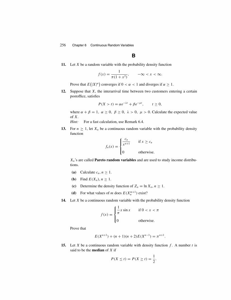
256 Chapter 6 Continuous Random Variables
B
11. Let X be a random variable with the probability density function
f (x) = 1
π(1 + x2), −∞ < x < ∞.
Prove that E(|X|α) converges if 0 < α < 1 and diverges if α ≥ 1.
12. Suppose that X, the interarrival time between two customers entering a certainpostoffice, satisfies
P(X > t) = αe−λt + βe−µt , t ≥ 0,
where α + β = 1, α ≥ 0, β ≥ 0, λ > 0, µ > 0. Calculate the expected valueof X.Hint: For a fast calculation, use Remark 6.4.
13. For n ≥ 1, let Xn be a continuous random variable with the probability densityfunction
fn(x) =
⎧⎪⎨⎪⎩cn
xn+1if x ≥ cn
0 otherwise.
Xn’s are called Pareto random variables and are used to study income distribu-tions.
(a) Calculate cn, n ≥ 1.
(b) Find E(Xn), n ≥ 1.
(c) Determine the density function of Zn = ln Xn, n ≥ 1.
(d) For what values of m does E(Xm+1n ) exist?
14. Let X be a continuous random variable with the probability density function
f (x) =
⎧⎪⎨⎪⎩1
πx sin x if 0 < x < π
0 otherwise.
Prove that
E(Xn+1) + (n + 1)(n + 2)E(Xn−1) = πn+1.
15. Let X be a continuous random variable with density function f . A number t issaid to be the median of X if
P(X ≤ t) = P(X ≥ t) = 1
2.

Section 6.3 Expectations and Variances 257
By Exercise 7, Section 6.1, X is symmetric about α if and only if for all x we havef (α − x) = f (α + x). Show that if X is symmetric about α, then
E(X) = Median(X) = α.
16. Let X be a continuous random variable with probability density function f (x).Determine the value of y for which E
(|X − y|) is minimum.
17. Let X be a nonnegative random variable with distribution function F . Define
I (t) ={
1 if X > t
0 otherwise.
(a) Prove that∫∞
0 I (t) dt = X.
(b) By calculating the expected value of both sides of part (a), prove that
E(X) =∫ ∞
0
[1 − F(t)
]dt.
This is a special case of Theorem 6.2.
(c) For r > 0, use part (b) to prove that
E(Xr) = r
∫ ∞
0t r−1
[1 − F(t)
]dt.
18. Let X be a continuous random variable. Prove that
∞∑n=1
P(|X| ≥ n
) ≤ E(|X|) ≤ 1 +
∞∑n=1
P(|X| ≥ n
).
These important inequalities show that E(|X|) < ∞ if and only if the series∑∞
n=1 P(|X| ≥ n
)converges.
Hint: By Exercise 17,
E(|X|) =
∫ ∞
0P(|X| > t
)dt =
∞∑n=0
∫ n+1
n
P(|X| > t
)dt.
Note that on the interval [n, n + 1),
P(|X| ≥ n + 1
)< P
(|X| > t) ≤ P
(|X| ≥ n).
19. Let X be the random variable introduced in Exercise 12. Applying the results ofExercise 17, calculate Var(X).
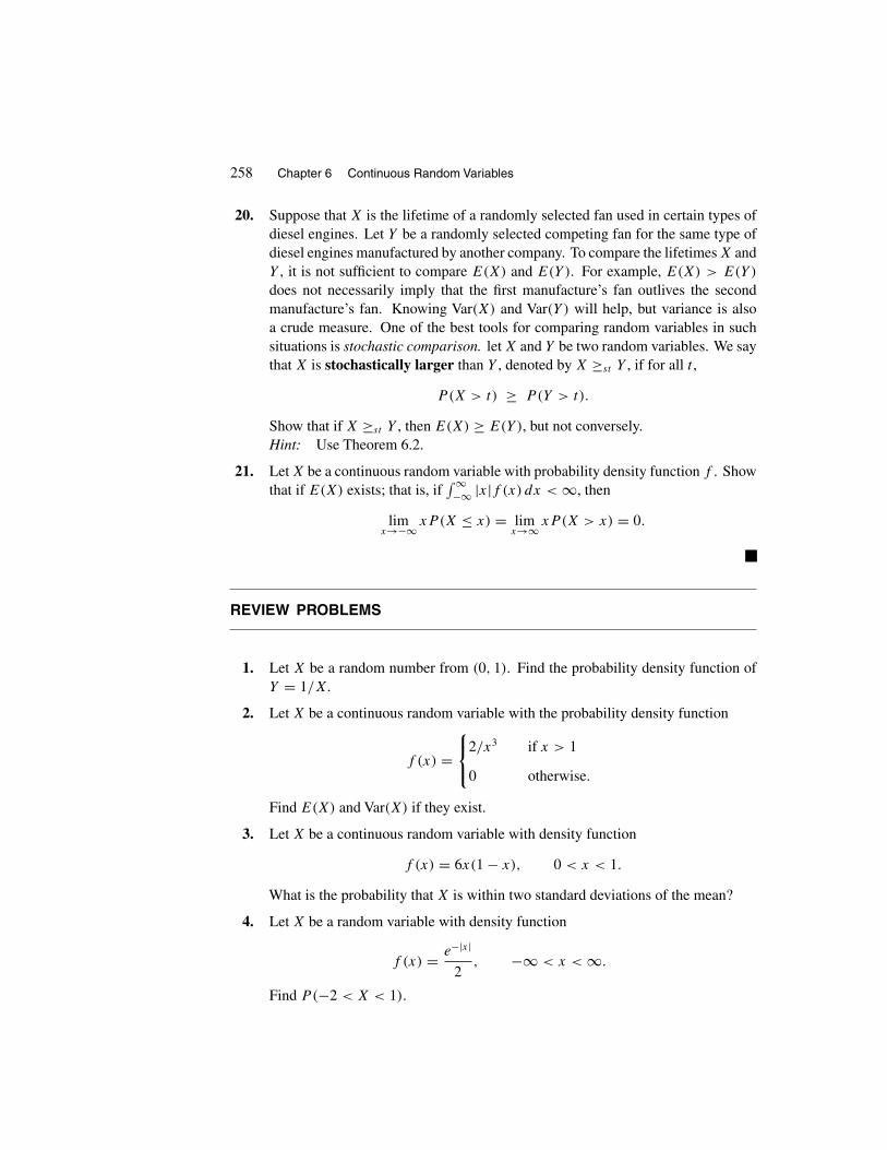
258 Chapter 6 Continuous Random Variables
20. Suppose that X is the lifetime of a randomly selected fan used in certain types ofdiesel engines. Let Y be a randomly selected competing fan for the same type ofdiesel engines manufactured by another company. To compare the lifetimes X andY , it is not sufficient to compare E(X) and E(Y ). For example, E(X) > E(Y )
does not necessarily imply that the first manufacture’s fan outlives the secondmanufacture’s fan. Knowing Var(X) and Var(Y ) will help, but variance is alsoa crude measure. One of the best tools for comparing random variables in suchsituations is stochastic comparison. let X and Y be two random variables. We saythat X is stochastically larger than Y , denoted by X ≥st Y , if for all t ,
P(X > t) ≥ P(Y > t).
Show that if X ≥st Y , then E(X) ≥ E(Y ), but not conversely.Hint: Use Theorem 6.2.
21. Let X be a continuous random variable with probability density function f . Showthat if E(X) exists; that is, if
∫∞−∞ |x|f (x) dx < ∞, then
limx→−∞ xP (X ≤ x) = lim
x→∞ xP (X > x) = 0.
REVIEW PROBLEMS
1. Let X be a random number from (0, 1). Find the probability density function ofY = 1/X.
2. Let X be a continuous random variable with the probability density function
f (x) =⎧⎨⎩2/x3 if x > 1
0 otherwise.
Find E(X) and Var(X) if they exist.
3. Let X be a continuous random variable with density function
f (x) = 6x(1 − x), 0 < x < 1.
What is the probability that X is within two standard deviations of the mean?
4. Let X be a random variable with density function
f (x) = e−|x|
2, −∞ < x < ∞.
Find P(−2 < X < 1).

Chapter 6 Review Problems 259
5. Does there exist a constant c for which the following is a density function?
f (x) =⎧⎨⎩
c
1 + xif x > 0
0 otherwise.
6. Let X be a random variable with density function
f (x) =⎧⎨⎩4x3/15 1 ≤ x ≤ 2
0 otherwise.
Find the density functions of Y = eX, Z = X2, and W = (X − 1)2.
7. The probability density function of a continuous random variable X is
f (x) ={
30x2(1 − x)2 if 0 < x < 1
0 otherwise.
Find the probability density function of Y = X4.
8. Let F , the distribution of a random variable X, be defined by
F(x) =
⎧⎪⎪⎪⎪⎪⎨⎪⎪⎪⎪⎪⎩
0 x < −1
1
2+ arcsin x
π−1 ≤ x < 1
1 x ≥ 1,
where arcsin x lies between −π/2 and π/2. Find f , the probability density func-tion of X and E(X).
9. Prove or disprove: If∑n
i=1 αi = 1, αi ≥ 0, ∀i, and{fi
}ni=1 is a sequence of density
functions, then∑n
i=1 αifi is a probability density function.
10. Let X be a continuous random variable with set of possible values {x : 0 < x < α}(where α < ∞), distribution function F , and density function f . Using integrationby parts, prove the following special case of Theorem 6.2.
E(X) =∫ α
0
[1 − F(t)
]dt.
11. The lifetime (in hours) of a light bulb manufactured by a certain company is arandom variable with probability density function
f (x) =
⎧⎪⎪⎨⎪⎪⎩0 if x ≤ 500
5 × 105
x3if x > 500.

260 Chapter 6 Continuous Random Variables
Suppose that, for all nonnegative real numbers a and b, the event that any lightbulb lasts at least a hours is independent of the event that any other light bulblasts at least b hours. Find the probability that, of six such light bulbs selected atrandom, exactly two last over 1000 hours.
12. Let X be a continuous random variable with distribution function F and densityfunction f . Find the distribution function and the density function of Y = |X|.
Chapter 7
Special Continuous
Distributions
In this chapter we study some examples of continuous random variables. Theserandom variables appear frequently in theory and applications of probability, statistics,and branches of science and engineering.
7.1 UNIFORM RANDOM VARIABLES
In Sections 1.6 and 1.7 we explained that in random selection of a point from an interval(a, b), the probability of the occurrence of any particular point is zero. As a result, westated that if [α, β] ⊆ (a, b), the events that the point falls in [α, β], (α, β), [α, β), and(α, β] are all equiprobable. Moreover, we said that a point is randomly selected from aninterval (a, b) if any two of its subintervals that have the same length are equally likely toinclude the point. We also mentioned that the probability associated with the event thatthe subinterval (α, β) includes the point is defined to be (β − α)/(b − a). Applicationsof these facts have been discussed throughout the book. Therefore, their significanceshould be clear by now. In particular, in Chapter 13 we show that the core of computersimulations is selection of random points from intervals. In this section we introduce theconcept of a uniform random variable. Then we study its properties and applications.As we will see now, uniform random variables are directly related to random selectionof points from intervals.
Suppose that X is the value of the random point selected from an interval (a, b).Then X is called a uniform random variable over (a, b). Let F and f be probabilitydistribution and density functions of X, respectively. Clearly,
F(t) =
⎧⎪⎪⎪⎪⎪⎨⎪⎪⎪⎪⎪⎩
0 t < a
t − a
b − aa ≤ t < b
1 t ≥ b.
261

262 Chapter 7 Special Continuous Distributions
Therefore,
f (t) = F ′(t) =
⎧⎪⎨⎪⎩1
b − aif a < t < b
0 otherwise.
(7.1)
Definition A random variable X is said to be uniformly distributed over an interval(a, b) if its probability density function is given by (7.1).
Another way of reaching this definition is to note that f (x) is a measure that deter-mines how likely it is for X to be close to x. Since for all x ∈ (a, b) the probability thatX is close to x is the same, f should be a nonzero constant on (a, b); zero, elsewhere.Therefore,
f (x) =⎧⎨⎩c if a < x < b
0 elsewhere.
Now∫ b
af (x) dx = 1 implies that
∫ b
ac dx = c(b − a) = 1. Thus c = 1/(b − a).
Figure 7.1 represents the graphs of f and F , the density function and the distributionfunction of a uniform random variable over the interval (a, b).
1b_a
a bx a b
x
F(x)
1
f(x)
Figure 7.1 Density and distribution functions of a uniform randomvariable.
In random selections of a large number of points from (a, b), we expect that theaverage of the values of the points will be approximately (a + b)/2, the midpoint of(a, b). This can be shown by calculating E(X), the expected value of a uniform randomvariable X over (a, b).
E(X) =∫ b
a
x1
b − adx = 1
b − a
[1
2x2]b
a= 1
b − a
(1
2b2 − 1
2a2)
= (b − a)(b + a)
2(b − a)= a + b
2.

Section 7.1 Uniform Random Variables 263
To find Var(X), note that
E(X2) =∫ b
a
x2 1
b − adx = 1
3
b3 − a3
b − a= 1
3(a2 + ab + b2).
Hence
Var(X) = E(X2) − [E(X)]2 = 1
3(a2 + ab + b2) −
(a + b
2
)2 = (b − a)2
12.
We have shown that
If X is uniformly distributed over an interval (a, b), then
E(X) = a + b
2, Var(X) = (b − a)2
12, σX = b − a√
12.
It is interesting to note that the expected value and the variance of a randomly selectedinteger Y from the set {1, 2, 3, . . . , N} are very similar to E(X) and Var(X) obtainedabove. By Exercise 5 of Section 4.5, E(Y ) = (1 + N)/2 and Var(Y ) = (N2 − 1)/12.
Example 7.1 Starting at 5:00 A.M., every half hour there is a flight from San Franciscoairport to Los Angeles International airport. Suppose that none of these planes is com-pletely sold out and that they always have room for passengers. A person who wants tofly to L.A. arrives at the airport at a random time between 8:45 A.M. and 9:45 A.M. Findthe probability that she waits (a) at most 10 minutes; (b) at least 15 minutes.
Solution: Let the passenger arrive at the airport X minutes past 8:45. Then X is auniform random variable over the interval (0, 60). Hence the density function of X isgiven by
f (x) ={
1/60 if 0 < x < 60
0 elsewhere.
Now the passenger waits at most 10 minutes if she arrives between 8:50 and 9:00 or 9:20and 9:30; that is, if 5 < X < 15 or 35 < X < 45. So the answer to (a) is
P(5 < X < 15) + P(35 < X < 45) =∫ 15
5
1
60dx +
∫ 45
35
1
60dx = 1
3.
The passenger waits at least 15 minutes if she arrives between 9:00 and 9:15 or 9:30 and9:45; that is, if 15 < X < 30 or 45 < X < 60. Thus the answer to (b) is
P(15 < X < 30) + P(45 < X < 60) =∫ 30
15
1
60dx +
∫ 60
45
1
60dx = 1
2. �

264 Chapter 7 Special Continuous Distributions
Example 7.2 A person arrives at a bus station every day at 7:00 A.M. If a bus arrives ata random time between 7:00 A.M. and 7:30 A.M., what is the average time spent waiting?
Solution: If the bus arrives X minutes past 7:00 A.M., then X is a uniform randomvariable over the interval (0, 30). Hence the average waiting time is
E(X) = 0 + 30
2= 15 minutes. �
The uniform distribution is often used to solve elementary problems in geometricprobability. In Chapter 8 we solve several such problems. Here we discuss only afamous problem introduced by the French mathematician Joseph Bertrand (1822–1900)in 1889. It is called Bertrand’s paradox. Bertrand seriously doubted that probabilitycould be defined on infinite sample spaces. To make his point, he posed this problem:
Example 7.3 What is the probability that a random chord of a circle is longer than aside of an equilateral triangle inscribed into the circle?
Solution: Since the exact meaning of a random chord is not given, we cannot solve thisproblem as stated. We interpret the expression random chord in three different ways andsolve the problem in each case. Let the center of the circle be at C and its radius be r .
First interpretation: To draw a random chord, by considerations of symmetry, firstchoose a random point A on the circle and connect it to C, the center; then choose arandom number d from (0, r) and place M on AC so that CM = d. Finally, from M
draw a chord perpendicular to the radius AC (see Figure 7.2). Since d < r/2 if and onlyif the chord is longer than a side of an equilateral triangle inscribed into the circle and d
is uniformly distributed over (0, r), the desired probability is
P(d <
r
2
)= r/2
r= 1
2.
CM
A
Figure 7.2 First interpretation.

Section 7.1 Uniform Random Variables 265
A
E
D
B
Figure 7.3 Second interpretation.
Second interpretation: To draw a random chord, by considerations of symmetry,first choose a random point A and then another random point D on the circle and connectAD. Let B and E be the points on the circle that make ABE an equilateral triangle. Therandom chord AD is longer than a side of ABE if and only if D lies on the arc BE.Since the length of the arc BE is one-third of the length of the whole circle and D is arandom point on the circle, D lies on the arc BE with probability 1/3. Thus the desiredprobability is 1/3 as well (see Figure 7.3).
C
M
Figure 7.4 Third interpretation.
Third interpretation: Since a chord is perpendicular to the radius connecting itsmidpoint to the center of the circle, every chord is uniquely determined by its midpoint.To draw a random chord, choose a random point M inside the circle, connect it to C, anddraw a chord perpendicular to MC from M . It is clear that the chord is longer than aside of the equilateral triangle inscribed into the circle if and only if its midpoint M liesinside the circle centered at C with radius r/2 (see Figure 7.4). Since each choice of M
uniquely determines one choice of a chord, the desired probability is the area of the small

266 Chapter 7 Special Continuous Distributions
circle divided by the area of the original circle (a fact discussed in detail in Section 8.1).It is equal to
π(r/2)2
πr2= 1
4.
As we showed, three different interpretations of random chord resulted in three dif-ferent answers. Because of this, Bertrand’s problem was once considered a paradox. Atthat time, one did not pay attention to the fact that the three interpretations correspond tothree different experiments concerning the selection of a random chord. In this processwe are dealing with three different probability functions defined on the same set of events.
�
EXERCISES
A
1. It takes a professor a random time between 20 and 27 minutes to walk from hishome to school every day. If he has a class at 9:00 A.M. and he leaves home at8:37 A.M., find the probability that he reaches his class on time.
2. Suppose that 15 points are selected at random and independently from the interval(0, 1). How many of them can be expected to be greater than 3/4?
3. The time at which a bus arrives at a station is uniform over an interval (a, b) withmean 2:00 P.M. and standard deviation
√12 minutes. Determine the values of a
and b.
4. Suppose that b is a random number from the interval (−3, 3). What is the proba-bility that the quadratic equation x2 + bx + 1 = 0 has at least one real root?
5. The radius of a sphere is a random number between 2 and 4. What is the expectedvalue of its volume? What is the probability that its volume is at most 36π?
6. A point is selected at random on a line segment of length �. What is the probabilitythat the longer segment is at least twice as long as the shorter segment?
7. A point is selected at random on a line segment of length �. What is the probabilitythat none of the two segments is smaller than �/3?
8. From the class of all triangles one is selected at random. What is the probabilitythat it is obtuse?Hint: The largest angle of a triangle is less than 180 degrees but greater than orequal to 60 degrees.

Section 7.2 Normal Random Variables 267
9. A farmer who has two pieces of lumber of lengths a and b (a < b) decides tobuild a pen in the shape of a triangle for his chickens. He sends his foolish son outto cut the longer piece and the boy, without taking any thought as to the ultimatepurpose, makes a cut on the lumber of length b, at a point selected randomly. Whatare the chances that the two resulting pieces and the piece of length a can be usedto form a triangular pen?Hint: Three segments form a triangle if and only if the length of any one ofthem is less than the sum of the lengths of the remaining two.
10. Let θ be a random number between −π/2 and π/2. Find the probability densityfunction of X = tan θ .
11. Let X be a random number from [0, 1]. Find the probability mass function of[nX], the greatest integer less than or equal to nX.
B
12. Let X be a random number from (0, 1). Find the density functions of (a) Y =− ln(1 − X), and (b) Z = Xn.
13. Let X be a uniform random variable over the interval (0, 1 + θ), where 0 < θ < 1is a given parameter. Find a function of X, say g(X), so that E
[g(X)
] = θ2.
14. Let X be a continuous random variable with distribution function F . Prove thatF(X) is uniformly distributed over (0, 1).
15. Let g be a nonnegative real-valued function on R that satisfies the relation∫∞−∞ g(t) dt = 1. Show that if, for a random variable X, the random variable
Y = ∫ X
−∞ g(t) dt is uniform, then g is the density function of X.
16. The sample space of an experiment is S = (0, 1), and for every subset A of S,P(A) = ∫
Adx. Let X be a random variable defined on S by X(ω) = 5ω − 1.
Prove that X is a uniform random variable over the interval (−1, 4).
17. Let Y be a random number from (0, 1). Let X be the second digit of√
Y . Provethat for n = 0, 1, 2, . . . , 9, P (X = n) increases as n increases. This is remarkablebecause it shows that P(X = n), n = 1, 2, 3, . . . is not constant. That is, Y isuniform but X is not.
7.2 NORMAL RANDOM VARIABLES
In search of formulas to approximate binomial probabilities, Poisson was not alone. Othermathematicians had also realized the importance of such investigations. In 1718, beforePoisson, De Moivre had discovered the following approximation, which is completelydifferent from Poisson’s.

268 Chapter 7 Special Continuous Distributions
De Moivre’sTheorem Let X be a binomial random variable with parameters n and1/2. Then for any numbers a and b, a < b,
limn→∞ P
(a <
X − (1/2)n
(1/2)√
n< b)
= 1√2π
∫ b
a
e−t2/2 dt.
Note that in this formula (1/2)n = E(X) and (1/2)√
n = σX.
De Moivre’s theorem was appreciated by Laplace, who recognized its importance.In 1812 he generalized it to binomial random variables with parameters n and p. Heshowed the following theorem, now called the De Moivre-Laplace theorem.
Theorem 7.1 (De Moivre-Laplace Theorem) Let X be a binomial randomvariable with parameters n and p. Then for any numbers a and b, a < b,
limn→∞ P
(a <
X − np√np(1 − p)
< b)
= 1√2π
∫ b
a
e−t2/2 dt.
Note that np and√
np(1 − p) appearing in this formula are, respectively, E(X) and σX.Poisson’s approximation, as discussed, is good when n is large, p is relatively small,
and np is appreciable. The De Moivre-Laplace formula yields excellent approximationsfor values of n and p for which np(1 − p) ≥ 10.
To find his approximation, Poisson first considered a binomial random variable X
with parameters (n, p). Then he showed that if λ = np, P (X = i) is approximately(e−λλi)/i! for large n. Finally, he proved that (e−λλi)/i! itself is a probability massfunction. The same procedure can be followed for the De Moivre-Laplace approximationas well. By this theorem, if X is a binomial random variable with parameters (n, p), thesequence of probabilities
P( X − np√
np(1 − p)≤ t), n = 1, 2, 3, 4, . . . ,
converges to1√2π
∫ t
−∞e−x2/2 dx, where the function (t) = 1√
2π
∫ t
−∞e−x2/2 dx is
a distribution function itself. To prove that is a distribution function, note that it isincreasing, continuous, and (−∞) = 0. The proof of (∞) = 1 is tricky. We use thefollowing ingenious technique introduced by Gauss to show it. Let
I =∫ ∞
−∞e−x2/2 dx.
Then
I 2 =( ∫ ∞
−∞e−x2/2 dx
)( ∫ ∞
−∞e−y2/2 dy
)=∫ ∞
−∞
∫ ∞
−∞e−(x2+y2)/2 dx dy.

Section 7.2 Normal Random Variables 269
To evaluate this double integral, we change the variables to polar coordinates. That is,we let x = r cos θ, y = r sin θ. We get dx dy = r dθ dr and
I 2 =∫ ∞
0
∫ 2π
0e−r2/2r dθ dr =
∫ ∞
0e−r2/2r
( ∫ 2π
0dθ)
dr
= 2π
∫ ∞
0re−r2/2 dr = 2π
[− e−r2/2
]∞0
= 2π.
Thus
I =∫ ∞
−∞e−x2/2 dx = √
2π,
and hence
(∞) = 1√2π
∫ ∞
−∞e−x2/2 dx = 1.
Therefore, is a distribution function.
Definition A random variable X is called standard normal if its distribution functionis , that is, if
P(X ≤ t) = (t) ≡ 1√2π
∫ t
−∞e−x2/2 dx.
By the fundamental theorem of calculus, f , the density function of a standard normalrandom variable, is given by
f (x) = �′(x) = 1√2π
e−x2/2.
The standard normal density function is a bell-shaped curve that is symmetric about they-axis (see Figure 7.5).
x0
f(x)
/1
Figure 7.5 Graph of the standard normal density function.

270 Chapter 7 Special Continuous Distributions
Since is the distribution function of the standard normal random variable, (t) is thearea under this curve from −∞ to t . Because (∞) = 1 and the curve is symmetricabout the y-axis, (0) = 1/2. Moreover,
�(−t) = 1 − �(t).
To see this, note that
(−t) = 1√2π
∫ −t
−∞e−x2/2 dx.
Substituting u = −x, we obtain
(−t) = −1√2π
∫ t
∞e−u2/2 du = 1√
2π
∫ ∞
t
e−u2/2 du
= 1√2π
∫ ∞
−∞e−u2/2 du − 1√
2π
∫ t
−∞e−u2/2 du
= 1 − (t).
Correction for Continuity
Thus far we have shown that the De Moivre-Laplace theorem approximates the dis-tribution of a discrete random variable by that of a continuous one. But we have notdemonstrated how this approximation works in practice. To do so, first we explain how,in general, a probability based on a discrete random variable is approximated by a prob-ability based on a continuous one. Let X be a discrete random variable with probabilitymass function p(x), and suppose that we want to find P(i ≤ X ≤ j), i < j . Considerthe histogram of X, as sketched in Figure 7.6 from i to j . In that figure the base of eachrectangle equals 1, and the height (and therefore the area) of the rectangle with the basemidpoint k is p(k), i ≤ k ≤ j . Thus the sum of the areas of all rectangles is
∑j
k=i p(k),which is the exact value of P(i ≤ X ≤ j). Now suppose that f (x), the density functionof a continuous random variable, sketched in Figure 7.7, is a good approximation to p(x).Then, as this figure shows, P(i ≤ X ≤ j), the sum of the areas of all rectangles of thefigure, is approximately the area under f (x) from i − 1/2 to j + 1/2 rather than from i
to j . That is,
P(i ≤ X ≤ j) ≈∫ j+1/2
i−1/2f (x) dx.
This adjustment is called correction for continuity and is necessary for approximationof the distribution of a discrete random variable with that of a continuous one. Similarly,the following corrections for continuity are made to calculate the given probabilities.

Section 7.2 Normal Random Variables 271
P(X = k) ≈∫ k+1/2
k−1/2f (x) dx,
P (X ≥ i) ≈∫ ∞
i−1/2f (x) dx,
P (X ≤ j) ≈∫ j+1/2
−∞f (x) dx.
k
p(k)
i jj_1i+1i+2
Figure 7.6 Histogram of X from i to j .
jj_1i i+1i+2
f
Figure 7.7 Histogram of X and the density function f .

272 Chapter 7 Special Continuous Distributions
In real-world problems, or even sometimes in theoretical ones, to apply the DeMoivre-Laplace theorem, we need to calculate the numerical values of
∫ b
ae−x2/2 dx for
some real numbers a and b. Since e−x2/2 has no antiderivative in terms of elementaryfunctions, such integrals are approximated by numerical techniques. Tables for suchapproximations have been available since 1799. Nowadays, most of the scientific calcu-lators give excellent approximate values for these integrals. Table 1 of theAppendix givesthe values of (x) = (1/
√2π )
∫ x
−∞ e−y2/2 dy for x = −3.89 to x = 0. For x ≤ −3.90, (x) ≈ 0. Table 2 of the Appendix gives the values of (x) for x = 0 to x = 3.89. Forx > 3.89, (x) ≈ 1. Note that, using the relation (x) = 1 − (−x), we can also useTable 1 to find (x) for x > 0 and Table 2 to find (x) for x < 0. Therefore, one of thetables 1 or 2 is sufficient to find (x) for all values of x. However, for convenience, wehave included a table for negative values of x and a separate table for positive values ofx. The following example shows how the De Moivre-Laplace theorem is applied.
Example 7.4 Suppose that of all the clouds that are seeded with silver iodide, 58%show splendid growth. If 60 clouds are seeded with silver iodide, what is the probabilitythat exactly 35 show splendid growth?
Solution: Let X be the number of clouds that show splendid growth. Then E(X) =60(0.58) = 34.80 and σX = √
60(0.58)(1 − 0.58) = 3.82. By correction for continuityand De Moivre-Laplace theorem,
P(X = 35) ≈ P(34.5 < X < 35.5)
= P(34.5 − 34.80
3.82<
X − 34.80
3.82<
35.5 − 34.80
3.82
)
= P(
− 0.08 <X − 34.8
3.82< 0.18
)≈ 1√
2π
∫ 0.18
−0.08e−x2/2 dx
= 1√2π
∫ 0.18
−∞e−x2/2 dx − 1√
2π
∫ −0.08
−∞e−x2/2 dx
= (0.18) − (−0.08) = 0.5714 − 0.4681 = 0.1033.
The exact value of P(X = 35) is
(60
35
)(0.58)35(0.42)25, which up to four decimal points
equals 0.1039. Therefore, the answer obtained by the De Moivre-Laplace approximationis very close to the actual probability. �
� Remark 7.1 Using today’s powerful scientific calculators, calculating the numer-ical value of (x) = (1/
√2π )
∫ x
−∞ e−y2/2 dy up to several decimal points of accuracyis almost as easy as addition or subtraction. However, both for theoretical and computa-tional reasons, approximating (x) by simpler functions has been the subject of many

Section 7.2 Normal Random Variables 273
studies. One such approximation was given by A. K. Shah in his paper “A Simpler Ap-proximation for Areas Under the Standard Normal Curve” (The American Statistician,39, 80, 1985). According to this approximation, for 0 ≤ x ≤ 2.2,
(x) ≈ 0.5 + x(4.4 − x)
10,
where the error of approximation is at most 0.005. That is,∣∣∣ (x) − 0.5 − x(4.4 − x)
10
∣∣∣ ≤ 0.005. �
Now that the importance of the standard normal random variable is clarified, we willcalculate its expectation and variance. The graph of the standard normal density function(Figure 7.5) suggests that its expectation is zero. To prove this, let X be a standard normalrandom variable. Then
E(X) = 1√2π
∫ ∞
−∞xe−x2/2 dx = 0,
because the integrand, xe−x2/2, is a finite odd function, and the integral is taken from−∞ to +∞. To calculate Var(X), note that
E(X2) = 1√2π
∫ ∞
−∞x2e−x2/2 dx.
Using integration by parts, we get (let u = x, dv = xe−x2/2 dx)∫ ∞
−∞xxe−x2/2 dx =
[− xe−x2/2
]∞−∞
+∫ ∞
−∞e−x2/2 dx = 0 + √
2π = √2π.
Therefore, E(X2) = 1, Var(X) = E(X2) − [E(X)]2 = 1, and σX = √
Var(X) = 1. Wehave shown that
The expected value of a standard normal random variable is 0. Itsstandard deviation is 1.
Although some natural phenomena obey a standard normal distribution, when itcomes to the analysis of data, due to the lack of parameters in the standard normaldistribution, it cannot be used. To overcome this difficulty, mathematicians generalizedthe standard normal distribution by introducing the following density function.
Definition A random variable X is called normal, with parameters µ and σ , if itsdensity function is given by
f (x) = 1
σ√
2πexp
[−(x − µ)2
2σ 2
], −∞ < x < ∞.

274 Chapter 7 Special Continuous Distributions
f is a density function because by the change of variable y = (x − µ)/σ :∫ ∞
−∞1
σ√
2πexp
[−(x − µ)2
2σ 2
]dx = 1√
2π
∫ ∞
−∞e−y2/2 dy = (∞) = 1.
If X is a normal random variable with parameters µ and σ , we write X ∼ N(µ, σ 2).
One of the first applications of N(µ, σ 2) was given by Gauss in 1809. Gauss usedN(µ, σ 2) to model the errors of observations in astronomy. For this reason, the normaldistribution is sometimes called the Gaussian distribution. Larsen and Marx, in their AnIntroduction to Mathematical Statistics and Its Applications (Prentice Hall, Upper SaddleRiver, N.J., 1986), explain that N(µ, σ 2) was popularized by the Belgian scholar LambertQuetelet (1796–1874), who used it successfully in data analysis in many situations.† Thechest measurement of Scottish soldiers is one of the studies of N(µ, σ 2) by Quetelet. Hemeasured Xi, i = 1, 2, 3, . . . , 5738, the respective sizes of the chests of 5738 Scottishsoldiers, and, using statistical methods, found that their average and standard deviationwere 39.8 and 2.05 inches, respectively. Then he counted the number of soldiers whohad a chest of size i, i = 33, 34, . . . , 48, and calculated the relative frequencies of sizes33 through 48. He showed that for i = 33, . . . , 48 the relative frequency of the sizei is very close to P(i − 1/2 < X < i + 1/2), where X is N(µ, σ 2) with µ = 39.8and σ = 2.05. Hence he concluded that the measure of the chest of a Scottish soldier isapproximately a normal random variable with parameters 39.8 and 2.05.
The following lemma shows that, by a simple change of variable, N(µ, σ 2) can betransformed to N(0, 1).
Lemma 7.1 If X ∼ N(µ, σ 2), then Z = (X − µ)/σ is N(0, 1). That is, if X ∼N(µ, σ 2), the standardized X is N(0, 1).
Proof: We show that the distribution function of Z is (1/√
2π )∫ x
−∞ e−y2/2 dy. Notethat
P(Z ≤ x) = P(X − µ
σ≤ x
)= P(X ≤ σx + µ)
= 1
σ√
2π
∫ σx+µ
−∞exp
[−(t − µ)2
2σ 2
]dt.
Let y = (t − µ)/σ ; then dt = σ dy and we get
P(Z ≤ x) = 1
σ√
2π
∫ x
−∞e−y2/2σ dy = 1√
2π
∫ x
−∞e−y2/2 dy. �
†An excellent treatise on the work of Quetelet concerning the applications of probability to the measure-ment of uncertainty in the social sciences can be found in Chapter 5 of The History of Statistics by StephenM. Stigler, The Belknap Press of Harvard University Press, 1986.

Section 7.2 Normal Random Variables 275
______1
0x
f (x)
Figure 7.8 Density of N(µ, σ 2).
Let X ∼ N(µ, σ 2). Quetelet’s analysis of the sizes of the chests of Scottish soldiersis an indication that µ and σ are the expected value and the standard deviation of X,respectively. To prove this, note that the random variable Z = (X − µ)/σ is N(0, 1)
and X = σZ + µ. Hence E(X) = E(σZ + µ) = σE(Z) + µ = µ and Var(X) =Var(σZ + µ) = σ 2 Var(Z) = σ 2. Therefore,
The parameters µ and σ that appear in the formula of the densityfunction of X are its expected value and standard deviation, respec-tively.
The graph of f (x) = 1
σ√
2πexp
[−(t − µ)2
2σ 2
]is a bell-shaped curve symmetric
about x = µ with the maximum at (µ, 1/σ√
2π ) and inflection points at µ ± σ (seeFigures 7.8 and 7.9).
The transformation Z = (X−µ)/σ enables us to use Tables 1 and 2 of the Appendixto calculate the probabilities concerning X. Some examples follow.
Example 7.5 Suppose that a Scottish soldier’s chest size is normally distributed withmean 39.8 and standard deviation 2.05 inches, respectively. What is the probability thatof 20 randomly selected Scottish soldiers, five have a chest of at least 40 inches?
Solution: Let p be the probability that a randomly selected Scottish soldier has a chestof 40 or more inches. If X is the normal random variable with mean 39.8 and standarddeviation 2.05, then

276 Chapter 7 Special Continuous Distributions
x
5=
= 8
=15
10 20 30
f(x)
Figure 7.9 Different normal densities with specified parameters.
p = P(X ≥ 40) = P(X − 39.8
2.05≥ 40 − 39.8
2.05
)= P
(X − 39.8
2.05≥ 0.10
)= P(Z ≥ 0.10) = 1 − (0.1) ≈ 1 − 0.5398 ≈ 0.46.
Therefore, the probability that of 20 randomly selected Scottish soldiers, five have a chestof at least 40 inches is (
20
5
)(0.46)5(0.54)15 ≈ 0.03. �
Example 7.6 Let X, the grade of a randomly selected student in a test of a probabilitycourse, be a normal random variable. A professor is said to grade such a test on the curveif he finds the average µ and the standard deviation σ of the grades and then assigns lettergrades according to the following table.
Range ofthe grade
X≥µ+σ µ≤X<µ+σ µ−σ ≤X<µ µ−2σ ≤X<µ−σ X<µ−2σ
Lettergrade
A B C D F
Suppose that the professor of the probability course grades the test on the curve.Determine the percentage of the students who will get A, B, C, D, and F, respectively.
Solution: By the fact that (X − µ)/σ is standard normal,
P(X ≥ µ + σ) = P(X − µ
σ≥ 1)
= 1 − (1) ≈ 0.1587,
P (µ ≤ X < µ + σ) = P(
0 ≤ X − µ
σ< 1)
= (1) − (0) ≈ 0.3413,

Section 7.2 Normal Random Variables 277
P(µ − σ ≤ X < µ) = P(
− 1 ≤ X − µ
σ< 0)
= (0) − (−1)
= 0.5 − 0.1587 ≈ 0.3413,
P (µ − 2σ ≤ X < µ − σ) = P(
− 2 ≤ X − µ
σ< −1
)= (−1) − (−2)
= 0.1587 − 0.0228 ≈ 0.1359,
P (X < µ − 2σ) = P(X − µ
σ< −2
)= (−2) ≈ 0.0228.
Therefore, approximately 16% should get A, 34% B, 34% C, 14% D, and 2% F. If aninstructor grades a test on the curve, instead of calculating µ and σ , he or she may assignA to the top 16%, B to the next 34%, and so on. �
Example 7.7 The scores on an achievement test given to 100,000 students are normallydistributed with mean 500 and standard deviation 100. What should the score of a studentbe to place him among the top 10% of all students?
Solution: Letting X be a normal random variable with mean 500 and standard deviation100, we must find x so that P(X ≥ x) = 0.10 or P(X < x) = 0.90. This gives
P(X − 500
100<
x − 500
100
)= 0.90.
Thus
(x − 500
100
)= 0.90.
From Table 2 of the Appendix, we have that (1.28) ≈ 0.8997, implying that(x − 500)/100 ≈ 1.28. This gives x ≈ 628; therefore, a student should earn 628or more to be among the top 10% of the students. �
Example 7.8 (Investment) The annual rate of return for a share of a specific stockis a normal random variable with mean 10% and standard deviation 12%. Ms. Couturebuys 100 shares of the stock at a price of $60 per share. What is the probability that aftera year her net profit from that investment is at least $750? Ignore transaction costs andassume that there is no annual dividend.
Solution: Let r be the rate of return of this stock. The random variable r is normalwith µ = 0.10 and σ = 0.12. Let X be the price of the total shares of the stock thatMs. Couture buys this year. We are given that X = 6000. Let Y be the total value of the

278 Chapter 7 Special Continuous Distributions
shares next year. The desired probability is
P(Y − X ≥ 750
) = P(Y − X
X≥ 750
X
)= P
(r ≥ 750
6000
)= P(r ≥ 0.125) = P
(Z ≥ 0.125 − 0.10
0.12
)= P(Z ≥ 0.21) = 1 − P(Z < 0.21)
= 1 − (0.21) = 1 − 0.5832 = 0.4168. �
It is important to note that a large family of random variables in mathematics andstatistics have distributions that are either normal or approximately normal. One of thereasons for this is the celebrated central limit theorem which we will study in Chapter 11.To express that theorem, we will use Richard von Mises’ words from his Probability,Statistics and the Truth (page 171, Dover Publications, 1981):
The normal curve represents the distribution in all cases where a final col-lective is formed by combination of a very large number of initial collectives,the attribute in the final collective being the sum of the results in the initialcollectives. The original collectives are not necessarily simple alternativesas they are in Bernoulli’s problem. It is not even necessary for them to havethe same attributes or the same distributions. The only conditions are thata very great number of collectives are combined and that the attributes aremixed in such a way that the final attribute is the sum of all the originalones. Under these conditions the final distribution is always represented bya normal curve.
For example, consider the annual profit of an insurance company that sells thousandsof policies each year. This is a normal random variable since the total profit is thesum of profits (losses being treated as negative profits) obtained from all policies sold.Some policies might be very complicated (i.e., those sold to the banks or oil companies).Moreover, the profit from each policy is itself a random variable which depends on manyfactors: the premium, risk involved, damages to be paid, quit claims, profit or loss frominvestments, the level of competition in the industry, and so on. To show the wide rangeof applications of normal random variables, in the next example, we will present, withoutproof, a celebrated formula in finance which is constructed based on normal distributionfunction.
� Example 7.9 (Black-Scholes Call Option Formula) In natural processes,the changes that take place are often the result of a sum of many insignificant randomfactors. Although the effect of each of these factors, separately, may be ignored, theeffect of their sum in general may not. Therefore, the study of distributions of sumsof a large number of independent random variables is essential and is the subject of

Section 7.2 Normal Random Variables 279
Chapter 11. In Section 11.5, we will show that for an immense number of randomphenomena, the distribution functions of such sums are approximately normal. In finance,random fluctuations of prices of shares of stocks, or other assets, are a result of anenormity of political, social, economical, and financial factors independently assessedby a large number of traders. For that reason financial scholars and consultants usenormal distributions as models for prices of assets in general, and shares of stocks inparticular. That is why the Black-Scholes call option formula, presented next, is basedon normal distribution function.
In finance, a contract that entitles a person to purchase a commodity is called calloption. To explain the concept of call option, we will present an example. Suppose thatMisha purchases, for a price of $7 per share, the option of buying a block of 100 sharesin a company at $80 per share during, say, the next six months. That is, Misha pays$700 to a seller and buys the right of purchasing 100 shares in the company at any timebefore or including the agreed expiration day at $80 per share. Misha is not obliged topurchase any number of the 100 shares he simply has the option to purchase. However,the premium paid to buy call options is not recovered whether or not he buys any numberof the shares. In the language of finance, Misha is the option holder, the seller is thewriter, and the predetermined price per share of $80, which is valid until the expirationday is called strike price. If Misha actually does buy a block of at least one share in thecompany, then we say that he exercises the option.
Suppose that sometime before the expiration day, the price of the shares in the com-pany rise to, say, $95 per share. If at that time Misha purchases 100 shares for $80 pershare, and sells them immediately for $95, he makes a profit of $9500−$8000−$700 =$800. On the other hand, if the price does not rise by the expiration day, Misha will lose$700 for having purchased the call option to buy the block of 100 shares. As for thewriter, in the latter case, she makes a profit of $700, whereas in the former case, she willend up selling the block of 100 shares, which is worth $9500, for only $8000, losing anopportunity to make $1500 − $700 = $800 more.
From this example, it should be evident that determining a fair price for an option is amajor problem in option theory. The question is whether or not the right to buy a share fora price of $7 is fair to both Misha and the writer. Until 1973, it was widely believed thatthe call option should be determined based on the principle assumption that the averagereturn from the stock should be lower than the average return from the option itself.However, in 1973, Fisher Black, an applied mathematician and a financial consultant,and MIT professor Myron Scholes presented a paper with a new approach. They argued,among other points, that all risk will be eliminated if option holders or writers chose twolines of investments with identical returns, buy one and sell the other simultaneously onthe expiration day. Based on such assumptions, in terms of normal distribution function,they derived formulas for call options that are extremely popular. To state a version ofBlack-Scholes’ widely used call option formula, note that, since periods remaining toexpiration are usually short, those stocks with higher standard deviation will rise abovestrick price with higher probability. Therefore, they should have higher option values.

280 Chapter 7 Special Continuous Distributions
Interest rate also has an effect on the value of an option. Usually, as interest rate increases,on average, the growth rate of stock price also increases. This should in turn increase theprices of options. Since dividends essentially reduce the stock price, they have negativeeffect on the values of the call option. For this reason, in the next formula we assumethat no dividends are paid before or on the expiration day.
We are now ready to state the Black-Scholes call option formula for European options,in which, unlike American options, the option holder can only exercise on the expirationday. The appearance of the normal distribution function in the following formula hassomething to do with the fact that the number of upward movements in price of a shareof a stock is binomial, and the limiting behavior of binomial is normal.
Black-Scholes Call Option Formula: In a European call option with standarddeviation σ , let K be the strike price, S be the current price, and τ denote the time periodover which the option is valid. Suppose that interest is compounded continuously at arate r . Then the Black-Scholes formula for the value of call option is given by
C = S (α) − Ke−rτ (α − σ√
τ),
where
α = ln(S/K) + (r + σ 2/2)τ
σ√
τ,
and, as usual, is the distribution function of a standard normal random variable.
To find the Black-Scholes call option value, per share, for the block of 100 shares ofthe stock Misha is interested in, suppose that the current price of the stock, per share, is$85 with standard deviation of 18% per year, and the option is valid for 6 months. Thestrike price is $80 and the interest rate is 12%. Therefore, S = 85, K = 80, σ = 0.18,r = 0.12, and τ = 6/12 = 1/2. Hence
α = ln(85/80) + (0.12 + 0.182/2)(1/2)
0.18√
1/2= 1.01,
and thus the value of the call option is
C = 85 (1.01) − 80e−(0.12)(1/2) (1.01 − 0.18
√1/2
)= 85 (1.01) − 75.34 (0.88)
= 85(0.8438) − 75.34(0.8106) = 10.65. �

Section 7.2 Normal Random Variables 281
EXERCISES
A
1. Suppose that 90% of the patients with a certain disease can be cured with a certaindrug. What is the approximate probability that, of 50 such patients, at least 45 canbe cured with the drug?
2. A small college has 1095 students. What is the approximate probability that morethan five students were born on Christmas day? Assume that the birthrates areconstant throughout the year and that each year has 365 days.
3. Let �(x) = 2 (x)−1. The function � is called the positive normal distribution.Prove that if Z is standard normal, then |Z| is positive normal.
4. Let Z be a standard normal random variable and α be a given constant. Find thereal number x that maximizes P(x < Z < x + α).
5. Let X be a standard normal random variable. Calculate E(X cos X), E(sin X),
and E( X
1 + X2
).
6. The ages of subscribers to a certain newspaper are normally distributed with mean35.5 years and standard deviation 4.8. What is the probability that the age of arandom subscriber is (a) more than 35.5 years; (b) between 30 and 40 years?
7. The grades for a certain exam are normally distributed with mean 67 and variance64. What percent of students get A(≥ 90), B(80 − 90), C(70 − 80), D(60 − 70),and F(< 60)?
8. Suppose that the distribution of the diastolic blood pressure is normal for a ran-domly selected person in a certain population is normal with mean 80 mm Hgand standard deviation 7 mm Hg. If people with diastolic blood pressures 95 orabove are considered hypertensive and people with diastolic blood pressures above89 and below 95 are considered to have mild hypertension, what percent of thatpopulation have mild hypertension and what percent are hypertensive? Assume inthat population no one has abnormal systolic blood pressure.
9. The length of an aluminum-coated steel sheet manufactured by a certain factoryis approximately normal with mean 75 centimeters and standard deviation 1 cen-timeter. Find the probability that a randomly selected sheet manufactured by thisfactory is between 74.5 and 75.8 centimeters.
10. Suppose that the IQ of a randomly selected student from a university is normalwith mean 110 and standard deviation 20. Determine the interval of values that iscentered at the mean and includes 50% of the IQ’s of the students at that university.

282 Chapter 7 Special Continuous Distributions
11. The amount of cereal in a box is normal with mean 16.5 ounces. If the packager isrequired to fill at least 90% of the cereal boxes with 16 or more ounces of cereal,what is the largest standard deviation for the amount of cereal in a box?
12. Suppose that the scores on a certain manual dexterity test are normal with mean12 and standard deviation 3. If eight randomly selected individuals take the test,what is the probability that none will make a score less than 14?
13. A number t is said to be the median of a continuous random variable X if
P(X ≤ t) = P(X ≥ t) = 1/2.
Calculate the median of the normal random variable with parameters µ and σ 2.
14. Let X ∼ N(µ, σ 2). Prove that P(|X − µ| > kσ
)does not depend on µ or σ .
15. Suppose that lifetimes of light bulbs produced by a certain company are normalrandom variables with mean 1000 hours and standard deviation 100 hours. Is thiscompany correct when it claims that 95% of its light bulbs last at least 900 hours?
16. Suppose that lifetimes of light bulbs produced by a certain company are normalrandom variables with mean 1000 hours and standard deviation 100 hours. Sup-pose that lifetimes of light bulbs produced by a second company are normal randomvariables with mean 900 hours and standard deviation 150 hours. Howard buysone light bulb manufactured by the first company and one by the second company.What is the probability that at least one of them lasts 980 or more hours?
17. (Investment) The annual rate of return for a share of a specific stock is a normalrandom variable with mean 0.12 and standard deviation of 0.06. The current priceof the stock is $35 per share. Mrs. Lovotti would like to purchase enough sharesof this stock to make at least $1000 profit with a probability of at least 90% in oneyear. Find the minimum number of shares that she should buy. Ignore transactioncosts and assume that there are no annual dividends.
18. Find the expected value and the variance of a random variable with the probabilitydensity function
f (x) =√
2
πe−2(x−1)2
.
19. Let X ∼ N(µ, σ 2). Find the probability distribution function of |X − µ| and itsexpected value.
20. Determine the value(s) of k for which the following is the probability densityfunction of a normal random variable.
f (x) = √ke−k2x2−2kx−1, −∞ < x < ∞.

Section 7.2 Normal Random Variables 283
21. The viscosity of a brand of motor oil is normal with mean 37 and standard deviation10. What is the lowest possible viscosity for a specimen that has viscosity higherthan at least 90% of that brand of motor oil?
22. In a certain town the length of residence of a family in a home is normal withmean 80 months and variance 900. What is the probability that of 12 independentfamilies, living on a certain street of that town, at least three will have lived theremore than eight years?
23. Let α ∈ (−∞, ∞) and Z ∼ N(0, 1); find E(eαZ).
24. Let X ∼ N(0, σ 2). Calculate the density function of Y = X2.
25. Let X ∼ N(µ, σ 2). Calculate the density function of Y = eX.
26. Let X ∼ N(0, 1). Calculate the density function of Y = √|X|.B
27. Suppose that the odds are 1 to 5000 in favor of a customer of a particular bookstorebuying a certain fiction bestseller . If 800 customers enter the store every day, howmany copies of that bestseller should the store stock every month so that, with aprobability of more than 98%, it does not run out of this book? For simplicity,assume that a month is 30 days.
28. Every day a factory produces 5000 light bulbs, of which 2500 are type I and 2500are type II. If a sample of 40 light bulbs is selected at random to be examined fordefects, what is the approximate probability that this sample contains at least 18light bulbs of each type?
29. To examine the accuracy of an algorithm that selects random numbers from theset {1, 2, . . . , 40}, 100,000 numbers are selected and there are 3500 ones. Giventhat the expected number of ones is 2500, is it fair to say that this algorithm is notaccurate?
30. Prove that for some constant k, f (x) = ka−x2, a ∈ (0, ∞), is a normal probability
density function.
31. (a) Prove that for all x > 0,
1
x√
2π
(1 − 1
x2
)e−x2/2 < 1 − (x) <
1
x√
2πe−x2/2.
Hint: Integrate the following inequalities:
(1 − 3y−4)e−y2/2 < e−y2/2 < (1 + y−2)e−y2/2.
(b) Use part (a) to prove that 1 − (x) ∼ 1
x√
2πe−x2/2. That is, as x → ∞,
the ratio of the two sides approaches 1.
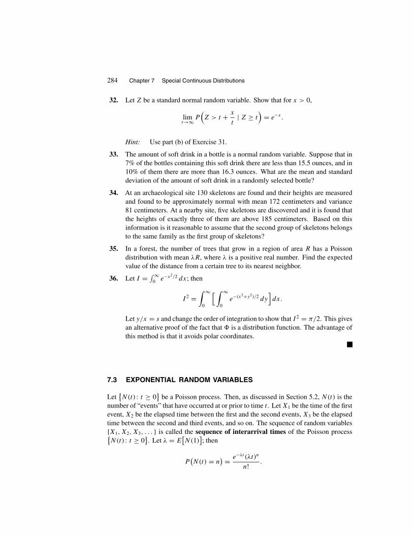
284 Chapter 7 Special Continuous Distributions
32. Let Z be a standard normal random variable. Show that for x > 0,
limt→∞ P
(Z > t + x
t| Z ≥ t
)= e−x.
Hint: Use part (b) of Exercise 31.
33. The amount of soft drink in a bottle is a normal random variable. Suppose that in7% of the bottles containing this soft drink there are less than 15.5 ounces, and in10% of them there are more than 16.3 ounces. What are the mean and standarddeviation of the amount of soft drink in a randomly selected bottle?
34. At an archaeological site 130 skeletons are found and their heights are measuredand found to be approximately normal with mean 172 centimeters and variance81 centimeters. At a nearby site, five skeletons are discovered and it is found thatthe heights of exactly three of them are above 185 centimeters. Based on thisinformation is it reasonable to assume that the second group of skeletons belongsto the same family as the first group of skeletons?
35. In a forest, the number of trees that grow in a region of area R has a Poissondistribution with mean λR, where λ is a positive real number. Find the expectedvalue of the distance from a certain tree to its nearest neighbor.
36. Let I = ∫∞0 e−x2/2 dx; then
I 2 =∫ ∞
0
[ ∫ ∞
0e−(x2+y2)/2 dy
]dx.
Let y/x = s and change the order of integration to show that I 2 = π/2. This givesan alternative proof of the fact that is a distribution function. The advantage ofthis method is that it avoids polar coordinates.
7.3 EXPONENTIAL RANDOM VARIABLES
Let{N(t) : t ≥ 0
}be a Poisson process. Then, as discussed in Section 5.2, N(t) is the
number of “events” that have occurred at or prior to time t . Let X1 be the time of the firstevent, X2 be the elapsed time between the first and the second events, X3 be the elapsedtime between the second and third events, and so on. The sequence of random variables{X1, X2, X3, . . . } is called the sequence of interarrival times of the Poisson process{N(t) : t ≥ 0
}. Let λ = E
[N(1)
]; then
P(N(t) = n
) = e−λt (λt)n
n! .

Section 7.3 Exponential Random Variables 285
This enables us to calculate the probability distribution functions of the random variablesXi, i ≥ 1. For t ≥ 0,
P (X1 > t) = P(N(t) = 0
) = e−λt .
Therefore,
P(X1 ≤ t) = 1 − P(X1 > t) = 1 − e−λt .
Since a Poisson process is stationary and possesses independent increments, at any timet , the process probabilistically starts all over again. Hence the interarrival time of any twoconsecutive events has the same distribution as X1; that is, the sequence {X1, X2, X3, . . . }is identically distributed. Therefore, for all n ≥ 1,
P(Xn ≤ t) = P(X1 ≤ t) ={
1 − e−λt t ≥ 0
0 t < 0.
Let
F(t) ={
1 − e−λt t ≥ 0
0 t < 0
for some λ > 0. Then F is the distribution function of Xn for all n ≥ 1. It is calledexponential distribution and is one of the most important distributions of pure andapplied probability. Since
f (t) = F ′(t) ={
λe−λt t ≥ 0
0 t < 0(7.2)
and ∫ ∞
0λe−λt dt = lim
b→∞
∫ b
0λe−λt dt = lim
b→∞
[− e−λt
]b0
= limb→∞(1 − e−λb) = 1,
f is a density function.
Definition A continuous random variable X is called exponential with parameterλ > 0 if its density function is given by (7.2).
Because the interarrival times of a Poisson process are exponential, the following areexamples of random variables that might be exponential.
1. The interarrival time between two customers at a post office
2. The duration of Jim’s next telephone call

286 Chapter 7 Special Continuous Distributions
3. The time between two consecutive earthquakes in California
4. The time between two accidents at an intersection
5. The time until the next baby is born in a hospital
6. The time until the next crime in a certain town
7. The time to failure of the next fiber segment in a large group of such segmentswhen all of them are initially fault free
8. The time interval between the observation of two consecutive shooting stars on asummer evening
9. The time between two consecutive fish caught by a fisherman from a large lakewith lots of fish
From Section 5.2 we know that λ is the average number of the events in one timeunit; that is, E
[N(1)
] = λ. Therefore, we should expect an average time 1/λ betweentwo consecutive events. To prove this, let X be an exponential random variable withparameter λ; then
E(X) =∫ ∞
−∞xf (x) dx =
∫ ∞
0x(λe−λx) dx.
Using integration by parts with u = x and dv = λe−λx dx, we obtain
E(X) =[
− xe−λx]∞
0+∫ ∞
0e−λx dx = 0 −
[1
λe−λx
]∞0
= 1
λ.
A similar calculation shows that
E(X2) =∫ ∞
−∞x2f (x) dx =
∫ ∞
0x2(λe−λx) dx = 2
λ2.
Hence
Var(X) = E(X2) − [E(X)]2 = 2
λ2− 1
λ2= 1
λ2,
and therefore σX = 1/λ. We have shown that
For an exponential random variable with parameter λ,
E(X) = σX = 1λ
, Var(X) = 1λ2
.
Figures 7.10 and 7.11 represent the graphs of the exponential density and exponentialdistribution functions, respectively.

Section 7.3 Exponential Random Variables 287
1/ 4/x
f (x)
Figure 7.10 Exponential density function with parameter λ.
4/x
F(x)
1
1/2
Figure 7.11 Exponential distribution function.
Example 7.10 Suppose that every three months , on average, an earthquake occurs inCalifornia. What is the probability that the next earthquake occurs after three but beforeseven months?
Solution: Let X be the time (in months) until the next earthquake; it can be assumedthat X is an exponential random variable with 1/λ = 3 or λ = 1/3. To calculateP(3 < X < 7), note that since F , the distribution function of X, is given by
F(t) = P(X ≤ t) = 1 − e−t/3 for t > 0,
we can write
P(3 < X < 7) = F(7) − F(3) = (1 − e−7/3) − (1 − e−1) ≈ 0.27. �
Example 7.11 At an intersection there are two accidents per day, on average. Whatis the probability that after the next accident there will be no accidents at all for the nexttwo days?

288 Chapter 7 Special Continuous Distributions
Solution: Let X be the time (in days) between the next two accidents. It can be assumedthat X is exponential with parameter λ, satisfying 1/λ = 1/2, so that λ = 2. To findP(X > 2), note that F , the distribution function of X, is given by F(t) = 1 − e−2t ,t > 0. Hence
P(X > 2) = 1 − P(X ≤ 2) = 1 − F(2) = e−4 ≈ 0.02. �
An important feature of exponential distribution is its memoryless property. A non-negative random variable X is called memoryless if, for all s, t ≥ 0,
P(X > s + t | X > t) = P(X > s). (7.3)
If, for example, X is the lifetime of some type of instrument, then (7.3) means that thereis no deterioration with age of the instrument. The probability that a new instrument willlast more than s years is the same as the probability that a used instrument that has lastedmore than t years will last at least another s years. In other words, the probability thatsuch an instrument will deteriorate in the next s years does not depend on the age of theinstrument.
To show that an exponential distribution is memoryless, note that (7.3) is equivalentto
P(X > s + t, X > t)
P (X > t)= P(X > s)
and
P(X > s + t) = P(X > s)P (X > t). (7.4)
Now since
P(X > s + t) = 1 − [1 − e−λ(s+t)] = e−λ(s+t),
P (X > s) = 1 − (1 − e−λs) = e−λs,
and
P(X > t) = 1 − (1 − e−λt ) = e−λt ,
we have that (7.4) follows. HenceX is memoryless. It can be shown that exponential is theonly continuous distribution which possesses a memoryless property (see Exercise 15).
Example 7.12 The lifetime of a TV tube (in years) is an exponential random variablewith mean 10. If Jim bought his TV set 10 years ago, what is the probability that its tubewill last another 10 years?
Solution: Let X be the lifetime of the tube. Since X is an exponential random variable,there is no deterioration with age of the tube. Hence
P(X > 20 | X > 10) = P(X > 10) = 1 − [1 − e(−1/10)10] ≈ 0.37. �
Section 7.3 Exponential Random Variables 289
Example 7.13 Suppose that, on average, two earthquakes occur in San Franciscoand two in Los Angeles every year. If the last earthquake in San Francisco occurred 10months ago and the last earthquake in Los Angeles occurred two months ago, what is theprobability that the next earthquake in San Francisco occurs after the next earthquake inLos Angeles?
Solution: It can be assumed that the number of earthquakes in San Francisco and LosAngeles are both Poisson processes with common rate λ = 2. Hence the times betweentwo consecutive earthquakes in Los Angeles and two consecutive earthquakes in SanFrancisco are both exponentially distributed with the common mean 1/λ = 1/2. Becauseof the memoryless property of the exponential distribution, it does not matter when thelast earthquakes in San Francisco and Los Angeles have occurred. The times betweennow and the next earthquake in San Francisco and the next earthquake in Los Angelesboth have the same distribution. Since these time periods are exponentially distributedwith the same parameter, by symmetry, the probability that the next earthquake in SanFrancisco occurs after that in Los Angeles is 1/2. �
Relationship between Exponential and Geometric: Recall that if a Bernoulli trialis performed successively and independently, then the number of trials until the firstsuccess occurs is geometric. Furthermore, the number of trials between two consecutivesuccesses is also geometric. Sometimes exponential is considered to be the continuousanalog of geometric because, for a Poisson process, the time it will take until the first eventoccurs is exponential, and the time between two consecutive events is also exponential.Moreover, exponential is the only memoryless continuous distribution, and geometric isthe only memoryless discrete distribution. It is also interesting to know that if X is anexponential random variable, then [X], the integer part of X; i.e, the greatest integer lessthan or equal to X, is geometric (see Exercise 14). �
Remark 7.2 In this section, we showed that if {N(t) : t ≥ 0} is a Poisson processwith rate λ, then the interarrival times of the process form an independent sequence ofidentically distributed exponential random variables with mean 1/λ. Using the tools ofan area of probability called renewal theory, we can prove that the converse of this factis also true:
If, for some process, N(t) is the number of “events” occurring in [0, t],and if the times between consecutive events form a sequence of in-dependent and identically distributed exponential random variableswith mean 1/λ, then
{N(t) : t ≥ 0
}is a Poisson process with rate λ.
�

290 Chapter 7 Special Continuous Distributions
EXERCISES
A
1. Customers arrive at a postoffice at a Poisson rate of three per minute. What is theprobability that the next customer does not arrive during the next 3 minutes?
2. Find the median of an exponential random variable with rate λ. Recall that for acontinuous distribution F , the median Q0.5 is the point at which F(Q0.5) = 1/2.
3. Let X be an exponential random variable with mean 1. Find the probability densityfunction of Y = − ln X.
4. The time between the first and second heart attacks for a certain group of people isan exponential random variable. If 50% of those who have had a heart attack willhave another one within the next five years, what is the probability that a personwho had one heart attack five years ago will not have another one in the next fiveyears?
5. Guests arrive at a hotel, in accordance with a Poisson process, at a rate of fiveper hour. Suppose that for the last 10 minutes no guest has arrived. What is theprobability that (a) the next one will arrive in less than 2 minutes; (b) from thearrival of the tenth to the arrival of the eleventh guest takes no more than 2 minutes?
6. Let X be an exponential random variable with parameter λ. Find
P(∣∣X − E(X)
∣∣ ≥ 2σX
).
7. Suppose that, at an Italian restaurant, the time, in minutes, between two customersordering pizza is exponential with parameter λ. What is the probability that (a) nocustomer orders pizza during the next t minutes; (b) the next pizza order is placedin at least t minutes but no later than s minutes (t < s)?
8. Suppose that the time it takes for a novice secretary to type a document is expo-nential with mean 1 hour. If at the beginning of a certain eight-hour working daythe secretary receives 12 documents to type, what is the probability that she willfinish them all by the end of the day?
9. The profit is $350 for each computer assembled by a certain person. Suppose thatthe assembler guarantees his computers for one year and the time between twofailures of a computer is exponential with mean 18 months. If it costs the assembler$40 to repair a failed computer, what is the expected profit per computer?Hint: Let N(t) be the number of times that the computer fails in [0, t]. Then{N(t) : t ≥ 0
}is a Poisson process with parameter λ = 1/18.

Section 7.3 Exponential Random Variables 291
10. Mr. Jones is waiting to make a phone call at a train station. There are two publictelephone booths next to each other, occupied by two persons, say A and B. If theduration of each telephone call is an exponential random variable with λ = 1/8,what is the probability that among Mr. Jones, A, and B, Mr. Jones will not be thelast to finish his call?
11. In a factory, a certain machine operates for a period which is exponentially dis-tributed with parameter λ. Then it breaks down and will be in repair shop for aperiod, which is also exponentially distributed with mean 1/λ. The operating andthe repair times are independent. For this machine, we say that a change of “state”occurs each time that it breaks down, or each time that it is fixed. In a time intervalof length t , find the probability mass function of the number of times a change ofstate occurs.
B
12. In data communication, messages are usually combinations of characters, and eachcharacter consists of a number of bits. A bit is the smallest unit of information andis either 1 or 0. Suppose that L, the length of a character (in bits) is a geometricrandom variable with parameter p. If a sender emits messages at the rate of 1000bits per second, what is the distribution of T , the time it takes the sender to emit acharacter?
13. The random variable X is called double exponentially distributed if its densityfunction is given by
f (x) = ce−|x|, −∞ < x < +∞.
(a) Find the value of c.
(b) Prove that E(X2n) = (2n)! and E(X2n+1) = 0.
14. Let X, the lifetime (in years) of a radio tube, be exponentially distributed withmean 1/λ. Prove that [X], the integer part of X, which is the complete number ofyears that the tube works, is a geometric random variable.
15. Prove that if X is a positive, continuous, memoryless random variable with dis-tribution function F , then F(t) = 1 − e−λt for some λ > 0. This shows that theexponential is the only distribution on (0, ∞) with the memoryless property.

292 Chapter 7 Special Continuous Distributions
7.4 GAMMA DISTRIBUTIONS
Let{N(t) : t ≥ 0
}be a Poisson process, X1 be the time of the first event, and for n ≥ 2,
let Xn be the time between the (n − 1)st and nth events. As we explained in Section 7.3,{X1, X2, . . . } is a sequence of identically distributed exponential random variables withmean 1/λ, where λ is the rate of
{N(t) : t ≥ 0
}. For this Poisson process let X be the
time of the nth event. Then X is said to have a gamma distribution with parameters(n, λ). Therefore, exponential is the time we will wait for the first event to occur, andgamma is the time we will wait for the nth event to occur. Clearly, a gamma distributionwith parameters (1, λ) is identical with an exponential distribution with parameter λ.
Let X be a gamma random variable with parameters (n, λ). To find f , the densityfunction of X, note that {X ≤ t} occurs if the time of the nth event is in [0, t], that is, ifthe number of events occurring in [0, t] is at least n. Hence F , the distribution functionof X, is given by
F(t) = P(X ≤ t) = P(N(t) ≥ n
) =∞∑
i=n
e−λt (λt)i
i! .
Differentiating F , the density function f is obtained:
f (t) =∞∑
i=n
[− λe−λt (λt)i
i! + λe−λt (λt)i−1
(i − 1)!]
=∞∑
i=n
−λe−λt (λt)i
i! +[λe−λt (λt)n−1
(n − 1)! +∞∑
i=n+1
λe−λt (λt)i−1
(i − 1)!]
=[
−∞∑
i=n
λe−λt (λt)i
i!]
+ λe−λt (λt)n−1
(n − 1)! +[ ∞∑
i=n
λe−λt (λt)i
i!]
= λe−λt (λt)n−1
(n − 1)! .
The density function
f (x) =
⎧⎪⎪⎨⎪⎪⎩λe−λx
(λx)n−1
(n − 1)! if x ≥ 0
0 elsewhere
is called the gamma (or n-Erlang) density with parameters (n, λ).Now we extend the definition of the gamma density from parameters (n, λ) to (r, λ),
where r > 0 is not necessarily a positive integer. As we shall see later, this extensionhas useful applications in probability and statistics. In the formula of the gamma densityfunction, the term (n − 1)! is defined only for positive integers. So the only obstacle insuch an extension is to find a function of r that has the basic property of the factorial

Section 7.4 Gamma Distributions 293
function, namely, n! = n · (n − 1)!, and coincides with (n − 1)! when n is a positiveinteger. The function with these properties is � : (0, ∞) → R defined by
�(r) =∫ ∞
0t r−1e−t dt.
The property analogous to n! = n · (n − 1)! is
�(r + 1) = r�(r), r > 1,
which is obtained by an integration by parts applied to �(r + 1) with u = t r anddv = e−t dt :
�(r + 1) =∫ ∞
0t re−t dt =
[− t re−t
]∞0
+ r
∫ ∞
0t r−1e−t dt
= r
∫ ∞
0t r−1e−t dt = r�(r).
To show that �(n) coincides with (n − 1)! when n is a positive integer, note that
�(1) =∫ ∞
0e−t dt = 1.
Therefore,
�(2) = (2 − 1)�(2 − 1) = 1 = 1!,�(3) = (3 − 1)�(3 − 1) = 2 · 1 = 2!,�(4) = (4 − 1)�(4 − 1) = 3 · 2 · 1 = 3!.
Repetition of this process or a simple induction implies that
�(n + 1) = n!.Hence �(r + 1) is the natural generalization of n! for a noninteger r > 0. This motivatesthe following definition.
Definition A random variable X with probability density function
f (x) =
⎧⎪⎪⎨⎪⎪⎩λe−λx(λx)r−1
�(r)if x ≥ 0
0 elsewhere
is said to have a gamma distribution with parameters (r, λ), λ > 0, r > 0.
Figures 7.12 and 7.13 demonstrate the shape of the gamma density function forseveral values of r and λ.

294 Chapter 7 Special Continuous Distributions
r = 4
r = 2
300
0.1
x
r = 3
f(x)
Figure 7.12 Gamma densities for λ = 1/4.
= 0.2
= 0.5
x30
= 0.6f (x)
Figure 7.13 Gamma densities for r = 4.
Example 7.14 Suppose that, on average, the number of β-particles emitted from aradioactive substance is four every second. What is the probability that it takes at least 2seconds before the next two β-particles are emitted?
Solution: Let N(t) denote the number of β-particles emitted from a radioactive sub-stance in [0, t]. It is reasonable to assume that
{N(t) : t ≥ 0
}is a Poisson process. Let
1 second be the time unit; then λ = E[N(1)
] = 4. X, the time between now and

Section 7.4 Gamma Distributions 295
when the second β-particle is emitted, has a gamma distribution with parameters (2, 4).Therefore,
P(X ≥ 2) =∫ ∞
2
4e−4x(4x)2−1
�(2)dx =
∫ ∞
216xe−4x dx
=[
− 4xe−4x]∞
2−∫ ∞
2−4e−4x dx = 8e−8 + e−8 ≈ 0.003.
Note that an alternative solution to this problem is
P(X ≥ 2) = P(N(2) ≤ 1
) = P(N(2) = 0
)+ P(N(2) = 1
)= e−8(8)0
0! + e−8(8)1
1! = 9e−8 ≈ 0.003. �
Let X be a gamma random variable with parameters (r, λ). To find E(X) and Var(X),note that for all n ≥ 0,
E(Xn) =∫ ∞
0xn λe−λx(λx)r−1
�(r)dx = λr
�(r)
∫ ∞
0xn+r−1e−λx dx.
Let t = λx; then dt = λ dx, so
E(Xn) = λr
�(r)
∫ ∞
0
tn+r−1
λn+r−1e−t 1
λdt = λr
�(r)λn+r
∫ ∞
0tn+r−1e−t dt = �(n + r)
�(r)λn.
For n = 1, this gives
E(X) = �(r + 1)
�(r)λ= r�(r)
λ�(r)= r
λ.
For n = 2,
E(X2) = �(r + 2)
�(r)λ2= (r + 1)�(r + 1)
λ2�(r)= (r + 1)r�(r)
λ2�(r)= r2 + r
λ2.
Thus
Var(X) = r2 + r
λ2−( r
λ
)2 = r
λ2.
We have shown that
For a gamma random variable with parameters r and λ,
E(X) = r
λ, Var(X) = r
λ2, σX =
√r
λ.

296 Chapter 7 Special Continuous Distributions
Example 7.15 There are 100 questions in a test. Suppose that, for all s > 0 and t > 0,the event that it takes t minutes to answer one question is independent of the event thatit takes s minutes to answer another one. If the time that it takes to answer a questionis exponential with mean 1/2, find the distribution, the average time, and the standarddeviation of the time it takes to do the entire test.
Solution: Let X be the time to answer a question and N(t) the number of questionsanswered by time t . Then
{N(t) : t ≥ 0
}is a Poisson process at the rate of λ = 1/E(X) =
2 per minute. Therefore, the time that it takes to complete all the questions is gamma withparameters (100, 2). The average time to finish the test is r/λ = 100/2 = 50 minuteswith standard deviation
√r/λ2 = √
100/4 = 5. �
Relationship between Gamma and Negative Binomial: Recall that if a Bernoullitrial is performed successively and independently, then the number of trials until the rthsuccess occurs is negative binomial. Sometimes gamma is viewed as the continuousanalog of negative binomial, one reason being that, for a Poisson process, the time it willtake until the rth event occurs is gamma. There are more serious relationships betweenthe two distributions that we will not discuss. For example, in some sense, in limit,negative binomial’s distribution approaches gamma distribution. �
EXERCISES
A
1. Show that the gamma density function with parameters (r, λ) has a unique maxi-mum at (r − 1)/λ.
2. Let X be a gamma random variable with parameters (r, λ). Find the distributionfunction of cX, where c is a positive constant.
3. In a hospital, babies are born at a Poisson rate of 12 per day. What is the probabilitythat it takes at least seven hours before the next three babies are born?
4. Let f be the density function of a gamma random variable X, with parameters(r, λ). Prove that
∫∞−∞ f (x) dx = 1.
5. Customers arrive at a restaurant at a Poisson rate of 12 per hour. If the restaurantmakes a profit only after 30 customers have arrived, what is the expected lengthof time until the restaurant starts to make profit?
6. A manufacturer produces light bulbs at a Poisson rate of 200 per hour. The proba-bility that a light bulb is defective is 0.015. During production, the light bulbs aretested one by one, and the defective ones are put in a special can that holds up toa maximum of 25 light bulbs. On average, how long does it take until the can isfilled?

Section 7.5 Beta Distributions 297
B
7. For n = 0, 1, 2, 3, . . . , calculate �(n + 1/2).
8. (a) Let Z be a standard normal random variable. Show that the random variableY = Z2 is gamma and find its parameters.
(b) Let X be a normal random variable with mean µ and standard deviation σ .
Find the distribution function of W =(X − µ
σ
)2.
9. Howard enters a bank that has n tellers. All the tellers are busy serving customers,and there is exactly one queue being served by all tellers, with one customer aheadof Howard waiting to be served. If the service time of a customer is exponentialwith parameter λ, find the distribution of the waiting time for Howard in the queue.
10. In data communication, messages are usually combinations of characters, and eachcharacter consists of a number of bits. A bit is the smallest unit of informationand is either 1 or 0. Suppose that the length of a character (in bits) is a geometricrandom variable with parameter p. Suppose that a sender emits messages at therate of 1000 bits per second. What is the distribution of T , the time it takes thesender to emit a message combined of k characters of independent lengths?Hint: Let N(t) be the number of characters emitted at or prior to t . First arguethat
{N(t) : t ≥ 0
}is a Poisson process and find its parameter.
7.5 BETA DISTRIBUTIONS
A random variable X is called beta with parameters (α, β), α > 0, β > 0 if f , its densityfunction, is given by
f (x) =
⎧⎪⎪⎨⎪⎪⎩1
B(α, β)xα−1(1 − x)β−1 if 0 < x < 1
0 otherwise,
where
B(α, β) =∫ 1
0xα−1(1 − x)β−1 dx.
B(α, β) is related to the gamma function by the relation
B(α, β) = �(α)�(β)
�(α + β).
Beta density occurs in a natural way in the study of the median of a sample of randompoints from (0, 1). Let X(1) be the smallest of these numbers, X(2) be the second smallest,

298 Chapter 7 Special Continuous Distributions
. . . , X(i) be the ith smallest, . . . , and X(n) be the largest of these numbers. If n = 2k+1is odd, X(k+1) is called the median of these n random numbers, whereas if n = 2k iseven, [X(k) +X(k+1)]/2 is called the median. It can be shown that the median of (2n+1)
random numbers from the interval (0, 1) is a beta random variable with parameters(n + 1, n + 1). As Figures 7.14 and 7.15 show, by changing the values of parametersα and β, beta densities cover a wide range of different shapes. If α = β, the median isx = 1/2, and the density of the beta random variable is symmetric about the median. Inparticular, if α = β = 1, the uniform density over the interval (0, 1) is obtained.
Beta distributions are often appropriate models for random variables that vary be-tween two finite limits—an upper and a lower. For this reason the following are examplesof random variables that might be beta.
1. The fraction of people in a community who use a certain product in a given periodof time
2. The percentage of total farm acreage that produces healthy watermelons
3. The distance from one end of a tree to that point where it breaks in a severe storm
In these three instances the random variables are restricted between 0 and 1, 0 and 100,and 0 and the length of the tree, respectively.
To find the expected value and the variance of a beta random variable X, with pa-rameters (α, β), note that for n ≥ 1,
E(Xn) = 1
B(α, β)
∫ 1
0xα+n−1(1 − x)β−1 dx = B(α + n, β)
B(α, β)= �(α + n)�(α + β)
�(α)�(α + β + n).
Letting n = 1 and n = 2 in this relation, we find that
E(X) = �(α + 1)�(α + β)
�(α)�(α + β + 1)= α�(α)�(α + β)
�(α) (α + β)�(α + β)= α
α + β,
E(X2) = �(α + 2)�(α + β)
�(α)�(α + β + 2)= (α + 1)α
(α + β + 1)(α + β).
Thus
Var(X) = E(X2) − [E(X)]2 = αβ
(α + β + 1)(α + β)2.
We have established the following formulas:
For a beta random variable with parameters (α, β),
E(X) = α
α + β, Var(X) = αβ
(α + β + 1)(α + β)2.
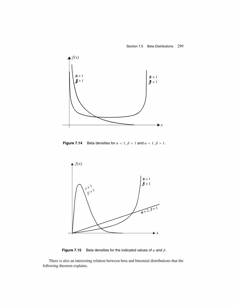
Section 7.5 Beta Distributions 299
< 1< 1
< 1> 1
x
f (x)
Figure 7.14 Beta densities for α < 1, β < 1 and α < 1, β > 1.
= 2, = 1
> 1
> 1
> 1< 1
x
f (x)
Figure 7.15 Beta densities for the indicated values of α and β.
There is also an interesting relation between beta and binomial distributions that thefollowing theorem explains.
300 Chapter 7 Special Continuous Distributions
Theorem 7.2 Let α and β be positive integers, X be a beta random variable withparameters α and β, and Y be a binomial random variable with parameters α + β − 1and p, 0 < p < 1. Then
P(X ≤ p) = P(Y ≥ α).
Proof: From the definition,
P(X ≤ p) = (α + β − 1)!(α − 1)! (β − 1)!
∫ p
0xα−1(1 − x)β−1 dx
= (α + β − 1)
(α + β − 2
α − 1
)∫ p
0xα−1(1 − x)β−1 dx
=α+β−1∑
i=α
(α + β − 1
i
)pi(1 − p)α+β−1−i
= P(Y ≥ α),
where the third equality follows from using integration by parts (α − 1) times. �
Example 7.16 The proportion of the stocks that will increase in value tomorrow is abeta random variable with parameters α and β. Today, these parameters were determinedto be α = 5 and β = 4, by a financial analyst, after she assessed the current political,social, economical, and financial factors. What is the probability that tomorrow thevalues of at least 70% of the stocks will move up?
Solution: Let X be the proportion of the stocks that will move up in value tomorrow; X
is beta with parameters α = 5 and β = 4. Hence the desired probability is
P(X ≥ 0.70) =∫ 1
0.70
1
B(5, 4)x4 (1 − x)3 dx = 280
∫ 1
0.70x4 (1 − x)3 dx = 0.194. �
Example 7.17 A beam of length �, rigidly supported at both ends, is hit suddenly at arandom point. This leads to a break in the beam at a position X units from the right end.If X/� is beta with parameters α = β = 3, find E(X), Var(X), and P(�/5 < X < �/4).
Solution: Since
E(X/�) = α
α + β= 3
6= 1
2,
Var(X/�) = αβ
(α + β + 1)(α + β)2= 9
7(6)2= 1
28,

Section 7.5 Beta Distributions 301
we have that E(X) = �/2, Var(X) = �2/28, and
P(�/5 < X < �/4) = P(1/5 < X/� < 1/4) =∫ 1/4
1/5
1
B(3, 3)x2(1 − x)2 dx
= 30∫ 1/4
1/5x2(1 − x)2 dx = 72953
1, 600, 000= 0.046. �
Example 7.18 Suppose that all 25 passengers of a commuter plane, departing at2:00 P.M., arrive at random times between 12:45 and 1:45 P.M. Find the probability thatthe median of the arrival times of the passengers is at or prior to 1:12 P.M.
Solution: Let the arrival time of a randomly selected passenger be W hours past 12:45.Then W is a uniform random variable over the interval (0, 1). Let X be the median ofthe arrival times of the 25 passengers. Since the median of (2n + 1) random numbersfrom (0, 1) is beta with parameters (n+1, n+1), we have that X is beta with parameters(13, 13). Since the length of the time interval from 12:45 to 1:12 is 27 minutes, the desiredquantity is P(X ≤ 27/60). To calculate this, let Y be a binomial random variable withparameters 25 and p = 27/60 = 0.45. Then, by Theorem 7.2,
P(X ≤ 0.45) = P(Y ≥ 13) =25∑
i=13
(25
i
)(0.45)i(0.55)25−i ≈ 0.306. �
EXERCISES
A
1. Is the following the probability density function of some beta random variableX?If so, find E(X) and Var(X).
f (x) ={
12x(1 − x)2 0 < x < 1
0 otherwise.
2. Is the following a probability density function? Why or why not?
f (x) ={
120x2(1 − x)4 0 < x < 1
0 otherwise.

302 Chapter 7 Special Continuous Distributions
3. For what value of c is the following a probability density function of some randomvariable X? Find E(X) and Var(X).
f (x) ={
cx4(1 − x)5 0 < x < 1
0 otherwise.
4. Suppose that new blood pressure medicines introduced are effective on 100p%of the patients, where p is a beta random variable with parameters α = 20 andβ = 13. What is the probability that a new blood pressure medicine is effectiveon at least 60% of the hypertensive population?
5. The proportion of resistors a procurement office of an engineering firm ordersevery month, from a specific vendor, is a beta random variable with mean 1/3 andvariance 1/18. What is the probability that next month, the procurement officeorders at least 7/12th of its purchase from this vendor?
6. At a certain university, the fraction of students who get a C in any section of acertain course is uniform over (0, 1). Find the probability that the median of thesefractions for the 13 sections of the course that are offered next semester is at least0.40.
7. Suppose that while daydreaming, the fraction X of the time that one commits bravedeeds is beta with parameters (5, 21). What is the probability that next time Jeffis daydreaming, he commits brave deeds at least 1/4 of the time?
8. For complicated projects such as construction of spacecrafts, project managersestimate two quantities, a and b, the minimum and maximum lengths of time itwill take for a project to be completed, respectively. In estimating b, they considerall of the possible complications that might delay the completion date. Experienceshows that the actual length of time it takes for a project to be completed is arandom variable defined by
Y = a + (b − a)X,
where X is beta with parameters α and β (α > 0, β > 0) that can be determinedfor the project.
(a) Find E(Y ) and Var(Y ).
(b) Find the probability density function of Y .
(c) Suppose that it takes Y years to complete a specific project, where Y =2 + 4X, and X is beta with parameters α = 2 and β = 3. What is theprobability that it takes less than 3 years to complete the project?

Section 7.6 Survival Analysis and Hazard Functions 303
B
9. Under what conditions and about which point(s) is the probability density functionof a beta random variable symmetric?
10. For α, β > 0, show that
B(α, β) = 2∫ ∞
0t2α−1(1 + t2)−(α+β) dt.
Hint: Make the substitution x = t2/(1 + t2) in
B(α, β) =∫ 1
0xα−1(1 − x)β−1 dx.
11. Prove that
B(α, β) = �(α)�(β)
�(α + β).
12. For an integer n ≥ 3, let X be a random variable with the probability densityfunction
f (x) =�(n + 1
2
)√
nπ �(n
2
)(1 + x2
n
)−(n+1)/2, −∞ < x < ∞.
Such random variables have significant applications in statistics. They are calledt-distributed with n degrees of freedom. Using the previous two exercises, findE(X) and Var(X).
� 7.6 SURVIVAL ANALYSIS AND HAZARD FUNCTIONS
In this section, we will study the risk or rate of failure, per unit of time, of lifetimes thathave already survived a certain length of time. The term lifetime is broad and applies toappropriate quantities in various models in science, engineering, and business. Depend-ing on the context of a study, by a lifetime, we might mean the lifetime of a machine,an electrical component, a living organism, an organism that is under an experimentalmedical treatment, a financial contract such as a mortgage, the waiting time until a cus-tomer arrives at a bank, or the time it takes until a customer is served at a post office.The failure for a living organism is its death. For a mortgage, it is when the mortgage is

304 Chapter 7 Special Continuous Distributions
paid off. For the time until a customer arrives at a bank, failure occurs when a customerenter the bank.
In the following discussion, for convenience, we will talk about the lifetime of asystem. However, our definitions and results are general and apply to other examplessuch as the ones just stated. Let the lifetime of a system be X, where X is a nonnegative,continuous random variable with probability distribution function F and probabilitydensity function f . The function defined by
F (t) = 1 − F(t) = P(X > t)
is called the survival function of X. For t > 0, F (t) is the probability that the systemhas already survived at least t units of time. Furthermore, the following relation, shownin Remark 6.4, enables us to calculate E(X), the expected value of the lifetime of thesystem, using F (t):
E(X) =∫ ∞
0F (t) dt.
The probability that a system, which has survived at least t units of time, fails on thetime interval (t, t + t ] is given by
P(X ≤ t + t | X > t) = P(t < X ≤ t + t)
P (X > t)= F(t + t) − F(t)
F (t).
To find the instantaneous failure rate of a system of age t at time t , note that during theinterval (t, t + t ], the system fails at a rate of
1
t
P (X ≤ t + t | X > t) = 1
F (t)· F(t + t) − F(t)
t
per unit of time. As t → 0, this quantity approaches the instantaneous failure rate ofthe system at time t , given that it has already survived t units of time. Let
λ(t) = limt→0
1
F (t)· F(t + t) − F(t)
t
= 1
F (t)· lim
t→0
F(t + t) − F(t)
t
= F ′(t)F (t)
= f (t)
F t).
Then λ(t) is called the hazard function of the random variable X. It is the instantaneousfailure rate at t , per unit of time, given that the system has already survived until time t .Note that λ(t) ≥ 0, but it is not a probability density function.
Remark 7.3 An alternate term used for F (t), the survival function of X, is the reliabil-ity function. Other terms used for λ(t), the hazard function, are hazard rate, failure rate

Section 7.6 Survival Analysis and Hazard Functions 305
function, failure rate, intensity rate, and conditional failure rate; sometimes actuarialscientists call it force of mortality. �
We know that if t > 0 is very small,
P(t < X ≤ t + t) =∫ t+t
t
f (x) dx
is the area under f from t to t + t . This area is almost equal to the area of a rectanglewith sides of length t and f (t). Thus
P(t < X ≤ t + t) ≈ f (t)t .
The smaller t , the closer f (t)t is to the probability that the system fails in (t, t +t ].This approximation implies that, for infinitesimal t > 0,
λ(t)t = f (t)t
F (t)≈ P(t < X ≤ t + t)
P (X > t)= P(X ≤ t + t | X > t).
Therefore,
For very small values of t > 0, the quantity λ(t)t is approximatelythe conditional probability that the system fails in (t, t +t), given thatit has lasted at least until t . That is,
P(X ≤ t + �t | X > t) ≈ λ(t)�t. (7.5)
Example 7.19 Dr. Hirsch has informed one of his employees, Dr. Kizanis, that shewill receive her next year’s employment contract at a random time between 10:00 A.M.
and 3:00 P.M. Suppose that Dr. Kizanis will receive her contract X minutes past 10:00 A.M.
Then X is a uniform random variable over the interval (0, 300). Hence the probabilitydensity function of X is given by
f (t) ={
1/300 if 0 < t < 300
0 otherwise.
Straightforward calculations show that the survival function of X is given by
F (t) = P(X > t) =
⎧⎪⎪⎪⎨⎪⎪⎪⎩1 if t < 0
300 − t
300if 0 ≤ t < 300
0 if t ≥ 300.

306 Chapter 7 Special Continuous Distributions
The hazard function, λ(t) = f (t)/F (t), is defined only for t < 300. It is unbounded fort ≥ 300. We have
λ(t) =⎧⎨⎩0 if t < 0
1
300 − tif 0 ≤ t < 300.
Since λ(0) = 0.003333, at 10:00 A.M. the instantaneous arrival rate of the contract (thefailure rate in this context) is 0.003333 per minute. At noon this rate will increase toλ(120) = 0.0056, at 2:00 P.M. to λ(240) = 0.017, at 2:59 P.M. it reaches λ(299) = 1.One second before 3:00 P.M., the instantaneous arrival of the contract is, approximately,λ(299.983) = 58.82. This shows that if Dr. Kizanis has not received her contract by onesecond before 3:00 P.M., the instantaneous arrival rate at that time is very high. That rateapproaches ∞, as the time approaches 3:00 P.M. To translate all these into probabilities,let t = 1/60. Then f (t)t is approximately the probability that the contract willarrive within one second after t , whereas λ(t)t is approximately the probability that thecontract will arrive within one second after t , given that it has not yet arrived by time t .The following table shows these probabilities at the indicated times:
t 0 120 240 299 299.983f (t)t 0.000056 0.000056 0.000056 0.000056 0.000056λ(t)t 0.000056 0.000093 0.000283 0.0167 0.98
The fact that f (t)t is constant is expected because X is uniformly distributed over(0, 300), and all of the intervals under consideration are subintervals of (0, 300) of equallengths. �
Let X be a nonnegative continuous random variable with probability distributionfunction F , probability density function f , survival function F , and hazard functionλ(t). We will now calculate F and f in terms of λ(t). The formulas obtained are veryuseful in various applications. Let G(t) = − ln
[F (t)
]. Then
G′(t) = f (t)
F (t)= λ(t).
Consequently, ∫ t
0G′(u) du =
∫ t
0λ(u) du.
Hence
G(t) − G(0) =∫ t
0λ(u) du.
Since X is nonnegative, G(0) = − ln[1 − F(0)
] = − ln 1 = 0. So
− ln[F (t)
]− 0 = G(t) − G(0) =∫ t
0λ(u) du

Section 7.6 Survival Analysis and Hazard Functions 307
implies that
F (t) = exp(−
∫ t
0λ(u) du
). (7.6)
By this equation,
F(t) = 1 − exp[
−∫ t
0λ(u) du
].
Differentiating both sides of this relation, with respect to t , yields
f (t) = λ(t) exp[
−∫ t
0λ(u) du
]. (7.7)
This demonstrates that the hazard function uniquely determines the probability densityfunction.
In reliability theory, a branch of engineering, it is often observed that λ(t), the hazardfunction of the lifetime of a manufactured machine, is initially large due to undetecteddefective components during testing. Later, λ(t) will decrease and remains more orless the same until a time when it increases again due to aging, which makes worn-outcomponents more likely to fail. A random variable X is said to have an increasing failurerate if λ(t) is increasing. It is said to have a decreasing failure rate if λ(t) is decreasing.In the next example, we will show that if λ(t) is neither increasing nor decreasing; thatis, if λ(t) is a constant, then X is an exponential random variable. In such a case, the factthat aging does not change the failure rate is consistent with the memoryless property ofexponential random variables. To summarize, the lifetime of a manufactured machineis likely to have a decreasing failure rate in the beginning, a constant failure rate lateron, and an increasing failure rate due to wearing out after an aging process. Similarly,lifetimes of living organisms, after a certain age, have increasing failure rates. However,for a newborn baby, the longer he or she survives, the chances of surviving is higher.This means that as t increases, λ(t) decreases. That is, λ(t) is decreasing.
Example 7.20 In this example, we will prove the following important theorem:
Let λ(t), the hazard function of a continuous, nonnegative randomvariable X, be a constant λ.Then X is an exponential random variablewith parameter λ.
To show this theorem, let f be the probability density function of X. By (7.7),
f (t) = λ exp(−∫ t
0λ du
)= λe−λt .
This is the density function of an exponential random variable with parameter λ. Thus arandom variable with constant hazard function is exponential. As mentioned previously,

308 Chapter 7 Special Continuous Distributions
this result is not surprising. The fact that an exponential random variable is memo-ryless implies that age has no effect on the distribution of the remaining lifetimes ofexponentially distributed random variables. For systems that have exponential lifetimedistribution, failures are not due to aging and wearing out. In fact, such systems do notwear out at all. Failures occur abruptly. There is no transition from the previous “state”of the system and no preparation for, or gradual approach to, failure. �
EXERCISES
1. Experience shows that the failure rate of a certain electrical component is a linearfunction. Suppose that after two full days of operation, the failure rate is 10% perhour and after three full days of operation, it is 15% per hour.
(a) Find the probability that the component operates for at least 30 hours.
(b) Suppose that the component has been operating for 30 hours. What is theprobability that it fails within the next hour?
2. One of the most popular distributions used to model the lifetimes of electric com-ponents is the Weibull distribution, whose probability density function is givenby
f (t) = αtα−1e−tα , t > 0, α > 0.
Determine for which values of α the hazard function of a Weibull random variableis increasing, for which values it is decreasing, and for which values it is constant.
REVIEW PROBLEMS
1. For a restaurant, the time it takes to deliver pizza (in minutes) is uniform over theinterval (25, 37). Determine the proportion of deliveries that are made in less thanhalf an hour.
2. It is known that the weight of a random woman from a community is normal withmean 130 pounds and standard deviation 20. Of the women in that communitywho weigh above 140 pounds, what percent weigh over 170 pounds?
3. One thousand random digits are generated. What is the probability that digit 5 isgenerated at most 93 times?

Chapter 7 Review Problems 309
4. Let X, the lifetime of a light bulb, be an exponential random variable with param-eter λ. Is it possible that X satisfies the following relation?
P(X ≤ 2) = 2P(2 < X ≤ 3).
If so, for what value of λ?
5. The time that it takes for a computer system to fail is exponential with mean 1700hours. If a lab has 20 such computer systems, what is the probability that at leasttwo fail before 1700 hours of use?
6. Let X be a uniform random variable over the interval (0, 1). Calculate E(− ln X).
7. Suppose that the diameter of a randomly selected disk produced by a certainmanufacturer is normal with mean 4 inches and standard deviation 1 inch. Findthe distribution function of the diameter of a randomly chosen disk, in centimeters.
8. Let X be an exponential random variable with parameter λ. Prove that
P(α ≤ X ≤ α + β) ≤ P(0 ≤ X ≤ β).
9. The time that it takes for a calculus student to answer all the questions on a certainexam is an exponential random variable with mean 1 hour and 15 minutes. If all10 students of a calculus class are taking that exam, what is the probability that atleast one of them completes it in less than one hour?
10. Determine the value(s) of k for which the following is a density function.
f (x) = ke−x2+3x+2, −∞ < x < ∞.
11. The grades of students in a calculus-based probability course are normal with mean72 and standard deviation 7. If 90, 80, 70, and 60 are the respective lowest, A, B,C, and D, what percent of students in this course get A’s, B’s, C’s, D’s, and F’s?
12.. The number of minutes that a train from Milan to Rome is late is an exponentialrandom variable X with parameter λ. Find P
(X > E(X)
).
13. In a measurement, a number is rounded off to the nearest k decimal places. LetX be the rounding error. Determine the probability distribution function of X andits parameters.
14. Suppose that the weights of passengers taking an elevator in a certain building arenormal with mean 175 pounds and standard deviation 22. What is the minimumweight for a passenger who outweighs at least 90% of the other passengers?
15. The breaking strength of a certain type of yarn produced by a certain vendor isnormal with mean 95 and standard deviation 11. What is the probability that, in arandom sample of size 10 from the stock of this vendor, the breaking strengths ofat least two are over 100?

310 Chapter 7 Special Continuous Distributions
16. The number of phone calls to a specific exchange is a Poisson process with rate23 per hour. Calculate the probability that the time until the 91st call is at least 4hours.
17. Let X be a uniform random variable over the interval (1 − θ, 1 + θ), where0 < θ < 1 is a given parameter. Find a function of X, say g(X), so that E
[g(X)
] =θ2.
18. A beam of length � is rigidly supported at both ends. Experience shows thatwhenever the beam is hit at a random point, it breaks at a position X units from theright end, where X/� is a beta random variable. If E(X) = 3�/7 and Var(X) =3�2/98, find P(�/7 < X < �/3).

Chapter 8
Bivariate Distributions
8.1 JOINT DISTRIBUTIONS OF TWO RANDOM VARIABLES
Joint Probability Mass Functions
Thus far we have studied probability mass functions of single discrete random variablesand probability density functions of single continuous random variables. We now con-sider two or more random variables that are defined simultaneously on the same samplespace. In this section we consider such cases with two variables. Cases of three or morevariables are studied in Chapter 9.
Definition Let X and Y be two discrete random variables defined on the same samplespace. Let the sets of possible values of X and Y be A and B, respectively. The function
p(x, y) = P(X = x, Y = y)
is called the joint probability mass function of X and Y .
Note that p(x, y) ≥ 0. If x �∈ A or y �∈ B, then p(x, y) = 0. Also,∑x∈A
∑y∈B
p(x, y) = 1. (8.1)
Let X and Y have joint probability mass function p(x, y). Let pX be the probabilitymass function of X. Then
pX(x) = P(X = x) = P(X = x, Y ∈ B)
=∑y∈B
P (X = x, Y = y) =∑y∈B
p(x, y).
Similarly, pY , the probability mass function of Y , is given by
pY (y) =∑x∈A
p(x, y).
311

312 Chapter 8 Bivariate Distributions
These relations motivate the following definition.
Definition Let X and Y have joint probability mass function p(x, y). Let A bethe set of possible values of X and B be the set of possible values of Y . Then thefunctions pX(x) = ∑
y∈B p(x, y) and pY (y) = ∑x∈A p(x, y) are called, respectively,
the marginal probability mass functions of X and Y .
Example 8.1 A small college has 90 male and 30 female professors. An ad hoccommittee of five is selected at random to write the vision and mission of the college.Let X and Y be the number of men and women on this committee, respectively.
(a) Find the joint probability mass function of X and Y .
(b) Find pX and pY , the marginal probability mass functions of X and Y .
Solution:
(a) The set of possible values for both X and Y is {0, 1, 2, 3, 4, 5}. The joint probabilitymass function of X and Y , p(x, y), is given by
p(x, y) =
⎧⎪⎪⎪⎪⎪⎪⎨⎪⎪⎪⎪⎪⎪⎩
(90
x
)(30
y
)(
120
5
) if x, y ∈ {0, 1, 2, 3, 4, 5}, x + y = 5
0 otherwise.
(b) To find pX and pY , the marginal probability mass functions of X and Y ,
respectively, note that pX(x) = ∑5y=0 p(x, y), pY (y) = ∑5
x=0 p(x, y). Since
p(x, y) = 0 if x + y �= 5,∑5
y=0 p(x, y) = p(x, 5 − x) and∑5
x=0 p(x, y) =p(5 − y, y). Therefore,
pX(x) =
(90
x
)(30
5 − x
)(
120
5
) , x ∈ {0, 1, 2, 3, 4, 5},
pY (y) =
(90
5 − y
)(30
y
)(
120
5
) , y ∈ {0, 1, 2, 3, 4, 5}.
Note that, as expected, pX and pY are hypergeometric. �

Section 8.1 Joint Distributions of Two Random Variables 313
Example 8.2 Roll a balanced die and let the outcome be X. Then toss a fair coin X
times and let Y denote the number of tails. What is the joint probability mass functionof X and Y and the marginal probability mass functions of X and Y ?
Solution: Let p(x, y) be the joint probability mass function of X and Y . Clearly,X ∈ {1, 2, 3, 4, 5, 6} and Y ∈ {0, 1, 2, 3, 4, 5, 6}. Now if X = 1, then Y = 0 or 1; wehave
p(1, 0) = P(X = 1, Y = 0) = P(X = 1)P (Y = 0 | X = 1) = 1
6· 1
2= 1
12,
p(1, 1) = P(X = 1, Y = 1) = P(X = 1)P (Y = 1 | X = 1) = 1
6· 1
2= 1
12.
If X = 2, then y = 0, 1, or 2, where
p(2, 0) = P(X = 2, Y = 0) = P(X = 2)P (Y = 0 | X = 2) = 1
6· 1
4= 1
24.
Similarly, p(2, 1) = 1/12, p(2, 2) = 1/24. If X = 3, then y = 0, 1, 2, or 3, and
p(3, 0) = P(X = 3, Y = 0) = P(X = 3)P (Y = 0 | X = 3)
= 1
6
(3
0
)(1
2
)0(1
2
)3 = 1
48,
p(3, 1) = P(X = 3, Y = 1) = P(X = 3)P (Y = 1 | X = 3)
= 1
6
(3
1
)(1
2
)2(1
2
)1 = 3
48.
Similarly, p(3, 2) = 3/48, p(3, 3) = 1/48. Similar calculations will yield the followingtable for p(x, y).
y
x 0 1 2 3 4 5 6 pX(x)
1 1/12 1/12 0 0 0 0 0 1/62 1/24 2/24 1/24 0 0 0 0 1/63 1/48 3/48 3/48 1/48 0 0 0 1/64 1/96 4/96 6/96 4/96 1/96 0 0 1/65 1/192 5/192 10/192 10/192 5/192 1/192 0 1/66 1/384 6/384 15/384 20/384 15/384 6/384 1/384 1/6
pY (y) 63/384 120/384 99/384 64/384 29/384 8/384 1/384
Note that pX(x) = P(X = x) and pY (y) = P(Y = y), the probability massfunctions of X and Y , are obtained by summing up the rows and the columns of thistable, respectively. �
314 Chapter 8 Bivariate Distributions
LetX andY be discrete random variables with joint probability mass function p(x, y).Let the sets of possible values of X and Y be A and B, respectively. To find E(X) andE(Y ), first we calculate pX and pY , the marginal probability mass functions of X and Y ,respectively. Then we will use the following formulas.
E(X) =∑x∈A
xpX(x); E(Y) =∑y∈B
ypY (y).
Example 8.3 Let the joint probability mass function of random variables X and Y begiven by
p(x, y) =
⎧⎪⎨⎪⎩1
70x(x + y) if x = 1, 2, 3, y = 3, 4
0 elsewhere.
Find E(X) and E(Y ).
Solution: To find E(X) and E(Y ), first we need to calculate pX(x) and pY (y), themarginal probability mass functions of X and Y , respectively. Note that
pX(x) = p(x, 3) + p(x, 4)
= 1
70x(x + 3) + 1
70x(x + 4)
= 1
35x2 + 1
10x, x = 1, 2, 3;
pY (y) = p(1, y) + p(2, y) + p(3, y)
= 1
70(1 + y) + 2
70(2 + y) + 3
70(3 + y)
= 1
5+ 3
35y, y = 3, 4.
Therefore,
E(X) =3∑
x=1
xpX(x) =3∑
x=1
x( 1
35x2 + 1
10x)
= 17
7≈ 2.43;
E(Y ) =4∑
y=3
ypY (y) =4∑
y=3
y(1
5+ 3
35y)
= 124
35≈ 3.54. �
We will now state the following generalization of Theorem 4.2 from one dimension totwo. As an immediate application of this important generalization, we will show that the

Section 8.1 Joint Distributions of Two Random Variables 315
expected value of the sum of two random variables is equal to the sum of their expectedvalues. We will prove a generalization of this theorem in Chapter 10 and discuss someof its many applications in that chapter.
Theorem 8.1 Let p(x, y) be the joint probability mass function of discrete randomvariables X and Y . Let A and B be the set of possible values of X and Y , respectively. Ifh is a function of two variables from R2 to R , then h(X, Y ) is a discrete random variablewith the expected value given by
E[h(X, Y )
] =∑x∈A
∑y∈B
h(x, y)p(x, y),
provided that the sum is absolutely convergent.
Corollary For discrete random variables X and Y ,
E(X + Y) = E(X) + E(Y).
Proof: In Theorem 8.1 let h(x, y) = x + y. Then
E(X + Y ) =∑x∈A
∑y∈B
(x + y)p(x, y)
=∑x∈A
∑y∈B
xp(x, y) +∑x∈A
∑y∈B
yp(x, y)
= E(X) + E(Y ). �
Joint Probability Density Functions
To define the concept of joint probability density function of two continuous randomvariables X and Y , recall from Section 6.1 that a single random variable X is calledcontinuous if there exists a nonnegative real-valued function f : R → [0, ∞) such thatfor any subset A of real numbers that can be constructed from intervals by a countablenumber of set operations,
P(X ∈ A) =∫
A
f (x) dx.
This definition is generalized in the following obvious way:
Definition Two random variables X and Y , defined on the same sample space, havea continuous joint distribution if there exists a nonnegative function of two variables,f (x, y) on R × R , such that for any region R in the xy-plane that can be formed fromrectangles by a countable number of set operations,
P((X, Y ) ∈ R
) =∫∫R
f (x, y) dx dy. (8.2)
The function f (x, y) is called the joint probability density function of X and Y .
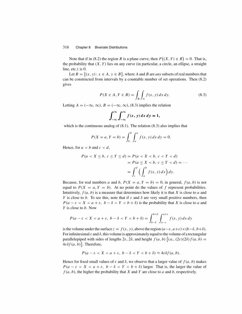
316 Chapter 8 Bivariate Distributions
Note that if in (8.2) the region R is a plane curve, then P((X, Y ) ∈ R
) = 0. That is,the probability that (X, Y ) lies on any curve (in particular, a circle, an ellipse, a straightline, etc.) is 0.
Let R = {(x, y) : x ∈ A, y ∈ B}, where A and B are any subsets of real numbers that
can be constructed from intervals by a countable number of set operations. Then (8.2)gives
P(X ∈ A, Y ∈ B) =∫
B
∫A
f (x, y) dx dy. (8.3)
Letting A = (−∞, ∞), B = (−∞, ∞), (8.3) implies the relation∫ ∞
−∞
∫ ∞
−∞f (x, y) dx dy = 1,
which is the continuous analog of (8.1). The relation (8.3) also implies that
P(X = a, Y = b) =∫ b
b
∫ a
a
f (x, y) dx dy = 0.
Hence, for a < b and c < d,
P(a < X ≤ b, c ≤ Y ≤ d) = P(a < X < b, c < Y < d)
= P(a ≤ X < b, c ≤ Y < d) = · · ·=∫ d
c
( ∫ b
a
f (x, y) dx)
dy.
Because, for real numbers a and b, P(X = a, Y = b) = 0, in general, f (a, b) is notequal to P(X = a, Y = b). At no point do the values of f represent probabilities.Intuitively, f (a, b) is a measure that determines how likely it is that X is close to a andY is close to b. To see this, note that if ε and δ are very small positive numbers, thenP(a − ε < X < a + ε, b − δ < Y < b + δ) is the probability that X is close to a andY is close to b. Now
P(a − ε < X < a + ε, b − δ < Y < b + δ) =∫ b+δ
b−δ
∫ a+ε
a−ε
f (x, y) dx dy
is the volume under the surface z = f (x, y), above the region (a−ε, a+ε)×(b−δ, b+δ).For infinitesimal ε and δ, this volume is approximately equal to the volume of a rectangularparallelepiped with sides of lengths 2ε, 2δ, and height f (a, b)
[i.e., (2ε)(2δ)f (a, b) =
4εδf (a, b)]. Therefore,
P(a − ε < X < a + ε, b − δ < Y < b + δ) ≈ 4εδf (a, b).
Hence for fixed small values of ε and δ, we observe that a larger value of f (a, b) makesP(a − ε < X < a + ε, b − δ < Y < b + δ) larger. That is, the larger the value off (a, b), the higher the probability that X and Y are close to a and b, respectively.

Section 8.1 Joint Distributions of Two Random Variables 317
Let X and Y have joint probability density function f (x, y). Let fY be the probabilitydensity function of Y . To find fY in terms of f , note that, on the one hand, for any subsetB of R,
P(Y ∈ B) =∫
B
fY (y) dy, (8.4)
and, on the other hand, using (8.3),
P(Y ∈ B) = P(X ∈ (−∞, ∞), Y ∈ B
) =∫
B
( ∫ ∞
−∞f (x, y) dx
)dy.
Comparing this with (8.4), we can write
fY (y) =∫ ∞
−∞f (x, y) dx. (8.5)
Similarly,
fX(x) =∫ ∞
−∞f (x, y) dy. (8.6)
Therefore, it is reasonable to make the following definition:
Definition Let X and Y have joint probability density function f (x, y); then thefunctions fX and fY , given by (8.6) and (8.5), are called, respectively, the marginalprobability density functions of X and Y .
Note that while from the joint probability density function of X and Y we can findthe marginal probability density functions of X and Y , it is not possible, in general, tofind the joint probability density function of two random variables from their marginals.This is because the marginal probability density function of a random variable X givesinformation about X without looking at the possible values of other random variables.However, sometimes with more information the marginal probability density functionsenable us to find the joint probability density function of two random variables. Anexample of such a case, studied in Section 8.2, is when X and Y are independent randomvariables.
Let X and Y be two random variables (discrete, continuous, or mixed). The jointprobability distribution function, or joint cumulative probability distribution function,or simply the joint distribution of X and Y , is defined by
F(t, u) = P(X ≤ t, Y ≤ u)
for all −∞ < t, u < ∞. The marginal probability distribution function of X, FX,can be found from F as follows:
FX(t) = P(X ≤ t) = P(X ≤ t, Y < ∞) = P(
limn→∞{X ≤ t, Y ≤ n})
= limn→∞ P(X ≤ t, Y ≤ n) = lim
n→∞ F(t, n) ≡ F(t, ∞).

318 Chapter 8 Bivariate Distributions
To justify the fourth equality, note that the sequence of events {X ≤ t, Y ≤ n}, n ≥ 1, isan increasing sequence. Therefore, by continuity of probability function (Theorem 1.8),
P(
limn→∞{X ≤ t, Y ≤ n}) = lim
n→∞ P(X ≤ t, Y ≤ n).
Similarly, FY , the marginal probability distribution function of Y , is
FY (u) = P(Y ≤ u) = limn→∞ F(n, u) ≡ F(∞, u).
Now suppose that the joint probability density function of X and Y is f (x, y). Then
F(x, y) = P(X ≤ x, Y ≤ y) = P(X ∈ (−∞, x], Y ∈ (−∞, y])
=∫ y
−∞
∫ x
−∞f (t, u) dt du. (8.7)
Assuming that the partial derivatives of F exist, by differentiation of (8.7), we get
f (x, y) = ∂2
∂x ∂yF(x, y).
Moreover, from (8.7), we obtain
FX(x) = F(x, ∞) =∫ ∞
−∞
( ∫ x
−∞f (t, u) dt
)du
=∫ x
−∞
( ∫ ∞
−∞f (t, u) du
)dt =
∫ x
−∞fX(t) dt,
and, similarly,
FY (y) =∫ y
−∞fY (u) du.
These relations show that if X and Y have joint probability density function f (x, y),then X and Y are continuous random variables with density functions fX and fY , anddistribution functions FX and FY , respectively. Therefore, F ′
X(x) = fX(x) and F ′Y (y) =
fY (y). We also have
E(X) =∫ ∞
−∞xfX(x) dx; E(Y) =
∫ ∞
−∞yfY (y) dy.
Example 8.4 The joint probability density function of random variables X and Y isgiven by
f (x, y) ={
λxy2 0 ≤ x ≤ y ≤ 1
0 otherwise.

Section 8.1 Joint Distributions of Two Random Variables 319
(a) Determine the value of λ.
(b) Find the marginal probability density functions of X and Y .
(c) Calculate E(X) and E(Y ).
Solution:
(a) To find λ, note that∫∞−∞∫∞−∞ f (x, y) dx dy = 1 gives
∫ 1
0
( ∫ 1
x
λxy2 dy)
dx = 1.
Therefore,
1 =∫ 1
0
( ∫ 1
x
y2 dy)λx dx =
∫ 1
0
[1
3y3]1
xλx dx
= λ
∫ 1
0
(1
3− 1
3x3)x dx = λ
3
∫ 1
0(1 − x3)x dx = λ
3
∫ 1
0(x − x4) dx
= λ
3
[1
2x2 − 1
5x5]1
0= λ
10,
and hence λ = 10.
(b) To find fX and fY , the respective marginal probability density functions of X andY , we use (8.6) and (8.5):
fX(x) =∫ ∞
−∞f (x, y) dy =
∫ 1
x
10xy2 dy =[10
3xy3]1
x
= 10
3x(1 − x3), 0 ≤ x ≤ 1;
fY (y) =∫ ∞
−∞f (x, y) dx =
∫ y
010xy2 dx =
[5x2y2
]y0
= 5y4, 0 ≤ y ≤ 1.
(c) To find E(X) and E(Y ), we use the results obtained in part (b):
E(X) =∫ 1
0x · 10
3x(1 − x3) dx = 5
9;
E(Y ) =∫ 1
0y · 5y4 dy = 5
6. �
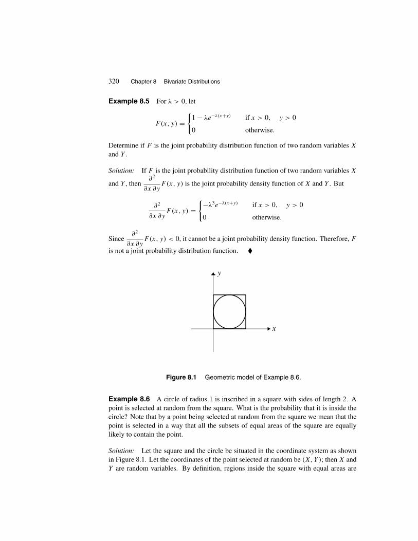
320 Chapter 8 Bivariate Distributions
Example 8.5 For λ > 0, let
F(x, y) ={
1 − λe−λ(x+y) if x > 0, y > 0
0 otherwise.
Determine if F is the joint probability distribution function of two random variables X
and Y .
Solution: If F is the joint probability distribution function of two random variables X
and Y , then∂2
∂x ∂yF (x, y) is the joint probability density function of X and Y . But
∂2
∂x ∂yF (x, y) =
{−λ3e−λ(x+y) if x > 0, y > 0
0 otherwise.
Since∂2
∂x ∂yF (x, y) < 0, it cannot be a joint probability density function. Therefore, F
is not a joint probability distribution function. �
x
y
Figure 8.1 Geometric model of Example 8.6.
Example 8.6 A circle of radius 1 is inscribed in a square with sides of length 2. Apoint is selected at random from the square. What is the probability that it is inside thecircle? Note that by a point being selected at random from the square we mean that thepoint is selected in a way that all the subsets of equal areas of the square are equallylikely to contain the point.
Solution: Let the square and the circle be situated in the coordinate system as shownin Figure 8.1. Let the coordinates of the point selected at random be (X, Y ); then X andY are random variables. By definition, regions inside the square with equal areas are

Section 8.1 Joint Distributions of Two Random Variables 321
equally likely to contain (X, Y ). Hence, for all (a, b) inside the square, the probabilitythat (x, y) is “close” to (a, b) is the same. Let f (x, y) be the joint probability densityfunction of X and Y . Since f (x, y) is a measure that determines how likely it is that X isclose to x and Y is close to y, f (x, y) must be constant for the points inside the square,and 0 elsewhere. Therefore, for some c > 0,
f (x, y) ={
c if 0 < x < 2, 0 < y < 2
0 otherwise,
where∫∞−∞∫∞−∞ f (x, y) dx dy = 1 gives∫ 2
0
∫ 2
0c dx dy = 1,
implying that c = 1/4. Now let R be the region inside the circle. Then the desiredprobability is
∫∫R
f (x, y) dx dy =∫∫R
1
4dx dy =
∫∫R
dx dy
4.
Note that∫∫R
dx dy is the area of the circle, and 4 is the area of the square. Thus the
desired probability is
area of the circle
area of the square= π(1)2
4= π
4. �
What we showed in Example 8.6 is true, in general. Let S be a bounded region inthe Euclidean plane and suppose that R is a region inside S. Fix a coordinate system,and let the coordinates of a point selected at random from S be (X, Y ). By an argumentsimilar to that of Example 8.6, we have that, for some c > 0, the joint probability densityfunction of X and Y , f (x, y), is given by
f (x, y) ={
c if (x, y) ∈ S
0 otherwise,
where ∫∫S
f (x, y) dx dy = 1.

322 Chapter 8 Bivariate Distributions
This gives c
∫∫S
dx dy = 1, or, equivalently, c× area(S) = 1. Therefore, c = 1/area(S)
and hence
f (x, y) =
⎧⎪⎪⎨⎪⎪⎩1
area(S)if (x, y) ∈ S
0 otherwise.
Thus
P((X, Y ) ∈ R
) =∫∫R
f (x, y) dx dy = 1
area(S)
∫∫R
dx dy = area(R)
area(S).
Based on these observations, we make the following definition.
Definition Let S be a subset of the plane with area A(S). A point is said to berandomly selected from S if for any subset R of S with area A(R), the probability thatR contains the point is A(R)/A(S).
This definition is essential in the field of geometric probability. By the followingexamples, we will show how it can help to solve problems readily.
Example 8.7 A man invites his fiancée to a fine hotel for a Sunday brunch. Theydecide to meet in the lobby of the hotel between 11:30 A.M. and 12 noon. If they arriveat random times during this period, what is the probability that they will meet within 10minutes?
Solution: Let X and Y be the minutes past 11:30 A.M. that the man and his fiancée arriveat the lobby, respectively. Let
S = {(x, y) : 0 ≤ x ≤ 30, 0 ≤ y ≤ 30}, and R = {(x, y) ∈ S : |x − y| ≤ 10
}.
Then the desired probability, P(|X − Y | ≤ 10
), is given by
P(|X − Y | ≤ 10
) = area of R
area of S= area of R
30 × 30= area(R)
900.

Section 8.1 Joint Distributions of Two Random Variables 323
x_ y =
10y_ x =
10
10
30
10 30
y
x
Figure 8.2 Geometric model of Example 8.7.
R = {(x, y) ∈ S : x − y ≤ 10 and y − x ≤ 10
}is the shaded region of Figure 8.2,
and its area is the area of the square minus the areas of the two unshaded triangles:(30)(30) − 2(1/2 × 20 × 20) = 500. Hence the desired probability is 500/900 = 5/9.
�
Example 8.8 A farmer decides to build a pen in the shape of a triangle for his chickens.He sends his son out to cut the lumber and the boy, without taking any thought as to theultimate purpose, makes two cuts at two points selected at random. What are the chancesthat the resulting three pieces of lumber can be used to form a triangular pen?
Solution: Suppose that the length of the lumber is �. Let A and B be the random pointsplaced on the lumber; let the distances of A and B from the left end of the lumber bedenoted by X and Y , respectively. If X < Y , the lumber is divided into three parts oflengths X, Y −X, and �−Y ; otherwise, it is divided into three parts of lengths Y , X−Y ,and � − X. Because of symmetry, we calculate the probability that X < Y , and X,Y − X, and � − Y form a triangle. Then we multiply the result by 2 to obtain the desiredprobability. We know that three segments form a triangle if and only if the length of anyone of them is less than the sum of the lengths of the remaining two. Therefore, we musthave
X < Y
X < (Y − X) + (� − Y )
(Y − X) < X + (� − Y )
� − Y < X + (Y − X),
or, equivalently,
X < Y, X <�
2, Y < X + �
2, and Y >
�
2.

324 Chapter 8 Bivariate Distributions
x
y
y = x
Figure 8.3 Geometric model of Example 8.8.
Since (X, Y ) is a random point from the square (0, �) × (0, �), the probability that itsatisfies these inequalities is the area of R, where
R ={(x, y) : x < y, x <
�
2, y < x + �
2, y >
�
2
},
divided by �2, the area of the square. Note that R is the shaded region of Figure 8.3 andits area is 1/8 of the area of the square. Thus the probability that (X, Y ) lies in R is 1/8and hence the desired probability is 1/4. �
Before closing this section, we state the continuous analog of Theorem 8.1, which is ageneralization of Theorem 6.3 from one dimension to two. As an immediate applicationof this important generalization, we will show the continuous version of the followingtheorem that we proved above for discrete random variables: The expected value of thesum of two random variables is equal to the sum of their expected values.
Theorem 8.2 Let f (x, y) be the joint probability density function of random variablesX and Y . If h is a function of two variables from R2 to R , then h(X, Y ) is a randomvariable with the expected value given by
E[h(X, Y )
] =∫ ∞
−∞
∫ ∞
−∞h(x, y)f (x, y) dx dy,
provided that the integral is absolutely convergent.
Corollary For random variables X and Y ,
E(X + Y) = E(X) + E(Y).

Section 8.1 Joint Distributions of Two Random Variables 325
Proof: In Theorem 8.2 let h(x, y) = x + y. Then
E(X + Y ) =∫ ∞
−∞
∫ ∞
−∞(x + y)f (x, y) dx dy
=∫ ∞
−∞
∫ ∞
−∞xf (x, y) dx dy +
∫ ∞
−∞
∫ ∞
−∞yf (x, y) dx dy
= E(X) + E(Y ). �
Example 8.9 Let X and Y have joint probability density function
f (x, y) =
⎧⎪⎪⎨⎪⎪⎩3
2(x2 + y2) if 0 < x < 1, 0 < y < 1
0 otherwise.
Find E(X2 + Y 2).
Solution: By Theorem 8.2,
E(X2 + Y 2) =∫ ∞
−∞
∫ ∞
−∞(x2 + y2)f (x, y) dx dy =
∫ 1
0
∫ 1
0
3
2(x2 + y2)2 dx dy
= 3
2
∫ 1
0
∫ 1
0(x4 + 2x2y2 + y4) dx dy = 14
15. �
EXERCISES
A
1. Let the joint probability mass function of discrete random variables X and Y begiven by
p(x, y) =
⎧⎪⎨⎪⎩k(x
y
)if x = 1, 2, y = 1, 2
0 otherwise.
Determine (a) the value of the constant k, (b) the marginal probability mass func-tions of X and Y , (c) P(X > 1 | Y = 1), (d) E(X) and E(Y ).
326 Chapter 8 Bivariate Distributions
2. Let the joint probability mass function of discrete random variables X and Y begiven by
p(x, y) ={
c(x + y) if x = 1, 2, 3, y = 1, 2
0 otherwise.
Determine (a) the value of the constant c, (b) the marginal probability mass func-tions of X and Y , (c) P(X ≥ 2 | Y = 1), (d) E(X) and E(Y ).
3. Let the joint probability mass function of discrete random variables X and Y begiven by
p(x, y) ={
k(x2 + y2) if (x, y) = (1, 1), (1, 3), (2, 3)
0 otherwise.
Determine (a) the value of the constant k, (b) the marginal probability mass func-tions of X and Y , and (c) E(X) and E(Y ).
4. Let the joint probability mass function of discrete random variables X and Y begiven by
p(x, y) =
⎧⎪⎪⎨⎪⎪⎩1
25(x2 + y2) if x = 1, 2, y = 0, 1, 2
0 otherwise.
Find P(X > Y), P(X + Y ≤ 2), and P(X + Y = 2).
5. Thieves stole four animals at random from a farm that had seven sheep, eight goats,and five burros. Calculate the joint probability mass function of the number ofsheep and goats stolen.
6. Two dice are rolled. The sum of the outcomes is denoted by X and the absolutevalue of their difference by Y . Calculate the joint probability mass function of X
and Y and the marginal probability mass functions of X and Y .
7. In a community 30% of the adults are Republicans, 50% are Democrats, and therest are independent. For a randomly selected person, let
X ={
1 if he or she is a Republican
0 otherwise,
Y ={
1 if he or she is a Democrat
0 otherwise.
Calculate the joint probability mass function of X and Y .
Section 8.1 Joint Distributions of Two Random Variables 327
8. From an ordinary deck of 52 cards, seven cards are drawn at random and withoutreplacement. Let X and Y be the number of hearts and the number of spadesdrawn, respectively.
(a) Find the joint probability mass function of X and Y .
(b) Calculate P(X ≥ Y ).
9. Let the joint probability density function of random variables X and Y be givenby
f (x, y) ={
2 if 0 ≤ y ≤ x ≤ 1
0 elsewhere.
(a) Calculate the marginal probability density functions of X and Y , respec-tively.
(b) Find E(X) and E(Y ).
(c) Calculate P(X < 1/2), P(X < 2Y ), and P(X = Y ).
10. Let the joint probability density function of random variables X and Y be givenby
f (x, y) ={
8xy if 0 ≤ y ≤ x ≤ 1
0 elsewhere.
(a) Calculate the marginal probability density functions of X and Y , respec-tively.
(b) Calculate E(X) and E(Y ).
11. Let the joint probability density function of random variables X and Y be givenby
f (x, y) =
⎧⎪⎪⎨⎪⎪⎩1
2ye−x if x > 0, 0 < y < 2
0 elsewhere.
Find the marginal probability density functions of X and Y .
12. Let X and Y have the joint probability density function
f (x, y) ={
1 if 0 ≤ x ≤ 1, 0 ≤ y ≤ 1
0 elsewhere.
CalculateP(X+Y ≤ 1/2), P(X−Y ≤ 1/2), P(XY ≤ 1/4), andP(X2+Y 2 ≤ 1).
328 Chapter 8 Bivariate Distributions
13. Let R be the bounded region between y = x and y = x2. A random point (X, Y )
is selected from R.
(a) Find the joint probability density function of X and Y .
(b) Calculate the marginal probability density functions of X and Y .
(c) Find E(X) and E(Y ).
14. A man invites his fiancée to an elegant hotel for a Sunday brunch. They decide tomeet in the lobby of the hotel between 11:30 A.M. and 12 noon. If they arrive atrandom times during this period, what is the probability that the first to arrive hasto wait at least 12 minutes?
15. A farmer makes cuts at two points selected at random on a piece of lumber oflength �. What is the expected value of the length of the middle piece?
16. On a line segment AB of length �, two points C and D are placed at random andindependently. What is the probability that C is closer to D than to A?
17. Two points X and Y are selected at random and independently from the interval(0, 1). Calculate P(Y ≤ X and X2 + Y 2 ≤ 1).
B
18. Let X and Y be random variables with finite expectations. Show that ifP(X ≤ Y ) = 1, then E(X) ≤ E(Y ).
19. Suppose that h is the probability density function of a continuous random variable.Let the joint probability density function of two random variables X and Y be givenby
f (x, y) = h(x)h(y), x ∈ R, y ∈ R.
Prove that P(X ≥ Y ) = 1/2.
20. Let g and h be two probability density functions with probability distributionfunctions G and H , respectively. Show that for −1 ≤ α ≤ 1, the function
f (x, y) = g(x)h(y)(1 + α[2G(x) − 1][2H(y) − 1])
is a joint probability density function of two random variables. Moreover, provethat g and h are the marginal probability density functions of f .Note: This exercise gives an infinite family of joint probability density functionsall with the same marginal probability density function of X and of Y .
21. Three points M , N , and L are placed on a circle at random and independently.What is the probability that MNL is an acute angle?

Section 8.1 Joint Distributions of Two Random Variables 329
22. Two numbers x and y are selected at random from the interval (0, 1). For i =0, 1, 2, determine the probability that the integer nearest to x + y is i.Note: This problem was given by Hilton and Pedersen in the paper “A Role forUntraditional Geometry in the Curriculum,” published in the December 1989 issueof Kolloquium Mathematik-Didaktik der Universität Bayreuth. It is not hard tosolve, but it has interesting consequences in arithmetic.
23. A farmer who has two pieces of lumber of lengths a and b (a < b) decides to builda pen in the shape of a triangle for his chickens. He sends his son out to cut thelumber and the boy, without taking any thought as to the ultimate purpose, makestwo cuts, one on each piece, at randomly selected points. He then chooses three ofthe resulting pieces at random and take them to his father. What are the chancesthat they can be used to form a triangular pen?
24. Two points are placed on a segment of length � independently and at random todivide the line into three parts. What is the probability that the length of none ofthe three parts exceeds a given value α, �/3 ≤ α ≤ �?
25. A point is selected at random and uniformly from the region
R = {(x, y) : |x| + |y| ≤ 1}.
Find the probability density function of the x-coordinate of the point selected atrandom.
26. Let X and Y be continuous random variables with joint probability density functionf (x, y). Let Z = Y/X, X �= 0. Prove that the probability density function of Z
is given by
fZ(z) =∫ ∞
−∞|x|f (x, xz) dx.
27. Consider a disk centered at O with radius R. Suppose that n ≥ 3 points P1, P2,. . . , Pn are independently placed at random inside the disk. Find the probabilitythat all these points are contained in a closed semicircular disk.Hint: For each 1 ≤ i ≤ n, let Ai be the endpoint of the radius through Pi andlet Bi be the corresponding antipodal point. Let Di be the closed semicircular diskOAiBi with negatively (clockwise) oriented boundary. Note that there is at mostone Di , 1 ≤ i ≤ n, that contains all the Pi’s.
28. For α > 0, β > 0, and γ > 0, the following function is called the bivariateDirichlet probability density function
f (x, y) = �(α + β + γ )
�(α)�(β)�(γ )xα−1yβ−1(1 − x − y)γ−1
if x ≥ 0, y ≥ 0, and x + y ≤ 1; f (x, y) = 0, otherwise. Prove that fX, themarginal probability density function of X, is beta with parameters (α, β + γ );

330 Chapter 8 Bivariate Distributions
and fY is beta with the parameters (β, α + γ ).Hint: Note that
�(α + β + γ )
�(α)�(β)�(γ )=[ �(α + β + γ )
�(α)�(β + γ )
][ �(β + γ )
�(β)�(γ )
]= 1
B(α, β + γ )
1
B(β, γ ).
29. As Liu Wen from Hebei University of Technology in Tianjin, China, has noted inthe April 2001 issue of The American Mathematical Monthly, in some reputableprobability and statistics texts it has been asserted that “if a two-dimensional dis-tribution function F(x, y) has a continuous density of f (x, y), then
f (x, y) = ∂2F(x, y)
∂x ∂y. (8.8)
Furthermore, some intermediate textbooks in probability and statistics even assertthat at a point of continuity for f (x, y), F(x, y) is twice differentiable, and (8.8)holds at that point.” Let the joint probability density function of random variablesX and Y be given by
f (x, y) =
⎧⎪⎪⎪⎪⎪⎪⎪⎪⎪⎪⎨⎪⎪⎪⎪⎪⎪⎪⎪⎪⎪⎩
1 + 2xey if y ≥ 0, (−1/2)e−y ≤ x ≤ 0
1 − 2xey if y ≥ 0, 0 ≤ x ≤ (1/2)e−y
1 + 2xe−y if y ≤ 0, (−1/2)ey ≤ x ≤ 0
1 − 2xe−y if y ≤ 0, 0 ≤ x ≤ (1/2)ey
0 otherwise.
Show that even though f is continuous everywhere, the partial derivatives of itsdistribution function F do not exist at (0, 0). This counterexample is constructedbased on a general example given by Liu Wen in the aforementioned paper.
8.2 INDEPENDENT RANDOM VARIABLES
Two random variables X and Y are called independent if, for arbitrary subsets A and B
of real numbers, the events {X ∈ A} and {Y ∈ B} are independent, that is, if
P(X ∈ A, Y ∈ B) = P(X ∈ A)P (Y ∈ B). (8.9)
Using the axioms of probability, we can prove that X and Y are independent if and onlyif for any two real numbers a and b,
P(X ≤ a, Y ≤ b) = P(X ≤ a)P (Y ≤ b). (8.10)

Section 8.2 Independent Random Variables 331
Hence (8.9) and (8.10) are equivalent.Relation (8.10) states that X and Y are independent random variables if and only if
their joint probability distribution function is the product of their marginal distributionfunctions. The following theorem states this fact.
Theorem 8.3 Let X and Y be two random variables defined on the same samplespace. If F is the joint probability distribution function of X and Y , then X and Y areindependent if and only if for all real numbers t and u,
F(t, u) = FX(t)FY (u).
Independence of Discrete Random Variables
If X and Y are discrete random variables with sets of possible values E and F , respec-tively, and joint probability mass function p(x, y), then the definition of independenceis satisfied if for all x ∈ E and y ∈ F , the events {X = x} and {Y = y} are independent;that is,
P(X = x, Y = y) = P(X = x)P (Y = y). (8.11)
Relation (8.11) shows that X and Y are independent if and only if their joint probabilitymass function is the product of the marginal probability mass functions of X and Y .Therefore, we have the following theorem.
Theorem 8.4 Let X and Y be two discrete random variables defined on the samesample space. If p(x, y) is the joint probability mass function of X and Y , then X andY are independent if and only if for all real numbers x and y,
p(x, y) = pX(x)pY (y).
Let X and Y be discrete independent random variables with sets of possible valuesA and B, respectively. Then (8.11) implies that for all x ∈ A and y ∈ B,
P(X = x | Y = y) = P(X = x)
and
P(Y = y | X = x) = P(Y = y).
Hence X and Y are independent if knowing the value of one of them does not change theprobability mass function of the other.

332 Chapter 8 Bivariate Distributions
Example 8.10 Suppose that 4% of the bicycle fenders, produced by a stamping ma-chine from the strips of steel, need smoothing. What is the probability that, of the next 13bicycle fenders stamped by this machine, two need smoothing and, of the next 20, threeneed smoothing?
Solution: Let X be the number of bicycle fenders among the first 13 that need smooth-ing. Let Y be the number of those among the next 7 that need smoothing. We want tocalculate P(X = 2, Y = 1). Since X and Y are independent binomial random variableswith parameters (13, 0.04) and (7, 0.04), respectively, we can write
P(X = 2, Y = 1) = P(X = 2)P (Y = 1)
=(
13
2
)(0.04)2(0.96)11
(7
1
)(0.04)1(0.96)6 ≈ 0.0175. �
The idea of Example 8.10 can be stated in general terms: Suppose that n + m
independent Bernoulli trials, each with parameter p, are performed. If X and Y are thenumber of successes in the first n and in the last m trials, then X and Y are binomialrandom variables with parameters (n, p) and (m, p), respectively. Furthermore, they areindependent because knowing the number of successes in the first n trials does not changethe probability mass function of the number of successes in the last m trials. Hence
P(X = i, Y = j) = P(X = i)P (Y = j)
=(
n
i
)pi(1 − p)n−i
(m
j
)pj(1 − p)m−j
=(
n
i
)(m
j
)pi+j (1 − p)(n+m)−(i+j).
We now prove that functions of independent random variables are also independent.
Theorem 8.5 Let X and Y be independent random variables and g : R → R andh : R → R be real-valued functions; then g(X) and h(Y ) are also independent randomvariables.
Proof: To show that g(X) and h(Y ) are independent, by (8.10) it suffices to prove that,for any two real numbers a and b,
P(g(X) ≤ a, h(Y ) ≤ b
) = P(g(X) ≤ a
)P(h(Y ) ≤ b
).
Let A = {x : g(x) ≤ a}
and B = {y : h(y) ≤ b}. Clearly, x ∈ A if and only if g(x) ≤ a,
and y ∈ B if and only if h(y) ≤ b. Therefore,
P(g(X) ≤ a, h(Y ) ≤ b
) = P(X ∈ A, Y ∈ B) = P(X ∈ A)P (Y ∈ B)
= P(g(X) ≤ a
)P(h(Y ) ≤ b
). �

Section 8.2 Independent Random Variables 333
By this theorem, if X and Y are independent random variables, then sets such as {X2, Y },{sin X, eY }, {X2 − 2X, Y 3 + 3Y } are sets of independent random variables.
Another important property of independent random variables is that the expectedvalue of their product is equal to the product of their expected values. To prove this, weuse Theorem 8.1.
Theorem 8.6 Let X and Y be independent random variables. Then for all real-valuedfunctions g : R → R and h : R → R ,
E[g(X)h(Y )
] = E[g(X)
]E
[h(Y )
],
where, as usual, we assume that E[g(X)
]and E
[h(Y )
]are finite.
Solution: Let A be the set of possible values of X, and B be the set of possible valuesfor Y . Let p(x, y) be the joint probability mass function of X and Y . Then
E[g(X)h(Y )
] =∑x∈A
∑y∈B
g(x)h(y)p(x, y) =∑x∈A
∑y∈B
g(x)h(y)pX(x)pY (y)
=∑x∈A
[g(x)pX(x)
∑y∈B
h(y)pY (y)]
=∑x∈A
g(x)pX(x)E[h(Y )
]= E
[h(Y )
]∑x∈A
g(x)pX(x) = E[h(Y )
]E[g(X)
]. �
By this theorem, if X and Y are independent, then E(XY) = E(X)E(Y ), andrelations such as the following are valid.
E(X2|Y |) = E(X2)E
(|Y |),E[(sin X)eY ] = E(sin X)E(eY ),
E[(X2 − 2X)(Y 3 + 3Y )
] = E(X2 − 2X)E(Y 3 + 3Y ).
However, the converse of Theorem 8.6 is not necessarily true. That is, two randomvariables X and Y might be dependent while E(XY) = E(X)E(Y ). Here is an example:
Example 8.11 Let X be a random variable with the set of possible values {−1, 0, 1}and probability mass function p(−1) = p(0) = p(1) = 1/3. Letting Y = X2, we have
E(X) = −1 · 1
3+ 0 · 1
3+ 1 · 1
3= 0,
E(Y ) = E(X2) = (−1)2 · 1
3+ 02 · 1
3+ (1)2 · 1
3= 2
3,
E(XY) = E(X3) = (−1)3 · 1
3+ 03 · 1
3+ (1)3 · 1
3= 0.
Thus E(XY) = E(X)E(Y ) while, clearly, X and Y are dependent. �
334 Chapter 8 Bivariate Distributions
Independence of Continuous Random Variables
For jointly continuous independent random variables X and Y having joint probabilitydistribution function F(x, y) and joint probability density function f (x, y), Theorem 8.3implies that, for any two real numbers x and y,
F(x, y) = FX(x)FY (y). (8.12)
Differentiating (8.12) with respect to x, we get
∂F
∂x= fX(x)FY (y),
which upon differentiation with respect to y yields
∂2F
∂y∂x= fX(x)fY (y),
or, equivalently,
f (x, y) = fX(x)fY (y). (8.13)
We leave it as an exercise that, if (8.13) is valid, then X and Y are independent. We havethe following theorem:
Theorem 8.7 Let X and Y be jointly continuous random variables with joint proba-bility density function f (x, y). Then X and Y are independent if and only if f (x, y) isthe product of their marginal densities fX(x) and fY (y).
Example 8.12 Stores A and B, which belong to the same owner, are located in twodifferent towns. If the probability density function of the weekly profit of each store, inthousands of dollars, is given by
f (x) ={
x/4 if 1 < x < 3
0 otherwise,
and the profit of one store is independent of the other, what is the probability that nextweek one store makes at least $500 more than the other store?
Solution: Let X and Y denote next week’s profits of A and B, respectively. The desiredprobability is P(X > Y + 1/2) + P(Y > X + 1/2). Since X and Y have the sameprobability density function, by symmetry, this sum equals 2P(X > Y + 1/2). Tocalculate this, we need to know f (x, y), the joint probability density function of X andY . Since X and Y are independent,
f (x, y) = fX(x)fY (y),

Section 8.2 Independent Random Variables 335
where
fX(x) ={
x/4 if 1 < x < 3
0 otherwise,fY (y) =
{y/4 if 1 < y < 3
0 otherwise.
Thus
f (x, y) ={
xy/16 if 1 < x < 3, 1 < y < 3
0 otherwise.
The desired probability, as seen from Figure 8.4, is therefore equal to
2P(X > Y + 1
2
)= 2P
((X, Y ) ∈
{(x, y) : 3
2< x < 3, 1 < y < x − 1
2
})= 2
∫ 3
3/2
( ∫ x−1/2
1
xy
16dy)dx = 1
8
∫ 3
3/2
[xy2
2
]x−1/2
1dx
= 1
16
∫ 3
3/2x[(
x − 1
2
)2 − 1]dx
= 1
16
∫ 3
3/2
(x3 − x2 − 3
4x)dx
= 1
16
[1
4x4 − 1
3x3 − 3
8x2]3
3/2= 549
1024≈ 0.54. �
y = x
_ 1/2
x
y
3
5/2
1
1 3/2 3
Figure 8.4 Figure of Example 8.12.

336 Chapter 8 Bivariate Distributions
Example 8.13 A point is selected at random from the rectangle
R = {(x, y) ∈ R2 : 0 < x < a, 0 < y < b}.
Let X be the x-coordinate and Y be the y-coordinate of the point selected. Determine ifX and Y are independent random variables.
Solution: From Section 8.1 we know that f (x, y), the joint probability density functionof X and Y , is given by
f (x, y) =
⎧⎪⎪⎨⎪⎪⎩1
area(R)= 1
abif (x, y) ∈ R
0 elsewhere.
Now the marginal density functions of X and Y , fX and fY , are given by
fX(x) =∫ b
0
1
abdy = 1
a, x ∈ (0, a),
fY (y) =∫ a
0
1
abdx = 1
b, y ∈ (0, b).
Therefore, f (x, y) = fX(x)fY (y), ∀x, y ∈ R, and hence X and Y are independent.�
We now explain one of the most interesting problems of geometric probability, Buf-fon’s needle problem. In Chapter 13, we will show how the solution of this problem andthe Monte Carlo method can be used to find estimations for π by simulation. GeorgesLouis Buffon (1707–1784), who proposed and solved this famous problem, was a Frenchnaturalist who, in the eighteenth century, used probability to study natural phenomena.In addition to the needle problem, his studies of the distribution and expectation of theremaining lifetimes of human beings are famous among mathematicians. These works,together with many more, are published in his gigantic 44-volume, Histoire Naturelle(Natural History; 1749–1804).
Example 8.14 (Buffon’s Needle Problem) A plane is ruled with parallel linesa distance d apart. A needle of length �, � < d, is tossed at random onto the plane. Whatis the probability that the needle intersects one of the parallel lines?
Solution: Let X denote the distance from the center of the needle to the closest line,and let � denote the angle between the needle and the line. The position of the needle iscompletely determined by the coordinates X and �.

Section 8.2 Independent Random Variables 337
Figure 8.5 Buffon’s needle problem.
As Figure 8.5 shows, the needle intersects the line if and only if the length of the hy-potenuse of the triangle, X/ sin �, is less than �/2. Since X and � are independentuniform random variables over the intervals (0, d/2) and (0, π), respectively, the prob-ability that the needle intersects a line is
∫∫R
f (x, θ) dx dθ, where f (x, θ) is the joint
probability density function of X and � and is given by
f (x, θ) = fX(x)f�(θ) =
⎧⎪⎨⎪⎩2
πdif 0 ≤ θ ≤ π, 0 ≤ x ≤ d
2.
0 elsewhere
and
R ={(x, θ) : x
sin θ<
�
2
}={(x, θ) : x <
�
2sin θ
}.
Thus the desired probability is∫∫R
f (x, θ) dx dθ =∫ π
0
∫ (�/2) sin θ
0
2
πddx dθ = �
πd
∫ π
0sin θ dθ = 2 �
πd. �
Example 8.15 Prove that two random variables X and Y with the following jointprobability density function are not independent.
f (x, y) ={
8xy 0 ≤ x ≤ y ≤ 1
0 otherwise.
Solution: To check the validity of (8.13), we first calculate fX and fY .

338 Chapter 8 Bivariate Distributions
fX(x) =∫ 1
x
8xy dy = 4x(1 − x2), 0 ≤ x ≤ 1,
fY (y) =∫ y
08xy dx = 4y3, 0 ≤ y ≤ 1.
Now since f (x, y) �= fX(x)fY (y), X and Y are dependent. This is expected because ofthe range 0 ≤ x ≤ y ≤ 1, which is not a Cartesian product of one-dimensional regions.
�
The results of Theorems 8.5 and 8.6 are valid for continuous random variables aswell:
Let X and Y be independent continuous random variables and g : R →R and h : R → R be real-valued functions; then g(X) and h(Y ) arealso independent random variables.
The proof of this fact is identical to the proof of Theorem 8.5. The continuous analog ofTheorem 8.6 and its proof are as follows:
Let X and Y be independent continuous random variables. Then forall real-valued functions g : R → R and h : R → R ,
E[g(X)h(Y )
] = E[g(X)
]E[h(Y )
],
where, as usual, we assume that E[g(X)
]and E
[h(Y )
]are finite.
Proof: Let f (x, y) be the joint probability density function of X and Y . Then
E[g(X)h(Y )
] =∫ ∞
−∞
∫ ∞
−∞g(x)h(y)f (x, y) dx dy
=∫ ∞
−∞
∫ ∞
−∞g(x)h(y)fX(x)fY (y) dx dy
=∫ ∞
−∞h(y)fY (y)
( ∫ ∞
−∞g(x)fX(x) dx
)dy
=( ∫ ∞
−∞g(x)fX(x) dx
)( ∫ ∞
−∞h(y)fY (y) dy
)= E
[g(X)
]E[h(Y )
]. �
Again, by this theorem, if X and Y are independent, then E(XY) = E(X)E(Y ).As we know from the discrete case, the converse of this fact is not necessarily true. (SeeExample 8.11.)

Section 8.2 Independent Random Variables 339
EXERCISES
A
1. Let the joint probability mass function of random variables X and Y be given by
p(x, y) =
⎧⎪⎪⎨⎪⎪⎩1
25(x2 + y2) if x = 1, 2, y = 0, 1, 2
0 elsewhere.
Are X and Y independent? Why or why not?
2. Let the joint probability mass function of random variables X and Y be given by
p(x, y) =
⎧⎪⎪⎨⎪⎪⎩1
7x2y if (x, y) = (1, 1), (1, 2), (2, 1)
0 elsewhere.
Are X and Y independent? Why or why not?
3. Let X and Y be independent random variables each having the probability massfunction
p(x) = 1
2
(2
3
)x
, x = 1, 2, 3, . . . .
Find P(X = 1, Y = 3) and P(X + Y = 3).
4. From an ordinary deck of 52 cards, eight cards are drawn at random and withoutreplacement. Let X and Y be the number of clubs and spades, respectively. AreX and Y independent?
5. What is the probability that there are exactly two girls among the first seven andexactly four girls among the first 15 babies born in a hospital in a given week?Assume that the events that a child born is a girl or is a boy are equiprobable.
6. Let X and Y be two independent random variables with distribution functions F
and G, respectively. Find the distribution functions of max(X, Y ) and min(X, Y ).
7. A fair coin is tossed n times by Adam and n times by Andrew. What is theprobability that they get the same number of heads?

340 Chapter 8 Bivariate Distributions
8. The joint probability mass function p(x, y) of the random variables X and Y isgiven by the following table. Determine if X and Y are independent.
y
x 0 1 2 3
0 0.1681 0.1804 0.0574 0.00411 0.1804 0.1936 0.0616 0.00442 0.0574 0.0616 0.0196 0.00143 0.0041 0.0044 0.0014 0.0001
9. Let the joint probability density function of random variables X and Y be givenby
f (x, y) ={
2 if 0 ≤ y ≤ x ≤ 1
0 elsewhere.
Are X and Y independent? Why or why not?
10. Suppose that the amount of cholesterol in a certain type of sandwich is 100X
milligrams, where X is a random variable with the following density function:
f (x) =
⎧⎪⎨⎪⎩2x + 3
18if 2 < x < 4
0 otherwise.
Find the probability that two such sandwiches made independently have the sameamount of cholesterol.
11. Let the joint probability density function of random variables X and Y be givenby
f (x, y) ={
x2e−x(y+1) if x ≥ 0, y ≥ 0
0 elsewhere.
Are X and Y independent? Why or why not?
12. Let the joint probability density function of X and Y be given by
f (x, y) ={
8xy if 0 ≤ x < y ≤ 1
0 otherwise.
Determine if E(XY) = E(X)E(Y ).

Section 8.2 Independent Random Variables 341
13. Let the joint probability density function of X and Y be given by
f (x, y) ={
2e−(x+2y) if x ≥ 0, y ≥ 0
0 otherwise.
Find E(X2Y ).
14. Let X and Y be two independent random variables with the same probabilitydensity function given by
f (x) ={
e−x if 0 < x < ∞0 elsewhere.
Show that g, the probability density function of X/Y , is given by
g(t) =
⎧⎪⎪⎨⎪⎪⎩1
(1 + t)2if 0 < t < ∞
0 t ≤ 0.
15. Let X and Y be independent exponential random variables both with mean 1. FindE[
max(X, Y )].
16. Let X and Y be independent random points from the interval (−1, 1). FindE[
max(X, Y )].
17. Let X and Y be independent random points from the interval (0, 1). Find theprobability density function of the random variable XY .
18. A point is selected at random from the disk
R = {(x, y) ∈ R2 : x2 + y2 ≤ 1}.
Let X be the x-coordinate and Y be the y-coordinate of the point selected. Deter-mine if X and Y are independent random variables.
19. Six brothers and sisters who are all either under 10 or in their early teens are havingdinner with their parents and four grandparents. Their mother unintentionallyfeeds the entire family (including herself) a type of poisonous mushrooms thatmakes 20% of the adults and 30% of the children sick. What is the probabilitythat more adults than children get sick?
20. The lifetimes of mufflers manufactured by company A are random with the fol-lowing density function:
f (x) =
⎧⎪⎪⎨⎪⎪⎩1
6e−x/6 if x > 0
0 elsewhere.

342 Chapter 8 Bivariate Distributions
The lifetimes of mufflers manufactured by company B are random with the fol-lowing density function:
g(y) =
⎧⎪⎪⎨⎪⎪⎩2
11e−2y/11 if y > 0
0 elsewhere.
Elizabeth buys two mufflers, one from company A and the other one from companyB and installs them on her cars at the same time. What is the probability that themuffler of company B outlasts that of company A?
B
21. Let E be an event; the random variable IE , defined as follows, is called theindicator of E:
IE ={
1 if E occurs
0 otherwise.
Show that A and B are independent events if and only if IA and IB are independentrandom variables.
22. Let B and C be two independent random variables both having the followingdensity function:
f (x) =
⎧⎪⎪⎨⎪⎪⎩3x2
26if 1 < x < 3
0 otherwise.
What is the probability that the quadratic equation X2 +BX +C = 0 has two realroots?
23. Let the joint probability density function of two random variables X and Y satisfy
f (x, y) = g(x)h(y), −∞ < x < ∞, −∞ < y < ∞,
where g and h are two functions from R to R. Show that X and Y are independent.
24. Let X and Y be two independent random points from the interval (0, 1). Calcu-late the probability distribution function and the probability density function ofmax(X, Y )/ min(X, Y ).
25. Suppose that X and Y are independent, identically distributed exponential randomvariables with mean 1/λ. Prove that X/(X + Y ) is uniform over (0, 1).

Section 8.3 Conditional Distributions 343
26. Let f (x, y) be the joint probability density function of two continuous randomvariables; f is called circularly symmetrical if it is a function of
√x2 + y2,
the distance of (x, y) from the origin; that is, if there exists a function ϕ so thatf (x, y) = ϕ(
√x2 + y2 ). Prove that if X and Y are independent random variables,
their joint probability density function is circularly symmetrical if and only if theyare both normal with mean 0 and equal variance.Hint: Suppose that f is circularly symmetrical; then
fX(x)fY (y) = ϕ(√
x2 + y2).
Differentiating this relation with respect to x yields
ϕ′(√
x2 + y2 )
ϕ(√
x2 + y2 )√
x2 + y2= f ′
X(x)
xfX(x).
This implies that both sides are constants, so that
f ′X(x)
xfX(x)= k
for some constant k. Solve this and use the fact that fX is a probability densityfunction to show that fX is normal. Repeat the same procedure for fY .
8.3 CONDITIONAL DISTRIBUTIONS
Let X and Y be two discrete or two continuous random variables. In this chapter westudy the distribution function and the expected value of the random variable X giventhat Y = y.
Conditional Distributions: Discrete Case
Let X be a discrete random variable with set of possible values A, and let Y be a discreterandom variable with set of possible values B. Let p(x, y) be the joint probability massfunction of X and Y , and let pX and pY be the marginal probability mass functions of X
and Y . When no information is given about the value of Y ,
pX(x) = P(X = x) =∑y∈B
P (X = x, Y = y) =∑y∈B
p(x, y) (8.14)
is used to calculate the probabilities of events concerning X. However, if the value of Y
is known, then instead of pX(x), the conditional probability mass function of X giventhat Y = y is used. This function, denoted by pX|Y (x|y), is defined as follows:
pX|Y (x|y) = P(X = x | Y = y) = P(X = x, Y = y)
P (Y = y)= p(x, y)
pY (y),

344 Chapter 8 Bivariate Distributions
where x ∈ A, y ∈ B, and pY (y) > 0. Hence, for x ∈ A, y ∈ B, and pY (y) > 0,
pX|Y (x|y) = p(x, y)
pY (y). (8.15)
Note that∑x∈A
pX|Y (x|y) =∑x∈A
p(x, y)
pY (y)= 1
pY (y)
∑x∈A
p(x, y) = 1
pY (y)pY (y) = 1.
Hence for any fixed y ∈ B, pX|Y (x|y) is itself a probability mass function with the setof possible values A. If X and Y are independent, pX|Y coincides with pX because
pX|Y (x|y) = p(x, y)
pY (y)= P(X = x, Y = y)
P (Y = y)= P(X = x)P (Y = y)
P (Y = y)
= P(X = x) = pX(x).
Similar to pX|Y (x|y), the conditional distribution function of X, given that Y = y isdefined as follows:
FX|Y (x|y) = P(X ≤ x | Y = y) =∑t≤x
P (X = t | Y = y) =∑t≤x
pX|Y (t |y).
Example 8.16 Let the joint probability mass function of X and Y be given by
p(x, y) =
⎧⎪⎪⎨⎪⎪⎩1
15(x + y) if x = 0, 1, 2, y = 1, 2
0 otherwise.
Find pX|Y (x|y) and P(X = 0 | Y = 2).
Solution: To use pX|Y (x|y) = p(x, y)/pY (y), we must first calculate pY (y).
pY (y) =2∑
x=0
p(x, y) = 1 + y
5.
Therefore,
pX|Y (x|y) = (x + y)/15
(1 + y)/5= x + y
3(1 + y), x = 0, 1, 2 when y = 1 or 2.
In particular, P(X = 0 | Y = 2) = 0 + 2
3(1 + 2)= 2
9. �
Example 8.17 Let N(t) be the number of males who enter a certain post office at orprior to time t . Let M(t) be the number of females who enter a certain post office at
Section 8.3 Conditional Distributions 345
or prior to t . Suppose that{N(t) : t ≥ 0
}and
{M(t) : t ≥ 0
}are independent Poisson
processes with rates λ and µ, respectively. So for all t > 0 and s > 0, N(t) is independentof M(s). If at some instant t , N(t)+M(t) = n, what is the conditional probability massfunction of N(t)?
Solution: For simplicity, let K(t) = N(t) + M(t) and p(x, n) be the joint probabilitymass function of N(t) and K(t). Then pN(t)|K(t)(x|n), the desired probability massfunction, is found as follows:
pN(t)|K(t)(x|n) = p(x, n)
pK(t)(n)= P
(N(t) = x, K(t) = n
)P(K(t) = n
)= P
(N(t) = x, M(t) = n − x
)P(K(t) = n
) .
Since N(t) and M(t) are independent random variables and K(t) = N(t) + M(t) isa Poisson random variable with rate λt + µt (accept this for now; we will prove it inTheorem 11.5),
pN(t)|K(t)(x|n) = P(N(t) = x
)P(M(t) = n − x
)P(K(t) = n
) =e−λt (λt)x
x!e−µt (µt)n−x
(n − x)!e−(λt+µt)(λt + µt)n
n!
= n!x! (n − x)!
λxµn−x
(λ + µ)n=(
n
x
)( λ
λ + µ
)x( µ
λ + µ
)n−x
=(
n
x
)( λ
λ + µ
)x(1 − λ
λ + µ
)n−x
, x = 0, 1, . . . , n.
This shows that the conditional probability mass function of the number of males whohave entered the post office at or prior to t , given that altogether n persons have enteredthe post office during this period, is binomial with parameters n and λ/(λ + µ). �
We now generalize the concept of mathematical expectation to the conditional case.Let X and Y be discrete random variables, and let the set of possible values of X beA. The conditional expectation of the random variable X given that Y = y is asfollows:
E(X | Y = y) =∑x∈A
xP (X = x | Y = y) =∑x∈A
xpX|Y (x|y),
where pY (y) > 0. Hence, by definition, for pY (y) > 0,
E(X | Y = y) =∑x∈A
xpX|Y (x|y). (8.16)

346 Chapter 8 Bivariate Distributions
Note that conditional expectations are simply ordinary expectations computed relativeto conditional distributions. For this reason, they satisfy the same properties that ordinaryexpectations do. For example, if h is an ordinary function from R to R , then for thediscrete random variables X and Y with set of possible values A for X, the expectedvalue of h(X) is obtained from
E[h(X) | Y = y
] =∑x∈A
h(x)pX|Y (x|y). (8.17)
Example 8.18 Calculate the expected number of aces in a randomly selected pokerhand that is found to have exactly two jacks.
Solution: Let X and Y be the number of aces and jacks in a random poker hand,respectively. Then
E(X | Y = 2) =3∑
x=0
xpX|Y (x|2) =3∑
x=0
xp(x, 2)
pY (2)
=3∑
x=0
x
(4
2
)(4
x
)(44
3 − x
)(
52
5
)(
4
2
)(48
3
)(
52
5
)=
3∑x=0
x
(4
x
)(44
3 − x
)(
48
3
) ≈ 0.25. �
Example 8.19 While rolling a balanced die successively, the first 6 occurred on thethird roll. What is the expected number of rolls until the first 1?
Solution: Let X and Y be the number of rolls until the first 1 and the first 6, respectively.The required quantity, E(X | Y = 3), is calculated from
E(X | Y = 3) =∞∑
x=1
xpX|Y (x|3) =∞∑
x=1
xp(x, 3)
pY (3).
Clearly,
pY (3) =(5
6
)2(1
6
)= 25
216, p(1, 3) =
(1
6
)(5
6
)(1
6
)= 5
216,
p(2, 3) =(4
6
)(1
6
)(1
6
)= 4
216, p(3, 3) = 0,

Section 8.3 Conditional Distributions 347
and for x > 3,
p(x, 3) =(4
6
)2(1
6
)(5
6
)x−4(1
6
)= 1
81
(5
6
)x−4.
Therefore,
E(X | Y = 3) =∞∑
x=1
xp(x, 3)
pY (3)= 216
25
∞∑x=1
xp(x, 3)
= 216
25
[1 · 5
216+ 2 · 4
216+
∞∑x=4
x · 1
81
(5
6
)x−4]
= 13
25+ 8
75
∞∑x=4
x(5
6
)x−4
= 13
25+ 8
75
∞∑x=4
(x − 4 + 4)(5
6
)x−4
= 13
25+ 8
75
[ ∞∑x=4
(x − 4)(5
6
)x−4 + 4∞∑
x=4
(5
6
)x−4]
= 13
25+ 8
75
[ ∞∑x=0
x(5
6
)x + 4∞∑
x=0
(5
6
)x]= 13
25+ 8
75
[ 5/6
(1 − 5/6)2+ 4( 1
1 − 5/6
)]= 6.28. �
Example 8.20 (The Box Problem: To Switch or Not to Switch) Suppose thatthere are two identical closed boxes, one containing twice as much money as the other.David is asked to choose one of these boxes for himself. He picks a box at random andopens it. If, after observing the content of the box, he has the option to exchange it forthe other box, should he exchange or not?
Solution: Suppose that David finds $x in the box. Then the other box has $(2x) withprobability 1/2 and $(x/2) with probability 1/2. Therefore, the expected value of thedollar amount in the other box is
x
2· 1
2+ 2x · 1
2= 1.25x.
This implies that David should switch no matter how much he finds in the box he picksat random. But as Steven J. Brams and D. Marc Kilgour observe in their paper “The BoxProblem: To Switch or Not to Switch” (Mathematics Magazine, February 1995, Volume68, Number 1),

348 Chapter 8 Bivariate Distributions
It seems paradoxical that it would always be better to switch to the secondbox, no matter how much money you found in the first one.
They go on to explain,
What is needed to determine whether or not switching is worthwhile is someprior notion of the amount of money to be found in each box. For particu-lar, knowing the prior probability distribution would enable you to calculatewhether the amount found in the first box is less than the expected value ofwhat is in the other box—and, therefore, whether a switch is profitable.
Let L be the event that David picked the box with the larger amount. Let X be the dollaramount David finds in the box he picks. According to a general exchange condition,discovered by Brams and Kilgour, on the average, an exchange is profitable if and onlyif for the observed value x,
P(L | X = x) < 2/3.
That is, David should switch if and only if the conditional probability that he picked thebox with the larger amount given that he found $x is less than 2/3. To show this, let Y bethe amount in the box David did not pick, and let S be the event that David picked thebox with the smaller amount. Then
E(Y | X = x) = x
2· P(L | X = x) + 2x · P(S | X = x).
On average, exchange is profitable if and only if E(Y | X = x) > x, or, equivalently, ifand only if
x
2· P(L | X = x) + 2x · P(S | X = x) > x.
Given that P(S | X = x) = 1 − P(L | X = x), this relation yields
1
2P(L | X = x) + 2
[1 − P(L | X = x)
]> 1,
which implies that P(L | X = x) < 2/3.As an example, suppose that the box with the larger amount contains $1, $2, $4, or
$8 with equal probabilities. Then, for x = 1/2, 1, 2, and 4, David should switch , forx = 8 he should not. This is because, for example, by Bayes’ formula (Theorem 3.5),
P(L | X = 2) = P(X = 2 | L)P (L)
P (X = 2 | L)P (L) + P(X = 2 | S)P (S)
=1
4× 1
21
4× 1
2+ 1
4× 1
2
= 1
2<
2
3,
whereas P(L | X = 8) = 1 > 2/3. �

Section 8.3 Conditional Distributions 349
Conditional Distributions: Continuous Case
Now let X and Y be two continuous random variables with the joint probability densityfunction f (x, y). Again, when no information is given about the value of Y , fX(x) =∫∞−∞ f (x, y) dy is used to calculate the probabilities of events concerning X. However,
when the value of Y is known, to find such probabilities, fX|Y (x|y), the conditionalprobability density function of X given that Y = y is used. Similar to the discretecase, fX|Y (x|y) is defined as follows:
fX|Y (x|y) = f (x, y)
fY (y), (8.18)
provided that fY (y) > 0. Note that∫ ∞
−∞fX|Y (x|y) dx =
∫ ∞
−∞f (x, y)
fY (y)dx = 1
fY (y)
∫ ∞
−∞f (x, y) dx = 1
fY (y)fY (y) = 1,
showing that for a fixed y, fX|Y (x|y) is itself a probability density function. If X and Y
are independent, then fX|Y coincides with fX because
fX|Y (x|y) = f (x, y)
fY (y)= fX(x)fY (y)
fY (y)= fX(x).
Similarly, the conditional probability density function of Y given that X = x isdefined by
fY |X(y|x) = f (x, y)
fX(x), (8.19)
provided that fX(x) > 0. Also, as we expect, FX|Y (x|y), the conditional probabilitydistribution function of X given that Y = y is defined as follows:
FX|Y (x|y) = P(X ≤ x | Y = y) =∫ x
−∞fX|Y (t |y) dt.
Therefore,
d
dtFX|Y (x|y) = fX|Y (x|y). (8.20)
Example 8.21 Let X and Y be continuous random variables with joint probabilitydensity function
f (x, y) =
⎧⎪⎪⎨⎪⎪⎩3
2(x2 + y2) if 0 < x < 1, 0 < y < 1
0 otherwise.
Find fX|Y (x|y).

350 Chapter 8 Bivariate Distributions
Solution: By definition, fX|Y (x|y) = f (x, y)
fY (y), where
fY (y) =∫ ∞
−∞f (x, y) dx =
∫ 1
0
3
2(x2 + y2) dx = 3
2y2 + 1
2.
Thus
fX|Y (x|y) = 3/2(x2 + y2)
(3/2)y2 + 1/2= 3(x2 + y2)
3y2 + 1
for 0 < x < 1 and 0 < y < 1. Everywhere else, fX|Y (x|y) = 0. �
Example 8.22 First, a point Y is selected at random from the interval (0, 1). Thenanother point X is chosen at random from the interval (0, Y ). Find the probability densityfunction of X.
Solution: Let f (x, y) be the joint probability density function of X and Y . Then
fX(x) =∫ ∞
−∞f (x, y) dy,
where from fX|Y (x|y) = f (x, y)
fY (y), we obtain
f (x, y) = fX|Y (x|y)fY (y).
Therefore,
fX(x) =∫ ∞
−∞fX|Y (x|y)fY (y) dy.
Since Y is uniformly distributed over (0, 1),
fY (y) ={
1 if 0 < y < 1
0 elsewhere.
Since given Y = y, X is uniformly distributed over (0, y),
fX|Y (x|y) ={
1/y if 0 < y < 1, 0 < x < y
0 elsewhere.
Thus
fX(x) =∫ ∞
−∞fX|Y (x|y)fY (y) dy =
∫ 1
x
dy
y= ln 1 − ln x = − ln x.

Section 8.3 Conditional Distributions 351
Therefore,
fX(x) ={− ln x if 0 < x < 1
0 elsewhere. �
Example 8.23 Let the conditional probability density function of X, given that Y = y,be
fX|Y (x|y) = x + y
1 + ye−x, 0 < x < ∞, 0 < y < ∞.
Find P(X < 1 | Y = 2).
Solution: The probability density function of X given Y = 2 is
fX|Y (x|2) = x + 2
3e−x, 0 < x < ∞.
Therefore,
P(X < 1 | Y = 2) =∫ 1
0
x + 2
3e−x dx = 1
3
[ ∫ 1
0xe−x dx +
∫ 1
02e−x dx
]= 1
3
[− xe−x − e−x
]1
0− 2
3
[e−x]1
0= 1 − 4
3e−1 ≈ 0.509.
Note that while we calculated P(X < 1 | Y = 2), it is not possible to calculateprobabilities such as P(X < 1 | 2 < Y < 3) using fX|Y (x|y). This is because theprobability density function of X, given that 2 < Y < 3, cannot be found from theconditional probability density function of X, given Y = y. �
Similar to the case where X and Y are discrete, for continuous random variables X
and Y with joint probability density function f (x, y), the conditional expectation of X
given that Y = y is as follows:
E(X | Y = y) =∫ ∞
−∞xfX|Y (x|y) dx, (8.21)
where fY (y) > 0.
As explained in the discrete case, conditional expectations are simply ordinary expecta-tions computed relative to conditional distributions. For this reason, they satisfy the sameproperties that ordinary expectations do. For example, if h is an ordinary function fromR to R , then, for continuous random variables X and Y , with joint probability densityfunction f (x, y),
E[h(X) | Y = y
] =∫ ∞
−∞h(x)fX|Y (x|y) dx. (8.22)

352 Chapter 8 Bivariate Distributions
In particular, this implies that the conditional variance of X given that Y = y is given by
σ 2X|Y=y =
∫ ∞
−∞
[x − E(X | Y = y)
]2fX|Y (x|y) dx. (8.23)
Example 8.24 Let X and Y be continuous random variables with joint probabilitydensity function
f (x, y) ={
e−y if y > 0, 0 < x < 1
0 elsewhere.
Find E(X | Y = 2).
Solution: From the definition,
E(X | Y = 2) =∫ ∞
−∞xfX|Y (x|2) dx =
∫ 1
0x
f (x, 2)
fY (2)dx =
∫ 1
0x
e−2
fY (2)dx.
But fY (2) = ∫ 10 f (x, 2) dx = ∫ 1
0 e−2 dx = e−2; therefore,
E(X | Y = 2) =∫ 1
0x
e−2
e−2dx = 1
2. �
Example 8.25 The lifetimes of batteries manufactured by a certain company are iden-tically distributed with probability distribution and probability density functions F andf , respectively. In terms of F , f , and s, find the expected value of the lifetime of ans-hour-old battery.
Solution: Let X be the lifetime of the s-hour-old battery. We want to calculateE(X | X > s). Let
FX|X>s(t) = P(X ≤ t | X > s),
and fX|X>s(t) = F′
X|X>s(t). Then
E(X | X > s) =∫ ∞
0tfX|X>s(t) dt.
Now
FX|X>s(t) = P(X ≤ t | X > s) = P(X ≤ t, X > s)
P (X > s)
=
⎧⎪⎪⎨⎪⎪⎩0 if t ≤ s
P (s < X ≤ t)
P (X > s)if t > s.

Section 8.3 Conditional Distributions 353
Therefore,
FX|X>s(t) =
⎧⎪⎪⎨⎪⎪⎩0 if t ≤ s
F (t) − F(s)
1 − F(s)if t > s.
Differentiating FX|X>s(t) with respect to t , we obtain
fX|X>s(t) =
⎧⎪⎪⎨⎪⎪⎩0 if t ≤ s
f (t)
1 − F(s)if t > s.
This yields
E(X | X > s) =∫ ∞
0tfX|X>s(t) dt = 1
1 − F(s)
∫ ∞
s
tf (t) dt. �
� Remark 8.1 Suppose that, in Example 8.25, a battery manufactured by the companyis installed at time 0 and begins to operate. If at time s an inspector finds the batterydead, then the expected lifetime of the dead battery is E(X | X < s). Similar to thecalculations in that example, we can show that
E(X | X < s) = 1
F(s)
∫ s
0tf (t) dt.
(See Exercise 21.) �
EXERCISES
A
1. Let the joint probability mass function of discrete random variables X and Y begiven by
p(x, y) =
⎧⎪⎨⎪⎩1
25(x2 + y2) if x = 1, 2, y = 0, 1, 2
0 otherwise.
Find pX|Y (x|y), P(X = 2 | Y = 1), and E(X | Y = 1).

354 Chapter 8 Bivariate Distributions
2. Let the joint probability density function of continuous random variables X and Y
be given by
f (x, y) ={
2 if 0 < x < y < 1
0 elsewhere.
Find fX|Y (x|y).
3. An unbiased coin is flipped until the sixth head is obtained. If the third head occurson the fifth flip, what is the probability mass function of the number of flips?
4. Let the conditional probability density function of X given that Y = y be givenby
fX|Y (x|y) = 3(x2 + y2)
3y2 + 1, 0 < x < 1, 0 < y < 1.
Find P(1/4 < X < 1/2 | Y = 3/4).
5. Let X and Y be independent discrete random variables. Prove that for all y,E(X | Y = y) = E(X). Do the same for continuous random variables X and Y .
6. Let X and Y be continuous random variables with joint probability density function
f (x, y) ={
x + y if 0 ≤ x ≤ 1, 0 ≤ y ≤ 1
0 elsewhere.
Calculate fX|Y (x|y).
7. Let X and Y be continuous random variables with joint probability density functiongiven by
f (x, y) ={
e−x(y+1) if x ≥ 0, 0 ≤ y ≤ e − 1
0 elsewhere.
Calculate E(X | Y = y).
8. First a point Y is selected at random from the interval (0, 1). Then another point Xis selected at random from the interval (Y, 1). Find the probability density functionof X.
9. Let (X, Y ) be a random point from a unit disk centered at the origin. FindP(0 ≤ X ≤ 4/11 | Y = 4/5).
10. The joint probability density function of X and Y is given by
f (x, y) ={
c e−x if x ≥ 0, |y| < x
0 otherwise.

Section 8.3 Conditional Distributions 355
(a) Determine the constant c.
(b) Find fX|Y (x|y) and fY |X(y|x).
(c) Calculate E(Y | X = x) and Var(Y | X = x).
11. Leon leaves his office every day at a random time between 4:30 P.M. and 5:00 P.M. Ifhe leaves t minutes past 4:30, the time it will take him to reach home is a randomnumber between 20 and 20 + (2t)/3 minutes. Let Y be the number of minutespast 4:30 that Leon leaves his office tomorrow and X be the number of minutes ittakes him to reach home. Find the joint probability density function of X and Y .
12. Show that if{N(t) : t ≥ 0
}is a Poisson process, the conditional distribution of
the first arrival time given N(t) = 1 is uniform on (0, t).
13. In a sequence of independent Bernoulli trials, let X be the number of successes inthe first m trials and Y be the number of successes in the first n trials, m < n. Showthat the conditional distribution of X, given Y = y, is hypergeometric. Also, findthe conditional distribution of Y given X = x.
B
14. A point is selected at random and uniformly from the region
R = {(x, y) : |x| + |y| ≤ 1}.
Find the conditional probability density function of X given Y = y.
15. Let{N(t) : t ≥ 0
}be a Poisson process. For s < t show that the conditional
distribution of N(s) given N(t) = n is binomial with parameters n and p = s/t .Also find the conditional distribution of N(t) given N(s) = k.
16. Cards are drawn from an ordinary deck of 52, one at a time, randomly and withreplacement. Let X and Y denote the number of draws until the first ace and thefirst king are drawn, respectively. Find E(X | Y = 5).
17. A box contains 10 red and 12 blue chips. Suppose that 18 chips are drawn, oneby one, at random and with replacement. If it is known that 10 of them are blue,show that the expected number of blue chips in the first nine draws is five.
18. Let X and Y be continuous random variables with joint probability density function
f (x, y) ={
n(n − 1)(y − x)n−2 if 0 ≤ x ≤ y ≤ 1
0 otherwise.
Find the conditional expectation of Y given that X = x.
19. A point (X, Y ) is selected randomly from the triangle with vertices (0, 0), (0, 1),and (1, 0).

356 Chapter 8 Bivariate Distributions
(a) Find the joint probability density function of X and Y .
(b) Calculate fX|Y (x|y).
(c) Evaluate E(X | Y = y).
20. Let X and Y be discrete random variables with joint probability mass function
p(x, y) = 1
e2y! (x − y)! , x = 0, 1, 2, . . . , y = 0, 1, 2, . . . , x,
p(x, y) = 0, elsewhere. Find E(Y | X = x).
21. The lifetimes of batteries manufactured by a certain company are identically dis-tributed with probability distribution and density functions F and f , respectively.Suppose that a battery manufactured by this company is installed at time 0 andbegins to operate. If at time s an inspector finds the battery dead, in terms of F ,f , and s, find the expected lifetime of the dead battery.
8.4 TRANSFORMATIONS OF TWO RANDOM VARIABLES
In our preceding discussions of random variables, cases have arisen where we havecalculated the distribution and the density functions of a function of a random variableX. Functions such as X2, eX, cos X, X3 + 1, and so on. In particular, in Section 6.2 weexplained how, in general, density functions and distribution functions of such functionscan be obtained. In this section we demonstrate a method for finding the joint densityfunction of functions of two random variables. The key is the following, which is theanalog of the change of variable theorem for functions of several variables.
Theorem 8.8 Let X and Y be continuous random variables with joint probabilitydensity function f (x, y). Let h1 and h2 be real-valued functions of two variables, U =h1(X, Y ) and V = h2(X, Y ). Suppose that
(a) u = h1(x, y) and v = h2(x, y) defines a one-to-one transformation of a set R inthe xy-plane onto a set Q in the uv-plane. That is, for (u, v) ∈ Q, the system oftwo equations in two unknowns,{
h1(x, y) = u
h2(x, y) = v,(8.24)
has a unique solution x = w1(u, v) and y = w2(u, v) for x and y, in terms of u
and v; and
Section 8.4 Transformations of Two Random Variables 357
(b) the functions w1 and w2 have continuous partial derivatives, and the Jacobianof the transformation x = w1(u, v) and y = w2(u, v) is nonzero at all points(u, v) ∈ Q; that is, the following 2 × 2 determinant is nonzero on Q:
J =
∣∣∣∣∣∣∣∣∣∂w1
∂u
∂w1
∂v
∂w2
∂u
∂w2
∂v
∣∣∣∣∣∣∣∣∣ =∂w1
∂u
∂w2
∂v− ∂w1
∂v
∂w2
∂u�= 0.
Then the random variables U and V are jointly continuous with the joint probabilitydensity function g(u, v) given by
g(u, v) =⎧⎨⎩f(w1(u, v), w2(u, v)
)∣∣J ∣∣ (u, v) ∈ Q
0 elsewhere.(8.25)
Theorem 8.8 is a result of the change of a variable theorem in double integrals. To seethis, let B be a subset of Q in the uv-plane. Suppose that in the xy-plane, A ⊆ R is theset that is transformed to B by the one-to-one transformation (8.24). Clearly, the events(U, V ) ∈ B and (X, Y ) ∈ A are equiprobable. Therefore,
P((U, V ) ∈ B
) = P((X, Y ) ∈ A
) =∫∫A
f (x, y) dx dy.
Using the change of variable formula for double integrals, we have∫∫A
f (x, y) dx dy =∫∫B
f(w1(u, v), w2(u, v)
)∣∣J ∣∣ du dv.
Hence
P((U, V ) ∈ B
) =∫∫B
f(w1(u, v), w2(u, v)
)∣∣J ∣∣ du dv.
Since this is true for all subsets B of Q, it shows that g(u, v), the joint density of U andV , is given by (8.25).
Example 8.26 Let X and Y be positive independent random variables with the identi-cal probability density function e−x for x > 0. Find the joint probability density functionof U = X + Y and V = X/Y .

358 Chapter 8 Bivariate Distributions
Solution: Let f (x, y) be the joint probability density function of X and Y . Then
fX(x) ={
e−x if x > 0
0 if x ≤ 0,
fY (y) ={
e−y if y > 0
0 if y ≤ 0.
Therefore,
f (x, y) = fX(x)fY (y) ={
e−(x+y) if x > 0 and y > 0
0 elsewhere.
Let h1(x, y) = x + y and h2(x, y) = x/y. Then the system of equations⎧⎪⎨⎪⎩x + y = u
x
y= v
has the unique solution x = (uv)/(v + 1), y = u/(v + 1), and
J =
∣∣∣∣∣∣∣∣v
v + 1
u
(v + 1)2
1
v + 1− u
(v + 1)2
∣∣∣∣∣∣∣∣ = − u
(v + 1)2�= 0,
since x > 0 and y > 0 imply that u > 0 and v > 0; that is,
Q = {(u, v) : u > 0 and v > 0}.
Hence, by Theorem 8.8, g(u, v), the joint probability density function of U and V , isgiven by
g(u, v) = e−u u
(v + 1)2, u > 0 and v > 0. �
The following example proves a well-known theorem called Box-Muller’s theorem,which, as we explain in Section 13.4, is used to simulate normal random variables (seeTheorem 13.3).
Example 8.27 Let X and Y be two independent uniform random variables over (0, 1);show that the random variables U = cos(2πX)
√−2 ln Y and V = sin(2πX)√−2 ln Y
are independent standard normal random variables.
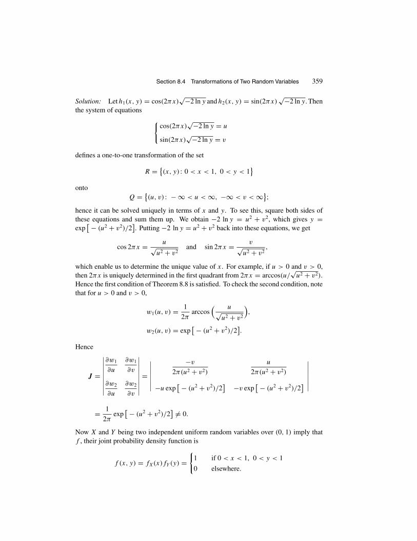
Section 8.4 Transformations of Two Random Variables 359
Solution: Let h1(x, y) = cos(2πx)√−2 ln y and h2(x, y) = sin(2πx)
√−2 ln y.Thenthe system of equations {
cos(2πx)√−2 ln y = u
sin(2πx)√−2 ln y = v
defines a one-to-one transformation of the set
R = {(x, y) : 0 < x < 1, 0 < y < 1}
ontoQ = {(u, v) : − ∞ < u < ∞, −∞ < v < ∞};
hence it can be solved uniquely in terms of x and y. To see this, square both sides ofthese equations and sum them up. We obtain −2 ln y = u2 + v2, which gives y =exp
[− (u2 + v2)/2]. Putting −2 ln y = u2 + v2 back into these equations, we get
cos 2πx = u√u2 + v2
and sin 2πx = v√u2 + v2
,
which enable us to determine the unique value of x. For example, if u > 0 and v > 0,then 2πx is uniquely determined in the first quadrant from 2πx = arccos(u/
√u2 + v2).
Hence the first condition of Theorem 8.8 is satisfied. To check the second condition, notethat for u > 0 and v > 0,
w1(u, v) = 1
2πarccos
( u√u2 + v2
),
w2(u, v) = exp[− (u2 + v2)/2
].
Hence
J =
∣∣∣∣∣∣∣∣∣∂w1
∂u
∂w1
∂v
∂w2
∂u
∂w2
∂v
∣∣∣∣∣∣∣∣∣ =∣∣∣∣∣∣∣
−v
2π(u2 + v2)
u
2π(u2 + v2)
−u exp[− (u2 + v2)/2
] −v exp[− (u2 + v2)/2
]∣∣∣∣∣∣∣
= 1
2πexp
[− (u2 + v2)/2] �= 0.
Now X and Y being two independent uniform random variables over (0, 1) imply thatf , their joint probability density function is
f (x, y) = fX(x)fY (y) ={
1 if 0 < x < 1, 0 < y < 1
0 elsewhere.

360 Chapter 8 Bivariate Distributions
Hence, by Theorem 8.8, g(u, v), the joint probability density function of U and V isgiven by
g(u, v) = 1
2πexp
[− (u2 + v2)/2], −∞ < u < ∞, −∞ < v < ∞.
The probability density function of U is calculated as follows:
gU(u) =∫ ∞
−∞1
2πexp
(− u2 + v2
2
)dv = 1
2πexp
(−u2
2
) ∫ ∞
−∞exp
(−v2
2
)dv,
where∫ ∞
−∞(1/
√2π) exp(−v2/2) dv = 1 implies that
∫ ∞
−∞exp(−v2/2) dv = √
2π.
Therefore,
gU(u) = 1√2π
exp(−u2
2
),
which shows that U is standard normal. Similarly,
gV (v) = 1√2π
exp(−v2
2
).
Since g(u, v) = gU(u)gV (v), U and V are independent standard normal random vari-ables. �
As an application of Theorem 8.8, we now prove the following theorem, an excellentresource for calculation of density and distribution functions of sums of continuousindependent random variables.
Theorem 8.9 (ConvolutionTheorem) Let X and Y be continuous independentrandom variables with probability density functions f1 and f2 and probability distributionfunctions F1 and F2, respectively. Then g and G, the probability density and distributionfunctions of X + Y , respectively, are given by
g(t) =∫ ∞
−∞f1(x)f2(t − x) dx,
G(t) =∫ ∞
−∞f1(x)F2(t − x) dx.
Proof: Let f (x, y) be the joint probability density function of X and Y . Thenf (x, y) = f1(x)f2(y). Let U = X + Y , V = X, h1(x, y) = x + y, and h2(x, y) = x.
Then the system of equations {x + y = u
x = v

Section 8.4 Transformations of Two Random Variables 361
has the unique solution x = v, y = u − v, and
J =
∣∣∣∣∣∣∣∣∣∂x
∂u
∂x
∂v
∂y
∂u
∂y
∂v
∣∣∣∣∣∣∣∣∣ =∣∣∣∣∣∣0 1
1 −1
∣∣∣∣∣∣ = −1 �= 0.
Hence, by Theorem 8.8, the joint probability density function of U and V , ψ(u, v), isgiven by
ψ(u, v) = f1(v)f2(u − v)|J | = f1(v)f2(u − v).
Therefore, the marginal probability density function of U = X + Y is
g(u) =∫ ∞
−∞ψ(u, v) dv =
∫ ∞
−∞f1(v)f2(u − v) dv,
which is the same as
g(t) =∫ ∞
−∞f1(x)f2(t − x) dx.
To find G(t), the distribution function of X + Y , note that
G(t) =∫ t
−∞g(u) du =
∫ t
−∞
( ∫ ∞
−∞f1(x)f2(u − x) dx
)du
=∫ ∞
−∞
( ∫ t
−∞f2(u − x) du
)f1(x) dx
=∫ ∞
−∞F2(t − x)f1(x) dx,
where, letting s = u − x, the last equality follows from∫ t
−∞f2(u − x) du =
∫ t−x
−∞f2(s) ds = F2(t − x). �
Note that by symmetry we can also write
g(t) =∫ ∞
−∞f2(y)f1(t − y) dy,
G(t) =∫ ∞
−∞f2(y)F1(t − y) dy.
Definition Let f1 and f2 be two probability density functions. Then the function g(t),defined by
g(t) =∫ ∞
−∞f1(x)f2(t − x) dx,
is called the convolution of f1 and f2.
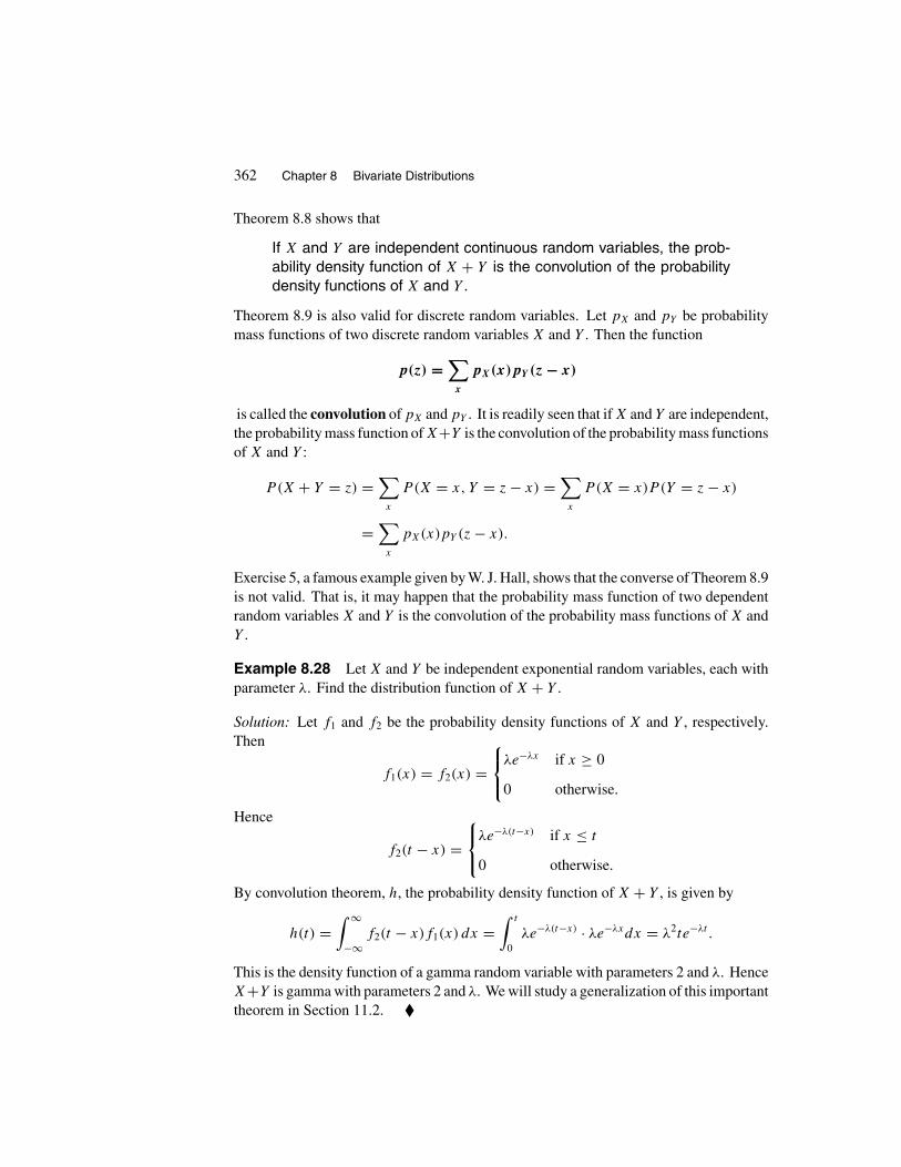
362 Chapter 8 Bivariate Distributions
Theorem 8.8 shows that
If X and Y are independent continuous random variables, the prob-ability density function of X + Y is the convolution of the probabilitydensity functions of X and Y .
Theorem 8.9 is also valid for discrete random variables. Let pX and pY be probabilitymass functions of two discrete random variables X and Y . Then the function
p(z) =∑
x
pX(x)pY (z − x)
is called the convolution of pX and pY . It is readily seen that if X and Y are independent,the probability mass function of X+Y is the convolution of the probability mass functionsof X and Y :
P(X + Y = z) =∑
x
P (X = x, Y = z − x) =∑
x
P (X = x)P (Y = z − x)
=∑
x
pX(x)pY (z − x).
Exercise 5, a famous example given by W. J. Hall, shows that the converse of Theorem 8.9is not valid. That is, it may happen that the probability mass function of two dependentrandom variables X and Y is the convolution of the probability mass functions of X andY .
Example 8.28 Let X and Y be independent exponential random variables, each withparameter λ. Find the distribution function of X + Y .
Solution: Let f1 and f2 be the probability density functions of X and Y , respectively.Then
f1(x) = f2(x) =⎧⎨⎩λe−λx if x ≥ 0
0 otherwise.
Hence
f2(t − x) =⎧⎨⎩λe−λ(t−x) if x ≤ t
0 otherwise.
By convolution theorem, h, the probability density function of X + Y , is given by
h(t) =∫ ∞
−∞f2(t − x)f1(x) dx =
∫ t
0λe−λ(t−x) · λe−λxdx = λ2te−λt .
This is the density function of a gamma random variable with parameters 2 and λ. HenceX+Y is gamma with parameters 2 and λ. We will study a generalization of this importanttheorem in Section 11.2. �

Section 8.4 Transformations of Two Random Variables 363
EXERCISES
A
1. Let X and Y be independent random numbers from the interval (0, 1). Find thejoint probability density function of U = −2 ln X and V = −2 ln Y .
2. Let X and Y be two positive independent continuous random variables with theprobability density functions f1(x) and f2(y), respectively. Find the probabilitydensity function of U = X/Y.
Hint: Let V = X; find the joint probability density function of U and V . Thencalculate the marginal probability density function of U .
3. Let X ∼ N(0, 1) and Y ∼ N(0, 1) be independent random variables. Find thejoint probability density function of R = √
X2 + Y 2 and � = arctan(Y/X).Show that R and � are independent. Note that (R, �) is the polar coordinaterepresentation of (X, Y ).
4. From the interval (0, 1), two random numbers are selected independently. Showthat the probability density function of their sum is given by
g(t) =
⎧⎪⎪⎨⎪⎪⎩t if 0 ≤ t < 1
2 − t if 1 ≤ t < 2
0 otherwise.
5. Let −1/9 < c < 1/9 be a constant. Let p(x, y), the joint probability massfunction of the random variables X and Y , be given by the following table:
y
x −1 0 1
−1 1/9 1/9 − c 1/9 + c
0 1/9 + c 1/9 1/9 − c
1 1/9 − c 1/9 + c 1/9
(a) Show that the probability mass function of X+Y is the convolution functionof the probability mass functions of X and Y for all c.
(b) Show that X and Y are independent if and only if c = 0.

364 Chapter 8 Bivariate Distributions
B
6. Let X and Y be independent random variables with common probability densityfunction
f (x) =
⎧⎪⎨⎪⎩1
x2if x ≥ 1
0 elsewhere.
Calculate the joint probability density function of U = X/Y and V = XY.
7. Let X and Y be independent random variables with common probability densityfunction
f (x) ={
e−x if x > 0
0 elsewhere.
Find the joint probability density function of U = X + Y and V = eX.
8. Prove that if X and Y are independent standard normal random variables, thenX + Y and X − Y are independent random variables. This is a special case of thefollowing important theorem.
Let X and Y be independent random variables with a commondistribution F . The random variables X + Y and X − Y are inde-pendent if and only if F is a normal distribution function.
9. Let X and Y be independent (strictly positive) gamma random variables withparameters (r1, λ) and (r2, λ), respectively. Define U = X + Y and V =X/(X + Y ).
(a) Find the joint probability density function of U and V .
(b) Prove that U and V are independent.
(c) Show that U is gamma and V is beta.
10. Let X and Y be independent (strictly positive) exponential random variables eachwith parameter λ. Are the random variables X + Y and X/Y independent?

Chapter 8 Review Problems 365
REVIEW PROBLEMS
1. The joint probability mass function of X and Y is given by the following table.
x
y 1 2 3
2 0.05 0.25 0.154 0.14 0.10 0.176 0.10 0.02 0.02
(a) Find P(XY ≤ 6).
(b) Find E(X) and E(Y ).
2. A fair die is tossed twice. The sum of the outcomes is denoted by X and the largestvalue by Y . (a) Calculate the joint probability mass function of X and Y ; (b) findthe marginal probability mass functions of X and Y ; (c) find E(X) and E(Y ).
3. Calculate the probability mass function of the number of spades in a random bridgehand that includes exactly four hearts.
4. Suppose that three cards are drawn at random from an ordinary deck of 52 cards.If X and Y are the numbers of diamonds and clubs, respectively, calculate the jointprobability mass function of X and Y .
5. Calculate the probability mass function of the number of spades in a random bridgehand that includes exactly four hearts and three clubs.
6. Let the joint probability density function of X and Y be given by
f (x, y) =
⎧⎪⎨⎪⎩c
xif 0 < y < x, 0 < x < 2
0 elsewhere.
(a) Determine the value of c.
(b) Find the marginal probability density functions of X and Y .

366 Chapter 8 Bivariate Distributions
7. Let X and Y have the joint probability density function below. Determine ifE(XY) = E(X)E(Y ).
f (x, y) =
⎧⎪⎨⎪⎩3
4x2y + 1
4y if 0 < x < 1 and 0 < y < 2
0 elsewhere.
8. Prove that the following cannot be the joint probability distribution function oftwo random variables X and Y .
F(x, y) ={
1 if x + y ≥ 1
0 if x + y < 1.
9. Three concentric circles of radii r1, r2, and r3, r1 > r2 > r3, are the boundariesof the regions that form a circular target. If a person fires a shot at random at thetarget, what is the probability that it lands in the middle region?
10. A fair coin is flipped 20 times. If the total number of heads is 12, what is theexpected number of heads in the first 10 flips?
11. Let the joint probability distribution function of the lifetimes of two brands oflightbulb be given by
F(x, y) ={
(1 − e−x2)(1 − e−y2
) if x > 0, y > 0
0 otherwise.
Find the probability that one lightbulb lasts more than twice as long as the other.
12. For � = {(x, y) : 0 < x + y < 1, 0 < x < 1, 0 < y < 1}, a region in the plane,
let
f (x, y) ={
3(x + y) if (x, y) ∈ �
0 otherwise
be the joint probability density function of the random variables X and Y . Findthe marginal probability density functions of X and Y , and P(X + Y > 1/2).
13. Let X and Y be continuous random variables with the joint probability densityfunction
f (x, y) ={
e−y if y > 0, 0 < x < 1
0 elsewhere.
Find E(Xn | Y = y), n ≥ 1.

Chapter 8 Review Problems 367
14. From an ordinary deck of 52 cards, cards are drawn successively and with replace-ment. Let X and Y denote the number of spades in the first 10 cards and in thesecond 15 cards, respectively. Calculate the joint probability mass function of X
and Y .
15. Let the joint probability density function of X and Y be given by
f (x, y) ={
cx(1 − x) if 0 ≤ x ≤ y ≤ 1
0 otherwise.
(a) Determine the value of c.
(b) Determine if X and Y are independent.
16. A point is selected at random from the bounded region between the curves y =x2 − 1 and y = 1 − x2. Let X be the x-coordinate, and let Y be the y-coordinateof the point selected. Determine if X and Y are independent.
17. Let X and Y be two independent uniformly distributed random variables over theintervals (0, 1) and (0, 2), respectively. Find the probability density function ofX/Y .
18. If F is the probability distribution function of a random variable X, is G(x, y) =F(x) + F(y) a joint probability distribution function?
19. A bar of length � is broken into three pieces at two random spots. What is theprobability that the length of at least one piece is less than �/20?
20. There are prizes in 10% of the boxes of a certain type of cereal. Let X be thenumber of boxes of such cereal that Kim should buy to find a prize. Let Y be thenumber of additional boxes of such cereal that she should purchase to find anotherprize. Calculate the joint probability mass function of X and Y .
21. Let the joint probability density function of random variables X and Y be givenby
f (x, y) ={
1 if |y| < x, 0 < x < 1
0 otherwise.
Show that E(Y | X = x) is a linear function of x while E(X | Y = y) is not alinear function of y.
22. (The Wallet Paradox) Consider the following “paradox” given by MartinGardner in his book Aha! Gotcha (W. H. Freeman and Company, New York,1981).
Each of two persons places his wallet on the table. Whoever has thesmallest amount of money in his wallet, wins all the money in the other

368 Chapter 8 Bivariate Distributions
wallet. Each of the players reason as follows: “I may lose what I havebut I may also win more than I have. So the game is to my advantage.”
As Kent G. Merryfield, Ngo Viet, and Saleem Watson have observed in theirpaper “The Wallet Paradox” in the August–September 1997 issue of the AmericanMathematical Monthly,
Paradoxically, it seems that the game is to the advantage of both play-ers. . . . However, the inference that “the game is to my advantage” isthe source of the apparent paradox, because it does not take into ac-count the probabilities of winning or losing. In other words, if the gameis played many times, how often does a player win? How often doeshe lose? And by how much?
Following the analysis of Kent G. Merryfield, Ngo Viet, and Saleem Watson, let X
and Y be the amount of money in the wallets of players A and B, respectively. LetWA and WB be the amount of money that player A and B will win, respectively.WA(X, Y ) = −WB(X, Y ) and
WA(X, Y ) =
⎧⎪⎨⎪⎩−X if X > Y
Y if X < Y
0 if X = Y .
Suppose that the distribution function of the money in each player’s wallet is thesame; that is, X and Y are independent, identically distributed random variableson some interval [a, b] or [a, ∞), 0 ≤ a < b < ∞. Show that
E(WA) = E(WB) = 0.
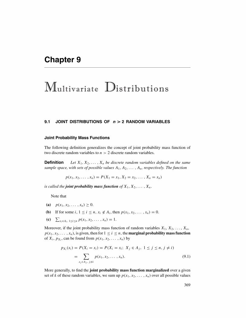
Chapter 9
Multivariate Distributions
9.1 JOINT DISTRIBUTIONS OF n >2 RANDOM VARIABLES
Joint Probability Mass Functions
The following definition generalizes the concept of joint probability mass function oftwo discrete random variables to n > 2 discrete random variables.
Definition Let X1, X2, . . . , Xn be discrete random variables defined on the samesample space, with sets of possible values A1, A2, . . . , An, respectively. The function
p(x1, x2, . . . , xn) = P(X1 = x1, X2 = x2, . . . , Xn = xn)
is called the joint probability mass function of X1, X2, . . . , Xn.
Note that
(a) p(x1, x2, . . . , xn) ≥ 0.
(b) If for some i, 1 ≤ i ≤ n, xi �∈ Ai , then p(x1, x2, . . . , xn) = 0.
(c)∑
xi∈Ai, 1≤i≤n p(x1, x2, . . . , xn) = 1.
Moreover, if the joint probability mass function of random variables X1, X2, . . . , Xn,p(x1, x2, . . . , xn), is given, then for 1 ≤ i ≤ n, the marginal probability mass functionof Xi , pXi
, can be found from p(x1, x2, . . . , xn) by
pXi(xi) = P(Xi = xi) = P(Xi = xi; Xj ∈ Aj, 1 ≤ j ≤ n, j �= i)
=∑
xj ∈Aj , j �=i
p(x1, x2, . . . , xn). (9.1)
More generally, to find the joint probability mass function marginalized over a givenset of k of these random variables, we sum up p(x1, x2, . . . , xn) over all possible values
369

370 Chapter 9 Multivariate Distributions
of the remaining n − k random variables. For example, if p(x, y, z) denotes the jointprobability mass function of random variables X, Y , and Z, then
pX,Y (x, y) =∑
z
p(x, y, z)
is the joint probability mass function marginalized over X and Y , whereas
pY,Z(y, z) =∑
x
p(x, y, z)
is the joint probability mass function marginalized over Y and Z.
Example 9.1 Dr. Shams has 23 hypertensive patients, of whom five do not use anymedicine but try to lower their blood pressures by self-help: dieting, exercise, not smok-ing, relaxation, and so on. Of the remaining 18 patients, 10 use beta blockers and 8 usediuretics. A random sample of seven of all these patients is selected. Let X, Y , and Z bethe number of the patients in the sample trying to lower their blood pressures by self-help,beta blockers, and diuretics, respectively. Find the joint probability mass function andthe marginal probability mass functions of X, Y , and Z.
Solution: Let p(x, y, z) be the joint probability mass function of X, Y , and Z. Thenfor 0 ≤ x ≤ 5, 0 ≤ y ≤ 7, 0 ≤ z ≤ 7, x + y + z = 7,
p(x, y, z) =
(5
x
)(10
y
)(8
z
)(
23
7
) ;
p(x, y, z) = 0, otherwise. The marginal probability mass function of X, pX, is obtainedas follows:
pX(x) =∑
x+y+z=70≤y≤70≤z≤7
p(x, y, z) =7−x∑y=0
(5
x
)(10
y
)(8
7 − x − y
)(
23
7
)
=
(5
x
)(
23
7
) 7−x∑y=0
(10
y
)(8
7 − x − y
).
Now7−x∑y=0
(10
y
)(8
7 − x − y
)is the total number of the ways we can choose 7−x patients
from 18 (in Exercise 41 of Section 2.4, let m = 10, n = 8, and r = 7 − x); hence it is

Section 9.1 Joint Distributions of n > 2 Random Variables 371
equal to
(18
7 − x
). Therefore, as expected,
pX(x) =
(5
x
)(18
7 − x
)(
23
7
) , x = 0, 1, 2, 3, 4, 5.
Similarly,
pY (y) =
(10
y
)(13
7 − y
)(
23
7
) , y = 0, 1, 2, . . . , 7,
pZ(z) =
(8
z
)(15
7 − z
)(
23
7
) , z = 0, 1, 2, . . . , 7. �
Remark 9.1 A joint probability mass function, such as p(x, y, z) of Example 9.1, iscalled multivariate hypergeometric. In general, suppose that a box contains n1 marblesof type 1, n2 marbles of type 2, . . . , and nr marbles of type r . If n marbles are drawn atrandom and Xi (i = 1, 2, . . . , r) is the number of the marbles of type i drawn, the jointprobability mass function of X1, X2, . . . , Xr is called multivariate hypergeometric andis given by
p(x1, x2, . . . , xr) =
(n1
x1
)(n2
x2
)· · ·(
nr
xr
)(
n1 + n2 + · · · + nr
n
) ,
where x1 + x2 + · · · + xr = n. �
We now extend the definition of the joint probability distribution from 2 to n > 2random variables. Let X1, X2, . . . , Xn be n random variables (discrete, continuous, ormixed). Then the joint probability distribution function of X1, X2, . . . , Xn is definedby
F(t1, t2, . . . , tn) = P(X1 ≤ t1, X2 ≤ t2, . . . , Xn ≤ tn) (9.2)
for all −∞ < ti < +∞, i = 1, 2, . . . , n.

372 Chapter 9 Multivariate Distributions
The marginal probability distribution function of Xi , 1 ≤ i ≤ n, can be foundfrom F as follows:
FXi(ti) = P(Xi ≤ ti)
= P(X1 < ∞, . . . , Xi−1 < ∞, Xi ≤ ti , Xi+1 < ∞, . . . , Xn < ∞)
= limtj →∞
1≤j≤n, j �=i
F (t1, t2, . . . , tn). (9.3)
More generally, to find the joint probability distribution function marginalized overa given set of k of these random variables, we calculate the limit of F(t1, t2, . . . , tn) astj → ∞, for every j that belongs to one of the remaining n − k variables. For example,if F(x, y, z, t) denotes the joint probability density function of random variables X, Y ,Z, and T , then the joint probability distribution function marginalized over Y and T isgiven by
FY,T (y, t) = limx,z→∞ F(x, y, z, t).
Just as the joint probability distribution function of two random variables, we have thatF , the joint probability distribution of n random variables, satisfies the following:
(a) F is nondecreasing in each argument.
(b) F is right continuous in each argument.
(c) F(t1, t2, . . . , ti−1, −∞, ti+1, . . . , tn) = 0 for i = 1, 2, . . . , n.
(d) F(∞, ∞, . . . ,∞) = 1.
We now generalize the concept of independence of random variables from two to anynumber of random variables.
Suppose that X1, X2, . . . , Xn are random variables (discrete, continuous, or mixed)on a sample space. We say that they are independent if, for arbitrary subsets A1, A2,. . . , An of real numbers,
P(X1 ∈ A1, X2 ∈ A2, . . . , Xn ∈ An) = P(X1 ∈ A1)P (X2 ∈ A2) · · · P(Xn ∈ An).
Similar to the case of two random variables, X1, X2, . . . , Xn are independent if and onlyif, for any xi ∈ R , i = 1, 2, . . . , n,
P(X1 ≤ x1, X2 ≤ x2, . . . , Xn ≤ xn) = P(X1 ≤ x1)P (X2 ≤ x2) · · ·P(Xn ≤ xn).
That is, X1, X2, . . . , Xn are independent if and only if
F(x1, x2, . . . , xn) = FX1(x1)FX2(x2) · · ·FXn(xn).

Section 9.1 Joint Distributions of n > 2 Random Variables 373
If X1, X2, . . . , Xn are discrete, the definition of independence reduces to the followingcondition:
P(X1 = x1, . . . , Xn = xn) = P(X1 = x1) · · · P(Xn = xn) (9.4)
for any set of points, xi , i = 1, 2, . . . , n.Let X, Y , and Z be independent random variables. Then, by definition, for arbitrary
subsets A1, A2, and A3 of R ,
P(X ∈ A1, Y ∈ A2, Z ∈ A3) = P(X ∈ A1)P (Y ∈ A2)P (Z ∈ A3). (9.5)
Now, if in (9.5) we let A2 = R, then since the event Y ∈ R is certain and has probability 1,we get
P(X ∈ A1, Z ∈ A3) = P(X ∈ A1)P (Z ∈ A3).
This shows that X and Z are independent random variables. In the same way it can beshown that {X, Y }, and {Y, Z} are also independent sets. Similarly, if {X1, X2, . . . , Xn}is a sequence of independent random variables, its subsets are also independent sets ofrandom variables. This observation motivates the following definition for the concept ofindependence of any collection of random variables.
Definition A collection of random variables is called independent if all of its finitesubcollections are independent.
Sometimes independence of a collection of random variables is self-evident andrequires no checking. For example, let E be an experiment with the sample space S.Let X be a random variable defined on S. If the experiment E is repeated n timesindependently and on the ith experiment X is called Xi , the sequence {X1, X2, . . . , Xn}is an independent sequence of random variables.
It is also important to know that the result of Theorem 8.5 is true for any number ofrandom variables:
If {X1, X2, . . . } is a sequence of independent random variables and fori = 1, 2, . . . , gi : R → R is a real-valued function, then the sequence{g1(X1), g2(X2), . . . } is also an independent sequence of random vari-ables.
The following theorem is the generalization of Theorem 8.4. It follows from (9.4).
Theorem 9.1 Let X1, X2, . . . , Xn be jointly discrete random variables with the jointprobability mass function p(x1, x2, . . . , xn). Then X1, X2, . . . , Xn are independent ifand only if p(x1, x2, . . . , xn) is the product of their marginal densities pX1(x1), pX2(x2),. . . , pXn
(xn).
The following is a generalization of Theorem 8.1 from dimension 2 to n.
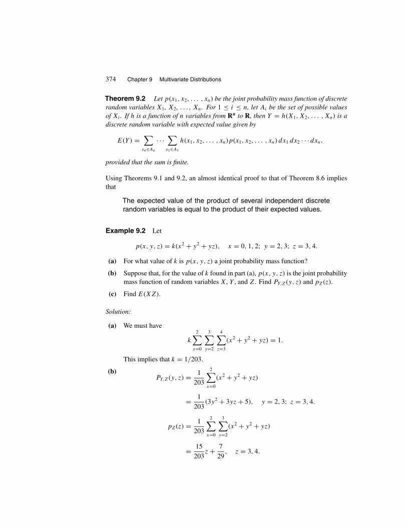
374 Chapter 9 Multivariate Distributions
Theorem 9.2 Let p(x1, x2, . . . , xn) be the joint probability mass function of discreterandom variables X1, X2, . . . , Xn. For 1 ≤ i ≤ n, let Ai be the set of possible valuesof Xi . If h is a function of n variables from Rn to R, then Y = h(X1, X2, . . . , Xn) is adiscrete random variable with expected value given by
E(Y ) =∑
xn∈An
· · ·∑
x1∈A1
h(x1, x2, . . . , xn)p(x1, x2, . . . , xn) dx1 dx2 · · · dxn,
provided that the sum is finite.
Using Theorems 9.1 and 9.2, an almost identical proof to that of Theorem 8.6 impliesthat
The expected value of the product of several independent discreterandom variables is equal to the product of their expected values.
Example 9.2 Let
p(x, y, z) = k(x2 + y2 + yz), x = 0, 1, 2; y = 2, 3; z = 3, 4.
(a) For what value of k is p(x, y, z) a joint probability mass function?
(b) Suppose that, for the value of k found in part (a), p(x, y, z) is the joint probabilitymass function of random variables X, Y , and Z. Find PY,Z(y, z) and pZ(z).
(c) Find E(XZ).
Solution:
(a) We must have
k
2∑x=0
3∑y=2
4∑z=3
(x2 + y2 + yz) = 1.
This implies that k = 1/203.
(b)PY,Z(y, z) = 1
203
2∑x=0
(x2 + y2 + yz)
= 1
203(3y2 + 3yz + 5), y = 2, 3; z = 3, 4.
pZ(z) = 1
203
2∑x=0
3∑y=2
(x2 + y2 + yz)
= 15
203z + 7
29, z = 3, 4.

Section 9.1 Joint Distributions of n > 2 Random Variables 375
An alternate way to find pZ(z) is to use the result obtained in part (b):
pZ(z) =3∑
y=2
PY,Z(y, z) = 1
203
3∑y=2
(3y2 + 3yz + 5)
= 15
203z + 7
29, z = 3, 4.
(c) By Theorem 9.2,
E(XZ) = 1
203
2∑x=0
3∑y=2
4∑z=3
xz(x2 + y2 + yz) = 774
203≈ 3.81. �
� Example 9.3 (Reliability of Systems)† Consider a system consisting of n
components denoted by 1, 2, . . . , n. Suppose that component i, 1 ≤ i ≤ n, is eitherfunctioning or not functioning, with no other performance capabilities. Let Xi be aBernoulli random variable defined by
Xi ={
1 if the component i is functioning,
0 if the component i is not functioning.
The random variable Xi determines the performance mode of the ith component of thesystem. Suppose that
pi = P(Xi = 1) = 1 − P(Xi = 0).
The value pi , the probability that the ith component functions, is called the reliability ofthe ith component. Throughout we assume that the components function independentlyof each other. That is, {X1, X2, . . . , Xn} is an independent set of random variables.
Suppose that the system itself also has only two performance capabilities, functioningand not functioning. Let X be a Bernoulli random variable defined by
X ={
1 if the system is functioning,
0 if the system is not functioning.
The random variable X determines the performance mode of the system. Suppose that
r = P(X = 1) = 1 − P(X = 0).
The value r , the probability that the system functions, is called the reliability of thesystem. We consider only systems for which it is possible to determine r from knowledgeof the performance modes of the components.
†If this example is skipped, then all exercises and examples in this and future chapters marked“(Reliability of Systems)” should be skipped as well.

376 Chapter 9 Multivariate Distributions
As an example, a system is called series system when it functions if and only if alln of its components function. For such a system,
X = min(X1, X2, . . . , Xn) = X1X2 · · · Xn.
This is because, if at least one component does not function, then Xi = 0 for at leastone i, which implies that X = 0, indicating that the system does not function. Similarly,if all n components of the system function, then Xi = 1 for 1 ≤ i ≤ n, implying thatX = 1, which indicates that the system functions. For a series system, the precedingrelationship, expressing X in terms of X1, X2, . . . , Xn, enables us to find the reliabilityof the system:
r = P(X = 1) = P(
min(X1, X2, . . . Xn) = 1)
= P(X1 = 1, X2 = 1, . . . , Xn = 1)
= P(X1 = 1)P (X2 = 1) · · · P(Xn = 1) =n∏
i=1
pi.
n _ n11 2 3
Figure 9.1 Geometric representation for a series system.
Geometrically, a series system is often represented by the diagram of Figure 9.1. Thereason for this representation is that, for a signal fed in at the input to be transmitted tothe output, all components must be functioning. Otherwise, the signal cannot go all theway through.
As another example, consider a parallel system. Such a system functions if and onlyif at least one of its n components functions. For a parallel system,
X = max(X1, X2, . . . , Xn) = 1 − (1 − X1)(1 − X2) · · · (1 − Xn).
This is because, if at least one component functions, then for some i, Xi = 1, implyingthat X = 1, whereas if none of the components functions, then for all i, Xi = 0 implyingthat X = 0. The reliability of a parallel system is given by
r = P(X = 1) = P(
max(X1, X2, . . . , Xn) = 1)
= 1 − P(
max(X1, X2, . . . , Xn) = 0)
= 1 − P(X1 = 0, X2 = 0, . . . , Xn = 0)
= 1 − P(X1 = 0)P (X2 = 0) · · · P(Xn = 0) = 1 −n∏
i=1
(1 − pi).

Section 9.1 Joint Distributions of n > 2 Random Variables 377
n_1
n
1
2
3
Figure 9.2 Geometric representation for a parallel system.
Geometrically, a parallel system is shown by the diagram of Figure 9.2. This repre-sentation shows that, for a signal fed in at the input, at least one component must functionto transmit it to the output.
Calculation of r , the reliability of a given system, is not, in general, as easy as it wasfor series and parallel systems. One useful technique for evaluating r is to write X, ifpossible, in terms of X1, X2, . . . , Xn, and then use the following simple relation:
r = P(X = 1) = 1 · P(X = 1) + 0 · P(X = 0) = E(X).
An example follows.
1 2
3
4 5
6
Figure 9.3 A combination of series and parallel systems.
Consider the system whose structure is as shown in Figure 9.3. This system is acombination of series and parallel systems. The fact that for a series system, X =X1X2 · · · Xn, and for a parallel system,
X = 1 − (1 − X1)(1 − X2) · · · (1 − Xn),
enable us to find out immediately that, for this system,
X = X1X2[1 − (1 − X3)(1 − X4X5)
]X6 = X1X2X6(X3 + X4X5 − X3X4X5).

378 Chapter 9 Multivariate Distributions
Since for 1 ≤ i ≤ 6,
E(Xi) = 1 · P(Xi = 1) + 0 · P(Xi = 0) = pi,
and the Xi’s are independent random variables, r = E(X) yields
r = E(X) = E(X1)E(X2)E(X6)[E(X3) + E(X4)E(X5) − E(X3)E(X4)E(X5)
]= p1p2p6(p3 + p4p5 − p3p4p5). �
Joint Probability Density Functions
We now define the concept of a jointly continuous density function for more than tworandom variables.
Definition Let X1, X2, . . . , Xn be continuous random variables defined on the samesample space. We say that X1, X2, . . . , Xn have a continuous joint distribution if thereexists a nonnegative function of n variables, f (x1, x2, . . . , xn), on R×R×· · ·×R ≡ Rn
such that for any region R in Rn that can be formed from n-dimensional rectangles by acountable number of set operations,
P((X1, X2, . . . , Xn) ∈ R
) =∫
· · ·∫
R
f (x1, x2, . . . , xn) dx1 dx2 · · · dxn. (9.6)
The function f (x1, x2, . . . , xn) is called the joint probability density function of X1, X2,. . . , Xn.
Let R = {(x1, x2, . . . , xn) : xi ∈ Ai, 1 ≤ i ≤ n
}, where Ai, 1 ≤ i ≤ n, is any
subset of real numbers that can be constructed from intervals by a countable number ofset operations. Then (9.6) gives
P(X1 ∈ A1, X2 ∈ A2, . . . , Xn ∈ An)
=∫
An
∫An−1
· · ·∫
A1
f (x1, x2, . . . , xn) dx1 dx2 · · · dxn.
Letting Ai = (−∞, +∞), 1 ≤ i ≤ n, this implies that∫ +∞
−∞· · ·
∫ +∞
−∞f (x1, x2, . . . , xn) dx1 dx2 · · · dxn = 1.
Let fXibe the marginal probability density function of Xi, 1 ≤ i ≤ n. Then
fXi(xi) =
∫ +∞
−∞· · ·∫ +∞
−∞︸ ︷︷ ︸n−1 terms
f (x1, x2, . . . , xn) dx1 · · · dxi−1 dxi+1 · · · dxn. (9.7)

Section 9.1 Joint Distributions of n > 2 Random Variables 379
Therefore, for instance,
fX3(x3) =∫ +∞
−∞· · ·∫ +∞
−∞︸ ︷︷ ︸n−1 terms
f (x1, x2, . . . , xn) dx1 dx2 dx4 · · · dxn.
More generally, to find the joint probability density function marginalized over agiven set of k of these random variables, we integrate f (x1, x2, . . . , xn) over all possiblevalues of the remaining n − k random variables. For example, if f (x, y, z, t) denotesthe joint probability density function of random variables X, Y , Z, and T , then
fY,T (y, t) =∫ +∞
−∞
∫ +∞
−∞f (x, y, z, t) dx dz
is the joint probability density function marginalized over Y and T , whereas
fX,Z,T (x, z, t) =∫ +∞
−∞f (x, y, z, t) dy
is the joint probability density function marginalized over X, Z, and T .The following theorem is the generalization of Theorem 8.7 and the continuous analog
of Theorem 9.1. Its proof is similar to the proof of Theorem 8.7.
Theorem 9.3 Let X1, X2, . . . , Xn be jointly continuous random variables with the jointprobability density function f (x1, x2, . . . , xn). Then X1, X2, . . . , Xn are independent ifand only if f (x1, x2, . . . , xn) is the product of their marginal densities fX1(x1), fX2(x2),. . . , fXn
(xn).
Let F be the joint probability distribution function of jointly continuous randomvariables X1, X2, . . . , Xn, with the joint probability density function f (x1, x2, . . . , xn),then
F(t1, t2, . . . , tn) =∫ tn
−∞
∫ tn−1
−∞· · ·∫ t1
−∞f (x1, x2, . . . , xn) dx1 · · · dxn, (9.8)
and
f (x1, x2, . . . , xn) = ∂nF (x1, x2, . . . , xn)
∂x1∂x2 · · · ∂xn
. (9.9)
The following is the continuous analog of Theorem 9.2. It is also a generalization ofTheorem 8.2 from dimension 2 to n.
Theorem 9.4 Let f (x1, x2, . . . , xn) be the joint probability density function of randomvariables X1, X2, . . . , Xn. If h is a function of n variables from Rn to R, then Y =h(X1, X2, . . . , Xn) is a random variable with expected value given by
E(Y ) =∫ ∞
−∞· · ·∫ ∞
−∞h(x1, x2, . . . , xn)f (x1, x2, . . . , xn) dx1 dx2 · · · dxn,
provided that the integral is absolutely convergent.

380 Chapter 9 Multivariate Distributions
Using Theorems 9.3 and 9.4, an almost identical proof to that of Theorem 8.6 impliesthat
The expected value of the product of several independent randomvariables is equal to the product of their expected values.
Example 9.4 A system has n components, the lifetime of each being an exponentialrandom variable with parameter λ. Suppose that the lifetimes of the components areindependent random variables, and the system fails as soon as any of its componentsfails. Find the probability density function of the time until the system fails.
Solution: LetX1, X2, . . . , Xn be the lifetimes of the components. ThenX1, X2, . . . , Xn
are independent random variables and for i = 1, 2, . . . , n,
P(Xi ≤ t) = 1 − e−λt .
Letting X be the time until the system fails, we have X = min(X1, X2, . . . , Xn). There-fore,
P(X > t) = P(
min(X1, X2, . . . , Xn) > t) = P(X1 > t, X2 > t, . . . , Xn > t)
= P(X1 > t)P (X2 > t) · · · P(Xn > t) = (e−λt )(e−λt ) · · · (e−λt ) = e−nλt .
Let f be the probability density function of X; then
f (t) = d
dtP (X ≤ t) = d
dt(1 − e−nλt ) = nλe−nλt . �
Example 9.5
(a) Prove that the following is a joint probability density function.
f (x, y, z, t) =
⎧⎪⎪⎨⎪⎪⎩1
xyzif 0 < t ≤ z ≤ y ≤ x ≤ 1
0 elsewhere.
(b) Suppose that f is the joint probability density function of random variables X, Y ,Z, and T . Find fY,Z,T (y, z, t), fX,T (x, t), and fZ(z).

Section 9.1 Joint Distributions of n > 2 Random Variables 381
Solution:
(a) Since f (x, y, z, t) ≥ 0 and∫ 1
0
∫ x
0
∫ y
0
∫ z
0
1
xyzdt dz dy dx =
∫ 1
0
∫ x
0
∫ y
0
1
xydz dy dx
=∫ 1
0
∫ x
0
1
xdy dx =
∫ 1
0dx = 1,
f is a joint probability density function.
(b) For 0 < t ≤ z ≤ y ≤ 1,
fY,Z,T (y, z, t) =∫ 1
y
1
xyzdx = 1
yzln x
∣∣∣1y
= − ln y
yz.
Therefore,
fY,Z,T (y, z, t) =
⎧⎪⎪⎨⎪⎪⎩− ln y
yzif 0 < t ≤ z ≤ y ≤ 1
0 elsewhere.
To find fX,T (x, t), we have that for 0 < t ≤ x ≤ 1,
fX,T (x, t) =∫ x
t
∫ y
t
1
xyzdz dy =
∫ x
t
[ ln z
xy
]ytdy
=∫ x
t
( ln y
xy− ln t
xy
)dy =
[ 1
2x(ln y)2 − ln t
xln y]x
t
= 1
2x(ln x)2 − 1
x(ln t)(ln x) + 1
2x(ln t)2 = 1
2x(ln x − ln t)2
= 1
2xln2 x
t.
Therefore,
fX,T (x, t) =
⎧⎪⎪⎨⎪⎪⎩1
2xln2 x
tif 0 < t ≤ x ≤ 1
0 otherwise.
To find fZ(z), we have that for 0 < z ≤ 1,

382 Chapter 9 Multivariate Distributions
fZ(z) =∫ 1
z
∫ x
z
∫ z
0
1
xyzdt dy dx =
∫ 1
z
∫ x
z
1
xydy dx
=∫ 1
z
[1
xln y]x
zdx =
∫ 1
z
(1
xln x − 1
xln z)dx
=[1
2(ln x)2 − (ln x)(ln z)
]1
z= 1
2(ln z)2.
Thus
fZ(z) =
⎧⎪⎪⎨⎪⎪⎩1
2(ln z)2 if 0 < z ≤ 1
0 otherwise. �
Random Sample
Definition: We say that n random variables X1, X2, . . . , Xn form a random sampleof size n, from a (continuous or discrete) distribution function F , if they are independentand, for 1 ≤ i ≤ n, the distribution function of Xi is F . Therefore, elements of a randomsample are independent and identically distributed.
To explain this definition, suppose that the lifetime distribution of the light bulbsmanufactured by a company is exponential with parameterλ. To estimate 1/λ, the averagelifetime of a light bulb, for some positive integer n, we choose n light bulbs at randomand independently from those manufactured by the company. For 1 ≤ i ≤ n, let Xi bethe lifetime of the ith light bulb selected. Then {X1, X2, . . . , Xn} is a random sample ofsize n from the exponential distribution with parameter λ. That is, for 1 ≤ i ≤ n, Xi’sare independent, and Xi is exponential with parameter λ. Clearly, an estimation of 1/λ
is the mean of the random sample X1, X2, . . . , Xn denoted by X:
X = X1 + X2 + · · · + Xn
n.
Thus all we need to do is to measure the lifetime of each of the n light bulbs of the randomsample and find the average of the observed values. In Sections 11.3 and 11.5, we willdiscuss methods to calculate n, the sample size, so that the error of estimation does notexceed a predetermined quantity.

Section 9.1 Joint Distributions of n > 2 Random Variables 383
EXERCISES
A1. From an ordinary deck of 52 cards, 13 cards are selected at random. Calculate
the joint probability mass function of the numbers of hearts, diamonds, clubs, andspades selected.
2. A jury of 12 people is randomly selected from a group of eight Afro-American,seven Hispanic, three Native American, and 20 white potential jurors. Let A,H , N , and W be the number of Afro-American, Hispanic, Native American, andwhite jurors selected, respectively. Calculate the joint probability mass functionof A, H, N, W and the marginal probability mass function of A.
3. Let p(x, y, z) = (xyz)/162, x = 4, 5, y = 1, 2, 3, and z = 1, 2, be the jointprobability mass function of the random variables X, Y , Z.
(a) Calculate the joint marginal probability mass functions of X, Y ; Y , Z; andX, Z.
(b) Find E(YZ).
4. Let the joint probability density function of X, Y , and Z be given by
f (x, y, z) ={
6e−x−y−z if 0 < x < y < z < ∞0 elsewhere.
(a) Find the marginal joint probability density function of X, Y ; X, Z; andY , Z.
(b) Find E(X).
5. From the set of families with two children a family is selected at random. LetX1 = 1 if the first child of the family is a girl; X2 = 1 if the second child of thefamily is a girl; and X3 = 1 if the family has exactly one boy. For i = 1, 2, 3,
let Xi = 0 in other cases. Determine if X1, X2, and X3 are independent. Assumethat in a family the probability that a child is a girl is independent of the gender ofthe other children and is 1/2.
6. Let X, Y , and Z be jointly continuous with the following joint probability densityfunction:
f (x, y, z) ={
x2e−x(1+y+z) if x, y, z > 0
0 otherwise.
Are X, Y , and Z independent? Are they pairwise independent?

384 Chapter 9 Multivariate Distributions
7. Let the joint probability distribution function of X, Y , and Z be given by
F(x, y, z) = (1 − e−λ1x)(1 − e−λ2y)(1 − e−λ3z), x, y, z > 0,
where λ1, λ2, λ3 > 0.
(a) Are X, Y , and Z independent?
(b) Find the joint probability density function of X, Y , and Z.
(c) Find P(X < Y < Z).
8. (a) Show that the following is a joint probability density function.
f (x, y, z) =
⎧⎪⎪⎨⎪⎪⎩− ln x
xyif 0 < z ≤ y ≤ x ≤ 1
0 otherwise.
(b) Suppose that f is the joint probability density function of X, Y , and Z. FindfX,Y (x, y) and fY (y).
9. Inside a circle of radius R, n points are selected at random and independently.Find the probability that the distance of the nearest point to the center is at least r .
10. A point is selected at random from the cube
� = {(x, y, z) : − a ≤ x ≤ a, −a ≤ y ≤ a, −a ≤ z ≤ a}.
What is the probability that it is inside the sphere inscribed in the cube?
11. Is the following a joint probability density function?
f (x1, x2, . . . , xn) ={
e−xn if 0 < x1 < x2 < · · · < xn
0 otherwise.
12. Suppose that the lifetimes of radio transistors are independent exponential randomvariables with mean five years. Arnold buys a radio and decides to replace itstransistor upon failure two times: once when the original transistor dies and oncewhen the replacement dies. He stops using the radio when the second replacementof the transistor goes out of order. Assuming that Arnold repairs the radio if it failsfor any other reason, find the probability that he uses the radio at least 15 years.
13. Let X1, X2, . . . , Xn be independent exponential random variables with means1/λ1, 1/λ2, . . . , 1/λn, respectively. Find the probability distribution function ofX = min(X1, X2, . . . , Xn).
14. (Reliability of Systems) Suppose that a system functions if and only if atleast k (1 ≤ k ≤ n) of its components function. Furthermore, suppose that pi = p
for 1 ≤ i ≤ n. Find the reliability of this system. (Such a system is said to be ak-out-of-n system.)
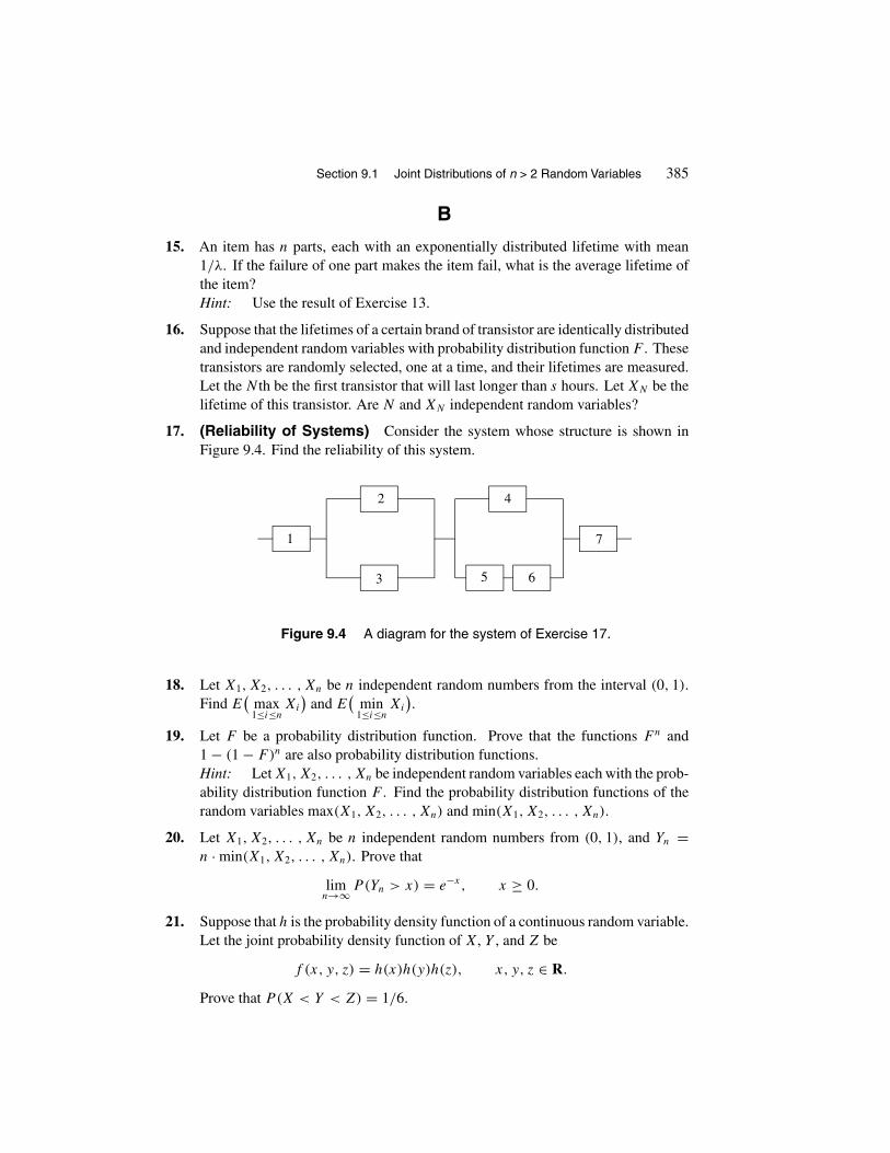
Section 9.1 Joint Distributions of n > 2 Random Variables 385
B
15. An item has n parts, each with an exponentially distributed lifetime with mean1/λ. If the failure of one part makes the item fail, what is the average lifetime ofthe item?Hint: Use the result of Exercise 13.
16. Suppose that the lifetimes of a certain brand of transistor are identically distributedand independent random variables with probability distribution function F . Thesetransistors are randomly selected, one at a time, and their lifetimes are measured.Let the N th be the first transistor that will last longer than s hours. Let XN be thelifetime of this transistor. Are N and XN independent random variables?
17. (Reliability of Systems) Consider the system whose structure is shown inFigure 9.4. Find the reliability of this system.
1
2
3
4
5 6
7
Figure 9.4 A diagram for the system of Exercise 17.
18. Let X1, X2, . . . , Xn be n independent random numbers from the interval (0, 1).Find E
(max1≤i≤n
Xi
)and E
(min
1≤i≤nXi
).
19. Let F be a probability distribution function. Prove that the functions Fn and1 − (1 − F)n are also probability distribution functions.Hint: Let X1, X2, . . . , Xn be independent random variables each with the prob-ability distribution function F . Find the probability distribution functions of therandom variables max(X1, X2, . . . , Xn) and min(X1, X2, . . . , Xn).
20. Let X1, X2, . . . , Xn be n independent random numbers from (0, 1), and Yn =n · min(X1, X2, . . . , Xn). Prove that
limn→∞ P(Yn > x) = e−x, x ≥ 0.
21. Suppose that h is the probability density function of a continuous random variable.Let the joint probability density function of X, Y , and Z be
f (x, y, z) = h(x)h(y)h(z), x, y, z ∈ R.
Prove that P(X < Y < Z) = 1/6.

386 Chapter 9 Multivariate Distributions
22. (Reliability of Systems) To transfer water from point A to point B, a water-supply system with five water pumps located at the points 1, 2, 3, 4, and 5 isdesigned as in Figure 9.5. Suppose that whenever the system is turned on for waterto flow from A to B, pump i, i ≤ 5, functions with probability pi independent ofthe other pumps. What is the probability that, at such a time, water reaches B?
A
B
12
3
5 4
Figure 9.5 The water-supply system of Exercise 22.
23. A point is selected at random from the pyramid
V = {(x, y, z) : x, y, z ≥ 0, x + y + z ≤ 1}.
Letting (X, Y, Z) be its coordinates, determine if X, Y , and Z are independent.Hint: Recall that the volume of a pyramid is Bh/3, where h is the height andB is the area of the base.
24. (Roots of Quadratic Equations) Three numbers A, B, and C are selectedat random and independently from the interval (0, 1). Determine the probabilitythat the quadratic equation Ax2 + Bx + C = 0 has real roots. In other words,what fraction of “all possible quadratic equations” with coefficients in (0, 1) havereal roots?
25. (Roots of Cubic Equations) Solve the following exercise posed byS. A. Patil and D. S. Hawkins, Tennessee Technological University, Cookeville,Tennessee, in The College Mathematics Journal, September 1992.

Section 9.2 Order Statistics 387
Let A, B, and C be independent random variables uniformly distributedon [0, 1]. What is the probability that all of the roots of the cubic equationx3 + Ax2 + Bx + C = 0 are real?
9.2 ORDER STATISTICS
Definition Let{X1, X2, . . . , Xn
}be an independent set of identically distributed
continuous random variables with the common density and distribution functions f andF , respectively. Let X(1) be the smallest value in
{X1, X2, . . . , Xn
}, X(2) be the second
smallest value, X(3) be the third smallest, and, in general, X(k) (1 ≤ k ≤ n) be the kthsmallest value in
{X1, X2, . . . , Xn
}. Then X(k) is called the kth order statistic, and the
set{X(1), X(2), . . . , X(n)
}is said to consist of the order statistics of
{X1, X2, . . . , Xn
}.
By this definition, for example, if at a sample point ω of the sample space, X1(ω) = 8,X2(ω) = 2, X3(ω) = 5, and X4(ω) = 6, then the order statistics of {X1, X2, X3, X4} is{X(1), X(2), X(3), X(4)}, where X(1)(ω) = 2, X(2)(ω) = 5, X(3)(ω) = 6, and X(4)(ω) = 8.Continuity of Xi’s implies that P(X(i) = X(j)) = 0. Hence
P(X(1) < X(2) < X(3) < · · · < X(n)) = 1.
Unlike Xi’s, the random variables X(i)’s are neither independent nor identically dis-tributed.
There are many useful and practical applications of order statistics in differentbranches of pure and applied probability, as well as in estimation theory. To showhow it arises, we present three examples.
Example 9.6 Suppose that customers arrive at a warehouse from n different locations.Let Xi , 1 ≤ i ≤ n, be the time until the arrival of the next customer from location i; thenX(1) is the arrival time of the next customer to the warehouse. �
Example 9.7 Suppose that a machine consists of n components with the lifetimesX1, X2, . . . , Xn, respectively, where Xi’s are independent and identically distributed.Suppose that the machine remains operative unless k or more of its components fail.Then X(k), the kth order statistic of {X1, X2, . . . , Xn}, is the time when the machinefails. Also, X(1) is the failure time of the first component. �
Example 9.8 Let X1, X2, . . . , Xn be a random sample of size n from a populationwith continuous distribution F . Then the following important statistical concepts areexpressed in terms of order statistics:
(i) The sample range is X(n) − X(1).

388 Chapter 9 Multivariate Distributions
(ii) The sample midrange is [X(n) + X(1)]/
2.
(iii) The sample median is
m =
⎧⎪⎨⎪⎩X(i+1) if n = 2i + 1
X(i) + X(i+1)
2if n = 2i. �
We will now determine the probability distribution and the probability density functionsof X(k), the kth order statistic.
Theorem 9.5 Let {X(1), X(2), . . . , X(n)} be the order statistics of the independent andidentically distributed continuous random variables X1, X2, . . . , Xn with the commonprobability distribution and probability density functions F and f , respectively. Then Fk
and fk, the probability distribution and probability density functions of X(k), respectively,are given by
Fk(x) =n∑
i=k
(n
i
)[F(x)
]i[1 − F(x)
]n−i, −∞ < x < ∞, (9.10)
and
fk(x) = n!(k − 1)! (n − k)!f (x)
[F(x)
]k−1[1 − F(x)
]n−k, −∞ < x < ∞. (9.11)
Proof: Let −∞ < x < ∞. To calculate P(X(k) ≤ x), note that X(k) ≤ x if and onlyif at least k of the random variables X1, X2, . . . , Xn are in (−∞, x]. Thus
Fk(x) = P(X(k) ≤ x)
=n∑
i=k
P(i of the random variables X1, X2, . . . , Xn are in (−∞, x] )
=n∑
i=k
(n
i
)[F(x)
]i[1 − F(x)
]n−i,
where the last equality follows because from the random variables X1, X2, . . . , Xn thenumber of those that lie in (−∞, x] has binomial distribution with parameters (n, p),p = F(x).
We will now obtain fk by differentiating Fk:

Section 9.2 Order Statistics 389
fk(x) =n∑
i=k
(n
i
)if (x)
[F(x)
]i−1[1 − F(x)
]n−i
−n∑
i=k
(n
i
)[F(x)
]i(n − i)f (x)
[1 − F(x)
]n−i−1
=n∑
i=k
n!(i − 1)! (n − i)!f (x)
[F(x)
]i−1[1 − F(x)
]n−i
−n∑
i=k
n!i! (n − i − 1)!f (x)
[F(x)
]i[1 − F(x)
]n−i−1
=n∑
i=k
n!(i − 1)! (n − i)!f (x)
[F(x)
]i−1[1 − F(x)
]n−i
−n∑
i=k+1
n!(i − 1)! (n − i)!f (x)
[F(x)
]i−1[1 − F(x)
]n−i.
After cancellations, this gives (9.11). �
Remark 9.2 Note that by (9.10) and (9.11), respectively, F1 and f1, the probabilitydistribution and the probability density functions of X(1) = min(X1, X2, . . . , Xn), arefound to be
F1(x) =n∑
i=1
(n
i
)[F(x)
]i[1 − F(x)
]n−i
=n∑
i=0
(n
i
)[F(x)
]i[1 − F(x)
]n−i − [1 − F(x)]n
= [F(x) + [1 − F(x)]]n − [1 − F(x)
]n= 1 − [1 − F(x)
]n, −∞ < x < ∞.
andf1(x) = nf (x)
[1 − F(x)
]n−1, −∞ < x < ∞.
Also, Fn and fn, the probability distribution and probability density functions of X =max(X1, X2, . . . , Xn), respectively, are found to be
Fn(x) = [F(x)]n
, −∞ < x < ∞,
and
fn(x) = nf (x)[F(x)
]n−1, −∞ < x < ∞.

390 Chapter 9 Multivariate Distributions
These quantities can also be calculated directly (see, for example, Example 9.4 orExercise 13, Section 9.1). �
Example 9.9 Let X1, X2, . . . , X2n+1 be 2n + 1 random numbers from (0, 1). Thenf and F , the respective probability density and distribution functions of Xi’s, are givenby
f (x) ={
1 if 0 < x < 1
0 elsewhere,
F(x) =
⎧⎪⎨⎪⎩0 if x < 0
x if 0 ≤ x < 1
1 if x ≥ 1.
Using (9.11), the probability density function of X(n+1), the median of these numbers,is found to be
fn+1(x) = (2n + 1)!n! n! xn(1 − x)n, 0 < x < 1;
0, elsewhere. Since for the beta function, B(n + 1, n + 1) = (n! n!)/(2n + 1)!, we have
fn+1(x) = 1
B(n + 1, n + 1)xn(1 − x)n, 0 < x < 1;
0, elsewhere. Hence X(n+1) is beta with parameters (n + 1, n + 1). In fact, it is straight-forward to see that in this example, for 1 ≤ k ≤ 2n + 1, X(k) is beta with parameters k
and 2n − k + 2. �
The following theorem gives the joint probability density function of X(i) and X(j).Its proof is similar to that of Theorem 9.5.
Theorem 9.6 Let {X(1), X(2), . . . , X(n)} be the order statistics of the independent andidentically distributed continuous random variables X1, X2, . . . , Xn with the commonprobability density and probability distribution functions f and F , respectively. Thenfor x < y, fij (x, y), the joint probability density function of X(i) and X(j) (i < j ), isgiven by
fij (x, y) =n!
(i − 1)! (j − i − 1)! (n − j)!f (x)f (y)[F(x)
]i−1[F(y) − F(x)
]j−i−1[1 − F(y)]n−j
.
It is clear that for x ≥ y, fij (x, y) = 0.
Another important quantity that is used often is the joint probability density functionof X(1), X(2), . . . , X(n). The following theorem, whose proof we skip, expresses thegeneral form of this function.
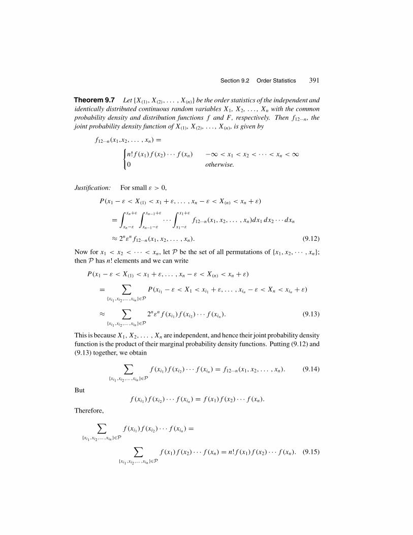
Section 9.2 Order Statistics 391
Theorem 9.7 Let {X(1), X(2), . . . , X(n)} be the order statistics of the independent andidentically distributed continuous random variables X1, X2, . . . , Xn with the commonprobability density and distribution functions f and F , respectively. Then f12···n, thejoint probability density function of X(1), X(2), . . . , X(n), is given by
f12···n(x1,x2, . . . , xn) ={n!f (x1)f (x2) · · · f (xn) −∞ < x1 < x2 < · · · < xn < ∞0 otherwise.
Justification: For small ε > 0,
P(x1 − ε < X(1) < x1 + ε, . . . , xn − ε < X(n) < xn + ε)
=∫ xn+ε
xn−ε
∫ xn−1+ε
xn−1−ε
· · ·∫ x1+ε
x1−ε
f12···n(x1, x2, . . . , xn)dx1 dx2 · · · dxn
≈ 2nεnf12···n(x1, x2, . . . , xn). (9.12)
Now for x1 < x2 < · · · < xn, let P be the set of all permutations of {x1, x2, · · · , xn};then P has n! elements and we can write
P(x1 − ε < X(1) < x1 + ε, . . . , xn − ε < X(n) < xn + ε)
=∑
{xi1 ,xi2 ,... ,xin }∈PP(xi1 − ε < X1 < xi1 + ε, . . . , xin − ε < Xn < xin + ε)
≈∑
{xi1 ,xi2 ,... ,xin }∈P2nεnf (xi1)f (xi2) · · · f (xin). (9.13)
This is because X1, X2, . . . , Xn are independent, and hence their joint probability densityfunction is the product of their marginal probability density functions. Putting (9.12) and(9.13) together, we obtain∑
{xi1 ,xi2 ,... ,xin }∈Pf (xi1)f (xi2) · · · f (xin) = f12···n(x1, x2, . . . , xn). (9.14)
Butf (xi1)f (xi2) · · · f (xin) = f (x1)f (x2) · · · f (xn).
Therefore,∑{xi1 ,xi2 ,... ,xin }∈P
f (xi1)f (xi2) · · · f (xin) =
∑{xi1 ,xi2 ,... ,xin }∈P
f (x1)f (x2) · · · f (xn) = n!f (x1)f (x2) · · · f (xn). (9.15)

392 Chapter 9 Multivariate Distributions
Relations (9.14) and (9.15) imply that
f12···n(x1, x2, . . . , xn) = n!f (x1)f (x2) · · · f (xn). �
Example 9.10 The distance between two towns, A and B, is 30 miles. If three gasstations are constructed independently at randomly selected locations between A and B,what is the probability that the distance between any two gas stations is at least 10 miles?
Solution: Let X1, X2, and X3 be the locations at which the gas stations are constructed.The probability density function of X1, X2, and X3 is given by
f (x) =
⎧⎪⎨⎪⎩1
30if 0 < x < 30
0 elsewhere.
Therefore, by Theorem 9.7, f123, the joint probability density function of the orderstatistics of X1, X2, and X3, is as follows.
f123(x1, x2, x3) = 3!( 1
30
)3, 0 < x1 < x2 < x3 < 30.
Using this, we have that the desired probability is given by the following triple integral.
P(X(1) + 10 < X(2) and X(2) + 10 < X(3))
=∫ 10
0
∫ 20
x1+10
∫ 30
x2+10f123(x1, x2, x3) dx3 dx2 dx1 = 1
27�
EXERCISES
A
1. Let X1, X2, X3, and X4 be four independently selected random numbers from(0, 1). Find P(1/4 < X(3) < 1/2).
2. Two random points are selected from (0, 1) independently. Find the probabilitythat one of them is at least three times the other.
3. Let X1, X2, X3, and X4 be independent exponential random variables, each withparameter λ. Find P(X(4) ≥ 3λ).

Section 9.2 Order Statistics 393
4. Let X1, X2, X3, . . . , Xn be a sequence of nonnegative, identically distributed, andindependent random variables. Let F be the probability distribution function ofXi , 1 ≤ i ≤ n. Prove that
E[X(n)] =∫ ∞
0
(1 − [F(x)
]n)dx.
Hint: Use Theorem 6.2.
5. Let X1, X2, X3, . . . , Xm be a sequence of nonnegative, independent binomialrandom variables, each with parameters (n, p). Find the probability mass functionof X(i), 1 ≤ i ≤ m.
6. Prove that G, the probability distribution function of [X(1)+X(n)]/
2, the midrangeof a random sample of size n from a population with continuous probability dis-tribution function F and probability density function f , is given by
G(t) = n
∫ t
−∞
[F(2t − x) − F(x)
]n−1f (x) dx.
Hint: Use Theorem 9.6 to find f1n; then integrate over the region x + y ≤ 2t
and x ≤ y.
B
7. Let X1 and X2 be two independent exponential random variables each with pa-rameter λ. Show that X(1) and X(2) − X(1) are independent.
8. Let X1 and X2 be two independent N(0, σ 2) random variables. Find E[X(1)].Hint: Let f12(x, y) be the joint probability density function of X(1) and X(2).The desired quantity is
∫∫xf12(x, y) dx dy, where the integration is taken over an
appropriate region.
9. Let X1, X2, . . . , Xn be a random sample of size n from a population with contin-uous probability distribution function F and probability density function f .
(a) Calculate the probability density function of the sample range, R =X(n) − X(1).
(b) Use (a) to find the probability density function of the sample range of n
random numbers from (0, 1).
10. Let X1, X2, . . . , Xn be n independently randomly selected points from the interval(0, θ), θ > 0. Prove that
E(R) = n − 1
n + 1θ,
where R = X(n) − X(1) is the range of these points.Hint: Use part (a) of Exercise 9. Also compare this with Exercise 18, Section 9.1.

394 Chapter 9 Multivariate Distributions
9.3 MULTINOMIAL DISTRIBUTIONS
Multinomial distribution is a generalization of a binomial. Suppose that, wheneveran experiment is performed, one of the disjoint outcomes A1, A2, . . . , Ar will occur.Let P(Ai) = pi , 1 ≤ i ≤ r. Then p1 + p2 + · · · + pr = 1. If, in n independentperformances of this experiment, Xi , i = 1, 2, 3, . . . , r , denotes the number of timesthat Ai occurs, then p(x1, . . . , xr), the joint probability mass function of X1, X2, . . . , Xr ,is called multinomial joint probability mass function, and its distribution is said to bea multinomial distribution. For any set of nonnegative integers {x1, x2, . . . , xr} withx1 + x2 + · · · + xr = n,
p(x1, x2, . . . , xr) = P(X1 = x1, X2 = x2, . . . , Xr = xr)
= n!x1! x2! · · · xr ! p
x11 p
x22 · · ·pxr
r . (9.16)
To prove this relation, recall that, by Theorem 2.4, the number of distinguishable permu-tations of n objects of r different types where x1 are alike, x2 are alike, · · · , xr are alike(n = x1 + · · · + xr) is n!/(x1! x2! · · · xr !). Hence there are n!/(x1! x2! · · · xr !) sequencesof A1, A2, . . . , Ar in which the number of Ai’s is xi , i = 1, 2, . . . , r . Relation (9.16)follows since the probability of the occurrence of any of these sequences is p
x11 p
x22 · · · pxr
r .
By Theorem 2.6, p(x1, x2, . . . , xr)’s given by (9.16) are the terms in the expansion of(p1 + p2 + · · · + pr)
n. For this reason, the multinomial distribution sometimes is calledthe polynomial distribution. The following relation guarantees that p(x1, x2, . . . , xr)
is a joint probability mass function:∑x1+x2+···+xr=n
p(x1, x2, . . . , xr)
=∑
x1+x2+···+xr=n
n!x1! x2! · · · xr ! p
x11 p
x22 · · · pxr
r = (p1 + p2 + · · · + pr)n = 1.
Note that, for r = 2, the multinomial distribution coincides with the binomial distribution.This is because, for r = 2, the experiment has only two possible outcomes, A1 and A2.Hence it is a Bernoulli trial.
Example 9.11 In a certain town, at 8:00 P.M., 30% of the TV viewing audience watchthe news, 25% watch a certain comedy, and the rest watch other programs. What is theprobability that, in a statistical survey of seven randomly selected viewers, exactly threewatch the news and at least two watch the comedy?
Solution: In the random sample, let X1, X2, and X3 be the numbers of viewers whowatch the news, the comedy, and other programs, respectively. Then the joint distributionof X1, X2, and X3 is multinomial with p1 = 0.30, p2 = 0.25, and p3 = 0.45. Therefore,for i + j + k = 7,
P (X1 = i, X2 = j, X3 = k) = 7!i! j ! k!(0.30)i(0.25)j (0.45)k.

Section 9.3 Multinomial Distributions 395
The desired probability equals
P(X1 = 3, X2 ≥ 2) = P(X1 = 3, X2 = 2, X3 = 2)
+ P(X1 = 3, X2 = 3, X3 = 1) + P(X1 = 3, X2 = 4, X3 = 0)
= 7!3! 2! 2!(0.30)3(0.25)2(0.45)2 + 7!
3! 3! 1!(0.30)3(0.25)3(0.45)1
+ 7!3! 4! 0!(0.30)3(0.25)4(0.45)0 ≈ 0.103. �
Example 9.12 A warehouse contains 500 TV sets, of which 25 are defective, 300 arein working condition but used, and the rest are brand new. What is the probability that,in a random sample of five TV sets from this warehouse, there are exactly one defectiveand exactly two brand new sets?
Solution: In the random sample, let X1 be the number of defective TV sets, X2 be thenumber of TV sets in working condition but used, and X3 be the number of brand newsets. The desired probability is given by
P(X1 = 1, X2 = 2, X3 = 2) =
(25
1
)(300
2
)(175
2
)(
500
5
) ≈ 0.067.
Note that, since the number of sets is large and the sample size is small, the joint dis-tribution of X1, X2, and X3 is approximately multinomial with p1 = 25/500 = 1/20,p2 = 300/500 = 3/5, and p3 = 175/500 = 7/20. Hence
P(X1 = 1, X2 = 2, X3 = 2) ≈ 5!1! 2! 2!
( 1
20
)1(3
5
)2( 7
20
)2 ≈ 0.066. �
Example 9.13 (Marginals of Multinomials) Let X1, X2, . . . , Xr (r ≥ 4) havethe joint multinomial probability mass function p(x1, x2, . . . , xr) with parameters n andp1, p2, . . . , pr . Find the marginal probability mass functions pX1 and pX1,X2,X3 .
Solution: From the definition of marginal probability mass functions,
pX1(x1) =∑
x2+x3+···+xr=n−x1
n!x1! x2! · · · xr ! p
x11 p
x22 · · · pxr
r
= n!x1! (n − x1)! p
x11
∑x2+x3+···+xr=n−x1
(n − x1)!x2! x3! · · · xr ! p
x22 p
x33 · · ·pxr
r
= n!x1! (n − x1)! p
x11 (p2 + p3 + · · · + pr)
n−x1
= n!x1! (n − x1)! p
x11 (1 − p1)
n−x1,

396 Chapter 9 Multivariate Distributions
where the next-to-last equality follows from multinomial expansion (Theorem 2.6) andthe last inequality follows from p1 + p2 + · · · + pr = 1. This shows that the marginalprobability mass function of X1 is binomial with parameters n and p1. To find the jointprobability mass function marginalized over X1, X2, and X3, let k = n − x1 − x2 − x3;then
pX1,X2,X3(x1, x2, x3)
=∑
x4+···+xr=k
n!x1! x2! x3! x4! · · · xr ! p
x11 p
x22 p
x33 p
x44 · · · pxr
r
= n!x1! x2! x3! k! p
x11 p
x22 p
x33
∑x4+···+xr=k
k!x4! · · · xr ! p
x44 · · ·pxr
r
= n!x1! x2! x3! k! p
x11 p
x22 p
x33 (p4 + · · · + pr)
k
= n!x1! x2! x3! (n − x1 − x2 − x3)! p
x11 p
x22 p
x33 (1 − p1 − p2 − p3)
n−x1−x2−x3 .
This shows that the joint probability mass function marginalized over X1, X2, and X3 ismultinomial with parameters n and p1, p2, p3, 1 − p1 − p2 − p3. �
Remark 9.3 The method of Example 9.13 can be extended to prove the followingtheorem:
Let the joint distribution of the random variables X1, X2, . . . , Xr bemultinomial with parameters n and p1, p2, . . . , pr . The joint probabilitymass function marginalized over a subset Xi1 , Xi2 , . . . , Xik of k (k > 1)of these r random variables is multinomial with parameters n and pi1 ,pi2 , . . . , pik , 1 − pi1 − pi2 − · · · − pik . �
EXERCISES
A
1. Light bulbs manufactured by a certain factory last a random time between 400 and1200 hours. What is the probability that, of eight such bulbs, three burn out before550 hours, two burn out after 800 hours, and three burn out after 550 but before800 hours?
2. An urn contains 100 chips of which 20 are blue, 30 are red, and 50 are green. Wedraw 20 chips at random and with replacement. Let B, R, and G be the numberof blue, red, and green chips, respectively. Calculate the joint probability massfunction of B, R, and G.

Section 9.3 Multinomial Distributions 397
3. Suppose that each day the price of a stock moves up 1/8 of a point with probability1/4, remains the same with probability 1/3, and moves down 1/8 of a point withprobability 5/12. If the price fluctuations from one day to another are independent,what is the probability that after six days the stock has its original price?
4. At a certain college, 16% of the calculus students get A’s, 34% B’s, 34% C’s, 14%D’s, and 2% F’s. What is the probability that, of 15 calculus students selected atrandom, five get B’s, five C’s, two D’s, and at least two A’s?
5. Suppose that 50% of the watermelons grown on a farm are classified as large, 30%as medium, and 20% as small. Joanna buys five watermelons at random from thisfarm. What is the probability that (a) at least two of them are large; (b) two of themare large, two are medium, and one is small; (c) exactly two of them are mediumif it is given that at least two of them are large?
6. Suppose that the ages of 30% of the teachers of a country are over 50, 20% arebetween 40 and 50, and 50% are below 40. In a random committee of 10 teachersfrom this country, two are above 50. What is the probability mass function of thosewho are below 40?
7. (Genetics) As we know, in humans, for blood type, there are three alleles A,B, and O. The alleles A and B are codominant to each other and dominant to O. Aman of genotype AB marries a woman of genotype BO. If they have six children,what is the probability that three will have type B blood, two will have type Ablood, and one will have type AB blood?
8. (Genetics) Let p and q be positive numbers with p + q = 1. For a gene withdominant allele A and recessive allele a, let p2, 2pq, and q2 be the probabilitiesthat a randomly selected person from a population has genotype AA, Aa, andaa, respectively. A group of six members of the population is selected randomly.Determine the value of p that maximizes the probability of the event of obtainingtwo AA’s, two Aa’s, and two aa’s.
B
9. Customers enter a department store at the rate of three per minute, in accordancewith a Poisson process. If 30% of them buy nothing, 20% pay cash, 40% usecharge cards, and 10% write personal checks, what is the probability that in fiveoperating minutes of the store, five customers use charge cards, two write personalchecks, and three pay cash?

398 Chapter 9 Multivariate Distributions
REVIEW PROBLEMS
1. An urn contains 100 chips of which 20 are blue, 30 are red, and 50 are green.Suppose that 20 chips are drawn at random and without replacement. Let B, R,and G be the number of blue, red, and green chips, respectively. Calculate thejoint probability mass function of B, R, and G.
2. Let X be the smallest number obtained in rolling a balanced die n times. Calculatethe probability distribution function and the probability mass function of X.
3. Suppose that n points are selected at random and independently inside the cube
� = {(x, y, z) : − a ≤ x ≤ a, −a ≤ y ≤ a, −a ≤ z ≤ a}.
Find the probability that the distance of the nearest point to the center is at least r
(r < a).
4. The joint probability density function of random variables X, Y , and Z is given by
f (x, y, z) ={
c(x + y + 2z) if 0 ≤ x, y, z ≤ 1
0 otherwise.
(a) Determine the value of c.
(b) Find P(X < 1/3 | Y < 1/2, Z < 1/4).
5. A fair die is tossed 18 times. What is the probability that each face appears threetimes?
6. Alvie, a marksman, fires seven independent shots at a target. Suppose that theprobabilities that he hits the bull’s-eye, he hits the target but not the bull’s-eye, andhe misses the target are 0.4, 0.35, and 0.25, respectively. What is the probabilitythat he hits the bull’s-eye three times, the target but not the bull’s-eye two times,and misses the target two times?
7. A system consists of n components whose lifetimes form an independent sequenceof random variables. In order for the system to function, all components mustfunction. Let F1, F2, . . . , Fn be the distribution functions of the lifetimes of thecomponents of the system. In terms of F1, F2, . . . , Fn, find the survival functionof the lifetime of the system.
8. A system consists of n components whose lifetimes form an independent sequenceof random variables. Suppose that the system functions as long as at least one ofits components functions. Let F1, F2, . . . , Fn be the distribution functions of thelifetimes of the components of the system. In terms of F1, F2, . . . , Fn, find thesurvival function of the lifetime of the system.

Chapter 9 Review Problems 399
9. A bar of length � is broken into three pieces at two random spots. What is theprobability that the length of at least one piece is less than �/20?
10. Let X1, X2, and X3 be independent random variables from (0, 1). Find the prob-ability density function and the expected value of the midrange of these randomvariables [X(1) + X(3)]/2.

Chapter 10
More Expectations
and Variances
10.1 EXPECTED VALUES OF SUMS OF RANDOM VARIABLES
As we have seen, for a discrete random variable X with set of possible values A andprobability mass function p, E(X) is defined by
∑x∈A xp(x). For a continuous random
variable X with probability density function f , the same quantity, E(X), is defined by∫∞−∞ xf (x) dx. Recall that for a random variable X, the expected value, E(X), might
not exist (see Examples 4.18 and 4.19 and Exercise 11, Section 6.3). In the followingdiscussion we always assume that the expected value of a random variable exists.
To begin, we prove the linearity property of expectation for continuous random vari-ables.
Theorem 10.1 For random variables X1, X2, . . . , Xn defined on the same samplespace,
E( n∑
i=1
αiXi
)=
n∑i=1
αiE(Xi).
Proof: For convenience, we prove this for continuous random variables. For discreterandom variables the proof is similar. Let f (x1, x2, . . . , xn) be the joint probabilitydensity function of X1, X2, . . . , Xn; then, by Theorem 9.4,
E( n∑
i=1
αiXi
)=∫ ∞
−∞
∫ ∞
−∞· · ·∫ ∞
−∞
( n∑i=1
αixi
)f (x1, x2, . . . , xn) dx1 dx2 · · · dxn
=n∑
i=1
αi
∫ ∞
−∞
∫ ∞
−∞· · ·∫ ∞
−∞xif (x1, x2, . . . , xn) dx1 dx2 · · · dxn
=n∑
i=1
αiE(Xi). �400

Section 10.1 Expected Values of Sums of Random Variables 401
In Theorem 10.1, letting αi = 1, 1 ≤ i ≤ n, we have the following importantcorollary.
Corollary Let X1, X2, . . . , Xn be random variables on the same sample space. Then
E(X1 + X2 + · · · + Xn) = E(X1) + E(X2) + · · · + E(Xn).
Example 10.1 A die is rolled 15 times. What is the expected value of the sum of theoutcomes?
Solution: Let X be the sum of the outcomes, and for i = 1, 2, . . . , 15; let Xi be theoutcome of the ith roll. Then X = X1 + X2 + · · · + X15. Thus
E(X) = E(X1) + E(X2) + · · · + E(X15).
Now since for all values of i, Xi is 1, 2, 3, 4, 5, and 6, with probability of 1/6 for all sixvalues,
E(Xi) = 1 · 1
6+ 2 · 1
6+ 3 · 1
6+ 4 · 1
6+ 5 · 1
6+ 6 · 1
6= 7
2.
Hence E(X) = 15(7/2) = 52.5. �
Example 10.1 and the following examples show the power of Theorem 10.1 and itscorollary. Note that in Example 10.1, while the formula
E(X1 + X2 + · · · + Xn) = E(X1) + E(X2) + · · · + E(Xn)
enables us to compute E(X) readily, computing E(X) directly from probability massfunction of X is not easy. This is because calculation of the probability mass function ofX is time-consuming and cumbersome.
Example 10.2 A well-shuffled ordinary deck of 52 cards is divided randomly intofour piles of 13 each. Counting jack, queen, and king as 11, 12, and 13, respectively, wesay that a match occurs in a pile if the j th card is j . What is the expected value of thetotal number of matches in all four piles?
Solution: Let Xi , i = 1, 2, 3, 4 be the number of matches in the ith pile. X = X1+X2+X3 +X4 is the total number of matches, and E(X) = E(X1)+E(X2)+E(X3)+E(X4).
To calculate E(Xi), 1 ≤ i ≤ 4, let Aij be the event that the j th card in the ith pile is j
(1 ≤ i ≤ 4, 1 ≤ j ≤ 13). Then by defining
Xij ={
1 if Aij occurs
0 otherwise,

402 Chapter 10 More Expectations and Variances
we have that Xi =∑13j=1 Xij . Now P(Aij ) = 4/52 = 1/13 implies that
E(Xij ) = 1 · P(Aij ) + 0 · P(Acij ) = P(Aij ) = 1
13.
Hence
E(Xi) = E( 13∑
j=1
Xij
)=
13∑j=1
E(Xij ) =13∑
j=1
1
13= 1.
Thus on average there is one match in every pile. From this we get
E(X) = E(X1) + E(X2) + E(X3) + E(X4) = 1 + 1 + 1 + 1 = 4,
showing that on average there are a total of four matches. �
Example 10.3 Exactly n married couples are living in a small town. What is theexpected number of intact couples after m deaths occur among the couples? Assume thatthe deaths occur at random, there are no divorces, and there are no new marriages.
Solution: Let X be the number of intact couples after m deaths, and for i = 1, 2, . . . , n
define
Xi ={
1 if the ith couple is left intact
0 otherwise.
Then X = X1 + X2 + · · · + Xn, and hence
E(X) = E(X1) + E(X2) + · · · + E(Xn),
where
E(Xi) = 1 · P(Xi = 1) + 0 · P(Xi = 0) = P(Xi = 1).
The event {Xi = 1} occurs if the ith couple is left intact, and thus all of the m deaths areamong the remaining n − 1 couples. Knowing that the deaths occur at random amongthese individuals, we can write
P(Xi = 1) =
(2n − 2
m
)(
2n
m
) =(2n − 2)!
m! (2n − m − 2)!(2n)!
(2n − m)! m!= (2n − m)(2n − m − 1)
2n(2n − 1).
Thus the desired quantity is equal to
E(X) = E(X1) + E(X2) + · · · + E(Xn) = n(2n − m)(2n − m − 1)
2n(2n − 1)
= (2n − m)(2n − m − 1)
2(2n − 1).

Section 10.1 Expected Values of Sums of Random Variables 403
To have a numerical feeling for this interesting example, let n = 1000. Then the followingtable shows the effect of the number of deaths on the expected value of the number ofintact couples.
m 100 300 600 900 1200 1500 1800
E(X) 902.48 722.44 489.89 302.38 159.88 62.41 9.95
This example was posed by Daniel Bernoulli (1700–1782). �
Example 10.4 Dr.Windler’s secretary accidentally threw a patient’s file into the waste-basket. A few minutes later, the janitor cleaned the entire clinic, dumped the wastebasketcontaining the patient’s file randomly into one of the seven garbage cans outside theclinic, and left. Determine the expected number of cans that Dr. Windler should emptyto find the file.
Solution: Let X be the number of garbage cans that Dr. Windler should empty to findthe patient’s file. For i = 1, 2, . . . , 7, let Xi = 1 if the patient’s file is in the ith garbagecan that Dr. Windler will empty, and Xi = 0, otherwise. Then
X = 1 · X1 + 2 · X2 + · · · + 7 · X7,
and, therefore,
E(X) = 1 · E(X1) + 2 · E(X2) + · · · + 7 · E(X7)
= 1 · 1
7+ 2 · 1
7+ · · · + 7 · 1
7= 4. �
Example 10.5 A box contains nine light bulbs, of which two are defective. What isthe expected value of the number of light bulbs that one will have to test (at random andwithout replacement) to find both defective bulbs?
Solution: For i = 1, 2, · · · , 8 and j > i, let Xij = j if the ith and j th light bulbs to beexamined are defective, and Xij = 0 otherwise. Then
∑8i=1
∑9j=i+1 Xij is the number
of light bulbs to be examined. Therefore,
E(X) =8∑
i=1
9∑j=i+1
E(Xij ) =8∑
i=1
9∑j=i+1
j1(9
2
)
= 1
36
8∑i=1
9∑j=i+1
j = 1
36
8∑i=1
90 − i2 − i
2≈ 6.67,

404 Chapter 10 More Expectations and Variances
where the next-to-last equality follows from
9∑j=i+1
j =9∑
j=1
j −i∑
j=1
j = 9 × 10
2− i(i + 1)
2= 90 − i2 − i
2. �
An elegant application of the corollary of Theorem 10.1 is that it can be used tocalculate the expected values of random variables, such as binomial, negative binomial,and hypergeometric. The following examples demonstrate some applications.
Example 10.6 Let X be a binomial random variable with parameters (n, p). Recallthat X is the number of successes in n independent Bernoulli trials. Thus, for i =1, 2, . . . , n, letting
Xi ={
1 if the ith trial is a success
0 otherwise,
we get
X = X1 + X2 + · · · + Xn, (10.1)
where Xi is a Bernoulli random variable for i = 1, 2, . . . , n. Now, since ∀i, 1 ≤ i ≤ n,
E(Xi) = 1 · p + 0 · (1 − p) = p,
(10.1) implies that
E(X) = E(X1) + E(X2) + · · · + E(Xn) = np. �
Example 10.7 Let X be a negative binomial random variable with parameters (r, p).Then in a sequence of independent Bernoulli trials each with success probability p, X isthe number of trials until the rth success. Let X1 be the number of trials until the firstsuccess, X2 be the number of additional trials to get the second success, X3 the numberof additional ones to obtain the third success, and so on. Then clearly
X = X1 + X2 + · · · + Xr,
where for i = 1, 2, . . . , n, the random variable Xi is geometric with parameter p. This isbecause P(Xi = n) = (1−p)n−1p by the independence of the trials. Since E(Xi) = 1/p
(i = 1, 2, . . . , r),
E(X) = E(X1) + E(X2) + · · · + E(Xr) = r
p.
This formula shows that, for example, in the experiment of throwing a fair die succes-sively, on the average, it takes 5/(1/6) = 30 trials to get five 6’s. �

Section 10.1 Expected Values of Sums of Random Variables 405
Example 10.8 Let X be a hypergeometric random variable with probability massfunction
p(x) = P(X = x) =
(D
x
)(N − D
n − x
)(
N
n
) ,
n ≤ min(D, N − D), x = 0, 1, 2, . . . , n.
Then X is the number of defective items among n items drawn at random and withoutreplacement from an urn containing D defective and N − D nondefective items. Tocalculate E(X), let Ai be the event that the ith item drawn is defective. Also, fori = 1, 2, . . . , n, let
Xi ={
1 if Ai occurs
0 otherwise;
then X = X1 + X2 + · · · + Xn. Hence
E(X) = E(X1) + E(X2) + · · · + E(Xn),
where for i = 1, 2, . . . , n,
E(Xi) = 1 · P(Xi = 1) + 0 · P(Xi = 0) = P(Xi = 1) = P(Ai) = D
N.
This follows since the ith item can be any of the N items with equal probabilities.Therefore,
E(X) = nD
N.
This shows that, for example, the expected number of spades in a random bridge hand is(13 × 13)/52 = 13/4 ≈ 3.25. �
Remark 10.1 For n = ∞, Theorem 10.1 is not necessarily true. That is, E(∑∞
i=1 Xi
)might not be equal to
∑∞i=1 E(Xi). To show this, we give a counterexample. For
i = 1, 2, 3, . . . , let
Yi ={
i with probability 1/i
0 otherwise,
and Xi = Yi+1 − Yi. Then since E(Yi) = 1 for i = 1, 2, . . . , E(Xi) = E(Yi+1) −E(Yi) = 0. Hence
∑∞i=1 E(Xi) = 0. However, since
∑∞i=1 Xi = −Y1, we have that
E(∑∞
i=1 Xi
) = E(−Y1) = −1. Therefore, E(∑∞
i=1 Xi
)�=∑∞
i=1 E(Xi). �

406 Chapter 10 More Expectations and Variances
It can be shown that, in general,
If∑∞
i=1 E(|Xi |
)< ∞ or if, for all i, the random variables X1, X1, . . .
are nonnegative[that is, P(Xi ≥ 0) = 1 for i ≥ 1
], then
E( ∞∑
i=1
Xi
)=
∞∑i=1
E(Xi). (10.2)
As an application of (10.2), we prove the following important theorem.
Theorem 10.2 Let N be a discrete random variable with set of possible values{1, 2, 3, . . . }. Then
E(N) =∞∑
i=1
P(N ≥ i).
Proof: For i ≥ 1, let
Xi ={
1 if N ≥ i
0 otherwise;
then
∞∑i=1
Xi =N∑
i=1
Xi +∞∑
i=N+1
Xi =N∑
i=1
1 +∞∑
i=N+1
0 = N.
Since P(Xi ≥ 0) = 1, for i ≥ 1,
E(N) = E( ∞∑
i=1
Xi
)=
∞∑i=1
E(Xi) =∞∑i=1
P(N ≥ i). �
Note that Theorem 10.2 is the analog of the fact that if X is a continuous nonnegativerandom variable, then
E(X) =∫ ∞
0P(X > t) dt.
This is explained in Remark 6.4.We now prove an important inequality called the Cauchy-Schwarz inequality.
Theorem 10.3 (Cauchy-Schwarz Inequality) For random variables X and Y ,
E(XY) ≤√
E(X2)E(Y 2).

Section 10.1 Expected Values of Sums of Random Variables 407
Proof: For all real numbers λ, (X − λY )2 ≥ 0. Hence, for all values of λ,X2 − 2XYλ + λ2Y 2 ≥ 0. Since nonnegative random variables have nonnegative ex-pectations,
E(X2 − 2XYλ + λ2Y 2) ≥ 0,
which implies that
E(X2) − 2E(XY)λ + λ2E(Y 2) ≥ 0.
Rewriting this as a polynomial in λ of degree 2, we get
E(Y 2)λ2 − 2E(XY)λ + E(X2) ≥ 0.
It is a well-known fact that if a polynomial of degree 2 is positive, its discriminant isnegative. Therefore,
4[E(XY)
]2 − 4E(X2)E(Y 2) ≤ 0
or [E(XY)
]2 ≤ E(X2)E(Y 2).
This gives
E(XY) ≤√
E(X2)E(Y 2). �
Corollary For a random variable X,[E(X)
]2 ≤ E(X2).
Proof: In Cauchy-Schwarz’s inequality, let Y = 1; then
E(X) = E(XY) ≤√
E(X2)E(1) =√
E(X2);thus
[E(X)
]2 ≤ E(X2). �
� Pattern Appearance†
Suppose that a coin is tossed independently and successively. We are interested in theexpected number of tosses until a specific pattern is first obtained. For example, theexpected number of tosses until the first appearance of HT, the first appearance of HHH,or the first appearance of, say, HHTHH. Similarly, suppose that in generating randomnumbers from the set {0, 1, 2, . . . , 9} independently and successively, we are interested
†This topic may be skipped without loss of continuity. If it is, then all exercises and examples in thisand future chapters marked “(Pattern Appearance)” should be skipped as well.

408 Chapter 10 More Expectations and Variances
in the expected number of digits to be generated until the first appearance of 453, the firstappearance of 353, or the first appearance of, say, 88588.
In coin tossing, for example, we can readily calculate the expected number of tossesafter the first appearance of a pattern until its second appearance. The same is true ingenerating random numbers and other similar experiments. As an example, shortly, wewill show that it is not difficult to calculate the expected number of digits to be generatedafter the first appearance of a pattern until its second appearance. We use this to calculatethe expected number of digits to be generated until the first appearance of the pattern.First, we introduce some notation and make some definitions:
Suppose that A is a pattern of certain characters. Let the number of random charactersgenerated until A appears for the first time be denoted by → A. Let the number of randomcharacters generated after the appearance of a pattern A until the next appearance of apattern B be denoted by A → B.
Definition Suppose that A is a pattern of length n of certain characters. For 1 ≤ i <
n, let A(i) and A(i) be the first i and the last i characters of A, respectively. If A(i) = A(i)
for some i (1 ≤ i < n), we say that the pattern is overlapping. Otherwise, we say it is apattern with no self-overlap. For an overlapping pattern A, if A(i) = A(i), then i is saidto be an overlap number.
For example, in successive and independent tosses of a coin, let A =HHTHH; we have
A(1) = H, A(2) = HH, A(3) = HHT, A(4) = HHTH;
A(1) = H, A(2) = HH, A(3) = THH, A(4) = HTHH.
We see that A is overlapping with overlap numbers 1 and 2. As another example, ingenerating random digits from the set {0, 1, 2, . . . , 9} independently and successively,consider the pattern A = 45345; we have
A(1) = 4, A(2) = 45, A(3) = 453, A(4) = 4534;
A(1) = 5, A(2) = 45, A(3) = 345, A(4) = 5345.
Since A(2) = A(2), the pattern A is overlapping, and 2 is its only overlap number. As athird example, the pattern 333333 is overlapping. Its overlap numbers are 1, 2, 3, 4, and5. The patterns 3334 and 44565 are patterns with no self-overlap.
Next, we make the following observations: For a pattern with no self-overlap suchas 453, E(→ 453) = E(453 → 453). That is, the expected number of random num-bers to be generated until the first 453 appears is the same as the expected number ofrandom numbers to be generated after the first appearance of 453 until its second ap-pearance. However, this does not apply to an overlapping pattern such as 353. To our

Section 10.1 Expected Values of Sums of Random Variables 409
surprise, E(→ 353) is larger than E(353 → 353). This is because E(353 → 353) =E(3 → 353) and
E(→ 353) = E(→ 3) + E(3 → 353)
= E(→ 3) + E(353 → 353).
That is, the expected number of digits to be generated until the pattern 353 appearsis the expected number of digits to be generated until the first appearance of 3, plus theexpected number of additional digits after that until 353 is obtained for the first time. Ingeneral, for patterns of the same length, on average, overlapping ones occur later thanthose with no self-overlap. For example, when random digits are generated one afteranother independently and successively, on average, 453 appears sooner than 353, and353 appears sooner than 333. Note that
E(→ 333) = E(→ 3) + E(3 → 33) + E(33 → 333)
= E(→ 3) + E(33 → 33) + E(333 → 333).
In general, let A be an overlapping pattern. Let i1, i2, i3, . . . , im be the overlap numbersof A arranged in (strictly) ascending order. Then
E(→ A) = E(→ A(i1)) + E(A(i1) → A(i2)) + E(A(i2) → A(i3))
+ · · · + E(A(im) → A).
Clearly, the number of digits to be generated to obtain, say, the first 3, the first 5, or thefirst 8 are all geometric random variables with parameter p = 1/10. So
E(→ 3) = E(→ 5) = E(→ 8) = 1
p= 10.
In general, for a pattern A, this and E(A → A) enable us to find E(→ A). So all thatremains is to find the expected number of digits to be generated after the first appearanceof a pattern until its second appearance. To demonstrate one method of calculation, wewill find E(353 → 353) using an intuitive probabilistic argument. To do so, in theprocess of generating random digits, let D1 be the first random digit and D2 be the firsttwo random digits generated. For i ≥ 3, let Di be the (i −2)nd, (i −1)st, and ith randomdigits generated. For example, if the first 6 random digits generated are 507229, thenD1 = 5, D2 = 50, D3 = 507, D4 = 072, D5 = 722, and D6 = 229. Let X1 = X2 = 0.For i ≥ 3, let
Xi ={
1 if Di = 353
0 if Di �= 353.
Then the number of appearances of 353 among the first n random digits generated is∑ni=1 Xi . Hence the proportion of the Di’s that are 353 is (1/n)
∑ni=1 Xi when n random
digits are generated. Now E(X1) = E(X2) = 0, and for i ≥ 3, E(Xi) = E(X3) since

410 Chapter 10 More Expectations and Variances
the Xi’s are identically distributed. Thus the expected value of the fraction of Di’s thatare 353 is
E(1
n
n∑i=1
Xi
)= 1
nE( n∑
i=1
Xi
)= 1
n
[ n∑i=1
E(Xi)]
= 1
n· (n − 2)E(X3)
= n − 2
nP (D3 = 353) = n − 2
n
( 1
10
)3 = n − 2
1000 n.
Thus the expected value of the fraction of Di’s in n random digits that are 353 is(n − 2)/(1000n). Now as n → ∞, this expected value approaches 1/1000, imply-ing that in the long-run, on average, the fraction of Di’s that are 353 is 1/1000. This andthe fact that the expected number of random digits between any two consecutive 353’sis the same, imply that the average number of random digits between two consecutive353’s is 1000. Hence E(353 → 353) = 1000. A rigorous proof for this fact needscertain theorems of renewal theory, a branch of stochastic processes. See, for example,Stochastic Modeling and the Theory of Queues, by Ronald W. Wolff, Prentice Hall, 1989.We can use the argument above to show that, for example,
E(23 → 23) = 100,
E(453 → 453) = 1000,
E(333 → 333) = 1000,
E(5732 → 5732) = 10, 000.
Therefore,
E(→ 453) = E(453 → 453) = 1000,
E(→ 353) = E(→ 3) + E(3 → 353)
= E(→ 3) + E(353 → 353)
= 10 + 1000 = 1010,
E(→ 333) = E(→ 3) + E(3 → 33) + E(33 → 333)
= E(→ 3) + E(33 → 33) + E(333 → 333)
= 10 + 100 + 1000 = 1110,
and
E(→ 88588) = E(→ 8) + E(8 → 88) + E(88 → 88588)
= E(→ 8) + E(88 → 88) + E(88588 → 88588)
= 10 + 100 + 100000 = 100110.
An argument similar to the preceding will establish the following generalization.

Section 10.1 Expected Values of Sums of Random Variables 411
Suppose that an experiment results in one of the outcomes a1, a2,. . . , ak, and P
({ai}) = pi , i = 1, 2, . . . , k;
∑ki=1 pi = 1. Let ai1 , ai2 ,
. . . , ai� , be (not necessarily distinct) elements of {a1, a2, . . . , ak}. Thenin successive and independent performances of this experiment, theexpected number of trials after the first appearance of the patternai1ai2 · · · ai� until its second appearances is 1/(pi1pi2 · · · pi�).
By this generalization, for example, in successive independent flips of a fair coin,
E(→ HH) = E(→ H) + E(H → HH)
= E(→ H) + E(HH → HH)
= 1
1/2+ 1
(1/2)(1/2)= 6,
whereas
E(→ HT) = E(HT → HT) = 1
(1/2)(1/2)= 4.
Similarly,
E(→ HHHH) = E(→ H) + E(H → HH) + E(HH → HHH)
+ E(HHH → HHHH)
= E(→ H) + E(HH → HH) + E(HHH → HHH)
+ E(HHHH → HHHH)
= 2 + 4 + 8 + 16 = 30,
whereas
E(→ THHH) = E(THHH → THHH) = 16.
At first glance, it seems paradoxical that, on the average, it takes nearly twice as manyflips of a fair coin to obtain the first HHHH as to encounter THHH for the first time.However, THHH is a pattern with no self-overlap, whereas HHHH is an overlappingpattern.
412 Chapter 10 More Expectations and Variances
EXERCISES
A
1. Let the probability density function of a random variable X be given by
f (x) ={
|x − 1| if 0 ≤ x ≤ 2
0 otherwise.
Find E(X2 + X).
2. A calculator is able to generate random numbers from the interval (0, 1). We needfive random numbers from (0, 2/5). Using this calculator, how many independentrandom numbers should we generate, on average, to find the five numbers needed?
3. Let X, Y , and Z be three independent random variables such that E(X) = E(Y ) =E(Z) = 0, and Var(X) =Var(Y ) =Var(Z) = 1. Calculate E
[X2(Y + 5Z)2
].
4. Let the joint probability density function of random variables X and Y be
f (x, y) ={
2e−(x+2y) if x ≥ 0, y ≥ 0
0 otherwise.
Find E(X), E(Y ), and E(X2 + Y 2).
5. A company puts five different types of prizes into their cereal boxes, one in eachbox and in equal proportions. If a customer decides to collect all five prizes, whatis the expected number of the boxes of cereals that he or she should buy?
6. An absentminded professor wrote n letters and sealed them in envelopes withoutwriting the addresses on the envelopes. Having forgotten which letter he had putin which envelope, he wrote the n addresses on the envelopes at random. What isthe expected number of the letters addressed correctly?Hint: For i = 1, 2, . . . , n, let
Xi ={
1 if the ith letter is addressed correctly
0 otherwise.
Calculate E(X1 + X2 + · · · + Xn).
7. A cultural society is arranging a party for its members. The cost of a band toplay music, the amount that the caterer will charge, the rent of a hall to givethe party, and other expenses (in dollars) are uniform random variables over theintervals (1300, 1800), (1800, 2000), (800, 1200), and (400, 700), respectively.If the number of party guests is a random integer from (150, 200], what is the leastamount that the society should charge each participant to have no loss, on average?

Section 10.1 Expected Values of Sums of Random Variables 413
8. (Pattern Appearance) Suppose that random digits are generated from the set{0, 1, . . . , 9} independently and successively. Find the expected number of digitsto be generated until the pattern (a) 007 appears, (b) 156156 appears, (c) 575757appears.
B
9. Solve the following problem posed by Michael Khoury, U.S. Mathematics OlympiadMember, in “The Problem Solving Competition,” Oklahoma Publishing Companyand the American Society for Communication of Mathematics, February 1999.
Bob is teaching a class with n students. There are n desks in theclassroom, numbered from 1 to n. Bob has prepared a seating chart,but the students have already seated themselves randomly. Bob callsoff the name of the person who belongs in seat 1. This person vacatesthe seat he or she is currently occupying and takes his or her rightfulseat. If this displaces a person already in the seat, that person standsat the front of the room until he or she is assigned a seat. Bob doesthis for each seat in turn. After k (1 ≤ k < n) names have been called,what is the expected number of students standing at the front of theroom?
10. Let {X1, X2, . . . , Xn} be a sequence of independent random variables withP(Xj = i) = pi (1 ≤ j ≤ n and i ≥ 1). Let hk = ∑∞
i=k pi . UsingTheorem 10.2, prove that
E[
min(X1, X2, . . . , Xn)] =
∞∑k=1
hnk .
11. A coin is tossed n times (n > 4). What is the expected number of exactly threeconsecutive heads?Hint: Let E1 be the event that the first three outcomes are heads and the fourthoutcome is tails. For 2 ≤ i ≤ n − 3, let Ei be the event that the outcome (i − 1)
is tails, the outcomes i, (i + 1), and (i + 2) are heads, and the outcome (i + 3)
is tails. Let En−2 be the event that the outcome (n − 3) is tails, and the last threeoutcomes are heads. Let
Xi ={
1 if Ei occurs
0 otherwise.
Then calculate the expected value of an appropriate sum of Xi’s.
12. Suppose that 80 balls are placed into 40 boxes at random and independently. Whatis the expected number of the empty boxes?

414 Chapter 10 More Expectations and Variances
13. There are 25 students in a probability class. What is the expected number ofbirthdays that belong only to one student? Assume that the birthrates are constantthroughout the year and that each year has 365 days.Hint: Let Xi = 1 if the birthday of the ith student is not the birthday of anyother student, and Xi = 0, otherwise. Find E(X1 + X2 + · · · + X25).
14. There are 25 students in a probability class. What is the expected number ofthe days of the year that are birthdays of at least two students? Assume that thebirthrates are constant throughout the year and that each year has 365 days.
15. From an ordinary deck of 52 cards, cards are drawn at random, one by one, andwithout replacement until a heart is drawn. What is the expected value of thenumber of cards drawn?Hint: See Exercise 9, Section 3.2.
16. (Pattern Appearance) In successive independent flips of a fair coin, what isthe expected number of trials until the pattern THTHTTHTHT appears?
17. Let X and Y be nonnegative random variables with an arbitrary joint probabilitydistribution function. Let
I (x, y) ={
1 if X > x, Y > y
0 otherwise.
(a) Show that ∫ ∞
0
∫ ∞
0I (x, y) dx dy = XY.
(b) By calculating expected values of both sides of part (a), prove that
E(XY) =∫ ∞
0
∫ ∞
0P(X > x, Y > y) dx dy.
Note that this is a generalization of the result explained in Remark 6.4.
18. Let {X1, X2, . . . , Xn} be a sequence of continuous, independent, and identicallydistributed random variables. Let
N = min{n : X1 ≥ X2 ≥ X3 ≥ · · · ≥ Xn−1, Xn−1 < Xn}.Find E(N).
19. From an urn that contains a large number of red and blue chips, mixed in equalproportions, 10 chips are removed one by one and at random. The chips that areremoved before the first red chip are returned to the urn. The first red chip, togetherwith all those that follow, is placed in another urn that is initially empty. Calculatethe expected number of the chips in the second urn.
20. Under what condition does Cauchy-Schwarz’s inequality become equality?

Section 10.2 Covariance 415
10.2 COVARIANCE
In Sections 4.5 and 6.3 we studied the notion of the variance of a random variable X.We showed that E
[(X − E(X)
)2], the variance of X, measures the average magnitude
of the fluctuations of the random variable X from its expectation, E(X). We mentionedthat this quantity measures the dispersion, or spread, of the distribution of X about itsexpectation. Now suppose that X and Y are two jointly distributed random variables.Then Var(X) and Var(Y ) determine the dispersions of X and Y independently ratherthan jointly. In fact, Var(X) measures the spread, or dispersion, along the x-direction,and Var(Y ) measures the spread, or dispersion, along the y-direction in the plane. Wenow calculate Var(aX + bY ), the joint spread, or dispersion, of X and Y along the(ax + by)-direction for arbitrary real numbers a and b:
Var(aX + bY )
= E[(aX + bY ) − E(aX + bY )
]2= E
[(aX + bY ) − aE(X) − bE(Y )
]2= E
[a(X − E(X)
)+ b(Y − E(Y )
)]2= E
[a2(X − E(X)
)2 + b2(Y − E(Y )
)2 + 2ab(X − E(X)
)(Y − E(Y )
)]= a2 Var(X) + b2 Var(Y ) + 2abE
[(X − E(X)
)(Y − E(Y )
)]. (10.3)
This formula shows that the joint spread, or dispersion, of X and Y can be measured inany direction (ax+by) if the quantities Var(X), Var(Y ), and E
[(X−E(X)
)(Y −E(Y )
)]are known. On the other hand, the joint spread, or dispersion, of X and Y depends onthese three quantities. However, Var(X) and Var(Y ) determine the dispersions of X
and Y independently; therefore, E[(
X − E(X))(
Y − E(Y ))]
is the quantity that givesinformation about the joint spread, or dispersion, of X and Y . It is called the covarianceof X and Y , is denoted by Cov(X, Y ), and determines how X and Y covary jointly.For example, by relation (10.3), if for random variables X, Y , and Z, Var(Y ) = Var(Z)
and ab > 0, then the joint dispersion of X and Y along the (ax + by)-direction isgreater than the joint dispersion of X and Z along the (ax + bz)-direction if and only ifCov(X, Y ) > Cov(X,Z).
Definition Let X and Y be jointly distributed random variables; then the covarianceof X and Y is defined by
Cov(X, Y ) = E[(
X − E(X))(
Y − E(Y ))]
.
Note thatCov(X, X) = Var(X).

416 Chapter 10 More Expectations and Variances
Also, by the Cauchy-Schwarz inequality (Theorem 10.3),
Cov(X, Y ) = E[(
X − E(X))(
Y − E(Y ))]
≤√
E[X − E(X)
]2E[Y − E(Y )
]2=√
σ 2Xσ 2
Y = σXσY ,
which shows that if σX < ∞ and σY < ∞, then Cov(X, Y ) < ∞.Rewriting relation (10.3) in terms of Cov(X, Y ), we obtain the following important
theorem:
Theorem 10.4 Let a and b be real numbers; for random variables X and Y ,
Var(aX + bY ) = a2 Var(X) + b2 Var(Y ) + 2ab Cov(X, Y ).
In particular, if a = 1 and b = 1, this gives
Var(X + Y) = Var(X) + Var(Y ) + 2 Cov(X, Y ). (10.4)
Similarly, if a = 1 and b = −1, it gives
Var(X − Y) = Var(X) + Var(Y ) − 2 Cov(X, Y ). (10.5)
Letting µX = E(X), and µY = E(Y ), an alternative formula for
Cov(X, Y ) = E[(
X − E(X))(
Y − E(Y ))]
is calculated by the expansion of E[(
X − E(X))(
Y − E(Y ))] :
Cov(X, Y ) = E[(X − µX)(Y − µY )
]= E(XY − µXY − µY X + µXµY )
= E(XY) − µXE(Y ) − µY E(X) + µXµY
= E(XY) − µXµY − µY µX + µXµY
= E(XY) − µXµY = E(XY) − E(X)E(Y ).
Therefore,
Cov(X, Y ) = E(XY) − E(X)E(Y ). (10.6)
Using this relation, we get

Section 10.2 Covariance 417
Cov(aX + b, cY + d) = E[(aX + b)(cY + d)
]− E(aX + b)E(cY + d)
= E(acXY + bcY + adX + bd) − [aE(X) + b][
cE(Y ) + d]
= ac[E(XY) − E(X)E(Y )
] = ac Cov(X, Y ).
Hence, for arbitrary real numbers a, b, c, d and random variables X and Y ,
Cov(aX + b, cY + d) = ac Cov(X, Y ), (10.7)
which can be generalized as follows: Let ai’s and bj ’s be constants. For random variablesX1, X2, . . . , Xn and Y1, Y2, . . . , Ym,
Cov( n∑
i=1
aiXi,
m∑j=1
bjYj
)=
n∑i=1
m∑j=1
aibj Cov(Xi, Yj ). (10.8)
(See Exercise 24.)
For random variables X and Y , Cov(X, Y ) might be positive, negative, or zero. It ispositive if the expected value of
[X − E(X)
][Y − E(Y )
]is positive, that is, if X and Y
decrease together or increase together. It is negative if X increases while Y decreases,or vice versa. If Cov(X, Y ) > 0, we say that X and Y are positively correlated.If Cov(X, Y ) < 0, we say that they are negatively correlated. If Cov(X, Y ) = 0,we say that X and Y are uncorrelated. For example, the blood cholesterol level ofa person is positively correlated with the amount of saturated fat consumed by thatperson, whereas the amount of alcohol in the blood is negatively correlated with motorcoordination. Generally, the more saturated fat a person ingests, the higher his or herblood cholesterol level will be. The more alcohol a person drinks, the poorer his or herlevel of motor coordination becomes. As another example, let X be the weight of a personbefore starting a health fitness program and Y be his or her weight afterward. Then X
and Y are negatively correlated because the effect of fitness programs is that, usually,heavier persons lose weight, whereas lighter persons gain weight. The best examples foruncorrelated random variables are independent ones. If X and Y are independent, then
Cov(X, Y ) = E(XY) − E(X)E(Y ) = 0.
However, as the following example shows, the converse of this is not true; that is,
Two dependent random variables might be uncorrelated.
Example 10.9 Let X be uniformly distributed over (−1, 1) and Y = X2. Then
Cov(X, Y ) = E(X3) − E(X)E(X2) = 0,
since E(X) = 0 and E(X3) = 0. Thus the perfectly related random variables X and Y
are uncorrelated. �

418 Chapter 10 More Expectations and Variances
Example 10.10 There are 300 cards in a box numbered 1 through 300. Therefore,the number on each card has one, two, or three digits. A card is drawn at random fromthe box. Suppose that the number on the card has X digits of which Y are 0. Determinewhether X and Y are positively correlated, negatively correlated, or uncorrelated.
Solution: Note that, between 1 and 300, there are 9 one-digit numbers none of whichis 0; there are 90 two-digit numbers of which 81 have no 0’s, 9 have one 0, and nonehas two 0’s; and there are 201 three-digit numbers of which 162 have no 0’s, 36 haveone 0, and 3 have two 0’s. These facts show that as X increases so does Y . Therefore,X and Y are positively correlated. To show this mathematically, let p(x, y) be the jointprobability mass function of X and Y . Simple calculations will yield the following tablefor p(x, y).
y
x 0 1 2 pX(x)
1 9/300 0 0 9/3002 81/300 9/300 0 90/3003 162/300 36/300 3/300 201/300
pY (y) 252/300 45/300 3/300
To see how we calculated the entries of the table, as an example, consider p(3, 0). Thisquantity is 162/300 because there are 162 three-digit numbers with no 0’s. Now fromthis table we have that
E(X) = 1 · 9
300+ 2 · 90
300+ 3 · 201
300= 2.91.
E(Y ) = 0 · 252
300+ 1 · 45
300+ 2 · 3
300= 0.017.
E(XY) =3∑
x=1
2∑y=0
xyp(x, y) = 2 · 9
300+ 3 · 36
300+ 6 · 3
300= 1.44.
Therefore,
Cov(X, Y ) = E(XY) − E(X)E(Y ) = 1.44 − (0.017)(2.91) = 1.39053 > 0,
which shows that X and Y are positively correlated. �
Example 10.11 Ann cuts an ordinary deck of 52 cards and displays the exposed card.Andy cuts the remaining stack of cards and displays his exposed card. Counting jack,queen, and king as 11, 12, and 13, let X and Y be the numbers on the cards that Ann andAndy expose, respectively. Find Cov(X, Y ) and interpret the result.

Section 10.2 Covariance 419
Solution: Observe that the number of cards in Ann’s stack after she cuts the deck, andthe number of cards in Andy’s stack after he cuts the remaining cards will not changethe probabilities we are interested in. The problem is equivalent to choosing two cardsat random and without replacement from an ordinary deck of 52 cards, and letting X bethe number on one card and Y be the number on the other card. Let p(x, y) be the jointprobability mass function of X and Y . For 1 ≤ x, y ≤ 13,
p(x, y) = P(X = x, Y = y) = P(Y = y | X = x)P (X = x)
=⎧⎨⎩
1
12· 1
13= 1
156x �= y
0 x = y.
Therefore,
pX(x) =13∑
y=1y �=x
p(x, y) = 12
156= 1
13, x = 1, 2, . . . , 13;
pY (y) =13∑
x=1x �=y
p(x, y) = 12
156= 1
13, x = 1, 2, . . . , 13.
By these relations,
E(X) =13∑
x=1
x
13= 1
13· 13 × 14
2= 7;
E(Y ) =13∑
y=1
y
13= 1
13· 13 × 14
2= 7.
By Theorem 8.1,
E(XY) =13∑
x=1
13∑y=1y �=x
xy
156= 1
156
13∑x=1
13∑y=1
xy − 1
156
13∑x=1
x2
= 1
156
( 13∑x=1
x)( 13∑
y=1
y)
− 1
156· 819
= 1
156· 13 × 14
2· 13 × 14
2− 819
156= 287
6.
Therefore,
Cov(X, Y ) = E(XY) − E(X)E(Y ) = 287
6− 49 = −7
6.

420 Chapter 10 More Expectations and Variances
This shows that X and Y are negatively correlated. That is, if X increses, then Y decreases;if X decreases, then Y increases. These facts should make sense intuitively. �
Example 10.12 Let X be the lifetime of an electronic system and Y be the lifetimeof one of its components. Suppose that the electronic system fails if the component does(but not necessarily vice versa). Furthermore, suppose that the joint probability densityfunction of X and Y (in years) is given by
f (x, y) =
⎧⎪⎨⎪⎩1
49e−y/7 if 0 ≤ x ≤ y < ∞
0 elsewhere.
(a) Determine the expected value of the remaining lifetime of the component whenthe system dies.
(b) Find the covariance of X and Y .
Solution:
(a) The remaining lifetime of the component when the system dies is Y − X. So thedesired quantity is
E(Y − X) =∫ ∞
0
∫ y
0(y − x)
1
49e−y/7 dx dy
= 1
49
∫ ∞
0e−y/7
(y2 − y2
2
)dy = 1
98
∫ ∞
0y2e−y/7 dy = 7,
where the last integral is calculated using integration by parts twice.
(b) To find Cov(X, Y ) = E(XY) − E(X)E(Y ), note that
E(XY) =∫ ∞
0
∫ y
0(xy)
1
49e−y/7 dx dy
= 1
49
∫ ∞
0ye−y/7
( ∫ y
0x dx
)dy
= 1
98
∫ ∞
0y3e−y/7 dy = 14, 406
98= 147,
where the last integral is calculated, using integration by parts three times. Wealso have
E(X) =∫ ∞
0
∫ y
0x
1
49e−y/7 dx dy = 7,
E(Y ) =∫ ∞
0
∫ y
0y
1
49e−y/7 dx dy = 14.
Therefore, Cov(X, Y ) = 147 − 7(14) = 49. Note that Cov(X, Y ) > 0 is expectedbecause X and Y are positively correlated. �

Section 10.2 Covariance 421
As Theorem 10.4 shows, one important application of the covariance of two randomvariables X and Y is that it enables us to find Var(aX + bY ) for constants a and b. Bydirect calculations similar to (10.3), that theorem is generalized as follows: Let a1, a2,. . . , an be real numbers; for random variables X1, X2, . . . , Xn,
Var( n∑
i=1
aiXi
)=
n∑i=1
a2i Var(Xi) + 2
∑ ∑i<j
aiaj Cov(Xi, Xj). (10.9)
In particular, for ai = 1, 1 ≤ i ≤ n,
Var( n∑
i=1
Xi
)=
n∑i=1
Var(Xi) + 2∑ ∑
i<j
Cov(Xi, Xj). (10.10)
By (10.9) and (10.10),
If X1, X2, . . . , Xn are pairwise independent or, more generally,pairwise uncorrelated, then
Var( n∑
i=1
aiXi
)=
n∑i=1
a2i Var(Xi) (10.11)
Var( n∑
i=1
Xi
)=
n∑i=1
Var(Xi), (10.12)
the reason being that Cov(Xi, Xj ) = 0, for all i, j , i �= j.
Example 10.13 Let X be the number of 6’s in n rolls of a fair die. Find Var(X).
Solution: Let Xi = 1 if on the ith roll the die lands 6, and Xi = 0, otherwise. ThenX = X1 + X2 + · · · + Xn. Since X1, X2, . . . , Xn are independent,
Var(X) = Var(X1) + Var(X2) + · · · + Var(Xn).
But for i = 1, 2, . . . , n,
E(Xi) = 1 · 1
6+ 0 · 5
6= 1
6,
E(X2i ) = (1)2 · 1
6+ 02 · 5
6= 1
6,
and hence
Var(Xi) = 1
6− 1
36= 5
36.
Therefore, Var(X) = n(5/36) = (5n)/36. �

422 Chapter 10 More Expectations and Variances
� Example 10.14 (Investment) Dr. Caprio has invested money in three uncor-related assets; 25% in the first one, 43% in the second one, and 32% in the third one.The means of the annual rate of returns for these assets, respectively, are 10%, 15%, and13%. Their standard deviations are 8%, 12%, and 10%, respectively. Find the mean andstandard deviation of the annual rate of return for Dr. Caprio’s total investment.
Solution: Let r be the annual rate of return for Dr. Caprio’s total investment. Let r1, r2,and r3 be the annual rate of returns for the first, second, and third assets, respectively. ByExample 4.25,
r = 0.25r1 + 0.43r2 + 0.32r3.
Thus
E(r) = 0.25E(r1) + 0.43E(r2) + 0.32E(r3)
= (0.25)(0.10) + (0.43)(0.15) + (0.32)(0.13) = 0.1311.
Since the assets are uncorrelated, by (10.11),
Var(r) = (0.25)2 Var(r1) + (0.43)2 Var(r2) + (0.32)2 Var(r3)
= (0.25)2(0.08)2 + (0.43)2(0.12)2 + (0.32)2(0.10)2 = 0.004087.
Therefore, σr = √0.004087 = 0.064. Hence Dr. Caprio should expect an annual rate
of return of 13.11% with standard deviation 6.4%. Note that Dr. Caprio has reduced thestandard deviation of his investments considerably by diversifying his investment; thatis, by not putting all of his eggs in one basket.
In general,
If Dr. Caprio divides his money into n equal portions and invests themin n uncorrelated financial assets with identically distributed rates ofreturns r1, r2, . . . , rn, each with variance σ 2, then by (10.11),
Var(r) = Var(1
nr1 + 1
nr2 + · · · + 1
nrn
)= 1
n2Var(r1) + 1
n2Var(r2) + · · · + 1
n2Var(rn) = 1
n2· nσ 2 = σ 2
n.
This shows that the more financial assets Dr. Caprio invests in, theless the variance of the return will be—an indication that diversifica-tion reduces the investment risks. �
Example 10.15 Using relation (10.10), calculate the variance of a binomial randomvariable X with parameters (n, p).
Solution: Recall that X is the number of successes in n independent Bernoulli trials.
Section 10.2 Covariance 423
Thus for i = 1, 2, . . . , n, letting
Xi ={
1 if the ith trial is a success
0 otherwise,
we obtain
X = X1 + X2 + · · · + Xn,
where Xi is a Bernoulli random variable for i = 1, 2, . . . , n. Note that E(Xi) = p andVar(Xi) = p(1−p). Since {X1, X2, . . . , Xn} is an independent set of random variables,by (10.12),
Var(X) = Var(X1) + Var(X2) + · · · + Var(Xn) = np(1 − p). �
Example 10.16 Using relation (10.10), calculate the variance of a negative binomialrandom variable X, with parameter (r, p).
Solution: Recall that in a sequence of independent Bernoulli trials, X is the numberof trials until the rth success. Let X1 be the number of trials until the first success, X2
the number of additional trials to get the second success, X3 the number of additionalones to obtain the third success, and so on. Then X = X1 + X2 + · · · + Xr, wherefor i = 1, 2, . . . , r , the random variable Xi is geometric with parameter p. SinceX1, X2, . . . , Xr are independent,
Var(X) = Var(X1) + Var(X2) + · · · + Var(Xr).
But Var(Xi) = (1 − p)/p2, for i = 1, 2, . . . , r (see Section 5.3). Thus Var(X) =r(1 − p)/p2. �
Let F be the distribution function of a certain characteristic of the elements of somepopulation. For example, let F be the distribution function of lifetimes of light bulbs man-ufactured by a company, the Scottish soldiers chest size, or the score on an achievementtest of a random student. Let X1, X2, . . . , Xn be a random sample from the distributionF . For example, let X1, X2, . . . , Xn be the chest sizes of n Scottish soldiers selected atrandom and independently. Then the following lemma enables us to find the expectedvalue and variance of the sample mean in terms of the expected value and variance of thedistribution function F (i.e., the population mean and variance).
Lemma 10.1 Let X1, X2, . . . , Xn be a random sample of size n from a distributionF with mean µ and variance σ 2. Let X be the mean of the random sample. Then
E(X) = µ and Var(X) = σ 2
n.

424 Chapter 10 More Expectations and Variances
Proof: By Theorem 10.1,
E(X) = E(X1 + X2 + · · · + Xn
n
)= 1
n
[E(X1)+E(X2)+· · ·+E(Xn)
] = 1
n·nµ = µ.
Since X1, X2, . . . , Xn are independent random variables, by (10.11),
Var(X) = Var(X1 + X2 + · · · + Xn
n
)= 1
n2
[Var(X1) + Var(X2) + · · · + Var(Xn)
]= 1
n2· nσ 2 = σ 2
n. �
EXERCISES
A
1. Ann cuts an ordinary deck of 52 cards and displays the exposed card. After Annplaces her stack back on the deck, Andy cuts the same deck and displays theexposed card. Counting jack, queen, and king as 11, 12, and 13, let X and Y be thenumbers on the cards that Ann and Andy expose, respectively. Find Cov(X, Y ).
2. Let the joint probability mass function of random variables X and Y be given by
p(x, y) =
⎧⎪⎨⎪⎩1
70x(x + y) if x = 1, 2, 3, y = 3, 4
0 elsewhere.
Find Cov(X, Y ).
3. Roll a balanced die and let the outcome be X. Then toss a fair coin X times andlet Y denote the number of tails. Find Cov(X, Y ) and interpret the result.Hint: Let p(x, y) be the joint probability mass function of X and Y . To savetime, use the table for p(x, y) constructed in Example 8.2.
4. Thieves stole four animals at random from a farm that had seven sheep, eight goats,and five burros. Calculate the covariance of the number of sheep and goats stolen.
5. In n independent Bernoulli trials, each with probability of success p, let X bethe number of successes and Y the number of failures. Calculate E(XY) andCov(X, Y ).

Section 10.2 Covariance 425
6. For random variables X, Y , and Z, prove that
(a) Cov(X + Y, Z) = Cov(X, Z)+Cov(Y, Z).
(b) Cov(X, Y + Z) = Cov(X, Y )+Cov(X, Z).
7. Show that if X and Y are independent random variables, then for all randomvariables Z,
Cov(X, Y + Z) = Cov(X, Z).
8. For random variables X and Y , show that
Cov(X + Y, X − Y ) = Var(X) − Var(Y ).
9. Prove that
Var(X − Y ) = Var(X) + Var(Y ) − 2 Cov(X, Y ).
10. Let X and Y be two independent random variables.
(a) Show that X−Y and X+Y are uncorrelated if and only if Var(X) =Var(Y ).
(b) Show that Cov(X,XY) = E(Y )Var(X).
11. Prove that if � is a random number from the interval [0, 2π ], then the dependentrandom variables X = sin � and Y = cos � are uncorrelated.
12. Let X and Y be the coordinates of a random point selected uniformly from the unitdisk
{(x, y) : x2 + y2 ≤ 1
}. Are X and Y independent? Are they uncorrelated?
Why or why not?
13. Mr. Jones has two jobs. Next year, he will get a salary raise of X thousand dollarsfrom one employer and a salary raise of Y thousand dollars from his second.Suppose that X and Y are independent random variables with probability densityfunctions f and g, respectively, where
f (x) =⎧⎨⎩8x/15 if 1/2 < x < 2
0 elsewhere,
g(y) =⎧⎨⎩6
√y/13 if 1/4 < y < 9/4
0 elsewhere.
What are the expected value and variance of the total raise that Mr. Jones will getnext year?
14. Let X and Y be independent random variables with expected values µ1 and µ2,and variances σ 2
1 and σ 22 , respectively. Show that
Var(XY) = σ 21 σ 2
2 + µ21σ
22 + µ2
2σ21 .
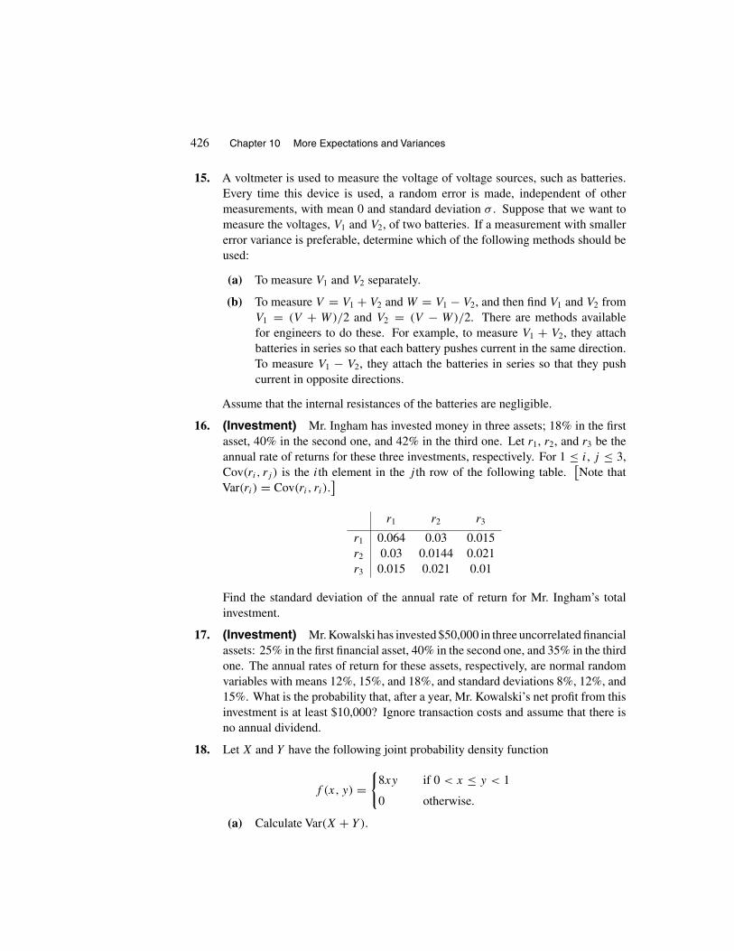
426 Chapter 10 More Expectations and Variances
15. A voltmeter is used to measure the voltage of voltage sources, such as batteries.Every time this device is used, a random error is made, independent of othermeasurements, with mean 0 and standard deviation σ . Suppose that we want tomeasure the voltages, V1 and V2, of two batteries. If a measurement with smallererror variance is preferable, determine which of the following methods should beused:
(a) To measure V1 and V2 separately.
(b) To measure V = V1 + V2 and W = V1 − V2, and then find V1 and V2 fromV1 = (V + W)/2 and V2 = (V − W)/2. There are methods availablefor engineers to do these. For example, to measure V1 + V2, they attachbatteries in series so that each battery pushes current in the same direction.To measure V1 − V2, they attach the batteries in series so that they pushcurrent in opposite directions.
Assume that the internal resistances of the batteries are negligible.
16. (Investment) Mr. Ingham has invested money in three assets; 18% in the firstasset, 40% in the second one, and 42% in the third one. Let r1, r2, and r3 be theannual rate of returns for these three investments, respectively. For 1 ≤ i, j ≤ 3,Cov(ri, rj ) is the ith element in the j th row of the following table.
[Note that
Var(ri) = Cov(ri, ri).]
r1 r2 r3
r1 0.064 0.03 0.015r2 0.03 0.0144 0.021r3 0.015 0.021 0.01
Find the standard deviation of the annual rate of return for Mr. Ingham’s totalinvestment.
17. (Investment) Mr. Kowalski has invested $50,000 in three uncorrelated financialassets: 25% in the first financial asset, 40% in the second one, and 35% in the thirdone. The annual rates of return for these assets, respectively, are normal randomvariables with means 12%, 15%, and 18%, and standard deviations 8%, 12%, and15%. What is the probability that, after a year, Mr. Kowalski’s net profit from thisinvestment is at least $10,000? Ignore transaction costs and assume that there isno annual dividend.
18. Let X and Y have the following joint probability density function
f (x, y) ={
8xy if 0 < x ≤ y < 1
0 otherwise.
(a) Calculate Var(X + Y ).

Section 10.2 Covariance 427
(b) Show that X and Y are not independent. Explain why this does not contradictExercise 23 of Section 8.2.
19. Find the variance of a sum of n randomly and independently selected points fromthe interval (0, 1).
20. Let X and Y be jointly distributed with joint probability density function
f (x, y) =
⎧⎪⎨⎪⎩1
2x3e−xy−x if x > 0, y > 0
0 otherwise.
Determine if X and Y are positively correlated, negatively correlated, or uncorre-lated.Hint: Note that for all a > 0,
∫∞0 xne−ax dx = n!/an+1.
21. Let X be a random variable. Prove that Var(X) = min t E[(X − t)2
].
Hint: Let µ = E(X) and look at the expansion of
E[(X − t)2
] = E[(X − µ + µ − t)2
].
B
22. Let S be the sample space of an experiment. Let A and B be two events of S. LetIA and IB be the indicator variables for A and B. That is,
IA(ω) ={
1 if ω ∈ A
0 if ω �∈ A,
IB(ω) ={
1 if ω ∈ B
0 if ω �∈ B.
Show that IA and IB are positively correlated if and only if P(A | B) > P(A),and if and only if P(B | A) > P(B).
23. Show that for random variables X, Y , Z, and W and constants a, b, c, and d,
Cov(aX + bY, cZ + dW)
= ac Cov(X,Z) + bc Cov(Y, Z) + ad Cov(X, W) + bd Cov(Y, W).
Hint: For a simpler proof, use the results of Exercise 6.
24. Prove the following generalization of Exercise 23:
Cov( n∑
i=1
aiXi,
m∑j=1
bjYj
)=
n∑i=1
m∑j=1
aibj Cov(Xi, Yj ).

428 Chapter 10 More Expectations and Variances
25. A fair die is thrown n times. What is the covariance of the number of 1’s and thenumber of 6’s obtained?Hint: Use the result of Exercise 24.
26. Show that if X1, X2, . . . , Xn are random variables and a1, a2, . . . , an are con-stants, then
Var( n∑
i=1
aiXi
)=
n∑i=1
a2i Var(Xi) + 2
∑∑i<j
aiaj Cov(Xi, Xj ).
27. Let X be a hypergeometric random variable with probability mass function
p(x) = P(X = x) =
(D
x
)(N − D
n − x
)(
N
n
) ,
n ≤ min(D, N − D), x = 0, 1, 2, . . . , n.
Recall that X is the number of defective items among n items drawn randomly andwithout replacement from a box containing D defective and N − D nondefectiveitems. Show that
Var(X) = nD(N − D)
N2
(1 − n − 1
N − 1
).
Hint: Let Ai be the event that the ith item drawn is defective. Also for i =1, 2, . . . , n, let
Xi ={
1 if Ai occurs
0 otherwise.
Then X = X1 + X2 + · · · + Xn.
28. Exactly n married couples are living in a small town. What is the variance of thesurviving couples after m deaths occur among them? Assume that the deaths occurat random, there are no divorces, and there are no new marriages.Note: This situation involves the Daniel Bernoulli problem discussed inExample 10.3.

Section 10.3 Correlation 429
10.3 CORRELATION
Although for random variables X and Y , Cov(X, Y ) provides information about how X
and Y vary jointly, it has a major shortcoming: It is not independent of the units in whichX and Y are measured. For example, suppose that for random variables X and Y , whenmeasured in (say) centimeters, Cov(X, Y ) = 0.15. For the same random variables, if wechange the measurements to millimeters, then X1 = 10X and Y1 = 10Y will be the newobserved values, and by relation (10.7) we get
Cov(X1, Y1) = Cov(10X, 10Y ) = 100 Cov(X, Y ) = 15,
showing that Cov(X, Y ) is sensitive to the units of measurement. From Section 4.6we know that for a random variable X, the standardized X, X∗ = [
X − E(X)]/σX, is
independent of the units in which X is measured. Thus, to define a measure of associationbetween X and Y , independent of the scales of measurements, it is appropriate to considerCov(X∗, Y ∗) rather than Cov(X, Y ). Using relation (10.7), we obtain
Cov(X∗, Y ∗) = Cov(X − E(X)
σX
,Y − E(Y )
σY
)= Cov
( 1
σX
X − 1
σX
E(X),1
σY
Y − 1
σY
E(Y ))
= 1
σX
1
σY
Cov(X, Y ) = Cov(X, Y )
σXσY
.
Definition Let X and Y be two random variables with 0 < σ 2X < ∞ and 0 < σ 2
Y <
∞. The covariance between the standardized X and the standardized Y is called thecorrelation coefficient between X and Y and is denoted by ρ = ρ(X, Y ). Therefore,
ρ = Cov(X, Y )
σXσY
.
The quantity Cov(X, Y )/(σXσY ) gives all the important information that Cov(X, Y )
provides about how X and Y covary and, at the same time, it is not sensitive to the scalesof measurement. Clearly, ρ(X, Y ) > 0 if and only if X and Y are positively correlated;ρ(X, Y ) < 0 if and only if X and Y are negatively correlated; and ρ(X, Y ) = 0 if andonly if X and Y are uncorrelated. Moreover, ρ(X, Y ) roughly measures the amount andthe sign of linear relationship between X and Y . It is −1 if Y = aX + b, a < 0, and+1 if Y = aX + b, a > 0. Thus ρ(X, Y ) = ±1 in the case of perfect linear relationshipand 0 in the case of independence of X and Y . The key to the proof of “ρ(X, Y ) = ±1if and only if Y = aX + b” is the following lemma.
Lemma 10.2 For random variables X and Y with correlation coefficient ρ(X, Y ),
Var( X
σX
+ Y
σY
)= 2 + 2ρ(X, Y );

430 Chapter 10 More Expectations and Variances
Var( X
σX
− Y
σY
)= 2 − 2ρ(X, Y ).
Proof: We prove the first relation; the second can be shown similarly. ByTheorem 10.4,
Var( X
σX
+ Y
σY
)= 1
σ 2X
Var(X) + 1
σ 2Y
Var(Y ) + 2Cov(X, Y )
σXσY
= 2 + 2ρ(X, Y ). �
Theorem 10.5 For random variables X and Y with correlation coefficient ρ(X, Y ),
(a) −1 ≤ ρ(X, Y ) ≤ 1.
(b) With probability 1, ρ(X, Y ) = 1 if and only if Y = aX + b for some constants a,b, a > 0.
(c) With probability 1, ρ(X, Y ) = −1 if and only if Y = aX + b for some constantsa, b, a < 0.
Proof:
(a) Since the variance of a random variable is nonnegative,
Var( X
σX
+ Y
σY
)≥ 0 and Var
( X
σX
− Y
σY
)≥ 0.
Therefore, by Lemma 10.2, 2 + 2ρ(X, Y ) ≥ 0 and 2 − 2ρ(X, Y ) ≥ 0. That is,ρ(X, Y ) ≥ −1 and ρ(X, Y ) ≤ 1.
(b) First, suppose that ρ(X, Y ) = 1. In this case, by Lemma 10.2,
Var( X
σX
− Y
σY
)= 2[1 − ρ(X, Y )
] = 0.
Therefore, with probability 1,
X
σX
− Y
σY
= c,
for some constant c. Hence, with probability 1,
Y = σY
σX
X − c σY ≡ aX + b,
with a = σY /σX > 0 and b = −c σY . Next, assume that Y = aX + b, a > 0. Wehave that
ρ(X, Y ) = ρ(X, aX + b) = Cov(X, aX + b)
σXσaX+b
= a Cov(X, X)
σX (aσX)= a Var(X)
a Var(X)= 1.
(c) The proof of this statement is similar to that of part (b). �

Section 10.3 Correlation 431
Example 10.17 Show that if X and Y are continuous random variables with the jointprobability density function
f (x, y) ={
x + y if 0 < x < 1, 0 < y < 1
0 otherwise,
then X and Y are not linearly related.
Solution: Since X and Y are linearly related if and only if ρ(X, Y ) = ±1 with proba-bility 1, it suffices to prove that ρ(X, Y ) �= ±1. To do so, note that
E(X) =∫ 1
0
∫ 1
0x(x + y) dx dy = 7
12,
E(XY) =∫ 1
0
∫ 1
0xy(x + y) dx dy = 1
3.
Also, by symmetry, E(Y ) = 7/12; therefore,
Cov(X, Y ) = E(XY) − E(X)E(Y ) = 1
3− 7
12
7
12= − 1
144.
Similarly,
E(X2) =∫ 1
0
∫ 1
0x2(x + y) dx dy = 5
12,
σX =√
E(X2) − [E(X)]2 =
√5
12−( 7
12
)2 =√
11
12.
Again, by symmetry, σY = √11/12. Thus
ρ(X, Y ) = Cov(X, Y )
σXσY
= −1/144√11/12 · √
11/12= − 1
11�= ±1. �
The following example shows that even if X and Y are dependent through a nonlinearrelationship such as Y = X2, still, statistically, there might be a strong linear associationbetween X and Y . That is, ρ(X, Y ) might be very close to 1 or −1, indicating that thepoints (x, y) are tightly clustered around a line.
Example 10.18 Let X be a random number from the interval (0, 1) and Y = X2. Theprobability density function of X is
f (x) ={
1 if 0 < x < 1
0 elsewhere,

432 Chapter 10 More Expectations and Variances
and for n ≥ 1,
E(Xn) =∫ 1
0xn dx = 1
n + 1.
Thus E(X) = 1/2, E(Y ) = E(X2) = 1/3,
σ 2X = Var(X) = E(X2) − [E(X)
]2 = 1
3− 1
4= 1
12,
σ 2Y = Var(Y ) = E(X4) − [E(X2)
]2 = 1
5−(1
3
)2 = 4
45,
and, finally,
Cov(X, Y ) = E(X3) − E(X)E(X2) = 1
4− 1
2
1
3= 1
12.
Therefore,
ρ(X, Y ) = Cov(X, Y )
σXσY
= 1/12
1/2√
3 · 2/3√
5=
√15
4= 0.968. �
� Example 10.19 (Investment) Mr. Kowalski has invested money in two finan-cial assets. Let r be the annual rate of return for his total investment. Let r1 and r2 bethe annual rates of return for the first and second assets, respectively. Let σ 2 = Var(r),σ 2
1 = Var(r1), and σ 22 = Var(r2). Prove that
σ 2 ≤ max(σ 2
1 , σ 22
).
In particular, by this inequality, if r1 and r2 are identically distributed, then σ 21 = σ 2
2implies that
σ 2 ≤ σ 21 = σ 2
2 .
This is an extension of the result discussed in Example 10.14. It shows that, even if thefinancial assets are correlated, still diversification reduces the investment risk.
Proof: We will show that if σ 22 ≤ σ 2
1 , then σ 2 ≤ σ 21 . By symmetry, if σ 2
1 ≤ σ 22 , then
σ 2 ≤ σ 22 . Therefore, σ 2 is either less than or equal to σ 2
1 , or it is less than or equal to σ 22 ,
implying thatσ 2 ≤ max
(σ 2
1 , σ 22
).
To show that σ 22 ≤ σ 2
1 implies that σ 2 ≤ σ 21 , let w1 and w2 be the fractions of Mr. Kowal-
ski’s investment in the first and second financial assets, respectively. Then w1 + w2 = 1and
r = w1r1 + w2r2.

Section 10.3 Correlation 433
Let ρ be the correlation coefficient of r1 and r2. Then
Cov(r1, r2) = ρσ1σ2.
We have
Var(r) = Var(w1r1 + w2r2) = Var(w1r1) + Var(w2r2) + 2Cov(w1r1, w2r2)
= w21 Var(r1) + w2
2 Var(r2) + 2w1w2 Cov(r1, r2).
Noting that w1 + w2 = 1, −1 ≤ ρ ≤ 1, and σ 22 ≤ σ 2
1 , this relation implies that
σ 2 = w21σ
21 + w2
2σ22 + 2w1w2ρσ1σ2
≤ w21σ
21 + w2
2σ21 + 2w1w2σ
21
= (w21 + w2
2 + 2w1w2)σ21
= (w1 + w2)2σ 2
1 = σ 21 . �
EXERCISES
A
1. Let X and Y be jointly distributed, with ρ(X, Y ) = 1/2, σX = 2, σY = 3. FindVar(2X − 4Y + 3).
2. Let the joint probability density function of X and Y be given by
f (x, y) ={
sin x sin y if 0 ≤ x ≤ π/2, 0 ≤ y ≤ π/2
0 otherwise.
Calculate the correlation coefficient of X and Y .
3. A stick of length 1 is broken into two pieces at a random point. Find the correlationcoefficient and the covariance of these pieces.
4. For real numbers α and β, let
sgn(αβ) =
⎧⎪⎪⎨⎪⎪⎩1 if αβ > 0
0 if αβ = 0
−1 if αβ < 0.
Prove that for random variables X and Y ,
ρ(α1X + α2, β1Y + β2) = ρ(X, Y ) sgn(α1β1).

434 Chapter 10 More Expectations and Variances
5. Is it possible that for some random variables X and Y , ρ(X, Y ) = 3, σX = 2, andσY = 3?
6. Prove that if Cov(X, Y ) = 0, then
ρ(X + Y, X − Y ) = Var(X) − Var(Y )
Var(X) + Var(Y ).
B
7. Show that if the joint probability density function of X and Y is
f (x, y) =
⎧⎪⎨⎪⎩1
2sin(x + y) if 0 ≤ x ≤ π
2, 0 ≤ y ≤ π
2
0 elsewhere,
then there exists no linear relation between X and Y .
10.4 CONDITIONING ON RANDOM VARIABLES
An important application of conditional expectations is that ordinary expectations andprobabilities can be calculated by conditioning on appropriate random variables. First,to explain this procedure, we state a definition.
Definition Let X and Y be two random variables. By E(X|Y) we mean a functionof Y that is defined to be E(X | Y = y) when Y = y.
Recall that a function of a random variable Y , say h(Y ), is defined to be h(a) at allsample points at which Y = a. For example, if Z = log Y , then at a sample point ω,where Y (ω) = a, we have that Z(ω) = log a. In this definition E(X | Y ) is a functionof Y , which at a sample point ω is defined to be E(X | Y = y), where y = Y (ω).Since E(X|Y ) is defined only when pY (y) > 0, it is defined at all sample points ω,where pY (y) > 0, y = Y (ω). E(X|Y ), being a function of Y , is a random variable. Itsexpectation, whenever finite, is equal to the expectation of X. This extremely importantproperty sometimes enables us to calculate expectations which are otherwise, if possible,very difficult to find. To see why the expected value of E(X|Y ) is E(X), let X and Y bediscrete random variables with sets of possible values A and B, respectively. Let p(x, y)
be the joint probability mass function of X and Y . On the one hand,

Section 10.4 Conditioning on Random Variables 435
E(X) =∑x∈A
xpX(x) =∑x∈A
x∑y∈B
p(x, y)
=∑y∈B
∑x∈A
xp(x, y) =∑y∈B
∑x∈A
xpX|Y (x|y)pY (y)
=∑y∈B
(∑x∈A
xpX|Y (x|y))pY (y)
=∑y∈B
E(X | Y = y)P (Y = y), (10.13)
showing that E(X) is the weighted average of the conditional expectations of X (givenY = y) over all possible values of Y . On the other hand, we know that, for a real-valuedfunction h,
E[h(Y )
] =∑y∈B
h(y)P (Y = y).
Applying this formula to h(Y ) = E(X|Y ) yields
E[E(X|Y )
] =∑y∈B
E(X | Y = y)P (Y = y). (10.14)
Comparing (10.13) and (10.14), we obtain
E(X) = E[E(X|Y)
] =∑y∈B
E(X | Y = y)P (Y = y). (10.15)
Therefore, E[E(X|Y )
] = E(X) is a condensed way to say that E(X) is the weightedaverage of the conditional expectations of X (given Y = y) over all possible values ofY . We have proved the following theorem for the discrete case.
Theorem 10.6 Let X and Y be two random variables. Then
E[E(X | Y)
] = E(X).
Proof: We have already proven this for the discrete case. Now we will prove it forthe case where X and Y are continuous random variables with joint probability densityfunction, f (x, y).
E[E(X|Y )
] =∫ ∞
−∞E(X|Y = y)fY (y) dy
=∫ ∞
−∞
( ∫ ∞
−∞xfX|Y (x|y) dx
)fY (y) dy
=∫ ∞
−∞x( ∫ ∞
−∞fX|Y (x|y)fY (y) dy
)dx

436 Chapter 10 More Expectations and Variances
=∫ ∞
−∞x( ∫ ∞
−∞f (x, y)
fY (y)fY (y) dy
)dx
=∫ ∞
−∞x( ∫ ∞
−∞f (x, y) dy
)dx
=∫ ∞
−∞xfX(x) dx = E(X). �
Example 10.20 Suppose that N(t), the number of people who pass by a museum ator prior to t , is a Poisson process having rate λ. If a person passing by enters the museumwith probability p, what is the expected number of people who enter the museum at orprior to t?
Solution: Let M(t) denote the number of people who enter the museum at or prior tot ; then
E[M(t)
] = E[E(M(t) | N(t)
)] =∞∑
n=0
E[M(t) | N(t) = n
]P(N(t) = n
).
Given that N(t) = n, the number of people who enter the museum at or prior to t , is abinomial random variable with parameters n and p. Thus E
[M(t) | N(t) = n
] = np.
Therefore,
E[M(t)
] =∞∑
n=1
npe−λt (λt)n
n! = pe−λtλt
∞∑n=1
(λt)n−1
(n − 1)! = pe−λtλteλt = pλt. �
Example 10.21 Let X and Y be continuous random variables with joint probabilitydensity function
f (x, y) =
⎧⎪⎨⎪⎩3
2(x2 + y2) if 0 < x < 1, 0 < y < 1
0 otherwise.
Find E(X|Y ).
Solution: E(X|Y ) is a random variable that is defined to be E(X | Y = y) when Y = y.First, we calculate E(X | Y = y):
E(X | Y = y) =∫ 1
0xfX|Y (x|y) dx =
∫ 1
0x
f (x, y)
fY (y)dx,
where
fY (y) =∫ 1
0
3
2(x2 + y2) dx = 3
2y2 + 1
2.

Section 10.4 Conditioning on Random Variables 437
Hence
E(X | Y = y) =∫ 1
0x
(3/2)(x2 + y2)
(3/2)y2 + 1/2dx =
∫ 1
0x
3(x2 + y2)
3y2 + 1dx
= 3
3y2 + 1
∫ 1
0(x3 + xy2) dx = 3(2y2 + 1)
4(3y2 + 1).
Thus, if Y = y, then
E(X | Y = y) = 3(2y2 + 1)
4(3y2 + 1).
Now since the random variable E(X|Y ) coincides with E(X | Y = y) if Y = y, we have
E(X|Y ) = 3(2Y 2 + 1)
4(3Y 2 + 1). �
Example 10.22 What is the expected number of random digits that should be gener-ated to obtain three consecutive zeros?
Solution: Let X be the number of random digits to be generated until three consecutivezeros are obtained. Let Y be the number of random digits to be generated until the firstnonzero digit is obtained. Then
E(X) = E[E(X|Y )
] =∞∑i=1
E(X | Y = i)P (Y = i)
=3∑
i=1
E(X | Y = i)P (Y = i) +∞∑i=4
E(X | Y = i)P (Y = i)
=3∑
i=1
[i + E(X)
]( 1
10
)i−1( 9
10
)+
∞∑i=4
3( 1
10
)i−1( 9
10
),
which gives
E(X) = 1.107 + 0.999 E(X) + 0.003.
Solving this for E(X), we find that E(X) = 1110. �
Example 10.23 Let X and Y be two random variables and f be a real-valued functionfrom R to R. Prove that
E[f (Y )X | Y
] = f (Y )E(X|Y).

438 Chapter 10 More Expectations and Variances
Proof: If Y = y, then f (Y )E(X|Y ) is f (y)E(X | Y = y). We show that E[f (Y )X|Y ]
is also equal to this quantity. Let fX|Y (x|y) be the conditional probability density functionof X given that Y = y; then
E[f (Y )X | Y = y
] = E[f (y)X|Y = y
] =∫ ∞
−∞f (y)xfX|Y (x|y) dx
= f (y)
∫ ∞
−∞xfX|Y (x|y) dx = f (y)E(X | Y = y). �
Suppose that a certain airplane breaks down N times a year, where N is a randomvariable. If the repair time for the ith breakdown is Xi , then the total repair time for thisairplane is the random variable X1 +X2 + · · ·+XN . To find the expected length of timethat, due to breakdowns, the plane cannot fly, we need to calculate E
(∑Ni=1 Xi
). What
is different about this sum is that, not only is each of its terms a random variable, butthe number of its terms is also a random variable. The expected values of such sums arecalculated using the following theorem, discovered by Abraham Wald, a statistician whois best known for developing the theory of sequential statistical procedures during WorldWar II.
Theorem 10.7 (Wald’s Equation) Let X1, X2, . . . be independent and identicallydistributed random variables with the finite mean E(X). Let N > 0 be an integer-valuedrandom variable, independent of {X1, X2, . . . }, with E(N) < ∞. Then
E( N∑
i=1
Xi
)= E(N)E(X).
Proof: By (10.15),
E( N∑
i=1
Xi
)= E
[E( N∑
i=1
Xi
∣∣N)] =∞∑
n=1
E( N∑
i=1
Xi
∣∣N = n)P(N = n), (10.16)
where
E( N∑
i=1
Xi
∣∣N = n)
= E( n∑
i=1
Xi
∣∣N = n)
= E( n∑
i=1
Xi
)=
n∑i=1
E(Xi) = nE(X),
since N is independent of {X1, X2, . . . }. Hence, by (10.16),
E( N∑
i=1
Xi
)=
∞∑n=1
nE(X)P (N = n) = E(X)
∞∑n=1
nP (N = n) = E(X)E(N). �
Example 10.24 Suppose that the average number of breakdowns for a certain airplaneis 12.5 times a year. If the expected value of repair time is 7 days for each breakdown,

Section 10.4 Conditioning on Random Variables 439
and if the repair times are identically distributed, independent random variables, find theexpected total repair time. Assume that repair times are independent of the number ofbreakdowns.
Solution: Let N be the number of breakdowns in a year and Xi be the repair time forthe ith breakdown. Then, by Wald’s equation, the expected total repair time is
E( N∑
i=1
Xi
)= E(N)E(Xi) = (12.5)(7) = 87.5. �
The following theorem gives a formula, analogous to Wald’s equation, for variance. Weleave its proof as an exercise.
Theorem 10.8 Let {X1, X2, . . . } be an independent and identically distributed se-quence of random variables with finite mean E(X) and finite varianceVar(X). Let N > 0be an integer-valued random variable independent of {X1, X2, . . . } with E(N) < ∞ andVar(N) < ∞. Then
Var( N∑
i=1
Xi
)= E(N)Var(X) + [E(X)
]2Var(N).
We now explain a procedure for calculation of probabilities by conditioning on ran-dom variables. Let B be an event associated with an experiment and X be a discreterandom variable with possible set of values A. Let
Y ={
1 if B occurs
0 if B does not occur.
Then
E(Y ) = E[E(Y |X)
]. (10.17)
But
E(Y ) = 1 · P(B) + 0 · P(Bc) = P(B) (10.18)
and
E[E(Y |X)
] =∑x∈A
E(Y | X = x)P (X = x)
=∑x∈A
P (B | X = x)P (X = x), (10.19)

440 Chapter 10 More Expectations and Variances
where the last equality follows since
E(Y | X = x) = 1 · P(Y = 1 | X = x) + 0 · P(Y = 0 | X = x)
= P(Y = 1, X = x)
P (X = x)= P(B and X = x)
P (X = x)= P(B | X = x).
Relations (10.17), (10.18), and (10.19) imply the following theorem.
Theorem 10.9 Let B be an arbitrary event and X be a discrete random variable withpossible set of values A; then
P(B) =∑x∈A
P (B | X = x)P (X = x). (10.20)
If X is a continuous random variable, the relation analogous to (10.20) is
P(B) =∫ ∞
−∞P(B | X = x)f (x) dx, (10.21)
where f is the probability density function of X.
Theorem 10.9 shows that the probability of an event B is the weighted average ofthe conditional probabilities of B (given X = x) over all possible values of X. For thediscrete case, this is a conclusion of Theorem 3.4, the most general version of the law oftotal probability.
Example 10.25 The time between consecutive earthquakes in San Francisco and thetime between consecutive earthquakes in Los Angeles are independent and exponentiallydistributed with means 1/λ1 and 1/λ2, respectively. What is the probability that the nextearthquake occurs in Los Angeles?
Solution: Let X and Y denote the times between now and the next earthquake in SanFrancisco and Los Angeles, respectively. Because of the memoryless property of expo-nential distribution, X and Y are exponentially distributed with means 1/λ1 and 1/λ2,respectively. To calculate P(X > Y), the desired probability, we will condition on Y :
P(X > Y) =∫ ∞
0P(X > Y | Y = y)λ2e
−λ2y dy
=∫ ∞
0P(X > y)λ2e
−λ2y dy =∫ ∞
0e−λ1yλ2e
−λ2y dy
= λ2
∫ ∞
0e−(λ1+λ2)y dy = λ2
λ1 + λ2,
where P(X > y) is calculated from
P(X > y) = 1 − P(X ≤ y) = 1 − (1 − e−λ1y) = e−λ1y. �

Section 10.4 Conditioning on Random Variables 441
Example 10.26 Suppose that Z1 and Z2 are independent standard normal randomvariables. Show that the ratio Z1/|Z2| is a Cauchy random variable. That is, Z1/|Z2| isa random variable with the probability density function
f (t) = 1
π(1 + t2), −∞ < t < ∞.
Solution: Let g(x) be the probability density function of |Z2|. To find g(x), note that,for x ≥ 0,
P(|Z2| ≤ x
) = P(−x ≤ Z2 ≤ x) =∫ x
−x
1√2π
e−u2/2 du = 2∫ x
0
1√2π
e−u2/2 du.
Hence
g(x) = d
dxP(|Z2| ≤ x
) = 2√2π
e−x2/2, x ≥ 0.
To find the probability density function of Z1/|Z2|, note that, by Theorem 10.9,
P( Z1
|Z2| ≤ t)
= 1 − P( Z1
|Z2| > t)
= 1 − P(Z1 > t |Z2|
)= 1 −
∫ ∞
0P(Z1 > t |Z2|
∣∣ |Z2| = x) 2√
2πe−x2/2 dx
= 1 −∫ ∞
0P(Z1 > tx)
2√2π
e−x2/2 dx
= 1 −∫ ∞
0
( ∫ ∞
tx
1√2π
e−u2/2 du) 2√
2πe−x2/2 dx.
Now, by the fundamental theorem of calculus,
d
dt
∫ ∞
tx
1√2π
e−u2/2 du = d
dt
(1 −
∫ tx
−∞1√2π
e−u2/2 du)
= −x1√2π
e−t2x2/2.
Therefore,
d
dtP( Z1
|Z2| ≤ t)
=∫ ∞
0
x√2π
e−t2x2/2 · 2√2π
e−x2/2 dx = 2
2π
∫ ∞
0xe−(t2+1)x2/2 dx.
Making the change of variable y = (1 + t2)x2/2 yields
d
dtP( Z1
|Z2| ≤ t)
= 1
π(1 + t2)
∫ ∞
0e−y dy = 1
π(1 + t2), −∞ < t < ∞. �
Example 10.27 At the intersection of two remote roads, the vehicles arriving areeither cars or trucks. Suppose that cars arrive at the intersection at a Poisson rate of λ per

442 Chapter 10 More Expectations and Variances
minute, and trucks arrive at a Poisson rate of µ per minute. Suppose that the arrivals areindependent of each other. If we are given that the next vehicle arriving at this intersectionis a car, find the expected value of the time until the next arrival.
Warning: Since cars and trucks arrive at this intersection independently, we might falla-ciously think that, given the next arrival is a car, the expected value until the next arrivalis 1/λ.
Solution: Let T be the time until the next vehicle arrives at the intersection. Let X bethe time until the next car arrives at the intersection, and Y be the time until the nexttruck arrives at the intersection. Let A be the event that the next vehicle arriving at thisintersection is a car. Note that X and Y are independent exponential random variableswith means 1/λ and 1/µ, respectively. We are interested in E(T |A) = E(X | X < Y).To find this quantity, we will first calculate the probability distribution function of X
given that X < Y :
P(X ≤ t | X < Y) = P(X ≤ t, X < Y)
P (X < Y),
where
P(X < Y) =∫ ∞
0P(X < Y | X = x)fX(x) dx
=∫ ∞
0P(Y > x | X = x)fX(x) dx =
∫ ∞
0P(Y > x)λe−λx dx
=∫ ∞
0e−µxλe−λx dx = λ
λ + µ,
and
P(X ≤ t, X < Y) = P(X < min{t, Y })
=∫ ∞
0P(X < min{t, Y } | X = x
)fX(x) dx
=∫ ∞
0P(
min{t, Y } > x | X = x)fX(x) dx
=∫ t
0P(Y > x | X = x)fX(x) dx
=∫ t
0P(Y > x)fX(x) dx =
∫ t
0e−µxλe−λx dx
= λ
λ + µ[1 − e−(λ+µ)t ].

Section 10.4 Conditioning on Random Variables 443
Thus
P(X ≤ t | X < Y) =λ
λ + µ[1 − e−(λ+µ)t ]
λ
λ + µ
= 1 − e−(λ+µ)t .
This result shows that, given that the next vehicle arriving is a car, the distribution of thetime until the next arrival is exponential with parameter λ + µ. Therefore,
E(T | A) = 1
λ + µ.
Similarly,
E(T | Ac) = 1
λ + µ. �
Let X and Y be two given random variables. Define the new random variableVar(X|Y) by
Var(X|Y) = E[(
X − E(X|Y))2 | Y
].
Then the formula analogous to Var(X) = E(X2) − [E(X)]2
is given by
Var(X|Y) = E(X2|Y) − E(X|Y)2. (10.22)
(See Exercise 20.) The following theorem shows that Var(X) is the sum of the expectedvalue of Var(X|Y ) and the variance of E(X|Y ).
Theorem 10.10 Var(X) = E[Var(X|Y)
] + Var(E[X|Y ]).
Proof: By (10.22),
E[Var(X|Y )
] = E[E(X2|Y )
]− E[E(X|Y )2
]= E(X2) − E
[E(X|Y )2
].
By the definition of variance,
Var(E[X|Y ]) = E
[E(X|Y )2
]− (E[E(X|Y )])2
= E[E(X|Y )2
]− [E(X)]2
.
Adding these two equations, we have the theorem. �
Example 10.28 A fisherman catches fish in a large lake with lots of fish, at a Poissonrate of two per hour. If, on a given day, the fisherman spends randomly anywhere between3 and 8 hours fishing, find the expected value and the variance of the number of fish hecatches.

444 Chapter 10 More Expectations and Variances
Solution: Let X be the number of hours the fisherman spends fishing. Then X is auniform random variable over the interval (3, 8). Label the time the fisherman beginsfishing on the given day at t = 0. Let N(t) denote the total number of fish caught at orprior to t . Then
{N(t) : t ≥ 0
}is a Poisson process with parameter λ = 2. Assuming
that X is independent of{N(t) : t ≥ 0
}, we have
E[N(X) | X = t
] = E[N(t)
] = 2t.
This implies thatE[N(X) | X
] = 2X.
Therefore,
E[N(X)
] = E[E(N(X) | X
)] = E(2X) = 2E(X) = 2 · 8 + 3
2= 11.
Similarly,Var(N(X) | X = t
) = Var(N(t)
) = 2t.
ThusVar(N(X) | X
) = 2X.
By Theorem 10.10,
Var(N(X)
) = E[Var(N(X) | X
)]+ Var(E[N(X) | X
])= E(2X) + Var(2X) = 2E(X) + 4Var(X)
= 2 · 8 + 3
2+ 4 · (8 − 3)2
12= 19.33. �
EXERCISES
A
1. A fair coin is tossed until two tails occur successively. Find the expected numberof the tosses required.Hint: Let
X ={
1 if the first toss results in tails
0 if the first toss results in heads,
and condition on X.

Section 10.4 Conditioning on Random Variables 445
2. The orders received for grain by a farmer add up to X tons, where X is a continuousrandom variable uniformly distributed over the interval (4, 7). Every ton of grainsold brings a profit of a, and every ton that is not sold is destroyed at a loss ofa/3. How many tons of grain should the farmer produce to maximize his expectedprofit?Hint: Let Y (t) be the profit if the farmer produces t tons of grain. Then
E[Y (t)
] = E[aX − a
3(t − X)
]P(X < t) + E(at)P (X ≥ t).
3. In a box, Lynn has b batteries of which d are dead. She tests them randomly andone by one. Every time that a good battery is drawn, she will return it to the box;every time that a dead battery is drawn, she will replace it by a good one.
(a) Determine the expected value of the number of good batteries in the boxafter n of them are checked.
(b) Determine the probability that on the nth draw Lynn draws a good battery.
Hint: Let Xn be the number of good batteries in the box after n of them arechecked. Show that
E(Xn | Xn−1) = 1 +(
1 − 1
b
)Xn−1.
Then, by computing the expected value of this random variable, find a recursiverelation between E(Xn) and E(Xn−1). Use this relation and induction to provethat
E(Xn) = b − d(
1 − 1
b
)n
.
Note that n should approach ∞ to get E(Xn) = b. For part (b), let En be the eventthat on the nth draw she gets a good battery. By conditioning on Xn−1 prove thatP(En) = E(Xn−1)/b.
4. For given random variables Y and Z, let
X ={
Y with probability p
Z with probability 1 − p.
Find E(X) in terms of E(Y ) and E(Z).
5. A typist, on average, makes three typing errors in every two pages. If pages withmore than two errors must be retyped, on average how many pages must she typeto prepare a report of 200 pages? Assume that the number of errors in a page is aPoisson random variable. Note that some of the retyped pages should be retyped,and so on.

446 Chapter 10 More Expectations and Variances
Hint: Find p, the probability that a page should be retyped. Let Xn be thenumber of pages that should be typed at least n times. Show that E(X1) = 200p,E(X2) = 200p2, . . . , E(Xn) = 200pn. The desired quantity is E
(∑∞i=1 Xi
),
which can be calculated using relation (10.2).
6. In data communication, usually messages sent are combinations of characters, andeach character consists of a number of bits. A bit is the smallest unit of informationand is either 1 or 0. Suppose that the length of a character (in bits) is a geometricrandom variable with parameter p. Suppose that a message is combined of K
characters, where K is a random variable with mean µ and variance σ 2. If thelengths of characters of a message are independent of each other and of K , and ifit takes a sender 1000 bits per second to emit a message, find the expected valueof T , the time it will take the sender to emit a message.
7. From an ordinary deck of 52 cards, cards are drawn at random, one by one andwithout replacement until a heart is drawn. What is the expected value of thenumber of cards drawn?Hint: Consider a deck of cards with 13 hearts and 39 − n nonheart cards. LetXn be the number of cards to be drawn before the first heart is drawn. Let
Y ={
1 if the first card drawn is a heart
0 otherwise.
By conditioning on Y , find a recursive relation between E(Xn) and E(Xn+1). UseE(X39) = 0 to show that E(Xi) = (39 − i)/14. The answer is 1 + E(X0). (Fora totally different solution see Exercise 15, Section 10.1.)
8. Suppose that X and Y are independent random variables with probability den-sity functions f and g, respectively. Use conditioning technique to calculateP(X < Y).
9. Prove that, for a Poisson random variable N , if the parameter λ is not fixed and isitself an exponential random variable with parameter 1, then
P(N = i) =(1
2
)i+1.
10. Suppose that X and Y represent the amount of money in the wallets of playersA and B, respectively. Let X and Y be jointly uniformly distributed on the unitsquare [0, 1]×[0, 1]. A and B each places his wallet on the table. Whoever has thesmallest amount of money in his wallet, wins all the money in the other wallet. LetWA be the amount of money that player A will win. Show that E(WA) = 0. (For ahistory of this problem, see the Wallet Paradox in Exercise 22, Review Problems,Chapter 8.)
11. A fair coin is tossed successively. Let Kn be the number of tosses until n consec-utive heads occur.

Section 10.4 Conditioning on Random Variables 447
(a) Argue that
E(Kn | Kn−1 = i) = (i + 1)1
2+ [i + 1 + E(Kn)
]12.
(b) Show that
E(Kn | Kn−1) = Kn−1 + 1 + 1
2E(Kn).
(c) By finding the expected values of both sides of (b) find a recursive relationbetween E(Kn) and E(Kn−1).
(d) Note that E(K1) = 2. Use this and (c) to find E(Kn).
B
12. In Rome, tourists arrive at a historical monument according to a Poisson process,on average, one every five minutes. There are guided tours that depart (a) wheneverthere is a group of 10 tourists waiting to take the tour, or (b) one hour has elapsedfrom the time the previous tour began. It is the policy of the Tourism Departmentthat a tour will only run for less than 10 people if the last guided tour left one hourago. If in any one hour period, there will always be tourists arriving to take thetour, find the expected value of the time between two consecutive tours.
13. During an academic year, the admissions office of a small college receives studentapplications at a Poisson rate of 5 per day. It is a policy of this college to double itsstudent recruitment efforts if no applications arrive for two consecutive businessdays. Find the expected number of business days until a time when the collegeneeds to double its recruitment efforts. Do the admission officers need to worryabout this policy at all?Hint: Let X1 be the time until the first application arrives. Let X2 be the timebetween the first and second applications, and so forth. Let N be the first integerfor which
X1 ≤ 2, X2 ≤ 2, . . . , XN ≤ 2, XN+1 > 2.
The time that the admissions office has to wait before doubling its student recruit-ment efforts is SN+1 = X1 + X2 + · · · + XN+1. Find SN+1 by conditioning onN .
14. Each time that Steven calls his friend Adam, the probability that Adam is availableto talk with him is p independently of other calls. On average, after how manycalls has Steven not missed Adam k consecutive times?
15. Recently, Larry taught his daughter Emily how to play backgammon. To encourageEmily to practice this game, Larry decides to play with her until she wins two of therecent three games. If the probability that Emily wins a game is 0.35 independentlyof all preceding and future games, find the expected number of games to be played.
448 Chapter 10 More Expectations and Variances
16. (Genetics) Hemophilia is a sex-linked disease with normal allele H dominantto the mutant allele h. Kim and John are married, and John is phenotypicallynormal. Suppose that, in the entire population, the frequencies of H and h are0.98 and 0.02, respectively. If Kim and John have four sons and three daughters,what is the expected number of their hemophilic children?
17. A spice company distributes cinnamon in one-pound bags. Suppose that the Foodand Drug Administration (FDA) considers more than 500 insect fragments in onebag excessive and hence unacceptable. To meet the standards of the FDA, thequality control division of the company begins inspecting the bags of the cinnamonat time t = 0 according to the following scheme. It inspects each bag withprobability α until it encounters an unacceptable bag. At that point, the divisioninspects every single bag until it finds m consecutive acceptable bags. When thishappens, the division has completed one inspection cycle. It then resumes itsnormal inspection process. Inspected bags that are found with excessive numbersof insect fragments are sent back for further cleaning. Let p be the probability thata bag is acceptable, independent of the number of insect fragments in other bags.Find the expected value of the number of bags inspected in one inspection cycle.
18. Suppose that a device is powered by a battery. Since an uninterrupted supply ofpower is needed, the device has a spare battery. When the battery fails, the circuitis altered electronically to connect the spare battery and remove the failed batteryfrom the circuit. The spare battery then becomes the working battery and emits asignal to alert the user to replace the failed battery. When that battery is replaced,it becomes the new spare battery. Suppose that the lifetimes of the batteries usedare independent uniform random variables over the interval (0, 1), where the unitof measurement is 1000 hours. For 0 < t ≤ 1, on average, how many batteriesare changed by time t? How many are changed, on average, after 950 hours ofoperation?
19. Let X and Y be continuous random variables. Prove that
E[(
X − E(X|Y ))2] = E(X2) − E
[E(X|Y )2
].
Hint: Let Z = E(X|Y ). By conditioning on Y and using Example 10.23, firstshow that E(XZ) = E(Z2).
20. Let X and Y be two given random variables. Prove that
Var(X|Y ) = E[X2|Y ] − E(X|Y )2.
21. Prove Theorem 10.8.

Section 10.5 Bivariate Normal Distribution 449
10.5 BIVARIATE NORMAL DISTRIBUTION
Let f (x, y) be the joint probability density function of continuous random variables X
and Y ; f is called a bivariate normal probability density function if
(a) The distribution function of X is normal. That is, the marginal probability densityfunction of X is
fX(x) = 1
σX
√2π
exp[
− (x − µX)2
2σ 2X
], −∞ < x < ∞. (10.23)
(b) The conditional distribution of Y , given that X = x, is normal for each x ∈(−∞, ∞). That is, fY |X(y|x) has a normal density for each x ∈ R.
(c) The conditional expectation of Y , given that X = x, E(Y | X = x), is a linearfunction of x. That is, E(Y | X = x) = a + bx for some a, b ∈ R.
(d) The conditional variance of Y , given that X = x, is constant. That is, σ 2Y |X=x is
independent of the value of x.
As an example, let X be the height of a man and let Y be the height of his daughter.It is reasonable to assume, and is statistically verified, that the joint probability densityfunction of X and Y satisfies (a) to (d) and hence is bivariate normal. As another example,let X and Y be grade point averages of a student in his or her freshman and senior years,respectively. Then the joint probability density function of X and Y is bivariate normal.
We now prove that if f (x, y) satisfies (a) to (d), it must be of the following form:
f (x, y) = 1
2πσXσY
√1 − ρ2
exp[
− 1
2(1 − ρ2)Q(x, y)
], (10.24)
where ρ is the correlation coefficient of X and Y and
Q(x, y) =(x − µX
σX
)2 − 2ρx − µX
σX
y − µY
σY
+(y − µY
σY
)2.
Figure 10.1 demonstrates the graph of f (x, y) in the case where ρ = 0, µX = µY = 0,
and σX = σY = 1. To prove (10.24), note that from Lemmas 10.3 and 10.4 (whichfollow) we have that for each x ∈ R the expected value and the variance of the normaldensity function fY |X(y|x) are µY + ρ(σY /σX)(x − µX) and (1 − ρ2)σ 2
Y , respectively.Therefore, for every real x,
fY |X(y|x) = 1
σY
√2π√
1 − ρ2exp
[−[y − µY − ρ(σY /σX)(x − µX)
]22σ 2
Y (1 − ρ2)
], (10.25)
−∞ < y < ∞.

450 Chapter 10 More Expectations and Variances
Figure 10.1 Bivariate normal probability density function.
Now f (x, y) = fY |X(y|x)fX(x), and fX(x) has the normal density given by (10.23).Multiplying (10.23) by (10.25), we obtain (10.24). So what remains to be shown is theproofs of the following general lemmas, which are valid even if the joint density functionof X and Y is not bivariate normal.
Lemma 10.3 Let X and Y be two random variables with probability density functionf (x, y). If E(Y | X = x) is a linear function of x, that is, if E(Y | X = x) = a + bx
for some a, b ∈ R , then
E(Y | X = x) = µY + ρσY
σX
(x − µX).
Proof: By definition,
E(Y | X = x) =∫ ∞
−∞y
f (x, y)
fX(x)dy = a + bx.
Therefore, ∫ ∞
−∞yf (x, y) dy = afX(x) + bxfX(x). (10.26)
This gives∫ ∞
−∞
∫ ∞
−∞yf (x, y) dy dx = a
∫ ∞
−∞fX(x) dx + b
∫ ∞
−∞xfX(x) dx, (10.27)
which is equivalent to
µY = a + bµX. (10.28)

Section 10.5 Bivariate Normal Distribution 451
Now, multiplying (10.26) by x and integrating both sides, we obtain∫ ∞
−∞
∫ ∞
−∞xyf (x, y) dy dx = a
∫ ∞
−∞xfX(x) dx + b
∫ ∞
−∞x2fX(x) dx,
which is equivalent to
E(XY) = aµX + bE(X2). (10.29)
Solving (10.28) and (10.29) for a and b, we get
b = E(XY) − µXµY
E(X2) − µ2X
= Cov(X, Y )
σ 2X
= ρσXσY
σ 2X
= ρσY
σX
and
a = µY − ρσY
σX
µX.
Therefore,
E(Y | X = x) = a + bX = µY + ρσY
σX
(x − µX). �
Lemma 10.4 Let f (x, y) be the joint probability density function of continuousrandom variables X and Y . If E(Y | X = x) is a linear function of x and σ 2
Y |X=x isconstant, then
σ 2Y |X=x = (1 − ρ2)σ 2
Y .
Proof: We have that
σ 2Y |X=x =
∫ ∞
−∞
[y − E(Y | X = x)
]2fY |X(y|x) dy.
Multiplying both sides of this equation by fX(x) and integrating on x gives
σ 2Y |X=x
∫ ∞
−∞fX(x) dx =
∫ ∞
−∞
∫ ∞
−∞
[y − E(Y | X = x)
]2fY |X(y|x)fX(x) dy dx.
Now, since f (x, y) = fY |X(y|x)fX(x), and
E(Y | X = x) = µY + ρσY
σX
(x − µX),
we get
σ 2Y |X=x =
∫ ∞
−∞
∫ ∞
−∞
[y − µY − ρ
σY
σX
(x − µX)]2
f (x, y) dx dy,

452 Chapter 10 More Expectations and Variances
or, equivalently,
σ 2Y |X=x = E
[(Y − µY ) − ρ
σY
σX
(X − µX)]2
.
Therefore,
σ 2Y |X=x = E
[(Y − µY )2
]− 2ρσY
σX
E[(Y − µY )(X − µX)
]+ ρ2 σ 2Y
σ 2X
E[(X − µX)2
]= σ 2
Y − 2ρσY
σX
ρσXσY + ρ2 σ 2Y
σ 2X
σ 2X
= (1 − ρ2)σ 2Y . �
We know that if X and Y are independent random variables, their correlation coeffi-cient is 0. We also know that, in general, the converse of this fact is not true. However,if X and Y have a bivariate normal distribution, the converse is also true. That is, ρ = 0implies that X and Y are independent, which can be deduced from (10.24). For ρ = 0,
f (x, y) = 1
2πσXσY
exp[
− (x − µX)2
2σ 2X
− (y − µY )2
2σ 2Y
]= 1
σX
√2π
exp[
− (x − µX)2
2σ 2X
] 1
σY
√2π
exp[
− (y − µY )2
2σ 2Y
]= fX(x)fY (y),
showing that X and Y are independent.
Example 10.29 At a certain university, the joint probability density function of X
and Y , the grade point averages of a student in his or her freshman and senior years,respectively, is bivariate normal. From the grades of past years it is known that µX = 3,µY = 2.5, σX = 0.5, σY = 0.4, and ρ = 0.4. Find the probability that a student withgrade point average 3.5 in his or her freshman year will earn a grade point average of atleast 3.2 in his or her senior year.
Solution: The conditional probability density function of Y , given that X = 3.5,is normal with mean 2.5 + (0.4)(0.4/0.5)(3.5 − 3) = 2.66 and standard deviation(0.4)
√1 − (0.4)2 = 0.37. Therefore, the desired probability is calculated as follows:
P(Y ≥ 3.2 | X = 3.5) = P(Y − 2.66
0.37≥ 3.2 − 2.66
0.37
∣∣∣ X = 3.5)
= P(Z ≥ 1.46 | X = 3.5) = 1 − (1.46) ≈ 1 − 0.9279 = 0.0721,
where Z is a standard normal random variable. �
Section 10.5 Bivariate Normal Distribution 453
EXERCISES
1. Let X be the height of a man and Y the height of his daughter (both in inches).Suppose that the joint probability density function of X and Y is bivariate normalwith the following parameters: µX = 71, µY = 60, σX = 3, σY = 2.7, andρ = 0.45. Find the probability that the height of the daughter, of a man who is 70inches tall, is at least 59 inches.
2. The joint probability density function of X and Y is bivariate normal with σX =σY = 9, µX = µY = 0, and ρ = 0. Find (a) P(X ≤ 6, Y ≤ 12); (b) P(X2 +Y 2 ≤36).
3. Let the joint probability density function of X and Y be bivariate normal. For whatvalues of α is the variance of αX + Y minimum?
4. Let f (x, y) be a joint bivariate normal probability density function. Determinethe point at which the maximum value of f is obtained.
5. Let the joint probability density function of two random variables X and Y begiven by
f (x, y) ={
2 if 0 < y < x, 0 < x < 1
0 elsewhere.
Find E(X | Y = y), E(Y | X = x), and ρ(X, Y ).Hint: To find ρ, use Lemma 10.3.
6. Let Z and W be independent standard normal random variables. Let X and Y bedefined by
X = σ1Z + µ1,
Y = σ2[ρZ +√
1 − ρ2 W ] + µ2,
where σ1, σ2 > 0, −∞ < µ1, µ2 < ∞, and −1 < ρ < 1. Show that the jointprobability density function of X and Y is bivariate normal and σX = σ1, σY = σ2,µX = µ1, µY = µ2, and ρ(X, Y ) = ρ.Note: By this exercise, if the joint probability density function of X and Y isbivariate normal, X and Y can be written as sums of independent standard normalrandom variables.
7. Let the joint probability density function of random variables X and Y be bivariatenormal. Show that if σX = σY , then X + Y and X − Y are independent randomvariables.Hint: Show that the joint probability density function of X + Y and X − Y isbivariate normal with correlation coefficient 0.

454 Chapter 10 More Expectations and Variances
REVIEW PROBLEMS
1. In a commencement ceremony, for the dean of a college to present the diplomasof the graduates, a clerk piles the diplomas in the order that the students will walkon the stage. However, the clerk mixes the last 10 diplomas in some random orderaccidentally. Find the expected number of the last 10 graduates walking on thestage who will receive their own diplomas from the dean of the college.
2. Let the probability density function of a random variable X be given by
f (x) ={
2x − 2 if 1 < x < 2
0 elsewhere.
Find E(X3 + 2X − 7).
3. Let the joint probability density function of random variables X and Y be
f (x, y) =
⎧⎪⎪⎨⎪⎪⎩3x3 + xy
3if 0 ≤ x ≤ 1, 0 ≤ y ≤ 2
0 elsewhere.
Find E(X2 + 2XY).
4. In a town there are n taxis. A woman takes one of these taxis every day at randomand with replacement. On average, how long does it take before she can claim thatshe has been in every taxi in the town?Hint: The final answer is in terms of an = 1 + 1/2 + · · · + 1/n.
5. Determine the expected number of tosses of a die required to obtain four consec-utive 6’s.
6. Let the joint probability density function of X, Y , and Z be given by
f (x, y, z) ={
8xyz if 0 < x < 1, 0 < y < 1, 0 < z < 1
0 otherwise.
Find ρ(X, Y ), ρ(X, Z), and ρ(Y, Z).
7. Let X and Y be jointly distributed with ρ(X, Y ) = 2/3, σX = 1, Var(Y ) = 9. FindVar(3X − 5Y + 7).
8. Let the joint probability mass function of discrete random variables X and Y begiven by
p(x, y) =⎧⎨⎩
1
25(x2 + y2) if (x, y) = (1, 1), (1, 3), (2, 3)
0 otherwise.

Chapter 10 Review Problems 455
Find Cov(X, Y ).
9. Two dice are rolled. The sum of the outcomes is denoted by X and the absolutevalue of their difference by Y . Calculate the covariance of X and Y . Are X and Y
uncorrelated? Are they independent?
10. Two green and two blue dice are rolled. If X and Y are the numbers of 6’s onthe green and on the blue dice, respectively, calculate the correlation coefficientof |X − Y | and X + Y .
11. A random point (X, Y ) is selected from the rectangle [0, π/2] × [0, 1]. What isthe probability that it lies below the curve y = sin x?
12. Let the joint probability density function of X and Y be given by
f (x, y) ={
e−x if 0 < y < x < ∞0 elsewhere.
(a) Find the marginal probability density functions of X and Y .
(b) Determine the correlation coefficient of X and Y .
13. In terms of the means, variances, and the covariance of the random variables X
and Y , find α and β for which E(Y − α − βX)2 is minimum. This is the methodof least squares; it fits the “best” line y = α + βx to the distribution of Y .
14. Let the joint probability density function of X and Y be given by
f (x, y) ={
ye−y(1+x) if x > 0, y > 0
0 otherwise.
(a) Show that E(X) does not exist.
(b) Find E(X|Y ).
15. Bus A arrives at a station at a random time between 10:00 A.M. and 10:30 A.M.
tomorrow. Bus B arrives at the same station at a random time between 10:00 A.M.
and the arrival time of bus A. Find the expected value of the arrival time of bus B.
16. Let {X1, X2, X3, . . . } be a sequence of independent and identically distributedexponential random variables with parameter λ. Let N be a geometric randomvariable with parameter p independent of {X1, X2, X3, . . . }. Find the distributionfunction of
∑Ni=1 Xi .
17. Slugger Bubble Gum Company markets its best-selling brand to young baseballfans by including pictures of current baseball stars in packages of its bubble gum.In the latest series, there are 20 players included, but there is no way of tellingwhich player’s picture is inside until the package of gum is purchased and opened.

456 Chapter 10 More Expectations and Variances
If a young fan wishes to collect all 20 pictures, how many packages must he buy,on average? Assume that there is no trading of one player’s picture for anotherand that the number of cards printed for each player is the same.

Chapter 11
Sums of Independent
Random Variables
and Limit Theorems
11.1 MOMENT-GENERATING FUNCTIONS
For a random variable X, we have demonstrated how important its first moment E(X) andits second moment E(X2) are. For other values of n also, E(Xn) is a valuable measureboth in theory and practice. For example, letting µ = E(X), µ
(r)X = E
[(X − µ)r
],
we have that the quantity µ(3)X /σ 3
X is a measure of symmetry of the distribution of X.It is called the measure of skewness and is zero if the distribution of X is symmetric,negative if it is skewed to the left, and positive if it is skewed to the right (for examplesof distributions that are, say, skewed to the right, see Figure 7.12). As another example,µ
(4)X /σ 4
X, the measure of kurtosis, indicates relative flatness of the distribution functionof X. For a standard normal distribution function this quantity is 3. Therefore, ifµ
(4)X /σ 4
X > 3, the distribution function of X is more peaked than that of standard normal,and if µ
(3)X /σ 3
X < 3, it is less peaked (flatter) than that of the standard normal. Themoments of a random variable X give information of other sorts, too. For example, it canbe proven that E
(|X|k) < ∞ implies that limn→∞ nkP(|X| > n
) → 0, which showsthat if E
(|X|k) < ∞, then P(|X| > n
)approaches 0 faster than 1/nk as n → ∞.
In this section we study moment-generating functions of random variables. Theseare real-valued functions with two major properties: They enable us to calculate the mo-ments of random variables readily, and upon existence, they are unique. That is, no twodifferent random variables have the same moment-generating function. Because of this,for proving that a random variable has a certain distribution function F , it is often shownthat its moment-generating function coincides with that of F . This method enables usto prove many interesting facts, including the celebrated central limit theorem (see Sec-tion 11.5). Furthermore, Theorem 8.9, the convolution theorem, which is used to find
457

458 Chapter 11 Sums of Independent Random Variables and Limit Theorems
the distribution of the sum of two independent random variables, cannot be extended soeasily to many random variables. This fact is a major motivation for the introduction ofthe moment-generating functions, which, by Theorem 11.3, can be used to find, almostreadily, the distribution functions of sums of many independent random variables.
Definition For a random variable X, let
MX(t) = E(etX).
If MX(t) is defined for all values of t in some interval (−δ, δ), δ > 0, then MX(t) iscalled the moment-generating function of X.
Hence if X is a discrete random variable with set of possible values A and probabilitymass function p(x), then
MX(t) =∑x∈A
etxp(x),
and if X is a continuous random variable with probability density function f (x), then
MX(t) =∫ ∞
−∞etxf (x) dx.
Note that the condition that MX(t) be finite in some neighborhood of 0, (−δ, δ),δ > 0, is an important requirement. Without this condition some moments of X may notexist.
As we mentioned in the beginning and as can be guessed from its name, the moment-generating function of a random variable X can be used to calculate the moments of X.The following theorem shows that the moments of X can be found by differentiatingMX(t) and evaluating the derivatives at t = 0.
Theorem 11.1 Let X be a random variable with moment-generating function MX(t).Then
E(Xn) = M(n)X (0),
where M(n)X (t) is the nth derivative of MX(t).
Proof: We prove the theorem for continuous random variables. For discrete randomvariables, the proof is similar. If X is continuous with probability density function f ,then
M ′X(t) = d
dt
( ∫ ∞
−∞etxf (x) dx
)=∫ ∞
−∞xetxf (x) dx,
M ′′X(t) = d
dt
( ∫ ∞
−∞xetxf (x) dx
)=∫ ∞
−∞x2etxf (x) dx,
...
M(n)X (t) =
∫ ∞
−∞xnetxf (x) dx, (11.1)

Section 11.1 Moment-Generating Functions 459
where we have assumed that the derivatives of these integrals are equal to the integrals ofthe derivatives of their integrands. This property is valid for sufficiently smooth densities.Letting t = 0 in (11.1), we get
M(n)X (0) =
∫ ∞
−∞xnf (x) dx = E(Xn).
Note that since in some interval (−δ, δ), δ > 0, MX(t) is finite, we have that M(n)X (0)
exists for all n ≥ 1. �
One immediate application of Theorem 11.1 is the following corollary.
Corollary The MacLaurin’s series for MX(t) is given by
MX(t) =∞∑
n=0
M(n)X (0)
n! tn =∞∑
n=0
E(Xn)
n! tn. (11.2)
Therefore, E(Xn) is the coefficient of tn/n! in the MacLaurin’s series representation ofMX(t).
It is important to know that if MX is to be finite, then the moments of all orders of X
must be finite. But the converse need not be true. That is, all the moments may be finiteand yet there is no neighborhood of 0, (−δ, δ), δ > 0, on which MX is finite.
Example 11.1 Let X be a Bernoulli random variable with parameter p, that is,
P(X = x) =
⎧⎪⎪⎨⎪⎪⎩1 − p if x = 0
p if x = 1
0 otherwise.
Determine MX(t) and E(Xn).
Solution: From the definition of a moment-generating function,
MX(t) = E(etX) = (1 − p)et · 0 + pet · 1 = (1 − p) + pet .
Since M(n)X (t) = pet for all n > 0, we have that E(Xn) = M
(n)X (0) = p. �
Example 11.2 Let X be a binomial random variable with parameters (n, p). Find themoment-generating function of X, and use it to calculate E(X) and Var(X).
Solution: The probability mass function of X, p(x), is given by
p(x) =(
n
x
)pxqn−x, x = 0, 1, 2, . . . , n, q = 1 − p.

460 Chapter 11 Sums of Independent Random Variables and Limit Theorems
Hence
MX(t) = E(etX) =n∑
x=0
etx
(n
x
)pxqn−x =
n∑x=0
(n
x
)(pet )xqn−x = (pet + q)n,
where the last equality follows from the binomial expansion (see Theorem 2.5). To findthe mean and the variance of X, note that
M ′X(t) = npet(pet + q)n−1
M ′′X(t) = npet(pet + q)n−1 + n(n − 1)(pet )2(pet + q)n−2.
Thus
E(X) = M ′X(0) = np
E(X2) = M ′′X(0) = np + n(n − 1)p2.
Therefore,
Var(X) = E(X2) − [E(X)]2 = np + n(n − 1)p2 − n2p2 = npq. �
Example 11.3 Let X be an exponential random variable with parameter λ. Usingmoment-generating functions, calculate the mean and the variance of X.
Solution: The probability density function of X is given by
f (x) = λe−λx, x ≥ 0.
Thus
MX(t) = E(etX) =∫ ∞
0etxλe−λx dx = λ
∫ ∞
0e(t−λ)x dx.
Since the integral∫∞
0 e(t−λ)x dx converges if t < λ, restricting the domain of MX(t)
to (−∞, λ), we get MX(t) = λ/(λ − t). Thus M ′X(t) = λ/(λ − t)2 and M ′′
X(t) =(2λ)/(λ − t)3. We obtain E(X) = M ′
X(0) = 1/λ and E(X2) = M ′′X(0) = 2/λ2.
Therefore,
Var(X) = E(X2) − [E(X)]2 = 2
λ2− 1
λ2= 1
λ2. �
Example 11.4 Let X be an exponential random variable with parameter λ. Usingmoment-generating functions, find E(Xn), where n is a positive integer.

Section 11.1 Moment-Generating Functions 461
Solution: By Example 11.3,
MX(t) = λ
λ − t= 1
1 − (t/λ), t < λ.
Now, on the one hand, by the geometric series theorem,
MX(t) = 1
1 − (t/λ)=
∞∑n=0
( t
λ
)n =∞∑
n=0
(1
λ
)n
tn,
and, on the other hand, by (11.2),
MX(t) =∞∑
n=0
E(Xn)
n! tn.
Comparing these two relations, we obtain
E(Xn)
n! =(1
λ
)n
,
which gives E(Xn) = n!/λn. �
Example 11.5 Let Z be a standard normal random variable.
(a) Calculate the moment-generating function of Z.
(b) Use part (a) to find the moment-generating function of X, where X is a normalrandom variable with mean µ and variance σ 2.
(c) Use part (b) to calculate the mean and the variance of X.
Solution:
(a) From the definition,
MZ(t) = E(etZ) =∫ ∞
−∞etz 1√
2πe−z2/2 dz = 1√
2π
∫ ∞
−∞etz−z2/2 dz.
Since
tz − z2
2= t2
2− (z − t)2
2,
we obtain
MZ(t) = 1√2π
∫ ∞
−∞exp
[ t2
2− (z − t)2
2
]dz
= 1√2π
et2/2∫ ∞
−∞exp
[− (z − t)2
2
]dz.

462 Chapter 11 Sums of Independent Random Variables and Limit Theorems
Let u = z − t . Then du = dz and
MZ(t) = 1√2π
et2/2∫ ∞
−∞e−u2/2 du
= et2/2 1√2π
∫ ∞
−∞e−u2/2 du = et2/2,
where the last equality follows since the function (1/√
2π)e−u2/2 is the probabilitydensity function of a standard normal random variable, and hence its integral on(−∞, +∞) is 1.
(b) Letting Z = (X − µ)/σ , we have that Z is N(0, 1) and X = σZ + µ. Thus
MX(t) = E(etX) = E(etσZ+tµ) = E(etσZetµ)
= etµE(etσZ) = etµMZ(tσ ) = etµ exp(1
2t2σ 2
)= exp
(tµ + 1
2σ 2t2
).
(c) Differentiating MX(t), we obtain
M ′X(t) = (µ + σ 2t) exp
(tµ + 1
2σ 2t2
),
which upon differentiation gives
M ′′X(t) = (µ + σ 2t)2 exp
(tµ + 1
2σ 2t2
)+ σ 2 exp
(tµ + 1
2σ 2t2
).
Therefore,
E(X) = M ′X(0) = µ and E(X2) = M ′′
X(0) = µ2 + σ 2.
Thus
Var(X) = E(X2) − [E(X)]2 = µ2 + σ 2 − µ2 = σ 2. �
Example 11.6 A positive random variable X is called lognormal with parameters µ
and σ 2 if ln X ∼ N(µ, σ 2). Let X be a lognormal random variable with parameters µ
and σ 2.
(a) For a positive integer r , calculate the rth moment of X.
(b) Use the rth moment of X to find Var(X).
(c) In 1977, a British researcher demonstrated that if X is the loss from a large fire,then ln X is a normal random variable. That is, X is lognormal. Suppose thatthe expected loss due to fire in the buildings of a certain industry, in thousands ofdollars, is 120 with standard deviation 36. What is the probability that the lossfrom a fire in such an industry is less than $100,000?

Section 11.1 Moment-Generating Functions 463
Solution:
(a) Let Y = ln X, then X = eY . Now Y ∼ N(µ, σ 2) gives
E(Xr) = E(erY ) = MY (r) = exp(µr + 1
2σ 2r2
).
(b) By part (a),
E(X) = eµ+(1/2)σ 2,
E(X2) = e2µ+2σ 2,
Var(X) = e2µ+2σ 2 − e2µ+σ 2 = e2µ+σ 2(eσ 2 − 1
).
(c) Let X be the loss from the fire in the industry. Let the mean and standard deviationof ln X be µ and σ , respectively. By part (b),
Var(X)[E(X)
]2 = eσ 2 − 1.
Hence eσ 2 − 1 = 362/1202 = 0.09, or, equivalently, eσ 2 = 1.09, which givesσ 2 = ln 1.09, or σ = √
ln 1.09 = 0.294. Therefore,
120 = eµ · e(1/2)σ 2 = eµ · √1.09,
which gives eµ = 114.939, or µ = ln(114.939) = 4.744. Thus the probabilitywe are interested in is
P(X < 100) = P(ln X < ln 100) = P(ln X < 4.605)
= P(Z <
4.605 − 4.744
0.294
)= P(Z < −0.47) = 0.3192. �
Another important property of a moment-generating function is its uniqueness, whichwe now state without proof.
Theorem 11.2 Let X and Y be two random variables with moment-generating func-tions MX(t) and MY (t). If for some δ > 0, MX(t) = MY (t) for all values of t in (−δ, δ),then X and Y have the same distribution.
Note that the converse of Theorem 11.2 is trivially true.Theorem 11.2 is both an important tool and a surprising result. It shows that a
moment-generating function determines the distribution function uniquely. That is, if tworandom variables have the same moment-generating function, then they are identicallydistributed. As we mentioned before, because of the uniqueness property, in order that a
464 Chapter 11 Sums of Independent Random Variables and Limit Theorems
random variable has a certain distribution function F , it suffices to show that its moment-generating function coincides with that of F .
Example 11.7 Let the moment-generating function of a random variable X be
MX(t) = 1
7et + 3
7e3t + 2
7e5t + 1
7e7t .
Since the moment-generating function of a discrete random variable with the probabilitymass function
i 1 3 5 7 Other values
p(i) 1/ 7 3/ 7 2/ 7 1/ 7 0
is MX(t) given previously, by Theorem 11.2, the probability mass function of X is p(i).�
Example 11.8 Let X be a random variable with moment-generating function MX(t) =e2t2
. Find P(0 < X < 1).
Solution: Comparing MX(t) = e2t2with exp
[µt +(1/2)σ 2t2
], the moment-generating
function of N(µ, σ 2) (see Example 11.5), we have that X ∼ N(0, 4) by the uniquenessof the moment-generating function. Let Z = (X − 0)/2. Then Z ∼ N(0, 1), so
P(0 < X < 1) = P(0 < X/2 < 1/2) = P(0 < Z < 0.5)
= (0.5) − (0) ≈ 0.6915 − 0.5 = 0.1915,
by Table 2 of the Appendix. �
One of the most important properties of moment-generating functions is that theyenable us to find distribution functions of sums of independent random variables. Wediscuss this important property in Section 11.2 and use it in Section 11.5 to prove thecentral limit theorem.
Often it happens that the moment-generating function of a random variable is knownbut its distribution function is not. In such cases Table 3 of the Appendix might help usidentify the distribution.

Section 11.1 Moment-Generating Functions 465
EXERCISES
A
1. Let X be a discrete random variable with probability mass function p(i) = 1/5,i = 1, 2, . . . , 5, zero elsewhere. Find MX(t).
2. Let X be a random variable with probability density function
f (x) =⎧⎨⎩1/4 if x ∈ (−1, 3)
0 otherwise.
(a) Find MX(t), E(X), and Var(X).
(b) Using MX(t), calculate E(X).
Hint: Note that by the definition of derivative,
M ′X(0) = lim
h→0
MX(h) − MX(0)
h.
3. Let X be a discrete random variable with the probability mass function
p(i) = 2(1
3
)i
, i = 1, 2, 3, . . . ; zero elsewhere.
Find MX(t) and E(X).
4. Let X be a continuous random variable with probability density function f (x) =2x, if 0 ≤ x ≤ 1, zero elsewhere. Find the moment-generating function of X.
5. Let X be a continuous random variable with the probability density functionf (x) = 6x(1 − x), if 0 ≤ x ≤ 1, zero elsewhere.
(a) Find MX(t).
(b) Using MX(t), find E(X).
6. Let X be a discrete random variable. Prove that E(Xn) = M(n)X (0).
7. (a) Find MX(t), the moment-generating function of a Poisson random variableX with parameter λ.
(b) Use MX(t) to find E(X) and Var(X).
8. Let X be a uniform random variable over the interval (a, b). Find the moment-generating function of X.

466 Chapter 11 Sums of Independent Random Variables and Limit Theorems
9. Let X be a geometric random variable with parameter p. Show that the moment-generating function of X is given by
MX(t) = pet
1 − qet, q = 1 − p, t < − ln q.
Use MX(t) to find E(X) and Var(X).
10. Let MX(t) = (1/21)∑6
n=1 nent . Find the probability mass function of X.
11. Suppose that the moment-generating function of a random variable X is given by
MX(t) = 1
3et + 4
15e3t + 2
15e4t + 4
15e5t .
Find the probability mass function of X.
12. Let MX(t) = 1/(1 − t), t < 1 be the moment-generating function of a randomvariable X. Find the moment-generating function of the random variable Y =2X + 1.
13. For a random variable X, MX(t) = [2/(2 − t)]3
. Find E(X) and Var(X).
14. Suppose that the moment-generating function of X is given by
MX(t) = et + e−t
6+ 2
3, −∞ < t < ∞.
Find E(Xr), r ≥ 1.
15. Prove that the function t/(1− t), t < 1, cannot be the moment-generating functionof a random variable.
16. In each of the following cases MX(t), the moment-generating function of X, isgiven. Determine the distribution of X.
(a) MX(t) =(1
4et + 3
4
)7.
(b) MX(t) = et/(2 − et ).
(c) MX(t) = [2/(2 − t)]r .(d) MX(t) = exp
[3(et − 1)
].
Hint: Use Table 3 of the Appendix.
17. For a random variable X, MX(t) = (1/81)(et + 2)4. Find P(X ≤ 2).
18. Suppose that for a random variable X, E(Xn) = 2n, n = 1, 2, 3, . . . . Calculatethe moment-generating function and the probability mass function of X.Hint: Use (11.2).

Section 11.1 Moment-Generating Functions 467
19. Let X be a uniform random variable over (0, 1). Let a and b be two positivenumbers. Using moment-generating functions, show that Y = aX+b is uniformlydistributed over (b, a + b).
B
20. Let Z ∼ N(0, 1). Use MZ(t) = et2/2 to calculate E(Zn), where n is a positiveinteger.Hint: Use (11.2).
21. Let X be a gamma random variable with parameters r and λ. Derive a formula forMX(t), and use it to calculate E(X) and Var(X).
22. Let X be a continuous random variable whose probability density function f iseven; that is, f (−x) = f (x), ∀x. Prove that (a) the random variables X and −X
have the same probability distribution function; (b) the function MX(t) is an evenfunction.
23. Let X be a discrete random variable with probability mass function
p(i) = 6
π2i2, i = 1, 2, 3, . . . ; zero elsewhere.
Show that the moment-generating function of X does not exist.Hint: Show that MX(t) is a divergent series on (0, ∞). This implies that on nointerval of the form (−δ, δ), δ > 0, MX(t) exists.
24. Suppose that ∀n ≥ 1, the nth moment of a random variable X, is given by E(Xn) =(n + 1)! 2n. Find the distribution of X.
25. Suppose that A dollars are invested in a bank that pays interest at a rate of X peryear, where X is a random variable.
(a) Show that if a year is divided into k equal periods, and the bank paysinterest at the end of each of these k periods, then after n such periods, with
probability 1, the investment will grow to A(
1 + X
k
)n
.
(b) For an infinitesimal ε > 0, suppose that the interest is compounded at theend of each period of length ε. If ε → 0, then the interest is said to becompounded continuously. Suppose that at time t , the investment hasgrown to A(t). By demonstrating that
A(t + ε) = A(t) + A(t) · εX,
show that, with probability 1,
A′(t) = XA(t).
(c) Using part (b), prove that,

468 Chapter 11 Sums of Independent Random Variables and Limit Theorems
If the bank compounds interest continuously, then, onaverage, the money will grow by a factor of MX(t), the moment-generating function of the interest rate.
26. Let the joint probability mass function of X1, X2, . . . , Xr be multinomial withparameters n and p1, p2, . . . , pr (p1 + p2 + · · · + pr = 1). Find ρ(Xi, Xj ),1 ≤ i �= j ≤ r .Hint: Note that by Remark 9.3, Xi and Xj are binomial random variables andthe joint marginal probability mass function of Xi and Xj is multinomial. To findE(XiXj), calculate
M(t1, t2) = E(et1Xi+t2Xj )
for all values of t1 and t2 and note that
E(XiXj) = ∂2M(0, 0)
∂t1 ∂t2.
The function M(t1, t2) is called the moment-generating function of the jointdistribution of Xi and Xj .
11.2 SUMS OF INDEPENDENT RANDOM VARIABLES
As mentioned before, the convolution theorem cannot be extended so easily to find thedistribution function of sums of more than two independent random variables. For thisreason, in this section, we study the distribution functions of such sums using moment-generating functions. To begin, we prove the following theorem, which together withthe uniqueness property of moment-generating functions (see Theorem 11.2) are two ofthe main tools of this section.
Theorem 11.3 Let X1, X2, . . . , Xn be independent random variables with moment-generating functions MX1(t), MX2(t), . . . , MXn
(t). The moment-generating function ofX1 + X2 + · · · + Xn is given by
MX1+X2+···+Xn(t) = MX1(t)MX2(t) · · · MXn
(t).
Proof: Let W = X1 + X2 + · · · + Xn; by definition,
MW(t) = E(etW ) = E(etX1+tX2+···+tXn
)= E
(etX1etX2 · · · etXn
)= E(etX1)E(etX2) · · · E(etXn)
= MX1(t)MX2(t) · · · MXn(t),
where the next-to-last equality follows from the independence of X1, X2, X3, . . . , Xn.�

Section 11.2 Sums of Independent Random Variables 469
We now prove that sums of independent binomial random variables are binomial.Let X and Y be two independent binomial random variables with parameters (n, p) and(m, p), respectively. Then X and Y are the numbers of successes in n and m independentBernoulli trials with parameter p, respectively. Thus X + Y is the number of successesin n + m independent Bernoulli trials with parameter p. Therefore, X + Y is a binomialrandom variable with parameters (n+m, p). An alternative for this probabilistic argumentis the following analytic proof.
Theorem 11.4 Let X1, X2, . . . , Xr be independent binomial random variables withparameters (n1, p), (n2, p), . . . , (nr, p), respectively. Then X1 + X2 + · · · + Xr is abinomial random variable with parameters n1 + n2 + · · · + nr and p.
Proof: Let, as usual, q = 1 − p. We know that
MXi(t) = (pet + q)ni , i = 1, 2, 3, . . . , n
(see Example 11.2). Let W = X1 + X2 + · · · + Xr ; then, by Theorem 11.3,
MW(t) = MX1(t)MX2(t) · · · MXr(t)
= (pet + q)n1(pet + q)n2 · · · (pet + q)nr
= (pet + q)n1+n2+···+nr .
Since (pet + q)n1+n2+···+nr is the moment-generating function of a binomial randomvariable with parameters (n1 + n2 + · · · + nr, p), the uniqueness property of moment-generating functions implies that W = X1 + X2 + · · · + Xr is binomial with parameters(n1 + n2 + · · · + nr, p). �
We just showed that if X and Y are independent binomial random variables withparameters (n, p) and (m, p), respectively, then X + Y is a binomial random variablewith parameters (n+m, p). For large values of n and m, small p, and moderate λ1 = np
and λ2 = mp, Poisson probability mass functions with parameters λ1, λ2, and λ1 + λ2
approximate probability mass functions of X, Y , and X + Y , respectively. Therefore,it is reasonable to expect that for independent Poisson random variables X and Y withparameters λ1 and λ2, X + Y is a Poisson random variable with parameter λ1 + λ2. Theproof of this interesting fact follows for n random variables.
Theorem 11.5 Let X1, X2, . . . , Xn be independent Poisson random variables withmeans λ1, λ2, . . . , λn, respectively. Then X1 + X2 + · · · + Xn is a Poisson randomvariable with mean λ1 + λ2 + · · · + λn.
Proof: Let Y be a Poisson random variable with mean λ. Then
MY (t) = E(etY ) =∞∑
y=0
ety e−λλy
y! = e−λ
∞∑y=0
(etλ)y
y!= e−λ exp(λet ) = exp
[λ(et − 1)
].

470 Chapter 11 Sums of Independent Random Variables and Limit Theorems
Let W = X1 + X2 + · · · + Xn; then, by Theorem 11.3,
MW(t) = MX1(t)MX2(t) · · · MXn(t)
= exp[λ1(e
t − 1)]
exp[λ2(e
t − 1)] · · · exp
[λn(e
t − 1)]
= exp[(λ1 + λ2 + · · · + λn)(e
t − 1)].
Now, since exp[(λ1 + λ2 + · · · + λn)(e
t − 1)]
is the moment-generating function ofa Poisson random variable with mean λ1 + λ2 + · · · + λn, the uniqueness property ofmoment-generating functions implies that X1 + X2 + · · · + Xn is Poisson with meanλ1 + λ2 + · · · + λn. �
Theorem 11.6 Let X1 ∼ N(µ1, σ21 ), X2 ∼ N(µ2, σ
22 ), . . . , Xn ∼ N(µn, σ
2n ) be
independent random variables. Then
X1 + X2 + · · · + Xn ∼ N(µ1 + µ2 + · · · + µn, σ21 + σ 2
2 + · · · + σ 2n ).
Proof: In Example 11.5 we showed that if X is normal with parameters µ and σ 2, thenMX(t) = exp
[µt + (1/2)σ 2t2
]. Let W = X1 + X2 + · · · + Xn; then
MW(t) = MX1(t)MX2(t) · · · MXn(t)
= exp(µ1t + 1
2σ 2
1 t2)
exp(µ2t + 1
2σ 2
2 t2)
· · · exp(µnt + 1
2σ 2
n t2)
= exp[(µ1 + µ2 + · · · + µn)t + 1
2(σ 2
1 + σ 22 + · · · + σ 2
n )t2].
This implies that
X1 + X2 + · · · + Xn ∼ N(µ1 + µ2 + · · · + µn, σ21 + σ 2
2 + · · · + σ 2n ). �
The technique used to show Theorems 11.4, 11.5, and 11.6 can also be used to provethe following and similar theorems.
• Sums of independent geometric random variables are negative binomial.
• Sums of independent negative binomial random variables are negativebinomial.
• Sums of independent exponential random variables are gamma.
• Sums of independent gamma random variables are gamma.
These important theorems are discussed in the exercises.If X is a normal random variable with parameters (µ, σ 2), then for α ∈ R, we can
prove that MαX(t) = exp[αµt + (1/2)α2σ 2t2
], implying that αX ∼ N(αµ, α2σ 2) (see
Exercise 1). This and Theorem 11.6 imply the following important theorem.

Section 11.2 Sums of Independent Random Variables 471
Linear combinations of sets of independent normal random variablesare normal:
Theorem 11.7 Let {X1, X2, . . . , Xn} be a set of independent random variables andXi ∼ N(µi, σ
2i ) for i = 1, 2, . . . , n; then for constants α1, α2, . . . , αn,
n∑i=1
αiXi ∼ N( n∑
i=1
αiµi ,
n∑i=1
α2i σ
2i
).
In particular, this theorem implies that if X1, X2, . . . , Xn are independent normalrandom variables all with the same mean µ, and the same variance σ 2, then Sn =X1 + X2 + · · · + Xn is N(nµ, nσ 2) and the sample mean, X = Sn/n, is N(µ, σ 2/n).That is,
X = 1n
n∑i=1
Xi, the sample mean of n independent N(µ, σ 2), is N(µ,
σ 2
n
).
Example 11.9 Suppose that the distribution of students’ grades in a probability testis normal, with mean 72 and variance 25.
(a) What is the probability that the average of grade of such a probability class with25 students is 75 or more?
(b) If a professor teaches two different sections of this course, each containing 25students, what is the probability that the average of one class is at least three morethan the average of the other class?
Solution:
(a) Let X1, X2, . . . , X25 denote the grades of the 25 students. Then X1, X2, . . . , X25
are independent random variables all being normal, with µ = 72 and σ 2 = 25.The average of the grades of the class, X = (1/25)
∑25i=1 Xi , is normal, with mean
µ = 72 and variance σ 2/n = 25/25 = 1. Hence
P(X ≥ 75) = P(X − 72
1≥ 75 − 72
1
)= P(X−72 ≥ 3) = 1− (3) ≈ 0.0013.
(b) Let X and Y denote the means of the grades of the two classes. Then, as seen inpart (a), X and Y are both N(72, 1). Since a student does not take two sections ofthe same course, X and Y are independent random variables. By Theorem 11.7,

472 Chapter 11 Sums of Independent Random Variables and Limit Theorems
X − Y is N(0, 2). Hence, by symmetry,
P(|X − Y | > 3
) = P(X − Y > 3 or Y − X > 3)
= 2P(X − Y > 3)
= 2P(X − Y − 0√
2>
3 − 0√2
)= 2P
(X − Y√2
> 2.12)
= 2[1 − (2.12)
] ≈ 0.034. �
As we mentioned previously, by using moment-generating functions, it can be shownthat a sum of n independent exponential random variables, each with parameter λ, isgamma with parameters n and λ (see Exercise 3). We now present an alternative prooffor this important fact: Let X be a gamma random variable with parameters (n, λ),where n is a positive integer. Consider a Poisson process
{N(t) : t ≥ 0
}with rate λ.
{X1, X2, . . . }, the set of interarrival times of this process[Xi is the time between the
(i − 1)st event and the ith event, i = 1, 2, . . .], is an independent, identically distributed
sequence of exponential random variables with E(Xi) = 1/λ for i = 1, 2, . . . . Sincethe distribution of X is the same as the time of the occurrence of the nth event,
X = X1 + X2 + · · · + Xn.
Hence
A gamma random variable with parameters (n, λ) is the sum of n
independent exponential random variables, each with mean 1/λ, andvice versa.
Using moment-generating functions, we can also prove that if X1, X2, . . . , Xn aren independent gamma random variables with parameters (r1, λ), (r2, λ), . . . , (rn, λ),respectively, then X1 + X2 + · · · + Xn is gamma with parameters (r1 + r2 + · · · + rn, λ)
(see Exercise 5). The following example is an application of this fact. It gives aninteresting class of gamma random variables with parameters (r, 1/2), where r is notnecessarily an integer.
Example 11.10 Office fire insurance policies by a certain company have a $1000deductible. The company has received three claims, independent of each other, for dam-ages caused by office fire. If reconstruction expenses for such claims are exponentiallydistributed, each with mean $45,000, what is the probability that the total payment forthese claims is less than $120,000?
Solution: Let X be the total reconstruction expenses for the three claims in thousandsof dollars; X is the sum of three independent exponential random variables, each with

Section 11.2 Sums of Independent Random Variables 473
parameter $45. Therefore, it is a gamma random variable with parameters 3 and λ =1/45. Hence its probability density function is given by
f (x) =
⎧⎪⎨⎪⎩1
45e−x/45 (x/45)2
2= 1
182, 250x2e−x/45 if x ≥ 0
0 elsewhere.
Considering the deductibles, the probability we are interested in is
P(X < 123) = 1
182, 250
∫ 123
0x2e−x/45 dx
= 1
182, 250(−45x2 − 4050x − 182, 250)e−x/45
∣∣∣∣123
0
= 0.5145. �
Example 11.11 Let X1, X2, . . . , Xn be independent standard normal random vari-ables. Then X = X2
1 + X22 + · · · + X2
n, referred to as chi-squared random variablewith n degrees of freedom, is gamma with parameters (n/2, 1/2). An example of such agamma random variable is the error of hitting a target in n-dimensional Euclidean spacewhen the error of each coordinate is individually normally distributed.
Proof: Since the sum of n independent gamma random variables, each with parameters(1/2, 1/2), is gamma with parameters (n/2, 1/2), it suffices to prove that for all i,1 ≤ i ≤ n, X2
i is gamma with parameters (1/2, 1/2). To prove this assertion, note that
P(X2i ≤ t) = P(−√
t ≤ Xi ≤ √t ) = (
√t ) − (−√
t ).
Let the probability density function of X2i be f . Differentiating this equation yields
f (t) =( 1
2√
t
1√2π
e−t/2)
−(
− 1
2√
t
1√2π
e−t/2).
Therefore,
f (t) = 1√2πt
e−t/2 = (1/2)e−t/2(t/2)1/2−1
√π
.
Since√
π = �(1/2) (see Exercise 7 of Section 7.4), this relation shows that X2i is a
gamma random variable with parameters (1/2, 1/2). �
Remark 11.1: If X1, X2, . . . , Xn are independent random variables and, for 1 ≤ i ≤ n,
Xi ∼ N(µi, σ2i ), then, by Example 11.11,
n∑i=1
(Xi − µi
σi
)2is gamma with parameters
(n/2, 1/2). This holds since (Xi − µi)/σi is standard normal for 1 ≤ i ≤ n.

474 Chapter 11 Sums of Independent Random Variables and Limit Theorems
EXERCISES
A
1. Show that if X is a normal random variable with parameters (µ, σ 2), then forα ∈ R, we have that MαX(t) = exp
[αµt + (1/2)α2σ 2t2
].
2. Let X1, X2, . . . , Xn be independent geometric random variables each with param-eter p. Using moment-generating functions, prove that X1 + X2 + · · · + Xn isnegative binomial with parameters (n, p).
3. Let X1, X2, . . . , Xn be n independent exponential random variables with the iden-tical mean 1/λ. Use moment-generating functions to find the probability distribu-tion function of X1 + X2 + · · · + Xn.
4. Using moment-generating functions, show that the sum of n independent negativebinomial random variables with parameters (r1, p), (r2, p), . . . , (rn, p) is negativebinomial with parameters (r, p), r = r1 + r2 + · · · + rn.
5. Let X1, X2, . . . , Xn be n independent gamma random variables with parameters(r1, λ), (r2, λ), . . . , (rn, λ), respectively. Use moment-generating functions to findthe probability distribution function of X1 + X2 + · · · + Xn.
6. The probability is 0.15 that a bottle of a certain soda is underfilled, independent ofthe amount of soda in other bottles. If machine one fills 100 bottles and machinetwo fills 80 bottles of this soda per hour, what is the probability that tomorrow,between 10:00 A.M. and 11:00 A.M., both of these machines will underfill exactly 27bottles altogether?
7. Let X and Y be independent binomial random variables with parameters (n, p)
and (m, p), respectively. Calculate P(X = i | X + Y = j) and interpret theresult.
8. Let X, Y , and Z be three independent Poisson random variables with parameters λ1,λ2, and λ3, respectively. For y = 0, 1, 2, . . . , t, calculate P(Y = y | X+Y +Z =t).
9. Mr. Watkins is at a train station, waiting to make a phone call. There is only onepublic telephone booth, and it is being used by someone. Another person aheadof Mr. Watkins is also waiting to call. If the duration of each telephone call is anexponential random variable with λ = 1/8, find the probability that Mr. Watkinsshould wait at least 12 minutes before being able to call.
10. Let X ∼ N(1, 2) and Y ∼ N(4, 7) be independent random variables. Findthe probability of the following events: (a) X + Y > 0, (b) X − Y < 2,(c) 3X + 4Y > 20.

Section 11.2 Sums of Independent Random Variables 475
11. The distribution of the IQ of a randomly selected student from a certain college isN(110, 16). What is the probability that the average of the IQ’s of 10 randomlyselected students from this college is at least 112?
12. Vicki owns two department stores. Delinquent charge accounts at store 1 show anormal distribution, with mean $90 and standard deviation $30, whereas at store 2they show a normal distribution with mean $100 and standard deviation $50. If 10delinquent accounts are selected randomly at store 1 and 15 at store 2, what is theprobability that the average of the accounts selected at store 1 exceeds the averageof those selected at store 2?
13. Let the joint probability density function of X and Y be bivariate normal. Provethat any linear combination of X and Y , αX + βY , is a normal random variable.Hint: Use Theorem 11.7 and the result of Exercise 6, Section 10.5.
14. Let X be the height of a man, and let Y be the height of his daughter (both ininches). Suppose that the joint probability density function of X and Y is bivariatenormal with the following parameters: µX = 71, µY = 60, σX = 3, σY = 2.7,and ρ = 0.45. Find the probability that the man is at least 8 inches taller than hisdaughter.Hint: Use the result of Exercise 13.
15. The capacity of an elevator is 2700 pounds. If the weight of a random athlete isnormal with mean 225 pounds and standard deviation 25, what is the probabilitythat the elevator can safely carry 12 random athletes?
16. The distributions of the grades of the students of probability and calculus at acertain university are N(65, 418) and N(72, 448), respectively. Dr. Olwell teachesa calculus section with 28 and a probability section with 22 students. What is theprobability that the difference between the averages of the final grades of thesetwo classes is at least 2?
17. Suppose that car mufflers last random times that are normally distributed withmean 3 years and standard deviation 1 year. If a certain family buys two new carsat the same time, what is the probability that (a) they should change the mufflerof one car at least 1 1
2 years before the muffler of the other car; (b) one car doesnot need a new muffler for a period during which the other car needs two newmufflers?
B
18. An elevator can carry up to 3500 pounds. The manufacturer has included a safetymargin of 500 pounds and lists the capacity as 3000 pounds. The building’smanagement seeks to avoid accidents by limiting the number of passengers on theelevator. If the weight of the passengers using the elevator is N(155, 625), what isthe maximum number of passengers who can use the elevator if the odds againstexceeding the rated capacity (3000 pounds) are to be greater than 10,000 to 3?

476 Chapter 11 Sums of Independent Random Variables and Limit Theorems
19. Let the joint probability mass function of X1, X2, . . . , Xr be multinomial, that is,
p(x1, x2, . . . , xr) = n!x1! x2! · · · xr ! p
x11 p
x22 · · · pxr
r ,
where x1 + x2 + · · · + xr = n, and p1 + p2 + · · · + pr = 1. Show that for k < r ,X1 + X2 + · · · + Xk has a binomial distribution.
20. Kim is at a train station, waiting to make a phone call. Two public telephonebooths, next to each other, are occupied by two callers, and 11 persons are waitingin a single line ahead of Kim to call. If the duration of each telephone call isan exponential random variable with λ = 1/3, what are the distribution and theexpectation of the time that Kim must wait until being able to call?
11.3 MARKOV AND CHEBYSHEV INEQUALITIES
Thus far, we have seen that, to calculate probabilities, we need to know probabilitydistribution functions, probability mass functions, or probability density functions. Itfrequently happens that, for some random variables, we cannot determine any of thesethree functions, but we can calculate their expected values and/or variances. In suchcases, although we cannot calculate exact probabilities, using Markov and Chebyshevinequalities, we are able to derive bounds on probabilities. These inequalities have usefulapplications and significant theoretical values. Moreover, Chebyshev’s inequality is afurther indication of the importance of the concept of variance. Chebyshev’s inequalitywas first discovered by the French mathematician Irénée Bienaymé (1796–1878). Forthis reason some authors call it the Chebyshev-Bienaymé inequality. In the middle of thenineteenth century, Chebyshev discovered the inequality independently, in connectionwith the laws of large numbers (see Section 11.4). He used it to give an elegant and shortproof for the law of large numbers, discovered by James Bernoulli early in the eighteenthcentury. Since the usefulness and applicability of the inequality were demonstrated byChebyshev, most authors call it Chebyshev’s inequality.
Theorem 11.8 (Markov’s Inequality) Let X be a nonnegative random variable;then for any t > 0,
P(X ≥ t) ≤ E(X)
t.
Proof: We prove the theorem for a discrete random variable X with probability massfunction p(x). For continuous random variables the proof is similar. Let A be the set ofpossible values of X and B = {x ∈ A : x ≥ t}. Then
E(X) =∑x∈A
xp(x) ≥∑x∈B
xp(x) ≥ t∑x∈B
p(x) = tP (X ≥ t).

Section 11.3 Markov and Chebyshev Inequalities 477
Thus
P(X ≥ t) ≤ E(X)
t. �
Example 11.12 A post office, on average, handles 10,000 letters per day. What can besaid about the probability that it will handle (a) at least 15,000 letters tomorrow; (b) lessthan 15,000 letters tomorrow?
Solution: Let X be the number of letters that this post office will handle tomorrow.Then E(X) = 10, 000.
(a) By Markov’s inequality,
P(X ≥ 15, 000) ≤ E(X)
15, 000= 10, 000
15, 000= 2
3.
(b) Using the inequality obtained in (a), we have
P(X < 15, 000) = 1 − P(X ≥ 15, 000) ≥ 1 − 2
3= 1
3. �
Theorem 11.9 (Chebyshev’s Inequality) If X is a random variable with ex-pected value µ and variance σ 2, then for any t > 0,
P(|X − µ| ≥ t
) ≤ σ 2
t2.
Proof: Since (X − µ)2 ≥ 0, by Markov’s inequality
P((X − µ)2 ≥ t2
) ≤ E[(X − µ)2
]t2
= σ 2
t2.
Chebyshev’s inequality follows since (X − µ)2 ≥ t2 is equivalent to |X − µ| ≥ t. �
Letting t = kσ in Chebyshev’s inequality, we get that
P(|X − µ| ≥ kσ
) ≤ 1/k2.
That is,
The probability that X deviates from its expected value at least k
standard deviations is less than 1/k2.

478 Chapter 11 Sums of Independent Random Variables and Limit Theorems
Thus, for example,
P(|X − µ| ≥ 2σ
) ≤ 1/4,
P(|X − µ| ≥ 4σ
) ≤ 1/16,
P(|X − µ| ≥ 10σ
) ≤ 1/100.
On the other hand,
P(|X − µ| ≥ kσ
) ≤ 1
k2
implies thatP
(|X − µ| < kσ) ≥ 1 − 1/k2.
Therefore,
The probability that X deviates from its mean less than k standarddeviations is at least 1 − 1/k2.
In particular, this implies that, for any set of data, at least a fraction 1 − 1/k2 of the dataare within k standard deviations on either side of the mean. Thus, for any data, at least1 − 1/22 = 3/4, or 75% of the data, lie within two standard deviations on either side ofthe mean. This implication of Chebyshev’s inequality is true for any set of real numbers.That is, let {x1, x2, . . . , xn} be a set of real numbers, and define
x = 1
n
n∑i=1
xi, s2 = 1
n − 1
n∑i=1
(xi − x)2;
then at least a fraction 1−1/k2 of the xi’s are between x−ks and x+ks (see Exercise 21).
Example 11.13 Suppose that, on average, a post office handles 10,000 letters a daywith a variance of 2000. What can be said about the probability that this post office willhandle between 8000 and 12,000 letters tomorrow?
Solution: Let X denote the number of letters that this post office will handle tomor-row. Then µ = E(X) = 10, 000, σ 2 = Var(X) = 2000. We want to calculateP(8000 < X < 12, 000). Since
P(8000 < X < 12, 000) = P(−2000 < X − 10, 000 < 2000)
= P(|X − 10, 000| < 2000
)= 1 − P
(|X − 10, 000| ≥ 2000),
by Chebyshev’s inequality,
P(|X − 10, 000| ≥ 2000
) ≤ 2000
(2000)2= 0.0005.

Section 11.3 Markov and Chebyshev Inequalities 479
Hence
P(8000 < X < 12, 000) = P(|X − 10, 000| < 2000
) ≥ 1 − 0.0005 = 0.9995.
Note that this answer is consistent with our intuitive understanding of the concepts ofexpectation and variance. �
Example 11.14 A blind will fit Myra’s bedroom’s window if its width is between41.5 and 42.5 inches. Myra buys a blind from a store that has 30 such blinds. What canbe said about the probability that it fits her window if the average of the widths of theblinds is 42 inches with standard deviation 0.25?
Solution: Let X be the width of the blind that Myra purchased. We know that
P(|X − µ| < kσ
) ≥ 1 − 1
k2.
Therefore,
P(41.5 < X < 42.5) = P(|X − 42| < 2(0.25)
) ≥ 1 − 1
4= 0.75. �
It should be mentioned that the bounds that are obtained on probabilities by Markov’sand Chebyshev’s inequalities are not usually very close to the actual probabilities. Thefollowing example demonstrates this.
Example 11.15 Roll a die and let X be the outcome. Clearly,
E(X) = 1
6(1 + 2 + 3 + 4 + 5 + 6) = 21
6,
E(X2) = 1
6(12 + 22 + 32 + 42 + 52 + 62) = 91
6.
Thus Var(X) = 91/6 − 441/36 = 35/12. By Markov’s inequality,
P(X ≥ 6) ≤ 21/6
6≈ 0.583.
By Chebyshev’s inequality,
P(∣∣∣X − 21
6
∣∣∣ ≥ 3
2
)≤ 35/12
9/4≈ 1.296,
a trivial bound because we already know that P(|X − 21/6| ≥ 3/2
) ≤ 1. However, theexact values of these probabilities are much smaller than these bounds: P(X ≥ 6) =1/6 ≈ 0.167 and
P(∣∣∣X − 21
6
∣∣∣ ≥ 3
2
)= P(X ≤ 2 or X ≥ 5) = 4
6≈ 0.667. �

480 Chapter 11 Sums of Independent Random Variables and Limit Theorems
The following example is an elegant proof of the fact, shown previously, that ifVar(X) = 0, then X is constant with probability 1. It is a good application of Chebyshev’sinequality.
Example 11.16 Let X be a random variable with mean µ and variance 0. In thisexample, we will show that X is a constant. That is,
P(X = µ) = 1.
To prove this, let Ei = {|X − µ| < 1/i}; then
E1 ⊇ E2 ⊇ E3 ⊇ · · · ⊇ En ⊇ En+1 ⊇ · · · .
That is, {Ei, i = 1, 2, 3, . . . } is a decreasing sequence of events. Therefore,
limn→∞ En =
∞⋂n=1
En =∞⋂
n=1
{|X − µ| <
1
n
}= {X = µ}.
Hence, by the continuity property of the probability function (Theorem 1.8),
limn→∞ P(En) = P( lim
n→∞ En) = P(X = µ).
Now, by Chebyshev’s inequality,
P(|X − µ| ≥ 1
n
)≤ Var(X)
1/n2= 0,
implying that ∀n ≥ 1,
P(En) = P(|X − µ| <
1
n
)= 1.
Thus
P(X = µ) = limn→∞ P(En) = 1. �
Chebyshev’s Inequality and Sample Mean
Let X1, X2, . . . , Xn be a random sample of size n from a (continuous or discrete)distribution function F with mean µ and variance σ 2. Let X be the mean of the sample.Then, by Lemma 10.1,
E(X) = E(X1 + X2 + · · · + Xn
n
)= µ,
Var(X) = Var(X1 + X2 + · · · + Xn
n
)= σ 2
n.

Section 11.3 Markov and Chebyshev Inequalities 481
Applying Chebyshev’s inequality to X, we have that, for any ε > 0,
P(|X − µ| ≥ ε
) ≤ σ 2
ε2n. (11.3)
Therefore, in other words, if {X1, X2, . . . , } is a sequence of independent and identicallydistributed random variables with mean µ and variance σ 2, then, for all n ≥ 1 andε > 0, (11.3) holds. Inequality (11.3) has many important applications, some of whichare discussed next.
Example 11.17 For the scores on an achievement test given to a certain populationof students, the expected value is 500 and the standard deviation is 100. Let X bethe mean of the scores of a random sample of 10 students. Find a lower bound forP(460 < X < 540).
Solution: Since
P(460 < X < 540) = P(−40 < X − 500 < 40)
= P(|X − 500| < 40
)= 1 − P
(|X − 500| ≥ 40),
by (11.3),
P(|X − 500| ≥ 40
) ≤ 1002
(40)210= 5
8.
Hence
P(460 < X < 540) ≥ 1 − 5
8= 3
8. �
Example 11.18 A biologist wants to estimate �, the life expectancy of a certain typeof insect. To do so, he takes a sample of size n and measures the lifetime from birth todeath of each insect. Then he finds the average of these numbers. If he believes thatthe lifetimes of these insects are independent random variables with variance 1.5 days,how large a sample should he choose to be at least 98% sure that his average is accuratewithin ±0.2 (± 4.8 hours)?
Solution: For i = 1, 2, . . . , n, let Xi be the lifetime of the ith insect of the sample. Wewant to determine n, so that
P(
− 0.2 <X1 + X2 + · · · + Xn
n− � < 0.2
)≥ 0.98;
that is,P(|X − �| < 0.2) ≥ 0.98.

482 Chapter 11 Sums of Independent Random Variables and Limit Theorems
This is equivalent toP(|X − �| ≥ 0.2) ≤ 0.02.
Since E(Xi) = � and Var(Xi) = 1.5, by (11.3),
P(|X − �| ≥ 0.2) ≤ 1.5
(0.2)2n= 37.5
n.
Therefore, all we need to do is to find n for which 37.5/n ≤ 0.02. This gives n ≥ 1875.
Hence the biologist should choose a sample of size 1875. �
In statistics, an important application of Chebyshev’s inequality is approximation ofthe parameter of a Bernoulli random variable. Suppose that, for a Bernoulli trial, p, theprobability of success is unknown, and we are interested in estimating it. Suppose that,for small ε > 0 and small α > 0, we want the probability to be at least 1 − α that theerror of estimation is less than ε. A simple way to do this is to repeat the Bernoulli trialindependently and, for i ≥ 1, let
Xi ={
1 if the ith trial is a success
0 otherwise.
Then (X1 + X2 + · · · + Xn)/n is the average number of successes in the first n trials.
The goal is to find the smallest n for which p = X1 + X2 + · · · + Xn
nsatisfies
P(|p − p| < ε
) ≥ 1 − α.
Note that, for i ≥ 1, E(Xi) = p and Var(Xi) = p(1 − p). Applying (11.3) to thesequence {X1, X2, . . . } yields
P(|p − p| ≥ ε
) ≤ p(1 − p)
ε2n,
or, equivalently,
P(|p − p| < ε
) ≥ 1 − p(1 − p)
ε2n. (11.4)
Thus we need to find the smallest n for which
1 − p(1 − p)
ε2n≥ 1 − α,
or
n ≥ p(1 − p)
ε2α.
The difficulty with this inequality is that p is unknown. To overcome this, note that thefunction f (p) = p(1 − p) is maximum for p = 1/2. Hence, for all 0 < p < 1,
p(1 − p) ≤ 1
4.
Section 11.3 Markov and Chebyshev Inequalities 483
Thus if we choose n to satisfy
n ≥ 14ε2α
, (11.5)
then
n ≥ 1
4ε2α≥ p(1 − p)
ε2α,
and we have the desired inequality; namely, P(|p − p| < ε
) ≥ 1 − α.
Example 11.19 To estimate the percentage of defective nails manufactured by a spe-cific company, a quality control officer decides to take a random sample of nails producedby the company and calculate the fraction of those that are defective. If the officer wantsto be sure, with a probability of at least 98%, that the error of estimation is less than 0.03,how large should the sample size be?
Solution: In (11.5), let ε = 0.03 and α = 0.02; we have
n ≥ 1
4(0.03)2(0.02)= 13, 888.89.
Therefore, at least 13,889 nails should be tested. Note that if the quality control officerreduces the confidence level from 98% to 95%, then α = 0.05, and we obtain n ≥5555.56. That is, the number of nails to be tested, in that case, is n = 5556, a numberconsiderably lower than the number required when the confidence level is to be 98%. �
Example 11.20 For a coin, p, the probability of heads is unknown. To estimate p,we flip the coin 3000 times and let p be the fraction of times it lands heads up. Showthat the probability is at least 0.90 that p estimates p within ±0.03.
Solution By (11.4),
P(|p − p| < 0.03
) ≥ 1 − p(1 − p)
(0.03)23000≥ 1 − 1
4(0.03)23000= 0.907,
since p(1 − p) ≤ 1/4 implies that −p(1 − p) ≥ −1/4. �

484 Chapter 11 Sums of Independent Random Variables and Limit Theorems
EXERCISES
A
1. According to the Bureau of Engraving and Printing,
http://www.moneyfactory.com/document.cfm/18/106, December 10, 2003,
the average life of a one-dollar Federal Reserve note is 22 months. Show that atmost 37% of one-dollar bills last for at least five years.
2. Show that if for a nonnegative random variable X, P(X < 2) = 3/5, then E(X) ≥4/5.
3. Let X be a nonnegative random variable with E(X) = 5 and E(X2) = 42. Findan upper bound for P(X ≥ 11) using (a) Markov’s inequality, (b) Chebyshev’sinequality.
4. The average and standard deviation of lifetimes of light bulbs manufactured by acertain factory are, respectively, 800 hours and 50 hours. What can be said aboutthe probability that a random light bulb lasts, at most, 700 hours?
5. Suppose that the average number of accidents at an intersection is two per day.
(a) Use Markov’s inequality to find a bound for the probability that at least fiveaccidents will occur tomorrow.
(b) Using Poisson random variables, calculate the probability that at least fiveaccidents will occur tomorrow. Compare this value with the bound obtainedin part (a).
(c) Let the variance of the number of accidents be two per day. Use Chebyshev’sinequality to find a bound on the probability that tomorrow at least fiveaccidents will occur.
6. The average IQ score on a certain campus is 110. If the variance of these scoresis 15, what can be said about the percentage of students with an IQ above 140?
7. The waiting period from the time a book is ordered until it is received is a randomvariable with mean seven days and standard deviation two days. If Helen wants tobe 95% sure that she receives a book by certain date, how early should she orderthe book?
8. Show that for a nonnegative random variable X with mean µ, P(X ≥ 2µ) ≤ 1/2.
9. Suppose that X is a random variable with E(X) = Var(X) = µ. What doesChebyshev’s inequality say about P(X > 2µ)?

Section 11.3 Markov and Chebyshev Inequalities 485
10. From a distribution with mean 42 and variance 60, a random sample of size 25 istaken. Let X be the mean of the sample. Show that the probability is at least 0.85that X ∈ (38, 46).
11. The mean IQ of a randomly selected student from a specific university is µ; itsvariance is 150. A psychologist wants to estimate µ. To do so, for some n, shetakes a sample of size n of the students at random and independently and measurestheir IQ’s. Then she finds the average of these numbers. How large a sampleshould she choose to make at least 92% sure that the average is accurate within±3 points?
12. For a distribution, the mean of a random sample is taken as estimation of theexpected value of the distribution. How large should the sample size be so that,with a probability of at least 0.98, the error of estimation is less than 2 standarddeviations of the distribution?
13. To determine p, the proportion of time that an airline operator is busy answer-ing customers, a supervisor observes the operator at times selected randomly andindependently from other observed times. Let Xi = 1 if the ith time the op-erator is observed, he is busy; let Xi = 0 otherwise. For large values of n, if(1/n)
∑ni=1 Xi’s are taken as estimates of p, for what values of n is the error of
estimation at most 0.05 with probability 0.96?
14. For a coin, p, the probability of heads is unknown. To estimate p, for some n, weflip the coin n times independently. Let p be the proportion of heads obtained.Determine the value of n for which p estimates p within ±0.05 with a probabilityof at least 0.94.
15. Let X be a random variable with mean µ. Show that if E[(X − µ)2n
]< ∞, then
for α > 0,
P(|X − µ| ≥ α
) ≤ 1
α2nE[(X − µ)2n
].
16. Let X be a random variable and k be a constant. Prove that
P(X > t) ≤ E(e kX)
e kt.
17. Prove that if the random variables X and Y satisfy E[(X − Y )2
] = 0, then withprobability 1, X = Y .
18. Let X and Y be two randomly selected numbers from the set of positive integers{1, 2, . . . , n}. Prove that ρ(X, Y ) = 1 if and only if X = Y with probability 1.Hint: First prove that E
[(X − Y )2
] = 0; then use Exercise 17.
19. Let X be a random variable; show that for α > 1 and t > 0,
P(X ≥ 1
tln α)
≤ 1
αMX(t).

486 Chapter 11 Sums of Independent Random Variables and Limit Theorems
B
20. Let the probability density function of a random variable X be
f (x) = xn
n! e−x, x ≥ 0.
Show that
P(0 < X < 2n + 2) >n
n + 1.
Hint: Note that∫∞
0 xne−x dx = �(n+ 1) = n!. Use this to calculate E(X) andVar(X). Then apply Chebyshev’s inequality.
21. Let {x1, x2, . . . , xn} be a set of real numbers and define
x = 1
n
n∑i=1
xi, s2 = 1
n − 1
n∑i=1
(xi − x)2.
Prove that at least a fraction 1 − 1/k2 of the xi’s are between x − ks and x + ks.
Sketch of a Proof: Let N be the number of x1, x2, . . . , xn that fall in A =[x − ks, x + ks]. Then
s2 = 1
n − 1
n∑i=1
(xi − x)2 ≥ 1
n − 1
∑xi �∈A
(xi − x)2
≥ 1
n − 1
∑xi �∈A
k2s2 = n − N
n − 1k2s2.
This gives (N − 1)/(n − 1) ≥ 1 − (1/k2). The result follows since N/n ≥(N − 1)/(n − 1).
11.4 LAWS OF LARGE NUMBERS
Let A be an event of some experiment that can be repeated. In Chapter 1 we mentionedthat the mathematicians of the eighteenth and nineteenth centuries observed that, in aseries of sequential or simultaneous repetitions of the experiment, the proportion oftimes that A occurs approaches a constant. As a result, they were motivated to definethe probability of A to be the number p = limn→∞ n(A)/n, where n(A) is the numberof times that A occurs in the first n repetitions. We also mentioned that this relative
Section 11.4 Laws of Large Numbers 487
frequency interpretation of probability, which to some extent satisfies one’s intuition,is mathematically problematic and cannot be the basis of a rigorous probability theory.We now show that despite these facts, for repeatable experiments, the relative frequencyinterpretation is valid. It is the special case of one of the most celebrated theoremsof probability and statistics: the strong law of large numbers. As a consequence ofanother important theorem called the weak law of large numbers, we have that, for
sufficiently large n, it is very likely that∣∣∣n(A)
n− P(A)
∣∣∣ is very small. Therefore, for
repeatable experiments, the laws of large numbers confirm our intuitive interpretation ofthe concept of probability as relative frequency of the occurrence of an event. Moreover,they play a pivotal role in the study of probability and statistics. It should be noted that,even though the weak law of large numbers is mathematically weaker than the strong lawof large numbers, strangely enough, it has more applications in certain areas of statistics.
Recall that a sequence X1, X2, . . . of random variables is called identically dis-tributed if all of them have the same distribution function. If X1, X2, . . . are identicallydistributed, then since they have the same probability distribution function, their set ofpossible values is the same. Also, in the discrete case their probability mass functions,and in the continuous case their probability density functions, are identical. Moreover,in both cases Xi’s have the same expectation, the same standard deviation, and the samevariance.
Theorem 11.10 (Weak Law of Large Numbers) Let X1, X2, X3, . . . be asequence of independent and identically distributed random variables with µ = E(Xi)
and σ 2 = Var(Xi) < ∞, i = 1, 2, . . . . Then ∀ε > 0,
limn→∞ P
(∣∣∣X1 + X2 + · · · + Xn
n− µ
∣∣∣ > ε)
= 0.
Note that, in the standard statistical models, (X1 +X2 +· · ·+Xn)/n is X, the samplemean.
Let {X1, X2, . . . , Xn} be a random sample of a population. The weak law of largenumbers implies that if the sample size is large enough (n → ∞), then µ, the mean ofthe population, is very close to X = (X1 + X2 + · · · + Xn)/n. That is, for sufficientlylarge n, it is very likely that |X − µ| is very small.
Note that the type of convergence in the weak law of large numbers is not the usualpointwise convergence discussed in calculus. This type of convergence is called conver-gence in probability and is defined as follows.
Definition Let X1, X2, . . . be a sequence of random variables defined on a samplespace S. We say that Xn converges to a random variable X in probability if, for eachε > 0,
limn→∞ P
(|Xn − X| > ε) = 0.

488 Chapter 11 Sums of Independent Random Variables and Limit Theorems
So if Xn converges to X in probability, then for sufficiently large n it is very likelythat |Xn − X| is very small. By this definition, the weak law of large numbers states thatif X1, X2, . . . is a sequence of independent and identically distributed random variableswith µ = E(Xi) and σ 2 = Var(Xi) < ∞, i = 1, 2, . . . , then (X1 + X2 + · · · + Xn)/n
converges to µ in probability. To prove Theorem 11.10, we use the fact that the varianceof a sum of independent random variables is the sum of the variances of the randomvariables
[see relation (10.12)
].
Proof of Theorem 11.10: Since
E(X1 + X2 + · · · + Xn
n
)= 1
n
[E(X1) + E(X2) + · · · + E(Xn)
] = 1
nnµ = µ
and
Var(X1 + X2 + · · · + Xn
n
)= 1
n2
[Var(X1)+Var(X2)+· · ·+Var(Xn)
] = 1
n2nσ 2 = σ 2
n,
by Chebyshev’s inequality we get
P( ∣∣∣X1 + X2 + · · · + Xn
n− µ
∣∣∣ > ε)
≤ σ 2/n
ε2= σ 2
ε2n.
This shows that
limn→∞ P
(∣∣∣X1 + X2 + · · · + Xn
n− µ
∣∣∣ > ε)
= 0. �
To show how the weak law of large numbers relates to the relative frequency inter-pretation of probability, in a repeatable experiment with sample space S, let A be anevent of S. Suppose that the experiment is repeated independently, and let Xi = 1 if A
occurs on the ith repetition, and Xi = 0 if A does not occur on the ith repetition. Then,for i = 1, 2, . . . ,
E(Xi) = 1 · P(A) + 0 · P(Ac) = P(A)
and
X1 + X2 + · · · + Xn = n(A), (11.6)
where n(A), as before, is the number of times that A occurs in the first n repetitions ofthe experiment. Thus, according to the weak law of large numbers,
limn→∞ P
(∣∣∣n(A)
n− P(A)
∣∣∣ > ε)
= limn→∞ P
(∣∣∣X1 + X2 + · · · + Xn
n− P(A)
∣∣∣ > ε)
= 0.
This shows that, for large n, the relative frequency of occurrence of A[that is, n(A)/n
],
is very likely to be close to P(A).

Section 11.4 Laws of Large Numbers 489
It is important to know that, historically, the weak law of large numbers was shown inan ingenious way by Jacob Bernoulli (1654–1705) for Bernoulli random variables. Later,this law was generalized by Chebyshev for a certain class of sequences of identicallydistributed and independent random variables. Chebyshev discovered his inequality inthis connection. Theorem 11.10 is Chebyshev’s version of the weak law of large numbers.This is weaker than the theorem that the Russian mathematician Khintchine proved; thatis, its conclusions are the same as Khintchine’s result, but its assumptions are morerestrictive. In Khintchine’s proof, it is not necessary to assume that Var(Xi) < ∞.
Theorem 11.11 (Strong Law of Large Numbers) Let X1, X2, . . . be an in-dependent and identically distributed sequence of random variables with µ = E(Xi),i = 1, 2, . . . . Then
P(
limn→∞
X1 + X2 + · · · + Xn
n= µ
)= 1.
As before, in a repeatable experiment, let A be an event of the sample space S. Then,by (11.6),
X1 + X2 + · · · + Xn
n= n(A)
n,
which, according to the strong law of large numbers, converges to P(A) with probability 1as n → ∞.
Note that, in Theorem 11.11, convergence of (X1 +X2 +· · ·+Xn)/n to µ is neitherthe usual pointwise convergence studied in calculus, nor is it convergence in probabilityas discussed earlier. This type of convergence is called almost sure convergence and isdefined as follows: Let X and the sequence X1, X2, X3, . . . be random variables definedon a sample space S. Let V be the set of all points ω, in S, at which Xn(ω) converges toX(ω). That is,
V = {ω ∈ S : limn→∞ Xn(ω) = X(ω)
}.
If P(V ) = 1, then we say that Xn converges almost surely to X.Therefore, almost sure convergence implies that, on a set whose probability is 1, at
all sample points ω, Xn(ω) − X(ω) gets smaller and smaller as n gets larger and larger.Whereas convergence in probability implies that the probability that Xn − X remainsnonnegligible gets smaller and smaller as n gets larger and larger. It is not hard to showthat, if Xn converges to X almost surely, it converges to X in probability. However, theconverse of this is not true (see Exercise 7).
To clarify the definition of almost sure convergence, we now give an example ofa sequence that converges almost surely but is not pointwise convergent. Consider anexperiment in which we choose a random point from the interval [0, 1]. The sample

490 Chapter 11 Sums of Independent Random Variables and Limit Theorems
space of this experiment is [0, 1]; for all ω ∈ [0, 1], let Xn(ω) = ωn and X(ω) = 0.
Then, clearly,
V = {ω ∈ [0, 1] : limn→∞ Xn(ω) = X(ω)
} = [0, 1).
Since P(V ) = P([0, 1)) = 1, Xn converges almost surely to X. However, this conver-gence is not pointwise because, at 1, Xn converges to 1 and not to X(1) = 0.
Example 11.21 At a large international airport, a currency exchange bank with onlyone teller is open 24 hours a day, 7 days a week. Suppose that at some time t = 0, the bankis free of customers and new customers arrive at random times T1, T1 +T2, T1 +T2 +T3,. . . , where T1, T2, T3, . . . are identically distributed and independent random variableswith E(Ti) = 1/λ. When the teller is free, the service time of a customer entering thebank begins upon arrival. Otherwise, the customer joins the queue and waits to be servedon a first-come, first-served basis. The customer leaves the bank after being served. Theservice time of the ith new customer is Si , where S1, S2, S3, . . . are identically distributedand independent random variables with E(Si) = 1/µ. Therefore, new customers arriveat the rate λ, and while the teller is busy, they are served at the rate µ. Show that ifλ < µ, that is, if new customers are served at a higher rate than they arrive, then withprobability 1, eventually, for some period, the bank will be empty of customers again.
Solution: Suppose that the bank will never again be empty of customers. We will showa contradiction. Let Un = T1 + T2 + · · · + Tn. Then Un is the time the nth new customerarrives. Let Zn = T1 + S1 + S2 + · · · + Sn. Since the bank will never be empty ofcustomers again, and customers are served on a first-come, first-served basis, Zn is thedeparture time of the nth new customer. By the strong law of large numbers,
limn→∞
Un
n= 1
λ
and
limn→∞
Zn
n= lim
n→∞
(T1
n+ S1 + S2 + · · · + Sn
n
)= lim
n→∞T1
n+ lim
n→∞S1 + S2 + · · · + Sn
n= 0 + 1
µ= 1
µ.
Clearly, the bank will never remain empty of customers again if and only if ∀n,
Un+1 < Zn.
This implies thatUn+1
n<
Zn
n,

Section 11.4 Laws of Large Numbers 491
or, equivalently,n + 1
n· Un+1
n + 1<
Zn
n.
Thus
limn→∞
n + 1
n· Un+1
n + 1≤ lim
n→∞Zn
n. (11.7)
Since limn→∞
n + 1
n= 1, and with probability 1, lim
n→∞Un+1
n + 1= 1
λand lim
n→∞Zn
n= 1
µ,
(11.7) implies that1
λ≤ 1
µor λ ≥ µ. This contradicts the fact that λ < µ. Hence, with
probability 1, eventually, for some period, the bank will be empty of customers again.�
Example 11.22 Suppose that an “immortal monkey” is constantly typing on a wordprocessor that is not breakable, lasts forever, and has infinite memory. Suppose that thekeyboard of the wordprocessor has m−1 keys, a space bar for blank spaces, and separatekeys for different symbols. If each time the monkey presses one of the m symbols(including the space bar) at random, and if at the end of each line and at the end of eachpage the word processor advances to a new line and a new page by itself, what is theprobability that the monkey eventually will produce the complete works of Shakespearein chronological order and with no errors?
Solution: The complete works of Shakespeare in chronological order and with no errorsare the result of typing N specific symbols (including the space bar) for some large N .For i = 1, 2, . . . , let Ai be the event that the symbols numbered (i − 1)N + 1 to numberiN , typed by the monkey, form the complete works of Shakespeare, in chronologicalorder with no errors. Also for i = 1, 2, . . . , let
Xi ={
1 if Ai occurs
0 otherwise;
then E(Xi) = P(Ai) = (1/m)N. Now, since {X1, X2, . . . } is a sequence of independentand identically distributed random variables, by the strong law of large numbers we havethat
P
(lim
n→∞X1 + X2 + · · · + Xn
n=( 1
m
)N) = 1.
This relation shows that∑∞
i=1 Xi = ∞, the reason being that otherwise∑∞
i=1 Xi < ∞implies that limn→∞(X1+X2+· · ·+Xn)/n is 0 and not (1/m)N > 0. Now
∑∞i=1 Xi = ∞
implies that an infinite number of Xi’s are equal to 1, meaning that infinitely many ofAi’s will occur. Therefore, not only once, but an infinite number of times, the monkeywill produce the complete works of Shakespeare in chronological order with no errors.

492 Chapter 11 Sums of Independent Random Variables and Limit Theorems
However, if the monkey types 200 symbols a minute, then for m = 88 and N = 107, it iseasily shown that, on average, it will take him T years to produce the complete works ofShakespeare for the first time, where T is a number with tens of millions of digits. �
Example 11.23 Suppose that f : [0, 1] → [0, 1] is a continuous function. We willnow present a probabilistic method for evaluation of
∫ 10 f (x) dx, using the strong law
of large numbers. Let {X1, Y1, X2, Y2, . . . } be a sequence of independent uniform ran-dom numbers from the interval [0, 1]. Then {(X1, Y1), (X2, Y2), . . . } is a sequence ofindependent random points from [0, 1] × [0, 1]. For i = 1, 2, 3, . . . , let
Zi ={
1 if Yi < f (Xi)
0 otherwise.
Note that Zi is 1 if (Xi, Yi) falls under the curve y = f (x), and is 0 if it falls abovey = f (x). Therefore, from the first n points selected, Z1 + Z2 + · · · + Zn of them fallbelow the curve y = f (x), and thus limn→∞(Z1 + Z2 + · · · + Zn)/n is the limit of therelative frequency of the points that fall below the curve y = f (x). We will show thatthis limit converges to
∫ 10 f (x) dx. To do so, note that Zi’s are identically distributed and
independent. Moreover, since g, the joint probability density function of (Xi, Yi), i ≥ 0,is given by
g(x, y) ={
1 if 0 ≤ x ≤ 1, 0 ≤ y ≤ 1
0 otherwise,
we have that
E(Zi) = P(Yi < f (Xi)
) =∫∫
{(x, y) : y < f (x)}g(x, y) dx dy
=∫ 1
0
( ∫ f (x)
0dy)
dx =∫ 1
0f (x) dx < ∞.
Hence, by the strong law of large numbers, with probability 1,
limn→∞
Z1 + Z2 + · · · + Zn
n=∫ 1
0f (x) dx.
This gives a new method for calculation of∫ 1
0 f (x) dx. Namely, to find an approximate
value for∫ 1
0 f (x) dx it suffices that, for a large n, we choose n random points from[0, 1] × [0, 1] and calculate m, the number of those falling below the curve y = f (x).The quotient m/n is then approximately
∫ 10 f (x) dx. This is elaborated further in our
discussion of Monte Carlo procedure and simulation in Section 13.5. �
Example 11.24 Suppose that F , the probability distribution function of the elementsof a class of random variables (say, a population), is unknown and we want to estimate it

Section 11.4 Laws of Large Numbers 493
at a point x. For this purpose we take a random sample from the population; that is, wefind independent random variables X1, X2, . . . , Xn, each with distribution function F .Then we let n(x) = the number of Xi’s ≤ x and Fn(x) = n(x)/n. Clearly, Fn(x) is therelative frequency of the number of data ≤ x
[in statistics, Fn(x) is called the empirical
distribution function of the sample]. We will show that limn→∞ Fn(x) = F(x). To do
so, let
Yi ={
1 if Xi ≤ x
0 otherwise.
Then Yi’s are identically distributed, independent, and
E(Yi) = P(Xi ≤ x) = F(x) ≤ 1 < ∞.
Thus, by the strong law of large numbers,
limn→∞ Fn(x) = lim
n→∞Y1 + Y2 + · · · + Yn
n= E(Yi) = F(x).
Therefore, for large n, Fn(x) is an approximation of F(x). �
Example 11.25 A number between 0 and 1 is called normal if for every d,0 ≤ d ≤ 9, the “frequency” of the digit d in the decimal expansion of the numberis 1/10. In the first version of the strong law of large numbers, in 1909, Émile Borelproved that, if X is a random number from the interval (0, 1), then, with probability 1,X is a normal number. In other words, the probability that a number selected at randomfrom (0, 1) is not normal is 0—a fact known as Borel’s normal number theorem. Itis interesting to know that in spite of this fact, constructing specific normal numbers isan extremely challenging problem. To prove Borel’s normal number theorem, let X be arandom number from the interval (0, 1). The probability that X has two distinct decimalexpansions is 0, since the set of such numbers is countable (see Exercise 10, Section 1.7).Therefore, with probability 1, X has a unique decimal expansion 0.X1X2 · · · Xn · · · .
For a fixed d, 0 ≤ d ≤ 9, let
Yn ={
1 if Xn = d
0 if Xn �= d.
Then∑n
i=1 Yi is the number of times that d appears among the first n digits of the
decimal expansion of X. Therefore,1
n
n∑i=1
Yi is the relative frequency of d. The fact that
{Y1, Y2, . . . } is a sequence of identically distributed random variables with µ = E(Yn) =P(Xn = d) = 1/10 is trivial. If we show that this sequence is independent, then by thestrong law of large numbers, with probability 1,
limn→∞
1
n
n∑i=1
Yn = µ = 1
10,

494 Chapter 11 Sums of Independent Random Variables and Limit Theorems
showing that X is normal. Therefore, all that is left is to show that {Y1, Y2, . . . } is asequence of independent random variables. To do so, we need to prove that for anysubsequence {Yi1, Yi2, . . . , Yim} of {Y1, Y2, . . . }, and any set of numbers αi ∈ {0, 1},1 ≤ i ≤ m, we have
P(Yi1 = α1, Yi2 = α2, . . . , Yim = αm) = P(Yi1 = α1)P (Yi2 = α2) . . . P (Yim = αm).
For 1 ≤ i ≤ m, let
βi ={
9 if αi = 0
1 if αi = 1.
Then, by the generalized counting principle (Theorem 2.2),
P(Yi1 = α1, Yi2 = α2, . . . , Yim = αm) = β1β2 · · ·βm
10m
= β1
10· β2
10· · · βm
10= P(Yi1 = α1)P (Yi2 = α2) · · · P(Yim = αm).
This establishes Borel’s normal number theorem. �
Example 11.26 Suppose that there exist N families on the earth and that the maximumnumber of children a family has is c. Let αj , j = 0, 1, . . . , c,
∑cj=0 αj = 1, be the
fraction of families with j children. Determine the fraction of the children in the worldwho are from a family with k (k = 1, 2, . . . , c) children.
Solution: Let Xi denote the number of children of family i (1 ≤ i ≤ N ) and
Yi ={
1 if family i has k children
0 otherwise.
Then the fraction of the children in the world who are from a family with k children is
k
N∑i=1
Yi
N∑i=1
Xi
=k
1
N
N∑i=1
Yi
1
N
N∑i=1
Xi
.
Now (1/N)∑N
i=1 Yi is the fraction of the families with k children; therefore, it is equalto αk. The quantity (1/N)
∑Ni=1 Xi is the average number of children in a family; hence
it is the same as∑c
j=0 jαj . So the desired fraction is kαk/∑c
j=0 jαj .
For large N , the strong law of large numbers can be used to show the same thing. Notethat it is reasonable to assume that {X1, X2, . . . } and hence {Y1, Y2, . . . } are sequences

Section 11.4 Laws of Large Numbers 495
of independent random variables. So we can write that
limN→∞
k1
N
N∑i=1
Yi
1
N
N∑i=1
Xi
= kE(Yi)
E(Xi)= kαk
c∑j=0
jαj
. �
� Proportion versus Difference in Coin Tossing
Suppose that a fair coin is flipped independently and successively. Let n(H) be thenumber of times that heads occurs in the first n flips of the coin. Let n(T ) be the numberof times that tails occurs in the first n flips. By the strong law of large numbers, withprobability 1,
limn→∞
n(H)
n= lim
n→∞n(T )
n= 1
2.
That is, with probability 1, the proportion of heads and the proportion of tails, as n → ∞,is 1/2. This result is subject to misinterpretation. Some might think that if a fair coin istossed a very large number of times, then heads occurs as often as tails. For example,Bertrand Russell (1872–1970), in his Religion and Science (Oxford University Press,1947, page 158), writes
It is said (though I have never seen any good experimental evidence)that if you toss a penny a great many times, it will come heads aboutas often as tails. It is further said that this is not certain, but onlyextremely probable.
None of these statements is false. But they are subject to interpretations.In Chapter 12, when discussing recurrent states of symmetric simple random walks,
we will show that, in successive and independent flips of a fair coin, it happens that at timesthe number of heads obtained is equal to the number of tails obtained. In that chapter, wewill show that, with probability 1, this happens infinitely often, but the expected numberof tosses between two such consecutive times is ∞. Hence, for some large number oftosses, what Bertrand Russell quotes is accurate. However, in general, when we sayheads occurs “about as often” as tails, it is important to note that the fuzzy term aboutas often is a relative term and should be interpreted only relative to the number of timesthe coin is flipped. Frequently, when a fair coin is flipped a large number of times, inthe usual sense, one side will not come “about as often” as the other side. But relativelyspeaking, it does. For example, we will show that if a fair coin is flipped independentlyand successively 1020 times, then the probability exceeds 0.96 that the absolute value ofthe difference between the number of heads and the number of tails obtained is at leasthalf a billion. This is a very large difference. Nevertheless when compared with the hugenumber of tosses, 1020, it is insignificant. In fact, it is straightforward to show that in

496 Chapter 11 Sums of Independent Random Variables and Limit Theorems
1020 tosses of the coin, almost certainly, the difference between the number of heads andthe number of tails is less than 40 billion. Considering the fact that 1020 is one hundred
billion billion, relative to 1020, 40 billion is really a small number. It is1
25 × 109th of
the number of times the coin is flipped. Therefore, relatively speaking, when the coin isflipped 1020 times, still “it will come heads about as often as tails.”
We will end this section by showing that in 1020 flips of a fair coin, successivelyand independently, the probability exceeds 0.96 that the absolute value of the differencebetween the number of heads and the number of tails obtained is at least half a billion.Let X be the number of heads obtained. Clearly, X is a binomial random variable withparameters 1020 and 1/2. Therefore,
E(X) = 1
2· 1020 and σX =
√1020
(1
2
)(1 − 1
2
)= 1
2· 1010·
To show that
P(∣∣X − (1020 − X)
∣∣ ≥ 1
2· 109
) ≥ 0.96,
we will use the DeMoivre-Laplace theorem, and we ignore the correction for continuitysince its effect, when dealing with large numbers, is negligible. We have
P(∣∣X−(1020 − X)
∣∣ ≥ 1
2· 109
)= P
(∣∣2X − 1020∣∣ ≥ 1
2· 109
)= P
(2X − 1020 ≥ 1
2· 109 or 2X − 1020 ≤ −1
2· 109
)= P
(X ≥ 1
2· 1020 + 1
4· 109
)+ P
(X ≤ 1
2· 1020 − 1
4· 109
)
= P
(X − 1
2· 1020
1
2· 1010
≥ 0.05
)+ P
(X − 1
2· 1020
1
2· 1010
≤ −0.05
)
≈∫ ∞
0.05
1√2π
e−x2/2 dx +∫ −0.05
−∞1√2π
e−x2/2 dx
= 1 − (0.05) + (−0.05) = 2[1 − (0.05)
]≈ 2(1 − 0.5199) = 0.9602.

Section 11.4 Laws of Large Numbers 497
EXERCISES
A
1. Let {X1, X2, . . . } be a sequence of nonnegative independent random variables and,for all i, suppose that the probability density function of Xi is
f (x) ={
4x(1 − x) if 0 ≤ x ≤ 1
0 otherwise.
Find
limn→∞
X1 + X2 + · · · + Xn
n.
2. Let {X1, X2, . . . } be a sequence of independent, identically distributed randomvariables with positive expected value. Show that for all M > 0,
limn→∞ P(X1 + X2 + · · · + Xn > M) = 1.
3. Let X be a nonnegative continuous random variable with probability density func-tion f (x). Define
Yn ={
1 if X > n
0 otherwise.
Prove that Yn converges to 0 in probability.
4. Let {X1, X2, . . . } be a sequence of independent, identically distributed randomvariables. In other words, for all n, let X1, X2, . . . , Xn be a random sample froma distribution with mean µ < ∞. Let Sn = X1 + X2 + · · · + Xn, Xn = Sn/n.
Show that Sn grows at rate n. That is,
limn→∞ P
(n(µ − ε) ≤ Sn ≤ n(µ + ε)
) = 1.
B
5. Suppose that in Example 11.21 rather than customers being served in their arrivalorder, they are served on a last-come, first-served basis, or they are simply servedin a random order. Show that if λ < µ, then still with probability 1, eventually,for some period, the bank will be empty of customers again.

498 Chapter 11 Sums of Independent Random Variables and Limit Theorems
6. In Example 11.21, suppose that at t = 0 the bank is not free, there are m > 0customers waiting in a queue to be served, and a customer is being served. Showthat, with probability 1, eventually, for some period, the bank will be empty ofcustomers.
7. For a positive integer n, let τ(n) = (2k, i), where i is the remainder when wedivide n by 2k, the largest possible power of 2. For example, τ(10) = (23, 2),τ(12) = (23, 4), τ(19) = (24, 3), and τ(69) = (26, 5). In an experiment a pointis selected at random from [0, 1]. For n ≥ 1, τ(n) = (2k, i), let
Xn =⎧⎨⎩1 if the outcome is in
[ i
2k,i + 1
2k
]0 otherwise.
Show that Xn converges to 0 in probability while it does not converge at any point,let alone almost sure convergence.
11.5 CENTRAL LIMIT THEOREM
Let X be a binomial random variable with parameters n and p. In Section 7.2 wediscussed the De Moivre-Laplace theorem, which states that, for real numbers a and b,a < b,
limn→∞ P
(a <
X − np√np(1 − p)
< b)
= 1√2π
∫ b
a
e−t2/2 dt.
We mentioned that, for values of n and p for which np(1 − p) ≥ 10, this theorem canbe used to approximate binomial by standard normal. Since this approximation is veryuseful, it is highly desirable to obtain similar ones for distributions other than binomial.However, this form of the De Moivre-Laplace theorem does not readily suggest anygeneralizations. Therefore, we restate it in an alternative way that can be generalized.To do so, note that if X is a binomial random variable with parameters n and p, then X
is the sum of n independent Bernoulli random variables, each with parameter p. That is,X = X1 + X2 + · · · + Xn, where
Xi ={
1 if the ith trial is a success
0 if the ith trial is a failure.
With this representation, the De Moivre-Laplace theorem is restated as follows:
Let X1, X2, X3, . . . be a sequence of independent Bernoulli randomvariables each with parameter p. Then ∀i, E(Xi) = p, Var(Xi) =p(1 − p), and
limn→∞ P
(X1 + X2 + · · · + Xn − np√np(1 − p)
≤ x)
= 1√2π
∫ x
−∞e−y2/2 dy.

Section 11.5 Central Limit Theorem 499
It is this version of the De Moivre-Laplace theorem that motivates elegant general-izations. The first was given in 1887 by Chebyshev. But since its proof was not rigorousenough, his student Markov worked on the proof and made it both rigorous and simpler.In 1901, Lyapunov, another student of Chebyshev, weakened the conditions of Cheby-shev and proved the following generalization of the De Moivre-Laplace theorem, whichis now called the central limit theorem, arguably the most celebrated theorem in bothprobability and statistics.
Theorem 11.12 (Central Limit Theorem) Let X1, X2, . . . be a sequence ofindependent and identically distributed random variables, each with expectation µ andvariance σ 2. Then the distribution of
Zn = X1 + X2 + · · · + Xn − nµ
σ√
n
converges to the distribution of a standard normal random variable. That is,
limn→∞ P(Zn ≤ x) = lim
n→∞ P(X1 + X2 + · · · + Xn − nµ
σ√
n≤ x
)
= 1√2π
∫ x
−∞e−y2/2 dy.
Remark 11.2 Note that Zn is simply X1 + X2 + · · · + Xn standardized. �
Remark 11.3 In Theorem 11.12, let X be the mean of the random variables X1, X2,. . . , Xn. The central limit theorem is equivalent to
limn→∞ P
(X − µ
σ/√
n≤ x
)= 1√
2π
∫ x
−∞e−y2/2 dy.
It is this version of the central limit theorem that has enormous applications in statistics.�
The central limit theorem shows that many natural phenomena obey approximately astandard normal distribution. In natural processes, the changes that take place are oftenthe result of a sum of many insignificant random factors. Although the effect of eachof these factors, separately, may be ignored, the effect of their sum in general may not.Therefore, the study of distributions of sums of a large number of independent randomvariables is essential. In this connection, the central limit theorem shows that in anenormous number of random phenomena, the distribution functions of such sums areapproximately normal. Some examples are the weight of a man; the height of a woman;the error made in a measurement; the position and velocity of a molecule of a gas; thequantity of diffused material; the growth distribution of plants, animals, or their organs;
500 Chapter 11 Sums of Independent Random Variables and Limit Theorems
and so on. The weight of a man, for example, is the result of many environmental andgenetic factors, more or less unrelated but each contributing a small amount to his weight.
The proof to the central limit theorem given here is a standard one based on thefollowing result of Lévy, which we state without proof.
Theorem 11.13 (Lévy Continuity Theorem) Let X1, X2, . . . be a sequence ofrandom variables with distribution functions F1, F2, . . . and moment-generating func-tions MX1(t), MX2(t), . . . , respectively. Let X be a random variable with distributionfunction F and moment-generating function MX(t). If for all values of t , MXn
(t) con-verges to MX(t), then at the points of continuity of F , Fn converges to F .
Proof of Theorem 11.12 (Central Limit Theorem): Let Yn = Xn −µ; then E(Yn) = 0and Var(Yn) = σ 2. We want to prove that the sequence of distribution functions of therandom variables Zn = (Y1 +Y2 +· · ·+Yn)/(σ
√n), n ≥ 1, converges to the distribution
of Z. Since Y1, Y2, . . . are identically distributed, they have the same moment-generatingfunction M . By independence of Y1, Y2, . . . , Yn,
MZn(t) = E
[exp
(Y1 + Y2 + · · · + Yn
σ√
nt)]
= MY1+Y2+···+Yn
( t
σ√
n
)= MY1
( t
σ√
n
)MY2
( t
σ√
n
)· · · MYn
( t
σ√
n
)=[M( t
σ√
n
)]n. (11.8)
By the Lévy continuity theorem, it suffices to prove that MZn(t) converges to exp(t2/2),
the moment-generating function of Z. Equivalently, it is enough to show that
limn→∞ ln MZn
(t) = t2
2. (11.9)
Let h = t/(σ√
n ); then n = t2/(σ 2h2). Thus (11.8) gives
ln MZn(t) = n ln M(h) = t2
σ 2h2ln M(h) = t2
σ 2
[ ln M(h)
h2
].
Therefore,
limn→∞ ln MZn
(t) = t2
σ 2limh→ 0
[ ln M(h)
h2
]. (11.10)
Since M(0) = 1, limh→ 0[
ln M(h)/h2]
is indeterminate. To determine its value, weapply l’Hôpital’s rule twice. We get
limh→ 0
[ ln M(h)
h2
]= lim
h→ 0
M ′(h)/M(h)
2h= lim
h→ 0
M ′(h)
2hM(h)
= limh→ 0
M ′′(h)
2M(h) + 2hM ′(h)= M ′′(0)
2M(0)= σ 2
2,

Section 11.5 Central Limit Theorem 501
where M ′′(0) = σ 2 since E(Yi) = 0. Thus, by (11.10),
limn→∞ ln MZn
(t) = t2
σ 2
σ 2
2= t2
2.
This establishes (11.9) and proves the theorem. �
We now show some of the many useful applications of the central limit theorem.
Example 11.27 The lifetime of a TV tube (in years) is an exponential random variablewith mean 10. What is the probability that the average lifetime of a random sample of36 TV tubes is at least 10.5?
Solution: The parameter of the exponential density function of the lifetime of a tubeis λ = 1/10. For 1 ≤ i ≤ 36, let Xi be the lifetime of the ith TV tube in the sample.Clearly, for 1 ≤ i ≤ 36, E(Xi) = 1/λ = 10 and σXi
= 1/λ = 10. By the version of thecentral limit theorem expressed in Remark 11.3, the desired probability is approximately
P(X ≥ 10.5) = P( X − 10
10/√
36≥ 10.5 − 10
10/√
36
)= P
( X − 10
10/√
36≥ 0.30
)≈ 1 − (0.30) = 1 − 0.6179 = 0.3821. �
Example 11.28 The time it takes for a student to finish an aptitude test (in hours) hasthe probability density function
f (x) ={
6(x − 1)(2 − x) if 1 < x < 2
0 otherwise.
Approximate the probability that the average length of time it takes for a random sampleof 15 students to complete the test is less than 1 hour and 25 minutes.
Solution: For 1 ≤ i ≤ 15, let Xi be the time that it will take for the ith student in thesample to complete the test. Let X = (1/15)
∑15i=1 Xi . Direct calculations show that,
for 1 ≤ i ≤ 15,
E(Xi) =∫ 2
16x(x − 1)(2 − x) dx = 3/2 = 1.5,
E(X2i ) =
∫ 2
16x2(x − 1)(2 − x) dx = 23/10 = 2.3,
σXi=√
(23/10) − (3/2)2 = 1/√
20 = 0.2236.

502 Chapter 11 Sums of Independent Random Variables and Limit Theorems
Using the central limit theorem, the desired probability is approximately equal to
P(X < 17/12) = P( X − 1.5
0.2236/√
15<
(17/12) − 1.5
0.2236/√
15
)= P
( X − 1.5
0.2236/√
15< −1.44
)≈ (−1.44) = 0.0749. �
Example 11.29 If 20 random numbers are selected independently from the interval(0, 1), what is the approximate probability that the sum of these numbers is at least eight?
Solution: Let Xi be the ith number selected, i = 1, 2, . . . , 20. To calculateP(∑20
i=1 Xi ≥ 8), we use the central limit theorem. Since ∀i, E(Xi) = (0+1)/2 = 1/2
and Var(X) = (1 − 0)2/12 = 1/12,
P( 20∑
i=1
Xi ≥ 8) = P
(∑20i=1 Xi − 20(1/2)√
1/12√
20≥ 8 − 20(1/2)√
1/12√
20
)= P
(∑20i=1 Xi − 10√
5/3≥ −1.55
)≈ 1 − (−1.55) ≈ 0.9394. �
Example 11.30 A biologist wants to estimate �, the life expectancy of a certain typeof insect. To do so, he takes a sample of size n and measures the lifetime from birth todeath of each insect. Then he finds the average of these numbers. If he believes that thelifetimes of these insects are independent random variables with variance 1.5 days, howlarge a sample should he choose to be 98% sure that his average is accurate within ±0.2(± 4.8 hours)?
Solution: For i = 1, 2, . . . , n, let Xi be the lifetime of the ith insect of the sample. Wewant to determine n, so that
P(
− 0.2 <X1 + X2 + · · · + Xn
n− � < 0.2
)≈ 0.98.
Since E(Xi) = � and Var(Xi) = 1.5, by the central limit theorem,
P(
− 0.2 <
∑ni=1 Xi
n− � < 0.2
)= P
((−0.2)n <
n∑i=1
Xi − n� < (0.2)n)
= P(−(0.2)n√
1.5n<
∑ni=1 Xi − n�√
1.5n<
(0.2)n√1.5n
)≈
[ (0.2)n√1.5n
]−
[(−0.2)n√1.5n
]= 2
(0.2√
n√1.5
)− 1.
Section 11.5 Central Limit Theorem 503
Thus the quantity 2 (0.2√
n/√
1.5) − 1 should approximately equal 0.98; that is, (0.2
√n/
√1.5) ≈ 0.99. From Table 1 of the Appendix, we find that 0.2
√n/
√1.5 =
2.33. This gives n = 203.58. Therefore, the biologist should choose a sample of size204. �
Remark 11.4: In the solution of Example 11.30, we have assumed implicitly that, fora sample of size 204, normal distribution is a good approximation. Although usually suchassumptions are reasonable, the size of n depends on the distribution function of Xi’s,which is not known in most cases. If the biologist wants to be absolutely sure about theresults of an analysis, he or she should use Chebyshev’s inequality instead. The resultsobtained by applying Chebyshev’s inequality are safe but, in most cases, much largerthan needed. For this example, the answer obtained by applying Chebyshev’s inequalityis 1875, a number much larger than the 204 obtained by using the central limit theorem.(See Example 11.18.) �
Example 11.31 Suppose that, with equal probabilities, the value of a specific stockon any trading day increases 30% or decreases 25%, independent of the fluctuations ofthe stock value on the past and future trading days. Let
ri ={
0.30 with probability 1/2
−0.25 with probability 1/2.
Then ri is the rate of return on the ith trading day. Schiller, a very conservative investor,invests A dollars in this stock thinking that
E(ri) = 0.30 · 1
2+ (−0.25) · 1
2= 0.025
implies that, on average, every day the value of his investment increases by 2.5% of itsvalue on the previous day. The fact that, by the end of the first trading day, the value ofhis stock shares is A + Ar1 = A(1 + r1), and
E[A(1 + r1)
] = A[1 + E(r1)
] = A(1.025) = 1.025A,
makes this investment attractive to Schiller. In this example, we show that Schiller ismistaken, and if he holds his shares of this stock long enough, eventually he will lose theentire value of his investment in this stock. To do so, note that at the end of the secondtrading day, the value of Schiller’s stock shares is
A(1 + r1) + A(1 + r1)r2 = A(1 + r1)(1 + r2);at the end of the third trading day, its value is
A(1 + r1)(1 + r2) + A(1 + r1)(1 + r2)r3 = A(1 + r1)(1 + r2)(1 + r3);

504 Chapter 11 Sums of Independent Random Variables and Limit Theorems
and, in general, at the end of the nth trading day its value is
A(1 + r1)(1 + r2) · · · (1 + rn).
Let Yi = 1 + ri ; then
Yi ={
1.30 with probability 1/2
0.75 with probability 1/2.
The sequence {Y1, Y2, . . . } is an independent sequence of identically distributed randomvariables. Using the central limit theorem, we will now find n, the number of tradingdays after which, with probability 0.99, the value of the stock decreases to 10% of itsoriginal value. That is, we will find n so that
0.99 ≤ P(A(1 + r1)(1 + r2) · · · (1 + rn) ≤ (0.10)A
)= P(Y1Y2 · · · Yn ≤ 0.10) = P(ln Y1 + ln Y2 + · · · + ln Yn ≤ ln 0.10).
Note that ln 0.10 = −2.303, and {ln Y1, ln Y2, . . . } is a sequence of identically distributedand independent random variables with
E(ln Yi) = ln(1.30) · 1
2+ ln(0.75) · 1
2= −0.127,
E[(ln Yi)
2] = [ ln(1.30
]2 · 1
2+ [ ln(0.75)
]2 · 1
2= 0.0758,
Var(ln Yi) = E[(ln Yi)
2]− [E(ln Yi)
]2 = (0.0758) − (−0.127)2 = 0.0597
σln Yi
= √0.0597 = 0.244.
Since by the central limit theorem,
P(ln Y1 + ln Y2 + · · · + ln Yn ≤ −2.303)
= P( ln Y1 + ln Y2 + · · · + ln Yn − n(−0.127)
0.244√
n≤ −2.303 − n(−0.127)
0.244√
n
)≈
(−2.303 + 0.127n
0.244√
n
),
for this probability to be at least 0.99, by Table 2 of the Appendix, we must have
−2.303 + 0.127n
0.244√
n= 2.33,
or, equivalently,0.127n − 0.569
√n − 2.303 = 0.
This is a quadratic equation in√
n. Solving it for√
n yields√
n = 7.052, or n = 49.73.
This shows that, with probability 0.99, after 50 trading days, the value of the stock reduces

Section 11.5 Central Limit Theorem 505
to 10% of its original value in spite of the fact that the expected return, on each tradingday, is positive. The assertion that, if Schiller holds his shares of the stock long enough,eventually he will lose the entire value of his investment in this stock follows from thepreceding observation. �
Example 11.32 A (nonrigorous) proof of Stirling’s formula (Theorem 2.7):
n! ∼ √2πn nn e−n.
That is,
limn→∞
n!√2πn nn e−n
= 1.
To justify this theorem, let {X1, X2, . . . } be a sequence of independent and identicallydistributed Poisson random variables with λ = 1. Then µ = E(Xi) = 1 and σ 2 =Var(Xi) = 1, i ≥ 1. Let Sn = ∑n
i=1 Xi ; then, by Theorem 11.5, Sn is Poisson withparameter n. Therefore,
P(Sn = n) = e−n · nn
n! . (11.11)
Since µ = σ = 1, by the central limit theorem,
P(Sn = n) = P(n − 1 < Sn ≤ n) = P(−1√
n<
Sn − n√n
≤ 0)
= P(−1√
n<
X1 + X2 + · · · + Xn − nµ
σ√
n≤ 0)
≈ (0) − (−1√
n
).
By the mean value theorem of calculus, there exists tn ∈ (−1/√
n, 0) such that
(0) − (−1√
n
)= ′(tn)
[0 −
(− 1√
n
)]= 1√
2πe−t2
n/2 · 1√n
= 1√2πn
e−t2n/2.
Clearly, the sequence {tn} converges to 0 as n → ∞. Therefore, for large n,
P(Sn = n) ≈ (0) − (−1√
n
)≈ 1√
2πn. (11.12)
Comparing (11.11) and (11.12), we have
limn→∞
1/√
2πn
e−n · nn/n! = 1,
or, equivalently,
limn→∞
n!√2πn nn e−n
= 1;
that is, n! ∼ √2πn nn e−n. �

506 Chapter 11 Sums of Independent Random Variables and Limit Theorems
EXERCISES
A
1. What is the probability that the average of 150 random points from the interval(0, 1) is within 0.02 of the midpoint of the interval?
2. For the scores on an achievement test given to a certain population of students,the expected value is 500 and the standard deviation is 100. Let X be the meanof the scores of a random sample of 35 students from the population. EstimateP(460 < X < 540).
3. A random sample of size 24 is taken from a distribution with probability densityfunction
f (x) =⎧⎨⎩
1
9
(x + 5
2
)1 < x < 3
0 otherwise.
Let X be the sample mean. Approximate P(2 < X < 2.15).
4. A random sample of size n (n ≥ 1) is taken from a distribution with the followingprobability density function:
f (x) = 1
2e−|x|, −∞ < x < ∞.
What is the probability that the sample mean is positive?
5. Let X1, X2, . . . , Xn be independent and identically distributed random variables,and let Sn = X1 +X2 +· · ·+Xn. For large n, what is the approximate probabilitythat Sn is between E(Sn) − σSn
and E(Sn) + σSn?
6. Each time that Jim charges an item to his credit card, he rounds the amount to thenearest dollar in his records. If he has used his credit card 300 times in the last 12months, what is the probability that his record differs from the total expenditureby, at most, 10 dollars?
7. A physical quantity is measured 50 times, and the average of these measurements istaken as the result. If each measurement has a random error uniformly distributedover (−1, 1), what is the probability that our result differs from the actual valueby less than 0.25?
8. Suppose that, whenever invited to a party, the probability that a person attends withhis or her guest is 1/3, attends alone is 1/3, and does not attend is 1/3. A companyhas invited all 300 of its employees and their guests to a Christmas party. What isthe probability that at least 320 will attend?

Chapter 11 Review Problems 507
9. Consider a distribution with mean µ and probability density function
f (x) =⎧⎨⎩
1
x ln(3/2)4 ≤ x ≤ 6
0 elsewhere.
Determine the values of n for which the probability is at least 0.98 that the meanof a random sample of size n from the population is within ±0.07 of µ?
B
10. An investor buys 1000 shares of the XYZ Corporation at $50.00 per share. Sub-sequently, the stock price varies by $0.125 (1/8) every day, but unfortunately it isjust as likely to move down as up. What is the most likely value of his holdingsafter 60 days?Hint: First calculate the distribution of the change in the stock price after 60days.
11. A fair coin is tossed successively. Using the central limit theorem, find an approx-imation for the probability of obtaining at least 25 heads before 50 tails.
12. Let {X1, X2, . . . } be a sequence of independent standard normal random variables.Let Sn = X2
1 + X22 + · · · + X2
n. Find
limn→∞ P(Sn ≤ n + √
2n ).
Hint: See Example 11.11.
13. Let {X1, X2, . . . } be a sequence of independent Poisson random variables, eachwith parameter 1. By applying the central limit theorem to this sequence, provethat
limn→∞
1
en
n∑k=0
nk
k! = 1
2.
REVIEW PROBLEMS
1. Yearly salaries paid to the salespeople employed by a certain company are nor-mally distributed with mean $27,000 and standard deviation $4900. What is theprobability that the average wage of a random sample of 10 employees of thiscompany is at least $30,000?

508 Chapter 11 Sums of Independent Random Variables and Limit Theorems
2. The moment-generating function of a random variable X is given by
MX(t) =(1
3+ 2
3et)10
.
Find Var(X) and P(X ≥ 8).
3. The moment-generating function of a random variable X is given by
MX(t) = 1
6et + 1
3e2t + 1
2e3t .
Find the distribution function of X.
4. For a random variable X, suppose that MX(t) = exp(2t2 + t). Find E(X) andVar(X).
5. Let the moment-generating function of a random variable X be given by
MX(t) =
⎧⎪⎨⎪⎩1
t(et/2 − e−t/2) if t �= 0
1 if t = 0.
Find the distribution function of X.
6. The moment-generating function of X is given by
MX(t) = exp(et − 1
2
).
Find P(X > 0).
7. The moment-generating function of a random variable X is given by
MX(t) = 1
(1 − t)2, t < 1.
Find the moments of X.
8. Suppose that in a community the distributions of heights of men and women (incentimeters) are N(173, 40) and N(160, 20), respectively. Calculate the proba-bility that the average height of 10 randomly selected men is at least 5 centimeterslarger than the average height of six randomly selected women.
9. Find the moment-generating function of a random variable X with Laplace densityfunction defined by
f (x) = 1
2e−|x|, −∞ < x < ∞.

Chapter 11 Review Problems 509
10. Let X and Y be independent Poisson random variables with parameters λ and µ,respectively.
(a) Show that
P(X + Y = n) =n∑
i=0
P(X = i)P (Y = n − i).
(b) Use part (a) to prove that X+Y is a Poisson random variable with parameterλ + µ.
11. Let X denote the mean of a random sample of size 28 from a distribution withµ = 1 and σ 2 = 4. Approximate P(0.95 < X < 1.05).
12. In a clinical trial, the probability of success for a treatment is to be estimated. Ifthe error of estimation is not allowed to exceed 0.01 with probability 0.94, howmany patients should be chosen independently and at random for the treatmentgroup?
13. For a coin, p, the probability of heads is unknown. To estimate p, we flip thecoin 5000 times and let p be the fraction of times it lands heads up. Show that theprobability is at least 0.98 that p estimates p within ±0.05.
14. A psychologist wants to estimate µ, the mean IQ of the students of a university.To do so, she takes a sample of size n of the students and measures their IQ’s.Then she finds the average of these numbers. If she believes that the IQ’s of thesestudents are independent random variables with variance 170, using the centrallimit theorem, how large a sample should she choose to be 98% sure that heraverage is accurate within ±0.2?
15. Each time that Ed charges an expense to his credit card, he omits the cents andrecords only the dollar value. If this month he has charged his credit card 20times, using Chebyshev’s inequality, find an upper bound on the probability thathis record shows at least $15 less than the actual amount charged.
16. In a multiple-choice test with false answers receiving negative scores, the meanof the grades of the students is 0 and its standard deviation is 15. Find an upperbound for the probability that a student’s grade is at least 45.
17. A randomly selected book from Vernon’s library is X centimeters thick, whereX ∼ N(3, 1). Vernon has an empty shelf 87 centimeters long. What is theprobability that he can fit 31 randomly selected books on it?
18. A fair die is rolled 20 times. What is the approximate probability that the sum ofthe outcomes is between 65 and 75?
19. Show that for a nonnegative random variable X with mean µ, we have that ∀n,nP (X ≥ nµ) ≤ 1.

510 Chapter 11 Sums of Independent Random Variables and Limit Theorems
20. An ordinary deck of 52 cards is divided randomly into 26 pairs. Using Chebyshev’sinequality, find an upper bound for the probability that, at most, 10 pairs consistof a black and a red card.Hint: For i = 1, 2, . . . , 26, let Xi = 1 if the ith red card is paired with a blackcard and Xi = 0 otherwise. Find an upper bound for
P( 26∑
i=1
Xi ≤ 10).

Chapter 12
Stochastic Processes
12.1 INTRODUCTION
To study those real-world phenomena in which systems evolve randomly, we need prob-abilistic models rather than deterministic ones. Such systems are usually studied asa function of time, and their mathematical models are called stochastic models. Thebuilding blocks of stochastic models are stochastic processes, defined as sets of randomvariables {Xn : n ∈ I } for a finite or countable index set I , or
{X(t) : t ∈ T
}for an un-
countable index set T . For example, let Xn be the number of customers served in a bankat the end of the nth working day. Then {Xn : n = 1, 2, . . . } is a stochastic process. It iscalled a discrete-time stochastic process since its index set, I = {1, 2, . . . }, is countable.As another example, let X(t) be the sum of the remaining service times of all customersbeing served in a bank at time t . Then
{X(t) : t ≥ 0
}is a stochastic process, and since
its index set, T = [0, ∞), is uncountable, it is called a continuous-time stochastic pro-cess. The set of all possible values of Xn’s in the discrete-time case and X(t)’s in thecontinuous-time case is called the state space of the stochastic process, and it is usuallydenoted by S. The state space for the number of customers served in a bank at the end ofthe nth working day is S = {0, 1, 2, . . . }. The state space for the sum of the remainingservice times of all customers being served in a bank at time t is S = [0, ∞). Otherexamples of stochastic processes follow.
Example 12.1 For n ≥ 1, let Xn = 1 if the nth fish caught in a lake by a fisherman istrout, and let Xn = 0 otherwise. Then {Xn : n = 1, 2, . . . } is a discrete-time stochasticprocess with state space {0, 1}. �
Example 12.2 Suppose that there are three machines in a factory, each working fora random time that is exponentially distributed. When a machine fails, the repair time isalso a random variable exponentially distributed. Let X(t) be the number of functioningmachines in the factory at time t . Then
{X(t) : t ≥ 0
}is a continuous-time stochastic
process with state space {0, 1, 2, 3}. �
Example 12.3 The electrical grid supplies electric energy to m identical electric ovenswhose heating elements cycle on and off as needed to maintain each oven’s temperature
511

512 Chapter 12 Stochastic Processes
at its desired level. Each oven’s electrical needs are independent of the other ovens. LetX(t) be the number of ovens with heating elements on at time t . Then
{X(t) : t ≥ 0
}is
a stochastic process with state space S = {0, 1, . . . , m}. �
Example 12.4 A cosmic particle entering the earth’s atmosphere collides with airparticles randomly and transfers kinetic energy to them. These in turn collide with otherparticles randomly transferring energy to them and so on. A shower of particles results.Let X(t) be the number of particles in the shower t units of time after the cosmic particleenters the earth’s atmosphere. Then
{X(t) : t ≥ 0
}is a stochastic process with state
space S = {1, 2, 3, . . . }. �
The theory of stochastic processes is a broad area, and it has applications in a widespectrum of fields. In this chapter, we study some basic properties of four areas ofstochastic processes: Poisson processes, discrete- and continuous-time Markov chains,and Brownian motions.
12.2 MORE ON POISSON PROCESSES
In Section 5.2, we showed how the Poisson distribution appears in connection with thestudy of sequences of random events occurring over time. Examples of such sequencesof random events are accidents occurring at an intersection, β-particles emitted froma radioactive substance, customers entering a post office, and California earthquakes.Suppose that, starting from a time point labeled t = 0, we begin counting the number ofevents. Then for each value of t , we obtain a number denoted byN(t), which is the numberof events that have occurred during [0, t]. The set of random variables
{N(t) : t ≥ 0
}is
called a counting process. This is because N(t) counts the number of events that haveoccurred at or prior to t . Theorem 5.2 indicates that if N(0) = 0, for all t > 0,
0 < P(N(t) = 0
)< 1,
and{N(t) : t ≥ 0
}is stationary, possesses independent increments, and is orderly, then
N(t) is a Poisson random variable with parameter λt , where λ = E[N(1)
]. Poisson
processes can be generalized in numerous ways. For example, in a branch of countingprocesses called renewal theory, the time between two consecutive events, unlike Poissonprocesses, is not necessarily exponential. As another example, in pure birth processes,to be studied later, unlike Poisson processes, the probability of an event (a birth) at timet , depends on the size of N(t), the population size at t . In this section, first, we will givea rigorous proof of Theorem 5.2 by studying counting processes further. Then we willpresent other important results for a better understanding of Poisson processes.
Definition: A function f : R → R is called o(h) if limh→0
f (h)
h= 0.

Section 12.2 More on Poisson Processes 513
If a function f is o(h), we write f (h) = o(h), and read “f is little o of h.” If f is o(h),then f approaches 0 “faster” than h. Clearly, the function f (x) = xr is o(h) if r > 1.This is because
limh→0
f (h)
h= lim
h→0
hr
h= lim
h→0hr−1 = 0.
If r < 1, then limh→0 f (h)/h does not exist. For r = 1, the limit is 1. Therefore, f (x)
is not o(h) if r ≤ 1.
Example 12.5 Show that if f and g are both o(h) and c is a constant, then f + g andcf are also o(h).
Proof: Clearly,
limh→0
(f + g)(h)
h= lim
h→0
f (h)
h+ lim
h→0
g(h)
h= 0 + 0 = 0.
Thus f + g is o(h). Also,
limh→0
(cf )(h)
h= lim
h→0
cf (h)
h= c · 0 = 0,
showing that cf is o(h) as well. �
Example 12.6 Show that if f is o(h) and g is a bounded function, then fg is alsoo(h).
Proof: We have that
limh→0
(fg)(h)
h= lim
h→0
f (h)g(h)
h= lim
h→0
f (h)
hg(h) = 0.
Thus g(h) · o(h) = o(h) if g is bounded. �
Example 12.7 Prove that et = 1 + t + o(t).
Proof: We know that the Maclaurin series of et converges to et . Thus
et = 1 + t + t2
2! + t3
3! + · · · + tn
n! + · · · .
Let
g(t) = t2
2! + t3
3! + · · · + tn
n! + · · · ;then et = 1 + t + g(t). But limt→0 g(t)/t = 0. Hence g(t) = o(t), and therefore,et = 1 + t + o(t). �

514 Chapter 12 Stochastic Processes
As in Section 5.2, a counting process{N(t) : t ≥ 0
}is called orderly if
limh→0
P(N(h) > 1
)h
= 0.
Hence{N(t) : t ≥ 0
}is orderly if P
(N(h) > 1
) = o(h). This implies that as h → 0, theprobability of two or more events in the time interval [0, h], P (N(h) > 1
), approaches 0
faster than h does. That is, if h is negligible, then P(N(h) > 1
)is even more negligible.
We will now prove the following important fact:
For a stationary counting process,{N(t) : t ≥ 0
}, P(N(h) > 1
) =o(h) means that simultaneous occurrence of two or more events isimpossible.
Proof: For an infinitesimal h, let A be the event that two or more events occur simul-taneously in the time interval [0, h]. We will prove that P(A) = 0. Let n be an arbitrarypositive integer and for j = 0, 1, . . . , n − 1, let Aj be the event that the two or more
events that occur in [0, h] are in the subinterval(jh
n,(j + 1)h
n
]. Then A ⊆ ⋃n−1
j=0 Aj .
Hence
P(A) ≤ P( n−1⋃
j=0
Aj
)=
n−1∑j=0
P(Aj).
Since the length of the time interval(jh
n,(j + 1)h
n
]is h/n, the stationarity of the
counting process implies that
P(Aj) = P(N(h/n) > 1
), j = 0, 1, . . . , n − 1.
Thus
P(A) ≤n−1∑j=0
P(Aj) = nP(N(h/n) > 1
) = h · P(N(h/n) > 1
)h/n
. (12.1)
Now (12.1) is valid for all values of n. Since P(N(h/n) > 1
) = o(h/n),
limn→∞
P(N(h/n) > 1
)h/n
= 0.
Hence (12.1) implies that P(A) ≤ 0. But P(A) < 0 is impossible. Therefore, P(A) = 0.�
For a Poisson process with parameter λ, let X be the time until the first event occurs.Then
P(X > t) = P(N(t) = 0
) = e−λt · (λt)0
0! = e−λt .

Section 12.2 More on Poisson Processes 515
That is, X is an exponential random variable with parameter λ. The following lemmashows that this result is true even if
{N(t) : t ≥ 0
}is not an orderly process.
Lemma 12.1 Let{N(t) : t ≥ 0
}be a stationary counting process that possesses
independent increments. Suppose that N(0) = 0 and, for all t > 0,
0 < P(N(t) = 0
)< 1.
Then, for any t ≥ 0,P(N(t) = 0
) = e−λt
for some λ > 0.
Proof: Let p = P(N(1) = 0
). We are given that 0 < p < 1. To begin, we show that
for any nonnegative rational number x, P(N(x) = 0
) = px. If x = 0, then P(N(0) =
0) = p0 = 1 is consistent with what we are given. If x �= 0, then x = k/n, where k and
n are positive integers. Since [0, 1] is the union of the nonoverlapping intervals [0, 1/n],(1/n, 2/n], . . . ,
((n− 1)/n, 1], by the independent-increments property and stationarity
of{N(t) : t ≥ 0
}:
p = P(N(1) = 0
)= P
(N(1/n) = 0, N(2/n) − N(1/n) = 0, . . . , N(1) − N((n − 1)/n) = 0
)= [P (N(1/n) = 0
)]n.
ThusP(N(1/n) = 0
) = p1/n.
Therefore,
P(N(k/n) = 0
)= P
(N(1/n) = 0, N(2/n) − N(1/n) = 0, . . . , N(k/n) − N((k − 1)/n) = 0
)= [P (N(1/n) = 0
)]k = (p1/n)k = pk/n.
Hence, for a nonnegative rational number x,
P(N(x) = 0
) = px. (12.2)
Now we show that, for any positive irrational number t , also P(N(t) = 0
) = pt .
From calculus, we know that any subinterval of real numbers contains infinitely manyrational points. For n = 1, 2, . . . , we choose a rational number xn in
[t, t + (1/n)
]. The
inequalities t ≤ xn ≤ t + 1
nimply that
t ≤ limn→∞ xn ≤ lim
n→∞
(t + 1
n
),
516 Chapter 12 Stochastic Processes
which yields limn→∞ xn = t. Also, since xn − 1
n≤ t ≤ xn, the occurrence of the event{
N(xn) = 0}
implies the occurrence of{N(t) = 0
}, and the occurrence of
{N(t) = 0
}implies the occurrence of
{N(xn − 1
n
)= 0}
. Hence
P(N(xn) = 0
) ≤ P(N(t) = 0
) ≤ P(N(xn − (1/n)) = 0
).
Since xn and xn − 1
nare rational numbers, (12.2) and these inequalities imply that
pxn ≤ P(N(t) = 0
) ≤ pxn− 1n .
Letting n → ∞ and noting that limn→∞ xn = t , this gives
pt ≤ P(N(t) = 0
) ≤ pt .
Therefore,
P(N(t) = 0
) = pt . (12.3)
Comparing this with (12.2), we see that (12.3) is valid for all rational and irrational t .Now because p satisfies 0 < p < 1, if we let λ = − ln(p), then λ > 0, p = e−λ, and(12.3) implies that
P(N(t) = 0
) = (e−λ)t = e−λt . �
We are now ready to give a rigorous proof for Theorem 5.2, stated in this chapter asTheorem 12.1:
Theorem 12.1 Let{N(t) : t ≥ 0
}be a Poisson process—that is, a counting process
with N(0) = 0 for which, for all t > 0,
0 < P(N(t) = 0
)< 1
and is stationary, orderly, and possesses independent increments. Then there exists λ > 0such that, for every t > 0, N(t) is a Poisson random variable with parameter λt; that is,
P(N(t) = n
) = e−λt · (λt)n
n! .
Proof: By Lemma 12.1, there exists λ > 0 such that P(N(t) = 0
) = e−λt . From theMaclaurin series of e−λt ,
P(N(t) = 0
) = e−λt = 1 − λt + (λt)2
2! − (λt)3
3! + · · · .
Section 12.2 More on Poisson Processes 517
So
P(N(t) = 0
) = 1 − λt + o(t). (12.4)
(See Example 12.7.) Now since
P(N(t) = 0
)+ P(N(t) = 1
)+ P(N(t) > 1
) = 1,
and{N(t) : t ≥ 1
}is an orderly process,
P(N(t) = 1
) = 1 − P(N(t) = 0
)− P(N(t) > 1
)= 1 − [1 − λt + o(t)
]− o(t) = λt + o(t). (12.5)
(See Example 12.5.) For n = 0, 1, . . . , let Pn(t) = P(N(t) = n
). Then, for n ≥ 2,
Pn(t + h) = P(N(t + h) = n
)= P
(N(t) = n, N(t + h) − N(t) = 0
)+ P
(N(t) = n − 1, N(t + h) − N(t) = 1
)+
n∑k=2
P(N(t) = n − k, N(t + h) − N(t) = k
). (12.6)
By the stationarity and independent-increments property of{N(t) : t ≥ 0
}, it is obvious
that
P(N(t) = n, N(t + h) − N(t) = 0
) = Pn(t)P0(h),
and
P(N(t) = n − 1, N(t + h) − N(t) = 1
) = Pn−1(t)P1(h).
We also have thatn∑
k=2
P(N(t) = n − k, N(t + h) − N(t) = k
) ≤n∑
k=2
P(N(t + h) − N(t) = k
) =n∑
k=2
Pk(h) =n∑
k=2
o(h) = o(h),
by orderliness of{N(t) : t ≥ 0
}. Substituting these into (12.6) yields
Pn(t + h) = Pn(t)P0(h) + Pn−1(t)P1(h) + o(h).
Therefore, by (12.4) and (12.5),
Pn(t + h) = Pn(t)[1 − λh + o(h)
]+ Pn−1(t)[λh + o(h)
]+ o(h)
= (1 − λh)Pn(t) + λhPn−1(t) + o(h).

518 Chapter 12 Stochastic Processes
(See Example 12.6.) This implies that
Pn(t + h) − Pn(t)
h= −λPn(t) + λPn−1(t) + o(h)
h.
Letting h → 0, we obtain
d
dtPn(t) = −λPn(t) + λPn−1(t),
which, by similar calculations, can be verified for n = 1 as well. Multiplying both sidesof this equation by eλt , we have
eλt[ d
dtPn(t) + λPn(t)
]= λeλtPn−1(t), n ≥ 1,
which is the same as
d
dt
[eλtPn(t)
] = λeλtPn−1(t). (12.7)
Since P0(t) = e−λt , (12.7) gives
d
dt
[eλtP1(t)
] = λ,
or, equivalently, for some constant c,
eλtP1(t) = λt + c,
where P1(0) = P(N(0) = 1
) = 0 implies that c = 0. Thus
P1(t) = λte−λt .
To complete the proof, we now use induction on n. For n = 1, we just showed thatP1(t) = λte−λt . Let
Pn−1(t) = (λt)n−1e−λt
(n − 1)! .
Then, by (12.7),
d
dt
[eλtPn(t)
] = λeλt · (λt)n−1e−λt
(n − 1)! = λntn−1
(n − 1)! ,
which yields
eλtPn(t) = (λt)n
n! + c,
for some constant c. But Pn(0) = P(N(0) = n
) = 0 implies that c = 0. Thus
Pn(t) = (λt)ne−λt
n! . �

Section 12.2 More on Poisson Processes 519
In Section 5.2, we showed that the Poisson distribution was discovered to approximatethe binomial probability mass function when the number of trials is large (n → ∞), theprobability of success is small (p → 0), and the average number of successes remainsa fixed quantity of moderate value (np = λ for some constant λ). Then we showedthat, on its own merit, the Poisson distribution appears in connection with the study ofsequence of random events over time. The following interesting theorems show that therelation between Poisson and binomial is not restricted to the approximation mentionedpreviously.
Theorem 12.2 Let{N(t) : t ≥ 0
}be a Poisson process with parameter λ. Suppose
that, for a fixed t > 0, N(t) = n. That is, we are given that n events have occurred bytime t . Then, for u, 0 < u < t , the number of events that have occurred at or prior to u
is binomial with parameters n and u/t .
Proof: We want to show that, for 0 ≤ i ≤ n,
P(N(u) = i | N(t) = n
) =(
n
i
)(u
t
)i(1 − u
t
)n−i
.
By the independent-increments property of Poisson processes,
P(N(u) = i | N(t) = n
) = P(N(u) = i, N(t) = n
)P(N(t) = n
)= P
(N(u) = i, N(t) − N(u) = n − i
)P(N(t) = n
)= P
(N(u) = i
)P(N(t) − N(u) = n − i
)P(N(t) = n
)= P
(N(u) = i
)P(N(t − u) = n − i
)P(N(t) = n
)(since stationarity implies that the number of events between u and t has the samedistribution as the number of events between 0 and t − u)
=e−λu · (λu)i
i! · e−λ(t−u) · [λ(t − u)]n−i
(n − i)!e−λt (λt)n
n!
= n!i! (n − i)! · ui(t − u)n−i
tn=(
n
i
)ui (t − u)n−i
t i tn−i
=(
n
i
)(u
t
)i(1 − u
t
)n−i
. �

520 Chapter 12 Stochastic Processes
Suppose that, at a certain district of a large city, cars and buses are the only vehiclesallowed to enter. Suppose that cars cross a specific intersection, located at that district,at a Poisson rate of λ and, independently, buses cross the same intersection at a Poissonrate of µ. If we are given that n vehicles have crossed the intersection by time t , thefollowing theorem shows that the distribution of the number of cars among the n vehiclesis binomial with parameters n and λ/(λ + µ).
Theorem 12.3 LetN1(t)andN2(t)be independent Poisson processes with parametersλ and µ, respectively. The conditional distribution of N1(t) given that N1(t)+N2(t) = n
is binomial with parameters n and λ/(λ + µ).
Proof: For each t , the independent random variables N1(t) and N2(t) are Poisson withparameters λt and µt , respectively. By Theorem 11.5, N1(t) + N2(t) is Poisson withparameter λt + µt = (λ + µ)t . For 1 ≤ i ≤ n, this and the independence of N1(t) andN2(t) yield
P(N1(t) = i | N1(t) + N2(t) = n
)= P
(N1(t) = i, N1(t) + N2(t) = n
)P(N1(t) + N2(t) = n
)= P
(N1(t) = i, N2(t) = n − i
)P(N1(t) + N2(t) = n
)= P
(N1(t) = i
)P(N2(t) = n − i
)P(N1(t) + N2(t) = n
)
=e−λt · (λt)i
i! · e−µt · (µt)n−i
(n − i)!e−(λ+µ)t · [(λ + µ)t
]nn!
= n!i! (n − i)! · λi · µn−i
(λ + µ)n=(
n
i
)λi · µn−i
(λ + µ)i · (λ + µ)n−i
=(
n
i
)( λ
λ + µ
)i( µ
λ + µ
)n−i =(
n
i
)( λ
λ + µ
)i(1 − λ
λ + µ
)n−i
. �
We will now discuss a useful property of the Poisson process that connects it to theuniform distribution. That property gives further insight into the distribution of the timesat which Poisson events occur. Suppose that calls arrive on Ann’s cellular phone at aPoisson rate of λ. Every time that Ann attends a lecture, she turns off her cellular phone.Suppose that, after a lecture, Ann turns on her cellular phone and receives a message that,during the last t minutes that her phone was off, n calls arrived on her cellular phone.

Section 12.2 More on Poisson Processes 521
However, no information is given concerning the times that the calls arrived. To find thedistributions of the arrival times of the calls, choose n independent points, X1, X2, . . . ,Xn, from the interval [0, t] at random. Let X(1) be the smallest value in {X1, . . . , Xn},X(2) be the second smallest value, and, in general, X(k) (1 ≤ k ≤ n) be the kth smallestvalue in {X1, . . . , Xn}. The following theorem shows that X(1) has the same distributionas the arrival time of the first call, X(2) has the same distribution as the arrival time ofthe second call, and so on. In other words, the order statistics of X1, X2, . . . , Xn can bethought of as the arrival times of the calls.
Theorem 12.4 Let{N(t) : t ≥ 0
}be a Poisson process with parameter λ, and
suppose that, for a fixed t , we are given that N(t) = n. For 1 ≤ i ≤ n, let Si be the timeof the ith event. Then the joint probability density function of S1, S2, . . . , Sn given thatN(t) = n is given by
fS1,... ,Sn|N(t)(t1, . . . , tn | n) = n!tn
, 0 < t1 < t2 < · · · < tn < t.
Let X1, X2, . . . , Xn be n independent random points from the interval [0, t]. For 1 ≤i ≤ n, the probability density function of Xi is
f (x) ={
1/t if 0 ≤ x ≤ t
0 elsewhere.
Hence, by Theorem 9.7, f12 ··· n, the joint probability density function of X(1), X(2), . . . ,X(n), the order statistics of X1, X2, . . . , Xn, is given by
f12 ··· n(t1, . . . , tn) ={
n!/tn if 0 < t1 < · · · < tn < t
0 otherwise.
Comparing this with Theorem 12.4, we have that, given N(t) = n, the order statistics ofX1, X2, . . . , Xn can be thought of as S1, S2, . . . , Sn.
Proof of Theorem 12.4: Let FS1,... ,Sn|N(t) be the joint probability distribution functionof S1, S2, . . . , Sn given that N(t) = n. Then, for 0 < t1 < t2 · · · < tn < t ,
FS1,... ,Sn|N(t)(t1, t2, . . . , tn | n) = P(S1 ≤ t1, S2 ≤ t2, . . . , Sn ≤ tn | N(t) = n
)= P(S1 ≤ t1, S2 ≤ t2, . . . , Sn ≤ tn, N(t) = n)
P(N(t) = n
) .
Note that the event{S1 ≤ t1, S2 ≤ t2, . . . , Sn ≤ tn, N(t) = n
}occurs if and only if
exactly one event occurs in each of the intervals [0, t1], (t1, t2], . . . , (tn−1, tn], and no

522 Chapter 12 Stochastic Processes
events occur in (tn, t]. Thus, by the independent-increments property and stationarity ofPoisson processes,
FS1,... ,Sn|N(t)(t1, t2, . . . , tn | n)
= λt1e−λt1 · λ(t2 − t1)e
−λ(t2−t1) · · · λ(tn − tn−1)e−λ(tn−tn−1) · e−λ(t−tn)
e−λt · (λt)n
n!= n!
tnt1(t2 − t1) · · · (tn − tn−1).
The theorem follows from
fS1,... ,Sn|N(t)(t1, . . . , tn | n) = ∂n
∂t1∂t2 · · · ∂tnFS1,... ,Sn|N(t)(t1, . . . , tn | n),
and the following fact, which we will verify by induction.
∂n
∂t1∂t2 · · · ∂tnt1(t2 − t1) · · · (tn − tn−1) = 1.
Observe that, for n = 2,∂2
∂t1∂t2t1(t2 − t1) = 1.
Suppose that∂n−1
∂t1∂t2 · · · ∂tn−1t1(t2 − t1) · · · (tn−1 − tn−2) = 1.
Then
∂n
∂t1∂t2 · · · ∂tnt1(t2 − t1) · · · (tn − tn−1)
= ∂n−1
∂t1∂t2 · · · ∂tn−1
[ ∂
∂tnt1(t2 − t1) · · · (tn−1 − tn−2)(tn − tn−1)
]= ∂n−1
∂t1∂t2 · · · ∂tn−1t1(t2 − t1) · · · (tn−1 − tn−2) = 1. �
Note that, by Theorem 12.4, the conditional distribution of the times at which the eventsoccur, given that N(t) = n, does not depend on λ. In particular, if N(t) = 1, byTheorem 12.4, the time at which the event occurred is a uniform random variable overthe interval (0, t).
For 1 ≤ i ≤ n, we will now find the conditional probability density function of Si
given that N(t) = n. Let X be a uniform random variable over the interval [0, t]. Theprobability density function of X is given by
f (x) ={
1/t if 0 ≤ x ≤ t
0 elsewhere.

Section 12.2 More on Poisson Processes 523
Let F be the probability distribution function of X. Then, for 0 ≤ x ≤ t ,
F(x) = P(X ≤ x) = x
t.
Thus, given that N(t) = n, by Theorems 12.4 and 9.5, for 1 ≤ i ≤ n, the probabilitydensity function of Si , the time that the ith event occurred is given by
fSi |N(t)(x|n) = n!(i − 1)! (n − i)!
1t
(x
t
)i−1(1 − x
t
)n−i
, 0 ≤ x ≤ t. (12.8)
Example 12.8 Suppose that jobs arrive at a file server at a Poisson rate of 3 perminute. If two jobs arrived within one minute, between 10:00 and 10:01, what is theprobability that the first job arrived before 20 seconds past 10:00 and the second jobarrived before 40 seconds past 10:00?
Solution: Label the time point 10:00 as t = 0. Then t = 60 corresponds to 10:01.Let S1 and S2 be the arrival times of the first and second jobs, respectively. Given thatN(60) = 2, by Theorem 12.4, the joint probability density function of S1 and S2 is
fS1,S2|N(60)(t1, t2 | 2) ={
2/3600 if 0 < t1 < t2 < 60
0 elsewhere.
Therefore,
P(S1 < 20, S2 < 40 | N(60) = 2
) =∫ 20
0
( ∫ 40
t1
2
3600dt2
)dt1
=∫ 20
0
1
1800(40 − t1) dt1 = 1
3. �
An important area for applications of stochastic processes is queueing theory. Here,we will explain what a queueing system is and introduce notations that we will usethroughout the rest of this chapter.
What Is a Queueing System?
A queueing system is a facility in which “customers” arrive and take their place in awaiting line for service if all of the servers are busy. If there is no queue and a server isfree, then customers will be served immediately upon arrival. Otherwise, the customerwaits in a line until his or her turn for service. First-come, first-served is a commonservice order. However, depending on the system, customers might be served on a last-come, first-served basis, in a random order, or based on some preassigned priority rule.A queueing system might have one waiting line, as in banks, or several waiting lines, asin grocery stores. In general, customers depart the system when they are served.

524 Chapter 12 Stochastic Processes
In examples of queueing systems such as banks, post offices, and hospital emergencyrooms, “customers” are people. However, queueing systems are mathematical modelsfor a wide range of phenomena, and depending on the application, “customer” may beanything from a broken-down machine waiting to be repaired at a maintenance station,to an airplane in a runway of an airport waiting to take off, to a computer program thatis waiting in a storage buffer to be served by the central processing unit. A queueingsystem might have finite or infinite capacity for customers. If it has a finite capacity, thencustomers may get lost forever, or they may return with certain probabilities. Servicetimes might have identical distributions, or they may depend on the number of customersin the system. Sometimes the system serves at a faster rate when it reaches a certaincapacity. Customers may be served one at a time, as in a post office, or in batches, asin an elevator. Similarly, the arrivals may occur one at a time as in a Poisson process,or in bulks, say, when buses of tourists arrive at a market. A queueing system may haveone, several, or infinitely many servers. A customer may need to be served only at onestation, or there might be a number of service stages for each or some customers. Theseare a few models of queueing systems. You can use your imagination to think of manyother systems, realistic or theoretical.
For a queueing system, we number customers C1, C2, . . . in the order of their arrival.Let the interarrival time between Cn and Cn+1 be Tn, and the service time of Cn be Sn, n =1, 2, . . . . By the GI/G/c queueing system, we mean that {T1, T2, . . . } ∪ {S1, S2, . . . }is an independent set of random variables, the random variables within each of thesequences {T1, T2, . . . } and {S1, S2, . . . } are identically distributed, there is one waitingline, and customers are served in the order of their arrival by c servers operating inparallel. Therefore, the service times are independent and identically distributed, theinterarrival times are independent and identically distributed, and the service times areindependent of the interarrival times, and hence independent of the arrival stream, ingeneral. The interarrival and service probability distribution functions will be denotedby A and G, respectively. Let 1/λ = E(Tn) and 1/µ = E(Sn) and ρ = λ/cµ. Weassume throughout that λ/cµ < 1. Under this assumption the queue is stable. Note thatthe customers are arriving at a rate of λ and are being served at a rate of cµ. If λ > cµ,then the queue will increase without bound as time passes by. If λ = cµ, then in the longrun, the system will not be stable. In 1972, Whitt showed that if P(Tn − Sn > 0) > 0,then, with probability 1, customers find the system empty infinitely often.† At epochswhere an arrival finds the system empty, the process probabilistically restarts itself, andthe system is regenerative.
In the GI/G/c queueing system just explained, both the interarrival and servicetimes have general distributions. An M/G/c queueing system is a GI/G/c system inwhich the arrival stream is a Poisson process and the service times have general distri-butions. Therefore, the interarrival times are exponential random variables with mean1/λ. Similarly, the queueing system GI/M/c is a special type of GI/G/c in whichthe interarrival times have general distributions, but the service times are exponentially
†Whitt, W. [1972] Embedded Renewal Processes in the GI/G/s Queue. J. Appl. Prob., 9, 650–658.

Section 12.2 More on Poisson Processes 525
distributed. It must be clear that, for example, by an M/M/2 queueing system we meana GI/G/c system in which the interarrival times are exponential with mean 1/λ, theservice times are exponential with mean 1/µ, and there are two servers operating in par-allel. Therefore, the arrival stream is a Poisson process. In the notation “GI/G/c,” weuse GI for “general distribution and independent interarrival times” and G for “generaldistribution.” For exponential interarrival times or service times, we use M , some believebecause of the “memoryless” property of exponential random variables. Others believethat M , the initial of “Markov,” is used in honor of the Russian mathematician Markov.
A GI/G/c queueing system is denoted by D/G/c if the interarrival times are aconstant d and the service times have a general distribution. Similarly, a GI/D/c
queueing system is a GI/G/c system in which the interarrival times have a generaldistribution, but the service times are a constant d. Hence in a D/D/1 system both theinterarrival and service times are constants. Obviously, D/D/1 is a deterministic system.For constant service times or interarrival times, the notation used is D for “deterministic.”
PASTA: Poisson Arrivals See Time Averages
For a queueing system, let U(t) be the number of customers present at time t . Let A(t)
be the number of customers found in the system by an arrival at time t . In general, theprobability distributions of U(t) and A(t) are not identical. For example, consider aqueueing system in which customers arrive at times 0, 5, 10, 15, . . . . Suppose that theservice time of each customer is 2.5 minutes. Then at a random time t ,
P(A(t) = 0
) = 1, P(A(t) = 1
) = 0,
whereas
P(U(t) = 0
) = P(U(t) = 1
) = 1
2.
One of the most interesting properties of the Poisson processes is that, if for a system,customers arrive according to a Poisson process, then, for t > 0, A(t) and U(t) areidentically distributed. To show this, let N(t) be the total number of customers arrivedat or prior to t
[note the difference between U(t) and N(t)
]. Then, for n ≥ 0,
P(A(t) = n
) = limε→0
P(U(t) = n | N(t + ε) − N(t) = 1
)= lim
ε→0
P(U(t) = n, N(t + ε) − N(t) = 1
)P(N(t + ε) − N(t) = 1
)= lim
ε→0
P(N(t + ε) − N(t) = 1 | U(t) = n
)P(U(t) = n
)P(N(t + ε) − N(t) = 1
) .
NowP(N(t + ε) − N(t) = 1 | U(t) = n
) = P(N(t + ε) − N(t) = 1
),

526 Chapter 12 Stochastic Processes
since, by the independent-increments property of the Poisson processes, the number ofarrivals in (t, t + ε] is independent of how many customers have arrived earlier or howthey have arrived. Hence, for n ≥ 0,
P(A(t) = n
) = limε→0
P(U(t) = n
) = P(U(t) = n
).
Intuitively, the fact that the arrival in (t, t + ε] is independent of N(t) and hence U(t)
makes the arrival time t no different from any other time. That is why A(t) and U(t) areidentically distributed.
The property we just explained was proved, in general, in 1982, by Berkeley professorRonald W. Wolff, stated as “PASTA: Poisson Arrivals See Time Averages.”† Wolffshowed that
For any system in which the arrival stream is a Poisson process, theproportion of the arrivals who find the system in a specific state isequal to the proportion of time that the system is in that state.
EXERCISES
1. For a Poisson process with parameter λ, show that, for all ε > 0,
P(∣∣∣N(t)
t− λ
∣∣∣ ≥ ε)
→ 0,
as t → ∞. This shows that, for a large t , N(t)/t is a good estimate for λ.
2. The number of accidents at an intersection is a Poisson process{N(t) : t ≥ 0
}with rate 2.3 per week. Let Xi be the number of injuries in accident i. Supposethat {Xi} is a sequence of independent and identically distributed random variableswith mean 1.2 and standard deviation 0.7. Furthermore, suppose that the numberof injuries in each accident is independent of the number of accidents that occurat the intersection. Let Y (t) = ∑N(t)
i=1 Xi ; then Y (t), the total number of injuriesfrom the accidents at that intersection, at or prior to t , is said to be a compoundPoisson process. Find the expected value and the standard deviation of Y (52),the total number of injuries in a year.
3. When Linda walks from home to work, she has to cross the street at a certainpoint. Linda needs a gap of 15 seconds in the traffic to cross the street at that point.Suppose that the traffic flow is a Poisson process, and the mean time between twoconsecutive cars passing by Linda is 7 seconds. Find the expected value of thetime Linda has to wait before she can cross the street.
†Wolff, R. W. [1982]. Poisson Arrivals See Time Averages. Oper. Res., 30, 223–231.

Section 12.2 More on Poisson Processes 527
Hint: Let X1 be the time between Linda’s arrival at the point and the first carpassing by her. Let X2 be the time between the first and second cars passing Linda,and so forth. Let N be the first integer for which
X1 ≤ 15, X2 ≤ 15, . . . , XN ≤ 15, XN+1 > 15.
The time Linda has to wait before being able to cross the street is 0 if N = 0(i.e., X1 > 15) and is SN = X1 + X2 + · · · + XN otherwise. Calculate SN byconditioning on N .
4. Suppose that a fisherman catches fish at a Poisson rate of 2 per hour. We know thatyesterday he began fishing at 9:00 A.M., and by 1:00 P.M. he caught 6 fish. What isthe probability that he caught the first fish before 10:00 A.M.?
5. A wire manufacturing company has inspectors to examine the wire for fracturesas it comes out of a machine. The number of fractures is distributed in accordancewith a Poisson process, having one fracture on the average for every 60 metersof wire. One day an inspector had to take an emergency phone call, so she lefther post for a few minutes. Later on, she was informed that, while she was awayfrom her post, 200 meters of wire was manufactured with three fractures. Whatis the probability that the consecutive fractures, among this portion of wire man-ufactured, were at least 60 meters apart?Hint: Let N(t) be the number of fractures in the first t meters of wire manufac-tured after the inspector left her post;
{N(t) : t ≥ 0
}is a Poisson process with rate
60.
6. Let{N(t) : t ≥ 0
}be a Poisson process. For k ≥ 1, let Sk be the time that the kth
event occurs. Show that
E[Sk | N(t) = n
] = kt
n + 1.
7. Recall that an M/M/1 queueing system is a GI/G/1 system in which there is oneserver, customers arrive according to a Poisson process with rate λ, and servicetimes are exponential with mean 1/µ. For anM/M/1 system, each time a customerarrives at or a customer departs from the system, we say that a transition occurs.For a fixed t > 0, let A be the event that there will be no transitions during thenext t minutes. Let B be the event that the next transition is an arrival. Show thatA and B are independent. Note that this phenomenon might be counterintuitive.
8. Recall that an M/M/1 queueing system is a GI/G/1 system in which there is oneserver, customers arrive according to a Poisson process with rate λ, and servicetimes are exponential with mean 1/µ. For an M/M/1 queueing system,
(a) show that the number of arrivals during a period in which a customer isbeing served is geometric with parameter µ/(λ + µ);

528 Chapter 12 Stochastic Processes
(b) suppose that there are n customers waiting in the queue, and a customeris being served. Find the probability mass function of the number of newcustomers arriving by the time that all of these n + 1 customers are served.
9. Customers arrive at a bank at a Poisson rate of λ. Let M(t) be the number ofcustomers who enter the bank by time t only to make deposits to their accounts.Suppose that, independent of other customers, the probability is p that a customerenters the bank only to make a deposit. Show that
{M(t) : t ≥ 0
}is a Poisson
process with parameter λp.
10. There are k types of shocks identified that occur, independently, to a system. For1 ≤ i ≤ k, suppose that shocks of type i occur to the system at a Poisson rateof λi. Find the probability that the nth shock occurring to the system is of type i,1 ≤ i ≤ n.Hint: For 1 ≤ i ≤ k, let Ni(t) be the number of type i shocks occurring to thesystem at or prior to t . It can be readily seen that N1(t) + N1(t) + · · · + Nk(t)
is a Poisson process at a rate of λ = λ1 + λ2 + · · · + λk. Merging these Poissonprocesses to create a new Poisson process is called superposition of Poissonprocesses. For 1 ≤ i ≤ k, let Vi be the time of the first shock of type i occurringto the system. Argue that the desired probability is P
(Vi = min(V1, V2, . . . , Vk)
).
Then calculate this probability by conditioning on Vi .
12.3 MARKOV CHAINS
Consider the gambler’s ruin problem (Example 3.14) in which two gamblers play thegame of “heads or tails.” Each time a fair coin lands heads up, player A wins $1 fromplayer B, and each time it lands tails up, player B wins $1 from player A. Suppose that,initially, player A has a dollars and player B has b dollars. Let Xi be the amount ofmoney that player A has after i games. Clearly, X0 = a, and X1, X2, . . . are discreterandom variables. One of the main properties of the sequence {Xi} is that, if at a certainstep n we know the value of Xn, then, from that step on, the amount of money player A
will have depends only on Xn and not on the values of X0, X1, . . . , Xn−1. That is, giventhe present amount of money player A has, the future of his fortune is independent of theamounts of money he had, at each step of the game, in the past. The subject of Markovchains is the study of such processes; namely, the processes in which given the presentstate, the future is independent of the past of the process. There are abundant examplesin natural, mathematical, and social sciences that possess this property. Such processesare called Markov chains, and they are studied in discrete steps. In the gambler’s ruinproblem, each step is one game. The state of the Markov chain in step n is the value ofXn. Another example of a Markov chain is the number of customers present at a bank attime n. Since we study Markov chains in discrete steps, in such a case, by “time n,” we

Section 12.3 Markov Chains 529
really mean “step n.” In this context, each step corresponds to a transition in the bank;that is, an arrival or a departure. Suppose that, at time n, there are 5 customers in thebank. If the next transition is an arrival, then at time n + 1 there will be 6 customers inthe bank. However, if the next transition is a departure, then at time n + 1 there will be4 customers in the bank.
Markov chains were introduced by the Russian Mathematician, Andrei AndreyevichMarkov (1856–1922), a student of Chebyshev and a graduate of Saint Petersburg Univer-sity (1878). During his fruitful life, Markov did extensive research in several branches ofmathematics including probability theory. He was also interested in poetry and did somework in poetic styles. The topic of Markov chains is one of his ever-lasting contributionsto the world of knowledge. He invented that branch of stochastic processes in an attemptto generalize the strong law of large numbers to cases in which the random variablesare not independent. Markov was a political activist and is known for protesting Czar’sintervention to stop the writer Maxim Gorky (1868–1936) from assuming an electiveposition at Saint Petersburg Academy.
Definition A stochastic process {Xn : n = 0, 1, . . . } with a finite or countably infinitestate space S is said to be a Markov chain, if for all i, j , i0, . . . , in−1 ∈ S, andn = 0, 1, 2, . . . ,
P(Xn+1 = j | Xn = i, Xn−1 = in−1, . . . , X0 = i0) = P(Xn+1 = j | Xn = i).
(12.9)
The elements of the state space S are not necessarily nonnegative integers (or num-bers). However, for simplicity, it is a common practice to label the elements of S bynonnegative integers. If S is finite, the Markov chain is called a finite Markov chain ora finite-state Markov chain. If S is infinite, it is called an infinite Markov chain or aninfinite-state Markov chain.
The main property of a Markov chain, expressed by (12.9), is called the Markovianproperty of the Markov chain. Thus, by the Markovian property,
Given the state of the Markov chain at present (Xn), its future state(Xn+1) is independent of the past states (Xn−1, . . . , X1, X0).
A Markov chain with state space S is said to have stationary transition probabilities,if, for all i, j ∈ S, the probability of a transition from state i to state j , in one step, doesnot depend on the time that the transition will occur—that is, if P(Xn+1 = j | Xn = i) isindependent of n. In this book, unless otherwise stated, we assume that Markov chainshave stationary transition probabilities. For i, j ∈ S, let
pij = P(Xn+1 = j | Xn = i);

530 Chapter 12 Stochastic Processes
then the matrix
P =
⎛⎜⎜⎜⎝p00 p01 p02 . . .
p10 p11 p12 . . .
p20 p21 p22 . . ....
⎞⎟⎟⎟⎠ ,
sometimes simply denoted by (pij ), is called the transition probability matrix of theMarkov chain {Xn : n = 0, 1, . . . }. Note that the j th entry in the ith row is the probabilityof a transition from state i − 1 to state j − 1. For i ∈ S, note that the probability of atransition from state i is
∑∞j=0 pij . Hence we must have
∑∞j=0 pij = 1; that is, the sum
of the elements of each row of the transition probability matrix is 1. However, the sumof the elements of a column is not necessarily 1. In matrix theory, if all of the entries ofa matrix are nonnegative and the sum of the entries of each row is 1, then it is called aMarkov matrix. This is because for such a matrix P , one can construct a sample space,associate probabilities to all events of the sample space, and then define a Markov chainover the sample space in such a way that its transition probability matrix is P .
Example 12.9 At an intersection, a working traffic light will be out of order the nextday with probability 0.07, and an out-of-order traffic light will be working the next daywith probability 0.88. Let Xn = 1 if on day n the traffic light will work; Xn = 0 if on dayn it will not work. Then {Xn : n = 0, 1, . . . } is a Markov chain with state space {0, 1}and transition probability matrix
P =(
0.12 0.880.07 0.93
). �
Example 12.10 Suppose that a mouse is moving inside the maze shown in Figure 12.1,from one cell to another, in search of food. When at a cell, the mouse will move to oneof the adjoining cells randomly. For n ≥ 0, let Xn be the cell number the mouse willvisit after having changed cells n times. Then {Xn : n = 0, 1, . . . } is a Markov chainwith state space {1, 2, . . . , 9} and transition probability matrix
P =
⎛⎜⎜⎜⎜⎜⎜⎜⎜⎜⎜⎜⎜⎝
0 1/2 0 1/2 0 0 0 0 01/3 0 1/3 0 1/3 0 0 0 00 1/2 0 0 0 1/2 0 0 0
1/3 0 0 0 1/3 0 1/3 0 00 1/4 0 1/4 0 1/4 0 1/4 00 0 1/3 0 1/3 0 0 0 1/30 0 0 1/2 0 0 0 1/2 00 0 0 0 1/3 0 1/3 0 1/30 0 0 0 0 1/2 0 1/2 0
⎞⎟⎟⎟⎟⎟⎟⎟⎟⎟⎟⎟⎟⎠. �

Section 12.3 Markov Chains 531
1
2
3
4
5
6
7
8
9
Figure 12.1 The moving mouse of Example 12.10.
Example 12.11 Experience shows that, whether or not a bidder is successful on a bid,depends on the successes and failures of his previous two bids. If his last two bids weresuccessful, his next bid will be successful with probability 0.5. If only one of his last twobids was successful, the probability is 0.6 that the next bid will be successful. Finally, ifnone of the last two bids were successful, the probability is 0.7 that the next one will besuccessful.
Suppose that each step corresponds to a new bid. If, at step n, the state of the processis defined based on whether bid n is a success or a failure, then, for this problem, themodel obtained is not a Markov chain. To construct a mathematical model using Markovchains, let a successful bid be denoted by s and an unsuccessful bid be denoted by f .Define Xn to be sf , if at step n the last bid was a failure and the bid before that was asuccess. Define ss, f s, and ff similarly. Let state 0 = sf , state 1 = ss, state 2 = f s,and state 3 = ff . The following transition probability matrix shows that {Xn : n ≥ 2}is a Markov chain. That is, given the present state, we can determine the transitionprobabilities to the next step no matter what the course of transitions in the past was.
P =
⎛⎜⎜⎝0 0 0.6 0.4
0.5 0.5 0 00.4 0.6 0 00 0 0.7 0.3
⎞⎟⎟⎠ .
To see that, for example, P(Xn+1 = 2 | Xn = 0) = 0.6 (that is, the probability of aone-step transition from sf to f s is 0.6), note that the probability is 0.6 that the last bidwas a failure and the next bid will be successful, given that the last bid was a failure andthe one before that was successful. As another example, P(Xn+1 = 3 | Xn = 2) = 0since it is impossible to move from f s to ff in one step. If it is given that the last bidwas a success and the bid before that was a failure, then the probability is 0 that the lastbid was a failure and the next bid will be a failure as well. �
532 Chapter 12 Stochastic Processes
Example 12.12 (One-Dimensional RandomWalks) In a large town, KennedyAvenue is a long north-south avenue with many intersections. A drunken man is wander-ing along the avenue and does not really know which way he is going. He is currentlyat an intersection O somewhere in the middle of the avenue. Suppose that, at the endof each block, he either goes north with probability p, or he goes south with proba-bility 1 − p. A mathematical model for the movements of the drunken man is knownas a one-dimensional random walk. Let α be an integer or −∞, β be an integer or+∞, and α < β. Consider a stochastic process {Xn : n = 0, 1, . . . } with state space{α, α + 1, . . . , β}, a subset of the integers, finite or infinite. Suppose that if, for some n,Xn = i, then Xn+1 = i + 1 with probability p, and Xn+1 = i − 1 with probability 1 −p.That is, one-step transitions are possible only from a state i to its adjacent states i − 1and i + 1. Clearly {Xn : n = 0, 1, . . . } is a Markov chain with transition probabilities
pij =
⎧⎪⎪⎨⎪⎪⎩p if j = i + 1
1 − p if j = i − 1
0 otherwise.
Such Markov chains are called one-dimensional random walks. As an example of arandom walk, consider the gambler’s ruin problem, Example 3.14, which was also dis-cussed at the beginning of this section. Let Xn be player A’s fortune after n games. Then{Xn : n = 0, 1, . . . } is a Markov chain. Suppose that, at some time n, Xn = i. On eachplay, gambler A wins $1 from B with probability p, 0 < p < 1, and loses $1 to B withprobability 1 − p. Therefore, gambler A’s fortune either increases by $1, moving to theadjacent state i + 1, or decreases by $1, moving to the adjacent state i − 1. This is afinite-state Markov chain with state space {0, 1, . . . , a+b}. Note that player A’s fortunecannot exceed a +b, in which case B is ruined, or go below 0, in which case A is ruined.The transition probability matrix of this Markov chain is
P =
⎛⎜⎜⎜⎜⎜⎜⎜⎝
1 0 0 0 . . . 0 0 01 − p 0 p 0 . . . 0 0 0
0 1 − p 0 p . . . 0 0 0...
0 0 0 0 . . . 1 − p 0 p
0 0 0 0 . . . 0 0 1
⎞⎟⎟⎟⎟⎟⎟⎟⎠.
The theory of random walks is a well-developed field with diverse applications.Historically, the study of random walks began in 1912 by George Pólya. Here isthe story of how he was motivated to study random walks in words of Gerald Alexander-son:†
†Gerald Alexanderson,The Random Walks of George pólya, The Mathematical Association of America(MAA Spectrum), 2000, page 51.

Section 12.3 Markov Chains 533
There was a particular wooded area near the hotel where he [Pólya] enjoyedtaking extended walks while thinking about mathematics. He would carrypencil and paper so he could jot down ideas as they came to him. Somestudents also lived at the Kurhaus [hotel] and Pólya got to know some ofthem. One day while out on his walk he encountered one of these studentsstrolling with his fiancée. Somewhat later their paths crossed again andeven later he encountered them once again. He was embarrassed andworried that the couple would conclude that he was somehow arrangingthese encounters. This caused him to wonder how likely it was that walkingrandomly through paths in the woods, one would encounter others similarlyengaged. This lead to one of his most famous discoveries, his 1921 paperon random walk, a phrase used for the first time by Pólya. The concept iscritical in the development of the investigation of Brownian Motions. �
Example 12.13 The computers in the Writing Center of a college are inspected at theend of each semester. If a computer needs minor repairs, it will be fixed. If the computerhas crashed, it will be replaced with a new one. For k ≥ 0, let pk > 0 be the probabilitythat a new computer needs to be replaced after k semesters. For a computer in use atthe end of the nth semester, let Xn be the number of additional semesters it will remainfunctional. Let Y be the lifetime, in semesters, of a new computer installed in the lab.Then
Xn+1 ={
Xn − 1 if Xn ≥ 1
Y − 1 if Xn = 0
shows that {Xn : n = 0, 1, . . . } is a Markov chain with transition probabilities
p0j = P(Xn+1 = j | Xn = 0) = P(Y = j + 1) = pj+1, j ≥ 0,
and for i ≥ 1,
pij = P(Xn+1 = j | Xn = i) ={
1 if j = i − 1
0 if j �= i − 1.
Therefore, the transition probability matrix for the Markov chain {Xn : n = 0, 1, . . . } is
P =
⎛⎜⎜⎜⎜⎜⎝p1 p2 p3 . . .
1 0 0 . . .
0 1 0 . . .
0 0 1 . . ....
⎞⎟⎟⎟⎟⎟⎠ . �
Example 12.14 Recall that an M/D/1 queue is a GI/G/1 queueing system in whichthere is one server, the arrival process is Poisson with rate λ, and the service times of the

534 Chapter 12 Stochastic Processes
customers are a constant d. For an M/D/1 queue, let Xn be the number of customersthe nth departure leaves behind. Let Zn be the number of arrivals during the time that thenth customer is being served. By the stationarity property of Poisson processes, {Zn} isa sequence of identically distributed random variables with probability mass function
p(k) = P(Zn = k) = e−λd(λd)k
k! , k = 0, 1, . . . .
Clearly,Xn+1 = max(Xn − 1, 0) + Zn+1.
This relation shows that {Xn : n = 0, 1, . . . } is a Markov chain with state space{0, 1, 2, . . . } and transition probability matrix
P =
⎛⎜⎜⎜⎜⎜⎜⎜⎝
p(0) p(1) p(2) p(3) p(4) . . .
p(0) p(1) p(2) p(3) p(4) . . .
0 p(0) p(1) p(2) p(3) . . .
0 0 p(0) p(1) p(2) . . .
0 0 0 p(0) p(1) . . ....
⎞⎟⎟⎟⎟⎟⎟⎟⎠. �
Example 12.15 (Ehrenfest Chain) Suppose that there are N balls numbered1, 2, . . . , N distributed among two urns randomly. At time n, a number is selected atrandom from the set {1, 2, . . . , N}. Then the ball with that number is found in one ofthe two urns and is moved to the other urn. Let Xn denote the number of balls in urn Iafter n transfers. It should be clear that {Xn : n = 0, 1, . . . } is a Markov chain with statespace {0, 1, 2, . . . , N} and transition probability matrix
P =
⎛⎜⎜⎜⎜⎜⎜⎜⎜⎜⎝
0 1 0 0 0 . . . 0 0 01/N 0 (N − 1)/N 0 0 . . . 0 0 0
0 2/N 0 (N − 2)/N 0 . . . 0 0 00 0 3/N 0 (N − 3)/N . . . 0 0 0...
0 0 0 0 0 . . . (N − 1)/N 0 1/N
0 0 0 0 0 . . . 0 1 0
⎞⎟⎟⎟⎟⎟⎟⎟⎟⎟⎠.
This chain was introduced by the physicists Paul and T. Ehrenfest in 1907 to explainsome paradoxes in connection with the study of thermodynamics on the basis of kinetictheory. It is noted that Einstein had said of Paul Ehrenfest (1880–1933) that Ehrenfestwas the best physics teacher he had ever known. �
The entries of the transition probability matrix give the probabilities of moving fromone state to another in one step. Let
pnij = P(Xn+m = j | Xm = i), n, m ≥ 0.

Section 12.3 Markov Chains 535
Then pnij is the probability of moving from state i to state j in n steps. Since the Markov
chains we study in this book have stationary transition probabilities, pnij ’s do not depend
on m. The matrix
P (n) =
⎛⎜⎜⎜⎝pn
00 pn01 pn
02 . . .
pn10 pn
11 pn12 . . .
pn20 pn
21 pn22 . . .
...
⎞⎟⎟⎟⎠is called the n-step transition probability matrix. Clearly, P (0) is the identity matrix.That is, p0
ij = 1 if i = j , and p0ij = 0 if i �= j . Also, P (1) = P , the transition probability
matrix of the Markov chain.
Warning: We should be very careful not to confuse the n-step transition proba-bility pn
ij with (pij )n, which is the quantity pij raised to the power n. In general,
pnij �= (pij )
n.
For a transition from state i to state j in n + m steps, the Markov chain will haveto enter some state k, along the way, after n transitions, and then move from k to j inthe remaining m steps. This observation leads us to the following celebrated equationscalled the Chapman-Kolmogorov equations:
pn+mij =
∞∑k=0
pnikp
mkj . (12.10)
The equations (12.10) can be proved rigorously by applying the law of total probability,Theorem 3.4, to the sequence of mutually exclusive events {Xn = k}, k ≥ 0:
pn+mij = P(Xn+m = j | X0 = i)
=∞∑
k=0
P(Xn+m = j | Xn = k, X0 = i)P (Xn = k | X0 = i)
=∞∑
k=0
P(Xn+m = j | Xn = k)P (Xn = k | X0 = i)
=∞∑
k=0
pmkjp
nik =
∞∑k=0
pnikp
mkj .
Note that in (12.10), pn+mij is the ij th entry of the matrix P (n+m), pn
ik is the ikthentry of the matrix P (n), and pm
kj is the kj th entry of the matrix P (m). As we know,from the definition of the product of two matrices, the defining relation for the ij th entryof the product of matrices P (n) and P (m) is identical to (12.10). Hence the Chapman-Kolmogorov equations, in matrix form, are
P (n+m) = P (n) · P (m),

536 Chapter 12 Stochastic Processes
which implies that
P (2) = P (1) · P (1) = P · P = P 2,
P (3) = P (2) · P (1) = P 2 · P = P 3,
and, in general, by induction,
P (n) = P (n−1) · P (1) = P n−1 · P = P n.
We have shown the following:
The n-step transition probability matrix is equal to the one-step tran-sition probability matrix raised to the power of n.
Example 12.16 For the Markov chain of Example 12.9, the two-step transition prob-ability matrix is given by
P (2) = P 2 =(
0.12 0.880.07 0.93
)(0.12 0.880.07 0.93
)=(
0.076 0.9240.0735 0.9265
).
This shows that, for example, an out-of-order traffic light will be working the day aftertomorrow with probability 0.924. Similarly, a working traffic light will be out of orderthe day after tomorrow with probability 0.0735. Also, to emphasize that, in general,pn
ij �= (pij )n, note that (p10)
2 = 0.0049 is not equal to p210 = 0.0735. The matrix
P (6) = p6 =(
0.0736842 0.9263160.0736842 0.926316
)shows that, whether or not the traffic light is working today, in six days, the probabilitythat it will be working is 0.926316, and the probability that it will be out of order is0.0736842. Later on, we will show that, for certain Markov chains, after a large numberof transitions, the probability of visiting a certain state becomes independent of the initialstate of the Markov chain. �
Example 12.17 Direct calculations show that the 5-step transition probability matrixfor the Markov chain of Example 12.10, in which a mouse is in a maze searching forfood, is given by
P (5) = P 5 =
⎛⎜⎜⎜⎜⎜⎜⎜⎜⎜⎜⎜⎜⎝
0 5/18 0 5/18 0 2/9 0 2/9 05/27 0 5/27 0 1/3 0 4/27 0 4/27
0 5/18 0 2/9 0 5/18 0 2/9 05/27 0 4/27 0 1/3 0 5/27 0 4/27
0 1/4 0 1/4 0 1/4 0 1/4 04/27 0 5/27 0 1/3 0 4/27 0 5/27
0 2/9 0 5/18 0 2/9 0 5/18 04/27 0 4/27 0 1/3 0 5/27 0 5/27
0 2/9 0 2/9 0 5/18 0 5/18 0
⎞⎟⎟⎟⎟⎟⎟⎟⎟⎟⎟⎟⎟⎠.

Section 12.3 Markov Chains 537
This matrix shows that, for example, if the mouse is in cell 4 at a certain time, then afterchanging cells five times, the mouse will be in cell 5 with probability 1/3, in cell 7 withprobability 5/27, and in cell 9 with probability 4/27. Calculating P 10, we can see thatafter changing cells 10 times, the probability is 0 that the mouse will end up in any of thecells 5, 7, or 9. �
Example 12.18 Consider the random walk of Example 12.12. In the model for theGambler’s ruin problem, suppose that player A’s initial fortune is $3 and player B’s initialfortune is $1. Furthermore, suppose that player A wins $1 from B with probability 0.6and loses $1 to B with probability 0.4. Let Xn be player A’s fortune after n games. Thenthe transition probability matrix of the Markov chain {Xn : n = 1, 2, . . . } is
P =
⎛⎜⎜⎜⎜⎝1 0 0 0 0
0.4 0 0.6 0 00 0.4 0 0.6 00 0 0.4 0 0.60 0 0 0 1
⎞⎟⎟⎟⎟⎠ .
Direct calculations show that
P (10) = P 10 =
⎛⎜⎜⎜⎜⎝1 0 0 0 0
0.575 0.013 0 0.019 0.3930.3 0 0.025 0 0.675
0.117 0.0085 0 0.0127 0.8620 0 0 0 1
⎞⎟⎟⎟⎟⎠ .
Therefore, given that gambler A’s initial fortune is $3, after 10 games, the probabilitythat A has, say, $2 is 0; the probability that his fortune is $3 is 0.0127; the probabilitythat he wins the game (his fortune is $4) is 0.862; and the probability that he loses thegame (his fortune is $0) is 0.117. �
Let {Xn : n = 0, 1, . . . } be a Markov chain with its transition probability matrix given.The following theorem shows that if the probability mass function of X0 is known, then,for all n ≥ 1, we can find the probability mass function of Xn.
Theorem 12.5 Let {Xn : n = 0, 1, . . . } be a Markov chain with transition probabilitymatrix P = (pij ). For i ≥ 0, let p(i) = P(X0 = i) be the probability mass function ofX0. Then the probability mass function of Xn is given by
P(Xn = j) =∞∑i=0
p(i)pnij , j = 0, 1, . . . .
Proof: Applying the law of total probability, Theorem 3.4, to the sequence of mutuallyexclusive events {X0 = i}, i ≥ 0, we have
P(Xn = j) =∞∑i=0
P(Xn = j | X0 = i)P (X0 = i) =∞∑i=0
pnijp(i) =
∞∑i=0
p(i)pnij . �

538 Chapter 12 Stochastic Processes
Example 12.19 Suppose that, in Example 12.10, where a mouse is in a maze searchingfor food, initially, it is equally likely that the mouse is in any of the 9 cells. That is,
p(i) = P(X0 = i) = 1
9, 1 ≤ i ≤ 9.
Then, using the matrix P 5, calculated in Example 12.17, we can readily find the proba-bility that the mouse is in cell j , 1 ≤ j ≤ 9, after 5 transitions. For example,
P(X5 = 4) =9∑
i=1
p(i)p5i4 = 1
9
9∑i=1
p5i4
= 1
9
( 5
18+ 0 + 2
9+ 0 + 1
4+ 0 + 5
18+ 0 + 2
9
)= 0.139. �
Classifications of States of a Markov Chain
Let {Xn : n = 0, 1, . . . } be a Markov chain with state space S and transition probabilitymatrix P . A state j is said to be accessible from state i if there is a positive probabilitythat, starting from i, the Markov chain will visit state j after a finite number of transitions.If j is accessible from i, we write i → j . Therefore, i → j if for some n ≥ 0, pn
ij > 0.If i and j are accessible from each other, then we say that i and j communicate and writei ↔ j . Clearly, communication is a relation on the state space of the Markov chain.We will now show that this relation is an equivalence relation. That is, it is reflexive,symmetric, and transitive.
Reflexivity: For all i ∈ S, i ↔ i since p0ii = 1 > 0.
Symmetry: If i ↔ j , then j ↔ i. This follows from the definition of i and j beingaccessible from each other.
Transitivity: If i ↔ j and j ↔ k, then i ↔ k. To show this, we will establish thati → k. The proof that k → i is similar. Now i → j implies that thereexists n ≥ 0 such that pn
ij > 0; j → k implies that there exists m ≥ 0such that pm
jk > 0. By the Chapman-Kolmogorov equations,
pn+mik =
∞∑�=0
pni�p
m�k ≥ pn
ijpmjk > 0,
showing that i → k.
As we know, an equivalence relation on a set divides that set into a collection of dis-joint subsets, called equivalence classes, or simply classes. For a Markov chain, theequivalence relation defined by communication divides the state space into a collectionof disjoint classes, where each class contains all of those elements of the state space that

Section 12.3 Markov Chains 539
communicate with each other. Therefore, the states that communicate with each otherbelong to the same class. If all of the states of a Markov chain communicate with eachother, then there is only one class. In such a case, the Markov chain is called irreducible.
To specify the classes of a Markov chain and to determine which states communicateand which do not, it is often helpful to draw a graph with the states as vertices. A directedline between i and j is drawn if pij > 0. Such a geometric representation is called atransition graph.
Example 12.20 Consider a Markov chain with transition probability matrix
P =
⎛⎜⎜⎜⎜⎝0 2/7 0 5/7 0
5/6 0 1/6 0 00 0 0 2/5 3/50 0 1/2 0 1/20 0 0 0 1
⎞⎟⎟⎟⎟⎠ .
0 1 2 3 4
Figure 12.2 Transition graph of Example 12.20.
Figure 12.2 is a transition graph for this Markov chain. It shows that states 0 and 1communicate so they belong to the same class. State 2 is accessible from 1, but notvice versa. So 2 does not belong to the class of 0 and 1. States 3 and 2 communicate.Therefore, 3 does not belong to the class of 0 and 1 either. States 2 and 3 belong to thesame class. State 4 is accessible from states 0, 1, 2, and 3, but no state is accessible from4. So 4 belongs to a class by itself. Thus this Markov chain consists of three classes:{0, 1}, {2, 3}, and {4}. �
In Example 12.20, note that, for state 4, p44 = 1. That is, once the process enters4, it will stay there forever. Such states are called absorbing. In general, state i of aMarkov chain is absorbing if pii = 1.
Example 12.21 A Markov chain with transition probability matrix
p =
⎛⎜⎜⎝0 1 0 00 0 1 00 0 0 1
1/8 0 7/8 0
⎞⎟⎟⎠

540 Chapter 12 Stochastic Processes
is irreducible. As Figure 12.3 shows, all four states 0, 1, 2, and 3 communicate. �
0
1
2
3
Figure 12.3 Transition graph of Example 12.21.
For a Markov chain {Xn : n = 0, 1, . . . }, let f nii be the probability that, starting from
state i, the process will return to state i, for the first time, after exactly n transitions. Letfi be the probability that, starting from state i, the process will return to state i after afinite number of transitions. Clearly, fi = ∑∞
n=1 f nii . If fi = 1, then the state i is called
recurrent. Suppose that, starting from i, the process returns to i with probability 1.Since each time at i the process probabilistically restarts itself, the first return to i impliesa second return to i, and so on. Therefore, if state i is recurrent, then the process entersi, with probability 1, infinitely many times. State i is called transient if fi < 1—thatis, if, starting from i, there is a positive probability that the process does not return toi. Starting from i, for a transient state i, the probability that the process returns to i
exactly n times is (fi)n(1 − fi), n ≥ 0. Thus the number of returns to i is a geometric
random variable with parameter 1 − fi , and hence the average number of returns to i is1/(1 − fi) < ∞. Therefore, if i is transient, then the average number of returns to i isfinite. The following theorem gives a tool to determine whether a state is transient or itis recurrent.
Theorem 12.6 For a Markov chain {Xn : n = 0, 1, . . . } with transition probabilitymatrix P = (pij ),
(a)∑∞
n=1 pnii = ∞ if and only if state i is recurrent.
(b)∑∞
n=1 pnii < ∞ if and only if state i is transient.
Proof: Clearly, (a) and (b) are equivalent. We will show that∑∞
n=1 pnii is the average
number of returns to state i, given that X0 = i. This will establish the theorem forthe following reasons. If i is recurrent, then the number of returns to state i is infinite;hence
∑∞n=1 pn
ii = ∞. The contrapositive of this statement will then be true as well.That is, if
∑∞n=1 pn
ii < ∞, then i is transient. Now suppose that i is transient; then theaverage number of returns to i is finite; hence
∑∞n=1 pn
ii < ∞. This statement being trueimplies that its contrapositive is also true. That is, if
∑∞n=1 pn
ii = ∞, then i is recurrent.
Section 12.3 Markov Chains 541
Therefore, what is left to show is that, given X0 = i,∑∞
n=1 pnii is the average number of
returns to state i. To prove this, for n ≥ 1, let
Zn ={
1 if Xn = i
0 if Xn �= i.
The number of returns to state i is∑∞
n=1 Zn, and we have
E( ∞∑
n=1
Zn | X0 = i)
=∞∑
n=1
E(Zn | X0 = i) =∞∑
n=1
P(Xn = i | X0 = i) =∞∑
n=1
pnii . �
We will now discuss some of the most important properties of recurrent and transientstates.
(a) If state i is transient, then the process will return to i only a finite number of times.
This follows from the facts that, the number of returns to i is a nonnegative randomvariable, and the expected number of returns to a transient state is finite. To provethis directly, note that, starting from i, for a transient state i, the probability thatthe process will return to state i exactly n times is f n
i (1 − fi), n ≥ 0. Therefore,the probability that at some point the process will never return to i is
∞∑n=0
f ni (1 − fi) = (1 − fi)
∞∑n=0
f ni = (1 − fi) · 1
1 − fi
= 1.
(b) A finite-state Markov chain has at least one recurrent state.
Suppose not; then all states are transient, and hence each state will be entered afinite number of times. Suppose that there are n states, and they are entered α1, α2,. . . , and αn times, respectively. Then, after α1 + α2 + · · · + αn transitions, therewill be no state to enter anymore; a contradiction. Thus at least one recurrent statemust exist.
(c) Recurrence is a class property. That is, if state i is recurrent and state j commu-nicates with state i, then state j is also recurrent.
Since i and j communicate, there exist n and m so that pnij > 0 and pm
ji > 0.Since i is recurrent,
∑∞k=1 pk
ii = ∞. For k ≥ 1, applying Chapman-Kolmogorovequations repeatedly yields
pn+m+kjj =
∞∑�=0
pmj�p
n+k�j ≥ pm
jipn+kij = pm
ji
∞∑�=0
pki�p
n�j ≥ pm
jipkiip
nij .
542 Chapter 12 Stochastic Processes
Hence ∞∑k=1
pn+m+kjj ≥
∞∑k=1
pmjip
kiip
nij = pm
jipnij
∞∑k=1
pkii = ∞,
since pmji > 0, pn
ij > 0, and∑∞
k=1 pkii = ∞. This implies that
∑∞k=1 pn+m+k
jj = ∞,which gives
∞∑k=1
pkjj ≥
∞∑k=1
pn+m+kjj = ∞,
or∑∞
k=1 pkjj = ∞. Hence j is recurrent as well.
(d) Transience is a class property. That is, if state i is transient, and state j commu-nicates with state i, then state j is also transient.
Suppose that j is not transient; then it is recurrent. Since j communicates withi, by property (c), i must also be recurrent; a contradiction. Therefore, state j istransient as well.
(e) In an irreducible Markov chain, either all states are transient, or all states arerecurrent. In a reducible Markov chain, the elements of each class are either alltransient, or they are all recurrent. In the former case the class is called a transientclass; in the latter case it is called a recurrent class.
These are all immediate results of the facts that transience and recurrence are classproperties.
(f) In a finite irreducible Markov chain, all states are recurrent.
By property (b), we know that a finite Markov chain has at least one recurrentstate. Since each of the other states communicates with that state, the states areall recurrent.
(g) Once a Markov chain enters a recurrent class R, it will remain in R forever.
Suppose that the process leaves a state i ∈ R and enters a state j /∈ R. If thishappens, then we must have pij > 0. However, since i is recurrent, eventuallythe process will have to return to i. This makes i accessible from j as well.Therefore, we must also have pji > 0. But then pij > 0 and pji > 0 implythat i communicates with j , implying that j ∈ R, a contradiction. Hence once ina recurrent class, the Markov chain cannot leave that class. This discussion alsoleads us to the observation that
For a recurrent class R, if i ∈ R and j /∈ R, then pij = 0.
Section 12.3 Markov Chains 543
Definition Let i be a recurrent state of a Markov chain. The state i is called positiverecurrent if the expected number of transitions between two consecutive returns to i isfinite. If a recurrent state i is not positive recurrent, then it is called null recurrent.
It can be shown that positive recurrence and null recurrence are both class properties.That is, if state i is positive recurrent, and i ↔ j , then state j is also positive recurrent.Similarly, if i is null recurrent, and i ↔ j , then j is also null recurrent. It can also beshown that
In a finite-state Markov chain, if a state is recurrent, then it is positiverecurrent.
For proofs of these theorems, a good reference is Markov Chains: Gibbs Fields, MonteCarlo Simulation, and Queues, by Pierre Brémaud (Springer-Verlag, New York Inc.,1999).
Example 12.22 (Random Walks Revisited) For random walks, introduced inExample 12.12, to find out whether or not the states are recurrent, we need to recall thefollowing concepts and theorems from calculus. Let an ∈ R, and consider the series∑∞
n=1 an. If limn→∞ n√|an| < 1, then∑∞
n=1 an is convergent. If limn→∞ n√|an| > 1,then
∑∞n=1 an is divergent. This is called the root test. If limn→∞ n√|an| = 1, then the
root test is inconclusive. Let {an} and {bn} be sequences of real numbers. We say that{an} and {bn} are equivalent and write an ∼ bn if limn→∞(an/bn) = 1. Therefore, ifan ∼ bn, then, by the definition of the limit of a sequence, ∀ε > 0, there exists a positiveinteger N , such that ∀n > N , ∣∣∣an
bn
− 1∣∣∣ < ε.
For positive sequences {an} and {bn} this is equivalent to bn(1 − ε) < an < bn(1 + ε),
which implies that
(1 − ε)
∞∑n=N+1
bn <
∞∑n=N+1
an < (1 + ε)
∞∑n=N+1
bn.
Hence, if an ∼ bn, an > 0, and bn > 0, then∑∞
n=1 an converges if and only if∑∞
n=1 bn
converges. Now consider the random walk of Example 12.12 in which {Xn : n =0, 1, . . . } is a Markov chain with state space {0, ±1, ±2, . . . }. If for some n, Xn = i,then Xn+1 = i + 1 with probability p, and Xn+1 = i − 1 with probability 1 − p. Thatis, one-step transitions are possible only from a state i to its adjacent states i − 1 andi + 1. For convenience, let us say that the random walk moves to the right every time theprocess makes a transition from some state i to its adjacent state i + 1, and the randomwalk moves to the left every time it makes a transition from some state i to its adjacentstate i − 1. A random walk with state space {0, ±1, ±2, . . . } in which, at each step, the

544 Chapter 12 Stochastic Processes
process either moves to the right with probability p or moves to the left with probability1 − p is said to be a simple random walk. It should be clear that all of the states of asimple random walk are accessible from each other. Therefore, a simple random walkis irreducible, and hence its states are all transient, or all recurrent. Consider state 0; ifwe show that 0 is recurrent, then all states are recurrent. Likewise, if we show that 0 istransient, then all states are transient. To investigate whether or not 0 is recurrent, we willexamine the convergence or divergence of the sequence
∑∞n=1 pn
00. By Theorem 12.6,state 0 is recurrent if and only if
∑∞n=1 pn
00 is ∞. To calculate pn00, note that for the
Markov chain to return back to 0, it is necessary that for every transition to the right,there is a transition to the left. Thus it is impossible to move from 0 to 0 in an oddnumber of transitions. Hence, for n ≥ 1, p2n+1
00 = 0. However, if starting from 0, in 2n
transitions the Markov chain makes exactly n transitions to the right and n transitions tothe left, then it will return to 0. Since in 2n transitions, the number of transitions to theright is a binomial random variable with parameters 2n and p, we have
p2n00 =
(2n
n
)pn(1 − p)n, n ≥ 1.
Now 0 is recurrent if and only if
∞∑n=1
p2n00 =
∞∑n=1
(2n)!n! n! pn(1 − p)n
is ∞. By Theorem 2.7 (Stirling’s formula), n! ∼ √2πn · nn · e−n. This implies that
(2n)!n! n! ∼
√4πn · (2n)2n · e−2n
(√
2πn · nn · e−n)2= 4n
√πn
.
Hence(2n)!n! n! pn(1 − p)n
∼
4n
√πn
pn(1 − p)n,
and∑∞
n=1 p2n00 is convergent if and only if
∞∑n=1
4n
√πn
pn(1 −p)n is convergent. Applying
the root test to this series, and noting that (√
πn )1/n → 1, we find that
limn→∞
n
√4n
√πn
pn(1 − p)n = 4p(1 − p).
By calculating the root of the derivative of f (p) = 4p(1 − p), we obtain that themaximum of this function occurs at p = 1/2. Thus, for p < 1/2 and p > 1/2,
4p(1 − p) < f (1/2) = 1; hence the series∞∑
n=1
4n
√πn
pn(1 − p)n converges. This
implies that∑∞
n=1 p2n00 is also convergent, implying that 0 is transient. For p = 1/2, the

Section 12.3 Markov Chains 545
root test is inconclusive. However, in that case, the series reduces to∞∑
n=1
1√πn
, which we
know from calculus to be divergent. This shows that∑∞
n=1 pn00 is also divergent; hence
0 is recurrent. It can be shown that 0 is null recurrent. That is, starting from 0, eventhough, with probability 1, the process will return to 0, the expected number of transitionsfor returning to 0 is ∞. If p = 1/2, the simple random walk is called symmetric. Tosummarize, in this example, we have discussed the following important facts.
For a nonsymmetric simple random walk, all states are transient. Fora symmetric simple random walk, all states are null recurrent.
Suppose that a fair coin is flipped independently and successively. Let n(H) bethe number of times that heads occurs in the first n flips of the coin. Let n(T ) be thenumber of times that tails occurs in the first n flips. Let X0 = 0 and, for n ≥ 1, letXn = n(H) − n(T ). Then {Xn : n ≥ 0} is a symmetric simple random walk with statespace {0, ±1, ±2, . . . } in which, every time a heads occurs, the process moves to the“right” with probability 1/2, and every time a tails occurs, the process moves to the “left”with probability 1/2. Clearly, Xn = i if, in step n, the number of heads minus the numberof tails is i. Thus, starting from 0, the process will return to 0 every time that the numberof heads is equal to the number of tails. Applying the results discussed previously to therandom walk Xn = n(H) − n(T ), n ≥ 0, we have the following celebrated result:
In successive and independent flips of a fair coin, it happens, withprobability 1, that at times the number of heads obtained is equal tothe number of tails obtained. This happens infinitely often, but theexpected number of tosses between two such consecutive times is∞.
Studying higher-dimensional random walks is also of major interest. For example, atwo-dimensional symmetric random walk is a Markov chain with state space{
(i, j) : i = 0, ±1, ±2, . . . , j = 0, ±1, ±2, . . .}
in which if for some n, Xn = (i, j), then Xn+1 will be one of the states (i + 1, j),(i − 1, j), (i, j + 1), or (i, j − 1) with equal probabilities. If the process moves from(i, j) to (i + 1, j), we say that it has moved to the right. Similarly, if it moves from(i, j), to (i − 1, j), (i, j + 1), or (i, j − 1), we say that it has moved to the left, up, ordown, respectively. A three-dimensional symmetric random walk is a Markov chainwith state space{
(i, j, k) : i = 0, ±1, ±2, . . . , j = 0, ±1, ±2, . . . , k = 0, ±1, ±2, . . .}
in which if for some n, Xn = (i, j, k), then Xn+1 will be one of the following six stateswith equal probabilities: (i +1, j, k), (i −1, j, k), (i, j +1, k), (i, j −1, k), (i, j, k+1),(i, j, k − 1). It can be shown that

546 Chapter 12 Stochastic Processes
All of the states of a symmetric two-dimensional random walk arenull recurrent, and all of the states of a three-dimensional symmetricrandom walk are transient. �
Example 12.23 The purpose of this example is to state, without proof, a few factsabout M/D/1 queues that might help enhance our intuitive understanding of recurrenceand transience in Markov chains. Consider the M/D/1 queue of Example 12.14 inwhich the arrival process is Poisson with rate λ, and the service times of the customersare a constant d. Let Xn be the number of customers the nth departure leaves behind.We showed that, if p(k) is the probability of k arrivals during a service time, then{Xn : n = 0, 1, . . . } is a Markov chain with the transition probability matrix given inExample 12.14. Let L = ∑∞
k=0 kp(k); L is the expected number of customers arrivingduring a service period. If L > 1, the size of the queue will grow without bound. IfL = 1, the system will be unstable, and if L < 1, the system is stable. Clearly, theMarkov chain {Xn : n = 0, 1, . . . } is irreducible since all of its states are accessible fromeach other. It can be shown that this Markov chain is positive recurrent if L < 1, nullrecurrent if L = 1, and transient if L > 1. �
Example 12.24 (Branching Processes) Suppose that before death an organismproduces j offspring with probability αj , (j ≥ 0) independently of other organisms. LetX0 be the size of the initial population of such organisms. The number of all offspringof the initial population, denoted by X1, is the population size at the first generation.All offspring of the first generation form the second generation, and the populationsize at the second generation is denoted by X2, and so on. The stochastic process{Xn : n = 0, 1, . . . } is a Markov chain with state space {0, 1, 2, . . . }. It is called abranching process and was introduced by Galton in 1889 when studying the extinctionof family names. Therefore, in Galton’s study, each “organism” is a family name andan “offspring” is a male child. Let P = (pij ) be the transition probability matrix of theMarkov chain {Xn : n = 0, 1, . . . }. Clearly, p00 = 1. Hence 0 is recurrent. Since thenumber of offspring of an organism is independent of the number of offspring of otherorganisms, we have that pi0 = αi
0. If α0 > 0, then pi0 > 0 implying that all states otherthan 0 are transient. Since a transient state is entered only a finite number of times, forevery positive integer N , the set {1, 2, . . . , N} is entered a finite number of times. Thatis, the population sizes of the future generations either get larger than N , for any positiveinteger N , and hence will increase with no bounds, or else extinction will eventuallyoccur. Let µ be the expected number of offspring of an organism. Then µ = ∑∞
i=0 iαi .Let Ki be the number of offspring of the ith organism of the (n − 1)st generation. ThenXn = ∑Xn−1
i=1 Ki. Since {K1, K2, . . . } is an independent sequence of random variables,and is independent of Xn−1, by Wald’s equation (Theorem 10.7),
E(Xn) = E(K1)E(Xn−1) = µE(Xn−1).

Section 12.3 Markov Chains 547
Let X0 = 1; this relation implies that
E(X1) = µ,
E(X2) = µE(X1) = µ2,
E(X3) = µE(X2) = µ3,
...
E(Xn) = µn.
We will prove that if µ < 1 (that is, if the expected number of the offspring of an organismis less than 1), then, with probability 1, eventually extinction will occur. To do this, notethat
P(Xn ≥ 1) =∞∑i=1
P(Xn = i) ≤∞∑i=1
iP (Xn = i) = E(Xn) = µn.
Hencelim
n→∞ P(Xn ≥ 1) ≤ limn→∞ µn = 0,
which gives that limn→∞ P(Xn = 0) = 1. This means that, with probability 1, extinctionwill eventually occur. This result can be proved for µ = 1 as well. For µ > 1, let A bethe event that extinction will occur, given that X0 = 1. Let p = P(A); then
p = P(A) =∞∑i=0
P(A | X1 = i)P (X1 = i) =∞∑i=0
piαi.
It can be shown that p is the smallest positive root of the equation x = ∑∞i=0 αix
i (seeExercise 31). For example, if α0 = 1/8, α1 = 3/8, α2 = 1/2, and αi = 0 for i > 2,then µ = 11/8 > 1. Therefore, for such a branching process, p, the probability thatextinction will occur, satisfies x = (1/8) + (3/8)x + (1/2)x2. The smallest positiveroot of this quadratic equation is 1/4. Thus, for organisms that produce no offspring withprobability 1/8, one offspring with probability 3/8, and two offspring with probability 1/2,the probability is 1/4 that, starting with one organism, the population of future generationsof that organism eventually dies out. �
� Example 12.25 (Genetics) Recall that in organisms having two sets of chro-mosomes, called diploid organisms, which we all are, each hereditary character of eachindividual is carried by a pair of genes. A gene has alternate alleles which usually aredominant A or recessive a, so that the possible pairs of genes are AA, Aa (same asaA), and aa. Suppose that the zeroth generation of a diploid organism consists of twoindividuals of opposite sex of the entire population who are randomly mated. Let thefirst generation be two opposite sex offspring of the zeroth generation who are randomlymated, the second generation be two opposite sex offspring of the first generation whoare randomly mated, and so on. For n ≥ 0, define Xn to be aa×aa if the two individualsof the nth generation both are aa. Define Xn to be Aa × aa if one individual of the nth

548 Chapter 12 Stochastic Processes
generation is AA and the other one is Aa. Define Xn to be Aa ×aa, Aa ×Aa, AA×Aa,and AA × AA similarly. Let
State 0 = aa × aa State 1 = AA × aa State 2 = Aa × aa
State 3 = Aa × Aa State 4 = AA × Aa State 5 = AA × AA.
The following transition probability matrix shows that {Xn : n ≥ 0} is a Markov chain.That is, given the present state, we can determine the transition probabilities to the nextstep no matter what the course of transitions in the past was.
P =
⎛⎜⎜⎜⎜⎜⎜⎝
1 0 0 0 0 00 0 0 1 0 0
1/4 0 1/2 1/4 0 01/16 1/8 1/4 1/4 1/4 1/16
0 0 0 1/4 1/2 1/40 0 0 0 0 1
⎞⎟⎟⎟⎟⎟⎟⎠ .
To see that, for example, the probabilities of one-step transitions from step 3 to varioussteps are given by the numbers in the fourth row, suppose that Xn is Aa × Aa. Then anoffspring of the nth generation is AA with probability 1/4, Aa with probability 1/2, andaa with probability 1/4. Therefore, Xn+1 is aa×aa with probability (1/4)(1/4) = 1/16.It is AA× aa if the father is AA and the mother is aa or vice versa. So Xn+1 is AA× aa
with probability 2(1/4)(1/4) = 1/8. Similarly, Xn+1 is Aa × aa with probability2(1/2)(1/4) = 1/4, it is Aa × Aa with probability (1/2)(1/2) = 1/4, AA × Aa withprobability 2(1/4)(1/2) = 1/4, and AA × AA with probability (1/4)(1/4) = 1/16.
It should be clear that the finite-state Markov chain above is reducible, and its com-munication classes are {0}, {1, 2, 3, 4} and {5}. Clearly, states 0 and 5 are absorbing.Therefore, the classes {0} and {5} are positive recurrent. The class {1, 2, 3, 4} is transient.
For the Markov chain {Xn : n ≥ 0}, starting from state i ∈ {1, 2, 3, 4}, absorption tostate 0 (aa × aa) will occur at the nth generation if the state at the (n − 1)st generationis either 2 (Aa × aa) or 3 (Aa × Aa), and the next transition is into state 0. Therefore,the probability of absorption to aa × aa at the nth generation is
pn−1i2 p20 + pn−1
i3 p30 = 1
4pn−1
i2 + 1
16pn−1
i3 ,
where pn−1i2 and pn−1
i3 are the i2-entry and i3-entry of the matrix P n−1. Similarly, startingfrom i ∈ {1, 2, 3, 4}, the probability of absorption to state AA×AA at the nth generationis
pn−1i3 p35 + pn−1
i4 p45 = 1
16pn−1
i3 + 1
4pn−1
i4 . �

Section 12.3 Markov Chains 549
� Absorption Probability†
For a Markov chain {Xn : n = 0, 1, . . . }, let j be an absorbing state; that is, a state forwhich pjj = 1. To find xj , the probability that the Markov chain will eventually beabsorbed into state j , one useful technique is the first-step analysis, in which relationsbetween xi’s are found, by conditioning on the possible first-step transitions, using the lawof total probability. It is often possible to solve the relations obtained for xi’s. Examplesfollow.
Example 12.26 (Gambler’s Ruin Problem Revisited) Consider the gambler’sruin problem (Example 3.14) in which two gamblers play the game of “heads or tails.”For 0 < p < 1, consider a coin that lands heads up with probability p and lands tailsup with probability q = 1 − p. Each time the coin lands heads up, player A wins $1from player B, and each time it lands tails up, player B wins $1 from A. Suppose that,initially, player A has a dollars and player B has b dollars. Let Xi be the amount ofmoney that player A will have after i games. Clearly, X0 = a and, as discussed inthe beginning of this section, {Xn : n = 0, 1, . . . } is a Markov chain. Its state space is{0, 1, . . . , a, a + 1, . . . , a + b}. Clearly, states 0 and a + b are absorbing. Player A
will be ruined if the Markov chain is absorbed into state 0. Player B will be ruined ifthe Markov chain is absorbed into a + b. Obviously, A wins if B is ruined and viceversa. To find the probability that the Markov chain will be absorbed into, say, state 0,for i ∈ {0, 1, . . . , a + b}, suppose that, instead of a dollars, initially player A has i
dollars. Let xi be the probability that A will be ruined given that he begins with i dollars.To apply first-step analysis, note that A will win the first game with probability p andwill lose the first game with probability q = 1 − p. By the law of total probability,
xi = xi+1 · p + xi−1 · q, i = 1, 2, . . . , a + b − 1.
For p �= q, solving these equations with the boundary conditions x0 = 1 and xa+b = 0yields
xi = 1 − (p/q)a+b−i
1 − (p/q)a+b, i = 0, 1, . . . , a + b.
(See Example 3.14 for details.) For p = q = 1/2, solving the preceding equationsdirectly gives
xi = a + b − i
a + b, i = 0, 1, . . . , a + b.
Therefore, the probability that the Markov chain is absorbed into state 0—that is, player A
is ruined—is
xa =
⎧⎪⎪⎪⎨⎪⎪⎪⎩1 − (p/q)b
1 − (p/q)a+bif p �= q
b
a + bif p = q = 1/2.
†This subsection can be skipped without loss of continuity.

550 Chapter 12 Stochastic Processes
Similar calculations show that the probability that the Markov chain is absorbed intostate a + b and, hence, player B is ruined, is
1 − (q/p)a
1 − (q/p)a+b,
for p �= q, and a/(a + b) for p = q = 1/2. �
Example 12.27 In Example 12.10, where a mouse is in a maze searching for food,suppose that a cat is hiding in cell 9, and there is a piece of cheese in cell 1 (see Figure 12.1).Suppose that if the mouse enters cell 9, the cat will eat him. We want to find the probabilitythat the mouse finds the cheese before being eaten by the cat. For n ≥ 0, let Xn be the cellnumber the mouse will visit after having changed cells n times. Then {Xn : n = 0, 1, . . . }is a Markov chain with absorbing state 9. To find the desired probability using first-stepanalysis, for i = 1, 2, . . . 9, let xi be the probability that, starting from cell i, the mouseenters cell 1 before entering cell 9. Applying the law of total probability repeatedly, weobtain ⎧⎪⎪⎪⎪⎪⎪⎪⎪⎪⎪⎪⎪⎪⎪⎨⎪⎪⎪⎪⎪⎪⎪⎪⎪⎪⎪⎪⎪⎪⎩
x2 = (1/3)x1 + (1/3)x3 + (1/3)x5
x3 = (1/2)x2 + (1/2)x6
x4 = (1/3)x1 + (1/3)x5 + 1/3)x7
x5 = (1/4)x2 + (1/4)x4 + (1/4)x6 + (1/4)x8
x6 = (1/3)x3 + (1/3)x5 + (1/3)x9
x7 = (1/2)x4 + (1/2)x8
x8 = (1/3)x5 + (1/3)x7 + (1/3)x9.
Solving this system of equations with boundary conditions x1 = 1 and x9 = 0, we obtain⎧⎪⎪⎨⎪⎪⎩x2 = x4 = 2/3
x3 = x5 = x7 = 1/2
x6 = x8 = 1/3.
Therefore, for example, if the mouse is in cell 3, the probability is 1/2 that he finds thecheese before being eaten by the cat.
Now forget about the cheese altogether, and let xi be the probability that the mousewill eventually be eaten by the cat if, initially, he is in cell i. Then xi’s satisfy all of thepreceding seven equations and the following equation as well:
x1 = (1/2)x2 + (1/2)x4.
Solving these eight equations in eight unknowns with the boundary condition x9 = 1,we obtain
x1 = x2 = · · · = x8 = 1,

Section 12.3 Markov Chains 551
showing that no matter which cell initially the mouse is in, the cat will eventually eat themouse. That is, absorption to state 9 is inevitable. �
� Example 12.28 (Genetics; The Wright-Fisher Model) Suppose that, ina population of N diploid organisms with alternate dominant allele A and recessiveallele a, the population size remains constant for all generations. Under random mating,for n = 0, 1, . . . , let Xn be the number of A alleles in the nth generation. Clearly,{Xn : n = 0, 1, . . . } is a Markov chain with state space {0, 1, . . . , 2N} and, given Xn = i,Xn+1 is a binomial random variable with parameters 2N and i/2N . (Note that there are2N alleles altogether.) Hence, for 0 ≤ i, j ≤ 2N , the transition probabilities are givenby
pij =(
2N
j
)( i
2N
)j(1 − i
2N
)2N−j
.
Furthermore,
E(Xn+1 | Xn = i) = 2N · i
2N= i.
HenceE(Xn+1 | Xn) = Xn.
This implies thatE(Xn+1) = E
[E(Xn+1 | Xn)
] = E(Xn),
showing that the expected value of the A alleles is the same for all generations.The Markov chain {Xn : n = 0, 1, . . . }has two absorbing states, 0 and 2N . Absorbing
to 0 means permanent loss of allele A from the population. Obviously, if for somegeneration, all individuals are aa, then, from that generation on, the individuals of allfuture generations will also be aa. Similarly, absorbing to 2N means permanent lossof allele a from the population and, hence, all of its future generations. Let xi be theprobability that the Markov chain will be absorbed into 0 or 2N given that, initially, thenumber of A alleles is i. By the law of total probability,⎧⎪⎪⎨⎪⎪⎩
xi =2N∑j=0
(2N
j
)( i
2N
)j(1 − i
2N
)2N−j
xj , 1 ≤ i ≤ 2N − 1,
x0 = x2N = 1.
It is readily seen that the solution to this system of 2N +1 equations in 2N +1 unknownsis
x0 = x1 = · · · = x2N = 1.
This is true since by the binomial expansion,
2N∑j=0
(2N
j
)( i
2N
)2N(1 − i
2N
)2N−j =( i
2N+ 1 − i
2N
)2N = 1.

552 Chapter 12 Stochastic Processes
Having x0 = x1 = · · · = x2N = 1 shows that no matter what the number of A allelesin the initial population is, the Markov chain will eventually be absorbed into state 0 orstate 2N with probability 1. We will now find yi , the probability that the Markov chainwill be absorbed into state 2N given that X0 = i, 0 ≤ i ≤ 2N . Note that (y0, y1, . . . ,y2N ) is the solution to the following system of linear equations obtained by the law oftotal probability:⎧⎪⎪⎪⎪⎪⎨⎪⎪⎪⎪⎪⎩
y0 = 0
yi =2N∑j=0
(2N
j
)( i
2N
)j(1 − i
2N
)2N−j
yj , 1 ≤ i ≤ 2N − 1
y2N = 1.
If we show that, for 0 ≤ i ≤ N , yi = i/2N satisfy the equations of this system, we aredone. The fact that, for i = 0 and 2N , yi = i/2N is trivial. For 1 ≤ i ≤ 2N − 1,
2N∑j=0
(2N
j
)( i
2N
)j(1 − i
2N
)2N−j
yj =2N∑j=0
(2N
j
)( i
2N
)j(1 − i
2N
)2N−j · j
2N
= 1
2N
2N∑j=0
j
(2N
j
)( i
2N
)j(1 − i
2N
)2N−j
= 1
2N· 2N · i
2N= i
2N= yi,
where2N∑j=0
j
(2N
j
)( i
2N
)j(1 − i
2N
)2N−j = 2N · i
2N
follows since it is the expected value of a binomial random variable with parameters 2N
and i/2N . Hence, if initially the number of A alleles is i, the probability that eventuallyall of the individuals in the population are AA is i/2N . The probability that eventuallythey are all aa is 1 − (i/2N). �
Period
Let {Xn : n = 0, 1, . . . } be a Markov chain with state space S and transition probabilitymatrix P = (pij ). For i ∈ S, suppose that, starting from i, there is only a positiveprobability to return to i after n1, n2, . . . transitions. Then p
n1ii > 0, p
n2ii > 0, . . . .
However, pnii = 0 if n /∈ {n1, n2, . . . }. Let d be the greatest common divisor of n1, n2,
. . . . Then d is said to be the period of i. Clearly, pnii = 0 if n is not a multiple of d.
However, not for all multiples of d, a return to the state i has a positive probability. Itcan be shown that, for a state i with period d, there is a positive integer N , depending oni, such that pnd
ii > 0 for all n ≥ N . That is, for sufficiently large multiples of d, a return

Section 12.3 Markov Chains 553
to state i always has a positive probability. A state with period 1 is said to be aperiodic.Clearly, if pii > 0, then i is aperiodic. If pn
ii = 0 for all n ≥ 1, then the period of i isdefined to be 0. It can be shown that period is a class property. That is,
If i ↔ j , then i and j have the same period.
(See Exercise 28.)
Example 12.29 As discussed in Example 12.22, in a simple random walk, the set ofall positive integers n ≥ 1 for which pn
00 > 0 is {2, 4, 6, . . . }. Since the greatest commondivisor of this set is 2, the period of state 0, and hence any other state, is 2. �
Example 12.30 Consider a Markov chain {Xn : n = 0, 1, . . . } with state space {0, 1,
. . . , m − 2, m − 1} and transition graph given by Figure 12.4. Clearly, the set of allintegers n ≥ 1 for which pn
00 > 0 is {m, 2m, 3m, . . . }. Since the greatest commondivisor of this set is m, the period of 0 is m. Since this Markov chain is irreducible, theperiod of any other state is also m. �
m _
m _ 2
10
1
2
34
Figure 12.4 Transition graph of Example 12.30.
Example 12.31 Consider a Markov chain with state space {0, 1, 2, 3}, and transi-tion graph given by Figure 12.5. The set of all integers n ≥ 1 for which pn
00 > 0 is{4, 6, 8, . . . }. For example, p6
00 > 0, since it is possible to return to 0 in 6 transitions:0 → 1 → 2 → 3 → 2 → 3 → 0. The greatest common divisor of {4, 6, 8, . . . } is 2.So the period of 0 is 2 while p2
00 = 0. �
0
1
2
3
Figure 12.5 Transition graph of Example 12.31.

554 Chapter 12 Stochastic Processes
Example 12.32 Consider a Markov chain with state space {0, 1, 2} and transitiongraph given by Figure 12.6. The set of all integers n ≥ 1 for which pn
00 > 0 is{2, 3, 4, . . . }. Since the greatest common divisor of this set is 1, the period of 0 is 1. ThisMarkov chain is irreducible, so the periods of states 1 and 2 are also 1. Therefore, this isan irreducible aperiodic Markov chain. �
0 1
2
Figure 12.6 Transition graph of Example 12.32.
Steady-State Probabilities
Let us revisit Example 12.9 in which a working traffic light will be out of order the nextday with probability 0.07, and an out-of-order traffic light will be working the next daywith probability 0.88. Let Xn = 1, if on day n the traffic light will work; Xn = 0, if onday n it will not work. We showed that {Xn : n = 0, 1 . . . } is a Markov chain with statespace {0, 1} and transition probability matrix
P =(
0.12 0.880.07 0.93
).
Direct calculations yield
P (6) = P 6 =(
0.0736842 0.9263160.0736842 0.926316
).
This shows that, whether or not the traffic light is working today, in six days, the proba-bility that it will be working is 0.926316, and the probability that it will be out of order is0.0736842. This phenomenon is not accidental. For certain Markov chains, after a largenumber of transitions, the probability of entering a specific state becomes independentof the initial state of the Markov chain. Mathematically, this means that for such Markovchains limn→∞ pn
ij converges to a limiting probability that is independent of the initialstate i. For some Markov chains, these limits either cannot exist or they do not convergeto limiting probabilities. For example, suppose that a Markov chain is reducible andhas two recurrent classes R1 and R2. Let j ∈ R2; then limn→∞ pn
ij might converge toa limiting probability for i ∈ R2. However, since no state of R1 is accessible from anystate of R2 and vice versa, for i ∈ R1, pn
ij = 0, for all n ≥ 1. That is, it is possiblefor the sequence {pn
ij }∞n=1 to converge to a probability for i ∈ R2. Since it converges to

Section 12.3 Markov Chains 555
0 for i ∈ R1, it is impossible for {pnij }∞n=1 to converge to a limiting probability that is
independent of state i. Thus we have established that, for pnij to converge, we need to
have an irreducible recurrent Markov chain. It turns out that two more conditions will benecessary. The recurrence must be positive recurrence, and the irreducible Markov chainneeds to be aperiodic. To see that this latter condition is necessary, consider the Ehrenfestchain of Example 12.15. There are N balls numbered 1, 2, . . . , N distributed amongtwo urns randomly. At time n, a number is selected at random from the set {1, 2 . . . , N}.Then the ball with that number is found in one of the two urns and is moved to the otherurn. Let Xn denote the number of balls in urn I after n transfers. {Xn : n = 0, 1, . . . } isan irreducible Markov chain with state space {0, 1, . . . , N}. Suppose that X0 = 3; thenthe possible values for Xi’s are given in the following table.
X0 X1 X2 X3 X4 X5 . . .
3 2, 4 1, 3, 5 0, 2, 4, 6 1, 3, 5, 7 0, 2, 4, 6, 8 . . .
Now, for pnij to converge to a limiting probability that is independent of i, we need that
pnjj also converge to the same quantity. However, the preceding table should clarify
that, for 0 ≤ j ≤ N , pnjj = 0 for any odd n. This makes it impossible for pn
jj , andhence pn
ij , to converge to a limiting probability that is independent of i. The reason forthis phenomenon is that the irreducible Ehrenfest Markov chain has period 2 and is notaperiodic.
In general, it can be shown that for an irreducible, positive recurrent, aperiodic Markovchain {Xn : n = 0, 1, . . . } with state space {0, 1, 2, . . . } and transition probability matrixP = (pij ), limn→∞ pn
ij exists and is independent of i. The limit is denoted by πj , and∑nj=0 πj = 1. In such a case, we can assume that
limn→∞ P(Xn = j) = πj .
Since, by conditioning on Xn,
P(Xn+1 = j) =∞∑i=0
P(Xn+1 = j | Xn = i)P (Xn = i) =∞∑i=0
pijP (Xn = i),
as n → ∞, we must have
πj =∞∑i=0
pijπi, j ≥ 0. (12.11)
This system of equations along with∑∞
j=0 πj = 1 enable us to find the limiting prob-
abilities πj . Let � =(
π0π1...
), and let P T be the transpose of the transition probability
matrix P ; then equations (12.11) in matrix form are
� = P T �.

556 Chapter 12 Stochastic Processes
In particular, for a finite-state Markov chain with space {0, 1, . . . , n}, this equation is⎛⎜⎜⎜⎝π0
π1...
πn
⎞⎟⎟⎟⎠ =
⎛⎜⎜⎜⎝p00 p10 . . . pn0
p01 p11 . . . pn1...
p0n p1n . . . pnn
⎞⎟⎟⎟⎠ =
⎛⎜⎜⎜⎝π0
π1...
πn
⎞⎟⎟⎟⎠ .
If for a Markov chain, for each j ≥ 0, limn→∞ pnij exists and is independent of i, we
say that the Markov chain is in equilibrium or steady state. The limits πj = limn→∞ pnij ,
j ≥ 0, are called the stationary probabilities of the Markov chain. We will now showthat πj , the stationary probability that the Markov chain is in state j , is the long-runproportion of the number of transitions to state j . To see this, let
Zk ={
1 if Xk = j
0 if Xk �= j.
Then1
n
n−1∑k=0
Zk is the average number of visits to state k between times 0 and n − 1. We
have
E(1
n
n−1∑k=0
Zk
∣∣∣ X0 = i)
= 1
n
n−1∑k=0
E(Zk | X0 = i)
= 1
n
n−1∑k=0
P(Xk = j | X0 = i) = 1
n
n−1∑k=0
pkij .
From calculus, we know that, if a sequence of real numbers {an}∞n=0 converges to �, then
1
n
n−1∑k=0
ak converges to � as well. Since {pnij } converges to πj , we have that
1
n
n−1∑k=0
pkij also
converges to πj , showing that the proportion of times the Markov chain enters j , in thelong-run, is πj . Now suppose that for some j , πj is, say, 1/5. Then, in the long-run,the fraction of visits to state j is 1/5. Therefore, on average, the number of transitionsbetween two consecutive visits to state j must be 5. This simple observation can beproved in general: 1/πj is the expected number of transitions between two consecutivevisits to state j . We summarize the preceding discussion in the following theorem.
Theorem 12.7 Let {Xn : n = 0, 1, . . . } be an irreducible, positive recurrent, aperi-odic Markov chain with state space {0, 1, . . . } and transition probability matrix P =(pij ). Then, for each j ≥ 0, limn→∞ pn
ij exists and is independent of i. Let πj =limn→∞ pn
ij , j ≥ 0 and π =(
π0π1...
). We have

Section 12.3 Markov Chains 557
(a) � = P T �, and∑∞
j=0 πj = 1. Furthermore, these equations determine thestationary probabilities, π0, π1, . . . , uniquely.
(b) πj is the long-run proportion of the number of transitions to state j , j ≥ 0.
(c) The expected number of transitions between two consecutive visits to state j is1/πj , j ≥ 0.
Remark 12.1 If {Xn : n = 0, 1, . . . } is an irreducible, positive recurrent Markovchain, but it is periodic, then the system of equations, � = P T �,
∑∞j=0 πj = 1, still
has a unique solution. However, for j ≥ 0, πj is no longer the limiting probability thatthe Markov chain is in state j . It is the long-run proportion of the number of visits tostate j . �
Remark 12.2 The property that the limiting probability limn→∞ pnij exists and is
independent of the initial state i is called ergodicity. Any Markov chain with thisproperty is called ergodic. �
Remark 12.3 The equations obtained from � = P T �, in some sense, are balancingequations when the Markov chain is in steady state. For each i, they basically equatethe “probability flux” out of i to the “probability flux” into i. For a Markov chain withn states, it should be clear that, if the probability flux is balanced for n − 1 states, thenit has to be balanced for the remaining state as well. That is why � = P T � gives oneredundant equation, and that is why we need the additional equation,
∑∞j=0 πj = 1, to
calculate the unique πj ’s. �
Example 12.33 On a given day, a retired English professor, Dr. Charles Fish, amuseshimself with only one of the following activities: reading (activity 1), gardening (ac-tivity 2), or working on his book about a river valley (activity 3). For 1 ≤ i ≤ 3, letXn = i if Dr. Fish devotes day n to activity i. Suppose that {Xn : n = 1, 2, . . . } is aMarkov chain, and depending on which of these activities he chooses on a certain day,the probability of engagement in any one of the activities on the next day is given by thetransition probability matrix
P =⎛⎝0.30 0.25 0.45
0.40 0.10 0.500.25 0.40 0.35
⎞⎠ .
Find the proportion of days Dr. Fish devotes to each activity.
Solution: Clearly, the Markov chain is irreducible, aperiodic, and recurrent. Since itis finite state, it is also positive recurrent. Let π1, π2, and π3 be the proportion of daysDr. Fish devotes to reading, gardening, and writing, respectively. Then, by Theorem 12.7,

558 Chapter 12 Stochastic Processes
π1, π2, and π3 are obtained from solving the system of equations⎛⎝π1
π2
π3
⎞⎠ =⎛⎝0.30 0.40 0.25
0.25 0.10 0.400.45 0.50 0.35
⎞⎠⎛⎝π1
π2
π3
⎞⎠along with π1 +π2 +π3 = 1. The preceding matrix equation gives the following systemof equations: ⎧⎪⎨⎪⎩
π1 = 0.30π1 + 0.40π2 + 0.25π3
π2 = 0.25π1 + 0.10π2 + 0.40π3
π3 = 0.45π1 + 0.50π2 + 0.35π3.
By choosing any two of these equations along with the relation π1 + π2 + π3 = 1, weobtain a system of 3 equations in 3 unknowns. Solving that system yields π1 = 0.306163,π2 = 0.272366, and π3 = 0.421471. Therefore, Dr. Charles Fish devotes approximately31% of the days to reading, 27% of the days to gardening, and 42% to writing. �
Example 12.34 An engineer analyzing a series of digital signals generated by atesting system observes that only 1 out of 15 highly distorted signals follows a highlydistorted signal, with no recognizable signal between, whereas 20 out of 23 recognizablesignals follow recognizable signals, with no highly distorted signal between. Given thatonly highly distorted signals are not recognizable, find the fraction of signals that arehighly distorted.
Solution: For n ≥ 1, let Xn = 1, if the nth signal generated is highly distorted; Xn = 0,if the nth signal generated is recognizable. Then {Xn : n = 0, 1, . . . } is a Markov chainwith state space {0, 1} and transition probability matrix
P =(
20/23 3/2314/15 1/15
).
Furthermore, the Markov chain is irreducible, positive recurrent, and aperiodic. Let π0
be the fraction of signals that are recognizable, and let π1 be the fraction of signals thatare highly distorted. Then, by Theorem 12.7, π0 and π1 satisfy(
π0
π1
)=(
20/23 14/153/23 1/15
)(π0
π1
),
which gives the following system of equations:⎧⎪⎪⎨⎪⎪⎩π0 = 20
23π0 + 14
15π1
π1 = 3
23π0 + 1
15π1.
By choosing one of these equations along with π0 + π1 = 1, we obtain a system of twoequations in two unknowns. Solving that system yields π0 = 322/367 ≈ 0.877, and
Section 12.3 Markov Chains 559
π1 = 45/367 ≈ 0.123. Therefore, approximately 12.3% of the signals generated by thetesting system are highly distorted. �
Example 12.35 A Markov chain {Xn : n = 0, 1, . . . }with state space {0, 1, . . . , k−1}and transition probability matrix P = (pij ) is called doubly stochastic if, in addition tothe sum of the entries of each row of P being 1, the sum of the entries of each columnof P is 1 as well—that is, if
∑k−1i=0 pij = 1, for all j . Show that, for an irreducible,
aperiodic, doubly stochastic, positive recurrent Markov chain, the limiting probabilitiesare πi = 1/k, for 0 ≤ i ≤ k − 1.
Solution: The system of equations � = P T �,∑k−1
j=0 πj = 1 has exactly one solution.
If we show that � =⎛⎜⎝
1/k1/k
...
1/k
⎞⎟⎠ satisfies this system, we have the theorem. Obviously,
πi = 1/k, 0 ≤ i ≤ k−1, satisfy∑k−1
j=0 πj = 1. We can verify readily that∑k−1
i=0 pij = 1,0 ≤ j ≤ k − 1, imply that⎛⎜⎜⎜⎝
1/k
1/k...
1/k
⎞⎟⎟⎟⎠ =
⎛⎜⎜⎜⎝p00 p10 . . . p(k−1)0
p01 p11 . . . p(k−1)1...
p0(k−1) p1(k−1) . . . p(k−1)(k−1)
⎞⎟⎟⎟⎠⎛⎜⎜⎜⎝
1/k
1/k...
1/k
⎞⎟⎟⎟⎠ .
Thus the conditions are satisfied, and the theorem is proved. �
Example 12.36 For an English course, there are four popular textbooks dominatingthe market. The English department of an institution allows its faculty to teach onlyfrom these four textbooks. Each year, Professor Rosemary O’Donoghue adopts thesame book she was using the previous year with probability 0.64. The probabilities ofher changing to any of the other three books are equal. Find the proportion of yearsProfessor O’Donoghue uses each book.
Solution: For 1 ≤ i ≤ 4, let Xn = i if on year n Professor O’Donoghue teaches frombook i. Then {Xn : n = 0, 1, 2, . . . } is a Markov chain with state space {1, 2, 3, 4} andtransition probability matrix
P =
⎛⎜⎜⎝0.64 0.12 0.12 0.120.12 0.64 0.12 0.120.12 0.12 0.64 0.120.12 0.12 0.12 0.64
⎞⎟⎟⎠ .
Clearly, {Xn : n = 0, 1, 2, . . . } is irreducible, aperiodic, and positive recurrent. More-over, it is doubly stochastic. That is, in addition to the sum of the entries of each rowof P being 1, the sum of the entries of each column of P is 1 as well. Therefore, byExample 12.35, for 1 ≤ i ≤ 4, the proportion of years Professor O’Donoghue usesbook i is 1/4. �

560 Chapter 12 Stochastic Processes
EXERCISES
A
1. In a community, there are N male and M female residents, N, M > 1000. Supposethat in a study, people are chosen at random and are asked questions concerningtheir opinion with regard to a specific issue. Let Xn = 1 if the nth person chosenis female, and Xn = 0 otherwise. Is {Xn : n = 1, 2, . . . } a Markov chain? Whyor why not?
2. For a Markov chain {Xn : n = 0, 1, . . . } with state space {0, 1, 2, . . . } and transi-tion probability matrix P = (pij ), let p be the probability mass function of X0;that is,
p(i) = P(X0 = i), i = 0, 1, 2, . . . .
Find the probability mass function of Xn.
3. Consider a circular random walk in which six points 1, 2, . . . , 6 are placed, in aclockwise order, on a circle. Suppose that one-step transitions are possible onlyfrom a point to its adjacent points with equal probabilities. Starting from 1, (a)find the probability that in 4 transitions the Markov chain returns to 1; (b) find theprobability that in 5 transitions the Markov chain enters to an adjacent point of 1,namely, to 2 or 6.
4. Let {Xn : n = 0, 1, . . . } be a Markov chain with state space {0, 1, 2} and transitionprobability matrix
P =⎛⎝1/2 1/4 1/4
2/3 1/3 00 0 1
⎞⎠ .
Starting from 0, what is the probability that the process never enters 1?
5. On a given day, Emmett drives to work (state 1), takes the train (state 2), or hails ataxi (state 3). Let Xn = 1 if he drives to work on day n, Xn = 2 if he takes the trainon day n, and Xn = 3 if he hails a taxi on that day. Suppose that {Xn : n = 1, 2, . . . }is a Markov chain, and depending on how Emmett went to work the previous day,the probability of choosing any one of the means of transportation is given by thefollowing transition probability matrix:
P =⎛⎝1/6 2/3 1/6
1/2 1/3 1/62/5 1/2 1/10
⎞⎠ .

Section 12.3 Markov Chains 561
(a) Given that Emmett took the train today and every day in the last five days,what is the probability that he will not take the train to work tomorrow?
(b) If Emmett took the train to work today, what is the probability that he willnot take the train to work tomorrow and the day after tomorrow?
6. Consider an Ehrenfest chain with 5 balls (see Example 12.15). If the probabilitymass function of X0, the initial number of balls in urn I, is given by
P(X0 = i) = i
15, 0 ≤ i ≤ 5,
find the probability that, after 6 transitions, urn I has 4 balls.
7. The following is the transition probability matrix of a Markov chain with state space{0, 1, 2, 3, 4}. Specify the classes, and determine which classes are transient andwhich are recurrent.
P =
⎛⎜⎜⎜⎜⎝2/5 0 0 3/5 01/3 1/3 0 1/3 00 0 1/2 0 1/2
1/4 0 0 3/4 00 0 1/3 0 2/3
⎞⎟⎟⎟⎟⎠ .
8. A fair die is tossed repeatedly. The maximum of the first n outcomes is denotedby Xn. Is {Xn : n = 1, 2, . . . } a Markov chain? Why or why not? If it is a Markovchain, calculate its transition probability matrix, specify the classes, and determinewhich classes are recurrent and which are transient.
9. Construct a transition probability matrix of a Markov chain with state space{1, 2, . . . , 8} in which {1, 2, 3} is a transient class having period 3, {4} is anaperiodic transient class, and {5, 6, 7, 8} is a recurrent class having period 2.
10. The following is the transition probability matrix of a Markov chain with statespace {1, 2, . . . , 7}. Starting from state 6, find the probability that the Markovchain will eventually be absorbed into state 4.
P =
⎛⎜⎜⎜⎜⎜⎜⎜⎜⎝
0.3 0.7 0 0 0 0 00.3 0.2 0.5 0 0 0 00 0 0 0.6 0.4 0 00 0 0 1 0 0 00 0 1 0 0 0 0
0.1 0.3 0.1 0 0.2 0.2 0.10 0 0 0 0 0 1
⎞⎟⎟⎟⎟⎟⎟⎟⎟⎠.
11. On a given vacation day, a sportsman goes horseback riding (activity 1), sailing(activity 2), or scuba diving (activity 3). Let Xn = 1 if he goes horseback riding

562 Chapter 12 Stochastic Processes
on day n, Xn = 2 if he goes sailing on day n, and Xn = 3 if he goes scuba divingon that day. Suppose that {Xn : n = 1, 2, . . . } is a Markov chain, and dependingon which one of these activities the sportsman chooses on a vacation day, hisprobability of engagement in any one of the activities on the next vacation day isgiven by the following transition probability matrix:
P =⎛⎝0.20 0.30 0.50
0.32 0.15 0.530.60 0.13 0.27
⎞⎠ .
Find the long-run probability that, on a randomly selected vacation day, the sports-man sails.
12. An observer at a lake notices that when fish are caught, only 1 out of 9 trout iscaught after another trout, with no other fish between, whereas 10 out of 11 non-trout are caught following nontrout, with no trout between. Assuming that all fishare equally likely to be caught, what fraction of fish in the lake is trout?
13. Three players play a game in which they take turns and draw cards from an ordinarydeck of 52 cards, successively, at random and with replacement. Player I drawscards until an ace is drawn. Then player II draws cards until a diamond is drawn.Next, player III draws cards until a face card is drawn. At that point, the deck willbe given to player I and the game continues. Determine the long-run proportionof cards drawn by each player.
14. For Example 12.10, where a mouse is moving inside the given maze, find theprobability that the mouse is in cell i, 1 ≤ i ≤ 9, at a random time in the future.
15. Consider an Ehrenfest chain with 5 balls (see Example 12.15). Find the expectednumber of balls transferred between two consecutive times that an urn becomesempty.
16. Seven identical balls are randomly distributed among two urns. Step 1 of a gamebegins by flipping a fair coin. If it lands heads up, urn I is selected; otherwise,urn II is selected. In step 2 of the game, a ball is removed randomly from the urnselected in step 1. Then the coin is flipped again. If it lands heads up, the ball willbe placed in urn I. Otherwise, it will be placed in urn II. If this game is playedsuccessively, what are the long-run probability mass functions of the number ofballs in urns I and II?
17. In Example 12.13, at the Writing Center of a college, pk > 0 is the probabilitythat a new computer needs to be replaced after k semesters. For a computer inuse at the end of the nth semester, let Xn be the number of additional semesters itremains functional. Then {Xn : n = 0, 1, . . . } is a Markov chain with transition

Section 12.3 Markov Chains 563
probability matrix
P =
⎛⎜⎜⎜⎜⎜⎝p1 p2 p3 . . .
1 0 0 . . .
0 1 0 . . .
0 0 1 . . ....
⎞⎟⎟⎟⎟⎟⎠ .
Show that {Xn : n = 0, 1, . . . } is irreducible, recurrent, and aperiodic. Find thelong-run probability that a computer selected randomly at the end of a semesterwill last at least k additional semesters.
18. Mr. Gorfin is a movie buff who watches movies regularly. His son has observedthat whether Mr. Gorfin watches a drama or not depends on the previous twomovies he has watched with the following probabilities: 7/8 if the last two movieshe watched were both dramas, 1/2 if exactly one of them was a drama, and 1/8 ifnone of them was a drama.
(a) Mr. Gorfin watched four movies last weekend. If the first two were dramas,what is the probability that the fourth one was a drama as well?
(b) What is the long-run probability that Mr. Gorfin will watch two dramas ina row?
19. A fair die is tossed repeatedly. We begin studying the outcomes after the first 6occurs. Let the first 6 be called the zeroth outcome, let the first outcome afterthe first six, whatever it is, be called the first outcome, and so forth. For n ≥ 1,define Xn = i if the last 6 before the nth outcome occurred i tosses ago. Thus,for example, if the first 7 outcomes after the first 6 are 1, 4, 6, 5, 3, 1, and 6, thenX1 = 1, X2 = 2, X3 = 0, X4 = 1, X5 = 2, X6 = 3, and X7 = 0. Show that{Xn : n = 1, 2, . . . } is a Markov chain, and find its transition probability matrix.Furthermore, show that {Xn : n = 1, 2, . . . } is an irreducible, positive recurrent,aperiodic Markov chain. For i ≥ 1, find πi , the long-run probability that the last6 occurred i tosses ago.
20. Alberto andAngela play backgammon regularly. The probability thatAlberto winsa game depends on whether he won or lost the previous game. It is p for Albertoto win a game if he lost the previous game, and p to lose a game if he won theprevious one.
(a) For n > 1, show that if Alberto wins the first game, the probability is1
2+ 1
2(1 − 2p)n that he will win the nth game.
(b) Find the expected value of the number of games Alberto will play betweentwo consecutive wins.
21. Let {Xn : n = 0, 1, . . . } be a random walk with state space {0, 1, 2, . . . } and

564 Chapter 12 Stochastic Processes
transition probability matrix
P =
⎛⎜⎜⎜⎜⎜⎜⎜⎝
1 − p p 0 0 0 0 . . .
1 − p 0 p 0 0 0 . . .
0 1 − p 0 p 0 0 . . .
0 0 1 − p 0 p 0 . . .
0 0 0 1 − p 0 p . . ....
⎞⎟⎟⎟⎟⎟⎟⎟⎠,
where 0 < p < 1. (See Example 12.12.) Determine those values of p for which,for each j ≥ 0, limn→∞ pn
ij exists and is independent of i. Then find the limitingprobabilities.
B
22. Carl and Stan play the game of “heads or tails,” in which each time a coin landsheads up, Carl wins $1 from Stan, and each time it lands tails up, Stan wins $1 fromCarl. Suppose that, initially, Carl and Stan have the same amount of money and, asnecessary, will be funded equally so that they can continue playing indefinitely. Ifthe coin is not fair and lands heads up with probability 0.46, what is the probabilitythat Carl will ever get ahead of Stan?
23. Let {Xn : n = 0, 1, . . . } be a Markov chain with state space S. For i0, i1, . . . , in,j ∈ S, n ≥ 0, and m > 0, show that
P(Xn+m = j | X0 = i0, X1 = i1, . . . , Xn = in) = P(Xn+m = j | Xn = in).
24. For a two-dimensional symmetric random walk, defined in Example 12.22, showthat (0, 0) is recurrent and conclude that all states are recurrent.
25. Recall that an M/M/1 queueing system is a GI/G/c system in which customersarrive according to a Poisson process with rate λ, and service times are exponentialwith mean 1/µ. For an M/M/1 queueing system, each time that a customer arrivesto the system or a customer departs from the system, we say that a transitionoccurs. Let Xn be the number of customers in the system immediately after thenth transition. Show that {Xn : n = 1, 2, . . . } is a Markov chain, and find itsprobability transition matrix. Find the period of each state of the Markov chain.
26. Show that if P and Q are two transition probability matrices with the same numberof rows, and hence columns, then PQ is also a transition probability matrix. Notethat this implies that if P is a transition probability matrix, then so is P n for anypositive integer n.
27. Consider a Markov chain with state space S. Let i, j ∈ S. We say that state j isaccessible from state i in n steps if there is a path
i = i1, i2, i3, . . . , in = j

Section 12.3 Markov Chains 565
with i1, i2, . . . , in ∈ S and pimim+1 > 0, 1 ≤ m ≤ n − 1. Show that if S is finitehaving K states, and j is accessible from i, then j is accessible from i in K orfewer steps.Hint: Use the Pigeonhole Principle: If n > K pigeons are placed into K
pigeonholes, then at least one pigeonhole is occupied by two or more pigeons.
28. Let {Xn : n = 0, 1, . . . } be a Markov chain with state space S and probabilitytransition matrix P = (pij ). Show that periodicity is a class property. That is, fori, j ∈ S, if i and j communicate with each other, then they have the same period.
29. Every Sunday, Bob calls Liz to see if she will play tennis with him on that day. IfLiz has not played tennis with Bob since i Sundays ago, the probability that shewill say yes to him is i/k, k ≥ 2, i = 1, 2, . . . , k. Therefore, if, for example, Lizdoes not play tennis with Bob for k − 1 consecutive Sundays, then she will playwith him the next Sunday with probability 1. On the nth Sunday, after Bob callsLiz, the number of times Liz has said no to Bob since they last played tennis isdenoted by Xn. For 0 ≤ i ≤ k − 1, find the long-run probability that Liz says noto Bob for i consecutive Sundays. (Note that the answer is not 1/k.)
30. Consider the gambler’s ruin problem (Example 3.14) in which two gamblers playthe game of “heads or tails.” Each time a fair coin lands heads up, player A wins $1from player B, and each time it lands tails up, player B wins $1 from A. Supposethat, initially, player A has a dollars and player B has b dollars. We know thateventually either player A will be ruined in which case B wins the game, or playerB will be ruined in which case A wins the game. Let T be the duration of thegame. That is, the number of times A and B play until one of them is ruined. FindE(T ).
31. Consider the branching process of Example 12.24. In that process, before deathan organism produces j (j ≥ 0) offspring with probability αj . Let X0 = 1, andlet µ, the expected number of offspring of an organism, be greater than 1. Let p
be the probability that extinction will occur. Show that p is the smallest positiveroot of the equation x =∑∞
i=0 αixi.
32. In this exercise, we will outline a third technique for solving Example 3.31: Wedraw cards, one at a time, at random and successively from an ordinary deck of 52cards with replacement. What is the probability that an ace appears before a facecard?Hint: Consider a Markov chain {Xn : n = 1, 2, . . . } with state space {1, 2, 3}and transition probability matrix
P =⎛⎝9/13 1/13 3/13
0 1 00 0 1
⎞⎠ .
The relation between the problem we want to solve and the Markov chain {Xn : n =1, 2, . . . } is as follows: As long as a non-ace, non-face card is drawn, the Markov

566 Chapter 12 Stochastic Processes
chain remains in state 1. If an ace is drawn before a face card, it enters the absorbingstate 2 and will remain there indefinitely. Similarly, if a face card is drawn beforean ace, the process enters the absorbing state 3 and will remain there forever. LetAn be the event that the Markov chain moves from state 1 to state 2 in n steps.Show that
A1 ⊆ A2 ⊆ · · · ⊆ An ⊆ An+1 ⊆ · · · ,
and calculate the desired probability P(⋃∞
n=1 An
)by applying Theorem 1.8:
P( ∞⋃
n=1
An
)= lim
n→∞ P(An) = limn→∞ pn
12.
33. For a simple random walk {Xn : n = 0, ±1, ±2, . . . }, discussed in Examples 12.12and 12.22, show that
P(Xn = j | X0 = i) =(
nn + j − i
2
)p(n+j−i)/2(1 − p)(n−j+i)/2
if n + j − i is an even nonnegative integer for whichn + j − i
2≤ n, and it is 0
otherwise.
The subject of the next section is continuous-time Markov chains. In this book, aspreviously mentioned, by a Markov chain we always mean a discrete-time Markov chain.Whenever we refer to continuous-time Markov chains, we shall always specify them bytheir complete title.
12.4 CONTINUOUS-TIME MARKOV CHAINS
Suppose that a certain machine is either operative or out of order. Let X(t) = 0 if attime t the machine is out of order, and let X(t) = 1 if it is operative at time t . Then{X(t) : t ≥ 0
}is a stochastic process with state space S = {0, 1}, but it is not a (discrete-
time) Markov chain. For a stochastic process to be a Markov chain, after entering a statei, it must move to another state j , in one unit of time, with probability pij . This is notthe case for X(t) defined above. After X(t) enters a state, it remains there for a periodof time that is a random variable and then moves to the other state. The main propertyof a Markov chain, expressed by (12.9), is that given the state of the Markov chain atpresent, its future state is independent of the past states. In this section, we will studythose stochastic processes
{X(t) : t ≥ 0
}that possess this property but when entering a
state will remain in that state for a random period before moving to another state. Suchprocesses are called continuous-time Markov chains and have a wide range of important

Section 12.4 Continuous-Time Markov Chains 567
applications in communication systems, biological systems, computer networks, variousindustrial engineering and operations research models, and other areas of engineeringand sciences.
If a stochastic process{X(t) : t ≥ 0
}with a finite or countably infinite state space S
(often labeled by nonnegative integers) possesses the Markovian property; that is, if it isa continuous-time Markov chain, then for all s ≥ 0, given the state of the Markov chain atpresent
(X(s)
), its future
(X(u), u > s
)is independent of its past
(X(u), 0 ≤ u < s
).
Let i, j ∈ S and, for u ≥ 0, let xu ∈ S. Then, by the Markovian property, for s, t > 0,
P(X(s+t) = j | X(s) = i, X(u) = xu for 0 ≤ u < s
) = P(X(s+t) = j | X(s) = i
).
Similarly,
P(X(u) = xu for u > s | X(s) = i, X(u) = xu for 0 ≤ u < s
)= P
(X(u) = xu for u > s | X(s) = i
).
Just as in Markov chains, throughout the book, unless otherwise explicitly specified, weassume that continuous-time Markov chains are time homogeneous. That is, they havestationary transition probabilities
[i.e., P
(X(s + t) = j | X(s) = i
)does not depend
on s]. In other words, for all s > 0,
P(X(s + t) = j | X(s) = i
) = P(X(t) = j | X(0) = i
).
For a Markov chain, a transition from a state i to itself is possible. However, fora continuous-time Markov chain, a transition will occur only when the process movesfrom one state to another. At a time point labeled t = 0, suppose that a continuous-timeMarkov chain enters a state i, and let Y be the length of time it will remain in that statebefore moving to another state. Then, for s, t ≥ 0,
P(Y > s + t | Y > s
)= P
(X(u) = i for s < u ≤ s + t | X(s) = i, X(u) = i for 0 ≤ u < s
)= P
(X(u) = i for s < u ≤ s + t | X(s) = i
) = P(Y > t).
The relation P(Y > s + t | Y > s) = P(Y > t) shows that Y is memoryless. Hence itis an exponential random variable. A rigorous mathematical proof of this fact is beyondthe scope of this book. However, the justification just presented should intuitively besatisfactory. The expected value of Y , the length of time the process will remain instate i, is denoted by 1/νi . To sum up, a continuous-time Markov chain is a stochasticprocess
{X(t) : t ≥ 0
}with a finite or countably infinite state space S and the following
property: Upon entering a state i, the process will remain there for a period of time,which is exponentially distributed with mean 1/νi . Then it will move to another state j
with probability pij . Therefore, for all i ∈ S, pii = 0.For a discrete-time Markov chain, we defined pn
ij to be the probability of movingfrom state i to state j in n steps. The quantity analogous to pn
ij in the continuous case is

568 Chapter 12 Stochastic Processes
pij (t), defined to be the probability of moving from state i to state j in t units of time.That is,
pij (t) = P(X(s + t) = j | X(s) = i
), i, j ∈ S; s, t ≥ 0.
It should be clear that pij (0) = 1 if i = j ; pij (0) = 0 if i �= j. Furthermore, pij (t) ≥ 0and
∑∞j=0 pij (t) = 1.
Clearly, for a transition from state i to state j in s + t units of time, the continuous-time Markov chain will have to enter some state k, along the way, after s units of time,and then move from k to j in the remaining t units of time. This observation leadsus to the following celebrated equations, the continuous analog of (12.10), called theChapman-Kolmogorov Equations for continuous-time Markov chains:
pij (s + t) =∞∑
k=0
pik(s)pkj (t). (12.12)
The equations (12.12) can be proved rigorously by applying the law of total probability,Theorem 3.4, to the sequence of mutually exclusive events
{X(s) = k
}, k ≥ 0:
pij (s + t) = P(X(s + t) = j | X(0) = i)
=∞∑
k=0
P(X(s + t) = j | X(0) = i, X(s) = k
)P(X(s) = k | X(0) = i)
=∞∑
k=0
P(X(s + t) = j | X(s) = k
)P(X(s) = k | X(0) = i
)=
∞∑k=0
pkj (t)pik(s) =∞∑
k=0
pik(s)pkj (t).
Remark 12.4 Note that, for a continuous-time Markov chain, while pii is 0, pii(t)
is not necessarily 0. This is because, in t units of time, the process might leave i, enterother states and then return to i.
Example 12.37 Suppose that a certain machine operates for a period which is ex-ponentially distributed with parameter λ. Then it breaks down, and it will be in a repairshop for a period, which is exponentially distributed with parameter µ. Let X(t) = 1if the machine is operative at time t ; X(t) = 0 if it is out of order at that time. Then{X(t) : t ≥ 0
}is a continuous-time Markov chain with ν0 = µ, ν1 = λ, p00 = p11 = 0,
p01 = p10 = 1. �
Example 12.38 Let{N(t) : t ≥ 0
}be a Poisson process with rate λ. Then
{N(t) : t ≥
0}
is a stochastic process with state space S = {0, 1, 2, . . . }, with the property that upon

Section 12.4 Continuous-Time Markov Chains 569
entering a state i, it will remain there for an exponential amount of time with mean1/λ and then will move to state i + 1 with probability 1. Hence
{N(t) : t ≥ 0
}is a
continuous-time Markov chain with νi = λ for all i ∈ S, pi(i+1) = 1; pij = 0, ifj �= i + 1. Furthermore, for all t, s > 0,
pij (t) = P(N(s + t) = j | N(s) = i
) =
⎧⎪⎨⎪⎩0 if j < i
e−λt · (λt)j−i
(j − i)! if j ≥ i. �
For a discrete-time Markov chain, to find pnij , the probability of moving from state i
to state j in n steps, we calculated the n-step transition probability matrix, which is equalto the one-step transition probability matrix raised to the power n. For a continuous-timeMarkov chain, to find pij (t)’s, the quantities analogous to pn
ij ’s in the discrete case, weshow that they satisfy two sets of systems of differential equations called Kolmogorovforward equations and Kolmogorov backward equations. Sometimes we will beable to find pij (t) by solving those systems of differential equations. To derive theKolmogorov forward and backward equations, we first need some preliminaries. Notethat a continuous-time Markov chain
{X(t) : t ≥ 0
}remains in state i for a period that
is exponentially distributed with mean 1/νi . Therefore, it leaves the state i at the rate ofνi . Since pij is the probability that the process leaves i and enters j , νipij is the rate atwhich the process leaves i and enters j . This quantity is denoted by qij and is called theinstantaneous transition rate. Since qij = νipij is the rate at which the process leavesstate i and enters j ,
∑∞i=0 qij =∑∞
i=0 νipij is the rate at which the process enters j .Let
{Ni(t) : t ≥ 0
}be a Poisson process with rate νi . It should be clear that, for an
infinitesimal h,pii(h) = P
(Ni(h) = 0
).
By (12.4),P(Ni(h) = 0
) = 1 − νih + o(h).
Thuspii(h) = 1 − νih + o(h),
or, equivalently,1 − pii(h)
h= νi − o(h)
h.
Therefore,
limh→0
1 − pii(h)
h= νi. (12.13)
Similarly, let{Nij : t ≥ 0
}be a Poisson process with rate qij . Then it should be clear
that, for an infinitesimal h,
pij (h) = P(Nij (h) = 1
).
570 Chapter 12 Stochastic Processes
By (12.5),P(Nij (h) = 1
) = qijh + o(h).
Therefore,pij (h) = qijh + o(h),
or, equivalently,pij (h)
h= qij + o(h)
h.
This gives
limh→0
pij (h)
h= qij . (12.14)
We are now ready to present the Kolmogorov forward and backward equations. In thefollowing theorem and discussions, we assume that for all i, j ∈ S, the functions pij (t)
and their derivatives satisfy appropriate regularity conditions so that we can interchangethe order of two limits as well as the order of a limit and a sum.
Theorem 12.8 Let{X(t) : t ≥ 0
}be a continuous-time Markov chain with state
space S. Then, for all states i, j ∈ S and t ≥ 0, we have the following equations:
(a) Kolmogorov’s Forward Equations:
p′ij (t) =
∑k �=j
qkjpik(t) − νjpij (t).
(b) Kolmogorov’s Backward Equations:
p′ij (t) =
∑k �=i
qikpkj (t) − νipij (t).
Proof: We will show part (a) and leave the proof of part (b), which is similar to theproof of part (a), as an exercise. Note that, by the Chapman-Kolmogorov equations,
pij (t + h) − pij (t) =∞∑
k=0
pik(t)pkj (h) − pij (t)
=∑k �=j
pik(t)pkj (h) + pij (t)pjj (h) − pij (t)
=∑k �=j
pik(t)pkj (h) + pij (t)[pjj (h) − 1
].
Thuspij (t + h) − pij (t)
h=∑k �=j
pkj (h)
hpik(t) + pij (t)
pjj (h) − 1
h.

Section 12.4 Continuous-Time Markov Chains 571
Letting h → 0, by (12.13) and (12.14), we have
p′ij (t) =
∑k �=j
qkjpik(t) − νjpij (t). �
Example 12.39 Passengers arrive at a train station according to a Poisson processwith rate λ and wait for a train to arrive. Independently, trains arrive at the same stationaccording to a Poisson process with rate µ. Suppose that each time a train arrives, all thepassengers waiting at the station will board the train. The train then immediately leavesthe station. If there are no passengers waiting at the station, the train will not wait untilpassengers arrive. Suppose that at time 0, there is no passenger waiting for a train at thestation. For t > 0, find the probability that at time t also there is no passenger waitingfor a train.
Solution: Clearly, the interarrival times between consecutive passengers arriving at thestation are independent exponential random variables with mean 1/λ, and the interarrivaltimes between consecutive trains arriving at the station are independent exponentialrandom variables with mean 1/µ. Let X(t) = 1, if there is at least one passenger waitingin the train station for a train, and let X(t) = 0, otherwise. Due to the memorylessproperty of exponential random variables, when a train leaves the station, it will take anamount of time, exponentially distributed with mean 1/λ, until a passenger arrives at thestation. Then the period from that passenger’s arrival time until the next train arrives isexponential with mean 1/µ. Therefore,
{X(t) : t ≥ 0
}is a stochastic process with state
space {0, 1} that will remain in state 0 for an exponential amount of time with mean 1/λ.Then it will move to state 1 and will remain in that state for an exponential length oftime with mean 1/µ. At that point another change of state to state 0 will occur, and theprocess continues. Hence
{X(t) : t ≥ 0
}is a continuous-time Markov chain for which
ν0 = λ, ν1 = µ, and
p01 = p10 = 1,
p00 = p11 = 0,
q10 = ν1p10 = ν1 = µ,
q01 = ν0p01 = ν0 = λ.
To calculate the desired probability, p00(t), note that by Kolmogorov’s forward equations,
p′00(t) = q10p01(t) − ν0p00(t)
p′01(t) = q01p00(t) − ν1p01(t),
or, equivalently,
p′00(t) = µp01(t) − λp00(t) (12.15)
p′01(t) = λp00(t) − µp01(t).

572 Chapter 12 Stochastic Processes
Adding these two equations yields
p′00(t) + p′
01(t) = 0.
Hencep00(t) + p01(t) = c.
Since p00(0) = 1 and p01(0) = 0, we have c = 1, which gives p01(t) = 1 − p00(t).
Substituting this into equation (12.15), we obtain
p′00(t) = µ
[1 − p00(t)
]− λp00(t),
or, equivalently,p′
00(t) + (λ + µ)p00(t) = µ.
The usual method to solve this simple differential equation is to multiply both sides of theequation by e(λ+µ)t . That makes the left side of the equation the derivative of a productof two functions, hence possible to integrate. We have
e(λ+µ)tp′00(t) + (λ + µ)e(λ+µ)tp00(t) = µe(λ+µ)t ,
which is equivalent tod
dt
[e(λ+µ)tp00(t)
] = µe(λ+µ)t .
Integrating both sides of this equation gives
e(λ+µ)tp00(t) = µ
λ + µe(λ+µ)t + c,
where c is a constant. Using p00(0) = 1 implies that c = λ/(λ + µ). So
e(λ+µ)tp00(t) = µ
λ + µe(λ+µ)t + λ
λ + µ,
and hence, p00(t), the probability we are interested in, is given by
p00(t) = µ
λ + µ+ λ
λ + µe−(λ+µ)t . �
Steady-State Probabilities
In Section 12.3, for a discrete-time Markov chain, we showed that limn→∞ pnij exists and
is independent of i if the Markov chain is irreducible, positive recurrent, and aperiodic.Furthermore, we showed that if, for j ≥ 0, πj = limn→∞ pn
ij , then πj = ∑∞i=0 pijπi,
and∑∞
j=0 πj = 1. For each state j , the limiting probability, πj , which is the long-runprobability that the process is in state j is also the long-run proportion of the number of

Section 12.4 Continuous-Time Markov Chains 573
transitions to state j . Similar results are also true for continuous-time Markov chains.Suppose that
{X(t) : t ≥ 0
}is a continuous-time Markov chain with state space S.
Suppose that, for each i, j ∈ S, there is a positive probability that, starting from i, theprocess eventually enters j . Furthermore, suppose that, starting from i, the process willreturn to i with probability 1, and the expected number of transitions for a first return to i
is finite. Then, under these conditions, limt→∞ pij (t) exists and is independent of i. Letπj = limt→∞ pij (t). Then πj is the long-run probability that the process is in state j . Itis also the proportion of time the process is in state j . Note that if limt→∞ pij (t) exists,then
limt→∞ p′
ij (t) = limt→∞ lim
h→0
pij (t + h) − pij (t)
h
= limh→0
limt→∞
pij (t + h) − pij (t)
h
= limh→0
πj − πj
h= 0.
Now consider Kolmogorov’s forward equations:
p′ij (t) =
∑k �=j
qkjpik(t) − νjpij (t).
Letting t → ∞ gives
0 =∑k �=j
qkjπk − νjπj ,
or, equivalently,
∑k �=j
qkjπk = νjπj . (12.16)
Observe that qkjπk is the rate at which the process departs state k and enters state j .Hence
∑k �=j qkjπk is the rate at which the process enters state j . νjπj is, clearly, the
rate at which the process departs state j . Thus we have shown that, for all j ∈ S, if thecontinuous-time Markov chain is in steady state, then
total rate of transitions to state j = total rate of transitions from state j .
Since equations (12.16) equate the total rate of transitions to state j with the total rate oftransitions from state j , they are called balance equations. Just as in discrete case, fora continuous-time Markov chain with n states, if the input rates are equal to the outputrates for n − 1 states, the balance equation must be valid for the remaining state as well.Hence equations (12.16) give one redundant equation, and therefore, to calculate πj ’s,we need the additional equation
∑∞j=0 πj = 1.

574 Chapter 12 Stochastic Processes
Example 12.40 Consider Example 12.39; let π0 be the long-run probability thatthere is no one in the train station waiting for a train to arrive. Let π1 be the long-runprobability that there is at least one person in the train station waiting for a train. For thecontinuous-time Markov chain
{X(t) : t ≥ 0
}of that example, the balance equations are
State Input rate to = Output rate from
0 µπ1 = λπ0
1 λπ0 = µπ1
As expected, these two equations are identical. Solving the system of two equations intwo unknowns {
λπ0 = µπ1
π0 + π1 = 1,
we obtain π0 = µ/(λ + µ) and π1 = λ/(λ + µ). Recall that in Example 12.39, weshowed that
p00(t) = µ
λ + µ+ λ
λ + µe−(λ+µ)t .
The results obtained can also be found by noting that
π0 = limt→∞ p00(t) = µ
λ + µ, π1 = 1 − π0 = λ
λ + µ. �
Example 12.41 In Ponza, Italy, a man is stationed at a specific port and can be hiredto give sightseeing tours with his boat. If the man is free, it takes an interested tourista time period, exponentially distributed with mean 1/µ1, to negotiate the price and thetype of tour. Suppose that the probability is α that a tourist does not reach an agreementand leaves. For those who decide to take a tour, the duration of the tour is exponentiallydistributed with mean 1/µ2. Suppose that tourists arrive at this businessman’s stationaccording to a Poisson process with parameter λ and request service only if he is free.They leave the station otherwise. If the negotiation times, the duration of the tours, andthe arrival times of the tourists at the station are independent random variables, find theproportion of time the businessman is free.
Solution: Let X(t) = 0 if the businessman is free, let X(t) = 1 if he is negotiating, andlet X(t) = 2 if he is giving a sightseeing tour. Clearly,
{X(t) : t ≥ 0
}is a continuous-time
Markov chain with state space {0, 1, 2}. Let π0, π1, and π2 be the long-run proportionof time the businessman is free, negotiating, and giving a tour, respectively. The balanceequations for
{X(t) : t ≥ 0
}are as follows:

Section 12.4 Continuous-Time Markov Chains 575
State Input rate to = Output rate from
0 αµ1π1 + µ2π2 = λπ0
1 λπ0 = µ1π1
2 (1 − α)µ1π1 = µ2π2
By these equations, π1 = (λ/µ1)π0 and π2 = (1 − α)(λ/µ2)π0. Substituting π1 and π2
in π0 + π1 + π2 = 1, we obtain
π0 = µ1µ2
µ1µ2 + λµ2 + λµ1(1 − α). �
Example 12.42 Johnson MedicalAssociates has two physicians on call, Drs. Dawsonand Baick. Dr. Dawson is available to answer patients’ calls for time periods that areexponentially distributed with mean 2 hours. Between those periods, he takes breaks,each of which being an exponential amount of time with mean 30 minutes. Dr. Baickworks independently from Dr. Dawson, but with similar work patterns. The time periodsshe is available to take patients’ calls and the times she is on break are exponentialrandom variables with means 90 and 40 minutes, respectively. In the long run, what isthe proportion of time in which neither of the two doctors is available to take patients’calls?
Solution: Let X(t) = 0 if neither Dr. Dawson nor Dr. Baick is available to answerpatients’ calls. Let X(t) = 2 if both of them are available to take the calls; X(t) = d ifDr. Dawson is available to take the calls and Dr. Baick is not; X(t) = b if Dr. Baick isavailable to take the calls but Dr. Dawson is not. Clearly,
{X(t) : t ≥ 0
}is a continuous-
time Markov chain with state space {0, 2, d, b}. Let π0, π2, πd , and πb be the long-runproportions of time the process is in the stats 0, 2, d, and b, respectively. The balanceequations for
{X(t) : t ≥ 0
}are
State Input rate to = Output rate from
0 (1/2)πd + (2/3)πb = 2π0 + (3/2)π0
2 (3/2)πd + 2πb = (1/2)π2 + (2/3)π2
d (2/3)π2 + 2π0 = (1/2)πd + (3/2)πd
b (1/2)π2 + (3/2)π0 = (2/3)πb + 2πb
Solving any three of these equations along with π0 + π2 + πd + πb = 1, we obtainπ0 = 4/65, π2 = 36/65, πd = 16/65, and πb = 9/65. Therefore, the proportion of timenone of the two doctors is available to take patients’ calls is π0 = 4/65 ≈ 0.06. �

576 Chapter 12 Stochastic Processes
Birth and Death Processes
Let X(t) be the number of individuals in a population of living organisms at time t .Suppose that members of the population may give birth to new individuals, and they maydie. Furthermore, suppose that, (i) if X(t) = n, n ≥ 0, then the time until the next birthis exponential with parameter λn; (ii) if X(t) = n, n > 0, then the time until the nextdeath is exponential with parameter µn; and (iii) births occur independently of deaths.For n > 0, given X(t) = n, let Tn be the time until the next birth and Sn be the timeuntil the next death. Then Tn and Sn are independent exponential random variables withmeans 1/λn and 1/µn, respectively. Under the conditions above, each time in state n, theprocess
{X(t) : t ≥ 0
}will remain in that state for a period of length min(Tn, Sn). Since
P(
min(Tn, Sn) > x) = P(Tn > x, Sn > x)
= P(Tn > x)P (Sn > x) = e−λnxe−µnx = e−(λn+µn)x,
we have that min(Sn, Tn) is an exponential random variable with mean 1/(λn +µn). Forn = 0, the time until the next birth is exponential with mean 1/λ0. Thus, each time instate 0, the process will remain in 0 for a length of time that is exponentially distributedwith mean 1/λ0. Letting µ0 = 0, we have shown that, for n ≥ 0, if X(t) = n, thenthe process remains in state n for a time period that is exponentially distributed withmean 1/(λn + µn). Then, for n > 0, the process leaves state n and either enters staten + 1 (if a birth occurs), or enters state n − 1 (if a death occurs). For n = 0, after anamount of time exponentially distributed with mean 1/λ0, the process will enter state 1with probability 1. These facts show that
{X(t) : t ≥ 0
}is a continuous-time Markov
chain with state space {0, 1, 2, . . . } and νn = λn + µn, n ≥ 0. It is called a birth anddeath process. For n ≥ 0, the parameters λn and µn are called the birth and deathrates, respectively. If for some i, λi = 0, then, while the process is in state i, no birthwill occur. Similarly, if µi = 0, then, while the process is in state i, no death will occur.We have
pn(n+1) = P(Sn > Tn) =∫ ∞
0P(Sn > Tn | Tn = x)λne
−λnx dx
=∫ ∞
0P(Sn > x)λne
−λnx dx =∫ ∞
0e−µnx · λne
−λnx dx
= λn
∫ ∞
0e−(λn+µn)x dx = λn
λn + µn
,
pn(n−1) = 1 − λn
λn + µn
= µn
λn + µn
.
The terms birth and death are broad abstract terms and apply to appropriate eventsin various models. For example, if X(t) is the number of customers in a bank at time t ,

Section 12.4 Continuous-Time Markov Chains 577
then every time a new customer arrives, a birth occurs. Similarly, every time a customerleaves the bank, a death occurs. As another example, suppose that, in a factory, there area number of operating machines and a number of out-of-order machines being repaired.For such a case, a birth occurs every time a machine is repaired and begins to operate.Similarly, a death occurs every time that a machine breaks down.
If for a birth and death process, µn = 0 for all n ≥ 0, then it is called a pure birthprocess. A Poisson process with rate λ is a pure birth process with birth rates λn = λ,n ≥ 0. Equivalently, a pure birth process is a generalization of a Poisson process inwhich the occurrence of an event at time t depends on the total number of events thathave occurred by time t . A pure death process is a birth and death process in whichλn = 0 for n ≥ 0. Note that a pure death process is eventually absorbed in state 0.
For a birth and death process with birth rates{λn
}∞n=0 and death rates
{µn
}∞n=1, let
πn be the limiting probability that the population size is n, n ≥ 0. The balance equations[equations (12.16)
]for this family of continuous-time Markov chains are as follows:
State Input rate to = Output rate from
0 µ1π1 = λ0π0
1 µ2π2 + λ0π0 = λ1π1 + µ1π1
2 µ3π3 + λ1π1 = λ2π2 + µ2π2
......
n µn+1πn+1 + λn−1πn−1 = λnπn + µnπn
......
By the balance equation for state 0,
π1 = λ0
µ1π0.
Considering the fact that µ1π1 = λ0π0, the balance equation for state 1 gives µ2π2 =λ1π1, or, equivalently,
π2 = λ1
µ2π1 = λ0λ1
µ1µ2π0.
Now, considering the fact that µ2π2 = λ1π1, the balance equation for state 2 implies thatµ3π3 = λ2π2, or, equivalently,
π3 = λ2
µ3π2 = λ0λ1λ2
µ1µ2µ3π0.
Continuing this argument, for n ≥ 1, we obtain
πn = λn−1
µn
πn−1 = λ0λ1 · · · λn−1
µ1µ2 · · · µn
π0. (12.17)
578 Chapter 12 Stochastic Processes
Using∑∞
n=0 πn = 1, we have
π0 +∞∑
n=1
λ0λ1 · · · λn−1
µ1µ2 · · · µn
π0 = 1.
Solving this equation yields
π0 = 1
1 +∞∑
n=1
λ0λ1 · · · λn−1
µ1µ2 · · · µn
. (12.18)
Hence
πn = λ0λ1 · · · λn−1
µ1µ2 · · · µn
(1 +
∞∑n=1
λ0λ1 · · ·λn−1
µ1µ2 · · ·µn
), n ≥ 1. (12.19)
Clearly, for πn, n ≥ 0, to exist, we need to have
∞∑n=1
λ0λ1 · · · λn−1
µ1µ2 · · ·µn
< ∞. (12.20)
It can be shown that if this series is convergent, then the limiting probabilities exist.For m ≥ 1, note that for a finite-state birth and death process with state space
{0, 1, . . . , m}, the balance equations are as follows:
State Input rate to = Output rate from
0 µ1π1 = λ0π0
1 µ2π2 + λ0π0 = λ1π1 + µ1π1
2 µ3π3 + λ1π1 = λ2π2 + µ2π2
......
m λm−1πm−1 = µmπm
Solving any m − 1 of these equations along with π0 + π1 + · · · + πm = 1, we obtain
πn = λ0λ1 · · · λn−1
µ1µ2 · · · µn
π0, 1 ≤ n ≤ m; (12.21)
π0 = 1
1 +m∑
n=1
λ0λ1 · · · λn−1
µ1µ2 · · · µn
; (12.22)

Section 12.4 Continuous-Time Markov Chains 579
πn = λ0λ1 · · · λn−1
µ1µ2 · · · µn
(1 +
m∑n=1
λ0λ1 · · · λn−1
µ1µ2 · · · µn
), 1 ≤ n ≤ m. (12.23)
Example 12.43 Recall that an M/M/1 queueing system is a GI/G/1 system inwhich there is one server, customers arrive according to a Poisson process with rate λ,and service times are exponential with mean 1/µ. For an M/M/1 queueing system, letX(t) be the number of customers in the system at t . Let customers arriving to the systembe births, and customers departing from the system be deaths. Then
{X(t) : t ≥ 0
}is
a birth and death process with state space {0, 1, 2, . . . }, birth rates λn = λ, n ≥ 0, anddeath rates µn = µ, n ≥ 1. For n ≥ 0, let πn be the proportion of time that there aren customers in the queueing system. Letting ρ = λ/µ, by (12.20), the system is stableand the limiting probabilities, πn’s, exist if and only if
∞∑n=1
λn
µn=
∞∑n=1
ρn < ∞.
We know that the geometric series∑∞
n=1 ρn converges if and only if ρ < 1. Therefore,the queue is stable and the limiting probabilities exist if and only if λ < µ. That is, if andonly if the arrival rate to the system is less than the service rate. Under this condition, by(12.18),
π0 = 1
1 +∞∑
n=1
ρn
= 1
1 + ρ
1 − ρ
= 1 − ρ,
and by (12.17),
πn = λn
µnπ0 = ρn(1 − ρ), n ≥ 0.
Let L be the number of customers in the system at a random future time. Let LQ be thenumber of customers in the system waiting in line to be served at a random future time.We have
E(L) =∞∑
n=0
nρn(1 − ρ) = (1 − ρ)
∞∑n=1
nρn = (1 − ρ) · ρ
(1 − ρ)2= ρ
1 − ρ,
E(LQ) =∞∑
n=0
nρn+1(1 − ρ) = ρ(1 − ρ)
∞∑n=1
nρn = ρ(1 − ρ) · ρ
(1 − ρ)2= ρ2
1 − ρ.
Note that E(L) is not E(LQ) + 1. This is because when the system is empty L and LQ
are both 0. That is, with probability 1 − ρ, we have that L = LQ = 0. �
Example 12.44 On a campus building, there are m offices of similar sizes with iden-tical air conditioners. The electrical grid supplies electric energy to the air conditioners

580 Chapter 12 Stochastic Processes
whose thermostats turn on and off in each individual office as needed to maintain each of-fice’s temperature at the desired level of 76◦ Fahrenheit, independent of the other offices.Suppose that a thermostat remains on or off for exponential amounts of times with means1/µ and 1/λ, respectively. Find the long-run probability that there will be i, 0 ≤ i ≤ m,thermostats on at the same time.
Solution: Let X(t) be the number of thermostats that are on at time t . We say thata birth occurs each time that a thermostat turns on, and a death occurs each time that athermostat turns off. It should be clear that
{X(t) : t ≥ 0
}is a birth and death process with
state space {0, 1, . . . , m}, and birth and death rates, respectively, given by λi = (m− i)λ
and µi = iµ for i = 0, 1, . . . , m. To find π0, first we will calculate the following sum:
m∑i=1
λ0λ1 · · · λi−1
µ1µ2 · · · µi
=m∑
i=1
(mλ)[(m − 1)λ
][(m − 2)λ
] · · · [(m − i + 1)λ]
µ(2µ)(3µ) · · · (iµ)
=m∑
i=1
mPi λi
i! µi=
m∑i=1
(m
i
)( λ
µ
)i
= −1 +m∑
i=0
(m
i
)( λ
µ
)i
1m−i = −1 +(
1 + λ
µ
)m
,
where mPi is the number of i-element permutations of a set containing m objects. Hence,by (12.22),
π0 =(
1 + λ
µ
)−m =(λ + µ
µ
)−m =( µ
λ + µ
)m
.
By (12.21),
πi = λ0λ1 · · · λi−1
µ1µ2 · · · µi
π0 = mPiλi
i! µiπ0
=(
m
i
)( λ
µ
)i( µ
λ + µ
)m =(
m
i
)( λ
µ
)i( µ
λ + µ
)i( µ
λ + µ
)m−i
=(
m
i
)( λ
λ + µ
)i(1 − λ
λ + µ
)m−i
, 0 ≤ i ≤ m.
Therefore, in steady-state, the number of thermostats that are on is binomial with param-eters m and λ/(λ + µ). �
Let{X(t) : t ≥ 0
}be a birth and death process with birth rates
{λi
}∞i=0 and death
rates{µi
}∞i=1. For i ≥ 0, let Hi be the time, starting from i, until the process enters state
i +1 for the first time. If we can calculate E(Hi) for i ≥ 0, then, for j > i,∑j−1
n=i E(Hn)
is the expected length of time, starting from i, it will take the process to enter state j

Section 12.4 Continuous-Time Markov Chains 581
for the first time. The following lemma gives a useful recursive relation for computingE(Hi), i ≥ 0.
Lemma 12.2 Let{X(t) : t ≥ 0
}be a birth and death process with birth rates
{λn
}∞n=0
and death rates{µn
}∞n=1; µ0 = 0. For i ≥ 0, let Hi be the time, starting from i, until the
process enters i + 1 for the first time. Then
E(Hi) = 1
λi
+ µi
λi
E(Hi−1), i ≥ 1.
Proof: Clearly, starting from 0, the time until the process enters 1 is exponential withparameter λ0. Hence E(H0) = 1/λ0. For i ≥ 1, starting from i, let Zi = 1 if the nextevent is a birth, and let Zi = 0 if the next event is a death. By conditioning on Zi , wehave
E(Hi) = E(Hi | Zi = 1)P (Zi = 1) + E(Hi | Zi = 0)P (Zi = 0)
= 1
λi
· λi
λi + µi
+ [E(Hi−1) + E(Hi)] µi
λi + µi
, (12.24)
where E(Hi | Zi = 0) = E(Hi−1) + E(Hi) follows, since the next transition beinga death will move the process to i − 1. Therefore, on average, it will take the processE(Hi−1) units of time to enter state i from i − 1, and E(Hi) units of time to enter i + 1from i. Solving (12.24) for E(Hi), we have the lemma. �
Example 12.45 Consider an M/M/1 queueing system in which customers arriveaccording to a Poisson process with rate λ and service times are exponential with mean1/µ. Let X(t) be the number of customers in the system at t . In Example 12.43, weshowed that
{X(t) : t ≥ 0
}is a birth and death process with birth rates λn = λ, n ≥ 0, and
death rates µn = µ, for n ≥ 1. Suppose that λ < µ. Under this condition, the queueingsystem is stable and the limiting probabilities exist. For i ≥ 0, let Hi be the time, startingfrom i, until the process enters state i + 1 for the first time. Clearly, E(H0) = 1/λ, andby Lemma 12.2,
E(Hi) = 1
λ+ µ
λE(Hi−1), i ≥ 1.
Hence
E(H1) = 1
λ+ µ
λ2= 1
λ
(1 + µ
λ
),
E(H2) = 1
λ+ µ
λ
[1
λ
(1 + µ
λ
)]= 1
λ
[1 +
(µ
λ
)+(µ
λ
)2].

582 Chapter 12 Stochastic Processes
Continuing this process, we obtain
E(Hi) = 1
λ
[1 +
(µ
λ
)+(µ
λ
)2 + · · · +(µ
λ
)i]= 1
λ· (µ/λ)i+1 − 1
(µ/λ) − 1= (µ/λ)i+1 − 1
µ − λ, i ≥ 0.
Now suppose that there are i customers in the queueing system. For j > i, the expectedlength of time until the system has j customers is
j−1∑n=i
E(Hn) =j−1∑n=i
(µ/λ)n+1 − 1
µ − λ= 1
µ − λ
[ j−1∑n=i
(µ
λ
)n+1]
− j − i
µ − λ
= 1
µ − λ
(µ
λ
)i+1[1 +
(µ
λ
)+ · · · +
(µ
λ
)j−i−1]− j − i
µ − λ
= 1
µ − λ
(µ
λ
)i+1[(µ/λ)j−i − 1
(µ/λ) − 1
]− j − i
µ − λ
= µ
(µ − λ)2
(µ
λ
)i[(µ/λ)j−i − 1
]− j − i
µ − λ. �
EXERCISES
A
1. Let{X(t) : t ≥ 0
}be a continuous-time Markov chain with state space S. Show
that for i, j ∈ S and t ≥ 0,
p′ij (t) =
∑k �=i
qikpkj (t) − νipij (t).
In other words, prove Kolmogorov’s backward equations.
2. The director of the study abroad program at a college advises one, two, or threestudents at a time depending on how many students are waiting outside his office.The time for each advisement session, regardless of the number of participants,is exponential with mean 1/µ, independent of other advisement sessions and thearrival process. Students arrive at a Poisson rate of λ and wait to be advised only iftwo or less other students are waiting to be advised. Otherwise, they leave. Uponthe completion of an advisement session, the director will begin a new session ifthere are students waiting outside his office to be advised. Otherwise, he begins

Section 12.4 Continuous-Time Markov Chains 583
a new session when the next student arrives. Let X(t) = f if the director of thestudy abroad program is free and, for i = 0, 1, 2, 3, let X(t) = i if an advisementsession is in process and there are i students waiting outside to be advised. Showthat
{X(t) : t ≥ 0
}is a continuous-time Markov chain and find πf , π0, π1, π2,
and π3, the steady-state probabilities of this process.
3. Taxis arrive at the pick up area of a hotel at a Poisson rate of µ. Independently,passengers arrive at the same location at a Poisson rate of λ. If there are nopassengers waiting to be put in service, the taxis wait in a queue until needed.Similarly, if there are no taxis available, passengers wait in a queue until their turnfor a taxi service. For n ≥ 0, let X(t) = (n, 0) if there are n passengers waiting inthe queue for a taxi. For m ≥ 0, let X(t) = (0, m) if there are m taxis waiting inthe queue for passengers. Show that
{X(t) : t ≥ 0
}is a continuous-time Markov
chain, and write down the balance equations for the states of this Markov chain.You do not need to find the limiting probabilities.
4. An M/M/∞ queueing system is similar to an M/M/1 system except that it hasinfinitely many servers. Therefore, all customers will be served upon arrival, andthere will not be a queue. Examples of infinite-server systems are service facilitiesthat provide self-service such as libraries. Consider an M/M/∞ queuing systemin which customers arrive according to a Poisson process with rate λ, and servicetimes are exponentially distributed with mean 1/λ. Find the long-run probabilitymass function and the expected value of the number of customers in the system.
5. (Erlang’s Loss System) Each operator at the customer service departmentof an airline can serve only one call. There are c operators, and the incomingcalls form a Poisson process with rate λ. The time it takes to serve a customeris exponential with mean 1/µ, independent of other customers and the arrivalprocess. If all operators are busy serving other customers, the additional incomingcalls are rejected. They do not return and are called lost calls.
(a) In the long-run, what proportion of calls are lost?
(b) Suppose that λ = µ. How many operators should the airline hire so thatthe probability that a call is lost is at most 0.004?
6. In Example 12.41, is the continuous-time Markov chain{X(t) : t ≥ 0
}a birth and
death process?
7. Consider an M/M/1 queuing system in which customers arrive according to aPoisson process with rate λ, and service times are exponential with mean 1/λ. Weknow that, in the long run, such a system will not be stable. For i ≥ 0, suppose thatat a certain time there are i customers in the system. For j > i, find the expectedlength of time until the system has j customers.
8. There are m machines in a factory operating independently. The factory hask (k < m) repairpersons, and each repairperson repairs one machine at a time.
584 Chapter 12 Stochastic Processes
Suppose that (i) each machine works for a time period that is exponentially dis-tributed with mean 1/µ, then it breaks down; (ii) the time that it takes to repair anout-of-order machine is exponential with mean 1/λ, independent of repair timesfor other machines; and (iii) at times when all repair persons are busy repairingmachines, the newly broken down machines will wait for repair. Let X(t) be thenumber of machines operating at time t . Show that
{X(t) : t ≥ 0
}is a birth and
death process and find the birth and death rates.
9. In Springfield, Massachusetts, people drive their cars to a state inspection centerfor annual safety and emission certification at a Poisson rate of λ. For n ≥ 1, ifthere are n cars at the center either being inspected or waiting to be inspected, theprobability is 1−αn that an additional driver will not join the queue and will leave.A driver who joins the queue has a patience time that is exponentially distributedwith mean 1/γ . That is, if the car’s inspection turn does not occur within thepatience time, the driver will leave. Suppose that cars are inspected one at a time,inspection times are independent and identically distributed exponential randomvariables with mean 1/µ, and they are independent of the arrival process andpatience times. Let X(t) be the number of cars being or waiting to be inspectedat t . Find the birth and death rates of the birth and death process
{X(t) : t ≥ 0
}.
10. (Birth and Death with Immigration) Consider a population of a certaincolonizing species. Suppose that each individual produces offspring at a Poissonrate λ as long as it lives. Moreover, suppose that new individuals immigrate into thepopulation at a Poisson rate of γ . If the lifetime of an individual in the population isexponential with mean 1/µ, starting with no individuals, find the expected lengthof time until the population size is 3.
11. Consider a pure death process with µn = µ, n > 0. For i, j ≥ 0, find pij (t).
12. Johnson Medical Associates has two physicians on call practicing independently.Each physician is available to answer patients’ calls for independent time periodsthat are exponentially distributed with mean 1/λ. Between those periods, thephysician takes breaks for independent exponential amounts of time each withmean 1/µ. Suppose that the periods a physician is available to answer the callsare independent of the periods the physician is on breaks. Let X(t) be the numberof physicians on break at time t . Show that
{X(t) : t ≥ 0
}can be modeled as a
birth and death process. Then write down the list of all the Kolmogorov backwardequations.
13. Recall that an M/M/c queueing system is a GI/G/c system in which there are c
servers, customers arrive according to a Poisson process with rate λ, and servicetimes are exponential with mean 1/µ. Suppose that ρ = λ/(cµ) < 1; hencethe queueing system is stable. Find the long-run probability that there are nocustomers in the system.

Section 12.4 Continuous-Time Markov Chains 585
B
14. Let{N(t) : t ≥ 0
}be a Poisson process with rate λ. By Example 12.38, the
process{N(t) : t ≥ 0
}is a continuous-time Markov chain. Hence it satisfies
equations (12.12), the Chapman-Kolmogorov equations. Verify this fact by directcalculations.
15. (TheYule Process) A cosmic particle entering the earth’s atmosphere collideswith air particles and transfers kinetic energy to them. These in turn collide withother particles transferring energy to them and so on. A shower of particles results.Suppose that the time that it takes for each particle to collide with another particleis exponential with parameter λ. Find the probability that t units of time after thecosmic particle enters the earth’s atmosphere, there are n particles in the showerit causes.
16. (Tandem or Sequential Queueing System) In a computer store, customersarrive at a cashier desk at a Poisson rate of λ to pay for the goods they want topurchase. If the cashier is busy, then they wait in line until their turn on a first-come, first-served basis. The time it takes for the cashier to serve a customer isexponential with mean 1/µ1, independent of the arrival process. After being servedby the cashier, customers join a second queue and wait until their turn to receive thegoods they have purchased. When a customer’s turn begins, it take an exponentialperiod with mean 1/µ2 to be served, independent of the service times of othercustomers and service times and arrival times at the cashier’s desk. Clearly, thefirst station, cashier’s desk, is an M/M/1 queueing system. The departure processof the first station forms an arrival process for the second station, delivery desk.Show that the second station is also an M/M/1 queueing system and is independentof the queueing system at the first station.Hint: For i ≥ 0, j ≥ 0, by the state (i, j) we mean that there are i customers inthe first queueing system and j customers in the second one. Let π(i,j) be the long-run probability that there are i customers at the cashier’s desk and j customers atthe delivery desk. Write down the set of balance equations for the entire processand show that
π(i,j) =( λ
µ1
)i(1 − λ
µ1
)( λ
µ2
)j(1 − λ
µ2
), i, j ≥ 0,
satisfy the balance equations. If this is shown, by Example 12.43, we have shownthat π(i,j) is the product of the long-run probabilities that the first queueing systemis M/M/1 and has i customers, and the second queueing system is M/M/1 andhas j customers.
17. (Birth and Death with Disaster) Consider a population of a certain coloniz-ing species. Suppose that each individual produces offspring at a Poisson rate of λ
as long as it lives. Furthermore, suppose that the natural lifetime of an individual

586 Chapter 12 Stochastic Processes
in the population is exponential with mean 1/µ and, regardless of the populationsize, individuals die at a Poisson rate of γ because of disasters occurring indepen-dently of natural deaths and births. Let X(t) be the population size at time t . IfX(0) = n (n > 0), find E
[X(t)
].
Hint: Using (12.5), calculate E[X(t + h) | X(t) = m
]for an infinitesimal h.
Then findE[X(t + h)
] = E[E[X(t + h) | X(t)
]].
Letting h → 0 inE[X(t + h)
]− E[X(t)
]h
, show that E[X(t)
]satisfies a
first-order linear differential equation. Solve that equation.
18. Let{X(t) : t ≥ 0
}be a birth and death process with birth rates
{λn
}∞n=0 and
death rates{µn
}∞n=1. Show that if
∞∑k=1
µ1µ2 · · ·µk
λ1λ2 · · · λk
= ∞, then, with probability 1,
eventually extinction will occur.
12.5 BROWNIAN MOTION
To show that all material is made up from molecules, in 1827, the English Botanist RobertBrown (1773–1851) studied the motion of pollen particles in a container of water. Heobserved that, even though liquid in a container may appear to be motionless, particlessuspended in the liquid, under constant and incessant random collisions with nearbyparticles, undergo unceasing motions in a totally erratic way. In 1905, unaware of RobertBrown’s work, Albert Einstein (1879–1955) presented the first mathematical descriptionof this phenomenon using laws of physics. After Einstein, much work was done by manyscientists to advance the physical theory of the motion of particles in liquid. However,it was in 1923 that Norbert Wiener (1894–1964) was able to formulate Robert Brown’sobservations with mathematical rigor.
Suppose that liquid in a cubic container is placed in a coordinate system, and attime 0, a particle is at (0, 0, 0), the origin. Unless otherwise specified, for mathematicalsimplicity, we assume that the container is unbounded from all sides and is full of liquid.Let
(X(t), Y (t), Z(t)
)be the position of the particle after t units of time. We will find
the distribution functions of X(t), Y (t), and Z(t). To do so, we will find the distributionfunction of X(t). It should be clear that the distribution functions of Y (t) and Z(t)
are similarly calculated and are identical to that of the distribution function of X(t).Observe that, in infinitesimal lengths of times during the time period (0, t), X(t) is asum of infinitely many small movements in the direction of the x-coordinate. One wayto find it is to divide the time interval t into n = [t/h] subintervals, where the length ofeach subinterval is h, for some infinitesimal h, and [t/h] is the greatest integer less than

Section 12.5 Brownian Motion 587
or equal to t/h. Suppose that, for infinitesimal δ > 0, in each of these time subintervals,the x-coordinate of the particle moves to the right δ units with probability 1/3, moves tothe left δ units with probability 1/3, and does not move with probability 1/3. For i ≥ 1,let
Xi =
⎧⎪⎪⎨⎪⎪⎩δ with probability 1/3
−δ with probability 1/3
0 with probability 1/3.
Then {Xi : i ≥ 1} is a random walk with E(Xi) = 0 and
Var(Xi) = E(X2i ) = 1
3· δ2 + 1
3· (−δ)2 + 1
3· 02 = 2δ2
3.
For large n, it should be clear that X(t) and∑n
i=1 Xi have approximately the same distri-bution. Since the motions of the particle are totally erratic, X1, X2, . . . are independentrandom variables. Hence, by the central limit theorem, for large n, the distribution of∑n
i=1 Xi is approximately N(
0,2δ2
3n)
or N(
0,2δ2
3ht)
. For the limiting behavior of the
random walk {Xi : i ≥ 1} to closely approximate the x-coordinate, X(t), of the positionof the particle after t units of time, we need to let h → 0 and δ → 0 in a way that(2δ2)/(3h) remains a constant σ 2. Doing this, we obtain that, for all t > 0, X(t) is anormal random variable with mean 0 and variance σ 2t. The same argument can be usedto show that Y (t), the y-coordinate, and Z(t), the z-coordinate of the position of theparticle after t units of time, are also normal with mean 0 and variance σ 2t . It can beshown that
X(t), Y (t), and Z(t) are independent random variables.
Moreover, physical observations show that they possess stationary and independent in-crements. For the process
{X(t) : t ≥ 0
}, by stationary increments we mean that, for
s < t and h ∈ (−∞, ∞), the random variables X(t) − X(s) and X(t + h) − X(s + h)
are identically distributed. Similarly, as previously defined, we say that{X(t) : t ≥ 0
}possesses independent increments if for s ≤ t ≤ u ≤ v, we have that X(t) − X(s)
and X(v) − X(u) are independent random variables. The properties of the processes{X(t) : t ≥ 0
},{Y (t) : t ≥ 0
}and
{Z(t) : t ≥ 0
}obtained by studying the x, y, and
z coordinates of the positions of a particles’s motion in a liquid motivate the followingdefinition.
Definition A stochastic process{X(t) : t ≥ 0
}with state space S = (−∞, ∞) that
possesses stationary and independent increments is said to be a Brownian motion ifX(0) = 0 and, for t > 0, X(t) is a normal random variable with mean 0 and varianceσ 2t , for some σ > 0.
Brownian motions are also called Wiener processes. σ 2 is called the varianceparameter of the Brownian motion. For t > 0, the probability density function of X(t)

588 Chapter 12 Stochastic Processes
is denoted by φt(x). Therefore,
φt(x) = 1
σ√
2πtexp
[− x2
2σ 2t
]. (12.25)
For a Brownian motion{X(t) : t ≥ 0
}, note that by stationarity of the increments:
For s, t ≥ 0, X(t + s) − X(s) is N(0, σ 2t).
Brownian motion is an important area in stochastic processes. It has diverse appli-cations in various fields. Even though its origin is in the studies of motions of particlesin liquid or gas, it is used in quantum mechanics, stock market fluctuations, and testingof goodness of fit in statistics.
Let{X(t) : t ≥ 0
}be a Brownian motion with variance parameter σ 2. Let W(t) =
X(t)/σ . It is straightforward to show that{W(t) : t ≥ 0
}is a Brownian motion with
variance parameter 1. A Brownian motion with variance parameter 1 is called a standardBrownian motion. For simplicity, we sometimes prove theorems about a Brownianmotion with variance parameter 1 and then use the transformation W(t) = X(t)/σ tofind the more general theorem.
Intuitively, it is not difficult to see that the graph of the x-coordinates of the positionsof a particle’s motion in a liquid, as a function of t , is continuous. This is true for they- and z-coordinates as well. It is interesting to know that these functions are everywherecontinuous but nowhere differentiable. Therefore, being at no point smooth, they areextremely kinky. The study of nowhere differentiability of such graphs is difficult andbeyond the scope of this book. However, from a mechanical point of view, nowheredifferentiability is a result of the assumption that the mass of the particle in motion is 0.
We will now discuss, step by step, some of the most important properties of Brownianmotions.
The Conditional Probability Density Function of X(t) Given that X(0) = x0
In Section 12.3, we showed that for a discrete-time Markov chain, pnij , the probability of
moving from state i to state j in n steps satisfies the Chapman-Kolmogorov equations.In Section 12.4, we proved that pij (t), the probability that a continuous-time Markovchain moves from state i to state j in t units of time satisfies the Kolmogorov forwardand backward equations. To point out the parallel between these and analogous resultsin Brownian motions, let ft |0(x|x0) be the conditional probability density function ofX(t) given that X(0) = x0.† This is the function analogous to pij (t) for continuous-timeMarkov chain, and pn
ij for the discrete-time Markov chain. The functions ft |0(x|x0) arecalled transition probability density functions of the Brownian motion. They shouldnot be confused with fX|Y (x|y), the conditional probability density function of a randomvariable X given that Y = y.
†Even though, in general, we adopt the convention of X(0) = 0, this choice is not necessary. It is notcontradictory to assume that X(0) = x0, for some point x0 �= 0.

Section 12.5 Brownian Motion 589
Note that, by definition of a probability density function, for u ∈ (−∞, ∞),
P(X(t) ≤ u | X(0) = x0
) =∫ u
−∞ft |0(x|x0) dx.
Also note that, since Brownian motions possess stationary increments, the probabilitydensity function of X(t + t0) given that X(t0) = x0 is ft |0(x|x0) as well. By selectingappropriate scales, Albert Einstein showed that ft |0(x|x0) satisfies the partial differentialequation
∂f
∂t= 1
2σ 2 ∂2f
∂x2, (12.26)
called the backward diffusion equation. Considering the facts that ft |0(x|x0) ≥ 0,∫∞−∞ ft |0(x|x0) dx = 1, and limt→0 ft |0(x|x0) = 0 if x �= x0, it is straightforward to see
that the unique solution to the backward diffusion equation under these conditions is
ft|0(x|x0) = 1
σ√
2πtexp
[− (x − x0)
2
2σ 2t
]. (12.27)
The Joint Probability Density Function of X(t1), X(t2), . . . , X(tn)
Next, for t1 < t2, let f (x1, x2) be the joint probability density function of X(t1) andX(t2). To find this important function, let U = X(t1) and V = X(t2) − X(t1). ApplyingTheorem 8.8, we will first find the joint probability density function of U and V . Observethat the system of equations {
x1 = u
x2 − x1 = v
has the unique solution x1 = u, x2 = u + v. Since
J =
∣∣∣∣∣∣∣∣∣∂x1
∂u
∂x1
∂v
∂x2
∂u
∂x2
∂v
∣∣∣∣∣∣∣∣∣ =∣∣∣∣1 01 1
∣∣∣∣ = 1 �= 0,
we have that, g(u, v), the joint probability density function of U and V is given by
g(u, v) = f (u, u + v)|J | = f (u, u + v).
By this relation, f (x1, x2) = g(x1, x2 − x1). Since U and V are independent randomvariables, g(x1, x2 − x1) is the product of the marginal probability density functions of

590 Chapter 12 Stochastic Processes
X(t1) and X(t2)−X(t1), which by the stationarity and independence of the increments ofBrownian motion processes, are N(0, σ 2t1) and N
(0, σ 2(t2 − t1)
), respectively. Hence
f (x1, x2) = 1
σ√
2πt1exp
(− x2
1
2σ 2t1
)· 1
σ√
2π(t2 − t1)exp
[− (x2 − x1)
2
2σ 2(t2 − t1)
],
or, equivalently,
f (x1, x2) =1
2σ 2π√
t1(t2 − t1)exp
[− 1
2σ 2
(x21
t1+ (x2 − x1)
2
t2 − t1
)], −∞ < x1, x2 < ∞.
(12.28)
For t1 < t2 < · · · < tn, let f (x1, x2, . . . , xn) be the joint probability density functionof X(t1), X(t2), . . . , X(tn). Let g(x1, x2, . . . , xn) be the joint probability density functionof X(t1), X(t2)−X(t1), . . . , X(tn)−X(tn−1). An argument similar to the one presentedfor the case n = 2, shows that
f (x1, x2, . . . , xn) = g(x1, x2 − x1, . . . , xn − xn−1).
Since the random variables X(t1), X(t2) − X(t1), . . . , X(tn) − X(tn−1) are independent,X(t1) ∼ N(0, σ 2t) and, for 2 ≤ i ≤ n, X(ti) − X(ti−1) ∼ N
(0, σ 2(ti − ti−1)
). Thus
f (x1,x2, . . . , xn) =
exp[− 1
2σ 2
(x21
t1+
n−1∑i=1
(xi+1 − xi)2
ti+1 − ti
)]σn
√(2π)nt1(t2 − t1) · · · (tn − tn−1)
, −∞ < x1, x2, . . . , xn < ∞.
(12.29)
For t1 < t < t2, the Conditional Probability Density Function of X(t) GivenThat X(t1) = x1 and X(t2) = x2
Let us begin with the special case in which t1 = 0, x1 = 0, t2 = u1, and x2 = 0. In sucha case, the x-coordinate of the particle under consideration in the liquid, which at time0 was at 0, is again at 0 at time u1. For 0 < u < u1, we want to find the conditionalprobability density function of X(u) given that X(u1) = 0.
[The condition X(0) = 0 is
automatically assumed for all Brownian motions unless otherwise stated.]
Let f (x, y)
be the joint probability density function of X(u) and X(u1). Then, by (12.28),
f (x, y) =1
2σ 2π√
u(u1 − u)exp
[− 1
2σ 2
(x2
u+ (y − x)2
u1 − u
)], −∞ < x, y < ∞. (12.30)

Section 12.5 Brownian Motion 591
Let fX(u)|X(u1)(x|0) be the conditional probability density function of X(u) given thatX(u1) = 0. Then, by (8.18) and (12.25),
fX(u)|X(u1)(x|0) = f (x, 0)
fX(u1)(0)= f (x, 0)
φu1(0)= σ
√2πu1f (x, 0).
Thus, by (12.30),
fX(u)|X(u1)(x|0) = σ√
2πu1 · 1
2σ 2π√
u(u1 − u)exp
[− 1
2σ 2
(x2
u+ x2
u1 − u
)]= 1
σ√
2π
√u1
u(u1 − u)· exp
[− 1
2σ 2· u1
u(u1 − u)x2], −∞ < x < ∞,
which is the probability density function of a normal random variable with mean 0 and
varianceσ 2u(u1 − u)
u1. Therefore, for 0 < u < u1,
E[X(u) | X(0) = 0 and X(u1) = 0
] = 0 (12.31)
and
Var[X(u) | X(0) = 0 and X(u1) = 0
] = σ 2u(u1 − u)
u1. (12.32)
Now, for t1 < t < t2, to find the conditional probability density function of X(t)
given that X(t1) = x1 and X(t2) = x2, define
X(t) = X(t + t1) − x1 − t
t2 − t1(x2 − x1).
This is equivalent to
X(t − t1) = X(t) − x1 − t − t1
t2 − t1(x2 − x1). (12.33)
Clearly, for t = t1, we obtain
X(0) = X(t1) − x1 = 0,
andX(t2 − t1) = X(t2) − x1 − (x2 − x1) = 0.
Since t1 < t < t2 implies that 0 < t − t1 < t2 − t1, in (12.31) and (12.32) lettingu1 = t2 − t1 and u = t − t1, for the process X(t) we have
E[X(t − t1) | X(0) = 0 and X(t2 − t1) = 0
] = 0

592 Chapter 12 Stochastic Processes
and
Var[X(t − t1) | X(0) = 0 and X(t2 − t1) = 0
]= σ 2(t − t1)
[(t2 − t1) − (t − t1)
]t2 − t1
= σ 2(t2 − t)(t − t1)
t2 − t1.
Now, by (12.33),
0 = E[X(t − t1) | X(0) = 0 and X(t2 − t1) = 0
]= E
[X(t) | X(t1) = x1 and X(t2) = x2
]− x1 − t − t1
t2 − t1(x2 − x1).
HenceE[X(t) | X(t1) = x1 and X(t2) = x2
] = x1 + x2 − x1
t2 − t1(t − t1),
which is the equation of a line passing through (t1, x1) and (t2, x2). Similarly, by (12.33),
Var[X(t) | X(t1) = x1 and X(t2) = x2
]= Var
[X(t − t1) | X(0) = 0 and X(t2 − t1) = 0
] = σ 2 (t2 − t)(t − t1)
t2 − t1.
We have shown the following important theorem:
Theorem 12.9 For t1 < t < t2, the conditional probability density function of X(t)
given that X(t1) = x1 and X(t2) = x2 is normal with mean x1 + x2 − x1
t2 − t1(t − t1) and
variance σ 2 (t2 − t)(t − t1)
t2 − t1.
Example 12.46 Suppose that liquid in a container is placed in a coordinate system,and at time 0, a pollen particle suspended in the liquid is at (0, 0, 0), the origin. LetX(t) be the x-coordinate of the position of the pollen after t minutes. Suppose that{X(t) : t ≥ 0
}is a Brownian motion with variance parameter 4 and, after one minute,
the x-coordinate of the pollen’s position is 2.
(a) What is the probability that after 2 minutes it is between 0 and 1?
(b) What is the expected value and variance of the x-coordinate of the position ofpollen after 30 seconds?
Solution:
(a) The desired probability is
P(0 < X(2) < 1 | X(1) = 2
) = P(− 2 < X(2) − X(1) < −1 | X(1) = 2
)= P
(− 2 < X(2) − X(1) < −1),

Section 12.5 Brownian Motion 593
by the independent-increments property of Brownian motion. Since X(2)−X(1)
is normal with mean 0 and variance (2 − 1)σ 2 = 4, letting Z ∼ N(0, 1), we have
P(− 2 < X(2) − X(1) < −1
) = P(−2 − 0
2< Z <
−1 − 0
2
)= P(−1 < Z < −0.5)
= (−0.5) − (−1) = 0.1523.
(b) In Theorem 12.9, let t1 = 0, t2 = 1, x1 = 0, x2 = 2. We have
E[X(1/2) | X(0) = 0 and X(1) = 2
] = 0 + 2 − 0
1 − 0
(1
2− 0)
= 1
Var[X(1/2) | X(0) = 0 and X(1) = 2
] = 4 ·(
1 − 1
2
)(1
2− 0)
1 − 0= 1. �
First Passage Time Distribution
Let{X(t) : t ≥ 0
}be a Brownian motion with variance parameter σ 2. The first passage
time to a point α, also called the time of hitting α first, denoted by Tα, is the minimumof the set
{t : X(t) = α
}. We will first find P(Tα ≤ t), −∞ < t < ∞, for α > 0. Then
we will calculate it for α < 0. For α > 0, note that, by Theorem 3.4,
P(X(t) ≥ α
) = P(X(t) ≥ α | Tα < t
)P(Tα < t) + P
(X(t) ≥ α | Tα = t
)P(Tα = t)
+ P(X(t) ≥ α | Tα > t
)P(Tα > t). (12.34)
Since α > 0, and the graph of X(t), as a function of t , is continuous, we have thatP(X(t) ≥ α | Tα > t
) = 0. Since Tα is a continuous random variable, P(Tα = t) = 0.Observe that after the process hits α, for t > Tα, by symmetry, it is equally likely thatX(t) ≥ α and X(t) ≤ α. Hence
P(X(t) ≥ α | Tα < t
) = 1
2.
Incorporating these facts into (12.34), we obtain
P(X(t) ≥ α
) = 1
2P(Tα < t).
Since X(t) ∼ N(0, σ 2t), we have
P(Tα ≤ t) = P(Tα < t) = 2P(X(t) ≥ α
) = 2
σ√
2πt
∫ ∞
α
e−x2/(2tσ 2) dx.

594 Chapter 12 Stochastic Processes
Lettingx
σ√
t= y, this reduces to
P(Tα ≤ t) = 2√2π
∫ ∞
α/(σ√
t)
e−y2/2 dy = 2[1 −
( α
σ√
t
)]. (12.35)
To find P(Tα ≤ t) for α < 0, note that Tα and T−α are identically distributed. Hence
P(Tα ≤ t) = P(T−α ≤ t) = 2[1 −
(− α
σ√
t
)]. (12.36)
Putting (12.35) and (12.36) together, we have that for all α ∈ (−∞, ∞), the distributionfunction of the first passage time to α is given by
P(Tα ≤ t) = 2[
1 − �( |α|
σ√
t
)]. (12.37)
As in the case of symmetric random walks, it can be shown that, even though, withprobability 1,
{X(t) : t ≥ 0
}eventually will hit α, none of the moments of the first
passage time to α is finite.
The Maximum of a Brownian Motion
As before, let Tα be the first passage time to α. By the continuity of the paths of Brownianmotions, for α > 0, the event max
0≤s≤tX(s) ≥ α occurs if and only if Tα ≤ t . Therefore,
P(
max0≤s≤t
X(s) ≥ α) = P(Tα ≤ t) = 2
[1 −
( α
σ√
t
)],
or, equivalently,
P(
max0≤s≤t
X(s) ≤ α) = 1 − 2
[1 −
( α
σ√
t
)]= 2
( α
σ√
t
)− 1.
Thus the distribution function of max0≤s≤t
X(s) is given by
P(
max0≤s≤t
X(s) ≤ x) =
⎧⎨⎩
2�( x
σ√
t
)− 1 if x ≥ 0
0 if x < 0.(12.38)
The Zeros of Brownian Motion
Let{X(t) : t ≥ 0
}be a Brownian motion with variance parameter σ 2. In this subsection,
we will find the probability that X(t) = 0 at least once in the time interval (t1, t2),0 < t1 < t2. The event that X(t) = 0 for at least one t in this interval is
⋃t1<t<t2
{X(t) = 0
}.

Section 12.5 Brownian Motion 595
To begin with, note that if X(t1) = a > 0, then, by the continuity of the Brownianmotion’s paths,
⋃t1<t<t2
{X(t) = 0
}occurs if and only if min
t1<t<t2X(t) ≤ 0. Hence, for
a > 0,
P( ⋃
t1<t<t2
{X(t) = 0
} ∣∣ X(t1) = a)
= P(
mint1<t<t2
X(t) ≤ 0 | X(t1) = a). (12.39)
For a < 0, we consider the Brownian motion{ − X(t) : t ≥ 0
}. Since, for all t ≥ 0,
X(t) and −X(t) are identically distributed, we have
P( ⋃
t1<t<t2
{X(t) = 0
} ∣∣ X(t1) = a)
= P( ⋃
t1<t<t2
{− X(t) = 0} ∣∣ − X(t1) = a
)= P
( ⋃t1<t<t2
{X(t) = 0
} ∣∣ X(t1) = −a),
which, by (12.39), is equal to P(
mint1<t<t2
X(t) ≤ 0 | X(t1) = −a)
since −a > 0. This
and (12.39) imply that, for all a ∈ (−∞, ∞),
P( ⋃
t1<t<t2
{X(t) = 0
} ∣∣ X(t1) = a)
= P(
mint1<t<t2
X(t) ≤ 0∣∣ X(t1) = |a|). (12.40)
Now, again, using the fact that X(t) and −X(t) are identically distributed, and
− mint1<t<t2
−X(t) = maxt1<t<t2
X(t),
we have
P(
mint1<t<t2
X(t) ≤ 0∣∣ X(t1) = |a|) = 1 − P
(min
t1<t<t2X(t) > 0
∣∣ X(t1) = |a|)= 1 − P
(min
t1<t<t2−X(t) > 0
∣∣ − X(t1) = |a|)= 1 − P
(− mint1<t<t2
−X(t) < 0∣∣ − X(t1) = |a|)
= 1 − P(
maxt1<t<t2
X(t) < 0∣∣ X(t1) = −|a|)
= P(
maxt1<t<t2
X(t) ≥ 0∣∣ X(t1) = −|a|)
= P(
maxt1<t<t2
X(t) ≥ |a| ∣∣ X(t1) = 0)
= P(
max0<t<t2−t1
X(t) ≥ |a| ∣∣ X(0) = 0)
= 2[1 −
( |a|σ√
t2 − t1
)], (12.41)

596 Chapter 12 Stochastic Processes
where the last equality follows from (12.38). Now, on the one hand, by conditioning onX(t1) and by relations (12.40) and (12.41), we obtain
P( ⋃
t1<t<t2
{X(t) = 0
}) =∫ ∞
−∞P( ⋃
t1<t<t2
{X(t) = 0
} ∣∣ X(t1) = a)φt1(a) da
=∫ ∞
−∞P(
mint1<t<t2
X(t) ≤ 0∣∣ X(t1) = |a|)φt1(a) da
=∫ ∞
−∞2[1 −
( |a|σ√
t2 − t1
)]φt1(a) da. (12.42)
On the other hand, letting Z ∼ N(0, 1), we get
P(X(t2) − X(t1) > |X(t1)|
) =∫ ∞
−∞P(X(t2) − X(t1) > |X(t1)|
∣∣ X(t1) = a)φt1(a) da
=∫ ∞
−∞P(X(t2) − X(t1) > |a|)φt1(a) da
=∫ ∞
−∞P(Z >
|a|σ√
t2 − t1
)φt1(a) da
=∫ ∞
−∞
[1 −
( |a|σ√
t2 − t1
)]φt1(a) da. (12.43)
Comparing (12.42) and (12.43) yields
P( ⋃
t1<t<t2
{X(t) = 0
}) = 2P(X(t2) − X(t1) > |X(t1)|
).
Let Z1 and Z2 be two independent standard normal random variables. Then X(t2) −X(t1) is identically distributed with σ
√t2 − t1Z1 and X(t1) is identically distributed
with σ√
t1Z2. Hence
P( ⋃
t1<t<t2
{X(t) = 0
}) = 2P(σ√
t2 − t1Z1 >∣∣σ√
t1Z2
∣∣) = 2P
(Z1
|Z2| >
√t1
t2 − t1
).
By Example 10.26, Z1/|Z2| is a Cauchy random variable. Therefore,
P( ⋃
t1<t<t2
{X(t) = 0
}) = 2∫ ∞
√t1/(t2−t1)
1
π(1 + x2)dx
= 2
π
[arctan x
]∞√
t1/(t2−t1)= 2
π
[π
2− arctan
√t1
t2 − t1
)
= 1 − 2
πarctan
√t1
t2 − t1. (12.44)
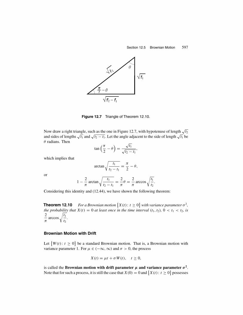
Section 12.5 Brownian Motion 597
1
2 1
2
_
_
Figure 12.7 Triangle of Theorem 12.10.
Now draw a right triangle, such as the one in Figure 12.7, with hypotenuse of length√
t2and sides of lengths
√t1 and
√t2 − t1. Let the angle adjacent to the side of length
√t1 be
θ radians. Then
tan(π
2− θ)
=√
t1√t2 − t1
,
which implies that
arctan
√t1
t2 − t1= π
2− θ,
or
1 − 2
πarctan
√t1
t2 − t1= 2
πθ = 2
πarccos
√t1
t2.
Considering this identity and (12.44), we have shown the following theorem:
Theorem 12.10 For a Brownian motion{X(t) : t ≥ 0
}with variance parameter σ 2,
the probability that X(t) = 0 at least once in the time interval (t1, t2), 0 < t1 < t2, is2
πarccos
√t1
t2.
Brownian Motion with Drift
Let{W(t) : t ≥ 0
}be a standard Brownian motion. That is, a Brownian motion with
variance parameter 1. For µ ∈ (−∞, ∞) and σ > 0, the process
X(t) = µt + σW(t), t ≥ 0,
is called the Brownian motion with drift parameter µ and variance parameter σ 2.Note that for such a process, it is still the case that X(0) = 0 and
{X(t) : t ≥ 0
}possesses
598 Chapter 12 Stochastic Processes
stationary and independent increments. However, for t > 0, X(t) is normal with meanµt and variance σ 2t .
For a Brownian motion{X(t) : t ≥ 0
}with drift parameter µ and variance parameter
σ 2, let ft |0(x|x0) be the conditional probability density function of X(t) given that X(0) =x0, or, equivalently, the conditional probability density function of X(t + t0) given thatX(t0) = x0. To find ft |0(x|x0), note that
P(X(t) ≤ x | X(0) = x0
) = P(µt + σW(t) ≤ x | σW(0) = x0
)= P
(W(t) ≤ x − µt
σ
∣∣ W(0) = x0
σ
)= P
(W(t) − W(0) ≤ x − x0 − µt
σ
∣∣ W(0) = x0
σ
).
Let Z ∼ N(0, 1); since W(t) − W(0) and W(0) are independent random variables, andW(t) − W(0) is N(0, t), this equation gives
P(X(t) ≤ x | X(0) = x0
) = P(W(t) − W(0) ≤ x − x0 − µt
σ
)
= P
(Z ≤
x − x0 − µt
σ− 0
√t
)=
(x − x0 − µt
σ√
t
).
Differentiating this equation with respect to x yields
ft |0(x|x0) = 1
σ√
t· 1√
2πexp
[−(x − x0 − µt
σ√
t
)2/2]
= 1
σ√
2πtexp
[−(x − x0 − µt)2
2σ 2t
],
which is the probability density function of a normal random variable with mean x0 +µt
and variance σ 2t .
Geometric Brownian Motion
As mentioned before, particles suspended in a liquid are constantly and incessantly underrandom collisions with nearby particles. As a result, they undergo unceasing motions ina totally erratic way, and the changes in each coordinate of the positions of a particle, ininfinitesimal time periods, form a Brownian motion. In finance, random fluctuations ofprices of shares of stocks, or other assets, are a result of an enormity of political, social,economical, and financial factors independently assessed by a large number of traders.For that reason financial scholars and consultants use Brownian motions as models forprices of assets in general and shares of stocks in particular. However, since such pricesare nonnegative and in the long run follow exponential growth or decay curves, they usea type of a stochastic process that is called geometric Brownian motion.

Section 12.5 Brownian Motion 599
Let{W(t) : t ≥ 0
}be a standard Brownian motion. Let X(t) = µt + σW(t) so that{
X(t) : t ≥ 0}
is a Brownian motion with drift parameter µ and variance parameter σ 2.The process
{V (t) : t ≥ 0
}defined by
V (t) = v0 exp[X(t)
] = v0 exp[µt + σW(t)
]is said to be a geometric Brownian motion with drift parameter µ and variance parameterσ 2. Clearly, W(0) = 0 implies that V (0) = v0.
Stock prices are often assumed to be Markov processes, since, usually, the price of astock in the future depends on its present value only. The past history of the value of astock and how it evolved to form the current price does not play a major role on the priceof the stock in the future. In the preceding geometric model, if V (t) is the price of somestock at t , then, for t0 < t1 < · · · < tn, the relations
V (ti)
V (ti−1)= exp
[µ(ti − ti−1)
] · exp[σ [W(ti) − W(ti−1)]
]show that
V (t1)
V (t0),
V (t2)
V (t1), . . . ,
V (tn)
V (tn−1),
the ratio changes of the price of the stock over nonoverlapping time intervals, are inde-pendent random variables.
We will now calculate the expected value and variance of V (t) given that V (0) = v0.To do so, let Z ∼ N(0, 1). We will first show that, for α ∈ (−∞, ∞),
E(eαZ) = eα2/2. (12.45)
This follows from the following calculations:
E(eαZ) =∫ ∞
−∞eαx · 1√
2πe−x2/2 dx
= eα2/2∫ ∞
−∞1√2π
e− 12 α2+αx− 1
2 x2dx
= eα2/2∫ ∞
−∞1√2π
e− 12 (x−α)2
dx = eα2/2,
where∫ ∞
−∞1√2π
e− 12 (x−α)2
dx = 1, since1√2π
e− 12 (x−α)2
is the probability density func-
tion of a normal random variable with mean α and variance 1.Using (12.45) and the fact that Z = W(t)/
√t ∼ N(0, 1), calculation of E
[V (t)
]and Var
[V (t)
]is straightforward. We have
E[V (t)
] = E[v0e
µt+σW(t)] = v0e
µtE(eσ
√tZ) = v0e
µt+ 12 σ 2t .

600 Chapter 12 Stochastic Processes
Also,
E[V (t)2
] = E[v2
0e2µt+2σW(t)
] = v20e
2µtE(e2σ
√tZ) = v2
0e2µt+2σ 2t .
Therefore,
Var[V (t)
] = E[V (t)2
]− E[V (t)
]2 = v20e
2µt+σ 2t (eσ 2t − 1).
Example 12.47 Let V (t) be the price of a stock, per share, at time t . Suppose thatthe stock’s current value, per share, is $40 with drift parameter $2 per year and varianceparameter 4.41. If
{V (t) : t ≥ 0
}is a geometric Brownian motion, what is the probability
that after 18 months the stock price, per share, exceeds $65?
Solution: Noting that√
4.41 = 2.1, we have
V (t) = 40e2t+2.1W(t),
where{W(t) : t ≥ 0
}is a standard Brownian motion. Hence W(t) ∼ N(0, t). The
desired probability is
P(V (1.5) > 65
) = P(40e2(1.5)+2.1W(1.5) > 65
)= P
(e2.1W(1.5) > 0.0809
) = P(W(1.5) > −1.197
)= P
(W(1.5) − 0√1.5
> −1.197√1.5
)= P(Z > −0.98)
= 1 − (−0.98) = (0.98) = 0.8365. �
EXERCISES
A
1. Suppose that liquid in a container is placed in a coordinate system, and at time0, a pollen particle suspended in the liquid is at (0, 0, 0), the origin. Let Z(t)
be the z-coordinate of the position of the pollen after t minutes. Suppose that{Z(t) : t ≥ 0
}is a Brownian motion with variance parameter 9. Suppose that
after 5 minutes the z-coordinate of the pollen’s position is 0 again.
(a) What is the probability that after 10 minutes it is between −1/2 and 1/2?

Section 12.5 Brownian Motion 601
(b) If after seven minutes the z-coordinate of the pollen’s position is −1, findthe expected value and variance of the z-coordinate of the position of pollenafter six minutes.
2. Let{X(t) : t ≥ 0
}be a Brownian motion with variance parameter σ 2. Show that,
for all t > 0, |X(t)| and max0≤s≤t
X(s) are identically distributed.
3. Let{X(t) : t ≥ 0
}be a Brownian motion with variance parameter σ 2. For ε > 0,
show that limt→0
P( |X(t)|
t> ε)
= 1, whereas limt→∞ P
( |X(t)|t
> ε)
= 0.
4. Let{X(t) : t ≥ 0
}be a Brownian motion with variance parameter σ 2. Let Tα be
the time of hitting α first. Let Y ∼ N(0, σ 2/α2). Show that, for α > 0, Tα and1/Y 2 are identically distributed.
5. Let{X(t) : t ≥ 0
}be a Brownian motion with variance parameter σ 2. For a fixed
t > 0, let T be the smallest zero greater than t . Find the probability distributionfunction of T .
6. Let{X(t) : t ≥ 0
}be a Brownian motion with variance parameter σ 2. As we know,
for t1 and t2, t1 < t2, the random variables X(t1) and X(t2) are not independent.Find the distribution of X(t1) + X(t2).
7. Let{X(t) : t ≥ 0
}be a Brownian motion with variance parameter σ 2. For u > 0,
show thatE[X(t + u) | X(t)
] = X(t).
Therefore, for s > t , E[X(s) | X(t)
] = X(t).
8. Let{X(t) : t ≥ 0
}be a Brownian motion with variance parameter σ 2. For u > 0,
t ≥ 0, find E[X(t)X(t + u)
].
9. (Reflected Brownian Motion) Suppose that liquid in a cubic container isplaced in a coordinate system in such a way that the bottom of the container isplaced on the xy-plane. Therefore, whenever a particle reaches the xy-plane, itcannot cross the bottom of the container. So it reverberates back to the nonnegativeside of the z-axis. Suppose that at time 0, a particle is at (0, 0, 0), the origin. LetV (t) be the z-coordinate of the particle after t units of time. Find E
[V (t)
],
Var[V (t)
], and P
(V (t) ≤ z | V (0) = z0
).
Hint: Let{Z(t) : t ≥ 0
}be a Brownian motion with variance parameter σ 2.
Note that
V (t) ={
Z(t) if Z(t) ≥ 0
−Z(t) if Z(t) < 0.
The process{V (t) : t ≥ 0
}is called reflected Brownian motion.
10. Suppose that liquid in a cubic container is placed in a coordinate system. Supposethat at time 0, a particle is at (0, 0, 0), the origin. Let
(X(t), Y (t), Z(t)
)be the

602 Chapter 12 Stochastic Processes
coordinates of the particle after t units of time, and assume that X(t), Y (t), andZ(t) are independent Brownian motions, each with variance parameter σ 2. LetD(t) be the distance of the particle from the origin after t units of time. FindE[D(t)
].
11. Let V (t) be the price of a stock, per share, at time t . Suppose that the stock’scurrent value, per share, is $95.00 with drift parameter −$2 per year and varianceparameter 5.29. If
{V (t) : t ≥ 0
}is a geometric Brownian motion, what is the
probability that after 9 months the stock price, per share, is below $80?
REVIEW PROBLEMS
1. Jobs arrive at a file server at a Poisson rate of 3 per minute. If 10 jobs arrivedwithin 3 minutes, between 10:00 and 10:03, what is the probability that the lastjob arrived after 40 seconds past 10:02?
2. A Markov chain with transition probability matrix P = (pij ) is called regular, iffor some positive integer n, pn
ij > 0 for all i and j . Let {Xn : n = 0, 1, . . . } be aMarkov chain with state space {0, 1} and transition probability matrix
P =(
0 11 0
)Is {Xn : n = 0, 1, . . . } regular? Why or why not?
3. Show that the following matrices are the transition probability matrix of the sameMarkov chain with elements of the state space labeled differently.
P 1 =
⎛⎜⎜⎜⎜⎝2/5 0 0 3/5 01/3 1/3 0 1/3 00 0 1/2 0 1/2
1/4 0 0 3/4 00 0 1/3 0 2/3
⎞⎟⎟⎟⎟⎠ , P 2 =
⎛⎜⎜⎜⎜⎝2/5 3/5 0 0 01/4 3/4 0 0 00 0 1/2 1/2 00 0 1/3 2/3 0
1/3 1/3 0 0 1/3
⎞⎟⎟⎟⎟⎠ .
4. Let {Xn : n = 0, 1, . . . } be a Markov chain with state space {0, 1} and transitionprobability matrix
P =(
2/5 3/51/3 2/3
)Starting from 0, find the expected number of transitions until the first visit to 1.
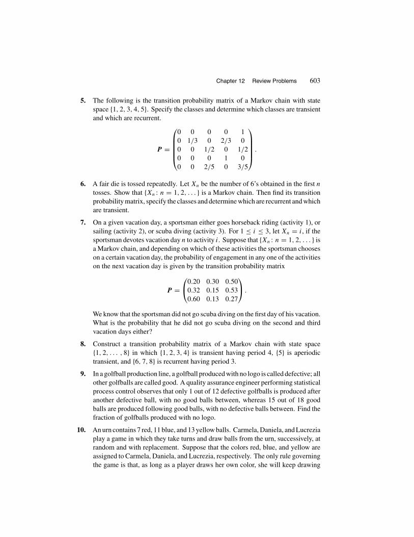
Chapter 12 Review Problems 603
5. The following is the transition probability matrix of a Markov chain with statespace {1, 2, 3, 4, 5}. Specify the classes and determine which classes are transientand which are recurrent.
P =
⎛⎜⎜⎜⎜⎝0 0 0 0 10 1/3 0 2/3 00 0 1/2 0 1/20 0 0 1 00 0 2/5 0 3/5
⎞⎟⎟⎟⎟⎠ .
6. A fair die is tossed repeatedly. Let Xn be the number of 6’s obtained in the first n
tosses. Show that {Xn : n = 1, 2, . . . } is a Markov chain. Then find its transitionprobability matrix, specify the classes and determine which are recurrent and whichare transient.
7. On a given vacation day, a sportsman either goes horseback riding (activity 1), orsailing (activity 2), or scuba diving (activity 3). For 1 ≤ i ≤ 3, let Xn = i, if thesportsman devotes vacation day n to activity i. Suppose that {Xn : n = 1, 2, . . . } isa Markov chain, and depending on which of these activities the sportsman chooseson a certain vacation day, the probability of engagement in any one of the activitieson the next vacation day is given by the transition probability matrix
P =⎛⎝0.20 0.30 0.50
0.32 0.15 0.530.60 0.13 0.27
⎞⎠ .
We know that the sportsman did not go scuba diving on the first day of his vacation.What is the probability that he did not go scuba diving on the second and thirdvacation days either?
8. Construct a transition probability matrix of a Markov chain with state space{1, 2, . . . , 8} in which {1, 2, 3, 4} is transient having period 4, {5} is aperiodictransient, and {6, 7, 8} is recurrent having period 3.
9. In a golfball production line, a golfball produced with no logo is called defective; allother golfballs are called good. A quality assurance engineer performing statisticalprocess control observes that only 1 out of 12 defective golfballs is produced afteranother defective ball, with no good balls between, whereas 15 out of 18 goodballs are produced following good balls, with no defective balls between. Find thefraction of golfballs produced with no logo.
10. An urn contains 7 red, 11 blue, and 13 yellow balls. Carmela, Daniela, and Lucreziaplay a game in which they take turns and draw balls from the urn, successively, atrandom and with replacement. Suppose that the colors red, blue, and yellow areassigned to Carmela, Daniela, and Lucrezia, respectively. The only rule governingthe game is that, as long as a player draws her own color, she will keep drawing
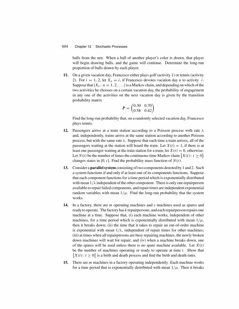
604 Chapter 12 Stochastic Processes
balls from the urn. When a ball of another player’s color is drawn, that playerwill begin drawing balls, and the game will continue. Determine the long-runproportion of balls drawn by each player.
11. On a given vacation day, Francesco either plays golf (activity 1) or tennis (activity2). For i = 1, 2, let Xn = i, if Francesco devotes vacation day n to activity i.Suppose that {Xn : n = 1, 2, . . . } is a Markov chain, and depending on which of thetwo activities he chooses on a certain vacation day, the probability of engagementin any one of the activities on the next vacation day is given by the transitionprobability matrix
P =(
0.30 0.700.58 0.42
)Find the long-run probability that, on a randomly selected vacation day, Francescoplays tennis.
12. Passengers arrive at a train station according to a Poisson process with rate λ
and, independently, trains arrive at the same station according to another Poissonprocess, but with the same rate λ. Suppose that each time a train arrives, all of thepassengers waiting at the station will board the train. Let X(t) = 1, if there is atleast one passenger waiting at the train station for a train; let X(t) = 0, otherwise.Let N(t) be the number of times the continuous-time Markov chain
{X(t) : t ≥ 0
}changes states in [0, t]. Find the probability mass function of N(t).
13. Consider a parallel system consisting of two components denoted by 1 and 2. Sucha system functions if and only if at least one of its components functions. Supposethat each component functions for a time period which is exponentially distributedwith mean 1/λ independent of the other component. There is only one repairpersonavailable to repair failed components, and repair times are independent exponentialrandom variables with mean 1/µ. Find the long-run probability that the systemworks.
14. In a factory, there are m operating machines and s machines used as spares andready to operate. The factory has k repairpersons, and each repairperson repairs onemachine at a time. Suppose that, (i) each machine works, independent of othermachines, for a time period which is exponentially distributed with mean 1/µ,then it breaks down; (ii) the time that it takes to repair an out-of-order machineis exponential with mean 1/λ, independent of repair times for other machines;(iii) at times when all repairpersons are busy repairing machines, the newly brokendown machines will wait for repair; and (iv) when a machine breaks down, oneof the spares will be used unless there is no spare machine available. Let X(t)
be the number of machines operating or ready to operate at time t . Show that{X(t) : t ≥ 0
}is a birth and death process and find the birth and death rates.
15. There are m machines in a factory operating independently. Each machine worksfor a time period that is exponentially distributed with mean 1/µ. Then it breaks

Chapter 12 Review Problems 605
down. The time that it takes to repair an out-of-order machine is exponential withmean 1/λ, independent of repair times for and operating times of other machines.For 0 ≤ i ≤ m, find the long-run proportion of time that there are exactly i
machines operating.
16. In Springfield, Massachusetts, people drive their cars to a state inspection center forannual safety and emission certification at a Poisson rate ofλ. Forn ≥ 0, if there aren cars at the center either being inspected or waiting to be inspected, the probabilityis 1/(n + 1) that an additional driver will join the queue. Hence the probabilityis n/(n + 1) that he or she will not join the queue and will leave. Suppose thatinspection times are independent and identically distributed exponential randomvariables with mean 1/µ and they are independent of the arrival process. Forn ≥ 0, find the probability that in the long run, at a random time, there are n carsat the center either being inspected or waiting to be inspected.
17. Consider a population of a certain colonizing species. Suppose that each individualproduces offspring at a Poisson rate of λ as long as it lives, and the time until thefirst individual arrives is exponential with mean 1/λ. If the lifetime of an individualin the population is exponential with mean 1/µ, starting with a single individual,find the expected length of time until the population size is 5.
18. (Death Process with Immigration) Consider a population of size n, n ≥0, of a certain species in which individuals do not reproduce. However, newindividuals immigrate into the population at a Poisson rate of γ . If the lifetime ofan individual in the population is exponential with mean 1/µ, find πi , i ≥ 0, thelong-run probability that the population size is i.
19. Suppose that liquid in a cubic container is placed in a coordinate system, and attime 0, a pollen particle suspended in the liquid is at (0, 0, 0), the origin. Let Y (t)
be the y-coordinate of the position of the pollen after t minutes. Suppose that theprocess
{Y (t) : t ≥ 0
}is a Brownian motion with variance parameter σ 2. For
0 < s < t , find E[Y (s) | Y (t) = y
]and Var
[Y (s) | Y (t) = y
].
20. Let{X(t) : t ≥ 0
}be a Brownian motion with variance parameter σ 2. For t, s > 0,
find E[X(s)X(t)
].
21. Let{X(t) : t ≥ 0
}be a Brownian motion with variance parameter σ 2. For t > 0,
let T be the smallest zero greater than t , and let U be the largest zero smaller thant . For x < t < y, find P(U < x and T > y).
22. Let V (t) be the price of a stock, per share, at time t . Suppose that{V (t) : t ≥ 0
}is a geometric Brownian motion with drift parameter $3 per year and varianceparameter 27.04. What is the probability that the price of this stock is at leasttwice its current price after two years?

Chapter 13
Simulation
13.1 INTRODUCTION
Solving a scientific or an industrial problem usually involves mathematical analysis and/orsimulation. To perform a simulation, we repeat an experiment a large number of timesto assess the probability of an event or condition occurring. For example, to estimatethe probability of at least one 6 occurring within four rolls of a die, we may do a largenumber of experiments rolling four dice and calculate the number of times that at leastone 6 is obtained. Similarly, to estimate the fraction of time that, in a certain bank all thetellers are busy, we may measure the lengths of such time intervals over a long period X,add them, and then divide by X. Clearly, in simulations, the key to reliable answers is toperform the experiment a large number of times or over a long period of time, whicheveris applicable. Since manually this is almost impossible, simulations are carried out bycomputers. Only computers can handle millions of operations in short periods of time.
To simulate a problem that involves random phenomena, generating random numbersfrom the interval (0, 1) is essential. In almost every simulation of a probabilistic model,wewill need to select random points from the interval (0, 1). For example, to simulate theexperiment of tossing a fair coin, we draw a random number from (0, 1). If it is in(0, 1/2), we say that the outcome is heads, and if it is in [1/2, 1), we say that it is tails.Similarly, in the simulation of die tossing, the outcomes 1, 2, 3, 4, 5, and 6, respectively,correspond to the events that the random point from (0, 1) is in (0, 1/6), [1/6, 1/3),[1/3, 1/2), [1/2, 2/3), [2/3, 5/6), and [5/6, 1).
As discussed in Section 1.7, choosing a random number from a given interval is,in practice, impossible. In real-world problems, to perform simulation we usepseudorandom numbers instead. To generate n pseudorandom numbers from a uni-form distribution on an interval (a, b), we take an initial value x0 ∈ (a, b), called theseed, and construct a function ψ so that the sequence {x1, x2, . . . , xn} ⊂ (a, b) obtainedrecursively from
xi+1 = ψ(xi), 0 ≤ i ≤ n − 1, (13.1)
satisfies certain statistical tests for randomness. (Choosing the tests and constructing the
606

Section 13.1 Introduction 607
function ψ are complicated matters beyond the scope of this book.) The function ψ takesa seed and generates a sequence of pseudorandom numbers in the interval (a, b). Clearly,in any pseudorandom number generating process, the numbers generated are roundedto a certain number of decimal places. Therefore, ψ can only generate a finite numberof pseudorandom numbers, which implies that, eventually, some xj will be generated asecond time. From that point on, by (13.1), a pitfall is that the same sequence of numbersthat appeared after xj ’s first appearance will reappear. Beyond that point, numbers arenot effectively random. One important aspect of the construction of ψ is that the secondappearance of any of the xj ’s is postponed as long as possible.
It should be noted that passing certain statistical tests for randomness does not meanthat the sequence {x1, x2, . . . , xn} is a randomly selected sequence from (a, b) in thetrue mathematical sense discussed in Section 1.7. It is quite surprising that there aredeterministic real-valued functions ψ that, for each i, generate an xi+1 that is completelydetermined by xi , and yet the sequence {x1, x2, . . . , xn} passes certain statistical tests forrandomness.
For convenience, throughout this chapter, in practical problems, by random numberwe simply mean pseudorandom number. In general, for good choices of ψ , the generatednumbers are usually sufficiently random for practical purposes.
Most of the computer languages and some scientific computer software are equippedwith subroutines that generate random numbers from intervals and from sets of integers.In Mathematica, from Wolfram Research, Inc. (http://www.wolfram.com), the commandRandom[ ] selects a random number from (0, 1), Random[Real, {a, b}] chooses arandom number from the interval (a, b), and Random [Integer, {m, m + n}] picks upan integer from {m, m + 1, m + 2, . . . , m + n} randomly. However, there are computerlanguages that are not equipped with a subroutine that generates random numbers, andthere are a few that are equipped with poor algorithms. As mentioned, it is difficult toconstruct good random number generators. However, an excellent reference for suchalgorithms is The Art of Computer Programming, Volume 2, Seminumerical Algorithms,3rd edition, by Donald E. Knuth (Addison-Wesley, 1998).
At this point, let us emphasize that the main goal of scientists and engineers is alwaysto solve a problem mathematically. It is a mathematical solution that is accurate, exact,and completely reliable. Simulations cannot take the place of a rigorous mathematicalsolution. They are widely used (a) to find good estimations for solutions of problems thateither cannot be modeled mathematically or whose mathematical models are too difficultto solve; (b) to get a better understanding of the behavior of a complicated phenomenon;and/or (c) to obtain a mathematical solution by acquiring insight into the nature of theproblem, its functions, and the magnitude and characteristics of its solution. Intuitively,it is clear why the results that are obtained by simulations are good. Theoretically, mostof them can be justified by the strong law of large numbers, as discussed in Section 11.4.
For a simulation in each of the following examples we have presented an algorithm, inEnglish, that can be translated into any programming language. Therefore, readers mayuse these algorithms to write and execute their own programs in their favorite computerlanguages.

608 Chapter 13 Simulation
Example 13.1 Two numbers are selected at random and without replacement fromthe set {1, 2, 3, . . . , �}. Write an algorithm for a computer simulation of approximatingthe probability that the difference of these numbers is at least k.
Solution: For a large number of times, say n, each time choose two distinct randomnumbers, a and b, from {1, 2, 3, . . . , �} and check to see if |a − b| ≥ k. In all of these n
experiments, let m be the number of those in which |a −b| ≥ k. Then m/n is the desiredapproximation. An algorithm follows.
STEP
1: Set i = 1;2: Set m = 0;3: While i ≤ n, do steps 4 to 7.4: Generate a random number a from {1, 2, . . . , �}.5: Generate a random number b from {1, 2, . . . , �}.6: If b = a, Goto step 5.7: If |a − b| ≥ k, then
Set m = m + 1;Set i = i + 1;Goto step 3.
elseSet i = i + 1;Goto step 3.
8: Set p = m/n;9: Output (p).
STOP
Since the exact answer to this problem, obtained by analytical methods, is the quantity(� − k)(� − k + 1)
2�(� − 1), any simulation result should be close to this number. �
Example 13.2 An urn contains 25 white and 35 red balls. Balls are drawn from the urnsuccessively and without replacement. Write an algorithm to approximate by simulationthe probability that at some instant the number of red and white balls drawn are equal (atie occurs).
Solution: For a large number of times n, we will repeat the following experiment andcount m, the number of times that at some instant a tie occurs. The desired quantity ism/n. To begin, let m = 0, w = 25, and r = 35. Generate a random number from (0, 1).
If it belongs to(
0,w
w + r
], a white ball is selected. Thus change w to w−1. Otherwise,
a red ball is drawn; thus change r to r − 1. Repeat this procedure and check each timeto see if 25 − w = 35 − r . If at some instance these two quantities are equal, change m

Section 13.1 Introduction 609
to m + 1 and start a new experiment. Otherwise, continue until either r = 0 or w = 0.An algorithm follows.
STEP
1: Set m = 0;2: Set i = 1;3: While i ≤ n, do steps 4 to 10.4: Set w = 25;5: Set r = 35;6: While r ≥ 0 and w ≥ 0 do steps 7 to 10.7: Generate a random number x from (0, 1).8: If x ≤ w/(w + r), then
Set w = w − 1;else
Set r = r − 1;9: If 25 − w = 35 − r , then
Set m = m + 1;Set i = i + 1;Goto step 3.
10: If r = 0 or w = 0, thenSet i = i + 1;Goto step 3.
11: Set p = m/n;12: Output (p).
STOP �
EXERCISES
1. A die is rolled successively until, for the first time, a number appears three con-secutive times. By simulation, determine the approximate probability that it takesat least 50 rolls before we accomplish this event.
2. In an election, the Democratic candidate obtained 3586 votes and the Republicancandidate obtained 2958. Use simulations to find the approximate probability thatthe Democratic candidate was ahead during the entire process of counting thevotes.Answer: Approximately 0.096.
3. The probability that a bank refuses to finance an applicant is 0.35. Using simu-lation, find the approximate probability that of 300 applicants more than 100 arerefused.
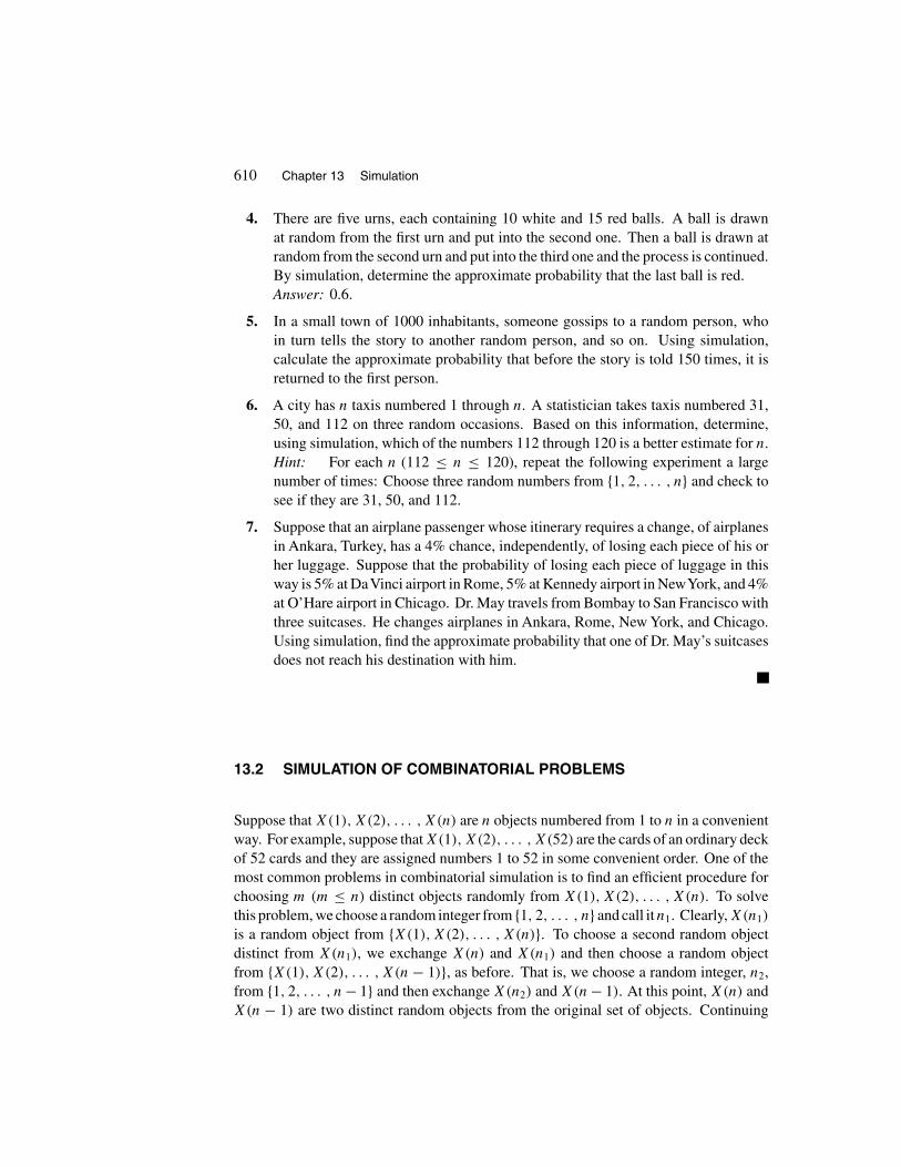
610 Chapter 13 Simulation
4. There are five urns, each containing 10 white and 15 red balls. A ball is drawnat random from the first urn and put into the second one. Then a ball is drawn atrandom from the second urn and put into the third one and the process is continued.By simulation, determine the approximate probability that the last ball is red.Answer: 0.6.
5. In a small town of 1000 inhabitants, someone gossips to a random person, whoin turn tells the story to another random person, and so on. Using simulation,calculate the approximate probability that before the story is told 150 times, it isreturned to the first person.
6. A city has n taxis numbered 1 through n. A statistician takes taxis numbered 31,50, and 112 on three random occasions. Based on this information, determine,using simulation, which of the numbers 112 through 120 is a better estimate for n.Hint: For each n (112 ≤ n ≤ 120), repeat the following experiment a largenumber of times: Choose three random numbers from {1, 2, . . . , n} and check tosee if they are 31, 50, and 112.
7. Suppose that an airplane passenger whose itinerary requires a change, of airplanesin Ankara, Turkey, has a 4% chance, independently, of losing each piece of his orher luggage. Suppose that the probability of losing each piece of luggage in thisway is 5% at DaVinci airport in Rome, 5% at Kennedy airport in NewYork, and 4%at O’Hare airport in Chicago. Dr. May travels from Bombay to San Francisco withthree suitcases. He changes airplanes in Ankara, Rome, New York, and Chicago.Using simulation, find the approximate probability that one of Dr. May’s suitcasesdoes not reach his destination with him.
13.2 SIMULATION OF COMBINATORIAL PROBLEMS
Suppose that X(1), X(2), . . . , X(n) are n objects numbered from 1 to n in a convenientway. For example, suppose that X(1), X(2), . . . , X(52) are the cards of an ordinary deckof 52 cards and they are assigned numbers 1 to 52 in some convenient order. One of themost common problems in combinatorial simulation is to find an efficient procedure forchoosing m (m ≤ n) distinct objects randomly from X(1), X(2), . . . , X(n). To solvethis problem, we choose a random integer from {1, 2, . . . , n} and call it n1. Clearly, X(n1)
is a random object from {X(1), X(2), . . . , X(n)}. To choose a second random objectdistinct from X(n1), we exchange X(n) and X(n1) and then choose a random objectfrom {X(1), X(2), . . . , X(n − 1)}, as before. That is, we choose a random integer, n2,from {1, 2, . . . , n − 1} and then exchange X(n2) and X(n − 1). At this point, X(n) andX(n − 1) are two distinct random objects from the original set of objects. Continuing
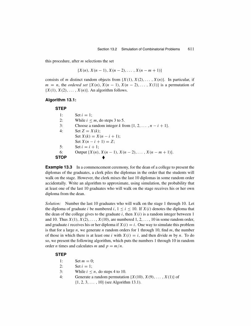
Section 13.2 Simulation of Combinatorial Problems 611
this procedure, after m selections the set
{X(n), X(n − 1), X(n − 2), . . . , X(n − m + 1)}consists of m distinct random objects from {X(1), X(2), . . . , X(n)}. In particular, ifm = n, the ordered set {X(n), X(n − 1), X(n − 2), . . . , X(1)} is a permutation of{X(1), X(2), . . . , X(n)}. An algorithm follows.
Algorithm 13.1:
STEP
1: Set i = 1;2: While i ≤ m, do steps 3 to 5.3: Choose a random integer k from {1, 2, . . . , n − i + 1}.4: Set Z = X(k);
Set X(k) = X(n − i + 1);Set X(n − i + 1) = Z;
5: Set i = i + 1;6: Output {X(n), X(n − 1), X(n − 2), . . . , X(n − m + 1)}.
STOP �
Example 13.3 In a commencement ceremony, for the dean of a college to present thediplomas of the graduates, a clerk piles the diplomas in the order that the students willwalk on the stage. However, the clerk mixes the last 10 diplomas in some random orderaccidentally. Write an algorithm to approximate, using simulation, the probability thatat least one of the last 10 graduates who will walk on the stage receives his or her owndiploma from the dean.
Solution: Number the last 10 graduates who will walk on the stage 1 through 10. Letthe diploma of graduate i be numbered i, 1 ≤ i ≤ 10. If X(i) denotes the diploma thatthe dean of the college gives to the graduate i, then X(i) is a random integer between 1and 10. Thus X(1), X(2), . . . , X(10), are numbered 1, 2, . . . , 10 in some random order,and graduate i receives his or her diploma if X(i) = i. One way to simulate this problemis that for a large n, we generate n random orders for 1 through 10, find m, the numberof those in which there is at least one i with X(i) = i, and then divide m by n. To doso, we present the following algorithm, which puts the numbers 1 through 10 in randomorder n times and calculates m and p = m/n.
STEP
1: Set m = 0;2: Set i = 1;3: While i ≤ n, do steps 4 to 10.4: Generate a random permutation {X(10), X(9), . . . , X(1)} of
{1, 2, 3, . . . , 10} (see Algorithm 13.1).

612 Chapter 13 Simulation
5: Set k = 0;6: Set j = 1;7: While j ≤ 10, do step 8.8: If X(j) = j , then
Set j = 11;Set k = 1;
elseSet j = j + 1.
9: Set m = m + k;10: Set i = i + 1;11: Set p = m/n;12: Output (p).
STOP
A simulation program based on this algorithm was executed for several values of n. Thecorresponding values of p were as follows:
n p
10 0.70001,000 0.6090
10,000 0.6340100,000 0.6326
For comparison, it is worthwhile to mention that the mathematical solution of this prob-lem, up to four decimal points, gives 0.6321 (see Example 2.24). �
EXERCISES
Warning: In some combinatorial probability problems, the desired quantity is very small.For this reason, in simulations, the number of experiments should be very large to getgood approximations.
1. Suppose that 18 customers stand in a line at a boxoffice, nine with $5 bills andnine with $10 bills. Each ticket costs $5, and the box office has no money initially.Write a simulation program to calculate an approximate value for the probabilitythat none of the customers has to wait for change.
2. A cereal company puts exactly one of its 20 prizes into every box of its cereals atrandom.
(a) Julie bought 50 boxes of cereals from this company. Write a simulationprogram to calculate an approximate value of the probability that she getsall 20 prizes.

Section 13.2 Simulation of Combinatorial Problems 613
(b) Suppose that Jim wants to have at least a 50% chance of getting all 20prizes. Write a simulation program to calculate the approximate value ofthe minimum number of cereal boxes that he should buy.
3. Nine students lined up in some order and had their picture taken. One year later, thesame students lined up again in random order and had their picture taken. Usingsimulation, find an approximate probability that, the second time, no student wasstanding next to the one next to whom he or she was standing the previously.
4. Use simulation to find an approximate value for the probability that, in a class of50, exactly four students have the same birthday and the other 46 students all havedifferent birthdays. Assume that the birth rates are constant throughout the yearand that each year has 365 days.
5. Using simulation, find the approximate probability that at least four students ofa class of 87 have the same birthday. Assume that the birth rates are constantthroughout the year and that each year has 365 days.Answer: Approximately 0.4998.
6. Suppose that two pairs of the vertices of a regular 10-gon are selected at randomand connected. Using simulations, find the approximate probability that they donot intersect.Hint: The exact value of the desired probability is
1
11
(20
10
)(
20
2
)(18
2
) ≈ 0.58.
7. Every day during the last 10 days, an executive wrote seven letters and his secretaryprepared seven envelopes for the letters. The secretary kept envelopes of eachday in chronological order in a packet, but she forgot to insert the letters in theenvelopes. Today, the secretary finds out that all 70 letters and all 10 packets ofenvelopes are mixed up. If she selects packets of envelopes at random and insertsrandomly chosen letters into the envelopes of each packet, what is the approximateprobability, obtained by using simulation, that none of the letters is addressedcorrectly? Note that the envelopes within a packet are left in chronological orderbut the packets themselves are mixed up.Answer: Approximately 0.53416. For an analytic discussion of this problem, seethe article by Steve Fisk in the April 1988 issue of Mathematics Magazine.

614 Chapter 13 Simulation
13.3 SIMULATION OF CONDITIONAL PROBABILITIES
Let S be the sample space of an experiment and A and B be two events of S withP(B) > 0. To find approximate values for P(A | B), using computer simulation, weeither reduce the sample space to B and then calculate P(AB) in the reduced samplespace, or we use the formula P(A | B) = P(AB)/P (B). In the latter case, we performthe experiment a large number of times, find n and m, the number of times in whichB and AB occur, respectively, and then divide m by n. In the former case, P(AB) isestimated simply by performing the experiment n times in the reduced sample space, fora large n, finding m, the number of those in which AB occurs, and dividing m by n. Weillustrate this method by Example 13.4, and the other method by Example 13.5.
Example 13.4 From an ordinary deck of 52 cards, 10 cards are drawn at random. Ifexactly four are hearts, write an algorithm to approximate by simulation the probabilityof at least two spades.
Solution: The problem in the reduced sample space is as follows: A deck of cardsconsists of 13 spades, 13 clubs, and 13 diamonds, but only 9 hearts. If six cards aredrawn at random, what is the probability that none of them is a heart and that two ormore are spades? To simulate this problem, suppose that hearts are numbered 1 to 9,spades 10 to 22, clubs 23 to 35, and diamonds 36 to 48. For a large number of times,say n, each time choose six distinct random integers between 1 and 48 and check to seeif there are no numbers between 1 and 9 and at least two numbers between 10 and 22.Let m be the number of those draws satisfying both conditions; then m/n is the desiredapproximation. For sufficiently large n, the final answer of any accurate simulation isclose to 0.42. An algorithm follows:
STEP
1: Set k = 1;2: Set m = 0;3: While k ≤ n, do steps 4 to 13.4: Choose six distinct numbers X(1), X(2), . . . , X(6) randomly
from {1, 2, . . . , 48} (see Algorithm 13.1, Section 13.2).5: For j = 1 to 6, do steps 6 and 7.6: For l = 1 to 9, do step 7.7: If X(j) = l, then
Set k = k + 1;Goto step 3.
8: Set s = 0;9: For j = 1 to 6, do steps 10 to 12.
10: For l = 10 to 22, do steps 11 and 12.11: If X(j) = l, then
Set s = s + 1;
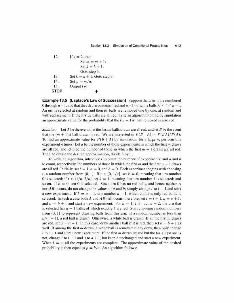
Section 13.3 Simulation of Conditional Probabilities 615
12: If s = 2, thenSet m = m + 1;Set k = k + 1;Goto step 3.
13: Set k = k + 1; Goto step 3.14: Set p = m/n.15: Output (p).
STOP �
Example 13.5 (Laplace’s Law of Succession) Suppose that u urns are numbered0 through u−1, and that the ith urn contains i red and u−1−i white balls, 0 ≤ i ≤ u−1.An urn is selected at random and then its balls are removed one by one, at random andwith replacement. If the first m balls are all red, write an algorithm to find by simulationan approximate value for the probability that the (m + 1)st ball removed is also red.
Solution: Let A be the event that the first m balls drawn are all red, and let B be the eventthat the (m + 1)st ball drawn is red. We are interested in P(B | A) = P(BA)/P (A).
To find an approximate value for P(B | A) by simulation, for a large n, perform thisexperiment n times. Let a be the number of those experiments in which the first m drawsare all red, and let b be the number of those in which the first m + 1 draws are all red.Then, to obtain the desired approximation, divide b by a.
To write an algorithm, introduce i to count the number of experiments, and a and b
to count, respectively, the numbers of those in which the first m and the first m+ 1 drawsare all red. Initially, set i = 1, a = 0, and b = 0. Each experiment begins with choosingt , a random number from (0, 1). If t ∈ (0, 1/u], set k = 0, meaning that urn number0 is selected; if t ∈ (1/u, 2/u], set k = 1, meaning that urn number 1 is selected; andso on. If k = 0, urn 0 is selected. Since urn 0 has no red balls, and hence neither A
nor AB occurs, do not change the values of a and b; simply change i to i + 1 and starta new experiment. If k = u − 1, urn number u − 1, which contains only red balls, isselected. In such a case both A and AB will occur; therefore, set i = i + 1, a = a + 1,
and b = b + 1 and start a new experiment. For k = 1, 2, 3, . . . , u − 2, the urn thatis selected has u − 1 balls, of which exactly k are red. Start choosing random numbersfrom (0, 1) to represent drawing balls from this urn. If a random number is less thank/(u − 1), a red ball is drawn. Otherwise, a white ball is drawn. If all the first m drawsare red, set a = a + 1. In this case, draw another ball if it is red, then set b = b + 1 aswell. If among the first m draws, a white ball is removed at any draw, then only changei to i + 1 and start a new experiment. If the first m draws are red but the (m + 1)st one isnot, change i to i + 1 and a to a + 1, but keep b unchanged and start a new experiment.When i = n, all the experiments are complete. The approximate value of the desiredprobability is then equal to p = b/a. An algorithm follows:

616 Chapter 13 Simulation
STEP
1: Set i = 1;2: Set a = 0;3: Set b = 0;4: While i ≤ n, do steps 5 to 20.5: Generate a random number t from (0, 1).6: Set r = 1;7: While r ≤ u, do step 8.8: If t ≤ r/u, then
Set k = r − 1;Set r = u + 1;
elseSet r = r + 1;
9: If k = 0, thenSet i = i + 1;Goto step 4.
10: If k = u − 1, thenSet i = i + 1;Set a = a + 1;Set b = b + 1;Goto step 4.
11: Set j = 0;12: While j < m, do steps 13 and 14.13: Generate a random number r from (0, 1).14: If r < k/(u − 1), then
Set j = j + 1;else
Set j = m + 1;15: If j �= m, then
Set i = i + 1;Goto step 4.
16: If j = m, then do steps 17 to 19.17: Set a = a + 1;18: Generate a random number r from (0, 1).19: If r < k/(u − 1), then
Set b = b + 1;20: Set i = i + 1;21: Set p = b/a.22: Output (p).
STOP
A sample run of a simulation program based on this algorithm gives us the following

Section 13.4 Simulation of Random Variables 617
results for n = 1000 and m = 5:
u 2 10 50 100 200 500 1000 2000 5000
p 1 0.893 0.886 0.852 0.852 0.848 0.859 0.854 0.853
It can be shown that, if the number of urns is large, the answer is approximately(m + 1)/(m + 2) = 6/7 ≈ 0.857 (see Exercise 44 of Section 3.5). Hence the results ofthese simulations are quite good. �
EXERCISES
1. An ordinary deck of 52 cards is dealt among A, B, C, and D, 13 each. If A andB have a total of six hearts and five spades, using computer simulation find anapproximate value for the probability that C has two of the remaining seven heartsand three of the remaining eight spades.
2. From families with five children, a family is selected at random and found to have aboy. Using computer simulation, find the approximate value of the probability thatthe family has three boys and two girls and that the middle child is a boy. Assumethat, in a five-child family, all gender distributions have equal probabilities.
3. In Example 13.5, Laplace’s law of succession, suppose that, among the first m
balls drawn, r are red and m − r are white. Using computer simulation, find theapproximate probability that the (m + 1)st ball is red.
4. TargetsA and B are placed on a wall. It is known that for every shot the probabilitiesof hitting A and hitting B with a missile are, respectively, 0.3 and 0.4. If target Awas not hit in an experiment, use simulation to calculate an approximate value forthe probability that target B was hit. (The exact answer is 4/ 7. Hence the resultof simulation should be close to 4/ 7 ≈ 0.571.)
13.4 SIMULATION OF RANDOM VARIABLES
Let X be a random variable over the sample space S. To approximate E(X) by simulation,we use the strong law of large numbers. That is, for a large n, we repeat the experimentover which X is defined independently n times. Each time we will find the value ofX. We then add the n values obtained and divide the result by n. For example, in theexperiment of rolling a die, let X be the following random variable:
X ={
1 if the outcome is 6
0 if the outcome is not 6.
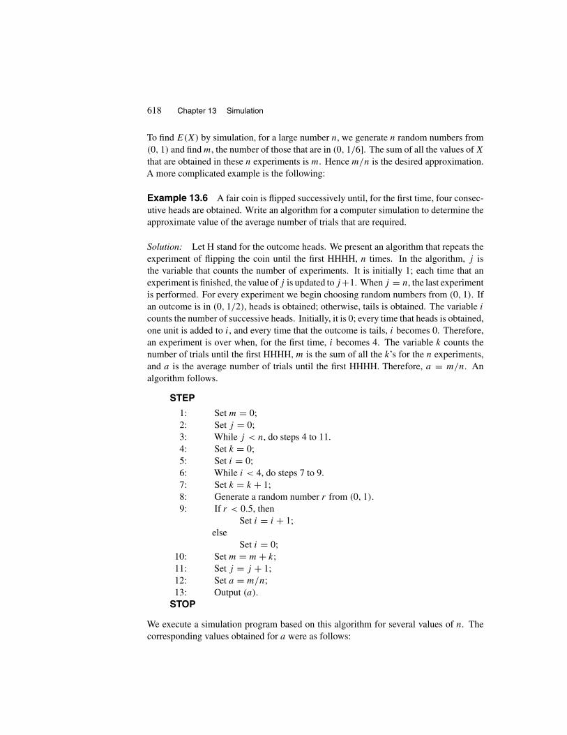
618 Chapter 13 Simulation
To find E(X) by simulation, for a large number n, we generate n random numbers from(0, 1) and find m, the number of those that are in (0, 1/6]. The sum of all the values of X
that are obtained in these n experiments is m. Hence m/n is the desired approximation.A more complicated example is the following:
Example 13.6 A fair coin is flipped successively until, for the first time, four consec-utive heads are obtained. Write an algorithm for a computer simulation to determine theapproximate value of the average number of trials that are required.
Solution: Let H stand for the outcome heads. We present an algorithm that repeats theexperiment of flipping the coin until the first HHHH, n times. In the algorithm, j isthe variable that counts the number of experiments. It is initially 1; each time that anexperiment is finished, the value of j is updated to j +1. When j = n, the last experimentis performed. For every experiment we begin choosing random numbers from (0, 1). Ifan outcome is in (0, 1/2), heads is obtained; otherwise, tails is obtained. The variable i
counts the number of successive heads. Initially, it is 0; every time that heads is obtained,one unit is added to i, and every time that the outcome is tails, i becomes 0. Therefore,an experiment is over when, for the first time, i becomes 4. The variable k counts thenumber of trials until the first HHHH, m is the sum of all the k’s for the n experiments,and a is the average number of trials until the first HHHH. Therefore, a = m/n. Analgorithm follows.
STEP
1: Set m = 0;2: Set j = 0;3: While j < n, do steps 4 to 11.4: Set k = 0;5: Set i = 0;6: While i < 4, do steps 7 to 9.7: Set k = k + 1;8: Generate a random number r from (0, 1).
9: If r < 0.5, thenSet i = i + 1;
elseSet i = 0;
10: Set m = m + k;11: Set j = j + 1;12: Set a = m/n;13: Output (a).
STOP
We execute a simulation program based on this algorithm for several values of n. Thecorresponding values obtained for a were as follows:

Section 13.4 Simulation of Random Variables 619
n a n a
5 23.80 5,000 29.9050 27.22 50,000 30.00
500 29.28 500,000 30.03
It can be shown that the exact answer to this problem is 30 (see the subsection “PatternAppearance" in Section 10.1). Therefore, these simulation results for n ≥ 5000 are quitegood. �
To simulate a Bernoulli random variable X with parameter p, generate a randomnumber from (0, 1). If it is in (0, p], let X = 1; otherwise, let X = 0. To simulatea binomial random variable Y with parameters (n, p), choose n independent randomnumbers from (0, 1), and let Y be the number of those that lie in (0, p]. To simulate ageometric random variable T with parameter p, we may keep choosing random pointsfrom (0, 1) until for the first time a number selected lies in (0, p]. The number ofrandom points selected is a simulation of T . However, this method of simulating T isvery inefficient. By the following theorem, T can be simulated most efficiently, namely,by just choosing one random point from (0, 1).
Theorem 13.1 Let r be a random number from the interval (0, 1) and let
T = 1 +[ ln r
ln(1 − p)
], 0 < p < 1,
where by [x] we mean the largest integer less than or equal to x. Then T is a geometricrandom variable with parameter p.
Proof: For all n ≥ 1,
P(T = n) = P(
1 +[ ln r
ln(1 − p)
]= n
)= P
([ ln r
ln(1 − p)
]= n − 1
)= P
(n − 1 ≤ ln r
ln(1 − p)< n
)= P
((n − 1) ln(1 − p) ≥ ln r > n ln(1 − p)
)= P
(ln(1 − p)n−1 ≥ ln r > ln(1 − p)n
)= P
((1 − p)n−1 ≥ r > (1 − p)n
) = (1 − p)n−1 − (1 − p)n
= (1 − p)n−1[1 − (1 − p)
] = (1 − p)n−1p,
which shows that T is geometric with parameter p. �

620 Chapter 13 Simulation
Therefore,
To simulate a geometric random variable T with parameter p,0 < p < 1, all we must do is to choose a point r at random from(0, 1) and let T = 1 + [ ln r/ ln(1 − p)
].
Let X be a negative binomial random variable with parameters (n, p), 0 < p < 1. ByExample 10.7, X is a sum of n independent geometric random variables. Thus
To simulate X, a negative binomial random variable with parameters(n, p), 0 < p < 1, it suffices to choose n independent random num-bers r1, r2, . . . , rn from (0, 1) and let
X =n∑
i=1
(1 +
[ ln ri
ln(1 − p)
]).
We now explain simulation of continuous random variables. The following theoremis a key to simulation of many special continuous random variables.
Theorem 13.2 Let X be a continuous random variable with probability distributionfunction F . Then F(X) is a uniform random variable over (0, 1).
Proof: Let S be the sample space over which X is defined. The functions X : S → Rand F : R → [0, 1] can be composed to obtain the random variable F(X) : S → [0, 1].Clearly,
P(F(X) ≤ t
) ={
1 if t ≥ 1
0 if t ≤ 0.
Let t ∈ (0, 1); it remains to prove that P(F(X) ≤ t
) = t . To do so, note that since F iscontinuous, F(−∞) = 0, and F(∞) = 1, the inverse image of t , F−1
({t}), is nonempty.We know that F is nondecreasing; since F is not necessarily strictly increasing, F−1
({t})might have more than one element. For example, if F is the constant t on some interval(a, b) ⊆ (0, 1), then F(x) = t for all x ∈ (a, b), implying that (a, b) is contained inF−1
({t}). Let x0 = inf{x : F(x) > t
}. Then F(x0) = t and F(x) ≤ t if and only if
x ≤ x0. Therefore,
P(F(X) ≤ t
) = P(X ≤ x0) = F(x0) = t.
We have shown that
P(F(X) ≤ t
) =
⎧⎪⎪⎨⎪⎪⎩0 if t ≤ 0
t if 0 ≤ t ≤ 1
1 if t ≥ 1,
meaning that F(X) is uniform over (0, 1). �

Section 13.4 Simulation of Random Variables 621
Based on this theorem, to simulate a continuous random variable X with strictlyincreasing probability distribution function F , it suffices to generate a random numberu from (0, 1) and then solve the equation F(t) = u for t . The solution t to this equation,F−1(u), is unique because F is strictly increasing. It is a simulation of X. For example,let X be an exponential random variable with parameter λ. Since F(t) = 1 − e−λt andthe solution to 1−e−λt = u is t = −1/λ ln(1−u), we have that, for any random numberu from (0, 1), the quantity −1/λ ln(1 − u) is a simulation of X. But, if u is a randomnumber from (0, 1), then (1 − u) is also a random number from (0, 1). Therefore,
−1
λln[1 − (1 − u)
] = −1
λln u
is also a simulation of X. So
To simulate an exponential random variable X with parameter λ, itsuffices to generate a random number u from (0, 1) and then calculate−(1/λ)ln u.
The method described is called the inverse transformation method and is good when-ever the equation F(t) = u can be solved without complications.
As we know, there are close relations between Poisson processes and exponentialrandom variables and also between exponential and gamma random variables. Theserelations enable us to use the results obtained for simulation of the exponential case
[e.g.,
to simulate Poisson processes and gamma random variables with parameters (n, λ), n
being a positive integer]. Let X be a gamma random variable with such parameters. Then
X = X1 + X2 + · · · + Xn, where Xi’s (i = 1, 2, . . . , n) are independent exponentialrandom variables each with parameter λ. Hence
If u1, u2, . . . , un are n independent random numbers generated from(0, 1), then
n∑i=1
−1
λln ui = −1
λln(u1u2 · · · un)
is a simulation of a gamma random variable with parameters (n, λ).
To simulate a Poisson process{N(t) : t ≥ 0
}with parameter λ, note that N(t) is the
number of “events” that have occurred at or prior to t . Let X1 be the time of the firstevent, X2 be the elapsed time between the first and second events, X3 be the elapsed timebetween the second and third events, and so on. Then the sequence {X1, X2, . . . } is anindependent sequence of exponential random variables, each with parameter λ. Clearly,
N(t) = max{n : X1 + X2 + · · · + Xn ≤ t}.

622 Chapter 13 Simulation
Let U1, U2, . . . be independent uniform random variables from (0, 1); then
N(t) = max{n : − 1
λln U1 − 1
λln U2 − · · · − 1
λln Un ≤ t
}= max
{n : − ln(U1U2 · · · Un) ≤ λt
}= max
{n : ln(U1U2 · · · Un) ≥ −λt
}= max{n : U1U2 · · · Un ≥ e−λt}.
This implies thatN(t) + 1 = min{n : U1U2 · · · Un < e−λt}.
We have the following:
Let{N(t) : t ≥ 0
}be a Poisson process with rate λ. To simulate N(t),
we keep generating random numbers u1, u2, . . . from (0, 1) until, forthe first time, u1u2 · · · un is less than e−λt . The number of randomnumbers generated minus 1 is a simulation of N(t).
Let N be a Poisson random variable with parameter λ. Since N has the same dis-tribution as N(1), to simulate N all we have to do is to simulate N(1) as explainedpreviously.
The inverse transformation method is not appropriate for simulation of normal randomvariables. This is because there is no closed form for F , the distribution function ofa normal random variable, and hence, in general, F(t) = u cannot be solved for t .However, other methods can be used to simulate normal random variables. Among themthe following, introduced by Box and Muller, is perhaps the simplest. It is based on thenext theorem, proved in Example 8.27.
Theorem 13.3 Let V and W be two independent uniform random variables over(0, 1). Then the random variables
Z1 = cos(2πV )√−2 ln W
and
Z2 = sin(2πV )√−2 ln W
are independent standard normal random variables.
Based on this theorem,
To simulate the standard normal random variable Z, we may generatetwo independent random numbers v and w from (0, 1) and let z =cos(2πv)
√−2 ln w. The number z is then a simulation of Z.

Section 13.4 Simulation of Random Variables 623
The advantage of Box and Muller’s method is that it can generate two independentstandard normal random variables at the same time. Its disadvantage is that it is notefficient.
As for an arbitrary normal random variable, suppose that X ∼ N(µ, σ 2). Then, sinceZ = (X − µ)/σ is standard normal, we have that X = σZ + µ. Thus
If X is a normal random variable with parameters µ and σ 2, to simulateX, we may generate two independent random numbers v and w from(0, 1) and let t = σ cos(2πv)
√−2 ln w + µ. The quantity t is then asimulation of X.
Example 13.7 Passengers arrive at a train station according to a Poisson process, withparameter λ. If the arrival time of the next train is uniformly distributed over the interval(0, T ), write an algorithm to approximate by simulation the probability that by the timethe next train arrives there are at least N passengers at the station. Solution: For a
large positive integer n, we generate n independent random numbers t1, t2, . . . , tn from(0, T ). Then for each ti we simulate a Poisson random variable Xi with parameter λti .Finally, we find m, the number of Xi’s that are greater than or equal to N . The desiredapproximation is p = m/n. An algorithm follows.
STEP
1: Set m = 0.2: Do steps 3 to 5 n times.3: Generate a random number t from (0, T ).4: Generate a Poisson random variable X with parameter λt .5: If X ≥ N , then set m = m + 1.
6: Set p = m/n.
7: Output (p).STOP �
Example 13.8 Let us assume that the time between any two earthquakes in town Aand the time between any two earthquakes in town B are exponentially distributed withmeans 1/λ1 and 1/λ2, respectively. Write an algorithm to approximate by simulationthe probability that the next earthquake in town B occurs prior to the next earthquake intown A.
Solution: Let X and Y denote the times between now and the next earthquakes in townA and town B, respectively. For a large n, let n be the total number of simulations ofthe times of the next earthquakes in town A and town B. If m is the number of thosesimulations in which X > Y , then p = P(X > Y) is approximately m/n. An algorithmfollows.

624 Chapter 13 Simulation
STEP
1: m = 0.
2: Do steps 3 to 5, n times.3: Generate an exponential random variable X with parameter λ1.4: Generate an exponential random variable Y with parameter λ2.5: If X > Y , then set m = m + 1.6: Set p = m/n.7: Output (p).
STOP �
Example 13.9 The grade distributions of students in calculus, statistics, music, com-puter programming, and physical education are, respectively, N(70, 400), N(75, 225),N(80, 400), N(75, 400), and N(85, 100). Write an algorithm to approximate by simu-lation the probability that the median of the grades of a randomly selected student takingthese five courses is at least 75.
Solution: Let X(1), X(2), X(3), X(4), and X(5) be the grades of the randomly selectedstudent in calculus, statistics, music, computer programming, and physical education,respectively. Let X be the median of these grades. We will simulate X(1) through X(5),n times. Each time we calculate X by sorting X(1), X(2), X(3), X(4), and X(5) andletting X = X(3). Then we check to see if X is at least 75. In all these n simulations,let m be the total number of X’s that are at least 75; m/n is the desired approximation.An algorithm follows.
STEP
1: Set m = 0.
2: Do steps 3 to 12 n times.3: Generate X(1) ∼ N(70, 400).
4: Generate X(2) ∼ N(75, 225).
5: Generate X(3) ∼ N(80, 400).
6: Generate X(4) ∼ N(75, 400).
7: Generate X(5) ∼ N(85, 100).
8: Do steps 9 and 10 for L = 1 to 3.9: Do step 10 for j = 1 to 5-L.
10: If X(j) > X(j + 1), thenSet K = X(j + 1);Set X(j + 1) = X(j);Set X(j) = K .
11: Set X = X(3).
12: If X ≥ 75, set m = m + 1.
13: Set p = m/n.
14: Output (p).STOP �

Section 13.4 Simulation of Random Variables 625
EXERCISES
1. Let X be a random variable with probability distribution function
F(x) =
⎧⎪⎪⎨⎪⎪⎩x − 3
x − 2if x ≥ 3
0 elsewhere.
Develop a method to simulate X.
2. Explain how a random variable X with the following probability density functioncan be simulated:
f (x) = e−2|x|, −∞ < x < +∞.
3. Explain a procedure for simulation of lognormal random variables. A randomvariable X is called lognormal with parameters µ and σ 2 if ln X ∼ N(µ, σ 2)
4. Use the result of Example 11.11 to explain how a gamma random variable withparameters (n/2, 1/2), n being a positive integer, can be simulated.
5. It can be shown that the median of (2n + 1) random numbers from the interval(0, 1) is a beta random variable with parameters (n+1, n+1). Use this property tosimulate a beta random variable with parameters (n+ 1, n+ 1), n being a positiveinteger.
6. Suppose that in a community the distributions of the heights of men and women,in centimeters, are N(173, 40) and N(160, 20), respectively. Write an algorithmto calculate by simulation the approximate value of the probability that (a) a wifeis taller than her husband; (b) a husband is at least 10 centimeters taller than hiswife.
7. Mr. Jones is at a train station, waiting to make a phone call. There are two publictelephone booths next to each other and occupied by two persons, say A andB. If the duration of each telephone call is an exponential random variable withλ = 1/8, using simulation, approximate the probability that among Mr. Jones, A,and B, Mr. Jones is not the last person to finish his call.
8. The distributions of students’grades for probability and calculus at a certain univer-sity are, respectively, N(65, 400) and N(72, 450). Dr. Olwell teaches a calculusclass with 28 and a probability class with 22 students. Write an algorithm to sim-ulate the probability that the difference between the averages of the final grades of

626 Chapter 13 Simulation
the classes of Dr. Olwell is at least 2.Hint: Note that if X1, X2, . . . , Xn are all N(µ, σ 2), then
X = X1 + X2 + · · · + Xn
n∼ N
(µ,
σ 2
n
).
13.5 MONTE CARLO METHOD
As explained in Section 8.1, if S is a subset of the plane with area A(S) and R is a subsetof S with area A(R), the probability that a random point from S falls in R is equal toA(R)/A(S). This important fact gives an excellent algorithm, called the Monte Carlomethod, for finding the area under a bounded curve y = f (x) by simulation. Supposethat we want to estimate I , the area under y = f (x), from x = a to x = b of Figure 13.1.To do so, we first construct a rectangle [a, b] × [0, d] that includes the region undery = f (x) from a to b as a subset. Then for a large integer n, we choose n random pointsfrom [a, b]× [0, d] and count m, the number of those that lie below the curve y = f (x).Now the probability that a random point from [a, b]×[0, d] is under the curve y = f (x)
is approximately m/n. Thus
m
n≈ area under f (x) from a to b
area of the rectangle [a, b] × [0, d] = I
(b − a)(d − 0)= I
(b − a)d,
and hence
I ≈ md(b − a)
n.
x
y
y = f (x)
a b
d
0
_______
Figure 13.1 Area under f to be calculated, using the Monte Carlo method.

Section 13.5 Monte Carlo Method 627
This method of simulation was introduced by the Hungarian-born American math-ematician John von Neumann (1903–1957), and Stanislaw Ulam (1909–1984). Theyused it during World War II to study the extent that neutrons can travel through variousmaterials. Since their studies were classified, von Neumann gave it the code name MonteCarlo method. An algorithm for this procedure is as follows.
STEP
1: Set m = 0;2: Set i = 1;3: While i ≤ n, do steps 4 to 6.4: Generate a random number x from [a, b].5: Generate a random number y from [0, d].6: If y < f (x), then
Set i = i + 1;Set m = m + 1;
elseSet i = i + 1.
7: Set I = [md(b − a)]/n.
8: Output (I ).
STOP �
Example 13.10 (Buffon’s Needle Problem Revisited) In Example 8.14, weexplained one of the most interesting problems of geometric probability, Buffon’s needleproblem: A plane is ruled with parallel lines a distance d apart. If a needle of length �,� < d, is tossed at random onto the plane, then the probability that the needle intersectsone of the parallel lines is 2�/πd. This formula has been used throughout the history ofprobability to determine approximate values for π . For fixed and predetermined valuesof d and �, � < d , rule a plane with parallel lines a distant d apart, and toss a needleof length �, n times; then count m, the number of times that the needle intersects aline. Then m/n determines an approximate value for the probability that the needleintersects a line, provided that n is a large number. Thus 2 �/πd ≈ m/n and henceπ ≈ 2 n�/md. In 1850, Rudolf Wolf, a Swiss scientist, conducted such an experiment.With 5000 tosses of a needle he got 3.1596 for π . In 1855, another mathematician,Smith, did the same experiment with 3204 tosses and got 3.1553. In 1860, De Morganrepeated the experiment; with 600 tosses he got 3.137 for π . In 1894 and 1901, Foxand Lazzarini conducted similar experiments; with 1120 and 3408 tosses, respectively,they got the values 3.1419 and 3.1415929. It should be noted that the latter results aresubject to skepticism, because it can be shown that the probability of getting such closeapproximations to π for such low numbers of tosses of a needle is extremely small. Fordetails, see N. T. Gridgeman’s paper “Geometric Probability and Number π ,” ScriptaMathematika, 1960, Volume 25, Number 3.

628 Chapter 13 Simulation
x
__________�/2
Figure 13.2 The curve x = (�/2) sin θ .
To find more accurate estimates for π , using the result of Buffon’s needle problem,we may use the Monte Carlo procedure. As we explained in Example 8.14, every timethat the needle is tossed, a point (�, X) is selected from the square [0, π] × [0, d/2],and the needle intersects the line if and only if X/ sin � < �/2. Therefore, if for a largenumber n, we select n random points from the square [0, π ] × [0, d/2] and find m, thenumber of those that fall below the curve x = (�/2) sin θ (see Figure 13.2), then m/n isapproximately the probability that the needle intersects a line; that is, m/n ≈ 2 �/πd,which gives π ≈ 2 n�/md. �
EXERCISES
1. Three concentric circles of radii 2, 3, and 4 are the boundaries of regions that forma circular target. If a person fires a shot at random at the target, use simulation toapproximate the probability that the bullet lands in the middle region.Hint: To simulate a random point located inside a circle of radius r centered atthe origin, choose random points (X, Y ) inside the square [−r, r] × [−r, r] untilyou obtain one that satisfies X2 + Y 2 < r2.
2. Using Monte Carlo procedure, write a program to estimate
(3) − (−1) =∫ 3
−1
1√2π
e−x2/2 dx.
Then run your program for n = 10, 000 and compare the answer with that obtainedfrom Tables 1 and 2 of the Appendix.

Section 13.5 Monte Carlo Method 629
3. In Buffon’s needle problem, let � = 1 and d = 2, and use Monte Carlo procedureto estimate π with n = 10, 000. Then do the same for � = 1 and d = 3/2, thenfor � = 1 and d = 5/4.

Appendix Tables
1. Area under the Standard Normal Distribution to the Left of Z0 : Negative z0
2. Area under the Standard Normal Distribution to the Left of Z0 : Positive z0
3. Expectations, Variances, and Moment-Generating Functions of ImportantDistributions
630

Appendix Tables 631
Table 1 Area under the Standard Normal Distribution to the Left of z0 : Negative z0
(z0) = P(Z ≤ z0) = 1√2π
∫ z0
−∞e−x2/2 dx
(z0)
z0
Note that for z0 ≤ −3.90, (z0) = P(Z ≤ z0) ≈ 0.
z0 0 1 2 3 4 5 6 7 8 9
−3.8 .0001 0001 0001 0001 0001 0001 0001 0001 0001 0001−3.7 .0001 0001 0001 0001 0001 0001 0001 0001 0001 0001−3.6 .0002 0002 0001 0001 0001 0001 0001 0001 0001 0001−3.5 0002 0002 0002 0002 0002 0002 0002 0002 0002 0002−3.4 .0003 .0003 .0003 .0003 .0003 .0003 .0003 .0003 .0003 .0002
−3.3 .0005 .0005 .0005 .0004 .0004 .0004 .0004 .0004 .0004 .0003−3.2 .0007 .0007 .0006 .0006 .0006 .0006 .0006 .0005 .0005 .0005−3.1 .0010 .0009 .0009 .0009 .0008 .0008 .0008 .0008 .0007 .0007−3.0 .0013 .0013 .0013 .0012 .0012 .0011 .0011 .0011 .0010 .0010−2.9 .0019 .0018 .0018 .0017 .0016 .0016 .0015 .0015 .0014 .0014
−2.8 .0026 .0025 .0024 .0023 .0023 .0022 .0021 .0021 .0020 .0019−2.7 .0035 .0034 .0033 .0032 .0031 .0030 .0029 .0028 .0027 .0026−2.6 .0047 .0045 .0044 .0043 .0041 .0040 .0039 .0038 .0037 .0036−2.5 .0062 .0060 .0059 .0057 .0055 .0054 .0052 .0051 .0049 .0048−2.4 .0082 .0080 .0078 .0075 .0073 .0071 .0069 .0068 .0066 .0064
−2.3 .0107 .0104 .0102 .0099 .0096 .0094 .0091 .0089 .0087 .0084−2.2 .0139 .0136 .0132 .0129 .0125 .0122 .0119 .0116 .0113 .0110−2.1 .0179 .0174 .0170 .0166 .0162 .0158 .0154 .0150 .0146 .0143−2.0 .0228 .0222 .0217 .0212 .0207 .0202 .0197 .0192 .0188 .0183−1.9 .0287 .0281 .0274 .0268 .0262 .0256 .0250 .0244 .0239 .0233
−1.8 .0359 .0351 .0344 .0336 .0329 .0322 .0314 .0307 .0301 .0294−1.7 .0446 .0436 .0427 .0418 .0409 .0401 .0392 .0384 .0375 .0367−1.6 .0548 .0537 .0526 .0516 .0505 .0495 .0485 .0475 .0465 .0455−1.5 .0668 .0655 .0643 .0630 .0618 .0606 .0594 .0582 .0571 .0559−1.4 .0808 .0793 .0778 .0764 .0749 .0735 .0721 .0708 .0694 .0681
−1.3 .0968 .0951 .0934 .0918 .0901 .0885 .0869 .0853 .0838 .0823−1.2 .1151 .1131 .1112 .1093 .1075 .1056 .1038 .1020 .1003 .0985−1.1 .1357 .1335 .1314 .1292 .1271 .1251 .1230 .1210 .1190 .1170−1.0 .1587 .1562 .1539 .1515 .1492 .1469 .1446 .1423 .1401 .1379−0.9 .1841 .1814 .1788 .1762 .1736 .1711 .1685 .1660 .1635 .1611
−0.8 .2119 .2090 .2061 .2033 .2005 .1977 .1949 .1922 .1894 .1867−0.7 .2420 .2389 .2358 .2327 .2296 .2266 .2236 .2206 .2177 .2148−0.6 .2743 .2709 .2676 .2643 .2611 .2578 .2546 .2514 .2483 .2451−0.5 .3085 .3050 .3015 .2981 .2946 .2912 .2877 .2843 .2810 .2776−0.4 .3446 .3409 .3372 .3336 .3300 .3264 .3228 .3192 .3156 .3121
−0.3 .3821 .3783 .3745 .3707 .3669 .3632 .3594 .3557 .3520 .3483−0.2 .4207 .4168 .4129 .4090 .4052 .4013 .3974 .3936 .3897 .3859−0.1 .4602 .4562 .4522 .4483 .4443 .4404 .4364 .4325 .4286 .4247−0.0 .5000 .4960 .4920 .4880 .4840 .4801 .4761 .4721 .4681 .4641

632 Appendix Tables
Table 2 Area under the Standard Normal Distribution to the Left of z0 : Positive z0
(z0) = P(Z ≤ z0) = 1√2π
∫ z0
−∞e−x2/2 dx
z0
z0 0 1 2 3 4 5 6 7 8 9
.0 .5000 .5040 .5080 .5120 .5160 .5199 .5239 .5279 .5319 .5359
.1 .5398 .5438 .5478 .5517 .5557 .5596 .5636 .5675 .5714 .5753
.2 .5793 .5832 .5871 .5910 .5948 .5987 .6026 .6064 .6103 .6141
.3 .6179 .6217 .6255 .6293 .6331 .6368 .6406 .6443 .6480 .6517
.4 .6554 .6591 .6628 .6664 .6700 .6736 .6772 .6808 .6844 .6879
.5 .6915 .6950 .6985 .7019 .7054 .7088 .7123 .7157 .7190 .7224
.6 .7257 .7291 .7324 .7357 .7389 .7422 .7454 .7486 .7517 .7549
.7 .7580 .7611 .7642 .7673 .7703 .7734 .7764 .7794 .7823 .7852
.8 .7881 .7910 .7939 .7967 .7995 .8023 .8051 .8078 .8106 .8133
.9 .8159 .8186 .8212 .8238 .8264 .8289 .8315 .8340 .8365 .8389
1.0 .8413 .8438 .8461 .8485 .8508 .8531 .8554 .8577 .8599 .86211.1 .8643 .8665 .8686 .8708 .8729 .8749 .8770 .8790 .8810 .88301.2 .8849 .8869 .8888 .8907 .8925 .8944 .8962 .8980 .8997 .90151.3 .9032 .9049 .9066 .9082 .9099 .9115 .9131 .9147 .9162 .91771.4 .9192 .9207 .9222 .9236 .9251 .9265 .9279 .9292 .9306 .9319
1.5 .9332 .9345 .9357 .9370 .9382 .9394 .9406 .9418 .9429 .94411.6 .9452 .9463 .9474 .9484 .9495 .9505 .9515 .9525 .9535 .95451.7 .9554 .9564 .9573 .9582 .9591 .9599 .9608 .9616 .9625 .96331.8 .9641 .9649 .9656 .9664 .9671 .9678 .9686 .9693 .9699 .97061.9 .9713 .9719 .9726 .9732 .9738 .9744 .9750 .9756 .9761 .9767
2.0 .9772 .9778 .9783 .9788 .9793 .9798 .9803 .9808 .9812 .98172.1 .9821 .9826 .9830 .9834 .9838 .9842 .9846 .9850 .9854 .98572.2 .9861 .9864 .9868 .9871 .9875 .9878 .9881 .9884 .9887 .98902.3 .9893 .9896 .9898 .9901 .9904 .9906 .9909 .9911 .9913 .99162.4 .9918 .9920 .9922 .9925 .9927 .9929 .9931 .9932 .9934 .9936
2.5 .9938 .9940 .9941 .9943 .9945 .9946 .9948 .9949 .9951 .99522.6 .9953 .9955 .9956 .9957 .9959 .9960 .9961 .9962 .9963 .99642.7 .9965 .9966 .9967 .9968 .9969 .9970 .9971 .9972 .9973 .99742.8 .9974 .9975 .9976 .9977 .9977 .9978 .9979 .9979 .9980 .99812.9 .9981 .9982 .9982 .9983 .9984 .9984 .9985 .9985 .9986 .9986
3.0 .9987 .9987 .9987 .9988 .9988 .9889 .9889 .9889 .9990 .99903.1 .9990 .9991 .9991 .9991 .9992 .9992 .9992 .9992 .9993 .99933.2 .9993 .9993 .9994 .9994 .9994 .9994 .9994 .9995 .9995 .99953.3 .9995 .9995 .9995 .9996 .9996 .9996 .9996 .9996 .9996 .99973.4 .9997 .9997 .9997 .9997 .9997 .9997 .9997 .9997 .9997 .9998
3.5 .9998 .9998 .9998 .9998 .9998 .9998 .9998 .9998 .9998 .99983.6 .9998 .9998 .9999 .9999 .9999 .9999 .9999 .9999 .9999 .99993.7 .9999 .9999 .9999 .9999 .9999 .9999 .9999 .9999 .9999 .99993.8 .9999 .9999 .9999 .9999 .9999 .9999 .9999 .9999 .9999 .9999
Note that for z0 > 3.89, (z0) = P(Z ≤ z0) ≈ 1.

633
App
endi
xTa
bles
Tabl
e3
Exp
ecta
tions
,Var
ianc
es,a
ndM
omen
t-G
ener
atin
gFu
nctio
nsof
Impo
rtan
tDis
trib
utio
ns
Dis
trib
utio
nof
XP
roba
bilit
yF
unct
ion
ofX
Ran
geof
XE
(X)
Var
(X)
MX
(t)
Bin
omia
lwith
para
met
ersn
and
p
( n x
) px(1
−p)n
−xx
=0,
1,..
.,n
np
np(1
−p)
(pet+
1−
p)n
Pois
son
with
para
met
erλ
>0
e−λ
λx
x!
x=
0,1,
2,..
.λ
λex
p[ λ
(et−
1)]
Geo
met
ric
with
para
met
erp
p(1
−p)x
−1x
=1,
2,..
.1 p
1−
p
p2
pet
1−
(1−
p)e
t
Neg
ativ
ebi
nom
ialw
ithpa
ram
eter
sr
and
p
( x−
1
r−
1) pr(1
−p)x
−rx
=r,
r+
1,r
+2,
...
r p
r(1
−p)
p2
[pet
1−
(1−
p)e
t
] rU
nifo
rmov
er(a
,b)
1
b−
aa
<x
<b
a+
b
2
(b−
a)2
12
etb
−eta
t(b
−a)
Nor
mal
with
para
met
ersµ
and
σ2
1 √ 2πex
p[ −
(x−
µ)2
2σ2
]−∞
<x
<∞
µσ
2ex
p( µ
t+
σ2t2
2
)E
xpon
entia
lwith
para
met
erλ
λe−λ
x0
≤x
<∞
1 λ
1 λ2
λ
λ−
t
Gam
ma
with
para
met
ersr
and
λλe−λ
x(λ
x)r
−1
�(r
)x
≥0
r λ
r λ2
( λ λ−
t
) r

Answers to
Odd-Numbered Exercises
Section 1.2
1. (a)Yes; (b) No. 3. {x : 0 < x < 20}; {1, 2, 3, . . . , 19}. 5. One 1 and one even;One 1 and one odd; Both even or both belong to {3, 5}. 7. S = {
x : 7 ≤ x ≤ 9 16
};{
x : 7 ≤ x ≤ 7 14
} ∪ {x : 7 34 ≤ x ≤ 8 1
4
} ∪ {x : 8 34 ≤ x ≤ 9 1
6
}. 9. For 1 ≤ i ≤ 3,
1 ≤ j ≤ 3, by aibj we mean passenger a gets off at hotel i and passenger b getsoff at hotel j . The answers are {aibj : 1 ≤ i ≤ 3, 1 ≤ j ≤ 3} and {a1b1, a2b2, a3b3},respectively. 11. (a) ABcCc; (b) A∪B ∪C; (c) AcBcCc; (d) ABCc ∪ABcC∪AcBC;(e) ABcCc ∪AcBcC ∪AcBCc; (f) (A−B)∪ (B −A) = (A∪B)−AB. 13. (a) True;(b) false; (c) true; (d) true. 19.
⋂∞m=1
⋃∞n=m An.
Section 1.4
1. No! 3. 0.9673. 5. 35%. 7. He was not. 9. 15/29. 11. (a) 1/13;(b) 8/13; (c) 9/13. 13. 65% and 10%, respectively. 17.
∑ni=1 pij . 19. (a) 1/8;
(b) 5/24; (c) 5/24. 21. 4/7. 25. 0.172. 27. 99/200. 31. Neither Q nor R isa probability on S.
Section 1.7
1. 2/3. 3. (a) False; (b) false. 5. 0. 7. No, it is not! 13. Let Et = (0, 1)−{t},0 < t < 1.
Review Problems for Chapter 1
1. 0.54. 3. (a) False; (b) true. 5.{x1x2 · · · xn : n ≥ 1, xi ∈ {H, T }; xi �=
xi+1, 1 ≤ i ≤ n − 2; xn−1 = xn
}. 9. 20%. 11. 1 − P(A) − P(B) +
P(AB). 13. Denote a box of books from publisher i by ai , i = 1, 2, 3. Then thesample space is S = {
x1x2x3x4x5x6 : two xi’s are a1, two are a2, and the remain-ing two are a3
}. The desired event is
{x1x2x3x4x5x6 ∈ S : x5 = x6
}. 15. 0.571.
634
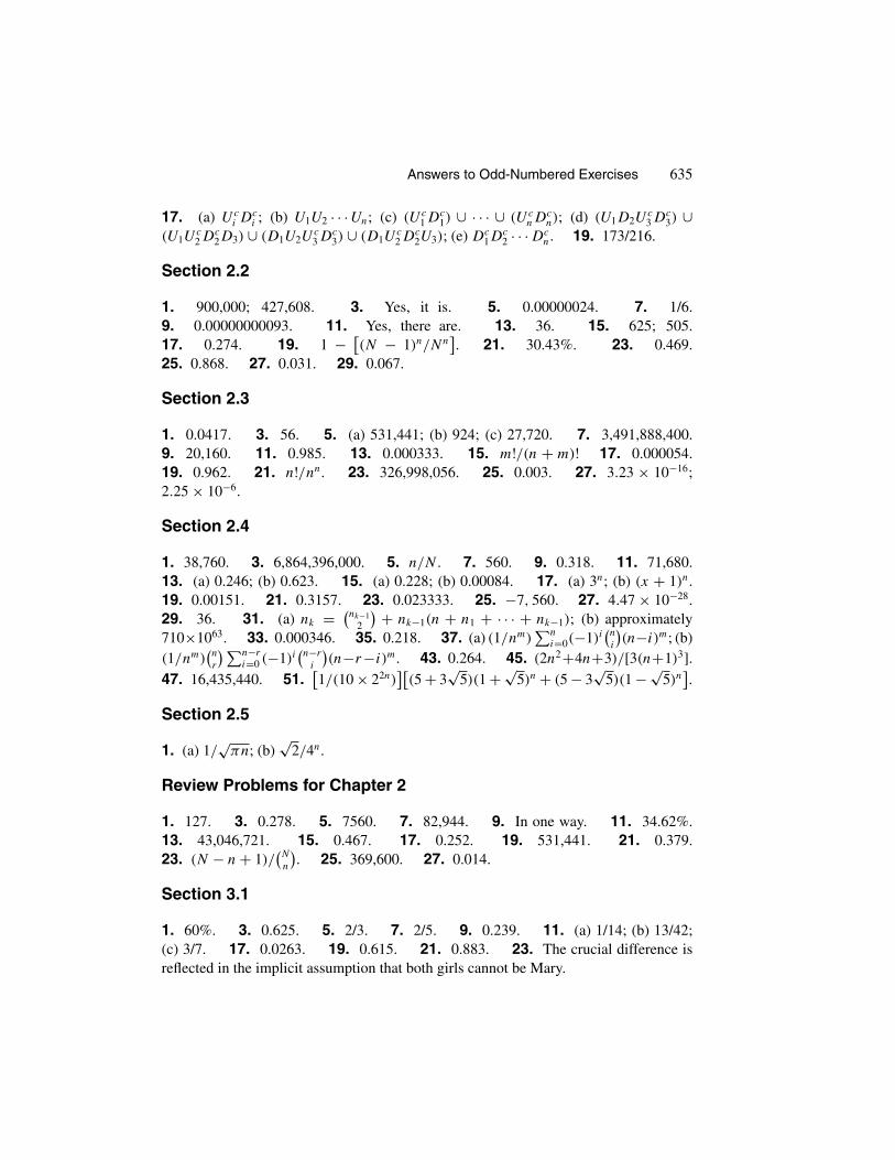
Answers to Odd-Numbered Exercises 635
17. (a) Uci Dc
i ; (b) U1U2 · · · Un; (c) (Uc1 Dc
1) ∪ · · · ∪ (UcnDc
n); (d) (U1D2Uc3 Dc
3) ∪(U1U
c2 Dc
2D3) ∪ (D1U2Uc3 Dc
3) ∪ (D1Uc2 Dc
2U3); (e) Dc1D
c2 · · · Dc
n. 19. 173/216.
Section 2.2
1. 900,000; 427,608. 3. Yes, it is. 5. 0.00000024. 7. 1/6.9. 0.00000000093. 11. Yes, there are. 13. 36. 15. 625; 505.17. 0.274. 19. 1 − [
(N − 1)n/Nn]. 21. 30.43%. 23. 0.469.
25. 0.868. 27. 0.031. 29. 0.067.
Section 2.3
1. 0.0417. 3. 56. 5. (a) 531,441; (b) 924; (c) 27,720. 7. 3,491,888,400.9. 20,160. 11. 0.985. 13. 0.000333. 15. m!/(n + m)! 17. 0.000054.19. 0.962. 21. n!/nn. 23. 326,998,056. 25. 0.003. 27. 3.23 × 10⁻¹⁶;2.25 × 10⁻⁶.
Section 2.4
1. 38,760. 3. 6,864,396,000. 5. n/N . 7. 560. 9. 0.318. 11. 71,680.13. (a) 0.246; (b) 0.623. 15. (a) 0.228; (b) 0.00084. 17. (a) 3n; (b) (x + 1)n.19. 0.00151. 21. 0.3157. 23. 0.023333. 25. −7, 560. 27. 4.47 × 10−28.29. 36. 31. (a) nk = (
nk−12
) + nk−1(n + n1 + · · · + nk−1); (b) approximately710×1063. 33. 0.000346. 35. 0.218. 37. (a) (1/nm)
∑ni=0(−1)i
(n
i
)(n−i)m; (b)
(1/nm)(n
r
)∑n−ri=0 (−1)i
(n−r
i
)(n−r−i)m. 43. 0.264. 45. (2n2+4n+3)/[3(n+1)3].
47. 16,435,440. 51.[1/(10 × 22n)
][(5 + 3
√5)(1 + √
5)n + (5 − 3√
5)(1 − √5)n].
Section 2.5
1. (a) 1/√
πn; (b)√
2/4n.
Review Problems for Chapter 2
1. 127. 3. 0.278. 5. 7560. 7. 82,944. 9. In one way. 11. 34.62%.13. 43,046,721. 15. 0.467. 17. 0.252. 19. 531,441. 21. 0.379.23. (N − n + 1)/
(N
n
). 25. 369,600. 27. 0.014.
Section 3.1
1. 60%. 3. 0.625. 5. 2/3. 7. 2/5. 9. 0.239. 11. (a) 1/14; (b) 13/42;(c) 3/7. 17. 0.0263. 19. 0.615. 21. 0.883. 23. The crucial difference isreflected in the implicit assumption that both girls cannot be Mary.

636 Answers to Odd-Numbered Exercises
Section 3.2
1. 0.1625. 3. 0.72. 5. (a) 0.00216; (b) 0.00216. 7. It makes no difference ifyou draw first, last, or anywhere in the middle. 9. 1/14. 11. 0.
Section 3.3
1. 0.02625. 3. 0.633. 5. 1/4. 7. 0.7055. 9. 0.034. 11. Yes, they are.13. 0.4. 17. 1/(n − 1). 19. 0.0383 21. 1/3. 23. To maximize the chancesof freedom, one urn must contain 1 green and 0 red balls, and the other one must containN − 1 green and N red balls.
Section 3.4
1. 3/5. 3. 0.87. 5. 0.1463. 7. 0.084. 9. 0.056. 11. 0.21. 13. 0.69.15. 0.61.
Section 3.5
1. You should not agree! 3. Neither Mia is right nor Jim. 5. 0.00503.7. (a) 0.526; (b) 0.076. 11. 0.9936. 17. 0.994. 19. 0.226.23. (a) 1 −[(n− 1)/n]n; (b) this approaches 1 − (1/e). 25. No, it is not. 27. 0.2.29. 2p4 − p6. 33. 0.5614. 35. 13/14. 37. 2/5.39. 1 − ∏n
i=1(1 − pi) − ∑ni=1
[pi
∏nj=1j �=i
(1 − pj)]. 41. 2p2 + 2p3 − 5p4 + p5.
43. (a) 1/8; (b) 1/8; (c) 13/16.
Section 3.6
1. 1. 3. The parents are rr and Rr . 5. The observed data shows that the genesare linked. 7. 40.71% 9. 0.17. 11. p/6.
Review Problems for Chapter 3
1. 0.347. 3. 65%. 5. (a) 0.783; (b) 0.999775; (c) 0.217; (d) 0.000225.7. 0.0796. 9. 1/6. 11. 0.35. 13. 0.03. 15. 0.36. 17. 0.748.19. 0.308; R, B, and S are not independent. They are conditionally independent giventhat Kevin is prepared, and they are conditionally independent given that Kevin is unpre-pared.
Section 4.2
1. Possible values are 0, 1, 2, 3, 4, and 5. Probabilities associated with these val-ues are 6/36, 10/36, 8/36, 6/36, 4/36, and 2/36, respectively. 3. (1 − p)i−1p if

Answers to Odd-Numbered Exercises 637
1 ≤ i ≤ N ; (1 − p)N if i = 0. 5. The answers are 1/2, 1/6, 1/4, 1/2, 0, and 1/3, re-spectively. 7. (a) 1/33; (b) 25/33; (c) 9/33; (d) 5/6. 11. F is a distribution function.13. F(t) = 0 if t < 0; t/45 if 0 ≤ t < 45; 1 if t ≥ 45. 15. 0.277. 17. F(t) = 0if t < 0; t/(1 − t) if 0 ≤ t < 1/2; 1 if t ≥ 1/2. 19. It is F(t) if t < 5; 1 if t ≥ 5.
Section 4.3
1. F(x) = 0 if x < 1, 1/15 if 1 ≤ x < 2, 3/15 if 2 ≤ x < 3, 6/15 if 3 ≤x < 4, 10/15 if 4 ≤ x < 5, and 1 if x ≥ 5. 3. Possible values are 2, 3, . . . ,12. Probabilities associated with these values are 1/36, 2/36, 3/36, 4/36, 5/36, 6/36,5/36, 4/36, 3/36, 2/36, 1/36, respectively. 5. (a) (9/10)i−1(1/10), i = 1, 2, . . . ;(b) (9/10)(j−3)/2(1/10), j = 3, 5, 7, . . . . 7. (a) 1/15; (b) 1/15; (c) 8; (d) 2
/[n(n+1)
];
(e) 6/[
n(n + 1)(2n + 1)]. 9. F(x) = 0 if x < 0; 1 − (1/4)n+1 if n ≤ x < n + 1,
n = 0, 1, 2, . . . . 11. (1/2)n−1, n ≥ 2. 13. Possible values are 0, 1, 2, 3, 4, 5.Probabilities associated with these values are 42/1001, 252/1001, 420/1001, 240/1001,45/1001, 2/1001, respectively. 15. (5/6)n−1−5(4/6)n−1+10(3/6)n−1−10(2/6)n−1+5(1/6)n−1, n ≥ 6.
Section 4.4
1. Yes, of course. 3. 0.86. 5. No, it is not. 7. Either 4 or 5 magazines shouldbe ordered. 9. (b) 0, 44/27, 349/27, respectively. 11. 5/8, 31/8, 23/8, respec-tively. 13. 3.98. 15.
∑ck=1
∑cj=k(kαj )/j. 17.
[Nn+1 −∑N
i=1(i − 1)n]/Nn.
19.[(n + 1)2
]/(2n − 1).
Section 4.5
1. The first business. 3. 3. 5. They are (N+1)/2, (N2−1)/12, and√
(N2 − 1)/12,respectively. 7. 36. 9. X is more concentrated about 0 than Y is.
Section 4.6
1. Mr. Norton should hire the salesperson who worked in store 2.
Review Problems for Chapter 4
1. It is 1/45 for i = 1, 2, 16, 17; 2/45 for i = 3, 4, 14, 15; 3/45 for i = 5, 6, 12, 13;4/45 for i = 7, 8, 10, 11; and 5/45 for i = 9. 3. 35. 5. 1.067. 7. They are 16,16, 0.013, and 0.008, respectively. 9. (a) e−2t ; (b) e−2t
[1 + 2t + 2t2 + (4t3/3)
]and
1 − e−2t − 2te−2t , respectively. 11. (a)(j−1
3
)/(52
4
). (b) 1/13. (c) 42.4.
Section 5.1
1. 0.087. 3. 0.054. 5. 0.33. 7. p(x) = (4x
)(0.60)x(0.4)4−x, x =0, 1,
2, 3, 4; q(y) = ( 4(y−1)/2
)(0.60)(y−1)/2(0.4)(9−y)/2, y = 1, 3, 5, 7, 9. 9. 0.108.

638 Answers to Odd-Numbered Exercises
11. They are np + p and np + p − 1. 13. 0.219. 15. k = 4 and the maximumprobability is 0.238. 17. 0.995. 19. It is preferable to send in a single parcel.
21. (a) Np(1 − p)N−1; (c) 1/e. 23. (1/2)n∑[ n+(b−a)
2
]i=0
(n
i
), where
[n+(b−a)
2
]is
the greatest integer less than or equal to n+(b−a)
2 . 27. 0.000028. 29. 90,072.31. 0.054. 33. 1
/[∑ni=0
(n
i
)(n−i
n)k].
Section 5.2
1. 0.9502. 3. 0.594. 5. 0.823. 7. 0.063. 9. 83%. 11. 0.21.13. 0.87. 15. 0.13. 17. 0.325. 19. 0.873716. 21. The least integer greaterthan or equal to −N ln(1 − α)/M . 23. (a) (1/2)(1 + e−2λα). (b) (1/2)(1 − e−2λα)
25. 0.035.
Section 5.3
1. {NNN, DNN, NDN, NND, NDD, DND, DDN}. 3. (a) 12; (b) 0.07.5. 0.055. 7. 0.42. 9. x/n. 11. 49. 13. (1/2)N+M−m+1
[(N+M−m
N
) +(N+M−m
M
)]. 15. 0.74. 17. p[t/2]+1, where [t/2] is the greatest integer less than
or equal to t/2. 19. 1/(1 − p)N−1. 21. 254.80. 23. Negative binomial withparameters k and p. 25.
(2N−M−1N−1
)(1/2)2N−M−1. 27. 1/7. 29. (a) D/N ;
(b) (D − 1)/(N − 1).
Review Problems for Chapter 5
1. 0.0009. 3. 1.067. 5. 0.179. 7. 0.244. 9. 0.285. 11. 2 and2, respectively. 13. p/(1 − p). 15. 0.772. 17. 0.91. 19. 0.10111.21. (a) 0.000368; (b) 0.000224. 23. (a) ( w
w+b)n−1( b
w+b); (b)( w
w+b)n−1. 25. k/n.
Section 6.1
1. (a) 3; (b) 0.78. 3. (a) 6; (b) 0 if x < 1, −2x3 + 9x2 − 12x + 5 if 1 ≤ x < 2, and1 if x ≥ 2; (c) 5/32 and 1/2, respectively. 5. (a) 1/π ; (b) 0 if x < −1, 1
πarcsin x + 1
2if −1 ≤ x < 1, 1 if x ≥ 1. 7. (b) They are symmetric about 3 and 1, respectively.9. 0.3327. 11. α = 1/2; β = 1/π ; f (x) = 2/
[π(4 + x2)
], −∞ < x < ∞.
Section 6.2
1. The probability density function of Y is (1/12)y−2/3 if −8 ≤ y < 8; 0, other-wise. The probability density function of Z is (1/8)z−3/4 if 0 < z ≤ 16; 0, otherwise.3. fY (y) = [2/(3 3
√y)]
exp(−y2/3
)if y ∈ (0, ∞); 0, elsewhere. fZ(z) = 1, z ∈ (0, 1);
0, elsewhere. 5. The probability density function of Y is (3λ/2)√
ye−λy√
y if y ≥ 0;0, otherwise. 7. The probability density function of Z is 1/π if −π/2 < z < π/2; 0,elsewhere.

Answers to Odd-Numbered Exercises 639
Section 6.3
1. (a) 8. 3. The muffler of company B. 5. 0. 7. (5/9)h((t − 32)/1.8
);
1.8∫∞−∞ xh(x) dx + 32. 9. 8.4. 13. (a) c1 is arbitrary, cn = n−1/(n−1);
(b) ∞ if n = 1, and n(n−2)/(n−1)/(n − 1) if n > 1; (c) cne−nt , t ≥ ln cn; (d) it
exists if and only if m−n < −1. 19. [(2α −α2)/λ2]+ [(2β −β2)/µ2]− [2αβ/λµ].
Review Problems for Chapter 6
1. 1/y2 if y ∈ (1, ∞); 0, elsewhere. 3. 11/(5√
5). 5. No!7. [15(1 − 4
√y )2]/(2 4
√y ) if y ∈ (0, 1); 0, elsewhere. 9. Valid. 11. 0.3.
Section 7.1
1. 3/7. 3. a = −6; b = 6. 5. 1/2. 7. 1/3. 9. a/b. 11. [nX] is a randomnumber from the set {0, 1, 2, . . . , n − 1}. 13. g(X) = 3X2 − 4X + 1.
Section 7.2
1. 0.5948. 5. They are all equal to 0. 7. 0.2%, 4.96%, 30.04%, 45.86%, and18.94%, respectively. 9. 0.4796. 11. 0.388. 13. The median is µ. 15. No,it is not correct. 17. 671. 19. 2 (t/σ ) − 1 if t ≥ 0; 0, otherwise. The expectedvalue is σ
√2/π . 21. 49.9. 23. eα2/2 25. 1
σ t√
2πexp [−(ln t − µ)2/(2σ 2)],
t ≥ 0; 0, otherwise. 27. 10 copies. 29. Yes, absolutely! 33. 15.93 and 0.29,respectively. 35. 1/(2
√λ).
Section 7.3
1. 0.0001234. 3. exp(−y − e−y), −∞ < y < ∞. 5. (a) 0.1535; (b) 0.1535.7. (a) e−λt ; (b) e−λt − e−λs . 9. $323.33. 11. It is a Poisson random variable withparameter λt . 13. (a) 1/2.
Section 7.4
3. 0.3208. 5. Two hours and 35 minutes. 7. (2n)!√π/(4n · n!). 9. Howard’swaiting time in the queue is gamma with parameters 2 and nλ.
Section 7.5
1. Yes, it is. 3. c = 1260; E(X) = 5/11; VarX = 5/242. 5. 0.17. 7. 0.214.9. Only beta density functions with α = β are symmetric, and they are symmetric about1/2.

640 Answers to Odd-Numbered Exercises
Section 7.6
1. (a) 0.392; (b) 0.0615.
Review Problems for Chapter 7
1. 5/12. 3. 0.248. 5. 0.999999927. 7.(1/
√2π) ∫ x/2.5
−∞ exp[− (t − 4)2/2
]dt.
9. 0.99966. 11. 0.51%, 12.2%, 48.7%, 34.23%, and 4.36%, respectively. 13. It isuniform over the interval
(− 5/10k+1, 5/10k+1). 15. 0.89. 17. g(X) = 3X2 − 1.
Section 8.1
1. (a) 2/9; (b) pX(x) = x/3, x = 1, 2; pY (y) = 2/(3y), y = 1, 2; (c) 2/3;(d) E(X) = 5/3, E(Y ) = 4/3. 3. (a) k = 1/25; (b) pX(x) is 12/25 if x = 1, 13/25if x = 2; pY (y) is 2/25 if y = 1, 23/25 if y = 3; (c) E(X) = 38/25, E(Y ) = 71/25.
5.[(7
x
)(8y
)( 54−x−y
)]/(204
), 0 ≤ x ≤ 4, 0 ≤ y ≤ 4, 0 ≤ x + y ≤ 4. 7. p(1, 1) = 0,
p(1, 0) = 0.30, p(0, 1) = 0.50, p(0, 0) = 0.20. 9. (a) fX(x) = 2x, 0 ≤ x ≤ 1;fY (y) = 2(1 − y), 0 ≤ y ≤ 1; (b) E(X) = 2/3, E(Y ) = 1/3; (c) they are 1/4, 1/2,and 0, respectively. 11. fX(x) = e−x, x > 0; fY (y) = (1/2)y, 0 < y < 2.
13. (a) f (x, y) = 6 if (x, y) ∈ R; 0, elsewhere. (b) fX(x) = 6x(1 − x), 0 < x < 1;fY (y) = 6(
√y − y), 0 < y < 1; (c) E(X) = 1/2, E(Y ) = 2/5. 15. �/3.
17. π/8. 21. 3/4. 23. a/2b. 25. f (x) = 1 − |x|, −1 ≤ x ≤ 1.
27. n(1/2)n−1.
Section 8.2
1. No, they are not. 3. 4/81 and 4/27, respectively. 5. 0.0179. 7. (1/2)2n(2n
n
).
9. No, they are not. 11. No, they are not. 13. 1. 15. 3/2. 17. f (t) =− ln t, 0 < t < 1; 0, elsewhere. 19. 0.22639.
Section 8.3
1. pX|Y (x|y) = (x2 + y2)/(2y2 + 5), x = 1, 2, y = 0, 1, 2. The desired condi-tional probability and conditional expectation are 5/7 and 12/7, respectively. 3. It is(x−6
2
)(1/2)x−5, x = 8, 9, 10, . . . . 7. 1/(y +1). 9. 10/33. 11. The joint proba-
bility density function of X and Y is 1/(20y) if 20 < x < 20 + (2y)/3 and 0 < y < 30.It is 0 otherwise. 13. Given that X = x, Y − x is binomial with parameters p andn − m. 15. Given that N(s) = k, N(t) − k is Poisson with parameter λ(t − s).
19. (a) f (x, y) = 2 if x ≥ 0, y ≥ 0, x + y ≤ 1; 0, otherwise; (b) fX|Y (x|y) =1/(1 − y) if 0 ≤ x ≤ 1 − y, 0 ≤ y < 1. (c) E(X|Y = y) = (1 − y)/2, 0 < y < 1.
21.[1/F (s)
] ∫ s
0 tf (t) dt.

Answers to Odd-Numbered Exercises 641
Section 8.4
1. g(u, v) = (1/4)e−(u+v)/2, v > 0, u > 0. 3. (1/2π)re−r2/2, 0 < θ < 2π,
r > 0. 7. g(u, v) = (1/v)e−u, u > 0, 1 < v < eu. 9. (a) g(u, v) =[λr1+r2ur1+r2−1e−λuvr1−1 (1 − v)r2−1]/[�(r1)�(r2)], u > 0, 0 < v < 1; (c) U is gammawith parameters r1 + r2 and λ; V is beta with parameters r1 and r2.
Review Problems for Chapter 8
1. (a) 0.69; (b) 2.05 and 3.38. 3.[(13
x
)( 269−x
)]/(39
9
), 0 ≤ x ≤ 9. 5.
[(13x
)( 136−x
)]/(26
6
),
0 ≤ x ≤ 6. 7. Yes, E(XY) = E(X)E(Y ). 9. (r22 − r2
3 )/r21 . 11. 2/5.
13. 1/(n + 1), n ≥ 1. 15. (a) c = 12; (b) they are not independent. 17. 0 ift < 0; 1 if 0 ≤ t < 1/2; 1/(4t2) if t ≥ 1/2. 19. 0.2775. 21. E(Y |X = x) = 0,
E(X|Y = y) = (1 − y)/2 if −1 < y < 0, and (1 + y)/2 if 0 < y < 1.
Section 9.1
1.[(13
h
)(13d
)(13c
)(13s
)]/(52
13
), h + d + c + s = 13, 0 ≤ h, d, c, s ≤ 13.
3. (a) pX,Y (x, y) = xy/54, x = 4, 5, y = 1, 2, 3. pY,Z(y, z) = yz/18, y =1, 2, 3, z = 1, 2. pX,Z(x, z) = xz/27, x = 4, 5, z = 1, 2. (b) 35/9. 5. They arenot independent. 7. (a) They are independent. (b) λ1λ2λ3 exp(−λ1x − λ2y − λ3z).
(c) λ1λ2/[(λ2 + λ3)(λ1 + λ2 + λ3)]. 9. [1 − (r2/R2)]n, r < R; 0, otherwise.11. Yes, it is. 13. X is exponential with parameter λ1 +λ2 +· · ·+λn. 15. 1/(nλ).
17. p1p7(p2p4 + p3p4 − p2p3p4 + p2p5p6 + p3p5p6 − p2p3p5p6 − p2p4p5p6 −p3p4p5p6 + p2p3p4p5p6). 23. They are not independent. 25. 1/2880.
Section 9.2
1. 0.26172. 3. 1 − (1 − e−3λ2)4. 5. Let p1 = ∑k−1
l=0
(n
l
)pl(1 − p)n−l , p2 =∑n
l=k+1
(n
l
)pl(1 − p)n−l . The answer is P(X(i) = k) = 1 −∑m
j=i
(m
j
)p
j
1(1 − p1)m−j−∑m
j=m−i+1
(m
j
)p
j
2(1 − p2)m−j . 9. (a)
∫∞−∞ n(n − 1)f (v − r)f (v)[F(v)−
F(v − r)]n−2 dv, r > 0. (b) n(n − 1)rn−2(1 − r), 0 < r < 1.
Section 9.3
1. 0.028. 3. 0.171. 5. (a) 0.8125; (b) 0.135, (c) 0.3046. 7. 0.117.9. 0.009033.
Review Problems for Chapter 9
1.(20
b
)(30r
)(50g
)/(100
20
), b + r + g = 20, 0 ≤ b, r, g ≤ 20. 3.
[1 − (π/6)(r/a)3
]n.
5. 0.00135. 7. F1(t)F2(t) · · · Fn(t). 9. 0.2775.

642 Answers to Odd-Numbered Exercises
Section 10.1
1. 13/6. 3. 26. 5. 11.42. 7. $28.49. 9. (n − k)k/n. 11. n/32.
13. 23.41 15. 3.786. 19. 9.001.
Section 10.2
1. 0. 3. 35/24. 5. n(n − 1)p(1 − p) and −np(1 − p), respectively.13. $2796 and $468, respectively. 15. The second method is preferable.17. 0.2611. 19. n/12. 25. −n/36.
Section 10.3
1. 112. 3. They are −1 and −1/12, respectively. 5. No! it is not. 7. Showthat ρ(X, Y ) = −0.248 �= ±1.
Section 10.4
1. 5. 5. 47.28. 7. 3.786. 11. 2(2n − 1). 13. It will take 4,407.286 businessdays, on average, until there is a lapse of two days between two consecutive applications.Since an academic year is 9 months long the admission officers should not be concernedabout this rule at all. 15. 7.805. 17. [(1 − α)pm + α]/[αpm(1 − p)].
Section 10.5
1. 0.5987. 3. −ρ(X, Y )(σY /σX). 5. They are (1 + y)/2, 0 < y < 1; x/2,0 < x < 1; and 1/2, respectively.
Review Problems for Chapter 10
1. 1. 3. 511/270. 5. 1554. 7. 204. 9. Cov(X, Y ) = 0; X and Y
are uncorrelated but not independent. 11. 2/π . 13. α = µY − ρ(σY /σX
)µX,
β = ρ(σY /σX). 15. 7.5 minutes past 10:00 A.M. 17. 71.9548.
Section 11.1
1. (1/5)(et + e2t + e3t + e4t + e5t ). 3. 2et/(3 − et ), t < ln 3. E(X) = 3/2.
5. (a) MX(t) = (12/t3)(1 − et )+ (6/t2)(1 + et ), t �= 0; MX(t) = 1 if t = 0.(b) E(X) = 1/2. 7. (a) MX(t) = exp
[λ(et − 1)
]. (b) E(X) = Var(X) = λ.
9. E(X) = 1/p, Var(X) = (1 − p)/p2. 11. p(1) = 5/15, p(3) = 4/15, p(4) =2/15, p(5) = 4/15; p(i) = 0, i �∈ {1, 3, 4, 5
}. 13. E(X) = 3/2, Var(X) = 3/4.
17. 8/9. 21. MX(t) = [λ/(λ − t)]r
, E(X) = r/λ, Var(X) = r/λ2.
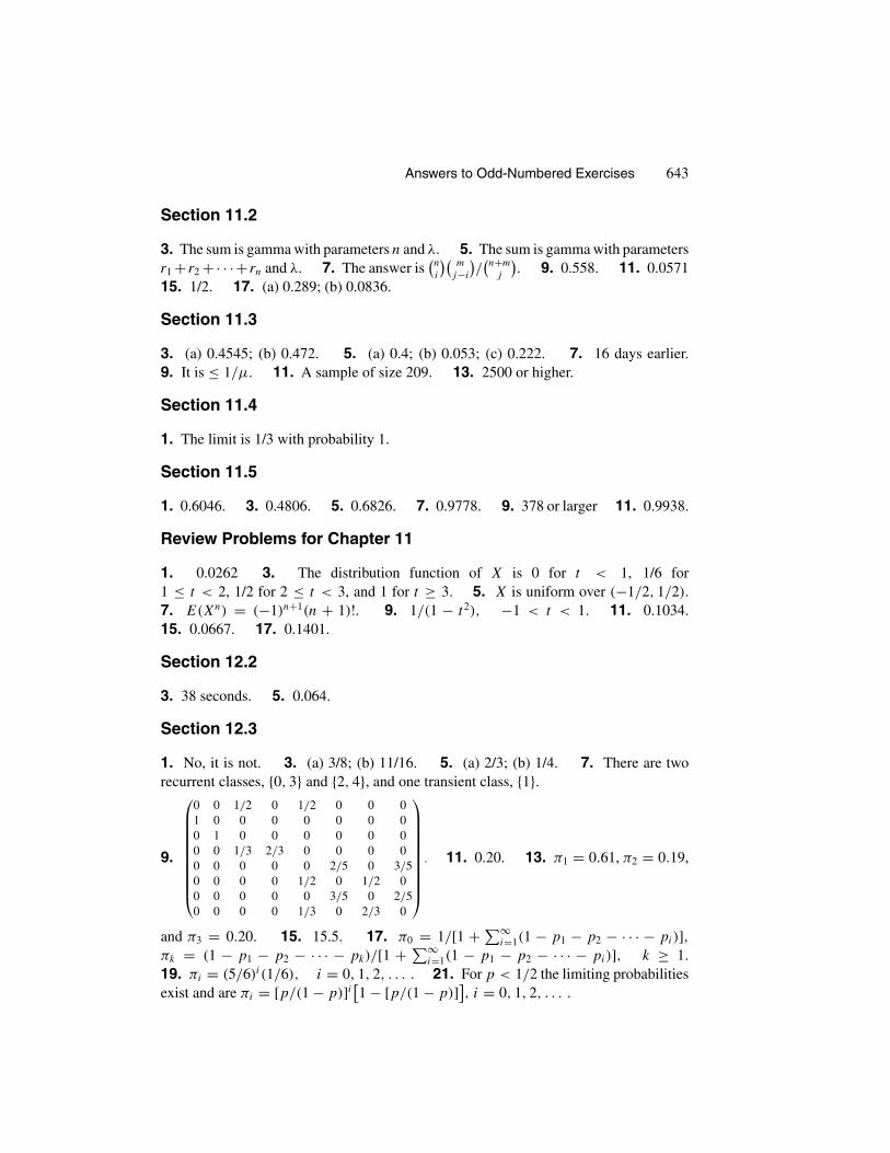
Answers to Odd-Numbered Exercises 643
Section 11.2
3. The sum is gamma with parameters n and λ. 5. The sum is gamma with parametersr1 + r2 +· · ·+ rn and λ. 7. The answer is
(n
i
)(m
j−i
)/(n+m
j
). 9. 0.558. 11. 0.0571
15. 1/2. 17. (a) 0.289; (b) 0.0836.
Section 11.3
3. (a) 0.4545; (b) 0.472. 5. (a) 0.4; (b) 0.053; (c) 0.222. 7. 16 days earlier.9. It is ≤ 1/µ. 11. A sample of size 209. 13. 2500 or higher.
Section 11.4
1. The limit is 1/3 with probability 1.
Section 11.5
1. 0.6046. 3. 0.4806. 5. 0.6826. 7. 0.9778. 9. 378 or larger 11. 0.9938.
Review Problems for Chapter 11
1. 0.0262 3. The distribution function of X is 0 for t < 1, 1/6 for1 ≤ t < 2, 1/2 for 2 ≤ t < 3, and 1 for t ≥ 3. 5. X is uniform over (−1/2, 1/2).7. E(Xn) = (−1)n+1(n + 1)!. 9. 1/(1 − t2), −1 < t < 1. 11. 0.1034.15. 0.0667. 17. 0.1401.
Section 12.2
3. 38 seconds. 5. 0.064.
Section 12.3
1. No, it is not. 3. (a) 3/8; (b) 11/16. 5. (a) 2/3; (b) 1/4. 7. There are tworecurrent classes, {0, 3} and {2, 4}, and one transient class, {1}.
9.
⎛⎜⎜⎜⎜⎜⎜⎜⎜⎜⎜⎝
0 0 1/2 0 1/2 0 0 01 0 0 0 0 0 0 00 1 0 0 0 0 0 00 0 1/3 2/3 0 0 0 00 0 0 0 0 2/5 0 3/50 0 0 0 1/2 0 1/2 00 0 0 0 0 3/5 0 2/50 0 0 0 1/3 0 2/3 0
⎞⎟⎟⎟⎟⎟⎟⎟⎟⎟⎟⎠. 11. 0.20. 13. π1 = 0.61, π2 = 0.19,
and π3 = 0.20. 15. 15.5. 17. π0 = 1/[1 +∑∞i=1(1 − p1 − p2 − · · · − pi)],
πk = (1 − p1 − p2 − · · · − pk)/[1 + ∑∞i=1(1 − p1 − p2 − · · · − pi)], k ≥ 1.
19. πi = (5/6)i(1/6), i = 0, 1, 2, . . . . 21. For p < 1/2 the limiting probabilitiesexist and are πi = [p/(1 − p)]i[1 − [p/(1 − p)]], i = 0, 1, 2, . . . .

644 Answers to Odd-Numbered Exercises
25. P =
⎛⎜⎜⎜⎜⎜⎜⎜⎜⎜⎜⎝
0 1 0 0 0 . . .µ
λ + µ0
λ
λ + µ0 0 . . .
0µ
λ + µ0
λ
λ + µ0 . . .
0 0µ
λ + µ0
λ
λ + µ. . .
...
⎞⎟⎟⎟⎟⎟⎟⎟⎟⎟⎟⎠. The period of each state is 2.
29. π0 = 2/(k + 1); πi = [2(k − i)]/[k(k + 1)], i = 0, 1, . . . , k − 1.
Section 12.4
3. µπ(1,0)+λπ(0,1) = λπ(0,0)+µπ(0,0); µπ(n+1,0)+λπ(n−1,0) = λπ(n,0)+µπ(n,0), n ≥ 1;λπ(0,m+1) + µπ(0,m−1) = λπ(0,m) + µπ(0,m), m ≥ 1.
5. (a) [(1/c!)(λ/µ)c]/[∑cn=0(1/n!)(λ/µ)n
]; (b) At least five operators.
7. [j (j+1)−i(i+1)]/(2λ). 9. λ0 = λ; λn = αnλ, n ≥ 1; µ0 = 0; µn = µ+(n−1)γ ,n ≥ 1. 11. p00(t) = 1; for i > 0, pi0(t) = ∑∞
k=i
[[e−µt (µt)k]/k!]; for 0 < j ≤ i,pij (t) = [e−µt (µt)i−j ]/(i − j)!.13. π0 = [c! (1 − ρ)]/[c! (1 − ρ)
∑cn=0[(1/n!)(λ/µ)n] + ccρc+1
]. 15. p1n(t) =
e−λt (1 − e−λt )n−1, n ≥ 1. 17. ne(λ−µ)t + [γ /(λ − µ)][1 − e(λ−µ)t].
Section 12.5
1. (a) 0.056; (b) −0.5 and 4.5, respectively. 5. 0, if x ≤ t ; (2/π) arccos√
t/x, ifx ≥ t . 9. σ
√2t/π , σ 2t[1 − (2/π)], and [(z + z0)/σ
√t] + [(z − z0)/σ
√t] − 1,
respectively. 11. 0.7486.
Review Problems for Chapter 12
1. 0.692. 3. If states 0, 1, 2, 3, and 4 are renamed 0, 4, 2, 1, and 3, respectively, thenthe transition probability matrix P 1 will change to P 2. 5. It consists of two recurrentclasses {3, 5} and {4}, and two transient classes {1} and {2}.7. 0.4715. 9. Approximately 15% have no logos. 11. 0.55.13. [µ(2λ+µ)]/(2λ2 +2λµ+µ2). 15. In steady state, the number of machines thatare operating is binomial with parameters m and λ/(λ + µ).17. (25λ4 + 34λ3µ + 30λ2µ2 + 24λµ3 + 12µ4)/(12λ5). 19. The desired quan-tities are (s/t)y and σ 2(t − s)(s/t), respectively. 21. 1 − (2/π) arccos
√x/y.

Index
The following abbreviations are used in this index: r.v. for random variable, p.d.f. for probabilitydensity function, p.m.f. for probability mass function, and m.g.f. for moment-generating function.
A
Absolutely continuous r.v.’s, 231Absolute moments, 181, 253Absorbing state, 539Absorption probability, 549–552Accessible states, 538Aczel, Amir, 121Allele, 127Almost sure convergence, 489Aperiodic Markov chains, 553Associative laws for events, 8Attrition ruin problem, 219Axiom of countable additivity, 13Axiomatic method, 11–12Axioms, 3, 12
of probability, 12
B
Balance equations, 573for birth and death processes, 577
Banach, Stefan, 220Banach matchbox problem, 220Bayes, Thomas, 102Bayes’ formula, 100–105Bayes’ theorem, 101Bernoulli, Daniel, 403, 428Bernoulli, Jacob, 489Bernoulli, James, 2, 38, 188, 476Bernoulli r.v.’s, 188–189
expectations of, 189m.g.f.’s of, 459moments of, 459p.m.f.’s of, 188simulation of, 619standard deviation of, 189sums of independent, 404
variances of, 189Bernoulli trials, 188
independent, 190Bernstein, Serge, 3Bertrand, Joseph, 264, 266Bertrand’s paradox, 264–266Beta r.v.’s, 297–301
expectations of, 298p.d.f.’s of, 297relation to binomial, 300relation to random numbers, 297–298simulation of, 625variances of, 298
Bhaskara II, 54Bienaymé, Irénée, 476Binomial expansion, 60Binomial r.v.’s, 190–196
approximation to hypergeometric, 224expectations of, 194–195, 404m.g.f.’s of, 459p.m.f.’s of, 190relation to beta, 300relation to normal, 268, 270–272relation to Poisson, 519, 520simulation of, 619standard deviation of, 195sums of independent, 469variances of, 195, 423
Birth and death processes, 576–582with disaster, 585with immigration, 584
Birth and death rates, 576Birthday problem, 41Bivariate Dirichlet p.d.f., 329Bivariate distribution, 311–325Bivariate normal, 449–452Black, Fisher, 279Black-Scholes call option, 278–280
645

646 Index
Blood type, 128Bolita, 177Boole’s inequality, 26Borel, Émile, 3Borel-Cantelli lemma, 35Borel normal number theorem, 493Bortkiewicz, L.V., 202Box, 358, 622Box problem, 347Box-Muller’s theorem, 358, 622Brams, Steve, 347, 348Branching processes, 546–547Brown, Robert, 586Brownian motions, 586–600
definition of, 587first passage time in, 593geometric, 598–600maximum of, 594reflected, 601standard, 588stationary increments in, 587transition p.d.f.’s of, 588with drift, 597zeros of, 594
Buffon, George Louis, 336Buffon’s needle problem, 336, 627
C
Call option, 279Cardano, Girolamo, 2, 60, 119Cauchy r.v.’s, 246, 248Cauchy-Schwarz inequality, 406, 415Central limit theorem, 498–505
statement of, 499proof of, 500
Central moments, 181, 253Certain event, 1, 6Chapman-Kolmogorov equations, 535, 568Chebyshev, Pafnuty, 2, 476, 489, 499, 529Chebyshev-Bienaymé inequality, see
Chebyshev inequalityChebyshev inequality, 477
and sample mean, 480–483Chevalier de Méré’s paradox, 120Chi-squared r.v.’s, 473Chromosome, 126Chuck-a-luck, 199
Circularly symmetrical joint p.d.f., 343Classical definition of probability, 16Classifications of states, 538–543Clock solitaire, 187Codominant allele, 128Codominant blood type, 128Coincidences, theory of, 41Combination, 53–63
r-element, 53–54Combinatorial analysis, 38Communicating states, 538Commutative laws for events, 8Complementary events, 6Compound Poisson processes, 526Concentration of r.v.’s, 180Conditional distribution, 343–353
continuous case, 349–353discrete case, 343–349function, 344, 349
Conditional expectation, 345, 351Conditional failure rate, 305Conditional probability, 75–82
distribution function, 344, 349Conditional p.d.f., 349
of Brownian motions, 588, 590Conditional p.m.f., 343Conditionally independent events, 124Conditioning on r.v.’s, 434–444Constant failure rate, 307Continuity of probability function, 27Continuity theorem, Lévy, 500Continuous r.v.’s, 231–237
expectations of, 246–252medians of, 256, 282standard deviations of, 252variances of, 252–254
Continuous-time Markov chains, 566–582Continuous-time stochastic processes, 511Convergence in probability, 487Convolution of p.d.f.’s, 361Convolution of p.m.f.’s, 362Convolution theorem
continuous case, 360discrete case, 362
Correction for continuity, 270–272Correlated events, 82Correlated r.v.’s, 417Correlation, 429–433

Index 647
Correlation (continued)and independence, 417coefficient, 429
Counterexample, 11Counting principle, 38
generalized, 39Counting processes, 512
orderly, 514Covariance, 415–424Cumulative distribution function, 144Czar, 529
D
d’Alembert, Jean Le Rond, 108, 119Davidson, 222Death process with immigration, 605Decreasing failure rate, 307Decreasing sequence of events, 27De Méré, Chevalier, 38De Moivre, Abraham, 2, 70, 76, 113, 267De Moivre-Laplace theorem, 268, 498De Moivre’s theorem, 268De Morgan, 627De Morgan’s law, 8, 11Density function, see
probability density functionDependent events, 108Derivative, 171D/G/c queueing systems, 524Diaconis, Persi, 41Dickens, Charles, 173Difference of events, 6Diffusion equation, backward, 589Dirichlet p.d.f., bivariate, 329Discrete probability function, 153Discrete r.v.’s, 153–157
expectations of, 159–172modes of, 158moments of, 181standard deviations of, 176variances of, 175–181
Discrete-time stochastic processes, 511Distribution function, see
probability distribution functionDistributive law for events, 8Dominant allele, 127Double exponential p.d.f.
= Laplace p.d.f., 291, 508Doubly stochastic Markov chains, 559
E
Effron, Bradley, 120Effron dice, 120Ehrenfest chain, 534, 555Ehrenfest, Paul and T., 534Einstein, Albert, 208, 534, 586Elementwise method, 8Empirical distribution, 493Equal events, 5Equally likely events, 13Equally likely sample points, 13Equity, 171Ergodicity, 557Erlang density, 292Erlang’s loss system, 583Euler, Leonhard, 38Events, 3, 4Exercising an option, 279Expectations
as center of gravity, 161as weighted average, 160conditional, 345, 351finiteness of, 160, 248linearity of, 170, 251, 315, 324, 400of continuous r.v.’s, 246–252of discrete r.v.’s, 159–172of functions of r.v.’s, 169, 250of functions of several r.v.’s, 374, 379of functions of two r.v.’s, 315, 324of means of a random samples, 423of products of independent r.v.’s, 333,
338, 374, 380of random sums of r.v.’s, 438of sums of r.v.’s, 400–407of the number of matches, 401–402table for, 633
Expected value, see expectationExponential r.v.’s, 284–289
definition of, 285distribution functions of, 285expectations of, 286memoryless property of, 288, 291, 307m.g.f.’s of, 460moments of, 461

648 Index
Exponential r.v.’s (continued)p.d.f.’s of, 285relation to gamma, 292, 472relation to geometric, 289relation to Poisson, 284–286, 289,
514–515simulation of, 621standard deviation of, 286sums of independent, 470variances of, 286, 460
F
Factorial, 48Failure rate, 305Failure rate function, 304Fair coin, 15Fair game, 160Fermat, Pierre de, 2, 38Fibonacci-type sequence, 70Financial asset, 171First passage time
in Brownian motions, 593–594First quartile of a distribution, 151Fisk, Steve, 613Fitzgerald, Edward, 185Fixed-income security, 171Force of mortality, 305Fox, 627Fry, Thornton, 208Frykman, James, 166Functions of r.v.’s, 142–143
G
Galilei, Galileo, 2Gambler’s ruin problem, 90, 528, 532,
549Game
Bolita, 177Chuck-a-luck, 199fair, 160hounds and jackals, 1Keno, 177poker, 57, 65
Gamete, 132Gamma r.v.’s, 292–296
definition of, 293
expectations of, 295m.g.f. of, 467p.d.f.’s of, 292, 293relation to chi-squared, 473relation to exponential, 292, 472relation to negative binomial, 296relation to normal, 297, 473relation to Poisson process, 292simulation of, 621standard deviation of, 295sums of independent, 471, 472, 474variances of, 295
Gardner, Martin, 367Gauss, Karl Friedrich, 2, 102, 274Gaussian, see normalGene, 126Genetics, 126–134Genotype, 127Geometric Brownian motions, 598–600Geometric probability, 264, 322–324Geometric r.v.’s, 215–217
expectations of, 216memoryless property of, 216, 217p.m.f.’s of, 215relation to exponential, 289relation to negative binomial, 404,
423, 474simulation of, 620standard deviation of, 216sums of independent, 470variances of, 216
GI/D/c queueing systems, 525GI/G/c queueing systems, 524GI/M/c queueing systems, 524Gorky, Maxim, 529Grading on the curve, 276Gridgeman, N. T., 627
H
Hall, W. J., 362Hardy-Weinberg law, 130–132Hazard functions, 303–308
definition of, 304Hazard rate, 304Hat Problem, 26Hawkins, 386Hilbert, David, 3

Index 649
Hilton, 329Histogram, 270Hounds and jackals, 1Huygens, Christian, 2, 160Hypergeometric, multivariate, 371Hypergeometric r.v.’s. 220–224
expectations of, 221, 405p.m.f.’s of, 221relation to binomial, 224relation to Poisson, 230standard deviation of, 221variances of, 221, 428
Hypotheses, 101
I
Identically distributed r.v.’s, 487Impossible event, 1, 6Inclusion-exclusion principle, 21, 62Increasing failure rate, 307Increasing sequence of events, 27Indicator of an event, 342Inequality
Boole’s, 26Cauchy-Schwarz, 406, 415Chebyshev, 477Markov, 476
Independence, 39, 107–118and correlation, 417conditional, 124of a collection of r.v.’s, 373of an infinite set of events, 115of continuous r.v.’s, 334–338of discrete r.v.’s, 331–333of functions of r.v.’s, 332, 338of more than three events, 115of sets of events, 107–118of several r.v.’s, 373of three events, 114of two events, 108of two r.v.’s, 330–338pairwise, 114, 421
Independent r.v.’s, 330–338, 372–373,sums of, 468–473
Increments in Poisson Process, 206Independent increment property, 206Inheritance, polygenic, 129
Instantaneous transition rate, 569Intensity rate, 305Interarrival time of a Poisson process,
284, 514–515Interest, compounded continuously, 467Intersection of events, 5Inverse transformation method, 621Irreducible Markov chains, 539
J
Jailer’s paradox, 111see also Prisoner’s dilemma
Johnson, 222Joint cumulative distribution, 317, 372Joint distribution, 317, 372
of two continuous r.v.’s, 315–325of n > 2 continuous r.v.’s, 378–382of n > 2 discrete r.v.’s, 369–378of two discrete r.v.’s, 311–315
Joint p.d.f.’sof Brownian motions, 589of two r.v.’s, 315–325of n > 2 r.v.’s, 378–382marginalized over a set of r.v.’s, 379
Joint p.m.f.of two r.v.’s, 311–325of n > 2 r.v.’s, 369–378marginalized over a set of r.v.’s, 369–370multinomial, 394
K
Kaigh, 219Keno, 177Khinchin, Alexander, 208, 489Khoury, Michael, 198, 413Khyyam, Omar, 60, 185Kilgour, D. Marc, 347, 348Knuth, Donald, E., 32, 607Kolmogorov, Andrei, 3, 16Kolmogorov backward equations, 569–571Kolmogorov forward equations, 569–571k-out-of-n system, 384Kramp, Christian, 48Kurtosis, 457

650 Index
L
Lack of memory, seememoryless property
Laplace, Pierre-Simon, 2, 102, 125, 268Laplace p.d.f.
= double exponential p.d.f., 291, 508Laplace’s law of succession, 124, 615Larsen, 274Law of large numbers, 486–496
strong, 489weak, 487
Law of multiplication, 85–86Law of total probability, 88–96Law of unconscious statistician, 168, 250Lazzarini, 627Least squares, method of, 455Leibniz, Gottfried Wilhelm, 23, 38Lévy, 500Lévy continuity theorem, 500Limits of events, 27Linearity of expectation, 170, 251, 315
324, 400Lognormal r.v.’s, 462
simulation of, 625Lyapunov, Aleksandr, 2, 499
M
Marginalp.d.f., 317probability distribution function, 317,
372p.m.f., 312, 369
Marginalizedjoint distribution, 372joint p.d.f., 379joint p.m.f., 369–370
Marginals of multinomials, 395–396Markov, Andrei, 2, 479, 499, 529Markov Chains, 528–559
aperiodic, 553continuous-time, 566–582discrete-time, 528–559doubly stochastic, 559irreducible, 5transition probabilities of, 529–530, 535
Markov inequality, 476
Markovian property, 529, 567Marx, 274Matchbox problem, see
Banach matchbox problemMathematical expectation, see
expectationMaximum likelihood estimator, 68Mean, see expectationMeasurable events, 14Median
of a continuous r.v., 256, 282of a distribution, 151of a sample of random points, 298, 390
Memoryless propertyof geometric r.v.’s, 216
uniqueness, 217of exponential r.v.’s, 288, 307
uniqueness, 288, 291Mendel, Greger Johann, 126, 127Merryfield, Kent G., 367, 368Method of distribution functions, 240–242Method of least squares, 455Method of transformations, 242–244M/G/c queueing systems, 524Migration, 131M/D/1 queueing system, 546M/M/1 queueing system, 564, 579,
581, 583M/M/c queueing system, 584M/M/∞ queueing system, 583Mode, 158Moment-generating function, 457–464
definition of, 458MacLaurin’s series for, 459of joint distributions, 468of limits of sequences of r.v.’s, 500of sums of independent r.v.’s, 468relation to moments, 458table for, 633uniqueness of, 463
Moments, 181, 253relation to m.g.f.’s, 458
Monte Carlo method, 626–628Mosteller, Frederick, 41Muller, 358, 622Multinomial
distribution, 394–396expansion, 63

Index 651
Multinomial (continued)marginals of, 395–396
Multivariate distributions, 369–382Multivariate hypergeometric, 371Mutagen, 130Mutation, 130Mutually exclusive events, 6
N
Natural selection, 130Negative binomial r.v.’s, 218–220
definition of, 218expectations of, 218, 404p.m.f.’s of, 218relation to geometric, 404, 423, 474relation to gamma, 296, 474simulation of, 620standard deviation of, 218sums of independent, 470variances of, 218, 423
Negatively correlated events, 82Negatively correlated r.v.’s, 417Normal number, 493Normal r.v.’s, 267–280
approximation to binomial, 268,270–272
definition of, 269, 273expectations of, 273, 275m.g.f.’s of, 461p.d.f.’s of, 269, 273relation to chi-squared, 473relation to gamma, 297, 473simulation of, 622, 623standard, 269–273standard deviations of, 273, 275sums of independent, 470tables for, 631–632variances of, 273, 275
Nucleus, 126Number of subsets of a set, 42, 61
O
o notation, 513Odds, against 22Odds, in favor, 22Option, 279
Order statistics, 387–392the kth, 387
Orderliness of Poisson processes, 206, 514
P
Paccioli, Luca, 2Pairwise independent events, 114Pairwise independent r.v.’s, 421Pairwise uncorrelated, 421Palindrome, 72Paradox
Bertrand’s, 264–266Chevalier de Méré’s, 120Jailer’s, 111St. Petersburg, 163Wallet, 367, 446
Parallel systems, 376, 604Pareto r.v.’s, 256Parity checking, 199Partition of a sample space, 92Pascal, Blaise, 2, 38, 60, 160PASTA, 525–526Patil, S. A., 386Pattern
appearance, 407–411no self-overlap, 408overlapping, 408
Pederson, 329Period of a state, 552Permutation, 47–50
r-element, 47–48Phenotype, 127Pointwise convergence, 489–490Poisson, Siméon Denis, 2, 201, 267Poisson processes, 206–211, 512–526
definition of, 208relation to binomial, 519, 520relation to exponential, 284–286, 289relation to gamma, 292relation to uniform, 521simulation of, 622stationarity of, 206superposition of, 528
Poisson r.v.’s, 201–211as an approximation to binomial, 201–205as limit of hypergeometric, 230definition of, 202

652 Index
Poisson r.v.’s (continued)expectations of, 203m.g.f.’s of, 465p.m.f.’s of, 202simulation of, 622standard deviation of, 203sums of independent, 469variances of, 203
Poker, 57, 65Pólya, George, 196Pólya’s urn model, 167Polygenic inheritance, 129Polynomial distribution, see
multinomial distributionPortfolio, 171Positive normal distribution, 281Positively correlated events, 82Positively correlated r.v.’s, 417Posterior probability, 101Postulate, 12Power set, 14, 42Principle of restricted choice, 112Prior probability, 101Prisoner’s dilemma, 99
see also Jailer’s paradoxProbabilities 0 and 1, 29–30Probability, 12
additivity of (= axiom ), 12axioms of, 12classical definition of, 16of an event, 12relative frequency interpretation of,
2–3, 486–487subjective, 3
Probability density functions, 231–237joint, 315–325, 378–382marginal, 317of functions of a r.v., 240–244table for, 633
Probability distribution functions, 143–149jump discontinuity of, 146
Probability functions, 27continuity of, 27of r.v.’s, 153
Probability mass functions, 153conditional, 343joint, 311–315, 369–378table for, 633
Prosecutor’s fallacy, 103Pseudorandom number, 606Ptolemy, 73Pure birth processes, 512, 577Pure death processes, 577
Q
Quantile of order p, 151Quetelet, Lambert, 274Queueing systems, 523–526
D/G/c, 525GI/D/c, 525GI/G/c, 524GI/M/c, 524M/G/c, 524M/D/1, 546M/M/1, 564, 579, 581, 583M/M/c, 584M/M/∞, 583sequential, 585tandem, 585
R
Random chord, 264–266Random event, 1Random mating, 130Random points
from intervals, 30–33from subsets of the plane, 322
Random sample, 382expectations of, 423variances of, 423
Random variables, 139–143concentration of, 180conditioning on, 434–444continuous, 231–237discrete, 153–157expected value of, 159–172, 246–252functions of, 142–143simulation of, 617–624standard deviation of, 176standardized, 184–185sums of independent, 468–473symmetric, 151, 239transformations of, 356–362variance of, 175–181, 252–254

Index 653
Random walks, 532–533, 537, 543–546one-dimensional, 532–533simple, 545symmetric, 545three-dimensional, 545two-dimensional, 545
Rate of a Poisson process, 208Rate of return, 171Recessive allele, 127Recurrent class, 542Recurrent state, 540Reduction of sample space, 79–82Reflected Brownian motions, 601Regular tetrahedron, 114Relative frequency, 2–3, 486–487Relatively prime integers, 25Reliability
function, 304of components, 375of systems, 375–378
Renewal theory, 289, 410, 512Restricted choice, 112Russell, Bertrand, 495
S
Sample, empirical distribution of, 493Sample mean
and Chebyshev inequality, 480–483of independent normal r.v.’s, 471
Sample median, 388Sample midrange, 388, 393Sample range, 387, 393Sample points, 4
equally likely, 13Sample space, 3
partition of, 92reduction of, 79–82
Scholes, Myron, 279Security, 171Seed, 606Sequence of events, 27Sequential queueing systems, 585Series system, 376Set function, 15Set, nonmeasurable, 33Sex chromosome, 132Sex-linked genes, 132
Shah, A. K., 273Simple random walks, 544Simulation, 606–628
of combinatorial problems, 610–612of conditional probabilities, 614–617of expected value, 618of r.v.’s, 617–624
Skewness, 457Smith, 627Smith, Karl, 48Smoluchowski, Roman, 208Sotades, 73Solitaire, the clock, 187Standard Brownian motions, 588Standard deviation
of continuous r.v.’s, 252of discrete r.v.’s, 176
Standard normal r.v.’s, 269–273Standardized r.v.’s, 184–185Stationarity of Poisson processes, 206Stationary increments
in Brownian motions, 587St. Petersburg paradox, 163Steady-state probabilities, 554–559,
572–575Steinhaus, Hugo, 220Stifel, 60Stiglar, Stephen M., 274Stirling, James, 70Stirling’s formula, 70
a nonrigorous proof of, 505Stochastic comparison, 258Stochastic processes, 511–512
continuous-time, 511discrete-time, 511
Strike price, 279Strong law of large numbers, 489Subjective probability, 3Subsets of events, 5Sums of independent r.v.’s, 468–473
m.g.f.’s of, 468Superposition of Poisson processes, 528Survival analysis, 303–308Survival function, 304Symmetric difference of events, 37Symmetric r.v.’s, 151, 239Symmetric random walks, 545

654 Index
T
t-distribution, 303Tandem queueing syatems, 585Tartaglia, Niccolò, 2, 38, 60Theorem, 12Third quartile, 151Total return, 171Transformation, method of, 242–244Transformations of two r.v.’s, 356–362Transient class, 542Transient state, 540Transition p.d.f. of Brownian motion, 588Transition probability matrix, 530
n-step, 535Tree diagram
for Bayes’ formula, 100–101, 104–105for counting problems, 42–44for law of total probability, 89, 94
Tusi, Nasir ad-Din, 60
U
Ulam, Stainslaw, 627Unbiased coin, 15Uncorrelated r.v.’s, 417Uniform r.v.’s, 261–266
definition of, 262distribution functions of, 261expectations of, 263m.g.f.’s of, 465p.d.f.’s of, 262relation to Poisson, 521standard deviation of, 263variances of, 263
Union of events, 6Unit normal, see standard normal
V
Variance parameter ofBrownian motions, 587
Variancesas moment of inertia, 177of continuous r.v.’s, 252–254of discrete r.v.’s, 175–181of linear combinations of r.v.’s,of the mean of a random sample, 423
of random sums of r.v.’s, 439of sums of r.v.’s, 416, 421table for, 633
Venn diagram, 9Viet, Ngo, 367, 368Von Neumann, John, 627Von Mises, Richard, 3, 41, 278Vos Savant, Marilyn, 36, 87, 97,
107, 113, 137
W
Wald, Abraham, 438Wald’s equation, 438Wallet paradox, 367, 446Watson, Saleem, 367, 368Weak law of large numbers, 487Weibull distribution, 308Weierstrass, 3Weight of asset, 172Whitt, W., 524Wiener, Norbert, 586Wiener processes, 587Wolf, Rudolf, 627Wolff, Ronald W., 410, 526Wright brothers, 177Wright-Fisher model, 551Writer, 279
X
X chromosome, 132X-linked genes, 132
Y
Y chromosome, 132Y-linked genes, 132Yule processes, 585
Z
Zeros of Brownian motions, 594Zweifel, 111, 112