
Full issue file - International Journal of Engineering
177
-
Upload
khangminh22 -
Category
Documents
-
view
0 -
download
0
Transcript of Full issue file - International Journal of Engineering

International Journal of EngineeringJournal Homepage: www.ije.ir
Volume 34, Number 03, March 2021 TRANSACTIONS C: Aspects
I. R. IRAN
Materials and Energy Research Center
ISSN: 2423-7167
Lorem IpsumLorem Ipsum
e-ISSN: 1735-9244

In the Name of God
INTERNATIONAL JOURNAL OF ENGINEERING
DIRECTOR-IN-CHARGE A. R. Khavandi
EDITOR-IN-CHIEF G. D. Najafpour
ASSOCIATE EDITOR
A. Haerian
EDITORIAL BOARD
S.B. Adeloju, Charles Sturt University, Wagga, Australia A. Mahmoudi, Bu-Ali Sina University, Hamedan, Iran
K. Badie, Iran Telecomm. Research Center, Tehran, Iran O.P. Malik, University of Calgary, Alberta, Canada
M. Balaban, Massachusetts Ins. of Technology (MIT), USA G.D. Najafpour, Babol Noshirvani Univ. of Tech. ,Babol, Iran
M. Bodaghi, Nottingham Trent University, Nottingham, UK F. Nateghi-A, Int. Ins. Earthquake Eng. Seis., Tehran, Iran
E. Clausen, Univ. of Arkansas, North Carolina, USA S. E. Oh, Kangwon National University, Korea
W.R. Daud, University Kebangsaan Malaysia, Selangor, Malaysia M. Osanloo, Amirkabir Univ. of Tech., Tehran, Iran
M. Ehsan, Sharif University of Technology, Tehran, Iran
M. Pazouki, Material and Energy Research Center,
Meshkindasht, Karaj, Iran
J. Faiz, Univ. of Tehran, Tehran, Iran J. Rashed-Mohassel, Univ. of Tehran, Tehran, Iran
H. Farrahi, Sharif University of Technology, Tehran, Iran S. K. Sadrnezhaad, Sharif Univ. of Tech, Tehran, Iran
K. Firoozbakhsh, Sharif Univ. of Technology, Tehran, Iran R. Sahraeian, Shahed University, Tehran, Iran
A. Haerian, Sajad Univ., Mashhad, Iran A. Shokuhfar, K. N. Toosi Univ. of Tech., Tehran, Iran
H. Hassanpour, Shahrood Univ. of Tech., Shahrood, Iran R. Tavakkoli-Moghaddam, Univ. of Tehran, Tehran, Iran
W. Hogland, Linnaeus Univ, Kalmar Sweden T. Teng, Univ. Sains Malaysia, Gelugor, Malaysia
A.F. Ismail, Univ. Tech. Malaysia, Skudai, Malaysia L. J. Thibodeaux, Louisiana State Univ, Baton Rouge, U.S.A
M. Jain, University of Nebraska Medical Center, Omaha, USA P. Tiong, Nanyang Technological University, Singapore
M. Keyanpour rad, Materials and Energy Research Center,
Meshkindasht, Karaj, Iran X.
Wang, Deakin University, Geelong VIC 3217, Australia
A. Khavandi, Iran Univ. of Science and Tech., Tehran, Iran
EDITORIAL ADVISORY BOARD S. T. Akhavan-Niaki, Sharif Univ. of Tech., Tehran, Iran A. Kheyroddin, Semnan Univ., Semnan, Iran
M. Amidpour, K. N. Toosi Univ of Tech., Tehran, Iran N. Latifi, Mississippi State Univ., Mississippi State, USA
M. Azadi, Semnan university, Semnan, Iran H. Oraee, Sharif Univ. of Tech., Tehran, Iran
M. Azadi, Semnan University, Semnan, Iran S. M. Seyed-Hosseini, Iran Univ. of Sc. & Tech., Tehran, Iran
F. Behnamfar, Isfahan University of Technology, Isfahan M. T. Shervani-Tabar, Tabriz Univ., Tabriz, Iran
R. Dutta, Sharda University, India E. Shirani, Isfahan Univ. of Tech., Isfahan, Iran
M. Eslami, Amirkabir Univ. of Technology, Tehran, Iran A. Siadat, Arts et Métiers, France
H. Hamidi, K.N.Toosi Univ. of Technology, Tehran, Iran C. Triki, Hamad Bin Khalifa Univ., Doha, Qatar
S. Jafarmadar, Urmia Univ., Urmia, Iran S. Hajati, Material and Energy Research Center,
Meshkindasht, Karaj, Iran
S. Hesaraki, Material and Energy Research Center,
Meshkindasht, Karaj, Iran
TECHNICAL STAFF M. Khavarpour; M. Mohammadi; V. H. Bazzaz, R. Esfandiar; T. Ebadi
DISCLAIMER The publication of papers in International Journal of Engineering does not imply that the editorial board, reviewers or
publisher accept, approve or endorse the data and conclusions of authors.
International Journal of Engineering Transactions A: Basics (ISSN 1728-1431) (EISSN 1735-9244) International Journal of Engineering Transactions B: Applications (ISSN 1728-144X) (EISSN 1735-9244)
International Journal of Engineering Transactions C: Aspects (ISSN 2423-7167) (EISSN 1735-9244) Web Sites: www.ije.ir & www.ijeir.info E-mails: [email protected], Tel: (+9821) 88771578, Fax: (+9821) 88773352
Materials and Energy Research Center (MERC)
Transactions C: Aspects

International Journal of Engineering, Volume 34, Number 3, March 2021
ISSN: 2423-7167, e-ISSN: 1735-9244
CONTENTS:
Chemical Engineering
A. Aminmahalati;
A. Fazlali;
H. Safikhani
Investigating the Performance of CO Boiler Burners in the
RFCC Unit with CFD Simulation
587-597
A. Poormohammadi;
Z. Ghaedrahmat;
M. Ahmad Moazam;
N. Jaafarzadeh;
M. Enshayi;
N. Sharifi
Photocatalytic removal of toluene from gas stream using
chitosan/AgI-ZnO Nanocomposite fixed on glass bed
under UVA irradiation
598-605
Civil Engineering
M. Dadashi Haji;
H. Taghaddos;
M.H. Sebt;
F. Chokan;
M. Zavari
The Effects of BIM Maturity Level on the 4D Simulation
Performance: An Empirical Study
606-614
F. Marchione Enhancement of Stiffness in GFRP Beams by Glass
Reinforcement
615-620
S. Sverguzova;
N. Miroshnichenko;
I. Shaikhiev;
Z. Sapronova;
E. Fomina;
N. Shakurova;
V. Promakhov
Application of Sorbent Waste Material for Porous
Ceramics Production
621-628
C. Jithendra;
S. Elavenil
Parametric Effects on Slump and Compressive Strength
Properties of Geopolymer Concrete using Taguchi
Method
629-635
B.A. Mir;
S.H. Reddy
Mechanical Behaviour of Nano-material (Al2O3)
Stabilized Soft Soil
636-643
H. Y. Khudhaire;
H. I. Naji
Management of Abandoned Construction Projects in Iraq
Using BIM Technology
644-649
Electrical & Computer Engineering
R. Badaghei;
H. Hassanpour;
T. Askari
Detection of Bikers without Helmet Using Image Texture
and Shape Analysis
650-655
Transactions C: Aspects

International Journal of Engineering, Volume 34, Number 3, March 2021
ISSN: 2423-7167, e-ISSN: 1735-9244
S.R. Salehinai;
E. Afjei;
A. Hekmati;
H. Aghazadeh
Design Procedure of an Outer Rotor Synchronous
Reluctance Machine for Scooter Application
656-666
J. Tavoosi;
A. Mohammadzadeh
A New Recurrent Radial Basis Function Network-based
Model Predictive Control for a Power Plant Boiler
Temperature Control
667-675
Z. Nejati;
A. Faraj
Actuator Fault Detection and Isolation for Helicopter
Unmanned Arial Vehicle in the Present of Disturbance
676-681
Industrial Engineering
A. Torabi;
H. Hamidi;
N. Safaie
Effect of Sensory Experience on Customer Word-of-
mouth Intention, Considering the Roles of Customer
Emotions, Satisfaction, and Loyalty
682-699
Material Engineering
M.R. Shojaei;
G.R. Khayati;
N. Assadat Yaghubi;
F. Bagheri
Sharebabaki;
S.M.J Khorasani
Removing of Sb and As from Electrolyte in Copper
Electrorefining Process: A Green Approach
700-705
Mechanical Engineering
E. Mohagheghpour;
M. M. Larijani;
M. Rajabi;
R. Gholamipour
Effect of Silver Clusters Deposition on Wettability and
Optical Properties of Diamond-like Carbon Films
706-713
A. Jabbar Hassan;
T. Boukharouba;
D. Miroud;
N. Titouche;
S. Ramtani
Direct Drive Friction Welding Joint Strength of AISI 304 714-720
H. Kohestani;
R. Ezoji
Synthesis and Characterization of TiO2/CuO/WO3
Ternary Composite and its Application as Photocatalyst
721-727
A. Mahmoodian;
M. Durali;
M. Saadat;
T. Abbasian
A Life Clustering Framework for Prognostics of Gas
Turbine Engines under Limited Data Situations
728-736
B. Meyghani;
M. Awang;
S. Emamian
Introducing an Enhanced Friction Model for Developing
Inertia Welding Simulation: A Computational Solid
Mechanics Approach
737-743

International Journal of Engineering, Volume 34, Number 3, March 2021
ISSN: 2423-7167, e-ISSN: 1735-9244
A. Assadi;
M. Nazemizadeh
Size-dependent Vibration Analysis of Stepped
Nanobeams Based on Surface Elasticity Theory
744-749
Petroleum Engineering
M. A. Guzev;
E. V. Kozhevnikov;
M. S. Turbakov;
E. P. Riabokon;
V. V. Poplygin
Experimental Investigation of the Change of Elastic
Moduli of Clastic Rocks under Nonlinear Loading
750-755


IJE TRANSACTIONS C: Aspects Vol. 34, No. 03, (March 2021) 587-597
Please cite this article as: A. Aminmahalati, A. Fazlali, H. Safikhani, Investigating the Performance of CO Boiler Burners in the RFCC Unit with CFD Simulation, International Journal of Engineering, Transactions C: Aspects Vol. 34, No. 03, (2021) 587-597
International Journal of Engineering
J o u r n a l H o m e p a g e : w w w . i j e . i r
Evaluating the Performance of CO Boiler Burners in RFCC Unit using CFD
Simulation
A. Aminmahalatia, A. Fazlali*a, H. Safikhanib a Department of Chemical Engineering, Faculty of Engineering, Arak University, Arak, Iran b Department of Mechanical Engineering, Faculty of Engineering, Arak University, Arak, Iran
P A P E R I N F O
Paper history: Received 27 December 2020 Received in revised form 10 January 2021 Accepted 16 January 2021
Keywords: CFD Simulation CO boiler Mechanisms Combustion
A B S T R A C T
The combustion chamber's internal refractory in Imam Khomeini Oil Refinery Company (IKORC) was
damaged in several parts, requiring operating conditions and re-inspecting the design of the combustion
chamber using CFD. Simplify the combustion chamber 3D simulation, decrease in the number of calculations, the symmetry principle was applied in the simulation. The results, independent of the mesh
network, were investigated via increasing the mesh nodes. The one-stage, two-stage, multi-stage and
overall mechanisms, which were designated, were examined and compared to actual measured data and a calculation error of less than 8% was obtained. Ultimately, selecting overall mechanisms, the
simulation results, streams mixing and length of the chamber were scrutinized, and as a result, the
current design was approved. The temperature and velocity of the flows in the combustion chamber were investigated. In the combustion chamber, the farther we are from the burners, the more uniform
the velocity and temperature profiles also become as the wall temperature increases. The rate of
combustion reaction was evaluated with the temperature of different points in the combustion chamber. The results showed that the combustion chamber wall's temperature is in the appropriate range and has
not suffered any thermal damage. Unlike the combustion chamber wall, the burner wall (at the mixing
point) has an unauthorized temperature; there is the possibility of thermal damage that can be eliminated
by changing the number of currents. Unsuitable thermal profiles also showed large amounts of oxygen
in the exhaust gas indicated that the steam boiler performance is far from the optimal condition and
specific changes would be required in the air streams. Streamline demonstrated that the primary air stream was more effective for decreasing CO and NOX amounts in the outlet stream. The secondary air
stream was also significant to prevent thermal damage to the internal coating and reduce safety hazards.
doi: 10.5829/ije.2021.34.03c.01
1. INTRODUCTION1
The increasing rate of fossil fuel consumption, such as
coal, crude oil and natural gas, followed by a gradual
reduction in their reservoirs, has become one of the most
controversial contemporary issues. Exhausting fossil
fuels harm the environment and cause significant
environmental damages. Their consumption leads to CO2
and CO production, and consequently, a continuous
increase in greenhouse gas emissions. Despite the highly
damaging impacts of CO2 on global warming, the effects
of CO are negligible. Nevertheless, it is noteworthy to
mention that CO has significant indirect impacts. It reacts
Corresponding Author Institutional Email: [email protected] (A.
Fazlali)
with the OH-radicals in the atmosphere, which behaves
as an inhibitor for greenhouse gases, such as methane.
Also, CO can boost the formation of Ozone [1].
Therefore, more improvement is vital in combustion
technologies and processes [2].
There are several different codes for numerical
calculations. These codes can generally be classified into
LP codes and Computational Fluid Dynamics (CFD)
codes. The significant advantage of CFD codes is their
capability to model the turbulent flows and complex
geometries. However, the most significant impediment of
this class is their high computational costs. On the other
hand, LP codes are suited to handle merely simple

A. Aminmahalati et al. / IJE TRANSACTIONS C: Aspects Vol. 34, No. 03, (March 2021) 587-597 588
geometries and their biggest strength lies in their
capability of running the equation fast [3]. For example,
CFD codes and other simulation methods have been used
to research references [4-11]. In CFD, we attempt to
model combustion utilizing simple reaction models
because detailed chemical reaction mechanisms are
composed of hundreds of species and side reactions that
cannot accommodate reasonable costs. Moreover, an
increase in the number of different reaction mechanisms
adds to the overall modeling complexity [2].
According to the inherent intricacy of interaction
among turbulency, combustion, convection, radiation,
buoyancy and compressibility of gases, CFD combustion
modeling is a complex subject. This complexity rises
specifically in large chambers when natural, or forced
convection must be considered. Thus, CFD combustion
modeling requires being validate using physical and
empirical results. Validation of CFD codes promotes
certainty of users in its forecast precision. Modeling
validation is of significance regarding complicated cases.
However, validation tests are not applicable since they
are costly and challenging to be implemented [12]. CFD
focus and strength have been on predicting reaction
structure, temperature, velocity and not the emission of
pollutants [2].
In the oil refinery's RFCC units, a 700-800 C ° gaseous
phase flows out of the regeneration unit. It carries less
than 5% of CO and the rest includes N2, H2O and CO2,
which is called flue gas [12].
CO burns with fuel gas in CO boilers, generating a
vast amount of heat. Hot gases from combustion are then
cooled down via heat exchangers using cooling water in
tubes. This interaction leads to superheated steam
production and the utility units can apply the steam.
Refineries deal with significant daily steam demands.
Accordingly, the CO boiler steam production can mainly
cut the costs down. Since then, CO boilers play a pivotal
role in the RFCC process [12].
The CO boiler internal wall is installed to protect the
refractory from thermal damages. The CO boiler
temperature can rise to 1200 C ° . Furthermore, this may
cause internal/external damages; for instance, high
temperatures can damage central refractories [12].
A typical CO boiler generates up to 300 tons of steam
per hour. This production annually reduces the expenses
in the refinery by 68 million dollars [13]. The CO boiler
maintenance, inspection and shut down have substantial
consequences in the RFCC process and any damage
would lead to a loss of 1 million dollars per day. Also,
possible threats to human and environmental safety are
crucial when the CO boiler is shut down [12-14]
The present study was conducted to investigate the
combustion chamber performance and its effects on the
refractory's internal wall. The above-mentioned CO
boiler produces 270 tons of high-pressure steam an hour,
RFCC unit in Imam Khomeini Oil Refinery Company
(IKORC). Two combustible streams of fuel gas and flue
gas flow into the chamber. Fuel gas stream is composed
of butane and lighter gases. Table 1 represents the
property details of this stream . The flue gas stream is the
regeneration unit output and it contains 1.25% of carbon
monoxide and a small amount of oxygen and other non-
combustible compounds. The required oxygen is
supplied with two air streams. The required oxygen is
supplied with two air streams (primary and secondary
air). Table 1 contains all the mentioned streams in detail.
The flue gas stream has a high temperature (702 C ° ) and
the other three streams (fuel gas, primary and secondary
air) enter the combustion chamber at a temperature close
to the environment. The output streamline from the
combustion chamber enters the steam generator heat
exchanger and its temperature is important in the amount
of steam production [15].
Once the CO boiler is not in service, in addition to the
enormous energy loss, a considerable amount of CO is
released into the environment. Therefore, timely
diagnosis and proper maintenance of internal walls in the
CO boiler will decrease possible maintenance and
prevent environmental pollution. The flowchart used for
this research is shown in Figure 1.
Significant damages have been spotted in the
refractory cover of the walls. In case of a lack of
diagnosis regarding the damages, financial losses are
expected, and wall raptures may lead to operators'
casualties. In this work, the chamber's flame profile was
investigated and the reason for the current damages was
represented. This study focuses specifically on the flame
in the combustion chamber and examines its effects in the
combustion chamber, especially its walls exhaust gas
compositions and It also investigates the effect of flame
on combustion gas compositions. In other words,
TABLE 1. Properties and components of the chamber inlet
streamlines
Secondary
air
Primary
Air
Fuel
gas
Flue
gas Unit
6.5 6.5 0.41 34.2 𝑘𝑔𝑠⁄ Flow
50 50 60 702 C Temperature
- - 13.6 - % H2
Co
mp
ou
nd
s o
f co
nst
itu
en
t - - 65.22 - % CH4
- - 5.16 - % C2H6
- - 3.24 - % C3H8
- - 1.86 - % C4H10+
- - - 1.25 % CO
- - 0.33 17.22 % CO2
79.81 79.81 10.59 80.3 % N2
20.19 20.19 - 0.13 % O2

589 A. Aminmahalati et al. / IJE TRANSACTIONS C: Aspects Vol. 34, No. 03, (March 2021) 587-597
Figure 1. Flowchart of the methodology used in the present
work
this study seeks to understand better the effects of flame
in the combustion chamber and ways to improve the
economic and environmental performance of the CO
boiler.
2. BURNER MODELING 2. 1. Physical Model As illustrated in Figure 2,
the combustion chamber is a 900 m3 cylinder with three
identical burners, in which three similar sets of burners
are installed. Each group consists of 9 smaller burners,
one in the center and the rest are located in the chamber
circumference. Due to the large volume of the chamber, a numerous
mesh network is required. The symmetrical principles are
significantly applied to cut down the simulation model
volume. As shown in Figure 3, splitting the chamber into
three subdivisions, streams in each burner set are not
Figure 2. Stimated boiler combustion chamber a) Overall
view b) Burners zone
Figure 3. Co boiler streamlines. a) Streamlines overall view
b) Fuel gas and primary air streamlines
intermixed. The smaller volume, there is to model, the
denser the mesh network we will get. Figure 3 illustrates
all the streamlines of the steam boiler. Figure 3.a
indicates streamlines and symmetrical principle effects,
and Figure 3.b represents the primary air and the fuel gas
streams. According to Figure 3, it can be concluded that
no stream intermix occurs.
Figure 4 shows all the entering streams to the
chamber. Figure 4.a represents the combustion chamber,
and Figure 4.b demonstrates the inlet section of the
chamber. Flue gas is sprayed from the periphery of the
torch, shown as α in yellow. The primary air streams
inflow the burners from internal rings, while the external
rings and holes located at the outer ring circumference
supply the secondary air. Due to the symmetry of the
combustion chamber, one-third of the combustion
chamber is modeled. The secondary air is divided into
two parts; part one is in the form of external rings around
flue gas, depicted as the thin rings as shown β in blue in
Figure 4. Simulated chamber inlet streamlines a) Overall
view of the combustion chamber, b) magnified view of the
inlets and c) magnified view of the inlets to the burner α-Inlet
Flue gas, β-Internal ring: primary air inlet, ω-External ring
and holes: secondary air inlets, γ-Primary air, δ-Inlet fuel gas

A. Aminmahalati et al. / IJE TRANSACTIONS C: Aspects Vol. 34, No. 03, (March 2021) 587-597 590
Figure 4.b. The part two ,consists of small circles shown
as ω in blue. The primary air stream is illustrated in
Figures 4.b and 4.c. It is shown to be charged to the
burner center represented as γ in blue. The input venue
for fuel gas includes nine small circles represented in
Figure 4.c as δ in red.
As illustrated in Figure 5, the wall temperature was of
the maximum error. When we do calculations with 3
million, this error progressively decreased to 1%. Other
variable deviation errors in this node number were less
than 0.3%. With the increase in mesh nodes up to 6
million, all the errors decreased to below 0.1%. Table 2
shows important information about meshing, including
simulation volume, the maximum and minimum size of
each mesh, the growth rate of mesh size, number of nodes
and number of elements.
2. 2. Numerical Method The ANSYS/CFX
v19.0 software was used for CFD simulations by solving
the numerical simulation carried out on a supercomputer
with Intel Xeon CPU E5-2630L V2(2.4 GHz * 8 CPUs,
30 GB RAM). The mathematical modeling in this study
is based on a steady-state condition. The turbulence
equation is standard k–ε [16-18]. The buoyancy force
was neglected in the gas type and steam boiler horizontal
geometry, following the simulation results. Three
different heat transfer governing equations are optionally
available. Meanwhile, due to combustion reaction nature
and high fluid temperature variations, the overall energy
governing equation was designated.
Figure 5. Mesh network independency deviation (major
variables deviation) vs. nodes number
TABLE 2. Important information about meshing, which is:
simulation volume, the maximum and minimum size of each
mesh, the growth rate of mesh size, number of nodes and
number of elements
Volume
(m³)
Max face
size (mm)
Min size
(mm)
Growth
rate
NO.
nodes
NO.
elements
290.68 25 1 1.2 6.17e+6 3.45e+7
Typical and defined reactions in the simulation must
cover combustions of methane, butane, ethane, propane,
CO and H2. Accordingly, the three mechanisms are
suggested as follows: One-stage, two-stage and multi-
stage reaction mechanism. Westbrook and Dryer [34 ]
proposed several simplified reaction mechanisms for the
oxidation of fuels, namely the WD one-step (WD1), WD
two-step (WD2) and multi-step with Water-Gas Shift
reaction (WGS) mechanisms. Table 3 shows the different
mechanisms used for the combustion reaction in the CO
boiler. All the three mechanisms, as mentioned earlier,
were applied in different simulations separately;
meanwhile, the fourth simulation was applied with all the
mechanisms simultaneously. A brief literature review is
presented in Table 4 concerning the combustion reactions
in the three mechanisms.
Generally, thermal radiation with different models
was studied and here, model P1 is considered [35-37]. P1
is a simple and accurate model and suitable for simulating
large objects.
3. MODEL VALIDATION Validation was confirmed by adapting actual and
empirical temperature and analysis of steam boiler
exhaust gases with results calculated by the simulation.
Four thermometers were set up on the steam boiler. The
control system gathered the mean temperature data as one
of the significant parameters to control the combustion
chamber. Actual and calculated temperatures are listed in
Table 5. The thermometers were installed in one
direction with the same distance to burners. Figure 6
illustrates the direction of the thermometer. Figure 7
simulates the thermometer's changes in the
thermometer's direction. The simulation shows that it can
be observed that the maximum temperature difference in
the thermocouple direction was 21 C ° . If an accurate
thermometers show more difference, they are damaged.
The simulation shows that The difference between the
average of the wall temperatures and the average
temperature of the exhaust gas was less than 8 C ° .
Therefore, the average of the wall temperatures is a
desirable criterion for estimating the outlet temperature.
Table 5 represents the compared values for the
exhaust gas analysis and four simulated reaction
mechanisms. The experimental values were dry-based.
The listed result in Table 5 indicates that the overall
reaction mechanism results are closer to the real data.
Defining the error function below (Equation (1)), the
simulation's temperature error for combining
mechanisms was less than 6%; however, each
mechanism's deviation was estimated to be less than 7%.
𝐸𝑟𝑜𝑟𝑟 =(𝑅𝑒𝑎𝑙 𝐷𝑎𝑡𝑎−𝑆𝑖𝑚𝑢𝑙𝑎𝑡𝑖𝑜𝑛 𝑑𝑎𝑡𝑎)
𝑅𝑒𝑎𝑙 𝐷𝑎𝑡𝑎 (1)

591 A. Aminmahalati et al. / IJE TRANSACTIONS C: Aspects Vol. 34, No. 03, (March 2021) 587-597
TABLE 3. Single-stage, two-stage and multi-stage reaction mechanisms in CO boiler
One-stage reactions (WD1) Two-stage reactions (WD2) Multi-stage reactions (WGS)
Butane
𝐶4𝐻10 + 6.5𝑂2𝑘[𝑂2]
1.6[𝐶4𝐻10]0.15
→ 4𝐶𝑂2 +
5𝐻2𝑂
𝐶4𝐻10 + 4.5𝑂2𝑘[𝑂2]
1.6[𝐶4𝐻10]0.15
→ 4𝐶𝑂 + 5𝐻2𝑂
𝐶𝑂 + 0.5𝑂2
𝑘[𝐶𝑂][𝐻2𝑂]0.5[𝑂2]
0.25
→ 𝐻2𝑂
𝐶𝑂2
𝐶4𝐻10 + 2𝑂2𝑘[𝑂2]
1.6[𝐶4𝐻10]0.15
→ 4𝐶𝑂 + 5𝐻2
𝐶𝑂 + 0.5𝑂2
𝑘[𝐶𝑂][𝐻2𝑂]0.5[𝑂2]
0.25
→ 𝐻2𝑂
𝐶𝑂2
𝐻2 + 0.5𝑂2 → 𝐻2𝑂
𝐶𝑂 + 𝐻2𝑂 ↔ 𝐶𝑂2 + 𝐻2
Propane 𝐶3𝐻8 + 5𝑂2
𝑘[𝑂2]1.65[𝐶3𝐻8]
0.1
→ 3𝐶𝑂2 +
4𝐻2𝑂
𝐶3𝐻8 + 3.5𝑂2𝑘[𝑂2]
1.65[𝐶3𝐻8]0.1
→ 3𝐶𝑂 + 4𝐻2𝑂
𝐶𝑂 + 0.5𝑂2
𝑘[𝐶𝑂][𝐻2𝑂]0.5[𝑂2]
0.25
→ 𝐻2𝑂
𝐶𝑂2
𝐶3𝐻8 + 1.5𝑂2𝑘[𝑂2]
1.65[𝐶3𝐻8]0.1
→ 3𝐶𝑂 + 4𝐻2
𝐶𝑂 + 0.5𝑂2
𝑘[𝐶𝑂][𝐻2𝑂]0.5[𝑂2]
0.25 →
𝐻2𝑂𝐶𝑂2
𝐻2 + 0.5𝑂2 → 𝐻2𝑂
𝐶𝑂 + 𝐻2𝑂 ↔ 𝐶𝑂2 + 𝐻2
Ethane 𝐶2𝐻6 + 3.5𝑂2
𝑘[𝑂2]1.65[𝐶2𝐻6]
0.1
→ 2𝐶𝑂2 +
3𝐻2𝑂
𝐶2𝐻6 + 2.5𝑂2𝑘[𝑂2]
1.65[𝐶2𝐻6]0.1
→ 2𝐶𝑂2 + 3𝐻2𝑂
𝐶𝑂 + 0.5𝑂2
𝑘[𝐶𝑂][𝐻2𝑂]0.5[𝑂2]
0.25
→ 𝐻2𝑂
𝐶𝑂2
𝐶2𝐻6 + 𝑂2𝑘[𝑂2]
1.65[𝐶2𝐻6]0.1
→ 2𝐶𝑂 + 3𝐻2
𝐶𝑂 + 0.5𝑂2
𝑘[𝐶𝑂][𝐻2𝑂]0.5[𝑂2]
0.25
→ 𝐻2𝑂
𝐶𝑂2
𝐻2 + 0.5𝑂2 → 𝐻2𝑂
𝐶𝑂 + 𝐻2𝑂 ↔ 𝐶𝑂2 + 𝐻2
Methane
𝐶𝐻4 + 2𝑂2
𝑘[𝑂2]
1.3
[𝐶𝐻4]0.3
→ 𝐶𝑂2 + 2𝐻2𝑂
0.5𝑁2 + 0.5𝑂2
𝑘[𝑁2][𝐶𝐻4][𝑂2]0.5
→ 𝐶𝐻4
𝑁𝑂
𝑁2 + 𝑂2𝑘[𝑁2][𝑂2]
0.5
→
2𝑁𝑂
𝐶𝐻4 + 1.5𝑂2
𝑘[𝑂2]
1.3
[𝐶𝐻4]0.3
→ 𝐶𝑂 + 2𝐻2𝑂
𝐶𝑂 + 0.5𝑂2
𝑘[𝐶𝑂][𝐻2𝑂]0.5[𝑂2]
0.25
→ 𝐻2𝑂
𝐶𝑂2
0.5𝑁2 + 0.5𝑂2
𝑘[𝑁2][𝐶𝐻4][𝑂2]0.5
→ 𝐶𝐻4
𝑁𝑂
𝑁2 + 𝑂2𝑘[𝑁2][𝑂2]
0.5
→
2𝑁𝑂
𝐶𝐻4 + 0.5𝑂2
𝑘[𝑂2]
1.3
[𝐶𝐻4]0.3
→ 𝐶𝑂 + 2𝐻2
𝐶𝑂 + 0.5𝑂2
𝑘[𝐶𝑂][𝐻2𝑂]0.5[𝑂2]
0.25
→ 𝐻2𝑂
𝐶𝑂2
𝐻2 + 0.5𝑂2 → 𝐻2𝑂
𝐶𝑂 + 𝐻2𝑂 ↔ 𝐶𝑂2 + 𝐻2
0.5𝑁2 + 0.5𝑂2
𝑘[𝑁2][𝐶𝐻4][𝑂2]0.5
→ 𝐶𝐻4
𝑁𝑂
𝑁2 + 𝑂2 𝑘[𝑁2][𝑂2]
0.5 → 2𝑁𝑂
Monoxide
Carbone 𝐶𝑂 + 0.5𝑂2
𝑘[𝐶𝑂][𝐻2𝑂]0.5[𝑂2]
0.25 →
𝐻2𝑂𝐶𝑂2 𝐶𝑂 + 0.5𝑂2
𝑘[𝐶𝑂][𝐻2𝑂]0.5[𝑂2]
0.25 →
𝐻2𝑂𝐶𝑂2 𝐶𝑂 + 0.5𝑂2
𝑘[𝐶𝑂][𝐻2𝑂]0.5[𝑂2]
0.25 →
𝐻2𝑂𝐶𝑂2
Hydrogen 𝐻2 + 0.5𝑂2 → 𝐻2𝑂 𝐻2 + 0.5𝑂2
→ 𝐻2𝑂 𝐻2 + 0.5𝑂2
→ 𝐻2𝑂
TABLE 4. Brief literature review
NO. The subject under
study
Power
(MW) WD1 WD2 WGS Ref.
1 circulating fluidized bed
(CFB) boiler 660 √ [19]
2 circulating fluidized bed
(CFB) boiler 350 √ [20]
3 ultra-supercritical BP 680
boiler 200 √ [21]
4 pulverized coal boilers 160 √ √ [22]
5 biomass boilers 35 √ [23]
6 circulating fluidized bed
(CFB) boiler 12 √ [24]
7 reciprocating grate boiler 4 √ [25]
8 oxy-fuel combustion with
pulverized coal 2.5 √ [26]
9 biomass combustion 0.3 √ [27]
10 MILD combustion
furnace 0.02 √ √ [28]
11 residential furnace 0.015 √ [29]
12 Moderate or intense low-oxygen dilution (MILD)
combustion .0130 √ [30]
13 combustion in a bubbling
fluidized bed - √ √ √ [31]
14 Flameless Combustion - √ [2]
15 swirled burner
combustion - √ [32]
16 industrial low swirl burner combustion
- √ [1]
17 rocket combustor - √ [33]
18 explosions in straight
large-scale tunnels - √ [17]
TABLE 5. Compared values for exhaust gas and simulated
exhaust gas
Compounds T O2 CO2 CO
Units OC % % ppm
WD1 806.94 6.32 18.412 1

A. Aminmahalati et al. / IJE TRANSACTIONS C: Aspects Vol. 34, No. 03, (March 2021) 587-597 592
WD2 807.80 6.33 18.388 2.3
WDG 807.75 6.32 18.39 2.9
Combined
Mechanisms 799.23 6.32 18.386 0.6
Real results 757 6.6 17.8 4
Figure 6. Thermometers' direction in the chamber. a) Overall
view and thermometers direction location and b) temperature
profile in the direction in the chamber
Figure 7. The temperature changes thermometers direction
and averages them
Reporting stream flow in the chamber shows that the
error rate of 5% is acceptable for industrial flow meters.
We attempted to reduce this error by accurate calibration.
This error was under 8% for CO2 and O2 and since the
CO amount was negligible, the error function would not
be a suitable option.
4. RESULTS AND DISCUSSIONS
Different streams flow in different combustion chamber
sectors, which causes the flow profile to form in the
combustion chamber. Combustion causes the
temperature change, resulting in an amendment in the
gases' velocity inside the combustion chamber. Figure 8
represents the velocity changes in the chamber, which is
composed of three parts. In the upper and lower parts, the
velocity profile is shown in the cross-section, while the
middle part of the figure indicates the middle section of
the chamber. Additionally, each of the cross-sections is
pointed out in the middle section. Figure 8 indicates that
the maximum velocity was observed in burner exhausts
and that the closer we got to the end of the chamber, the
more uniform flow we had.
Figure 9 illustrates the wall temperature for all four
mechanisms. As can be seen, the three mechanisms'
general profiles were almost the same, yet it was different
for the overall mechanism profile. Moreover, the reaction
temperature increased as we got closer to the end of the
chamber.
Temperature changes in the combustion chamber's
flames can be seen through its few cross-sections in
Figure 10. Figure 10 shows that firstly, the heat
accumulated in the center, and then, by moving away
Figure 8. The velocity profiles in different cross-sections in
the chamber
Figure 9. The chamber walls temperature profiles in
different mechanisms

593 A. Aminmahalati et al. / IJE TRANSACTIONS C: Aspects Vol. 34, No. 03, (March 2021) 587-597
from the burners, the intermixing of flows reduces the
temperature difference. As it can be seen in Figure 10,
the burner's wall temperature increased and our
calculations revealed that this temperature could reach to
1017 C ° . While the vendor's maximum allowable
temperature in refractory is announced to be less than
982 C ° . This increase of 35 C
° indicates the possible
occurrence of the damage.
Two parallel cross-sections adjoining burners are
shown in Figure 11, representing flames profile changes
as cold air was added to the flow. In Figure 11.a, mixing
air and fuel gas is illustrated where combustion occurred
around the central burner. According to Figure 11.b, the
flame profile was fully developed due to air and fuel gas
combustion. As shown in Figure 11, with an increase in
the airflow, refractory would cool down; therefore, the
temperature rising issue detected in Figure 10 was
solved.
In Figure 12, we increased the burner's distance so
that flame profiles would be in three cross-sections in 0.5,
5 and 15 m distance from the burner. As it can be seen in
Figure 12.a, the temperature difference was higher than
1800 C ° while whereas this difference reduced
significantly to less than 52 C ° according to Figure 12.c.
According to Figures.10-12, it can be concluded that
in the combustion chamber, as we got approached to the
end of the chamber, the temperature difference between
fluid and wall decreased. In the center of the burner, the
flame's core was at high temperature and the end of the
chamber, no significant difference was detected. These
results reveal that walls at the end of the chamber are
more vulnerable to possible temperature rising damages.
Figure 13 illustrates a 3D image of the flame profile
in the combustion chamber. Detecting the temperatures
above a specified value, the profiles were obtained.
Herein, the specified values were the temperatures above
1200, 982 and 850 C ° , respectively. At temperatures
above 1200 C ° , we only had a profile in front of the
burner. At lower temperatures, the profiles were
developed. A remarkable issue represented in Figure 13
is that the flame, profiles even at 850 C ° , is not close
adequately to any walls of the chamber and the flame was
Figure 10. The flame temperature changes in different
cross-sections of the chamber
Figure 11. The temperature profile in two different sections
near the burner
Figure 13. Flame profile 3D image
centrally developed. As mentioned before, 982 C ° is the
maximum allowable temperature for the walls, indicating
that construction problems might trigger refractory
damage in sidewalls.
As mentioned, four streams enter the simulation
combustion chamber, including primary air, secondary
air, fuel gas and flue gas. The secondary air entered the
chamber in two different spots, which can be seen in
Figure 4c. The streamlines are illustrated in Figs.14 and
15. The streamline shows the path through which each
stream flowed in the chamber. Figure 14 represents
primary air, secondary air and their mixture streams.
Figure 15 illustrates a combination of streams in which
the primary air stream covered fuel gas and supplied the
combustion that required oxygen. In the case of excess
air, this amount of air helps obtain the full combustion of
CO. Figure 15.a shows the mixture of air and fuel gas. As
shown in Figure 15.b, the secondary air streams
surrounded CO content flows and initially supplied this
reaction, which required oxygen. In the case of excessive
air, it helps fuel gas combustion. Figure 15.c illustrates
all the flow mixtures.

A. Aminmahalati et al. / IJE TRANSACTIONS C: Aspects Vol. 34, No. 03, (March 2021) 587-597 594
Figure 12. Temperature profile at cross-sections in different distances from the burner
Figure 14. Inlet air streamlines. a) Primary air, b) secondary
air (external ring), c) Secondary air (holes) and d) Total inlet
air streamlines
Figure 15. Inlet air streamlines. a) Primary air and fuel gas,
b) Secondary air and flue gas and c) Total inlet streamlines
Figure 16 illustrates the reaction progress as a result
of the reduction in reactants in the streamlines. This
figure shows that molar fractions of CH4, C2H6, C3H8 and
C4H10 rapidly reduced, which led to a decrease in the
reaction rate. Meanwhile, the CO reaction rate was far
slower compared to the other components. Furthermore,
according to the temperature differences of various
streamlines and high CO combustion dependency on
temperature, CO velocity differed from the other
reactants. Figure 17 illustrates the Oxygen rate changes
in the primary and secondary air streams. As could be
perceived, the primary air reacted faster than the
secondary one. The difference between primary and
secondary air reaction rates is due to the different mixing
of them with other streams.
Figure 16. Reaction progress in the chamber via reactions
changes

595 A. Aminmahalati et al. / IJE TRANSACTIONS C: Aspects Vol. 34, No. 03, (March 2021) 587-597
Figure 17. Oxygen level change in primary and secondary
air streamlines
5. CONCLUSION
The combustion chamber of the CO boiler corresponding
to the RFCC unit of the IKORC was simulated.
Streamlines showed that the conditions of symmetry in
the combustion chamber could be used. Also, the
condition of non-dependence of the simulation results on
the mesh size was investigated. The simulation results for
one-stage, two-stage, multi-stage and overall combustion
mechanisms showed that the closest simulation result to
the actual results is the overall mechanisms. Comparison
of real and simulation results shows that the
simplification assumptions and calculations performed
have a total error of less than 8%. Flame velocity and temperature profiles were plotted.
The results show that the flames are in the center of the
combustion chamber and do not damage the combustion
chamber wall, but as shown in Figure 9, there is a
possibility of damage to the burner wall.
According to Figures 16 and 8, the combination of
streams in the chamber was well-designed. Figure 16 also
shows that the CO fraction slope decreased at the end of
the chamber to reach less than 1%; thus, the chamber's
length was optimally designed. Regarding Figures.14 and
15, the following results can be derived:
1. Primary air was applied for fuel gas combustion. Since
then, any change in this factor altered the primarily
required air.
2. Secondary air was applied for CO content stream
combustion. Since then, any change in this factor alters
the air required as secondary.
3. Primary air was more effective in the center, while the
secondary air affects the walls. Therefore, to regulate
wall temperatures, the secondary air needed to be
changed. On the other hand, any other changes in CO and
NO content streams require alteration of the primary air.
The maximum allowable temperature in the
refractory was not observed in the burner, yet the wall
temperature was much less than the allowable
temperature. It can be concluded that refractory damage
is not associated with functional temperature .
To prevent further damage to the burner, it is
recommended to increase the primary air or modify it.
Concerning the wall temperature, it is suggested to
reduce the secondary air to increase thermal efficiency.
The optimal amount of oxygen for burners was calculated
to be approximately 3; accordingly, it is recommended to
reduce the chamber's overall air entrance .This
modification increases thermal efficiency and decreases
fuel consumption, which ultimately reduces
environmental pollution.
6. REFERENCES
1. Cellek, M.S. and Pınarbaşı, A., "Investigations on performance
and emission characteristics of an industrial low swirl burner
while burning natural gas, methane, hydrogen-enriched natural gas and hydrogen as fuels", International Journal of Hydrogen
Energy, Vol. 43, No. 2, (2018), 1194-1207, DOI:
10.1016/j.ijhydene.2017.05.107.
2. Perpignan, A.A.V., Sampat, R. and Gangoli Rao, A., "Modeling
pollutant emissions of flameless combustion with a joint cfd and chemical reactor network approach", Frontiers in Mechanical
Engineering, Vol. 5, (2019), DOI: 10.3389/fmech.2019.00063.
3. Cherbański, R. and Molga, E., "Cfd simulations of hydrogen deflagration in slow and fast combustion regime", Combustion
Theory and Modelling, Vol. 24, No. 4, (2020), 589-605, DOI:
10.1080/13647830.2020.1724336.
4. Aminoroayaie Yamini, O., Mousavi, S.H., Kavianpour, M.R. and
Movahedi, A., "Numerical modeling of sediment scouring
phenomenon around the offshore wind turbine pile in marine environment", Environmental Earth Sciences, Vol. 77, No. 23,
(2018), DOI: 10.1007/s12665-018-7967-4.
5. Sengupta, A.R., Gupta, R. and Biswas, A., "Computational fluid dynamics analysis of stove systems for cooking and drying of
muga silk", Emerging Science Journal, Vol. 3, No. 5, (2019),
285-292, DOI: 10.28991/esj-2019-01191.
6. Dirbude, S.B. and Maurya, V.K., "Effect of uniform magnetic
field on melting at various rayleigh numbers", Emerging Science
Journal, Vol. 3, No. 4, (2019), 263-273, DOI: 10.28991/esj-
2019-01189.
7. Movahedi, A., Kavianpour, M.R. and Aminoroayaie Yamini, O.,
"Evaluation and modeling scouring and sedimentation around downstream of large dams", Environmental Earth Sciences,
Vol. 77, No. 8, (2018), DOI: 10.1007/s12665-018-7487-2.
8. Movahedi, A., Kavianpour, M. and Aminoroayaie Yamini, O., "Experimental and numerical analysis of the scour profile
downstream of flip bucket with change in bed material size", ISH
Journal of Hydraulic Engineering, Vol. 25, No. 2, (2017), 188-
202, DOI: 10.1080/09715010.2017.1398111.
9. Gharibshahian, E., "The effect of polyvinyl alcohol concentration
on the growth kinetics of ktiopo4 nanoparticles synthesized by the co-precipitation method", HighTech and Innovation Journal,
Vol. 1, No. 4, (2020), 187-193, DOI: 10.28991/hij-2020-01-04-
06.
10. Jabbarzadeh Sani, M., "Spin-orbit coupling effect on the
electrophilicity index, chemical potential, hardness and softness
of neutral gold clusters: A relativistic ab-initio study", HighTech
A. Aminmahalati et al. / IJE TRANSACTIONS C: Aspects Vol. 34, No. 03, (March 2021) 587-597 596
and Innovation Journal, Vol. 2, No. 1, (2021), 38-50, DOI:
10.28991/hij-2021-02-01-05.
11. Trang, G.T.T., Linh, N.H., Linh, N.T.T. and Kien, P.H., "The
study of dynamics heterogeneity in SiO2 liquid", HighTech and
Innovation Journal, Vol. 1, No. 1, (2020), 1-7, DOI:
10.28991/hij-2020-01-01-01.
12. Yeh, C.-L., "Numerical analysis of the combustion and fluid flow in a carbon monoxide boiler", International Journal of Heat and
Mass Transfer, Vol. 59, (2013), 172-190, DOI:
10.1016/j.ijheatmasstransfer.2012.12.020.
13. Yeh, C.-L., "Numerical investigation of the heat transfer and fluid
flow in a carbon monoxide boiler", International Journal of Heat
and Mass Transfer, Vol. 55, No. 13-14, (2012), 3601-3617, DOI:
10.1016/j.ijheatmasstransfer.2012.02.073.
14. Yeh, C.L. and Liang, C.W., "Nox reduction in a carbon monoxide boiler by reburning", Procedia Engineering, Vol. 67, (2013),
378-387, DOI: 10.1016/j.proeng.2013.12.037.
15. Aminmahalati, A., Fazlali, A. and Safikhani, H., "Multi-objective optimization of CO boiler combustion chamber in the RFCC unit
using NSGA II algorithm", Energy, Vol. 221, (2021), DOI:
10.1016/j.energy.2021.119859.
16. Echi, S., Bouabidi, A., Driss, Z. and Abid, M.S., "Cfd simulation
and optimization of industrial boiler", Energy, Vol. 169, (2019),
105-114, DOI: 10.1016/j.energy.2018.12.006.
17. Zhu, Y., Wang, D., Shao, Z., Zhu, X., Xu, C. and Zhang, Y.,
"Investigation on the overpressure of methane-air mixture gas
explosions in straight large-scale tunnels", Process Safety and
Environmental Protection, Vol. 135, (2020), 101-112, DOI:
10.1016/j.psep.2019.12.022.
18. Jóźwiak, P., Hercog, J., Kiedrzyńska, A. and Badyda, K., "Cfd analysis of natural gas substitution with syngas in the industrial
furnaces", Energy, Vol. 179, (2019), 593-602, DOI:
10.1016/j.energy.2019.04.179.
19. Ji, J., Cheng, L., Wei, Y., Wang, J., Gao, X., Fang, M. and Wang,
Q., "Predictions of nox/n2o emissions from an ultra-supercritical
cfb boiler using a2-d comprehensive cfd combustion model", Particuology, Vol. 49, (2020), 77-87, DOI:
10.1016/j.partic.2019.04.003.
20. Xu, L., Cheng, L., Ji, J., Wang, Q. and Fang, M., "A comprehensive cfd combustion model for supercritical cfb
boilers", Particuology, Vol. 43, (2019), 29-37, DOI:
10.1016/j.partic.2017.11.012.
21. Hernik, B., Zabłocki, W., Żelazko, O. and Latacz, G., "Numerical
research on the impact of changes in the configuration and the
location of the over fire air nozzles on the combustion process in the ultra-supercritical bp 680 boiler", Process Safety and
Environmental Protection, Vol. 125, (2019), 129-142, DOI:
10.1016/j.psep.2019.02.029.
22. Modlinski, N. and Hardy, T., "Development of high-temperature
corrosion risk monitoring system in pulverized coal boilers based
on reducing conditions identification and cfd simulations", Applied Energy, Vol. 204, (2017), 1124-1137, DOI:
10.1016/j.apenergy.2017.04.084.
23. Gómez, M.A., Martín, R., Chapela, S. and Porteiro, J., "Steady cfd combustion modeling for biomass boilers: An application to
the study of the exhaust gas recirculation performance", Energy
Conversion and Management, Vol. 179, (2019), 91-103, DOI:
10.1016/j.enconman.2018.10.052.
24. Gu, J., Shao, Y. and Zhong, W., "Study on oxy-fuel combustion behaviors in a s-co2 cfb by 3d cfd simulation", Chemical
Engineering Science, Vol. 211, (2020), DOI:
10.1016/j.ces.2019.115262.
25. Karim, M.R., Bhuiyan, A.A., Sarhan, A.A.R. and Naser, J., "Cfd
simulation of biomass thermal conversion under air/oxy-fuel
conditions in a reciprocating grate boiler", Renewable Energy, Vol. 146, (2020), 1416-1428, DOI:
10.1016/j.renene.2019.07.068.
26. Guo, J., Hu, F., Jiang, X., Li, P. and Liu, Z., "Effects of gas and particle radiation on ifrf 2.5 mw swirling flame under oxy-fuel
combustion", Fuel, Vol. 263, (2020), DOI:
10.1016/j.fuel.2019.116634.
27. Smith, J.D., Sreedharan, V., Landon, M. and Smith, Z.P.,
"Advanced design optimization of combustion equipment for biomass combustion", Renewable Energy, Vol. 145, (2020),
1597-1607, DOI: 10.1016/j.renene.2019.07.074.
28. Hu, F., Li, P., Guo, J., Liu, Z., Wang, L., Mi, J., Dally, B. and Zheng, C., "Global reaction mechanisms for mild oxy-combustion
of methane", Energy, Vol. 147, (2018), 839-857, DOI:
10.1016/j.energy.2018.01.089.
29. Milcarek, R.J., DeBiase, V.P. and Ahn, J., "Investigation of
startup, performance and cycling of a residential furnace
integrated with micro-tubular flame-assisted fuel cells for micro-combined heat and power", Energy, Vol. 196, (2020), DOI:
10.1016/j.energy.2020.117148.
30. Si, J., Wang, G., Li, P. and Mi, J., "Optimization of the global reaction mechanism for mild combustion of methane using
artificial neural network", Energy & Fuels, Vol. 34, No. 3,
(2020), 3805-3815, DOI: 10.1021/acs.energyfuels.9b04413.
31. Hu, C., Luo, K., Zhou, M., Lin, J., Kong, D. and Fan, J.,
"Influences of secondary gas injection pattern on fluidized bed
combustion process: A cfd-dem study", Fuel, Vol. 268, (2020),
DOI: 10.1016/j.fuel.2020.117314.
32. Franzelli, B., Riber, E., Gicquel, L.Y.M. and Poinsot, T., "Large
eddy simulation of combustion instabilities in a lean partially premixed swirled flame", Combustion and Flame, Vol. 159, No.
2, (2012), 621-637, DOI: 10.1016/j.combustflame.2011.08.004.
33. Garby, R., Selle, L. and Poinsot, T., "Large-eddy simulation of combustion instabilities in a variable-length combustor",
Comptes Rendus Mécanique, Vol. 341, No. 1-2, (2013), 220-
229, DOI: 10.1016/j.crme.2012.10.020.
34. Fureby, C., "Large eddy simulation of turbulent reacting flows
with conjugate heat transfer and radiative heat transfer",
Proceedings of the Combustion Institute, (2020), DOI:
10.1016/j.proci.2020.06.285.
35. Shi, Y., Zhong, W., Chen, X., Yu, A.B. and Li, J., "Combustion
optimization of ultra supercritical boiler based on artificial intelligence", Energy, Vol. 170, (2019), 804-817, DOI:
10.1016/j.energy.2018.12.172.
36. Paul, C., Haworth, D.C. and Modest, M.F., "A simplified cfd model for spectral radiative heat transfer in high-pressure
hydrocarbon–air combustion systems", Proceedings of the
Combustion Institute, Vol. 37, No. 4, (2019), 4617-4624, DOI:
10.1016/j.proci.2018.08.024.
37. Perrone, D., Castiglione, T., Klimanek, A., Morrone, P. and
Amelio, M., "Numerical simulations on oxy-mild combustion of pulverized coal in an industrial boiler", Fuel Processing
Technology, Vol. 181, (2018), 361-374, DOI:
10.1016/j.fuproc.2018.09.001.

597 A. Aminmahalati et al. / IJE TRANSACTIONS C: Aspects Vol. 34, No. 03, (March 2021) 587-597
Persian Abstract
چکیده شازند چندین بار دچار آسیب شده است، برای ریشه یابی علت این مشکل و تعیین شرایط )ره( محافظ حرارتی دیگ بخار مونواکسید کربن پاالیشگاه امام خمینی داخلی وششپ
تقارن در شبیه سازی محفظه احتراق شرطاز سه بعدی و کاهش حجم محاسبات برای ساده سازی شبیه سازی .استفاده شد (CFD) جدید عملیاتی از دینامیک ساالت محاسباتی
از شبیه سازی شرط استقالل نتایج با استفاده از و گردید کند. تعداد نقاط شبکه بهینه دهد که استفاده از تقارن خطا در شبیه سازی ایجاد نمیمیاستفاده شد، خطوط جریان نشان
انجام گردید و ،مکانیسم هر سه ای و مجموعانیسم های احتراق تک مرحله ای، دو مرحله ای، چند مرحلهمک شبیه سازی با .تعداد نقاط شبکه بهینه گردید ،تعداد نقاط شبکه
است که ها مجموع مکانیسم، نتایج نشان می دهد که بهترین حالت برای شبیه سازی مونواکسید کربن مقایسه شد اندازه گیری شده از دیگ بخار واقعی شبیه سازی با نتایج نتایج
نتایج نشان می دهد که هرچه از مشعل ها فاصله بگیریم پروفایل در قسمت های مختلف محفظه احتراق بررسی شد، ی شعله. پروفایل سرعت و دما% دارد8خطایی کمتر از
محفظه احتراق از طریق رسم خطوط جریان بررسی های مختلف ورودی درنحوه اختالط جریان دمای دیواره افزایش پیدا می کند و سرعت و دما یکنواخت تر می شود همچنین
ده مناسب احتراق در محدو وارمحفظهید یدهد که دما ینشان م جینتا و همچنین دمای دیواره ها احتراق و مکان یابی مناطق داغ محفظه پیشرفت واکنش احتراق بررسی گردید.
امکان آسیب جزئی دارد که با تغییر مقدار جریان ها قابل رفع است. پروفایل نامناسب حرارتی ها انیدر محل اختالط جرولی دیواره مشعل است. دهیند ی حرارت بیاست و آس
د که برای کاهش مقدارنتایج شبیه سازی نشان می ده ه دارد وشرایط عملکرد دیگ بخار از شرایط بهینه فاصل همچنین مقدار زیاد اکسیژن در گاز خروجی نشان می دهد که
CO و XNO ان هوای در جریان خروجی باید شدت جریان هوای اولیه تغییر کند و همچنین برای جلوگیری از آسیب حرارتی به پوشش داخلی و کاهش خطرات ایمنی، جری
ثانویه تغییر یابد.

IJE TRANSACTIONS C: Aspects Vol. 34, No. 03, (March 2021) 598-605
Please cite this article as: A. Poormohammadi, Z. Ghaedrahmat, M. Ahmad Moazam, N. Jaafarzadeh, M. Enshayi, N. Sharafi, Photocatalytic Removal of Toluene from Gas Stream using AgI-ZnO/Chitosan Nanocomposite Fixed on Glass Bed under UVA Irradiation, International Journal of Engineering, Transactions C: Aspects Vol. 34, No. 03, (2021) 598-605
International Journal of Engineering
J o u r n a l H o m e p a g e : w w w . i j e . i r
Photocatalytic Removal of Toluene from Gas Stream using AgI-ZnO/Chitosan
Nanocomposite Fixed on Glass Bed under UVA Irradiation
A. Poormohammadia, Z. Ghaedrahmatb, M. Ahmad Moazamb, N. Jaafarzadeh*b,c, M. Enshayib, N. Sharafib
a Center of Excellence for Occupational Health, Research Center for Health Sciences, School of Public Health, Hamadan University of Medical Sciences, Hamadan, Iran b Department of Environmental Health Engineering, School of Health, Ahvaz Jundishapur University of Medical Sciences, Ahvaz, Iran c Environmental Technologies Research Center, Ahvaz Jundishapur University of Medical Sciences, Ahvaz, Iran
P A P E R I N F O
Paper history: Received 16 December 2020 Received in revised form 25 January 2021 Accepted 16 February 2021
Keywords: Toluene Photocatalyst Ultraviolent Chitosan Nanocomposite
A B S T R A C T
In this study, AgI-ZnO/chitosan nanocomposite was synthesized and then was coated on 2×40×200 glass
plates under UVA irradiation for the removal of toluene from air streams. The AgI-ZnO/chitosan Nanocomposite was characterized using XRD, SEM, FTIR and BET techniques. The analyses showed
Zn and Ag were added to the composite structure with weight percentages of 32.02 and 7.31,
respectively. The results confirmed that the AgI-ZnO/chitosan nanocomposite was successfully synthetized. According to the results, the photocatalytic process was able to remove 74.6% of toluene at
an air flow rate of 1 L/min after 3.3 min. Also, by increasing the passing flow rate from 0.3 to 1.5 L/min
through the photocatalytic reactor, the process efficiency for toluene removal increased. The toluene removal efficiency decreased with increasing relative humidity with respect to time. Moreover,
increasing relative humidity decreased the photocatalyst capacity for the removal of the target pollutants.
The results implied that the initial toluene concentration in the inlet stream played a key role on the photocatalysis of toluene and by further increase in the pollutant concentration higher than 20 ppm, its
performance decreased dramatically. Therefore, the proposed process can be used and an effective
technique for the removal of toluene from the polluted air stream under UV irradiation and increasing temperature up to 60 °C could increase its performance.
doi: 10.5829/ije.2021.34.03c.02
1. INTRODUCTION1 Nowadays, the quality of indoor air in residential and
occupational environments has become an important
issue around the world [1]. Toluene as an aromatic
hydrocarbon is widely found in coal tar that can pose a
major threat to human health. Toluene (methylbenzene or
phenyl methane) is a colorless, odorless, water-insoluble
and flammable liquid, which is commonly used as a
solvent in various industries such as paints, resins,
solvents, thinners, silicone sealants, chemical reagents,
plastics, printing inks, adhesives, lacquers and
disinfectants. It can also be used in the manufacture of
foam and TNT [2]. Toluene exposure is associated with
many adverse effects on human health. Low-level
*Corresponding Author Email: [email protected] (H.
Koohestani)
exposure to toluene can cause fatigue, dizziness,
weakness, unbalanced behavior, memory impairment,
insomnia, anorexia, and blurred vision and hearing loss.
Toluene can also cause damage to liver and kidney [3].
There is no evidence at present that toluene causes cancer
in humans [4]. Occupational Safety and Health
Administration (OSHA) standard concentration has
established a maximum exposure limit of 3 ppm for the
workplace and EPA has recommended 14.3 mg/L for
drinking water [5]. Due to the adverse effects of toluene
on human health, it must be removed from polluted air
streams before being released into the ambient air. In
recent years, there has been a growing interest in the use
of heterogeneous photocatalytic oxidation for indoor air
purification, especially gaseous pollutants such as
benzene, toluene, ethylbenzene, zylene isomers, and

A. Poormohammadi et al. / IJE TRANSACTIONS C: Aspects Vol. 34, No. 03, (March 2021) 598-605 599
ethylene trichloride. Because the indoor pollutants can
pose a serious health risk to human [6]. The use of Nano-
crystalline semiconductors as photocatalysts to initiate
surface reduction-oxidation reactions has gained much
interest due to their unique physicochemical properties
such as nano-dimensions and high specific surface area.
Until now, numerous photocatalysts have been used in
photocatalytic degradation of different pollutants from
air and water media. Among them, zinc oxide (ZnO)
nanoparticle is one of the most widely used inorganic
nanoparticles, which offers good physical and chemical
properties like high chemical stability, low dielectric
constant, low toxicity, high electromechanical coupling
coefficient, high optical absorption thresholds and high
ability to degrade some organic compounds, and high
catalytic activity [7-9].
ZnO as a semiconductor (type II–VI) has a band gap
of 3.37 eV and an excitation binding energy of 60 eV at
room temperature. Due to its non‐toxicity and low‐cost,
it offers high potential to be used as photocatalyst.
However, some limitations of ZnO such as low quantum
efficiency and low visible light absorption limit its
practical applications as photocatalyst. AgI is a
plasmonic semiconductor that offers a narrow band gap,
and hence provides excellent visible light sensitivity and
photocatalytic performance. So that the combined
composite of this photocaalyst can make it a more
practical catalyst and boosts its application under
different types of light sourses [10].
Nowadays, in order to enhance the adsorption and
condensation of gaseous compounds, various stabilizers
such as activated carbon, bone ash, silica, alumina,
zeolites are applied. In this regard, chitosan as a natural
polysaccharide provides many advantages such as
hydrophilicity, biocompatibility, biodegradability and
antibacterial properties. Chitosan is also capable of
absorbing many metal ions because its amino groups can
act as a chelating site [11]. In a review study on the
applicability of chitosan based nanocomposite materials
as a photocatalyst, it was found that the use of natural
organic materials such as chitosan in the synthesis of
nano-sized material causes an interface for the charge
transfer, resulting in an increase of photocatalytic
efficiency [12]. Therefore, the use of chitosan as
supporting material in photocatalytic process can
increase the adsorption rate of pollutant molecules, and
consequently increase the photocatalytic process
efficiency. Recent studies have showed that Ag-based
semiconductors exhibits strong visible light absorption
and high photocatalytic activity under visible light due to
its narrow band gap energy [13]. Until now, there has
been no study investigating the performance of AgI-
ZnO/chitosan nanocomposite for the removal of toluene
from polluted air stream.
Therefore, this study aimed at investigating the
performance of AgI-ZnO/chitosan nanocomposite fixed
on glass bed in photocatalytic degradation of toluene
from polluted air stream under UVA irradiation. For this
reason, on the proposed photocatalytic efficiency, the
effects of various parameters, such as volumetric flow
Rate, TiO2/chitosan ratio, volumetric flow rate, and
toluene concentration were investigated. Moreover, in
order to evaluate the applicability of the proposed system
under visible light as a cost effective and available
energy, the experiments were conducted under UVA and
visible light.
2. MATERIALS AND METHODS 2. 1. Materials Toluene with >99% purity were
analytical grade and purchased from Merck (Darmstadt,
Germany). AgI powders were purchased from Sigma
Aldrich Co (USA). Chitosan was provided from tiger or
pink shrimp shells that is available in the domestic
markets and shrimp shops in Ahwaz city of Khuzestan
province. 2. 2. Preparation of Chitosan from Chitin Chemical and biological methods are commonly used for
the production of chitin and chitosan from the shrimp
shell including. In this study, the chemical method was
used for the production of chitosan from tiger or pink
shrimp shells that is available in the domestic markets
and shrimp shops in Ahwaz city of Khuzestan province.
For this reason, chitin was first extracted in four steps
including: 1) size reduction: In this step, the pink shrimp
shells were rinsed with distilled water and stored in 0.5%
sodium hydroxide solution for 4 h. Next, the resulting
shells were rinsed with distilled water, dried in open air
and grinded machine, 2) protein removal: 2% caustic
soda solution with a weight ratio of 1:30 was used at 90
° C for 24 h. Then, the resulting shells were rinsed and
washed with distilled water until the sample pH reached
near neutral and dried at 70 ° C, 3) demineralization: the
shell residues were poured in 2% hydrochloric acid,
mixed in 5% hydrochloric acid solution at 60 ° C for 24
h, filtered, washed to reach neutral pH and finally dried,
and 4) decolorization: the obtained chitin was kept in
acetone-ethanol solution (1: 1 ratio) for 24 h until the
color became clear, washed to reach neutral pH, and then
dried. Eventually, chitosan was obtained the
deacetylation of the prepared chitin from the previous
stages .
2. 2. Preparation of AgI-ZnO Nanocomposite In
order to prepare 0.188 mol of silver iodide crystal, 0.578
g of zinc nitrate and 506.08 g of silver nitrate were
dissolved in 100 mL of distilled water and stirred at room
temperature. Then, NaOH solution (5 M) was added
dropwise to the resulting solution at room temperature to
reach pH of 9.5. Then, the aqueous sodium iodide

600 A. Poormohammadi et al. / IJE TRANSACTIONS C: Aspects Vol. 34, No. 03, (March 2021) 598-605
solution (0.076 g of sodium iodide dissolved in 50 mL of
distilled water) was slowly added into the light brown
suspension until the solution turned yellow. The resulting
yellow suspension was then refluxed for 60 min at
approximately 196 °C. The formed olive product was
centrifuged. The obtained precipitate was removed and
washed twice with distilled water and ethanol to remove
unreacted reagents and dried at 60 ° C for 24 h .
2. 3. Synthesis of AgI-ZnO/Chitosan Nanocomposite In the present study, AgI-
ZnO/chitosan nanocomposite was synthetized in three
different ratios of 0.5: 1, 1: 1, and 1: 2 chitosan: AgI-ZnO.
For preparing AgI-ZnO/chitosan nanocomposite with a
ratio of 1: 1, 2 g of AgI-ZnO powder was poured into 100
mL of distilled water, and then placed in an ultrasonic
bath for 5 h to form a suspension. Next, 2 g of the
chitosan powder was added into 100 mL of 5% acetic
acid solution and placed on a shaker at 60 rpm.
Afterward, the resulting mixture was added into the AgI-
ZnO suspension until white gel was formed 2. 4. Characterization of AgI-ZnO/Chitosan Nanocomposite In this step, the prepared AgI-
ZnO/chitosan nanocomposite was characterized using
XRD technique (to identify crystalline compounds or
phases), (to study surface morphology), FTIR (to
determine functional groups) and BET (to measure
specific surface area) . 2. 5. Experiments In this research, AgI-
ZnO/chitosan nanocomposite was first synthetized and
then was coated on 2×40×200 glass plates. Next, the glass
containing harmonious nanocomposite was placed inside
a plexiglass chamber with a useful volume of 1 L (5 ×8×
25 mm). All experiments were conducted in this set-up
as continuous–flow reactor. The airflow was generated
using the air pump (BioLite High-volume Sample Pump,
SKC) and passed through the chamber containing toluene
(37% toluene was used to provide various concentrations
of toluene in the gas phase) and a humidifier (containing
water) to provide the desirable humidity. Afterward, the
humid air stream containing toluene was entered into a
mixing chamber and the photocatalytic reactor. The air
stream containing the compounds of interest was entered
into the reactor and passed on the photocatalytic glass
containing photo catalyst under UV irradiation at a
wavelength of 365 nm, which provided by two UVA
lamps (6 watt). The concentration of toluene in the inlet
and outlet of the reactor was measured by sampling
valves embedded in the inlet and outlet of the reactor
using a direct-reading monitor (PhoCheck TIGER). In
order to evaluate the effects of visible light on the process
performance, a 30-watt fluorescent tube was applied in
the reactor. A schematic illustration of the reactor used is
shown in Figure 1.
In order to determine the optimum conditions of the
various parameters affecting the photocatalytic process,
the experiments were performed at three different levels
of each parameter under UV irradiation (Table 1). In
order to determine the effect of irradiation type on
process efficiency, the experiments were conducted
under UV and visible irradiation. The parameter were
optimized by the one-factor-at-a-time method as
presented in Table 1. Moreover, in order to investigate
kinetics and thermodynamics of the process, the effects
of time and temperature variables under optimal
conditions were also investigated. Table 2 shows how the
experiments were performed. Sample size determination
was based on the simplicity of the design of the
experiment (combining factors to perform the
experiments) based on the one-factor-at-a-time method.
It should be noted that in the present study, the effect of
irradation time was evalauted by changing the duration
of the use of UVA lump in the reactor. Because,
increasing the irradiation time may affect on the
photocatalyst. Moreover, the effects of temperature and
time (in a specific range) on the process efficiency were
investigated (see Table 3).
3. RESULTS AND DISCUSSION
3. 1. Nano-composite Characterization The AgI-
ZnO/chitosan nanocomposite was characterized using
XRD, FTIR and BET techniques. Figure 2 a presents the
FTIR spectrum of the synthetized AgI-ZnO/chitosan
nanocomposite. As observed here, the broader and
stronger peak at 3425 cm-1 is attributed to the NH2 and
OH group stretching vibration, which may be due to the
interaction between these groups and ZnO. Moreover, the
presence of peaks at 2924 and 2859 cm-1 may be assigned
to asymmetric stretching OH, CH3 and CH2 of chitosan
polymer in the structure of the Nan-composite [14].
Moreover, the presence of peak at 1647 cm-1 may be
assigned to addition of silver nanoparticles to the
Figure 1. A schematic illustration of the reactor used (1-Air
Pump, 2- Flow adjustment valve, 3- Humidifier, 4- Toluene
chamber, 5- Toluene solution, 6- Mixing chamber, 7-
Flowmeter, 8-Photocatalyst, 9- Reaction reactor, 10-
Ultraviolet lamp, 11- Input sampling valve, 12- Output
sampling valve, 13- Humidity meter)

A. Poormohammadi et al. / IJE TRANSACTIONS C: Aspects Vol. 34, No. 03, (March 2021) 598-605 601
TABLE 1. Determination of optimum parameters under UV irradiation
Volumetric flow rate (L/min) TiO2/chitosan ratio Relative humidity (%) Toluene concentration (ppm) Volumetric flow rate (L/min)
1 0.6 0.2 1:1 60 4
Volumetric Flow Rate (L/min) TiO2/chitosan ratio Volumetric flow rate
(L/min) Toluene concentration (ppm) Relative humidity (%)
80 50 20 1:1 Optimum 4
TiO2/Chitosan Ratio Relative humidity
(%)
Volumetric flow rate
(L/min) Toluene concentration (ppm) AgI-ZnO/chitosan ratio
2:1 1:1 1:0.5 Optimum Optimum 4
18 Total runs with 2 replicates
TABLE 2. Effect of toluene concentration under optimum operating conditions on process efficiency
Toluene concentration (ppm) Optimal conditions Irradiation source
8 6 4 2 1 Flow, Relative humidity and Chitosan /Agi-Zno ratio UV-A
8 6 4 2 1 Flow, Relative humidity and Chitosan /Agi-Zno ratio Visible Light
20 Total runs with 2 replicates
TABLE 3. Effect of temperature and time on process efficiency
Levels Parameters Irradiation source Optimal conditions
300 150 100 75 60 Irradiation time* (s) UV-A
Concentration, relative
humidity and chitosan
/AgI-ZnO ratio
65 45 25 Temperature (˚ C)
300 150 100 75 60 Irradiation time (s) Visible light
65 45 25 Temperature (˚ C)
32 Total runs with two replicates
*irradiation time: Duration of use of UV lamp before sampling
proposed composite. According to the XRD analysis of
the synthetized nanocomposite (Figure 1b), the peaks
observed at 2θ values of 37.9002 °, 47.3018 °, 56.1889 °,
and 76.8833 ° that are assigned to (111), (200), (220) and
(311) planes of pure silver based on the face-centered
cubic structure (JCPDS, file No. 04-0783) [15,16].
Figures 2c and 2d show the EDAX analysis results of the
synthetized nanocomposite. As can be see here, Zn and
Ag was added to the composite structure with weight
percentages of 32.02 and 7.31, respectively, which
confirmed that the AgI-ZnO/chitosan nanocomposite
was successfully synthetized. Figure 2e demonstrates the
SEM images of the AgI-ZnO/chitosan nanocomposite.
The SEM analysis indicated spherical shape of Ag
nanoparticles that the size of most particles are more than
100 nm.
3. 2. Effect of Flow Rate In this study, in order to
investigate the performance of the photocatalytic process
under different flow rates, the experiments were
conducted under 5 flow rates (0.3, 0.5, 1, 1.5 and 2
L/min). Figure 3 presents the changes of process
efficiency with increasing flow rates with respect to time.
As observed, by increasing passing flow rate from 0.3 to
1.5 L/min through the photocatalytic reactor, the process
Figure 2. (a) FTIR analysis, (b) XRD, (c and d) EDAX, and
(e) SEM analyses of AgI-ZnO/chitosan Nanocomposite

602 A. Poormohammadi et al. / IJE TRANSACTIONS C: Aspects Vol. 34, No. 03, (March 2021) 598-605
efficiency for toluene removal increased. Flow rate of the
entrance stream to a photocatalytic reactor plays a key
role in the photocatalysis of the target pollutant, due to its
role in the determination of irradiation time of pollutant
in the reactor. It is suspected that increasing flow rate up
to certain amount provides enough irradiation time of the
pollutant and sufficient mixing for the photocatalytic
process. While further increasing the air flow rate can
decrease the residence time of the pollutant, and thereby
decreases the process efficiency. As can be seen in Figure
2, the process efficiency of the proposed photocatalytic
process increased with increasing air flow rate up to 1.5
L/min, while by further increasing the air flow rate to 2
L/min, a dramatic decrease was observed in the process
performance. This phenomenon may be attributed to the
high speed of the air stream inside the reactor, which
decreases the UV irradiation time in the reactor.
According to the results, photocatalytic process increased
with increasing UV irradiation time from 0 to 0.6 min and
then a constant efficiency was observed with respect to
time. The photocatalytic process was able to remove
74.6% of toluene in at an air flow rate of 1 L/min after
3.3 min of irradiation time. This finding indicated that the
proposed process requires low contact time to remove the
pollutant in the air stream and further increasing in the
contact time did not have an obvious effect on increasing
process efficiency. In a recent study, the synergistic
effect of pollutant initial concentration and air flow rate
on the plasma-photocatalytic process for ethylbenzene
removal was investigated. It was found that the flow rate
had a negative effect on the ethylbenzene removal
efficiency. The highest performance was observed at the
lowest air flow rate. This difference with our findings
may be attributed to the difference in the volume of
entrance air and the dimensions of the used reactor. In the
present study, the effect of air flow rate was investigated
in the range 0.3-2 L/min, while in the mentioned study,
the effect of air flow rate was very lower (15-45 mL). On
the other hand, the simultaneous effect of increasing the
pollutant concentration can also be related to decrease in
overall process efficiency in the mentioned study in
compared to the present study [17].
Figure 3. Effect of air flow rate on photocatalysis of toluene
3. 3. Effect of Relative Humidity Water vapor is
generated as a byproduct in the most of reactions in
industries such as burning in petroleum and gas
refineries. The content of water vapor is measured as
relative humidity in contaminated air stream. It is
recommended to measure the relative humidity along
with other parameters in the exhaust air flow from many
industries due to its effects on the control processes. In
this regard, it is necessary to evaluate relative humidity
on the performance of control processes. For this reason,
in the present study, the influences of different levels of
relative humidity in the range 30-80% on the proposed
process efficacy were investigated. Figure 4 illustrates
the effects of the relative humidity on the photocatalysis
of toluene with respect to time. As can be seen here, the
performance of the photocatalytic process with the AgI-
ZnO/chitosan nanocomposite fixed on glass bed
decreased with increasing relative humidity level.
Moreover, this decreasing effect increased with respect
to time. Based on the results, the highest removal
efficiency was obtained at 30% of relative humidity,
which was about 70%. This phenomenon is clearly
attributed to the competition of water molecules at higher
humidity to absorb on the vacant sites on the
photocatalyst surface, which decreases the available
vacant sites of the photocatalyst for the target pollutant
[18]. These results are in agreement with the findings of
Jiancai et al. [19] study on the catalytic combustion of
toluene over copper based catalysts with different
supports in presence of water vapor.
3. 4. Effect of AgI-ZnO/Chitosan Ratios In this
step, the effect of different ratios of Ag-ZnO/chitosan
(0.5:1, 1:1 and 2:1) on the process performance in the
removal of toluene from air stream was investigated. As
can be seen in Figure 5, at the Ag-ZnO/chitosan ratio of
0.5:1, the photocatalytic efficiency reached about 70%.
This result is due to the photocatalytic activity of the AgI-
ZnO at this ratio, which can generate higher active
species such as •OH and •O2-. Various photocatalysts
generate different main active species because of the
difference in their band structure or phase composition.
Figure 4. Effect of relative humidity on photocatalysis of
toluene

A. Poormohammadi et al. / IJE TRANSACTIONS C: Aspects Vol. 34, No. 03, (March 2021) 598-605 603
Figure 5. Effects of different ratios of AgI-ZnO /chitosan in
the process performance
Therefore, the different ratio of the proposed
photocatalyst can affect its photocatalytic activity. So
that the process efficiency decreased by increasing AgI-
ZnO/chitosan ratio and the most removal efficacy was
observed at 0.5:1 ratio [9,10]. On the other hand, chitosan
as supporting material in photocatalytic process can
increase the adsorption rate of the pollutant molecules
and consequently increase the photocatalytic process
efficiency, which is consistent with our findings, because
increasing chitosan with a specific ratio of AgI-ZnO in
the proposed nanocomposite could increase the
photocatalytic efficiency for the removal of toluene from
air stream. While, further increase of AgI-ZnO could
reduce the light transmittance and decrease the light
penetration. Therefore, a high dosage of AgI-ZnO limits
the photocatalysis of toluene in the air. This result is
consistent with the finding of Xie et al. [20] study, on the
enhanced photocatalytic activity of Se-doped TiO2 under
visible light irradiation. They reported that further
increasing the doping concentration decreased the
photocatalytic activity of the photocatalyst.
3. 5. Effect of Toluene Concentrations The
efficiency of photocatalytic process for the removal of
pollutants is obviously dependent to the pollutant
concentration. In air purification processes using
photocatalytic, due to short UV irradiation time of the
pollutant inside the reactor, the pollutant concentration
plays a key role in the process efficiency. For this reason,
in the present study, the effects of various toluene
concentration on the process performance were
investigated. As observed in Figure 6, the efficiency of
the proposed photocatalytic process reduced with
increasing toluene concentration from 20 to 50 ppm. This
is clearly due to the limited capacity of the nanocatalyst
used in the process, which by increasing the pollutant
concentration from a certain amount, the empty sites
available on the nanocomposite surface is reduced, and
hence there is no enough capacity in the nanocomposite
to decompose the high concentration of the pollutant
Figure 6. Effects of different toluene concentration on the
process performance
molecules. This result is consistent with the findings of
previous studies [1-3]. In contrast, the highest removal
efficiency was obtained at 20 ppm of toluene in the inlet
stream into the reactor. Indeed, the process efficiency
increased with increasing toluene concentration from 10
to 20 ppm. This phenomenon can be due to the absence
of the minimum concentration of contaminants at low
concentrations for the reaction in the process. This result
implied that this process can efficiency used for different
concentrations of air pollutants up to a certain
concentration without decreasing its performance. Binas
et al. [21] in a similar study on the removal of toluene
along with other organic and inorganic pollutants,
reported that the photocatalytic process with modified
TiO2 decreased with increasing toluene concentration;
however, this decreasing effect was negligible at low
concentrations of toluene in the range 10-20 ppm, which
is in agreement with our findings.
3. 6. Comparison of Effect of Ultraviolet Light and Visible Light In this study due to the use of Ag in
the synthesis of photocatalyst it was expected to be
applicable under visible light in addition to UV
irradiation. For this reason, the performance of the AgI-
ZnO/chitosan nanocomposite fixed on glass bed under
the UV irradiation was compared to visible light for the
photocatalytic removal of toluene from gas stream. The
results are presented in Figure 7. As can be see here, the
photocatalytic process offered a better efficiency under
UV irradiation at different temperatures compared to
visible light. This result can be attributed to the high
photocatalytic acitivity of AgI-ZnO/chitosan
nanocomposite under UVA, which generates higher
active species such as •OH and •O2-[9,10]. Therefore, our
findings implied that the proposed photocatalyst showed
higher photocatalyst activity under UVA irradiation
compared to visible light, because of higher degradation
rate of toluene under UVA irradiation. According to the
results, the highest removal efficiency of toluene was

604 A. Poormohammadi et al. / IJE TRANSACTIONS C: Aspects Vol. 34, No. 03, (March 2021) 598-605
Figure 7. Effects of ultraviolet irradiation and visible light
on photocatalytic removal of toluene from gas stream using
AgI-ZnO/chitosan Nanocomposite fixed on glass bed
observed at 60 °C under UV irradiation. Therefore, the
photocatalytic process has high performance at higher
reaction temperature that can be attributed to the increase
in the rate of chemical reactions at high temperatures.
This result is consistent with the findings of Hu et al. [22]
on the effect of reaction temperature on the
photocatalytic degradation of methyl orange under UV-
Vis light irradiation. In the mentioned study, it was
reported that the photo catalytic efficiency increased five
times by increasing reaction temperature in the range 30-
100 °C [22-24]. This finding emphasize the role of solar
energy in such photocatalytic processes that can be used
for activation of the used catalyst simultaneously with
increasing the reaction temperature.
4. CONCLUSION AND FUTURE PERSPECTIVE
In this study, AgI-ZnO/chitosan nanocomposite was first
synthetized and used for photocatalytic degradation of
toluene from polluted air. The laboratory experiments
indicated that the process efficiency of the proposed
photocatalytic process increased with increasing air flow
rate up to 1.5 L/min, while by further increasing the air
flow rate to 2 L/min, a dramatic decrease was observed
in the process performance, and obviously decreased
with increasing relative humidity. Moreover, the process
efficiency was also decreased by increasing AgI-
ZnO/chitosan ratio and the most removal efficacy was
observed at 0.5:1 ratio. The results implied that the initial
toluene concentration in the inlet stream played a key role
on the photocatalysis of toluene and by further increase
in the pollutant concentration higher than 20 ppm, its
performance decreased dramatically. Our findings also
indicated that the proposed process offered a better
performance under UV irradiation compared to visible
light and increasing temperature up to 60 °C could
increase its performance. It can be concluded that the
AgI-ZnO/chitosan nanocomposite fixed on glass bed can
effectively remove toluene from air stream under UV
light, and given the synergetic effect of high temperature
on the process efficiency, it is recommended to perform
further study on the application of such process under
sunlight as a natural and cost-effective source for UV and
temperature rise. Lack of analysis of the production of
by-products during photocatalytic process to determine
the quality of the outlet gase and lack of investigation of
the effect of other contaminants on the process efficiency
are considered as the main limitations in conducting this
research. Further studies are requred to investigate the
effect of some other parameters such as other polutants
on the AgI-ZnO/chitosan photocatalyst under UVA
irradiation as well as by-products in the outlet gas of the
proposed process in order to determine the quality of the
process exhaust gas.
5.ACKNOWLEDGMENT
This research work was financially supported by the
Environmental Technologies Research Center, Ahvaz
Jundishapur University of Medical Sciences (Grant No.
ETRC-9629) .
6. REFERENCES
1. Samarghandi, M. R., Daraee, Z., Shekher Giri, B., Asgari, G.,
“Reza Rahmani, A.and Poormohammadi, A., Catalytic ozonation
of ethyl benzene using modified pumice with magnesium nitrate from polluted air”, International Journal of Environmental
Studies, Vol. 74, (2017) 486-499. DOI:
10.1080/00207233.2017.1316042.
2. Zhu, B., Zhang, L.-Y., Li, M., Yan, Y., Zhang, X.-M.andZhu, Y.-
M., “High-performance of plasma-catalysis hybrid system for
toluene removal in air using supported Au nanocatalysts” Chemical Engineering Journal, Vol. 381, (2020), 122599. DOI:
10.1016/j.cej.2019.122599.
3. Samarghandi, M.R., Babaee, S.A., Ahmadian, M., Asgari, G., Ghorbani Shahna, F.and Poormohammadi, A., Performance
catalytic ozonation over the carbosieve in the removal of toluene
from waste air stream, Journal of Research in Health Sciences,
Vol. 14, (2014), 227-232.
4. Pitarque, M., Vaglenov, A., Nosko, M., Hirvonen, A., Norppa, H.,
Creus, A., Marcos, R., “Evaluation of DNA damage by the Comet assay in shoe workers exposed to toluene and other organic
solvents, Mutation”, Research/Genetic Toxicology and
Environmental Mutagenesis, Vol. 441, (1999) 115-127. DOI:
10.1016/s1383-5718(99)00042-x.
5. Hsieh, G. C., Sharma, R. P., Parker, R. D., “Immunotoxicological
evaluation of toluene exposure via drinking water in mice”, Environmental Research, Vol. 49, (1989) 93-103. DOI:
10.1016/S0013-9351(89)80024-6.
6. Poormohammadi, A., Bahrami, A., Ghiasvand, A., Shahna, F. G.
and Farhadian, M., “Preparation of Carbotrap/silica composite for
needle trap field sampling of halogenated volatile organic compounds followed by gas chromatography/mass spectrometry
determination”, Journal of Environmental Health Science and
Engineering, (2019) 1-9. DOI: 10.1007/s40201-019-00418-2.

A. Poormohammadi et al. / IJE TRANSACTIONS C: Aspects Vol. 34, No. 03, (March 2021) 598-605 605
7. Salehi, R., Arami, M., Mahmoodi, N. M., Bahrami, H., Khorramfar, S., “Novel biocompatible composite (chitosan–zinc
oxide nanoparticle): preparation, characterization and dye
adsorption properties”, Colloids and Surfaces B: Biointerfaces,
Vol. 80, (2010), 86-93. DOI: 10.1016/j.colsurfb.2010.05.039.
8. Scharnberg, A. A., de Loreto, A. C., Alves, A. K. “Optical and
structural characterization of Bi2FexNbO7 nanoparticles for environmental applications”, Emerging Science Journal, Vol. 4,
(2020) 11-17. DOI: 10.28991/esj-2020-01205
9. Gharibshahian, E. “The Effect of Polyvinyl Alcohol Concentration on the Growth Kinetics of KTiOPO4 Nanoparticles
Synthesized by the Co-precipitation Method”, High Tech and
Innovation Journal. Vol. 1, (2020), 187-193. Doi: 10.28991/HIJ-
2020-01-04-06
10. Lu, J., Wang, H., Dong, Y., Wang, F., Dong, S., “Plasmonic AgX nanoparticles-modified ZnO nanorod arrays and their visible-
light-driven photocatalytic activity”, Chinese Journal of
Catalysis, Vol. 35, (2014), 1113-1125. DOI: 10.1016/S1872-
2067(14)60055-3.
11. Yaghmaeian, K., Jaafarzadeh, N., Nabizadeh, R., Rasoulzadeh,
H., Akbarpour, B., “Evaluating the performance of modified adsorbent of zero valent iron nanoparticles–Chitosan composite
for arsenate removal from aqueous solutions”, Iranian Journal
of Health and Environment, Vol. 8 (2016) 535-548.
12. Nithya, A., Jothivenkatachalam, K., Prabhu, S., Jeganathan, K.
“Chitosan based nanocomposite materials as photocatalyst–a
review”, In Materials Science Forum, Vol. (2014), 79-94. DOI:
10.4028/www.scientific.net/MSF.781.79.
13. Li, J., Fang, W., Yu, C., Zhou, W., Xie, Y., “Ag-based
semiconductor photocatalysts in environmental purification”, Applied Surface Science, Vol. 358, (2015). DOI: 46-56.
10.1016/j.apsusc.2015.07.139
14. Abbasipour, M., Mirjalili, M., Khajavi, R., Majidi, M. M., “Coated cotton gauze with Ag/ZnO/chitosan nanocomposite as a
modern wound dressing”, Journal of Engineered Fibers and
Fabrics, Vol. 9, (2014) 155892501400900114.
15. Meng, Y., “A sustainable approach to fabricating Ag
nanoparticles/PVA hybrid nanofiber and its catalytic activity”,
Nanomaterials, Vol. 5, (2015) 1124-1135. DOI:
10.3390/nano5021124.
16. Samadi, M. T., Shokoohi, R., Poormohammadi, A., Azarian, G., Harati, M., Shanesaz, S., “Removal of bisphenol, using antimony
nanoparticle multi-walled carbon nanotubes composite from
aqueous solutions”, Oriental Journal of Chemistry, Vol. 32,
(2016) 1015-1024. DOI : 10.13005/ojc/320227
17. Parvari, R., Ghorbani‑Shahna, F., Bahrami, A., Azizian, S.,
Assari, M. J., Farhadian, M., “Core‑Discontinuous Shell Nanocomposite as an Indirect Z‑Scheme Photocatalyst for
Degradation of Ethylbenzene in the Air Under White LEDs
Irradiation”, Catalysis Letters, (2020) 150, 3455-3469. DOI:
10.1007/s10562-020-03236-6.
18. Bose, R., “Methane gas recovery and usage system for coalmines, municipal land fills and oil refinery distillation tower vent stacks”,
Google Patents, 2010.
19. Jiancai, F., Xiao, C., Qibin, X., Hongxia, X., Zhong, L., “Effect of relative humidity on catalytic combustion of toluene over
copper based catalysts with different supports”, Chinese Journal
of Chemical Engineering, Vol.17, (2009) 767-772. DOI:
10.1016/S1004-9541(08)60275-X.
20. Xie, W., Li, R. Xu, Q., “Enhanced photocatalytic activity of Se-
doped TiO2 under visible light irradiation”, Scientific Reports,
Vol. 8, (2018) 8752.
21. Binas, V., Venieri, D., Kotzias, D.andKiriakidis, G., “Modified
TiO2 based photocatalysts for improved air and health quality”, Journal of Materiomics, Vol. 3, (2017) 3-16. DOI:
https://doi.org/10.1016/j.jmat.2016.11.002.
22. Hu, Q., Liu, B., Song, M., Zhao, X., “Temperature effect on the photocatalytic degradation of methyl orange under UV-vis light
irradiation”, Journal of Wuhan University of Technology-
Materials Science Edition, Vol. 25, (2010) 210-213. DOI:
10.1007/s11595-010-2210-5.
23. Priscilla, S. J., Judi, V. A., Daniel, R., Sivaji, K. “Effects of
chromium doping on the electrical properties of zno nanoparticles”, Emerging Science Journal, Vol. 4, (2020), 82-
88. DOI: 10.28991/esj-2020-01212
24. Sohrabi, S., Akhlaghian, F., “Fe/TiO2 catalyst for photodegradation of phenol in water”, International Journal of
Engineering, Transactions A: Basics, Vol. 28 (2015) 499-506.
DOI: 10.5829/idosi.ije.2015.28.04a.02
Persian Abstract
چکیده . به کار برده شد هوا یانتولوئن از جر حذفاز یسپس برا ،پوشانده شد UVAتحت تابش 200× 40× 2 یا یشهصفحات ش یسنتز شد و رو یتوزانک/AgI-ZnO یتمطالعه، نانوکامپوز یندر ا
درصد 7/ 31و 32/ 02 یبا درصد وزن یببه ترت Agو Znنشان داد که یل و تحل یه شد. تجز بررسی BETو XRD ،SEM ،FTIR ی ها یکبا استفاده از تکن AgI-ZnO/یتوزانک یتنانوکامپوز
سرعت با را درصد تولوئن 6/74توانست یستیفوتوکاتال یند ، فرآ یج سنتز شده است. با توجه به نتا یتبا موفق یتوزان ک /AgI-ZnO یتکرد که نانوکامپوز یید اضافه شدند که تأ یتبه ساختار کامپوز
یش حذف تولوئن افزا یند، راندمان فرآ یستی راکتور فوتوکاتال یقاز طر یقهدر دق یترل 1/ 5به 3/0از یعبور یانجر یزانم یش، با افزا ینحذف کند. همچن یقهدق 3/3پس از لیتر بر دقیقه 1هوا انجری
یج دهد. نتا یهدف کاهش م یندهحذف آال ی را برا یستفوتوکاتال یتظرف یرطوبت نسب یش، افزاین. عالوه بر ایابد یبا گذشت زمان کاهش م یرطوبت نسب یش. راندمان حذف تولوئن با افزایافت
ی کاهش م یری، عملکرد آن به طرز چشمگ ppm 20باالتر از یندهغلظت آال یشترب یشتولوئن داشته و با افزا یزدر فتوکاتال ینقش اساس یورود یانتولوئن در جر یهاول ظتاز آن است که غل یحاک
یگراد درجه سانت 60دما تا یش.و افزا یردآلوده تحت تابش اشعه ماورا بنفش مورد استفاده قرار گ ی هوا یانحذف تولوئن از جر ی موثر برا یکتکن یک تواند و ی م یشنهادی پ یند ، فرآ ین . بنابرایابد
دهد. یشعملکرد آن را افزا
IJE TRANSACTIONS C: Aspects Vol. 34, No. 03, (March 2021) 606-614
Please cite this article as: M. Dadashi Haji, H. Taghaddos, M. H. Sebt, F. Chokan, M. Zavari, The Effects of BIM Maturity Level on the 4D Simulation Performance: An Empirical Study, International Journal of Engineering, Transactions C: Aspects Vol. 34, No. 03, (2021) 606-614
International Journal of Engineering
J o u r n a l H o m e p a g e : w w w . i j e . i r
The Effects of BIM Maturity Level on the 4D Simulation Performance: An Empirical
Study
M. Dadashi Hajia, H. Taghaddos*b, M. H. Sebta, F. Chokanb, M. Zavaria a Department of Civil and Environmental Engineering, Amirkabir University of Technology (Tehran polytechnic), Tehran, Iran b School of Civil Engineering, College of Engineering, University of Tehran, Tehran, Iran
P A P E R I N F O
Paper history: Received 04 December 2020 Received in revised form 05 January 2021 Accepted 11 January 2021
Keywords: Building Information Modeling Simulation Maturity Model 4D BIM BIM Benefits
A B S T R A C T
Building information modeling (BIM) has attracted considerable interest in the area of 4D simulation. The performance and benefits of the 4D simulation can be affected by different factors, such as the
organizational integration of the teams involved in the project and the models’ content, which is
recognized as the maturity level of BIM. Despite the various advantages of implementing 4D BIM and the significance of obtaining the full potential of 4D simulation, there is a scant number of researches
that have considered this issue. Thus, this study aims not only to assess the relationship between the
performance of 4D simulation and different maturity levels but also to clarify the required Level of Development (LOD) and maturity level in BIM application to synchronize the BIM implementation
process with its expected benefits. For this purpose, the differences in gained benefits of implementing 4D BIM in various projects, which had different BIM maturity levels, were examined. The results
showed that promoting the integration of the BIM implementation process, considering suitable LOD
for modeling, and clarifying the expectation from different parts of a project lead to an enhancement in the performance of BIM 4D simulation.
doi: 10.5829/ije.2021.34.03c.03
NOMENCLATURE AIA American Institute of Architecture LOD Level of development
AEC Architecture, engineering, and construction MEP Mechanical, electrical, and plumbing
BIM Building information modeling NBIMS The National BIM Standard
ISPS Integrated Site Planning System PMO Project management office
1. INTRODUCTION1 Nowadays, one of the main goals of every country is
obtaining faster growth compared to others. Adopting
new technologies and the need for modernization play a
significant role in achieving this objective [1]. For
instance, the advent of science and technology parks,
which intend to develop new techniques, skills, methods,
and processes used for producing goods or services or the
accomplishment of objectives, provides a mechanism for
sustainable development [2]. In this regard, researchers
have been trying to reduce the negative impact of new
technologies and improve their capabilities [3]. For
example, different studies aimed to decrease global
*Corresponding Author Institutional Email: [email protected] (H. Taghaddos)
environmental problems by offering new suggestions [4-
6]. Building information modeling (BIM) as a relatively
new technology in the construction industry can play a
crucial role in industry development.
Before discussing any aspects of building information
modeling, it is necessary to establish a clear definition of
the term. Since BIM has drawn the interest of researchers
in recent years, they have also attempted to define their
terms that have led to a proliferation of definitions for
BIM in the literature [7]. It is most frequently perceived
as a tool for visualizing and coordinating architecture,
engineering, and construction (AEC) tasks to avoid errors
and omissions while improving the productivity,
schedule, safety, cost, and quality of construction
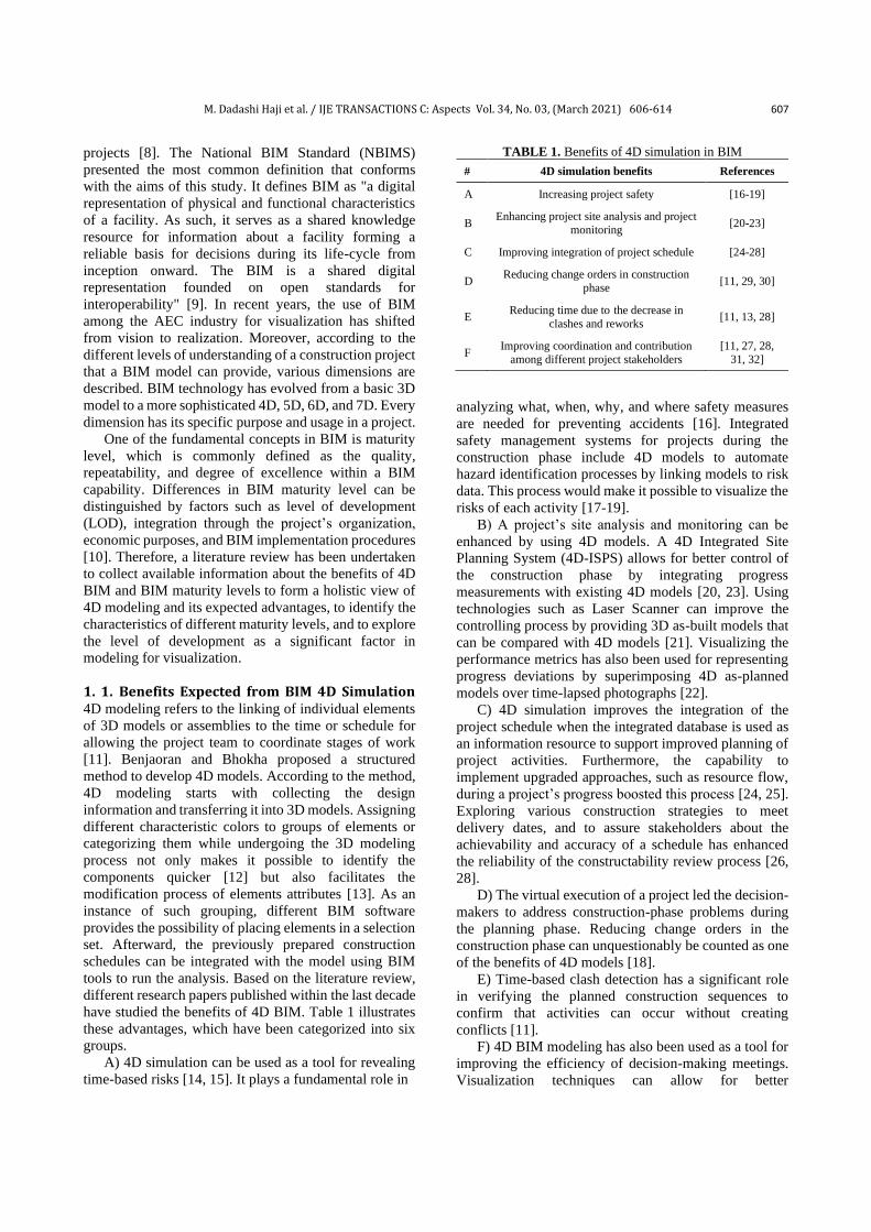
M. Dadashi Haji et al. / IJE TRANSACTIONS C: Aspects Vol. 34, No. 03, (March 2021) 606-614 607
projects [8]. The National BIM Standard (NBIMS)
presented the most common definition that conforms
with the aims of this study. It defines BIM as "a digital
representation of physical and functional characteristics
of a facility. As such, it serves as a shared knowledge
resource for information about a facility forming a
reliable basis for decisions during its life-cycle from
inception onward. The BIM is a shared digital
representation founded on open standards for
interoperability" [9]. In recent years, the use of BIM
among the AEC industry for visualization has shifted
from vision to realization. Moreover, according to the
different levels of understanding of a construction project
that a BIM model can provide, various dimensions are
described. BIM technology has evolved from a basic 3D
model to a more sophisticated 4D, 5D, 6D, and 7D. Every
dimension has its specific purpose and usage in a project.
One of the fundamental concepts in BIM is maturity
level, which is commonly defined as the quality,
repeatability, and degree of excellence within a BIM
capability. Differences in BIM maturity level can be
distinguished by factors such as level of development
(LOD), integration through the project’s organization,
economic purposes, and BIM implementation procedures
[10]. Therefore, a literature review has been undertaken
to collect available information about the benefits of 4D
BIM and BIM maturity levels to form a holistic view of
4D modeling and its expected advantages, to identify the
characteristics of different maturity levels, and to explore
the level of development as a significant factor in
modeling for visualization.
1. 1. Benefits Expected from BIM 4D Simulation 4D modeling refers to the linking of individual elements
of 3D models or assemblies to the time or schedule for
allowing the project team to coordinate stages of work
[11]. Benjaoran and Bhokha proposed a structured
method to develop 4D models. According to the method,
4D modeling starts with collecting the design
information and transferring it into 3D models. Assigning
different characteristic colors to groups of elements or
categorizing them while undergoing the 3D modeling
process not only makes it possible to identify the
components quicker [12] but also facilitates the
modification process of elements attributes [13]. As an
instance of such grouping, different BIM software
provides the possibility of placing elements in a selection
set. Afterward, the previously prepared construction
schedules can be integrated with the model using BIM
tools to run the analysis. Based on the literature review,
different research papers published within the last decade
have studied the benefits of 4D BIM. Table 1 illustrates
these advantages, which have been categorized into six
groups. A) 4D simulation can be used as a tool for revealing
time-based risks [14, 15]. It plays a fundamental role in
TABLE 1. Benefits of 4D simulation in BIM
# 4D simulation benefits References
A Increasing project safety [16-19]
B Enhancing project site analysis and project
monitoring [20-23]
C Improving integration of project schedule [24-28]
D Reducing change orders in construction
phase [11, 29, 30]
E Reducing time due to the decrease in
clashes and reworks [11, 13, 28]
F Improving coordination and contribution
among different project stakeholders
[11, 27, 28,
31, 32]
analyzing what, when, why, and where safety measures
are needed for preventing accidents [16]. Integrated
safety management systems for projects during the
construction phase include 4D models to automate
hazard identification processes by linking models to risk
data. This process would make it possible to visualize the
risks of each activity [17-19].
B) A project’s site analysis and monitoring can be
enhanced by using 4D models. A 4D Integrated Site
Planning System (4D-ISPS) allows for better control of
the construction phase by integrating progress
measurements with existing 4D models [20, 23]. Using
technologies such as Laser Scanner can improve the
controlling process by providing 3D as-built models that
can be compared with 4D models [21]. Visualizing the
performance metrics has also been used for representing
progress deviations by superimposing 4D as-planned
models over time-lapsed photographs [22].
C) 4D simulation improves the integration of the
project schedule when the integrated database is used as
an information resource to support improved planning of
project activities. Furthermore, the capability to
implement upgraded approaches, such as resource flow,
during a project’s progress boosted this process [24, 25].
Exploring various construction strategies to meet
delivery dates, and to assure stakeholders about the
achievability and accuracy of a schedule has enhanced
the reliability of the constructability review process [26,
28].
D) The virtual execution of a project led the decision-
makers to address construction-phase problems during
the planning phase. Reducing change orders in the
construction phase can unquestionably be counted as one
of the benefits of 4D models [18].
E) Time-based clash detection has a significant role
in verifying the planned construction sequences to
confirm that activities can occur without creating
conflicts [11].
F) 4D BIM modeling has also been used as a tool for
improving the efficiency of decision-making meetings.
Visualization techniques can allow for better

608 M. Dadashi Haji et al. / IJE TRANSACTIONS C: Aspects Vol. 34, No. 03, (March 2021) 606-614
coordination among the project planners. Moreover,
clarifying the activities for project teams may cause a
better understanding of the expectations and would make
the schedule more reliable [11].
1. 2. BIM Maturity Levels BIM maturity levels
have been established to define BIM capabilities clearly
in the AEC industry. These refer to quality, repeatability,
and degree of excellence within a BIM capability [32].
BIM maturity levels (depicted in Figure 1) are classified
into five categories: (a) Initial, (b) Defined, (c) Managed,
(d) Integrated and (e) Optimized.
Each maturity level is defined concerning the content
of models, procedure and strategies, integration among
different parts of a project, and purposes of BIM
implementation [29]:
• Maturity Level A (Initial): At this level, the
lack or absence of an overall strategy and shortage of
defined processes for BIM implementation is tangible.
BIM software tools are applied without sufficient prior
investigations and preparations. BIM adoption looks like
separated islands through the project, and some
individuals distinctively try to use the BIM tools in part
of their activities. This process suffers from the lack of
active and consistent support of middle and senior
management. A low rate of collaboration is the main
characteristic of this level. Hence, BIM implementation
typically occurs with little or no pre-defined process
guides or standards [29].
• Maturity Level B (Defined): At this level,
senior managers are familiar with BIM implementation.
The processes and policies have been established to
utilize BIM tools. Basic BIM guidelines are available,
including training manuals, workflow guides, and BIM
delivery standards. Training requirements are well-
defined and typically provided only when needed.
Collaboration between different parts of the project
increases based on mutual relationships following
process guides and standards [29]. • Maturity Level C (Managed): The aims and
processes of BIM implementation are understood by
most staff at this level. Moreover, a monitoring system
and a detailed action plan are being devised. Business
opportunities arising from BIM are acknowledged and
used in marketing efforts. Modeling, 2D representation,
quantification, specifications, and analytical properties of
3D models are managed through detailed standards and
quality plans. BIM managers are hired to collaborate the
responsibilities based on temporary project alliances or
longer-term partnerships [29].
• Maturity Level D (Integrated): BIM
implementation requirements and processes are
integrated between different parts of a project through
pre-defined channels at this level. Economic purposes of
implementation are adopted with the activities of all staff
involved in the project, from managers to lower-level
Figure 1. BIM Maturity Levels [27]
team members. Software choice follows the main
objectives of the projects, not just operational
requirements. Documentation of gained experiences and
knowledge is carried out systematically, making it easy
to access and retrieve [29].
• Maturity Level E (Optimized): BIM
implementation at this level is pervasive among project
stakeholders, as their strategies and processes are
continuously monitored and revised to best match with
each other. BIM software tools used in the project can
change if needed to meet strategic benchmarks.
Contractual models are also modified to achieve the
highest value for all stakeholders [33].
1. 3. Level of Development The concept of level of
development specifies the graphical representation and
the information that a model must contain for its use at
each phase of the project’s life cycle [34]. One of the
most cited definitions in the literature is related to the
American Institute of Architecture (AIA), which
categorizes the LOD into five levels [35, 36]: LOD100 to
LOD500. At the first level, LOD100, a project model has
represented generally, and some sorts of analysis (e.g.,
cost per square meter and building orientation) can be
carried out. The next level, LOD200, is more precise than
LOD100, and its generic elements can approximately
represent the orientation, location, shape, size, and
quantities. This level can be used for the analysis of
selected systems by application of generalized
performance criteria, such as investigation of the effects
of colors in architecture [37]. In the third level, LOD300,
building elements are specific and non-graphical

M. Dadashi Haji et al. / IJE TRANSACTIONS C: Aspects Vol. 34, No. 03, (March 2021) 606-614 609
information can be added into the model, making it viable
for use in documentation. The next level is LOD400, in
which detailed elements can be useful for accurately
representing processes such as fabrication, assembly, and
installation. The last level, LOD500, is the most detailed
level corresponding to a project’s as-built model. Models
at this level can be used for facility management and
maintenance. Additionally, an intermediary level,
LOD350, has been proposed between LOD300 and
LOD400 to support different trades during construction
by adding requirements on interfaces with other building
systems [38]. LOD300 or LOD350 is sufficient for
modeling during design phases unless some parts of the
project deal with fabrication and assembly procedures.
LOD grows during the design phase and reaches its peak
during the construction phase [39]. The level of
development at the design stage usually concentrates on
geometrical issues, while at the construction phase,
resources including equipment, materials, and labor are
dominant.
The level of development is also related to the BIM
maturity level, especially at the initiation of the project
and contractual phases. Implementing BIM at higher
maturity levels entails addressing more issues and more
complicated details based on the differences in the
responsibilities, relationships, collaboration level, and
technologies at each level of maturity [40].
In conclusion, BIM maturity level has been clarified
in different contexts, such as software platforms [41];
however, a lack of assessment of the consequences of
implementing BIM at those levels was apparent in past
studies. Moreover, although Dakhil and Alshawi
explained BIM implementation benefits within each BIM
maturity level, they neglected to quantify such
implementation benefits within each maturity level [42].
Furthermore, researchers have been studying the
visualization provided by BIM, but few studies have
examined the distinction in the benefits gained from
implementing 4D BIM simulation at different levels of
maturity. Thus, this research aims to empirically measure
survey data from two actual construction projects with
different BIM maturity levels to investigate the expected
benefits of implementing 4D simulation.
The remainder of the article is organized as follows.
The research methodology is discussed in section 2.
Section 3 defines the details of projects, which are
considered for the case study. Section 4 demonstrates the
results and discussion. In the end, some conclusions are
presented in Section 5.
2. METHODOLOGY In this study, the benefits of increasing from the initial
maturity level to the integrated maturity level, and the
effectiveness of BIM maturity level for profitable BIM
implementation are investigated empirically. For this
intention, the BIM maturity level of two construction
projects is determined. Next, the collected data about the
gained benefits within each case is discussed. Figure 2
shows the proposed methodology of this study. The
above two steps are further elaborated below.
For the first step, the major measuring aspects of BIM
maturity level were investigated by reviewing the
literature. Then, the procedure of BIM implementation,
coordination, and integration between different parts of
the project, the financial aims of implementation, and its
perception in project organization were surveyed in both
projects to determine their maturity levels.
Next, a questionnaire was designed to assess the
benefits of increasing from the initial maturity level to the
integrated maturity level, and the effectiveness of BIM
maturity level for profitable BIM implementation based
on the information gathered from the literature. Then, the
questionnaire was reviewed and improved according to
the comments of a group of six BIM experts, including
both BIM engineers and academic researchers. Four of
the BIM experts worked on both projects and also had
experience in the field of building information modeling.
The two others were academic experts who worked on
BIM and project scheduling as their field of study. The
questionnaire was distributed among 36 BIM experts
chosen from design engineers, engineers of project
management office (PMO), and teams of Research and
Development involved in both projects. The
questionnaire was distributed through individual
Figure 2. Flowchart of the proposed research methodology

610 M. Dadashi Haji et al. / IJE TRANSACTIONS C: Aspects Vol. 34, No. 03, (March 2021) 606-614
interviews instead of sending via email, fax, or mailing
them to clarify possible ambiguous questions for
respondents. Ambiguities are one of the most dangerous
elements of a survey that might affect the reliability and
the usefulness of the results. In the survey, the following
items were measured by reflective indicators with a five-
point Likert scale (1= very low, 2= low, 3= medium, 4=
high, 5= very high):
• improving integration of project schedule
• improving project site analysis and project
monitoring
• increasing safety level in project
• reducing time-based clashes and reworks
• reducing change orders in construction phase
• enhancing coordination and contribution among
different parts of the project
The reliability of the three questionnaires was
measured by utilizing Cronbach’s α coefficient, which is
the most common measure of integral reliability when
questions are asked on a Likert scale [43]. According to
the definition of Cronbach’s α coefficient, its normal
range cannot be less than 0.0 and cannot be greater than
+1.0. The reliability coefficients of 0.7 or higher are
considered satisfactory, and the higher values reflect a
higher degree of internal consistency.
3. CASE STUDIES
As mentioned, there are two construction projects in this
study. The first case is a commercial building located in
Tehran, named Atlas Mall. This project was the first of
the company for BIM implementation. They utilized
Autodesk products (e.g., Revit, Navisworks) to develop
BIM models. The project details are as follows:
• Location of project: Tehran, Iran
• Number of floors: 19
• Total area: About 130,000 m2
• Schedule: 48 months
The second project is a commercial-therapeutic
building located in Kerman, named Atlas Clinic (Figure
3). The project details are as follows:
• Location of project: Kerman, Iran
• Number of floors: 11
• Total area: About 12,000 m2
• Schedule: 48 months
4. RESULTS AND DISCUSSION
As mentioned, the survey was conducted among experts
involved in two commercial construction projects
undertaken by Iranian Atlas Company, a large-scale
general contractor in Iran. All experts were familiar with
the benefits and challenges of implementing 4D BIM in
Figure 3. BIM model of Atlas Clinic project, a) 3D, b) 4D
both projects. The calculated Cronbach’s α coefficient of
the questionnaires was 0.876, which means that the
reliability of the questionnaires was assured. Atlas Mall
was the first project that was investigated for determining
its level of BIM maturity. Autodesk BIM software, such
as Revit, was used to model the various disciplines of the
project. As it was the first attempt of the company for
BIM implementation and there was a lack of experience,
no specified procedure was employed within the project.
Additionally, there was inconsistent LOD for different
disciplines due to a lack of integration among various
parts of the project. For instance, no commercial
advantage was gained from detailed architectural 3D
modeling, in which interior furnishing was modeled
completely. While the model of mechanical, electrical,
and plumbing (MEP) was not developed in detail. Thus,
BIM implementation was at the initial maturity level
according to the available definition of the literature.
Atlas Clinic, the second project investigated for
determining its BIM maturity level, was also modeled
using Autodesk products. In contrary to Atlas Mall, BIM
implementation procedures and standards were set
systematically by senior managers. Additionally, a
procedure was established to define the duties of each
part of the project organization and determine their
relations. For instance, a committee that includes
structural, architectural, MEP designers, a project control
manager, and a representative of the scheduling team was
in charge of promoting the integration between different
parts of the project. They aimed to select a suitable LOD
for the model based on the project’s phases and needs.
In the process of 3D modeling, the most time-
consuming activity was developing an architectural

M. Dadashi Haji et al. / IJE TRANSACTIONS C: Aspects Vol. 34, No. 03, (March 2021) 606-614 611
model, and the wrong decision for LOD resulted in a
large amount of time wasted on the first project. If the
chosen LOD for the 3D model is higher than that required
for scheduling, linking operations number and the length
of time taken will increase. Moreover, the project
schedule gains more details with the progress of the
project. If any change is required in the 3D model or
project scheduling, modifying the 4D simulation will be
more difficult and time-consuming. Therefore, the joint
committee played a significant role in better BIM
implementation. The proposed LOD for the pre-
construction phase was between LOD200 and LOD300,
and the LOD for construction was developed from
LOD100 to LOD400. One of the most significant issues
noticed in the integration of design and project control
sections was that LOD would not be the same for all the
model’s elements. For instance, in finding crane
locations in the project site, LOD100 is adequate, and its
increase does not impact the results.
Another challenging factor in the Atlas Clinic project
was the process of matching the LOD of the 3D model to
the required one for the project schedule in the 4D
simulation. As the project schedule consisted of
approximate activity sequences in the pre-construction
phase, and it did not contain construction dates and
project milestones. One of the experiences gained
through this project was the preferability of providing a
detailed schedule just before the construction phase.
Consulting with the site manager can also be efficacious
in optimizing the scheduling process. Moreover, the 4D
modeler team devoted considerable effort to develop a
project schedule that matches with the 3D models.
Providing selection sets in 3D models and naming the
elements helped reduce the amount of work necessary to
link the model to the schedule. Furthermore, the
anticipation of many problems and solving them before
being encountered during project execution was the
result of undertaking project simulation before on-site
execution and caused considerable cost and time savings.
The relation defined between the site and 4D modeling
teams was improved by comments sent from the project’s
site through the BIM implementation process.
Alternative solutions were assessed in 4D simulation to
help managers choose the best option, such that 4D
simulation played the role of decision support system. In
conclusion, the Atlas Clinic project can be categorized at
the fourth maturity level according to the literature. Table
2 shows a comparison of the two projects in regards to
maturity criteria.
Considering the different criteria that are
determinative of the BIM maturity level of a project, the
maturity level of Atlas Mall and Atlas Clinic was initial
and integrated, respectively. Figure 4 depicts the impacts
of BIM maturity level on different benefits of BIM
implementation. The chart is drawn based on the results
of the questionnaire analysis. The positive effects
TABLE 2. A comparison between Atlas Mall and Atlas Clinic
projects
Criteria Atlas Mall Atlas Clinic
BIM implementation
process
No pre-defined
process
BIM implementation
procedure was defined concerning the integration
and interaction between
different parts of the project
Software
selection
No strategy
was defined
for choosing
software
The software was chosen
based on the project's needs
and the analysis required
during project execution
Economic
purposes of BIM
implementation
No economic
purpose BIM models were used in the
process of preselling
Systematic
documentation No BIM-
based process
An internal system for communication, integration,
and documentation was
carried out
Figure 4. Effectiveness of BIM maturity level for
advantageous BIM implementation
of BIM maturity level on the advantages of BIM
implementation can be concluded clearly.
As shown in the chart, the 4D simulation of the Atlas
Mall project had not gained the full potential of most of
BIM 4D’s benefits, including safety, schedule
integration, change order reduction, decreased time-
based clashes, and coordination improvement. However,
it can be inferred that the first and most easily achieved

612 M. Dadashi Haji et al. / IJE TRANSACTIONS C: Aspects Vol. 34, No. 03, (March 2021) 606-614
benefit of 4D modeling is improving project site analysis
and monitoring. This benefit stems from BIM’s
visualization outputs provided by time-based modeling
of the project. This capability allows for a visual
comparison, even with low or inconsistent levels of detail
among the elements, between a project’s real progress
and what the managers expected to see. The media
representing the discrepancies between planned and
actual progress of the project (e.g., charts, graphs, and
still photos) may not facilitate the communication of
progress information clearly and quickly, which makes
the process time-consuming and distracts decision-
makers from the vital task of corrective decision making
[44]. A series of conceptual visualization techniques have
been recently developed to facilitate the communication
of progress information and decision making on
corrective actions. However, it should be considered that
the increase in the effectiveness of 4D BIM in the
project’s site analysis and monitoring was not dramatic
by implementing BIM at a higher level of maturity.
The low maturity level of the Atlas Mall project
caused many of the 4D modeling benefits to be
marginalized, whereas Atlas Clinic had benefited
remarkable advantages due to its increase in the level of
maturity to the integrated stage. For instance, considering
the results of time-based clash reduction and safety
improvement can be concluded that in the Atlas Mall
project time-based risk identification did not occur due to
its initial maturity level. On the other hand, entering the
high maturity level terms in the project execution process
of Atlas Clinic improved BIM 4D utilization. One of the
most significant applications of 4D models is discovering
the time-based clashes. For instance, based on the
experience of implementing BIM, simultaneous
executions of a part of the roof and a lower floor’s shear
wall was not possible. This fact’s clarification prevented
unforeseen changes in the schedule during the
construction phase. As shown in the result, the more
detailed and integrated modeling process is, the more
applicable the 4D models become.
In addition, the relationship between the number of
BIM projects that each of the respondents experienced
and their respective answers to the survey questions were
analyzed. The results showed that former experience of
working on BIM projects had a profound effect on
respondents’ opinions. In other words, experts with three
or more years of experience on BIM-based projects had
a significantly higher evaluation of the benefits of 4D
BIM simulation at the integrated level of maturity. Thus,
it can be implied that highly experienced experts have a
deeper insight into the potential of 4D BIM simulation.
Figure 5 depicts the differences between the responses of
experts considering their duration of BIM involvement
experience.
Finally, this study results depict the positive impact
of BIM maturity level on the 4D simulation, which is
Figure 5. The effect of BIM experience on the experts'
responses
consistent with existing literature. For instance, Smits et
al. presented the maturity of the BIM implementation
strategy as the only reliable predictor of time, cost, and
quality performance [45]. In this study, other factors that
would impact the project performance were examined,
and their positive effects were shown. The other lesson
following from this research was the significance of
developing and observing specified standards and
procedures for BIM implementation.
5. CONCLUSION
BIM, as a digital representation of physical and
functional characteristics of a facility, has drawn
exceptional attention from researchers and practitioners
of the AEC industry. Among the vast area of BIM
studies, 4D simulation is one of the prevalent issues that
has been frequently investigated and implemented in
many cases. Nonetheless, there is a lack of research that
examines the relationship between the different factors,
such as the BIM maturity level, and the potential benefits
that can be gained from a 4D simulation of construction
projects. The objective of this paper is to study the effects
of BIM maturity level on the performance of the 4D
simulation. For this purpose, two commercial
construction projects, which were undertaken by the

M. Dadashi Haji et al. / IJE TRANSACTIONS C: Aspects Vol. 34, No. 03, (March 2021) 606-614 613
Iranian Atlas Company, were selected as cases. Both
projects have 4D BIM models, which were developed in
different disciplines. The BIM maturity level and gained
benefits of implementing the 4D simulation of each
project were assessed to clarify whether there is a
relationship between them .
BIM maturity level is illustrated the BIM capabilities
in the AEC industry. The maturity level of projects’ BIM
models was investigated and determined, considering the
criteria extracted from the literature. On the other hand, a
questionnaire was distributed among 36 professionals
engaged with both projects ask them to rate the
achievability of various benefits expected from the 4D
simulation. The results depict that enhancing the maturity
from initial to integrated level has a profound effect on
the achievement of expected benefits, such as increasing
the safety level of a project, improving the integration of
the project schedule, reducing change orders in the
construction phase, improving coordination and
contribution among different parts of projects and
reducing time-based clashes and reworks. Moreover, it
was notable that improving the project's site analysis and
project monitoring is an advantage that can be obtained
easily by implementing 4D BIM, regardless of
considering inconsistent levels of detail in model
elements, temporary facilities such as cranes or scaffolds,
and an integrated procedure for BIM implementation.
Additionally, the results showed that highly experienced
experts have a deeper insight into the potential of 4D
BIM simulation.
Future efforts will focus on extending the research
scope to all stakeholders involved in construction
projects and assessing all five levels of maturity by
surveying on a higher number of projects.
6. ACKNOWLEDGEMENT The authors would like to thank the experts and staff of
the Iranian Atlas Company, who shared their time for
supporting this study.
7. REFERENCES 1. Aryal, K., Thapa, P.S. and Lamichhane, D., "Revisiting
agroforestry for building climate resilient communities: A case of
package-based integrated agroforestry practices in nepal", Emerg
Science Journal, Vol. 3, No. 5, (2019), 303-311. doi:10.28991/esj-2019-01193
2. Saryazdi, A.H.G. and Poursarrajian, D., "Qualitative system
dynamics model for analyzing of behavior patterns of smes",
HighTech and Innovation Journal, Vol. 2, No. 1, (2021), 9-19. doi:10.28991/HIJ-2021-02-01-02
3. Borowski, P.F., "New technologies and innovative solutions in the development strategies of energy enterprises", HighTech and
Innovation Journal, Vol. 1, No. 2, (2020), 39-58. doi:10.28991/HIJ-2020-01-02-01
4. Burciaga, U.M., Sáez, P.V. and Ayón, F.J.H., "Strategies to reduce co2 emissions in housing building by means of cdw",
Emerging Science Journal, Vol. 3, No. 5, (2019), 274-284. doi:10.28991/esj-2019-01190
5. Procházka, L. and Boháčová, J., "Effect of admixtures on
durability characteristics of fly ash alkali-activated material", Emerging Science Journal, Vol. 4, No. 6, (2020), 493-502. doi:10.28991/esj-2020-01247
6. Burciaga, U.M., "Sustainability assessment in housing building
organizations for the design of strategies against climate change",
HighTech and Innovation Journal, Vol. 1, No. 4, (2020), 136-147. doi:10.28991/HIJ-2020-01-04-01
7. Barlish, K. and Sullivan, K., "How to measure the benefits of
bim—a case study approach", Automation in construction, Vol. 24, (2012), 149-159. doi:10.1016/j.autcon.2012.02.008
8. Zuppa, D., Issa, R.R. and Suermann, P.C., Bim's impact on the
success measures of construction projects, in Computing in civil engineering (2009). 2009.503-512. doi:10.1061/41052(346)50
9. AlizadehKharazi, B., Alvanchi, A. and Taghaddos, H., "A novel building information modeling-based method for improving cost
and energy performance of the building envelope", International
Journal of Engineering, Vol. 33, No. 11, (2020), 2162-2173. doi:10.5829/IJE.2020.33.11B.06
10. Alvanchi, A., Shiri, N. and Alikhani, H., "In-depth investigation of project planning and control software package application in
the construction industry of iran", International Journal of
Engineering, Vol. 33, No. 10, (2020), 1817-1825. doi:10.5829/IJE.2020.33.10A.01
11. Trebbe, M., Hartmann, T. and Dorée, A., "4d cad models to support the coordination of construction activities between
contractors", Automation in construction, Vol. 49, No., (2015), 83-91. doi:10.1016/j.autcon.2014.10.002
12. Benjaoran, V. and Bhokha, S., "Enhancing visualization of 4d cad
model compared to conventional methods", Engineering,
Construction and Architectural Management, Vol. 16, No. 4,
(2009), 392-408. doi:10.1108/09699980910970860
13. Zhou, Y., Ding, L., Wang, X., Truijens, M. and Luo, H.,
"Applicability of 4d modeling for resource allocation in mega
liquefied natural gas plant construction", Automation in
Construction, Vol. 50, (2015), 50-63. doi:10.1016/j.autcon.2014.10.016
14. Hernadewita, H. and Saleh, B., "Identifying tools and methods for
risk identification and assessment in construction supply chain",
International Journal of Engineering, Vol. 33, No. 7, (2020), 1311-1320. doi:10.5829/IJE.2020.33.07A.18
15. El Hiri, M., En-Nadi, A. And Chafi, A., "Suppliers selection in consideration of risks by a neural network", International
Journal of Engineering, Vol. 32, No. 10, (2019), 1454-1463. doi:10.5829/IJE.2019.32.10A.15
16. Chantawit, D., Hadikusumo, B.H., Charoenngam, C. and
Rowlinson, S., "4dcad‐safety: Visualizing project scheduling and safety planning", Construction Innovation, Vol. 5, No. 2, (2005), 99-114. doi:10.1191/1471417505ci091oa
17. Benjaoran, V. and Bhokha, S., "An integrated safety management
with construction management using 4d cad model", Safety
Science, Vol. 48, No. 3, (2010), 395-403. doi:10.1016/j.ssci.2009.09.009
18. Zhang, J. and Hu, Z., "Bim-and 4d-based integrated solution of analysis and management for conflicts and structural safety
problems during construction: 1. Principles and methodologies",
Automation in Construction, Vol. 20, No. 2, (2011), 155-166. doi:10.1016/j.autcon.2010.09.013
19. Kang, L.-S., Moon, H.-S., Kim, H.-S., Choi, G.-Y. and Kim, C.-H., Development of 5d cad system for visualizing risk degree and
progress schedule for construction project, in Computing in civil engineering (2011). 2011.690-697. doi:10.1061/41182(416)85

614 M. Dadashi Haji et al. / IJE TRANSACTIONS C: Aspects Vol. 34, No. 03, (March 2021) 606-614
20. Ma, Z., Shen, Q. and Zhang, J., "Application of 4d for dynamic site layout and management of construction projects",
Automation in Construction, Vol. 14, No. 3, (2005), 369-381. doi:10.1016/j.autcon.2004.08.011
21. Turkan, Y., Bosche, F., Haas, C.T. and Haas, R., "Automated
progress tracking using 4d schedule and 3d sensing technologies", Automation in Construction, Vol. 22, (2012), 414-421. doi:10.1016/j.autcon.2011.10.003
22. Golparvar-Fard, M., Peña-Mora, F., Arboleda, C.A. and Lee, S.,
"Visualization of construction progress monitoring with 4d
simulation model overlaid on time-lapsed photographs", Journal
of Computing in Civil Engineering, Vol. 23, No. 6, (2009), 391-404. doi:10.1061/(ASCE)0887-3801(2009)23:6(391)
23. Zhang, C. and Arditi, D., "Automated progress control using laser
scanning technology", Automation in Construction, Vol. 36, (2013), 108-116. doi:10.1016/j.autcon.2013.08.012
24. Dawood, N., Sriprasert, E., Mallasi, Z. and Hobbs, B., "Development of an integrated information resource base for
4d/vr construction processes simulation", Automation in
Construction, Vol. 12, No. 2, (2003), 123-131. doi:10.1016/S0926-5805(02)00045-6
25. Jongeling, R. and Olofsson, T., "A method for planning of work-flow by combined use of location-based scheduling and 4d cad",
Automation in Construction, Vol. 16, No. 2, (2007), 189-198. doi:10.1016/j.autcon.2006.04.001
26. Russell, A., Staub-French, S., Tran, N. and Wong, W.,
"Visualizing high-rise building construction strategies using linear scheduling and 4d cad", Automation in Construction, Vol. 18, No. 2, (2009), 219-236. doi:10.1016/j.autcon.2008.08.001
27. Kang, J.H., Anderson, S.D. and Clayton, M.J., "Empirical study
on the merit of web-based 4d visualization in collaborative
construction planning and scheduling", Journal of Construction
Engineering and Management, Vol. 133, No. 6, (2007), 447-461. doi:10.1061/(ASCE)0733-9364(2007)133:6(447)
28. Hartmann, T. and Fischer, M., "Supporting the constructability
review with 3d/4d models", Building Research & Information, Vol. 35, No. 1, (2007), 70-80. doi:10.1080/09613210600942218
29. Succar, B. and Kassem, M., "Building information modelling:
Point of adoption", in CIB World Conference Proceedings. Vol. 1, No., (Year).
30. Zhao, Q., Li, Y., Hei, X. and Wang, X., "Toward automatic calculation of construction quantity based on building
information modeling", in 2015 11th International Conference on
Computational Intelligence and Security (CIS), IEEE. (2015), 482-485. doi:10.1109/CIS.2015.122
31. Mahalingam, A., Kashyap, R. and Mahajan, C., "An evaluation of the applicability of 4d cad on construction projects", Automation
in Construction, Vol. 19, No. 2, (2010), 148-159. doi:10.1016/j.autcon.2009.11.015
32. Boton, C., Kubicki, S. and Halin, G., "Designing adapted
visualization for collaborative 4d applications", Automation in
Construction, Vol. 36, (2013), 152-167. doi:10.1016/j.autcon.2013.09.003
33. Succar, B., Sher, W. and Williams, A., "Measuring bim performance: Five metrics", Architectural Engineering and
Design Management, Vol. 8, No. 2, (2012), 120-142. doi:10.1080/17452007.2012.659506
34. The American Institute of Architects, "AIA Document G202-2013," The American Institute of Architects, 2013.
35. Pinheiro, A.P., "Architectural rehabilitation and sustainability of
green buildings in historic preservation", HighTech and
Innovation Journal, Vol. 1, No. 4, (2020), 172-178. doi:10.28991/HIJ-2020-01-04-04
36. Solihin, W. and Eastman, C., "Classification of rules for
automated bim rule checking development", Automation in
Construction, Vol. 53, (2015), 69-82. doi:10.1016/j.autcon.2015.03.003
37. Kriphal, M. and Grilo, A., "Compatibility between design and
construction building information models", ECPPM
Proceedings, London, UK, Taylor & Francis Group, (2012), 447-452.
38. Sinclair, S., Building information modelling (bim) & english law. 2015, London, UK, John Wiley & Sons, Ltd. doi:10.1002/9781118838167.app3
39. Bouška, R., "Evaluation of maturity of bim tools across different
software platforms", Procedia Engineering, Vol. 164, (2016), 481-486. doi:10.1016/j.proeng.2016.11.648
40. Dakhil, A. and Alshawi, M., "Client's role in building disaster
management through building information modelling", Procedia
Economics and Finance, Vol. 18, (2014), 47-54. doi:10.1016/S2212-5671(14)00912-5
41. Boton, C., Kubicki, S. and Halin, G., "The challenge of level of
development in 4d/bim simulation across aec project lifecyle. A
case study", Procedia Engineering, Vol. 123, (2015), 59-67. doi:10.1016/j.proeng.2015.10.058
42. AIA, A., "Document e202-2008", Building Information Modeling Protocol Exhibit, Washington, DC: American Institute of Architects, (2008).
43. Masood, R., Kharal, M. and Nasir, A., "Is bim adoption
advantageous for construction industry of pakistan?", Procedia
Engineering, Vol. 77, (2014), 229-238. doi:10.1016/j.proeng.2014.07.021
44. Fard, M.G. and Peña-Mora, F., Application of visualization techniques for construction progress monitoring, in Computing in
civil engineering (2007). 2007.216-223. doi:10.1061/40937(261)27
45. Smits, W., van Buiten, M. and Hartmann, T., "Yield-to-bim:
Impacts of bim maturity on project performance", Building
Research & Information, Vol. 45, No. 3, (2017), 336-346. doi:10.1080/09613218.2016.1190579
Persian Abstract
چکیده های اری تفاوت ذاثرگ .استسازی چهاربعدی پروژه در سالیان اخیر مورد توجه پژوهشگران مختلف قرار داشته الخصوص شبیهساختمان و علی سازی اطالعات ابعاد مختلف مدل
مختلفی عواملها که از ت این تفاو .قرار دهدتأثیر تواند کارکردهای مورد انتظار را تحث می ،گیردکه ذیل مبحث سطح بلوغ قرار می ،سازی اطالعات ساختمانسازی مدلپیاده
سازی این پژوهش مزایای شبیه .ستا شده به طور کامل مورد توجه قرار نگرفتههای انجامباشد در پژوهشثر می أمت ،کننده و یا محتوای مدلاز جمله یکپارچگی سازمان پیاده
به آوری شده، سطح جزئیات و بلوغ مورد نیاز برای نیل استفاده از تحلیل اطالعات جمع با و شده در سطوح بلوغ متفاوت را مورد بررسی قرار داده استسازیچهاربعدی پیاده
سازی مدل اطالعاتی ساختمان در سازمان باشد که یکپارچگی پیاده نتایج حاکی از این می .نمایدسازی مدل اطالعاتی ساختمان را تعیین می شده از پیادهاهداف از پیش تعیین
سازی مدل پیادههای مختلف سازمانی از پیاده سازی مدل اطالعاتی ساختمان منجر به بهبود کارایی و اثربخشی سازی انتظارات بخشطح جزئیات و شفافپروژه، درنظرگرفتن س
. شونداطالعاتی ساختمان می

IJE TRANSACTIONS C: Aspects Vol. 34, No. 03, (March 2021) 615-620
Please cite this article as: F. Marchione, Enhancement of Stiffness in GFRP Beams by Glass Reinforcement, International Journal of Engineering, Transactions C: Aspects Vol. 34, No. 03, (2021) 615-620
International Journal of Engineering
J o u r n a l H o m e p a g e : w w w . i j e . i r
Enhancement of Stiffness in GFRP Beams by Glass Reinforcement
F. Marchione* Dipartimento di Ingegneria Civile, Edile e Architettura (DICEA), Università Politecnica delle Marche, via B. Bianche, Ancona, Italy
P A P E R I N F O
Paper history: Received 13 Decemeber 2020 Received in revised form 30 December 2020 Accepted 11 January 2021
Keywords: Bending Tests GFRP Beams Adhesive Joint Stiffness Enhancement
A B S T R A C T
Glass is a stiff material with brittle structural behaviour. Hence, it is usually a material mostly decorative or simply structurally supported, and it is hardly ever a load-bearing element within a structure. Although
in recent years there have been several experiments in its use in civil engineering, to date little data has been collected or design methodologies disseminated. The present study proposes the innovative concept
of considering glass as a structural material, cooperating within a structural system thanks to the adhesive
joining technique. In detail, the case of a GFRP structural beam element subjected to bending is herein considered. The evaluation of the stiffness of the mentioned element is compared with that of the same
element reinforced with glass plates of different thicknesses. The results show the possibility to increase
the global stiffness of the structural element. These outcomes are validated by FEM analysis, which showed excellent agreement with the analytical ones. The effectiveness of the reinforced system, thanks
to the considerable stiffness characteristics, allows both the use of glass and the respect of the
requirements related to the displacements of the structural elements in their service life.
doi: 10.5829/ije.2021.34.03c.04
NOMENCLATURE
URM Unreinforced model k Stiffness
RM-i Reinforced model with i–thick reinforcement E Young Modulus
I Moment of inertia b Cross area width t Thickness l Beam Length
s Displacement F Applied load
1. INTRODUCTION1 Glass is a stiff material with brittle structural behaviour.
In the building sector, there has been a significant
increase in its use [1-3]. In fact, it is an element that
allows light spaces to be created and gives a sense of
lightness to the resulting element. However, despite the
fact that the use of glass is very frequent (e.g.
doors/windows [4], decorations, etc.) its structural
applications are limited to date. In fact, in its usual
applications, it is often configured as a supported object
without any load-bearing function. Recent scientific and
research advances are considering the development of
glass or hybrid structures, characterised by the joining of
glass with other traditional materials, such as timber [5-
7], steel [8], GFRP [9].
*Corresponding Author Institutional Email:
[email protected] (F. Marchione)
However, in the study of these new structures, the
main point is represented by the joints. In fact, joints are
the most vulnerable points in any structure. In particular,
in the case of glass structures, classical mechanical joints
introduce undesirable concentrated stresses due to the
brittle behaviour of glass. Stress peaks could lead to the
diffusion of micro-cracks and therefore the rapid collapse
of the structure or part of it for values of stresses lower
than those characteristics of the material.
Therefore, the types of joints that could overcome this
type of problem are the adhesive ones.
This type of joint provides several advantages, such
as better and more uniform stress distribution, ease of
application and little added weight to the resulting
structure [10, 11].
Several papers, such as in Refs. [12, 13] show how
the use of glass (a fragile material) coupled with other

F. Marchione / IJE TRANSACTIONS C: Aspects Vol. 34, No. 03, (March 2021) 615-620 616
ductile materials (steel, GFRP, aluminium, timber) is
able to create high-performance structures, capable of
withstanding significant external actions both in and out
of plane.
Parate [14] studied Propellant Actuated Devices
(PAD), usually installed on various combat aircraft of Air
Force. This study explains the development aspects of
PAD, its use, function, testing and performance
evaluation methodology in a suitable fabricated Velocity
Test Rig (VTR). The main objective of this paper is to
device a novel method to measure actual slug velocity of
the aircraft gun inside a cartridge using VTR and Doppler
RADAR. Ntintakis et al. [15] studied the topology
optimization by the use of 3D Printing Technology in the
Product Design Process. In this study the authors initially
print furniture models with different wall thicknesses
using the Inject Binder technique and then we check their
durability and resilience by compression tests. Then, the
optimized models are redesigned in order to improve
their durability. Ha [16] proposed a simple but effective
trailing edge flap system. This preliminary concept uses
a more practical and stable actuation system which
consists of a motor-driven worm gear drive and flexible
torsion bar. A preliminary level design study was
performed to show the applicability of the new trailing
edge flap system for wind turbine rotor blades or
helicopter blade. Rastegarian et al. [17] studied the
dependency of structural performance level and its
corresponding inter-story drift in conventional RC
moment frames. For this purpose, inter-story drift as a
dependent variable and other structural characteristics
have been assumed. Specimens were studied by means of
pushover analysis.
Silvestru et al. [18] studied two configurations for
such glass-metal façade elements, with silicone and
acrylic adhesive respectively. Full-scale tests and FEA
simulations are carried out for the two configurations
with loads acting in three different directions, both
separately and in combination. The results of the tests
performed under in-plane shear load reveal a high load
capacity of both configurations and show that the failure
begun inside the adhesive layers.
Haldimann et al. [19] studied the performance of five
adhesives for load-bearing steel-glass connections.
Mechanical tests on the connections provided useful data
for the selection of a suitable adhesive (silicone).
Richter et al. [20] illustrated the possibilities offered
by existing hyperelastic material models for specific
steel-glass components. Small-scale tests were carried
out to characterise the adhesives and determine the
material model for subsequent FEA.
Figure 1 illustrates the research methodology
proposed.
Glass-fiber-reinforced pultruded materials (GFRP)
represent innovative high-strength materials with low
dead weight. However, they are particularly vulnerable
Figure 1. Research flowchart
to concentrated stresses (e.g. bolted joints). Therefore,
the adhesive joint allows both to solve the problem of
stress distribution and to improve the global behavior of
the resulting structure, making the glass and the support
beam structurally cooperating [21].
This paper illustrates the study of the problem of a
GFRP beam and illustrates a simple method to improve
its characteristics in terms of the overall stiffness of the
structural element. This is sought through the insertion of
a glass plate reinforcement at its extrados. The analytical
and numerical methods for the evaluation of the stiffness
of the structural configurations analysed are detailed in
the following.
2. PROBLEM STATEMENT
In this section the simulations and calculations program
carried out is defined.
The present paper illustrates the possibility of
obtaining a significant increase in stiffness by means of
an adhesive joint between a GFRP beam and a glass plate.
GFRP and glass panels are bonded together by means of
structural adhesive, as shown in Figure 2. The cross-
section of the beam is depicted in Figure 2, and it will be
analysed in the following. Numbers 1 and 2 indicate the
GFRP and glass substrates, respectively. The adhesive
thickness between the adherents is always considered
constant and equal to 0.30 mm. The length of the beams
is always considered to be 1.00 m.
Figure 3 illustrates the static scheme used in the
subsequent analytical analysis. A pressure of 2.00 kPa is
applied to the extrados surface of the beam.
The novelty of this concept concerns the realisation
of a new type of load-bearing beam for structural uses,
characterised by the coupling of a ductile material (e.g.
GFRP) and a material known to be brittle (e.g. glass). The
reinforcement by means of a glass plate is proposed only
on the extrados of the beam both for architectural needs
(e.g. transparent and light finish) and for needs related to
the safety of the users.

617 F. Marchione / IJE TRANSACTIONS C: Aspects Vol. 34, No. 03, (March 2021) 615-620
Figure 2. Beam cross section
Figure 3. Static model of the beam
Table 1 shows the mechanical characteristics of the
materials used in the models shown below.
Table 2 illustrates the acronyms and geometric
characteristics of the beams considered in the following
analyses
The results obtained from analytical calculations and
FEM simulations are shown below.
TABLE 1. Materials’ characteristics
E [MPa]
Adhesive 3000
GFRP 26000
Glass 75000
TABLE 2. Beams geometric characteristics
Parameters
Specimen b (mm) t1 (mm) t2 (mm) l (mm)
URM 70 50 - 1000
RM -10 70 50 10 1000
RM -15 70 50 15 1000
RM -20 70 50 20 1000
3. ANALYTICAL MODEL
Considering the static model of the beam (Figure 2)
simply supported at its ends, the following equation
could be written in relation to the value of the beam
displacement:
𝑠 =𝐹 𝑙3
48 𝐸𝑏 𝐼𝑏 (1)
where l is the length of the beam, Eb is the modulus of
elasticity and F is the applied load. I represents the
moment of inertia of the beam, given by the well-known
equation:
𝐼 =𝑏 ℎ3
12 (2)
where b e tb are width and length of the beam cross-
section, rispectively.
Stiffness k, defined as the load required to produce a unit
displacement, is given by the following:
𝑘 =𝐹
𝑠=
48 𝐸𝑏 𝐼𝑏
𝑙3 (3)
To verify the effectiveness of the reinforcement in terms
of stiffness, it is necessary to distinguish between
perfectly adhesive behaviour between glass and substrate
and no structural collaboration between the two elements.
In the case of structural collaboration, the stiffness could
be evaluated as follows:
𝑘𝑐𝑜𝑜𝑝 =48
𝑙3 ∑ 𝐸𝑖𝐼𝑖∗2
𝑖=1 (4)
in which the moments of inertia are expressed as follows:
𝐼1∗ = 𝐼1 + 𝐴1 ⋅ 𝑥2 (5)
𝐼2∗ = 𝐼2 + 𝐴2 ⋅ [(𝑡2 − 𝑥) +
𝑡2
2]
2 (6)
The position of the neutral axis in relation to the centre
of gravity of the section is then determined:
𝑥 =𝐸2·𝑏·𝑡2·
𝑡12
+𝐸2·𝑏·𝑡22·
1
2
2 𝐸1·𝑡1·𝑡2+2 𝐸1·𝑏·𝑡2+𝐸1·𝑏·𝑡2 (7)
In the case of non-collaborating elements, the stiffness
could be expressed as follows:
𝑘𝑛𝑜−𝑐𝑜𝑜𝑝 =48
𝑙3 ∑ 𝐸𝑖𝐼𝑖2𝑖=1 (8)
Where the moments of inertia are expressed as shown in
Equation (2).
4. FEA ANALYSIS
This section illustrates finite element modeling for the
above mentioned problem.
Finite element analyses are performed both in the
case of unreinforced and reinforced beams, according to
the geometric configurations illustrated in section 2.

F. Marchione / IJE TRANSACTIONS C: Aspects Vol. 34, No. 03, (March 2021) 615-620 618
The “Static Structural” module, present in
ANSYS©19 is used, and the results are herein reported.
The analysis is linear elastic, and the analysis is of 3D-
type. The geometries illustrated are meshed with PLANE
182 elements, a 4-node structural solid and a maximum
element size of 0.10 mm. Once the loads are applied, it is
possible to correlate the maximum displacement with the
force reactions at the ends of the beam, both for
unreinforced and in reinforced beams.
4. RESULTS AND DISCUSSION
The present paragraph reports on the results obtained
according to both the analytical and numerical analysis
just presented.
Different geometrical characteristics have been
considered in the reinforcement of the GFRP beam in the
condition of cooperating reinforcement.
The beam theory is used to analyze the ductility and
to evaluate the position of the neutral axis for a composite
beam simply supported at its ends. The simulation
validates the theoretical results by means of a linear
elastic analysis of the model considered. The FEA
simulation is conducted by means of the static analysis of
the ANSYS©19 software. Table 3 illustrates and
compares the results obtained from the different analyses.
The results obtained show a very accurate
approximation of the analytical analysis for the
evaluation of the stiffness increase brought by the glass
reinforcement. In fact, a small evaluation error is
observed for the reinforced configurations (within 15%).
Figure 4 shows the force-displacement graphs
obtained from the analyses.
Figure 4. Load-displacement graph
TABLE 3. Analytical and FEA results
Specimen b (mm) t1 (mm) t2 (mm) l (mm) k (N/mm)
ANSYS Equation (4) Δ (%)
URM 70 50 - 1000 719.22 910.00 -26.53
RM -10 70 50 10 1000 1934.98 1755.95 + 9.25
RM -15 70 50 15 1000 2505.64 2165.32 + 13.58
RM -20 70 50 20 1000 7409.29 3184.06 - 1.88
4. CONCLUSIONS
Recent legislations and technological developments lead
to a continuous escalation of the technical requirements
of structural elements in terms of both global and local
ultimate strength. On the other hand, modern
architectural language makes extensive use of glass as
both a structural and purely decorative material. Indeed,
glass allows the creation of luminous structures and
provides an idea of lightness to the user. However, the
structural applications of glass are currently very limited.
The study here presented proposes a new hybrid beam in
GFRP and glass for structural purpose. The result is a
light and design structural element, which is therefore not
relegated to a load-bearing function only, but also
assumes an architectural value.
In detail, a GFRP beam in unreinforced configuration
is considered and its stiffness is evaluated both
numerically and analytically. Then, different
combinations of glass reinforcements (i.e. plates of
different thicknesses) were considered and analysed.
The main outcomes are:
- The hybrid system enables very high stiffness
values to be obtained when compared with the same
unreinforced structural element;
- The increase in stiffness that could be achieved
makes it possible to meet very high requirements in
terms of permissible displacements with the same
structural elements, without introducing significant
geometric changes in the section;
- FEA and analytical results are in good agreement
and therefore make it possible to adequately assess
0
10
20
30
40
50
60
70
80
0.00 0.02 0.04 0.06 0.08 0.10
F [
N]
s [mm]
URM-FEA URM-Analytical
RM-10-FEA RM-10-Analytical
RM-15-FEA RM-15-Analytical
RM-20-FEA RM-20-Analytical

619 F. Marchione / IJE TRANSACTIONS C: Aspects Vol. 34, No. 03, (March 2021) 615-620
the increase in stiffness that could be achieved;
- The methodology illustrated allows for a quick and
easy assessment of the stiffness contribution of the
reinforcement and is therefore an effective design
tool. In conclusion, the present study provides an example of
the calculation and application of glass in the field of civil
engineering. The aim is to overcome the concept of glass
as a material with merely decorative functions and to
extend its function to the field of structures. The results
reported demonstrate the effectiveness of its application
in this purpose.
5. REFERENCES
1. Quini, J.G. and Marinucci, G., "Polyurethane structural adhesives
applied in automotive composite joints", Materials Research,
Vol. 15, No. 3, (2012), 434-439. doi: 10.1590/S1516-
14392012005000042
2. Fecht, S., Vallée, T., Tannert, T. and Fricke, H., "Adhesively
bonded hardwood joints under room temperature and elevated
temperatures", The Journal of Adhesion, Vol. 90, No. 5-6,
(2014), 401-419. doi: 10.1080/00218464.2013.836968
3. Godat, A., Légeron, F., Gagné, V. and Marmion, B., "Use of frp
pultruded members for electricity transmission towers", Composite Structures, Vol. 105, (2013), 408-421. doi:
10.1016/J.COMPSTRUCT.2013.05.025
4. Appelfeld, D., Hansen, C.S. and Svendsen, S., "Development of a slim window frame made of glass fibre reinforced polyester",
Energy and Buildings, Vol. 42, No. 10, (2010), 1918-1925. . doi:
10.1016/J.ENBUILD.2010.05.028
5. Rodacki, K., Tekieli, M. and Furtak, K., "Contactless optical
measurement methods for glass beams and composite timber-
glass i-beams", Measurement, Vol. 134, (2019), 662-672. doi:
10.1016/j.measurement.2018.09.061
6. Dorn, M., Enquist, B. and Serrano, E., "Load bearing timber glass
composites—a woodwisdom—net project for innovative building system", in COST Action TU0905 Mid-term Conference on
Structural Glass, CRC Press. (2013), 269. doi:
http://dx.doi.org/10.1201/b14563-38
7. Unuk, Ž., Ivanič, A., Leskovar, V.Ž., Premrov, M. and Lubej, S.,
"Evaluation of a structural epoxy adhesive for timber-glass bonds
under shear loading and different environmental conditions", International Journal of Adhesion and Adhesives, Vol. 95,
(2019), 102425. doi: 10.1016/j.ijadhadh.2019.102425
8. Machalická, K., Vokáč, M. and Eliášová, M., "Influence of artificial aging on structural adhesive connections for façade
applications", International Journal of Adhesion and Adhesives,
Vol. 83, (2018), 168-177. doi: 10.1016/j.ijadhadh.2018.02.022
9. Bedon, C. and Louter, C., "Structural glass beams with embedded
gfrp, cfrp or steel reinforcement rods: Comparative experimental,
analytical and numerical investigations", Journal of Building
Engineering, Vol. 22, (2019), 227-241. doi:
10.1016/j.jobe.2018.12.008
10. Marchione, F., "Investigation of vibration modes of double-lap adhesive joints: Effect of slot", International Journal of
Engineering, Vol. 33, No. 10, (2020), 1917-1923. doi:
10.5829/ije.2020.33.10a.10
11. Marchione, F., "Stress distribution in double-lap adhesive joints:
Effect of adherend reinforcement layer", International Journal
of Adhesion and Adhesives, Vol. 105, (2021), 102780. doi:
10.1016/j.ijadhadh.2020.102780
12. Machalická, K. and Eliášová, M., "Adhesive joints in glass structures: Effects of various materials in the connection,
thickness of the adhesive layer, and ageing", International
Journal of Adhesion and Adhesives, Vol. 72, (2017), 10-22. doi:
10.1016/j.ijadhadh.2016.09.007
13. Marchione, F. and Munafò, P., "Experimental strength evaluation
of glass/aluminum double-lap adhesive joints", Journal of
Building Engineering, Vol. 30, (2020), 101284. doi:
10.1016/j.jobe.2020.101284
14. Parate, B.A., "Propellant actuated device for parachute deployment during seat ejection for an aircraft application",
HighTech and Innovation Journal, Vol. 1, No. 3, (2020), 112-
120. . doi: 10.28991/HIJ-2020-01-03-03
15. Ntintakis, I., Stavroulakis, G.E. and Plakia, N., "Topology
optimization by the use of 3d printing technology in the product
design process", HighTech and Innovation Journal, Vol. 1, No.
4, (2020), 161-171. doi: 10.28991/HIJ-2020-01-04-03
16. Ha, K., "Innovative blade trailing edge flap design concept using
flexible torsion bar and worm drive", HighTech and Innovation
Journal, Vol. 1, No. 3, (2020), 101-106. doi: 10.28991/HIJ-
2020-01-03-01
17. Rastegarian, S. and Sharifi, A., "An investigation on the correlation of inter-story drift and performance objectives in
conventional rc frames", Emerging Science Journal, Vol. 2, No.
3, (2018), 140-147. doi: 10.28991/esj-2018-01137
18. Silvestru, V.A., Kolany, G., Freytag, B., Schneider, J. and
Englhardt, O., "Adhesively bonded glass-metal façade elements
with composite structural behaviour under in-plane and out-of-plane loading", Engineering Structures, Vol. 200, (2019),
109692. doi: 10.1016/j.engstruct.2019.109692
19. Haldimann, M., Luible, A. and Overend, M., "Structural use of
glass, Iabse, Vol. 10, (2008).
20. Richter, C., Abeln, B., Geßler, A. and Feldmann, M., "Structural
steel–glass facade panels with multi-side bonding–nonlinear stress–strain behaviour under complex loading situations",
International Journal of Adhesion and Adhesives, Vol. 55, No.,
(2014), 18-28. doi: 10.1016/j.ijadhadh.2014.07.004
21. Alderucci, T., Terlizzi, V., Urso, S., Borsellino, C. and Munafò,
P., "Experimental study of the adhesive glass-steel joint behavior
in a tensegrity floor", International Journal of Adhesion and
Adhesives, Vol. 85, (2018), 293-302. doi:
10.1016/j.ijadhadh.2018.04.017

F. Marchione / IJE TRANSACTIONS C: Aspects Vol. 34, No. 03, (March 2021) 615-620 620
Persian Abstract
چکیده از نظر ساختاری پشتیبانی می شود شیشه ماده ای سفت و سخت و دارای رفتار ساختاری شکننده است. از این رو ، این ماده معموال یک ماده عمدتا تزئینی است و یا به سادگی
عمران انجام شده است ، اما تاکنون اطالعات کمی جمع و به سختی یک عنصر باربر درون سازه است. اگرچه در سالهای اخیر چندین آزمایش در استفاده از آن در مهندسی
یستم ساختاری را به لطف آوری شده یا روشهای طراحی منتشر شده است. مطالعه حاضر مفهوم ابتکاری در نظر گرفتن شیشه به عنوان یک ماده ساختاری ، همکاری در یک س
تحت خمش مورد بررسی قرار می گیرد. ارزیابی سختی عنصر ذکر GFRPاز عناصر پرتوی ساختاری روش اتصال چسب ارائه می دهد. به طور جزئی ، در اینجا یک مورد
سازه. این نتایج با تجزیه شده با همان عنصر تقویت شده با صفحات شیشه ای با ضخامت های مختلف مقایسه می شود. نتایج نشان می دهد امکان افزایش سختی جهانی عنصر
تحلیلی را نشان داد. اثربخشی سیستم تقویت شده ، به لطف ویژگی های قابل توجهی از سختی ، هم استفاده از شیشه تأیید می شود ، که توافق عالی با نتایج FEMو تحلیل
می کند. فراهمو هم رعایت الزامات مربوط به جابجایی عناصر سازه ای را در طول عمر آنها

IJE TRANSACTIONS C: Aspects Vol. 34, No. 03, (March 2021) 621-628
Please cite this article as: S. Sverguzova, N. Miroshnichenko, I. Shaikhiev, Z. Sapronova, E. Fomina, N. Shakurova, V. Promakhov, Application of Sorbent Waste Material for Porous Ceramics Production, International Journal of Engineering, Transactions C: Aspects Vol. 34, No. 03, (2021) 621-628
International Journal of Engineering
J o u r n a l H o m e p a g e : w w w . i j e . i r
Application of Sorbent Waste Material for Porous Ceramics Production
S. Sverguzovaa, N. Miroshnichenkoa, I. Shaikhievb, Z. Sapronovaa, E. Fomina*a, N. Shakurovaa, V. Promakhovc a Department of Industrial Ecology, Belgorod State Technological University, Belgorod, Russia b Department of Environmental Engineering, Kazan National Research Technological University, Kazan, Russia c National Research Tomsk State University, Tomsk, Russia
P A P E R I N F O
Paper history: Received 03 September 2020 Received in revised form 11 November 2020 Accepted 10 December 2020
Keywords: Agricultural Waste Porosity Pumpkin Seed Husks Waste Sorption Material Sludge Disposal Combustible Additive
A B S T R A C T
The paper considers the application of waste sorption material utilization and pumpkin seed husks formed during the extraction of heavy metal ions from aqueous solutions, as a combustible additive to
clay mixtures in production of the porous ceramics. In this regard, this study evluates the effects of
different amounts (2-8%) of the spent sorption material in the charge composition with changes in the physical and mechanical properties of ceramic samples obtained by firing at temperatures of 950-1050
° C. One finding is that the combustion of the organic additive is accompanied by the formation of voids
and the release of gases with the formation of pores in the ceramic piece. Another finding is that all clay mixtures with a combustible additive allow the production of porous ceramics to meet the requirements
for compressive strength, porosity, density, water absorption and linear shrinkage. It is recommended
using 4 % of combustive additive in order to obtain optimal properties in terms of density and strength. During the testing of the developed porous ceramics for heavy metal leaching, the material does not pose
an environmental hazard. Finally, the results of this study are applicable for the construction of internal
partitions and household buildings.
doi: 10.5829/ije.2021.34.03c.05
1. INTRODUCTION
Wastewater treatment sludge is one of the most
widespread and large-scale wastes. Annually, around the
world, millions of tons of such wastes are generated,
which are partially utilized and used later in agriculture
and production cycles. However, most of them are stored
at industrial landfills, disposing large areas of fertile soils
and having a negative impact on the environment. In
addition, construction is an industry where sewage sludge
can be used. This excludes some costly and energy-
intensive recycling steps and the resulting construction
material is often stable and safe [1-3]. Extensive research
was carried out on the use of sewage sludge in the
production of building materials such as roofing tile,
bricks, lightweight aggregates, cement, concrete and
geopolymers [4,5]. Particular attention is paid to
wastewater treatment sludge containing heavy metals.
The potential hazard of heavy metals depends on the
physic-chemical forms of metals in the sludge. Heavy
metals are considered as one of the hazardous pollutants
*Corresponding Author Email: [email protected] (E. Fomina)
because they are toxic with high persistence in the
environment and food chain. In addition, these metals do
not decompose and have the ability to accumulate in the
environment and present one of the most dangerous
pollutants in the biosphere [6,7].
The existing literature sources touch upon the issue of
the economic efficiency of sorbents from agricultural
crops for removing heavy metal ions from wastewater [8]
and the efficiency of using agricultural waste in the
construction industry [9-11]. The metal-containing
wastes formed after water treatment pose an
environmental hazard and necessitate their disposal. The
use of organic sediments for water treatment of heavy
metals is a promising option in the production of ceramic
products [12,13] and porous ceramics [14]. This solution
makes it possible to avoid secondary pollution and also
increases the value of the waste converting it into a useful
material. In addition, sewage sludge acts as a fuel during
the sintering process and saves up to 40% of energy for
firing [15].

S. Sverguzova et al. / IJE TRANSACTIONS C: Aspects Vol. 34, No. 03, (March 2021) 613-620 622
During sintering the components of organic matter
coming from the sewage sludge additionally emit gases,
which contribute to the formation of pores and the
creation of a porous structure of ceramic material, which
characterizes it as a combustive additive [16].
Recent studies in this research area reveal that the
heat treatment allows the fixation of heavy metals
coming from the sludge of treated wastewater in a silicate
structure. When the sintering temperature of ceramics is
reached, heavy metals interact with basic clay minerals
(for example, alumina, kaolinite, and hematite) and form
a crystalline phase of aluminosilicates and silicates
[17,18]. The synthesis of various compounds can depend
on temperature and basic oxide content.
One of the main trends in the literature review refers
that the ceramic matrix stabilizes the mobility of heavy
metals, reducing the potential hazard of their release
[19,20]. According to the results of the leaching test, a
low limit of extraction of metals such as Pb, Cd, Zn, Cr,
Ni and Cu is noted [6], this confirms their stabilization in
the ceramic structure of building material [21]. The tests
carried out in the work [22] confirm the harmlessness of
ceramic materials obtained using wastewater treatment
sludge from heavy metals during their operation.
To provide an additional step to the advancement of
knwoledge in this research area and in order to expand
the range of methodological approaches to the disposal
of wastewater treatment sludge containing heavy metals
in the production of ceramic products, we studied the
effect of wastewater treatment sludge with nickel ions
Ni2+ (WTSN), where crushed pumpkin seed husk (PSH)
was used as a sorbent. The main purpose of this research
is to develop porous ceramics with low density, high
porosity and without significant changes in mechanical
strength.
2. MATERIALS AND METHODS
We used the Yastrebovsky deposit clay (Belgorod region,
Russia). The chemical composition (Table 1) was
determined by X-ray fluorescence using ARL 9900
WorkStation X-ray fluorescence spectrometer with a
built-in diffraction system, cobalt anode. According to
the classification of clay raw materials GOST 9169-75
(Russia), this clay in terms of content (Al2O3 <15 %)
belong to acidic clay, in terms of the content of coloring
oxides it belongs to a group with a high Fe2O3 content
and a low TiO2 content.
In order to study the features of phase formation and
sintering of a ceramic piece, the measurements of heat
and mass fluxes were carried out when clay samples were
heated to 1000 ° C. We used a STA 449 F1 Jupiter®
synchronous thermal analysis by NETZSCH Proteus®
software. According to the results (Figure 1) in the range
from 70 to 130°C (peak point is 86.3 °C) the endothermic
effect is observed associated with the removal of
adsorbed water. The exo-effect is observed in the range
from 130-430°C - organic impurities are combusted.
Endoeffects characterizing the phase transitions of clay
minerals occur in the ranges from 430 to 550°C (peak
point is 469.3°C). The endothermic effect characterizing
the polymorphic transformations of quartz occurs in the
range from 550 to 650°C (peak point is 577.8 °C). The
endothermic effect of the decomposition of carbonates is
observed in the range from 650 to 750°C (peak point is
724.6 °C). The determination of the phase composition
of a clay sample, ground through a 008 sieve, was carried
out by powder X-ray diffraction using ARL XTRA
Termo Fisher Scientific diffractometer, copper Cu anode.
In this regard, the results of X-ray of the clay are drwan
in Figure 2.
TABLE 1. Clay chemical composition percentage SiO2 ТiO2 Fe2O3 CaO MgO Na2O K2O Al2O3 LOI ∑
71.3 1.02 4.62 1.61 1.2 0.62 2.06 14.3 3.27 100.00
Figure 1. DTA and TG curves for the clay
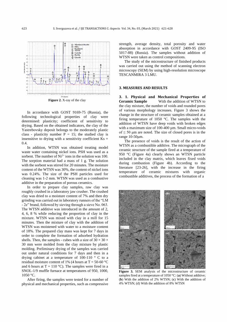
623 S. Sverguzova et al. / IJE TRANSACTIONS C: Aspects Vol. 34, No. 03, (March 2021) 621-628
Figure 2. X-ray of the clay
In accordance with GOST 9169-75 (Russia), the
following technological properties of clay were
determined: plasticity; coefficient of sensitivity to
drying. Based on the obtained indicators, the clay of the
Yastrebovsky deposit belongs to the moderately plastic
class - plasticity number P = 15; the studied clay is
insensitive to drying with a sensitivity coefficient Ks =
0.4.
In addition, WTSN was obtained treating model
waste water containing nickel ions. PSH was used as a
sorbent. The number of Ni2+ ions in the solution was 100.
The sorption material had a mass of 1 g. The solution
with the sorbent was stirred for 20 minutes. The moisture
content of the WTSN was 30%, the content of nickel ions
was 0.24%. The size of the PSH particles used for
cleaning was 1-2 mm. WTSN was used as a combustive
additive in the preparation of porous ceramics.
In order to prepare clay samples, raw clay was
roughly crushed in a laboratory jaw crusher. The crushed
clay was dried to a moisture content of 7% and then dry
grinding was carried out in laboratory runners of the “LM
- 2e” brand, followed by sieving through a sieve No. 063.
The WTSN additive was introduced in the amount of 2,
4, 6, 8 % while reducing the proportion of clay in the
mixture. WTSN was mixed with clay in a mill for 15
minutes. Then the mixture of clay with the addition of
WTSN was moistened with water to a moisture content
of 18%. The prepared clay mass was kept for 7 days in
order to complete the formation of adsorbed hydration
shells. Then, the samples - cubes with a size of 30 × 30 ×
30 mm were molded from the clay mixture by plastic
molding. Preliminary drying of the samples was carried
out under natural conditions for 7 days and then in a
drying cabinet at a temperature of 100-110 ° C to a
residual moisture content of 1% (4 hours at T = 50-60 °C
and 6 hours at T = 110 °C). The samples were fired in a
SNOL-1/9 muffle furnace at temperatures of 950, 1000,
1050 °C.
After firing, the samples were tested for a number of
physical and mechanical properties, such as compressive
strength, average density, total porosity and water
absorption in accordance with GOST 2409-95 (ISO
5017-88) (Russia). The samples without addition of
WTSN were taken as control compositions.
The study of the microstructure of finished products
was carried out using the method of scanning electron
microscopy (SEM) by using high-resolution microscope
TESCANMIRA 3 LMU.
3. MEASURES AND RESULTS 3. 1. Physical and Mechanical Properties of Ceramic Sample With the addition of WTSN to
the clay mixture, the number of voids and rounded pores
of various morphology increases. Figure 3 shows the
change in the structure of ceramic samples obtained at a
firing temperature of 1050 °C. The samples with the
addition of WTSN have deep voids with broken edges
with a maximum size of 100-400 µm. Small micro-voids
of ≤ 50 μm are noted. The size of closed pores is in the
range 10-50μm.
The presence of voids is the result of the action of
WTSN as a combustible additive. The micrograph of the
ceramic structure of the sample fired at a temperature of
950 °C (Figure 4a) clearly shows an WTSN particle
included in the clay matrix, which leaves fixed voids
during combustion (Figure 4b). According to the
literature [23-26], with the increase in the firing
temperature of ceramic mixtures with organic
combustible additives, the process of the formation of a
Figure 3. SEM analysis of the microstructure of ceramic
samples fired at a temperature of 1050 °C: (a) Without additive;
(b) With the addition of 2% WTSN; (c) With the addition of
4% WTSN; (d) With the addition of 8% WTSN

624 S. Sverguzova et al. / IJE TRANSACTIONS C: Aspects Vol. 34, No. 03, (March 2021) 621-628
Figure 4. SEM analysis of the microstructure of ceramic
samples: (a) With the addition of 4% WTSN, fired at a
temperature of 950 ° C; (b) With the addition of 4% WTSN,
fired at a temperature of 1050 °C
liquid phase on the surface of the raw mixture particles
intensifies. The formed water penetrates into pores and
capillaries formed by gas release and participate in the
processes of hydration of the cementing binder with the
formation of thin films at the interface between the
phases, contributing to the consolidation of pores and
voids.
The pores in the structure of a ceramic piece are
formed as a result of the participation of gaseous products
of CO2, released during the combustion of organic matter
[27]. The visual analysis of ceramic brick samples is
shown in Figure 5; where there is no color change and
increase in the number of voids with the introduction of
WTSN additive.
An increase in the concentration of voids has
reflected in the total porosity of ceramic samples (Figure
6). It goes without saying that voids act as a barrier for
heat flow. With an increase in the firing temperature from
950 to 1050 °C, the total porosity of the product
decreases. The highest porosity of 30.9% was achieved
with the addition of 8% WTSN and a firing temperature
of 950 °C. The lowest values of porosity were 24.6%
with the addition of 2% WTSN and a firing temperature
of 1050 °C. An increase in the total porosity is reflected
in the decrease in the density of ceramic samples (Figure
7). In this regard, this study uses the metal in the structure of the ceramic samples that potentially enhance thermal
conductivity. It is noted that the maximum density
Figure 5. Samples of ceramic products based on 4% WTSN and
0% WTSN
reduction of 1590 kg/m3 is achieved with the introduction
of an 8% additive and a firing temperature of 950 °C. The
porous microstructure offers advantages for specific
applications of the developed, such as thermal insulation
or thermal resistance, which allows bricks to withstand
sudden temperature changes through the reduction of the
modulus of elasticity and shear [28]. Voids isolate the
heat flow, causing the decrease in the thermal
conductivity of the samples. The developed porous
structure leads to an increase in the value of water
absorption (Figure 8). It is known [29] that water
absorption of a high-quality porous ceramic product
should be within the range of 6 - 20% by mass. It is noted
that in all studied cases, the water absorption indicators
do not cross the permissible limit (20%). Figure 9 shows
the change in the mechanical strength of clay samples.
The strength of the samples decreases with an increase in
the amount of additive and the increase in porosity, which
is typical for porous ceramic materials [30]. The average
compressive strength of the developed ceramic samples
of the control composition (without additives) in the
firing temperature range of 950-1050 °C was 21.5 MPa.
Higher sintering temperatures increased compressive
strength. With an increase in the concentration of WTSN
in the ceramic matrix, it is accompanied by the decrease
in the strength of the fired samples.
Figure 6. Change in the total porosity of ceramic samples from
the composition of the charge and the firing temperature
Figure 7. Change in the average density of ceramic samples
from the composition of the charge and firing temperature

625 S. Sverguzova et al. / IJE TRANSACTIONS C: Aspects Vol. 34, No. 03, (March 2021) 621-628
Figure 8. Change in water absorption of ceramic samples from
the composition of the charge and firing temperature
Figure 9. Change in the physical and mechanical properties of
ceramic samples from the composition of the charge and firing
temperature
According to the purpose of this study to obtain
highly porous clay ceramics with sufficient strength, it is
necessary to note that, in connection with the available
data, the strength of porous ceramics with the use of
organic combustible additives is in average 20-25 MPa
[25,31-33].
We should admit that the optimal introduction of
WTSN into the clay mixture as a combustible additive is
up to 4 %. In this case, the compressive strength is within
acceptable limits of at least 20 MPa. The migration of
gases through the matrix, obtained as a result of the
combustion of WTSN in an amount of more than 4 %,
created a highly porous clay material, which negatively
affected the mechanical strength.
In order to select the optimal firing mode and obtain
ceramic objects with specified dimensions, the values of
air and fire shrinkage of the dried and fired samples were
determined at different firing temperatures (950-1050
°C) and different contents of the combustible additive
WTSN. Shrinkage during drying is based on the amount
of water in the test material. The amount of air shrinkage
varies depending on the crystallinity of clay mineral. The
change in the firing shrinkage based on the firing
temperature indicates the level of the caking of clay raw
materials. Table 2 shows the observed shrinkage during
the drying and firing cycles of clay bricks containing
various concentrations of additives.
An increase in the mass fraction of WTSN in the
composition of the clay mixture leads to the increase in
the indicators of air and fire shrinkage. However, these
changes do not lead to the deformation and deterioration
in the quality of the resulting products. In accordance
with GOST 530-2012 (Russia), for ceramic bricks, air
shrinkage is allowed up to 8%, fire shrinkage - from 1%
to 2%. All the values obtained are within the standard
range. The observed relatively low values of air
shrinkage of 2.27-2.79% when firing clay without
additives is typical for sandy clays, such as used clay with
a content of 71.3% SiO2 (Table 1). An increase in the
amount of introduced additive causes a natural increase
in air and fire shrinkage, which is associated with the
removal of residual and chemically combined water, as
well as with the transformation of additives into ash.
These chemical reactions during firing, along with
rearrangement of particles and regulation in the crystal
lattice, form a more compact solid texture in comparison
with the initial state, which causes shrinkage
deformations [34].
3. 2. Nickel Ion Leaching Testing of Porous Ceramics The additive of waste sorption material
contains compounds of heavy metals, potentially
hazardous to the environment. We investigated the
probability of migration into the environment of WTSN
nickel ions, enclosed in the structure of a ceramic piece.
Powder of porous ceramics with the addition of WTSN
was ground to a particle size of less than 0.08 mm and
placed in solutions of hydrochloric acid at pH = 3; 4; 5;
6, was kept for 24 hours at an aqueous medium
temperature of 20 ± 0.5 ° C. During the experiments, the
specified pH value was maintained by acidification. Then
the suspensions were filtered through a paper filter and
the concentration of Ni2+ ions were determined by the
atomic adsorption method according to GOST R 57162-
2016 (Russia). The experimental results (Table 3)
indicate the resistance of ceramic products to leaching of
Ni2+ ions, which is estimated as the value of the
concentration of Ni2+ ions in an acid solution.
TABLE 2. The impact of the content of wastewater treatment
sludge in the raw mixture on the shrinkage1 of ceramic samples
Burning
temperature
(°С)
Additive content in the charge percentage
0 2 4 6 8
950 2.27/0.80 2.28/0.90 2.99/0.98 2.84/1.12 3.04/1.20
1000 2.31/0.91 2.58/1.02 3.04/1.20 3.19/1.26 3.52/1.39
1050 2.79/1.10 3.12/1.23 3.52/1.39 3.73/1.47 4.03/1.59
1linear air shrinkage value (%) / fire shrinkage value (%).

626 S. Sverguzova et al. / IJE TRANSACTIONS C: Aspects Vol. 34, No. 03, (March 2021) 621-628
TABLE 3. Ion washout dynamics Ni2+
WTSN content in
clay mixture (%)
Ion concentration Ni2+ (mg/dm3)
рН=3 рН=4 рН=5 рН=6 рН=7
0 0.000 0.000 0.000 0.000 0.000
2 0.000 0.000 0.000 0.000 0.000
4 0.000 0.000 0.000 0.000 0.000
6 0.000 0.000 0.000 0.000 0.000
8 0.001 0.001 0.000 0.000 0.000
16 0.001 0.001 0.000 0.000 0.000
24 0.001 0.001 0.000 0.000 0.000
The insignificant leaching of nickel from ceramic
powder occurs in the samples containing more than 8%
WTSN at pH=3 and 4. At pH>4, nickel is not leached
out. We should note that according to GOST R 57162-
2016 (Russia), the concentration of nickel ions in
solutions with pH=3 and 4 is lower than the LOC for
nickel water for fishery facilities (0.01 mg/dm3). Thus,
the disposal of waste sorption material in the production
of ceramic bricks eliminates the risk of nickel entering
the environment.
4. CONCLUSION Here, we provide the conclusion and findings of this
paper as follows:
• The possibility of the use of WTSN based on
pumpkin seed husks as a combustible additive to
clay mixtures was investigated.
• Microstructure SEM analysis showed that the
combustion of the organic additive promotes the
formation of voids, and the emission of gases to the
formation of pores in the ceramic piece during
firing.
• The addition of WTSN and changing the firing
temperature within the range of 950-1050°C is
reflected in the indicators of ultimate strength in
compression, water absorption, total porosity and
density of ceramic samples.
• The optimal amount of WTSN as a combustible
additive for the production of porous ceramics is not
more than 4 %. In this case, as a result of firing at
the temperature range from 950 to 1050°C, the
compressive strength was 20.0-20.7 MPa, the
density of the product was 1800-1860 kg/m3, and
the water absorption was in the range of 15.6-
13.4%. The linear shrinkage values of the resulting
products were within the standard range.
• The dynamics of the washing out of heavy metal
ions from the ceramic matrix began when the
content of the WTSN additive was over 8% and
ended completely at pH values> 4, which
eliminated the danger of their entry into the
environment.
• The use of WTSN in a clay mixture allowed
obtaining porous ceramics with satisfactory
technical and operational characteristics, which
could be used as an effective building material for
the construction of internal partitions and household
buildings.
• The use of optimization theory to reduce the waste
materials with novel metaheuristics like red deer
algorithm [35-36], water wave optimization [37-38]
and social engineering optimizer [39], is another
interesting idea for further research.
5. ACKNOWLEDGMENTS
The work is realized in the framework of the Program of
flagship university development on the base of the
Belgorod State Technological University named after
V.G. Shoukhov, using equipment of High Technology
Center at BSTU named after V.G. Shoukhov and by the
Tomsk State University competitiveness improvement
program
6. REFERENCES
1. Bauman-Kaszubska, H., & Sikorski, M. "Selected problems of
waste water disposal and sludge handling in the Mazovian province" Journal of Water and Land Development, Vol. 13,
No. 1, (2009), 149-159.
2. Valencia, J. A., González, J. P., Jimenez-Pitre, I., & Molina-Bolívar, G. "Physico-chemical treatment of waste water
contaminated with heavy metals in the industry of metallic
coatings" Journal of Water and Land Development, Vol. 43, No.
1, (2019), 171-176..
3. Yasin Mousavi, S., Tavakkoli, A., Jahanshahi, M., Dankoub, A.
“Performance of High-Strength Concrete Made with Recycled Ceramic Aggregates (Research Note).” International Journal of
Engineering, Transactions C: Aspects, Vol. 33, No. 6, (2020),
1085-1093. 10.5829/ije.2020.33.06c.05.
4. Chang, Z., Long, G., Zhou, J. L., Ma, C. “Valorization of Sewage
Sludge in the Fabrication of Construction and Building Materials:
A Review.” Resources, Conservation and Recycling, Vol. 154,
(2020), 104606. https://doi.org/10.1016/j.resconrec.2019.104606
5. Świerczek, L., Cieślik, B. M., Konieczka, P. “The Potential of
Raw Sewage Sludge in Construction Industry-a Review.” Journal of Cleaner Production, Vol. 200, (2018), 342-356.
https://doi.org/10.1016/j.jclepro.2018.07.188
6. Foroutan, R., Mohammadi, R., Farjadfard, S., Esmaeili, H.,
Saberi, M., Sahebi, S., Dobaradaran, S., Ramavandi, B.
“Characteristics and Performance of Cd, Ni, and Pb Bio-Adsorption Using Callinectes Sapidus Biomass: Real Wastewater
Treatment.” Environmental Science and Pollution Research,
Vol. 26, No. 7, (2019), 6336-6347.
https://doi.org/10.1007/s11356-018-04108-8
7. Lupandina, N. S., Sapronova, Z. A. “Modified Bleaching Clay as
a Sorption Material.” IOP Conf. Series: Earth and Environmental

627 S. Sverguzova et al. / IJE TRANSACTIONS C: Aspects Vol. 34, No. 03, (March 2021) 621-628
Science, 459, (2020), 042063 IOP Publishing. doi:10.1088/1755-
1315/459/4/042063
8. Dai, Y., Sun, Q., Wang, W., Lu, L., Liu, M., Li, J., Yang, S., Sun,
Y., Zhang, K., Xu, J. “Utilizations of Agricultural Waste as Adsorbent for the Removal of Contaminants: A Review.”
Chemosphere, Vol. 211, (2018), 235-253.
https://doi.org/10.1016/j.chemosphere.2018.06.179
9. Fediuk, R. S., Lesovik, V. S., Svintsov, A. P., Mochalov, A. V.,
Kulichkov, S. V., Stoyushko, N. Y., Gladkova, N. A., Timokhin,
R. A. “Self-Compacting Concrete Using Pretreatmented Rice Husk Ash.” Magazine of Civil Engineering, Vol. 79, No. 3,
(2018).
10. Chandra Paul, S., Mbewe, P. B., Kong, S. Y., Šavija, B.
“Agricultural Solid Waste as Source of Supplementary
Cementitious Materials in Developing Countries.” Materials, Vol. 12, No. 7, (2019), 1112. https://doi.org/10.3390/ma12071112
11. Sapronova, Z., Sverguzova, S., Fomina, E., Fokina, E. “Carbonate-Containing Precipitate of Sugar Production from
Sugar Beet as Filler for Polymer Concrete.” (2018).
12. Franus, M., Barnat-Hunek, D., Wdowin, M. “Utilization of Sewage Sludge in the Manufacture of Lightweight Aggregate.”
Environmental Monitoring and Assessment, Vol. 188, No. 1,
(2016), DOI: 10. 10.1007/s10661-015-5010-8
13. Galvez-Martos, J.-L. “Sewage Sludge Ashes as Additives for the
Cement and Ceramics Industries.” Wastewater Treatment
Residues as Resources for Biorefinery Products and Biofuels,
(2019), 49.
14. Qi, Y., Yue, Q., Han, S., Yue, M., Gao, B., Yu, H., Shao, T.
“Preparation and Mechanism of Ultra-Lightweight Ceramics Produced from Sewage Sludge.” Journal of Hazardous
Materials, Vol. 176, No. 1-3, (2010), 76-84.
https://doi.org/10.1016/j.jhazmat.2009.11.001
15. Areias, I. O. R., Vieira, C. M. F., Colorado, H. A., Delaqua, G. C.
G., Monteiro, S. N., Azevedo, A. R. G. “Could City Sewage
Sludge Be Directly Used into Clay Bricks for Building Construction? A Comprehensive Case Study from Brazil.”
Journal of Building Engineering, (2020), 101374.
https://doi.org/10.1016/j.jobe.2020.101374
16. Tuan, B. L. A., Hwang, C.-L., Lin, K.-L., Chen, Y.-Y., Young,
M.-P. “Development of Lightweight Aggregate from Sewage
Sludge and Waste Glass Powder for Concrete.” Construction and
Building Materials, Vol. 47, (2013), 334-339.
https://doi.org/10.1016/j.conbuildmat.2013.05.039
17. Xu, G. R., Zou, J. L., Li, G. B. “Stabilization of Heavy Metals in Sludge Ceramsite.” Water Research, Vol. 44, No. 9, (2010),
2930-2938. https://doi.org/10.1016/j.watres.2010.02.014
18. Lotfollahi, M. N., Saeidi, N. “A Procedure for Preparation of Semi-Activated Carbon Fiber without Any Treatment under High
Temperature.” International Journal of Engineering,
Transaction A: Basics, Vol. 27, No. 10, (2014), 1519-1526.
19. Qiao, L., Ho, G. “The Effect of Clay Amendment on Speciation
of Heavy Metals in Sewage Sludge.” Water Science and
Technology, Vol. 34, No. 7-8, (1996), 413-420.
https://doi.org/10.1016/S0273-1223(96)00773-1
20. Othman, M. H. D., Adam, M. R., Hubadillah, S. K., Puteh, M. H.,
Harun, Z., Ismail, A. F. “Evaluating the Sintering Temperature Control Towards the Adsorptivity of Ammonia onto the Natural
Zeolite Based Hollow Fibre Ceramic Membrane.” International
Journal of Engineering, Transaction B: Applications, Vol. 31,
No. 8, (2018), 1398-1405.
21. Shih, K., White, T., Leckie, J. O. “Nickel Stabilization Efficiency
of Aluminate and Ferrite Spinels and Their Leaching Behavior.” Environmental Science & Technology, Vol. 40, No. 17, (2006),
5520-5526. https://doi.org/10.1021/es0601033
22. Cusidó, J. A., Cremades, L. V. “Environmental Effects of Using Clay Bricks Produced with Sewage Sludge: Leachability and
Toxicity Studies.” Waste Management, Vol. 32, No. 6, (2012),
1202-1208. https://doi.org/10.1016/j.wasman.2011.12.024
23. Starostina, I., Simonov, M., Volodchenko, A., Starostina, Y.,
Fomin, A., Fokina, E. “The Usage of Iron-Containing Sludge
Wastes in Ceramic Bricks Production.” IOP Conference Series:
Materials Science and Engineering, Vol. 365, No. 3, 032066).
IOP Publishing doi:10.1088/1757-899X/365/3/032066
24. Obada, D. O., Dodoo-Arhin, D., Dauda, M., Anafi, F. O., Ahmed, A. S., Ajayi, O. A. “The Impact of Kaolin Dehydroxylation on the
Porosity and Mechanical Integrity of Kaolin Based Ceramics
Using Different Pore Formers.” Results in physics, Vol. 7,
(2017), 2718-2727. https://doi.org/10.1016/j.rinp.2017.07.048
25. Al-Qadhi, E., Li, G., Ni, Y. “Influence of a Two-Stage Sintering
Process on Characteristics of Porous Ceramics Produced with
Sewage Sludge and Coal Ash as Low-Cost Raw Materials.”
Advances in Materials Science and Engineering, Vol. 2019,
(2019). https://doi.org/10.1155/2019/3710692
26. Obada, D. O., Dodoo-Arhin, D., Dauda, M., Anafi, F. O., Ahmed,
A. S., Ajayi, O. A., Csaki, S., Bansod, N. D., Kirim, I. I., Momoh,
O. J. “Crack Behaviour and Mechanical Properties of Thermally Treated Kaolin Based Ceramics: The Influence of Pore
Generating Agents.” Applied Clay Science, Vol. 194, (2020),
105698. https://doi.org/10.1016/j.clay.2020.105698
27. Ahmad, S., Iqbal, Y., Muhammad, R. “Effects of Coal and Wheat
Husk Additives on the Physical, Thermal and Mechanical
Properties of Clay Bricks.” Boletín de la Sociedad Española de
Cerámica y Vidrio, Vol. 56, No. 3, (2017), 131-138.
https://doi.org/10.1016/j.bsecv.2017.02.001
28. Vakifahmetoglu, C., Semerci, T., Soraru, G. D. “Closed Porosity Ceramics and Glasses.” Journal of the American Ceramic
Society, Vol. 103, No. 5, (2020), 2941-2969.
https://doi.org/10.1111/jace.16934
29. Olawuyi, B. J., Olusola, K. O., Ogunbode, E. B., Kyenge, S. S.
“Performance Assessment of Makurdi Burnt Bricks.” Civil
Eingineering, (2014).
30. Knudsen, F. P. “Dependence of Mechanical Strength of Brittle
Polycrystalline Specimens on Porosity and Grain Size.” Journal
of the American Ceramic Society, Vol. 42, No. 8, (1959), 376-
387. https://doi.org/10.1111/j.1151-2916.1959.tb13596.x
31. Thalmaier, G., Cobîrzan, N., Balog, A. A., Constantinescu, H., Streza, M., Nasui, M., Neamtu, B. V. “Influence of Sawdust
Particle Size on Fired Clay Brick Properties.” Materiales de
Construcción, Vol. 70, No. 338, (2020), 215.
https://doi.org/10.3989/mc.2020.04219
32. Chiang, K.-Y., Chou, P.-H., Hua, C.-R., Chien, K.-L.,
Cheeseman, C. “Lightweight Bricks Manufactured from Water Treatment Sludge and Rice Husks.” Journal of Hazardous
Materials, Vol. 171, No. 1-3, (2009), 76-82.
https://doi.org/10.1016/j.jhazmat.2009.05.144
33. Starostina, I. V., Simonov, M. M., Denisova, L. V. "The Use of
Ferrovanadium Production Sludge Wastes in Claydite Gravel
Technology." Solid State Phenomena, No. 265, (2017), 501-506.
https://doi.org/10.4028/www.scientific.net/SSP.265.501
34. Chemani, B., Chemani, H. “Effect of Coal on Engineering
Properties in Building Materials: Opportunity to Manufacturing Insulating Bricks.” International Journal of Materials and
Metallurgical Engineering, Vol. 8, No. 8, (2014), 805-811.
35. Hajiaghaei-Keshteli, M., J Afshari, A., & Nasiri, E., "Addressing the freight consolidation and containerization problem by recent
and hybridized meta-heuristic algorithms." International
Journal of Engineering, Transactions C: Aspects, Vol. 30, No.
3, (2017), 403-410.
36. Fathollahi-Fard, A. M., Hajiaghaei-Keshteli, M. & Tavakkoli-
Moghaddam, R., "Red deer algorithm (RDA): a new nature-

628 S. Sverguzova et al. / IJE TRANSACTIONS C: Aspects Vol. 34, No. 03, (March 2021) 621-628
inspired meta-heuristic," Soft Computing, Vol. 24, (2020),
14637-14665. DOI: 10.1007/s00500-020-04812-z.
37. Hajiaghaei-Keshteli, M., Abdallah, K. S., & Fathollahi-Fard, A.
M. (2018). "A collaborative stochastic closed-loop supply chain network design for tire industry." International Journal of
Engineering, Transaction A: Basics, Vol. 31, No. 10, (2018),
1715-1722.
38. Zheng, Y. J. "Water wave optimization: a new nature-inspired metaheuristic." Computers & Operations Research, Vol. 55,
(2015), 1-11. https://doi.org/10.1016/j.cor.2014.10.008
39. Fathollahi-Fard, A. M., Hajiaghaei-Keshteli, M., & Tavakkoli-Moghaddam, R., "The social engineering optimizer (SEO)."
Engineering Applications of Artificial Intelligence, Vol. 72,
(2018), 267-293. https://doi.org/10.1016/j.engappai.2018.04.009
Persian Abstract
چکیده یافزودن کیبه عنوان که شده است، ارائه یآب یاز محلول ها نیفلزات سنگ یها ونیپوسته بذر کدو تنبل، که هنگام استخراج -ذب زباله امقاله امکان استفاده از مواد ج نیدر ا
ر ییشارژ در تغ بترکی در شده صرف شده جذب مواد (٪جرم ٪8- 2مختلف ) ریمقاد ری. تأثاستفاده گردیدمتخلخل یها کیسرام دیرس در تول یمخلوط ها یقابل احتراق برا
ی آل یافزودنمواد قرار گرفت. مشخص شد که احتراق ی مورد بررس گرادی درجه سانت 1050-950 یبدست آمده در دما یکیسرام ینمونه ها یکی و مکان یکیزیف ات یدر خصوص
متخلخل را فراهم کیسرام دیقابل احتراق امکان تول ی رس با افزودن یهمراه است. همه مخلوط ها یکی ممنافذ در قطعه سرا لیحفره ها و انتشار گازها با تشک ل یتشک موجب
د. گردیاستفاده درصد وزنی 4شود تا حداکثر ی م هیکند. توص ی را برآورده م ی ، جذب آب و انقباض خط ی، تخلخل ، چگال یمقاومت فشار یالزم برا ط یآورد که شرا یم
ن یفلزات سنگ یشستشو یبرا افتهیمتخلخل توسعه کیسرام شیو استحکام. در طول آزما یاز نظر چگال نهیقابل احتراق به منظور به دست آوردن خواص به افزودنی مواد درصد
.ودش یم هیتوص یخانگ یو ساختمانها یداخل یها شنیساخت پارت یحاصل برا یساختمانکند. مصالح ینم جادیا ستیز طیمح یبرا یماده خطر نی، مشخص شد که ا
IJE TRANSACTIONS C: Aspects Vol. 34, No. 03, (March 2021) 629-635
Please cite this article as: C. Jithendra, S. Elavenil, Effects of Parameters on Slump and Characteristic Strength of Geopolymer Concrete using Taguchi Method, International Journal of Engineering, Transactions C: Aspects Vol. 34, No. 03, (2021) 629-635
International Journal of Engineering
J o u r n a l H o m e p a g e : w w w . i j e . i r
Parametric Effects on Slump and Compressive Strength Properties of Geopolymer
Concrete using Taguchi Method
C. Jithendra*a, S. Elavenilb a Assistant Professor, Department of Civil Engineering, CMR Institute of Technology, Bengaluru, India b Professor, School of Civil Engineering, Vellore Institute of Technology, Chennai, India
P A P E R I N F O
Paper history: Received: 21 July 2020 Received in revised form: 23 September 2020 Accepted: 26 October 2020
Keywords: Geopolymer Concrete By-products Taguchi Method Ambient Curing
A B S T R A C T
This paper represents the parametric effects on slump and compressive strength of aluminosilicate based Geopolymer concrete using by Taguchi method. A total of nine mix proportions were considered to
evaluate the effect of sodium hydroxide (NaOH) solution, Solution/Binder (SB) ratio and the percentage
of superplasticizer. Results indicated that the highest slump of 165 mm and 28 days compressive strength of 68.37 MPa was obtained for aluminosilicate based Geopolymer concrete with the superplasticizer,
Solution to Binder (SB) ratio and extra water) parameters. By using the selected (Signal-to-Noise (SN)
ratio graphs, the best combination of parameters for slump and compressive strength properties was also obtained. The mix with the best combination of parameters was considered and partially replaced with
silica fume and rice husk ash. The inclusion of additional silica (in form of silica fume and rice husk ash as Ground Granulated Blast Furnace Slag (GGBFS) replacement), most significantly influenced the
slump and compressive strength properties.
doi: 10.5829/ije.2021.34.03c.06
1. INTRODUCTION1
There is a rapid increase in the use of Ordinary Portland
Cement (OPC) as primary binder in the preparation of
concrete. The OPC manufacturing industry contributes to
7% (apporximately) of the total CO2 emission as per
International Energy Agency (IEA) [1,2,3]. On the other,
the accumulation of industrial by-products in agricultural
and residential lands poses varied threats and challenges
to the country’s productive development [4]. Hence, an
extensive research has been initiated over the last few
decades to explore alternate and suitable cementitious
materials to mitigate this issue [3,5]. Thus considering a
wide range of by-products in the manufacturing of
concrete as a potiential replacement becomae a new
scope of research.
In 1978, Joseph Davidovits invented the concept of
“Geopolymer” [5, 6]. Since 1978, due to its excellent
properties and environmental benefits, the popularity of
Geopolymer Concrete (GC)has increased as a promising
*Corresponding Author Institutional Email: [email protected]
(C Jithendra)
alternative to OPC concrete [7]. The production of GC
has reduced the emission of CO2 to 80% (approximately)
as compared to OPC [6]. The major steps involved in the
mechanism of polymerization include the dilution of
Silica (Si) and Alumina (Al) in alkaline medium, the
condensation of elements into monomers and the,
formation of polymeric structure by polycondensation of
monomers [8].
A vast number of research studies have been carried
out on GC that is manufactured using low calcium
content fly ash as primary binding material along with
alkali solution (sodium hydroxide (NaOH)/sodium
silicate (Na2SiO3) based) cured under oven temperatures
[1,7,9]. Nevertheless, the manufacturing of GC under
oven curing temperatures had minimized its usage to
precast concrete elements [10]. Consequently, the field of
applications using GC incorporating Ground Granulated
Blast Furnace Slag (GGBFS) as partial substitute to fly
ash at ambient curing came into existence[10-15].
Several studies focused on setting time, workability and
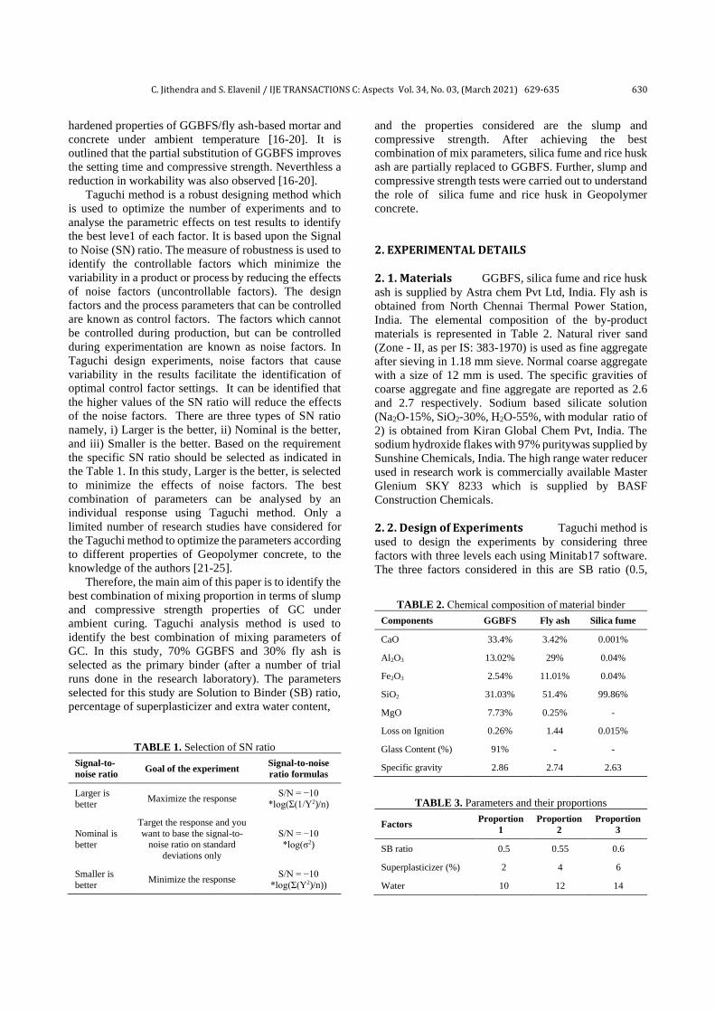
C. Jithendra and S. Elavenil / IJE TRANSACTIONS C: Aspects Vol. 34, No. 03, (March 2021) 629-635 630
hardened properties of GGBFS/fly ash-based mortar and
concrete under ambient temperature [16-20]. It is
outlined that the partial substitution of GGBFS improves
the setting time and compressive strength. Neverthless a
reduction in workability was also observed [16-20].
Taguchi method is a robust designing method which
is used to optimize the number of experiments and to
analyse the parametric effects on test results to identify
the best leve1 of each factor. It is based upon the Signal
to Noise (SN) ratio. The measure of robustness is used to
identify the controllable factors which minimize the
variability in a product or process by reducing the effects
of noise factors (uncontrollable factors). The design
factors and the process parameters that can be controlled
are known as control factors. The factors which cannot
be controlled during production, but can be controlled
during experimentation are known as noise factors. In
Taguchi design experiments, noise factors that cause
variability in the results facilitate the identification of
optimal control factor settings. It can be identified that
the higher values of the SN ratio will reduce the effects
of the noise factors. There are three types of SN ratio
namely, i) Larger is the better, ii) Nominal is the better,
and iii) Smaller is the better. Based on the requirement
the specific SN ratio should be selected as indicated in
the Table 1. In this study, Larger is the better, is selected
to minimize the effects of noise factors. The best
combination of parameters can be analysed by an
individual response using Taguchi method. Only a
limited number of research studies have considered for
the Taguchi method to optimize the parameters according
to different properties of Geopolymer concrete, to the
knowledge of the authors [21-25].
Therefore, the main aim of this paper is to identify the
best combination of mixing proportion in terms of slump
and compressive strength properties of GC under
ambient curing. Taguchi analysis method is used to
identify the best combination of mixing parameters of
GC. In this study, 70% GGBFS and 30% fly ash is
selected as the primary binder (after a number of trial
runs done in the research laboratory). The parameters
selected for this study are Solution to Binder (SB) ratio,
percentage of superplasticizer and extra water content,
TABLE 1. Selection of SN ratio
Signal-to-
noise ratio Goal of the experiment
Signal-to-noise
ratio formulas
Larger is
better Maximize the response
S/N = −10
*log(Σ(1/Y2)/n)
Nominal is
better
Target the response and you
want to base the signal-to-noise ratio on standard
deviations only
S/N = −10
*log(σ2)
Smaller is
better Minimize the response
S/N = −10
*log(Σ(Y2)/n))
and the properties considered are the slump and
compressive strength. After achieving the best
combination of mix parameters, silica fume and rice husk
ash are partially replaced to GGBFS. Further, slump and
compressive strength tests were carried out to understand
the role of silica fume and rice husk in Geopolymer
concrete.
2. EXPERIMENTAL DETAILS 2. 1. Materials GGBFS, silica fume and rice husk
ash is supplied by Astra chem Pvt Ltd, India. Fly ash is
obtained from North Chennai Thermal Power Station,
India. The elemental composition of the by-product
materials is represented in Table 2. Natural river sand
(Zone - II, as per IS: 383-1970) is used as fine aggregate
after sieving in 1.18 mm sieve. Normal coarse aggregate
with a size of 12 mm is used. The specific gravities of
coarse aggregate and fine aggregate are reported as 2.6
and 2.7 respectively. Sodium based silicate solution
(Na2O-15%, SiO2-30%, H2O-55%, with modular ratio of
2) is obtained from Kiran Global Chem Pvt, India. The
sodium hydroxide flakes with 97% puritywas supplied by
Sunshine Chemicals, India. The high range water reducer
used in research work is commercially available Master
Glenium SKY 8233 which is supplied by BASF
Construction Chemicals.
2. 2. Design of Experiments Taguchi method is
used to design the experiments by considering three
factors with three levels each using Minitab17 software.
The three factors considered in this are SB ratio (0.5,
TABLE 2. composition ofChemical material binder
Components GGBFS Fly ash Silica fume
CaO 33.4% 3.42% 0.001%
Al2O3 13.02% 29% 0.04%
Fe2O3 2.54% 11.01% 0.04%
SiO2 31.03% 51.4% 99.86%
MgO 7.73% 0.25% -
Loss on Ignition 0.26% 1.44 0.015%
Glass Content (%) 91% - -
Specific gravity 2.86 2.74 2.63
TABLE 3. Parameters and their proportions
Factors Proportion
1
Proportion
2
Proportion
3
SB ratio 0.5 0.55 0.6
Superplasticizer (%) 2 4 6
Water 10 12 14

631 C. Jithendra and S. Elavenil / IJE TRANSACTIONS C: Aspects Vol. 34, No. 03, (March 2021) 629-635
0.55, 0.6), percentage of superplasticizer (2, 4, 6%) and
extra water (10, 12, 14%) are reported in Table 3. A total
of nine mixes were generated using Taguchi L9 (33) array
as reported in Table 4. The concentration of sodium
hydroxide 12M is kept constant.
2. 3. Preparation of Samples The raw materials
are mixed for 2 minutes using a pan mixer. Later, the
solution content is added slowly and mixed for another 5
minutes. Immediately after mixing, the fresh concrete is
tested for workability using slump cone test and then the
concrete is cast in 100 mm size steel moulds with proper
compaction and placed on a vibrator for 10 seconds. The
specimens were subjected to ambient curing (250C ± 20C)
for 24 hours. Following this, the specimens are removed
from the moulds and kept for 7, 28, and 90 days for
ambient curing. 3. RESULTS AND DISCUSSION
3. 1. Slump Value The slump value of
Geopolymer concrete has been tested using a normal
slump cone test as per IS 7320-1974. The dimensions of
the slump cone are top diameter-10 cmm, height-30 cm
and bottom diameter-20 cm. The concrete has been
placed into the cone in three layers and tamped properly
to remove the air voids. The cone is then lifted vertically
and the readings are noted using a steel scale. The slump
values of nine mixes are as shown in Figure 1. The
minimum slump of 63 mm is achieved by the mix
consisting of 0.5 SB ratio, superplasticizer 2% and extra
water 10%. The maximum slump value of 150 mm is
achieved in the mix consisting of 0.6 SB ratio, 6%
superplasticizer and 12% extra water (Table 5). The
slump value is significantly influenced by the three
factors: SB ratio, Superplasticizer and water content. It
clearly indicates that with an increase in the parameter
levels, the workability also increases. However, to
TABLE 4. Taguchi mix proportions
Mix Id's SB ratio Superplasticizer (%) Water (%)
TM1 0.5 2 10
TM2 0.5 4 12
TM3 0.5 6 14
TM4 0.55 2 12
TM5 0.55 4 14
TM6 0.55 6 10
TM7 0.6 2 14
TM8 0.6 4 10
TM9 0.6 6 12
analyze the individual parameter that influences the
slump value, Taguchi analysis was conducted using
Minitab17 software.
From Figure 2, with the help of SN ratio’s the
individual effect of parameters has been determined.
Firstly, SB ratio significantly influences the slump
Figure 1. Slump values of Taguchi mixes
TABLE 5. Test results of Geopolymer concrete
Mix ID Slump (mm) Compressive strength (MPa)
7 days 28 days 90 days
M1 63 58 66.8 68.4
M2 75 53.1 62.2 64.2
M3 97 49.4 57.9 60
M4 105 53 60.12 62.6
M5 130 47.66 56.77 59.4
M6 110 54.8 63.4 66.74
M7 140 44.9 57.05 60.45
M8 100 54 61.45 64.87
M9 150 43.2 52.24 54.29
Figure 2. Main effects plot of SN ratios for slump
0
20
40
60
80
100
120
140
160
M1 M2 M3 M4 M5 M6 M7 M8 M9
Slu
mp
va
lues

C. Jithendra and S. Elavenil / IJE TRANSACTIONS C: Aspects Vol. 34, No. 03, (March 2021) 629-635 632
values. The slump value gradually increases with
increase in parameter level of SB ratio from 0.5 to 0.6.
The second parameter that influences the slump value is
the extra water content. When extra water content is
increased from 10 to 14%, there is a linear increment in
the slump value. The third parameter, the percentage of
superplasticizer also affects the workability properties.
With a change in the parameter levels of superplasticizer
from 2 to 4%, a slight increase in workabilityis achieved.
When this is futher increased from 4 to 6%, a higher rate
of workability is noticed.
3. 2. Compressive Strength A total of nine
mixes (M1 to M9) have been cast and subjected to
ambient curing. The compressive strength test was
conducted as per to IS 516: 1959. The compressive
strength of the nine mixes was tested at 7, 28, and 90-
days age of concrete, and the average strength of the three
specimens are reported in Table 5. The highest
compressive strength of 68.4 is achieved with the mix of
SB ratio-0.5, 2% superplasticizer and 10% extra water.
The lowest compressive strength of 54.29 is achieved
with mix that has SB ratio of 0.6, 6% superplasticizer
and 12% extra water as shown in Figure 3. However, to
deeply understand the effect of parameters on
compressive strength, Taguchi analysis is conducted
using Minitab17 software. From Figure 4, the first
parameter to affect the strength properties is found to be
the superplasticizer. It is observed that the strength
properties gradually decrease with an increase in the
superplasticizer. The second parameter that affects the
strength properties is the SAS/Binder content. Even with
a change from 0.5 to 0.55, there is a drastic reduction in
the strength. Further increasing it from 0.55 to 0.6,
indicates a slight reduction in the strength properties.
However, there is not much effect of extra water (10, 12,
14%) on the strength properties.
The selection of the best mix proportion is considered
in terms of both slump and compressive strength
properties of GGBFS Geopolymer concrete. The mix
Figure 3. Compressive strength of Taguchi mixes
Figure 4. Main effects plot of SN ratios for compressive
strength
with SB ratio of 0.5, 2% superplasticizer and 10% extra
water has produced 63 mm slump and compressive
strength of 66.8 MPa for 28 days The mix with SB ratio
of 0.55, 6% superplasticizer and 10% extra water content
has produced 110 mm slump and compressive strength of
63.4 MPa for 28 days. The mix with SB ratio of 0.6, 4%
superplasticizer and 10% extra water content has
produced 100 mm slump and compressive strength of
61.45 MPa for 28 days. From Taguchi analysis, the best
parameter levels are considered as follows: SB ratio 0.5,
Superplasticizer 4% and extra water 14%. MID10 is
designated as the optimum mix from the Taguchi analysis
as reported in Table 5. Finally, the mix MID10 is seen to
have achieved 165 mm slump and 68.37 MPa
compressive strength at 28-days.
3. 3. Effects of Silica Fume and Rice Husk Ash The mix MID10 is considered as the best parametric
combination which is examined further with GGBFS is
partially replaced by silica fume and rice husk ash such
as 0, 5, 10, 15, and 20%, respectively. The test results are
reported in Table 6.
TABLE 6. Effects of silica fume and rice husk ash
Mix ID Slump (mm) Average Compressive
strength (MPa) @ 28 days
MID10 165 68.37
M10SF5 175 71.05
M10SF10 185 78.42
M10SF15 205 80.1
M10SF20 210 78.8
M10RA5 170 69.4
M10RA10 180 74.25
M10RA15 185 73.02
M10RA20 190 71.2
0
10
20
30
40
50
60
70
80
M1 M2 M3 M4 M5 M6 M7 M8 M9
Com
pre
ssiv
e S
tren
gth
(M
Pa)
Mix proportions
7 Day 28 Day 90 Day

633 C. Jithendra and S. Elavenil / IJE TRANSACTIONS C: Aspects Vol. 34, No. 03, (March 2021) 629-635
3. 3. 1. Effects on Slump The Geopolymer
concrete slump values are significatly influenced by
silica fume and rice husk ash as shown in Figures 5 and
6. The highest slump of 205 mm was achieved with the
mix of 20% silica fume as compared to the mix of 0%
silica fume. The slump growth rate increases about
27.2% with 20% silica fume as compared to control mix
(Table 6). On the other hand, rice husk ash also
significantly affects the slump value of Geopolymer
concrete. The maximum replacement of 20% rice husk
ash to GGBFS results in an increase in the slump value
of about 15.5% as compared to the control mix (0% rice
husk ash). This is due to the large surface area of the
materials with fine particles that improves the
workability of the Geopolymer concrete. However, it has
been observed that the slump value is higly influenced by
the mixes of silica fume as compared to the mixes of rice
husk ash. This is due to the larger surface area in rice husk
ash as compared to silica fume. Increase in dosage of fine
particles leads to an increase in the demand of water
content.
Figure 5. Effect of silica fume on slump
Figure 6. Effect of rice husk ash on slump
3. 3. 2. Effects on Compressive Strength The
test results show that the silica fume and rice husk ash
play a significant impact on compressive strength of GC
as represented in Figures 7 and 8. The mix 15% silica
fume has achieved the highest compressive strength of
80.1 MPa at 28-days as compared to other mixes in the
experiment. The growth rate of compressive strength has
increased about 17.1% with partial replacement of silica
fume (15%) to GGBFS. The addition of silica content in
the mix leads to an improvement in the strength of GC
[26]. However, the partial replacement of silica fume
beyond 15% results in a slight decrease in strength. This
is due to the over dose of silica content in the mixtures
which hinders the geopolymerization under ambient
curing [27]. On other hand, the rice husk ash also has shown
significant effect on compressive strength as shown in
Figure 8. The growth rate increases about 8.6% with
partial replacement of 10% rice husk ash to GGBFS in
the mix. Also, the partial replacment of GGBFS with rice
husk ash beyond 10% tends to decrease the compressive
strength .The extra rice husk ash which is rich in silica
Figure 7. Effect of silica fume on Compressive strength
Figure 8. Effect of rice husk ash on Compressive strength
0 5 10 15 20
140
160
180
200
220
Slu
mp v
alue
(mm
)
Silica fume (%)
0 5 10 15 20
160
170
180
190
200
Slu
mp
valu
e (
mm
)
Rice husk ash (%)
0 5 10 15 20
60
65
70
75
80
85
Com
pre
ssiv
e s
trength
(M
Pa)
@ 2
8-d
ays
Silica fume (%)
0 5 10 15 20
65.0
67.5
70.0
72.5
75.0
Co
mp
ress
ive s
tren
gth
(M
Pa)
@ 2
8-d
ay
s
Rice husk ash (%)

C. Jithendra and S. Elavenil / IJE TRANSACTIONS C: Aspects Vol. 34, No. 03, (March 2021) 629-635 634
causes a problem in unreactive silica that leads to the
rise in Si/Al ratio of Geopolymer concrete. This is mainly
due to the effect of geopolymer concrete in the
compressive strength of the mixes of rice husk ash
beyond 10%. The mixes which are partially replaced
with fly ash and micro silica, resulted in a decrease in the
strength at ambient curing condition. The reason for
decrease in strength was due to a decrease in the intensity
of calcium [28], polymerization that was delayed and the
hindered formation of Ca-Al-Si gel [29]. The
combination of GGBFS with partial replacement of silica
rich materials thus seens to be suitable under ambient
curing.
4. CONCLUSION
The optimum mix M10 designed from the Taguchi
analysis has achieved 165 mm slump and 68.37 MPa
compressive strength at 28-days. The highest slump of
205 mm was achieved with the mix of 20% silica fume
as compared to the mix of 0% silica fume. The slump
growth rate increases about 27.2% with 20% silica fume
as compared to control mix. The maximum replacement
of 20% rice husk ash to GGBFS resulted in, an increase
in the slump value of about 15.5% as compared to control
mix. The growth rate of 17.1% increment in compressive
strength has been observed with partial replacement of
silica fume (15%) to GGBFS. Additionally, there is an
8.6% an increase in the growth rate with partial
replacement of 10% rice husk ash to GGBFS in the mix.
Beyond 10% replacement of the rice husk ash to GGBFS,
there is decreasing trend in the growth rate under ambient
curing.
5. ACKNOWLEDGEMENT
I am thankful to Vellore Institute of Technology, Chennai
for providing the research facilities.
6. REFERENCES
1. Part, W. K., Ramli, M., Cheah, C. B., “An overview on the
influence of various factors on the properties of geopolymer
concrete derived from industrial by-products”, Construction and
Building Materials, Vol. 77 (2015) 370-395.
https://doi.org/10.1016/j.conbuildmat.2014.12.065
2. Gartner, E., “Industrially interesting approaches to ‘low-CO2’ cements”, Cement and Concrete Research, Vol. 34, (2004) 1489-
1498. https://doi.org/10.1016/j.cemconres.2004.01.021
3. Huseien, G.F., Mirza, J., Ismail, M., Ghoshal, S. K., Hussein, A. A., “Geopolymer mortars as sustainable repair material: A
comprehensive review”, Renewable and Sustainable Energy
Reviews. Vol. 80 (2017) 54-74.
https://doi.org/10.1016/j.rser.2017.05.076
4. Liew, K. M., A. O. Sojobi, and L. W. Zhang. "Green concrete: Prospects and challenges." Construction and Building Materials,
Vol. 156 (2017) 1063-1095.
https://doi.org/10.1016/j.conbuildmat.2017.09.008
5. Wang, Kai-tuo, Li-qiu Du, Xue-sen Lv, Yan He, and Xue-min
Cui. "Preparation of drying powder inorganic polymer cement
based on alkali-activated slag technology." Powder Technology, Vol. 312 (2017) 204-209.
https://doi.org/10.1016/j.powtec.2017.02.036
6. Davidovits, J., "Properties of geopolymer cements.", in: First International Conference on Alkaline Cements and Concretes,
Scientific Research Institute on Binders and Materials, Kiev State
Technical University, Kiev, Ukraine, (1994), 131-149.
7. Singh, B., Ishwarya, G., Gupta, M., Bhattacharyya, S. K.,
"Geopolymer concrete: A review of some recent developments." Construction and Building Materials, Vol. 85 (2015) 78-90. https://doi.org/10.1016/j.conbuildmat.2015.03.036
8. Lee, N. K., Hammad R. Khalid, Haeng-Ki Lee. "Synthesis of mesoporous geopolymers containing zeolite phases by a
hydrothermal treatment." Microporous Mesoporous Materials
Vol. 229 (2016) 22-30. https://doi.org/10.1016/j.micromeso.2016.04.016
9. Mehta, A., Siddique, R., "An overview of geopolymers derived
from industrial by-products.", Construction and Building
Materials, Vol. 127 (2016) 183-198. https://doi.org/10.1016/j.conbuildmat.2016.09.136
10. Nath, P., Sarker, P. K., “Effect of GGBFS on setting, workability and early strength properties of fly ash geopolymer concrete cured
in ambient condition”, Construction and Building Materials,
Vol. 66 (2014) 163-171.
https://doi.org/10.1016/j.conbuildmat.2014.05.080
11. Li, Z., Liu, S., “Influence of slag as additive on compressive
strength of fly ash based geopolymer”, Journal of Materials in
Civil Engineering, Vol. 19 (2007) 470-474. https://doi.org/10.1061/(ASCE)0899-1561(2007)19:6(470)
12. Puligilla, S., Mondal, P., “Role of slag in microstructural development and hardening of fly ash-slag geopolymer”, Cement
and Concrete Research, Vol. 43 (2013) 70-80. https://doi.org/10.1016/j.cemconres.2012.10.004
13. Deb, P. S., Nath, P., Sarker, P. K., “The effects of ground
granulated blast-furnace slag blending with fly ash and activator
content on the workability and strength properties of geopolymer concrete cured at ambient temperature”, Materials and Design,
Vol. 62, (2014), 32-39. https://doi.org/10.1016/j.matdes.2014.05.001
14. Singh, B., Rahman, M. R., Paswan, R., Bhattacharyya, S. K.,
“Effect of activator concentration on the strength, ITZ and drying
shrinkage of fly ash/slag geopolymer concrete”, Construction
and Building Materials, Vol. 118, (2016), 171-179. https://doi.org/10.1016/j.conbuildmat.2016.05.008
15. Nath, P., Sarker, P. K., “Fracture properties of GGBFS-blended fly ash geopolymer concrete cured in ambient temperature”,
Materials and Structures, Vol. 50, No. 32, (2017) 1-12. https://doi.org/10.1617/s11527-016-0893-6
16. Saha, S., Rajasekaran, C., “Enhancement of the properties of fly
ash based geopolymer paste by incorporating ground granulated
blast furnace slag”, Construction and Building Materials, Vol. 146 (2017), 615-620.
https://doi.org/10.1016/j.conbuildmat.2017.04.139
17. Phoo-ngernkham, T., Maegawa, A., Mishima, N., Hatanaka, S., & Chindaprasirt, P., “Effects of sodium hydroxide and sodium
silicate solutions on compressive and shear bond strengths of FA–
GBFS geopolymer”, Construction and Building Materials, Vol.
91, (2015), 1-8. 10.1016/j.conbuildmat.2015.05.001
18. Rao, G. M., & Rao, T. G., “Final setting time and compressive strength of fly ash and GGBS based geopolymer paste and

635 C. Jithendra and S. Elavenil / IJE TRANSACTIONS C: Aspects Vol. 34, No. 03, (March 2021) 629-635
mortar”, Arabian Journal of Science and Engineering, Vol. 40,
(2015), 3067-3074. https://doi.org/10.1007/s13369-015-1757-z
19. Khan, M. Z. N., Hao, Y., Hao, H., “Synthesis of high strength
ambient cured geopolymer composite by using low calcium fly ash”, Construction and Building Materials, Vol. 125, (2016),
809-820. https://doi.org/10.1016/j.conbuildmat.2016.08.097
20. Rafeet, A., Vinai, R., Soutsos, M., Sha, W., “Guidelines for mix proportioning of fly ash/GGBS based alkali activated concretes”,
Construction and Building Materials, Vol. 147, (2017), 130-
142. https://doi.org/10.1016/j.conbuildmat.2017.04.036
21. Olivia, M., Nikraz, H., “Properties of fly ash geopolymer concrete
designed by Taguchi method”. Materials and Design, Vol. 36,
(2012), 191-198. 10.1016/j.matdes.2011.10.036
22. Riahi, S., Nazari, A., Zaarei, D., Khalaj, G., Bohlooli, H., &
Kaykha, M. M., ”Compressive strength of ash-based geopolymers at early ages designed by Taguchi method”, Materials and
Design Vol. 37, (2012), 443-449. https://doi.org/10.1016/j.matdes.2012.01.030
23. Siyal, A. A., Azizli, K. A., Man, Z., Ullah, H., “Effects of
parameters on the setting time of Fly ash based Geopolymers
using Taguchi method.” Procedia Engineering, Vol. 148, (2016),
302-307. 10.1016/j.proeng.2016.06.624
24. Dave, S. V., & Bhogayata, A. “The strength oriented mix design
for geopolymer concrete using Taguchi method and Indian concrete mix design code”, Construction and Building
Materials, Vol. 262, (2020), 120853. https://doi.org/10.1016/j.conbuildmat.2020.120853
25. Onoue, K., Iwamoto, T., Sagawa, Y., “Optimization of the design
parameters of fly ash-based geopolymer using the dynamic approach of the Taguchi method”, Construction and Building
Materials, Vol. 219, (2019), 1-10. 10.1016/j.conbuildmat.2019.05.177
26. Hadi, M. N., Farhan, N. A., Sheikh, M. N., “Design of
geopolymer concrete with GGBFS at ambient curing condition
using Taguchi method.” Construction and Building Materials, Vol. 140, (2017), 424-431. https://doi.org/10.1016/j.conbuildmat.2017.02.131
27. Cheah, C. B., Tan, L. E., Ramli, M., “The engineering properties
and microstructure of sodium carbonate activated fly ash/ slag
blended mortars with silica fume”, Composites Part B, Vol. 160, (2019), 558-572. https://doi.org/10.1016/j.compositesb.2018.12.056
28. Guo, X., Shi, H., Dick, W. A., “Compressive strength and microstructural characteristics of class C fly ash geopolymer”.
Cement and Concrete Composites Vol. 32, (2010), 142-147. https://doi.org/10.1016/j.cemconcomp.2009.11.003
29. Venkatesan, R. P., Pazhani, K. C., “Strength and Durability
Properties of Geopolymer Concrete made with Ground
Granulated Blast furnace Slag and Black Rice Husk Ash”, KSCE
Journal of Civil Engineering, Vol. 20, (2016), 2384-2391. https://doi.org/10.1007/s12205-015-0564-0
Persian Abstract
چکیده بتن ژئوپلیمر بر پایه آلومینوسیلیکات با استفاده از روش تاگوچی است. در مجموع نه نسبت مخلوط برای این مقاله نشان دهنده اثرات پارامتری بر شیب و مقاومت فشاری
میلی متر 165و درصد فوق روان کننده در نظر گرفته شد. نتایج نشان داد که بیشترین کسری (SB) ، نسبت محلول / بایندر (NaOH) ارزیابی اثر محلول هیدروکسید سدیم
و آب اضافی برای بتن ژئوپلیمر بر پایه آلومینوسیلیکات (SB) مگاپاسکال برای پارامترهای فوق روان کننده ، نسبت محلول به اتصال دهنده 28/68ومت فشاری روز مقا 28و
ت در برابر افت و فشار نیز بدست آمد. ، بهترین ترکیب پارامترها برای خواص مقاوم (SN) نسبت سیگنال به سر و صدا بدست آمد. با استفاده از نمودارهای انتخاب شده
به صورت بخار سیلیس و خاکستر مخلوط با بهترین ترکیب پارامترها در نظر گرفته شد و تا حدی با بخار سیلیس و پوسته برنج جایگزین شد گنجاندن خاکستر اضافی سیلیس
.جهی بر خصوصیات افت و مقاومت در برابر فشار تأثیر می گذارد، به طور قابل تو (GGBFS) پوسته برنج به عنوان جایگزینی سرباره کوره بلند
IJE TRANSACTIONS C: Aspects Vol. 34, No. 03, (March 2021) 636-643
Please cite this article as: B. A. Mir, S. H. Reddy, Mechanical Behaviour of Nano-material (Al2O3) Stabilized Soft Soil, International Journal of Engineering, Transactions C: Aspects Vol. 34, No. 03, (2021) 636-643
International Journal of Engineering
J o u r n a l H o m e p a g e : w w w . i j e . i r
Mechanical Behaviour of Nano-material (Al2O3) Stabilized Soft Soil
B. A. Mir, S. H. Reddy*
Department of Civil Engineering, National Institute of Technology Srinagar, J&K, India
P A P E R I N F O
Paper history: Received 13 June 2020 Received in revised form 03 August 2020 Accepted 03 September 2020
Keywords: Soft Soil Nano-material Stabilization Unconfined Compressive Strength Scanning Electron Microscopy
A B S T R A C T
Rapid urbanization and requirement of infrastructure, stable construction sites are not available.
Therefore, there is a dire need for improvement of marginal soils to be used as a construction material. However, weak soils comprise of saturated clays, fine silts, and loose sand, which are susceptible to
failure and pose problems of stability. Therefore, this research aims to study the strength and
microstructural behavior of soft soils treated with nano-alumina (Al2O3) additive. In this study, Al2O3 of different percentages (0.5, 1.0, 1.5, and 2.0%) by dry weight of soil was added to a clayey soil and
subjected to compaction and unconfined compression strength tests. The compaction tests showed that nano-Al2O3 (< 2.0%) stabilized soils exhibit higher unit weight and lower water content compared to
untreated soils. This may be attributed due to the fact that nano-materials possess higher unit weight
compared to untreated soils and these materials occupy the pore spaces in-between the soil grains, which reduce soil porosity and increase the shear strength. The unconfined compressive strength test
on cured treated soil specimens showed a significant increase in shear strength on the addition of nano-
alumina. The scanning electron microscopic analysis on untreated and treated soil specimens showed that untreated soil samples exhibit a compact array of clay grains and nano-material treated soil display
closely packed and condensed fine structure, which authenticates an increase in shear strength. Thus,
with the addition of Al2O3, there has been a significant improvement in the engineering properties of
soft soils.
doi: 10.5829/ije.2021.34.03c.07
1. INTRODUCTION1
Soil is being used as an engineered construction
material and as a foundation medium to support
virtually all structures, becomes an indispensable
component of the construction industry and, therefore,
plays a most prominent role in geotechnical engineering
design. However, rapid urbanization and the
requirement of infrastructure, stable construction sites
are not available. Therefore, there is a dire need for
improvement of marginal soils to be used as a
construction material. Previous researchers have done
their research by using nanomaterials with the
combination of additives like Fly ash, Lime, cement, etc
on the weak soils. In this present research, different
percentages (0.5, 1.0, 1.5, and 2.0%) of nanomaterials
were used to enhance the improvement of soft soils. But
*Corresponding Author Email: [email protected] (S. H.
Reddy)
the weak soils comprise of saturated clays, marine clays,
fine silts, and loose sand, which possess low bearing
capacity and are susceptible to failure and pose
problems of stability [1-2]. These soils are not suitable
in its in situ state to be used either as building stuff or
as foundation support and pose high- risk engineers in
terms of both strength and serviceability requirements
[3-4]. However, their mineralogy and geotechnical
properties allow using of these soils if properly
characterized and improved [5]. Thus, there is a dire
need for establishing suitable strategies for the
improvement of weak soil deposits to avoid stability
problems. Among various ground improvement
techniques available, the nanotechnology is eco-friendly
and sustainable improvement techniques for
stabilization of soft soils in which nano-material as an
additive in nanoscale can be used in soil stabilization to
enhance mechanical characteristics of weak/soft soil
deposits [6].

B. A. Mir and S. H. Reddy / IJE TRANSACTIONS C: Aspects Vol. 34, No. 03, (March 2021) 636-643 637
Nanotechnology, as a ground improvement
technique could be utilized to improve the physical and
engineering properties of weak soils and to avoid the
stability problems. It has been reported that the use of
nanomaterials as an additive is one of the most effective
and eco-friendly stabilization techniques for improving
engineering behaviour of marginal soils in various
geotechnical applications [7-8]. It is a well-established
fact that clayey soil exhibits the smallest particle size (<
2um) and there are also some commonly occurring soil
nanoparticles classified as “nanoscale particles” formed
in an uncontrolled natural environment, which possess
large specific surface area and would impact the
engineering behaviour of soil [9]. These soil
nanoparticles or “nanoscale particles” are entirely
different from the conventional type of micro-sized soil
minerals in terms of engineering behaviour of soils [10].
Zohair et al. [11] in their research analyzed the slope at
different angles in silty soil. The proposed methods to
stabilize the existing slope are replacing soil-cement
(7% by weight) by vertical layering and layering along
the slope. After replacing soil-cement with both
methods, the FOS improved significantly. Ekeleme et
al. [12] conducted an experimental dispersion
coefficient in soil by using three different soil samples
which include sand, clay and silt soil. Each sample was
gradually introduced into a fabricated iron column with
a dimension of 30cm*60.96cm. Silver nitrate solution
was allowed to pass through the vertical column.
Samples of soil were collected at a constant distance of
10cm and a time interval of 5mins for up to 60mins. The
absorption of nitrate was taken at a constant distance of
10cm. Thereafter, the dispersion coefficient was
calculated. In this research work, Kassou et al. [13],
estimated the undrained shear strength of clay by using
SHANSEP method as well as the slope stability analysis
of embankments on soft soils during staged
construction. In additin, the variations of undrained
shear strength and the safety factor have been presented.
However, at the nano-scale, a nano-material is a particle
with one dimension at the nanometer scale (1nm-
100nm) and has a very high specific surface area (SSA),
contain intraparticle nanoscale voids compared to
classical clay particles at micro-scale and exhibits
different forms such as nanoplatelets, nanowires,
nanotubes and nanodots [14]. Due to high SSA, surface
charges and different formations, there is a tremendous
potential of nanomaterials in various geotechnical
applications, which can significantly improve the
physical and engineering characteristics of soft soils
[15-16]. Norazlan et al. [17] in their study reported that
due to a higher ratio of surface to volume, a small
proportion of nanoparticle of kaolin significantly altered
the geotechnical properties of kaolin clay. Nano kaolin
has been successfully used for many high-quality
constructions works in geotechnical applications for
civil engineering design [18].
Many researchers have reported that adding nano-
material as an additive to clayey soils reduce the
swelling index of clay [19], increase index properties of
soil [20], decrease permeability [21] and increase the
compressive strength of the treated soft soils [22]. Lee
et al. [23] conducted extensive research on the use of
nanomaterials in the construction industry and found
that the application of nanotechnology helps in
developing unique products, which can improve
conventional construction materials in terms of strength
and serviceability. Arabania et al. [24] also reported that
use of nano clay improved the microstructure and
mechanical properties of soil stabilized by cement.
Çelik [25] injected different percentages of
nanoparticles of nano-silica oxide (SiO2) and nano
alumina oxide (Al2O3) into poorly graded sand and
found that the compressive strength increased
significantly at an optimum content of 0.9% of nano-
silica and 0.6% of nano alumina oxide and there was a
marginal effect of nanoparticles beyond optimum
content. Nazari et al. [26] investigated some tests on
nano alumina stabilized concrete and concluded that not
only the tensile and flexural strength of concrete
improved but the cement could also be replaced by
adding high purity Al2O3 as an additive. Similar results
have also been by various researchers [27-28]. Jahromi
and Zahedi H [29] and Khalid et al. [30] found that
Al2O3 as an additive in combination with cement
content rapidly improved strength and CBR value at an
early stage of soil stabilization, which is advantageous
in completion of projects with time-bound constraints.
There are extensive studies available on soft soil treated
with SiO2 nanoparticles [31-34], however, only a few
results are available on soft soil treated with Al2O3
nanoparticles and hence more investigations are
desirable. Therefore, the main objective of the
aforementioned research was to study the effect of
nano-alumina as a stabilizing agent on the physical and
engineering characteristics of soft soils. The nano-
material (Al2O3) was chosen as an additive for
determination of the compaction parameters (e. g.
maximum dry unit weight and optimum moisture
content) and the unconfined compression strength
(UCS) of stabilized samples at different curing periods
of 0, 7, 14 and 28 days. Further, the test results were
supported by conducting SEM analysis tests on
untreated and treated soil samples.
2. MATERIALS AND METHODS
2. 1. Soil In this study, disturbed and
undisturbed soil samples were obtained at a depth of
0.5-1.0m below the ground surface from two sites at

638 B. A. Mir and S. H. Reddy / IJE TRANSACTIONS C: Aspects Vol. 34, No. 03, (March 2021) 636-643
Nagbal (Site: S-1) and Pampore (Site: S-2) in J&K
respectively. All the basic tests, which physical
properties [35-37], index properties [38], compaction
characteristics [39] and strength parameters [40-41]
were determined as codal procedure as given in Table-1.
Scanning electron microscopy tests were conducted on
untreated soil samples, which clearly depicted that soil
samples collected from site-1 exhibit large size clay
lumps while as soil samples from site 2 show clay
particles of different arrangements. The pore void
spaces are clearly observed between the soil particles
and exhibits dispersed structure with no aggregations.
2. 2. Nano-material Nanomaterial (Nano-Al2O3)
in powder form having purity higher than 99.5% was
procured from M/S Nano Research Lab. Jharkhand. The
average particle size (APS) of nanomaterial particle was
about 30nm. The chemical properties of nanomaterial
powder are given in Table 2. Scanning electron microscopy and XRD tests were
also conducted nano-alumina powder samples. The
SEM images of the nanoparticles showed (Figure. 1a)
that the nano Al2O3 are agglomerated particles with
large pore voids. Also, the X-ray diffraction (XRD)
analysis is used for mineral phase's identification and
quantification present in a sample. In this study, XRD
technique was also conducted to access the crystallite
size of nano-material particles, to measure the average
TABLE 1. Properties of soil test data
Property Site-1 Site-2
In situ or natural water content, wn (%) 30.3 35.7
In situ or natural water content, wn (%) 15.4 14.6
Specific Gravity, Gs 2.67 2.65
Sand (%) 01 04
Silt (%) 89 91
Clay (%) 10 5
Liquid limit, LL (%) 37 42.8
Plasticity index, PI (%) 14.4 26.3
Plasticity index of A-line, PIA (%) 12.4 16.6
Plasticity index of A-line, PIU (%) 26.1 31.3
Clay mineral type Illite Illite
Soil classification (as per USCS) ML ML
Consistency index, IC 0.47 0.43
In situ cohesion by UCS test, cu (kN/m2) 28.6 24.3
In situ cohesion by DST test, cu (kN/m2) 16.7 14.9
Angle of internal friction by DST, u (Deg) 31 25
Optimum moisture content, OMC (%) 23.1 24.9
Maximum dry unit weight, MDU (kN/m3) 15.4 14.9
TABLE 2. Chemical Properties of Nano-Alumina Oxide
(Al2O3)
Property Value
Purity (%) 99.9 %
Molecular formula Al2O3
Color and form White powder
Al2O3 >99.5 %
CaO <0.017 %
Fe2O3 <0.035 %
MgO <0.001 %
SiO2 <0.05 %
Average particle size 30-50 nm
Specific surface area (SSA) 120-140 m2/g
Bulk density 1.5 g/cm3
True density 3.97 g/cm3
pH 7-9
Morphology Spherical
Crystallographic structure Rhombohedral
Atomic weight 101.96 g mol-1
Melting point 2072 oC
Boiling point 2977°C
Loss on ignition (850°C/2h) < 0.5 %
spacings between layers of rows of atoms in a substance
and to determine the orientation of an individual grain
or crystal. XRD tests were performed by irradiating a
crystalline sample with a beam of X-rays, which interact
with the sample in such a way that these rays
are diffracted from the atomic planes. The interaction of
the incident rays with a certain set of atomic planes
produces constructive interference when the interference
angle 2θ satisfies the Bragg's Law:
= dSin2n (1)
where: n is an integer number (known as diffraction
order), λ is the wavelength of the used radiation and d is
the lattice spacing between the atomic planes θ is the
diffraction angle.
Figure 1b shows the XRD image of the Nano-
Al2O3, which illustrates that the diffraction angle and
the intensity of each of the diffraction peaks can be
measured, processed and counted. Nine reflections were
observed at 2θ angles around 19, 20, 28, 38, 41, 49, 530,
64 and 710 respectively. Average particle size was
calculated from all peaks and was found to be 30 nm.
2. 3. Testing Materials and Research Plan The
testing programme includes soil classification and
preparation of test specimen [35], specific gravity [36],

B. A. Mir and S. H. Reddy / IJE TRANSACTIONS C: Aspects Vol. 34, No. 03, (March 2021) 636-643 639
Pore voids
Nano Al2O3 agglomerated particles
0
20000
40000
60000
80000
100000
120000
140000
160000
180000
0 20 40 60 80 100
2-theta (deg)In
tensi
ty (
cps)
2θ=19˚
2θ=20˚
2θ=28˚
2θ=38˚
2θ=41˚
2θ=49˚
2θ=53˚
2θ=64˚2θ=71˚
Nano-material: Nano-alumina (Al2O3)
Al2O3
Figure 1a. SEM image of the
Nano-Al2O3 Figure 1b. XRD image of the
Nano- Al2O3
gradation [37], the Atterberg limits [38], compaction
test [39] and shear strength tests [40-41]. Table 1 shows
the physical properties of the two soil samples. In this
study, the experimental program includes Standard
Proctor compaction tests and unconfined compression
strength (UCS) tests on nano-material stabilized soil
samples with varying nano-Al2O3 percentages (0.5, 1.0,
1.5, and 2.0%) by dry weight of soil. The soil samples
admixed with different proportions of nanomaterial
were prepared in a custom-designed UCS set-up of a
cylindrical mold of a diameter of 38 mm and 76mm
long. All soil samples for UCS tests were mixed on the
basis of optimum moisture content at 0.95dmax
(Standard Proctor test) maximum dry unit weight of soft
soil samples and then extruded from the cylindrical tube
using a soil sample extractor carefully. The unconfined
compression tests were carried out immediately on
remolded soil samples and other soil samples were
stored for 7, 14 and 18 days curing period in the
desiccator respectively. After completion of the UCS
test on uncured and cured soil samples, sample pellets
were collected for the SEM analysis on/along the failure
plane.
3. RESULTS AND DISCUSSIONS
3. 1. Physical and Engineering Properties of Virgin Soil Samples Based on basic soil
investigations, the soil is poorly graded clayey silt with
low compressibility (ML). The specific gravity values
of soil samples are in the narrow range of 2.65 to 2.67.
The standard Proctor light compaction tests were carried
out on untreated soil and the optimum moisture content
varies between 23-25% and the maximum dry unit
weight varies in the range of 14-16 kN/m3 respectively.
The unconfined compression strength and direct shear
tests were carried out to determine the shear strength
parameters of the in-situ soil samples as per codal
procedures. Based on test results, it is seen that soil can
be classified as soft consistency and as such cannot be
used either as building material or as foundation support
and hence needs improvement.
3. 2. Effect of Nano-material on Compaction
Characteristics of Soil The soil samples were
prepared by adding different proportions of nano-
alumina (0.5, 1.0, 1.5 and 2.0%) by dry weight of soil
and thoroughly mixed before compaction tests. The
Standard Proctor compaction test [39] was performed to
determine the maximum dry unit weight (MDU) and
optimum moisture content (OMC) of nano-alumina
admixed soil samples. The effect of nanomaterial
additive on the compaction characteristic of stabilized
soils is illustrated in Figure. 2. It is seen that OMC
gradually decreases and the dry unit weight increases
for both sites. The soil samples are admixed with 1.5%
nano-alumina turns-out to be optimum content to yield
MDU and OMC for both sites. The MDU varies in the
range of 15.4 kN/m3 to 16.4 kN/m3 for site-1 and 14.9
kN/m3 to 15.5 kN/m3 for site-2. Similarly, the OMC
decreased from 23 to 20% for site-1 and from 25 to 22%
for site-2 respectively. This may be attributed due to the
fact that nano-materials possess higher unit weight
compared to untreated soils and these materials occupy
the pore spaces in-between the soil grains, which reduce
soil porosity and increase shear strength. However, it is
also observed that the moisture content gradually
increased beyond the optimum content of nano-material.
This is understandable since the nano-materials exhibit
a very large surface area, which absorbed more water
resulting in a gradual increase in water content.
Furthermore, there would be the formation of
agglomeration of nano-material particles beyond the
optimum limit, which would result in an increase in
pore void spaces, which results in absorbing higher
water content. Similar results have also been reported
by various researchers [42].
3. 3. Effect of Nano-material on Strength Characteristics of Soil The unconfined
compression strength (UCS) test is the quickest test to
determine the undrained shear strength of clayey soils
for short-term stability analysis. The test was carried out
as per BIS [40]. In this study, soil specimens were
prepared and compacted under standard compaction at
13.5
14.0
14.5
15.0
15.5
16.0
16.5
5 10 15 20 25 30 35
Water content, w (%)
Dry
un
it w
eig
ht,
g
d (
kN
/m3)
S-1: Untreated soil
S-1+0.5% N.M.
S-1+1.0% N.M.
S-1+1.5% N.M.
S-1+2.0% N.M.
ZAV: G=2.67
ZAV line:
G = 2.67
S1-Nagbal Site
N.M-Nano-
material
(Al2O3)
13.5
14.0
14.5
15.0
15.5
16.0
10 15 20 25 30 35
Water content, w (%)
Dry
un
it w
eig
ht,
g
d (
kN
/m3)
S-2: Untreated soil
S-2+0.5% N.M.
S-2+1.0% N.M.S-2+1.5% N.M.
S-2+2.0% N.M.
ZAV: G=2.67
ZAV line:
G = 2.65
S-2: Pampore Site
N.M-Nano-
material
(Al2O3)
Figure 2. Compaction curves for Nano-Al2O3 stabilized soils
for: (a). site-1 and (b). site-2

640 B. A. Mir and S. H. Reddy / IJE TRANSACTIONS C: Aspects Vol. 34, No. 03, (March 2021) 636-643
0.95 γdmax and optimum moisture content in a custom-
designed UCS set-up. The UCS tests were conducted in
two stages. In stage first, UCS tests were conducted
immediately after preparing nano-material admixed soil
specimens at varying percentages of nano-material (0.5,
1.0, 1.5, and 2.0%) by dry weight of soil material. In
stage two, the UCS specimens were cured for 7days,
14days and 28days curing period before testing. The
UCS tests were also carried out on cured soil specimens
and specimens were collected for SEM analysis. The
effect of the addition of nano-material on strength
behaviour of soils for the two sites for immediate and 14
days curing period is illustrated in Figure. 3. Figure 3
demonstrates that the virgin soils possess very low shear
strength and exhibit non-linear behaviour. However, the
undrained strength increases and the failure strain
decreases by adding nano-material with varying
proportions at different curing periods. The maximum
unconfined compressive strength is achieved at an
optimum nano-material content of 1.5% as shown in
Figure. 3. It is seen that beyond the optimum content of
nano-material, the strength decreases. The undrained
strength increases gradually for the initial curing period
of 7 days (179 to 187 kPa), after which a rapid
enhancement by curing for 14 days (187 to 236 kPa)
and a rapid decrease in strength after 14 days of the
curing period (236 to 128 kPa) at 28days for site-1
treated for an optimum content of nano-material of
1.5% as shown in Figure. 3. This may be attributed due
to the fact that there is a very slow pozzolanic reaction
between nano-materials and soil particles for initial
curing period 7days and a rapid pozzolanic reaction for
site-2, which indicates that soil from site-2 has higher
reactive minerals compared to site-1. The nano-material particles interact very actively
with other reactive particles present in the soils, which
can alter the soil behaviour. The decrease in strength
beyond the optimum limit of nano-material at higher
curing period may be attributed due formation of a
stiffer soil matrix and flocculated structure, which
resulted in lower strength. The variation of strength with
0
50
100
150
200
0 5 10 15 20
Axial strain, εa (%)
Un
con
fin
ed c
om
p. st
ren
gth
, qu
(k
Pa)
In situ test
Untreated soil
Soil+0.5% N.M
Soil+1.0% N.M
Soil+1.5% N.M
Soil+2.0% N.M
S-1: Nagbal Site
0 days curing test
series series
N.M: Nano-
material (Al2O3)
a
0
50
100
150
0 5 10 15 20
Axial strain, εa (%)
Un
con
fin
ed c
om
p. st
ren
gth
, qu
(k
Pa)
In situ test
Untreated soil
Soil+0.5% N.M
Soil+1.0% N.M
Soil+1.5% N.M
Soil+2.0% N.M
S-2: Pampore Site
0 days curing test
series
N.M: Nano-
material (Al2O3)
b
0
50
100
150
200
250
0 5 10 15 20
Axial strain, εa (%)
Un
con
fin
ed c
om
p. st
ren
gth
, qu
(k
Pa)
In situ test
Untreated soil
Soil+0.5% N.M
Soil+1.0% N.M
Soil+1.5% N.M
Soil+2.0% N.M
S-1: Nagbal Site
14 days curing test
series
N.M: Nano-
material (Al2O3)
c
0
50
100
150
200
250
300
350
0 5 10 15 20
Axial strain, εa (%)
Un
con
fin
ed c
om
p. st
ren
gth
, qu
(k
Pa)
In situ test
Untreated soil
Soil+0.5% N.M
Soil+1.0% N.M
Soil+1.5% N.M
Soil+2.0% N.M
S-2: Pampore Site
14 days curing test
series
d
N.M: Nano-
material (Al2O3)
Figure 3. Effect of nano-Al2O3 content on stress-strain
behaviour of soil collected from site-1 (a &c) & site-2 (b & d)
for different curing periods (0 and 14 days)
increasing percentages of nanomaterials for both sites is
shown in Figure. 4, and it is observed that 1.5% nano-
material is the optimum limit for maximum strength for
nano-material stabilized soils for different curing
periods. Beyond the optimum limit, nano-material is not
beneficial and cost-effective. Similar investigations
have also been reported by various other researchers
[19, 43].
3. 4. Microstructural Behaviour of Nano-material Treated Soils In this study, SEM specimens
extracted near the shear failure plane of tested untreated
and treated soils were prepared as per the required pallet
size of 10mmx10mm in the laboratory as shown in
Figure 5.
The SEM tests were conducted in the CRF
laboratory, NIT Srinagar to assess the microstructural
arrangement and particle shape of untreated and treated
soil specimens. The SEM images of nano-material
stabilized soil specimens (1.5%) for different curing
periods are shown in Figure 6. From SEM analysis, it is
50
100
150
200
250
300
350
0 0.5 1 1.5 2
Nano-material content, Al2O3 (%)
Un
con
fin
ed c
om
p. st
ren
gth
, qu
(k
Pa)
S1- 0 Days curing test series
S1- 7 Days curing test series
S1- 14 Days curing test series
S1- 28 Days curing test series
S2- 0 Days curing test series
S2- 7 Days curing test series
S2- 14 Days curing test series
S2- 28 Days curing test series
S-1: Nagbal site
S-2: Pampore site
Figure 4. Variation in UCS for nano-material (Al2O3)
stabilized soil samples

B. A. Mir and S. H. Reddy / IJE TRANSACTIONS C: Aspects Vol. 34, No. 03, (March 2021) 636-643 641
Pallet size:
10*10 mm
0.5
% A
l 2O
3
1.0
% A
l 2O
3
1.5
% A
l 2O
3
2.0
% A
l 2O
3
(a). Curing soil samples (b). Nano-Al2O3 stabilized cured samples (c). Soil samples for SEM test
Figure 5. Cured soil samples for 28days for UCS tests
Figure 6. SEM images of nano-Al2O3 stabilized soil at
optimum content (1.5%) during different curing periods
seen that soil samples collected from site-1 exhibit large
size clay lumps while soil samples from site 2 show clay
particles of different arrangements. However, the
particles of treated soil specimens are closely packed
with a dense microstructure with complete
destructuration along the shear plane. The inter-
aggregate pore void spaces are clearly seen between the
soil particles and the nanomaterial particles
agglomerated more than that of soil particles due to van
der Waal forces between the nanoparticles. Similar
investigations have also been reported by various other
researchers [44, 45].
4. SUMMARY AND CONCLUSIONS
This present research provides an overview of the
applications of nanometric (Nano-alumina) additive for
the stabilization of marginal soils in Geotechnical
engineering applications. The main findings are
summarized as:
1. The maximum dry unit weight increased in the ratio
of 1.1 for an optimum content of nano-Al2O3 of
1.5% for site-1 and 1.05 for site-2 respectively.
2. The unconfined compression strength of the soil
improved with addition of varying proportions of
nano-material (0.5, 1.0, 1.5 and 2.0%) and curing
periods (0, 7days, 14 days and 28 days) for both
sites.
3. The maximum strength was achieved for an
optimum content of 1.5% nano-material. The
increase ratios of the maximum strength for nano-
material stabilized soil specimens cured for different
curing periods (0, 7, 14 and 28 days) are 2.5, 2.1, 2.1
and 1.5 for site-1 and 2.5, 3.8, 3.1 and 1.9 for site-2
respectively for nano-material content of 0, 0.5, 1.0,
1.5 and 2.0%.
4. The SEM images demonstrated that the addition of
various percentages of nano-material to the soil
changes the structural arrangement of the clay
particles with curing time.
5. REFERENCES
1. Munfakh, G.A. “Ground improvement engineering-the State of the US practice: Part 1- Methods.” Proceedings of the
Institution of Civil Engineers-Ground Improvement, Vol. 1,
No. 4, (1997), 193-214, DOI: 10.1680/gi.1997.010402
2. Hayal, A. L., Al-Gharrawi, A. M. B. and Fattah, M. Y.
“Collapse Problem Treatment of Gypseous Soil by
Nanomaterials.” International Journal of Engineering,
Transactions C: Aspects, Vol. 33, No. 9, (2020), 1737-1742,
doi: 10.5829/ije.2020.33.09c.06.
3. Mir, B.A. “Some studies on the effect of fly ash and lime on physical and mechanical properties of expansive clay.”
International Journal of Civil Engineering-Transaction B:
Geotechnical Engineering, Vol. 13, (2015), 203-212, DOI:
10.22068/IJCE.13.3.203.
4. Mir, B. A. and Sridharan, A. “Mechanical behavior of fly ash
treated expansive soil.” Proceedings of the Institution of Civil
Engineers - Ground Improvement, Vol. 172, No. 1, (2019), 12-
24, DOI: 10.1680/jgrim.16.00024
5. Mir, B. A., Basit, M. Shah and Shah, F. A. “Some model studies on reinforced dredged soil for sustainable environment.” In A.
Kallel et al. (eds.): Recent Advances in Environmental Science
from the Euro-Mediterranean and Surrounding Regions- Advances in Science, Technology & Innovation, (2018), DOI:
10.1007/978-3-319-70548-4_494.
6. Majeed, Z. H. and Taha, M.R. “The Effects of Using Nanomaterials to Improvement Soft Soils.” Saudi Journal of
Engineering and Technology, Scholars Middle East Publishers
Dubai, United Arab Emirates, (2016), 58-63, DOI:
10.21276/sjeat.2016.1.3.1.
7. Izadia, M., Tabatabaee Ghomi, and Pircheraghib, M. G.
“Mechanical Strength Improvement of Mud Motor’s Elastomer by Nano Clay and Prediction the Working Life via Strain
Energy.” International Journal of Engineering, Transactions
B: Applications, Vol. 32, No. 2, (2019), 338-345,
DOI:10.5829/ije.2019.32.02b.20.
8. Rezaei, G. and Arab, N.B.M. "Investigation on tensile strength
of friction stir welded joints in PP/EPDM/clay nanocomposites." International Journal of Engineering-Transactions C:
Aspects, Vol. 28, No. 9, (2015), 1383-1391, DOI:
10.5829/idosi.ije.2015.28.09c.17
9. Zhang, G. “Soil nanoparticles and their influence on engineering
properties of soils.” Advances in Measurement and Modeling
of Soil Behavior, New Peaks in Geotechnics, GSP 173, (2007),
1-13, DOI:10.1061/40917(236)37.
Flocculation
Large inter-aggregate pore voids
Large soil aggregates
Bonding
between clay
grains
(b). 1.5% nano-Al2O3 14 days test series: Site-1
Inter-aggregate pore voids
Soil aggregates/
Domain
Soil
Cluster
Bonding
between
clay grains
(a). 1.5% nano-Al2O3 7 days test series: Site-1
Soil-Nano particle
bonding
(c). 1.5% nano-Al2O3 7 days test series: Site-2
(d). 1.5% nano-Al2O3 14 days test series: Site-2
Large soil
aggregate
Soil-nano
particle bonding
Soil-Nano
particle
bonding
Flocculated
structure

642 B. A. Mir and S. H. Reddy / IJE TRANSACTIONS C: Aspects Vol. 34, No. 03, (March 2021) 636-643
10. Majeed, Z. H. and Taha, M. R. “Effect of nanomaterial treatment on geotechnical properties of a Penang soft soil.” Asian
Scientific Research, Vol. 2, No. 11, (2012), 587–592,
http://aessweb.com/journal-detail.php?id=5003.
11. Zohair, M, Mangnejo, D. A. and Mangi, N. “Analysis for
stabilization of soil slope in silty soil with replacement of soil
cement.” Civil Engineering Journal, Vol. 5, No. 10, (2019),
2233-2246, DOI: 10.28991/cej-2019-03091407.
12. Ekeleme, A.C. and Agunwamba, J. C. “Experimental
determination of dispersion coefficient in soil.” Emerging
Science Journal, Vol. 2, No. 4, (2018), 213-218,
DOI:10.28991/esj-2018-01145.
13. Kassou, F., Bouziyane, J..B., Ghafiri, A. and Sabihi, A. “Slope
stability of embankments on soft soil improved with vertical
drains.” Civil Engineering Journal, Vol. 6, No. 1, (2020), 164-
173, DOI: 10.28991/cej-2020-03091461
14. Khalkhali, A. and Daghighi, S. “Optimum design of a coir fiber
biocomposite tube reinforced with nano silica and nano clay powder.” International Journal of Engineering, Transactions
C: Aspects, Vol. 30, No. 12, (2017), 1894-1902, DOI:
10.5829/ije.2017.30.12c.11
15. Mosalman, S., Rashahmadi, S. and Hasanzadeh, R. "The effect
of TiO2 nano particles on mechanical properties of poly methyl
metacrylate nanocomposites." Internation Journal of
Engineering, Transactions B: Applications, Vol. 30, No. 5,
(2017), 807-813, DOI: 10.5829/idosi.ije.2017.30.05b.22
16. Jamal, M. A. Alsharef, Taha,M. R., Firoozi, A.A. and Govindasamy P. “Potential of using nanocarbons to stabilize
weak soils.” Applied and Environmental Soil Science, Vol.
2016, 5060531, (2016), 1-9, DOI: 10.1155/2016/5060531.
17. Norazlan, K., Arshad, M.F., Mazidah, M., Kamaruzzaman, M
and Kamarudin, F. “The Properties of Nano-Kaolin Mixed with
Kaolin.” Electronic Journal of Geotechnical Engineering, Vol.
19, (2014), 4247-4255, Bund. Q.
18. Fadzil, M.A., Sidek M. N. M., Norliyati, M.A., Hamidah, M. S.,
Wan-Ibrahim M.H., and Assrul, R.Z. “Characterization of kaolin as nano material for high quality construction.” MATEC
Web of Conferences, Vol. 103, No. 7, (2017), 1-9, DOI:
10.1051/matecconf/20171030 ISCEE 2016 9019.
19. Pham, H. and Nguyen, Q.P. “Effect of silica nanoparticles on
clay swelling and aqueous stability of nanoparticle dispersions.”
Journal of Nanoparticle Research, Vol. 16, No. 1, 2137,
(2014), 1-11, DOI: 10.1007/s11051-013-2137-9.
20. Zhang, G., Germaine, J. T., Whittle, A. J. and Ladd, C. “Index
properties of a highly weathered old alluvium.” Géotechnique, Vol. 54, No. 7, (2004), 441–451,
DOI:10.1680/geot.2004.54.7.441.
21. Moradi, G. and Seyedi S. “Effect of Soils Hydraulic Conductivity on Colloidal Nano-Silica Permeation.” Biological
Forum – An International Journal, Vol. 7, No. 2, (2015), 493-
497, ISSN: 2249-3239.
22. Niroumand, H., Zain M.F.M. and Alhosseini, S.N. “The
influence of nano-clays on compressive strength of earth bricks
as sustainable materials.” Procedia Social and Behavioral
Sciences, Vol. 89, (2013), 862-865, DOI:
10.1016/j.sbspro.2013.08.945.
23. Lee, J., Mahendra, S. and Alvarez, P. “Nanomaterials in the Construction Industry: A Review of their Applications and
Environmental Health and Safety Considerations”. ACS Nano,
Vol. 4, No. 7), (2010), 3580-3590, DOI: 10.1021/nn100866w
24. Arabani,M., Haghi,A. K., Sani, A. M. and Kamboozia, N. “Use
of nano clay for improvement the microstructure and mechanical
properties of soil stabilized by cement”. Proceedings of the 4th International Conference on Nanostructures (ICNS4), Kish
Island, Iran, (2012), 1552-1554.
25. Çelik, S., Alireza, N. and Mehdi, J. B. “Effect of nanoparticles on geotechnical engineering properties of granular soils by using
injection method.” Journal of Biochcemica Technology,
(2019), 56-60, ISSN: 0794-2328.
26. Nazari, A., Shadi, R., Sharin, R., Shamekhi, S. F. and
Khademno, A. “Mechanical properties of cement mortar with
Al2O3 nanoparticles.” Journal of American Science, Vol. 5(7),
(2009). 94-97, http://www.americanscience.org.
27. Jha, K. K. “An energy based nanomechanical properties
evaluation method for cementitious materials.” Ph.D. Dissertation, (2012), Florida International University, Miami,
FL, USA.
28. Scrivener, K. L. “Nanotechnology and Cementitious Materials”
In: Bittnar Z., Bartos P.J.M., Němeček J., Šmilauer V., Zeman J.
(eds), Nanotechnology in Construction 3, (2009), Springer,
Berlin, Heidelberg, DOI:10.1007/978-3-642-00980-8_4
29. Jahromi, S. G. and Zahedi, H. “Investigating the effecting of
nano aluminum on mechanical and volumetric properties of clay.” Amirkabir Journal of Civil Engineering, Vol. 50, No. 3,
(2018), 597-606, DOI: 10.22060/ceej.2017.12241.5157.
30. Khalid, N., Arshad, M. F., Mukri, M., Mohamad, K. and Kamarudin, F. “Influence of nano-soil particles in soft soil
stabilization.” Electronic Journal of Geotechnical Engineering,
Vol. 20, No. 2, (2015), 731-738, (2015).
31. Bahmani, S. H., Huat, B. B., Asadi, A. and Farzadnia, N.
“Stabilization of residual soil using SiO2 nanoparticles and
cement.” Construction and Building Materials, Vol. 64, (2014),
350-359, DOI:10.1016/j.conbuildmat.2014.04.086.
32. Ghasabkolaei, N., Janalizadeh, A., Jahanshahi, M., Roshan N.
and Ghassemi, S. E. “Physical and geotechnical properties of cementtreated clayey soil using silica nanoparticles: an
experimental study.” The European Physical Journal Plus,
Vol. 131, No. 5, (2016), 1-11, DOI 10.1140/epjp/i2016-16134-3.
33. Kong, R., Zhang, F., Gonghui, W. and Jianbing, P. “Stabilization
of loess using nano-SiO2.” Materials, Vol. 11, No. 6, (2018).
1014, DOI:10.3390/ma11061014.
34. Reddy, H. S. and Mir, B. A. (2020). “Some studies on
microstructural behaviour and unconfined compressive strength
of soft soil treated with SiO2 nanoparticles.” Innovative
Infrastructure Solutions, Vol. 5, No. 1, 34,
DOI:10.1007/s41062-020-0283-3.
35. BIS: 2720-Part 1 (1980) Indian Standard Code for preparation of
soil samples. Bureau of Indian Standards, New Delhi.
36. BIS: 2720-Part 3(1) (1980). Method of test for soils:
Determination of specific gravity of fine grained soils. Bureau of
Indian Standards, New Delhi.
37. BIS: 2720-Part 4 (1985). Method of test for soils: Determination
of grain size distribution. Bureau of Indian standards, New
Delhi.
38. BIS: 2720-Part 5 (1985). Method of test for soils: Determination
of Atterberg limits. Bureau of Indian standards, New Delhi.
39. BIS: 2720-Part 7 (1980). Method of test for soils: Determination
of Water Content-Dry Density Relation Using Light
Compaction. Bureau of Indian standards, New Delhi.
40. BIS 2720-10 (1973). Methods of test for soils, Part 10:
Determination of shear strength parameter by Unconfined
compression test. Bureau of Indian standards, New Delhi.
41. BIS 2720-13 (1986). Methods of test for soils, Part 13:
Determination of shear strength parameter by Direct shear test.
Bureau of Indian standards, New Delhi.
42. Majeed, Z. H., Taha, M. R. and Jawad I. T. “Stabilization of soft
soil using nano-materials.” Research Journal of Applied
Sciences, Engineering and Technology, Vol. 8, No. 4, (2014),
503-509, DOI: 10.19026/rjaset.8.999.

B. A. Mir and S. H. Reddy / IJE TRANSACTIONS C: Aspects Vol. 34, No. 03, (March 2021) 636-643 643
43. Mir, B. A. and Reddy, S. H. “Enhancement in Shear Strength Characteristics of Soft Soil by Using Nanomaterials.”
Sustainable Environment and Infrastructure, (2020), Springer,
Cham, 421-435, DOI: 10.1007/978-3-030-51350-4_39
44. Gillott, J. E. “Study of the fabric of fine-grained sediments with
the scanning electron microscope.” Journal of Sedimentary
Research, Vol. 39, No. 1, (1969), 90-105,
DOI:10.1306/74D71BEA-2B21-11D7-8648000102C1865D.
45. Kamruzzaman, A. H. M., Chew, S. H. and Lee, F.H.
“Microstructure of cement-treated Singapore marine clay.” Proceedings of the Institution of Civil Engineers-Ground
Improvement, ICE, UK, Vol. 10, No. 3, (2006), 113-123, DOI:
10.1680/grim.2006.10.3.113.
Persian Abstract
چکیده ای وجو خاکهای حاشیه بهبود به مبرم نیاز ، بنابراین نیست. دسترس در پایدار ساختمانی های ، سایت ها زیرساخت به نیاز و سریع ماده شهرسازی عنوان به تا دارد د
ستعد شکست هستند و مشکالت پایداری را ایجاد می ساختمانی استفاده شود. با این حال ، خاکهای ضعیف شامل رسهای اشباع ، ذرات ریز و ماسه های سست هستند که م
با 3O2Al( انجام می شود. در این مطالعه ، 3O2Alکنند. بنابراین ، این تحقیق با هدف بررسی مقاومت و رفتار ریزساختاری خاکهای نرم تیمار شده با افزودنی نانو آلومینا )
خشک خاک به خاک رسی اضافه شده و تحت آزمایشات فشردگی و مقاومت فشاری غیر محدود قرار ( از نظر وزن٪2.0و ٪ 1.5، ٪1.0، ٪0.5درصد های مختلف )
خاکهای تثبیت شده نسبت به خاکهای تیمار نشده دارای واحد وزن باالتر و مقدار آب کمتری هستند. این ممکن 3O2Al 2/0)٪ (-گرفت. آزمونهای تراکم نشان داد که نانو
ال می بین دانه های خاک را اشغ است به دلیل این واقعیت باشد که مواد نانو در مقایسه با خاکهای تیمار نشده دارای وزن واحد بیشتری هستند و این مواد فضاهای منافذی
بل توجهی در ، که باعث کاهش تخلخل خاک و افزایش مقاومت برشی می شوند. آزمون مقاومت فشاری بدون محدودیت در نمونه های خاک تیمار شده ، افزایش قا کنند
تیمار نشده نشان داد که نمونه های خاک مقاومت برشی بر افزودن نانو آلومینا را نشان داد. تجزیه و تحلیل میکروسکوپی الکترونی روبشی روی نمونه های خاک تیمار شده و
و متراکم شده است ، که افزایش تصفیه نشده آرایه ای فشرده از دانه های رس و صفحه نمایش خاک با تیمار با مواد نانو را نشان می دهند که ساختار ظریف بسته بندی شده
ابل توجهی در خصوصیات مهندسی خاک نرم وجود دارد. ، بهبود ق 3O2Alمقاومت برشی را تأیید می کند. بنابراین ، با افزودن

IJE TRANSACTIONS C: Aspects Vol. 34, No. 03, (March 2021) 644-649
Please cite this article as: H. Y. Khudhaire, H. I. Naji, Using Building Information Modeling to Retrofit Abandoned Construction Projects in Iraq to Achieve Low-energy, International Journal of Engineering, Transactions C: Aspects Vol. 34, No. 03, (2021) 644-649
International Journal of Engineering
J o u r n a l H o m e p a g e : w w w . i j e . i r
Using Building Information Modeling to Retrofit Abandoned Construction Projects
in Iraq to Achieve Low-energy
H. Y. Khudhaire*, H. I. Naji Department of Civil Engineering, University of Diyala, Diyala, Iraq
P A P E R I N F O
Paper history: Received 09 January 2021 Received in revised form 03 February 2021 Accepted 08 February 2021
Keywords:
A B S T R A C T
In recent years, the Iraqi construction sector has faced many abandoned projects that have a negative
impact on stakeholders, the economy, and the environment. Retrofitting existing buildings offer significant opportunities to reduce energy consumption and carbon emissions since buildings consume
the largest amount of energy. The research methodology adopting building information Modeling (BIM) technology, is one of the modern techniques for retrofitting abandoned buildings to achieve low
energy buildings and reduce the environmental effect. The concept of the study is applied to one of the
projects in Iraq. The author finds that the use of BIM technology is very useful in carrying out various analyses and helping to find retrofitting strategies to improve the energy efficiency of the project. The
results showed that the energy savings of 24% of the total improvement compared to the baseline
design situation and the most efficient alternatives are heating, ventilation and air conditioning (HVAC) systems with energy savings of 71.36 kWh/m2 .year.
doi: 10.5829/ije.2021.34.03c.08
1. INTRODUCTION1 Globally, the construction sector is responsible for the
largest environmental impacts, consumes 32% of final
energy, and generates 25% of greenhouse gas emissions
[1]. Therefore, the environmental effect needs to be
minimized by improving energy quality and reducing
energy use in the construction sector [2]. Retrofitting an
abandoned building is one of the most important
strategies to reduce environmental problems associated
with energy use in buildings [3]. Retrofitting existing
buildings improve sustainable development, decrease
energy consumption, reduces maintenance costs, and
mitigates climate change [4]. Retrofit of buildings has
several advantages that can be classified into
environmental, economic, and social benefits [5]. The
traditional method of computer-aided design uses two-
dimensional viewing planning does not have the
capability to perform energy simulation during the
initial phase of design [6]. Building Information
Modeling (BIM) is a digital representation of the
*Corresponding Author Email: [email protected] (H. Y. Khudhaire)
physical and functional characteristics of the facility,
which constitutes a shared and accurate knowledge
platform for conducting sustainability measures and the
analysis of energy performance at an early stage of
design [7]. BIM is an innovative technology that uses
several methods that can accurately measure energy
efficiency in buildings [8]. BIM Technology has many
tools for performance analysis (Insight 360, Autodesk
Green Building Studio (GBS), Design Builder) [9]. BIM
technology can create a virtual environment similar to
the actual work site environment which helps in the
early stages of the project to identify and solve safety
problems [10]. BIM technology has the ability to effect
the energy of the school building in the retrofit phases
[11]. Fuzzy inference method for the indeterminacy
model has the potential to solve the health and safety,
and environmental risk in the construction sector [12].
In recent years, a lot of research has used BIM
technology in various aspects of construction, the
technology of BIM can be applied to retrofitting the
building to minimize energy demand [13], identify and
assess sustainable design parameters based on the tools
provided by Building Information Modeling to improve
sustainability in the building sector [14], use the BIM
Retrofitting Abandoned Projects Energy Simulation Building Information Modeling BIM Insight 360

H. Y. Khudhaire and H. I. Naji / IJE TRANSACTIONS C: Aspects Vol. 34, No. 03, (March 2021) 644-649 645
approach to achieve a sustainable design by using
alternative waste from demolished buildings in the
construction process [15], documentation using GIS and
BIM data [16]. The use of the BIM technique to suggest
construction alternatives to lower electricity
consumption in Iraq, for example, the selection of the
best construction materials for walls and roofs. It is
found that the rock block is the best alternative for
walls, and the Autoclaved Aerated Concrete Block
(AAC block) rib slab is the best alternative for roofing
[17].
In recent years, the construction sector in Iraq has
faced several problems associated with an increase in
the number of abandoned construction projects that
have had negative impacts on the environment and
increased consumption of electricity and natural
resources. So, the authors of this study adopt BIM
technology as one of the modern technologies to
retrofitting abandoned projects to reduce environmental
impacts and to improve energy efficiency in Iraq.
2. RESEARCH METHODOLOGY AND CASE STUDY
In this section, the authors present a description of the
methodology for this study and also illustrate the case
study.
2. 1. Research Methodology This
methodology consists of two parts, the first part is the
theoretical part and the second part is the experimental
part, as shown in Figure 1. data collection consists of
BIM data and this data includes all building information
(Quantities Schedule, 2D Drawings) through interviews
with specialist construction engineers at Diyala
governorate and the creation of the BIM 3D case study
model using the Revit Software 2020, energy analysis
and simulation was performed with the plug in for
Rivet, Insight 360. Finally, clarify the conclusions that
the authors have reached.
2. 2. Case Study In order to achieve the
objective of the study, one of the residential buildings at
Diyala is selected as a case study. The work has started
in 2010 project and in 2013 the construction work in the
project is stopped with a total area of 2845,22 m2,
consisting of four floors, four apartments on each floor.
Creating a 3D model for a case study, completion of
about 55% of the work is shown in Figure 2. The
benefit from the possibilities offered by BIM to
complete work of the abandoned buildings is shown in
Figure 3. The other information about the project is
summarized as follows: • Project location: Diyala, Iraq
• Height of Buildings12.45 m
Figure 1. Research Methodology
Figure 2. 3D model of the case study
Figure 3. BIM 3D model finish work of the building
• Project supervision: engineers of the headquarters
of the ministry of construction and housing at
Diyala

646 H. Y. Khudhaire and H. I. Naji / IJE TRANSACTIONS C: Aspects Vol. 34, No. 03, (March 2021) 644-649
• Type of contract: unit price contract
• The project is unfinished and is abandoned
because of the country's economic crisis.
• Details of construction were used for the model
building shown in the Table 1.
3. BUILDING ENERGY MODEL Energy analysis and simulation of the building was
performed with the plug in for Rivet, Insight 360. The
energy analysis steps are as follows:
• Creating the BIM 3D model of the case study using
Revit Software 2020.
• Selection of the building's geographical location and
weather station data in Revit as shown in Figure 4.
• Creating the space and energy model of the building in Revit as shown in Figures 5 and 6.
• Select the optimizing panel in Rivet 2020 to run the
energy analysis in Insight360.
4. RESULTS AND DISCUSSION The findings of this study are based on the energy settings in
Revit 2020 and retrofit alternatives which are selected in
Insight 360 cloud, as shown in Figure 7.
TABLE 1. Detailed construction of case studies
Construction
Details Conductivity
(W/m k)
Specific
heat
J/(kg·°C) Materials Thickness
(m)
External Wall
Brick 0.24 0.54 840
Cement mortar
0.02 0.72 840
Gypsum 0.02 0.65 840
Oil paint 0.01 0.51 960
Interior walls 1
Brick
cement plaster
0.24 0.54 840
Gypsum 0.01 0.72 840
Plaster 0.02 0.65 840
Interior walls 2
Brick 0.24 0.54 840
Ceramic
tiles 0.02 1.2 850
Roof
Concrete 0.15 1.046 657
Asphalt 0.03 1.15 840
Sand 0.02 0.335 100
Concrete
tiles 0.04 1.046 657
Floor
Concrete 0.15 1.046 657
Mosaic Tile
0.03 0.8 850
Window Single-glass
0.06 1.2 840
Figure 4. Building's geographical location and weather station
in Revit
Figure 5. Analytical spaces of the building energy model in
Revit
Figure 6. Building energy model in Revit
Figure 7. The building and findings obtained on platform
insight 360

H. Y. Khudhaire and H. I. Naji / IJE TRANSACTIONS C: Aspects Vol. 34, No. 03, (March 2021) 644-649 647
4. 1. Energy Simulation of Baseline Design Energy simulation uses the basic building materials of the
case-study residential building. The results showed that
energy consumption is equal to 413 kWh/(m2 year) as
illustrated in Figure 8.
4. 2. Retrofitting Alternatives Many
abandoned projects in Iraq are designed and constructed
according to criteria which do not take into account the
reduction of energy consumption or sustainability.
Therefore, the retrofitting of existing projects is necessary
to minimize environmental impacts and to improve
sustainability. Retrofitting alternatives for the case study
are selected in consultation with experts and evaluated on
the 360 insight platform.
4. 2. 1. Lights System The lighting system affects
the use of energy and causes a large amount of depletion of
energy in the building. The retrofitting consists of the
replacement of existing fluorescent luminaires with
another LED system. The results of energy simulation after
the improvement has achieved energy consumption 397.16
kWh/(m2 year) and energy-saving 15.52 kWh/(m2 year), as
shown in Figure 9.
Figure 8. Energy simulation on insight 360 platform
Figure 9. lighting improvement selected in insight 360
4. 2. 2. HVAC System One of the key
components of energy usage is the heating, ventilation, and
air conditioning (HVAC) system and influences the quality
of indoor air and air temperature in the building.
Retrofitting consists of replacing the existing building
HVAC systems with a modern system based on highly
efficient heat pumps. After improving, the energy
consumption is 325.81 kWh/(m2 year) and energy savings
by 71.36 kWh/(m2 year). It should be noted that this
measure has produced significant energy savings and is
actually one of the main components of energy
consumption and has an impact on indoor air quality and
the temperature of the air in the building as shown in
Figure 10.
4. 2. 3. Window Glass The type of window glass
plays a major role in how much heat gain and loss in
construction and its effect on energy consumption. The
retrofitting consists of replacing existing single-glass
windows with triple Low-E glass. After improving, the
energy consumption is 303.41 kWh/(m2 year) and energy
savings of 12.47 kWh/(m2 year) as shown in Figure 11. In summary, as shown in Figure 12, the various
scenarios examined in the applied energy simulation can
be graphically represented. This section shows the various
Figure 10. HVAC improvement in insight 360
Figure 11. Window improvement selected in insight 360

648 H. Y. Khudhaire and H. I. Naji / IJE TRANSACTIONS C: Aspects Vol. 34, No. 03, (March 2021) 644-649
Figure 12. Various retrofit alternatives analyzed for the
building
energy simulation retrofitting alternatives analyzed,
where one can see the energy savings of 24% of the total
improvement compared to the baseline design situation. 5. CONCLUSION
One of the largest contributors to energy use and
environmental impact is the building industry.
Therefore, by applying modern techniques such as BIM
techniques, the authors try to renovate abandoned
buildings to achieve low-energy buildings. The authors
concluded that the findings are stated as in the
following:
• Insight 360 is used effectively with BIM
technology which is very useful to evaluate
retrofitting alternatives and it enables designers
and owners to the simulation of the energy
efficiency of the building
• The results illustrate that the most efficient
alternatives are HVAC systems with energy
savings of 71.36 kWh/(m2 year).
• The results clarified that the energy savings of the
total improvement compared to the baseline design
situation is 24%.
6. REFERENCES
1. Haruna, A., Shafiq, N. and Montasir, O., "Building information
modelling application for developing sustainable building (multi criteria decision making approach)", Ain Shams Engineering
Journal, (2020), https://doi.org/10.1016/j.asej.2020.06.006.
2. Pérez-Lombard, L., Ortiz, J. and Pout, C., "A review on buildings energy consumption information", Energy and
Buildings, Vol. 40, No. 3, (2008), 394-398.
https://doi.org/10.1016/j.enbuild.2007.03.007
3. Vizzarri, C. and Fatiguso, F., "A multicriteria model description
for the refurbishment of abandoned industries", in 2019 IEEE
International Conference on Systems, Man and Cybernetics (SMC), IEEE., 970-975.
https://doi.org/10.1109/smc.2019.8914318
4. Akande, O.K. and Olagunju, R.E., "Retrofitting and greening existing buildings: Strategies for energy conservation, resource
management and sustainability of the built environment in
nigeria", Journal of Sustainable Architecture and Civil
Engineering, Vol. 15, No. 2, (2016), 6-12.
https://doi.org/10.5755/j01.sace.15.2.15557
5. Amstalden, R.W., Kost, M., Nathani, C. and Imboden, D.M., "Economic potential of energy-efficient retrofitting in the swiss
residential building sector: The effects of policy instruments and
energy price expectations", Energy Policy, Vol. 35, No. 3,
(2007), 1819-1829. https://doi.org/10.1016/j.enpol.2006.05.018
6. Azhar, S. and Brown, J., "Bim for sustainability analyses", International Journal of Construction Education and
Research, Vol. 5, No. 4, (2009), 276-292.
https://doi.org/10.1080/15578770903355657
7. Schlueter, A. and Thesseling, F., "Building information model
based energy/exergy performance assessment in early design
stages", Automation in Construction, Vol. 18, No. 2, (2009),
153-163. https://doi.org/10.1016/j.autcon.2008.07.003
8. Najjar, M.K., Tam, V.W., Di Gregorio, L.T., Evangelista,
A.C.J., Hammad, A.W. and Haddad, A., "Integrating parametric analysis with building information modeling to improve energy
performance of construction projects", Energies, Vol. 12, No. 8,
(2019), 1515. https://doi.org/10.3390/en12081515
9. Østergård, T., Jensen, R.L. and Maagaard, S.E., "Building
simulations supporting decision making in early design–a
review", Renewable and Sustainable Energy Reviews, Vol. 61,
(2016), 187-201. https://doi.org/10.1016/j.rser.2016.03.045
10. Abed, H.R., Hatem, W.A. and Jasim, N.A., "Adopting bim
technology in fall prevention plans", Civil Engineering Journal, Vol. 5, No. 10, (2019), 2270-2281. https://doi.org/10.28991/cej-
2019-03091410
11. Di Giuda, G.M., Villa, V. and Piantanida, P., "Bim and energy efficient retrofitting in school buildings", Energy Procedia,
Vol. 78, (2015), 1045-1050.
https://doi.org/10.1016/j.egypro.2015.11.066
12. Ardeshir, A., Farnood Ahmadi, P. and Bayat, H., "A
prioritization model for hse risk assessment using combined
failure mode, effect analysis, and fuzzy inference system: A case study in iranian construction industry", International Journal of
Engineering, Vol. 31, No. 9, (2018), 1487-1497.
https://doi.org/10.5829/ije.2018.31.09c.03
13. Ma, Z., Cooper, P., Daly, D. and Ledo, L., "Existing building
retrofits: Methodology and state-of-the-art", Energy and
Buildings, Vol. 55, (2012), 889-902.
https://doi.org/10.1016/j.enbuild.2012.08.018
14. Taha, F., Hatem, W. and Jasim, N., "Adoption of bim technol-
ogy to develop sustainable buildings in the iraqi construction sector", Indian Journal of Science and Technology, Vol. 13,
No. 15, (2020), 1596-1606.
https://doi.org/10.17485/ijst/v13i15.223
15. Jalil, Z.A., Naji, H.I. and Mahmood, M.S., "Developing
sustainable alternatives from destroyed buildings waste for
reconstruction projects", Civil Engineering Journal, Vol. 6, No. 1, (2020), 60-68. https://doi.org/10.28991/cej-2020-
03091453
16. Abd, A.M., Hameed, A.H. and Nsaif, B.M., "Documentation of construction project using integration of bim and gis technique",
Asian Journal of Civil Engineering, Vol. 21, No. 7, (2020),
1249-1257. https://doi.org/10.1007/s42107-020-00273-9
17. Naji, H.I., Mahmood, M. and Mohammad, H.E., "Using bim to
propose building alternatives towards lower consumption of
electric power in iraq", Asian Journal of Civil Engineering, Vol. 20, No. 5, (2019), 669-679. https://doi.org/10.1007/s42107-
019-00134-0

H. Y. Khudhaire and H. I. Naji / IJE TRANSACTIONS C: Aspects Vol. 34, No. 03, (March 2021) 644-649 649
Persian Abstract
چکیده ها بس ریاخ یدر سال با ها یاری، بخش ساخت و ساز عراق پروژه تأث یاز که است مواجه شده اقتصاد و مح ی منف ر یرها شده ، مقاوم ساز ستیز طیبر سهامداران یدارد.
با ق یکنند. روش تحق ی را مصرف م یانرژ زان یم ن یشتریها بساختمان رای کند ، ز یو انتشار کربن فراهم م ی کاهش مصرف انرژ یرا برا ی قابل توجه یموجود فرصتها یساختمانها
و کاهش ی کم انرژ یبه ساختمانها یابیدست ی متروکه برا ی ساختمانها ی مقاوم ساز یمدرن برا یها کیاز تکن یک ی، (BIM)اطالعات ساختمان یمدل ساز یاستفاده از فناور
مختلف و یها لیو تحل هیدر انجام تجز BIM یکه استفاده از فناور افتیدر سندهیشده است. نو اعمالعراق یاز پروژه ها یکیاست. مفهوم مطالعه در یطیمح ستیاثرات ز
با سهمقای در کل بهبود از ٪24 یدر انرژ ییدهد که صرفه جو ینشان م جیاست. نتا دی مف اریپروژه بس یانرژ یبهبود بهره ور یبرا یمقاوم ساز یها یاستراتژ افتنیکمک به
)مترمربع سال( است.بر ساعت لووات یک 71.36 یدر انرژ ییبا صرفه جو HVAC یها ستمیها ، س نهی گز نیو کارآمدتر هیپا یطراح تیوضع

IJE TRANSACTIONS C: Aspects Vol. 34, No. 03, (March 2021) 650-655
Please cite this article as: R. Badaghi, H. Hassanpour, T. Askari, Detection of Bikers without Helmet Using Image Texture and Shape Analysis, International Journal of Engineering, Transactions C: Aspects Vol. 34, No. 03, (2021) 650-655
International Journal of Engineering
J o u r n a l H o m e p a g e : w w w . i j e . i r
Detection of Bikers without Helmet Using Image Texture and Shape Analysis
R. Badaghia, H. Hassanpour*a, T. Askarib
a Faculty of Computer Engineering and IT, Shahrood University of Technology, Shahrood, Iran b Computer Science Department, Faculty of Mathematics and Computer, Higher Education Complex of Bam, Bam, Iran
P A P E R I N F O
Paper history: Received 11 November 2020 Received in revised form 04 January 2021 Accepted 14 January 2021
Keywords: Helmet Biker Detection Local Binary Pattern Local Variance Histogram of Oriented Gradient
A B S T R A C T
Helmet are essential for preventing head injuries in bikers. Traffic laws are applied in most countries to bikers who don’t wear a helmet. Manually checking bikers for the usage of a helmet is a very costly and
tedious task. In this regard, several helmet detection methods were developed in literature for detecting
bikers violating the law in recent years. This paper proposes an image processing method based on the Local Binary Pattern (LBP), Local Variance (LV), and Histogram of Oriented Gradient (HOG)
descriptors for detection of bikers without a helmet. The innovation of the proposed method is mainly
on the feature extraction step, which leads the classification towards appropriately discriminating between the two classes of helmet and non-helmet. The experimental results show our method is superior
to the existing methods for helmet detection. The accuracy of the proposed helmet detection method is
98.03% using the Support Vector Machine classifier.
doi: 10.5829/ije.2021.34.03c.09 1. INTRODUCTION1
Biker safety helmets are very effective at preventing head
injuries in road accidents [1]. Due to its effectiveness,
laws in many countries enforce bikers to wear a safety
helmet. Unfortunately, some bikers refuse to wear it for
various reasons.
Image processing techniques can be used to
automatically detect violators [2]. Several studies have
been conducted on the recognition of bikers without
helmets using image processing techniques. The low
quality of traffic images is one of the dilemmas for the
detection task. To reduce the processing time for helmet
detection, only the area containing the biker’s head is
considered. In most methods, this issue is considered by
using the 1/5 (one-fifth) top of the image as the Region
of Interest (ROI) (the area containing the biker’s head)
[3-6]. The process of helmet detection contains three
steps: pre-processing, feature extraction, and
classification. Different lighting and climate conditions
cause unwanted data, such as noise, on traffic images.
Therefore, a pre-process is required before the feature
extraction step. Feature extraction is the most important
step in the bikers' helmet detection. Most of the existing
*Corresponding Author Institutional Email:
[email protected] (H. Hassanpour)
approaches use several descriptors, based on color,
texture, and the geometric shape of the helmet, to extract
the features from ROI. Local Binary Pattern (LBP),
Histogram of Oriented Gradient (HOG), Circle Hough
Transform (CHT), Scale-Invariant Feature Transform
(SIFT), and Haar Wavelet are common descriptors in this
context [2-6].
This paper proposes a method to detect the biker
without a helmet. After a simple pre-processing of
images, LBP, Local Variance (LV), and HOG descriptors
are used to extract features from the ROI. In order to
evaluate the extracted features, a Support Vector
Machine (SVM) classifier is used. The rest of the paper
is organized as follows. In Section 2, we review previous
works on helmet detection. The proposed method is
described in Section 3. The results of applying the
proposed method on a dataset are provided in Section 4.
Finally, the paper is concluded in Section 5.
2. RELATED WORKS
Dinesh et al. provided a method for automatic detection
of bikers' non-use of safety helmet [3]. After

R. Badaghi et al. / IJE TRANSACTIONS C: Aspects Vol. 34, No. 03, (March 2021) 650-655 651
differentiating motorcycles from the other vehicles, the
candidate area (head area) from the biker's image is
considered for helmet detection. SIFT, LBP, and HOG
descriptors were used to extract the features from the
head area. The achieved feature vector was employed for
classification using SVM. Silva et al. suggested the use
of CHT technique to determine the position of the biker’s
head from 1/5 (one-fifth) of the top image [7]. The LBP,
HOG, and Wavelet Transform (WT) descriptors were
used for feature extraction. They used several classifiers
to evaluate the output of the descriptors. Although the
computational complexity of the method is significant,
the accuracy of the detection is acceptable. Shine and Jiji
provided a method for the detection of bikers without
helmets [8]. After determining the ROI, the extracted
features using the LBP, HOG, and Haarlick descriptors
were used for classification. The accuracy of this method
is higher than the method proposed by Silva et al. [7].
In another study, Talaulikar et al. used image
processing and machine learning techniques to detect the
biker’s helmet, [9]. They applied median filtering, flood
fill, erode and dilate on the ROI. The region area was
divided into four quadrants, and the average of intensities
and hues were measured in each quadrant. The Principal
Component Analysis (PCA) method was applied on the
derived features. The accuracy of the method was
suitable.
A method was provided to identify construction
workers that didn’t use safety helmets [10]. Although the
purpose of this system is different from our research, the
feature extraction step gives useful insights. In this
method, the CHT technique is used to detect circular
objects inside the image. Since safety helmets used by
construction workers are in certain unique colors, i.e.
yellow, blue, or red, the circular areas detected by the
CHT are searched for helmets in these colors. Color is
not a reliable feature for helmet detection in bikers,
because the biker’s hair may also be the same color as the
helmet. The use of CHT technique lonely increases the
number of false-positive (FP) predictions in helmet
detection, because both the helmet and head are circular.
A study was conducted on workers without helmets
in construction sites [11]. Statistical features were
calculated from the Gray Level Co-occurrence Matrix
(GLCM) after achieving the LBP image. The statistical
features include contrast, correlation, entropy, energy,
and homogeneity. To evaluate the method, an Artificial
Neural Network (ANN) was used. Although the image
texture is well analyzed using statistical features, but high
time complexity is the disadvantage of the method.
In another study, a method was provided for detecting
power substation perambulatory workers without a safety
helmet [12]. From the head area, color space
transformation and color feature discrimination were
extracted. For the color segmentation, the HSV color
space (with three channels of Hue, Saturation, and Value)
is more robust than the other color spaces, because this
model can easily distinguish the desired color from the
range of other colors. Hence, the images were
transformed from the RGB to HSV color space. In this
method, to segment various colors, two different
thresholds were used for the Hue and Saturation
channels. The threshold value for the Hue channel (which
represents the color) was set manually, whereas the
threshold value for the Saturation channel was
automatically determined by the OTSU thresholding
algorithm. By employing the color segmentation on the
two channels, it can be recognized whether the workers
are wearing helmets or not.
A detection method for bikers without helmets was
proposed using image processing and Convolutional
Neural Network (CNN) [13]. Initially, the method
identifies bikers using the HOG and the SVM classifier.
Then, by applying a CNN to the area of interest, bikers
without helmets are identified. While in another method,
CNN is used in two steps: discriminating bikers from
other vehicles; and the detection of the bikers without
helmets. The algorithm was less accurate for motorcycles
with a large number of riders or motorcycles with an
uncommon passenger position [14].
3. PROPOSED METHOD In this paper, we propose a new method for detecting
bikers not wearing a helmet. After a simple pre-
processing, we focus on the feature extraction step. Three
descriptors are used to describe samples of the two
classes, i.e. helmet and non-helmet.
The SVM is used for classification. Therefore, the
proposed method consists of three steps: preprocessing,
feature extraction and classification. Each of the three
steps is described below.
The LBP extracts homogeneous patterns from the
image and pays less attention to heterogeneous patterns.
In contrast, heterogeneous patterns in the image are well
extracted using the variance [15]. So, simultaneous use
of these descriptors can be effective for image texture
analyzing and for extracting useful information. On the
other hand, the HOG specifies the local shape and the
direction of the edges in the image. Hence, this descriptor
can describe samples of the two classes. The final
descriptor is the feature vector achieved from the
descriptors detailed below.
3. 1. Database The database used in this work,
thankfully provided by Silva et al. [7], contains 255
images of bikers’ head. There are 152 images with
helmet, and 103 images without helmet, in the database.
Some of the images contain bikers wearing casual hats,
which are classified into the non-helmet category. A
number of these images are shown in Figure 1. The

652 R. Badaghi et al. / IJE TRANSACTIONS C: Aspects Vol. 34, No. 03, (March 2021) 650-655
images have been captured under different lighting and
climate conditions. Also, surveillance cameras were
installed far from the road, and they have a low image
quality, hence, as seen, the captured images are in low
resolution.
3. 2. Pre-processing Initially, images are resized
to 40×40 pixels. Usually, shape, texture, and color are
used for object feature extraction. Safety helmets are in
different colors, but the biker’s hair may be in the same
color range as the helmet. So the color is not a trustable
feature for this purpose. The descriptors used in the next
step are independent of the color space, therefore we
obtained gray level images from the RGB color space.
3. 3. LBP Operator The LBP operator is a
powerful descriptor to analyze texture information from
low-resolution images. The operator is locally applied,
reflecting the appearance and the structure of the various
regions in the image. The original method is applied on
windows of size 3×3 pixels. The LBP uses a thresholding
method in which the value of the central pixel is
considered as the threshold. The neighboring pixels
within the window are labeled considering the threshold
value. The pixel is labeled as 0 if its value is smaller than
the threshold, otherwise it is labeled as 1. Then, the
resulting LBP can be expressed in decimal form as
follows:
𝐿𝐵𝑃𝑃,𝑅 = ∑ (𝑆(𝑔𝑖 − 𝑔𝑐))𝑃−1𝑖=0 2𝑖
𝑖 , (1)
where 𝑔𝑖 and 𝑔𝑐 are the gray-level values of neighboring
pixels and the central pixel, respectively. 𝑃 is the number
of neighborhoods and 𝑅 is neighborhood radius, where
𝑃 = 8 and 𝑅 = 1 in this research. Function 𝑆(𝑥) is a sign
function defined as:
𝑆(𝑥) = {0, 𝑥 < 01, 𝑥 ≥ 0
(2)
The decimal value obtained from the encoded bit string
(in clockwise direction) replaces the central pixel in the
window. Since the LBP is applied to the gray level image,
the resulting value is between 0 and 255 (see Figure 2).
This process is repeated for all pixels in the image and
Figure 1. Samples of images from the database used in the
paper
45 60 69
60 57 50
70 52 59
0 1 1
1 0
1 0 1
=1072(01101011)
(a) (b) (c)
Figure 2. Example of the LBP descriptor calculation. (a) a
sample window. (b) Thresholding considering the central
pixel. (c) Pattern computed from the threshold result
the histogram obtained from the LBP image is used as a
descriptor.
A Uniform Local Binary Pattern (ULBP) that can
describe uniform patterns, is one of the basic LBP
extensions. In the LBP, a pattern with a maximum of two
bitwise transitions is called uniform. For example, the
patterns 00000000 (0 transition), 11111110 (1 transition)
and 11100111 (2 transitions) are uniform, whereas
00110010 (4 transitions), 10110110 (5 transitions) are
not. ULBP operator is based on the original LBP in which
neighborhood radius and the number of neighbors can be
more than the basis (3×3 neighborhood). The descriptor
considers a bin for each uniform pattern. Hence, the
number of bins from 256 (different labels that can be
obtained with the basic LBP) is reduced to a smaller
number [8]. The number of patterns obtained using the
descriptor depends on the number of neighbors. For 𝑃
neighbors, 𝑃 × (𝑃 − 1) + 3 bins are obtained, where
the last bin is used for all non-uniform patterns. For
example, for 𝑃 = 8, 59 patterns are obtained [16]. We
used the 𝐿𝐵𝑃𝑈2 where 𝑈2 means uniform, 𝑃 is the
number of neighbors and 𝑅 is the neighborhood radius
(in this paper the best value of 𝑃 and 𝑅 are 8 and 1 that
were obtained empirically (see Figure 3)).
A biker head image can be represented as a
combination of micro-patterns by an LBP histogram.
Using one histogram for the whole image cannot encode
the shape information and indicate locations of these
micro-patterns in the image [17]. Hence, the image is
divided into neighboring cells (in a 5 × 5 window) and
the LBP histogram is calculated in each cell. In this
research, 59 features were extracted. Eventually, these
histograms are concatenated into a single histogram
feature vector (as shown in Figure 4).
3. 4. Local Variance The Local Variance (LV)
defines the gray level distribution between pixels within
(a) (b)
Figure 3. Examples of the Uniform LBP operator; (a) the
circular (8, 1) and; (b) the circular (16, 2) neighborhoods

R. Badaghi et al. / IJE TRANSACTIONS C: Aspects Vol. 34, No. 03, (March 2021) 650-655 653
N bins
𝐻1
N bins
𝐻2
.
[𝐻𝑚]
Input image
LBP feature
LBP Histogram from each cell
Histogram Features
Figure 4. LBP-based image descriptor.
a neighborhood. The smaller the variance, the closer the
gray level of pixels within the neighborhood, and vice
versa [16]. As mentioned earlier, image variance can
extract non-homogeneous patterns. On the other hand,
ULBP analyzes homogeneous patterns. The descriptors
can be good supplements for extracting the image’s
textural patterns. In our approach, a local variance is used
with a window size of 4. The window moves on each row
of the image, horizontally across each column, and the
variance of each image pixel is computed. The second
row of Figure 5 shows the heterogeneous regions.
Equation (3) shows the calculation of a pixel variance,
where 𝐴 is a vector made up of 𝑁 scalar observations. In
this paper, the value of 𝑁 is considered as 4.
V=1
𝑁−1. ∑ |𝐴𝑖 − 𝜇|2𝑁
𝑖=1 (3)
µ= 1
𝑁. ∑ 𝐴𝑖
𝑁𝑖=1 (4)
Also, 𝜇 is the mean in the vector, shown in Equation (4).
The dimensions of this vector is 1×36. A number of
variance images are shown in Figure 5.
3. 5. Histogram Descriptor The HOG feature
descriptor is an efficient and popular method for object
detection. The main idea behind the algorithm is to
identify the local object shape and appearance using the
distribution of local intensity gradients or edge directions
[18]. This descriptor works even without knowing the
edge’s precise position. The steps for implementation of
the HOG descriptor are as follows:
(1) Dividing the image into small regions (cells). In
the paper, cell size is 8×8 pixels and the cell
histogram is computed using nine bins.
Figure 5. A number of images (top row) with their variance
(bottom row)
(2) Calculating the gradient in 𝑥 and y directions for
each pixel within the cell, and putting them into a
𝑥-bin histogram. Value of 𝑥 depends on the
gradient orientation. For the unsigned gradients,
this value is 9, else it is 18. Because larger values
of 𝑥 cannot get the important information, we used
the unsigned gradients [19]. The range of
orientation is from 0 to 180 degrees. The mask
array used for computing the gradient is [-1, 0,
+1].
(3) For invariance to illumination and shadows, a
group of adjacent cells is considered as a block,
then all the cells in the block are normalized (as
shown in Equation (5) and Equation (6)). We used
blocks with 2×2 cells, where each of them
contains 16×16 pixels; for more robust results,
blocks have a 50% overlap. In total, each block
contains a histogram with 36 bins (4 × 9). See
Figure. 6.
3. 6. Image Classification Our dataset consists
of bikers wearing and not-wearing a helmet, so we use
binary classifiers to classify the images. The classifier’s
input is the extracted feature vector from the hybrid
descriptor, which consists of LBP, HOG and LV. The
linear SVM classifier is used for the classification. SVM
is a supervised learning model which is used in
classification and regression. Data is divided into two
categories: train and test. The technique produces a
model based on training data and their labels, and uses
this model to predict test data labels. If the data are
linearly separated, SVM uses a linear hyper plane,
otherwise, using a kernel function, SVM can separate the
data using a non-linear hyper plane. The data is
transferred to a higher-dimensional space; in which data
can be linearly separable in the new space [20].
𝐻𝐵1 =[HC1
𝑁𝐵1,
HC2
𝑁𝐵1,
HC5
𝑁𝐵1,
HC6
𝑁𝐵1] (5)
𝐹𝑉 = [𝐻𝐵1,2,𝐻𝐵3,…] (6)
4. EXPERIMENTAL RESULTS
By applying the proposed method on the introduced data,
we evaluated the effectiveness of this method. The cross
C1 C2 C3 C4
C5 C6 C7 C8
C9 C10 C11 C12
C13 C14 C15 C16
Figure 6. Example of cells and blocks,𝐶1 is a cell and
[𝐶1, 𝐶2, 𝐶5, 𝐶6] are a block
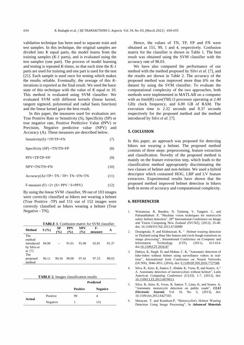
654 R. Badaghi et al. / IJE TRANSACTIONS C: Aspects Vol. 34, No. 03, (March 2021) 650-655
validation technique has been used to separate train and
test samples. In this technique, the original samples are
divided into K equal parts, the model learns from the
training samples (K-1 parts), and is evaluated using the
test samples (one part). The process of model learning
and testing is repeated K-times, so that each time the K-1
parts are used for training and one part is used for the test
[21]. Each sample is used once for testing which makes
the results reliable. Eventually, the average of this K-
iterations is reported as the final result. We used the basic
state of this technique with the value of K equal to 10.
This method is evaluated using SVM classifier. We
evaluated SVM with different kernels (linear kernel,
tangent sigmoid, polynomial and radial basis function)
and the linear kernel gave the best result.
In this paper, the measures used for evaluation are:
True Positive Rate or Sensitivity (S), Specificity (SP) or
true negative rate, Positive Predictive Value (PPV) or
Precision, Negative predictive value (NPV) and
Accuracy (A). These measures are described below.
Sensitivity(S) =TP/TP+FN (7)
Specificity (SP) =TN/TN+FP (8)
PPV=TP/TP+FP (9)
NPV=TN/TN+FN (10)
Accuracy(A)=TP+ TN / TP+ TN +FN+TN (11)
F-measure (F) =2× (S× PPV / S+PPV) (12)
By using the linear SVM classifier, 99 out of 103 images
were correctly classified as bikers not wearing a helmet
(True Positive -TP) and 151 out of 152 images were
correctly classified as bikers wearing a helmet (True
Negative - TN).
TABLE 1. Confusion matrix for SVM classifier
Method S (%) SP
(%) PPV
(%) NPV
(%) F-
measure A
The
method introduced
by Silva et
al. [7]
94.00 - 91.61 91.00 92.81 91.37
The
proposed
method
96.11 99.34 99.00 97.41 97.53 98.03
TABLE 2. Images classification results
Predicted
Positive Negative
Actual Positive 99 4
Negative 1 151
Hence, the values of TN, TP, FP and FN were
obtained as 151, 99, 1 and 4, respectively. Confusion
matrix for the classifier is shown in Table 1. The best
result was obtained using the SVM classifier with the
accuracy rate of 98.03.
We have also compared the performance of our
method with the method proposed by Silvi et al. [7], and
the results are shown in Table 2. The accuracy of the
proposed method was improved more than 6% on the
dataset by using the SVM classifier. To evaluate the
computational complexity of the two approaches, both
methods were implemented in MATLAB on a computer
with an Intel(R) core(TM) i3 processor operating at 2.40
GHz clock frequency, and 6.00 GB of RAM. The
execution time is 2.32 seconds and 8.37 seconds
respectively for the proposed method and the method
introduced by Silvi et al. [7].
5. COCLUSION
In this paper, an approach was proposed for detecting
bikers not wearing a helmet. The proposed method
consists of three steps: preprocessing, feature extraction
and classification. Novelty of the proposed method is
mainly on the feature extraction step, which leads to the
classification method appropriately discriminating the
two classes of helmet and non-helmet. We used a hybrid
descriptor which contained HOG, LBP and LV feature
extractors. Experimental results have shown that the
proposed method improved helmet detection in bikers
both in terms of accuracy and computational complexity.
6. REFERENCESR
1. Waranusas. R, Bundon. N, Timtong. V, Tangnoi. C, and Pattanathaburt. P, “Machine vision techniques for motorcycle
safety helmet detection”, 28th International Conference on Image
and Vision Computing New Zealand (IVCNZ), (2013), 35-40.
doi: 10.1109/IVCNZ.2013.6726989
2. Doungmala. P, and Klubsuwan. K, “ Helmet wearing detection
in Thailand using Haar like feature and circle hough transform on image processing”, International Conference on Computer and
Information Technology (CIT), (2011), 611-614.
doi:10.1109/CIT.2016.87
3. Dahiya. K, Singh. D, and Mohan. C. K, “Automatic detection of
bike-riders without helmet using surveillance videos in real-
time”, International Joint Conference on Neural Networks
(IJCNN), 3046-3051, (2016), doi: 0.1109/IJCNN.2016.7727586
4. Silva. R, Aires. K, Santos.T, Abdala. K, Veras. R, and Soares. A,”
A. Automatic detection of motorcyclists without helmet”, Latin American Computing Conference (CLEI), 1-7, (2013), doi:
10.1109/CLEI.2013.6670613
5. Silva. R, Aires. K, Veras. R, Santos. T, Lima. K, and Soares. A, ”Automatic motorcycle detection on public roads”, CLEI
Electronic Journal, Vol. 16, No. 3, (2013), doi:
10.1109/clei.2012.6427165
6. Marayatr. T, and Kumhom.P, “Motorcyclist's Helmet Wearing
Detection Using Image Processing”, In Advanced Materials

R. Badaghi et al. / IJE TRANSACTIONS C: Aspects Vol. 34, No. 03, (March 2021) 650-655 655
Research, Vol. 931, (2014), 588-592,
doi:10.4028/www.scientific.net/AMR.931-932.588
7. Silva. R. V, Aires. K. R. T, and Veras. R. D.M, “Helmet detection
on motorcyclists using image descriptors and classifiers”, 27th Conference on Graphics, Patterns and Images, (2014), 141-148.
doi:10.1109/sibgrapi.2014.28
8. Shine. L, and Jiji. C.V,” Automated detection of helmet on motorcyclists from traffic surveillance videos: a comparative
analysis using hand-crafted features and CNN”, Journal of
Multimedia Tools and Applications, Vol. 1380, (2020), 1-21, doi:
10.1007/s11042-020-08627-w
9. Alaulikar. A.S, Sanathanan. S, and Modi. C.N,” An enhanced approach for detecting helmet on motorcyclists using image
processing and machine learning techniques”, In Advanced
Computing and Communication Technologies, Vol. 702,
(2019), 109-119, doi: 10.1007/978-981-13-0680-8_11
10. Rubaiyat. A.H, Toma. T.T, Kalantari-Khandani. M, Rahman.
S.A, Chen. L, Ye. Y, and Pan. C.S., “Automatic detection of helmet uses for construction safety”, WIC/ACM International
Conference on Web Intelligence Workshops (WIW), (2016), 135-
142. doi: 10.1109/WIW.2016.045
11. JIANG. X, XUE. H, ZHANG. L, and ZHOU. Y,” A Study of
Low-resolution Safety Helmet Image Recognition Combining
Statistical Features with Artificial Neural Network”, International Journal of Simulation-Systems, Science and
Technology, Vol. 17, No. 37, (2016), 1473-8031, doi:
10.5013/IJSSST.a.17.37.11
12. Li. K, Zhao. X, Bian. J, and Tan. M,” Automatic Safety Helmet
Wearing Detection”, arXiv labs:experimental projects with
community collaborators, 1802.00264, (2014).
13. Raj. K. D, Chairat. A, Timtong. V, Dailey. M. N, and
Ekpanyapong. M, “Helmet violation processing using deep
learning”, International Workshop on Advanced Image Technology (IWAIT), (2018), 1-4, doi:
10.1109/IWAIT.2018.8369734
14. Siebert. F.W, and Lin. H,” Detecting motorcycle helmet use with deep learning”, Journal of Accident Analysis and Prevention,
Vol. 134, (2020), doi:10.1016/j.aap.2019.105319
15. Shakour.M. H and Tajeripour. F,” Local entropy pattern to extract
textural images features”, Vol. 3, No. 2, (2016), 73-85.
16. Lenc. L, and Král. P,” Automatically detected feature positions
for LBP based face recognition”, In IFIP International Conference on Artificial Intelligence Applications and
Innovations, (2014), 246-255, doi: 10.1007/978-3-662-44654-
6_24
17. Huang.D, Shan. C, Ardabilian. M, Wang. Y, and Chen. L, “Local
binary patterns and its application to facial image analysis: a survey”, Journal of Transactions on Systems, Man, and
Cybernetics, Part C (Applications and Reviews), Vol. 41, No. 6,
(2011), 765-781, doi: 10.1109/TSMCC.2011.2118750.
18. Dalal, N, and Triggs. B,” Histograms of oriented gradients for
human detection”, Computer Society Conference on Computer
Vision and Pattern Recognition, (2005), 886-893.
19. Başa. B,” Implementation of Hog Edge Detection Algorithm
Onfpga's”, Procedia-Social and Behavioral Sciences, Vol. 174,
(2015), 1567-1575, doi: 10.1016/j.sbspro.2015.01.806
20. Boser. B. E, Guyon. I. M, and Vapnik. V. N, “A training algorithm
for optimal margin classifiers”, In Proceedings of the fifth annual
workshop on Computational learning theory, (1992), 144-152.
doi: 10.1145/130385.130401
21. Ellis. R. P, and Mookim. P. G, “Cross-validation methods for risk
adjustment models”, Mimeo, Boston University, (2008).
Persian Abstract
چکیده اکثر کشورها برای موتورسوارانی که از کاله ایمنی استفاده نمی کنند، قوانینی وضع شده است. کاله ایمنی برای جلوگیری ازآسیب های ناحیه سر موتورسواران ضروری است. در
بدون کاله ایمنی ارائه بررسی موتورسواران متخلف به صورت دستی کاری وقت گیر و پرهزینه است. در این راستا، در طی سال های اخیر چندین روش تشخیص موتورسواران
ک روش بر حسب پردازش تصویر برای شناسایی موتورسواران بدون کاله ایمنی پیشنهاد شده است.این روش از توصیفگرهای الگوی دودویی محلی، شده است.در این مقاله ی
و کالس با و بدون کاله بندی د واریانس محلی و هیستوگرام مبتنی بر گرادیان استفاده می کند. نوآوری این روش اساسا در مرحله استخراج ویژگی است که باعث می شود طبقه
است. دقت روش پیشنهادی ایمنی بهتر انجام شود.نتایج تجربی نشان می دهد که روش پیشنهادی ما نسبت به روش های موجود دیگر، دارای برتری در تشخیص و طبقه بندی
درصد است. 98.03برای تشخیص کاله ایمنی با استفاده از دسته بند ماشین بردار پشتیبان
IJE TRANSACTIONS C: Aspects Vol. 34, No. 03, (March 2021) 656-666
Please cite this article as: S. R. Salehinia, S. E. Afjei, A. Hekmati, H. Aghazadeh, Design Procedure of an Outer Rotor Synchronous Reluctance Machine for Scooter Application, International Journal of Engineering, Transactions C: Aspects Vol. 34, No. 03, (2021) 656-666
International Journal of Engineering
J o u r n a l H o m e p a g e : w w w . i j e . i r
Design Procedure of an Outer Rotor Synchronous Reluctance Machine for Scooter
Application
S. R. Salehiniaa, S. E. Afjei*a, A. Hekmatib, H. Aghazadeha
a Department of Power Electrical Eng., Faculty of Electrical Engineering, University of Shahid Beheshti, Tehran, Iran b Electric Machine Research Group Niroo Research Institute
P A P E R I N F O
Paper history: Received 21 June 2020 Received in revised form 23 September 2020 Accepted 30 December 2020
Keywords: Finite Element Method Magnetic Flux Barrier Synchronous Reluctance Motor Torque Ripple
A B S T R A C T
Synchronous reluctance motors, despite their cost-effective types and wide range of speed, generally
have a considerable torque ripple due to changes in magnetic resistance between the flux barriers and
the stator teeth. Given the numerous possible rotor combinations with different forms of flux barriers, designing an optimal synchronous reluctance motor without the use of mathematical equations and a
clear algorithm will be very time-consuming. In this study, a comprehensive method is used to design a
synchronous reluctance motor with an external rotor and a flux barrier shape adopted from the behavior of fluids around a solid rotor. According to the new topology, an external rotor synchronous
reluctance motor is designed. Multi-objective Taguchi optimization algorithm based on finite element analysis (FEM) is used to maximize the average torque and reduce the torque ripple.This motor is
designed for 300 W electric scooters with a six-pole rotor, a 36-slot stator, and a distributed winding.
Finally, a prototype of the proposed motor is constructed to validate the results of simulations. The experimental results confirm the accuracy of the design method.
doi: 10.5829/ije.2021.34.03c.10
NOMENCLATURE
avT Average Torque (N.m) Greek Symbols
SynRM Synchronous Reluctance Motor Mass density (kg/m3)
EX SynRM− External rotor Synchronous Reluctance Motor Efficiency
TR Torque ripple potential(m2/s2)
FEM Finite Element Method differential operator with the flow field
MMF Magneto-motive force Kinematic viscosity (m2/s)
g Air-gap width (mm) viscosity coefficient(kg/(m.s)
I Rated current (A) Subscripts
f Average MMF k flux barriers number
Pr Pressure(kg/m3) m flux barriers number
S Iron parts thickness q along the q-axis
sN Rated Speed (rpm) d along the d-axis
1. INTRODUCTION1
implicity the synchronous reluctance motor, with no
need for a squirrel cage in the rotor and permanent
magnet, and the similarity of its stator production line
*Corresponding Author Institutional Email: [email protected] (S.E Afjei)
with the widely used induction motor [1-4], have
attracted the electric motors’ designers and
manufacturers in recent years. Most studies into the
basics of this motor have been carried out on internal
rotor models and there are a limited number of articles
regarding external rotor architecture [5-9]. However,
external rotor electric motors, thanks to their higher
torque compared to the internal rotor architecture, have
S

S. R. Salehinia et al. / IJE TRANSACTIONS C: Aspects Vol. 34, No. 03, (March 2021) 656-666 657
more practical applications, especially in electrical
vehicles [10, 11].
Limited amounts of studies are conducted in the
field of reluctance motor design with external. The
proposed method in considers the thickness of the flux
barrier to be equal along the flux barrier. The chief
reason behind this design is said to be mechanical
strength. While it is shown that the closer the flux
barrier shape is to the behavior of the flux lines in the
rotor, the more optimized the design procedure is
discussed in literature [12]. In this paper, the shape of
flux barriers is designed based on the fluid-liquid
velocity equation. By selecting the appropriate
parameters and optimizing, a comprehensive design for
the external rotor synchronous motor is presented. The
present study intends to introduce a new comprehensive
design method for the Ex-SynRM based on the
formation in the shape of flux barriers in the solid rotor
using its similarity to the pattern of fluid velocity
equations around a solid object. To design external
rotors in a synchronous reluctance motor (SynRM), it is
tried to block the flux along the q-axis and maximize the
magnetic conductance along the d-axis [12, 13]. The
flux barriers in the rotor are designed in three steps: (i)
determining the flux barriers shape using mathematical
equations, (ii) barriers placement on the q-axis, and (iii)
optimizing the designed rotor. Then, the shape of flux
barriers between the d and q axes is determined through
defining some equations that depend on the radius and
angle of the points on the flux barrier line in the rotor.
The flux barriers start from the q-axis and end around
the d-axis. All points between the start and endpoints on
the flux barrier line have their own radius, angle and a
constant parameter (parameter C). Figure 1 depicts a
mathematical definition used for the internal rotor in
more details are discussed in literature [14,15]. The
design is further optimized through the optimization
method, so that the closer the shape of the generated
flux barriers is to the shape of the flux lines, the higher
average torque discussed in literature [14]. The
proposed design procedure of the external rotor is
shown in Figure 2.
Figure 1. Mathematical definition of the parameters
describing the barriers line in a two paire pole machine [15]
Start
Input initial
parameters
Mathematical Equ.
to form flux
barriers
Determining the
position of the
points Bi in the q
axis
Selecting the
number of flux
barriers
Initial design of the
external rotor
Optimization of the
external rotor
Final design of the
external rotor
End
Figure 2. Design procedure of the proposed EX-SynRM
In this regard, this paper presents a new strategy for
the design and analysis of EX-SynRM. The contents are
organized as follows. The flux barriers shape in the
rotor is provided in the second section of the proposed
mathematical equations, considering some variables for
improvement of the motor performance. Then the
variables are evaluated through finite element analysis.
In the last part of this section, the number of flux
barriers is determined. Section 4 pertains to
optimization through Taguchi method taking numerous
variables into account. Finally, the proposed design is
constructed for an electric scooter and the results of
finite element analysis are compared with those of the
manufactured motor.
2. MATHEMATICAL APPROACH
As a symmetric Stokes flow around a solid sphere
shown in Figure 3a [16], the fluid flow lines around a
solid sphere are similar to the magnetic flux lines
distribution in Figure 3b. The equations expressing the
motion of the fluid, with two properties of adhesion and
incompressibility can be expressed as follows [16].
0V = (1)
2PrDV
VDt
= − + (2)
Pr pr = + (3)
where V(m2/s) is the liquid instantaneous velocity,
Pr(kg/m3) is the liquid natural pressure, ρψ is the

658 S. R. Salehinia et al. / IJE TRANSACTIONS C: Aspects Vol. 34, No. 03, (March 2021) 656-666
gravitational potential energy per unit volume (the
combination of these two pressures is known as the
effective pressure) Equation (3), ρ is the liquid mass
density, µ(kg/(m.s) is the liquid viscosity coefficient
which is calculated experimentally, and ψ(m2/s2) is the
gravitational potential [16]. Assume a solid sphere of
radius a in the standard spherical coordinates plane with
the components r, θ, and φ. The fluid flow surrounds the
sphere (r>a), which is an example of the axial Stokes
flow [16]. the symmetric axial Stokes flow, the fluid
velocity equation can be considered as follows.
( ) ( , ) ( , )r rV r v r e v r e = + (4)
According to literature [16] and assuming an
incompressible liquid:
=V (5)
where ψ (r, θ) is the Stokes flow function. Then,
2
1 ( , , )( , )
sinr
rv r
r
= −
(6)
1 ( , , )( , )
sin
rv r
r r
=
(7)
Consider ωr = ωθ = 0
( )1 1 ( )( , )
sin
rrv v
rr r r r
= − =
(8)
2
2 2
sin 1
sinr r
= +
(9)
where ζ is a differential operator with the flow field
symmetry outside the sphere having an axial symmetry,
i.e. ∂⁄∂φ = 0. In other words, here is Vφ =0 (Vφ is
component in spherical coordinates) and it behaves like
a cylindrical coordinate system due to symmetry.
Evaluation of physical boundary around the sphere
surface results in:
( , ) 0rv a = (10)
( , ) 0v a = (11)
Which indicates zero speed on the sphere surface and a
long distance from the sphere surface; it can be stated
that:
( , ) cos( )rv r V → →− (12)
( , ) sin( )v r V → →− (13)
According to Equation (5) discussed in literature [16],
the specifications of the axial stocks flow can be
expressed by the following equation.
2( ) 0 = (14)
By writing the boundary conditions from Equations (4)
to (7), one can write:
0, 0r a r ar
= =
= =
(15)
2 21( , ) sin
2r Vr → → (16)
2 2
2
cos sin ( )( , ) ,
2r
Vr Vrv r v
r r dr
= − = (17)
Equation (2) can be summarized as follows [16]:
Pr ( sin )r = − = (18)
Therefore,
3
Pr 3 cosVa
r r
= −
(19)
2
Pr 3 sin
2
Va
r
= −
(20)
This means that the pressure distribution in that fluid is:
0 2
3 cosPr( , )
2
Var p
r
= + (21)
where p0 is initial pressure Figure 3a shows the axial
stocks flow lines under the influence of the effective
pressure on the x-z plane around a solid sphere using
Equation (21).
As shown in Figure 3a, each stokes flow line is
affected by constant pressure and velocity in Equation
(21); therefore, the parameters Pe, p0, V, and µ in
Equation (21) are in a fixed line, and hence Equation
(21) can be properly converted to an appropriate
equation for the barrier`s lines.
2
cos( * )2
2 p
p
Cr
= (22)
1 22*cos (2 . )pC r
p
−
= (23)
In the above equations, C is a constant function of
the point coordinates through which the curve passes, p
is the number of poles. The initial shape of the flux
barriers is presented using mathematical equations and
parameter C is determined. The results of FEM analysis
for the solid rotor and the designed six-pole rotor with
three flux barriers are compared in Figure 4. As can be
seen, the flux barriers shape is similar to the flux lines
shape in the solid rotor. It should be noted that this step,

S. R. Salehinia et al. / IJE TRANSACTIONS C: Aspects Vol. 34, No. 03, (March 2021) 656-666 659
(a)
(b)
Figure 3. (a) Stokes under pressure P-p0 around a sphere,
(b) Magnetic flux line in the external rotor SynRM whit
two poles without flux barriers
i.e. designing the flux barriers, is the starting point for
rotor design to achieve an optimal design with the least
number of simulations. Figures 3b and 4a depict the flux
lines in the solid rotor when there are no barriers in the
rotor. Since the flux lines in the solid rotor and the fluid
pressure lines are similar at equal velocities [16], the
fluid velocity and pressure line pattern in fluid
mechanics are used to design the flux barriers shape in
the external rotor SynRM.
General specifications of the prototype motor
suitable for electric scooters are given in Table 1.
Design procedure is initiated according to the selected
(a)
(b)
Figure 4. (a) Magnetic flux line in the external rotor
SynRM whit six poles without flux barriers, (b) Initial
model of the six-pole design with three flux barriers
dimensions in Table 1. Based on the rotor flux lines
shape and Equations (22) and (23), the general sketch of
the proposed rotor output with the k number of flux
barriers is shown in Figure 5.
The angle is equal to π/2p along the q-axis, where p
is the number of the rotor pole pairs. The position of
Bk1, Bk2, …, and Bkn (Bki in which B and k denote the
barrier and the selected flux barriers number,
respectively) along the q-axis can be determined by
Equations (25)-(31).
Definition of the parameters for determining the size
and position of flux barriers in the external rotor is as
follows: g is the air gap length, Si is the iron parts
thickness in each section, WBk is the Kth barrier width,
BK is the flux barriers initial and end points on the q-
axis, and β is a constant value that determines the flux
barrier’s arc length.
Selecting insulation ratio in the q-axis (kwq, which is
defined as the ratio of the thickness of total insulation
TABLE 1. General specifications of the designed motor
Parameter Definition Value
Rsh Shaft outer diameter 20 mm
RSt Stator outer diameter 120.5 mm
ROr Rotor outer diameter 168 mm
Rinr Rotor outer diameter 121 mm
L Stack Length (L Stack) 40 mm
Po Power 290 W
N Number of turns 29turns/slot
Ns Rated Speed 1500 rpm
I Rated current 6 A
P Number of pole pairs 3
Efficiency 0.84
g Air-gap width(g) 0.5 mm
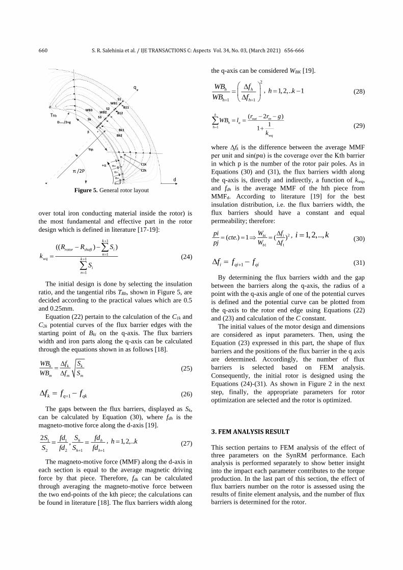
660 S. R. Salehinia et al. / IJE TRANSACTIONS C: Aspects Vol. 34, No. 03, (March 2021) 656-666
q
d
+α
αm/2
αm
αm
αm
ᵝ
S1
S2
S3Sk
WB1
WB2WB3
Yqk
Dstator/2+g
B11
B12
Bk1
Bk2
C1k
C2k
TRb
π /2P
Figure 5. General rotor layout
over total iron conducting material inside the rotor) is
the most fundamental and effective part in the rotor
design which is defined in literature [17-19]:
1
1
1
1
(( ) )k
rotor shaft i
nwq k
i
n
R R S
k
S
+
=
+
=
− −
=
(24)
The initial design is done by selecting the insulation
ratio, and the tangential ribs TRb, shown in Figure 5, are
decided according to the practical values which are 0.5
and 0.25mm.
Equation (22) pertain to the calculation of the C1k and
C2k potential curves of the flux barrier edges with the
starting point of Bki on the q-axis. The flux barriers
width and iron parts along the q-axis can be calculated
through the equations shown in as follows [18].
k k k
m m m
WB f S
WB f S
=
(25)
1k q qkf f f+ = − (26)
The gaps between the flux barriers, displayed as Sk,
can be calculated by Equation (30), where fdh is the
magneto-motive force along the d-axis [19].
1 1
2 2 1 1
2, h h
h h
S fdS fd
S fd S fd+ +
= = , 1,2,..h k= (27)
The magneto-motive force (MMF) along the d-axis in
each section is equal to the average magnetic driving
force by that piece. Therefore, fdk can be calculated
through averaging the magneto-motive force between
the two end-points of the kth piece; the calculations can
be found in literature [18]. The flux barriers width along
the q-axis can be considered WBK [19].
2
1 1
h h
h h
WB f
WB f+ +
=
, 1,2,.. 1h k= − (28)
1
( 2 )
11
kout in
h a
h
wq
r r gWB l
k=
− −= =
+
(29)
where ∆fk is the difference between the average MMF
per unit and sin(pα) is the coverage over the Kth barrier
in which p is the number of the rotor pair poles. As in
Equations (30) and (31), the flux barriers width along
the q-axis is, directly and indirectly, a function of kwq,
and fdh is the average MMF of the hth piece from
MMFd. According to literature [19] for the best
insulation distribution, i.e. the flux barriers width, the
flux barriers should have a constant and equal
permeability; therefore:
2
1 1
( .) 1 ( )bi i
b
W fpicte
pj W f
= = =
, 1,2,..,i k=
(30)
1i qi qif f f+ = − (31)
By determining the flux barriers width and the gap
between the barriers along the q-axis, the radius of a
point with the q-axis angle of one of the potential curves
is defined and the potential curve can be plotted from
the q-axis to the rotor end edge using Equations (22)
and (23) and calculation of the C constant.
The initial values of the motor design and dimensions
are considered as input parameters. Then, using the
Equation (23) expressed in this part, the shape of flux
barriers and the positions of the flux barrier in the q axis
are determined. Accordingly, the number of flux
barriers is selected based on FEM analysis.
Consequently, the initial rotor is designed using the
Equations (24)-(31). As shown in Figure 2 in the next
step, finally, the appropriate parameters for rotor
optimization are selected and the rotor is optimized.
3. FEM ANALYSIS RESULT
This section pertains to FEM analysis of the effect of
three parameters on the SynRM performance. Each
analysis is performed separately to show better insight
into the impact each parameter contributes to the torque
production. In the last part of this section, the effect of
flux barriers number on the rotor is assessed using the
results of finite element analysis, and the number of flux
barriers is determined for the rotor.

S. R. Salehinia et al. / IJE TRANSACTIONS C: Aspects Vol. 34, No. 03, (March 2021) 656-666 661
3. 1. Effect of q-axis Insulation Ratio on the Torque Production The effect of insulation
ratio in the q-axis (kwq) on the average torque and torque
ripple of the selected external rotor SynRM with six
poles in a rotor with one flux barrier and the constant β
is considered in the above equations, the results of
which are shown in Figure 6. As can be seen, the
maximum torque (2.2 N.m) and with peak to peak
torque ripple of 1.3(N.m) value is related to kwq=0.7.
3. 2. Effect of the Flux Barriers Arc Length on the Torque Production The effect of changing of
the flux barriers arc length (β) on the average torque and
peak to peak torque ripple, when kwq is set to the optimal
value (kwq= 0.7), is shown in Figure 7. As shown in Figure 7, β = 3 is the best choice for a
rotor with one flux barrier, resulting in the maximum
average of 2.2 (N.m) torque and the minimum torque
ripple of 1.38 (N.m). It is worth mentioning that higher
amounts of β may lead to flux barriers interference.
3. 3. Effect of the Number of Flux Barriers on the Torque Production The effect of the number
of flux barriers for a special external rotor SynRM on
0.2 0.3 0.4 0.5 0.6 0.7 0.81
1.2
1.4
1.6
1.8
2
2.2
2.4
X: 0.7
Y: 2.19
Kwq, insulation ratio in q-axis
torq
ue (
N.m
)
Avrage torque Torque Ripple
Figure 6. Average Torque and peak to peak torque ripple
for different values of kwq for a special β
Figure 7. Torque and peak to peak torque ripple (FEM) for
different values of β when kwq is 0.7
avrage torque and torque ripple should be investigated
because all design parameters can be affected. For the
preliminary study, the calculated optimal values of the
q-axis insulation ratio and the optimal arc length
coefficient are assumed equal for all cases. Then, a
motor with already mentioned characteristics is
analyzed with equal parameters and different numbers
of flux barriers through the finite element method, the
results of which are depicted in Figure 8. According to the results and considering the average
torque and torque ripple values at the same time, a rotor
with two flux barriers is the most logical and simplest
choice.
4. MULTI-OBJECTIVE OPTIMIZATION OF THE EXTERNAL ROTOR SYNRM In order to optimally design the motor, the main
effective parameters should be analyzed simultaneously.
The design variables in this study are the insulation ratio
in the q-axis (kwq), the flux barriers arc length (β), the
flux barriers width (∆WB), the displacement of the flux
barrier center from the motor shaft center (∆Yq), and
the magnetic thickness of the rib from the rotor edges
(TRb) as shown in Figure 5.
In this design, the average amounts of torque and
torque ripple are considered as the main goals in the
fitness function, when the percentage of torque ripple
can be expressed as follows:
( )min% 100
Max
R
ave
T TT
T
−=
(32)
Where TMax, Tmin, and Tave are the maximum torque,
minimum torque, and average torque, respectively. The
Taguchi method involves the following steps [20]: (a)
defining the number of levels of factors, (b) choosing
the number of factors, (c) selecting a suitable orthogonal
array and construct the matrix, (d) calculating signal-to-
noise (S/N) ratio, (e) analysis of Variance (ANOVA),
1 2 3
0.6
0.8
1
1.2
1.4
1.6
1.8
2
2.2
Number of barriers at Kwq=.7,=3
To
rqu
e(N
.m)
Ave Torque Torque Ripple pp
Figure 8. Avrage torque and torque ripple (FEM) for
different values of k, where k is the number of barriers

662 S. R. Salehinia et al. / IJE TRANSACTIONS C: Aspects Vol. 34, No. 03, (March 2021) 656-666
(f) identifying the control factors and their levels, and
(g) analysis of the results. Therefore, Taguchi method
involves the identification of proper control factors to
obtain the optimum results of the process. According to
Figure 5, the rotor with two flux barriers is selected,
resulting in 9 parameters for optimization. This
experiment has 9 variables at 3 different levels which
are shown in Table 2.
A full factorial experiment would require 3^9
=19683 combinations of factor levels which takes long
time to analyze all the cases. To overcome this problem,
Taguchi suggested a special method to take the effects
of all mentioned states into consideration in less time to
consider all conditions called orthogonal array. The
experiment is arranged as L27 = (3^9) in which L
represents an orthogonal table with 27 scenarios
consisted of nine variables having three levels, the
details of which are shown in Table 3.
After performing the experiments according to the
orthogonal scenarios, mean effects of optimization
parameters on the average torque and torque ripple are
plotted.
The type of the control functions related to S/N are
“large is the better” and “smaller is the better” for the
average torque and torque ripple, repectively [21].
TABLE 2. The levels of design variables
Variable Level 1 Level 2 Level 3
kwq 0.5 0.6 0.7
ΔYq1 (mm) -2 0 +2
ΔYq2 (mm) -2 -1 0
ΔWB1 (mm) -1 0 1
ΔWB2 (mm) -1 0 1
β1 0 1.5 3
β2 0 1.5 3
ΔTRb1 (mm) 0.25 0.5 1
ΔTRb2 (mm) 0.25 0.5 1
TABLE 3. Experimental plan of L27
N
o. kwq
ΔY
q1
ΔY
q2
ΔW
B1
ΔW
B2
β
1
β
2
ΔTR
b1
ΔTR
b2
1 1 1 1 1 1 1 1 1 1
2 1 1 1 1 2 2 2 2 2
3 1 1 1 1 3 3 3 3 3
…………
25 3 3 2 1 1 3 2 3 2
26 3 3 2 1 2 1 3 1 3
27 3 3 2 1 3 2 1 2 1
Typical mean effect plots of parameters with respect to
torque and torque ripple for motors are shown in Figure
9. As it can be seen, for achieving the maximum torque,
the best combination is as fallows: 1set level of ΔWB2, β2, ΔTRb1 and ΔTRb2, 2set level of ΔYq1, ΔYq2 and β2 ,
and 3set level of kwq and ΔWB1.
Considering Figure 9b, Minimum torque ripple is
obtained as fallows:1set level of kwq and ΔTRb2, 2set
level of ΔYq1, ΔWB1 , β1 and ΔTRb1, 3set level ΔYq2,
ΔWB2, β2.
Using ANOVA can be useful to determine the effect
of input parameter on output results. Then, according to
Equations (33) to (35), the sum of the squares of each
factor can be calculated [20-22]:
1
n
i
i
T y=
= (33)
22
1
1 m
A i
i
TSS A
t n=
= − (34)
22
1
n
T i
i
TSS y
n=
= − (35)
where m is the number of levels of factor A, n is the
total number of tests performed, Ai is the sum of the
outputs corresponding to the ith level of factor A, t is the
number of tests performed at the ith level of factor A, T
is equal to the total output of all tests, yi is the output of
the ith test, and SST is the sum of all squares.
The effects of the impact weight of all design
variables on the desired output obtained through
calculations are presented in Table 4.
The selection of appropriate levels of variables is
done by comparing the S/N analysis results shown in
Figure 9 and the results obtained in Table 3. Then, the
optimization variables are selected to achieve the best
design results for both average torque and torque ripple.
Consequently, 1set level of kwq, β2, TRb1, and TRb2 , 2set
level of ∆Yq1 and β1, and 3set level of ∆Yq2, ∆WB1,
and ∆WB2 .
(a)

S. R. Salehinia et al. / IJE TRANSACTIONS C: Aspects Vol. 34, No. 03, (March 2021) 656-666 663
(b)
Figure 9. S/N ratio of the optimization parameters for: (a)
average torque, (b) torque ripple
TABLE 4. Impact weight of design variables
Variable Impact weight on
average torque
Impact weight on
average torque ripple
kwq 2.41% 20.55%
ΔYq1 0.27% 5.66%
ΔYq2 1.89% 5.82%
ΔWB1 14.82% 1.28%
ΔWB2 4.90% 24.34%
β1 7.55% 34.08%
β2 9.02% 0.80%
ΔTRb1 19.44% 0.93%
ΔTRb2 39.70% 6.53%
The comparison of the optimized motor with the
initial design is presented in Table 5. It is worth
mentioning, the variable kwq is set to 0.5, TRb1 and TRb2
are set to 0.25 mm and the other variables are set to zero
for the initial design.
As shown in Figure 10, it is obvious that the
optimization of the external rotor motor, with 9
simultaneous effective variables and an acceptable
number of tests, is performed well. Accordingly, the
primary average torque and torque ripple are improved
by 2.6% and 17.7%, respectively.
The magnetizing inductances along the d and q axes
are the most important parameters in creating torque of
the SynRM. As Figure 11 shows by increasing the air
gap length Ld decreases while due to the presence of
flux barriers in the q axis Lq remains unchanged.
TABLE 5. Comparison of the initial and optimized motors
Definition Primary motor Optimized motor
Ave. Torque (N.m) 1.87 1.92
Torque ripple (%) 22.62% 18.61%
(a)
0 10 20 30 40 50 601.6
1.7
1.8
1.9
2
2.1
2.2
2.3
2.4
X: 18
Y: 1.92
Rotor position(deg.)
Torq
ue(N
.m)
Taguchi Optimized rotor torque
Average value
(b)
Figure 10. Torque of Ex-SynRM (a) primary desigen, (b)
Optimized by Taguchi method
Figure 11. Effect of air-gap on the inductances of Ex-SynRM
Figure 12 shows the maximum flux density on the
stator at the rated current is 1.5 Tesla, which is lower
than 1.7 Tesla.
5. THE PROTOTYPED MOTOR AND THE EXPERIMENTAL RESULTS Experimental verification the results of the initial test
and a prototype motor with the same dimensions of the
optimal design are presented in this section. Figure 13
shows the rotor and stator laminations of the
manufactured motor.

664 S. R. Salehinia et al. / IJE TRANSACTIONS C: Aspects Vol. 34, No. 03, (March 2021) 656-666
Figure 12. Flux density on the stator and rotor of Ex-SynRM
(a) (b)
Figure 13. The laminations of (a) rotor and (b) stator
Figure 14. The experimental setup for testing the prototype
external rotor SynRM
A 0.3 kW motor is constructed in this study as a
prototype motor. The motor is tested in a test setup
(shown in Figure 14) equipped with the ABB ACS140
Multi drive system where the current electric angle is 50
degrees. The results of the FEM analysis and measured
comparisons are given in Table 7 and Figure 15. The
torque measured with FEM is almost the same. The
copper loss difference between the practical test and the
FEM analysis can be attributed to the difference
between the estimated current and the amount required
for torque generation of the shaft in the practice.
Regarding the iron loss difference, the lamination
manufacturing and wire cutting, the accuracy of the
rotor and stator assembly processes can be pointed out.
0 10 20 30 40 50 601.6
1.7
1.8
1.9
2
2.1
2.2
2.3
2.4
X: 18.9
Y: 1.931
Rotor position(deg.)
Torq
ue(N
.m)
FEM
Average value
(a)
0 10 20 30 40 50 601.6
1.7
1.8
1.9
2
2.1
2.2
2.3
2.4
X: 27.9
Y: 1.904
Rotor Position(deg)
To
rqu
e(N
.m)
(b)
Figure 15. Torque of Ex-SynRM (a) FEM result, (b)
Experimental result
TABLE 7. Comparison of the simulation results and
experimental reults
Definition FEM measurement
Ave. Torque (N.m) 1.93 1.90
Torque ripple (%) 22% 23%
Pout (W) 303 294
η% 76 71.5
PCu (W) 48.4 56.2
PF 0.74 0.69
Finally, in order to be more accurate in practical
results, more specific experiments are needed to
accurately examined the core losses and the mechanical
losses which data were lost during the experiments.
6. CONCULSION The present study proposes a new method for designing
an external rotor SynRM. Given the similar behaviors of
a fluid around a solid object in fluid mechanics and
electromagnetic magnetic flux lines and duality
relations between fluid pressure lines and potential
electric lines, some simplified equations were provided
for further predicting the flux lines in external rotor

S. R. Salehinia et al. / IJE TRANSACTIONS C: Aspects Vol. 34, No. 03, (March 2021) 656-666 665
reluctance synchronous motors. In the next step,
considering the concept of reluctance in SynRMs,
certain parameters are considered in the presented
equations for controlling the position and shape of the
flux barriers in the rotor body. The experiments were
performed through Taguchi optimization method using
the FEM analysis of an external rotor SynRM. Finally,
the selected cases are analyzed and an appropriate rotor
model was identified and designed for use in electric
scooters. The proposed method is applied for
construction of a motor which confirmed through
comparing the measured practical results and the design
procedure.
7. REFERENCES
1. Boglietti, A., Cavagnino, A., Pastorelli, M., and Vagati, A.:
‘Experimental comparison of induction and synchronous
reluctance motors performance’, Fourtieth IAS Annual Meeting. Conference Record of the 2005 Industry Applications
Conference, Vol. 1, (2005), 474-479. DOI;
10.1109/IAS.2005.1518350.
2. Boglietti, A., and Pastorelli, M.: ‘Induction and synchronous
reluctance motors comparison’, 2008 34th annual conference of
IEEE industrial electronics, (2008), 2041-2044. DOI;
10.1109/IECON.2008.4758270.
3. Sahebjam, M., Sharifian, B., Feyzi, M.R., and Sabahi, M.:
‘Novel Unified Control Method of Induction and Permanent Magnet Synchronous Motors’, International Journal of
Engineering, Transactions B: Applications Vol. 32, (2019),
pag no. 256-269. DOI; 10.5829/ije.2019.32.02b.11.
4. Arehpanahi, M., and Kheiry, E.: ‘A New Optimization of
Segmented Interior Permanent Magnet Synchronous Motor Based on Increasing Flux Weakening Range and Output Torque
(Research Note)’, International Journal of Engineering,
Transactions C: Aspects Vol. 33, No. 6 (2020), 1122-1127.
DOI; 10.5829/ije.2020.33.06c.09.
5. Chan, C.: ‘The state of the art of electric and hybrid vehicles’,
Proceedings of the IEEE, Vol. 90, (2002), 247-275. DOI;
10.1109/JPROC.2007.892489.
6. Zaim, M.E.H.: ‘High-speed solid rotor synchronous reluctance
machine design and optimization’, IEEE Transactions on
Magnetics, Vol. 45, (2009), 1796-1799. DOI;
10.1109/TMAG.2009.2012824.
7. Kolehmainen, J.: ‘Synchronous reluctance motor with form blocked rotor’, IEEE Transactions on Energy Conversion, Vol.
25, (2010), 450-456. DOI; 10.1109/TEC.2009.2038579.
8. Taghavi, S.M., and Pillay, P.: ‘A mechanically robust rotor with
transverse laminations for a wide-speed-range synchronous
reluctance traction motor’, IEEE Transactions on Industry
Applications, Vol. 51, (2015), 4404-4414. DOI;
10.1109/TIA.2015.2445819.
9. Aghazadeh, H., Afjei, E., and Siadatan, A.: ‘Sizing and detailed
design procedure of external rotor synchronous reluctance machine’, IET Electric Power Applications, Vol. 13, (2019),
1105-1113. DOI; 10.1049/iet-epa.2018.5802.
10. Deshpande, Y., and Toliyat, H.A.: ‘Design of an outer rotor ferrite assisted synchronous reluctance machine (Fa-SynRM) for
electric two-wheeler application’, IEEE energy conversion
congress and exposition (ECCE), (2014), 3147-3154. DOI;
10.1109/ECCE.2014.6953828.
11. Sankestani, M.M.R., and Siadatan, A.: ‘Design of outer rotor
synchronous reluctance motor for scooter application’, 2019 10th International Power Electronics, Drive Systems and
Technologies Conference (PEDSTC), (2019). 132-137. DOI;
10.1109/PEDSTC.2019.8697636.
12. Moghaddam, R.-R., and Gyllensten, F.: ‘Novel high-
performance SynRM design method: An easy approach for a complicated rotor topology’, IEEE Transactions on Industrial
Electronics, Vol. 61, (2013) 5058-5065. DOI;
10.1109/TIE.2013.2271601.
13. Moghaddam, R.-R.: ‘Design optimization of SynRM with
Ladybird rotor’, 2017 International Conference on Optimization
of Electrical and Electronic Equipment (OPTIM) & 2017 Intl Aegean Conference on Electrical Machines and Power
Electronics (ACEMP), (2017), 317-323. DOI;
10.1109/OPTIM.2017.7974990.
14. Dziechciarz, A., and Martis, C.: ‘Magnetic equivalent circuit of
synchronous reluctance machine’, ELEKTRO, (2016), 500-503.
DOI; 10.1109/ELEKTRO.2016.7512126.
15. Rajabi Moghaddam, R.: ‘Synchronous reluctance machine
(SynRM) in variable speed drives (VSD) applications’, KTH
Royal Institute of Technology, 2011
16. Fitzpatrick, R.: ‘Theoretical fluid mechanics’2017). DOI;
10.1088/978-0-7503-1554-8.
17. Moghaddam, R.R., Magnussen, F., and Sadarangani, C.: ‘Theoretical and experimental reevaluation of synchronous
reluctance machine’, IEEE Transactions on Industrial
Electronics, Vol. 57, (2009), 6-13. DOI;
10.1109/TIE.2009.2025286.
18. Aghazadeh, H., Afjei, E., and Siadatan, A.: ‘Comprehensive
Design Procedure and Manufacturing of Permanent Magnet Assisted Synchronous Reluctance Motor’, International
Journal of Engineering, Transactions C: Aspects Vol. 32, No.
9 (2019),. 1299-1305. DOI; 10.5829/ije.2019.32.09c.10. 1.
19. Moghaddam, R.R., Magnussen, F., and Sadarangani, C.: ‘A
FEM 1 investigation on the Synchronous Reluctance Machine
rotor geometry with just one flux barrier as a guide toward the optimal barrier's shape’, IEEE EUROCON, (2009), 663-670.
DOI; 10.1109/EURCON.2009.5167704.
20. Ajamloo, A.M., Ghaheri, A., and Afjei, E.: ‘Multi-objective Optimization of an Outer Rotor BLDC Motor Based on Taguchi
Method for Propulsion Applications’, 2019 10th International
Power Electronics, Drive Systems and Technologies Conference (PEDSTC), (2019), 34-39. DOI;
10.1109/PEDSTC.2019.8697586.
21. Arkadan, A., and Al Aawar, N.: ‘Taguchi-EM-AI Design Optimization Environment for SynRM Drives in Traction
Applications’, International Applied Computational
Electromagnetics Society Symposium (ACES), (2020). 1-2.
DOI; 10.23919/ACES49320.2020.9196111.
22. Mansoursamaei, M., Hadighi, A., and Javadian, N.: ‘A New
Approach Applying Multi-Objective Optimization using a Taguchi Fuzzy-based for Tourist Satisfaction Management’,
International Journal of Engineering, Transactions C: Aspects
Vol. 32, (2019), 405-412. DOI; 10.5829/ije.2019.32.03c.08.

666 S. R. Salehinia et al. / IJE TRANSACTIONS C: Aspects Vol. 34, No. 03, (March 2021) 656-666
Persian Abstract
چکیده نوباشدمیبا عملکرد در محدوده وسیع سرعت اقتصادی موتور سنکرون رلوکتانسی یک موتور این اما به طور عمومی ریپل گشتاور تغییر مقاومت ع. به دلیل از موتورها
م بین استمغناطیسی قابل مالحظه استاتور دندانه و بهینه .وانع شار به طراحی تمامی انسیرلوکت سنکرون ماشین یک دستیابی میان اشکال روتور های ممکن ترکیب از با
موتور طراحی روتور برای جامع دراین مطالعه یک روش .استبر بدون استفاده از روابط تئوری ریاضی و الگوریتم مشخص طراحی کاری بسیار زمان و مختلف موانع شار
جدید استفاده از این روش ا. بشده استگرفته شده از رفتار مایعات جاری اطراف یک جسم جامد ارائه شکل موانع شار الگوبا بیرونی ساختار روتور سنکرون رلوکتانسی با
متوسط مقدار به حداکثر رساندن با هدف ( FEMالمان محدود ) تحلیل ی بر نمبت تاگوچی چند هدفهبا استفاده از الگوریتم در ادامه روتور بیرونی پیشنهاد و یک طرح طراحی،
تولیدیگشتاور و ک از شبیه بهینه سازی شده است. اهش ریپل گشتاور نتایج حاصل اعتبارسنجی صحت انتها برای از موتور در اولیه نمونه سازی های صورت گرفته یک
ه است. مقایسه ی توزیع شده ساخته شدبا سیم پیچهمراه شیار 63و با استاتور مغناطیسی مانع الیه دو با روتوری با تعداد قطب، 6و وات 003پیشنهادی برای اسکوتر برقی
.کندسازی را تائید مینتایج عملی به خوبی درستی نتایج شبیه

IJE TRANSACTIONS C: Aspects Vol. 34, No. 03, (March 2021) 667-675
Please cite this article as: J. Tavoosi, A. Mohammadzadeh, A New Recurrent Radial Basis Function Network-based Model Predictive Control for a Power Plant Boiler Temperature Control, International Journal of Engineering, Transactions C: Aspects Vol. 34, No. 03, (2021) 667-675
International Journal of Engineering
J o u r n a l H o m e p a g e : w w w . i j e . i r
A New Recurrent Radial Basis Function Network-based Model Predictive Control for
a Power Plant Boiler Temperature Control
J. Tavoosi*a, A. Mohammadzadehb
a Department of Electrical Engineering, Ilam University, Ilam, Iran b Department of Electrical Engineering, University of Bonab, Bonab, Iran
P A P E R I N F O
Paper history: Received 23 November 2020 Received in revised form 25 December 2020 Accepted 08 February 2021
Keywords: Boiler Temperature Model Predictive Control Parameter Uncertainty Radial Basis Function Network
A B S T R A C T
In this paper, a new radial basis function network-based model predictive control (RBFN-MPC) is
presented to control the steam temperature of a power plant boiler. For the first time in this paper the
Laguerre polynomials are used to obtain local boiler models based on different load modes. Recursive least square (RLS) method is used as observer of the Laguerre polynomials coefficient. Then a new
locally recurrent radial basis function neural network with self-organizing mechanism is used to model
these local transfer function and it used to estimate the boiler future behavior. The recurrent RBFN tracks system is dynamic online and updates the model. In this recurrent RBFN, the output of hidden layer
nodes at the past moment is used in modelling, So the boiler model behaves exactly like a real boiler.
Various uncertainties have been added to the boiler and these uncertainties are immediately recognized by the recurrent RBFN. In the simulation, the proposed method has been compared with traditional MPC
(based on boiler mathematical model). Simulation results showed that the recurrent RBFN-based MPC
perform better than mathematical model-based MPC. This is due to the neural network's online tracking of boiler dynamics, while in the traditional way the model is always constant. As the amount of
uncertainty increases, the difference between our proposed method and existing methods can clearly be
observed.
doi: 10.5829/ije.2021.34.03c.11
NOMENCLATURE
𝑝 Time scale factor 𝑀(𝑘) Gain matrix in RLS
𝛷𝑖 Laguerre functions 𝜇𝑖(𝑘) the coefficients of the functions in MPC
𝑌𝑚(𝑠) Laplase transform of system’s output 𝐻𝑖 The horizon sample
𝐶𝑖 Output matrices u(k) Control input
𝑈(𝑠) Laplase transform of system’s input ∅𝑖(𝑢) Output of RBF neurons
𝑙𝑖(𝑠) Terms of Laguerre Ladder network 𝑤𝑖 Waights in RBFN
𝜏𝑖 Time constant of the system 𝑦𝑚(𝑘) Output of the model
1. INTRODUCTION1 Boilers are used in many industries such as power plants.
Power plants use boilers to generate steam for electrical
power in steam turbines. The more precise control of the
boiler outlet temperature is crucial. If the outlet steam
temperature is not properly controlled, the pressure
needed to rotate the turbines may not be reached or the
*Corresponding Author Institutional Email: [email protected] (J. Tavoosi)
efficiency of the boiler and turbine may be reduced. Due
to the long history of using boilers in various industries,
which reaches more than 150 years, naturally, various
methods have been proposed to control outlet
temperature. From simple methods such as PID [1] to
model free methods such as variable structures adaptive
control [2], are each proposed to control the boiler
system. The above methods do not require an accurate
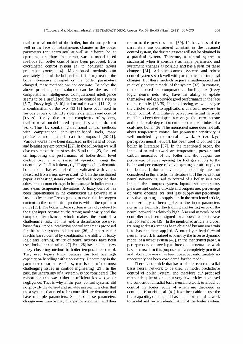
J. Tavoosi and A. Mohammadzadeh / IJE TRANSACTIONS C: Aspects Vol. 34, No. 03, (March 2021) 667-675 668
mathematical model of the boiler, but do not perform
well in the face of instantaneous changes in the boiler
parameters (or uncertainty) as well as different boiler
operating conditions. In contrast, various model-based
methods for boiler control have been proposed, from
coordinated control system [3] to nonlinear model
predictive control [4]. Model-based methods can
accurately control the boiler; but, if for any reason the
boiler dynamics changed or the boiler parameters
changed, these methods are not accurate. To solve the
above problems, one solution can be the use of
computational intelligence. Computational intelligence
seems to be a useful tool for precise control of a system
[5-7]. Fuzzy logic [8-10] and neural network [11-12] or
a combination of the two [13-15] have been used in
various papers to identify systems dynamics and control
[16-19]. Today, due to the complexity of systems,
mathematical model-based approaches alone do not
work. Thus, by combining traditional control methods
with computational intelligence-based tools, more
precise control methods can be proposed [20-21].
Various works have been discussed in the field of boiler
and heating system control [22]. In the following we will
discuss some of the latest results. Sunil et al. [23] focused
on improving the performance of boiler-drum level
control over a wide range of operation using the
quantitative feedback theory (QFT) approach. A dynamic
boiler model has established and validated with values
measured from a real power plant [24]. In the mentioned
paper, a reheating steam control method is proposed that
takes into account changes in heat storage in boiler metals
and steam temperature deviations. A fuzzy control has
been implemented in the combustion air flowrate of a
large boiler in the Tereos group, to maintain the oxygen
content in the combustion products within the optimum
range [25]. The boiler turbine system is usually subject to
the tight input constraint, the strong nonlinearity and the
complex disturbance, which makes the control a
challenging task. To this end, a disturbance observer
based fuzzy model predictive control scheme is proposed
for the boiler system in literature [26]. Support vector
machin based control by combination the ability of fuzzy
logic and learning ability of neural network have been
used for boiler control in [27]. Shi [28] has applied a new
fuzzy clustering method to boiler temperature control.
They used type-2 fuzzy because this tool has high
capacity on handling with uncertainty. Uncertainty in the
parameter or structure of a system is one of the most
challenging issues in control engineering [29]. In the
past, the uncertainty of a system was not considered. The
reason for this was either insufficient knowledge or
negligence. That is why in the past, control systems did
not provide the desired and suitable answer. It is clear that
most systems that need to be controlled are dynamic and
have multiple parameters. Some of these parameters
change over time or may change for a moment and then
return to the previous state [30]. If the values of the
parameters are considered constant in the designed
control system, the desired answer will not be obtained in
a practical system. Therefore, a control system is
successful when it considers as many parametric and
systematic changes as possible and has a plan for these
changes [31]. Adaptive control systems and robust
control systems work well with parametric and structural
changes. But these methods require a mathematical and
relatively accurate model of the system [32]. In contrast,
methods based on computational intelligence (fuzzy
logic, neural nets, etc.) have the ability to update
themselves and can provide good performance in the face
of uncertainties [33-35]. In the following, we will analyze
the articles related to applications of neural network in
boiler control. A multilayer perceptron neural network
model has been developed to envisage the corrosion rate
and oxide scale deposition rate in economizer tubes of a
coal-fired boiler [36]. The mentioned paper does not talk
about temperature control, but parametric sensitivity is
well modeled by the neural network. A two layer
perceptron neural network has been used to control of a
boiler in literature [37]. In the mentioned paper, the
inputs of neural network are temperature, pressure and
carbon monoxide of the boiler and the outputs are
percentage of valve opening for fuel gas supply to the
boiler and percentage of valve opening for air supply to
the boiler. Unfortunately, load uncertainty are not
considered in this article. In literature [38] the perceptron
neural network is used to control of a boiler as a two
inputs - three outputs system. Inputs are: temperature,
pressure and carbon dioxide and outputs are: percentage
of valve opening for fuel gas supply and percentage
of valve opening to supply air. In the mentioned article,
no uncertainty has been applied neither in the parameters
nor in the load, also the training and testing error of the
neural network is relatively high. A neural network-based
controller has been designed for a power boiler to save
fuel consumption [39]. In the mentioned article, a proper
training and test error has been obtained but any uncertain
load has not been applied. A multilayer feed-forward
neural network is trained to identify the inverse dynamic
model of a boiler system [40]. In the mentioned paper, a
perceptron-type three-input-three-output neural network
has been used for this purpose, and a completely practical
and laboratory work has been done, but unfortunately no
uncertainty has been considered for the model.
There is no article that has used the recurrent radial
basis neural network to be used in model predictiove
control of boiler system, and therefore our proposed
method is quite original, but very few articles have used
the conventional radial basis neural network to model or
control the boiler, some of which are discussed in
continue. Kouadri et al. [41] have been able to use the
high capability of the radial basis function neural network
to model and system identification of the boiler system.

669 J. Tavoosi and A. Mohammadzadeh / IJE TRANSACTIONS C: Aspects Vol. 34, No. 03, (March 2021) 667-675
In the mentioned paper, an ordinary (not recurrent) radial
base function neural network with training based on
genetic algorithm has been used. In literature [42], the
ordinary radial base function neural network has been
used to inverse control of a boiler system. In the
mentioned paper the load uncertainty is not considered
and the boiler equations are not clear. An ordinary radial
basis function neural network has been performed to
identify the boiler system and then use it in the optimal
control of the boiler, but not any type of uncertainty (load
or parameters) is considered [43]. We have justified by
reviewing the above articles that there are shortcomings
in this regard. Therefore, in this paper, we proposed a
new method to eliminate them. The innovations of our
proposed method are as follows:
- In most of the articles, general feedback was used
in recurrent RBFNs, while in our proposed
method, local feedback was used. In general
feedback, the information from the past moment of
the last layer is applied as input to the first layer,
but in local feedback, the information from the past
moment of the output of the neuron itself is used as
the input of the same neuron. It should be noted
that neural network training with local feedback is
far more complex than training with general
feedback.
- The second innovation of our method is the use of
structural training (Self-Organizing) in regulating
the number of neurons in the middle layer of the
neural network. In this way, starting from one
neuron and due to the complexity of the data, the
number of neurons increases, until we achieve the
desired minimum error.
- The third innovation is using the Laguerre
polynomials to obtain the local boiler models for
different boiler load modes.
- The forth innovation is proposed a new structure
for MPC based on RBFN. The innovation of this
section is using difference formulation for MPC.
- Considering the parameters of a real boiler with
real uncertainty is fifth innovation. All numerical
and parametric values were measured from a
laboratory and practical boiler.
In this paper, the main focus is on the load uncertainty
problem. First, the dynamic equations of the boiler
system are expressed. Then, the radial basis function
neural network prediction model control system is
presented. Finally, simulations and conclusions are
presented.
2. MATHEMATICAL MODELING OF SUPER HEATED STEAM OF POWER PLANT In this section, first the Laguerre functions are
introduced; then, the boiler modeling method is
expressed using these functions. Laguerre functions are a
complete set of orthogonal functions in Judicial 𝐿2(0,∞)
which are widely used because of the simple and easy
expression of its network. These functions come in a
series of functions [44]:
𝛷𝑖(𝑡)=√2𝑝 𝑒𝑝𝑡 𝑑𝑖−1
(i − 1)!𝑑𝑡𝑖−1 [𝑡𝑖−1. 𝑒2𝑝𝑡], 𝑖 = 1,2,...,∞ (1)
are defined where 𝑝 is a constant called the time scale
factor. The laplace transform of Equation (1) is:
𝛷𝑖(𝑡)=𝑙{𝛷𝑖(𝑡)}= √2𝑝 (𝑠−𝑝)𝑖−1
(s+p)𝑖) . 𝑖= 1,2,...,∞ (2)
Every open loop system can be approximated by
Laguerre functions as Equation (3):
𝑌𝑚(𝑠) = ∑ 𝐶𝑖𝛷𝑖(𝑠)𝑈(𝑠)𝑛𝑖=1 = ∑ 𝐶𝑖𝑙𝑖(𝑠)
𝑛𝑖=1 (3)
There are several ways to express the Laguerre Ladder
network. However, it is desirable for us to express the
Laguerre ladder network in the state space so that it can
directly predict the outputs of the system. The system
state space expression using the Laguerreithmic
functions after discretization is as follows [44] :
L(k + 1) = AL(k) + Bu(k)
y(k) = CL(k) (4)
In Equation (4), the system state vector is L(k) of the
order n and u (k) is the input of the system. The matrix A
is the lower triangular matrix of NxN. Also B is the
matrix of input coefficients of the system (Nx1) whose
elements are determined by line-off. This way the
amount of computation is greatly reduced. If 𝑇 is the
system sampling period, therefore [44]:
𝜏1 = 𝑒−𝑝𝑇
𝜏2 = 𝑇 + 2
𝑃 (𝑒−𝑝𝑇-1)
𝜏3 =- 𝑇𝑒−𝑝𝑇 − 2
𝑃 (𝑒−𝑝𝑇-1)
𝜏4 =√2𝑝 (1−𝜏1)
𝑝
𝑎 = 𝜏1𝜏2 + 𝜏3
(5)
Then the system description matrices for Equation (4) are
expressed as follows:
𝐴 =
[
𝜏1 0
−𝑎
𝑇𝜏1
… 0… 0
⋮ ⋮(−1)𝑁−1𝜏2
𝑛−2𝑎
𝑇𝑁−1 …
⋱ ⋮
−𝑎
𝑇𝜏1]
𝐵 = [𝜏1 (−𝜏2
𝑇) 𝜏4 … (
−𝜏2
𝑇)𝑁−1
𝜏4]𝑇
L(k)=[𝑙1(𝑘) 𝑙2(𝑘)… 𝑙𝑁(𝑘)]𝑇
C= [𝑐1 𝑐2…𝑐𝑁]
(6)
The vector C, which is the system observer coefficients
vector with N + 1 dimensional, is determined by using

J. Tavoosi and A. Mohammadzadeh / IJE TRANSACTIONS C: Aspects Vol. 34, No. 03, (March 2021) 667-675 670
the recursive least squares (RLS) to express the
relationship between the Laguerre model and the desired
system.
𝐶(𝑘) = 𝐶(𝑘 − 1) + {𝑀(𝑘)[𝑦(𝑘) − 𝐶(𝑘 − 1)𝐿(𝑘)]}𝑇
𝑀(𝑘) =𝑃(𝐾−1)𝐿(𝐾)
𝜆+𝐿𝑇(𝐾)𝑃(𝐾−1)𝐿(𝐾)
P(k) =1
λ[𝑃(𝑘 − 1) − 𝑀(𝑘)𝐿𝑇(𝑘)𝑃(𝑘 − 1)]
(7)
where λ is forgetting factor. From Equations (1) to (7), a
model of a boiler system can be obtained. As it is clear
from the above equations, the obtained model is dynamic
and with exponential coefficients and can be a relatively
accurate mathematical model of a practical boiler.
3. MODEL PREDICTIVE CONTROL
Model predictive control has rules similar to classical
prediction control, as both methods use a model to predict
the future output of the system. Model predictive control
considers the structure of control law as a linear
combination of a set of basic functions. Then the weight
of the coefficients of the basic functions in the linear
combination has to be calculated. The selection of basic
functions is also based on the process properties and the
desired reference inputs. The structure of the control law
can be considered as follows.:
𝑢(𝑘 + 𝑖) = ∑ 𝜇𝑛𝑢𝑏𝑛(𝑖) 𝑁𝑛=1 (8)
where the 𝜇𝑛 is the coefficients of the functions with is
linear in sequence and specifies the number of base types
(𝑢𝑏𝑛(𝑖)). The values of the basic functions are
instantaneous k+i (𝑢(𝑘 + 𝑖)). The choice of these basic
functions depends on the nature of the process and the
reference input and generally uses step-slope and
parabolic functions. In most cases, however, using two
steps to the step and the ramp is sufficient:
𝑢(𝑘 + 𝑖) = 𝜇1(𝑘) + 𝜇2(𝑘) ∗ 𝑖 (9)
The model predictive control algorithm finds the sum of
future control variables in such a way that the output of
the process is as close to the reference sequence as
possible. The feedback correction sequence is computed
by an exponential relation:
𝑦𝑝(𝑘 + 𝑖) = 𝑦𝑚(𝑘 + 𝑖) − λ𝑖[𝑦𝑚(𝑘) − 𝑦(𝑘)] (10)
where 𝑖 = 1,2, … , 𝐻𝑖 are the total number of matching
points. 𝑦𝑝(𝑘 + 𝑖) are the values of the feedback
correction sequence at time 𝑘 + 𝑖, 𝑦𝑚(𝑘) is also the
model outputs (RBFN output) and y(k) are process
outputs. λ𝒊 = 𝒆−
𝑻𝒔𝑻𝒓 which is 𝑇𝑠 the sampling time and 𝑇𝑟
the expected response time to the reference sequence .
By combination of Equations (4) and (9), the future
output can be obtained.
𝑦𝑚(𝑘 + 𝑖) = 𝐶𝐴𝑖𝐿(𝑘) + 𝐶[𝐴𝑖−1 + 𝐴𝑖−2 + ⋯+
𝐼]𝐵𝜇1(𝑘) + 𝐶[𝐴𝑖−2 + 2𝐴𝑖−3 + ⋯+ (𝑖 −
1)𝐼]𝐵𝜇2(𝑘)
(11)
where 𝑦𝑚(𝑘 + 𝑖) is output of the model at 𝑘 + 𝑖. MPC is a control strategy that explicitly uses the
process model to predict the future behavior of the
process output in a finite horizon, and the control effort
is achieved by minimizing the interaction between the
predicted output of the model and the reference sequence
at a given time horizon. The predictive control law is
generally computed by minimizing the axial scaling:
J=∑ [𝑦𝑝(𝑘 + 𝑖) + 𝑒(𝑘 + 𝑖) − 𝑦𝑟(𝑘 + 𝑖)]2𝐻2 𝑖=𝐻1
(12)
In relation to the control effort, only two coefficients of
the basic functions, 𝜇1(𝑘) and 𝜇2(𝑘), are uncertain. In
order to determine these unknown parameters, we rewrite
the above relations [44]:
J= [𝑦𝑝(𝑘 + 𝐻1) + 𝑒(𝑘 + 𝐻1) − 𝑦𝑟(𝑘 + 𝐻1)]2 +
[𝑦𝑝(𝑘 + 𝐻2) + 𝑒(𝑘 + 𝐻2) − 𝑦𝑟(𝑘 + 𝐻2)]2
(13)
We will have the following relationship by replacing the
reference sequence and predicting the process output .
[𝑋1(k) + 𝑀11μ1(𝑘) + 𝑀12μ2(𝑘)]2 + [𝑋2(𝑘) +𝑀12μ1(𝑘) + 𝑀22μ2(𝑘)]2
(14)
In this regard :
𝑋1(𝑘) = 𝐶𝐴𝐻1𝐿(𝑘) + 𝑒(𝑘 + 𝐻1) − 𝑦𝑟(𝑘 + 𝐻1)
𝑋2(𝑘) = 𝐶𝐴𝐻2𝐿(𝑘) + 𝑒(𝑘 + 𝐻2) − 𝑦𝑟(𝑘 + 𝐻2)
𝑀11 = 𝐶(𝐴𝐻1−1 + 𝐴𝐻1−2 + ⋯+ 𝐼)𝐵
𝑀12 = 𝐶(𝐴𝐻1−2 + 2𝐴𝐻1−3 + ⋯+ (𝐻1 − 1)𝐼)𝐵
𝑀21 = 𝐶(𝐴𝐻2−1 + 𝐴𝐻2−2 + ⋯+ 𝐼)𝐵
𝑀22 = 𝐶(𝐴𝐻2−2 + 2𝐴𝐻2−3 + ⋯+ (𝐻2 − 1)𝐼)𝐵
(15)
From Equation (15), all required coefficient and variables
in Equation (14) are calculated. Now, by deriving the
relation to the unknown parameters, we obtain:
μ1(𝑘) = 𝑆𝑦𝑦(𝑘) + 𝑆𝐿𝐿(𝐾) + 𝑆𝑊𝑊(𝑘) (16)
In this regard
𝑆𝑦 = 𝑄(𝑄3𝑀12 − 𝑄2𝑀11)(1-𝛼𝐻1)+Q(𝑄3𝑀22 −
𝑄2𝑀21)(1 − 𝛼𝐻2)
𝑆𝐿 = 𝑄(𝑄3𝑀12 − 𝑄2𝑀11)𝐶(𝐴𝐻1 − 𝐼)+Q(𝑄3𝑀22 −𝑄2𝑀21)𝐶(𝐴𝐻2 − 𝐼)
𝑆𝑤 = −𝑆𝑦
𝑄1 = 𝑀112 + 𝑀21
2
𝑄2 = 𝑀122 + 𝑀22
2
𝑄3 = 𝑀11𝑀12 + 𝑀21𝑀22
Q=1/(𝑄1𝑄2 − 𝑄32)
(17)

671 J. Tavoosi and A. Mohammadzadeh / IJE TRANSACTIONS C: Aspects Vol. 34, No. 03, (March 2021) 667-675
Using the above relationships, we can write the
following relation for control effort :
u(k)= μ1(𝑘) = 𝑆𝑦𝑦(𝑘)+𝑆𝐿𝐿(𝑘) + 𝑆𝑤𝑤(𝑘) (18)
Note that only the parameter (μ1(𝑘)) can be specified if
(Q) exists, so in selecting the free controller parameters,
𝐻1 and 𝐻2, care should be taken to select the matrix (Q)
would have existed. There are three main factors that can
affect the output temperature of the boiler: load, steam
flow and boiler internal steam temperature. The effect of
load is more than others. Each change in load leads to a
different behavior from the boiler. In such a way that for
each load, the boiler will have a different conversion
function. Other factors such as: the temperature of the
injected water, the temperature of the injected steam into
the super heater, the pollution on the walls, the sediment
in the steam pipes, etc. can all be of uncertainty sources.
Five local transfer functions with different load
percentages are summarized in Table 1. For five different
load modes, five transfer functions can be obtained.
Thus, all five transfer function can be modeling in one
model by using recurrent RBFN. The prposed recurrent
RBFN is shown in Figure 1.
In the middle layer containing RBF neurons, the
neuron-governing relationship is as follows:
∅𝑖(𝑢) = 𝑒𝑥𝑝 (−‖𝑢−𝑐𝑖‖
2
𝜎𝑖2 ) , 𝑖 = 1,… ,𝑚 (19)
TABLE 1. Five local transfer function
Load % Equivalent Transfer Function
30 −11.24
1 + 124.4𝑠𝑒−115𝑠
40 −10.16
1 + 91.8𝑠𝑒−101𝑠
60 −9.55
1 + 80.7𝑠𝑒−94.5𝑠
80 −7.61
1 + 78.1𝑠𝑒−82.1𝑠
100 −4.59
1 + 53.83𝑠𝑒−58.5𝑠
Figure 1. The proposed recurrent RBFN
where σi ∈ R the width of the neuron is, ci =[c1i, c2i, … , cni]
T is the center vector of the neuron and u = [u1, u2, … , un, ∅(𝑢(𝑘 − 1))]T is the network input.
In the last layer, the output is calculated.
𝑦 = ∑ 𝑤𝑖𝑚𝑖=1 ∅𝑖(𝑢) (20)
Here the output from the given weight of the nonlinear
bases is ∅𝑖(𝑢) which it must be orthogonal. In the
structural training (Self-Organaizing) of the radial basis
function neural network, there is initially only one
neuron. Upon entering the first data, the Euclidean
distance of this data from the center of the neuron is
calculated. If this data belonged to an existing neuron
then the next data is coming, but if it did not belong, a
new neuron will be created for this data. This process of
adding neurons continues until the end of training and
applying the latest data. For more details of RBFN
training one can refer to literature [7]. The overall goal is to reduce the error between the
actual system and the model.
𝑒(𝑘 + 𝑖) = 𝑦(𝑘) − 𝑦𝑚(𝑘) (21)
The structure of the proposed control system is shown in
Figure 2.
The process is as follows: first, all transfer functions
(here are 5 functions) are modeled by a single recurrent
RBF neural network (green block in Figure 2), and so this
neural network simultaneously includes all models.
Therefore, if the boiler load changes, the recurrent RBF
neural network immediately generates the appropriate
signal and assists the controller. The boiler block (red
block in Figure 2) contains the transfer functions in Table
1. The feedback correction block (orange block in Figure
2) performs the calculations for Equation (10). Finally,
the optimization algorithm (blue block in Figure 2)
performs the calculations for Equation (18).
4. SIMULATIONS
In this section, simulation of the boiler with the proposed
control method in MATLAB software is discussed. The
parameters of boiler are shown in Table 2.
In continue, the performance of the proposed control
system, i.e. the neural network-based MPC, as well as the
Figure 2. The structure of the proposed control system

J. Tavoosi and A. Mohammadzadeh / IJE TRANSACTIONS C: Aspects Vol. 34, No. 03, (March 2021) 667-675 672
TABLE 2. System parameter values
100 MW Nominal power
120 𝑘𝑔/𝑠𝑒𝑐 Vapor flow rate
120 𝑘𝑔/𝑐𝑚2 Steam pressure
510 ℃ Steam temperature
30 𝑚3 Drum size
30000 𝑘𝑔 Water mass
1500 𝑘𝑔 Steam mass under pressure
37 ℃ Inlet water temperature
12 𝑘𝑔/𝑠𝑒𝑐 Fuel flow rate
performance of the conventional MPC, are compared. It
is expected that in our proposed method, the existence of
a RBF neural network will lead to a more precise
handling of the uncertainty and follow the changes well,
and it should perform better than the traditional method.
Figure 3 shows the boiler temperature control by
recurrent RBFN-based MPC and traditional MPC
without load uncertainty.
For greater clarity, part of Figure 3 is enlarged and
shown in Figure 4.
According to Figures 3 and 4, the complete
superiority of the proposed MPC method based on RBFN
over the traditional MPC is clear. As can be clearly seen
in Figure 4, in the traditional MPC method the boiler
temperature range is from 870 to 923, while in the RBFN-
based method this range is from 890 to 905. In other
Figure 3. Simulation results of recurrent RBFN-MPC and
traditional MPC for temperature boiler control without any
uncertainty
Figure 4. Zoom in on part of Figure 3
words, the RBFN softens some of the controller
switching. In continue, the performance of both
traditional MPC and RBFN-based MPC are challenged
with uncertainty in load. It is assumed that the boiler
load will change randomly by ±15%. Figure 5 shows
the boiler temperature control by recurrent RBFN-
based MPC and traditional MPC ±15% in load
uncertainty.
For greater clarity, part of Figure 5 is enlarged and
shown in Figure 6.
In order to evaluate the performance of the controllers
by increasing the load uncertainty, the uncertainty value
of the boiler load is increased randomly to ±25%. Figure
7 shows the boiler temperature control by recurrent
RBFN-based MPC and traditional MPC ±25% in load
parameter uncertainty.
For greater clarity, part of Figure 7 is enlarged and
shown in Figure 8.
Finally, increase the uncertainty on the boiler load to
±50% and you will see the result in Figure 9.
Figure 5. Simulation results of recurrent RBFN-MPC and
traditional MPC for temperature boiler control with ±15%
in load uncertainty
Figure 6. Zoom in on part of the Figure 5
Figure 7. Simulation results of recurrent RBFN-MPC and
traditional MPC for temperature boiler control with ±25%
in load uncertainty

673 J. Tavoosi and A. Mohammadzadeh / IJE TRANSACTIONS C: Aspects Vol. 34, No. 03, (March 2021) 667-675
Figure 8. Zoom in on part of the Figure 7
Figure 9. Simulation results of recurrent RBFN-MPC and
traditional MPC for temperature boiler control with ±50%
in load uncertainty
For greater clarity, part of Figure 9 is enlarged and
shown in Figure 10.
From Figures 3 to 10 can be conclude that if the more
uncertainty of the load, the greater the superiority of the
recurrent RBFN-MPC over the traditional MPC. When
the uncertainty reaches ±50%, the traditional MPC is
practically useless, because the teprarature changes from
800 ℃ to 1000 ℃ instead of being fixed at 900 ℃. See
Table 3 for further comparison of the proposed method
with some of the existing works. In this table, the
measurement criterion is the root mean square tracking
error (RMSE) [20].
As shown in Table 3, the use of computational
intelligence (neural network, fuzzy logic, etc.) as a
complement to a control system can be very useful.
Boiler is a highly nonlinear system with uncertain
parameters. As shown in the simulation results, for a real
boiler can not be considered a fixed model with fixed
parameters. It seems that the traditional MPC method
behaves like this, but by combining it with computational
intelligence, changes can be tracked immediately. This
becomes especially critical when the rate of change is
Figure 10. Zoom in on part of Figure 9
TABLE 3. Comparison of the proposed method with some of
the existing works
No.
load
±𝟏𝟓%
uncertainty
±𝟐𝟓%
uncertainty
±𝟓𝟎%
uncertainty
Method
of [23] 2.271 2.441 3.318 4.776
Method
of [25] 1.421 1.948 2.559 2.985
Method
of [37] 1.258 1.882 2.052 2.891
Method
of [42] 1.326 1.691 2.174 2.221
Alone
MPC 1.545 1.962 2.498 2.993
Our
proposed
method
0.855 1.121 1.573 1.989
high and traditional methods do not respond well at all.
Neural networks, if properly trained with appropriate and
useful data, can well approximate a function and estimate
future moments, and this is very useful in controlling
systems.
5. CONCLUSION
In this paper, a combination of computational
intelligence with model predictive control was used to
control the power plant boiler. In this method, a self-
organazing recurrent radial base function neural network
was used for online modeling of the boiler. First, several
local transfer functions of the boiler were created using
the Laguerre polynomials method, then the recurrent
RBF neural network was used to approximate these
models. Laguerre polynomial coefficients are calculated
and updated by the recursive least squares algorithm
(RLS). The recurrent RBFN can estimate future moments
for the model predictive method and use it to accurately
control the boiler. As observed in the simulation results,
when we have uncertainty in the load, the neural
network-based model predictive control works better
than the traditional model predictive control, especially
when the uncertainty is high. All numerical values of the
parameters and their mathematical relations are based on
a real boiler system. Therefore, the proposed method in
this paper has the capability to implement hardware and
practice.
REFERENCES
1. Gao J.L., “Research on Boiler Water Supply Control System
Based on AT89C55 and Fractional order PID Algorithm”,
Procedia Computer Science, Vol. 154, (2019) 173-180. DOI:
10.1016/j.procs.2019.06.026

J. Tavoosi and A. Mohammadzadeh / IJE TRANSACTIONS C: Aspects Vol. 34, No. 03, (March 2021) 667-675 674
2. Tavoosi, J., “Sliding mode control of a class of nonlinear systems based on recurrent type-2 fuzzy RBFN”, International Journal
of Mechatronics and Automation, Vol. 7, No. 2, (2020), 72-80.
DOI: 10.1504/IJMA.2020.108797
3. Gao, Y., Zeng, D., Ping, B., Zhang, L., Liu, J., “Research on
coordinated control system of drum boiler units considering
energy demand decoupling”, Control Engineering Practice, Vol.
102, (2020). DOI: 10.1016/j.conengprac.2020.104562
4. Siddiqui, I., Ingole, D., Sonawane, D., Agashe, S., “Offset-free
Nonlinear Model Predictive Control of A Drum-boiler Pilot Plant”, IFAC-PapersOnLine, Vol. 53, No. 1, (2020), 506-511,
DOI: 10.1016/j.ifacol.2020.06.085
5. Tavoosi, J., Azami, R., “A New Method for Controlling the Speed
of a Surface Permanent Magnet Synchronous Motor using Fuzzy
Comparative Controller with Hybrid Learning”, Journal of
Computational Intelligence in Electrical Engineering, Vol. 10,
(2019), 57-68. DOI: 10.22108/isee.2019.112834.1148
6. Mohammadzadeh, A., Kayacan, E., “A novel fractional-order type-2 fuzzy control method for online frequency regulation in ac
microgrid”, Engineering Applications of Artificial Intelligence,
Vol. 90, (2020), DOI: 10.1016/j.engappai.2020.103483
7. Hesarian, M.S., Tavoosi, J., “Green Technology used in Finishing
Process Study of the Wrinkled Cotton Fabric by Radial Basis
Function neurons. (Experimental and Modeling analysis)”, Advances in Environmental Technology, Vol. 5, No. 1, (2019),
35-45. DOI: 10.22104/aet.2019.3730.1183
8. Hesarian, M.S., Tavoosi, J., Hosseini, S.H., “Neuro-fuzzy Modelling and Experimental Study of the Physiological Comfort
of Green Cotton Fabric Based on Yarn Properties”, International
Journal of Engineering, Transactions C: Aspects, Vol. 33, No.
12, (2020), 2443-2449. DOI:10.5829/ije.2020.33.12c.02
9. Tavoosi, J., “A New Type-2 Fuzzy Sliding Mode Control for
Longitudinal Aerodynamic Parameters of a Commercial Aircraft, Journal Européen des Systèmes Automatisés, Vol. 53, No. 4,
(2020) , 479-485. DOI:10.18280/jesa.530405
10. Mohammadzadeh, A., Rathinasamy, A., “Energy management in photovoltaic battery hybrid systems: A novel type-2 fuzzy
control”, International Journal of Hydrogen Energy, Vol. 45,
No. 41, (2020), 20970-20982.
DOI:10.1016/j.ijhydene.2020.05.187
11. Tavoosi, J., Suratgar, A.A., and Menhaj, M.B., “Nonlinear
System Identification Based on a Self-Organizing Type-2 Fuzzy RBFN,” Engineering Applications of Artificial Intelligence,
Vol. 54, (2016), 26-38. DOI: 10.1016/j.engappai.2016.04.006
12. Tavoosi, J., Suratgar, A.A., and Menhaj, M.B., “Stable ANFIS2 for Nonlinear System Identification,” Neurocomputing, Vol. 182,
(2016), 235-246. DOI: 10.1016/j.neucom.2015.12.030
13. Tavoosi, J., Suratgar, A.A., and Menhaj, M.B., “Stability Analysis of Recurrent Type-2 TSK Fuzzy Systems with Nonlinear
Consequent Part” Neural Computing and Applications, Vol. 28,
No.1, (2017), 47-56. DOI: 10.1007/s00521-015-2036-3
14. Tavoosi, J., Suratgar, A.A., and Menhaj, M.B., “Stability Analysis
of a Class of MIMO Recurrent Type-2 Fuzzy Systems”,
International Journal of Fuzzy Systems, Vol. 19, No. 3, (2017),
895-908. DOI: 10.1007/s40815-016-0188-7
15. Tavoosi, J., A. Shamsi Jokandan, and M. A. Daneshwar, “A New
Method for Position Control of a 2-DOF Robot Arm Using Neuro-Fuzzy Controller,” Indian Journal of Science and
Technology, Vol. 5, No. 3, (2012), 1-5. DOI:
10.17485/ijst/2012/v5i3.10
16. Tavoosi, J., “PMSM speed control based on intelligent sliding
mode technique”, In COMPEL - The international journal for
computation and mathematics in electrical and electronic engineering, Vol. 39 No. 6, (2020), 1315-1328.
DOI:10.1108/COMPEL-04-2020-0137
17. Tavoosi, J., and F. Mohammadi, “Design a New Intelligent Control for a Class of Nonlinear Systems”, In 6th International
Conference on Control, Instrumentation and Automation
(ICCIA), Sanandaj, Iran, (2019), 1-5, DOI:
10.1109/ICCIA49288.2019.9030868
18. Tavoosi, J., and F. Mohammadi, “A 3-PRS Parallel Robot Control
Based on Fuzzy-PID Controller”, In 6th International Conference on Control, Instrumentation and Automation (ICCIA), Sanandaj,
Iran, (2019), 1-4, DOI: 10.1109/ICCIA49288.2019.9030860
19. Asad, Y.P., Shamsi, A., Tavoosi, J., “Backstepping-Based Recurrent Type-2 Fuzzy Sliding Mode Control for MIMO
Systems (MEMS Triaxial Gyroscope Case Study)”, International
Journal of Uncertainty, Fuzziness and Knowledge-Based
Systems, Vol. 25, No. 2, (2017), 213-233. DOI:
10.1142/S0218488517500088
20. Tavoosi, J., Badamchizadeh, M.A., “A class of type-2 fuzzy
neural networks for nonlinear dynamical system identification”,
Neural Computing & Applications, Vol. 23, (2013) 707-717.
DOI: 10.1007/s00521-012-0981-7
21. Tavoosi, J., “A New Type-2 Fuzzy Systems for Flexible-Joint
Robot Arm Control”, AUT Journal of Modeling and Simulation,
Vol. 51, No. 2, (2019). DOI: 10.22060/miscj.2019.14478.5108
22. Nasiri Soloklo, H., Bigdeli, N., “A PFC-based Hybrid Approach
for Control of Industrial Heating Furnace”, Journal of Electrical
and Computer Engineering Innovations, Vol. 7, No. 1, (2019),
81-92. DOI: 10.22061/jecei.2020.5744.253
23. Sunil, P.U., Desai, K., Barve, J., Nataraj, P.S.V., “An experimental case study of robust cascade two-element control of
boiler drum level”, ISA Transactions, Vol. 96, (2020), 337-351.
DOI: 10.1016/j.isatra.2019.06.016
24. Wang, C., Qiao, Y., Liu, M., Zhao, Y., Yan, J., “Enhancing peak
shaving capability by optimizing reheat-steam temperature
control of a double-reheat boiler”, Applied Energy, Vol. 260,
(2020). DOI: 10.1016/j.apenergy.2019.114341
25. Mello, F.M., Cruz, A.G.B., Sousa, R., “Fuzzy Control Applied to
Combustion in Sugarcane Bagasse Boilers”, Editor(s): Anton A. Kiss, Edwin Zondervan, Richard Lakerveld, Leyla Özkan,
Computer Aided Chemical Engineering, Vol. 46, (2019), 1135-
1140. DOI: 10.1016/B978-0-12-818634-3.50190-9
26. Kong, L., Yuan, J., “Generalized Discrete-time nonlinear
disturbance observer based fuzzy model predictive control for
boiler–turbine systems”, ISA Transactions, Vol. 90, (2019), 89-
106. DOI: 10.1016/j.isatra.2019.01.003
27. Annadurai, S., Arock, M., “Fuel Classification based on Flame
Characteristics using a Time Series Analysis with Fuzzy Support Vector Machine Algorithm”, Asia-Pacific Journal of Chemical
Engineering, Vol. 15, No. 5, (2020). DOI: 10.1002/apj.2395
28. Shi, J., “Identification of Circulating Fluidized Bed Boiler Bed Temperature Based on Hyper-Plane-Shaped Fuzzy C-Regression
Model”, International Journal of Computational Intelligence
and Applications, Vol. 19, No. 4, (2020). DOI:
10.1142/S1469026820500297
29. Guo, C., Xie, X.J., “Output feedback control of feedforward
nonlinear systems with unknown output function and input matching uncertainty”, International Journal of Systems
Science, Vol. 51, No. 6, (2020), 971-986. DOI:
10.1080/00207721.2020.1746438
30. Hu, M., Wang, F., “Maximum Principle for Stochastic Recursive
Optimal Control Problem under Model Uncertainty”, SIAM
Journal on Control and Optimization, Vol. 58, No. 3, (2020),
1341-1370. DOI: 10.1137/19M128795X
31. Chaoui, H., Yadav, S. “Adaptive Control of a 3-DOF Helicopter
Under Structured and Unstructured Uncertainties”, Journal of
Control, Automation and Electrical Systems, Vol. 31, (2020),
94–107. DOI: 10.1007/s40313-019-00544-0

675 J. Tavoosi and A. Mohammadzadeh / IJE TRANSACTIONS C: Aspects Vol. 34, No. 03, (March 2021) 667-675
32. Zhang, S., Hui, Y., Chi, R., Li, J., “Nonholonomic dynamic linearisation based adaptive PID-type ILC for nonlinear systems
with iteration-varying uncertainties”, International Journal of
Systems Science, Vol. 51, No. 5, (2020), 903-921. DOI:
10.1080/00207721.2020.1746434
33. Sajedi, S., Sarfaraz, A., Bamdad, S., Khalili-Damghani, K.
Designing a Sustainable Reverse Logistics Network Considering the Conditional Value at Risk and Uncertainty of Demand under
Different Quality and Market Scenarios, International Journal
of Engineering, Transactions B: Applications, Vol. 33, No. 11,
(2020), 2252-2271. DOI: 10.5829/ije.2020.33.11b.17
34. Tavoosi, J., “A Novel Recurrent Type-2 Fuzzy Neural Network Stepper Motor Control”, Mechatronic Systems and Control, Vol
49, No. 1, (2021), DOI: 10.2316/J.2021.201-0097
35. Choug, N., Benaggoune, S., Belkacem, S., “Hybrid Fuzzy Reference Signal Tracking Control of a Doubly Fed Induction
Generator”, International Journal of Engineering, Transactions
A: Basics, Vol. 33, No. 4, (2020), 567-574. DOI:
10.5829/ije.2020.33.04a.08
36. Kumari, A., Das, S.K. and Srivastava, P.K., Data-driven modeling
of corrosion and scale deposition rate in economizer, Anti-
Corrosion Methods and Materials, Vol. 64 No. 2, (2017), 178-
187. DOI: 10.1108/ACMM-11-2015-1595
37. Yu, W., Zhao, F., Xu, H., Xu, M., Yang, W., Siah, K.B., Prabakaran, S., “Predictive control of CO2 emissions from a grate
boiler based on fuel nature structures using intelligent neural
network and Box-Behnken design”, Energy Procedia, Vol. 158,
(2019), 364-369. DOI: 10.1016/j.egypro.2019.01.116
38. Sharipov, M., “Steam Boiler Control Using Neural Networks”, In
International Multi-Conference on Industrial Engineering and Modern Technologies (FarEastCon), Vladivostok, Russia,
(2019), 1-7. DOI: 10.1109/FarEastCon.2019.8934742
39. Savargave, S.B. and Lengare, M.J., Modeling and Optimizing Boiler Design using Neural Network and Firefly Algorithm,
Journal of Intelligent Systems, Vol. 27, No. 3, (2018), 393–412.
DOI: 10.1515/jisys-2016-0113
40. Muravyova, E.A., Uspenskaya, N.N. Development of a Neural
Network for a Boiler Unit Generating Water Vapour Control. Opt.
Mem. Neural Networks, Vol. 27, (2018), 297–307. DOI:
10.3103/S1060992X18040070
41. Kouadri, A., Namoun, A. and Zelmat, M. , “Modelling the nonlinear dynamic behaviour of a boiler-turbine system using a
radial basis function neural network”, International Journal of
robust and nonlinear Control, Vol. 24, (2014), 1873-1886.
DOI:10.1002/rnc.2969
42. Tavoosi, J., “An experimental study on inverse adaptive neural
fuzzy control for nonlinear systems”, International Journal of
Knowledge-based and Intelligent Engineering Systems, Vol. 24,
No. 2, (2020). DOI: 10.3233/KES-200036
43. Liao, B., Peng, K., Song, S., Lin, X. Optimal Control for Boiler Combustion System Based on Iterative Heuristic Dynamic
Programming. In: Advances in Neural Networks. Lecture Notes
in Computer Science, Vol. 6675. Springer, Berlin, Heidelberg,
(2011). DOI: 10.1007/978-3-642-21105-8_49
44. Wang, L., “Model Predictive Control System Design and
Implementation Using MATLAB”, 1st edition, Springer Publishing Company, Incorporated, (2009). DOI: 10.1007/978-1-
84882-331-0
Persian Abstract
چکیده ارائه شده است. برای اولین بار در این مقاله ی برای کنترل دمای دیگ بخار نیروگاه (RBFN-MPC)تابع پایه شعاعی بینی مبتنی بر شبکهکنترل پیش در این مقاله، مدل جدید
جهت (RLS) های مختلف بار استفاده شده است. از روش حداقل مربعات بازگشتیهای محلی دیگ بخار بر اساس حالتای الگر برای بدست آوردن مدلاز چند جمله
با مکانیزم خودتنظیمی استفاده شده و از آن برای بازگشتی شعاعی تابع پایهاز شبکه عصبی سازی محلی شود. سپس برای مدلای الگر استفاده مییب چند جملهاضربروزرسانی
شود، بنابراین مدل دیگ بخار سازی استفاده میهای الیه پنهان در لحظه گذشته در مدل، از خروجی گره بازگشتی RBFN در این .شودتخمین رفتار آینده دیگ بخار استفاده می
شوند. در بازگشتی شناسایی می RBFN ها بالفاصله توسطهای مختلفی به دیگ بخار اضافه شده و این عدم قطعیتکند. عدم قطعیتیگ بخار واقعی رفتار می دقیقا مانند یک د
عملکرد بازگشتی RBFN نی برمبت MPC دهد کهسازی نشان می سنتی )بر اساس مدل ریاضی دیگ بخار( مقایسه شده است. نتایج شبیه MPC ، روش پیشنهادی باسازیشبیه
ست. مدل همیشه ثابت ا ،، در حالی که به روش سنتیمیک دیگ بخار توسط شبکه عصبی استمبتنی بر مدل ریاضی دارد. این به دلیل ردیابی آنالین دینا MPC بهتری نسبت به
شود. بیشتر مشخص میای موجود ه، تفاوت بین روش پیشنهادی ما و روش با افزایش میزان عدم اطمینان

IJE TRANSACTIONS C: Aspects Vol. 34, No. 03, (March 2021) 676-681
Please cite this article as: Z. Nejati, A. Faraji, Actuator Fault Detection and Isolation for Helicopter Unmanned Arial Vehicle in the Present of Disturbance, International Journal of Engineering, Transactions C: Aspects Vol. 34, No. 03, (2021) 676-681
International Journal of Engineering
J o u r n a l H o m e p a g e : w w w . i j e . i r
Actuator Fault Detection and Isolation for Helicopter Unmanned Arial Vehicle in the
Present of Disturbance
Z. Nejati, A. Faraji* Department of Electrical and Computer Engineering, University of Kashan, Kashan, Iran
P A P E R I N F O
Paper history: Received 21 August 2020
Received in revised form 11 November 2020 Accepted 18 January 2021
Keywords: Actuator Faults Fault Detection Fault Isolation Helicopter Unmanned Arial Vehicle Unknown Input Observer
A B S T R A C T
Helicopter unmanned aerial vehicle (HUAV) are an ideal platform for academic researchs. Abilities of this vehicle to take off and landing vertically while performing hover flight and various flight maneuvers
have made them proper vehicles for a wide range of applications. This paper suggests a model-based
fault detection and isolation for HUAV in hover mode. Moreover in HUAV, roll, pitch and yaw actuator faults are coupled and affect each other, hence, we need a method that decouples them and also separates
fault from disturbance. For this purpose, a robust unknown input observer (UIO) is designed to detect
bias fault and also catastrophic fault such as stuck in actuators of HUAV. The robust UIO isolates roll and pitch actuator faults from yaw actuator fault. The novelty of this manuscript is the design of two
UIO observers to detect and decouple the faults of helicopter actuators, one for lateral and longitudinal
actuators and the other for pedal actuator. Also the proposed method is compared with extended Kalman filter (EKF). Simulation results show effectiveness of the proposed method for detection and isolation
of actuator faults with less number of observers and it is able to decouple fault and disturbance effects.
doi: 10.5829/ije.2021.34.03c.12
NOMENCLATURE
cold collective input 1 fa , 1 fb Longitudinal and lateral stabilizer flapping angles
lond longitudinal input g gravity acceleration
latd lateral input k Main rotor blade restoring spring constant
pedd pedal input mrh Height of main rotor hub above center of mass
[ ]B TW p q r= Roll, pitch, and yaw rates in body frame trh Height of tail rotor axis above center of mass
,hmrT ,h
trT main and tail rotor thrust hmrQ , h
trQ main and tail rotor counter-torque
1. INTRODUCTION1 To provide a safe flight with a helicopter unmanned aerial
vehicle (HUAV), it is necessary to detect its faults and
make emergency landings on time. The fault may occur
in sensors, controllers, or actuators. Loss of control is the
most important factor in air events [1]. This paper
addresses the additive faults such as bias and stuck in
case of an external disturbance.
In case of a bias fault, the control level always has a
constant difference between the actual and expected
deviation. In the stuck fault, the actuator is locked in a
*Corresponding Author Institutional Email: [email protected] (A. Faraji)
place. In the last decade, some FDI methods have been
proposed to deal with actuator faults and enhance the
safety of various unmanned aerial vehicles UAVs.
A sliding mode observer (SMO) is designed for
detection, isolation and estimation of the actuator faults
for the quadrature nonlinear Lipschitz model for an
incipient fault that is more difficult to detect [1, 2].
Multiple model adaptive estimation (MMAE) method is
used to detect and isolate actuator or sensor faults [3, 4].
Two systematic algorithms, intelligent Output-Estimator
and Model-Free technique were presented that detect and
isolate actuator fault of quadrotor UAV [5]. Lee and Choi

Z. Nejati and A. Faraji / IJE TRANSACTIONS C: Aspects Vol. 34, No. 03, (March 2021) 676-681 677
[6] used the Interactive Multiple Neural Adaptive
Observer for Sensor and Actuator Fault Detection and
Isolation of quadcopter. Zhong et al. [7] have presented a
robust actuator fault detection and diagnosis (FDD)
scheme for a quadrotor UAV (QUAV) in the case of
external disturbances. In literature [8, 9] an applicable
method was proposed for detecting an incipient fault in
the QUAV.
Avram et al. [10] designed a nonlinear adaptive
estimation technique for a quadrotor that consists of a
nonlinear fault detection estimator and a bank of
nonlinear adaptive fault isolation estimators .
In general, the major problem in HUAV actuator FDI
methods is the detection of various faults when HUAV is
in a windy environment. HUAVs almost have small size
and lightweight and external disturbance affects their
correct operation. So, detecting actuator fault and the
external disturbances separating faults and disturbances
is more difficult. Also, in this model, roll, pitch and yaw
actuators faults are coupled and affect each other.
Unknown input observers (UIOs) are used to separate
FDI from external disturbances. The major contribution
of this paper is the design of just two UIOs for decoupling
actuator faults.
The rest of this paper is organized as follows. Section
2 describes plant model. The UIO is designed in Section
3 for detecting actuator faults. Section 4 presents
simulation of the designed observers. Finally, the results
are given in Section 5.
2. HUAV MODEL DESCRIPTION HUAVs are categorized in terms of weight and size, and
have four input references to perform various flight
maneuvers that are collective input and change the
reference value of the main rotor thrust. In fact, this input
changes the thrust vector and HUAV flight height, The
longitudinal input and lateral input that causes the device
to move forward and backward right and left respectively
and the pedal input that changes the tail rotor thrust value
as a result of which, the HUAV rotates around it [11].
This inputs are applied to HUAV with four servo
actuators, including the collective pitch servo, elevator
servo, aileron servo and rudder servo.
2. 1. Mathematical Model Equations of the
helicopter are explained in literature [12, 13]. The cross-
coupling terms are neglected as they small in hover mode
and are summarized in a single x = f(x. u) expression as
Equation (1).
1
1(( )( ) )h h
mr mr B lat F f tr trxx
p T h k K d K b T hJ
= + + −
1
1(( )( ) )h h
mr mr B lon F f tryy
q T h k K d K a QJ
= + + − (1)
1( )h h
tr tr mrzz
r T d QJ
= −
11
f Hf lon
f f
a Ka q d
= − − +
11
f Hf lat
f f
b Kb p d
= − − +
The main rotor thrust ( hmrT ) and counter-torque ( h
mrQ )
are in the following form: 2
2
( )( ) ...
2
( )( )
4
Th h mr
mr mr c col c
TT T mrmr mr c col c
DT C C d D
DD C C d D
= + + −
+ +
(2)
3/2( )h Q h Qmr mr mr mrQ C T D= + , (3)
where TmrC , T
mrD , QmrC and Q
mrD are constant, and
depend on the density of air and some characteristic of
the HUAV main rotor including the radius of disc,
angular rotation rate, lift curve slope and blade chord
length. The tail rotor thrust and counter-torque is in
following form.
2
2
( )( ) ...
2
( )( )
4
Th h tr
tr tr t ped t
TT T trtr tr t ped t
DT C C d D
DD C C d D
= + + −
+ +
(4)
3/2( )h Q h Qtr tr tr trQ C T D= + , (5)
where TtrC , T
trD , QtrC and Q
trD are constant, and depend on
density of air and some characteristic of HUAV tail rotor
such as the radius of disc, angular rotation rate, the lift
curve slope and blade chord length.
3. UNKNOWN INPUT OBSERVER According to the study on fault detection, one of the best
methods for fault detection in systems is the use of
observers. The UIO observer is a robust observer that can
detect or estimate faults and is robust to external
disturbances and uncertainties. Assuming the use of
output sensors, two UIO observers can be used to detect
the faults of helicopter operators, one for lateral operators
and the other for pedal operators. The observer's function
is such that the third input in the first observer and the
first and second inputs do not play a role in the second
observer.
3. 1. Unknown Input Observer Design Unknown input Observer (UIO) is design as state
estimation error vector e(t) approaches zero
asymptotically, regardless of the presence of the
unknown input or disturbance in the system. Suppose
equation of system is described as:

678 Z.Nejati and A. Faraji / IJE TRANSACTIONS C: Aspects Vol. 34, No. 03, (March 2021) 676-681
( ) ( ) ( )
( ) ( )
x Ax t Bu t Ed t
y t Cx t
= + +
=
(6)
The structure for a full-order observer is described as:
( ) ( ) ( )
ˆ ( ) ( )
z Fz t TBu t Ky t
x z t Hy t
= + +
= +
(7)
where �� and z are estimated state vector and state of
observer respectively. For error we have
ˆ( ) ( ) ( )
( ) ( ) ( ) ( ) ( )
e t x t x t
Ax t Bu t Ed t z t Hy t
= −
= + + − −
(8)
With substituting Equations (6) and (7) into Equation (8),
we obtain:
( ) ( ) ( ) ( ) ( ) ( )
( ) ( ( ) ( ) ( ))
e t Ax t Bu t Ed t Fz t TBu t
KCx t HC Ax t Bu t Ed t
= + + − −
− − + + (9)
With adding and subtracting ˆ( ) ( )A HCA KC x t− − from
Equation (9), we have
( ) ( ) ( )
( ) ( ) ( )
( ) ( ) ( ) ( )
e t A HCA KC e t
A HCA KC F z t A HCA KC Hy
B TB HCB u t I HC Ed t
= − −
+ − − − + − −
+ − − + −
(10)
F, T, K and H are matrices to be designed as the state
estimation error vector e(t) which approaches zero
asymptotically and the following relation must be true.
1
2
1 2
( ) 0HC I E
T I HC
F A HCA K C
K FH
K K K
− =
= −
= − −
=
= +
(11)
Necessary and sufficient conditions to design and prove
of observer stability have been demonstrated by Ducard
[4] and are not mentioned here.
3. 2. Robust Actuator Fault Isolation Schemes System equation with actuator fault can be described
using the following equation for 1,2,... .i r=
( ) ( ) ( ) ( ( ) ( )) ( )
( ) ( )
i i i i
a i i aix Ax t B u t B f t b u t f t Ed t
y t Cx t
= + + + + +
=
(12)
where ib is
thi column of the matrix B, iB is obtained
from the matrix B by deleting the thi column
ib , iu is
thi component of u, iu is obtained from the vector u by
deleting the thi component
iu . If we define
( )[ ], ( )
( ) ( )
i i
i
i ai
d tE E b d t
u t f t
= =
+
:
( ) ( ) ( ) ( )
( ) ( )
i i i i i i
ax Ax t B u t B f t E d t
y t Cx t
= + + +
=
(13)
Based on the above system description, r UIO-based
residual generators can be constructed as:
( ) ( ) ( ) ( )
( ) ( ) ( ) ( )
i i i i i i i
i i i
z t F z t T B u t K y t
r t I CH y t Cz t
= + +
= − −
(14)
where , ,i i iF T K and iH (i= 1, 2…r) are obtained in each
observer as before.
4. SIMULATION RESULTS In order to validate the RThSEKF approach, seven
scenarios are simulated on an unmanned helicopter. In
this paper, model parameters are adopted from the
literature [14] which describes the ANCL helicopter.
The wind gust model block implements a wind gust
of standard “1-cosine” shape [14].
0 0 0 0 2.78(0.2112 80.52)
0 0 0 0.67(0.2112 80.52) 0
0 0 0 0 0
0 1 0 7.14 0
1 0 0 0 7.14
mr
mr
T
T
A
+
+ =
− − − −
2.78(0.0288 10.98) 0 0.3336
0 0.67(0.0288 10.98) 0.075
0 0 0.8798
0 2 0
2 0 0
mr
mr
T
T
B
+ −
+ =
0
1 0 0 0 0 0
0 1 0 0 0 , .83 ( )
0 0 1 0 0 0
0
mrC E Q T
= = −
The goal is to hold the helicopter in hover and check the
actuator’s fault. The state vector and the input vector that
we use in this goal are in the form of Equation (7):
1 1[ , , , , ]f fx p q r a b= and [ , , ]lon lat tru d d T= . For designing
UIO, according to [14] and considering the fact that the
collective actuator is healthy and considering that the
fault in the longitudinal and lateral actuator results in the
change of the pitch angle of the main rotor blades and the
fault in the pedal actuator results in the change of the
pitch angle of tail Rotor blades, two UIO are used to
detect faults. The design method is described below. The
UIO 1 is used to detect faults in longitudinal and lateral
actuator, and the UIO 2 is used to detect a fault in the
pedal actuator.
UIO 1: The dynamic equation for the first UIO is:
11 1 1 1
1 2
2
( )( ) ( ) ( )
( )
u tz t F z t K y t T b b
u t
= + +
where 𝑏1 and 𝑏2 are the first two columns of B, and the
parameter matrix for this UIO are:

Z. Nejati and A. Faraji / IJE TRANSACTIONS C: Aspects Vol. 34, No. 03, (March 2021) 676-681 679
1 1
0.9995 0.0225 0 0.0005 0.0225 0 0 0
0.0225 0.0005 0 0.0225 0.9995 0 0 0
,0 0 1 0 0 0 0 0
0 0 0 0 0 0 1 0
0 0 0 0 0 0 0 1
H T
− − = =
1 1
10 0 0 1.6618 .1551 0.0051 0.2248 0
0 20 0 73.8759 6.8951 0.4497 19.9899 0
,0 0 30 0 0 0 0 0
0 1 0 7.14 0 0.0225 0.0005 0
1 0 0 0 7.14 0.9995 0.0225 0
F K
−
− = =−
− − − − − −
The third element of vector 𝑧1 (𝑧31) has no inputs of y, 𝑢1
and 𝑢2 , hence it will stay at zero if the initial values of
𝑧31 is zero and the observer matrix 𝐹1 is designed to be
stable. The full-order UIO can be reduced to:
• The state estimation is:
1 1
1 1
1 1
2 2
1 1
4 4
1 1
5 5
10 0 1.6618 0.1551
0 20 73.8759 6.8951
0 1 7.14 0
1 0 0 7.14
z z
z z
z z
z z
−
− = − −
− −
0.0211 0.2266 0.0051 0.2248
0.9402 10.074 0.4497 19.9899
0 2 0.0225 0.0005
2 0 0.9995 0.0225
lat
lon
uy
u
+ + −
−
1
1 1
1
2
1
3
1
4
1
5
.9995 .0225 2
.0225 1 .0005 2
z y y
z y y
x y
z
z
+ −
− + =
• The residual is generated by:
1 1
1 1 1 1 1 1 2
1
1 1 2
.9995 .0225
0.0005 0.0225
r y y y x z y y
y z y
= − = − = + −
= − +
As is clear, this relationship only depends on the first and
second inputs and outputs. The third input and output do
not play a role in this observer, so in the event of a fault,
the third input does not represent a diagnostic observer.
Also, disturbance does not appear in the residual, and
disturbance, and fault in the UIO observer are completely
separate.
UIO 2: The dynamic equation for the second UIO is:
2 2 2 2
3 3( ) ( ) ( ) ( )z t F z t K y t T b u t= + +
where 𝑏3 is the third column of B, and the parameter
matrices for this UIO are:
2 2
1 0 0 0 0 0 0 0
0 1 0 0 0 0 0 0
,0 0 0 0 1 0 0 0
0 0.1984 0 0 -0.1984 0 1 0
0.0478 0 0 -0.0478 0 0 0 1
H T
= =
2 2
0 0 0 0 0 0 0 0
0 0 0 0 0 0 0 0
,0 0 30 0 0 0 0 0
0 2 0 21.8067 0 0 -5.3271 0
2 0 0 0 21.8067 -2.0429 0 0
F K
= =−
− − − −
Similar to UIO 1 the first and the second states
can be eliminated, and the UIO2 can also be
reduced as:
2 2
3 3
2 2
4 4
2 2
5 5
30 0 0
0 21.8067 0
0 0 21.8067
0.8798 0 0 0
0.0015 0 -5.3271 0
0.016 -2.0429 0 0
ped
z z
z z
z z
u y
−
= − + −
− +
The residual is generated by:
3 2
3 3 3 3 3 3r y y y x y z= − = − = −
This relationship indicates that the residual only
depends on the third input, and the change indicates
the occurrence of a fault in the system. Various
types of fault are introduced to the system in two
scenarios in following. In these scenarios we
suppose 0.001sin( ) 0.005cos(2 )d t t= + and also
we compare the designed method with the EKF
[3].
4. 1. Scenario 1: Bias Faults In this scenario,
small bias faults are simulated for three actuator
inputs in the case of disturbances. From t=5-10s, lateral
servo has a bias fault at 0.02. For t=10-15s,
longitudinal servo has a bias fault near to the
equilibrium position in the no fault mode in 0.01. For
t=15-20s, ruder servo has a bias fault whose value
equals 0.05. Figure 1 shows residuals for the UIO 1
and UIO 2 for this scenario. As can be seen, the
method is capable of accurately diagnosing the faults
by the two observers, and the disturbance dose not
affect it, in other words it is robust but in EKF we
need more observers and it is not decoupled from
disturbance.
4. 2. Scenario 2: Actuator Stuck Faults In
order to apply stuck fault to the HUAV actuator, the
control between the actuator and the controller is
disconnected, and the actuator stuck at a point. In this
scenario, starting from t=5-10s, the lateral servo (dlat)
has a stuck fault in position 0.01. Figure 2 shows that the
method is able to detected faults in the presence of
disturbance. As it is shown that disturbance is decoupled
from the fault in UIO, but in EKF disturbance affect on
the residuals.

680 Z.Nejati and A. Faraji / IJE TRANSACTIONS C: Aspects Vol. 34, No. 03, (March 2021) 676-681
(b)
(a)
Figure 1. Residuals for Scenario 1: (a) UIO,(b): EKF
(b)
(a)
Figure 2. Residuals for scenario 2: (a) UIO,(b): EKF
5. CONCLUSION
This paper describes FDI for HUAV actuators for
detecting and isolating additive faults such as bias and
stuck in the presence of external disturbances in hover
mode. It is important that, actuator fault detection can be
decoupled and separated from disturbance. For this
purpose, the unknown input observer is proposed. Two
unknown input observers are designed for decoupling
actuator faults. Results show effectiveness of the
proposed method for various faults in HUAV actuators in
comparison to the EKF. In EKF, we need three observers
and it is not decoupled from disturbance. The proposed
method can be used for other plants with additive faults.
6. REFERENCES
1. Liu, C., Jiang, B., and Zhang, K., "Incipient Fault Detection Using
an Associated Adaptive and Sliding-Mode Observer for
Quadrotor Helicopter Attitude Control Systems", Circuits,
Systems, and Signal Processing, Vol. 35, No. 10, (2016), 3555–
3574. doi:10.1007/s00034-015-0229-8
2. Zhang, Y. M., Chamseddine, A., Rabbath, C. A., Gordon, B. W., Su, C.-Y., Rakheja, S., Fulford, C., Apkarian, J., and Gosselin, P.,
"Development of advanced FDD and FTC techniques with
application to an unmanned quadrotor helicopter testbed", Journal of the Franklin Institute, Vol. 350, No. 9, (2013), 2396–
2422. doi:10.1016/j.jfranklin.2013.01.009
3. Ducard, G., and Geering, H. P., "Efficient Nonlinear Actuator Fault Detection and Isolation System for Unmanned Aerial
Vehicles", Journal of Guidance, Control, and Dynamics, Vol.

Z. Nejati and A. Faraji / IJE TRANSACTIONS C: Aspects Vol. 34, No. 03, (March 2021) 676-681 681
31, No. 1, (2008), 225–237. doi:10.2514/1.31693
4. Ducard, G. J. J., "Fault-tolerant Flight Control and Guidance
Systems", Practical Methods for Small Unmanned Aerial
Vehicles, London, Springer London, (2009). doi:10.1007/978-1-
84882-561-1
5. Younes, Y. Al, Noura, H., Rabhi, A., and Hajjaji, A. El, "Actuator
Fault-Diagnosis and Fault-Tolerant-Control using intelligent-Output-Estimator Applied on Quadrotor UAV", 2019
International Conference on Unmanned Aircraft Systems
(ICUAS), (2019), IEEE, 413–420.
doi:10.1109/ICUAS.2019.8798232
6. Lee, W.-C., and Choi, H.-L., "Interactive Multiple Neural Adaptive Observer based Sensor and Actuator Fault Detection
and Isolation for Quadcopter", 2019 International Conference on
Unmanned Aircraft Systems (ICUAS), (2019), IEEE, 388–396.
doi:10.1109/ICUAS.2019.8797779
7. Zhong, Y., Zhang, Y., Zhang, W., Zuo, J., and Zhan, H., "Robust
Actuator Fault Detection and Diagnosis for a Quadrotor UAV With External Disturbances", IEEE Access, Vol. 6, (2018),
48169–48180. doi:10.1109/ACCESS.2018.2867574
8. He, Z., Wei, J., and Hou, B., "Detecting Incipient Faults in Quad-rotor Unmanned Aerial Vehicle Based on Detrending and
Denoising Techniques", 2018 IEEE 7th Data Driven Control and
Learning Systems Conference (DDCLS), (2018), IEEE, 959–964.
doi:10.1109/DDCLS.2018.8515954
9. Yi, Y., and Zhang, Y., "Fault diagnosis of an unmanned quadrotor
helicopter based on particle filter", 2017 International Conference
on Unmanned Aircraft Systems (ICUAS), (2017), IEEE, 1432–
1437. doi:10.1109/ICUAS.2017.7991322
10. Avram, R. C., Zhang, X., and Muse, J., "Quadrotor Actuator Fault
Diagnosis and Accommodation Using Nonlinear Adaptive Estimators", IEEE Transactions on Control Systems
Technology, Vol. 25, No. 6, (2017), 2219–2226.
doi:10.1109/TCST.2016.2640941
11. McLean, D., "Aircraft flight control systems", The Aeronautical
Journal, Vol. 103, No. 1021, (1999), 159–166.
doi:10.1017/S0001924000064976
12. Barczyk, M., Nonlinear State Estimation and Modeling of a
Helicopter UAV, Doctoral dissertations, University of Alberta,
(2012).
13. Faraji, A., Nejati, Z., and Abedi, M., "Actuator Faults Estimation
for a Helicopter UAV in the Presence of Disturbances", Journal
of Control, Automation and Electrical Systems, Vol. 31, No. 5,
(2020), 1153–1164. doi:10.1007/s40313-020-00621-9
14. Cai, G., Chen, B. M., and Lee, T. H., Unmanned Rotorcraft Systems, London, Springer London, (2011). doi:10.1007/978-0-
85729-635-1
Persian Abstract
چکیده باشد. توانایی این وسیله در فرود و فراز عمودی و همچنین قابلیت پرواز در حالت هاور و مانورهای بالگردهای بدون سرنشین سیستمی کاربردی برای تحقیقات دانشگاهی می
کاربردهای تبدیل کرده است. این مقاله یک روش تشخیص و جداسازی عیب برای بالگردهای بدون سرنشین در حالت از پروازی مختلف، آن را به وسیله محبوبی در بسیاری
ا از هم ها رگذارد بنابراین ما نیاز به روشی داریم که آن ها روی یکدیگر تاثیر می های آندهد. در این وسیله عملگرهای رول، پیتچ و یاو کوپل بوده و عیب پروازی هاور ارائه می
های بایاس و گر ورودی ناشناخته مقاوم ارائه شده است که قادر به تشخیص عیب کوپل کند و همچنین قادر به جداسازی عیب از اغتشاش باشد. برای این منظور مشاهده
گر برای این ی مقاله در طراحی تنها دو مشاهدهآورکند. نویهای جانبی را از عیب یاو جدا مگر ورودی ناشناخته عیب مشاهدهاین باشد. های مهمتر مانند قفل عملگر می عیب
گر را با ده است. نتایج عملکرد خوب مشاهدهگر با کالمن فیلتر توسعه یافته مقایسه شی برای یاو. همچنین این مشاهدههای جانبی و دیگرباشد یکی برای عیب سازی میجدا
دهد. غتشاش را نشان می اگر و دکوپله کردن اثر عیب و تعداد کمتر مشاهده

IJE TRANSACTIONS C: Aspects Vol. 34, No. 03, (March 2021) 682-699
International Journal of Engineering
J o u r n a l H o m e p a g e : w w w . i j e . i r
Effect of Sensory Experience on Customer Word-of-mouth Intention, Considering the
Roles of Customer Emotions, Satisfaction, and Loyalty
A. Torabi, H. Hamidi*, N. Safaie
P A P E R I N F O
Paper history: Received 08 October 2020 Received in revised form 18 December 2020 Accepted 14 January 2021
Keywords: Customer Emotions Customer Loyalty Customer Satisfaction Customer Sensory Experience Customer Word-of-mouth Intention
A B S T R A C T
Although word-of-mouth (WOM) intention has been studied as an outcome variable of some constructs
such as loyalty, satisfaction, and trust in retail businesses but less attention has been given to the
investigating the effect of sensory experience on customer WOM intention. Since studying concurrently the effects of sensory experience on customer emotions and customer WOM intention in retail chain
stores are rare, the purpose of this paper is to study how customer sensory experience affect customer
WOM intention in retail chain stores, considering the mediating role of customer emotions. For this purpose, 306 valid questionnaires were collected and analyzed from customers of one of the largest and
oldest retail chain stores in Iran (ETKA chain stores). The proposed conceptual model of this research is
developed on the basis of S-O-R model. Structural Equation Modeling (SEM) and multiple regression analysis used to examine the conceptual model of research. This model has been tested using the Partial
Least Squares (PLS) approach by SmartPLS software. The results demonstrate that customer sensory
experience directly and significantly affects customer emotions. It was also found that the direct effect of customer sensory experience on customer WOM intention is not very considerable but customer
sensory experience indirectly affects customer WOM intention through customer emotions, satisfaction,
and loyalty. In addition, regression analysis demonstrates that among the five sensory experiences (taste, touch, sight, sound, and smell), taste has the most effect on customer positive emotions. After taste
experience, touch, sight, and sound have the most effect on customer positive emotions, respectively.
Similarly, it was found that taste and touch experiences have negative and significant effect on customer negative emotions, and the effect of taste experience is stronger than the effect of touch experience.
doi: 10.5829/ije.2021.34.03c.13
1. INTRODUCTION1
Initially the major attraction of retail chain stores for
customers in the world was the low price of products due
to the economy of scale advantage. But nowadays, due to
the increase in number of these stores and consequently
the intensification of competition among them, it is not
possible to compete in this market with only low pricing
strategy. Delivering the best services and creating a
distinctive and enjoyable customer experience, as well as
gaining satisfaction, trust, and thereby creating a loyal
customer is one of the major competitive strategies in
service businesses. There are a lot of research in this area;
for example Terblanche [1], Thuan et al. [2], Choi et al.
[3], Baser et al. [4], and Kim et al. [5].
*Corresponding Author Institutional Email: [email protected]
(H. Hamidi)
The last century is considered the age of experience
economy, where marketing activities are expected to
create valuable experiences for customers [6]. In
experiential marketing, the customer is seen as both
rational and emotional person, in which the marketer
seeks to create an emotional experience for the customer
by creating an emotional connection between the
customer and the brand [6]. Creating a distinctive
experience in the services providing will make the brand
lasting in the customer's mind. Brand experience comes
from a set of customer interactions with a brand, and
involves sensations, feelings, cognitions, and behavioral
responses evoked by brand related stimuli that are part of
a brand’s design, identity, packaging, communications,
and environments [7]. Brand experience consists of four
Please cite this article as: A. Torabi, H. Hamidi, N. Safaie, Effect of Sensory Experience on Customer Word-of-mouth Intention, Considering the Roles of Customer Emotions, Satisfaction, and Loyalty, International Journal of Engineering, Transactions C: Aspects Vol. 34, No. 03, (2021) 682-699
Faculty of Industrial Engineering, K.N. Toosi University of Technology, Tehran, Iran

A. Torabi et al. / IJE TRANSACTIONS C: Aspects Vol. 34, No. 03, (March 2021) 682-699 683
dimensions: sensory, affective, intellectual, and
behavioral experience [7]. Sensory experience as one of
the subsets of brand experience focuses on the five senses
of human such as sight, sound, smell, touch and taste [8].
Studying about customer sensory experience creation is
related to the sensory marketing scope, where the
marketer seeks to influence customer perception,
judgment and behavior by stimulating the customer's five
senses through sensory stimuli [9]. In recent years, some
research has been conducted on the impact of sensory
experience on customer behavior in different businesses.
For example, Iglesias et al. [10] in banking industry,
Yoganathan et al. [11] in ethical brands, Chen and Lin [6]
in chain coffeehouses, and Moreira et al. [12] in catering
industry studied the impact of sensory experience on
customer behavior.
Based on the stimulus-organism-response (S-O-R)
model that was developed by Mehrabian and Russell
[13], environmental stimuli elicit an emotional response
that results in the behavioral response of individuals. The
S-O-R model consists of three parts: stimuli, a set of
interface or mediator variables, and response variables
that must be conceptually explicit and comprehensive
and measurable operationally [13]. One application of the
S-O-R model is its use in marketing science and customer
behavior analysis; for example, Choi and Kandampully
[14] based on the S-O-R model concluded that a hotel
atmosphere such as social and room design, influences
customer satisfaction and subsequently customer WOM
intention. Also, according to the study of Ha and Im [15]
based on the S-O-R model to examine the role of website
design quality on customer satisfaction and WOM
intention in online shopping, revealed that website design
quality as an external stimulus through the three
mediators such as pleasure, arousal, and perceived
quality of information influences customer satisfaction
and customer WOM intention. In addition, some research
has used S-O-R model to examine the effect of external
stimuli on customer behavior. For example, Chen and Lin
[6] and Han et al. [16] used the S-O-R model to examine
customer behavior in coffeehouses. Jang and Namkung
[17], Liu and Jang [18], and Kim and Moon [19] have
used this model to examine customer behavior in
restaurants enviornment (See Table 1).
In this research, we consider sensory experience as an
external stimulus; emotion as an organism, and customer
behaviour such as WOM intention as a response on the
basis of S-O-R model.
In this research, we attempted to study the
relationships between customer sensory experience,
customer emotions, and customer WOM intention based
on the proposed model. In addition, the role of customer
emotions as a mediator variable in the relationships
between customer sensory experience and customer
WOM intention was examined. Also, we determined the
effect of each of the customer's five senses on customer
emotions by means of regression analysis.
This paper is organized as follows: In the second
section, the literature of the research are reviewed and in
the third section, the research model and hypotheses are
presented. Section forth provides research method and
results, and section fifth discusses about findings and
conclusions. In the final section, limitations of the
research and suggestions for future research are
presented.
TABLE 1. References using S-O-R model
References S-O-R Variables Research area
Chen and Lin [6]
S: Sensory experience (Sight, Sound, Smell, Touch, Taste)
O: Positive emotions, Negative emotions
R: Behavioral intentions, Buying behavioral
Chain coffee house
Choi and
Kandampully [14]
S: Atmosphere (Social, Public
design, Room design, Ambience)
O: Customer satisfaction
R: Customer engagement
(Willingness to suggest, Word of mouth)
Upscale Hotel
Ha and Im
[15]
S: Website design
O: Pleasure, Arousal,
Perceived quality of
information
R: Satisfaction, Word of mouth intention
Online
shopping
website
Han et al. [16]
S: Cognitive drivers (Brand
awareness, perceived quality, Brand image, Perceived value)
O: Affective drivers (Pleasure, Arousal)
R: Brand satisfaction, Brand
loyalty, Relationship commitment
Chain coffee shop
Jang and
Namkung [17]
S: Product quality, Service quality, Atmospherics
O: Positive emotions, Negative emotions
R: Behavioral intentions
Restaurant
Liu and Jang [18]
S: Dining atmospherics
O: Positive emotions, Negative emotions, Perceived value
R: Behavioral intentions
Chinese restaurant
Kim and Moon [19]
S: Service scape (Facility
aesthetics, Layout, Electric equipment, Seating comfort,
Ambient Condition)
O: Pleasure-Feeling, Perceived service quality
R: Revisit intention
Restaurant

684 A. Torabi et al. / IJE TRANSACTIONS C: Aspects Vol. 34, No. 03, (March 2021) 682-699
2. LITERATURE REVIEW
2. 1. Customer Sensory Experience Sensory
marketing is a type of marketing strategy that aims to
influence customer perception, behavior and judgment
by engaging the five senses such as sight, sound, taste,
touch and smell [9]. These five senses are the basis of
creating customer sensory experience. Lindstrom [20]
has stated that creating a sensory experience is vital
to building an emotional relationship between customer
and product. According to Brakus et al. [7], brand
sensory experience is one of four subsets of brand
experience that focuses on the customer's senses. In this
paper customer sensory experience defines as customer
sensory perception that is stimulated by the store
environment.
Most research focused on only two aspects of the
visual and auditory of customer sensory experience. For
example, Iglesias et al. [10], and Ong et al. [21] focused
on the visual dimension of the customer sensory
experience. Yoganathan et al. [11] in addition to
examining the impact of visual and auditory cues on the
willingness to pay for ethical brands in online shopping,
examined tactile cues in the form of a tactile priming
statement. But in limited research the impact of all five
types of sensory experience on customer behavior has
been analyzed. For example, Chen and Lin [6] in the
vision section examined the impact of color, interior
design, lighting, layout, staff clothing, and store logo; in
the auditory section examined the impact of store
background music; in the smell section examined the
impact of aromas; in the touch section examined the
impact of store temperature and the texture of the table,
chairs, and other item in store; and in the taste section,
examined the impact of the taste of coffee and other foods
which sold in the store. So in general we can say that, in
a shop or store atmosphere all visual cues, sounds and
aromas of the environment, the taste and quality of the
foods and the ambient temperature and anything related
to the customer's sense of touch can be considered as a
sensory stimulus for creating customer sensory
experience. One study found that 37% of respondents
feel that sight is the most important sense, followed by
smell (23%), sound (20%), taste (15%), and touch (5%)
respectively [20]. But this may not be true in different
environments. For example, according to Chen and Lin
[6] the sense of taste has the greatest impact on customer
positive emotion; then sight, sound and, touch are the
most effective senses respectively in coffeehouses.
Multi-sensory experience occurs when more than one
sense help customers to perception sensory experience.
Hulten et al. [22] stated that each of the five senses can
affect and be affected by other senses. According to
Yoganathan et al. [11], the influence of two sensory cues
is greater than one cue and the influence of three sensory
cues is greater than two cues.
2. 2. Customer WOM Intention Markovic et al.
[23] stated that usually when a customer is loyal to the
brand or product, he or she tends to convey positive
emotion to others. The concept of word of mouth is
defined as oral and person-to-person communication
about a brand, product or service between a receiver and
a communicator whom the receiver perceives as non-
commercial [24]. WOM refers to informal interpersonal
communication regarding the evaluation of a store,
product, service, and related experience [25]. WOM is
the exchange of information and experiences among
customers that helps them make purchasing decisions
[26]. WOM as one of the most common non-trading
behaviors, plays a fundamental role in disseminating
information about products and services [27]. WOM is
defined as providing a particular brand or product by
customers that can be positive or negative; positive
WOM is the result of customer satisfaction and loyalty,
and negative WOM is caused by customer dissatisfaction
with a particular brand or product [23]. Positive WOM
not only helps to create a positive image of the brand or
firm, but also increases the confidence of customers who
are unfamiliar with the brand or firm [28]. Creating
positive WOM among Consumers, has become an
important marketing strategy, due to its important impact
on Consumer Purchasing Decision [15]. A study found
that WOM is nine times more effective than traditional
advertising [29]. It was also found that customers who
are affected by WOM have a higher chance of purchasing
a product than customers who watch its advertising [30].
In many papers, customer loyalty and satisfaction
have been considered as predictors of customer WOM.
For example Choi and Kandampully [14], Markovic et al.
[23], and De Matos and Rossi [31]. For this reason, in this
paper WOM is defined as a result of customer satisfaction
and loyalty based on three components of saying good
things about the store, encouraging friends and relatives,
and recommending the store to them.
2. 3. Customer Emotions Emotion is a mental
state of readiness that arisen from the cognitive appraisal
of events or thoughts [32]. Understanding customers’
emotional responses to a product is very important,
because it influences customer buying decisions [33].
Customer emotion is considered as a key element for
perception of service experiences [34]. Positive emotions
lead to positive responses and less thinking about
decision [35]. Consumers’ emotional responses not only
appear briefly but lingers in their consciousness and is
more persuasive than cognitive messages in switching
consumer behavior [6]. In this paper, customer emotions
is defined as customer’s affective responses to the
environmental stimuli available in the store. According to Mehrabian and Russell [13] in the S-O-
R model, emotion is considered as mediator variable
between environmental stimuli and individual behavior.

A. Torabi et al. / IJE TRANSACTIONS C: Aspects Vol. 34, No. 03, (March 2021) 682-699 685
They stated that the main structures of emotional
response are pleasant, arousal, and dominance. The
modified S-O-R model stated that emotional response
can be interpreted as pleasure and arousal [36].
According to previous studies, there are two different
approaches to emotion segmentation: the unipolar view
and the bipolar view. In the bipolar view, according to
the S-O-R model, emotions are divided into two poles:
pleasant and unpleasant, or arousal and non-arousal. In
unipolar View Unlike bipolar view, emotions are in one
pole, for example, Plutchik [37] suggested eight basic
emotions: fear, anger, joy, sadness, acceptance, disgust,
expectancy, and surprise. According to Izard [38]
suggestion, there are ten Primary emotions: interest, joy,
surprise, sadness, anger, disgust, contempt, fear, shame,
and guilt. According to the unipolar approach of
Differential Emotions Scale (DES), he categorized these
ten emotions into two groups of positive and negative
emotions, namely positive emotions: interest, joy, and
surprise, and negative emotions: sadness, anger, disgust,
contempt, fear, shame, and guilt. Dividing emotions into
two poles has some limitations, for example, individuals
may have neither a pleasant emotion nor an unpleasant
emotion towards a stimulus. In addition, the occurrence
of a positive emotion does not prevent the occurrence of
negative emotion in the individual [17]. In general, using
a unipolar approach with differential emotion scales is
more appropriate than a bipolar approach for studying
customer emotions. For this reason, in this paper like
some other papers, such as Chen and Lin [6], Jang and
Namkung [17], and Liu and Jang [18], DES approach has
been used for studying customer emotions.
2. 4. Customer Satisfaction The concept of
satisfaction in marketing was introduced by Cardozo for
the first time in 1965 [39]. Traditionally, customer
satisfaction is defined as the post-consumption
evaluation of a brand, firm or their offer that depends on
the perceived value, quality, and consumer expectations
[10]. Satisfaction is a judgment of the product or service
feature, or the product or service itself, that providing a
high or low level of consumer pleasure. Customer
satisfaction refers to fulfilling a consumer’s needs and
desires, and is a fundamental factor in marketing [3].
Customer satisfaction can be defined as customer
response to the perceived discrepancy between prior
expectations and actual product performance observed
after consumption [40]. It is also stated that customer
satisfaction is based on the comparing product or service
profitability with customer expectations, and satisfaction
is achieved if the profitability is equal to or greater than
the customer expectations [41]. The level of customer
satisfaction depends on the relationship between
expectations and actual consumption experiences [42]. Customer emotions (e.g., pleasure and arousal) and
customer cognition (e.g., perception of the retail
environment) are prerequisites of satisfaction [15]. In
some papers customer satisfaction is defined as customer
emotional and affective responses. For example, it has
been stated that customer satisfaction is the result of
positive or negative emotional responses and cognitive
dissonance. Satisfaction or dissatisfaction is determined
by the level of difference after comparing expected
functions before purchase and the actual function
experienced after purchase [5]. It is also stated that
satisfaction is a positive emotional response to the result
of past experience [43]. In this paper customer
satisfaction defines as customer emotional and
psychological state after sensory experiences in the store.
2. 5. Customer Loyalty In marketing, loyalty
is defined as the intention to perform a diverse set of
behaviors that indicate the motivation to maintain
relationship with a brand or company [44]. Loyalty can
be attributed the attitude of customers who are satisfied
by a brand's products or services and use the same
products and services continuously and repeatedly [5].
Brand loyalty refers to the consumer willingness to
repurchase a brand product [3]. Customers with a high
level of loyalty tend to repurchase a particular product or
brand or continue to use a particular service or brand over
a wide range of times. Loyal customer tends to continue
shopping even when the cost or packaging of the product
changes, but the non-loyal customer tends to buy other
products without the slightest change or even no change.
Despite the situational impact and marketing efforts, a
loyal customer does not tend to change behavior [45]. In
some papers, loyalty is defined as a kind of customer
commitment. For example, Thuan et al. [2] defined
loyalty as the customer commitment to buy a product or
choose a service. Customer loyalty has been expressed as
a deep commitment to repurchase a product or service
consistently in the future, resulting in repeated purchases
from the same brand or set [40]. Customer loyalty is a
key goal for strategic market planning and an important
basis for developing a sustainable competitive advantage,
because it is possible to achieve long-term profits by
loyal customers and making meaningful relationships
with them [46]. Loyal customers do not think pay more;
because they believe comparing brands will never offer
unique value that obtain from their loyal brand [47].
Loyal customers tend to pay more money for a particular
product or brand. Loyal customers will continue to buy
and use the brand as long as they are satisfied with the
brand; in addition, a loyal customer tends to pay more for
a particular brand because thinks other brands cannot
offer the same offers as the brand [4]. Jacoby explored
the psychological meaning of loyalty and introduced a
concept of brand loyalty that encompasses both
behavioral and attitudinal components. Behavioral
loyalty is measured by probability of repurchase,
probability of long-term choice, or switch in customer

686 A. Torabi et al. / IJE TRANSACTIONS C: Aspects Vol. 34, No. 03, (March 2021) 682-699
behavior and attitudinal loyalty is defined as brand
preference or emotional commitment, therefore
measured by repurchase intention, resistance against
better options, WOM intention, or price tolerance [48]. In the marketing literature, repeat purchase,
preference, commitment, and allegiance used as
alternatives to loyalty [49]. Ong et al. [21] defined loyalty
based on three indicators of willingness to pay more,
WOM, and repurchase intention. Customer loyalty is
considered as the most important metric for developing
marketing strategies, and refers to continued consumer
patronage for a particular brand. In this paper customer
loyalty is defined as the result of customer satisfaction
and is operationalized based on the three components of
shop non-change, price sensitivity, and repurchase
intention.
Due to the importance of customer loyalty in
marketing, a lot of research has been done in this scope.
In most of which satisfaction has been mentioned as the
most important factor affecting customer loyalty. What
matters in marketing science is how to build loyalty and
create positive WOM among customers. Research in this
field has examined the impact of various variables as a
key factor of loyalty and subsequently positive WOM in
customers, such as service quality, product price,
employee attitudes, brand image, product diversity, and
etc. But the impact of customer sensory experience on
customer WOM intention has not been extensively
explored in past research. In addition, it is rare to study
this topic in retail chain stores environment. Therefore,
the purpose of this paper is to investigate the effect of
customer sensory experience on WOM intention by
considering customer emotions as a mediator.
3. RESEARCH MODEL AND HYPOTHESES 3. 1. Relationships between Sensory Experience and Emotions The influence of customer sensory
experience from surrounding environment as an external
stimulus on customer emotions has been studied in some
papers. Studies conducted at some Starbucks
coffeehouses in Taiwan found that customer sensory
experience has direct and significant effect on customer
positive and negative emotions, also became clear in this
research that the taste experience has the most influence
on customer positive emotions among the five sensory
experiences [6]. In restaurants, the service scape (such as
facility aesthetics, layout, electric equipment, seating
comfort, and ambient conditions) directly and positively
affects customer pleasure-feeling [19]. It was also found
in another study, that in the restaurant environment,
atmospherics and service quality as external stimuli
increase customer positive emotions, and product quality
decrease customer negative emotions [17]. Liu and Jang
[18] concluded that dining atmospherics (such as interior
design, ambience, spatial layout, and human elements) as
external stimuli directly and significantly affect customer
positive and negative emotions and customer perceived
value. Studying the influence of sensory experience on
customer emotions is not limited to restaurants and
coffeehouses, Iglesias et al. [10] found that sensory
experience directly and positively influences customer
affective commitment in a service business environment
such as bank industry. In the research that conducted in
three markets such as laptops, sneakers, and cars; stated
that sensory experience positively and significantly
affects customer affective commitment [50]. In the
university environment, the space design style has an
active role in the affective experience of students [51]. In
addition, the impact of sensory experience on emotions
has been studied in the digital environments; for
example, Ha and Im [15] stated that the website design
as a visual stimulus has a positive and direct effect on the
customer emotions in an online shopping website.
Therefore, the following hypotheses are proposed: H1: Customer sensory experience has a positive and
direct effect on customer positive emotions.
H2: Customer sensory experience has a negative and
direct effect on customer negative emotions.
3. 2. Relationships between Emotions and Satisfaction The direct effect of customer
emotions on customer satisfaction has not been studied in
many papers. Terblanche [1] stated that customer in-shop
emotions as one of the subsets of shopping experience
have a strong and significant relationship with customer
satisfaction in the supermarket environment. According
to Lin and Liang [34] that examined the effect of physical
and social environment on customer emotions,
satisfaction, and behavioral intentions; both
environments affect customer emotion, satisfaction, and
subsequently their behavioral intentions. Moreover, Lin
and Liang [34] stated customer emotion directly and
positively affect customer satisfaction in both
environments. In the coffee shop environment, two
affective drives of pleasure and arousal that induced by
cognitive drives have positive and significant effect on
brand satisfaction, while the effect of pleasure is stronger
than arousal [16]. Ha and Im [15] found that the pleasure
and arousal of the website design quality have positive
and significant effect on customer satisfaction in an
online shopping context. Therefore, the following
hypotheses are proposed: H3: Customer positive emotions have a positive and
direct effect on customer satisfaction.
H4: Customer negative emotions have a negative and
direct effect on customer satisfaction.
3. 3. Relationships between Sensory Experience and Three Behavioral Responses (Satisfaction, Loyalty, and WOM) Numerous studies have been

A. Torabi et al. / IJE TRANSACTIONS C: Aspects Vol. 34, No. 03, (March 2021) 682-699 687
conducted to investigate the effect of brand experience
on customer satisfaction, customer loyalty, and to some
extent on customer WOM; but the effect of customer
sensory experience as a separate construct on these three
variables less studied in the previous papers. For
example, in a study on customers of four brands such as
Apple, Coca-Cola, Nike, and PlayStation, it was found
that sensory experience directly and positively affects
customer satisfaction, trust, and loyalty [4]. Brakus et al.
[7] found that brand sensory experience as one of the
subsets of brand experience directly influences brand
satisfaction and loyalty, they also stated that brand
sensory experience indirectly influences brand loyalty
through brand satisfaction as a mediator variable.
Similarly, Kim et al. [5] found that in shopping malls,
brand sensory experience as one of the subsets of brand
experience directly influences brand satisfaction and
loyalty, and indirectly influences brand loyalty through
brand satisfaction. According to Sahin et al. [49]
regarding the impact of brand experience on brand
satisfaction, trust, and loyalty in several global brands, it
was stated that brand experience directly and positively
affects brand satisfaction, trust, and loyalty. In addition,
it was specified that brand experience indirectly affects
brand loyalty through two separate path with two
mediators, namely satisfaction and trust (satisfaction is a
better mediator than trust). In studies that conducted in
several US coffee shops, specified that brand sensory
experience as a subset of brand experience indirectly
affects brand satisfaction, trust, and attitudinal loyalty
through brand prestige as a mediator variable. It was also
specified that attitudinal loyalty directly and significantly
affects behavioral loyalty [3]. In the three categories of
laptop, sneakers, and cars markets, brand sensory
experience as a subset of brand experience directly (and
indirectly through affective commitment) affects brand
loyalty [50]. Ong et al. [19] in studies that explored the
impact of brand experience on customer loyalty with
three dimensions such as willingness to pay more, WOM,
and repurchase intentions in restaurant industry, found
that brand sensory experience has a significant and
positive effect on customer willingness to pay more and
repurchase intentions, but doesn’t have significant effect
on WOM. According to Mukerjee [29], brand sensory
experience directly and positively affects customer
loyalty and WOM, and indirectly affects customer WOM
through customer loyalty in the banking industry. In addition, some research has been conducted on the
impact of customer sensory experience separately, as
well as the impact of the environment and interior design
as a sensory stimulus on customer satisfaction, loyalty,
and WOM. For example, it was clarified that in the
banking industry, brand sensory experience has a direct
and positive influence on customer satisfaction, and
satisfaction plays a mediating role in the influence of
brand sensory experience on brand equity [10].
Elsewhere, it was stated the sensory experience has a
direct and positive effect on customer satisfaction, and
has an indirect effect through this mediator on customer
loyalty in the supermarket environment [2]. In addition,
it has been stated that internal shop environment as a
sensory stimulus has a significant and positive effect on
customer satisfaction in supermarkets [1]. In hotels, the
room design as a visual stimulus has a direct and positive
effect on customer satisfaction and has an indirect effect
on customer WOM through customer satisfaction
variable [14]. Moreover, the results of an experimental
study clarified that store design and store novelty
influence brand loyalty in retail fashion stores [52]. In
addition to physical environments, website design as an
external stimulus indirectly affects customer satisfaction
and WOM intention through customer emotions and
perceived quality of information [16]. Therefore, the
following hypotheses are proposed:
H5: Customer sensory experience has a positive and
direct effect on customer satisfaction.
H6: Customer sensory experience has a positive and
direct effect on customer loyalty.
H7: Customer sensory experience has a positive and
direct effect on customer WOM intention.
3. 4. Relationships between Satisfaction, Loyalty, and WOM A lot of research has been done to
investigate the relationships between customer
satisfaction, loyalty, and WOM intention. For example,
Baser et al. [4] found that satisfaction and trust from
customer brand experience, positively and significantly
affect customer loyalty. A study conducted at several US
coffee shops found that customer satisfaction has a direct
and positive effect on attitudinal and behavioral loyalty,
as well as an indirect effect through attitudinal loyalty on
behavioral loyalty [3]. According to Han et al. [16]
regarding the process of customer loyalty generation by
studying a case in a chain coffee shops in South Korea, it
was found that customer satisfaction directly and
indirectly affects customer loyalty. Another study also
found that in social media, customer loyalty affected by
customer satisfaction and behavioral intentions. Studies
of several global brands have specified that satisfaction
and trust from brand experience have positive effect on
brand loyalty [49]. In the tourism industry, customer
satisfaction directly and indirectly through affective
commitment influences customer loyalty [40]. In a
research conducted in five Asian countries, it was found
that in all five countries, service quality has a positive and
significant effect on customer satisfaction, which in turn
leads to loyalty and customer happiness [53]. Some other
research has also confirmed the direct and positive effect
of customer satisfaction and brand satisfaction on
customer loyalty [2, 5, 7].
In addition to the relationship between customer
satisfaction and loyalty, some papers have examined the
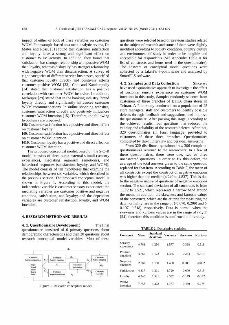
688 A. Torabi et al. / IJE TRANSACTIONS C: Aspects Vol. 34, No. 03, (March 2021) 682-699
impact of either or both of these variables on customer
WOM. For example, based on a meta-analytic review, De
Matos and Rossi [31] found that customer satisfaction
and loyalty have a strong and significant effect on
customer WOM activity. In addition, they found that
satisfaction has stronger relationship with positive WOM
than loyalty, whereas disloyalty has stronger relationship
with negative WOM than dissatisfaction. A survey of
eight categories of different service businesses, specified
that customer loyalty directly and positively affects
customer positive WOM [23]. Choi and Kandampully
[14] stated that customer satisfaction has a positive
correlation with customer WOM behavior. In addition,
Mukerjee [29] stated that in the banking industry, brand
loyalty directly and significantly influences customer
WOM recommendations. In online shopping websites,
customer satisfaction directly and positively influences
customer WOM intention [15]. Therefore, the following
hypotheses are proposed:
H8: Customer satisfaction has a positive and direct effect
on customer loyalty.
H9: Customer satisfaction has a positive and direct effect
on customer WOM intention.
H10: Customer loyalty has a positive and direct effect on
customer WOM intention.
The proposed conceptual model, based on the S-O-R
model, consists of three parts: external stimuli (sensory
experience), mediating organism (emotions), and
behavioral responses (satisfaction, loyalty, and WOM).
The model consists of ten hypotheses that examine the
relationships between six variables, which described in
the previous section. The proposed conceptual model is
shown in Figure 1. According to this model, the
independent variable is customer sensory experience; the
mediating variables are customer positive and negative
emotions, satisfaction, and loyalty; and the dependent
variables are customer satisfaction, loyalty, and WOM
intention.
4. RESEARCH METHOD AND RESULTS
4. 1. Questionnaire Development The final
questionnaire consisted of 6 primary questions about
demographic characteristics and then 30 questions about
research conceptual model variables. Most of these
Figure 1. Research conceptual model
questions were selected based on previous studies related
to the subject of research and some of them were slightly
modified according to society condition, country culture
and environment of study in order to be tangible and
acceptable for respondents (See Appendix Table A for
list of constructs and items used in the questionnaire).
The answers of conceptual model questions were
collected by a Likert’s 7-point scale and analyzed by
SmartPLS software.
4. 2. Samples and Data Collection Since we
have used a quantitative approach to investigate the effect
of customer sensory experience on customer WOM
intention in this study, Samples randomly selected from
customers of three branches of ETKA chain stores in
Tehran. A Pilot study conducted on a population of 25
store managers, staff and customers to identify possible
defects through feedback and suggestions, and improve
the questionnaire. After passing this stage, according to
the achieved results, four questions that reduced the
validity and reliability of the research deleted. After that,
320 questionnaires (in Farsi language) provided to
customers of these three branches. Questionnaires
completed by direct interview and personal answering.
From 320 distributed questionnaires, 306 completed
questionnaires returned to the researchers. In a few of
these questionnaires, there were one, two or three
unanswered questions. In order to fix this defect, the
average of the total answers given to the same question,
replaced for that item. According to Table 2, the mean of
all constructs except the construct of negative emotions
was higher than the median (4.240 to 4.837). This is due
to the negative nature of questions of negative emotions
section. The standard deviation of all constructs is from
1.172 to 1.521, which represents a narrow band around
the mean. In addition, the skewness and kurtosis values
of the constructs, which are the criteria for measuring the
data normality, are in the range of (-0.670, 0.209) and (-
0.197, 0.518), respectively. Data is normal when the
skewness and kurtosis values are in the range of (-1, 1)
[54], therefore this condition is confirmed in this study.
TABLE 2. Descriptive statistics
Construct Mean Standard
deviation Variance Skewness Kurtosis
Sensory experience
4.763 1.250 1.577 -0.368 0.518
Positive emotions
4.765 1.172 1.375 -0.254 0.313
Negative emotions
2.769 1.180 1.400 0.209 -0.082
Satisfaction 4.837 1.311 1.720 -0.670 0.515
Loyalty 4.240 1.521 2.332 -0.179 -0.197
WOM intention
7.758 1.328 1.767 -0.439 0.278

A. Torabi et al. / IJE TRANSACTIONS C: Aspects Vol. 34, No. 03, (March 2021) 682-699 689
Table 3 shows different values for mean, standard
deviation, variance, skewness coefficient and kurtosis.
4. 3. Respondent Profile Among 306
respondents, 65.36% are male and 34.64% are female.
18.95% are single and 81.05% are married.
Approximately the age of 66% are in the range of 30 to
49 years, from the rest of the respondents, approximately
18% are less than 30 years old and 16% are 50 years or
older. In addition, many have a college or university
education (77.78%). It is necessary to mention that
67.32% live in a family of three or four, 16.67% live in a
family of two, 11.67% live in a family of five or six and
TABLE 3. Demographic profile of respondents
Characteristics Range Number %
Gender Male 200 65.36
Female 106 34.64
Age
<18 2 0.65
18-29 53 17.32
30-39 121 39.54
40-49 82 26.80
50-59 31 10.13
>60 17 5.56
Marital status Single 58 18.95
Married 248 81.05
Level of education
Under high school
diploma 9 2.94
High school
diploma 59 19.28
Associate degree 40 13.07
Bachelor of
Science degree 118 38.56
Master of science
degree 64 20.92
Doctor of
Philosophy degree 16 5.23
Number of family
member
1 10 3.27
2 51 16.67
3 or 4 206 67.32
5 or 6 36 11.76
≥7 3 0.98
Family monthly
expenditure
(million tomans)
<2 57 18.63
2-3 109 35.62
3-5 105 34.31
5-7 23 7.52
>7 12 3.92
4.25% live alone or in families with more than six
members. Family monthly expenditure of 18.63% are
under two million tomans, 35.62% are between two and
three million, 34.31% are between three and five million,
7.52% are between five and seven million and the rest are
more than seven million tomans. All demographic
statistics are shown in Table 3.
4. 4. Data Analysis As mentioned earlier,
structural equation modeling approach has been used in
this research. According to Hsu et al. [55], there are two
different approaches to analysis in structural equation
modeling: Covariance-based and variance-based. In this
research, we used partial least squares method, due to the
accuracy and appropriateness of the variance-based
approach in small-scale cases and predictive purposes
[54]. According to Hair et al. [56], partial least square
analysis consists of two parts: measurement model (outer
model) and structural model (inner model). The
measurement model examines the quality of all
constructs for evaluating validity and reliability, and the
structural model examines the relationships between
different model constructs for hypothesis analysis [56].
4. 4. 1. Measurement Model Analysis (Outer Model) According to the model analysis algorithm
in PLS method, two main criteria of reliability and
validity have to examine for outer model evaluation.
Cronbach's alpha, factor loadings, and composite
reliability (CR) are the criteria for measuring reliability.
In addition, average variance extracted (AVE) and
composite reliability calculated as convergent validity
criteria, and the Fornell-Larcker criterion and HTMT
ratio of correlation computed to assess discriminant
validity [57] (Tables 4-6). The version 3.2.6 of SmartPLS
software used to calculate Cronbach's alpha, factor
loadings, and composite reliability. According to
Bagozzi and Yi [58] the factor loading of each indicator
should be greater than 0.5. Based on Table 5, the factor
loadings obtained in this research are above 0.5 (Three
indicators above 0.6 and others above 0.7). The value of
Cronbach’s alpha coefficient can be between 0 and 1 and
how much is closer to 1, shows higher internal
consistency [59]. According to Moazanzadeh and
Hamidi [60], the acceptable value of alpha coefficient in
exploratory research is 0.7 or more. Based on Table 5, the
alpha coefficients obtained in this research are above 0.7.
The third step to assess reliability is to calculate
composite reliability. The minimum accepted value for
composite reliability is 0.7 [61]. Based on Table 5, the
composite reliability of all constructs are higher than 0.7. According to Fornell and Larcker [62], the AVE
value for each construct should be greater than 0.5, in
addition Hamidi and Chavoshi [63] believe that to
confirm convergent validity, the CR value should be
greater than AVE. In this study, the AVE of all structures

690 A. Torabi et al. / IJE TRANSACTIONS C: Aspects Vol. 34, No. 03, (March 2021) 682-699
is greater than 0.5 and the CR of each construct is greater
than the AVE of the same construct. The results of
convergent reliability and validity calculation are shown
in Table 5. Based on these results, it can be concluded
that convergent validity and reliability have been
confirmed.
After examining the convergent validity, we assessed
the discriminant validity using heterotrait-monotrait
(HTMT) ratio of correlation and Fornell-Larcker
criterion. Version 3.2.6 of SmartPLS software has been
used for this purpose. The Fornell-Larcker method
evaluates discriminant validity at the latent variables
TABLE 4. Descriptive, reliability and convergent validity
Construct Indicator F. loading α CR AVE
Sensory
experience
SEV.1 0.817
0.901 0.917 0.503
SEV.2 0.747
SEV.3 0.764
SEA.1 0.667
SEA.2 0.687
SES.1 0.732
SES.2 0.766
SES.3 0.742
SETO.1 0.619
SETO.2 0.657
SETA.1 0.683
Positive
emotions
PE.1 0.865
0.940 0.955 0.808
PE.2 0.926
PE.3 0.936
PE.4 0.889
PE.5 0.877
Negative
emotions
NE.1 0.848
0.941 0.955 0.809
NE.2 0.922
NE.3 0.951
NE.4 0.916
NE.5 0.856
Satisfaction
SA.1 0.913
0.916 0.947 0.855 SA.2 0.929
SA.3 0.933
Loyalty
LO.1 0.925
0.854 0.911 0.774 LO.2 0.776
LO.3 0.930
WOM
intention
WOM.1 0.947
0.958 0.973 0.923 WOM.2 0.970
WOM.3 0.966
level [64]. This method compares the square root of AVE
with the correlation of latent variables and states that the
square root of each construct’s AVE should greater than
the correlations with other latent variables [64]. Based on
Table 5, in this research the square root of each
construct’s AVE is greater than the correlations with
other latent variables. HTMT is able to achieve higher
specificity and sensitivity rates compared to the Fornell-
Larcker [64]. If all ratios in the HTMT matrix are less
than 0.9, the discriminant validity of measurement model
is confirmed. HTMT values close to 1, indicates a lack of
discriminant validity [64]. Based on Table 6, all ratios in
the HTMT matrix are less than 0.9.
4. 4. 2. Structural Model Analysis (Inner Model) The structural model describes the relationship between
latent variables. According to Malekinezhad and Bin
[65], in evaluation of structural model, β (path
coefficient), 𝑅2 (determination coefficient), 𝑓2 (effect
size) and 𝑄2 (predictive relevance) should be calculated.
In this research, all criteria were calculated using version
3.2.6 of SmartPLS software.
Table 7 shows the path coefficients (β) between the
constructs in the conceptual model. The path coefficient
indicates the existence of a relationship, intensity, and
direction of the relationship between two latent variables.
TABLE 5. Discriminant validity, Fornell-Larcker criterion
6 5 4 3 2 1
0.880 Loyalty
0.900 -0.538 Negative
emotions
0.899 -
0.634 0.723
Positive
emotions
0.925 0.777 -
0.610 0.762 Satisfaction
0.709 0.673 0.684 -
0.500 0.651
Sensory
experience
0.961 0.649 0.786 0.738 -
0.880 0.819
WOM
intention
TABLE 6. Discriminant validity, Heterotrait-Monotrait Ratio
6 5 4 3 2 1
Loyalty
0.577 Negative
emotions
0.674 0.790 Positive emotions
0.835 0.655 0.840 Satisfaction
0.719 0.729 0.533 0.721 Sensory
experience
0.683 0.683 0.777 0.620 0.888 WOM intention

A. Torabi et al. / IJE TRANSACTIONS C: Aspects Vol. 34, No. 03, (March 2021) 682-699 691
TABLE 7. Structural model’s hypotheses
NO. Hypothesis Path
coefficient t-value p-value Supported
1 SE->PE 0.684 18.666 0.000 Yes
2 SE->NE -0.500 9.502 0.000 Yes
3 PE->SA 0.502 8.496 0.000 Yes
4 NE->SA -0.169 3.751 0.000 Yes
5 SE->SA 0.245 4.261 0.000 Yes
6 SE->LO 0.252 4.477 0.000 Yes
7 SE->WOM 0.095 2.031 0.043 Yes
8 SA->LO 0.593 10.949 0.000 Yes
9 SA->WOM 0.347 5.307 0.000 Yes
10 LO->WOM 0.492 8.428 0.000 Yes
We used bootstrapping method by version 3.2.6 of
SmartPLS software to analyze path correlations. As
shown in Table 7, all t-statistics pass from ±1.96 and all
p-values are less than 0.05, so according to Zare et al.
[66], all research hypotheses are confirmed.
From the path analysis, it can be stated that the
sensory experience has a direct and positive effect on
customer positive emotions with significant β value of
0.684 (t = 18.666 >1.96, p <0.001), thus the H1
hypothesis is supported. It was also found that the
sensory experience has a direct and negative effect on
customer negative emotions with significant β value of -
0.500 (t = 9.502 >1.96, p <0.001), thus the H2 hypothesis
is supported. Customer positive emotions have a direct
and positive effect on customer satisfaction with
significant β value of 0.502 (t = 8.496 >1.96, p <0.001)
and customer negative emotions have a direct and
negative effect on customer satisfaction with significant
β value of -0.196 (t = 3.751 >1.96, p <0.001), thus the H3
and H4 hypotheses are supported. From the results it can
be deduced that the sensory experience has a direct and
positive effect on customer satisfaction with significant β
value of 0.254 (t = 4.261 >1.96, p <0.001), hence H5
hypothesis is supported. In addition, this construct has
direct and positive effect on customer loyalty and
customer WOM intention with significant β value of
0.252 (t = 4.477 >1.96, p <0.001) and 0.095 (t = 2.031
>1.96, p <0.05), respectively, thus the H6 and H7
hypotheses are supported. Moreover, it was specified that
customer satisfaction has direct and positive effect on
customer loyalty and customer WOM intention with
significant β value of 0.593 (t = 10.949 >1.96, p <0.001)
and 0.347 (t = 5.307 >1.96, p <0.001), respectively, thus
the H8 and H9 hypotheses are supported. In addition, It
can be deduced from the results that customer loyalty has
a direct and positive effect on customer WOM intention
with significant β value of 0.492 (t = 8.428 >1.96, p
<0.001), thus the H10 hypothesis is supported.
The 𝑅2 value is a criterion used to connect the
measurement and structural components of structural
equation modeling and indicates the influence of an
independent variable on a dependent variable. The value
of 𝑅2 is between 0 and 1, and the higher the 𝑅2, the better
the independent variable predicts for the dependent
variable [67]. The values of 0.75, 0.5 and 0.25 for 𝑅2
indicate respectively that the model is substantial,
moderate and weak [67]. In addition, the values of 𝑅2
larger than 0.35 represent a substantial model. According
to Figure 2, the model is approximately substantial.
After evaluating hypotheses, the effect of each
independent variable on dependent variables should be
calculated. We can measure the of an independent
variable on a dependent variable by 𝑓2 criterion [67]. The
values of 0.02, 0.15 and 0.35, indicate small, medium and
large effect size. According to Table 8, there are three
variables with medium effect size and three variables
with large effect size in model.
𝑄2 criterion indicates the predictive relationships of
model. We calculated 𝑄2 by blindfolding process of
SmartPLS. If the value of 𝑄2 is greater than zero, the
dependent variable has predictive relevance [56].
According to Hair et al. [56], the three values of 0.02,
0.15 and 0.35 are considered as low, medium and high
predictive relevance. As shown in Table 9, all predictive
relationships are high except one, that is medium.
Figure 2. Obtained values of β and 𝑹𝟐 through SmartPLS
TABLE 8. Effect size of independent variables
6 5 4 3 2 1
0.354 Loyalty
0.049 Negative emotions
0.308 Positive emotions
0.167 0.501 Satisfaction
0.017 0.092 0.879 0.333 0.091 Sensory experience
WOM intention

692 A. Torabi et al. / IJE TRANSACTIONS C: Aspects Vol. 34, No. 03, (March 2021) 682-699
TABLE 9. Indicator of model’s predictive relevance
𝑸𝟐 Dependent variable
0.352 Positive emotions
0.187 Negative emotions
0.528 Satisfaction
0.445 Loyalty
0.641 WOM intention
4. 4. 3. Mediating Effect Analysis The indirect effect is examined in paths that exist one or more
mediator variables. In the following, the effect of positive
emotions, negative emotions, and loyalty as partial
mediator variables are examined. According to Baron
and Kenny [68] the existence of a partial mediator
variable is confirmed: if the total effect is significant (The
sum of direct and indirect effects), the indirect effect is
significant (from independent variable to mediator and
from mediator to dependent variable), and the direct
effect is significantly less than the total effect. We used regression analysis to examine how
customer sensory experience affects customer
satisfaction through two mediator variables of customer
positive and negative emotions and how customer
satisfaction affects customer WOM intention through
customer loyalty as a mediator variable. According to
Baron and Kenny [68] and as shown in Table 10, the
existence of three partial mediator variables: customer
positive emotions, customer negative emotions and
TABLE 10. verification of mediators
NO. Hypothesis Path
coefficient
Standard
deviation t-value p-value
Sensory experience->Positive emotion->Satisfaction
1* SE->SA 0.676 0.031 21.543 0.000
2 SE->PE 0.685 0.034 20.016 0.000
3 PE->SA 0.590 0.050 11.708 0.000
4** SE->SA 0.272 0.055 4.912 0.000
Sensory experience->Negative emotion->Satisfaction
1* SE->SA 0.678 0.032 21.363 0.000
2 SE->NE -0.503 0.050 10.085 0.000
3 NE->SA -0.359 0.048 7.473 0.000
4** SE->SA 0.497 0.048 10.424 0.000
Satisfaction->Loyalty->WOM
1* SA->WOM 0.787 0.028 28.508 0.000
2 SA->LO 0.764 0.026 29.599 0.000
3 LO->WOM 0.524 0.055 9.555 0.000
4** SA->WOM 0.387 0.061 6.344 0.000
*Total effect, **Direct effect
customer loyalty confirmed. Thus, it is clarified that
sensory experience has indirect effect on customer
satisfaction through customer positive and negative
emotions, and customer satisfaction has an indirect effect
on customer WOM intention through customer loyalty. It
can be deducted that positive sensory experience promote
positive emotions and relieve negative emotions, leading
to customer satisfaction. Moreover, it can be deducted
that satisfaction strengthens customer WOM intention
through customer loyalty. Therefore, sensory experience
is a strong and critical antecedent of three customer
behavioral responses, especially customer WOM, and
focus on this aspect can help retail businesses owner to
improve his/her business.
4. 4. 4. Effect of Five Types of Customer Sensory Experiences on Customer Emotions According
to Chen and Lin [6], we used regression analysis to
examine the effect of five types of customer sensory
experiences on customer positive and negative emotions.
Each of these effects will discuss below.
4. 4. 4. 1. Effect on Customer Positive Emotions In this regression analysis, sensory experiences have
been considered as independent variables and positive
emotions as dependent variable. As shown in Table 11,
all VIF values are less than 2.5, indicating no notable
collinearity in the regression model. The regression
model is highly significant with the determination
coefficient of 52.7%. According to Table 11, the greatest
effect of sensory experience on customer positive
emotions is taste experience, and subsequently touch,
sight, and sound experiences, respectively. It should be
noted that the effect of smell experience on positive
emotions is not significant.
4. 4. 4. 2. Effect on Customer Negative Emotions Similarly, we considered sensory experiences as
independent variables and positive emotions as
dependent variable. As shown in Table 12, all VIF values
are less than 2.5, indicating no notable collinearity in the
regression model. The regression model is highly
significant with the determination coefficient of 29.6%.
According to Table 12, only the effect of touch and taste
TABLE 11. regression analysis of five types of sensory
experience on positive emotions
Sensory
experience β t-value p-value 𝑹𝟐 VIF
Sight 0.134 2.053 0.041
0.527
1.998
Sound 0.134 2.058 0.038 2.360
Smell 0.062 0.942 0.347 2.453
Touch 0.193 3.600 0.000 1.798
Taste 0.386 7.019 0.000 1.542

A. Torabi et al. / IJE TRANSACTIONS C: Aspects Vol. 34, No. 03, (March 2021) 682-699 693
TABLE 12. regression analysis of five types of sensory
experience on negative emotions
Sensory
experience β t-value p-value 𝑹𝟐 VIF
Sight -0.041 0.579 0.563
0.296
1.979
Sound -0.114 1.328 0.185 2.337
Smell -0.023 0.245 0.806 2.449
Touch -0.248 3.874 0.000 1.765
Taste -0.251 3.814 0.000 1.547
experiences on customer negative emotions are
significant, while the effect of taste on customer negative
emotions is slightly greater than the effect of touch
experience.
5. DISCUSSION AND CONCLUSIONS
As mentioned earlier, the purpose of this study is to
examine the effect of sensory experience on customer
WOM intention in retail chain stores. Structural equation
modeling (SEM) and questionnaire have been used to
achieve this purpose. Version 3.2.6 of SmartPLS
software used to test the hypotheses and calculate path
coefficients. We describe the research findings below,
and then the results related to the effect of sensory
experience on customer emotions in the retail chain
stores is compared with similar results obtained in the
chain coffeehouses by Chen and Lin [6]. In the last part,
the conclusions of this research will be express.
5. 1. Findings Related to Customer Sensory Experience According to the path analysis
carried out in section four of the paper, hypothesis 1 (SE-
> PE) and hypothesis 2 (SE-> NE) are confirmed, which
indicates that, sensory experience in the retail chain
stores directly and significantly affects customer positive
and negative emotions. These results are supported by the
results of Chen and Lin [6] in coffeehouses, and Liu and
Jang [18] in restaurant environments. According to the
path analysis, hypothesis 5 (SE-> SA) is confirmed,
which shows the direct and positive effect of customer
sensory experience on customer satisfaction. This result
is supported by the results of Iglesias et al. [10] in
banking industry and Thuan et al. [2] in supermarket
environments. In addition, it was found that sensory
experience indirectly affects customer satisfaction
through partial mediators of customer positive emotions
and customer negative emotions. According to Variance
Accounted For (VAF) proposed by Zhao et al. [69], and
path coefficients, over 51% (0.684×0.502/0.673) of the
total effect of sensory experience on customer
satisfaction is transmitted through customer positive
emotions, and approximately 13% (-0.500×-0.169/0.673)
of the total effect of sensory experience on customer
satisfaction is transmitted through customer negative
emotions (so approximately 64% of the total effect is
transmitted through customer emotions), and the rest of
the total effect is transmitted directly. Finally based on
the path coefficients and VAF, it can be concluded that
customer positive emotions mediator is better than
customer negative emotions mediator, and the major
effect of customer sensory experience on customer
satisfaction is transmitted indirectly through customer
positive emotions. The path analysis also shows that
hypothesis 6 (SE-> LO) and hypothesis 7 (SE-> WOM)
are confirmed, that reflect the direct and positive effect
of customer sensory experience on customer loyalty and
customer WOM intention. Due to the calculated path
coefficients, it can be stated that, the direct effect of
sensory experience on customer loyalty is considerable,
but the direct effect of sensory experience on customer
WOM intention is not very considerable, and much of the
total effect (with coefficient of 0.649) is transmitted
indirectly through available mediators on the path, such
as emotions, satisfaction and loyalty. According to VAF
and path coefficients, it can be concluded that
approximately 85.5% of the total effect of sensory
experience on customer WOM intention is transmitted
indirectly, that is described separately below:
• 18.5% of the total effect is transmitted through the
path of sensory experience-> positive emotions->
satisfaction-> WOM (0.684×0.502×0.347/0.649).
• 15.5% of the total effect is transmitted through the
path of sensory experience-> positive emotions->
satisfaction-> loyalty-> WOM intention
(0.684×0.502×0.593×0.492/0.649).
• 4.5% of the total effect is transmitted through the path
of sensory experience-> negative emotions->
satisfaction-> WOM intention (-0.500×-
0.169×0.347/0.649).
• 4% of the total effect is transmitted through the path
of sensory experience-> negative emotions->
satisfaction-> loyalty-> WOM intention (-0.500×-
0.169×0.593×0.492/0.649).
• 13% of the total effect, is transmitted through the path
of sensory experience-> satisfaction-> WOM
intention (0.245×0.347/0.649).
• 11% of the total effect is transmitted through the path
of sensory experience-> satisfaction-> loyalty->
WOM intention (0.245×0.593×0.492/0.649).
• 19% of the total effect is transmitted through the path
of sensory experience-> loyalty-> WOM intention
(0.252×0.492/0.649).
5. 2. Findings Related to Customer Satisfaction, Loyalty and WOM Intention According to the
path analysis carried out in section four, Hypothesis 8
(satisfaction-> loyalty) and Hypothesis 9 (satisfaction->
WOM intention) are confirmed, which indicates that

694 A. Torabi et al. / IJE TRANSACTIONS C: Aspects Vol. 34, No. 03, (March 2021) 682-699
customer satisfaction in the retail chain stores directly
and positively affects customer loyalty and WOM
intention. The positive effect of customer satisfaction on
customer loyalty is similar to the results of Choi et al. [3],
Baser et al. [4], Brakus et al. [7], Han et al. [16], Richard
and Zhang [40], LV et al. [46], and Gong and Yi [53] in
different businesses. In addition, the positive effect of
customer satisfaction on customer WOM intention is
similar to the results of Choi and Kandampully [14], Ha
and Im [15]], and De Matos and Rossi [31]. Based on the
calculated path coefficients, it can be concluded that both
effects are significant, but the direct effect of customer
satisfaction on customer loyalty is greater than the direct
effect of customer satisfaction on customer WOM
intention, which is justified by considering the mediating
role of customer loyalty in the indirect effect of customer
satisfaction on customer WOM intention. In addition,
according to the path analysis Hypothesis 10 (loyalty->
WOM intention) is confirmed, indicating a direct and
positive effect of customer loyalty on customer WOM
intention. This result is supported by the results of
Markovic et al. [23], Mukerjee [29], and De Matos and
Rossi [31]. Based on the results, it can be inferred that
customer loyalty is a partial mediator in the relationship
between customer satisfaction and customer WOM
intention; according to the concept of VAF, it can be
concluded that approximately 46% (0.593×0.492/0.639)
of the total effect of customer satisfaction on customer
WOM intention is transmitted through the customer
loyalty. In general, it can be stated that satisfaction affects
customer loyalty and this loyalty will lead to customer
WOM intention.
5. 3. Comparison of The Effect of Sensory Experiences on Customer Emotions in Two Different Environments In this section, we
compare the regression analysis performed in this study
with the similar regression analysis performed by Chen
and Lin [6]. According to Table 13, in this study, all VIF
values (variance inflation factor) are less than 2.5, which
is similar to study of Chen and Lin [6]. In addition, the
value of 𝑅2 obtained in both studies are approximately
equal. Based on the results of this analysis, and similar to
study of Chen and Lin [6], the effect of smell experience
on positive emotions is not significant but the effects of
the other four senses on positive emotions are significant.
In both studies, taste experience has the most effect on
positive emotions, but unlike result of Chen and Lin [6],
touch experience has more effect on positive emotion
than the other two senses. In addition, it is specified that
in this study, the effects of sight and sound experiences
on positive emotions are approximately equal, that is not
the case in Chen and Lin [6]. The differences in the effect
of five type of sensory experiences on positive emotions
between two different environments of retail chain stores
and chain coffeehouses are shown in Table 13.
TABLE 13. Comparison of two different environments (PE)
Proposed model
Sensory experience β t-value 𝑹𝟐 VIF
Sight 0.134 2.053*
0.527
1.998
Sound 0.134 2.058* 2.360
Smell 0.062 0.942 2.453
Touch 0.193 3.600*** 1.798
Taste 0.386 7.019*** 1.542
Chen and Lin [6] model
Sensory experience β t-value 𝑹𝟐 VIF
Sight 0.284 6.798***
0.524
2.065
Sound 0.134 3.494** 1.741
Smell 0.055 1.390 1.846
Touch 0.111 2.566* 2.212
Taste 0.298 7.469*** 1.887
Significance levels: *p<0.05, **p<0.01, ***p<0.001
Similar to the analysis performed in the positive
emotions section, in the negative emotions section, all
VIF values are less than 2.5, which is similar to the result
obtained in Chen and Lin [6] (See Table 14). In this
study, the effects of taste and touch experiences on
negative emotions are significant and approximately
equal, but in the research of Chen and Lin [6], only the
effect of sight experience on negative emotions is
significant. In addition, the regression analysis performed
in this study revealed that the 𝑅2 value of customer
negative emotions is approximately three times the 𝑅2
value of customer negative emotions in the regression
analysis performed by Chen and Lin [6].
Regression analysis suggests that among the five
senses related to the customer sensory experience, the
sense of taste has the most effect on positive emotions.
After that, touch has the most effect on positive emotions.
Sight and sound are the next. From these results, it can be
inferred that the taste and quality of food products sold in
retail chain stores have the greatest effect on positive
emotions. Moreover, the feature that customers in the
retail chain stores can touch goods before buying, as well
as the condition of ventilation and temperature of the
store have the greatest effect on the positive emotions
after taste and quality of food products. Sight experience
that affects the sense of vision, such as the lighting,
cleanliness of the store and the layout of products, and
sound experience that affects the sense of auditory, such
as music playing or annoying sounds in the store, have
less effect on positive emotions than taste and touch
experiences. In addition, according to regression
analysis, it can be stated that like positive emotions, the

A. Torabi et al. / IJE TRANSACTIONS C: Aspects Vol. 34, No. 03, (March 2021) 682-699 695
TABLE 14. Comparison of two different environments (NE)
Proposed model
Sensory experience β t-value 𝑹𝟐 VIF
Sight -0.041 0.579
0.296
1.979
Sound -0.114 1.328 2.337
Smell -0.023 0.245 2.449
Touch -0.248 3.874*** 1.765
Taste -0.251 3.814*** 1.547
Chen and Lin [6] model
Sensory experience β t-value 𝑹𝟐 VIF
Sight -0.269 -4.703***
0.106
2.065
Sound 0.009 0.180 1.741
Smell -0.069 -1.281 1.846
Touch 0.039 0.662 2.212
Taste 0.066 -1.215 1.887
Significance levels: *p<0.05, **p<0.01, ***p<0.001
sense of taste has the most effect on negative emotions
and the sense of touch is next. It means that the good taste
and high quality of food products will reduce the negative
emotions more than desirable touch of goods before
buying or favorable temperature and ventilation of the
store.
6. CONCLUSIONS In this research, it is concluded that among the three
constructs related to customer behavioral responses
namely satisfaction, loyalty, and WOM intention;
customer satisfaction acts as a strong predictor of
customer loyalty and customer WOM intention. In
addition, due to the indirect effect of customer sensory
experience on customer satisfaction through partial
mediators of customer positive and negative emotions, it
can be concluded that sensory experience as an external
stimulus, affects customer satisfaction as a behavioral
response and predictor of two other behavioral responses
(loyalty and WOM). Moreover, according to the research
findings, it can be concluded that taste and touch
experiences have the most effect on customer positive
and negative emotions respectively. Smell does not affect
either positive or negative emotions, in addition, sight
and sound do not affect negative emotions. In general, it
can be concluded that engaging five senses of customers
as a sensory marketing strategy can affect customer
emotions, and consequently, based on the proposed
model it can be used as a way to develop customer loyalty
programs in retail chain stores and subsequently create
positive WOM.
7. LIMITATIONS AND FUTURE RESEARCH
Usually in any research, obstacles and limitations placed
on the way to the researchers. This research is not an
exception, so the limitations of the research will discuss:
• One of the limitations is the community under study.
The focus of this research was on customers of three
branches of a retail chain store in Tehran. So due to
the differences in culture, attitude, shopping behavior,
etc. of the customers under study, compared to the
customers of other retail chain stores or even
customers of other branches of this store, different
results may be obtained. Thus, future research could
explore this topic in other retail chain stores.
• The inherent limitations of questionnaire, such as
superficial attitude to the actual events and scalability
of the responses, could prevent the results from being
real. In addition, respondents may answer questions
with their own understanding. Because of this issue,
newer methods of data collection, such as
neuromarketing could be used in future research.
Moreover, the total questionnaires distributed for data
collection was 320 copies, out of which 306 analyzed.
Naturally, increasing the number of questionnaires
and consequently increasing the available data can
increase the consistency and validity of the results.
• It should note that the present study used only the
opinions of customers and did not use the views of
business owners and marketers, therefore in future
research, researchers can collect other views and
compare these results with customer opinions. In
addition, it should not overlooked that the moderator
variable not used in this study. In general, using
moderator variables could provide more
comprehensive and accurate results.
• Variables affecting WOM intention include a wide
range, that in this study, we sought to investigate the
effect of sensory experience on this variable. Future
research can examine the effect of other independent
variables such as service quality, price, technological
facilities, etc., along with sensory experience, and
compare these effects with each other.
8. REFERENCES
1. Terblanche, N. S., "Revisiting the supermarket in-store customer shopping experience", Journal of Retailing and Consumer
Services, Vol. 40, (2018), 48–59.
doi:10.1016/j.jretconser.2017.09.004
2. Luu Tien Thuan, Nguyen Huynh Bao Ngoc, and Nguyen Thu Nha
Trang, "Does Customer Experience Management Impact
Customer Loyalty Shopping at Supermarket? The Case in the Mekong Delta, Vietnam", Economics World, Vol. 6, No. 1,
(2017), 13–21. doi:10.17265/2328-7144/2018.01.002
3. Choi, Y. G., Ok, C. “Michael”, and Hyun, S. S., "Relationships between brand experiences, personality traits, prestige,

696 A. Torabi et al. / IJE TRANSACTIONS C: Aspects Vol. 34, No. 03, (March 2021) 682-699
relationship quality, and loyalty", International Journal of
Contemporary Hospitality Management, Vol. 29, No. 4, (2017),
1185–1202. doi:10.1108/IJCHM-11-2014-0601
4. Başer, İ. U., Cintamür, İ. G., and Arslan, F. M., "Examining the effect of brand experience on consumer satisfaction, brand trust
and brand loyalty", Marmara University Journal of Economic &
Administrative Sciences, Vol. 37, No. 2, (2016), 101–128.
doi:10.14780/iibd.51125
5. Kim, J. W., Lee, F., and Suh, Y. G., "Satisfaction and Loyalty
From Shopping Mall Experience and Brand Personality", Services Marketing Quarterly, Vol. 36, No. 1, (2015), 62–76.
doi:10.1080/15332969.2015.976523
6. Chen, H.-T., and Lin, Y.-T., "A study of the relationships among
sensory experience, emotion, and buying behavior in coffeehouse
chains", Service Business, Vol. 12, No. 3, (2018), 551–573.
doi:10.1007/s11628-017-0354-5
7. Brakus, J. J., Schmitt, B. H., and Zarantonello, L., "Brand
Experience: What is It? How is it Measured? Does it Affect Loyalty?", Journal of Marketing, Vol. 73, No. 3, (2009), 52–68.
doi:10.1509/jmkg.73.3.052
8. Hultén, B., "Sensory marketing: the multi‐sensory brand‐experience concept", European Business Review, Vol. 23, No. 3,
(2011), 256–273. doi:10.1108/09555341111130245
9. Krishna, A., "An integrative review of sensory marketing:
Engaging the senses to affect perception, judgment and behavior",
Journal of Consumer Psychology, Vol. 22, No. 3, (2012), 332–
351. doi:10.1016/j.jcps.2011.08.003
10. Iglesias, O., Markovic, S., and Rialp, J., "How does sensory brand
experience influence brand equity? Considering the roles of customer satisfaction, customer affective commitment, and
employee empathy", Journal of Business Research, Vol. 96,
(2019), 343–354. doi:10.1016/j.jbusres.2018.05.043
11. Yoganathan, V., Osburg, V.-S., and Akhtar, P., "Sensory
stimulation for sensible consumption: Multisensory marketing for
e-tailing of ethical brands", Journal of Business Research, Vol.
96, (2019), 386–396. doi:10.1016/j.jbusres.2018.06.005
12. Moreira, A. C., Fortes, N., and Santiago, R., "Influence of sensory
stimuli on brand experience, brand equity and purchase intention", Journal of Business Economics and Management,
Vol. 18, No. 1, (2017), 68–83.
doi:10.3846/16111699.2016.1252793
13. Mehrabian, A., and Russell, J. A., "The Basic Emotional Impact
of Environments", Perceptual and Motor Skills, Vol. 38, No. 1,
(1974), 283–301. doi:10.2466/pms.1974.38.1.283
14. Choi, H., and Kandampully, J., "The effect of atmosphere on
customer engagement in upscale hotels: An application of S-O-R paradigm", International Journal of Hospitality Management,
Vol. 77, (2019), 40–50. doi:10.1016/j.ijhm.2018.06.012
15. Ha, Y., and Im, H., "Role of web site design quality in satisfaction and word of mouth generation", Journal of Service Management,
Vol. 23, No. 1, (2012), 79–96. doi:10.1108/09564231211208989
16. Han, H., Nguyen, H. N., Song, H., Chua, B.-L., Lee, S., and Kim,
W., "Drivers of brand loyalty in the chain coffee shop industry",
International Journal of Hospitality Management, Vol. 72,
(2018), 86–97. doi:10.1016/j.ijhm.2017.12.011
17. Jang, S. (Shawn), and Namkung, Y., "Perceived quality,
emotions, and behavioral intentions: Application of an extended
Mehrabian–Russell model to restaurants", Journal of Business
Research, Vol. 62, No. 4, (2009), 451–460.
doi:10.1016/j.jbusres.2008.01.038
18. Liu, Y., and Jang, S. (Shawn), "The effects of dining atmospherics: An extended Mehrabian–Russell model",
International Journal of Hospitality Management, Vol. 28, No.
4, (2009), 494–503. doi:10.1016/j.ijhm.2009.01.002
19. Kim, W. G., and Moon, Y. J., "Customers’ cognitive, emotional,
and actionable response to the servicescape: A test of the moderating effect of the restaurant type", International Journal
of Hospitality Management, Vol. 28, No. 1, (2009), 144–156.
doi:10.1016/j.ijhm.2008.06.010
20. Lindstrom, M., "Broad sensory branding", Journal of Product &
Brand Management, Vol. 14, No. 2, (2005), 84–87.
doi:10.1108/10610420510592554
21. Ong, C. H., Lee, H. W., and Ramayah, T., "Impact of brand
experience on loyalty", Journal of Hospitality Marketing &
Management, Vol. 27, No. 7, (2018), 755–774.
doi:10.1080/19368623.2018.1445055
22. Hultén, B., Broweus, N., and van Dijk, M., "What is Sensory Marketing?", Sensory Marketing, London, Palgrave Macmillan
UK., (2009), 1–23 doi:10.1057/9780230237049_1
23. Markovic, S., Iglesias, O., Singh, J. J., and Sierra, V., "How does the Perceived Ethicality of Corporate Services Brands Influence
Loyalty and Positive Word-of-Mouth? Analyzing the Roles of
Empathy, Affective Commitment, and Perceived Quality", Journal of Business Ethics, Vol. 148, No. 4, (2018), 721–740.
doi:10.1007/s10551-015-2985-6
24. Arndt, J., "Role of Product-Related Conversations in the Diffusion of a New Product", Journal of Marketing Research,
Vol. 4, No. 3, (1967), 291–295.
doi:10.1177/002224376700400308
25. Gupta, P., and Harris, J., "How e-WOM recommendations
influence product consideration and quality of choice: A
motivation to process information perspective", Journal of
Business Research, Vol. 63, Nos. 9–10, (2010), 1041–1049.
doi:10.1016/j.jbusres.2009.01.015
26. Kim, Y., Chang, Y., Wong, S. F., and Park, M. C., "Customer attribution of service failure and its impact in social commerce
environment", International Journal of Electronic Customer
Relationship Management, Vol. 8, No. 1/2/3, (2014), 136.
doi:10.1504/IJECRM.2014.066890
27. Kumar, V., Aksoy, L., Donkers, B., Venkatesan, R., Wiesel, T.,
and Tillmanns, S., "Undervalued or Overvalued Customers: Capturing Total Customer Engagement Value", Journal of
Service Research, Vol. 13, No. 3, (2010), 297–310.
doi:10.1177/1094670510375602
28. Phillips, W. J., Wolfe, K., Hodur, N., and Leistritz, F. L., "Tourist
Word of Mouth and Revisit Intentions to Rural Tourism
Destinations: a Case of North Dakota, USA", International
Journal of Tourism Research, Vol. 15, No. 1, (2013), 93–104.
doi:10.1002/jtr.879
29. Mukerjee, K., "The impact of brand experience, service quality and perceived value on word of mouth of retail bank customers:
investigating the mediating effect of loyalty", Journal of
Financial Services Marketing, Vol. 23, No. 1, (2018), 12–24.
doi:10.1057/s41264-018-0039-8
30. Alhulail, H., Dick, M., and Abareshi, A., "The Influence of Word
of Mouth on Customer Loyalty to Social Commerce Websites: Trust as a Mediator", (2019), 1025–1033. doi:10.1007/978-3-319-
99007-1_95
31. de Matos, C. A., and Rossi, C. A. V., "Word-of-mouth communications in marketing: a meta-analytic review of the
antecedents and moderators", Journal of the Academy of
Marketing Science, Vol. 36, No. 4, (2008), 578–596.
doi:10.1007/s11747-008-0121-1
32. Ding, C. G., and Tseng, T. H., "On the relationships among brand
experience, hedonic emotions, and brand equity", European
Journal of Marketing, Vol. 49, No. 7/8, (2015), 994–1015.
doi:10.1108/EJM-04-2013-0200
33. Barsky, J., and Nash, L., "Evoking Emotion: Affective Keys to Hotel Loyalty", The Cornell Hotel and Restaurant
Administration Quarterly, Vol. 43, No. 1, (2002), 39–46.
doi:10.1177/0010880402431004

A. Torabi et al. / IJE TRANSACTIONS C: Aspects Vol. 34, No. 03, (March 2021) 682-699 697
34. Lin, J. C., and Liang, H., "The influence of service environments on customer emotion and service outcomes", Managing Service
Quality: An International Journal, Vol. 21, No. 4, (2011), 350–
372. doi:10.1108/09604521111146243
35. Barger, P. B., and Grandey, A. A., "Service with A Smile and
Encounter Satisfaction: Emotional Contagion and Appraisal
Mechanisms", Academy of Management Journal, Vol. 49, No.
6, (2006), 1229–1238. doi:10.5465/amj.2006.23478695
36. Russell, J. A., and Pratt, G., "A description of the affective quality
attributed to environments.", Journal of Personality and Social
Psychology, Vol. 38, No. 2, (1980), 311–322. doi:10.1037/0022-
3514.38.2.311
37. Plutchik, R., "A general psychoevolutionary theory of emotion",
In Theories of Emotion, Academic press, Elsevier, (1980), 3–33
doi:10.1016/B978-0-12-558701-3.50007-7
38. Izard, C. E., "Differential Emotions Theory", In Human
Emotions, Boston, MA, Springer US, (1977), 43–66.
doi:10.1007/978-1-4899-2209-0_3
39. Yeh, T.-M., Chen, S.-H., and Chen, T.-F., "The Relationships
among Experiential Marketing, Service Innovation, and Customer
Satisfaction—A Case Study of Tourism Factories in Taiwan", Sustainability, Vol. 11, No. 4, (2019), 1041.
doi:10.3390/su11041041
40. Richard, J. E., and Zhang, A., "Corporate image, loyalty, and commitment in the consumer travel industry", Journal of
Marketing Management, Vol. 28, Nos. 5–6, (2012), 568–593.
doi:10.1080/0267257X.2010.549195
41. Wikhamn, W., "Innovation, sustainable HRM and customer
satisfaction", International Journal of Hospitality Management,
Vol. 76, (2019), 102–110. doi:10.1016/j.ijhm.2018.04.009
42. Lee, Y.-C., Wang, Y.-C., Lu, S.-C., Hsieh, Y.-F., Chien, C.-H.,
Tsai, S.-B., and Dong, W., "An empirical research on customer
satisfaction study: a consideration of different levels of performance", SpringerPlus, Vol. 5, No. 1, (2016), 1–9.
doi:10.1186/s40064-016-3208-z
43. Ganesan, S., "Determinants of Long-Term Orientation in Buyer-Seller Relationships", Journal of Marketing, Vol. 58, No. 2,
(1994), 1–19. doi:10.1177/002224299405800201
44. Sirdeshmukh, D., Singh, J., and Sabol, B., "Consumer Trust, Value, and Loyalty in Relational Exchanges", Journal of
Marketing, Vol. 66, No. 1, (2002), 15–37.
doi:10.1509/jmkg.66.1.15.18449
45. Oliver, R. L., "Whence Consumer Loyalty?", Journal of
Marketing, Vol. 63, No. 4_suppl1, (1999), 33–44.
doi:10.1177/00222429990634s105
46. Lv, H., Yu, G., and Wu, G., "Relationships among customer
loyalty, customer satisfaction, corporate image and behavioural
intention on social media for a corporation", International
Journal of Information Technology and Management, Vol. 17,
No. 3, (2018), 170–183. doi:10.1504/IJITM.2018.092879
47. Fullerton, G., "When Does Commitment Lead to Loyalty?", Journal of Service Research, Vol. 5, No. 4, (2003), 333–344.
doi:10.1177/1094670503005004005
48. Yi, Y., and La, S., "What influences the relationship between customer satisfaction and repurchase intention? Investigating the
effects of adjusted expectations and customer loyalty",
Psychology and Marketing, Vol. 21, No. 5, (2004), 351–373.
doi:10.1002/mar.20009
49. Sahin, A., Zehir, C., and Kitapçı, H., "The Effects of Brand
Experiences, Trust and Satisfaction on Building Brand Loyalty; An Empirical Research On Global Brands", Procedia - Social and
Behavioral Sciences, Vol. 24, (2011), 1288–1301.
doi:10.1016/j.sbspro.2011.09.143
50. Iglesias, O., Singh, J. J., and Batista-Foguet, J. M., "The role of
brand experience and affective commitment in determining brand
loyalty", Journal of Brand Management, Vol. 18, No. 8, (2011),
570–582. doi:10.1057/bm.2010.58
51. Khaleghimoghaddam, N., and Bala, H. A., "The Impact of
Environmental and Archıtectural Design on Users’ Affective
Experience", YBL Journal of Built Environment, Vol. 6, No. 1, (2018), 5–19. doi:10.2478/jbe-2018-0001
52. Murray, J., Elms, J., and Teller, C., "Examining the role of store
design on consumers’ cross-sectional perceptions of retail brand loyalty", Journal of Retailing and Consumer Services, Vol. 38, (2017), 147–156. doi:10.1016/j.jretconser.2017.06.001
53. Gong, T., and Yi, Y., "The effect of service quality on customer
satisfaction, loyalty, and happiness in five Asian countries", Psychology & Marketing, Vol. 35, No. 6, (2018), 427–442. doi:10.1002/mar.21096
54. Chavoshi, A., and Hamidi, H., "Social, individual, technological
and pedagogical factors influencing mobile learning acceptance
in higher education: A case from Iran", Telematics and
Informatics, Vol. 38, (2019), 133–165. doi:10.1016/j.tele.2018.09.007
55. Hsu, S.-H., Chen, W., and Hsieh, M., "Robustness testing of PLS,
LISREL, EQS and ANN-based SEM for measuring customer
satisfaction", Total Quality Management & Business
Excellence, Vol. 17, No. 3, (2006), 355–372. doi:10.1080/14783360500451465
56. F. Hair Jr, J., Sarstedt, M., Hopkins, L., and G. Kuppelwieser, V.,
"Partial least squares structural equation modeling (PLS-SEM)",
European Business Review, Vol. 26, No. 2, (2014), 106–121. doi:10.1108/EBR-10-2013-0128
57. Japutra, A., and Molinillo, S., "Responsible and active brand personality: On the relationships with brand experience and key
relationship constructs", Journal of Business Research, Vol. 99, (2019), 464–471. doi:10.1016/j.jbusres.2017.08.027
58. Bagozzi, R. P., and Yi, Y., "On the evaluation of structural
equation models", Journal of the Academy of Marketing
Science, Vol. 16, No. 1, (1988), 74–94. doi:10.1007/BF02723327
59. Cronbach, L. J., "Coefficient alpha and the internal structure of tests", Psychometrika, Vol. 16, No. 3, (1951), 297–334. doi:10.1007/BF02310555
60. Moazenzadeha, D., and Hamidi, H., "Analysis and Development
of Technology Acceptance Model in Mobile Bank Field",
International Journal of Engineering, Transactions C: Aspects, Vol. 31, No. 9, (2018), 1521–1528. doi:10.5829/ije.2018.31.09c.07
61. Mohammadi, A., "Analyzing Tools and Algorithms for Privacy
Protection and Data Security in Social Networks", International
Journal of Engineering, Transaction B: Applications, Vol. 31, No. 8, (2018), 1267–1273. doi:10.5829/ije.2018.31.08b.15
62. Fornell, C., and Larcker, D. F., "Evaluating Structural Equation Models with Unobservable Variables and Measurement Error",
Journal of Marketing Research, Vol. 18, No. 1, (1981), 39–50. doi:10.1177/002224378101800104
63. Hamidi, H., and Chavoshi, A., "Analysis of the essential factors
for the adoption of mobile learning in higher education: A case study of students of the University of Technology", Telematics
and Informatics, Vol. 35, No. 4, (2018), 1053–1070. doi:10.1016/j.tele.2017.09.016
64. Ab Hamid, M. R., Sami, W., and Mohmad Sidek, M. H.,
"Discriminant Validity Assessment: Use of Fornell & Larcker criterion versus HTMT Criterion", Journal of Physics:
Conference Series, Vol. 890, (2017), 012163. doi:10.1088/1742-6596/890/1/012163
65. Malekinezhad, F., and Lamit, B., "Investigation into University
Students Restoration Experience: The Effects of Perceived Sensory Dimension and Perceived Restorativeness", Preprints,
(2017). doi:10.20944/preprints201708.0085.v1

698 A. Torabi et al. / IJE TRANSACTIONS C: Aspects Vol. 34, No. 03, (March 2021) 682-699
66. Zare, M. R., Aghaie, A., Samimi, Y., and Asl Hadad, A., "A Novel Excellence Model of the ICT Industry: Case Study on
Telecommunications Backbone Network of Iran", International
Journal of Engineering, Transaction B: Applications, Vol. 33,
No. 10, (2020), 2016–2029. doi:10.5829/ije.2020.33.10a.20
67. Hair, J. F., Ringle, C. M., and Sarstedt, M., "PLS-SEM: Indeed a
Silver Bullet", Journal of Marketing Theory and Practice, Vol.
19, No. 2, (2011), 139–152. doi:10.2753/MTP1069-6679190202
68. Baron, R. M., and Kenny, D. A., "The moderator–mediator
variable distinction in social psychological research: Conceptual, strategic, and statistical considerations.", Journal of Personality
and Social Psychology, Vol. 51, No. 6, (1986), 1173–1182.
doi:10.1037/0022-3514.51.6.1173
69. Zhao, X., Lynch, J. G., and Chen, Q., "Reconsidering Baron and
Kenny: Myths and Truths about Mediation Analysis", Journal of
Consumer Research, Vol. 37, No. 2, (2010), 197–206.
doi:10.1086/651257
70. Choi, B., and Choi, B.-J., "The effects of perceived service recovery justice on customer affection, loyalty, and word-of-
mouth", European Journal of Marketing, Vol. 48, No. 1/2,
(2014), 108–131. doi:10.1108/EJM-06-2011-0299
8. APPENDIX: CONSTRUCTS AND ITEMS USED IN THE QUESTIONNAIRE
TABLE A. Constructs and measurement items
Construct Item Reference
Sensory
experience
SEV.1: The lighting at this store is comfortable Chen and Lin [6]
SEV.2: The interior space of this store is clean and tidy By researchers
SEV.3: The products arrangement and appearance at this store are attractive Chen and Lin [6]
SEA.1: The background music at this store is pleasing Chen and Lin [6]
SEA.2: There are no annoying sounds in this store By researchers
SES.1: The aroma in this store is pleasant Kim and moon [19]
SES.2: I like the aroma in this store Chen and Lin [6]
SES.3: The staff at this store are fragrant By researchers
SETO.1: It is pleasant for me that touch the products before purchase Yoganathan et al. [11]
SETO.2: This store has comfortable indoor temperature and ventilation Chen and Lin [6]
SETA.1: The food products sold at this store are delicious and quality By researchers
Positive
emotions
PE.1: Satisfaction (pleasing, fulfilling) Chen and Lin [6]
PE.2: Joy (happy, enjoyable) Chen and Lin [6]
PE.3: Excitement (appealing, animating) Chen and Lin [6]
PE.4: Peacefulness (comfortable, relaxed) Chen and Lin [6]
PE.5: Refreshment (fresh, novel) Chen and Lin [6]
Negative
emotions
NE.1: Regret (remorse, penitence) Liu and Jang [18]
NE.2: Anger (upsetting, irritating) Chen and Lin [6]
NE.3: Sadness (disappointing, gloomy) Chen and Lin [6]
NE.4: Fear (frightful, uneasy) Chen and Lin [6]
NE.5: Shame (embarrassing, awkward) Chen and Lin [6]
Satisfaction
SA.1: The performance of this store has fulfilled my expectations Iglesias et al. [10]
SA.2: This retail store responds well to my needs Sahin et al. [49]
SA.3: I am satisfied with my decision to visit this store Choi et al. [3]
Loyalty
LO.1: I will continue to visit this store, even if other alternatives are available Choi and Choi [70]
LO.2: If the price of products in this store is more than the other stores, I will buy again from this store By researchers
LO.3: I purchase from this store again, because it is the best choice for me Choi et al. [3]
WOM
intention
WOM.1: I say positive things about this store to other people Choi and Choi [70]
WOM.2: I encourage my friends and relatives to use this store Choi and Choi [70]
WOM.3: I would provide my relatives with positive things about this store when deciding to shopping By researchers

A. Torabi et al. / IJE TRANSACTIONS C: Aspects Vol. 34, No. 03, (March 2021) 682-699 699
Persian Abstract
چکیده
فروشی مورد مطالعه قرار گرفته وکارهای خردههایی همچون وفاداری، رضایت و اعتماد در کسببه عنوان یک متغیر حاصل از سازه (WOM)اگرچه قصد توصیه دهان به دهان
از آنجایی که مطالعه همزمان تاثیرات تجربه حسی بر احساسات و قصد .استشدهدر این زمینه مشتری WOMحسی بر قصد توجه کمتری به بررسی تاثیر تجربهاست، اما شده
WOM ای نادر است، هدف این مقاله مطالعه چگونگی تاثیر تجربه حسی برقصد فروشی زنجیره های خردهمشتری در فروشگاهWOM ر میانجیگر یمشتری با در نظر گرفتن متغ
ای زنجیره های پرسشنامه معتبر از مشتریان یکی از بزرگترین و قدیمی ترین فروشگاه 306باشد. برای این منظور ای می فروشی زنجیرههای خردهمشتری در فروشگاه احساسات
یافته پاسخ توسعه-اورگانیسم-تحلیل قرار گرفته شد. مدل مفهومی پیشنهادی این پژوهش بر مبنای مدل محرکتجزیه و ای اتکا( جمع آوری و مورد ایران )فروشگاه زنجیره
و با استفاده (PLS)وسیله روش حداقل مربعات جزئی ن مدل بهاست. ایو تحلیل رگرسیونی استفاده شده (SEM)سازی معادالت ساختاری و.برای بررسی این مدل از روش مدل
حسی تاثیر مستقیم و معتاداری بر احساسات مشتری دارد. عالوه بر این مشخص دهد که تجربهاست. نتایج حاصله نشان میمورد آزمون قرار گرفته شده SmartPLSاز نرم افزار
بر قصد مشتری ندارد ولی به صورت غیرمستقیم و از طریق میانجیگرهای احساسات، رضایت و وفاداری WOMی بر قصد اگردید که تجربه حسی تاثیر مستقیم قابل مالحضه
WOM بر دهد که در بین پنج تجربه حسی )چشایی، المسه، شنوایی، بینایی و بویایی(، چشایی بیشترین تاثیر را گرفته نشان می آنالیز رگرسیونی صورت گذارد. مشتری تاثیر می
گذارند. به صورت مشابه مشخص احساسات مثبت مشتری دارد. بعد از تجربه چشایی، تجربیات المسه، بینایی و شوایی به ترتیب بیشترین تاثیر را بر احساسات مثبت مشتری می
باشد. تر از از تجربه المسه میشایی قوی گردید که تجربیات چشایی و المسه تاثیر منفی و معناداری بر احساسات منفی مشتریان دارند، که تاثیر تجربه چ

IJE TRANSACTIONS C: Aspects Vol. 34, No. 03, (March 2021) 700-705
Please cite this article as: M. R. Shojaei, G. R. Khayati, N. Assadat Yaghubi, F. Bagheri Sharebabaki, S. M. J. Khorasani, Removing of Sb and As from Electrolyte in Copper Electrorefining Process: A Green Approach, International Journal of Engineering, Transactions C: Aspects Vol. 34, No. 03, (2021) 700-705
International Journal of Engineering
J o u r n a l H o m e p a g e : w w w . i j e . i r
Removing of Sb and As from Electrolyte in Copper Electrorefining Process: A Green
Approach
M. R. Shojaeia, G. R. Khayati*b, N. Assadat Yaghubic, F. Bagheri Sharebabakid, S. M. J. Khorasanie a Department of Materials Science and Engineering, Sharif University of Technology, Tehran, Iran b Department of materials science and Engineering, Shahid Bahonar University of Kerman, Kerman, Iran c Research & Development Center, Shahrbabak Copper Complex, National Iranian Copper Industries Company, Kerman, Iran dSupervisor of Copper Electrorefining Operation, Khatoonabad copper refinery, Shahrebabak copper complex, National Iranian copper industries company, Kerman, Iran eSenior metallurgical engineer, Process control unit, Khatoonabad copper refinery, Shahrebabak copper complex, National Iranian copper industries company, Kerman, Iran
P A P E R I N F O
Paper history: Received 08 August 2020
Received in revised form 26 September 2020
Accepted 29 October 2020
Keywords: Antimony Arsenic Copper Cooling Electrorefining
A B S T R A C T
Removing of arsenic and antimony from electrolyte of copper electrorefining plant by cooling treatment
is the subject of current study. In this regards, the temperature of various electrolyte samples reduce to 5, 10, 15 and 20 °C and hold at different times without any turbulency. Experimental results reveal that
decreasing the temperature of the electrolyte, facilitate the deposition of As and Sb in the form of
AsO5Sb, AsO4Sb and As2O3 as the white precipitate at a critical time. Also, in the case of the electrolyte retention times exceed than the critical time, the copper content of electrolyte precipitate as blue phase.
Typically, it is possible to remove 27 wt.% of Sb and 6 wt.% of As by the cooling of the electrolyte to 5
ᵒC after 8 h. It seems that due to the biocompatibility, the lack of need to the complex technology and its simplicity, the proposed method is a suitable alternative to the common approaches for the removal of
antimony and arsenic from industrial electrolyte.
doi: 10.5829/ije.2021.34.03c.14
1. INTRODUCTION1
Electrorefining is one of the most common technique in
which the high quality of copper cathode (99.99 wt.%) is
produced. In this technique, impure copper cast anodes
(about 98.5 wt.%) uses as the source of copper and
dissolve electrochemically in H2SO4 solution as the
electrolyte. Then, the Cu ions selectively
electrodeposited on the stainless steel cathode blanks.
The impurities in the electrorefining cell can be
categorized into two groups:
(i) Au, Os, Ru, Ir, Rh, Pd, Pt, Pb, Te, Se and Sn with a
negligible tendency for dissolution in the electrorefining
cell. These impurities are not electrodeposited at the
stainless cathode blank and in the ideal condition go to
the anodic slimes;
*Corresponding Author Email: [email protected]
(M. R. Shojaei)
(ii) Sb, Bi, As, S, Fe, Co and Ni that dissolve in the
electrolyte with the significant tendency for dissolution
in the electrolytes.
Due to the deposition of copper at lower potentials
than type (ii), these impurities accumulate in the
electrolyte. In these conditions fail to remove these
impurities from the electrolyte has a detrimental effect on
the purity of the cathode produced. As a result, these
impurities must be continuously removed from the
electrolytes, [1].
Historically, As and Sb have been recognized as two
of the most challenging impurities in the copper
electrorefining. Typically, the former segregates at the
grain boundary and deteriorate the mechanical properties
of copper through the drawing. While, the later causes the
nodulation of the cathode, lowering of current efficiency
and passivation [2, 3]. In this regard, the removal of As
and Sb is a hot issue with the significant desirability in

M. R. Shojaei et al. / IJE TRANSACTIONS C: Aspects Vol. 34, No. 03, (March 2021) 700-705 701
the copper electrorefining plants. Numerous methods
have been introduc to remove As and Sb from
electrorefining copper plants, including the bleeding of
electrolyte that strongly dependent on the location of the
electrorefining plant [4], usage of liberator cells [3], ion
exchange [4], adding the removal agents [5], using of the
organic phase by solvent extraction [6], absorption by
activated carbon [6], co-precipitation of Bi and Sb by
adding of barium or lead carbonates [7], crystallization of
As with SO2 [8], removal of Sb and Bi by titanium (IV)
oxysulfate co-precipitation [9] and self-purification of
copper electrolyte [10]. To the best of our knowledge, all
of above methods are complicated and finding of an eco-
friendly way to remove As and Sb from the electrolyte is
strongly appreciated. This paper is an attempt to remove
As and Sb with a green method to reduce the energy
consumption and costs. As a first report, in this paper, a
simple method is proposed for the removal of As and Sb
ions from the electrolyte of the copper electrorefining
plants in the industrial scale.
2. EXPERIMENTAL
The industrial electrolyte (mother sample) is selected
from the output of the polishing filter of Khatoon Abad
industrial company in Shahrbabak, Iran. It is free of
suspended and floating slimes and reflects the actual
behavior of electrolyte through the cooling treatment. It
is necessary to note that the amount of Bi in Sarcheshmeh
mine is too low (10-20 ppm). Also, the additives
including leveling agent and grain refining agent animal
glue and thiourea at the electrolyte have no effect on the
removal of As and Sb due to dissociation after about 120
min [11-12]. Since the mole fraction of As/(Bi+Sb) in
casting anode of a selected plant is higher than 4, it is
possible to provide the possibility of self-purification and
caused the errors in the results. Accordingly, the mother
sample is holed for 24 h in 62 ᵒC (i.e., the operational
temperature of the electrorefining plant) as a first step.
Then, four samples selected and cooled until 5, 10, 15,
and 20 ᵒC, separately in an incubator (Hanchen Model:
ES-60). Figure 1 shows schematic steps of the proposed
method for removing the impurities. To determine the
critical time required for the removal of arsenic and
antimony, all samples were allowed to form a white
precipitate (its constituents are As, Sb and O) in selected
cooling temperature. It is important to note all samples
are quite stagnant until the formation of white precipitate
is completed. Also, to determine the critical times for the
crystallization of CuSO4 as a blue precipitate, the cooling
process is continued until the crystallization has occurred
on the white precipitate. Collected precipitates are
washed four times with deionized water and then dried at
50 ᵒC for 60 min. Each experiment is repeated three times
and 10 mL of each sample is selected and mixed to make
the sample for chemical analysis. A scanning electron
microscope (SEM, VGA, TESCAN, XMU) at 20KV as
an accelerating voltage equipped with an EDS detector is
used to analyze the chemical component of the
precipitates. The X-ray diffraction (XRD) pattern is
recorded by Riqaku mini flex diffractometer with Cu-Ka
X-ray diffraction at 35 kV and 20 mA. The vibration
characteristic is determined by IR spectroscope (Nexus
670, Nicolet crop). ANALYAST DIVISION: WET,
AAS, ELECTRO ANALYSE are also employed for
chemical analysis of selected electrolytes before and after
the cooling treatment.
The density functional theory calculations are
performed utilizing the CP2K software package [13].
Double ζ-valence polarized basis set [14], Perdew-Burke-
Ernzerhof generalized gradient approximation exchange-
correlation functional [15], and Goedecker-Teter-Hutter
pseudopotential [16] are used for self-consistent field
(SCF) calculations. The charge density cutoff radius of
300 Ry with the convergence limit of 10-6 is adopted. The
geometries are optimized until the force on each atom is
less than 15 meV/Å with a maximum displacement of
0.002 Bohr using the Broyden-Fletcher-Goldfarb-Shanno
algorithm [17]. For calculation of the normal modes of the
vibrations, the geometries are further optimized until the
force on each atom is less than 1 meV/Å. The convergence
criterion for SCF calculations is set to 10-8. The structures
and the isosurfaces of molecular orbitals are shown using
a piece of VESTA software [17].
3. RESULTS AND DISCUSSION
3. 1. Selected Cooling Cycles To determine the
critical time for the formation of the white precipitate and
crystallization of blue copper sulfates, each sample is
kept at the selected temperature until the blue copper
sulfates is formed as reported in Table 1. As a first result,
there is a significant difference between the critical time
Figure 1. Schematic presentation of the purposed method for
the removal of As, Sb

702 M. R. Shojaei et al. / IJE TRANSACTIONS C: Aspects Vol. 34, No. 03, (March 2021) 700-705
TABLE 1. Temperature and critical time for the precipitation
of white and blue type in various samples
Temperature (ᵒC) 5 10 15 20
Minimum time required for the
formation of a white precipitate (h) 8 11 14 16
Minimum time required for the crystallization of copper sulfate as a
blue precipitate (h) 12 15 20 24
of the formation of white precipitate and the
crystallization of the copper sulfate at the selected
cooling temperatures. Typically, this difference from 3 h
at 2 °C enhanced to the about 8 h at 20 °C for the
formation of white precipitate. The critical times
increases at higher temperature for the storage of the
electrolyte. Therefore, compared to the temperature, the
super saturation due to the decrease in temperature is the
administrated factor on the formation of white
precipitate. In other words, the higher the degree of
saturation is performed at a lower temperature. It is also
possible to selectively separate the two phases over a
relatively long time for all investigated temperatures. 3. 2. Phase and Structural Analysis of Collected White Precipitates The phase analysis of a white
precipitate is carried out using XRD. All samples showed
similar XRD patterns. Figure 2 typically shows the XRD
pattern of white precipitate from cooled electrolyte for 8
h at 5 °C. As shown, AsO5Sb (PDF: 98-001-6465), As2O3
(PDF no. 01-083-1548) and AsO4Sb (PDF no.: 73-0875),
respectively are the main phases with relatively
crystalline characteristics. Peak broadening can be
related to the amorphous characteristics of these phases
and/or the ultra-fine particles size of the precipitate. Also,
the weight percent of other possible impurities in white
precipitates is lower than 5 wt.% and as a consequence
there is not any peaks of these impurities. Figure 3(a) typically illustrates the SEM image (using
a backscatter detector) of collected white precipitates
after the storage of electrolyte at 5 °C for 8 h.
Figure 2. Typically, the XRD pattern of white precipitate
after the cooling of electrolyte at 5 °C for 8 h
Accordingly, the presence of three various morphologies
including plate-like, rod-like and spherical is obvious. As
shown, the sizes of spherical particles are lower than 500
nm and may be one of the reasons of peak broadening in
the XRD pattern. Also, due to the different average
atomic mass units of observed phases in the XRD pattern
(Amu AsO5Sb =39.5, Amu As2O3=39.6 and Amu
AsO4Sb=43.5), it can be concluded that the brighter
spherical particles are related to AsO4Sb due to the higher
average atomic mass unit. In this regard, the similar
brightness of rod-like and plate-like particles can be
related to a similar average atomic mass unit of these
phases. The EDS is used to determine the chemical
composition of A, B and C points in Figures 3(b), 3(c)
and 3(d). As can be seen from the EDS spectrum of point
A, As, Sb and O are the main constituents of selected
flake particles. Similar elements are also be observed in
the EDS spectrum of point C at the surface of rod-like
particles. While, at the EDS of point B (Figure 3(c)),
instead of Sb, there are some minor amounts of Cu and S
due to the entrapment of electrolyte at the surface crack
of rod-like particles.
To further investigate of these phases, the chemical
analysis of electrolyte is determined before and after the
cooling and the formation of a white precipitate. Table 1
typically, compares the chemical composition of as
received and cooled electrolyte to 5 °C for 8 h.
As the first conclusion of Table 2, the content of Ni,
Cu, Bi, Co and Fe are relatively constant for both the
electrolytes and strongly rejected the co-precipitation of
these ions through the cooling. The concentration of
As(III) and Sb(III) experience little change including
0.03 g/L and 0.03 g/L, respectively. While, the maximum
decrease in the concentration related to the As(V) and
Sb(V) to be about 0.23 g/L and 0.09 g/L after the cooling,
respectively.
3. 3. Mechanism of the Removal of Antimony and Arsenic from Electrolyte The phase analysis of
precipitates confirms the presence of crystalline AsO5Sb,
AsO4Sb and As2O5 phases. As shown in Table 2, As(V),
As(III), Sb(V), Sb(III) are the main constituents that
change their concentration after the cooling. According
to the literature, H3AsO4, AsO+/HAsO2, HSb(OH)6 and
SbO+ are the stable component of these components in
the electrolyte [18]. Given that, the pressure, acidity and
type of electrolytes are not changed through the cooling.
It can be concluded that the temperature has a key role in
the ratio of As(V)/As(III) and Sb(V)/Sb(III) through the
cooling. An increase in As(III) after the cooling cycle,
despite the decrease in As(V), Sb(III) and Sb(V) contents
is the other notable concept in Table 1. Ying-Lin Peng et
al. [19] showed that the oxidation of As(III) to As(V)
facilitates at the higher temperature. They reported that at
constant electrolysis time of 168 h, the oxidation rates of
As(III) from As(V) at the temperature75 °C is 2.21 times

M. R. Shojaei et al. / IJE TRANSACTIONS C: Aspects Vol. 34, No. 03, (March 2021) 700-705 703
Figure 3. Typically, (a) SEM micrographs and EDS
spectrums of the white precipitate after the cooling of
electrolyte at 5 °C for 8 h at point (b) A, (c) B and (d) C,
respectively
TABLE 2. Typically abbreviation of chemical composition of as received electrolyte and cooled electrolyte at 5 °C for 8 h (±1 ppm
or ± 0.001 g/L)
Element/ion Ast (g/L) As5+ (g/L) As3+ (g/L) Sbt (g/L) Sb5+ (g/L) Sb3+ (g/L) Bi (ppm) Cu (g/L)
As received electrolyte 3.27 3.07 0.20 0.44 0.18 0.26 12 45
After cooling to 5 °C for 8 h 3.07 2.84 0.23 0.32 0.09 0.23 12 45
of its value at 45 °C. Dependency between the
temperature and solubility of oxygen is the other factor
that must be considered. As a general trend, the solubility
of O2 decreases at the higher temperature. For example,
the equilibrium content of O2 solubility in synthetic
electrolyte with 200 g/L H2SO4 is to be about 0.72 mM/L
at 62 ᵒC and 1.61 mM/L at 5ᵒC [20]. While, in our
experiments, due to the lower retention time (8 h) and
being stagnant of the electrolyte there is not sufficient
time for the diffusion of O2 from the atmosphere to the
electrolyte. Accordingly, from one hand the lower O2
content of electrolyte respect to the equilibrium amount
and on the other hand the higher stability of As(III)
respect to As(V) at lower temperature providing a
suitable condition for the conversion of As(III) to As(V).
Accordingly, by consideration of the results of the XRD
spectra as well as the chemical analysis of filtered
electrolytes, it can be concluded that the following
reactions (Equations (1)-(4)) are responsible for the
removal of As and Sb from the electrolyte.
H3AsO4+ HSb(OH)6 =AsO5Sb↓+5H2O (1)
H3AsO4+SbO+= AsO4Sb↓+H++H2O (2)
AsO43-+4H++2e - =AsO2
-+2H2O (3)
2AsO2-+ 0.5O2=As2O3↓+ e - (4)
The mixture of AsO5Sb and AsO4Sb is formed and
deposits according to reactions (1) and (2). Moreover, the
cooling of the electrolyte promoted the reduction of
As(V) to As(III) [21] as shown in reaction 3. Then, some
amount of As(III) ion oxidized by dissolved oxygen in
the electrolyte and produce As2O3 as precipitate (reaction
4). Wang et al. [22] proposed that the formation AsO4Sb
as the white powder is possible through the cooling of
copper refining electrolyte.
3. 4. Molecular Structures of the Formation Phases The optimized geometry of the structures
is shown in Figure 4. Accordingly, three structures can
be considered for As2O3. Since, the structure of As2O3-2
in Figure 4(b) has the lowest total energy, it is more
probable that this structure is formed. The total energies
of the three structures of As2O3 are shown in Table 3.
The highest occupied molecular orbital (HOMO)
isosurfaces of each structure are shown in Figure 5. For

704 M. R. Shojaei et al. / IJE TRANSACTIONS C: Aspects Vol. 34, No. 03, (March 2021) 700-705
(a) As2O3-1
(b) As2O3-2
(c) As2O3-3
(d) AsO5Sb
(e) AsO4Sb
Figure 4. The optimized structures of observed phases
including (a-c): As2O3, (d): AsO5Sb and (e): AsO4Sb
TABLE 3. Total energies of the three structure of As2O3
Structures of As2O3 Energy (kJ/mol)
1 -159102.466
2 -159166.75
3 -158953.023
(a) As2O3-2
(b) AsO5Sb
(c) AsO4Sb
Figure 5. HOMO isosurfaces of the formation phases
obtained from DFT calculations
each structure, the HOMO energy levels are mostly
localized on oxygen atoms of the structures and have a
negligible portion on As and Sb except for AsO4Sb. This
may be indicative of the ionic nature of the structures in
which the most of the electron sharing is from As and Sb
atoms. Also, for AsO4Sb structure, the Sb atom is about
12 Å further from the AsO4 in the simulation cell, which
again shows the ionic nature of the structure.
3. 5. FTIR Analysis of White Precipitates FTIR
pattern of the white precipitate is given in Figure 6. There
is a vibration bond at 2605.27 cm-1 due to the adsorption
of CO2 in the atmosphere to the precipitate. The bond at
1287.43, 1013.84, 1071.65 and 1175.67cm-1 are the
bending vibration absorption spectrum of As-OH [23-
Figure 6. FTIR spectrum of white precipitate that collected
from cooled electrolyte at 5 °C for 8 h
25], the bond at 868.59 cm-1 is the anti-stretching
vibration absorption spectrum of As-O-Sb and/or As-O-
As [26]. The bond at 1287.44, 878.42, 1628.57 and
1175.69 cm-1 are the anti-stretching vibration absorption
spectrum of Sb-OH [23-25], and the bond at 578.42 cm-1
is the anti-stretching vibration absorption spectrum of
Sb-O-As [27-29], and the bend at 3348.65 and 1628.27
cm-1 are the bending vibration absorption spectrum of O-
H [23, 24]. The bond at 450.10 cm-1 is inferred as the
bending vibration absorption spectrum of O-As-O [26].
The presence of these valence bonds confirms the results
of the XRD.
4.CONCLUSION
In this study, a green approach is proposed for selective
removal of Sb and As from the electrolyte of copper the
electrorefining plant. Experimental results showed that
the cooling of industrial electrolyte is able to remove
about 27 wt.% of Sb, 6 wt.% of As(V) and reactivation
of 1 wt.% of As(v) to As(III) by effecting on the
solubility of As(V), As(III), Sb(III) and Sb(V).
Removing of these impurities is done by the formation of
As2O3, AsO5Sb and AsO4Sb as white precipitates. The
results confirm the need for the storage of electrolyte at
any selected temperature for a specified period. Longer
storage time results in the precipitation of copper as blue
copper sulfates on the primary white precipitate.
Accordingly, an efficient approach proposed without
using an organic solvent, expensive the raw materials,
and complicated equipments for selective removal of Sb
and As from the industrial electrolyte.
5. REFERENCES
1. Schlesinger, M. E., Sole, K. C., & Davenport, W. G., "Extractive
metallurgy of copper", Elsevier, Fourth ed., , 2011.

M. R. Shojaei et al. / IJE TRANSACTIONS C: Aspects Vol. 34, No. 03, (March 2021) 700-705 705
2. Artzer, A., Moats, M. & Bender, "Removal of Antimony and Bismuth from Copper Electrorefining Electrolyte: Part I—A
Review", Jom, Vol. 70, No. 10, (2018), 2033-2040.
https://doi.org/10.1007/s11837-018-3075-x
3. Artzer, A., Moats, M., & Bender, "Removal of Antimony and
Bismuth from Copper Electrorefining Electrolyte: Part II—An
Investigation of Two Proprietary Solvent Extraction Extractants", Jom, Vol.70, No. 12, (2018), 2856-2863.
https://doi.org/10.1007/s11837-018-3129-0
4. Acharya, S., "Copper Refining Electrolyte and Slime Processing-Emerging Techniques", In Advanced Materials Research, Vol.
828, (2014), 93-115.
https://doi.org/10.4028/www.scientific.net/AMR.828.93
5. Zeng, W., Wang, S., & Free, M., L., "Experimental studies of the
effects of anode composition and process parameters on anode slime adhesion and cathode copper purity by performing copper
electrorefining in a pilot-scale cell", Metallurgical and Materials
Transactions B, Vol. 47, No. 5, (2016), 3178-3191.
https://doi.org/10.1007/s11663-016-0736-4
6. Navarro, P., Simpson, J., & Alguacil, F., "Removal of antimony
(III) from copper in sulphuric acid solutions by solvent extraction with LIX 1104SM", Hydrometallurgy, Vol. 53, No. 2, (1999),
121-131. https://doi.org/10.1016/S0304-386X(99)00033-X
7. Hyvarinen, O., V., 1979. P. U.S. Patent, No. 4,157,946.
Washington, DC: U.S. Patent and Trademark Office.
8. Wang. X., Wang. X., Liu, B., Wang. M., Wang, H., Liu, X., &
Zhou, S., "Promotion of copper electrolyte self-purification with antimonic oxides", Hydrometallurgy, Vol. 175, (2018), 28-34. https://doi.org/10.1016/j.hydromet.2017.10.028
9. Nie, H., Cao, C., Xu, Z., & Tian, "Novel method to remove arsenic and prepare metal arsenic from copper electrolyte using
titanium (IV) oxysulfate coprecipitation and carbothermal
reduction", Separation and Purification Technology, Vol. 231,
(2020), 115919. https://doi.org/10.1016/j.seppur.2019.115919
10. Xiao, F. X., Dao. C. A. O., Mao, J. W. Shen, X. N. & Ren. F. Z.,
"Role of Sb (V) in removal of As, Sb and Bi impurities from copper electrolyte", Transactions of Nonferrous Metals Society
of China, Vol. 24, (2014), 271-278.
https://doi.org/10.1016/S1003-6326(14)63057-0
11. Stantke, P., "Using CollaMat to measure glue in copper
electrolyte", JOM, Vol.54, (2002), 19-22.
12. Hutter, J., Iannuzzi, M., Schiffmann, F., & VandeVondele, "CP2K: atomistic simulations of condensed matter systems.
Wiley Interdisciplinary Reviews", Computational Molecular
Science, Vol. 4, (2014), 15-25.
https://doi.org/10.1002/wcms.1159
13. V., Vondele, J. & Hutter, "Gaussian basis sets for accurate
calculations on molecular systems in gas and condensed phases",
Chemical Physics, Vol. 127, No. 11, (2007), 114105.
https://doi.org/10.1063/1.2770708
14. Perdew, J., P., Burke, K., & Ernzerhof, M., "Generalized gradient
approximation made simple", Physical Review Letters, Vol. 77,
(1996), 3865.
15. Goedecker. S., Teter, M., & Hutter, "Separable dual-space
Gaussian pseudopotentials", Physical Review B, Vol. 54, (1996),
1703. https://doi.org/10.1103/PhysRevB.54.1703
16. Press, W. H., Teukolsky, S. A., Vetterling, W. T., & Flannery, B.
P., "Numerical recipes 3rd edition: The art of scientific
computing. Third ed", Cambridge University Press, 2007.
17. Momma, K., & Izumi, F., "VESTA 3 for three-dimensional visualization of crystal, volumetric and morphology data",
Applied Crystallography, Vol. 44, (2011), 1272-1276.
https://doi.org/10.1107/S0021889811038970
18. Xiao, F., X., Cao, D., Mao, J., W., & Shen, X., N., "Mechanism
of precipitate removal of arsenic and bismuth impurities from
copper electrolyte by antimony", In Advanced Materials
Research, Vol. 402, (2012), 51-56.
https://doi.org/10.4028/www.scientific.net/AMR.402.51
19. Peng, Y., L., Zheng, Y., J., & Chen, W., M., "The oxidation of arsenic from As (III) to As (V) during copper electrorefining",
Hydrometallurgy, Vol. 129, (2012), 156-160.
https://doi.org/10.1016/j.hydromet.2012.06.009
20. Xing, W., Yin, G., & Zhang, J., "Rotating electrode methods and
oxygen reduction electrocatalysts. Elsevier, Fourth (Ed.), (2014).
21. Jergensen, G. V., "Copper leaching", Solvent Extraction, and
Electrowinning Technology, Third (Ed.) SME, (1999).
22. Xue-Wen, W., Qi-Yuan, C., Zhou-Lan, Y., & Lian-Sheng, X.,
"Identification of arsenato antimonates in copper anode slimes", Hydrometallurgy. Vol. 84, (2006), 211-217.
https://doi.org/10.1016/j.hydromet.2006.05.013
23. Naıli, H., & Mhiri, T., "X-ray structural, vibrational and
calorimetric studies of a new rubidium pentahydrogen arsenate
RbH5(AsO4)2", Alloys and Compounds, Vol. 315, (2001), 143-
149. https://doi.org/10.1016/S0925-8388(00)01309-8
24. Qureshi, M., & Kumar, V., "Synthesis and IR, X-ray and ion-
exchange studies of some amorphous and semicrystalline phases
of titanium antimonate: separation of VO2+ from various metal ions", Chromatography A, Vol. 62, (1971), 431-438.
https://doi.org/10.1016/S0021-9673(00)91395-5
25. Colomban, P., Doremieux-Morin, C., Piffard, Y., Limage, M. H., & Novak, A., "Equilibrium between protonic species and
conductivity mechanism in antimonic acid, H2Sb4O11·nH2O",
Journal of Molecular Structure, Vol. 213, (1989), 83-96.
https://doi.org/10.1016/0022-2860(89)85108-7
26. Zongsheng, Z., "Mechanism of arsenic removal in oxidized Fe-
As system". Journal of China Environmental Science, Vol. 1,
(1995).
Persian Abstract
چکیده تیالکترول ی، دماپژوهش حاضر ، درنوین ریمس کی. به عنوان ی کارخانه پاالیش الکتریکی مس صورت گرفتصنعت تیالکترول ی سازسرد قی از طر موانیو آنت کیحذف آرسن
، رسوب تیالکترول یدهد که کاهش دما ی نشان م یتجرب ج ید. نتاگردی یمختلف بدون تالطم نگهدار یو در زمان ها افتهیکاهش گرادی درجه سانت 20و 15، 10، 5به
sA وSb را به شکل Sb5AsO ،Sb4AsO 3وO2As در ت یالکترول نگهداری که زمان ی، در مواردنی. همچنآوردبحرانی بوجود می زمان کیدر د یبه عنوان رسوب سف
را As یدرصد وزن 6و Sb یدرصد وزن 27توان یمعن،ان مثال، کند. به یرسوب م یبه صورت فاز آب تیمس الکترول یباشد، محتوا یاز زمان بحران ترشیب دماهای مذکور
، روش یو سادگ دهیچیپ یآورنبه ف ازی، عدم نمحیطی ستیز یرسد با توجه به سازگار یساعت حذف کرد. به نظر م 8پس از گرادیدرجه سانت 5تا تیالکترول یبا خنک ساز
.باشد یصنعت اسی در مق کیو آرسن موانیآنتحذف از یبرا جیرا هایی روشبرا یمناسب نیگزیجا یشنهادیپ

IJE TRANSACTIONS C: Aspects Vol. 34, No. 03, (March 2021) 706-713
Please cite this article as: E. Mohagheghpour, M. M. Larijani, M. Rajabi, S. Sheibani, R. Gholamipour, Effect of Silver Clusters on Wettability and Optical Properties of Diamond-like Carbon Films, International Journal of Engineering, Transactions C: Aspects Vol. 34, No. 03, (2021) 706-713
International Journal of Engineering
J o u r n a l H o m e p a g e : w w w . i j e . i r
Effect of Silver Clusters Deposition on Wettability and Optical Properties of Diamond-
like Carbon Films
E. Mohagheghpour*a, M. M. Larijanib, M. Rajabic, R. Gholamipourc a Radiation Applications Research School, Nuclear Sciences and Technology Research Institute, Tehran, Iran b Physics and Accelerators Research school, Nuclear Sciences and Technology Research Institute, Tehran, Iran c Department of Advanced Materials and Renewable Energy, Iranian Research Organization for Science and Technology (IROST), Tehran, Iran
P A P E R I N F O
Paper history: Received 19 November 2020 Received in revised form 18 January 2021 Accepted 03 February 2021
Keywords: Biomedical Applications Contact Angle Diamond-Like Carbon Hydrophobic Silver Surface Treatment
A B S T R A C T
In this study, the effect of silver clusters deposition was investigated on optical, wettability and surface properties of diamond-like carbon (DLC) films. Silver clusters and DLC films were deposited on Ni-Cu
(70.4-29.6;W/W) alloy substrates by ion beam sputtering deposition (IBSD) technique. Optical and
structural properties were measured using UV-visible spectroscopy and Raman spectroscopy, respectively. The wettability and surface free energy of films were determined by the contact angle (CA)
measurements. Raman spectra of DLC thin film with 121±6nm thickness without accumulated Ag
showed that the size of the graphite crystallites with sp2 bands (La) was 3.36Å by the ID/IG ratio equal to 0.062 with large optical band gap equal 3eV extracted from Tauc relation. The results of the deposition
Ag in the various ion beam energy between 0.6 to 2keV showed the Ag clusters were accumulated
uniformity on the surface of DLC films at 0.9keV. The volume percentage of silver clusters was varied from 5.0±2.01 to 16.3±1.4. The variation was caused by controlling the screen voltage and the deposition
time. The CA of the deposited films increases from 79°±2 to 95°±2 as well as the reflection values in the
visible and near-infrared region due to the increase in the Ag concentration in the surface of DLC films; while the surface free energy decrease from 86±1 to 66±2mJ/m2 and the optical transmittance is almost
constant. Our results demonstrate that the deposition of silver particles on DLC films is potentially useful
for biomedical applications having good hydrophobic characteristics without causing a destructive effect on the optical properties of DLC films.
doi: 10.5829/ije.2021.34.03c.15
1. INTRODUCTION1 Diamond-like carbon (DLC) film is an interesting
protective coating for modifying the surface properties of
biomedical implants [1-3] due to their excellent
mechanical properties such as wear and corrosion
resistance, low friction coefficient, excellent chemical
inertness and biocompatibility [4, 5]. Also, due to the
optical properties, DLC films have widespread
application in optical lens, anti-reflection coatings for
optical devices, photodiodes and electroluminescence
devices [5, 6].
In medical implants, the chemical properties of a
protective coating at the interface strongly affect the
biological behavior of coating [7]. Thus, controlling the
*Corresponding Author Institutional Email: [email protected]
(E. Mohagheghpour)
surface chemistry of an implant and investigation about
effective factors on it, for producing a specific surface
with a well-defined biological reaction, is very important.
On the other hand, there are reports that hydrophobic
surfaces are better than hydrophilic ones for coating
medical tools such as medical guide-wire and protein
absorption, platelet attachment and activation for
cardiovascular applications [8].
Doped DLC films have recently attracted a lot of
attention [9] because of the addition of the other elements
into DLC can change the surface free energy. Among the
large number of NPs investigated, Ag is a powerful
antibacterial agent that increases surface hydrophobic
properties, improves hemocompatibility [10-12] and
enhances the electron field emission property with

E. Mohagheghpour et al. / IJE TRANSACTIONS C: Aspects Vol. 34, No. 03, (March 2021) 706-713 707
lowering the work function [13]. Ag incorporation in the
DLC films reduces surface free energy [14, 15],
decreases the residual stress, improve the wear
performance [14-16], and promote faster biointegration
of DLC films [17]. Although the surface modification of
diamond like carbon film by silver (Ag:DLC) can solve
some of the major drawbacks of pure DLC films, this
process has a destructive effect on the transparency,
optical and structural properties of these films [18] due to
the decreasing of the fraction of sp3 bonds in the carbon
structure [14, 16]. Koutsokeras et al. [19] reported that by
limiting the interactions between metal (Ag, Cu) and
carbon during deposition can retain the transparency
level of the hydrogenated diamond like carbon films.
So, it is valuable to find a process that improves the
surface properties without changing the DLC film
properties. In this research that follows our previous
work [20]. We want to introduce a new method for
modifying the surface properties of DLC thin films by
depositing silver particles without optical properties
disturbance.
Although, several researches have been investigated
the deposition of silver particles, in the recent years, the
synthesis of silver particles is usually done by wet
chemical reduction starting from a molecular precursor
containing Ag in an oxidized state [21, 22]. This method
has several drawbacks such as the presence of impurities,
high cost of synthesis process and weak adhesion of the
obtained nano particles to the substrate [22, 23]. In
addition, Liu et al. [24] have reported the use of silver
nano particles to decorate the surface of graphene oxide.
In order to enhanced catalytic applications Ag
nanoparticles, Jeon et al. [25] and Lim et al. [26]
dispersed Ag nanoparticles on graphene oxide
nanosheets and reduced graphene oxide, respectively.
So, there is lack of systematic studies about of Ag
deposition on DLC film and investigation about of the
relation between Ag concentration and surface properties
of DLC film.
In the present study, we deposited silver clusters via
ion beam sputtering deposition (IBSD) method directly
on the surface of DLC films which were deposited on the
Ni-Cu alloy and microscope slides for studying the
optical properties of thin films. IBSD method has been
used for silver particles deposition with excellent
adhesion to DLC thin film which is a result of controlling
energetic particles precisely by adjusting the particle
flux, energy and incidence angle, independently [27].
We investigated the effect of Ag concentration on the
surface of DLC films on the optical and wetting
properties of DLC films deposited on Ni-Cu (70.4-29.6;
W/W) alloy by IBSD method. The optical property, the
wetting behavior and the surface free energy dependence
on the Ag concentration and the existing relations are
systematically determined.
2. EXPERIMENTAL
DLC thin films were deposited on the Ni–Cu alloy
substrate by ion beam sputtering deposition technique. Nickel with a purity higher than 99% and copper with
purity higher than 99.9% produced at Mes Sarcheshmeh
(Rafsanjan, Iran) were used to make Ni-Cu (70.4-29.6;
W/W) alloy by a vacuum arc remelting (VAR) furnace
and were homogenized with four times remelting. After
rolling, the samples were cut into pieces with an
approximate size of 10 × 20 mm and 0.5 mm thickness,
and then were mechanically wet ground, polished and
smoothed with Al2O3 to get a finished mirror surface.
These substrates were cleaned ultrasonically with
acetone, ethanol, and deionized water prior to film
deposition.
The carbon source for deposition DLC films was a
high purity graphite plate (>99%; 12 cm × 15 cm)
produced by SGL carbon group. During the deposition
process of DLC film, the pressure was kept constant at
2×10⁻⁵ Torr by introducing a high purity argon gas. Eight
sets of DLC films were prepared under identical
conditions. The accelerator voltage, the ion current, the
substrate temperature and the deposition time were
2200V, 25 mA, 100 oC, and 30 min, respectively. After
that, for determining the appropriate parameters for
depositing silver particles, the ion beam energy and
deposition time were changed in the ranges of 0.6 to 2
keV and 10 to 90s, respectively. During the deposition of
silver particles, the pressure and the ion current were kept
constant at 2×10⁻⁵ and 10 mA, respectively.
The thickness of DLC films as a surface for
deposition of Ag was determined by reflection
measurement (AvaSpec-2048). The AFM was operated
in a tapping mode (DME dual scope DS 95, Danish Micro
Engineering, Herlev, Denmark) with a scan rate of
approximately 3 Hz and 0.1 nN force in the typical scan
area of 1×1μm2. The surface roughness of Ni–Cu alloy
substrates was measured by the portable surface
roughness tester (TR 200, Time Instruments, Beijing,
China). The Raman spectra were measured using the 785
nm excitation wavelength of Nd: YLF laser with a power
of 30 mW. The optical properties of DLC films were
obtained by simultaneous deposition of the films on the
glass substrate (microscope slides). The optical
properties were investigated from the reflectance and
transmittance data using a UV/visible spectrophotometer
(Cary 500, Varian, Palo Alto, and California). The optical
microscope (Olympus BX_60), a field emission gun
SEM (MIRA3\\TESCAN) and scanning electron
microscopy (VEGA\\TESCAN-LMU, RONTEC) was
employed to evaluate the amount and manner of Ag
accumulation on the surface of DLC thin films. The
amount of Ag on the DLC films was determined by
energy dispersive spectrometer (EDS;

708 E. Mohagheghpour et al. / IJE TRANSACTIONS C: Aspects Vol. 34, No. 03, (March 2021) 706-713
VEGA\\TESCAN-LMU, RONTEC). The wetting test
was carried out at room temperature by using a contact
angle-measuring device (CAM). The contact angle (CA)
was determined from digital images taken by a
DFK23U618 USB3.0 color industrial camera with the help
of an a2X lens. An open-source image processing
software, ImageJ1.46v, was used to measure contact
angles.
3. RESULTS AND DISCUSSION
Figure 1 shows the Raman spectra of DLC film deposited
on the Ni-Cu (70.4-29.6; W/W) alloy and the glass
substrate. The average surface roughness of the Ni–Cu
alloy substrates was 272± 20 nm before the coating. The
accelerator voltage, the ion current and the substrate
temperature were 2200V, 25 mA, and 100 oC,
respectively. The deposition time was 30 min that
generated a DLC thin film with 121±6 nm thickness.
The Raman spectra of the carbon film are mainly
composed of two broad peaks that are associated with D
and G peaks. The D peak contributed to the disordered
graphitic carbon and G peak contributed to the graphite
carbon in aromatic (rings) and olefinic (chains)
molecules [2, 28].
The spectra were deconvoluted by Gaussian functions
to determine the ID/IG ratio, as well as D and G peak
positions. The data extracted from the Raman
deconvolution of DLC film on Ni-Cu alloy and glass
substrate are reported in Table S1. It is observed that the
integrated intensity ratio ID/IG increases from 0.062 to
0.072 while the G peak band shifts from 1577.9 to 1541.7
cm-1 due to DLC film deposition on the Ni-Cu alloy and
glass substrate, respectively.
According to amorphization trajectory proposed by
Ferrari and Robertson [29], structural evolutions from
graphite to diamond consist of three stages. When the
ID/IG ratio is very small and the decrease in the ID/IG ratio
Figure 1. Raman spectra of DLC films deposited on Ni-Cu
alloy (TA) and glass substrate (Tg),( ion beam energy,
Gussian fit peak, deconvoluted peaks)
associated with the G peak band shifts to the greater
values, the structure changes from amorphous carbon to
DLC. Therefore, in this research, the structure of the
deposited film is diamond-like amorphous carbon with
large optical band gap (3 eV) extracted from Tauc
relation [2, 30] (Figure 2).
On the other hand, according to this trajectory [29], in
very low ID/IG ratio, there exists a simple relation
between the ID/IG ratio and optical band gap given in
Equation (1):
ID
IG=
C"
Eg2 (1)
According to the Raman deconvoluted spectra, since
the integrated intensity ratio ID/IG is very low- with a
small increase from 0.062 to 0.072 which is due to
deposition of DLC film on the Ni-Cu alloy and glass
substrate, respectively. We can use this equation for
predicting the evolution of optical properties of deposited
DLC thin film on the Ni-Cu alloy by the optical
properties study of the deposited DLC thin film on the
glass substrate.
The surface free energy is an important parameter in
controlling the adsorption, wetting and surface adhesion
of DLC film that depends on the amount and nature of
surface bonds. This parameter can be determined by the
CA of a surface [31]
Here, we investigated the effect of silver
accumulation on the wettability properties of DLC thin
film. With the deposition of Ag at 2keV ion beam energy,
a continuous thin layer was formed. The microscopic
images of accumulated clusters at 1.2 keV ion beam
energy (Figure S1) show high percentage coverage of the
surface of DLC film by silver clusters with a diameter of
about 50-100 microns. In addition, according to FESEM
images of deposited Ag at 0.6 keV ion beam energy
(Figure S2), the accumulation of SNPs was done only in
the surface defect regions that have higher energy levels
in comparison with the other parts of the deposited layer.
Therefore, the investigation was done at 0.9
Figure 2. Tauc plot to determine the optical band gap of
DLC thin film without accumulation of silver nanoparticles
(SNPs)

E. Mohagheghpour et al. / IJE TRANSACTIONS C: Aspects Vol. 34, No. 03, (March 2021) 706-713 709
keV ion beam energy in different deposition times
ranging from 10 to 30 s (Figure 3).
Figure 4 shows the profile of the distilled liquid water
drop and its contact angle on the DLC thin films as a
function of Ag weight percentage in the surface. The
corresponding values of the contact angle are presented
in Table 1. The CA measurements indicated that the
hydrophobicity of the DLC films increased with the
silver clusters deposition on its surface.
(a)
(b)
(c)
Figure 3. Scanning Electron Microscopy (SEM) image of
accumulated SNPs at 0.9 keV ion beam energy (a) after 10s
deposition time (TA-Ag10) with magnification13KX and 40
KX, (b) after 20s deposition time (TA-Ag20)with
magnification13KX and 50 KX, (c) after 30s deposition
time (TA-Ag30) with magnification13KX and 40 KX
Since a hydrophobic surface usually has a contact
angle higher than 70°, while a hydrophilic surface has a
contact angle lower than 70°[32] and CA of the uncoated
substrate (Ni-Cu alloy), shown in our previous work, is
around 62° [20], this surface has the hydrophilic nature
before coating. By DLC coating of the substrates, the
hydrophobic property is induced to the surface due to the
hydrophobic nature of the amorphous carbon films [33].
By depositing Ag clusters on the surface of DLC films,
the value of the CA will vary between 79°±2–95°±2 by
increasing the volume percentage of Ag from 5.0±2.01 to
16.3±1.4%.
The surface free energy can be calculated using
Young–Dupre Equation (2) [34]:
E = γ(1 + cos θ) (2)
where γ is the surface tension of water at 20◦C (γ = 72.8
mJ/m2), and θ is the contact angle (◦).
The volume percentage of the DLC films covered by
Ag clusters was calculated by image analysis software
(Table 1). In addition, the weight percentage of Ag
calculated by EDC analysis is reported in Table 1. As
expected, the volume percentage and the weight
percentage of Ag increase in the surface by increasing the
deposition time of SNPs.
The result of calculating surface free energy by
Equation 2 shows that the surface free energy decreases
with the increase in the volume percentage and the weight
percentage of Ag due to the increase in the deposition
time on the surface of DLC film (Table 1).
When silver nanoparticles or silver ions accelerate
towards the substrate, they first accumulate in high-
energy areas of the surface. FESEM images of silver
nanoparticles on the surface of DLC thin films (Figure
S2) confirm this phenomenon. Therefore, with the
accumulation of particles in high-energy areas, the
reaction centers (dangling bonds) decrease on the
surface, and as a result, the surface free energy decreases.
Since any factor that reduces the surface free energy
of the interface increases the wetting angle and
hydrophobic property [35, 36], hence, the increase in CA
caused by silver particles deposition on the surface of
DLC thin films is explained. This trend continues with an
increase in concentration of Ag to a point that CA reaches
TABLE 1. The contact angle (CA), surface free energy, weight and volume percentage of accumulated Ag extracted from EDS analysis
Sample
code
Contact
angel
(°)
surface
free energy
(mJ/m2)
Weight
percentage
(%)
Volume
percentage
(%)
TA 74°±1 92±1 0.00 0.0
TA-Ag10 79°±2 86±2 0.29 5.0±2.01
TA-Ag20 87°±1 75±1 0.37 7.4±0.35
TA-Ag30 95°±2 66±2 0.57 16.3±1.4

710 E. Mohagheghpour et al. / IJE TRANSACTIONS C: Aspects Vol. 34, No. 03, (March 2021) 706-713
(a) (b)
(c) (d)
Figure 4. Profiles of the liquid distilled water droplet on
DLC films deposited by different SNPs content (a) TA (b)
TA-Ag10 (c) TA-Ag20 and (d) TA-Ag30
95°±2 as a result of the increase in the Ag up to 16.3%
volume percentage on the surface of DLC thin films.
Cavaliere et al. [12] deposited highly bactericidal Ag
nanoparticle films on the glass by cluster beam
deposition method.
Since there are several reports about improving
hemocompatibility of the surface with antibacterial
properties [32, 37], it can be concluded that with the
accumulation of Ag on the surface of DLC film,
hemocompatibility of the surface increases as a result of
the increased hydrophobicity. The results from the other
studies confirm our findings [24, 29, 38-40].
Figure 5 shows the transmittance and reflection
spectra of DLC films deposited on a glass substrate at the
same condition of Ni–Cu substrates. The values of
optical density (OD) of DLC are presented in Figure S3.
It was observed that the optical transmittance stays
almost constant, but the reflection values increase in the
visible and near-infrared region due to Ag deposition on
the surface of DLC films. It means that, there are no significant
physical changes in DLC films, but with an increase in
light reflection from the surface, the amount of light
absorption and hence the optical density in the DLC films
decreases (Figure S3). We found that in addition to the
increase in hydrophobicity of the DLC thin films caused
by deposition of Ag, the optical density of DLC increases
without any reduction in the transparency of DLC films;
while according to the other studies [32] the transparency
and optical band gap of DLC film decreased due to Ag
incorporation in the film. The reduction in the total
(a)
(b)
Figure 5. (a) Optical transmission and (b) the reflection of
DLC films deposited on glass substrates surface energy of Ag-incorporated DLC films are
attributed to the decrease in both polar and dispersive
component [32]; but due to the increase in sp2/sp3 ratio of
the DLC films and the changes in electronic structure by
the incorporation of substitutional defect states in the
films, the transparency and optical band gap of Ag:DLC
film is lower than pure DLC film [15, 16, 18].
Thus, as noted in the other research [8, 10], the
hydrophobic surface is better than the hydrophilic surface
for coating on medical device. Similarly, according to the
results of this research the hydrophobicity of DLC films
improved by accumulation Ag on the surface without
destructive effects on the optical properties; it can be said
that this coating method is an excellent candidate for a
wide variety of engineering applications in optical
devices and biomedical implantation.
4. CONCLUSION
Deposition of silver clusters on the DLC films was done
uniformity at 0.9 keV ion beam energy by ion beam
sputtering method.
The hydrophobicity of the DLC thin film on the Ni-
Cu (70.4-29.6; W/W) alloy substrate has improved
because of the deposition of silver clusters on the surface

E. Mohagheghpour et al. / IJE TRANSACTIONS C: Aspects Vol. 34, No. 03, (March 2021) 706-713 711
of thin film. The contact angle shifted from 79°±2 to
95°±2 due to the increase in the Ag volume percentage in
the surface of DLC films from 5.0±2.01 to 16.3±1.4.
The reflection values increased in the visible and
near-infrared region due to deposition of Ag on the
surface of DLC thin films while the optical transmittance
stayed almost constant. Therefore, an increase in the
hydrophobicity and the optical density of the DLC thin
films without any decrease in the transparency of DLC
films is due to the deposition of Ag clusters.
In fact, with the accumulation of Ag in the high-
energy areas on the surface of the DLC films, the reaction
centers (dangling bonds) on the surface reduced and CA
increased because of the decrease in the surface free
energy. This kind of nanostructured DLC film is an
excellent candidate for a wide variety of engineering
applications in optical devices and biomedical
applications.
5. ACKNOWLEDGMENT The authors would like to acknowledge Mr. Majid Malek
for his kind collaboration while working with IBSD
system. Also, we would like to thank Yasser Amoosi for
offering help in reviewing and revising the manuscript
for grammar and syntax.
6. REFERENCES
1. Zhang, M., Xie, T., Qian, X., Zhu, Y., Liu, X., "Mechanical
properties and biocompatibility of Ti-doped diamond-like carbon films." ACS Omega, Vol. 5, No. 36, (2020), 22772-22777,
https:// doi.org/10.1021/acsomega.0c01715.
2. Robertson, J., "Diamond-like amorphous carbon." Materials
Science and Engineering: R: Reports, Vol. 37, No. 4-6, (2002),
129-281, https://doi.org/10.1016/S0927-796X(02)00005-0.
3. Waseem, B.; Alam, S.; Irfan, M.; Shahid, M.; Farooq, M.; Soomro, B. D.; Hashim, S.; Iqbal, R., "Optimization and
Characterization of Adhesion Properties of DLC Coatings on
Different Substrates." Materials Today: Proceedings, Vol. 2, No.
10, Part B, (2015), 5308-5312.
https://doi.org/10.1016/j.matpr.2015.11.041.
4. HABIBI, B. H., GOLAZAR, M., "Morphological Characterization of Combustion Deposited Diamond Crystals and
Films." International Journal of Engineering, Transaction B:
Applications, Vol. 15, No. 3, (2002), 255-260. 2002.
5. Peng, K.-Y., Wei, D.-H., Lin, C.-R., Yu, Y.-C., Yao, Y.-D., Lin,
H.-M., "Hydrophobic and high transparent honeycomb diamond-like carbon thin film fabricated by facile self-assembled
nanosphere lithography." Japanese Journal of Applied Physics,
Vol. 53, No. 5S1, (2014), 05FC02.
https://doi.org/10.7567/JJAP.53.05FC02.
6. Mednikarov, B., Spasov, G., Babeva, T., Pirov, J., Sahatchieva,
M., Popova, C., Kulischa, W., "Optical properties of diamond-like carbon and nanocrystalline diamond films." Journal of
Optoelectronics and Advanced Materials, Vol. 7, No. 3, (2002),
1407-1413.
7. Yang, P., Huang, N., Leng, Y. X., Chen, J. Y., Fu, R. K. Y.,
Kwok, S. C. H., Leng, Y., Chu, P. K., "Activation of platelets
adhered on amorphous hydrogenated carbon (a-C:H) films synthesized by plasma immersion ion implantation-deposition
(PIII-D)." Biomaterials, Vol. 24, No. 17, (2003), 2821-2829.
https://doi.org/10.1016/S0142-9612(03)00091-7.
8. Jones, M. I., McColl, I. R., Grant, D. M., Parker, K. G., Parker, T.
L., "Protein adsorption and platelet attachment and activation, on
TiN, TiC, and DLC coatings on titanium for cardiovascular applications." Journal of Biomedical Materials Research, Vol.
52, No. 2, (2000), 413-421. https://doi.org/10.1002/1097-
4636(200011)52:2<413::AID-JBM23>3.0.CO;2-U.
9. Chen, J. S., Lau, S. P., Sun, Z., Chen, G. Y., Li, Y. J., Tay, B. K.,
Chai, J. W., "Metal-containing amorphous carbon films for hydrophobic application." Thin Solid Films, Vol. 398-399,
(2001), 110-115. https://doi.org/10.1016/S0040-6090(01)01455-
9.
10. Juknius, T., Ružauskas, M., Tamulevičius, T., Šiugždinienė, R.,
Juknienė, I., Vasiliauskas, A., Jurkevičiūtė, A., Tamulevičius, S.,
"Antimicrobial properties of diamond-like carbon/silver nanocomposite thin films deposited on textiles: towards smart
bandages." Materials, Vol. 9, No. 5, (2016), 371.
https://doi.org/10.3390/ma9050371.
11. Wai, K. P., Koo, C. H., Chong, W. C., Lai, S. O., Pang, Y. L.,
"Improving Hydrophilicity of Polyethersulfone Membrane Using
Silver Nanoparticles for Humic Substances Removal." International Journal of Engineering, Transactions B:
Applications, Vol. 31, No. 8, (2018), 1364-1372.
12. Cavaliere, E., De Cesari, S., Landini, G., Riccobono, E., Pallecchi, L., Rossolini, G. M., Gavioli, L., "Highly bactericidal
Ag nanoparticle films obtained by cluster beam deposition."
Nanomedicine: Nanotechnology, Biology and Medicine, Vol. 11, No. 6, (2015), 1417-1423.
https://doi.org/10.1016/j.nano.2015.02.023.
13. Ahmed, S. F., Moon, M.-W., Lee, K.-R., "Enhancement of electron field emission property with silver incorporation into
diamondlike carbon matrix." Applied Physics Letters, Vol. 92,
No. 19, (2008), 193502. https://doi.org/10.1063/1.2926676.
14. Jastrzębski, K., Jastrzębska, A., Bociąga, A., "A review of
mechanical properties of diamond-like carbon coatings with
various dopants as candidates for biomedical applications." Acta
Innovations, Vol. 22, (2017), 40-57.
15. Choi, H. W., Choi, J.-H., Lee, K.-R., Ahn, J.-P., Oh, K. H.,
"Structure and mechanical properties of Ag-incorporated DLC films prepared by a hybrid ion beam deposition system." Thin
Solid Films, Vol. 516, No. 2, (2007), 248-251.
https://doi.org/10.1016/j.tsf.2007.06.154.
16. Jing, P., Ma, D., Gong, Y., Luo, X., Zhang, Y., Weng, Y., Leng,
Y., "Influence of Ag doping on the microstructure, mechanical
properties, and adhesion stability of diamond-like carbon films." Surface and Coatings Technology, Vol. 405, (2021), 126542.
https://doi.org/10.1016/j.surfcoat.2020.126542.
17. de Oliveira, A., Placias, F., da Silva Sobrinho, A., Leite, D., Miyakawa, W., Neto, J. J., Koh, I., Liberatore, A., dos Santos, M.,
Matieli, J., "Secondary ion mass spectrometry and atomic force
microscopy analysis of silver-doped diamond-like carbon films on titanium alloy (Ti6Al4V) for possible biomedical application."
Thin Solid Films, Vol. 719, (2021), 138487.
https://doi.org/10.1016/j.tsf.2020.138487.
18. Ahmed, S. F., Moon, M.-W., Lee, K.-R., "Effect of silver doping
on optical property of diamond like carbon films." Thin Solid
Films, Vol. 517, No. 14, (2009), 4035-4038.
https://doi.org/10.1016/j.tsf.2009.01.135.
19. Koutsokeras, L., Constantinou, M., Nikolaou, P., Constantinides,
G., Kelires, P., "Synthesis and Characterization of Hydrogenated Diamond-Like Carbon (HDLC) Nanocomposite Films with Metal
(Ag, Cu) Nanoparticles." Materials, Vol. 13, No. 7, (2020), 1753.
https://doi.org/10.3390/ma13071753.

712 E. Mohagheghpour et al. / IJE TRANSACTIONS C: Aspects Vol. 34, No. 03, (March 2021) 706-713
20. Mohagheghpour, E., Rajabi, M., Gholamipour, R., Larijani, M. M., Sheibani, S., "Ion beam energy dependence of surface and
structural properties of amorphous carbon films deposited by
IBSD method on Ni–Cu alloy." Journal of Materials Research,
Vol. 32, No. 7, (2017) 1258-1266. DOI:10.1557/jmr.2017.43.
21. Rycenga, M., Cobley, C. M., Zeng, J., Li, W., Moran, C. H.,
Zhang, Q., Qin, D., Xia, Y., "Controlling the Synthesis and Assembly of Silver Nanostructures for Plasmonic Applications."
Chemical Reviews, Vol. 111, No. 6, (2011), 3669-3712.
https://doi.org/10.1021/cr100275d.
22. Taglietti, A., Arciola, C. R., D'Agostino, A., Dacarro, G.,
Montanaro, L., Campoccia, D., Cucca, L., Vercellino, M., Poggi, A., Pallavicini, P., Visai, L., "Antibiofilm activity of a monolayer
of silver nanoparticles anchored to an amino-silanized glass
surface." Biomaterials, Vol. 35, No. 6, (2014), 1779-1788.
https://doi.org/10.1016/j.biomaterials.2013.11.047.
23. Yliniemi, K., Vahvaselkä, M., Ingelgem, Y. V., Baert, K., Wilson,
B. P., Terryn, H., Kontturi, K., "The formation and characterisation of ultra-thin films containing Ag nanoparticles."
Journal of Materials Chemistry, Vol. 18, No. 2, (2008), 199-206.
https://doi.org/10.1039/B713313H.
24. Liu, G., Wang, Y., Pu, X., Jiang, Y., Cheng, L., Jiao, Z., "One-
step synthesis of high conductivity silver nanoparticle-reduced
graphene oxide composite films by electron beam irradiation." Applied Surface Science, Vol. 349, (2015), 570-575.
https://doi.org/10.1016/j.apsusc.2015.05.044.
25. Jeon, E. K., Seo, E., Lee, E., Lee, W., Um, M.-K., Kim, B.-S., "Mussel-inspired green synthesis of silver nanoparticles on
graphene oxide nanosheets for enhanced catalytic applications."
Chemical Communications, Vol. 49, No. 33, (2013), 3392-3394.
https://doi.org/10.1039/C3CC00115F.
26. Lim, E. J., Choi, S. M., Seo, M. H., Kim, Y., Lee, S., Kim, W. B.,
"Highly dispersed Ag nanoparticles on nanosheets of reduced graphene oxide for oxygen reduction reaction in alkaline media."
Electrochemistry Communications, Vol. 28, (2013), 100-103.
https://doi.org/10.1016/j.elecom.2012.12.016.
27. Yu, X., Qin, Y., Wang, C. B., Yang, Y. Q., Ma, X. C., "Effects of
nanocrystalline silver incorporation on sliding tribological
properties of Ag-containing diamond-like carbon films in multi-ion beam assisted deposition." Vacuum, Vol. 89, (2013), 82-85.
https://doi.org/10.1016/j.vacuum.2011.11.007.
28. Shin, J.-K., Lee, C. S., Lee, K.-R., Eun, K. Y., "Effect of residual stress on the Raman-spectrum analysis of tetrahedral amorphous
carbon films." Applied Physics Letters, Vol. 78, (2001), 631-633.
https://doi.org/10.1063/1.1343840.
29. Ferrari, A. C., "Interpretation of Raman Spectra of Disordered and
Amorphous Carbon." Physical Review B, Vol. 61, (2000), 14095-
14107. https://doi.org/10.1103/PhysRevB.61.14095.
30. Sánchez-Vergara, M. E., Alonso-Huitron, J. C., Rodriguez-
Gómez, A., Reider-Burstin, J. N., "Determination of the Optical
GAP in Thin Films of Amorphous Dilithium Phthalocyanine Using the Tauc and Cody Models." Molecules, Vol. 17, No. 9,
(2012), . https://doi.org/10.3390/molecules170910000.
31. Banerjee, D., Mukherjee, S., Chattopadhyay, K. K., "Controlling the surface topology and hence the hydrophobicity of amorphous
carbon thin films." Carbon, Vol. 48, No. 4, (2010), 1025-1031.
https://doi.org/10.1016/j.carbon.2009.11.021.
32. Choi, H. W., Dauskardt, R. H., Lee, S.-C., Lee, K.-R., Oh, K. H.,
"Characteristic of silver doped DLC films on surface properties
and protein adsorption." Diamond and Related Materials, Vol. 17, No. 3, (2008), 252-257.
https://doi.org/10.1016/j.diamond.2007.12.034.
33. Vogler, E. A., "Structure and reactivity of water at biomaterial surfaces." Advances in Colloid and Interface Science, Vol. 74,
No. 1-3, (1998), 69-117. https://doi.org/10.1016/S0001-
8686(97)00040-7.
34. Pauleau, Y., "Generation and evolution of residual stresses in physical vapour-deposited thin films." Vacuum, Vol. 61, No. 2,
(2001), 175-181. https://doi.org/10.1016/S0001-8686(97)00040-
7.
35. Ostrovskaya, L. Y., Dementiev, A. P., Kulakova, I. I., Ralchenko,
V. G., "Chemical state and wettability of ion-irradiated diamond
surfaces." Diamond and Related Materials, Vol. 14, No. 3,
(2005), 486-490. https://doi.org/10.1016/j.diamond.2004.09.010.
36. Ostrovskaya, L. Y., "Studies of diamond and diamond-like film
surfaces using XAES, AFM and wetting." Vacuum, Vol. 68, No. 3, (2002), 219-238. https://doi.org/10.1016/S0042-
207X(02)00460-8.
37. Kwok, S., Zhang, W., Wan, G., McKenzie, D., Bilek, M., Chu, P.
K., "Hemocompatibility and anti-bacterial properties of silver
doped diamond-like carbon prepared by pulsed filtered cathodic vacuum arc deposition." Diamond and Related Materials, Vol.
16, No. 4-7, (2007), 1353-1360.
https://doi.org/10.1016/j.diamond.2006.11.001.
38. Aisenberg, S., Chabot, R., "Ion‐beam deposition of thin films of
diamondlike carbon." Journal of applied physics, Vol. 42, No. 7,
(1971), 2953-2958. https://doi.org/10.1063/1.1660654.
39. Oganov, A. R., Hemley, R. J., Hazen, R. M., Jones, A. P.,
"Structure, bonding, and mineralogy of carbon at extreme
conditions." Reviews in Mineralogy and Geochemistry, Vol. 75,
No. 1, (2013), 47-77. https://doi.org/10.2138/rmg.2013.75.3.
40. Paulmier, T., Bell, J. M., Fredericks, P. M., "Deposition of nano-
crystalline graphite films by cathodic plasma electrolysis." Thin
Solid Films, Vol. 515, No. 5, (2007), 2926-2934.
https://doi.org/10.1016/j.tsf.2006.08.027.
7. APPENDIX
TABLE S1. The data extracted from Gaussian deconvolution
of Ramman spectra
Sample code G- peak (cm-1) ID/IG ratio La(Å)
Tg 1541.7 0.072 3.62
TA 1577.9 0.062 3.36
(a)

E. Mohagheghpour et al. / IJE TRANSACTIONS C: Aspects Vol. 34, No. 03, (March 2021) 706-713 713
(b)
Figure S1. Microscopic images of accumulated silver
cluster at 1.2 keV ion beam energy
Figure S2. Field Emission Scanning Electron Microscopy
(FESEM) image of accumulated silver nano particles at 0.6
keV ion beam energy
Figure S3. Optical density of DLC films with accumulated
SNPs on the surface
Persian Abstract
چکیده بر زیرالیه DLCبررسی شده است. نقره و فیلم (DLC)الماسی های نقره بر خواص نوری، ترشوندگی و خواص سطحی فیلم کربن شبهدر تحقیق حاضر، تاثیر انباشت خوشه
- تیب با استفاده از طیف سنجی فرابنفشانباشت شد. خواص نوری و ساختاری به تر (IBSD)( با استفاده از روش کندوپاش پرتو یونی 4/70- 6/29؛ W/Wمس ) -آلیاژ نیکل
بدون nm 6±121با ضخامت DLCگیری شد. طیف رامان فیلم اندازه (CA)ها با استفاده از زاویه ترشوندگی رئی و رامان انجام شد. ترشوندگی و خواص سطحی الیهم
باشد که با استفاده از معادله تاک می eV3باند گپ و انرژی 062/0برابر با GI/DIا نسبت ب 2sp ،Å 36/3دهد که اندازه کریستالهای گرافیت با پیوندهای انباشت نقره نشان می
keVدر DLCهای نقره به صورت یکنواخت برروی فیلم نشاندهنده انباشت خوشه keV2 تا keV 6/0بدست آمده است. نتیجه انباشت نقره در انرژی یون متفاوت بین
در فیلمهای CAشود. کند. تغییرات با کنترل ولتاژ شتابدهنده و زمان انباشت ایجاد می % تغییر می 16/±40/1تا 5/ 0±01/2های نقره از باشد. درصد حجمی خوشهمی 9/0
یابد افزایش می DLCیابد و مقادیر انعکاس در محدوده مرئی و فروسرخ نزدیک در نتیجه افزایش غلظت نقره در سطح فیلم ایش میافز 95° ±2به 79° ±2انباشت شده از
های دهد که انباشت ذرات نقره بر فیلمماند. نتایج نشان مییابد و میزان عبور نور تقریبا ثابت می کاهش می mJ/m66±1 2 به mJ/m86±1 2 در حالی که انرژی آزاد سطح از
DLC با توجه به ویژگی آبگریزی خوب بدون تاثیر مخرب بر خواص نوری فیلمDLC باشد. پتانسیل استفاده برای کاربردهای بیوپزشکی را دارا می

IJE TRANSACTIONS C: Aspects Vol. 34, No. 03, (March 2021) 714-720
Please cite this article as: A. Jabbar Hassan, T. Boukharouba, D. Miroud, N. Titouche, S. Ramtani, Direct Drive Friction Welding Joint Strength of AISI 304, International Journal of Engineering, Transactions C: Aspects Vol. 34, No. 03, (2021) 714-720
International Journal of Engineering
J o u r n a l H o m e p a g e : w w w . i j e . i r
Direct Drive Friction Welding Joint Strength of AISI 304
A. Jabbar Hassan*a, T. Boukharoubaa, D. Miroudb, N. Titouchec, S. Ramtanid
a LMA, USTHB, BP. 32, El-Alia, 16111 Bab-Ezzoaur, Algiers, Algeria b LSGM, USTHB, BP. 32; El-Alia, 16111 Bab-Ezzouar, Algiers, Algeria c DE M E M, DTN, Centre de Recherche Nucléaire de Birine, BP. 180, Ain Oussera, Djelfa, Algeria d CSPBAT–LBPS, UMR 7244 CNRS, Paris University, Galilée Institute, Villetaneuse, France
P A P E R I N F O
Paper history: Received 04 November 2020 Received in revised form 15 December 2020 Accepted 18 January 2021
Keywords: Austenitic Stainless Steel Micro-hardness Ultimate Tensile Strength
A B S T R A C T
The present study describes the effect of friction welding process on mechanical and metallurgical
properties of AISI 304 steel. The joints were made by direct drive friction welding (DDFW) machine, while the characteristics of friction welded joints were evaluated by macro-microstructure,
microhardness, tensile test with 4 mm and 6 mm effective diameter, and scanning electron microscope
(SEM). The results showed severe flash formation at stationary side related to rotating side, highly plastically deformed zone (HPDZ) was revealed at the interface with large dimension of 110 µm.
Maximum microhardness values were recorded at welded center and increased from peripheral to central
zones. Reducing ratio of ultimate tensile strength (UTS) and ductility for welded joint related to AISI 304 were 86 and 67%, respectively. Tensile fractures occurred adjacent to the interface at thermo-
mechanically affected zone (TMAZ). Fracture morphologies by SEM were discovered cleavage features
and mostly ductile mode with micro-porosities of different forms and dimensions.
doi: 10.5829/ije.2021.34.03c.16
1. INTRODUCTION1
The metal used in the present study is austenitic stainless
steel (AISI 304), which has several applications such as
in chemical, petrochemical, medical, food processing and
pharmaceutical equipment, cryogenic vessels, heat
exchangers and corrosive environments. AISI 304 is
weldable by fusion processes [1], but fusion welding
produces harmful welded joint characterizations such as
phase transformation in the welding and heat affected
zone. Therefore, to avoid all these problems several
studies have attempted to replace fusion welding by
modern techniques such as friction welding [2].
Friction welding is one of the solid state welding
techniques; it provides welding below melting
temperature of the metal being joined. There are two
most famous processes: DDFW [3] and friction stir [4-8].
DDFW is a technique which causes joining by heat
developed between contact surfaces under effect of
rotation speed and applied pressure. In this setup, one part
*Corresponding Author Email: [email protected] (A. Jabbar Hassan)
is stationary, while the other is rotating and the two are
still in contact with each other until rotation is stopped
abruptly, where the pressure increases to complete
welded joint. This technique is preferred because of sub-
melting temperature, high reproducibility, low input
energy, easy and fast procedure with reduced formation
intermetallic compounds [3, 9]. Principle applications of
friction welding technology are for fabrication of
automobile parts like drive shafts, engine valves, pumps
and compressor [10].
Several works have reported the influence of friction
welded joint on the characterization of AISI 304.
According to earlier studies, Sahin [11] proposed that
suitable welding conditions for 10 mm diameter of AISI
304 were 1440 rpm (rotation speed), 60 MPa (friction
pressure), 110 MPa (forging pressure) and 9 s (friction
time). Bouarroudj et al. [10] also have mentioned and
considered these conditions. Sathiya et al. [12] have
showed that tensile strength of friction welded joints
exhibited equivalent strength with AISI 304. SEM

A. Jabbar Hassan et al. / IJE TRANSACTIONS C: Aspects Vol. 34, No. 03, (March 2021) 714-720 715
observations showed ductile mode on the tensile fracture
surface morphology without dimples. The impact
strength is more or less the same as that of AISI 304
material. Thus, impact fracture surface morphology by
SEM also observed ductile mode without dimples. The
increase in hardness at the welded joint zone may be
credited to the heating temperature of material at the
welding region. Hassan et al. [13] have reported the
results of compression yield strength with different
angles of 0, 45 and 90° under effect of friction time for
AISI 304. The values of compression yield strength for
AISI 304 reduced with increasing friction time for 0°
angle, whilst 45 and 90° angle kept comparatively at the
same values. From the compression results, apparent
anisotropy of the yield strength of AISI 304 under effect
of friction time is obvious.
AISI 304 is one of the most famous steels in
manufacturing. It is used fundamentally in applications
relating to continuous and alternating high service
temperatures. This study is aimed at contributing to
understanding of the mechanical and metallurgical
behavior of DDFW for AISI 304. The strength of friction
welding joints were estimated by macro-microstructure
to view physical consideration of welded joint,
microhardness examinations for welding region
distinguish along the axial direction and variations along
with interface. On the other hand, according to the values
of microhardness along with interface, which will liable
on variation of microstructural and mechanical properties
along the interface, tensile tests were carried out for two
effective diameters of 4 mm and 6 mm. SEM observation,
finally, exposes nature of tensile fracture morphology for
welded joint and compared to AISI 304.
2. MATERIALS AND METHOD
Austenitic stainless steels AISI 304 has a Ref. No. of
4301 according to the original technical chart. It received
as a long shaft of 6 m length. The metal was cut to small
pieces (12 mm diameter and 45 mm length).
Microstructural and mechanical tests were carried out in
LMA and LSGM, USTHB, Algeria. AISI 304 is a high
Cr and Ni steel as shown in Table 1, and it has excellent
mechanical properties as reveled in Tables 2. Figure 1
shows the optical microstructure of austenitic equiaxed
grains for AISI 304. Figure 2 exposes DDFW conditions
variation during time of welding.
Friction welding machine used in the present study
was designed and fabricated as a DDFW machine; it is
CNC machine as shown in Figure 3. This machine has
TABLE 1. Alloying elements of AISI 304 (wt.%)
C Mn Si P S Mo Cr Ni
0.070 1.650 0.750 0.045 0.030 0.80 19.00 8.00
TABLE 2. Mechanical properties of AISI 304 (as it is, Ref. No.
4301)
UTS (MPa) Young’s modulus
(MPa)
Elongation
(%)
Average
Hv0.1
760 - 780 1.93 105 ≈ 47 280 - 285
operating speed varied from 0 to 3000 rpm and maximum
pressure applied is 300 MPa. Welding conditions were
rotation speed 3000 rpm; friction pressure 130 MPa;
friction time 10 s; forging pressure 260 MPa and forging
time 5 s. These welding conditions depended principally
on the type of metal, dimension of specimen and last
publication articles [2, 3, 9, 13].
NIKON SMZ 745T device was used for macroscopic
observations with a magnification of X 0.67 to evaluate
flash formation and macro-graphic of welded joint.
NIKON ECLIPSE LV100ND apparatus was utilized for
Figure 1. Optical microstructure of the base metal, AISI 304
Figure 2. DDFW conditions diagram
Figure 3. DDFW machine used in the present study
100 µm
Friction time Brake
Forging pressure
Forging
time
Friction pressure
Rotation speed
Time
Weld
ing
co
nd
itio
ns
Control unit box Hydraulic unit
Main body
Press Chucks Clutch Motor Bearings

716 A. Jabbar Hassan et al. / IJE TRANSACTIONS C: Aspects Vol. 34, No. 03, (March 2021) 714-720
microscopic observations with a magnification of X 50
and X 100. Microstructure test piece was cut by using a
Presi mecatome T180 cutting machine. The test pieces
were embedded in a cold curing epoxy resin and polished
with wet SiC abrasive paper up to 1200 grit and followed
by polishing with 1 μm diamond polishing paste. The
electrolytic etching of the test pieces was carried out by
STRUERS LECTROPOL-5 equipment by 10 g oxalic
acid hydrate and 90 ml water at 15 V for period of 300 s.
Tensile fracture surface observations were realized by
scanning electronic microscopy (SEM) using JEOL JSM-
6360 device; the magnification of images were X 50 and
X 300 .
SHIMADZU HMV tester machine was carried out for
microhardness measurements according to ASTM E384
specifications. The tests were achieved at room
temperature with 100 gf indentation force and 10 s dwell
time. Micro-hardness measurements performed along the
axial direction and the interface. The tensile test
specimens were cut by the lathe machine in the axial
direction under standard specification of ISO 6892-1:
2009 (F) with effective diameter of 4 mm and 6
mm.Tensile tests were achieved by INSTRON 5500
universal testing machine with load capacity of ± 100 kN.
The quasi-static strain rate was 0.0016 s -1.
3. RESULTS AND DISCUSSION
During friction welding operation, as the temperature
increases due to high rotation speed and pressure,
accumulated heat causes the metal to be softened at the
interface, and the metal moves toward the peripheral to
form flash. Figure 4a reveals large amount of flash
formation built up on the rotating side due to mechanical
action. AISI 304 contains high amounts of Cr and Ni that
make it more refractory, which requires high pressure
and temperature during welding process to obtain
significant amount of flash [3]. According to previous
study, the degree of flash formation depends on the
mechanical properties of the metal being welded [14]
such as hardness [15] and on the capability of the metal
to undergo thermo-plastic deformation [13]. Figure 4b
shows macro-graphic view of the welded joint. It shows
the amount of thermo-plastic deformation during
process, which is responsible for flash formation and
large separation of welding line.
Figure 5 demonstrates different magnifications of
microscopic investigation for welding center. From this
figure, it is possible to find out HPDZ at the interface,
with very fine grains and moderately blackish color. The
HPDZ is 110 μm; this zone is created because of period
of friction and forging which causes large amount of
plastic deformation.
Forging pressure is responsible for dynamic
recrystallization at welding interface, that leads to
refinement of grains to form HPDZ. While, high plastic
(a) Flash formation (b) Macro-graphic view
Figure 4. Macro-graphic observation for welded joint
Figure 5. Microstructure of welded joint
deformation and elevated temperature are blaming on
this. Grain size, deformation conditions, chemical
composition and nature of crystal structure are most
important factors that affect dynamic recrystallization
[16].
Khidhir and Baban [15] welded AISI 1045 and AISI
316L by DDFW and have found grain refinement at
welding joint for side of AISI 316L due to severe plastic
deformation of grains because of dynamic
recrystallization. Generally, Cr-Ni-Mo austenitic
stainless steel improves the microstructure grains and
longer friction time obtains high thermo-plastic
deformation that control the dimension of HPDZ.
Therefore, grain refinement occurs at welding region due
to dynamic recrystallization, thermo-mechanical-
deformation and quality of welding. HPDZ does not
extend to the peripheral because of temperature, dynamic
recrystallization and thermo-plastic deformation have not
the same effect along the interface [3].
Microhardness profile along the axial direction as
demonstrated in Figure 6 explains that there are three
basic regions depending on the microhardness variations.
The first region is HPDZ; microhardness at this region is
very high related to the base metal with average value is
310 Hv0.1 and dimension of 110 µm as mentioned in
microscopic investigation. HPDZ is created because of
high friction and forging pressure application under
effect of input heat during process. Second region is
TMAZ at neighboring of the interface of welding joint
with low values of microhardness related to AISI 304
with average 270 Hv0.1 and enlarged dimensions of at
least of 450 µm. Input heat along the axial direction
permits TMAZ to expand due to speed of cooling guides
to grain growth [15]. Third region is the base metal or
zone which is not affected by heat of welding; average of
micro-hardness is 285 Hv0.1.
2 mm
2 mm
Ro
tati
ng
sid
e
Sta
tio
nary
sid
e
100 µm 50 µm
HPDZ

A. Jabbar Hassan et al. / IJE TRANSACTIONS C: Aspects Vol. 34, No. 03, (March 2021) 714-720 717
Figure 7 shows the microhardness profile along the
interface with high values of microhardness of AISI 304,
highest values recorded at the welding center. However,
microhardness decreases when moving from central
toward peripheral. This is because the interface is subject
to highest changes of pressure and temperature during
welding process. P. M. AJITH et al. [17-18] have
proposed that the elevation of microhardness is due to
high friction pressure. Friction pressure and temperature
cause thermoplastic deformation and dynamic
recrystallization along the interface resulting in fine
grains.
According to Figure 7, and as mentioned previously
that the maximum values of micro-hardness were
recorded at the welding center, though, these values are
falling when moving from central toward peripheral,
which will responsible on the variation of micro-
structural and mechanical properties along the interface.
Therefore, tensile tests were carried out for two effective
diameters of 4 mm and 6 mm of welding joint as well as
for the AISI 304. The propagation of deformation
through the tests were measured locally by the
displacement sensor with 19.5 mm ± 2.5 open space; the
sensor was chucked on the tensile piece around the
welding interface. The welding line was put at the center
of the tensile pieces, which allows to achieve an accurate
strain sensor position. Figure 8 illustrates tensile test
curves for welding joint with 4 mm and 6 mm related to
AISI 304.
Figure 6. Micro-hardness profile along the axial direction
Figure 7. Micro-hardness profile along the interface
Figure 8. Curves of tensile tests for 4 mm and 6 mm with
regard to AISI 304
Table 3 shows tensile tests results. The values of UTS
for 4 mm and 6 mm are about 86 and 84% respectively
for AISI 304, while, the ductility for 4 mm and 6 mm are
approximately 67%. According to previous studies,
welding conditions have important effect on UTS and
ductility. Kirik and Ozdemir [14] have exposed that UTS
related to the amount of input heat and plastic
deformation at the interface under effect of high rotation
speed. Handa et al. [19] have explained that welding
conditions influence the UTS and ductility due to
thermoplastic deformation in the bond line which
increases during welding process and leads to more mass
displaced at the interface.
Figure 9 illustrate tensile specimens after the tests.
The position of fracture as shown in the figure in the zone
is closer to the welding interface at TMAZ (Figure 10)
for both cases of 4 mm and 6 mm. This region as shown
in the figure, contains deformed grains due to high
rotation speed and severe pressure, that also cause micro
defects along grains boundary. In addition, TMAZ
absorbs high amount of input heat and causes grain
growth as mentioned previously which is responsible for
weakness in tension. Table 4 demonstrates the results of
necking region, the elongation values for 4 mm and 6 mm
are around 22.04 and 22.27%, respectively. The values of
reduction in cross sectional area for 4 mm and 6 mm are
roughly 25 and 30%, respectively. Consequently,
elongation in the gauge length and the necking as shown
in the fracture position clarifies the quantity of input heat
at TMAZ.
TABLE 3. Tensile tests results
Case UTS
(MPa)
εmax
(mm/
mm)
UTSwelded/
UTS AISI
304 (%)
εmax
welded/εmax
AISI 304 (%)
AISI 304 781 0.403 100 100
4 mm 674 0.189 86 67
6 mm 661 0.191 84 67
260
270
280
290
300
310
320
330
340
-5 -4 -3 -2 -1 0 1 2 3 4 5
Mic
ro-h
ard
ness (H
v0
.1)
Distance (mm)
260
270
280
290
300
310
320
330
340
-5 -4 -3 -2 -1 0 1 2 3 4 5
Mic
ro-h
ard
ne
ss
(H
v0
.1)
Distance (mm)
Hv0.1 for AISI 304 Welding line
Welding center Hv0.1 for AISI 304
HPDZ
TMAZ
Rotating side Stationary side
260
270
280
290
300
310
320
330
340
-5 -4 -3 -2 -1 0 1 2 3 4 5
Mic
ro-h
ard
ness (H
v0
.1)
Distance (mm)
260
270
280
290
300
310
320
330
340
-5 -4 -3 -2 -1 0 1 2 3 4 5
Mic
ro-h
ard
ness (
Hv
0.1
)
Distance (mm)
Hv0.1 for AISI 304 Welding line
Welding center Hv0.1 for AISI 304
HPDZ
TMAZ
Rotating side Stationary side
300
400
500
600
700
800
0 0,05 0,1 0,15 0,2 0,25 0,3 0,35 0,4 0,45
Str
ess
(M
Pa
)
Strain (mm/mm)
AISI 3044 mm6 mm

718 A. Jabbar Hassan et al. / IJE TRANSACTIONS C: Aspects Vol. 34, No. 03, (March 2021) 714-720
(a) AISI 304
(b) 4 mm
(c) 6 mm
Figure 9. Tensile fracture position for 4 mm and 6 mm
diameter with regard to AISI 304
Figure 10. Microstructure of rotating side reveals
orientation of grains and micro defects
TABLE 4. Necking results of tensile test pieces
Case Elongation (%) Reduction in cross
sectional area (%)
AISI 304 47.00 55
4 mm 22.04 25
6 mm 22.27 30
Figure 11 shows nature of fracture morphology as
revealed by SEM for 4 and 6 mm as well as AISI 304.
Magnification of center region of fracture shows
cleavage features with most ductile mode and micro-
porocities of different forms and dimensions. It also
reveals some form of fingerprint as a result of large
amounts of thermoplastic deformation under influence of
high pressure and rotation speed. This guides the soft
metal to flow from the center towards the peripheral
during welding process [9, 20]. However, fracture
mechanism of welded joints and AISI 304 seem clear.
For AISI 304 there is a ductile zone of fracture (A), circle
(a) AISI 304
(b) 4 mm
(c) 6 mm
Figure 11. Tensile fracture surface for 4 mm and 6 mm with
regard to AISI 304
of deformation determines this nature of fracture. As
shown welded joint fracture for 4 mm and 6 mm, there
are two important regions, zone (A) clears most ductile
and micro deformation, while zone (B) shows fracture
propagation with severe deformation through finger-
print. The same opinion was clarified in the
microstructure of rotating side, where the fracture
occurred, which reveals the orientation of grains and
micro defects under influence of rotation speed and high
pressure.
4. CONCLUSION
Effect of direct drive friction welding on the evolution of
metallurgical and mechanical properties of AISI 304 are
summarized as follows: - Large amounts of flash is built up on the rotating side
due to mechanical action,
- High plastic deformation zone (HPDZ) appears at the
interface, with very fine grains and moderately blackish
color with dimension of 110 μm,
- There are three basic regions depending on the
microhardness variations; the first region is HPDZ, with
average microhardness value of 310 Hv0.1. The second
region is TMAZ at neighboring of welding interface with
low average values of micro-hardness of 270 Hv0.1. The
2 mm
2 mm
2 mm
2 mm
2 mm
2 mm
2 mm
2 mm
2 mm
Orientation of grains
100 µm
Micro defects
TMAZ
Weld
ing
line
HPDZ
A
B A
B A

A. Jabbar Hassan et al. / IJE TRANSACTIONS C: Aspects Vol. 34, No. 03, (March 2021) 714-720 719
third region is the base metal or zone which is not
affected by heat of welding with average of
microhardness of 285 Hv0.1,
- The values of UTS for 4 mm and 6 mm are about 86 and
84%, respectively for AISI 304. While, the value of
ductility for both 4 mm and 6 mm is approximately 67 %
for AISI 304,
- The position of fracture in the zone is closer to the
welding interface at TMAZ for both cases of 4 mm and 6
mm; this region is absorbing high amount of input heat
and that is the reasons for grain growth,
- Fracture morphology shows cleavage features with
most ductile mode and micro-porocities mocroporosities
of different forms and dimensions.
5. REFERENCES
1. Rizvi, S. A., Effect of Heat Input on Microstructural and
Mechanical Properties of AISI 304 Welded Joint Via MIG
Welding, International Journal of Engineering, Transactions
C: Aspects Vol. 33, No. 9, (2020), 1811-1816,
https://doi.org/10.5829/IJE.2020.33.09C.16.
2. Titouche, N., Boukharoubab, T., Amzert, S., Hassan, A. J., Lechelah, and R., Ramtani, S., Direct Drive Friction Welding
Effect on Mechanical and Electrochemical Characteristics of
Titanium Stabilized Austenitic Stainless Steel (AISI 321) Research Reactor Thick Tube, Journal of Manufacturing
Processes, Vol. 41 (2019), 273-283,
https://doi.org/10.1016/j.jmapro.2019.03.016.
3. Hassan, A. J., Boukharouba, T., Miroud, D, and Ramtani, S.,
Metallurgical and Mechanical Behavior of AISI 316- AISI 304
during Friction Welding Process, International Journal of
Engineering , Transactions B: Applications, Vol. 32, No. 2,
(2019), 284-291, https://doi.org/10.5829/ije.2019.32.02b.16.
4. Ethiraj, N., Sivabalan, T., Sivakumar, B., Vignesh Amar, S., N. Vengadeswaran, and Vetrivel K., Effect of Tool Rotational Speed
on the Tensile and Microstructural Properties of Friction Stir
Welded Different Grades of Stainless Steel Joints, International
Journal of Engineering, Transactions A: Basics, Vol. 33, No. 1,
(2020), 141-147, https://doi.org/ 10.5829/ije.2020.33.01a.16.
5. Villegas, J.F., Guarín, A.M., and Unfried-Silgado, J., A Coupled Rigid-viscoplastic Numerical Modeling for Evaluating Effects of
Shoulder Geometry on Friction Stir-welded Aluminum Alloys,
International Journal of Engineering, Transactions B:
Applications, Vol. 32, No. 2, (2019), 184-191,
https://doi.org/10.5829/ije.2019.32.02b.17.
6. Hasanzadeh, R., Azdast, T., Doniavi, A., Babazadeh, S., Lee, R. E., Daryadel, M., and Shishavan, S. M., Welding Properties of
Polymeric Nanocomposite Parts Containing Alumina
Nanoparticles in Friction Stir Welding Proces, International
Journal of Engineering Transactions A: Basics, Vol. 30, No. 1,
(2017): 143-151, https://doi.org/
10.5829/idosi.ije.2017.30.01a.18.
7. Singh, R., Rizvi, S. A., and Tewari, S. P., Effect of Friction Stir
Welding on the Tensile Properties of AA6063 Under Different
Conditions, International Journal of Engineering. Transactions
A: Basics, Vol. 30, No. 4, (2017), 597-603, https://doi.org/
10.5829/idosi.ije.2017.30.04a.19.
8. Shishavan, S. M., Azdast, T., Aghdam, K. M., Hasanzadeh, R., Moradian, M., and Daryadel, M., Effect of Different
Nanoparticles and Friction Stir Process Parameters on Surface Hardness and Morphology of Acrylonitrile Butadiene Styrene,
International Journal of Engineering Transactions A: Basics,
Vol. 31, No. 7, (2018), 1117-1122,
https://doi.org/10.5829/ije.2018.31.07a.16.
9. Hassan, A. J., Boukharouba, T., and Miroud, D.,
Characterizations of Friction Welding Joint Interface for AISI 316, China Welding, Vol. 28, No. 1, (2019), 42-48, doi:
10.12073/j.cw.20180811001.
10. Bouarroudj E., Chikh S., Abdi S., Miroud D., Thermal Analysis During Rotational Friction Welding. Applied Thermal
Engineering, Vol. 110, (2017), 1543-1553.
https://doi.org/10.1016/j.applthermaleng.2016.09.067.
11. Sahin, M., Evaluation of the Joint-Interface Properties of
Austenitic-Stainless Steels (AISI 304) Joined by Friction Welding, Materials & Design, Vol. 28, No. 7, (2007), 2244-2250,
https://doi.org/10.1016/j.matdes.2006.05.031.
12. Sathiya, P., Aravindan, S., and Noorul Haq, A., Mechanical and Metallurgical Properties of Friction Welded AISI 304 Austenitic
Stainless Steel, International Journal of Advanced
Manufacturing Technology, Vol. 26, (2005), 505-511, DOI
10.1007/s00170-004-2018-6
13. Hassan, A. J., Boukharouba, T., and Miroud, D, Friction Welding
of AISI 304: Effect of Friction Time on Micro-structure, Micro-hardness and Tension-Compression Properties, Acta
Metallurgica Slovaca, Vol. 26, No. 3, (2020), 78-84,
https://doi.org/10.36547/ams.26.3.631
14. Kirik, I., and Ozdemir, N., Weldability and Joining
Characteristics of AISI 420/AISI 1020 Steels using friction
welding, International Journal of Materials Research, Vol. 104,
No. 8, (2013), 769-775, https://doi.org/10.3139/146.110917.
15. Khidhir, G. I., and S. A. Baban, Efficiency of Dissimilar Friction
Welded 1045 Medium Carbon Steel and 316L Austenitic Stainless Steel Joints, Journal of Materials Research and
Technology, Vol. 8, No. 2, (2019), 1926-1932,
https://doi.org/10.1016/j.jmrt.2019.01.010.
16. Hassan, A. J., Boukharouba, T., and Miroud, D., Concept of Forge
Application Under Effect of Friction Time for AISI 316 Using
Friction Welding Process, International Journal of Advanced
Manufacturing Technology, Vol. 112, No. 7-8, (2021), 2223-
2231, https://doi.org/10.1007/s00170-020-06421-4.
17. Ajith, P. M., Afsal Husain, T. M., Sathiya, P., and Aravindan, S., Multi-objective Optimization of Continuous Drive Friction
Welding Process Parameters Using Response Surface
Methodology with Intelligent Optimization Algorithm, Journal
of Iron and Steel Research, International, Vol. 22, No. 10,
(2015), 954-960, https://doi.org/10.1016/S1006-706X(15)30096-
0.
18. Ajith, P.M., Barik, B. K., Sathiya, P., and Aravinda S.,
Multiobjective Optimization of Friction Welding of UNS S32205
Duplex Stainless Steel, Defence Technology, Vol. 11, (2015),
157-165, https://doi.org/10.1016/j.dt.2015.03.001.
19. Handa, A., and Chawla, V., Mechanical Characterization of
Friction Welded Dissimilar Steels at 1000 rpm, Materials
Engineering, Vol. 20, (2013), 102-111,
http://fstroj.uniza.sk/journal-mi/PDF/2013/14-2013.pdf.
20. Hassan, A. J., Boukharouba, T., Miroud, D, Titouche, N., and R., Ramtani, S., Experimental Investigation of Friction Pressure
Influence on the Characterizations of Friction Welding Joint for
AISI 316, International Journal of Engineering, Transactions
C: Aspects, Vol. 33, No. 12, (2020), 2514-2520,
https://doi.org/10.5829/ije.2020.33.12c.12.

720 A. Jabbar Hassan et al. / IJE TRANSACTIONS C: Aspects Vol. 34, No. 03, (March 2021) 714-720
Persian Abstract
چکیده و یدرا ی کند. اتصاالت توسط دستگاه جوش اصطکاکی م فیرا توص AISI 304 فوالد یکیو متالورژ یکیمکان ات یبر خصوص یاصطکاک ی جوشکار ندایفر ریلعه حاضر تأث مطا
ی الکترون کروسکوپ یمتر و می لیم 6و 4وثر با قطر م شکش شی، آزمایزسختی، رزساختاریتوسط ر یشده اصطکاکدادهاتصاالت جوش. اندساخته شده (DDFW) میمستق
با سان وسیعموم (HPDZ) افتهیشکل ریی، منطقه تغ (مربوط به سمت چرخش)در سمت ثابت پلیسه دیشد یریگنشان داد که شکل جیشده است. نتا یابیارز (SEM) یروبش
(UTS) یینها یکششاستحکام . کاهش افتی شیافزا یبه مناطق مرکز ی رامونیشده ثبت شد و از مناطق پدادهدر مرکز جوش یسخت رحداکث ری. مقاداست کرومتری م 110ابعاد
ک ی حرارت مکان ریدر مجاورت رابط در منطقه تحت تأث یکشش یهای شکستگمشاهده شد. AISI 304 برای ٪67 و 86 ب یشده به ترتدادهاتصال جوش یبرا یریپذو شکل
(TMAZ) شکست توسط یرخ داده است. مورفولوژ SEM شد مشاهدهاشکال و ابعاد مختلف با یهاتخلخل ریزبا ریپذشکل و حالت عمدتا برگیرخ یهای ژگیو.

IJE TRANSACTIONS C: Aspects Vol. 34, No. 03, (March 2021) 721-727
Please cite this article as: H. Koohestani, R. Ezoji, Synthesis and Characterization of TiO2/CuO/WO3 Ternary Composite and its Application as Photocatalyst, International Journal of Engineering, Transactions C: Aspects Vol. 34, No. 03, (2021) 721-727
International Journal of Engineering
J o u r n a l H o m e p a g e : w w w . i j e . i r
Synthesis and Characterization of TiO2/CuO/WO3 Ternary Composite and its
Application as Photocatalyst
H. Koohestani*, R. Ezoji
Faculty of Materials and Metallurgical Engineering, Semnan University, Semnan, Iran
P A P E R I N F O
Paper history: Received 07 October 2020 Received in revised form 29 November 2020 Accepted 21 December 2020
Keywords: Ternary Composite TiO2/CuO TiO2/CuO/WO3 Photocatalyst
A B S T R A C T
Photocatalytic removal of water and air pollution has received much attention today. Many
photocatalysts based on semiconductors have been developed and used. Binary and even ternary
composites have been developed to solve the drawback of semiconductors, including high band gaps and short life time of charge carriers. In this study, a three-component composite of TiO2/CuO/WO3 was
synthesized by adding WO3 to TiO2/CuO. Their structural properties were evaluated by analyzes X-ray
diffraction (XRD), field-emission scanning electron microscopy (FESEM), and diffusive reflectance spectra (DRS) and their performance by methylene orange dye removal. The results of XRD and SEM
analysis showed purity and uniform distribution of elements. The combination of TiO2/10%CuO and
15%WO3 with band gap 2.66 eV showed the highest rate constant of dye removal (0.0301 min-1).
doi: 10.5829/ije.2021.34.03c.17
1. INTRODUCTION1 Due to the increasing demand for solar energy, treated
water and air, and the removal of hazardous and toxic
pollutants, the use of semiconductor photocatalysts that
have a wide variety of capabilities in these fields have
attracted considerable attention [1-4]. Especially TiO2,
which due to its good photocatalytic activity in the
removal of organic pollutants such as rhodamine B [5],
tetracycline [6], phenols [7], dye reagents [8], etc., has
been further studied under ultraviolet irradiation.
Heterogeneous photocatalysts based on advanced
oxidation processes using semiconductor materials such
as TiO2 have been of great interest over the past two
decades for the treatment of environmental pollution in
water and air. However, this technique can not
significantly improve the practical quality of water [9].
Because TiO2 has drawbacks such as: rapid
recombination of photo-excited charge carriers (electron-
hole) and extensive band gaps [10-14]. The excited
direction of TiO2 in practical applications, due to its low
efficiency in photon utilization and relatively high band
gap energy (3.0-3.2 eV), requires a source of ultraviolet
*Corresponding Author Email: [email protected] (H.
Koohestani)
light illustration, which is only a small part of sunlight
(3-5%) [15].
Many strategies have been used to solve these
problems to develop the TiO2 photocatalytic system with
improved activity under UV-vis irradiation. Some of
these strategies include: use of transition metal ions,
precious metal deposition, dye sensitized TiO2 and
coupling with other semiconductors such as ZnO, CdS
and WO3 [16, 17]. Among semiconductors, WO3 and
CuO coupling have been extensively studied. WO3 with
band gap energy of 2.5-2.9 eV improves the
photocatalytic efficiency of TiO2 in various ways. It
prevents the recombination of ecb-/hvb
+ pairs and transmits
the useful region of the excitation beam to the visible
spectrum [14, 16]. In addition, the presence of WO3
increases the surface acidity on TiO2 particles [18]. They
are composed in different ways to adsorb more OH- or
H2O molecules and produce larger amounts of HO°
radicals [11, 19]. Accordingly, many studies have
evaluated the photocatalytic activity of WO3/TiO2 to
reduce the amount of methylene blue and methyl orange
using light irradiation [16, 20].
Another TiO2 composite, as a successful combination
of monoxide properties, is the CuO/TiO2 composite,

H. Koohestani and R. Ezoji/ IJE TRANSACTIONS C: Aspects Vol. 34, No. 03, (March 2021) 721-727 722
which is particularly attractive due to its low p-CuO band
gap and high n-TiO2 reactivity [21, 22]. The p-n junction
coupling is expected to produce an improved lifetime of
the charge carriers with positive effects on photocatalytic
activity [23, 24]. The high photocatalytic activity of
CuO/TiO2 has been attributed to the transfer of photo-
excited electrons from the TiO2 conduction band to the
CuO conduction band. This accumulation of extra
electrons in the CuO conduction band causes a negative
shift in Fermi level and thus improves its photocatalytic
performance in removing organic pollutants from water
as well as hydrogen production from water [25].
Recently, a number of composites with three
compounds have been fabricated and their photocatalytic
performance has been investigated. Miwa et al. [26]
synthesized CuO/Al2O3/TiO2 composite by mechanical
method. They showed that the combination of 0.2wt%
CuO/0.3wt% Al2O3/TiO2 had a better performance in the
photocatalytic production of hydrogen. Yanyan et al. [27]
synthesized the WO3/TiO2/SiO2 composite by sol-gel
method. The results of photocatalytic performance in
photodegradation of Ace showed that 3%
WO3/TiO2/SiO2 had the highest efficiency of 88%. Li et
al. [28] showed that the simultaneous addition of 15%
MoS2/MoO3 to TiO2 produced a fast degradation rate
(maximum ~0.138 min-1), of rhodamine B degradation
(95%) in 20 min under visible-light irradiation.
Because in the three compounds due to the difference
in the edge of the conduction band and the valence band,
after the production of photo-excited charge carriers,
electrons and holes are transferred at the junction of these
semiconductors, the timelife of the charge carriers
increases and the chance their participation in oxidation
reactions increases. Therefore, in this work,
WO3/TiO2/CuO ternary nanocomposites are synthesized.
The samples were examined by X-ray diffraction (XRD),
Field-emission scanning electron microscopy (FESEM)
and diffusive reflectance spectra (DRS) analyzes. To
study the photocatalytic performance of synthesized
composites, methyl orange removal test is performed.
2. MATERIALS AND EXPERIMENTS
2. 1. Materials In this research, Titanium
tetraisopropoxide (TTIP) from Daejung (Korea),
hydrochloric acid (HCl), 2-propanol, methyl orange
(MeO), WO3 nanopowder, ascorbic acid and Cupric
sulfate pentahydrate (CuSO4.5H2O) from Merck
(Darmstadt, Germany) were purchased.
2. 2. Synthesis of TiO2-based Composites To
make the ternary nanocomposite of TiO2/CuO/WO3,
initially similar to the flowchart of Figure 1 and by
adjusting the time and amount of each compound, two
solutions were prepared as follows:
Solution A: 6 ml of 2-propanol was mixed with 6 ml
of hydrochloric acid and 85 ml of distilled water for 10
min. Then 6 ml of TTIP was added dropwise into the
solution and the temperature was slowly raised to 50 °C.
The solution was stirred for 60 min.
Solution B: 0.4 g of copper sulfate was dissolved in
100 ml of distilled water and stirred for 20 min. 30 ml of
sodium hydroxide 0.05 M was added to the solution.
After stirring for 30 min, 30 ml of ascorbic acid 0.05 M
was added and stirred for 30 min.
To prepare a ternary composite with a specific
composition, certain ratio of solution B were added
dropwise into solution A (to achieve a TiO2 to CuO ratio
of 1:9). Also, a certain amount of WO3 nanoparticle
powder was added to it. The resulting solution was stirred
for 1 h and then allowed to precipitate for 24 h. The
precipitate was calcined after drying for 2 h at 400 °C.
The resulting samples were named 5WTC, 10WTC,
15WTC and 20WTC according to the composition of
90TiO2-10CuO and the amount of WO3 at 5, 10, 15 and
20%.
2. 3. Characterizations In order to investigate the
phases formed in the composite samples, the XRD
Figure 1. Flowchart of synthesis of TiO2/CuO/WO3 ternary
composite
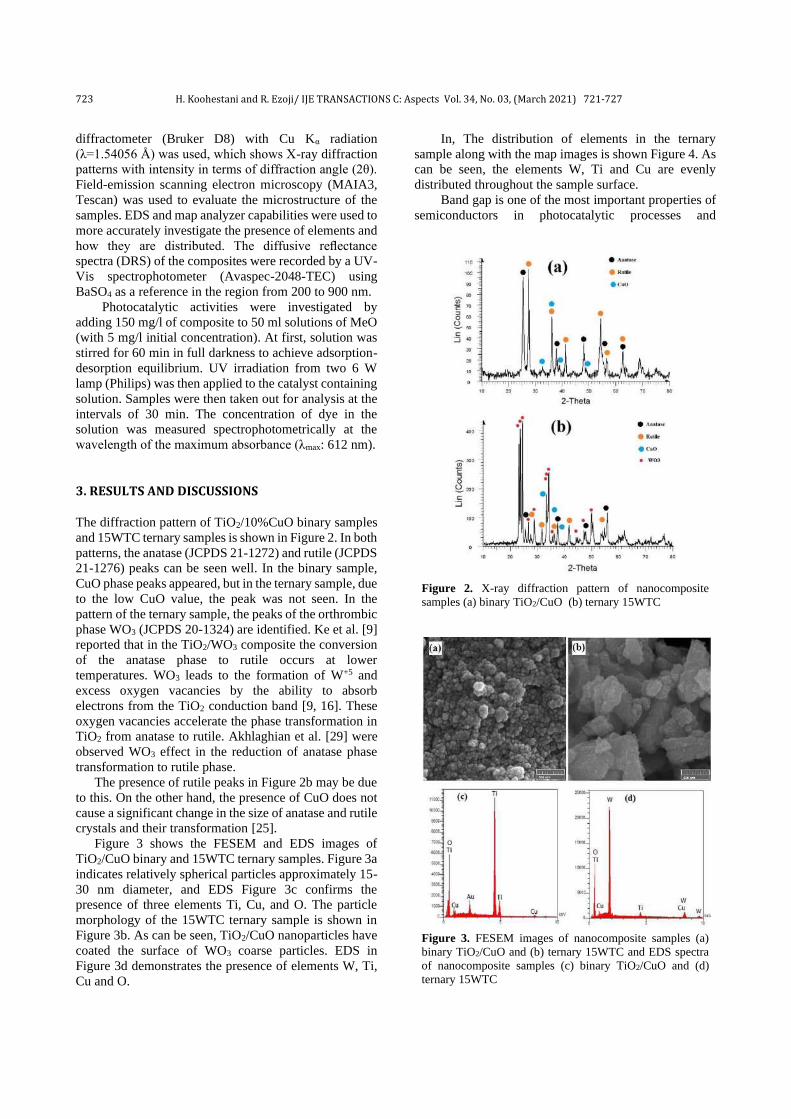
723 H. Koohestani and R. Ezoji/ IJE TRANSACTIONS C: Aspects Vol. 34, No. 03, (March 2021) 721-727
diffractometer (Bruker D8) with Cu Kα radiation
(λ=1.54056 Å) was used, which shows X-ray diffraction
patterns with intensity in terms of diffraction angle (2θ).
Field-emission scanning electron microscopy (MAIA3,
Tescan) was used to evaluate the microstructure of the
samples. EDS and map analyzer capabilities were used to
more accurately investigate the presence of elements and
how they are distributed. The diffusive reflectance
spectra (DRS) of the composites were recorded by a UV-
Vis spectrophotometer (Avaspec-2048-TEC) using
BaSO4 as a reference in the region from 200 to 900 nm.
Photocatalytic activities were investigated by
adding 150 mg/l of composite to 50 ml solutions of MeO
(with 5 mg/l initial concentration). At first, solution was
stirred for 60 min in full darkness to achieve adsorption-
desorption equilibrium. UV irradiation from two 6 W
lamp (Philips) was then applied to the catalyst containing
solution. Samples were then taken out for analysis at the
intervals of 30 min. The concentration of dye in the
solution was measured spectrophotometrically at the
wavelength of the maximum absorbance (λmax: 612 nm). 3. RESULTS AND DISCUSSIONS The diffraction pattern of TiO2/10%CuO binary samples
and 15WTC ternary samples is shown in Figure 2. In both
patterns, the anatase (JCPDS 21-1272) and rutile (JCPDS
21-1276) peaks can be seen well. In the binary sample,
CuO phase peaks appeared, but in the ternary sample, due
to the low CuO value, the peak was not seen. In the
pattern of the ternary sample, the peaks of the orthrombic
phase WO3 (JCPDS 20-1324) are identified. Ke et al. [9]
reported that in the TiO2/WO3 composite the conversion
of the anatase phase to rutile occurs at lower
temperatures. WO3 leads to the formation of W+5 and
excess oxygen vacancies by the ability to absorb
electrons from the TiO2 conduction band [9, 16]. These
oxygen vacancies accelerate the phase transformation in
TiO2 from anatase to rutile. Akhlaghian et al. [29] were
observed WO3 effect in the reduction of anatase phase
transformation to rutile phase.
The presence of rutile peaks in Figure 2b may be due
to this. On the other hand, the presence of CuO does not
cause a significant change in the size of anatase and rutile
crystals and their transformation [25].
Figure 3 shows the FESEM and EDS images of
TiO2/CuO binary and 15WTC ternary samples. Figure 3a
indicates relatively spherical particles approximately 15-
30 nm diameter, and EDS Figure 3c confirms the
presence of three elements Ti, Cu, and O. The particle
morphology of the 15WTC ternary sample is shown in
Figure 3b. As can be seen, TiO2/CuO nanoparticles have
coated the surface of WO3 coarse particles. EDS in
Figure 3d demonstrates the presence of elements W, Ti,
Cu and O.
In, The distribution of elements in the ternary
sample along with the map images is shown Figure 4. As
can be seen, the elements W, Ti and Cu are evenly
distributed throughout the sample surface.
Band gap is one of the most important properties of
semiconductors in photocatalytic processes and
Figure 2. X-ray diffraction pattern of nanocomposite
samples (a) binary TiO2/CuO (b) ternary 15WTC
Figure 3. FESEM images of nanocomposite samples (a)
binary TiO2/CuO and (b) ternary 15WTC and EDS spectra
of nanocomposite samples (c) binary TiO2/CuO and (d)
ternary 15WTC

H. Koohestani and R. Ezoji/ IJE TRANSACTIONS C: Aspects Vol. 34, No. 03, (March 2021) 721-727 724
applications. Figure 5 shows the DRS analysis results
including the absorption spectrum (Figure 5a) and how to
determine the band gap (Figure 5b). The value of optical
band gap obtained from the diagrams is represented in
Table 1. The band gap of the samples was obtained using
the kubelka-Munk relationship from the absorption
spectrum [25]:
n
gEhvhv )()( −= (1)
where Eg is the sample band gap energy (eV), ν is the
light frequency (s-1), h is the Planck constant (J.s), β is
the absorption constant and α is the absorption
coefficient. The value of index n is considered to be 1.2,
3.2 and 2 for direct transition, forbidden direct transition
or indirect transition, respectively. The band gap can be
determined by extrapolating the linear portion of the
(αhν)n-hν curve. n=1/2 value better defines our
composites [25].
It should be noted that the band gap energy of TiO2,
CuO and WO3 are 3.20, 1.70 and 2.70, respectively [30].
According to the results, the addition of other compounds
to TiO2 has reduced the band gap energy. For example,
the band gap value has been reduced to 2.95 eV for
TiO2/10%CuO. A shift in the absorption edge for
TiO2/CuO composites with CuO is shown to be possibly
related to the formation of a defect levels in an energy
range in TiO2 [31].
Addition of WO3 to the binary compound further
reduces the band gap. Baia et al. [32] in the presence of
WO3, were only able to reduce the gap of composite
to3.02 eV. Therefore, in order to further reduce the band
gap energy, the presence of both components is required.
The lowest band gap energy (2.66 eV) was obtained for
Figure 4. Map images of the distribution of Ti, W and Cu
elements in a 15WTC ternary sample
TABLE 1. The band gap of samples
Samples Band gap energy, Eg (eV)
TiO2 3.20*
TC 2.95
5WTC 2.70
10WTC 2.68
15WTC 2.66
20WTC 2.71
* ref. [25]
the 15WTC sample, and then by adding more WO3 value,
due to the fact that a higher level of the TC compound
was covered; the ability to absorb the compound
decreased, resulting in an increase in the band gap.
Table 2 presents the edge of the conduction band and
edge of the valance band for TiO2, CuO and WO3 [30].
Because the conduction band of tungsten oxide is lower
than that of TiO2, electron transfer from titanium particles
to WO3 is possible. This action effectively separates the
charge carriers and increases their lifetime. In the case of
(a)
(b)
Figure 5. synthesized nanocomposites (a) UV-Vis diffuse
reflectance spectra (b) Tauc plot obtained from UV-Vis DRS
spectra

725 H. Koohestani and R. Ezoji/ IJE TRANSACTIONS C: Aspects Vol. 34, No. 03, (March 2021) 721-727
TABLE 2. valance and conduction band edge of different
semiconductor [30]
Conduction Band edge (eV) Valence Band edge (eV)
TiO2 -4.21 -1.01
CuO -4.96 -3.26
WO3 -5.24 -2.54
TiO2/WO3 composition, due to the lower valance band of
WO3 than TiO2, the transfer of holes in WO3 is possible.
In the case of CuO, the unequilibrium transfer of charge
carriers at the TiO2/CuO junction causes holes to move
from TiO2 to CuO and electrons to move from CuO to
TiO2.
In the case of the TiO2/CuO/WO3 ternary compound,
UV light excites electrons in the conduction band WO3
and CuO, which are transferred to the conduction band
TiO2. On the other hand, the holes travel in the opposite
direction and migrate from the TiO2 valence band to the
WO3 and CuO valence bands. This migratations of
charge carriers restrict their recombination rate and thus
enhances the separation of electron-hole pair. The photo-
generated electrons can be trapped by oxygen molecules
in the organic solution to form superoxide radical anions
( −•
2O ), which can effectively degradate organic
pollutants. These holes convert the water molecules into
OH• and react with organic pollutants to genrate H2O and
CO.
Figure 6 shows the function of the compounds in
removing methylene orange dye. The photocatalytic
performance kinetics of the samples can be evaluated
according to the following relation and rate constant
comparison [17]:
tkC
Capp=
−
0
ln
(2)
where C0 is the initial concentration of dye, and kapp is the
apparent constant (min-1). Investigating the changes in ln
Figure 6. Linear correlation between reaction time and
logarithm of relative concentration of methylene orange (ln
C0/C)
(C/C0) over time for different samples, it is observed that
the addition of CuO and WO3 to the TiO2 constant speed
is improved. The highest rate constant is for the 15WTC
sample and is 0.0301 min-1. Akhlaghian et al. [29] in a
study showed that the 28.11% CuO/2.1%WO3/TiO2
composition was very successful in phenol
photodegradation and had a rate constant of 0.0621 min-
1. These results indicate that the charge transfer between
the compounds and an increase in electron-hole life, their
photocatalytic performance is improved.
4. CONCLUSIONS
In this study, ternary TiO2/CuO/WO3 composites were
synthesized and evaluated by different analyzes (XRD,
FESEM, DRS and etc.). The results of XRD and FESEM
analysis showed purity and uniform distribution of
elements. With the production of the ternary omposites,
the band gap decreased. Due to the difference in the edge
of the conduction band and the valance band, after the
production of excited charge carriers with light, electrons
and holes are moved at the junction of these
semiconductors. This will increase their lifetime and give
them a greater chance of participating in redox reactions
to remove water pollutions. The results of methylene
orange dye removal showed that the ternary composite
TiO2/10%CuO with 15%WO3 and 2.66 eV band gap, had
the highest performance.
5. REFERENCES
1. Bi, D. and Y. Xu, "Synergism between Fe2O3 and WO3 particles:
Photocatalytic activity enhancement and reaction mechanism".
Journal of Molecular Catalysis A: Chemical, Vol. 367, 103-107. https://doi.org/10.1016/j.molcata.2012.09.031
2. Feng, C., S. Wang and B. Geng, "Ti (iv) doped WO3 nanocuboids:
fabrication and enhanced visible-light-driven photocatalytic performance." Nanoscale, Vol. 3, No. 9, (2011), 3695-3699. https://doi.org/10.1039/C1NR10460H
3. Liu, Y., C. Xie, J. Li, T. Zou and D. Zeng, "New insights into the relationship between photocatalytic activity and photocurrent of
TiO2/WO3 nanocomposite." Applied Catalysis A: General, Vol.
433, (2012), 81-87. https://doi.org/10.1016/j.apcata.2012.05.001
4. Karácsonyi, É., L. Baia, A. Dombi, V. Danciu, K. Mogyorósi,
L.C. Pop, G. Kovács, V. Coşoveanu, A. Vulpoi, S. Simon and Zs.
Pap, "The photocatalytic activity of TiO2/WO3/noble metal (Au or Pt) nanoarchitectures obtained by selective photodeposition."
Catalysis today, Vol. 208, (2013), 19-27. https://doi.org/10.1016/j.cattod.2012.09.038
5. Zhuang, J., W. Dai, Q. Tian, Z. Li, L. Xie, J. Wang, P. Liu, X. Shi
and D. Wang, "Photocatalytic degradation of RhB over TiO2
bilayer films: effect of defects and their location." Langmuir,
Vol. 26, No. 12, (2010), 9686-9694. Doi: 10.1021/la100302m
6. Reyes, C., J. Fernández, J. Freer, M.A. Mondac, C. Zaror, S.
Malato and H.D. Mansill, "Degradation and inactivation of tetracycline by TiO2 photocatalysis." Journal of Photochemistry
and Photobiology A: Chemistry, Vol. 184, No. 1-2, (2006), 141-
146. https://doi.org/10.1016/j.jphotochem.2006.04.007

H. Koohestani and R. Ezoji/ IJE TRANSACTIONS C: Aspects Vol. 34, No. 03, (March 2021) 721-727 726
7. Laoufi, N., D. Tassalit and F. Bentahar, "The degradation of phenol in water solution by TiO2 photocatalysis in a helical
reactor." Global NEST Journal, Vol. 10, No. 3, (2008), 404-418.
8. Kuo, W. and P. Ho, "Solar photocatalytic decolorization of dyes in solution with TiO2 film." Dyes and Pigments, Vol. 71, No. 3,
(2006), 212-217. https://doi.org/10.1016/j.dyepig.2005.07.003
9. Ke, D., H. Liu, T. Peng, X. Liu and K. Dai, "Preparation and photocatalytic activity of WO3/TiO2 nanocomposite particles."
Materials Letters, Vol. 62, No. 3, (2008), 447-450. https://doi.org/10.1016/j.matlet.2007.05.060
10. Iliev, V., D. Tomova, S. Rakovsky, A. Eliyas and G. Li Puma,
"Enhancement of photocatalytic oxidation of oxalic acid by gold modified WO3/TiO2 photocatalysts under UV and visible light
irradiation." Journal of Molecular Catalysis A: Chemical, Vol.
327, No. (1-2): (2010), 51-57. https://doi.org/10.1016/j.molcata.2010.05.012
11. Li, X., F.B. Li, C.L. Yang and W.K. Ge, "Photocatalytic activity
of WOx-TiO2 under visible light irradiation." Journal of
Photochemistry and Photobiology A: Chemistry, Vol. 141, No.
(2-3), (2001), 209-217. https://doi.org/10.1016/S1010-
6030(01)00446-4
12. Sajjad, A.K.L., S. Shamaila, B. Tian, F. Chen and J. Zhang,
"Comparative studies of operational parameters of degradation of
azo dyes in visible light by highly efficient WOx/TiO2 photocatalyst." Journal of Hazardous Materials, Vol. 177, No.
1-3, (2010), 781-791. https://doi.org/10.1016/j.jhazmat.2009.12.102
13. Kwon, Y.T., K.Y. Song, W.I. Lee, G.J. Choi and Y.R. Do,
"Photocatalytic behavior of WO3-loaded TiO2 in an oxidation
reaction." Journal of Catalysis, Vol. 191, No. 1, (2000), 192-199. https://doi.org/10.1006/jcat.1999.2776
14. Leghari, S.A.K., S. Sajjad, F. Chen and J. Zhang, "WO3/TiO2
composite with morphology change via hydrothermal template-free route as an efficient visible light photocatalyst." Chemical
Engineering Journal, Vol. 166, No. 3, (2011), 906-915. https://doi.org/10.1016/j.cej.2010.11.065
15. Lv, K., J. Li, X. Qing, W. Li and Q. Chen, "Synthesis and photo-
degradation application of WO3/TiO2 hollow spheres." Journal
of Hazardous Materials, Vol. 189, No. 1-2, (2011), 329-335. https://doi.org/10.1016/j.jhazmat.2011.02.038
16. Koohestani, H., "Characterization of TiO2/WO3 composite
produced with recycled WO3 nanoparticles from W-Ni-Fe alloy." Materials Chemistry and Physics, Vol. 229, (2019), 251-256. https://doi.org/10.1016/j.matchemphys.2019.03.027
17. Koohestani, H. and S.K. Sadrnezhaad, "Improvement in TiO2 photocatalytic performance by ZrO2 nanocompositing and
immobilizing." Desalination and Water Treatment, Vol. 57, No.
58, (2016), 28450-28459. DOI:
10.1080/19443994.2016.1183233
18. Papp, J., B. Podolsky, and N. Rosen, "Surface acidity and
photocatalytic activity of TiO2, WO3/TiO2, and MoO3/TiO2 photocatalysts." Chemistry of Materials, Vol. 6, No. 4, (1994),
496-500. DOI: 10.1021/cm00040a026
19. Sajjad, A.K.L., S. Shamaila, B. Tian, F. Chen and J. Zhang, "One step activation of WOx/TiO2 nanocomposites with enhanced
photocatalytic activity." Applied Catalysis B: Environmental,
Vol. 91, No. 1-2, (2009), 397-405. https://doi.org/10.1016/j.apcatb.2009.06.005
20. Ramos-Delgado, N., L. Hinojosa-Reyes, I.L. Guzman-Mar, M.A.
Gracia-Pinilla and A. Hernández-Ramírez, "Synthesis by sol-gel
of WO3/TiO2 for solar photocatalytic degradation of malathion pesticide." Catalysis Today, Vol. 209, (2013), 35-40. https://doi.org/10.1016/j.cattod.2012.11.011
21. Scuderi, V., G. Amiard, R. Sanz, S. Boninelli, G. Impellizzeri and V. Privitera, "TiO2 coated CuO nanowire array: Ultrathin p–n
heterojunction to modulate cationic/anionic dye photo-
degradation in water." Applied Surface Science, Vol. 416,
(2017), 885-890. https://doi.org/10.1016/j.apsusc.2017.04.229
22. Sawicka-Chudy, P., M. Sibiński, G. Wisz, E. Rybak-Wilusz and
M. Cholewa, "Numerical analysis and optimization of Cu2O/TiO2, CuO/TiO2, heterojunction solar cells using SCAPS."
Journal of Physics: Conference Series. (2018). IOP Publishing. https://doi.org/10.1088/1742-6596/1033/1/012002
23. Zhang, X. and A. Tang, "Novel CuO/TiO2 nanocomposite films
with a graded band gap for visible light irradiation." Materials
Express, Vol. 2, No. 3, (2012), 238-244. https://doi.org/10.1166/mex.2012.1069
24. Koohestani, H. and A. Kheilnejad, "Hydrogen Generation and Pollution Degradation from Wastewater Using TiO2-CuO
Nanocomposite." Journal of Nanoscience and Nanotechnology,
Vol. 20, No. 9, (2020), 5970-5975. https://doi.org/10.1166/jnn.2020.18544
25. Koohestani, H. and S.K. Sadrnezhaad, "Photocatalytic
degradation of methyl orange and cyanide by using TiO2/CuO composite." Desalination and Water Treatment, Vol. 57, No. 46,
(2016), 22029-22038. https://doi.org/10.1080/19443994.2015.1132395
26. Miwa, T., S. Kaneco, H. Katsumata, T. Suzuki, K. Ohta, S. Chand
Verma and K. Sugihara, "Photocatalytic hydrogen production
from aqueous methanol solution with CuO/Al2O3/TiO2 nanocomposite." International Journal of Hydrogen Energy,
Vol. 35, No. 13, (2010), 6554-6560. https://doi.org/10.1016/j.ijhydene.2010.03.128
27. Yanyan, L., T.A. Kurniawan. Z. Ying, A.B. Albadarin and G.
Walker, "Enhanced photocatalytic degradation of acetaminophen
from wastewater using WO3/TiO2/SiO2 composite under UV-vis irradiation." Journal of Molecular Liquids, Vol. 243, (2017),
761-770. https://doi.org/10.1016/j.molliq.2017.08.092
28. Li, Z., F. Cao, L. Wang, Z. Chen and X. Ji, "A novel ternary MoS2/MoO3/TiO2 composite for fast photocatalytic degradation
of rhodamine B under visible-light irradiation." New Journal of
Chemistry, Vol. 44, No. 2, (2020), 537-542. https://doi.org/10.1039/C9NJ04107A
29. Akhlaghian, F. and A. Najafi, "CuO/WO3/TiO2 photocatalyst for
degradation of phenol wastewater." Scientia Iranica, Vol. 25, No. 6, (2018), 3345-3353.
https://dx.doi.org/10.24200/sci.2018.20611
30. Xu, Y. and M.A. Schoonen, "The absolute energy positions of conduction and valence bands of selected semiconducting
minerals." American Mineralogist, Vol. 85, No. 3-4, (2000), 543-
556. https://doi.org/10.2138/am-2000-0416
31. Lebedev, V., V.V. Sudin, D.A. Kozlov and A.V. Garshev,
"Photocatalytic properties of nanocrystalline TiO2 modified with
CuO and WO3." Nanotechnologies in Russia, Vol. 11, No. 1-2,
(2016), 20-28. DOI: 10.1134/S1995078016010092
32. Baia, L., E. Orbán, S. Fodor, B. Hampel, E.Z. Kedves, K. Saszet
and I. Székely, "Preparation of TiO2/WO3 composite photocatalysts by the adjustment of the semiconductors' surface
charge." Materials Science in Semiconductor Processing, Vol.
42, (2016), 66-71. https://doi.org/10.1016/j.mssp.2015.08.042

727 H. Koohestani and R. Ezoji/ IJE TRANSACTIONS C: Aspects Vol. 34, No. 03, (March 2021) 721-727
Persian Abstract
چکیده رفع مشکالت یشده و مورد استعمال قرار گرفته است. برا ید تول ها یهاد یمه ن یهبر پا یادی ز هاییستمورد توجه قرار گرفته است. فتوکاتال یار هوا، امروزه بسآب و یهای آلودگ یستیحذف فتوکاتال
انرژ هایهاد یمهن گاف جمله پا یاز عمر طول و ترکحفره(- )الکترون بار یهاحامل یینباال جزئ یبات، جزئ حتی و یدو تول یسه ا یدآنها در است. ترک ینشده جز یبپژوهش، یئ سه
3CuO/WO/2TiO3 نانوذرات ، با افزودنWO بهCuO/2TiO پراش پرتو یزآنال یج قرار گرفت. نتا یابیمورد ارز نارنجی یلنو عملکرد آنها با حذف رنگ مت ی سنتز شده است. خواص ساختارX
نرخ حذف رنگ را ترینیشب الکترون ولت 2/ 66 یانرژ افگ و WO%315با CuO/2TiO%10 یبعناصر را نشان داد. ترک یکنواخت یعخالص بودن و توز میکروسکوپ الکترونی روبشی،و
نشان داد.
IJE TRANSACTIONS C: Aspects Vol. 34, No. 03, (March 2021) 728-736
Please cite this article as: A. Mahmoodian, M. Durali, M. Saadat, T. Abbasian, A Life Clustering Framework for Prognostics of Gas Turbine Engines under Limited Data Situations, International Journal of Engineering, Transactions C: Aspects Vol. 34, No. 03, (2021) 728-736
International Journal of Engineering
J o u r n a l H o m e p a g e : w w w . i j e . i r
A Life Clustering Framework for Prognostics of Gas Turbine Engines under Limited
Data Situations
A. Mahmoodiana, M. Durali*a, M. Saadatb, T. Abbasianb a Mechanical Engineering Department, Sharif University of Technology, Tehran, Iran b ECE Faculty, Tehran University, Tehran, Iran
P A P E R I N F O
Paper history: Received 23 August 2020 Received in revised form 01 January 2021 Accepted 04 January 2021
Keywords: Limited Data Prognosis and Health Management Remaining Useful Life Estimation Robustness
A B S T R A C T
The reliability of data driven prognostics algorithms severely depends on the volume of data. Therefore in case of limited data availability, life estimations usually are not acceptable; because the quantity of
run to failure data is not sufficient to train prognostics model efficiently. To board this problem, a life
clustering prognostics (LCP) framework is proposed. LCP regenerates the train data at different ages and outcomes to increment of the training data volume. So, the method is useful for limited data conditions.
In this research, initially LCP performance is studied in normal situation is; successively robustness of
the framework under limited data conditions is considered. For this purpose, a case study on turbofan engines is performed. The accuracy for the proposed LCP approach is 71% and better than other
approaches. The prognostics accuracy is compared in various situations of data deficiency for the case
study. The prognostic measures remain almost unchanged when the training data is even one third. Successively, prognostics accuracy decreases with a slight slope; so that when the training data drops
from 100 to 5%, the accuracy of the results drops 26%. The results indicates the robustness of the
proposed algorithm in limited data situation. The main contribution of this paper include: (1) The effectiveness of life clustering idea for use in prognostics algorithms is proven; (2) A step-by-step
framework for LCP is provided; (3) A robustness analysis is performed for the proposed prognostics
algorithm.
doi: 10.5829/ije.2021.34.03c.18
1. INTRODUCTION1 In recent years, prognostics and health management
(PHM) of complex mechanical systems has become more
prominent. Prognostic and Remained Useful Life (RUL)
prediction has been initialized in medical field [1];
subsequently attracted much attention in engineering
issues due to economical and operational considerations
[2]. Predicting future behavior of a complex machine
such as a gas turbine is a complicated task. Prognostics is
currently at the core of systems’ health management to
achieve reliable and safe operation of machines. In the
framework of PHM, many techniques exist which are
basically classified into two principal classes: data-driven
and model-based prognostics approach [3-4]. The fact
that most researches are focusing on data-driven methods
shows the desire to work with easily accessible data as
*Corresponding Author Institutional Email: [email protected] (M.
Durali)
compared to model-based methods, irrespective of the
difficulties in gaining accessing statistically significant
run-to-failure data. Despite acceptance of data-driven
methods, the on-going difficulty with these methods is
that they show acceptable RUL estimation only when
abundant run-to-failure data are available for training.
Although, under the condition of limited failure data,
model-based solutions are unsuccessful due to their
requirement to large amounts of failure data for
validating physical models [5].
In this research, data driven methods are focused and
divided mainly in two groups: typical methods and robust
methods. A typical prognostics method rely on large
amounts of historical failure data (i.e. run-to failure data
indicating past degradation patterns) to estimate
prognostics model parameters [5]. Otherwise, the
predictions may be unreliable and the training can not be

A. Mahmoodian et al. / IJE TRANSACTIONS C: Aspects Vol. 34, No. 03, (March 2021) 728-736 729
carried out. The fact limits the application of typical
prognostics methods in problems with small amount of
available training data [6]. Failure data are limited in real
industrial cases due to some reasons: (1) rare failures; (2)
overprotective maintenance and replacement regimes;
(3) incomplete reports [7].
Majority of prognostics researches are developed
assuming enough run-to-failure data are available for
training. Some researchers have used combined
regression techniques, including linear and quadratic
models to predict the RUL of gas turbine engines [8].
Other methods like particle filter [9], adaptive-order
particle filter [10], Kaplan Meier [11] and support vector
machine (SVM) [12] have been used for prognostics. Yu
et al. [13] have developed a prognostics system for
engine health assessment based on logistic regression and
state-space-model. Simon et al. [14] have compared the
estimation accuracy and computational effort of variants
of the Kalman filter like linearized Kalman filter (LKF),
extended Kalman filter (EKF), and unscented Kalman
filter (UKF) for aircraft engine health estimation. Lu et
al. [15] have presented a nonlinear state estimation
method based on EKF and obtained a significant
improvement in estimation accuracy and robustness.
Ding et al. [16] have fused support vector machine and
the genetic algorithm and proposed an intelligent
prognostics approach. Goebel et al. [17] compared the
results of a relevance vector machine (RVM), a Gaussian
process regression (GPR), and an artificial neural
network (ANN) approach in prognostics.
On the contrary, with the robust methods, the RUL
estimation is acceptable despite the lack of abundant
trained data. Recently, some novel prognostics methods
based on classic algorithms are suggested, such as fusion
of prognostics algorithms [18], multistate structure [19],
etc. Xu et al. [18] have integrated the strengths of the
experience-based prognostics approach and the data-
driven approach. The developed fusion prognostics
framework has been employed to predict the RUL of a
gas turbine engine as an application example [18].
Moghaddass et al.[19] have demonstrated that
deterioration process occurs through different levels of
health states before failure, leading to a multistate
deterioration process in many real-world cases. Xiang et
al. [20] have proposed a probabilistic methodology for
fatigue prognostics using an inverse first-order reliability
method. However, the robustness tests are rarely
reported .
In this paper, a novel methodology is presented based
on life clustering that allows training datasets to be
augmented. Usually, the goal of clustering in literature
has been to organize data into homogeneous groups to
compact clusters with minimum intra group similarity
and to increase separation among clusters with
maximized inter group dissimilarity [21]. The proposed
method of life clustering prognostics (LCP) is able to
increase the train data set samples; in addition to organize
data into homogeneous groups.
The case study is to compare the prognostics accuracy
for a robust framework in abundant data and little data
condition with for turbofan engines Prognostic Health
Management (PHM) Challenge data [22]. For 2008 PHM
challenge, many authors have reported the RUL
estimation for a given data set. Only typical tests using
large scale data have been stated. The best results have
been obtained by using RULCLIPPER algorithm [23],
EVIPRO algorithm [24] and a similarity-instance based
approach [25]. These results are used as the reference
point of the current study .
The main contributions of this paper can be
summarized as follows. First, the effectiveness of the
idea of life clustering for use in prognostics algorithms is
proven. Although artificial neural network is used as the
main prediction tool in this paper, the idea of LCP can be
combined and used with other classical methods of
prognostics. Second, a step-by-step framework for
prognostics based on life clustering is provided. This
method significantly improves the reliability of this
algorithm while using all the advantages of a predictive
algorithm as the core prediction algorithm. Third, a
robustness analysis is performed for the proposed
prediction algorithm. This study evaluates the
performance of the algorithm in different conditions of
lack of sufficient data. Based on the evaluations, the LCP
algorithm is robust in limited information conditions and
has acceptable results. Robustness of a prognostics
algorithm is a critical issue in industrial and real-world
cases, where predictive maintenance is required against
lack of abundant run-to-failure data .
The outline of this paper is as follows. In section 2
layout of the study is presented. Data processing and
prognostics method is explained in section 3. In sections
4, implementation of the proposed method on a case
study is described. This paper ends with results and
conclusions in two last sections.
2. LAYOUT OF THE STUDY 2. 1. Data Description To illustrate the outcomes of
this method on prognostics and health monitoring, a case
study on turbofan engines from NASA's prognostics
Information Repository is performed. The structure of the
data set and the effectiveness of the proposed model are
presented in this section. The data consists of 21
Measurements, including the measurements listed in
Table 1, that are measured during every flight cycle. In
the dataset, multiple units operate until failure occurs,
providing training set. The other units run to different
levels of destruction, forming test set. The challenge is to
predict the RUL of test units. This dataset is one of the
most widely datasets used for the development and

730 A. Mahmoodian et al. / IJE TRANSACTIONS C: Aspects Vol. 34, No. 03, (March 2021) 728-736
TABLE 1. List of sensors and Measurements used in this paper
[22]
Unit Description Symbol
O R Total temperature at LPC outlet T24
O R Total temperature at HPC outlet T30
Psia Total pressure at HPC outlet P30
Rpm Physical core speed Nc
- Engine pressure ratio (P50 / P2) Pr
- Ratio of fuel flow to Ps30 Phi
- Bypass ratio BPR
- Bleed enthalpy BE
O R Total temperature at LPT outlet T50
Psia static pressure at HPC outlet Ps30
- Burner Fuel air ratio farB
validation of prognostics algorithms [2, 18-19]. Figure 1
shows the main components of the aircraft gas turbine
engine model.
2. 2. Prognostic Measures In the PHM context,
sometimes it is desirable to predict early as compared to
predicting late. Therefore, the asymmetric interval I= [-
10, +13] around the true RUL is considered to evaluate
the performance. Accuracy measure is defined as the
percentage of correct estimations which falls within the
interval I [25].
Mean square error (MSE) and mean absolute error
(MAE) are two other measures which are used to evaluate
the performance of LCP method more accurately,
𝑒𝑚𝑠𝑒 =1
𝑁√∑ (𝑒𝑟𝑟𝑡)2𝑁
𝑡=1 (1)
𝑒𝑚𝑎𝑒 =1
𝑁∑ |𝑒𝑟𝑟𝑡|𝑁
𝑡=1 (2)
where error is defined for a given prediction by Equation
(2):
(3) err = True RUL - Estimated RUL
3. PROGNOSTICS METHOD
In a data-driven PHM process, after data acquisition, the
first challenge is how to map the conditions between a
complex and interconnected system with its level of the
drop; for this purpose, data processing and signal feature
extraction should be done. Two general approaches are
considered to extract features and design a health
indicator (HI). The first approach is to use gas-path
parameters such as temperature, vibrations, flow
capacity, pressure, compressor efficiency, fan efficiency,
Figure 1. Simplified diagram of the gas turbine engine [22]
etc. Vibration and modal analysis is widely used to
estimate life of mechanical systems [26-27].
Mohammadi et al. [28] determined performance
deterioration according to efficiency and flow capacity as
health indicators. The second approach is the
combination of functional and performance sensors. In
this field, we can mention the works [18, 29, 30], that
combine different sensors with different fusion
techniques. Diallo [11] has shown in his research that
multi-sensor data fusion approach is more reliable. A step
by step methodology is indicated in literature [30] to
produce a Health Indicator Feature [HIF] vector, which
is used in this article.
3. 1. The LCP Prognostic Framework A
prognostics framework based on life clustering is
developed as shown in Figure 2. RUL estimation is
accomplished through the life clustering of the engines
and subsequently construction of a specific prediction
module for each cluster. The proposed framework can be
implemented as the following phases. Clustering In the first phase, clustering is performed.
The estimation start time of each test engine is shown
with symbol tc. In the prognostics issue for a fleet of
engines, a range of tc [min (tc): max (tc)] exists. The
range must be separated to several divisions in the
clustering phase. The cluster width (CW) is defined as
follows:
𝐶𝑊𝑖 = 𝑡𝑖 − 𝑡𝑖−1, ∑ 𝐶𝑊𝑖 =𝑛𝑖=1 𝑡𝑛 − 𝑡0 (4)
where tis are clustering borders, t0 is the min (tc), tn is
the max (tc) and n is the number of partitions. In the
simple form, clusters widths may be assumed equal. To
attain more accurate results, the number of partitions and
cluster widths can be found by an optimization process.
Reproduction In the second phase, a time step (ts) is
considered so that train data set is observed several times
at each time step. Considering maximum observation
resolution, each time step is an observation point (ts=1).
For example, the ith cluster width is mi (CWi = mi), so the
train data set is reproduced mi times. For any

A. Mahmoodian et al. / IJE TRANSACTIONS C: Aspects Vol. 34, No. 03, (March 2021) 728-736 731
Figure 2. The framework of LCP prognostics
reproduction, units with life lengths less than the relevant
observation point are withdrawn; the others are stopped
at that point .
Till now, mi reproductions of train data set are
produced for each cluster. Now, data processing of units
in each reproduction is performed and mi vectors HIF are
produced. In the last step of this phase, the HIF vectors
for each cluster are merged to one and finally n
cumulative HIF vectors are remained for n clusters.
Mapping In the previous phase, train data was
reproduced several times and n cumulative HIF vectors
were resulted. Now in the third phase, a prediction tool
such as neural network is used to find a relation between
HIFs and RULs for train data. The HIFs are selected as
the input, and the corresponding true RUL data are
selected as the target values to train the prediction
modules. The results of the third phase are n prediction
modules for n different life clusters.
RUL estimation In the fourth phase, RUL estimation
of the target unit is performed. Initially, signal processing
for the device is performed and the relevant HIF vector is
calculated. Then, cluster selection must be done
according to the prediction start age (tc) of the test unit.
It can be done in two ways:
1. Classic way, so that each unit belongs to a cluster if
its tc is between the minimum and maximum age of that
cluster
2. Fuzzy way, in which each unit belongs to a cluster
to some degree that is specified by a membership
function.
After cluster selection, the HIF vector of the test unit is
inputted to the related prediction module and the device
RUL is estimated.
4. CASE STUDY
The steps taken in this study are based on the framework
given in Figure 2. The main parameters of the LCP
framework are the number of clusters (n), the clusters
width (CW) and the observation time step (ts). The
optimum values for these parameters are different for
each problem and must be optimized. To achieve this
goal, various prognostics measures may be defined as the
objective function. Sequential phases of the LCP
framework are executed and the best parameters are
found through an optimization process.
Phase 1 To determine the clustering parameters, four
phases of LCP prognostics are implemented and the
prognostics measures were compared. For the current
case study, prognostics criterions remain almost
unaffected while n>2, as shown in Figure 3. Thus, n = 4
is chosen to evade costly computations. Sequentially, the
optimum clusters widths (CW) are found out by genetic
algorithm to maximize the accuracy. The optimal
clustering parameters are summarized in Table 2.
Phase 2 Considering observation time step =1 cycle,
the train data set is reproduced at each cycle. For every
cycle, for instance the cth cycle, all engines with age
longer than c cycles are stopped at the cth cycle. Then
data process is performed and health indicator
features HIFtr(c) are extracted. Finally relevant HIFs
Figure 3. Prognostic measures via. number of clusters

732 A. Mahmoodian et al. / IJE TRANSACTIONS C: Aspects Vol. 34, No. 03, (March 2021) 728-736
TABLE 2. Summary of optimal clustering scheme
Cluster width Life interval Cluster
45 cycles 31-75 cycles I
50 cycles 76-125 cycles II
71 cycles 126-196 cycles III
107 cycles 197-303 cycles IV
for each cluster are merged to one, for example
𝑯𝑰𝑭𝒕𝒓(𝟑𝟏), 𝑯𝑰𝑭𝒕𝒓(𝟑𝟐) … & 𝑯𝑰𝑭𝒕𝒓(𝟕𝟓) are merged to
one cumulative vector for the 1st cluster,
𝑯𝑰𝑭𝒕𝒓(𝟕𝟔), 𝑯𝑰𝑭𝒕𝒓(𝟕𝟕) … & 𝑯𝑰𝑭𝒕𝒓(𝟏𝟐𝟓) are merged to
one cumulative vector for the 2nd cluster and so on for
other clusters from Table 2. Summary of reproductions
of train data set are represented in Table 3.
Phase 3 In the third phase, the algorithm creates a map
between HIFs and RULs for each cluster. For this aim,
neural network fitting tool is used [31]. In the present
study, a forward multilayer perceptron (MLP) with
backward propagation Bayesian training algorithm is
applied. The network is composed from 10 hidden layers,
70% of data is used for train, 15% for test and 15% for
validation. The summary of the formation of four
networks is presented in Table 4.
Phase 4 RUL estimation is performed through the
following steps:
1. For the jth test engine, tc is considered (tcj).
2. Depending on its age, the appropriate group from
Table 2 is selected (group #k).
3. The relevant HIF vector of jth test engine is
extracted (HIFte (j)).
TABLE 3. Summary of train data set reproductions
Cluster length of cumulative HIF
1 4500
2 5000
3 5971
4 2240
TABLE 4. Summary of the formation of the prediction
modules
Target Input ANN
1x4500 matrix, representing
RULs of engines
2x4500 matrix, representing
2 features of 4500 HI signals I
1x5000 matrix, representing
RULs of engines
2x5000 matrix, representing
2 features of 5000 HI signals II
1x5971 matrix, representing
RULs of engines
2x5971 matrix, representing
2 features of 5971 HI signals III
1x2240 matrix, representing
RULs of engines
2x2240 matrix, representing
2 features of 2240 HI signals IV
4. HIFte (j) is applied as an input to the kth network.
5. The network output is the estimated RUL of the test
engine.
5. RESULTS AND DISCUSSION The performance of the proposed prognostics method is
evaluated in two states:
1. Full train data: In this state, all engines (100 units)
of train dataset #1 from turbofan engines of the
NASA Prognostic Data Repository are utilized to
train the LCP algorithm. This is similar to the
condition in which most researches have used for
training their algorithms and represented their
results.
2. Limited train data: In this state, a portion of train
dataset #1 is used for training LCP algorithm. Tests
are performed with 50, 30, 20 and 10% of train data
(equal to 50, 30, 20 and 10 engines). This state is
similar to real world in industries when one should
deal with a limited train data.
5. 1. LCP Results in Full Train Data Condition To
evaluate the effectiveness of the LCP algorithm, a
comparison with other approaches is performed as
indicated in Table 5. Full testing dataset is used in few
papers to our knowledge: Ramasso et al. [23, 24], Khelif
et al. [25] and Wang et al. [32] that achieved the best
score in PHM challenge 2008. The accuracy for the
proposed LCP approach is better in comparison with
other approaches.
5. 2. LCP Results under Limited Train Data Condition It was shown in the previous section
that the accuracy of the LCP method is reliable for full
data condition in comparison with other methods. In this
section a sensitivity analysis is performed under limited
data condition. As mentioned earlier, four tests are
performed in this section with 50, 30, 20 and 10% of train
data. Each test is repeated several times in a way that
different portions of the train data are selected. Finally,
the mean value of prognostic measures for each test is
TABLE 5. Comparison of accuracy for different methods
Method Correct % Early % Late %
LCP model (using ANN for
prediction modules) 71 23 6
Ramasso [24] 67 Nan Nan
Khelif et al.[25] 54 18 28
Ramasso et al. [23] 53 36 11
Javed et al. [33] 53 27 20
Wang et al. [32] 44 19 37

A. Mahmoodian et al. / IJE TRANSACTIONS C: Aspects Vol. 34, No. 03, (March 2021) 728-736 733
summarized in Table 6. A comparison of prognostics
measures for different sizes of train data is indicated in
Figure 4.
While the proposed algorithm reproduces train data
several times for each life cluster, the size of the training
set is several times larger than the initial train data set.
Comparison of results for different numbers of training
data showed that when the number of training data
decreases, (1) prediction accuracy remains almost
unchanged for about 30% of available train data, (2)
prediction accuracy decreases about 14% with a slight
slope when the available train data falls from 30 units to
10 units and (3) when the available train data goes down
from 10 units to 5 units, prediction drops 10%
significantly .
Further investigations can be made on the robustness
of the proposed algorithm under limited training data
condition. Prognostics results of engines in different
cycles are studied in this paper. The actual RUL value
and the RUL estimate with limited train data (10 units for
TABLE 6. Summary of prognostic measures
Number of train
data units
Accuracy (%) MAE MSE
Mean STD
100 58 2 0 14.14 1.97
50 57 3.1 14.5 2
30 56 3.4 14.4 2
20 46.6 3.1 17.3 2.3
10 42 5.7 21.2 2.9
5 32 7.8 31.75 4.4
Figure 4. Comparison of prognostics measures for different
sizes of train data
2 The neural network training multiple times will generate different
results due to different initial conditions; Therefore, for sensitivity
analysis, the polynomial regression is used for composing prediction
Figure 5. Prognostics results of engines #99-100 in different
cycles with limited train data set (10 units for training)
training) are shown in Figure 5 for engines #99-100.
Other engines results (#91-98) are shown in Appendix A
The results showed that overall (1) the RUL estimate with
small data is reasonably close to the actual RUL
especially in large ages, (2) as the engine ages, the
prediction error for the RUL gets narrower, means that,
the prognostics uncertainty declines, and (3) in some
cases, lack of enough data especially in the last cluster,
results to increase prediction error. In general, the results
indirectly support the hypothesis that, life clustering
method leads to acceptable results in condition of train
data deficiency (although not necessarily the best
method).
6. CONCLUSION
In this paper, a prognostic algorithm is proposed that first
classifies the test units in different age groups, then
estimates their RUL using predictive techniques. The
modules of the ABC method and the resulted accuracy is different with
table 5 (ABC model using ANN)

734 A. Mahmoodian et al. / IJE TRANSACTIONS C: Aspects Vol. 34, No. 03, (March 2021) 728-736
proposed algorithm uses one of the conventional and
available prediction methods (such as ANN as presented
in this study) as the core prediction tool and rectifies it
with more reliable and robust results .
A case study shows that the results achieved by this
method were significantly improved compared to other
conventional methods and it was observed that life
clustering can be very effective in prognostics. LCP was
able to predict with 71% accuracy, a little better than the
best published results on the same case study. While the
performance of the LCP method was evaluated under
normal conditions, its results were examined in the
condition of limited training data, which happens
frequently in industry .
Comparison of results for different conditions of
available training data showed that the prognostic
measures remain almost unchanged when the training
data is even one third. The reason is that the training data
set has been multiplied several times and it compensates
the lack of enough training data. Successively,
prognostics accuracy decreases with a slight slope; so
that when the available training data drops from 30 to
10%, the accuracy of the results drops from 56 to 42%.
After that accuracy drops considerably to 32% for 5% of
available train data. Although significant accuracy drop
is observed below 10% of available train data, it is
notable that LCP is using train data of only 5 units to
predict remaining life of 100 test units .
In the final stage, more cases were tested and the
results of the prognostics algorithm were plotted using a
low number of training data (10 engines). The results
show that the RUL estimate with small data is rationally
close to the actual RUL, although in some cases, severe
lack of data especially in the last cluster, results to
increase prediction error .
The results of this case study confirmed that the LCP
method (1) is a powerful prognostics tool in normal
condition and (2) is a robust technique under limited data
condition. So the proposed method can be integrated with
any classic method to result more accurate and robust
RUL estimates for real-world situations. The
methodology developed in this paper is not limited to the
use with turbojet engine prognostics. It can be extended
to other prognostics problems .
Integration and modification of more prediction
methods with life clustering idea are to be investigated in
future works. However, there are some potential
limitations existing in the prediction for the last cluster
(in case of severe lack of data) which could be improved
with fusion of previous clusters predictions in the future
study.
7. REFERENCES
1. Khezri R, Hosseini R, Mazinani M. “A fuzzy rule- based expert
system for the prognosis of the risk of development of the breast
cancer.” International Journal of Engineering, Transactions A:
Basics. Vol 27, No 10, (2014), 1557-1564. doi: 10.5829/idosi.ije.2014.27.10a.09
2. Hu C, Zhou Z, Zhang J, Si X. “A survey on life prediction of
equipment.” Chinese Journal of Aeronautics. Vol 28, No 1, (2015), 25-33. doi.org/10.1016/j.cja.2014.12.020
3. Hamidi H, Daraee A. “Analysis of pre-processing and post-
processing methods and using data mining to diagnose heart diseases.” International Journal of Engineering, Transactions
A: Basics . Vol 29, No 7, (2016), 921-930. doi: 10.5829/idosi.ije.2016.29.07a.06
4. Amini M, Moharrami A, Poursaeidi E. “Failure probability and remaining life assessment of reheater tubes.” International
Journal of Engineering, Transactions B: Applications. Vol 26, No 5, (2013), 543-552. doi: 10.5829/idosi.ije.2013.26.05b.11
5. Peng Y, Dong M, Zuo MJ. “Current status of machine prognostics
in condition-based maintenance: a review.” The International
Journal of Advanced Manufacturing Technology. Vol 50, (2010), 297-313. doi.org/10.1007/s00170-009-2482-0
6. Mao R, Zhu H, Zhang L, Chen A. “A new method to assist small
data set neural network learning. InIntelligent Systems Design
and Applications.” IEEE ISDA'06. Vol 1, (2006), 17-22. DOI:10.1109/ISDA.2006.67
7. Ranasinghe GD, Lindgren T, Girolami M, Parlikad AK. “A Methodology for Prognostics Under the Conditions of Limited
Failure Data Availability”. IEEE Access. Vol 17, (2019), 173-179. DOI: 10.1109/ACCESS.2019.2960310
8. Li YG, Nilkitsaranont P. “Gas turbine performance prognostic for
condition-based maintenance.” Applied Energy. Vol 86, No 10, (2009), 2152-2161. doi.org/10.1016/j.apenergy.2009.02.011
9. Xiongzi CH, Jinsong YU, Diyin TA, Yingxun WA. “A novel pf-lssvr-based framework for failure prognostics of nonlinear
systems with time-varying parameters.” Chinese Journal of
Aeronautics. Vol 25, (2012), 715-724. doi.org/10.1016/S1000-9361(11)60438-X
10. Tongyang LI, Shaoping WA, Jian SH, Zhonghai MA. “An adaptive-order particle filter for remaining useful life prediction
of aviation piston pumps.” Chinese Journal of Aeronautics.Vol 31, (2018), 941-948. doi.org/10.1016/j.cja.2017.09.002
11. Diallo ON. “A data analytics approach to gas turbine prognostics
and health management” (Doctoral Dissertation, Georgia Institute of Technology).
12. Caesarendra W, Widodo A, Yang BS. “Combination of probability approach and support vector machine towards
machine health prognostics.” Probabilistic Engineering
Mechanics. Vol 26, (2011), 165-173. doi.org/10.1016/j.probengmech.2010.09.008
13. Huang HZ, Wang HK, Li YF, Zhang L, Liu Z. “Support vector machine based estimation of remaining useful life: current
research status and future trends.” Journal of Mechanical
Science and Technology. Vol 29, (2015), 151-163. doi.org/10.1007/s12206-014-1222-z
14. Simon D. “A comparison of filtering approaches for aircraft
engine health estimation.” Aerospace Science and
Technology.Vol 12, (2008), 276-284. doi.org/10.1016/j.ast.2007.06.002
15. Lu F, Ju H, Huang J. “An improved extended Kalman filter with
inequality constraints for gas turbine engine health monitoring.” Aerospace Science and Technology. Vol 30, (2016), 36-47. doi.org/10.1016/j.ast.2016.08.008
16. Ding C, Xu J, Xu L. “ISHM-based intelligent fusion prognostics
for space avionics.” Aerospace Science and Technology. Vol 29, (2013), 200-205. doi.org/10.1016/j.ast.2013.01.013
17. Goebel K, Saha B, Saxena A. “A comparison of three data-driven techniques for prognostics.” In 62nd Meeting of the Society for
Machinery Failure Prevention Technology (Mfpt), (2008), 119-131.

A. Mahmoodian et al. / IJE TRANSACTIONS C: Aspects Vol. 34, No. 03, (March 2021) 728-736 735
18. Xu J, Wang Y, Xu L. “PHM-oriented integrated fusion prognostics for aircraft engines based on sensor data.” IEEE
Sensors Journal. Vol 14, (2014), 1124-1132. DOI: 10.1109/JSEN.2013.2293517
19. Moghaddass R, Zuo MJ. “An integrated framework for online
diagnostic and prognostic health monitoring using a multistate deterioration process.” Reliability Engineering & System Safety. Vol 124, (2014), 92-104. doi.org/10.1016/j.ress.2013.11.006
20. Xiang Y, Liu Y. “Application of inverse first-order reliability method for probabilistic fatigue life prediction.” Probabilistic
Engineering Mechanics. Vol 26, (2011), 148-156. doi.org/10.1016/j.probengmech.2010.11.001
21. Javed K. “A robust & reliable Data-driven prognostics approach
based on extreme learning machine and fuzzy clustering” (Doctoral Dissertation).
22. Saxena A, Goebel K, Simon D, Eklund N. “Damage propagation
modeling for aircraft engine run-to-failure simulation.” IEEE
InPrognostics and Health Management, (2008). 1-9. DOI:10.1109/PHM.2008.4711414
23. Ramasso E, Rombaut M, Zerhouni N. “Joint prediction of
observations and states in time-series: a partially supervised
prognostics approach based on belief functions and knn. Networks”. (2013). DOI: ff10.1109/TSMCB.2012.2198882
24. Ramasso E. “Investigating computational geometry for failure prognostics.” International Journal of Prognostics and Health
Management. Vol 5, (2014).
25. Khelif R, Malinowski S, Chebel-Morello B, Zerhouni N. “RUL prediction based on a new similarity-instance based approach.”
IEEE InIndustrial Electronics (ISIE), (2014), 2463-2468. DOI: 10.1109/ISIE.2014.6865006
26. Yakout M, Elkhatib A, Nassef MG. “Rolling element bearings
absolute life prediction using modal analysis.” Journal of
Mechanical Science and Technology. Vol 32, (2018), 91-99. doi.org/10.1007/s12206-017-1210-1
27. Prasad SR, Sekhar AS. “Life estimation of shafts using vibration based fatigue analysis.” Journal of Mechanical Science and
Technology. Vol 32, (2018), 4071-4078. DOI: 10.1007/s12206-018-0806-4
28. Mohammadi E, Montazeri-Gh M. “Simulation of full and part-
load performance deterioration of industrial two-shaft gas turbine.” Journal of Engineering for Gas Turbines and
Power.Vol 136, (2014), 26-35. DOI: 10.1115/1.4027187
29. Dabaghi E, Kashanian H. “Feature dimension reduction of
multisensor data fusion using principal component fuzzy
analysis.” International Journal of Engineering, Transactions
A: Basics, Vol 30, No. 4, (2017), 493-499. doi: 10.5829/idosi.ije.2017.30.04a.06
30. Mahmoodian A., Durali M., Abbasain T., Saadat M., “Optimized Age Dependent Clustering Algorithm for Prognosis: A Case
Study on Gas Turbines”, Scientiairanica Transaction B:
Mechanical Engineering, (2020), (Articles in Press, Available Online) DOI:10.24200/SCI.2020.53863.3459
31. An D, Kim NH, Choi JH. “Statistical aspects in neural network for the purpose of prognostics.” Journal of Mechanical Science
and Technology. Vol 29, (2015), 1369-1375. DOI: 10.1007/s12206-015-0306-8
32. Wang T, Yu J, Siegel D, Lee J. “A similarity-based prognostics
approach for remaining useful life estimation of engineered
systems.” IEEE InPrognostics and Health Management, (2008). 1-6. DOI: 10.1109/PHM.2008.4711421
33. Javed K, Gouriveau R, Zerhouni N., “Novel failure prognostics approach with dynamic thresholds for machine degradation.”
IEEE InIndustrial Electronics Society IECON 2013-39th Annual
Conference of the IEEE, (2013) 4404-4409. DOI: 10.1109/IECON.2013.6699844
8. APPENDIX A
Prognostics results of engines #81-96 in different cycles
with limited train data set are shown in Figure A-1.

736 A. Mahmoodian et al. / IJE TRANSACTIONS C: Aspects Vol. 34, No. 03, (March 2021) 728-736
Figure A-1. Prognostics results of engines #91-98 in
different cycles with limited train data set
Persian Abstract
چکیده ین حل ا ی. برایستداده، برآورد عمر معموال قابل قبول ن یتدر صورت محدود یندارد. بنابرا یها بستگبه شدت به حجم داده یهپا-داده یآگه یشپ هاییتم الگور ینان اطم یتقابل
ها را داده ینحجم ا یجهکرده و در نت یمختلف بازساز ینآموزش را در سن یساختار داده ها ینشده است. ا یشنهادعمر پ یبر خوشه بند یمبتن یآگه یشساختار پ یکمشکل ،
یعاد یطدر شرا یشنهادیپ یتم، ابتدا عملکرد الگور یقتحق ینکارآمد باشد. در ا تواندیکه با داده محدود مواجه هستند م یمسائل یروش برا ینجهت ا ین. از ادهدیم یشافزا
حاصل یجشود. نتا یتوربوفن انجام م یموتورها یرو یمطالعه مورد یکمنظور، ینا ی. براشودیداده مطالعه م یتمحدود ایطدر شر یتمشود. متعاقبا عملکرد الگور یم یبررس
یآگه یشدقت پ یافته،سوم کاهش یک یزانآموزش به م ی که داده ها یبوده است. هنگام یگرد ی% و بهتر از روشها71 یعاد یطدر شرا یشنهادیدقت روش پ دهدینشان م
از مقاوم بودن یبدست آمده حاک نتایج مجموع، در. است کرده افت ٪26 یجدقت نتا یافته، کاهش ٪5 به 100آموزش از یداده ها یمانده است. وقت یبدون افت باق قریبات
داده است. یتمحدود یطدر شرا یشنهادیپ یتمالگور

IJE TRANSACTIONS C: Aspects Vol. 34, No. 03, (March 2021) 737-743
Please cite this article as: B. Meyghani, M. Awang, S. S. Emamian, Introducing an Enhanced Friction Model for Developing Inertia Welding Simulation: A Computational Solid Mechanics Approach, International Journal of Engineering, Transactions C: Aspects Vol. 34, No. 03, (2021) 737-743
International Journal of Engineering
J o u r n a l H o m e p a g e : w w w . i j e . i r
Introducing an Enhanced Friction Model for Developing Inertia Welding Simulation:
A Computational Solid Mechanics Approach
B. Meyghani*a, M. Awangb, S. S. Emamianc a Institute of Materials Joining, Shandong University, Jingshi Road, Jinan, China b Department of Mechanical Engineering, Faculty of Engineering, Universiti Teknologi PETRONAS (UTP), Bandar Seri Iskandar, Perak
Darul Ridzuan, Malaysia c Center of Advance Manufacturing and Material Processing (AMMP), Department of Mechanical Engineering, Faculty of Engineering,
University of Malaya, Malaysia
P A P E R I N F O
Paper history: Received 13 December 2020 Received in revised form 01 January 2021 Accepted 15 January 2021
Keywords: Solid-state Welding Friction Model Coulomb Friction Model Computational Solid Mechanics
A B S T R A C T
Numerical simulation of inertia welding attracts enormous research interest during the past decades.
Extremely large plastic deformation and complicated frictional behavior make this simulation
challenging. In this paper, Norton friction model is modified to be employed in a computational solid mechanics model of inertia welding. A continuous remeshing technique is used to avoid the mesh
distortion problem. The results show that after 1.5 (s) the temperature reaches the maximum value of 1200 ℃. After that, a decreasing pattern is found for the welding temperature. Moreover, the maximum
deformation of 6 mm is obtained. The stress increased to the maximum values of 975 MPa.
Consequently, successful prediction of the temperature distribution, thermal history, equivalent plastic deformation, axial shortening and stress distribution is made. The comparisons between the results of
this study and the literature showed that implementing the proposed methodology leads to achieving
high accuracy results. doi: 10.5829/ije.2021.34.03c.19
1. INTRODUCTION1
Inertia welding or inertia friction welding is a solid-state
joining process that is considered as a suitable method for
joining different materials together. In this welding,
intimate contact of a plasticized at the welding interfaces
produces by the frictional heat and the pressure. In order
to achieve an accurate finite element modeling of the
process, the implementation of the contact interface
should be considered as a significant issue. Thus,
different available models were presented by researchers
[1, 2] for modeling the friction-based joining processes.
Different friction models are proposed by researchers
for thermomechanical analysis of the solid-state joining
processes such as inertia and friction stir welding (FSW)
processes [3-5]. In these models, both computational
solid mechanics (CSM) and computational fluid
*Corresponding Author Institutional Email:
[email protected] (B. Meyghani)
dynamics (CFD) methods are used in different models.
Here, it should be noted that CSM models that are based
on finite element methods are mostly used for solving
solid mechanics problems, while CFD models are based
on finite volume methods and can be appropriate for
solving fluid dynamics problems.
In the majority of the proposed CSM based finite
element packages, Coulomb friction law is used. In the
above-mentioned models, constant or limited ranges for
the friction coefficient are employed because the
Coulomb friction model is based on the sliding condition
[6]. To illustrate the problem, due to the usage of the
constant values for the friction coefficient [7, 8], the
Coulomb friction model is limited to the sliding frictional
condition where the temperature values are low [9].
Based on CSM, Shun et al. [10] employed the Coulomb
friction law in DEFORM-3D finite element package for

B. Meyghani et al. / IJE TRANSACTIONS C: Aspects Vol. 34, No. 03, (March 2021) 737-743 738
modeling the inertia welding process. Nimesh et al. used
the Coulomb friction model for modeling the dissimilar
inertia welding [11] in the Abaqus software environment;
however, the model results were limited to the
temperature prediction. Constant values of the friction
are used in the Coulomb model to simulate FSW process
to achieve an accurate prediction of the temperature [12].
From the above-mentioned descriptions, the Coulomb
model cannot be accurate to simulate the inertia welding
or FSW processes where a partial sliding/sticking
condition is available [13]. Consequently, there is a need
to use a complicated friction law for simulating the
sticking behavior at the tool-workpiece interface.
Although in some limited cases there is an ability
(like user-defined subroutines) to modify the package in
order to use a more complicated friction model, these
modifications are challenging because of the mesh
distortion and thereby increasing the computational cost.
To explain more, there are different techniques for mesh
modeling, Lagrangian, Eulerian and arbitrary
Lagrangian-Eulerian (ALE). ALE has been successful in
solving the mesh distribution problem which is one of the
key and significant difficulties during modeling large
plastic deformation processes. However, the
computational costs of the ALE method for employing a
complicated friction model by user-defined subroutines
are high. Norton friction model is proposed by some
researchers [13, 14]. In this model, the shear stress is
defined to be as a function of relative velocity between
the tool velocity and the material velocity. It was claimed
that in comparison to the Coulomb friction model, this
model has higher accuracy. Another advantage of this
model over Coulomb law is the avoidance of a constant
value for the friction coefficient. Moreover, in this model
the ratio between the shear stress and the pressure is
defined as a complicated function of the interface relative
velocity (the difference between the velocity of the tool
and the material flow velocity). In some model CFD
models, Norton friction law is used to achieve a partial
sliding sticking condition. They [4, 14] used Norton
friction law in the case of sticking condition. These
researchers also claim that this formulation can be
appropriate for modeling the FSW. As discussed, the
majority of the above-mentioned researchers used CFD
models, because it can easily handle the distribution of
the mesh and its computational costs are low. Here, it
should be noted that, the accuracy of the CSM for
modeling the inertia welding leads to achieving higher
accuracy and efficiency. To illustrate, CSM deals with
both mathematical modeling and numerical simulation of
solid related phenomena. Thus, these methods can be
appropriate for modeling inertia welding. From the
above-mentioned descriptions, it can be claimed that
accurate implementation of the friction law in the CSM
models is mandatory.
Up to now, quite a few models have been developed
to analyze the heat generation, temperature field, plastic
deformation and stress in inertia welding quantitatively.
Moreover, all proposed models used the Eulerian
formulation in CFD models. It should be noted that there
are limitations in predicting the strain rate and residual
stress for CFD-based models. In the case of using an
Eulerian based CSM models, implementing a
complicated friction mode, overcoming the mesh
distortion and reducing the computational costs are
significant challenges.
In this paper, the Norton-Hoff viscoplastic law is
modified in order to investigate the relative velocity
between the workpieces. Then, a novel method is used to
implement this modified friction law to a three-
dimensional finite element model (FEM) model. A
proper continuous remeshing method is also employed to
avoid the distortion of mesh and decreasing the
computational costs. Finally, the model is validated by
comparing the results of the FE model with experimental
tests and the data in the literature.
2. Materials and Methods 2. 1. Interaction Definitions Five different
conditions and one actuator-sensor for the interaction
section are defined at the welding interfaces. The
constant workpiece is considered to be the master surface
and the rotating one is considered to be the slave surface.
Two different user-defined subroutines are applied to the
model. The first one (Fric) is applied to implement the
Norton friction model at the interfaces. A prescribed
pressure of 360 MPa is also applied to complete the
treatment of friction force. Thus, the generation of the
heat is based on the traction and the sliding velocity. The
second subroutine UEL is applied as an actuator-sensor.
As mentioned, the modified Norton friction model is
used in this model that is based on the friction law
proposed by Moal and Massoni [15]. Equation 1 shows
the general form of the model.
𝜏 = −𝑃 × 𝑔(∆𝑣𝑔) ×∆𝑣𝑔
|∆𝑣𝑔| (1)
where 𝜏 is the shear stress, 𝑃 is the prescribed pressure
and 𝑔(∆𝑣𝑔) is the defined function for the ratio between
the tool velocity and the material velocity.
It should be noted that Equation 1 is calculated based
on the experiments done by Moal and Massoni [15]. In
this equation the ratio between the shear stress and the
pressure (𝜏 𝑃⁄ ) is equal to the relative velocity function.
Different conditions are defined for the relative velocity
function (𝑔(∆𝑣𝑔)) [16, 17]. These conditions are based
on the difference between the velocity of the tool and the
material velocity at each point and each increment. A
sticking condition is proposed near the tool-workpiece
interface, where the relative velocity is not high [18]. Far

739 B. Meyghani et al. / IJE TRANSACTIONS C: Aspects Vol. 34, No. 03, (March 2021) 737-743
from the welding tool, a sliding condition is proposed. In
this sliding condition, a constant value for the ratio
between the shear and the pressure is considered, while a
complicated polynominal function is considered for the
sticking condition.
2. 1. Finite Element Model Descriptions A fully
coupled temperature displacement analysis is selected as
the analysis type [19, 20]. Two deformable parts are
defined for the workpieces. The element type of
CGAX4HT and CGAX3HT are selected for the
simulation. The remeshing technique is also employed to
avoid mesh distortion [21, 22]. In order to approximate
the high-temperature behavior for Astroloy, the Norton-
Hoff constitutive law is proposed to explain the
complicated temperature and strain rate viscoplastic
behavior. It needs to be explained that a rate dependent
perfectly plastic material model is also defined [23].
Figure 1 shows a brief explanation for the initial model
of the welding in a 2-dimensional viewpoint. Moreover,
the room temperature of 20 °C is defined as the initial
temperature [24, 25]. The initial rotating velocity for the
workpiece is defined to be 48.17 radians per second and
the mass moment of inertia of 102,000 Mg mm2 is
applied to the model.
3. RESULTS AND DISCUSSION
As mentioned earlier, two different subroutines are used
to simulate the welding. At each step of the welding, the
mesh converts to the geometry, then a new meshing
applies for the new geometry (deformed geometry). It
should be noted that all of the calculated results
(temperature, stress, strains, etc.) at each step will be
mapped and considered as new boundary conditions for
the next step.
Figure 1. Schematic view and the initial mesh for the
workpiece
3. 1. Temperature Distribution The distribution
of the temperature in 2 and 3-dimensional viewpoints are
shown in Figure 2. As can be seen in Figure 2 section a,
the upset is formed successfully and accurately. The
contour plot shows the temperature of 1103 ℃ at the
interface between two pipes. The achieved values of the
temperature are confirmed by the literature [26]. The temperature decreases along with the fully plastic
deformed zone (the maximum temperature of 1011 ℃).
Far from the welding interface, the temperature has a
decreasing rate pattern, because of the distance from the
heat source. The main reason for this issue is the
conduction, which transfers the heat along with the
welding interface [27]. Moreover, due to the continuous
remeshing, the mesh distortion problem is solved
properly. From Figure 2, it can be seen that there is an
extrude flash near the welding interface. This issue is also
reported in the literature [27].
Figure 3 indicates the relationship between the time
and the temperature at the welding interface. As can be
seen, the temperature values sharply increase up to 1200
℃ after 1.5 (s) of the welding. This indicates that the
main source for the generating of the heat is the frictional
force at the welding interface. Due to the implementation
of an accurate frictional model in this study, the
temperature pattern is in line with the literature [28]. This
sharp increase in the values of temperature softens the
(a) (b)
Figure 2. The temperature distribution a) three dimensional
and the welding zone b) cross section of the welding
Figure 3. Temperature history at the welding interface

B. Meyghani et al. / IJE TRANSACTIONS C: Aspects Vol. 34, No. 03, (March 2021) 737-743 740
material, and make the deformation of the interface
material easier. It can also be observed that a periodic
fluctuation of temperature has happened during welding.
The contour plots of the temperature history are
shown in Figure 4. As can be seen, after starting the
welding (Figure 4-a), the temperature increases to the
maximum value of 1178 ℃. Applying a high pressure at
the beginning of the welding can be the main reason for
this sharp increasing rate for the temperature. Figure 4-b
shows that with increasing the welding time, the
temperature values decrease to 1150℃. It is obvious
from Figure 4-c (at 1109 ℃) and Figure 4-d (at 1150 ℃)
that the temperature is decreased as the welding
continues. This is happening because of the increase in
the amount of the transferred hat from radiation and
convection. It should be noted that as the area of the fully
plastic deformed zone increases, the heat transfer by
radiation and convection increases as well, thus the
welding interface temperature decreases. This
phenomenon is also reported in the literature [29], which
shows the accuracy of the results of this study.
3. 2. Equivalent Plastic Strain Figure 5 shows
the relationship between the shortening of the welding
interface and time. As can be seen, before achieving the
peak temperature, the workpiece did not deform
significantly. After 1.5 (s) the deformation begins and
followed a sharp increasing pattern. To illustrate, the
deformation sharply increased from 0 to 5 mm until the
step time of 4.5 (s) (where the pressure is relieved from
the pipes). This issue means that the length of the pipes
decreases almost around 5 mm. From the welding time of
4.5 (s) to 5 (s) the deformation rate becomes constant, due
to decreasing the pressure on the pipes. Comparisons
with the data in literature show that the results of this
section are in good agreement with the literature [30].
The equivalent plastic strain during the welding in 2
and 3 dimensions are shown in Figure 6-a. It is obvious
a)
b)
c)
d)
Figure 4. Contour plot of the temperature distribution
history
Figure 5. The relationship between the shortening and the
time at the welding interface
that the maximum plastic strain is happening at the center
of the welding, where two plates are joining together.
Achieving the highest plastic deformation in this area is
happening because the maximum temperature is located
in this area. The plastic deformation decreases far from
the welding interface (where the temperature drops
gradually). This shows that there is a proportional
relationship between plastic deformation and
temperature. Figure 6 also indicates plastic deformation
history. The results show that with increasing the welding
time, the equivalent plastic deformation increases as
well. As can be seen in Figure 6-e the maximum plastic
deformation is happening in the peripheral regions. An
almost asymmetric pattern for the upper and lower
surfaces is achieved at the equilibrium stage. From the
results of the fully plastic deformation zone, it is obvious
a)
b)
c)
d)
e)
Figure 6. Equivalent plastic strain distribution

741 B. Meyghani et al. / IJE TRANSACTIONS C: Aspects Vol. 34, No. 03, (March 2021) 737-743
that the remeshing technique could accurately handle the
mesh distortion problem.
3. 3. Stress Distribution The stress distribution
is one of the most significant issues during inertia
welding, thus in the last part of the results and discussion
section, this issue is addressed. Figure 7-a shows the
distribution of the stress field in 2 and 3-dimensional
viewpoints. The stress history also can be seen from
Figure 7-b to Figure 7-e. The decreasing values of the
stress at the welding are caused because of the decrease
in the temperature. This matter indicates that, like the
plastic deformation, there is a proportional relationship
between the stress and the temperature. The stress
distribution has an almost symmetrical pattern at the
welding interface. As the distance from the welding
interface increases, this symmetrical pattern changes to
an almost asymmetrical shape. The maximum values of
the stress are observed to be around 975 MPa (at the fully
plastic deformed zone). It should be noted that the stress
behavior is in good agreement with the achieved results
in the literature [31].
4. CONCLUSIONS In this paper, a modified Norton friction model is
proposed for finite element modeling of the inertia
welding process. A continuous remeshing technique is
also employed to avoid mesh distortions.
a)
b)
c)
d)
e)
Figure 7. The distribution of the stress during welding
The summary of the findings can be concluded as below:
• The maximum temperature of 1200 ℃ is reached at
the welding interface (at the welding time of 1.5
seconds).
• After that, the temperature decreased due to the
increase of the radiation and convection heat transfer
from the workpiece to the outside region.
• At the welding interface, the maximum deformation
of 6 mm is observed.
• The maximum values of 975 MPa for the stress is
achieved.
• Equivalent plastic deformation and stress are found
to have an almost symmetrical pattern.
• A proportional relationship between the temperature
and both the plastic deformation and stress is
obtained.
• Comparisons showed a good agreement between the
results of this study and the previous literature.
5. REFERENCES
1. Buffa, G., Fratini, L., Impero, F., Masnata, A., Scherillo, F. and
Squillace, A., "Surface and mechanical characterization of
stationary shoulder friction stir welded lap joints: Experimental and numerical approach", International Journal of Material
Forming, Vol., (2020), 1-12. https://doi.org/10.1007/s12289-
020-01574-9
2. Sun, Z., Wu, C. and Kumar, S., "Determination of heat generation
by correlating the interfacial friction stress with temperature in
friction stir welding", Journal of Manufacturing Processes, Vol. 31, (2018), 801-811.
https://doi.org/10.1016/j.jmapro.2018.01.010
3. Meyghani, B., Awang, M.B., Emamian, S.S., Mohd Nor, M.K.B. and Pedapati, S.R., "A comparison of different finite element
methods in the thermal analysis of friction stir welding (fsw)",
Metals, Vol. 7, No. 10, (2017), 450.
https://doi.org/10.3390/met7100450
4. Meyghani, B. and Wu, C., "Progress in thermomechanical
analysis of friction stir welding", Chinese Journal of Mechanical
Engineering, Vol. 33, No. 1, (2020), 12.
https://doi.org/10.1186/s10033-020-0434-7
5. Miles, M., Nelson, T., Gunter, C., Liu, F., Fourment, L. and Mathis, T., "Predicting recrystallized grain size in friction stir
processed 304l stainless steel", Journal of Materials Science &
Technology, Vol. 35, No. 4, (2019), 491-498.
https://doi.org/10.1016/j.jmst.2018.10.021
6. Meyghani, B., Awang, M.B., Momeni, M. and Rynkovskaya, M.,
"Development of a finite element model for thermal analysis of friction stir welding (fsw)", in IOP Conference Series: Materials
Science and Engineering, IOP Publishing. Vol. 495, (2019),
012101. Doi:10.1088/1757-899X/495/1/012101
7. Meyghani, B., Awang, M. and Emamian, S., "A mathematical
formulation for calculating temperature dependent friction coefficient values: Application in friction stir welding (fsw)", in
Defect and Diffusion Forum, Trans Tech Publ. Vol. 379, (2017),
73-82. https://doi.org/10.4028/www.scientific.net/DDF.379.73
8. Meyghani, B., Awang, M.B., Poshteh, R.G.M., Momeni, M.,
Kakooei, S. and Hamdi, Z., "The effect of friction coefficient in
thermal analysis of friction stir welding (FSW)", in IOP Conference Series: Materials Science and Engineering, IOP

B. Meyghani et al. / IJE TRANSACTIONS C: Aspects Vol. 34, No. 03, (March 2021) 737-743 742
Publishing. Vol. 495, (2019), 012102. Doi:10.1088/1757-
899X/495/1/012102
9. Dialami, N., Cervera, M., Chiumenti, M. and de Saracibar, C.A.,
"Local–global strategy for the prediction of residual stresses in fsw processes", The International Journal of Advanced
Manufacturing Technology, Vol. 88, No. 9, (2017), 3099-3111.
https://doi.org/10.1007/s00170-016-9016-3
10. JI, S.-d., LIU, J.-g., YUE, Y.-m., Zan, L. and Li, F., "3d numerical
analysis of material flow behavior and flash formation of 45# steel
in continuous drive friction welding", Transactions of
Nonferrous Metals Society of China, Vol. 22, (2012), s528-
s533. https://doi.org/10.1016/S1003-6326(12)61756-7
11. NIMESH, P., "Simulation of inertia friction welding of mild steel
and aluminium 6061 using finite element method on abaqus",
(2016).
12. Meyghani, B., Awang, M. and Wu, C., "Thermal analysis of
friction stir welding with a complex curved welding seam
(technical note)", International Journal of Engineering, Transactions A: Basics, Vol. 32, No. 10, (2019), 1480-1484.
https://dx.doi.org/10.5829/ije.2019.32.10a.17
13. Dialami, N., Cervera, M., Chiumenti, M., Segatori, A. and Osikowicz, W., "Experimental validation of an fsw model with an
enhanced friction law: Application to a threaded cylindrical pin
tool", Metals, Vol. 7, No. 11, (2017), 491.
https://doi.org/10.3390/met7110491
14. Dialami, N., Cervera, M., Chiumenti, M. and de Saracibar, C.A.,
"A fast and accurate two-stage strategy to evaluate the effect of the pin tool profile on metal flow, torque and forces in friction stir
welding", International Journal of Mechanical Sciences, Vol.
122, (2017), 215-227.
https://doi.org/10.1016/j.ijmecsci.2016.12.016
15. Moal, A. and Massoni, E., "Finite element simulation of the
inertia welding of two similar parts", Engineering Computations,
(1995). https://doi.org/10.1108/02644409510799730
16. MEYGHANI, B., "Thermomechanical analysis of friction stir
welding (fsw) on curved plates by adapting calculated temperature dependent properties", Universiti Teknologi
PETRONAS, (2018),
17. Meyghani, B. and Awang, M., "A comparison between the flat and the curved friction stir welding (fsw) thermomechanical
behaviour", Archives of Computational Methods in
Engineering, (2019), 1-14. https://doi.org/10.1007/s11831-019-
09319-x
18. Meyghani, B., Awang, M. and Wu, C., "Finite element modeling
of friction stir welding (fsw) on a complex curved plate", Journal
of Advanced Joining Processes, Vol. 1, (2020), 100007.
https://doi.org/10.1016/j.jajp.2020.100007
19. Meyghani, B., Awang, M., Emamian, S. and Akinlabi, E., "A comparison between temperature dependent and constant young's
modulus values in investigating the effect of the process
parameters on thermal behaviour during friction stir welding: Vergleich zwischen den temperaturabhängigen und konstanten
elastizitätsmodulwerten in der untersuchung der
prozessparameter auf die wärmewirkung beim rührreibschweißen", Materialwissenschaft und
Werkstofftechnik, Vol. 49, No. 4, (2018), 427-434.
https://doi.org/10.1002/mawe.201700255
20. Meyghani, B., Awang, M., Emamian, S. and Khalid, N.M., "Developing a finite element model for thermal analysis of
friction stir welding by calculating temperature dependent friction
coefficient", in 2nd International Conference on Mechanical, Manufacturing and Process Plant Engineering, Springer. (2017),
107-126. https://doi.org/10.1007/978-981-13-8297-0_64
21. Meyghani, B., Awang, M., Emamian, S. and Nor, M.K.B.M., Thermal modelling of friction stir welding (FSW) using
calculated young’s modulus values, in The advances in joining
technology. 2018, Springer.1-13. https://doi.org/10.1007/978-
981-10-9041-7_1
22. Meyghani, B., Awang, M. and Emamian, S., "A comparative study of finite element analysis for friction stir welding
application", ARPN Journal of Engineering and Applied
Sciences, Vol. 11, No. 22, (2016), 12984-12989.
23. Meyghani, B., Awang, M. and Wu, C., "Thermal analysis of
friction stir processing (FSP) using arbitrary lagrangian‐eulerian
(ALE) and smoothed particle hydrodynamics (SPH) meshing techniques", Materialwissenschaft und Werkstofftechnik, Vol.
51, No. 5, (2020), 550-557.
https://doi.org/10.1002/mawe.201900222
24. Meyghani, B. and Awang, M., "A novel tool path strategy for
modelling complicated perpendicular curved movements", Key
Engineering Materials, Vol. 796, (2019), 164-174.
https://doi.org/10.4028/www.scientific.net/KEM.796.164
25. Meyghani, B. and Awang, M., "Developing a finite element
model for thermal analysis of friction stir welding (fsw) using hyperworks", in Advances in Material Sciences and Engineering,
Singapore, Springer Singapore., (2020), 619-628.
https://doi.org/10.1007/978-981-13-8297-0_64
26. Wang, K., "Transient temperature distribution in inertia welding
of steels", Welding Journal, Vol. 49, (1970), 419s-426s.
27. Qin, G., Geng, P., Zhou, J. and Zou, Z., "Modeling of thermo-mechanical coupling in linear friction welding of ni-based
superalloy", Materials & Design, Vol. 172, (2019), 107766.
https://doi.org/10.1016/j.matdes.2019.107766
28. Okeke, S., Harrison, N. and Tong, M., "Thermomechanical
modelling for the linear friction welding process of ni-based
superalloy and verification", Proceedings of the Institution of
Mechanical Engineers, Part L: Journal of Materials: Design
and Applications, Vol. 234, No. 5, (2020), 796-815.
https://doi.org/10.1177%2F1464420719900780
29. Mohammed, M., Bennett, C., Shipway, P. and Hyde, T.,
"Optimization of heat transfer in the finite element process
modelling of inertia friction welding of scmv and aermet 100", WIT Transactions on Engineering Sciences, Vol. 68, (2010),
253-265.
30. Meyghani, B., Awang, M. and Wu, C., "Thermal analysis of friction stir welding with a complex curved welding seam",
International Journal of Engineering, Transactions A: Basics,
Vol. 32, No. 10, (2019), 1480-1484. Doi: https://dx.doi.org/10.5829/ije.2019.32.10a.17
31. Meyghani, B. and Awang, M.B., "Prediction of the temperature
distribution during friction stir welding (FSW) with a complex curved welding seam: Application in the automotive industry",
MATEC Web Conference, Vol. 225, (2018), 01001.
https://doi.org/10.1051/matecconf/201822501001

743 B. Meyghani et al. / IJE TRANSACTIONS C: Aspects Vol. 34, No. 03, (March 2021) 737-743
Persian Abstract
چکیده یسازه یشب نیا دهیچیپ یبزرگ و رفتار اصطکاک ار یبس سانمومشکل ریی قرار گرفته است. تغ یادیز ی قاتی گذشته مورد توجه تحق یدر دهه ها ینرسیا یجوشکار یعدد ی ساز هیبش
از مشکل ی ریجلوگ یاستفاده شود. برا ینرس یا ی شکارجو ی جامد محاسبات ی کی مدل مکان کیمقاله مدل اصطکاک نورتون اصالح شده است تا در ن یکشد. در ا یرا به چالش م
ی برا یکاهش یرسد. پس از آن، الگومی 1200℃دما به حداکثر مقدار هیثان 1.5دهد که بعد از ینشان م جیشود. نتایمداوم استفاده م یروش بازساز کیمش از واپیچش
ز ی آم تی موفق ینیب شی، پجهی. در نت افتی شیمگاپاسکال افزا 975تنش به حداکثر ری. مقاددیآی ست مده متر بی لیم 6شکل ر یی، حداکثر تغ نیعالوه بر ا کندی م بروزجوش یدما
نشان ات یادب اطالعات گزارش شده در مطالعه و نیا جینتا نیب سهیشود. مقایم ممکنتنش عیو توز یمحور انقباضمعادل، سانمومشکل ریی ، تغ یحرارت خچهیدما، تار عیتوز
.شودی به نتایج با دقت باال می ابیمنجر به دست یشنهادیپ شرو یداد که اجرا

IJE TRANSACTIONS C: Aspects Vol. 34, No. 03, (March 2021) 744-749
Please cite this article as: A. Assadi, M. Nazemizadeh, Size-dependent Vibration Analysis of Stepped Nanobeams Based on Surface Elasticity Theory, International Journal of Engineering, Transactions C: Aspects Vol. 34, No. 03, (2021) 744-749
International Journal of Engineering
J o u r n a l H o m e p a g e : w w w . i j e . i r
Size-dependent Vibration Analysis of Stepped Nanobeams Based on Surface
Elasticity Theory
A. Assadi*, M. Nazemizadeh Faculty of Mechanics, Malek Ashtar University of Technology, Tehran, Iran
P A P E R I N F O
Paper history: Received 12 September 2020 Received in revised form 22 November 2020 Accepted 04 December 2020
Keywords: Vibration Nanobeams Stepped Size-dependent Surface Effect
A B S T R A C T
This paper investigates size-dependent vibrations of stepped nanobeams taken into account surface
elasticity theory. To do this, the nanobeams are modeled as stepped beams and size-dependent
governing vibration equations are derived considering compatibility conditions in stepped sections. Then, an analytical solution is developed to simulate natural frequencies and mode shapes of the
nanobeam with various surface properties. Also, a backward procedure is proposed to verify the
obtained results and calculate size-dependent effective surface modulus. The results indicate that surface effects and appropriate steps selection have noticeable impact on natural frequencies of non-
uniform nanobeams. Also, the stepped modeling of the nanobeam became more important for longer
and slender ones. Moreover, despite uniform nanobeams, the mode shapes of the non-uniform nanobeams are also extremely dependent on the surface effects.
doi: 10.5829/ije.2021.34.03c.20
NOMENCLATURE
E Young’s modulus of the nanobeam Greek Symbols
sE Surface Young’s modulus of the nanobeam Mass density
effEI Effective bending rigidity Strain components
iL Length of ith section Stress components
pd Particle diameter (µm) σo Residual normal stress
w transverse deflection of the nanobeam s Surface stress components
1. INTRODUCTION1
In the recent years, remarkable developments in science
and technology have afforded the ability to fabricate
small size structures with micron to nano dimensions [1-
2]. Among these novel structures, micro/nanobeams
have recognized as important components of
micro/nano systems such as micro/nano resonators,
atomic force microscopes (AFM), etc [3-4]. Therefore,
development of advanced micro/nano systems requires
proper prediction of their mechanical behavior.
Korayem et al. [5] presented dynamic modeling of an
atomic force beam for micro/nano manipulation in
*Corresponding Author Institutional Email: [email protected] (A. Assadi)
which the beam was modeled as a lumped mass.
However, lumped mass modeling cannot be approved as
an accurate model for a continuous beam, especially in
the nano-scale.
On the other hand, the capability of classical
continuum theory to model micro/nano systems is
strongly doubted through conducting experimental tests
and molecular simulations. Accordingly, various
analytical higher-order theories have been established to
fix the problem. Bakhtiari-Nejad et al. [6] studied size-
dependent free vibrations of piezoelectric nanobeams
based on the nonlocal elasticity theory. Also, they [7]
developed a general formulation of linear natural
frequencies and corresponding quality factors for
micro/nano composite beams having arbitrary laminated
layers based on the nonlocal elasticity theory. Beni [8]

A. Assadi and M. Nazemizadeh / IJE TRANSACTIONS C: Aspects Vol. 34, No. 03, (March 2021) 744-749 745
employed couple stress theory to model and analyze an
isotropic Euler-Bernoulli nano-beam. Nazemizadeh et
al. [9] studied size-dependent nonlinear free vibration of
a pizoelectic-laminated nanobeam considering the
nonlocal elasticity theory. Also, they [10] investigated
size effects on the nonlinear dynamic modeling and
vibration analysis of a nanobeam at higher modes of
vibration.
Furthermore, among the higher-order mechanics
theories, the theory of surface elasticity initiated by
Gurtin and Murdoch [11] has attracted great interests in
nanotechnology. Jiang and Yan [12] employed the
surface elasticity theory for static bending of shear
deformable nanobeams. They derived the governing
equation of the nanobeam and analytically solved the
problem. Farshi et al. [13] presented size effects of
vibration of the nanobeams taken into account the
surface elasticity theory. Assadi and Nazemizadeh [14]
presented size-dependent static bending of a Nanobeam
based on the surface elasticity theory. They developed
Euler nanobeam model to derive the differential
equation and used a theoretical solution for the static
behavior of the nanobeam.
According to the literature review, there is a need to
take into account size-dependent vibration characteristic
of the surface parameters. So in this paper, an inverse
procedure is proposed to verify the obtained results and
calculate size-dependent effective surface modulus of
the nanobeam. To do this, the nanobeams are modeled
as stepped beams and size-dependent governing
vibration equations are derived considering
compatibility conditions in stepped sections. Then, an
analytical solution is developed to simulate natural
frequencies and mode shapes of the nanobeam with
various surface properties.
2. PROBLEM FORMULATION
In this section, the governing equation of the size-
dependent vibration of the nanobeam is presented.
Figure 1 shows a nanobeam with non-uniform cross
section and its equivalent stepped beam. For analysis of
the problem here it is intended to find the generalized
governing equations in the presence of any type of
external loadings. For more information, every section
Figure 1. A non-uniform nanobeam
of the beam follows this general equation but we have to
satisfy the relating boundary conditions in each case
which will be explained in the next section. According
to the Euler-Bernoulli beam theory, the strain field of a
beam is given as follows:
2
2; 0xx xz
wz
x
= − =
(1)
In this relation, w is the transverse deflection of the
nanobeam. Also, xx and xz are the normal and
tangential strains. Moreover, x and z are the coordinate
selections across the nanobeams’ length and thickness,
respectfully. It is to be noted that the origin of z is the
nanobeams’ neutral axes. The stress field of the
deflected nanobeams can be given as follows:
2
2
oxx xx
wEz
x
= −
(2)
In this equation σo is the residual normal stress induced
in nanobeams by surface residual stresses. According to
generalized Gurtin-Murdoch relation [14], it will be
obtained for Euler-Bernoulli beam model:
2
2
s s s
xx
S
s s
xz
wE z
x
w
x
= −
=
(3)
Accordingly, the bending moment of the cross section
will be obtained from the following integral equation:
2
2
s
xx xx
A z
o s
xx eff
A z
M zdA zdS
wz dA zdS EI
x
= + =
+ −
(4)
While the effective bending rigidity EIeff is obtained
from the following relation:
2 2s
eff
A z
EI Ez dA E z dS= + (5)
In the above equation, the effective bending rigidity is a
combination of bulk and surface elasticity rigidity. In
fact, the surface rigidity is originated from the surface
effects at nano scales.
On the other hand and according to the self-
equilibrating condition, the integral relations in the right
hand side of Equation (4) cancel each other and the
bending moment is obtained as follows:
2
2eff
wM EI
x
= −
(6)
Finally the governing general differential equation for
the deflected nanobeams with consideration of surface
effects as follows:

746 A. Assadi and M. Nazemizadeh / IJE TRANSACTIONS C: Aspects Vol. 34, No. 03, (March 2021) 744-749
4 2 2 2
4 2 2 22 s
eff
w w w wEI F A b
x x t x
+ + =
(7)
where b is the length of the nanobeams’ neutral axis.
3. PROBLEM SOLUTION
The general solution of Equation (7) is taken as
w(x,t)=W(x).sin(ωnt) from simple variable separation
method. Therefore, the following equation must be
satisfied for each section of the nanobeams for W(x):
4 22
4 22 0s
eff n
W WEI b A W
x x
− − =
(8)
For simplicity of the problem, another form of Equation
(8) is given in bellow:
4 22 4
4 2
2
2 4
0
2
n
s
n
n
eff eff
W WW
x x
Ab
EI EI
− − =
= =
(9)
Next, Equation (9) is separated as two 2nd order
independent differential equations from which the
summation of the solutions represents the general
solution of Equation (9):
2 4 42
2 2
2
2 4 42
2 2
2
40
2
40
2
nI
n I n
nII
n II n
I II
WW
x
WW
x
W W W
+ ++ = =
− + + = =
= +
(10)
In this equation, IW is the shape function at the first
section of the beam and IIW is the shape function at the
second section of the nanobeam. Also, it is seen that ζ2
is a positive definite parameter but ψ2 is always
negative. On the other hand, in order to reduce the
number of unknowns of the problem, the following
relation governs between these parameters:
2 2 2
n n + = (11)
From solving Equation (10), the general solution for W
in the case of free vibration is given by the following
equation:
( ) ( )
( ) ( )
1 2
3 4
sin cos
sinh cosh
n n
n n
W C x C x
C x C x
= +
+ + (12)
Next, the boundary conditions of Equation (12) must be
satisfied to valid the eigenvalue problem of free
vibration for each sets of boundary conditions. Here the
whole nanobeam is assumed to be simply supported.
Similar to the buckling analysis, the following matrix
equation is obtained for the common boundary
conditions of i-th and (i+1)-th sections:
( )
1 1
2 2 2 2 1 2 1 2
3 3 3 3 1 3 1 3
0 1 0 1
0 0
0 ( ) 0 ( )
( ) 0 ( ) 0
sin ; cos
i i i i
n n n n
i i i i i i i i i i
n n n n n n n n n n
i i i i i i i i i i
n n n n n n n n i n i n
i i i i i i i i i i
n n n n n n n n i n i n
i i i i
n n i n n
f g h l
g f l h
f g h l
g f l h
f L g L
+ +
+ +
+ +
− −
− − − − − − − −
= = ( ) ( ) ( )1
; sinh ; cosh ;
i
effi i i i
i n n i n n i i i
eff
EIh L l L
EI
+
= = =
(13)
On the other hand, the boundary conditions for the
left side of the first section and the right side of the last
section make the problem to follow the given relations
in Equation (14):
1 1
2 4
1 1 2 1 1 2
2 4
1 2 3 4
2 2
1 2
2 2
3 4
0;
( ) ( ) 0
( ) ( ) 0
( ) ( )
n n
N N N N N N N N
n n n n
N N N N N N
n n n n
N N N N N N
n n n n
C C
C C
C f C g C h C l
C f C g
C h C l
+ =
− =
+ + + + + = − −
(14)
Finally, all the matrixes of Equation (13) for i =
2…N together with Equation (14) must be merged to
give the general matrix equation of a step-wised
nanobeam with N sections. It is seen that if all the
material and geometric parameters are given, then the
only unknown parameter in the coefficient matrix of
Equation (13) is the natural frequency ωn.
4. SIMULATION RESULTS
In this section, a wide range of vibration simulations are
presented for aluminum and silicon-100 nanobeams
with the following material parameters (see Table 1)
[14].
To verify the proposed method, in Figure 2, the
obtained results for vibration analysis of a uniform
nanobeam are compared with experiment results
presented by He and Lilley [15].
From this figure it is observed that, satisfactory
agreement is achieved between the results of this work
and those of experimental investigations of other
references.
For other simulations, the problem is solved once for
nanobeams with surface effects, then for nanobeams
without surface effects and the results are
comprehensively compared. For this purpose the
TABLE 1. Material properties of the nanobeam
Material E(Gpa) υ Es(N/m) τs(N/m)
Al 68.50 0.35 6.090 0.910
Si [100] 130.0 0.24 -11.50 -0.505

A. Assadi and M. Nazemizadeh / IJE TRANSACTIONS C: Aspects Vol. 34, No. 03, (March 2021) 744-749 747
Figure 2. Comparison of effective Young’s modulus between
the present work and experiment results given by He and
Lilley [15]
parameter of NNF (normalized natural frequency) is
introduced which the ratio of natural frequency ωn to
that of nanobeams without surface effects. Figure 3
gives the results for size dependent behavior of NNF for
one-step nanobeams.
According to Figure 3, it is seen that as D2 gets
higher, the surface effects reduce. In addition, the
surface effects on the natural frequency are higher at
longer nanobeams. The positive surface residual stress
increases the natural frequency but the negative one
decreases. Moreover, sensitivity of the problem to
D2/D1 is higher for longer nanobeams. Also, in the
cases of nanobeams with total lengths lower than 30 nm,
the whole structure may be modeled as a uniform
nanobeam with a simple solution with errors less than
%15. In addition, in general the nanobeams with
negative surface effects must be modeled more precisely
since their natural frequency extremely depend on the
magnitude of D2 .
Next, the vibration problem is solved for two-step
nanobeams with the numerical results given in Figure 4.
From this figure, it is seen that, for the constant
length of the nanobeams, NNF can be taken
independent of D3 but with an engineering
approximation. Moreover, it is observed that thickening
and shortening of one section of the step-wised
Figure 3. NNF of the one-step nanobeams based on different
beam theories (D1 = 10 nm, L1 = L2)
nanobeams reduces the effect of surface properties on
the fundamental natural frequency.
For the next simulation, it is tried to clarify the effect
of proper modeling of the non-uniform nanobeam on its
vibration analysis. For this purpose, a non-uniform
nanobeam is once solved by the developed method in
this section and again is considered as a uniform
nanobeam with mean diameter. The ratio of the results
of this analysis is plotted versus D2 in Figure 5.
(a)
(b)
Figure 4. NNF of the two-step nanobeams (a): D3 = 8 nm, D1
= 10 nm and (b): L = 90 nm, D1 = 10 nm
Figure 5. Significance of modeling for proper prediction of
NNF for non-uniform nanobeams (D1 = 10 nm)
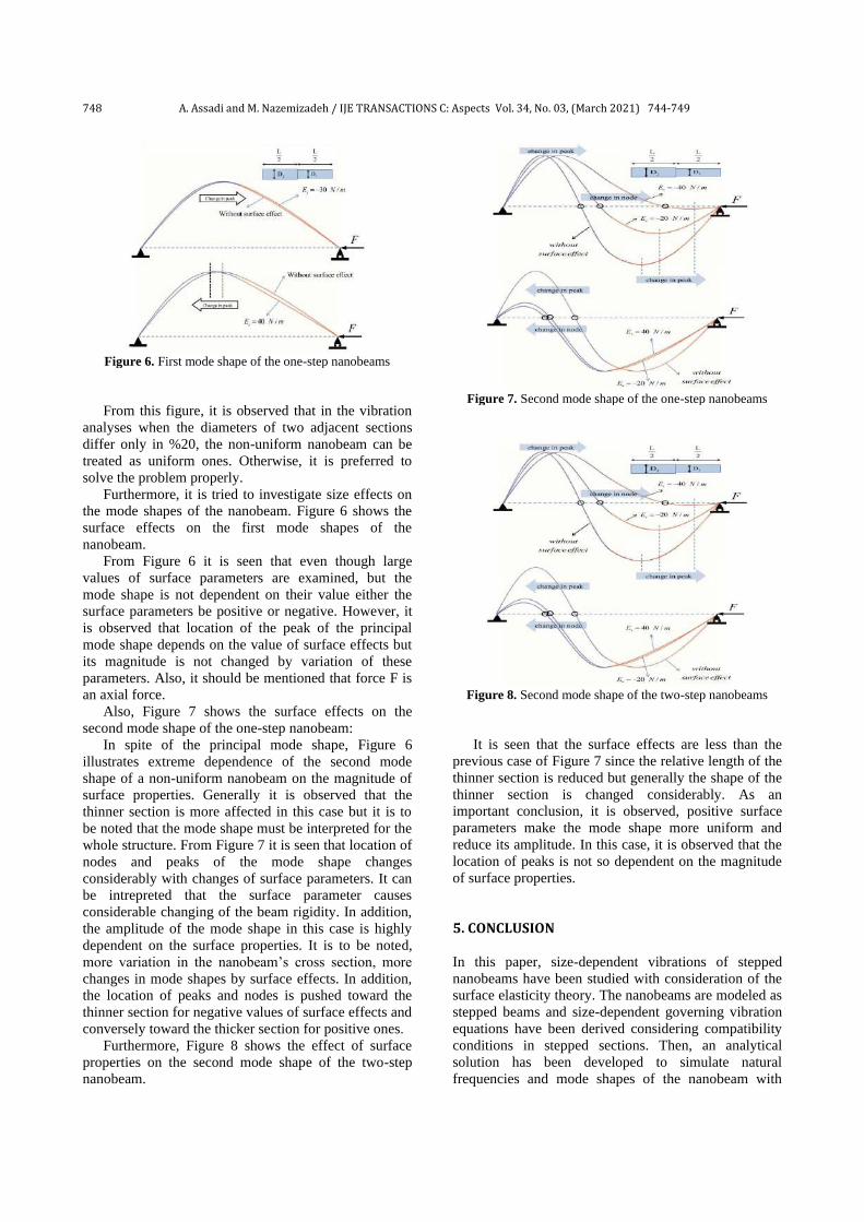
748 A. Assadi and M. Nazemizadeh / IJE TRANSACTIONS C: Aspects Vol. 34, No. 03, (March 2021) 744-749
Figure 6. First mode shape of the one-step nanobeams
From this figure, it is observed that in the vibration
analyses when the diameters of two adjacent sections
differ only in %20, the non-uniform nanobeam can be
treated as uniform ones. Otherwise, it is preferred to
solve the problem properly.
Furthermore, it is tried to investigate size effects on
the mode shapes of the nanobeam. Figure 6 shows the
surface effects on the first mode shapes of the
nanobeam.
From Figure 6 it is seen that even though large
values of surface parameters are examined, but the
mode shape is not dependent on their value either the
surface parameters be positive or negative. However, it
is observed that location of the peak of the principal
mode shape depends on the value of surface effects but
its magnitude is not changed by variation of these
parameters. Also, it should be mentioned that force F is
an axial force.
Also, Figure 7 shows the surface effects on the
second mode shape of the one-step nanobeam:
In spite of the principal mode shape, Figure 6
illustrates extreme dependence of the second mode
shape of a non-uniform nanobeam on the magnitude of
surface properties. Generally it is observed that the
thinner section is more affected in this case but it is to
be noted that the mode shape must be interpreted for the
whole structure. From Figure 7 it is seen that location of
nodes and peaks of the mode shape changes
considerably with changes of surface parameters. It can
be intrepreted that the surface parameter causes
considerable changing of the beam rigidity. In addition,
the amplitude of the mode shape in this case is highly
dependent on the surface properties. It is to be noted,
more variation in the nanobeam’s cross section, more
changes in mode shapes by surface effects. In addition,
the location of peaks and nodes is pushed toward the
thinner section for negative values of surface effects and
conversely toward the thicker section for positive ones .
Furthermore, Figure 8 shows the effect of surface
properties on the second mode shape of the two-step
nanobeam.
Figure 7. Second mode shape of the one-step nanobeams
Figure 8. Second mode shape of the two-step nanobeams
It is seen that the surface effects are less than the
previous case of Figure 7 since the relative length of the
thinner section is reduced but generally the shape of the
thinner section is changed considerably. As an
important conclusion, it is observed, positive surface
parameters make the mode shape more uniform and
reduce its amplitude. In this case, it is observed that the
location of peaks is not so dependent on the magnitude
of surface properties.
5. CONCLUSION
In this paper, size-dependent vibrations of stepped
nanobeams have been studied with consideration of the
surface elasticity theory. The nanobeams are modeled as
stepped beams and size-dependent governing vibration
equations have been derived considering compatibility
conditions in stepped sections. Then, an analytical
solution has been developed to simulate natural
frequencies and mode shapes of the nanobeam with

A. Assadi and M. Nazemizadeh / IJE TRANSACTIONS C: Aspects Vol. 34, No. 03, (March 2021) 744-749 749
various surface properties. The obtained results indicate
that as one section of a step-wised nanobeam gets
shorter; the effect of surface properties on the natural
frequency of the nanobeam reduces considerably. In
addition, the nanobeams with negative surface effects
must be modeled more precisely since their natural
frequency extremely depend on the diameter magnitude.
In fact, proper modeling and choosing the number of
steps plays important roles in proper determination of
the vibration behavior of non-uniform nanobeams.
Moreover, it is seen that the corresponding mode shapes
of the nanobeam in some case are extremely dependent
on the magnitude of surface effects while their
amplitude and locations of nodes and peaks varies a lot
by changes of surface effects. It is observed that the
thinner section is more affected in this case but it is to
be noted that the mode shape must be interpreted for the
whole structure. Finally, the obtained results illustrate
the capability of the proposed method to model and
analyze the size-dependent vibration of the nanobeams
6. REFERENCES
1. Akbari, G., Nikravesh, M., Poladi, A. “Mechanical Properties
and Microstructural Evolution of Ta/TaNx Double Layer Thin Films Deposited by Magnetron Sputtering.” International
Journal of Engineering, Transactions B: Applications, (2017),
Vol. 30, No. 2, 288-293. DOI: 10.5829/idosi.ije.2017.30.02b.16.
2. Mofidian, R., Barati, A., Jahanshahi, M., Shahavi, M. H.
“Generation Process and Performance Evaluation of Engineered
Microsphere Agarose Adsorbent for Application in Fluidized-bed Systems.” International Journal of Engineering,
Transactions B: Applications, (2020), Vol. 33, No. 8, 1450-
1458. DOI: 10.5829/ije.2020.33.08b.02
3. Bagheri, M., Sangpour, P., Badiei, E., Pazouki, M. “Graphene
Oxide Antibacterial Sheets: Synthesis and Characterization
(RESEARCH NOTE).” International Journal of Engineering
Transactions C: Aspects, (2014), Vol. 27, No. 12, 1803-1808.
DOI: 0.5829/idosi.ije.2014.27.12c.01
4. Bakhtiari-Nejad, F., Nazemizadeh, M. “Size-dependent dynamic modeling and vibration analysis of MEMS/NEMS-based
nanomechanical beam based on the nonlocal elasticity theory.”
Acta Mechanica, Vol. 227, No. 5, 1363-1379. DOI:
10.1007/s00707-015-1556-3
5. Korayem, M. H., Taheri, M., Korayem, A. H. “Manipulation with atomic force microscopy: DNA and yeast
micro/nanoparticles in biological environments”, Proceedings of
the Institution of Mechanical Engineers, Part K: Journal of
Multi-body Dynamics, (2014), Vol. 228, No. 4, 414-425. DOI:
10.1177/1464419314542544.
6. Nazemizadeh, M., Bakhtiari-Nejad, F. “Size-dependent free vibration of nano/microbeams with piezo-layered actuators”,
Micro & Nano Letters, (2015), Vol. 10, No. 2, 93-98. DOI:
10.1049/mnl.2014.0317
7. Nazemizadeh, M., Bakhtiari-Nejad, F., “A general formulation
of quality factor for composite micro/nano beams in the air environment based on the nonlocal elasticity theory”, Composite
Structures, (2015), Vol. 132, 772-783. DOI:
10.1016/j.compstruct.2015.05.070
8. Beni, Y. T. “A nonlinear electro-mechanical analysis of
nanobeams based on the size-dependent piezoelectricity theory”.
Journal of Mechanics, (2017), Vol. 33, No. 3, 289-301. DOI:
10.1017/jmech.2016.65.
9. Nazemizadeh, M., Bakhtiari-Nejad, F., Assadi, A., Shahriari, B.,
“Size-dependent nonlinear dynamic modeling and vibration analysis of piezo-laminated nanomechanical resonators using
perturbation method”, Archive of Applied Mechanics, (2020), 1-
14. DOI: 10.1007/s00419-020-01678-3
10. Nazemizadeh, M., Bakhtiari-Nejad, F., Assadi, A. Shahriari, B.,
“Nonlinear vibration of piezoelectric laminated nanobeams at
higher modes based on nonlocal piezoelectric theory” Acta
Mechanica, (2020), Vol. 231, No. 10, 4259-4274. DOI:
10.1007/s00707-020-02736-1
11. Gurtin, M. E., Murdoch, A. I. “A continuum theory of elastic material surfaces”. Archive for Rational Mechanics and
Analysis, (1975), Vol. 57, No. 4, 291-323. DOI:
10.1007/BF00261375
12. Jiang, L. Y., Yan, Z. “Timoshenko beam model for static
bending of nanowires with surface effects”, Physica E: Low-
dimensional Systems and Nanostructures, (2010), Vol. 42, No.
9, 2274-2279. DOI: 10.1016/j.physe.2010.05.007
13. Farshi, B., Assadi, A., Alinia-Ziazi, A. “Frequency analysis of
nanotubes with consideration of surface effects”, Applied
Physics Letters, (2010), Vol. 96. No. 9, 093105. DOI:
10.1063/1.3332579
14. Assadi, A., Nazemizadeh, M. “Size effects on stability and self-instability of non-uniform nanobeams with consideration of
surface effects” Micro & Nano Letters, (2020), Vol. 15, No. 12,
858-862. DOI: 10.1049/mnl.2020.0262
15. He, J., Lilley, C. M. “Surface effect on the elastic behavior of
static bending nanowires”. Nano Letters, (2008), Vol. 8, No. 7,
1798-1802. DOI: 10.1021/nl0733233
Persian Abstract
چکیده ای مدلسازی شده پردازد. برای این منظور، نانوتیر به عنوان تیر پلهاین مقاله به بررسی ارتعاش وابسته به ابعاد نانوتیرهای پله ای با در نظر گرفتن تئوری االستیسیته سطحی می
انسهای طبیعی و شکل مودهای نانوتیر با در نظر آید. سپس یک حل تحلیلی برای شبیه سازی فرکسازگاری بدست می ت حاکم ارتعاشی آن با در نظر گرفتن شرایطالد و معا
شود. نتایج نشان شود. همچنین، یک رویکرد بازگشتی برای صحت سنجی نتایج و محاسبه مدول االستیسیته وابسته به ابعاد پیشنهاد میگرفتن اثرات سطح، گسترش داده می
نس طبیعی نانوتیر غیریکنواخت دارد. همچنین، برخالف تیرهای یکنواخت، شکل مودهای نانوتیرهای ها، اثر چشمگیری بر فرکادهد که اثرات سطح و انتخاب مناسب پلهمی
غیریکنواخت به شدت وابسته به اثرات سطح است.

IJE TRANSACTIONS C: Aspects Vol. 34, No. 03, (March 2021) 750-755
Please cite this article as: M. A. Guzev, E. V. Kozhevnikov, M. S. Turbakov, E. P. Riabokon, V. V. Poplygin, Experimental Investigation of the Change of Elastic Moduli of Clastic Rocks under Nonlinear Loading, International Journal of Engineering, Transactions C: Aspects Vol. 34, No. 03, (2021) 750-755
International Journal of Engineering
J o u r n a l H o m e p a g e : w w w . i j e . i r
Experimental Investigation of the Change of Elastic Moduli of Clastic Rocks under
Nonlinear Loading
M. A. Guzev, E. V. Kozhevnikov*, M. S. Turbakov, E. P. Riabokon, V. V. Poplygin Department of Oil and Gas Technologies, Perm National Research Polytechnic University, Russia
P A P E R I N F O
Paper history: Received 29 October 2020 Received in revised form 26 December 2020 Accepted 18 January 2021
Keywords: Nonlinear Dynamic Loads Clastic Rock Elastic Moduli Dispersion
A B S T R A C T
This paper presents an experimental investigation on the nonlinear nature of the dynamic geomechanical
characteristics of a clastic rock (sandstone). Rock samples of 7.5 mm in diameter and 15.6 mm in length
were prepared. Rock properties were identified. Firstly, the limits of the rock linear elasticity zone were defined during quasistatic loading and uniaxial compressive strength determination at the Tinius
Hounsfield rig. Secondly, the small experimental custom-built rig was designed to study the nonlinear
nature of the Young’s modulus in the zone of linear elasticity. At the rig the sample was stationary preloaded. The dynamic load was generated by a piezoelectric actuator powered with a signal generator.
The displacement of rock sample surfaces was recorded by a laser sensor and an eddy current probe. The
dynamic experiments were conducted at the load amplitude ranging from 50 to 250 N for each of frequencies of 25 Hz and 40 Hz. It was found that the dynamic Young’s modulus increased with
amplitude for all the frequencies studied. The newly developed experimental rig allows to investigate
elastic moduli dispersion of rocks at the strain up to 10-3 under vibrations with frequency up to 40 Hz.
doi: 10.5829/ije.2021.34.03c.21
NOMENCLATURE
d Sample’s diameter (m) l0 Sample’s length at preloading (m)
d0 Sample’s diameter at preloading (m) t Time (s)
E Young’s modulus (GPa) ε Strain
Edyn Dynamic Young’s modulus (GPa) εax Axial strain
f Frequency of the dynamic load (Hz) εrad Radial strain
Fdyn Dynamic load (N) ν Poisson’s ratio
Fmax Maximum load applied to a sample (N) σ Stress (MPa)
Fmin Minimum load applied to a sample (N) σlim.low Lower limit of the linear elasticity zone (MPa)
Fst Preload value (N) σlim.up Upper limit of the linear elasticity zone (MPa)
l Sample’s length (m) σUCS av. Average uniaxial compressive strength (MPa)
1. INTRODUCTION1
Elastic moduli of rocks are not constant and have
nonlinear nature under the influence of the dynamic
loading [1]. The phenomenon of the dispersion of elastic
moduli under vibrations is considered while geotechnical
engineering in such fields as mining [2], modelling the
tunnels constructed in liquefiable soil rock [3], cutting
*Corresponding Author Email: [email protected] (E. V.
Kozhevnikov)
and blasting [4, 5], construction in limestone sands [6],
well drilling and completion [7] and reservoir
engineering [8]. Experimental studies of clastic rocks
elastic moduli dispersion can be differentiated in two
groups in accordance with rock saturation during the
investigation. In the first group, dynamic elastic moduli
are studied on rocks saturated with a fluid (e.g., brine). A
study of Opalinus clay in literature [9, 10] and Mancos

M. A. Guzev et al. / IJE TRANSACTIONS C: Aspects Vol. 34, No. 03, (March 2021) 750-755 751
shale by Szewczyk et al. [11], showed an increase in the
Young’s modulus and a decrease in Poisson’s ratio with
an increase in frequency of the dynamic loading from 1
to 100 Hz at the strain of 10-6. Similar dispersion of the
Young’s modulus was also reported in literature [12, 13]
for Fontainebleau sandstone for frequency ranging from
1 to 100 Hz at the strain lower than 10-5. An increase in
Young’s modulus was also reported in literature [14]
while studying the Berea sandstone in the range of
frequencies from 1 to 100 Hz. A schematic nonlinear
relation among clastic rock elastic moduli and load
frequency is given by Batzle et al. [15]. A strong
frequency and rate amplitude dependent elastic behavior
over variety of sandstones was reported in literature [16].
Based on these and other works, a number of poroelastic
mechanisms have been proposed and modelled on the
nonlinear nature of the Young’s modulus while studying
saturated rocks. Those models characterize in saturated
porous media global inertia mechanisms [17], local
mechanisms [18, 19], both global and local mechanisms
[20] and other (see literature [21]).
In the second group, the studies are performed on dry
rocks. It was exhibited in literature [22] that with an
increase of frequency from 1 to 100 Hz for samples with
a strain range between 10-8 and 10-6, the Young’s
modulus and Poisson’s ratio of Donnybrook sandstone
are nearly constant, i.e. no dispersion of the Young’s
modulus is observed. Earlier, it was reported in literature
[23] that Young’s moduli of Navajo sandstone, Spergen
limestone and Oklahoma granite do not depend on
frequency of the dynamic loading at the strain of 10-7 in
the frequency range from 4 to 400 Hz. Similarly, studies
conducted by Winkler [24] on vacuum dry sandstones
Massilon, Berea and Boise at frequencies up to 0.1 MHz
did not reveal any relationship between attenuation and
frequency at small strain, which is also relevant for man-
made rocks with no intergranular cement. However, the
phenomenon of dispersion of elastic moduli in dry clastic
rocks is still exists and can be captured by hysteresis loop
on the strain–stress diagram as shown in literature [16].
Manifestation of dispersion in dry clastic rocks is
accompanied by the phenomenon when the dynamic
Young’s modulus exceeds the static one which is directly
related to a strain rate and a loading path [25, 26]. There
is a number of models designed to describe the nature of
dynamic elastic characteristics observed under high
strain by, for example, inertial approach (see literature
[27]). Nevertheless, the mechanism of the dynamic
dispersion of elastic moduli under vibrations is still open
for research.
Since the standard loading rigs allow us to perform
linear loading of rocks at frequency ranging from 0.1 to
2 Hz and strain up to 10-3 [26-28], it is practically not
possible to use such the rigs to study the effect of
nonlinear dynamic loads (vibrations) on rocks. As is
shown in literature [4, 29] studying of the dynamic elastic
characteristics of rocks at high strain is limited by the
complexity of experiments and data processing. It is
possible to study the effect of nonlinear dynamic loads on
rocks in the range of seismic frequencies from 1 to 100
Hz at the strain of 10-8..10-6 using custom-built
experimental set-ups, described in literature [10, 12, 15,
30-32]. Recently, Borgomano et al. [33] have built the
experimental apparatus able to measure the dynamic rock
elastic characteristics at frequencies up to 1 kHz and
strain up to 10-5. However, considering that during
mining (e.g., well drilling and perforation [34]) the rocks
experience much higher strain (≥ 10-2) the capacity
expansion of existing rigs is required. Studying of the
effect of significant dynamic loads up to 101-104 is
possible using the Kolsky-Hopkinson bar machines [35,
36], but those machines do not allow to create cyclic
(harmonic) loads on rock samples. Therefore, to study the
elastic moduli under high strain nonlinear dynamic loads
new experimental techniques are necessary. The aim of
this paper is to study the nonlinear nature of the dynamic
elastic moduli of a dry clastic rock being in the zone of
the linear elasticity using a small custom-built
experimental rig.
The paper is organized as follows. In Section 2, the
experimental methodology, details on samples
preparation procedure, quasistatic and nonlinear dynamic
experiments are described. The obtained experimental
results and its discussion are given in Section 3, followed
by the conclusion in Section 4.
2. MATERIALS AND METHODS 2. 1. Description of Rock Samples A clastic
Permian age rock (sandstone) was used for this study.
The properties of the rock are given in Table 1 and Figure
1. Each sample was 7.5 mm in diameter d and 15.6 mm
in length l. The samples were prepared in accordance
with industrial standards [37, 38].
TABLE 1. Properties of the studied rock
Property Value Study rig
Porosity, fr. units 11.7 Helium porosimeter
PHI-220
Gas permeability, 𝜇m2 0.353 Benchtop Permeability
Sistem BPS-805
Pore size, mm 0.02-0.24
Microfocus X-ray
tomography rig, Nikon
Metrology XT H 225
Pore distribution uniform
Fracturing no
X-ray density
composition
nonuniform (0.05
mm high-density
inclusions)

752 M. A. Guzev et al. / IJE TRANSACTIONS C: Aspects Vol. 34, No. 03, (March 2021) 750-755
Figure 1. Characteristics of the prepared samples: (a) a
photograph depicting a sandstone sample; (b) a sample’s pore
space model; (с) a diagram for pore distribution
Using diamond drill bits Tacklife AHS02C the
samples were cored form rock blocks with water flush,
then cut, washed and dried. In total there were 18 samples
prepared. For both quasistatic tests and dynamic
experiments there were 9 samples used in order to ensure
reliable results.
2. 2. Methodology of Nonlinear Loading Since
the elastic moduli, and the dynamic ones in particular,
have to be studied in the state when a rock experiences
elastic deformation (the Young’s modulus can be
determined as 𝐸 = 𝜎/ε𝑙) the limits of the linear elasticity
zone should be defined prior to the dynamic experiments.
In order to obtain the repeatable dependencies of elastic
moduli the experiments on nonlinear dynamic loading
were performed on 9 samples (Figure 2). Elastic limits of the studied clastic rock were defined
during quasistatic loading of prepared samples at the
Tinius Hounsfield rig. Quasistatic loading was performed
at the loading rate of displacement plate of 0.05 mm/min.
As a result, the standard diagram of loading–displacement
was obtained for all the samples tested which comprised
compaction, elastic deformations, irreversible
deformations and fracture. Figure 3 shows the limits of the
linear elasticity zone equal to 𝜎𝑙𝑖𝑚.𝑙𝑜𝑤 = 10.2 MPa and
𝜎𝑙𝑖𝑚.𝑢𝑝 = 31.7 MPa defined as average values of limits of
the linear section according to literature [39].
After the elasticity zone being determined in order to
study the nonlinear behaviour of elastic moduli under
dynamic loads at the strain up to 10-3 the small
experimental rig was built. In the rig (see Figure 4) the
rock sample was installed at a load table, below which
load sensor Kistler 9027C was mounted. There was a
piezoelectric actuator Extrema Model 250µ located on top
of the sample through the metal dist. Above the actuator
there was a static load ensuring sample’s preloaded
(compacted) state. The actuator was powered with a
signal generator Manual MOS-01 able to set the
amplitude and frequency of the actuator operation and
produce axial-stress oscillations.
During the dynamic experiment the sample was
experiencing stationary load Fst equal to 700 N and
periodic dynamic load Fdyn the amplitude of which was
varied between 50 N and 250 N at two frequencies f such
as 25 Hz to 40 Hz. At stationary load Fst the sample’s
length was equal to l0 and sample’s diameter was equal to
d0 (see Figure 5). The largest Fmax=Fst+Fdyn.max and the
smallest Fmin=Fst-Fdyn.min load applied to a sample
corresponded to maximum distance between the sensors
and samples top and side surfaces (see Figure 4) and
consequently the sample’s strain. The radial displacement
Figure 2. Prepared nine samples of a clastic rock
Figure 3. The zone of linear elasticity determined during UCS
tests of nine samples
Figure 4. A clastic rock sample at the small experimental rig
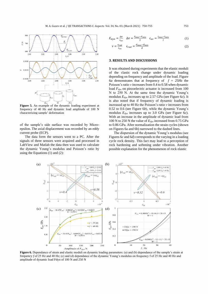
M. A. Guzev et al. / IJE TRANSACTIONS C: Aspects Vol. 34, No. 03, (March 2021) 750-755 753
Figure 5. An example of the dynamic loading experiment at
frequency of 40 Hz and dynamic load amplitude of 100 N
characterizing sample’ deformation
of the sample’s side surface was recorded by Micro-
epsilon. The axial displacement was recorded by an eddy
current probe (ECP).
The data form the sensors went to a PC. After the
signals of three sensors were acquired and processed in
LabView and Matlab the data then was used to calculate
the dynamic Young’s modulus and Poisson’s ratio by
using the Equations (1) and (2):
𝐸𝑑𝑦𝑛 =𝛥𝜎
𝜀𝑎𝑥 𝛥𝜎 =
𝐹𝑚𝑎𝑥−𝐹𝑚𝑖𝑛
𝑆 𝜀𝑎𝑥 =
𝑙𝑚𝑎𝑥−𝑙𝑚𝑖𝑛
𝑙 (1)
𝜈 =𝜀𝑟𝑎𝑑
𝜀𝑎𝑥 𝜀𝑟𝑎𝑑 =
𝑑𝑚𝑎𝑥−𝑑𝑚𝑖𝑛
𝑑 (2)
3. RESULTS AND DISCUSSIONS
It was obtained during experiments that the elastic moduli
of the clastic rock change under dynamic loading
depending on frequency and amplitude of the load. Figure
6a demonstrates that at frequency of f = 25Hz the
Poisson’s ratio ν increases from 0.4 to 0.58 when dynamic
load Fdyn on piezoelectric actuator is increased from 100
N to 250 N. At the same time the dynamic Young’s
modulus Edyn increases up to 2.57 GPa (see Figure 6c). It
is also noted that if frequency of dynamic loading is
increased up to 40 Hz the Poisson’s ratio ν increases from
0.52 to 0.6 (see Figure 6b), while the dynamic Young’s
modulus Edyn increases up to 3.0 GPa (see Figure 6c).
With an increase in the amplitude of dynamic load from
100 N to 250 N the value of Edyn increased from 0.75 GPa
to 0.86 GPa. After normalization the strain cycles (shown
on Figures 6a and 6b) narrowed to the dashed lines.
The dispersion of the dynamic Young’s modulus (see
Figures 6c and 6d) corresponds to the varying in a loading
cycle rock density. This fact may lead to a perception of
rock hardening and softening under vibration. Another
possible explanation for the phenomenon of rock elastic
Figure 6. Dependance of strain and elastic moduli on dynamic loading parameters: (a) and (b) dependance of the sample’s strain at
frequency f of 25 Hz and 40 Hz; (c) and (d) dependance of the dynamic Young’s modulus on frequency f of 25 Hz and 40 Hz and
amplitude of dynamic load Fdyn of 100 N and 250 N

754 M. A. Guzev et al. / IJE TRANSACTIONS C: Aspects Vol. 34, No. 03, (March 2021) 750-755
moduli dispersion under high strain vibrations can be
inertial resistance of the rock to the dynamic load applied.
However, the experimental results represent a basis
for further elastic moduli mathematical models’
formulations. The phenomenon of dispersion of the
dynamic elastic moduli under high strain vibrations has
to be conceptualized, and further developed
mathematical models needs to be verified. 4. CONCLUSION
In this work, we present the results of investigation of the
nonlinear nature of clastic rock (sandstone) elastic moduli
obtained during the series of experiments. The
investigation was conducted in two phases. First, the
limits of the zone of linear elasticity of samples of 7.5 mm
in diameter were determined in quasistatic loading. Then,
at the second stage, the experiments on dynamic loading
were performed with help of a custom-built small
experimental rig. During the course of dynamic loading
experiments elastic properties were studied at two
frequencies f such as 25 Hz and 40 Hz. At both these
frequencies amplitude of nonstationary load varied from
50 N to 250 N. The nonlinear nature of the Poisson’s ratio
and the dynamic Young’s modulus was revealed as a
result of the study. The dispersion of elastic moduli values
under dynamic loading was observed at each amplitude of
the load for both frequencies at the strain up to 10-3. The
obtained results confirm the nonlinear nature of the
dynamic elastic moduli of a clastic rock shown in the
similar mentioned researches on dry rocks but at smaller
strain. The newly developed experimental rig allows to
investigate elastic moduli dispersion of rocks at the strain
up to 10-3 under vibrations with frequency up to 40 Hz.
5. ACKNOWLEDGEMENTS
This work was financially supported by the Russian
Science Foundation (project No. 19-19-00408).
6. REFERENCES
1. He, M., Li, N., “Experimental research on the non-linear energy
characteristics of granite and sandstone”, Géotechnique Letters,
Vol. 10, No. 3, (2020), 385-392. doi: 10.1680/jgele.19.00117
2. Geranmayeh Vaneghi, R., Ferdosi, B., Okoth, A. D., Kuek, B.,
“Strength degradation of sandstone and granodiorite under uniaxial cyclic loading”, Journal of Rock Mechanics and
Geotechnical Engineering, Vol. 10, No. 1, (2018), 114-126. doi:
10.1016/j.jrmge.2017.09.005
3. Marandi, S. M., Rasti, A. R., “Parametric study of the covering
soil of tunnels constructed in liquefiable soil”, International
Journal of Engineering, Transactions A: Basics, Vol. 25, No. 4,
(2012), 375-388.
4. Xia, K., Yao, W., Wu, B., “Dynamic rock tensile strengths of Laurentian granite: Experimental observation and micromechanical model”, Journal of Rock Mechanics and Geotechnical Engineering, Vol. 9, No. 1, (2017), 116-124. doi: 10.1016/j.jrmge.2016.08.007
5. Jiang, Y.-Z., He, K.-F., Dong, Y.-L., Yang, D.-L., Sun, W., “Influence of load weight on dynamic response of vibrating screen”, Shock and Vibration, Vol. 2019, (2019), 4232730. doi: 10.1155/2019/4232730
6. Lv, Y., Liu, J., Xiong, Z., “One-dimensional dynamic compressive behavior of dry calcareous sand at high strain rates”, Journal of Rock Mechanics and Geotechnical Engineering, Vol. 11, No. 1, (2019), 192-201. doi: 10.1016/j.jrmge.2018.04.013
7. LeCompte, B., Franquet, J. A., Jacobi, D., “Evaluation of Haynesville Shale vertical well completions with a mineralogy based approach to reservoir geomechanics”, in SPE Annual Technical Conference and Exhibition 2009, Vol. 3, (2009), 1417-1430. doi: 10.2118/124227-ms
8. Behnoud far, P., Hassani, A. H., Al-Ajmi, A. M., Heydari, H., “A novel model for wellbore stability analysis during reservoir depletion”, Journal of Natural Gas Science and Engineering, Vol. 35, (2016), 935-943. doi: 10.1016/j.jngse.2016.09.051
9. Lozovyi, S., Bauer, A., “Static and dynamic stiffness measurements with Opalinus Clay”, Geophysical Prospecting, Vol. 67, No. 4, (2018), 997-1019. doi: 10.1111/1365-2478.12720
10. Lozovyi, S., Bauer, A., “From static to dynamic stiffness of shales: Frequency and stress dependence”, Rock Mechanics and Rock Engineering, Vol. 52, (2019), 5085-5098. doi: 10.1007/s00603-019-01934-1
11. Szewczyk, D., Bauer, A., Holt, R. M., “A new laboratory apparatus for the measurement of seismic dispersion under deviatoric stress conditions”, Geophysical Prospecting, Vol. 64, No. 4, (2016), 789-798. doi: 10.1111/1365-2478.12425
12. Pimienta, L., Fortin, J., Guéguen, Y., “Bulk modulus dispersion and attenuation in sandstones”, Geophysics, Vol. 80, No. 2, (2015), A25-A30. doi: 10.1190/geo2014-0335.1
13. Pimienta, L., Fortin, J., Guéguen, Y., “Effect of fluids and frequencies on Poisson’s ratio of sandstone samples”, Geophysics, Vol. 81, No. 2, (2016), D183-D195. doi: 10.1190/geo2015-0310.1
14. Tisato, N., Quintal, B., “Measurements of seismic attenuation and transient fluid pressure in partially saturated Berea sandstone: Evidence of fluid flow on the mesoscopic scale”, Geophysical Journal International, Vol. 195, (2013), 342-351. doi: 10.1093/gji/ggt259
15. Batzle, M. L., Han, D.-H., Hofmann, R., “Fluid mobility and frequency-dependent seismic velocity - Direct measurements”, Geophysics, Vol. 71, No. 1, (2006), N1-N9. doi: 10.1190/1.2159053
16. Tutuncu, A. N., Podio, A. L., Gregory, A. R., Sharma, M. M., “Nonlinear viscoelastic behavior of sedimentary rocks, Part I: Effect of frequency and strain amplitude”, Geophysics, Vol. 63, No. 1, (1998), 184-194. doi: 10.1190/1.1444311
17. Biot, M. A., “Theory of propagation of elastic waves in a fluid-saturated porous solid II. Higher frequency range”, The Journal of the Acoustical Society of America, Vol. 28, No. 179, (1956), 179-191. doi: 10.1121/1.1908241
18. O’Connell, R. J., Budiansky, B., “Viscoelastic properties of fluid‐saturated cracked solids”, Journal of Geophysical Research, Vol. 82, No. 36, (1977), 5719-5735. doi: 10.1029/JB082i036p05719
19. Mavko, G., Nur, A., “Melt squirt in the asthenosphere”, Journal of Geophysical Research, Vol. 80, No. 11, (1975), 1444-1448. doi: 10.1029/JB080i011p01444

M. A. Guzev et al. / IJE TRANSACTIONS C: Aspects Vol. 34, No. 03, (March 2021) 750-755 755
20. Dvorkin, J., Nur, A., “Dynamic poroelasticity: a unified model with the squirt and the Biot mechanisms”, Geophysics, Vol. 58, No. 4, (1993), 524-533. doi: 10.1190/1.1443435
21. Müller, T. M., Gurevich, B., Lebedev, M., “Seismic wave attenuation and dispersion resulting from wave-induced flow in porous rocks: A review”, Geophysics, Vol. 75, No. 5, (2010), X75A147-75A164. doi: 10.1190/1.3463417
22. Mikhaltsevitch, V., Lebedev, M., Gurevich, B., “A laboratory study of the elastic and anelastic properties of the sandstone flooded with supercritical CO2 at seismic frequencies”, Energy Procedia, Vol. 63, (2014), 4289-4296. doi: 10.1016/j.egypro.2014.11.464
23. Spencer Jr, J. W., “Stress relaxations at low frequencies in fluid-saturated rocks: attenuation and modulus dispersion”, Journal of Geophysical Research, Vol. 86, No. B3, (1981), 1803-1812. doi: 10.1029/JB086iB03p01803
24. Winkler, K. W., “Frequency dependent ultrasonic properties of high-porosity sandstones”, Journal of Geophysical Research, Vol. 88, No. B11, (1983), 9493-9499. doi: 10.1029/JB088iB11p09493
25. Peng, K., Zhou, J., Zou, Q., Song, X., “Effect of loading frequency on the deformation behaviours of sandstones subjected to cyclic loads and its underlying mechanism”, International Journal of Fatigue, Vol. 131, (2020), 105349. doi: 10.1016/j.ijfatigue.2019.105349
26. Khosroshahi, A. A., Sadrnejad, S. A., “Substructure model for concrete behavior simulation under cyclic multiaxial loading”, International Journal of Engineering, Transactions A: Basics, Vol. 21, No. 4, (2008), 329-346.
27. Zhang, Q. B., Zhao, J., “A review of dynamic experimental techniques and mechanical behaviour of rock materials”, Rock Mechanics and Rock Engineering, Vol. 47, (2014), 1411-1478. doi: 10.1007/s00603-013-0463-y
28. Zheng, Q., Liu, E., Sun, P., Liu, M., Yu, D., “Dynamic and damage properties of artificial jointed rock samples subjected to cyclic triaxial loading at various frequencies”, International Journal of Rock Mechanics and Mining Sciences, Vol. 128, (2020), 104243. doi: 10.1016/j.ijrmms.2020.104243
29. Subramaniyan, S., Quintal, B., Tisato, N., Saenger, E. H., Madonna, C., “An overview of laboratory apparatuses to measure seismic attenuation in reservoir rocks”, Geophysical Prospecting, Vol. 62, (2014), 1211-1223. doi: 10.1111/1365-2478.12171
30. Szewczyk, D., Holt, R. M., Bauer, A., “The impact of saturation on seismic dispersion in shales - laboratory measurements”, Geophysics, Vol. 83, No. 1, (2018), 15-34. doi 10.1190/geo20 17-0169.1
31. Tisato, N., Madonna, C., “Attenuation at low seismic frequencies in partially saturated rocks: Measurements and description of a new apparatus”, Journal of Applied Geophysics, Vol. 86, (2012), 44-53. doi: 10.1016/j.jappgeo.2012.07.008
32. Szewczyk, D., Bauer, A., Holt, R. M., “A new laboratory apparatus for the measurement of seismic dispersion under deviatoric stress conditions”, Geophysical Prospecting, 64, (2016), 789-798. doi: 10.1111/1365-2478.12425
33. Borgomano, J. V. M., Gallagher, A., Sun, C., Fortin, J., “An apparatus to measure elastic dispersion and attenuation using hydrostatic- and axial-stress oscillations under undrained conditions”, Review of Scientific Instruments, Vol. 91, No. 3, (2020), 034502. doi: 10.1063/1.5136329
34. Riabokon, E., Turbakov, M., Kozhevnikov, E., Poplygin, V., Wiercigroch, M., “Rock Fracture During Oil Well Perforation”, Lecture Notes in Mechanical Engineering, (2020), 185-192. doi: 10.1007/978-3-030-49882-5_18
35. Yan, Z., Dai, F., Liu, Y., Du, H., “Experimental investigations of the dynamic mechanical properties and fracturing behavior of cracked rocks under dynamic loading”, Bulletin of Engineering Geology and the Environment, Vol. 79, No. 10, (2020), 5535-5552. doi: 10.1007/s10064-020-01914-8
36. Li, X. B., Lok, T. S., Zhao, J., “Dynamic characteristics of granite subjected to intermediate loading rate”, Rock Mechanics and Rock Engineering, Vol. 38, No. 1, (2005), 21-39. doi: 10.1007/s00603-004-0030-7
37. ASTM (2001). ASTM D4543: Standard practices for preparing rock core specimens and determining dimensional and shape tolerances. West Conshohocken, PA, USA: ASTM International.
38. Brown E. T. Suggested Methods for Determining the Uniaxial Compressive Strength and Deformability of Rock Materials. ISRM. Brown E. T., editor. Oxford: Pergamon Press; 1981.
39. Jaeger, J. C., Cook, N. G. W., Zimmerman, R. W. Laboratory testing of rocks. In Fundamentals of Rock Mechanics, 4th ed.; Blackwell Publishing: Malden, MA, USA, 2007, 145-167.
Persian Abstract
چکیده و طول 7.5سنگهای قطر در این مقاله یک تحقیق تجربی در مورد ماهیت غیر خطی ویژگی های ژئومکانیکی دینامیکی یک سنگ آواری )ماسه سنگ( ارائه شده است. نمونه
ک و تعیین مقاومت فشاری تک محوری میلی متر تهیه شد. خواص سنگ شناسایی شد. در مرحله اول ، محدوده منطقه کشش خطی سنگ در هنگام بارگذاری کوآیستاتی 6.6
در منطقه کشش خطی طراحی Youngتعریف شد. در مرحله دوم ، دکل کوچک سفارشی ساخته شده برای آزمایش ماهیت غیرخطی مدول Tinius Hounsfieldدر دکل
یک مولد سیگنال تغذیه می کند تولید شد. جابجایی سطوح نمونه سنگ شده است. در دکل نمونه از قبل ثابت مانده بود. بار دینامیکی توسط یک محرک پیزوالکتریک که از
هرتز انجام شد. 40هرتز و 25برای هر یک از فرکانس های N 250تا 50توسط یک سنسور لیزر و یک پروب جریان گردابی ثبت شد. آزمایش های پویا در دامنه بار از
انسهای مورد مطالعه افزایش می یابد. دکل آزمایشی تازه توسعه یافته امکان بررسی پراکندگی مدول االستیک سنگها را مشخص شد که مدول جوان پویا با دامنه برای تمام فرک
کند هرتز فراهم می 40تحت ارتعاشات با فرکانس تا 3-10در فشار تا

AIMS AND SCOPE
The objective of the International Journal of Engineering is to provide a forum for communication of information among the world's scientific and technological community and Iranian scientists and engineers. This journal intends to be of interest and utility to researchers and practitioners in the academic, industrial and governmental sectors. All original research contributions of significant value focused on basics, applications and aspects areas of engineering discipline are welcome.
This journal is published in three quarterly transactions: Transactions A (Basics) deal with the engineering fundamentals, Transactions B (Applications) are concerned with the application of the engineering knowledge in the daily life of the human being and Transactions C (Aspects) - starting from January 2012 - emphasize on the main engineering aspects whose elaboration can yield knowledge and expertise that can equally serve all branches of engineering discipline.
This journal will publish authoritative papers on theoretical and experimental researches and advanced applications embodying the results of extensive field, plant, laboratory or theoretical investigation or new interpretations of existing problems. It may also feature - when appropriate - research notes, technical notes, state-of-the-art survey type papers, short communications, letters to the editor, meeting schedules and conference announcements. The language of publication is English. Each paper should contain an abstract both in English and in Persian. However, for the authors who are not familiar with Persian, the publisher will prepare the latter. The abstracts should not exceed 250 words.
All manuscripts will be peer-reviewed by qualified reviewers. The material should be presented clearly and concisely: • Full papers must be based on completed original works of significant novelty. The papers are not strictly limited in length. However,
lengthy contributions may be delayed due to limited space. It is advised to keep papers limited to 7500 words. • Research notes are considered as short items that include theoretical or experimental results of immediate current interest. • Technical notes are also considered as short items of enough technical acceptability with more rapid publication appeal. The length
of a research or technical note is recommended not to exceed 2500 words or 4 journal pages (including figures and tables). Review papers are only considered from highly qualified well-known authors generally assigned by the editorial board or editor in
chief. Short communications and letters to the editor should contain a text of about 1000 words and whatever figures and tables that may be required to support the text. They include discussion of full papers and short items and should contribute to the original article by providing confirmation or additional interpretation. Discussion of papers will be referred to author(s) for reply and will concurrently be published with reply of author(s).
INSTRUCTIONS FOR AUTHORS
Submission of a manuscript represents that it has neither been published nor submitted for publication elsewhere and is result of research carried out by author(s). Presentation in a conference and appearance in a symposium proceeding is not considered prior publication. Authors are required to include a list describing all the symbols and abbreviations in the paper. Use of the international system of measurement units is mandatory.
• On-line submission of manuscripts results in faster publication process and is recommended. Instructions are given in the IJE web sites: www.ije.ir-www.ijeir.info
• Hardcopy submissions must include MS Word and jpg files. • Manuscripts should be typewritten on one side of A4 paper, double-spaced, with adequate margins. • References should be numbered in brackets and appear in sequence through the text. List of references should be given at the end of
the paper. • Figure captions are to be indicated under the illustrations. They should sufficiently explain the figures. • Illustrations should appear in their appropriate places in the text. • Tables and diagrams should be submitted in a form suitable for reproduction. • Photographs should be of high quality saved as jpg files. • Tables, Illustrations, Figures and Diagrams will be normally printed in single column width (8cm). Exceptionally large ones may be
printed across two columns (17cm).
PAGE CHARGES AND REPRINTS
The papers are strictly limited in length, maximum 6 journal pages (including figures and tables). For the additional to 6 journal pages, there will be page charges. It is advised to keep papers limited to 3500 words.
Page Charges for Papers More Than 6 Pages (Including Abstract)
For International Author *** $55 / per page
For Local Author 100,000 Toman / per page
AUTHOR CHECKLIST
• Author(s), bio-data including affiliation(s) and mail and e-mail addresses). • Manuscript including abstracts, key words, illustrations, tables, figures with figure captions and list of references. • MS Word files of the paper.
International Journal of Engineering, P.O. Box 13145-1659, Tehran, I.R. Iran
Materials and Energy Research Center, 5 Ahuramazda St., Alvand Ave., Argentina Sq., Tehran, Islamic Republic of Iran www.merc.ac.ir - www.emerc.ac.ir


![Vincentiana Vol. 29, No. 2-3 [Full Issue] - Via Sapientiae](https://static.fdokumen.com/doc/165x107/631e53945ff22fc74506a45c/vincentiana-vol-29-no-2-3-full-issue-via-sapientiae.jpg)