arX

iv:m

ath-

ph/0

6030

03v2

3 M

ar 2

006

Free energy topological expansion for the

2-matrix model

L. Chekhov,∗

Steklov Mathematical Institute, ITEP, and Poncelet Laboratoire, Moscow, Russia

B. Eynard,†and N. Orantin ‡

Service de Physique Theorique de Saclay,

F-91191 Gif-sur-Yvette Cedex, France.

SPhT-T06/016ITEP/TH-05/06

Abstract

We compute the complete topological expansion of the formal hermitian two-matrix model. For this, we refine the previously formulated diagrammatic rulesfor computing the 1

Nexpansion of the nonmixed correlation functions and give a

new formulation of the spectral curve. We extend these rules obtaining a closedformula for correlation functions in all orders of topological expansion. We thenintegrate it to obtain the free energy in terms of residues on the associatedRiemann surface.

1 Introduction

Matrix models is a fascinating topic unifying many otherwise seemingly unrelateddisciplines, including integrable systems, conformal theories, topological expansion,etc [33,14]. However, only recently the understanding came that geometry itself playsa crucial role in constructing perturbative solutions to matrix models. Dijkgraaf andVafa [15] studies in the one-matrix model (1MM), together with subsequent observa-tions [28, 4, 31, 32] based on the idea of [30] that topological hierarchies are encodedalready in the planar limit of the solutions to the Hermitian one-matrix model withmultiple-connected support of eigenvalues, led to understanding of a crucial role of thecorresponding spectral curve in constructing explicit solutions.

The first attempts of computing the subleading terms in the 1/N2 expansion, wherebased on loop equations [2,3], and allowed the authors of [3] to find the first few termsof the expansion of the free energy, only in the 1-cut case of the 1-hermitean matrixmodel.

∗E-mail: chekhov@mi.ras.ru†E-mail: eynard@saclay.cea.fr‡E-mail: orantin@cea.fr

1

In the begining of the 2000’s, a geometrical approach, supported by using themaster loop equation, resulted in constructing solutions in the first subleading orderof the 1MM in the mutlticut case [19, 10, 20, 36].

Then, a Feynmann-like diagrammatic technique was invented in [16], which allowedto reformulate the loop equations themselves in a proper geometric way, and it becamepossible to compute all correlation functions of the 1-MM to all orders in the 1/N2

expansion [16]. However, the diagrammatic technique of [16] could not be applieddirectly to the expansion of the free energy. The topological expansion of the freeenergy to all orders was found with a refined diagrammatic technique in [11], wherethe key ingredient was the homogenity property of the free energy to all orders.

In parallel, the hermitian two-matrix model (2MM) solutions have been obtained,at early stages, in the planar limit of the 1/N -expansion [34,21]. It was however almostimmediately observed [5, 18, 21] that the 2MM solution in the planar limit enjoys thesame geometrical properties as the 1MM solution; only the spectral curve becomesan arbitrary algebraic curve, not just an hyperellitic curve arising in the 1MM case.The subsequent progress was however hindered by that the corresponding master loopequation in the 2MM case cannot immediately be expressed in terms of correlationfunctions alone. Nevertheless, using the geometrical properties of this equation, thesolution in the first subleading order has been constructed [19, 20] on the base ofknowledge of Bergmann tau function on Hurwitz spaces. However, the general beliefarose that the 2MM case should not be very much different from the 1MM case, thatis, we expect to find all ingredients of the 1MM solution in the 2MM case. Next steptowards constructing the topological expansion of the 2MM was performed in [24],where the first variant of the diagrammatic technique for the correlation functions inthe 2MM case was constructed. In the present paper we improve the technique of [24](actually effectively simplifying it) to accommodate the action of the loop insertionoperator. In fact, we demonstrate that the diagrammatic technique for the 2MM caseis even closer to the one in the 1MM case that was before: in particular, we need onlythree-valent vertices, and the additional operator H we need to obtain the free energyturns out to be of the same origin as the one in the 1MM.

The paper is organized as follows. In Sec. 2, we collect all the definitions, algebraic-geometrical notation, and facts about loop equations and filling fractions we need inwhat follows. In Sec. 3, we provide a new formula for the spectral curve, which resultsin the new diagrammatic rules formulated in Sec. 4. In the same section, we expressthe action of the loop insertion operator in terms of our diagrammatic technique, whichmakes the construction closed as regarding the nonmixed multipoint correlation func-tions. We introduce the “integration” operator H in Sec. 5 and, using this operator,present the diagrammatic technique that enables us to construct the complete topologi-cal expansion for the 2MM to all orders except the subleading order. But for this latter,the answer has been found in [20], so we eventually formulate a complete procedurefor constructing the topological expansion in the 2MM. In Appendix A, we extend ourtechnique to calculating the first mixed correlation function; higher mixed correlationfunctions need further refining of this technique, which is beyond the scope of thispublication. In Appendix B, we prove the symmetricity of the free-energy expressionw.r.t. interchanging x and y variables, which is crucial for the proper integration of

2

the expression for the first mixed correlation function.

2 Definitions and algebraic-geometrical notation

2.1 Definition of the model

We study the formal two-matrix model [27] and compute the free energy F of thismodel in the asymptotic 1

N-expansion. The partition function Z is the formal matrix

integral

Z :=

∫

HN×HN

dM1dM2 e−1

~Tr(V1(M1)+V2(M2)−M1M2) = e−F , (2-1)

where M1 and M2 are two N×N Hermitian matrices, dM1 and dM2 are the products ofLebesgue measures of the real components of M1 and M2, ~ = T

Nis a formal expansion

parameter and V1 and V2 are two polynomial potentials of respective degrees d1 + 1and d2 + 1

V1(x) =

d1+1∑

k=1

tkk

xk , V2(y) =

d2+1∑

k=1

tkk

yk. (2-2)

Formal integral means that it is computed order by order in powers of the tk’s (seesection 2.3 or [22]). We consider polynomial potentials here only for simplicity ofnotations, but it is clear that the whole method presented in this paper extends to”rational potentials” (i.e. such that V ′

1 and V ′2 are rational functions), and we expect

it to extend to the whole semiclassical setting [6] including hard edges as well.One can expand the free energy as well as all the correlation functions of this model

in a ~ series assuming ~ to the order of the reciprocal matrix size; this procedure iscustomarily called the topological expansion pertaining to the fat-graph representationfor formal integrals ( [35, 9, 14]).

The topological expansion of the Feynman diagrams series reads, in terms of thefree energy,

F = F(N, T, t1, t2, . . . , td1+1, t1, t2, . . . , td2+1) =

∞∑

h=0

~2h−2F (h)(T, . . .). (2-3)

We find a general formula for F (h) for any positive integer h. Actually, we addressthe problem for h ≥ 2; the solutions for h = 0 ( [30, 4]) and h = 1 ( [20]) are alreadyknown.

2.2 Notations

2.2.1 Variable sets

We consider functions of many variables x1, x2, x3, . . ., or of a subset of those variables.For this, we introduce the following notation:

Let K be a set of k integers:

K = (i1, i2, . . . , ik). (2-4)

3

Let k = |K| denote the length (or cardinality) of K. For any j ≤ |K|, let Kj denotethe set of all j−upples (i.e., subsets of length j) contained in K:

Kj := {J ⊂ K , |J | = j}. (2-5)

We define the following k−upple of complex numbers:

xK := (xi1 , xi2 , . . . , xik) , dxK :=

k∏

j=1

dxj. (2-6)

2.2.2 Resolvents

For given integers k and l, we define the resolvents:

w|K|,|L|(xK ,yL) := ~2−|K|−|L|

⟨|K|∏

i=1

tr1

xi − M1

|L|∏

i=1

tr1

yi − M2

⟩

conn

= −~2 ∂

∂V2(y|L|). . .

∂

∂V2(y1)

∂

∂V1(x|K|)

∂

∂V1(x|K|−1). . .

∂F

∂V1(x1)

+δ|K|,1δ|L|,0

x1

+δ|K|,0δ|L|,1

y1

(2 − 7)

with the formal loop insertion operators

∂

∂V1(x)= −

∞∑

j=1

j

xj+1

∂

∂tjand

∂

∂V2(x)= −

∞∑

j=1

j

yj+1

∂

∂tj. (2-8)

We also introduce the polynomials in y:

uk(x, y; x|K|) := ~1−k

⟨tr

1

x − M1

V ′2(y) − V ′

2(M2)

y − M2

|K|∏

r=1

tr1

xr − M1

⟩

conn

, (2-9)

where the subscript conn denotes the connected component.For convenience, we renormalize the two-point functions:

w|K|,|L|(xK ,yL) = w|K|,|L|(xK ,yL) +δ|K|,2δ|L|,0

(x1 − x2)2+

δ|K|,0δ|L|,2

(y1 − y2)2(2-10)

and their polynomial correspondent:

uk(x, y; xK) := uk(x, y; xK) − δk,0(V′2(y) − x). (2-11)

We consider the ~2-expansions of the above quantities:

w|K|,|L|(xK ,yL) =∞∑

h=0

~2h w

(h)|K|,|L|(xK ,yL), (2-12)

4

uk(x, y; xK) =

∞∑

h=0

~2h u

(h)k (x, y; xK). (2-13)

We also need the functions closely related to the algebraic structure of the problem:

Y (x) := V ′1(x) − w1(x) (2-14)

and

P (x, y) := ~

⟨tr

V ′1(x) − V ′

1(M1)

x − M1

V ′2(y) − V ′

2(M2)

y − M2

⟩

conn

. (2-15)

The latter function together with all its terms of ~2-expansion, is a polynomial of

degree d1 − 1 in x and d2 − 1 in y.

2.2.3 The master loop equation

Among many different ways to solve matrix models [33], addressing the formal 2-matrixmodel problem, we choose the so-called loop equations [34, 13] encoding the matrixintegral in (2-1) to be invariant under special changes of variables. They correspondto the generalization of the Virasoro constraints of the one-matrix model, i.e. theW-algebra.

Considering a particular change of variables, we come to the master loop equa-tion [19]:

E(x, y) = (y − Y (x))u0(x, y) + ~2u1(x, y; x)

, (2-16)

whereE(x, y) = (V ′

1(x) − y)(V ′2(y) − x) − P (x, y) + T (2-17)

is a polynomial in x and y defining the spectral curve.Considering the ’t Hooft expansion in orders of ~

2, for any h ≥ 1, we have:

E(h)(x, y) = (y − Y (x))u(h)0 (x, y) + w

(h)1,0 (x)u

(0)0 (x, y)

+

h−1∑

m=1

w(m)1,0 (x)u

(h−m)0 (x, y) +

∂

∂V1(x)u

(h−1)0 (x, y),

(2 − 18)

where E(h)(x, y) is the h’th term in the ~2-expansion of the spectral curve E(x, y).

2.2.4 Algebraic geometry notations

In this section, we recall the algebraic-geometrical pattern of our problem (see moredetails in [24, 26, 25]).

To leading order, the master loop equation (2-18) reduces to an algebraic equation

E(0)(x, Y (x)) = 0 (2-19)

5

with E(0)(x, y) being a polynomial of degree d1 + 1 in x and d2 + 1 in y.We parameterize the algebraic curve E(0)(x, y) = 0 implied by (2-19) by a running

point p on the corresponding compact Riemann surface E . We therefore define twoanalytical meromorphic functions x(p) and y(p) on E such that:

E(0)(x, y) = 0 ⇔ ∃! p ∈ E x = x(p) , y = y(p). (2-20)

The functions x and y are not bijective. Indeed, since E(0)(x, y) has a degree d2 + 1 iny, it admits d2 + 1 solutions for a given x; that is we have d2 + 1 points p on E suchthat x(p) = x. Thus, the Riemann surface is made of d2 + 1 x-sheets, or respectively,of d1 + 1 y-sheets. We then denote

x(p) = x ⇔ p = p(j)(x) for j = 0, . . . , d2, (2-21)

y(p) = y ⇔ p = p(j)(x) for j = 0, . . . , d1. (2-22)

Among the different x-sheets (resp. y-sheet), there exists only one wherey(p) ∼x(p)→∞ V ′

1(x(p))− Tx(p)

+O(x2(p)) (resp. x(p) ∼y(p)→∞ V ′2(y(p))− T

y(p)+O(y2(p))).

We call it the physical sheet, and it bears the superscript 0.

Genus and cycles. The curve E is a compact Riemann surface of finite genusg ≤ d1d2 − 11 . We do not require g to be equal to d1d2 − 1, that is, we allow doublepoints on the corresponding Riemann surface. We choose 2g canonical cycles as Ai,Bi, i = 1, . . . , g, such that:

Ai ∩Aj = 0 , Bi ∩ Bj = 0 , Ai ∩ Bj = δij . (2-23)

Branch points. The x-branch points µα, α = 1, . . . , d2 + 1 + 2g, are the zeroesof the differential dx, respectively, the y-branch points νβ, β = 1, . . . , d1 + 1 + 2g, arethe zeroes of dy. We assume here that all branch points are simple and distinct. Notealso that E

(0)y (x(p), y(p)) vanishes (simple zeroes) at the branch points (it vanishes in

other points as well).

A branch point is a point where two sheets of the Riemann surface meet. If p is apoint on the Riemann surface near a branch point, there is another point pi, which wenote p, near the same branch point. In other words:

∀α ∃!p 6= p such that x(p) = x(p) and y(p) →p→µαy(p) (2-24)

Let us emphasize that the point p and the corresponding sheet, depend on whichbranch point we are considering.

Bergmann kernel. On the Riemann surface E , we have a unique Abelian bilineardifferential B(p, q), with one double pole at p = q such that

B(p, q) ∼p→q

dx(p)dx(q)

(x(p) − x(q))2+ finite and ∀i

∮

p∈Ai

B(p, q) = 0. (2-25)

1This genus g must not be confused with the genus indicating the order of the topological expansion

6

It is symmetric,B(p, q) = B(q, p), (2-26)

it can be expressed in terms of theta-functions [26,25], and depends only on the complexstructure of E .

Abelian differential of the third kind.

On the Riemann surface E , there exists a unique Abelian differential of the thirdkind dSq,r(p), with two simple poles at p = q and at p = r, such that

Resp→q

dSq,r(p) = 1 = − Resp→r

dSq,r(p) and ∀i

∮

Ai

dSq,r(p) = 0. (2-27)

Notice that the Abelian differential of the third kind and the Bergmann kernel arelinked by

dSq,r(p) =

∫ q

ξ=r

B(ξ, p) and B(p, q) = dq (dSq,r(p)) . (2-28)

where the contour of integration is a line from r to q, which does not cross any A or Bcycle.

Given a branch point µα, and a point q in the vicinity of µα, we introduce thefollowing notation:

dEq,q(p) =

∫ q

q

B(ξ, p), (2-29)

where now, the integration path is chosen as the shortest path between q and q, i.e. apath which lies in a small vicinity of µα. That definition differs from the one above. Ifthe branchpoint µα is surrounded by contour Ai, we have:

dEq,q(p) = dSq,q(p) +

∮

Bi

B(p, ξ) (2-30)

The main property of that dEq,q(p), is that it vanishes at q = q, i.e. it vanishes at thebranch point µα.

Correlation functions on the Riemann surface

Given the algebraic curve, we see that we can redefine the correlation functions(2-12) and (2-13) more precisely. Indeed, they are defined only as formal series as theirarguments xK and yL tend to infinity. The loop equations show that these formal seriesare in fact algebraic functions and hence have a finite radius of convergency, with cutsbeyond the radius. As functions of the x and y variables, they are multivalued.

If instead of writing them as functions of x or y, we write them as functions on theRiemann surface, they become monovalued. This is the reason why we prefer to in-troduce the following notation for the correlation functions, as meromophic differentialforms on the Riemann surface:

W|K|,|L|(pK ,qL) := w|K|,|L|(x(pK), y(qL))dx(pK)dy(qL), (2-31)

andU|K|(p, y;pK) := u|K|(x(p), y; x(pK))dx(pK), (2-32)

7

where pi’s and qj ’s are points on the surface E whose images x(pi) or y(qi) are complexnumbers. y is a complex number.

Remark 2.1 The interpretation of those correlation functions as generating series for the

moments <∏

i Tr Mki

1

∏j Tr M

lj2 >c, corresponds to the situation where all pi’s are in the

x-physical sheet, in a vicinity of ∞x, and all qj ’s are in the y-physical sheet in a vicinity of∞y.

2 point function

It is well known ( see for instance [1,30,29,5,28,19,21]) that, to leading order, the2-point function W2,0 is the Bergmann kernel:

W(0)2,0 (p, q) = B(p, q) (2-33)

The non-renormalized 2 point function:

W 2,0(p, q) = W2,0(p, q) −dx(p)dx(q)

(x(p) − x(q))2(2-34)

is finite at p = q.

2.3 Loop equations and fixed filling fractions

We have showed that to leading order, the 1-point function Y (0)(x) obeys an algebraicequation (2-19):

E(0)(x, Y (x)) = 0, (2-35)

whereE(0)(x, y) = (V ′

1(x) − y)(V ′2(y) − x) − P (0)(x, y) + T (2-36)

But so far we have not discussed how to determine the polynomial P (0)(x, y).As this was extensively discussed in the literature, we only briefly summarize it

below.

We need d1d2 − 1 equations to fix the d1d2 − 1 unknown coefficients of P (0). Thoseadditional d1d2 − 1 equations do not come from any loop equation, so we need anindependent hypothesis related to the precise definition of our matrix model. In asense, loop equations express the invariance of the integral under reparameterizations,independently on the integration paths. Additional equations are those that dependon the choice of integration path.

For arbitrary integration paths, the ~ expansion may not exist. The choice ofintegration method we use in this paper, corresponds to the so-called formal matrix

model, with fixed filling fractions.

We consider here the problem of a formal matrix model, i.e. the one represented bythe formal power series expansion of a matrix integral, where the non-quadratic termsin the potentials V1 and V2 are treated as perturbations near quadratic potentials. Such

8

a perturbative expansion can be performed only near local extrema of V1(x)+V2(y)−xy,i.e. near the points (ξi, ηi), i = 1, . . . , d1d2, such that

V ′1(ξi) = ηi and V ′

2(ηi) = ξi (2-37)

which has in general d1d2 solutions. Therefore, perturbative expansion can be per-formed near matrices of the form:

M1 = diag (

n1︷ ︸︸ ︷ξ1, . . . , ξ1,

n2︷ ︸︸ ︷ξ2, . . . , ξ2, . . . ,

nd1d2︷ ︸︸ ︷ξd1d2

, . . . , ξd1d2), (2-38)

M2 = diag (

n1︷ ︸︸ ︷η1, . . . , η1,

n2︷ ︸︸ ︷η2, . . . , η2, . . . ,

nd1d2︷ ︸︸ ︷ηd1d2

, . . . , ηd1d2), (2-39)

such that∑d1d2

i=1 ni = N . The perturbative integral is computed by writing M1 =M1 + δM1 and M2 = M2 + δM2, by expanding higher order terms (cubic and higher) inδM1 and δM2, and by treating quadratic terms in δM1 and δM2 as gaussian integrals.

In other words, a formal integral can be computed as soon as we have chosen avacuum around which to make a perturbative expansion. The choice of a vacuum isequivalent to choosing a partition of N into d1d2 parts:

d1d2∑

i=1

ni = N. (2-40)

It is easy to see that if we truncate the perturbative expansion to any finite order,we have:

1

2iπ

∮

Ci

⟨tr

1

x − M1

⟩dx =

1

2iπ

∮

Ci

tr1

x − M1

dx = −ni, (2-41)

where Ci is a small direct circle around the point ξi in the complex plane. And thus:

1

2iπ

∮

Ci

w1,0(x)dx = −ni~ := −ǫi. (2-42)

If we do not truncate to a finite order, all functions become algebraic, with cuts, andthe contours Ci are then enhanced to finite contours around the cuts, and up to aredefinition of the contours, the filling fractions are the A-cycle integrals. We define:

1

2iπ

∮

Ai

ydx = −1

2iπ

∮

Ai

xdy = ǫi (2-43)

We call ǫi’s the filling fractions, and they are given new parameters (moduli) of themodel. In what follows, we consider them to be independent of the potential or on anyother parameter. Let us notice that the such defined ǫi’s are not necessarily of the formni/N with ni a positive integer, but they can be arbitrary complex numbers, providedthat: ∑

i

ǫi = t = N~ (2-44)

9

In particular, since all correlation functions wk,0(x1, . . . , xk) are obtained by deriva-tion of w1,0 with respect to the potential V1, we have:

1

2iπ

∮

Ai

wk,0(x1, . . . , xk)dx1 = 0. (2-45)

Eq.(2-43) together with the large x and y behaviors, suffices for determining com-pletely all the coefficients of the polynomial E(0)(x, y), and thus the leading large Nresolvents w1,0(x) and w0,1(y).

Remark 2.2 It is easy to see that if we truncate the perturbative gaussian integral toany finite order, the result is a polynomial in 1/N2, and thus, formal matrix models alwayshave a 1/N2 expansion. This comes from the fact that, to any finite order, the perturbativegaussian integral is the generating function for counting discrete surfaces made of a finitebounded number of polygons, thus having a maximal Euler characteristic (power of N).

Remark 2.3 We emphasize again the formality of our model: in principle, the A-cycles donot necessarily lie in the physical sheet, so we would need additional assumptions to segregatephysically meaningful models. Recall that the ǫi’s can be arbitrary complex numbers.

Remark 2.4 We have d1d2 non vanishing contour integrals, but they are not all indepen-dent. Their sum can be deformed as a contour around ∞. Thus, we only have d1d2 − 1independent non vanishing contour integrals, and thus the maximal genus of our curve isd1d2 − 1. The number of independent filling fractions is d1d2 − 1, due to the constraint ontheir sum.

Double points The Riemann surface E may have double points.A point p ∈ E is a double point iff:

∃q 6= p, x(p) = x(q) and y(p) = y(q). (2-46)

Double points are such that both derivatives Ex and Ey vanish, and thus the curve hastwo tangents at such points. The differential forms dx and dy do not vanish at doublepoints.

We need an extra asumption to deal with double points.We may consider that in the framework of the perturbative gaussian matrix integral

seen above, double points correspond to vanishing filling fractions ǫi = 0. Thus:

∮

C

w1,0(x)dx = 0 (2-47)

where C is a contour which encircles the double point. In other words, we make theassumption that the resolvent has no residue at double points, to all orders in the~ expansion. We will see below that this vanishing residue condition is sufficient toensure that correlation functions never have poles at double points.

Another reason to make that assumption is based on the Krichever formula [30],which involves summation only over branch-points and not over double points.

10

3 A new formula for the spectral curve

The ’t Hooft expansion of the master loop equation (2-18), links correlation functionsof genus h to correlation functions of lower genus. The knowledge of the LHS E(x, y)would then give a way of deriving the whole topological expansion of the W|K|,0.

From the definition of the surface E , one derives the leading term as:

E(0)(x(p), y(q)) = −td1+1 ×

d1∏

i=0

(x(p) − x(q(i)(y)))

= −td2+1 ×

d2∏

i=0

(y(q) − y(p(i)(x))) (3-1)

Actually, not only the leading term, but the whole function admits such a productstructure:

Theorem 3.1 The functions E(x, y) and U0(p, y) can be written:

E(x(p), y) = −td2+1 ”

⟨d2∏

i=0

(y − V ′1(x(p)) + ~ Tr

1

x(pi) − M1)

⟩”

(3-2)

and

U0(p, y) = −td2+1 ”

⟨d2∏

i=1

(y − V ′1(x(p)) + ~ Tr

1

x(pi) − M1)

⟩”. (3-3)

where the quotes ” 〈.〉 ” mean that when we expand into cumulants, each time we finda 2-point function w2,0, we replace it by w2,0 = w2,0 + 1

(x1−x2)2as in (2-10).

In other words, E(x, y) is the (d2 + 1)−point correlation function, with all pointscorresponding to the same x in all the d2 + 1 sheets, and U0(p, y) is the d2-pointcorrelation function, with all points corresponding to the same x(p) in all sheets butthe same as p.proof:

We prove this theorem by showing that the two sides of the equalities (3-2) and(3-3) are defined by the same recursion relations.

We let E(x(p), y) and U0(p, y) be defined by the respective RHS of (3-2) and (3-3).Consider their topological expansions:

E(x, y) =

∞∑

h=0

~2hE(h)(x, y) and U0(p, y) =

∞∑

h=0

~2hU

(h)0 (x(p), y) (3-4)

By expanding in cumulants (connected parts), one can observe that:

11

E(h)(x(p), y) = (y − y(p))U(h)0 (p, y) + W

(h)1,0 (p)U

(0)0 (p, y)

+

h−1∑

m=1

W(m)1,0 (p)U

(h−m)0 (p, y) +

∂

∂V1(x(p))U

(h−1)0 (p, y),

(3 − 5)

which has exactly the same form as (2-18).

Obviously we have E(0)(x, y) = E(0)(x, y) and U (0)(p, y) = U (0)(p, y).Let us now show that, given E(0)(x, y), (2-18) admits unique solution. For this,

assume that we know E(h−1)(x, y) and U(m)0 (p, y) for all m ≤ h − 1 and prove that

(2-18) allows computing E(h)(x, y) and U(h)0 (p, y).

Consider (2-18) for p = qi and y = y(p) for any i = 0 . . . d2. It reads

E(h)(x(p), y(pi)) =

h∑

m=1

W(m)1,0 (pi)U

(h−m)0 (pi, y(pi)) +

∂

∂V1(pi)U

(h−1)0 (pi, y(pi); pi). (3-6)

By the recursion hypothesis, one knows the RHS totally, so one knows the LHS. Thisgives the value of E(h)(x, y) for d2 +1 values of y. Because E(h)(x, y) is a polynomial iny of degree d2, an interpolation formula gives its value for any y. It remains to computeU

(h)0 (p, y) which is straightforward due to (2-18).

Thus, because E(h)(x, y) and E(h)(x, y) obey the same equations with the same

initial condition, we conclude that E(h)(x, y) = E(h)(x, y) for any h.�

4 Diagrammatic rules for the correlation functions:

new insight.

Using loop equations, two of the authors have derived two sets of diagrammatic rulesallowing to compute any W|K|,0 as residues on the Riemann surface [24]. One of thesetheories involved only cubic vertices but presented the disadvantage of using explicitlythe auxiliary functions U|K|, whereas the second one involved only the W|K|,0’s butexpressed it through vertices of valence up to d2.

In this section, we present new diagrammatic rules composed of cubic vertices andinvolving only W ’s whose arguments are in the vicinity of the branch points. They aremuch simpler than all the preceding ones.

From (3-2) and the definition (2-17) of E(x, y), we obtain the following equation:

−td2+1 ”⟨∏d2

i=0(y − V ′1(x(p)) + ~ Tr 1

x(pi)−M1

)⟩

” = (V ′2(y) − x(p))(V ′

1(x(p)) − y)

−P (x(p), y) + 1.(4-1)

Recall that P (x, y) is a polynomial both in y (of degree d2 − 1) and in x.

12

The large y expansion of the LHS reads

−td2+1 yd2+1 − td2+1

d2∑

i=0

⟨~ Tr

1

x(pi) − M1

− V ′1(x(p))

⟩yd2

−td2+1

d2∑

i=0

∑

j 6=i

”

⟨(~ Tr

1

x(pi) − M1− V ′

1(x(p))

)×

×

(~ Tr

1

x(pj) − M1− V ′

1(x(p))

)⟩”yd2−1

+O(yd2−2),(4 − 2)

and the large y expansion of the RHS yields:

− td2+1 yd2+1 − yd2(td2− td2+1V

′1(x(p))) − td2+1Q(x(p))yd2−1 + O(yd2−2), (4-3)

where Q(x(p)) is a polynomial in x of degree d1 − 1.

• Equating the coefficient of yd2 gives

d2∑

i=0

Y (pi) = V ′1(x(p)) −

td2

td2+1

, (4-4)

which is a polynomial in x(p). Expanded to order h, this means that

d2∑

i=0

W(h)1,0 (pi) = 0 forh ≥ 1. (4-5)

Applying the loop insertion operator to (4-4) we get:

d2∑

i=0

W(h)2,0 (pi, q) = δh,0

dx(p)dx(q)

(x(p) − x(q))2, (4-6)

which can also be written:

W 2,0(pi, q) +

∑

j 6=i

W2,0(pj, q) = 0. (4-7)

• Equating the coefficient of yd2−1 gives

1

2

d2∑

i6=j=0

Y (pi) Y (pj) + ~2w2,0(p

i, pj) = V ′1(x(p))

td2

td2+1

+td2−1

td2+1

+ Q(x(p)) (4-8)

where

Q(x) = ~

⟨Tr

V ′1(x) − V ′

1(M1)

x − M1

⟩(4-9)

13

is a polynomial in x of degree d1 − 1. Using (4-4) and (4-7) we get:

d2∑

i=0

Y (pi)2 + ~2w2,0(p

i, pi) = V ′1(x(p))2 − 2

td2−1

td2+1

+

(td2

td2+1

)2

− 2Q(x(p)) (4-10)

Expanding this equation in ~, we obtain for h ≥ 1

2∑d2

i=0 y(pi)W(h)1,0 (pi)dx(p)

=∑d2

i=0

∑h−1m=1 W

(m)1,0 (pi)W

(h−m)1,0 (pi) +

∑d2

i=0 W(h−1)

2,0 (pi, pi) + 2Q(h)(x(p))dx(p)2.

(4-11)

We consider this equation when p is near a branch point µα, multiply it by 12

dEp,p(q)

y(p)−y(p),

take the residues when p → µα and sum over all the branch points. Notice that12

dEp,p(q)

y(p)−y(p)is finite at p = p, i.e. it has no poles at branch points.

Let us first compute the LHS:

∑

α

Resp→µα

dEp,p(q)∑d2

i=0 y(pi)W(h)1,0 (pi)

y(p) − y(p)

=∑

α

Resp→µα

dEp,p(q)[y(p)W

(h)1,0 (p) + y(p)W

(h)1,0 (p) +

∑pi 6=p,p y(pi)W

(h)1,0 (pi)

]

y(p) − y(p)

=∑

α

Resp→µα

dEp,p(q)[y(p)W

(h)1,0 (p) + y(p)W

(h)1,0 (p)

]

y(p) − y(p)

=∑

α

Resp→µα

dEp,p(q)[y(p)W

(h)1,0 (p) − y(p)(W

(h)1,0 (p) +

∑pi 6=p,p W

(h)1,0 (pi))

]

y(p) − y(p)

=∑

α

Resp→µα

dEp,p(q)[y(p)W

(h)1,0 (p) − y(p)W

(h)1,0 (p)

]

y(p) − y(p)

=∑

α

Resp→µα

dEp,p(q) W(h)1,0 (p)

=∑

α

Resp→µα

dSp,o(q) W(h)1,0 (p) − dSp,o(q) W

(h)1,0 (p)

=∑

α

Resp→µα

dSp,o(q) (W(h)1,0 (p) − W

(h)1,0 (p))

=∑

α

Resp→µα

dSp,o(q) (2W(h)1,0 (p) +

∑

pi 6=p,p

W(h)1,0 (pi))

= 2∑

α

Resp→µα

dSp,o(q) W(h)1,0 (p)

= −2 Resp→q

dSp,o(q) W(h)1,0 (p)

+1

2iπ

∑

i

(∮

Ai

W(h)1,0 (p)

∮

Bi

B(p, q) +

∮

Bi

W(h)1,0 (p)

∮

Ai

B(p, q)

)

= −2 Resp→q

dSp,o(q) W(h)1,0 (p)

14

= 2W(h)1,0 (q)

(4 − 12)

Let us compute the RHS in a similar way. It reads

∑

α

Resp→µα

12dEp,p(q)

(y(p) − y(p))dx(p)

[ d2∑

i=0

(W

(h−1)

2,0 (pi, pi)

+h−1∑

m=1

W(m)1,0 (pi)W

(h−m)1,0 (pi)

)+ 2Q(h)(x(p))dx(p)2

]

=∑

α

Resp→µα

12dEp,p(q)

(y(p) − y(p))dx(p)

[W

(h−1)

2,0 (p, p) +

h−1∑

m=1

W(m)1,0 (p)W

(h−m)1,0 (p)

+W(h−1)

2,0 (p, p) +h−1∑

m=1

W(m)1,0 (p)W

(h−m)1,0 (p)

]

= 2∑

α

Resp→µα

12dEp,p(q)

(y(p) − y(p))dx(p)

[W

(h−1)

2,0 (p, p) +

h−1∑

m=1

W(m)1,0 (p)W

(h−m)1,0 (p)

]

(4 − 13)

Thus we have, for h ≥ 1:

W(h)1,0 (q) =

∑

α

Resp→µα

12dEp,p(q)(W

(h−1)

2,0 (p, p) +∑h−1

m=1 W(m)1,0 (p)W

(h−m)1,0 (p))

(y(p) − y(p))dx(p)(4-14)

Using properties (4-5) and (4-7), this last equation can be changed into (we addterms which don’t have poles at branch points, and thus whose resiudes vanish):

W(h)1,0 (q) = −

∑

α

Resp→µα

12dEp,p(q)(W

(h−1)2,0 (p, p) +

∑h−1m=1 W

(m)1,0 (p)W

(h−m)1,0 (p))

(y(p) − y(p))dx(p)(4-15)

This is the case k = 0 of the following theorem (proved below by recursively applyingthe loop insertion operator ∂/∂V1):

Theorem:

W(h)k+1,0(q, pK) = −

∑α Res p→µα

1

2dEp,p(q)

(y(p)−y(p)) dx(p)

(W

(h−1)k+1,0 (p, p, pK)+

+∑

j,m W(m)j+1,0(p, pJ) W

(h−m)k+1−j,0(p, pK−J)

),

(4-16)

which can be diagrammatically represented by

= +(4-17)

15

where a sphere with h holes and k legs is the k-point function to order h W(h)k , and

the arrow means the following integration:

pq

q=

∑

α

Resp→µα

−12dEq,q(p)

(y(q) − y(q)) dx(q)(4-18)

This equation is a recursion relation, whose initial condition is given by (2-33), i.e.

= p q = B(p, q). (4-19)

proof:

We have already proved theorem (4-16) for k = 0. Let us now show that the rule(4-18) is compatible with the derivation wrt the potential V1.

One preliminary needed formula is the action of the loop insertion operator on thefunction y(p). It is well known (see for exemple [19]) that:

∂y(p)

∂V1(x(r))dx(r) = −

B(p, r)

dx(p)(4-20)

First, the action of the loop insertion operator on the Bergmann kernel gives [24]:

∂B(p, q)

∂V1(x(r))dx(r) =

∑

α

Resξ→µα

dEξ,ξ(q)B(p, ξ)B(ξ, r)(y(ξ) − y(ξ)

)dx(ξ)

=∑

α

Resξ→µα

1

2

dEξ,ξ(q)[B(p, ξ)B(ξ, r) + B(r, ξ)B(ξ, p)

](y(ξ) − y(ξ)

)dx(ξ)

.

(4 − 21)

Note that this corresponds exactly to the conjecture for k = 1 and h = 0.By integrating this expression with respect to p, we obtain the action on the arrowed

edges:

∂dEp,p(q)

∂V1(x(r))dx(r) =

∑

α

Resξ→µα

1

2

dEξ,ξ(q)[dEp,p(ξ)B(ξ, r) + B(r, ξ)dEp,p(ξ)

](y(ξ) − y(ξ)

)dx(ξ)

, (4-22)

where q, p and r are outside the integration contour.There is one last quantity to evaluate, corresponding to the vertices:

∂

∂V1(r)

(1

y(p) − y(p)

)dx(r) =

B(p, r) − B(p, r)

(y(p) − y(p))2dx(p)(4-23)

Let us now interpret diagrammatically these relations.Eq. (4-21) represents the action of the loop insertion operator on the non arrowed

edges:

=∂

∂V1

p q = q

p

r

+ q

r

p

.

(4-24)

16

In order to interpret (4-22), one has to move the point p inside the integrationcontour for ξ. For this purpose, let us consider the action of the loop operator on the

vertex, dx(r) ∂∂V1(x(r))

∑α Res q→µα

dEq,q(p)

21

(y(q)−y(q))dx(q). It gives the contribution

∑α Res q→µα

dEq,q(p)

2B(q,r)−B(q,r)

(y(q)−y(q))2dx(q)2

+∑

α Res q→µαRes ξ→µα

dEξ,ξ

(p)

2(y(ξ)−y(ξ))dx(ξ)

dEq,q(ξ)B(ξ,r)+dEq,q(ξ)B(ξ,r)

2(y(q)−y(q))dx(q)

(4-25)

where q lies outside the integration contour for ξ. We move the integration contour forξ in the second term so that q lies inside. One has poles only when ξ → q and ξ → qwhich can be written

Resq→µα

Resξ→µα

= Resξ→µα

Resq→µα

− Resq→µα

Resξ→q

− Resq→µα

Resξ→q

. (4-26)

These contributions cancel totally the first term in (4-25). Thus one finally obtains:

dx(r)∂

∂V1(x(r))

∑

α

Resq→µα

dEq,q(p)

2

1

(y(q) − y(q))dx(q)=

=∑

α

Resξ→µα

Resq→µα

dEξ,ξ(p)

2(y(ξ) − y(ξ))dx(ξ)

dEq,q(ξ)B(ξ, r) + dEq,q(ξ)B(ξ, r)

2(y(q) − y(q))dx(q),

(4 − 27)

which corresponds to adding one leg to the vertex:

dx(r)∂

∂V1(x(r))= +

(4-28)This ensures that the theorem is true. �

Therefore we have the following diagrammatic rules:

Theorem 4.1 The k + 1 point function to order h, W(h)k+1 is the sum over all possible

diagrams obtained as follows:

• choose one of the variables, say p1 as the root.

• draw all rooted skeleton binary trees (i.e. trees with vertices of valence ≤ 3) withk − 1 + 2h edges. Draw arrows going from root to leaves, that puts a partialordering on vertices. A vertex V1 preceeds V2 if there is an oriented path from V1

to V2, and a vertex always preceeds itself.

• add, in all possible ways, k non arrowed edges ending at the point p2, . . . , pk+1,so that each vertex has valence ≤ 3.

• complete the diagrams in all possible ways with h non arrowed edges joining 2comparable (with the partial ordering of the tree) vertices, so as to get diagramswith valence 3 only.

17

• At each vertex, mark one leg with a dot, in all possible inequivalent ways. Ingeneral there are 2 possibilities at each vertex, except if the 2 branches comingout of the vertex are symetric (either 1 non-oriented edge, or 2 identical subgraphswith no external legs). Each inequivalent diagram is counted exactly once (this isthe standard way of computing symmetry factors).

• assign to each such diagram a value obtained as follows: each non-arrowed edgeis a Bergmann kernel, a residue of the form (4-18) is computed at each vertex,where the q variable corresponds to the marked edge. The ordering for computingresidues is given by the arrows, from leaves to root.

Notice that those rules are extremely similar to those first found for the 1-matrixmodel in [16, 24, 11]. The 1-MM is merely the reduction of those rules to the case ofan hyperelliptical surfaces.

5 Topological expansion of the free energy

In order to find the topological expansion of the free energy, one has to ”integratewrt the potential V1” the expansion of the one point function. First let us define theHx and Hy operators corresponding respectively to the ”inverse” of the loop insertionoperator ∂

∂V1

and ∂∂V2

.

5.1 The H operators

We define the operators Hx and Hy such that, for any meromorphic differential formφ, one has

Hx.φ := Res∞x

V1(x) φ − Res∞y

(V2(y) − xy) φ + T

∫ ∞y

∞x

φ +∑

i

ǫi

∮

Bi

φ (5-1)

and

Hy.φ := Res∞y

V2(y) φ− Res∞x

(V1(x) − xy) φ + T

∫ ∞x

∞y

φ −∑

i

ǫi

∮

Bi

φ. (5-2)

Note that(Hx + Hy).φ = Res

∞x,∞y

xy.φ (5-3)

Note that if φ = df is an exact differential, we have:

Hx.df = − Res∞x,∞y

f ydx , Hy.df = − Res∞x,∞y

f xdy. (5-4)

We now compute the action of Hx on the two-point function on the Bergmannkernel B(p, q) (in this computation Hx acts on the variable p), that is

Hx.B(p, q) = Res∞x

V1(x(p)) B(p, q) − Res∞y

(V2(y(p)) − xy) B(p, q)

18

+T

∫ ∞y

∞x

B(p, q) +∑

i

ǫi

∮

Bi

B(p, q).

(5 − 5)

We integrate by parts the residues at infinities. Provided that B(p, q) = dpdSp,o(q),that V ′

1(x(p))− y(p) ∼ Tx(p)

as p → ∞x and that V ′2(y(p))− x(p) ∼ T

y(p)as p → ∞y, we

can write

Hx.B(p, q) = − Res∞x

T

x(p)dx(p) dSp,o(q) − Res

∞x,∞y

y(p)dx(p) dSp,o(q)

+ Res∞y

T

y(p)dy(p) dSp,o(q) + TdE∞y,∞x

(q) +∑

i

ǫi

∮

Bi

B(p, q).

(5 − 6)

Finally, the Riemann bilinear identities [25, 26] associated to the fixed filling fractionsconditions give

HX .B(p, q) = TdS∞x,o(q) − Res∞x

y(p)dx(p) dSp,o(q) − Res∞y

y(p)dx(p) dSp,o(q)

−T dS∞y,o(q) + TdS∞y,∞x(q) +

∑

i

ǫi

∮

Bi

B(p, q)

= Resq

y(p)dx dSp,o(q)

−1

2iπ

∑

i

∮

Ai

y(p)dx(p)

∮

Bi

B(p, q) +1

2iπ

∑

i

∮

Bi

y(p)dx(p)

∮

Ai

B(p, q)

+∑

i

ǫi

∮

Bi

B(p, q)

= −y(q)dx(q). (5-7)

That is:Hx.B(., q) = −y(q)dx(q). (5-8)

Remark 5.1 The leading order of the free energy is already known [4]:

2F (0) = Res∞x

(V1(x) + V2(y) − xy) ydx + T

∫−∞y

∞x

ydx +∑

i

ǫi

∮

Bi

ydx

= Res∞y

(V1(x) + V2(y) − xy)xdy + T

∫−∞x

∞y

xdy −∑

i

ǫi

∮

Bi

xdy.

(5 − 9)

In other terms, one has2F (0) = Hx(ydx) (5-10)

5.2 Finding the free energy

Theorem 5.1 For any h we have :

(1 − 2h)W(h)1,0 = Hx.W

(h)2,0 (5-11)

19

Notice that this is already proven for h = 0.proof:

Let us study how Hx acts on the diagrams composing W(h)2,0 . By symmetry, one can

consider that Hx acts on the leaf of the diagram2. Two different configurations canoccur.

If the leaf is linked to an innermost vertex, one has to compute

∑

α

Resr→µα

dEr,r(q)Hx.B(r, .)B(r, p)f(p)

2((y(r) − y(r))dx(r)= −

∑

α

Resr→µα

dEr,r(q)y(r)B(r, p)f(p)

2((y(r) − y(r))

= 0.(5 − 12)

Otherwise, Hx acts on B(r, .) where there is an arrow going out of the vertexcorresponding to the integration of r:

A =∑

α′

Resr→µα′

∑

α

Resp→µα

dEr,r(q)dEp,p(r)y(r)f(p)

2(y(r) − y(r))(y(p) − y(p))dx(r)dx(p). (5-13)

By moving the integration contours so that r lies inside the contour of p, one keepsonly the contributions when r → p and r → p, that is

A =∑

α

Resp→µα

Resr→p

dEr,r(q)dEp,p(r)y(r)f(p)

2(y(r) − y(r))(y(p) − y(p))dx(r)dx(p)

+∑

α

Resp→µα

Resr→p

dEr,r(q)dEp,p(r)y(r)f(p)

2(y(r)− y(r))(y(p) − y(p))dx(r)dx(p)

=∑

α

Resp→µα

dEp,p(q)f(p)

2(y(p) − y(p))dx(p). (5-14)

The same diagram with Hx acting on B(r, .) gives the same contribution and cancelsthe 1

2factor.

Diagrammatically, this reads

Hx

qr

p+

Hx

qr

p= − (5-15)

and

Hx

qr

p= 0. (5-16)

2The diagrams composing W(h)2,0 have two external legs, one root with an arrow and one leaf which

is a Bergmann kernel.

20

Thus, because there are 2h−1 arrowed edges composing any graph contributing toW

(h)1 , one has:

Hxq.W

(h)2,0 (p, q) = Hxq

.∂

∂V1(q)W

(h)1,0 (p)

= −(2h − 1)W(h)1,0 (p). (5-17)

�

Beside, we have the following property:

Lemma 5.1 For any h 6= 1:

Hx.W(h)1,0 (q) − Hy.W

(h)0,1 (q) = 0 (5-18)

whose rather technical proof is found in appendix B.

Corollary 5.1 One easily derive from this theorem that for any h 6= 1, the free energycan be written as

(2 − 2h)F (h) = −HxW(h)1,0 = −HyW

(h)0,1 ,

(5-19)

up to an integration constant which does not depend on V1 or V2.

5.3 Dependence on other parameters

Now, with the explicit dependence of the free energy on the potentials V1 and V2

in hands, one is interested in the dependence in the other momenta, i.e. the fillingfractions ǫi and the temperature T .

The definitions of the filling fractions implies that

∂y(p)dx(p)

∂ǫi

= 2iπdui =

∮

Bi

B(p, q), (5-20)

where the dui’s denote the normalized holomorphic differential on cycles Ai. Thisallows to check that the derivation wrt the filling fractions is compatible with ourdiagrammatic rules through

∂B(p, q)

∂ǫi

=

∮

Bi

∂

∂V1(x(p))B(q, r)dx(q), (5-21)

which generalizes to

∂W(h)1,0 (p)

∂ǫi

=

∮

Bi

W(h)2,0 (p, q). (5-22)

In the same fashion, one derives

∂W(h)1,0 (p)

∂T=

∫ ∞y

∞x

W(h)2,0 (p, q). (5-23)

21

5.4 Scaling equation

For the sake of completeness and in order to interpret the formula found for the free en-ergy, one has to consider a slightly more general model, in which the coupling constantbetween the two matrices is not fixed, i.e. we consider the partition function

Z :=

∫

HN×HN

dM1dM2 e−1

~Tr (V1(M1)+V2(M2)−κM1M2) = e−F . (5-24)

where κ is an arbitrary non vanishing coupling constant.One can easily obtain this model by rescaling our momenta:

tk →tkκ

, tk →tkκ

and T →T

κ. (5-25)

After this redefinition of the parameters, all the results presented in this paperremain valid3 and one obtains

(2 − 2h)F (h) = −HxW(h)1,0 + f(T, ǫi, κ), (5-26)

with

Hx.φ := Res∞x

V1(x) φ − Res∞y

(V2(y) − κxy) φ + T

∫ ∞y

∞x

φ +∑

i

ǫi

∮

Bi

φ. (5-27)

Now, define

∀h 6= 1 F (h) = −HxW

(h)1,0 (p)

2 − 2h. (5-28)

Eq. (5-22) and (5-23) give

(2 − 2h)∂F (h)

∂ǫi

= −∂HxW

(h)1,0 (p)

∂ǫi

= −

(∂Hx

∂ǫi

)W

(h)1,0 (p) − Hx

∂W(h)1,0 (p)

∂ǫi

= −(2 − 2h)

∮

Bi

W(h)1,0 (p).

(5 − 29)

That is to say

∂F (h)

∂ǫi

= −

∮

Bi

W(h)1,0 (p) and

∂F (h)

∂T= −

∫ ∞y

∞x

W(h)1,0 (p). (5-30)

On the other hand, by definition

d1∑

k=1

tk∂F (h)

∂tk= Res

∞x

V1(x(p))∂F (h)

∂V1(x(p)). (5-31)

3Note that the diagrammatic rules remain the same, only the Riemann surface is affected by thisrescaling.

22

Which leads tod1∑

k=1

tk∂F (h)

∂tk= − Res

∞x

V1(x(p))W(h)1,0 (p). (5-32)

One can also derive

d2∑

k=1

tk∂F (h)

∂tk= − Res

∞y

V2(y(p))

(2 − 2h)

∂Hx.W(h)1,0 (.)

∂V2(y(p))

= − Res∞y

V2(y(p))

(2 − 2h)

∂(Hx + Hy).W(h)1,0 (.)

∂V2(y(p))

+ Res∞y

V2(y(p))

(2 − 2h)

∂Hy.W(h)1,0 (.)

∂V2(y(p))

= Res∞y

V2(y(p))W(h)1,0 (p).

(5 − 33)

The last identity uses the property (5-3) of the H operators.There is one additive momentum that one has to consider now, which gives

∂F (h)

∂κ= − Res

∞y

x(p)y(p)W0,1(p) (5-34)

Thus, putting everything together, for any set of filling fractions ǫi, any couplingconstant κ and any temperature T , F (h) fulfills the homogenous equation

(2 − 2h)F (h) =

d1+1∑

k=1

tk∂F (h)

∂tk+

d2+1∑

k=1

tk∂F (h)

∂tk+ T

∂F (h)

∂T+ κ

∂F (h)

∂κ+

∑

i

ǫi

∂F (h)

∂ǫi

.

(5-35)Hence, F (h) is our final answer for the free energy:

F (h) = F (h) =1

2h − 2Hx.W

(h)(1,0) =

1

2h − 2Hy.W

(h)(0,1). (5-36)

Remark 5.2 One can note that (5-35) is nothing but saying that rescaling the expansionparameter ~ is equivalent to rescaling all the other momenta in the same way:

0 = ~∂F

∂~+

d1+1∑

k=1

tk∂F

∂tk+

d2+1∑

k=1

tk∂F

∂tk+ T

∂F

∂T+ κ

∂F

∂κ+

∑

i

ǫi∂F

∂ǫi. (5-37)

5.5 Explicit computation of the free energy: diagrammatic

rules

The equation (5-36) allows to compute any term in the expansion of the free energy, butthe first correction to the leading order, using diagrammatic rules. For this purpose,

23

one just introduce a new bi-valent vertex corresponding to the action of the Hx operatoron the root of the diagrams composing the one point functions. One represent it,

q q =∑

α

Resq→µα

−12

∫ q

qy(ξ)dx(ξ)

(y(q) − y(q))dx(q)(5-38)

Using this new vertex, one obtains the h’th order correction to the free energy byconsidering the sum of the diagrams contributing to W

(h)1,0 where the ingoing arrow is

replaced by this new bi-valent vertex.

Remark 5.3 We must remind that this technic does not give the first order correction.Nevertheless this particular correction has already been computed in the literature [20].

6 Conclusion

In this paper, we have obtained a closed expression for the complete expansion of thefree energy of the formal hermitian two-matrix model as residues on the spectral curvegiving an answer to one of the problems left undone in [24]. On the way, we alsorefined the diagrammatic rules used to compute non-mixed correlation functions. Weparticularly exhibit that these functions actually only depend on what happens nearthe branch points. The link with the diagrammatic technique of [16] for the 1MM looksalso more evident.

Nevertheless, there still remain many different problems one should address fromthis starting point. In this paper, we begin the computation of correlation functionsmixing traces in M1 and traces in M2, but the general case does not seem as simplefor the moment. In the same way, using the result of [17], one would like to computethe expansion of mixed traces.

This natural generalization of diagrammatic techniques from the 1MM to the 2MMalso points out that the study of the chain of matrices [21] would give a more generalknowledge of the link between algebraic geometry and matrix models.

Let us also mention that we have considered here only polynomial potentials, butit is clear that the whole method should extend easily to the more general class ofsemi-classical potentials [6, 7], whose loop equations are very similar [23]. The 1-MMwith hard edges was already treated in [12].

Another extension of this problem is to compute the 1/N expansion of randommatrix models for non-hermitian matrices. This problem is already partialy addressedin [36, 37, 38], but a diagrammatic technique has not been found yet.

Finally, as we already mentioned it, solving the formal model is different fromsolving the physical problem corresponding to a convergent integral and constrainedfilling fractions lowering the energy. This problem, which is expected to be similarto [8] is not addressed for the moment and should give a natural complement to thiswork.

24

Aknowledgements

We are grateful to A. ZAbrodin for discussions. L. Chekhov thanks RFBR grant No05-01-00498, grant for Support Scientific Schools 2052.2003.1, the program Mathemat-ical Methods of Nonlinear Dynamics. All the authors thank the Enigma european net-work MRT-CT-2004-5652, and the ANR project Geometrie et integrabilite en physiquemathematique ANR-05-BLAN-0029-01.

Appendix A Computation of W(h)k,1 .

In this section, we compute a new set of correlation functions including one trace inM2. In other words, we compute all the W

(h)k,1 ’s. More precisely, we explain how the

diagrammatic rules are modified when one changes one trace

Tr1

x(p) − M1→ Tr

1

y(p) − M2. (1-1)

We do not give explicit formulas for all the W(h)k,l with l > 1. This problem will be

addressed in another work.

A.1 Examples

In order to give some idea of the result, let us review some already known functions [19,5, 30].

A.1.1 2-point functions

W(0)2,0 (p, q) = W

(0)0,2 (p, q) = −W

(0)1,1 (p, q) = B(p, q) (1-2)

A.1.2 3-point functions

W(0)3,0 (p1, p2, p3) =

∑

alpha

Resq→µα

B(p1, q)B(p2, q)B(p3, q)

dx(q)dy(q)(1-3)

W(0)2,1 (p1, p2, p3) = −

∑

α

Resq→µα

B(p1, q)B(p2, q)B(p3, q)

dx(q)dy(q)− Res

q→p3

B(p1, q)B(p2, q)B(p3, q)

dx(q)dy(q)

(1-4)proof:

W2,1(p1, p2, q) =∂

∂V1(x(p2))(w1,1(p1, q))dy(q)dx(p1)dx(p2)

= −∂

∂V1(x(p2))(w2,0(p1, q)

dx(q)

dy(q))dy(q)dx(p1)dx(p2)

= −W3,0(p1, p2, q) +W2,0(p1, q)

dx(q)dq

(W1,1(p2, q)

dy(q)

)

25

+W1,1(p2, q)

dy(q)dq

(W2,0(p1, q)

dx(q)

)

= −W3,0(p1, p2, q) + dq

(W2,0(p1, q)W1,1(p2, q)

dx(q)dy(q)

)

(1 − 5)

�

A.2 General case

Theorem A.1 For any |K| + h > 1

W(h)|K|,1(p1, . . . , pk, q) + W

(h)|K|+1,0(p1, . . . , pk, q) = dqf

(h)(p1, . . . , pk, q) (1-6)

where f (h)(p1, . . . , pk, q) is obtained from the diagrams composing W(h)|K|,0(p1, . . . , pk) by

cutting any of its propagator as follows:

p p1 2

→1

dx(q)dy(q) 2p

1q q p (1-7)

and

p →1

dx(q)dy(q)qqp . (1-8)

proof:

W(h)|K|,1(pK , q) can be obtained by differentiating W

(h)|K|,0(pK) wrt V2(y(q)). So one has

to know the action of ∂∂V2

on the diagrammatic rules.One can reexpress the 3-point function of (1-4) as

∂

∂V2(y(s))B(q, p) = −

∂

∂V1(x(s))B(q, p) − ds

(B(s, p)B(s, q)

dx(s)dy(s)

). (1-9)

This can be graphically represented by

∂

∂V2(y(s))p q = −

∂

∂V1(x(s))p q

−ds

(1

dx(s)dy(s)p s qs

).

(1 − 10)

On the other hand, by integration, this implies that

∂

∂V2(y(s))dEp,r(q) = −

∑

α

Resa→µα

dEa,a(q) [dEp,r(a)B(a, s) + B(s, a)dEp,r(a)]

2(y(a) − y(a))dx(a)

−∑

α

Resa→µα

Resb→a

dEa,b(q)dEp,r(b)B(a, s)

(y(b) − y(a))(x(b) − x(a)).

(1 − 11)

26

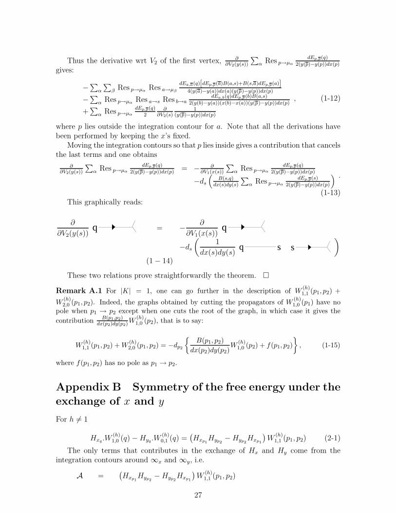
Thus the derivative wrt V2 of the first vertex, ∂∂V2(y(s))

∑α Res p→µα

dEp,p(q)

2(y(p)−y(p))dx(p)

gives:

−∑

α

∑β Res p→µα

Res a→µβ

dEa,a(q)[dEp,p(a)B(a,s)+B(s,a)dEp,p(a)]4(y(a)−y(a))dx(a)(y(p)−y(p))dx(p)

−∑

α Res p→µαRes a→s Res b→a

dEa,b(q)dEp,p(b)B(a,s)

2(y(b)−y(a))(x(b)−x(a))(y(p)−y(p))dx(p)

+∑

α Res p→µα

dEp,p(q)

2∂

∂V2(s)1

(y(p)−y(p))dx(p)

, (1-12)

where p lies outside the integration contour for a. Note that all the derivations havebeen performed by keeping the x’s fixed.

Moving the integration contours so that p lies inside gives a contribution that cancelsthe last terms and one obtains

∂∂V2(y(s))

∑α Res p→µα

dEp,p(q)

2(y(p)−y(p))dx(p)= − ∂

∂V1(x(s))

∑α Res p→µα

dEp,p(q)

2(y(p)−y(p))dx(p)

−ds

(B(s,q)

dx(s)dy(s)

∑α Res p→µα

dEp,p(s)

2(y(p)−y(p))dx(p)

) .

(1-13)This graphically reads:

∂

∂V2(y(s))q = −

∂

∂V1(x(s))q

−ds

(1

dx(s)dy(s)s sq

)

(1 − 14)

These two relations prove straightforwardly the theorem. �

Remark A.1 For |K| = 1, one can go further in the description of W(h)1,1 (p1, p2) +

W(h)2,0 (p1, p2). Indeed, the graphs obtained by cutting the propagators of W

(h)1,0 (p1) have no

pole when p1 → p2 except when one cuts the root of the graph, in which case it gives the

contribution B(p1,p2)dx(p2)dy(p2)W

(h)1,0 (p2), that is to say:

W(h)1,1 (p1, p2) + W

(h)2,0 (p1, p2) = −dp2

{B(p1, p2)

dx(p2)dy(p2)W

(h)1,0 (p2) + f(p1, p2)

}, (1-15)

where f(p1, p2) has no pole as p1 → p2.

Appendix B Symmetry of the free energy under the

exchange of x and y

For h 6= 1

Hxq.W

(h)1,0 (q) − Hyq

.W(h)0,1 (q) =

(Hxp1

Hyp2− Hyp2

Hxp1

)W

(h)1,1 (p1, p2) (2-1)

The only terms that contributes in the exchange of Hx and Hy come from theintegration contours around ∞x and ∞y, i.e.

A =(Hxp1

Hyp2− Hyp2

Hxp1

)W

(h)1,1 (p1, p2)

27

= − Resp1→∞x

Resp2→p1

V1(x(p1))(V1(x(p2)) − x(p2)y(p2))W(h)1,1 (p1, p2)−

− Resp1→∞y

Resp2→p1

V2(y(p2))(V2(y(p1)) − x(p1)y(p1))W(h)1,1 (p1, p2).

(2 − 2)

On the other hand, one knows from remark (1-15), that

W(h)1,1 (p1, p2) = −W

(h)2,0 (p1, p2) − dp2

{B(p1, p2)

dx(p2)dy(p2)W

(h)1,0 (p2) + f(p1, p2)

}. (2-3)

where f(p1, p2) has no pole when p2 → p1. Note that W(h)2,0 (p1, p2) do not have pole

when p2 → p1 either.

Thus, the only non vanishing terms in (2-2) come from dp2

{B(p1,p2)

dx(p2)dy(p2)W

(h)1,0 (p2)

}.

This reads

Res p1→∞xRes p2→p1

V1(x(p1))(V1(x(p2)) − x(p2)y(p2))dp2

{B(p1,p2)

dx(p2)dy(p2)W

(h)1,0 (p2)

}

+ Res p1→∞yRes p2→p1

V2(y(p2))(V2(y(p1)) − x(p1)y(p1))dp2

{B(p1,p2)

dx(p2)dy(p2)W

(h)1,0 (p2)

}.

(2-4)We now evaluate these residues by part and obtain that

A = − Resp→∞x

V1(x(p))dp

[(V ′

1(x(p)) − y(p))dx(p) − x(p)dy(p)

dx(p)dy(p)W

(h)1,0 (p)

]

− Resp→∞y

(V2(y(p)) − x(p)y(p))dp

[V ′

2(y(p))W(h)1,0 (p)

dx(p)

].

(2 − 5)

Another integration by part can be written

A = + Resp→∞x

V ′1(x(p))

(V ′1(x(p)) − y(p))dx(p) − x(p)dy(p)

dy(p)W

(h)1,0 (p)

+ Resp→∞y

(V ′2(y(p))dy(p)− x(p)dy(p) − y(p)dx(p))

V ′2(y(p))W

(h)1,0 (p)

dx(p).

(2 − 6)

Knowing that V ′1(x(p)) − y(p) ∼ T

x(p)when p → ∞x and V ′

2(y(p)) − x(p) ∼ Ty(p)

when p → ∞y and that the other factors do not have poles at infinities, one can finallywrite that

(Hxp1

Hyp2− Hyp2

Hxp1

)W

(h)1,1 (p1, p2) = − Res

q→∞x ,∞y

x(q)y(q)W(h)1,0 (q). (2-7)

Let us now show that the RHS vanishes by looking precisely at the form of W(h)1,0 (q).

Because it comes from a vertex, (4-16), with moving the integration contour, impliesthat

2 Res∞x ,∞y

x(q)y(q)W(h)1,0 (q) = −2

∑

α

Resq→µα

x(q)y(q)W(h)1,0 (q)

28

= −∑

α

∑

β

Resq→µα

Resp→µβ

x(q)y(q)dEp,p(q)

(y(p) − y(p))dx(p)×

×

[W

(h−1)2,0 (p, p) +

h−1∑

m=1

W(m)1,0 (p)W

(h−m)1,0 (p)

].

(2 − 8)

Now we move one more time the integration contour and clearly segregate the casewhen p and q are near the same branch point.

2 Res∞x ,∞y

x(q)y(q)W(h)1,0 (q) = −

∑

α6=beta

Resp→µα

Resq→µβ

x(q)y(q)dEp,p(q)

(y(p) − y(p))dx(p)

×

[W

(h−1)2,0 (p, p) +

h−1∑

m=1

W(m)1,0 (p)W

(h−m)1,0 (p)

]−

−∑

α

[Resp→µα

Resq→µα

− Resq→µα

Resp→q , q

]x(q)y(q)dEp,p(q)

(y(p) − y(p))dx(p)

×

[W

(h−1)2,0 (p, p) +

h−1∑

m=1

W(m)1,0 (p)W

(h−m)1,0 (p)

].

(2 − 9)

One can see that the integrand has no pole as q approaches a branch point. Thusone keeps only

∑

α

Resq→µα

Resp→q , q

x(q)y(q)dEp,p(q)

(y(p) − y(p))dx(p)

[W

(h−1)2,0 (p, p) +

h−1∑

m=1

W(m)1,0 (p)W

(h−m)1,0 (p)

]. (2-10)

We finally perform the integration and get

2 Res∞x ,∞y

x(q)y(q)W(h)1,0 (q) =

∑

α

Resq→µα

x(q)

dx(q)

[W

(h−1)2,0 (p, p) +

h−1∑

m=1

W(m)1,0 (p)W

(h−m)1,0 (p)

]

= 0. (2-11)

QED.

References

[1] G.Akemann, “Higher genus correlators for the Hermitian matrix model with mul-tiple cuts”, Nucl. Phys. B482 (1996) 403, hep-th/9606004

[2] G.Akemann and J.Ambjørn, “New universal spectral correlators”, J.Phys. A29

(1996) L555–L560, cond-mat/9606129.

[3] J.Ambjørn, L.Chekhov, C.F.Kristjansen and Yu.Makeenko, “Matrix model calcu-lations beyond the spherical limit”, Nucl.Phys. B404 (1993) 127–172; Erratumibid. B449 (1995) 681, hep-th/9302014.

29

[4] M. Bertola, ”Free Energy of the Two-Matrix Model/dToda Tau-Function”,preprint CRM-2921 (2003), hep-th/0306184.

[5] M. Bertola, ”Second and Third Order Observables of the Two-Matrix Model”, J.High Energy Phys. JHEP11(2003)062 , hep-th/0309192.

[6] M. Bertola, ”Bilinear semi-classical moment functionals and their integral repre-sentation”, math/02051.

[7] M. Bertola, ”Two-matrix model with semiclassical potentials and extendedWhitham hierarchy”, hep-th/0511295.

[8] G. Bonnet, F. David, B. Eynard, “Breakdown of universality in multi-cut matrixmodels”, J.Phys. A33 6739-6768 (2000).

[9] E. Brezin, C. Itzykson, G. Parisi, and J. Zuber, Comm. Math. Phys. 59, 35 (1978).

[10] L.Chekhov, “Genus one corrections to multi-cut matrix model solutions”, Theor.Math. Phys. 141 (2004) 1640–1653, hep-th/0401089.

[11] L.Chekhov and B.Eynard, ”Hermitian matrix model free energy: Feynman graphtechnique for all genera”, hep-th/0504116

[12] L.Chekhov, ”Matrix models with hard walls: Geometry and solutions”; contribu-tion to special volume of J.Phys.A on matrix models, hep-th/0602013.

[13] David F., “Loop equations and nonperturbative effects in two-dimensional quan-tum gravity”. Mod.Phys.Lett. A5 (1990) 1019.

[14] P. Di Francesco, P. Ginsparg, J. Zinn-Justin, “2D Gravity and Random Matrices”,Phys. Rep. 254, 1 (1995).

[15] R.Dijkgraaf and C.Vafa, “Matrix Models, Topological Strings, and Supersymmet-ric Gauge Theories”, Nucl.Phys. 644 (2002) 3–20, hep-th/0206255; “On Geometryand Matrix Models”, Nucl.Phys. 644 (2002) 21–39, hep-th/0207106; “A Pertur-bative Window into Non-Perturbative Physics”, hep-th/0208048.

[16] B. Eynard, “Topological expansion for the 1-hermitian matrix model correlationfunctions”, JHEP/024A/0904, xxx, hep-th/0407261.

[17] B. Eynard, N. Orantin, “Mixed correlation functions in the 2-matrix model, andthe Bethe ansatz”, J. High Energy Phys. JHEP08(2005)028, hep-th/0504029.

[18] B. Eynard, “Large N expansion of the 2-matrix model”, JHEP 01 (2003) 051,hep-th/0210047.

[19] B. Eynard, “Large N expansion of the 2-matrix model, multicut case”, preprintSPHT03/106, ccsd-00000521, math-ph/0307052.

[20] B. Eynard, A. Kokotov, and D. Korotkin, “1/N2 corrections to free energy inHermitian two-matrix model”, hep-th/0401166.

30

[21] B. Eynard, “Master loop equations, free energy and correlations for the chainof matrices”, J. High Energy Phys. JHEP11(2003)018, hep-th/0309036, ccsd-00000572.

[22] B. Eynard, “Polynomes biorthogonaux, probleme de Riemann-Hilbert et geometriealgebrique”, Habilitation a diriger les recherches, universite Paris VII, (2005).

[23] B.Eynard, “Loop equations for the semiclassical 2-matrix model with hard edges”,math-ph/0504002.

[24] B.Eynard, N.Orantin, ”Topological expansion of the 2-matrix model correlationfunctions: diagrammatic rules for a residue formula”, J. High Energy Phys.JHEP12(2005)034, math-ph/0504058.

[25] H.M. Farkas, I. Kra, ”Riemann surfaces” 2nd edition, Springer Verlag, 1992.

[26] J.D. Fay, ”Theta functions on Riemann surfaces”, Springer Verlag, 1973.

[27] V.A. Kazakov, “Ising model on a dynamical planar random lattice: exact solu-tion”, Phys Lett. A119, 140-144 (1986).

[28] V.A. Kazakov, A. Marshakov, ”Complex Curve of the Two Matrix Model and itsTau-function”, J.Phys. A36 (2003) 3107-3136, hep-th/0211236.

[29] I.K.Kostov, “ Conformal field theory techniques in random matrix models”, hep-th/9907060.

[30] I.Krichever “The τ -function of the universal Whitham hierarchy, matrix modelsand topological field theories”, Commun.Pure Appl.Math. 47 (1992) 437; hep-th/9205110

[31] L.Chekhov and A.Mironov, ”Matrix models vs. Seiberg–Witten/Whitham theo-ries”, Phys.Lett. 552B (2003) 293–302, hep-th/0209085

[32] L.Chekhov, A.Marshakov, A.Mironov, and D.Vasiliev, ”DV and WDVV”, Phys.Lett. 562B (2003) 323–338, hep-th/0301071

[33] M.L. Mehta, Random Matrices,2nd edition, (Academic Press, New York, 1991).

[34] M. Staudacher, “ Combinatorial solution of the 2-matrix model”, Phys. Lett. B305

(1993) 332-338.

[35] G. ’t Hooft, Nuc. Phys. B72, 461 (1974).

[36] P. Wiegmann, A. Zabrodin, ’Large N expansion for normal and complex matrixensembles’, hep-th/0309253.

[37] I. Krichever, M. Mineev-Weinstein, P. Wiegmann, A. Zabrodin, ’Laplacian Growthand Whitham Equations of Soliton Theory’, nlin.SI/0311005.

[38] A.Zabrodin, P. Wiegmann, ’Large N expansion for the 2D Dyson gas’, hep-th/0601009.

31