Fractures and faults in tight gas sandstones:   

a study using laboratory and field data  

 

 

 

From the Faculty of Georesources and Materials Engineering of the 

RWTH Aachen University 

 

 

Submitted by 

ZoltánKomoróczi, MSc 

from Budapest 

 

in respect of the academic degree of 

Doctor of Natural Sciences 

approved thesis 

 

 

 

Advisors:   Univ.‐Prof. Dr. Janos Urai 

apl. Prof. Dr. rer. nat. Christoph Hilgers 

 

Date of the oral examination: 15. October 2014 

 

 

This thesis is available in electronic format on the university library’s website 

2 | P a g e   

   

3 | P a g e   

TableofContents

Acknowledgements ................................................................................................................ 5 Abstract .................................................................................................................................. 7 Zusammenfassung .................................................................................................................. 9 1  Introduction .................................................................................................................. 11 

1.1  Project rationale .............................................................................................. 11 1.2  Theoretical background of strength, fracturing and brittleness ........................ 12 1.3  Classification of fractures ................................................................................. 19 1.4  Fluid flow in granular materials ........................................................................ 27 1.5  Aim of the thesis .............................................................................................. 31 1.6  Thesis outline ................................................................................................... 32 

2  Large scale analyses of fractures in sandstone – natural field analogue ......................... 33 2.1  Introduction to field study in Moab, Utah ........................................................ 33 2.2  Study area ........................................................................................................ 38 2.3  Geology setting of the Moab area .................................................................... 41 

2.3.1  Structural history ................................................................................... 41 2.3.2  Stratigraphy........................................................................................... 44 

2.4  Method ............................................................................................................ 46 2.5  Results ............................................................................................................. 47 

2.5.1  Courthouse Junction.............................................................................. 47 2.5.2  Klondike Bluffs ...................................................................................... 57 

2.6  Discussion ........................................................................................................ 68 2.7  Conclusion and outlook.................................................................................... 80 

3  Microstructure analysis of sandstone fractures ............................................................. 83 3.1  Introduction ..................................................................................................... 83 3.2  Geology setting of North Sea ........................................................................... 88 

3.2.1  Stratigraphy........................................................................................... 88 3.2.2  Structural history of the North Sea area ................................................ 89 

3.3  Method ............................................................................................................ 91 3.4  Results of Moab samples ................................................................................. 92 

3.4.1  Courthouse Junction samples ................................................................ 92 3.4.2  Klondike Bluffs samples ....................................................................... 111 

3.5  Natural fractures in North Sea sandstone samples ......................................... 124 3.5.1  Sample: L5‐9‐1 .................................................................................... 124 3.5.2  Sample: L5‐9‐3 .................................................................................... 128 3.5.3  Sample: L5‐9‐4 .................................................................................... 134 

3.6  Discussion ...................................................................................................... 136 3.7  Conclusion and outlook.................................................................................. 138 

4  Correlation analysis between mechanical properties and borehole  log properties  in North Sea sandstones ............................................................................................................. 141 

4.1  Introduction of correlation analysis of mechanical properties ........................ 141 4.1.1  General introduction ........................................................................... 141 4.1.2  Data .................................................................................................... 145 

4.2  Method .......................................................................................................... 147 4.2.1  Sampling method – quality control ...................................................... 147 4.2.2  Sample preparation ............................................................................. 150 

4 | P a g e   

4.2.3  Rock physical measurements ............................................................... 151 4.2.4  Rock mechanical measurements ......................................................... 151 4.2.5  Regression analysis .............................................................................. 154 

4.3  Results ........................................................................................................... 156 4.3.1  Quality control of the log data ............................................................. 156 4.3.2  Rock physical and mechanical measurement results ........................... 162 4.3.3  Results of regression analysis of UCS versus well logs .......................... 166 4.3.4  Results of regression analysis of elastic moduli versus well logs .......... 180 4.3.5  Analyses of relation between laboratory‐measured rock properties .... 187 

4.4  Discussion ...................................................................................................... 190 4.4.1  Mechanical  characterisation  of  Rotliegend  and  Lower  German  Triassic 

Sandstone Groups ...................................................................................................... 190 4.4.2  Discussion of regression analysis of UCS data ...................................... 193 4.4.3  DISCUSSION OF REGRESSION ANALYSIS OF ELASTIC MODULI DATA .......................... 196 4.4.4  INTERPRETATION OF THE PREDICTED LOGS ....................................................... 203 4.4.5  COMPARISON OF OUR RESULTS WITH OTHER CORRELATION MODELS ...................... 203 

4.5  Conclusion ..................................................................................................... 208 5  Brittleness Index for North Sea sandstones .................................................................. 211 

5.1  Introduction and background ......................................................................... 211 5.2  Proposed new brittleness index equation (BRI3): ............................................ 218 5.3  Results: Brittleness Index logs ........................................................................ 223 5.4  Discussion ...................................................................................................... 229 5.5  Conclusion ..................................................................................................... 239 

6  References ................................................................................................................... 241     

5 | P a g e   

Acknowledgements

 

Firstly  I'd  like to say a big thank to Janos Urai for the opportunity to be part of this 

comprehensive  and  very  exciting  PhD  project  that  involved  a  wonderful  filed  work, 

microscopy study and rock mechanical tests with state of the art devices. Thank you for your 

guidance and support. It was a pleasure to work with you. I really enjoyed being part of your 

great team. 

This PhD project was part of Wintershall Tight Gas Initiative. I would also  like to say 

many  thanks  to Wintershall  Holding GmbH  and Wintershall  Noordzee  B.V.  for  this  great 

project and  for  the excellent and unique data  that was provided  to my work. And special 

thanks  go  to Wintershall Noordzee  B.V.,  Energie  Beheer Nederland  B.V.  (EBN)  and Dana 

Petroleum Netherlands B.V.  for facilitating the early release of data  from their L06‐08 well 

data. Many thanks to Bert de Wijn and Andreas Frischbutter for their support and help with 

this project. 

I would  like  to  thank my other  supervisor, Heijn  van Gent  for  your help especially 

with the field work in Utah that was one of my greatest adventures of my live.  I learned a lot 

from you. Thank you Heijn.   Many  thanks go  to Werner  for  the  thin  sections,  the  sample 

preparation  and many help with  technical questions.  I would  like  to  thank  to GED  team: 

Steffen, Guillaume,  Joyce, Ben,  Jop, Maartje, Max, Michael, Simon, Shiyuan, Sohrab, Susan 

and  the Hiwis  for  every  help.  I would  also  like  to  thank  Dr. Norbert  Klitzsch  and  Lothar 

Ahrensmeier for helping me with geophysical measurements and all helps. 

Furthermore, I would like to thank to all my best friends for the lot of help, especially 

to Ákos and special thanks go to Zsuzsi. 

I would  like  to  thank  to my parents. Köszönöm Apu és Anyu a rengeteg segítséget, 

amit kaptam tőletek az életem során és a támogatást, ami nélkülözhetetlen volt ahhoz, hogy 

elérjem mindezt. 

And  last,  I would  like  to  thank  to Andi my wife  for motivating me  to start  this PhD 

study and supporting me all the time in both our private life and at work too and thank you 

Andi and to my son, Ádam for being my solid background. 

 

I would like to dedicate this thesis to my family. 

   

6 | P a g e   

 

7 | P a g e   

Abstract

In  low  permeability,  tight  gas  sandstone  reservoirs,  an  understanding  of  fracture systems is important in hydrocarbon exploration and production, because fracture networks affect  the  fluid  flow properties  in  such  reservoirs. Rocks can deform either  in a ductile or brittle way depending on the rock mechanical properties and the stress condition. To better understand the fluid flow characteristics of a fault system within a reservoir, the knowledge of the mechanical properties and the stress condition of the reservoir and the geometry of the  fracture  networks,  both  in  seismic‐scale  and  micro‐scale,  is  important.  This  thesis presents  a multidisciplinary  and multi‐scale  analysis  of  the  rock mechanical  properties  in sandstones relevant to tight reservoirs. 

Fractures and the geometry of fault damage zones were studied in two normal faults in Moab, Utah. The Courthouse Junction fault, which  is a branch of the Moab Fault (with a throw of about 80 m) is characterised by cataclastic deformation bands and slip planes and minor fluid‐flow alteration. In the cataclastic bands, grain and pore sizes range from about 1 to 0.1 µm in diameter, about two orders of magnitude smaller than those of the host rock; so significantly reducing the permeability of this fault zone. The other fault is located at the Klondike Bluffs area  (the maximum  throw of about 10 m) which  is characterised by minor cataclasis,  strong  diagenesis  and  dislocation  or  disaggregation  deformation  bands.  In  the deformation bands, the grains are not crushed and  the average pore size  is nearly double, which  increases the permeability within the  fractures. As a result of past  fluid  flow, calcite now  fully  fills  the  fractures,  so  rendering  them  as  impermeable  barriers.  In  general,  the fracture  density  decreases  logarithmically  outwards  from  the  fault  core;  however, irregularities tend to often disrupt this tendency. Peaks,  i.e.  increases  in deformation band density, are not always related to faults. The orientations of the deformation bands are sub‐parallel  and  their  dip  varies  between  70°  and  90°.  The width of  the  damage  zone  in  the footwall at Klondike Bluffs  is about 150 m and at the Courthouse Junction this varies  from 200 to >300 m. In the hanging wall at Klondike Bluffs, the damage zone ranges from 180 to 300  m.  Along  the  faults,  the  width  and  the  deformation  band  distribution  change significantly;  the  range  of  dip  and  dip‐direction  varies  moderately,  while  the  fracture characteristics remain constant. 

The microstructure of fractures in North Sea Rotliegend Sandstone core samples and in  the Moab  field  samples was  analysed.  The  results  show  that  the  characteristics of  the fractures and the host rocks of both the field study samples and the North Sea core samples are  similar.  In  conclusion,  the Moab  sandstones may provide  a  good  analogue  to  that of these North Sea sandstones. 

The  second  aim  of  the  study  was  to  analyse  the  relationship  between  the  rock mechanical properties, log properties and the brittleness of rocks. The relationship between unconfined compressive strength (UCS), Young’s modulus and wireline well logs (i.e. acoustic velocity, density, resistivity, natural gamma‐ray, spectral gamma‐ray and neutron‐porosity) was studied in North Sea Lower Germanic Triassic Sandstone (depths range 2700 to 4050 m) and Rotliegend Sandstone (depths range 3900 to 4900 m). A multivariate regression method was used to calculate the empirical correlation equations. In the Triassic sandstone, acoustic velocity has a much weaker dependence on velocity than it has in the Rotliegend sandstone. Multivariate  regressions  using  more  prediction  variables  provided  better‐fit  correlation equations. A significant  increase was observed  in the goodness of regression using spectral gamma logs. The highest squared regression coefficient was attained as a result of a UCS‐log 

8 | P a g e   

multivariate regression for Rotliegend samples: R2 = 0.84 using spectral gamma logs, and for Triassic samples R2 = 0.55 when using a cumulative gamma  log (due to the unavailability of spectral gamma  logs). This same tendency was found in the results of regressions made for Young’s moduli  and  log  properties.  Strong  dependency was  exhibited  between  UCS  and Young’s moduli (R2 = 0.9) in the Rotliegend samples; however, dependency was much lower in the Triassic samples (R2 = 0.46). 

Based on the brittleness index approach of Ingram and Urai (1999) and Hoogerduijn‐Strating  and Urai  (2003),  a  new  brittleness  index  equation  has  been  developed  in which stress conditions and UCS are considered. The derived UCS‐log correlation equations were used  to  calculate brittleness  logs  in  the wells  from where  the  rock  samples  originate.  By applying the calculated BRI logs to characterise the brittle, less brittle and ductile formations or  intervals of North Sea  sandstones were  identified and provided good examples  for  the application of this BRI concept. 

The results of my work can provide a better understanding of the properties of faults and fractures, together with hydrocarbon migration through tight sandstone reservoirs, and may be applied to improve the seismic interpretation of faults.  

 

 

9 | P a g e   

Zusammenfassung

Risse  und  Störungen  in  „tight  gas“  Sandsteinen:  Eine  Studie  über  Labor‐  und 

Geländedaten 

In  Exploration  und  Produktion  von  Kohlenwasserstoffen  ist  in  gering  permeablen, 

gasdichten Sandsteinreservoiren (engl.: “tight gas reservoirs”) ein umfassendes Verständnis 

über Risssysteme wichtig, da diese die Fluidflusseigenschaften von Reservoiren beeinflussen. 

Gesteine  können  entweder  duktil  oder  spröde  deformieren,  je  nach  mechanischen 

Gesteinseigenschaften  und  Spannungszustand.  Um  die  Fluidflusseigenschaften  in 

Risssystemen  beschreiben  zu  können,  ist  es  notwendig  die  in‐situ  gesteinsmechanischen 

Eigenschaften  sowie  die  Geometrie  des  Rissnetzwerkes  vom  Seismik‐  bis  hin  zum 

Mikrometermaßstab  zu  verstehen.  Diese  Arbeit  zeigt  eine  maßstabsübergreifende, 

interdisziplinäre  Analyse  von  Rissen  und  mechanischen  Eigenschaften  von  Reservoir‐

Sandsteinen, welche in der Betrachtung gasdichter Reservoirs von Bedeutung sind. 

An  zwei  Abschiebungen  in  Moab  (Utah,  U.S.A.)  wurden  Risse  und 

Störungszonengeometire untersucht. Die Courthouse‐Junction‐Störung, eine  Seitenstörung 

der  Moab  Hauptstörung  mit  einem  Versatz  von  80  m,  weist  kataklastische 

Deformationsbänder,  Harnischflächen  und  geringe  Fluidfluss  Alterationen  auf.  In  den 

kataklastischen Bändern  reichen Poren‐ und Korngrößen von 1 µm bis zu 0,1 µm,  in etwa 

zwei Größenordnungen  kleiner  als Poren und Körner  im Umgebungsgestein. Dies  führt  zu 

einer  Permeabilitätsverringerung  innerhalb  der  Störungszone.  Die  zweite  Abschiebung 

(maximaler Versatz um 10 m)  liegt  im Klondike‐Bluff Gebiet. Die Störung  ist durch geringe 

Kataklase,  starke  Diagenese  und  Dislokation  oder  Auflockerung  innerhalb  von 

Deformationsbändern  gekennzeichnet.  Die  Körner  der  Deformationsbänder  sind  nicht 

zerbrochen,  die  durchschnittliche  Porengröße  ist  fast  verdoppelt  gegenüber  dem 

Umgebungsgestein. Dies hat eine Permeabilitätserhöhung zur Folge. Durch Paleo‐Fluidfluss 

konnte Kalzit  in den Rissen ausfällen, was diese zu undurchlässigen Fluidsperren macht.  Im 

Allgemeinen verringert sich die Rissdichte  logarithmisch mit zunehmender Entfernung zum 

Störungskern,  Ausnahmen  unterbrechen  jedoch  diesen  Trend.  Eine  Dichte  von 

Deformationsbändern  ist  nicht  immer  Störungsgebunden.  Die  Orientierung  der 

Deformationsbänder ist sub‐parallel und ihr Fallen liegt zwischen 70° bis 90°.  Die Breite der 

äußeren Störungszone (engl.: “damage zone”) variiert von 200 m bis > 300 m. Im Hangenden 

der Klondike‐Bluff‐Störung  ist die äußere Störungszone 180 m bis 300 m breit. Breite und 

Häufigkeit der Deformationsbänder entlang der Störungen  ist sehr variable. Das Fallen und 

Streichen der Bänder variiert ebenfalls leicht, während die Rissart gleichbleibend ist. 

Die Mikrostruktur  der Risse  in  Bohrkernen  des  Rotliegend  Sandsteins der Nordsee 

sowie die Moab Geländeproben wurden untersucht. Die Ergebnisse zeigen, dass Risse und 

Umgebungsgesteine  der  Moab  Geländestudie  mit  den  der  Nordseebohrkernproben 

vergleichbar  sind.  Die  Moab  Sandsteine  können  ein  gutes  Analogon  zu  den  Rotliegend 

Sandsteinen der Nordsee sein. 

 

10 | P a g e   

Das  zweite  Ziel  dieser  Studie  war  es,  Korrelationen  von  gesteinsmechanischen 

Eigenschaften,  Borchlochloggindaten  und  der  Brüchigkeit  der Gesteine  zu  analysieren.  Es 

wurde  eine  Korrelation  zwischen  der  einaxialen  Druckfestigkeit,  dem  E‐Modul  und 

Bohrloggingdaten  (Schallwellengeschwindigkeit,  Dichte,  Wiederstand,  natürliche  Gamma‐

Strahlung,  spektrale Gamma‐  und Neutronporosität)  für Nordsee  Sandsteine  der  unteren 

Trias (Tiefe: 2700 m bis 4050 m) und für Rotliegend Sandsteine (Tiefe: 3900 m bis 4900 m) 

untersucht. Die empirischen Beziehungen wurden durch multivariate Regression errechnet. 

Triassischer  Sandstein  zeigt  einen  viel  kleineren  Regressionskoeffizienten  der 

Schallwellengeschwindigkeit,  also  eine  geringere  Geschwindigkeitsabhängigkeit,  als 

Rotliegend  Proben  bei  univariabler  Regression.  Multivariate  Regression  mit  weiteren 

Einflussvariablen  zeigt  ein  Ergebnis  mit  größeren  Korrelationskoeffizienten.  Ein 

bemerkenswerter Anteil der Regressionsqualität  ist auf Daten des spektralen Gamma Logs 

zurückzuführen.  Der  größte  Korrelationskoeffizient  der  einaxialen  Druckfestigkeit  lag  bei 

Rotliegend  Proben  bei  R²  =  0.84  (mit  spektralen  Gamma‐Log  Daten)  und  für  triassische 

Proben bei R² = 0.55 (mit kumulativem Gamma‐Log). Die gleiche Tendenz   zeigt sich  in den 

Regressionsergebnissen  zu  E‐Modul  und  Log‐Daten.  Eine  deutliche  Abhängigkeit  liegt 

zwischen  einaxialer  Druckfestigkeit  und  E‐Modul  der  Rotliegend  Proben  vor  (R²  =  0.9). 

Allerdings war die Abhängigkeit für triassische Proben viel geringer (R² = 0.46). 

Die  errechneten  Logs  der  einaxialen  Druckfestigkeit  wurden  zur  Vorhersage  der 

Brüchigkeit  genutzt.  Basierend  auf  Studien  von  Ingram  und  Urai  (1999)  sowie  von 

Hoogerduijn‐Strating  und  Urai  (2003)  wurde  eine  neue  Gleichung  zu 

Brüchigkeitsbestimmung  (engl.:  „brittleness  index“)  entwickelt. Mithilfe  dieser  Gleichung 

wurden  Brüchigkeits‐Logs  für  die  untersuchten  Schichten  berechnet  und  brüchige  und 

weniger brüchige Sandsteingruppen erkannt. 

Die  Ergebnisse meiner  Arbeit  geben  ein  besseres  Verständnis  von  Störungs‐  und 

Risseigenschaften  im  Zusammenhang  mit  Kohlenwasserstoffmigration  durch  gasdichte 

Sandsteinreservoire.  Diese  Ergebnisse  können  genutzt  werden  um  seismische 

Störungsinterpretationen zu verbessern. 

 

11 | P a g e   

1 Introduction

1.1 Projectrationale

Sandstones  are  common  reservoir  rocks.  The  porosity  and  the  permeability  of 

sandstones are usually relatively high hence they are able to store large volumes of fluid or 

gas  that  can be  produced  relatively  easily.  These properties make  sandstones  a  potential 

reservoir rock and a main target of conventional hydrocarbon explorations. However, there 

are  sandstones, which have  significant  storage  capacity but have  low permeability.  These 

low‐permeability  sandstones  are  commonly  called  tight  sandstone  reservoirs  or  tight  gas 

reservoirs. The definition of the tight gas reservoirs by Holditch is based on the economical 

flow rate of the production (Holditch 2006). Law and Curtis (Naik 2003) defined the tight gas 

reservoirs of  the United States where permeability  is  lower  than 0.1 mD. On  the contrary, 

reservoirs with permeability lower than 0.6 mD are considered as tight gas reservoirs by the 

German  Society  for  Petroleum,  Coal  Science  and  Technology  (DGMK)  (Naik  2003). With 

increasing energy prices and available technology, production of tight gas reservoirs became 

profitable, playing an increasing role in hydrocarbon research all over the world (e.g. North 

America, Northern  Africa)  these  decades. Moreover,  tight  reservoirs might  provide  large 

potential for energy resources for the following decades according to estimations of GTI E&P 

Services (Holditch 2006).  In Europe, the Middle Permian Rotliegend aeolian sandstones are 

considered potential tight reservoir. According to the estimation of BGR (Cramer et al. 2009) 

more than 100 billion m3 is stored in the Southern Permian Basin. 

Thorough  understanding  of  characteristics  of  the  tight  sandstone  reservoirs  is 

essential  for  successful  hydrocarbon  production.  Many  factors  control  the  hydrocarbon 

systems  in  sandstones;  for  instance,  depositional  environment,  palaeo‐topography,  syn‐

depositional tectonics, diagenetic processes, which involve quartz cementation (Walderhaug 

2000, Taylor et al. 2010, Tobin et al. 2010), plagioclase albitization  (Perez and Boles 2005), 

fibrous  illite  formation  (Franks  and Zwingmann  2010) etc.  Tectonic events  are one of  the 

most important factors that have significant effects on fluid flow and hydrocarbon migration 

of a reservoir (Aydin 2000). As a result of tectonic processes, different types of fractures can 

occur  in  brittle  regime,  for  instance:  faults,  joints,  veins,  cracks  or  deformation  bands. 

Reflection  seismic provides  an opportunity  to map  the  underground  structures; however, 

even the highest resolution seismic data provide only about 2‐3 m vertical resolution. Hence, 

only  the  larger  structures  (e.g.  faults)  are  visible  in  the  seismic  images.  Well  bore 

measurements  and  core  samples  can  provide  information  on  investigated  rocks  in more 

details; however, might not be representative in an inhomogeneous reservoir environment. 

Therefore, prediction of reservoir quality is a great challenge (Ajdukiewicz and Lander 2010). 

Natural  field analogues can provide  invaluable opportunity to obtain  information to better 

understand  the properties of  reservoirs which are similar  to  those  in  the depth. Outcrops 

allow studying the 3D architectures of the reservoirs in large scale and also in small scale i.e. 

microstructures of fractures. 

12 | P a g e   

1.2 Theoreticalbackgroundofstrength,fracturingandbrittleness

The stress theory was introduced by Cauchy using the concept of traction (Jaeger et 

al. 2007). Traction (p)  is a vector which  is defined at a point (x) on a plane whose outward 

normal unit vector is n as the ratio of the resultant force (F) and the area A across which the 

force acts:  

To specify the traction at a given point, the differential resultant force (dF) acting on 

the infinitesimal area (dA) is calculated: 

According to Cauchy stress theory, the traction acting on a plane can be given by the stress 

tensor . 

In 3D, the stress tensor has 9 components. The diagonal terms describe the normal 

stresses, and the off‐diagonal terms describe the shear stresses acting on each plane of the 

coordinate system.  If the  forces are balanced, the stress tensor  is symmetric ( xy = yx   , a 

xz = yz   and  yz = zy );  therefore,  it  can  be  transformed  into  a  diagonal  matrix  by 

calculating its eigenvectors, which are the principal stresses. In this way, the stress‐state of a 

point can be described by three orthogonal normal stress vectors:  1  being the maximum, 

2  being the intermediate and  3 being the least principle stress.  

The stress tensor can be visualised as a stress ellipsoid, with its axes, the principal stresses, 

oriented normal to the principal planes of stresses. 

 

  Fp

A   Eq. 1‐1

 

0

1, lim

dAp x n dF

dA   Eq. 1‐2

  p n  Eq. 1‐3

 1

2

3

0 0

0 0

0 0

xx xy xz

yx yy yz

zx zy zz

  Eq. 1‐4

13 | P a g e   

 

 

Figure 1‐1  A) The stress ellipsoid is a three‐dimensional visualisation of the stress state of all possible plane in an infinitesimal cube ( , ,   are the principle stresses and  ,  , 

  are  the  principle  coordinates).  B)  The  general  stress  components  on  the  panes normal  to  the  coordinate  axes  of  the  general  coordinate  system  in  an  infinitesimal cube. C) The principal stress components are shown in a principal coordinate system in an infinitesimal cube. (modified after Twiss and Moores 2007) 

 

The  two dimensional graphical  representation of  the  state of  the  stress of a given 

point is the Mohr’s diagram (Figure 1‐3). In the Mohr diagram, the horizontal axis represents 

the  normal  stress  and  the  vertical  axis  represents  the  shear  stress  acting  on  a  particular 

plane at a given point. The Mohr’s circle represents all normal‐shear stress relations acting 

on planes of all possible orientation at a given point, where the angle of the given plane (θ) 

is half of  the  angle between  the  radius  to  the  given point  and  the  radius  to  the point of 

maximum stress. 

 1 3 1 3 cos2

2 2N

  Eq. 1‐5

 1 3 sin 2

2

       Eq. 1‐6

 

Equations 1‐5 and 1‐6 describe  the equation of  the Mohr circle  in  the  (σN‐τ) space, 

with  its  centre  being  at  the  point  1 3 / 2; 0N   and  with  its  radius  being

1 3r . 

14 | P a g e   

Figure 1‐2 A) The stress diagram  in physical space  in the principal coordinate system shows the  relationships  between  the  stress  components  and  the  plane  P where  n(P)  is  the normal of the plane P stresses with superscripts (P)  indicate stress components acting on plane P.   B) The stress on the plain  in  figure “A” showed  in a Mohr diagram  in 2D. (modified after Twiss and Moores 2007) 

 The Mohr’s  diagram  is  often  used  to  determine  the  failure  of  rocks.  The Mohr‐

failure‐envelope  (Figure  1‐3)  is  the  curve,  which  describes  the  critical  states  of  stresses 

where a given rock fails. Parameter of the failure envelope (internal friction angle, cohesion) 

is different for every rock. 

Strength  is an  important parameter of  the rocks;  therefore,  it has been extensively 

studied. In the field of rock mechanics, several strength theories have been developed since 

the beginning of last century. These theories use different approaches; Asszonyi and Richter 

and then later Ván and Vásárhelyi analysed the rock strength as a thermo dynamical system 

(Asszonyi and Richter 1974, Asszonyi and Richter 1979, Ván 2001, Ván and Vásárhelyi 2001); 

other  theories  use mechanical,  physical  and/or  statistical  approaches  and many  empirical 

failure criterion were created that are based on well‐known theories (Andreev 1995).  

The Coulomb‐Navier  theory describes  the  shear  failure,  a  rock or  soil  fails  along a 

plane due to shear stress acting on that plane.  It also states that the  fractures only  form  if 

the  internal  strength  (cohesion)  of  the  rock  is  exceeded  (Griffith  1921,  Panich  and  Yong 

2005,  Jaeger et al. 2009). The Coulomb‐fracture‐criteria describe  the state of  the stress at 

which  a  given  rock  under  compression  fails.  In  the Mohr  diagram  the  Coulomb  fracture 

criteria are shown as a straight line with the internal fiction of the rock (µ) representing the 

slope of the line, and the cohesion (C) of the rock is the intercept of the line.   

  tanS N NC C Eq. 1‐7

Based on the Griffith theory, the tensile strength of the rock is defined. He assumed that 

both tensile and shear fractures develop from planar microdefects or microfractures. Griffith 

15 | P a g e   

proposed non‐linear relationship between the principal stresses for a critically stressed rock. 

In the Mohr‐space the representation of the Griffith failure criterion (Eq. 1 8) is a parabola, 

where  the  tensile strength of  the rock  is  the  intersection with  the horizontal axis.  (Griffith 

1921, Fossen 2010) 

 2 24 4 0S NT T     Eq. 1‐8

When  the  rock  deforms  in ductile way,  the  failure of  the  rock  can  be  estimated by  a 

constant shear stress criterion, referred to as the von Mises criterion;  its representation  in 

the Mohr space is a horizontal line (σs=constant) (Mises 1913). 

Figure 1‐3: The fracture criterions (Griffith, Coulomb and Von Mises)  in 2D Mohr space with related fracture types brittle to ductile (modified after Fossen, 2010). 

In porous rock, the stress due to the weight of the overlying rock layers (lithostatic or 

overburden stress) is distributed over the grain contact area. The pressure of the pore fluid 

reduces the effective stress. Terzaghi (1923) defined the effective stress   as the difference 

between externally applied stresses   and internal pore pressure :  

    Eq. 1‐9

This means that pore pressure influences the diagonal elements of the stress tensor (normal 

stresses, σ11, σ22, σ33) and not the off‐diagonal elements (shear components σ12, σ23, σ13) 

(Zoback 2007). 

In a porous elastic solid saturated with a fluid, the theory of poroelasticity describes 

the constitutive behaviour of rock. Empirical data showed that the effective stress concept 

of Terzaghi  is a good approximation  for  intact  rock  strength and  the  frictional  strength of 

faults,  but  for  other  rock  properties  it  is  needs  to  be modified. Nur  and  Byerlee  (1971) 

proposed a formula which works well for volumetric strain:  

    Eq. 1‐10 

16 | P a g e   

where α is the Biot parameter (α = 1 − Kb/Kg) and Kb is drained bulk modulus of the rock or 

aggregate and Kg is the bulk modulus of the rock’s individual solid grains. 

There  have  been  several  studies,  which  examined  the  different  parameters,  that 

affect the strength of a given rock, such as porosity (Brace and Riley 1972, Dunn et al. 1973, 

Scott 1989, Palchik 1999), mineralogical properties (Fahy and Guccione 1979, Winkler 1985, 

Singh 1988, Shakoor and Bonelli 1991, Haney and Shakoor 1994, Ulusay et al. 1994, Schön 

1996, Bell and Culshaw 1998, Tuğrul and Zarif 1999, Hale and Shakoor 2003, Jeng et al. 2004, 

Meng  and  Pan  2007,  Pomonis  et  al.  2007,  Hsieh  et  al.  2008),  clay  content  (Jizba  1991, 

Samsuri et al. 1999, Swanson et al. 2002, Takahashi et al. 2007, Li and Zhang 2011), moisture 

content (Colback and Wiid 1900, Simpson and Fergus 1968, Broch 1974, Ballivy et al. 1976, 

Michalopoulos  1976,  Priest  and  Selvakumar  1982, Venkatappa  Rao  et  al.  1985, Dyke  and 

Dobereiner  1991,  Hawkins  and  McConnell  1992,  Hale  and  Shakoor  2003,  Shakoor  and 

Barefield 2009),  fabric  (Paterson and Wong 2005,  Li and Zhang 2011).  In addition  to  rock 

properties, there are also external factors which can determine the strength of a given rock, 

such as effective  confining pressure  (Jaeger, et  al. 2009), principal  stresses  (Paterson  and 

Wong 2005), strain rate  (Sangha and Dhir 1972, Fischer and Paterson 1989), pore pressure 

and temperature (Fischer and Paterson 1989). 

Failure of the rock can occur in a ductile or brittle way. The ductile deformation is a 

continuous deformation at the scale of observation; without macroscopic  fracturing;  it can 

be the result of plastic or brittle micromechanisms as  it can be seen on Figure 1‐4. Ductile 

deformation usually occurs  in metamorphic rocks  in  the middle and  lower crust; however, 

soils  and  poorly  consolidated  sediments  can  also  deform  in  a  ductile  way.  The  ductile 

deformations  in the middle and  lower crust are usually due to plastic mechanism; such as, 

dislocation  creep,  twinning  or  diffusion.  In  contrast,  the  ductile  deformation  of  poorly 

consolidated sediments is usually the result of brittle mechanisms; such as, microfracturing, 

rolling or frictional sliding of the grains. The brittle deformation is discontinuous deformation 

by fracturing. The complex fracture process is basically a combination of microscopic cracks 

and frictional movement (Brace et al. 1966). As the stress closes to critical point, the number 

of  micro‐cracks  increases  and  reaches  critical  condition,  at  which  the  rock  fails  along 

through‐going shear plane (Lockner et al. 1991). Griggs and Handin (1960) distinguished two 

styles of fractures; such as, shear fracture and extension fracture. Later, Ramsey and Chester 

(2004)  inferred that also hybrid fractures can formed as a combination of compression and 

tensile states. Wong and Baud (2012) showed that there is an intermediate regime between 

the brittle and the ductile field, which is associated with the localized strain. However, style 

of fracturing depends on several different properties of the rock and also external physical 

parameters.  Experimental  studies  show,  that  the  mode  of  the  fracturing  depends  on 

deformation  style, which  is  affected by  the  confining  pressure  (Figure  1‐5). During brittle 

deformation,  without  confining  pressure,  extensional  fractures  develop,  and  as  the 

confinement  increases,  the  fractures  turn  into shear  fractures and shear bands and during 

ductile deformation plastic  flow occurs. The  temperature also has an effect on  the brittle 

ductile  transition of  rocks; however,  in  the upper crust,  this effect  is not dominant.  In  the 

continental upper crust to approximately ten kilometres depth, rocks have in general brittle 

behaviour (Figure 1‐6). 

17 | P a g e   

Figure  1‐4  –  Illustration  of  brittle,  ductile  and  plastic  deformation  styles.  (modified  after Fossen 2010) 

Figure 1‐5 – Experimental deformation structures (P, T). (modified after Fossen 2010) 

18 | P a g e   

Figure 1‐6 – Rheological stratigraphy of continental lithosphere. (Fossen 2010) 

There have been several studies on the brittle and the ductile characteristic of rocks, 

which tried to define the parameters that distinguish the brittle and the ductile deformation. 

In  some  cases,  the  brittle‐ductile  transition  was  characterized  by  the  permanent  strain 

before failure; for the brittle rock, the strain was 3% according to Paterson and Wong (2005) 

and Heard  (1960); and  for the ductile rock, strain was more than 5%  (Paterson and Wong, 

2005  and Heard,  1960). Other  studies  focused  on  the  brittleness  of  the  rock, which was 

estimated based on the Mohr diagram (Hucka and Das 1974), or the ratio of the reversible 

strain  or  total  strain  or  energy  (Hucka  and  Das,  1974);  or  the  ratio  of  Brazilian  tensile 

strength and uniaxial compressive  strength of  the given  rock  (Table 5.2); or  the  results of 

punch penetration or impact tests (Protodyakonov 1962, Blindheim and Bruland 1998, Copur 

et  al.  2003,  Yagiz  2009,  Yagiz  and  Gokceoglu  2010). However,  in  some  cases,  the  terms 

brittle and ductile are used in an unconventional way. The ductile deformation of mudrocks 

was defined with the lack of dilatancy and the associated creation of fracture permeability. 

In contrast, the brittle deformation of mudrocks was defined with the presence of dilatancy 

and  consequently  the  increase of  fracture  permeability  (Urai  and Wong  1994, Urai 1995, 

Ingram  and Urai  1999).  Furthermore, Wong  and Baud  (2012)  reviewed  several  studies of 

brittle‐ductile  transitions  including  constitutive models  for  plasticity  and micromechanical 

models  for  the  brittle  and  ductile  failure,  however,  complete model  of  the  brittle‐ductile 

transition is still lacking. 

 

 

 

 

 

19 | P a g e   

1.3 Classificationoffractures

Fractures can be classified by the relative displacement that has occurred across the 

fracture  surface  during  formation.  For  extensional  fractures,  i.e.  mode  I  fractures,  the 

displacement is normal to the fracture walls (Figure 1‐7 A). For shear fractures, the relative 

motion is parallel to the surface. There are two modes of shear fractures: in case of mode II 

shear  fractures, there  is a sliding motion normal to the edge of the fracture (Figure 1‐7 B); 

whereas, in case of mode III shear fractures, there is a sliding motion parallel to the fracture 

edge (Figure 1‐7 C).   There are also oblique extensional, or fracture mixed mode fractures, 

when the displacement along the fracture has both parallel and perpendicular components. 

(Twiss and Moores 2007) 

 

Figure  1‐7–  The  three  most  characteristic  fracture  types  classified  based  on  the  relative displacement  are:  A.  extensional  fracture  or  mode  I.  ‐  the  displacement  is perpendicular  to  the  fracture  (opening);  B.  Shear  fracture  or  mode  II.  ‐  The displacement  is parallel to fracture and perpendicular to the fracture edge; C. fracture or  mode  III.  ‐  The  displacement  is  parallel  to  fracture  and  to  the  fracture  edge. (modified after Twiss and Moores 2007) 

Based on its mode of formation, fractures can be classified as the following (Aydin 2000): 

Dilatant‐mode fractures/joints, veins, dikes, sills 

Contraction/compaction‐mode fractures/pressure solution seams and compaction bands 

Shear‐mode fractures/faults 

Dilatant fractures exhibit displacement normal to their surface. There are more types 

of dilatant  fractures; such as,  joints, veins or dykes.  Joint are dilatant  fractures with no or 

very  small  displacement  (Twiss  and Moores  2007). Veins  are  filled with mineral  deposits 

(Twiss and Moores 2007). Hydrofractures are generated by high fluid pressure (Hubbert and 

Willis  1957)  and may  be  vertical  (dikes)  or  horizontal  (sills)  or  a  combination  of  the  two 

depending  on  the  interplay  between  the  state of  stress  and  the  abnormal  fluid  pressure 

leading to fracturing (Mandl and Harkness 1987). 

In  contraction/compaction‐mode  fractures,  the  fracture walls move  towards  each 

other, which may be  characterized  as anti‐crack  (Fletcher and Pollard 1981). This  class of 

structures includes pressure solution surfaces and compaction bands (Aydin 2000). 

20 | P a g e   

Faults  are  defined  as  structures  across  which  appreciable  (minimum  a  metre  or 

more)  shear  displacement  discontinuities  occur.  Fractures  with  shear  displacement  of  a 

centimetres or less are called shear fractures, and shear fractures at the scale of a millimetre 

or less are microfaults that may be visible only under microscope. (Twiss and Moores 2007)  

Figure 1‐8, The orientation of different types of fractures formed in intact rock relative to the principal  stress  orientations:  Stylolites  are  perpendicular  to  the maximum  principal stress direction  (σ1);  faults,  shear  fractures are parallel  to  the  intermediate principal stress  direction  (σ2);  joints  are  perpendicular  to minimum  principal  stress  direction (σ3). (modified after Lacazette, 2009) 

The orientation of the different mode of fractures is determined by the orientation of 

the principal stresses.  Joints grow normal  to  least principal stress  (σ3). Faults usually  form 

with an approximately constant acute angle  to  the maximum principal stress  (σ1) and  the 

orientations of the  faults and their conjugates ranges from 25° to 40° but  in general about 

30°. Compaction bands form normal to σ1 (Lacazette 2009). Faults are often accompanied by 

conjugate  fractures which are  two sets of small‐scale shear  fractures at approximately 60° 

angle to each other with opposite senses of shear (Twiss and Moores 2007). In many cases, 

there are smaller‐scale faults which are parallel to major fault and have the same sense of 

shear and are called as synthetic faults; or they are in the conjugate orientation and referred 

as antithetic faults (Twiss and Moores 2007). 

The fault separates the rock  into two blocks. The one above the fault is the hanging 

wall and the one below the fault  is the footwall. The zone connecting the footwall and the 

hanging wall of  the  fault  is referred as  the relay zone  (Peacock and Sanderson 1991). One 

major  parameter  of  the  fault  is  the  displacement  blocks.  The  lateral  component  of  the 

displacement  along  the  fault  is  the  horizontal  separation.  The  vertical  component  of  the 

displacement is the throw and the horizontal component of the displacement normal to the 

fault is the throw (Figure 1‐9). (Twiss and Moores 2007)  

21 | P a g e   

 

Figure 1‐9 – The general  geometrical properties of  fault are  illustrated by a normal with a dextral (right‐handed) component. (modified after Fossen, 2012)

The surface of the fault planes are often smooth as a result of shearing on the fault 

planes  or  in  the  fault  gouge,  this  features  is  referred  as  slickensides.  Furthermore,  fault 

surfaces  can  contain  strongly  oriented  linear  features,  known  as  slickenlines,  slickenside 

lineations, or striations, that are parallel to the direction of slip. (Twiss and Moores 2007) 

Fault  can be  categorised based on  the dynamics of  faulting as  it was described by 

Anderson  (1905).  According  to  this  Andersonian  classification  scheme,  there  are  three 

classes:  reverse  faults,  normal  faults  and  strike  slip  faults  with  respect  to  the  relative 

orientation  of  the  principal  stresses  acting  on  the  fault  planes.  If  the maximum  principal 

stress  is vertical,  it  is a normal fault;  if the minimum principal stress  is vertical,  it  is reverse 

fault and if the intermediate stress is vertical, it is a strike‐slip fault. 

The  3D  architecture  of  fault  arrays was  analysed  by Walsh  et  al.  (1999).  Seismic 

mapping of normal fault arrays allows 3D geometries, slip variations and branch‐lines to be 

determined objectively by mapping of numerous branch‐points. Branch lines are defined as 

lines of intersection between a master fault and a synthetic splay, or between two segments 

of a multi‐strand  fault. The shape of branch  lines varies between straight  lines and closed 

loops  representing  different  stages  in  the  failure  of  relay  zones  and  in  the  progressive 

replacement of fault tip‐lines with fault branch‐lines.   

Faults  can  be  classified  into  displacement‐normal  offsets,  displacement‐parallel 

offsets and displacement‐oblique offsets. Displacement‐normal offsets faults are associated 

with neutral relays. Displacement‐ parallel offsets and displacement‐oblique offsets can be 

further  subdivided  into  those which are  constrictional and extensional and are associated 

with restraining relays and releasing relays respectively. (Peacock and Sanderson 1991) 

Neutral,  restraining and  releasing  relays can develop  in normal,  reverse and strike‐

slip  faults. As a  combination of  these, 9 different branch  line  structures  can develop.   An 

important factor to control the structure of the branch lines is the orientation of the axis of a 

22 | P a g e   

relay  and  its  associated  bends  relative  to  a  fault  slip  direction.  This  relative  orientation 

determines how the relay strain is accommodated and hence it also determines the degree 

of hard‐linkage and development of branch‐lines. (Walsh, et al. 1999) 

Field  observations  showed  that  seismic  size  faults  (throw  is  larger  than  seismic 

resolution)  and  also  faults  below  the  seismic  resolution  have  complex  3D  architecture 

(Chester  et  al.  1993,  Sibson  1977, Wallace  and Morris  1986),  they  usually  consist of  two 

structural  elements:  the  fault  core  and  the  damage  zone.  The  core of  the  fault, which  is 

often referred as fault slip zone, shows the largest displacement of the fault (Gudmundsson 

et al. 2010). Most of the displacements occur  in the central part of the zone, the fault core 

(Caine et al. 1996), where slip planes and  fine‐  to ultra‐fine grained rocks e.g. cataclasites, 

gouges  can  be  found.  It  contains many  small  fractures  and  also  breccias  and  cataclastic 

rocks. The fault core often shows ductile or semi brittle behaviour as the core rock is crushed into a fine grain material. The thickness of the core usually varies from several metres to a 

few tens of metres (Berg and Skar 2005, Agosta and Aydin 2006, Tanaka et al. 2007, Li and 

Malin 2008, Gudmundsson, et al. 2010); however, very large faults zones, such as transform 

faults,  may  develop  several  fault  cores  and  damage  zones  (Faulkner  et  al.  2006, 

Gudmundsson 2007).

Figure 1‐10 A  schematic  illustration of  the  structure of a  (strike‐slip)  fault  zone  is  showed. The  fault  core  consists  of  breccia  and/or  cataclastic  rock  and  the  damage  zone  is characterized by fractures   (modified after Gudmundsson et al. 2010). 

The  damage  zone  of  a  fault,  which  is  also  referred  to  as  the  transition  zone,  is 

fractured host rock, where the fracture density decreases with distance from the fault core 

(Bruhn et al. 1994). The damage zone deforms in a brittle way, therefore it consists of mainly 

lenses of breccias and other heterogeneities,  less extension fractures, and also some shear 

fractures present  (Gudmundsson et al. 2002). According  to Aydin  (2000),  the width of  the 

damage zone and the density of joints therein are related to the magnitude of slip across the 

fault. Furthermore, in some studies, a third element of the fault zone is described, which is 

23 | P a g e   

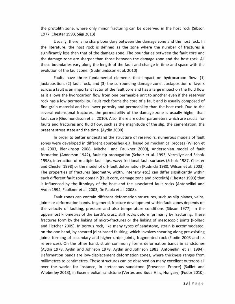
the protolith  zone, where only minor  fracturing  can be observed  in  the host  rock  (Sibson 

1977, Chester 1993, Sági 2013)  

Usually, there is no sharp boundary between the damage zone and the host rock. In 

the  literature,  the  host  rock  is  defined  as  the  zone  where  the  number  of  fractures  is 

significantly  less than that of the damage zone. The boundaries between the fault core and 

the damage zone are sharper than  those between the damage zone and  the host rock. All 

these boundaries vary along the  length of the fault and change  in time and space with the 

evolution of the fault zone. (Gudmundsson et al. 2010) 

Faults  have  three  fundamental  elements  that  impact  on  hydrocarbon  flow:  (1) 

juxtaposition,  (2)  fault  rock, and  (3)  the surrounding damage  zone.  Juxtaposition of  layers 

across a fault is an important factor of the fault core and has a large impact on the fluid flow 

as  it allows the hydrocarbon flow from one permeable unit to another even if the reservoir 

rock has a low permeability. Fault rock forms the core of a fault and is usually composed of 

fine grain material and has  lower porosity and permeability than the host rock. Due to the 

several  extensional  fractures,  the permeability of  the damage  zone  is usually higher  than 

fault core (Gudmundsson et al. 2010). Also, there are other parameters which are crucial for 

faults and fractures and fluid flow, such as the magnitude of the slip, the cementation, the 

present stress state and the time. (Aydin 2000) 

In order to better understand the structure of reservoirs, numerous models of fault 

zones were developed in different approaches e.g. based on mechanical process (Wilson et 

al.  2003,  Blenkinsop  2008,  Mitchell  and  Faulkner  2009),  Andersonian  model  of  fault 

formation  (Anderson 1942),  fault  tip propagation  (Scholz et al. 1993, Vermilye and Scholz 

1998),  interaction of multiple fault  tips, wavy frictional fault surfaces (Scholz 1987, Chester 

and Chester 1998) or the model of off‐fault deformation (Rudnicki 1980, Wilson et al. 2003). 

The properties of  fractures  (geometry, width,  intensity  etc.)  can differ  significantly within 

each different fault zone domain (fault core, damage zone and protolith) (Chester 1993) that 

is  influenced  by  the  lithology  of  the  host  and  the  associated  fault  rocks  (Antonellini  and 

Aydin 1994, Faulkner et al. 2003, De Paola et al. 2008). 

Fault zones can contain different deformation structures, such as slip planes, veins, 

joints or deformation bands. In general, fracture development within fault zones depends on 

the  velocity  of  faulting,  pressure  and  also  temperature  conditions  (Sibson  1977).  In  the 

uppermost kilometres of the Earth’s crust, stiff rocks deform primarily by fracturing. These 

fractures  form by the  linking of micro‐fractures or the  linking of mesoscopic  joints  (Pollard 

and Fletcher 2005). In porous rock,  like many types of sandstone, strain  is accommodated,  

on the one hand, by sheared joint‐based faulting, which involves shearing along pre‐existing 

joints  forming of  secondary and higher order  joints,  fragmented  rock  (Flodin 2003 and  its 

references). On  the other hand,  strain  commonly  forms deformation bands  in  sandstones 

(Aydin  1978, Aydin  and  Johnson  1978,  Aydin  and  Johnson  1983,  Antonellini  et  al.  1994). 

Deformation bands are  low‐displacement deformation zones, where thickness ranges  from 

millimetres to centimetres. These structures can be observed on many excellent outcrops all 

over  the  world;  for  instance,  in  cretaceous  sandstone  (Provence,  France)  (Saillet  and 

Wibberley 2013), in Eocene eolian sandstone (Vértes and Buda Hills, Hungary) (Fodor 2010), 

24 | P a g e   

in Palaeozoic sandstones (Western Sinai, Egypt) (Rotevatn et al. 2008) and in many places in 

Entrada  and  Navaho  Sandstones  (Utah  and  Nevada,  USA)  (e.g.  Antonellini,  et  al.  1994, 

Fossen  2010).  From  hydrogeological  and  petroleum  geological  point  of  view,  fluid  flow 

systems  are one of  the most  important  factors. And  in  general,  fractures have  significant 

effect on fluid flow; they can behave differently. Role of deformation bands in fluid flow was 

studied  whether  they  are  seal  or  conduit  for  fluid  flow  (Antonellini  and  Aydin  1994, 

Antonellini and Aydin 1995, Antonellini et al. 1999). 

The  terms  used  for  description  of  deformation  band  varies  widely;  such  as, 

microfault, cataclastic fault, fault, (micro)fracture, shear band, cataclastic slip band, Lüder’s 

band, deformation band shear zone, granulation seams. One reason for the wide variety of 

names of this structure might be that there are several different types of deformation bands. 

It  is  important  to know  the characteristics of deformation bands  to distinguish  them  from 

ordinary  fractures.  Deformation  bands  occur  in  porous  granular  media  (e.g.  sand  or 

sandstones). Certain  amount  of  pore  space  is  required  for  grain  rotation  and  translation, 

whether grain‐crushing or friction sliding along grain boundaries happens during fracturing. 

Grain  rotation  and  translation  are  essential  elements  of  deformation  band  formation. 

Deformation bands  form as either  individual bands or zone  (bundle) of bands, which does 

not have a slip surface. In general, the offset of individual deformation bands is less than few 

centimetres even  if  lengths of the bands are 100 m. In sandstone,  larger displacements are 

accommodated  in  slip  surfaces.  The  deformation  bands  commonly  develop  related  to 

vertical uplift and monoclinal  folds  in  rifts  (Fisher and Knipe 2001), around  salt  structures 

(Antonellini, et al. 1994), around  thrusts and  reverse  faults, above shale diapirs  (Cashman 

and Cashman 2000) or gravity driven collapse (Hesthammer and Fossen 1999). (Fossen et al. 

2007) 

Deformation bands were classified by Fossen et al.  (2007). The deformation bands 

can be classified kinematically: there are compactional‐, shear‐, dilatational bands; and the 

combinations of these: compactional shear bands and dilatational shear bands (Figure 1‐11). 

And  the  deformation  bands  can  be  classified  according  to  the  mechanisms  of  the 

deformation (Figure 1‐12). 

We  can  distinguish  cataclastic  bands  where  the main  deformation mechanism  is 

grain  fracturing  as  described  e.g.  by  Aydin  (1978),  Aydin  and  Johnson  (1983)  and  Davis 

(1999).  In  the core of  the  structure, high grain  size and pore  space  reduction and angular 

grains  can  be  observed, while  compaction  and  slightly  fractured  grains  are  typical  in  the 

surrounding  area.  As  a  result  of  grain  crushing,  the  grain  interlocking  increases  which 

promotes  strain hardening  (Aydin 1978). Cataclastic bands  form mostly at burial depth of 

1.5‐2.5 km. However, evidence  for cataclastic band was  found at depth of  less  than 50 m 

(Cashman and Cashman 2000). Grain crushing may generate approximately up to one order 

of magnitude drop  in porosity, that reduces the permeability by around  two, three  (locally 

even six) orders of magnitude within  the bands  (Antonellini and Aydin 1994, Gibson 1998, 

Antonellini et al. 1999, Jourde et al. 2002, Shipton et al. 2002). Permeability can decrease to 

0.001 mD in the cores of deformation bands where porosity is very low (porosity < 1%). 

25 | P a g e   

Figure 1‐11: Kinematic classification of deformation bands (modified after Fossen 2007) 

Figure 1‐12: Classification of deformation bands by deformation mechanism  (modified after Fossen 2010) 

 

 

 

 

26 | P a g e   

Other deformation band types are solution, cementation and diagenesis bands which 

are characterised by little grain size reduction in comparison to the host rock matrix without 

significant  cataclasis  but  commonly  with  dissolution,  in  particular  quartz  dissolution. 

Dissolution  bands  occur  frequently  at  shallower  depth.  Dissolution  is  promoted  by  clay 

minerals on grain boundaries. Cementation can occur preferably on uncoated quartz surface 

as a result of grain crushing, localised tensile fractures or grain boundary sliding. The coating 

prevents cementation within the deformation band. Partial cementation occurs if grains are 

coated with diagenetic minerals for instance illite (Storvoll et al. 2002) or chlorite (Ehrenberg 

1993). These fractures can increase and also reduce porosity and permeability. Initial dilation 

opens a path way for fluids (Bernabe and Brace 1990) into these structures which can be the 

explanation  of  the  bleaching  of  deformation  bands  (Parry  et  al.  2004). Within  cataclastic 

deformation bands, the same mechanism can promote the cementation.  

Furthermore, disaggregation (dislocation) bands form by disaggregation of the grains 

as granular flow (Twiss and Moores 1992) or particular flow which  involves grain boundary 

sliding, grain rolling, breaking of cementation. Disaggregation bands mainly occur in sand or 

poorly  consolidated  sandstones.  Shearing  and  compaction  can  be  observed  along  the 

structure.  In  compacted  sandstones,  shearing  related  dilation  can  be  observed  initially, 

which later might be reduced due to grain reorganization. Displacement within the bands is 

a  few  centimetres  in  general;  the  lengths  of  the  bands  are  not  longer  than  a  couple  of 

meters. The thickness of the band,  in general,  is up to approximately 5 mm which depends 

on the grain size;  in fine‐grain sandstone thickness  is  less than 1 mm. Porosity  increases by 

up to 8 % in disaggregation bands characterised by dilatational component (Antonellini et al. 

1994,  Du  Bernard  et  al.  2002).  Due  to  porosity  increase,  permeability  also  increases 

according  of  fluid  flow  observation  of  Bense  et  al.  (2003). Where  cataclasis  is  dominant 

within  a  disaggregation  band,  porosity  decreases.  Nevertheless,  the  porosity  and  also 

permeability contrasts are not significant  in  these structures  therefore their effect on  fluid 

flow is also not significant. 

Finally, phyllosilicate bands develop  in sand or sandstones which have platy mineral 

content of higher  than 10‐15%. These bands  show  similarities  in  fracturing mechanism  to 

disaggregation bands where the main process  is frictional grain boundary sliding promoted 

by  platy  minerals  while  cataclasis  is  not  significant.  In  sandstones,  platy  minerals  are 

commonly  clay minerals  that mix with  other mineral  during  the  deformation  procedure 

called  deformation‐induced  mixing  (Gibson  1998).  If  the  clay  content  higher  than 

approximately 40 %, clay smear forms (Fisher and Knipe 2001). Permeability is often reduced 

in  phyllosilicate  bands.  The  degree  of  the  reduction  depends  on  for  instance:  type, 

abundance and distribution of the phyllosilicates and, offset of the band (Knipe 1992). The 

permeability  reduction  is  around  two  orders  of magnitude  on  average.  Fisher  and  Knipe 

(2001) found that this value can  increase up to five orders of magnitude  if the grain size  is 

less  than  5 m  for North  Sea  reservoirs. Phyllosilicate bands  can occur  at  various depths 

(Fossen et al. 2007). 

 

27 | P a g e   

There have been studies to analyse the effect of deformation bands on fluid flow. In 

most cases, the deformation bands reduce the permeability of the rocks, although their role 

is  not  completely  understood  yet  (Fossen,  et  al.  2007).  In  case  of  single  phase  flow,  the 

thickness  and  the  permeability  of  the  deformation  band  zone  are  the  most  important 

parameters.  It  has  been  shown  by  numerical  simulations,  that  the  increased  number  of 

deformation  bands  in  a  deformation  band  zone  decreases  the  permeability  of  the  rock 

(Matthäi  et  al.  1998, Walsh  et  al.  1998). Moreover,  as  a  consequence  also  reduces  the 

productivity  in  oil  wells  (Harper  and Moftah  1985).  In  the  case  of  two  phase  flow,  the 

capillary entry pressure  is the most important factor. Deformation bands can hold up to 20 

m (Harper and Lundin 1997) or even up to 75 m (Gibson 1998) high column of hydrocarbons. 

Irrespectively of the case of one or two phase flow, the continuity or variation  in thickness 

and 3D permeability are important parameters.  The pattern of the fluid flow can change, if 

the  deformation  bands  have  a  preferred  orientation.  For  example,  because  of  the  clay 

content  of  the  low  permeability  deformation  bands,  it  can  behave  as  a  channel  for 

groundwater  flow  through  the  vadose  zone  (Sigda  et  al.  1999).  Similar  effect  can  be 

observed  in oil reservoirs, when water  is pumped  into the well to  increase the productivity 

of oil;  residual oil  can be  trapped  in  shadow  zone because of  the capillary entry pressure 

(Manzocchi et al. 2002).  

1.4 Fluidflowingranularmaterials

In sedimentary rocks, fluid can flow within the interconnected pore system or along 

fractures or faults. The pressure gradient is the most effective transport driving mechanism. 

The fluid flows from a place where the pressure is higher toward the low pressure place. The 

velocity and quantity of the fluid depend on many factors, such as texture and properties of 

grain and pore system of the rock (including for instance: grain and pore size, grain and pore 

shape, grain and pore size distribution or mineral composition). Most important parameters 

are porosity, permeability and tortuosity regarding the fluid flow. 

Porosity (sign: ) measures the void space within a porous medium as a ratio of the 

volume  of  the  total pore  space  to  the  bulk  volume of  the  studied material.  Porosity  is  a 

dimensionless number; it is often given in per cent. See (Eq. 1‐11) and (Eq. 1‐12)  

Φ   (Eq. 1‐11) 

Φ   (Eq. 1‐12) 

Primary porosity  is  the remaining void space after physical compaction  for example 

burial process of a rock body. Secondary porosity occurs as a result of additional processes 

such as  fracturing or dissolution. The entire pore space within a material  is called  total or 

absolute porosity. However, certain part of the entire pore space can be isolated from other 

pores  that  are  not  interconnected  and  are  available  for  fluid  or  gas.  The  ratio  of  the 

interconnected pore volume  to  the bulk volume of a measured material  is called effective 

28 | P a g e   

porosity. Furthermore, a part of  the  interconnected pore  space does not  take part of  the 

fluid  flow system because of dead‐end pores. The porosity where dead‐end pores are not 

included in the pore space is called transport porosity. (Urai et al. 2008) 

The  permeability  is  another  important  physical  property  regarding  the  fluid  flow 

which  quantifies  the  fluid  transport  capability  of  a  porous  material.  One  type  of  fluid 

transport is separate phase flow. Volume flux (Darcy velocity) (sign: v, SI unit: m/s) is derived 

from  the rate of  the volumetric  fluid  flow  (sign: q, SI unit: m3/s) and  the area of  the cross 

section of  the material. Furthermore, volume  flux depends on  the permeability  (sign: k, SI 

unit: m2), pressure gradient (SI unit: Pa/m) and the viscosity of the fluid (sign: ; SI unit: Pa.s) (Eq. 1‐13). This permeability definition (absolute permeability) assumes that the pore system 

is fully saturated with one single type of fluid (single phase flow). 

A  (Eq. 1‐13) 

In  case  of multi‐phase  flow,  pore  space  contains more  than  one  phase  (e.g.  gas, 

water, oil) and the permeability of this system, called relative permeability, depends on the 

relative volume fraction of the phases. The effective permeability is the sum of all the phases 

in a given system, which is always lower than the absolute permeability. The Kozeny‐Carman 

equation  is  a  fundamental  correlation  equation  between  porosity  and  permeability  (Eq. 

1‐14); where KT is effective zoning factor (depending on for instance: pore size, pore shape, 

grain size, grain shape,  their distribution or  tortuosity) and Spore2  is specific surface area of 

pores. Several different type of permeability models have been developed earlier; such as, 

sand pack, grain‐based, surface area or pore size mode (Table 1‐1). (Urai et al., 2008) 

ΦK 1 Φ

  (Eq. 1‐14) 

Table 1‐1 – List of different permeability models and correlation equations (Urai et al. 

2008).  Where  k:  permeability  coefficient,  D:  grain  diameter,  :  standard deviation  of  the  grain  diameter,  :  fractional  porosity,  m:  formation  factor (consolidation  for  sand  and  sandstones),  C:  sorting  index  for  grain  diameters, Swi:  sorting index, Rc: characteristic radius and Rh: hydraulic radius. 

29 | P a g e   

In addition to separate phase flow, the other type of fluid transport of hydrocarbon is 

the diffusional transport.  Methane and light hydrocarbons dissolve in water and this gas can 

flow through the seals of reservoirs by diffusion. This can be an important mechanism in the 

leakage  of  seals  in  geologic  time  scale.  In  water‐saturated  system,  diffusional  flux  is 

controlled by gradient of equilibrium concentration in hydrostatic column. (Urai et al. 2008) 

A certain amount of pressure difference  is  required  for oil or gas  to move  through 

pore  throats  in a water‐wet rock  (Berg 1975, Schowalter 1979). This pressure difference  is 

called  capillary  pressure  and  it  is  given  by  the  following  equation where  r  is  pore  throat 

radius,  is the wetting angle and  is surface tension. 

2γ cosr

  (Eq. 1‐15) 

Based  on  the  equation  above,  height  (h)  of hydrocarbon  column held by  capillary 

pressure  can  be  calculated  by  the  equation  below  (Eq.  1‐16)  assuming  stationary  fluid. 

Where g  is the gravitational acceleration and   is the density difference between the two media. 

2γ cosrg∆ρ

  (Eq. 1‐16) 

In  sedimentary  reservoirs,  top  seal  and  fault  seals  play  a  significant  role  in 

distribution of fluid pressure hence also in accumulation of hydrocarbon. Evaporites, organic 

rich  rock  and  shales  are  found  to  be  the most  effective  seals.  Lateral  continuous, ductile 

rocks with high capillary pressure are potential seals; ranked by lithology (from better seal to 

less  effective  seal):  salt,  anhydrite,  organic‐rich  shales,  clay  shales,  silty  shales,  carbonate 

mudstones and cherts  (Downey 1984). A given  layer can be a seal  for  fluid  flow as  long as 

capillary  entry  pressure  is  higher  than  the  pressure  of  the  hydrocarbon  in  the  reservoir. 

Hydrocarbon can start  leaking  if capillary entry pressure of  top seal  is  lower  than  the  fluid 

pressure or the  top seal  in not water‐wet. Furthermore,  leaking of a top seal can occur by 

fractures  or  diffusion.  Figure  1‐13  shows  the  illustration  of microstructures  and  pressure 

regime of the above mentioned top seal leakage situations.  

In multi‐phase fluid system, a single pore throat diameter is sufficient for calculation 

of  capillary  entry  pressure  or  capillary  displacement  pressure.  Capillary  displacement 

pressure is defined as the pressure which can result in significant saturation (approximately 

10  %)  related  to  the  second  phase  permeability.  Analogue  approach  to  the  above 

mentioned,  is  to  calculate  the  maximum  hydrocarbon  pressure  based  on  the  relevant 

properties of the fluid and the rock (Berg 1975, Schowalter 1979, Watts 1987, Ingram et al. 

1997).   

2g∆ρ

  (Eq. 1‐17) 

30 | P a g e   

Figure  1‐13  –  Sealing mechanism  (a)  and  leakage  (b,  c  and  d)  at micro  scale  and pressure regimes in reservoir (Urai et al. 2008) 

In order to describe the behaviour of the fluid in porous rock, a complete pore map is 

required, in which all the pores from the smallest to the largest pore size are quantitatively 

represented.  In  sedimentary  rocks,  the  size  of  the  pores  covers  a  wide  range  from 

nanometres to hundreds of micrometres; therefore it presents a challenge to analyse them 

quantitatively  (Radlinski et  al.  2004). However, not only  the  pore  size,  but  also  the  pore‐

throat  size  is  an  important  parameter  to  characterize  the  flow  particularly  in  tight 

sandstones  (Nelson  2009).  The  pore  throat  radius  was  investigated  by  several  studies 

(Dullien and Dhawan 1974, Wardlaw and Cassan 1978, Swanson 1981, Katz and Thompson 

1986,  Thompson  and  Raschke  1987,  Ioannidis  et  al.  1996).  It was  shown,  that  there  is  a 

relationship between the pore throat, permeability and porosity (Heid et al. 1950, Kolodzie 

1980, Aguilera 2002). Furthermore, it was also found, that permeability is influenced by the 

size distribution of pore  throats,  the  connectivity properties of  the pore network and  the 

spatial  correlation  of  pore  sizes  (Constantinides  and  Payatakes  1989,  Bryant  et  al.  1993, 

Ioannidis and Chatzis 1993). Based on these relationships, Ziarani and Aguilera (2012) built a 

model  to  estimate  the  pore  throat  using  the  permeability  and  the  formation  factor 

(resistivity factor). 

 

31 | P a g e   

1.5 Aimofthethesis

 

The  main  aim  of  this  thesis  is  to  better  understand  the  fracture  and  fracture 

networks  which  affect  the  fluid  flow  system  in  sandstone  reservoirs  especially  in  low 

permeability  tight gas sandstone reservoirs. This study has basically  two  targets. Firstly,  to 

analyse natural faults and fractures on large scale (Chapter 2) and on small scale (Chapter 3). 

Secondly, the intact host rock was analysed in order to estimate the mechanical parameters 

of  deep  located  reservoirs  and  consequently  estimate  the  tendency  for  open  fracturing 

(Chapter 4 and 5).   

In reflection seismic sections, only the larger faults with several meters offset can be 

seen; however, smaller faults which are  invisible  in seismic sections have also  large  impact 

on  the hydrocarbon migration.  The  full  structure of  the  faults  systems  can be  studied by 

natural  field analogues.  In  this  study  the  spatial distribution and orientation of  subseismic 

scale fractures were analysed relative to the seismic scale faults. One aim of this study is to 

analyse the spatial distribution, orientation and other physical parameters of  fractures and 

fracture networks of fault zones.  

Further aim  is to better understand the microstructure of the fault related fractures 

and accordingly determine the types of fractures. The key question  is whether a fracture  is 

dilatant or compacting and accordingly the permeability of the rock and the fluid flow rate 

increase or decrease by the fracture. And, also the type of the fracture allows us to estimate 

the brittleness of the rock at the moment of fracturing. 

The  other main  objective  of  this work  is  to  study  the mechanical  properties  (e.g. 

unconfined compressive strength and Young’s modulus) of the intact rock body in borehole 

core  samples,  in  order  to  be  created  correlation  equation  between  rock  mechanical 

properties  and  wireline  log  data.    Wireline  log  data  are  available  almost  always  from 

boreholes  but  core  samples  are  rarely.  Therefore  log  based  correlation  equations  may 

provide  a  useful  tool  to  predict  rock  mechanical  properties  of  reservoirs.  Numerous 

correlation equations have already been developed for many different types of sandstones. 

However,  the available equations show  relatively high uncertainty. Therefore,  in  this work 

multivariate regression method is applied in order to analyse the relation between different 

log data (acoustic velocity, density, resistivity, natural gamma, spectral gamma and neutron 

porosity) and rock strength and create correlation equation with lower uncertainty. 

Brittleness  is  not  a  well‐defined  material  property.  Having  developed  brittleness 

indices,  authors  have  tried  to  quantify  the  degree of  brittleness  of  rocks.  In most of  the 

studies,  the brittleness was determined using  the parameters of  the  rock. However, other 

parameters, such as stress conditions have large effect on the brittleness of rocks. This study 

aims  to  create  a  new  brittleness  index  based  on  formula  of Urai  (1995);  furthermore  to 

predict brittleness index logs for the studied sandstones.

 

32 | P a g e   

1.6 Thesisoutline

 

Chapter 1: gives a general overview of the relevant areas starting with the project rationales 

in  Chapter  1.1.  In  Chapter  1.2,  the  theoretical  background  of  strength,  fracturing  and 

brittleness  is presented  followed by an  introduction of  fault and  fractures  focusing on  the 

fractures specific in sandstones in Chapter 1.3. In Chapter 1.4, general overview of fluid flow 

properties of granular material  is discussed. Finally, the objectives and aims of all the parts 

of this study are summarised in Chapter 1.5.  

Chapter 2: architecture of fracture network in fault damage zone is analysed at two normal 

faults: one is a branch fault of Moab Fault at the Courthouse Junction the other one is at the 

Klondike Bluff in Utah. Properties of the fractures were measured along the scan lines; such 

as,  distance  on  the  line,  dip,  dip  direction,  thickness  and  signs  of  fluid  flow  in  order  to 

analyse the effect of the fracture network of the fault damage zone on the fluid flow.  

Chapter  3:  microstructures  of  different  type  of  fractures  of  sandstones  were  analysed. 

Samples  studied  from both  analogue  field area  (Courthouse  Junction  and Klondike Bluffs) 

and additionally  five  samples were analysed  from  the Rotliegend Sandstone of North Sea. 

Fractures were  studied  by  transmitted  light microscope  in  thin  sections  and  also  in  BIB 

polished  samples  by  scanning  electron microscope. Microstructures  of  fractures  and  host 

rock were compared to show how pore space, pore throats and grain sizes changed  inside 

the structure and estimate the effect of the fractures on fluid flow.  

Chapter 4:  the  relation between mechanical properties and wired  line well  log properties 

were  studied  in  order  to  be  able  to  predict  rock mechanical  properties  from  well  logs. 

Therefore, unconfined  compressive  strength and Young’s moduli of Rotliegend and  Lower 

German Triassic samples from the North Sea were measured in this work. The relations were 

analysed by multivariate regression technique.    

Chapter  5:  the  final  chapter  is  focusing on prediction of brittleness of  rock. Brittleness  is 

related to the developing fracture types. In this work a new brittleness  index equation was 

proposed  in order  to  quantify  the  rock brittleness.  In  the brittleness  index  equation  rock 

strength and stress is considered. Furthermore, brittleness index log were calculated for the 

North Sea wells which were  involved  in the Chapter 4. And based on these  logs brittleness 

characteristic of Rotliegend and Lower German Triassic sandstone layer were predicted. 

 

33 | P a g e   

2 Large scale analyses of fractures in sandstone – naturalfieldanalogue

2.1 IntroductiontofieldstudyinMoab,Utah

Faults,  including the damage zone around them, are very often  large size structures 

which play an important role in the subsurface fluid flow systems. The permeability of faults 

varies widely.  Faults  can  act  either  as  baffle  to  fluid  flow  reducing  or  stopping  the  fluid 

migration or can be conduit for fluid flow creating fluid pathways. Therefore, the knowledge 

of  the permeability of  the  faults  is essential  to better understand  the  fluid  flow  system  in 

faulted  reservoirs.  Several  factors  can  control  the  permeability  of  the  fault  zones.  Some 

properties of faults can be studied in reflexion seismic data and also in borehole data. These 

data sources have limitations, such as seismic data have limited resolution, or borehole can 

provide  information  from  a  very  small  volume which might  not  be  representative.  Field 

analogues  can  provide  good  opportunity  to  gain  information  on  the  properties  of  the 

structures  of  the  fault  zones  in  detail  from  km  to micrometre  scale.  In  the  fault  damage 

zone, fracture network can be found, formed by relatively thick fractures, with thickness up 

to few centimetres (e.g. Fossen et al. 2007, Rotevatn et al. 2008, Solum et al. 2010). These 

fracture  networks  can  influence  the  fluid  flow  significantly.  For  example,  disaggregation 

bands, which  are  related  to  gravitational  or  fluid  expulsion‐controlled  processes  or  non‐

cataclastic granular  flow have  little or no  influence on  fluid  flow;  in contrast, phyllosilicate 

deformation  bands  can  reduce  the  permeability  by  0–6  orders  of magnitude  (Fisher  and 

Knipe 2001) and  tectonic related disaggregation and cataclastic deformation bands reduce 

the permeability of the rock by up to 3‐4 orders of magnitude (Fossen 2010). 

This study aimed  to analyse  the  fractures networks  (fracture  type, geometry of  the 

fracture, spatial distribution of the fracture) related to major faults  in sandstones to better 

understand  the architectures of  the  fault damage zone and  the effect of  the  fault damage 

zones on  the permeability and  the  fluid  flow  system. These data can help  to  improve  the 

seismic  interpretations  and  to  improve our understanding of  the properties of  subsurface 

structures.  

One of  the most  famous and most visited areas  is the vicinity of Moab  (Utah, USA) 

where many  excellent  sandstone  outcrops  can  be  found  along  the Moab  Fault  and  also 

around the Arches National Park. The geological setting of the sandstones of Moab region is 

similar  to  the sandstones  in  the North Sea. Both areas are characterized by normal  faults, 

extended  salt  tectonics,  the  burial depth  at  the  time of  faulting were  in  the  same  range 

approximately 2000 m and also similar type of sandstones (e.g. aeolian dune formation) (e.g. 

Doelling 1985, Draut 2005, Wong et al. 2007, Doelling 2010). 

Many geoscientists  (e.g. Aydin 1978, Cruikshank et  al. 1991, Cruikshank  and Aydin 

1994, Cruikshank and Aydin 1995, Fossen and Hesthammer 1997, Fossen 2010) have studied 

the  sandstone  outcrops  in  the  Moab  area  from  many  aspects.  The  geometrical  and 

petrophysical properties of  the  fractures have been  the  subject of  several  studies. Fossen 

34 | P a g e   

and  Hesthammer  (1997)  studied  the  displacement,  the  length  and  the  linkage  of  the 

deformation bands  in Jurassic Entrada sandstone  in south‐eastern Utah. According  to their 

observations, deformation bands show various structures, they can be isolated, soft or hard 

linked; furthermore, they can form dense cluster zones with associated slip surfaces. Shipton 

and Cowie  (2001)  analysed  the  3D  architecture of  fault  zones  along  two normal  faults  in 

Navajo sandstone, Utah. They found that the damage zone consist of deformation bands and 

slip surfaces which are sub‐parallel to the faults, and outside the damaged zone only few or 

no deformations were observed. The zone of deformation bands is about 12 m wide around 

the Blueberry fault, and continues for 45 m beyond the fault tip (Shipton and Cowie 2001). 

The scaling relation between the maximum displacement (D) and the  length (L) was 

also investigated by several studies. Basically, the displacement profile of deformation bands 

is qualitatively similar to the displacement profile of faults; for instance, both develop along 

strike with  a  central maximum  (Fossen  and  Hesthammer  1997,  Fossen  and  Hesthammer 

1998,  Fossen,  et  al.  2007).  However,  there  are  also  some  differences.  The  scaling 

relationship  usually  can  be  expressed  by  a  power‐law  function  with  an  exponent  of 

approximately  one  to  nine  orders  of  magnitude  for  small  faults  (approx.  10  cm  long). 

However, for deformation bands, the exponent is about 0.5 (Fossen and Hesthammer 1997). 

The  lower D/L  ratio of deformation bands  in Orange,  France was explained by  the  lower 

shear moduli  of porous  sandstones  compared  to other  coarse  grained  sedimentary  rocks 

(Wibberley  et  al.  2000).  Also  low  D/L  ratio was  observed  for  Entrada  sandstone,  due  to 

lithological  layering;  namely,  it  was  difficult  for  deformation  bands  which  nucleate  in 

sandstone layers to propagate into the adjacent low porosity silty layers (Schultz and Fossen 

2002). 

Kolyukhin et al. (2009) showed, that the density of deformation band  is the highest 

close to the fault core (up to 200 bands/m), and decrease moving away from the fault core. 

However, at certain distances, significantly large deformation band clusters also exist. Similar 

tendency  was  found  by  Gudmundsson  et  al.  (2010)  where  the  number  of  deformation 

started to decrease at about 10 m from the core. Roznovsky and Aydin (2001) showed that 

there  is  strong  correlation  between  the  rapid  changes  of  fold  strikes  and  increases  in 

deformation band density within the Waterpocket monocline of the Colorado Plateau. Berg 

and Skar  (2005)  studied  the  fault  zone architecture of  the Bartlett  fault which  is a branch 

fault of the Moab fault. They found that the fault damage zone can be divided into subzones 

based on the deformation band distribution (Figure 2‐1): The inner zone is a relatively short 

section adjacent  to  the  fault core where  the deformation band distribution  is  the highest. 

The  outer  zone  is  next  to  the  inner  zone  where  the  deformation  band  distribution  is 

significantly lower than that of the inner zone. The transitional zone is next to the outer zone 

where the deformation band distribution is approaching zero. 

 

35 | P a g e   

Figure  2‐1  –  The  diagram  shows  the  theoretical  sub‐zones  (inner  zone,  outer  zone  and transitional zone) of fault damage zone based on fractures distribution (modified after Berg 2005). 

 

The orientation of the deformation bands was also analysed by several studies. In the 

fault damage zone, the deformation bands are generally sub‐parallel to the major faults (e.g.  

Kolyukhin  et  al.  2009);  however,  the  range  of  the  orientation  of  the  deformation  bands 

varies.  For  example,  Shipton  and  Cowie  (2001)  studied  the  deformation  bands  around 

normal faults in Utah: In the case of Big Hole Fault, the orientation of the deformation bands 

varied by about 25°, and  in the case of Blueberry fault the variation of the orientation was 

about 30°.  In both cases, the scatter of deformation bands was approximately symmetrical 

around  the main  fault.  In  contrast,  the  deformation  bands  around  the Moab  fault  (Utah) 

show very wide scatter of orientation, although the majority of the deformation bands are 

sub‐parallel  to  the  fault  (Fossen 2010). Similarly, wide scatter of  the orientation with  fault 

parallel tendency were reported in Muley Tanks region (Utah), and in Oak Creek area (Utah) 

(Roznovsky and Aydin 2001). Furthermore, in some cases, the orientation of the deformation 

bands trend are oblique to the main fault (Flodin et al. 2001, Jourde, et al. 2002). However, 

the change of orientation of the deformation bands along a line normal to the fault has not 

been extensively analysed yet.  

The deformation bands usually have synthetic or antithetic dip (Antonellini and Aydin 

1994,  Shipton  and Cowie 2001,  Johansen  and Fossen 2008, Kolyukhin et  al. 2009).  It was 

shown  that  in  the case of  large  faults  (displacement > 30 m),  the  synthetic and antithetic 

structures  are  coeval  and  in  equal  proposition;  whereas,  in  the  case  of  smaller  faults 

(displacement < 30 m), the synthetic structures are dominant (Antonellini and Aydin, 1994). 

It was also observed, that the deformation bands within a cluster (max. 10 cm to each other) 

usually  have  the  same  dip  direction  (Hesthammer  et  al.  2000,  Shipton  and  Cowie  2001, 

Odling et al. 2004, Kolyukhin et al. 2009). 

Kolyukhin  et  al.  (2009)  studied  the  effect  of  the  different  properties  of  the 

deformation band networks in comparison to a reference model where the fracture network 

is simple and has only minor influence on the fluid flow (Figure 2‐2). Several properties were 

36 | P a g e   

taken into consideration, such as relative facture permeability i.e. contrast between the host 

rock  and  the  fracture  permeability  (KDB/KHR),  deformation  band  density,  dip  and  dip 

direction  of  the  deformation  band,  clustering  of  the  deformation  band  (Dc)  (fracture 

distribution around faults which is 1 if the distribution is uniform and about 0.1 if most of the 

fractures  are  very  close  the  fault  core  and  about  0.8  if  the  distribution  is  decreasing 

logarithmically  going  away  from  the  fault  core),  fragmentation  of  the  fault  (i.e. 

discontinuities,  “holes”  in  the  fault planes) and  the distribution of  the  fragmentation. The 

model  of  Kolyukhin  et  al.  (2009)  showed  that  in  addition  to  the  most  characteristic 

parameters  relevant  to  fault  zone permeability,  the  relative permeability and  the  fracture 

density,  fracture  orientation  relative  to  fluid  flow  direction,  fracture  clustering,  fracture 

fragmentation and its distribution may have considerable impact on the bulk permeability of 

fault zones. 

To gain a better understanding of natural fracture networks of fault damage zones in 

sandstones,  two  normal  faults  with  different  characteristics were  analysed  in  sandstone 

outcrops: one  at  the Moab  fault and  the other  at  the Klondike Bluffs  (Utah, USA), where 

excellent quality outcrops are available in eolian sandstones (Slick Rock Member of Entrada 

Sandstone and Moab Member of Curtis Formation). These sandstone structures can provide 

good  analogue  to  the  subsurface  sandstone  reservoirs  and  can  provide  information  for 

better understanding of seismic  interpretation. This study focuses on the type of fractures, 

dip and dip direction of the fractures, thickness, distribution and density of fractures  in the 

damage  zones of  faults.  The  two  studied  fault  segments  are  close  to  fault  junctions. Two 

scan‐lines were measured along each  fault  in order  to be able  to study  the change of  the 

fracture network along the fault relative to fault junctions. 

 

37 | P a g e   

Figure  2‐2  –  The  figure  shows  the  summary  of  the  parameters  of  the  deformation  band network  model  of  Kolyukhin  (2009).  By  this  model,  the  effect  of  the  different properties of  the deformation band network on  the bulk permeability. Parameters of the model are: relative facture permeability i.e. contras between the host rock and the fracture permeability (KDB/KHR), deformation band density, dip and dip direction of the deformation band, clustering of the deformation band (Dc), fragmentation of the fault (i.e. discontinuities, “holes”) and the distribution of the fragmentation. (modified after Kolyukhin et al. 2009) 

   

38 | P a g e   

2.2 Studyarea

Faults were  studied  in  two  sandstone outcrops. One of  the outcrops  is  located  at 

Courthouse  Junction and  the other  is at Klondike Bluffs about 7 km  from each other near 

Moab city  in Utah, USA  (Figure 2‐3, Figure 2‐4)  to  the west  from  the Arches National park 

between the Green‐ and Colorado River.  

 

Courthouse Junction Area

 The Courthouse Junction area is located to the north‐west from Moab city and to the 

west  from  the  Arches  National  Park  (Figure  2‐6).  The  area  is  close  to  one  of  the major 

junction  points  of  the Moab  Fault where  the main  fault  splits  into more,  smaller  faults 

branches. This  fault system  is normal faulted. Close to the  junction point,  the offset of the 

main  fault  branch  segment  is  about  70‐80  metres.  Only  the  footwall  of  the  fault  is 

uncovered. Cretaceous and Quaternary formations cover the hanging wall of the  fault. The 

total  length of  the outcrop of  this  fault branch  is around 10 km  long, which  is divided by 

canyons where the studied sandstone layers are completely eroded. Along this fault branch, 

about 7‐8 tower‐like outcrops can be found. In the centre of the  junction point a triangular 

shape,  intensively  fractured outcrop can be  found  that was  studied by many authors  (see 

Chapter 2.1). The  first segment of  these outcrops  is  the Courthouse Rock  that  is an about 

110 m wide and about 1000 m long rock block is about 100 m from the centre of the Moab 

Fault. On  the  top  of  the  Courthouse  Rock,  the  upper most Moab Member  of  the  Curtis 

Formation  is heavily eroded especially close  to  the  junction point. The  second  segment  is 

between the Courthouse Canyon and Mill Canyon, about 300 m from the Moab Fault, and it 

is about 650 m wide and about 1000 m long. This relatively large outcrop was in the focus of 

this study which is only locally covered by vegetation. The upper most rock is Moab Member 

of  the Curtis Formation which covers most of  the surface of  the outcrop. Underneath,  the 

Slick Rock Member of Entrada Sandstone can be found on the surface where the top layer is 

missing. 

 

Klondike Bluffs area

The  Klondike  Bluffs  area  is  located  to  northwest  from  the  Arches  National  Park 

(Figure 2‐4)  and  1.5  km  from  the  Salt Valley  anticline which  is  part of  the  Pennsylvanian 

Paradox Basin area of SE Utah and SW Colorado. Klondike Bluffs area is about 7 km to NNE 

from  the  Courthouse  Junction  area.  The  surface  rock  is  the  Moab  member  of  Entrada 

Sandstone  at  this outcrop.  The  fault  is  approximately 1000 m  long  and  striking  in NE‐WS 

orientation. The main  fault splits up  into  three  fault branches. The  fault  tips can be  found 

approximately 600 m from the branch point to the SW. The main fault has a maximum offset 

of around 10 m at  the  south part of  the  fault. The  fault at  this branch point was  strongly 

eroded and covered by vegetation so these values are only rough estimates.  

 

39 | P a g e   

Figure 2‐3 ‐ Topographical map of area of Moab and Arches National Park (Doelling 2010). 

 

Figure 2‐4 ‐ Overview map of the Moab Fault Zone and its vicinity, yellow boxes indicate the two study areas. The geological profile can be seen in Figure 2‐5. (satelite image source: NAIP, 2009; fault structure after Doelling, 2010) 

40 | P a g e   

Figure 2‐6 ‐ Satellite image map of the Courthouse Junction area. (satelite image: NAIP, 2009; faults structure: Davatzes et al., 2005) 

Figure 2‐7 ‐ Satellite image map of the Klondike Bluffs area. (satelite image: NAIP, 2009) 

41 | P a g e   

2.3 GeologysettingoftheMoabarea

The  two  studied normal  faults,  the Courthouse  Junction which  is a branch  fault of  the 

Moab fault and the Klondike Bluffs in the Salt Valley fault zone, are part of the fault and fold 

belt of  the Paradox basin. The area  is affected by Triassic  salt  tectonics  started at Middle 

Pennsylvanian. As a result of the tectonic activities, several fault systems developed  in this 

area. The Moab Member of Curtis Formation, the Slick Rock Member of Entrada Sandstone, 

the Salt Wash and  the Tidwell Member of Morrison Formation are present at  the  surface 

now (Doelling 2010). 

2.3.1 Structural history 

About  300 million  years  ago,  SE‐Utah  and  SW‐Colorado  subsided  to  form  a  basin 

called Paradox basin. This basin was formed as mostly northwest trending and normal faults 

were intermittently activated. In the basin, evaporitic sediments were deposited. After being 

covered and confined by heavier sediments,  the salt moved upward toward the surface as 

enormous salt walls  (salt cored anticlines) parallel to the  faults. This process continued  for 

75 million years. Several boreholes  indicate that the sides of the salt walls are mostly very 

steep and about 3.2 km high. (Doelling 2010) 

During the Jurassic and Cretaceous periods, the area stayed near sea level, receiving 

continental  deposition  during  Early  Cretaceous  time  and  marine  deposition  during  Late 

Cretaceous time. During the Late Cretaceous and the early Tertiary, the rocks in the Arches 

area were  faulted  and  folded.  Relatively  large‐sized  uplifts  and  basins  developed  in  the 

Colorado  Plateau  region  after  the  withdrawal  of  the  Late  Cretaceous  Western  Interior 

Seaway  (Mancos Sea). The Arches area  lies between  the Uinta Basin  to  the north and  the 

Monument Unwrap  to  the  south and  the  regional dip of  the area  is 2°  to 4° northwards. 

(Foxford 1993, Doelling 2010) 

The major tertiary normal faults are associated with each of the salt walls. The Moab 

fault is located in the north of Moab Valley and cuts through the middle of the 3.2 km wide 

Moab  salt wall parallel  to  its  strike.  The downthrown block  is on  the northeast  side.  The 

Honaker Trail Formation is abutted against the Entrada Sandstone, indicating a displacement 

of 730 m across the Moab fault. The Moab fault has two branches. A thin slice of Moenkopi 

Formation  separates  the Honaker  Trail  Formation  from  Entrada  Sandstone. A  similar,  but 

less obvious fault cuts the middle of the salt under Salt and Cache Valley. On one side of the 

fault,  cupolas  of  Paradox  Formation  caprock  are  covered  by  the  upper Chinle  Formation. 

Gardner et al (2001) reconstructed the burial history of the Jurassic sandstone units adjacent 

to the Moab Fault and  found that the deformations related to  the Moab  fault occurred at 

the maximum depth of burial of about 2 km. (Doelling 2010) 

 

42 | P a g e   

 

Figure 2‐8 – Geologic map of  the  study areas  (yellow circles), where blue  line  indicates  the location of the geologic cross section in Figure 2‐9.  (modified after Doelling, 2010). 

 

 

Figure 2‐9 ‐ Cross‐sectional block diagram of geological layers of area of Arches National Park (Doelling 2010),   blue  rectangular  indicates  the part of  cross‐section  that can be  seen on the map of the study area above by the blue line. 

  

 

Courthouse Junction

Klondike Bluffs 

43 | P a g e   

During  the  Late  Tertiary  –  Quaternary,  about  15 million  years  ago,  the  Colorado 

Plateau  area  began  rising  in  elevation.  Erosion  gradually  stripped  away  overlying  rock 

formations; the detritus is being carried to the sea by the Colorado River and its tributaries. 

Joints  and  faults  provided  the plumbing  for  fresh water  to  reach  and dissolve  salt  in  the 

upper parts of the salt walls. As dissolution progressed, graben valleys developed over the 

salt walls and gradually widened. The rocks on the top of the salt wall were undermined and 

collapsed  into  the  graben  valleys  along  fractures  that opened parallel  to  the  valleys.  The 

collapse  created  graben‐valleys  that  overlie  the  salt walls  today.  Brittle  hard  sandstones 

rolled over  into the salt dissolution valleys or grabens and were eroded  into thin fins along 

their previously formed, now‐opened  joints. Weathering then attacked weak the horizontal 

zones such as formational boundaries, bedding planes and soft partings, forming alcoves and 

arches in and through the fins. (Foxford et al. 1996, Doelling 2010) 

The brittle sandstone formations of the Arches area are generally intensely fractured. 

The most part  the  fractures are sub‐parallel  to  the northwest  trends of  the salt anticlines, 

but locally their trends vary. A swarm of northwest‐trending normal faults are sub‐parallel to 

the Moab anticline northwest of Moab Valley. These are essentially joints along which there 

has been some vertical movement. Gardner et al (2001) reconstructed the burial history of 

the  Jurassic  sandstone units adjacent  to  the Moab Fault and  found  that  the deformations 

related to the Moab fault occurred at the maximum depth of burial of about 2 km. 

In the Cache and Salt Valley, the fracturing occurred in the Tertiary and Quarternary, 

during and  following  the Colorado Plateau uplift and  the Colorado River  incision  (Doelling 

and Kuehne, 2013). The oldest  fractures of  the Salt Valley area are  the deformation band. 

According  to Aydin &  Johnson  (1978),  the Klondike bluffs area  is characterized by at  least 

two sets of deformation bands, striking N55°‐75°E and dipping to either the south or north. 

Field observation showed that the presence of the deformation bands has not affected the 

development of  systematic  joints except where a  slip  surface has  formed along a  zone of 

deformation bands, which happened for example in the case of Klondike Bluffs fault (Aydin 

& Johnson 1978, Cruikshank and Aydin 1995). Joints in the Entrada Sandstone appear to be 

related  to  the  salt‐cored  Salt‐  and  Cache‐Valley  structures,  and  do  not  reflect  a  regional 

pattern  (Doelling  1988,  Cruikshank  and  Aydin  1995).  In  the  Salt  Valley  Anticline,  three 

generations  of  joint  can  be  distinguished  according  to  their  orientation.    First,  N5°‐10°E 

striking  joints formed within the Moab Member. Then, N15°‐22°W striking joints generated 

in the Moab Member. Finally, N20°‐28°W striking joints developed in the Slick Rock Member. 

(Cruikshank and Aydin 1995). 

   

44 | P a g e   

2.3.2 Stratigraphy 

   

In this study, two  formations, the Slick Rock Member of Entrada Sandstone and the 

Moab Member of Curtis Formation, are in the focus. These two types of sandstones form the 

surface of the studied areas, and also most of the other places where sandstone outcrop can 

be found. 

 

Slick Rock Member of Entrada Sandstone (JES):  

The Slick Rock Member is the only member of the Entrada Sandstone, which overlies 

the Dewey Bridge Member of Caramel Formation. The  thickness of  the  layer  is 20‐150 m. 

The Slick Rock Member  is a massive, well‐intruded, red‐orange or brown, very fine to fine‐

grained sandstone. It contains spare and scattered medium to coarse grains, which are held 

together with calcite and  iron‐oxide  cement.  It  commonly weathers  to  form  smooth  cliffs 

and bare‐rock slope. Parts of this member are cross stratified eolian deposition other parts 

are planned bedded. The member is cut by numerous closely spaced vertical joints and also 

other fractures can be found here such as deformation bands and veins. (Doelling 2010) 

 

Moab Member of the Curtis Formation (Jctm) 

The Moab Member  overlies  the  Slick  Rock Member.  The  unconformable  contact 

between these two members is sharp. This is a conspicuous, resistant sandstone that forms 

a capping surface on  the Entrada sandstone.  It  is mostly a pale‐orange, gray‐orange, pale‐

yellow‐brown, or light gray, fine‐ to medium‐grained sandstone that weathers white or light 

gray.  It  is  typically well  intruded,  exhibits  low  angle  cross‐stratification,  and  is  in  general 

highly jointed in the outcrop. The thickness of this member varies from 20 to 35 m. (Doelling 

2010) 

 

45 | P a g e   

Figure 2‐10 – Lithologic column of Moab area (modified after Doelling 2010) 

46 | P a g e   

2.4 Method

 

One of the main purposes of the fieldwork is to measure the spatial location and the 

orientation of  the  fractures and the related geological features  (e.g. mineral concretion)  in 

order to be able to study the properties of the fracture network in the fault zones. With this 

purpose, scan‐lines were measured perpendicular to the strike of the master faults to gain 

information on the structures. The measurement was done with measuring tape, which was 

laid  on  the  surface.  The  length  and  dip  of  every  dipping  section was measured  at  every 

section. The  location, position, orientation and dip of every single structure was measured 

and also other properties of the structures, such as type, thickness, colour and the shape of 

the fractures relative to the host rock were noted. In this thesis, the shape of the fractures 

means the shape of the fractures relative to the host rock. Fractures can be in plane with the 

host  rock or  if  the  fracture  is eroded  it  is  lower  than  the host  rock  i.e.  concave or  if  the 

fracture  is higher, out of  the host  rock  i.e.  convex. This  can  indicate  the weakness of  the 

fracture or its resistance against the weathering. The fractures microstructures were studied 

by loupe to identify the types of the fractures. 

The  reading uncertainty of  the distance measurements by measuring  tape  is ± 0.5 

mm.  The  uncertainty  of  the  horizontal  distance  measurement  along  the  lines  is  higher 

because  of  the  uncertainty  of  dip  measurement,  where  the  reading  uncertainty  of  dip 

measurement  ±  0.5  degree.  And  also  the measuring  tape may  have  deviation  from  the 

straight  line which can cause 0.5 ‐ 3 m error  in distance at a 100 m  long  line depending on 

the variety of surface undulation. 

 

The different types of field data are visualized by diagrams. The fracture frequency is 

plotted in 1 and 5 m resolution against the horizontal distance along the lines starting from 

north. In addition, cumulative number of the deformation bands is plotted in the frequency 

plot. Furthermore, the different other properties of the fractures and the outcrops is plotted 

along the lines (in the lower part of fracture frequency plots). In the plots, the master faults 

(vertical solid line) and the smaller faults (vertical dashed line) are plotted too. The dip and 

dip  direction  of  the  fractures  are  plotted  in  rose  diagrams  and  stereographic  lower‐

hemisphere projections. 

 

   

47 | P a g e   

2.5 Results

2.5.1 Courthouse Junction 

Two  scan‐lines  were  measured  approximately  perpendicular  to  the  main  fault 

segment  on  the  foot wall  (Figure  2‐6)  at  the  Courthouse  Junction  outcrop.  Line  CRT‐1  is 

closer to the junction point at the east part of the outcrop about 300 metres from the Moab 

fault;  and,  Line  CRT‐2  is  about  360  m  far  from  Line  CRT‐1  to  the  west.  Deformation 

structures  were  investigated  around  the  studied  faults  to  gain  information  on  the 

characteristics of  the  fractures of  the  fault  zone. This  fault  zone  is characterised by major 

cataclasis. The majority of the deformation structures were cataclastic deformation bands. In 

addition, many slip planes were observed along the studied fault segment. Slickenlines can 

be observed on the surface of the slip plains. Only minor,  local  fluid flow alterations (small 

spots  ‐  diameter  <  1‐2  meters),  such  as  mineral  concretions  (nodules)  and  mineral 

precipitations were observed close to the fault core (distance < 25‐30 meters). 

 

LineCRT‐1 

Figure  2‐11  shows  the  deformation  band  frequency  of  all  the  deformation  bands 

including bands  in bundles and also  the position of  the different  types of  the deformation 

structures along the scan‐line. The line starts from the estimated start of the damage zone of 

the fault. The first 45 m  long section of this 212 m long  line was a steeply dipping, strongly 

eroded and covered section.  It was not appropriate  for scan‐line measurements. However, 

based on field observations, short not covered areas showed relatively high fracture density 

close to the fault core, so it is assumed as the inner zone of the damage zone. In the first 10 

metres  of  the measured  line,  only  few  joints  and  one  slip  plain  were  observed.  In  the 

following  20 metre  long  section of  the  line,  the deformation band  density  is  significantly 

higher  than  the  rest  of  the  line.  Besides,  in  the  same  section,  also  the  density  of  the 

deformation band bundles  is higher. Only  few  joints were observed  farther  from  the main 

fault. Most of the slip plains were located in the section of the line between 60 m and 120 m 

and only one was found farther. Fault throws were measured at four structures: at about 58 

m, the first faulted structure had a throw of about 1.5 m where slip plain was not observed; 

the other three measurable throw were observed at slip planes. At 102 m, the slip plain had 

also 1.5 m throw and around this, the deformation density locally increased. The slip plain at 

183 m had a throw of only about 25 cm, and there was no fractures observed around it. The 

last marked structure was out of the line, the surface was covered at this section. It was not 

possible  to measure  the structure.  It was a  relatively  large 40‐50 wide  faulted  zone which 

had a throw of about 2 m and started about 10 metres from the end of this line (at 222 m) 

marked  in the plot. At the end of the measured  line, there  is no noticeable  increase  in the 

fracture density even though this relatively large fault zone is close to the line end. 

 The deformation band frequency plot (Figure 2‐11) shows a decreasing overall tendency. 

However, the deformation band frequency does not decrease monotonously. There are local 

48 | P a g e   

peaks  in  the deformation band  frequency;  shorter  section at 105, 145, 168 m and  slightly 

longer  sections  at 116  to 121 m.  The deformation band  density peaks  are not  located at 

faults in general. The number of the deformation bands exceeds 5‐7 deformation bands per 

metre close  to  the main  fault  from 65 m  to 88 m. The number of  the deformation bands 

exceeds  5‐6  bands  per metre  at  only  few  places.  There  are  several metre  long  sections 

without any fractures from 88 m to 167 m. From 88 m, the most common deformation band 

frequency  is  1‐2  deformation  bands  per  metre.  Farther  than  167  m  number  of  the 

deformation bands is maximum 2 deformation bands per metre. 

The  cumulative  deformation  band  curve  (Figure  2‐11)  can  be  divided  into  two main 

sections. One  is closer to the main fault which  is a 23 m  long steep sub‐linear section from 

65 – 88 m where 50 % of the deformation bands are located showing only slightly decreasing 

tendency  in deformation band frequency. The other section is 130 m long from 88 m – 218 

m less steep section where the deformation band density is significantly lower (except local 

peaks)  and  decreasing  more  intensively.  The  plots  do  no  show  unambiguous  relation 

between the locations of the faults and the distribution of the deformation bands. 

 

Figure 2‐11 – The deformation band  frequency  (bin  size=1 m),  the  cumulative deformation band  frequency  in  percentage  (including  deformation  bands  in  bundles)  and  the location  of  the  fractures  are  shown  along  the  line  CRT‐1  in  the  plot.  The  numbered sections show the separated sections for stereographic projections on Figure 2‐15. 

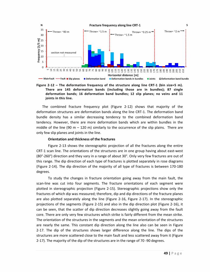
49 | P a g e   

Figure  2‐12  –  The  deformation  frequency of  the  structure  along  line CRT‐1  (bin  size=5 m). There  are  145  deformation  bands  (including  those  are  in  bundles);  87  single deformation  bands;  16  deformation  band  bundles;  12  slip  planes;  no  veins  and  11 joints in this line. 

The  combined  fracture  frequency  plot  (Figure  2‐12)  shows  that  majority  of  the 

deformation structures are deformation bands along the  line CRT‐1. The deformation band 

bundle  density  has  a  similar  decreasing  tendency  to  the  combined  deformation  band 

tendency. However,  there  are more  deformation  bands which  are within  bundles  in  the 

middle of the  line  (90 m – 120 m) similarly to the occurrence of the slip plains.   There are 

only few slip planes and joints in the line. 

Orientation and thickness of the fractures 

Figure 2‐13 shows  the stereographic projection of all  the  fractures along  the entire    

CRT‐1 scan line. The orientations of the structures are in one group having about east‐west 

(80°‐260°) direction and they vary in a range of about 30°. Only very few fractures are out of 

this range. The dip direction of each type of fractures is plotted separately in rose diagrams 

(Figure 2‐14). The dip direction of  the majority of all  type of  fractures  is between 170‐180 

degrees.  

To  study  the  changes  in  fracture orientation  going  away  from  the main  fault,  the 

scan‐line  was  cut  into  four  segments.  The  fracture  orientations  of  each  segment  were 

plotted  in  stereographic projection  (Figure 2‐15). Stereographic projections  show only  the 

fractures of which dip was measured; therefore, dip and dip directions of the fracture planes 

are  also plotted  separately  along  the  line  (Figure  2‐16,  Figure  2‐17).  In  the  stereographic 

projections of the segments  (Figure 2‐15) and also  in the dip direction plot (Figure 2‐16),  it 

can be seen,  that  the scatter of dip direction decreases slightly going away  from  the  fault 

core. There are only very few structures which strike is fairly different from the mean strike. 

The orientation of the structures in the segments and the mean orientation of the structures 

are nearly  the  same. This  constant dip direction along  the  line also  can be  seen  in Figure 

2‐17.  The  dip  of  the  structures  shows  larger  difference  along  the  line.  The  dips  of  the 

structures are more scattered close to the main fault and less scattered away from it (Figure 

2‐17). The majority of the dip of the structures are in the range of 70 ‐90 degrees.  

50 | P a g e   

The  thickness of  the bands  is also nearly  constant;  it  varies between 1  and 2 mm 

(Figure 2‐18). The thickness of deformation band bundles and also the shape of the bands do 

not  show  any  trend  along  the  line.  The  number  of  the  deformation  bands  in  bundles  is 

increasing going away from the main fault. 

Figure 2‐13 –  Stereographic  lower‐hemisphere projection of  the planes of  all  the  fractures along  line  CRT‐1  (red:  slip  plane;  blue:  deformation  band;  cyan:  deformation  band bundle; green: joint). 

 

Figure  2‐14  – Rose  diagram  of  the  dip  directions  of  the  fractures  along  the  line CRT‐1 per fracture type (red: slip plane; blue: deformation band; cyan: deformation band bundle; green: joint). 

Figure 2‐15 – Stereographic  lower‐hemisphere projection of  the  four  sections of  line CRT‐1 (red: slip plane; blue: deformation band; cyan: deformation band bundle; green: joint). 

51 | P a g e   

Figure 2‐16 – Dip direction of the fractures along the Line CRT‐1. 

 

Figure 2‐17 – Dip of the fractures along the Line CRT‐1. 

Figure 2‐18 ‐ The thickness, the shape (referenced to the host rock) of the deformation bands and the number of the deformation bands in bundles along Line CRT‐1. 

52 | P a g e   

LineCRT‐2 

This line starts at a large slip plane, which has fine, polished, white colour slickenlines 

on the surface and it is presumably very close to the core of the studied fault branch. There 

is a not measured section in the first part of the  line from 14 m to 64 m where the surface 

was weathered and covered and was not appropriate  to measure scan‐line. However,  the 

short, not  covered  areas  showed  relatively high  fracture density  in  this  section. The  fault 

zone shows a more complex structure  in comparison with the  line CRT‐1 and smaller faults 

were observed  in the far third of the  line. The fracture frequency plots (Figure 2‐19, Figure 

2‐20) show a moderate decreasing tendency  in the deformation band frequency; however, 

there are several peaks evenly distributed along the line. There is no clear relation between 

the occurrence of  the peaks and occurrence of the  faults. The number of  the deformation 

bands exceeds 8‐10 deformation bands per metre close to the main fault from 0 m to 14 m. 

The number of the deformation bands exceeds 20‐22 band per metre at peaks only  locally 

(sections <1 m). And at end of the line, deformation band frequency often exceeds 3‐4 bands 

per metre. There are some several metres long gaps without any fractures. The occurrence 

of the joints shows also a moderately decreasing tendency; however, more slip planes were 

observed at the end of the line than close to the main fault. 

The cumulative deformation band  curve  (Figure 2‐19)  contains  sequences of  steep 

and  less steep sections. The curve can be divided  into five sections: The first one  is a 23 m 

long steep section from 0 m – 14 m at the main fault where 20 % of the deformation bands 

are  located with decreasing deformation band  frequency  from  the main  fault. The second 

section is 130 m  long from 88 m – 210 m less steep where the deformation band density  is 

significantly  lower  including a 30 m  long gap, the cumulative deformation band reach 50 % 

by the end of the section. The next section is a short 15 m long steep section which contains 

20 % of deformation bands; followed by a 45 m long from plateau from 228 m – 273 m and 

at end of the line there is again a steep section involving 26 % of the deformation bands. The 

plots  do  no  show  unambiguous  relation  between  the  locations  of  the  faults  and  the 

distribution of the fractures. 

Along  this  line,  the majority  of  the  deformation  structures  are  also  deformation 

bands (Figure 2‐20). The deformation band bundles are in the middle (65‐115 m) and at the 

end of the line (>225 m) only, and their numbers range between 1 to 5 bundles per 5 metres. 

The  total  number  of  the  single  deformation  bands  is  only  slightly  higher  than  the  total 

number of deformation bands inside bundles. However, in the same bins where deformation 

band  bundles  occur,  the  number  of  the  deformation  bands  which  are  within  bundles 

significantly  higher.  There  are  two  sections  (65‐115 m  and  225 m  to  the  end) which  are 

characterised by deformation band bundles. 

 

53 | P a g e   

Figure 2‐19 – The deformation band frequency, the cumulative deformation band frequency in percentage and the  location of the  fractures and  features are shown along the  line CRT‐2 in the plot. The numbered sections show the separated section for stereographic projection of Figure 2‐22. 

 

Figure 2‐20 ‐ Deformation structure frequency along line CRT‐2 (bin size=5 m). There are 383 deformation bands (including those are  in bundles); 205 single deformation bands; 40 deformation band bundles; 16 slip planes; 4 veins and 77 joints in this line. 

 

 

 

 

 

 

54 | P a g e   

Orientation and thickness of the fractures 

The stereographic projection of all the fractures in the entire line CRT‐2 scan is shown 

in  Figure  2‐21.  The  orientations  of  the  fracture  planes  are  about  90‐270°,  east‐west 

bounding  having  a  40° wide  homogeneous  scatter.  However,  the majority  of  the  planes 

scatter within a  range of 20 degrees. The  rose diagrams of Figure 2‐22  show  that  the dip 

directions  of  the  majority  of  the  slip  planes,  joints  and  veins  are  about  200°;  the  dip 

directions of the majority of the deformation bands are 180° and 200°; the dip directions of 

the majority of the deformation band bundles are 175°. The variation of the dip directions of 

the joints is the largest about 80 degrees, much larger than the others fractures. 

 This  line  is  cut  into  five  segments  and  fracture  plain  orientations  plotted  in 

stereographic lower‐hemisphere projections (Figure 2‐23). Plots show larger angle scatter in 

the  fracture plain orientations  (about 80‐90°)  close  to  the main  fault  than  farther  (where 

variation  is  about  40°)  showing  similar  tendency  to  line  CRT‐1.  In  the  first  segment,  two 

groups  of  the  fractures  can  be  distinguished;  in  the  other  segments  only  one  main 

orientation was  dominant.  The  graph of  dip  and  dip  direction  of  all  the  fractures  (Figure 

2‐24, Figure 2‐25) shows, that  in the zones near to the main branch fault, the variations of 

both dip and dip direction are  larger; but farther  from the fault, the variations are smaller. 

The variation of the dip directions is larger locally around at the main fault, the faults at 222 

m and 285 m; and the variation of the dip is larger locally around the faults at the main fault, 

at 125 m, 195 m and 222 m. 

The  thickness  of  the  deformation  bands  exceeds  2‐3  mm  at  the main  fault  and 

further  the  thickness  is  less  than 1 mm. Number of deformation bands  in bundles  ranges 

between 2 and 5 along the entire line; it increases to 9 around the fault at 222 m. The shape 

of the bands does not show any trend along the line. More convex deformation band can be 

found along the  line than concave or plain; consequently, the majority of the fractures are 

stronger than the host rock. 

Figure  2‐21  ‐  Stereographic  lower‐hemisphere  projection  of  the  planes  of  all  the  fractures along  line  CRT‐2  (red:  slip  plane;  blue:  deformation  band;  cyan:  deformation  band bundle; green: joint; yellow: vein). 

55 | P a g e   

Figure 2‐22 ‐ Rose diagrams of the dip directions of the fractures of the Line CRT‐2. 

 

Figure 2‐23  ‐ Stereographic  lower‐hemisphere projection of the sections of Line CRT‐2  (red: slip  plane;  blue:  deformation  band;  cyan:  deformation  band  bundle;  green:  joint; yellow: vein). 

Figure 2‐24 ‐ Dip direction of the fractures on line CRT‐2. 

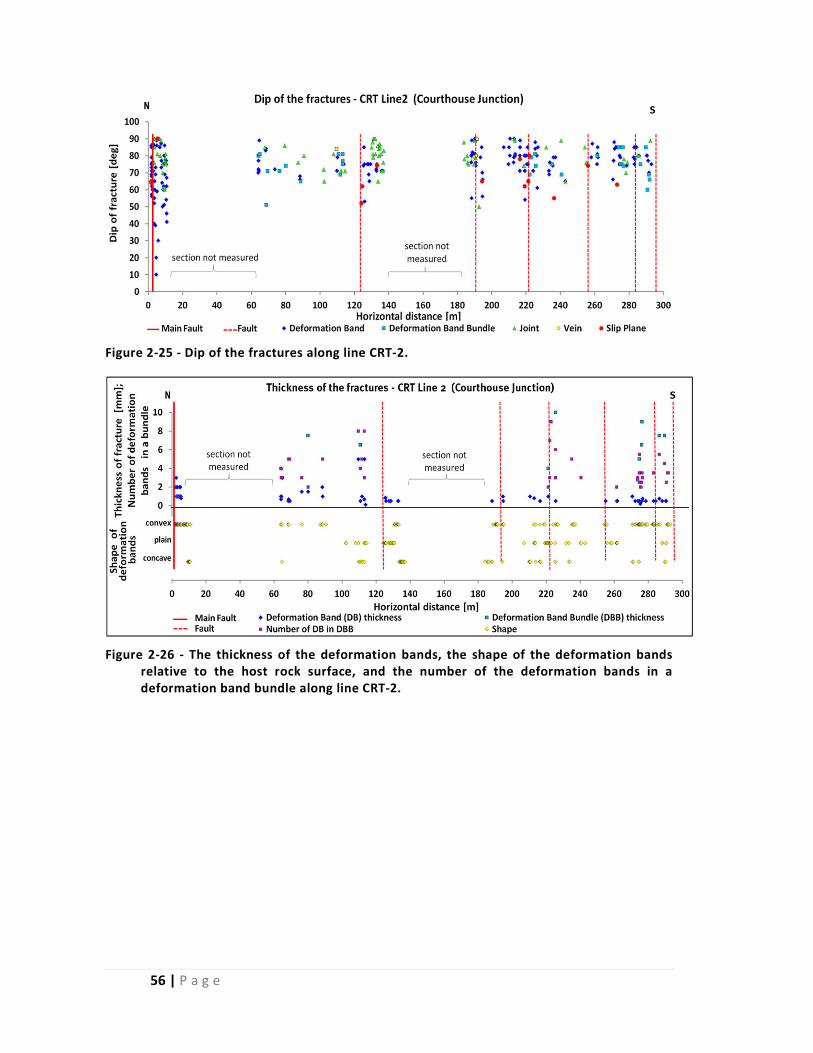
56 | P a g e   

Figure 2‐25 ‐ Dip of the fractures along line CRT‐2. 

Figure 2‐26  ‐ The  thickness of  the deformation bands,  the  shape of  the deformation bands relative  to  the  host  rock  surface,  and  the  number  of  the  deformation  bands  in  a deformation band bundle along line CRT‐2. 

 

   

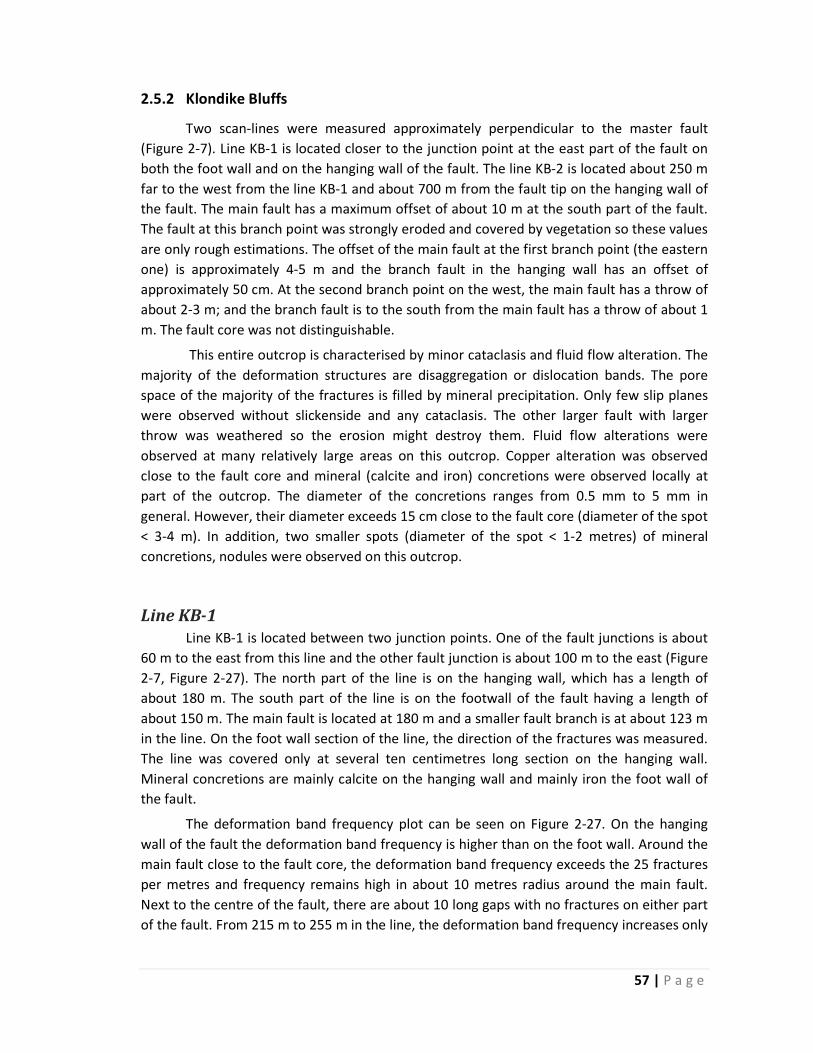
57 | P a g e   

2.5.2 Klondike Bluffs 

Two  scan‐lines  were  measured  approximately  perpendicular  to  the  master  fault 

(Figure 2‐7). Line KB‐1 is located closer to the junction point at the east part of the fault on 

both the foot wall and on the hanging wall of the fault. The line KB‐2 is located about 250 m 

far to the west from the line KB‐1 and about 700 m from the fault tip on the hanging wall of 

the fault. The main fault has a maximum offset of about 10 m at the south part of the fault. 

The fault at this branch point was strongly eroded and covered by vegetation so these values 

are only rough estimations. The offset of the main fault at the first branch point (the eastern 

one)  is  approximately  4‐5 m  and  the  branch  fault  in  the  hanging  wall  has  an  offset  of 

approximately 50 cm. At the second branch point on the west, the main fault has a throw of 

about 2‐3 m; and the branch fault is to the south from the main fault has a throw of about 1 

m. The fault core was not distinguishable. 

 This entire outcrop is characterised by minor cataclasis and fluid flow alteration. The 

majority  of  the  deformation  structures  are  disaggregation or  dislocation  bands.  The  pore 

space of the majority of the fractures  is filled by mineral precipitation. Only few slip planes 

were  observed without  slickenside  and  any  cataclasis.  The  other  larger  fault with  larger 

throw  was  weathered  so  the  erosion  might  destroy  them.  Fluid  flow  alterations  were 

observed  at many  relatively  large  areas  on  this  outcrop. Copper  alteration was observed 

close  to  the  fault core and mineral  (calcite and  iron) concretions were observed  locally at 

part  of  the  outcrop.  The  diameter  of  the  concretions  ranges  from  0.5 mm  to  5 mm  in 

general. However, their diameter exceeds 15 cm close to the fault core (diameter of the spot 

<  3‐4 m).  In  addition,  two  smaller  spots  (diameter  of  the  spot  <  1‐2 metres)  of mineral 

concretions, nodules were observed on this outcrop. 

 

LineKB‐1Line KB‐1 is located between two junction points. One of the fault junctions is about 

60 m to the east from this line and the other fault junction is about 100 m to the east (Figure 

2‐7, Figure 2‐27). The north part of  the  line  is on  the hanging wall, which has a  length of 

about 180 m. The  south part of  the  line  is on  the  footwall of  the  fault having a  length of 

about 150 m. The main fault is located at 180 m and a smaller fault branch is at about 123 m 

in the line. On the foot wall section of the line, the direction of the fractures was measured. 

The  line was  covered  only  at  several  ten  centimetres  long  section  on  the  hanging wall. 

Mineral concretions are mainly calcite on the hanging wall and mainly  iron the foot wall of 

the fault. 

The deformation band  frequency plot can be  seen on Figure 2‐27. On  the hanging 

wall of the fault the deformation band frequency is higher than on the foot wall. Around the 

main fault close to the fault core, the deformation band frequency exceeds the 25 fractures 

per metres and  frequency  remains high  in about 10 metres  radius around  the main  fault. 

Next to the centre of the fault, there are about 10 long gaps with no fractures on either part 

of the fault. From 215 m to 255 m in the line, the deformation band frequency increases only 

58 | P a g e   

locally.  The  deformation  band  frequency  increases  around  the  smaller  fault  at  123  m 

exceeding 10 fractures per metre.  

On the hanging, the decreasing tendency of the deformation band frequency is more 

constant;  however,  this  is  not  the  case  along  the  foot wall.  In  the  foot wall,  the  typical 

deformation band frequency is 2‐3 per metre; however, there is an increase in the frequency 

between 270 m  and 290 m  (5‐7  deformation  bands  per metre). At  the  hanging wall,  the 

cumulative  deformation  band  frequency  curve  (Figure  2‐27)  increases  steeply  from main 

fault to 60 m; this section contains 90 % of the fractures of the hanging wall. The cumulative 

deformation band curve of foot wall  increases very steeply close to the  fault centre where 

about 30 % of the  fractures are  located. From 193 m to 250 m, the curve  is  flat, and  from 

250 m to the end of the scan‐line, the cumulative frequency curve increases having a similar 

steepness to curve in the hanging. 

Along  this  line,  the majority  of  the  deformation  structures  are  also  deformation 

bands (Figure 2‐28). The majority of the deformation bands are in bundles on the foot wall. 

In the hanging wall, the number of the single deformation bands is higher than the number 

of the deformation bands in bundles. Far from the faults between 0 m and 35 m, only single 

deformation  bands were observed.  The  number of  the  deformation  band  bundles  ranges 

between 4 and 5 bundles per 5 metres around the main fault (130 m – 195 m). At other part 

of the  line,  the deformation band bundle  frequency varies between 1 and 3 bundles per 5 

metres. Only few joints can be found on the hanging wall slightly closer to the main fault. 

 

Figure 2‐27 ‐ Deformation band frequency and fracture location along line KB‐1. 

 

59 | P a g e   

Figure 2‐28  ‐ Deformation structure frequency along  line KB‐1 (bin size=5 m). There are 189 deformation bands (including those are  in bundles); 473 single deformation bands; 82 deformation band bundles; 2 slip planes; 1 veins and 25 joints in this line. 

Orientation and thickness of the fractures 

Figure 2‐29   shows  the stereographic  lower‐hemisphere projection of  the planes of 

all  the  fractures. Two groups can be distinguished based on  the dip directions. The group 

which contains the majority of the fractures is east‐west bounding. The other group has an 

orientation of 120‐300°. The angle between the two groups is about 25° which is about the 

same as the angle between the main fault and the branch fault. Orientation of the planes of 

each group has about 30 degrees variation. The fault branch is conjugate of the main faults. 

The rose diagrams of the dip direction of the fractures (Figure 2‐30) shows that single 

deformation bands are sub‐parallel to the branch fault and the majority of the deformation 

band bundles sub‐parallel to the main fault. The orientation of the majority of the  joints  is 

similar to the branch fault; however, the orientation of the joints has a wide variation.   

To show the variation in dip directions of the fracture plane along the line, the data 

set is cut into five sections and these sections are plotted in stereographic projection (Figure 

2‐31).  The  stereographic  projections  show  only  those  fractures  where  dips  also  were 

measured;  therefore,  the  dip  and  the  dip  directions  of  the  fracture  planes  are  plotted 

separately along the  line (Figure 2‐32 and Figure 2‐33). These plots show that the variation 

of the direction of the fractures  is  large close  to  the main  fault  in the  first 5 metres of the 

hanging wall. On  the  hanging wall  from  about  60 m  to  160 m,  the  dip  direction  of  the 

fractures  varies  between  about  160‐250°  and  50‐350°.  The  average  orientation  in  this 

section  is sub‐parallel  to  the smaller  fault branch. The dip direction of  the  fractures varies 

between 160° and 210° at the far end of the hanging wall from 0 m to 30 m where the mean 

strike of the fractures is more similar to the strike of the main fault. The strike directions of 

the  deformation  structures  are  sub‐parallel  to  both  the main  fault  and  the  branch  fault 

around the main fault from 160 m – 200 m (section 4). Most of the fractures are conjugate 

to the main fault. The majority of the dip of the fractures range between 60° and 90°; only 

few fracture have dips below this range. The lowest dip was 42 degrees. 

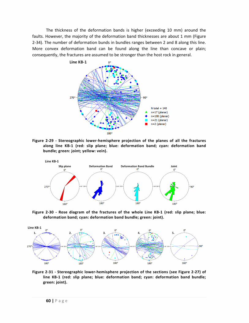
60 | P a g e   

The  thickness  of  the  deformation  bands  is  higher  (exceeding  10 mm)  around  the 

faults. However, the majority of the deformation band thicknesses are about 1 mm (Figure 

2‐34). The number of deformation bunds in bundles ranges between 2 and 8 along this line. 

More  convex  deformation  band  can  be  found  along  the  line  than  concave  or  plain; 

consequently, the fractures are assumed to be stronger than the host rock in general. 

Figure  2‐29  ‐  Stereographic  lower‐hemisphere  projection  of  the  planes  of  all  the  fractures along  line  KB‐1  (red:  slip  plane;  blue:  deformation  band;  cyan:  deformation  band bundle; green: joint; yellow: vein). 

Figure  2‐30  ‐  Rose  diagram  of  the  fractures  of  the whole  Line  KB‐1  (red:  slip  plane;  blue: deformation band; cyan: deformation band bundle; green: joint). 

Figure 2‐31 ‐ Stereographic  lower‐hemisphere projection of the sections (see Figure 2‐27) of line  KB‐1  (red:  slip  plane;  blue:  deformation  band;  cyan:  deformation  band  bundle; green: joint). 

61 | P a g e   

Figure 2‐32 ‐ Dip direction of the fractures along line KB‐1. 

Figure 2‐33 ‐ Dip of the fractures along line KB‐1 

62 | P a g e   

Figure 2‐34  ‐ The thickness of the  fractures, the shape of the deformation fractures, related to  the  host  rock,  and  the  number  of  the  deformation  bands  in  a  deformation  band bundle on line KB‐1. 

 

LineKB‐2 

Line KB‐2 is located approximately 190 m to the west from the line KB‐1 (Figure 2‐7), 

about 130 m  to  the west  from  the western  fault  junction and about 300 m  from  the east 

fault junction point. This line is located on the hanging wall of the fault. The south end of the 

line is at the main fault where the fault throw is about 2 m and the strike of this fault at the 

line  is about 124°. The throw of the branch  fault  is  located at about 194 m  in the  line and 

from main fault is about 0.1 m. The strike of this fault branch is about 136°. In the middle of 

the line, an about 100 m long section was not measured, because it was covered by soil and 

vegetation. 

The deformation band frequency plot (Figure 2‐35) shows that the deformation band 

frequency  is  the  highest  next  to  the main  fault. However, only  locally,  deformation  band 

frequency exceeds the 25 bands per metre at the north branch fault. The deformation band 

frequency tendency decreases but not monotonously going farther from the faults. Several 

local peaks can be seen along the line. The magnitude of the peaks of the deformation band 

frequency decreases gradually going away from the faults at distance of 280 m to 210 m and 

90 m to 0 m along the line. At about 240 m horizontal distance in the line, the deformation 

band  frequency  has  a minimum  between  the  two  faults  from where  the  trend  increases 

steeper towards the north fault and a less steep trend towards the main fault.  

 

 

63 | P a g e   

These tendencies can be seen in the cumulative deformation band curve too (Figure 

2‐35). The segment of the decreasing trend next to the main fault between 240 m – 305 m 

contains the 40 % of the deformation bands. The segment with the increasing trend next to 

the north fault between 240 m – 195 m contains 37 % of the bands, nearly the same number 

of deformation band as the other larger fault. 10 % of the deformation bands can be found 

at the  first peak of the north section of the  line between 90 m  ‐ 70 m distance. The other 

part of this section is 70 m long and the remaining 15 % of the bands are located here. The 

steps  in  the cumulative curve show  that  the deformation band distribution  is not uniform 

but  there  are  local  fracture  groups.  At many  paces, mineral  concretions were  observed 

between  the two  faults; majority of  these are close to the main  fault. At the north part of 

the  line,  less mineral  concretions were  observed  and  their  distribution  shows  correlation 

with the deformation band frequency peaks. 

Figure 2‐36 shows  that  the majority of  the deformation structures are deformation 

bands and deformation bundles. The distribution of  the deformation bund bundles  is very 

similar  to  the  distribution  of  the  deformation  band  bundle  with  lower  amplitudes.  The 

deformation bundle number exceeds 8 bundles per 5 metres in the south section of the line 

and 5 bundles per 5 metres farther from the faults in the north section of the line. Along the 

entire line, the majority of the deformation bands are in bundles. 

  

Figure 2‐35 – The deformation band frequency, the cumulative deformation band frequency in percentage and the location of the fractures and features are shown along line CRT‐2 in  the  plot.  The  numbered  sections  show  the  separated  section  for  stereographic projection on Figure 2‐22. 

 

64 | P a g e   

Figure 2‐36  ‐ Deformation structure frequency along  line KB‐2  (bin size=5 m). There are 142 deformation bands (including those are in bundles); 493 single deformation bands; 106 deformation band bundles; 3 slip planes; 0 veins and 12 joints in this line. 

 

Orientation and thickness of the fractures 

The  stereographic projection of  the all  the  fractures  in  the entire  scan  line  (Figure 

2‐37) shows that the mean fracture orientation is about 290° ‐ 110°  and scatters in a range 

of about ± 40°. This range of  the  fracture orientation covers  the direction of  the  two  fault 

groups of the orientations cannot be distinguished in this plot. The rose diagrams of the dip 

direction of the fractures (Figure 2‐38) show that the majority of the deformation bands and 

deformation  band  bundles  are  sub‐parallel  to  the  faults.  In  the  rose  diagrams  of  the 

deformation bands and deformation band bundles,  two sets of deformation bands can be 

distinguished. The direction of one of the sets is similar to the major fault and the other set 

is sub‐parallel to the branch fault. The few number of joints do not show unambiguous main 

direction; some of  the  joints have similar directions  to  the  faults some of  them are nearly 

perpendicular to the directions of faults.   

The variations of dip and dip direction of the fracture planes along the line are shown 

by  four  stereographic  projections  (Figure  2‐39)  and  the  dip  and  the  dip  directions  of  the 

fracture planes are plotted separately along the line (Figure 2‐40 and Figure 2‐41) similarly to 

the previous  lines. The variations of  the dips and  the dip directions of  the  fractures show 

similar trends. Close to the faults, the variation of the orientations of the fractures larger is 

larger than farther from them. The dip of the fractures ranges between 50 and 90 degrees. 

The majority of the fractures are conjugates to the faults. 

The  thickness  of  the  deformation  band  bundles  is  extremely  high;  their  thickness 

exceeds the 40 mm between the faults and farther from the faults the maximum thickness 

of the bundles is 6 mm (Figure 2‐42). The thickness of the deformation bands varies between 

0.5‐ 4 mm along the line. Majority of the deformation bands have a convex shape along the 

line especially between  the  two  faults  indicating  that  the deformation bands are  stronger 

than the host rock. 

65 | P a g e   

Figure  2‐37  ‐  Stereographic  lower‐hemisphere  projection  of  the  planes  of  all  the  fractures along  line  KB‐2  (red:  slip  plane;  blue:  deformation  band;  cyan:  deformation  band bundle; green: joint). 

 

Figure 2‐38 ‐ Rose diagram of the fractures of the whole Line KB‐2. 

 

Figure  2‐39  ‐  Stereographic  lower‐hemisphere  projection  of  the  sections  of  line  KB‐2  (red: slip plane; blue: deformation band; cyan: deformation band bundle; green: joint). 

66 | P a g e   

Figure 2‐40 ‐ Dip direction of the fractures on line KB‐2. 

Figure 2‐41 ‐ Dip of the fractures on line KB‐2. 

67 | P a g e   

Figure 2‐42  ‐ The thickness of the fractures, the shape of the deformation fractures, related to  the  host  rock,  and  the  number  of  the  deformation  bands  in  a  deformation  band bundle on line KB‐2. 

68 | P a g e   

2.6 Discussion

 

In this study, the architectures of two normal faults were analysed in order to better 

understand the properties of the fracture networks in fault zones. The types of the observed 

fractures were: deformation band, deformation band bundles, joints, veins slip planes in the 

studied  outcrops  along  the  scan‐lines.  The  upper  part  of Table 2‐1 shows  the  elementary 

data of the measured scan lines and the number of the different type of fractures. Only very 

few veins, 15 at Courthouse Junction and 4 at Klondike Bluffs  lines were  found. Combined 

about 130 joints were observed along the lines, majority of them (77) were along line CRT‐2 

at the Courthouse Junction. No slip planes with slickensides were observed at the Klondike 

Bluffs faults; however, 26 slip planes with slickensides at Courthouse Junction fault. Majority 

of the fractures were deformation bands along the scan  lines. The normalised deformation 

band number  (number of  the  fractures divided by  the  length of  the measured  section)  is 

significantly lower (less than half) at scan‐line CRT‐1 which is closer to the fault junction than 

at  scan‐line  CRT‐2  at  the  Courthouse  Junction  fault.  The  normalised  deformation  band 

number  is  higher  farther  from  the  junction  on  the  Klondike  Bluffs  but  the  difference 

between the values is not significant. The same relations can be seen at the normalised total 

deformation band number values. The normalised deformation band bundle numbers show 

a similar relation to the normalised deformation band at the Courthouse Junction. However, 

at  the Klondike Bluffs,  the numbers of  bands  are  significantly  higher with  the  increase  in 

distance  from  the  junction.  The  typical  deformation  band  number  based  on  the  total 

numbers of  the deformation band  is on one hand, close  to  the  junction point and on  the 

other, farther from them in both areas. 

 

Table  2‐1  –  The  tables  shows  the  basic  statistics  of  the  deformation  bands  (DB)  and deformation band bundles (DBB) along each scan‐line.  

* Thickness was calculated  for the not measured section using the average thickness of the line KB‐2. 

69 | P a g e   

Table 2‐1  also  shows  some  statistics of  the deformation bands  and bundles which 

were  the  most  relevant  to  the  study.  In  addition  to  the  average,  the  median  of  the 

deformation  bands  and  bundles were  calculated  too.  The median  provide  a more  robust 

statistics which is not biased by the outlier values in general. The average and median of the 

number  of  deformation  bands  in  the  bundles  do  not  show  significant  differences  in 

comparison  with  of  the  scan‐lines  of  either  areas.  At  the  two  outcrops,  typically  3‐4 

deformation bands can be found in the deformation band bundles. 

The typical thickness of the deformation bands  is 1 mm at the Courthouse Junction 

and farther from the  junction at the Klondike Bluffs. However, closer to the  junction at the 

Klondike Bluffs the average thickness  is about 2 mm. The average of the deformation band 

bundle thickness is 13‐15 mm at the Courthouse Junction and 18 mm at the Klondike Bluffs. 

However,  the median of  the deformation band bundle  thickness  is smaller about 10‐11 at 

each  line  showing  that  the average  is biased by  the higher  values. Rotevatn et  al.  (2008) 

analysed the cataclastic deformation bands in Western Sinai, Suez rift, Egypt and found that 

the average thickness of the bands  is 0.8 mm. Solum et al. (2010) studied the deformation 

bands around a reverse and a normal fault  in Utah. They found that the deformation band 

thicknesses  at  Buckskin Gulch  (in  a  reverse‐faulting  environment)  have  a  skewed  normal 

distribution, with a maximum at 1–2 mm or approximately 3–6  times  the mean grain size. 

Whereas,  deformation  band  thicknesses  at  the  Big  Hole  fault  show  an  exponential 

distribution with a maximum at less than 1 mm (smallest bin size) (Solum et al. 2010). 

The Courthouse Junction fault is a seismic scale fault branch of the major Moab fault, 

which is much larger and more complex than the Klondike Bluffs fault system. At both areas, 

the deformation band distribution has a decreasing tendency from the main faults along the 

scan‐lines  (lines CRT‐1 and KB‐1). At Courthouse Junction, the deformation band frequency 

at the fault is lower than that of the Klondike Bluffs and the degree of the decrease is slower 

i.e.  the  envelope  of  the  fracture  frequency  curve  is  less  steep.  The  deformation  band 

frequency decrease  is  irregular, not monotonous with distance. There are  local  smaller or 

larger  peaks,  irregularities  in  the  deformation  band  frequency.  Similar  deformation  band 

distribution  style  is documented  for example:  in Wadi el Khaboba  (Sinai)  in  sandstone by 

Rotevatn et al. (2008), also by Solum et al. (2010) at Buckskin Gulch and the Big Hole faults in 

Navajo  Sandstone,  Utah.  Similar  irregular,  decreasing  deformation  band  distribution was 

reported by Berg and Skar (2005) at the Bartlett fault segment. The Bartlett fault segment is 

part of the same fault branch of the Moab fault (in the same sandstone formations) as was 

studied  in this work.  It  is about 3 km from the studied Courthouse Junction outcrop to the 

west.  Furthermore,  similar  fracture  characteristics  were  observed  in  damage  zones  of 

normal fault in other rock types, such as gneiss (Gudmundsson et al. 2010) or tuff (Riley et al. 

2010). 

The deformation bands occur  in  local groups; there are  irregularities (i.e. peaks and 

gaps)  in  the  deformation  band  frequency which break  the  deformation  band  distribution 

trend. Berg and Skar (2005) found that deformation bands appear either isolated from each 

other  or  they  occur  associated  with  slip  surfaces  and  joints  and  deformation  band 

distribution also related to lithology changes. The results of the present study partly support 

70 | P a g e   

this  statement.  Based  on  visual  observation  and  microstructure  analysis  of  some  rock 

samples, there was not any significant change observed  in lithology in either of the studied 

faults. Furthermore,  the  results  show  that  irregularities and  increase  in deformation band 

frequency, occur  just at some of the faults (throw>10 cm). However, the deformation band 

frequency  increases also where  there was no  fault,  joint or slip surface. The degree of the 

increases  of  the  deformation  band  frequency  in  the  studied  scan‐lines  does  not  show  a 

significant relationship with the throw. The deformation band distribution around a fault  is 

not affected by the throw of the fault. This observation is in agreement with the observation 

of Schueller et al. (2013). 

Solum et al. (2010) analysed the deformation band networks in Utah sandstones, and 

found them to be really extensive and lacking of association with discrete faults at the area 

of Buckskin Gulch. Whereas, the presence of the deformation band network was  limited to 

the  damage  zone  at  Big  Hole  Fault.  Both  areas  are  characterized  by  similar  lithology, 

porosity,  permeability  and  deformed  at  similar  burial  depth  (1.5‐3  km).  However,  the 

Buckskin Gulch formed in a contractional tectonic setting, whereas the Big Hole Fault formed 

in  an  extensional  tectonic  setting.  Solum  et  al.  (2010)  explained  the  differences  of  the 

deformation  bands  distribution  by  the  different  tectonic  regimes.  Fossen  and  Rotevatn 

(2012) stated that the tectonic regime has some influence on the distribution of deformation 

bands;  however,  the  lithological  and  petrophysical  parameters,  and  the  tectonic  style  or 

boundary  conditions  can have  larger effect,  than  the  tectonic  regime. Solum et al.  (2010) 

reported  that  the average deformation band density  is 24.6 deformation bands per metre 

(DB/m)  in  contractional  environment  and  significantly  lower,  5.1  DB/m  in  extensional 

environment. In this study, at Klondike Bluffs the band density is 1.4 DB/m and 2.2 DB/m and 

at  the  Courthouse  Junction  0.9  DB/m  and  2.1  DB/m.  In  addition,  Solum  et  al.  (2010) 

observed  that  the  average  deformation  band  thickness  is  2.2  mm  in  contractional 

environment  and  1.9  mm  in  extensional  environment.  These  thicknesses  are  similar  to 

average  deformation  band  thicknesses  (1.3  –  2.2 mm)  at  Klondike  Bluffs.  However,  the 

average deformation band thickness at the Courthouse Junction  is about half of that about 

0.8 – 1.0 mm. It was also shown by several studies (e.g. Aydin 1978, Hesthammer and Fossen 

2001, Mair et al. 2002, Fossen et al. 2007), that the number of deformation bands is affected 

by the vertical stress i.e. burial depth. The average or normalized deformation band number 

is in the same order of magnitude at the Klondike Bluffs and the Courthouse Junction area. 

However,  the  two  areas  are  characterized  by  different  types  of  deformation  bands: 

cataclastic  and  dislocation  band which  indicates  that  the  differences  in  stress  conditions 

between the two areas. 

Several works aimed to define models for fracture distribution in fault zones. Some of 

the models  use  analytical,  other models  use  numerical  approach.  Anders  and Wiltschko 

(1994) analysed  the deformation bands and micro‐fractures  in the Navajo and  the Entrada 

sandstones  in  Arches  National  Park.  They  found  that  fracture  distribution  follows  an 

exponential decrease as a  function of the distance  from the  fault core. Similar exponential 

decrease  was  reported  by  Mitchell  and  Faulkner  (2009)  who  studied  fractures  in  the 

granodiorite and diorite of  the Atacama  fault system. Power  law  function based approach 

was  used  by  Savage  and  Brodsky  (2011)  to  model  the  fracture  density  decay.  Others 

71 | P a g e   

observed  that  there  is a  logarithmic decrease of  fracture density with  increasing distance 

from  the  fault  core  (Scholz  et  al.  1993, Anders  and Wiltschko  1994, Vermilye  and  Scholz 

1998, Chester et al. 2004, Schueller et al. 2013). According  to Kolyukhin et al.  (2009) and 

Schueller et al. (2013) there is a  logarithmic decrease in the frequency of deformation bands 

away from the fault core which  can be defined as: Y =A + Ln(X), where Y is the frequency of 

deformation bands per metre   and X  is the distance  from the  fault core  (Figure 2‐43). This 

model  can  be  used  to  calculate  the  theoretical width  of  the  damage  zone  and  also  the 

average deformation band density at a certain distance from the fault core. 

Figure  2‐43  –  Deformation  band  frequency  plot,  on  the  left,  shows  logarithmical  like decreasing  tendency  from  the  fault  core  (at  0  metre);  on  the  right,  a  combined logarithmic  fit  deformation  band  density  plot  based  on  normal  fault  measurement database of Schueller et al. (2013) is shown. (modified after Schueller et al. 2013) 

The fracture distribution analysis along the four studied scan‐lines at Klondike Bluffs 

and  Courthouse  Junction  showed  that  the  best  fitting  function  to  the  distribution  is  the 

logarithmic  in general. At analysing  the correlation between  the  logarithmic curve and  the 

deformation band  frequency was significantly  lower  for  the entire  line than  for sections of 

the lines next to faults. Figure 2‐44 shows an example for this. In two segments (length are 

50 m and 65 m) of the line KB‐2 between the two faults, the correlation is much higher than 

at the entire line. Along the local irregularities has significant effect on the deformation band 

trend.  In a  smaller vicinity of  fault  the  logarithmic  trend  is more valid. The  lengths of  the 

sections vary widely from 15 m up to 75 m; however, the logarithmic trend has a relatively 

good  approximation  along  the  entire  line  for  example  where  no  significant  frequency 

irregularity (Figure 2‐45) exist. 

72 | P a g e   

Figure 2‐44 – Logarithmic deformation band frequency trends of the entire KB‐2 line (plot A.) and  sections  of  this  line  (plot  B.  and  C.)  are  shown.  To  the  calculation  of  the logarithmic curve, the distance scale started at the faults at zero in all the cases. 

 

Figure 2‐45 ‐ Deformation band frequency and fitted logarithmic trend along line CRT‐1. 

 

A.

B. C.

73 | P a g e   

Numerical approach also was applied to create more reliable, more precise model to 

describe fracture distribution around faults. Schueller et al. (2013) analysed the evolution of 

deformation  band  distribution with  increasing  fault  throw  using  a  numerical model.  The 

results showed that with increasing throw both the deformation band density and the width 

of the damage zone  increase. They proposed that the maximum deformation band density 

(25‐60 even >120 DB/m) may be related to the critical stress at which the deformation band 

cluster becomes saturated with deformation band. This critical stress may be  influenced by 

the lithology. 

The  changes  of  the  deformation  band  frequency  perpendicular  to  the  fault might 

allow distinguishing internal subsets of the fault damage zone. Berg and Skar (2005) divided 

the  fault damage  zones  into  sub‐zones based on  the deformation band  frequency  (Figure 

2‐46). The  inner zone  is adjacent  to  the  fault core where  the deformation band  frequency 

next  to  fault core  is  the highest  i.e.  the cumulative curve  increases  steeply  from  the  fault 

core.  The  next  zone  going  farther  from  the  fault  core  is  the  outer  zone  where  the 

deformation  band  frequency  gets  significantly  lower  i.e.  the  cumulative  curve  increases 

moderately. Finally, the furthest zone from the fault core is the transitional zone where the 

deformation band  frequency  is very  low and become  zero;  the cumulative curve  is nearly 

flat. Beyond the transitional zone the not fractured protolith or host rock can be found. Berg 

and Skar (2005) found that the  inner zone  is about 4‐5 m; the end of the outer  is between 

about 20 m to 45 m and length ranges between 15‐30 m; while the length of the transitional 

zone  is  about  10  to  30 m  in  the  footwall.  In  some  cases,  the  inner  zone might  not  be 

identified around the fault; an example for this is shown in Figure 2‐47. Along the lines CRT‐2 

(Figure 2‐19), the sub‐zones of the damage zone cannot be identified, the characteristics of 

the  deformation  band  distribution  is  fairly  different  from  the most  common  distribution 

style because of the effect of the several smaller  faults. The  line CRT‐1 shows more similar 

deformation band distribution characteristics to the theoretical characteristics; however, the 

section  adjacent  to  fault  core was  not measured.  The  deformation  band  frequency was 

about 10 per metre  in the first 5 m from the fault core. Assuming the same distribution  in 

the start of the line CRT‐1, the first 5 m is the inner zone, the outer zone is between about 5 

m  and  170  m  and  transitional  zone  terminates  at  about  210  m  (Figure  2‐47/A).  The 

deformation band distribution  along  line KB2  is more  similar  to  the  characteristics of  the 

second example  showed  in Figure 2‐47/B where  the  inner  zone  is missing – no significant 

increase  in deformation band  frequency may be observed close to  the  fault core. This  line 

starts with an about 175 m  long outer zone where around a minor  fault,  the deformation 

band frequency increases and breaks the trend locally. At the end of the line, the transitional 

zone is 25 m long in this line. 

74 | P a g e   

Figure 2‐46 – Theoretical sub‐zones (inner, outer and transitional) of the fault damage zone based  on  deformation  band  frequency  and  cumulative  fractures  density  curve curvature (on the  left). An example for a typical  fracture distribution around a  fault  is shown on right hand side plot. (modified after Berg and Skar 2005)  

 

In  this  study, only  scan‐line KB‐1  at  the Klondike Bluffs was measured at both  the 

footwall and the hanging wall of the faults. Along this line on the hanging wall, the fracture 

density  is slightly higher (by about 12%) than the footwall, having a typically logarithmically 

decreasing  trend moving away  from  the  fault centre.  In addition,  there  is more  fluid  flow 

alteration and the fracture network is more complex in the hanging wall in comparison with 

the  footwall.  In the  footwall, the  fracture distribution  is very high close to  the  fault centre 

within 12 m and does not follow a logarithmical like trend. Other authors (e.g. Berg and Skar 

2005, Brogi 2008, Schueller, et al. 2013) made  similar observation  the  fracture network  is 

more complex on the hanging wall than the footwall at normal faults. 

 

 

 

75 | P a g e   

Figure 2‐47 – The deformation  frequency plots shows  the  zones of  the damage  zone of  the line CRT‐1  (Courthouse  Junction,  footwall) where  inner,  outer  and  transitional  zones can be  identified  and  line KB‐2  (Klondike Bluffs, hanging wall) where only outer and transitional can be identified zones. 

Berg and Skar (2005) observed that the hanging wall is more than three times wider 

than the footwall and more complex at the Bartlett fault segment of Moab fault where the 

fault  throw  is 170‐300 m having a NW‐SE strike. Furthermore, Berg and Skar  (2005)  found 

that in the footwall in Moab member of Curtis formation, the deformation bands orientation 

is NWE‐ESE and their dip is 85° with a slight predominance of antithetic structures (55%) and 

the deformation bands are either associated with  slip surfaces and  joints or  isolated  from 

each  other. Whereas,  there  are more  fractures  in  the  hanging  wall  in  Cedar Mountain 

formation  where  the  deformation  band  distribution  is  related  to  lithology  changes,  the 

deformation band are sub‐parallel to the strike of the master fault. They have mostly (72%) 

antithetic dip and  their dip  is  lower  than at  the  footwall.  In  the present study,  the  results 

show  that  the  dips  of  the majority  of  the  fractures  are  around  80‐85  degrees,  are  sub‐

parallel  to  the master  fault; and  there are more conjugate  fractures at  the  footwall of  the 

same fault branch at the Moab fault at Courthouse Junction, as well as in the Moab member 

 

 

 

Outer zone 

     

 

Transitional 

zone    Tran

sitional zone 

         Outer zone 

 

    Assumed  inner zone based on line CRT‐1 

76 | P a g e   

of  Curtis  formation.  Furthermore,  the  results  did  not  show  unambiguous  relationship 

between the occurrence of the deformation bands and other fractures. 

Brogi  (2008)  documented  that  the  damage  zones  is  characteristically  asymmetric 

around the Rapolano normal fault (Northern Apennines, Italy) in siliceous sedimentary rock. 

Better developed fractures can be found especially in the hanging wall where fault throw is 

larger  than 10 m and  the  fracture density  is  increasing rapidly while approaching  the  fault 

core. In the footwall, the fracture density is more complex and there is no discernible density 

decrease  away  from  the  fault  centre.  Furthermore,  mineralisation  and  hydrothermal 

alteration were  found around  this  fault, which could be an  indication of high permeability. 

Similarly  to  the  results of Brogi  (2008), asymmetric  fracture distribution was  found at  the 

Klondike  Bluffs;  however,  the  fracture  distribution was  higher  and more  complex  in  the 

hanging wall than the footwall. 

The width  of  the  damage  zone was  also  investigated  by  several  studies  and  they 

found that the hanging wall is wider than the footwall in case of normal faults (Berg and Skar 

2005,  Brogi  2008,  Schueller,  et  al.  2013). Berg  and  Skar  (2005) measured  about  40‐60 m 

damage zone width on the footwall and on the hanging wall about 210 m in the Bartlett fault 

branch. Others’  results  also on  the Bartlett  fault branch  showed  that damage  zone width 

ranges along the fault. Koestler et al. (1995) measured damage zone width of 12 m (Berg and 

Skar, 2005), Davatzes and Aydin (2003) measured 15‐22 m, Koestler et al. (1994) measured 

20‐50 m and Harris et al.  (2003) observed damage zone width up  to 60 m.  In  the present 

work, at the Klondike Bluffs along the line KB‐1, the width of the damage zone is also shorter 

on  the  footwall about 150 m  than on  the hanging about 180 m. However,  the difference 

between  the  damage  zone width  of  the  hanging wall  and  the  footwall  is  not  significant. 

Moreover,  the  length of  the  damage  zone  along  the  line  KB‐2, which  is  farther  from  the 

junction  point,  exceeds  300 m  on  the  hanging wall which  is  significantly  longer  than  the 

damage zone width in the hanging wall at the other line. 

According to Knott et al. (1996), there is a linear relationship between the fault throw 

and the width of the damage zone.  However, based on the analysis of 106 scan‐lines around 

normal faults in Utah and other places, Schueller, et al. (2013) found that there  is a power‐

law  relationship, with an exponent of approximately 0.5, between  throw of  the  faults and 

the width of  corresponding damage  zones.  The  results of  the present  study do not  show 

clear  relationship  between  the  fault  throw  and  the  width  of  the  damage  zone.  At  the 

Klondike  Bluffs  fault,  the  overall  damage  zone  width  (including  the  related  minor  fault 

branches) is about 180 m closer to the  junction point where the fault throw is about 10 m; 

further  from  the  junction  point  where  the  fault  throw  is  significantly  lower,  the  overall 

damage zone width  is  larger than 300 m. At the Courthouse Junction  fault where the  fault 

throw is about 80 m, the overall damage zone width was not clearly identified. Along the line 

CRT‐1, which  is closer to the  junction point,  fracture frequency drops significantly at about 

220  m  from  the  fault  core  but  the  line  terminates  at  a  fault  cliff.  In  line  CRT‐2,  the 

deformation band  frequency  is still high at the end of the  line. Based on off scan‐line  field 

observations of  fractures,  the approximate width of damage zone of  this  fault segment at 

this outcrop  is 400‐500 m.  In contrast, Berg  (2005) observed a much smaller  (about 70 m) 

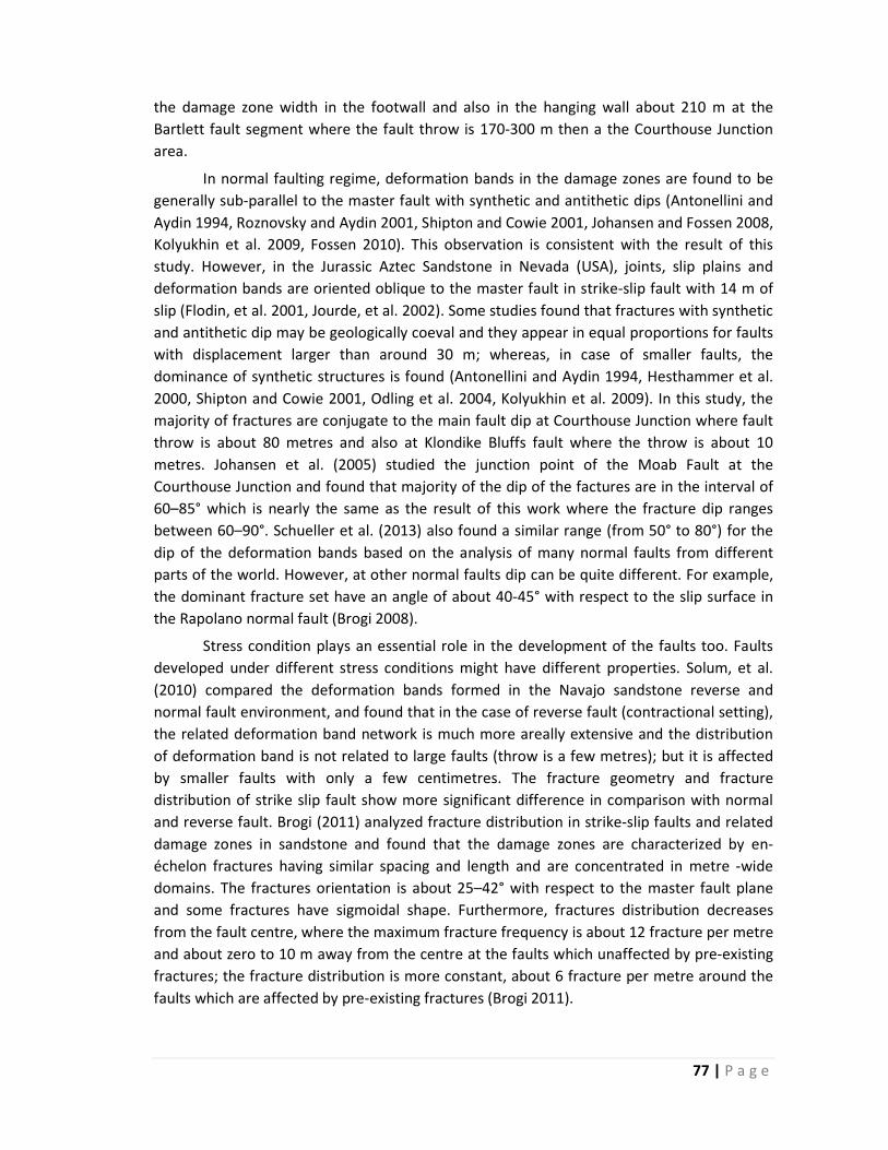
77 | P a g e   

the damage  zone width  in  the  footwall  and  also  in  the hanging wall  about 210 m  at  the 

Bartlett fault segment where the fault throw  is 170‐300 m then a the Courthouse Junction 

area. 

In normal  faulting regime, deformation bands  in the damage zones are found to be 

generally sub‐parallel to the master fault with synthetic and antithetic dips (Antonellini and 

Aydin 1994, Roznovsky and Aydin 2001, Shipton and Cowie 2001, Johansen and Fossen 2008, 

Kolyukhin et  al. 2009,  Fossen  2010).  This observation  is  consistent with  the  result of  this 

study.  However,  in  the  Jurassic  Aztec  Sandstone  in  Nevada  (USA),  joints,  slip  plains  and 

deformation bands are oriented oblique to the master fault in strike‐slip fault with 14 m of 

slip (Flodin, et al. 2001, Jourde, et al. 2002). Some studies found that fractures with synthetic 

and antithetic dip may be geologically coeval and they appear in equal proportions for faults 

with  displacement  larger  than  around  30  m;  whereas,  in  case  of  smaller  faults,  the 

dominance of synthetic structures  is found (Antonellini and Aydin 1994, Hesthammer et al. 

2000, Shipton and Cowie 2001, Odling et al. 2004, Kolyukhin et al. 2009). In this study, the 

majority of fractures are conjugate to the main fault dip at Courthouse Junction where fault 

throw  is  about  80 metres  and  also  at  Klondike  Bluffs  fault where  the  throw  is  about  10 

metres.  Johansen  et  al.  (2005)  studied  the  junction  point  of  the  Moab  Fault  at  the 

Courthouse Junction and found that majority of the dip of the factures are in the interval of 

60–85° which  is nearly  the  same as  the  result of  this work where  the  fracture dip  ranges 

between 60–90°. Schueller et al. (2013) also found a similar range (from 50° to 80°) for the 

dip of  the deformation bands based on  the analysis of many normal  faults  from different 

parts of the world. However, at other normal faults dip can be quite different. For example, 

the dominant fracture set have an angle of about 40‐45° with respect to the slip surface  in 

the Rapolano normal fault (Brogi 2008). 

Stress condition plays an essential role  in the development of the  faults too. Faults 

developed under different  stress  conditions might have different properties. Solum, et al. 

(2010)  compared  the  deformation  bands  formed  in  the  Navajo  sandstone  reverse  and 

normal fault environment, and found that in the case of reverse fault (contractional setting), 

the related deformation band network  is much more areally extensive and the distribution 

of deformation band is not related to  large faults (throw is a few metres); but  it is affected 

by  smaller  faults  with  only  a  few  centimetres.  The  fracture  geometry  and  fracture 

distribution of strike slip  fault show more significant difference  in comparison with normal 

and reverse fault. Brogi (2011) analyzed fracture distribution in strike‐slip faults and related 

damage  zones  in  sandstone  and  found  that  the  damage  zones  are  characterized  by  en‐

échelon  fractures having  similar  spacing  and  length  and  are  concentrated  in metre  ‐wide 

domains. The  fractures orientation  is about 25–42° with  respect  to  the master  fault plane 

and  some  fractures  have  sigmoidal  shape.  Furthermore,  fractures  distribution  decreases 

from the fault centre, where the maximum fracture frequency is about 12 fracture per metre 

and about zero to 10 m away from the centre at the faults which unaffected by pre‐existing 

fractures; the fracture distribution is more constant, about 6 fracture per metre around the 

faults which are affected by pre‐existing fractures (Brogi 2011). 

78 | P a g e   

The  results of  the present work shows  that  in normal  faulting  regime, deformation 

bands  form  close  to  the  fault  core  and  also  relatively  far  from  the  fault  core.  The 

deformation  band  frequency  has  peaks  as  the  distance  grows  going  from  the  fault  core. 

Some of the deformation bands are not related to faults. However, some peaks are related 

to faults but this relation is independent from the size of the fault throw. Both studied faults 

are  normal  faults;  however,  they  are  characterized  by  significantly  different  deformation 

band types. At Courthouse Junction, the majority of the fractures are cataclastic deformation 

bands which may significantly reduce the permeability of the rock. Whereas, at the Klondike 

Bluffs, most of the fractures are dislocation (disaggregation) deformation bands which might 

increase the permeability of the rock. 

The two most important fault parameters are: the permeability and the extent of the 

fault which need to be known to better understand fluid migration processes in rock bodies. 

To define the extent of a fault, the  length, the fault throw, the height of the  faulted  layers 

and  the  total width of  the  fault  zone  (core + hanging wall damage  zone width +  footwall 

damage zone width) need to be considered. The parameters of a fault e.g. width of the fault 

zone,  fracture density,  fracture distribution,  fracture dips, dip direction of the  fracture etc. 

change along the fault plane. This variation of the fault related fracture network can be seen 

from the studies performed along the branch fault of the Moab fault. Johansen et al. (2005) 

observed that the fracture network is complex, as it contains three generations of fractures 

with  different  orientations  in  the  junction  point  (Courthouse  Junction  triangular).  In  this 

work, line CRT‐1 was about 320 m from the junction point and the line CRT‐2 was about 900 

m from it. The fracture distribution and the width of the fault zone are fairly different along 

the  two  lines.  In  comparison with  the  Bartlett  fault  section,  the  fracture  density  is much 

higher in the inner zone but the width of the fault is significantly smaller. 

Kolyukhin et al. (2009) studied the effect of the parameters of the deformation band 

network  on  the  bulk  permeability  of  the  fault  damage  zone  using  stochastic model  (see 

Figure 2‐2). The  following parameters of  the deformation bands were considered:  relative 

deformation band permeability (KDB/KHR ‐ deformation band / host rock), deformation band 

density, dip angle, dip direction, heterogeneity of  the deformation band permeability  (i.e. 

holes  in the  fractures planes) and clustering. The clustering  is expressed by the correlation 

dimension (Dc) i.e. fracture distribution around faults which is 1 if the distribution is uniform, 

about  0.1  if most  of  the  fractures  are  very  close  to  the  fault  core  and  about  0.8  if  the 

distribution  is  decreasing  logarithmically moving  away  from  the  fault  core.  The  results  of 

Kolyukhin et al. (2009) indicated that deformation band density has a constant permeability 

of 0.01 darcy (lower than the host rock) and by being perpendicular to the flow direction the 

effective permeability was  reduced by about 50%  related  to  the host  rock.  If  the  fracture 

density  exceeds  10 deformation bands  per metre.  Furthermore, with  the  increase of  the 

cluster parameter  i.e.  the  increase of  the width of  the  fault  zone  (where  the deformation 

band density is increase farther from the fault core), the bulk permeability of a fault damage 

zone decreases where  the permeability of  the deformation bands are  lower  than  the host 

rock regardless of other properties. In addition, the orientation of the dip of the deformation 

bands  does  not  affect  the  effective  permeability  if  the  correlation  dimension  Dc>0.8; 

however,  if  the  correlation  dimension  Dc<0.8  it  might  have  considerably  effect  on  the 

79 | P a g e   

effective permeability  (Kolyukhin et al. 2009). The dip of the  fractures has more significant 

effect on  the  fluid  flow. For  instance,  the model of Kolyukhin et al.  (2009) showed  that  in 

comparison with  the host  rock  the  effective permeability decreased by  50%  in  a damage 

zone where the dip of the deformation bands are ±60° if the permeability is lower relative to 

the  host  rock  (KDB  =  0.01  darcy)  and  with  a  common  decreasing  deformation  band 

distribution  (Dc = 0.8) and a density of 15 deformation bands per metre. Kolyukhin et al. 

(2009) also showed that the discontinuities  (holes)  in the plains of the deformation bands, 

i.e. heterogeneity of the deformation band permeability, also affect the permeability of the 

fault damage zone. The higher the number of the holes is, the higher the permeability of the 

fault  zone;  if  the  holes  are  aligned,  then  the  permeability  is higher  than  if  the  holes  are 

randomly  distributed;  with  increasing  clustering  (Dc  is  decreasing),  the  bulk  effective 

permeability decreases if holes are randomly distributed and it is increasing if the holes are 

uniformly distributed. 

The geometry of  the studied  two  faults  in present work  (Courthouse  Junction  fault 

and Klondike Bluffs  fault) has similar parameters using model definition of Kolyukhin et al. 

(2009).  Orientation  of  the  deformation  bands  is  sub‐parallel  to  the major  fault  having  a 

moderate wide variation  (30‐40°). The dip of  the deformation bands which has about 30° 

variation. The distributions of  the deformation bands at  the Courthouse  Junction and  the 

Klondike Bluffs faults have similar logarithmically decreasing style; the correlation dimension 

is about 0.8. The deformation band density is also range in the same order of magnitude at 

both  faults  about  10  deformation  bands  per metre. Based on  the  field  observations,  the 

most significant difference between the studied faults  is the type of deformation bands.  In 

the  damage  zone  of  the  Courthouse  Junction  fault,  almost  only  cataclastic  deformation 

bands  (baffle  the  fluid  flow) can be  found and  in  the damage zone of  the   Klondike Bluffs 

fault  almost only dislocation deformation bands  (conduit  to  the  fluid  flow)  can be  found. 

Combined  the  results of  the present  field observation and  the conclusion of  the model of 

Kolyukhin et al. (2009), the relative complex fracture network  geometry in the fault damage 

zone at the Courthouse Junction, where the relative permeability between the  deformation 

bands  and  the  host  rock  is  low  (KDB/KHR<<1),  enhances  the  effect  of  the  individual 

deformation bands. Consequently, the bulk permeability of the damage zone might be lower 

than the permeability of the individual deformation bands. At this fault, the fluid flow rate is 

low or zero  if the pressure gradient  is normal to the fault plane.  If the pressure gradient  is 

not normal to the fault plane direction  is the flow rate  is higher parallel to the fault plane. 

The fracture network geometry in the fault damage zone the Klondike Bluffs fault, where the 

relative permeability  is probably higher  than one  (KDB/KHR>1),  the deformation bands also 

might  increase  the  effect  of  the  permeability  of  the  damage  zone  relative  to  the 

permeability of the individual deformation bands. However, this effect might be marginal if 

the pressure gradient  is normal to the fault plane because in this case the bottleneck is the 

host rock itself. If the pressure gradient is not normal or parallel to the fractures the dilatant 

fractures might  able  to  enhance  the  flow  rate  significantly  along  the  fracture  path ways. 

Based on the field observation, the majority of fluid flow occurred along the Klondike Bluffs 

fault.  

80 | P a g e   

In conclusion,  the geometry of  the  fracture network plays an  important  role  in  the 

fluid migration  in a reservoir which  is either barrier or conduit  to  fluid  flow. However,  the 

most  important parameter of  the  fault damage  zone  is  the permeability of  the  individual 

fractures which characterize the fault zone. If the stress is greater than a certain limit (yield 

stress),  the  rock  deforms  irreversibly and  fractures  develop.  The  type  of  the  developed 

fractures is affected by the stress condition which generated the fracture. In an extensional 

environment  (normal  faulting  regime)  tensile  fractures  may  form.  In  a  contractional 

environment  (reverse  faulting  regime)  compactional  can  form more  commonly. However, 

the differential stress and the confining pressure play an important role in formation of the 

fractures. Both studied faults are in normal faulting regime and at the Courthouse Junction, 

the characterized by compactional, cataclastic,  low permeability  fractures.  In contrast,  the 

Klondike Bluffs fault zone  is characterized by dislocation bands, relatively high permeability 

fractures. At the Courthouse Junction, as a result of the higher confining pressure and lower 

differential  stress,  cataclastic  fractures  developed.  As  a  result  of  the  stress,  the 

microstructure of  the  rock deforms  that  result  in different degree of permeability change 

along  the deformed  rock. The microstructure of different  types of  fractures  from  the  two 

study areas investigated in the chapter 3. 

2.7 Conclusionandoutlook

The damage zones of the two study normal faults are characterised by different types 

of fractures. The Courthouse Junction fault segment is characterised by major cataclasis. This 

fault is a branch of the major Moab Fault, where the rocks on the surface are Moab Member 

of  the Curtis Formation and Slick Rock Member of Entrada Sandstone. The most common 

fracture  type  is  cataclastic deformation band or  cataclastic deformation band  bundles.  In 

addition, slip planes with slickenside and joints can be found in the fault zone and there are 

only  few  locations where  fluid  flow  alteration  can be observed.  In  contrast,  the  Klondike 

Bluffs  fault  is  characterised  by  extensional  fractures  and major  fluid  flow  alteration.  This 

fault is adjacent to the Salt Valley anticline, where the rock on the surface is Moab Member 

of Curtis  Formation.  The most  common  fracture  type  is dislocation  (disaggregation band) 

deformation band or dislocation deformation band bundles.  In addition,  joints also can be 

found  in  the  fault  zone  but  slip  planes with  slickenside  were  not  observed.  Both  faults 

formed  in  normal  faulting  regime;  however,  the  stress  condition  (confining  pressure, 

differential stress) was not the same which resulted in different fracture style. 

The distribution of the type of the deformation bands  is uniform around each fault: 

cataclastic deformation bands only can be observed at  the Courthouse  Junction  faults and 

higher  relative  permeability  dislocation  deformation  bands  only  can  be  observed  at  the 

Klondike Bluffs  faults. This  indicates  that  the stress condition did not changed significantly 

during the process of the faulting. The deformation bands formed in one generation at each 

fault. The orientation of the joint setting shows larger discrepancy related to the orientation 

of  the master  fault  indicating  that  they are a different generation of  the  fractures  formed 

under different stress conditions. 

81 | P a g e   

Orientations of the majority of fractures are sub‐parallel to the master fault at both 

scan‐lines at both study areas. The variation on the strike of the deformation bands is about 

30° and dip ranges between 70 and 90° approximately 300 m far from the fault junction and 

the strike is about 40 degrees and dip ranges between 40 and 90° approximately about 660 

m from the fault  junction. The variation of the orientation of the deformation bands at the 

scan‐line closer to the master fault is similar to the other scan‐line which is farther from the 

junction point. This  shows  that both  faults are  far enough  from  the  junction of  the Moab 

fault,  which  is  nearly  perpendicular  to  the  studied  fault  branch,  and  it  does  not  have 

significant influence on the fracture system at the scan‐lines. The slightly larger scatter of the 

deformation  bund  orientation  at  the  scan‐line  farther  from  the  junction  point  can  be 

explained by the local variation of the complexity of the fault damage zone along the fault. 

The distribution of the deformation bands shows a decreasing trend going away from 

the fault core in both studied fault damage zone. In general, a logarithmic function provided 

a good approximation to describe this decreasing trend. However, local irregularities (peaks 

in  the deformation band density) are relatively common  too which have an  impact on  the 

general  trend.  These  local  irregularities  are  not  necessarily  related  to  faults;  several 

deformation band density peaks are present at both areas where there are no faults  in the 

interval  of  the  peaks.    In  conclusion,  a  single,  simple  function  can  provide  only  a  rough 

estimate  of  the  deformation  band density of  a  fault damage  zone. A  statistical  approach 

might provide a more realistic estimate. 

The  widths  of  the  damage  zones  are  relatively  wide  at  both  study  areas.  In  the 

footwall at Klondike Bluffs,  the damage zone width  is about 150 m and at  the Courthouse 

Junction  200 m  and  >300 m.  In  addition,  at  the  Klondike  Bluffs  in  the  hanging wall,  the 

damage  zone widths are 180 m  and 300 metres.  The  two  studied  faults  characterised by 

different fracture styles (compactional and dilatational) also have significantly different fault 

throws but  the width of their damage zones are similarly  large. These results  indicate that 

there  is  no  clear  relationship  between  the width  of  the  fault  damage  zone  and  the  fault 

throw, and between the fault damage zone width and the stress condition under the normal 

faults  formed.  Furthermore,  the  other  dimensions  of  the  faults  need  to  be  taken  into 

account.  The  length  of  the  Klondike  Bluffs  fault  is  about  3.5  km  and  the  length  of  the 

Courthouse  Junction  fault  is  about  7  km  long.  The  combined  thickness  of  the  faulted 

formations  varies  between  260  and  620 m.  The  size  of  the  fault  zones  shows  that  the 

impacted rock body has a considerably large extension. 

The  average  number  of  the  deformation  bands  is  similar  at  both  study  areas; 

however,  about  double  the  average  number  of  the  deformation  band  bundles  at  the 

Klondike Bluffs  fault.  There  is no  significant difference  in  the number of  the deformation 

band  within  bundles  at  the  areas.  The  average  thickness  of  the  cataclastic  deformation 

bands (0.8 and 1 mm)  is smaller than the average thickness of the dislocation deformation 

bands  (2.2  and  1.3  mm).  The  sum  of  the  deformation  band  thickness  is  higher  at  the 

Klondike Bluffs fault. 

 

82 | P a g e   

Some  parameters  of  the  fracture  network  of  the  fault damage  zone  are  relatively 

constant along the faults; however, other parameters vary quite a lot. The type of fractures 

does not change along the studied faults. The dip and dip direction and also the thickness of 

the  deformation  bands,  having  a  certain  degree  of  general  variations,  do  not  change 

significantly along  the  faults. However,  the widths of  the  fault damage zones,  the  fracture 

distribution and also the fracture density have significant variation along the faults. 

The  effect  of  the  two  studied  normal  faults  on  the  permeability  is  different.  The 

permeability of the deformation bands in the damage zone in Klondike Bluffs fault is higher 

than  the permeability of  the host rock and also  the geometry of  the  fracture network can 

support the effect of the permeability of the individual fractures. This fault disturbs the fluid 

flow system creating a fluid pathway in the fault zone. The permeability of the deformation 

bands  in  the damage  zone of  the Courthouse  Junction  fault  is  significantly  lower  than  the 

permeability of the host rock and the geometry of the fracture network supports the effect 

of  the permeability of  the  individual  fractures. This  fault  is an effective baffle  to  the  fluid 

flow  system which diverts  the  fluid migration,  fluid  tends  to  flow outside,  along  the  fault 

plain. 

The results of this work show that the properties of fault related  fracture networks 

vary  in  different  degree  along  the  fault;  some  properties  vary  only  slightly  and  other 

properties vary significantly. Therefore, it is important to collect data more frequently along 

the fault to analyse the structure of the fault zone in more detail. Scan‐line technic has been 

applied by  several  studies. However, other  technics  such  as  2D map  (e.g.  high‐resolution 

outcrop panorama photomosaic applied by e.g. Laurich et al. (2011) or 3D structural model 

(applied by e.g. Kokkalas et al. 2007, Wawrzyniec et al. 2007, Jones et al. 2008, McCaffrey et 

al. 2008, Jones et al. 2009, Sági 2013) of the fracture network of outcrops can provide good 

data source for a detailed analysis. Because the structure of a fault zone  is a very complex 

system with several parameters with great uncertainties, statistical analysis of field data can 

help  to better understand  the  relationship between  the different parameters of  the  fault 

zone which can improve the fault interpretation in seismic and well data.   

83 | P a g e   

3 Microstructureanalysisofsandstonefractures

 

3.1 Introduction

This study focuses on fractures of the tight sandstone reservoirs such as the Rotliegend 

sandstone  in  the North  Sea  and  in Moab,  Utah.  The  Broad  Ion  Beam  Scanning  Electron 

Microscope (BIB‐SEM) images allow us to study the nano‐structure of the fractures. The BIB 

polished surface allows us to trace the pores and minerals in order to calculate statistics to 

gain  information on  the properties of  the  fracture porosity. Besides,  the properties of  the 

single  fractures, having a  large number of samples with  fractures should allow us  to study 

the spatial distribution. To better understand the fracture systems, an essentially important 

factor is to understand the host rocks and the stress field; which determine the type of the 

fractures. The knowledge of the spatial distribution and the physical properties, the types of 

the  fractures and  the properties of  the host  rock allow us  to create a  theoretical  fracture 

model, which  is  able  to  improve  the  seismic  interpretation. Applying  these  results  to  the 

seismic data, the reservoir can be better described and characterized. 

The  microstructure  of  porous  rock  has  been  widely  studied  since  the  fractal 

behaviour of porous rock was discovered (Mandelbrot 1983, Katz and Thompson 1985). Katz 

and Thompson (1985) were the first who used SEM and optical microscope to calculate the 

fractal dimension of the pore space of various sandstones (with pores ranging from 10 Å to 

100µm).  The  method  to  determine  fractal  dimension  of  the  pore  size  distribution  in 

sandstones using SEM  images was automated by Krohn and Thompson  (1986). Since then, 

the fractal dimension of the size distribution of grains, pores and soil pore interface has been 

calculated  by  several  authors  (Krohn  and  Thompson  1986,  Hansen  and  Skjeltorp  1988, 

Martín and Taguas 1998, Dathe et al. 2001, Li et al. 2004, Menéndez et al. 2005, Desbois et 

al. 2009, Yu et al. 2009, Houben et al. 2013). 

The pore  throat  radius  is an  important parameter  to characterize  the  flow  through 

porous  reservoirs  (Nelson  2009).  Firstly,  pore  throats  were  investigated  in  photo 

micrographic  images of pore casts  (Dullien and Dhawan 1974) and  thin sections  (Wardlaw 

and Cassan 1978). There is correlation between reservoir permeability and the characteristic 

pore  throat  size  determined  by  mercury  injection  tests  (e.g.  Swanson  1981,  Katz  and 

Thompson  1986,  Thompson  and  Raschke  1987,  Ioannidis,  et  al.  1996).  The  relationship 

between  the pore  throat, permeability and porosity was shown analytically by Heid, et al. 

(1950) and experimentally by Windland (Kolodzie 1980) and Aguilera (2002). Based on these 

equations, Ziarani and Aguilera (2012) proposed a model to estimate the pore throat using 

the  permeability  and  the  formation  factor  (resistivity  factor).  It was  also  shown,  that  the 

permeability  is affected by the size distribution of pore throats, the connectivity properties 

of the pore network and the spatial correlation of pore sizes (Constantinides and Payatakes 

1989, Bryant, et al. 1993, Ioannidis and Chatzis 1993).  Furthermore, the pore throat is also 

used  to  characterize  the  flow  units  of  a  reservoir which  are  stratigraphically  continuous 

subdivisions  in a reservoir and can be used to  identify seals and faults. Martin et al. (1997) 

84 | P a g e   

worked  out  a  classification  scheme  for  pores  based on  the  size  of  the  pore  throats.  This 

classification  corresponds  to  Oil  Production  Rate  (OPR)  for medium  gravity  oil.  Similarly, 

Deng et al. (2011) proposed an initial relationship between the pore throat size and natural 

gas production. 

Although  the pore network of  the porous  rock  is  three dimensional,  some  studies 

have shown relationship between the 2D pore geometry and the permeability of the 3D pore 

network (Ehrlich et al. 1991, McCreesh et al. 1991, Coskun and Wardlaw 1993). Ioannidis, et 

al.  (1996)  analysed  the  statistical properties of microstructures of porous  rock using  SEM 

images, and they developed an empirical relationship to determine permeability from image 

porosity  and  integral  correlation  scale which  can  be  calculated  from  the  autocorrelation 

function of binary SEM images. 

The microstructure  of  the  deformation  bands  of  Arches National  Park, Utah  have 

been  the  subjects of many  studies  (Aydin  1978, Antonellini, et  al.  1994,  Fossen  and Bale 

2007, Torabi et al. 2007, Eichhubl et al. 2009, Fossen et al. 2011). Aydin (1978) found, that 

the deformation bands in the Entrada and Navajo Sandstones are formed by a combination 

of  various  different  processes,  such  as  shear  and  volume  change  accommodated  in  the 

matrix and pore spaces, microfracturing of grains  into smaller grains, shattering of smaller 

grains, and mixing of the fragments of grains with the matrix.  

Antonellini,  et  al.  (1994)  documented  two  generations  of  deformation  bands  at 

Arches National  Park.  The  older  generation  of  deformation  bands  are  characterized with 

little or no cataclasis, and distributed  in  relatively undeformed  sandstone,  in contrast,  the 

younger generation of deformation bands are characterized with well‐developed cataclasis, 

and  localized  in  the  vicinity of major  structures. According  to  laboratory experiments,  the 

different  deformation  band  generations  developed  under  different  stress  states,  and 

therefore  it can be assumed, that the first generation of deformation bands formed during 

the growth of the salt anticline while  the second generation of deformation bands  formed 

during the collapse of the salt anticline.  

Fossen and Bale (2007) found that deformation bands present  locally high decrease 

in permeability (about 4 orders of magnitude) and porosity. However, the thickness and the 

porosity of the bands vary rapidly, which reduce the effect of deformation bands to decrease 

the  permeability  of  the  reservoir.  Therefore,  they  concluded  that  the  deformation  bands 

unlikely control the fluid flow, although they might influence the pattern of fluid flow (Figure 

3‐1). 

85 | P a g e   

Figure 3‐1 – Thickness of deformation bands  shows  rapid  changes along  the band  (Entrada sandstone, San Rafael Desert, Utah) (modified after Fossen and Bale 2007). 

 

Figure 3‐2 – Porosity changes rapidly in the deformation band from the left side to right side of the sample (modified after Fossen and Bale 2007). 

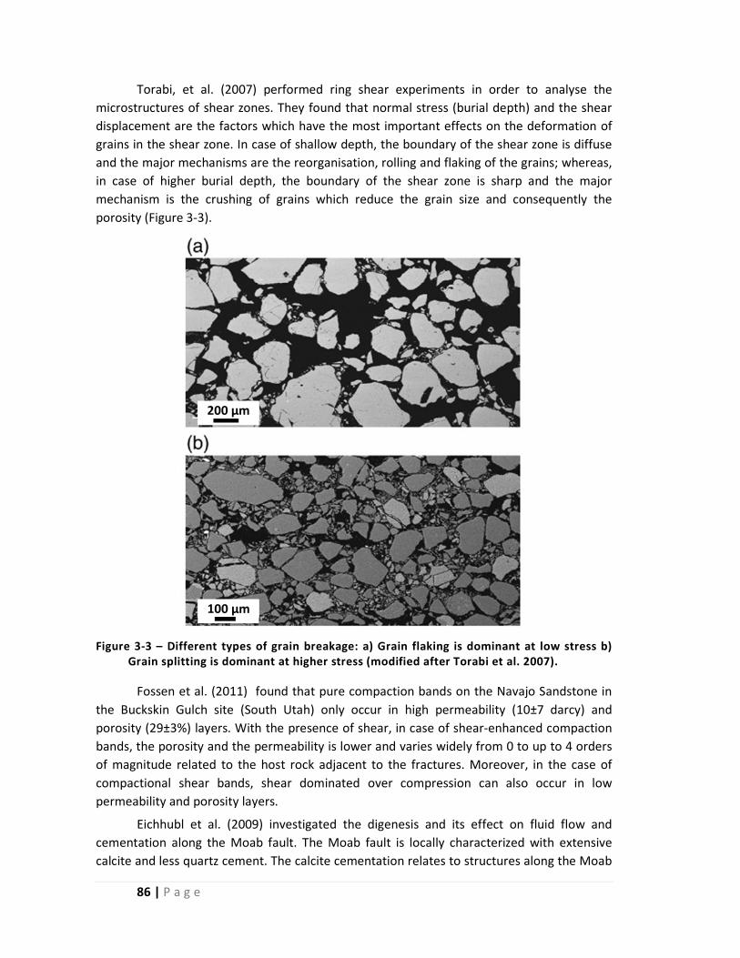
86 | P a g e   

Torabi,  et  al.  (2007)  performed  ring  shear  experiments  in  order  to  analyse  the 

microstructures of shear zones. They found that normal stress (burial depth) and the shear 

displacement are the factors which have the most  important effects on the deformation of 

grains in the shear zone. In case of shallow depth, the boundary of the shear zone is diffuse 

and the major mechanisms are the reorganisation, rolling and flaking of the grains; whereas, 

in  case  of  higher  burial  depth,  the  boundary  of  the  shear  zone  is  sharp  and  the major 

mechanism  is  the  crushing  of  grains  which  reduce  the  grain  size  and  consequently  the 

porosity (Figure 3‐3). 

Figure 3‐3 – Different  types of grain breakage: a) Grain  flaking  is dominant at  low stress b) Grain splitting is dominant at higher stress (modified after Torabi et al. 2007). 

Fossen et al. (2011)   found that pure compaction bands on the Navajo Sandstone in 

the  Buckskin  Gulch  site  (South  Utah)  only  occur  in  high  permeability  (10±7  darcy)  and 

porosity (29±3%) layers. With the presence of shear, in case of shear‐enhanced compaction 

bands, the porosity and the permeability is lower and varies widely from 0 to up to 4 orders 

of magnitude  related  to  the host  rock adjacent  to  the  fractures. Moreover,  in  the case of 

compactional  shear  bands,  shear  dominated  over  compression  can  also  occur  in  low 

permeability and porosity layers.  

Eichhubl  et  al.  (2009)  investigated  the  digenesis  and  its  effect  on  fluid  flow  and 

cementation  along  the Moab  fault. The Moab  fault  is  locally  characterized with extensive 

calcite and less quartz cement. The calcite cementation relates to structures along the Moab 

200 µm 

100 µm 

87 | P a g e   

fault in the Courthouse Rock – Mill Canyon area, and occurs as spherical calcite concretions 

and  calcite  veins  and  associated  cement  halos. Also,  ferroan  dolomite  and malachite  are 

present as fault related carbonate cement. Fe and Mn oxides are also reported in the wider 

Moab  fault  area  as  concretions  and  pipes  (Chan  et  al.  2000). Only moderate  amount  of 

quartz was found in the area. Furthermore, minor amounts of pore filling poikilotopic barite 

and residual hydrocarbons were observed.  

However,  the deformation bands of North Sea have not been extensively analysed, 

the microstructure studies mainly focus on the northern part of the North Sea (Fossen and 

Hesthammer 2000, Hesthammer,  et  al.  2000,  Fisher  and Knipe 2001,  Fossen et  al.  2003). 

Hesthammer et al. (2000) reported three types of deformation bands from the Gullfaks area, 

in  the  northern  North  Sea:  disaggregation  bands,  shear  bands  with  clay  smearing  and 

cataclastic  deformation  bands.  Disaggregation  bands  occur  in  sandstones  with  low 

phyllosilicate content (< 20‐25%); whereas, in case of higher clay content (> 20‐25%), shear 

bands  dominate,  and  clay  smear  occur  with  high  phyllosilicate  content  (>  40‐50%). 

Cataclastic deformation bands are present  in  the area,  they are  found  to be  less common 

structures. It was shown, that disaggregation bands decrease the permeability only in minor 

amount. Cataclastic bands were found in the Permian Rotliegend sandstones of the southern 

North Sea  (Fisher and Knipe 2001). Here,  the cementation probably occurred after,  rather 

than  during,  the  formation  of  deformation  bands  causing  the  general  decrease  of 

permeability with depth. 

The main  aims  of  this  study were  to  characterize  the microstructure  of  different 

types  of  fractures  of  reservoir  sandstones. On  the  analogue  field,  it  is  easily  possible  to 

collect  samples  from  large  areas  of  the  surface  of  the  outcrop. With  a  sample  collection 

which  contains  samples  from  the most  common deformation  structures,  the  fault  related 

fracture network  can be  characterized. From  the prospect area, North Sea  reservoir, only 

limited number of  samples are available  for  fracture  study;  therefore,  field analogues are 

important  data  source  to  improve  our  understanding  of  the  architecture  of  fault  zones 

including subseismic size fracture network. Nevertheless, the small amount of samples from 

North  Sea  area  provides  possibility  to  compare  the  analogue  and  prospect  areas  and  to 

define the basic fault type on the prospect area. 

 

88 | P a g e   

3.2 GeologysettingofNorthSea

3.2.1 Stratigraphy 

The Carboniferous basement of the North Sea  is covered by Mesozoic and Cenozoic 

sediments.  Several hydrocarbon  source  rocks  are distributed over  the  entire  stratigraphic 

sequence, such as  Posidonia Shale Everik Member (Namurian) (> 10m thickness), Zechstein 

(100‐900m  thickness), Kimmeridge  (11‐120 m  thickness)   and   Wealden  (Coevorden)  (500‐

700m thickness)  are the major source rocks for oil, and Westphalian B (> 10m thickness)  is 

the major source rock for gas (Gerling et al. 1999, Baldschuhn et al. 2001).  The sandstones 

of  the Permian Rotliegend  and  Triassic Buntsandstein are  the major  reservoir  rocks. They 

both may form tight gas reservoirs as they are  interbedded with clay rich layers. Carbonate 

reservoirs also present in the North Sea both in the Rotliegend such as the Groningen field, 

and  in  the  Zechstein  strata  (area  L8,  L9,  P6, Q9  and  Z2).  There  are  gas  reservoirs of  the 

Westphalian C and D starta, such as the Coevorden field.   

Permian Rotliegend  

The Rotliegend sandstones reservoir rocks are  in a depth of approximately 2500  to 

5000 m  and  overlain  by  Zechstein  salt which  provide  a  perfect  seal  for  a  reservoir.  The 

Rotliegend  sediments  are divided  into  an upper  and  lower  group,  and  the  lower  group  is 

subdivided  into  the Slochteren and  the Silverpit  formation. The  southern  rim of  the basin 

and the Upper Rotliegend formation mainly consist of desert type sediments (Verdier 1996); 

furthermore, well sorted aeolian dune sands are present in the Rotliegend sandstones which 

may be interbedded with wadi sandstones, sabkha siltstones and shales (Glennie and Provan 

1990). Finely dispersed hematite also occurs  in the Rotliegend sandstones which resposible 

for the red color and also a sign of an arid depositional environment. The diagenesis affected 

the  compaction,  pressure  solution,  clay  mineral  transformation  and  cementation  of  the 

sandstone. Therefore,  the porosity and permeability also  vary as an  impact of diagenesis, 

resulting porosities between 5 % and 30 % and permeabilities between 1 mD and  several 

hundreds of mD (Glennie and Provan 1990). 

Triassic Buntsandstein  

In the Lower Buntsandstein, continental, lacustrine influence is found in the western 

parts  of  the  basin, which  is  approximately  20  to  40 m  thick  and  can  be  correlated  over 

distances of several 100 km and the strongest subsidence up to 400 m is also present in the 

northern and western offshore areas  (Ziegler 1990, Geluk and Röhling 1997, Wong, et al. 

2007). Marine influence is found in the eastern part of the basin (Roman, 2004), and several, 

up  to 5‐m‐thick  limestone oolite beds are present  (Rogenstein Member); elsewhere  in  the 

basin these beds are much thinner. Up to 200 m of massive sandstones are present at the 

southern margin of the basin,  in the southern Netherlands and  the adjacent German area. 

Conglomerates also occur in the south‐east part of the basin (Geluk, 1999). 

 

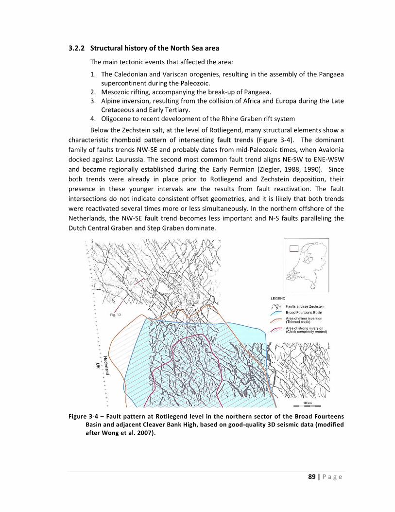
89 | P a g e   

3.2.2 Structural history of the North Sea area 

The main tectonic events that affected the area: 

1. The Caledonian and Variscan orogenies, resulting in the assembly of the Pangaea supercontinent during the Paleozoic. 

2. Mesozoic rifting, accompanying the break‐up of Pangaea. 3. Alpine inversion, resulting from the collision of Africa and Europa during the Late 

Cretaceous and Early Tertiary. 4. Oligocene to recent development of the Rhine Graben rift system 

Below the Zechstein salt, at the level of Rotliegend, many structural elements show a 

characteristic  rhomboid  pattern  of  intersecting  fault  trends  (Figure  3‐4).    The  dominant 

family of faults trends NW‐SE and probably dates from mid‐Paleozoic times, when Avalonia 

docked against Laurussia. The second most common fault trend aligns NE‐SW to ENE‐WSW 

and  became  regionally  established  during  the  Early  Permian  (Ziegler,  1988,  1990).    Since 

both  trends  were  already  in  place  prior  to  Rotliegend  and  Zechstein  deposition,  their 

presence  in  these  younger  intervals  are  the  results  from  fault  reactivation.  The  fault 

intersections do not  indicate consistent offset geometries, and  it  is  likely  that both  trends 

were reactivated several times more or less simultaneously. In the northern offshore of the 

Netherlands,  the NW‐SE  fault  trend becomes  less  important and N‐S  faults paralleling  the 

Dutch Central Graben and Step Graben dominate. 

Figure 3‐4 – Fault pattern at Rotliegend  level  in the northern sector of  the Broad Fourteens Basin and adjacent Cleaver Bank High, based on good‐quality 3D seismic data (modified after Wong et al. 2007). 

 

90 | P a g e   

The area of blocks of L‐05 and L‐06 (Terschelling Basin and the southern part of the 

Dutch  Central  Graben)  is  characterized  by  several  faults.  There  are  two  dominant  fault 

trends  in  this  area: NNE‐SSW  and WNW‐ESE  (De  Jager  2007)  (Figure  3‐5).  The NNE‐SSW 

trending  faults were active as normal  faults during  the early Kimmerian  tectonic phase  in 

Late  Triassic.  Both  NNE‐SSW  and WNW‐ESE  trending  faults  were  active  during  the  Late 

Jurassic  in a  trans‐tensional stress  field  (normal  faults and strike slips) and during  the Late 

Cretaceous as strike slips (Verweij and Witmans, 2009).  

The burial depths of the Rotliegend sandstones were approximately 2 km during the 

Late Triassic tectonic phase, approximately 3 km during the Late Jurassic tectonic phase and 

approximately 4 km during the Late Cretaceous tectonic phase (Verweij 2009). 

Figure 3‐5 ‐Structural elements of offshore sub‐region NCP‐2A of the North Sea (Verweij and Witmans 2009). 

 

 

91 | P a g e   

3.3 Method

The Broad  Ion Beam  (BIB) sample preparation provides really  fine polished sample, 

the Argon  Ion Beam cross milling  reduces  the  surface  roughness up  to about 5nm on  the 

area of about one square millimetre (Klaver et al. 2012). Figure 3‐6 shows an example for a 

polished SEM sample. Samples were coated with gold for SE and BSE imaging and carbon for 

Electron Back‐Scatter Diffraction  (EBSD)  imaging. The samples were  imaged by Zeiss Supra 

55 Scanning Electron Microscopy  (SEM) and BIB polished by  JEOL, SM 09010 cross‐section 

polisher. The SEM provides no  true  images by  scanning  the  sample with  focused beam of 

electrons.  With  BIB‐polished  surface,  the  magnification  of  the  SEM  can  go  up  to 

approximately 100000 times. 

Figure 3‐6 – Argon Ion Beam (BIB) cross‐section on the SEM sample. The ion beam  irradiates the unmasked edge of the sample (modified after Desbois et al. 2010). 

In this study, SE, BSE and EBSD images were used for the analyses applying different 

magnifications. Overview images have about 100x‐300x magnification having a resolution is 

3‐1 µm and  for  fine details of the samples were studied  in higher resolution  images which 

was taken with magnification of 1000x to up to 50000x which resolution are about 300 nm ‐ 

5 nm  image  resolutions. These  resolution  images allow studying  the  fine structures of  the 

fractures and the pore filling minerals. Beside single images, also image mosaics were taken 

in order to gain high resolution overview images to study larger areas of the samples in high 

resolution. Images were merged Autopano Giga 2.6 software developed by Kolor (2012). To 

gain  information  on  the  mineral  content,  EDX  were  measured  in  lower  resolution  for 

overview and also high resolution in points.  

Thin section study of the structures and the host rock 

Thin sections study provides information about the microstructure of the fractures, in 

larger scale than the SEM microscopy. Thin sections were created on 24 mm x 36 mm glass 

plate without upper glass cover. The thickness of the thin sections were polished about 20‐

40 m. 

 

92 | P a g e   

3.4 ResultsofMoabsamples

Samples were collected  from  the most common and  typical deformation structures 

which  characterise  the  studied  areas.  From  the  Courthouse  Junction  area  30  hand 

specimens, from Klondike Bluffs area 10 hand specimens and from well L5‐9 of North Sea 6 

core  samples were collected  and  fractures of  these  samples were  studied by microscopy. 

These samples are presented in this chapter with field photos, thin section micrographs and 

BIB‐SEM images. The description of the deformation structures of these areas based on field 

observations and also the geology characterisation of the areas are in chapter 2. 

3.4.1 Courthouse Junction samples 

This area is characterised with major cataclasis; and, only minor fluid flow alteration 

was observed. Samples were collected from most common types of fractures. The majority 

of the samples were cataclastic deformation bands. Furthermore, slip plains were found  in 

the  centre  of  the  majority  of  the  faults.  Samples  Z062  and  Z064  show  examples  for 

cataclastic  deformation  bands  and  slip  planes.  Besides,  close  to  the main  fault  core  as  a 

result of the fluid flow, mineral concretions can be observed at some spots. Samples Z030, 

Z040 and Z052 show examples for these features. Furthermore, close to the main fault core, 

a few dilatant fractures were also found (samples Z019 and Z008). Figure 3‐7 shows the map 

of samples which were collected on Courthouse Junction area, and the colours indicate the 

type of the deformation structures. 

Figure 3‐7 – The  studied  rock  samples on Courthouse  Junction area.  (satelite  image: NAIP, 2009; faults structure: Davatzes et al., 2005) 

93 | P a g e   

Z062/JU130410‐1This sample represents the most common deformation structures of the Courthouse 

Junction  area,  namely  the  cataclastic  deformation  bands.  Besides,  slip  planes  are  also 

common in the centre of the faults. This sample is from the footwall of the fault. Figure 3‐7 

shows the  location of the sample where  it was found.   Figure 3‐8 shows the photos of the 

samples  pieces  after  cutting.  Results  of  the microscopy  analysis  of  the  sample  are  listed 

below. 

Rock type:   Slick Rock Member of Entrada Sandstone 

Structure in the sample:   Cataclastic bands and slip plane 

Grain size: out of structure: ~70‐300 μm; in the structure: ~ 0.5 ‐ 15 μm  

Pore type: intergrain and intragrain porosity in K‐Feldspar 

Pore size: out of structure: ~25‐300 μm; in the structure: ~0.2 ‐ 3 μm  

Pore throat diameter: out of structure: ~ 5‐35 μm; in the structure: ~ 0.1‐0.8 μm 

Pore distribution: inhomogeneous 

Pore orientation: random 

Cementation, pore filling:  

Quartz: habitus: overgrowth, growth direction: along grain surfaces  

Calcite: habitus euhedral, growth direction: along grain surfaces;  

Illite:  habitus:  fibrous,  growth  direction:  perpendicular  and  tangential  to  grain 

surfaces;  

K‐Feldspar: habitus: along grain surfaces, growth direction: pore filling. 

 

General observation based on BIB‐SEM images: 

Granular SiO and calcite on the quartz grains reduce the pore space slightly. 

Lining clay minerals and SiO at the boundary of quartz grains. 

Calcite and clay minerals fill the pore throat. 

Randomly oriented fractures in the K‐feldspar which locally fills the pore space. 

Illite significantly reduces the pore space. 

Inside the deformation structure, drastic grain size reduction can be seen. 

94 | P a g e   

Figure 3‐8 – The photo of cut parts of sample Z062 shows the  location of  the SEM and thin section samples. 

 

ThinsectionThis is an excellent example for cataclastic deformation band bundle network which 

is next to a slip plane (Figure 3‐8). The right hand side of the micrograph of the thin section 

of the sample  (Figure 3‐9) shows the more  fractured zone of the rock which  is next to the 

slip plane  (right edge).  The open  fractures  in  the  area might  be  the  result of  the  sample 

preparation. On  the  left hand side of  the micrograph,  in  the host  rock, a single cataclastic 

band  can  be  found.  On  the  detailed  pictures  of  the  thin  section,  the  strong  grain  size 

reduction can be seen (Figure 3‐9). Thin sections allow us to study the shape and the size of 

the structures in a 2‐3 cm long section. The grains inside the structure are too small to study 

them by optical microscope. 

95 | P a g e   

Figure 3‐9  ‐ A) Overview  image of sample Z062a; B) detailed  images of the structures of the sample. 

 

A 

B 

96 | P a g e   

SEMBIB‐SEM  overview  images  of  sample  Z062c  can  be  seen  on  Figure  3‐10.  The  red 

dashed line indicates the deformation band in the middle of the picture. The SEM sample is 

taken from the same single band which can be seen on the left hand side of the thin section, 

too. The 1 mm long segment of the structure can be studied on the SEM sample. The width 

of the structure is about 0.25 mm which is in the middle of the cross section; therefore, the 

contrast can be seen well between the structure and undamaged rock. The size of the grains, 

outside of the structure, ranges from about 80 to 250 m on the SEM cross section (Figure 

3‐11).  The relatively large pores are partly filled with calcite and clay minerals. The pores are 

filled  in different degree by amount of pore  filling materials;  some pores are  filled almost 

totally  (right  part  of  Figure  3‐11)  others  are  only  slightly.  Outside  of  the  fracture,  grain 

crushing  or  damage  cannot  be  seen.  There  is  no  transition  zone  observed  between  the 

fracture  and  the  not  fractured  parts  of  the  rock, where  grain  size  reduction  less  than  in 

general  in  the structure. Figure 3‐12 shows a segment of  the cataclastic band where  large 

degree of grain size reduction can be seen; approximately 1:10 is the average ratio between 

the structure and the undamaged grains. On the SEM  images, the grain boundaries are not 

visible  at many places;  in  conclusion,  it  is hard  to distinguish  the  grains.  Therefore,  EBSD 

method was used to distinguish the different grains  (Figure 3‐13).  Inside the structure, the 

grain  size  distribution  covers  a  relatively  wide  range,  since  some  larger  slightly  crushed 

grains also remained  in the deformation band.  In general,  inside structure  large amount of 

pore size reduction and consequently this porosity reduction is present which can reduce the 

permeability of the rock significantly.  

Figure  3‐10  –  BIB‐SEM  overview  images  of  sample  Z062c  (originated  from  the  Courthouse Junction fault zone). The red dashed rectangular indicates the location of a segment of a cataclastic deformation band. 

97 | P a g e   

Figure 3‐11 – Section of outside of the cataclastic deformation band of sample Z062c. 

Figure 3‐12 – SEM image of a segment of the cataclastic deformation band of sample Z062c. 

98 | P a g e   

Figure 3‐13 – EBSD image of a segment of the cataclastic deformation band of sample Z062c. 

 

 

10 µm 

10 µm 

99 | P a g e   

Z032/ZK240410‐2

Rock type:   Slick Rock Member of Entrada Sandstone 

Structure in the sample:   Cataclastic deformation bands 

Grain size: out of structure: ~60‐280 μm; in the structure: ~ 0.5 ‐ 25 μm 

Pore type: intergrain, intragrain porosity in calcite and clay minerals 

Pore size: out of structure: ~ 20‐110 μm; in the structure: ~ 0.1 ‐ 3 μm  

Pore throat size: out of structure: ~ 5‐20 μm; in the structure: ~ 0.5‐2 μm 

Pore distribution: inhomogeneous 

Pore orientation: random 

Cementation, pore filling: 

Quartz: habitus: overgrowth, growth direction: along grain surfaces;  

Calcite:  habitus:  fibrous,  euhedral,  granular,  growth  direction:  along  grain 

surfaces;  

Ton‐mineral:  usually mixed with  calcite,  habitus:  fibrous,  euhedral,  growth 

direction: along grain surfaces;  

Illite: habitus: fibrous, euhedral, growth direction: along grain surfaces. 

 

General observation based on BIB‐SEM images: 

Clay minerals significantly reduce the pore space. 

Grain size reduction can be seen inside the deformation structure, where, in the pores, also calcite and clay minerals can be found. 

Porous calcite and clay minerals fill the pore throats and pore space. 

Significant quartz grain size reductions can be seen  in  the pore space and small amount of illite as well. 

Quartz overgrowth fills the pore throat, and calcite and clay minerals can be seen in the pore throat. 

Porous clay minerals and calcite fill the pore space. 

100 | P a g e   

Figure 3‐14 – a) original location of sample Z032; b) deformation band in the cut samples. 

 

2 cm 

101 | P a g e   

ThinsectionThis  sample  is  located approximately 15 cm  from a  large  slip plane which  is  in  the 

core of the main fault and has an offset of about 80 m. In the footwall of the fault, a complex 

and relatively dense fractures network can be seen (Figure 3‐14/a). This complexity can be 

seen in the samples as well (Figure 3‐14/b). On one half of the sample, there is no fractures; 

however,  the other half of  the sample  is highly  fractured. The boundary between  the  two 

parts is distinct and plain. On the Figure 3‐15, three different sizes of fractures can be seen. 

The most  right hand side  fracture  is  the boundary of  this bundle. Their size changes along 

the structure quite  lot. On the higher magnification  image of the thin section (Figure 3‐16) 

nicely considerable  grain  size  reduction  can be  seen which  is  the  result of  cataclasis. The 

boundary of the structure might be a slip plane. 

 

Figure 3‐15 ‐ overview of thin section of sample Z032c 

 

102 | P a g e   

Figure 3‐16 ‐ Detailed picture of thin section of sample Z032c 

SEMThe  SEM  cross‐section  is  taken  from  the  boundary  of  the  deformation  structure, 

which  is  a  seemingly  homogenous,  white  coloured  deformation  band  in  red  host  rock. 

However,  the  overview  images  (Figure  3‐17)  there  are  seen  large  changes  inside  the 

structure going away from the host rock, which is on the right side of the image, towards the 

centre  of  the  deformation  band.  In  the  middle  of  the  BIB‐SEM  cross  section,  an 

approximately 0.3 mm wide band can be seen where high degree of grain size reduction can 

be observed. On the right side of this band,  there  is a transition zone where the cataclasis 

decreases and grain size gradually  increases. The width of this zone  is about 0.3 – 0.5 mm. 

On  the  left  side of  the highly cataclastic band,  the boundary  is a distinct  line, which  is an 

open fracture and seems to be a slip surface. On the left side of this fracture, the cataclasis is 

still relatively high; however, significantly lower than in the band in the middle of the image. 

Figure 3‐18 shows a 65 μm by 100 μm size are (red rectangular on Figure 3‐17) which is the 

in boundary of  the  two zones. An almost continuous separation can be seen between  the 

two  zones which  can  be  an  open  fracture;  however,  no  significant  displacement  can  be 

observed along this line. In conclusion, this fracture is likely not a slip surface.  

103 | P a g e   

Figure 3‐17 ‐ SEM overview images of sample Z032a The red box indicates the location of the image in Figure 3‐18. 

Figure 3‐18 ‐ SEM images left side of sample Z032; intermediate cataclasis 

Missing 

image 

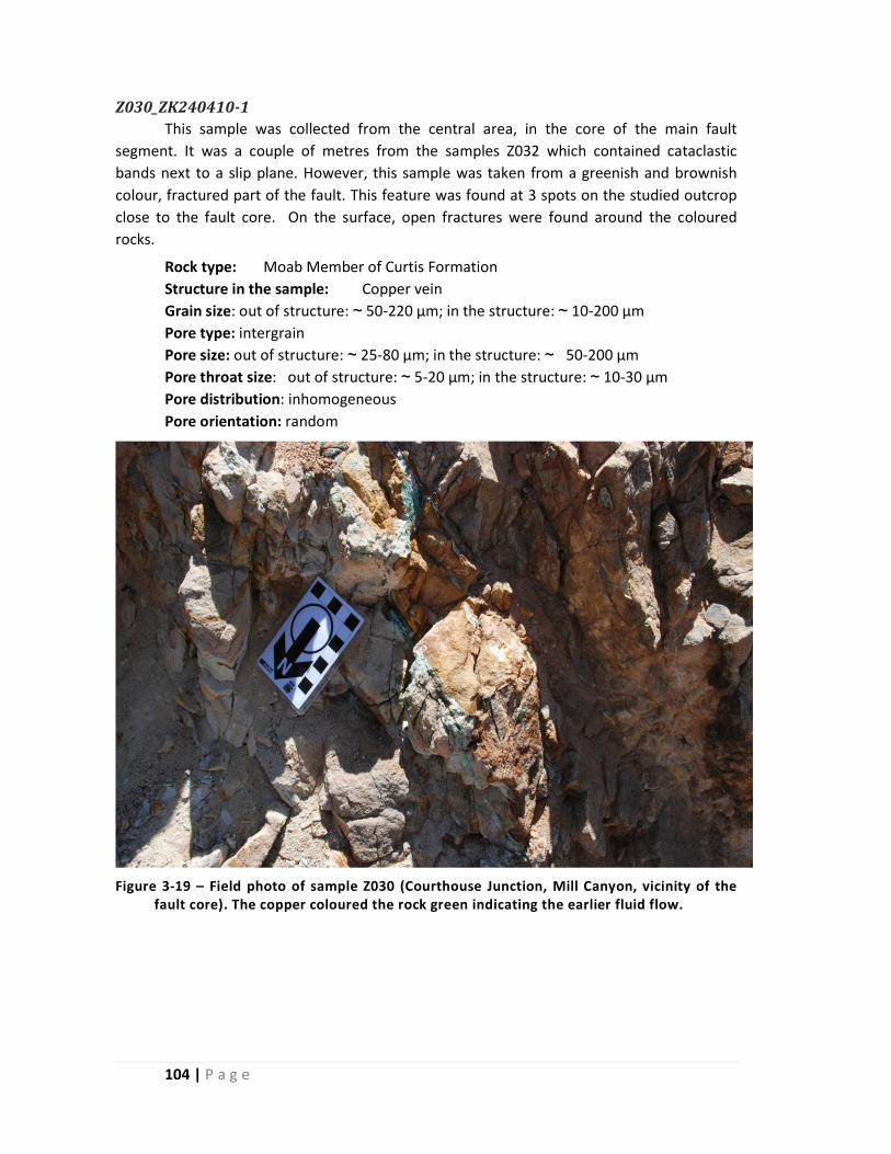
104 | P a g e   

Z030_ZK240410‐1This  sample  was  collected  from  the  central  area,  in  the  core  of  the  main  fault 

segment.  It was  a  couple  of metres  from  the  samples  Z032 which  contained  cataclastic 

bands next  to a slip plane. However,  this sample was  taken  from a greenish and brownish 

colour, fractured part of the fault. This feature was found at 3 spots on the studied outcrop 

close  to  the  fault  core.   On  the  surface, open  fractures were  found  around  the  coloured 

rocks. 

Rock type:   Moab Member of Curtis Formation 

Structure in the sample:   Copper vein 

Grain size: out of structure: ~ 50‐220 μm; in the structure: ~ 10‐200 μm 

Pore type: intergrain 

Pore size: out of structure: ~ 25‐80 μm; in the structure: ~   50‐200 μm  

Pore throat size:   out of structure: ~ 5‐20 μm; in the structure: ~ 10‐30 μm 

Pore distribution: inhomogeneous 

Pore orientation: random 

Figure 3‐19 – Field photo of  sample Z030  (Courthouse  Junction, Mill Canyon, vicinity of  the fault core). The copper coloured the rock green indicating the earlier fluid flow.  

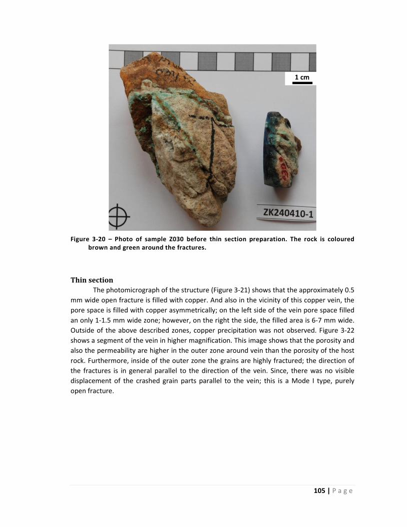
105 | P a g e   

Figure  3‐20  – Photo  of  sample  Z030  before  thin  section  preparation.  The  rock  is  coloured brown and green around the fractures. 

 

ThinsectionThe photomicrograph of the structure (Figure 3‐21) shows that the approximately 0.5 

mm wide open fracture is filled with copper. And also in the vicinity of this copper vein, the 

pore space is filled with copper asymmetrically; on the left side of the vein pore space filled 

an only 1‐1.5 mm wide zone; however, on the right the side, the filled area is 6‐7 mm wide. 

Outside of  the above described zones, copper precipitation was not observed. Figure 3‐22 

shows a segment of the vein in higher magnification. This image shows that the porosity and 

also the permeability are higher in the outer zone around vein than the porosity of the host 

rock. Furthermore,  inside of the outer zone the grains are highly fractured; the direction of 

the  fractures  is  in general parallel  to  the direction of  the vein. Since,  there was no visible 

displacement of  the  crashed grain parts parallel  to  the vein;  this  is a Mode  I  type, purely 

open fracture. 

1 cm 

106 | P a g e   

Figure 3‐21 – Photomicrograph of thin section of sample Z030. 

Figure  3‐22  –  Photomicrograph  of  thin  section  of  sample  Z030.  Grains  are  fractured perpendicularly close to the copper vein. 

 

1 mm 

0.5 mm 

107 | P a g e   

Z040_ZK260410‐3andZ052_ZK010510‐3In the vicinity of the core of the main fault segment in addition to veins, also mineral 

concretions, nodules were found. One type of the concretions was copper concretions that 

can be seen on Figure 3‐23. They were found at only some smaller, some tens of centimetres 

diameter spots. Photomicrograph of the sample shows the copper spots randomly scattered 

in  the  rock  sample  (Figure 3‐24).  In  the concretions every pores  is  filled both  smaller and 

larger;  however,  there  are  same  size  or  larger  pores  outside  of  concretions, which  have 

without pore filling. The diameter is not more than about 3‐4 mm. 

The  other  type  of  the  concretions  have  basically  white  colour  with  some  brown 

colour parts (Figure 3‐25). Two larger, about diameter of 2‐3 m spots were found very close 

the core of the main fault segment and also in the junction of the studied fault segment and 

the  main  Moab  Fault.  This  type  of  concretions  has  larger  approximately  0.5  –  8  cm 

diameters; however, the numbers of the concretions are smaller  than  the other type. Thin 

section  of  this  sample  shows  that  pore  space  of  some  parts  of  the  sample  is  filled with 

calcite. Besides, at some other parts of the sample, pore space is filled with opaque minerals 

which are likely iron. 

Figure 3‐23 – Photo of sample Z040 before the thin section preparation. 

1 cm

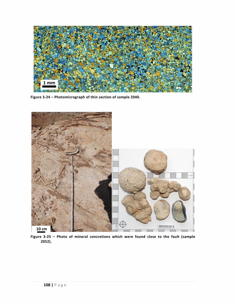
108 | P a g e   

Figure 3‐24 – Photomicrograph of thin section of sample Z040. 

 

Figure  3‐25  –  Photo  of mineral  concretions  which  were  found  close  to  the  fault  (sample Z052). 

1 mm 

10 cm 

109 | P a g e   

Figure  3‐26  –  The  photomicrograph  of  the  thin  section  of  sample  Z052  shows  that  calcite (lighter greenish yellowish  intergrain areas) and hematite  (darker  intergrain areas)  fill the pore space. 

Z008_ZK140410‐1This type of fracture was found only in the junction of the studied fault segment and 

the main Moab Fault. Fracture network has brown colour and they are close to a slip plane 

that can be  seen on Figure 3‐27. The pigmentation of  the  fractures  refers  to  foot print of 

fluid  flow  in permeable  fractures. Photomicrograph of  this  sample  can  be  seen on  Figure 

3‐28.    The  image  shows  that  the  fractures  are  cataclastic  deformation  bands  with  high 

degree  of  cataclasis.  However, mineral  filling  can  be  seen  in  the  pore  space  around  the 

deformation band which  is generated by  fluid  flow  that also  indicates a certain degree of 

increase of porosity around the fractures. 

Rock type:   Moab Member of Curtis Formation 

Structure in the sample:   Cataclastic deformation band 

Grain size: out of structure: ~ 40‐200 μm; in the structure: ~ 10‐100 μm 

Pore type: intergrain 

Pore size: out of structure: N/A; in the structure: N/A 

Pore throat size:   out of structure: N/A; in the structure: N/A 

Pore distribution: inhomogeneous 

Pore orientation: random 

 

 

 

110 | P a g e   

Figure 3‐27 – Photo of sample Z008 (Courthouse Junction,  cataclastic  band  with  fluid  flow alteration) after cutting. 

 

Figure 3‐28 – Photomicrograph of sample Z008 (lower  image is with crossed polarization). In the vicinity of a cataclastic band, calcite can be seen in the pore space (yellow ellipses).

0.5 cm 

0.5 cm 

2 cm 

111 | P a g e   

3.4.2 Klondike Bluffs samples 

The studied faults at the Klondike Bluffs area and the location of the studied samples 

can  be  seen  on  Figure  3‐29.  The majority  of  the  fractures  are  dislocation,  disaggregation 

band. Furthermore,  in general, mineral precipitation was observed  inside  the deformation 

structures which  indicate previous fluid migration. At several parts of this outcrop, mineral 

concretions were observed. The size of the individual areas featured by mineral concretions 

ranged from 0.5‐3 m2 and the diameter of the single nodules ranges between 0.5 and 2 mm 

in  general. On  the west  part  of  the  footwall  of  the  fault,  large  size,  brownish  yellowish 

mineral concretions were  found  (Figure 3‐30). Samples were collected  from most common 

types of fractures. However, slip plains were not found on this area. Samples Z012, Z017 and 

Z045 show examples for the three more often observed types of deformation structures. 

 

Figure  3‐29  –  Location  of  the  field  samples  collected  at  the  Klondike  Bluffs  area.  (satelite image: NAIP, 2009) 

112 | P a g e   

Figure 3‐30 – Large size mineral concretions on the west part of the footwall of the fault. 

Z012_ZK150410‐2Sample  Z012  represents one of  the most  common  type deformation bands of  this 

area, namely the dislocation band. Field photo and sample cut for thin section preparation 

can  be  seen  on  Figure  3‐31.  In  general,  these  deformation  bands  have white,  light  grey 

colour and their thickness are relatively large, about 2‐6 mm. These deformation bands were 

found about 15‐20 m far from the core of the main fault, on the eastern part of the out crop, 

in reddish rocks. 

Rock type:   Moab Member of Curtis Formation 

Structure in the sample:   Dislocation band filled with calcite 

Grain size: out of structure: ~ 30‐300 μm; in the structure: ~ 30‐300 μm 

Pore type: intergrain 

Pore size: out of structure: ~ 10‐70 μm; in the structure: ~ 25‐160 μm  

Pore throat size:   out of structure: ~ 5‐35 μm; in the structure: ~ 5‐50 μm 

Pore distribution: inhomogeneous 

Pore orientation: random 

 

 

ThinsectionA segment of the deformation structure can be seen on the photomicrograph of the 

sample on  Figure 3‐32.  Inside  the  approximately 3 mm wide deformation band,  the  pore 

space  is  filled  totally with calcite. The grains  less  touch each other and significantly higher 

permeability  can  be  seen  inside  the  structure.  Outside  of  the  band,  grains  show  more 

crowded  characteristic with  less  pore  space.  Very  few  grain  crushing  can  be  found  both 

113 | P a g e   

outside  and  inside  the  structures.  The orientations of  the elongated  grains  show  random 

orientation outside of the band; however, the orientations of the elongated grains are gently 

oriented within the band. This observation allows to conclude that the deformation contains 

both dilatancy and shear components. 

 

Figure 3‐31 – Field photo of sample Z012 from Klondike Bluffs fault zone on the  left (size of the black rectangles on the scale card are 1 cm x 1 cm) and sample pieces before thin section preparation on the right. 

Figure 3‐32 – Photomicrograph of sample Z012; calcite fills the pore space (dashed yellow ellipse) inside the dislocation band indicating the present of earlier fluid flow. 

1 cm 

1 mm 

114 | P a g e   

Z017_ZK190410‐1Sample Z017 shows a nice example for dislocation band, which is the most common 

deformation structure of the Klondike Bluffs area. These bands have very bright grey, almost 

white colour in general. In general, their thickness varies in relatively large range about 0.5‐

10 mm; mostly some mm.   These deformation bands were  found  farther  from  the core of 

the main fault on the western part of the hanging wall of the out crop in light, whitish rocks. 

Around these structures, usually mm size mineral concretions can be found in the host rock. 

Rock type:   Moab Member of Curtis Formation 

Structure in the sample:   Dislocation band filled with calcite 

Grain size: out of structure: ~ 40‐200 μm; in the structure: ~ 40‐200 μm 

Pore type:  intergrain: remains of small size and thin pores around the quartz grains 

because of the calcite growth; intragrain: porosity in calcite 

Pore size: out of structure: ~ 20‐75 μm; in the structure: ~ 40‐130 μm 

Pore throat size: 5‐35 μm; out of structure: ~   μm; in the structure: ~ 5‐40 μm 

Pore distribution: inhomogeneous 

Pore orientation: random 

Cementation, pore filling:  

Quartz: habitus: overgrowth, growth direction: along grain surfaces 

Calcite: habitus: homogeneously fills the pores, growth direction: pore filling, 

deformation features: few fractures, size less than 1 μm minerals 

Illite: habitus: fibrous, growth direction: perpendicular and tangential to grain 

surfaces 

Clay mineral: habitus: euhedral; growth direction: along grain surfaces. 

 

General observation based on BIB‐SEM images: 

Inside this dislocation (shear) band, the pores are filled with calcite entirely, only mm‐size gaps remained along the quartz grains in some places.  

Granular clay minerals in the remaining pore‐space.   mm or smaller size fractures can be seen in the pore filling material (calcite, illite, 

rutile, clay minerals).   Empty pore throat in calcite filled deformation area.   Locally in the pore space, illite also can be found which is fractured. Illite is grown 

together with calcite without any pores.  Secondary pores between quartz grains, and calcite  is  filled with  less  than mm‐

size quartz, illite and calcite grains. 

 

115 | P a g e   

Figure 3‐33  ‐ Sample Z017 at  the  field above, and  two pieces of  this prepared  for  creating thin section. 

ThinsectionThe pore space inside the structure is larger than in undamaged host rock area. This 

can be seen on the micrograph images below (Figure 3‐34). Figure 3‐35 shows a part of the 

structure in higher resolution. Within the fracture, the intergrain space is significantly higher 

than  outside  of  the  fracture.  Only  very  few  broken  grains  can  be  observed  both  in  the 

fracture  and  out  of  the  fracture.  There was  no  distinguishable  pore  or  grain  orientation 

either in or out of the structure. In conclusion, this fracture is a dislocation of disaggregation 

deformation band; where  likely no significant amount of shearing or offset is occurred. The 

boundary  of  the  band  (yellow  dashed  line  on  Figure  3‐34)  is  not  a  straight  line,  more 

crisscross present depending on  the degree of  the penetration of  the pore  filling material. 

The pore  space  is  totally  filled with calcite  inside  the deformation band as a  result of  the 

earlier fluid flow. Next to the band,  smaller calcite concretions can be seen with diameter of 

about 0.2‐0.5 mm.  

116 | P a g e   

Figure  3‐34  ‐  Micrograph  image  of  sample  Z017b.  Yellow  arrows  indicate  the  mineral concretions and the dashed line the location of the deformation band. 

 

Figure  3‐35  ‐  Detailed  pictures  of  sample  Z017b.  Left  part  of  the micrographs  shows  the deformation band and  the  right part  is  the host  rock. The picture on  the  left  is  taken with  lambda  filter  and no  polarization;  picture on  the  right  is  taken without  gamma filter with cross polarized light. 

 

117 | P a g e   

BIB‐SEMThe overview image of the BIB‐SEM sample can be seen on the Figure 2‐39. The cross 

section was taken from the middle of the deformation band. The  loose arrangement of the 

grains  can  be  seen  nicely on  the overview  image  and  that  the  intergrain  space  is  almost 

entirely filled. Some fractures, cracks can be seen in grains and also in the pore filling calcite 

volume. The cracks of the grains outside of the BIB cross section  likely occurred during the 

sample  preparation.  There  are  only  very  few  intergrain  cracks.  The  orientation  and  the 

distribution of  the  cracks  seem  to be  random  and  the  cracks  do  not  propagate  from  the 

touching point of  the grains  in general. The  fine  structure of  the  sample,  for example  the 

pore  throats,  can  be  studied  by  BIB‐SEM  images.  Figure  3‐37  and  Figure  3‐38  show  two 

examples for interaction of pore throat and pore filling material. Where the intergrain gap is 

lower  than about 1 m,  the  space  is not  filled by calcite. Furthermore, Figure 3‐37 shows 

that the neighbouring grains have very similar boundary lines, so probably they had touched 

each other earlier; the gap opened latter and pore space got filled by calcite and finally, they 

both cracked slightly.   

 

Figure 3‐36 ‐ SEM overview images of sample Z017b. 

118 | P a g e   

Figure  3‐37  –  High  resolution  BIB‐SEM  images  of  sample  Z017  showing  a  few  µm  wide parallel gap between the grains (indicating a probably natural dislocation) pore throat and pore filling. 

Figure 3‐38 ‐ High resolution BIB‐SEM  images of sample Z017 showing pore throat and a few µm wide parallel gap between the grains which pore filling material is only partly filled up. 

Quartz grain 

Quartz grain

Quartz grain 

Intergrain pore 

Calcite  in 

the pore 

Quartz grain 

Intergrain pore 

Calcite  in 

the pore 

Quartz grain

Calcite  in 

the pore 

Quartz  

grain 

Intergrain pore 

119 | P a g e   

Z045/ZK280410‐3This sample contains a unique type of fractures because of their visual appearance. 

Their  colour  is  dark  reddish  brown  and  their  thickness  is  about  2‐3  mm  which  slightly 

varying. Only some bands were found from this type of fracture and only on the middle part 

of the footwall wall of the fault around the south end of the line KB‐1.   

Rock type:   Moab Member of Curtis Formation 

Structure in the sample:   Dislocation bands with iron precipitation 

Grain size: out of structure: ~ 65‐210 μm; in the structure: ~ 60‐180 μm 

Pore type: intergrain 

Pore size: out of structure: ~ 0.5‐2.5 μm; in the structure: ~ 1‐3 μm 

Pore throat size: out of structure: ~ 0.2‐1.5 μm; in the structure: ~ 0.2‐1.3 μm 

Pore distribution: homogeneous 

Pore orientation: random 

Cementation:  

Quartz: habitus: overgrowth, growth direction: along grain surfaces 

Kaolinite:  habitus:  euhedral,  growth  direction:  platy,  face‐to‐face, 

perpendicular and tangential to detrital grains 

Iron: habitus: euhedral, growth direction: along grain surfaces 

 

General observation based on BIB‐SEM images: 

Inside  the  deformation  structure,  quartz  grains  are  covered  with  kaolinite  and 

hematite. 

Zooming  into the pore space, platy kaolinite and relatively  large amount of  iron can 

be seen. 

Thin layer kaolinite and less amount of iron cover the quartz grains approaching the 

boundary of the structure. 

Platy kaolinite covers the quartz grains, and  there  is no measurable amount of  iron 

here. 

Only few minerals can be seen on the surface of the quartz grains, the pore space is 

almost empty. 

The contrast can be seen between the original rock matrix and iron rich structure. 

120 | P a g e   

Figure 3‐39 ‐ Origin of sample Z045 and Z046 from the footwall of Klondike Bluffs fault.  

 

121 | P a g e   

ThinsectionThe  Figure  3‐40  shows  the  photomicrograph  of  sample  Z045.  The  deformation 

structure can be distinguished from the host rock. In the band, the pore space  is filed with 

opaque  minerals.  Small  amount  of  difference  can  be  observed  in  grain‐  and  pore  size 

between the host rock and the band. However, this small amount of porosity  increase was 

enough  to support  the  fluid  flow  (making a  fluid pathway) and as a result of the  fluid  flow 

likely iron precipitation occurred inside the band. Based on the thin section, this fracture is a 

dislocation deformation band in which the pore space is partially filled with hematite. 

 

Figure 3‐40  ‐ Micrograph of sample Z045a. Top half  is  the deformation band, bottom half  is the host rock. 

SEMBecause  the  sample was very weak,  the BIB polishing did not work out;  therefore, 

only ordinary SEM images were taken. The SEM overview image of sample Z045 can be seen 

on Figure 3‐41. The right side of the  image shows the bright host rock and on the  left side 

the deformation structure. On this  image,  it  is also visible that the porosity  is higher  in the 

structure than outside of it. Furthermore, the grains seem to be clean and the pores seem to 

be empty in the host rock which can be seen also at the higher magnification SEM image of 

Figure 3‐42. Figure 3‐43  shows a  small part of  the deformation band where nicely can be 

seen that the pores space is partially filled with minerals. EDX measurement showed that the 

pore filling minerals are kaolinite (flat platy minerals) and iron. 

122 | P a g e   

Figure  3‐41  ‐  Photomicrograph  of  sample  Z045a where  top‐left  half  of  the  sample  is  the deformation band and bottom‐right half  is the host rock. (The black rectangular  in the image is a missing photo mosaic.) 

Figure 3‐42 ‐ Higher magnification photomicrograph of a part of the host rock of the sample Z045a. 

1 mm 

123 | P a g e   

Figure 3‐43 – Higher magnification photomicrograph of a part of the deformation band of the sample  Z045a.  The white  box  in  the  image  on  the  top  indicates  the  location  of  the image of the bottom. 

 

124 | P a g e   

3.5 NaturalfracturesinNorthSeasandstonesamples

Five core samples were studied  in  this work  from well L5‐9 of the North Sea which 

contain  fractures.  Two  samples  contain  cataclastic  deformation  bands  and  three  samples 

contain veins. The samples originated  from about 4629‐4667 metres depth  (TVD)  from the 

Permian Upper Rotliegend Group Slochteren Formation ‐unit. The orientations of the cored sections were nearly vertical; black arrows on the samples show the top of the samples on 

the  photos.  The  dip  of  the  cataclastic  bands were  nearly  vertical  (80‐90°),  and  the  open 

fractures, and veins had the dip of 10‐70 degree. 

 

3.5.1 Sample: L5‐9‐1 

Depth:   True Vertical Depth: 4629.27 m 

Rock type:   Upper Rotliegend Group Slochteren Formation ‐unit Grain size: out of structure: ~ 25‐230 μm; in the structure: ‐ 

Structure in the sample:   vein 

Dip of the structures:  ~ 45 ° Pore type: intergrain 

Pore size: out of structure: ~ 0.5‐26 μm; in the structure: ‐ 

Pore throat size: out of structure: ~ 1‐20 μm; in the structure: - Pore distribution: inhomogeneous 

Pore orientation: random 

Cementation, pore filling: 

Quartz: habitus: overgrowth, growth direction: along grain surfaces;  

Ankerite: habitus: homogeneously fills the pores, growth direction: pore filling;  

Illite:  habitus  fibrous,  growth  direction:  perpendicular  and  tangential  to  grain 

surfaces; 

Kaolinite: habitus: euhedral, growth direction: pore filling. 

 

General observation based on BIB‐SEM images: 

Ankerite  filled  vein  contains quite  complex  fracture  system with different orientations and different types. 

2‐3 mm thick fracture (micro joint) inside the vein material. 

Close to the vein‐matrix boundary, iron poor ankerite spot. 

Illite and kaolinite fill the pores between the quartz grains. 

Rutile and anatase pore filling material on the vein‐matrix boundary. 

Quartz overgrowth with sharp edges and randomly growing illite crystals on quartz grains (in the rock matrix). Kaolinite grains in the pores. 

 

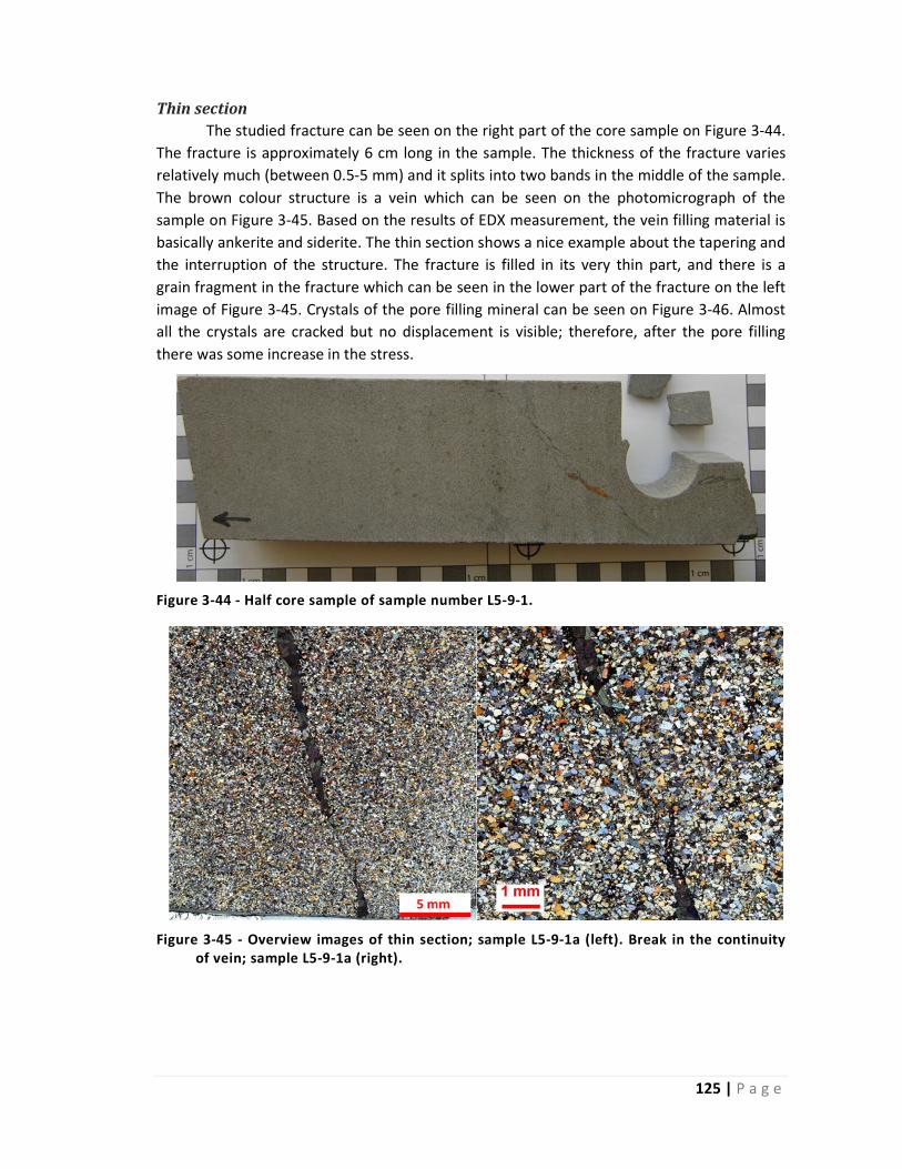
125 | P a g e   

ThinsectionThe studied fracture can be seen on the right part of the core sample on Figure 3‐44. 

The fracture  is approximately 6 cm  long  in the sample. The thickness of the fracture varies 

relatively much (between 0.5‐5 mm) and it splits into two bands in the middle of the sample. 

The  brown  colour  structure  is  a  vein which  can  be  seen  on  the  photomicrograph  of  the 

sample on Figure 3‐45. Based on the results of EDX measurement, the vein filling material is 

basically ankerite and siderite. The thin section shows a nice example about the tapering and 

the  interruption of  the  structure. The  fracture  is  filled  in  its  very  thin part, and  there  is a 

grain fragment in the fracture which can be seen in the lower part of the fracture on the left 

image of Figure 3‐45. Crystals of the pore filling mineral can be seen on Figure 3‐46. Almost 

all  the  crystals are  cracked but no displacement  is  visible;  therefore, after  the pore  filling 

there was some increase in the stress. 

Figure 3‐44 ‐ Half core sample of sample number L5‐9‐1. 

Figure 3‐45  ‐ Overview  images of  thin section; sample L5‐9‐1a (left). Break  in the continuity of vein; sample L5‐9‐1a (right). 

126 | P a g e   

Figure 3‐46 ‐ Cracks inside the vein; sample L5‐9‐1a. 

 

 

BIB‐SEMThe BIB‐SEM overview  image of the sample L5‐9‐1a can be seen on Figure 3‐47. On 

the left side, there is the vein (light grey) and on the top right, there are the quartz grains of 

the sandstone. The finer and tinier fractures and the fractures network of veins can be seen. 

And also inside the vein, small size (3‐15 µm) pores can be observed. Close to the boundary 

of the vein in the host rock, material of the vein can be found in the larger (10‐30 µm) pores. 

There is no sharp boundary between the vein and host rock. However, smaller pore spaces 

(less  than 2‐3 µm) do not contains  vein material.  Intergrain  space  (outside of  the  vein)  is 

filled basically with clay minerals, such as illite and kaolinite which do not allow the ankerite 

to penetrate  into  the pores  (Figure 3‐48 and Figure 3‐49). Based on  this, presumably  illite 

and kaolinite formed before ankerite. 

127 | P a g e   

Figure 3‐47 –  SEM overview  image of  sample  L5‐9‐1. The  red dot  indicates  the  location of image of Figure 3‐48.  

Figure 3‐48 – Pore  space close to the vein boundary  in sample L5‐9‐1 where Qz  is stand  for quartz. 

128 | P a g e   

Figure  3‐49  –  Pore  space  close  to  the  vein  boundary  in  sample  L5‐9‐1 where  Qz:  quartz, Ank/Sid: ankerite and siderite. 

 

3.5.2 Sample: L5‐9‐3 

Depth:   Measured depth: 4691.5 m; True Vertical Depth: 4644.6 m 

Rock type:   Upper Rotliegend Group Slochteren Formation ‐unit  Grain size: out of structure: ~ 25‐250 μm; in the structure: ~ 15‐ 200 μm 

Structure in the sample:   Cataclastic deformation band 

Dip of the structures:  ~ 80‐90 ° Pore type: intergrain, intragrain porosity in dolomite; 

Pore size: out of structure: ~ 20‐120 μm; in the structure: ~ 4‐30 μm 

Pore throat size: out of structure: ~ 5‐20; in the structure: ~ 0.1‐5 μm 

Pore distribution: inhomogeneous 

Pore orientation: random 

Cementation, pore filling:  

Quartz: habitus: overgrowth, growth direction: along grain surfaces 

Dolomite: habitus: homogeneously fills the pores, growth direction: pore filling 

Illite:  habitus:  fibrous,  growth  direction:  perpendicular  and  tangential  to  grain 

surfaces 

Kaolinite: habitus: euhedral, growth direction: pore filling 

 

 

129 | P a g e   

General observation based on BIB‐SEM images: 

The  pore  space,  between  the  quartz  grains,  is  filled with  dolomite  and  ankerite entirely. There are some mm‐size pores in pore filling material, and mm size gaps on the grain‐pore boundary. 

The general grain size is about 100 µm in the matrix, and the general pore size is 20‐40 µm which  is  filled with randomly oriented kaolinite grains, ankerite and a small amount of gypsum. 

Illite lining on the quartz grains, and fibrous illite in the pore space. 

Original matrix on the  left and deformation structure on the right, where grain and pore size reduction can be seen. 

Inside the deformation area, the pore space size, between the quartz grains, is about 5‐10 µm. Randomly oriented illite can be found which reduces the pore space. 

Kaolinite grains and illite reduced the pore space. 

ThinsectionA bunch of deformation  structures  can be  seen  in  this  core  sample piece which  is 

plotted on Figure 3‐50. These bands are relatively light; it is hard to distinguish the host rock 

from the structures even in thin sections. Photomicrograph of this structure can be seen on 

Figure 3‐51. The  fracture goes  from  the  top‐left  to bottom‐right. The higher magnification 

image of a part of the structure can be seen on Figure 3‐52 which shows the structure on the 

bottom half of the image. Small degree of grain size reduction can be seen in the structure. 

 

Figure 3‐50 ‐ Core piece of sample L5‐9‐3. 

130 | P a g e   

Figure 3‐51 ‐ Thin section overview image of sample L5‐9‐3. 

 

Figure 3‐52 – Thin section  image of structure of the sample L5‐9‐3. Structure  is on the  lower half of the image. 

 

1 mm 

131 | P a g e   

BIB‐SEMOn  the overview  image of  this sample a short section of  the deformation structure 

can be seen nicely (Figure 3‐53); however, the structure stops at the lower part of the cross 

section. Inside the structure, grain size reduction is observed. The higher resolution BIB‐SEM 

image shows the inside of the structure (Figure 3‐55). Locally, significant grain size reduction 

can be  found  in  the deformation structure; and  therefore, porosity  is  reduced. The Figure 

3‐54  shows  the  schematic  drawing of  the mechanism of  the  formation  of  the  cataclastic 

deformation band (Fossen et al. 2007). Further higher magnification images of the host rock 

part of the sample show that kaolinite, ankerite, dolomite,  illite, gypsum and halite can be 

found in the pore space (Figure 3‐56, Figure 3‐57 and Figure 3‐58). 

Figure 3‐53 – BIB‐SEM overview images of samples L5‐9‐3. 

Figure  3‐54  –  Cataclastic  types  of  deformation  bands,  based  on  deformation  mechanism (modified after Fossen, 2010). 

132 | P a g e   

Figure 3‐55 ‐ Higher resolution images of sample L5‐9‐3; inside of the structure. Location of the spot is indicated by red dot on Figure 3‐53. 

Figure 3‐56 ‐ Higher resolution images of sample L5‐9‐3. Outside of the structure, illite and Halite can be found in the pore space where Qz: quartz, TM: trace minerals. 

133 | P a g e   

Figure 3‐57 ‐ Higher resolution images of sample L5‐9‐3. Outside of the structure, Dolomite and Ankerite fill the pore space where Qz: quartz. 

Figure 3‐58 ‐ Higher resolution images of sample L5‐9‐3. Outside of the structure, Kaolinite and gypsum can be found in the pore space where Qz: quartz. 

134 | P a g e   

3.5.3 Sample: L5‐9‐4 

Depth:   Measured depth: 4703.9 m; True Vertical Depth: 4657.0 m 

Rock type:   Upper Rotliegend Group Slochteren Formation ‐unit  Grain size: out of structure: ~ 5‐450 μm; in the structure: ~ 5‐220 μm 

Structure in the sample: Deformation bands, veins, open fractures 

Dip of the structures:  main fracture: ~ 70 °; smaller, branch fracture: ~ 10‐60 ° Pore type: intergrain, intragrain porosity in dolomite; 

Pore size: out of structure: N/A; in the structure: N/A 

Pore throat size: out of structure: N/A; in the structure: N/A 

Pore distribution: inhomogeneous 

Pore orientation: random 

Cementation, pore filling: N/A 

 

 

 

ThinsectionA quite complex fracture network can be seen in the half core samples on the figure 

above, with different types of fractures with varying thickness (Figure 3‐59). The thin section 

was cut from the centre of the fracture network; therefore, it contains more fractures such 

as  open  cracks  and  also  deformation  bands.  On  the  left  side  of  the  core  sample,  open 

fractures  are  partially  filled  with  clay  minerals.  In  the  thin  section  (Figure  3‐60),  two 

cataclastic deformation bands  can be  found  (above  the open  fracture) where  grains  sizes 

reduction can be seen. Besides, significant grain size reduction can be seen next to the open 

fracture as well. This sample represents a nice example where cataclastic bands which result 

of compaction and open fractures which result of dilatancy are mixed and very close to each 

other.    Presumable,  the  compaction  had occurred  earlier  than  open  fractures  generated. 

Some of the open fractures might have formed during the unloading of the core sample as it 

was from well; however,  it  is sure that open fractures were present  in the depth; because, 

some of the open fractures are filled with minerals.  

135 | P a g e   

Figure 3‐59 – Photo of the half core sample where sample L5‐9‐4 was taken. 

Figure 3‐60  ‐ Overview  image of  thin  section of  sample  L5‐9‐4  is  shown where dashed,  red polygons indicate the deformation structure. 

 

2 mm 

136 | P a g e   

3.6 Discussion

In this work, the most characteristic fractures of sandstones were studied in samples 

of two different filed analogues in Utah and core samples of one well of the North Sea. The 

characteristics of  the  fractures of  the  two analogue  field areas  seemed  to be  significantly 

different. All  the  samples which were  collected  around  the  faults  of  Klondike  Bluffs  area 

were the same type. Ten samples were collected on the Klondike Bluffs area; they all were 

dilatant  fractures,  disaggregation  bands.  In  addition,  all  of  these  fractures  have  different 

degree of fluid generated pore filling. In general, calcite almost fully filled the pore space in 

the fractures and iron filled the pore in the fractures in only a small degree. It is important to 

notice  that  there were no  fractures analysed  from very close  to  the main  fault where  the 

fracture density was high. However,  there were  sample  analysed  from  close  to  a  smaller 

fault branch. The properties of deformation band did not show symmetry around the main 

fault.  In  the  hanging wall,  the  calcite  filled  disaggregation  bands  are  the most  common 

deformation structures which can be observed even 500 metres from the main fault. On the 

footwall  of  the  fault,  the  iron  filled  deformation  bands  were  found.  In  the  Courthouse 

Junction area, majority of the fractures were cataclastic deformation bands in the main fault 

core and further from the fault as well. In addition, a few open fractures were found in the 

core of the main fault segment in which pore space was filled with more or less with calcite 

or copper likely malachite. 

The North Sea samples originated from about 4629‐4675 metres deep (TVD). In this 

relatively short vertical section, different types of  fractures were  found to be both dilatant 

and  cataclastic.    Veins  were  found  with  different  degree  of  pore  filling.  In  addition, 

cataclastic bands were found as well. There were dilatant and cataclastic fractures relatively 

close  to each other  in  this core.  In  the Courthouse  Junction area,  there were dilatant and 

cataclastic fractures close to each other in or close to the fault core. In conclusion, the core 

samples presumably were  located close to a fault core which  is  likely more cataclastic type 

of fault. Dip of the fractures varied  from 10‐90° where open fractures; however, dip of the 

cataclastic bands and dip of open type of fractures showed differences. Cataclastic bands are 

steeply dipping nearly vertically and open fractures have lower angle.  

According  to  Aydin  (1978),  the  deformation  bands  in  the  Entrada  and  Navajo 

Sandstones are formed by a combination of various different processes, including shear and 

volume change microfracturing of grains into smaller grains, shattering of smaller grains, and 

mixing of the fragments of grains with the matrix. On the one hand, the result of this study is 

in agreement with Aydin’s statement. On  the other hand,  in case of  the cataclastic bands, 

there  is more  shear which  is  the  dominant  type of deformation; whereas,  in  case of  the 

disaggregation bands, there is less shear, and the main deformation style is slight dilatancy. 

Based  on  the  results  of  Antonellini  et  al.  (1994),  the  studied  structures  in  the 

Klondike  Bluffs  area  belong  to  the  older  generation  of  deformation  bands which  formed 

during  the  growth  of  the  salt  anticline  because  they  are  characterised  by  minor  or  no 

cataclasis. 

137 | P a g e   

According to Fossen and Bale (2007), deformation bands present only local barrier to 

fluid flow, as the thickness of deformation bands changes rapidly. Similarly, the thickness of 

the  analysed deformation bands  varies  in  relatively wide  range and  thickness  can  change 

rapidly in cataclastic deformation bands (e.g. this can be seen on images of thin sections of 

sample Z062 and Z032) and in dilatant fractures as well, for example sample L5‐9‐1 a vein in 

Rotliegend  sandstone  which  thinned  and  interrupted.  However,  the  thickness  change  of 

disaggregation band was not observed in thin section. Besides, the veins have blocky fill (e.g. 

sample L5‐9‐1), which  indicates that  the rocks already had some strength when they were 

fractured and stayed open during fracture filling (Hilgers et al. 2001, Nollet et al. 2005). 

In this study, high degree of cataclasis and in general relatively sharp gain edges can 

be  found  in  the  samples of Courthouse  Junction which  refer  to  the  relatively  large  shear 

displacement and high stress state. However,  in some cases, diffuse  fracture edges can be 

seen  in cataclastic bands close to each other  in sample from the same  location. In some of 

the cases, one of  the edges of  the  same cataclastic band  is very  sharp whereas  the other 

edge  is diffuse. In general, the edge of the disaggregation bands  is relatively sharp which  is 

well visible by the mineral precipitation. However, locally some edges became more diffuse. 

In general, observation of this work is in agreement with results of Torabi et al. (2007), who 

related  the  type of  the boundary  zone  to  the burial depth:  in  case of  shallow depth,  the 

boundary of the shear zone is diffuse; whereas, in case of higher burial depth, the boundary 

of the shear zone is sharp. 

The cementation of the studied samples is basically the same as what was described 

by Eichhubl et al.  (2009). The Moab fault  is  locally characterized with extensive calcite and 

lesser quartz  cement.  The  calcite  cementation occurs  as  spherical  calcite  concretions  and 

calcite veins and associated cement halos and mainly relates to fractures. Also, malachite is 

observed as fault related cement.  

The North Sea samples of this study showed that different types of fractures such as 

dilatant and compaction  fractures can be  found  in  sandstone  reservoirs of  the North Sea. 

This  observation  is  similar  to  the  observations  of  Hesthammer  et  al.  (2000).  However, 

cataclastic band was found in low clay content sandstone (clay content by image analysis) in 

this study (sample L5‐9‐3). In this sample, the clay content is about 6.5%, the porosity in the 

host rock is 14% and the porosity in the fracture is about 8% (by image analysis). This result 

shows  deviation  from  general  observation  of  Hesthammer  et  al.  (2000) who  found  that 

cataclastic bands usually occur if the clay content is higher than 20‐25%. 

Based on  the  result of  the microstructure  analyses of  this  study  and  other earlier 

results  as  well,  the  Rotliegend  sandstone  shows  basically  similar  characteristics  to  the 

sandstones  of  the  Moab  area.  Besides,  geological  characteristics  of  the  Moab  area: 

geological  settings,  tectonics  events,  extensive  fault  and  fracture  system,  salt  tectonics, 

show similarity to the North Sea area. Therefore, the Moab area is an appropriate analogue 

outcrop to better understand reservoirs of North Sea and its structures. 

Basically,  two different  types of structures characterize  these  reservoir sandstones. 

There are dilatant, i.e. open fractures such as veins, disaggregation bands, in which the pore 

space  larger  and  in  conclusion  the  permeability  as  well.  They  help  the  fluid  migration; 

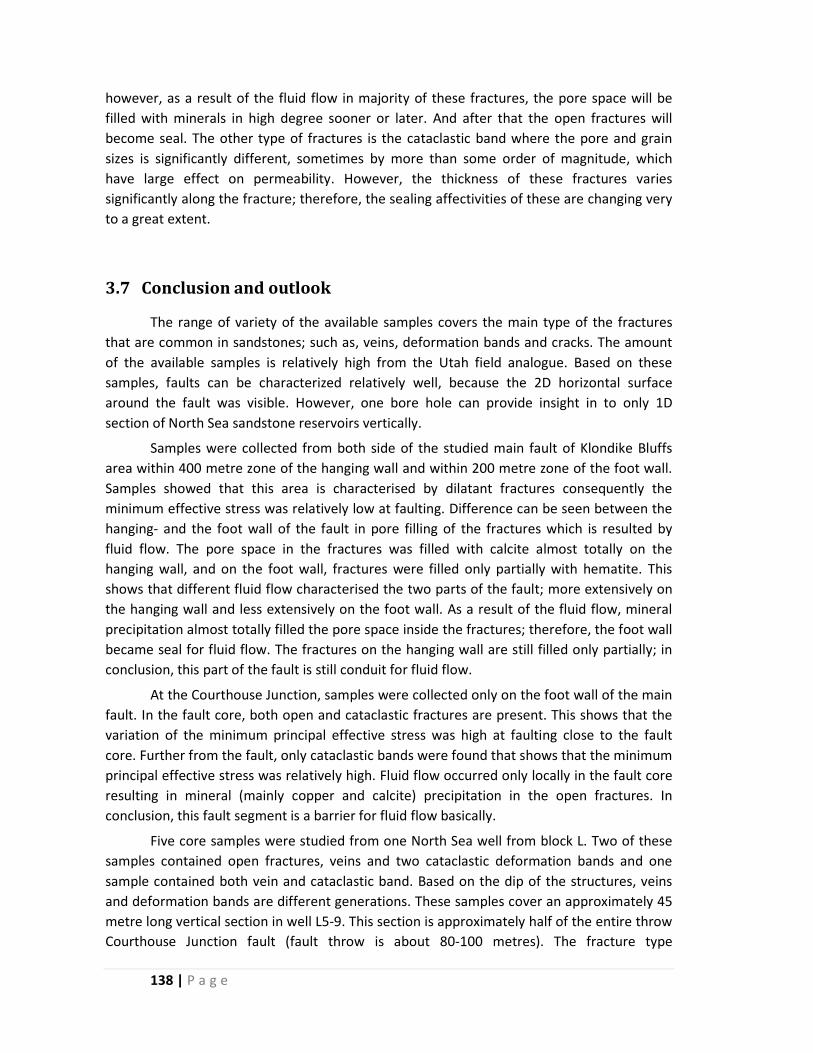
138 | P a g e   

however, as a result of the  fluid  flow  in majority of these  fractures,  the pore space will be 

filled with minerals  in high degree  sooner or  later. And  after  that  the open  fractures will 

become seal. The other type of  fractures  is  the cataclastic band where  the pore and grain 

sizes  is  significantly  different,  sometimes  by more  than  some  order  of magnitude, which 

have  large  effect  on  permeability.  However,  the  thickness  of  these  fractures  varies 

significantly along the fracture; therefore, the sealing affectivities of these are changing very 

to a great extent.  

 

3.7 Conclusionandoutlook

The range of variety of the available samples covers  the main  type of  the  fractures 

that are common in sandstones; such as, veins, deformation bands and cracks. The amount 

of  the  available  samples  is  relatively  high  from  the Utah  field  analogue.  Based  on  these 

samples,  faults  can  be  characterized  relatively  well,  because  the  2D  horizontal  surface 

around  the  fault was  visible.  However,  one  bore  hole  can  provide  insight  in  to  only  1D 

section of North Sea sandstone reservoirs vertically. 

Samples were collected  from both side of  the studied main  fault of Klondike Bluffs 

area within 400 metre zone of the hanging wall and within 200 metre zone of the foot wall. 

Samples  showed  that  this  area  is  characterised  by  dilatant  fractures  consequently  the 

minimum effective stress was relatively low at faulting. Difference can be seen between the 

hanging‐ and  the  foot wall of  the  fault  in pore  filling of  the  fractures which  is  resulted by 

fluid  flow.  The  pore  space  in  the  fractures  was  filled  with  calcite  almost  totally  on  the 

hanging wall, and on  the  foot wall,  fractures were  filled only partially with hematite. This 

shows that different fluid flow characterised the two parts of the fault; more extensively on 

the hanging wall and  less extensively on the foot wall. As a result of the fluid flow, mineral 

precipitation almost totally filled the pore space inside the fractures; therefore, the foot wall 

became seal for fluid flow. The fractures on the hanging wall are still filled only partially; in 

conclusion, this part of the fault is still conduit for fluid flow. 

At the Courthouse Junction, samples were collected only on the foot wall of the main 

fault. In the fault core, both open and cataclastic fractures are present. This shows that the 

variation of  the minimum principal  effective  stress was high  at  faulting  close  to  the  fault 

core. Further from the fault, only cataclastic bands were found that shows that the minimum 

principal effective stress was relatively high. Fluid flow occurred only locally in the fault core 

resulting  in  mineral  (mainly  copper  and  calcite)  precipitation  in  the  open  fractures.  In 

conclusion, this fault segment is a barrier for fluid flow basically. 

Five core samples were studied from one North Sea well from block L. Two of these 

samples  contained  open  fractures,  veins  and  two  cataclastic  deformation  bands  and  one 

sample contained both vein and cataclastic band. Based on the dip of the structures, veins 

and deformation bands are different generations. These samples cover an approximately 45 

metre long vertical section in well L5‐9. This section is approximately half of the entire throw 

Courthouse  Junction  fault  (fault  throw  is  about  80‐100  metres).  The  fracture  type 

139 | P a g e   

characteristics of the North Sea samples shows similarity to fractures type characteristics of 

the fault zone of the Courthouse Junction fault. Both fault zones have dilatant and cataclastic 

fractures close to each other. 

In comparison,  the Moab  sandstones are analogue  to  the  sandstones of North Sea 

prospect area; the host rock of the areas  is similar, porosities and also pore throat radii of 

these sandstones are similar. Furthermore, fractures in Moab samples and also those of the 

North  Sea  samples  are  characterised  by  diagenesis  (mainly  calcite)  as  results  of  fluid 

migration.  In addition,  the characteristics of  the  fractures of  the  field analogue area show 

also similarities to the North Sea fractures. Furthermore, the tectonic circumstances on both 

areas  (North Sea and Moab area) are  similar: extended  fault network,  involved  in general 

normal faults, and also salt tectonic characterize both areas. In conclusion, the sandstones of 

Moab area; such as, Slick Rock Member of Entrada Sandstone and Moab Member of Curtis 

Formation,  are  a  good  analogue  for North  Sea  reservoir  sandstones  (Permian, Rotliegend 

Sandstone Group). 

The deformation features  in the studied samples  indicate that the properties of the 

structures;  such  as  thickness,  pore  size,  grain  size,  pore  throat  radius  vary  along  the 

structures. Therefore, future works should aim to study longer sections of these structures in 

order  to measure  the  range of  the  changes of  the most  important properties which have 

influence on the fluid flow.  

Besides,  the  BIB‐SEM  images  showed  that  the  very  precisely  polished,  even  rock 

surfaces  provide  possibility  to  study  2D  microstructures  of  fractures  and  pore  space  in 

images where structures can be traced, which allow us to calculate statistics to quantify the 

properties of  the rocks. Furthermore, serial cross section of 2D surfaces allow  to study 3D 

architecture of rocks where  fluid paths can be measured and pore  throats radius, porosity 

and permeability can be measured more precisely. 

A comprehensive fault model is necessary to better understand fluid flow properties 

of complex fault networks. The results of microstructure analyses, including BIB‐SEM  image 

analyses,  are  able  to  provide  important  information  and  parameters  for  extended  fault 

structures and its fluid flow model. This model also can improve the seismic interpretation.  

   

140 | P a g e   

 

141 | P a g e   

4 Correlation analysis betweenmechanical properties andboreholelogpropertiesinNorthSeasandstones

4.1 Introductionofcorrelationanalysisofmechanicalproperties

4.1.1 General introduction 

In study of the fractures and fracture mechanism, it is essential to understand under 

what  condition  fractures  can  form.  Strength  is  one  of  the  most  important  material 

properties. The  strength measures under what  stress  conditions a  given material will  fail. 

Other  important material  property  is  the  elasticity  that measures  the  relation  between 

deformation  of  a material  and  the  acting  stress.  Rock  strength  and  elastic modulus  are 

important  factors  in engineering and rock mechanical  investigations. Rock mechanical data 

are used  to wellbore  stability  to determine proper mud weight, hydraulic  fracturing, pore 

compressibility, sand production, subsidence‐ and compaction calculation, well completion 

section  or  well  case  planning.  Besides,  knowledge  of  the  rock  strength  also  provides 

opportunity  to predict  the tendency  for  fracturing and  the possible  type of  the developing 

fractures under  a  given  condition.  Several methods exist  in order  to measure mechanical 

properties of  rocks  including  in‐situ and  in  laboratory  too. However,  these measurements 

are expensive, especially  if  rocks are  in  thousands of meters depth, as  they are usual  in a 

hydrocarbon  reservoir  and  appropriate  samples  are  relatively  rarely  available  for 

measurements from these depths. Therefore, rock mechanical property prediction methods 

play  important  roles  in  field  of  reservoir  geomechanics. Wireline  geophysical  logs, which 

measure  physical  properties  of  the  rock  body  around  the  borehole,  are  almost  always 

measured  after  and/or  during  borehole  drilling.  Therefore,  wireline  log  data  often  can 

provide possibility to predict rock mechanical properties. 

Brittle failure of rock is a complex process of fracture. The fracturing process is basically a 

combination  of microscopic  tensile  cracks  and  frictional movement  on  grain  boundaries 

(Brace,  et  al.  1966). As  stress  is  closing  the  critical  point,  the  numbers  of micro‐cracks  is 

increasing and  reach  the  critical  stress condition,  the  rock  fails along  through‐going  shear 

plane (Lockner, et al. 1991). Griggs and Handin  (1960) distinguished two modes of fracture 

such  as  shear  fracture  and extension  fracture.  Later, Ramsey  and Chester  (2004)  inferred 

that  also  hybrid  fractures  can  form  as  a  combination  of  compression  and  tensile  state. 

However, mode of fracturing depends on several different properties of the rock and also on 

external physical parameters. 

In order to predict rock strength, it is necessary to understand which factors control rock 

strength.  Rock  strength  depends  on  structural  properties  of  the  rocks  that  are  strongly 

related to the mineral composition of the rock. According to the Mohr‐Coulomb theory, rock 

internal properties  are defined  as  cohesion  (chemical  and physical bonds between  grains 

and  crystals,  cementation)  and  internal  friction.  Several  studies  showed  that  porosity 

decreases brittle failure strength of rocks (Brace and Riley 1972, Dunn, et al. 1973, Hoshino 

1974, Scott 1989, Palchik 1999).  In addition, relation between petrographic properties and 

mechanical properties of a rock was analysed  in many aspects; such as, grain shape, grain 

142 | P a g e   

size, mode of  connection between  grains,  cementation or mineral  composition  (Fahy  and 

Guccione 1979, Winkler 1985,  Singh 1988, Shakoor  and Bonelli 1991, Haney  and  Shakoor 

1994, Ulusay, et al. 1994, Schön 1996, Bell and Culshaw 1998, Tuğrul and Zarif 1999, Hale 

and Shakoor 2003, Jeng, et al. 2004, Meng and Pan 2007, Pomonis, et al. 2007, Hsieh, et al. 

2008).  Since  in  sandstones,  clay  very  often  presents  and  clay  content  can  change 

significantly,  the effect of clay on rock strength was analysed  in several works  (Jizba 1991, 

Samsuri,  et  al.  1999,  Takahashi,  et  al.  2007,  Li  and  Zhang  2011).  The  outcome  of  these 

studies  is that increasing clay content decreases the strength of sandstone and dry clay can 

increase strength  in comparison to wet clay  (Swanson et al. 2002).  In addition, the type of 

clay content has effect on the mechanical behaviour of rocks: illite or chlorite clay is stronger 

than  smectite‐rich  clay  which  smears  easier  (Lockner  and  Beeler  2002).  Furthermore, 

moisture  content  also  has  effect  on  rock  strength;  numerous  researches  observed  that 

increasing saturation reduces the rock strength (Colback and Wiid 1900, Simpson and Fergus 

1968,  Broch  1974,  Ballivy,  et  al.  1976, Michalopoulos  1976,  Priest  and  Selvakumar  1982, 

Venkatappa Rao, et al. 1985, Dyke and Dobereiner 1991, Hawkins and McConnell 1992, Hale 

and  Shakoor  2003,  Shakoor  and  Barefield  2009).  Anisotropy  also  has  an  effect:  the  rock 

strength  in compression, parallel to the foliation plane, may be greater or  less than normal 

(Paterson and Wong 2005). Textural anisotropy can also  result  in  significant anisotropy of 

tensile and compressive strength  that may be associated with different  failure modes and 

deformation mechanisms,  depending  on  how  stress  is  applied  relative  to  the  anisotropy 

planes (Li and Zhang 2011). 

In  addition  to  rock  properties,  rock  strength  depends  on  external  factors.  Rock 

strength monotonically increases with increasing confining pressure (Jaeger, et al. 2009) and 

not only the  lowest principal stress, as suggested by the Coulomb‐Mohr failure criteria, but 

also  the  intermediate  principal  stress  has  effect  on  strength  (Paterson  and Wong  2005). 

There  is generally some  influence of strain  rate,  temperature and  time on brittle  fracture, 

which may vary with the material and the experimental conditions. This observation points 

to  there  being  some  participation  of  thermally  activated  processes  in  brittle  fracture. 

According to Sangha and Dhir (Sangha and Dhir 1972) at strain rates of 10‐1 s‐  I or  less, the 

fracture  stress measured by uniaxial  tests  increas by around 10%  for 103‐fold  increase  in 

strain rate and this effect is smaller in the case of triaxial tests. Donath and Fruth (Hirth and 

Tullis 1994)  found no  significant  influence of  strain  rate on  the  shear  fracture  strength of 

sandstones  and  siltstones  under  a  confining  pressure  of  100  MPa.  There  are  several 

observations  which  show  that  there  is  some  decrease  in  strength  with  increase  in 

temperature  (Fischer  and Paterson 1989).  The  fracture  strength decreases only  slightly  at 

moderate temperatures, below 300°C (Handin and Hager Jr 1958). 

The previous studies clearly showed that many factors controls rock strength. Therefore, 

the prediction of the rock strength dependencies and influences present a challenge because 

of its complexity. One way to determine strength of reservoir rocks that are in thousands of 

meters deep, is to use geophysical well logs (Zhou et al. 2005, Chang et al. 2006). 

 

143 | P a g e   

Well  logs  measure  several  rock  properties  which  are  also  related  to  rock  strength. 

Different types of resistivity tools provide information on water saturation, porosity and also 

clay  content of  rock around  the bore hole. Natural gamma  ray measurement data mainly 

indicates clay content; in addition, spectral gamma ray measurement that involves Thorium 

(Th),  Uranium  (U)  and  Potassium  (K)  logs,  provides  further  information  on  mineral 

composition  of  the  rock.  Sonic  or  acoustic  logs  allow  estimating  the  compression  and 

shearing  wave  velocity  of  rocks  which  are  related  to  rock  types,  density,  porosity  and 

saturation.  Furthermore,  generated  gamma  ray  based  density  tool  measures  the  bulk 

density  of  the  formation  more  accurately.  Neutron  log,  which  is  the  reaction  of  the 

formation  to  fast  neutron  bombardment,  indicates  the  richness  of  formation  in 

hydrocarbon; furthermore, with correction, formation density can be calculated too. (Rider 

1986, Ellis and Singer 2008) 

The first attempts tried to correlate only one well log to UCS in order to predict the 

rock strength. McNally defined an exponential relationship between  the sonic  log and UCS 

(McNally 1987). This method  is a  first order estimate of  the rock strength. The correlation 

can be improved by distinguishing weak and strong strata (McNally, 1990).   

Fjar et al. (2008) developed a quartic relationship between P‐wave velocity and UCS for 

sandstones of the Gulf of Mexico. Schön (1996) described the relationship between seismic 

velocity  and UCS  as either  a  linear, polynomial or  logarithmic  relationship. Bradford  et  al 

(Bradford et al. 1998) calculated UCS  from static Young’s moduli, which were derived  from 

velocity and density measurements using  linear relationship and built a model for the very 

weak North Sea  sandstones. Moos et al.  (1999) used a quadratic  relationship between P‐

wave  velocity  and  UCS  for  coarse  grained  sandstones  and  conglomerates  in  Cook  Inlet, 

Alaska.  Lawrence developed  a  correlation  equation  between  sonic  log  and UCS  based on 

lithological  variations  (Lawrence,  1999).  However,  these  approaches  tend  to  show  high 

uncertainty, due to the fundamental difference between the static (UCS) and dynamic (sonic 

velocity) rock strength properties.   

To  solve  this  issue, Hatherly et al.  (2001) correlated  the composition of well  logs with 

UCS. Although,  the variability  in  the  strength behaviour due  to;  for example, cement  type 

and the  location of the cement (whether the cementation  is only around the grains or also 

filling the pore space), cannot be investigated by such an analysis (Hatherly et al. 2004). 

It is well known that stress levels affect sonic velocity magnitudes in rocks. This is one of 

the reasons why UCS estimates based on sonic velocity alone tend to be accurate only when 

determined  for  a  specific  site  or  lithology  at  that  site. Whilst  only marginally  better,  the 

compositional  approach  aims  to  provide  a  more  generalized  formula  that  allows  UCS 

estimates  to some extent account  for  local variations. Therefore Zhou et al.  (2005)  tested 

two new methods, the Radial Basis Function (RBF) and the Self‐Organizing Maps (SOM), for 

predicting the rock strength from all available, geophysical logs; however, these results were 

valid only locally (Zhou et al. 2005). 

  Chang,  Zoback  et  al.  (Chang  et  al.  2006)  summarized  the  empirical  equations 

between  UCS  and  mechanical  properties  derived  from  well  logs.  They  stated  that  the 

reviewed relations may be useful to predict the wellbore stability, especially when there  is 

144 | P a g e   

no  other  available  information  on  the  rock  strength. However,  they  also  highlighted  that 

there is a need for the calibration of the correlation equations. 

Urai et  al.  (1994)  studied  the deformation mechanism  in  clay  and mudrocks. They 

developed a brittleness  index  to quantify  the  tendency of  forming dilatant  fractures  (Urai 

1995,  Urai  et  al.  1997,  Hoogerduijn‐Strating  and  Urai  2003).  The  brittleness  index  was 

calculated  from  the UCS, which was derived  from P‐wave and S‐wave velocity  logs using a 

logarithmic  relationship.  Relation  between  log  properties,  such  as,  natural  gamma  ray, 

resistivity  and  sonic  velocity,  and  rock  mechanical  properties  were  studied  on  rocks, 

including sandstones in the well RWTH‐1, in order to gain input parameters for stress model 

(Trautwein‐Bruns  et  al.  2010).  Trautwein‐Bruns  et  al.  (2010)  also  studied  the  relation 

between rock strength and borehole breakout properties as well. 

One  other  important  parameter  is  the  Young’s modulus  or  elastic modulus which 

defines  the stiffness of  the  rock. The Young’s modulus describes  the  relationship between 

the  stress  and  strain  in  elastic materials:  it  is  the  ratio  between  normal  stress  and  the 

resulted elastic extension or shortening in the same direction (Fossen 2010). 

There are many ways to determine the Young’s modulus of the rock (Jizba 1991). In 

situ and laboratory tests can be performed to measure rock mechanical properties directly. 

Alternatively,  it  is  possible  to  obtain  the  elastic  moduli  using  methods  based  on  wave 

propagation. Although,  the static and dynamic moduli of a homogeneous material such as 

steel  are  identical  (Fjær  1999),  there  can  be  large  differences  between  the  static  and 

dynamic moduli of heterogeneous materials such as porous rocks, particularly at  low stress 

levels:  the  static  moduli  of  rock  determined  from  static  compression  tests  are 

characteristically  lower  than  dynamic moduli  determined  from  acoustic  sound  velocities 

(Simmons  and  Brace  1965,  Cheng  and  Johnston  1981,  King  1983,  Jizba  and  Nur  1990, 

Tomosawa and Noguchi 1993, Fjar et al. 2008, Fjær 2009). 

The relationship between  the static and dynamic Young’s moduli  is affected by  the 

lithology, especially the shale content and the degree of saturation also has an effect. (Jizba 

1991) The value of the static Young's modulus depends on  loading/unloading path and the 

level of confining pressure (Walsh 1965, Chang et al. 2006). 

Young’s modulus has  also been used  to  estimate UCS, Bradford proposed  a  linear 

relationship between the static Young’s modulus and UCS; although, in this study, the static 

Young’s  modulus  was  not  measured  directly,  it  was  derived  for  velocity  and  density 

measurements (Bradford et al. 1998, Chang et al. 2006). 

In this study, correlations between strength and static elastic moduli and wireline log 

properties  are  analysed  by  multivariate  regression  technique  in  two  different  types  of 

sandstones  of  the  North  Sea  namely  Rotliegend  Sandstone  and  Lower  German  Triassic 

Sandstone  groups  (Wong  et  al.  2007).  These  sandstones  are  found  to  be  potential 

hydrocarbon reservoirs and they are important target of hydrocarbon researches. However, 

relatively  large  volume  of  sandstone  strata  is  tight  reservoir  (Holditch  2006),  where 

production of hydrocarbon even gas  is  very challenging. Therefore, knowledge and better 

understanding of physical and mechanical properties of sandstone reservoirs is necessary for 

exploitation of hydrocarbon resources. The aim of this study is to investigate the relationship 

145 | P a g e   

between  the  rock  strength  and  different  geophysical  wireline  well  logs.  Multivariate 

regression analyses are performed to improve the existing rock strength prediction formulas. 

Such analysis of North Sea sandstone samples has not been carried out before.  In addition 

regression  analysis,  mechanical  characterisation  of  the  studied  sandstone  strata  can  be 

accomplished based on the measured rock properties. 

 

4.1.2 Data 

CORE SAMPLES 

To  perform  the  rock  mechanical  tests,  64  sandstone  plug  core  samples  were 

available. The samples were taken from four boreholes of the south and south‐west part of 

the North Sea,  from block K, P and L: K18‐8, L6‐8, P2‐SE2 and P6‐9. The samples originate 

from the Lower Germanic Triassic Group from the depth of about 2700 m and about 4050 m 

and the Rotliegend Group of sandstones from the depth of 3900 m to 4900 m. This sample 

collection  contains 52 Rotliegend‐ and 12  Lower Germanic Triassic  rock  samples  from  the 

four  wells  combined  (Table  4‐1).  In  the  two  rock  groups,  there  are  10  different  rock 

members.  In  chapter  4.2,  Table  4‐3  and  Table  4‐4  show  the  list  of  the  rock  type  of  the 

samples. 

Figure 4‐1 – Map of the studied wells in the North Sea 

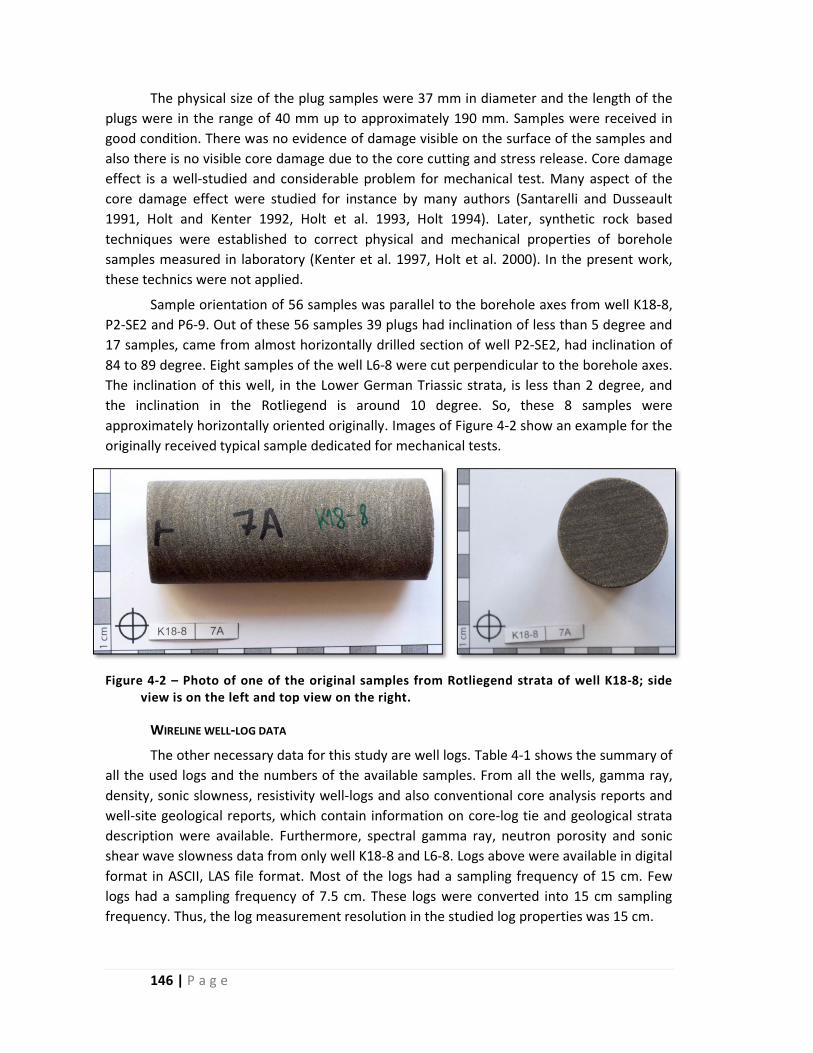
146 | P a g e   

The physical size of the plug samples were 37 mm in diameter and the length of the 

plugs were  in the range of 40 mm up to approximately 190 mm. Samples were received  in 

good condition. There was no evidence of damage visible on the surface of the samples and 

also there is no visible core damage due to the core cutting and stress release. Core damage 

effect  is a well‐studied and considerable problem  for mechanical  test. Many aspect of  the 

core  damage  effect were  studied  for  instance  by many  authors  (Santarelli  and Dusseault 

1991,  Holt  and  Kenter  1992,  Holt  et  al.  1993,  Holt  1994).  Later,  synthetic  rock  based 

techniques  were  established  to  correct  physical  and  mechanical  properties  of  borehole 

samples measured  in  laboratory (Kenter et al. 1997, Holt et al. 2000). In the present work, 

these technics were not applied.  

Sample orientation of 56 samples was parallel to the borehole axes from well K18‐8, 

P2‐SE2 and P6‐9. Out of these 56 samples 39 plugs had inclination of less than 5 degree and 

17 samples, came from almost horizontally drilled section of well P2‐SE2, had inclination of 

84 to 89 degree. Eight samples of the well L6‐8 were cut perpendicular to the borehole axes. 

The  inclination of this well,  in the Lower German Triassic strata,  is  less than 2 degree, and 

the  inclination  in  the  Rotliegend  is  around  10  degree.  So,  these  8  samples  were 

approximately horizontally oriented originally. Images of Figure 4‐2 show an example for the 

originally received typical sample dedicated for mechanical tests. 

Figure 4‐2 – Photo of one of the original samples  from Rotliegend strata of well K18‐8; side view is on the left and top view on the right. 

WIRELINE WELL‐LOG DATA 

The other necessary data for this study are well logs. Table 4‐1 shows the summary of 

all the used  logs and the numbers of the available samples. From all the wells, gamma ray, 

density, sonic slowness, resistivity well‐logs and also conventional core analysis reports and 

well‐site geological reports, which contain  information on core‐log tie and geological strata 

description were  available.  Furthermore,  spectral  gamma  ray,  neutron  porosity  and  sonic 

shear wave slowness data from only well K18‐8 and L6‐8. Logs above were available in digital 

format  in ASCII, LAS  file  format. Most of the  logs had a sampling  frequency of 15 cm. Few 

logs had a sampling  frequency of 7.5 cm. These  logs were converted  into 15 cm sampling 

frequency. Thus, the log measurement resolution in the studied log properties was 15 cm. 

147 | P a g e   

Table  4‐1  –  Table  contains  information  on  available  logs  and  numbers  of  available  core samples from each well and from rock types. 

 

4.2 Method

4.2.1 Sampling method – quality control 

Measurement  results were analysed by  statistical  calculation;  such as, multivariate 

regression analysis. Therefore, a statistically representative sample set  is critical. Histogram 

is one appropriate  tool  to  check  the quality of  the  samples  set.  The histogram of  the  log 

values of the studied rock is supposed to show similar characteristic to the histogram of the 

log  values of  the  selected  samples  including  the  covered  range  (minimum  and maximum 

values).    Figure  4‐3  shows  example  histograms  for  a  representative  sample  subset 

(histogram on the right) out of an entire studied dataset. The covered range of the values is 

nearly the same as range of the entire cored section and the distribution  (characteristic of 

the histograms) of the values is also very similar to entire section too. 

Figure 4‐3 – Histogram of gamma ray  log values of the entire studied rock column (left) and histogram  of  gamma  ray  log  values  of  a  sample  set  (right)  which  is  an  ideally representative subset of the entire dataset. 

148 | P a g e   

Besides the analysis of the distribution of the datasets, permutations of the values of 

the different log properties were created, which belong to a sample or a point of the studied 

strata, also a critical  factor. With multivariate regression,  the relation between mechanical 

properties and four or more log properties  is analysed. For  instance, what is the strength if 

gamma ray and density values are high while sonic slowness and resistivity values are low; or 

gamma  ray value  is  low and etc.  If  ranges of  logs are classified  in  three sections;  such as, 

high,  medium,  low  values;  then,  this  way  64  variation  of  the  log  properties  can  exist. 

However, many of the class  types do not exist, because a given class type simply does not 

present  in  the  studied  section  or  because  of  law  of  nature.  In  this  study  three  and  four 

classes were used as it can be seen in Table 4‐2. Furthermore, rock type or facies also can be 

involved  in  this checking procedure  if  it  is necessary.  In  this study,  facies was not used  for 

quality check. Table 4‐2 shows the  list of the used  limits of log properties for quality check. 

Two limit means three classes and three limits means four classes. 

Table  4‐2  –  Limits  of  the  log properties  listed  in  this  table were  used  for  quality  check  of selected sample set. 

Sonic slowness [µs/ft] 

Density 

[ / ] 

Resistivity[Ohmm] 

Gamma ray [api] 

Potassium[%] 

Uranium[ppm] 

Thorium [ppm] 

Neutron porosity[pu] 

Class 1  <65  <2.45  <10 <50 <1.5 <4 <4  <8

Class 2  65‐80  2.45‐2.7  10‐50  50‐100  1.5‐2‐5  4‐8  4‐8  8‐16 

Class 3  80<  2.7<  50‐100  100‐150 2.5<  8<  8<  16< 

Class 4      100< 150<  

Classes were created according to the limits (see Table 4‐2) in numerical format with 

the following digits system for the four basic logs: ####.  These artificial numbers reflect type 

of  log  properties  hence  they  are  called  “log  property  type”.  The  first  digit  stands  for 

compression wave  slowness  (DTC),  the  second  digit  for  density  (DEN),  the  third  digit  for 

resistivity  (RES), and  the  fourth digit  for gamma  ray  (GR). And  for quality  check of all  the 

used  logs  (spectral  gamma  instead  of  GR)  the  log  property  pattern  was: 

DCT|DEN|RES|K|U|TH|CNC (864 theoretical variations of log properties).  

Using the log property types as bins for histogram, log property type histogram(s) can 

be created. Based on the  log property type histogram, number of required samples can be 

defined.    Ideally, a  representative data  set  contains  around 4‐6  samples  from every  type. 

However,  there  are  types  from  where  only  very  limited  number  of  sample  available. 

Furthermore,  these  rare  log  property  types  not  significantly  represent  the  studied  rock; 

therefore, they can be neglected from the analysis. 

The core‐to‐well tie is very important in order to know the right log values of the core 

samples.  The  core‐log  tie  is  defined  by  those  points  (markers) where  correlation  can  be 

observed  between  log  and  the  related  core  rock.  However,  the  distance  between  these 

markers  is often several meters  to  ten‐twenty meters. Moreover, between  the markers,  it 

still has an uncertainty because of  the  cable  stretch which  is hard  to predict.   Figure 4‐4 

shows an example for log curve characteristics in gamma ray log. At some points, log values 

149 | P a g e   

change relatively much considerably over a short depth range – curve of the log is steep. If 

the log value changes very “quickly” in shorter interval then the reliability of log value belong 

to a given sample is low. Log values hardly change between depths of 3951 m to 3953 m. Log 

value of a sample from this section is much more reliable than a sample from depth of 3954 

m.  Log  value  change  to more  than  double within  15  cm  distance.  This  factor  has  to  be 

checked and considered during data processing. 

Figure 4‐4 – Figure shows an eight m  long section of a gamma ray  log. Orange dots  indicate the  measured  log  values  and  the  green  line  is  log  curve  simply  connecting  the measured  points.  Data  frequency  of  the  log  is  15  cm.  Dimension  lines  show  some 

examples  how  the  value  of  neighbour  points  change  relative  (GR %)  and  absolute (GR), too. 

Numerically, the slope of a continuous function can be analysed by first derivative of 

the  function.  For  well  logs,  which  are  rather  like  discrete  functions,  the  slope  can  be 

calculated by the difference of the neighbouring  log values of a given range. To analyse the 

log  curve  shape, 60  cm  radius was used around  the given  location according  to  (Eq. 4‐1). 

Where, DValue%  is  between  the minimum  and  the maximum  log  values within  the given 

range  (MaxValueRadius‐MinValueRadius) relative  to  the range of  the entire studied  log section 

(MaxValueTotal‐MinValueTotal).  

% ∙ 100 % (Eq. 4‐1) 

In  this  part  of  the  quality  check,  the  cable  tension  logs  can  provide  further 

information on the reliability of depth of logger equipment. Therefore, the total tension was 

involved in the quality check; the log curve shape was analysed with the same calculation. 

Core‐log  depth  shift  data  were  available  from  all  the  wells  which  were  used  to 

synchronize the log data (depth measured by loggers) and core data (depth measured by the 

drillers).  Besides,  the  measured  depth  was  converted  into  true  vertical  depth  for  the 

comparison of the data from different wells. 

150 | P a g e   

4.2.2 Sample preparation 

Sample  quality  check  is  also  essential  to  gain  reliable  results.  The  received  rock 

samples were  intact samples,  in undamaged condition. The suggestion of  ISRM and ASTM 

(Ulusay  and Hudson 2007, ASTM‐D7012 2010)  standards  for  sample  preparation  and UCS 

test measurements were followed for the rock tests. The most important parameters are the 

sample size and sample dimension ratio. The suggested diameter to  length ratio has  to be 

1:2 to 1:3 and the diameter is not allowed being smaller than 10 times the diameter of the 

largest grain. The lengths of 10 samples (15% of all the samples) were shorter than the other 

samples. Therefore, all  the samples were re‐drilled with smaller diameter  to have uniform 

plug sample size: diameter of 20 mm and length 40‐45 mm.  

Figure 4‐5 – Side and top view photos of two samples (left: K18‐8/1; right: L6‐8/A) which are prepared for unconfined compressive test measurement. 

For the sample preparation, diamond core drill bit was used. Water cooling was used 

at drilling in general; however, weaker samples were cooled by air. Diamond blade was used 

to cut the length of the samples with water cooling. The plug ends were prepared even and 

perpendicular with a special grinding machine for plug samples with diamond wheel. 

Combined 70 UCS plug samples were prepared from the received 64 core samples. At 

six samples, the  length of the samples allowed us to prepare two UCS plugs from one core 

sample.  Two of  the  samples  (P2‐SE2/7  and  P2‐SE2/20) were  fairly weak  and washed‐out, 

therefore  the  required  shape  conditions were  not been  able  to  reach;  and  the  plug ends 

were uneven and not perpendicular. In this condition, these may not provide reliable results; 

therefore, they were skipped from the mechanical measurements.  

Some of the samples were found potential outliers. One sample (P6‐9/12) broke into 

two parts during cutting with perpendicular to the plug ends. Two of the samples (P2‐SE2/23 

and P2‐SE2/22) were  relatively weak. Therefore,  it was not possible  to grind plug‐ends as 

even as the standards require; but, deviation was not significant. Two of the samples (K18‐

8/12  and  K18‐8/13)  contained  larger  grains  than  it  is  allowed  (the  ten  times  of  the  plug 

diameter). 

2 cm

151 | P a g e   

4.2.3 Rock physical measurements 

The  second  stage  was  the  measurement  of  rock  physical  properties  of  the  core 

samples.    The  porosity  and  the  density  of  the  samples  was measured  in  the  UCS  plug 

samples or  in  the  remains,  tube shaped part of  the UCS plugs. The samples were dried at 

60°C until samples mass decrease were less than 0.1 % during 4 hours drying time, according 

to  the  ISRM  standard  (Ulusay  and  Hudson  2007).  The mass measurement  accuracy was 

±0.0001 g. 

In  dried  samples,  the  matrix  volume  was  measured  with  helium  pycnometer 

(machine type: AccuPyc 1330). After that, the sample bulk volume was measured by vernier 

caliper  and  also  by  Archimedes  method.  The  Archimedes  volume  measurements  were 

achieved on saturated samples, directly before the UCS measurements;  therefore porosity 

had no effect on bulk volume  results. Balance with accuracy of ±0.001 g was used  for  the 

mass measurements during the Archimedes measurements. The matrix‐ (grain) density, bulk 

density  and  porosity  of  the  rock  samples  were  calculated. Measurement  uncertainty  of 

porosity values are less than ±0.2 %. 

 

4.2.4 Rock mechanical measurements 

In the main stage of the work, the unconfined compressive strength of the prepared 

samples was measured.  The UCS  tests were measured with  Zwick/Roell  Z100  load  frame 

using testXpert II software. This test machine is able to measures the applied force with an 

accuracy of ± 0.5 Newton and the frame displacement with an accuracy of ± 0.0005 mm. The 

measurement  uncertainty  values  produce  around ±  0.1 MPa uncertainties  in UCS  results.

  The  samples were  saturated with  tap water  samples  for UCS  tests.  Samples were 

saturated higher  than 2 %, because above 2 % saturation UCS does not change much with 

increasing  saturation  (Hawkins and McConnell 1992, Barefield and Shakoor 2006, Shakoor 

and Barefield 2009). 

Unconfined compressive strength measurements were performed in accordance with 

ASTM  and  also  ISRM  (Ulusay  and  Hudson  2007,  ASTM‐D7012  2010).  Since  the  size  of 

available  core  samples were  limited;  therefore,  samples were  prepared  smaller  than  the 

standard suggestion in order to create uniform size plug samples. The sample diameter was 

20 mm ± 0.5 mm and length 40 mm ± 1 mm. Measurement of all the samples were planned 

to perform with a single, relatively short unload‐reload loop, as suggested by the standards. 

Unload‐reload behaviour of rock is analysed often in pressuremeter tests (Byrne et al. 1990, 

Clarke 1994). The positions of the  loops were defined with the applied force; ranges of the 

loops were from 1500 N (for lower UCS rock) to 3000 N (for higher UCS rock). Rock strengths 

were measured applying constant  loading speed. These results were used to estimate UCS 

for planning  loop parameters. During the tests, the tool separations were decreased with a 

predefined  constant  speed,  0.1 mm/minute,  strain  rate=5·10‐5  s‐1.  The  UCS  values  were defined as the highest measured force divided by area of the specimen. The Young’s moduli 

values were calculated  from  the  longest  linear  section of  the  stress and  stain  curve.   The 

152 | P a g e   

unloading moduli were calculated  from  linear sections of unloading part of  the stress and 

stain curve. Figure 4‐8 shows an example for the source of calculation of both moduli. 

For calculation of the elastic moduli of the samples, the calibration of the measuring 

tool  is  necessary.  For  calibration  purpose,  21  calibration  tests were measured where  the 

load frame was empty and clean in order to define the elastic behaviour of the test machine. 

Figure 4‐6 shows the 21 measured calibration test. The strain of the load frame was defined 

with a third grade polygon (equation can be found in the graph) when force was lower than 

25000 N. The red  line on  the  left graph of Figure 4‐6 shows  the  trend  line of  the polygon. 

And when force was higher than 25000 N, strain was corrected linearly that can be seen on 

the right graph of Figure 4‐6  together with  the applied equation. The measured  force and 

strain curves of the samples were corrected with the self‐strain of the load frame defined by 

the two equations. The real strain is the difference of the measured strain and the strain of 

the  test machine at  the given  force  (machine(F)). On Figure 4‐7, an example  for calibration 

correction  can be  seen originally measured  (black dashed  line) and  corrected  (green  solid 

line) stress and strain curve of sample K‐1.  

Static  elastic  moduli  of  the  samples  were  calculated  on  two  segments  of  the 

corrected stress and strain curves of  the samples. On  the one hand,  the  linear part of  the 

main  loading  segment  of  the  stress  and  strain  curve  was  used  for  calculation  of  elastic 

modulus. And on the other hand, also the unload part of the unload‐reload loop was used to 

gain unload elastic modulus. Figure 4‐8 shows an example of the two sections of stress and 

strain curve. Static elastic modulus (Young’s moduli) was calculated as the dip of the curves. 

 

Figure 4‐6 –  Load  frame  calibration measurements  results  (blue  lines)  and  the  fitted  trend lines (red lines) and the equation of these can be seen on the graphs. Graph on the left shows the curve that was used when force was lower than 25000 N. Graph on the right shows the curve that was used when force was higher than 25000 N.    

153 | P a g e   

Figure 4‐7 – Graph shows measured and corrected strain curve of samples K‐01,  self‐strain of the frame was subtracted from measured strain. 

Figure 4‐8 – Graphs shows on the left the entire measured stress and strain curve of samples K‐01 which  contains  an  unload‐reload  loop.  The  two  sections were  used  for  elastic moduli calculation. Purple  line  indicates  linear part of the normal  loading section and dashed blue  line  indicates the unloading section of the curve. Graph on the  left shows the loop section of the same graph. 

 

 

 

154 | P a g e   

4.2.5 Regression analysis 

In  order  to  estimate  the  relationship  between  UCS  and  different  log  properties, 

regression analysis was performed. Simple and multivariate linear regression was calculated, 

which implies, that the dependent variable (UCS) is a linear combination of the independent 

variables (log properties), however it is not necessarily linear in the independent variables. In 

case  of  simple  linear  regression,  there  is  one  independent  variable; whereas,  in  case  of 

multivariate linear regression, there are more independent variables.  

The simple linear regression model can be given as:  

 

The two constants, intercept (β0) and slope (β1) are the regression coefficients which 

need to be estimated from a sample of y values with their associated values of x, and u is a 

random variable which represents the deviation of y about its mean.  (Soong, 2004) 

The  multivariate  linear  regression  model  with  m  independent  variables  can  be 

described as: 

⋯  

where are m+1 regression coefficients (β0, β1, … , βm), and u is the error with mean of 0 and 

variance of σ2, which is identical to the variance of y (Soong, 2004). 

The regression coefficients were calculated using the least squared method. The goal 

of this method is to choose the regression coefficient in a way that the sum of the squared 

differences between observed sample values and the estimated expected value of the model 

is minimized. The detailed description of this method can be found  in e.g. Björck (1996) or 

Allen (1997). 

There are some parameters to measure the “goodness” of the fit. The coefficient of 

the multivariate  regression  (R) estimates  the degree  to which  variation  in  the dependent 

variable  is  associated  with  variations  in  the  several  independent  variables  taken 

simultaneously. The coefficient of multivariate determination (R2), measures the percentage 

of  the  variation  in  the  dependent  variable  which  is  explained  by  variations  in  the 

independent variables taken together (Schroeder et al. 1986). This can be calculated as the 

following:  

 

where SSM  is  the  sum of  squares  for  regression and SST  is  the corrected  sum of  squares 

total, and calculated as the following: 

ŷ  

 

 

Where n is the number of observation, ŷi is the estimated y value,   is the mean value of y.  

155 | P a g e   

Before calculating the regression coefficient, the ANOVA (Analysis of Variance) table 

was calculated. All the calculations were done using the Microsoft Excel Analysis ToolPak and 

also Matlab scripts. As a part of ANOVA, F statistic was calculated to test the hypothesis (H0) 

whether all of the coefficient equal to zero.  

0: . . . 0 

If  this  hypothesis  can  be  rejected,  it  means  that  there  that  the  entire  model  is 

statistically significant. 

The F statistic  is the ratio of the mean squares for the model and the mean squares 

for  the error. Based on  the model,  the corresponding significance F can be also calculated 

which  gives  the  probability  that  the  null  hypothesis  for  the  full  model  is  true.  If  this 

significance F  is a  low value, the null hypothesis can be rejected which would mean that at 

least one of the regression parameters are nonzero. Thus, the regression equation does have 

some validity  in  fitting  the data, so  the  independent variables are not purely random with 

respect to the dependent variable. 

The residuals of the regression model are the difference between the observed value 

and the least square estimate. During the regression, the sum of the absolute residuals and 

also the sum of  the absolute standard residuals  (standard residual: residual divided by the 

standard deviation of all the residuals of a model) were supposed to be minimized. 

In addition to an appropriately large R2 value, there are some requirements regarding 

the residuals to verify the model. The residuals are supposed to have a normal distribution 

with an expected value of zero and with the same standard deviation as the original dataset. 

They also supposed to be independent. (Kutner et al. 2004) 

The main aim of this study is to analyse the relationship between log properties and 

rock  mechanical  properties.  One  way  is  to  analyse  relationship  between  data  sets  is 

regression  calculation  that  provides  correlation  equations.  These  equations  are  empirical 

equations  because  these  are  created  only  based  on  regression.  In  this  case,  UCS  was 

predicted by different models and  the explanatory variables of  the calculation models are 

the different log types. The logs were also converted by non‐linear functions; such as 1/x, x2, 

x1/2,  log10(x),  exp(x)  functions.  Microsoft  Excel  and  Matlab  software  was  used  for  the 

calculation and data visualization.  

 

 

156 | P a g e   

4.3 Results

4.3.1 Quality control of the log data 

Firstly, the best fit resistivity log was selected from the two wells where six different 

logs were measured with different  long  receivers. The next  step was  to  filter  the outliers 

based on the result of the linear multivariate regressions between P‐wave slowness, density, 

resistivity  and  gamma  ray  logs  and  UCS  involved  all  the  samples.  Linear  multivariate 

regressions  of  different models were  calculated where  numbers  of  explanatory  variables 

were  increased  step  by  step.  This  way,  the  effect  of  the  newly  added  variable  on  the 

regression quality was studied.  In addition,  the  relation between non‐linear  functions  (e.g. 

exponential‐,  logarithmical‐,  parabolic‐,  and  hyperbolic)  of  the  logs  and  the  UCS  were 

studied. Finally,  the data  set was  separated by  formations  (Rotliegend and Lower German 

Triassic Group) and linear multivariate regressions were calculated in the same way as it was 

for the entire data. 

The distribution of the log properties of the studied formations and samples from all 

the wells can be seen on histograms of Figure 4‐9. The distribution and also  log values of 

samples cover nearly the same ranges as the log values of the entire core section cover. The 

histograms  of  samples  show  similar  characteristics  values  to  the  entire  section  at most 

frequent occurrence. Figure 4‐10 shows the  log type histograms of the studied rock section 

and core samples in order to compare the distribution of these data. Histograms shows that 

the sample set contains the most frequent log property types and only the very low frequent 

occurrence types are not represented by sample set. Hence, it allows gaining information on 

the dominant part of the structure. 

The uncertainty of  log  values  is  showed on Figure 4‐11  for  four most  common  log 

properties namely: gamma ray, resistivity, sonic slowness and density on a segment of well 

P2‐SE2. Red dots  indicate the  location of samples  in  logs. As  it can be seen on the graphs, 

most of the samples are at relatively flat section of the log curves. Thus, uncertainties of the 

log value of the samples, because of the possible depth shift of the logs, are small. However, 

several  samples  are  at or  close  to  steep  section of  the  log  curve. The  changes of  the  log 

values around the samples were calculated by equation (Eq. 4‐1), which can be seen in right 

part of Table 4‐3 and Table 4‐4 Higher value means that the given sample has more chance 

for different value  in case of depth shift. Besides, Table 4‐3 and Table 4‐4 shows all the  log 

parameters of all the samples that were used for the calculations. 

 

157 | P a g e   

Figure  4‐9  – Histograms  of  the  log  properties  of  the  entire  cored  sections  (first  and  third rows) and received samples (second and fourth rows). The distribution of the  log data of  the  studied  borehole  section  and  core  samples  is  compared  by  the  histograms. (Where  DTC  is  compression  wave  slowness,  DEN  is  density,  RES  is  resistivity,  GR  is gamma ray, CNC is compensated neutron porosity, K is potassium GR log, TH is thorium GR log and u is uranium GR log.) 

158 | P a g e   

Figure 4‐10 – Histogram of  log property types, based on the  four basic  logs (DTC, DEN, RES, GR),  of  the  entire  section  (upper  graph)  and  samples  (lower  graph)  can  be  seen  on figure  “a”.  On  figure  “b”,  histogram  of  log  property  types  of  entire  section  (upper graph)  and  samples  (lower  graph)  can  be  seen  based  on  all  available  log  types (involved well K18‐8 and L6‐8). 

a

b

159 | P a g e   

Figure 4‐11 – Changes  in  log values around  the  selected  samples. The  red dots  indicate  the position  (after  core  depth  shift)  of  the  samples  that  are  involved  in  the mechanical tests. Green lines are the log values. In some cases, log values change very fast around samples; for  instance  in gamma ray  log: sample P2‐6, P2‐23, P2‐24, P2‐27 or  in the  log of resistivity sample P‐24.  (Where DTC  is compression wave  slowness, DEN  is density, RES is resistivity, GR is gamma ray.) 

True vertical dep

th [m] 

160 | P a g e   

Table 4‐3 –Log values of all the  log types of samples from well K18‐8 and L6‐8. On the right part of the table, maximum of change of  log values around the samples within ~ ± 60 cm relative to the total range of the cored section can be seen. Cells with “n.a.” mean that there was no data available.  

161 | P a g e   

Table 4‐4 ‐ Log values of all the log types of samples from well P2‐SE2 and P6‐9. On the right part of the table, maximum of change of  log values around the samples within ~ ± 60 cm relative to the total range of the cored section can be seen. Cells with “n.a.” mean that there was no data available. 

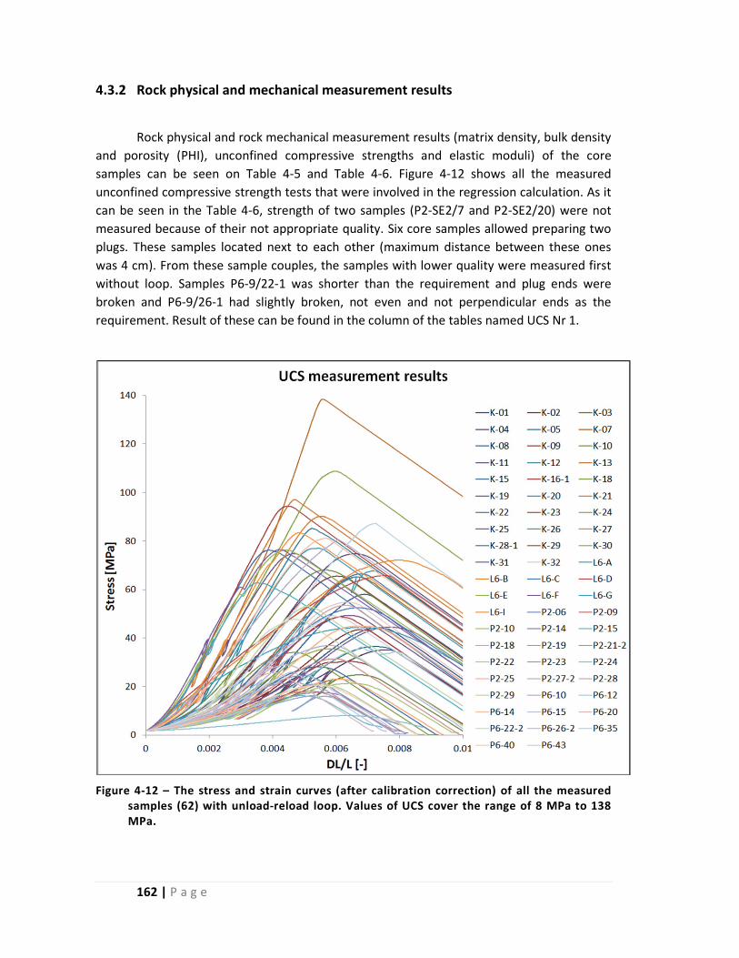
162 | P a g e   

4.3.2 Rock physical and mechanical measurement results 

 

Rock physical and rock mechanical measurement results (matrix density, bulk density 

and  porosity  (PHI),  unconfined  compressive  strengths  and  elastic  moduli)  of  the  core 

samples  can  be  seen  on  Table  4‐5  and  Table  4‐6.  Figure  4‐12  shows  all  the measured 

unconfined compressive strength tests that were involved in the regression calculation. As it 

can be seen  in  the Table 4‐6, strength of  two samples  (P2‐SE2/7 and P2‐SE2/20) were not 

measured because of their not appropriate quality. Six core samples allowed preparing two 

plugs. These  samples  located next  to each other  (maximum distance between  these ones 

was 4 cm). From these sample couples, the samples with lower quality were measured first 

without  loop.  Samples  P6‐9/22‐1 was  shorter  than  the  requirement  and  plug  ends were 

broken  and  P6‐9/26‐1  had  slightly  broken,  not  even  and  not  perpendicular  ends  as  the 

requirement. Result of these can be found in the column of the tables named UCS Nr 1.  

 

Figure 4‐12 – The  stress and  strain curves  (after calibration correction) of all  the measured samples  (62) with unload‐reload  loop. Values of UCS cover the range of 8 MPa to 138 MPa.  

163 | P a g e   

The UCS values of sample couples (core plugs where double samples were prepared) 

were compared with each other. The difference between UCS of sample couples of K‐16 and 

K‐28  is small approximately 2% (~1 MPa). Sample P2‐SE2/27‐1 without unloading‐reloading 

loop had 9 % higher UCS  than P2‐SE2/27‐2  (37 and 40 MPa)  this difference  is  small.  The 

differences between UCS of the sample couples of samples P6‐22 and P6‐26 were relatively 

high, approximately 35%. However,  sample P6‐22 measured without  loop was  shorter  (33 

mm)  than  the  standard  and  broken;  and,  plugs  of  sample  P6‐26  were  slightly  different 

because  of  the  clay  layers.  Furthermore,  for  both  samples  P6‐22  and  P6‐26,  the  UCS 

measured without  loop, were  lower  than UCS with  loop.  Sample  P2‐SE2/21‐1, measured 

without loop, had significantly lower (‐38 %) UCS than P2‐SE2/22‐2 measured with loop. The 

reason for this was some possible invisible damage and cracks because of the preparation. 

The water  saturation of  the plug  samples  for  the unconfined compressive  strength 

tests were always higher than 2 %, except  in case of three samples, namely: L6‐8/A (1.4%), 

L6‐8/D (1.7 %) and P6‐9/12 (1.3%). The saturation of the samples did not increase over these 

values after approximately 90 minutes. During  saturation,  salt dissolved  from  samples  L6‐

8/A, B, C and D therefore these samples were saturated longer to get rid of the salt content 

of  the pores. After  the saturation of  these samples, no structural change was experienced 

due to the water. 

The unload‐reload loop was not accomplished at three samples (P2‐23, P2‐24 and P6‐

40); because the sample strength was  lower than the start point of the planned unloading. 

The unload‐reload  loops were  very close  to  the breaking point at  two  samples  that  could 

have effect on the strength of the samples (K‐3; P2‐19). 

Static elastic moduli were calculated both on loading and unloading sections of stress 

and strain curves (see: chapter 4.2.4). The calculated elastic moduli can be found in Table 4‐5 

and Table 4‐6. 

In addition, the observed fracturing types of the samples can be found  in the Table 

4‐5 and Table 4‐6. Four different types of fractures were distinguished; such as, single shear 

fracture  (shear/),  shear  fracture with  its  conjugate  fractures  (shearX),  open  fractures  and 

combination of open and shear fractures (hybrid). 

164 | P a g e   

Table 4‐5  ‐ Rock mechanical measurements  results  (UCS, elastic modulus)  from unconfined compression  test  and  rock  physical measurements  results  (matrix‐  and  bulk  density, porosity, water  saturation) of  the  core  samples  from well K‐18 and  L6‐8.  In addition, the type of fracturing, as a result of UCS tests, is listed in the table. 

165 | P a g e   

Table 4‐6  ‐ Rock mechanical measurements  results  (UCS, elastic modulus)  from unconfined compression  test  and  rock  physical measurements  results  (matrix‐  and  bulk  density, porosity, water saturation) of the core samples from well P2‐SE2 and P6‐9. In addition, the type of fracturing, as a result of UCS tests, is listed in the table. 

   

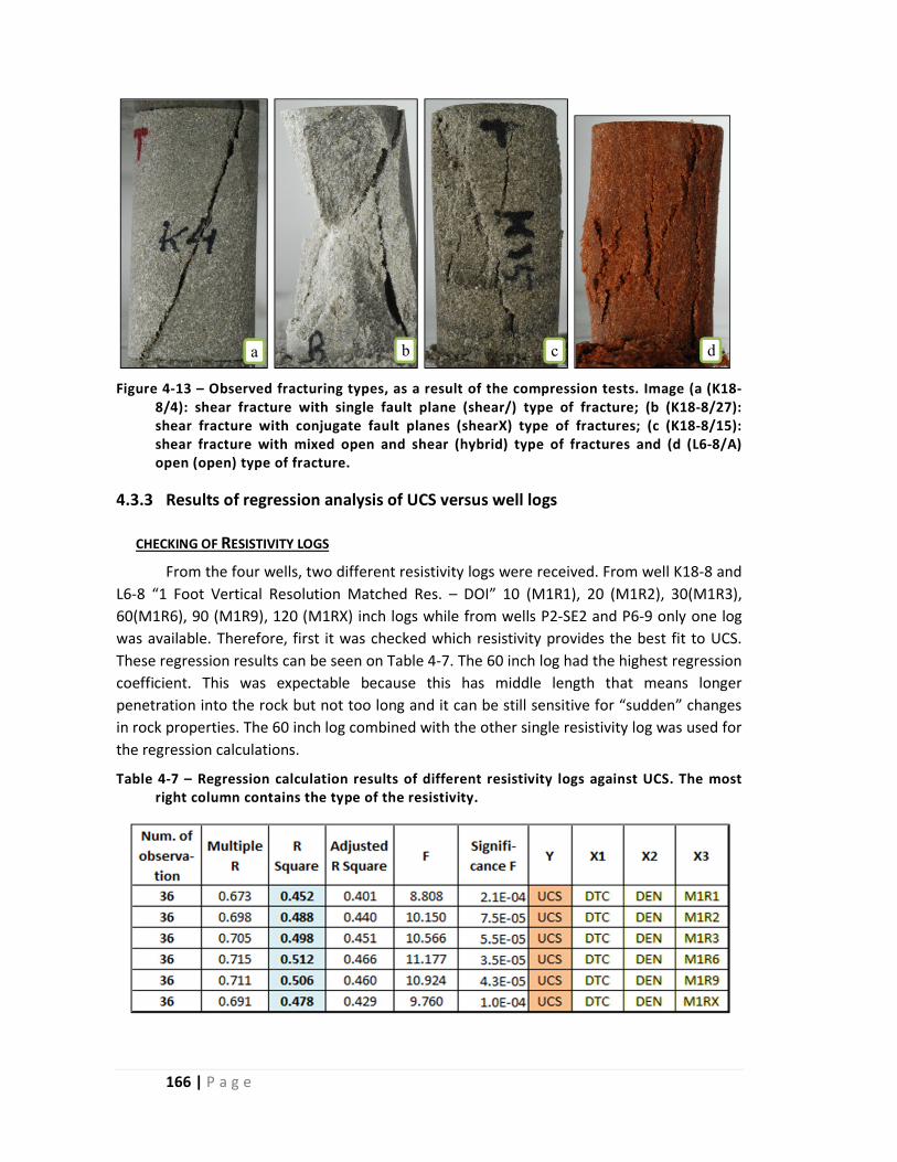
166 | P a g e   

Figure 4‐13 – Observed fracturing types, as a result of the compression tests. Image (a (K18‐8/4):  shear  fracture with  single  fault  plane  (shear/)  type  of  fracture;  (b  (K18‐8/27): shear  fracture with  conjugate  fault  planes  (shearX)  type  of  fractures;  (c  (K18‐8/15): shear  fracture with mixed  open  and  shear  (hybrid)  type  of  fractures  and  (d  (L6‐8/A) open (open) type of fracture. 

4.3.3 Results of regression analysis of UCS versus well logs  

CHECKING OF RESISTIVITY LOGS 

From the four wells, two different resistivity logs were received. From well K18‐8 and 

L6‐8  “1  Foot  Vertical  Resolution Matched  Res.  – DOI”  10  (M1R1),  20  (M1R2),  30(M1R3), 

60(M1R6), 90 (M1R9), 120 (M1RX)  inch  logs while from wells P2‐SE2 and P6‐9 only one  log 

was available. Therefore,  first  it was checked which resistivity provides the best  fit to UCS. 

These regression results can be seen on Table 4‐7. The 60 inch log had the highest regression 

coefficient.  This  was  expectable  because  this  has  middle  length  that  means  longer 

penetration into the rock but not too long and it can be still sensitive for “sudden” changes 

in rock properties. The 60 inch log combined with the other single resistivity log was used for 

the regression calculations. 

Table 4‐7 – Regression calculation results of different resistivity  logs against UCS. The most right column contains the type of the resistivity. 

a b c d

167 | P a g e   

OUTLIER CHECKING 

First,  the  outliers were  filtered.  Regression  of UCS was  calculated  against  P‐wave 

slowness  (DTC),  density  (DEN),  resistivity  (RES)  and  gamma  ray  (GR).  The  result  of  these 

regressions can be found in Table 4‐8. In the first column, the model identification numbers 

can  be  found.  The  second  column  contains  the  number  of  samples  involved  in  the 

calculations. The  following  six  columns contain  statistical parameter of  the  regression. On 

the right side of the table, the calculation’s variables and the involved logs are listed. Figure 

4‐14 shows, on  the  left,  the predicted  results against  the measured data where  the green 

dashed line is the theoretical, perfectly predicted case. On the right side of the Figure 4‐14, a 

histogram of residuals can be seen showing the standard normal distribution of the residuals 

which  is a requirement  for a valid model. Furthermore, the histogram shows that only  few 

samples have relatively high residuals. 

Table  4‐8  –  Result  of  the multivariate  regression  of  all  the  62  samples  can  be  seen  UCS against P‐wave interval travel time, density, resistivity and gamma ray values. 

Figure 4‐14 ‐ On the left, the cross‐plot shows the measured‐ against predicted UCS values of Model‐1. Green dashed  line shows the theoretical (predicted = measured)  line. On the right, residual histogram of Model‐1 can be seen. 

Predicted vs. measured UCS results Model Id‐1

168 | P a g e   

Figure  4‐15  shows  the  residuals  of  the  regression  of  all  the  measured  samples. 

Samples K18‐8/13; K18‐8/23; K18‐8/24; P2‐SE2/23; P6‐9/10; P6‐9/14; P6‐9/35 were found as 

potential outliers, because their residuals were high  (>35 MPa). Only sample K18‐8/13 and 

P2‐SE2/23 have  reasons  for excluding  from  the  study.   Sample K18‐8/13 had much  larger 

grains (>10 mm) than the maximum allowed size (2 mm); and consequently, its strength was 

higher than as it was expected. Sample P2‐SE2/23 had numerous grains which had around 2 

mm of diameter;  its structure was quite heterogeneous with embedded clay  fractions and 

the plug‐end quality was  lower  than  the average of  the plugs;  its strength was  lower  than 

the  expected.  In  addition,  sample  P2‐SE2/24  had  significantly  lower  UCS.  However,  its 

residual was relatively low so this was not excluded. In conclusion, only two samples, namely 

K18‐8/13, P2‐SE2/23, were excluded from the calculation. 

Figure  4‐15  –  Residuals  histograms  of  regression  of  all  the measured UCS  results  vs.  DTC, density and UCS against DTC, density, gamma ray, resistivity. 

Figure 4‐16 – On the  left, photo of sample K18‐8/13 can be seen. On the right, two photo of sample P2‐SE‐2/23 can be seen. These  two samples were skipped  from  the regression calculation because of their quality (grain size, inhomogeneity). 

 

 

169 | P a g e   

REGRESSION ANALYSIS RESULTS COMBINED ALL THE SAMPLES 

LINEAR REGRESSION OF ALL THE SAMPLES 

The  linear regression parameters of all the samples can be seen on Table 4‐9. Sonic 

transit time of P‐wave (DTC) showed the highest regression coefficient square (0.42) out of 

single  regression  calculations.  The Multivariate  regression  of  combined  all  the  four  logs, 

which were available from all the wells, gave regression coefficient square 0.48. On the  left 

of  Figure  4‐17  the prediction  results  against  the measured  data  are  shown.  Points  in  the 

cross‐plot show similar tendency to the green dashed line which is the theoretical, perfectly 

predicted case. However, relatively large uncertainty of the prediction also can be seen. The 

histogram  of  the  residuals  is  presented  on  the  right  of  Figure  4‐17.  On  this  histogram, 

residual distribution shows normal distribution which proves that the relation between the 

predicted data (UCS, Y) and predictors (log data as X1, X2...) and  it  is not  just as a result of 

accident.  

Besides DT, DEN, GR, RES logs further logs were available only from wells K18‐8 and 

L6‐8; such as, neutron porosity (CNC), spectral gamma ray: Potassium (K), Thorium (TH), and 

Uranium  (U).  This means  we  had  only  36  samples  instead  of  57  for  these  calculations. 

Therefore, the effect of the sample number (observations) on the regression coefficient was 

tested. The regression of UCS against DTC, DEN, RES, GR (Table 4‐9 Model‐14) was repeated 

but using only samples from wells K18‐8 and L6‐8. In the first row of (Model‐14a), the result 

of this calculation can be seen. The regression coefficient was only slightly higher (0.51). In 

conclusion, there is no significant effect of sample number on regression. Table 4‐10 shows 

the results of the linear multivariate regression with these logs. 

 

Table  4‐9  –  Results  of  regression  analysis  of  all  the  samples  (two  outliers  excluded). UCS against P‐wave transit time (DTC), density (DEN), resistivity (RES), gamma ray (GR). 

 

 

 

 

 

170 | P a g e   

 

Figure 4‐17 – On the  left,  the measured vs. predicted UCS values of Model‐14; on the right, residual histogram of Model‐14 can be seen. Variables listed on left graph. 

Adding  neutron  porosity  log  to  the Model‐17,  the  regression  coefficient  increased 

above 0.6 (Model‐18); however, here only two wells were involved in the regression. Using 

only one of the spectral of gamma ray, the regression coefficient did not change significantly 

(Model‐19, 20 and  ‐21). However, combined all of them, the regression coefficient  jumped 

significantly  above  0.7  (Model‐25).  Adding  neutron  porosity  log  to  this  variable  set,  the 

regression coefficient increased up to almost 0.75 (Model‐32). Further small increase can be 

seen by adding also convention gamma ray log (Model‐33); however, because this log does 

not add new information to the model, it was not used. 

Figure  4‐18  shows  the  predicted  UCS  vs. measured  UCS  check  cross‐plot  and  the 

residual  histogram.  The  cross‐plot  shows  less  scattering  and  the  histogram  is  normal 

distributed and the range of residuals narrowed from 80 MPa (‐30 to 50 MPa) to 50 MPa (‐20 

to 30 MPa). 

 

   

171 | P a g e   

Table 4‐10  ‐ Regression analysis  results of  all  the  samples:  Spectral  gamma  ray, Potassium (K), Uranium (U), Thorium (TH) and neutron porosity (CNC) logs are involved from wells K18‐8 and L6‐8. 

Figure 4‐18  ‐ On the  left,  the measured vs. predicted UCS values of Model‐32; on the right, residual  histogram  of  Model‐32  can  be  seen.  Regression  was  calculated  with  UCS against DTC, DEN, RES, K, U, TH, CNC data. 

   

172 | P a g e   

LINEAR REGRESSION OF THE ALL THE SAMPLES USING NON‐LINEAR FUNCTION OF THE LOGS 

First, only sonic slowness logs were converted to velocity (hyperbolic (1/x) non‐linear 

transformation).  Result  of  Vp  (P‐wave  velocity  in m/s)  and  V  (1/DT  in m/s) multivariate 

regression  can  be  seen on  Table 4‐11.  P‐wave  velocity  shows  always  stronger  correlation 

with UCS  than  1/DT;  and,  P‐wave  velocity  shows more  similar  correlation  to UCS  than  P‐

wave slowness. Multivariate regression was calculated in the same system as in the previous 

case replaced DTC with Vp. The regression coefficients of UCS against Vp, DTC, RES and GR 

was  a  little  higher  in  comparison  to  regression  coefficient  of  the  same  calculation  with 

slowness  calculations.  Figure  4‐19  shows  prediction  check  cross‐plot  and  the  residual 

histogram of calc. Id 39 which is the best fit model using only basic logs and all the samples. 

In the next phase, the non‐linear functions of the  logs were used for the regression 

analysis. The effect of the different functions on the goodness of the model was tested step 

by  step with  each  log  type.  The  result  of  this  can  be  seen  on  Table  4‐12.  In  the  table, 

variables that had the best fit are highlighted with green. Slight (0.01‐0.02)  increase can be 

seen  in  case  of  1/DEN,  1/RES,  1/CNC  and  K,  TH  and U  square.  Combined  these  best  fit 

transformations;  model  82  had  the  highest  coefficient  and  the  lowest  sum  of  absolute 

residuals  in  this  stage  of  the  analysis  where  all  samples  were  used.  Figure  4‐20  shows 

prediction’s cross‐plot of models 82 and the residual histogram. The scattering of the points 

is  in a narrower  range  around  the  theoretical  line  in  the  cross‐plot.  The histogram  is  still 

normally distributed. Sum of the absolute value of the residuals decreased while correlation 

coefficient increased to 0.79. Range of residuals did not show narrowing still about 50 MPa. 

Table 4‐11 ‐ Regression analysis results of all samples using Vp (Vp=1/DTC) – P‐wave velocity and V (V=1/DT) interval sonic velocity in m/s instead of slowness. 

   

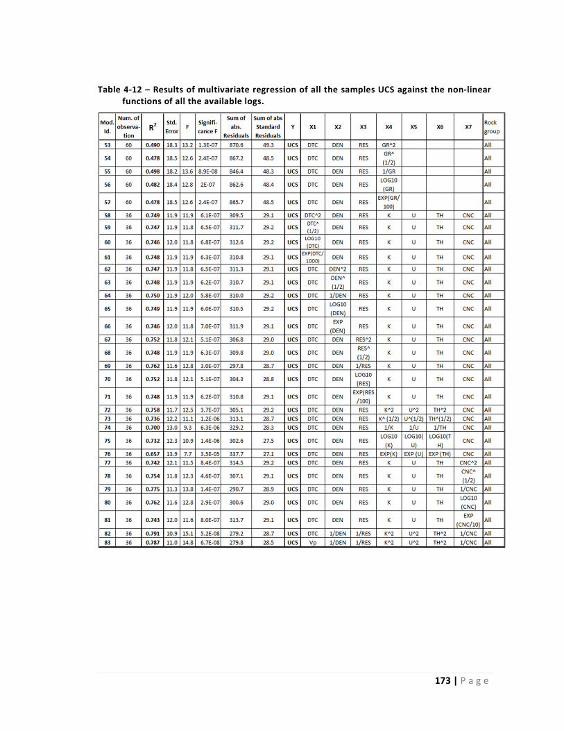
173 | P a g e   

 

Table 4‐12 – Results of multivariate regression of all the samples UCS against the non‐linear functions of all the available logs. 

174 | P a g e   

Figure 4‐19  ‐ On the  left,  the measured vs. predicted UCS values of Model‐39; on the  right, 

residual histogram of Model‐39. Used variables are listed in the graph. 

Figure 4‐20  ‐ On the  left,  the measured vs. predicted UCS values and; on  the right,  residual 

histogram of Model‐82. Used variables are listed in the graph. 

CORRELATION EQUATIONS AS A RESULT OF MULTIVARIATE REGRESSION OF ALL THE SAMPLES 

Equation 14: (UCS vs. DTC, DEN, RES, GR) 

2.175289 ∗ 87.855 ∗ 0.936849 ∗ 0.0628188 ∗18.638

Equation 32: (UCS vs. UCS vs. DTC, DEN, RES, K, U, TH and CNC) 

4.131961 ∗ 85.5265 ∗ 0.179683 ∗ 13.3598 ∗1.427968 ∗ 7.22465 ∗ 1.371356 ∗ 532.18

Equation 39: (UCS vs. Vp, DEN, RES, GR) 

0.0367799 ∗ 88.4717 ∗ 1.345097 ∗ 0.102739 ∗ 334.56 

Equation 82: (UCS vs. DTC, 1/DEN, LOG10(RES), K^2, U^2, TH^2 and 1/CNC) 

4.74094 ∗ DTC 985.77/DEN 18.520/RES 2.9206 ∗ K^2 1.9627 ∗ U^20.76793 ∗ TH^2 140.08/CNC 6.2667   

175 | P a g e   

REGRESSION ANALYSIS RESULTS OF THE LOWER GERMAN TRIASSIC SAMPLES 

Regression analyses were accomplished separately on both  rock groups  in order  to 

check the effect of rock type on the correlation. Linear multivariate regression results can be 

seen in Table 4‐13. In this case, similar tendency can be noticed that it can be seen in case of 

regression of all the samples. At single regression of UCS against density and sonic logs, the 

correlation coefficient is low; furthermore, at UCS against gamma ray and resistivity logs, the 

correlation is almost zero. Model‐92 had higher regression coefficient than the other models 

with less variables. Besides, F decreased and significance F increased. Thus, the probability of 

the hypothesis, reliability of the result decreased since the number of the samples relatively 

low.  The  regression  coefficient  did  not  increase  by  applying  non‐linear  functions  of  the 

parameters (Table 4‐14). Figure 4‐21 shows cross‐plot and the residual histogram of Model‐

92. The scattering of the point  is  in a relatively narrow range around the theoretical  line  in 

the cross‐plot. The residual histogram shows normal distribution. 

Table 4‐13  ‐ Result of multivariate  regression using  the non‐linear  functions of  the  logs of Lower German Triassic samples. 

 

Table 4‐14 – Result of multivariate regression of Lower German Triassic  samples using non‐linear functions of the parameters. 

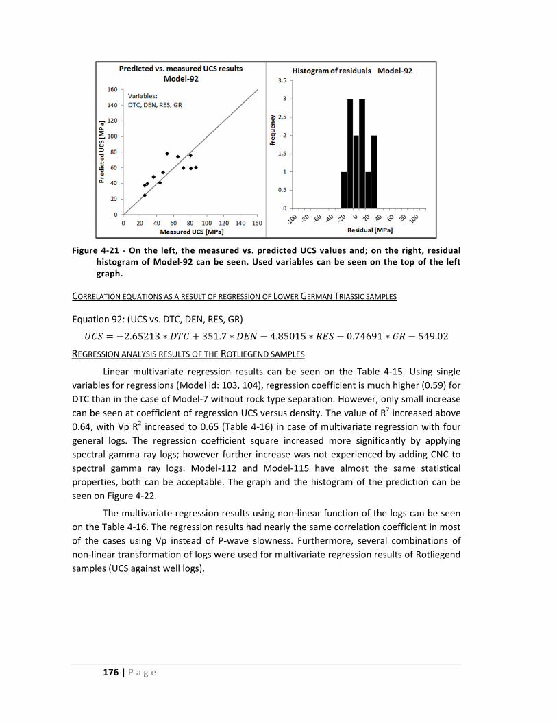
176 | P a g e   

Figure 4‐21  ‐ On the  left,  the measured vs. predicted UCS values and; on  the right,  residual histogram of Model‐92 can be seen. Used variables can be seen on the top of the  left graph. 

CORRELATION EQUATIONS AS A RESULT OF REGRESSION OF LOWER GERMAN TRIASSIC SAMPLES 

Equation 92: (UCS vs. DTC, DEN, RES, GR) 

2.65213 ∗ 351.7 ∗ 4.85015 ∗ 0.74691 ∗ 549.02 

REGRESSION ANALYSIS RESULTS OF THE ROTLIEGEND SAMPLES 

Linear multivariate  regression  results  can  be  seen  on  the  Table  4‐15. Using  single 

variables for regressions (Model id: 103, 104), regression coefficient is much higher (0.59) for 

DTC than in the case of Model‐7 without rock type separation. However, only small increase 

can be seen at coefficient of regression UCS versus density. The value of R2 increased above 

0.64, with Vp R2  increased to 0.65 (Table 4‐16)  in case of multivariate regression with  four 

general  logs.  The  regression  coefficient  square  increased  more  significantly  by  applying 

spectral gamma ray  logs; however  further  increase was not experienced by adding CNC  to 

spectral  gamma  ray  logs.  Model‐112  and  Model‐115  have  almost  the  same  statistical 

properties, both can be acceptable. The graph and  the histogram of  the prediction can be 

seen on Figure 4‐22. 

The multivariate regression results using non‐linear function of the  logs can be seen 

on the Table 4‐16. The regression results had nearly the same correlation coefficient in most 

of  the  cases  using Vp  instead  of  P‐wave  slowness.  Furthermore,  several  combinations  of 

non‐linear transformation of logs were used for multivariate regression results of Rotliegend 

samples (UCS against well logs). 

177 | P a g e   

Table 4‐15 –  Linear multivariate  regression  results of Rotliegend  samples  (UCS against well logs). 

Table 4‐16 – Multivariate  regression  results using  the  functions of  the  logs of of Rotliegend samples (UCS against well logs). 

178 | P a g e   

 

Figure 4‐22  ‐ On the  left,  the measured vs. predicted UCS values and; on  the right,  residual histogram of calc. of  Id 115 can be seen. Used variables can be seen on the top of the left graph. 

Figure 4‐23  ‐ On the  left,  the measured vs. predicted UCS values and; on  the right,  residual histogram of Mode‐121 can be seen. Used variables can be seen on the top of the  left graph. 

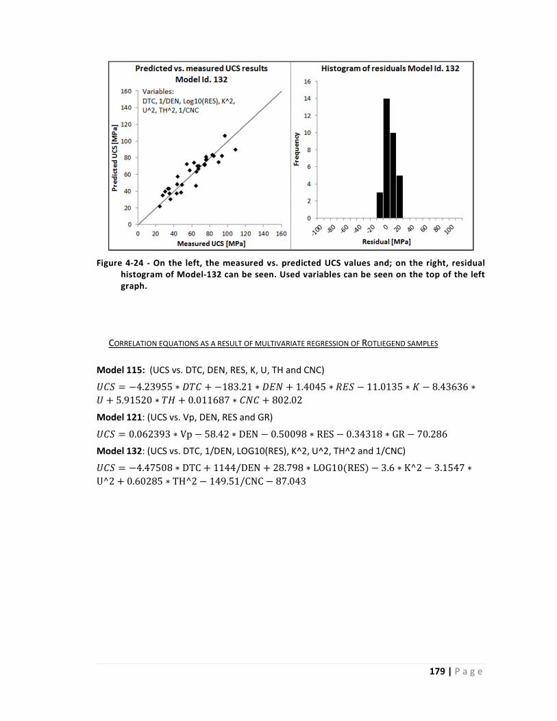
179 | P a g e   

Figure 4‐24  ‐ On the  left,  the measured vs. predicted UCS values and; on  the right,  residual histogram of Model‐132 can be seen. Used variables can be seen on the top of the  left graph. 

 

 

CORRELATION EQUATIONS AS A RESULT OF MULTIVARIATE REGRESSION OF ROTLIEGEND SAMPLES 

Model 115:  (UCS vs. DTC, DEN, RES, K, U, TH and CNC) 

  4.23955 ∗ 183.21 ∗ 1.4045 ∗ 11.0135 ∗ 8.43636 ∗5.91520 ∗ 0.011687 ∗ 802.02 

Model 121: (UCS vs. Vp, DEN, RES and GR) 

  0.062393 ∗ Vp 58.42 ∗ DEN 0.50098 ∗ RES 0.34318 ∗ GR 70.286 

Model 132: (UCS vs. DTC, 1/DEN, LOG10(RES), K^2, U^2, TH^2 and 1/CNC) 

  4.47508 ∗ DTC 1144/DEN 28.798 ∗ LOG10 RES 3.6 ∗ K^2 3.1547 ∗U^2 0.60285 ∗ TH^2 149.51/CNC 87.043 

 

 

 

 

 

 

 

 

180 | P a g e   

4.3.4 Results of regression analysis of elastic moduli versus well logs 

OUTLIER CHECKING 

First, regressions were calculated between Young’s moduli and log properties with all 

the  samples  in  order  to  check  outliers  (Model‐201).  Then,  the  potential  outliers  defined 

earlier  in  the  UCS  study  (K‐13,  P2‐23,  P2‐24,  P614,  P6‐35)  were  excluded  from  the 

calculations  (Model‐202  to  Model‐207,  Table  4‐17).  Figure  4‐25  and  Figure  4‐26  show 

statistical graphs of results of regression of Model‐201.  Residuals of this model did not show 

extreme values. Besides, no significant effect was seen on regression coefficients because of 

the  skipped  samples,  even  in  the  case when  all  the  five  potential  outlier  samples were 

excluded  (Model‐207).  Therefore,  no  sample  was  excluded  as  outlier  from  regression 

calculations between Young’s moduli and log properties. 

Table 4‐17  ‐ Table  shows  the  result of  regression outlier  tests  for elastic moduli  regression analysis. Results where, outlier(s) were skipped, was compared with result were all the samples were involved (Model‐201). 

Figure 4‐25 ‐ On the left, the measured elastic modulus against predicted elastic modulus (E) values of Model‐201; on the right, residual histogram of Model‐201 can be seen. Used variables can be seen on the top of the left graph. 

181 | P a g e   

Figure 4‐26  ‐ Residuals histograms of  regression of Model‐201 can be  seen.  In which all the measured  elastic moduli  (E)  results  was  used  against  DTC,  density  and  UCS  against compression wave velocity, density, gamma ray and resistivity properties. 

 

 

REGRESSION ANALYSES OF ELASTIC MODULI AGAINST LOG PROPERTIES OF ALL THE SAMPLES 

The regression analyses of the elastic moduli were performed in the same system as 

the UCS results. Young’s moduli and unload moduli, measured in the loading and unloading 

sections of  stress‐stain  curve, were  involved  in  the  analyses.  The  result of  the  regression 

analysis between elastic moduli and well logs can be seen in Table 4‐18 where the different 

rock types were not separated. In general, these results show similar main tendencies to the 

result of UCS‐log regressions. The regression coefficients were  low  in models where single 

variable was used (e.g. E vs. DTC or E vs. DEN). The regression of Potassium gamma  log (K)  

against  Young’s  modulus  resulted  in  the  highest  R2,  values  was  almost  0.5.  While, 

compression  wave  slowness  against  Young’s  modulus  had  0.36  of  R2  and  against 

compression wave  velocity  even  lower  (0.31).    The  regression  of  density  versus  Young’s 

modulus  had  only  0.16  of  R2  and  the  rest  of  the  log  properties  had  lower  R2  values. 

Combined the four basic logs (DTC or Vp, DEN, GR, RES), the squared regression coefficients 

increased to 0.41 (Model 216 and Model 242). Model 217 has the same parameter, but only 

samples from well K18‐8 and L6‐8 were involved in regression in order to check the effect of 

reduction of sample number. The squared regression coefficient of Model 217 (R2= 0.62)  is 

significantly higher than the coefficient of Model 216.  Involving neutron log (CNC) increased 

the value R2 of the regression to 0.7 (Model‐221). From spectral gamma logs, the potassium 

showed the larges effect on the regression, R2 increased to 0.72 (Model‐222); while, adding 

uranium  and  thorium  logs  to  the  model,  the  regression  coefficient  slightly  decreased 

(Model‐223 and Model‐224). Models in which all the available log properties were involved 

had  the  highest  regression  coefficients  R2=0.81.  These  models  were  Model‐235  which 

involved  compression  wave  slowness  and Model‐254  which  involved  compression  wave 

velocity.  The  difference  between  the  regression  coefficients  of  these  two  models  is 

182 | P a g e   

negligible.  Linear  regression  analysis  using  the  functions  of  the  logs,  resulted  in  higher 

regression coefficient with  the setting of Model‐286 where hyperbolic  (for DEN, RES, CNC) 

and parabolic (for K, U, TH) transformations were applied. Besides, the regression results of 

unload  moduli  showed  very  similar  correlation  coefficients  to  the  regression  results  of 

Young’s moduli. Figure 4‐27 and Figure 4‐28 show the measured vs. predicted plots and the 

residual histogram of Model‐242 (based on the four basic logs) and Model‐286 (based on all 

the available logs). Histograms show close normally distributed residuals. 

 

Table 4‐18 ‐ Figure shows result of regression analysis of Rotliegend samples, Young’s moduli (E)  unloading  modulus  (E‐UL)  against  well  logs:  compression  wave  slowness  (DTC), density  (DEN),  resistivity  (RES),  spectral  gamma  ray,  Potassium  (K),  Uranium  (U), Thorium (TH) and neutron porosity (CNC) logs are involved from wells K18‐8 and L6‐8. 

183 | P a g e   

Figure 4‐27 ‐ On the left, the measured against predicted elastic moduli (E) values of Model‐242; on the right, residual histogram of Model‐242 can be seen. 

 

Figure 4‐28 ‐ On the left, the measured against predicted elastic moduli (E) values of Model‐286; on the right, residual histogram of Model‐286 can be seen. 

 

 

 

 

 

 

184 | P a g e   

REGRESSION ANALYSES OF ELASTIC MODULI AGAINST LOG PROPERTIES OF TRIASSIC SAMPLES 

Table 4‐19 shows  the  result of  regression analysis between elastic moduli and well 

log where only Lower German Triassic samples were  involved and only  the  four basic  logs 

were available. The regression coefficients of single variable models were very low for all the 

four  five models. The correlation of  resistivity versus Young’s modulus had  the highest R2 

value.  In  the  case of  linear multivariate  regression of Model‐295 where  all  the  logs were 

included  R2 was  almost  0.6. Model‐299 with Vp  had  nearly  the  same  R2. Model‐304  had 

almost 0.7 of square correlation coefficient where square of gamma ray values were applied 

for  the calculation. The  relatively  low F values  indicate  that  the  reliability of  the  results  is 

low. Regressions with unload moduli had significantly higher R2 values above 0.8.  However, 

the standard error and also the sum of absolute value of Model‐ 299a and Model‐304a are 

higher  than  the  values  of  the  regression  of Model‐299  and Model‐304.  Therefore,  these 

results of unload moduli are less reliable than Young’s moduli models. 

Table  4‐19  ‐  Figure  shows  the  result  of  regression  analysis  of Rotliegend  samples,  Young’s moduli  (E)  unloading modulus  (E‐UL)  against  well  logs:  compression  wave  slowness (DTC),  compression  wave  velocity  (Vp),  sonic  velocity  (V),  density  (DEN),  resistivity (RES),  spectral  gamma  ray,  Potassium  (K),  Uranium  (U),  Thorium  (TH)  and  neutron porosity (CNC) logs are involved from wells K18‐8 and L6‐8. 

REGRESSION ANALYSES OF ELASTIC MODULI AGAINST LOG PROPERTIES OF ROTLIEGEND SAMPLES 

Table 4‐20 shows the results of regression analysis between elastic moduli and well 

log where only Rotliegend samples were  involved. And all type of  logs was available  for 33 

samples out of  50  samples.  There was  no outlier  skipped. When only  single  variable was 

used  (e.g. E  vs. DTC or E  vs. DEN),  square  regression coefficients were  low. Regression of 

potassium spectral gamma  log (K) and slowness (DTC) regressions against Young’s modulus  

resulted  the highest R2,  its value was almost 0.5. The regression of density versus Young’s 

modulus had only 0.2 of R2 and the rest of the log properties resulted in significantly lower 

R2  values.  Combined  the  four  basic  logs  (DTC  or  Vp,  DEN,  GR,  RES),  square  correlation 

coefficients  increased  to  above  0.7  (Model  315  and  Model  329).  Square  regression 

coefficient of Model 316  (R2= 0.7)  is significantly higher  than  the coefficient of Model 315. 

Related to Model‐317, R2 increased to about 0.8 adding neutron log to the regression. And, 

regression  coefficient  increased  further  to  about  0.9  extending  the model  with  spectral 

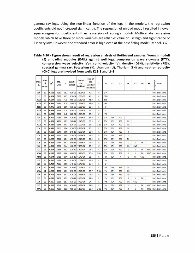
185 | P a g e   

gamma  ray  logs. Using  the  non‐linear  function  of  the  logs  in  the models,  the  regression 

coefficients did not increased significantly. The regression of unload moduli resulted in lower 

square  regression  coefficients  than  regression  of  Young’s moduli. Multivariate  regression 

models which have three or more variables are reliable: value of F is high and significance of 

F is very low. However, the standard error is high even at the best fitting model (Model‐337). 

 

Table 4‐20 ‐ Figure shows result of regression analysis of Rotliegend samples, Young’s moduli (E)  unloading  modulus  (E‐UL)  against  well  logs:  compression  wave  slowness  (DTC), compression  wave  velocity  (Vp),  sonic  velocity  (V),  density  (DEN),  resistivity  (RES), spectral  gamma  ray, Potassium  (K), Uranium  (U),  Thorium  (TH)  and neutron porosity (CNC) logs are involved from wells K18‐8 and L6‐8. 

 

 

 

 

 

 

186 | P a g e   

 

YOUNG’S MODULUS CORRELATION EQUATIONS AS A RESULT OF MULTIVARIATE REGRESSIONS 

Model 242:  (E vs. Vp, DEN, RES, GR)      

11.213 ∗ 16551 ∗ 665.86 ∗ 1.4628 ∗ 75960 

Model 242a:  (E‐unload vs. Vp, DEN, RES, GR) 

E unload 20.817 ∗ 17625.6 ∗ 641.11 ∗ 8.38138 ∗ 112014 

Model 286:  (E vs. Vp, 1/DEN, 1/RES, LOG10(K), LOG10(U), LOG10(TH), 1/CNC ) 

21.726 ∗ 366979/ 3276.4/ 15287 ∗ 10 1925.9∗ 10 7888.9 ∗ 10 45891/ 225470 

Model 286a:  (E‐unload vs. Vp, 1/DEN, 1/RES, LOG10(K), LOG10(U), LOG10(TH), 1/CNC) 

E unload 30.991 ∗ 219860 ∗ 1178.2 ∗ 19492.6 ∗ 103717 ∗ 10 15927.8 ∗ 10 80363.8/ 198469 

Model 299:  (E vs. Vp, DEN, RES, GR)  

304.55 ∗ 681.9 ∗ 85351 ∗ 3.5608 ∗ 157645 

Model 299a:  (E‐unload vs. Vp, DEN, RES, GR) 

E unload 28.512 ∗ 82768 ∗ 2021 ∗ 146.148 ∗ 282524 

Model 304:  (E vs. Vp, DEN, RES, GR) 

0.2085 ∗ 94753 ∗ 944.52 ∗ 1.9404 ∗ ^2 204966 

Model 304a:  (E‐unload vs. Vp, DEN, RES, GR)   

E unload 30.085 ∗ 87717.4 ∗ 2147.6 ∗ 0.941529 ∗ ^2306104 

Model 329:  (E vs. Vp, DEN, RES, GR)  

20.0046 ∗ 29519 ∗ 226.4 ∗ 175.53 ∗ 4263.2 

Model 329a:  (E‐unload vs. Vp, DEN, RES, GR)   

E unload 30.324 ∗ 23336.7 ∗ 865.03 ∗ 275.57 ∗ 42153 

Model 337:  (E vs. Vp, DEN, RES, K, U, TH, CNC) 

17.002 ∗ 62332 ∗ 390.8 ∗ 5206.3 ∗ 2555.4 ∗ 1133.6∗ 111.57 ∗ 101076 

Model 337a:  (E‐unload vs. Vp, DEN, RES, K, U, TH, CNC)   

E unload 28.8946 ∗ 43158 ∗ 291.5 ∗ 7752.4 ∗ 4010.6 ∗2031.8 ∗ 417.44 ∗ 9378.96 

 

 

 

 

187 | P a g e   

4.3.5 Analysis of the relation between the rock properties measured in laboratory 

The  last stage of the data analysis was to analyse relations between rock properties 

that were measured  in  laboratory; such as: unconfined compressive strength  (UCS), elastic 

modulus, both loading (E) and unloading (E‐unload), porosity (PHI), matrix density (DEN‐MX), 

bulk density (DEN). The result of the simple linear regression of UCS against the above listed 

rock properties and Young’s modulus against unloading modulus can be seen  in  the Table 

4‐21. Calculations were done on  the  total sample set and separately by  the different  rock 

types as well. 

No  correlation  was  found  between  UCS  and  matrix  density  (Model‐404)  which 

indicates that the studied samples consist of very similar density minerals. Low correlations 

(R2= 0.2 to 0.4) were found between UCS and porosity. And also similar low correlation was 

found  between  UCS  and  density.  Separating  the  rock  groups,  only  little  bit  higher 

correlations can be seen in Rotliegend sample set. And lower correlation can be seen in the 

Triassic sample set. Very strong correlation was  found between UCS and elastic moduli  for 

Rotliegend sample set, R2  is about 0.9  (Model‐412, Model‐413). Line  fit plot of Model‐412 

can be seen on Figure 4‐29. However, the correlation between UCS and elastic moduli was 

much  lower by Lower German Triassic samples. R2 was about 0.46 at Model‐216 and R2  is 

about 0.42 at Model‐417. The Triassic sample set was separated further by wells in order to 

check whether  the  low correlation  is related  to the  location of  the source. Model‐420 and 

Model‐421 were calculated based on samples of well P6‐9. These models had significantly 

higher correlations than the models where the two wells were combined. Two models were 

created based on samples of well L6‐8: Model‐421 and Model‐423. There was almost zero 

correlation  found  between  UCS  and  Young’s  modulus.  While  Model‐423  had  higher 

correlation (R2=0.64) between UCS and unload moduli. However, here the calculation based 

on only four samples therefore reliability of this result is low. Graphs of Model‐416, Model‐

420 and Model‐422 furthermore Model 417, Model‐421 and Model‐423 are plotted in Figure 

4‐30.  In  general,  correlation between UCS  and  unload  elastic modulus was  found  slightly 

lower than correlation between UCS and Young’s modulus. 

188 | P a g e   

Table  4‐21  –  Result  of  linear  multivariate  regression,  UCS  against  rock  physical  and mechanical  properties:  elastic modulus,  loading  (E)  and  unloading  (E‐loop),  porosity (PHI), matrix density (DEN‐MX), bulk density (DEN). 

Figure 4‐29 – Line fit plot and residual histogram of Model‐412. 

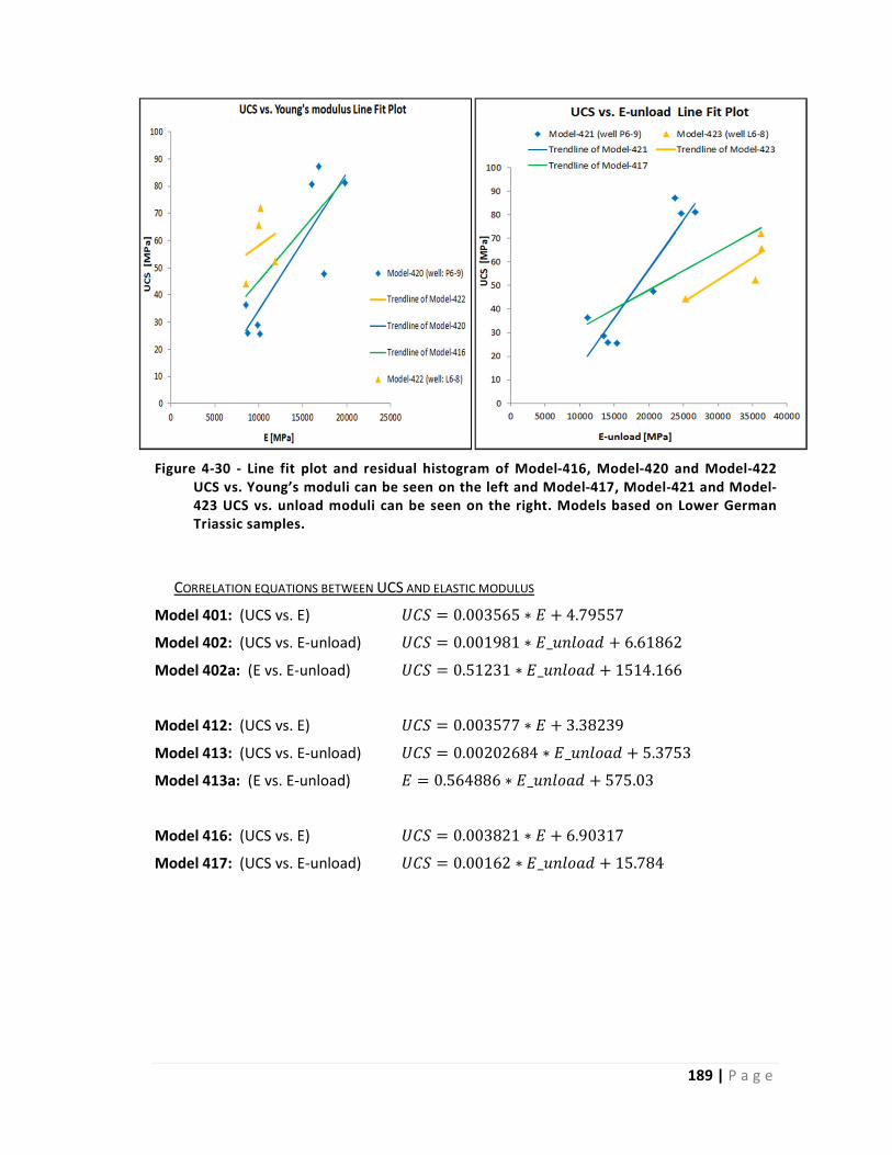
189 | P a g e   

Figure 4‐30  ‐  Line  fit plot and  residual histogram of Model‐416, Model‐420 and Model‐422 UCS vs. Young’s moduli can be seen on the left and Model‐417, Model‐421 and Model‐423 UCS vs. unload moduli can be seen on the right. Models based on Lower German Triassic samples. 

 

CORRELATION EQUATIONS BETWEEN UCS AND ELASTIC MODULUS 

Model 401:  (UCS vs. E)       0.003565 ∗ 4.79557 

Model 402:  (UCS vs. E‐unload)  0.001981 ∗ _ 6.61862 

Model 402a:  (E vs. E‐unload)   0.51231 ∗ _ 1514.166 

 

Model 412:  (UCS vs. E)    0.003577 ∗ 3.38239 

Model 413:  (UCS vs. E‐unload)  0.00202684 ∗ _ 5.3753 

Model 413a:  (E vs. E‐unload)   0.564886 ∗ _ 575.03 

 

Model 416:  (UCS vs. E)    0.003821 ∗ 6.90317 

Model 417:  (UCS vs. E‐unload)  0.00162 ∗ _ 15.784  

 

190 | P a g e   

4.4 Discussion

4.4.1 Mechanical  characterisation  of  Rotliegend  and  Lower  German  Triassic 

Sandstone Groups 

In this study, rock physical properties (porosity, matrix density and bulk density) and 

rock  mechanical  properties  (unconfined  compressive  strengths,  Young’s  modulus  and 

unloading  modulus)  of  two  sandstone  groups  of  the  North  Sea  were  measured:  Lower 

German Triassic Sandstone samples (from five members) originating from a depth of about 

2700  to 2800 m and about 4090 m TVDSS, and Rotliegend Sandstone  samples  (from  four 

members) originating from depth of 3800 m to 4900 m TVDSS.  

Based on  the  results,  the mechanical properties of  the  studied  sandstones  can be 

characterized. Table 4‐22 contains the basic statistics of the rock’s physical and mechanical 

results  for both sandstones separately. The average and  the median of all mechanical and 

physical properties of both the Rotliegend and Lower German Triassic sandstones are nearly 

the same. Combining the two groups of sandstones, average values are: porosity 9%; bulk density 2.44 g/cm3; UCS 52 MPa; Young’s modulus12.9 GPa; unloading modulus 23 GPa and ration of Young’s modulus and unloading modulus E/EUL= 0.54 (based on the averages). 

The effect of moisture content on the rock strength was considered and corrected when the 

present  results were  compared with others  test  results measured  in dry  samples.  Several 

studies have described the relationship between strength of dry and wet rocks (see chapter 

4.1.1). Hawkins and McConnell (1992) showed that the effect of the moisture content might 

generate  up  to  70%  loss  in  strength  for  British  sandstone.  The magnitude  of  this  effect 

depends on material properties of  the  rock material  and  the degree of  saturation.  In  the 

present work, the strength of wet samples was measured. These strength results were then 

corrected  to  take  into account  the effect of  the moisture content  so as  to compare  them 

with strength measured  in dry samples. The strength of the samples was reduced by 30%. 

Many researchers have investigated the relation between log data and rock strength and the 

elasticity  of  different  sandstones.  Chang  et  al.  (2006)  and  Zoback  (2007)  studied  the 

mechanical properties of sandstone which originated from different parts of the world based 

on 260 sandstone test results by six authors. The unconfined compressive strengths  in this 

database  range widely  from  5 MPa  to  about  360 MPa  for  dry  samples.  The  unconfined 

compressive strengths of the studied samples range between 8 and 138 MPa for Rotliegend 

sandstones  and  26  and  87 MPa  for  Lower German  Triassic  sandstone.  Young’s moduli  of 

sandstones range from 1 to 70 GPa  in Chang et al.’s (2006) and Zoback (2007) data and,  in 

this work,  from 1 GPa  to 30 GPa  for Rotliegend sandstones and  from 8 GPa  to 20 GPa  for 

Lower German Triassic sandstone.  

   

191 | P a g e   

Table  4‐22  –  Basic  statistics  of  rock  physical  and  mechanical  measurement  results  of   Rotliegend  Group  (50  samples)  and  Lower  German  Triassic  Group  (12  samples) samples. 

The values of all the measured properties of Rotliegend sandstone cover a relatively 

wider  range  than  that  of  the  Lower  German  Triassic  sandstones.  This  indicates  that  the 

properties of  the Rotliegend  sandstone  vary widely  in general. The  lower  variation of  the 

results of the Triassic sandstones may indicate that the properties of the Triassic sandstone 

change moderately in general. However, the reason also could also be that the relatively low 

number  of  samples  (12  pieces  of  sample)  does  not  cover  the  entire  range.  To  study  the 

properties of the subunits of the rock groups, statistical analysis was calculated. Table 4‐23 

shows  the basic statistics of  the  four members of  the Rotliegend Group separately, Upper 

and Lower Slochteren Members of the Rotliegend Group. Zone 3 and 4 are reservoir zones of 

Upper‐Slochteren Member in the area of well P2‐SE2 in block P2 of the North Sea. Based on 

the  average  of  the  four  members,  the  Upper  Slochteren  member  has  a  slightly  lower 

strength and elastic modulus than the average of the entire group. The average porosity and 

density of the Upper Slochteren Member  is similar to the average of the entire group. The 

Zone 3 of the Upper Slochteren Member  (the shallowest strata) has twice as high porosity 

(indicated in red in the table) as the average of the whole member; and has significant lower 

(lowest of all the members; 21 MPa) strength and elastic modulus than the average of the 

entire group. Furthermore, Zone 4 of Upper‐Slochteren shows slightly  lower porosity  than 

the average of the group. However, the average strength of this zone (36 MPa) is higher than 

that of Zone 3, but significantly lower than the average strength of the group, while values of 

elastic moduli  are  slightly  lower  than  the  overall  average.  In  contrast,  the  strength  and 

elastic moduli  of  the  Lower  Slochteren  Group  are much  higher  than  the  average  of  the 

group, while  its average porosity  is nearly the same as that of Slochteren Zone 4 (8%). The 

ratios of the elastic moduli of the four Rotliegend members are close to the average of the 

group. Only Zone 3 has higher E/ EUL value (0.64) than the average of the group, where the 

strength and  the elastic moduli were  the  lowest  in comparison with all  the members. The 

unconfined compressive strength of Slochteren Zone 3 and Zone 4 sandstones in well P2‐NE, 

measured by Collins  (2002),  is very similar to the UCS results  from well P2‐SE2  (this work). 

However, Young’s modulus in well P2‐SE2 is lower than in well P2‐NE (E8‐16 GPa). 

Table 4‐24 shows the basic statistics of the sandstones of the Lower German Triassic 

Group (Hardegsen Formation, Lower Detfurth Sandstone Member and Lower Volpriehausen 

Sandstone Member) separately. The porosity of all  three Triassic sandstones  is around  the 

same as the overall average. Only the Volpriehausen Sandstone, which is the deepest strata, 

192 | P a g e   

has a slightly lower porosity. The Lower Detfurth Sandstone showed lower strength (34 MPa) 

than  the  other  Triassic  sandstones  and  also  lower  than  the  average  of  all  the measured 

sandstone. However, the elastic modulus of this rock is average, while its E/EUL value (0.76) is 

the  highest  of  all  the  rock members.  Furthermore,  the  Lower  Volpriehausen  Sandstone 

Member has significantly higher strength and also unload‐modulus, but its Young’s modulus 

is  average,  and  it  has  significantly  lower  E/EUL  value  (0.39)  than  the  average  of  all  the 

samples.  

Table  4‐23  ‐  Basic  statistics  of  rock  physical  and mechanical measurement  results  of  rock members of Rotliegend Group samples. 

Table  4‐24  ‐  Basic  statistics  of  rock  physical  and mechanical measurement  results  of  rock members of Lower German Triassic Group samples. 

193 | P a g e   

4.4.2 Discussion of regression analysis of UCS data 

In  the  regression  analysis,  64  North  Sea  sandstone  samples  were  involved.  The 

correlation  between  log  data  and  both  UCS  and  elastic moduli  were  studied.  From  the 

statistical  point  of  view,  sample  number  is  an  important  factor.  The  number  of  Lower 

German Triassic sandstone samples is relatively low considering that they originate in three 

facies.  However,  as  the  standard  deviations  of  the  results  are  not  significantly  high  (in 

comparison with those of the Rotliegend results), the results of Triassic samples may provide 

a good  representation of  the  Lower German Triassic Sandstone members. The number of 

Rotliegend samples  is relatively high, even the number of those samples that have spectral 

gamma and neutron log data, which were available only from two wells. Two outlier samples 

were  excluded  from  the  regression  analysis  of UCS  versus  log.  Both  originated  from  the 

Rotliegend  Sandstone  Group.  The  sample  set  of  Rotliegend  sandstone  provides  a  more 

representative and more reliable result.  

The  results of  single  variation  regression  analysis of UCS  against well  logs  showed 

significant  differences  between  the  Rotliegend  and  the  Triassic  sandstone  groups.  The 

results of  the Rotliegend  sandstone are  in agreement with observation of  results  in other 

studies: strength shows  the highest correlation with sonic velocity  (Vp)  (R2= 0.6) and R2  is 

just  slightly  lower  between  UCS  and  compressive  wave  slowness  (DTC)  (R2=  0.58).  The 

correlation of the UCS and the bulk density (DEN) is slightly lower (R2= 0.34). In general, the 

correlation between the acoustic wave slowness (velocity) of the compressive wave and UCS 

is relatively high. The acoustic wave slowness is an often used parameter in UCS correlation 

equations.  In  contrast,  single  variation  regression  of  UCS  of  the  Lower  German  Triassic 

Sandstone Group showed a lower correlation between UCS and acoustic slowness (R2= 0.11). 

The single regression coefficient of Triassic samples was the highest between UCS and bulk 

density (R2= 0.28). This observation already indicates a certain degree of difference between 

the two studied rock groups. The linear regression results of UCS combined both rock groups 

and  resulted  in  lower  regression  coefficients. UCS against DTC had  the highest  regression 

coefficient  (R2= 0.42) combining  the  two  rock groups. The exponential  approach provided 

the highest R2 values using non‐linear function of logs for the regression. Figure 4‐31 shows 

the  line‐fit  plot  of  UCS  versus  DTC  data  combined  and  separated  by  rock  groups.  This 

tendency  is  in  accordance with  others’  observation,  as  can  be  seen  in  Table  4‐25 where 

many  correlation  equations  (UCS‐DT)  are  exponential.  The  regression  coefficients  of  the 

models  with  the  function  of  single  variables  are  low.  Figure  4‐32  shows  the  UCS‐sonic 

velocity cross plot by Chang et al. (2006), which contains the results of three previous works 

from different sandstones (Lama and Vutukuri 1978, Carmichael 1982, Jizba 1991). The cross 

plot  shows  a much  larger  scatter  in  the  data  and  large  deviation  from  the  fitted  curves. 

Therefore,  the  application  of  multiple  physical  rock  properties,  i.e.  more  variables,  is 

reasonable. 

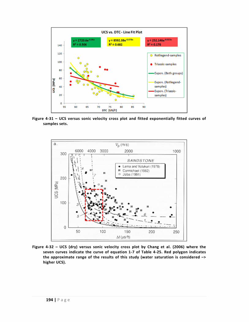
194 | P a g e   

Figure 4‐31 – UCS versus  sonic  velocity  cross plot  and  fitted  exponentially  fitted  curves of samples sets. 

 

Figure  4‐32  – UCS  (dry)  versus  sonic  velocity  cross  plot  by  Chang  et  al.  (2006) where  the seven  curves  indicate  the  curve of equation 1‐7 of Table 4‐25. Red polygon  indicates the approximate  range of  the  results of  this  study  (water  saturation  is  considered –> higher UCS). 

 

 

 

195 | P a g e   

The correlation between UCS and sonic velocity, together with bulk density, has been 

studied by several authors (e.g. Moos et al. 1999, Chang et al. 2006) (see equation 5, 6, and 7 

in Table 4‐25. In chapter 4.1.1, it was shown that many factors control the strength of a rock. 

The  regression  coefficient of  the Triassic Group  shows a  significant  increase with multiple 

variables  (UCS  vs. DTC, DEN  and GR)  in  comparison with  the  single  regression  results:  R2 

increased  from 0.28  (Model‐86 UCS vs. DEN)  to 0.55  (Model‐92). Model‐89, Model‐90 and 

Model‐91  show  that  each  log  property  played  a  role  in  the  increase  of  the  correlation 

coefficient. The  resistivity and  the natural gamma  ray  log data  increased  the R2  from 0.34 

(Model‐89 UCS vs. DTC, DEN) to 0.55 (Model‐92). The square of the regression coefficient of 

the Rotliegend Group  increased  slightly, 0.6  (Model‐117)  to 0.65  (Model‐121). This  shows 

that the strength of this rock group more depends on sonic velocity‐related factors. 

The effect of the mineral composition on rock’s mechanical properties was observed 

in previous studies (see chapter 4.1.1). However, only very few works have been published 

on  correlation  analysis between  rock’s mechanical properties  and multiple  log properties, 

apart  from  the  combination  of  sonic  velocity  and  density.  There  is  only  one  correlation 

equation in which clay content and Poisson’s ratio is also involved (Equation 4 in Table 4‐25). 

In addition, a few works applied resistivity, spectral gamma and/or neutron porosity logs for 

rock strength prediction (e.g. Hatherly, et al. 2001, Hatherly, et al. 2004, Zhou, et al. 2005).  

Zhou et  al.  (2005) used Prompt Gamma Neutron Activation Analysis  (Borsaru et  al. 2001) 

logs to gain mineral composition and also some other log properties which were also applied 

in this study. They used Radial Basis Function and Self‐Organizing Maps (Kohonen 2001) to 

predict the strength of sandstone and siltstone samples. The strength prediction of the Self‐

Organizing Maps had a correlation coefficient of 0.65 and  the Radial Basis Function had a 

correlation coefficient of 0.72. In addition, they reviewed the equation of McNally (Equation 

2 in Table 4‐25 UCS vs. DTC) with the same samples, which resulted in a squared regression 

coefficient of 0.62. The Radial Basis Function showed that additional logs, such as resistivity 

and  spectral  gamma  logs,  provide  further  information  for  strength  prediction,  which 

increased  the  correlation.  In  this  study,  each  component  of  the  spectral  gamma  log was 

tested  rather  than  the  general  gamma  ray  log with  the  Rotliegend  samples  (Model‐109, 

Model‐110 and Model‐111). Each of  these models has higher  regression  coefficients  than 

the Model‐108 with  the GR  log  only.  In  addition,  the model with  the  uranium  log  had  a 

slightly higher regression coefficient  (R2=0.69) than  the other two spectral gamma models. 

The combined application of all the three spectrums increased the correlation significantly in 

Model‐112,  where  R2  was  0.83.  Regression  results  of  all  the  samples  showed  similar 

tendencies with  spectral  gamma  ray  logs  (Model‐19, Model‐20, Model‐21  and Model‐25). 

However, here,  the model with  the  thorium  log had slightly higher correlation  than  these 

three models. The  results of  the  regressions, where  the  two  rock groups were  combined, 

gave  slightly  lower  correlation  coefficients  than  the  correlation  coefficients  for  the 

Rotliegend Group. 

Figure 4‐33 shows the predicted UCS logs by the five best correlation equations along 

a 200 m  long segment of Rotliegend strata of well K18‐8. Figure 4‐34 shows the predicted 

UCS log by the three best correlation equations along a 70 m long segment of Lower German 

Triassic  strata  of well  P2‐SE2.  The  predicted  UCS  logs  (Figure  4‐33  and  Figure  4‐34)  are 

196 | P a g e   

relatively hectic with very quick and large changes. The extreme values are not realistic. The 

predicted results are unrealistic at several points, such as zero, negative or very high values. 

Nevertheless,  the  main  characteristics  and  tendencies  of  the  UCS  log  fit  well  to  the 

measured points. The reasons for this kind of behaviour of the predicted  logs could be: on 

the one hand, the source data (the wireline logs) already have this kind of behaviour, and, on 

the other hand,  the multivariate  regression  itself may produce  some artificial waviness  to 

create  a  better  fit  out  of  the  variables.  Figure  4‐35  shows  the predicted UCS  logs of  the 

Rotliegend strata of all the four wells. In general, the measured UCS values fit the predicted 

logs well. However, some parts of the logs show very low values. For instance, in the top part 

of the log of well P6‐9, the predicted values are very close to zero in an approximately 50–60 

metres  long section. The reason for the unrealistic prediction could be either unreliable log 

data or significant different characteristics of the rock there. There is no sample taken from 

this part of the well, so the regression does not involve this section; therefore, the prediction 

might not provide  reliable  results.  This  section needs  to be  calibrated by using additional 

samples. 

 

 

4.4.3 DISCUSSION OF REGRESSION ANALYSIS OF ELASTIC MODULI DATA 

The  following  three  figures  show  the  logs of  the  same well and  the  rock  strata  for 

Young’s modulus. Figure 4‐36 shows the predicted Young’s modulus  logs of the Rotliegend 

layer  in  well  K18‐8,  Figure  4‐37  shows  the  Young’s modulus  logs  of  the  Lower  German 

Triassic sandstone and Figure 4‐38 shows the Young’s modulus logs of the Rotliegend layers 

in all  the  four wells. Since,  there  is strong correlation between UCS and Young’s modulus, 

the UCS logs and Young’s modulus logs show very similar characteristics.  

 

197 | P a g e   

Figure  4‐33  –  Predicted  UCS  logs  calculated  by  present  correlation  equations  in  the Rotliegend section of well K18‐8. The red dots indicate the measured UCS values. Boxes on the right show the basic data of the given model. 

Samples: Triassic

Variables:

DTC, DEN,

RES, GR

Samples: Rotliegend

Variables:

DTC, 1/DEN,

LOG10(RES),

K^2, U^2,

TH^2, 1/CNC

Samples: Rotliegend

Variables:

Vp, DEN,

RES, GR

Samples: All

Variables:

DTC, 1/DEN,

LOG10 (RES),

K^2, U^2,

TH^2, 1/CNC

Samples: All

Variables:

Vp, DEN,

RES, GR

198 | P a g e   

Figure  4‐34  ‐  Predicted UCS  logs  calculated  by  present  correlation  equations  in  the  Lower German Triassic strata of well P6‐9. Red dots indicate the measured UCS values. Boxes on the right show the basic data of the given model. 

Samples: Rotliegend

Variables:

Vp, DEN,

RES, GR

Samples: All

Variables:

Vp, DEN,

RES, GR

Samples: Triassic

Variables:

DTC, DEN,

RES, GR

199 | P a g e   

Figure  4‐35  ‐  Predicted  UCS  logs  calculated  by  present  correlation  equations  in  the Rotliegend strata of all the four wells. Logs were calculated by the best fitting models. Red dots  indicate the measured UCS values. Boxes on the right show the basic data of the given model. 

Samples: Rotliegend

Variables:

Vp, DEN,

RES, GR

Samples: Rotliegend

Variables:

Vp, DEN,

RES, GR

Samples: Rotliegend

Variables:

DTC, 1/DEN,

LOG10(RES),

K^2, U^2,

TH^2, 1/CNC

Samples: Rotliegend

Variables:

DTC, 1/DEN,

LOG10(RES),

K^2, U^2,

TH^2, 1/CNC

200 | P a g e   

Figure  4‐36  ‐  Predicted  Young’s  logs  calculated  by  present  correlation  equations  in  the Rotliegend section of well K18‐8. The red dots indicate the measured Young’s modulus values of the samples. Boxes on the right show the basic data of the given model. 

Samples: Triassic

Variables:

Vp, DEN,

RES, GR

Samples: Rotliegend

Variables:

Vp, DEN, RES, K, U, TH, CNC

Samples: Rotliegend

Variables:

Vp, DEN,

RES, GR

Samples: All

Variables:

DTC, DEN, RES,

K, U, TH, CNC

Samples: All

Variables:

Vp, DEN,

RES, GR

201 | P a g e   

Figure 4‐37 ‐ Predicted Young’s logs calculated by present correlation equations in the Lower German  Triassic  strata  of  well  P6‐9.  The  red  dots  indicate  the  measured  Young’s modulus  values of  the  samples. Boxes on  the  right  show  the basic data of  the  given model. 

Samples: All

Variables:

Vp, DEN,

RES, GR^2

Samples: Triassic

Variables:

Vp, DEN,

RES, GR

Samples: Triassic

Variables:

DT, DEN,

RES, GR

Samples: All

Variables:

Vp, DEN,

RES, GR

202 | P a g e   

Figure  4‐38  ‐  Predicted  Young’s  logs  calculated  by  present  correlation  equations  in  the Rotliegend strata of all the four wells. Red dots  indicate the measured Young’s moduli values. Boxes on the right show the basic data of the given model. 

 

Samples: Rotliegend

Variables:

Vp, DEN, RES, K, U, TH, CNC

Samples: Rotliegend

Variables:

Vp, DEN,

RES, GR

Samples: Rotliegend

Variables:

Vp, DEN,

RES, GR

Samples: Rotliegend

Variables:

Vp, DEN, RES, K, U, TH, CNC

203 | P a g e   

4.4.4 INTERPRETATION OF THE PREDICTED LOGS 

As can be seen in the UCS and Young’s moduli logs, there are very high and very low 

peaks in the logs. The UCS of rock cannot be negative; however, high values might be valid. 

Nevertheless, the reason for the peaks in predicted UCS logs is probably an artificial effect of 

the function or source log data. Therefore, a meaningful  interpretation of the predicted log 

is necessary to filter the unrealistic data. An interpretation of a 60 metre long section of well 

K18‐8 can be seen in Figure 4‐39. 

Figure 4‐39 – Graph shows only a 60 m  long section of the Rotliegend strata from well K‐18‐8; where the black dash dot  line  indicates an  interpretation of  the predicted UCS  log. Red dots indicate the measured UCS values. 

 

4.4.5 COMPARISON OF OUR RESULTS WITH OTHER CORRELATION MODELS 

Numerous empirical equations have been developed to estimate rock strength from 

wireline log data. In this study, eleven UCS‐log correlation equations for sandstones, listed in 

Table 4‐25, were applied using the data of the present work and compared with the present 

results.  Seven  out  of  the  eleven  equations  (Equation‐1  to  Equation‐7)  were  based  on 

measured  log properties  (Vp, DTC, DEN) and  the  rest were based on elastic modulus and 

porosity, which can be derived from log data or measured in a laboratory. The UCS logs were 

calculated by  these equations using  the  log data. Six equations were modified  in order  to 

gain  better  fit.  The  names  of  these  modified  equations  have  an  extension:  “v2”.  The 

measured versus predicted UCS graphs of the results can be seen in Figure 4‐40 and Figure 

4‐41. The basic statistics of  the  residuals of  these predictions are  listed  in Table 4‐25. The 

sum  of  the  absolute  differences  between  the  calculated  and  the  measured  values  are 

relatively large. Therefore, the equations were corrected with a constant shift. As a result of 

the correction, the sum of absolute difference decreased significantly. The Young’s modulus 

based on Equation 9 provided the best prediction. The graph of the UCS  log created by the 

best log property based on equations can be seen in Figure 4‐42. The plot shows that these 

equations provide relatively good prediction only in short sections of the log – each equation 

in a different part of the log. Only Equation 4, which involves multiple variables (DT, DEN and 

Vclay), provides a relatively good prediction in the long sections of the log. This supports that 

the more variables that are involved in the correlation equation, the better prediction can be 

achieved.  

204 | P a g e   

 

Table 4‐25 – List of the equations were used to predict UCS from well  log properties. On the right side of the table, the residual statistics are listed as a result of the equations with data  of  this  study.  (RHO=  density,  Vclay=volume  of  clay  from  gamma  ray  log, v=0.21=Poisson’s ratio, FI=porosity) 

   

205 | P a g e   

Figure 4‐40 – Measured versus predicted data cross plot of the UCS calculations by equations listed in Table 4‐25. 

 

 

 

 

 

 

 

UCS~Vp  UCS~Vp UCS~DTC

UCS~DTC  UCS~DTC

Equation 2 v2

UCS~DEN, Vp 

UCS~DEN,Vp

UCS~DEN,Vp,Vclay,v

UCS~DEN,Vp,Vclay,v

206 | P a g e   

 

 

Figure 4‐41 ‐ Measured versus predicted data cross plot of the UCS prediction calculations by equations listed in Table 4‐25. 

UCS~DTC UCS~DTC UCS~DTC

UCS~DTC UCS~DTC

UCS~DTC

UCS~DTC

207 | P a g e   

Figure  4‐42  –  Graphs  show  predicted  UCS  logs  by  equations  1‐5  (Table  4‐25)  where  “v2” indicates  that  the  equation was modified.  The  red  dots  indicate  the measured  UCS values. 

 

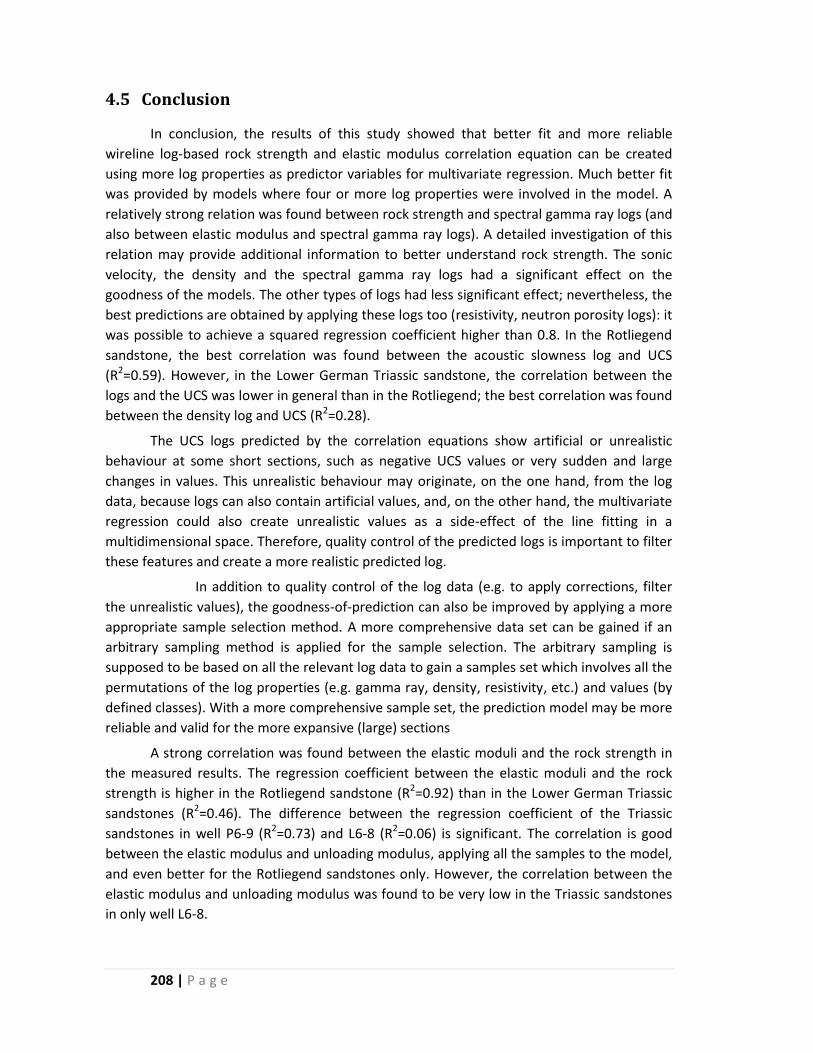
208 | P a g e   

4.5 Conclusion

In  conclusion,  the  results  of  this  study  showed  that  better  fit  and more  reliable 

wireline  log‐based  rock  strength and elastic modulus  correlation equation  can be  created 

using more log properties as predictor variables for multivariate regression. Much better fit 

was provided by models where  four or more  log properties were  involved  in  the model. A 

relatively strong relation was found between rock strength and spectral gamma ray logs (and 

also between elastic modulus and spectral gamma ray logs). A detailed  investigation of this 

relation may provide additional  information  to better understand  rock strength. The sonic 

velocity,  the  density  and  the  spectral  gamma  ray  logs  had  a  significant  effect  on  the 

goodness of the models. The other types of logs had less significant effect; nevertheless, the 

best predictions are obtained by applying these logs too (resistivity, neutron porosity logs): it 

was possible  to achieve a squared regression coefficient higher than 0.8.  In the Rotliegend 

sandstone,  the  best  correlation  was  found  between  the  acoustic  slowness  log  and  UCS 

(R2=0.59). However,  in  the Lower German Triassic sandstone,  the correlation between  the 

logs and the UCS was lower in general than in the Rotliegend; the best correlation was found 

between the density log and UCS (R2=0.28). 

The  UCS  logs  predicted  by  the  correlation  equations  show  artificial  or  unrealistic 

behaviour  at  some  short  sections,  such  as negative UCS  values or  very  sudden  and  large 

changes  in values. This unrealistic behaviour may originate, on the one hand,  from the  log 

data, because logs can also contain artificial values, and, on the other hand, the multivariate 

regression  could  also  create  unrealistic  values  as  a  side‐effect  of  the  line  fitting  in  a 

multidimensional space. Therefore, quality control of the predicted logs is important to filter 

these features and create a more realistic predicted log. 

  In addition  to quality control of  the  log data  (e.g.  to apply corrections,  filter 

the unrealistic values), the goodness‐of‐prediction can also be improved by applying a more 

appropriate sample selection method. A more comprehensive data set can be gained  if an 

arbitrary  sampling method  is  applied  for  the  sample  selection.  The  arbitrary  sampling  is 

supposed to be based on all the relevant log data to gain a samples set which involves all the 

permutations of the log properties (e.g. gamma ray, density, resistivity, etc.) and values (by 

defined classes). With a more comprehensive sample set, the prediction model may be more 

reliable and valid for the more expansive (large) sections 

A strong correlation was found between the elastic moduli and the rock strength  in 

the measured  results. The  regression  coefficient between  the elastic moduli and  the  rock 

strength  is higher  in the Rotliegend sandstone (R2=0.92) than  in the Lower German Triassic 

sandstones  (R2=0.46).  The  difference  between  the  regression  coefficient  of  the  Triassic 

sandstones  in well P6‐9  (R2=0.73) and L6‐8  (R2=0.06)  is significant. The correlation  is good 

between the elastic modulus and unloading modulus, applying all the samples to the model, 

and even better for the Rotliegend sandstones only. However, the correlation between the 

elastic modulus and unloading modulus was found to be very low in the Triassic sandstones 

in only well L6‐8. 

209 | P a g e   

A comprehensive study on the relation between log properties and rock mechanical 

properties, which  includes,  for example triaxial rock mechanical  tests, mineral composition 

analysis  and  microstructure  analysis,  can  produce  more  general  equations.  The  better 

understanding of  the  factors which  influence  rock mechanical properties  can  improve  the 

log‐based rock mechanical property prediction models. 

 

210 | P a g e   

 

211 | P a g e   

5 BrittlenessIndexforNorthSeasandstones

5.1 Introductionandbackground

Brittleness is an important property of a reservoir rock, especially for tight reservoirs, 

where  open  fractures  contribute  considerably  to  the  hydrocarbon  production.  The 

brittleness  of  the  rock  is  related  to  the  fracture  behaviour  and  sand  production  of  a 

reservoir. In a more brittle rock, considerably more open fractures can develop; moreover, in 

less brittle sandstones the sand production can increase significantly. 

Although  brittleness  is  an  important  and  widely  used  parameter,  there  is  no 

conventional  definition  of  it.  The  brittleness  of  a  rock  has  been  defined  in many ways. 

Morley (1944) and Hetenyi (1950) described the brittleness as the lack of ductility. According 

to Ramsay  (1967), a rock  is brittle when the  internal cohesion of  the rock  is broken. Obert 

and Duvall (1967) and Fossen (2010) defined the brittle material as the one which deforms 

by fractures at or only slightly beyond the yield stress. A rock is brittle if its strength becomes 

zero or nearly zero after the failure and there  is no significant elastic, defined Jaeger, et al. 

(2009). According to Yagiz and Gokceoglu (2010), a rock is brittle when it breaks at very little 

deformation. 

Some studies, such as Paterson and Wong (2005) and Heard (1960) elaborated on the 

brittle‐ductile characteristics of rocks  (listed  in Table 5‐1). They analysed different types of 

rocks  under  different  conditions;  nevertheless,  some  of  their  observations  are  similar. 

Paterson (1978) studied the Wombeyan Marble under compression with changing confining 

pressure. Heard (1960) analysed Solnhofen Limestone samples which were deformed under 

compression or extension with changing confining pressures and temperatures. According to 

the  results  of  Paterson  and Wong  (2005)  and  Heard  (1960),  in  case  of  brittle  rocks,  the 

permanent strain before failure is less than 3%, and between 3‐5% rocks are semi‐brittle. In 

case of ductile rock, they all measured more than 5% permanent strain before failure. Also, 

all of these studies showed, that; on the one hand, in brittle rocks, there  is loss of cohesion 

and  strong dilatancy,  the  strain  is  localized, one of  the major deformation mechanisms  is 

microcracking, stress drop related to failure; and on the other hand, in ductile rocks, there is 

no loss of cohesion, and the strain and the distribution of macroscopic deformation features 

are homogenous and there is no stress drop at failure. However; there are also differences in 

the results due to the different rock types and different conditions. For example, in the cases 

of marble and limestone, axial splitting was observed in the brittle samples, conjugate shear 

fractures  were  described  in  the  semi‐brittle  samples;  whereas,  in  the  case  of  brittle 

sandstone, single shear  fractures were reported. Further differences are  that  in  the brittle 

marble and the brittle limestone besides microcracking there was also minor twinning; while 

in ductile marble, crystal plasticity, twinning and microcracking were observed; however, in 

ductile limestone (at 700 °C and 700 MPa) there was no microcracking, but crystal plasticity 

and grain boundary  sliding.  In  contrast,  in both brittle and ductile  sandstones, particulate 

sliding  and  grain  size  reduction  were  observed  in  addition  to  microcracking.  Pressure 

dependence of strength was also analysed in the studies above. Patterson (1978) found that 

212 | P a g e   

the strength of brittle marble is strongly affected by the pressure, the strength of the semi‐

brittle marble decreases with increasing pressure; and, also in ductile marble, the strength is 

influenced by the confining pressure. Furthermore, Heard (1960) found that the strength of 

ductile  limestone  is strongly affected by both the temperature and  the confining pressure, 

whereas  in brittle  limestone the effect of temperature on strength is  low. Holt et al. (2015) 

described  the  importance  of  the  effect  of  the  stress  condition,  the  pore  pressure,  the 

temperature and also the bedding plane on the brittleness. 

 

Table  5‐1  –  Definitions  of  brittle  –  ductile  characteristics  of  rocks  by  Paterson  and Wong (2005) and Heard (1960). 

   

213 | P a g e   

In  the  literature,  several  empirical  equations  are  available  which  estimate  the 

brittleness  of  the  rock  with  different  approaches.  The  brittleness  indices  and  equations 

referenced in this thesis are listed in. Protodyakonov (1962) calculated the brittleness as the 

product of  the UCS and percentage of  fines  formed  in Protodyakonov  impact  test. Coates 

and Parsons (1966) defined the brittleness as the ratio of reversible strain and total strain. 

The same concept was used by Baron et al. (1962) and reviewed by Hucka and Das (1974), as 

the brittleness is the ratio of the reversible energy and the total energy. Furthermore, they 

also  suggested more  equation  to  calculate  the  brittleness.  Firstly,  the  brittleness  can  be 

expressed as the ratio of the difference of the UCS and tensile strength and the sum of the 

UCS and tensile strength. Secondly, brittleness can be calculated using the Mohr’s envelope 

as the sinus of the angle of the internal friction. Thirdly, the brittleness can be estimated as 

the  difference  of macro  and micro  indentation  hardness.  An  absolute  index was  created 

based  on  the  absolute  irreversible  longitudinal  strain  at  failure  (George  1995,  Yagiz  and 

Gokceoglu 2010).  If the strain was  lower than 3%, the rock was said to be brittle, between 

3% and 5% strain, the rock was brittle‐ductile and if the strain of the rock at failure is higher 

than 5%,  then  the  rock  is said  to be ductile. Holt et al.  (2015) analysed several brittleness 

indices  by  laboratory  experiences  in  shales  and  found  that  the  quantification  of  the 

brittleness  is challenging even  for well‐defined approaches  like B2 and B3. They also  found 

that  the  B2  index  strongly  depends  on  the  applied  method  to  estimate  it  (stress‐strain 

curves, unload–reload cycles or elastic moduli from ultrasonic velocity measurements) (Holt 

et al. 2015). Altindag (2002) estimated the brittleness as the arithmetic mean of the UCS and 

Brazilian tensile strength. Heidari et al. (2013) calculated the brittleness index as the ratio of 

the UCS and the Brazilian tensile strength and also as the half of the product of the UCS and 

the Brazilian tensile strength. In addition, Rickman et al. (2008) suggested a brittleness index 

based  on  the  Young’s modulus  and  Poisson’s  ratio  (B8) which  can be  gain  by mechanical 

laboratory tests or  log based empirical equations. Brittleness  index B8 considering effect of 

the stress of the compression wave velocity (i.e. compression wave velocity  increases with 

increasing stress and thus depth) has an  inverse relation with the magnitude of brittleness 

index B8  (Holt et al. 2015). Some  researches  (e.g. Varga 2012 and Gray 2012) applied  this 

approached to find brittle sections (sweet spots) in shale reservoirs. Sahloo (2013) proposed 

an  integrated mineralogy based method  to classify  lithofacies  to  find sweet spots  in Eagle 

Ford  shale. Later,  Lie and Sun  (2015)  (B9) proposed a brittleness  index as  the  ratio of  the 

Young’s  modulus  and  the  Poisson’s  ratio  and  proposed  to  take  into  consideration  the 

mineral composition of the rock by the volume fraction of the brittle and plastics minerals. 

Others have used punch penetration or  impact  tests  to measure  the brittleness of 

the rock (Protodyakonov 1962, Blindheim and Bruland 1998, Copur, et al. 2003, Yagiz 2009, 

Yagiz and Gokceoglu 2010). Blindheim and Bruland  (1998) measured  the brittleness as  the 

percentage of fines formed in an impact test for NTNU model (Blindheim and Bruland 1998, 

Yagiz and Gokceoglu 2010). According to Yagiz, the brittleness can be expressed as the ratio 

of maximum  force  applied  on  the  rock  and  the  corresponding  penetration  during  punch 

penetration tests  (Yagiz 2009). Copur et al. (2003) estimated the brittleness as the ratio of 

force decrement and force increment in punch penetration tests. 

214 | P a g e   

 Several studies have focused on the parameters that influence the brittleness of the 

rock  (Göktan  1991,  Copur  et  al.  2003,  Yagiz  2009,  Yagiz  and Gokceoglu  2010).  Yagiz  and 

Gokceoglu (2010) developed two models to estimate the brittleness of rock by constructing 

fuzzy  inference  system  and  nonlinear  regression  analysis.  They  measured  several  rock 

properties,  such  as  punch  penetration,  uniaxial  compressive  strength,  Brazilian  tensile 

strength and unit weight of  rock on different  types of  rock samples  retrieved  from  tunnel 

cases, and predicted the brittleness of these rocks by these parameters. Heidari, et al. (2013) 

investigated 8 different types of rocks and they found no relationship between the porosity 

and  the brittleness of  the  rock. However,  they noted  that  the brittleness of  the  rock was 

reduced due to saturation. They also predicted the brittleness using point load tests results, 

and calculated brittleness  indices  (B4, B5, B6) using three different combinations of the UCS 

and  the  Brazilian  tensile  strength,  and  they  found  good  correlation  between  these 

brittleness indices and the point load index (Is50). 

Fracture  toughness  is  an often used  rock mechanical property  in  civil engineering, 

mining  or  tunnel  boring.  Fracture  toughness measures  the  required  stress  or  energy  for 

fracturing and propagation of pre‐existing fractures. A special laboratory test was developed 

to  obtain  fracture  toughness  of  materials  (Srawley  and  Brown  Jr  1965).  Kahraman  and 

Altindag  (2004) studied  the  relationship between  fracture  toughness and brittleness. They 

studied two brittleness indices: B5 Hucka and Das (1974) and B6 Altindag (2002), more details 

Table  52.  A  strong  relation  was  found  between  the  brittleness  index  B5  and  fracture toughness;  however,  there  was  no  correlation  found  between  brittleness  index  B6  and 

fracture toughness. 

The majority of  the above‐mentioned definitions of  the brittleness  indices consider 

only  the  rock  mechanical  properties,  such  as  strength,  internal  friction  angle,  elastic 

properties that are constant for a material. These are independent of stress condition (more 

details in chapter 1.2 and chapter 4.1) which has a significant effect on the in situ brittleness 

(e.g.  Jaeger  et  al.  2007).  Others  defined  the  brittle‐ductile  behaviour  of  rock  materials 

considering  many  properties,  for  example  stress  drop,  strain  distribution,  measure  of 

permanent  strain,  deformation  mechanism  or  microcracking.  The  qualitative  brittleness 

definition of Heard (1960) considers several significant factors, such as temperature or stress 

condition.  Qualitative  definitions  can  provide  valuable  information  on  the  phenomena; 

however, it is difficult to apply them in practice without a quantitative approach. 

Urai and Wong  (1994) and Urai  (1995) defined  the brittle mudrock as  the one  that 

dilates during deformation and allows fracture permeability to develop. According to Ingram 

and Urai (1999), as the strain starts to localize at peak differential stress, the shear fracture 

starts to undulate. And due to the curvature of the fracture, the permeability of the fracture 

can increase or decrease depending on whether the confining pressure is low or high (Figure 

5‐1). Using  this  brittleness  concept,  Ingram  and Urai  (1999)  quantified  the  brittleness  of 

mudrocks as the ratio of the UCS of the given rock and the UCS of a normally consolidated 

rock in non‐overpressured domains (UCSNC) (BRI1 in). They found that if this brittleness index 

is  higher  than  two,  the  risk  of  embrittlement  and  the  risk  of  developing  open  fractures 

increases as the brittleness index increases. They proposed to apply this brittleness index to 

215 | P a g e   

predict  the  leakage of mudrock  top‐seals on a  regional  scale by constructing a brittleness 

index map of a  formation using  the UCS values estimated  from sonic velocity  logs  (Ingram 

and Urai 1999). This approach was used by  Ishii et al.  (2011)  to analyse  the  relationships 

between brittleness and transport properties in mudstones. They measured triaxial tests to 

gain rock mechanical data of the mudstone including the brittle‐ductile transition. Ishii et al. 

(2011) found that if the brittleness index is lower than two, the mudstone failed in a ductile 

way, in agreement with statement of Ingram and Urai (1999). Furthermore, they found that 

the mudstone fails in a semi‐brittle way if the index is between two and eight, and it will fail 

in ductile way if the index is larger than eight. 

These above‐mentioned indices are not able to express the brittle behaviour of rock 

strata  located  in  the  deeper  region  of  the  brittle  Earth  crust;  for  instance,  hydrocarbon 

reservoirs  or  related  seal  layers  that  are  usually  in  thousands  of  meters  of  depth. 

Hoogerduijn‐Strating and Urai  (2003) presented a brittleness  index  that considers  ‐ beside 

rock  properties  such  as  unconfined  compressive  strength  ‐  the  stress  conditions  as well. 

Their  proposed  index  (BRI2)  can  be  found  in  Table  52.  This  index  was  developed  for prediction  of  brittleness  of  shale  top  seals  in  order  to  predict  the  sealing  capability  and 

chance of the leakage of reservoir top seals. The index was developed for Pierre shale (about 

Pierre shale e.g. in Olgaard et al. (1997)). For calculation of brittleness index, they apply the 

earlier developed  correlation equation  for Pierre  shale  to predict UCS  from  sonic well  log 

(Urai  1995,  Ingram  and  Urai  1999)  and  the  internal  friction  angle  was  predicted  based 

surface area. Hoogerduijn‐Strating and Urai (2003) studied the brittle behaviour of Paleozoic 

and Mesozoic mudrock  top  seals  in North Oman.  They were  able  to  distinguish  different 

characteristic top seals from excellent to poor based on their brittleness index. 

   

216 | P a g e   

Table 5‐2 ‐ List of the empirical brittleness indices.  

   

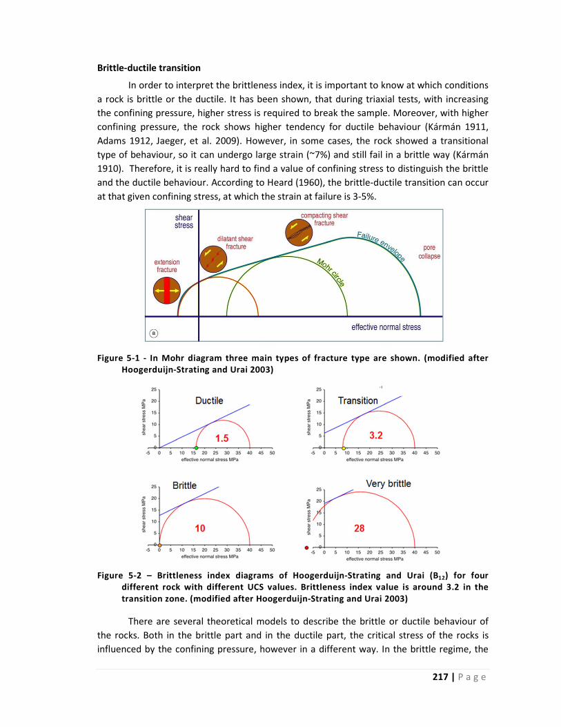
217 | P a g e   

Brittle‐ductile transition 

In order to interpret the brittleness index, it is important to know at which conditions 

a rock  is brittle or the ductile.  It has been shown,  that during triaxial tests, with  increasing 

the confining pressure, higher stress is required to break the sample. Moreover, with higher 

confining  pressure,  the  rock  shows  higher  tendency  for  ductile  behaviour  (Kármán  1911, 

Adams 1912,  Jaeger, et al. 2009). However,  in some cases,  the  rock showed a  transitional 

type of behaviour, so it can undergo large strain (~7%) and still fail in a brittle way (Kármán 

1910).  Therefore, it is really hard to find a value of confining stress to distinguish the brittle 

and the ductile behaviour. According to Heard (1960), the brittle‐ductile transition can occur 

at that given confining stress, at which the strain at failure is 3‐5%. 

Figure 5‐1  ‐  In Mohr diagram  three main  types of  fracture  type are  shown.  (modified after Hoogerduijn‐Strating and Urai 2003) 

Figure  5‐2  –  Brittleness  index  diagrams  of  Hoogerduijn‐Strating  and  Urai  (B12)  for  four different  rock with different UCS  values. Brittleness  index  value  is  around  3.2  in  the transition zone. (modified after Hoogerduijn‐Strating and Urai 2003) 

There are several  theoretical models  to describe  the brittle or ductile behaviour of 

the  rocks. Both  in  the brittle part and  in  the ductile part,  the critical stress of  the  rocks  is 

influenced by the confining pressure, however  in a different way. In the brittle regime, the 

218 | P a g e   

peak differential stress is linearly proportional to the effective mean stress according to the 

Mohr‐Coulomb theory. Contrarily, in the ductile regime, the relationship between the critical 

differential stress and the effective mean stress can be estimated by an elliptical model, such 

as  the Cam clay model  (Wood 1990), Carroll’s critical state model  (1991) or the DiMaggio‐

Sandler model (1970) cap model (Wong and Baud 2012). These models are affected by the 

porosity and the grain size of the rock, and also the strain rate of the deformation. According 

to Wong  and Baud  (2012), we  can  identify  the  stress  state of a given  rock  at  the brittle‐

ductile  transition with  the  intersection of  the Mohr  failure envelop and  the elliptical yield 

cap. 

In this work, the aims of the study of brittleness are; on the one hand, to develop an 

improved brittleness  index equation which quantifies the brittleness of rocks under a given 

stress similarly to the brittleness index of Hoogerduijn‐Strating and Urai (B12). However, this 

work aims to find a single equation  instead of combination of two equations. On the other 

hand, to calculate a brittleness  index  log for the studied sandstone reservoir strata  in order 

to characterise the brittle behaviour of these rocks and predict the type of possibly occurring 

fractures. 

5.2 Proposednewbrittlenessindexequation(BRI3):

In the development of new brittleness index (BRI) equation, the following objectives 

were considered: 

The brittleness  index  is supposed to quantify a property of rock materials related to the tendency of the type of fractures at failure. The condition of rock failure can be approached by Mohr‐Coulomb equation, where the relevant rock properties are the internal friction angle, the cohesion or the UCS. 

Different types of fractures can be formed  in the same type of rock under different stress  conditions  (in  chapter‐1  Figure  1‐3).  Therefore,  it  is  necessary  to  consider stress  condition  at  failure  at  brittleness  prediction  of  a  rock.  The  two  dominant 

factors are the maximum and the minimum effective stress values (’1 and ’3). The intermediate  principle  stress,  ’2  has  an  effect  on  the  rock  strength;  but,  less significantly than the others; therefore, ’2 was not involved in this approach. 

The parameters of the transition zone are also necessary to consider. The transition zone  between  brittle  and  ductile  status where  a  rock  is  semi  brittle  located  in  a certain distance  from  the origin of  the Mohr diagram and  it also covers a  range of normal stress of the Mohr diagram. 

The  temperature plays an  important role  in rock strength and  fracturing and  in  the study of  the brittle behaviour of  rocks. However,  the  temperature does not  reach that  level where  the brittle behaviour of  rock material  significantly  changed  in  the depth  region  of  reservoir  strata.  Therefore,  the  temperature was  not  considered parameter either in the brittleness index equation. 

Parameter n is supposed to be an even round number. 

The above‐mentioned objectives are in agreement with the concept of Hoogerduijn‐Strating 

and Urai equation the BRI2 in Table 5‐2. Graph of BRI2 equation can be seen on Figure 5‐3 for 

a given rock with changing stress conditions. As it can be seen, equation BRI2 contains two 

219 | P a g e   

different type of equation one for the case if ’1 > UCS and another equation for the case if ’1 < UCS. The value of BRI2 is equal to 10 if ’1 = UCS; and, at this point there is a break in the graph and it jumps suddenly in the negative, brittle part of the graph. However, the 

behaviour does not fit the behaviour of the rock very well in general.   

Figure 5‐3 – Graph of brittleness  index of BRI2 by Hoogerduijn‐Strating and Urai 2003 (Table 

52).  

The basic  idea of the newly proposed brittleness  index equation (BRI3)  is to use the 

UCS  of  the  rock  as  a  reference  value  and  compared  with  the  stress  conditions.  This  is 

demonstrated in a Mohr diagram in Figure 5‐4 where the blue Mohr circle indicates the UCS 

stress state. If the diameter of a Mohr circle at failure  is smaller (green circle  in Figure 5‐4) 

than  the diameter of  the Mohr  circle of UCS,  then  the  analysed  rock  is more brittle. The 

larger the diameter of a Mohr circle relative to the UCS case, the more ductile the material is 

under that stress condition. In the proposed brittleness index equation, the UCS is divided by 

the  differential  stress  (Eq.  5‐1).  The  characteristic  of  the  function  without  of  these 

parameters  is very similar to BRI2 as  it can be seen on Figure 5‐5. Therefore, to modify the 

behaviour of the function, two parameters named m and n were applied. The equation (Eq. 

5‐1) is the proposed new brittleness index equation (BRI3). Where n is a power index which 

can change the curvature of the function which related to width transition zone. In addition, 

n is a multiplication factor for UCS which can shift function along the X axis. Figure 5‐6 shows 

the effect of these parameters. The location of the brittle‐ductile transition zone of the rock 

on the X axis can be set with n parameter i.e. what the stress condition range is where the 

rock is semi brittle. 

Because there is no available exact method to define the brittle‐ductile transition of a 

given rock; therefore, the applied parameter values were estimated based on the result of 

previous  studies. The m and n parameters of  the brittleness  index equation were defined 

based on  Kármán’s  sandstone  triaxial measurement  results  (Kármán 1910). Based on  this 

stress and strain curves of triaxial series of sandstone, the brittle zone ends at approximately 

15 MPa  confining  pressure  because  the  stress  and  strain  curve  with  28 MPa  confining 

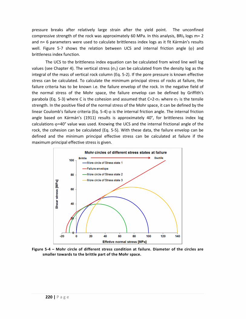
220 | P a g e   

pressure  breaks  after  relatively  large  strain  after  the  yield  point.    The  unconfined 

compressive strength of the rock was approximately 60 MPa. In this analysis, BRI3 logs m= 2 

and n= 6 parameters were used to calculate brittleness  index  logs as  it fit Kármán’s results 

well.  Figure  5‐7  shows  the  relation  between  UCS  and  internal  friction  angle  ()  and brittleness index function. 

The UCS to the brittleness index equation can be calculated from wired line well log 

values (see Chapter 4). The vertical stress (1) can be calculated from the density log as the 

integral of the mass of vertical rock column (Eq. 5‐2). If the pore pressure is known effective 

stress can be calculated. To calculate  the minimum principal stress of  rocks at  failure,  the 

failure criteria has to be known  i.e. the  failure envelop of the rock.  In the negative  field of 

the  normal  stress  of  the  Mohr  space,  the  failure  envelop  can  be  defined  by  Griffith’s 

parabola (Eq. 5‐3) where C is the cohesion and assumed that C=2∙T where T is the tensile 

strength. In the positive filed of the normal stress of the Mohr space, it can be defined by the 

linear Coulomb’s failure criteria (Eq. 5‐4)  is the internal friction angle. The internal friction angle  based  on  Kármán’s  (1911)  results  is  approximately  40°,  for  brittleness  index  log 

calculations =40° value was used. Knowing the UCS and the internal frictional angle of the rock, the cohesion can be calculated  (Eq. 5‐5). With these data, the  failure envelop can be 

defined  and  the  minimum  principal  effective  stress  can  be  calculated  at  failure  if  the 

maximum principal effective stress is given. 

Figure 5‐4 – Mohr  circle of different  stress  condition at  failure. Diameter of  the  circles are smaller towards to the brittle part of the Mohr space. 

 

221 | P a g e   

Figure 5‐5 –BRI3 function without parameters (or in case m=1 and n=1) (UCS=100, =30°). 

Figure 5‐6 –BRI3  function with different  functions  (UCS= 80 MPa, =40°);  figure A: effect of parameter “n”; figure B: effect of parameter “m”. 

A

B

222 | P a g e   

Figure 5‐7 – Brittleness  index function with parameter m= 2 and n= 6 for rocks with UCS and internal fiction angel. 

BRI∙

  (Eq. 5‐1) 

 

′ ∙   (Eq. 5‐2) 

 

4 ∙ ∙ 4 ∙ 0   (Eq. 5‐3) 

 

C tan φ   (Eq. 5‐4) 

 

C∙ 1 sin2 ∙ cos

  (Eq. 5‐5) 

 

′ ∙1 sin1 sin

∙ 1 sin1 sin

  (Eq. 5‐6) 

 

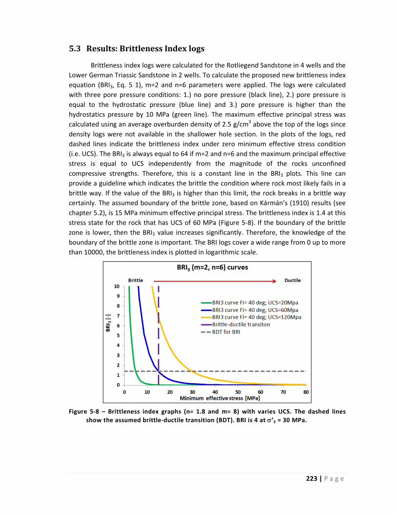
223 | P a g e   

5.3 Results:BrittlenessIndexlogs

Brittleness index logs were calculated for the Rotliegend Sandstone in 4 wells and the 

Lower German Triassic Sandstone in 2 wells. To calculate the proposed new brittleness index 

equation  (BRI3, Eq. 5 1), m=2 and n=6 parameters were applied. The  logs were calculated 

with  three pore pressure conditions: 1.) no pore pressure  (black  line), 2.) pore pressure  is 

equal  to  the  hydrostatic  pressure  (blue  line)  and  3.)  pore  pressure  is  higher  than  the 

hydrostatics pressure by 10 MPa  (green  line). The maximum effective principal  stress was 

calculated using an average overburden density of 2.5 g/cm3 above the top of the logs since 

density  logs were not available  in  the  shallower hole section.  In  the plots of  the  logs,  red 

dashed  lines  indicate  the brittleness  index under  zero minimum effective  stress  condition 

(i.e. UCS). The BRI3 is always equal to 64 if m=2 and n=6 and the maximum principal effective 

stress  is  equal  to  UCS  independently  from  the  magnitude  of  the  rocks  unconfined 

compressive  strengths.  Therefore,  this  is  a  constant  line  in  the  BRI3  plots.  This  line  can 

provide a guideline which indicates the brittle the condition where rock most likely fails in a 

brittle way. If the value of the BRI3  is higher than this  limit, the rock breaks  in a brittle way 

certainly. The assumed boundary of the brittle zone, based on Kármán’s (1910) results (see 

chapter 5.2), is 15 MPa minimum effective principal stress. The brittleness index is 1.4 at this 

stress state for the rock that has UCS of 60 MPa (Figure 5‐8). If the boundary of the brittle 

zone  is  lower,  then  the BRI3 value  increases significantly. Therefore,  the knowledge of  the 

boundary of the brittle zone is important. The BRI logs cover a wide range from 0 up to more 

than 10000, the brittleness index is plotted in logarithmic scale.  

Figure  5‐8  – Brittleness  index  graphs  (n=  1.8  and m=  8) with  varies UCS.  The  dashed  lines 

show the assumed brittle‐ductile transition (BDT). BRI is 4 at ’3 = 30 MPa. 

   

224 | P a g e   

Figure 5‐9 shows the brittleness index graphs of Rotliegend sandstone strata of wells 

P2‐SE2 and K18‐8. In the approximately 250 m section of the well P2‐SE2, nine facies can be 

separated which  are  indicated  by  the  coloured  column on  the  right  side of  the  graph. A 

strong correlation between rock facies and brittleness index log can be seen. This correlation 

can be seen even at a relatively layer thin e.g. around a depth of 3360 m in well P2‐SE2. Four 

facies  can be  considered as brittle: Zone‐2A, Zone‐2C, Zone‐4 and Zone‐6. The brittleness 

indices  in  these  rocks are  relatively high  (they are  in  the brittle  range) with hydrostatic or 

higher pore pressure. Without pore pressure the brittleness  indices slightly  lower than  the 

UCS  line.  Besides,  brittleness  indices  of  other  facies  in  this  log  are  low  even higher  pore 

pressure.  

The brittleness index log in Rotliegend strata in well K18‐8 can be seen on right side 

of  Figure  5‐9.  In  the  approximately  240 metres  long  section  in  this well,  four  facies was 

distinguished. The correlation  is  lower between brittleness  log and rock  layers than  in well 

P2‐SE2. The brittleness  index values higher are  in  the Silverpit Ameland Member almost  in 

the entire  section;  the BRI3 without pore pressure  is  slightly  lower  than  the UCS  limit but 

with  pore  pressure  it  is unambiguously  higher. Only  several metres  of  Silverpit  Ten  Boer 

Member are available; therefore, the brittleness of this sandstone might be not reliable.  In 

this short section,  the brittleness  index values are higher  than  the UCS  limit on  the upper 

part  of  it.  In more  than  100 metre  long  Upper  Slochteren  strata,  the  BRI3  log  contains 

subsequences of more brittle and non‐brittle  sections. One  longer and one  shorter brittle 

section can be found  in this facies where the rock  is definitely  in the brittle range but only 

with  at  least  hydrostatic  pore  pressure.  Furthermore,  in  a  relatively  long  section  of  this 

facies,  the brittleness  index values are much  lower  (close  to zero even with overpressure) 

than  in  the  other  parts  of  the  log.  The  approximately  100 metre  long  Lower  Slochteren 

Member has also brittle and less brittle subsequence. In the top and the middle part of the 

rock, non‐brittle  sections can be  found  locally  (several metres). This member contains  the 

most brittle section of the entire log of this well. The Rotliegend sandstones are more brittle 

in well K18‐8 than in well P2‐S2 even though rocks are located deeper in well K18‐8. 

Figure  5‐10  (on  the  left)  shows  the  brittleness  index  logs  of  Rotliegend  Lower 

Slochteren Sandstone Alpha Member of wells L6‐8. This  log, which  is only 30 metres  long, 

shows  relatively homogeneous  characteristic. Only  a  few,  local  (approximately one metre 

long sections) higher and lower peaks can be seen in this section. In general, this sandstone 

is brittle  if the pore pressure exceeds the hydrostatic pore pressure. If the pore pressure  is 

lower than the hydrostatic pore pressure then it is in the brittle‐ductile transitional zone and 

with zero pore pressure it might fail in a ductile way.  

 

225 | P a g e   

Figure 5‐9 – Brittleness index (BRI3) where m=2; n=6 logs of sections of Rotliegend Sandstone of well P2‐SE2 (on the  left) and well K18‐8 (on the right) with zero, hydrostatic (Phyd) and  hydrostatic  +  10  MPa  pore  pressures  (Phyd  +  10  MPa).  The  dashed  red  line indicates the BRI3 for zero minimum principal effective stresses condition (UCS). 

Figure  5‐10  shows  (on  the  right)  the  brittleness  index  logs  of  Upper  Rotliegend 

Slochteren Sandstone Formation  in wells P6‐9. This about 100 metres  long section shows a 

heterogeneous characteristic. There are three approximately 10 metres long sections where 

the brittleness index values are higher. The logs only locally reach the UCS line without pore 

pressure. However,  the  log  gets  into  the brittle  range with  hydrostatic  pressure. Besides, 

those sections of the log where the brittleness index is low, the logs stay in the ductile range 

even with higher pore pressure. These sections most  likely fail  in a ductile way. Only  in the 

very  bottom  of  the  log,  there  is  a  several metre  long  section  where  the  relatively  low 

brittleness  index  values  can  increase  above  the  UCS  line  with  at  least  hydrostatic  pore 

pressure.  In  this  formation,  the brittle and ductile sections can be separated based on  the 

brittleness  index  inside  the  formation.  In  the  upper  about  50  m  section,  the  very  low 

brittleness index is likely related to the lithology. This section is a clay reach section based on 

the geological  log. The  low brittleness  index section at 3550 m  is related  to  the clay reach 

226 | P a g e   

lithology.  However,  there  is  no  lithological  change  reported  between  3490 m  and  3510 

section where the brittleness index low too.   

Figure 5‐11 shows the brittleness  index  logs of the Main Buntsandstein Subgroup of 

the Lower German Triassic Sandstone Group  in wells P6‐9 and L6‐8.  In  the approximately 

350 metres long section of log of well L6‐8, two sandstone layers are present. The upper 25 

metres relatively thin section is part of 40 metres thick Volpriehausen Sandstone Member. In 

this member,  the brittleness  index  is  low except  two very short peaks which might be not 

reliable. Below the layer boundary (approximately from 4040 m to 4100 TVDSS), there is an 

transition zone where brittleness index log without pore pressure  jumps up to the UCS line 

and it stays there in the top 60 metres of the Lower Buntsandstein Formation. At a depth of 

4110 TVDSS metres, the brittleness index log jumps up over the UCS line even with no pore 

pressure.  In  the very bottom of the strata at 4360 m TVDSS, the  log  jumps up significantly 

which might be related to  lithological changes. The Lower Buntsandstein Formation can be 

separated into three sections by brittleness. 

In  the  approximately  140 metres  long  section  of  log  of well  P6‐9,  the Hardegsen 

Formation,  Lower  Detfurth  Sandstone  Member  and  Lower  Volpriehausen  Sandstone 

Member  of  the  Lower German  Triassic  Group  are  present  (on  the  right  of  Figure  5‐11). 

Between  these  sandstone members  and  formation,  clay  and  siltstone  can  be  found.  In 

general the brittleness  index  logs are above the UCS  line  in the Hardegsen Formation even 

with no pore pressure. The brittleness index logs are lower in the Lower Detfurth Sandstone 

Member and Lower Volpriehausen Sandstone Member. The brittleness index is higher than 

the brittleness  index of UCS only with  at  least hydrostatic pore pressure. All  the  logs  are 

relatively hectic which might be related to the quality of the source log or less likely related 

to lithological variation. The brittleness index logs have a slight decreasing tendency with the 

depth. 

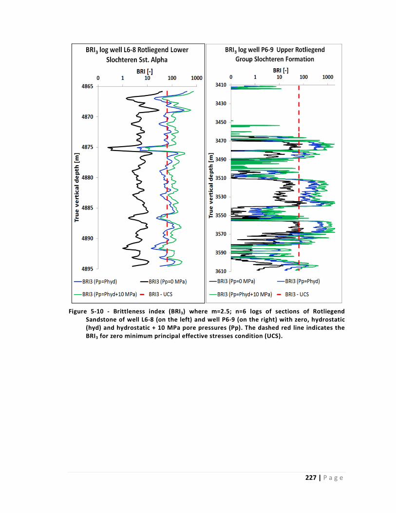
227 | P a g e   

Figure  5‐10  ‐  Brittleness  index  (BRI3)  where  m=2.5;  n=6  logs  of  sections  of  Rotliegend Sandstone of well L6‐8 (on the  left) and well P6‐9 (on the right) with zero, hydrostatic (hyd) and hydrostatic + 10 MPa pore pressures (Pp). The dashed red  line  indicates the BRI3 for zero minimum principal effective stresses condition (UCS). 

 

228 | P a g e   

Figure  5‐11  ‐Brittleness  index  (BRI3) where m=2.5;  n=6  logs  of  sections  of  Lower  German Triassic  Sandstone  of well  L6‐8  (on  the  left)  and well  P6‐9  (on  the  right) with  zero, hydrostatic  (hyd) and hydrostatic + 10 MPa pore pressures  (Pp). The dashed  red  line indicates the BRI3 for zero minimum principal effective stresses condition (UCS). 

 

229 | P a g e   

5.4 Discussion

There were two aims to develop a new brittleness index equation (BRI3) which works 

according to the idea of the equation of Hoogerduijn‐Strating and Urai. One of the aims was 

to make  the existing equation  simpler by using only one equation. The other  aim was  to 

have an option to setup the brittle‐ductile transition by parameters and make the equation 

adjustable. As  can be  seen  in Figure 5‐12,  the BRI2 brittleness  index  (Hoogerduijn‐Strating 

and Urai 2003), increases rapidly if 3< 0 MPa. The BRI2 function varies in a relatively narrow 

range, between 10 and about 3,  if  the 3  is between 0 and 50 MPa. This kind of  function 

characteristic is not ideal because the brittle‐ductile transition boundary may be in this 0 and 

50 MPa 3  range. Since  there are no parameters  in  the BRI2  function,  it  is not allowed  to 

change the characteristic of the function to become more appropriate for a studied rock. 

Figure  5‐12  ‐  Brittleness  index  graphs  of  Hoogerduijn‐Strating  and  Urai  (BRI2) with  varies UCS. The dashed  lines  show  the assumed brittle‐ductile  transition  (BDT). BRI  is 3.3 at 

’3 = 30 MPa. 

The results showed that the BRI3 brittleness index log revealed good correlation with 

lithology (see Chapter 5.3). In general, the variation of these brittleness  indices  is relatively 

low within a formation in well P2‐SE2 Rotliegend Sandstone, well L6‐8 Rotliegend and Lower 

German Triassic Sandstone and well P6‐9 Lower German Triassic Sandstone. However, there 

were some  layers where significant changes could be noticed, such as wells K18‐8 and P6‐9 

Rotliegend  Sandstones.  Furthermore,  Lower  Buntsandstein  (LGT)  of  well  L6‐8  or  Lower 

German Triassic Sandstone of well P6‐9 or Zone 2A, 2C, 4, 6 of Rotliegend Sandstone were 

found to be relatively brittle. Several semi‐brittle layers become brittle if the pore pressure is 

above the hydrostatic pressure (here the applied overpressure=10 MPa). Since the definition 

of  the brittle‐ductile  transition  is only approximate,  the brittleness  logs might not provide 

reliable  results  in  this  range. Nevertheless,  the BRI3  log  can provide  a  good  prediction  to 

identify major changes in the brittleness. 

230 | P a g e   

Figure  5‐13  shows  brittleness  index  logs  for  the  Rotliegend  section  of well  P2‐SE, 

calculated  by  the  equations  as  follows:  BRI3 with  parameters m=8  and n=1  and with  the 

parameters m=2  and  n=10;  BRI2;  BRI1;  and  B3  (see  Table  5‐2).  The  B3  index  is  based  on 

internal friction angle, which was calculated by gamma ray (Eq. 5‐8; Chang et al. 2006) and 

acoustic  velocity‐based empirical equations  (Eq. 5‐7; Lal 1999).  The behaviour of  the BRI3 

logs with the two different parameter setting is very different in the brittle‐ductile zone (i.e. 

below the UCS line). These logs show an example of how the parameters allow the change in 

BRI3 function in the lower minimum stress range. The BRI2 logs give high values if ’3 is lower than zero and, if it is higher, i.e. below the UCS line, the  index remains relatively high, here 

about 4. The BRI1  index values are  lower; here they range between 0‐5. The brittle‐ductile 

boundary for the BRI1 index  is two (2) defined empirically for shale by Hoogerduijn‐Strating 

and  Urai  (2003)  and,  more  recently,  Ishii  et  al.  (2011)  found  the  same  brittle‐ductile 

boundary  for  shale. The position of  this boundary  relative  to  log with no pore pressure  is 

very similar to those of the BRI3 and BRI2  logs. This  indicates that the UCS curve might be a 

good estimate of the brittle‐ductile boundary in sandstone too. The main trends (position of 

the high brittleness  index section) are  the same  for  the BRI3, BRI2 and BRI1  logs. However, 

only  the  rock  property‐based  B3  logs  are  significantly  different.  There  is  no  correlation 

between the gamma ray‐based log and the BRI logs. The acoustic velocity‐based log shows a 

relatively  good  correlation  with  trends  of  the  BRI  logs;  however,  not  everywhere,  for 

example  at  about  3440 m.  The  reason  of  the  similarities  is  that  the  UCS  log  calculation 

involves the velocity, which is a dominant parameter of the UCS calculation. The gamma ray‐ 

based  log  brittleness  index  (B1)  has  no  correlation with  lithology.  This  log  provides  very 

different  brittleness  prediction  in  comparison  with  the  other  logs.  It  is  nearly  constant, 

except two short sections where it has low values. 

φ sin10001000

  (Eq. 5‐7) 

 

φ tan∙ ∙

  (Eq. 5‐8) 

 

The  brittleness  index  equation  contains  two  independent  variables:  the  UCS  and 

maximum principle effective stress. The stress varies relatively slowly with depth, while UCS 

can  change  very  fast,  e.g.  at  the  layer  boundary  or  because  of  local  change  in  rock 

properties. However,  the  logs  in  Figure 5‐13  cover only  an about 50  long  vertical  section 

where  the stress condition  is nearly constant. Therefore,  the effect of  the variation of  the 

depth and stress on the different type of brittleness indices cannot be seen in Figure 5‐13. To 

demonstrate  this,  brittleness  index  logs were  calculated  based with  the  same  brittleness 

indices used above in Figure 5‐13 for nine rock models based on three different UCS (20, 80 

and 150 MPa) and  three different  internal  friction angles  (30˚, 40˚ and 50˚)  (Figure 5‐14). 

Since  the  B3  index, which  is  calculated  by  gamma  ray,  does  not  involve  the  stress,  it  is 

constant in the entire section. B3 index calculated from compressional wave velocity has an 

inverse  relation with  increasing  stress, which was also concluded by Holt et al.  (2015). As 

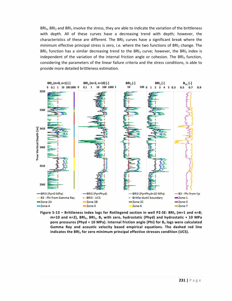
231 | P a g e   

BRI3, BRI2 and BRI1 involve the stress, they are able to indicate the variation of the brittleness 

with  depth.  All  of  these  curves  have  a  decreasing  trend  with  depth;  however,  the 

characteristics of  these  are  different.  The BRI2  curves  have  a  significant  break where  the 

minimum effective principal stress is zero,  i.e. where the two functions of BRI2 change. The 

BRI1  function has a  similar decreasing  trend  to  the BRI3  curve; however,  the BRI2  index  is 

independent of  the  variation of  the  internal  friction angle or  cohesion. The BRI3  function, 

considering the parameters of the  linear failure criteria and the stress conditions, is able to 

provide more detailed brittleness estimation. 

 

Figure 5‐13 – Brittleness  index  logs  for Rotliegend section  in well P2‐SE: BRI3 (m=1 and n=8; m=10 and n=2), BRI2, BRI1, B3 with  zero, hydrostatic  (Phyd) and hydrostatic + 10 MPa pore pressures (Phyd + 10 MPa). Internal friction angle (Phi) for B3 logs were calculated Gamma  Ray  and  acoustic  velocity  based  empirical  equations.  The  dashed  red  line indicates the BRI3 for zero minimum principal effective stresses condition (UCS). 

232 | P a g e   

Figure 5‐14 – Brittleness  index  log (BRI3, BRI2, BRI1 and gamma ray (GR) and compressional wave velocity based (Vp) B1) plots of a for nine rock models (UCS: 20, 80 and 150 MPa; and internal friction angle (Phi): 30˚, 40˚ and 50˚) with hydrostatic pore pressure. 

Figure 5‐15 shows the results of the triaxial measurement series of Kármán (1910) on 

sandstone. Brittleness indices were calculated for test results of Kármán applying the newly‐

developed brittleness  index equation  (BRI3).  In Figure 5‐15/A, the stress and strain curve  I, 

measured without confining pressure, shows brittle failure. Curve II and curve III (where the 

applied confining pressures were 28 MPa and 56 MPa , respectively) show that the rock fails 

in a  transitional way between brittle and ductile  failure mode. The  test samples  (curve  IV. 

and curve V.)  failed  in a ductile way applying 157 MPa and 250.8 MPa confining pressure, 

respectively. Based on these results, the lower bound of the brittle‐ductile transitional zone 

is between curve  I and curve  II, while  the upper bound  is between curve  III and curve  IV. 

Figure 5‐15/B shows that the failure envelope has a parabola‐like shape, which  is common 

for sandstone. However, the curve is nearly linear below about 100 MPa normal stress. The 

linear approximation of  the  failure envelope  is a commonly used simplification. Therefore, 

there  is  a  difference  between  BRI  values  calculated with  the  linear  failure  envelope  and 

calculated with the measured data (parabola‐like failure envelope). Based on the results of 

test I, II and III, the cohesion (13 MPa) and the internal friction angle (42°) of this sandstone 

were  calculated using  linear  failure  criteria. Applying  these  rock properties,  the minimum 

effective principal stresses were calculated and the BRI3 curve (Figure 5 17) was calculated 

with  two  parameter  sets. One  is m=1.8,  n=8,  as  introduced  in  the  previous  chapter.  The 

other parameter  set  is m=10, n=4, which  is  able  to  separate  the brittleness  values  in  the 

transitional zone having elongated curvature in the lower effective stress section. BRI3 values 

233 | P a g e   

were calculated for Kármán’s test samples based on their measured strength as well as the 

applied confining pressures.  

The difference  between  the  two brittleness  indices  ‐  the one  calculated  using  the 

measured data and the one calculated based on the linear failure criteria ‐ is not significant 

with  respect  to  the  interpretation  of  the  brittleness  index  (Figure  5‐16).  The  absolute 

difference is high in the brittle zone because the BRI curve is nearly parallel to the BRI axes; 

however,  the  relative  difference  is  low.  If  the  parameters  are  m=1.8,  n=8,  the  relative 

difference  increases with minimum effective stress out of the brittle section; however, the 

absolute difference  is negligible. If the parameters are m=10, n=4, the relative difference  is 

smaller;  the  absolute  difference  decreases  too,  but  not  as  significantly  as with  the  other 

settings. Nevertheless, the deviation of the brittleness index applying a linear approximation 

is  not  significant  in  comparison with  the  parabola  envelope.  The  brittleness  index  using 

parameters  m=1.8,  n=8,  the  brittle  zone  can  be  distinguished  by  high  brittleness  index 

values, while the other parameter set m=10, n=4 also allows to distinguish the brittle‐ductile 

transitional zone by very low values in the ductile zone. 

 

Figure  5‐15  –Stress  and  strain  diagrams  (on  the  left)  and Mohr diagram  (with  an  assumed failure  envelope)  of  (on  the  right)  the  triaxial  test  results  of  Kármán  (1910)  for sandstone (modified after Karman 1910). 

 

   

234 | P a g e   

 

Table  5‐3  –  Results  of  Kármán’s  triaxial  test  series  for  sandstone  and  their  BRI3  values 

calculated based on measured 3 and calculated 3 using linear failure criterion. 

 

Figure 5‐16 – BRI3 curve of Kármán’s studied sandstone together with the actually measured results.  

Jizba (1991) measured triaxial tests  in several sandstone samples with different clay 

content. These results showed that the linear failure envelope fit better with increasing clay 

content.  Brittleness  indices  (BRI3)  were  calculated  for  each  sample  of  three  triaxial  test 

series. Brittleness  indices were  calculated  based on  the measured  strength  and  confining 

pressure data. In addition, BRI3 curves were calculated based on the estimated linear failure 

envelope  derived  from  the Mohr  circles  of  the  triaxial  tests  (Figure  5‐17  and  Table  5‐4). 

Because  the  failure  envelope  of  the  higher  clay  content  samples  is  nearly  linear,  the 

difference is smaller between the brittleness indices based on the liner failure envelope and 

those that were calculated based on the measured data (Figure 5‐17/A lower clay content; C 

and E higher clay content). 

235 | P a g e   

These triaxial test results, measured by Jizba (1991), show that the samples failed in a 

brittle way by applying no confining pressure and also with 15 MPa confining pressure. The 

failure of  the  samples under 50 MPa confining pressure  seems  to be  in  the brittle‐ductile 

transition, which might be  close  to  the boundary of  the brittle  stress  range. The  samples 

failed  in  a  brittle‐ductile  transitional  way  under  100 MPa  confining  pressure.  For  these 

sandstones,  the  brittleness  index  equation with  the  parameters m=8  and  n=1.8  provides 

high values only  in cases of unconfined case. However, the brittleness  index equation with 

the parameters m=4 and n=10  is able to provide  larger separation between the brittle and 

less brittle failures. The zone of the ductile failure  is not covered by the triaxial test series. 

Based on the BRI3 curves the ductile zone starts above about 120 MPa confining pressure in 

the case of sample 9975 and 6853. In the case of sample 8675, the ductile zone starts above 

about  140 MPa  confining  pressure.  The  ductile  zone  of  sample  8675,  having  lower UCS, 

starts at higher confining than those of the other two samples, because the internal friction 

angle of sample 8675  is  lower. In comparison with the results of Kármán  (1911) where the 

sandstone had a relatively low 28 MPa UCS, the boundary of the ductile zone is between 56 

MPa and 157 MPa, based on  the  reported  results, and 110 MPa  is estimated by  the BRI3 

function.  The  UCS  of  the  measured  samples  of  Jizba  (1991)  was  higher;  however,  the 

estimated boundary of the ductile zone by the BRI3 function  is nearly the same. To set the 

parameters  for  the BRI3 equation  that provides good estimation  in  the entire range of  the 

brittle‐ductile  transition  zone,  it  is necessary  to measure more  tests with gradual  steps  to 

reach the ductile failure of the sample. 

Table 5‐4  – Brittleness  indices  (BRI3) of  each  sample based on  the measured  strength  and confining  pressure  data  and  based  on  the  estimated  linear  failure  derived  from  the Mohr circles of the triaxial results. 

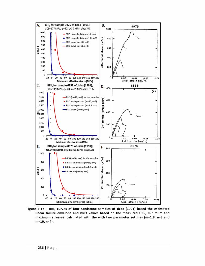
236 | P a g e   

Figure  5‐17  –  BRI3  curves  of  four  sandstone  samples  of  Jizba  (1991)  based  the  estimated linear  failure  envelope  and  BRI3  values  based  on  the measured  UCS, minimum  and maximum  stresses    calculated with  the with  two parameter  settings  (m=1.8, n=8 and m=10, n=4).

237 | P a g e   

Figure 5‐18 – Cross‐section photo and Mohr diagrams of analogue normal fault model of van Gent  (2010).  The  three  Mohr  diagrams  indicate  the  difference  in  the  mechanical properties of a fault with depth.  

 

Figure 5‐19 ‐ BRI3 curves based on analogue normal fault model of van Gent (2009) with two parameter settings (m=1.8, n=8 and m=10, n=4).

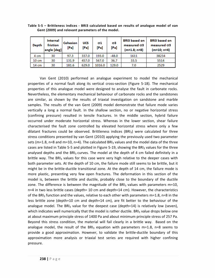
238 | P a g e   

Table 5‐5 – Brittleness  indices  ‐ BRI3 calculated based on  results of analogue model of van Gent (2009) and relevant parameters of the model.  

Van  Gent  (2010)  performed  an  analogue  experiment  to  model  the  mechanical 

properties of  a  normal  fault  along  its  vertical  cross‐section  (Figure  5‐18).  The mechanical 

properties of  this  analogue model were designed  to  analyse  the  fault  in  carbonate  rocks. 

Nevertheless, the elementary mechanical behaviour of carbonate rocks and the sandstones 

are  similar,  as  shown  by  the  results  of  triaxial  investigation  on  sandstone  and  marble 

samples. The  results of  the  van Gent  (2009) model demonstrate  that  failure mode  varies 

vertically  a  long  a  normal  fault.  In  the  shallow  section,  no  or  negative  horizontal  stress 

(confining  pressure)  resulted  in  tensile  fractures.  In  the  middle  section,  hybrid  failure 

occurred  under moderate  horizontal  stress. Whereas  in  the  lower  section,  shear  failure 

characterised  the  fault  zone  controlled  by  elevated  horizontal  stress  where  only  a  few 

dilatant  fractures  could  be  observed.  Brittleness  indices  (BRI3) were  calculated  for  three 

stress conditions presented by van Gent (2010) applying the previously used two parameter 

sets (m=1.8, n=8 and m=10, n=4). The calculated BRI3 values and the model data of the three 

cases are listed in Table 5‐5 and plotted in Figure 5‐19, showing the BRI3 values for the three 

analysed depths and the BRI3 curves. The model at the depth of 4 cm  failed definitely  in a 

brittle way. The BRI3 values  for  this case were very high  relative  to  the deeper cases with 

both parameter sets. At the depth of 10 cm, the failure mode still seems to be brittle, but it 

might be  in the brittle‐ductile transitional zone. At the depth of 14 cm, the failure mode  is 

more  plastic,  presenting  very  few  open  fractures.  The  deformation  in  this  section  of  the 

model  is,  between  the  brittle  and  ductile,  probably  close  to  the  boundary  of  the  ductile 

zone. The difference  is between  the magnitude of  the BRI3 values with parameters m=10, 

n=4 in two less brittle cases (depth= 10 cm and depth=14 cm). However, the characteristics 

of the BRI3 function and the values, relative to each other with parameters m=1.8, n=8 in the 

less  brittle  zone  (depth=10  cm  and  depth=14  cm),  are  fit  better  to  the  behaviour  of  the 

analogue model. The BRI3  value  for  the deepest case  (depth=14)  is  relatively  low  (seven), 

which indicates well numerically that the model is rather ductile. BRI3 value drops below one 

at about maximum principle stress of 1400 Pa and about minimum principle stress of 257 Pa. 

Beyond  this  stress  condition,  the material will  fail  clearly  in  a  brittle way.   Based on  the 

analogue model,  the  result  of  the  BRI3  equation with  parameters m=1.8,  n=8  seems  to 

provide  a  good  approximation.  However,  to  validate  the  brittle‐ductile  boundary  of  this 

approximation  more  analysis  or  triaxial  test  series  are  required  with  higher  confining 

pressure.  

 

239 | P a g e   

5.5 Conclusion

The newly‐developed brittleness index equation (BRI3), which is based on the idea of 

Hoogerduijn‐Strating  and  Urai  (2003),  takes  into  account  the  unconfined  compressive 

strength  of  the  rocks  and  also  the  stress  condition  at  failure.  Predicting  the  UCS,  the 

maximum and the minimum stresses and the pore pressure (for example, based on wireline 

log data)  in  a  subsurface  rock,  the brittleness of  the  rock  can be predicted.  Knowing  the 

brittleness of a  rock,  the  tendency  to  form open  fractures can be predictable, which  is an 

important factor to estimate the fluid migration potential in reservoirs. 

The new BRI equation without parameters (“m” and “n”) works basically in the same 

way as the brittleness index equation of Hoogerduijn‐Strating and Urai (BRI2). They are both 

hyperbolic functions. The BRI2 equation has a fixed value (BRI2= 10) if the minimum effective 

stress is zero (UCS). The BRI3 is equal to 1 under unconfined same stress condition; however, 

the characteristic of the function can be varied to allow setting the brittle‐ductile transition 

for a particular case. The parameters “m” and “n” allow modifying the BRI curve according to 

the  failure  characteristics of  the  given  rock. With  the  parameters  of  the  newly  proposed 

brittleness index equation, the brittle and ductile zones can be better separated numerically, 

which  can  improve  the  interpretation  of  the  BRI  logs.  However,  these  parameters  are 

required  to  be  set  carefully,  considering  the  entire  range  of  the  UCS  of  the  studied 

formation, since the brittle‐ductile transition zone depends on the strength of the rock. 

Applying the newly proposed equation, the brittleness index logs were calculated for 

the Rotliegend and  the  Lower German Triassic Sandstones  in  four wells  in  the North Sea. 

These  logs  allow  classifying  the  sections  of  these  sandstones  by  their  brittleness.  Four 

members of  the Rotliegend  sandstone  in well P2‐SE2, at a depth of around 3500‐3650 m 

TVDSS, were found to be relatively brittle, even without any pore pressure. In contrast, other 

formations are ductile even in the case when pore pressure was over hydrostatic. In well L6‐

8, the Rotliegend Lower Slochteren sandstone was found ductile at a depth of around 4480 

m TVDSS; even with over‐hydrostatic pore pressure it is around the brittle‐ductile transition 

limit. However,  the Rotliegend  Lower  Slochteren  sandstone  seemed  to be more brittle  in 

well K18‐8 than in well L6‐8. The Upper Slochteren sandstone in well K18‐8 and P6‐9 seemed 

to be brittle. The Lower German Triassic sandstones were found to be brittle in general. The 

deeper section (depth > 4100 m TVDSS) of the Lower Buntsandstein strata was  found very 

brittle,  even without  pore  pressure  in well  L6‐8, while  the  Volpriehausen  sandstone was 

found to be very ductile, even applying over‐hydrostatic pore pressure in shallower depth of 

this well.  In  the Upper  Slochteren  in well  K18‐8,  Slochteren  in well  P6‐9  and  the  Lower 

Buntsandstein in well L6‐8, in both brittle and less brittle sections were distinguished by the 

brittleness index logs. 

By applying the calculated BRI3 logs to characterise the brittle and less brittle‐ductile 

formations,  intervals of North Sea sandstones were  identified and provided good examples 

for the application of the BRI concept. Considering the analogue field experiences, Klondike 

Bluffs  faults  and  fractures  can  be  analogues  for  the  high  BRI  sections  of  the  North  Sea 

sandstones, where we can expect brittle deformation and open  fractures. Whereas,  in  the 

240 | P a g e   

sections  with  low  brittleness  index, more  similar  to  Courthouse  Junction  faults,  we  can 

expect ductile deformation and baffle compaction fractures. 

In order to be able to set the parameters of the proposed brittleness index equation 

more properly, it is necessary to know the stress condition of the brittle‐ductile transition for 

the studied rock. Since, there  is not an available adequate method to estimate the brittle‐

ductile  transition,  future  work  should  aim  to  measure  triaxial  test  series  on  different 

sandstones  with  small  confining  pressure  steps  in  order  to  define  the  brittle‐ductile 

transition zone of sandstones. This analysis also should  involve rock physical, mineralogical 

and  microstructure  analysis  of  the  studied  rock  to  better  understand  the  relationship 

between the rock properties and their brittle behaviour. 

 

241 | P a g e   

6 References

Adams, F. D. [1912] An experimental contribution to the question of the depth of the zone of flow in the earth's crust. The Journal of Geology 20(2), 97‐118. 

Agosta, F. and Aydin, A. [2006] Architecture and deformation mechanism of a basin‐bounding normal fault in mesozoic platform carbonates, central italy. Journal of Structural Geology 28(8), 1445‐1467. 

Aguilera, R.  [2002]  Incorporating  capillary pressure, pore  throat  aperture  radii, height  above  free‐water table, and winland r35 values on pickett plots. AAPG Bulletin 86(4), 605‐624. 

Ajdukiewicz, J. M. and Lander, R. H. [2010] Sandstone reservoir quality prediction: The state of the art. AAPG Bulletin 94(8), 1083‐1091. 

Allen, M. P. [1997] Understanding regression analysis. Springer Science & Business Media. 

Altindag, R.  [2002] The evaluation of rock brittleness concept on rotary blast hole drills.  Journal of the South African Institute of Mining and Metallurgy 102(1), 61‐66. 

Anders, M. H.  and Wiltschko, D.  V.  [1994] Microfracturing,  paleostress  and  the  growth  of  faults. Journal of Structural Geology 16(6), 795‐815. 

Anderson, E. M.  [1905] The dynamics of  faulting. Transactions of  the Edinburgh Geological Society 8(3), 387‐402. 

Anderson,  E. M.  [1942] The dynamics of  faulting  and dyke  formation with  applications  to britain. Oliver and Boyd, Edinburgh. 

Andreev, G. E. [1995] Brittle failure of rock materials: Test results and constitutive models. Taylor & Francis Group. 

Antonellini,  M.  and  Aydin,  A.  [1994]  Effect  of  faulting  on  fluid  flow  in  porous  sandstones; petrophysical properties. AAPG Bulletin 78(3), 355‐377. 

Antonellini, M. and Aydin, A. [1995] Effect of faulting on fluid flow  in porous sandstones; geometry and spatial distribution. AAPG Bulletin 79(5), 642‐671. 

Antonellini, M., Aydin, A. and Orr, L. [1999] Outcrop‐aided characterization of a faulted hydrocarbon reservoir:  Arroyo  grande  oil  field,  california,  USA.  GEOPHYSICAL  MONOGRAPH‐AMERICAN GEOPHYSICAL UNION 113, 7‐26. 

Antonellini, M. A., Aydin, A. and Pollard, D. D. [1994] Microstructure of deformation bands in porous sandstones at arches national park, utah. Journal of Structural Geology 16(7), 941‐959. 

Asszonyi,  C.  and  Richter,  R.  [1974]  Bevezetés  a  kőzetmechanika  reológiai  elméletébe. Nehézipari Minisztérium Továbbképző Központja. 

Asszonyi, C. and Richter, R. [1979] The continuum theory of rock mechanics. Trans Tech Publications, [Clausthal, Ger.]. 

ASTM‐D7012.  [2010] Astm d7012  ‐ 10  standard  test method  for  compressive  strength  and elastic moduli of  intact rock core specimens under varying states of stress and temperatures. ASTM International. 

Aydin,  A.  [1978]  Small  faults  formed  as  deformation  bands  in  sandstone.  Pure  and  Applied Geophysics 116(4), 913‐930. 

Aydin,  A.  [2000]  Fractures,  faults,  and  hydrocarbon  entrapment, migration  and  flow. Marine  and Petroleum Geology 17(7), 797‐814. 

Aydin, A. and Johnson, A. M. [1978] Development of faults as zones of deformation bands and as slip surfaces in sandstone Pure and Applied Geophysics 116(4‐5), 931‐942. 

Aydin, A. and Johnson, A. M.  [1983] Analysis of faulting  in porous sandstones. Journal of Structural Geology 5(1), 19‐31. 

242 | P a g e   

Baldschuhn,  R.,  Binot,  F.,  Fleig,  S.  and  Kockel,  F.  [2001]  Geotektonischer  atlas  von  nordwest‐deutschland und dem deutschen nordsee‐sektor. Hannover. 

Ballivy, G., Ladanyi, B. and Gill, D.  [1976] Effect of water saturation history on the strength of  low‐porosity rocks. ASTM special technical publication (599), 4‐20. 

Barefield,  E.  H.  and  Shakoor,  A.  [2006]  The  effect  of  degree  of  saturation  on  the  unconfined compressive strength of selected sandstones. 

Baron,  L.,  Loguntsov,  B.  and  Pozin,  E.  [1962]  Determination  of  the  properties  of  rocks. Gosgortekhizdat, Moscow. 

Bell, F. G. and Culshaw, M. G. [1998] Petrographic and engineering properties of sandstones from the sneinton  formation, nottinghamshire, england. Quarterly  Journal of Engineering Geology and Hydrogeology 31(1), 5‐19. 

Bense, V. F., Van den Berg, E. H. and Van Balen, R. T. [2003] Deformation mechanisms and hydraulic properties  of  fault  zones  in  unconsolidated  sediments;  the  roer  valley  rift  system,  the netherlands. Hydrogeology Journal 11(3), 319‐332. 

Berg, R. R. [1975] Capillary pressures in stratigraphic traps. AAPG Bulletin 59(6), 939‐956. 

Berg, S. S. and Skar, T. [2005] Controls on damage zone asymmetry of a normal fault zone: Outcrop analyses of a segment of the moab fault, se utah. Journal of Structural Geology 27(10), 1803‐1822. 

Bernabe, Y. and Brace, W. F. [1990] Deformation and fracture of berea sandstone. The brittle‐ductile transition in rocks, 91‐101. American Geophysical Union. 

Björck, A. [1996] Numerical methods for least squares problems. Siam. 

Blenkinsop,  T.  G.  [2008]  Relationships  between  faults,  extension  fractures  and  veins,  and  stress. Journal of Structural Geology 30(5), 622‐632. 

Blindheim,  O.  and  Bruland,  A.  [1998]  Boreability  testing  norwegian  tbm  tunnelling  30  years  of experience  with  tbms  in  norwegian  tunnelling.  Norwegian  Soil  and  Rock  Engineering Association 11, 29‐34. 

Borsaru, M., Rojc, A. and Stehle, R. [2001] The application of the pgnaa technique to in‐situ analysis of coal. Exploration and Mining Report C 848. 

Brace, W., Paulding, B. and Scholz, C. [1966] Dilatancy in the fracture of crystalline rocks. Journal of Geophysical Research 71(16), 3939‐3953. 

Brace, W. F. and Riley, D. K.  [1972] Static uniaxial deformation of 15  rocks  to 30 kb.  International Journal of Rock Mechanics and Mining Sciences & Geomechanics Abstracts 9(2), 271‐288. 

Bradford,  I.,  Fuller,  J.,  Thompson,  P.  and  Walsgrove,  T.  [1998]  Benefits  of  assessing  the  solids production  risk  in  a  north  sea  reservoir  using  elastoplastic  modelling.  SPE/ISRM  Rock Mechanics in Petroleum Engineering. 

Broch, E. [1974] The influence of water on some rock properties. ISRM Congress. 

Brogi, A.  [2008]  Fault  zone  architecture  and  permeability  features  in  siliceous  sedimentary  rocks: Insights  from the  rapolano geothermal area (northern apennines,  italy).  Journal of Structural Geology 30(2), 237‐256. 

Brogi, A. [2011] Variation in fracture patterns in damage zones related to strike‐slip faults interfering with  pre‐existing  fractures  in  sandstone  (calcione  area,  southern  tuscany,  italy).  Journal  of Structural Geology 33(4), 644‐661. 

Bruhn,  R.  L.,  Parry, W.  T.,  Yonkee, W.  A.  and  Thompson,  T.  [1994]  Fracturing  and  hydrothermal alteration in normal fault zones. Pure and Applied Geophysics 142(3‐4), 609‐644. 

Bryant,  S.,  King,  P.  and Mellor,  D.  [1993]  Network model  evaluation  of  permeability  and  spatial correlation in a real random sphere packing. Transport in Porous Media 11(1), 53‐70. 

243 | P a g e   

Byrne, P. M., Salgado, F. M. and Howie, J. A. [1990] Relationship between the unload shear modulus from pressuremeter tests and the maximum shear modulus for sand. Thomas Telford Services Ltd, London. 

Caine, J. S., Evans, J. P. and Forster, C. B. [1996] Geology 24(11), 1025‐1028. 

Carmichael, R. S. [1982] Crc handbook of physical properties of rocks. CRC Press. Inc. 

Cashman, S. and Cashman, K.  [2000] Cataclasis and deformation‐band  formation  in unconsolidated marine terrace sand, humboldt county, california. Geology 28(2), 111‐114. 

Chan, M. A., Parry, W. T. and Bowman, J. R. [2000] Diagenetic hematite and manganese oxides and fault‐related  fluid  flow  in  jurassic  sandstones,  southeastern  utah.  Aapg  Bulletin‐American Association of Petroleum Geologists 84(9), 1281‐1310. 

Chang,  C.,  Zoback, M.  D.  and  Khaksar,  A.  [2006]  Empirical  relations  between  rock  strength  and physical properties in sedimentary rocks. Journal of Petroleum Science and Engineering 51(3), 223‐237. 

Cheng, C. H.  and  Johnston, D. H.  [1981] Dynamic  and  static moduli. Geophysical Research  Letters 8(1), 39‐42. 

Chester, F., Chester, J., Kirschner, D., Schulz, S. and Evans, J. [2004] Structure of large‐displacement, strike‐slip  fault  zones  in  the  brittle  continental  crust.  Rheology  and  Deformation  in  the Lithosphere at Continental Margins 1, 223‐260. 

Chester,  F. M.  and  Chester,  J.  S.  [1998]  Ultracataclasite  structure  and  friction  processes  of  the punchbowl fault, san andreas system, california. Tectonophysics 295(1–2), 199‐221. 

Chester, F. M. E., J P; Biegel, R L J. [1993]  Internal structure and weakening mechanisms of the san andreas  fault  International  Journal  of  Rock  Mechanics  and  Mining  Sciences  &amp; Geomechanics Abstracts 30(5), 270. 

Clarke, B. G. [1994] Pressuremeters in geotechnical design. Taylor & Francis. 

Coates,  D.  and  Parsons,  R.  [1966]  Experimental  criteria  for  classification  of  rock  substances. International Journal of Rock Mechanics and Mining Sciences & Geomechanics Abstracts, 181‐189. 

Colback, P. and Wiid, B.  [1900] The  influence of moisture content on  the  compressive  strength of rocks. Geophysics. 

Collins, P.  [2002] Geomechanics and wellbore stability design of an offshore horizontal well, north sea.  SPE  International  Thermal  Operations  and  Heavy  Oil  Symposium  and  International Horizontal Well Technology Conference. 

Constantinides,  G.  N.  and  Payatakes,  A.  C.  [1989]  A  three  dimensional  network  model  for consolidated porous media. Basic studies. Chemical Engineering Communications 81(1), 55‐81. 

Copur, H., Bilgin, N., Tuncdemir, H. and Balci, C. [2003] A set of indices based on indentation tests for assessment  of  rock  cutting  performance  and  rock  properties.  JOURNAL‐SOUTH  AFRICAN INSTITUTE OF MINING AND METALLURGY 103(9), 589‐599. 

Coskun, S. B. and Wardlaw, N. C. [1993] Estimation of permeability from image analysis of reservoir sandstones. Journal of Petroleum Science and Engineering 10(1), 1‐16. 

Cramer, B., Andruleit, H., Rempel, H., Babies, H., Schlömer, S., Schmidt, S., Schwarz‐Schampera, U., Ochmann, N., MEßNER, J. and Rehder, S. [2009] Energierohstoffe 2009: Reserven, ressourcen, verfügbarkeit.  Erdöl,  Erdgas,  Kohle,  Kernbrennstoffe, Geothermische  Energie.  Bundesanstalt für Geowissenschaften und Rohstoffe (BGR), Hannover, 2009. www. bgr. bund. de. 

Cruikshank,  K. M.  and  Aydin,  A.  [1994]  Role  of  fracture  localization  in  arch  formation,  arches‐national‐park, utah. Geological Society of America Bulletin 106(7), 879‐891. 

Cruikshank, K. M. and Aydin, A.  [1995] Unweaving the  joints  in entrada sandstone, arches national park,next term utah, u.S.A. Journal of Structural Geology 17(3), 409‐421. 

244 | P a g e   

Cruikshank, K. M., Zhao, G. Z. and Johnson, A. M. [1991] Duplex structures connecting fault segments in entrada sandstone. Journal of Structural Geology 13(10), 1185‐1196. 

Dathe, A., Eins, S., Niemeyer, J. and Gerold, G. [2001] The surface fractal dimension of the soil–pore interface as measured by image analysis. Geoderma 103(1–2), 203‐229. 

Davatzes, N. C. and Aydin, A. [2003] Overprinting faulting mechanisms in high porosity sandstones of se utah. Journal of Structural Geology 25(11), 1795‐1813. 

Davatzes, N. C., Eichhubl, P. and Aydin, A. [2005] Structural evolution of fault zones in sandstone by multiple deformation mechanisms: Moab fault, southeast Utah. Geological Society of America Bulletin 117(1‐2), 135‐148. 

Davis, G. H. [1999] Structural geology of the colorado plateau region of southern utah, with special emphasis on deformation bands. Geological Society of America. 

De  Jager,  J.,  2007.  Geological  Development.  In: Wong,  Th.E,  Batjes,  D.A.J.  &  De  Jager,  J.  (eds): Geology of the Netherlands. Royal Netherlands Academy of Arts and Sciences (Amsterdam): p. 5 ‐26. 

De  Paola,  N.,  Collettini,  C.,  Faulkner,  D.  R.  and  Trippetta,  F.  [2008]  Fault  zone  architecture  and deformation processes within evaporitic rocks in the upper crust. Tectonics 27(4), TC4017. 

Deng,  J.,  Leguizamon,  J. and Aguilera, R.  [2011] Petrophysics of  triple‐porosity  tight gas  reservoirs with a link to gas productivity. SPE Reservoir Evaluation & Engineering 14(5), 566‐577. 

Desbois, G., Urai, J. and Kukla, P. [2009] Morphology of the pore space in claystones–evidence from bib/fib ion beam sectioning and cryo‐sem observations. eEarth Discussions 4(1), 1‐19. 

Desbois, G., Enzmann, F., Urai, J. L., Baerle, C., Kukla, P. A., & Konstanty, J. [2010]. Imaging pore space in tight gas sandstone reservoir: insights from broad ion beam cross‐sectioning. In EPJ Web of conferences (Vol. 6, p. 22022). EDP Sciences. 

Doelling, H. H. [1985] Geological map of arches national park and vicinity, gran country, utah. State of Utach Department of Natural Resources Utah Geological and Mineral Survey, Utah. 

Doelling, H. H. [2010] Geology of arches national park utah. Geology of utah’s parks and monuments, P. B. Anderson, T. C. C.  Jr.  and D. A.  Sprinkel  (eds.). Utah Geological Association  and Bryce Canyon Natural History Assotiation. 

Doelling and Kuehne, 2013 Geologic maps of the Klondike Bluffs, Mollie Hogans, and The Windows Section 7.5' Quadrangles, Grand Count y, Utah, Utah Geological Survey 

Downey, M. W. [1984] Evaluating seals for hydrocarbon accumulations. AAPG Bulletin 68(11), 1752‐1763. 

Draut, A. E.  [2005] The geology of central and southeastern utah:  Itinerary  for a one‐day  field trip. Penrose Conference Field Trip Guide, 20. Geological Society of America. 

Du Bernard, X., Eichhubl, P. and Aydin, A.  [2002] Dilation bands: A new  form of  localized  failure  in granular media. Geophysical Research Letters 29(24), 2176. 

Dullien,  F. A.  L.  and Dhawan, G. K.  [1974] Characterization of pore  structure by  a  combination of quantitative  photomicrography  and  mercury  porosimetry.  Journal  of  Colloid  and  Interface Science 47(2), 337‐349. 

Dunn, D. E., LaFountain, L. J. and Jackson, R. E. [1973] Porosity dependence and mechanism of brittle fracture in sandstones. Journal of Geophysical Research 78(14), 2403‐2417. 

Dyke,  C.  G.  and  Dobereiner,  L.  [1991]  Evaluating  the  strength  and  deformability  of  sandstones. Quarterly Journal of Engineering Geology and Hydrogeology 24(1), 123‐134. 

Ehrenberg, S. [1993] Preservation of anomalously high porosity in deeply buried sandstones by grain‐coating  chlorite: Examples  from  the norwegian continental  shelf. AAPG Bulletin 77(7), 1260‐1286. 

245 | P a g e   

Ehrlich, R., Etris, E. L., Brumfield, D., Yuan, L. and CRABTREE, S. J. [1991] Petrography and reservoir physics  iii:  Physical models  for permeability  and  formation  factor  (1). AAPG Bulletin 75(10), 1579‐1592. 

Eichhubl, P., Davatz, N. C. and Becker, S. P. [2009] Structural and diagenetic control of fluid migration and cementation along the moab fault, utah. AAPG Bulletin 93(5), 653‐681. 

Ellis, D. V. and Singer, J. M. [2008] Well logging for earth scientists. Springer. 

Fahy, M. and Guccione, M. [1979] Estimating strength of sandstone using petrographic thin‐section data. Bull Assoc Eng Geol 16(4), 467‐485. 

Faulkner,  D., Mitchell,  T.,  Healy,  D.  and  Heap, M.  [2006]  Slip  on'weak'faults  by  the  rotation  of regional stress in the fracture damage zone. Nature 444(7121), 922‐925. 

Faulkner, D. R., Lewis, A. C. and Rutter, E. H. [2003] On the internal structure and mechanics of large strike‐slip  fault  zones:  Field  observations  of  the  carboneras  fault  in  southeastern  spain. Tectonophysics 367(3–4), 235‐251. 

Fischer, G. J. and Paterson, M. S. [1989] Dilatancy during rock deformation at high temperatures and pressures. Journal of Geophysical Research: Solid Earth 94(B12), 17607‐17617. 

Fisher, Q. J. and Knipe, R. J. [2001] The permeability of faults within siliciclastic petroleum reservoirs of  the  north  sea  and  norwegian  continental  shelf. Marine  and  Petroleum  Geology  18(10), 1063‐1081. 

Fjær, E. [1999] Static and dynamic moduli of weak sandstones. stress 100, 80. 

Fjær, E. [2009] Static and dynamic moduli of a weak sandstone. Geophysics 74(2), WA103‐WA112. 

Fjar, E., Holt, R. M., Raaen, A., Risnes, R. and Horsrud, P. [2008] Petroleum related rock mechanics. Elsevier Science. 

Fletcher, R. C. and Pollard, D. D. [1981] Anticrack model for pressure solution surfaces. Geology 9(9), 419‐424. 

Flodin, E., Aydin, A., Durlofsky, L. and Yeten, B. [2001] Representation of fault zone permeability  in reservoir flow models. SPE Annual Technical Conference and Exhibition. 

Flodin,  E.  A.  [2003]  Structural  evolution,  petrophysics,  and  large‐scale  permeability  of  faults  in sandstone, valley of fire, nevada. Stanford University. 

Fodor, L. I. [2010] Mesozoic‐cenozoic stress fields and fracture systems in the north‐east of pannon‐basin  ‐  methodology  and  structural  analysis  (mezozoos‐kainozoos  feszültségmezõk  és törésrendszerek  a  pannonmedence  ény‐i  részén  –  módszertan  és  szerkezeti  elemzés). Hungarian Academy of Sciences. 

Fossen, H. [2010] Deformation bands formed during soft‐sediment deformation: Observations from se utah. Marine and Petroleum Geology 27(1), 215‐222. 

Fossen, H. [2010] Structural geology. Cambridge University Press. 

Fossen, H. and Bale, A.  [2007] Deformation bands and  their  influence on  fluid  flow. AAPG Bulletin 91(12), 1685‐1700. 

Fossen, H. and Hesthammer, J. [1997] Geometric analysis and scaling relations of deformation bands in porous sandstone. Journal of Structural Geology 19(12), 1479‐1493. 

Fossen, H. and Hesthammer, J. [1998] Deformation bands and their significance in porous sandstone reservoirs. First Break (16), 21‐25. 

Fossen, H. and Hesthammer, J. [2000] Possible absence of small faults in the gullfaks field, northern north  sea:  Implications  for  downscaling  of  faults  in  some  porous  sandstones.  Journal  of Structural Geology 22(7), 851‐863. 

Fossen, H., Hesthammer, J., Skeie Johansen, T. E. and Sygnabere, T. O. [2003] Structural geology of the huldra field, northern north sea‐‐a major tilted fault block at the eastern edge of the horda platform. Marine and Petroleum Geology 20(10), 1105‐1118. 

246 | P a g e   

Fossen,  H.,  Schultz,  R.  A.,  Shipton,  Z.  K.  and Mair,  K.  [2007]  Deformation  bands  in  sandstone:  A review. Journal of the Geological Society 164, 755‐769. 

Fossen, H.,  Schultz,  R. A.  and  Torabi,  A.  [2011]  Conditions  and  implications  for  compaction  band formation in the navajo sandstone, utah. Journal of Structural Geology 33(10), 1477‐1490. 

Foxford, K.A., Garden,  I.R., Guscott, S.C., Burley, S.D., Lewis,  J.L.L., Walsh,  J.J., Watterson,  J., 1996. The  field  geology  of  the Moab  Fault.  In:  Huffman,  A.C.,  Lund, W.R.J.,  Godwin,  L.H.  (Eds.), Geology and Resources of the Paradox Basin, 25. Utah Geological Association Guidebook, pp. 265–283. 

Franks, S. G. and Zwingmann, H.  [2010] Origin and  timing of  late diagenetic  illite  in  the permian–carboniferous unayzah sandstone reservoirs of saudi arabia. AAPG Bulletin 94(8), 1133‐1159. 

Freyburg,  E.  [1972]  Der  untere  und  mittlere  buntsandstein  sw‐thuringen  in  seinen gesteinstechnicschen eigenschaften. Ber. Dte. Ges. Geol. Wiss. A; Berlin 176, 911‐919. 

Garden, I. R., Guscott, S. C., Burley, S. D. and Foxford, K. A. [2001] An exhumed palaeo‐hydrocarbon migration fairway in a faulted carrier system, entrada sanstone of se utah, USA Geofluids 1, 19. 

Geluk, M.  and  Röhling,  H.‐G.  [1997]  High‐resolution  sequence  stratigraphy  of  the  lower  triassic ‘buntsandstein’in  the netherlands and northwestern germany. Geologie en Mijnbouw 76(3), 227‐246. 

George,  E.  [1995]  Brittle  failure  of  rock  material‐test  results  and  constitutive  models.  AA Balkema/Rotterdam/Brolkfield, 123‐128. 

Gerling, P., Geluk, M., Kockel, F., Lokhorst, A.,  Lott, G. and Nicholson, R.  [1999]  ’nw european gas atlas’–new  implications  for  the  carboniferous gas plays  in  the western part of  the  southern permian basin. Geological Society, London, Petroleum Geology Conference series, 799‐808. 

Gibson, R. G. [1998] Physical character and fluid‐flow properties of sandstonederived 

fault zones. Structural geology  in reservoir characterization, M. P. Coward, Johnson, H. & Daltaban, T.S. (ed.), 83–97. The Geological Society, London. 

Glennie, K. and Provan, D. [1990] Lower permian rotliegend reservoir of the southern north sea gas province. Geological Society, London, Special Publications 50(1), 399‐416. 

Göktan,  R.  M.  [1991]  Brittleness  and  micro‐scale  rock  cutting  efficiency.  Mining  Science  and Technology 13(3), 237‐241. 

Gray, D., Anderson, P., Logel, J., Delbecq, F., Schmidt, D. and Schmid, R. [2012] Estimation of stress and geomechanical properties using 3D seismic data. First Break 30(3), 59‐68. 

Griffith, A. A. [1921] The phenomena of rupture and flow in solids. Philosophical transactions of the royal  society of  london. Series A,  containing papers of a mathematical or physical  character 221, 163‐198. 

Griggs, D. T. and Handin, J. [1960] Observations on fracture and a hypothesis of earthquakes. Rock deformation Geol. Soc Am (79), 347‐364. 

Gudmundsson,  A.  [2007]  Infrastructure  and  evolution  of  ocean‐ridge  discontinuities  in  iceland. Journal of Geodynamics 43(1), 6‐29. 

Gudmundsson, A., Fjeldskaar, I. and Brenner, S. L. [2002] Propagation pathways and fluid transport of hydrofractures  in  jointed and  layered  rocks  in geothermal  fields.  Journal of Volcanology and Geothermal Research 116(3), 257‐278. 

Gudmundsson, A., Simmenes, T. H., Larsen, B. and Philipp, S. L.  [2010] Effects of  internal structure and  local  stresses  on  fracture  propagation,  deflection,  and  arrest  in  fault  zones.  Journal  of Structural Geology 32(11), 1643‐1655. 

Hale,  P.  A.  and  Shakoor, A.  [2003]  A  laboratory  investigation  of  the  effects  of  cyclic  heating  and cooling, wetting and drying, and freezing and thawing on the compressive strength of selected sandstones. Environmental & Engineering Geoscience 9(2), 117‐130. 

247 | P a g e   

Handin, J. and Hager Jr, R. V. [1958] Experimental deformation of sedimentary rocks under confining pressure: Tests at high temperature. AAPG Bulletin 42(12), 2892‐2934. 

Haney, M. and Shakoor, A.  [1994] The  relationship between  tensile and compressive strengths  for selected  sandstones  as  influenced  by  index  properties  and  petrographic  characteristics. Proceedings of 7th Int IAEG Congress, Lisbon, Portugal, 493‐500. 

Hansen,  J. and Skjeltorp, A.  [1988] Fractal pore  space and  rock permeability  implications. Physical review. B, Condensed matter 38(4), 2635‐2638. 

Harper,  T.  and Moftah,  I.  [1985]  Skin  effect  and  completion options  in  the  ras bud  ran  reservoir. Middle East Oil Technical Conference and Exhibition. 

Harper, T. R. and Lundin, E. R.  [1997] Fault seal analysis: Reducing our dependence on empiricism. Norwegian  petroleum  society  special  publications,  P.  Møller‐Pedersen  and  A.  G.  Koestler (eds.), 149‐164. Elsevier. 

Harris, S., McAllister, E., Knipe, R. and Odling, N. [2003] Predicting the three‐dimensional population characteristics of  fault  zones: A  study using  stochastic models.  Journal of Structural Geology 25(8), 1281‐1299. 

Hatherly, P., Medhurst, T., Zhou, B. and Guo, H. [2001] Geotechnical evaluation for mining–assessing rock mass conditions using geophysical logging. Final report ACARP Project C8022b. 

Hatherly, P., Sliwa, R., Turner, R. and Medhurst, T. [2004] Quantitative geophysical log interpretation for  rock mass characterisation. Final  report  to Australian Coal Association Research Program (ACARP), project C 11037. 

Hawkins, A. B.  and McConnell, B.  J.  [1992]  Sensitivity of  sandstone  strength  and deformability  to changes in moisture‐content. Quarterly Journal of Engineering Geology 25(2), 115‐130. 

Heard, H.  C.  [1960]  Transition  from  brittle  fracture  to  ductile  flow  in  solenhofen  limestone  as  a function of temperature, confining pressure, and interstitial fluid pressure. Geological Society of America Memoirs 79, 193‐226. 

Heid,  J.,  McMahon,  J.,  Nielsen,  R.  and  Yuster,  S.  [1950]  Study  of  the  permeability  of  rocks  to homogeneous fluids. Drilling and Production Practice. 

Heidari, M., Khanlari, G. R., Torabi‐Kaveh, M., Kargarian, S. and Saneie, S. [2013] Effect of porosity on rock brittleness. Rock Mechanics and Rock Engineering, 1‐6. 

Hesthammer, J. and Fossen, H. [1999] Evolution and geometries of gravitational collapse structures with  examples  from  the  statfjord  field, northern north  sea. Marine  and  Petroleum Geology 16(3), 259‐281. 

Hesthammer, J. and Fossen, H. [2001] Structural core analysis from the gullfaks area, northern north sea. Marine and Petroleum Geology 18(3), 411‐439. 

Hesthammer,  J.,  Johansen,  T.  E.  S.  and Watts,  L.  [2000]  Spatial  relationships within  fault  damage zones in sandstone. Marine and Petroleum Geology 17(8), 873‐893. 

Hetenyi, M. I. [1950] Handbook of experimental stress analysis. 

Hilgers, C., Koehn, D., Bons, P. D. and Urai,  J. L.  [2001] Development of crystal morphology during unitaxial growth in a progressively widening vein: Ii. Numerical simulations of the evolution of antitaxial fibrous veins. Journal of Structural Geology 23(6‐7), 873‐885. 

Hirth,  G.  and  Tullis,  J.  [1994]  The  brittle‐plastic  transition  in  experimentally  deformed  quartz aggregates. Journal of Geophysical Research: Solid Earth (1978–2012) 99(B6), 11731‐11747. 

Holditch, S. [2006] Tight gas sands. Journal of Petroleum Technology 58(6), 86‐93. 

Holt, R. M. [1994] Effects of coring on petrophysical measurements. 1994 International Symposium of the Society of Core Analysts, Proceedings, 77‐86. 

Holt, R. M., Brignoli, M. and Kenter, C. J. [2000] Core quality: Quantification of coring‐induced rock alteration. International Journal of Rock Mechanics and Mining Sciences 37(6), 889‐907. 

248 | P a g e   

Holt,  R. M.,  Fjær,  E.,  Stenebråten,  J.  F.  and Nes, O.‐M.  [2015]  Brittleness  of  shales:  Relevance  to borehole collapse and hydraulic fracturing. Journal of Petroleum Science and Engineering 131, 200‐209. 

Holt, R. M. and Kenter, C. J. [1992] Laboratory simulation of core damage induced by stress release. Rock Mechanics : Proceedings of the 33rd U S Symposium, 959‐968. 

Holt, R. M., Unander, T. E., Kenter, C. J. and Santarelli, F. J. [1993] Unloading effects on mechanical‐properties of a very weak artificial sandstone ‐ applications to coring. Geotechnical Engineering of Hard Soils ‐ Soft Rocks, Vol 2, 1609‐1614. 

Hoogerduijn‐Strating, E. and Urai, J. L. [2003] Brittleness index ‐ a tool to quantify the probability of dilatant fracturing in mudrock topseals. Proceedings, EAGE Conference on Fault and Top Seals, ISBN, 2003, 90‐73781. 

Horsrud, P. [2001] Estimating mechanical properties of shale from empirical correlations. SPE Drilling & Completion 16(2), 68‐73. 

Hoshino, K. [1974] Effect of porosity on the strength of the clastic sedimentary rocks. 

Houben, M. E., Desbois, G. and Urai, J. L. [2013] Pore morphology and distribution in the shaly facies of  opalinus  clay  (mont  terri,  switzerland):  Insights  from  representative  2d  bib–sem investigations on mm to nm scale. Applied Clay Science 71(0), 82‐97. 

Hsieh, Y.‐M.,  Li, H.‐H., Huang, T.‐H. and  Jeng, F.‐S.  [2008]  Interpretations on how  the macroscopic mechanical behavior of  sandstone affected by microscopic properties—revealed by bonded‐particle model. Engineering Geology 99(1–2), 1‐10. 

Hubbert, M. K. and Willis, D. G. [1957] Mechanics of hydraulic fracturing. 

Hucka, V. and Das, B. [1974] Brittleness determination of rocks by different methods.  International Journal of Rock Mechanics and Mining Sciences & Geomechanics Abstracts 11(10), 389‐392. 

Ingram,  G. M.  and  Urai,  J.  L.  [1999]  Top‐seal  leakage  through  faults  and  fractures:  The  role  of mudrock properties. Geological Society, London, Special Publications 158(1), 125‐135. 

Ingram,  G. M.,  Urai,  J.  L.  and  Naylor, M.  A.  [1997]  Sealing  processes  and  top  seal  assessment Norwegian Petroleum Society Special Publications 7, 165‐174. 

Ioannidis, M. A. and Chatzis, I. [1993] Network modelling of pore structure and transport properties of porous media. Chemical Engineering Science 48(5), 951‐972. 

Ioannidis, M. A., Kwiecien, M. J. and Chatzis, I. [1996] Statistical analysis of the porous microstructure as  a  method  for  estimating  reservoir  permeability.  Journal  of  Petroleum  Science  and Engineering 16(4), 251‐261. 

Ishii, E., Sanada, H., Funaki, H., Sugita, Y. and Kurikami, H. [2011] The relationships among brittleness, deformation behavior, and transport properties in mudstones: An example from the Horonobe Underground  Research  Laboratory,  Japan.  Journal  of  Geophysical  Research:  Solid  Earth 116(B9) 

Jaeger,  J.  C.,  Cook,  N.  G.  and  Zimmerman,  R.  [2009]  Fundamentals  of  rock  mechanics.  Wiley‐Blackwell. 

Jeng, F. S., Weng, M. C., Lin, M. L. and Huang, T. H. [2004] Influence of petrographic parameters on geotechnical properties of tertiary sandstones  from taiwan. Engineering Geology 73(1‐2), 71‐91. 

Jizba, D. and Nur, A. [1990] Static and dynamic moduli of tight gas sandstones and their relation to formation properties. SPWLA 31st Annual Logging Symposium, Paper BB. 

Jizba, D.  L.  [1991] Mechanical  and  acoustical properties of  sandstones  and  shales. Department of Geophysics, School of Earth Sciences. Stanford University. Dept. of Geophysics. 

Johansen, T.  E.  S.  and  Fossen, H.  [2008]  Internal  geometry of  fault damage  zones  in  interbedded siliciclastic sediments. Geological Society, London, Special Publications 299(1), 35‐56. 

249 | P a g e   

Johansen, T. E. S., Fossen, H. and Kluge, R. [2005] The  impact of syn‐faulting porosity reduction on damage  zone  architecture  in  porous  sandstone:  An  outcrop  example  from  the moab  fault, utah. Journal of Structural Geology 27(8), 1469‐1485. 

Jones, R. R., Wawrzyniec, T. F., Holliman, N. S., McCaffrey, K. J., Imber, J. and Holdsworth, R. E. [2008] Describing the dimensionality of geospatial data in the earth sciences—Recommendations for nomenclature. Geosphere 4(2), 354‐359. 

Jones, R. R., McCaffrey, K. J. W., Clegg, P., Wilson, R. W., Holliman, N. S., Holdsworth, R. E., Imber, J. and Waggott, S. [2009] Integration of regional to outcrop digital data: 3D visualisation of multi‐scale geological models. Computers & Geosciences 35(1), 4‐18. 

Jourde, H., Flodin, E. A., Aydin, A., Durlofsky, L. J. and Wen, X. H. [2002] Computing permeability of fault zones in eolian sandstone from outcrop measurements. AAPG Bulletin 86(7), 1187‐1200. 

Kahraman, S. and Altindag, R. [2004] A brittleness index to estimate fracture toughness. International Journal of Rock Mechanics & Mining Sciences 41(2), 343–348. 

Kármán, T. [1911] Festigkeitsversuche unter allseitigem druck. Z. Ver. Dt. Ing 55, 1749‐1757. 

Kármán,  T.  [1910]  Mitől  függ  az  anyag  igénybevétele?  (what  influences  the  strength  of  the material?). Magyar Mérnök és Építészegylet Közlönye 10, 212–226. 

Kattenhorn, S. A., Aydin, A. and Pollard, D. D. [2000] Joints at high angles to normal fault strike: An explanation using 3‐d numerical models of  fault‐perturbed stress  fields.  Journal of Structural Geology 22(1), 1‐23. 

Katz, A.  J.  and  Thompson, A. H.  [1985]  Fractal  sandstone pores:  Implications  for  conductivity  and pore formation. Physical Review Letters 54(12), 1325. 

Katz,  A.  J.  and  Thompson,  A.  H.  [1986]  Quantitative  prediction  of  permeability  in  porous  rock. Physical review. B, Condensed matter 34(11), 8179‐8181. 

Kenter, C.  J., Brignoli, M.  and Holt, R. M.  [1997] Cms  (constant mean  stress)  vs. Ucs  (unconfined strength) tests: A tool to reduce core damage effects. International Journal of Rock Mechanics and Mining Sciences 34(3–4), 129.e1‐129.e11. 

King, M. [1983] Static and dynamic elastic properties of rocks from the canadian shield.  Int. J. Rock Mech. Min. Sci. Geomech. Abstr.;(United States) 20(5). 

Klaver, J., Desbois, G., Urai, J. L. and Littke, R. [2012] Bib‐sem study of the pore space morphology in early  mature  posidonia  shale  from  the  hils  area,  germany.  International  Journal  of  Coal Geology 103(0), 12‐25. 

Knipe,  R.  J.  [1992]  Faulting  processes  and  fault  seal.  Structural  and  tectonic  modelling  and  its application to petroleum geology, R. M. Larsen, H. Brekke, B. T. Larsen and E. Talleraas (eds.), 325‐342. Elsevier, Amsterdam. 

Knott, S. D., Beach, A., Brockbank, P.  J., Lawson Brown, J., McCallum, J. E. and Welbon, A.  I. [1996] Spatial  and mechanical  controls  on  normal  fault  populations.  Journal  of  Structural Geology 18(2‚Äì3), 359‐372. 

Koestler,  A.,  Buller,  A., Milnes,  A.  and  Olsen,  S.  [1994]  A  structural  simulation  tool  for  faulted sandstone reservoirs: Exploratory study using field data from utah and gullfaks. North Sea Oil and Gas Reservoirs III. Kluwer, Dordrecht, 157‐165. 

Kohonen, T. [2001] Self‐organizing maps. Springer, New York. 

Kokkalas, S., Jones, R., McCaffrey, K. and Clegg, P. [2007] Quantitative fault analysis at Arkitsa, central Greece, using terrestrial laser‐scanning (“LIDAR”). Bulletin of the Geological Society of Greece 37, 1‐14. 

Kolodzie, S. [1980] Analysis of pore throat size and use of the waxman‐smits equation to determine ooip in spindle field, colorado. SPE9382. 

Kolor. [2012] Autopano giga 2.6.2. Challes‐les Eaux, France. 

250 | P a g e   

Kolyukhin D., Schueller, S., Espedal, M. S. and Fossen, H.  [2009] Deformation band populations  in fault damage zone‐impact on fluid flow. Computational Geosciences 14(2), 231‐248. 

Krohn, C. E. and Thompson, A. H.  [1986] Fractal sandstone pores: Automated measurements using scanning‐electron‐microscope images. Physical Review B 33(9), 6366‐6374. 

Kutner,  M.  H.,  Nachtsheim,  C.  and  Neter,  J.  [2004]  Applied  linear  regression  models.  McGraw‐Hill/Irwin. 

Lacazette, A. [2009] Paleostress analysis from image logs using pinnate joints as slip indicators. AAPG Bulletin 93(11), 1489‐1501. 

Lama, R. and Vutukuri, V. [1978] Handbook on mechanical properties of rocks‐testing techniques and results. Volume 2. 

Laurich,  B.,  Arndt, M.,  Virgo,  S.,  Raith,  A., Wuestefeld,  P.,  Thronberens,  S.  and  Urai,  J.  L.  [2011] Insights  in  dynamics  of  high‐pressure  cells  based  on  high‐resolution  outcrop  panoramas:  A geometry database for calcite vein networks in the Oman Mountains. EGU. 

Li,  H.  and  Zhang,  J.  [2011]  Elastic  moduli  of  dry  rocks  containing  spheroidal  pores  based  on differential effective medium theory. Journal of Applied Geophysics 75(4), 671‐678. 

Li, J. F., Li, L. and Stott, F. H. [2004] Fractal characteristics of apparent pores present on polished cross sections of alumina coatings prepared by laser‐assisted flame hybrid spraying. Thin Solid Films 453–454(0), 229‐233. 

Li, Y. G. and Malin, P. E. [2008] San andreas fault damage at safod viewed with fault‐guided waves. Geophysical Research Letters 35(8). 

Zhishui,  L.  and  Zandong,  S.  [2015] New brittleness  indexes  and  their  application  in  shale/clay  gas reservoir prediction. Petroleum Exploration and Development 42(1), 129‐137. 

Lockner, D. A.  and Beeler, N. M.  [2002]  Rock  failure  and  earthquakes.  International  handbook  of earthquake & engineering  seismology, W. H. Lee, P.  Jennings, C. Kisslinger and H. Kanamori (eds.), 505‐537. Academic Press, Amsterdam. 

Lockner, D. A., Byerlee,  J. D., Kuksenko, V., Ponomarev, A. and Sidorin, A.  [1991] Quasi‐static  fault growth and shear fracture energy in granite. Nature 350(6313), 39‐42. 

Mair,  K.,  Elphick,  S.  and Main,  I.  [2002]  Influence  of  confining  pressure  on  the mechanical  and structural evolution of laboratory deformation bands. Geophysical Research Letters 29(10), 49‐1‐49‐4. 

Mandelbrot, B. B. [1983] The fractal geometry of nature. Macmillan. 

Mandl, G. and Harkness, R. [1987] Hydrocarbon migration by hydraulic fracturing. Geological Society, London, Special Publications 29(1), 39‐53. 

Manzocchi, T., Heath, A. E., Walsh, J. J. and Childs, C. [2002] The representation of two phase fault‐rock properties in flow simulation models. Petroleum Geoscience 8(2), 119‐132. 

Martin, A. J. J., Solomon, S. T. and Hartmann, D. J. [1997] Characterization of petrophysical flow units in carbonate reservoirs. AAPG Bulletin 81(5), 734‐759. 

Martín, M. A. and Taguas, F. J. [1998] Fractal modelling, characterization and simulation of particle‐size distributions  in soil. Proceedings of the Royal Society of London. Series A: Mathematical, Physical and Engineering Sciences 454(1973), 1457‐1468. 

Matthäi, S. K., Aydin, A., Pollard, D. D. and Roberts, S. G. [1998] Numerical simulation of departures from  radial  drawdown  in  a  faulted  sandstone  reservoir with  joints  and  deformation  bands. Geological Society, London, Special Publications 147(1), 157‐191. 

McCaffrey, K.,  Feely, M., Hennessy, R.  and  Thompson,  J.  [2008] Visualization of  folding  in marble outcrops,  Connemara,  western  Ireland:  An  application  of  virtual  outcrop  technology. Geosphere 4(3), 588‐599. 

251 | P a g e   

McCreesh, C. A., Ehrlich, R. and Crabtree, S. J. [1991] Petrography and reservoir physics  ii: Relating thin section porosity to capillary pressure, the association between pore types and throat size (1). AAPG Bulletin 75(10), 1563‐1578. 

McNally,  G.  [1987]  Estimation  of  coal  measures  rock  strength  using  sonic  and  neutron  logs. Geoexploration 24(4), 381‐395. 

Menéndez, I., Caniego, J., Gallardo, J. F. and Olechko, K. [2005] Use of fractal scaling to discriminate between and macro‐ and meso‐pore sizes  in forest soils. Ecological Modelling 182(3–4), 323‐335. 

Meng, Z. and Pan, J. [2007] Correlation between petrographic characteristics and failure duration in clastic rocks. Engineering Geology 89(3–4), 258‐265. 

Michalopoulos,  A.  [1976]  Influence  of  water  on  hardness,  strength  and  compressibiity  of  rock. Association of Engineering Geologists, Bulletin 13(1). 

Mises, R. v.  [1913] Mechanik der festen körper  im plastisch‐deformablen zustand. Nachrichten von der Gesellschaft der Wissenschaften  zu Göttingen, Mathematisch‐Physikalische Klasse 1913, 582‐592. 

Mitchell,  T. M.  and  Faulkner, D. R.  [2009]  The nature  and origin of  off‐fault damage  surrounding strike‐slip fault zones with a wide range of displacements: A field study from the atacama fault system, northern chile. Journal of Structural Geology 31(8), 802‐816. 

Moos, D., Zoback, M. and Bailey, L. [1999] Feasibility study of the stability of openhole multilaterals, cook inlet, alaska. SPE Mid‐Continent Operations Symposium. 

Morley, A. [1944] Strengh of materials. Longmans. 

Naik, G.  [2003] Tight gas  reservoirs‐an unconventional natural energy source  for  the  future. www. sublette‐se. org/files/tight_gas. pdf. Accessado em 1(07), 2008. 

NAIP  (National  Agriculture  Imagery  Program)  [2009]  http://gis.utah.gov/;  Automated  Geographic Reference Center (AGRC) 

Nelson,  P. H.  [2009]  Pore‐throat  sizes  in  sandstones,  tight  sandstones,  and  shales.  AAPG  Bulletin 93(3), 329‐340. 

Nollet, S., Urai, J. L., Bons, P. D. and Hilgers, C. [2005] Numerical simulations of polycrystal growth in veins. Journal of Structural Geology 27(2), 217‐230. 

Nur, A. and Byerlee,  J. D.  [1971] An exact effective stress  law  for elastic deformation of  rock with fluids. Journal of Geophysical Research 76(26), 6414‐6419. 

Obert, L. and Duvall, W. I. [1967] Rock mechanics and the design of structures in rock. Wiley. 

Odling, N. E., Harris,  S. D.  and Knipe, R.  J.  [2004] Permeability  scaling properties of  fault damage zones in siliclastic rocks. Journal of Structural Geology 26(9), 1727‐1747. 

Olgaard, D. L., Urai, J., Dell'Angelo, L. N., Nüesch, R. and Ingram, G. [1997] The influence of swelling clays on  the deformation of mudrocks.  International  Journal of Rock Mechanics and Mining Sciences 34(3–4), 235.e1‐235.e15. 

Palchik, V. [1999] Influence of porosity and elastic modulus on uniaxial compressive strength in soft brittle porous sandstones. Rock Mechanics and Rock Engineering 32(4), 303‐309. 

Panich, N. and Yong, S. [2005] Improved method to determine the hardness and elastic moduli using nano‐indentation. KMITL Science Journal 5(2), 483‐492. 

Parry, W. T., Chan, M. A. and Beitler, B. [2004] Chemical bleaching indicates episodes of fluid flow in deformation bands in sandstone. AAPG Bulletin 88(2), 175‐191. 

Paterson, M.  S.  [1978]  Experimental  rock  deformation  ‐  the  brittle  field.  Springer‐Verlag,  Berlin Heidelberg New York  

Paterson, M.  S.  and Wong,  T.‐f.  [2005]  Experimental  rock  deformation‐the  brittle  field.  Springer Verlag. 

252 | P a g e   

Peacock, D. C.  P.  and  Sanderson, D.  J.  [1991] Displacements,  segment  linkage  and  relay  ramps  in normal fault zones. Journal of Structural Geology 13(6), 721‐733. 

Perez, R.  J.  and Boles,  J. R.  [2005] An empirically derived kinetic model  for  albitization of detrital plagioclase. American Journal of Science 305(4), 312‐343. 

Pollard, D. D. and Fletcher, R. C.  [2005] Fundamentals of  structural geology. Cambridge University Press. 

Pomonis,  P.,  Rigopoulos,  I.,  Tsikouras,  B.  and  Hatzipanagiotou,  K.  [2007]  Relationships  between petrographic  and  physicomechanical  properties  of  basic  igneous  rocks  from  the  pindos ophiolitic complex, nw greece. Bulletin of the Geological Society of Greece 37. 

Priest, S. and Selvakumar, S. [1982] The failure characteristics of selected british rocks. 

Protodyakonov, M.  [1962] Mechanical  properties  and  drillability  of  rocks.  Proceedings  of  the  5th Symposium on rock mechanics, 103‐118. 

Radlinski, A. P., Ioannidis, M. A., Hinde, A. L., Hainbuchner, M., Baron, M., Rauch, H. and Kline, S. R. [2004] Angstrom‐to‐millimeter characterization of sedimentary rock microstructure. Journal of Colloid and Interface Science 274(2), 607‐612. 

Ramsay, J. G. [1967] Folding and fracturing of rocks. 568. McGraw‐Hill Book Company, New York  San Francisco  St.Louis  Toronto  London  Sydney. 

Ramsey, J. M. and Chester, F. M. [2004] Hybrid fracture and the transition from extension fracture to shear fracture. Nature 428(6978), 63‐66. 

Rickman, R., Mullen, M. J., Petre, J. E., Grieser, W. V. and Kundert, D. [2008] A Practical Use of Shale Petrophysics for Stimulation Design Optimization: All Shale Plays Are Not Clones of the Barnett Shale. Society of Petroleum Engineers. 

Rider, M. H. [1986] The geological interpretation of well logs. 

Riley, P. R., Goodwin, L. B. and Lewis, C. J. [2010] Controls on fault damage zone width, structure, and symmetry in the bandelier tuff, new mexico. Journal of Structural Geology 32(6), 766‐780. 

Rotevatn, A., Torabi, A., Fossen, H. and Braathen, A. [2008] Slipped deformation bands: A new type of cataclastic deformation bands in western sinai, suez rift, egypt. Journal of Structural Geology 30(11), 1317‐1331. 

Roznovsky, T. A. and Aydin, A.  [2001] Concentration of shearing deformation related to changes  in strike of monoclinal fold axes: The waterpocket monocline, utah. Journal of Structural Geology 23(10), 1567‐1579. 

Rudnicki,  J. W.  [1980] Fracture mechanics aplied  to  the earth's  crust. Annual Review of Earth and Planetary Sciences 8, 489. 

Sági,  D.  [2013]  Characterisation  of  the  2d  and  3d  density  and  connectivity  attributes  of  fracture systems in carbonate reservoir analogues: Implications for fluid flow. Durham University. 

Sahoo, A. K., Mukherjee, D., Mukherjee, A. and Srivastava, M.  [2013] Reservoir Characterization of Eagle Ford Shale through Lithofacies Analysis for Identification of Sweet Spot and Best Landing Point. 

Saillet, E. and Wibberley, C. A. [2013] Permeability and flow impact of faults and deformation bands in high‐porosity sand reservoirs: Southeast basin, france, analog. AAPG Bulletin 97(3), 437‐464. 

Samsuri, A.,  Sukirman, Y.  and Pham Vu, C.  [1999] Effects of petrographical  rock properties  to  the strength and behavior of rock. 

Sangha, C. and Dhir, R. [1972] Influence of time on the strength, deformation and fracture properties of a lower devonian sandstone. International Journal of Rock Mechanics and Mining Sciences & Geomechanics Abstracts, 343‐352. 

Santarelli,  F.  J.  and  Dusseault, M.  B.  [1991]  Core  quality‐control  in  petroleum  engineering.  Rock Mechanics as a Multidisciplinary Science : Proceedings of the 32nd Us Symposium, 111‐120. 

253 | P a g e   

Savage, H. M. and Brodsky, E. E.  [2011] Collateral damage: Evolution with displacement of  fracture distribution  and  secondary  fault  strands  in  fault  damage  zones.  Journal  of  Geophysical Research: Solid Earth (1978–2012) 116(B3). 

Scholz, C. H. [1987] Wear and gouge formation in brittle faulting. Geology 15(6), 493‐495. 

Scholz, C. H., Dawers, N. H., Yu, J. Z., Anders, M. H. and Cowie, P. A. [1993] Fault growth and fault scaling laws: Preliminary results. J. Geophys. Res. 98(B12), 21951‐21961. 

Schön, J. H. [1996] Physical properties of rocks: Fundamentals and principles of petrophysics. Oxford, UK: Pergamon. 

Schowalter,  T.  T.  [1979] Mechanics of  secondary hydrocarbon migration  and  entrapment.  Journal Name: Am. Assoc.  Pet. Geol.  Bull.;  (United  States);  Journal Volume:  63:5, Medium: X;  Size: Pages: 723‐760. 

Schroeder,  L.  D.,  Sjoquist,  D.  L.  and  Stephan,  P.  E.  [1986]  Understanding  regression  analysis:  An introductory guide. Sage. 

Schueller,  S., Braathen, A.,  Fossen, H.  and Tveranger,  J.  [2013] Spatial distribution of deformation bands  in damage zones of extensional faults  in porous sandstones: Statistical analysis of field data. Journal of Structural Geology 52, 148‐162. 

Schultz, R. A. and Fossen, H. [2002] Displacement‐length scaling in three dimensions: The importance of  aspect  ratio  and  application  to  deformation  bands.  Journal  of  Structural Geology  24(9), 1389‐1411. 

Scott, T. E. J. [1989] The effects of porosity on the mechanics of faulting in sandstones. 

Shakoor, A. and Barefield, E. H. [2009] Relationship between unconfined compressive strength and degree of saturation for selected sandstones. Environmental & Engineering Geoscience 15(1), 29‐40. 

Shakoor,  A.  and  Bonelli,  R.  [1991]  Relationship  between  petrographic  characteristics,  engineering index properties and mechanical properties of selected sandstones. Bull Assoc Eng Geol 28(1), 55‐71. 

Shipton, Z. K. and Cowie, P. A. [2001] Damage zone and slip‐surface evolution over μm to km scales in high‐porosity navajo sandstone, utah. Journal of Structural Geology 23(12), 1825‐1844. 

Shipton,  Z.  K.,  Evans,  J.  P.,  Robeson,  K.  R.,  Forster,  C.  B.  and  Snelgrove,  S.  [2002]  Structural heterogeneity  and  permeability  in  faulted  eolian  sandstone:  Implications  for  subsurface modeling of faults. AAPG Bulletin 86(5), 863‐883. 

Sibson, R. H. [1977] Fault rocks and fault mechanisms. Journal of the Geological Society 133(3), 191‐213. 

Sigda,  J. M., Goodwin,  L. B., Mozley, P. S. and Wilson,  J. L.  [1999] Permeability alteration  in small‐displacement  faults  in  poorly  lithified  sediments:  Rio  grande  rift,  central  new  mexico. Geophysical Monograph Series 113, 51‐68. 

Simmons,  G.  and  Brace,  W.  [1965]  Comparison  of  static  and  dynamic  measurements  of compressibility of rocks. Journal of Geophysical Research 70(22), 5649‐5656. 

Simpson, D. R. and Fergus, J. H. [1968] The effect of water on the compressive strength of diabase. Journal of Geophysical Research 73(20), 6591‐6594. 

Singh, S. [1988] Relationship among fatigue strength, mean grain size and compressive strength of a rock. Rock Mechanics and Rock Engineering 21(4), 271‐276. 

Solum, J. G., Brandenburg, J. P., Naruk, S. J., Kostenko, O. V., Wilkins, S.  J. and Schultz, R. A. [2010] Characterization of deformation bands associated with normal and reverse stress states in the navajo sandstone, utah. AAPG Bulletin 94(9), 1453‐1475. 

Soong, T. T. [2004] Fundamentals of probability and statistics for engineers. John Wiley & Sons. 

254 | P a g e   

Srawley,  J. E. and Brown  Jr, W. F.  [1965] Fracture toughness testing methods. ASTM STP 381, 133‐198. 

Storvoll,  V.,  Bjørlykke,  K.,  Karlsen,  D.  and  Saigal,  G.  [2002]  Porosity  preservation  in  reservoir sandstones due to grain‐coating  illite: A study of the  jurassic garn  formation  from the kristin and lavrans fields, offshore mid‐norway. Marine and Petroleum Geology 19(6), 767‐781. 

Swanson,  B.  [1981] A  simple  correlation  between  permeabilities  and mercury  capillary  pressures. Journal of Petroleum Technology 33(12), 2498‐2504. 

Swanson,  J., Ward,  C.  R.  and  Franklin,  B.  J.  [2002] Mineralogy  of  sydney  building  sandstones  in relation  to geotechnical properties 1: Relation of quantitative x‐ray diffraction data  to other chemical  and  petrographic  indicators.  Australian  Geomechanics:  Journal  and  News  of  the Australian Geomechanics Society 37(4), 53. 

Swanson,  J., Ward,  C.  R.  and  Franklin,  B.  J.  [2002] Mineralogy  of  sydney  building  sandstones  in relation to geotechnical properties 2: Relation of quantitative x‐ray diffraction data and cation exchange  capacity  to  geotechnical  indicators  of  rock  durability.  Australian  Geomechanics: Journal and News of the Australian Geomechanics Society 37(5), 97. 

Takahashi, M., Mizoguchi,  K.,  Kitamura,  K.  and Masuda,  K.  [2007]  Effects  of  clay  content  on  the frictional strength and fluid transport property of faults. Journal of Geophysical Research: Solid Earth 112(B8), B08206. 

Tanaka, H., Omura, K., Matsuda, T.,  Ikeda, R., Kobayashi, K., Murakami, M. and Shimada, K.  [2007] Architectural evolution of the nojima fault and identification of the activated slip layer by kobe earthquake. Journal of Geophysical Research: Solid Earth (1978–2012) 112(B7). 

Taylor, T. R., Giles, M. R., Hathon, L. A., Diggs, T. N., Braunsdorf, N. R., Birbiglia, G. V., Kittridge, M. G., Macaulay, C. I. and Espejo,  I. S. [2010] Sandstone diagenesis and reservoir quality prediction: Models, myths, and reality. AAPG Bulletin 94(8), 1093‐1132. 

Thompson,  A.  H.  and  Raschke,  R.  A.  [1987]  Estimation  of  absolute  permeability  from  capillary pressure measurements. SPE Annual Technical Conference and Exhibition. 

Tobin, R. C., McClain, T., Lieber, R. B., Ozkan, A., Banfield, L. A., Marchand, A. M. and McRae, L. E. [2010]  Reservoir  quality  modeling  of  tight‐gas  sands  in  wamsutter  field:  Integration  of diagenesis, petroleum systems, and production data. AAPG Bulletin 94(8), 1229‐1266. 

Tomosawa, F. and Noguchi, T.  [1993] Relationship between  compressive  strength and modulus of elasticity  of  high‐strength  concrete.  Proceedings  of  the  Third  International  Symposium  on Utilization of High‐Strength Concrete, 1247‐1254. 

Torabi, A., Braathen, A., Cuisiat, F. and Fossen, H. [2007] Shear zones  in porous sand:  Insights from ring‐shear experiments and naturally deformed sandstones. Tectonophysics 437(1‐4), 37‐50. 

Trautwein‐Bruns,  U.,  Schulze,  K.  C.,  Becker,  S.,  Kukla,  P.  A.  and  Urai,  J.  L.  [2010]  In  situ  stress variations at the variscan deformation front — results from the deep aachen geothermal well. Tectonophysics 493(1–2), 196‐211. 

Tuğrul,  A.  and  Zarif,  I.  H.  [1999]  Correlation  of  mineralogical  and  textural  characteristics  with engineering properties of selected granitic rocks from turkey. Engineering Geology 51(4), 303‐317. 

Twiss, R. and Moores, E. [2007] Structural geology, 736 pp. WH Freeman and Company, New York. 

Twiss, R. J. and Moores, E. M. [1992] Structural geology. WH Freeman & Company. 

Ulusay, R. and Hudson, J. A. [2007] The complete  isrm suggested methods for rock caracterization, testing  and  monitoring:  1974‐2006.  Suggested  methods  prepared  by  the  commission  on testing methods, international society for rock mechanics (isrm), I. T. N. Group (ed.), 628. ISRM Turkish National Group, Ankara. 

255 | P a g e   

Ulusay, R., Türeli, K. and Ider, M. [1994] Prediction of engineering properties of a selected litharenite sandstone  from  its  petrographic  characteristics using  correlation  and multivariate  statistical techniques. Engineering Geology 38(1), 135‐157. 

Urai,  J.  L.  [1995] Brittle  and  ductile  deformation  of mudrocks. American Geophysical Union, AGU 1995 fall meeting, F565, San Francisco, CA, United States. 

Urai, J. L. [1995] Brittle and ductile deformation of mudrocks. EOS November 7(1995), F565. 

Urai, J. L., Nover, G., Zwach, C., Ondrak, R., Schöner, R. and Krooss, B. M. [2008] Transport processes. Dynamics  of  complex  intracontinental  basins:  The  central  european  basin  system,  R.  Littke (ed.). Springer. 

Urai,  J. L., Oort, E. v. and Zee, W. v. d.  [1997] Correlations to predict the mechanical properties of mudrocks from wireline logs and drill cuttings.  . EGS XXII General Assembly, Vienna. 

Urai, J. L. and Wong, S. W. [1994] Deformation mechanisms in experimentally deformed shales. Euro. Geophys. Soc. Annales Geophysicae 12(1), C98. 

van Gent, H. W., Holland, M., Urai, J. L. and Loosveld, R. [2010] Evolution of fault zones in carbonates with mechanical  stratigraphy  –  Insights  from  scale models  using  layered  cohesive  powder. Journal of Structural Geology 32(9), 1375‐1391. 

Ván, P.  [2001]  Internal  thermodynamic variables and  failure of microcracked materials.  Journal of Non‐Equilibrium Thermodynamics 26(2), 167‐189. 

Ván, P. and Vásárhelyi, B. [2001] Second law of thermodynamics and the failure of rock materials. DC Rocks 2001, The 38th US Symposium on Rock Mechanics (USRMS). 

Varga, R.,  Pachos, A., Holden, T.,  Pendrel,  J.,  Lotti,  R., Marini,  I.  and  Spadafora,  E.  [2012]  Seismic Inversion  in  the  Barnett  Shale  Successfully  Pinpoints  Sweet  Spots  to  Optimize  Wellbore Placement and Reduce Drilling Risks. Society of Exploration Geophysicists. 

Venkatappa Rao, G., Priest, S. and Selva Kumar, S.  [1985] Effect of moisture on  strength of  intact rocks and the role of effective stress principle. Indian Geotechnical Journal 15(4), 246‐283. 

Verdier,  J.  [1996]  The  rotliegend  sedimentation  history  of  the  southern  north  sea  and  adjacent countries. Geology of gas and oil under the netherlands, 45‐56. Springer. 

Vermilye, J. M. and Scholz, C. H. [1998] The process zone: A microstructural view of fault growth. J. Geophys. Res. 103(B6), 12223‐12237. 

Verweij,  J. M., Echternach, M. S. C., & Witmans, N.  (2009). Terschelling Basin and  southern Dutch Central  Graben,  Burial  history,  temperature,  source  rock  maturity  and  hydrocarbon generation:  Area  2A,  TNO  Built  Environment  and  Geosciences‐National  Geological  Survey, Utrecht,  The  Netherlands.  Built  Environment  and  Geosciences–National  Geological  Survey, Utrecht, Netherlands, TNO report TNO‐034‐UT‐2009‐02065/A. 

Verweij,  J.  M.,  &  Witmans,  N.  (2009).  Terschelling  Basin  and  southern  Dutch  Central  Graben, Mapping and modeling – Area 2A, TNO Built Environment and Geosciences‐National Geological Survey,  Utrecht,  The  Netherlands.  Built  Environment  and  Geosciences–National  Geological Survey, Utrecht, Netherlands, TNO report TNO‐034‐UT‐2009‐01569 

Walderhaug, O.  [2000] Modeling quartz  cementation  and  porosity  in middle  jurassic brent  group sandstones of the kvitebjørn field, northern north sea. AAPG Bulletin 84(9), 1325‐1339. 

Walsh, J. [1965] The effect of cracks on the compressibility of rock. Journal of Geophysical Research 70(2), 381‐389. 

Walsh,  J.  J., Watterson,  J., Bailey, W. R. and Childs, C.  [1999] Fault  relays, bends and branch‐lines. Journal of Structural Geology 21(8‐9), 1019‐1026. 

Walsh,  J.  J., Watterson,  J., Heath, A. E. and Childs, C. [1998] Representation and scaling of faults  in fluid flow models. Petroleum Geoscience 4(3), 241‐251. 

256 | P a g e   

Wardlaw, N. C.  and Cassan,  J. P.  [1978] Estimation of  recovery efficiency by  visual observation of pore systems in reservoir rocks. Bulletin of Canadian Petroleum Geology 26(4), 572‐585. 

Watts,  N.  L.  [1987]  Theoretical  aspects  of  cap‐rock  and  fault  seals  for  single‐  and  two‐phase hydrocarbon columns. Marine and Petroleum Geology 4(4), 274‐307. 

Wawrzyniec, T. F.,  Jones, R. R., McCaffrey, K.,  Imber,  J., Holliman, N. and Holdsworth, R. E.  [2007] Introduction:  Unlocking  3D  earth  systems—Harnessing  new  digital  technologies  to revolutionize multi‐scale geological models. Geosphere 3(6), 406‐407. 

Wibberley, C. A. J., Petit, J.‐P. and Rives, T. [2000] Mechanics of cataclastic deformation band faulting in high‐porosity sandstone, provence. Comptes Rendus de l'Académie des Sciences ‐ Series IIA ‐ Earth and Planetary Science 331(6), 419‐425. 

Wilson, J. E., Chester, J. S. and Chester, F. M. [2003] Microfracture analysis of fault growth and wear processes,  punchbowl  fault,  san  andreas  system,  california.  Journal  of  Structural  Geology 25(11), 1855‐1873. 

Winkler,  E. M.  [1985]  A  durability  index  for  stone.  Ve  congres  international  sur  l'alteration  et  la conservation de la pierre. Actes. Vth international congress on deterioration and conservation of stone. Proceedings, lausanne, 25‐27‐9, 1985, 151‐156. 

Wong,  T.‐f.  and Baud,  P.  [2012]  The brittle‐ductile  transition  in porous  rock: A  review.  Journal of Structural Geology 44(0), 25‐53. 

Wong, T. E., Batjes, D. A.  J. and  Jager, J. d.  [2007] Geology of the netherlands. Edita‐the Publishing House of the Royal. 

Wood, D. M. [1990] Soil behaviour and critical state soil mechanics. Cambridge university press. 

Yagiz, S.  [2009] Assessment of brittleness using  rock  strength and density with punch penetration test. Tunnelling and Underground Space Technology 24(1), 66‐74. 

Yagiz,  S.  and Gokceoglu, C.  [2010] Application of  fuzzy  inference  system  and nonlinear  regression models for predicting rock brittleness. Expert Systems with Applications 37(3), 2265‐2272. 

Yu, B., Cai,  J. and Zou, M.  [2009] On  the physical properties of apparent  two‐phase  fractal porous media. Vadose Zone Journal 8(1), 177‐186. 

Zhao, G. and Johnson, A. M. [1992] Sequence of deformations recorded  in  joints and faults, arches national park, utah. Journal of Structural Geology 14(2), 225‐236. 

Zhou, B., Fraser, S., Borsaru, M., Aizawa, T., Sliwa, R. and Hashimoto, T. [2005] New approaches for rock  strength  estimation  from  geophysical  logs.  Bowen  Basin  Symposium  The  Future  For Coal—Fuel For Thought, Beeston, JW (ed.), 12‐14. 

Ziarani, A.  S.  and Aguilera, R.  [2012]  Pore‐throat  radius  and  tortuosity  estimation  from  formation resistivity data for tight‐gas sandstone reservoirs. Journal of Applied Geophysics 83(0), 65‐73. 

Ziegler,  P.  [1990]  Geological  atlas  of western  and  central  europe,  shell  internationale  petroleum maatschappij bv/geological society of london. Elsevier, Amsterdam. 

Zoback, M. D. [2007] Reservoir geomechanics. Cambridge University Press, Cambridge.