Fractional optimal control of a 2-dimensional distributed system using eigenfunctions

Nonlinear Dyn (2009) 55: 251–260DOI 10.1007/s11071-008-9360-4

O R I G I NA L PA P E R

Fractional optimal control of a 2-dimensional distributedsystem using eigenfunctions

Necati Özdemir · Om Prakash Agrawal ·Beyza Billur Iskender · Derya Karadeniz

Received: 31 October 2007 / Accepted: 3 April 2008 / Published online: 25 April 2008© Springer Science+Business Media B.V. 2008

Abstract This paper presents an eigenfunctions ex-pansion based scheme for Fractional Optimal Con-trol (FOC) of a 2-dimensional distributed system.The fractional derivative is defined in the Riemann–Liouville sense. The performance index of a FOCproblem is considered as a function of both state andcontrol variables, and the dynamic constraints are ex-pressed by a Partial Fractional Differential Equation(PFDE) containing two space parameters and one timeparameter. Eigenfunctions are used to eliminate theterms containing space parameters and to define theproblem in terms of a set of generalized state and con-trol variables. For numerical computation Grünwald–Letnikov approximation is used. A direct numericaltechnique is proposed to obtain the state and the con-trol variables. For a linear case, the numerical tech-nique results into a set of algebraic equations whichcan be solved using a direct or an iterative scheme.The problem is solved for different number of eigen-functions and time discretization. Numerical resultsshow that only a few eigenfunctions are sufficient to

N. Özdemir (�) · B.B. Iskender · D. KaradenizDepartment of Mathematics, Faculty of Science and Arts,Balikesir University, Balikesir, Turkeye-mail: [email protected]

O.P. AgrawalMechanical Engineering, Southern Illinois University,Carbondale, IL, USA

obtain good results, and the solutions converge as thesize of the time step is reduced.

Keywords Eigenfunction · Fractional derivative ·Fractional optimal control ·Grünwald–Letnikov approximation ·Riemann–Liouville derivative ·Two-dimensional distributed system

1 Introduction

Fractional calculus deals with the generalization ofdifferentiation and integration of noninteger orders. Inrecent years, it has played a significant role in physics,chemistry, biology, electronics, and control theory. Ex-tensive treatment and various applications of the frac-tional calculus are discussed in [1–9]. It has beendemonstrated that Fractional Order Differential Equa-tions (FODEs) model dynamic systems and processesmore accurately than integer order differential equa-tions do, and fractional controllers perform better thaninteger order controllers (see, [1, 6, 7, 10–17]).

Oustaloup [18] introduced fractional order controlsfor dynamic systems and applied them to control a carsuspension and a flexible-transmission-hydraulic actu-ator. It was demonstrated that the CRONE (CommandeRobuste d’Ordre Non-Entier) method out perform thePID control. References [6, 19] demonstrate that afractional PIλDμ controller performs better than clas-sical PID controller when used for control of fractional

mailto:[email protected]

252 N. Özdemir et al.

order systems. Fractional PDδ and other controllershave been suggested in [10, 20]. More recently, newfractional order controllers have been developed andapplied in robotics control (see, [14, 16, 21, 22]). Ap-plications of fractional order controllers to viscoelas-tically damped structures could be found in [23].

The papers cited should be sufficient to emphasizethe fact that fractional controllers are becoming pop-ular. However, these papers do not develop the fieldof fractional optimal control (FOC). Although a sig-nificant amount of work has been done in the area ofInteger Order Optimal Controls (IOOCs), very littlework has been published in the area of optimal controlof Fractional Dynamical Systems (FDSs), particularlyin FOC of distributed systems. Like the formulationof an IOOC problem, the roots of the formulations ofFractional Order Optimal Control Problems (FOCPs)lie in variational calculus. Excellent books, review ar-ticles, and papers are available on Integer Order Varia-tional Calculus (IOVC) (see, [24–27]). However, theyare limited to integer order systems.

Lately, some authors have presented theories andanalytical and numerical schemes for FOCPs. In [28],the Euler–Lagrange equations for fractional calculusof variations which has been the basis for severalFOCPs developed later. Reference [29] presents a gen-eral formulation and a numerical scheme for FOCPs.A general scheme for stochastic analysis of FOCPs ispresented in [30]. A formulation for FOCPs is definedin terms of Caputo fractional derivatives in [31, 32]and in terms of Riemann–Liouville (R–L) fractionalderivatives in [33]. Reference [34] presents an eigen-function expansion approach for an FOC formulationof a one dimensional distributed systems in terms ofCaputo fractional derivatives. The formulation leadsto an infinite dimensional FOCP. However, the re-sulting differential equations can be grouped into in-finite sets, each of which could be solved indepen-dently. Several authors have recently considered so-lutions of fractional diffusion-wave equations definedin multi-dimensional space (e.g., see [35, 36] and thereferences therein). However, these papers focus onthe response of the system, and they do not considerFOC.

This paper presents a formulation and some nu-merical results for FOC of a two- dimensional distrib-uted system. The fractional derivative is defined in theRiemann–Liouville sense. The performance index ofa FOCP is considered as a function of both state and

control variables, and the dynamic constraints are ex-pressed by a fractional diffusion-wave equation con-taining two space parameters and one time parame-ter. The formulation uses an eigenfunction approachto transform the continuum problem to a problem incountable infinite dimension and a Hamiltonian ap-proach to obtain the fractional differential equationsof the system (see, [33, 34]). For numerical computa-tion, the Grünwald–Letnikov (G–L) approximation isused. It is a simple but effective method for evalua-tion of fractional-order derivatives. This approach isbased on the fact that in the limit, for a wide classof functions appearing in real and engineering appli-cations, the R–L and the G–L definitions are equiv-alent. This allows one to use the R–L definition dur-ing problem formulation, and then turn to the G–Ldefinition for obtaining the numerical solution (see,[6]). The problem is solved for different number ofeigenfunctions and time discretization. The formula-tion is very similar to the formulation presented in[34] with three exceptions: (1) The formulation in [34]considers the Caputo fractional derivatives whereasthis research considers the Riemann–Liouville frac-tional derivatives, (2) Reference [34] converts the re-sulting equations to Volterra type integral equations,whereas this paper uses a direct numerical scheme tosolve the resulting equations, and (3) Reference [34]considers a 1-dimensional distributed system, whereasthis paper considers a 2-dimensional distributed sys-tem.

The paper is organized as follows. In Sect. 2, theR–L fractional derivative, the G–L approximation, andan FOCP are briefly reviewed. In Sect. 3, the FOCof a Two Dimensional Distributed System (TDDS) isformulated using the approach presented in [33]. Sec-tion 4 presents numerical results for the TDDS to showthe effectiveness of the approach. Finally, Sect. 5 isdedicated to conclusions.

2 Fractional optimal control problem

Many definitions have been given of a fractional deriv-ative, which include Riemann–Liouville, Grünwald–Letnikov, Weyl, Caputo, Marchaud, and Riesz frac-tional derivative (see, [1, 2, 6, 37]). We will formulatethe problem in terms of the left and right Riemann–Liouville fractional derivatives which are given as

Fractional optimal control of a 2-dimensional distributed system using eigenfunctions 253

The left Riemann–Liouville fractional derivative:

aDαt f (t) = 1

�(n − α)

(d

dt

)n

×t∫

a

(t − τ)n−α−1f (τ) dτ. (1)

The right Riemann–Liouville fractional derivative:

tDαb f (t) = 1

�(n − α)

(− d

dt

)n

×b∫

t

(τ − t)n−α−1f (τ) dτ (2)

where f (.) is a time dependent function, �(.) is thegamma function, and α is the order of the derivativesuch that n − 1 < α < n, n is an integer number.These derivatives will be denoted as the LRLFD andthe RRLFD, respectively. When α is an integer the left(forward) and the right (backward) derivatives are re-placed with D and −D, respectively, where D is an or-dinary differential operator. Note that in the literaturethe Riemann–Liouville fractional derivative generallymeans the LRLFD.

Using these definitions, the FOCP can be defined asfollows: Find the optimal control uij (t) that minimizesthe performance index

J (uij ) =1∫

0

F(xij , uij , t) dt (3)

subject to the system dynamic constraints

aDαt xij = G(xij , uij , t) (4)

and the initial condition

xij (0) = xij0, (5)

where t represents time, xij (t) and uij (t) are the stateand the control variables, respectively, and F and G

are two arbitrary functions. In defining the above prob-lem, subscripts ij are not necessary. However, our laterderivations will require these subscripts. Therefore,for consistency, they are included here, also. Equation(3) may include additional terms containing state vari-ables at the end points. When α = 1, the above prob-lem reduces to a standard optimal control problem.Here, we take 0 < α < 1. It is assumed that xij (t),uij (t), and G(xij , uij , t) are all scalar functions. These

assumptions are made for simplicity. The same proce-dure could be followed if the upper limit of integrationis different from 1, α is greater than 1, and/or xij (t),uij (t), and G(xij , uij , t) are vector functions. How-ever, in the case of α > 1, additional initial conditionsmay be necessary. In optimal control formulations, tra-ditionally the differential equations governing the dy-namics of the system are written in state space form,in which case, the order of the derivatives turns out tobe less than 1. For this reason, we consider 0 < α < 1.

To find the optimal control, we define a modifiedperformance index as

J (uij ) =1∫

0

[H(xij , uij , λij , t)

− λij 0Dαt xij (t)

]dt (6)

where H(xij , uij , λij , t) is the Hamiltonian of the sys-tem defined as

H(xij , uij , λij , t) = F(xij , uij , t)

+ λijG(xij , uij , t). (7)

Here λij is the Lagrange multiplier. Using the ap-proach presented in [33], the necessary conditions forthe optimal control are given as

tDα1 λij = ∂F

∂xij

+ λij

∂G

∂xij

, (8)

∂F

∂uij

+ λij

∂G

∂uij

= 0, (9)

0Dαt xij = G(xij , uij , t) (10)

and

λij (1) = 0. (11)

Another approach to obtain these conditions is pre-sented in [29].

Equations (8)–(11) represent the Euler–Lagrangeequations for the FOCP defined by (3)–(5). They arevery similar to the Euler–Lagrange equations for clas-sical optimal control problems, except that the result-ing differential equations contain the left and the rightfractional derivatives. This indicates that the solutionof optimal control problems requires knowledge of notonly forward derivatives but also backward derivatives


to account for end conditions. This issue is not dis-cussed in classical optimal control theory.

In the next section, a formulation for an FOC of a2-D distributed system will be presented, and an eigen-functions expansion method will be used to reduce thisformulation into a set of FOCPs in which each FOCPcan be solved independently.

3 Formulation of fractional optimal control of a2-dimensional distributed system

We consider the following problem: Find the controlu(ξ, η, t) which minimizes the cost functional

J (u) = 1

2

∫ 1

0

∫ L

0

∫ L

0

[Q′x2(ξ, η, t)

+ R′u2(ξ, η, t)]dξ dη dt (12)

subjected to the system dynamic constraints

0Dαt x(ξ, η, t) = ∂2x(ξ, η, t)

∂ξ2+ ∂2x(ξ, η, t)

∂η2

+ u(ξ, η, t), (13)

the initial condition

x(ξ, η,0) = x0(ξ, η), (14)

and the boundary conditions

∂x(0, η, t)

∂ξ= ∂x(L,η, t)

∂ξ= ∂x(ξ,0, t)

∂η

= ∂x(ξ,L, t)

∂η= 0, (15)

where x(ξ, η, t) and u(ξ, η, t) are the state and thecontrol functions which depend on three parameters(ξ , η , t), 0D

αt x(ξ, η, t) represents the R–L fractional

derivative of x(ξ, η, t) of order α > 0 with respectto time t , (ξ, η) ∈ [0, L] × [0, L] are the space pa-rameters, and Q′ and R′ are two arbitrary functionswhich may depend on time. Note that the partial deriv-ative symbol is used here to emphasize the fact thatx(ξ, η, t) and u(ξ, η, t) depend in addition to t on ξ

and η also. The upper limit for time t is taken as 1 forconvenience. This limit could be any positive number.The formulation developed here is not limited to thissystem, but it can also be applied to other distributedsystems.

Using the eigenfunctions φij (ξ, η), i, j = 0,1,

2, . . . ,∞, functions x(ξ, η, t) and u(ξ, η, t) can bewritten as

x(ξ, η, t) =∞∑i=0

∞∑j=0

xij (t)φij (ξ, η) (16)

and

u(ξ, η, t) =∞∑i=0

∞∑j=0

uij (t)φij (ξ, η) (17)

where xij (t) and uij (t) are the state and the controleigencoordinates. Using the method of separation ofvariables, it could be demonstrated that the eigenfunc-tions for this problem are given as

φij (ξ, η) = cos

(iπ

ξ

L

)cos

(jπ

η

L

),

i, j = 0,1,2, . . . ,∞. (18)

Using direct calculations, it can be demonstratedthat in most applications, the terms associated withhigher order eigenvalues do not contribute much.Hence, for computational purposes, one needs to con-sider only a finite number of terms. Furthermore, themaximum limits considered for i and j need not bethe same. However, for simplicity, we shall take m asthe upper limits for both i and j .

Substituting (16) and (17) into (12), we get

J = L2

2

∫ 1

0

[Q′

(x2

00 +m∑

i=1

1

2x2i0 +

m∑j=1

1

2x2

0j

+m∑

i=1

m∑j=1

1

4x2ij

)

+ R′(

u200 +

m∑i=1

1

2u2

i0 +m∑

j=1

1

2u2

0j

+m∑

i=1

m∑j=1

1

4u2

ij

)]dt. (19)

Substituting (16) and (17) into (13), and equating thecoefficients of φij (ξ, η), we get

0Dαt xij (t) = −

{(iπ

L

)2

+(

jπ

L

)2}xij (t) + uij (t),

i, j = 0,1, . . . ,m. (20)


Finally, substituting (16) into (14), multiplying bothsides by cos(iπ ξ

L) cos(jπ

ηL), and integrating both ξ ,

η from 0 to L, we get

xij (0)

= xij0

= 1

L2

⎧⎪⎪⎪⎪⎪⎪⎪⎪⎪⎪⎪⎪⎪⎪⎪⎪⎪⎪⎪⎨⎪⎪⎪⎪⎪⎪⎪⎪⎪⎪⎪⎪⎪⎪⎪⎪⎪⎪⎪⎩

∫ L

0

∫ L

0 x0(ξ, η) dξ dη i = 0, j = 0

2∫ L

0

∫ L

0 x0(ξ, η)

× cos( jπη

L

)dξdη i = 0, j > 0

2∫ L

0

∫ L

0 x0(ξ, η)

× cos(

iπξL

)dξdη j = 0, i > 0

4∫ L

0

∫ L

0 x0(ξ, η)

× cos(

iπξL

)× cos

( jπηL

)dξ dη i > 0, j > 0.

(21)

Using the above approximations, the Hamiltonian forthis system can be defined as

H = L2

2

[Q′

(x2

00 +m∑

i=1

1

2x2i0 +

m∑j=1

1

2x2

0j

+m∑

i=1

m∑j=1

1

4x2ij

)

+ R′(

u200 +

m∑i=1

1

2u2

i0 +m∑

j=1

1

2u2

0j

+m∑

i=1

m∑j=1

1

4u2

ij

)]

+m∑

i=1

m∑j=1

λij

[−

{(iπ

L

)2

+(

jπ

L

)2}xij (t) + uij (t)

]. (22)

The necessary conditions for optimality of this systemare given as [33]

0Dαt xij (t) = ∂H

∂λij

, (23)

∂H

∂uij

= 0, (24)

0Dαt λij (t) = ∂H

∂xij

, (25)

λij (1) = 0, i, j = 0,1, . . . ,m. (26)

Equations (19) to (21) are very similar to (3) to (5).They are also a finite dimension approximation of (12)to (15).

Using (22) to (25), the necessary conditions forfractional optimal control can be found. For i = j = 0,they are given as

L2Q′x00(t) − tDα1 λ00(t) = 0,

L2R′u00(t) − λ00(t) = 0,

u00(t) − 0Dαt x00(t) = 0,

(27)

otherwise, they are given as

L2

4Q′xij (t) − λij (t)

{(iπ

L

)2

+(

jπ

L

)2}

− tDα1 λij (t) = 0, (28)

L2

4R′uij (t) + λij (t) = 0, (29)

−{(

iπ

L

)2

+(

jπ

L

)2}xij (t)

+ uij (t) − 0Dαt xij (t) = 0. (30)

Substituting λij (t) from (29) into (28), and after rear-ranging the terms, we can obtain the differential equa-tions as

tDα1 uij (t) = −Q′

R′ xij (t)

− uij (t)

{(iπ

L

)2

+(

jπ

L

)2},

i, j = 0,1, . . . ,m. (31)

Using (21), (26), and (28), we obtain the terminal con-dition as

xij (0) = xij0 (32)

and

uij (1) = 0. (33)

Note that (30) and (31) depend only on xij (t) anduij (t), and they are decoupled from other variables.


Therefore, these two equations along with the end con-ditions (32) and (33) can be solved using Grünwald–Letnikov approximation. For α = 1, (30) and (31) leadto

xij (t) = −{(

iπ

L

)2

+(

jπ

L

)2}xij (t) + uij (t), (34)

uij (t) = Q′

R′ xij (t)

+ uij (t)

{(iπ

L

)2

+(

jπ

L

)2}. (35)

A closed form solution for this set of equations is givenin the Appendix. This solution will be used to demon-strate that in the limit, when α approaches to 1, thenumerical approach and the analytical solution over-lap.

4 Numerical results

To solve the FOCP we use direct numerical schemewhich is proposed in [33]. According to this scheme,the entire time domain is divided into N equal subdo-mains, and the nodes are labeled as 0,1, . . . ,N. Forthe present case, the size of each subdomain is h = 1

N,

and the time at node j is tj = jh.Consider the following fractional differential equa-

tions, correspond to (20) and (31)

0Dαt x = ax + bu, (36)

tDα1 u = cx + du. (37)

These equations can be approximated at node M byusing Grünwald–Letnikov approximation of the leftand right RLFDs as

0Dαt x = 1

hα

M∑j=0

w(α)j x(hM − jh), (38)

tDα1 u = 1

hα

N−M∑j=0

w(α)j u(hM + jh), (39)

where

wα0 = 1, wα

j =(

1 − α + 1

j

)wα

(j−1). (40)

Thus, the above equations reduce to

1

hα

M∑j=0

w(α)j x(hM − jh) = ax(Mh) + bu(Mh), (41)

1

hα

N−M∑j=0

w(α)j u(hM + jh) = cx(Mh)

+ du(Mh) (42)

and

x(0) = x0, u(1) = 0. (43)

These are linear equations which can be solved us-ing a standard solver. Note that for large number ofsubdomains, the dimension of the resulting problemwould also be large. In this case, one can use a “shortmemory” principle to reduce the computational cost.However, for the size of the problem considered, thisis not a major issue. For this reason, we use the “ab-solute memory” approach.

In the following, we present some simulation re-sults for FOC of the 2-dimensional distributed system.For simulation purposes, we take the following data:Q

′ = R′ = L = 1, and the following initial conditions

x0(ξ, η) = 1 + βξ + γ η. (44)

Using (21), we get

xij (0)

=

⎧⎪⎪⎪⎪⎪⎪⎪⎪⎪⎪⎨⎪⎪⎪⎪⎪⎪⎪⎪⎪⎪⎩

1 + L, i = 0, j = 02L

(jπ)2 (cos(jπ) − 1), i = 0,

j = 1,3,5, . . . ,m

2L

(iπ)2 (cos(iπ) − 1), j = 0,

i = 1,3,5, . . . ,m

0, otherwise.

(45)

We further take β = 1, γ = 1, and only the firstfew values of i and j . Once xij (t) and uij (t) areknown, x(ξ, η, t) and u(ξ, η, t) can be found using(16) and (17). Simulations are performed for differentvalues of α and N . Some of the results of the simula-tions are discussed below.

Figures 1 and 2 show the analytical results (forα = 1) and the numerical results (for α = 0.6, 0.8,0.95, 0.99 and 1) for the state x00(t) and control u00(t)


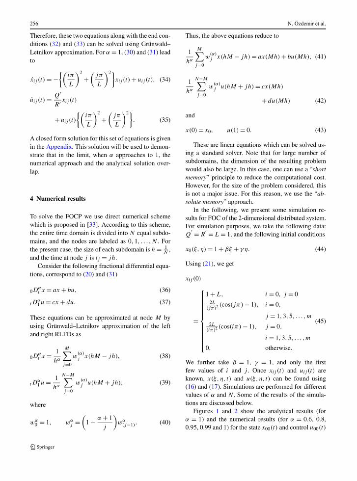
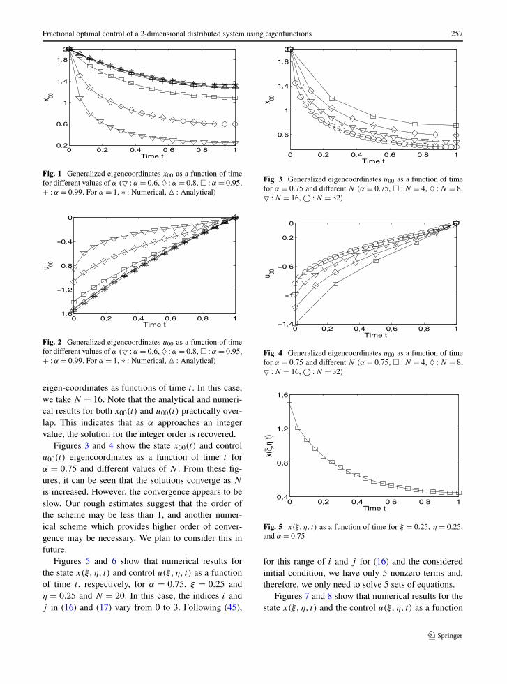
Fig. 1 Generalized eigencoordinates x00 as a function of timefor different values of α (� : α = 0.6, ♦ : α = 0.8, � : α = 0.95,+ : α = 0.99. For α = 1, ∗ : Numerical, � : Analytical)

Fig. 2 Generalized eigencoordinates u00 as a function of timefor different values of α (� : α = 0.6, ♦ : α = 0.8, � : α = 0.95,+ : α = 0.99. For α = 1, ∗ : Numerical, � : Analytical)

eigen-coordinates as functions of time t . In this case,we take N = 16. Note that the analytical and numeri-cal results for both x00(t) and u00(t) practically over-lap. This indicates that as α approaches an integervalue, the solution for the integer order is recovered.

Figures 3 and 4 show the state x00(t) and controlu00(t) eigencoordinates as a function of time t forα = 0.75 and different values of N . From these fig-ures, it can be seen that the solutions converge as N

is increased. However, the convergence appears to beslow. Our rough estimates suggest that the order ofthe scheme may be less than 1, and another numer-ical scheme which provides higher order of conver-gence may be necessary. We plan to consider this infuture.

Figures 5 and 6 show that numerical results forthe state x(ξ, η, t) and control u(ξ, η, t) as a functionof time t , respectively, for α = 0.75, ξ = 0.25 andη = 0.25 and N = 20. In this case, the indices i andj in (16) and (17) vary from 0 to 3. Following (45),

Fig. 3 Generalized eigencoordinates u00 as a function of timefor α = 0.75 and different N (α = 0.75, � : N = 4, ♦ : N = 8,� : N = 16, © : N = 32)

Fig. 4 Generalized eigencoordinates u00 as a function of timefor α = 0.75 and different N (α = 0.75, � : N = 4, ♦ : N = 8,� : N = 16, © : N = 32)

Fig. 5 x(ξ, η, t) as a function of time for ξ = 0.25, η = 0.25,and α = 0.75

for this range of i and j for (16) and the consideredinitial condition, we have only 5 nonzero terms and,therefore, we only need to solve 5 sets of equations.

Figures 7 and 8 show that numerical results for thestate x(ξ, η, t) and the control u(ξ, η, t) as a function


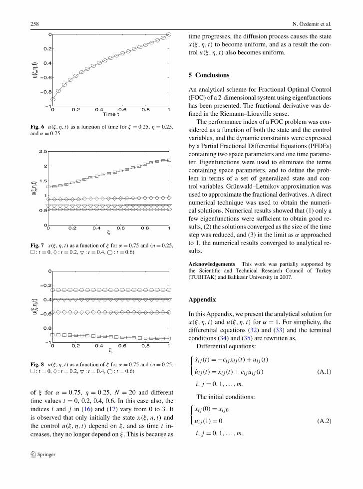
Fig. 6 u(ξ, η, t) as a function of time for ξ = 0.25, η = 0.25,and α = 0.75

Fig. 7 x(ξ, η, t) as a function of ξ for α = 0.75 and (η = 0.25,� : t = 0, ♦ : t = 0.2, � : t = 0.4, © : t = 0.6)

Fig. 8 u(ξ, η, t) as a function of ξ for α = 0.75 and (η = 0.25,� : t = 0, ♦ : t = 0.2, � : t = 0.4, © : t = 0.6)

of ξ for α = 0.75, η = 0.25, N = 20 and differenttime values t = 0, 0.2, 0.4, 0.6. In this case also, theindices i and j in (16) and (17) vary from 0 to 3. Itis observed that only initially the state x(ξ, η, t) andthe control u(ξ, η, t) depend on ξ , and as time t in-creases, they no longer depend on ξ . This is because as

time progresses, the diffusion process causes the statex(ξ, η, t) to become uniform, and as a result the con-trol u(ξ, η, t) also becomes uniform.

5 Conclusions

An analytical scheme for Fractional Optimal Control(FOC) of a 2-dimensional system using eigenfunctionshas been presented. The fractional derivative was de-fined in the Riemann–Liouville sense.

The performance index of a FOC problem was con-sidered as a function of both the state and the controlvariables, and the dynamic constraints were expressedby a Partial Fractional Differential Equations (PFDEs)containing two space parameters and one time parame-ter. Eigenfunctions were used to eliminate the termscontaining space parameters, and to define the prob-lem in terms of a set of generalized state and con-trol variables. Grünwald–Letnikov approximation wasused to approximate the fractional derivatives. A directnumerical technique was used to obtain the numeri-cal solutions. Numerical results showed that (1) only afew eigenfunctions were sufficient to obtain good re-sults, (2) the solutions converged as the size of the timestep was reduced, and (3) in the limit as α approachedto 1, the numerical results converged to analytical re-sults.

Acknowledgements This work was partially supported bythe Scientific and Technical Research Council of Turkey(TUBITAK) and Balikesir University in 2007.

Appendix

In this Appendix, we present the analytical solution forx(ξ, η, t) and u(ξ, η, t) for α = 1. For simplicity, thedifferential equations (32) and (33) and the terminalconditions (34) and (35) are rewritten as,

Differential equations:{

xij (t) = −cij xij (t) + uij (t)

uij (t) = xij (t) + cij uij (t)

i, j = 0,1, . . . ,m,

(A.1)

The initial conditions:{xij (0) = xij0

uij (1) = 0

i, j = 0,1, . . . ,m,

(A.2)


where

cij =(

iπ

L

)2

+(

jπ

L

)2

, i, j = 0,1, . . . ,m, (A.3)

and xij0, i, j = 0,1, . . . ,m are given by (21). From(A.1) we have

xij (t) − (c2ij + 1

)xij (t) = 0. (A.4)

This is an ordinary second order differential equationfor which a closed form solution can be found in astraight forward manner. Using (A.1) and (A.2), thesolution of (A.4) is given as

xij (t)

= xij0

√c2ij

+ 1 cosh(√

c2ij

+ 1(1 − t))√c2ij

+ 1 cosh(√

c2ij

+ 1) + cij sinh(√

c2ij

+ 1)

+ xij0

cij sinh(√

c2ij

+ 1(1 − t))√c2ij

+ 1 cosh(√

c2ij

+ 1) + cij sinh(√

c2ij

+ 1).

(A.5)

Using (A.1) and (A.5), we have

uij (t)

= −kxij0

sinh(√

c2ij

+ 1(1 − t))√c2ij

+ 1 cosh(√

c2ij

+ 1) + c2ij

sinh(√

c2ij

+ 1).

(A.6)

Finally, x(ξ, η, t) and u(ξ, η, t) are given by (16)and (17), where xij (t) and uij (t) are given by (A.5)and (A.6).

References

1. Oldham, K.B., Spanier, J.: The Fractional Calculus. Acad-emic Press, New York (1974)

2. Miller, K.S., Ross, B.: An Introduction to the FractionalCalculus and Fractional Differential Equations. Wiley, NewYork (1993)

3. Samko, S.G., Kilbas, A.A., Marichev, O.I.: Fractional In-tegrals and Derivatives—Theory and Applications. Gordonand Breach, Longhorne (1993)

4. Carpinteri, A., Mainardi, F.: Fractal and Fractional Calculusin Continuum Mechanics. Springer, Vienna (1997)

5. Rossikhin, Y.A., Shitikova, M.V.: Applications of frac-tional calculus to dynamic problems of linear and nonlin-ear hereditary mechanics of solids. Appl. Mech. Rev. 50,15–67 (1997)

6. Podlubny, I.: Fractional Differential Equations. AcademicPress, New York (1999)

7. Hilfer, R.: Applications of Fractional Calculus in Physics.World Scientific, River Edge (2000)

8. Magin, R.L.: Fractional Calculus in Bioengineering. BegellHouse, Redding (2006)

9. Kilbas, A.A., Srivastava, H.M., Trujillo, J.J.: Theory andApplications of Fractional Differential Equations. Elsevier,Amsterdam (2006)

10. Dorcak, L.: Numerical models for simulation the fractional-order control systems. UEF SAV, The Academy of SciencesInstitute of Experimental Physics, Kosice, Slovak Republic(1994)

11. Dorcak, L., Lesco, V., Kostial, I.: Identification offractional-order dynamical systems. In: Proceedings of the12th International Conference on Process Control and Sim-ulation ASRTP’96, pp. 62–68. Kosice, Slovak Republic(1996)

12. Podlubny, I., Dorcak, L., Kostial, I.: On fractional deriva-tives, fractional-order dynamic systems and PIλDμ con-trollers. In: Proceedings of the 1997 36th IEEE Conferenceon Decision and Control, Part 5, pp. 4985–4990. San Diego,CA, USA, 10–12 December 1997

13. Vinagre, B.M., Podlubny, I., Hernández, A., Feliu, V.:Some applications of fractional order operators used in con-trol theory and applications. Fract. Calc. Appl. Anal. 3,231–248 (2000)

14. Barbosa, R.S., Machado, J.A.T., Ferreira, I.M.: A Frac-tional calculus perspective of PID tuning. In: Proceedingsof DETC03 ASME 2003 Design Engineering TechnicalConference and Computers and Information in Engineer-ing Conference Chicago, IL, 2–6 September 2003

15. Ma, C., Hori, Y.: Fractional order control and its applica-tions of PIαD controller robust two-inertia speed control.In: The 4th International Power Electronics and MotionControl Conference, IPEMC, 14–16 August 2004

16. Barbosa, R.S., Machado, J.A.T.: Implementation ofdiscrete-time fractional-order controllers based on LS ap-proximations. Acta Polytech. Hung. 3, 4 (2006)

17. Rudas, I.J., Tar, J.K., Patkai, B.: Compensation of dynamicfriction by a fractional order robust controller. In: IEEEInternational Conference on Computational Cybernetics,pp. 9–14. Tallinn, 20–22 August 2006

18. Outsaloup, A.: La Commande CRONE: Commande Ro-buste d’Ordre Non Entiére. Hermes, Paris (1991)

19. Podlubny, I.: Fractional-order systems and PIλDμ con-trollers. IEEE Trans. Autom. Control 44, 208–214 (1999)

20. Petras, I.: The fractional-order controllers: methods fortheir synthesis and application. J. Electr. Eng. 50, 284–288(1999)

21. Machado, J.A.T.: Analysis and design of fractional-orderdigital control systems. Syst. Anal. Model. Simul. 27, 107–122 (1997)

22. Machado, J.A.T.: Fractional-order derivative approxima-tions in discrete-time control systems. Syst. Anal. Model.Simul. 34, 419–434 (1999)

23. Bagley, R.L., Calico, R.A.: Fractional order state Equationsfor the control viscoelastically damped structures. J. Guid.Control Dyn. 14, 304–311 (1991)

24. Hestenes, M.R.: Calculus of Variations and Optimal Con-trol Theory. Wiley, New York (1966)


25. Bryson, Jr., A.E., Ho, Y.C.: Applied Optimal Control: Op-timization, Estimization, and Control. Blaisdell, Waltham(1975)

26. Sage, A.P., White, III, C.C.: Optimum Systems Control.Prentice-Hall, Englewood Cliffs (1977)

27. Gregory, J., Lin, C.: Constraint Optimization in the Cal-culus of Variations and Optimal Control Theory. VanNostrand-Reinhold, New York (1992)

28. Agrawal, O.P.: Formulation of Euler–Lagrange equationsfor fractional variational problems. Math. Anal. Appl. 272,368–379 (2002)

29. Agrawal, O.P.: A general formulation and solution schemefor fractional optimal control problems. Nonlinear Dyn. 38,323–337 (2004)

30. Agrawal, O.P.: A general scheme for stochastic analysisof fractional optimal control problems. In Mahaute, A.L.,Machado, J.A.T., Trigeassou, J.C., Sabatier, J. (eds.) Frac-tional Differentiation and Its Applications, pp. 615–624(2005)

31. Agrawal, O.P.: A formulation and a numerical scheme forfractional optimal control problems. In: Proceedings of the2nd IFAC Conference on Fractional Differentiations and ItsApplications, IFAC (2006)

32. Agrawal, O.P.: A quadratic numerical scheme for fractionaloptimal control problems. J. Dyn. Syst. Measur. Control(2008, to appear)

33. Agrawal, O.P., Baleanu, D.: A Hamiltonian formulationand a direct numerical scheme for fractional optimal con-trol problems. J. Vib. Control 13, 1269–1281 (2007)

34. Agrawal, O.P.: Fractional Optimal Control of a DistributedSystem Using Eigenfunction. In: Proceedings of the 2007ASME International Design Engineering Technical Confer-ences, Las Vegas, NV, 4–7 September 2007

35. Hanyga, A.: Multi-dimensional solutions of space-time-fractional diffusion euations. Proc. R. Soc. Lond. A 458,429–450 (2002)

36. Hanyga, A.: Multi-dimensional solutions of time-fractionaldiffusion-wave equations. Proc. R. Soc. Lond. A 458, 933–957 (2002)

37. Butzer, P.L., Westphal, U.: An introduction to fractionalcalculus. In: Hilfer, R. (ed.) Applications of Fractional Cal-culus in Physics, pp. 1–85. World Scientific, Singapore(2000)

Fractional optimal control of a 2-dimensional distributed system using eigenfunctions

Documents

Transcript of Fractional optimal control of a 2-dimensional distributed system using eigenfunctions