Four different study designs to evaluate vaccine safety were equally validated with contrasting...

Journal of Clinical Epidemiology 59 (2006) 808–818

Four different study designs to evaluate vaccine safety wereequally validated with contrasting limitations

Jason M. Glanza,*, David L. McClurea, Stanley Xua, Simon J. Hambidgea,b,c, Martin Leed,Margarette S. Kolczake, Ken Kleinmanf, John P. Mulloolyg, Eric K. Francea

aClinical Research Unit, Kaiser Permanente, P. O. Box 378006, Colorado, Denver, CO, 80237-8066, USAbCommunity Health Services, Denver Health Medical Center, Denver, CO, USA

cDepartment of Pediatrics, University of Colorado School of Medicine, Denver, CO, USAdUCLA Center for Vaccine Research, Torrance, CA, USA

eCenters for Disease Control and Prevention, Atlanta, GA, USAfDepartment of Ambulatory Care and Prevention, Harvard Medical School and Harvard Pilgrim Health Care, Boston, MA, USA

gCenter for Health Research, Northwest Kaiser Permanente, Portland, OR, USA

Accepted 16 November 2005

Abstract

Objective: We conducted a simulation study to empirically compare four study designs [cohort, case–control, risk-interval, self-controlled case series (SCCS)] used to assess vaccine safety.

Study Design and Methods: Using Vaccine Safety Datalink data (a Centers for Disease Control and Prevention-funded project), wesimulated 250 case sets of an acute illness within a cohort of vaccinated and unvaccinated children. We constructed the other three studydesigns from the cohort at three different incident rate ratios (IRRs, 2.00, 3.00, and 4.00), 15 levels of decreasing disease incidence, and twoconfounding levels (20%, 40%) for both fixed and seasonal confounding. Each of the design-specific study samples was analyzed witha regression model. The design-specific b̂ estimates were compared.

Results: The b̂ estimates of the case–control, risk-interval, and SCCS designs were within 5% of the true risk parameters or cohortestimates. However, the case–control’s estimates were less precise, less powerful, and biased by fixed confounding. The estimates of SCCSand risk-interval designs were biased by unadjusted seasonal confounding.

Conclusions: All the methods were valid designs, with contrasting strengths and weaknesses. In particular, the SCCS method proved tobe an efficient and valid alternative to the cohort method. � 2006 Elsevier Inc. All rights reserved.

Keywords: Simulation study; Cohort; Case–control; Risk-interval; Self-controlled case series (SCCS); Bias (epidemiology); Confounding factors (epidemiology)

1. Introduction

The most widely accepted methods for evaluating vac-cine safety have been study designs that compare distinctexposed and unexposed, or diseased and nondiseased pop-ulations. These study methods include prospective designssuch as the cohort, and retrospective designs such as thecase–control. This investigation evaluates these traditionalstudy designs as well as two newer designs in a simulatedanalysis of a known, rare, and acute vaccine reaction: idio-pathic thrombocytopenic purpura (ITP) after measles-mumps-rubella (MMR) vaccination [1,2].

In a cohort study, a group of healthy vaccinated and unvac-cinated individuals are followed forward in time, and the in-cidence of illness in the two groups is compared. This design

* Corresponding author. Tel.: 303-636-3118; fax: 303-636-3109.

E-mail address: [email protected] (J.M. Glanz).

0895-4356/06/$ – see front matter � 2006 Elsevier Inc. All rights reserved.

doi: 10.1016/j.jclinepi.2005.11.012

provides a direct estimate of effect (the incidence rate ratio,IRR), is well suited for rare exposures, and can be used toanalyze multiple outcomes [3,4]. It can, however, be difficultand costly to implement when the disease is rare, and becausevaccine safety studies typically involve populations withhigh vaccine coverage rates, there may be few unvaccinatedcontrols available. The design is also susceptible to biasesthat can be introduced by comparing vaccinated and unvacci-nated populations, as these groups may differ by ethnicity,socioeconomic status, and underlying health states [5].

In nested case–control studies, individuals who experi-enced a particular event over a defined time period are iden-tified. This group of cases is then compared to a controlgroup of event-free individuals from the same time period,who are often matched to the cases on variables such asgender, managed care organization (MCO), and age [1,6–8]. This design is economical and well suited for rare ill-nesses. In addition, because the cases are typically matched

mailto:[email protected]

809J.M. Glanz et al. / Journal of Clinical Epidemiology 59 (2006) 808–818

to the controls by age and calendar time (e.g., the age at thedate of diagnosis), particular time-varying confounders,such as age and seasonality, are adjusted for by proxy. Aswith the cohort method, however, confounding variables re-lated to both the outcome and vaccination statusdas wellas other time-varying factors such as underlying healthstatesdwill bias the case-control design.

Since 1995, alternative methods known as the risk-interval(or vaccinated cohort) and self-controlled case series (SCCS)study designs have been used for vaccine safety studies[2,7,9–15]. These designs differ from more traditionalmethods in that time intervals both before and after vaccina-tion within the same individual are used to classify a personas exposed or unexposed. In the risk-interval design, inci-dence rates for risk and nonrisk time periods are compared,but only vaccinated individuals are included in the study. Atime period immediately following vaccination is designatedas the risk-interval, and events that occur during this periodare classified as exposed cases. Time periods outside of therisk-intervaldbefore and after the vaccinationdare consid-ered the nonrisk (or control) periods, where occurrences ofillness are classified as unexposed cases. Because only vacci-nated individuals are included in the study, biases introducedby comparing vaccinated and unvaccinated populations areminimized. In addition, because control time periods bothbefore vaccination and after the risk period are included inthe analysis, the design is ideal for assessing the risk of acute,self-limiting events following vaccination.

The SCCS method is a similar design in which incidencerates for risk and nonrisk time periods are compared, but onlycases are necessary for the analysis [14–17]. The study pop-ulation comprises only cases that occur over a predefined ob-servation period, and each case acts as its own control,thereby controlling for both measured and unmeasured con-founding variables that do not vary over time. With the SCCSmethod, multiple occurrences of independent events withinan individual can be analyzed. Theoretical calculations havealso demonstrated that the method’s statistical power closelyapproximates that of a cohort study when the vaccinationcoverage rate is high and the periods of risk following vacci-nation are short [14,15]. To our knowledge, however, theseassertions have not been validated empirically.

Possible limitations of the risk-interval and SCCSmethods stem from their ability to implicitly control fortime-varying confounders, such as seasonality or age. Incontrast to the case–control analysis, these covariates can-not be adjusted for by proxy in the risk-interval and SCCSanalyses. Instead, time-varying confounders must be ex-plicitly defined as either continuous functions or categoricalvariables and added to multiple Poisson regression models[12,14]. Mis-specifying such variables can lead to biasedresultsdparticularly when the event is rare [18].

To address some of the gaps in the current literature, weconducted a simulation study that evaluated the bias andprecision of the four study designs’ IRR estimates, the sta-bility of the design-specific IRR estimates at different levels

of disease incidence, and each design’s ability to handle un-measured confounding.

2. Materials and methods

2.1. Data

This study was conducted under the Vaccine SafetyDatalink (VSD), a Centers for Disease Control and Preven-tion-funded project that links large administrative databasesfrom eight MCOs located across the United States. The fo-cus of the VSD is to conduct epidemiologic studies of vac-cine safety [19]. Currently, the VSD databases containhealth care data from 1991 to 2003, representing a cohortof over 5,000,000 children younger than 18 years of age.For this study, we used VSD data through year 2000 fromfive of the MCO sites.

2.2. Cohort construction and simulation

We first constructed a retrospective cohort study popula-tion using the following VSD data fields: MCO, birth date,gender, membership dates, and MMR vaccination dates. Toensure a balanced distribution of important variables amongthe study groups, each MMR vaccinated child was matchedto one unvaccinated child by gender, MCO, and age (within7 days) at the date of the vaccination (n 5 2,774,122). Upto 365 days before and after the matched dates were usedas follow-up times (i.e., the observation periods). Unvacci-nated children did not receive a vaccination during their en-tire follow-up time of up to 730 days surrounding thematched date. In the exposed children, the 42-day period fol-lowing vaccination was defined as exposed person-time. The6-week postvaccination period is an exposure time interval inwhich ITP has been attributed to the MMR vaccine [1,2]. Allof the time outside of the 42-day risk period was designatedas unexposed person-time. On average, each cohort membercontributed 591 days of person-time follow-up.

After the study population was constructed, cases of ITPwere simulated on a specific date (diagnosis date) withinthe defined follow-up times at a fixed IRR. Exposed caseswere simulated in the 42-day risk periods, while unexposedcases were simulated in the time periods outside of the riskperiods. In the unexposed (or unvaccinated) subjects, caseswere simulated within the entire 365-day periods before orafter the matching date. The following probabilistic modelwas used to simulate the cases:

p 5 pt1

1 1 e2

�b0 1 b1x1Þ

ð1Þ

where p is the probability of being a case, b0 is the inter-cept of the model, b1 is the main parameter of interest, x1

is the exposure indicator (1 5 exposed and 0 5 unex-posed), and pt represents person-time contributed. For un-exposed individuals (x1 5 0), p is a function of pt andb0. To approximate b0, we used the estimated annual

810 J.M. Glanz et al. / Journal of Clinical Epidemiology 59 (2006) 808–818

incidence rate of ITP (eight cases per 100,000 children)[20]. In the cohort population, the estimated incidence rate(cases per person-day) among the unexposed was 2.19 3

1027; the natural log of this number is b0. The b1s werechosen to be 0.693, 1.099, and 1.386 for IRR levels 2.00,3.00, and 4.00, respectively. We chose these IRR levels be-cause they represent strengths of associations that tend toinfluence vaccination policy.

The form of equation 1 implies that the probability ofbeing a case is proportional to the amount of person-timecontributed. The second term of eq. (1) represents the prob-ability of being a case on any day during the follow-upperiod. But, because our study population was so large, itwas not feasible to simulate cases based on each day’s prob-ability. Instead, we used eq. (1) to simulate the cases withineach subject’s predefined follow-up periods: prevaccinationunexposed, postvaccination exposed, and postvaccinationunexposed. Given the maximum amount of person-timecontributed (i.e., 730 days) and the range of b0 and b1, theprobability of being a case could never be greater than 1.

The goal of the simulation was to compare the gold stan-dard b̂1estimates of the cohort to those of the risk-interval,SCCS, and case–control study designs. Therefore, we firstcreated a cohort gold standard population from the actualVSD data and simulated the cases to create each of thethree fixed b1 levels (IRR 5 2.00, 3.00, and 4.00). We thenused these cohort populations to build the populations forthe three remaining study designs. Each design was nestedwithin the cohort so that direct comparisons could be made.In addition, the b̂1 estimates of all four designs were com-pared to the true, fixed b1 values.

To determine a suitable number of iterations, we simu-lated 100, 250, 500, 1,000, 1,500, and 2,000 cohort popula-tions at an IRR of 2.00. As the number of iterationsincreased, the variances of the b̂1 estimates expectedly de-creased, but the differences between the mean b̂1 estimatesdemonstrated little variability. The differences between themean b̂1 estimates and the true b1 (b1 5 0.693) remainedwithin 2.5 to 3.0% as the number of iterations increasedfrom 250 to 2,000. Thus, at each of the three IRR levels,we constructed 250 cohort, risk-interval, SCCS and case–control study populationsdthe latter three of which werenested within the cohort. Each of the 250 simulated studypopulations was analyzed with an appropriate regressionmodel, and the design-specific b̂1 estimates of the nesteddesigns were compared to those of the cohort and to thetrue b1 values (Fig. 1).

To evaluate the stability of the different study designs, wecontinuously reduced the case population by 20% in the co-hort design and repeated the simulation. The case populationswere decreased by lowering the baseline disease incidencerate, that is, decreasing the value of b0 in the probabilisticmodel used to simulate the cases. For each successive casepopulation, the amount of person-time contributed (thedenominator of the incidence rate) remained constant. Theobjective of this study component was to demonstratedat

various IRR levelsdhow the design-specific regression esti-mates differ as the incidence of disease decreases.

2.3. The nested study designs

2.3.1. Case–controlThe simulated cases from the cohort were identified and

matched to nondiseased controls by age (within 67 days) atthe simulated diagnosis date, MCO, and gender. Cases andall of their matched controls represented risk sets [21]. Inour primary analysis, four controls were randomly sampledfrom each risk set. A 1:4 case-to-control match was sufficientto detect an odds ratio of 1.95 with a case population size of400 and 80% power (two-sided, a 5 0.05). We also conductedanalyses using case-to-control matches of 1:10, 1:100, and1:n (all available controls). For the 1:n design, there were 2to 1,326 (median, 629) available controls for each case.

A case or matched control was considered exposed if anMMR vaccination date was within 42 days prior to the diag-nosis date of the matched case. The sampled risk sets repre-sented matched strata, which were included in conditionallogistic regression models to estimate odds ratios (OR) forthe risk of the event in the 42-day risk period. The b̂1 esti-mates for the ORs of the case–control design were compared

At a fixed incidence rate ratio and incidence level,randomly assign case status (250 simulations)

Construct 250 study populations for the risk-interval,SCCS and case-control study designs

Analyze the data from the four study designs

Calculate mean estimate, mean squared error(MSE), percent bias and empirical power for eachdesign*

Evaluateconfounding?

Randomly assign confounding variable statusat fixed or time-varyingconfounding levels

YES

NO

To evaluate stability, reduce case populationsize by 20% and repeat simulation

Make a cohort of vaccinated and unvaccinatedindividuals from the VSD cohort, matched on ageat vaccination, gender and MCO

Fig. 1. Summary of steps for the simulation study. *See text for definitions.


to the b̂1 estimates for the IRRs of the cohort design and to thetrue b1 values; the OR approximates the IRR when the inci-dence of disease is rare and the risk periods are short [14,22].

2.3.2. Risk-intervalThe risk-interval analysis was limited to the MMR vacci-

nated children from the cohort population (n 5 1,387,061).The 42-day periods following vaccination represented theexposed risk intervals, and the time outside of this peri-oddup to 365 days before and 42 to 364 days after vaccina-tiondrepresented the unexposed nonrisk intervals. Becausethis study population was half the size of the cohort popula-tion, only cases that had been simulated during the obser-vation periods (i.e., up to 365 days before and after thevaccination date) of the vaccinated cohort subjects wereincluded. The risk-interval data were analyzed with Poissonregression.

2.3.3. Self-control case series (SCCS)The simulated cases from the cohort population were in-

cluded in the SCCS analysis. Once the cases were identi-fied, the follow-up timesdup to 365 days before andafter the matched cohort vaccination datedwere used to as-certain exposure status. The incidence of simulated ITP inthe 42-day risk period following vaccination was comparedto the incidence in the time periods outside of the risk pe-riod. Conditional Poisson regression was used to estimatethe IRR of ITP in the 42-day risk window, treating eachcase as a unique stratum [15].

2.4. Confounding

The final objective was to examine how well each designhandled unmeasured confounding, which we simulated intwo different forms. The first form was a fixed confoundingvariable that did not vary over time, and the second wasa time-varying confounder that represented a fluctuatingrisk of illness across the follow-up periods.

2.4.1. Unmeasured/unknown fixed confoundingFirst, we simulated a hypothetical secondary disease

state (the confounder) in the cohort, so that the prevalenceof disease was both higher in the vaccinated than in theunvaccinated and associated with the primary outcome ofinterest (ITP). The overall prevalence of the secondary dis-ease state was 10%, representing the percentage of VSD co-hort members with a hypothetical preexisting condition thatrendered them at high-risk for developing ITP. This 10%prevalence was disproportionately distributed so that 16%of the vaccinated and 4% of the unvaccinated were classifiedas high risk. Then, using the form of eq. (1) with vaccinationexposure (x1) and high-risk status (x2) as dichotomouscovariates, we simulated two sets of 250 cohort populationsat a vaccine-associated IRR of 2.00 (b1 5 0.693) and at twodifferent high risk-associated IRRs of 4.50 (b2 5 1.50) and12.20 (b2 5 2.50). At both of the fixed b2s of 1.50 and 2.50,

the mean coefficient estimate for vaccination exposure (b̂1)was 0.671 (IRR 5 1.95). When the high risk variables wereremoved from both sets of regression models, the b̂1 valuesincreased by 20% (b̂1 5 0.805, IRR 5 2.24) and 40% (b̂1 5

0.939, IRR 5 2.56), respectively. Although evaluatingconfounding in a regression model is somewhat arbitrary,a change of 20% or more is often described as meaningful[23,24].

From each of the 250 simulated cohort populations, thestudy populations for the other designs were created. Thedesign-specific data were analyzed as if the confoundingbias was unmeasured or unknown, and the results werecompared to the adjusted regression coefficient estimatesof the cohort.

2.4.2. Seasonal time-varying confoundingNext, we simulated 20 and 40% seasonal, time-varying

confounding in the cohort. We created a seasonal effect inwhich the probability of being simulated as a case dependedon calendar time as well as vaccination status. A greater per-centage of MMR vaccinations were given in the summermonths between May and August, mainly due to the vacci-nation pattern of children ages 4–12 years (school physi-cals). To create the seasonal effect, we simulated anincreased risk for developing ITP between Decemberthrough March, even though a seasonal pattern of ITP isnot known to exist. As with the fixed confounding, we usedeq. (1) with vaccination exposure (x1) as the main effect andadded a covariate (x2) for the time-varying, seasonal factor.Specifically, we simulated 250 cohort populations at twodifferent seasonal, time-varying effect (b2) levels of 1.30(IRR 5 3.67) and 2.90 (IRR 5 18.11). These relatively largeeffect levels were necessary because of the mild seasonaldistribution of MMR administration: 42.5% were given inthe four summer months vs. 26.1% during the 4-month,high-risk, winter period. At the two seasonal effect levels,the mean exposure coefficient estimates (b̂1) were 0.679(IRR 5 1.97) and 0.702 (IRR 5 2.02), respectively. Whenthe seasonal covariates were removed from the regressionmodels, the mean b̂1s decreased to 0.538 and 0.417, repre-senting changes of approximately 20 and 40%, respectively.From these simulated cohorts with the infused time-varying,seasonal confounding, we created the other design-specificstudy populations and observed how the nested designshandled the confounding bias. We examined the bias bothas if season was unmeasured and with the seasonal covari-ates adjusted in the regression analyses.

2.5. Outcome measures

After the design-specific analyses were completed, eachof the 250 design-specific regression estimates at each IRRlevel was compared to the corresponding regression esti-mate from the simulated cohort design and to the true b1

values. The differences between regression estimates wereexpressed as percent biases.


2.5.1. BiasBias is presented in two forms:

1. The percent bias from the truth measures the percent dif-ference between the true parameter (b1) and the regres-sion estimates (b̂1) of the four study designs [eq. (2)].

Percent Bias from True 5

nested design estimate 2 true parameter

true parameter3 100

ð2Þ

2. The percent bias from the cohort is defined as the per-cent difference between the cohort regression estimatesand the corresponding regression estimates of the risk-interval, SCCS and case–control designs [eq. (3)].

Percent Bias from Cohort 5

nested design estimate 2 cohort gold standard estimate

cohort gold standard estimate

3 100

ð3Þ

Percent biases are presented at each IRR level using thelargest case incidence level (average case population sizeacross the three IRR levels 5 392; estimated incidencerate 5 8 cases per 100,000 person-years).

2.5.2. Mean squared errorThe mean squared error (MSE) measures the average

squared difference between the parameter estimate and itstrue value [eq. (4)]. It contains two components: the vari-ance of the 250 parameter estimates (precision) and thesquare of the average bias (accuracy).

MSE 5

P250

i 5 1

�b̂i 2 b

�2

2505 Var

�b̂�

1

0BB@

P250

i 5 1

b̂i 2 b

250

1CCA

2

ð4Þ

2.5.3. Empirical powerEmpirical power demonstrates, at each incidence level,

what percentage of the 250 design-specific IRR estimateswas positive and significant (P ! .05). It is the proportionof the statistical models that had enough cases to generateIRR estimates that rejected the null hypothesis. As the casepopulation decreases, it is less likely the null hypothesiswill be rejected.

3. Results

3.1. Bias and precision

The mean estimates, mean percent biases, and MSEs foreach design are displayed in Table 1. Across the three IRR
T
able

1

Mea

nes

tim

ates

of

b̂1

(mea

nsq

uar

eder

ror)

and

mea

np

erce

nt

bia

sesa

,b(s

tan

dar

der

rors

)w

ith

resp

ect

toth

eco

ho

rtan

dtr

ue

risk

par

amet

er,

by

des

ign

,b

yin

cid

ence

rate

rati

o(I

RR

)le

vel,

bas

edo

n250

sim

ula

tionsc

Tru

eva

lue

of

b1

50

.69

3

(IR

R5

2.0

0)

Tru

eva

lue

of

b1

51

.09

9

(IR

R5

3.0

0)

Tru

eva

lue

of

b1

51

.386

(IR

R5

4.0

0)

Stu

dy

des

ign

sb̂

1(M

SE

)%

Bia

sco

ho

rt(S

E)

%B

ias

tru

e(S

E)

b̂1

(MS

E)

%B

ias

coh

ort

(SE

)%

Bia

str

ue

(SE

)b̂

1(M

SE

)%

Bia

sco

ho

rt(S

E)

%B

ias

tru

e(S

E)

Coh

ort

0.6

71(0

.04

4)d

23

.2(1

.9)

1.0

67(0

.02

9)d

22

.9(1

.0)

1.3

76(0

.02

2)d

20

.8(0

.7)

Ris

kin

terv

al0

.674

(0.0

48)

20

.6(1

.4)

22

.7(2

.0)

1.0

66(0

.03

0)0

.0(0

.3)

23

.0(1

.0)

1.3

80(0

.02

3)0

.4(0

.3)

20

.4(0

.7)

SC

CS

d0

.661

(0.0

48)

22

.7(1

.8)

24

.7(2

.0)

1.0

55(0

.03

2)2

1.1

(0.4

)2

4.0

(1.0

)1

.363

(0.0

24)

20

.9(0

.3)

21

.7(0

.7)

Cas

eco

ntr

ole

1:4

0.6

57(0

.07

5)2

2.7

(1.9

)2

5.2

(2.5

)1

.074

(0.0

56)

0.6

(1.0

)2

2.3

(1.4

)1

.369

(0.0

43)

20

.4(0

.7)

21

.2(0

.9)

1:1

00

.664

(0.0

56)

20

.8(2

.1)

24

.2(2

.2)

1.0

68(0

.03

9)0

.3(0

.7)

22

.8(1

.1)

1.3

72(0

.03

4)2

0.3

(0.5

)2

1.0

(0.8

)

1:1

00

0.6

61(0

.04

9)2

2.6

(1.7

)2

4.6

(2.0

)1

.063

(0.0

33)

20

.3(0

.5)

23

.3(1

.0)

1.3

68(0

.02

9)2

0.6

(0.4

)2

1.3

(0.8

)

1:n

0.6

62(0

.04

9)2

2.6

(1.6

)2

4.5

(2.0

)1

.063

(0.0

33)

20

.2(0

.5)

23

.2(1

.0)

1.3

69(0

.02

8)2

0.5

(0.4

)2

1.3

(0.8

)

aP

erce

nt

bia

sco

ho

rt5

nes

ted

des

ign

esti

mat

e2

cohort

gold

stan

dar

des

tim

ate

coh

ort

go

ldst

anda

rdes

tim

ate

310

0:

bP

erce

nt

bia

str

ue

5n

este

dd

esig

nes

tim

ate

2tr

ue

par

amet

er

tru

ep

aram

eter

310

0:

cT

he

foll

owin

gpro

bab

ilis

tic

model

was

use

dto

sim

ula

teth

eca

ses:

p5

per

son

tim

e1

11

e2ðb

01

b1x 1Þ,

wh

ere

b0

52

15

.3an

db

15

0.6

93,

1.0

99

,o

r1

.38

6.

dS

elf-

con

tro

lled

case

seri

es.

eM

atch

edca

se-t

o-c

ontr

ol

rati

os

1:4

,1

:10

,1

:10

0,

1:n

(all

avai

lab

le).


levels, the cohort design produced mean biases of 23.2 to20.8% when compared to the true value of b1. The meanpercent biases with respect to the cohort estimates or tothe true parameters ranged from 25.2 to 0.6% across thefour study methods and three IRR levels. These measuresfor the case–control design remained within the same rangewhen the case-to-control ratio increased to 1:10, 1:100,and 1:n.

The MSEs of the estimates for the risk-interval andSCCS were within 11.0% of the cohort’s MSEs acrossthe three IRR levels, while the MSEs of the case–control(1:4) were from 70.5 to 95.5% larger than those of the co-hort (Table 1). The case–control’s MSEs for case-to-controlratios of 1:10, 1:100, and 1:n were between 11.4 to 54.5%larger than those of the cohort. When compared to the co-hort, the percentage differences for ratios 1:100 and 1:nwere approximately equivalent, suggesting no additionalefficiency was gained by using more than 100 controls.

Across the three IRR levels, the mean coefficient esti-mates of the four designs remained within 5.0% of eachother as the incidence rate decreased (Fig. 2). However, be-low an incidence rate of 0.66 cases per 100,000 person-years (33 cases), all of the designs produced mean coeffi-cient estimates that were approximately 5.0 to 50.0%greater than the true effect. At the low incidence levels,fewer of the regression models were able to generate stable,bounded b̂1 estimates due to zero cells, that is, either nosimulated exposed or unexposed cases. When the models

did converge at the low incidence levels, the resulting re-gression estimates tended to overestimate the true effect,with wide confidence intervals. This occurred because a re-gression model needed at least one exposed case to gener-ate a bounded estimate. Often, at the low incidence levels,the incidence rate in the exposed with only one case wasdisproportionately larger than the unexposed incidence rate,leading to a mean b̂ estimate that overestimated the trueeffect.

Overall, at each IRR level, the MSEs of the regressionestimates increased as the incidence rate decreased, butthe differences between the MSEs of the designs varied(Fig. 3). As the case population declined, the MSEs ofthe case–control were consistently higher than those ofthe other designs, and the magnitude of the difference in-creased as the incidence rate decreased. This pattern wasobserved with all of the case-to-control ratios.

3.2. Empirical power

Across all of the IRR levels, the empirical power of therisk-interval and SCCS designs were within 15.4% of thecohort values (Fig. 4). With decreasing case populationsizes, the empirical power of the case-control design (1:4)was up to 75.0% lower than that of the other designs. Asthe case-to-control ratio increased from 1:4 to 1:n, thecase–control’s power approached that of the cohort design,

Mean β estimates of four study designs

β1=1.386 (IRR=4.00)

β1=0.693 (IRR=2.00)

∆ Cohort + Risk-intervalo SCCSx Case-control

β1=1.099 (IRR=3.00)

1.5

1.0

Mea

n β

estim

ates

0.5

1.5

1.0

0.5

400 1740130

400 1740130Mean number of cases

Fig. 2. The mean of each design’s 250 regression estimates, by mean case population size, by incidence rate ratio (IRR) levels 2.00, 3.00, and 4.00. The

mean case numbers represent the mean case population size of the 250 simulations. The mean case numbers 400, 130, 40, and 17 represent incidence rates of

8.00, 2.70, 0.80, and 0.35 cases per 100,000 person-years.


0.2

0.4

0.6

0.8

0.0

0.8

0.6

0.4

0.2

0.0

Mean squared error of β estimates of four study designs

β1=1.386 (IRR=4.00)

β1=0.693 (IRR=2.00)


β1=1.099 (IRR=3.00)

M

ean

squa

red

erro

r of β

est

imat

es

400 1740130

400 1740130Mean number of cases

Fig. 3. The mean squared error of each design’s 250 regression estimates, by mean case population size, by incidence rate ratio (IRR) levels 2.00, 3.00, and

4.00. The mean case numbers represent the mean case population size of the 250 simulations. The mean case numbers 400, 130, 40, and 17 represent in-

cidence rates of 8.00, 2.70, 0.80, and 0.35 cases per 100,000 person-years.

and it remained within 11.9% of the cohort as the case pop-ulation decreased (data not shown).

3.3. Confounding

3.3.1. Unmeasured/unknown fixed confoundingIn the presence of 20 or 40% confounding, the mean per-

cent biases of the risk-interval and SCCS designs rangedfrom 24.8% to 0.5% when compared to the adjusted cohortestimates or to the true parameters (Table 2). In contrast,when compared to the adjusted cohort or to the truth, themean percent biases of the case–control for all case-to-control ratios were approximately 20 and 40% for the tworespective levels of confounding.

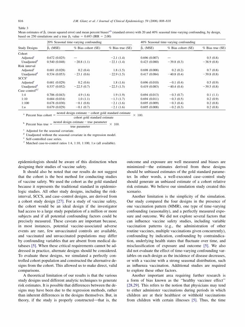
3.3.2. Seasonal time-varying confoundingAt 20 or 40% confounding, the mean percent biases of

the case–control estimates for all case-to-control ratioswere within 4.9% of the adjusted cohort estimates or thetrue parameters (Table 3). The estimates of the unadjustedrisk-interval and SCCS designs, on the other hand, were bi-ased by approximately 220 and 240% when compared tothe adjusted cohort estimates or to the truth. Conversely, themean percent biases of the adjusted risk-interval and SCCSdesigns were within 1.8% of the adjusted cohort estimatesor the true parameters.

4. Discussion

In this study using vaccine safety databases and simu-lated cases of a rare, acute illness (ITP) after MMR vacci-nation, the risk-interval, SCCS, and case–control studydesigns produced valid IRR estimates that were within3% of a cohort gold standard. The case–control designwas associated with the highest MSEs, the lowest empiricalpower, and the highest mean percent bias in the presence ofunmeasured, fixed confounding. Its estimates, nonetheless,were not biased when the confounding was simulated asa seasonal effect because the cases were matched to thecontrols by age and diagnosis date. The SCCS and risk-in-terval designs, in contrast, proved to be as powerful as thecohort (corroborating previously published theoretical re-sults) [14,15], demonstrated the ability to control for un-measured fixed confounding, and produced mean percentbiases that were considerably higher than those of thecase–control when the effect of seasonality was not ad-justed in the analysis.

While the case–control design proved to be more vari-able and less powerful than the other designs, the degreeof difference decreased as the number of controls for eachcase increased. At 100 or more controls for each case, theMSE and power of the case–control design approachedthose of the cohort. When conducting a case–control study(particularly if the analysis is limited to electronic data on-ly), more controls than the customary 4:1 ratio are chosen


Empirical power of four study designs

0.0

1.0

0.8

0.6

0.4

0.2Em

piric

al p

ower

0.0

1.0

0.8

0.6

0.4

0.2

β1=1.386 (IRR=4.00)

β1=0.693 (IRR=2.00)


β1=1.099 (IRR=3.00)

400 1740130

400 1740130

Mean number of cases

Fig. 4. The proportion of the 250 regression models with positive estimates (O0) and P ! .05, by study design, by mean case population size, by IRR levels

2.00, 3.00, and 4.00. The mean case numbers 400, 130, 40, and 17 represent incidence rates of 8.00, 2.70, 0.80, and 0.35 cases per 100,000 person-years.

to increase power and to detect effect modification [25,26].However, when additional data is collected through medicalchart review, the case–control design is no longer econom-ical at these higher case-to-control ratios.

We demonstrated empirically that the SCCS and risk-in-terval designs are biased if a seasonal effect is overlooked.However, we also showed that seasonality can be adjustedin a self-controlled design if a seasonal effect is suspected

a priori [12,18]. The challenge of conducting such an anal-ysis is that the form of seasonal variable must be explicitlydefined prior to conducting the analysis. This can be partic-ularly difficult if the event is rare, as there may not beenough information to estimate the seasonal effect. Thenested case–control design, on the other hand, providesa seasonal adjustment by proxy, since the cases are matchedto the controls by age and calendar time. We believe that

Table 2

Mean estimates of b̂1 (mean squared error) and mean percent biasesa,b (standard errors) with 20 and 40% unmeasured/unknown fixed confounding,

by design, based on 250 simulations and a true b1 value 5 0.693 (IRR 5 2.00)

20% Fixed confounding 40% Fixed confounding

Study designs b̂1 (MSE) % Bias cohort (SE) % Bias true (SE) b̂1 (MSE) % Bias cohort (SE) % Bias true (SE)

Cohortc 0.671 (0.030) d 23.1 (1.6) 0.671 (0.015) d 23.2 (1.1)

Risk intervald 0.674 (0.032) 0.3 (0.4) 22.8 (1.6) 0.673 (0.015) 0.5 (0.2) 22.7 (1.1)

SCCSd,e 0.660 (0.032) 21.9 (0.5) 24.8 (1.6) 0.661 (0.016) 21.5 (0.3) 24.7 (1.1)

Case–controld,f

1:4 0.838 (0.076) 26.1 (1.8) 20.9 (2.1) 0.961 (0.101) 45.0 (1.4) 38.7 (1.6)

1:10 0.825 (0.059) 24.5 (1.2) 19.0 (1.9) 0.965 (0.094) 45.3 (0.9) 39.2 (1.3)

1:100 0.822 (0.052) 24.3 (0.9) 18.7 (1.7) 0.965 (0.091) 45.4 (0.8) 39.2 (1.2)

1:n 0.823 (0.052) 24.3 (0.8) 18.7 (1.7) 0.965 (0.091) 45.4 (0.7) 39.3 (1.2)

a Percent bias cohort 5nested design estimate 2 cohort gold standard estimate

cohort gold standard adjusted estimate3 100:

b Percent bias true 5nested design estimate 2 true parameter

true parameter3 100:

c Controlling for x2, the fixed confounding factor.d Analyzed as if the confounding was unmeasured or unknown.e Self-controlled case series.f Matched case-to-control ratios 1:4, 1:10, 1:100, 1:n (all available).


Table 3

Mean estimates of b̂1 (mean squared error) and mean percent biasesa,b (standard errors) with 20 and 40% seasonal time-varying confounding, by design,

based on 250 simulations and a true b1 value 5 0.693 (IRR 5 2.00)

20% Seasonal time-varying confounding 40% Seasonal time-varying confounding

Study Designs b̂1 (MSE) % Bias cohort (SE) % Bias true (SE) b̂1 (MSE) % Bias cohort (SE) % Bias true (SE)

Cohort

Adjustedc 0.672 (0.025) d 22.1 (1.4) 0.696 (0.007) d 0.5 (0.8)

Unadjustedd 0.540 (0.048) 220.8 (1.1) 222.1 (1.4) 0.423 (0.080) 239.8 (0.3) 238.9 (0.8)

Risk interval

Adjustedc 0.681 (0.028) 0.2 (0.4) 1.8 (1.5) 0.698 (0.008) 0.2 (0.2) 0.7 (0.8)

Unadjustedd 0.534 (0.053) 223.1 (0.6) 222.9 (1.5) 0.417 (0.084) 240.8 (0.4) 239.8 (0.8)

SCCSe

Adjustedc 0.681 (0.029) 0.2 (0.6) 1.8 (1.6) 0.696 (0.010) 20.1 (0.4) 0.5 (0.9)

Unadjustedd 0.537 (0.052) 222.5 (0.7) 222.5 (1.5) 0.419 (0.083) 240.4 (0.4) 239.5 (0.8)

Case–controld,f

1:4 0.706 (0.043) 4.9 (1.6) 1.9 (1.9) 0.694 (0.013) 20.3 (0.7) 0.1 (1.1)

1:10 0.684 (0.034) 1.0 (1.1) 21.3 (1.7) 0.694 (0.011) 20.3 (0.5) 0.2 (0.9)

1:100 0.678 (0.030) 20.1 (0.8) 22.1 (1.6) 0.695 (0.009) 20.3 (0.4) 0.2 (0.8)

1:n 0.679 (0.029) 20.1 (0.7) 22.1 (1.6) 0.695 (0.008) 20.2 (0.3) 0.2 (0.8)

a Percent bias cohort 5nested design estimate 2 cohort gold standard estimate

cohort gold standard estimate3 100:

b Percent bias true 5nested design estimate 2 true parameter

true parameter3 100:

c Adjusted for the seasonal covariate.d Unadjusted without the seasonal covariate in the regression model.e Self-controlled case series.f Matched case-to-control ratios 1:4, 1:10, 1:100, 1:n (all available).

epidemiologists should be aware of this distinction whendesigning their studies of vaccine safety.

It should also be noted that our results do not suggestthat the cohort is the best method for conducting studiesof vaccine safety. We used the cohort as the gold standardbecause it represents the traditional standard in epidemio-logic studies. All other study designs, including the risk-interval, SCCS, and case–control designs, are derived froma cohort study design [27]. For a study of vaccine safety,the cohort would be an ideal design if the investigatorhad access to a large study population of a million or moresubjects and if all potential confounding factors could beprecisely measured. These caveats are important because,in most instances, potential vaccine-associated adverseevents are rare, few unvaccinated controls are available,and vaccinated and unvaccinated populations may differby confounding variables that are absent from medical da-tabases [5]. When these critical requirements cannot be ad-dressed in practice, alternate designs should be considered.To evaluate these designs, we simulated a perfectly con-trolled cohort population and constructed the alternative de-signs from the cohort. This allowed us to make direct, validcomparisons.

A theoretical limitation of our results is that the variousstudy designs used different analytic techniques to generaterisk estimates. It is possible that differences between the de-signs may have been due to the regression methods, ratherthan inherent differences in the designs themselves. But, intheory, if the study is properly constructeddthat is, the

outcome and exposure are well measured and biases areminimizeddthe estimates derived from these designsshould be unbiased estimates of the gold standard parame-ter. In other words, a well-executed case–control studyshould generate an unbiased estimate of a cohort relativerisk estimate. We believe our simulation study created thisscenario.

Another limitation is the simplicity of the simulation.Our study compared the four designs in the presence ofone vaccination pattern (MMR), one type of time-varyingconfounding (seasonality), and a perfectly measured expo-sure and outcome. We did not explore several factors thatcan influence vaccine safety studies, including variablevaccination patterns (e.g., the administration of otherroutine vaccines, multiple vaccinations given concurrently),confounding by indication, confounding by contraindica-tion, underlying health states that fluctuate over time, andmisclassification of exposure and outcome [5]. We alsodid not evaluate the effect of time-varying confounding var-iables on each design as the incidence of disease decreases,or with a vaccine with a strong seasonal distribution, suchas influenza vaccination. Additional studies are requiredto explore these other factors.

Another important area requiring further research isa form of bias known as the ‘‘healthy vaccinee effect’’[28,29]. This refers to the notion that physicians may tendto either administer vaccinations during periods in whichchildren are at their healthiest or withhold vaccinationsfrom children with certain illnesses [5]. Thus, the time


period immediately preceding vaccination may represent anunusually healthy period where the incidence of illness isan underestimate of the true background rate of illness. In-cluding this period in a self-controlled analysis could adda disproportionate amount of unexposed person-time intothe analysis, which would lead to overinflated relative riskestimates. Suggested remedies for the healthy vaccinee biasinclude censoring a time period preceding the vaccinationfrom the analysis [29] or starting person-time follow-upafter vaccination [15].

Although we used the cohort design as the gold stan-dard, its estimates appeared to be biased when comparedto the true values of b1. To investigate this further, we in-creased the incidence of disease by increasing b0 to214.50, 213.80, and 213.10dholding b1 fixed at 0.693(IRR 5 2.00). The mean b1 estimates (MSE) from 250 sim-ulations with these b0 values were 0.676 (0.022), 0.686(0.010), and 0.693 (0.004), respectively. The mean diseaseincidence rate at each successive b0 value was approxi-mately 17, 38, and 81 cases per 100,000 person-years, re-spectively. The bias, therefore, appears to diminish as theincidence of disease increases, corroborating previouslypublished data demonstrating that logistic regression tendsto underestimate the relative risk when the outcome is rare[30]. Based on these published results, Poisson regressionwould also underestimate the true IRR because Poissonmodels approximate logistic models when the incidenceof disease is low (!5%).

As a validation exercise, we conducted 2,000 simulations(in increments of 250) across the four designs at an IRR of2.00 and for two case incidence levels of approximatelyeight cases/100,000 person-years (n | 400 cases) and 1.4cases/100,000 person-years (n | 64 cases) per simulation.The mean estimates within and between the designs re-mained relatively stable across the various simulation num-bers. When compared to the cohort design, the meanpercent bias for each design remained within 3% as thenumber of simulations increased. Therefore, our final re-sults would not have changed had we increased the numberof simulations from 250 to 2,000.

Our simulation study represents a typical scenario whenevaluating the safety of a vaccine. We constructed a cohortwith a common exposure (MMR) and an acute exposure pe-riod (42 days), and we simulated a rare, self-limiting illness(ITP). In this setting, the risk-interval, SCCS, and case–control designs were valid methods. However, each designdemonstrated several different strengths and limitations.The case–control design minimized bias in the presenceof seasonality, but it was less powerful than the other de-signs and produced comparatively high MSEs. Its IRR es-timates were also biased when the confounding wasunmeasured and stable across time (i.e., fixed). The risk-in-terval design, in contrast, produced stable, unbiased esti-mates when the unmeasured confounding was fixed, butits estimates were biased when the seasonal covariates werenot incorporated into the Poisson regression models.

Moreover, it required 50.0% (1,387,061/2,774,122) of thetotal cohort for analysis. The SCCS design displayed simi-lar characteristics to those of the risk-interval, but requiredonly 0.01% of the total study population for analysis. Thus,the SCCS method proved to be a valid and economic designthat controls for unmeasured confounding variables unaf-fected by the passage of time.

Acknowledgments

This work was supported by the Vaccine Safety Data-link, funded by the Centers for Disease Control and Preven-tion (contract number 200-2002-00732). Parts of the workin this article were supported by the University of ColoradoHealth Sciences Center, Department of Preventive Medi-cine and Biometrics, as partial fulfillment of the Epidemi-ology Doctoral Program for Dr. Glanz. The authors thankDr Paul Gargiullo for his statistical assistance.

References

[1] Black C, Kaye J, Jick H. MMR vaccine and idiopathic thrombo-

cytopenic purpura. J Clin Pharmacol 2003;55:107–11.

[2] Miller E, Waight P, Farrington CP, et al. Idiopathic thrombocytopenic

purpura and MMR vaccine. Arch Dis Child 2001;84(3):227–9.

[3] Szklo M, Nieto M. Basic study designs in analytical epidemiology.

In: Szklo M, Nieto M, editors. Epidemiology: Beyond the basics.

Gaithersburg, MD: Aspen Publishers, Inc., 2000. p. 3–52.

[4] Rothman K, Greenland S. In: Rothman K, Greenland S, editors. Mod-

ern epidemiology. 2nd ed. Philadelphia, PA: Lippincott-Raven Pub-

lishers; 1998. p. 79–91.

[5] Fine PE, Chen RT. Confounding in studies of adverse reactions to

vaccines. Am J Epidemiol 1992;136(2):121–35.

[6] Destefano F, Mullooly JP, Okoro CA, et al. Childhood vaccinations,

vaccination timing, and the risk of type I diabetes mellitus. Pediatrics

2001;108(6):112–7.

[7] Murphy TV, Gargiullo PM, Massoudi MS, et al. Intussusception

among infants given an oral rotavirus vaccine. N Engl J Med 2001;

344(8):564–72.

[8] Black S, Shinefield H, Ray P, et al. Risk of hospitalization because of

aseptic meningitis after measles-mumps-rubella vaccination in one-

to two-year-old children: an analysis of the Vaccine Safety Datalink

(VSD) project. Pediatr Infect Dis J 1997;16(5):500–3.

[9] Mullooly JP, Pearson J, Drew L, et al. Wheezing lower respiratory

disease and vaccination of full-term infants. Pharmacoepidemiol

Drug Saf 2002;11:21–30.

[10] Mutsch M, Zhou W, Rhodes P, et al. Use of the inactivated intranasal

influenza vaccine and the risk of bell’s palsy in Switzerland. N Engl J

Med 2004;350(9):896–903.

[11] Farrington PC, Miller E, Taylor B. MMR and autism: further evi-

dence against a causal association. Vaccine 2001;19:3632–5.

[12] Kramarz P, DeStefano F, Gargiullo P, et al. Does influenza exacerbate

asthma? Analysis of a large cohort of children with asthma. Arch

Fam Med 2000;9(7):617–23.

[13] Chen RT. Safety of vaccines. In: Plotkin SA, Orenstein WA., editors.

Vaccines. 3rd ed. Philadelphia, PA: W.B. Saunders Company; 1999.

p. 1144–63.

[14] Farrington CP, Nash J, Miller E. Case series analysis of adverse

reactions to vaccines: a comparative evaluation. Am. J Epidemiol

1996;143:1165–73.

[15] Farrington CP. Relative incidence estimation from case series for

vaccine safety evaluation. Biometrics 1995;51:228–35.


[16] Andrew NJ. Statistical assessment of the association between vacci-

nation and rare events post-licensure. Vaccine 2002;20:S49–53.

[17] Farrington CP. Control without separate methods: evaluation of

vaccine safety using case-only methods. Vaccine 2004;22(15–16):

2064–70.

[18] Whitaker HJ, Farrington CP, Spiessens B, Musonda P. Tutorial in bio-

statistics: The self-controlled case series method. Stat Med 2006.

[Epub ahead of print].

[19] Chen RT, Glasser JW, Rhodes PH, et al. Vaccine Safety Datalink

project: a new tool for improving vaccine safety monitoring in the

United States. Pediatrics 1997;99:765–73.

[20] Chu YW, Korb J, Sakamoto KM. Idiopathic thrombocytopenic pur-

pura. Pediatr Rev 2000;21(3):95–104.

[21] Langholz B, Goldstein L. Risk set sampling in epidemiologic cohort

studies. Stat Sci 1996;11:35–53.

[22] Greenland S. Estimation of exposure-specific rates from sparse case-

control data. J Chronic Dis 1987;40(12):1087–94.

[23] Hosmer DM, Lemethow S. Interpretation of the coefficients of the

logistic regression model. In: Hosmer DM, Lemeshow S, editors. Ap-

plied logistic regression. 2nd ed. New York: John Wiley and Sons,

Inc., 2000. p. 8–81.

[24] Kleinbaum DG, Kupper LL, Muller KE, et al. Confounding and

interaction in regression. In: Kleinbaum DG, Kupper LL,

Muller KE, et al, editors. Applied regression analysis and other

multivariable methods. 3rd ed. Pacific Grove, CA: Duxbury; 1998.

p. 186–211.

[25] Pang D. A relative power table for nested matched case-control

studies. Occup Environ Med 1999;56:67–9.

[26] Cologne JB, Sharp GB, Neriishi K, et al. Improving the efficiency of

nested case–control studies of interaction by selecting controls using

counter matching on exposure. Int. J Epidemiol 2004;33(3):485–92.

[27] Schneeweiss S, Sturmer T, Maclure M. Case–crossover and case–

time–control designs as alternatives in Phamacoepidemiologic re-

search. Pharmacoepidemiology and Drug Safety 1997;3:S51–9.

[28] Virtanen M, Peltola H, Paunio M, et al. Day-to-day reactogenicity

and the healthy vaccinee effect of measles-mumps-rubella vaccina-

tion. Pediatrics 2000;106(5):e62.

[29] France EK, Glanz JM, Xu S, et al. Safety of the inactivated influenza

vaccine among children: A population based study. Arch Pediatr

Adolesc Med 2004;158(11):1031–5.

[30] King G, Zeng L. Logistic regression in rare events data. Soc Politic

Methodol 2001;12(54):137–63.

Four different study designs to evaluate vaccine safety were equally validated with contrasting...

Documents

Transcript of Four different study designs to evaluate vaccine safety were equally validated with contrasting...