
Partitioning of interaction-induced nonlinear optical properties ...
Upload
independentCategory
view
3download
0
Forest-core partitioning algorithm for speeding up analysis of water
distribution systems by
Simpson, A.R., Elhay, S. and Alexander, B.
Journal of Water Resources Planning and Management
Citation: Simpson, A.R., Elhay, S. and Alexander, B. (2013). “Forest-core partitioning algorithm for speeding up analysis of water distribution systems.” Journal of Water Resources Planning and Management, Apr 2014, Vol. 140, No. 4, pp. 435-443, DOI: 10.1061/(ASCE)WR.1943-5452.0000336.
For further information about this paper please email Angus Simpson at [email protected]

Accep
ted M
anus
cript
Not Cop
yedit
ed
A Forest–Core Partitioning Algorithm for Speeding
up the Analysis of Water Distribution Systems
Angus R. Simpson∗ Sylvan Elhay† Bradley Alexander‡
Abstract
Commonly, water distribution networks have many treed or branched sub-
graphs. The equations for these systems are often solved for the steady-state
flows and heads with a fast implementation of Newton’s method such as the
Global Gradient Algorithm (GGA). Applying the GGA to the whole of a net-
work which has a treed portion means using a non-linear solver on a problem
which has separable linear and non-linear parts. This is not optimal and the
flows and heads of treed networks can be found more quickly if the flows and
heads of the treed portions are first solved explicitly by a linear process and then
only the flows and heads of the smaller looped part of the network are found
using the non-linear GGA solver. The main contributions in this paper are: (i)
the development of a Forest-Core Partitioning Algorithm (FCPA) which sepa-
rates the (linear) treed part of the network (the forest) from the (non-linear)
looped part (the core) by inspection of the incidence matrix. This allows the
linear and non-linear parts of the problem to be solved separately by appropriate
(linear and non-linear, respectively) methods. (ii) explaining the mathematical
∗Professor, School of Civil, Environmental and Mining Engineering, University of Adelaide, SouthAustralia, 5005.
†Visiting Research Fellow, School of Computer Science, University of Adelaide, South Australia,5005.
‡Lecturer, School of Computer Science, University of Adelaide, South Australia, 5005.
Page 1
Journal of Water Resources Planning and Management. Submitted March 5, 2012; accepted November 19, 2012; posted ahead of print November 21, 2012. doi:10.1061/(ASCE)WR.1943-5452.0000336
Copyright 2012 by the American Society of Civil Engineers
J. Water Resour. Plann. Manage.
Dow
nloa
ded
from
asc
elib
rary
.org
by
AD
EL
AID
E, U
NIV
ER
SIT
Y O
F on
09/
08/1
3. C
opyr
ight
ASC
E. F
or p
erso
nal u
se o
nly;
all
righ
ts r
eser
ved.

Accep
ted M
anus
cript
Not Cop
yedit
ed
basis for the adjustment of the network as the forest is identified and relating the
mathematics to adjusting the graph of the network, (iii) a demonstration of flop
count savings of between about 40% and 70% achievable in the linear phase of the
GGA with forest-core partitioning on eight realistic case study water distribution
networks ranging in size from 932 to 19,647 pipes. These savings lead, in turn,
to savings in total CPU times of between 11% and 31% on the same networks,
and (iv) removing the need to use special techniques to deal with zero flows in
forest pipes which have head loss modeled by the Hazen-Williams formulation.
Where zero flows occur in the core, as a result of equal heads at the two ends of
a pipe, special techniques will still need to be used.
INTRODUCTION
The Todini & Pilati (1988) version of Newton’s method, now known (Giustolisi
& Todini 2009) as the Global Gradient Algorithm (GGA), for solving the non–linear
water distribution system (WDS) equations is implemented in the popular package
EPANET of Rossman (2000). The speed of the GGA has made it a routine matter
to solve problems in which the number, np, of pipes and the number, nj, of nodes
in the network is very large. Consequently, the central parts of the freely available
source code for EPANET are at the heart of many commercially produced WDS
simulation packages. As the capacity to solve large problems has grown so has the
scale of problems attempted. Thus, optimization algorithms, which are sometimes
formulated so as to require thousands of variations of one particular WDS problem
to be solved, are regularly used in the design of very large WDSs. Examples include
Page 2
Journal of Water Resources Planning and Management. Submitted March 5, 2012; accepted November 19, 2012; posted ahead of print November 21, 2012. doi:10.1061/(ASCE)WR.1943-5452.0000336
Copyright 2012 by the American Society of Civil Engineers
J. Water Resour. Plann. Manage.
Dow
nloa
ded
from
asc
elib
rary
.org
by
AD
EL
AID
E, U
NIV
ER
SIT
Y O
F on
09/
08/1
3. C
opyr
ight
ASC
E. F
or p
erso
nal u
se o
nly;
all
righ
ts r
eser
ved.

Accep
ted M
anus
cript
Not Cop
yedit
ed
the work of (Alperovits & Shamir 1977, Bhave & Sonak 1992, Dandy, Simpson &
Murphy 1996, Reca & Martnez 2006, Perelman, Ostfeld & Salomons 2009, Tolson,
Asadzadeh, Maier & Zecchin 2009, Zheng, Simpson & Zecchin 2011). In this context
significant savings in computation time are regarded as particularly important.
The most time–consuming part of the GGA centers on the, symmetric, sparse, nj-
square linear matrix system which must be solved at each iteration. In this paper new
pre– and post– processing phases are proposed which, when applied to the GGA, give
savings in the linear solution step of between 40% and 70% for a set of realistic case
study networks which have between 932 and 19,651 pipes. These savings in the linear
stages of the iteration lead to total CPU time savings for the whole computation of
between 11% and 31%. Although the GGA will be indicated throughout this paper
as the method to solve the non-linear WDS equations, any other equivalent solution
method which solves the non–linear equations can be substituted.
The origin of the newly proposed FCPA has its roots in what is probably the most
famous manual method for solving for the flows and heads in a WDS: the Hardy Cross
loop flow corrections method (Cross 1936). This method computes the corrections to
the flows in the np−nj loops of the system one at a time. The process iterates until the
corrections are sufficiently small. Epp & Fowler (1970) developed the first computer
implementation of a loop flow correction method which used Newton’s method to
compute all the corrections simultaneously.
Some nomenclature is now introduced. The union of all the trees in the graph of a
network is called its forest (Diestel 2010). That part of the network which is not the
forest but which includes the root nodes of all the trees in the forest will be referred to
Page 3
Journal of Water Resources Planning and Management. Submitted March 5, 2012; accepted November 19, 2012; posted ahead of print November 21, 2012. doi:10.1061/(ASCE)WR.1943-5452.0000336
Copyright 2012 by the American Society of Civil Engineers
J. Water Resour. Plann. Manage.
Dow
nloa
ded
from
asc
elib
rary
.org
by
AD
EL
AID
E, U
NIV
ER
SIT
Y O
F on
09/
08/1
3. C
opyr
ight
ASC
E. F
or p
erso
nal u
se o
nly;
all
righ
ts r
eser
ved.

Accep
ted M
anus
cript
Not Cop
yedit
ed
as the network’s core. The node in a tree which belongs to both the tree and the core
will be designated the tree’s root node.
The Hardy Cross loop flows correction method requires a set of initial pipe flows
which must satisfy continuity at all the nodes in the network. This initialization
usually starts at a reservoir and progresses down the network generating, by using mass
balance, a set of flows which satisfy continuity. Now, if all the flows in a network satisfy
continuity then the flows in any pipes that are a part of the forest must necessarily
be the steady state flows. Thus, the forest is not involved in the iterative part of the
Hardy Cross method. In effect, the Hardy Cross method solves for the flows of the
forest before iterating for the flows and heads of the core. The forest heads are found
later in the process.
In this paper a new technique, referred to as the Forest–Core Partitioning Algorithm
(FCPA), is proposed. The savings that are achievable by using it derive from treating
the forest and the core separately. Solving for the flows and heads of the forest are
both linear problems while solving for the flows and heads of the core is a non–linear
problem. Many WDS networks with loops also have significant subgraphs which are
trees or are branched.
An essential contribution of this paper is the partitioning of the network into forest
and core by inspection of the unknown–head node–arc incidence matrix, A1. It is
shown that, for the efficient application of the GGA to a looped network which has
a forest, (i) the graph of a network should be partitioned into forest and core (ii)
the forest flows should be found explicitly during the partitioning, (iii) the flows and
heads of the (smaller) core can be found using the GGA to solve the non–linear set of
Page 4
Journal of Water Resources Planning and Management. Submitted March 5, 2012; accepted November 19, 2012; posted ahead of print November 21, 2012. doi:10.1061/(ASCE)WR.1943-5452.0000336
Copyright 2012 by the American Society of Civil Engineers
J. Water Resour. Plann. Manage.
Dow
nloa
ded
from
asc
elib
rary
.org
by
AD
EL
AID
E, U
NIV
ER
SIT
Y O
F on
09/
08/1
3. C
opyr
ight
ASC
E. F
or p
erso
nal u
se o
nly;
all
righ
ts r
eser
ved.

Accep
ted M
anus
cript
Not Cop
yedit
ed
equations, and (iv) the forest heads should be found by the solution of a (typically)
smaller linear system.
Rahal (1995) and Gupta & Prasad (2000) have all proposed different decomposition
methods for the steady state analysis of water distribution systems. They all used
graph theory to formulate their reduced systems of flow equations. The purpose of the
decomposition method is to reduce the number of governing equations that need to
be solved during the analysis. Rahal (1995) partitioned the network into a spanning
tree and co-tree to develop a new solution method. Another decomposition method for
water networks was proposed by Shacham (1984). In his paper, there were two steps
(i) replacing non-linear expressions with new variables to eliminate the non-linearity
of some equations and (ii) formulating a smaller problem by tearing the linear subset
of equations. The result is a loop flows formulation of the equations. None of these
papers suggest partitioning a network into a looped portion and a treed portion. The
only paper that the authors are aware of that suggests partitioning of the network is
the decomposition method suggested by Deuerlein (2008) that divides the network into
forests, blocks and bridges and uses loop flow corrections as the solution technique. The
idea of Deuerlein (2008) is here extended by identifying the forest by reference only to
the A1 matrix, but ignoring the bi–connected blocks. The forest and the single block
are then solved separately.
Iterative solvers of non-linear systems, such as Newton’s method, require the solu-
tion of linear systems at each iteration. Solving a full nj–square linear system requires
O(n3j) floating point × and ÷ operations. Even when sparse matrix techniques are used
to exploit the special structure of the matrices involved in WDSs, the computational
Page 5
Journal of Water Resources Planning and Management. Submitted March 5, 2012; accepted November 19, 2012; posted ahead of print November 21, 2012. doi:10.1061/(ASCE)WR.1943-5452.0000336
Copyright 2012 by the American Society of Civil Engineers
J. Water Resour. Plann. Manage.
Dow
nloa
ded
from
asc
elib
rary
.org
by
AD
EL
AID
E, U
NIV
ER
SIT
Y O
F on
09/
08/1
3. C
opyr
ight
ASC
E. F
or p
erso
nal u
se o
nly;
all
righ
ts r
eser
ved.

Accep
ted M
anus
cript
Not Cop
yedit
ed
complexity determined by an empirically-derived approximation (accurate to within
1.2% for the case study networks reported), is typically O(n2j).
The simplicity of the solution process for the forest, and the savings obtained by
the pre–processing step, mean that the FCPA is worth using even when the forest in a
network is small.
More importantly, solving separately for the flows and heads in the forest may mini-
mize the need to use special techniques for handling zero flows (Elhay & Simpson 2011,
Simpson & Elhay 2011). Zero flows occur relatively commonly in networks especially
at dead–end branched sections that have zero demands. This is particularly true for
“all pipes” models that include the offtakes to residences. If an extended period simu-
lation is run to model water usage during the day then many of these offtakes will have
zero demands at various times of the day and hence zero flows. When zero flows occur
in forest pipes which have head loss modeled by the Hazen-Williams formulation, the
GGA fails catastrophically and so using the FCPA avoids this failure. Of course, zero
flows in pipes of the core (when heads at both ends of a pipe are equal) still present
a difficulty for the GGA when the head loss is modeled by the Hazen-Williams for-
mulation (but not for the Darcy-Weisbach formulation, as shown in Elhay & Simpson
(2011))
It is worth noting that forest-core partitioning is not skeletonization. The process
of skeletonization (see e.g. Saldarriaga, Ochoa, Rodriguez & Arbelez (2008)) produces
a network which approximates the original given network in some way and, by solving
the skeletonized network, solves for those parts of the network deemed to be important.
In FCPA no approximation is used. The whole given network is solved but the FCPA
Page 6
Journal of Water Resources Planning and Management. Submitted March 5, 2012; accepted November 19, 2012; posted ahead of print November 21, 2012. doi:10.1061/(ASCE)WR.1943-5452.0000336
Copyright 2012 by the American Society of Civil Engineers
J. Water Resour. Plann. Manage.
Dow
nloa
ded
from
asc
elib
rary
.org
by
AD
EL
AID
E, U
NIV
ER
SIT
Y O
F on
09/
08/1
3. C
opyr
ight
ASC
E. F
or p
erso
nal u
se o
nly;
all
righ
ts r
eser
ved.

Accep
ted M
anus
cript
Not Cop
yedit
ed
step reduces the amount of solution time required. Nor does FCPA comprise solely
of removing dead-end pipes from a network. All the pipes in the network’s forest,
including the dead end pipes if there are any, are separated from the core network and
solved by the faster linear process.
The new technique described in this paper has been applied only to demand–driven
analysis. Whether or not it can be extended to the case of pressure–driven analysis
remains the topic of further research.
THE NETWORK EQUATIONS
The head loss equation
Consider the flow, Qj , in pipe pj , with head loss exponent n = 2 or n = 1.852 and
pipe resistance factor rj. The relation between the heads at two ends, node i and node
k, of a pipe pj and the flow in the pipe is defined by Hi −Hk = rjQj |Qj|n−1. Consider
a network with np pipes and denote the vector of flows by q = (Q1, Q2, . . . , Qnp)T .
Define also a square, diagonal matrix G (Todini & Pilati 1988) which has non–linear
elements
[G]jj = rj |Qj|n−1, j = 1, 2, . . . , np. (1)
In what follows let nj denote the number of nodes at which the heads are unknown,
nf denote the number of nodes with fixed head, A1 denote the unknown–head node–
arc incidence matrix of dimension np × nj , h = (H1, H2, . . . , Hnj)T denote the vector
of unknown heads, A2 denote the fixed–head node–arc incidence matrix of dimension
Page 7
Journal of Water Resources Planning and Management. Submitted March 5, 2012; accepted November 19, 2012; posted ahead of print November 21, 2012. doi:10.1061/(ASCE)WR.1943-5452.0000336
Copyright 2012 by the American Society of Civil Engineers
J. Water Resour. Plann. Manage.
Dow
nloa
ded
from
asc
elib
rary
.org
by
AD
EL
AID
E, U
NIV
ER
SIT
Y O
F on
09/
08/1
3. C
opyr
ight
ASC
E. F
or p
erso
nal u
se o
nly;
all
righ
ts r
eser
ved.

Accep
ted M
anus
cript
Not Cop
yedit
ed
np × nf , e the vector of dimension nf of fixed–head node elevations and d the vector
of dimension nj of nodal demands.
The flow and head equations
The energy and continuity equations describing the flows and nodal heads in a
water distribution system (Todini & Pilati 1988) are
Gq −A1h−A2e = 0, (2)
−AT1 q − d = 0, (3)
Equations (2) and (3) can be written more conveniently in matrix form as
z(x) =
⎛⎝ G −A1
−AT1 O
⎞⎠
⎛⎝ q
h
⎞⎠−
⎛⎝A2e
d
⎞⎠ = 0, (4)
where x = (qT ,hT )T is the vector of dimension np + nj and O denotes an nj-square,
zero matrix.
Let us denote, for later use, the Jacobian of the function z(x) in (4) by⎛⎝ F −A1
−AT1 O
⎞⎠ (5)
(see (Simpson & Elhay 2011) for the F which correctly accounts for the dependence
of the Jacobian on the flow via the Reynolds number when the head loss is modeled
by the Darcy–Weisbach formula and the independence of the Jacobian on flow for the
Hazen-Williams case).
THE FOREST–CORE PARTITIONINGALGORITHMFOR A NETWORK
WITH LOOPS AND A FOREST
Page 8
Journal of Water Resources Planning and Management. Submitted March 5, 2012; accepted November 19, 2012; posted ahead of print November 21, 2012. doi:10.1061/(ASCE)WR.1943-5452.0000336
Copyright 2012 by the American Society of Civil Engineers
J. Water Resour. Plann. Manage.
Dow
nloa
ded
from
asc
elib
rary
.org
by
AD
EL
AID
E, U
NIV
ER
SIT
Y O
F on
09/
08/1
3. C
opyr
ight
ASC
E. F
or p
erso
nal u
se o
nly;
all
righ
ts r
eser
ved.

Accep
ted M
anus
cript
Not Cop
yedit
ed
The GGA, applied without using the FCPA, solves unnecessarily for all the flows
and heads of the pipes and nodes of the forest at each iteration. By comparison, when
using the GGA with the FCPA, the flow for each forest pipe is found as each leaf is
identified and all the heads at the forest nodes are found just once at the end of the
process. In addition, reducing the dimension of the non–linear system which must be
solved from nj to nj < nj significantly reduces program execution time because the
linear solver must be used once at each iteration of the GGA.
The steps in the FCPA are now described. The first of these identifies the forest
and partitions is from the core, at the same time finding the flows of the forest pipes
and adjusting certain demands. Lists of the indices of pipes and nodes which define
the unknown–head node–arc incidence matrices for the forest and core are determined
by inspection of the A1 matrix. It is convenient in the exposition, and in the practical
algorithm, to work with the submatrices and subvectors of A1 by indirectly addressing
via the lists of indices. Thus, for any two suitable index lists P, V , A1(P, V ) is inter-
preted to mean the submatrix of A1 comprised of the rows indicated by the values
in P and the columns indicated by the values in V . Initially the lists are set to (i)
P = (1, 2, . . . , np), the indices of all pipes in the network, (ii) V = (1, 2, . . . , nj), the
indices of all nodes in the network with unknown–head, (iii) S = (), an empty list to
which are added, as they are identified, the indices of the forest pipes, (iv) T = (), an
empty list to which are added, as they are identified, the indices of the forest nodes
which are not root nodes of their respective trees. When the identification of the forest
has been completed (i) P will contain the indices of the pipes in the core, (ii) S will
contain the indices of the pipes in the forest, (iii) V will contain the indices of the
Page 9
Journal of Water Resources Planning and Management. Submitted March 5, 2012; accepted November 19, 2012; posted ahead of print November 21, 2012. doi:10.1061/(ASCE)WR.1943-5452.0000336
Copyright 2012 by the American Society of Civil Engineers
J. Water Resour. Plann. Manage.
Dow
nloa
ded
from
asc
elib
rary
.org
by
AD
EL
AID
E, U
NIV
ER
SIT
Y O
F on
09/
08/1
3. C
opyr
ight
ASC
E. F
or p
erso
nal u
se o
nly;
all
righ
ts r
eser
ved.

Accep
ted M
anus
cript
Not Cop
yedit
ed
nodes in the core and (iv) T will contain the indices of the nodes in the forest which
are not the root nodes of trees. Thus, at the end of the partitioning A1(P, V ) will be
the incidence matrix for the core network and A1(S, T ) will be the incidence matrix
for the forest nodes which are not root nodes of the trees in the forest.
Identifying the forest and partitioning it from the core.
The identification of the forest in a network is conducted in a series of sweeps. Each
sweep identifies all nodes which are currently leaves Thus, at the end of each sweep the
submatrix A1(S, T ) represents the unknown–head incidence matrix for that part of the
network that has so far been identified as being the forest and A1(P, V ) represents the
incidence matrix for what is so far identified as belonging to the core. After the first
sweep ‘new’ leaf nodes may be found in the current core submatrix, A1(P, V ). These
‘new’ leaf nodes will be processed in a second sweep and the process of sweeping is
repeated until a core submatrix, A1(P, V ), which has no nodes left that are connected
to only one pipe is reached. Within each sweep the process advances in stages: one
stage for each leaf node and its pipe. Thus, for each leaf node it is required to (i)
identify the pipe and, if the other end of the pipe does not connect to a fixed-head
node, the node at the other end of the pipe, (ii) set the flow in the pipe, (iii) adjust the
demands vector so that the steady state flows and heads in the core will be the same
as those of the full network and (iv) update the four lists of indices, P, V, S, and T .
Stage 1 of Sweep 1: the analysis for the first leaf node.
Page 10
Journal of Water Resources Planning and Management. Submitted March 5, 2012; accepted November 19, 2012; posted ahead of print November 21, 2012. doi:10.1061/(ASCE)WR.1943-5452.0000336
Copyright 2012 by the American Society of Civil Engineers
J. Water Resour. Plann. Manage.
Dow
nloa
ded
from
asc
elib
rary
.org
by
AD
EL
AID
E, U
NIV
ER
SIT
Y O
F on
09/
08/1
3. C
opyr
ight
ASC
E. F
or p
erso
nal u
se o
nly;
all
righ
ts r
eser
ved.

Accep
ted M
anus
cript
Not Cop
yedit
ed
Consider first a single leaf node vi, identified by the fact that column i of the matrix
A1 has only one non–zero element α = ±1. Suppose that by searching column i of A1
it is found that α sits in the j-th row of A1. That means that pipe pj is the (only)
pipe connected to node vi.
The next step in the FCPA depends on whether or not the other end of the forest
pipe, pj , is connected to a reservoir. Consider next the first of these two cases.
Case 1: The pipe pj connects node vi to a node at which the head is unknown. In
this case there exists a second non–zero, −α, in A1 in row j, corresponding to pipe pj.
Suppose that the other non-zero in row j is the −α which lies in column m. Thus, pipe
pj connects to node, vm, with unknown head. The flow in pipe pj can be computed,
using the demand di, as
Qj = −αdi. (6)
Let ei be the i-th unit vector of dimension nj. Then from (3)
eTi A
T1 q = −eT
i d. (7)
The i–th column of A1 can be written, denoting the j-th unit vector of dimension np
by uj , as
A1ei = αuj = (
j−1︷ ︸︸ ︷0, 0, . . . , 0, α, 0, . . . , 0︸ ︷︷ ︸
np
)T . (8)
Transposing (8) gives eTi A
T1 = αuT
j . Substituting into (7) gives αuTj q = −eT
i d. The
left–hand–side simplifies to αQj because uTj q = Qj and so (6) follows because α = ±1.
The flow Qj , which is no longer unknown, can be removed from the system of
continuity equations, (3) as follows. The product AT1 q in (3) can be rewritten as
AT1 Inp
q = AT1
∑np
k=1ukuTk q. Taking the constant matrix A1 inside the summation
Page 11
Journal of Water Resources Planning and Management. Submitted March 5, 2012; accepted November 19, 2012; posted ahead of print November 21, 2012. doi:10.1061/(ASCE)WR.1943-5452.0000336
Copyright 2012 by the American Society of Civil Engineers
J. Water Resour. Plann. Manage.
Dow
nloa
ded
from
asc
elib
rary
.org
by
AD
EL
AID
E, U
NIV
ER
SIT
Y O
F on
09/
08/1
3. C
opyr
ight
ASC
E. F
or p
erso
nal u
se o
nly;
all
righ
ts r
eser
ved.

Accep
ted M
anus
cript
Not Cop
yedit
ed
and isolating the term for k = j gives
AT1uju
Tj q +
∑k �=j
AT1uku
Tk q = AT
1ujQj +∑k �=j
AT1uku
Tk q (9)
for AT1 q because uT
j q = Qj . Column j of AT1 has zeros everywhere except for α in the
i–th row and −α in the m–th row so
AT1uj = α(ei − em) = (0, . . . , 0, α, 0, . . . , 0,−α, 0, . . . , 0)T . (10)
Using (6) and (10) in (9) means that AT1 q can be written, noting that α2 = 1,
as −di(ei − em) +∑
k �=j AT1uku
Tk q. Therefore, (3) can be rewritten, di(ei − em) −∑
k �=j AT1uku
Tk q − d = 0 which gives, on rearrangement,
∑k �=j
AT1uku
Tk q = −d+ di(ei − em) = −
(d1, d2, . . . , di−1, 0, di+1, . . . , dm + di, . . . , dnj
)T.
(11)
The matrix B =∑
k �=j AT1uku
Tk of (11) is the matrix AT
1 with its j-th column
replaced by zeros and its i–th row replaced by all zeros. This is because the i–th row
of AT1 has only one non–zero and it lies in column j.
It is therefore possible to deal with an equivalent system in which (i) the node–
arc incidence matrix is B adjusted by removing the all–zero row i and removing the
all–zero column j, (ii) the vector q has its i–th component removed and (iii) the right–
hand–side vector d is the vector on the right of (11) with its i–th component deleted
and the m-th component adjusted accordingly.
To achieve this it is necessary to move the pipe index j from the list P to the
list of forest pipe indices S = (j). This leaves P as the relative complement of S,
P = (1, 2, . . . , j − 1, j + 1, . . . , np). Similarly, it is necessary to move the node index
Page 12
Journal of Water Resources Planning and Management. Submitted March 5, 2012; accepted November 19, 2012; posted ahead of print November 21, 2012. doi:10.1061/(ASCE)WR.1943-5452.0000336
Copyright 2012 by the American Society of Civil Engineers
J. Water Resour. Plann. Manage.
Dow
nloa
ded
from
asc
elib
rary
.org
by
AD
EL
AID
E, U
NIV
ER
SIT
Y O
F on
09/
08/1
3. C
opyr
ight
ASC
E. F
or p
erso
nal u
se o
nly;
all
righ
ts r
eser
ved.

Accep
ted M
anus
cript
Not Cop
yedit
ed
i from the list V to the list of forest (not root) node indices, T = (i), Then V =
(1, 2, . . . , i − 1, i + 1, . . . , nj) is the relative complement of T . Next, add di to dm
and finally set the forest pipe flow in the j-th component of the flows vector, q, to
Qj = −αdi. At this point the vector of forest flows is q(S) = (Qj).
Thus, the equivalent subsystem AT1 (P, V )q(P ) = −d is the continuity equation for
a network with dimension reduced by one andA1(P, V ) now has dimension np−1×nj−1
and the vector q(P ) has become q(P ) = (Q1, . . . , Qj−1, Qj+1, . . . , Qnp)T .
The incidence matrix for the forest is then A1(S, T ) (a 1× 1 matrix with the single
element α) and for the (as established so far) core network is A1(P, V ) with the new
definitions of P , and V . Specifically, A1(P, V ) is the matrix A1 with column i and
row j omitted. Following the adjustment of demands shown in (11), the amended
continuity equation is
AT1 (P, V )q(P ) = −
(d1, d2, . . . , di−1, di+1, . . . , dm + di, . . . , dnj
)T. (12)
The forest relation corresponding (at this point) to (12) is AT1 (S, T )q(S) = −di. The
incidence matrices are (i) for the core: AT1 (P, V ) is as in (12), (ii) and for the forest:
AT1 (S, T ) = (α ).
Case 2: The other end of pipe pj connects to a node with fixed head. In this case
row j has only one non–zero and it is in column i. Everything else in this case parallels
Case 1, above, except that (10) is now replaced by AT1uj = αei and consequently (11)
is replaced by∑
k �=j AT1uku
Tk q = −d+ diei = −
(d1, d2, . . . , di−1, 0, di+1, . . . , dnj
)T.
Solving for the heads and flows of the equivalent core network
Page 13
Journal of Water Resources Planning and Management. Submitted March 5, 2012; accepted November 19, 2012; posted ahead of print November 21, 2012. doi:10.1061/(ASCE)WR.1943-5452.0000336
Copyright 2012 by the American Society of Civil Engineers
J. Water Resour. Plann. Manage.
Dow
nloa
ded
from
asc
elib
rary
.org
by
AD
EL
AID
E, U
NIV
ER
SIT
Y O
F on
09/
08/1
3. C
opyr
ight
ASC
E. F
or p
erso
nal u
se o
nly;
all
righ
ts r
eser
ved.

Accep
ted M
anus
cript
Not Cop
yedit
ed
Once the forest and core have been identified, the flows, q(P ), and heads, h(V ) of
the (smaller) equivalent core network can now be determined by the GGA. Once this
is complete the flows in all the network pipes (i.e. in both the forest and the core) are
known and the heads of the forest nodes can be computed as described in the next
section.
Finding the heads of the forest nodes
The nj–square identity can be written, Inj=
∑nj
k=1 ekeTk and so the term A1h on
the left of (2) can be written, separating the core node terms and the forest node terms,
as
A1h = A1
(nj∑k=1
ekeTk
)h =
∑k∈V
A1ekeTkh+
∑k∈T
A1ekeTkh. (13)
The matrix C =∑
k∈T A1ekeTk here summarizes the forest network topology: it is the
matrix A1 but with those columns which represent core network nodes and those rows
which represent core network pipes replaced entirely by zeros. In fact, the submatrix
C(S, T ) (i.e. C with the all-zero rows and columns omitted) is precisely the unknown–
head node–arc incidence matrix for the forest, A1(S, T ). The term h(T ) omits the
corresponding rows of h (i.e. the rows representing the heads at the core nodes) and
so the term∑
k∈T A1ekeTkh is, in fact, equivalent to A1(S, T )h(T ). Note that the
submatrix A1(S, T ) is square and has dimension nfor = np − np because it represents
the unknown–head node–arc incidence matrix for the union of a set of trees.
Similarly, the matrix D =∑
k∈V A1ekeTk summarizes the core network topology:
it is the matrix A1 with zeros replacing both (i) those columns that represent nodes
Page 14
Journal of Water Resources Planning and Management. Submitted March 5, 2012; accepted November 19, 2012; posted ahead of print November 21, 2012. doi:10.1061/(ASCE)WR.1943-5452.0000336
Copyright 2012 by the American Society of Civil Engineers
J. Water Resour. Plann. Manage.
Dow
nloa
ded
from
asc
elib
rary
.org
by
AD
EL
AID
E, U
NIV
ER
SIT
Y O
F on
09/
08/1
3. C
opyr
ight
ASC
E. F
or p
erso
nal u
se o
nly;
all
righ
ts r
eser
ved.

Accep
ted M
anus
cript
Not Cop
yedit
ed
in the forest which have indices in T and (ii) those rows which represent pipes in the
forest.
Since immediate interest centers on the heads of the forest nodes, it is helpful to
rewrite (2), using (13), as
∑k∈T
A1ekeTkh = Gq −A2e−
∑k∈V
A1ekeTkh (14)
and note that all the terms on the right–hand–side of (14) are known (the heads of the
equivalent core network were found by the GGA). Thus, the square, nfor–dimensional
subsystem
A1(S, T )h(T ) = G(S, S)q(S)−A2(S, :)e−A1(S, V )h(V ), (15)
where the colon in the second term on the right–hand–side represents all columns
in matrix A2, is equivalent to (14). Note that A1(S, V ) is the incidence matrix for
the pipes in the forest and the nodes in the core network: essentially, it shows the
connections that any pipes in the forest have to nodes in the core. Note also that the
right–hand–side of (15) involves the flows, q(S), in the forest, the heads, h(V ), in the
core but not the flows, q(P ), in the core.
Now, A1(S, T ) is the unknown–head node–arc incidence matrix for a tree or a union
of disjoint trees and so it has full rank. The next step is then to compute the right–
hand–side, w(S), of (15) and then solve the nfor–square (invertible) linear system
A1(S, T )h(T ) = w(S) (16)
for h(T ), the heads at the forest nodes which have indices in T .
Example
Page 15
Journal of Water Resources Planning and Management. Submitted March 5, 2012; accepted November 19, 2012; posted ahead of print November 21, 2012. doi:10.1061/(ASCE)WR.1943-5452.0000336
Copyright 2012 by the American Society of Civil Engineers
J. Water Resour. Plann. Manage.
Dow
nloa
ded
from
asc
elib
rary
.org
by
AD
EL
AID
E, U
NIV
ER
SIT
Y O
F on
09/
08/1
3. C
opyr
ight
ASC
E. F
or p
erso
nal u
se o
nly;
all
righ
ts r
eser
ved.

Accep
ted M
anus
cript
Not Cop
yedit
ed
The network shown in Figure 1 is used to illustrate the various parts of the FCPA.
This network has np = 8 pipes and nj = 7 nodes at which the heads are unknown.
The A1 matrix for this network is shown in Table 1. The four lists of indices are, at
the outset, (i) P = (1, 2, 3, 4, 5, 6, 7, 8), (ii) V = (1, 2, 3, 4, 5, 6, 7), (iii) S = (), and (iv)
T = ().
Begin Sweep 1: examine the matrix A1 to identify all the leaf nodes by finding
columns of A1 which have only one non–zero element. For this example, columns 6
and 7 of A1 each have only one non-zero and so indicate that there are two leaves,
nodes v6 and v7, in the full network.
Begin Stage 1 of Sweep 1: Consider first the node v6. It is evident that the
non–zero value, α = −1, lies in row j = 7 for v6. Thus, node v6 connects (only) to
pipe p7. The indices for pipe p7 and node v6 now need to be moved from P and V to
the forest lists, S and T . This gives (i) P = (1, 2, 3, 4, 5, 6, 8), (ii) V = (1, 2, 3, 4, 5, 7),
(iii) S = (7), and (iv) T = (6). Now set the discharge in this forest pipe as Q7 =
−αd6 = −(−1)d6 = d6. Next, node v5 is identified as the node at the other end of pipe
p7 by searching row j = 7 of A1, in all columns but the 6–th, of the matrix A1 shown
in Table 1. Equation (10) now reads AT1u7 = −(e6 − e5). As in (11), d6 is added
to d5 and d6 is replaced in d by zero to get d = (d1, d2, d3, d4, d5 + d6, d7)T where the
demand at node v6 has been removed. The smaller dimension matrix A1(P, V ) (after
the identification of v6 as part of the forest) at the end of the first stage of Sweep 1 is
shown in Table 2.
Begin Stage 2 of Sweep 1: The process for node v6 is then applied to node v7
in the second and final stage of this sweep. Then (i) the flow in pipe p6 would be set
Page 16
Journal of Water Resources Planning and Management. Submitted March 5, 2012; accepted November 19, 2012; posted ahead of print November 21, 2012. doi:10.1061/(ASCE)WR.1943-5452.0000336
Copyright 2012 by the American Society of Civil Engineers
J. Water Resour. Plann. Manage.
Dow
nloa
ded
from
asc
elib
rary
.org
by
AD
EL
AID
E, U
NIV
ER
SIT
Y O
F on
09/
08/1
3. C
opyr
ight
ASC
E. F
or p
erso
nal u
se o
nly;
all
righ
ts r
eser
ved.

Accep
ted M
anus
cript
Not Cop
yedit
ed
to Q6 = −αd7 = d7 and (ii) the demand at node v5 would be adjusted to d5 + d6 + d7.
Begin Sweep 2: The incidence matrix A1(P, V ) at the start of the second sweep
is shown in Table 3 and clearly has exactly one new leaf: node v5.
Begin Stage 1 of Sweep 2: This is now processed in Stage 1 (the only stage) of
Sweep 2 to give (i) the flow in pipe p5 as Q5 = −α(d5 + d6 + d7) = (d5 + d6 + d7), and
(ii) the adjusted demand at node v4 as d4 + d5 + d6 + d7.
This completes the partitioning and the equivalent core network is now known to be
made up of the pipes and nodes with the indices P = (1, 2, 3, 4, 8) and V = (1, 2, 3, 4).
The incidence matrix A1(P, V ) for these P and V is shown in Table 4. The forest
has pipes with indices S = (7, 6, 5), (corresponding to the known flows (Q7, Q6, Q5) =
(d6, d7, [d5 + d6 + d7]) and the non-root nodes in the forest have indices T = (6, 7, 5).
The incidence matrix A1(S, T ) is the matrix shown in Table 5.
Now the non–linear solver will be applied to the equivalent core, a network with
np = 5 pipes and nj = 4 nodes: the pipes p1 to p4 and p8 and the heads at nodes v1 to
v4. This completes the determination of the flows in the whole network and of the heads
in the equivalent core network: the complete flows vector q = (Q1, Q2, . . . , Q8)T and
the vector, h(V ), of heads of nodes in the equivalent core h(V ) = (H1, H2, H3, H4)T .
Note that finding the heads and flows of the equivalent core network in this example
has required the solution of a matrix system with dimension nj × nj = 4 × 4 rather
than nj × nj = 7× 7 had the FCPA not been used.
Note also that had the demand at node v6 (or v7) been zero and the head loss in
pipe p7 (or p6, respectively) used the Hazen-Williams model, the GGA applied to this
network would have failed because the key matrix, F of (5) would have been singular
Page 17
Journal of Water Resources Planning and Management. Submitted March 5, 2012; accepted November 19, 2012; posted ahead of print November 21, 2012. doi:10.1061/(ASCE)WR.1943-5452.0000336
Copyright 2012 by the American Society of Civil Engineers
J. Water Resour. Plann. Manage.
Dow
nloa
ded
from
asc
elib
rary
.org
by
AD
EL
AID
E, U
NIV
ER
SIT
Y O
F on
09/
08/1
3. C
opyr
ight
ASC
E. F
or p
erso
nal u
se o
nly;
all
righ
ts r
eser
ved.

Accep
ted M
anus
cript
Not Cop
yedit
ed
(Elhay & Simpson 2011). Use of the FCPA overcomes this problem.
It is now possible to complete the determination of the unknowns in the system by
computing the heads, h(T ), at the nodes in the forest with indices T . For this is it
necessary to solve (16), which expands out to,
A1(S, T )h(T ) =
⎛⎝ −1 0 1
0 −1 10 0 −1
⎞⎠
⎛⎜⎜⎜⎜⎝
H6
H7
H5
⎞⎟⎟⎟⎟⎠ =
⎛⎜⎜⎜⎜⎝
w7
w6
w5
⎞⎟⎟⎟⎟⎠ (17)
for h(T ). The matrix A1(S, T ) of (16) for this system is also shown in Table 5 with
pipe and node labels. It is comprised of rows 7, 6 and 5 of columns 6, 7 and 5 of the
original incidence matrix A1.
Denote the j, i element of A1 by aji, the j–th element of A2 by bj and the j–th
diagonal element of G by gjj. Then, the right–hand–side vector in (15) is the known
quantity
w(S) =
⎛⎜⎜⎜⎜⎝
g77
g66
g55
⎞⎟⎟⎟⎟⎠
⎛⎜⎜⎜⎜⎝
Q7
Q6
Q5
⎞⎟⎟⎟⎟⎠−
⎛⎜⎜⎜⎜⎝
b7
b6
b5
⎞⎟⎟⎟⎟⎠ e−
⎛⎝ 0 0 0 0
0 0 0 00 0 0 1
⎞⎠
⎛⎜⎜⎜⎜⎜⎜⎜⎜⎝
H1
H2
H3
H4
⎞⎟⎟⎟⎟⎟⎟⎟⎟⎠
,
where the vector of fixed–head elevations e here is a scalar, again because the number
of fixed head nodes in this network nf = 1.
SUMMARY OF THE FOREST–CORE PARTITIONING ALGORITHM
There are three steps in the solution process which uses FCPA that are now summa-
rized. It is worth noting that the only data quantity which changes during the FCPA
is the vector of demands, the elements of which are overwritten as the demands are
Page 18
Journal of Water Resources Planning and Management. Submitted March 5, 2012; accepted November 19, 2012; posted ahead of print November 21, 2012. doi:10.1061/(ASCE)WR.1943-5452.0000336
Copyright 2012 by the American Society of Civil Engineers
J. Water Resour. Plann. Manage.
Dow
nloa
ded
from
asc
elib
rary
.org
by
AD
EL
AID
E, U
NIV
ER
SIT
Y O
F on
09/
08/1
3. C
opyr
ight
ASC
E. F
or p
erso
nal u
se o
nly;
all
righ
ts r
eser
ved.

Accep
ted M
anus
cript
Not Cop
yedit
ed
adjusted. All other data matrices and vectors (namely, A1,A2, e,d) are accessed, in a
practical implementation of the algorithm, by indirect addressing via the lists P, V, S, T
and so do not actually change in memory. A flow chart of the process is displayed in
Figure 2.
1. Partitioning of the network, solving for the flows in the forest pipes
and determining the equivalent core network
Denote the j–th element of P by P (j) and the i–th element of V by V (i). Thus,
A1(P (j), V (i)) is a single element in row P (j) and in column V (i) of A1.
(i) Assign P = (1, 2, . . . , np) and V = (1, 2, . . . , nj). At the start they define the
whole network and at the end of the partitioning process they define the core
network.
(ii) Assign S = () and T = (), two empty sets which will define, at the end, the forest
pipes and forest nodes which are not the roots of trees.
(iii) Begin the sweep: Search rows listed in P of columns listed in V of A1 to find
all columns which have only one non–zero element.
(a) Begin the stage: For each column i which has exactly one non–zero ele-
ment find the row j of the submatrix A1(P, V ) which contains the non–zero.
(b) Find, if it exists, the column m of row j of the submatrix A1(P, V ) which
contains the other non–zero element. If none exists the node is connected
by a pipe to a reservoir or fixed-head node and m remains undefined.
Page 19
Journal of Water Resources Planning and Management. Submitted March 5, 2012; accepted November 19, 2012; posted ahead of print November 21, 2012. doi:10.1061/(ASCE)WR.1943-5452.0000336
Copyright 2012 by the American Society of Civil Engineers
J. Water Resour. Plann. Manage.
Dow
nloa
ded
from
asc
elib
rary
.org
by
AD
EL
AID
E, U
NIV
ER
SIT
Y O
F on
09/
08/1
3. C
opyr
ight
ASC
E. F
or p
erso
nal u
se o
nly;
all
righ
ts r
eser
ved.

Accep
ted M
anus
cript
Not Cop
yedit
ed
(c) Set α = A1(P (j), V (i)). A1(P (j), V (m)) = −α if m is defined.
(d) Set the flow in pipe pj to Qj = −αdV (i) and insert the value for Qj into the
q vector.
(e) If m is defined, (i.e. if the other end of the pipe leads to a node that is not
a fixed-head node) replace dm by dm + di in the demand vector d.
(f) Move i from the list V to the list T and move j from the list P to the list
S.
(iv) Repeat steps (iii)(a) to (iii)(f) until none of the rows in P of the columns in V
of A1 have just one non–zero element.
2. Solving for the flows and heads in the equivalent core network
(i) Solve the reduced non–linear system for the np pipe flows, {Qk}k∈P , and nj nodal
heads, {Hk}k∈V , of the core network.
(ii) Place the flows from this computation, into the appropriate locations of the
solution vector, q, and insert the heads into the appropriate locations of the
solution vector, h.
3. Solving for the heads of the forest nodes
(i) Compute the heads of the nfor forest nodes {Hk}k∈T by solving the linear system
(16) for h(T ).
Page 20
Journal of Water Resources Planning and Management. Submitted March 5, 2012; accepted November 19, 2012; posted ahead of print November 21, 2012. doi:10.1061/(ASCE)WR.1943-5452.0000336
Copyright 2012 by the American Society of Civil Engineers
J. Water Resour. Plann. Manage.
Dow
nloa
ded
from
asc
elib
rary
.org
by
AD
EL
AID
E, U
NIV
ER
SIT
Y O
F on
09/
08/1
3. C
opyr
ight
ASC
E. F
or p
erso
nal u
se o
nly;
all
righ
ts r
eser
ved.

Accep
ted M
anus
cript
Not Cop
yedit
ed
(ii) Place the forest heads into the appropriate locations of the heads solution vector,
h.
CASE STUDY NETWORKS
A total of eight different networks with between 932 and 19,647 pipes are considered
in this paper. Table 6 summarizes the network characteristics. The details are:
(i) Network N1: This network is based on the Richmond network (van Zyl, Savic &
Walters 2004) and has two reservoirs and six tanks. Seven pumps and a PRV
were removed from the network to enable testing.
(ii) Network N2: This network has two reservoirs at one end and is a long narrow
network.
(iii) Network N3: This network is based on the Wolf-Cordera network from Colorado
Springs (Lippai 2005) in the USA. It has four reservoirs two of which are centrally
located and two on the extremities. Network N3 is shown in Figure 3.
(iv) Network N4: This is the Exnet network sourced from the Centre for Water Sys-
tems of the University of Exeter website. There are two tanks.
(v) Network N5: This network is spread out with five main clusters of demand.
(vi) Network N6: This network is in two satellite clusters with two tanks at one
extremity.
Page 21
Journal of Water Resources Planning and Management. Submitted March 5, 2012; accepted November 19, 2012; posted ahead of print November 21, 2012. doi:10.1061/(ASCE)WR.1943-5452.0000336
Copyright 2012 by the American Society of Civil Engineers
J. Water Resour. Plann. Manage.
Dow
nloa
ded
from
asc
elib
rary
.org
by
AD
EL
AID
E, U
NIV
ER
SIT
Y O
F on
09/
08/1
3. C
opyr
ight
ASC
E. F
or p
erso
nal u
se o
nly;
all
righ
ts r
eser
ved.

Accep
ted M
anus
cript
Not Cop
yedit
ed
(vii) Network N7: This network is based on the Battle of Network Sensors competi-
tion (Ostfeld, Uber, J.W. Berry, Hart, J. Watson, Dorini, Jonkergouw, Kapelan,
di Pierro, Khu, Savic, Eliades, S.R. Ghimire, Barkdoll, Gueli, Huang, McBean,
A. Krause, Leskovec, J. Xu, Guestrin, M. Small, Fischbeck, Preis, Propato, Piller,
Z.Y. Wu & Walski 2008) with five reservoirs and two tanks.
(viii) Network N8: This is the largest network tested. The network is square in char-
acter with eight reservoirs and six tanks.
THEGLOBAL GRADIENTALGORITHMWITHAND WITHOUT FOREST–
CORE PARTITIONING
The Forest–Core Partitioning Algorithm provides an advantage in the solution of a
network with loops and a forest regardless of the method of solution if, as is usually the
case, the non–linear solver is more expensive to apply than the linear solver. However,
to make the discussion more concrete a comparison of the GGA with and without
the use of the FCPA on networks in which there are some loops and a forest is now
discussed.
The comparison for networks which have loops and a forest
When a network has loops and a forest the FCPA identifies that part of the network
problem which is linear (the forest) and solves that part with a linear solver. This
reduces the complexity of the problem by isolating that part which is truly non–linear
(the core) and applying the (computationally more expensive) GGA to just that part.
Page 22
Journal of Water Resources Planning and Management. Submitted March 5, 2012; accepted November 19, 2012; posted ahead of print November 21, 2012. doi:10.1061/(ASCE)WR.1943-5452.0000336
Copyright 2012 by the American Society of Civil Engineers
J. Water Resour. Plann. Manage.
Dow
nloa
ded
from
asc
elib
rary
.org
by
AD
EL
AID
E, U
NIV
ER
SIT
Y O
F on
09/
08/1
3. C
opyr
ight
ASC
E. F
or p
erso
nal u
se o
nly;
all
righ
ts r
eser
ved.

Accep
ted M
anus
cript
Not Cop
yedit
ed
In other words, it is possible to achieve savings by not applying a non–linear iterative
solver to that part of the problem which is linear. Eq. (6) can be thought of as one
step in the solution of linear system with a diagonal matrix, unknowns which are the
forest flows, Q(S), and a right–hand–side made up of adjusted demands.
In order to better understand the savings possible, the actual number of ×,÷
operations that were required to solve the key linear systems that arise in the GGA,
were counted for the eight benchmark WDS networks shown in Table 6 (only × and
÷ operations were counted in the analysis because the number of × and ÷ operations
in linear algebraic computations is a very good proxy for the number of additions
and subtractions). Included in the counts are the number of operations to find the
triangular Cholesky factor after the application of AMD reordering (Amestoy, Davis
& Duff 2004) and the number to solve the system by forward– and back–substitution.
These are likely to be reasonably representative of the number of operations required
to solve many other real WDS networks. For example, the key matrix in the linear
phase of the GGA for the full network N8, which has 19, 647 pipes, required about 323
million ×,÷,± operations for its solution at each iteration. The comparable figure for
the core of N8, which has 15, 232 pipes, is 184 million per iteration, a saving of about
43%.
For all the networks shown in Table 6 the approximation,
ψ(nj) =1
2n2j ,
to the actual number of ×,÷ operations required to solve the system has relative error
no greater than 1.2%. Thus, the savings in the linear solution phase of the GGA which
Page 23
Journal of Water Resources Planning and Management. Submitted March 5, 2012; accepted November 19, 2012; posted ahead of print November 21, 2012. doi:10.1061/(ASCE)WR.1943-5452.0000336
Copyright 2012 by the American Society of Civil Engineers
J. Water Resour. Plann. Manage.
Dow
nloa
ded
from
asc
elib
rary
.org
by
AD
EL
AID
E, U
NIV
ER
SIT
Y O
F on
09/
08/1
3. C
opyr
ight
ASC
E. F
or p
erso
nal u
se o
nly;
all
righ
ts r
eser
ved.

Accep
ted M
anus
cript
Not Cop
yedit
ed
are achieved by using the FCPA, rather than not using it, are very well approximated
by
ψ(nj)− ψ(nj)
ψ(nj)= 1−
(nj
nj
)2
. (18)
These savings in the linear phases of the iteration process for the case study networks
ranged between about 40% and 70% and lead, in turn, to savings in overall CPU time of
between about 11% and 31% for the case study networks. The net effect of savings with
this magnitude can be particularly important, for example, in evolutionary algorithms
or extended period simulations where systems with the same topology must be solved
thousands or even millions of times.
Note that, for all the networks reported in this paper, the GGA took exactly the
same number of iterations (see column 7 of Table 7) to solve both the full network and
the core network. The authors conjecture that this is, most likely, a consequence of
the fact that all the forest flows are very accurately determined in the second iteration
of the GGA applied to a full network.
Now consider the case studies. Table 6 shows the characteristics of the eight case
study networks which were used to demonstrate the advantages of using FCPA. All
the calculations for these timings were computed using the authors’ codes written for
Matlab 7.14 (R2012a) (Mathworks 2008). The FCPA was implemented as a C++
extension library for MATLAB. This implementation uses dual sparse representations
of the A1 matrix to enable fast row-wise and column-wise accesses.
The data in Table 7 show some statistics derived from 15 runs of the GGA with, and
without, FCPA applied to the eight case study networks. Column 2 of Table 7 shows
Page 24
Journal of Water Resources Planning and Management. Submitted March 5, 2012; accepted November 19, 2012; posted ahead of print November 21, 2012. doi:10.1061/(ASCE)WR.1943-5452.0000336
Copyright 2012 by the American Society of Civil Engineers
J. Water Resour. Plann. Manage.
Dow
nloa
ded
from
asc
elib
rary
.org
by
AD
EL
AID
E, U
NIV
ER
SIT
Y O
F on
09/
08/1
3. C
opyr
ight
ASC
E. F
or p
erso
nal u
se o
nly;
all
righ
ts r
eser
ved.

Accep
ted M
anus
cript
Not Cop
yedit
ed
the number of iterations (identical for the GGA with and without FCPA) required to
solve the system to a stopping tolerance of 10−3 m. The quantity denoted by τWF is
the mean time in seconds to solve the network using GGA with FCPA. The quantity
denoted by τNF is the mean time for the GGA applied to the full network (i.e. without
FCPA). The quantity denoted by φ is the mean of φ = 1 − τWF/τNF expressed as
a percentage and σ(φ) is its standard error. Thus, φ represents the saving achieved
by using the GGA with FCPA over using the GGA on the whole network. The last
column of Table 7 shows, I95%, The 95% confidence interval.
As an example of the performance of the algorithm, it took 30 sweeps to identify
the forest of network N6 and six sweeps to identify the forest of network N3. The
number of leaves identified at the sweeps on N3 were, respectively, 674, 120, 23, 4, 1, 1.
CONCLUSIONS
In this paper it is shown that computation time can be saved in the calculation of
the steady–state flows and heads of a network in which there are loops and a forest
by introducing pre– and post–processing steps, called the Forest–Core Partitioning
Algorithm, which (i) first solves for the unknown flows in the forest by a linear process
(ii) then solves for the flows and heads of the core using a non–linear solver such as the
GGA, and (iii) lastly solves for the heads of the forest nodes which are not the roots
of trees with a second linear step.
The mathematical basis for the adjustment of the network as the forest is identified
and its relationship to adjusting the graph of the network is explained. Flop count
savings of between about 40% and 70% are shown to be achievable in the linear phase
Page 25
Journal of Water Resources Planning and Management. Submitted March 5, 2012; accepted November 19, 2012; posted ahead of print November 21, 2012. doi:10.1061/(ASCE)WR.1943-5452.0000336
Copyright 2012 by the American Society of Civil Engineers
J. Water Resour. Plann. Manage.
Dow
nloa
ded
from
asc
elib
rary
.org
by
AD
EL
AID
E, U
NIV
ER
SIT
Y O
F on
09/
08/1
3. C
opyr
ight
ASC
E. F
or p
erso
nal u
se o
nly;
all
righ
ts r
eser
ved.

Accep
ted M
anus
cript
Not Cop
yedit
ed
of the GGA with forest-core partitioning on eight realistic case study water distribution
networks ranging in size from 932 to 19,647 pipes. These savings lead, in turn, to
savings in total CPU times of between 11% and 31% for the same networks.
The FCPA in this paper has been developed for demand–driven analysis. Future
research will be needed to determine if its application can be extended to pressure–
driven analysis.
An important advantage of the FCPA is that it avoids the need to use special
techniques to deal with zero flows in forest pipes which have head loss modeled by the
Hazen-Williams formulation. Where zero flows occur in the core, as a result of equal
heads at the two ends of a pipe, special techniques still need to be used.
Given the significance of the savings that are possible and the ease of implemen-
tation, it is recommended that the FCPA be included as standard pre– and post–
processing steps in the design of software for the determination of steady state flows
and heads in water distribution systems.
References
Alperovits, E. & Shamir, U. (1977), ‘Design of optimal water distribution systems’,
Water Resources Research 13(6), 885–900. doi:10.1029/WR013i006p00885.
Amestoy, P. R., Davis, T. A. & Duff, I. (2004), ‘Algorithm 837: AMD, an approximate
minimum degree ordering algorithm’, ACM Trans. Math. Softw. 30(3), 381–388.
Bhave, P. & Sonak, V. (1992), ‘A critical study of the linear programming gradient
method of optimal design of water supply networks’, Water Resources Research
Page 26
Journal of Water Resources Planning and Management. Submitted March 5, 2012; accepted November 19, 2012; posted ahead of print November 21, 2012. doi:10.1061/(ASCE)WR.1943-5452.0000336
Copyright 2012 by the American Society of Civil Engineers
J. Water Resour. Plann. Manage.
Dow
nloa
ded
from
asc
elib
rary
.org
by
AD
EL
AID
E, U
NIV
ER
SIT
Y O
F on
09/
08/1
3. C
opyr
ight
ASC
E. F
or p
erso
nal u
se o
nly;
all
righ
ts r
eser
ved.

Accep
ted M
anus
cript
Not Cop
yedit
ed
28(6), 1577–1584. doi:10.1029/92wr00555.
Cross, H. (1936), ‘Analysis of flow in networks of conduits or conductors’, Bulletin,
The University of Illinois Eng. Experiment Station 286.
Dandy, G., Simpson, A. & Murphy, L. (1996), ‘An improved genetic algorithm
for pipe network optimization’, Water Resources Research 32(2), 449–457.
doi:10.1029/95wr02917.
Deuerlein, J. W. (2008), ‘Decomposition model of a general water supply network
graph’, Journal of Hydraulic Engineering 134(6), 822–832.
Diestel, R. (2010), Graph Theory, Vol. 173 of Graduate texts in mathematics, fourth
edn, Spriger-Verlag, Heidelberg.
Elhay, S. & Simpson, A. (2011), ‘Dealing with zero flows in solving the non–
linear equations for water distribution systems’, Journal of Hydraulic Engineer-
ing 137(10), 1216–1224. doi:10.1061/(ASCE)HY.1943-7900.0000411. ISSN: 0733-
9429.
Epp, R. & Fowler, A. (1970), ‘Efficient code for steady-state flows in networks’, Journal
of the Hydraulics Division, Proceedings of the ASCE 96(HY1), 43–56.
Giustolisi, O. & Todini, E. (2009), ‘Pipe hydraulic resistance correction in wdn analy-
sis’, Urban Water Journal 6(1), 39–52. Special Issue on WDS Model Calibration.
Gupta, R. & Prasad, T. (2000), ‘Extended use of linear graph theory for analysis of
pipe networks’, Journal of Hydraulic Engineering 126(1), 56–62.
Page 27
Journal of Water Resources Planning and Management. Submitted March 5, 2012; accepted November 19, 2012; posted ahead of print November 21, 2012. doi:10.1061/(ASCE)WR.1943-5452.0000336
Copyright 2012 by the American Society of Civil Engineers
J. Water Resour. Plann. Manage.
Dow
nloa
ded
from
asc
elib
rary
.org
by
AD
EL
AID
E, U
NIV
ER
SIT
Y O
F on
09/
08/1
3. C
opyr
ight
ASC
E. F
or p
erso
nal u
se o
nly;
all
righ
ts r
eser
ved.

Accep
ted M
anus
cript
Not Cop
yedit
ed
Lippai, I. (2005), Colorado springs utilities case study: Water system calibra-
tion/optimization, in ‘Proceedings of Pipeline Conference’, ASCE. August.
Mathworks, T. (2008), Using Matlab, The Mathworks Inc., Natick, MA.
Ostfeld, A., Uber, J., J.W. Berry, E. S., Hart, W., J. Watson, C. P., Dorini, G., Jonker-
gouw, P., Kapelan, Z., di Pierro, F., Khu, S., Savic, D., Eliades, D., S.R. Ghimire,
M. P., Barkdoll, B., Gueli, R., Huang, J., McBean, E., A. Krause, W. J., Leskovec,
J., J. Xu, S. I., Guestrin, C., M. Small, J. V., Fischbeck, P., Preis, A., Propato,
M., Piller, O., Z.Y. Wu, G. T. & Walski, T. (2008), ‘The battle of the water sensor
networks (BWSN): A design challenge for engineers and algorithms’, Journal of
Water Resources Planning and Management 134(6), 556–568.
Perelman, L., Ostfeld, A. & Salomons, E. (2009), ‘Cross entropy multiobjective
optimization for water distribution systems design’, Water Resources Research
44(W09413). doi:10.1029/2007WR006248.
Rahal, H. (1995), ‘A co–tree formulation for steady state in water distribution net-
works’, Advances in Engineering Software 22(3), 169–178.
Reca, J. & Martnez, J. (2006), ‘Genetic algorithms for the design of looped ir-
rigation water distribution networks’, Water Resources Research 42(W05416).
doi:10.1029/2005WR004383.
Rossman, L. (2000), EPANET 2 Users Manual, Water Supply and Water Resources
Division, National Risk Management Research Laboratory, Cincinnati, OH45268.
Page 28
Journal of Water Resources Planning and Management. Submitted March 5, 2012; accepted November 19, 2012; posted ahead of print November 21, 2012. doi:10.1061/(ASCE)WR.1943-5452.0000336
Copyright 2012 by the American Society of Civil Engineers
J. Water Resour. Plann. Manage.
Dow
nloa
ded
from
asc
elib
rary
.org
by
AD
EL
AID
E, U
NIV
ER
SIT
Y O
F on
09/
08/1
3. C
opyr
ight
ASC
E. F
or p
erso
nal u
se o
nly;
all
righ
ts r
eser
ved.

Accep
ted M
anus
cript
Not Cop
yedit
ed
Saldarriaga, J., Ochoa, S., Rodriguez, D. & Arbelez, J. (2008), Water dis-
tribution network skeletonization using the resilience concept, in ‘Proceed-
ings of Water Distribution Systems Analysis 2008’, ASCE, pp. 1–13. (doi
http://ascelibrary.org/doi/abs/10.1061/41024(340)74).
Shacham, M. (1984), ‘Decomposition of systems of non-linear algebraic equations’,
AICHE Journal 30(1), 92–99.
Simpson, A. & Elhay, S. (2011), ‘The Jacobian for solving water distribution sys-
tem equations with the Darcy-Weisbach head loss model’, Journal of Hydraulic
Engineering 137(6), 696–700. doi:10.1061/(ASCE)HY.1943-7900.0000341. ISSN:
0733-9429.
Todini, E. & Pilati, S. (1988), A gradient algorithm for the analysis of pipe networks.,
John Wiley and Sons, London, pp. 1–20. B. Coulbeck and O. Chun-Hou (eds).
Tolson, B., Asadzadeh, M., Maier, H. R. & Zecchin, A. C. (2009), ‘Hybrid
discrete dynamically dimensioned search (hd-dds) algorithm for water distri-
bution system design optimization’, Water Resources Research 45(W12416).
doi:10.1029/2008WR007673.
van Zyl, J., Savic, D. & Walters, G. (2004), ‘Operational optimization of water dis-
tribution systems using a hybrid genetic algorithm’, Journal of Water Resources
Planning and Management 130(3), 160–170.
Page 29
Journal of Water Resources Planning and Management. Submitted March 5, 2012; accepted November 19, 2012; posted ahead of print November 21, 2012. doi:10.1061/(ASCE)WR.1943-5452.0000336
Copyright 2012 by the American Society of Civil Engineers
J. Water Resour. Plann. Manage.
Dow
nloa
ded
from
asc
elib
rary
.org
by
AD
EL
AID
E, U
NIV
ER
SIT
Y O
F on
09/
08/1
3. C
opyr
ight
ASC
E. F
or p
erso
nal u
se o
nly;
all
righ
ts r
eser
ved.

Accep
ted M
anus
cript
Not Cop
yedit
ed
Zheng, F., Simpson, A. & Zecchin, A. (2011), ‘A combined nlp-differential evolution
algorithm approach for the optimization of looped waterdistribution systems’,
Water Resources Research 47(W08531). doi:10.1029/2011WR010394.
Page 30
Journal of Water Resources Planning and Management. Submitted March 5, 2012; accepted November 19, 2012; posted ahead of print November 21, 2012. doi:10.1061/(ASCE)WR.1943-5452.0000336
Copyright 2012 by the American Society of Civil Engineers
J. Water Resour. Plann. Manage.
Dow
nloa
ded
from
asc
elib
rary
.org
by
AD
EL
AID
E, U
NIV
ER
SIT
Y O
F on
09/
08/1
3. C
opyr
ight
ASC
E. F
or p
erso
nal u
se o
nly;
all
righ
ts r
eser
ved.

TABLES
Table 1: The full A1 matrix for the network shown in Figure 1
v1 v2 v3 v4 v5 v6 v7
p1 1 0 −1 0 0 0 0
p2 1 −1 0 0 0 0 0
p3 0 1 0 −1 0 0 0
p4 0 0 1 −1 0 0 0
p5 0 0 0 1 −1 0 0
p6 0 0 0 0 1 0 −1
p7 0 0 0 0 1 −1 0
p8 −1 0 0 0 0 0 0
Page 31
Accepted Manuscript Not Copyedited
Journal of Water Resources Planning and Management. Submitted March 5, 2012; accepted November 19, 2012; posted ahead of print November 21, 2012. doi:10.1061/(ASCE)WR.1943-5452.0000336
Copyright 2012 by the American Society of Civil Engineers
J. Water Resour. Plann. Manage.
Dow
nloa
ded
from
asc
elib
rary
.org
by
AD
EL
AID
E, U
NIV
ER
SIT
Y O
F on
09/
08/1
3. C
opyr
ight
ASC
E. F
or p
erso
nal u
se o
nly;
all
righ
ts r
eser
ved.

Table 2: The matrix A1(P, V ), with P, V, S and T at the end of the first stage of thefirst sweep of the network in Figure 1.
v1 v2 v3 v4 v5 v7
p1 1 0 −1 0 0 0
p2 1 −1 0 0 0 0
p3 0 1 0 −1 0 0
p4 0 0 1 −1 0 0
p5 0 0 0 1 −1 0
p6 0 0 0 0 1 −1
p8 −1 0 0 0 0 0
Page 32
Accepted Manuscript Not Copyedited
Journal of Water Resources Planning and Management. Submitted March 5, 2012; accepted November 19, 2012; posted ahead of print November 21, 2012. doi:10.1061/(ASCE)WR.1943-5452.0000336
Copyright 2012 by the American Society of Civil Engineers
J. Water Resour. Plann. Manage.
Dow
nloa
ded
from
asc
elib
rary
.org
by
AD
EL
AID
E, U
NIV
ER
SIT
Y O
F on
09/
08/1
3. C
opyr
ight
ASC
E. F
or p
erso
nal u
se o
nly;
all
righ
ts r
eser
ved.

Table 3: The matrix A1(P, V ) at the start of the second sweep of the network shownin Figure 1.
v1 v2 v3 v4 v5
p1 1 0 −1 0 0
p2 1 −1 0 0 0
p3 0 1 0 −1 0
p4 0 0 1 −1 0
p5 0 0 0 1 −1
p8 −1 0 0 0 0
Page 33
Accepted Manuscript Not Copyedited
Journal of Water Resources Planning and Management. Submitted March 5, 2012; accepted November 19, 2012; posted ahead of print November 21, 2012. doi:10.1061/(ASCE)WR.1943-5452.0000336
Copyright 2012 by the American Society of Civil Engineers
J. Water Resour. Plann. Manage.
Dow
nloa
ded
from
asc
elib
rary
.org
by
AD
EL
AID
E, U
NIV
ER
SIT
Y O
F on
09/
08/1
3. C
opyr
ight
ASC
E. F
or p
erso
nal u
se o
nly;
all
righ
ts r
eser
ved.

Table 4: The A1(P, V ) matrix for the network shown in Figure 1 after the second, andfinal, sweep of forest–core partitioning.
v1 v2 v3 v4
p1 1 0 −1 0
p2 1 −1 0 0
p3 0 1 0 −1
p4 0 0 1 −1
p8 −1 0 0 0
Page 34
Accepted Manuscript Not Copyedited
Journal of Water Resources Planning and Management. Submitted March 5, 2012; accepted November 19, 2012; posted ahead of print November 21, 2012. doi:10.1061/(ASCE)WR.1943-5452.0000336
Copyright 2012 by the American Society of Civil Engineers
J. Water Resour. Plann. Manage.
Dow
nloa
ded
from
asc
elib
rary
.org
by
AD
EL
AID
E, U
NIV
ER
SIT
Y O
F on
09/
08/1
3. C
opyr
ight
ASC
E. F
or p
erso
nal u
se o
nly;
all
righ
ts r
eser
ved.

Table 5: The, square, invertible, node–arc incidence matrix, A1(S, T ), of the forest inthe network shown in Figure 1 with S and T at completion of the pre–processing phaseof FCPA.
v6 v7 v5
p7 −1 0 1
p6 0 −1 1
p5 0 0 −1
Page 35
Accepted Manuscript Not Copyedited
Journal of Water Resources Planning and Management. Submitted March 5, 2012; accepted November 19, 2012; posted ahead of print November 21, 2012. doi:10.1061/(ASCE)WR.1943-5452.0000336
Copyright 2012 by the American Society of Civil Engineers
J. Water Resour. Plann. Manage.
Dow
nloa
ded
from
asc
elib
rary
.org
by
AD
EL
AID
E, U
NIV
ER
SIT
Y O
F on
09/
08/1
3. C
opyr
ight
ASC
E. F
or p
erso
nal u
se o
nly;
all
righ
ts r
eser
ved.

No. offixedheadnodes,nf
No ofpipesin fullnet-work,np
No ofnodesin fullnet-work,nj
No. ofpipesinforest,nfor
nfor
as %of np
No. ofpipesincore,np
No. ofnodesincore,nj
N1 8 932 848 399 43% 533 449
N2 2 1118 1039 321 29% 797 718
N3 4 1975 1770 823 42% 1152 947
N4 3 2465 1890 429 17% 2036 1461
N5 2 2509 2443 702 28% 1807 1741
N6 2 8585 8392 1850 22% 6735 6542
N7 4 14830 12523 2932 20% 11898 9591
N8 15 19647 17971 4414 22% 15232 13557
Table 6: Basic characteristics of the case study networks
Page 36
Accepted Manuscript Not Copyedited
Journal of Water Resources Planning and Management. Submitted March 5, 2012; accepted November 19, 2012; posted ahead of print November 21, 2012. doi:10.1061/(ASCE)WR.1943-5452.0000336
Copyright 2012 by the American Society of Civil Engineers
J. Water Resour. Plann. Manage.
Dow
nloa
ded
from
asc
elib
rary
.org
by
AD
EL
AID
E, U
NIV
ER
SIT
Y O
F on
09/
08/1
3. C
opyr
ight
ASC
E. F
or p
erso
nal u
se o
nly;
all
righ
ts r
eser
ved.

No. ofitera-tions
Mean to-tal CPUtime withFCPA,τWF (s)
Mean to-tal CPUtime noFCPA,τNF (s)
MeansavingsusingFCPA, φ
Standarderror ofsavings,σ(φ)
95% confidenceinterval, I95%,for φ
N1 11 0.163 0.210 21.0% 2.6% [15.9%, 26.0%]
N2 7 0.148 0.166 11.3% 2.1% [7.1%, 15.5%]
N3 7 0.083 0.099 14.5% 2.4% [9.7%, 19.3%]
N4 8 0.397 0.470 15.5% 0.6% [14.4%, 16.7%]
N5 7 0.344 0.407 15.6% 0.7% [14.2%, 17.0%]
N6 8 2.409 3.193 24.5% 0.2% [24.1%, 25.0%]
N7 8 5.919 8.264 28.4% 0.1% [28.1%, 28.6%]
N8 9 9.911 14.429 31.3% 0.1% [31.0%, 31.6%]
Table 7: The mean total CPU times based on 15 runs for GGA with (WF) and without(NF) FCPA and the corresponding savings.
Page 37
Accepted Manuscript Not Copyedited
Journal of Water Resources Planning and Management. Submitted March 5, 2012; accepted November 19, 2012; posted ahead of print November 21, 2012. doi:10.1061/(ASCE)WR.1943-5452.0000336
Copyright 2012 by the American Society of Civil Engineers
J. Water Resour. Plann. Manage.
Dow
nloa
ded
from
asc
elib
rary
.org
by
AD
EL
AID
E, U
NIV
ER
SIT
Y O
F on
09/
08/1
3. C
opyr
ight
ASC
E. F
or p
erso
nal u
se o
nly;
all
righ
ts r
eser
ved.

Accep
ted M
anus
cript
Not Cop
yedit
ed
FIGURES
Page 38
Journal of Water Resources Planning and Management. Submitted March 5, 2012; accepted November 19, 2012; posted ahead of print November 21, 2012. doi:10.1061/(ASCE)WR.1943-5452.0000336
Copyright 2012 by the American Society of Civil Engineers
J. Water Resour. Plann. Manage.
Dow
nloa
ded
from
asc
elib
rary
.org
by
AD
EL
AID
E, U
NIV
ER
SIT
Y O
F on
09/
08/1
3. C
opyr
ight
ASC
E. F
or p
erso
nal u
se o
nly;
all
righ
ts r
eser
ved.

Accep
ted M
anus
cript
Not Cop
yedit
ed
LIST OF FIGURES
1 The network used to illustrate the FCPA. . . . . . . . . . . . . . . . . 33
2 A flow chart of the FCPA. . . . . . . . . . . . . . . . . . . . . . . . . . 34
3 The network N3 of Table 6 (np = 1975, nj = 1770). . . . . . . . . . . . 35
List of Tables
1 The full A1 matrix for the network shown in Figure 1 . . . . . . . . . 30
2 The matrix A1(P, V ), with P, V, S and T at the end of the first stage of
the first sweep of the network in Figure 1. . . . . . . . . . . . . . . . . 31
3 The matrix A1(P, V ) at the start of the second sweep of the network
shown in Figure 1. . . . . . . . . . . . . . . . . . . . . . . . . . . . . . 32
4 TheA1(P, V ) matrix for the network shown in Figure 1 after the second,
and final, sweep of forest–core partitioning. . . . . . . . . . . . . . . . . 33
5 The, square, invertible, node–arc incidence matrix, A1(S, T ), of the for-
est in the network shown in Figure 1 with S and T at completion of the
pre–processing phase of FCPA. . . . . . . . . . . . . . . . . . . . . . . 34
6 Basic characteristics of the case study networks . . . . . . . . . . . . . 35
7 The mean total CPU times based on 15 runs for GGA with (WF) and
without (NF) FCPA and the corresponding savings. . . . . . . . . . . . 36
Page 39
Journal of Water Resources Planning and Management. Submitted March 5, 2012; accepted November 19, 2012; posted ahead of print November 21, 2012. doi:10.1061/(ASCE)WR.1943-5452.0000336
Copyright 2012 by the American Society of Civil Engineers
J. Water Resour. Plann. Manage.
Dow
nloa
ded
from
asc
elib
rary
.org
by
AD
EL
AID
E, U
NIV
ER
SIT
Y O
F on
09/
08/1
3. C
opyr
ight
ASC
E. F
or p
erso
nal u
se o
nly;
all
righ
ts r
eser
ved.

Accepted Manuscript Not Copyedited
Journal of Water Resources Planning and Management. Submitted March 5, 2012; accepted November 19, 2012; posted ahead of print November 21, 2012. doi:10.1061/(ASCE)WR.1943-5452.0000336
Copyright 2012 by the American Society of Civil Engineers
J. Water Resour. Plann. Manage.
Dow
nloa
ded
from
asc
elib
rary
.org
by
AD
EL
AID
E, U
NIV
ER
SIT
Y O
F on
09/
08/1
3. C
opyr
ight
ASC
E. F
or p
erso
nal u
se o
nly;
all
righ
ts r
eser
ved.
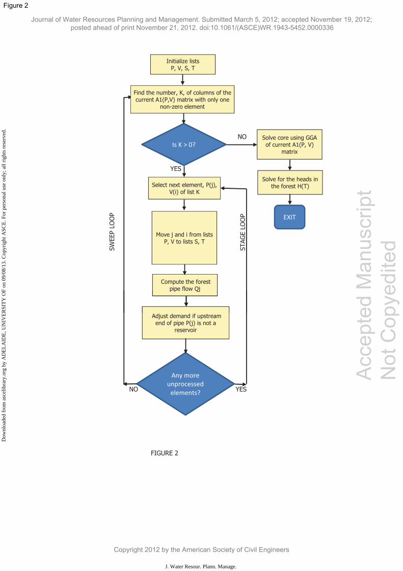
Acc
epte
d M
anus
crip
t N
ot C
opye
dite
d
Journal of Water Resources Planning and Management. Submitted March 5, 2012; accepted November 19, 2012; posted ahead of print November 21, 2012. doi:10.1061/(ASCE)WR.1943-5452.0000336
Copyright 2012 by the American Society of Civil Engineers
J. Water Resour. Plann. Manage.
Dow
nloa
ded
from
asc
elib
rary
.org
by
AD
EL
AID
E, U
NIV
ER
SIT
Y O
F on
09/
08/1
3. C
opyr
ight
ASC
E. F
or p
erso
nal u
se o
nly;
all
righ
ts r
eser
ved.
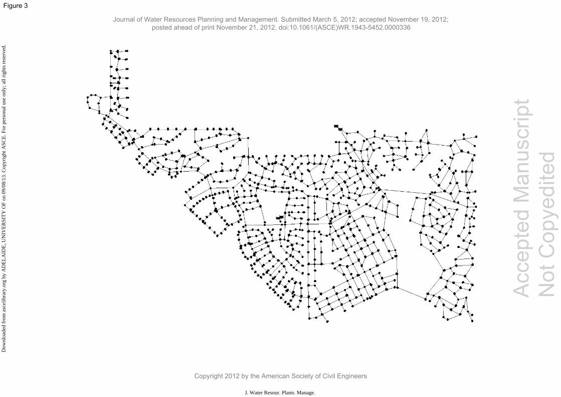
Acc
epte
d M
anus
crip
t N
ot C
opye
dite
d
Journal of Water Resources Planning and Management. Submitted March 5, 2012; accepted November 19, 2012; posted ahead of print November 21, 2012. doi:10.1061/(ASCE)WR.1943-5452.0000336
Copyright 2012 by the American Society of Civil Engineers
J. Water Resour. Plann. Manage.
Dow
nloa
ded
from
asc
elib
rary
.org
by
AD
EL
AID
E, U
NIV
ER
SIT
Y O
F on
09/
08/1
3. C
opyr
ight
ASC
E. F
or p
erso
nal u
se o
nly;
all
righ
ts r
eser
ved.
Copyright © 2022 FDOKUMEN