F L O W C O M PA R E : C O N D I T I O N A LN O R M A L I Z I N G F L O W S F O R P O I N T C L O U D

C H A N G E D E T E C T I O N

samuel j. galanakis

Artificial IntelligenceUtrecht University

August 2021

Samuel J. Galanakis: Flow Compare: Conditional Normalizing Flows forPoint Cloud Change Detection , ©August 2021

supervisors:Remco C. VeltkampRonald PoppeBas Boom

location:Utrecht, Netherlands

student number:6950388

time frame: 1/11/2020 - 15/10/2021

A B S T R A C T

Despite significant progress in 3D deep learning for tasks such as clas-sification and semantic segmentation, robust change detection tech-niques for complex, coloured environments have not been developed.This is in part due to the absence of labelled change detection datasetsand the inherent difficulty of constructing such datasets despite theabundance of unlabeled data. Flow Compare is a fully unsupervisedapproach that leverages expressive generative models with iterativeattention trained on multi-temporal coloured point clouds. Changedetection is achieved by reframing the problem as anomaly detec-tion given a learnt conditional distribution. Training pairs are formedby co-registered multi-temporal extracts from coloured point cloudscenes. The inherent class imbalance due to the rarity of semanticallyimportant change, which is problematic for supervised approaches,is here harnessed to guarantee that relevant changes are consideredanomalies under the learnt distribution. This approach shows promisein detecting not only geometric change but also colour change whilstbeing robust to common semantically unimportant change.

iii

A C K N O W L E D G E M E N T S

Throughout the writing of my thesis, I have received a great deal ofsupport.

I would first like to thank my supervisor, Remco for his valuableguidance and continued support. I would also like to thank Tao forhis technical assistance, particularly regarding early dataset construc-tion.

I could not have completed this thesis without the weekly meet-ings with Cyclomedia. My utmost thanks to Bas, Dan and Zill forthe invaluable support and advice. I am especially thankful for help-ing me work through and refine often questionable ideas in the ini-tial research stages. Furthermore, I greatly appreciated Mursit’s helpwhenever I had any technical issues with the company systems andgeneral logistics.

In addition, I would like to thank my parents for supporting methroughout, as they always have. Finally, my time spent would havebeen much duller without my friends whose company I am very for-tunate to have had.

Samuel GalanakisUtrecht, August 2021

iv

C O N T E N T S

1 introduction 1

2 background 4

2.1 Normalizing Flows . . . . . . . . . . . . . . . . . . . . . 4

2.1.1 Coupling Blocks . . . . . . . . . . . . . . . . . . 4

2.2 Flow Expressivity & Extensions . . . . . . . . . . . . . . 5

2.2.1 SurVAE Flows . . . . . . . . . . . . . . . . . . . . 6

2.2.2 Augmented Normalizing Flows . . . . . . . . . 6

2.2.3 Continuously Indexed Normalizing Flows . . . 7

2.3 Attention . . . . . . . . . . . . . . . . . . . . . . . . . . . 7

2.3.1 Dot-Product Attention . . . . . . . . . . . . . . . 7

2.3.2 Cross & Self Attention . . . . . . . . . . . . . . . 8

3 literature review 9

3.1 Change Detection . . . . . . . . . . . . . . . . . . . . . . 9

3.2 Deep learning on point clouds . . . . . . . . . . . . . . 9

3.3 Point Cloud Classification . . . . . . . . . . . . . . . . . 10

3.4 Generative models for point clouds . . . . . . . . . . . 11

4 methodology 13

4.1 Change detection as Anomaly Detection . . . . . . . . . 13

4.2 Data & Pre-processing . . . . . . . . . . . . . . . . . . . 14

4.3 Conditioning . . . . . . . . . . . . . . . . . . . . . . . . . 15

4.4 Model Architecture . . . . . . . . . . . . . . . . . . . . . 16

4.4.1 Full Model . . . . . . . . . . . . . . . . . . . . . . 18

4.5 Voxel Dataloader . . . . . . . . . . . . . . . . . . . . . . 19

5 evaluation 22

5.1 Method of Evaluation . . . . . . . . . . . . . . . . . . . 22

5.2 Experiments . . . . . . . . . . . . . . . . . . . . . . . . . 22

5.3 Qualitative Assessment . . . . . . . . . . . . . . . . . . . 23

6 discussion 30

6.1 Regarding Evaluation Method . . . . . . . . . . . . . . 30

6.2 Unwanted Bias Through Training Regime . . . . . . . . 30

6.3 Attention Maps . . . . . . . . . . . . . . . . . . . . . . . 31

6.4 Generation Examples . . . . . . . . . . . . . . . . . . . . 31

6.5 Continuously Indexed Normalising Flows . . . . . . . 32

7 conclusion & future work 35

7.1 Conclusion . . . . . . . . . . . . . . . . . . . . . . . . . . 35

7.2 Future Work . . . . . . . . . . . . . . . . . . . . . . . . . 36

bibliography 39

v

1I N T R O D U C T I O N

Cyclomedia is a company specializing in the large-scale and system-atic visualization of environments based on 360° panoramic photographs(Cycloramas) enhanced by AI-powered analytics. Data is capturedthrough a proprietary recording system (depicted by figure 2), mountedto the roof of each vehicle with data capture occurring at 5-meter in-tervals. At each location, 5 images are subsequently stitched together,and LiDAR data is captured. This data is then leveraged to provideservices to entities including but not limited to local governments,utility companies, communication providers, and transportation de-partments.

Taking for example the case of transportation, reliable data capturereplaces the need for costly in-person inspections of assets such asstreet signs and lamps with remote inspection. While this is a greatimprovement it still requires individual inspection of the digital repre-sentations. Fully automated change detection would allow only assetsflagged as significantly changed to be individually inspected. Since inmost cases the majority of assets do not exhibit significant change thisresults in substantial efficiency gains. Geo-databases may also be up-dated automatically with the full history of objects being tracked oversuccessive scans.

The majority of research regarding change detection has been fo-cused on the image domain. Specifically, repeated data acquisition byremote sensing technologies such as satellites and aircraft have beenleveraged to identify changes of interest. Examples include landscapemonitoring [26], large scale urban change detection and natural dis-asters [22].

Most recent research in this field leverages the recent developmentsin deep learning, utilizing Convolutional Neural Networks (CNN)to perform change detection. This is done in both a supervised [14,50] and unsupervised manner [38, 82]. A comprehensive overview ofchange detection for images can be gained from the following reviews[8, 41, 40, 6, 4].

Thanks to the increased availability of mobile mapping systems(MMS) change detection for 3D data such as point clouds has gar-nered increased interest. 3D change detection has been applied to awide variety of cases including topography [34], natural disasters [18,64], at small scale [32] and for buildings [5].

Of special interest is change detection for dense urban scenes at thestreet level. However, conducting change detection in such an envi-ronment has significant challenges. These include complex 3D geom-

1

introduction 2

etry, occlusion, and density variations. Furthermore, the concept ofchange in such an environment is not semantically straightforward,especially with the inclusion of the colour space. Ideally, geometrywise the model should be able to detect changes such as the additionof signs to posts, significant deformation, replaced objects while ig-noring changes such as the growth of vegetation and noise due to thedata collection process. Colour-wise, the model should detect changesin posters, painted buildings, and graffiti while ignoring changes dueto weather, time of day, and shadows.

The area of 3D to 3D change detection in complex environmentssuch as street scenes does not yet, to the best of our knowledge, haverobust methods that can distinguish both colour space, geometricchanges and has not yet seen improvements due to the applicationof deep learning as seen in the image domain. This is likely due tothe absence of comprehensive annotated datasets that are requiredfor supervised learning. Such datasets are hard to construct due tothe work-intensive process of labelling multi-temporal 3D data, oftenill-defined semantics concerning change and the inherent class imbal-ance between change and no change examples. Additionally, giventhe variability of urban environments datasets would have to be spe-cialized to the target area, further incentivising an unsupervised ap-proach.

This paper aims to leverage the latest developments in 3D deeplearning in combination with likelihood-based generative modellingto tackle the deficiencies of current approaches in an unsupervisedway. Specifically, Normalizing Flow models are used to model thedensity of the cloud at time t0 and then subsequently evaluate thelikelihood of points at a later time t1. Given this framework, changedetection can be viewed as a form of outlier detection under the orig-inal learned distribution.

introduction 3

Figure 1: Flow Compare is a conditional Normalizing Flow architecture thatdetects changes in an unsupervised fashion through anomaly de-tection. Specifically, given point cloud samples at time t0 and latertime t1 the model outputs conditional likelihood p(t1 | t0) fromwhich change is inferred.

Figure 2: DCR10L mobile mapping system from Cyclomedia Technology.The main components of this recording system are the cameras,positioning technology, data processing unit and the LiDARsystem.Source: https://www.cyclomedia.com/en/product/data-capture/data-capture

2B A C K G R O U N D

This section serves as a brief introduction to key methods and con-cepts that are referred to in the following sections.

2.1 normalizing flows

Normalizing Flows are a technique for learning the distribution of anunknown variable x ∼ px(x) through mapping from a known distri-bution z ∼ pz(z). Since the distribution of z is predefined, it is usu-ally chosen to be a simple distribution such as a Gaussian. In orderfor the transformation to be valid the total probability mass of theoriginal pdf must be preserved. The relation between the densities isexpressed by the change of variables formula, given that the transfor-mation f : Z→ X is invertible and differentiable the following holds:

px(x) = pz(f−1(x))

∣∣det Jf(f−1(x))∣∣−1

(likelihood)

logpx(x) = logpz(f−1(x)) + log

∣∣det Jf(f−1(x))∣∣−1

(log-likelihood)

Where Jf is the Jacobian of partial derivatives of the transformation.For the transformation to be invertible, differentiable it must also bethe case that dimensionality is preserved, z, x ∈ Rd and thus Jf ∈Rd×Rd In practice, the log-likelihood is usually used whilst traininga Normalizing Flow as it is equivalent and numerically preferable.

Once such a transformation has been learned, one can sample byfirst sampling from the known distribution pz(z) and then transform-ing through f. Model density can then be calculated through thechange of variables formula.

In practice Normalizing Flows are usually constructed by chain-ing invertible, differentiable blocks parametrized by neural networks.To preserve these assumptions while still retaining a balance betweencomputational feasibility and expressivity different architectures havebeen proposed including but not limited to coupling blocks [11], au-toregressive models [30] and continuous-time Flows [7]. A compre-hensive review has been made by Papamakarios et al. [49]

2.1.1 Coupling Blocks

Coupling blocks [11] are invertible nonlinear layers with efficient Ja-cobian calculation. This is achieved by splitting the input z into com-ponents z0, z1 and subsequently transform z0 by an easily invertible

4

2.2 flow expressivity & extensions 5

function whose parameters are determined by z1. In this way whilstthe transformation of z1 is invertible, the function that determinesits parameters can be arbitrarily complex and does not need to beinvertible, it is usually parameterized by a fully connected network.The Jacobian determinant of the transformation is efficiently calcu-lated due to the triangular Jacobian matrix. A common choice for thetransformation is a simple affine function involving scaling s(z1) andtranslation t(z1) terms 3:

z ′1 = z1

z ′2 = s(z1) · z0 + t(z1)

Figure 3: Affine coupling schematic reproduced from [11].

Since only a fixed subset of the input dimensions are transformedby each coupling block the dimensions must be permuted betweenstacked coupling blocks. Originally fixed permutations were used[11] but due to the inflexibility of these transforms learned generaliza-tions such as invertible 1× 1 convolutions [28] have been developed.

2.2 flow expressivity & extensions

As Normalizing Flows are bijective maps, input dimensionality mustbe preserved. One of the most common applications of Flows is tothe image domain, in such cases multi-scale architectures [11] are of-ten employed in order to to mitigate the computational cost of high-dimensional input dimension. On the contrary, in the case of pointclouds the base object being modeled is a single point thus the prob-lem is that of low dimensionality. Specifically, each colored point isof dimension 6 with dimensions split between coordinates and color.Following a strictly bijective Flow in this dimensionality limits theflexibility of the Flow. Furthermore, the topology-preserving prop-erty of homeomorphisms dictates that the (complex) topology of the

2.2 flow expressivity & extensions 6

data must be preserved while being mapped to the (simple) topol-ogy of the target distribution [9]. In order alleviate these issues bothaugmented Flows and continuously indexed Flows are employed.

2.2.1 SurVAE Flows

In order to incorporate these extensions into a single model, a unifiedapproach is needed. Such an overarching theoretical and practicalframework is provided by SurVAE Flows: Surjections to Bridge theGap between VAEs and Flows [47]. This is a recent work that pro-vides such a modular framework that connects VAEs and Normaliz-ing Flows through the notion of surjective transformations. Surjectivetransformations here are those that are deterministic in one directionwhile being stochastic in the reverse. In the SurVAE framework, eachtransformation is characterized by a forward, inverse and correspond-ing likelihood contribution term. The likelihood contribution termis used in the calculation of the log-likelihood, needs to be trackedthroughout the composed transformations and in the case of bijec-tive transformations corresponds to log

∣∣det Jf(f−1(x))∣∣−1. Surjective

transforms that are utilised are summarily reproduced below for fu-ture reference, for detailed information one may refer to the originalwork.

inference tensor slicing Let f : X→ Z be a tensor slicing sur-jection that for input X = (x1, x2) has deterministic forward f(x) = x1and stochastic inverse : f−1(z1) = (z1, z2) where z2 is sampled fromdistribution q(z | z1). Such a transform has corresponding likelihoodcontribution term −logq(x2 | x1).

generative tensor slicing Let f : X → Z be a tensor slicingsurjection that for input x1 has stochastic forward f(x1) = (x1, z2)where z2 is sampled from distribution q(z | x1) and deterministicinverse : f−1((z1, z2)) = z1. Such a transform has corresponding like-lihood contribution term −logq(z2 | x1).

2.2.2 Augmented Normalizing Flows

Augmented Normalizing Flows [23] address the limitations of low di-mensionality and complex topologies by first embedding the data in ahigher-dimensional space and subsequently using standard Normal-izing Flows to model densities in that space. Specifically, independentnoise E ∼ q(E) is generated and then joint density χ× E is modeled.The distribution q is usually taken to be a simple distribution suchas a standard normal. In the SurVae framework, such an augmentedFlow may be implemented by a generative tensor slicing followed bybijections in the augmented space.

2.3 attention 7

2.2.3 Continuously Indexed Normalizing Flows

Continuously indexed Normalizing Flows (CIFs) [10] address the is-sue of modelling targets with complicated topologies as compared tothe base distribution being transformed, usually a simple Gaussian.This is done by replacing standard bijections by a continuously in-dexed family of bijections F(·;u) : Z → χ where the bijection F canbe chosen according to existing Normalizing Flow architectures. Thefull transformation is defined as follows:

Z ∼ PZ, U ∼ PU|Z(· | Z), X := F(Z;U)

The authors propose a conditional Gaussian with parameters de-pending on Z for PU|Z(· | Z) and F(z;u) = f

(e−s(u) � z− t(u)

)where

s, t are neural networks and f is an invertible map such as for examplea coupling block.

2.3 attention

The attention mechanism allows neural networks to attend to certainsalient parts of available information while fading out the rest in alearnable fashion. This mechanism is at the core of transformer mod-els, pioneered by Vaswani et al. [67] in the field of NLP and continuesto be a core component of SOTA models whilst also seeing increas-ingly widespread use. In computer vision such mechanisms allowprocessing to be focused on specific images or local sub regions of asingle image [2, 2]. Attention mechanisms are generally implementedas a function of query and a set of key-value pairs. Intuitively this canbe thought of as generating a query, calculating how well the querymatches each key and then summarizing the values accordingly.

2.3.1 Dot-Product Attention

Scaled dot-product attention [67] involves matrices Q,K,V of dimen-sions dk,dk,dv respectively. These are usually generated via fullyconnected networks. Compatibility of the query and keys is calcu-lated through dot products, implemented via matrix multiplication.The resulting values are then normalized via a softmax function andused as weights of the weighted sum of the values. Before applyingthe softmax the values may also be divided by

√dk in order to avoid

small gradients due to the shape of the softmax function at large in-put values, resulting in Scaled Dot-Product Attention.

A(Q,K,V) = softmax(QKT )V (Dot-Product Attention)

A(Q,K,V) = softmax(QKT

√dk

)V (Scaled Dot-Product Attention)

2.3 attention 8

2.3.2 Cross & Self Attention

Apart from the method used to calculate key-query similarity andthe subsequent summarization, attention implementations can differas to how the matrices Q,K,V are produced.

Self-attention is an attention mechanism that relates each entry ina sequence to each other in order to compute a representation of thesame sequence. It has been shown to be very useful in machine read-ing, abstractive summarization, and image description generation.

Cross attention on the other hand is a method by which the keysare generated from a different source rather than from the sequenceitself. This has been used for example in the case of modality fusionwhere information from one modality generates attention maps forthe other modality [45, 35].

3L I T E R AT U R E R E V I E W

3.1 change detection

Methods have been proposed to detect geometric changes in streetscenes through solely imagery [37][62], and also a combination ofpoint clouds and imagery [54, 66].

There has been limited work regarding the use of exclusively pointclouds to conduct change detection for street scenes. Xiao et al. [75]detect change by comparing occupancy. Tsakiri, Anagnostopoulos[65] utilize point correspondence relations computed through near-est neighbour and iterative closest point algorithms.

There are also general distance-based approaches such as those ofPalma et al. [48] and Montaut et al. [19] that can be applied to this do-main. The former uses the comparison of multi-scale, context-awareshape descriptors. The latter employs an octree-based strategy, withcell wise distances being computed based on different distance met-rics, the most accurate results being obtained with the Hausdorff met-ric.

More recently Tao Ku et al. [33] introduced a street furniture fo-cused coloured point cloud dataset created as part of the presentwork. While the better performing of the two supervised methods,graph neural network-based SiamGCN performs well, creating morecomprehensive datasets as would be needed for use in productionwould likely prove problematic. The distance-based approach PoCha-DeHH performs relatively poorly on the set challenge and due tothe lack of a learning component necessarily suffers the associatedlimitations of handcrafted methods.

The focus on geometric change and the lack of learning-based ap-proaches, especially when seen in the light of the recent use of deeplearning in the image space provides a clear motivation for exploringdifferent approaches in 3D to 3D change detection.

3.2 deep learning on point clouds

Two key tasks of point cloud understanding are that of classificationand segmentation. The former corresponds simply to a classificationof the point cloud as a whole while the latter is a point-wise classifi-cation.

The adaptation of classic network architectures from 2D images to3D point clouds is challenging due to the inherent irregularity andunordered nature of 3D points.

9

3.3 point cloud classification 10

3.3 point cloud classification

Earlier methods proposed various approaches to project the pointclouds to 2D space to then utilize classical convolutional networks(CNN). MvCNN [61] was an early approach that extracts featuresfrom snapshots taken at various angles via a CNN, applies cross-view pooling, and then obtains a classification through another CNN.GVCNN improves this multi-view approach by incorporating infor-mation regarding the content of each view and then processing itaccording to corresponding groupings [17]. Further improvements tomulti-view classification methods have been made by [80, 78].

While multi-view methods allow direct use of classical CNN net-works, the projection to 2D unavoidably results in loss of informationand may introduce errors due to rendering and interpolation. Oneway of addressing this issue is to extend the CNN architecture to 3Dand split the point cloud into a volumetric grid. VoxNet [42] is anearly method which maps the point cloud to a 32× 32× 32 voxelgrid and then applies a 3D CNN for classification. The volumetric ap-proach was further improved by Vote3Deep [15] through the additionof a voting procedure.

Although volumetric methods produce respectable results they areinherently limited by the memory and computational cost of high-resolution grid representations. To improve the efficiency of this ap-proach OctNet [56] was proposed which hierarchically partitions thepoint cloud through a hybrid grid-octree representation. O-cnn [70]then proposed an adaptation of 3D CNN that can be used to ex-tract features from octrees. Despite such developments, volumetricapproaches still struggle with striking a balance between efficiencyand sufficient resolution.

Non-volumetric focused approaches to extending convolution topoint clouds directly have also been proposed. These usually entaila mapping to a space with desirable properties followed by spectral[79, 69] or spatial [60, 39, 63] convolutional filters.

In contrast to most previous approaches that try to extend classicalmethods by projecting the point cloud onto a regular structure, meth-ods that process the points directly have been the focus of most recentwork. The approach was pioneered by PointNet [52]. PointNet firsttransforms the points by a learned affine transformation matrix toachieve invariance to geometric transformations. Subsequently, eachpoint is passed through fully connected layers with shared weightsand followed by a learned feature transformation which fulfils a rolesimilar to the first transform in feature space. Finally, after beingmapped through more fully connected layers with shared weightsa max-pooling layer gives the latent representation. This method wasiterated upon in PointNet++ [53] by enhancing its ability to capture

3.4 generative models for point clouds 11

local structures. This was done by recursively applying PointNet tonested partitions of the point cloud.

PointNet++ has seen further iterations, PointWeb [81] introducedAdaptive Feature Adjustment to improve feature quality by includinglocal neighbourhood context. Duan et al. [12] proposed the additionof a Structural Relation Network module that facilitates structuralreasoning between the local neighbourhoods to further improve per-formance.

An alternative approach is to represent point clouds as graphs. Inthis case, graphs are formed by treating the points as nodes and form-ing edges with neighbouring points. This approach was first takenby ECC [58] where edges are formed between each neighbouringpair and subsequently edge conditioned convolution (ECC) is appliedwith a filter generating network such as an MLP.

DGCNN [72] proposed a neural network module dubbed Edge-Conv which is a convolution like operation that is applied to localneighbourhood graphs that are dynamically generated at each layerusing k-nearest neighbours.

3.3.0.1 Point Cloud Segmentation

Since 3D segmentation requires point-wise labelling the model mustcollect both global context and detailed local information at eachpoint such tasks are generally more demanding than classification.Most all point classification methods can easily be applied to seman-tic segmentation with minimum architectural changes, semantic seg-mentation tasks are generally used as one of the main forms of evalu-ations for classification method backbones. The most common way ofachieving this is concatenating the per point features with the globallatent representation vector and subsequently individually classify-ing each point.

3.4 generative models for point clouds

Early works [1, 16] in generative modelling of point clouds mostlyfocused on generating fixed size sets of points which limits flexibilitysignificantly. AtlasNet [21] drops this limitation, is able to generatea varying number of points by mapping a set of 2D patches usingpatch-specific MLPs based on the 2D patch coordinates and a globalshape embedding.

Variational AutoEncoders (VAEs) [29], Generative Adversarial Net-works (GANs) [20] have long been the focus of research into gener-ative models in general. VAEs use neural networks as function ap-proximators and maximize a lower bound on the data log-likelihoodto model a continuous latent variable with an intractable posteriordistribution. GANs sidestep the need for likelihood estimation com-

3.4 generative models for point clouds 12

pletely by exploiting an adversarial strategy between a generator anda discriminator network.

A different approach is taken by Normalizing Flows [55] whichhas recently been gaining attention. Normalizing Flows model a dis-tribution through a series of learned invertible transformations whichmap the intractable posterior to a simple preset density. This methodallows for exact log-likelihood estimation, stable training, and flexibleapproximate posterior distributions.

Both GANs [57, 73], VAEs [43, 46] have been used for generativemodelling of point clouds. For the current work, change detectionis done based on (conditional) likelihood estimation which makesNormalizing Flows an attractive choice although approximate likeli-hood estimation methods like VAEs offer superior flexibility due todecreased limitations on the mapping.

There has been limited research done regarding the application ofthese methods to point clouds. The first work is PointFlow [77] whichemploys a two-level hierarchy of distributions. The first level is thedistribution of object shapes and the second is the distribution ofpoints given a shape which is modelled using a Normalizing Flow.

C-Flow [51] employs two parallel Flow branches with mutual con-nections formed by coupling layers to learn conditional distributionsand a 3D Hilbert curve projection to order and process points in aninvertible manner. This approach allows for conditional density mod-elling and thus is suitable for tasks such as 3D reconstruction.

Stypułkowski et al. [59] propose a method for generative modelingof point clouds that combines Normalizing Flows and point encoders,specifically PointNet [52]. The model is trained by first taking twosample subsets of a given point cloud and then encoding one as alatent vector via PointNet. Subsequently, the latent vector is mappedto a normally distributed latent vector e by a Flow function g and asecond Flow function f is conditioned on it. Both the Flows and theencoder are then trained end-to-end by maximizing the log-likelihoodof the second sample being mapped through f. In order to sample anew shape, a latent vector e is sampled, f is conditioned on it, thenpoints are sampled by first sampling from the prior and then map-ping them through f−1.

Discrete Point Flow (DPF ) [68] takes a similar approach using acombination of VAEs and Normalizing Flows. Discrete NormalizingFlows are used to construct shape conditional densities and expres-sive latent shape priors. PointNet is used to generate the mean anddiagonal covariance matrix of a Gaussian which serves as the latentshape representation.

4M E T H O D O L O G Y

4.1 change detection as anomaly detection

Change detection is simply the process of identifying differences inthe state of an object through multi-temporal samples. In practice,taking for example change detection for street scenes, only a smallsubset of all changes that occur are of interest. Changes due to light-ing, weather, plant growth etc. may not be of interest whilst removedsigns or graffiti may be. Often, this subset of changes that is of in-terest is also much less frequent than cases of no change or changethat is not of interest. Picking a sign at random and monitoring itsstate over multiple years it is much more likely that one will observeunimportant or essentially no change rather than significant changelike damage or removal. Attempting to tackle change detection insuch cases in a supervised manner becomes very challenging due tothe extreme class imbalance coupled with the semantically ill-definedand practically challenging task of creating such labelled datasets.

Due to these issues, a different, unsupervised approach is takenhere. Given the assumption that the vast majority of objects do notchange in semantically relevant ways, the change detection problemcan be viewed as a form of anomaly detection. Specifically, one canmodel the distribution of change over multi-temporal samples andsubsequently perform outlier detection under the learned distribu-tion. If the learned distribution was accurate, outliers under the dis-tribution should correspond to semantically relevant cases of change.Essentially, the model learns to become indifferent to common aug-mentations such as lighting and only detect rare changes. This methodrelies heavily on the aforementioned assumption of the comparativerarity of semantically relevant change as if such cases are too commonthey will not be considered outliers under the learnt distribution.

In order to learn the required distributions Normalizing Flows arechosen due to the desirable ability of exact log-likelihood estimationand the fact that generative performance is not relevant. First, thedataset and preprocessing steps for the input point clouds are de-tailed. The following subsections focus on different model architec-tures, the accompanying intuition and their respective features, weak-nesses.

13

4.2 data & pre-processing 14

4.2 data & pre-processing

The dataset is composed of scenes collected during 2019-2020 in a 500

and 150 meter radius area for the training and test sets respectively,at the centre of Amsterdam as depicted by figure 5. The unprocesseddata consists of coloured point clouds with an associated centre point(approximate sensor location) and time of capture as illustrated by fig-ures 4, 6. Since data capture occurs every couple of meters adjacentscans from the same date are combined to create one higher qualityscan with reduced occlusion and more complete coverage. After com-bining adjacent scans a 20x20m cloud centred at the sensor positionis extracted to minimize overlap with adjacent scenes and maximizequality. The dataset consists of 2250 scenes for the training set and550 in the test set with 2-4 scans of the same area from different dateseach. Subsequently, scans of the same scene are registered using the It-erative closest point (ICP) algorithm [3]. Lastly, voxel downsamplingis applied with a voxel size of 7cm, significantly reducing the pointdensity to keep the computational requirements manageable.

Figure 4: Aerial view of successive capture points denoted by coloured cir-cles. Colour corresponds to the date of capture.

4.3 conditioning 15

Figure 5: Aerial view of areas where dataset scenes are located. Larger andsmaller radiuses correspond to training and test set respectively.

Figure 6: Example scene.

4.3 conditioning

Given a dataset of point cloud pairs t0, t1 which correspond to thesame coordinates the goal is to model the conditional probabilityp(t1 | t0). Previous works that model point-wise densities [59, 31]achieve this by concatenating a latent representation z of the condi-tion to the input of the fully connected networks that parametrizeeach coupling block. While this tactic may be sufficient to allow globalinformation of the conditioned entity to be modelled it becomes prob-lematic if fine-grained information needs to be accessed. Intuitively,given clouds t1 that depicts a street sign, in order for the modelto assign a likelihood to a given point p it must have access to notonly global information (is there a sign in t1?) but also detailed in-formation regarding the points in the local neighbourhood. In order

4.4 model architecture 16

for such fine-grained information to be available given the aforemen-tioned method, the latent embedding zwould have to encode all suchinformation in essence resulting in a sort of compression rather thanjust relevant global information. In order to achieve such compres-sion, z would have to be of high dimensionality and lead to signifi-cant computational and memory requirements as this vector is pro-cessed by each coupling block. Ideally, the processing of each pointshould be able to access only the information that is relevant to it andnot have to process full detailed information of the whole condition.This is achieved by using a combination of segmentation-like embed-ding network on the conditional cloud t0 in combination with cross-attention modules at each coupling block. The classical approach ofsimply concatenating a latent embedding to the input of each cou-pling block is also tested and referred to as the global embeddingapproach.

4.4 model architecture

4.4.0.1 Conditioning Embedder

In the global embedding approach, an embedding z of the conditionalcloud N0 × 6 is computed through a classification like architecture,namely a Dynamic Graph CNN (DGCNN) [71]. This output is thenconcatenated to the input of fully connected layers at each couplingblock.

The cross attention approach roughly resembles that taken by [25]as far as the iterative attention mechanism is concerned althoughin that case there is no conditioning embedder, with the raw pointclouds being used as input to each attention module. The embedderis added here in order to process the condition and aggregate rele-vant features at each point once so that this initial processing doesnot have to be repeated at each block. The architecture used for theembedder is very similar to those used for semantic segmentation asin both cases the goal is to aggregate local neighbourhood as well asglobal information at each point. Specifically, a Dynamic Graph CNN[71] network and a PAConv [76] network with PointNet++ [53] back-bone are compared. In both cases the embedder takes input conditioncloudN0× 6 and outputs point-wise embeddingN0×E. This outputis then further processed by the Cross Attention Modules.

4.4.0.2 Cross Attention Module

Before computing the attention matrices, layer norm [36] is appliedto the inputs for increased stability and efficiency. Subsequently, thecross attention module generates K,V ∈ RA from condition embed-ding N0 × E and Q ∈ RA from the main Flow input using fully con-nected networks. The dimension A is the inner dimension in which

4.4 model architecture 17

the main attention operation is performed and is set as a hyperparam-eter. Specifically Scaled Dot-Product Attention is used with a singlehead, multiple heads did not show increased performance. This mod-ule is used for all modules of the main Flow that require conditioning,weight sharing was not explored although it may be a viable optionfor reducing overall parameter count.

4.4.0.3 Flow Block

A coupling block architecture is used for the Flow blocks, parametrizedby fully connected networks with residual connections. Affine cou-pling blocks [11] are chosen as they offer a balance between expressiv-ity and memory requirements. Rational Quadratic Spline Flows [13]and Matrix Exponential Flows [74] were also considered but chaininga larger number of memory efficient affine layers was found to per-form better. Each such Flow block is conditional, accompanied by across attention module that takes as input the part of the input notbeing transformed and outputs an attention embedding used as in-put to the fully connected network. In the global embedding case, theembedding is instead simply concatenated before going through thefully connected network. A sigmoid scaling function is used in placeof the exponential for increased stability.

4.4.0.4 Augmenter

Augmented Normalizing Flows [23] address the limitations of low di-mensionality and complex topologies by first embedding the data in ahigher-dimensional space and subsequently using standard Normal-izing Flows to model densities in that space. Specifically, independentnoise E ∼ q(E) is generated and then joint density χ× E is modeled.

A conditional normal distribution is chosen for q, with locationand scale parameters being a function of the context, using cross at-tention or a global embedding as in the Flow block. The module isimplemented as in the SurVae framework [47] with a generative ten-sor slicing resulting in a larger augmented dimension in which allfollowing bijections are done. Experimentation showed that increas-ing the augmented dimension size is beneficial with a value of 300

being chosen as a balance between dimensionality and the number oflayers allowed by memory limits.

4.4.0.5 Permuter

Since coupling blocks only transform a fixed subset of the input di-mensions, they must be shuffled between stacked coupling blocks.Originally fixed permutations were used [11] but due to the inflex-ibility of these transforms learned generalizations such as invertible1× 1 convolutions [28] have been developed. Here 1× 1 convolutionscorrespond to simply multiplication by a learned matrix as each point

4.4 model architecture 18

is modelled separately. The matrix is parametrized by a learned LUDecomposition so as to avoid training instabilities associated withsingular matrices.

4.4.0.6 Actnorm

Each coupling block is followed by an Actnorm layer [28] which isused as an alternative to batch normalization [24] which uses data-dependent initialization.

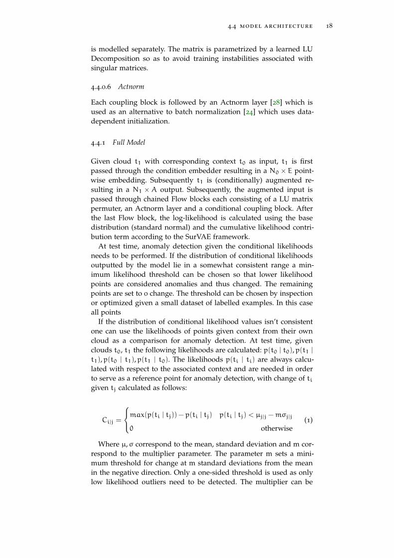
4.4.1 Full Model

Given cloud t1 with corresponding context t0 as input, t1 is firstpassed through the condition embedder resulting in a N0 × E point-wise embedding. Subsequently t1 is (conditionally) augmented re-sulting in a N1 × A output. Subsequently, the augmented input ispassed through chained Flow blocks each consisting of a LU matrixpermuter, an Actnorm layer and a conditional coupling block. Afterthe last Flow block, the log-likelihood is calculated using the basedistribution (standard normal) and the cumulative likelihood contri-bution term according to the SurVAE framework.

At test time, anomaly detection given the conditional likelihoodsneeds to be performed. If the distribution of conditional likelihoodsoutputted by the model lie in a somewhat consistent range a min-imum likelihood threshold can be chosen so that lower likelihoodpoints are considered anomalies and thus changed. The remainingpoints are set to 0 change. The threshold can be chosen by inspectionor optimized given a small dataset of labelled examples. In this caseall points

If the distribution of conditional likelihood values isn’t consistentone can use the likelihoods of points given context from their owncloud as a comparison for anomaly detection. At test time, givenclouds t0, t1 the following likelihoods are calculated: p(t0 | t0),p(t1 |

t1),p(t0 | t1),p(t1 | t0). The likelihoods p(ti | ti) are always calcu-lated with respect to the associated context and are needed in orderto serve as a reference point for anomaly detection, with change of tigiven tj calculated as follows:

Ci|j =

max(p(ti | tj)) − p(ti | tj) p(ti | tj) < µj|j −mσj|j

0 otherwise(1)

Where µ,σ correspond to the mean, standard deviation and m cor-respond to the multiplier parameter. The parameter m sets a mini-mum threshold for change at m standard deviations from the meanin the negative direction. Only a one-sided threshold is used as onlylow likelihood outliers need to be detected. The multiplier can be

4.5 voxel dataloader 19

set according to desired sensitivity, with larger values correspondingto lower sensitivity as only lower likelihood points are flagged aschange. A default value of 5.4 was found to work well.

In the present case, both methods were found to perform similarlyas the likelihoods were sufficiently consistent. Thus, the direct thresh-olding approach was taken as it requires significantly less computa-tion. In what follows the threshold is set to 5 unless otherwise speci-fied.

The final change values are normalized to the range 0, 1. For eachpair both C0|1 and C1|0 are computed so as to detect change for pointsthat are not present in both clouds such as removed or added objects.The final change map is arrived at by merging the two change maps,where changed points can be marked according to their point cloudof origin.

K×

N0xE

N0x6 Condition

Embedder

FlowBlockN

1xL

N1x6 Augmenter

N1xL

/2N

1xL

/2

FlowBlockN

1xL

N1xL

/2N

1xL

/2 Like

lihoo

d

BaseDistribution

Attention

CouplingLayer Permuter

ActNorm

Figure 7: Flow Compare with cross attention. Cloud t1 (being evaluated)and t0 (context) are taken as input, t0 is processed by the con-dition embedder and subsequently and serves as input to eachconditional module. t1 first goes through the augmenter, beingaugmented with conditionally generated noise to have L dimen-sions. Subsequently, for each Flow block, the tensor dimensionsare split, half used as input to the attention along with the contextand then the tensor is transformed by the coupling, permuter andact norm modules. This process is repeated K times ending withlikelihood evaluation through the base distribution.

4.5 voxel dataloader

Ideally, for each point being evaluated, the context would consist ofeither all points within a certain distance or the k nearest neighbours.With the present model architecture, such an approach with a uniquecontext for each point was not computationally viable and thus avoxel-based approach was taken. Given a list of clouds correspond-

4.5 voxel dataloader 20

ing to the same scene a common voxel grid with dimensions (2, 2, 4)is imposed and each voxel is then downsampled separately using theiterative farthest point sampling (FPS) algorithm [44]. This is doneas opposed to random sampling in order to achieve even coverage.When considering a pair of clouds, for each voxel a corresponding,slightly larger voxel (2.2, 2.2, 4.2) with the same centre is taken fromthe other cloud as context and vice versa. This voxel is taken to beslightly larger so as to guarantee that points that are on the edge ofthe voxel have sufficient context. During training, only voxels with aminimum of 1024 points and 1250 context points are considered. Fur-thermore, pairs from the same cloud are also considered, with slightnoise added to the coordinates which results in a 1:1 ratio of self-pairs and different time training pairs. This ratio was kept constantthroughout all experiments but different values may prove advan-tageous. At test time only different cloud pairs are considered. Eachvoxel-context pair is normalized so as to be zero mean and within theunit sphere. Lastly, a randomized rotation augmentation is applied tothe xy plane.

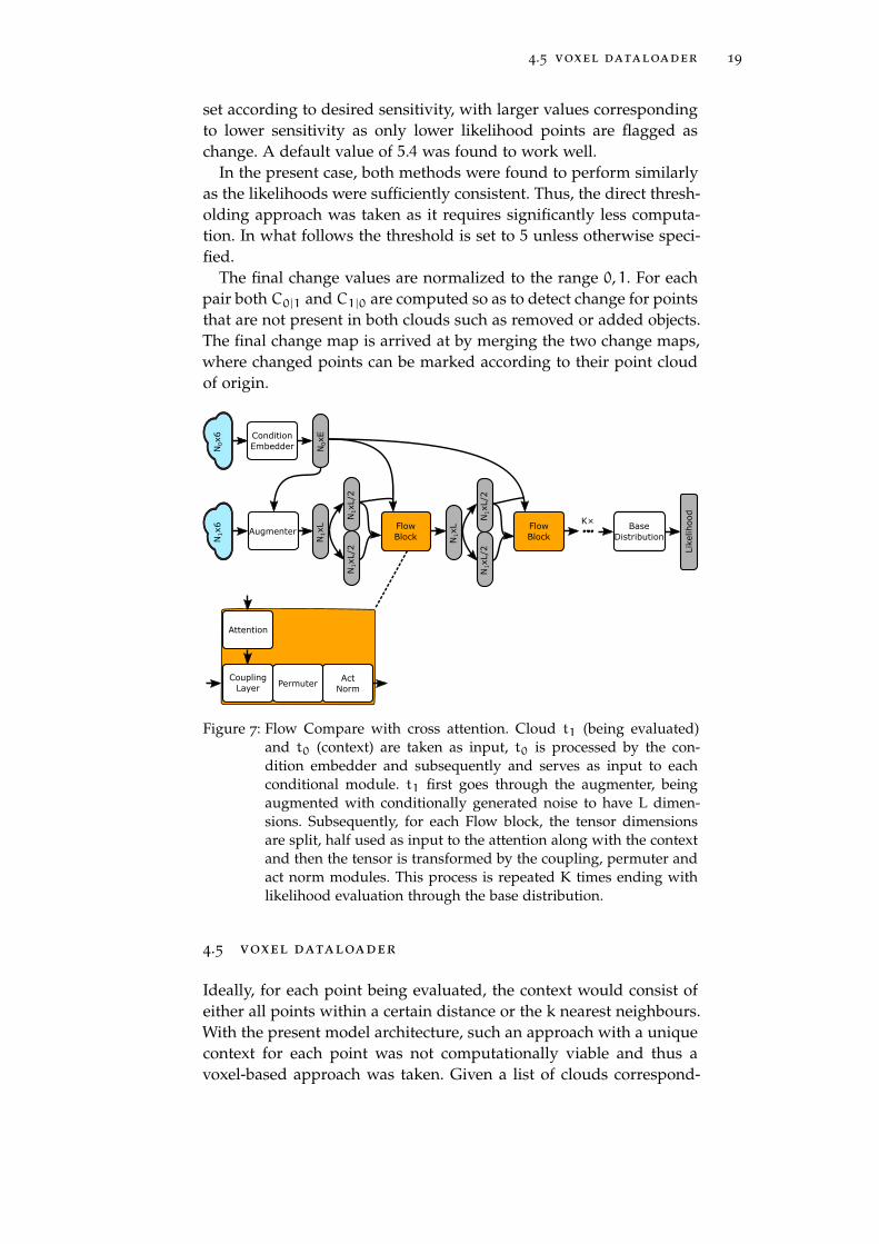
Due to the uniform placement of the voxel grid, without regardfor the geometry, voxels contain partial objects and the frequency dis-tribution of objects types is highly skewed. Specifically, the datasetis dominated by building facades with other objects such as streetsigns and trees making up the remaining samples. Figure 8 depictsvoxel pairs that can be found in the training set. Examples a,b,d,fshow common examples of colour differences due to lighting condi-tions and shadows. Example c shows a rare example of actual changewhere what appears to be a utility box has been installed. Lastly, ex-ample e depicts a case of occlusion where the pole of a traffic lightisn’t captured. Such cases are some extent unavoidable due to the na-ture of data collection in urban areas and the model may learn to atleast cope with partial occlusion.

4.5 voxel dataloader 21

(a) Light difference due to shadow (b) Sampling and slight color difference

(d) Color difference(c) Actual change

(e) Occlusion (f) Color difference

Figure 8: Example voxel pairs from the dataset.

5E VA L U AT I O N

5.1 method of evaluation

The absence of a point-wise labelled change detection dataset andthe unsupervised nature of the method means that the performancecan’t be quantified directly on the task at hand using standard met-rics and necessitates a different evaluation approach. A combinationof quantitative evaluation via log-likelihood on a test set and qualita-tive evaluation through hand-picked varied change detection exam-ples is used. Log-likelihood is used as a proxy for change detectionperformance because intuitively a more accurate model of the condi-tional distributions should translate into better change detection, aslong as overfitting is avoided. This intuition matches the qualitativeresults observed during the experiments.

Regarding model architecture ablations are performed with respectto the global vs cross attention embeddings, embedder architectureand the inclusion of extra context. Where extra context refers to theheight of the voxel centre relative to the ground. This is done asthe point cloud normalization step removes such information whichcould be useful as knowing the height of the voxel being assesseddoes provide certain information such as not expecting ground orcars at certain heights.

There are many other hyperparameters associated with the variousmodules which were set in accordance with other generative mod-elling approaches when possible or based on limited experimentationotherwise. Due to the novelty of the approach and the limited com-putational resources only certain key, hyperparameters were focusedon. A more comprehensive hyperparameter optimization may lead tosignificantly increased performance in future works.

5.2 experiments

In all cases, training is performed for a total of two epochs ( 2 days)with an initial learning rate of 10−4 with the Adam optimizer [27] oruntil early stopping on a Nvidia A100-40GB graphics card. Detailedhyperparameter configurations and training code can be found at theassociated repository.

22

5.3 qualitative assessment 23

embedder nats (↑) parameters (m) ExtraContext

DGCNN Global 1.737 199.5 No

PACONV Attention 2.034 170.7 No

PACONV Attention 2.125 170.8 Yes

DGCNN Attention 2.144 165.1 No

DGCNN Attention 2.222 165.2 Yes

Table 1: Log-likelihood of the test set in nats (higher is better)

From the experiments, it is clear that the global embedding ap-proach is significantly inferior despite the higher number of parame-ters. The parameters here are added by using a larger embedding dimE = 124 as opposed to 64 used for the attention approach and extend-ing the fully connected layers that parameterize each flow block to off-set the parameter count of the absent attention blocks. This is likelydue to the inability of the global embedding to encode all neededlocal information. The attention approach sidesteps this by allowingdirect, dynamic access to the local information at each flow block.

All further experiments are conducted with the use of Attention,differ with respect to embedder architecture and the use of extra con-text. The extra context seems to help to some extent as it increases thescores for both embedder types despite the extra parameters addedbeing insignificant. This makes sense as knowing the relative voxelheight is intuitively useful in assigning likelihoods but more numer-ous experiments would be needed to more precisely quantify the ef-fect. Between the two embedder types, the DGCNN network outper-forms in both cases despite having fewer parameters, it is not clearwhy this is the case but it may have to do with the dynamic graphcreation (and thus message passing) that is present in DGCNN.

5.3 qualitative assessment

All visualizations are done with the best performing model accordingto the previous experiments. Change 0 corresponds to change of voxel0 conditioned on the corresponding context voxel in cloud 1 and viceversa. Blue denotes no change and red denotes change. Full 3D viewof the chosen examples and for the rest of the test set is providedthrough the associated repository.

5.3 qualitative assessment 24

(a)

(b)

(c)

Voxel 0 Voxel 1 Change 0 Change 1

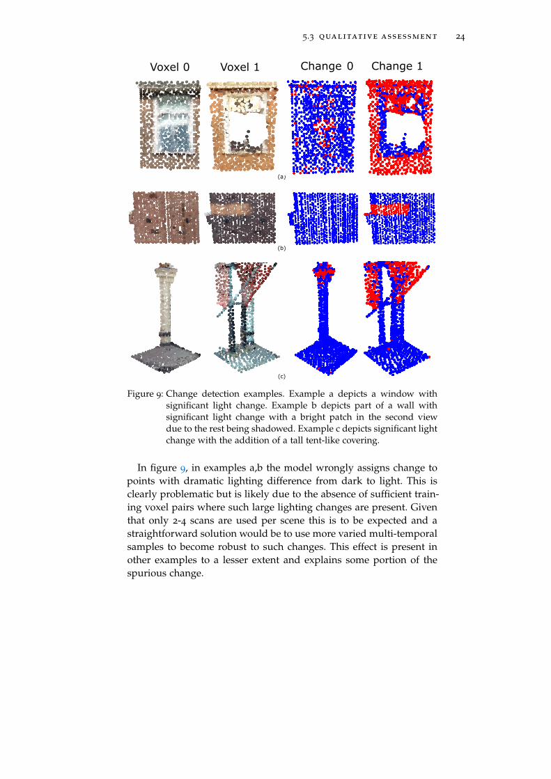
Figure 9: Change detection examples. Example a depicts a window withsignificant light change. Example b depicts part of a wall withsignificant light change with a bright patch in the second viewdue to the rest being shadowed. Example c depicts significant lightchange with the addition of a tall tent-like covering.

In figure 9, in examples a,b the model wrongly assigns change topoints with dramatic lighting difference from dark to light. This isclearly problematic but is likely due to the absence of sufficient train-ing voxel pairs where such large lighting changes are present. Giventhat only 2-4 scans are used per scene this is to be expected and astraightforward solution would be to use more varied multi-temporalsamples to become robust to such changes. This effect is present inother examples to a lesser extent and explains some portion of thespurious change.

5.3 qualitative assessment 25

Figure 10: Generated point cloud conditioned on voxel 0 of example c, prob-lem figure 9 with a standard deviation of 0.6

In the last example of this figure, the model is able to detect the topof the added object while ignoring change in lighting in the rest of thescene. Although the upper parts of the object are classified the lowersupports are not, looking at the generation 10 gives an indication asto why. Essentially the model seems to expect points in the centreof the voxel with the same approximate colour as the missed points.Why this is the case is not obvious but it may be due to the fact thatonly voxels with a certain number of points are used in the training.This has the effect that very few voxels have a vacant middle sectionand the model thus learns to expect points of some average colourin that area by default. This could be addressed by using a paddingapproach to batching rather than fixed point counts and thus notfiltering training voxel pairs by a minimum size.

5.3 qualitative assessment 26

(a)

(b)

(c)

Voxel 0 Voxel 1 Change 0 Change 1

Figure 11: Change detection examples. Example a depicts a pillar and aplant pot. The former is covered by plant growth and the latter isflowering in the second voxel. Example b depicts an area where abike is parked and the addition of a red garbage bin in the secondview. Example c depicts a partial building facade and a cobbledfloor which is mossy in the second view.

In the first row of figure 11, the model is able to pick up the addedplant growth on the pillar, the changes on the flowerpot and the linesin the ground whilst not assigning change values due to voxel 0 be-ing significantly darker. Example b shows a bike in the first voxel anda bike in roughly the same area in the second voxel next to a newlyadded garbage bin. The model assigns change to the added bin andcorrectly assigns no change to the rest of the scene. In the last exam-ple, a partial building front is shown, the main difference betweenthe two times being the change in the ground colour due to mossgrowing between the cobblestones. The model assigns change wherethe moss is present but also assigns some spurious change to the topof the facade, likely due to the aforementioned issue with bright lightspots. Changes such as the appearance of moss may or may not be

5.3 qualitative assessment 27

of interest and the model will learn to ignore them if they are verycommon in the training set.

(a)

(b)

(c)

Voxel 0 Voxel 1 Change 0 Change 1

Figure 12: Change detection examples. Example a depicts a building facadewhere scaffolding is added in the second view. Example b depictsa partial facade where a flag and a pole shaped object appears inthe second view. Part of the building visible in the first case isoccluded in the second. Example c shows a partial window thatis later covered by plant growth.

Switching to figure 12, the first example depicts newly added scaf-folding to the front of a building. The model correctly classified mostof the scaffolding as change whilst assigning no change to the un-changed facade. Some lower parts of the scaffolding are not detectedand this is likely the same issue observed earlier where spurious den-

5.3 qualitative assessment 28

sity is assigned to the centre of the voxel to such colours. Exampleb shows two added pole-like objects in front of a building, both de-tected as change. In this case, even the parts close to the ground aredetected, likely due to them being of a different colour. Further as-signed change is likely due to severe occlusion of parts of the buildingin the second scan. Lastly, example c shows a partial window whichis later covered in vine growth. The vine growth is classified fairlyaccurately as change whilst the underlying wall is not.

(a)

(b)

(c)

Voxel 0 Voxel 1 Change 0 Change 1

Figure 13: Change detection examples. Example a depicts a poster that issubsequently changed and occluded by a newly placed garbagebin. Example b shows a window that is subsequently boardedup. Example c shows significant colour change and the partialappearance of a red object.

Example a of figure 13 shows a fairly complex scene where a posteris changed and partially occluded by a garbage bin. At the currentthreshold of 5, the green part of the bin is detected but not the advertbehind it. Trying a higher threshold value of 7.5n as seen in figure 14,this is mostly corrected although at the cost of slightly more spuri-

5.3 qualitative assessment 29

ous change classifications. The second example shows a window thatis subsequently boarded up, the model is able to detect it accurately.Lastly, example c depicts a case of significant lighting change andshadow which are both ignored and an added red object being classi-fied correctly. Again in this case the whole object is classified withoutissue likely due to being a different colour than that of the spuriousdensity problem observed earlier.

Figure 14: Change of example a figure 13 for looser threshold 7.5

Overall the model shows promise, is able to achieve the set goalsto some extent. Problems observed in the examples are likely due toproblems in the training regime such as the voxel point count filteringand the lack of enough, sufficiently variable data to allow robustnessto be learned. These and other avenues for improvements are outlinedin the following section.

6D I S C U S S I O N

6.1 regarding evaluation method

The Change3D benchmark [33] was created as an evaluation set forFlow Compare it was later decided that it was not fit for this purpose.The first key reason for this decision was the mismatch between theannotations provided by the dataset and the output of Flow Compare.Specifically, the dataset provided object-wise labels (one label perobject) which are fitting for most supervised methods but problem-atic given point-wise change values. A mapping from the point-wisechange values to the object wise labels of the dataset is non-trivial,would likely require supervised training and would significantly ob-scure evaluation. The other concern was the mismatch in the distri-bution caused by the location of the point clouds in the Change3Dbenchmark and that of the available training set, the benchmark itselfnot having enough point clouds to train the present model.

The specific evaluation route taken was chosen as an alternativedue to the absence of any other labelled datasets. The quantitativeanalysis with respect to the log-likelihood on the test set is the stan-dard approach in likelihood-based generative modelling and is aneffective way of comparing different architecture variations. Whilethe qualitative assessment is not an objective assessment it showcaseshow the model performs in varied change detection cases and high-lights problematic aspects. Future work on this task would benefitfrom the creation of a point-wise labelled change detection bench-mark for evaluation purposes.

6.2 unwanted bias through training regime

As pointed out in the results section the proposed method can per-form problematically in certain cases such as due to the erroneousdensity assigned to the centre of the voxel and when certain signifi-cant lighting variations are present. The former problem is suspectedto be due to the training regime (minimum voxel point count filter-ing) and the latter is due to such variations not being present in thetraining set. Thus, it is clear that much care must be taken to not im-plicitly introduce unwanted bias through the chosen training regimeand that the training set contains sufficient examples of the conditionsthat the model is expected to be robust to at test time.

30

6.3 attention maps 31

6.3 attention maps

The key reason for using the cross attention approach to conditioningis to allow the main flow to dynamically focus on different parts ofthe context and thus avoiding the bottleneck of a global embedding.One intuitive way that such a model may have attended to the contextcould have been going from general focus to more targeted (aroundthe point being processed) in the deeper layers , or vice versa. Fromvisual inspection of attention maps, as depicted by figure 15, it wasfound that this was not generally the case and that no such easilyinterpretable pattern was present. The attention maps do not seem tofocus around the point being processed, it is conjectured that differentflow blocks specialize on semantically similar structures or specificcolours but this requires further investigation.

(a)Augmenter (b) Flow block 50 (c) Flow block 110

Figure 15: Attention maps of modules of progressively later conditionalmodules, with the lighter colour corresponding to more attention.The exaggerated green point is the location of the point being pro-cessed.

6.4 generation examples

Although the goal is not to generate point clouds, given the dual na-ture of Normalizing Flows one can generate point clouds by samplingfrom the base distribution and then passing the points through the in-verse conditioned on a context cloud with such examples depicted byfigures 16, 17. This is useful as it offers a way of visualizing the learntdistributions, seeing to some extent what the model expects. This maybe informative and allow deficiencies to be identified or explained butmust be done with caution as the interpretation of the results can bemisleading. This is chiefly the case due to the fact that while the geo-metric component of the distribution is clearly visualized the colourcomponent is not made clear to the same extent by the generation.

Each shown generated voxel consists of 4000 points that are sam-pled from a Gaussian with a standard deviation of 0.6 rather than 1

which was used for training so as to obtain tidier visualizations. The

6.5 continuously indexed normalising flows 32

ideal output is not necessarily an exact reproduction of the condi-tion as the generation roughly represents the average expected scenewhich may differ significantly. By inspecting the generations it seemsthat the model in most cases expects a slightly fuzzier version of thegiven geometry, filling in small gaps (present due to coarse downsam-pling and irregular capture) by interpolating between adjacent points.The colours generally match the context but are often of slightly dif-ferent hues, usually in the direction of more common variations ofthe given colour. Taking for example f of figure 17 where a darkerground is expected, likely due to such light ground being relativelyuncommon in the training dataset as suspected due to the erroneouschange detection results found for similar cases.

6.5 continuously indexed normalising flows

Continuously indexed Flows were implemented as proposed by theauthors, with the f mapping being an affine coupling block and dis-tribution U a conditional Gaussian with an attention block. Due tothe changes in architecture and the extra mapping a smaller augmentdimension had to be used due to memory constraints. Limited ex-perimentation found that the training was very unstable, comparableresults to the other approaches were not able to be obtained thus re-sults are omitted included in the experiments. Further experimenta-tion and hyperparameter tuning are needed with this method as themain use case, modelling complex topologies are clearly present inthe problem at hand where complex coloured geometry is modelledoften containing disconnected objects.

6.5 continuously indexed normalising flows 33

(a) (b)

(c) (d)

(e) (f)

Figure 16: Examples of condition-generation pairs with the condition on theleft and generation on the right respectively.

6.5 continuously indexed normalising flows 34

(a) (b)

(c) (d)

(e) (f)

Figure 17: Examples of condition-generation pairs with the condition on theleft and generation on the right respectively.

7C O N C L U S I O N & F U T U R E W O R K

7.1 conclusion

In this thesis, the problem of robust change detection in complexstreet scenes through coloured point clouds is addressed. We presentthe first approach to this important task that leverages the latest ad-vancements in deep learning. Significant challenges associated withthe creation of comprehensive labelled datasets such as costly anno-tation and extreme class imbalance are sidestepped through a fullyunsupervised approach. Additionally, this novel approach has the po-tential to detect geometric and colour change while being robust tosemantically unimportant changes.

The method works by first using a Normalizing Flow model tolearn the conditional distribution of points from unlabeled multi-temporal samples. Once this distribution is learned the problem ofchange detection can be reframed as one of anomaly detection un-der the learned distribution. Essentially, the model learns what toexpect on average given one sample and then significant deviationsi.e. anomalies are classified as changed. In order for this approach tobe effective two complementary assumptions are needed. First thatchanges of interest are rare and second that common changes are notof interest. Furthermore, we detailed a voxel-based training regimeand pre-processing pipeline which allows the model to learn the tar-get distribution.

In order for the approach to be realized we designed a model archi-tecture capable of modelling the target conditional density. The twokey challenges here are maintaining sufficient flexibility of the mainflow mapping and designing an effective conditioning mechanism.

Flexibility is addressed by pairing affine coupling blocks with anAugmenter module which embeds the initially low dimensional pointsinto a high dimensional space.

The standard conditioning method was shown to be ineffective forthe problem at hand due to not being conducive to capturing localinformation which is key for point-wise change detection. As an al-ternative a novel attention-based conditioning method is proposedwhich allows the model to dynamically query point-wise embeddingsof the context. This allows not only each point but also each condi-tional module at different layers to flexibly extract information andwas shown to outperform the standard approach significantly.

The proposed model is quantitatively evaluated with respect to theaverage likelihood on the test but also qualitatively through visual in-

35

7.2 future work 36

spection of varied examples. It was demonstrated that the approachis able to effectively detect geometric change, colour change while be-ing robust to semantically unimportant change, the last two of whichhave not been achieved by previous methods.

Lastly, although the approach is here applied to point cloud datastraightforward adaptations could be made for change detection indifferent modalities such as the image domain or even combiningmodalities for increased performance.

7.2 future work

Due to the novelty of the proposed method and the accompanyingmodel architecture, there is much room for further improvements.The following outlines how identified deficiencies may be addressedas well as promising avenues for further improvement.

large scale training : Due to the training paradigm, this modelbenefits from large scale training as the training set needs to containsufficient examples of all semantically uninteresting changes so thatthe model can learn to expect such cases (not flag them as anoma-lies). For example, if the training set does not contain fallen leavespresent in autumn it would likely flag such cases as anomalies. Inturn, the model must have the expressive capacity to model such di-verse relations. Thus, the method itself necessitates large scale train-ing which was not possible through the current project and highlightsthe need for improved efficiency to manage computational costs. Anideal training procedure may mirror in certain ways the training oflarge language models where large, varied unlabeled text corpusesare used. The equivalent being point clouds covering significant ge-ographic areas of interest over varying conditions such as seasonalchanges.

augmentation and simulation : In absence of sufficient multi-temporal data, augmentation and simulation methods can be used tosynthetically generate new variations of the existing data. For exam-ple, modern game engines are capable of simulating realistic, full dayand night cycles which would allow any lighting variations of theavailable point clouds to be generated. Training could then be doneusing both the original and generated data.

data filtering : In the current project minimal filtering was donewith regards to the voxel pairs used for training, only with regards tothe number of points present. Given that the voxel grid is placed uni-formly over large geographic areas it is natural that certain classes orscenes dominate the dataset. For example, building facades may beoverabundant while benches are relatively rare. Performing filtering

7.2 future work 37

in advance, possibly with the aid of point cloud segmentation andclassification methods may alleviate this issue, lead to faster trainingand improved overall performance. Some form of importance sam-pling may also prove useful but runs the danger of focusing on actualchanges present in the data which would be detrimental.

improving colour accuracy : The point cloud data used fortraining while generally geometrically accurate does contain colourinaccuracies which are artefacts of the image colour to coordinate thematching process used in their construction. The consistent presenceof these artefacts seems to lead the model to expect large variationin colour which hinders its ability to detect actual semantically im-portant colour change. Using data with improved colour accuracyor mitigating such issues in pre-processing will improve colour wisechange detection.

weight sharing : One way of decreasing the parameter count ofthe model would be to share parameters across different flow blocks,especially those that parametrize the attention modules. Althoughnot explored it seems likely that some level of parameter sharingcould be employed without significantly degrading performance. Forexample, weights could be shared between a certain number of con-secutive flow blocks with the intuition that consecutive flow blocksmay be summarizing the context in similar ways.

specialized normalizing flow architecture : There arefew works modelling point clouds with Normalizing Flows and thecore architectures used (usually affine coupling blocks) are used es-sentially as-is. Future work may improve such modelling by introduc-ing architectures specialized to point clouds by for example leverag-ing permutation invariance and further tackling the problem of lowdimensionality. Such advancements would of course directly improvethe performance of this approach.

semantic information : For more efficient training semanticinformation could be included for each point. This could for exam-ple be achieved by including the class of each point as given by apre-trained semantic segmentation network or even the point-wiseembeddings of such a network. This should significantly speed upthe learning of the network as it does not need to learn to recognizeclasses from scratch.

hyperparameter optimization : Due to the novelty of the ap-proach, there are limited existing works to base hyperparameter choiceson, thus most hyperparameters were chosen heuristically with lim-ited experimentation and optimization due to prohibitive computa-

7.2 future work 38

tional costs. Further optimization of hyperparameters is key to im-proved efficiency and performance.

B I B L I O G R A P H Y

[1] Panos Achlioptas, Olga Diamanti, Ioannis Mitliagkas, and LeonidasGuibas. “Learning representations and generative models for3d point clouds.” In: International conference on machine learning.PMLR. 2018, pp. 40–49.

[2] Peter Anderson, Xiaodong He, Chris Buehler, Damien Teney,Mark Johnson, Stephen Gould, and Lei Zhang. “Bottom-up andtop-down attention for image captioning and visual questionanswering.” In: Proceedings of the IEEE conference on computervision and pattern recognition. 2018, pp. 6077–6086.

[3] K Somani Arun, Thomas S Huang, and Steven D Blostein. “Least-squares fitting of two 3-D point sets.” In: IEEE Transactions onpattern analysis and machine intelligence 5 (1987), pp. 698–700.

[4] Anju Asokan and J Anitha. “Change detection techniques forremote sensing applications: a survey.” In: Earth Science Infor-matics 12.2 (2019), pp. 143–160.

[5] Mohammad Awrangjeb, Clive S Fraser, and Guojun Lu. “Build-ing change detection from LiDAR point cloud data based onconnected component analysis.” In: ISPRS annals of the photogram-metry, remote sensing and spatial information sciences 2 (2015), p. 393.

[6] Yifang Ban and Osama Yousif. “Change detection techniques: areview.” In: Multitemporal Remote Sensing. Springer, 2016, pp. 19–43.

[7] Changyou Chen, Chunyuan Li, Liqun Chen, Wenlin Wang, YunchenPu, and Lawrence Carin Duke. “Continuous-time flows for effi-cient inference and density estimation.” In: International Confer-ence on Machine Learning. PMLR. 2018, pp. 824–833.

[8] JonckheereI CoppinP et al. “DigitalChangeDetection Method-sinEcosystem Monito ring: a Review.” In: InternationalJournalofRemote Sensing 25.9 (2004), p. 1565.

[9] Rob Cornish, Anthony Caterini, George Deligiannidis, and Ar-naud Doucet. “Localised generative flows.” In: (2019).

[10] Rob Cornish, Anthony Caterini, George Deligiannidis, and Ar-naud Doucet. “Relaxing bijectivity constraints with continuouslyindexed normalising flows.” In: International Conference on Ma-chine Learning. PMLR. 2020, pp. 2133–2143.

[11] Laurent Dinh, Jascha Sohl-Dickstein, and Samy Bengio. “Den-sity estimation using real nvp.” In: arXiv preprint arXiv:1605.08803(2016).

39

bibliography 40

[12] Yueqi Duan, Yu Zheng, Jiwen Lu, Jie Zhou, and Qi Tian. “Struc-tural relational reasoning of point clouds.” In: Proceedings of theIEEE/CVF Conference on Computer Vision and Pattern Recognition.2019, pp. 949–958.

[13] Conor Durkan, Artur Bekasov, Iain Murray, and George Papa-makarios. “Neural spline flows.” In: Advances in Neural Informa-tion Processing Systems 32 (2019), pp. 7511–7522.

[14] Arabi Mohammed El Amin, Qingjie Liu, and Yunhong Wang.“Convolutional neural network features based change detectionin satellite images.” In: 10011 (2016), 100110W.

[15] Martin Engelcke, Dushyant Rao, Dominic Zeng Wang, Chi HayTong, and Ingmar Posner. “Vote3deep: Fast object detection in3d point clouds using efficient convolutional neural networks.”In: 2017 IEEE International Conference on Robotics and Automation(ICRA). IEEE. 2017, pp. 1355–1361.

[16] Haoqiang Fan, Hao Su, and Leonidas J Guibas. “A point setgeneration network for 3d object reconstruction from a singleimage.” In: Proceedings of the IEEE conference on computer visionand pattern recognition. 2017, pp. 605–613.

[17] Yifan Feng, Zizhao Zhang, Xibin Zhao, Rongrong Ji, and YueGao. “Gvcnn: Group-view convolutional neural networks for3d shape recognition.” In: Proceedings of the IEEE Conference onComputer Vision and Pattern Recognition. 2018, pp. 264–272.

[18] Sajid Ghuffar, Balázs Székely, Andreas Roncat, and NorbertPfeifer. “Landslide displacement monitoring using 3D rangeflow on airborne and terrestrial LiDAR data.” In: Remote Sens-ing 5.6 (2013), pp. 2720–2745.

[19] Daniel Girardeau-Montaut, Michel Roux, Raphaël Marc, andGuillaume Thibault. “Change detection on points cloud dataacquired with a ground laser scanner.” In: International Archivesof Photogrammetry, Remote Sensing and Spatial Information Sciences36.part 3 (2005), W19.

[20] Ian Goodfellow, Jean Pouget-Abadie, Mehdi Mirza, Bing Xu,David Warde-Farley, Sherjil Ozair, Aaron Courville, and YoshuaBengio. “Generative Adversarial Networks.” In: Commun. ACM63.11 (Oct. 2020), 139–144. issn: 0001-0782. doi: 10.1145/3422622.url: https://doi.org/10.1145/3422622.

[21] Thibault Groueix, Matthew Fisher, Vladimir G Kim, Bryan CRussell, and Mathieu Aubry. “A papier-mâché approach to learn-ing 3d surface generation.” In: Proceedings of the IEEE conferenceon computer vision and pattern recognition. 2018, pp. 216–224.

bibliography 41

[22] Daniel Hölbling, Barbara Friedl, and Clemens Eisank. “An object-based approach for semi-automated landslide change detectionand attribution of changes to landslide classes in northern Tai-wan.” In: Earth Science Informatics 8.2 (2015), pp. 327–335.

[23] Chin-Wei Huang, Laurent Dinh, and Aaron Courville. “Aug-mented normalizing flows: Bridging the gap between genera-tive flows and latent variable models.” In: arXiv preprint arXiv:2002.07101(2020).

[24] Sergey Ioffe and Christian Szegedy. “Batch normalization: Ac-celerating deep network training by reducing internal covari-ate shift.” In: International conference on machine learning. PMLR.2015, pp. 448–456.

[25] Andrew Jaegle, Felix Gimeno, Andrew Brock, Andrew Zisser-man, Oriol Vinyals, and Joao Carreira. “Perceiver: General Per-ception with Iterative Attention.” In: arXiv preprint arXiv:2103.03206(2021).

[26] Robert E Kennedy, Philip A Townsend, John E Gross, Warren BCohen, Paul Bolstad, YQ Wang, and Phyllis Adams. “Remotesensing change detection tools for natural resource managers:Understanding concepts and tradeoffs in the design of land-scape monitoring projects.” In: Remote sensing of environment113.7 (2009), pp. 1382–1396.

[27] Diederik P. Kingma and Jimmy Ba. “Adam: A Method for Stochas-tic Optimization.” In: CoRR abs/1412.6980 (2015).

[28] Diederik P. Kingma and Prafulla Dhariwal. “Glow: GenerativeFlow with Invertible 1x1 Convolutions.” In: Advances in NeuralInformation Processing Systems. Vol. 31. 2018, pp. 10215–10224.

[29] Diederik P. Kingma and Max Welling. “Auto-Encoding Varia-tional Bayes.” In: 2nd International Conference on Learning Repre-sentations, ICLR 2014, Banff, AB, Canada, April 14-16, 2014, Con-ference Track Proceedings. Ed. by Yoshua Bengio and Yann LeCun.2014. url: http://arxiv.org/abs/1312.6114.

[30] Durk P Kingma, Tim Salimans, Rafal Jozefowicz, Xi Chen, IlyaSutskever, and Max Welling. “Improved variational inferencewith inverse autoregressive flow.” In: Advances in neural infor-mation processing systems 29 (2016), pp. 4743–4751.

[31] Roman Klokov, Edmond Boyer, and Jakob Verbeek. “Discretepoint flow networks for efficient point cloud generation.” In:Computer Vision–ECCV 2020: 16th European Conference, Glasgow,UK, August 23–28, 2020, Proceedings, Part XXIII 16. Springer.2020, pp. 694–710.

bibliography 42

[32] Ryan A Kromer, Antonio Abellán, D Jean Hutchinson, MattLato, Tom Edwards, and Michel Jaboyedoff. “A 4D filtering andcalibration technique for small-scale point cloud change detec-tion with a terrestrial laser scanner.” In: Remote Sensing 7.10

(2015), pp. 13029–13052.

[33] Tao Ku, Sam Galanakis, Bas Boom, Remco C. Veltkamp, Dar-shan Bangera, Shankar Gangisetty, Nikolaos Stagakis, Gerasi-mos Arvanitis, and Konstantinos Moustakas. “SHREC 2021: 3Dpoint cloud change detection for street scenes.” In: ComputersGraphics 99 (2021), pp. 192–200. issn: 0097-8493. doi: https :

//doi.org/10.1016/j.cag.2021.07.004. url: https://www.sciencedirect.com/science/article/pii/S0097849321001369.

[34] Dimitri Lague, Nicolas Brodu, and Jérôme Leroux. “Accurate3D comparison of complex topography with terrestrial laserscanner: Application to the Rangitikei canyon (NZ).” In: ISPRSjournal of photogrammetry and remote sensing 82 (2013), pp. 10–26.

[35] Kuang-Huei Lee, Xi Chen, Gang Hua, Houdong Hu, and Xi-aodong He. “Stacked cross attention for image-text matching.”In: Proceedings of the European Conference on Computer Vision (ECCV).2018, pp. 201–216.

[36] Jimmy Lei Ba, Jamie Ryan Kiros, and Geoffrey E Hinton. “Layernormalization.” In: ArXiv e-prints (2016), arXiv–1607.

[37] Yinjie Lei, Duo Peng, Pingping Zhang, Qiuhong Ke, and HaifengLi. “Hierarchical Paired Channel Fusion Network for Street SceneChange Detection.” In: IEEE Transactions on Image Processing 30

(2020), pp. 55–67.

[38] Xuelong Li, Zhenghang Yuan, and Qi Wang. “Unsuperviseddeep noise modeling for hyperspectral image change detec-tion.” In: Remote Sensing 11.3 (2019), p. 258.

[39] Yangyan Li, Rui Bu, Mingchao Sun, Wei Wu, Xinhan Di, andBaoquan Chen. “Pointcnn: Convolution on x-transformed points.”In: Advances in neural information processing systems 31 (2018),pp. 820–830.

[40] Dengsheng Lu, Guiying Li, and Emilio Moran. “Current situa-tion and needs of change detection techniques.” In: InternationalJournal of Image and Data Fusion 5.1 (2014), pp. 13–38.

[41] Dengsheng Lu, Paul Mausel, Eduardo Brondizio, and EmilioMoran. “Change detection techniques.” In: International journalof remote sensing 25.12 (2004), pp. 2365–2401.

[42] Daniel Maturana and Sebastian Scherer. “Voxnet: A 3d convo-lutional neural network for real-time object recognition.” In:2015 IEEE/RSJ International Conference on Intelligent Robots andSystems (IROS). IEEE. 2015, pp. 922–928.

bibliography 43

[43] Lars Mescheder, Michael Oechsle, Michael Niemeyer, SebastianNowozin, and Andreas Geiger. “Occupancy networks: Learn-ing 3d reconstruction in function space.” In: Proceedings of theIEEE/CVF Conference on Computer Vision and Pattern Recognition.2019, pp. 4460–4470.

[44] Carsten Moenning and Neil A Dodgson. Fast marching farthestpoint sampling. Tech. rep. University of Cambridge, ComputerLaboratory, 2003.

[45] Satyam Mohla, Shivam Pande, Biplab Banerjee, and SubhasisChaudhuri. “Fusatnet: Dual attention based spectrospatial mul-timodal fusion network for hyperspectral and lidar classifica-tion.” In: Proceedings of the IEEE/CVF Conference on Computer Vi-sion and Pattern Recognition Workshops. 2020, pp. 92–93.

[46] Charlie Nash and Christopher KI Williams. “The shape varia-tional autoencoder: A deep generative model of part-segmented3D objects.” In: Computer Graphics Forum. Vol. 36. 5. Wiley On-line Library. 2017, pp. 1–12.

[47] Didrik Nielsen, Priyank Jaini, Emiel Hoogeboom, Ole Winther,and Max Welling. “Survae flows: Surjections to bridge the gapbetween vaes and flows.” In: Advances in Neural Information Pro-cessing Systems 33 (2020).

[48] Gianpaolo Palma, Paolo Cignoni, Tamy Boubekeur, and RobertoScopigno. “Detection of geometric temporal changes in pointclouds.” In: Computer Graphics Forum. Vol. 35. 6. Wiley OnlineLibrary. 2016, pp. 33–45.

[49] George Papamakarios, Eric Nalisnick, Danilo Jimenez Rezende,Shakir Mohamed, and Balaji Lakshminarayanan. “Normalizingflows for probabilistic modeling and inference.” In: Journal ofMachine Learning Research 22.57 (2021), pp. 1–64.

[50] Daifeng Peng, Yongjun Zhang, and Haiyan Guan. “End-to-endchange detection for high resolution satellite images using im-proved unet++.” In: Remote Sensing 11.11 (2019), p. 1382.

[51] Albert Pumarola, Stefan Popov, Francesc Moreno-Noguer, andVittorio Ferrari. “C-flow: Conditional generative flow modelsfor images and 3d point clouds.” In: Proceedings of the IEEE/CVFConference on Computer Vision and Pattern Recognition. 2020, pp. 7949–7958.

[52] Charles R Qi, Hao Su, Kaichun Mo, and Leonidas J Guibas.“Pointnet: Deep learning on point sets for 3d classification andsegmentation.” In: Proceedings of the IEEE conference on computervision and pattern recognition. 2017, pp. 652–660.

bibliography 44

[53] Charles R. Qi, Li Yi, Hao Su, and Leonidas J. Guibas. “: Deep Hi-erarchical Feature Learning on Point Sets in a Metric Space.” In:Proceedings of the 31st International Conference on Neural Informa-tion Processing Systems. NIPS’17. Long Beach, California, USA:Curran Associates Inc., 2017, 5105–5114. isbn: 9781510860964.

[54] Rongjun Qin and Armin Gruen. “3D change detection at streetlevel using mobile laser scanning point clouds and terrestrialimages.” In: ISPRS Journal of Photogrammetry and Remote Sensing90 (2014), pp. 23–35.

[55] Danilo Rezende and Shakir Mohamed. “Variational inferencewith normalizing flows.” In: International Conference on MachineLearning. PMLR. 2015, pp. 1530–1538.

[56] Gernot Riegler, Ali Osman Ulusoy, and Andreas Geiger. “Oct-net: Learning deep 3d representations at high resolutions.” In:Proceedings of the IEEE conference on computer vision and patternrecognition. 2017, pp. 3577–3586.

[57] Dong Wook Shu, Sung Woo Park, and Junseok Kwon. “3d pointcloud generative adversarial network based on tree structuredgraph convolutions.” In: Proceedings of the IEEE/CVF Interna-tional Conference on Computer Vision. 2019, pp. 3859–3868.

[58] Martin Simonovsky and Nikos Komodakis. “Dynamic edge-conditioned filters in convolutional neural networks on graphs.”In: Proceedings of the IEEE conference on computer vision and pat-tern recognition. 2017, pp. 3693–3702.

[59] Michał Stypułkowski, Kacper Kania, Maciej Zamorski, MaciejZieba, Tomasz Trzcinski, and Jan Chorowski. “Representing pointclouds with generative conditional invertible flow networks.”In: Pattern Recognition Letters (2021).

[60] Hang Su, Varun Jampani, Deqing Sun, Subhransu Maji, Evange-los Kalogerakis, Ming-Hsuan Yang, and Jan Kautz. “SPLATNet:Sparse Lattice Networks for Point Cloud Processing.” In: Pro-ceedings of the IEEE Conference on Computer Vision and PatternRecognition (CVPR). 2018.

[61] Hang Su, Subhransu Maji, Evangelos Kalogerakis, and Erik Learned-Miller. “Multi-view convolutional neural networks for 3d shaperecognition.” In: Proceedings of the IEEE international conferenceon computer vision. 2015, pp. 945–953.

[62] Aparna Taneja, Luca Ballan, and Marc Pollefeys. “Geometricchange detection in urban environments using images.” In: IEEEtransactions on pattern analysis and machine intelligence 37.11 (2015),pp. 2193–2206.

bibliography 45

[63] Maxim Tatarchenko, Jaesik Park, Vladlen Koltun, and Qian-YiZhou. “Tangent convolutions for dense prediction in 3d.” In:Proceedings of the IEEE Conference on Computer Vision and PatternRecognition. 2018, pp. 3887–3896.

[64] J Trinder and M Salah. “Aerial images and LiDAR data fusionfor disaster change detection.” In: ISPRS Ann. Photogramm. Re-mote Sens. Spat. Inf. Sci 1 (2012), pp. 227–232.

[65] M Tsakiri and V Anagnostopoulos. “Change detection in ter-restrial laser scanner data via point cloud correspondence.” In:IJEIR 4.3 (2015), pp. 476–486.

[66] Ali Osman Ulusoy and Joseph L. Mundy. “Image-Based 4-d Re-construction Using 3-d Change Detection.” In: Computer Vision– ECCV 2014. Ed. by David Fleet, Tomas Pajdla, Bernt Schiele,and Tinne Tuytelaars. Cham: Springer International Publishing,2014, pp. 31–45. isbn: 978-3-319-10578-9.

[67] Ashish Vaswani, Noam Shazeer, Niki Parmar, Jakob Uszkor-eit, Llion Jones, Aidan N Gomez, Łukasz Kaiser, and Illia Polo-sukhin. “Attention is all you need.” In: Advances in neural infor-mation processing systems. 2017, pp. 5998–6008.

[68] Jakob Verbeek. “Discrete Point Flow Networks for Efficient PointCloud Generation.” In: ().

[69] Chu Wang, Babak Samari, and Kaleem Siddiqi. “Local spectralgraph convolution for point set feature learning.” In: Proceed-ings of the European conference on computer vision (ECCV). 2018,pp. 52–66.

[70] Peng-Shuai Wang, Yang Liu, Yu-Xiao Guo, Chun-Yu Sun, andXin Tong. “O-cnn: Octree-based convolutional neural networksfor 3d shape analysis.” In: ACM Transactions on Graphics (TOG)36.4 (2017), pp. 1–11.

[71] Yue Wang, Yongbin Sun, Ziwei Liu, Sanjay E. Sarma, MichaelM. Bronstein, and Justin M. Solomon. “Dynamic Graph CNNfor Learning on Point Clouds.” In: CoRR abs/1801.07829 (2018).arXiv: 1801.07829. url: http://arxiv.org/abs/1801.07829.

[72] Yue Wang, Yongbin Sun, Ziwei Liu, Sanjay E Sarma, MichaelM Bronstein, and Justin M Solomon. “Dynamic graph cnn forlearning on point clouds.” In: Acm Transactions On Graphics (tog)38.5 (2019), pp. 1–12.

[73] Jiajun Wu, Chengkai Zhang, Tianfan Xue, William T Freeman,and Joshua B Tenenbaum. “Learning a probabilistic latent spaceof object shapes via 3d generative-adversarial modeling.” In:Proceedings of the 30th International Conference on Neural Informa-tion Processing Systems. 2016, pp. 82–90.

bibliography 46

[74] Changyi Xiao and Ligang Liu. “Generative Flows with MatrixExponential.” In: International Conference on Machine Learning.PMLR. 2020, pp. 10452–10461.

[75] Wen Xiao, Bruno Vallet, Mathieu Brédif, and Nicolas Paparo-ditis. “Street environment change detection from mobile laserscanning point clouds.” In: ISPRS Journal of Photogrammetry andRemote Sensing 107 (2015), pp. 38–49.

[76] Mutian Xu, Runyu Ding, Hengshuang Zhao, and Xiaojuan Qi.“PAConv: Position Adaptive Convolution with Dynamic KernelAssembling on Point Clouds.” In: Proceedings of the IEEE/CVFConference on Computer Vision and Pattern Recognition. 2021, pp. 3173–3182.

[77] Guandao Yang, Xun Huang, Zekun Hao, Ming-Yu Liu, SergeBelongie, and Bharath Hariharan. “Pointflow: 3d point cloudgeneration with continuous normalizing flows.” In: Proceedingsof the IEEE/CVF International Conference on Computer Vision. 2019,pp. 4541–4550.

[78] Ze Yang and Liwei Wang. “Learning relationships for multi-view 3D object recognition.” In: Proceedings of the IEEE/CVF In-ternational Conference on Computer Vision. 2019, pp. 7505–7514.

[79] Li Yi, Hao Su, Xingwen Guo, and Leonidas J Guibas. “Syncspec-cnn: Synchronized spectral cnn for 3d shape segmentation.” In:Proceedings of the IEEE Conference on Computer Vision and PatternRecognition. 2017, pp. 2282–2290.

[80] Tan Yu, Jingjing Meng, and Junsong Yuan. “Multi-view harmo-nized bilinear network for 3d object recognition.” In: Proceed-ings of the IEEE Conference on Computer Vision and Pattern Recog-nition. 2018, pp. 186–194.

[81] Hengshuang Zhao, Li Jiang, Chi-Wing Fu, and Jiaya Jia. “Pointweb:Enhancing local neighborhood features for point cloud process-ing.” In: Proceedings of the IEEE/CVF Conference on Computer Vi-sion and Pattern Recognition. 2019, pp. 5565–5573.

[82] K. L. de Jong and A. Sergeevna Bosman. “Unsupervised ChangeDetection in Satellite Images Using Convolutional Neural Net-works.” In: (2019), pp. 1–8. doi: 10.1109/IJCNN.2019.8851762.