African Trade Partners compare China with other Emerging Markets

Advanced Master in International and Development Economics

Facultés Universitaires Notre-Dame de la Paix, Namur

Université Catholique de Louvain, Louvain-la-Neuve

Rapport de stage

Blaise EHOWE NGUEM

Academic year 2011/2012

a

39

African Trade Partners: CompareChina with other Emerging

Markets

By Blaise EHOWE NGUEM

A project submitted in partial fulfillment of

the requirements for the degree of Advanced

Master in International and Development

Economics

Economics School of Louvain

University of Namur — FUNDP

Catholic University of Louvain — UCL

39

Academic year 2011-2012

39

ABSTRACT

During this last decade, trade between African countries and

BRIC has more than double and China is the one which dominates

this trade. This strong increase has raised a lot of debate on

the invasion of African by BRIC and especially China whom many

politics and economist accuse to no deal with governance in

Africa. The aim of this paper is to provide some responses by

trying to understand what determinants motivate trade between

African countries and BRIC and also to see if China is

different to other emerging market. To rich that goal, we

compute a gravity model usually uses on international trade to

estimate the level of trade between Africa and it BRIC trade

partner. In addition to traditional variables, we add some

variables of interest such as governance for African and

exchange rate. We run pooled OLS model and panel data approach

to check for the robustness and the dynamic. The result from

this model shows that the resource abundance of African country

is not a significant driver of China trade as many authors

think even if the main part of imports is composed by oil and

natural resource. China is trading more and more with rich

natural resource countries. In addition, China and India are

not really different in the way of trading with African

countries. Those two countries are influenced by the same

variables except governance in case of imports because they

have approximately same needs. And finally, these two countries

differ at some level from Brazil and Russia..

39

Keywords: BRIC, Africa, trade, gravity model, exchange rate,

governance

39

ACKNOWLEDGMENTS

This personal project has benefited from the contribution of

many people, and I would especially like to acknowledge their

support.

I am grateful to my promoter, Professor Romain HOUSSA. I would

like to thank him for his encouragements, support, remarks and

critics which significantly ameliorated this work.

I express also my gratitude to Mrs. Maelys de LA RUPELLE, my

tutor, for his helpful comments and suggestions.

I benefit immensely from the comments and suggestions of Angele

BAHA, Ritchelle ALBURO, Loudine BESSONG, Edouard TSAGUE, Jules

KEMBOU, Carine NZEYANG, and Patrick EWANE. They also provided

particular care to review the original manuscript.

My thanks go to Mrs Pierrette NOEL, staff members of the

University of Namur and especially for the organization

committee of the Advanced master in international and

development economics, for the promptitude with which they

overcome problems we have encountered during this academic

year. Financial support from CUD is gratefully acknowledged and

I am finally indebted to all my family for their moral support

at critical moments and for their encouragements.

Finally, I want to thank specially my wife Rosine EHOWE, my

kids Chanelle and Giovanni and my whole family for their

sacrifice, constant and unfailing support and encouragements

despite the distance.

39

TABLE OF CONTENTSI: INTRODUCTION....................................................1

2: EVOLUTION OF TRADE BETWEEN AFRICA AND BRIC’s COUNTRIES..........6

2.1: Rapid view of BRIC and Africa...............................6

2.1.1: BRIC in the World economy................................6

2.1.2: Africa: the poorest economy in the world.................7

2.2: Trade between Africa and BRIC...............................9

2.2.1: BRIC: New trade partner of African countries.............9

2.2.2: BRIC investments and trade with Africa..................11

III: METHODOLOGY..................................................13

3.1: Gravity model..............................................13

3.1.1: Background..............................................13

3.1.2: The gravity model.......................................14

3.2: The model and data.........................................15

3.2.1: The model specification.................................15

3.2.2: The Data................................................17

IV: EMPIRICALS ANALYSIES..........................................20

4.1: Mains results for African exports..........................20

4.1.1: The gravity model with Pooled OLS.......................20

4.1.2: The gravity model with panel random effects.............22

4.1: Analysis for African imports...............................23

4.2.1: The gravity model for African imports with Pooled OLS...23

4.2.1: The gravity model for African imports with panel data approach.......................................................24

IV: CONCLUSION AND REMARKS........................................26

BIBLIOGRAPHY......................................................28

39

APPENDIX..........................................................32

39

LIST OF TABLES AND FIGURES

Figure 1 : BRICs in the World Economy...........................................................................................................6

Figure 2 : Share of BRICs production in World GDP......................................................................................7

Figure 3 : Africa economic growth.................................................................................................................. 8

Figure 4 : BRIC-Africa trade as a proportion of Africa-world trade..............................................................9

Figure 5 : BRIC-AFRICA trade......................................................................................................................... 10

Figure 6 : Composition of Chinese Imports from Africa.............................................................................10

Figure 7 : Total capital investment in FDI projects in Africa (2003-2009)..................................................11

Figure 8: Number of BRIC FDI projects in Africa between 2003 and 2009................................................12

Figure 9 : Structure of resource abundance among African countries......................................................18

Figure 10 : Evolution of governance............................................................................................................. 19

Figure 11 : Variables in the models............................................................................................................... 19

Figure 12 : Gravity model on African exports, Pooled OLS.........................................................................20

Figure 13 : Gravity model on African exports, panel data approach.........................................................22

Figure 14 : Gravity model on African import, Pooled OLS...........................................................................23

Figure 15 : Gravity model on African import, Pooled OLS..................25

39

ABBREVIATIONS

AFD : Agence Française de Developpement

IMF : International Monetary Fund

WTO : World Trade Organization

EU : European Union

USA : United States of America

BRIC : Brazil-Russia-India-China

OECD : Organisation for Economic Co-operation and

Development

UNCTAD :United Nations Conference on Trade and Development

:

:

:

:

:

http://www.google.fr/url?sa=t&rct=j&q=unctad&source=web&cd=8&sqi=2&ved=0CGMQFjAH&url=http%3A%2F%2Fen.wikipedia.org%2Fwiki%2FUnited_Nations_Conference_on_Trade_and_Development&ei=VFGhT8-JDoay8gOKr-CmCA&usg=AFQjCNHAJlPOU_vOYqJjSSN76WyIjaqgxA&cad=rja

http://www.google.fr/url?sa=t&rct=j&q=unctad&source=web&cd=8&sqi=2&ved=0CGMQFjAH&url=http%3A%2F%2Fen.wikipedia.org%2Fwiki%2FUnited_Nations_Conference_on_Trade_and_Development&ei=VFGhT8-JDoay8gOKr-CmCA&usg=AFQjCNHAJlPOU_vOYqJjSSN76WyIjaqgxA&cad=rja

http://www.google.fr/url?sa=t&rct=j&q=oecd&source=web&cd=1&sqi=2&ved=0CEEQFjAA&url=http%3A%2F%2Fwww.oecd.org%2F&ei=IlGhT5G-AsiD8gP1pdmoCA&usg=AFQjCNHOvha_Kgd0PZryx-7E0w8swGHlKA&cad=rja

http://www.google.fr/url?sa=t&rct=j&q=oecd&source=web&cd=1&sqi=2&ved=0CEEQFjAA&url=http%3A%2F%2Fwww.oecd.org%2F&ei=IlGhT5G-AsiD8gP1pdmoCA&usg=AFQjCNHOvha_Kgd0PZryx-7E0w8swGHlKA&cad=rja

39

I: INTRODUCTION

According to a recent report by the United Nations Conference

on Trade and Development (UNCTAD) in 2010, the level of trade

between Africa and other developing regions including China has

known an important rise.

This report indicates that the total African trade in

merchandise with developing countries outside the continent

increased significantly from 8 percent to 29 percent in 2008.

Even if the European Union as an economic bloc still

constitutes the largest trading partner of Africa, the share of

trade with Europe has shrunk from 55 percent during the 1980s

to less than 40 percent in 2008.

However, by analyzing the speed of the increase of trade

between Africa and emerging countries, it appears that BRIC’

countries (Brazil, China, India and Russia) are the new

important African trade partners (Freemantle and Stevens,

2009). The proportion of BRIC-Africa trade as a proportion of

Africa-world trade grew from 4.6% in 1993 to over 19% in 2008.

In 2009, China, India and Brazil are classified as Africa’s

2nd, 6th and 10th largest trade partners, respectively.

Among those countries, China is the most important and actually

is becoming the second African partner after USA (Bamidele

Adekunle, 2011). De Grauwe, Houssa and Piccillo (2011) note

that the values of China-Africa exports and imports surged from

US$ 676.5 and 227.4 millions in 1980 to 43.3 and 52.9 billion

in 2008.

39

There is a lot of debates and controversy about the increasing

power of China in Africa. Two sides emerge from discussion. The

first group estimates that China practices imperialism in

Africa and have an unique objective to exploit natural

resources it needs for its development. The second group thinks

that the relationship between China and Africa is a win-win

partnership.

For the first side, the arguments are that: China is motivated

by the abundance of oil and minerals resources in many African

countries and operates in countries abundant regardless of

governance, respect of environment and human rights. This can

be seen by looking to China investment in drilling rights in

Nigeria, Sudan and Angola and exploration contracts with Chad,

Gabon, Mauritania, Kenya, Equatorial Guinea, Sudan, Zimbabwe,

Ethiopia and the Republic of the Congo. Apart oil, China trades

in copper industry in Zambia and the Democratic Republic of

Congo and buy timber in Mozambique, Liberia, Gabon, Cameroon

and Equatorial Guinea. The particularity of many of those

countries is that they are corrupted, mismanaged or faced civil

war conflict (Rosenstein, 2006).

The second argument presented by skeptic is that the Chinese

investments will destroy African manufacturing industry because

those investments reduce market for African firms, don’t

generate transfer of technology and don’t increase the number

and the quality of African jobs. Indeed, according to Cheung et

al (2010) and Kent (2006), in contrary to Western industries in

Africa which usually deal with African firms and reduce

39

unemployment by employing residents, Chinese firms tend to

bring their own workers from China. In addition, for all aids,

technical assistance and interest-free loans to business-

friendly African governments, Chinese companies are the one

which win contracts to build infrastructures instead of African

companies. The other damageable effect is that cheapest

manufacturing good imported from China are competing with the

same African products and in the long run will destroy those

fragile firms. The last effect is due to the increasing number

of Chinese emigrants who reduce the labor opportunities of

residents even in sector like retailing or catering (Freemantle

et al, 2009).

This presence of China become worrying for some African leaders

such as the Zambian opposition leader Michael Sata. He said

that aid and investment from China are Trojan horses. He

thought: “You recruit Chinese doctors and they end up having

Chinese restaurants in town. They are just flooding the country

with human beings instead of investment and the government is

jumping”. He charged: “We have to be very careful because if we

leave them unchecked, we will regret it. China is sucking from

us. We are becoming poorer because they are getting our wealth”

(see Brautigam, 2009). But despite his advices, people didn’t

vote for him because in Africa, the relationship and the

cooperation between China and Africa is analyzed by population

as win-win and concrete.

The second group thinks that the relationship between China and

Africa can be seen as friendship and mutual beneficial. One of

39

the arguments is about aid. According to Brautigam (2009),

despite nearly sixty years of aid, it seems to be difficult to

western to show that their aid really promotes growth and

reduce poverty because data don’t really show improvement on

those fields. Another grief is that the policies they implement

depend on donor and change frequently contrary to China aid and

economic cooperation. In fact, the content of Chinese

assistance is simpler and inspired from his experience as

developing country. This cooperation focuses on

infrastructures, production, and university scholarships that

are visible by population and seen as solving real problems.

China in this case appears as different donor and strategic

partner because it is also a developing country and its

development success (explicitly, its rapid economic

transformation and its reduction of poverty) give it a great

deal of credibility as a partner with relevant recent

experience.

Many facts try to reinforce the image of Chinese investment.

Indeed, nearly half of the amount invested between 1979 and

2001 (46.3 %) was in the manufacturing sector (World Bank,

2004a and 2004b). Resource development accounts for just over

one quarter of the investments (27.5 %), even if this share is

probably increasing. The balance of the investments went to

services (18.3 %), including construction services. Agriculture

(7.1 %) and other (0.9 %) claimed the balance (Zafar, 2007).

The other argument given by pro China is that, Africa is not

the only case of increasing interest of China and the country

39

is acting the same way with its all trading partners. To

support this idea, Bokilo (2011) shows that imports of China

from all developing countries out of Africa increase in the

same range as with African countries. He goes further by

showing that Chinese FDI in Africa represents only 0,2% of

global FDI in 2010 while the world invest 4,4 %.

In addition to the theoretical discussion on presence of China

in Africa, many studies try empirically to estimate the factors

that are driving the China-Africa relationship. Ademola et al

(2009) analyzed the impact of China-Africa trade relations and

found out that there are gains and losses in this engagement.

Nabine (2009) conclude that in this partnership, more cost

incurred than benefits for Africa. Kandiero and Chitiga (2003)

also indicate a positive relationship between openness and FDI

in Africa.

Adekunle and Gitau (2011) with objective to identify the main

drivers of trade between Africa and China indicate that GDP of

SSA countries and exchange rate, were significant predictors of

exports to China taken into consideration all SSA except

Somalia. The result was still the same even after removing oil

rich countries from the model. De Grauwe, Houssa and Piccillo

and al (2010 and 2011) go further comparing China with

developed markets (French, USA, England, German…). They found

that, next to the standard gravity variables, governance plays

a significant role in the dynamics of African trade. In

particular, ceteris paribus, China, France, Germany, UK, and

USA export significantly more to African countries with a

39

better quality of governance. But this result is different in

the case of imports. China covers the unique role of importing

more from African countries that display bad governance because

those countries are excluded more or less form market by

western countries. China is now importing from these countries

and creating a market for these countries to export and is

playing a key role in the future development of these left out

countries.

The absence of consensus on the debate on the relation between

China and Africa motivates this paper. Our work is an extension

of De Grauwe et al paper. The aim is to compare China with

other emerging markets which trade with Africa. To achieve this

goal, we have chosen others BRIC countries because those

countries have many similarities with China such as rapid

growth, an important need of natural resources and energy, a

rapid increase of industrial sector, an important population

and approximately the same level of governance.

So the question is: What explain the difference between African

trade partners especially China and other emerging market? The

main objective of this paper is to determine the factors that

can explain the increasing and the difference of level of trade

between Africa and BRIC partners especially between China and

the three other emerging markets.

Earlier studies on determinants of international trade use the

gravity model to estimate the level of trade flow among two

countries. The gravity model is an empirical model which is

derived from the equation of gravitational attraction proposed

39

in Newtonian Mechanics. While the equation in Physics states

that the force of gravitational attraction between two bodies

is directly proportional to their masses and inversely

proportional to the square of the distance between them, i.e,

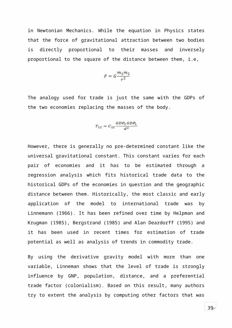
The analogy used for trade is just the same with the GDPs of

the two economies replacing the masses of the body.

However, there is generally no pre-determined constant like the

universal gravitational constant. This constant varies for each

pair of economies and it has to be estimated through a

regression analysis which fits historical trade data to the

historical GDPs of the economies in question and the geographic

distance between them. Historically, the most classic and early

application of the model to international trade was by

Linnemann (1966). It has been refined over time by Helpman and

Krugman (1985), Bergstrand (1985) and Alan Deardorff (1995) and

it has been used in recent times for estimation of trade

potential as well as analysis of trends in commodity trade.

By using the derivative gravity model with more than one

variable, Linneman shows that the level of trade is strongly

influence by GNP, population, distance, and a preferential

trade factor (colonialism). Based on this result, many authors

try to extent the analysis by computing other factors that was

39

omitted by Linneman. For example, Srivastava (1986) uses

demographic variables, political variables (political

instability, membership in a particular economic union,

colonial heritage), cultural variables (religion and language)

and the geographic distance to determine the share of trade

among two countries. Variable such as tariffs,

transaction/transport cost, and foreign direct investment have

being introduced in recent studies (see Eichengreen and Tong

(2007); Boughanmi et al (2009)). De Grauwe et al (2011) have

gone further by adding governance in addition to traditional

variables, to show that this variable can play a key role in

trade between African countries and their partners.

To address the issue of this paper, we will derive a gravity

model. Based on the paper of De Grauwe et al (2011), we will

use most of the same variables (distance, GDP per capita,

population, governance, oil resources, historical

relationship). Additionally, we will control for as exchange

rate (trade revenue of many African countries are in dollar and

the levels of exchange rate of currencies of BRIC countries

with dollar can influence the direction of trade). Empirically,

we will estimate the trade flows for each BRIC countries with

Africa by using two methods. First, we will use a simple pooled

OLS regression to determine significant variables. Finally, to

check for the robustness and the dynamics of the estimation, we

will compute the panel data approach for the period 2000 -2010.

The data we will use come from many sources: CEPII, COMTRADE,

IFM, WORLD BANK and other sources.

39

2: EVOLUTION OF TRADE BETWEEN AFRICA AND BRIC’sCOUNTRIES

This section focuses on Africa and BRIC macroeconomics’

situation. We will analyze some elements such as production and

trade variables.

2.1: Rapid view of BRIC and Africa

2.1.1: BRIC in the World economy

The term BRIC was used for the first time in 2001 by Jim O’Neil

in the global Economics paper “Building Better Global economies

BRICs” published on November 30th of that year by Goldman Sachs

Inc. The term have been used to designate the group of

countries constitute by (Brazil, Russia, India and China) which

continuously increase their power in the world economy since

the beginning of nineties.

This block is becoming more en more powerful among others

developing countries. In fact, BRIC population count for one-

third of world population and represent a big market. In terms

of growth, those countries have increased their share in world

GDP from 5,8% during the period 1991-94 to 13% in 2005-09 (IMF,

2010). This dynamic can be also observed in trade flows.

According to Freemantle et al (2009), BRIC are now important

actors of world trade and their proportion of world trade rise

from 6.3% in 2000 to 12.8% in 2010

39

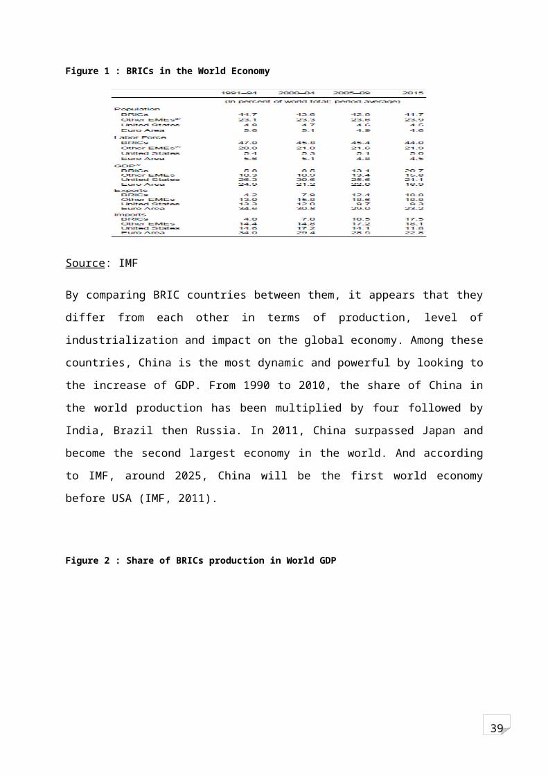
Figure 1 : BRICs in the World Economy

Source: IMF

By comparing BRIC countries between them, it appears that they

differ from each other in terms of production, level of

industrialization and impact on the global economy. Among these

countries, China is the most dynamic and powerful by looking to

the increase of GDP. From 1990 to 2010, the share of China in

the world production has been multiplied by four followed by

India, Brazil then Russia. In 2011, China surpassed Japan and

become the second largest economy in the world. And according

to IMF, around 2025, China will be the first world economy

before USA (IMF, 2011).

Figure 2 : Share of BRICs production in World GDP

39

Source: IMF; * (estimation), ** (forecasts)

2.1.2: Africa: the poorest economy in the world

Actually, by looking on many international macroeconomics

studies, Africa and South Asia are the poorest groups in the

world. In terms of production, Africa is a very small player in

the global economy. Compare to another group of countries,

Africa produce only 3.3% of global GDP in 2011 and contributes

to only 10% to the world GDP growth.

Despite the fact that African participation to world economy is

weak, its production is increasing continuously since 2000 at 5

% growth rate per year sustained principally by higher

commodity prices and exports (IMF, 2010). But the global

financial and economic crisis of 2008/2009 had interrupted this

period of high growth such that it decreases to 3.1% in 2009.

Figure 3 : Africa economic growth

39

Source: Africa Development bank

This improvement in production influences the level of trade

between the continent and the rest of the world. According to

the WTO (2011), the volume and even the value of goods and

services has increased significantly from USD 13 trillion in

2000 to an estimated USD30 trillion in 2010. Also the share of

world export rose from 2.2% to 3.6% between 2000 and 2010. But

African countries have not really benefited from the steady

increase in the volume of international trade. Indeed, Africa’s

share of in world trade has been in decline since 1980 from

5.80 % in 1980 to 2.23% in 2000.

Many reasons can explain this lost of competitiveness of

African trade. First of all, the key and major reason is the

declining of price of primary commodities which constitutes the

main part of their exports. The second explanation is the low

productivity and even sometimes the absence of manufacturing

sector. Another constraint is the weakness of intra-African

trade comparatively to trade within other regions. On average

39

over the past decade, only about 10–12 % of African trade is

with African nations (UNECA, 2009). This limitation is due to

difficulties to promote regional integration, the absence of

subregional communication infrastructures and the inexistence

of deeper financial and capital markets.

2.2: Trade between Africa and BRIC

2.2.1: BRIC: New trade partner of African countries

Due to some history facts such as colonization, the traditional

African trade partners are European countries and United States

of America. Since two decades, BRIC are becoming important

partners for African countries. In 2008, China, India and

Brazil rank as Africa’s 2nd, 6th and 10th largest trade partners,

respectively (Freemantle et al, 2009). The BRIC-Africa trade as

a proportion of Africa-world trade grew from 4% in 1995 to over

23% in 2010.

Figure 4 : BRIC-Africa trade as a proportion of Africa-world trade

39

Source: IMF

Analysis across African countries shows that those which are

natural resources abundant and large population dominate flows.

Among them, South Africa, Egypt, Nigeria and Angola are the

most significant partners for the BRICs in Africa. For example,

Angola accounts for 20% of all BRIC-Africa trade and South

Africa accounts for 20% of BRIC exports to Africa and 15% of

BRIC imports from Africa.

This intensification of trade between Africa and BRIC can be

explained by the fact that countries as China, India and Brazil

are growing very rapidly countries need enough minerals

resource to support their rapid domestic economic growth and

development (Simon Fremantle et al, 2009; Raphael Kaplinsky et

al, 2008). But the share of each BRIC in this trade is not

equal.

China dominates BRIC-Africa trade flows and accounts for around

two-third of BRIC-Africa trade. But adjusted for economic size,

India and China’s, Brazil and Russia’s percentages of trade

with Africa as a proportion of GDP are relatively 2.6% and

2.3%, 1.7% and 0.6%, respectively.

39

Figure 5 : Evolution of share of each BRIC in African trade (%)

Source: IMF

By looking to products import from Africa, It appears that

nearly 80% of China’s imports from Africa consist of oils,

mineral and natural resources such as seaborne iron, diamonds,

logs, nickel, copper, aluminum, zinc and steel. This share is

increasing since the nineties. This can be explained by the

discovery of news reserves in Africa.

Figure 6 : Composition of Chinese Imports from Africa

Source: Vidyarthee (2010°

39

This state of affairs can explain why many authors think that

natural resources enlighten the strong presence of China in

many African countries. But, it is necessary to remind that

African exports even to western countries are dominated by

primary products. It can also be observe that it is not a

Chinese specificity because when looking at others BRIC which

are similar to China, the pattern is similar.

Indeed, over 70% of India’s imports from Africa comprise

mineral fuels and oil. Africa also provides India with 50% of

its inorganic chemical and precious metal compounds, which

account for 11% of Africa’s exports to India. Brazil imports

mainly mineral and chemical products from Africa, while Russia

import cocoa and fruits (Freemantle et al, 2009)

2.2.2: BRIC investments and trade with Africa.

One of the most important dimensions of the relationship

between Africa and BRIC is Foreign Direct Investment (FDI).

Although most FDI to Africa still comes from OECD countries,

the largest increase in FDI to Africa in recent years has come

from BRIC. Over the past 10 years, FDI flows from BRIC to

Africa have increased consistently, only falling slightly in

2009 due to the global economic crisis. However, despite this

significant evolution, one should note BRIC were only the

fourth largest FDI investor region into Africa between 2003 and

2009 far behind the United States, Western Europe and Japan.

39

Another fact is that while at the beginning, the immensity of

the BRICs’ FDI to Africa has been concentrated in South Africa,

Egypt and Morocco, recently other countries are becoming new

destination of investment (Mwangi, 2009).

Figure 7 : Total capital investment in FDI projects in Africa (2003-2009)

Source: FDI Intelligence from Financial Times Ltd

According to the FDI Markets from Financial Times, India was

the largest of the BRIC countries in terms of overseas

investment projects in Africa between 2003 and 2009. But in

terms of global value China is before with cumulative value of

USD28.7 billion of investments followed by India (USD25

billion) then Brazil (USD10 billion) and Russia (USD9.3 bn). As

in case of trade, natural resource sector is the main

destination of BRIC’s FDI.

Figure 8: Number of BRIC FDI projects in Africa between 2003 and 2009

39

Source: FDI Intelligence from Financial Times Ltd

A recent IMF study conducted by Mlachila and Takebe (2011)

shows that the natural resource and infrastructure sectors

attract the biggest share of Chinese FDI to Africa in terms of

volume. But the lack of data doesn’t permit to determine the

precise sector that attracts the investment. But authors

estimate that since the largest recipients of Chinese FDI are

mostly natural resource countries, it is reasonable to conclude

that Chinese FDI to SSA countries is mostly concerned with

natural resources and infrastructure.

But as in previous case of trade, China is not the only one

with this model but also India and Brazil invest in primary

sector. The study by Chanda, Banerjee and Vishnoi (2008)

explains that pressure on production costs in those countries

oblige them to look Africa as a major source of cheap raw

material and natural resources to secure their growth.

39

III: METHODOLOGY

3.1: Gravity model

3.1.1: Background

The earlier studies (e.g., Beckerman 1956; Ullman 1956; Smith

1964; Linneman 1969; Yeats 1969) that try to evaluate trade

flow between two countries have used a relation between

distance and trade (see Rajendra Srivastava et al, 1986). Those

studies have shown that distance influence negatively the

intensity of trade flows that occur between nations. So

countries that are geographically proximate will tend to trade

relatively more than will nations that are further. But only

distance was not sufficient as determinant of intensity of

trade.

Based on the gravity model uses in Physics to determine the

intensity of attraction between two objects, Tinbergen (1962)

and Pöyhönen (1963) were the first authors applying the gravity

equation to analyze international trade flows. The model assume

that trade between two countries is directly related to

countries’ size and inversely related to distance between them.

Linneman (1966) has conducted the most interesting study on the

determinants of trade. He used an econometric model to study

the factors that determined the trade flows between 80 nations

in 1959. He introduce GNP, population, distance, and a

preferential trade factor as independents variables in the

39

model, with preferential trade factor as a dummy variable

indicating whether the nation was in the British, French, or

Belgian or Portugese sphere of influence. He found that all the

variables had a statistically significant relation with the

volume of imports and the volume of exports flowing between the

pairs of nations.

Based on Linneman paper, Rajendra Srivastava et al (1986) have

extended the model to several factors that could affect trade

flows but that were omitted from the Linneman study. These

factors include political instability, membership in specific

economic unions, and such cultural factors as religion and

language. They also controls for variation in the size of

nations' economies (GNP).

But all those studies were empirical analysis, theoretical

support of the research in this field was originally very poor,

but since the second half of the 1970s several theoretical

developments have appeared in support of the gravity model

(Inmaculada Martinez-Zarzoso, 2003, Laura Marquez RAMOS, 2007).

Anderson (1979) is the first who try to formalize the gravity

equation from a model that assumed product differentiation.

Bergstrand (1985, 1989) also explored the theoretical

determination of bilateral trade in a series of papers in which

gravity equations were associated with simple monopolistic

competition models. The differences in these theories help to

explain the various specifications and some diversity in the

results of the empirical applications.

39

There is a huge number of empirical applications in the

literature of international trade, which have contributed to

the improvement of performance of the gravity equation. Some of

them are closer related to our work. First, in recent papers,

Chen and Wall (1999), Breuss and Egger (1999) and Egger (2000),

Rose (2004), improved the econometric specification of the

gravity equation when explaining trade flows among countries.

Second, Berstrand (1985), Helpman (1987), Wei, (1996), Soloaga

and Winters (1999), Limao and Venables (1999), and Bougheas et

al, (1999), De Grauwe et al (2011) among others, contributed to

the refinement of the explanatory variables considered in the

analysis and to the addition of new variables.

3.1.2: The gravity model

According to the generalized gravity model of trade, the volume

of exports between pairs of countries, Xij, is a function of

their incomes (GDPs), their populations, their physical

distance and a set of dummies variables ( see Deardorff, 1995;

Martinez, 2003; Marquez 2007).

(1)

Where Yi (Yj) represents the GDP of the exporter (importer)

country, Pi (Pj) are the population of exporter (importer), Dij

indicates the distance between the two countries’ capitals (or

economics main centers), Aij represents another factor that can

39

enhance the level of trade among the partners (language,

colonialism…) and uij is the error term

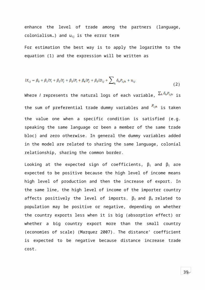
For estimation the best way is to apply the logarithm to the

equation (1) and the expression will be written as

(2)

Where l represents the natural logs of each variable, is

the sum of preferential trade dummy variables and is taken

the value one when a specific condition is satisfied (e.g.

speaking the same language or been a member of the same trade

bloc) and zero otherwise. In general the dummy variables added

in the model are related to sharing the same language, colonial

relationship, sharing the common border.

Looking at the expected sign of coefficients, β1 and β1 are

expected to be positive because the high level of income means

high level of production and then the increase of export. In

the same line, the high level of income of the importer country

affects positively the level of imports. β3 and β4 related to

population may be positive or negative, depending on whether

the country exports less when it is big (absorption effect) or

whether a big country export more than the small country

(economies of scale) (Marquez 2007). The distance’ coefficient

is expected to be negative because distance increase trade

cost.

39

3.2: The model and data

3.2.1: The model specification The gravity model in the paper is derived from the paper of De

Grauwe, Houssa and Piccillo (2011) where they use it to compare

the trade flows between Africa and its traditional partners and

China. They constructed an extension on the model developed by

Rose and Spiegel (2004) use to determine the link between trade

and external debt.

In this model Xij (imports or exports) is determined by

(3)

Where, Dij is the distance, YiYj/PopiPopj represents the GDP per

capita of the countries i and j; Colonyij is a binary variable

that takes the value 1 if i was colonized by j or vice versa,

Langi,j is a binary variable that takes the value 1 if the

countries i and j have a common official language, Ressourcej

is a binary variable that takes the value 1 if an African

country is abundant in oil and minerals, Tt is the time fixed

effects that takes the value 1 at time t and 0 otherwise,

Governancejt is the quality of governance of an African country

at time t; where higher values indicate good governance and εijt

is the error term.

In our study, to compare China and other emerging markets

(India, Brazil and Russia), we will use the same extended

39

gravity model but we will drop the variable colonization which

is not apply and language will be turn in to historical

relationship (same language for Brazil, have been partner of

Russia during the cold war, have historical trade relationship

with China or India). This variable take the value one if the

is a relationship and 1 otherwise. To have

In addition, we will add:

The real exchange of BRIC currencies relatively to dollar.

Abdur R Chowdhury (1993) show that the volatility of

exchange rate depresses trade flows. Linda S. Goldberg et

al (1998) say that in addition to this direct linkage

between trade flows and direct investment, the real

exchange rate influences trade flows. In our study we

choose US dollar as reference money because the huge part

of export revenue of African countries is in US dollar.

In the result our model estimates export of BRIC country i to

African country j as:

(4)

Where i represents one of the following African trade partners,

China, India, Brazil, Russia; and j represents an African

country. is the logarithm of export or import of BRIC

country i from African country j in real term. measures the

39

cost of trade, YiYj/PopiPopj represents the level of wellbeing of

each countries i and j; is the size of countries i and j,

is a binary variable representing the historical

relationship between BRIC country i and African country j. This

variable takes the value 1 when the two countries are related

and 0 otherwise. is logarithm of real exchange rate of the

currency of BRIC relative to dollar.

In our equation, we expect , , , , and to be positive

and , to be negative. Finally, following the analysis of De

Grauwe, Houssa and Piccillo (2011), we expect the coefficient

on governance to have a positive sign. The main intuition is

that the governance quality of a country affects the

transaction costs involved in economic activities and a country

with low governance will display a high transaction cost and

should trade less with others.

For African export in direction of BRIC countries we change a

bit the equation by removing exchange rate because this

variable doesn’t logically affect the level of export.

3.2.2: The Data In the paper, we will estimate separately aggregate exports and

aggregate imports between each of BRIC (Brazil, Russia, China

and India) and 50 African trade partner countries1. The data1 Algeria, Angola, Benin, Botswana, Burundi, Cameroon, Cape Verde, CentralAfrican Republic, Chad, Comoros, Republic of Congo, Djibouti, Egypt,Equatorial Guinea, Ethiopia, Gabon, Gambia, Ghana, Guinea, Guinea Bissau,Ivory coast, Kenya, Liberia, Libya, Madagascar, Malawi, Mali, Mauritania,

39

use in the model cover the period 2000-2010 and those data are

yearly. This period is choosing because of the availability of

the date on governance. In total we have 550 observations for

each variable.

Data on total exports and imports are in current dollars and

are taken from the IMF-DOTS2 database. We use the US CPI series

(2005 = 100) from the World Bank database to convert the trade

data in real terms. Always from World Bank database, we obtain

data on aggregate GDP and GDP per capita are in constant prices

of 2005 dollar.

Data on landlocked and distance are taken from the CEPII

distance database. For distance, we choose the relative

distance between the two mains economic cities of trade

partners. For landlocked countries, the statistic shows that

64% (34/51) have direct access to the sea.

The information on African resource abundant countries is

derived from Collier and O.Connell (2009). He takes in account

the existence of oil resource in a country but also other

minerals resources like gold, diamond, uranium, steel, bauxite

copper… But one limit of this data is that he don’t consider

Mauritius, Morocco, Mozambique, Namibia, Niger, Nigeria, Rwanda, Sao Tomeand Principe, Senegal, Seychelles, Sierra Leone, Somalia, South Africa,Sudan, Tanzania, Togo, Tunisia, Uganda, Burkina Faso, Congo Dem.Rep,Zambia, Zimbabwe, Lesotho, Swaziland, and Eritrea.

2 The DOTS data was accessed from MACROBOND at the Facultés UniversitairesNotre Dame de la Paix de Namur. It’s a financial database provided byMacrobond Financial AB. Macrobond Feed Solutions is a system for customdata delivery. www.macrobondfinancial.com/

39

timber as resource while it becoming a non negligible part of

products trade by African countries.

Figure 9 : Structure of resource abundance among African countries

Source: Data Conell’ data

For governance quality Kaufman et al (2011) provides estimated

values for six governance indicators:

Voice and Accountability (defined as the voice that each

citizen has in the making of the government);

Political Stability and Absence of Violence/Terrorism (The

stability of the government and the perceived danger that

this will be overthrown violently);

Government Effectiveness (Looking at the quality of the

government policies; and their effectiveness and

credibility);

Regulatory Quality (the ability of the government to pass

a regulatory framework to regulate private property);

Rule of Law (summarizing the perceptions on the

credibility and enforcement of contracts);

39

Control of Corruption (Looking at the perception of

government power yielded to defend private interests and

the extent of private elites).

The range of those indicators is -2,5 to 2,5 in 1996- 2009,

where higher values indicate better governance outcomes. In

this paper, we use the period 1999-2010 and we drop the year

2002 because of the absence of governance data that year. To

obtain the final governance indicator, we compute the mean of

the six indicators.

Figure 10 : Evolution of governance

-2-1

01

0 5 10tim e

Gouvernance gouv_m ean

Source: Author from Kaufman data

All the variable we have use are specified in the next figure.

Figure 11 : Variables in the models

lgdp Logarithm of GDP

ldist Logarithm of distance

rel Historical relationship

39

landlocked Landlocked country

exchange Exchange rate

resource Resource abundant country

governance governance

Source: Author

39

IV: EMPIRICALS ANALYSIES In this paper we use two methods to estimate the gravity model

for exports and export between each four BRIC countries and 50

Africans countries. Firstly, we use the pooled OLS with robust

standard errors to deal with heteroscedasticity and

autocorrelation in the residuals. Secondly, we use a panel data

approach. In this case as we have some variables which don’t

change across time (relation, resource, distance) and we want

to estimate their specific effect on trade flows, we opted for

panel data with random effect instead of fixed effects. Because

with fixed effect model, these variables are absorbed by the

intercept and we cannot evaluate in that case their influence

on dependant variable.

4.1: Mains results for African exportsIn the exports model, we remove the GDP deflator for BRIC

countries because this variable affects neither the price nor

the quantities of good that African countries export.

4.1.1: The gravity model with Pooled OLSBy using the pooled OLS, the result show globally that

traditional gravity variables are significant as determinant of

African countries exports to BRIC. The results also confirm

what we expected in terms of sign of coefficient. Aggregate GDP

is positive and significant. Except for India, distance

explains significantly and negatively African imports.

Moreover, it appears that landlocked African countries trade

significantly less with BRIC than do their costal counterparts.

39

Figure 12 : Gravity model on African exports, Pooled OLS

Variables Brazil China India RussiaR2 0,80 0,95 0,93 0,84

lgdp .7574685 *(.0968618)

.6256379 *(.0629981)

.5759051 *(.0558143)

.7214511 *(.0750926)

ldist -2.970361 *(.5807309)

-.9175969 *(.4525468)

-.5377276(.4456519)

-2.724806 *(.423442)

rel -1.650869 **(.9827139)

1.221354 *(.4407211)

-.4932146 *(.3440997)

-1.620627 *(.692052)

landlocked -1.687183 *(.5620353)

-1.018588 *(.3550577)

-1.973281 *(.3426607)

.4167407(.5013581)

ressource 1.477204 *(.5471312)

1.908505 *(.3505314)

.5206762(.3395439)

.5468317(.4889804)

gouvernance -.1057868(.4581973)

-1.068914 *(.2996361)

.0467965(.2964291)

.1971954(.4217983)

Source: Author; * p value < 0,05; ** p value

<0,10

A deep look on this estimation shows some differences across

BRICs countries that need to be analyze.

The historical relationship variable affects differently the

BRIC. The negative sign means that the probability for the BRIC

from a country which don’t have historical relationship instead

of a historical partner is low. For Brazil, India and Russia,

the existence of past relation with an African country increase

the level of export from that country to his counterpart. But

we observe that the coefficient is high for Brazil and Russia

than for India. This can be explained by language barrier for

Brazil (few countries are lusophone in Africa) and the Cold War

for Russia (trade is high in countries which was in the soviet

side during the Cold war). For India, there are contacts with

some African countries for many centuries this affect

positively the level of trade between them, but the coefficient

39

is not too high (contrary to the other BRIC) because India is

trying to diversify his trade partner in Africa. For China, the

historical contact reduces the level of exports. One of the

possible explanations can be that actually, China is creating

new market in many ex European colonies.

The impact of resource is not significant for India and Russia

contrary to China and Brazil. Indeed, India’s import

composition has changed dramatically over the last decade. The

import volume for commodities in got more than twelve-fold

increase; machinery and transport equipment sector has had a

seven-fold increase, while the import volume of mineral

fuel/lubricants reduced to its one-fifth. (Kaushal Vidyarthee,

2010). So India’s imports depend less and less from the

availability of natural resource in the origin country. Russia

is full of natural resource and imports mostly cocoa, iron and

fruits (80 % of total share) from six African countries

(Freemantle et al, 2009).

But for China and Brazil, it appears that the rich resource

countries are most targeted. This confirms the statistics of

composition of China’s imports (80 % of oil and mineral

resources) and Brazil’s import (85 % of crude oil and other

mineral). The difference between India’s and China’s imports

structure is due to the fact that growth in china is driven by

the industrial sector which need enough natural resources while

services are the main sector of growth in India.

Turn to the one of variable of interest which is governance,

it’s appears that the effect is not clear on trade with BRIC’s

39

countries except for China. For this country, the level of

governance is negatively and highly correlated with imports

from the African trade partner. This can be explain by the fact

that African countries that are well govern or improve their

governance usually trade more with western democratic

countries. But China imports more from African countries with

corrupted governments, with less rules of law, with less

accountability and with less regulation confirming the wide-

spread belief that China is deliberately pursuing tighter

economic relations with those countries that are isolated by

the rest of world and help them get access to world market.

Another reason can be the fact that as trade of natural

resources is very costly for importer because of some

externalities. Actually there is a lot of demand of adequate

transparency and accountability on the sector to ensure that

wealth is managed for the benefit of the whole population.

Transparency in oil sector operations allows democratic debate

on how oil wealth should be handled. This situation obliges the

extractive firm to pay the right price and preserve the

environment. So to make more profits or integrated the market,

there is an incentive for firm to cheat and deal with

dictatorial and corrupted government. As china needs huge

quantity of oil and mineral resources, it is easy to trade at

low cost with countries in which the level of governance is

low.

.

39

4.1.2: The gravity model with panel random effectsTo check the robustness and the consistency across time of the

results we obtain with OLS, we use a panel data approach. The

first observation is that many variables are not significant

with the introduction of dynamic.

Figure 13 : Gravity model on African exports, panel data approach

Variables Brazil China India Russialgdp .175578 **

(.0934818).195246 * (.0570544)

.3636274 * (.055933)

.2713067 * (.0575557)

ldist 2.096626 (2.486186)

-2.899291 (3.116068)

1.19706 (1.747389)

-1.402899 (2.552221)

rel -1.702719 (1.946541)

1.551641 (1.04993)

-.2752746 (.7967731)

-.9391929 * (1.795206)

landlocked -2.073243 * (1.090561)

-1.19344 (.8514889)

-1.971702 * (.7812281)

.2789076 (1.324452)

ressource 2.649835 (1.087956)

2.277442 (.8715931)

.4017141 (.8116567)

1.014883 (1.263318)

governance .4493497 (.772603)

-1.887032 * (.5572432)

-.0561473 (.5516696)

.9766322 (.7255014)


<0,10

As the figure 14 shows, only the size of economy keep its

significativity across time. Distance, historical relationship

and the resource abundance of African countries don’t explain

the level of trade between Africa and BRIC countries.

Governance remains consistent with the introduction of dynamic

for China and landlocked African countries trade less with

Brazil and India even in the long run.

39

4.1: Analysis for African imports

4.2.1: The gravity model for African imports with Pooled OLS

Figure 15 displays estimated result of our gravity model for

African imports with OLS and we can see that the results are in

conformity with was we expected. Indeed, the traditional

determinants of trade present the predictable sign. Moreover,

the size of economies affects positively the level of imports

and the distance reduces the intensity of trade between African

countries and BRIC trade partners. Similarly, landlocked

countries trade less because of the increase of cost of

transportation..

Figure 14 : Gravity model on African import, Pooled OLS

Variables Brazil China India RussiaR2 0,93 0,99 0,99 0,87

lgdp .4760997 *(.0702333)

.3968157 *(.025087)

.4391558 *(.0236686)

.7808313 *(.0737461)

ldist -1.075653 *(.4090991)

-.1961674*(.1357263)

-.5096221 *(.1300193)

-2.945054 *(.4285991)

exchange .0298744(.5338681)

-1.046257 *(.2742648)

-.1590585 *(.0686968)

5.14e-14( 5.35e-13)

rel -1.20653 **(.7153498)

.7042033 *(.1765367)

.3497662 *(.1426651)

.535896(.6738921)

landlocked -3.787598 *(.4090668)

-1.26202 *(.1427028)

-.8975385 *(.1431466)

-2.85762 *(.4883512)

governance -.5522061 **(.3335356)

.2289114 **(.120377)

.3484688 *(.1229952)

-.7370076 **(.4109777)


<0,10

39

The impact of historical relationship is changing across BRICs

countries. For Brazil, African country which speaks Portuguese

has a big probability to import more from this country than

other African countries. This can be explain by the fact that

Brazilian exports are confined to few key trading partner and

Angola represent the most significant one. In the contrary, for

China and India, historical relation has the opposite effect.

Countries which have historical contact with those BRIC are not

the main direction of export of China and India. One

explanation can be that actually China and India are

intensifying their cooperation with other African partners than

their historical partner. And those news partners which were

trading before most with their colonizer are now open and

represent large market for China and India.

The exchange rate don’t have effect on Brazil’s and Russia’s

exports but affect negatively the level of trade between

African countries, China and India. For those two African trade

partner, when their currency appreciate relatively to dollar,

this reduce the size of exports because many African countries

have their trade revenue in dollar or euro. And also because

China and India are competing in many goods with developed

countries and a rise in price in those two BRIC, due to the

appreciation of currencies, creates a deviation of trade.

Finally, looking to our variable of interest governance, it

appears that the sign diverge from one BRIC to another even if

the significativity is not really strong. Brazil and Russia

trade more with countries with low level of governance maybe

because they trade more with their historical partner that are

39

in general not well governed. But China and India export more

to countries with relative good governance level. This is due

to fact that those two countries are competing with developed

countries in Africa and the good governance tends to facilitate

the trade transaction and reduce costs for exporter.

4.2.1: The gravity model for African imports with panel data approachThe introduction of dynamic with panel data approach shows that

many results that we obtain with OLS are not consistent across

time. Figure 16 reveals that only the size of economies, the

GDP deflator and the situation of African countries relatively

to the sea remain constant through time. The historical

relation and distance don’t count in the long run. For

governance, only Chinese exports are affected by the quality of

African countries governance but the significativity is not

robust. The exchange rate remains significant for China and

India from which African countries import more. Those countries

are very sensitive to change in price of good due the

appreciation of currencies.

Figure 15 : Gravity model on African imports, Pooled OLS

Variables Brazil China India Russialgdp .2889984 *

(.0778604).1807244 * (.0203047)

2087098 * (.0190228)

.0736883 .0697255

ldist -.8980085 (1.309506)

-1.155951 (1.211694)

-.8585673 (.7917513)

-6.988357 * (2.324247)

rel -1.5155 (1.024974)

.9429454 * (.4081831)

.3953858 (.3600178)

.7338865 (1.621302)

exchange -.4139441 (.4060152)

-1.641073 * (.1924888)

-.0981517* (.0551623)

4.08e-13 (2.77e-13)

39

landlocked -3.902144 * (.5741144)

-1.255487 *(.3310995)

-.9922131 * (.3551281)

-2.581588 *(1.198228)

gouvernance -.7314077 (.4519326)

.4093277 **(.2122693)

.1032534 .2138818

-.6024147 (.7652006)


<0,10

39

IV: CONCLUSION AND REMARKS

The aim of this paper was to understand the increasing interest

of BRIC countries for Africa and verify if China is a different

trade partner. We have shown the rising of their share in

African trade and found out that China dominates this trade

followed by India. Those two BRIC, to support and sustain their

rapid development, need enough inputs for their industries from

Africa. The analysis points out the fact that all BRIC

countries import essentially oil and naturals resources except

Russia which is full of oil. And African countries imports

manufactured goods and receive an increasing quantity of FDI in

primary sector but also in services. Additionally their receive

aid aids, gifts and preferential loans from BRIC partners.

To identify the main determinants of trade between Africa and

BRIC, we have computed a gravity model. The model regresses

African trade on variables such as size of economy, distance,

historical relationship and access to sea. In addition, we

added a set of variables to capture some particularities. Those

variables are the level of governance and the exchange of BRIC

relatively to dollar. First, we use pooled OLS model to

estimate the model for each BRIC countries. To verify the

robustness and the consistency across time, we apply a panel

data approach to introduce the dynamic.

The result shows that for exports, size of economy is the first

determinant. In a contrary, distance, historical relationship

and the resource abundance of African countries don’t explain

39

the level of trade between Africa and BRIC countries except for

Russia. In addition landlocked African countries trade less

with Brazil and India in the long run and governance affect

negatively only China imports. One of the explanations can be

that as there is a pressure for transparency and accountability

on the natural resource sector, it is tempting for Chinese

firms which need enough resource to deal with bad governed

countries. This helps them to have access to the market which

is dominated by western countries and also reduce cost of

production.

For African imports, the main result is that exchange rate

reduces trade from China and India, the core origin of imports.

Those countries are very sensitive to change in price of good

due the appreciation of currencies.

To answer to question of particularity of China in African

trade that we have rise at the beginning of this paper, the

result of the model shows that:

The resource abundance of African country is not a

significant driver of China trade as many authors think.

This can be explained by the fact that across time China

is trying to diversify imports and create new market for

his excess production such that actually he is trading

also with non resource abundant countries in Africa.

China and India are not really different in the way of

trading with African countries. Those two countries are

influence by the same variable except governance in case

of imports. This difference is due to structure of the

39

two economies. China is more industrialize than India

(more specialize in tertiary activities) and for this

reason the first needs more oil than the second. Or as it

had been shown, many oil African have low level of

governance and face some conditionality (improve

governance) to trade with western country. And to bypass

those rules, trade with China is the good issue. But when

looking their exports, the two prefer better govern

African countries to reduce the cost of trade.

China and India are at some level different to Brazil and

Russia. Brazil is facing the problem of language (huge

barrier for communication) and Russia is full of resource

and don’t really present a rapid increase of his

production that can require input or new market for

export. But still all BRIC trade with Africa is affected

by same variable such as landlocked situation of African

country.

So to conclude, it is very difficult and even inappropriate to

say that China is a different trade African partner but still

some research need to be done to present a stronger conclusion.

For example one of the limits of this paper is that we use

global data on exports and imports. It will be important to

analyze deeper types of goods that are traded by using a

gravity model which include a third dimension which is the type

of products. Another extension of this paper can be the

evaluation the possible impact of the increasing of FDI on the

trade flows between African countries and BRIC.

39

BIBLIOGRAPHY

Ademola, O. T., Bankole, A. S., Adewuyi, A. O. (2009).

“China-Africa Trade Relations: Insights from AERC Scoping

Studies”. European Journal of Development Research, 21:

485-505.

Akinola, O. (2010). “The Patterns of Chinese and Western

Trade, aid and Investment in Africa: A Comparison”. MSc

Thesis, Graduate Institute of International Development

Studies. Geneva.

Bamidele Adekunle, Ciliaka Wanjiru Gitau (2011), “Illusion

or Reality: Understanding the Trade Flow between China and

Sub-Saharan Africa”, CSAE 25th Anniversary Conference.

Bokilo Julien (2011), “China in Africa, Competition

between china, traditional trade partners of Africa and

BRIC countries”,L’Harmattan.

Deborah Brautigam (2009), “The Dragon’s Gift, the real

story of china in Africa,” Oxford University press.

Human Rights Watch (2003), ‘Imperialist intervention is

never humanitarian’ in World Report 298.

IMF (2010), World Economic Outlook, October.

Issouf Samake and Yongzheng Yang (2010), “Low-Income

Countries' BRIC Linkage: Are There Growth Spillovers?” IMF

working paper.

39

Jodi Rosenstein (2005), “Oil, corruption and conflict in

West Africa”, KAIPTC, Monograph N°2, October 2005.

John Hawksworth and Gordon Cookson (2010), “The World In

2050: a broader look at emerging market growth prospect”,

PricewaterHouseCoopers.

Kent Ewing (2006), “China mixes rice and neo-colonialism”,

Asia Times edition of 6th October 2006.

Laura Marquez RAMOS (2007), “New determinants of trade: an

empirical analysis for developed and developing

countries”. Universitat Jaume.

Montfort Mlachila and Misa Takebe : FDI from BRICs to

LICs: Emerging Growth Driver?, IMF working paper, 2011

Mwangi s. Kimenyi and Zenia lewis (2009), “The BRICS and

the new scramble for Africa, The Brookings Institution”,

IMF working paper..

Paul De Grauwe, Romain Houssa and Giulia Piccillo (2011),

“African Trade Dynamics: Is China a Different Trading

Partner”, Center for Economics Studies.

Paul De Grauwe, Romain Houssa and Giulia Piccillo (2010),

“China Africa relationship: good for both parts?”, Center

for Economics Studies.

Paulo Roberto de Almeida (2009), “The Brics’ role in the

global economy”, British Embassy in Brasília:Rio de

Janeiro.

39

Pöyhönen P (1963), “Atentative model for the volume of

trade between countries”, Weltwirtschafliches Archiv 90,

pp 93-99.

Rajendra Srivastava and Robert Green (1986), “Determinant

of bilateral trade flows, Journal of Business”, vol. 59.

Raphael Kaplinsky, Dirk Messner (2007), “The impact of

Asian Drivers on the Developing World”, World Development,

Elsevier.

Raphael Kaplinsky, Dorothy McCormick, and Mike Morris

(2008), “China and Sub Saharan Africa: Impacts and

Challenges of a Growing Relationship”, working paper in

Africa studies.

Simon Freemantle, Jeremy Stevens (2009), “Tectonic shifts

tie BRIC and Africa’s economic destinies”, Standard Bank.

Timbergen J (1962), “Sharping the world economy:

Suggestions for an international economy policy”,

International Century Fund.

Martinez-Zarzoso Inmaculada and Felicitas Nowak-Lehmann

(June 2003), “Gravity model: an application to trade

between Regional Blocs”, Atlantic Economy Journal. 31(2):

pp.174-187.

Rose Andrew k and Spiegel Mark M (2004), “A Gravity Model

of Sovereign Lending: Trade, Default, and Credit”, IMF

Staff Papers Vol. 51, Special Issue.

Scott L. Baier and Jeffrey H. Bergstrand (2001), “The

growth of world trade: tariffs, transport costs, and

39

income similarity”, Journal of International Economics 53

pp. 1–27.

Linda S. Goldberg and Michael Klein (1998), “Foreign

Direct Investment, Trade and Real Exchange Rate Linkages

in Developing Countries”, Cambridge University Press

pp.73-100.

Abdur R Chowdhury (1993), “Does exchange rate volatility

depress trade flows? Evidence from error correction

models”, The Review of Economics and Statistics Vol. 75, No. 4, pp.

700-706.

Peter K. Schott (2006), “The relative sophistication of

Chinese exports”, Working Paper, National Bureau of

Economic Research.

World Bank, (2004a), “Patterns of Africa-Asia Trade and

Investment, Potential for Ownership and Partnership”.

Volume 1 and Volume 2, Africa Region Private Sector Group.

Washington: World Bank.

World Bank, (2004b). “Country Analytical Briefs with

Compendium of Country-Specific Analysis of Africa-Asia

Trade Complementarity”. Africa Region Private Sector

Group. Washington: World Bank.

Zafar, Ali (2007) “The Growing Relationship Between China

and SSA: Macroeconomic, Trade, Investment and Aid Links.”

World Bank Research Observer 22(1): 103-130.

Yin-Wong Cheung and Xing Wang Qian (2010), “China’s

Outward Direct Investment in Africa”, University of

California, Santa Cruz.

39

Rupa Chanda, Saikat Banerjee and Aayush Vishnoi (2008),

“India and China: Analysis of Trade Relations with Africa

using Gravity Models”.

Eichengreen Barry and Tong Hui (2007). "Is China's FDI

coming at the expense of other countries?," Journal of the

Japanese and International Economies, Elsevier, vol.

21(2), pages 153-172,

Boughami H, J.Al Shidhani, M. Mbaga and Kotagama H. (2009),

“The effects of trade agreements on agri-food trade: an

application of gravity modeling to the Arab Gulf Cooperation

Council (GCC) countries”. Review of Middle East Economics

and Finance, 5(3): 1-17.

Kaushal Vidyarthee (2010); “India’s Trade Engagements WithAfrica: A Comparison With China”; University of Oxford,

http://ideas.repec.org/s/eee/jjieco.html

http://ideas.repec.org/s/eee/jjieco.html

http://ideas.repec.org/a/eee/jjieco/v21y2007i2p153-172.html

http://ideas.repec.org/a/eee/jjieco/v21y2007i2p153-172.html

39

APPENDIX

Appendix 1 : Brazil estimation

ressource 1.477204 .5471312 2.70 0.007 .4022024 2.552206 landlocked -1.687183 .5620353 -3.00 0.003 -2.791469 -.5828976 gouvernance -.1057868 .4581973 -0.23 0.818 -1.006052 .7944781 exchange .0298744 .5338681 0.06 0.955 -1.019068 1.078817 rel -1.650869 .9827139 -1.68 0.094 -3.581703 .2799645 ldist -2.970361 .5807309 -5.11 0.000 -4.11138 -1.829342 lgdp .7574685 .0968618 7.82 0.000 .5671548 .9477823 limport Coef. Std. Err. t P>|t| [95% Conf. Interval]

Total 84866.2344 499 170.072614 Root MSE = 5.752 Adj R-squared = 0.8055 Residual 16278.3496 492 33.0860764 R-squared = 0.8082 Model 68587.8848 7 9798.26925 Prob > F = 0.0000 F( 7, 492) = 296.14 Source SS df MS Number of obs = 499

. regress limport lgdp ldist rel exchange gouv landlocked ressource, noconstant

rho .36946027 (fraction of variance due to u_i) sigma_e 4.071436 sigma_u 3.1165583 _cons -15.0079 22.50557 -0.67 0.505 -59.11801 29.1022 ressource 2.649835 1.087956 2.44 0.015 .51748 4.78219 landlocked -2.073243 1.090561 -1.90 0.057 -4.210702 .0642165 gouvernance .4493497 .772603 0.58 0.561 -1.064924 1.963624 rel -1.702719 1.946541 -0.87 0.382 -5.517869 2.112431 exchange -.4139441 .4060152 -1.02 0.308 -1.209719 .3818311 ldist 2.096626 2.486186 0.84 0.399 -2.776209 6.96946 lgdp .175578 .0934818 1.88 0.060 -.0076428 .3587989 limport Coef. Std. Err. z P>|z| [95% Conf. Interval]

corr(u_i, X) = 0 (assumed) Prob > chi2 = 0.0104Random effects u_i ~ Gaussian Wald chi2(7) = 18.37

overall = 0.1228 max = 10 between = 0.2015 avg = 10.0R-sq: within = 0.0026 Obs per group: min = 9

Group variable: id Number of groups = 50Random-effects GLS regression Number of obs = 499

. xtreg limport lgdp ldist exchange rel gouv landlocked ressource,re

Prob > chi2 = 0.0000 chi2(1) = 316.86 Test: Var(u) = 0

u 9.712935 3.116558 e 16.57659 4.071436 limport 39.84326 6.312152 Var sd = sqrt(Var) Estimated results:

limport[id,t] = Xb + u[id] + e[id,t]

Breusch and Pagan Lagrangian multiplier test for random effects

. xttest0

39

ressource .6217428 .3990621 1.56 0.120 -.1623334 1.405819 landlocked -3.783473 .4099328 -9.23 0.000 -4.588908 -2.978038 gouvernance -.5466744 .3341963 -1.64 0.103 -1.203302 .1099536 exchange 1.114324 .3893884 2.86 0.004 .349255 1.879394 rel -1.215186 .716764 -1.70 0.091 -2.623482 .1931097 ldist -1.14958 .4235689 -2.71 0.007 -1.981807 -.3173534 lgdp .4783011 .0706483 6.77 0.000 .3394916 .6171106 lexport Coef. Std. Err. t P>|t| [95% Conf. Interval]


. regress lexport lgdp ldist rel exchange gouv landlocked ressource, noconstant

rho .11077941 (fraction of variance due to u_i) sigma_e 3.7729616 sigma_u 1.3317023 _cons 7.474423 12.04957 0.62 0.535 -16.14231 31.09115 ressource .734883 .5742253 1.28 0.201 -.3905779 1.860344 landlocked -3.900516 .574075 -6.79 0.000 -5.025683 -2.77535 gouvernance -.7217012 .4520415 -1.60 0.110 -1.607686 .1642837 rel -1.51083 1.024974 -1.47 0.140 -3.519741 .4980813 exchange .9089203 .370457 2.45 0.014 .1828379 1.635003 ldist -.8994592 1.309483 -0.69 0.492 -3.465999 1.667081 lgdp .2918293 .0787322 3.71 0.000 .1375169 .4461417 lexport Coef. Std. Err. z P>|z| [95% Conf. Interval]




. xtreg lexport lgdp ldist exchange rel gouv landlocked ressource,re


u 1.773431 1.331702 e 14.23524 3.772962 lexport 22.89564 4.784939 Var sd = sqrt(Var) Estimated results:

lexport[id,t] = Xb + u[id] + e[id,t]


. xttest0

39

Appendix 2 : China estimation

ressource 1.908505 .3505314 5.44 0.000 1.219786 2.597225 landlocked -1.018588 .3550577 -2.87 0.004 -1.716201 -.3209755 gouvernance -1.068914 .2996361 -3.57 0.000 -1.657635 -.4801927 exchange -1.046257 .2742648 -3.81 0.000 -1.585129 -.507385 rel 1.221354 .4407211 2.77 0.006 .3554309 2.087277 ldist -.9175969 .4525468 -2.03 0.043 -1.806755 -.0284386 lgdp .6256379 .0629981 9.93 0.000 .50186 .7494157 limport Coef. Std. Err. t P>|t| [95% Conf. Interval]



rho .55065084 (fraction of variance due to u_i) sigma_e 2.4375038 sigma_u 2.6983078 _cons 44.22981 29.1595 1.52 0.129 -12.92176 101.3814 ressource 2.277442 .8715931 2.61 0.009 .5691506 3.985733 landlocked -1.19344 .8514889 -1.40 0.161 -2.862328 .4754472 gouvernance -1.887032 .5572432 -3.39 0.001 -2.979208 -.794855 rel 1.551641 1.04993 1.48 0.139 -.5061844 3.609466 exchange -1.641073 .1924888 -8.53 0.000 -2.018344 -1.263802 ldist -2.899291 3.116068 -0.93 0.352 -9.006671 3.20809 lgdp .195246 .0570544 3.42 0.001 .0834213 .3070706 limport Coef. Std. Err. z P>|z| [95% Conf. Interval]









. xttest0

39

ressource .0794651 .1354515 0.59 0.558 -.1866683 .3455986 landlocked -1.262132 .1372005 -9.20 0.000 -1.531702 -.9925621 gouvernance .2021897 .1157847 1.75 0.081 -.0253026 .4296819 exchange -.8338481 .1059807 -7.87 0.000 -1.042078 -.6256185 rel .7955149 .1703024 4.67 0.000 .4609069 1.130123 ldist .6740403 .174872 3.85 0.000 .3304539 1.017627 lgdp .3745573 .0243436 15.39 0.000 .3267274 .4223873 lexport Coef. Std. Err. t P>|t| [95% Conf. Interval]

Total 173032.601 500 346.065201 Root MSE = 1.4544 Adj R-squared = 0.9939 Residual 1042.82724 493 2.11526824 R-squared = 0.9940 Model 171989.773 7 24569.9676 Prob > F = 0.0000 F( 7, 493) =11615.53 Source SS df MS Number of obs = 500


rho .74707899 (fraction of variance due to u_i) sigma_e .61606021 sigma_u 1.0588001 _cons 36.49533 11.4008 3.20 0.001 14.15017 58.84049 ressource .514073 .3418966 1.50 0.133 -.156032 1.184178 landlocked -1.264366 .3348745 -3.78 0.000 -1.920708 -.6080239 gouvernance .4075673 .1745541 2.33 0.020 .0654475 .749687 rel 1.076801 .4130286 2.61 0.009 .2672798 1.886322 exchange -1.2515 .0500677 -25.00 0.000 -1.349631 -1.153369 ldist -1.273067 1.225801 -1.04 0.299 -3.675593 1.129459 lgdp .0738566 .0150299 4.91 0.000 .0443985 .1033148 lexport Coef. Std. Err. z P>|z| [95% Conf. Interval]






u 1.121058 1.0588 e .3795302 .6160602 lexport 4.230844 2.056901 Var sd = sqrt(Var) Estimated results:



. xttest0

39

Appendix 2 :India estimation

rho .48268508 (fraction of variance due to u_i) sigma_e 2.5324455 sigma_u 2.4462145 _cons -7.678187 16.08762 -0.48 0.633 -39.20934 23.85297 ressource .4017141 .8116567 0.49 0.621 -1.189104 1.992532 landlocked -1.971702 .7812281 -2.52 0.012 -3.502881 -.4405234 gouvernance -.0561473 .5516696 -0.10 0.919 -1.1374 1.025105 rel -.2752746 .7967731 -0.35 0.730 -1.836921 1.286372 exchange -.0981517 .0551623 -1.78 0.075 -.2062678 .0099644 ldist 1.19706 1.747389 0.69 0.493 -2.227758 4.621879 lgdp .3636274 .055933 6.50 0.000 .2540007 .4732542 limport Coef. Std. Err. z P>|z| [95% Conf. Interval]









. xttest0

ressource -.3544671 .1440333 -2.46 0.014 -.637462 -.0714722 landlocked -.8952897 .1453555 -6.16 0.000 -1.180882 -.609697 gouvernance .3534813 .1257442 2.81 0.005 .1064207 .600542 exchange .0058893 .0291409 0.20 0.840 -.0513664 .0631451 rel .3426232 .1459659 2.35 0.019 .0558312 .6294152 ldist -.5567832 .189044 -2.95 0.003 -.9282144 -.1853519 lgdp .4567781 .0236762 19.29 0.000 .4102593 .5032968 lexport Coef. Std. Err. t P>|t| [95% Conf. Interval]



39

rho .60525617 (fraction of variance due to u_i) sigma_e .90062103 sigma_u 1.1152032 _cons 15.36836 7.177877 2.14 0.032 1.299981 29.43674 ressource -.2018683 .366523 -0.55 0.582 -.9202403 .5165036 landlocked -.9783228 .3537302 -2.77 0.006 -1.671621 -.2850244 gouvernance .1450833 .2246411 0.65 0.518 -.2952052 .5853719 rel .3796814 .3592503 1.06 0.291 -.3244363 1.083799 exchange -.0461965 .0198989 -2.32 0.020 -.0851977 -.0071954 ldist -.875729 .7894022 -1.11 0.267 -2.422929 .6714708 lgdp .249072 .0204222 12.20 0.000 .2090453 .2890987 lexport Coef. Std. Err. z P>|z| [95% Conf. Interval]









. xttest0

39

Appendix 4 :Russia estimation

ressource .5468317 .4889804 1.12 0.264 -.4139598 1.507623 landlocked .4167407 .5013581 0.83 0.406 -.5683716 1.401853 gouvernance .1971954 .4217983 0.47 0.640 -.6315908 1.025982 exchange 5.14e-14 5.35e-13 0.10 0.924 -1.00e-12 1.10e-12 rel -1.620627 .692052 -2.34 0.020 -2.980432 -.2608229 ldist -2.724806 .423442 -6.43 0.000 -3.556822 -1.89279 lgdp .7214511 .0750926 9.61 0.000 .5739025 .8689997 limport Coef. Std. Err. t P>|t| [95% Conf. Interval]



rho .71212044 (fraction of variance due to u_i) sigma_e 2.6363833 sigma_u 4.1464827 _cons 11.0074 22.65753 0.49 0.627 -33.40055 55.41535 ressource 1.014843 1.263089 0.80 0.422 -1.460765 3.490451 landlocked .2788713 1.324212 0.21 0.833 -2.316536 2.874279 gouvernance .9764573 .7254662 1.35 0.178 -.4454303 2.398345 rel -.9392284 1.794878 -0.52 0.601 -4.457125 2.578668 exchange 4.08e-13 2.77e-13 1.47 0.141 -1.35e-13 9.52e-13 ldist -1.402743 2.55177 -0.55 0.583 -6.404121 3.598634 lgdp .2713228 .0575569 4.71 0.000 .1585133 .3841323 limport Coef. Std. Err. z P>|z| [95% Conf. Interval]

corr(u_i, X) = 0 (assumed) Prob > chi2 = .Random effects u_i ~ Gaussian Wald chi2(6) = .








. xttest0

39

ressource -.0900187 .4774059 -0.19 0.851 -1.028068 .8480301 landlocked -2.887253 .4894905 -5.90 0.000 -3.849047 -1.925459 gouvernance -.7670502 .411814 -1.86 0.063 -1.576218 .042118 exchange -1.49e-13 5.23e-13 -0.28 0.776 -1.18e-12 8.78e-13 rel .5663062 .6756706 0.84 0.402 -.7613107 1.893923 ldist -2.744471 .4134188 -6.64 0.000 -3.556792 -1.932149 lgdp .7612699 .0733151 10.38 0.000 .6172139 .9053259 lexport Coef. Std. Err. t P>|t| [95% Conf. Interval]



rho .60525617 (fraction of variance due to u_i) sigma_e .90062103 sigma_u 1.1152032 _cons 15.36836 7.177877 2.14 0.032 1.299981 29.43674 ressource -.2018683 .366523 -0.55 0.582 -.9202403 .5165036 landlocked -.9783228 .3537302 -2.77 0.006 -1.671621 -.2850244 gouvernance .1450833 .2246411 0.65 0.518 -.2952052 .5853719 rel .3796814 .3592503 1.06 0.291 -.3244363 1.083799 exchange -.0461965 .0198989 -2.32 0.020 -.0851977 -.0071954 ldist -.875729 .7894022 -1.11 0.267 -2.422929 .6714708 lgdp .249072 .0204222 12.20 0.000 .2090453 .2890987 lexport Coef. Std. Err. z P>|z| [95% Conf. Interval]









. xttest0

African Trade Partners compare China with other Emerging Markets

Documents

Transcript of African Trade Partners compare China with other Emerging Markets