
Flood protection and marine power in the Wash Estuary ...
181
Flood protection and marine power in the Wash Estuary, United Kingdom Technical and economical feasibility study Appendices Delft University of Technology Faculty of Civil Engineering and Geosciences Department of Hydraulic Engineering In association with Royal Haskoning Rotterdam Department Coastal & Rivers Bram Hofschreuder Delft, May 23 th 2012
-
Upload
khangminh22 -
Category
Documents
-
view
1 -
download
0
Transcript of Flood protection and marine power in the Wash Estuary ...

Flood protection and marine power in the Wash Estuary,
United Kingdom Technical and economical feasibility study
Appendices
Delft University of Technology Faculty of Civil Engineering and Geosciences
Department of Hydraulic Engineering In association with
Royal Haskoning Rotterdam Department Coastal & Rivers
Bram Hofschreuder Delft, May 23th 2012

Courtesy cover photo: John Watson.

Flood protection and marine power in the Wash Estuary,
United Kingdom Technical and economical feasibility study
Appendices
Graduation student: Bram Hofschreuder Student number 1401661 [email protected]
Graduation Committee: Prof. dr.ir. J.K. Vrijling TU Delft, Department of Hydraulic Engineering Ir. W.F. Molenaar TU Delft, Department of Hydraulic Engineering Dr. ir. R. J. Labeur TU Delft, Department of Hydraulic Engineering Ir. L.F. Mooyaart Royal Haskoning Rotterdam, Coastal & Rivers
Delft University of Technology Faculty of Civil Engineering and Geosciences
Department of Hydraulic Engineering In association with
Royal Haskoning Rotterdam Department Coastal & Rivers
Version 2 Delft, May 23th 2012


Flood protection and marine power in the Wash Estuary, UK Technical and economical feasibility study
TABLE OF CONTENTS Appendix 1: geology and bottom sediments Appendix 2: land reclamation areas bordering the Wash estuary Appendix 3: locations of mussel and cockle beds in the Wash estuary through the years Appendix 4: nature protection areas Appendix 5: astronomical tide and shallow water tides Appendix 6: predicted tidal signals in the Wash estuary Appendix 7: asymmetry of the vertical tide in the Wash estuary Appendix 8: analysis of extremes Appendix 9: extreme offshore wave and wind conditions
9.1: monthly distribution of significant wave height
9.2: monthly distribution of wind speed Appendix 10: analysis of the UK’s energy market Appendix 11: top views and longitudinal cross-sections navigation locks
11.1: commercial navigation lock 11.2: recreational navigation lock
Appendix 12: preliminary design tidal power plant
12.1: determination of the discharge coefficient for a single turbine Appendix 13: determination of the discharge coefficient for a single sluice Appendix 14: estimation construction costs
14.1: embankment dam 14.2: caisson dam 14.3: final conceptual design
Appendix 15: storage basin approach

Flood protection and marine power in the Wash Estuary, UK Technical and economical feasibility study
Appendix 16: final conceptual design
16.1: Boston Deeps 16.2: Lynn Deeps
Appendix 17: economic analysis
17.1: credit estimate Wash barrier and tidal power plant 17.2: discounted value of the expenses 17.3: discounted value of the revenues of energy 17.4: discounted value of the revenues of improved flood protection

Flood protection and marine power in the Wash Estuary, UK Technical and economical feasibility study
APPENDICES

Flood protection and marine power in the Wash Estuary, UK Technical and economical feasibility study

Flood protection and marine power in the Wash Estuary, UK Technical and economical feasibility study
Appendix 1
Geology and bottom sediments

Flood protection and marine power in the Wash Estuary, UK Technical and economical feasibility study

Flood protection and marine power in the Wash Estuary, UK Technical and economical feasibility study
Geological structure of England and Wales (Courtesy: the British Geological Survey ©NERC 1995. All rights reserved)

Flood protection and marine power in the Wash Estuary, UK Technical and economical feasibility study
Flood protection and marine power in the Wash Estuary, UK Technical and economical feasibility study
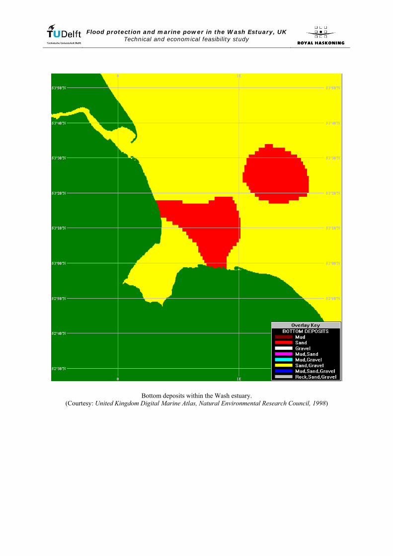
Bottom deposits within the Wash estuary. (Courtesy: United Kingdom Digital Marine Atlas, Natural Environmental Research Council, 1998)

Flood protection and marine power in the Wash Estuary, UK Technical and economical feasibility study

Flood protection and marine power in the Wash Estuary, UK Technical and economical feasibility study
Appendix 2
Land reclamations bordering the Wash estuary

Flood protection and marine power in the Wash Estuary, UK Technical and economical feasibility study

Flood protection and marine power in the Wash Estuary, UK Technical and economical feasibility study
Source: New Scientist, edition 6-9-1962, article “The old coastline of the Wash” by F.T.J. Kestner, Hydraulic
research station, Department of Scientific and Industrial Research.

Flood protection and marine power in the Wash Estuary, UK Technical and economical feasibility study

Flood protection and marine power in the Wash Estuary, UK Technical and economical feasibility study
Appendix 3
Locations of mussel and cockle beds in the Wash estuary through the years

Flood protection and marine power in the Wash Estuary, UK Technical and economical feasibility study

Flood protection and marine power in the Wash Estuary, UK Technical and economical feasibility study
Location of mussel beds in the Wash estuary through the years [Dare, 2004].

Flood protection and marine power in the Wash Estuary, UK Technical and economical feasibility study

Flood protection and marine power in the Wash Estuary, UK Technical and economical feasibility study
Location of cockle beds in the Wash estuary through the years [Dare, 2004]. Black shading : > 100 cockles/m2; grey shading: 10-99 cockles/m2.

Flood protection and marine power in the Wash Estuary, UK Technical and economical feasibility study

Flood protection and marine power in the Wash Estuary, UK Technical and economical feasibility study
Appendix 4
Nature protection areas

Flood protection and marine power in the Wash Estuary, UK Technical and economical feasibility study

Flood protection and marine power in the Wash Estuary, UK Technical and economical feasibility study
Ramsar sites in Norfolk and Lincolnshire. (Courtesy: Environmental resources Management)
SPA sites in Norfolk and Lincolnshire. (Courtesy: Environmental resources Management)
SAC sites in Norfolk and Lincolnshire. (Courtesy: Environmental resources Management)
EMS site in Norfolk and Lincolnshire. (Courtesy: The Wash and North Norfolk Coast Site Plan, November 2010)
SPA : Special Protection Area SAC : Special Area of Conservation EMS : European Marine Sites
Areas of Outstanding Natural Beauty in Wash estuary and along the North Norfolk Coast. (Courtesy: Norfolk Coast Partnership)

Flood protection and marine power in the Wash Estuary, UK Technical and economical feasibility study

Flood protection and marine power in the Wash Estuary, UK Technical and economical feasibility study
Appendix 5
Astronomical tide and shallow water tides

Flood protection and marine power in the Wash Estuary, UK Technical and economical feasibility study

Flood protection and marine power in the Wash Estuary, UK Technical and economical feasibility study
5.1 Astronomical tide The forces involved in the generation of the astronomical tide originate from the gravitational pull caused by the rotation of the earth-moon system around a common centre of gravity and the rotation of the sun-earth system around their common centre of gravity. The astronomical tides or ocean tides are generated as a result of the differences between the gravitational pull on the ocean water masses located at different distances from both moon and sun. In box 1 the derivation of this tide generating force, or differential pull, is presented. Newton’s equilibrium theory of tides1 will be used to explain some tidal phenomena, namely the daily inequality, the spring and neap tide cycle and the main tidal constituents. Box 1: tide generating force or differential pull.
Newton’s Law of gravitation states: 221
rmm
GF⋅
⋅= (5.1)
Where F is the force between the masses [N], G is the gravitational constant [Nm2/kg2], m1 is the first mass [kg], m2 is the second mass [kg] and r is the distance between the masses [m]. The gravitational pull of the moon on 1 kg of mass on earth, using the distance between the centres of gravity of both earth and moon, is:
2M
MEMEEME r
MMGaMF ⋅⋅=⋅= −− (5.2)
and hence ( ) gr
MGaM
MME ⋅⋅=⋅=
⋅
⋅⋅⋅=⋅= −−−
−65
28
2211
2 1038.31032.31084.31035.71067.6 (5.3)
Where: FE-M is the gravitational pull of the moon on 1 kg of mass on earth [N], ME is the mass on earth [1 kg], aE-M is the gravitational acceleration of the centre of the earth in the earth-moon system [m/s2], MM is the mass of the moon [kg], rM is the distance between the centres of earth and moon [m] and g is the gravitational acceleration of earth itself at the earth’s surface [m/s2]. Similarly for the sun:
( ) gr
MGaS
SSE ⋅⋅=⋅=
⋅
⋅⋅⋅=⋅= −−−
−43
211
3011
2 1001.61090.5105.11099.11067.6 (5.4)
Where: FE-S is the gravitational pull of the sun on 1 kg of mass on earth [N], aE-M is the gravitational acceleration of the centre of the earth in the earth-sun system [m/s2], MS is the mass of the sun [kg] and rS is the distance between the centres of earth and sun [m].
Figure 5.1: tidal forcing.
The upper image of figure 5.1 shows the gravitational pull of the moon on the earth. As can be seen the distance between the centre of the attracting body (moon or sun) varies slightly for different locations at the earth’s surface, hence nowhere on earth is the gravitational acceleration exactly equal to the gravitational acceleration of the centre of gravity of the earth in respectively the earth- moon or earth- sun system. These differences in gravitational pull along earth’s surface is known as the differential pull (see lower image in figure 5.1) and this phenomenon is responsible for the generation of the astrological tides.
1 Newton made the following assumptions in his theory: 1) the Earth is entirely covered by water, 2) the water surface responds immediately to the forcing, 3) the presence of the continents is neglected.

Flood protection and marine power in the Wash Estuary, UK Technical and economical feasibility study
Computing this differential pull (ΔaE-M) on 1 kg of mass situated on the earth’s near side of the moon can be done as follows:
( )g
rRMG
rMG
RrMGaaa
M
EM
M
M
EM
MMEnsMEME ⋅⋅=
⋅⋅⋅≈⋅−
−⋅=−=Δ −
−−−7
322_ 1013.12 (5.5)
Similarly for the sun:
( )
gr
RMGr
MGRr
MGaaaS
ES
S
S
ES
SSEnsSESE ⋅⋅=
⋅⋅⋅≈⋅−
−⋅=−=Δ −
−−−7
322_ 10515.02 (5.6)
Where: ΔaE-M is the differential pull of the moon on 1kg of mass on the near side of earth [m/s2], ΔaE-S is the differential pull of the sun on 1 kg of mass on the near side of earth [m/s2] and RE is the radius of the earth [m]. From the above can be concluded that the differential pull caused by the moon is the most influential regarding
the generation of the earth’s astrological tides: %69%100 =⋅Δ+Δ
Δ
−−
−
MESE
ME
aaa
(5.7)
The resulting differential pull as presented in the lower image of figure 5.1 can be decomposed into components normal and parallel to the earth’s surface. The normal components have a size negligible compared to the earth’s own gravitational acceleration (g). Although the components parallel to the earth’s surface are of the same order of magnitude as g, they are perpendicular to the earth’s gravity field and therefore shift the water mass both to the side facing the celestial body and the side opposing it, see figure 5.2. Without some opposing force all the water would pile up at either side of the earth, which is obviously not the case. The shift of the water mass is compensated for by a pressure gradient in the opposite direction that is the result of the sloping water surface, resulting in the typical ellipsoid as described in Newton’s equilibrium theory of tides.
Figure 5.2: components of the tidal force perpendicular to the earth’s gravity field, in case the celestial body is above the equator at point Z. (Courtesy: Dietrich, 1980)
Flood protection and marine power in the Wash Estuary, UK Technical and economical feasibility study
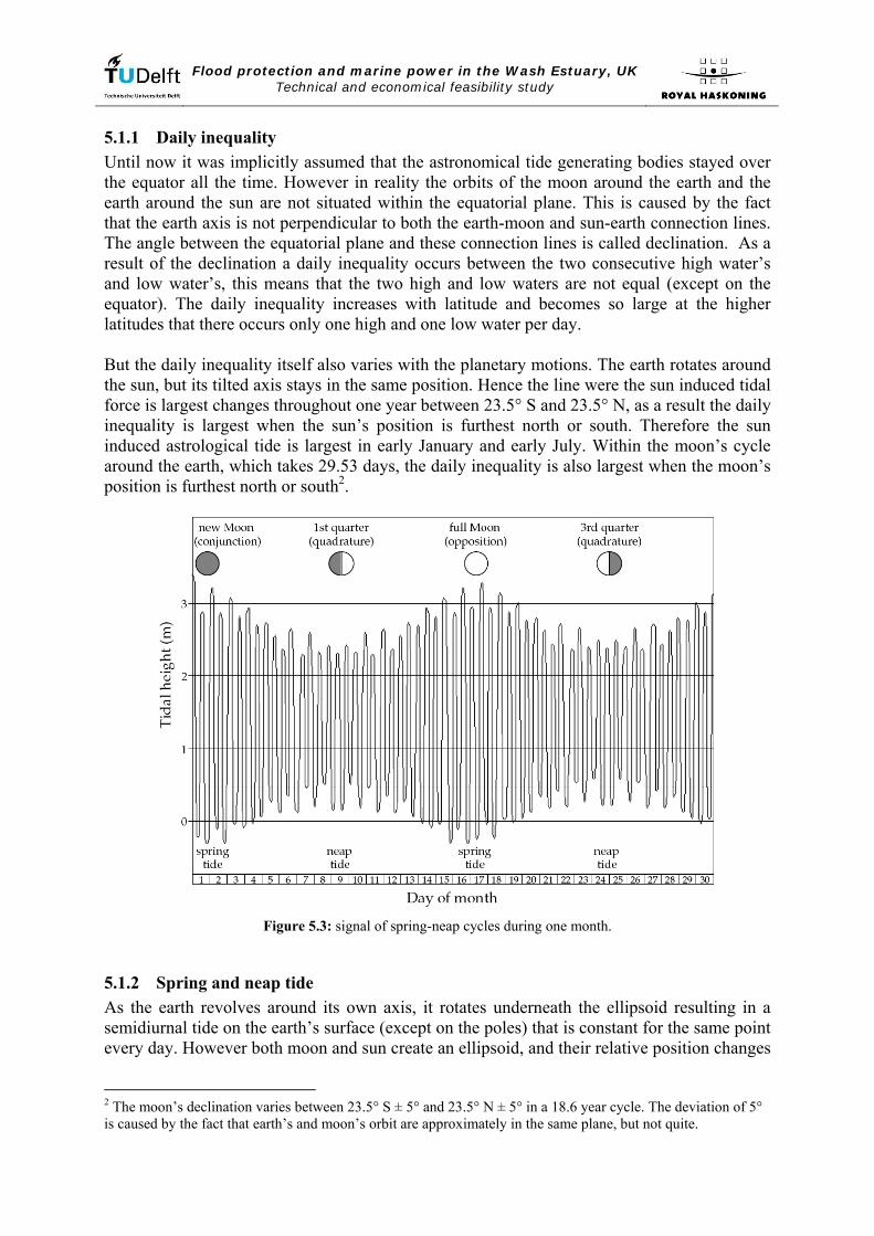
5.1.1 Daily inequality Until now it was implicitly assumed that the astronomical tide generating bodies stayed over the equator all the time. However in reality the orbits of the moon around the earth and the earth around the sun are not situated within the equatorial plane. This is caused by the fact that the earth axis is not perpendicular to both the earth-moon and sun-earth connection lines. The angle between the equatorial plane and these connection lines is called declination. As a result of the declination a daily inequality occurs between the two consecutive high water’s and low water’s, this means that the two high and low waters are not equal (except on the equator). The daily inequality increases with latitude and becomes so large at the higher latitudes that there occurs only one high and one low water per day. But the daily inequality itself also varies with the planetary motions. The earth rotates around the sun, but its tilted axis stays in the same position. Hence the line were the sun induced tidal force is largest changes throughout one year between 23.5° S and 23.5° N, as a result the daily inequality is largest when the sun’s position is furthest north or south. Therefore the sun induced astrological tide is largest in early January and early July. Within the moon’s cycle around the earth, which takes 29.53 days, the daily inequality is also largest when the moon’s position is furthest north or south2.
Figure 5.3: signal of spring-neap cycles during one month.
5.1.2 Spring and neap tide As the earth revolves around its own axis, it rotates underneath the ellipsoid resulting in a semidiurnal tide on the earth’s surface (except on the poles) that is constant for the same point every day. However both moon and sun create an ellipsoid, and their relative position changes
2 The moon’s declination varies between 23.5° S ± 5° and 23.5° N ± 5° in a 18.6 year cycle. The deviation of 5° is caused by the fact that earth’s and moon’s orbit are approximately in the same plane, but not quite.
Flood protection and marine power in the Wash Estuary, UK Technical and economical feasibility study
in time. If moon and sun are in the same line their ellipsoids enhance each other and the tidal amplitude is increased, this is called spring tide and occurs both at new moon and full moon. When the position of moon and sun is 90° out of phase the combined effect of their ellipsoids approaches a circle and the amplitude of the astronomical tide is reduced, this is called neap tide and occurs both in the first and last quarter of the moon. In figure 5.3 the signal of the tidal amplitude variation during one month is depicted, the signal shows clearly the two spring-neap tide cycles. Also the daily inequality can be recognized. During the year the amplitude of the astronomical spring-neap cycle does not remain constant, it varies as a result of the elliptic orbit of the earth-moon system around the sun and the elliptic orbit of the moon around the earth. First the effect of the orbit of the moon will be considered as the moon has the most influence on the generation of the astronomical tides. When the moon is in apogee the exerted gravitational pull is smallest and hence the amplitude of the lunar tide will be smallest, when the moon is at perigee the gravitational pull is largest as is the amplitude of the lunar tide. Regarding the sun a similar effect occurs, only the duration of the cycle is one year instead of one lunar month. When the earth is at aphelion the gravitational pull exerted by the sun is smallest and when at perihelion it is largest.
5.1.3 Tidal constituents In the idealized situation the differential pull of moon and sun only generates the two main tidal constituents, the principal lunar and solar tides. All deviations from this idealized situation, e.g. a elliptic orbit instead of a circular orbit, the declination of the earth axis, etc., result in additional astronomical tidal constituents to the aforementioned main constituents. The eleven most dominant tidal constituents are listed in table 5.1.
Tidal constituent Nomenclature Equilibrium amplitude
Ai [m]
Period
Ti [h]
Radian frequency ωi [10-4/s]
Semidiurnal Principal lunar M2 0.242334 12.421 1.40519 Principal solar S2 0.112841 12.000 1.45444 Lunar elliptic N2 0.046398 12.658 1.37880 Lunisolar K2 0.030704 11.967 1.45842 Diurnal Lunisolar K1 0.141565 23.935 0.72921 Principal lunar O1 0.100514 25.819 0.67598 Principal solar P1 0.046843 24.066 0.72523 Lunar elleptic Q1 0.019256 26.868 0.64959 Long period Fortnightly Mf 0.041742 327.86 0.053234 Monthly Mm 0.022026 661.31 0.026392 Semi-annual Ssa 0.019446 4383.05 0.003982
Table 5.1: principal tidal constituents [Apel, 1987]. In contrast to wind and short waves, tidal constituents have their own precise frequencies. Hence the spectrum consists of discrete lines. This characteristic of the tide makes it possible to decompose a measured tidal signal into its separate tidal constituents, its building blocks so

Flood protection and marine power in the Wash Estuary, UK Technical and economical feasibility study
to speak. In paragraph 5.2 this property will be used to determine the characteristic of the tide in the North Sea offshore of the Wash estuary. In section 5.3 physical processes causing non-linear deviations from the astronomical equilibrium tides will be discussed, resulting in the so called overtides or shallow water tides.
5.1.4 Harmonic analysis Since the harmonic constituents of the astronomical tide are the result of regular astronomical phenomena it is possible to predict the tide accurately at every location on earth, as their frequencies are known and fixed. Performing a Fourier analysis on a measured time series of water levels will result in the amplitudes and phases of the main tidal constituents on that specific location. In principle it boils down to determining amplitudes and phases.
( )nnN
n n taat αωη −⋅⋅+= ∑ =cos)(
10 (5.8) Were:
η(t) : measured tidal level with reference to ordnance level [m] ao : mean level [m] an : amplitude of constituent number n [m] ωn : angular velocity of constituent number n [rad/s]αn : phase angle of constituent number n [rad] t : time [s]
When the tidal constituents are known the character of the tide (diurnal, semidiurnal or mixed) at a certain location can be determined. The tidal character is defined by means of the form factor F, which is defined as the ratio of amplitudes of the sum of the two main diurnal components over the main two main semidiurnal components.
22
11
SMOK
F++
= (5.9)
Were: F : form factor [-] K1 : amplitude of the lunar-solar declinational diurnal tidal constituent [m] O1 : amplitude of the principal lunar diurnal tidal constituent [m] M2 : amplitude of the principal lunar semidiurnal tidal constituent [m] S2 : amplitude of the principal solar semidiurnal tidal constituent [m]
In table 5.2 the four tidal categories that are distinguished are shown:
Tidal category Value for F [-]
Semidiurnal tide 0.00-0.25 Mixed tide, mainly semidiurnal 0.25-1.50 Mixed tide, mainly diurnal 1.50-3.00 Diurnal tide > 3.00
Source: Bosboom, 2011.
Table 5.2: tidal character expressed by the form factor.
Flood protection and marine power in the Wash Estuary, UK Technical and economical feasibility study
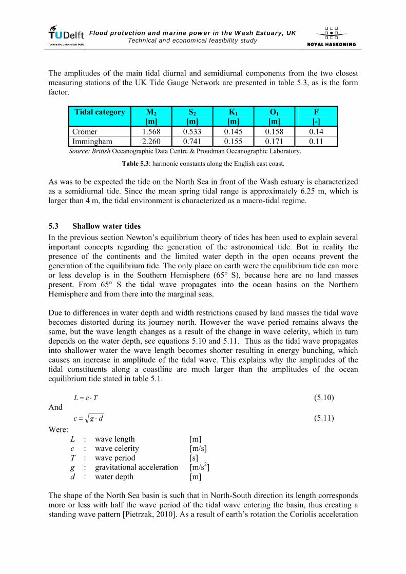
The amplitudes of the main tidal diurnal and semidiurnal components from the two closest measuring stations of the UK Tide Gauge Network are presented in table 5.3, as is the form factor.
Tidal category M2 [m]
S2 [m]
K1 [m]
O1 [m]
F [-]
Cromer 1.568 0.533 0.145 0.158 0.14 Immingham 2.260 0.741 0.155 0.171 0.11
Source: British Oceanographic Data Centre & Proudman Oceanographic Laboratory.
Table 5.3: harmonic constants along the English east coast. As was to be expected the tide on the North Sea in front of the Wash estuary is characterized as a semidiurnal tide. Since the mean spring tidal range is approximately 6.25 m, which is larger than 4 m, the tidal environment is characterized as a macro-tidal regime.
5.3 Shallow water tides In the previous section Newton’s equilibrium theory of tides has been used to explain several important concepts regarding the generation of the astronomical tide. But in reality the presence of the continents and the limited water depth in the open oceans prevent the generation of the equilibrium tide. The only place on earth were the equilibrium tide can more or less develop is in the Southern Hemisphere (65° S), because here are no land masses present. From 65° S the tidal wave propagates into the ocean basins on the Northern Hemisphere and from there into the marginal seas. Due to differences in water depth and width restrictions caused by land masses the tidal wave becomes distorted during its journey north. However the wave period remains always the same, but the wave length changes as a result of the change in wave celerity, which in turn depends on the water depth, see equations 5.10 and 5.11. Thus as the tidal wave propagates into shallower water the wave length becomes shorter resulting in energy bunching, which causes an increase in amplitude of the tidal wave. This explains why the amplitudes of the tidal constituents along a coastline are much larger than the amplitudes of the ocean equilibrium tide stated in table 5.1.
TcL ⋅= (5.10)
And dgc ⋅= (5.11)
Were: L : wave length [m] c : wave celerity [m/s] T : wave period [s] g : gravitational acceleration [m/s2] d : water depth [m]
The shape of the North Sea basin is such that in North-South direction its length corresponds more or less with half the wave period of the tidal wave entering the basin, thus creating a standing wave pattern [Pietrzak, 2010]. As a result of earth’s rotation the Coriolis acceleration

Flood protection and marine power in the Wash Estuary, UK Technical and economical feasibility study
transforms the standing wave pattern into a rotary wave propagating around an amphidromic point. The vertical tide is zero in the amphidromic point and maximum along the coastline of the North Sea basin. As can be seen in figure 5.4, amplification of the tidal range along the UK coastline is particular large.
Figure 5.4: amphidromic systems in the North Sea basin. (Courtesy: M. Tomczak, Flinders university, 1996)
The red lines represent the co-phase lines (in hrs) of the M2 tidal constituent, the blue lines represent the mean tidal range at spring tide in metres (co-range lines of the sum of M2 and S2 tidal constituents). Furthermore non-linear effects are introduced in shallow water as bottom friction becomes important because the tidal amplitude is no longer small compared to the water depth. Also the effect on the propagation speed of the tidal wave due to the difference between wave crest and trough in combination with a finite depth results in non-linear effects. Besides resonance phenomena that are the result of the basin’s geometry, additional non-linear effects are caused by interactions between tidal constituents. All these non-linear effects contribute to the tidal asymmetry that is observed in shallow water signals. The higher harmonics resulting from the processes mentioned above are not a direct result from the tide generating forces and are therefore called overtides or shallow water tides. These tidal constituents have a period that is a integer fraction of the original tidal constituents. Bottom friction induced tides have a period that is 1/3 of that of the original

Flood protection and marine power in the Wash Estuary, UK Technical and economical feasibility study
constituent, e.g. M2 => M6 and K1 => K3. The difference in wave speed between the crest and through results in overtides with a period that is 1/2 of the original astronomical period, e.g. M2 => M4 => M8 or S2 => S4 => S8. The same holds for the interactions between tidal constituents, e.g. M2 + S2 => MS4. Although all higher harmonics contribute to the tidal distortion in shallow water, the most important are the M4 and M6 overtides, because these contribute most (together with the M2 astronomical tidal constituent) to the tidal amplitude. Also with respect to sediment transport the overtides also play a very important role.
5.4 Propagation and deformation of the tidal wave within the Wash estuary The sea-borne tidal asymmetry is transferred into the estuary where, as a result of the further decreasing depth, non-linear effects are being enhanced, resulting in an increasing tidal asymmetry. Some amplitude amplification is to be expected as the tide propagates into the estuary. Due to the presence of bottom friction both the incoming and reflected wave are partly damped, resulting in a wave pattern with a partly standing character and a partly propagating character. As a result of the partly standing wave character a phase difference between water level and current velocity is to be expected (current velocity leads the water level variation). Apparently damping of the tidal wave due to bottom friction has a large effect in the Wash estuary as the amplitude of the tidal wave only increases approximately 0.10 m from the mouth of the estuary to the landward side of the basin (see section 2.1.3), despite a considerable decrease in water depth towards the end of the basin. Also the wave celerity decreases in shallower water, resulting in a shortening of the wave length as the wave period remains constant, see equations 5.10 and 5.11.
Tidal constituent Wave period [hr]
Wave length [km]
Amplitude 1)
[m] M2 12.42 443 2.260 K1 23.93 853 0.155 S2 12.00 428 0.741 O1 25.82 256 0.171
Wave celerity of all constituents is 9.9 m/s. 1) Because no data with respect to the amplitudes of the four main tidal constituents is available at the time for the tide within the Wash estuary, the data of the Immingham measuring station of the UK Tide Gauge Network is used. This station was preferred over the Cromer station since the mean tidal amplitude is closer to that of the Wash estuary. Mean tidal amplitude Immingham 4.20 m; Cromer 2.92 m.
(Source: British Oceanographic Data Centre & Proudman Oceanographic Laboratory)
Table 5.4: wave length and amplitude of the four major tidal constituents. From table 5.4 can be concluded that the basin length is in the order of 1/20 of the wave length of the M2 and S2 tidal constituents, being the main tidal constituents along the English eastern shoreline. Therefore a storage basin approach can be used to describe the change in time of the water level within the future basin and also assess the influence of the barrier on the tidal amplitude behind it.

Flood protection and marine power in the Wash Estuary, UK Technical and economical feasibility study
5.4.1 Tidal asymmetry As described in section 2.1.2 the amplitudes of both the horizontal and vertical tide are damped progressively as a result of bottom friction, the depth decreases considerably further into the basin and the partly standing wave pattern resulted in a phase difference between the horizontal and vertical tide (0 < phase shift < π/2). As a result both the vertical and horizontal tide are deformed. The vertical and horizontal deformation of the horizontal tide are very important factors in relation to the net sediment transport processes within the Wash estuary. The horizontal deformation of the horizontal tide results in a skewed velocity signal and relates to the transport of coarse sediment. In section 2.1.3 it was shown that the flood currents are larger than the ebb currents in the main channel. As a result the flood duration in the central part of the estuary is shorter than the ebb duration, thus causing net sediment transport into the estuary (flood dominance). According to theory flood dominance can be expected for a large ratio of tidal amplitude over water depth, shallow channels and limited intertidal storage area. On the other hand ebb dominance is expected to occur in case of the presence of deep channels and large intertidal storage area.
Figure 5.5: simplified bathymetry of the wash estuary, contour lines in m below ODN. (Courtesy: Royal Haskoning)

Flood protection and marine power in the Wash Estuary, UK Technical and economical feasibility study
At first sight the fact that the central part of the estuary is characterized by flood dominance seems contradictory with theory, indeed the main channels are deep (see figure 5.5) and the intertidal storage area within the basin is approximately 290 km2. However most of these intertidal flats are located at the landward end of the estuary and here the residual flow, depicted in figure 5.6, clearly indicates ebb dominance. In the central part the width of the intertidal storage area is small compared to the width of the area permanently covered by water, which is consistent with flood dominance. Flood dominance results in a net transport of coarse sediment into the estuary, which is consistent with the situation depicted in figure 5.7.
Figure 5.6: residual tidal flow direction.
(Courtesy: Wingfield et at, 1978) In contrast to the central part of the estuary both along the eastern and western boundary the residual flow direction is in ebb direction, which indicates ebb dominance and hence net sediment transport towards the North Sea. Here the channels are bordered by vast intertidal flats which is a typical configuration leading to ebb dominance. In these sections ebb dominance is further enhanced as a result of the rivers Witham, Welland, Nene and Great Ouse discharging into the estuary, thus contributing to a residual flow in ebb direction, see figure 5.6. However the net trend is the overall import of sediment in the estuary basin [The Wash SMP2, appendix C, 2010]. The vertical asymmetry of the horizontal tide relates to the transport of fine sediment and results in a saw-tooth velocity signal. The governing process with respect to the sediment transport of fines is the difference in duration between high-water slack and low-water slack. The location within the estuary were flood dominance occurs, Lynn Deeps, the high-water slack duration is longest and hence net transport of fines in landward direction occurs. This is consistent with the distribution of intertidal sediments as depicted in figure 5.6. The margins of the estuary, were ebb dominance occurs, are characterized by a longer low-water slack duration. According to theory this will result in a net export of fines. This seems

Flood protection and marine power in the Wash Estuary, UK Technical and economical feasibility study
not to be the situation, as mud is also present along the eastern and western shoreline. However because of the large intertidal area another mechanism plays a role. Due to the small water depth and large concentration fines in the water column strong settling occurs, apparently this process compensates for the short high-water slack duration.
Figure 5.7: distribution of intertidal sediments in the Wash. (Courtesy: Ke et al, 1996, after Wingfield et al 1978)
Horizontal and vertical asymmetry of the vertical tide influence the water level within the estuary and are therefore of importance with respect to the energy potential. As is already shown in section 2.1.2, within the Wash estuary the main drivers are the tidal asymmetry already present at sea, the decreasing depth and the bottom friction. Already at the mouth of the Wash estuary the falling period is longer than the rising period, this vertical asymmetry of the vertical tide increases slightly as the tidal wave progresses further into the estuary, see appendix 7. The asymmetry is most pronounced near the ports of Boston and King’s Lynn that are located some distance upstream the tidal rivers Witham and Great Ouse respectively. Keeping in mind the propagation speed of the tidal wave explains this vertical asymmetry. During rising tide the crest of the tidal wave propagates into the estuary, hence the water depth is larger and as a result the wave celerity is faster than during the falling tide. From table 5.5 can be concluded that horizontal asymmetry of the vertical tide is barely present at the mouth of the Wash estuary. During spring tide the high waters are slightly higher above mean sea level than the low waters and during neap tide it is the other way around. This asymmetry progressively increases in landward direction.

Flood protection and marine power in the Wash Estuary, UK Technical and economical feasibility study
SK BOS HUN KLY TAHE OWK WES
MSL 3.93 3.56 4.10 3.77 4.08 3.75 4.06 MHWS - MSL 2.92 2.94 3.25 3.08 3.37 3.32 3.31 MSL - HLWS 2.93 2.16 3.12 2.47 3.28 3.17 3.01 MHWN - MSL 1.17 0.96 1.28 1.03 1.27 1.33 1.24 MSL - MLWN 1.26 1.84 1.43 1.77 1.50 1.58 1.64 MSL in m above CD (CD = -3.00 m ODN) SK BOS HUN KLY TAHE OWK WES
= = = = = = =
Skegness Boston Hunstanton King’s Lynn Tabs Head Outer Westmark Knock West Stones
MSL MHWS MLWS MHWN MLWN
= = = = =
Mean Sea Level Mean High Water Spring Mean Low Water Spring Mean High Water Neap Mean Low Water Neap
Table 5.5: water levels and tidal ranges.

Flood protection and marine power in the Wash Estuary, UK Technical and economical feasibility study
Appendix 6
Predicted tidal signals in the Wash estuary

Flood protection and marine power in the Wash Estuary, UK Technical and economical feasibility study

Flood protection and marine power in the Wash Estuary, UK Technical and economical feasibility study
The figures below are plotted using data from the tidal prediction service provided by Admiralty EasyTide.
08/05 08/15 08/25 09/04 09/14 09/24 10/040
1
2
3
4
5
6
7
8
Time
Wat
er le
vel [
CD
]
Tidal prediction Skegness 2011
MSL = 3.92
08/05 08/15 08/25 09/04 09/14 09/24 10/040
1
2
3
4
5
6
7
8
9
Time
Wat
er le
vel [
CD
]
Tidal prediction Hunstanton 2011
MSL = 4.12

Flood protection and marine power in the Wash Estuary, UK Technical and economical feasibility study
08/05 08/15 08/25 09/04 09/14 09/24 10/040
1
2
3
4
5
6
7
8
Time
Wat
er le
vel [
CD
]Tidal prediction Boston 2011
MSL = 3.56
08/05 08/15 08/25 09/04 09/14 09/24 10/040
1
2
3
4
5
6
7
8
Time
Wat
er le
vel [
CD
]
Tidal prediction Port Sutton Bridge 2011
MSL = 3.86

Flood protection and marine power in the Wash Estuary, UK Technical and economical feasibility study
08/05 08/15 08/25 09/04 09/14 09/24 10/040
1
2
3
4
5
6
7
8
Time
Wat
er le
vel [
CD
]Tidal prediction Kings Lynn 2011
MSL = 3.77
08/05 08/15 08/25 09/04 09/14 09/24 10/040
1
2
3
4
5
6
7
8
9
Time
Wat
er le
vel [
CD
]
Tidal prediction Tabs Head 2011
MSL = 4.06
Flood protection and marine power in the Wash Estuary, UK Technical and economical feasibility study
08/05 08/15 08/25 09/04 09/14 09/24 10/04-1
0
1
2
3
4
5
6
7
8
Time
Wat
er le
vel [
CD
]Tidal prediction Outer Westmark Knock 2011
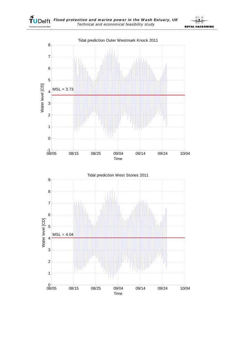
MSL = 3.73
08/05 08/15 08/25 09/04 09/14 09/24 10/040
1
2
3
4
5
6
7
8
9
Time
Wat
er le
vel [
CD
]
Tidal prediction West Stones 2011
MSL = 4.04

Flood protection and marine power in the Wash Estuary, UK Technical and economical feasibility study
Appendix 7
Asymmetry of the vertical tide in the Wash estuary

Flood protection and marine power in the Wash Estuary, UK Technical and economical feasibility study

Flood protection and marine power in the Wash Estuary, UK Technical and economical feasibility study
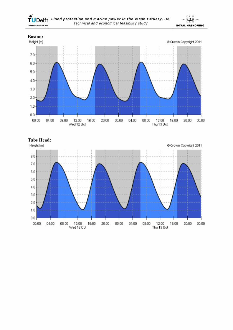
The figures below are copied from the website of the tidal prediction service provided by Admiralty EasyTide. Skegness:
Hunstanton:
Flood protection and marine power in the Wash Estuary, UK Technical and economical feasibility study
Boston:
Tabs Head:

Flood protection and marine power in the Wash Estuary, UK Technical and economical feasibility study
Port Sutton Bridge:
Outer Westmark Knock:

Flood protection and marine power in the Wash Estuary, UK Technical and economical feasibility study
King’s Lynn:
West Stones:

Flood protection and marine power in the Wash Estuary, UK Technical and economical feasibility study
Appendix 8
Analysis of extremes

Flood protection and marine power in the Wash Estuary, UK Technical and economical feasibility study
Flood protection and marine power in the Wash Estuary, UK Technical and economical feasibility study
8.1 Introduction In order to be able to design flood defence structures the extreme values of the significant wave height, peak period and wind speed have to be determined. Because usually extreme conditions fall outside the observed range, these conditions must be estimated. This can be done by fitting a curve through the observations and extrapolate this curve to the desired probability of occurrence. In this case two sources containing observations regarding significant wave height, peak period and wind speed are available, namely the wave atlas from Global Wave Statistics and the database from BMT ARGOSS3. After comparing both data sets it was decided to use the database from BMT ARGOSS, since this database is more site-specific. The data set contains observations gathered from an area of 200·200 km2 offshore from the Wash estuary, while the Global Wave Statistics data set contains observations gathered throughout the whole North Sea basin. Also the maximum significant wave height and wave period in the Global Wave Statistics database are slightly larger than in that of BMT ARGOSS. This is most probably the result of the larger area of observation, as the significant wave height and wave period are larger in other parts of the North Sea basin [Holthuisen et al, 1995]. The data provided by BMT ARGOSS consist of synthetic aperture radar (SAR) data. The data are grouped statistics of satellite observations, which means that the data are not sequential, in the sense that it is one continuous wave or wind record, also the number of storms per year is unknown. Therefore it is not possible to use the Peak-over-Threshold method to determine the extremes, instead a different approach is used. This initial distribution approach will be explained in this appendix, as is the interpretation of the end result, being design tables representing the probability of exceedance of significant wave height and wind speed corresponding to a certain design storm and return period. 8.2 Initial distribution approach for extreme wave height and period In order to solve the problem of not knowing the number of storms per year, it is assumed that one year consists of a number of periods with a certain duration (tstorm). It is also assumed that during those periods the significant wave height does not vary. The basic idea behind these assumptions is that, due to the persistence of winds, storm periods will have more or less the same duration. Next it is assumed that each random observation of a significant wave height describes an observation of one storm event. As a result such observation of a significant wave height represents the average significant wave height during that storm event (Hs, storm). The storm event is defined by a predetermined storm duration [Verhagen, 2009]. Two distributions that are widely used for determining the long term distribution of the significant wave height are the log normal distribution and Weibull distribution [Holthuijsen, 2008]. Although the choice of distribution is rather arbitrary, a distribution with more degrees of freedom will generally provide a better fit. As the log normal distribution has only two degrees of freedom and the Weibull distribution three, it was decided to use the latter in the performed analysis of extremes.
3 www.waveclimate.com

Flood protection and marine power in the Wash Estuary, UK Technical and economical feasibility study
The Weibull distribution is given by:
( )α
βγ
⎥⎥⎦
⎤
⎢⎢⎣
⎡⎟⎟⎠
⎞⎜⎜⎝
⎛⎟⎟⎠
⎞⎜⎜⎝
⎛ −−=> storms
stormss
HHHP ,
, exp [8.1]
Were: α : shape parameter [-] β : location parameter, determines position of the distribution on the x-axis [-] γ : scaling parameter, determines the width of the distribution [-]
The degrees of freedom in this distribution, α, β and γ, can be determined by performing a linear regression analysis on the data. As a linear regression analysis will lead to only two constants, β and γ, the third coefficient, α, is determined by trial-and-error. By assuming different values for α, the curvature of the data and the correlation coefficient of the regression line will change. The value for α that visually results in the straightest line and the highest possible correlation coefficient, will be chosen [Verhagen, 2009]. In order to be able to perform a linear regression analysis, equation 8.1 must be rewritten in the form: W = a·Hs,storm + b, were W is called the Weibull reduced variable, a is the slope of the regression line and b the y-intercept. Rewriting equation 8.1 results finally in:
( )βγ
βα −=− stormsHQ ,
1 1ln [8.2]
And ( )α
1lnQW −= [8.3]
The exceedance probability per year is found by using the relation presented in equation 8.4, were Qs represents the probability of exceedance of a significant wave height in a storm per year in a random year, as long as Qs < 1. If Qs > 1 the value has no statistical meaning, but physically the value indicates the expected number of storms that occurs in a year with a certain time averaged significant wave height. Q (= 1-P) indicates the probability of exceedance of a single storm and Ns is the number of occurring storms during a year, based on the storm duration set. The values for Qs >1 are used to have sufficient basis for extrapolation.
ss NQQ ⋅= [8.4] In order to compute the significant wave height belonging to the design storm, the Weibull reduced variable, equation 8.3, must be transformed by substituting equation 8.4, resulting in:
( )α1
ln sQW −= [8.5] And
( )αβγ1
, ln sstorms QH −⋅+= [8.6] Finally the design line is found by plotting the significant wave height against the Weibull reduced variable, while equation 8.6 can be used to compute the significant wave height corresponding to a certain probability of exceedance in a direct way.

Flood protection and marine power in the Wash Estuary, UK Technical and economical feasibility study
All in all the initial distribution approach is a relative objective method as the fitting of the curve through the observation is done by using the least-squares technique4, which is an objective method. On the other hand however the choice of the distribution to be used is subjective. 8.2.1 Extreme significant wave height In appendix 9.1 a table is included indicating the monthly distribution of significant wave height. Because the number of observations regarding the average significant wave heights is large the observations are grouped into 45° directional bins. The non-exceedance probability of a certain significant wave height is then defined as:
( )Nn
HHP iistormsis =< ,,, [8.7]
Were: ni : number of observations in directional bin i [-] N : total number of observations [-]
The chosen duration of a storm event is very important in this method, as it determines the number of storms and consequently the probability of exceedance, Qs, of a certain significant wave height. To establish the sensitivity of the method used, several storm durations were used. In table 8.1 a summary is presented of the results for the selected storm durations.
Storm duration 3 hrs 6 hrs 8 hrs 9 hrs 12 hrs 15 hrs Ns 2920 1460 1095 973 730 584 Hs 9.85 9.55 9.41 9.35 9.20 9.08 Ns = number of storms per year return period: 200 yrs Hs = extreme significant wave height
Table 8.1: summary of the initial distribution approach regarding Hs.
Note that the extreme significant wave height becomes lower as the storm duration increases. As can be seen in table 8.2 this trend is the same, independent from the return period chosen. This is strange because physically a longer storm will result in a higher significant wave height. Most probably this is a result of the combined effect of the fitting of the shape parameter α by hand and the fact that the larger the data set the more accurate the Weibull distribution becomes. Hence the result of the performed analysis will only state the order of magnitude of the design wave condition. When the feasibility of the project depends solely on an one metre difference in design wave height, the project is by definition not feasible as in this stage only crude date are available and no local wave height measurements.
4 This fitting technique is recommended by Goda for the Weibull distribution [Holthuijsen, 2008].

Flood protection and marine power in the Wash Estuary, UK Technical and economical feasibility study
SoP Hs for storm duration [m]
Return period [yr]
Qs [-] 3 hrs 6 hrs 8 hrs 9 hrs 12 hrs 15 hrs
50 0.02 8.74 8.40 8.25 8.19 8.02 7.89 200 0.005 9.85 9.55 9.41 9.35 9.20 9.08 500 0.002 10.62 10.35 10.23 10.17 10.03 9.91 1000 0.001 11.22 10.98 10.86 10.81 10.68 10.57 2000 0.0005 11.84 11.62 11.51 11.47 11.34 11.23
10,000 0.0001 13.33 13.17 13.08 13.04 12.94 12.84 SoP = standard of protection Hs = extreme significant wave height
Table 8.2: Hs for different return periods and storm durations.
Since the results of the fit may be unintentionally biased by the many observations of low values, more importance is assigned to the higher observations by ignoring all observations lower than one metre. The results are summarized in table 8.3.
Storm duration 3 hrs 6 hrs 8 hrs 9 hrs 12 hrs 15 hrs
Ns 2920 1460 1095 973 730 584 Hs 9.79 9.50 9.36 9.30 9.15 9.02
Ns = number of storms per year return period: 200 yrs Hs = extreme significant wave height
Table 8.3: summary of the initial distribution approach regarding Hs, using censoring.
Comparing tables 8.2 and 8.4 learns that in this specific case the bias as a result of the lower wave heights is restricted to only a few centimetres, therefore the original data set will be used.
SoP Hs for storm duration [m] Return period
[yr] Qs [-] 3 hrs 6 hrs 8 hrs 9 hrs 12 hrs 15 hrs
50 0.02 8.70 8.36 8.21 8.15 7.98 7.85 200 0.005 9.79 9.50 9.36 9.30 9.15 9.02 500 0.002 10.55 10.29 10.16 10.10 9.96 9.84 1000 0.001 11.15 10.90 10.79 10.73 10.60 10.48 2000 0.0005 11.76 11.54 11.43 11.38 11.25 11.14
10,000 0.0001 13.23 13.07 12.98 12.93 12.82 12.72 SoP = standard of protection Hs = extreme significant wave height
Table 8.4: Hs for different return periods and storm durations, using censoring.

Flood protection and marine power in the Wash Estuary, UK Technical and economical feasibility study
8.3 Initial distribution approach for extreme wind speed For determining the extreme offshore wind speed the same approach is followed for the extreme significant wave height. For a more elaborate description the reader is referred to section 8.1 of this appendix. For the analysis of wind speed often a Rayleigh or Weibull distribution are used [Twidell, 2006]. Because the Weibull distribution has one degree of freedom more than the Rayleigh distribution and therefore tends to be more accurate, this distribution is used. A table containing the monthly distribution of the offshore wind speed is included in appendix 9.2. The results of the performed analysis are summarized in table 8.5. Again the influence of the storm duration on the results is assessed.
Storm duration 3 hrs 6 hrs 8 hrs 9 hrs 12 hrs 15 hrs Ns 2920 1460 1095 973 730 584 Us 25.1 25.4 26.1 26.1 26.0 25.9 Ns = number of storms per year return period: 200 yrs Us = extreme wind speed
Table 8.5: summary of the initial distribution approach regarding wind speed.
Note that there are no significant changes in wind speed for the different storm durations, this clearly shows the persistence of the wind. Table 8.6 shows that this trend is independent of the return period chosen.
SoP Us for storm duration [m/s] Return period
[yr] Qs [-] 3 hrs 6 hrs 8 hrs 9 hrs 12 hrs 15 hrs
50 0.02 22.0 21.8 22.3 22.2 22.0 21.8 200 0.005 25.1 25.4 26.1 26.1 26.0 25.9 500 0.002 27.8 28.6 29.2 29.3 29.4 29.4 1000 0.001 30.2 30.2 31.9 32.0 32.2 32.2 2000 0.0005 32.9 23.9 34.9 35.0 35.4 35.7
SoP = standard of protection Us = extreme wind speed
Table 8.6: Us for different return periods and storm durations.
As can be seen from table 8.6, without censoring the extrapolated values of the extreme wind speed are unrealistic for long return periods (34-36 m/s), corresponding with wind force 12 on the Beaufort scale. However hurricanes are not likely to occur on the North Sea. This is the result of bias caused by the many observations of low wind speeds that are present in the dataset. Therefore all observations with a wind speed smaller than 4 m/s are discarded in the analysis. This wind speed corresponds with wind force 2 on the Beaufort scale. The results of the initial distribution approach using censoring are included in table 8.7.

Flood protection and marine power in the Wash Estuary, UK Technical and economical feasibility study
SoP Us for storm duration [m/s]
Return period [yr]
Qs [-] 3 hrs 6 hrs 8 hrs 9 hrs 12 hrs 15 hrs
50 0.02 21.5 21.3 21.7 21.6 21.4 21.2 200 0.005 24.4 24.7 25.2 25.2 25.1 25.0 500 0.002 26.9 27.6 28.0 28.1 28.1 28.1 1000 0.001 29.1 30.2 30.5 30.6 30.8 30.8 2000 0.0005 31.6 33.1 33.2 33.4 33.7 33.8
SoP = standard of protection Us = extreme wind speed
Table 8.7: Us for different return periods and storm durations, using censoring.
Now the wind speed for longer return periods corresponds to wind force 11 on the Beaufort scale, which indicates a very severe storm and is a realistic value for the North Sea basin. Hence these figures will be used.

Flood protection and marine power in the Wash Estuary, UK Technical and economical feasibility study
Appendix 9
Extreme offshore wave and wind conditions

Flood protection and marine power in the Wash Estuary, UK Technical and economical feasibility study

Flood protection and marine power in the Wash Estuary, UK Technical and economical feasibility study
Appendix 9.1
Monthly distribution of significant wave height (Courtesy: BMT ARGOSS)

Flood protection and marine power in the Wash Estuary, UK Technical and economical feasibility study

Flood protection and marine power in the Wash Estuary, UK Technical and economical feasibility study
Appendix 9.2
Monthly distribution of wind speed (Courtesy: BMT ARGOSS)

Flood protection and marine power in the Wash Estuary, UK Technical and economical feasibility study

Flood protection and marine power in the Wash Estuary, UK Technical and economical feasibility study
Appendix 10
Analysis of the UK’s energy market

Flood protection and marine power in the Wash Estuary, UK Technical and economical feasibility study

Flood protection and marine power in the Wash Estuary, UK Technical and economical feasibility study
10.1 Introduction The long term vision of the UK Government regarding the country’s energy supply is that the 2050 climate change objectives5 must be achieved, while ensuring secure and affordable energy supplies. In order to achieve these goals, the current energy market, that is heavily dependent on fossil fuels, must be reformed towards a low carbon energy market. This means that renewable energy sources (solar energy, wind energy, water power, etc.), nuclear energy and fossil fuel combined with carbon capture and storage are bound to get a larger market share on the expense of traditional coal and gas fired electricity generation. Within this light the UK Government has committed that 15% of its total energy consumption comes from renewable sources by 2020, which means that approximately 30% of the UK’s electricity generation should be provided by renewable energy sources [HM Treasury, 2010]. This creates opportunities for the generation of tidal energy in the UK. However, the focus of the Government seems to be more on onshore and offshore wind energy schemes. Besides one of the most reliable supplies in Europe, the UK’s energy market is also one of the most liberalised energy markets in the world. As a result of this liberalisation, the UK market is currently dominated by six large energy companies6 that are acting both on the wholesale market and the retail market. These companies together dominate 99% of the retail market and 67% of the wholesale market [HM Treasury, 2010]. In other words, these companies generate a large part of the energy that they sell on the retail market themselves. In this appendix first the historical developments of the UK’s energy market will be sketched. Next the short, medium and long term objectives of the current energy policy will be treated, followed by an overview of the most important European and national policies that must enable the achievement of these objectives. Last but not least the current level of energy prices in the UK energy market is explored.
10.2 Short history During the 1970s the UK was a net importer of energy, as result of the developing gas and oil production in the North Sea the UK became a net exporter of energy during the 1980s and continued to be so until 2004, when it became a net importer again [DECC, 2011]. Before the 1960’s 90% of the energy production in the UK was provided by coal fired energy plants, the remaining 10% was provided mostly by oil fuelled electricity production. During the 1960’s the first generation nuclear power plants were built, followed by the second generation during the 1970’s and 1980’s. During the 1990’s the market share of nuclear power increased further as a result of improved plant performance and the commissioning of a third generation nuclear power plant. By the late 1990’s nuclear power plants provided 26% of the national electricity supply [Redpoint, 2010]. Since then no new nuclear power plants have been commissioned and its market share declined due to the retirement of the first generation power plants. Within the light of the Government’s low carbon energy policy plans exist to build new nuclear power plants in the near future.
5 The UK Government has committed to a legally binding target to cut greenhouse gas emissions by 80 %, from 1990 levels, by 2050 [HM Treasury, 2010]. 6 The six largest energy companies in the UK are: E.ON, RWE npower, SSE, EDF, Centrica and Scottish power [HM Treasury, 2010].

Flood protection and marine power in the Wash Estuary, UK Technical and economical feasibility study
As a result of the liberalization of the UK energy market in 1989 the gas market was opened up [Redpoint, 2010] on the expense of the coal fired power plants. This so-called “dash for gas” started in 1993 and continued until the early 2000’s, see also figure 10.1. At the same time of the energy market liberalization a Non-Fossil Fuel Obligation was introduced, which remained the primary renewable support scheme until it was replaced by the Renewables Obligation in 2002 [Redpoint, 2010].
Source: DTI, 2005.
Figure 10.1: energy mix by fuel type, 1990 vs. 2004. Before 1990 the only renewable energy source of some scale in the UK was hydro power, predominantly situated in Scotland. Since the mid 1990’s a steady increase in renewable energy production capacity is noticeable, mainly in the form of landfill gas and biomass fired power plants. From the mid 2000’s a significant growth can be seen with respect to wind farms, as a result of which nowadays wind energy is the second largest renewable energy source in the UK. These wind farms are for the larger part land based, however since 2009 also large offshore wind farms have been installed. The construction of offshore wind farms is expected to speed up in the coming years as onshore and offshore wind energy play a key role in reaching the 2020 target [DECC, 2010]. Marine energy in the form of wave power and tidal stream power are also a priority for the UK Government, since the UK coast has large potential and because the Government strives to develop a new world leading UK based energy sector [DECC, 2010]. In spite of the fact that already since the 1920’s the feasibility of tidal barrages is studied, no tidal range power plant was ever built. According to the Sustainable Development Commission the reasons for this are mainly the high capital costs and, more recent, environmental concerns. As can be seen in figure 10.2; nowadays natural gas and coal are still the primary energy sources in the UK (71%), followed by nuclear energy (13%). All renewable energy sources together have a market share of only 14%. When regarding the figure above, it is not surprisingly that in the UK electricity generation is one of the primary sources of carbon emissions. In order to reduce the emission of harmful greenhouse gasses the UK Government has decided that the domestic energy market must reform towards a low carbon energy market, through the use of renewable energy sources, nuclear power and clean fossil fuels through Carbon Capture and Storage (CCS). The

Flood protection and marine power in the Wash Estuary, UK Technical and economical feasibility study
transition towards a more sustainable energy market does not only ensure a reduction in the emission of greenhouse gasses, it also results in a domestic energy market that is much less dependent on foreign energy supplies, which also benefits the long term security of energy supply in the UK.
CCGT = Combined Cycle Gas Turbine7 GT = Conventional Gas Turbine Figure 10.2: UK’s electricity generation capacity (Courtesy: Redpoint estimates, 2010).
10.3 Objectives for energy policy On the short term (2020) the security of energy supply is still guaranteed in the UK. But in order to meet de carbon emission reduction targets, the contribution of renewable and low carbon energy sources to the energy mix must increase considerably, see figure 10.3. In the short term this will be achieved by large investments in onshore and offshore wind energy. On the other hand consumers need to make energy efficiency improvements to control the growth of the energy demand and better manage the impacts of the expected increase in energy price. Other spear heads of the short term energy policy are [HM Treasury, 2010]:
- become a world leader in the low carbon and environmental sector; - create sufficient generating capacity to meet peak demand; - increase the gas storage capacity.
On the medium term (2020-2050) efforts have to be made in order to maintain the security of energy supply. In order to do so large investments have to be made in nuclear power, fossil fuel generation with CCS and renewable energy sources (mainly wind) to replace ageing existing power plants. Also the energy sources should be diversified and further efficiency improvements must be realized. Due to the increasing energy demand both by consumers and
7 Combined Cycle Gas Turbine = the turbine’s generator generates electricity and heat in the exhaust is used to make steam, which in turn drives a steam turbine that generates additional electricity. Conventional Gas Turbine = turbine in which electricity is generated and the heated gasses are exhausted to the atmosphere. Many old gas-fired electricity plants are of this type.

Flood protection and marine power in the Wash Estuary, UK Technical and economical feasibility study
as a result of the expected elimination of fossil fuels in both transport and domestic heating, the electricity production must increase markedly. This additional electricity generation capacity is to be provided by low carbon energy sources (nuclear energy, fossil fuel with CCS and renewables).
Figure 10.3: energy mix by fuel type, 2009 vs. 2020.
Because renewable energy sources are characterized by large intermittent and inflexible energy generation and because peak energy demand must be ensured, interconnection with neighbouring countries is strived for, as is the development of energy storage technologies. Additional capacity to meet energy demand when renewables are unable to deliver a constant energy supply, is provided by nuclear power plants and fossil fuel fired plants combined with CCS. A very hard to tackle problem is the reduction in emissions from agriculture, waste, industry and (international) transport. However this must be tackled in order to be able to meet the 2050 emission target. By some point in the 2030’s the electricity sector must be largely decarbonised and becoming a world leader in the low carbon and environmental sector is still aimed for. On the long term (2050 and beyond) the ambition is to have ensured secure, clean and affordable energy supplies through a independently regulated and competitive energy market [HM Treasury, 2010]. This must be achieved by continuing the medium term objectives. The energy mix in 2050 will be characterized by large contributions from wind energy, nuclear power and fossil fuel power in combination with CCS. The use of oil will further decline, however gas will remain a important energy source. Potentially important contributions could be made from other renewable energy sources. Regarding the policy objectives for the short, medium and long term it can be concluded that Government supported development of tidal range power plants is most likely to occur in the medium and long term, depending on the development of the global energy demand. On the

Flood protection and marine power in the Wash Estuary, UK Technical and economical feasibility study
short term all effort is directed to the construction of onshore and offshore wind farms, tidal range power plants are not considered to be an option due to their environmental impacts. However this does not mean that a tidal range power plant is not technical or economical feasible. Depending on developments on the global energy market and the availability of fossil fuels, in the long term using the vast tidal range energy potential may become important in sustaining the way of life in the UK and therefore the economical benefits may be overshadowing environmental interests.
10.4 Current energy policy In this section the UK’s Government ‘s strategy to reach the 2050 climate change objectives will be treated, starting with European policy that forms one of the central pillars under the UK’s energy policy. Next the national Renewable Energy Strategy will be discussed as this strategy is of importance in the framework of this thesis. Other important policies, like the Household Energy Efficiency, Climate Change Levy and Carbon Capture and Storage Incentive, though important in reaching the UK’s climate change objectives, are not directly related to this thesis’s subject and therefore will not be discussed.
10.4.1 European policy Already in the 2001 Renewable Directive the UK was allocated a target of 10% regarding the contribution of renewable energy sources to the total electricity consumption by 2010. In March 2007 the European Commission agreed to a European wide strategy regarding both climate change and the security of energy supply in its member states. One of the targets set was ensuring that by 2020, 20% of the European energy supply comes from renewable energy sources. In the 2009 Renewable Energy Directive an agreement was reached regarding each country’s share in reaching the target set for 2020. For the UK this means that by then 15% of the total energy consumption (electricity consumption, traffic, industry. etc.) should come from renewable energy sources. One of the major pillars under the European Climate Policy is the European Union Emissions Trading System (EU ETS). In principle the system comes down to putting a price on carbon emissions. All large emitters of carbon dioxide are obliged to monitor and report their annual carbon dioxide emissions and are also obliged to return annually an amount of emission allowances equal to their emission to the Government. These emission allowances are annually allocated by the Government. In case an installation has performed well the company is allowed to sell its excess emission allowances. On the other hand if their allowances do not cover the amount of emitted carbon dioxide, allowances have to be purchased from other companies.
Year Carbon price [£/ tonne CO2]
2010 14.10 2020 16.30 2030 70.00 2040 135.00
Source: Mott MacDonald, 2010.
Table 10.1: carbon prices. The idea behind the EU ETS system is that large sources of carbon dioxide, like heavy industry and electricity generating plants , are encouraged to reduce their emissions or trade

Flood protection and marine power in the Wash Estuary, UK Technical and economical feasibility study
emissions. The trading results in a carbon price, see table 10.1, and hence ensures that throughout the system emissions cuts are made there where they are cheapest. With respect to the electricity market this ensures on the longer term that producing electricity from high carbon sources will be replaced by low carbon sources.
10.4.2 National policy The UK Government is planning to reach its 2050 climate changes objectives through a combination of regulatory and financial measures, which are:
- the Renewables Obligation Order, which requires 30% of the UK’s electricity to be generated from renewable energy sources by 2020;
- Feed-in-Tariffs for small scale renewable energy generation (up to 5 MW). This are fixed prices that are not linked to the wholesale market prices and provide a high level of security for investors not traditionally involved in the production of electricity.
Also the Government intends to make the UK a world leader in the low-carbon and environmental sector. This sector includes new forms of energy including wave and tidal power, offshore wind and civil nuclear power [HM Treasury 2010]. Further the Government is looking into the possibility of a Green Investment Bank that should co-invest in major projects in the low carbon energy sector and hence help fund the introduction of renewable energy [DECC, 2010].
Electricity generation type ROCs per MWh
Hydro-electric 1 Onshore wind 1 Offshore wind 1.5 Wave 2 Tidal stream 2 Tidal barrage 2 Tidal lagoon 2 Standard gasification 1 Advanced gasification 2 Dedicated biomass 1.5
ROCs = Renewables Obligation Certificates. Source: DECC, 2010.
Table 10.2: differentiation of ROCs by technology.
Renewables Obligation Order The Renewables Obligation (RO) primarily focuses on large scale renewable electricity generation by energy companies. Licensed electricity suppliers are obliged to source an increasing proportion of their annual sales from renewable energy or pay a penalty. Different electricity generators are issued Renewables Obligation Certificates (ROCs) for each MWh of eligible renewable electricity they produce [DECC, 2010]. Different technologies receive different numbers of ROCs, thus taking into account differences in technology costs. See table 10.2 for some characteristic values.

Flood protection and marine power in the Wash Estuary, UK Technical and economical feasibility study
As said the RO requires electricity suppliers to source at least part of their electricity from renewable energy generators. These obligation levels are set annually by the Department of Energy and Climate Change, see table 10.3 for an overview of past and future obligation levels.
Obligation period
Obligation level [ROCs/MWh]
2002-2003 3.0 2009-2010 9.7 2010-2011 11.1 2011-2012 12.4 2012-2013 15.8
Source: website DECC.
Table 10.3: Renewables Obligation Certificates per MWh. The electricity generators can sell their ROCs to electricity suppliers or traders in order to receive a premium on top of their electricity price. When an electricity supplier does not have acquired enough ROCs proportionate to the electricity that was sold, a penalty has to be paid, the so-called buy-out price. This price is annually updated by the Office for Gas and Electricity Markets (Ofgem), in the base year 2002-2003 the buy-out price was £30/MWh, in 2009-2010 £37.19 and it will be £36.99 in the year 2010-20118.
Figure 10.4: growth in renewable energy generation from 1996 to 2008.
Since the introduction of the Renewables Obligation the amount of renewable energy generated had been tripled, see figure 10.4. Because the UK’s main electricity network is located close to the Wash estuary and the networks ability to exploit tidal power is deemed
8 Source: Ofgem information note on the Renewables Obligation buy-out price.

Flood protection and marine power in the Wash Estuary, UK Technical and economical feasibility study
large, see figure 10.6, the RO may offer opportunities. Despite the fact the RO is not specifically meant for this purpose a electricity generator company may be interested in participate in a tidal range scheme in the Wash estuary. Feed-in-Tariffs The Feed-in-Tariffs (FIT) are meant to support eligible small scale low carbon electricity technologies financially. The scheme supports projects up to a 5 MW limit by requiring electricity suppliers to pay generation tariffs to the owners of the scheme, based on the number of kWh they generate. In case a surplus of energy is available and this surplus is exported to the electricity network a guaranteed additional export tariff of 3 p/kWh is to be paid by the electricity supplier [Energy Trends, 2011]. The FIT support:
- new anaerobic digestion schemes; - solar photovoltaic schemes; - hydro schemes; - wind schemes.
The present target groups are individual households, organisations, communities and businesses not traditionally engaged in the electricity market, but the new Government has proposed to introduce a FIT for renewable electricity schemes with a generation capacity larger than 5 MW [DECC, 2010]. So this may be an interesting development regarding the economic feasibility of a tidal power plant in the Wash estuary.
10.5 Current UK energy prices The energy prices in this section are given as the average lifetime levelised energy generating costs (LEC). The LEC represents the price at which a specific source should generate energy in order to break even. As shown in the equation below the LEC is computed as the ratio of the net present value of the total of construction, operating and maintenance costs during the economic lifetime over the net present value of net electricity generation during the economic lifetime:
( )
( )∑
∑
=
=
+
+
++
=n
1tt
t
n
1tt
ttt
r1E
r1FMI
LEC [10.1]
Were: LEC : average lifetime levelised electricity generation costs [£/MWh] It : capital costs in year t [£] Mt : fixed operating and maintenance costs in year t [£] Ft : variable operating and maintenance costs in year t [£] Et : net electricity generation in year t [MWh] r : discount rate1 [-] n : economic lifetime of power plant [yr]
1) At present a discount rate of 10% is advised by DECC, source: Mott MacDonald 2010 and Parsons Brinkerhoff 2010.
The variable operating and maintenance costs include forecasted changes in carbon and fuel prices, which are likely to increase the LEC of high carbon emission power plants in the future. On the other hand nuclear and renewable energy sources are very likely to benefit from these developments as they do not emit carbon dioxide and do not rely on fossil fuels,

Flood protection and marine power in the Wash Estuary, UK Technical and economical feasibility study
hence their operational costs will be relatively low compared to those of high carbon energy schemes and thus these techniques become more competitive. However the drawbacks of renewable energy are first of all the fact that these schemes require high upfront investments and therefore tend to be more sensitive with respect to future uncertainty in the electricity prices and secondly that most of these technologies are still at the beginning of their learning curve, see the box 2. In 2010 both Mott MacDonald and Parsons Brinkerhoff published figures on LEC in the UK. In both studies fuel and carbon emission costs are included, as is a 10% discount rate. The prices in both studies are based on cost data of recent tender contacts [Mott MacDonald 2010 and Parsons Brinkerhoff 2010]. The results of both studies need careful interpretation as they are based on cost estimates and not the actual costs after construction, but it is believed that these figures are accurate enough to determine the economic feasibility of a tidal power plant in the Wash estuary. Box 2: technology learning and experience curve. Figure 10.5 shows the principle of a learning curve. A new technology is at first much more expensive than an already established technology, but in time the costs tend to decrease as a result of learning effects (R&D, increased efficiency & experience) and economies of scale. As the installed capacity increases at some point the break even point is reached (point A) and the new technology is competitive with the established technology. As a result of the European carbon pricing policy the break even point is reached in an earlier stage (point B).
Solid black line: new technology; solid grey line: established technology; Dotted grey line: established technology with CO2 pricing
Figure 10.5: technology learning and experience curve (Courtesy: Stern, 2007).
In the table below the results of the Parsons Brinkerhoff study are presented, in this study the stated price per kWh is based on the assumption that the electricity is delivered at the power plant’s high voltage grid connection. This is done in order to exclude current uncertainties concerning transmission costs due to the geographical distribution of generating types.

Flood protection and marine power in the Wash Estuary, UK Technical and economical feasibility study
Because different scenarios with respect to future developments in fossil fuel and carbon prices were regarded in the study, cost ranges are defined.
Technology LEC range [p/kWh]
Natural gas turbine, no CO2 capture 5.5-11 Natural gas turbine, with CO2 capture 6-13 Coal, with CO2 capture 10-15.5 New nuclear energy 8-10.5 Onshore wind farm 8-11 Offshore wind farm 15-21 Tidal range power (Severn estuary) 15.5-39
Source: Parsons & Brinkerhoff 2010.
Table 10.4: UK energy LEC ranges for different generation technologies. Table 10.5 presents the findings of the Mott MacDonald study. In this study the transmission costs are included, which may lead to a skewed comparison as at any one location the transmission costs may differ considerably. On the other hand the transmission costs are an important cost factor. The Mott MacDonald study adopts the central projections, made by DECC, for both the future fuel and carbon price developments.
Technology LEC [p/kWh]
Natural gas turbine, no CO2 capture 8 Natural gas turbine, with CO2 capture 11.3 Coal, with CO2 capture 14.2 New nuclear energy 9.9 Onshore wind farm 9.4 Offshore wind farm 16.1
Source: Mott MacDonald 2010.
Table 10.5: UK energy LEC for different generation technologies. In advance it is to be expected that both studies should lead to more or less the same results as they are both based on the same data and development scenarios and also that the Mott MacDonald figures should be close to the middle of the ranges as defined by Parsons and Brinkerhoff, as Mott MacDonald used central projections for both fuel and carbon prices. Initially this seems to be the case as the Mott MacDonald results lie within the LEC ranges of the Parsons and Brinkerhoff study, but a closer inspection learns that the Mott MacDonald results lie more close to the upper boundary for energy from natural gas turbines with CCS, coal plants with CCS and nuclear power plants. For offshore wind farms the Mott Mac Donald value ends up close to the lower boundary of the LEC range. An possible explanation would be the rapidly increasing carbon prices over the coming decades, see table 10.1. However in that case the LEC of the natural gas turbine without CCS should also lie more close to the upper boundary of the LEC range and moreover, the LEC for nuclear energy should lie around the centre of the range as no carbon dioxide is produced. Therefore the most probable explanation is that this is an effect of including the transmission costs in the Mott MacDonald study.

Flood protection and marine power in the Wash Estuary, UK Technical and economical feasibility study
Because the Parsons and Brinkerhoff LEC ranges includes also high and low projections and therefore express the uncertainties of future development in the global energy market it is decided to use these figures while determining the economical feasibility of a tidal range power plant in the Wash estuary. However the main reason to choose the LEC ranges as a basis for comparison is the fact that the transmission costs are excluded from the study, which makes the comparison between generation technologies more fair. As can be seen in the figure 10.6 the UK transmission networks ability to exploit tidal power is very high, hence no exorbitant high costs are to be expected to make changes to the national grid.
Figure 10.6: grid constraints on tidal power (Courtesy: National Grid).

Flood protection and marine power in the Wash Estuary, UK Technical and economical feasibility study

Flood protection and marine power in the Wash Estuary, UK Technical and economical feasibility study
Appendix 11
Top views and longitudinal cross-sections navigation locks

Flood protection and marine power in the Wash Estuary, UK Technical and economical feasibility study

Flood protection and marine power in the Wash Estuary, UK Technical and economical feasibility study
Appendix 11.1
Commercial navigation lock

Flood protection and marine power in the Wash Estuary, UK Technical and economical feasibility study

Flood protection and marine power in the Wash Estuary, UK Technical and economical feasibility study
Appendix 11.2
Recreational navigation lock

Flood protection and marine power in the Wash Estuary, UK Technical and economical feasibility study

Flood protection and marine power in the Wash Estuary, UK Technical and economical feasibility study
Appendix 12
Preliminary design tidal power plant

Flood protection and marine power in the Wash Estuary, UK Technical and economical feasibility study
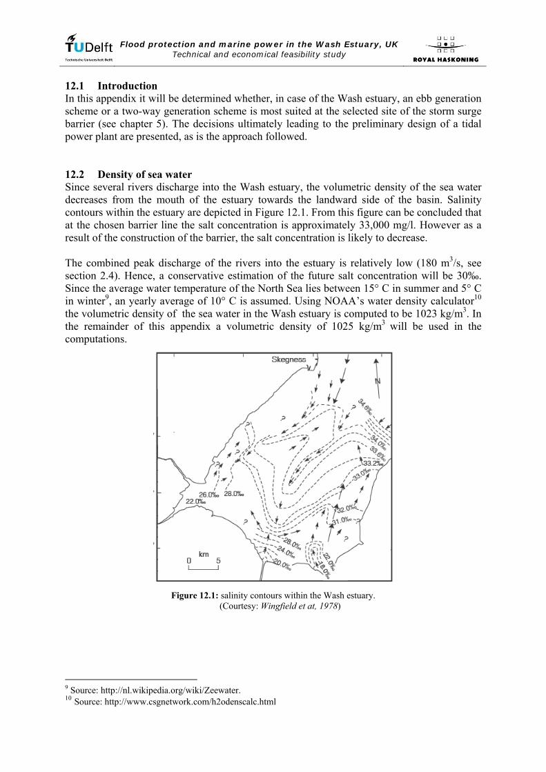
Flood protection and marine power in the Wash Estuary, UK Technical and economical feasibility study
12.1 Introduction In this appendix it will be determined whether, in case of the Wash estuary, an ebb generation scheme or a two-way generation scheme is most suited at the selected site of the storm surge barrier (see chapter 5). The decisions ultimately leading to the preliminary design of a tidal power plant are presented, as is the approach followed. 12.2 Density of sea water Since several rivers discharge into the Wash estuary, the volumetric density of the sea water decreases from the mouth of the estuary towards the landward side of the basin. Salinity contours within the estuary are depicted in Figure 12.1. From this figure can be concluded that at the chosen barrier line the salt concentration is approximately 33,000 mg/l. However as a result of the construction of the barrier, the salt concentration is likely to decrease. The combined peak discharge of the rivers into the estuary is relatively low (180 m3/s, see section 2.4). Hence, a conservative estimation of the future salt concentration will be 30‰. Since the average water temperature of the North Sea lies between 15° C in summer and 5° C in winter9, an yearly average of 10° C is assumed. Using NOAA’s water density calculator10 the volumetric density of the sea water in the Wash estuary is computed to be 1023 kg/m3. In the remainder of this appendix a volumetric density of 1025 kg/m3
will be used in the computations.
Figure 12.1: salinity contours within the Wash estuary. (Courtesy: Wingfield et at, 1978)
9 Source: http://nl.wikipedia.org/wiki/Zeewater. 10 Source: http://www.csgnetwork.com/h2odenscalc.html
Flood protection and marine power in the Wash Estuary, UK Technical and economical feasibility study
12.3 Rated head The runner diameter and generated power of a turbine depend on the rated head11. When the head over the TPP exceeds the rated head the guide vanes are gradually closed. Thus reducing the discharge, while keeping the generator at rated capacity12. In case the head drops below the rated head the capacity of the generator reduces and as a consequence the generated power decreases. According to Song and van Walsum the rated head is accurately estimated using equation 12.1 [Song and van Walsum, 2006]:
meanTPPr RCH ⋅= [12.1] Were:
Hr : rated head [m] CTPP : factor expressing the mode of operation of a TPP:
- single effect mode of operation: CTPP = 0.66 - double effect mode of operation: CTPP = 0.50
[-]
Rmean : mean tidal range [m] In case of the Wash estuary the mean tidal range is 4.70 m. Hence, the rated head for both an ebb generation scheme and a two-way generation scheme is 3.10 m and 2.35 m respectively. In reality the head difference over the barrier is likely to vary between 65% and 125% of the rated head13. However it is not economical to design the TPP based on the mean spring tidal range, because the corresponding head difference will only occur during 20%14 of the total time during one year. This would lead to the installation of too many turbines. 12.4 Runner diameter The runner diameter is an important parameter in the design of a TPP because:
- the electromechanical equipment generally accounts for 45% to 55% of the direct costs of the TPP. Hence, the number of turbines needed, significantly influences the economy of the TPP scheme;
- it has a large influence on the civil engineering costs, as the dimensions of the turbine governs the dimensions of the power house, see figure 12.1;
- the turbine discharge capacity determines the number and size of the sluices. Historically the effort to reduce unit costs has lead to an increase in turbine size. According to manufactures of turbines, a diameter of 9 to 10 m is considered to be a reasonable extension of existing knowledge and technology [Clarke, 2007]. Generally larger turbines tend to have a higher turbine and generator efficiency. Therefore it seems logical to install a limited number or turbines with a large runner diameter. It should be kept in mind however, that the required submergence in order to avoid cavitation should be available without the need for excavation.
11 Rated head = lowest head for which the turbine is capable of driving the generator at its rated capacity. Hence, the turbine guide vanes are opened to their maximum. 12 Rated capacity = maximum power that the generator is allowed to produce. 13 Source: Indian Institute of Technology Kharagpur. 14 Spring tide occurs each 14.765 days, hence 24.72 times a year. Assuming a duration of 3 days, during which the tidal range is equal to or larger than the mean spring tidal range, results in 24.72·3/365 = 0.20.

Flood protection and marine power in the Wash Estuary, UK Technical and economical feasibility study
Due to the fact that the main channel in the Wash estuary is deep and very wide, the selection of a large runner diameter is economical. With increasing runner diameter the power generated also increases (larger discharge), resulting in decreasing cost per kW. Furthermore the number of required turbine caissons decreases. This is beneficial due to the fact that the longitudinal axis of these caissons is orientated perpendicular to the barrier line, while the sluice caissons and normal caissons have a longitudinal axis parallel to the barrier line. Based on preliminary calculations, the required number of turbines will be so large that the TPP’s flexibility is not at risk.
Taken from Bernshtein, 1996.
Figure 12.1: overall dimensions of the power house setting in case of a bulb unit. (a) single effect operation (b) double effect operation.
The relation between the runner diameter of the turbine (D1) and the required Bottom of Structure (BoS), based on figure 12.1, is presented in table 12.1. In case of an ebb generation scheme the BoS is located 2.25·D1 beneath Mean Low Water Spring (-2.00 mODN, see table 11 in section 2.1.3), while in case of a two-way generation scheme this is 2.50·D1 below Mean Low Water Spring. Based on the bottom profile at the location of the most suitable barrier line, see figure 58, a runner diameter of 8.0 m is selected for both schemes.

Flood protection and marine power in the Wash Estuary, UK Technical and economical feasibility study
Runner diameter
[m]
BoS ebb generation
[mODN]
BoS two-way generation
[mODN 4.0 -11.00 -12.00 4.5 -12.15 -13.25 5.0 -13.25 -14.50 5.5 -14.40 -15.75 6.0 -15.50 -17.00 6.5 -16.65 -18.25 7.0 -17.75 -19.50 7.5 -18.90 -20.75 8.0 -20.00 -22.00 8.5 -21.15 -23.25 9.0 -22.25 -24.50
Table 12.1: relation between runner diameter and Bottom of Structure (BoS). 12.5 Turbine, generator and plant efficiency Turbine efficiency cannot be considered to be constant, it varies with the load and is largest at the design head15. In table 12.2 an overview is given of both the turbine and generator efficiency of bulb turbines, as are the discharge coefficient in turbining mode and the plant efficiency.
Scheme ηt 1) ηg
2) m η Ebb generation 0.90 0.95 0.93 0.80 2-way generation 0.85 0.95 0.92 0.75
1) Source: Alstom Power France. 2) Source: RETScreen international.
Table 12.2: turbine, generator and plant efficiency. The approach followed for determining the discharge coefficient is included in appendix 12.1. Note that the values included in the table above are only a crude estimation of m. The plant efficiency is computed using equation 12.2.
mgt ⋅⋅= ηηη [12.2] Were:
η : plant efficiency [-] ηt : turbine efficiency [-] ηg : generator efficiency [-] m : discharge coefficient [-]
Despite the fact that the head difference changes in time the efficiency remains fairly constant over a large range of loads and is only expected to be lower during neap tide.
15 Design head = net head for which the turbine has preferably its maximum efficiency.

Flood protection and marine power in the Wash Estuary, UK Technical and economical feasibility study
12.6 Rated discharge The rated discharge per turbine can be computed using the rated head and runner diameter, see equation 12.3 [Schweiger and Gregori, 1992]:
rttr HgAmQ ⋅⋅⋅⋅⋅= 2η [12.3] Were:
Qr : rated discharge [m3/s] ηt : turbine efficiency [-] m : discharge coefficient [-] At : area of the turbine runner [m2] g : gravitational acceleration [m2/s] Hr : rated head [m]
In case of an ebb generation scheme the rated discharge per turbine amounts to:
/sm32810.381.9284
93.090.0 32 =⋅⋅⋅⋅⋅⋅=π
rQ
In the same way the rated discharge for a two-way generation scheme is computed, resulting in:
/sm26735.281.9284
92.085.0 32 =⋅⋅⋅⋅⋅⋅=π
rQ
As discussed in section 12.3 the maximum discharge occurs at the rated head, see figure 12.2. The discharge relation as a function of the head difference over the barrier is presented in equation 12.4.
50.00
100.00
150.00
200.00
250.00
300.00
350.00
1.0 2.0 3.0 4.0 5.0 6.0 7.0 8.0
Head [m]
Disc
harg
e [m
3/s]
Ebb generation 2-way generation
Figure 12.2: turbine discharge as a function of the head difference over the barrier.

Flood protection and marine power in the Wash Estuary, UK Technical and economical feasibility study
( )
⎪⎪⎩
⎪⎪⎨
⎧
⋅⋅⋅=>
⋅⋅⋅⋅⋅⋅=≤≤=
HgP
QHH
HgDmQHHQf
g
ratedr
tr
ρη
πη 24
0 2
[12.4]
Were: Prated : rated capacity, see section 12.7 [W] ηg : generator efficiency [-]
12.7 Rated capacity Figure 12.3 depicts the power output per turbine as a function of the head difference over the storm surge barrier, as described by equation 12.5.
Figure 12.3: power output as a function of the head difference over the barrier.
( )⎩⎨⎧
=>
⋅⋅⋅⋅=≤≤=
ratedr
gr
PPHHHQgPHH
Pfρη0
[12.5]
Were: P : power [W] Prated : rated capacity16 [W] ηg : generator efficiency [-] ρ : volumetric density of sea water [kg/m3] g : gravitational acceleration [m2/s] Q : discharge [m3/s] H : head [m]
16 Rated capacity = maximum power that the generator is allowed to produce.

Flood protection and marine power in the Wash Estuary, UK Technical and economical feasibility study
The rated capacity for both an ebb generation scheme and a two-way generation scheme is calculated using equation 12.6 [Schweiger and Gregori, 1992].
rrgrated HQgP ⋅⋅⋅⋅= ρη [12.6]
Were: Qr : rated discharge [m3/s] Hr : rated head [m]
This results in a rated capacity per turbine of 9.70 MW for an ebb generation scheme and of 6.00 MW for a two-way generation scheme. 12.8 Specific speed, number of pole pairs and operating speed Because generators only operate at a predefined fixed rotational speed [Krueger, 1976] the operating speed has to be determined. In order to be able to do that, first several turbine parameters have to be determined. Starting with the specific speed of the turbine, that depends on the rated head. The specific speed can be computed using the empirical relation presented in equation 12.7 [Schweiger and Gregori, 1992].
058.21
920650⎟⎟⎠
⎞⎜⎜⎝
⎛=
rq H
n [12.7]
Were: nq : specific speed [rpm] Hr : rated head [m]
With Hr = 3.10 m for an ebb generation scheme and Hr = 2.35 m for a two-way generation scheme, equation 12.7 results in a specific speed of 456.30 rpm and 522.04 rpm respectively. Now a first estimate of the operation speed can be found using equation 12.8 [Schweiger and Gregori, 1992].
4 3−⋅=
rr
q
HQ
nn [12.8]
Were: n : operational speed [rpm] nq : specific speed [rpm] Qr : rated discharge [m3/s] Hr : rated head [m]
In case of an ebb generation scheme a first estimate of the operational speed is 58.86 rpm, while in case of a two-way generation scheme the first estimation amounts to 60.64 rpm. Using equation 12.9 the number of pole pairs on the generator can be determined [Schweiger and Gregori, 1992]. A multiple of four generator pole pairs is preferred, however in practice most standard generators are available in a multiple of two pole pairs. In the United Kingdom the frequency of the national power grid is 50 Hz [National Grid].

Flood protection and marine power in the Wash Estuary, UK Technical and economical feasibility study
nfN p
⋅=
120 [12.9]
Were: Np : number of generator pole pairs [-] n : operational speed [rpm] f : national grid frequency [Hz]
In case of an ebb generation scheme the number of generator pole pairs is (multiple of two poles) :
10294.10186.5850120
⇒=⋅
=pN
While for a two-way generation scheme the number of pole pairs is:
10094.9864.6050120
⇒=⋅
=pN
The required number of generator pole pairs is rounded upwards because the variation of the head difference over the storm surge barrier is expected to vary more than 10% of the rated head, in which case the next lower operational speed is to be selected [Krueger, 1976]. For both schemes the operational speed of the turbine, and hence the generator, is computed using a rewritten form of equation 12.9 and the above determined number of generator pole pairs. For an ebb generation scheme this results in an operational speed of 58.82 rpm and for a two-way generation scheme in 60.00 rpm. Because the generator only operates with a predefined rotational speed the turbine also has to operate with a fixed operational speed. Since the head varies during the tidal cycle, which in turn varies over the lunar month, the discharge should be regulated by means of the turbine’s adjustable guide and runner vanes, see equation 12.8. In order to keep the operational speed constant, the relation between head difference over the barrier and discharge is presented in figure 12.4 for the selected turbine.
0
50
100
150
200
250
300
350
400
450
500
550
0 0.5 1.0 1.5 2.0 2.5 3.0 3.5 4.0 4.5 5.0 5.5 6.0 6.5 7.0 7.5 8.0
Head [m]
Dis
char
ge [m
3/s]
ebb generation 2-way generation
Figure 12.4: relation between head and discharge to maintain a constant operational speed.
Flood protection and marine power in the Wash Estuary, UK Technical and economical feasibility study
12.9 Check on cavitation Now the relevant turbine parameters are known it is time to check whether or not the turbine axis is located low enough below tailwater level to prevent cavitation17. The required distance between the minimum tailwater level and the cavitation reference point at the axis of the turbine runner can be computed using equation 12.10 [Kpordze, 1983]:
HgppHHHH
w
vavatail ⋅−
⋅−
=⋅−−= σρ
σ [12.10]
Were: Htail : required difference between minimum tailwater level
and the cavitation reference point18 [m]
Ha : atmospheric pressure head [m] Hv : vapour pressure head at 20° C [m] σ : cavitation coefficient [-] H : net effective head, here rated head [m] Pa : atmospheric pressure, 101.325·103 19 [Pa] Pv : vapour pressure at 20° C, 2.3·103 Pa 20 [Pa] ρw : volumetric density of water [kg/m3] g : gravitational acceleration [m/s2]
The average temperature of the surface water layer within the North Sea is around 5° to 6° C in winter and 14° to 15° C in summer. Near the coast the temperature in summer can rise to 17° C 21. Therefore it is not likely that the sea water in the Wash estuary will reach temperatures higher than 20° C. Thus the vapour pressure at 20° C is used to check for the occurrence of cavitation. For a bulb turbine the governing equations for the specific speed and cavitation coefficient are [Kpordze, 1983]:
485.1510625.7 qn⋅⋅= −σ [12.11] Were:
σ : cavitation coefficient [-] nq : specific speed [rpm]
And
25.1r
rq H
Pnn
⋅= [12.12]
Were: n : operating speed [rpm] Pr : rated capacity of the turbine [kW] Hr : rated head [m]
17 Cavitation occurs when the absolute pressure at the axis of the turbine runner approaches the vapour pressure. In case the absolute pressure in the water flow equals the vapour pressure, vapour bubbles come into existence. These bubbles will suddenly implode when areas of higher pressure are reached, causing large temporary tension stresses in the material of the runner blades. The development and imploding of the vapour bubbles is called cavitation. 18 Htail is defined positive from the tailwater level in upward direction. 19 Source: http://nl.wikipedia.org/wiki/Atmosfeer_%28eenheid%29. 20 Source: http://nl.wikipedia.org/wiki/Dampdruk. 21 Source: http://nl.wikipedia.org/wiki/Zeewater.
Flood protection and marine power in the Wash Estuary, UK Technical and economical feasibility study
Equation 12.11 represents the regression equation of an analysis performed by Kpordze, based on the empirical equations for the cavitation coefficient provided by six manufacturers of bulb turbines. Note that according to Kpordze the correlation coefficient is not very high [Kpordze, 1983]. Since it is not known in advance which manufacturer will deliver the turbines it is in this stage considered to be sufficient to get a general impression of the cavitation coefficient. Hence, equation 12.11 will be used in this study. In case of an ebb generation scheme:
rpm140810.3
1070.982.5825.1
3
=⋅⋅
=qn Therefore, 61.3140810625.7 485.15 =⋅⋅= −σ
m35.110.361.381.91025
103.210325.101 33
−≈⋅−⋅
⋅−⋅=tailH
In case of two-way generation scheme:
rpm159535.2
1098.500.6025.1
3
=⋅⋅
=qn Therefore, 35.4159510625.7 485.15 =⋅⋅= −σ
m40.035.235.481.91025
103.210325.101 33
−≈⋅−⋅
⋅−⋅=tailH
In case of ebb generation scheme the tailwater level must be at least 1.35 m above the runner axis, for the two-way generation scheme this should be at least 0.40 m. Based on the turbine’s specific speed it seems that this outcome is wrong, because a higher specific speed should result in a lower absolute pressure in the draft tube. The computed cavitation coefficients confirm this, as this coefficient has a larger value in case of a two-way generation scheme. However the net effective head for such a scheme is smaller compared to that of an ebb generation scheme. This explains the unexpected smaller value of Htail for the two-way generation scheme. Both the minimum water levels at the North Sea side of the storm surge barrier and within the basin occur during Low Water Spring. The lowest outside water level is taken to be Mean Low Water Spring (MLWS) and is approximately -2.00 mODN, see table 11 in section 2.1.3. The lowest basin levels are computed using the following assumptions:
- in ebb mode the two-way generation scheme will stop generating just after low water occurs, the ebb generation scheme just before reaching half the mean spring tidal range above MLWS;
- the minimum required head under which the turbine can operate is 1.00 m; - the mean spring tidal range is 6.25 m.
This results in the following minimum basin water levels:
Ebb generation:
Two-way generation:
-2.00 mODN -2.00 mODN 3.13 m + 1.00 m + +1.13 mODN -1.00 mODN 1.00 m - ≈ 0.00 mODN
Flood protection and marine power in the Wash Estuary, UK Technical and economical feasibility study
Hence, for both schemes the lowest tailwater level during operation occurs at the North Sea side. Taking into account the annual significant wave height on the North Sea (Hs = 2.80 m), the governing lowest tailwater level with respect to cavitation is -4.80 mODN. According to Bernshtein the runner axis is located at -9.20 mODN, see figure 12.1.
Turbine parameter Unit Ebb generation
2-way operation
Lowest tailwater level [mODN] -4.80 -4.80 Htail 1)
[m] 1.35 0.40 Required runner axis level [mODN] -6.15 -5.20 Actual runner axis level 2) [mODN] -9.20 -9.20
1) Htail = required difference between minimum tailwater level and the cavitation reference point (runner axis). 2) The runner axis is located 0.9·D1 below the lowest outside water level [Bernshtein, 1996].
Table 12.3: check on cavitation. Based on table 12.3 it can be concluded that no problems concerning cavitation are to be expected, because the actual runner axis level lies well below the runner axis level required to prevent cavitation. Even under storm conditions when wave heights may exceed 2.80 m no cavitation will occur. 12.10 Annual energy yield and power During every one year not all tidal cycles can be used to generate energy. The main reasons for not using a tidal cycle are; maintenance, (electro) mechanic failure and severe storm conditions. According to Clarke every year 3-5% of the tidal cycles are lost to the generation of energy [Clarke, 2007]. So on average 96% of the annual tidal cycles is used to generate energy, this amounts to 0.96·705.50 = 677.30 tidal cycles per annum. The annual energy yield can be estimated using equations 12.13 and 12.14 [Duivendijk, 2007].
12106.3 ⋅⋅⋅⋅⋅⋅
= avavtideannum
VHgNE
ρη [12.13]
Were: Eannum : annual energy yield [GWh] η : plant efficiency [-] Ntide : number of tides in a year generating energy [-] ρ : volumetric density of water [kg/m3] g : gravitational acceleration [m/s2] Hav : average head per tidal cycle [m] Vav : average volume of water per tidal cycle [m3]
And
avavav AV ⋅Δ= ζ [12.14] Were:
Vav : average volume of water per tidal cycle [m3] Δζav : average water level variation [m] Aav : average basin area [m2]
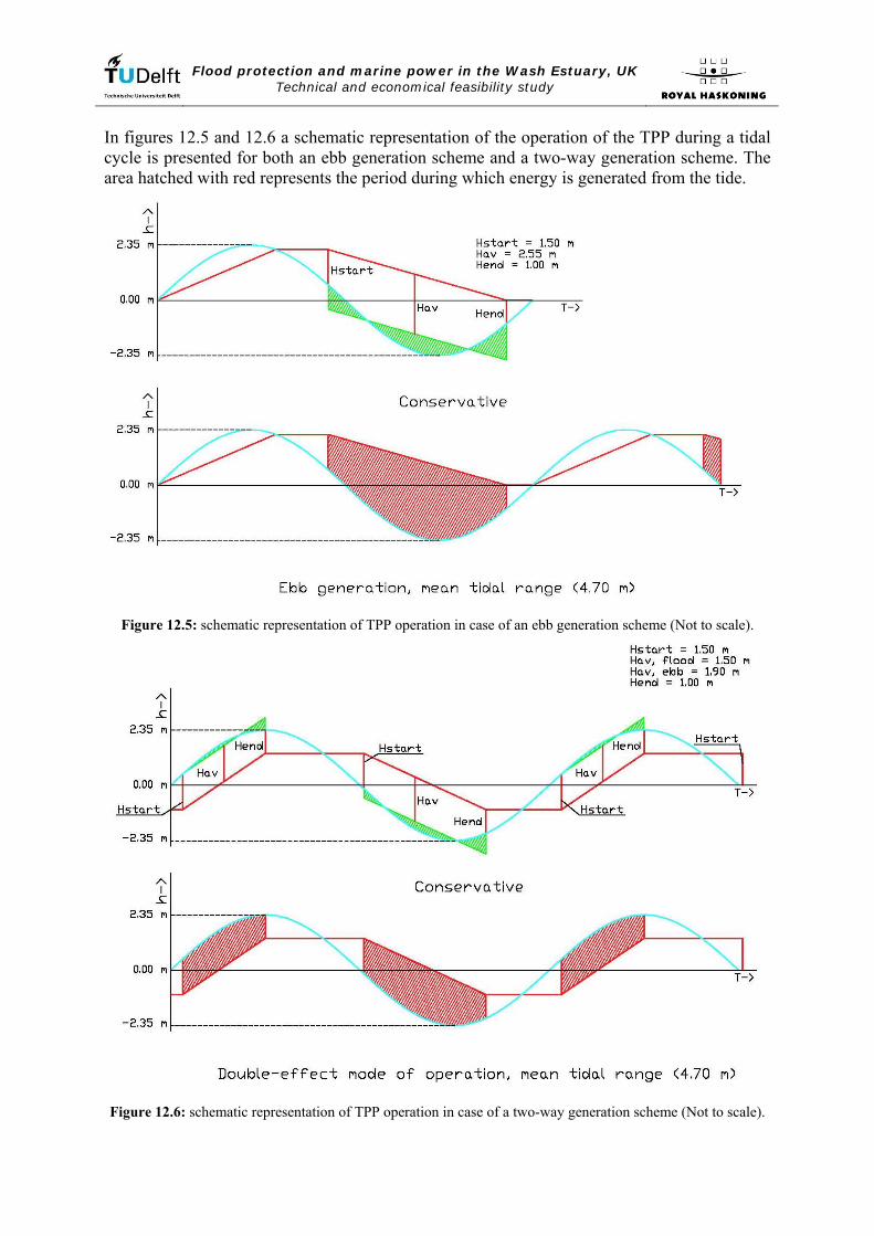
Flood protection and marine power in the Wash Estuary, UK Technical and economical feasibility study
In figures 12.5 and 12.6 a schematic representation of the operation of the TPP during a tidal cycle is presented for both an ebb generation scheme and a two-way generation scheme. The area hatched with red represents the period during which energy is generated from the tide.
Figure 12.5: schematic representation of TPP operation in case of an ebb generation scheme (Not to scale).
Figure 12.6: schematic representation of TPP operation in case of a two-way generation scheme (Not to scale).

Flood protection and marine power in the Wash Estuary, UK Technical and economical feasibility study
In the upper images of figures 12.5 and 12.6, the green hatched area above the tidal curve equals the areas below the curve. The vertical distance between basin level (red line) and the parallel green line represents the average head during the period that the TPP is generating energy. This average head is tabulated in table 12.4 for the mean tidal range, mean neap tidal range and mean spring tidal range. In the performed schematisation the water level within the basin is assumed to change linearly during turbining and sluicing modes, in reality the water level variation in the basin will be non-linear.
Neap tide Mean tide Spring tide Type of scheme Hav, ebb
[m]
Hav, flood
[m]
Hav, ebb
[m]
Hav, flood
[m]
Hav, ebb
[m]
Hav, flood
[m]
Ebb generation 1.85 - 2.55 - 3.25 - 2-way generation 1.35 1.30 1.90 1.50 2.45 1.65
Table 12.4: average head during TPP operation at neap, mean and spring tide. In order to be able to determine the average volume of water that passes through the turbines during one tidal cycle, first the average basin area and water level variation must be known. The water level variation is measured from figures 12.5 and 12.6 as the distance between highest and lowest basin level. This results in 2.15 m and 2.40 m for an ebb generation scheme and a two-way generation scheme respectively. The water covered area of the Wash estuary during high tide is approximately 615 km2, during low tide the water covered area reduces to 325 km2 [Dare, 2004]. Because the Wash estuary’s geometry is very complex and no numerical model of the sea bed topography is available, it is assumed that the average water covered area amounts to 470 km2, which is the mean value. As a result of the fact that the selected barrier line does not enclose the whole estuary the water covered area during high tide is determined to be 465 km2. Using the same ratio between the water covered area during high and low tide as was found by Dare, results in a water covered area during low tide of approximately 245 km2. Hence the average water covered area is established to be approximately 355 km2. However this is a very crude estimation, therefore during any future design stage a numerical model describing the relation between water level and basin area should be developed. In table 12.5 an overview is given of all basin parameters required to estimate the annual energy yield and the generated power per tidal cycle.
Basin parameter Unit Ebb 2-way operation generation Ebb mode Flood mode
Average head per tidal cycle [m] 2.55 1.90 1.50 Average water level variation [m] 2.15 2.40 2.40 Average basin area [m2] 355·106 355·106 355·106 Average volume of water per tidal cycle [m3] 763·106 852·106 852·106 fraction of tidal cycle during which TPP is operational [-] 0.50 0.33 0.22
Average discharge per tidal cycle [m3/s] 34.15·103 57.76·103 86.64·103
Table 12.5: overview basin parameters.
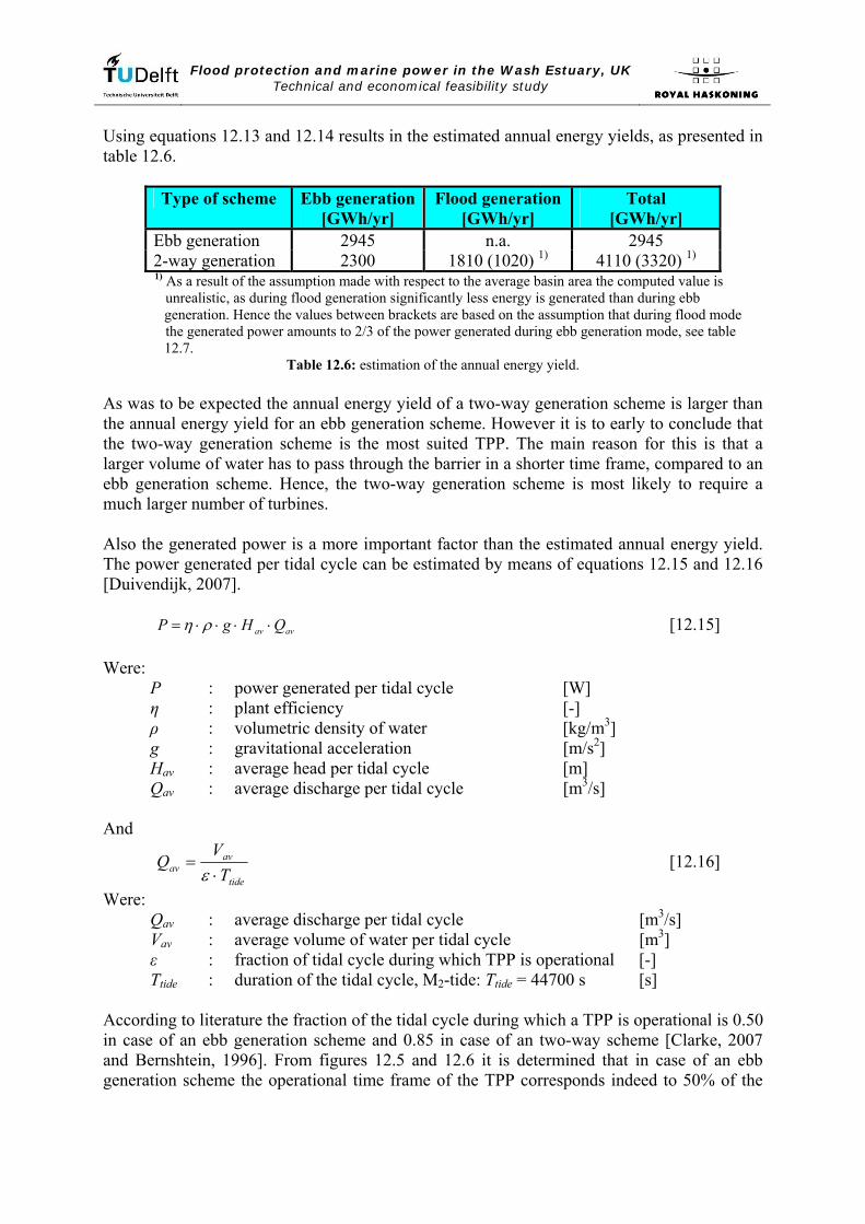
Flood protection and marine power in the Wash Estuary, UK Technical and economical feasibility study
Using equations 12.13 and 12.14 results in the estimated annual energy yields, as presented in table 12.6.
Type of scheme Ebb generation[GWh/yr]
Flood generation [GWh/yr]
Total [GWh/yr]
Ebb generation 2945 n.a. 2945 2-way generation 2300 1810 (1020) 1) 4110 (3320) 1)
1) As a result of the assumption made with respect to the average basin area the computed value is unrealistic, as during flood generation significantly less energy is generated than during ebb
generation. Hence the values between brackets are based on the assumption that during flood mode the generated power amounts to 2/3 of the power generated during ebb generation mode, see table
12.7. Table 12.6: estimation of the annual energy yield.
As was to be expected the annual energy yield of a two-way generation scheme is larger than the annual energy yield for an ebb generation scheme. However it is to early to conclude that the two-way generation scheme is the most suited TPP. The main reason for this is that a larger volume of water has to pass through the barrier in a shorter time frame, compared to an ebb generation scheme. Hence, the two-way generation scheme is most likely to require a much larger number of turbines. Also the generated power is a more important factor than the estimated annual energy yield. The power generated per tidal cycle can be estimated by means of equations 12.15 and 12.16 [Duivendijk, 2007].
avav QHgP ⋅⋅⋅⋅= ρη [12.15] Were:
P : power generated per tidal cycle [W] η : plant efficiency [-] ρ : volumetric density of water [kg/m3] g : gravitational acceleration [m/s2] Hav : average head per tidal cycle [m] Qav : average discharge per tidal cycle [m3/s]
And
tide
avav T
VQ
⋅=ε
[12.16]
Were: Qav : average discharge per tidal cycle [m3/s] Vav : average volume of water per tidal cycle [m3] ε : fraction of tidal cycle during which TPP is operational [-] Ttide : duration of the tidal cycle, M2-tide: Ttide = 44700 s [s]
According to literature the fraction of the tidal cycle during which a TPP is operational is 0.50 in case of an ebb generation scheme and 0.85 in case of an two-way scheme [Clarke, 2007 and Bernshtein, 1996]. From figures 12.5 and 12.6 it is determined that in case of an ebb generation scheme the operational time frame of the TPP corresponds indeed to 50% of the

Flood protection and marine power in the Wash Estuary, UK Technical and economical feasibility study
tidal cycle, but in case of a two-way generation scheme the operational time frame is only 55% of the tidal cycle22. The generated power per tidal cycle, as computed using equations 12.15 and 12.16, is presented in table 12.7.
Type of scheme Ebb generation[MW]
Flood generation [MW]
Total [MW]
Ebb generation 700 n.a. 700 2-way generation 828 980 (552) 1) 1808 (1380) 1) 1) As a result of the assumption made with respect to the average basin area the computed value is unrealistic. It is assumed that the power generated during flood generation mode equals 2/3 of the power generated during ebb generation mode. These values are shown between brackets.
Table 12.7: estimation of the power generated per tidal cycle. From table 12.7 can be concluded that the power generated per tidal cycle in case of a two-way generation scheme is approximately 2.5 times as large as for an ebb generation scheme. However, as will be shown in the next section, this will require a much larger number of turbines, while on the other hand no sluices will be required. Therefore a fair comparison is only possible based on the estimated cost, see section 6.6.4 of the main report. Note that the power generated during flood generation mode is 154 MW larger than during ebb generation mode. This is a direct result of the assumption made with respect to the average basin area. In reality this will be the other way around because during flood generation the highest head occurs when the basin level is lowest and as a consequence a large part of the basin area consists of sand and mudflats that have fallen dry. Hence the water level in the basin will rise faster during the beginning of flood generation than near the end of the operation. During ebb generation mode the opposite occurs, the basin’s water level will fall relatively slow during the early stages, when the largest head differences are present, compared to the end of operation when the sand and mud flats fall dry again. Therefore in case of a two-way generation scheme the power generated during ebb generation mode will be assumed governing with respect to the design of the tidal power plant. 12.11 Design discharge and installed power In order to be able to determine the installed power of the tidal power plant, the required number of turbines has to be established with equation 12.17.
dt P
Pn = [12.17]
Were: nt : number of turbines [-] P : power generated per tidal cycle [MW] Pd : power per turbine during mean tidal cycle [MW]
22 During 33% of the tidal cycle, the tidal power plant is in ebb generation mode. And during 22% of the duration of the tidal cycle the tidal power plant is in flood generation mode.

Flood protection and marine power in the Wash Estuary, UK Technical and economical feasibility study
With the use of equations 12.3 and 12.6 the design discharge23 and power per turbine during a mean tidal cycle in case of an ebb generation scheme turn out to be:
/sm29855.281.9284
93.090.02 32 ≈⋅⋅⋅⋅⋅⋅=⋅⋅⋅⋅⋅=πη avttd HgAmQ
And
W1026.755.229881.9102595.0 6⋅=⋅⋅⋅⋅=⋅⋅⋅⋅= avdgd HQgP ρη Hence the number of turbines required for an ebb generation scheme is:
9741.9626.7
700=>==tn
For a two-way generation scheme the design discharge and power per turbine during ebb generation mode are:
/sm24090.181.9284
92.085.02 32 =⋅⋅⋅⋅⋅⋅=⋅⋅⋅⋅⋅=πη avttd HgAmQ
And W1036.490.124081.9102595.0 6⋅=⋅⋅⋅⋅=⋅⋅⋅⋅= avdgd HQgP ρη
Despite the fact that on paper the power generated during flood generation mode is larger than during ebb generation mode, the power generated during ebb generating mode is used for the calculation of the required number of turbines. The reason for this is already discussed in the previous section:
19091.18936.4
828=>==tn
Since during flood generation mode per tidal cycle the same average volume of water must be able to enter the basin as is discharged during ebb generation mode, only in a shorter period of time, it should be checked whether or not this is possible with the derived number of turbines. During flood generation mode the design discharge and power per turbine are:
/sm21350.181.9284
92.085.02 32 =⋅⋅⋅⋅⋅⋅=⋅⋅⋅⋅⋅=πη avttd HgAmQ
And W1005.350.121381.9102595.0 6⋅=⋅⋅⋅⋅=⋅⋅⋅⋅= avdgd HQgP ρη
The required number of turbines during flood generation mode is: 18005.3
550==tn .
Therefore the 190 turbines required for ebb generation mode have also sufficient capacity during flood generation mode.
23 Design discharge = discharge corresponding to the average head during a mean tidal cycle.

Flood protection and marine power in the Wash Estuary, UK Technical and economical feasibility study
By means of equation 12.18 the installed power can be determined.
ratedtinst PnP ⋅= [12.18] Were:
Pinst : installed power [MW] nt : number of turbines [-] Prated : rated capacity [MW]
The installed power in case of an ebb generation scheme is:
MW94070.997 =⋅=instP And in case of a two-way generation scheme:
MW114000.6190 =⋅=instP

Flood protection and marine power in the Wash Estuary, UK Technical and economical feasibility study

Flood protection and marine power in the Wash Estuary, UK Technical and economical feasibility study
Appendix 12.1
Determination of the discharge coefficient for a single turbine

Flood protection and marine power in the Wash Estuary, UK Technical and economical feasibility study

Flood protection and marine power in the Wash Estuary, UK Technical and economical feasibility study
12.1.1 Introduction In this appendix a crude estimation of the discharge coefficient (m) is made for both an ebb generation scheme and a two-way generation scheme. The following assumptions are made:
- the maximum discharge (discharge at rated head) is used, because in that case the flow velocities are largest and hence the energy losses; - the draft tube is schematized as a square straight tube with a width and height that is the average between the runner diameter and the entree and exit of the draft tube; - the draft tube is considered to be symmetrical; - when sluicing the turbine capacity reduces to 70% of the capacity during turbining [Bernshtein, 1996].
Taken from Bernshtein, 1996.
Figure 12.1.1: overall dimensions of the power house setting in case of a bulb unit. (a) single effect operation (b) double effect operation.
Using figure 1, the overall dimensions of the draft tube are determined for a runner diameter of 8.0 m. The results are listed in table 12.1.1.
Dimension of draft tube
Unit Single effect operation
Double effect operation
Length [m] 57.60 78.40 Height opening [m] 16.00 16.00 Width opening [m] 16.00 16.00 Runner diameter [m] 8.00 8.00 Rated discharge [m3/s] 392 341 Flow velocity [m/s] 2.70 2.40
Table 12.1.1: overall dimensions of the draft tube.

Flood protection and marine power in the Wash Estuary, UK Technical and economical feasibility study
12.1.2 Discharge coefficients According to Nortier the discharge coefficient can be computed using equation 12.1.1 [Nortier and de Koning, 1991].
total
mξ1
= [12.1.1]
Were: m : discharge coefficient [-] ξtot : overall loss coefficient [-]
Bernshtein states that when a turbine operates in sluicing mode the turbine capacity equals approximately 70% of the capacity in turbining mode [Bernshtein, 1996]. Therefore the discharge coefficient during sluicing is found by multiplying the result found with equation 12.1.1 by a factor 0.7. The computed discharge coefficients are presented in table 12.1.2.
Single effect operation
Double effect operation
In turbine mode 0.93 0.92 In sluicing mode 0.65 0.64
Table 12.1.2: discharge coefficients (m). The discharge through the turbine, without taking the efficiency of both the generator and the turbine into account, is computed using equation 12.1.2 [Nortier and de Koning, 1991].
HgAmQt Δ⋅⋅⋅⋅= 2 [12.1.2] Were:
Qt : discharge through turbine [m3/s] m : discharge coefficient [-] A : wet area of the draft tube [m2] g : gravitational acceleration [m/s2] ΔH : head over the barrier [m]
12.1.3 Energy losses The total energy loss in the draft tube is the summation of the energy losses at the entry and exit and the friction losses inside the draft tube. In the remainder of this section these losses will be computed for both schemes. A summary is presented in table 12.1.3 stating the computed energy losses and loss coefficients, as are the total energy loss and the overall loss coefficient (ξtotal).
Type of scheme ξin [-]
ξfriction [-]
ξout [-]
ξtotal [-]
ΔHin [m]
ΔHfriction [m]
ΔHout [m]
ΔHtotal [m]
Single effect operation 0.1 0.063 1.0 1.16 0.037 0.023 0.37 0.43
Double effect operation 0.1 0.085 1.0 1.19 0.029 0.025 0.29 0.34
Table 12.1.3: energy losses and loss coefficients.

Flood protection and marine power in the Wash Estuary, UK Technical and economical feasibility study
Energy loss at entry The energy loss at entry of the turbine caisson can be computed using equation 12.1.3 [Nortier and de Koning, 1991].
guH inin ⋅
⋅=Δ2
2
ξ [12.1.3]
Were: ΔHin : energy loss at entry [m] ξin : entrance loss [-] u : flow velocity in the draft tube [m/s] g : gravitational acceleration [m/s2]
And
2
11⎟⎟⎠
⎞⎜⎜⎝
⎛−=
μξ in [12.1.4]
Were: μ : contraction coefficient [-]
The edges of the turbine caissons are rounded (small radius), according to Nortier resulting in a contraction coefficient of 0.76 [Nortier and de Koning, 1991]. Hence the entrance loss (ξin) is 0.1. Using equation 12.1.3 the energy loss at entry amounts to 0.037 m for a ebb generation scheme and 0.029 m for a two-way generation scheme. Energy loss due to friction The energy loss due to friction in the turbine caisson can be computed using equation 12.1.5 [Nortier and de Koning, 1991].
guH frictionfriction ⋅
⋅=Δ2
2
ξ [12.1.5]
Were: ΔHv : energy loss at entry [m] ξfriction : friction loss [-] u : flow velocity in the draft tube [m/s] g : gravitational acceleration [m/s2]
And
RL
friction ⋅⋅
=4λξ with
OAR = [12.1.6]
Were:
λ : friction factor [-] L : length of the draft tube [m] R : hydraulic radius [m] A : wet area of the draft tube [m2] O : wet circumference of the draft tube [m]

Flood protection and marine power in the Wash Estuary, UK Technical and economical feasibility study
And also
2
8C
g⋅=λ with ⎟
⎠⎞
⎜⎝⎛ ⋅
⋅=k
RC 12log18 [12.1.7]
Were: λ : friction factor [-] g : gravitational acceleration [m/s2] C : Chézy constant [m0.5/s] R : hydraulic radius [m] k : wall roughness, for concrete k = 1.5·10-3 m [m]
The dimensions of the fictional draft tube are 12·12 m2. This results in a hydraulic radius of 3.0 m. With equation 12.1.7 the friction factor is computed to be 0.013. Combining equations 12.1.5 and 12.1.6 results for an ebb generation scheme in an energy loss due to friction of:
mg
uRLH friction 023.0
81.927.2
348.57013.0
24
22
=⋅
⋅⋅⋅
=⋅
⋅⋅⋅
=Δλ
For a two-way generation scheme this becomes:
mg
uRLH friction 025.0
81.924.2
344.78013.0
24
22
=⋅
⋅⋅⋅
=⋅
⋅⋅⋅
=Δλ
Energy loss at exit The energy loss at the exit of the turbine caisson can be computed using equation 12.1.8 [Nortier and de Koning, 1991].
guH outout ⋅
⋅=Δ2
2
ξ [12.1.8]
Were: ΔHout : energy loss at entry [m] ξout : exit loss [-] u : flow velocity in the draft tube [m/s] g : gravitational acceleration [m/s2]
Because the water is discharged into a basin the total velocity head is dissipated. Hence, the exit loss (ξout) is 1.0. Hence for an ebb generation scheme the energy loss at exit is 0.37 m and for a two-way generation scheme 0.29 m.

Flood protection and marine power in the Wash Estuary, UK Technical and economical feasibility study
Appendix 13
Discharge coefficient for a single sluice

Flood protection and marine power in the Wash Estuary, UK Technical and economical feasibility study
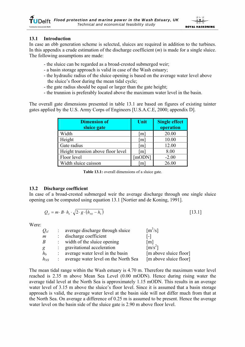
Flood protection and marine power in the Wash Estuary, UK Technical and economical feasibility study
13.1 Introduction In case an ebb generation scheme is selected, sluices are required in addition to the turbines. In this appendix a crude estimation of the discharge coefficient (m) is made for a single sluice. The following assumptions are made:
- the sluice can be regarded as a broad-crested submerged weir; - a basin storage approach is valid in case of the Wash estuary; - the hydraulic radius of the sluice opening is based on the average water level above the sluice’s floor during the mean tidal cycle; - the gate radius should be equal or larger than the gate height; - the trunnion is preferably located above the maximum water level in the basin.
The overall gate dimensions presented in table 13.1 are based on figures of existing tainter gates applied by the U.S. Army Corps of Engineers [U.S.A.C.E, 2000; appendix D].
Dimension of sluice gate
Unit Single effect operation
Width [m] 20.00 Height [m] 10.00 Gate radius [m] 12.00 Height trunnion above floor level [m] 8.00 Floor level [mODN] -2.00 Width sluice caisson [m] 26.00
Table 13.1: overall dimensions of a sluice gate. 13.2 Discharge coefficient In case of a broad-crested submerged weir the average discharge through one single sluice opening can be computed using equation 13.1 [Nortier and de Koning, 1991].
( )bNSbsl hhghBmQ −⋅⋅⋅⋅⋅= 2 [13.1] Were:
Qsl : average discharge through sluice [m3/s] m : discharge coefficient [-] B : width of the sluice opening [m] g : gravitational acceleration [m/s2] hb : average water level in the basin [m above sluice floor] hNS : average water level on the North Sea [m above sluice floor]
The mean tidal range within the Wash estuary is 4.70 m. Therefore the maximum water level reached is 2.35 m above Mean Sea Level (0.00 mODN). Hence during rising water the average tidal level at the North Sea is approximately 1.15 mODN. This results in an average water level of 3.15 m above the sluice’s floor level. Since it is assumed that a basin storage approach is valid, the average water level at the basin side will not differ much from that at the North Sea. On average a difference of 0.25 m is assumed to be present. Hence the average water level on the basin side of the sluice gate is 2.90 m above floor level.

Flood protection and marine power in the Wash Estuary, UK Technical and economical feasibility study
The discharge coefficient can be computed using equation 13.2 [Nortier and de Koning, 1991].
total
mξ1
= [13.2]
Were: m : discharge coefficient [-] ξtot : overall loss coefficient [-]
The overall loss coefficient represents the summation of entrance loss, friction loss and exit loss coefficients. In the remainder of this section these single coefficients will be determined, in order to derive the overall loss coefficient. A summary of the computed loss coefficients is presented in table 13.2.
Type of scheme ξin [-]
ξfriction [-]
ξout [-]
ξtotal [-]
m [-]
Ebb generation 0.44 0.08 1.0 1.52 0.80
Table 13.2: loss coefficients. With an overall loss coefficient (ξtotal) of 1.56 the discharge coefficient (m) for a single sluice is 0.80 (equation 13.2). 13.2.1 Entrance loss coefficient The entrance loss coefficient of the sluice opening can be computed using equation 13.3 [Nortier and de Koning, 1991].
2
11⎟⎟⎠
⎞⎜⎜⎝
⎛−=
μξ in [13.3]
Were: ξin : entrance loss [-] μ : contraction coefficient [-]
Since the sluice opening has a rectangular shape and is not fully submerged, Nortier advises a contraction coefficient of 0.60 [Nortier and de Koning, 1991]. Therefore the entrance loss coefficient (ξin) is 0.44.

Flood protection and marine power in the Wash Estuary, UK Technical and economical feasibility study
13.2.2 Friction loss coefficient The friction loss coefficient for the sluice is computed using equations 13.4 and 13.5 [Nortier and de Koning, 1991].
RL
friction ⋅⋅
=4λξ with
OAR = [13.4]
Were: ξfriction : friction loss [-] λ : friction factor [-] L : width of the sluice caisson [m] R : hydraulic radius [m] A : wet area of the sluice opening [m2] O : wet circumference of the sluice opening [m]
And
2
8C
g⋅=λ with ⎟
⎠⎞
⎜⎝⎛ ⋅
⋅=k
RC 12log18 [13.5]
Were: λ : friction factor [-] g : gravitational acceleration [m/s2] C : Chézy constant [m0.5/s] R : hydraulic radius [m] k : wall roughness, for concrete k = 1.5·10-3 m [m]
As the governing average water level above the sluice floor is 2.90 m, the hydraulic radius becomes 1.27 m. Hence the friction factor is computed to be 0.015 (equation 13.5) and the friction loss coefficient 0.08 (equation 13.4). 13.2.3 Exit loss coefficient Because the water is discharged into a large basin the total velocity head is dissipated. Hence, the exit loss coefficient (ξout) is 1.0 [Nortier and de Koning, 1991].

Flood protection and marine power in the Wash Estuary, UK Technical and economical feasibility study

Flood protection and marine power in the Wash Estuary, UK Technical and economical feasibility study
Appendix 14
Estimation construction costs

Flood protection and marine power in the Wash Estuary, UK Technical and economical feasibility study

Flood protection and marine power in the Wash Estuary, UK Technical and economical feasibility study
Appendix 14.1
Embankment dam

Flood protection and marine power in the Wash Estuary, UK Technical and economical feasibility study

Flood protection and marine power in the Wash Estuary, UK Technical and economical feasibility study
Appendix 14.2
Caisson dam

Flood protection and marine power in the Wash Estuary, UK Technical and economical feasibility study

Flood protection and marine power in the Wash Estuary, UK Technical and economical feasibility study
Appendix 14.3
Final conceptual design

Flood protection and marine power in the Wash Estuary, UK Technical and economical feasibility study

Flood protection and marine power in the Wash Estuary, UK Technical and economical feasibility study
Appendix 15
Storage basin approach

Flood protection and marine power in the Wash Estuary, UK Technical and economical feasibility study

Flood protection and marine power in the Wash Estuary, UK Technical and economical feasibility study
15.1 Introduction The theoretical basis for analysing and performing computations with respect to the behaviour of long waves in shallow water are the continuity equation (equation 15.1) and the equation of motion (equation 15.2), together also referred to as the St. Venant equations or shallow water equations. These equations represent a coupled system of differential equations describing the relation between water level and discharge as function of time and distance.
0=∂∂
+∂∂⋅
xQ
thB (15.1)
And
02
=⋅
⋅⋅+
∂∂⋅⋅+⎟⎟
⎠
⎞⎜⎜⎝
⎛∂∂
+∂∂
RAQQ
cxhAg
AQ
xtQ
sfs
s
(15.2)
Were: B : storage width [m] h : water level [m] t : time [s] Q : discharge [m3/s] x : distance [m] As : current-carrying cross-section [m2] cf : friction coefficient [-] R : hydraulic radius [m]
In this appendix this theory will be used to determine the effects of the barrier on the tidal amplitude within the Wash basin. This is relevant with respect to the optimisation of the sluicing capacity of the tidal power plant. In the approach followed the number of turbines remains fixed at 97, as was determined in chapter 6. The reason for this is that the number of turbines is based on the average head during the mean tidal cycle, where it was implicitly assumed that the average water level at the basin side will not differ much from that at the North Sea24. The purpose of the performed analysis is to see what sluicing capacity is required so that the basin level will approximately equal the maximum outside water level during the mean tidal cycle. 15.2 Storage basin approach In case both the basin is closed except for a narrow opening at one side and if the time frame required by the tidal wave to propagate through the basin is small compared too the period of the tidal wave, the velocities are so small that resistance and inertia can be neglected. Hence, the water level within the basin may be assumed horizontal at all times, only changing in time. The precondition is checked using equation 15.3.
waveba LL ⋅≤201
sin (15.3)
Were: Lbasin : basin length [m] Lwave : length tidal wave [m]
24 On average a difference of 0.25 m is assumed to be present during the filling of the basin.

Flood protection and marine power in the Wash Estuary, UK Technical and economical feasibility study
The basin length of alternative 2-3 is 18,750 m. while the length of the tidal wave corresponds too 442,733 m, assuming a depth of 10 m. Since the basin behind the future storm surge barrier is a closed basin with only a storage function25, both conditions are met. Hence the storage basin approach may be used. Integration of equation 15.1 over space results in the continuity equation applicable for a storage basin:
QdtdhAb =⋅ (15.4)
Were: Ab : basin area [m2] h : water level [m] t : time [s] Q : net discharge [m3/s]
In the analysis the basin area is assumed to be constant in time. This is a simplification because in reality the surface area of the basin will be a function of the water level. However this relation is unknown. 15.3 Rigid column approach The turbine and sluice openings form the connection between the basin and the North Sea. Since no storage is possible within the turbine openings and because the free surface area of the sluice openings is small compared too the free surface area within the basin, storage in the connection may be neglected. Therefore the connection has only a transport function. Due to the fact that the length of the connection is much smaller than the wave length of the tidal wave, the connection can be schematised as a rigid column. Integration of the equation of motion (equation 15.2) over the entire length of the connection results in the equation of motion applicable to the rigid column approach:
( ) ( ) 2ss
bNS AgQQ
dtdQ
AgLthth
⋅
⋅⋅+⋅
⋅=− χ (15.5)
Were: h : water level [m] t : time [s] Q : discharge [m3/s] hNS : water level on North Sea [m] hb : basin water level [m] L : length [m] g : gravitational acceleration [m/s2] As : current-carrying cross-section [m2] χ : loss coefficient [-]
25 As was already proved in chapter 2, the discharge from the tidal rivers into the estuary is small compared to the tidal prism and therefore is neglected. Also tidal locking ensures that the discharge is only present during low tide, while the analysis is used to look at the water levels within the basin during rising tide.

Flood protection and marine power in the Wash Estuary, UK Technical and economical feasibility study
15.4 Discrete system with storage and resistance Equations 15.4 and 15.5 form a coupled system of two first order differential equations, eliminating the discharge results in a second order differential equation:
( ) ( )dtdh
dtdh
AgA
dthd
AgALthth bb
s
bb
s
bbNS ⋅⋅
⋅⋅
+⋅⋅⋅
=− 2
2
2
2 χ (15.6)
Were: hNS : water level on North Sea [m] hb : basin water level [m] t : time [s] L : length [m] g : gravitational acceleration [m/s2] As : current-carrying cross-section [m2] Ab : basin area [m2] χ : loss coefficient [-]
The resistance term is quadratic, which makes the computation more complicated. By linearization of the resistance term the effect of the resistance over the tidal period is the same as the quadratic term, only the gradient of the resistance term in time differs, see figure 15.1.
Figure 15.1: comparison quadratic and linear resistance term (Courtesy: battjes, 2002). By introducing the linear resistance equation 15.6 reduces to:
( ) ( )dt
dhdt
hdAgAL
thth bb
s
bbNS ⋅+⋅
⋅⋅
=− τ2
2
(15.7)
And
QAg
A
s
b ˆ38
2 ⋅⋅⋅⋅= χ
πτ (15.8)

Flood protection and marine power in the Wash Estuary, UK Technical and economical feasibility study
Were: hNS : water level on North Sea [m] hb : basin water level [m] t : time [s] L : length [m] g : gravitational acceleration [m/s2] As : current-carrying cross-section [m2] Ab : basin area [m2] τ : relaxation time [s] χ : loss coefficient [-] Q̂ : amplitude of the discharge [m3/s]
Because the length of the connection between the North Sea and the basin behind the storm surge barrier is very small, the resistance term will be dominant over the inertia term. As a result the exit loss will dominate over the friction and χ → ½ if L/R → 0. Hence equation 15.7 reduces to:
( ) ( )dt
dhthth b
bNS ⋅=− τ (15.9)
Were: hNS : water level on North Sea [m] hb : basin water level [m] t : time [s] τ : relaxation time [s]
Neglecting the inertia term means that the extreme values of the basin water level occur when the discharge through the openings in the barrier is zero. Hence, when the outside and inside levels are equal (no head difference). 15.5 Computational model A MATLAB routine is used to compute the variation of the basin water level in time, the following assumptions are made:
- the discharge from the North Sea into the basin is assumed positive; - the water level within the basin does not affect the geometry of the cross-section.
This is a simplification of the reality, as the Wash estuary’s geometry changes considerably during the rising and falling of the tide;
- no river discharge is taken into account, since the discharge is small and not continuously present during time (tidal locking) and only adds a few centimetres to the head difference over the barrier during peak discharge;
- the tidal wave is composed of the four main tidal constituents (M2; S2; K1 and O1), see table 15.1;
- the surface area of the basin is 355 km2, the length of the connection is 26 m; - the cross-sectional width of the estuary at the barrier line is 21586 m; the channel
width of the Boston and Lynn Deeps are 1936 m and 9892 m respectively, the average depth is assumed to be 10 m;
- the roughness factor, cf, is assumed to be 0.004.

Flood protection and marine power in the Wash Estuary, UK Technical and economical feasibility study
Tidal constituent Wave period [hr]
Wave length [km]
Amplitude 1)
[m] M2 12.42 443 1.596 K1 23.93 853 0.110 S2 12.00 428 0.524 O1 25.82 256 0.120
Wave celerity of all constituents is 9.9 m/s. 1) Because no data with respect to the amplitudes of the four main tidal constituents is available at the time for the tide within the Wash estuary, the data of the Immingham measuring station of the UK Tide Gauge Network is used. Per harmonic the ratio between its amplitude and the total tidal amplitude was determined, from which the amplitudes of the harmonics within the Wash estuary were determined.
Table 15.1: wave length and amplitude of the four major tidal constituents. The variation of the outside water level is described by equation 15.9, using the four main harmonic constituents stated in the table above.
( )tAh i
n
iiNS ⋅⋅= ∑
=ωcos
1 (15.9)
Were: hNS : water level on North Sea [m] Ai : amplitude of tidal constituent i [m] ω : angular velocity [rad/s] t : time [s]
15.6 Outcome of the analysis The preliminary design consists of 97 turbines and 135 sluices, the combined current-carrying cross-section amounts to 135·(20·2.90) + 97·(π/4·82) = 12,706 m2. Table 15.2 presents the parameters computed by the MATLAB-routine.
Variable Equation Value
Unit
Relaxation time QAg
A
s
b ˆ38
2 ⋅⋅⋅⋅= χ
πτ 12770 [s]
Loss coefficient R
Lcf ⋅+= 5.0χ 0.5970 [-]
Discharge amplitude bb hAQ ˆˆ ⋅⋅= ω 112420 [m3/s]
Response parameter g
hAA b
s
bˆ
38 2
2
2 ⋅⋅⋅⋅=ω
χπ
ωτ 1.7950 [-]
Phase difference ( )ωτθ atan= 1.0625 [rad]
Gamma gh
AA
rNS
s
bˆ
38 2
2
2 ⋅⋅⋅⋅==Γω
χπ
ωτ 1.8723 [-]
Amplitude ratio 2411
21
Γ++−⋅Γ⋅
=r 0.6405 [-]
Table 15.2: computed parameters of the preliminary design.

Flood protection and marine power in the Wash Estuary, UK Technical and economical feasibility study
The amplitude ratio between the basin water level and the outside level is 0.64. In other words, as a consequence of the presence of a storm surge barrier, the amplitude of the basin water level is approximately 0.42 m lower than the amplitude of the outside water level. In figure 15.2 the blue line represents the amplitude variation of the outside water level, while the green line represents the amplitude variation of the water level within the basin.
0 10 20 30 40 50 60 70 80-2.5
-2
-1.5
-1
-0.5
0
0.5
1
1.5
2
2.5
Time [hour]
Wat
er le
vel [
m re
lativ
e to
MS
L]
Water level North SeaWater level basin
Figure 15.2: impact of the preliminary design on the amplitude of the water level within the basin. Because the reduction of the amplitude of the outside water level is rather large, the current-carrying cross-section is raised in steps of 174 m2, being the current-carrying cross-section of one sluice caisson, to determine an optimum value. The results are presented in figure 15.3. The optimum current-carrying cross-section is found to be 18,622 m2, corresponding to an additional 34 sluice caissons compared too the preliminary design. The computed amplitude ratio is 0.83. Hence the reduction of the amplitude of the outside water level as a result of the presence of a storm surge barrier is 0.20 m. However placing an additional 34 sluice caissons requires an extra length of 2720 m, which is not available along the barrier line without large dredging works. Analysis learned that the available space along the barrier line allows for the placement of 30 additional sluice caissons, with a total length of 2400 m. The minimum distance between the sluices and both the commercial and recreational lock complexes is at least 140 metres at either side of the navigation locks, thus assuring that the flow conditions induced by the presence of the intake sluices does not interfere with navigation.
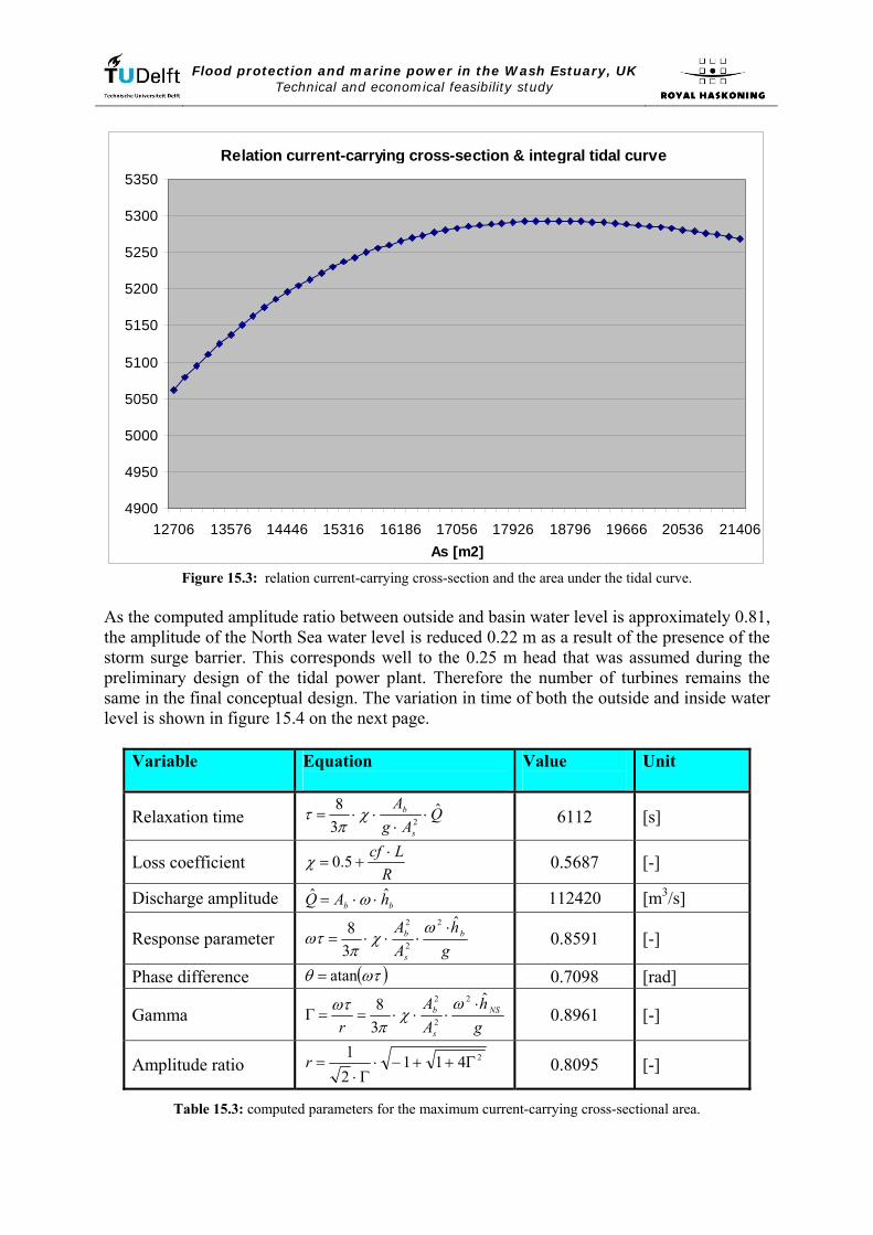
Flood protection and marine power in the Wash Estuary, UK Technical and economical feasibility study
Relation current-carrying cross-section & integral tidal curve
4900
4950
5000
5050
5100
5150
5200
5250
5300
5350
12706 13576 14446 15316 16186 17056 17926 18796 19666 20536 21406As [m2]
Figure 15.3: relation current-carrying cross-section and the area under the tidal curve.
As the computed amplitude ratio between outside and basin water level is approximately 0.81, the amplitude of the North Sea water level is reduced 0.22 m as a result of the presence of the storm surge barrier. This corresponds well to the 0.25 m head that was assumed during the preliminary design of the tidal power plant. Therefore the number of turbines remains the same in the final conceptual design. The variation in time of both the outside and inside water level is shown in figure 15.4 on the next page.
Variable Equation
Value
Unit
Relaxation time QAg
A
s
b ˆ38
2 ⋅⋅⋅⋅= χ
πτ 6112 [s]
Loss coefficient R
Lcf ⋅+= 5.0χ 0.5687 [-]
Discharge amplitude bb hAQ ˆˆ ⋅⋅= ω 112420 [m3/s]
Response parameter g
hAA b
s
bˆ
38 2
2
2 ⋅⋅⋅⋅=ω
χπ
ωτ 0.8591 [-]
Phase difference ( )ωτθ atan= 0.7098 [rad]
Gamma gh
AA
rNS
s
bˆ
38 2
2
2 ⋅⋅⋅⋅==Γω
χπ
ωτ 0.8961 [-]
Amplitude ratio 2411
21
Γ++−⋅Γ⋅
=r 0.8095 [-]
Table 15.3: computed parameters for the maximum current-carrying cross-sectional area.

Flood protection and marine power in the Wash Estuary, UK Technical and economical feasibility study
0 10 20 30 40 50 60 70 80-2.5
-2
-1.5
-1
-0.5
0
0.5
1
1.5
2
2.5
Time [hour]
Wat
er le
vel [
m re
lativ
e to
MS
L]
Water level North SeaWater level basin
Figure 15.4: impact of the final conceptual design on the amplitude of the water level within the basin.

Flood protection and marine power in the Wash Estuary, UK Technical and economical feasibility study
Appendix 16
Final conceptual design

Flood protection and marine power in the Wash Estuary, UK Technical and economical feasibility study

Flood protection and marine power in the Wash Estuary, UK Technical and economical feasibility study
Appendix 16.1
Boston Deeps

Flood protection and marine power in the Wash Estuary, UK Technical and economical feasibility study

Flood protection and marine power in the Wash Estuary, UK Technical and economical feasibility study
Figure 16.1.1: cross-section sluiced caisson Boston Deeps (not to scale).
Figure 16.1.2: cross-section sluice caisson Boston Deeps (not to scale).

Flood protection and marine power in the Wash Estuary, UK Technical and economical feasibility study
Figure 16.1.3: front view sluiced caisson Boston Deeps (not to scale).
Figure 16.1.4: front view sluice caisson Boston Deeps (not to scale).
Figure 16.1.5: abutment caisson Boston Deeps (not to scale).

Flood protection and marine power in the Wash Estuary, UK Technical and economical feasibility study
Appendix 16.2
Lynn Deeps

Flood protection and marine power in the Wash Estuary, UK Technical and economical feasibility study
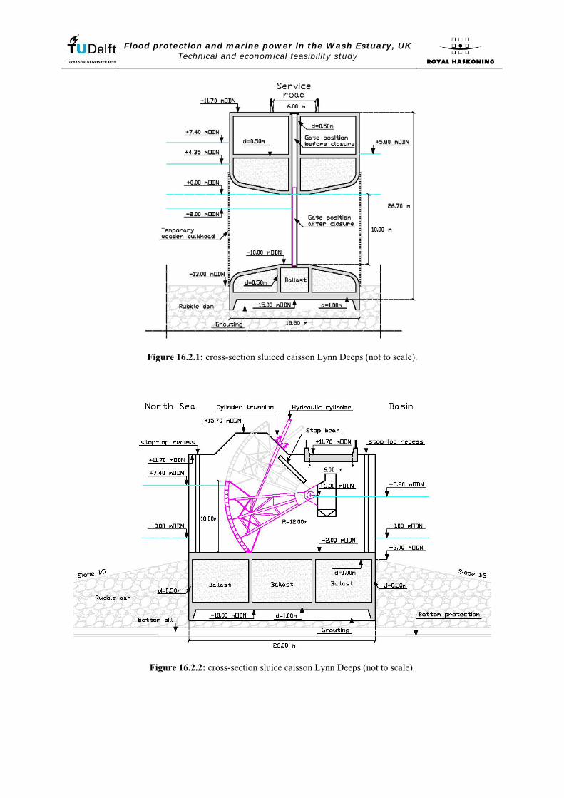
Flood protection and marine power in the Wash Estuary, UK Technical and economical feasibility study
Figure 16.2.1: cross-section sluiced caisson Lynn Deeps (not to scale).
Figure 16.2.2: cross-section sluice caisson Lynn Deeps (not to scale).

Flood protection and marine power in the Wash Estuary, UK Technical and economical feasibility study
Figure 16.2.3: front view sluiced caisson Lynn Deeps (not to scale).
Figure 16.2.4: front view sluice caisson Lynn Deeps (not to scale).
Figure 16.2.5: cross-section recreational navigation lock complex (not to scale).

Flood protection and marine power in the Wash Estuary, UK Technical and economical feasibility study
Figure 16.2.6: cross-section commercial navigation lock complex (not to scale).
Figure 16.2.7: cross-section turbine caisson (not to scale).

Flood protection and marine power in the Wash Estuary, UK Technical and economical feasibility study

Flood protection and marine power in the Wash Estuary, UK Technical and economical feasibility study
Appendix 17
Economic analysis

Flood protection and marine power in the Wash Estuary, UK Technical and economical feasibility study

Flood protection and marine power in the Wash Estuary, UK Technical and economical feasibility study
17.1 Introduction In this appendix the methodology and the results of the performed economic analysis are explained. In order to be able to determine the economic feasibility of the combined storm surge barrier and tidal power plant in the Wash estuary, the discounted values of all expenses and revenues are computed. After which the net present value (NPV) is determined for several energy prices (p/kWh). Also the break-even energy price will be derived. But first the preconditions and assumptions will be stated. 17.2 Preconditions and assumptions The following assumptions are made with respect to the economic analysis:
- the design lifetime of the structure is120 years; - the construction time is estimated to be five years; - the cost distribution of both the total investment costs and the construction costs is
as follows: 55% of the cost is allocated to civil works and 45% is allocated to electromechanical equipment [Clarke, 2007];
- costs for the transmission lines is not included, see section 3.4 of the main report; - compensation for landowners is not included; - V.A.T. is not included in the present value (PV) computations; - the residual value of the structure at the end of the design lifetime is not included; - the regular maintenance and operation costs sum up to an annual sum equal to 1%
of the total construction costs (direct costs only); - transmission losses are set to be 3% of the annual energy yield.
17.2.1 Annual real interest rate In view of the global economic crisis the Bank of England has lowered the official annual interest rate in March 2009 to 0.50% and has kept this rate artificially since. This measure was taken to rescue several UK banks from bankruptcy and give the banks the opportunity to rebuild their balance sheets. With the current annual inflation rate of 3.40%26 (February 2012) this results in a negative annual real interest rate of -2.90%, which does not represent a sound climate for investment. However, considered over longer periods the annual real interest rate is positive, see table 17.1.
Time period Average inflation rate
Average interest rate
Average real interest rate
1989-2010 2.72 1971-2010 8.58 5.86
Source: www.tradingeconomics.com/united-kingdom.
Table 17.1: long term average annual interest and inflation rates. Based on the data presented in the table above, the following rates are used in the performed economic appraisal: - annual inflation rate: 3.00%; - annual interest rate: 9.00%; - annual real interest rate: 6.00%; 17.2.2 Allocation of the cost of electromechanical equipment As stated before 45% of the total construction costs is allocated to electromechanical equipment, which in turn is subdivided per part or group of parts as shown in table 17.2. 26 Source: www.tradingeconomics.com/united-kingdom

Flood protection and marine power in the Wash Estuary, UK Technical and economical feasibility study
Part Percentage of cost electromechanical equipment
Turbines 25% Generator 12%
Transformer 4% Control equipment 55%
Miscellaneous equipment 4% Source: Vrijling et al., 2008.
Table 17.2: subdivision costs electromechanical equipment. Miscellaneous equipment refers to the gantry cranes and cooling and drainage equipment. 17.3 Discounted value expenses The project’s expenses consist of three parts, first the total investment costs, which in this case equal the value of the credit estimate before taxes, as shown in appendix 17.1. And secondly the operation and regular maintenance costs, which sum up to an annual value of 1% of the construction costs (total direct costs as presented in appendix 17.1). The last factor contributing to the expenses are the refurbishment27 costs. The costs of the refurbishment are based on the schedule presented in table 17.3. The figures concerning the first three scheduled refurbishments are after Slangen [Slangen, 2008], the remaining three refurbishments are derived on the basis of an expansion of the trends present within the schedule after Slangen. Table 17.4 gives an overview of the monetary value of the refurbishments.
Refurbishment 1 Refurbishment 2 Refurbishment 3 Time period Year Percentage Year Percentage Year Percentage
Civil structures 20 3% 40 6% 60 6% Turbines 25 10% 45 40% 70 75% Generators 25 10% 45 40% 70 75% Transformers - - 40 5% 50 100% Control equipment 20 25% 40 50% 60 25% Miscellaneous equipment 25 10% 50 50% 75 75%
Refurbishment 4 Refurbishment 5 Refurbishment 6 Year Percentage Year Percentage Year Percentage
Civil structures 80 6% 100 6% 120 6% Turbines - - 95 10% 115 40% Generators - - 95 10% 115 40% Transformers 90 5% 100 100% 140 5% Control equipment 80 50% 100 25% 120 50% Miscellaneous equipment - - 100 10% 125 50%
Source: partly after Slangen, 2008. Note: dates exceeding the design lifetime of 120 years are of course not included in the computation.
Table 17.3: refurbishment schedule. 27 Refurbishment = an investment made to repair or improve existing equipment or civil works, with the purpose to restore the unit to or above its original state.
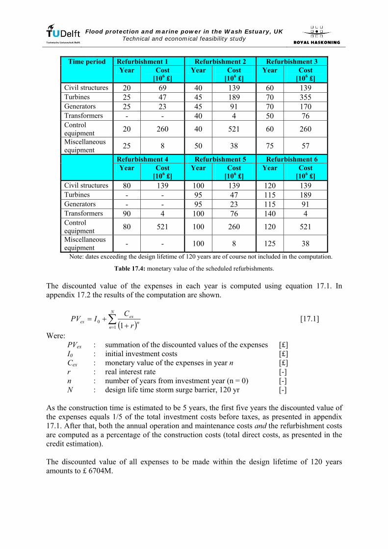
Flood protection and marine power in the Wash Estuary, UK Technical and economical feasibility study
Refurbishment 1 Refurbishment 2 Refurbishment 3 Time period Year Cost
[106 £] Year Cost
[106 £] Year Cost
[106 £] Civil structures 20 69 40 139 60 139 Turbines 25 47 45 189 70 355 Generators 25 23 45 91 70 170 Transformers - - 40 4 50 76 Control equipment 20 260 40 521 60 260 Miscellaneous equipment 25 8 50 38 75 57
Refurbishment 4 Refurbishment 5 Refurbishment 6 Year Cost
[106 £] Year Cost
[106 £] Year Cost
[106 £] Civil structures 80 139 100 139 120 139 Turbines - - 95 47 115 189 Generators - - 95 23 115 91 Transformers 90 4 100 76 140 4 Control equipment 80 521 100 260 120 521 Miscellaneous equipment - - 100 8 125 38
Note: dates exceeding the design lifetime of 120 years are of course not included in the computation.
Table 17.4: monetary value of the scheduled refurbishments. The discounted value of the expenses in each year is computed using equation 17.1. In appendix 17.2 the results of the computation are shown.
( )∑= +
+=N
nn
exex r
CIPV
10 1
[17.1]
Were: PVex : summation of the discounted values of the expenses [£] I0 : initial investment costs [£] Cex : monetary value of the expenses in year n [£] r : real interest rate [-] n : number of years from investment year (n = 0) [-] N : design life time storm surge barrier, 120 yr [-]
As the construction time is estimated to be 5 years, the first five years the discounted value of the expenses equals 1/5 of the total investment costs before taxes, as presented in appendix 17.1. After that, both the annual operation and maintenance costs and the refurbishment costs are computed as a percentage of the construction costs (total direct costs, as presented in the credit estimation). The discounted value of all expenses to be made within the design lifetime of 120 years amounts to £ 6704M.

Flood protection and marine power in the Wash Estuary, UK Technical and economical feasibility study
17.4 Discounted value revenues The revenues from the combined storm surge barrier and tidal power plant are two fault, first the revenues from the generated electricity and secondly the revenues from the reduction of the flood risk in the protected area behind the Wash barrier. Although the latter only holds when the UK Government participates in the project, as for a private investment group as the Wash Tidal Barrier Corporation plc the reduction of the potential damage does not generate additional revenues and therefore does not contribute to the profitability of the project. 17.4.1 Discounted value revenues from energy In chapter 6 of the main report the annual energy yield is estimated to be 2945 GWh, this amount already includes 4% loss due to (electro)mechanical failure and severe storm conditions. Transmission losses are assumed to cause an additional loss of 3% of the amount of energy generated per annum. Since energy generation can only take place after finishing the construction work, the revenues start in the 6th year. The discounted value of the revenues from the annual energy yield is computed by means of equation 17.2, using energy prices of 8 p/kWh, 9 p/kWh, 10 p/kWh and 11 p/kWh.
( )∑= +
=N
nn
EErev r
CPV
1, 1
[17.2]
Were: PVrev,E : summation of the discounted values of the energy revenues [£] CE : monetary value of the generated energy in year n [£] r : real interest rate [-] n : number of years from investment year (n = 0) [-] N : design life time storm surge barrier, 120 yr [-]
The results of the computation are included in appendix 17.3, a summary of the results is presented in table 17.5.
Energy price [p/kWh]
Discounted value [106 £]
8 3013 9 3390 10 3767 11 4143
Table 17.5: discounted values of revenues from energy. 17.4.2 Discounted value revenues from enhanced flood protection In order to be able to determine the discounted value of the revenues gained from enhancing the present flood protection level, the current and future SoP’s should be known. Also the extent of the flooding and the economic value of damages and losses have to be determined. Assumptions made with respect to the analysis:
- the growth of the damages and losses as a result of regular economic development will be ignored;
- the coastal defences and the river defences of the four major rivers are regarded as primary flood defences, thus dividing the Fenlands into five areas, see figure 17.1;

Flood protection and marine power in the Wash Estuary, UK Technical and economical feasibility study
- secondary structures, such as (rail)road embankments and former primary flood defences still present in the hinterland, that could restrict the extent of the flooding are not taken into account. Once the primary flood defences are breached it is assumed that the whole hinterland will flood;
- since the hinterland only benefits from the enhanced flood protection when the storm surge barrier is finished, the revenues start in the 6th year.
Figure 17.1: division of the Fenland’s in flood prone areas (not to scale).

Flood protection and marine power in the Wash Estuary, UK Technical and economical feasibility study
Extent of the flooding The extent of the flooding is determined on the basis of the flood maps provided by the Environment Agency28. The contours of the area that is likely to flood, either by sea or rivers, in a 1:200 flood event and in absence of flood defences were transferred to the Ordnance Survey Landranger Maps series (scale 1:50,000), from which the surface area of the flood extent has been determined. A distinction is made between rural areas and small and large cities, the outcome is presented in table 17.6. As a result of the construction of a storm surge barrier the flood protection level is raised to 1:500.
Flood prone area
SoP Rural area [ha]
Minor city [ha]
Major city [ha]
Total area [ha]
Area 1 1:50 43,850 200 650 44,700 Area 2 1:200 77,150 1,000 750 78,900 Area 3 1:200 74,100 800 - 74,900 Area 4 1:200 144,900 100 800 145,800 Area 5 1:200 8,600 - 1000 9,600
Total 348,600 2,100 3,200 353,900
Table 17.6: flood prone areas. Economic damages and losses The economic value of the expected damages and losses is determined using the estimated annual average damages figures as drawn up by Halcrow in the National Appraisal of Assets at Risk from Flooding and Coastal erosion, that was commissioned by the Department for Environment, Food and Rural Affairs in 2001 [DEFRA, 2001]. The estimated annual average damages are defined as the flood risk (probability of failure times damages). The Ordnance Survey Addresspoint database29 has been used to establish the number of properties within the flooded area, while their capital value is determined based on regional house price values. Limitations of the method followed by Halcrow are [Defra, 2001]:
- size and use of commercial properties is not known from private properties; - high rise buildings are not distinguished. Hence, double-counting of losses occurs; - accuracy concerning agricultural land values and productivity is limited to regional
pricing; - loss of life and human suffering/health is not included; - wider impacts of flooding are not included, e.g. damage to the natural
environment, impact on regional and national productivity, etc.. The values represented on the map shown in figure 17.2 should be treated as indicative for the order of magnitude of the damages and losses, not as absolute values. Current standards maintained means that maintenance and adaptation costs are only included to the extent that the current SoP continues to be provided [Defra, 2001]. The estimated annual average damages, include the following [Defra, 2001]:
- capitalised values of built property and agricultural land; - damage and damage avoided to built property; - damage to and loss of agricultural production; - increased travel cost due to road traffic disruption.
28 http://maps.environment-agency.gov.uk 29 The Ordnance Survey Adresspoint database provides locations for individual postal delivery points.
Flood protection and marine power in the Wash Estuary, UK Technical and economical feasibility study
In table 17.7 an overview is given of the values of the damages per hectare that are applied in the present value computations. The figures stated are based on the median values of the estimated annual average damages (AAD) ranges for a Standard op Protection of 1:200, as depicted in the legend of figure 17.2.
Category Mean value AAD [£/ha]
Damages [£/ha]
Rural area 250 50,000 Minor city 700 140,000 Major city 3000 600,000
Table 17.7: applied value of the annual damages. The flood risk is capitalized as the failure probability times the economic value of the sum of both damages and losses. Based on the data presented in tables 17.6 and 17.7 the present day and future flood risk are computed, see the table below.
Failure probability
[1/yr]
Total value of damages
[106 £]
Annual flood risk [106 £/yr]
Present day 1:50 / 1:200 19,644 137.38 Future 1:500 19,644 39.29
Table 17.8: present day and future flood risk. The discounted value of the revenues from the enhanced flood protection level is computed by means of equation 17.3. The results of the performed computations are presented in appendix 17.4.
( ) ( )( )∑
= +
⋅−⋅=
N
nn
fupdSoPrev r
DPDPPV
1, 1
[17.3]
Were: PVrev,SoP : summation of the discounted values of the
revenues from raising the SoP [£]
Ppd : present day failure probability [1/yr] Pfu : future failure probability [1/yr] D : total damage [£] r : real interest rate [-] n : number of years from investment year (n = 0) [-] N : design life time storm surge barrier, 120 yr [-]
The discounted value of all revenues from an enhanced flood protection level within the design lifetime of 120 years amounts to £ 1293M.

Flood protection and marine power in the Wash Estuary, UK Technical and economical feasibility study
Figure 17.2: estimated annual average damages [DEFRA, 2001].

Flood protection and marine power in the Wash Estuary, UK Technical and economical feasibility study
17.5 Net present value corresponding to several energy prices The net present value (NPV) represents the current value of an investment by means of comparing the discounted cash flows of expenses and revenues, see equation 17.4. As long as the NPV is larger than or equal too zero an investment is considered to be feasible.
( )( ) ( )
( ) ( ) ⎟⎟⎠
⎞⎜⎜⎝
⎛
++−⎟⎟
⎠
⎞⎜⎜⎝
⎛
+
⋅−⋅+
+= ∑∑∑
===
N
nn
exN
nn
fupdN
nn
E
rC
Ir
DPDP
rC
NPV1
011 111
[17.4]
Were: NPV : net present value of the investment [£] CE : Monetary value of the generated energy in year n [£] Ppd : present day failure probability [1/yr] Pfu : future failure probability [1/yr] D : total damage [£] I0 : initial investment costs [£] Cex : monetary value of the expenses in year n [£] r : real interest rate [-] n : number of years from investment year (n = 0) [-] N : design life time storm surge barrier, 120 yr [-]
The NPV’s corresponding to several energy prices are presented in table 17.9. From the table can be concluded that the investment is economically not feasible, based on the present day preconditions and the assumptions made in the performed analysis. However possible financial incentives from the UK Government, such as the buy-out price and Feed-in-Tariffs are not included in the analysis, these may tip the scales and make the investment profitable.
Energy price [p/kWh]
Net Present Value public-private cooperation
[106 £]
Net Present Value private cooperation
[106 £] 8.00 -2398 -3691 9.00 -2021 -3314 10.00 -1644 -2938 11.00 -1268 -2561
Table 17.9: NPV corresponding to several energy prices. 17.6 Break-even point The energy price corresponding to the break-even point is computed as follows:
kWhpErev
SoPex
PVPVPV
BEP.1,,
−= [17.5]
Were: BEP : energy price corresponding to the break-even point [£/kWh] PVex : summation of the discounted values of the expenses [£] PVrev,SoP : summation of the discounted values of the revenues
from raising the SoP [£]
PVrev,E, 1 p/kWh : summation of the discounted values of the energy revenues for a energy price of 1p/kWh
[£]

Flood protection and marine power in the Wash Estuary, UK Technical and economical feasibility study
The energy price at the BEP amounts 14.4 p/kWh, including the revenues from an enhanced SoP. Without the revenues from an enhanced SoP, the energy price at the BEP amounts to 17.8 p/kWh.

Flood protection and marine power in the Wash Estuary, UK Technical and economical feasibility study
Appendix 17.1
Credit estimate Wash barrier and tidal power plant

Flood protection and marine power in the Wash Estuary, UK Technical and economical feasibility study

Flood protection and marine power in the Wash Estuary, UK Technical and economical feasibility study
Appendix 17.2
Discounted value of the expenses

Flood protection and marine power in the Wash Estuary, UK Technical and economical feasibility study

Flood protection and marine power in the Wash Estuary, UK Technical and economical feasibility study
Appendix 17.3
Discounted value of the revenues of energy

Flood protection and marine power in the Wash Estuary, UK Technical and economical feasibility study

Flood protection and marine power in the Wash Estuary, UK Technical and economical feasibility study
Appendix 17.4
Discounted value of the revenues of improved flood protection

Flood protection and marine power in the Wash Estuary, UK Technical and economical feasibility study

lower upper Jan Feb Mar Apr May Jun Jul Aug Sep Oct Nov Dec Total0.0 0.2 85 123 291 370 412 461 622 402 257 169 36 95 33230.2 0.4 150 167 336 513 490 483 824 574 325 245 74 147 43280.4 0.6 359 536 936 1237 1365 1625 1891 1648 1095 686 421 588 123870.6 0.8 624 720 1004 1396 1540 1668 1796 1488 1124 803 498 636 132970.8 1.0 953 1090 1233 1670 1944 2062 1867 1866 1518 1319 949 1133 176041.0 1.2 1056 1082 1150 1429 1677 1463 1271 1476 1493 1190 1055 1151 154931.2 1.4 1845 1495 1693 1733 1982 1727 1417 1715 2058 2045 1760 1847 213171.4 1.6 629 524 499 477 515 382 366 469 568 630 646 504 62091.6 1.8 1061 814 830 793 739 495 490 735 772 929 1209 972 98391.8 2.0 1007 832 875 724 541 372 365 581 660 876 1105 992 89302.0 2.2 825 609 695 431 352 247 190 391 442 628 808 805 64232.2 2.4 901 546 555 262 245 182 172 277 384 562 736 679 55012.4 2.6 547 388 366 162 128 104 101 158 267 481 475 379 35562.6 2.8 729 547 510 233 163 128 163 192 338 736 706 592 50372.8 3.0 192 146 94 59 36 41 26 28 94 191 148 206 12613.0 3.2 331 261 162 77 55 39 74 39 128 272 222 370 20303.2 3.4 225 163 120 58 41 32 57 34 98 201 185 275 14893.4 3.6 178 115 117 26 30 27 53 32 80 145 146 205 11543.6 3.8 164 103 105 30 11 24 27 17 72 125 161 170 10093.8 4.0 57 46 46 8 1 10 10 4 32 46 44 42 3464.0 4.2 56 82 63 13 3 16 5 3 50 72 92 78 5334.2 4.4 43 56 33 11 0 12 7 2 73 36 59 62 3944.4 4.6 38 52 26 5 0 14 6 0 40 29 52 50 3124.6 4.8 28 44 29 4 0 5 4 1 23 23 57 40 2584.8 5.0 23 41 20 1 0 1 1 0 18 17 46 22 1905.0 5.2 14 22 18 1 0 0 0 1 11 16 37 35 1555.2 5.4 5 26 5 0 0 0 0 0 4 8 29 23 1005.4 5.6 8 20 1 0 0 0 0 0 2 4 17 16 685.6 5.8 0 18 0 1 0 0 0 0 1 4 14 14 525.8 6.0 2 18 0 2 0 0 0 0 0 0 8 12 426.0 6.2 5 8 0 0 0 0 0 0 0 0 8 7 286.2 6.4 2 15 0 2 0 0 0 0 1 0 9 6 356.4 6.6 1 12 0 0 0 0 0 0 1 0 4 2 206.6 6.8 0 3 0 1 0 0 0 0 1 0 3 1 96.8 7.0 0 4 0 0 0 0 0 0 3 0 1 0 87.0 7.2 0 3 0 0 0 0 0 0 1 0 0 0 47.2 7.4 0 3 0 0 0 0 0 0 0 0 0 0 37.4 7.6 2 1 0 0 0 0 0 0 0 0 0 0 37.6 7.8 1 1 0 0 0 0 0 0 1 0 0 0 37.8 8.0 0 2 0 0 0 0 0 0 0 0 0 0 28.0 8.2 0 0 0 0 0 0 0 0 0 0 0 0 0
12146 10738 11812 11729 12270 11620 11805 12133 12035 12488 11820 12156 142752
Monthly distribution of wave height (m)
totalCopyright ARGOSS, August 2011

lower upper Jan Feb Mar Apr May Jun Jul Aug Sep Oct Nov Dec Total0 1 25 93 98 185 352 313 408 281 182 126 39 43 21451 2 163 237 470 824 782 931 913 687 486 237 181 216 61272 3 243 316 597 995 873 1127 1119 942 667 455 274 370 79783 4 375 520 894 1098 1111 1280 1375 1153 820 603 377 515 101214 5 570 664 1132 1316 1526 1551 1730 1375 1054 854 534 723 130295 6 701 876 1248 1410 1545 1808 1698 1686 1326 1141 777 1035 152516 7 882 1050 1268 1214 1469 1394 1238 1517 1392 1369 1039 1113 149457 8 1097 1093 1110 997 1197 928 971 1460 1402 1429 1174 1121 139798 9 1334 1192 978 896 1033 509 682 1019 1335 1386 1335 1150 128499 10 1454 894 925 830 764 304 400 666 942 1180 1394 1083 1083610 11 1196 705 693 486 363 176 185 307 512 838 1226 928 761511 12 984 616 525 296 164 153 151 148 454 787 853 795 592612 13 811 557 378 155 72 96 55 77 238 555 691 773 445813 14 614 470 277 129 38 41 92 46 165 451 565 633 352114 15 371 337 178 40 17 30 34 24 138 304 332 414 221915 16 160 182 60 13 1 9 21 8 77 164 191 234 112016 17 189 164 79 8 0 3 9 4 77 151 160 125 96917 18 87 76 36 1 0 0 3 1 32 62 66 48 41218 19 5 60 17 0 0 0 5 0 3 9 36 16 15119 20 1 20 0 0 0 0 2 0 0 4 27 4 5820 21 1 0 0 0 0 0 0 0 0 0 1 0 221 22 0 0 0 0 0 0 0 0 0 0 0 0 0
11263 10122 10963 10893 11307 10653 11091 11401 11302 12105 11272 11339 133711
Monthly distribution of wind speed (m/s)
totalCopyright ARGOSS, August 2011


Description L L_cumm h Volume Total volume soil Total volume rubble Total volume Costs[m] [m] [mODN] [m3/m1] [m3] [m3] [m3] [10^6 £]
Land connection western shorelineEmbankment dam (new) 10,000 ‐ 3.00 270 2,700,000 2,700,000 40.50Embankment dam (addapted) 8,200 ‐ 6.80 180 1,476,000 1,476,000 22.14Friskney FlatsEmbankment dam 350 350 3.70 443 155,050 155,050 4.65Embankment dam 4,113 4,463 0.00 854 3,512,502 3,512,502 105.38Embankment dam 26 4,489 ‐3.90 1418 36,868 36,868 1.11Embankment dam 11 4,500 ‐5.00 1795 19,745 19,745 0.59Boston DeepsEmbankment dam 50 4,550 ‐6.10 1519 71,378 4,590 75,968 4.64Embankment dam 61 4,611 ‐9.40 2119 123,775 5,490 129,265 8.61Embankment dam 28 4,639 ‐15.20 3488 88,785 8,882 97,667 5.32Sluices tidal power plant 583 5,222 ‐15.20 ‐ 655,525 655,525 110.05Sluices tidal power plant 71 5,293 ‐8.90 ‐ 49,842 49,842 11.45Sluices tidal power plant 222 5,515 ‐7.70 ‐ 155,844 155,844 35.81Sluices tidal power plant 166 5,681 ‐8.90 ‐ 116,532 116,532 26.78Sluices tidal power plant 463 6,144 ‐14.10 ‐ 448,022 448,022 82.68Sluices tidal power plant 96 6,240 ‐10.90 ‐ 55,723 55,723 14.73Embankment dam 50 6,290 ‐10.90 2491 118,512 6,056 124,568 6.15Embankment dam 20 6,310 ‐6.50 1592 31,254 593 31,847 1.86Long SandEmbankment dam 20 6,330 ‐5.00 1868 37,360 37,360 1.12Embankment dam 69 6,399 ‐3.90 1418 97,842 97,842 2.94Embankment dam 1,463 7,862 0.00 854 1,249,402 1,249,402 37.48Embankment dam 333 8,195 ‐3.70 1385 461,205 461,205 13.84Embankment dam 204 8,399 ‐6.15 1804 368,016 368,016 11.04Embankment dam 136 8,535 ‐10.50 2678 364,208 364,208 10.93Lynn DeepsEmbankment dam 197 8,732 ‐10.50 2301 435,488 17,730 453,218 30.51Embankment dam 153 8,885 ‐14.10 3150 475,073 6,816 481,889 27.35Commercial lock complex 35 8,920 ‐14.10 ‐ 31,938 31,938 41.58Embankment dam 368 9,288 ‐14.10 3113 1,112,317 33,120 1,145,437 76.36Embankment dam 203 9,491 ‐18.90 4424 854,843 43,148 897,991 50.98Embankment dam 809 10,300 ‐25.00 6383 4,475,873 687,650 5,163,523 268.75Turbines tidal power plant 877 11,177 ‐25.00 ‐ 670,905 670,905 900.31Turbines tidal power plant 222 11,399 ‐21.40 ‐ 57,942 57,942 220.63Turbines tidal power plant 630 12,029 ‐24.50 ‐ 432,968 432,968 643.56Turbines tidal power plant 211 12,240 ‐21.40 ‐ 55,071 55,071 209.70Embankment dam 630 12,870 ‐21.40 5187 2,997,414 270,144 3,267,558 177.39Sluices tidal power plant 196 13,066 ‐21.40 ‐ 437,903 437,903 51.14Sluices tidal power plant 685 13,751 ‐17.10 ‐ 975,200 975,200 142.63Sluices tidal power plant 1,119 14,870 ‐16.70 ‐ 1,519,210 1,519,210 228.19Embankment dam 492 15,362 ‐16.70 3890 1,688,126 225,803 1,913,929 101.90Embankment dam 138 15,500 ‐11.30 2535 342,399 7,445 349,844 21.02Recreational lock complex 26 15,526 ‐11.30 ‐ 11,868 11,868 17.67Embankment dam 96 15,622 ‐11.30 2535 238,191 5,179 243,370 14.62Embankment dam 113 15,735 ‐7.00 1640 175,161 10,170 185,331 14.32Stubborn SandsEmbankment dam 1,276 17,011 ‐7.00 1962 2,503,512 2,503,512 75.11Embankment dam 741 17,752 ‐4.60 1533 1,135,953 1,135,953 34.08Embankment dam 3,834 21,586 0.00 854 3,274,236 3,274,236 98.23Land connection eastern shorelineEmbankment dam (addapted) 2,000 ‐ 4.50 165 330,000 330,000 5.42
Total 41,786 37,957,796 4011
Description L L_cumm h Sill level Crest width sill Sill height Volume/m1 Total volume sill Height rubble Width rubble Volume/m1 Total volume rubble Total Volume Costs[m] [m] [mODN] [m] [m] [mODN] [m3/m1] [m3] [m] [m] [m3/m1] [m3] [m3] [10^6 £]
Land connection western shorelineEmbankment dam (new) 10,000 ‐ 3.00 270 2,700,000 40.50Embankment dam (addapted) 8,200 ‐ 6.80 180 1,476,000 22.14Friskney FlatsEmbankment dam 350 350 3.70 443 155,050 4.65Embankment dam 4,113 4,463 0.00 854 3,512,502 105.38Embankment dam 26 4,489 ‐3.90 1418 36,868 1.11Embankment dam 11 4,500 ‐5.00 1795 19,745 0.59Boston DeepsAbutment caisson 50 4,550 ‐6.10 ‐7.00 35.00 2.00 90 4,500 0.00 0.00 0 0 4,500 2.49Small sluiced caisson & abutment caisson 61 4,611 ‐9.40 ‐9.90 35.00 2.00 90 5,490 2.00 10.00 80 4,880 10,370 4.63Small sluiced caisson 28 4,639 ‐15.20 ‐10.00 35.00 5.20 317 8,882 2.00 10.00 80 2,240 11,122 2.80Sluices tidal power plant 583 5,222 ‐15.20 ‐10.00 96.00 5.20 634 369,855 7.00 0.00 490 285,670 655,525 110.05Sluices tidal power plant 71 5,293 ‐8.90 ‐10.00 96.00 2.00 212 15,052 7.00 0.00 490 34,790 49,842 11.45Sluices tidal power plant 222 5,515 ‐7.70 ‐10.00 96.00 2.00 212 47,064 7.00 0.00 490 108,780 155,844 35.81Sluices tidal power plant 166 5,681 ‐8.90 ‐10.00 96.00 2.00 212 35,192 7.00 0.00 490 81,340 116,532 26.78Sluices tidal power plant 463 6,144 ‐14.10 ‐10.00 96.00 4.10 478 221,152 7.00 0.00 490 226,870 448,022 82.68Sluices tidal power plant 96 6,240 ‐10.90 ‐10.00 96.00 0.90 90 8,683 7.00 0.00 490 47,040 55,723 14.73Abutment caisson 50 6,290 ‐10.90 ‐8.40 35.00 2.50 119 5,938 0.00 0.00 0 0 5,938 2.58Abutment caisson 20 6,310 ‐6.50 ‐5.70 35.00 0.80 31 624 0.00 0.00 0 0 624 0.92Long SandEmbankment dam 20 6,330 ‐5.00 1868 37,360 1.12Embankment dam 69 6,399 ‐3.90 1418 97,842 2.94Embankment dam 1,463 7,862 0.00 854 1,249,402 37.48Embankment dam 333 8,195 ‐3.70 1385 461,205 13.84Embankment dam 204 8,399 ‐6.15 1804 368,016 11.04Embankment dam 136 8,535 ‐10.00 2678 364,208 10.93Lynn DeepsMedium sluiced caisson 197 8,732 ‐10.50 ‐13.00 35.00 2.00 90 17,730 2.00 10.00 80 15,760 33,490 18.47Medium sluiced caisson 153 8,885 ‐14.10 ‐13.00 35.00 1.10 45 6,816 2.00 10.00 80 12,240 19,056 13.89Commercial lock complex 35 8,920 ‐14.10 ‐15.00 300.00 2.00 620 21,700 4.50 10.00 293 10,238 31,938 41.58Large sluiced caisson 368 9,288 ‐14.10 ‐15.00 35.00 2.00 90 33,120 2.00 10.00 80 29,440 62,560 44.90Large sluiced caisson 203 9,491 ‐18.90 ‐15.00 35.00 3.90 213 43,148 2.00 10.00 80 16,240 59,388 26.39Large sluiced caisson 809 10,300 ‐25.00 ‐15.00 35.00 10.00 850 687,650 2.00 10.00 80 64,720 752,370 138.68Turbines tidal power plant 877 11,177 ‐25.00 ‐20.00 108.00 5.00 665 583,205 2.00 15.00 100 87,700 670,905 900.31Turbines tidal power plant 222 11,399 ‐21.40 ‐20.00 108.00 1.40 161 35,742 2.00 15.00 100 22,200 57,942 220.63Turbines tidal power plant 630 12,029 ‐24.50 ‐20.00 108.00 4.50 587 369,968 2.00 15.00 100 63,000 432,968 643.56Turbines tidal power plant 211 12,240 ‐21.40 ‐20.00 108.00 1.40 161 33,971 2.00 15.00 100 21,100 55,071 209.70Large sluiced caisson 630 12,870 ‐21.40 ‐15.00 35.00 6.40 429 270,144 2.00 10.00 80 50,400 320,544 90.75Sluices tidal power plant 196 13,066 ‐21.40 ‐10.00 96.00 11.40 1744 341,863 7.00 0.00 490 96,040 437,903 51.14Sluices tidal power plant 685 13,751 ‐17.10 ‐10.00 96.00 7.10 934 639,550 7.00 0.00 490 335,650 975,200 142.63Sluices tidal power plant 1,119 14,870 ‐16.70 ‐10.00 96.00 6.70 868 970,900 7.00 0.00 490 548,310 1,519,210 228.19Small sluiced caisson 492 15,362 ‐16.70 ‐10.00 35.00 6.70 459 225,803 2.00 10.00 80 39,360 265,163 53.81Small sluiced caisson 138 15,500 ‐11.30 ‐10.00 35.00 1.30 54 7,445 2.00 10.00 80 11,040 18,485 11.46Recreational lock complex 26 15,526 ‐11.30 ‐10.00 160.00 1.30 216 5,628 4.00 10.00 240 6,240 11,868 17.67Small sluiced caisson 96 15,622 ‐11.30 ‐10.00 35.00 1.30 54 5,179 2.00 10.00 80 7,680 12,859 7.97Small sluiced caisson 113 15,735 ‐7.00 ‐10.00 35.00 2.00 90 10,170 2.00 10.00 80 9,040 19,210 9.65Stubborn SandsEmbankment dam 1,276 17,011 ‐7.00 1962 2,503,512 75.11Embankment dam 741 17,752 ‐4.60 1533 1,135,953 34.08Embankment dam 3,834 21,586 0.00 854 3,274,236 98.23Land connection eastern shorelineEmbankment dam (addapted) 2,000 ‐ 4.50 165 330,000 5.42
Total 41,786 24,992,070 3,631

Description L L_cumm h Sill level Crest width sill Sill height Volume/m1 Total volume sill Height rubble Width rubble Volume/m1 Total volume rubble Total Volume Costs[m] [m] [mODN] [m] [m] [mODN] [m3/m1] [m3] [m] [m] [m3/m1] [m3] [m3] [10^6 £]
Land connection western shorelineEmbankment dam (new) 10,000 ‐ 3.00 270 2,700,000 40.50Embankment dam (addapted) 8,200 ‐ 6.80 180 1,476,000 22.14Friskney FlatsEmbankment dam 350 350 3.70 443 155,050 4.65Embankment dam 4,113 4,463 0.00 854 3,512,502 105.38Embankment dam 26 4,489 ‐3.90 1418 36,868 1.11Embankment dam 11 4,500 ‐5.00 1795 19,745 0.59Boston DeepsAbutment caisson 50 4,550 ‐6.10 ‐7.00 35.00 2.00 90 4,500 0.00 0.00 0 0 4,500 2.49Small sluiced caisson & abutment caisson 61 4,611 ‐9.40 ‐9.90 35.00 2.00 90 5,490 2.00 10.00 80 4,880 10,370 4.63Small sluiced caisson 28 4,639 ‐15.20 ‐10.00 35.00 5.20 317 8,882 2.00 10.00 80 2,240 11,122 2.80Sluices tidal power plant 583 5,222 ‐15.20 ‐10.00 96.00 5.20 634 369,855 7.00 0.00 490 285,670 655,525 110.05Sluices tidal power plant 71 5,293 ‐8.90 ‐10.00 96.00 2.00 212 15,052 7.00 0.00 490 34,790 49,842 11.45Sluices tidal power plant 222 5,515 ‐7.70 ‐10.00 96.00 2.00 212 47,064 7.00 0.00 490 108,780 155,844 35.81Sluices tidal power plant 166 5,681 ‐8.90 ‐10.00 96.00 2.00 212 35,192 7.00 0.00 490 81,340 116,532 26.78Sluices tidal power plant 463 6,144 ‐14.10 ‐10.00 96.00 4.10 478 221,152 7.00 0.00 490 226,870 448,022 82.68Sluices tidal power plant 96 6,240 ‐10.90 ‐10.00 96.00 0.90 90 8,683 7.00 0.00 490 47,040 55,723 14.73Abutment caisson 50 6,290 ‐10.90 ‐8.40 35.00 2.50 119 5,938 0.00 0.00 0 0 5,938 2.58Abutment caisson 20 6,310 ‐6.50 ‐5.70 35.00 0.80 31 624 0.00 0.00 0 0 624 0.92Long SandEmbankment dam 20 6,330 ‐5.00 1868 37,360 1.12Embankment dam 69 6,399 ‐3.90 1418 97,842 2.94Embankment dam 1,463 7,862 0.00 854 1,249,402 37.48Embankment dam 333 8,195 ‐3.70 1385 461,205 13.84Embankment dam 204 8,399 ‐6.15 1804 368,016 11.04Embankment dam 136 8,535 ‐10.00 2678 364,208 10.93Lynn DeepsMedium sluiced caisson 197 8,732 ‐10.50 ‐13.00 35.00 2.00 90 17,730 2.00 10.00 80 15,760 33,490 18.47Medium sluiced caisson 83 8,815 ‐14.10 ‐13.00 35.00 1.10 45 3,698 2.00 10.00 80 6,640 10,338 7.54Commercial lock complex 35 8,850 ‐14.10 ‐15.00 300.00 2.00 620 21,700 4.50 10.00 293 10,238 31,938 41.58Large sluiced caisson 70 8,920 ‐14.10 ‐15.00 35.00 2.00 90 6,300 2.00 10.00 80 5,600 11,900 8.54Sluices tidal power plant 368 9,288 ‐14.10 ‐15.00 96.00 2.00 212 78,016 7.00 0.00 490 180,320 258,336 59.36Sluices tidal power plant 203 9,491 ‐18.90 ‐15.00 96.00 3.90 450 91,441 7.00 0.00 490 99,470 190,911 35.89Sluices tidal power plant 709 10,200 ‐25.00 ‐15.00 96.00 10.00 1460 1,035,140 7.00 0.00 490 347,410 1,382,550 171.88Large sluiced caisson 100 10,300 ‐25.00 ‐15.00 35.00 10.00 850 85,000 2.00 10.00 80 8,000 93,000 17.14Turbines tidal power plant 877 11,177 ‐25.00 ‐20.00 108.00 5.00 665 583,205 2.00 15.00 100 87,700 670,905 900.31Turbines tidal power plant 222 11,399 ‐21.40 ‐20.00 108.00 1.40 161 35,742 2.00 15.00 100 22,200 57,942 220.63Turbines tidal power plant 630 12,029 ‐24.50 ‐20.00 108.00 4.50 587 369,968 2.00 15.00 100 63,000 432,968 643.56Turbines tidal power plant 211 12,240 ‐21.40 ‐20.00 108.00 1.40 161 33,971 2.00 15.00 100 21,100 55,071 209.70Large sluiced caisson 70 12,310 ‐21.40 ‐15.00 35.00 6.40 429 30,016 2.00 10.00 80 5,600 35,616 10.08Sluices tidal power plant 560 12,870 ‐21.40 ‐10.00 96.00 11.40 1744 976,752 7.00 0.00 490 274,400 1,251,152 146.10Sluices tidal power plant 196 13,066 ‐21.40 ‐10.00 96.00 11.40 1744 341,863 7.00 0.00 490 96,040 437,903 51.14Sluices tidal power plant 685 13,751 ‐17.10 ‐10.00 96.00 7.10 934 639,550 7.00 0.00 490 335,650 975,200 142.63Sluices tidal power plant 1,119 14,870 ‐16.70 ‐10.00 96.00 6.70 868 970,900 7.00 0.00 490 548,310 1,519,210 228.19Sluices tidal power plant 492 15,362 ‐16.70 ‐10.00 96.00 6.70 868 426,884 7.00 0.00 490 241,080 667,964 100.33Sluices tidal power plant 67 15,429 ‐11.30 ‐10.00 96.00 1.30 133 8,928 7.00 0.00 490 32,830 41,758 10.46Small sluiced caisson 140 15,569 ‐11.30 ‐10.00 35.00 1.30 54 7,553 2.00 10.00 80 11,200 18,753 11.63Recreational lock complex 26 15,595 ‐11.30 ‐10.00 160.00 1.30 216 5,628 4.00 10.00 240 6,240 11,868 17.67Small sluiced caisson 27 15,622 ‐11.30 ‐10.00 35.00 1.30 54 1,457 2.00 10.00 80 2,160 3,617 2.24Small sluiced caisson 113 15,735 ‐7.00 ‐10.00 35.00 2.00 90 10,170 2.00 10.00 80 9,040 19,210 9.65Stubborn SandsEmbankment dam 1,276 17,011 ‐7.00 1962 2,503,512 75.11Embankment dam 741 17,752 ‐4.60 1533 1,135,953 34.08Embankment dam 3,834 21,586 0.00 854 3,274,236 98.23Land connection eastern shorelineEmbankment dam (addapted) 2,000 ‐ 4.50 165 330,000 5.42
Total 41,786 27,447,539 3,824

Credit estimate Wash barrier and Tidal Power Plant
Direct costsEstimated construction costs £ 3,824,000,000.00
Subtotal direct costs £ 3,824,000,000
To be detailed 10% £ 3,824,000,000.00 £ 382,400,000.00
Total direct costs £ 4,206,400,000
Indirect costsGeneral construction site costs 13% £ 4,206,400,000.00 £ 546,832,000.00
Subtotal indirect costs 546,832,000Subtotal including direct costs £ 4,753,232,000
General costs 7% £ 4,753,232,000.00 £ 332,726,240.00Profit and risk 4% £ 5,085,958,240.00 £ 203,438,329.60
Subtotal indirect costs £ 1,082,996,570
To be detailed 10% £ 1,082,996,569.60 £ 108,299,656.96
Total indirect costs 0.28 £ 1,191,296,227Total direct and indirect costs £ 5,397,696,227
Contingency 10% £ 5,397,696,226.56 £ 539,769,622.66
Total construction costs £ 5,937,465,849
Engineering costsEngineering, administration & survey costs 20% £ 5,937,465,849.22 £ 11,874,931.70Contingency 5% £ 11,874,931.70 £ 2,374,986.34
Total engineering costs £ 14,249,918
Total credit estimate 5,951,715,767
Project contingency Prob. Cons. Prob.* Cons.Political influences 50% £ 1,000,000,000 £ 500,000,000.00Scope changes 5% £ 1,000,000,000 £ 50,000,000.00Mitigation measures 75% £ 500,000,000 £ 375,000,000.00
Total project contingency £ 925,000,000
Total investment costs 6,876,715,767V.A.T. 20% 1,375,343,153Total investment costs incl. V.A.T. 8,252,058,921

Year Civil work PV_Civil work Electromechanical PV_Electromechanical Year Civil work PV_Civil work Electromechanical PV_Electromechanical Year Civil work PV_Civil work Electromechanical PV_Electromechanical Summary: NPV_Investment : 6704 10^6 £1 756.44 756.44 618.90 618.90 41 23.14 2.25 0.00 0.00 81 23.14 0.22 0.00 0.002 756.44 713.62 618.90 583.87 42 23.14 2.12 0.00 0.00 82 23.14 0.21 0.00 0.003 756.44 673.23 618.90 550.82 43 23.14 2.00 0.00 0.00 83 23.14 0.19 0.00 0.004 756.44 635.12 618.90 519.64 44 23.14 1.89 0.00 0.00 84 23.14 0.18 0.00 0.005 756.44 599.17 618.90 490.23 45 23.14 1.78 280.15 21.57 85 23.14 0.17 0.00 0.006 23.14 17.29 0.00 0.00 46 23.14 1.68 0.00 0.00 86 23.14 0.16 0.00 0.007 23.14 16.31 0.00 0.00 47 23.14 1.59 0.00 0.00 87 23.14 0.15 0.00 0.008 23.14 15.39 0.00 0.00 48 23.14 1.50 0.00 0.00 88 23.14 0.15 0.00 0.009 23.14 14.52 0.00 0.00 49 23.14 1.41 0.00 0.00 89 23.14 0.14 0.00 0.0010 23.14 13.69 0.00 0.00 50 23.14 1.33 113.57 6.54 90 23.14 0.13 3.79 0.0211 23.14 12.92 0.00 0.00 51 23.14 1.26 0.00 0.00 91 23.14 0.12 0.00 0.0012 23.14 12.19 0.00 0.00 52 23.14 1.18 0.00 0.00 92 23.14 0.12 0.00 0.0013 23.14 11.50 0.00 0.00 53 23.14 1.12 0.00 0.00 93 23.14 0.11 0.00 0.0014 23.14 10.85 0.00 0.00 54 23.14 1.05 0.00 0.00 94 23.14 0.10 0.00 0.0015 23.14 10.23 0.00 0.00 55 23.14 0.99 0.00 0.00 95 23.14 0.10 70.04 0.2916 23.14 9.65 0.00 0.00 56 23.14 0.94 0.00 0.00 96 23.14 0.09 0.00 0.0017 23.14 9.11 0.00 0.00 57 23.14 0.89 0.00 0.00 97 23.14 0.09 0.00 0.0018 23.14 8.59 0.00 0.00 58 23.14 0.84 260.27 9.40 98 23.14 0.08 0.00 0.0019 23.14 8.11 0.00 0.00 59 23.14 0.79 0.00 0.00 99 23.14 0.08 0.00 0.0020 92.54 30.59 260.27 86.02 60 161.95 5.20 0.00 0.00 100 161.95 0.51 343.56 1.0721 23.14 7.21 0.00 0.00 61 23.14 0.70 0.00 0.00 101 23.14 0.07 0.00 0.0022 23.14 6.81 0.00 0.00 62 23.14 0.66 0.00 0.00 102 23.14 0.06 0.00 0.0023 23.14 6.42 0.00 0.00 63 23.14 0.62 0.00 0.00 103 23.14 0.06 0.00 0.0024 23.14 6.06 0.00 0.00 64 23.14 0.59 0.00 0.00 104 23.14 0.06 0.00 0.0025 23.14 5.71 77.61 19.17 65 23.14 0.56 0.00 0.00 105 23.14 0.05 0.00 0.0026 23.14 5.39 0.00 0.00 66 23.14 0.52 0.00 0.00 106 23.14 0.05 0.00 0.0027 23.14 5.09 0.00 0.00 67 23.14 0.49 0.00 0.00 107 23.14 0.05 0.00 0.0028 23.14 4.80 0.00 0.00 68 23.14 0.47 0.00 0.00 108 23.14 0.05 0.00 0.0029 23.14 4.53 0.00 0.00 69 23.14 0.44 0.00 0.00 109 23.14 0.04 0.00 0.0030 23.14 4.27 0.00 0.00 70 23.14 0.42 525.27 9.43 110 23.14 0.04 0.00 0.0031 23.14 4.03 0.00 0.00 71 23.14 0.39 0.00 0.00 111 23.14 0.04 0.00 0.0032 23.14 3.80 0.00 0.00 72 23.14 0.37 0.00 0.00 112 23.14 0.04 0.00 0.0033 23.14 3.58 0.00 0.00 73 23.14 0.35 0.00 0.00 113 23.14 0.03 0.00 0.0034 23.14 3.38 0.00 0.00 74 23.14 0.33 0.00 0.00 114 23.14 0.03 0.00 0.0035 23.14 3.19 0.00 0.00 75 23.14 0.31 56.79 0.76 115 23.14 0.03 280.15 0.3736 23.14 3.01 0.00 0.00 76 23.14 0.29 0.00 0.00 116 23.14 0.03 0.00 0.0037 23.14 2.84 0.00 0.00 77 23.14 0.28 0.00 0.00 117 23.14 0.03 0.00 0.0038 23.14 2.68 0.00 0.00 78 23.14 0.26 0.00 0.00 118 23.14 0.03 0.00 0.0039 23.14 2.53 0.00 0.00 79 23.14 0.25 0.00 0.00 119 23.14 0.02 0.00 0.0040 161.95 16.69 524.33 54.03 80 161.95 1.62 520.54 5.22 120 161.95 0.16 558.40 0.54
4800.14 3680.51 3956.73 2922.70 1203.03 41.72 1756.59 52.91 1203.03 4.06 1255.93 2.30

Year PV_8p/kWh PV_9p/kWh PV_10p/kWh PV_11p/kWh Year PV_8p/kWh PV_9p/kWh PV_10p/kWh PV_11p/kWh Year PV_8p/kWh PV_9p/kWh PV_10p/kWh PV_11p/kWh Summary: NPV_8p/kWh : 3013 10^6 £1 0.0000 0.0000 0.0000 0.0000 41 22.2184 24.9957 27.7730 30.5503 81 2.1601 2.4301 2.7001 2.9702 NPV_9p/kWh : 3390 10^6 £2 0.0000 0.0000 0.0000 0.0000 42 20.9607 23.5808 26.2009 28.8210 82 2.0378 2.2926 2.5473 2.8020 NPV_10p/kWh : 3767 10^6 £3 0.0000 0.0000 0.0000 0.0000 43 19.7743 22.2461 24.7178 27.1896 83 1.9225 2.1628 2.4031 2.6434 NPV_11p/kWh : 4143 10^6 £4 0.0000 0.0000 0.0000 0.0000 44 18.6550 20.9869 23.3187 25.6506 84 1.8137 2.0404 2.2671 2.4938 BEP (NPV=0) : 14.37 p/kWH5 0.0000 0.0000 0.0000 0.0000 45 17.5990 19.7989 21.9988 24.1987 85 1.7110 1.9249 2.1388 2.35266 170.7724 192.1190 213.4655 234.8121 46 16.6029 18.6782 20.7536 22.8289 86 1.6142 1.8159 2.0177 2.21957 161.1060 181.2443 201.3826 221.5208 47 15.6631 17.6210 19.5789 21.5367 87 1.5228 1.7131 1.9035 2.09388 151.9868 170.9852 189.9835 208.9819 48 14.7765 16.6236 18.4706 20.3177 88 1.4366 1.6162 1.7958 1.97539 143.3838 161.3068 179.2298 197.1527 49 13.9401 15.6826 17.4251 19.1676 89 1.3553 1.5247 1.6941 1.8635
10 135.2677 152.1762 169.0847 185.9931 50 13.1510 14.7949 16.4388 18.0827 90 1.2786 1.4384 1.5982 1.758011 127.6111 143.5625 159.5138 175.4652 51 12.4066 13.9575 15.5083 17.0591 91 1.2062 1.3570 1.5077 1.658512 120.3878 135.4363 150.4848 165.5332 52 11.7044 13.1674 14.6305 16.0935 92 1.1379 1.2802 1.4224 1.564613 113.5734 127.7701 141.9668 156.1634 53 11.0419 12.4221 13.8023 15.1826 93 1.0735 1.2077 1.3419 1.476114 107.1447 120.5378 133.9309 147.3240 54 10.4168 11.7189 13.0211 14.3232 94 1.0127 1.1393 1.2659 1.392515 101.0799 113.7149 126.3499 138.9849 55 9.8272 11.0556 12.2840 13.5124 95 0.9554 1.0749 1.1943 1.313716 95.3584 107.2782 119.1980 131.1178 56 9.2710 10.4298 11.5887 12.7476 96 0.9013 1.0140 1.1267 1.239317 89.9608 101.2059 112.4510 123.6961 57 8.7462 9.8395 10.9327 12.0260 97 0.8503 0.9566 1.0629 1.169218 84.8687 95.4772 106.0858 116.6944 58 8.2511 9.2825 10.3139 11.3453 98 0.8022 0.9025 1.0027 1.103019 80.0648 90.0729 100.0810 110.0891 59 7.7841 8.7571 9.7301 10.7031 99 0.7568 0.8514 0.9460 1.040620 75.5328 84.9744 94.4160 103.8576 60 7.3435 8.2614 9.1793 10.0973 100 0.7139 0.8032 0.8924 0.981721 71.2574 80.1645 89.0717 97.9789 61 6.9278 7.7938 8.6597 9.5257 101 0.6735 0.7577 0.8419 0.926122 67.2239 75.6269 84.0299 92.4329 62 6.5357 7.3526 8.1696 8.9865 102 0.6354 0.7148 0.7943 0.873723 63.4188 71.3461 79.2735 87.2008 63 6.1657 6.9364 7.7071 8.4779 103 0.5994 0.6744 0.7493 0.824224 59.8291 67.3077 74.7863 82.2649 64 5.8167 6.5438 7.2709 7.9980 104 0.5655 0.6362 0.7069 0.777625 56.4425 63.4978 70.5531 77.6084 65 5.4875 6.1734 6.8593 7.5453 105 0.5335 0.6002 0.6669 0.733626 53.2476 59.9036 66.5596 73.2155 66 5.1769 5.8240 6.4711 7.1182 106 0.5033 0.5662 0.6291 0.692027 50.2336 56.5128 62.7920 69.0712 67 4.8838 5.4943 6.1048 6.7153 107 0.4748 0.5342 0.5935 0.652928 47.3902 53.3140 59.2378 65.1615 68 4.6074 5.1833 5.7592 6.3351 108 0.4479 0.5039 0.5599 0.615929 44.7077 50.2962 55.8847 61.4732 69 4.3466 4.8899 5.4332 5.9766 109 0.4226 0.4754 0.5282 0.581130 42.1771 47.4493 52.7214 57.9935 70 4.1006 4.6131 5.1257 5.6383 110 0.3987 0.4485 0.4983 0.548231 39.7897 44.7635 49.7372 54.7109 71 3.8684 4.3520 4.8356 5.3191 111 0.3761 0.4231 0.4701 0.517132 37.5375 42.2297 46.9219 51.6140 72 3.6495 4.1057 4.5618 5.0180 112 0.3548 0.3992 0.4435 0.487933 35.4127 39.8393 44.2659 48.6925 73 3.4429 3.8733 4.3036 4.7340 113 0.3347 0.3766 0.4184 0.460234 33.4082 37.5843 41.7603 45.9363 74 3.2480 3.6540 4.0600 4.4660 114 0.3158 0.3553 0.3947 0.434235 31.5172 35.4568 39.3965 43.3361 75 3.0642 3.4472 3.8302 4.2132 115 0.2979 0.3351 0.3724 0.409636 29.7332 33.4499 37.1665 40.8832 76 2.8907 3.2521 3.6134 3.9748 116 0.2810 0.3162 0.3513 0.386437 28.0502 31.5565 35.0627 38.5690 77 2.7271 3.0680 3.4089 3.7498 117 0.2651 0.2983 0.3314 0.364638 26.4624 29.7703 33.0781 36.3859 78 2.5727 2.8943 3.2159 3.5375 118 0.2501 0.2814 0.3127 0.343939 24.9646 28.0851 31.2057 34.3263 79 2.4271 2.7305 3.0339 3.3373 119 0.2360 0.2655 0.2950 0.324540 23.5515 26.4954 29.4394 32.3833 80 2.2897 2.5759 2.8622 3.1484 120 0.2226 0.2504 0.2783 0.3061
2624.4544 2952.5112 3280.5680 3608.6248 354.3626 398.6579 442.9533 487.2486 34.4519 38.7584 43.0649 47.3714
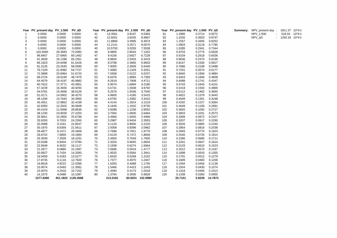
Year PV_present day PV_1:500 PV_ΔD Year PV_present day PV_1:500 PV_ΔD Year PV_present day PV_1:500 PV_ΔD Summary: NPV_present day : 1811.37 10^6 £1 0.0000 0.0000 0.0000 41 13.3561 3.8197 9.5365 81 1.2985 0.3714 0.9272 NPV_1:500 : 518.03 10^6 £2 0.0000 0.0000 0.0000 42 12.6001 3.6035 8.9967 82 1.2250 0.3503 0.8747 NPV_ΔD : 1293.34 10^6 £3 0.0000 0.0000 0.0000 43 11.8869 3.3995 8.4874 83 1.1557 0.3305 0.82524 0.0000 0.0000 0.0000 44 11.2141 3.2071 8.0070 84 1.0903 0.3118 0.77855 0.0000 0.0000 0.0000 45 10.5793 3.0255 7.5538 85 1.0285 0.2941 0.73446 102.6565 29.3583 73.2982 46 9.9805 2.8543 7.1262 86 0.9703 0.2775 0.69287 96.8457 27.6965 69.1492 47 9.4156 2.6927 6.7228 87 0.9154 0.2618 0.65368 91.3639 26.1288 65.2351 48 8.8826 2.5403 6.3423 88 0.8636 0.2470 0.61669 86.1923 24.6498 61.5426 49 8.3798 2.3965 5.9833 89 0.8147 0.2330 0.581710 81.3135 23.2545 58.0590 50 7.9055 2.2609 5.6446 90 0.7686 0.2198 0.548811 76.7109 21.9382 54.7727 51 7.4580 2.1329 5.3251 91 0.7251 0.2074 0.517712 72.3688 20.6964 51.6723 52 7.0358 2.0122 5.0237 92 0.6840 0.1956 0.488413 68.2724 19.5249 48.7475 53 6.6376 1.8983 4.7393 93 0.6453 0.1846 0.460814 64.4079 18.4197 45.9882 54 6.2619 1.7908 4.4711 94 0.6088 0.1741 0.434715 60.7622 17.3771 43.3851 55 5.9074 1.6894 4.2180 95 0.5743 0.1643 0.410116 57.3228 16.3935 40.9293 56 5.5731 1.5938 3.9792 96 0.5418 0.1550 0.386917 54.0781 15.4656 38.6126 57 5.2576 1.5036 3.7540 97 0.5112 0.1462 0.365018 51.0171 14.5902 36.4270 58 4.9600 1.4185 3.5415 98 0.4822 0.1379 0.344319 48.1294 13.7643 34.3650 59 4.6792 1.3382 3.3410 99 0.4549 0.1301 0.324820 45.4051 12.9852 32.4199 60 4.4144 1.2624 3.1519 100 0.4292 0.1227 0.306421 42.8350 12.2502 30.5848 61 4.1645 1.1910 2.9735 101 0.4049 0.1158 0.289122 40.4103 11.5568 28.8536 62 3.9288 1.1236 2.8052 102 0.3820 0.1092 0.272723 38.1230 10.9026 27.2203 63 3.7064 1.0600 2.6464 103 0.3603 0.1031 0.257324 35.9651 10.2855 25.6796 64 3.4966 1.0000 2.4966 104 0.3399 0.0972 0.242725 33.9293 9.7033 24.2260 65 3.2987 0.9434 2.3553 105 0.3207 0.0917 0.229026 32.0088 9.1541 22.8547 66 3.1120 0.8900 2.2220 106 0.3026 0.0865 0.216027 30.1970 8.6359 21.5611 67 2.9358 0.8396 2.0962 107 0.2854 0.0816 0.203828 28.4877 8.1471 20.3406 68 2.7696 0.7921 1.9776 108 0.2693 0.0770 0.192329 26.8752 7.6859 19.1893 69 2.6129 0.7472 1.8656 109 0.2540 0.0726 0.181430 25.3539 7.2509 18.1031 70 2.4650 0.7049 1.7600 110 0.2396 0.0685 0.171131 23.9188 6.8404 17.0784 71 2.3254 0.6650 1.6604 111 0.2261 0.0647 0.161432 22.5649 6.4532 16.1117 72 2.1938 0.6274 1.5664 112 0.2133 0.0610 0.152333 21.2877 6.0880 15.1997 73 2.0696 0.5919 1.4777 113 0.2012 0.0575 0.143734 20.0827 5.7434 14.3393 74 1.9525 0.5584 1.3941 114 0.1898 0.0543 0.135535 18.9459 5.4183 13.5277 75 1.8420 0.5268 1.3152 115 0.1791 0.0512 0.127936 17.8735 5.1116 12.7620 76 1.7377 0.4970 1.2407 116 0.1689 0.0483 0.120637 16.8618 4.8222 12.0396 77 1.6393 0.4688 1.1705 117 0.1594 0.0456 0.113838 15.9074 4.5493 11.3581 78 1.5466 0.4423 1.1043 118 0.1504 0.0430 0.107439 15.0070 4.2918 10.7152 79 1.4590 0.4173 1.0418 119 0.1418 0.0406 0.101340 14.1575 4.0488 10.1087 80 1.3764 0.3936 0.9828 120 0.1338 0.0383 0.0955
1577.6390 451.1822 1126.4568 213.0181 60.9201 152.0980 20.7101 5.9228 14.7873