Flexible Scheduling of Distributed Analytic Applications - arXiv

Flexible Scheduling of Distributed

Analytic Applications

Francesco Pace1, Daniele Venzano1, Damiano Carra2 and PietroMichiardi1

1 Data Science Department - Eurecom, Sophia Antipolis - France,[email protected]

2 Computer Science Department - University of Verona, Verona -Italy, [email protected]

December 7, 2016

Abstract

This work addresses the problem of scheduling user-defined analyticapplications, which we define as high-level compositions of frameworks,their components, and the logic necessary to carry out work. The keyidea in our application definition, is to distinguish classes of components,including rigid and elastic types: the first being required for an applica-tion to make progress, the latter contributing to reduced execution times.We show that the problem of scheduling such applications poses new chal-lenges, which existing approaches address inefficiently.

Thus, we present the design and evaluation of a novel, flexible heuris-tic to schedule analytic applications, that aims at high system responsive-ness, by allocating resources efficiently. Our algorithm is evaluated usingtrace-driven simulations, with large-scale real system traces: our flexi-ble scheduler outperforms a baseline approach across a variety of metrics,including application turnaround times, and resource allocation efficiency.

We also present the design and evaluation of a full-fledged system,which we have called Zoe, that incorporates the ideas presented in thispaper, and report concrete improvements in terms of efficiency and per-formance, with respect to prior generations of our system.

1

arX

iv:1

611.

0952

8v4

[cs

.DC

] 7

Dec

201

6

Contents

1 Introduction 3

2 Definitions and Problem statement 52.1 Definitions . . . . . . . . . . . . . . . . . . . . . . . . . . . . . . . 52.2 Problem Statement . . . . . . . . . . . . . . . . . . . . . . . . . . 6

3 A Flexible Scheduling Algorithm 83.1 Design guidelines . . . . . . . . . . . . . . . . . . . . . . . . . . . 83.2 Algorithm Details . . . . . . . . . . . . . . . . . . . . . . . . . . . 93.3 Preemptive policies . . . . . . . . . . . . . . . . . . . . . . . . . . 11

4 Numerical evaluation 114.1 Methodology . . . . . . . . . . . . . . . . . . . . . . . . . . . . . 114.2 Comparison with the baseline . . . . . . . . . . . . . . . . . . . . 144.3 Comparison between different definitions of size . . . . . . . . . . 254.4 Impact of different workloads . . . . . . . . . . . . . . . . . . . . 414.5 Preemption . . . . . . . . . . . . . . . . . . . . . . . . . . . . . . 42

5 Implementation: The Zoe system 46

6 Experiments with Zoe 48

7 Related Work 50

8 Conclusions 51

2

1 Introduction

The last decade has witnessed the proliferation of numerous distributed frame-works to address a variety of large-scale data analytics and processing projects.First, MapReduce [1] has been introduced to facilitate the processing of bulkdata. Subsequently, more flexible tools, such as Dryad [2], Spark [3], Flink [4]and Naiad [5], to name a few, have been conceived to address the limitationsand rigidity of the MapReduce programming model. Similarly, specialized li-braries [6] and systems like TensorFlow [7] have seen the light to cope withlarge-scale machine learning problems. In addition to a fast growing ecosystem,individual frameworks are driven by a fast-pace development model, with newreleases every few months, introducing substantial performance improvements.Since each framework addresses specific needs, users are left with a wide choiceof tools and combination thereof, to address the various stages of their projects.

The context depicted above has driven a lot of research [8–21] in the areaof resource allocation and scheduling, both from academia and the industry.These efforts materialize in cluster management systems that offer simple mech-anisms for users to request the deployment of the framework they need. Thegeneral underlying idea is that of sharing cluster resources among a heteroge-neous set of frameworks, as a response to static partitioning, which has beendismissed for it entails low resource utilization [8–10]. Existing systems dividethe resources at different levels. Some of them, e.g. Mesos and YARN, tar-get low-level orchestration of distributed computing frameworks: to this aim,they require non-trivial modifications of such frameworks to operate correctly.Others, e.g. Kubernetes [22] and Docker Swarm [23], focus on provisioning anddeployment of containers, and are thus oblivious to the characteristics of theframeworks running in such containers. To the best of our knowledge, no exist-ing tool currently addresses the problem of scheduling analytic applications asa whole, leveraging the intrinsic properties of the frameworks such applicationsuse, but without requiring substantial modification of such frameworks.

The endeavor of this paper is to fill the gap that exists in current approaches,and raise the level of abstraction at which scheduling works. We introduce ageneral and flexible definition of applications, how they are composed, and howto execute them. For example, a user application addressing the training ofa statistical model involves: a user-defined program implementing a learningalgorithm, a framework (e.g., Spark) to execute such a program together withinformation about its resource requirements, the location for input and outputdata and possibly hyper-parameters exposed as application arguments. Usersshould be able to express, in a simple way, how such an application must bepackaged and executed, submit it, and expect results as soon as possible.

We show that scheduling such applications represents a departure from whathas been studied in the scheduling literature, and present the design of a newalgorithm to address the problem. A key insight of our approach is to exploitthe properties of the frameworks used by an application, and distinguish theircomponents according to classes, core and elastic: the first being required foran application to produce work, the latter contributing to reduced execution

3

times. Our heuristic focuses cluster resources to few applications, and uses theclass of application components to pack them efficiently. Our scheduler aimsat high cluster utilization and a responsive system. It can easily accommodatea variety of scheduling policies, beyond the traditional “first-come-first-served”or “processor sharing” strategies, that are currently used by most existing ap-proaches. We study the performance of our scheduler using realistic, large-scaleworkload traces from Google [24, 25], and show it consistently outperforms theexisting baseline approach which ignores component classes: application turn-around times are more than halved, and queuing times are drastically reduced.This induces fewer applications waiting to be served, and increases resourceallocation up to 20% more than the baseline.

Finally, we present a full-fledged system, called Zoe, that schedules analyticapplications according to our original algorithm and that can use sophisticatedpolicies to determine application priorities. Our system exposes a simple and ex-tensible configuration language that allows application definition. We validateour system with real-life experiments, and report conspicuous improvementswhen compared to a baseline scheduler, when using a representative workload:median turnaround times are reduced by up to 37% and median resource allo-cation is 20% higher.

In summary, the contributions of our work are as follows:

• We define, for the first time, a high-level construct to represent analyticapplications, focusing on their heterogeneity, and their end-to-end life-cycle;

• We establish a new scheduling problem, and propose a flexible heuristic ca-pable of handling heterogeneous requests, as well as a variety of schedulingpolicies, with the ultimate objective of improving system responsivenessunder heavy loads;

• We evaluate our scheduling policy using realistic, large-scale workloadtraces and show it consistently outperforms the baseline approach;

• We build a system prototype which materializes the ideas of analytic ap-plications and their scheduling. Our system has been in use for over oneyear, serving a variety of analytic application workloads. Using our newheuristic, we were able to achieve substantial improvements in terms ofsystem responsiveness and cluster utilization.

This paper is organized as follows. We start by clarifying what analytic ap-plications are, give examples and formulate our problem statement in Section 2.We then describe the details of our flexible scheduling heuristic, in Section 3,which we evaluate using simulations in Section 4. The system implementationis described in Section 5, and its evaluation is presented in Section 6. Finally,in Section 7 and Section 8 we discuss related work and conclude, hinting at ourcurrent research agenda.

4

2 Definitions and Problem statement

2.1 Definitions

We define a data analytics framework as a set of one or more software com-ponents (executable binaries) to accomplish some data processing tasks. Dis-tributed frameworks are generally composed by a controller, a master and anumber of worker components. Examples of distributed frameworks are ApacheSpark [26], Google TensorFlow [27] and MPI [28]. Another example of simpledata analytics framework we consider is an interactive Notebook [29].

Distributed frameworks require a scheduler to orchestrate their work: theyexecute jobs, each of which consists of one or more tasks that run in parallel thesame program. Such schedulers operate at the task level : they assign tasks toworkers, and they are highly specialized to take into account the peculiaritiesof each framework.

Framework schedulers such as Mesos [8] and Yarn [21] introduce an addi-tional scheduling component to share cluster resources among concurrent frame-works: sharing policies are based on simple variations of Processor Sharing.Similarly, cluster management systems such as Docker Swarm [23] and Kuber-netes [22] use a scheduler that assigns resources to generic frameworks. Theproblem to solve is the efficient allocation of resources by placing frameworkcomponents and their tasks on cluster machines that satisfy a set of constraints.

We are now ready to define analytics applications, which are the elementswe schedule in our work. Our main objective is to raise the level of abstractionby manipulating an abstract entity encompassing one or more analytics frame-works, their components and the necessary logic for them to cooperate towardproducing useful work by running user-defined jobs. What sets apart our workfrom the state of the art is that our scheduler takes into account the notionof component classes, which allows modeling the specificity of each frame-work. We have found two distinct component classes to be sufficient to modelexisting analytic frameworks: thus, framework components either belong to acore or to an elastic class. Core components are compulsory for a frameworkto produce useful work; elastic components, instead, optionally contribute to ajob, e.g. by decreasing its runtime. Consider, for example, Spark. To producework, it needs some core components: a controller (the spark client runningthe DAG scheduler), a master (in a standalone deployment), and one worker(running executors). We treat additional workers as elastic components. Analternative example is an application using TensorFlow, which only works withcore components: one or more parameter servers and a number of workers.These two frameworks have substantially different runtime behavior: Spark isan elastic framework that can dynamically integrate workers to dispatch tasks.TensorFlow is rigid, and uses only core components to make progress.

To summarize, the nature of an application is that of raising the level ofabstraction and an application is considered as being a collection of frameworksand their heterogeneous components as a single entity to schedule and allocatein a cluster of computers.

5

2.2 Problem Statement

We now treat the applications defined above as abstract entities that we callrequests: they include one or more components, which belong to a given class,either core or elastic. In the literature, the classical problem of schedulinggeneric requests to be served by a distributed system has been extensively stud-ied [30–32]. Requests composed solely by core components are usually referredto as rigid, while requests composed solely by elastic components are referredto as moldable (if the assigned resources are decided when the request is servedand they do not change for the whole execution) or malleable (if the resourcescan vary during the execution1). A key difference with respect to previous workis that we consider heterogeneous requests, composed by both core and elasticcomponents.

For simplicity of exposition, we assume system resources that can be mea-sured in units, and that there are R available units overall to satisfy the re-quests. Each request i specifies the amount of units for its core and elasticcomponents, labeled Ci and Ei respectively. Ideally, with enough available re-sources, a request is allocated all of its components: in this case, we define theservice (or execution) time as Ti. The amount of work to satisfy a request isthe area of the square Wi = Ti × (Ci + Ei). More generally, a request is al-located at least Ci + xi(t) resources, where 0 ≤ xi(t) ≤ Ei. Then, the servicetime is T ′

i = Wi

Ci+xi(t). This simple model allows updating the service time T ′

i

when a scheduling decision modifies xi(t), by measuring the amount of workaccomplished so far, and by computing the remaining amount of work to bedone. While more complex models to describe T ′

i can be conceived, for exampletaking into account the multi-dimensional nature of system resources, our sim-ple approximation doesn’t affect the nature of the scheduling problem we arestudying.

Essentially, the problem of scheduling the execution of an incoming workloadof requests amounts to: i) sorting requests to decide in which order to servethem; ii) allocating distributed resources to requests selected for service. Thesorting phase can be solved using naive approaches, e.g. FIFO ordering, or moresophisticated policies, that use request size information. Even more generally,requests can be placed into “pools” and be assigned priorities, to mimic thehierarchical organization of the users, for example. The allocation phase is moretricky: in the abstract, it is a “packing” problem that has to decide how to shaperequests being served. Even assuming service times to be known a-priori (e.g.,Ti is given as an input), it is well known that the on-line scheduling problem isNP-hard [30]. Therefore, we need to find a suitable heuristic to approximatea solution to the scheduling optimization problem. In our case, it amountsto minimizing the application turnaround times, which is the interval of timebetween request i submission and its completion. In the context we consider,optimizing the average turnaround time represents a meaningful performancemetric, as it caters system responsiveness. Next, we motivate our problem with

1An example of malleable framework is Spark [33]. Worker can be added or removedwithout destroying the application execution.

6

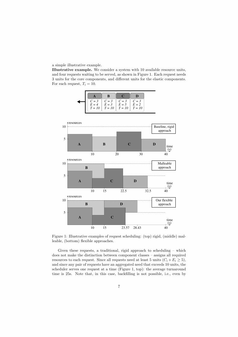
a simple illustrative example.Illustrative example. We consider a system with 10 available resource units,and four requests waiting to be served, as shown in Figure 1. Each request needs3 units for the core components, and different units for the elastic components.For each request, Ti = 10.

(s)

10

resources

15

5

10

5

10

5

resources

10

28.4323.57

C = 3

E = 4

T = 10

C = 3

E = 3

T = 10

C = 3

E = 5

T = 10

C = 3

E = 2

T = 10

30 40

time(s)

10 20

40

time(s)

10

resources

15 22.5 32.5

40

time

approach

DB

A B C D

A C D

B

A C

B D

approach

Malleable

approach

C

Our flexible

A

Baseline, rigid

Figure 1: Illustrative examples of request scheduling: (top) rigid, (middle) mal-leable, (bottom) flexible approaches.

Given these requests, a traditional, rigid approach to scheduling – whichdoes not make the distinction between component classes – assigns all requiredresources to each request. Since all requests need at least 5 units (Ci +Ei ≥ 5),and since any pair of requests have an aggregated need that exceeds 10 units, thescheduler serves one request at a time (Figure 1, top): the average turnaroundtime is 25s. Note that, in this case, backfilling is not possible, i.e., even by

7

changing the order in which requests are served the situation does not change.Another scheduling approach comes from the literature of malleable job

scheduling. The scheduler assigns all resources to the first request in the waitingline, then assigns the remaining resources (if any) to the next request, and soon, until no more free resources are available. This heuristic has been shown tobe close to optimal [31]. Figure 1, middle, illustrates the idea: request B can beserved along with request A. When request A has completed, the scheduler firstassigns more resources to request B, and then tries to serve the next request.Similarly, when request B has completed, the scheduler first assigns more re-sources to request C, then attempts at serving request D. However, since requestD needs at least Ci = 3 units, the scheduler is blocked (note that request C uses8 units), so request D needs to wait, and some system resources remain unused.The average turnaround time is 20s.

In this work we advocate the need for a new approach to scheduling, whichdistinguishes component classes. The idea is to exploit the flexibility of elasticcomponents and use system resources more efficiently. Intuitively, a solutionto the problems of existing heuristics is to reclaim some resources assigned toelastic components of a running request and assign them to a pending request.This is shown in the bottom of Figure 1: the scheduler reclaims just one unitfrom request C so that it can provide 3 units to request D, which are sufficientfor starting its core components and produce useful work. With this approach,the average turnaround is 19.25s.

While the above solution seems simple, it poses many challenges: how manyunits assigned to elastic components can be sacrificed for serving the next re-quest? How many requests should be served concurrently? Should the schedulerfocus on core components alone, to make sure many requests are served con-currently? How can scheduling take into account the priorities assigned by thesorting phase?

The last point introduces an additional challenge, related to preemptivescheduling policies. If a high priority request arrives, since it is not possibleto interrupt core components – for this would kill the request – how can weselect and preempt elastic components to accommodate the new request?

Given heterogeneous, composite requests, which are neither rigid, nor mal-leable (but both), available scheduling heuristics in the literature fall short inaddressing the sorting and allocation problems: a new approach is thus trulydesirable.

3 A Flexible Scheduling Algorithm

3.1 Design guidelines

We characterize a request by its arrival time, its priority (to decide the order inwhich the requests should be served), the resources it asks for (core and elastic)and the execution time (in isolation, i.e., when all required resources are grantedto the application). Given an incoming workload, our goal is to optimize the

8

sum of the turnaround times τi, that is:

min∑

i

τi ⇒ min∑

i

(queuingi + executioni)

The actual execution time depends on the amount of resources assigned overtime to the request. Now, recall that the scheduling problem can be broken intosorting and allocation phases. Sorting determines when a request is served, thusit has an impact on its queuing time. The allocation phase contributes both toqueuing and actual execution times. Depending on allocation granularity [9],a request might need to wait for a number of resources to be available beforeoccupying them, thus increasing – albeit indirectly – the queuing time. Theexecution time is directly related to the allocation algorithm and to the workloadcharacteristics.

In this work we decouple request sorting from allocation:2 our schedulermaintains the request ordering, as imposed by an external component, and onlyfocuses on resource allocation. Sorting can be simply based on arrival times(which amounts to implement a FIFO queuing discipline), or can use additionalinformation, such as request size (thus implementing a variety of size-baseddisciplines).

Overall, we optimize request turnaround times through careful resource al-location, and design an algorithm that strives at allocating all available clusterresources, by serving the least number of requests at a time. Intuitively, by “fo-cusing” resources to few requests, we expect their execution times to be small.Consequently, queued requests also enjoy smaller wait times, because resourcesare freed more quickly.

3.2 Algorithm Details

Although we support preemptive scheduling policies, to simplify exposition, wefirst consider the case with no preemption: resources assigned to a request canonly increase, and a new request can be placed, at most, at the head of thewaiting line, depending on the sorting component. We stress that the output ofour scheduling algorithm is a virtual assignment, i.e., the mechanism to physi-cally allocate resources according to the computed assignment (core and elasticcomponents for running applications) is separate from the scheduling logic, andconsidered as an implementation detail.

Our resource allocation procedure is called Rebalance, and it is triggeredby two events: request arrivals and departures – see Algorithm 1, ignoring high-lighted lines. When a new request arrives (procedure OnRequestArrival),the resource assignment is done only if such a request is placed at the head ofthe waiting line and there are unused resources that are sufficient for runningits core components. When a request is completed (procedure OnRequestDe-parture), the released resources are always reassigned.

2This approach is similar to the one used in the SLURM scheduler [34], where the order ofthe pending jobs is given by an external, pluggable, component, and the scheduler processesthe jobs following that order.

9

Algorithm 1: Resource assignment procedures

1 procedure OnRequestArrival(req)

2 if req.P > S.tail.P then

3 if req.C ≤∑

j∈Sreqj .E then

4 Insert(req, S)

5 Rebalance( )6 else

7 Insert(req, W)

8 else9 Insert(req, L)

10 if req == L.head and req.C ≤ avail then11 Rebalance( )

12 procedure OnRequestDeparture( )

13 while W.head.C +∑

j∈Sreqj .C < total and (W not ∅) do

14 Insert(pop(W), S)

15 Rebalance( )

16 procedure Rebalance( )

17 while∑

j∈S(reqj .C + reqj .E) < total and (L not ∅) do

18 req ← L.head19 if req.C +

∑

j∈Sreqj .C < total then

20 Insert(pop(L), S)21 else22 break

23 avail← total −∑

j∈Sreqj .C

24 forall req ∈ S do25 req.G← 0

26 req ← S.head27 while avail > 0 and (req not null) do28 req.G← min(req.E, avail)29 avail← (avail − req.G)30 req ← req.next

10

The scheduler maintains two ordered sets: the requests waiting to be served(L), and the requests in service (S). Each request req needs req.C core compo-nents and req.E elastic components; depending on the allocation, request reqis granted 0 ≤ req.G ≤ req.E elastic components. The core of the procedureRebalance (lines 27-30) operates as follows: each request req in the serving setS has always at least req.C resources assigned. Excess resources are assignedto the requests in S following the request order. The scheduler assigns as manyelastic components as possible to the first request, then to the second, and soon, in cascade.

Following the design guidelines, the set S should only contain the requeststhat are strictly necessary to use all the available resources. This is accomplishedby the first part of the procedure Rebalance (lines 17-22): a request is addedto S if the current requests in S are not able to saturate the total resources(total, line 17). Note that we add a request to S only if there is room to allocateall of its core components.

3.3 Preemptive policies

We now consider preemptive policies: request arrivals can trigger (partial) pre-emption of running requests, e.g. if new requests have higher priority thanthat of the last request in service. In this case, the tuple describing a requestalso stores its priority, req.P . It is important to note that, in this work, thepreemption mechanism only operates on elastic components of running appli-cations, whereas core components (that are vital for an application) cannot bepreempted.

The highlighted lines in Algorithm 1 show the modifications to the proce-dures OnRequestArrival and OnRequestDeparture to support preemp-tion. When a new request arrives, if its priority is higher than the requests inservice, we check if its core components can be allocated using the resourcesoccupied by the elastic components of currently running requests. If so, weinsert the request into the set S and call Rebalance. Otherwise, we insert therequest into an auxiliary waiting line W, which is given priority when resourcesbecome available. Indeed, procedure OnRequestDeparture indicates thatwe first consider the waiting requests in W, and we add to the set S as manyof them as possible, considering solely the core components. In other words,requests in W have higher priority than those in L. Finally, the call of Rebal-ance assigns the remaining resources to the elastic components of high priorityrequests.

4 Numerical evaluation

4.1 Methodology

We evaluate our algorithm using an event-based, trace-driven discrete simula-tor developed to study the scheduler Omega [9], which we extended in order to

11

0 2 4 6 8 10CPU

0.0

0.2

0.4

0.6

0.8

1.0

Components CPU

101 102 103 104 105 106 107 108

Memory (KB)

0.0

0.2

0.4

0.6

0.8

1.0

Components memory

10-3 10-2 10-1 100 101 102 103 104 105

Time (s)

0.0

0.2

0.4

0.6

0.8

1.0

Inter-Arrival Time

100 101 102 103

Num Services

0.0

0.2

0.4

0.6

0.8

1.0

Core components

100 101 102 103 104 105

Num Services

0.0

0.2

0.4

0.6

0.8

1.0

Elastic components

10-1 100 101 102 103 104 105 106

Runtime (s)

0.0

0.2

0.4

0.6

0.8

1.0

Estimated Runtime

Figure 2: Workload Definition.

make it work with applications, instead of low-level jobs and to use the con-cept of component classes. Our scheduler implementation supports a variety

12

of policies3: we present results for the FIFO and the shortest job first (SJF)policies, which further optimizes system responsiveness. Our implementationfirst obtains a “virtual assignment” with Algorithm 1, then fulfills it by allo-cating resources accordingly, which happens instantaneously. Additionally, wehave implemented a baseline, consisting of a rigid scheduler that does not distin-guish component classes, which is representative of current cluster managementsystems. In our simulations, we consider two-dimensional resources, includingdefinitions of CPU and RAM requirements. We would like to stress that the“virtual assignment” can take into consideration other constraints as well (e.g.,GPU).

Our scheduler currently accepts application workloads of two kinds. Thefirst is batch applications, that take from a few seconds to a few days to com-plete: these are delay-tolerant applications, with a very simple life-cycle. Corecomponents must first start to produce useful work, by executing user-definedjobs that are “passed” to the application; eventually, elastic components cancontribute to the application progress. Once the user programs are concluded,the application finishes, releasing resources occupied by its frameworks and com-ponents. The second is interactive applications, which involve a “human inthe loop”: these are latency-sensitive applications, with a life-cycle triggered byhuman activity. In this case, core components must start as soon as possible,to allow user interaction with the application (e.g., a Notebook).

For our performance evaluation, we use publicly available traces [24,25], andgenerate a workload by sampling the empirical distributions we compute fromsuch traces. First, we focus on batch applications alone, and simulate both rigid(e.g. TensorFlow) and elastic (e.g. Spark) variants: the label B-R representsrigid applications with only core components; the label B-E stands for elasticapplications, with both core and elastic components. Then, we evaluate thebenefit of preemption by complementing the above workload with (simulated)interactive applications.

Figure 2 shows the definition of the workload: in particular we can see theCDFs for requested CPU and memory, then the inter-arrival time and esti-mated run time and finally, the number of core and elastic components. Batchapplications are assigned a number ranging from a few to tens of thousandsof components. Instead, interactive applications are smaller, and use up tohundreds of elastic components. The resource requirements of application com-ponents follow that of the input traces, ranging from few MB to a few dozensGB of memory, and up to 6 cores. Application runtime is generated accord-ing to the input traces, and range from a few dozen seconds to several weeks(of simulated time). Application inter-arrival times are drawn from the empir-ical distributions of the input traces, and exhibit a bi-modal distribution withfast-paced bursts, as well as longer intervals between application submissions.In summary, our workload consists of 80,000 applications, with 80% batch and20% interactive applications. Batch applications include 80% elastic and 20%

3We support size-based disciplines in the family of SMART policies [35]. Here we assumeapplication size information to be known a-priori.

13

rigid variants.We simulate a cluster consisting of 100 machines, each with 32 cores and

128GB of memory. All results shown here include 10 simulation runs, for atotal of roughly 3 months of simulation time for each run.

Finally, the metrics we use to analyze the results include: application turn-around, which allow to reason about the scheduling objective function, andqueuing time, which is an important factor contributing to the turnaroundtime. Additionally, we measure the queue sizes that hold pending and run-ning applications, and resource allocation, measured as the percentage ofCPU and memory the scheduler allocates to each application.

4.2 Comparison with the baseline

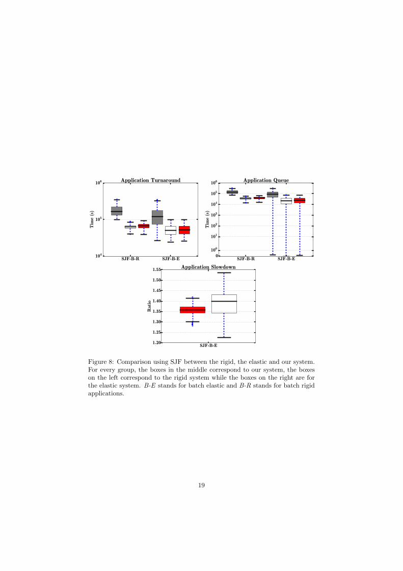
We now perform a comparative analysis between our flexible scheduler and thebaseline, and start by disabling preemption: we omit interactive applicationsfrom the workload. Figure 3 (left) illustrates the most important percentiles(in a box-plot) of the distribution of turnaround times, where we compare twopolicies (namely, FIFO and SJF) used by both the baseline and our scheduler.The benefits of our approach are noticeable, irrespectively of the schedulingdiscipline: the median turnaround is halved when compared to the baseline,indicating superior system responsiveness. Additionally, we observe the ben-efits of a size-based policy in further decreasing turnaround times. We notethat our approach is beneficial for both rigid and elastic batch applications:Figure 3 (center) shows a box-plot of application queuing times, which con-tribute to their turnaround. With our approach, both kinds of applicationsspend less time waiting in a queue to be served. By differentiating classes ofcomponents, applications can execute as soon as enough resources to producework are available. Finally, Figure 3 (right) focuses on application runtime: wereport the slowdown computed as the ratio between the nominal applicationruntime (i.e., the time required for an application to complete in an empty sys-tem, with all application components allocated their requested resources) andthe effective application runtime obtained with the simulation. Values aboveone indicate that applications run slower in a system absorbing a given work-load when compared to applications running in an empty system. Overall, theseresults show that our scheduling approach does not impose a high toll on appli-cation runtime, while globally contributing to improved turnaround times.

Next, we support the general results discussed above with additional details.Figure 4 shows the box-plots of the distribution of queue sizes, for both thepending and the running queues. Our approach induces a smaller number ofapplications waiting to be served, as well as a larger number of applicationsrunning in the system, compared to the baseline and across different policies.Indeed, our flexible scheduler achieves a better packing of applications, whichmeans they can start sooner. Additionally, the benefits of a size-based disciplineare clear: the number of applications waiting is almost one order of magnitudesmaller compared to a FIFO policy, while the number of running applicationsis similar.

14

Fifo-

B-R

SJF-B

-R

Fifo-

B-E

SJF-B

-E104

105

106

107

Tim

e (s

)

Application Turnaround

Fifo-

B-R

SJF-B

-R

Fifo-

B-E

SJF-B

-E

0100

101

102

103

104

105

106

107

Tim

e (s

)

Application Queue

Fifo-

B-E

SJF-B

-E

1.2

1.3

1.4

1.5

1.6

1.7

Rat

io

Application Slowdown

Figure 3: Comparison of turnaround and queue time distributions, and appli-cation slowdown distributions for FIFO and SJF policies. White boxes (rightbox of every pair) corresponds to our flexible scheduler, gray boxes correspondto the baseline. B-E stands for batch elastic and B-R stands for batch rigidapplications.

Figure 5 shows metrics from the cluster perspective: our approach (for bothdisciplines) induces a far better resource allocation compared to the baseline,achieving more than 20% gains in both CPU and RAM allocation.4

Finally, we are going to show more results, that compare a rigid, a mal-leable and our flexible scheduler with different policies. It is worth mentioningthat currently no solution support a malleable scheduler as we presented it inSection 2.2.

In single-server systems, the policies that are optimal for minimizing the av-erage turn around time are called SMART [35]; they prioritize short applicationover longer one. Two example of SMART policies are SFJ (Shorted-Job First)

4Allocation is different from utilization: the simulator does not account for real applicationexecution, so we cannot report utilization figures.

15

Fifo SJF101

102

103

104

Applica

tions

in q

ueu

e

Pending Queue

Fifo SJF20

40

60

80

100

120

140

160

180

Applica

tion

s ru

nnin

g

Running Applications

Figure 4: Comparison of queues size for FIFO and SJF between our flexiblescheduler and the baseline. The white boxes (right box of every group) corre-spond to our flexible algorithm, gray boxes to the baseline.

Fifo SJF0.0

0.2

0.4

0.6

0.8

1.0

% C

PU

Cluster CPU allocation

Fifo SJF0.0

0.2

0.4

0.6

0.8

1.0

% m

emor

y

Cluster Memory allocation

Figure 5: Comparison of resource allocation distributions for FIFO and SJFpolicies, between our flexible scheduler and the baseline. White boxes (rightbox of every pair) correspond to our approach, dashed boxes to the baseline.

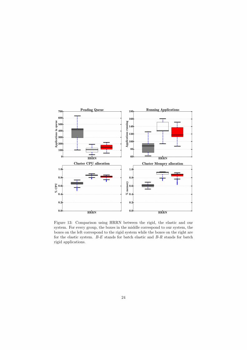
and SRPT (Shortest-Remaining-Processing-Time). However, even if SRPT isconsidered optimal, it is rarely used because it leads to starvation of long run-ning application. For this reason policies like HRRN (Higher-Response-RationNext) can be used; they calculate a virtual size that is updated the longer theapplication reside in queue. In this evaluation we are going to use four differentpolicies: FIFO, SFJ, SRPT and HRRN.

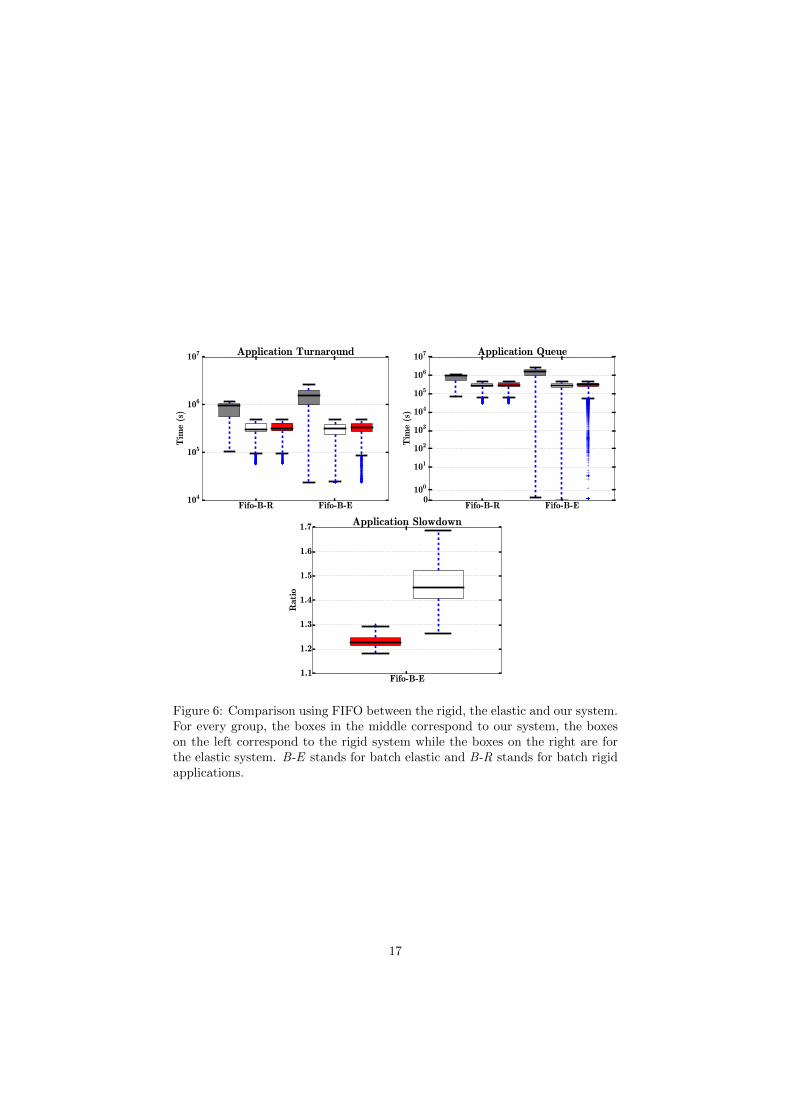
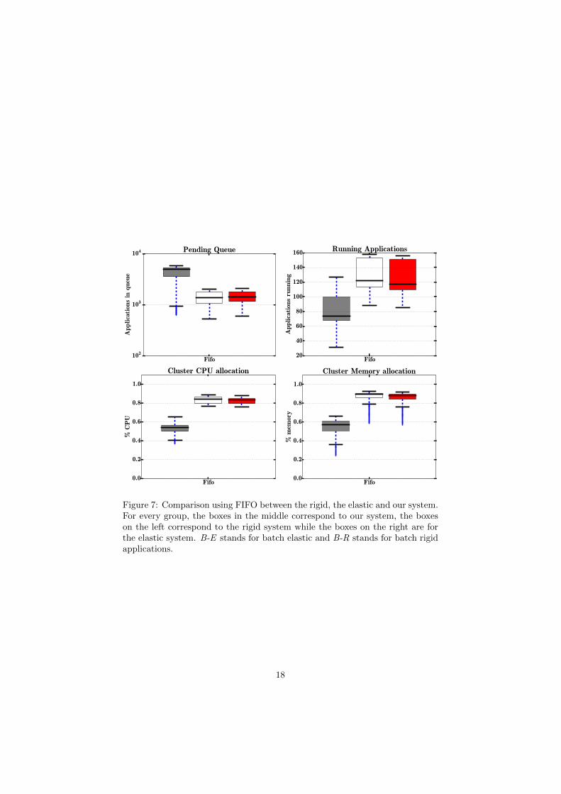
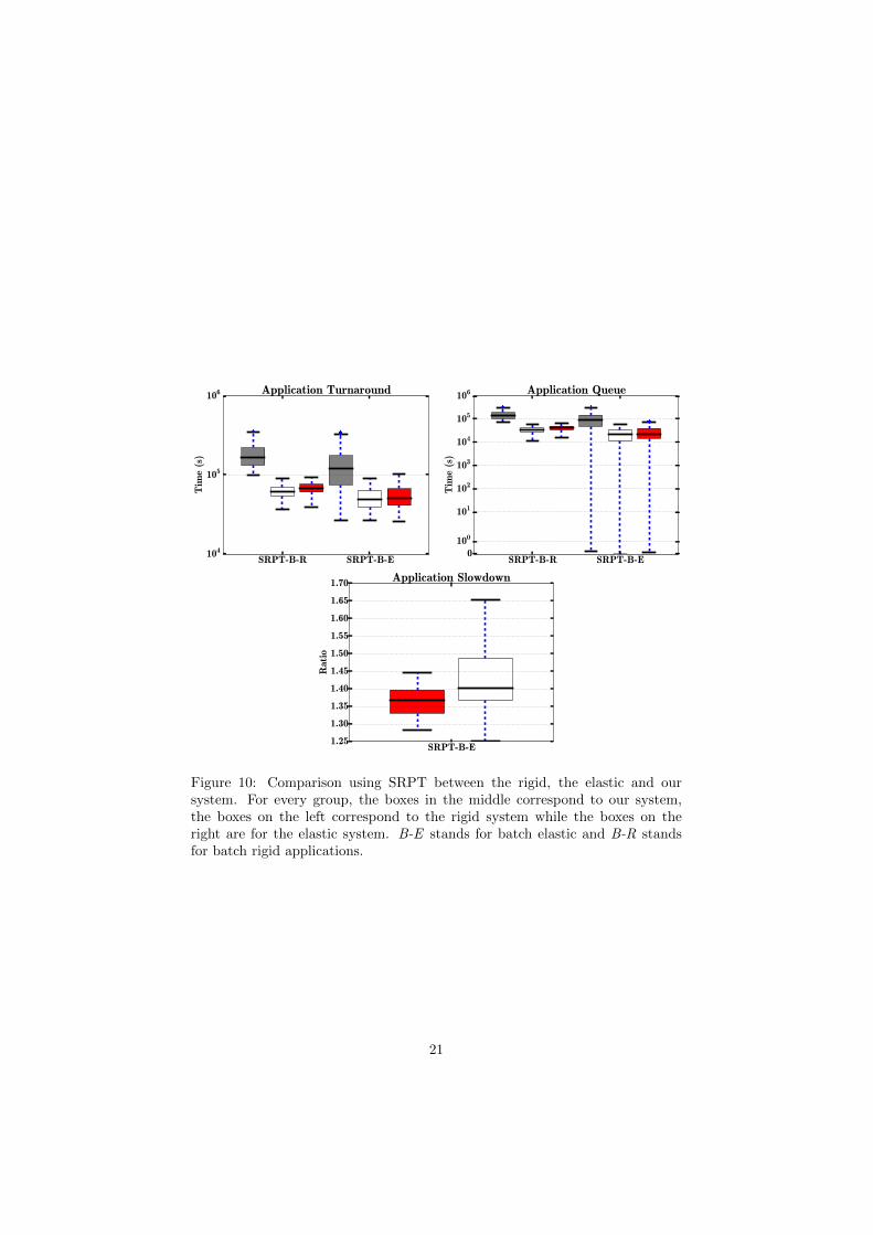
Figures 6 to 13 confirm that our solution performs far better than a rigidscheduler and slightly better than a malleable regarding of the policy used tosort the queue.

In conclusion using our flexible scheduler can greatly reduce the turn aroundtime while improving resources allocation regardless of the policy that is used tosort the applications in the pending queue.

16

Fifo-B-R Fifo-B-E104

105

106

107

Tim

e (s

)


Fifo-B-R Fifo-B-E0

100

101

102

103

104

105

106

107

Tim

e (s

)

Application Queue

Fifo-B-E1.1

1.2

1.3

1.4

1.5

1.6

1.7

Rat

io


Figure 6: Comparison using FIFO between the rigid, the elastic and our system.For every group, the boxes in the middle correspond to our system, the boxeson the left correspond to the rigid system while the boxes on the right are forthe elastic system. B-E stands for batch elastic and B-R stands for batch rigidapplications.

17

Fifo102

103

104

Applica

tions

in q

ueu

e

Pending Queue

Fifo20

40

60

80

100

120

140

160

Applica

tion

s ru

nnin

g


Fifo0.0

0.2

0.4

0.6

0.8

1.0

% C

PU


Fifo0.0

0.2

0.4

0.6

0.8

1.0

% m

emor

y


Figure 7: Comparison using FIFO between the rigid, the elastic and our system.For every group, the boxes in the middle correspond to our system, the boxeson the left correspond to the rigid system while the boxes on the right are forthe elastic system. B-E stands for batch elastic and B-R stands for batch rigidapplications.

18

SJF-B-R SJF-B-E104

105

106

Tim

e (s

)


SJF-B-R SJF-B-E0

100

101

102

103

104

105

106

Tim

e (s

)

Application Queue

SJF-B-E1.20

1.25

1.30

1.35

1.40

1.45

1.50

1.55

Rat

io


Figure 8: Comparison using SJF between the rigid, the elastic and our system.For every group, the boxes in the middle correspond to our system, the boxeson the left correspond to the rigid system while the boxes on the right are forthe elastic system. B-E stands for batch elastic and B-R stands for batch rigidapplications.

19

SJF0

100

200

300

400

500

600

700

Applica

tion

s in

queu

e

Pending Queue

SJF

80

100

120

140

160

Applica

tion

s ru

nnin

g


SJF0.0

0.2

0.4

0.6

0.8

1.0

% C

PU


SJF0.0

0.2

0.4

0.6

0.8

1.0

% m

emor

y


Figure 9: Comparison using SJF between the rigid, the elastic and our system.For every group, the boxes in the middle correspond to our system, the boxeson the left correspond to the rigid system while the boxes on the right are forthe elastic system. B-E stands for batch elastic and B-R stands for batch rigidapplications.

20

SRPT-B-R SRPT-B-E104

105

106

Tim

e (s

)


SRPT-B-R SRPT-B-E0

100

101

102

103

104

105

106

Tim

e (s

)

Application Queue

SRPT-B-E1.25

1.30

1.35

1.40

1.45

1.50

1.55

1.60

1.65

1.70

Rat

io


Figure 10: Comparison using SRPT between the rigid, the elastic and oursystem. For every group, the boxes in the middle correspond to our system,the boxes on the left correspond to the rigid system while the boxes on theright are for the elastic system. B-E stands for batch elastic and B-R standsfor batch rigid applications.

21

SRPT0

100

200

300

400

500

600

700

Applica

tion

s in

queu

e

Pending Queue

SRPT

80

100

120

140

160

Applica

tion

s ru

nnin

g


SRPT0.0

0.2

0.4

0.6

0.8

1.0

% C

PU


SRPT0.0

0.2

0.4

0.6

0.8

1.0

% m

emor

y


Figure 11: Comparison using SRPT between the rigid, the elastic and oursystem. For every group, the boxes in the middle correspond to our system,the boxes on the left correspond to the rigid system while the boxes on theright are for the elastic system. B-E stands for batch elastic and B-R standsfor batch rigid applications.

22

HRRN-B-R HRRN-B-E104

105

106

Tim

e (s

)


HRRN-B-R HRRN-B-E0

100

101

102

103

104

105

106

Tim

e (s

)

Application Queue

HRRN-B-E1.20

1.25

1.30

1.35

1.40

1.45

1.50

1.55

1.60

Rat

io


Figure 12: Comparison using HRRN between the rigid, the elastic and oursystem. For every group, the boxes in the middle correspond to our system, theboxes on the left correspond to the rigid system while the boxes on the right arefor the elastic system. B-E stands for batch elastic and B-R stands for batchrigid applications.

23

HRRN0

100

200

300

400

500

600

700

Applica

tion

s in

queu

e

Pending Queue

HRRN60

80

100

120

140

160

180

Applica

tion

s ru

nnin

g


HRRN0.0

0.2

0.4

0.6

0.8

1.0

% C

PU


HRRN0.0

0.2

0.4

0.6

0.8

1.0

% m

emor

y


Figure 13: Comparison using HRRN between the rigid, the elastic and oursystem. For every group, the boxes in the middle correspond to our system, theboxes on the left correspond to the rigid system while the boxes on the right arefor the elastic system. B-E stands for batch elastic and B-R stands for batchrigid applications.

24

Name Definition

SJF-2D runT ime ∗#RequestedServices

SRPT-2D1 remainingRunTime ∗#RequestedServices

SRPT-2D2 remainingRunTime ∗#ServicesY etToBeScheduled

HRRN-2D (1 + waitT imerunTime ) ∗#RequestedServices

SJF-3D runT ime ∗∑servicesi=1 CPUi ∗RAMi

SRPT-3D1 remainingRunTime ∗∑servicesi=1 CPUi ∗RAMi

SRPT-3D2 remainingRunTime ∗∑servicesToSchedulei=1 CPUi ∗RAMi

HRRN-3D (1 + waitT imerunTime ) ∗∑services

i=1 CPUi ∗RAMi

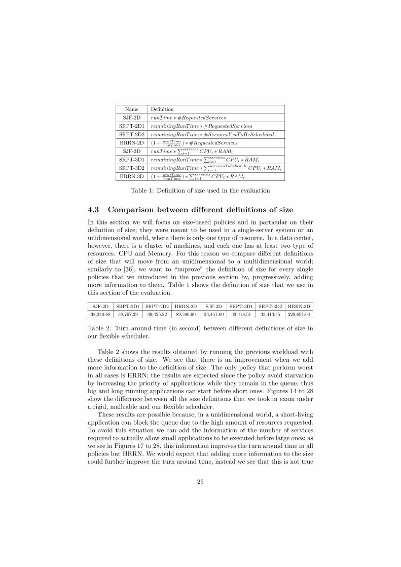
Table 1: Definition of size used in the evaluation

4.3 Comparison between different definitions of size

In this section we will focus on size-based policies and in particular on theirdefinition of size; they were meant to be used in a single-server system or anunidimensional world, where there is only one type of resource. In a data center,however, there is a cluster of machines, and each one has at least two type ofresources: CPU and Memory. For this reason we compare different definitionsof size that will move from an unidimensional to a multidimensional world;similarly to [36], we want to “improve” the definition of size for every singlepolicies that we introduced in the previous section by, progressively, addingmore information to them. Table 1 shows the definition of size that we use inthis section of the evaluation.

SJF-2D SRPT-2D1 SRPT-2D2 HRRN-2D SJF-3D SRPT-3D1 SRPT-3D2 HRRN-3D

38,340.68 38,767.29 39,425.82 89,596.90 33,451.60 33,418.51 33,413.45 229,691.64

Table 2: Turn around time (in second) between different definitions of size inour flexible scheduler.

Table 2 shows the results obtained by running the previous workload withthese definitions of size. We see that there is an improvement when we addmore information to the definition of size. The only policy that perform worstin all cases is HRRN; the results are expected since the policy avoid starvationby increasing the priority of applications while they remain in the queue, thusbig and long running applications can start before short ones. Figures 14 to 28show the difference between all the size definitions that we took in exam undera rigid, malleable and our flexible scheduler.

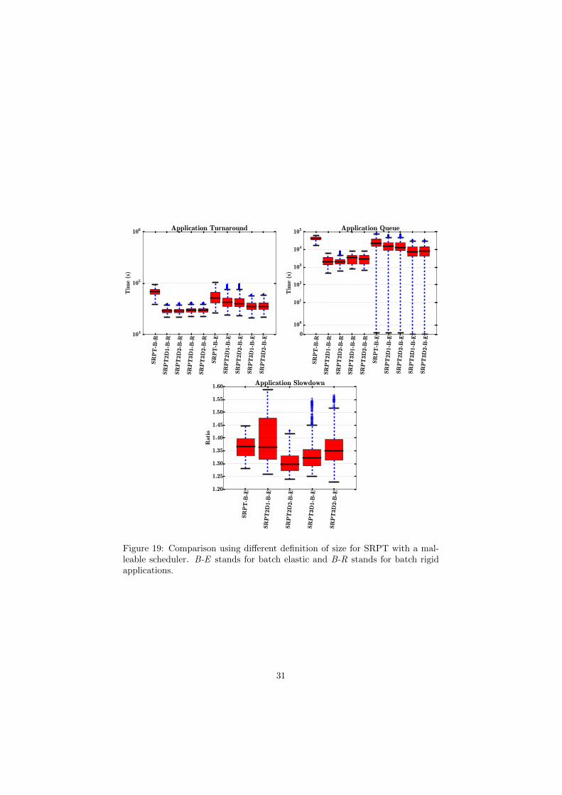
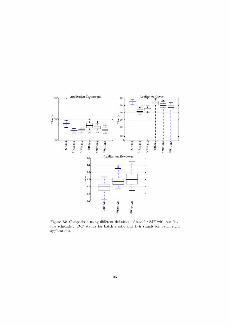
These results are possible because, in a unidimensional world, a short-livingapplication can block the queue due to the high amount of resources requested.To avoid this situation we can add the information of the number of servicesrequired to actually allow small applications to be executed before large ones; aswe see in Figures 17 to 28, this information improves the turn around time in allpolicies but HRRN. We would expect that adding more information to the sizecould further improve the turn around time, instead we see that this is not true

25

SJF-B

-R

SJF2D

-B-R

SJF3D

-B-R

SJF-B

-E

SJF2D

-B-E

SJF3D

-B-E

104

105

106

Tim

e (s

)


SJF-B

-R

SJF2D

-B-R

SJF3D

-B-R

SJF-B

-E

SJF2D

-B-E

SJF3D

-B-E

0

100

101

102

103

104

105

106

Tim

e (s

)

Application QueueSJF

SJF2D

SJF3D

0

100

200

300

400

500

600

700

Applica

tion

s in

queu

e

Pending QueueSJF

SJF2D

SJF3D

0

20

40

60

80

100

120

140

160

180

Applica

tions

runnin

g


SJF

SJF2D

SJF3D

0.0

0.2

0.4

0.6

0.8

1.0

% C

PU


SJF

SJF2D

SJF3D

0.0

0.2

0.4

0.6

0.8

1.0

% m

emor

y


Figure 14: Comparison using different definition of size for SJF with a rigidscheduler. B-E stands for batch elastic and B-R stands for batch rigid applica-tions.

26

SR

PT

-B-R

SR

PT

2D1-

B-R

SR

PT

2D2-

B-R

SR

PT

3D1-

B-R

SR

PT

3D2-

B-R

SR

PT

-B-E

SR

PT

2D1-

B-E

SR

PT

2D2-

B-E

SR

PT

3D1-

B-E

SR

PT

3D2-

B-E

104

105

106

Tim

e (s

)


SR

PT

-B-R

SR

PT

2D1-

B-R

SR

PT

2D2-

B-R

SR

PT

3D1-

B-R

SR

PT

3D2-

B-R

SR

PT

-B-E

SR

PT

2D1-

B-E

SR

PT

2D2-

B-E

SR

PT

3D1-

B-E

SR

PT

3D2-

B-E

0

100

101

102

103

104

105

106

Tim

e (s

)

Application QueueSR

PT

SR

PT

2D1

SR

PT

2D2

SR

PT

3D1

SR

PT

3D20

100

200

300

400

500

600

700

Applica

tion

s in

queu

e

Pending QueueSR

PT

SR

PT

2D1

SR

PT

2D2

SR

PT

3D1

SR

PT

3D20

20

40

60

80

100

120

140

160

180

Applica

tion

s ru

nnin

g


SR

PT

SR

PT

2D1

SR

PT

2D2

SR

PT

3D1

SR

PT

3D20.0

0.2

0.4

0.6

0.8

1.0

% C

PU


SR

PT

SR

PT

2D1

SR

PT

2D2

SR

PT

3D1

SR

PT

3D20.0

0.2

0.4

0.6

0.8

1.0

% m

emor

y


Figure 15: Comparison using different definition of size for SRPT with a rigidscheduler. B-E stands for batch elastic and B-R stands for batch rigid applica-tions.

27

HR

RN

-B-R

HR

RN

2D-B

-R

HR

RN

3D-B

-R

HR

RN

-B-E

HR

RN

2D-B

-E

HR

RN

3D-B

-E104

105

106

107

Tim

e (s

)


HR

RN

-B-R

HR

RN

2D-B

-R

HR

RN

3D-B

-R

HR

RN

-B-E

HR

RN

2D-B

-E

HR

RN

3D-B

-E

0100

101

102

103

104

105

106

107

Tim

e (s

)

Application Queue

HR

RN

HR

RN

2D

HR

RN

3D

102

103

104

Applica

tion

s in

queu

e

Pending QueueH

RR

N

HR

RN

2D

HR

RN

3D

0

50

100

150

200

250

Applica

tion

s ru

nnin

g


HR

RN

HR

RN

2D

HR

RN

3D

0.0

0.2

0.4

0.6

0.8

1.0

% C

PU


HR

RN

HR

RN

2D

HR

RN

3D

0.0

0.2

0.4

0.6

0.8

1.0

% m

emor

y


Figure 16: Comparison using different definition of size for HRRN with a rigidscheduler. B-E stands for batch elastic and B-R stands for batch rigid applica-tions.

28

SJF-B

-R

SJF2D

-B-R

SJF3D

-B-R

SJF-B

-E

SJF2D

-B-E

SJF3D

-B-E

104

105

Tim

e (s

)


SJF-B

-R

SJF2D

-B-R

SJF3D

-B-R

SJF-B

-E

SJF2D

-B-E

SJF3D

-B-E

0

100

101

102

103

104

105

Tim

e (s

)

Application Queue

SJF-B

-E

SJF2D

-B-E

SJF3D

-B-E

1.20

1.25

1.30

1.35

1.40

1.45

1.50

1.55

1.60

1.65

Rat

io


Figure 17: Comparison using different definition of size for SJF with a mal-leable scheduler. B-E stands for batch elastic and B-R stands for batch rigidapplications.

29

SJF

SJF2D

SJF3D

0

50

100

150

200

250

Applica

tion

s in

queu

e

Pending Queue

SJF

SJF2D

SJF3D

60

80

100

120

140

160

180

200

Applica

tion

s ru

nnin

g


SJF

SJF2D

SJF3D

0.0

0.2

0.4

0.6

0.8

1.0

% C

PU


SJF

SJF2D

SJF3D

0.0

0.2

0.4

0.6

0.8

1.0

% m

emor

y


Figure 18: Comparison using different definition of size for SJF with a mal-leable scheduler. B-E stands for batch elastic and B-R stands for batch rigidapplications.

30

SR

PT

-B-R

SR

PT

2D1-

B-R

SR

PT

2D2-

B-R

SR

PT

3D1-

B-R

SR

PT

3D2-

B-R

SR

PT

-B-E

SR

PT

2D1-

B-E

SR

PT

2D2-

B-E

SR

PT

3D1-

B-E

SR

PT

3D2-

B-E

104

105

106

Tim

e (s

)


SR

PT

-B-R

SR

PT

2D1-

B-R

SR

PT

2D2-

B-R

SR

PT

3D1-

B-R

SR

PT

3D2-

B-R

SR

PT

-B-E

SR

PT

2D1-

B-E

SR

PT

2D2-

B-E

SR

PT

3D1-

B-E

SR

PT

3D2-

B-E

0

100

101

102

103

104

105

Tim

e (s

)

Application Queue

SR

PT

-B-E

SR

PT

2D1-

B-E

SR

PT

2D2-

B-E

SR

PT

3D1-

B-E

SR

PT

3D2-

B-E

1.20

1.25

1.30

1.35

1.40

1.45

1.50

1.55

1.60

Rat

io


Figure 19: Comparison using different definition of size for SRPT with a mal-leable scheduler. B-E stands for batch elastic and B-R stands for batch rigidapplications.

31

SR

PT

SR

PT

2D1

SR

PT

2D2

SR

PT

3D1

SR

PT

3D20

50

100

150

200

250

Applica

tion

s in

queu

e

Pending Queue

SR

PT

SR

PT

2D1

SR

PT

2D2

SR

PT

3D1

SR

PT

3D260

80

100

120

140

160

180

200

Applica

tions

runnin

g


SR

PT

SR

PT

2D1

SR

PT

2D2

SR

PT

3D1

SR

PT

3D20.0

0.2

0.4

0.6

0.8

1.0

% C

PU


SR

PT

SR

PT

2D1

SR

PT

2D2

SR

PT

3D1

SR

PT

3D20.0

0.2

0.4

0.6

0.8

1.0

% m

emor

y


Figure 20: Comparison using different definition of size for SRPT with a mal-leable scheduler. B-E stands for batch elastic and B-R stands for batch rigidapplications.

32

HR

RN

-B-R

HR

RN

2D-B

-R

HR

RN

3D-B

-R

HR

RN

-B-E

HR

RN

2D-B

-E

HR

RN

3D-B

-E

104

105

106

107

Tim

e (s

)


HR

RN

-B-R

HR

RN

2D-B

-R

HR

RN

3D-B

-R

HR

RN

-B-E

HR

RN

2D-B

-E

HR

RN

3D-B

-E

0100

101

102

103

104

105

106

107

Tim

e (s

)

Application Queue

HR

RN

-B-E

HR

RN

2D-B

-E

HR

RN

3D-B

-E

1.15

1.20

1.25

1.30

1.35

1.40

1.45

1.50

Rat

io


Figure 21: Comparison using different definition of size for HRRN with a mal-leable scheduler. B-E stands for batch elastic and B-R stands for batch rigidapplications.

33

HR

RN

HR

RN

2D

HR

RN

3D

101

102

103

104

Applica

tion

s in

queu

e

Pending Queue

HR

RN

HR

RN

2D

HR

RN

3D

80

90

100

110

120

130

140

150

160

170

Applica

tion

s ru

nnin

g


HR

RN

HR

RN

2D

HR

RN

3D

0.0

0.2

0.4

0.6

0.8

1.0

% C

PU


HR

RN

HR

RN

2D

HR

RN

3D

0.0

0.2

0.4

0.6

0.8

1.0

% m

emor

y


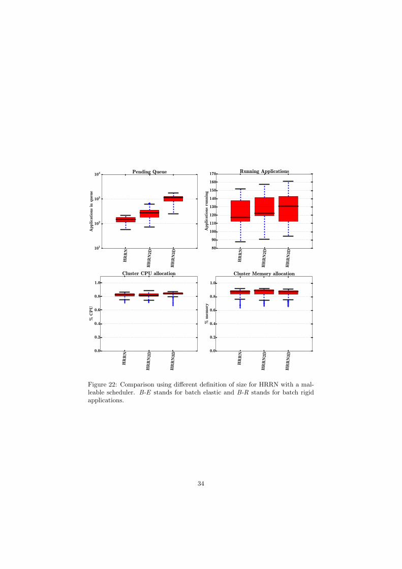
Figure 22: Comparison using different definition of size for HRRN with a mal-leable scheduler. B-E stands for batch elastic and B-R stands for batch rigidapplications.

34

SJF-B

-R

SJF2D

-B-R

SJF3D

-B-R

SJF-B

-E

SJF2D

-B-E

SJF3D

-B-E

104

105

106

Tim

e (s

)


SJF-B

-R

SJF2D

-B-R

SJF3D

-B-R

SJF-B

-E

SJF2D

-B-E

SJF3D

-B-E

0

100

101

102

103

104

105

Tim

e (s

)

Application Queue

SJF-B

-E

SJF2D

-B-E

SJF3D

-B-E

1.2

1.3

1.4

1.5

1.6

1.7

1.8

Rat

io


Figure 23: Comparison using different definition of size for SJF with our flex-ible scheduler. B-E stands for batch elastic and B-R stands for batch rigidapplications.

35

SJF

SJF2D

SJF3D

0

50

100

150

200

250

Applica

tion

s in

queu

e

Pending Queue

SJF

SJF2D

SJF3D

80

100

120

140

160

180

200

Applica

tion

s ru

nnin

g


SJF

SJF2D

SJF3D

0.0

0.2

0.4

0.6

0.8

1.0

% C

PU


SJF

SJF2D

SJF3D

0.0

0.2

0.4

0.6

0.8

1.0

% m

emor

y


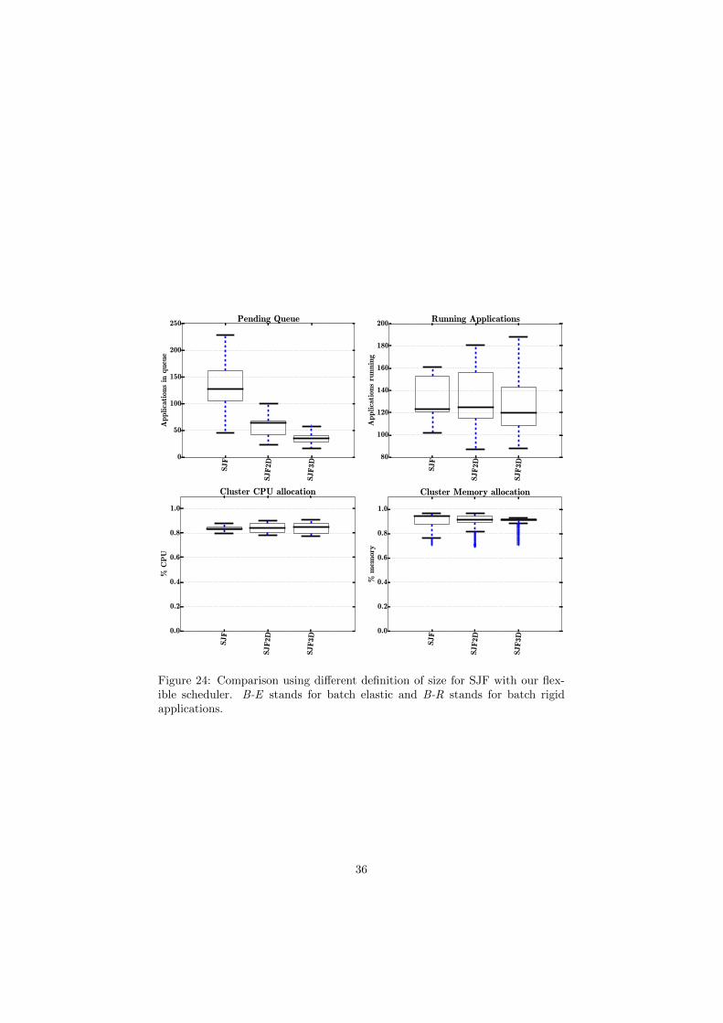
Figure 24: Comparison using different definition of size for SJF with our flex-ible scheduler. B-E stands for batch elastic and B-R stands for batch rigidapplications.

36

SR

PT

-B-R

SR

PT

2D1-

B-R

SR

PT

2D2-

B-R

SR

PT

3D1-

B-R

SR

PT

3D2-

B-R

SR

PT

-B-E

SR

PT

2D1-

B-E

SR

PT

2D2-

B-E

SR

PT

3D1-

B-E

SR

PT

3D2-

B-E

104

105

Tim

e (s

)


SR

PT

-B-R

SR

PT

2D1-

B-R

SR

PT

2D2-

B-R

SR

PT

3D1-

B-R

SR

PT

3D2-

B-R

SR

PT

-B-E

SR

PT

2D1-

B-E

SR

PT

2D2-

B-E

SR

PT

3D1-

B-E

SR

PT

3D2-

B-E

0

100

101

102

103

104

105

Tim

e (s

)

Application Queue

SR

PT

-B-E

SR

PT

2D1-

B-E

SR

PT

2D2-

B-E

SR

PT

3D1-

B-E

SR

PT

3D2-

B-E

1.2

1.4

1.6

1.8

2.0

2.2

2.4

2.6

2.8

Rat

io


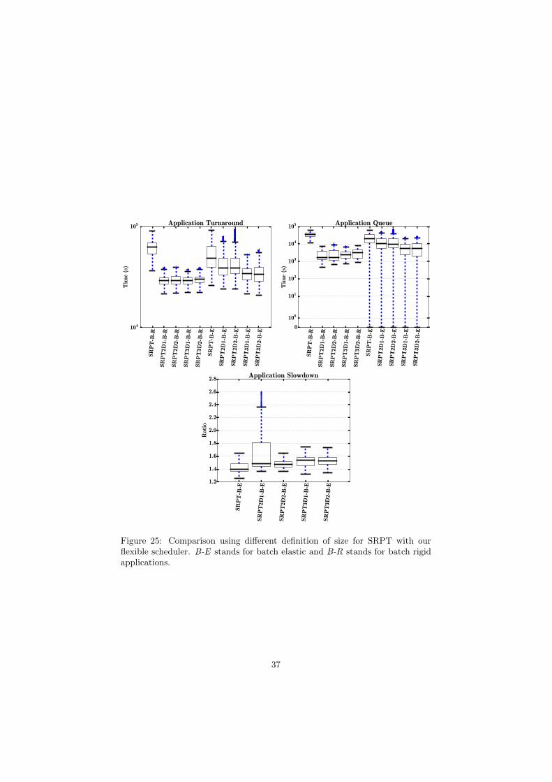
Figure 25: Comparison using different definition of size for SRPT with ourflexible scheduler. B-E stands for batch elastic and B-R stands for batch rigidapplications.

37

SR

PT

SR

PT

2D1

SR

PT

2D2

SR

PT

3D1

SR

PT

3D20

50

100

150

200

250

Applica

tion

s in

queu

e

Pending Queue

SR

PT

SR

PT

2D1

SR

PT

2D2

SR

PT

3D1

SR

PT

3D280

100

120

140

160

180

200

Applica

tions

runnin

g


SR

PT

SR

PT

2D1

SR

PT

2D2

SR

PT

3D1

SR

PT

3D20.0

0.2

0.4

0.6

0.8

1.0

% C

PU


SR

PT

SR

PT

2D1

SR

PT

2D2

SR

PT

3D1

SR

PT

3D20.0

0.2

0.4

0.6

0.8

1.0

% m

emor

y


Figure 26: Comparison using different definition of size for SRPT with ourflexible scheduler. B-E stands for batch elastic and B-R stands for batch rigidapplications.

38

HR

RN

-B-R

HR

RN

2D-B

-R

HR

RN

3D-B

-R

HR

RN

-B-E

HR

RN

2D-B

-E

HR

RN

3D-B

-E

104

105

106

Tim

e (s

)


HR

RN

-B-R

HR

RN

2D-B

-R

HR

RN

3D-B

-R

HR

RN

-B-E

HR

RN

2D-B

-E

HR

RN

3D-B

-E

0

100

101

102

103

104

105

106

Tim

e (s

)

Application Queue

HR

RN

-B-E

HR

RN

2D-B

-E

HR

RN

3D-B

-E

1.3

1.4

1.5

1.6

1.7

1.8

1.9

2.0

2.1

Rat

io


Figure 27: Comparison using different definition of size for HRRN with ourflexible scheduler. B-E stands for batch elastic and B-R stands for batch rigidapplications.

39

HR

RN

HR

RN

2D

HR

RN

3D

101

102

103

104

Applica

tion

s in

queu

e

Pending Queue

HR

RN

HR

RN

2D

HR

RN

3D

80

90

100

110

120

130

140

150

160

170

Applica

tion

s ru

nnin

g


HR

RN

HR

RN

2D

HR

RN

3D

0.0

0.2

0.4

0.6

0.8

1.0

% C

PU


HR

RN

HR

RN

2D

HR

RN

3D

0.0

0.2

0.4

0.6

0.8

1.0

% m

emor

y


Figure 28: Comparison using different definition of size for HRRN with ourflexible scheduler. B-E stands for batch elastic and B-R stands for batch rigidapplications.

40

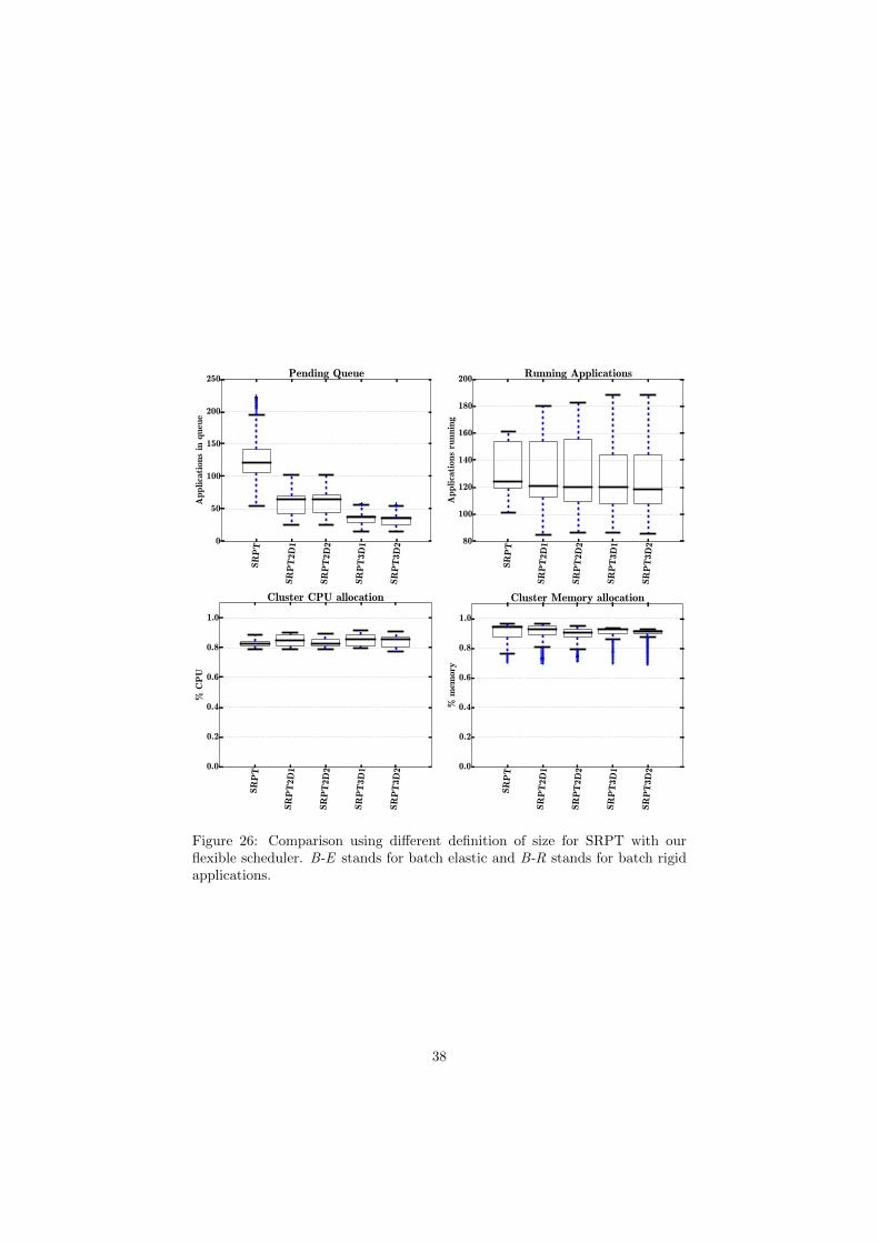
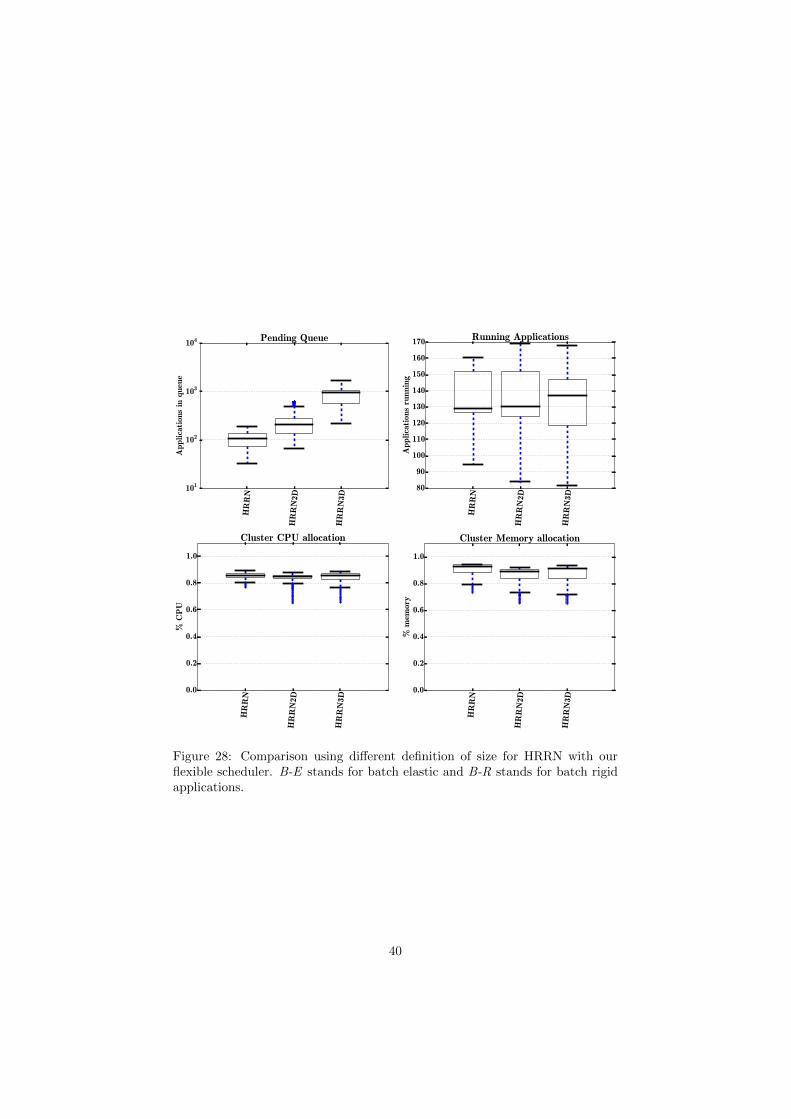
for rigid schedulers (Figs. 14 to 16); having a three dimensional size definitionmay improve the turn around of some policies compared to a unidimensionaldefinition, but in all cases having a two dimensional definition is sufficient toobtain good results. The resource allocation, however, decreases a bit in a rigidsystem as more information is added; it will allows big-but-short (big resourcerequirement but short lived) applications to block the queue thus, increase queuetimes and reduce resources utilization in the cluster. Since our flexible schedulerallows only the indispensable (inelastic) services to be launched, it can overcomethe problems that a rigid has with a three dimensional definition and, as a result,we can see that it performs better than a one or two dimensional definitions.

In conclusion, adding more information to the size does not always improvethe turn around time in a rigid scheduler because some big-but-short applicationscan block the queue. However, with a malleable and with our flexible schedulerthis can be avoided and we can have lower turn around time and higher clusterresources utilization with a three dimensional definition of size. We would liketo stress more the fact that the malleable scheduler is something widely adoptedin theory, but not in use real systems.

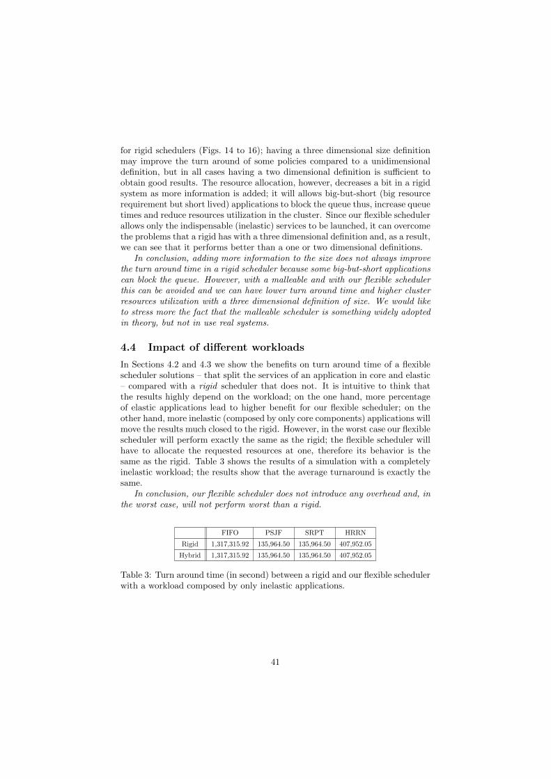
4.4 Impact of different workloads

In Sections 4.2 and 4.3 we show the benefits on turn around time of a flexiblescheduler solutions – that split the services of an application in core and elastic– compared with a rigid scheduler that does not. It is intuitive to think thatthe results highly depend on the workload; on the one hand, more percentageof elastic applications lead to higher benefit for our flexible scheduler; on theother hand, more inelastic (composed by only core components) applications willmove the results much closed to the rigid. However, in the worst case our flexiblescheduler will perform exactly the same as the rigid; the flexible scheduler willhave to allocate the requested resources at one, therefore its behavior is thesame as the rigid. Table 3 shows the results of a simulation with a completelyinelastic workload; the results show that the average turnaround is exactly thesame.

In conclusion, our flexible scheduler does not introduce any overhead and, inthe worst case, will not perform worst than a rigid.

FIFO PSJF SRPT HRRN

Rigid 1,317,315.92 135,964.50 135,964.50 407,952.05

Hybrid 1,317,315.92 135,964.50 135,964.50 407,952.05

Table 3: Turn around time (in second) between a rigid and our flexible schedulerwith a workload composed by only inelastic applications.

41

B-R B-E Int0

100

101

102

103

104

105

Tim

e (s

)

Application Queue

B-R B-E Int0.9

1.0

1.1

1.2

1.3

1.4

1.5

Wit

hou

t/W

ith p

reem

pti

on

Turnaround Ratio

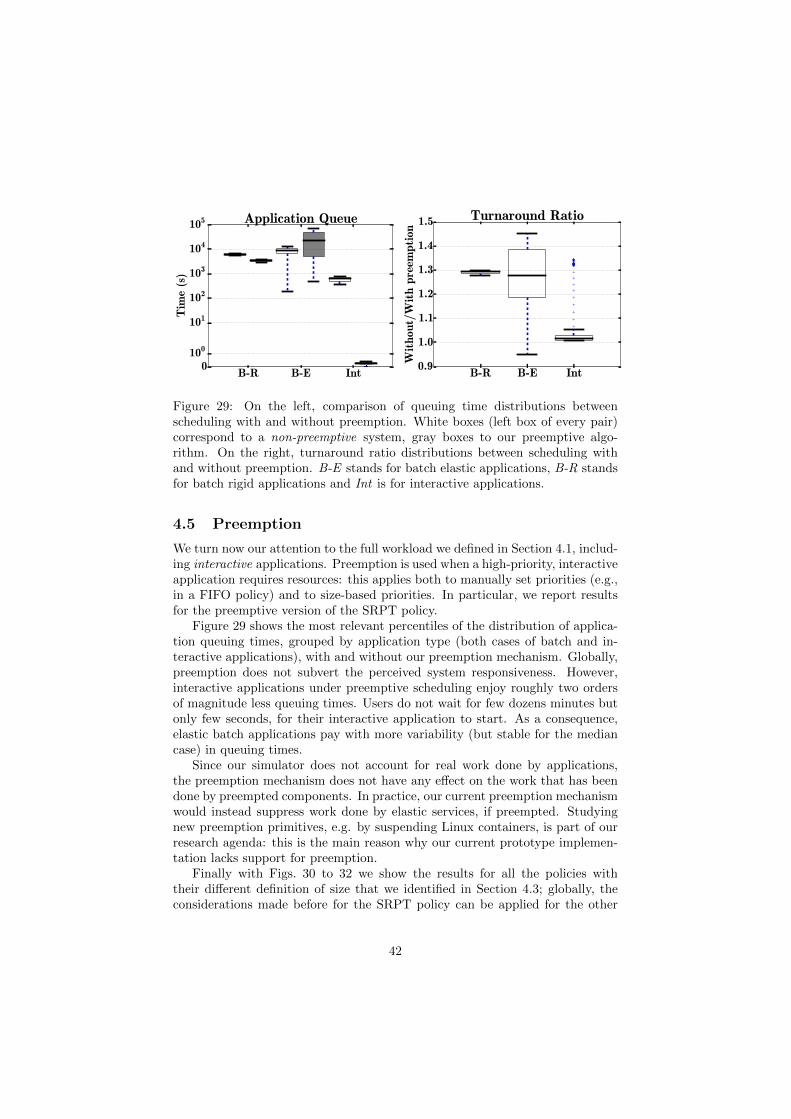
Figure 29: On the left, comparison of queuing time distributions betweenscheduling with and without preemption. White boxes (left box of every pair)correspond to a non-preemptive system, gray boxes to our preemptive algo-rithm. On the right, turnaround ratio distributions between scheduling withand without preemption. B-E stands for batch elastic applications, B-R standsfor batch rigid applications and Int is for interactive applications.

4.5 Preemption

We turn now our attention to the full workload we defined in Section 4.1, includ-ing interactive applications. Preemption is used when a high-priority, interactiveapplication requires resources: this applies both to manually set priorities (e.g.,in a FIFO policy) and to size-based priorities. In particular, we report resultsfor the preemptive version of the SRPT policy.

Figure 29 shows the most relevant percentiles of the distribution of applica-tion queuing times, grouped by application type (both cases of batch and in-teractive applications), with and without our preemption mechanism. Globally,preemption does not subvert the perceived system responsiveness. However,interactive applications under preemptive scheduling enjoy roughly two ordersof magnitude less queuing times. Users do not wait for few dozens minutes butonly few seconds, for their interactive application to start. As a consequence,elastic batch applications pay with more variability (but stable for the mediancase) in queuing times.

Since our simulator does not account for real work done by applications,the preemption mechanism does not have any effect on the work that has beendone by preempted components. In practice, our current preemption mechanismwould instead suppress work done by elastic services, if preempted. Studyingnew preemption primitives, e.g. by suspending Linux containers, is part of ourresearch agenda: this is the main reason why our current prototype implemen-tation lacks support for preemption.

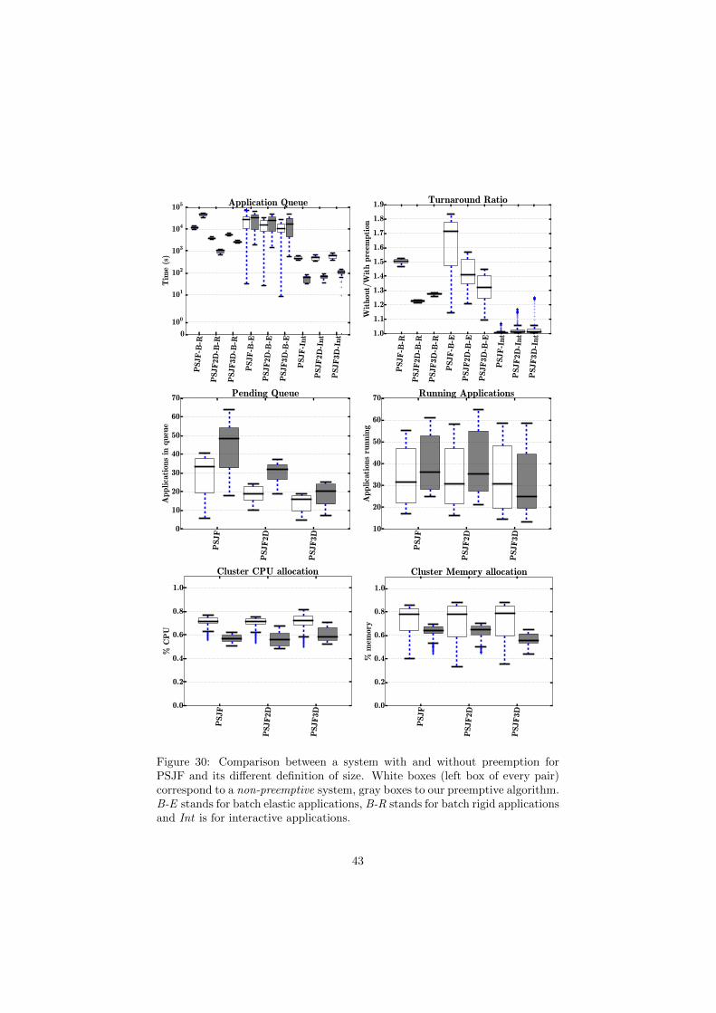
Finally with Figs. 30 to 32 we show the results for all the policies withtheir different definition of size that we identified in Section 4.3; globally, theconsiderations made before for the SRPT policy can be applied for the other

42

PSJF-B

-R

PSJF2D

-B-R

PSJF3D

-B-R

PSJF-B

-E

PSJF2D

-B-E

PSJF3D

-B-E

PSJF-I

nt

PSJF2D

-Int

PSJF3D

-Int0

100

101

102

103

104

105

Tim

e (s

)

Application Queue

PSJF-B

-R

PSJF2D

-B-R

PSJF3D

-B-R

PSJF-B

-E

PSJF2D

-B-E

PSJF3D

-B-E

PSJF-I

nt

PSJF2D

-Int

PSJF3D

-Int1.0

1.1

1.2

1.3

1.4

1.5

1.6

1.7

1.8

1.9

Wit

hout/

Wit

h p

reem

pti

on

Turnaround Ratio

PSJF

PSJF2D

PSJF3D

0

10

20

30

40

50

60

70

Applica

tion

s in

queu

e

Pending Queue

PSJF

PSJF2D

PSJF3D

10

20

30

40

50

60

70

Applica

tion

s ru

nnin

g


PSJF

PSJF2D

PSJF3D

0.0

0.2

0.4

0.6

0.8

1.0

% C

PU


PSJF

PSJF2D

PSJF3D

0.0

0.2

0.4

0.6

0.8

1.0

% m

emor

y


Figure 30: Comparison between a system with and without preemption forPSJF and its different definition of size. White boxes (left box of every pair)correspond to a non-preemptive system, gray boxes to our preemptive algorithm.B-E stands for batch elastic applications, B-R stands for batch rigid applicationsand Int is for interactive applications.

43

SR

PT

-B-R

SR

PT

2D1-

B-R

SR

PT

2D2-

B-R

SR

PT

3D1-

B-R

SR

PT

3D2-

B-R

SR

PT

-B-E

SR

PT

2D1-

B-E

SR

PT

2D2-

B-E

SR

PT

3D1-

B-E

SR

PT

3D2-

B-E

SR

PT

-Int

SR

PT

2D1-

Int

SR

PT

2D2-

Int

SR

PT

3D1-

Int

SR

PT

3D2-

Int0

100

101

102

103

104

105

106

Tim

e (s

)

Application Queue

SR

PT

-B-R

SR

PT

2D1-

B-R

SR

PT

2D2-

B-R

SR

PT

3D1-

B-R

SR

PT

3D2-

B-R

SR

PT

-B-E

SR

PT

2D1-

B-E

SR

PT

2D2-

B-E

SR

PT

3D1-

B-E

SR

PT

3D2-

B-E

SR

PT

-Int

SR

PT

2D1-

Int

SR

PT

2D2-

Int

SR

PT

3D1-

Int

SR

PT

3D2-

Int0.4

0.6

0.8

1.0

1.2

1.4

1.6

1.8

Wit

hou

t/W

ith p

reem

pti

on

Turnaround RatioSR

PT

SR

PT

2D1

SR

PT

2D2

SR

PT

3D1

SR

PT

3D20

10

20

30

40

50

60

Applica

tion

s in

queu

e

Pending QueueSR

PT

SR

PT

2D1

SR

PT

2D2

SR

PT

3D1

SR

PT

3D210

20

30

40

50

60

70

Applica

tion

s ru

nnin

g


SR

PT

SR

PT

2D1

SR

PT

2D2

SR

PT

3D1

SR

PT

3D20.0

0.2

0.4

0.6

0.8

1.0

% C

PU


SR

PT

SR

PT

2D1

SR

PT

2D2

SR

PT

3D1

SR

PT

3D20.0

0.2

0.4

0.6

0.8

1.0

% m

emor

y


Figure 31: Comparison between a system with and without preemption forSRPT and its different definition of size. White boxes (left box of every pair)correspond to a non-preemptive system, gray boxes to our preemptive algorithm.B-E stands for batch elastic applications, B-R stands for batch rigid applicationsand Int is for interactive applications.

44

HR

RN

-B-R

HR

RN

2D-B

-R

HR

RN

3D-B

-R

HR

RN

-B-E

HR

RN

2D-B

-E

HR

RN

3D-B

-E

HR

RN

-Int

HR

RN

2D-I

nt

HR

RN

3D-I

nt101

102

103

104

105

106

107

Tim

e (s

)

Application Queue

HR

RN

-B-R

HR

RN

2D-B

-R

HR

RN

3D-B

-R

HR

RN

-B-E

HR

RN

2D-B

-E

HR

RN

3D-B

-E

HR

RN

-Int

HR

RN

2D-I

nt

HR

RN

3D-I

nt0.2

0.4

0.6

0.8

1.0

1.2

1.4

1.6

1.8

2.0

Wit

hou

t/W

ith p

reem

pti

on

Turnaround Ratio

HR

RN

HR

RN

2D

HR

RN

3D

0

100

200

300

400

500

600

700

800

900

Applica

tions

in q

ueu

e

Pending Queue

HR

RN

HR

RN

2D

HR

RN

3D

10

20

30

40

50

60

70

Applica

tion

s ru

nnin

g


HR

RN

HR

RN

2D

HR

RN

3D

0.0

0.2

0.4

0.6

0.8

1.0

% C

PU


HR

RN

HR

RN

2D

HR

RN

3D

0.0

0.2

0.4

0.6

0.8

1.0

% m

emor

y


Figure 32: Comparison between a system with and without preemption forHRRN and its different definition of size. White boxes (left box of every pair)correspond to a non-preemptive system, gray boxes to our preemptive algorithm.B-E stands for batch elastic applications, B-R stands for batch rigid applicationsand Int is for interactive applications.

45

policies as well. However, we can see a drop in the resource utilization and anincrease in the size of the pending queue when using a preemptive system; this isbecause we are no longer respecting the order imposed by the policy, but we areprioritizing interactive applications that have a much longer duration comparedto the batch, thus a lot of shorter applications are forced to wait.

5 Implementation: The Zoe system

Next, we describe Zoe5, the system we have built to materialize the conceptsdeveloped earlier.

Zoe allows defining analytics applications and schedule them in a cluster ofmachines. It is designed to run on top of an existing low-level cluster manage-ment system, which is used as a back-end to provision resources to applications.Raising the level of abstraction to manipulate analytics application is benefi-cial for users and ultimately to the system design itself: application schedulingdecisions can be taken with a small amount of state information, and do nothappen at the same (extremely fast) pace as low-level task scheduling. Next weoverview Zoe’s design, and provide relevant details for the subject of this work.Zoe applications. In Zoe, the concepts introduced in Section 2 take the formof simple JSON description files that follow a high-level configuration language(CL) to specify applications, frameworks and components with their classes(core or elastic), resource reservations and constraints. The CL is simple andextensible: it aims at conciseness and, with framework templates, can be usedby “casual” and “power” users [10].

The key aspect that determines the application type (batch, interactive,or any new type) is the way application life-cycle is managed. This is deter-mined by a flexible attribute, reminiscent of a “command line”, which allowspassing runtime configuration options, user-defined arguments and environmentvariables, as well as setup and cleanup procedures. For application design,the “command line” attribute requires minimal knowledge of the frameworksthat constitute an application. As an example of the simplicity and effective-ness of the Zoe CL, building a batch application for the distributed versionof TensorFlow [27] only requires tens of lines of CL. The most important at-tribute is the “command line”, which is required to run a TensorFlow pro-gram, i.e., python $TF PROGRAM $PS HOSTS $WK HOSTS program-args. Envi-ronment variables are appropriately handled by Zoe, including information un-known at scheduling time (e.g., host names).

A note on application failures is required. Any failure of an elastic compo-nent is practically harmless, whereas core component failures imply applicationfailure. An area of future work is to exploit failure tolerance mechanisms avail-able from some back-ends (e.g., Kubernetes) to steer application-level failure

5Zoe, https://zoe-analytics.eu/, was conceived in August 2015, named after the biggestcontainer boat in the world, which, has touched sea [37] in the same period of time. In thiswork, we omit several implementation details that stem from our continuous effort to extendZoe.

46

tolerance modes.Zoe back-ends. The main design idea of our system is to hide the complexi-ties of low-level resource provisioning from application scheduling and exploit anexisting cluster management system, for which many alternatives exists. Cur-rently, Zoe builds on top of Docker Swarm [23], and uses it to achieve a seriesof objectives we list below:

• Orchestration: Zoe interacts with all the machines in a cluster using theDocker orchestration API (known as Swarm [23]), which governs the be-havior of the Docker engine [38] deployed in each machine. Thus, Zoemanages to distribute the necessary binaries for the components of anapplication that is scheduled for execution, their configuration, life-cycle,and provisioning.

• Dependency management: Zoe applications materialize as a series of Dockerimages, which contain all dependencies and external libraries required foran application to run. Zoe applications can be built from community-provided or custom Docker images of existing frameworks.

• Resource isolation: framework components specified in an application runin Linux containers, which are managed by a Docker engine. We also usethe Docker engine to achieve memory allocation, whereas CPU partition-ing is left to the machine OS. This means, we have a one dimensionalpacking problem.

• Resource matching: application descriptions include resource constraints.When an application is scheduled for execution, Zoe instructs the back-endto adhere to component constraints when provisioning the relevant Dockerimages with framework binaries, as determined by the virtual assignmentobtained by Algorithm 1.

• Naming and networking: the services for application components to coop-erate in producing useful work, and to interact with the outside world arean important aspect to consider when choosing an appropriate back-endfor Zoe. We use Docker networking, but we also have developed our ownservice discovery mechanism to allow a more flexible application configu-ration and deployment.

Zoe architecture. Although Zoe is separated in several modules, it does notrequire any cluster-wide installation, because it uses its back-end to interactwith the cluster.

The Zoe master polls a high-fidelity view of the cluster state through itsback-end, whenever the scheduler is triggered, and stores it into a state store,backed by a PostgreSQL database. The state store also holds applications state,which is modeled as a simple state-machine. Because Zoe handles high-levelobjects (applications), the strain on the system is minimal: the rate of schedul-ing decisions scales well even with heavy workloads. The virtual assignmentprocedure avoids application interference by construction because it considers

47

requests in sequence, according to their priority. The virtual assignment isimposed on the back-end, using its API.

The Zoe client API handles REST calls that mutate the system state, or thatcan be used to monitor the system behavior. Command-line and web interfacesallow users and administrators to interact with the system and the cluster.

The Zoe scheduler implements the algorithm described in Section 3. Whenan application is submitted, the Zoe master creates an entry in the applicationstate store, and adds it to a pending queue. Our system allows plugging sev-eral scheduling policies to manage the pending queue, ranging from simple tosophisticated size-based policies. Such policies determine which application isgranted “access” to cluster resources: to this end, the scheduler uses the clusterstate store to simulate possible deployments before accepting an application.Framework components underlying an application are scheduled according totheir type. The scheduler strives at making sure the application selected forexecution can make progress as soon as resources are allocated to it. The Zoemonitoring module uses the Docker event stream to update the state of eachapplication component running in the system.

Currently, the Zoe system supports a naive preemption mechanism: entireapplications can be killed upon a command. The finer strategy described inSection 3 and Section 4 is currently under development.

Finally, although Zoe supports many data sources and sinks, we report ex-periments using a HDFS cluster to store input data to applications, and CEPHvolumes to store application-specific logs.

6 Experiments with Zoe

Our goal now is to perform a comparative analysis of two generations of Zoe:the first, implementing a rigid scheduler, as for the baseline, the second with theflexible scheduler we present here. In our experiments, we replay the exact sameworkload trace for both generations. Each trace takes about 3 hours from thefirst submission to the last. During our experiments, no other user was allowedto submit jobs to Zoe.Workload. We use two representative batch application templates, including:1) an elastic application using the Spark framework; 2) a rigid application usingthe TensorFlow framework. Following the statistical distribution of our his-torical traces, we set our workload to include 80% of elastic and 20% of rigidapplications, for a total of 100 applications. Application inter-arrival times fol-low a Gaussian distribution with parameters µ = 60 sec, and σ = 40 sec, whichis compatible with our historical data. More specifically, using the elastic ap-plication templates, we run two use cases. First, an application to induce arandom-forest regression model to predict flight delays, using publicly availabledata from the US DoT.6 Second, a music recommender system based on al-ternating least squares algorithm, using publicly available data from Last.fm7.

6http://stat-computing.org/dataexpo/2009/the-data.html7http://www-etud.iro.umontreal.ca/~bergstrj/audioscrobbler_data.html

48

B-E B-R0

1000

2000

3000

4000

5000

6000

7000

Tim

e (s

)


Base ZOE50

60

70

80

90

100

Per

centa

ge

(%)

Memory Allocated

Figure 33: Comparison of turnaround time distributions using the FIFO disci-pline. White boxes (right box of every pair) correspond to the second generationof Zoe that implements our algorithm. B-E stands for batch elastic and B-Rstands for batch rigid applications.

Both applications have two different requirements in term of memory for eachelastic component. The random-forest regression model has 3 core componentsand then 32 elastic components of 16GB or 8GB RAM each; every elastic com-ponent uses 1 CPU. The music recommender system has 3 core componentsand then 24 elastic components of 16GB RAM or 8GB each; every elastic com-ponent uses 6 CPU. Instead, using the rigid application template, we train adeep Gaussian Process model [39], and use both a single-node and a distributedTensorFlow program, requiring 1 and 10 workers (and 5 parameter servers) eachwith 16GB of RAM.Experimental setup. We run our experiment on a platform with ten servers,each with two 16-core Intel E5-2630 CPU running at 2.40GHz (total of 32 coreswith hyper-threading enabled), 128GB of memory, 1Gbps Ethernet networkfabric and ten 1TB hard drives. No GPU-enabled machines are available in ourplatform, at the moment. The servers use Ubuntu 14.04, Docker 1.11 and thestandalone Swarm manager. Docker images for the applications are preloadedon each machine to prevent container startup delays and network congestion.Summary of results. Using the FIFO scheduling policy, we compare thetwo generations of Zoe according to the distributions of application turnaroundtimes, as shown in Figure 33 (left). The behavior of the two systems indicatea clear advantage for our approach: the median turnaround times are 37% and22% lower, for elastic and rigid applications respectively. Note also that thetails of the distributions are in favor of our approach.

Overall, the new generation of Zoe that implements the flexible scheduler ismore efficient, with a 20% improvement, in allocating and packing applications,as illustrated in Figure 33 (right), where we show the ratio of the distributionof allocated over available resources.

Finally, we present results concerning a low-level metric that measure theapplication ramp-up time, i.e., the time it takes for applications scheduled for

49

running, to receive their allocations and start producing work. Zoe achieves acontainer startup time, including placement decisions, of 0.90 ± 0.25ms. Full-fledged applications, made by several containers, only take few seconds to start,which is a compelling property, especially when compared to existing solutionssuch as Amazon EMR.

7 Related Work

While we cannot do justice to the richness of the scheduling literature, in thissection we organize related work in three groups. The “competitors” are exist-ing, mature systems that could be considered sufficient to address our problemstatement, at a first sight. The second group includes recent works in the sys-tems research literature, while the third covers works on scheduling at the tasklevel.

Many “competitor” systems have been designed to cope with the problemof sharing cluster resources across a heterogeneous set of applications, some ofwhich can be tweaked to achieve the goals we set in this work. For example,Yarn [21] and Mesos [8] have been among the first to enable multiple frameworksto coexist in the same cluster: usage of these “two-level” schedulers yield a bigimprovement as compared with monolithic approaches to resource scheduling.Originally designed for analytic frameworks, such systems deal with the schedul-ing of low-level processing tasks. Recently, more general approaches addressthe problem of cluster-wide resource management: Omega [9], then Borg [10](and Kubernetes [22]) reason at the “container” level, and are optimized toachieve efficient placement and utilization of cluster resources, when absorbinga very heterogeneous workload. This latter includes a majority of long-runningservices, which power Web-scale, latency-sensitive applications. Additionally,container orchestration frameworks, such as Docker Swarm [23], also provideefficient and scalable solutions to the problem of scheduling (that is, placingand provisioning) containers in a cluster. Our work relies on many of the abovesystems, and can use them as a back-end to support scheduling of high-levelapplications rather than provisioning low-level containers. Existing auxiliarydeployment tools such as Aurora [40] and Docker Compose [41], do not addressscheduling problems.

In the systems research literature, we find several inspiring system designs,with ideas that can be “borrowed” to further extend our system prototype andresearch scope. For example, Koala-f [14] tackles dynamic resource allocationproblems, which manifest in our case with “idle” interactive applications. Sim-ilarly to HCloud [13], we believe important to break the reservation paradigm,and allow users to express performance requirements rather than machine-levelresource counts. This can be easily included in an application description, butrequires developing additional components to infer statistical models of applica-tion properties based on systems observations, as done for example in Tarcil [19],Paragon [15] and Quasar [16]. Overall, by focusing on a higher-level of abstrac-tion, the focus of our work is to address a rather abstract scheduling problem:

50

our implementation indicates that our ideas work in practice and also bringtangible benefits.

Finally, many works address the problem of low-level task scheduling. Suchschedulers are designed to support a specific “data-flow” programming model,but many of their design choices can also be used at a higher level. For example,Tyrex [20] and HFSP [42, 43] are a sample of size-based schedulers, which is afamily of policies known to drastically improve turnaround times, as we also haveverified with our experiments. Similarly, Quincy [17] and DRF [44] study max-min fair, task-level resource allocation, specifically working on multi-dimensionalresources. Although our prototype currently consider a one-dimensional packingproblem, due to the characteristics of the back-end we use, which does not yetsupport CPU-level partitioning, ideas presented in [44] can be extended to ourwork, considering alternative back-ends supporting multi-resource partitioning.Recently, schedulers supporting complex directed acyclic graphs representinglow-level, parallel computations have also appeared: Graphene [45], for exam-ple, addresses the problem of complex dependencies and heterogeneous demandsamong the various stages of the computational graph. The work in [46] indicatesubstantial improvements in terms of resource utilization (and not only alloca-tion) thanks to worker queues, that independently schedule tasks. Bistro [11]employs a novel hierarchical model of data and computational resources, whichenable efficient scheduling of data-parallel workloads. Firmament [47] is a cen-tralized scheduler that has been shown to scale to over ten thousand machinesat sub-second task placement latency, using a min-cost max-flow optimizationapproach. Issues related to scheduling scalability, due to the sheer number oflow-level tasks that are typically required by analytic jobs, have been addressedthrough a distributed design, such as in Sparrow [18] and in Condor [12]. Al-though working at the application-level as we do in our work imposes a low tollon the scheduler, distributed designs are interesting also from the failure toler-ance point of view, which is why they represent a valid option for our futurework.

8 Conclusions

Efficient resource management of computer clusters has been a long-lasting areaof research, with peaks of attention happening in conjunction to improvementsin computing machinery, e.g. lately with cloud computing and big data. Anew breed of cluster management systems, aiming at becoming “data-centeroperating systems”, are currently been confronted with problems of efficiencyand performance at scale.

Despite recent advances, there exists a gap between the goal of low-levelresource management, and that of manipulating high-level, heterogeneous, dis-tributed (analytic) applications running in such cluster environments. In thispaper we presented a first possible step to fill this gap, in the form of a newapplication scheduler that interacts with a cluster management back-end, toschedule and allocate resources to applications defined with a simple language

51

and semantics. In addition to careful engineering, required us to design andimplement our system we call Zoe, our research identified a more fundamentalproblem, that required to design a novel scheduling heuristic capable of manip-ulating composite applications, while contributing to system responsiveness.

We validated our algorithm to address our scheduling problem along twolines. We used a numerical approach to simulate large-scale deployments andworkloads. We showed our scheduling algorithm to be highly effective in re-ducing turnaround times, in particular by reducing applications queuing times.Consequently, cluster resources were better allocated. In addition, we reportedan overview of the evaluation of Zoe, that indicates superior performance andefficiency related to our flexible scheduling heuristic.

Our road-map includes the development of a method to redeem untappedresources from idle but running applications, which calls for a substantial re-thinking of the resource reservation paradigm; the design and implementationof application fault tolerance mechanisms; and a long list of pending “tickets”stemming from our open-source Zoe project.

52

References

[1] J. Dean et al., “Mapreduce: simplified data processing on large clusters,”Communications of the ACM, vol. 51, no. 1, pp. 107–113, 2008.

[2] M. Isard et al., “Dryad: distributed data-parallel programs from sequen-tial building blocks,” in ACM SIGOPS Operating Systems Review, vol. 41,no. 3, 2007, pp. 59–72.

[3] M. Zaharia et al., “Resilient distributed datasets: A fault-tolerant abstrac-tion for in-memory cluster computing,” in Proc. of the USENIX NSDI2012.

[4] “Flink,” https://flink.apache.org/.

[5] D. G. Murray et al., “Naiad: a timely dataflow system,” in Proc. of theACM SOSP 2013.

[6] X. Meng et al., “Mllib: Machine learning in apache spark,” JMLR, vol. 17,no. 34, pp. 1–7, 2016.

[7] M. Abadi et al., “Tensorflow: Large-scale machine learning on heteroge-neous distributed systems,” arXiv preprint arXiv:1603.04467, 2016.

[8] B. Hindman et al., “Mesos: A platform for fine-grained resource sharing inthe data center,” in Proc. of the USENIX NSDI 2011.

[9] M. Schwarzkopf et al., “Omega: Flexible, scalable schedulers for large com-pute clusters,” in Proc. of the ACM EuroSys 2013.

[10] A. Verma et al., “Large-scale cluster management at Google with Borg,”in Proc. of the EuroSys 2015.

[11] A. Goder et al., “Bistro: Scheduling data-parallel jobs against live produc-tion systems,” in Proc. of the USENIX ATC 2015.

[12] T. Tannenbaum et al., “Beowulf cluster computing with linux,” 2002, ch.Condor: A Distributed Job Scheduler.

[13] C. Delimitrou et al., “Hcloud: Resource-efficient provisioning in sharedcloud systems,” in Proc. of the ACM ASPLOS 2016.

[14] A. Kuzmanovska et al., “Koala-f: A resource manager for scheduling frame-works in clusters,” in Proc. of the CCGrid 2016.

[15] C. Delimitrou et al., “Paragon: Qos-aware scheduling for heterogeneousdatacenters,” in Proc. of the ACM ASPLOS 2013.

[16] ——, “Quasar: Resource-efficient and qos-aware cluster management,” inProc. of the ACM ASPLOS 2014.

53

[17] M. Isard et al., “Quincy: fair scheduling for distributed computing clus-ters,” in Proc. of the ACM SOSP 2009.

[18] K. Ousterhout et al., “Sparrow: distributed, low latency scheduling,” inProc. of the ACM SOSP 2013.

[19] C. Delimitrou et al., “Tarcil: Reconciling Scheduling Speed and Quality inLarge Shared Clusters,” in Proc. of the ACM SOCC 2015.

[20] B. Ghit et al., “Tyrex: Size-based resource allocation in mapreduce frame-works,” in Proc. of the CCGrid 2016.

[21] V. K. Vavilapalli et al., “Apache hadoop yarn: Yet another resource nego-tiator,” in Proc. of the ACM SoCC 2013.

[22] “Kubernetes,” http://kubernetes.io/.

[23] “Docker Swarm,” https://docs.docker.com/swarm/.

[24] C. Reiss et al., “Heterogeneity and dynamicity of clouds at scale: Googletrace analysis,” in Proc. of the SoCC 2012.

[25] “Google Public Traces,” https://github.com/google/cluster-data.

[26] “Spark,” http://spark.apache.org/.

[27] “TensorFlow,” https://www.tensorflow.org/.

[28] “Open MPI,” https://www.open-mpi.org/.

[29] M. Ragan-Kelley et al., “The jupyter/ipython architecture: a unified viewof computational research, from interactive exploration to communicationand publication.” in AGU Fall Meeting Abstracts 2014, vol. 1.

[30] K. Pruhs et al., “Online scheduling,” Handbook of scheduling: algorithms,models, and performance analysis, pp. 15–1, 2004.

[31] P.-F. Dutot et al., “Scheduling parallel tasks: Approximation algorithms,”Handbook of scheduling: Algorithms, models, and performance analysis, pp.26–1, 2004.

[32] J. Sgall, “Online preemptive scheduling on parallel machines.” 2015.

[33] M. Zaharia et al., “Spark: cluster computing with working sets.” HotCloud,vol. 10, pp. 10–10, 2010.

[34] “Slurm workload manager,” https://slurm.schedmd.com/.

[35] A. Wierman et al., “Nearly insensitive bounds on smart scheduling,” inACM SIGMETRICS Performance Evaluation Review, vol. 33, no. 1, 2005,pp. 205–216.

54

[36] U. Schwiegelshohn and R. Yahyapour, “Analysis of first-come-first-serveparallel job scheduling,” in SODA, vol. 98. Citeseer, 1998, pp. 629–638.

[37] “MSC Zoe,” https://en.wikipedia.org/wiki/MSC Zoe.

[38] “Docker,” http://www.docker.com/.

[39] K. Cutajar et al., “Practical learning of deep gaussian processes via randomfourier features,” arXiv:1610.04386, 2016.

[40] “Aurora,” http://aurora.apache.org/.

[41] “Docker Compose,” https://docs.docker.com/compose/.

[42] M. Pastorelli et al., “HFSP: size-based scheduling for hadoop,” in Proc. ofthe IEEE BigData 2013.

[43] M. Dell’Amico et al., “Revisiting size-based scheduling with estimated jobsizes,” in Proc. of the IEEE MASCOTS 2014.

[44] A. Ghodsi et al., “Dominant resource fairness: Fair allocation of multipleresource types,” in Proc. of the USENIX NSDI 2011.

[45] R. Grandl et al., “GRAPHENE: packing and dependency-aware schedulingfor data-parallel clusters,” in Proc. of the USENIX OSDI 2016.

[46] J. Rasley et al., “Efficient queue management for cluster scheduling,” inProc. of the ACM EuroSys 2016.

[47] I. Gog et al., “Firmament: Fast, centralized cluster scheduling at scale,” inProc. of the USENIX OSDI 2016.

55

Flexible Scheduling of Distributed Analytic Applications - arXiv

Documents

Transcript of Flexible Scheduling of Distributed Analytic Applications - arXiv