A concept for parametric surface fitting which avoids the parametrization problem
Upload
khangminh22Category
view
4download
0
���������� ��� ��� ���������Institut fur Informatik
der Technischen Universitat Munchen
Fitting Parametric Curve Models to
Images Using Local Self-adapting
Separation Criteria
Dissertation
Robert Hanek


Institut fur Informatikder Technischen Universitat Munchen
Fitting Parametric Curve Models to
Images Using Local Self-adapting
Separation Criteria
Robert Hanek
Vollstandiger Abdruck der von der Fakultat fur Informatik der TechnischenUniversitat Munchen zur Erlangung des akademischen Grades eines
Doktors der Naturwissenschaften (Dr. rer. nat.)
genehmigten Dissertation.
Vorsitzender: Univ.-Prof. Dr. Dr. h.c. Wilfried Brauer
Prufer der Dissertation:
1. Univ.-Prof. Dr. Bernd Radig
2. Univ.-Prof. Nassir Navab, Ph.D.
Die Dissertation wurde am 28.11.2003 bei der Technischen Universitat Muncheneingereicht und durch die Fakultat fur Informatik am 02.07.2004 angenommen.


Abstract
The task of fitting parametric curve models to boundaries of perceptually meaningful image
regions is a key problem in computer vision with numerous applications, such as image seg-
mentation, pose estimation, 3-D reconstruction, and object tracking. In this thesis, we propose
the Contracting Curve Density (CCD) algorithm and the CCD tracker as solutions to this pro-
blem. The CCD algorithm solves the curve-fitting problem for a single image whereas the CCD
tracker solves it for a sequence of images.
The CCD algorithm extends the state-of-the-art in two important ways. First, it applies a
novel likelihood function for the assessment of a fit between the curve model and the image
data. This likelihood function can cope with highly inhomogeneous image regions because it
is formulated in terms of local image statistics that are learned on the fly from the vicinity
of the expected curve. Second, the CCD algorithm employs blurred curve models as efficient
means for iteratively optimizing the posterior density over possible model parameters. Blurred
curve models enable the algorithm to trade-off two conflicting objectives, namely a large area
of convergence and a high accuracy.
The CCD tracker is a fast variant of the CCD algorithm. It achieves a low runtime, even
for high-resolution images, by focusing on a small set of carefully selected pixels. In each
iteration step, the tracker takes only such pixels into account that are likely to further reduce the
uncertainty of the curve. Moreover, the CCD tracker exploits statistical dependencies between
successive images, which also improves its robustness. We show how this can be achieved
without substantially increasing the runtime.
In extensive experimental investigations, we demonstrate that the CCD approach outper-
forms other state-of-the-art methods in terms of accuracy, robustness, and runtime. The CCD
algorithm and the CCD tracker achieve sub-pixel accuracy and robustness even in the presence
of strong texture, shading, clutter, partial occlusion, poor contrast, and substantial changes of il-
lumination. We present results for different curve-fitting problems such as image segmentation,
3-D pose estimation, and object tracking.
i

ii

Zusammenfassung
Das Anpassen parametrischer Kurvenmodelle an die Grenzen perzeptuell relevanter Bildregio-
nen ist ein Kernproblem der Bildverarbeitung. Es tritt in zahlreichen wichtigen Anwendungen
wie z.B. Bildsegmentierung, Lageschatzung, 3-D Rekonstruktion und Objektverfolgung auf. In
dieser Dissertation werden der Contracting Curve Density (CCD) Algorithmus und der CCD
Tracker als Losungen fur dieses Problem vorgeschlagen. Der CCD Algorithmus lost das An-
passungsproblem fur ein einzelnes Bild, der CCD Tracker hingegen fur eine Bildsequenz.
Der CCD Algorithmus erweitert den derzeitigen Stand der Forschung in zweierlei Hin-
sicht. Erstens verwendet er eine neuartige Likelihood-Funktion fur die Bewertung der Uberein-
stimmung zwischen dem Kurvenmodell und den Bilddaten. Die Likelihood-Funktion ist selbst
fur inhomogene Bildregionen geeignet, da sie auf lokalen Statistiken basiert, welche iterativ
von der Umgebung der Kurve gelernt werden. Zweitens verwendet der CCD Algorithmus un-
scharfe Kurvenmodelle als effektives Mittel zur iterativen Optimierung der a-posteriori-Dichte.
Unscharfe Kurvenmodelle erlauben einen Ausgleich zwischen zwei gegensatzlichen Zielen,
namlich einem großen Konvergenzbereich und einer hohen Genauigkeit.
Der CCD Tracker ist eine schnelle Variante des CCD Algorithmus. Selbst fur Bilder mit
hoher Auflosung erzielt er eine geringe Rechenzeit, indem er sich auf eine kleine Menge spe-
ziell ausgewahlter Pixel fokussiert. In jedem Iterationsschritt verwendet er nur solche Pixel,
die hochstwahrscheinlich die Unsicherheit der Kurve weiter reduzieren. Daruber hinaus nutzt
der Tracker statistische Abhangigkeiten zwischen aufeinanderfolgenden Bildern. Dies fuhrt zu
einer zusatzlichen Steigerung der Robustheit, ohne die Rechenzeit substanziell zu erhohen.
Umfangreiche experimentelle Untersuchungen zeigen, dass der CCD Ansatz anderen An-
satzen sowohl in der Genauigkeit, der Robustheit als auch der Rechenzeit uberlegen ist. Der
CCD Algorithmus und der CCD Tracker erzielen Subpixel-Genauigkeit und Robustheit selbst
bei starken Texturen, Schattierungen, Teilverdeckungen, geringem Kontrast und erheblichen
Beleuchtungsanderungen. In dieser Arbeit werden Ergebnisse fur verschiedene Anpassungs-
probleme vorgestellt, z.B. Bildsegmentierung, 3-D Lageschatzung und Objektverfolgung.
iii

iv

Acknowledgments
This dissertation would not have been possible without the assistance of several people. First
of all, I would like to thank my thesis advisor, Prof. Dr. Bernd Radig, for giving me the oppor-
tunity to work on this dissertation. I am particularly grateful for his enthusiasm in supporting
Thorsten’s and my idea of founding our own company.
I would like to express my thanks to Prof. Dr. Nassir Navab, the second reporter on this
dissertation. His passion for science was one of the sources of my motivation.
Special thanks go to Michael Beetz. His comments, encouragement, and constructive crit-
icism helped me many times, especially in writing publications and preparing presentations.
I would especially like to thank Thorsten Schmitt and Sebastian Buck for being great colleagues
and close friends. Working with you and the other members of the AGILO robot soccer team
was fun even during stressful periods such as the preparations for World Cups and other events.
I would also like to thank my other colleagues at the “Image Understanding and Knowledge-
Based Systems Group” at Munich Technical University. Thank you for your assistance and
many amazing lunch and coffee breaks. I am indebted to Fabian Schwarzer, Bea Horvath,
Andreas Hofhauser, and Gillian McCann for proofreading this thesis.
Thanks go to Michael Isard, Andrew Blake, and the other members of the “Oxford Visual
Tracking Group” for providing the code of their tracking library. I am grateful to Juri Platonov
for his assistance in conducting the experiments with the condensation and the Kalman tracker.
I would like to thank Carsten Steger for helpful discussions and for providing the DLL of the
color edge detector. Jianbo Shi and Jitendra Malik at the University of California at Berkeley
provided the executable of their Normalized Cuts algorithm. Thanks go to Lothar Hermes at the
University of Bonn for running the PDC algorithm on the test data, see Figure 2.1. Furthermore,
I am grateful to Christoph Hansen for providing the PDM depicted in Figure 5.13.
Last, but certainly not least, I would like to thank my girl-friend, Wiebke Bracht, who
supported me with her love, encouragement, and assistance in many ways.
v

vi

Contents
Abstract i
Zusammenfassung iii
Acknowledgments v
1 Introduction 11.1 The Curve-fitting Problem . . . . . . . . . . . . . . . . . . . . . . . . . . . . 2
1.1.1 Problem Description . . . . . . . . . . . . . . . . . . . . . . . . . . . 3
1.1.2 Applications . . . . . . . . . . . . . . . . . . . . . . . . . . . . . . . 5
1.1.3 Requirements for a Curve-fitting Method . . . . . . . . . . . . . . . . 6
1.2 The Contracting Curve Density (CCD) Approach . . . . . . . . . . . . . . . . 7
1.2.1 Key Questions . . . . . . . . . . . . . . . . . . . . . . . . . . . . . . 7
1.2.2 Sketch of the CCD Approach . . . . . . . . . . . . . . . . . . . . . . 8
1.3 Main Contributions of the Thesis . . . . . . . . . . . . . . . . . . . . . . . . 9
1.4 Overview of the Thesis . . . . . . . . . . . . . . . . . . . . . . . . . . . . . . 12
2 Related Work 132.1 Classification according to the Objective Function . . . . . . . . . . . . . . . 13
2.2 Classification according to the Optimization Method . . . . . . . . . . . . . . 18
2.3 Classification according to other Dimensions . . . . . . . . . . . . . . . . . . 19
3 The CCD Algorithm 213.1 Overview . . . . . . . . . . . . . . . . . . . . . . . . . . . . . . . . . . . . . 21
3.1.1 Input and Output Data . . . . . . . . . . . . . . . . . . . . . . . . . . 21
3.1.2 Steps of the CCD Algorithm . . . . . . . . . . . . . . . . . . . . . . . 23
3.2 Learning Local Statistics . . . . . . . . . . . . . . . . . . . . . . . . . . . . . 27
3.2.1 Determining the Pixels in the Vicinity of the Image Curve . . . . . . . 27
vii

viii
3.2.2 Computing Local Statistics . . . . . . . . . . . . . . . . . . . . . . . 30
3.2.2.1 Context-sensitive Statistical Models . . . . . . . . . . . . . 30
3.2.2.2 Weighting the Pixels in the Vicinity of the Curve . . . . . . 32
3.2.2.3 Recursive Computation of Local Statistics . . . . . . . . . . 36
3.3 Refining the Estimate of the Model Parameter Vector . . . . . . . . . . . . . . 39
3.3.1 Observation Model . . . . . . . . . . . . . . . . . . . . . . . . . . . . 39
3.3.1.1 One Pixel . . . . . . . . . . . . . . . . . . . . . . . . . . . 39
3.3.1.2 Multiple Pixels . . . . . . . . . . . . . . . . . . . . . . . . . 40
3.3.2 Updating the Mean Vector . . . . . . . . . . . . . . . . . . . . . . . . 42
3.3.2.1 MAP Estimation . . . . . . . . . . . . . . . . . . . . . . . . 42
3.3.2.2 Fitting a Blurred Model . . . . . . . . . . . . . . . . . . . . 43
3.3.2.3 Newton Iteration Step . . . . . . . . . . . . . . . . . . . . . 47
3.3.2.4 Outlier Treatment . . . . . . . . . . . . . . . . . . . . . . . 48
3.3.3 Updating the Covariance Matrix . . . . . . . . . . . . . . . . . . . . . 50
3.4 Summary of the Algorithm . . . . . . . . . . . . . . . . . . . . . . . . . . . . 51
4 The CCD Tracker 53
4.1 Real-time CCD Algorithm . . . . . . . . . . . . . . . . . . . . . . . . . . . . 54
4.1.1 Choosing Pixels in the Vicinity of the Curve . . . . . . . . . . . . . . 55
4.1.2 Assigning Pixels to a Side of the Curve . . . . . . . . . . . . . . . . . 56
4.1.3 Recursive Computation of Local Statistics . . . . . . . . . . . . . . . 57
4.1.4 Confirmation Measurement . . . . . . . . . . . . . . . . . . . . . . . 59
4.2 Dynamical Models of Curves in Image Sequences . . . . . . . . . . . . . . . 60
4.3 Temporal Coherence of Pixel Values in Image Sequences . . . . . . . . . . . . 61
4.3.1 Accumulating Local Statistics of Pixel Values over Time . . . . . . . . 62
4.3.2 One-to-one Propagation of Local Statistics . . . . . . . . . . . . . . . 64
4.3.3 M-to-one Propagation of Local Statistics . . . . . . . . . . . . . . . . 66
4.3.4 Merging Propagated and New Local Statistics . . . . . . . . . . . . . 71
4.4 Summary of the Algorithm . . . . . . . . . . . . . . . . . . . . . . . . . . . . 71
4.5 Related Methods for Object Tracking . . . . . . . . . . . . . . . . . . . . . . 76
5 Experimental Evaluation 77
5.1 Quantifying the Performance . . . . . . . . . . . . . . . . . . . . . . . . . . . 77
5.2 Evaluation of the CCD Algorithm . . . . . . . . . . . . . . . . . . . . . . . . 78
ix
5.2.1 Results for Semi-synthetic Images . . . . . . . . . . . . . . . . . . . . 78
5.2.2 Results for Real Images . . . . . . . . . . . . . . . . . . . . . . . . . 90
5.3 Evaluation of the CCD Tracker . . . . . . . . . . . . . . . . . . . . . . . . . 96
5.3.1 Compared Trackers . . . . . . . . . . . . . . . . . . . . . . . . . . . 96
5.3.2 Results for Semi-synthetic Image Sequences . . . . . . . . . . . . . . 96
5.3.3 Results for Real Image Sequences . . . . . . . . . . . . . . . . . . . . 116
5.4 Summary of the Results . . . . . . . . . . . . . . . . . . . . . . . . . . . . . 120
6 Conclusion 121
A Further Results for the Fast CCD Algorithm 123A.1 Error Histograms . . . . . . . . . . . . . . . . . . . . . . . . . . . . . . . . . 123
A.2 Star Shape . . . . . . . . . . . . . . . . . . . . . . . . . . . . . . . . . . . . 127
B Parametric Curve Models 133B.1 Rigid 3-D Models . . . . . . . . . . . . . . . . . . . . . . . . . . . . . . . . 133
B.2 Deformable 2-D Models . . . . . . . . . . . . . . . . . . . . . . . . . . . . . 136
C Remarks on the Implementation 139
Glossary of Notation 140
Bibliography 143
Index 152

x

List of Figures
1.1 Mug on a table . . . . . . . . . . . . . . . . . . . . . . . . . . . . . . . . . . 2
1.2 The curve-fitting problem . . . . . . . . . . . . . . . . . . . . . . . . . . . . . 4
1.3 Curve-fitting by the CCD algorithm . . . . . . . . . . . . . . . . . . . . . . . 10
2.1 Results of three state-of-the-art image segmentation methods . . . . . . . . . . 15
3.1 Curve defined by a curve function . . . . . . . . . . . . . . . . . . . . . . . . 22
3.2 Outline of the CCD algorithm . . . . . . . . . . . . . . . . . . . . . . . . . . 24
3.3 Steps of the CCD algorithm . . . . . . . . . . . . . . . . . . . . . . . . . . . . 26
3.4 Local linear approximation of the model curve . . . . . . . . . . . . . . . . . . 28
3.5 Two bimodal distributions and their Gaussian approximations . . . . . . . . . . 31
3.6 Computation of local statistics from windows . . . . . . . . . . . . . . . . . . 33
3.7 Weights over the displacement to the expected curve . . . . . . . . . . . . . . 35
3.8 Weights over the displacement along the curve . . . . . . . . . . . . . . . . . . 36
3.9 Contour plot of the local windows . . . . . . . . . . . . . . . . . . . . . . . . 37
3.10 Quantities of the fitting process I . . . . . . . . . . . . . . . . . . . . . . . . . 38
3.11 Conditional probability density of a pixel value . . . . . . . . . . . . . . . . . 41
3.12 Likelihood of the assignment . . . . . . . . . . . . . . . . . . . . . . . . . . . 41
3.13 Negative log-likelihood of the assignment . . . . . . . . . . . . . . . . . . . . 42
3.14 1-D edge detection . . . . . . . . . . . . . . . . . . . . . . . . . . . . . . . . 44
3.15 Quantities of the fitting process II . . . . . . . . . . . . . . . . . . . . . . . . 46
3.16 The CCD algorithm . . . . . . . . . . . . . . . . . . . . . . . . . . . . . . . . 52
4.1 Localization of a ball by an autonomous soccer robot . . . . . . . . . . . . . . 56
4.2 Failure of the CCD tracker . . . . . . . . . . . . . . . . . . . . . . . . . . . . 63
4.3 One-to-one propagation of color distributions over time . . . . . . . . . . . . . 65
4.4 M-to-one propagation of color distributions over time . . . . . . . . . . . . . . 67
4.5 Steps of the M-to-one propagation . . . . . . . . . . . . . . . . . . . . . . . . 69
xi

xii
4.6 The CCD tracker . . . . . . . . . . . . . . . . . . . . . . . . . . . . . . . . . 73
5.1 Generating semi-synthetic images . . . . . . . . . . . . . . . . . . . . . . . . 79
5.2 Real images used for generating semi-synthetic images . . . . . . . . . . . . . 80
5.3 Error histogram of variant A . . . . . . . . . . . . . . . . . . . . . . . . . . . 83
5.4 Images yielding the highest failure rate I . . . . . . . . . . . . . . . . . . . . . 84
5.5 Images yielding the lowest failure rate I . . . . . . . . . . . . . . . . . . . . . 85
5.6 Images yielding the highest mean error I . . . . . . . . . . . . . . . . . . . . . 86
5.7 Images yielding the lowest mean error I . . . . . . . . . . . . . . . . . . . . . 87
5.8 Fitting a circle with three degrees of freedom . . . . . . . . . . . . . . . . . . 90
5.9 An only partially visible curve . . . . . . . . . . . . . . . . . . . . . . . . . . 90
5.10 Area of convergence . . . . . . . . . . . . . . . . . . . . . . . . . . . . . . . 91
5.11 Tea box with flower pattern lying in a flower meadow . . . . . . . . . . . . . . 93
5.12 Partially occluded box . . . . . . . . . . . . . . . . . . . . . . . . . . . . . . 94
5.13 Fitting a deformable model . . . . . . . . . . . . . . . . . . . . . . . . . . . . 95
5.14 Masks used for generating semi-synthetic image sequences . . . . . . . . . . . 98
5.15 Real image sequences used for generating semi-synthetic image sequences . . . 99
5.16 Failure rate over dimension of parameter vector I . . . . . . . . . . . . . . . . 100
5.17 Failure rate over runtime . . . . . . . . . . . . . . . . . . . . . . . . . . . . . 102
5.18 Error over dimension of parameter vector . . . . . . . . . . . . . . . . . . . . 103
5.19 Image sequence A . . . . . . . . . . . . . . . . . . . . . . . . . . . . . . . . . 106
5.20 Image sequence B . . . . . . . . . . . . . . . . . . . . . . . . . . . . . . . . . 108
5.21 Image sequence C . . . . . . . . . . . . . . . . . . . . . . . . . . . . . . . . . 110
5.22 Image sequence D . . . . . . . . . . . . . . . . . . . . . . . . . . . . . . . . . 112
5.23 Failure of the CCD tracker . . . . . . . . . . . . . . . . . . . . . . . . . . . . 115
5.24 Failure rate over dimension of parameter vector II . . . . . . . . . . . . . . . . 117
5.25 Bottle sequence . . . . . . . . . . . . . . . . . . . . . . . . . . . . . . . . . . 118
5.26 Largest errors for the bottle sequence . . . . . . . . . . . . . . . . . . . . . . . 119
A.1 Error histogram of variant A . . . . . . . . . . . . . . . . . . . . . . . . . . . 124
A.2 Error histogram of variant B . . . . . . . . . . . . . . . . . . . . . . . . . . . 124
A.3 Error histogram of variant C . . . . . . . . . . . . . . . . . . . . . . . . . . . 125
A.4 Error histogram of variant D . . . . . . . . . . . . . . . . . . . . . . . . . . . 125
A.5 Error histogram of variant E . . . . . . . . . . . . . . . . . . . . . . . . . . . 126
A.6 Error histogram of variant F . . . . . . . . . . . . . . . . . . . . . . . . . . . 126

xiii
A.7 Error histogram of variant G . . . . . . . . . . . . . . . . . . . . . . . . . . . 127
A.8 Images yielding the highest failure rate II . . . . . . . . . . . . . . . . . . . . 128
A.9 Images yielding the lowest failure rate II . . . . . . . . . . . . . . . . . . . . . 129
A.10 Images yielding the highest mean error II . . . . . . . . . . . . . . . . . . . . 130
A.11 Images yielding the lowest mean error II . . . . . . . . . . . . . . . . . . . . . 131

xiv

List of Tables
5.1 Variants of parameters and input data . . . . . . . . . . . . . . . . . . . . . . . 81
5.2 Failure rate over error of initialization . . . . . . . . . . . . . . . . . . . . . . 82
5.3 Error and runtime overview . . . . . . . . . . . . . . . . . . . . . . . . . . . 82
5.4 Performance of different trackers over dimension of parameter vector . . . . . 104
xv

xvi

Chapter 1
Introduction
In our daily lives the number of devices equipped with cameras is steadily increasing. PCs
are equipped with webcams. Mobile phones and entertainment robots are equipped with small
cameras. Even many cars will soon be equipped with imaging devices, such as infrared cameras,
in order to amplify the driver’s vision at night. Cameras are increasingly being used in different
environments, such as conference rooms, shopping malls, train stations, and highways.
The variety of environments and imaging conditions constitute a great challenge for the de-
velopment of interpretation and image understanding methods. Obviously, methods that can
achieve their interpretation task in natural and unmodified environments are becoming partic-
ularly important. The mug depicted in Figure 1.1 illustrates the resulting challenge for image
understanding, also known as computer vision and scene analysis. Both the mug and its back-
ground show a large variety of pixel values, textures, and other image properties. Hence, seg-
menting the mug, i.e. separating the mug region from the background, is challenging. Several
other tasks in computer vision are based on the crucial task of image segmentation.
Many important computer vision problems can only be solved by using a priori knowledge
about the scene. In the image formation process the 3-D world is transformed to a 2-D image.
Due to the loss of information, the transformation cannot be uniquely inverted. Hence, many
computer vision problems are ill-posed1 (Bertero, Poggio, and Torre, 1988). For example,
determining the 3-D location and orientation of an unknown object from a single image is not
possible without additional information.
Due to the ill-posedness of many computer vision problems, models specifying a priori
knowledge are commonly used. Particularly effective models are parametric curve models, also
known as deformable2 models, deformable templates, snakes, or active contours (Kass, Witkin,
1Ill-posed in the sense of Hadamard (1902) means that the problems have either no solution, no unique solution,or a solution that does not depend continuously on the input.
2We prefer the term parametric curve models since in many applications the model is not deformable, but rigid.
1

2 CHAPTER 1. INTRODUCTION
Figure 1.1: A typical computer vision task is to identify the image region corresponding to themug and to determine the location and orientation of the mug in the 3-D space.
and Terzopoulos, 1988; Yuille, Cohen, and Hallinan, 1992; Blake and Isard, 1998). This class
of models defines the set of expected shapes in the image using geometric properties of the
curve. The parametric curve model guides the image interpretation process towards particularly
likely interpretations.
A number of important and challenging computer vision tasks, including image segmen-
tation, pose estimation, object tracking, and object recognition can be formulated as variants
of the curve-fitting problem. This is the problem of fitting a given parametric curve model to
sensed image data. In this thesis, we propose robust, accurate, efficient, and versatile methods
for fitting parametric curve models to a single image or a sequence of images.
1.1 The Curve-fitting Problem
Let us now introduce the curve-fitting problem by first giving an informal problem description,
then listing some of its most important applications, and finally specifying requirements for a
method performing curve-fitting.

1.1. THE CURVE-FITTING PROBLEM 3
1.1.1 Problem Description
The curve-fitting problem can be described as follows:3
Input data: Given are (a) the image data (one or multiple images) and (b) a parametric curve
model. The curve model describes region boundaries, i.e. edges, in the image as a function of
a vector of model parameters. Such a boundary could be, for example, the contour of an object
of interest. The model parameters specify possible variations of the curve. For example, the
model parameters could define the 3-D pose (position and orientation), size, and shape of the
object of interest. Furthermore, the curve model contains an a priori distribution of the model
parameters which represents a priori knowledge about the curve.
Goal (output data): The goal of the curve-fitting process is to estimate the model parameters
that best match both the image data and the a priori distribution. In the process of curve-fitting,
evidence from the image data is combined with the a priori distribution to form a posteriori
estimate of the model parameters.
Figure 1.2 depicts a curve-fitting problem. The input image shows the coffee mug in front
of an inhomogeneous background. The curve model describes the set of expected contours of
the mug. The thick line in Figure 1.2b is the curve corresponding to the mean of the a priori
distribution. The a priori distribution probabilistically assigns pixels either to the mug region
or to the background region. The pixels having the most uncertain assignments lie between the
two thin lines in Figure 1.2b. After the fitting process, the uncertainty is widely reduced and
the estimated contour (black curve in Figure 1.2c) accurately matches the contour of the mug.
Based on curve-fitting, different levels of computer vision tasks can be performed:
Image segmentation: Image segmentation can be performed by curve-fitting. Image segmen-
tation is the process of locating regions in an image that correspond to objects in the scene. By
curve-fitting, for example the image in Figure 1.2a can be partitioned in a region corresponding
to the coffee mug and another region corresponding to the background.
3A more formal description of the input and the output data will be given in section 3.1.1.

4 CHAPTER 1. INTRODUCTION
c) fitted curve (black)
b) curve model
fittingcurve−
input
output
a) input image
Figure 1.2: The curve-fitting problem: a) The input image. b) A parametric curve model with ana priori distribution of the model parameters. The thick line is the mug contour corresponding tothe mean of the a priori distribution. The thin lines illustrate the initial uncertainty of the regionboundary. c) The goal is to estimate the model parameters such that the resulting curve (black)fits to the image data and to the a priori distribution. During the fitting process, the uncertaintyof the region boundary is widely reduced.

1.1. THE CURVE-FITTING PROBLEM 5
Parameter estimation: By curve-fitting, meaningful properties of the scene can be directly
estimated. Depending on the curve model, properties of observed objects (e.g. pose, size, and
shape) or properties of the observing camera (internal and external camera parameters) can be
estimated. By curve-fitting, e.g. in Figure 1.2a the 3-D pose of the coffee mug can be estimated
with respect to the observing camera. Note that this information is of a higher level than the raw
image segments are. The obtained 3-D data may, for example, allow a robot to grasp the object,
whereas the raw image segments, which contain only 2-D information, are not sufficient for this
task. To estimate such higher-level data, a priori knowledge is required. For example, 3-D pose
estimation from a single view requires knowledge about the camera (internal parameters) and
about the observed object. This knowledge is represented by the curve model.
Why is Curve-fitting Difficult?
Unfortunately, solving image segmentation and the related curve fitting problem is often very
difficult, especially in natural and unconstrained scenes. For example, segmenting the coffee
mug from the background is difficult because both the mug region and the background region
are very inhomogeneous. Both regions exhibit large variations of the pixel values (e.g. RGB
values) due to clutter, shading, texture, and highlights, see Figure 1.2a. Furthermore, the sensed
image data depend on physical conditions, such as the illumination or surface properties, that are
usually unknown. As a consequence, it is often impossible to determine adequate segmentation
criteria in advance or even find a single criteria that is applicable for all parts of an object
boundary. This is exactly what causes problems for related state-of-the-art methods, which will
be discussed in chapter 2.
1.1.2 Applications
Let us now briefly illustrate the wide range of applications of curve-fitting.
Robotics: Many applications of computer vision are in the field of robotics. For example,
parametric curves can be used to describe landmarks in the robot’s environment. A robot
equipped with a camera can localize itself within the environment by fitting the curve models
to the sensed image (Aider, Hoppenot, and Colle, 2002; Hanek and Schmitt, 2000). Similarly,
it can also localize other objects (Lowe, 1987; Phong et al., 1995; Hanek et al., 2002a). Based
on the object’s contour, a robot can also establish a set of safe grasps on the observed object
(Davidson and Blake, 1998; Rimon and Blake, 1996).

6 CHAPTER 1. INTRODUCTION
Medical applications: Parametric curve models, i.e. deformable models, have been exten-
sively employed for extracting clinically useful information about anatomic structures imaged
through computer tomography (CT), magnetic resonance (MR), and other modalities. McIner-
ney and Terzopoulos (1996) provide a survey on medical applications. For example, parametric
curve models are used for measuring the area of leg ulcers (Jones and Plassmann, 2000) or ex-
tracting the contour of a cyst from ultrasound breast images (Yezzi et al., 1997). A primary use
of parametric models is to measure the dynamic behavior of the human heart, especially the left
ventricle (Herlin and Ayache, 1992; Geiger et al., 1995). This allows for isolating the severity
and extent of diseases such as ischemia.
User interfaces: A computer equipped with a video camera can provide new perceptual inter-
faces between humans and machines. The computer can be controlled by gestures and motions
captured by a camera (Azarbayejani et al., 1993). Furthermore, the video image can be aug-
mented by artificial elements generated by the computer.
Surveillance and biometrics: In surveillance applications, contour tracking is used to follow
and quantify the motions of persons or cars in a video sequence (Siebel, 2003; Sullivan, 1992).
Tracking the articulated motion of a human body has several applications in biometrics and
clinical gait analysis (Huang, 2001).
1.1.3 Requirements for a Curve-fitting Method
A method for curve-fitting has to meet several requirements in order to be widely applicable to
practical computer vision problems:
Robustness: The method should be robust against several variations of the input data. In par-
ticular, the method should not fail even in the presence of clutter, texture, changing illumination,
highlights, partial occlusion, and shadows. We say a method fails if the distance between the
correct solution and the solution returned by the method exceeds a given limit.
Accuracy: In many applications, high sub-pixel accuracy is required. This is especially chal-
lenging for textured image regions.
Efficiency / Runtime: In particular, methods for object tracking have to be computationally
efficient, i.e. their runtime should be low. The runtime should scale gradually with respect to

1.2. THE CONTRACTING CURVE DENSITY (CCD) APPROACH 7
1. the resolution of the images. This allows for processing high resolution images within a
limited time.
2. the dimension of the parameter vector. This allows for processing complex models, i.e.
models with many parameters, within a limited time.
Any-time property: For many time-constrained applications, e.g. in the field of robotics,
any-time algorithms are required. These algorithms yield at any time a solution whose quality
improves, if more computation time is given (Boddy and Dean, 1994). This allows, for example,
a vision-guided robot to react quickly on new image data and to continuously refine its action.
Versatility: The method should be versatile enough to cope with different classes of curve
models. In particular, the method should be suitable for rigid and deformable models, as well
as for linear and non-linear models. For non-linear curve models, the relations between points
on the curve and the model parameter vector is non-linear. Relevant classes of curve models
will be explained in appendix B.
1.2 The Contracting Curve Density (CCD) Approach
In this section we introduce the Contracting Curve Density (CCD) approach, a novel solution
to the curve-fitting problem. We first identify two key questions in the design of curve-fitting
methods. Then, in section 1.2.2, we sketch the CCD approach.
1.2.1 Key Questions
The curve-fitting problem that we informally introduced in section 1.1.1 can be formalized as
a Bayesian inference problem. The maximum a posteriori (MAP) estimate��
of the model
parameters�
is given as �� �arg ���� � �� ���� ����� � � ����� (1.1)
where � � ��� is the a priori probability density of the model parameters and � �� � � ��� is the
observation probability density specifying the likely range of images �
given the model param-
eters�
. (The superscript � indicates input data.) The conditional probability density � �� � � ���is also known as the likelihood or fitness function for the model parameters
�. It evaluates
the fit between the observed image data �
and the assumed model parameters�
. In order to
implement the MAP estimation above, we have to address two key questions:

8 CHAPTER 1. INTRODUCTION
1. How can the likelihood function be approximated appropriately? In general, the actual
likelihood function, i.e. the probabilistic relation between the model parameters�
and the
image data �
, is not known. The image data not only depend on the model parameters, but
also on other usually unknown properties of the scene, such as the illumination, surface
properties, and characteristics of the camera. Approximating the likelihood is especially
challenging in the presence of clutter and strong texture.
2. How can the fit be optimized efficiently, despite the existence of possibly multiple local
optima?
Related curve-fitting methods address the first question by making some assumptions about the
image data. For example, edge-based methods assume that the model curve coincides with
edges in the image, where edges are usually defined by a maximum image gradient. Region-
based methods assume that the image regions defined by the curve are homogeneous. In sec-
tion 2.1, we will describe such assumptions in more detail. These assumptions are usually not
flexible enough to cope with local variations of the image data, e.g. varying texture and clutter.
Representative examples will be given in Figure 2.1 (page 15). The second question also poses
a challenge for ongoing research. Existing optimization methods are often either inefficient or
inaccurate, especially for high dimensional parameter vectors. In section 2.2, we will discuss
different optimization methods used for curve-fitting.
1.2.2 Sketch of the CCD Approach
This section sketches two novel methods for curve-fitting, namely the CCD algorithm and the
CCD tracker. The CCD algorithm solves the curve-fitting problem for a single image, whereas
the CCD tracker solves it for a sequence of images. Let us start with the CCD algorithm. This
algorithm iteratively refines the a priori distribution of the model parameters to an a posterior
distribution of the parameters. This is achieved by alternately performing two steps until con-
vergence:
1. Learn local statistics of the pixel values from the vicinity of the expected curve. In this
step, for each pixel � in the vicinity of the expected curve, two sets of local statistics
are computed, one set for each side of the curve. The local statistics are obtained from
pixels that are close to pixel � and most likely lie on the corresponding side of the curve,
according to the current estimate of the model parameters. The resulting local statistics
represent an expectation of “what the two sides of the curve look like”.

1.3. MAIN CONTRIBUTIONS OF THE THESIS 9
2. Refine the estimated model parameters by assigning the pixels in the vicinity of the
expected curve to the side they fit best, according to the local statistics. In this step, a
likelihood function is constructed based on the local statistics. By optimizing the resulting
MAP criterion, the model parameters are updated, thus changing the expected curve.
In the first step, the estimated model parameters are fixed and based on the fixed model param-
eters, local statistics of the pixel values are computed. In the second step, the local statistics are
fixed and based on the local statistics, the estimated model parameters are updated.
This process is depicted in Figure 1.3. In this example, a radially distorted straight line4 is
being fitted to the image data. Here, the curve has just two parameters, namely the y-coordinates
at the left and the right image border.5 The input image and the estimated curve are depicted
in row a) for different iteration steps. The image data expected, according to the learned local
statistics, are depicted in row b). During the iteration, the estimated curve converges to the
actual image curve, and the expected image data (row b) describe the actual vicinity of the image
curve (row a) with increasing accuracy. During the fitting process, the probability density of the
curve in the image contracts towards a single curve estimate. Therefore, we call the algorithm
Contracting Curve Density (CCD) algorithm.
The CCD tracker is based on the CCD algorithm. It tracks a curve in an image sequence by
performing two steps for each image:
1. Fitting: In the fitting step, the model curve is fitted to the image using a fast real-time
variant of the CCD algorithm.
2. Propagating: In the propagating step, the parameters of the curve are propagated (pre-
dicted) over time, using a dynamical model which describes the set of likely curve mo-
tions. In addition, also local statistics of the pixel values can be propagated over time.
Using the propagation, the CCD tracker allows for exploiting two kinds of statistical depen-
dencies between successive images: 1.) dependencies between successive curves (shapes and
positions); and 2.) dependencies between successive pixel values.
1.3 Main Contributions of the Thesis
This thesis advances the state-of-the-art in curve-fitting in four important ways:
4The line is straight in 3-D coordinates, but due to the radial distortion caused by the lens, it appears curved inthe image.
5In general, the curve model may have an arbitrary number of parameters.

10 CHAPTER 1. INTRODUCTION
iteration: 0 2 5a.) Input image with superimposed curve
b.) Expected image according to the learned local statistics
Figure 1.3: The CCD algorithm converges to the corresponding image curve, despite the heavyclutter and texture next to the initialization. During the iteration, the expected image data(row b) describe the actual vicinity of the image curve (row a) with increasing accuracy.
1. We propose a likelihood function that can cope with highly inhomogeneous imageregions: The likelihood function is based on local image statistics, which are iteratively
learned from the vicinity of the expected image curve. The local statistics allow for
probabilistically separating adjacent regions even in the presence of spatially changing
properties, such as texture, color, shading, or illumination. The resulting locally adapted
separation criteria replace predefined fixed criteria (e.g. image gradients or homogeneity
criteria). An efficient method is proposed for computing the required local statistics.
2. We propose a “blurred model” as an efficient and robust means for optimization:We optimize the MAP criterion, not only for a single vector of model parameters, but for
a Gaussian distribution of model parameters. Thus, multiple curves are simultaneously
taken into account. This can be seen as fitting a blurred curve model to the image data,
where the local scale of blurring depends on the local uncertainty of the curve.
In order to increase the capture range, other methods typically blur the image first and then
fit a single model curve to the blurred image data, e.g. (Kass, Witkin, and Terzopoulos,
1988). We take the opposite approach. We use non-blurred image data and a blurred
model. The advantages are as follows:

1.3. MAIN CONTRIBUTIONS OF THE THESIS 11
(a) The capture range, i.e. the local scale, is enlarged according to the uncertainty of the
model parameters. This yields, for each pixel and each iteration step, an individual
compromise between the two conflicting goals, namely a large area of convergence
and a high accuracy. Figure 1.3 row b) shows that the blurring in the direction
perpendicular to the curve depends on the iteration step and the position along the
curve. In the first iteration steps, the blurring is more intense at the right side than at
the left side.
(b) Optimizing the fit between an image and a blurred model is usually computationally
cheaper than blurring the image. Especially if the uncertainty of the initialization is
small, only a small fraction of the pixels covered by possible curve points is needed
in order to refine the fit.
(c) No high frequency information of the image data is lost. This is particularly impor-
tant for separating textured regions or for achieving high sub-pixel accuracy.
3. We propose the CCD algorithm for accurately and robustly fitting a parametriccurve model to an image: The method achieves a high level of accuracy and robustness,
even in heavily cluttered and textured scenes. It can cope with partial occlusion, poor
contrast, and changing illumination. Moreover, it reliably works also for curves with a
relatively high number of parameters.
4. We propose the CCD tracker, which allows for efficient, accurate, and robust objecttracking: The CCD tracker is based on a fast real-time variant of the CCD algorithm.
This method achieves a high speed-up by using only a limited number of carefully cho-
sen pixels lying in the vicinity of the expected curve. The algorithm yields, for each
iteration step, a runtime complexity that is independent of the image resolution. Hence,
even high-resolution images can be processed within limited time. We show that the
method achieves sub-pixel accuracy and high robustness even if only a relatively small
fraction of the pixels is taken into account. The CCD tracker gains additional robustness
and accuracy by exploiting statistical dependencies between pixel values of successive
images. The method clearly outperforms other state-of-the-art trackers.
Contribution 1 and 2 give two novel answers to the key questions raised in section 1.2.1. Con-
tributions 3 and 4 are two novel methods for curve-fitting based on these answers.

12 CHAPTER 1. INTRODUCTION
1.4 Overview of the Thesis
The remainder of this thesis is organized as follows:
Chapter 2. In the next chapter, we classify the body of related work on curve-fitting and
image segmentation according to several criteria. In particular, we discuss how related methods
address the key questions raised in section 1.2.1.
Chapter 3. In chapter 3, we derive the Contracting Curve Density (CCD) algorithm. First, we
give an overview of the method. Then we describe, in detail, the steps and sub-steps performed
by the algorithm.
Chapter 4. In chapter 4, we derive an object tracking algorithm called the CCD tracker. To
this end, we first propose a fast real-time variant of the CCD algorithm. We then show how two
different kinds of statistical dependencies between successive images can be exploited in order
to further increase the performance of the tracker.
Chapter 5. In chapter 5, we evaluate the performance of the CCD algorithm and the CCD
tracker in terms of robustness, accuracy, and runtime. For the evaluation we use both semi-
synthetic images and real images. Furthermore, we compare the CCD tracker with other state-
of-the-art trackers.
Chapter 6. Finally, in chapter 6, we conclude this thesis.
Appendix A. Appendix A contains further results of different variants of the CCD algorithm.
Appendix B. In appendix B, we describe different classes of curve models used in this thesis.
Appendix C. Appendix C contains some remarks on our implementation.

Chapter 2
Related Work
In this chapter, we classify the body of related work according to the key questions raised in
section 1.2.1. First, in section 2.1, we discuss how related methods construct an objective func-
tion that evaluates the quality of the fit. Then, in section 2.2, we describe different methods used
for optimizing the fit. Finally, in section 2.3, we classify related work according to alternative
dimensions.
2.1 Classification according to the Objective Function
Existing methods for curve-fitting typically optimize, explicitly or implicitly, an objective func-
tion that evaluates the quality of the fit. Such an objective function is, for example, the posterior
density of the model parameters, see equation (1.1). It usually consists of two parts: The first,
the likelihood function, evaluates the fit between the model parameters and the image data. The
second part, the a priori distribution, evaluates the fit of the model parameters to the a priori
knowledge. Often, the two parts are not expressed in terms of probabilities, but as energies. For
example, Kass, Witkin, and Terzopoulos (1988) use the terms “external energy” and “internal
energy”. The former corresponds to the likelihood function while the latter corresponds to the
a priori distribution.
In order to obtain a likelihood function, curve-fitting methods usually make some assump-
tions about the image data and the associated curve. These assumptions correspond to image
segmentation criteria commonly used in the image segmentation literature. In this section, we
first discuss these image segmentation criteria. Then, at the end of this section, we describe how
related model-based methods construct an objective function based on the image segmentation
criteria. We distinguish four (not disjunct) categories: edge-based, region-based, hybrid, and
graph-theoretic segmentation methods.
13

14 CHAPTER 2. RELATED WORK
Edge-based Segmentation
Edge-based segmentation (also referred to as boundary-based segmentation) methods assume
that region boundaries coincide with discontinuities of the pixel value or their spatial derivatives.
Different edge-profiles, i.e. types of discontinuities, are used: step-edge (Baker, Nayar, and
Murase, 1998; Nalwa and Binford, 1986; Canny, 1986), roof-edge (Baker, Nayar, and Murase,
1998; Nalwa and Binford, 1986), and others (Baker, Nayar, and Murase, 1998; Nalwa and
Binford, 1986; Cootes et al., 1994). The problem of edge-based segmentation is that usually the
edge-profile is not known in practice. Furthermore, in typical images, the profile often varies
heavily along the edge caused by, e.g. shading and texture. Due to these difficulties, often a
simple step-edge is assumed and edge detection is performed based on a maximum magnitude
of image gradient. In Figure 2.1a, the color values on either side of the mug’s contour are not
constant even within a small vicinity. Hence, methods maximizing the magnitude of the image
gradient have difficulties separating the mug and the background. Figure 2.1b shows the result
of a typical edge-based segmentation method. Three kinds of difficulties can be observed:
1. Edges not corresponding to the object boundary are detected (false positives).
2. Parts of the object boundary are not detected (false negatives).
3. Some detected edges are very inaccurate due to the inhomogeneities.
These problems may be alleviated by performing edge detection without assuming a particular
edge profile. Ruzon and Tomasi (2001) maximize a distance measurement, called the earth
mover’s distance, between the color distributions of two adjacent windows. However, this ap-
proach is computationally expensive.
Region-based Segmentation
Region-based segmentation methods assume that the pixel values within one region satisfy
a specific homogeneity criterion. Most of these methods assume that the pixel values of
all pixels within one region are statistically independently distributed according to the same
probability density function (Zhu and Yuille, 1996; Chesnaud, Refregier, and Boulet, 1999;
Mirmehdi and Petrou, 2000). Methods using Markov random fields (MRF) explicitly model
the statistical dependency between neighboring pixels which allows for characterizing tex-
tures. MRF methods have been proposed for gray value images (Geman and Geman, 1984;
Li, 2001) and color images (Bouman and Sauer, 1993; Panjwani and Healey, 1995; Bennett and

2.1. CLASSIFICATION ACCORDING TO THE OBJECTIVE FUNCTION 15
a.) input color image b.) edge-based segmentation
c.) region-based segmentation d.) graph-theoretic segmentation
Figure 2.1: Different categories of image segmentation methods: a) Input color image b.) Coloredges detected by a gradient-based method (Steger, 2000). c.) Result of a region-based method(Hermes, Zoller, and Buhmann, 2002). d.) Result of a graph-theoretic method called normal-ized cuts (Shi and Malik, 2000) - All three approaches fail to accurately separate the mug andthe background region. These methods do not exploit (nor require) model knowledge about theshape of the mug.
Khotanzad, 1998). In section 3.2.2.1, we discuss the similarities and differences between MRF
methods and the CCD algorithm proposed in this thesis.
In contrast to edge-based methods, region-based methods do not require an edge-profile.
Furthermore, they are able to exploit higher statistical moments of the distributions. For exam-
ple, two regions which have the same mean pixel value but different covariance matrices (e.g.
caused by texture) can be separated. However, often the underlying homogeneity assumption
does not hold for the entire region. In Figure 2.1a both the mug region and the background
region are inhomogeneous. Hence, the region-based method employed in Figure 2.1c fails to

16 CHAPTER 2. RELATED WORK
accurately separate the mug and the background region.
Hybrid Segmentation
Hybrid segmentation methods, also known as integrating segmentation methods, try to over-
come the individual shortcomings of edge-based and region-based segmentation by inte-
grating both segmentation principles (Thirion et al., 2000; Paragios and Deriche, 2000;
Chakraborty and Duncan, 1999; Jones and Metaxas, 1998). Hybrid methods seek a tradeoff
between an edge-based criterion, e.g. the magnitude of the image gradient, and a region-based
criterion evaluating the homogeneity of the regions. However, it is doubtful whether a tradeoff
between the two criteria yields reasonable results when both the homogeneity assumption and
the assumption regarding the edge profile do not hold as in Figure 2.1a.
Graph-theoretic Segmentation
Graph-theoretic methods formulate the problem of image segmentation as a graph-theoretic
problem (Shi and Malik, 2000; Felzenszwalb and Huttenlocher, 1998; Cox, Zhong, and Rao,
1996; Wu and Leahy, 1993). The image is represented by a weighted undirected graph. The
pixels are the nodes of the graph and each pair of neighboring nodes is connected by an edge.
The edges are labeled by edge weights quantifying the similarity between the connected pix-
els. Image segmentation is achieved by removing edges, i.e. cutting the graph into disjoint
subgraphs. Suitable cuts are found by minimizing a cost function evaluating the weights of the
removed edges. Figure 2.1d depicts the result of the normalized cuts algorithm (Shi and Malik,
2000). This method also fails to accurately segment the mug. We suppose that this failure is
caused by the predefined similarity function used for computing the weights of the edges. The
edge weights only depend on the two pixels connected by the edge. The similarity function does
not take the neighborhood of the pixels into account. Hence, the resulting separation criterion
does not adapt to the local context of the pixels to be separated.
In order to separate adjacent regions, we do not rely on a predefined fixed edge profile,
homogeneity criterion, or similarity measure. Instead, we propose locally adapted separation
criteria which are iteratively learned from the vicinity of the curve.
Constructing an Objective Function
Let us now describe how related methods construct an objective function, based on the segmen-
tation criteria discussed above. We distinguish two classes: feature-extracting and non-feature-

2.1. CLASSIFICATION ACCORDING TO THE OBJECTIVE FUNCTION 17
extracting methods.
Feature-extracting methods perform two steps. First salient features, e.g. edge points or
region boundaries, are extracted using image segmentation methods as described above. In this
step, the image data is substantially reduced to a relatively small set of image features. Then,
in the second step, a likelihood function is constructed based on the deviation between the ex-
tracted image features and the assumed model curve. In this step, most methods assume that
1.) the errors of extracted features are mutually statistically independent, and 2.) the errors
are distributed according to the same constant and known probability density function. Unfor-
tunately, these assumptions do not usually hold, for example, if the illumination is changing.
Based on these assumptions, a likelihood function can be obtained quite efficiently. The process
of fitting a model to a set of extracted image features is also known as matching.
If relevant image features can be extracted reliably, this two-step approach can be very effi-
cient (Blake and Isard, 1998; Lanser, 1997; Xu and Prince, 1998; Luo et al., 2000). In tracking
applications, image features can often be found reliably based on background subtraction, if
the background, the illumination, and the camera are fixed (Deutscher, Blake, and Reid, 2000;
Hansen, 2002). Curve-fitting methods using previously extracted image features have been
proposed, e.g. for pose estimation (Lowe, 1991; Hanek, Navab, and Appel, 1999), self-
localization (Schmitt et al., 2002), 3-D reconstruction (Sullivan and Ponce, 1998), image seg-
mentation (Cootes et al., 1994), and tracking (Harris., 1992; Koller, Daniilidis, and Nagel, 1993;
Blake and Isard, 1998).
Often image features cannot be extracted reliably, see Figure 2.1. The problem caused by
missing features and outliers can be alleviated, to some extent, by robust objective functions, i.e.
robust estimators (Beck and Arnold, 1977; Huber, 1981; Werman and Keren, 2001; Fitzgibbon,
Pilu, and Fisher, 1999; Zhang, 1997; Dierckx, 1993; Blake and Isard, 1998).
Non-feature-extracting methods do not reduce the image data to a relatively small set
of image features. They employ a likelihood function based on the dense image data rather
than on sparse image features (Kass, Witkin, and Terzopoulos, 1988; Pece and Worrall, 2002;
Robert, 1996; Kollnig and Nagel, 1995; Ulrich et al., 2001; Ronfard, 1994). For example
Kass, Witkin, and Terzopoulos (1988) obtain the “external energy”, which corresponds to the
likelihood function, by integrating the spatial derivatives of the pixel values along the assumed
curve. Unlike feature-extracting methods, non-feature-extracting methods usually do not make
decisions based on local image properties only. Hence, such methods may be applied even if
suitable image features cannot be extracted reliably, e.g. in Figure 2.1a. The CCD algorithm
proposed here belongs to the class of non-feature-extracting methods.

18 CHAPTER 2. RELATED WORK
In order to construct an objective function, evidence from the image data and the a priori
knowledge have to be weighted appropriately. Usually a heuristically obtained weighting pa-
rameter is applied, e.g. by Kass, Witkin, and Terzopoulos (1988). The CCD algorithm derives
the weighting directly from the image statistics. Hence, for example, if a camera with less noise
is used or the illumination changes, the CCD algorithm automatically adapts the weighting
between the image data and the a priori knowledge.
2.2 Classification according to the Optimization Method
Methods for curve-fitting can be classified according to the optimization technique. Global and
local optimization methods are applied.
Global Optimization Methods
Several global optimization methods are employed for curve fitting. These methods can
be classified in deterministic and stochastic methods. Deterministic methods include dy-
namic programming and other shortest path algorithms (Amini, Weymouth, and Jain, 1990;
Geiger et al., 1995; Mortensen and Barrett, 1998; Dubuisson-Jolly and Gupta, 2001; Coughlan
et al., 1998) as well as Hough transform (Hough, 1962; Ballard, 1981). These methods re-
quire a discretization of the search space, which usually leads to a limited accuracy or to a high
computational cost, depending on the number of discretization levels.
Stochastic methods are methods such as Monte Carlo optimization or simulated annealing.
The former is also known as particle filter or the condensation algorithm (Isard and Blake,
1996; Li, Zhang, and Pece, 2003). Particle filters have been applied successfully, e.g. for
tracking. However, the computational cost of particle filters increases exponentially with respect
to the dimension of the search space (the dimension of the parameter vector) (MacCormick and
Isard, 2000). Usually, particle filters are fast and accurate only if the search space is of low
dimension or sufficiently small. Simulated annealing (Geman and Geman, 1984; Storvik, 1994;
Bongiovanni, Crescenzi, and Guerra, 1995) is generally computationally demanding.
Local Optimization Methods
Local optimization methods may achieve a fast, i.e. quadratic, convergence (Press et al., 1996).
Approaches aiming to increase the area of convergence such as (Kass, Witkin, and Terzopoulos,
1988; Xu and Prince, 1998; Luo et al., 2000) are edge-based. For methods maximizing the
image gradient, the area of convergence depends on the window size used for computing the

2.3. CLASSIFICATION ACCORDING TO OTHER DIMENSIONS 19
spatial derivatives. Often a multi-scale description of the image data is used. First, the curve
model is fitted to a large scale description yielding a smoothed objective function. Then, the
blurring of the image data, i.e. the window size, is gradually reduced. Scale-space theory
provides means for automatic scale selection (Lindeberg, 1998). However, blurring the image
data eliminates useful high frequency information.
In this thesis, we propose a local optimization method which achieves a large area of con-
vergence and a high accuracy with a relatively small number of iterations (see section 3.3.2).
2.3 Classification according to other Dimensions
Methods for curve-fitting and image segmentation can be further classified according to the
used image cues. Several methods integrate different image cues such as texture together with
color or brightness (Belongie et al., 1998; Malik et al., 1999; Manduchi, 1999; Thirion et al.,
2000; Panjwani and Healey, 1995; Zhong, Jain, and Dubuisson-Jolly, 2000; Zoller, Hermes,
and Buhmann, 2002; Mirmehdi and Petrou, 2000; Konishi et al., 2003). We use local statistics
which jointly characterize texture, color, and brightness.
Methods for curve-fitting can be further classified according to the types of possible curve
models. Some methods, e.g. (Blake and Isard, 1998), require linear curve models; that is, the
relation between a point on the curve and the model parameters has to be linear. Our method
can cope with both the linear and non-linear cases.
Several methods use a priori knowledge about the pixel values, e.g. intensity or color values
(Cootes et al., 1993; Schmitt et al., 2002; Cootes, Edwards, and Taylor, 2001). This has been
proven to be very helpful in applications where such a priori knowledge is given with sufficient
accuracy. However, in this thesis we address problems where such a priori knowledge is not
given. Our method iteratively learns a local model of the pixel values from the pixels in the
vicinity of the expected image curve.

20 CHAPTER 2. RELATED WORK

Chapter 3
The CCD Algorithm
In this chapter we describe the Contracting Curve Density (CCD) algorithm, a novel curve-
fitting algorithm that has been successfully applied to different challenging problems, e.g.
model-based image segmentation and object localization (Hanek, 2001b; Hanek, 2001a;
Hanek et al., 2002b; Hanek and Beetz, 2004). First, in section 3.1, we give a brief overview of
the algorithm. Sections 3.2 and 3.3 then describe, in detail, the two main steps of the algorithm.
Finally, we summarize the algorithm in section 3.4.
3.1 Overview
The CCD algorithm fits a parametric curve model to an image. The algorithm determines the
vector of model parameters that best match the image data and a given a priori distribution of
model parameters.
3.1.1 Input and Output Data
The input of the CCD algorithm consists of the image data and the curve model.
Image data: The image, denoted by �
, is a matrix of pixel values. The superscript � indicates
input data. The pixel value �� is a vector of local single- or multi-channel image data associated
with pixel � . In this thesis we use raw RGB values. However, other types of local features
computed in a pre-processing step may also be used, e.g. texture descriptors (Portilla and
Simoncelli, 2000; Clausi and Jernigan, 2000) or color values in a different color space (Luong,
1993).
21

22 CHAPTER 3. THE CCD ALGORITHM
PSfrag replacements
���! #"%$'&)(+*���! ,".-/&)(+*
�0�! ,"213&)(+*���! ,"243&)(�*
���! #"657&)(+*Figure 3.1: Curve defined by a curve function 8 : The vector of model parameters
�specifies
the shape of a particular curve. The scalar 9 specifies an individual point on this curve.
Curve model: The curve model is composed of two parts:
1. A curve function 8 � 9 �:��� describing a set of possible model curves in pixel coordinates.
The vector of model parameters�
specifies a particular curve, i.e. a particular shape,
of the set of possible curves. The scalar 9 specifies an individual point on the curve
defined by�
. The scalar 9 monotonically increases as the curve 8 � �;�:��� is traversed,
see Figure 3.1. For example, 9 could correspond to the arc length of the curve between
a starting point 8 �=< �:��� and the point 8 � 9 �:��� . Such curve functions are often used in
computer vision (Kass, Witkin, and Terzopoulos, 1988; Blake and Isard, 1998). Models
with multiple curve segments, as in Figure 5.12 on page 94, can be described using
multiple curve functions. Appendix B gives more details about the curve functions used
in this thesis.
2. A Gaussian a priori distribution � � ���>� � � � �@? � �:A � � of the model parameters�
,
defined by the mean vector? � and the covariance matrix
A � . Depending on the appli-
cation, the quantities? � and
A � may, for example, be supplied by an user or obtained
from a prediction over time. Sclaroff and Liu (2001) obtain object hypotheses from an
over-segmented image. Object hypotheses can also be generated by global optimization
methods, e.g. Monte Carlo methods (Blake and Isard, 1998) or Hough transform (Hough,
1962).
The output of the algorithm consists of the maximum a posteriori (MAP) estimate? of
the model parameter vector�
and the corresponding covariance matrixA . The estimate
? specifies the best fit of the curve to the image data
�and the a priori distribution � � ��� . The
covariance matrixA defines the expected uncertainty of the estimate. The estimate
? and

3.1. OVERVIEW 23
the covarianceA describe a Gaussian approximation � � � �B? �:A � of the posterior density� � � �C � �
.
3.1.2 Steps of the CCD Algorithm
The CCD algorithm represents its belief of the model parameter vector by a Gaussian distribu-
tion. We denote the mean vector, the current estimate of the model parameters, by? , and the
corresponding covariance matrix byA . The quantities
? andA are initialized using the
mean? � and covariance
A � of the a priori distribution:? � ?%� (3.1)A � D/E��3A �GF (3.2)
Here, the scaling factorDCEIHKJ
can be used to increase the initial uncertainty of the curve and
thereby it further enlarges the capture range of the CCD algorithm. For the moment, assume
thatDLEM�NJ
.
The CCD algorithm refines its belief of the model parameters, i.e. the mean vector?
and the covariance matrixA , by iterating two steps as shown in Figure 3.2. In the first step,
the mean vector? and the covariance matrix
A are fixed. Based on the fixed? and
A ,
local statistics of the pixel values are learned from the vicinity of the expected curve. In the
second step, the local statistics are fixed. The mean vector? and the covariance matrix
A are updated by assigning the pixels in the curve’s vicinity to the side they fit best according to
the local statistics.
At the beginning, usually the uncertainty about the location and shape of the curve is high.
Due to this high uncertainty, the windows used for computing the local statistics are relatively
large and not close to the actual image curve. Hence, the resulting statistics describe the vicinity
of the image curve only roughly, see Figure 1.3 on page 10. As a consequence, after the first
iteration step the uncertainty is only partially reduced.
Due to the partial reduction of uncertainty, in the next iteration step, the windows used for
computing the local statistics are less wide and closer to the actual image curve. The resulting
statistics, thus, describe the vicinity of the curve better than the previous statistics. This yields,
in turn, a better estimate of the curve parameters and a further reduction of the uncertainty. The
CCD algorithm iterates these two steps until convergence, i.e. until the changes of the estimate? and the covariance matrixA are below some given thresholds. During the iterations,
the probability density of the curve in the image contracts towards a single curve estimate.

24 CHAPTER 3. THE CCD ALGORITHM
Outline of the Contracting Curve Density (CCD) algorithm
Input: image data �
, curve function 8 , mean vector? � , and covariance matrix
A��Output: estimate
? of the model parameter vector and associated covariance matrixA
Initialization:? � ? � ,
A �OD/E��3A��repeat
1. Learn local statistics of the pixel values from the vicinity of the expected curve based onthe current mean vector
? and the current covariance matrixA . The resulting local
statistics characterize the two sides of the curve. This step consists of two substeps:
(a) Determine the pixels in the vicinity of the expected image curve and assign themprobabilistically to either side of the curve, based on
? andA .
(b) Compute local image statistics for both curve sides. For each side use only the setof pixels assigned to that side in (a). These local statistics are obtained using localwindows, i.e. weights which are adapted in size and shape to the expected curve andits uncertainty, see Figure 3.3. The resulting local statistics represent an expectationof “what the two sides of the curve look like”.
2. Refine the estimate of the model parameter vector. This step consists of two substeps:
(a) Update the mean vector? using a maximum a posteriori (MAP) criterion derived
from the local statistics. In this step, the mean vector? is modified such that
the pixels are assigned to the side of the curve they fit best according to the localstatistics computed in step 1.
(b) Update the covariance matrixA based on the Hessian of the objective function
used in (a).
until changes of? and
A are small enoughPost-processing: estimate the covariance matrix
A from the Hessian of objective functionreturn mean vector
? and covariance matrixA
Figure 3.2: The CCD algorithm iteratively refines a Gaussian a priori density � � ���P� � � � �? � �QA�� � of model parameters to a Gaussian approximation � � � �R? �QA � of the posteriordensity � � � �C ���
.
Therefore, we call the algorithm Contracting Curve Density (CCD) algorithm. Figure 3.3
depicts the process for two iteration steps.
Without making any assumptions about the image data �
and the curve functions 8 , it is
difficult to prove convergence or to derive the speed of convergence. However, our experiments
with challenging image data show that the area of convergence is quite large and that already
a small number of iterations, i.e. 5 to 20, is sufficient to reduce the initial uncertainty by more
than 99%.

3.1. OVERVIEW 25
The CCD algorithm has some similarities to the Expectation-Maximization (EM) algorithm
(Dempster, Laird, and Rubin, 1977). The EM algorithm is often used for clustering-based
image segmentation, which is a subset of region-based image segmentation (Hermes, Zoller,
and Buhmann, 2002; Belongie et al., 1998). The first step computes local statistics defining an
expectation of the pixel values (E-step). The second step maximizes this expectation (M-step).
The CCD algorithm differs mainly by: 1.) using local statistics, 2.) exploiting a curve model
and optimizing model parameters rather than pixel classifications.

26C
HA
PTE
R3.
TH
EC
CD
AL
GO
RIT
HM
p
pixel value
itera
tion
N+1
of the curve and assign characterizing the two mean covariancepixels to the two sides
1a. determine pixels in the vicinity 1b. compute local statistics 2b. update the
sides of the curve vector matrix
p
pixel value
1. learn local statistics of pixel values
defined by local statisticscurve
distribution(input)
local probability densities estimated curvedistribution with
updated mean
windows used forcomputing local statistics
for one pixel from thevicinity of the curve
distribution withestimated curve
updated mean and updated covariance
2a. update theite
ratio
n N
2. refine estimate of model parameter vector
Figure 3.3: In each iteration of the CCD algorithm two steps are performed: 1. learn local statistics of pixel values from the vicinity ofthe expected curve; and 2. refine the estimate of the model parameter vector by assigning the pixels to the side they fit best according tothe local statistics. Both steps consist of two substeps.
3.2. LEARNING LOCAL STATISTICS 27
3.2 Learning Local Statistics
Let us now describe, in detail, how the CCD algorithm learns the local statistics. This step
consists of two substeps. Step 1a (section 3.2.1) determines the set of pixels in the vicinity of
the expected image curve and probabilistically assigns them to either side of the curve, based
on the current belief of the model parameters. Then, step 1b (section 3.2.2) computes local
statistics of the pixel values for each of the two curve sides.
3.2.1 Determining the Pixels in the Vicinity of the Image Curve
The Gaussian distribution of model parameters � � � �B? �:A � and the model curve function 8define a probability distribution of the curve in the image. This curve distribution probabilisti-
cally assigns pixels in the vicinity of the curve to either side of the curve. In this section, the
computation of the probabilistic assignments is derived.
The assignment SUT ��? �:A �V� ��W TYX E ��? �QA �Q� W TYX Z ��? �QA �[�]\ of a pixel � is a function
of the mean? and the covariance
A . The first componentW T�X E_^O` < �/J�a
describes to which
extent pixel � is expected to be influenced by sideJ
of the curve. The second component is the
equivalent for side b given byW TYX Z �NJ@c W TYX E . Before we define the assignment of a pixel � for a
distribution of model parameters, we first define the assignment dW TYX E � �>� for a single vector�
of
model parameters. We model a standard charge-coupled device image sensor, which integrates
the radiance function over the photosensitive element of the pixel (Baker, Nayar, and Murase,
1998). The assignment d W TYX E � ��� is the fraction of the photosensitive area which belongs to sideJ.
It is given as an integral over the photosensitive area e�T of pixel � :dW TYX E � �>�f� J� egT �h/iUjlk ��m �:���@n m � (3.3)
where� egT � is the size of the photosensitive area and the label function k ��m �:��� indicates on
which side of the curve the pointm
lies:k �om �:���f� pq r J if pointm
is on side 1 of the image curve 8 � �;�:���<otherwise .
(3.4)
We define the probabilistic assignmentW T�X E ��? �:A � induced by the Gaussian distribution� � � �? �:A � of model parameters as the expectation of d W TYX E � ��� :W T�X E ��? �:A �f� st` dW TYX E � ���ua (3.5)� hLv wUx7y d W TYX E � ���z� � � � �? �:A �@nU�{� (3.6)

28 CHAPTER 3. THE CCD ALGORITHM
PSfrag replacements
e|T } Tn T
Figure 3.4: Local linear approximation (thick dashed line) of the curve function (thick solidline). The thin solid and thin dashed lines indicate the confidence interval of the curve and itsapproximations, respectively.
where ~ denotes the dimension of the model parameter vector�
. For an arbitrary curve func-
tion 8 , the probabilistic assignments cannot be computed in a closed form due to the integrations
in equations (3.3) and (3.6). We next derive an efficient approximation of these assignments.
Efficient Approximation of the Assignments
For each pixel � we approximate the curve function 8 � 9 �Q�>� in the vicinity of� 9�T � ? � by a
function that is linear in 9 and in�
. The value 9�T is chosen such that} T�� ��D � 9@T � ? � is the
point on the ‘mean’ curve 8 � �;� ? � that is closest to the center of gravity of the photosensitive
area e|T , see Figure 3.4. For a linear curve function 8 , the point 8 � 9�T �:��� is Gaussian distributed
with mean vector} T ��D � 9@T � ? � and covariance matrix �lT �3A � � \ T . The matrix ��T denotes
the Jacobian of 8 , i.e. the partial derivatives of 8 with respect to the model parameters�
, in the
point� 9zT � ? � . The displacement ~>T �om �:��� , i.e. the signed distance, between a point
m ^ e+Tand the curve 8 � �!�:��� can be approximated by~�T �om �:���f� � \T � �om c�D � 9@T �:�����Q� (3.7)
where�R\T is the unit normal vector to the curve at the point 8 � 9�T � ? � . For a linear curve
function 8 , the displacement ~>T ��m �:��� is Gaussian distributed, ~�T �om �:���g��� � n T ��m �Q�)� ZT � . Its
meann T �om � is given by n T ��m �M��� \T � �om c } T � (3.8)

3.2. LEARNING LOCAL STATISTICS 29
and its variance� ZT holds � ZT � � \ T � ��T �3A � � \ T �C� T F (3.9)
The variance� ZT describes the uncertainty of the curve along the curve normal, induced by the
covarianceA . 1 The probability � TYX E ��m � ? �QA � that a point
mlies on side 1 of the curve can
be obtained by integrating the Gaussian probability density function (pdf) of the displacement~�T ��m �:��� , which yields � TYX E ��m � ? �:A ��� Jb ���Q����� n T ��m �� b �L� T���� Jb � (3.10)
where�Q�o� � ���
is the error function. Finally, the probabilistic assignmentW TYX E �=? �:A � is ob-
tained by integrating � TYX E ��m � ? �QA � over the photosensitive area e�T of pixel � :W TYX E �=? �:A �f� J� e|T � hLi j � TYX E �om � ? �:A �@n m F (3.11)
The assignment for side 2 is simply given byW TYX Z �=? �:A �G�NJ|c W TYX E ��? �QA � F (3.12)
For the integration in equation (3.11), a piecewise polynomial approximation of the error func-
tion is used. Note that the accuracy of the approximations used in this section increases as the
uncertainty specified by the covarianceA decreases. In step 2b of the algorithm (see Fig-
ure 3.2) the covarianceA is updated, which usually decreases the uncertainty. This is the
reason why the CCD algorithm achieves high sub-pixel accuracy despite the used approxima-
tions. Higher accuracies may be possible by using higher order approximations of the curve
function 8 .By �R� we denote the set of potential edge pixels � , i.e. pixels which are not clearly assigned
to either side of the curve. For these pixels � ^ �@� , the assignments must be refined. By ��� we
denote the set of pixels, which are assigned to one side with high certainty but which are close
to pixels in ��� . From pixels in �z� , local statistics are learned in step 1b. In step 1a, the vicinity� � �R�I���@� of the expected curve is determined and for all pixels � ^ � , the probabilistic
assignments S T are computed. Figure 3.10 row b on page 38 depicts the componentsW T�X E of
the assignments for different iterations. In the first iteration step, the uncertainty of the curve is
higher at the right side than at the left side. Hence, the assignments are smoother at the right
side.1Additional inaccuracies, e.g. an inaccurate curve function ¡¢�£¥¤ or image blurring, can be taken into account by
adding an appropriate variance to the right hand side of equation (3.9).

30 CHAPTER 3. THE CCD ALGORITHM
Local Curve Coordinates
Furthermore, for all pixels � ^ � local curve coordinates� n T �Yn =T � \ are determined, which are
better suited to describe the vicinity of the curve than pixel coordinates. The first componentn T
is the displacement of the pixel’s center point ¦ to the mean curve according to functionn T � ��� ,
defined in equation (3.8): n T �§n T � ¦ � F (3.13)
The second componentn
=T denotes the perpendicular coordinate, i.e. the position of � along the
curve. All pixels in � are sorted according to the coordinaten
=T , which allows for a more efficient
computation in step 1b. Exploiting the fact that adjacent pixels have similar coordinates, this
sorting can be done efficiently.
3.2.2 Computing Local Statistics
For the two sides separated by the curve, local statistics of the pixel values are learned from
pixels that are assigned to one side of the curve with high certainty. The purpose of these
statistics is to locally characterize the two sides of the curve. First, in section 3.2.2.1, we relate
our statistical model to other context-sensitive statistical models used in computer vision. Then,
in section 3.2.2.2, local windows (weights) describing the impact of a pixel on the local statistics
are derived. Finally, in section 3.2.2.3, a fast recursive computation of the local statistics is
proposed.
3.2.2.1 Context-sensitive Statistical Models
In order to decide to which side of the curve a pixel fits best, we consider the surrounding, i.e.
the context of the pixel. Popular means of probabilistically modeling contextual constraints are
Markov Random Fields (MRF). Some of the most frequently used MRFs are auto-normal mod-
els, also called Gaussian MRFs (Chellappa, 1985; Li, 2001). Gaussian MRFs and the related
simultaneous auto-regression (SAR) models (Li, 2001) regard the pixel value as a Gaussian
random variable with its expectation depending linearly on the neighboring pixels. However, in
these models the variance/covariance does not directly depend on the pixel’s vicinity. Homoge-
neous Gaussian MRFs and SAR models have a single variance/covariance per image region.
We propose a statistical model, which is related to Gaussian MRF and SAR models in the
sense that it also employs Gaussian distributions that are conditioned on the pixels’ vicinities.
However, in our model the vicinity of a pixel does not only affect the mean vector but also the

3.2. LEARNING LOCAL STATISTICS 31
0
20
40
60
80
100
120
140
160
180
200
220
240
260
280
0 20 40 60 80 100 120 140 160 180 200 220 240 260
PSfrag replacements
channel 1 (red)
channel 2 (green)
Figure 3.5: Two bimodal distributions and the confidence regions of their Gaussian approxima-tions: The two distributions are non-Gaussian and have similar mean values. Nevertheless, aGaussian classifier is able to accurately separate the two classes for almost all pixel values. Thisis due to the significantly different covariance matrixes.
covariance matrix. Our model allows both the mean vectors and the covariance matrixes of both
sides of the curve to smoothly vary along the curve. For each side of the curve and for each
pixel the local mean vectors and local covariance matrices define local multi-variate Gaussian
approximations of the underlying distributions.2 The local adaptation of both the mean vector
and the covariance matrix is the key to the flexibility of our statistical model. Due to the local
adaptation of the statistics, very often the two sides of the curve can accurately be separated
even if the actual distributions are non-Gaussian. For example, often a multi-modal distribution
of local pixel values spans roughly just a linear sub-space within the multi-dimensional space
of possible pixel values. Such linear sub-spaces can be described accurately by a Gaussian
distribution even if the actual distribution is non-Gaussian. Figure 3.5 illustrates the importance
of locally adapted covariance matrices.
2Higher order moments of the underlying distribution may be taken into account by a pre-processing step,which maps the pixel value ¨)© to a possibly higher dimensional vector using a non-linear transformation.

32 CHAPTER 3. THE CCD ALGORITHM
Our approach is related to the approach of Ronfard (1994) who also uses local statistics. The
author partitions the vicinity of the curve into stripes perpendicular to the curve and assumes
constant statistics within each stripe for each side of the curve. In order to avoid the spatial
discretization involved in this approach, we model the statistics as a function of the position
along the curve. While Ronfard uses the same variance for all stripes, we use locally adapted
covariance matrixes.3 For each pixel, i.e. positionn
=T along the curve, we employ two sets of
pixels in order to compute the local statistics ª E � n =T � and ªlZ � n =T � corresponding to the two sides
of the curve. The pixels within such a set are scaled by weights, which are described in the next
section.
3.2.2.2 Weighting the Pixels in the Vicinity of the Curve
The purpose of the local statistics ª E � n =T � and ª«Z � n =T � is to describe whether pixel � fits better to
side 1 or to side 2 of the curve. The local statistics are functions of the coordinaten
=T , specifying
the position of pixel � in the direction along the curve. The statistics are obtained from local
windows, i.e. weights, see Figure 3.6. The weight ¬ � X � � n =T � describes to which extent pixel � is
taken into account for the computation of ª@� � n =T � , i.e. the local statistics for side ^¯®°J'� b�± at
positionn
=T . In this section, we derive suitable weights ¬ � X � � n =T � .First, we formulate seven partially conflicting requirements for the weights ¬ � X � � n =T � :
1. Only pixels � that are likely to belong to the desired side should have a positive weight;
all other pixels � should have a weight of zero.
2. Since the statistical dependency between two pixels decreases with the distance between
the pixels, only pixels that are not too far apart from the expected curve should be taken
into account.
3. In an area, in which the uncertainty of the curve is small, the weight should be higher
than in an area with a high uncertainty of the curve.
4. The distance between pixel � and pixel � along the curve should be small. This corre-
sponds to point 2. However, it takes the perpendicular direction into account.
5. The weights should allow for efficient computation of the local statistics.
6. The number of pixels with a non-zero weight should be sufficient in order to reliably
estimate the local statistics.3Moreover, the two approaches differ in the way the statistics are obtained and in the way the optimization for
the curve parameters is performed.

3.2. LEARNING LOCAL STATISTICS 33
PSfrag replacements
side 1
side 2² ³³´@µ�¶=·
=:¹´lº¶=·
= ¹
»�¼/½ µ:¶�· =:¹
»�¼L½ ºL¶=· = ¹
Figure 3.6: For each pixel � in the vicinity of the curve, local statistics ª E � n =T � and ª«Z � n =T � arecomputed which locally characterize the two sides of the curve.
7. For reasons of numerical stability the weights should be continuous.
Since these requirements are hard to quantify, we propose a heuristic compromise4. We compute
the weight ¬ � X � � n =T � as a product of two functions:¬ � X � � n =T �M��¾ � � � ���¾ =�Y� n =T c�n =� � � F (3.14)
The first function,¾ � , assesses the relation between pixel � and the curve. It represents a
compromise between requirement 1, 2, and 3. The second function,¾
=, takes requirement 4
into account. Requirements 5, 6, and 7 are general requirements that are important for function¾ � and for function¾
=. We first define the functions¾ � and
¾=, respectively. Then we
illustrate the resulting weights.
4A compromise could also be learned from a set of labeled images.

34 CHAPTER 3. THE CCD ALGORITHM
Evaluating the Distance to the Mean Curve
The function¾ � � � � , used in equation (3.14), assesses the relation between the pixel � and the
current curve distribution. It mainly computes a compromise between requirements 1, 2, and 3
described above. We compute¾ � � � � as a product of three functions corresponding to the three
requirements: ¾ � � � �G��¾ i �=W � X � ���¾À¿ � n � �[� � ���C¾ÀÁ � � � � F (3.15)
Function¾ i : The first function
¾ i ��W � X � � assesses the probability that pixel � belongs to the
desired side . The quantityW � X � is the probabilistic side assignment for pixel � according to
equations (3.11) and (3.12). The function¾ i �=W � X � � is defined by¾ i �=W � X � ��� max Âà < �lÄ W � X � c6ÅÆEJVc%ÅÆE�ÇÆÈ Z[É Ê0Ë°ÌoÍÎ � (3.16)
whereÅÆEV^�` < �/J7`
and Ï i H�J. The function
¾ iis monotonically increasing and holds Ð W � X � ^` < ��ÅÑEÒa � ¾ �=W � X � �Ó� <
and¾ � JC�Ô�ÕJ
. For our experiments we useÅÖEÔ� < FØ× . That is, pixels that
belong to the desired side with a confidence of 50% or less are not used for computing the local
statistics. For parameter Ï i we recommend Ï i � b or Ï i ��Ù.
Function¾Ú¿
: The second function¾�¿ � n � �)� � � evaluates the proximity of pixel � to the
curve. The quantityn � denotes the expected signed distance between pixel � and the curve
according to equation (3.13). The quantityn � is evaluated relative to the uncertainty
� � of
the curve. The second parameter,� � , denotes the standard deviation of
n � according to equa-
tion (3.9). For¾À¿ � n � �)� � � we choose a zero mean truncated Gaussian density:¾À¿ � n � �)� � �f� Û��
max Ü < �)Ý �0Þ�ß cgn Z�à b �� Z�3á c2Ý �0Þ � câÅ Z �uã where (3.17)�� � � Å�äÔ��� � � Å°å F (3.18)
Here,Û
is a normalization constant ensuring that¾6¿ � n � �)� � � be a probability density function.
The parameterÅ Z H <
defines the truncation of the Gaussian. It is used in order to limit the
number of pixels with a non-zero weight, i.e. pixels which are taken into account. The standard
deviation�� � of the Gaussian is a linear function of the curve’s uncertainty, i.e.
� � . Hence,
the width of the window automatically adapts to the uncertainty of the curve. The parameterÅ�å+H <defines a lower boundary of the window’s width. We recommend the following values:Å Z ^�`æÙU� × a , Å�ä|^�`æçU�YèBa , and
Å°å|^é` b �)ÙBa .

3.2. LEARNING LOCAL STATISTICS 35
0
0.01
0.02
0.03
0.04
–140 –100 –80 –60 –40 –20 0 20 40 60 80 100 120 140
PSfrag replacements
displacement to the expected curve position in pixels
pdf¾ �Òê E
¾ �Òê E¾ �Òê Z
¾ �Òê Z
Figure 3.7: Weighting functions¾ �Òê E , ¾ �Òê Z , and probability density function (pdf) of the curve
position: Only those pixels that are likely to belong to the desired side and are close to theexpected curve have a high weight.
Function¾ÀÁ
: The third function¾�Á � � � � at the right hand side of equation (3.15) evaluates
the uncertainty� � of the curve. In an area where the uncertainty is high, the weight ¬ � X � � n =T �
should be smaller than in an area where the uncertainty is small. Hence, the local statistics are
propagated more from areas with high uncertainty to areas with low uncertainty than vice versa.
We use the function¾ÀÁ � � � � : ¾ÀÁ � � � �M� � � � � JC�)ë ÊUì (3.19)
where Ï Á is a constant in`�J'�)ç3a
.
Figure 3.7 shows the probability density function (pdf) of the curve and the resulting
weighting functions¾ � for the two sides ^%®°J'� b�± . Only those pixels that are likely to belong
to the desired side and are close to the expected curve have a high weighting¾ � .
Evaluating the Distance Along the Curve
The second function,¾
=, in equation (3.14) assesses the distance� n
=T c�n =� � between pixel �and pixel � along the curve (see requirement 4 on page 32). Function
¾= is defined as an
exponentially declining function:¾ =� ~ ���îíb �/Ý �UÞ � c í � ~ � � (3.20)
where the parameter í defines the speed of decline. Figure 3.8 illustrates the function¾
=.

36 CHAPTER 3. THE CCD ALGORITHM
0
0.02
0.04
0.06
0.08
0.1
0.12
–30 –20 –10 0 10 20 30
PSfrag replacements ~ , displacement (signed distance) along the curve in pixels
¾=� ~ � , weighting function
Figure 3.8: The weighting function¾
=� ~ � exponentially declines with the distance along the
curve.
The multiplicative structure of equation (3.14), combining two independent criteria, and the
exponential decline of¾
=� ~ � allow for a fast recursive computation of the local statistics. This
will be described in section 3.2.2.3.
The Resulting Weights
Figure 3.9 depicts the resulting weights ¬ � X E � n =T � and ¬ � X Z � n =T � for different pixels � and a fixed
curve coordinaten
=T . It shows that pixels � , which are too close to the expected curve, i.e. pixels
which may have been assigned to the wrong side, have weights equal or close to zero. Pixels �which are too far from the expected curve or which have a large distance
� n=T cïn =� � along the
curve also have low weight. Furthermore, the size of the window adapts to the uncertainty of the
curve, i.e. for a high uncertainty the window is wider than for a small uncertainty. Compare e.g.
the left and the right side in Figure 3.9. Row c in Figure 3.10 depicts the weights of one side
for different iterations. This illustrates how the local window sizes decrease during the progress
of the iteration. (In contrast to Figure 3.9, the weights in Figure 3.10 are not depicted for a
fixed positionn
=T along the curve but for the positionn
=� which yields the maximum weight.)
3.2.2.3 Recursive Computation of Local Statistics
Based on the weights ¬ � X � � n =T � derived in the previous section, we now derive the local mean
vectors? T�X � and local covariance matrices
A TYX � of the pixel values �
for each side ^ð®°J'� b�±of the curve and each pixel � in the vicinity �z� of the curve. The local mean vectors
? T�X � and

3.2. LEARNING LOCAL STATISTICS 37
PSfrag replacements
} T ��¬ � X E � n =T �¬ � X Z � n =T �
n=T = const.
Figure 3.9: Contour plot of the windows (weights) used for computing local statistics: Thebundle of the three lines describes the expected position and uncertainty (
�-interval) of the
curve. For the pixels on the perpendicular line, local statistics are computed from the twodepicted windows. The windows are adapted in size and shape to the expected curve and itsuncertainty.
local covariance matricesA TYX � are obtained by? TYX � � ñ �òX E � n =T � à ñ �òX ó � n =T � (3.21)A TYX � � ñ �òX Z � n =T � à ñ �òX ó � n =T ��c ? TYX � ? \ TYX � �ïôRõ (3.22)
where the local weighted moments of order<,J, and b are defined as 5ñ �uX ó � n =T �f� ö�/÷�ø ¬ � X � � n =T � (3.23)ñ �uX E � n =T �f� ö�/÷�ø ¬ � X � � n =T � �� (3.24)ñ �uX Z � n =T �f� ö�/÷�ø ¬ � X � � n =T � �� � �� \ F (3.25)
The local weights ¬ � X � � n =T � are specified in equation (3.14) and �� denotes the vector of pixel
values of pixel � . In equation (3.22), ôRõ is the identity matrix õ scaled by ô . This term is used
5The moments of order ù are scalars; the moments of order ú are vectors; and the moments of order û arematrices.

38 CHAPTER 3. THE CCD ALGORITHM
iteration:0 2 5
a.) �T , image data with superimposed mean curve
b.)W TYX E , probabilistic assignments for the lower side
c.) ¬tT�X E , weights used for estimating the local statistics of the lower side
Figure 3.10: Quantities of the fitting process I: The weights depend on the distance to theexpected curve and the uncertainty of the curve positions. (The images in rows b and c areindividually normalized such that the gray values are within [0,255].)
in order to avoid singularities, i.e. numerical problems, for degenerated distributions. In our
experiments, we choose ô to be fairly small, ô � < Fü× . (The pixel values are between 0 and 255.)
The time complexity of computing the local statistics ª�T+� � ��? TYX E��:A TYX E�� ? TýZ �:A TYX Z � for a
single pixel � is þ �=ÿ T � whereÿ T denotes the number of pixels � with a non-zero weight¬ � X � � n =T � . An independent computation of ª«T for all uncertainly assigned pixels � ^ �@� would
result in a time complexity of þ ��� T ÷:ø�� ÿ T � , which is too expensive. However, the special
structure of the weights ¬ � X � � n =T � defined in equation (3.14) allows for a faster simultaneous
computation of the local statistics ª«T . The function¾ � � � � evaluates the relation between the

3.3. REFINING THE ESTIMATE OF THE MODEL PARAMETER VECTOR 39
curve and pixel � and is independent of pixel � . The function¾
=�Y� n
=T c�n =� � � defines an expo-
nential decline along the curve. Hence, the local momentsñ �òX ó � n =T � with � ^%® < �/J3� b�± defined
in equations (3.23), (3.24), and (3.25) can be obtained as follows. First the expressions¾ � � � � , ¾ � � � ��� �� , and¾ � � � ��� �� � �� \
are computed for all pixels � in ��� and then these quantities are blurred along the curve using
the exponential filter defined by¾
=� ���
. This blurring can be done efficiently in a recursive
manner. The resulting time complexity for the simultaneous computations of the statistics ª@Tfor all � ^ ��� is þ ��� � � � where
� � � is the number of pixels in the vicinity � of the curve. Due
to the choice of¾
=� �ü�
, the runtime does not increase with the blurring in the direction of the
curve, which allows for efficiently processing high resolution images.
3.3 Refining the Estimate of the Model Parameter Vector
In step 2 of the CCD algorithm (see Figure 3.2) the estimate of the model parameter vec-
tor is refined using the probabilistic pixel assignments SÑT ��? �:A � and the local statistics ªlTobtained in step 1. In section 3.3.1, we detail our observation model, specifying the assumed
probabilistic relation between the model parameter vector and the image data. In sections 3.3.2
and 3.3.3, we show how the mean vector and the covariance matrix of the posterior density can
be updated using the observation model.
3.3.1 Observation Model
The observation model, i.e. the likelihood function, describes the range of likely image data
for a given vector of model parameters�
. First, we derive an observation model that takes only
one pixel into account. Then we extend this model to multiple pixels.
3.3.1.1 One Pixel
We model the pixel value T of pixel � ^ � as a weighted sum of two random variables
TYX E and TYX Z : T � dW TYX E�� TYX E � d W TYX Z � TYX Z where (3.26)dSUT � � dW TYX EQ� dW T�X Z � \ � � dW TYX EQ�/JVc dW T�X E[� \ (3.27)
and d W TYX E>^ ` < ��J�a. The random variables
TYX E and TYX Z correspond to the two sides of the curve
and are assumed to be distributed according to the statistics of the corresponding side. We

40 CHAPTER 3. THE CCD ALGORITHM
approximate the distributions of TYX E and
TYX Z by two Gaussians. Their mean vectors (? TYX E and? TYX Z ) and covariance matrices (
A TYX E andA TYX Z ) are obtained according to equations (3.21) and
(3.22). The quantity d W TYX E specifies the fraction of the photosensitive area of pixel � , which lies
at side 1 of the curve. The linear mix assumed in (3.26) corresponds to the sensor model used
by Baker, Nayar, and Murase (1998). It is also used in the alpha estimation literature (Ruzon
and Tomasi, 2000; Chuang et al., 2001).
Due to the linear relation in (3.26), we obtain a Gaussian probability density � �� T �B? T �QA T �for the pixel value
T . The mean vector? T and covariance
A T are given by? T � dW TYX E ? TYX E � d W TYX Z ? TYX Z (3.28)A T � dW TYX EYA TYX E � dW T�X Z A TYX Z F (3.29)
To obtain an intuitive notation we define� �� T � dSUT � ªlT � � � � �� T �? T �:A T � F (3.30)
The notation � �� T � dSUT � ª�T � indicates that the distribution of the pixel value T depends on
the assignment dSUT � � dW TYX EQ�/J�c dW TYX E[� \ and the local statistics ª«T . Figure 3.11 depicts the
conditional density � �� T � dSUT � ªlT � for the case where the pixel value T is only of dimension 1.
In this example the two sides of the curve have different mean values and different covariances.
A cross section of this surface is illustrated in Figure 3.12. It shows the conditional density,
i.e. the likelihood, for the pixel value T ��� <
. The likelihood of the assignment d W TYX E is non-
Gaussian and non-symmetric since the two sides of the curve have different covariances. The
assignment that most likely caused the pixel value T ��� <
is approximately dW T�X EI� < F è� , i.e.
the abscissa of the maximum in Figure 3.12. Later it will prove convenient not to optimize
the likelihood but the negative log-likelihoodc� �R` � �� T � dSUT � ª�T �òa . This function is depicted in
Figure 3.13 for T ��� <
. Due to the different covariances of the two sides, the log-likelihood
function penalizes deviations from the optimum to the right (towards increasing d W TYX E ) more than
to the left.
3.3.1.2 Multiple Pixels
Above we defined the assumed probabilistic relation between a single pixel value T and the
corresponding assignment dSUT . Now we derive the probabilistic relation between all pixels ø in
the vicinity � of the curve and the model parameters�
.
The assignments dSUT can be written as a function of the model parameters�
. The proba-
bility density � �� ø � dS ø � ����� ª ø � of observing the image data ø in � subjected to the model

3.3. REFINING THE ESTIMATE OF THE MODEL PARAMETER VECTOR 41
020
4060
80100
120140
160180
200220
240260 0
0.2
0.4
0.6
0.8
1
0
0.02
0.04
PSfrag replacements �� ¸ ½ µ� ¸
� ¶ � ¸�� �� ¸�� ´ ¸ ¹
Figure 3.11: Conditional probability density function for a pixel value T of dimension one. The
Gaussian distribution of the pixel value T depends on the assignment d W TYX E .
00.0020.0040.0060.008
0.010.0120.0140.0160.018
0.020.0220.0240.0260.028
0 0.2 0.4 0.6 0.8 1
PSfrag replacements dW TYX E
� �� T ��� < � dSUT � ªlT �
Figure 3.12: Likelihood of the assignment. The likelihood is non-Gaussian and non-symmetricsince the two sides of the curve have different covariances.

42 CHAPTER 3. THE CCD ALGORITHM
468
1012141618202224
0.2 0.4 0.6 0.8 1
PSfrag replacements dW T�X E
c� ��` � �� T ��� < � dS0T � ªlT �òa
Figure 3.13: The negative log-likelihood of the assignment is not quadratic. The function pe-nalizes deviations from the optimum to the right (increasing dW TYX E ) more than to the left.
parameters�
can be estimated by� �� ø � dS ø � �>��� ª ø �M���T ÷:ø � �� T � dSUT � ���Q� ª�T � F (3.31)
The index � indicates quantities of a single pixel � . Analogously, the index � indicates quanti-
ties of all pixels � in � . For neighboring pixels, similar windows are used in order to estimate
the local statistics ªlT . Hence, in (3.31) values of pixels on the same side of the curve are mod-
eled as statistically dependent. The intensity of the statistical dependency is defined by the
degree of overlap of the windows. Equation (3.31) takes only those pixels into account that are
in the vicinity � of the curve. Pixels outside � are not used.
3.3.2 Updating the Mean Vector
Let us now describe the update of the mean vector.
3.3.2.1 MAP Estimation
Using the observation density derived in equation (3.31) the MAP estimate��
of the model
parameters�
can be written as�� �arg ���� � � �>� with (3.32)� � �>� � � �� ø � �ø � dS ø � ���Q� ª ø ��� � � � �3? � �:A � �Q� (3.33)

3.3. REFINING THE ESTIMATE OF THE MODEL PARAMETER VECTOR 43
where �ø denotes the sensed image data in the curve vicinity � and � � � �3? � �:A � � denotes the
Gaussian a priori density. By applying the logarithm to the objective function, an equivalent but
numerically more favorable optimization is obtained:6�� �arg ��� � d� Z � ��� with (3.34)d� Z � ���f� c b �R` � �� ø � �ø � dS ø � ���Q� ª ø ��� � � � �? � �:A � �òa F (3.35)
Due to the nature of an imaging sensor, the optimization in (3.34) is not trivial. An imaging
sensor performs a spatial discretization of the scene which causes a non-smooth relation be-
tween the image data
and the model parameters�
. For most pixels � , the assignments dW T�X E are
equal toJ
or<. Only for the edge pixels the partial derivatives of d W T�X E for the model parameters�
are not equal to zero. The objective function d� Z typically has multiple points with high or
even infinite curvature, see Figure 3.14. Hence, gradient descent optimization methods such as
Newton iteration yield a very small area of convergence. In the next section, we show how the
area of convergence can be substantially increased.
3.3.2.2 Fitting a Blurred Model
In order to obtain a smooth objective function evaluating the fit between the image data and a
single vector of model parameters, the image data are usually blurred, e.g. (Kass, Witkin, and
Terzopoulos, 1988; Cremers, Schnorr, and Weickert, 2001). We take the opposite approach. We
use non-blurred image data and a blurred model. Our objective function takes the uncertainty
of the estimated model parameters into account by evaluating the fit between the non-blurred
image data and a Gaussian distribution of model parameters. The advantages are as follows:
1. The capture range, i.e. local scale, is enlarged according to the uncertainty of the model
parameters. This causes a twofold adaptation: (i) locally: For parts of the curve with a
high uncertainty, the local scale is enlarged more than for parts with a small uncertainty.
(ii) adaptation within iteration: The scale is automatically adapted to the progress of the
iteration. This yields, for each pixel and each iteration step, an individual compromise
between the two conflicting goals, namely a large area of convergence and a high accu-
racy.
2. Optimizing the fit between an image and a blurred model is usually computationally
cheaper than blurring the image. Especially if the uncertainty of the initialization is small,
only a small fraction of the image data is needed in order to refine the fit.6Due to the logarithm, the product can be written as a sum. Hence, the partial derivatives can be obtained more
easily.

44 CHAPTER 3. THE CCD ALGORITHM
0
100
200
300
400
2 4 6 8 10 12 14
PSfrag replacements
�
image coordinate (¯""!
d# Z �=(+* # Z �$! &ò$%'&C*# Z �$! &ý1C*
# Z & �
Figure 3.14: Detection of an edge in an 1-D array of gray values �
: the objective functiond� Z � ��� which assesses the edge hypothesis�
is non-differentiable. The smooth approximations� Z �=? �:A � , depicted forA � < FØ× and
A � b , are differentiable. However, they have(slightly) different global minima. The horizontal lines (left and right margins) indicate the�
-interval characterizing the distributions of the two sides.
3. No high frequency information of the image data is lost. This is particularly important in
order to separate textured regions or to achieve high sub-pixel accuracy.
The discontinuities of the derivatives of d� Z are caused by the non-smooth assign-
ments dS0T � ��� . Hence, we substitute dSUT � ��� by the smooth probabilistic assignment SÆT �=? �:A �obtained in step 1a. While dSUT � �>� is the assignment for a single vector of model parameters,SUT �=? �:A � is the expectation of the assignment for a Gaussian distribution of model param-
eters. If the mean? approaches
�and the covariance
A approaches the zero matrix thenSUT �=? �:A � approaches dSUT � ��� . For a non-singular covarianceA , the function S T � �!�:A � is a
smooth approximation of dS0T � ��� . In each iteration, the covariance matrix is updated in step 2b and
thereby the smoothing is (usually) reduced. Figure 3.14 illustrates the objective function for
different uncertainties (levels of smoothing). The function � Z � �!� < FØ× � with little blurring better
approximates the objective function d� Z � ��� than the function � Z � �!� b � with more blurring. How-

3.3. REFINING THE ESTIMATE OF THE MODEL PARAMETER VECTOR 45
ever, � Z � �!� < Fü× � has a smaller area of convergence when using Newton iteration as optimization
method.
We interpret the estimate��
of the model parameters�
as the mean? of a Gaussian
approximation of the posterior distribution. Therefore, in the following we denote the estimate
of the model parameters by? . With this notation and the substitution of dSUT � �ü� by SUT � �!�QA �
the estimate? of the model parameters
�can be written as? �
arg �(� �) y � Z ��? � with (3.36)� Z ��? ��� c b *� � �� ø � ��ø � S ø �=? �:A ��� ª ø ��c b *� � �=? �B?%� �:A � � F (3.37)
The termc b � � �� ø � �ø � S ø �=? �:A ��� ª ø � evaluates the fit between the sensed image
data �ø and the Gaussian distribution of model parameters with mean
? and covarianceA .
The termc b *� � ��? ��? � �:AP� � evaluates the fit between the estimate
? and the a priori
density. In order to optimize � Z ��? � only a single Newton iteration step is performed. There-
after, the steps 2b and 1 of the CCD algorithm are executed, which yield new local statistics ª øand an evaluation
c b � � �� ø � �ø � S ø �=? �:A �Q� ª ø � to be optimized.
Figure 3.15 row d depicts the image data expected by the blurred model, i.e. the image data ø optimizing the blurred observation density � �� ø � S ø �=? �:A �Q� ª ø � . The evaluation of a fit
between the image data and the blurred model not only depends on the difference between the
sensed image data (row a) and the expected image data (row d). The evaluation of a fit depends
also on the covariance expected by the blurred model. Due to the high number of covariance
elements, only the determinants of the covariances are illustrated in row e. The upper side of the
curve is more inhomogeneous than the lower side (see row a). Hence, the expected uncertainty
is higher at the upper side (see row e).
Figure 3.15 row f depicts the energy � ZT �ðc b *� � �� T � �T � SUT �=? �:A �Q� ª�T � for each
pixel � , i.e. the contribution of � to the objective function � Z . The energy is approximately two
times the squared difference between the observed pixel value �T (row a) and the expectation
according to the blurred model (row d) weighted by the expected covariances (row e).
For the estimate? optimizing � Z ��? � , the partial derivatives of � Z �=? � must be zero.
For each pixel in the vicinity � of the curve, the partial derivative of the energy � ZT can be
interpreted as a force. Step 2a of the CCD algorithm seeks to find the estimate? that yields an
equilibrium between the pixel forces. Figure 3.15 row g depicts the forces acting in the direction
perpendicular to the expected curve. Pixels depicted as bright act in a direction opposite to the
pixels depicted as dark. During the first iterations, the majority of the pixels forces the curve
downward. In iteration 2, the curve is already aligned on the left side but not on the right side.

46 CHAPTER 3. THE CCD ALGORITHM
continued from Figure 3.10 on page 38iteration: 0 2 5a.)
�T , image data with superimposed mean curve
d.)? T , expected image according to the blurred model
e.)� A T � , determinants of the expected covariances according to the
blurred model, bright pixels indicate a high expected uncertainty
f.) energies, approximately proportional to the squared differencebetween row a and row d weighted by the covariance
A T (see row e)
g.) forces, intensities indicate strengths and orientations of the forces(bright pixels force the curve downward, dark pixels force it upward)
down
up
Figure 3.15: Quantities of the fitting process II: See text for description. (The images in rows eto g are individually normalized such that the gray values are within [0,255].)

3.3. REFINING THE ESTIMATE OF THE MODEL PARAMETER VECTOR 47
On the left, the equilibrium of forces keeps the curve aligned. On the right, the curve is forced
further down.
The area of pixels, which influence the position of the expected curve, depends on the un-
certainty of the curve in the image. In Figure 3.15 the initial uncertainty of the curve is high
on the right side and smaller on the left side. Consequently, on the right side the area of pixels
affecting the curve estimate is wider than on the left side. However, pixels in the wider area
exert, on average, lower forces than pixels in the narrow area. Furthermore, pixels which are
close to the expected curve exert stronger forces, on average, than pixels which are further apart.
3.3.2.3 Newton Iteration Step
In a Newton iteration step, the estimate? of the model parameters is updated by minimizing
the objective function � Z ��? � for? . The objective function � Z �=? � consists of two parts� Z ��? ��� � Z E ��? � � � ZZ �=? � (3.38)� Z E ��? ��� c b öT ÷�ø *� � � �� T � �T � SUT �=? �:A �Q� ª�T �[� (3.39)� ZZ ��? ��� c b *� � � ��? �B? � �:A � ���Q� (3.40)
where � Z E �=? � assesses the fit between the image and the estimate? , and � ZZ �=? � assesses
the fit between the a priori density and the estimate? . The estimate
? È + Ì of iteration step ,can be obtained by the update equation? È + Ì � ? È + ë E Ì c ß.- È + ë E Ì á ë E � È + ë E Ì � (3.41)
where? È + ë E Ì is the estimate of iteration step , c J . The matrix - È + ë E Ì is the Hessian and � È + ë E Ì
is the Jacobian of � Z in the point? È + ë E Ì .
Modified Newton Iteration Step
In this section, we propose a modification of the Newton iteration step defined in equation 3.41.
The modification achieves an enlarged area of convergence especially for high dimensional
parameter vectors. However, in many cases the area of convergence of the original Newton
iteration is sufficient. Therefore, the following modification is optional.
Equation (3.41) yields a valid update only if the Hessian - is positive definite, i.e. its
eigenvalues are strictly positive. However, for large initial errors, the Hessian may have non-
positive eigenvalues. Components of the parameter vector�
that correspond to eigenvectors of- with non-positive eigenvalues cannot be updated according to equation (3.41). We update

48 CHAPTER 3. THE CCD ALGORITHM
these components based on the a priori distribution only, i.e. by minimizing � ZZ �=? � . According
to equation (3.38), the Hessian - and the Jacobian � of � Z �=? � can be written as sums
- � - E � - Z (3.42)� � � E � �lZ � (3.43)
where - E and � E correspond to � Z E ��? � ; and - Z and �lZ correspond to � ZZ �=? � . The Hes-
sian - Z is given by
- Z � b � A � � ë E � (3.44)
which is positive definite for any valid covariance matrixA�� . However, - E may have non-
positive eigenvalues. Using eigenvalue decomposition, the matrix - E can be written as
- E�� �0/ E�� F/F/F � /21 y ��� diag�03 EQ� F/F/F � 3�1 y ��� �0/ E�� F/F�F � /41 y � \ � (3.45)
where/�5
(6 ^é®°J'� F/F�F � ~ ± ) are the eigenvectors and375
are the eigenvalues of - E . We substi-
tute in - E and � E the partial derivatives, which correspond to directions/5
of negative eigen-
values375
, by zero. The resulting modified Hessian -98 E is given by
- 8 E � �0/ EQ� F�F/F � /21 y ��� diag�03 8 E � F/F/F � 3 8 1 y ��� �0/ EQ� F/F/F � /41 y � \ where (3.46)3 85 � ���� �=< � 3:5 � F (3.47)
The resulting modified Jacobian �;8 E is given by� 8 E � �</ EQ� F/F/F � /21 y ��� diag�03>= E � F/F/F � 3�=1 y ��� �0/ EQ� F/F�F � /41 y � \ � � E where (3.48)3�=5 � pq r J if
3:5 H <<otherwise F (3.49)
We substitute - E by -?8 E in equation (3.42), and � E by �@8 E in equation (3.43). With the resulting
matrixes - and � , the update equation (3.41) can always be applied. Components of the pa-
rameter vector that are not improved in iteration step , are usually improved in the successive
iteration steps. Our experiments presented in chapter 5 show that the CCD algorithm generally
achieves a high convergence rate.
3.3.2.4 Outlier Treatment
In this section, we show how the update of the mean vector can be further improved. The
observation model derived in section 3.3.1 assumes that the pixel value T of a pixel � is a

3.3. REFINING THE ESTIMATE OF THE MODEL PARAMETER VECTOR 49
linear mix of two random variables TYX E and
T�X Z . Furthermore, it assumes that the two random
variables are distributed according to the corresponding statistics of the two sides computed in
step 1 of the CCD algorithm. Our experiments show that this observation model is appropriate
even for heavily textured and cluttered scenes. However, the performance of the CCD algorithm
can be further improved by reducing the impact of outliers.
We define an outlier as a pixel value T that does not fit to the observation model, i.e. it is not
a linear mix of the two sides. Such outliers are local variations of the pixel values that have not
been observed in the windows used for computing the local statistics. One reason for outliers
are e.g. local highlights. The number of outlier pixels is usually relatively small. Nevertheless,
outliers can still have a strong impact on the fitting process because they can exert very strong
forces on the curve. In some cases, the outliers can not be counterbalanced by the non-outliers
and thus the area of convergence is reduced substantially. Furthermore, outliers may also limit
the accuracy of the final fit.
Pixels that do not fit to any of the two sides of the curve should not exert any forces on the
curve; these pixels should simply be ignored. We achieve this goal by performing a weighted fit.
For each pixel in the vicinity of the curve, we compute the probability of being not an outlier.
This non-outlier probability is used as a weight in order to construct a weighted variant of the
objective function.
This approach is related to other robust estimators commonly used in computer vision
(Zhang, 1997; Huber, 1981). The basic strategy of these methods is to iteratively adapt the
weights based on the distance between the measurements (in our case the sensed pixel values)
and the fitted model (in our case the expected pixel values).
We formulate the problem of computing appropriate weights as a classification problem
with two classes. The two classes are the outlier class A and the non-outlier class�
with the a
priori probabilities �@B and �DC ��J«c �EB , respectively. We assume that the classes generate pixel
values T according to the conditional densities � �� T � A � and � �� T � ���
. For the non-outlier
class, we employ the distribution � �� T � SUT � ªlT � derived in section 3.3.1:� �� T � � ��� � �� T � SUT � ª�T � F (3.50)
In contrast to equation (3.30), we here use the probabilistic assignment SÖT �=? �:A � instead
of the sharp assignment dS �=? � . For reasons of simplicity, we employ a uniform distribution
for the outlier distribution � �� T � A � . However, one could also apply a more sophisticated
distribution, e.g. a distribution that takes into account that outliers often have clipped pixel
values. Such pixel values have a maximum value in one or more RGB channels.

50 CHAPTER 3. THE CCD ALGORITHM
The non-outlier probability � � � �C T � of the pixel value T can be obtained by Bayes’ rule:� � � �C T ��� � JVc �EB ��� � �� T � ����EB � � �� T � A � � � Jâc �EB ��� � �� T � ��� F (3.51)
In our experiments, we choose an a priori outlier probability of �;B � < F < × . The weighted
objective function � Z �=? � is obtained by including the non-outlier probability � � � �C T � in the
function � Z E ��? � :� Z �=? �f� � Z E �=? � � � ZZ �=? � (3.52)� Z E �=? �f� c b öT ÷:ø ` � � � �C T ����*� � � �� T � �T � SUT �=? �:A �Q� ª�T �[�òa (3.53)� ZZ �=? �f� c b � � � �=? �B? � �:A � ��� F (3.54)
Our experiments described in section 5.2.1 (page 88 variant D) show the advantages of the CCD
algorithm using the outlier treatment over the CCD algorithm without outlier treatment.
3.3.3 Updating the Covariance Matrix
In step 2b, the covariance matrixA describing the uncertainty of the estimate
? is updated.
For the case where the relation between the model parameters and the observations is linear and
the observation noise is Gaussian, the covariance matrixA of the � Z -estimate
? is given byA � b- �(3.55)
where - denotes the Hessian of � Z ��? � in the point? minimizing � Z �=? � (Press et al.,
1996). Since in our case, the relation between the model parameters and the image data is
not linear, equation (3.55) can only be regarded as an estimate of the uncertainty. Another
uncertainty arises due to the way the estimate? is obtained. In step 2a, only a single iteration
step is performed. Hence, the resulting estimate? È + Ì of iteration , does not necessarily minimize
the objective function � Z . Therefore, we update the covarianceA by the following heuristics:A È + Ì � �OD Z A È + ë E Ì � � Jâc2D Z � b- È F ëHG Ì F (3.56)
Here,A È + ë E Ì is the covariance computed in the last iteration step and ZIKJMLON�P Q is the estimate of the
covariance according to (3.55). However, - È + ë E Ì is the Hessian in the point? È + ë E Ì , which does
not necessarily maximize � Z exactly. The parameterD Z ^ ` < �/J7`
, e.g.D Z � < F b × , specifies the
maximum decrease of the covariance within one iteration step. IfD Z is too high, the covariance
declines slowly which leads to a high number of iterations. IfD Z is too small, the CCD algorithm
may converge to a wrong solution.

3.4. SUMMARY OF THE ALGORITHM 51
At the beginning of the iteration, the covarianceA usually decreases roughly exponen-
tially. However, for an overrated estimate? , i.e. an estimate
? , which is not as good as
specified byA , the curvature (Hessian) of the objective function decreases. In Figure 3.14,
the curvature of the � Z function has its maximum close to the minimum of � Z . This slows down
the reduction ofA or even increases
A if the quality of the estimate? is overrated byA . Hence, the chance that the iteration still converges is increased. Steps 1 and 2 of the CCD
algorithm are iterated until the changes of the estimate? and the associated covariance
A are small enough.
After the last iteration step, a post-processing step is performed, see Figure 3.2 on page 24.
In this step, the covariance of the estimate? È + Ì is estimated by
A È + Ì � � ZI JMLRNSP Q . Finally, the
estimate? È + Ì of the model parameters and the estimate
A È + Ì of the corresponding covariance
are returned.
3.4 Summary of the Algorithm
Figure 3.16 summarizes the CCD algorithm using the notation introduced above. The algo-
rithm represents its belief of the model parameters by the mean vector? and the covariance
matrixA which are initialized based on the a priori density. In step 1, local statistics of the
pixel values are computed from pixels in the vicinity of the curve. In step 2, the mean vector?
and the covariance matrixA are updated using a MAP criterion. This MAP criterion is derived
from the local statistics obtained in step 1. The resulting objective function � Z �=? � is either
defined according to equation (3.38) (without outlier treatment) or according to equation (3.52)
(with outlier treatment). Step 1 and step 2 are alternately performed until the changes of?
andA are small enough. Alternatively, for example, a predefined number of iterations can be
performed. Finally, in the post-processing step, the covariance matrixA is estimated using
the Hessian of the last objective function.

52 CHAPTER 3. THE CCD ALGORITHM
Contracting Curve Density (CCD) algorithmInput: image data
�, curve function 8 , mean
? � and covarianceA��
Output: estimate? of model parameters and associated covariance
A Initialization: mean
? � ? � , covarianceA �§DLE��3A �
repeat
1. learn local statistics of image data from the vicinity of the curve
(a) determine pixels � in vicinity � of the image curve from 8 , ? andA Ð�� ^ � compute probabilistic assignment SÆT �=? �:A � to the sides of the curve
(b) Ð�� ^ � compute local statistics ª«T of image data �ø
which characterize the two sides of the curve
2. refine estimate of model parameter vector
(a) update the mean? by performing one iteration step of MAP estimation:? � arg �(� �) y � Z �=? � with� Z �=? �M�Nc b �R` � �� ø � �ø � S ø �=? �:A �Q� ª ø ���� � �=? �? � �:A � �òa
(b) update the covarianceA from the Hessian of � Z ��? �
until changes of? and
A are small enoughPost-processing: estimate covariance
A from the Hessian of � Z ��? �return mean
? and covarianceA
Figure 3.16: The CCD algorithm iteratively refines a Gaussian a priori density � � ����� � � � �? � �QA�� � of model parameters to a Gaussian approximation � � � �R? �QA � of the posteriordensity � � � �C � �
.

Chapter 4
The CCD Tracker
The CCD algorithm, derived in the previous chapters, fits a parametric curve model to a single
image. In this chapter we propose the CCD tracker, a method for fitting a curve model to a
sequence of images. The image sequence could be for example, video data, i.e. a sequence of
images captured at successive time-steps. It could also consist of neighboring 2-D slices of a
higher-dimensional volume. Such higher-dimensional image data are often given in medical ap-
plications where, for example, magnetic resonance (MR) or computer tomography (CT) images
are common.
A naive tracking algorithm can be obtained by applying the CCD algorithm, as described in
the previous chapter, to each image independently. However, such a tracker would be of limited
use. The CCD tracker achieves a better performance by implementing two key ideas:
1. Focus on a small set of relevant pixels: The CCD tracker employs a fast real-time variant
of the CCD algorithm. This algorithm achieves a high speed-up mainly by focusing only
on a small set of carefully chosen pixels. In each iteration step the fast variant of the
CCD algorithm takes only such pixels into account that are likely to further reduce the
uncertainty of the curve. Thus, the CCD tracker can cope with the large amount of data,
which needs to be processed in many tracking applications.
2. Exploit statistical dependencies between successive images: The CCD tracker achieves
an additional improvement of its performance by exploiting statistical dependencies be-
tween successive images. The CCD tracker uses two kinds of statistical dependencies:
(a) Coherence of motion1: In general, the motion of the curve follows a particular mo-
tion pattern. For example, usually the acceleration of the curve is limited. Hence, the
positions and shapes of the curve in successive images are statistically dependent.1The term coherence of motion has been coined by Yuille and Grzywacz (1988).
53

54 CHAPTER 4. THE CCD TRACKER
(b) Temporal2 coherence of pixel values: Typically, the pixel values, e.g. RGB values,
between successive images are highly statistically dependent. For example, the same
surface point of an object yields often similar pixel values in two successive images.
This holds even for moving objects and for gradually changing illumination.
The CCD tracker exploits both kinds of statistical dependencies by performing two steps
for each image: 1. Propagate knowledge about the curve motion and/or the pixel values to
the next image. 2. Use the propagated knowledge for improving the curve fitting process.
This chapter is organized as follows. First, in section 4.1, we propose a fast or real-time variant
of the CCD algorithm which is based on the first key idea described above. In section 4.2,
we describe dynamical models that allow for exploiting the coherence of curve motion. Then,
in section 4.3, we propose methods for exploiting the temporal coherence of pixel values. In
section 4.4, we summarize the CCD tracker and analyze its runtime and space complexity.
Finally, in section 4.5, we relate the CCD tracker to previous work.
4.1 Real-time CCD Algorithm
In many applications, e.g. in the context of mobile autonomous robots, scene analysis has to
be performed with limited computational resources and within given tight time limits. Hence,
often methods for curve-fitting have to be particularly efficient. To meet this requirement, we
propose the real-time CCD (RT-CCD) algorithm, also called fast CCD algorithm. This variant
of the CCD algorithm allows for processing even high-resolution images at frame-rate (Hanek
et al., 2002a). Despite its low runtime, the RT-CCD algorithm achieves sub-pixel accuracy even
for high-resolution images. Furthermore, the RT-CCD algorithm is an any-time algorithm. That
is, the algorithm provides a solution at any time and continuously improves the quality of the
solution. The RT-CCD algorithm is obtained by modifying the CCD algorithm of chapter 3 as
follows:
1. The RT-CCD algorithm uses only a small number of carefully chosen pixels lying on spe-
cific perpendiculars to the expected image curve. In contrary, the original CCD algorithm
uses all pixels in the vicinity of the curve.
2. The RT-CCD algorithm ignores the sub-pixel distances between a perpendicular and the
2Spatial coherence of pixel values is already used by the CCD algorithm. By coherence of pixel values we referto the temporal coherence.

4.1. REAL-TIME CCD ALGORITHM 55
center points of the pixels intersected by this perpendicular. Thus, several quantities, e.g.
the local statistics, need to be computed only once per perpendicular.
3. The RT-CCD algorithm approximates a pixel by a point if the local uncertainty of the
curve is high, compared to the size of the pixel.
In the following we refer to the original CCD algorithm as dense CCD algorithm. The sub-
sequent sections describe, in detail, the modifications to obtain the RT-CCD algorithm. Sec-
tion 4.1.1 describes how the RT-CCD algorithm chooses the set of used pixels. In section 4.1.2,
we show how to speed-up the probabilistic assignment of a pixel to either side of the curve.
Then, in section 4.1.3, we derive an efficient method for computing the local statistics for each
perpendicular. In section 4.1.4, we show how the performance of the RT-CCD algorithm can
further be improved, based on a confirmation measurement evaluating the overlap between two
successive solutions.
4.1.1 Choosing Pixels in the Vicinity of the Curve
Let us now describe how the RT-CCD algorithm chooses the set of pixels it takes into account.
The algorithm uses only pixels lying on one of T different straight line segments U ^ `�J'� T a ,see Figure 4.1b. Such a line segment U is a perpendicular on the point}WV � 8 � 9 V � ? � (4.1)
of the expected image curve 8 � �!� ? � . The scalars 9 V ^%® 9 E�� F�F/F � 9YXâ± are chosen such that the
corresponding curve points}ZV
are roughly equally spaced along the curve. The line segments
are centered at the curve points}ZV
. The lengths of the segments depend on the local uncertain-
ties of the curve. We choose the segments to have minimal lengths but such that they reach all
pixels having a non-zero weighting¾ � . See equation (3.14) for the definition of the weighting
function¾ � .
For each perpendicular U , we use up to [ (e.g. [ =25) equally spaced pixels � V X \ , wherek ^�` J3� [ a . Since the number of considered pixels is limited (at most T � [ ), the time complexity
of each iteration step is independent of the image resolution. At the beginning of the iteration,
the local uncertainty of the curve is high and the pixels on a perpendicular have relatively high
distances. During the iteration the distances decrease, see Figure 4.1b. The RT-CCD algorithm
continuously focuses on those pixels that are expected to be most relevant. The focusing enables
the algorithm to be both fast and accurate even for high-resolution images.

56 CHAPTER 4. THE CCD TRACKER
iteration:0 2 6
a.) �
, image data with superimposed mean curve
b.) � , set of pixels taken into account
c.)W V X \�X E , probabilistic assignments for side 1 (background)
d.) ¬ V X \�X E , weights used for estimating the local statistics of side 1 (background)
Figure 4.1: Localization of a ball by an autonomous soccer robot: In each iteration step, onlya small number of pixels is taken into account. However, these pixels contain the necessaryinformation for refining the fit. (red = initial curve, black = fitted curve)
In the following, let ] V X \ denote some variable ] corresponding to pixel � V X \ . We denote the
center point of pixel � V X \ by ¦ V X \ . Quantities that correspond to a whole perpendicular U rather
than to individual pixels are indexed by U .
4.1.2 Assigning Pixels to a Side of the Curve
In order to probabilistically assign a pixel to either side of the curve, the dense CCD algorithm
takes the photosensitive area of the pixel into account. This requires an integration over the
pixel’s photosensitive area, see equation (3.11). A faster approximation can be obtained by
approximating the integral by the value resulting for the pixel’s center point ¦ V X \ . The RT-CCD
algorithm applies this approximation if the local uncertainty of the curve is high, compared with
the pixel size. If the local standard deviation� V
defined in equation (3.9) exceeds the size of

4.1. REAL-TIME CCD ALGORITHM 57
one pixel, then the probabilistic assignment S V X \ for pixel � V X \ is obtained byS V X \ � �=W V X \�X EY�/Jâc W V X \�X E�� where (4.2)W V X \�X E � Jb �U�Q�o�#� n V X \� b �L� V ��� Jb F (4.3)
Here,n V X \ is the displacement between the pixel’s center point ¦ V X \ and the curve point
}�Vin the
direction of the perpendicular: n V X \ �§� \ V � � ¦ V X \ c }WV � F (4.4)
In this equation,� V
denotes the unit normal vector to the curve at the point}^V
. Figure 4.1c de-
picts an example of the resulting probabilistic assignments to the background. During the iter-
ation, the blurring of the probabilistic assignments decreases.
4.1.3 Recursive Computation of Local Statistics
The RT-CCD algorithm employs the same set of local statistics for all pixels belonging to the
same perpendicular. The local statistics are obtained by (1) computing local statistics for each
perpendicular independently; and (2) smoothing the local statistics along the curve. These two
steps are detailed below.
Statistics for one Perpendicular
For each perpendicular and each side of the curve, we compute individual local statistics. These
statistics take only the pixels � V X \ of the respective perpendicular U into account. The pixels � V X \are scaled by weights ¬ V X \�X � ��¾ � � � V X \ �Q� (4.5)
where ^é®°J'� b�± indicates the side of the curve. The weighting function¾ � evaluates the dis-
tance to the curve, see equation (3.15). For each perpendicular U and each side , the weighted
statistical moments? V X �uX ó of order � ^6® < �/J'� b � ± are obtained by? V X �òX _ � ö\ ÷�ø>` ¬ V X \ X � (4.6)? V X �òX Eð� ö\ ÷�ø ` ¬ V X \ X � �V X \ (4.7)? V X �òX Z � ö\ ÷�ø ` ¬ V X \ X � :�V X \ � ��V X \ \ (4.8)
where �V X \ is the pixel value of pixel � V X \ . The summations are performed only over the pixels � V
of the respective perpendicular U .

58 CHAPTER 4. THE CCD TRACKER
Smoothing Statistics along the Curve
In order to exploit statistical dependencies between pixels on neighboring perpendiculars,
the statistical moments? V X �òX ó computed individually for each perpendicular are blurred, i.e.
smoothed, along the curve. We use an exponential filter since it allows for fast blurring with
time complexity independent of the window size, i.e. the blurring parameter í . By applying the
same blurring along the curve as in equation (3.20), we can write the smoothed momentsñ V X �òX ó
as a weighted sum of the non-smoothed moments? V X �uX ó :ñ V X �òX ó � í b XöVba ê E Ý �UÞ `�c í � ~ � }WVba � }WV �uaÆ� ? Vba X �uX ó F (4.9)
The distance ~ � }�Vba � }WV � is the arc length of the expected curve between point}^Vba
and point}�V
.
The dense CCD algorithm computes this distance using all pixels along the curve between the
two points. For reasons of efficiency, the RT-CCD algorithm uses just the points}cV
defined in
equation (4.1) in order to approximate the distances along the curve.
The momentsñ V X �òX ó can be computed efficiently as follows. We split the sum defined in
equation (4.9) into a lower and an upper part:ñ V X �òX ó � c dñ V X �uX ó � e cñ V X �òX ó (4.10)c dñ V X �uX ó � í b VöV a ê E Ý �0Þ ` c í � ~ � }WVba � }WV �uaÆ� ? Vba X �òX ó (4.11)e cñ V X �uX ó � í b XöVfa ê V = E Ý �UÞ `�c í � ~ � }WVba � }WV �uaÆ� ? Vba X �uX ó F (4.12)
Both parts can be obtained in a fast recursive manner. The lower partc dñ V X �uX ó is computed by3
U � J � c dñ V X �uX ó � í b ? V X �uX ó (4.13)ÐgU ^6® b � F/F/F � T6±�� c dñ V X �uX ó � Ý �UÞ `�c í � �;� }WV c }WV ë E �;� aÑ� c dñ V ë E X �uX ó � í b ? V X �òX ó (4.14)
and the upper parte cñ V X �uX ó byU � T � e cñ V X �uX ó � h
(4.15)ÐgU ^6®°J3� F/F/F � T c.J ±P� e cñ V X �uX ó � Ý �0Þ `�c í � �;� }WV c }WV = E �;� aÆ��Ä e cñ V = E X �òX ó � í b ? V = E X �òX óÒÇ F(4.16)
In equation (4.15),h
denotes a zero scalar, vector, or matrix, depending on the order � of
the momentsñ V X �òX ó . From the local moments
ñ V X �uX ó , the mean vectors? V X � and covariance
matricesA V X � specifying the local Gaussian distributions can be obtained according to equations
(3.21) and (3.22), respectively.3Here, the recursions are derived for a non-closed curve. For a closed curve, similar recursions can be used.

4.1. REAL-TIME CCD ALGORITHM 59
4.1.4 Confirmation Measurement
In this section, we show how the performance of the real-time CCD algorithm can be further
improved by using a confirmation measurement. Based on the confirmation measurement, the
real-time CCD algorithm decides whether a result of an iteration step should be used or not.
The real-time CCD algorithm takes only a relatively small number of pixels into account.
The considered set of pixels depends on the current estimate? of the model parameters. In
some cases, even a very small change of the estimate? may cause a change of the considered
set of pixels. This, in turn, may cause a small change of the estimate? . For this reason
and due to the limited machine precision, two successive estimates of the model parameters are
usually not identical, even after a high number of iterations. In order to pick the most promising
estimate from a sequence of estimates, we employ a confirmation measurement. It evaluates
to which extent two successive Gaussian distributions agree with each other. The confirmation
measurement i È + Ì of iteration step , is defined by:
i È + Ì � i ß ? È + Ì �:A È + Ì � ? È + ë E Ì �QA È + ë E Ì á� h v w x y � ß m �? È + Ì �:A È + Ì á � � ß mé�? È + ë E Ì �:A È + ë E Ì á n m � (4.17)
where? È + Ì and
? È + ë E Ì are the mean vectors, andA È + Ì and
A È + ë E Ì are the covariance matrices of
the two successive Gaussian distributions. The measurement i È + Ì evaluates the degree of overlap
between the two distributions. For two distributions without overlap the measurement i È + Ì is
zero. The measurement i È + Ì also evaluates the uncertainty, i.e. the covariance matrices, of the
two distributions. Thus, i È + Ì is high if and only if the overlap is high and the two covariance
matrices indicate a small uncertainty of the estimates. Note that the integral in equation (4.17)
can be written in closed form as a Gaussian probability density:
i È + Ì � � ß ? È + Ì �? È + ë E Ì �:A È + Ì � A È + ë E Ì á F (4.18)
During the first few iterations, the value i È + Ì usually increases strictly monotonically since the
uncertainty decreases. Then, typically after about 10 iterations, further changes of i È + Ì are
usually small and less predictable. The RT-CCD algorithm chooses the estimate of the iteration
step , that yields the highest confirmation measurement i È + Ì . Based on equation (4.18), the
computation of i È + Ì causes no substantial increase of the runtime.

60 CHAPTER 4. THE CCD TRACKER
4.2 Dynamical Models of Curves in Image Sequences
In the previous section, we proposed a fast method for fitting a curve to a single image. Here,
we show how this method can be extended for tracking a curve in a sequence of images4. A
simple tracker may be obtained by applying curve-fitting to each image independently. How-
ever, the performance of such a tracker can be improved substantially by exploiting statistical
dependencies between successive curves.
In this section, we describe a probabilistic dynamical model which represents a priori knowl-
edge about typical motions of curves in image sequences. Using a dynamical model the curve
motion is extrapolated. That is, the distribution of model parameters is predicted based on the
previous distributions. The predicted (or propagated) distribution is used as the a priori distri-
bution in the next image. Hence, curve tracking is accomplished by alternately performing two
steps:
1. Fit the curve to the image data (using the fast RT-CCD algorithm) and
2. Propagate the distribution of the curve parameters to the next image.
For the propagation (or prediction) we employ a second-order auto-regressive process. Auto-
regressive (AR) processes are statistical models commonly used for describing motion patterns.
We briefly review the foundations of AR processes and describe how they can be used for
propagating the model parameters�
of the curve. The following review of AR processes is
mainly adapted from Blake and Isard (1998).
Second-order AR processes are based on the second-order Markov assumption. That is,
they assume that the distribution of the model parameter vector� �<j �
at timej
only depends on
the two most recent model parameter vectors,� �<j c.JC�
and� �<j c b � . Statistical dependencies
across more than two frames are ignored. Second-order AR processes model the parameter vec-
tors� �<j �
as Gaussian random variables and assume that the relation between three successive
vectors� �<j �
,� �$j c.JL�
, and� �<j c b � is given by� �<j ��c ����k E Ü � �$j c.JL��c �Iã � k ZVÜ � �$j c b ��c �Iã �ml _bn �$j � F (4.19)
The vector�
specifies the mean of the random motion. Theÿ �o ÿ matrices
k Eand
k Zdescribe the influence of
� �<j c JL�and
� �$j c b � , respectively, on� �<j �
. By choosing appro-
priate values fork E
,k Z , and
�different types of deterministic motions can be described, e.g.
oscillation or translation. The random component of the motion is described by theÿ po ÿ
4The images could be recorded by a single camera or by multiple cameras from possibly different viewpoints.

4.3. TEMPORAL COHERENCE OF PIXEL VALUES IN IMAGE SEQUENCES 61
matrix l _ . The vector n �<j � consists ofÿ independent random
� ��< �/JC�variables where n �<j E��
and n �$j Z � are also independent forj Erq� j Z . Procedures for learning such motion models, i.e.
estimating the motion parameters�
,k#E
,k Z , and l _ from training sets, have been published
(Blake and Isard, 1998).
The second-order AR process can be expressed more compactly by defining a state-vector swhich consists of the model parameters
�of two successive time-steps
s �<j �M� Âtà � �$j c¯JC�� �<j � ÍvuÎ F (4.20)
Based on the state vector s , the second-order AR process can be written in the form of a first-
order AR process: s �$j �zc s �<j �M��k Ü s �<j c¯JC��c s ã �pl n �<j � (4.21)
where k � Âtà h õk Z k E ÍvuÎ � s �$j �G� Âtà �� ÍvuÎ �and l � Âtà h
l _ÍvuÎ F (4.22)
The a priori estimate w?�x��$j �, i.e. the prediction of the state for frame
j, is obtained from the
posterior estimate y?�xÖ�<j c¯JC�of the previous frame
j c¯Jbyw?�x��$j �M��k Üzy?�xÖ�$j c.JL��c s ã � s F (4.23)
The covariance matrix dA x�<j � of the prediction is obtained from the covariance matrix�A x�<j c,JC�
of the previous posterior estimate bydA x��<j �M��k �A x�<j c.JC�fk \ �pl^l \ F (4.24)
From equation (4.20) follows that the mean parameter vector w? �$j � is the second half of the
mean state vector w?�x�<j �. Analogously, the covariance matrix dA �$j � is the lower right subma-
trix of dA x��<j � . The mean vector w? �<j � and the covariance matrix dA �<j � describe the propagated
(predicted) distribution of the model parameters in framej. These parameters specify the re-
quired a priori distribution for framej.
4.3 Temporal Coherence of Pixel Values in Image Sequences
The CCD tracker described in the previous section does not exploit statistical dependencies
between pixel values of successive frames. This means, the tracker implicitly assumes that the

62 CHAPTER 4. THE CCD TRACKER
color of an object may change completely between two successive frames. However, objects
or parts of an object usually have similar pixel values in successive frames. By exploiting the
temporal coherence of pixel values , the performance of the tracker can be further improved.
Figure 4.2 depicts an example. Due to shade, the pixels (a) directly below the bottle’s
contour are darker than the pixels (b) used for computing the corresponding local statistics. This
leads to wrong expectations for the pixels (a) and a wrong fit of the curve. A better expectation
for the pixel values (a) can be obtained by propagating the local statistics of the pixels (c) from
the previous framej c�J
to the current framej. For such a temporal propagation, we assume
that the pixels in the vicinity of the curve points 8 � 9 V �:� �<j ��� in framej
are distributed similarly
to the pixels in the vicinity of the curve points 8 � 9 V �:� �$j cNJC�[�in the previous frame
j c J.
Note that in some cases this assumption does not hold.5 However, this problem is alleviated by
combining spatial and temporal propagation of local statistics. This means, we propagate local
statistics of the pixel values over time and merge them with the local statistics of the current
frame. The merged statistics yield a likelihood function that takes both the temporal and spatial
coherence of the pixel values into account.
In the next section we describe how local statistics of pixel values are accumulated over
time. The resulting local statistics represent the knowledge about the pixel values obtained
from all previous images. In sections 4.3.2 and 4.3.3, we propose two methods for propagating
the accumulated local statistics to the current frame. Finally, in section 4.3.4, we specify how
the local statistics propagated over time are merged with the new statistics obtained from the
current frame.
4.3.1 Accumulating Local Statistics of Pixel Values over Time
In section 4.1, we showed how local statistical moments? V X �uX ó could be obtained efficiently
from a single image. We summarize the history of all past moment? V X �òX ó �<j c JC�Q� ? V X �òX ó �$j cb �Q� F�F/F � ? V X �òX ó � JC� by computing accumulated or smoothed moments y? V X �òX ó �<j c¯JC� . By applying
an exponential filter, the smoothed moments y? V X �uX ó �$j � of framej
can be efficiently obtained in
a recursive manner:j � J � y? V X �òX ó �<j �f� ? V X �òX ó � JL� (4.25)Ð j HOJ �2y? V X �òX ó �<j �f� D:{|� ? V X �uX ó �<j � � � J|c%D7{L��� y? V X �òX ó �$j c¯JC� F (4.26)
5For example, the pixels next to the curve point ¡¢O|E}>~��g¢O��� ú[¤=¤ in frame ����ú may not exactly correspond tothe pixels next to the curve point ¡¢O|E}�~��g¢z��¤�¤ in the current frame. Furthermore the illumination may change.

4.3. TEMPORAL COHERENCE OF PIXEL VALUES IN IMAGE SEQUENCES 63
(b) bright
image 277
image 276
(c) dark
(a) dark
temporal propagation
spatial propagation
Figure 4.2: Due to the shade in image 277, the pixels (a) between the bottle’s true contour(dashed line) and the estimated contour (thick solid line) are clearly darker than the pixels (b)used for computing the corresponding local statistics. Hence, the pixels (a) are assigned tothe bottle region instead of the background region. Better local statistics for pixels (a) can beobtained from pixels (c) of the previous image. Therefore, we combine spatial and temporalpropagation of local statistics.

64 CHAPTER 4. THE CCD TRACKER
The parameterD7{2^Ra < �/J°`
specifies the level of temporal smoothing (e.g.D�{�� Eä ). The mo-
ments? V X �òX ó �$j � at the right hand side of equations (4.25) and (4.26) are the moments obtained
according to equations (4.6) to (4.8) in the iteration step yielding the highest confirmation mea-
surement for framej.
4.3.2 One-to-one Propagation of Local Statistics
The smoothed moments y? V X �òX ó �<j c§JC�summarize the history of the past pixel values. In order
to utilize these moments in the current framej, they are propagated from frame
j cÚJto frame
j.
A straightforward propagation or prediction w? V X �òX ó �<j � is given byw? V X �uX ó �$j �M� y? V X �uX ó �<j cïJC� F (4.27)
This prediction assumes that the local distributions of the pixel values do not substantially
change from one frame to the next one. Instead of equation (4.27) other prediction methods
could be applied. In particular, prediction methods taking a trend into account may be worth
investigating. The advantage of equation (4.27) is that it does not require any parameters de-
scribing an expected dynamic behavior of the pixel values.
Equation (4.27) propagates the local statistical moments of each perpendicular U , inde-
pendently. That is, statistical moments of perpendicular U are not propagated to perpendicu-
lars U48 q� U . We call this one-to-one propagation. It is extremely efficient and easy to imple-
ment.
Drawback of the One-to-one Propagation
The one-to-one propagation has a drawback if the local statistics change along the curve. Fig-
ure 4.3a shows the perpendiculars for a curve that is aligned in framej cÕJ
. For the per-
pendiculars U�� è, the algorithm learns that the region below the curve is black, and for the
perpendiculars U H��, it learns that the region below the curve is white. Figure 4.3b depicts
the propagated perpendiculars and the propagated colors for framej. Due to the uncertainty in
the curve propagation process, the propagated curve points 8 � 9 V �:��� are uncertain not only in
the direction perpendicular to the curve but also along the curve. Hence, the propagated per-
pendiculars are usually also shifted along the curve. The short arrow in Figure 4.3b illustrates
the shift of the curve point 8 � 9�� �:��� . Because of this shift, the one-to-one propagation yields
wrong constraints on the pixel values for perpendiculars U � è, U ���
, and U ���. For ex-
ample, the propagated color for the lower side of perpendicular U ���is white. However, at
this position the correct color is black. The problem is that the pixels on perpendicular U ���

4.3. TEMPORAL COHERENCE OF PIXEL VALUES IN IMAGE SEQUENCES 65
a.)
b.)
frame t−1:
propagation to frame t:
k=1
k=6k=5
k=4k=3
k=2
k=8k=9
k=11
k=7
k=1
k=6k=5
k=4k=3
k=2
k=7k=8
k=10k=11
k=9
wrong propagated
color distribution
whiteblack
blue
k=10
Figure 4.3: One-to-one propagation of color distributions over time: a.) For each perpendicular,color distributions are learned from the vicinity of the aligned curve in frame
j cOJ. b.) Then
the curve points and the associated color distributions are propagated to framej. Due to the
propagation error, the curve points are shifted along the curve (see short arrow). Hence, for per-pendiculars U ��èU�7�0�:�
wrong color distributions are obtained. The lower half of perpendicularU ���is predicted to be white. However, in frame
jit should be black.

66 CHAPTER 4. THE CCD TRACKER
in framej c§J
do not correspond to the pixels on perpendicular U ���in frame
j. In the next
section, we propose another propagation method which takes the uncertainty of correspondence
into account.
4.3.3 M-to-one Propagation of Local Statistics
The one-to-one propagation described above uses the statistical moments of a perpendicu-
lar U only for the same perpendicular U in the following frames. In this section, we propose
an M-to-one approach. We propagate the statistical moments of multiple perpendiculars of
framej c#J
to a perpendicular U in framej
and merge them according to the expected likelihood
of correspondence.
Figure 4.4 illustrates the M-to-one propagation from framej c§J
to framej. After propa-
gating the curve from framej c J
to framej, the uncertainty of the propagated curve points is
relatively high. The ellipse illustrates the uncertainty of the propagated curve point 8 � 9�� �:��� ,the center point of perpendicular U ���
. Due to the uncertainty, it is not clear which points in
framej c.J
correspond to the points on perpendicular U ���in frame
j.6
Hence, we propagate the statistics of all perpendiculars in framej cÚJ
to each of the perpen-
diculars in framej
and merge them according to the expected likelihood of correspondence. The
perpendiculars with significant influence on perpendicular U ���are indicated in Figure 4.4a
by thin lines. The lower halves of these perpendiculars contain either black or white pixels.
Therefore, in framej
for perpendicular U ���both black and white pixels are expected in the
region below the curve. For perpendiculars that are relatively far away from the border between
the black and white area, the expected color distributions are almost unchanged.
In contrast to Figure 4.3b, in Figure 4.4b all predicted color distributions are consistent
with the actual colors in the image. However, due to the merging of multiple perpendiculars, the
predicted distributions are less specific, i.e. the magnitude of the covariance is higher than for
the one-to-one propagation. During the iteration process, the uncertainty of the curve is reduced
step-by-step. Hence, the number of perpendiculars essentially propagated to one perpendicular
decreases and the M-to-one propagation approaches the one-to-one propagation.
Locally Adapted Blurring of Propagated Statistics
The M-to-one propagation is realized efficiently by first performing the one-to-one propaga-
tion as described above, and then smoothing the resulting statistical moments w? V X �uX ó along the
6In extreme cases not a single point in frame ���Iú corresponds to any point in frame � , for example, if an objectsuddenly occludes the entire scene or the camera is rotating very fast.

4.3. TEMPORAL COHERENCE OF PIXEL VALUES IN IMAGE SEQUENCES 67
a.)
b.)
frame t−1:
propagation to frame t:
k=1
k=6k=5
k=4k=3
k=2
k=8k=9
k=11
k=7
k=1
k=6k=5
k=4k=3
k=2
k=7k=8
k=10k=11
k=9
black white
blue
k=10
Figure 4.4: M-to-one propagation: Local statistical moments of multiple perpendiculars offrame
j c�Jare propagated to one perpendicular in frame
jand merged according to the estimated
likelihood of correspondence. In contrast to the one-to-one propagation, for the lower side ofperpendicular U ���
both black and white pixels are accepted.

68 CHAPTER 4. THE CCD TRACKER
curve. The first step accomplishes temporal smoothing and the second step accomplishes spatial
smoothing. The two steps are depicted in Figure 4.5.
For the smoothing or blurring along the curve, locally adapted window sizes are applied
which depend on the local uncertainty of the curve. We now show how the locally adapted
blurring of the temporarily propagated statistical moments w? V X �uX ó can be performed efficiently,
again by employing a recursive implementation of a filter. However, this time the amount of
blurring along the curve is not constant. Instead it depends on the local uncertainties of the
curve points, i.e. the uncertainty in the direction along the curve. This can be taken into account
as follows.
The local uncertainty, i.e. the standard deviation,�
=V of the curve point 8 � 9 V �:��� in the
direction along the curve can be obtained analogously to equation (3.9). It is given by� =V � � � \ V � � V �3A � � \ V ��� V � (4.28)
where� V
is the tangent vector of unit length and � V denotes the Jacobian of the curve in the
point 8 � 9 V � ? � . The average uncertainty along the curve in the interval between two points8 � 9 V ë EY� ? � and 8 � 9 V � ? � can be estimated by� =V ë E X V � �=V ë E � � =Vb F (4.29)
The uncertainty�
=V ë E X V could be used as the window size for smoothing the propagated statistical
moments w? V X �òX ó between perpendicular U c.Jand perpendicular U . However, this would result
in no smoothing if the uncertainty of the curve was zero. In this case, the statistical dependency
between the pixel values of neighboring perpendiculars would not be exploited. Therefore, we
apply a minimum window size even if the uncertainty of the curve is zero. We compute the
window size�
=V ë E X V by � =V ë E X V ��� � � =V ë E � � =Vb � Z � � �=� +�� � Z F (4.30)
The choice of the minimum window size�
=� +�� will be described below.
For reasons of efficiency, we smooth the statistical moments w? V X �òX ó using an exponential
filter in a manner similar to equations (4.13)-(4.16) in section 3.2.2.3. However, here we do
not use a constant window size but the local window sizes�
=V ë E X V . The local blurring parameterí V ë E X V that yields an exponential filter of window size (i.e. standard deviation)�
=V ë E X V holdsí V ë E X V � � b�=V ë E X V F (4.31)

4.3. TEMPORAL COHERENCE OF PIXEL VALUES IN IMAGE SEQUENCES 69
weighting
smoo
thin
g ov
er ti
me
k k+1 k+2 k+3k−1k−2smooting along the curve
wei
ghtin
g
t−2
t−3
t−1
t
1−to−1propagation
Figure 4.5: Steps of the M-to-one propagation: First, the temporarily smoothed moments arepropagated from frame
j c§Jto the current frame
jusing the one-to-one propagation. Second,
the propagated moments are smoothed along the curve based on the local uncertainty of thepredicted curve. This way, the local statistics of perpendicular U at frame
jget contributions
from all perpendiculars of all previous frames. However, the influence decreases with increasingtemporal and spatial distance.
Using this relation, we choose the minimum window size�
=� +�� � � Z� . The parameter í was
introduced in equation (3.20). It specifies the window size used for blurring the moments of the
current frame along the curve. By choosing�
=� +�� ��� Z� , the temporarily propagated moments
are blurred at least as much as the moments of the current frame are blurred.
The moments wñ V X �uX ó obtained by smoothing the propagated moments w? V X �òX ó along the curve

70 CHAPTER 4. THE CCD TRACKER
can be written as a sum of two terms:wñ V X �òX ó � c d wñ V X �òX ó � e cwñ V X �òX ó F (4.32)
The first term
c d wñ V X �òX ó accumulates the moments w? V X �òX ó in the direction of increasing indices Uand the second term
e cwñ V X �uX ó accumulates the moments w? V X �òX ó in the opposite direction. Both
terms can be efficiently computed in a recursive manner. For a non-closed curve, the first term
holds
U � J � c d wñ V X �uX ó � �|ë EV � w? V X �òX ó (4.33)ÐgU ^6® b � F/F/F � T6±�� c d wñ V X �uX ó � Ý �0Þ � c í V ë E X V � �!� }�V c }�V ë E �!� ��� c d wñ V ë E X �òX ó �� � ë EV � w? V X �uX ó (4.34)
and the second term is given by
U � T�� e cwñ V X �uX ó � h(4.35)ÐgU ^6®°J'� F/F/F � T c.J ±P� e cwñ V X �uX ó � Ý �0Þ ` c í V X V = E@� �!� }�V c }�V = E �!� aÆ��;� e cwñ V = E X �uX ó � � ë EV = E � w? V = E X �òX ó� F (4.36)
For a closed curve, minor modifications are necessary. In contrast to equations (4.13) to (4.16),
local normalization variables� V
are necessary here. These variables depend on the local blur-
ring parameters í V ë E X V . They ensure that perpendiculars in an area with a high uncertainty of
the curve do not have a higher overall influence than perpendiculars in an area with a low un-
certainty. The normalization variables� V
are obtained by applying the above filtering scheme
to a T -dimensional vector of ones. The normalization variables� V
are given by� V � cd � V � e c� V � (4.37)
wherecd � V
holds
U ��J � cd � V � J(4.38)ÐgU ^6® b � F�F/F � T6±�� cd � V � Ý �UÞ `�c í V ë E X V � �;� }WV c }WV ë E �;� aÆ� cd � V ë E � J(4.39)
ande c� V
equals
U � Tf� e c� V � <(4.40)ÐgU ^6J'� F/F/F � T c.J � e c� V � Ý �0Þ ` c í V X V = Ez� �!� }�V c }�V = E �!� aÑ� Ü e c� V = E � J ã F (4.41)
4.4. SUMMARY OF THE ALGORITHM 71
4.3.4 Merging Propagated and New Local Statistics
We merge the local statistical moments wñ V X �òX ó , propagated over time, with the new statistical
momentsñ V X �uX ó obtained from the current frame. The merged moments yñ V X �uX ó are given by
yñ V X �òX ó � ñ V X �uX óñ V X �òX _ �m¡ V X � � wñ V X �òX ówñ V X �òX _ � (4.42)
where ¢ `v£ ¤¥£ ¦¢ `v£ ¤¥£ § and d¢ `v£ ¤¥£ ¦d¢ `v£ ¤¥£ § are the statistical moments normalized by the corresponding moments
of order zero. The parameter ¡ V X � specifies the weighting of the moments propagated over time.
We use ¡ V X � � Jfor the side of the curve belonging to the object to be tracked. Since in
the background region the pixel values next to the curve usually change more heavily, we use¡ V X � � J à Ù for the background side. Obviously, for the first frame, no prediction of the pixel
values exists. Hence, for the first frame we substitute equation (4.42) by yñ V X �òX ó � ¢ `v£ ¤¥£ ¦¢ `v£ ¤¥£ § . Based
on the merged moments yñ V X �òX ó , the local mean vectors and covariance matrices describing the
local expectation of the pixel values can be obtained according to equations (3.21) and (3.22).
4.4 Summary of the Algorithm
In this section, we summarize the CCD tracker and discuss its runtime and space complexity.
The Algorithm
Figure 4.6 summarizes the CCD tracker using the M-to-one propagation described above. The
input consists of the image sequence � �$j �
, the curve function 8 , the mean vector? � x
, and
the covariance matrixA>� x
. The latter two define the a priori distribution of the initial state
vector s . (We use a second-order state vector s , which consists of two successive model
parameter vectors�
, see equation (4.20)). The CCD tracker estimates the state vector for
each image. The output consists of the sequence of estimated state vectors y?�xÖ�$j �and the
corresponding sequence of covariance matrices�A x��<j �
.
The initialization for the first image is obtained from the a priori mean vector? � x
and
covariance matrixA�� x
(lines 010-020). The iteration, which is performed for each image, is
initialized based on the predicted state s (lines 060-130). In lines 060-070, those components
of the predicted mean w?�x�<j �and covariance dA x��$j � that correspond to the current image, are
used for initializing the mean w? �<j � and covariance dA �$j � of the model parameters�
.
In the loop (lines 140-350), the estimate of the model parameter vector is iteratively refined.
To this end, first the pixels on the perpendiculars are determined and local statistical moments

72 CHAPTER 4. THE CCD TRACKER
are computed from the image data (lines 160-170). Then the resulting statistical moments are
blurred along the curve (line 180). These moments are merged with the temporarily propagated
and blurred moments (lines 200-210). Line 220 computes the local statistics, i.e. the mean
vectors and covariance matrices, of the pixel values from the merged statistical moments. For
the first image�<j �ðJC�
no temporarily propagated statistical moments exist. Hence, only the
moments of the current image are used (line 230).
Line 240 computes the Hessian and the Jacobian of the MAP objective function, which is
derived from the local statistics. Using a modified Newton iteration step, the mean vector is
updated (line 250). Then, in line 260, the covariance matrix is updated based on the Hessian.
At the end of the loop, the current solution is stored as the estimate of the model parameters if
it achieves the highest confirmation measurement (lines 270-340).
After the iteration, the estimate of the state vector s is updated based on the estimate of
the model parameter vector�
(line 360). Then the local statistical moments are accumulated
(lines 370-400) and predicted over time (lines 420). Finally, in line 430, the state vector of the
next image is predicted using a motion model. Then the CCD algorithm continues with the next
image.
Complexity Analysis
Let us now discuss the runtime and the space complexity of the CCD tracker.
Runtime Complexity
The most expensive part in the initialization (see lines 010-130 in Figure 4.6) is the computation
of the confirmation measurement i (line 120). This computation requires inverting a matrix of
the size of the covariance matrix, i.e. a matrix of size ~ ¨o ~ , where ~ is the dimension of
the parameter vector�
. In the general case, this takesþ�ß)~ ä átime. (If the matrix is sparse, the inversion can be achieved more efficiently.)
The next steps are iterated in the loop. First, in line 160, the set of considered pixels is
determined. This requires per perpendicular ~ � b evaluations of the curve function 8 or its
partial derivatives. We denote the complexity of such an evaluation by þW© . Thus, the complexity
of line 160 is of þ � T � ~ ��� þª© �

4.4. SUMMARY OF THE ALGORITHM 73
Contracting Curve Density (CCD) tracker
Input: image sequence � �$j �
curve function 8mean vector
? � xand covariance matrix
A � xdefining a Gaussian
a priori distribution of the state vector s in the first imageOutput: sequence of estimated state vectors y?�x��<j �
and corresponding covariance matrices�A xÖ�<j �
// initialization for first image010 w?�x� JC��� ? � x020 dA x�� JC�M� AP� x030
j ��J040 while (
j¬«#Images)
050®
// initialization for iteration060 set mean vector w? �$j � of parameters using subvector of the state’s mean vector w?�xÖ�$j �070 set covar. matrix dA �<j � of parameters using submatrix of the state’s covar. matrix dA xÖ�<j �080
? È _òÌ �<j �M� w? �<j �090
A È _òÌ �$j �G�§DLE�� dA �$j �100 y? �<j �M� w? �$j �110
�A �<j �M� dA �$j �120
Û®$¯ �0° � i ß w? �<j ��� dA �$j �Q� w? �<j ��� dA �$j � á130 , $¯ �0° �NJ
// perform iteration140 for
� , �NJ'� , « #Iterations� , � , � JL�
150®
// learn local statistics160 determine pixels on perpendiculars of the curve 8 using
? È + ë E Ì �<j �and
A È + ë E Ì �$j �170 compute local stat. moments
? È + ÌV X �òX ó �<j � for each perpendicular using image � �$j �
180 blur stat. moments? È + ÌV X �òX ó �<j � along the curve yielding
ñ È + ÌV X �òX ó �<j �190 if(j HOJ
)®
200 blur propagated stat. moments w? V X �òX ó �<j � along the curve yielding wñ È + ÌV X �òX ó �<j �210 merge stat. moments
ñ È + ÌV X �uX ó �$j � and wñ È + ÌV X �uX ó �$j � yielding yñ È + ÌV X �òX ó �<j �220 compute statistics ª È + ÌV X � �<j � (mean and covar.) from stat. moments yñ È + ÌV X �uX ó �$j � ±230 else
®compute statistics ª È + ÌV X � �<j � (mean and covar.) from stat. moments
ñ È + ÌV X �uX ó �$j � ±continued on next page
Figure 4.6: The CCD tracker

74 CHAPTER 4. THE CCD TRACKER
continued from previous page
// update the mean vector by performing one modified Newton iteration step// optimizing the MAP criterion � Z
240 compute modified Hessian - È + ë E Ì �<j � and Jacobian � È + ë E Ì �$j � of� Z ��? �M� c b *� � ß ø � �ø � S ø ß ? �QA È + ë E Ì �<j � á � ª È + ÌV X � �$j � ác b � � �=? � w? �$j �Q� dA �<j �[�in the point
? � ? È + ë E Ì �<j �250 update mean vector? È + Ì �<j ��� ? È + ë E Ì �$j ��c ß - È + ë E Ì �<j � á ë E � È + ë E Ì �<j �260 update covariance matrixA È + Ì �<j �M��D Z A È + ë E Ì �<j � � � Jâc�D Z � ZI JMLON�P Q È ° Ì
// store solution if confirmation measurement i increases270
Û � ¯¥±�� i,ß ? È + Ì �<j ���:A È + Ì �$j �Q� ? È + ë E Ì �<j ���:A È + ë E Ì �<j � á280 if(
Û � ¯0±�² Û¬$¯ �<° )290
®300 , $¯ �0° � ,310
Û¬$¯ �<° �§Û � ¯¥±320 y? �<j �M� ? È + Ì �<j �330
�A �<j �M� ZI JMLRNSP Q È ° Ì340 ±350 ±360 set mean vector y?�xÖ�$j �
and covariance matrix�A x��<j �
of the stateusing mean vector y? �<j � and covariance matrix
�A �$j � of the model parameters
//accumulate statistical moments370 if(
j ��J)
380® y? V X �uX ó �$j ��� ? È +R³z´ ¤¶µ ÌV X �uX ó �<j � ±
390 else400
® y? V X �uX ó �$j ����D:{â� ? È +�³ ´ ¤*µ ÌV X �òX ó �<j � � � Jâc�D7{L��� y? V X �òX ó �$j c.JC� ±410 t=t+1
// prediction for next image420 propagate (predict) statistical momentsw? V X �òX ó �$j �G� y? V X �òX ó �$j c.JC�430 predict state usingy?�x��<j c.JC�
,�A x��<j c.JC�
, and a motion model (e.g. an AR process)yielding mean vector w?�xÖ�$j �
and covariance matrix dA x��<j �440 ±

4.4. SUMMARY OF THE ALGORITHM 75
where T is the number of perpendiculars. For lines 170-230, the dominating part is the com-
putation of the statistical moments of order two. This computation runs inþ ß T � [ � ~ Z·0¸ á �where ~ · ¸ is the dimension of the pixel values. Usually, the dimension ~ · ¸ is fairly small, e.g.
for RGB values ~ · ¸ � Ù. The quantity [ denotes the maximum number of pixels used per
perpendicular. The computation of the Hessian and the Jacobian (line 240) runs inþ ß T � [ � ~ ä· ¸ � T � ~ Z á FInverting the Hessian (line 250) takes þ ß)~ ä átime. For less general but practically highly relevant curve functions 8 , the complexity can be
further reduced. For example, in the case of snakes (Kass, Witkin, and Terzopoulos, 1988), a
point on the curve depends only on a small subset of the model parameters. This yields sparse
matrices allowing for an additional speed-up.
The remaining parts of the algorithm (lines 260-440) do not further increase the runtime
complexity. Hence, a complete iteration step runs inþ�ß.T � ~ � þª© � T � [ � ~ ä· ¸ � T � ~ Z � ~ ä átime. The runtime for processing an image isþ ß #Iterations
� ßfT � ~ � þª© � T � [ � ~ ä· ¸ � T � ~ Z � ~ ä á'á �where #Iterations is the number of iterations. Note that the runtime complexity does not depend
on the image resolution. This allows for processing high resolution images in a limited time.
Furthermore, the CCD tracker does not require any expensive computation before the iteration.
For example, no feature detection or filtering of the image data is performed. Hence, the CCD
tracker achieves the first updates of the model parameters without substantial latency. This is
essential for many time-constrained applications, e.g. in the field of robotics.
Space Complexity
The space complexity of the CCD tracker isþ ß.T � ~ Z· ¸ � ~ Z � � � � á �where þ � T � ~ Z· ¸ � is the space required for the statistical moments, þ � ~ Z � is the space for the
Hessian, and þ ��� � � �is the size of an image. In practice, the storage requirement of the CCD
tracker is relatively small and mainly depends on the image size� � �
.

76 CHAPTER 4. THE CCD TRACKER
4.5 Related Methods for Object Tracking
In this section we briefly compare the CCD tracker with related tracking methods. The CCD
tracker differs most notably from other contour-based trackers by employing a novel likelihood
function and a novel optimization method based on a blurred curve model. In previous chapters
we discussed, in detail, the advantages of both. Here, we focus on aspects that are of particular
relevance for image sequences.
Several methods achieve a substantial speed-up by considering only pixels on some perpen-
diculars (Blake and Isard, 1998; Cootes and Taylor, 2001; Pece, 2003). The CCD tracker differs
from these methods by iteratively ’focusing’ on the boundary. This means the CCD tracker uses
a small set of equally spaced pixels on the perpendiculars and iteratively adapting the spacing
to the remaining uncertainty of the curve. Thus, the accurate boundary can be found without
using all pixels on the perpendicular.
The CCD tracker is related to the iterative Kalman tracker and similar iterative methods,
e.g. (Bar-Shalom and Fortmann, 1988; Lowe, 1992). These methods also propagate a Gaussian
distribution of the model parameters over time and then use an iterative procedure for updating
the Gaussian distribution based on the observations.
Several methods use a priori knowledge about pixel values, e.g. appearance models (Cootes,
Edwards, and Taylor, 1998) or others (Hanek et al., 2000). These methods learn the knowledge
in an off-line stage before tracking. The CCD tracker does not need a priori knowledge about
pixel values. It incrementally acquires the knowledge while tracking.
Optical flow methods exploit dependencies between pixel values of successive images, e.g.
(Black, 1992; Horn and Schunck, 1981). These methods usually employ the intensity or bright-
ness constancy assumption: They assume that a point on a surface has similar pixel values in
successive images. Furthermore, many optical flow methods assume that the intensity/pixel val-
ues are spatially smooth, i.e. the spatial derivatives exist. We generalize these two assumptions
as follows. We model a pixel value as a random variable. We assume that not the pixel values
but their local probability distributions are spatially and temporally smooth. This has significant
advantages in cases where the intensity constancy assumption is violated, for example, due to
reflections or changes of illumination.

Chapter 5
Experimental Evaluation
In this chapter we provide an experimental evaluation of the CCD algorithm and the CCD
tracker. We analyze the performances of both methods in terms of robustness, accuracy, and
runtime. Section 5.1 defines the criteria we use to quantify the performance. Section 5.2 de-
scribes, in detail, the experimental evaluation of the CCD algorithm. Then, in section 5.3, we
evaluate the CCD tracker and compare it with other state-of-the-art trackers. Finally, in sec-
tion 5.4, we summarize the obtained results.
5.1 Quantifying the Performance
In section 1.1.3, we stated requirements for curve-fitting methods. We now define quantities
that characterize to which extent a method meets these requirements.
Robustness: We quantify the robustness of a method by the failure rate it achieves for a
given set of test data. We classify a result as a failure if its error Ï , i.e. the distance between
the ground truth and the result, exceeds a given threshold ¹�Ê . The distance measurement and
the threshold ¹lÊ will be described later individually for each experiment. The failure rate is
defined as
number of failuresnumber of cases
�7J <'<Dº F (5.1)
We say a method is robust if its failure rate is low.
Accuracy: We characterize the accuracy by the mean error and the standard deviation of the
errors Ï . For the computation of these quantities only those cases are taken into account where
77

78 CHAPTER 5. EXPERIMENTAL EVALUATION
the method does not fail, i.e. the resulting error Ï does not exceed the threshold ¹@Ê . 1
Runtime: We characterize the computational cost by the mean and the standard deviation of
the runtime. We run our methods on an off-the-shelf PC with a 500 MHz Intel Pentium III pro-
cessor and operating system Windows NT. We compare the CCD tracker with several variants
of the condensation tracker and the Kalman tracker (Blake and Isard, 1998), see section 5.3.1.
For these methods, we use the original implementation of the Oxford Tracking Group which has
been developed for SGI computers. We run the condensation tracker and the Kalman tracker on
an SGI Octane with a 195 MHz IP30 processor. In order to allow for a quantitative comparison,
for experiments conducted on the SGI, we provide a normalized runtime ¹ � defined by:
¹ � �OÛ � � (runtime measured on SGI) F (5.2)
The normalization constantÛ � takes the differences in the hardware into account. For the
constant we useÛ � � < F ç × � . This value is obtained by comparing the performances of both
computers based on the Dhrystone benchmark (Weicker, 1984).
5.2 Evaluation of the CCD Algorithm
In this section, we evaluate the CCD algorithm, including the fast variant of the CCD algorithm
described in section 4.1. First, in section 5.2.1, we report on results for ’semi-synthetic’ images
with a known ground truth. Then, in section 5.2.2, we present results for real images.
5.2.1 Results for Semi-synthetic ImagesGenerating Semi-synthetic Images
To obtain ground truth data, in this section, we use semi-synthetic images in order to evaluate
the performance of the CCD algorithm. Figure 5.1 illustrates how a semi-synthetic image is
composed of two real images. For a given curve function and a given parameter vector, i.e.
the ground truth, a mask image is computed representing a perfect segmentation correspond-
ing to the ground truth. This mask image specifies background and foreground pixels. The
semi-synthetic image is obtained by taking foreground pixels from the first input image and
background pixels from the second input image. Pixels which are not clearly assigned to the
foreground or the background, i.e. pixels which are intersected by the curve, are obtained by
1Since the error » is defined as a distance, it is non-negative by definition. Hence, the mean error accumulatesindividual errors, i.e. individual errors do not cancel each other out.

5.2. EVALUATION OF THE CCD ALGORITHM 79
*
* =
+
real image 1
real image 2
mask
inverted mask semi−synthetic image
Figure 5.1: A semi-synthetic image is generated from two real images and a given vector ofmodel parameters, i.e. the ground truth. From the ground truth a mask image is generated thatspecifies an ideal segmentation. For foreground pixels (white in the mask), the RGB values aretaken from the first input image. For background pixels (white in the inverted mask), the RGBvalues are taken from the second input image.
interpolation. Resulting semi-synthetic images are depicted, for example, on pages 84 to 87 and
page 106.
This procedure allows for generating a large number of images with an exact ground truth.
Furthermore, it allows us to systematically vary relevant properties of the curve, e.g. the set
of deformations allowed by the curve model. In section 5.3.2, we use a similar procedure for
generating semi-synthetic image sequences from real image sequences.
Fast CCD Algorithm
In the first experiment we generate 90 semi-synthetic images from 10 real images depicted in
Figure 5.2. For each pair of input images a semi-synthetic image is generated. Note that some
of the input images, e.g. image 5 and image 6, have very similar textures. As model curve we
use a circle with a radius of 50 pixels. Using the fast CCD algorithm, we fit a circle with known
radius to the test images. The parameters to be estimated are the two coordinates of the circle’s
center point. We declare a fit as a failure if the Euclidean distance between the correct center
point and the estimated center point exceeds ¹RÊ ��J F < pixel.
For each of the 90 test images, we run the fast CCD algorithm with 45 different initial

80 CHAPTER 5. EXPERIMENTAL EVALUATION
0 1 2
3 4 5
6 7 8
9
Figure 5.2: 10 real images used for generating 90 semi-synthetic images. Some images, e.g.image 5 and image 6, have very similar textures.

5.2. EVALUATION OF THE CCD ALGORITHM 81
variants of parameters variants of input datanumber ofperpen-diculars¼¾½ number of
iterations#Itera-tions=
reductionof co-variance¿ÁÀ ½
outliertreatment
uncertaintyof prior(stand. dev.in pixels)
shape blurredinputimages
A standard 15 20J à b yes 5 circle no
B more accurate 60 20J à b yes 5 circle no
C faster 15 5 õ à� yes 5 circle noD no outlier treatment 15 20
J à b no 5 circle noE prior with smaller
standard deviation15 20
J à b yes 2 circle no
F star shape 15 20J à b yes 5 star no
G blurred images 15 20J à b yes 5 circle yes
Table 5.1: Variants of parameters and input data used for evaluating the CCD algorithm: Below,we compare the variants B to G with the standard variant A.
positions of the circle. The 45 initial positions are obtained by combining 9 different magnitudes
of initial error ( 1, 2, 5, 10, 20, 30, 40, 50, and 60 pixels) with 5 different angles of the initial
error (0�72,
J+�� b , b �� b , ��D� b , and�S� b degrees). This results in
� < ���� × � ç � < × < runs.
We perform theseçU� < × < runs for 7 different variants (A to G) of the algorithm’s parameters and
input data, which sums up to b �U�YÙ × < runs. Tab. 5.1 gives an overview of the 7 variants. We
now discuss each variant and the corresponding performance of the fast CCD algorithm.
Variant A: Variant A is the standard variant. We compare all other variants with this variant.
Table 5.2 shows the failure rate over the error of the initialization. For initial errors of up to 10
pixels, i.e. 20% of the circle’s radius, variant A of the CCD algorithm converges to the correct
solution in all cases. The failure rate monotonically increases with the initial error. For initial
errors higher than 50 pixels, convergence to the correct solution is unlikely. In 21.23% of all
runs, variant A does not converge to the correct solution.
Columns 2 and 3 in Table 5.3 summarize the error of the CCD algorithm. Variant A achieves
a mean error of 0.0347 pixels, which is very accurate, given the intense texture of the images.
For variant A, only 15 perpendiculars are used. The standard deviation of 0.0281 pixels in-
dicates that errors much higher than the mean error are quite rare. Figure 5.3 depicts the
histogram of the errors. In more than 96% of all cases the error is less than 0.1 pixels.
The right four columns in Table 5.3 summarize the runtime. For cases where variant A of

82 CHAPTER 5. EXPERIMENTAL EVALUATION
variant Euclidean distance between initialization and ground truth (in pixels) total1 2 5 10 20 30 40 50 60 (average)
A 0.00 0.00 0.00 0.00 4.22 14.00 35.11 56.22 81.56 21.23
B 0.00 0.00 0.00 0.00 6.67 16.22 31.56 54.89 81.11 21.16C 0.00 0.00 0.00 2.44 28.22 58.22 82.22 93.56 99.11 40.42D 0.00 0.00 0.00 0.22 4.67 15.56 36.67 59.33 84.89 22.37E 0.00 0.00 0.00 3.78 38.67 65.33 99.33 100.00 100.00 45.23F 0.00 0.00 0.22 0.44 2.89 18.22 52.44 66.66 90.00 25.65G 0.00 0.00 0.00 0.00 3.56 13.78 35.33 55.78 83.78 21.36
Table 5.2: Failure rate (in %) over the error of the initialization. For initial errors up to 5 pixels,the CCD algorithm converges almost in all cases to the correct solution. For initial errors higherthan the circle’s radius (50 pixels), the CCD algorithm usually fails in accurately estimating theposition of the curve.
error in pixels runtime in seconds(measured on a 0.5 GHz computer)
non-failure failurevariant mean
�mean
�mean
�A 0.0347 0.0281 1.027 0.177 1.285 0.205
B 0.0186 0.0231 4.088 0.655 5.122 0.926C 0.1088 0.1236 0.246 0.017 0.282 0.017D 0.0354 0.0713 1.016 0.127 1.274 0.151E 0.0342 0.0265 0.835 0.168 1.201 0.259F 0.0388 0.0292 1.192 0.053 1.355 0.114G 0.0439 0.0339 1.013 0.130 1.241 0.152
Table 5.3: Error and runtime overview: Using different variants, i.e parameterization, the CCDalgorithm can be tailored to different requirements. For example, variant B is very accurate andachieves a mean error of 0.0186 pixels. Variant C is quite fast and achieves a mean runtime of0.246 seconds (for the non-failure case). It is more than 16 times faster than variant B but alsoabout 6 times less accurate.
the CCD algorithm converges to the right solution, the mean runtime is 1.027 seconds. In cases
where the method does not converge to the right solution, the mean runtime is 1.285 seconds.
In both cases, the standard deviation is less than 20% of the mean values. Hence, the runtime
does not vary substantially. Both the runtime and the failure rate improve if the initial error
decreases.

5.2. EVALUATION OF THE CCD ALGORITHM 83
0
5
10
15
20
25
10.63
0.5
21.03
1.5
. . .
. . .
. . .
19.59
2.5
. . .
18.90
3.5
. . .
. . .
11.84
4.5
. . .
. . .
7.15
5.5
. . .
. . .
. . .
2.88
6.5
. . .
. . .
. . .
. . .
2.44
7.5
. . .
. . .
. . .
. . .
. . .
1.88
8.5
. . .
. . .
. . .
. . .
. . .
0.22
9.5. .
. . .
. . .
. . .
. . .
. . .
0.31
10.5
. . .
. . .
. . .
. . .
. . .
0.90
11.5
. . .
. . .
. . .
. . .
. . .
0.09
12.5.
. . .
. . .
. . .
. . .
. . .
0.69
13.5
. . .
. . .
. . .
. . .
. . .
0.06
14.5.
. . .
. . .
. . .
. . .
. . .
0.66
15.5
. . .
. . .
. . .
. . .
. . .
0.34
16.5.
. . .
. . .
. . .
. . .
. . .
0.13
17.5
. . .
. . .
. . .
. . .
. . .
0.00
18.5
. . .
. . .
. . .
. . .
. . .
0.16
19.5
. . .
. . .
. . .
. . .
. . .
0.00
20.5
. . .
. . .
. . .
. . .
. . .
0.03
21.5
. . .
. . .
. . .
. . .
. . .
0.00
22.5
. . .
. . .
. . .
. . .
. . .
0.03Ã 23
. . .
. . .
. . .
. . .
. . .
. . .
. . .
. . .
. . .
. . .
Error in % of a pixel (bin size 1%)
Relative frequency of errors in %
Figure 5.3: Error histogram of variant A: In more than 96% of all cases the error is less than0.1 pixels and in more than 99.9% of all cases the error is less than 0.2 pixels.
Let us now discuss how the performance of the CCD algorithm depends on the image tex-
ture. Figures 5.4 and 5.5 depict the images yielding the highest and the lowest failure rate,
respectively. Salient edges surrounding the circle lead to a clearly higher failure rate of up to
40%, see Figure 5.4. The average failure rate of variant A is 21.23%. For mainly homogeneous
regions, the area of convergence is clearly larger. For such images the failure rate is less than
10%, see Figure 5.5.
Figures 5.6 and 5.7 depict the images with the highest and the lowest mean errors, respec-
tively. In images yielding high errors, salient edges are given close to the circle, see Figure 5.6,
whereas the images yielding low errors have clearly less edges close to and parallel to the circle,
see Figure 5.7. We now compare variant A with the other variants.
Variant B: Variant B achieves a higher accuracy than variant A by using more perpendiculars.
In variant B we use 60 perpendiculars, four times as many as in variant A. Thus, the mean
error decreases by about 46% to only 0.0186 pixels, see Table 5.3. (For completeness, the error
histograms of variants B to G are given in appendix A.1.) The almost two times higher accuracy
requires an about 4 times higher runtime, see Table 5.3. The failure rate of variant B is 21.16%
which is only slightly lower than for variant A, see Table 5.2. Due to these results, we think
that an even higher accuracy and a reduced runtime could be obtained as follows. First, run the
algorithm with a small number of perpendiculars and then substantially increase the number of
perpendiculars in the last iteration steps.

84 CHAPTER 5. EXPERIMENTAL EVALUATION
1: failure rate = 40.0 % 2: failure rate = 40.0 %
3: failure rate = 37.8 % 4: failure rate = 37.8 %
5: failure rate = 37.8 % 6: failure rate = 35.6 %
Figure 5.4: Images yielding the highest failure rate: In these images salient edges are given nextto the circle’s boundary.

5.2. EVALUATION OF THE CCD ALGORITHM 85
1: failure rate = 4.4 % 2: failure rate = 6.7 %
3: failure rate = 6.7 % 4: failure rate = 6.7 %
5: failure rate = 6.7 % 6: failure rate = 8.9 %
Figure 5.5: Images yielding the lowest failure rate: In these images the histograms of the tworegions have little overlap.

86 CHAPTER 5. EXPERIMENTAL EVALUATION
1: mean error in pixels = 0.1523 2: mean error in pixels = 0.1505
3: mean error in pixels = 0.1095 4: mean error in pixels = 0.0868
5: mean error in pixels = 0.0782 6: mean error in pixels = 0.0670
Figure 5.6: Images yielding the highest mean error: In these images strong edges are givenclose to the circle.

5.2. EVALUATION OF THE CCD ALGORITHM 87
1: mean error in pixels = 0.0025 2: mean error in pixels = 0.0055
3: mean error in pixels = 0.0069 4: mean error in pixels = 0.0105
5: mean error in pixels = 0.0106 6: mean error in pixels = 0.0108
Figure 5.7: Images yielding the lowest mean error

88 CHAPTER 5. EXPERIMENTAL EVALUATION
Variant C: Variant C is a fast variant. It performs only 5 iteration steps (variant A: 20).
Furthermore, variant C uses a smaller value for parameterD Z . This parameter specifies how
fast the uncertainty of the curve is reduced, see equation (3.56). We chooseD Z � J à ç instead
ofD Z � J à b which yields an about two times faster reduction of the covariance matrix
A .
Therefore, the curve distribution does faster contract. These modifications lead to an about two
times higher failure rate (Table 5.2). Nevertheless, for small initial errors (which are common
in tracking applications) the failure rate is still zero. The mean error of 0.1088 pixels is about
three times higher than for variant A, see Table 5.3. On a 0.5 GHz computer Variant C achieves
a runtime of 0.246 seconds, which is about four times faster than variant A. On a more up-
to-date computer, i.e. a 6 times faster computer, variant C can process about 24 frames per
second. A higher frame rate can be achieved by performing less iteration steps. However, for
heavily textured images, this usually results in a significant deterioration of the accuracy and
the robustness.
Variant D: We investigate the impact of the outlier treatment described in section 3.3.2.4. In
variant D we switch off the outlier treatment. This results in an increased failure rate (+1.14%)
and a slightly higher mean error. However, the most significant change is the 2.54 times higher
standard deviation of the error. It increases from 0.0281 to 0.0713 pixels, see Table 5.3. Without
outlier treatment, relatively high errors are clearly more frequent than with outlier treatment.
In most applications, a more constant quality of the estimates is preferred. For example, in
tracking applications, high errors can substantially increase the risk of loosing track of the
object. Therefore, we recommend the use of the outlier treatment.
Variant E: Let us now investigate the impact of the a priori uncertainty. In variant A, the ini-
tial covariance matrix isA�� � diag
� × Z � × Z � . For variant E, we useA�� � diag
� J Z �/J Z � represent-
ing a 5 times smaller uncertainty, i.e. standard deviation. For small initial errors, up to 5 pixels,
variant E converges to the correct solution in all cases (Table 5.2). However, for initial errors
clearly higher than the initial uncertainty of one pixel, the failure rate significantly increases.
For initial errors of 50 pixels, variant E never converges to the correct solution. Variant E fails
in 45.23% of all runs, whereas variant A fails only in 21.23%. Hence, an a priori uncertainty
that substantially underestimates the initial error leads to a too small area of convergence.
Variant F: We evaluate the impact of the shape to be extracted. In variant A we employ a
circle, whereas in variant F we employ a non-convex shape with higher curvature. The shape is

5.2. EVALUATION OF THE CCD ALGORITHM 89
defined by the curve function8 � 9 �:����� × <Æ� J � < F J ×YÄ � � � × 9 �[�z�°`ÆÅ�Ç Ä � 9 ��� Ä � � � 9 �ua \ � � F (5.3)
This yields a shape somewhat similar to a star or a starfish, see Figure A.8 (page 128). For
this more complex shape, the failure rate is 25.65%, i.e. 4.42% higher than for the circle. The
mean error increases by 11.8% to 0.0388 pixels. Further results for this shape are given in
appendix A.2.
Variant G: For variant A to F, we used semi-synthetic images which are generated according
to section 5.2.1. These images are constructed using a perfectly sharp mask image. However,
real imaging devices blur the image. In order to simulate this effect, in variant G we use blurred
mask images. We blur the mask with an isotropic Gaussian kernel with a standard deviation of�,� < Fü× pixels. This yields semi-synthetic images with blurred edges. For the resulting images,
the failure rate is only 0.13% higher than for the sharp images, i.e. variant A. The mean error
increases from 0.0347 pixels to 0.0439 pixels. However, compared to the blurring this increase
is relatively small and the achieved accuracy is still very high.
Dense CCD Algorithm
We now analyze the performance of the dense CCD algorithm, i.e. the CCD algorithm as
described in chapter 3. We apply the dense CCD algorithm to the segmentation of a circle. Now
the circle is modeled with three degrees of freedom, namely the two coordinates of the center
point and the radius. Figs. 5.8 and 5.9 depict the iterations for two semi-synthetic images. In
both cases, the initial error is reduced by more than 99.8% and the final error is less than 5% of
a pixel.
Figure 5.10 depicts the area of convergence for the image shown in Figure 5.8. The CCD
algorithm is started with a radius of 35 pixels, which is 5 pixels higher than the correct radius.
A high initial covariance defining an uninformed a priori distribution is used, leading to a large
area of convergence. The area of convergence has roughly the size of the image circle. On
a 0.5 GHz computer, the first iteration step of Figure 5.8 takes about 4 seconds. The initial
uncertainty is high and roughly 10,000 pixels are used. After about 5 iterations the runtime is
reduced to less than 1 second per iteration. For 10 iterations the runtime is about 20 seconds
which is much longer than for the fast CCD algorithm.

90 CHAPTER 5. EXPERIMENTAL EVALUATION
iteration: error in pixels (x, y, radius)0: 23.0, 10.0, -5.0 2: 8.39, 2.07, -6,71 6: .214, .012, -.272 10: -.025, .028, -.033
Figure 5.8: Despite the inhomogeneity of the foreground and the background the initial error isreduced by more than 99.8%.
iteration: error in pixels (x, y, radius)0: 35.0, 20.0, -5.5 2: 6.43, 3.74, -4.93 8: -.041, -.018, -.053 13: -.040, -.013, -.044
Figure 5.9: The circle is only partially visible. Nevertheless, the final error is less than 5% of apixel.
5.2.2 Results for Real Images
We apply the CCD algorithm to different kinds of curve fitting problems using real images: (i)
3-D pose estimation of cylindrical objects, (ii) 3-D pose estimation of polyhedral objects, (iii)
fitting deformable models, i.e. Point Distribution Models (Cootes et al., 1993). Details about
the used curve models, i.e. the curve functions, are given in appendix B.
Cylindrical Objects
In the introductory example depicted in Figure 1.2 on page 4 we model the mug as a cylinder
of known dimensions. We assume that the internal camera parameters are given. These param-
eters are, for example the focal length, the pixel size, and parameters, which define the radial
distortion of the lens (see appendix B for details). By fitting the cylinder contour to the image,

5.2. EVALUATION OF THE CCD ALGORITHM 91
Figure 5.10: Area of convergence for the image depicted in Figure 5.8. The thick line sepa-rates all investigated converging center points (green rectangles) from the non-converging cen-ter points (red crosses). The thin blue line is the real image circle. The area of convergence hasroughly the size of the real circle.
we estimate the 3-D pose of the mug with respect to the camera coordinate system. Despite
the strong background clutter, the texture, and the shading, the CCD algorithm accurately esti-
mates the mug’s contour as illustrated in Figure 1.2c. Note that methods fitting the curve model
not directly to the image data but to an edge map have to deal with multiple false positive and
false negative errors, see Figure 2.1b on page 15. Furthermore, the edge map shows a limited
accuracy, for example, in the presence of inhomogeneous regions.
Polyhedral Objects
The 6 pose parameters defining the 3-D pose of a given polyhedral object are estimated by fitting
the object contour to the image data. The contour consists of radially distorted line segments.
Figure 5.11a shows a tea box with flower pattern lying in a flower meadow. Both the box and
the background region have multiple internal edges, see Figure 5.11b. Nevertheless, the CCD
algorithm accurately estimates the contour of the tea box.
The next example shows that the CCD algorithm is not only able to exploit object contours,

92 CHAPTER 5. EXPERIMENTAL EVALUATION
but it can also use internal model edges separating multiple, possibly dependent, image regions.
We fit a rigid wire frame model to the image depicted in Figure 5.12a. The degrees of freedom
are the 6 pose parameters. The CCD algorithm reliably estimates the pose of the box despite
the partial occlusion. Again, a gradient-based edge detector (Steger, 2000) yields multiple false
positive and false negative errors, see Figure 5.12b.
Deformable Models
We fit a deformable model, i.e. a Point Distribution Model (Cootes et al., 1993), with 12 degrees
of freedom to the image data. Figure 5.13 depicts the results for different iteration steps.
Only 4 iterations are needed in order to largely reduce the initial error. Note that the number
of necessary iterations is small despite the relatively high dimension of the parameter vector.
While region-based and graph-theoretic methods usually require closed region boundaries, the
CCD algorithm can also deal with non-closed curves as depicted in Figure 5.13.

5.2. EVALUATION OF THE CCD ALGORITHM 93
a.)
b.)
Figure 5.11: Tea box with flower pattern lying in a flower meadow: a.) Despite the inhomo-geneities of the foreground and the background, the CCD algorithm accurately fits the model ofthe tea box to the image contour (red
�initialization, yellow
�estimated contour). b.) Color
edges detected by a gradient-based approach (Steger, 2000): The huge majority of the detectededges does not correspond to the contour of the box. Furthermore, the result of the edge detec-tion depends heavily on the illumination. In the bright part, bottom right, clearly more edgesare detected.
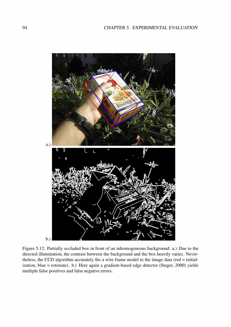
94 CHAPTER 5. EXPERIMENTAL EVALUATION
a.)
b.)
Figure 5.12: Partially occluded box in front of an inhomogeneous background: a.) Due to thedirected illumination, the contrast between the background and the box heavily varies. Never-theless, the CCD algorithm accurately fits a wire frame model to the image data (red = initial-ization, blue = estimate). b.) Here again a gradient-based edge detector (Steger, 2000) yieldsmultiple false positives and false negative errors.

5.2. EVALUATION OF THE CCD ALGORITHM 95
iteration 0 (initialization): iteration 1: iteration 2:
iteration 3: iteration 4: iteration 5:
Figure 5.13: Fitting a deformable model with 12 degrees of freedom: Already after 4 iterationsthe initial error is largely reduced.

96 CHAPTER 5. EXPERIMENTAL EVALUATION
5.3 Evaluation of the CCD Tracker
We evaluate the CCD tracker using both semi-synthetic image sequences (section 5.3.2) and
real image sequences (section 5.3.3). In both cases, we compare the performance of the CCD
tracker with other well-known standard trackers.
5.3.1 Compared Trackers
We compare the CCD tracker with different variants of the condensation tracker and the Kalman
tracker (Blake and Isard, 1998). Since the seminal work of Isard and Blake (1996), the conden-
sation tracker represents the state-of-the-art in contour-based tracking.
For the comparison with the CCD tracker, we employ the original implementation of the
condensation tracker developed by Michael Isard. This implementation and an implementation
of the Kalman tracker are part of the Oxford Tracking Library2. In addition, we apply extensions
of these two methods. The original methods perform edge detection on gray values. For color
images, these methods first convert the color values into gray values and then perform edge
detection on the gray values. We apply RGB-variants of the trackers. These variants perform
edge detection directly on the RGB values. The advantage is that edges can be detected even if
no significant gradient of the corresponding gray values is given. The disadvantage is that the
edge detection process is more expensive, since it takes three channels into account.
We run the condensation tracker with different numbers of samples: 10, 100, 1,000, and
10,000 samples. Each of these sample sizes is applied for the RGB variant and the gray value
variant. Additionally, in some cases we even use 100,000 samples for the RGB variant. Further-
more, we apply the RGB variant and the gray value variant of the Kalman tracker. All together
we compare the CCD tracker with 11 different trackers in terms of robustness, accuracy, and
runtime.
5.3.2 Results for Semi-synthetic Image Sequences
In this section, we use semi-synthetic image sequences to compare the CCD tracker with the
other trackers. In most relevant applications, a tracker has to cope with flexible curve models
having multiple degrees of freedom. A rigid object with an arbitrary 3-D pose has 6 degrees
of freedom. For deformable objects, usually much more parameters are required. For example,
for approximating the human body, models with more than 25 degrees of freedom are used
(Aggarwal and Cai, 1999; Deutscher, Blake, and Reid, 2000; MacCormick and Isard, 2000). In2The Oxford Tracking Library is available at http://www.robots.ox.ac.uk/ È vdg/Darling.html .

5.3. EVALUATION OF THE CCD TRACKER 97
this section, we analyze how the performances of the CCD tracker and other trackers depend on
the dimension of the parameter vector.
Generating Image Sequences
We use shape-space models (Blake and Isard, 1998) with different numbers of parameters. Ap-
pendix B.2 explains the foundations of these deformable 2-D models. We start with a model
that has 15 degrees of freedom, two parameters for the 2-D translation and 13 parameters speci-
fying deformations. Using a dynamical model as described in section 4.2, we generate a random
sequence of 200 model parameter vectors defining a sequence of 200 successive shapes. We ob-
tain sequences of less deformable shapes by substituting some or all deformation parameters by
zeros. Thus, we construct sequences of shapes with 2, 3, 4, 5, 7, 10, and 15 degrees of freedom.
For each of the resulting shapes, we generate an ideal mask image according to section 5.2.1.
Figure 5.14 depicts some of the�+� b <'< �NJ3�)ç <'<
mask images.
We use the resulting sequences of masks in order to merge 4 pairs (A to D) of real image
sequences. Figure 5.15 depicts some images of these sequences. The merging is performed
by employing the merging procedure described in section 5.2.1. This yields���3ç � b � image
sequences, each with a length of 200 images which results in b ��� b <'< � × �Yè <'< images. Since
we apply the CCD tracker and 11 other trackers to these image sequences, in this experiment,
we obtain 64,000 individual fits.3
Definition of a failure: We classify a fit as a failure if the error Ï , i.e. the distance between
the correct curve and the estimated curve, exceeds ¹RÊ � Ùpixels. Here, error Ï is defined as
the maximum distance between a point on the correct curve and the corresponding point on the
estimated curve, projected onto the curve normal. The error Ï is given byÏ � ����É � É ` 8 � 9 É �:����c 8 � 9 É � ? �uaÒ� (5.4)
where�
is the ground truth parameter vector and? is the estimated parameter vector. We
evaluate the two curve functions for 200 equally spaced values 9 É . The vector� É denotes the
unit normal vector to the curve at the point 8 � 9 É �:��� .Parameterization: We apply the same parameterization as in variant A, the standard variant,
introduced in section 5.2.1 (see Table 5.1). However, in order to adapt the CCD tracker to
3Due to the very high runtime, we apply the condensation tracker with 100,000 samples only to 12 out of the28 image sequences.

98 CHAPTER 5. EXPERIMENTAL EVALUATION
000 100 199
7
2
15
time
dim
ensi
on o
f par
amet
er v
ecto
r
Figure 5.14: Masks used for generating semi-synthetic image sequences: The masks dependon the time, i.e. the frame number, and on the dimension of the parameter vector defining thedeformations of the shape.
different degrees of freedom, i.e. different dimensions ~ of the model parameter vector�
,
we choose the number T of perpendiculars byT � × � ~ � ×0F (5.5)
Note that more accurate or faster variants of the CCD tracker can be obtained by choosing the
parameters of the tracker according to variant B or variant C (see Table 5.1).
Results
Figure 5.16 shows the failure rates over the dimension of the parameter vector. For dimensions
2 to 10 the CCD tracker achieves an almost perfect result. (Only for dimension 3, the CCD
tracker fails in a single image.) For dimension 15, the CCD tracker fails in 67 images (8.38%).

5.3. EVALUATION OF THE CCD TRACKER 99
fore
grou
nd A
fore
grou
nd B
fore
grou
nd C
fore
grou
nd D
back
grou
nd A
back
grou
nd B
back
grou
nd C
back
grou
nd D
time (image number)
1000 199im
age
sequ
ence
Figure 5.15: From these image sequences, we generate 28 semi-synthetic image sequences eachwith a length of 200 images and a resolution of
è3ç < o çD� < pixels. The images cover a varietyof different textures.

100 CHAPTER 5. EXPERIMENTAL EVALUATION
0
20
40
60
80
100
2 4 6 8 10 12 14
failu
re ra
te in
%
dimension of parameter vector
Kalman (gray values)Kalman (RGB)
Condensation 100 samples (gray values)Condensation 100 samples (RGB)
Condensation 10,000 samples (gray values)Condensation 10,000 samples (RGB)
CCD
Figure 5.16: Failure rate over the dimension of the parameter vector: Up to dimension 10 thefailure rate of the CCD tracker is less than 0.13%. For dimension 15, the CCD tracker fails in8.4% of the images. The other trackers fail for all dimensions at least 9 times more often thanthe CCD tracker.
The other trackers yield much higher failure rates. Due to clutter and texture, the Kalman
tracker fails in more than 80% of the images. The condensation tracker yields a relatively low
failure rate for small dimensions (2 and 3). However, its failure rate rapidly increases with
the dimension of the parameter vector. The trackers using RGB values are clearly more robust
than the corresponding trackers using gray values. For all dimensions the failure rate of the
CCD tracker is at least 9 times lower than the failure rate of the best compared tracker, i.e. the
condensation tracker using 10,000 samples and RGB values. Table 5.4 (page 104) shows the
failure rates in more detail.
Different sample sizes of the condensation tracker yield different failure rates and runtimes.
For dimensions 5, 10, and 15, Figure 5.17 shows the failure rate of the condensation (RGB)
trackers over the runtime. The runtime and the corresponding failure rate of the CCD tracker are

5.3. EVALUATION OF THE CCD TRACKER 101
illustrated in these plots by additional points. For all dimensions, the point characterizing the
performance of the CCD algorithm is clearly below the curve characterizing the condensation
tracker. Thus, given the same runtime, the condensation tracker achieves a much better failure
rate. For dimension 5, the CCD tracker achieves a failure rate of 0.0%. The condensation
tracker with the same runtime fails in about 20% of the images. For dimensions 10 and 15, the
differences between the condensation tracker and the CCD tracker are even larger. Even with a
3 to 7 times higher runtime, the condensation tracker does not achieve a significant reduction of
the failure rate.
Figure 5.18 depicts the error of the CCD tracker and the condensation tracker (RGB, 10,000
samples) over the dimension of the parameter vector. For both trackers, the mean error mono-
tonically increases with the dimension of the parameter vector. The CCD tracker achieves high
sub-pixel accuracy. Up to dimension 7, the mean error of the CCD tracker is not higher than
0.080 pixels. For dimension 15, the mean error is 0.158 pixels. This is a very high accuracy,
given the heavy texture of the images. The condensation tracker is about 12 to 22 times less
accurate.
Table 5.4 shows the failure rate, the mean error, and the standard deviation of the error for
different trackers and different dimensions of the parameter vector. For all dimensions, the CCD
tracker clearly outperforms all other trackers in terms of robustness and accuracy.

102 CHAPTER 5. EXPERIMENTAL EVALUATION
a.) Dimension of the parameter vector: 5
0
20
40
60
80
100
0 2 4 6 8 10 12 14
failu
re ra
te in
%
runtime is seconds
condensation (RGB)
CCD
b.) Dimension of the parameter vector: 10
0
20
40
60
80
100
0 2 4 6 8 10 12 14
failu
re ra
te in
%
runtime is seconds
condensation (RGB)
CCD
c.) Dimension of the parameter vector: 15
0
20
40
60
80
100
0 2 4 6 8 10 12 14
failu
re ra
te in
%
runtime is seconds
condensation (RGB)
CCD
Figure 5.17: Failure rate over runtime for different dimensions of parameter vector: Given thesame runtime, the CCD tracker achieves a much lower failure rate than the condensation tracker.Even with a 3-7 times higher runtime, the failure rate of the condensation tracker still clearlyexceeds the failure rate of the CCD tracker.

5.3. EVALUATION OF THE CCD TRACKER 103
0
0.5
1
1.5
2
2.5
3
2 4 6 8 10 12 14
erro
r in
pixe
ls
dimension of parameter vector
Condensation 10,000 samples (RGB)CCD
Figure 5.18: Error over dimension of parameter vector: The CCD tracker achieves sub-pixelaccuracy. Its average error is less than 0.1 pixels up to dimension 7. For all dimensions, theaverage error of the condensation tracker is more than 10 times higher.

104 CHAPTER 5. EXPERIMENTAL EVALUATION
dimension of parameter vectortracker 2 3 4 5 7 10 15
CCD 00.000.0360.030
00.130.0530.069
00.000.0590.042
00.000.0600.040
00.000.0800.061
00.000.1100.106
08.380.1580.243
Condensation 10,000 sam-ples (RGB)
01.380.6640.478
07.381.0360.640
12.631.2540.707
20.631.3620.702
38.751.5870.691
59.501.8290.703
76.001.9560.720
Condensation 10,000 sam-ples (gray values)
03.880.9490.612
18.751.4100.717
33.131.5950.710
49.631.6530.720
73.631.8960.754
90.501.8360.842
94.881.4540.836
Condensation 1,000 sam-ples (RGB)
01.130.7070.516
09.131.1180.667
19.631.3040.669
27.631.5420.711
53.251.8890.679
75.882.0130.705
90.382.0340.765
Condensation 1,000 sam-ples (gray values)
04.880.9750.623
25.381.4250.713
40.751.7050.710
64.881.7190.731
87.131.8950.761
93.251.7700.805
96.131.5830.769
Condensation 100 samples(RGB)
02.880.8490.584
28.501.3800.723
45.631.7190.691
61.631.8240.683
89.251.9230.621
92.632.0880.734
96.501.9720.809
Condensation 100 samples(gray values)
08.001.1190.657
58.751.6410.705
77.631.8800.707
93.501.6940.867
95.881.5180.748
96.881.8360.816
96.502.0040.815
Condensation 10 samples(RGB)
62.251.2610.722
87.381.7320.752
93.631.8830.673
96.751.4790.737
97.131.8070.870
97.881.7370.779
98.631.9550.786
Condensation 10 samples(gray values)
86.381.3660.729
94.631.7740.730
94.632.0050.659
98.131.5100.765
98.131.6870.836
98.001.8630.795
99.131.5310.824
Kalman (RGB) 83.381.6000.686
89.501.6400.713
90.251.7970.729
93.501.8070.713
94.251.7580.717
95.132.0260.789
95.501.8120.788
Kalman (gray values) 87.501.6840.747
92.881.6790.791
94.001.6570.764
95.001.6260.752
95.381.7630.712
95.381.8640.755
95.501.8250.750
Table 5.4: Performance of different trackers over the dimension of the parameter vector. Eachcell contains: a) the failure rate in %, b) the mean error in pixels, c) the standard deviation of theerror in pixels. The CCD tracker is more than 9 times better in terms of robustness (failure rate)and in terms of accuracy (mean error) than the second best tracker, the condensation trackerwith 10,000 samples using RGB values. The performance of the condensation tracker quicklydeclines with an increasing dimension of the parameter vector.

5.3. EVALUATION OF THE CCD TRACKER 105
Sequences A to D
Let us now briefly discuss the four image sequences (A to D) resulting for the most flexible
shape, i.e. the shape with 15 degrees of freedom. In sequence A, both image regions are heavily
textured. Figure 5.19 (pages 106-107) compares the results of the condensation tracker (RGB,
10,000 samples) and the CCD tracker. The CCD tracker is clearly more robust especially for
those images where the two regions have poor contrast.
In sequence B, the background region shows very dark and very bright pixels, see Fig-
ure 5.20 on pages 108-109. The condensation tracker fails particularly often in images where
salient edges are given that are parallel and close to the correct curve (e.g. images 030 and 130).
The CCD tracker reliably works also in these cases.
In sequence C, the background and the foreground are mainly homogeneous. However,
in several images the RGB values of the background and the foreground are very similar, see
Figure 5.21 on pages 110-111. The CCD tracker copes better with the poor contrast and
localizes the curve with more accuracy than the condensation tracker.
For image sequence D, the CCD tracker accurately tracks the curve for all dimensions up
to and including dimension 10. However, for dimension 15, the CCD tracker looses track
of the curve, see Figure 5.22. Starting in image 134 the error significantly increases. The
magnification depicted in Figure 5.23 on page 115 shows the reason for this failure. Since the
foreground and the background region have locally the same pixel values, the CCD algorithm
fails to accurately estimate the region boundary. The CCD algorithm converges to a wrong
salient edge nearby. In the remainder of the image sequence, the CCD tracker does not find the
correct boundary anymore.

106 CHAPTER 5. EXPERIMENTAL EVALUATION
condensation 10,000 samples (RGB) CCD
error in pixels: 00.34 image: 000 error in pixels: 00.04
error in pixels: 36.53 image: 030 error in pixels: 00.72
error in pixels: 05.25 image: 050 error in pixels: 00.06
continued on next page
Figure 5.19: Image sequence A (15 dimensions): The CCD tracker accurately tracks the shapeeven if the contrast between the two regions is poor (e.g. images 030 and 150).

5.3. EVALUATION OF THE CCD TRACKER 107
continued from previous page
condensation 10,000 samples (RGB) CCD
error in pixels: 24.07 image: 100 error in pixels: 00.09
error in pixels: 41.27 image: 150 error in pixels: 00.52
error in pixels: 21.49 image: 199 error in pixels: 00.18

108 CHAPTER 5. EXPERIMENTAL EVALUATION
condensation 10,000 samples (RGB) CCD
error in pixels: 00.43 image: 000 error in pixels: 00.05
error in pixels: 12.19 image: 030 error in pixels: 00.15
error in pixels: 18.13 image: 070 error in pixels: 00.07
continued on next page
Figure 5.20: Image sequence B (15 dimensions): The CCD tracker is robust against strongedges next to the shape to be tracked (e.g. images 030 and 130).

5.3. EVALUATION OF THE CCD TRACKER 109
continued from previous page
condensation 10,000 samples (RGB) CCD
error in pixels: 26.56 image: 130 error in pixels: 00.07
error in pixels: 02.71 image: 170 error in pixels: 00.05
error in pixels: 02.88 image: 199 error in pixels: 00.08

110 CHAPTER 5. EXPERIMENTAL EVALUATION
condensation 10,000 samples (RGB) CCD
error in pixels: 00.38 image: 000 error in pixels: 00.06
error in pixels: 07.34 image: 080 error in pixels: 00.02
error in pixels: 08.15 image: 090 error in pixels: 00.03
continued on next page
Figure 5.21: Image sequence C (15 dimensions): This sequence has little clutter. However, insome images the contrast is very poor. Again, the CCD tracker is clearly more accurate than thecondensation tracker.

5.3. EVALUATION OF THE CCD TRACKER 111
continued from previous page
condensation 10,000 samples (RGB) CCD
error in pixels: 09.17 image: 120 error in pixels: 00.10
error in pixels: 05.59 image: 160 error in pixels: 00.05
error in pixels: 06.93 image: 199 error in pixels: 00.12

112 CHAPTER 5. EXPERIMENTAL EVALUATION
condensation 10,000 samples (RGB) CCD
error in pixels: 00.34 image: 000 error in pixels: 00.03
error in pixels: 15.02 image: 030 error in pixels: 00.12
error in pixels: 14.34 image: 090 error in pixels: 00.11
continued on next page
Figure 5.22: Image sequence D (15 dimensions): This is the only sequence out of the 28 imagesequences where the CCD tracker fails in keeping track of the shape. Starting in image 134 theerror significantly increases. The magnification depicted in Figure 5.23 shows the reason forthis failure. In the remainder of the image sequence, the CCD tracker does not recover fromthis failure.

5.3. EVALUATION OF THE CCD TRACKER 113
continued from previous page
condensation 10,000 samples (RGB) CCD
error in pixels: 07.23 image: 120 error in pixels: 00.10
error in pixels: 18.24 image: 133 error in pixels: 0.44
error in pixels: 22.26 image: 134 error in pixels: 03.22
continued on next page

114 CHAPTER 5. EXPERIMENTAL EVALUATION
continued from previous page
condensation 10,000 samples (RGB) CCD
error in pixels: 26.25 image: 135 error in pixels: 07.07
error in pixels: 31.47 image: 136 error in pixels: 13.20
error in pixels: 41.96 image: 140 error in pixels: 29.25

5.3. EVALUATION OF THE CCD TRACKER 115
Figure 5.23: Failure of the CCD tracker: The pixels between the arrows belong to the back-ground region. However, their color values fit better to the adjacent foreground region. Hence,the CCD tracker assigns these pixels to the wrong side of the curve. The algorithm converges tothe next salient boundary, the edge of the white region. Due to the small error of about 3 pixels,this wrong solution still complies with the motion model.

116 CHAPTER 5. EXPERIMENTAL EVALUATION
5.3.3 Results for Real Image Sequences
In this section we evaluate the CCD tracker using real images. In order to obtain a quantitative
evaluation of the CCD tracker, at least a rough ground truth is required. For a small number of
images, such a ground truth can be provided manually. However, for image sequences consist-
ing of more than hundred images this is hardly feasible. Therefore, we proceed as follows.
We record a non-moving object, a bottle, with a static camera. During recording, we con-
tinuously change the background and the illumination of the bottle. Then, for the first image,
we manually specify the correct contour of the bottle. Since both the bottle and the camera are
fixed, this contour describes the location of the bottle in the entire image sequence. In order to
obtain a moving contour, we use rectangular sub-images with changing offsets, i.e. we shift the
original images. The offset of the sub-images are random numbers obtained by a 2-D motion
model using an AR process according to section 4.2. This yields a sequence of images with
a moving contour and a given ground truth. However, the contour does not deform. An arbi-
trary motion would result in a deforming contour. Therefore, we fit a curve model to the image
sequences that also allows for deformations.
As in section 5.3.2, we describe the contour by a shape-space model. We use a planar affine
shape-space, which has six degrees of freedom, two translation parameters and four parameters
defining the deformation (including size and orientation). Appendix B.2 (page 138) gives a
description of planar affine shape-spaces. Additionally, we apply curve models with less degrees
of freedom. By reducing the number of possible deformations, we obtain less flexible curve
models with 2, 3, 4, and 5 degrees of freedom.
Figure 5.24 shows the failure rate of different trackers over the dimension of the parameter
vector. The CCD tracker is clearly more robust than the other trackers. For more than three
degrees of freedom, the CCD algorithm achieves a 5 to 77 times lower failure rate than the best
compared tracker, the condensation tracker with 10,000 samples using RGB values.
Figure 5.25 shows the fitting result for the curve model with 6 degrees of freedom. The first
and the third columns contain the results of the condensation tracker (10,000 samples, RGB).
The second and fourth columns contain the results of the CCD tracker. The CCD tracker reliably
tracks the contour of the bottle despite the heavy changes of the illumination. The condensation
tracker is frequently distracted by other edges and finally yields a collapsed contour. Figure 5.26
depicts two images for which the CCD tracker yields exceptionally large errors. Even in these
images, the CCD tracker roughly finds the contour of the bottle.

5.3. EVALUATION OF THE CCD TRACKER 117
0
20
40
60
80
100
120
2 2.5 3 3.5 4 4.5 5 5.5 6
failu
re ra
te in
%
dimension of parameter vector
Kalman (gray values)Kalman (RGB)
Condensation 100 samples (gray values)Condensation 100 samples (RGB)
Condensation 10,000 samples (gray values)Condensation 10,000 samples (RGB)
CCD
Figure 5.24: Failure rate over the dimension of the parameter vector (bottle sequence): the CCDtracker is clearly more robust than the other trackers. For dimension 4 to 6, the CCD trackerachieves a 5 to 77 times lower failure rate than the best compared tracker.

118 CHAPTER 5. EXPERIMENTAL EVALUATION
condensation CCD condensation CCDimage 000 image 250
image 050 image 300
image 100 image 350
image 150 image 400
image 200 image 450
Figure 5.25: Bottle sequence: The background of the bottle and the illumination are constantlychanging. Nevertheless, the CCD tracker successfully tracks the contour of the bottle. Thecondensation tracker converges to wrong edges.

5.3. EVALUATION OF THE CCD TRACKER 119
condensation CCDimage 277
error: 190.8 pixels error: 10.2 pixels
image 222error: 5.3 pixels error: 6.2 pixels
Figure 5.26: For these images, the CCD tracker (right column) yields exceptionally large errors.In image 277, the CCD tracker has difficulties finding the bottom of the bottle due to the shadowand the resulting poor contrast. In image 222, the CCD tracker does not accurately find the lidof the bottle. The tracker converges to the much stronger edge caused by the lamp. In bothimages, the condensation tracker (left column) has similar or even greater difficulties.

120 CHAPTER 5. EXPERIMENTAL EVALUATION
5.4 Summary of the Results
In order to evaluate the CCD algorithm, we performed more than 28,000 individual fits, using
different curve models and images, i.e. real and semi-synthetic images. Our experiments show
that the CCD algorithm is very robust. For moderate initial errors, the approach converges to
the correct solution in 99.8 - 100% of the cases, even in the presence of challenging texture.
The CCD algorithm achieves a high level of accuracy; the mean error is 0.0186-0.1088 pixels,
depending on the parameterization. Furthermore, the method can process up to 24 images per
second on a standard PC if the curve has a small number of parameters. The CCD algorithm
allows for a reliable 3-D pose estimation, despite partial occlusion, heavy texture, and poor
contrast.
We compared the CCD tracker with other state-of-the-art trackers. For this comparison
more than 30 different image sequences and more than 65,000 individual fits were used. Our
experiments show that the CCD tracker is clearly more robust than the condensation and the
Kalman tracker. The condensation tracker fails in all experiments at least 5 times (often 20
times) more often than the CCD tracker. Furthermore, the CCD tracker is 12 to 22 times more
accurate. The runtimes of the trackers depend on the parameterization of the algorithms and on
the degrees of freedom of the curve. For a curve with 15 degrees of freedom, the runtime of the
CCD tracker is about 5 seconds per image on a 0.5 GHz computer. Given the same runtime,
the condensation tracker performs clearly worse in terms of robustness and accuracy. While the
CCD tracker is much better at accurately keeping track of the curve, the condensation tracker is
better at finding already lost curves.
The CCD tracker and the condensation tracker show different capabilities to take advantage
of the continuously increasing computing power. Given a longer runtime, the CCD tracker
achieves a substantial improvement in accuracy and robustness. However, the accuracy and the
robustness of the condensation tracker increase only very slowly with the number of samples,
i.e. with the length of the runtime. Hence, given the rapidly increasing computing power of
modern machines, the performance of the CCD tracker improves faster than the performance of
the condensation tracker.

Chapter 6
Conclusion
In this thesis, we propose two novel methods for fitting parametric curve models to images: the
Contracting Curve Density (CCD) algorithm and the CCD tracker. The CCD algorithm fits a
model curve to a single image and the CCD tracker fits a model curve to a sequence of images.
The CCD algorithm contributes to the state-of-the-art in two important ways. First, for the
assessment of a fit between the curve model and the image data, the CCD algorithm employs
a novel likelihood function that can cope with highly inhomogeneous image regions. This ca-
pability is achieved by formulating the likelihood function in terms of local image statistics
that are iteratively learned from the vicinity of the expected curve. The local statistics provide
locally adapted criteria for separating adjacent image regions. This replaces often used prede-
fined fixed criteria, relying on homogeneous image regions or specific edge properties, such as
a particular edge profile or an image gradient exceeding a preset threshold. The second key
contribution is a blurred curve model. This is an efficient means for iteratively optimizing the
posterior density over possible model parameters. Blurred curve models enable the algorithm
to trade-off two conflicting objectives, namely a large area of convergence and a high level of
accuracy.
The CCD tracker employs a fast real-time variant of the CCD algorithm. The method yields
for each iteration step a runtime complexity that is independent of the image resolution. Hence,
it achieves a low runtime even for high-resolution images. The CCD tracker extends the real-
time CCD algorithm by exploiting two kinds of statistical dependencies between successive im-
ages: dependency between successive shapes and dependency between successive pixel values.
By exploiting both kinds of statistical dependencies between successive images, the robustness
of the tracking algorithm is substantially increased. We showed how this improvement can be
achieved without significantly increasing the runtime.
We applied our methods to several image segmentation, 3-D pose estimation, and object
121

122 CHAPTER 6. CONCLUSION
tracking problems. Our experimental analysis demonstrates that the CCD algorithm and the
CCD tracker are capable of achieving high sub-pixel accuracy and robustness even in the pres-
ence of heavy texture, shading, clutter, partial occlusion, poor contrast, and severe changes of
illumination. The mean error of the CCD algorithm is between 0.0186 and 0.1088 pixels, de-
pending on the parameterization of the algorithm. A comparison with different variants of the
state-of-the-art condensation tracker and the Kalman tracker shows that the CCD tracker clearly
outperforms these trackers. The CCD tracker achieved an at least 5 times (usually more than
20 times) lower failure rate and a 12 to 22 times lower mean error. Furthermore, in non-trivial
cases, the CCD tracker proved to be computationally cheaper than the condensation tracker.

Appendix A
Further Results for the Fast CCDAlgorithm
In section 5.2.1 we described an experimental evaluation of the fast CCD algorithm using semi-
synthetic images. Here, we present further results of these experiments. First, in section A.1,
we compare the error histogram of the variant A with the error histograms of variants B-G.
Then, in section A.2, we depict the images for which variant F, the variant fitting the star shape,
performs exceptionally well or badly.
A.1 Error Histograms
Let us now briefly compare the error histogram of variant A with the error histograms of vari-
ants B-G. A detailed description of the different variants is given in section 5.2.1. Figures A.1
and A.2 illustrate, respectively, the error histograms of variant A, i.e. the standard variant, and
variant B, i.e. the more accurate variant using four times as many perpendiculars. Variant B
achieves a clearly higher accuracy. Only in less than 0.3% of all cases the error of variant B
exceeds 0.1 pixels. This is more than 10 times less frequent than for variant A. For variant C,
the faster variant, the histogram is relatively flat, see Figure A.3. Errors larger than 0.2 pix-
els are more than 200 times more likely than for variant A. Figure A.4 shows that variant D,
the variant without outlier treatment, yields more often relatively large errors than variant A.
Therefore, we recommend to use the outlier treatment proposed in section 3.3.2.4.
The last three variants (E-G) do not correspond to different parameters of the CCD algorithm
but to different input data. In variant E the a priori distribution represents a smaller initial
uncertainty. The resulting error histogram is depicted in Figure A.5. It is similar to the error
histogram of variant A. (However, the areas of convergence differ substantially.) Figure A.6
depicts the error histogram for variant F. In this variant the shape to be extracted is not a circle
123

124 APPENDIX A. FURTHER RESULTS FOR THE FAST CCD ALGORITHM
0
5
10
15
20
25
10.63
0.5
21.03
1.5
. . .
. . .
. . .
19.59
2.5
. . .
18.90
3.5
. . .
. . .
11.84
4.5
. . .
. . .
7.15
5.5
. . .
. . .
. . .
2.88
6.5
. . .
. . .
. . .
. . .
2.44
7.5
. . .
. . .
. . .
. . .
. . .
1.88
8.5
. . .
. . .
. . .
. . .
. . .
0.22
9.5. .
. . .
. . .
. . .
. . .
. . .
0.31
10.5
. . .
. . .
. . .
. . .
. . .
0.90
11.5
. . .
. . .
. . .
. . .
. . .
0.09
12.5.
. . .
. . .
. . .
. . .
. . .
0.69
13.5
. . .
. . .
. . .
. . .
. . .
0.06
14.5.
. . .
. . .
. . .
. . .
. . .
0.66
15.5
. . .
. . .
. . .
. . .
. . .
0.34
16.5.
. . .
. . .
. . .
. . .
. . .
0.13
17.5
. . .
. . .
. . .
. . .
. . .
0.00
18.5
. . .
. . .
. . .
. . .
. . .
0.16
19.5
. . .
. . .
. . .
. . .
. . .
0.00
20.5
. . .
. . .
. . .
. . .
. . .
0.03
21.5
. . .
. . .
. . .
. . .
. . .
0.00
22.5
. . .
. . .
. . .
. . .
. . .
0.03Ã 23
. . .
. . .
. . .
. . .
. . .
. . .
. . .
. . .
. . .
. . .
Error in % of a pixel (bin size 1%)
Relative frequency of errors in %
Figure A.1: Error histogram of variant A: For variant A, i.e.the standard variant, in more than96% of all cases the error is less than 0.1 pixels and in more than 99.9% of all cases the error isless than 0.2 pixels. The mean error is 0.0347 pixels and the standard deviation is 0.0281 pixels.
0
5
10
15
20
25
30
35
40
31.51
0.5
34.73
1.5
. . .
. . .
17.63
2.5
. . .
. . .
8.74
3.5
. . .
. . .
. . .
. . .
. . .
3.82
4.5
. . .
. . .
. . .
. . .
. . .
. . .
. . .
1.79
5.5
. . .
. . .
. . .
. . .
. . .
. . .
. . .
. . .
0.16
6.5. .
. . .
. . .
. . .
. . .
. . .
. . .
. . .
. . .
0.19
7.5
. . .
. . .
. . .
. . .
. . .
. . .
. . .
. . .
1.13
8.5
. . .
. . .
. . .
. . .
. . .
. . .
. . .
. . .
0.03
9.5.
. . .
. . .
. . .
. . .
. . .
. . .
. . .
. . .
0.06
10.5
. . .
. . .
. . .
. . .
. . .
. . .
. . .
. . .
0.03
11.5
. . .
. . .
. . .
. . .
. . .
. . .
. . .
. . .
0.13
12.5
. . .
. . .
. . .
. . .
. . .
. . .
. . .
. . .
0.00
13.5
. . .
. . .
. . .
. . .
. . .
. . .
. . .
. . .
0.00
14.5
. . .
. . .
. . .
. . .
. . .
. . .
. . .
. . .
0.00
15.5
. . .
. . .
. . .
. . .
. . .
. . .
. . .
. . .
0.00
16.5
. . .
. . .
. . .
. . .
. . .
. . .
. . .
. . .
0.03
17.5
. . .
. . .
. . .
. . .
. . .
. . .
. . .
. . .
0.00
18.5
. . .
. . .
. . .
. . .
. . .
. . .
. . .
. . .
0.00
19.5
. . .
. . .
. . .
. . .
. . .
. . .
. . .
. . .
0.00
20.5
. . .
. . .
. . .
. . .
. . .
. . .
. . .
. . .
0.00
21.5
. . .
. . .
. . .
. . .
. . .
. . .
. . .
. . .
0.00
22.5
. . .
. . .
. . .
. . .
. . .
. . .
. . .
. . .
0.03Ã 23
. . .
. . .
. . .
. . .
. . .
. . .
. . .
. . .
. . .
. . .
. . .
. . .
. . .
. . .
. . .
. . .
Error in % of a pixel (bin size 1%)
Relative frequency of errors in %
Figure A.2: Error histogram of variant B: For variant B, the more accurate variant, errors ex-ceeding 0.1 pixels are more than 10 times less likely than for variant A. The mean error ofvariant B is 0.0186 pixels and the standard deviation is 0.0231 pixels.

A.1. ERROR HISTOGRAMS 125
0
5
10
15
20
25
5.35
0.5
8.83
1.5
. . .
. . .
. . .
. . .
10.28
2.5
. . .
. . .
. . .
. . .
7.71
3.5
. . .
. . .
. . .
8.16
4.5
. . .
. . .
. . .
. . .
8.04
5.5
. . .
. . .
. . .
. . .
5.80
6.5
. . .
. . .
. . .
. . .
4.19
7.5
. . .
. . .
. . .
. . .
3.73
8.5
. . .
. . .
. . .
. . .
. . .
3.81
9.5
. . .
. . .
. . .
. . .
. . .
2.24
10.5
. . .
. . .
. . .
. . .
. . .
2.61
11.5. . .
. . .
. . .
. . .
. . .
. . .
1.74
12.5
. . .
. . .
. . .
. . .
. . .
1.86
13.5. .
. . .
. . .
. . .
. . .
. . .
1.78
14.5. .
. . .
. . .
. . .
. . .
. . .
0.95
15.5. .
. . .
. . .
. . .
. . .
. . .
1.08
16.5.
. . .
. . .
. . .
. . .
. . .
1.57
17.5.
. . .
. . .
. . .
. . .
. . .
1.66
18.5. .
. . .
. . .
. . .
. . .
. . .
1.24
19.5. .
. . .
. . .
. . .
. . .
. . .
1.16
20.5.
. . .
. . .
. . .
. . .
. . .
1.95
21.5.
. . .
. . .
. . .
. . .
. . .
1.91
22.5. .
. . .
. . .
. . .
. . .
. . .
12.35
à 23. .
. . .
. . .
. . .
. . .
. . .
. . .
. . .
. . .
Error in % of a pixel (bin size 1%)
Relative frequency of errors in %
Figure A.3: Error histogram of variant C: For variant C, the faster variant, relatively large errorsare clearly more likely than for variant A. For example, errors exceeding 0.2 pixels are morethan 200 times more likely than for variant A. The mean error of variant C is 0.1088 pixels andthe standard deviation is 0.1236 pixels.
0
5
10
15
20
25
9.06
0.5
23.41
1.5
. . .
. . .
. . .
. . .
19.23
2.5
. . .
18.94
3.5
. . .
. . .
11.54
4.5
. . .
. . .
6.86
5.5
. . .
. . .
. . .
2.14
6.5
. . .
. . .
. . .
. . .
2.04
7.5. . .
. . .
. . .
. . .
. . .
. . .
2.10
8.5. . .
. . .
. . .
. . .
. . .
. . .
0.22
9.5. . .
. . .
. . .
. . .
. . .
. . .
0.19
10.5
. . .
. . .
. . .
. . .
. . .
1.15
11.5
. . .
. . .
. . .
. . .
. . .
0.06
12.5.
. . .
. . .
. . .
. . .
. . .
0.57
13.5
. . .
. . .
. . .
. . .
. . .
0.06
14.5
. . .
. . .
. . .
. . .
. . .
0.61
15.5
. . .
. . .
. . .
. . .
. . .
0.32
16.5.
. . .
. . .
. . .
. . .
. . .
0.13
17.5
. . .
. . .
. . .
. . .
. . .
0.06
18.5
. . .
. . .
. . .
. . .
. . .
0.16
19.5
. . .
. . .
. . .
. . .
. . .
0.00
20.5
. . .
. . .
. . .
. . .
. . .
0.06
21.5
. . .
. . .
. . .
. . .
. . .
0.03
22.5
. . .
. . .
. . .
. . .
. . .
1.05Ã 23
. . .
. . .
. . .
. . .
. . .
.
. . .
. . .
. . .
. . .
. . .
Error in % of a pixel (bin size 1%)
Relative frequency of errors in %
Figure A.4: Error histogram of variant D: In variant D the outlier treatment is switched off.Without outlier treatment, errors larger than 0.2 pixels are about 20 times more likely than withoutlier treatment. The mean error of variant D is 0.0354 pixels, only slightly higher than forvariant A (0.0347 pixels). However, the standard deviation of 0.0713 pixels is more than 2.5times higher than those of variant A.
but a star-like shape. (The shape will be depicted in section A.2.) Despite the differences in
shape, the errors in variant F and variant A are quite similarly distributed. In variant G the input
images are not perfectly sharp but blurred. Figure A.7 depicts the resulting error histogram.

126 APPENDIX A. FURTHER RESULTS FOR THE FAST CCD ALGORITHM
0
5
10
15
20
25
11.90
0.5
18.49
1.5
. . .
. . .
. . .
19.66
2.5
. . .
. . .
20.51
3.5
. . .
. . .
12.49
4.5
. . .
7.35
5.5
. . .
. . .
. . .
2.39
6.5
. . .
. . .
. . .
. . .
1.67
7.5. . .
. . .
. . .
. . .
. . .
. . .
1.80
8.5. .
. . .
. . .
. . .
. . .
. . .
0.45
9.5. .
. . .
. . .
. . .
. . .
. . .
0.14
10.5
. . .
. . .
. . .
. . .
. . .
0.95
11.5
. . .
. . .
. . .
. . .
. . .
0.09
12.5.
. . .
. . .
. . .
. . .
. . .
0.95
13.5
. . .
. . .
. . .
. . .
. . .
0.00
14.5.
. . .
. . .
. . .
. . .
. . .
0.86
15.5
. . .
. . .
. . .
. . .
. . .
0.14
16.5.
. . .
. . .
. . .
. . .
. . .
0.00
17.5
. . .
. . .
. . .
. . .
. . .
0.05
18.5
. . .
. . .
. . .
. . .
. . .
0.09
19.5
. . .
. . .
. . .
. . .
. . .
0.00
20.5
. . .
. . .
. . .
. . .
. . .
0.05
21.5
. . .
. . .
. . .
. . .
. . .
0.05
22.5
. . .
. . .
. . .
. . .
. . .
0.00Ã 23
. . .
. . .
. . .
. . .
. . .
. . .
. . .
. . .
. . .
. . .
Error in % of a pixel (bin size 1%)
Relative frequency of errors in %
Figure A.5: Error histogram of variant E: For variant E, the variant with a lower initial uncer-tainty, the error is similarly distributed as for variant A. The mean error of variant E is 0.0342pixels and the standard deviation is 0.0265 pixels.
q0
5
10
15
20
25
8.73
0.5
18.20
1.5
. . .
. . .
. . .
. . .22.29
2.5
. . .
. . .
16.21
3.5
. . .
10.20
4.5
. . .
. . .
6.22
5.5
. . .
. . .
. . .
5.18
6.5
. . .
. . .
. . .
. . .
3.22
7.5
. . .
. . .
. . .
. . .
2.26
8.5
. . .
. . .
. . .
. . .
. . .
3.75
9.5. . .
. . .
. . .
. . .
. . .
. . .
1.43
10.5
. . .
. . .
. . .
. . .
. . .
1.43
11.5. .
. . .
. . .
. . .
. . .
. . .
0.10
12.5. .
. . .
. . .
. . .
. . .
. . .
0.07
13.5
. . .
. . .
. . .
. . .
. . .
0.00
14.5
. . .
. . .
. . .
. . .
. . .
0.43
15.5
. . .
. . .
. . .
. . .
. . .
0.07
16.5
. . .
. . .
. . .
. . .
. . .
0.00
17.5
. . .
. . .
. . .
. . .
. . .
0.00
18.5
. . .
. . .
. . .
. . .
. . .
0.00
19.5
. . .
. . .
. . .
. . .
. . .
0.00
20.5
. . .
. . .
. . .
. . .
. . .
0.03
21.5
. . .
. . .
. . .
. . .
. . .
0.00
22.5
. . .
. . .
. . .
. . .
. . .
0.20Ã23
. . .
. . .
. . .
. . .
. . .
. . .
. . .
. . .
. . .
. . .
Error in % of a pixel (bin size 1%)
Relative frequency of errors in %
Figure A.6: Error histogram of variant F: In variant F the shape to be extracted has a muchhigher curvature than in variant A. Nevertheless, the error histograms are relatively similar. Themean error of variant F is 0.0388 pixels and the standard deviation is 0.0292 pixels.
Due to the blurring, very small errors ( � < F < J pixels) are clearly less likely and errors larger
than 0.2 pixels are more likely.

A.2. STAR SHAPE 127
0
5
10
15
20
25
2.24
0.5
16.66
1.5. . .
. . .
. . .
. . .
. . .
. . .
14.86
2.5
. . .
. . .
19.08
3.5
. . .
. . .
. . .22.13
4.5
. . .
. . .
7.02
5.5
. . .
6.30
6.5
. . .
. . .
. . .
. . .
3.56
7.5
. . .
. . .
. . .
. . .
1.42
8.5
. . .
. . .
. . .
. . .
. . .
1.98
9.5. .
. . .
. . .
. . .
. . .
. . .
0.98
10.5. .
. . .
. . .
. . .
. . .
. . .
1.51
11.5.
. . .
. . .
. . .
. . .
. . .
0.03
12.5. .
. . .
. . .
. . .
. . .
. . .
0.03
13.5
. . .
. . .
. . .
. . .
. . .
0.28
14.5
. . .
. . .
. . .
. . .
. . .
0.06
15.5
. . .
. . .
. . .
. . .
. . .
0.91
16.5
. . .
. . .
. . .
. . .
. . .
0.00
17.5.
. . .
. . .
. . .
. . .
. . .
0.00
18.5
. . .
. . .
. . .
. . .
. . .
0.00
19.5
. . .
. . .
. . .
. . .
. . .
0.00
20.5
. . .
. . .
. . .
. . .
. . .
0.00
21.5
. . .
. . .
. . .
. . .
. . .
0.00
22.5
. . .
. . .
. . .
. . .
. . .
0.94Ã 23
. . .
. . .
. . .
. . .
. . .
.
. . .
. . .
. . .
. . .
. . .
Error in % of a pixel (bin size 1%)
Relative frequency of errors in %
Figure A.7: Error histogram of variant G: For variant G the mask image is blurred using aGaussian kernel of window size 0.5 pixels. This simulates the blurring caused by an imagingdevice. Due to the blurring, the mean error increases from 0.0347 pixels to 0.0439 pixels. Thisis a quite small increase compared to the window size of 0.5 pixels. The standard deviation ofthe error increases from 0.0281 pixels to 0.0339 pixels.
A.2 Star Shape
This section shows the images for which variant F of the CCD algorithm performs exceptionally
well or badly. The following images correspond to the images depicted on pages 84 to 87.
However, not the circle but the star-like shape defined by equation (5.3) is used here. Figures A.8
and A.9 depict the images yielding the highest and the lowest failure rate, respectively. For
images where the local distributions have much overlap, the failure rate is about three times
higher than for images, where the local distributions have little overlap. Figures A.10 and A.11
depict the images yielding the highest and the lowest mean error, respectively.

128 APPENDIX A. FURTHER RESULTS FOR THE FAST CCD ALGORITHM
1: failure rate = 51.1 % 2: failure rate = 44.4 %
3: failure rate = 42.2 % 4: failure rate = 42.2 %
5: failure rate = 37.8 % 6: failure rate = 35.6 %
Figure A.8: Images yielding the highest failure rate: In these images, salient edges are givennext to the region boundary, or the histograms of the two regions have a significant overlap.

A.2. STAR SHAPE 129
1: failure rate = 8.9 % 2: failure rate = 13.3 %
3: failure rate = 13.3 % 4: failure rate = 13.3 %
5: failure rate = 13.3 % 6: failure rate= 15.6 %
Figure A.9: Images yielding the lowest failure rate: In these images the histograms of the tworegions have little overlap.

130 APPENDIX A. FURTHER RESULTS FOR THE FAST CCD ALGORITHM
1: mean error in pixels = 0.1116 2: mean error in pixels = 0.1092
3: mean error in pixels = 0.1091 4: mean error in pixels = 0.0915
5: mean error in pixels = 0.0905 6: mean error in pixels = 0.0883
Figure A.10: Images yielding the highest mean error.

A.2. STAR SHAPE 131
1: mean error in pixels = 0.0054 2: mean error in pixels = 0.0093
3: mean error in pixels = 0.0099 4: mean error in pixels = 0.0117
5: mean error in pixels = 0.0135 6: mean error in pixels = 0.0139
Figure A.11: Images yielding the lowest mean error.

132 APPENDIX A. FURTHER RESULTS FOR THE FAST CCD ALGORITHM

Appendix B
Parametric Curve Models
In this appendix we describe classes of parametric curve models, i.e. curve functions 8 � 9 �:��� ,which we employ in our experiments. First, in section B.1, we define image curves as per-
spective projections of rigid 3-D models. Then, in section B.2, we specify image curves by
deformable 2-D models.
B.1 Rigid 3-D Models
In several experiments we estimate the 3-D pose�
of a rigid object by fitting a rigid 3-D model
to the image data. For example, the box in Figure 5.11 (page 93) is described by a wire frame
model consisting of multiple 3-D line segments. For each of the line segments a different curve
function 8 is used. The curve function is obtained by two steps. First, a point on the 3-D line
segment is computed, and then the 3-D point is projected onto the image. Let us start with the
projection. For this step we use a pinhole camera model.
Pinhole Camera Model
Here, we describe the relation between a point on the 3-D curve given in object coordinate Ê�Ëand its corresponding projection given in pixel coordinates 8 . For this projection, we apply the
pinhole camera model , e.g. (Niemann, 1990; Faugeras, 1993). The relation is established in
four steps: First, the object coordinates are transformed into camera coordinates. Second, the
3-D camera coordinates are projected onto the image plane. Third, radial distortions caused
by the lens are modeled. Finally, the radially distorted coordinates are converted into pixel
coordinates.
133

134 APPENDIX B. PARAMETRIC CURVE MODELS
Rigid Transformation
The object coordinates Ê�Ë are transformed into camera coordinates Ê Á using the rigid trans-
formation
Ê Á ��ÌK� � ÊWË c"Í�� F (B.1)
The vectorÍN� � ¹ÏÎ � ¹@Ð � ¹;Ñ �]\ specifies the location of the camera, i.e. the position of the optical
center, in object coordinates. TheÙ o Ù rotation matrix
Ìdescribes the rotation between the
object and the camera coordinate system. AÙ o Ù rotation matrix has only three degrees of
freedom. Several compact representations of a rotation have been proposed, see e.g. (Faugeras,
1993; Shoemake, 1994). We represent a rotation by three Euler angles�0Ò Î � Ò Ð � Ò Ñ �u\ . The rotation
matrixÌ
can be written as the product of three individual rotations:Ì ��Ì Î �<Ò Î ���ÓÌ Ð �<Ò Ð ����Ì Ñ �0Ò Ñ � F (B.2)
Each of the matrixesÌ Î �<Ò Î � , Ì Ð �0Ò Ð � , and
Ì Ñ �0Ò Ñ � defines a rotation about one axis. The three
Euler-angels�0Ò Î � Ò Ð � Ò Ñ � \ specify the angle of the respective rotation. The three rotation ma-
trixes are given by
Ì Î �0Ò Î �M� Âttà J < << Å�Ç Ä �<Ò Î � c Ä � � �<Ò Î �< Ä � � �<Ò Î � Å�Ç Ä �<Ò Î �ÍvuuÎ
(B.3)
Ì Ð �0Ò Ð �M� Âttà Å�Ç Ä �<Ò Ð � < Ä � � �0Ò Ð �< J <c Ä � � �0Ò Ð � < Å�Ç Ä �0Ò Ð �Í uuÎ
(B.4)
Ì Ñ �0Ò Ñ �M� Âttà Å�Ç Ä �0Ò Ñ � c Ä � � �0Ò Ñ � <Ä � � �0Ò Ñ � Å�Ç Ä �0Ò Ñ � << < J Í uuÎ F (B.5)
A rigid transformation is compactly represented by the parameter vector�� � � ¹@Î � ¹@Ð � ¹ÏÑ � Ò Î � Ò Ð � Ò Ñ � \ � (B.6)
which consists of the three elements of the translation vector and the three Euler-angles.

B.1. RIGID 3-D MODELS 135
Perspective Projection
The relation between a 3-D point with camera coordinate Ê Á � � D Î �YD Ð �)D Ñ � \ and its perspective
projection Ô onto the image plane is given by
Ô � ÂÃÖÕ ÎÕ Ð ÍÎ �Ø×D Ñ Âà D ÎD Ð ÍÎ � (B.7)
where × is the focal length of the camera. Due to occlusion, the projection Ô may not be visible
in the image. To deal with the problem of occlusion, for general objects, additional machinery
is needed, which is beyond the scope of this dissertation. In our experiments we use convex
objects that allow for an efficient solution to the occlusion problem.
Radial Distortions
The lens of the camera may cause radial distortions of the image. The relation between the
undistorted coordinates Ô � � Õ Î � Õ Ð �u\ and the corresponding distorted image coordinates ¦ �� ��Î � ��Ð � \ can be approximated by¦ � Âà ��Î��Ð ÍÎ � bJ � � Jâc2ç ô � Õ ZÎ � Õ ZÐ � ÂÃÖÕ ÎÕ Ð ÍÎ � (B.8)
where the distortion parameter ô describes the shape and intensity of the radial distortions.
Some authors use two or even more parameters in order to describe the radial distortions, e.g.
(Niemann, 1990).
Transformation into Pixel Coordinates
The pixel coordinates 8 are obtained from the radially distorted image coordinates ¦ � � �DÎ � ��Ð � \by 8 � Âà �>Î àÙ Î � Û Î�>Ð àÙ Ð � Û Ð ÍÎ � (B.9)
where the step sizes Ù Î and Ù Ð represent the size of the pixels. The point� Û Î �YÛ Ð � \ specifies
the intersection between the optical axis of the camera and the image plane.
Equations (B.1) to (B.9) define the relation between a 3-D point (given in object coordinatesÊWË ) and its projection onto the image plane (given in pixel coordinates 8 ). By proj we denote
the resulting projection function which holds8 � proj� Ê�Ë �Q�>� F (B.10)

136 APPENDIX B. PARAMETRIC CURVE MODELS
Projecting Polyhedral Objects
Based on the projection function, 2-D projections of polyhedral wire frame models can by
obtained. The points P on a straight model line segment are defined by
Ê � 9 ��� Ê Ez� � Jâc 9 � � Ê�Z � 9 � (B.11)
with 9 ^Õ` < �/J:a. The points Ê E and Ê�Z are the end points of the line segment given in object
coordinates. The curve function 8 � 9 �:��� corresponding to the 3-D line segment is given by8 � 9 �:����� proj� Ê � 9 �Q�:��� F (B.12)
Projecting Cylinders and Spheres
We model the mug depicted in Figure 1.2 as a cylinder and the ball depicted in Figure 4.1
as a sphere. For these object a slightly different procedure is required, since the occluding
edges do not correspond to 3-D model curves but rather to surfaces. The contour of the sphere
corresponds to a 3-D circle of tangent points. The tangents are defined by the optical center of
the camera and the sphere. We first determine the 3-D circle of tangent points using the pose
parameters. Then we project the 3-D circle onto the image, see (Hanek et al., 2002b) for more
details. For the cylinder we use a similar approach. The computation of occluding lines of a
cylinder has been addressed in (Hanek, Navab, and Appel, 1999).
B.2 Deformable 2-D Models
In this section, we describe a class of deformable 2-D models called shape-space models. This
representation of curves is used by Blake and Isard (1998). We apply this representation in order
to compare the CCD tracker with the condensation and the Kalman tracker, see section 5.3. The
following review of shape-space models is adapted from Blake and Isard (1998).
Shape-space models define parametric curves 8 � 9 �V� �<Úz� 9 �Q�.Û � 9 ����\ as a pair of two para-
metric B-spline functions, one for theÚ
-coordinate and one for theÛ-coordinate.
B-spline Functions
A B-spline functionÚz� 9 � is constructed as a weighted sum of
ÿ ¿basis functions Ü � � 9 � , Ý ^® < � F F;F � ÿ ¿ c.J ± : Úz� 9 ����ÞEß ë Eö� ê�_ Ú � Ü � � 9 �Q� (B.13)

B.2. DEFORMABLE 2-D MODELS 137
whereÚ � are the weights applied to the respective basis function Ü � � 9 � . This can be written
compactly in matrix notation as Úz� 9 �M� l � 9 � \gà Î � (B.14)
where the vectorà Î is composed of the weights
Ú �à Î � �$Ú _ � Ú E�� F F;F � Ú ÞEß ë Eý� \ (B.15)
and l � 9 � is a vector of basis functions
l � 9 ��� � Üá_ � 9 �Q� Ü E � 9 �Q� F;F F � Ü ÞEß ë E � 9 �[� \ F (B.16)
We use quadratic basis functions as described in (Blake and Isard, 1998).
Spline Curve
A spline curve 8 � 9 � is defined as a pair of two spline functions8 � 9 ��� �<Úz� 9 �Q�.Û � 9 ��� \ F (B.17)
The spline functionsÚz� 9 � and
Û � 9 � denote the pixel coordinates of the curve point 8 � 9 � . A
curve point 8 � 9 � can be expressed compactly in matrix notation:8 � 9 ����â � 9 � à F (B.18)
The spline-vectorà
consists of the weights of the two spline functions, first the weights of theÚ-coordinate, then the weights of the
Û-coordinate:à � � à Î � à Ð � \ F (B.19)
The matrixâ � 9 � contains twice the basis functions l � 9 � , once for each coordinate:â � 9 ��� Âà l � 9 � \ hh l � 9 �u\ ÍÎ F (B.20)
Definition of Shape-space Models
A shape-space is a linear mapping of the curve parameters�
to a spline-vectorà
:à ��ã � � à _ F (B.21)

138 APPENDIX B. PARAMETRIC CURVE MODELS
In the context of shape-space models, the vector of curve parameters�
is called shape-space
vector and theÿZä o ~ matrix
ãis called shape-matrix. The vector
à _ is a template vector
defining a standard or template curve. The shape matrixã
and the shape-space vector�
define linear variations of the template. Usually, the dimensionÿcä
of the shape-space vector�is clearly smaller than the dimension of the spline-vector
à. Hence, the shape-space vector
�represents the curve in a more compact manner than the spline-vector
àdoes.
Based on the desired variations different shape matrixesã
are used. The planar affine
shape-space, which is used in Figure 5.25, has six degrees of freedom. It is given by the
shape-matrix ã � ÂÃ õ h à Î _ h h à Ð _h õ h à Ð _ à Î _ h ÍÎ �(B.22)
where the vectorh
consists ofÿ ¿
zeros and the vector õ consists ofÿ ¿
ones. The vectorsà Î _ andà Ð _ contain the
Ú-coordinates and the
Û-coordinates, respectively, of the template vec-
torà _ . The shape matrix
ãallows for translation (horizontal and vertical), scaling (horizontal,
vertical, and diagonal), and rotation of the template.
Note that the shape-space, i.e. the shape-matrixã
and the template vectorà _ , can also
be learned from characteristic training images using principle component analysis (Blake and
Isard, 1998). The resulting model is similar to a Point Distribution Model (PDM) proposed by
Cootes et al. (1993). The curve model used in Figure 5.13 is based on such a PDM.

Appendix C
Remarks on the Implementation
The CCD algorithm and the CCD tracker are implemented in C++ on an off-the-shelf PC run-
ning Windows NT. Our implementation is optimized for versatility and not for speed. We apply
the library LEDA (http://www.mpi-sb.mpg.de/LEDA/leda.html) which uses double precision.
By using a less general implementation and single precision, presumably a substantial speed-up
can be achieved.
139

140 APPENDIX C. REMARKS ON THE IMPLEMENTATION

Glossary of Notation
SYMBOL MEANING see page�Úan estimate of the quantity
ÚdÚ a prediction of the quantityÚ\
superscript denoting vector / matrix transpose�superscript denoting input data 7,21�model parameter vector to be estimated 7,22? mean vector of
�22A covariance matrix of
�22s state-vector, a pair of two successive parameter vectors 61?�x
mean vector of s 61A xcovariance matrix of s 61 �pixel values (image data) 218 curve function 229 parameter specifying a point on the image curve 22SUT probabilistic assignment of pixel � to one side of the curve 27egT photosensitive area of pixel � 27~ dimension of the model parameter vector
�27~ ·0¸ dimension of the pixel value (number of channels of the image) 75� ZT variance of the curve point next to pixel � 29� T unit normal vector to the curve at the curve point closest to pixel � 28� a pixel in the vicinity of the image curve 8 27� set of pixels in the vicinity of the image curve 8 29ª local statistics (mean vector and covariance matrix) of the pixel values 32 side of the curve,
� ^6®°J'� b�± � 32¬ weight of a pixel used for computing local image statistics ª 32continued on next page
141

142 APPENDIX C. REMARKS ON THE IMPLEMENTATION
SYMBOL MEANING see pagendisplacement to the expected curve 30n
= position along the expected curve 30� Z objective function be be optimized 43� Jacobian matrix of the curve or the objective function 28,47- Hessian matrix of the objective function 47� , � number of the iteration 47}�Vintersection between perpendicular U and the mean curve 55U perpendicular on the curve 55k index indicating a pixel on a perpendicular U 55[ maximum number of pixels per perpendicular 55T number of perpendiculars 55ñlocal statistical moments of the pixel values obtained from one image 37?moments of the pixel values for one perpendicular 57y? moments
?accumulated over time 62w? moments y? predicted (propagated) over time 64wñ predicted moments w? smoothed along the curve 69yñ moments combining predicted moments and moments of the latest image 71� order of the moments,
� � ^6®°J'� b �YÙ ± � 39jtime 60¾ � function evaluating the relation between a pixel and the curve 33¾
= function evaluating the distance along the curve 33í parameter specifying the window size for blurring along the curve 35, 68kdeterministic coefficient matrix in discrete dynamical model 60l stochastic coefficient matrix in discrete dynamical model 60n �<j � motion noise of frame
j60

Bibliography
Aggarwal, J.K. and Q. Cai (1999). Human motion analysis: A review. Computer Vision and
Image Understanding 73(3): 428–440.
Aider, O. A., P. Hoppenot, and E. Colle (2002). A Model to Image Straight Line Matching
Method for Vision-Based Indoor Mobile Robot Self-Location. In Proc. of the IEEE/RSJ Int.
Conf. on Intelligent Robots and Systems, Lausanne, pp. 460–465.
Amini, A.A., T.E. Weymouth, and R.C. Jain (1990). Using dynamic programming for solving
variational problems in vision. IEEE Transactions on Pattern Analysis and Machine Intelli-
gence 12(9): 855–867.
Azarbayejani, A., T. Starner, B. Horowitz, and A.P. Pentland (1993). Visually controlled
graphics. IEEE Transactions on Pattern Analysis and Machine Intelligence 15(6): 602–605.
Baker, S., S.K. Nayar, and H. Murase (1998). Parametric feature detection. International
Journal of Computer Vision 27(1): 27–50.
Ballard, D. H. (1981). Generalizing the hough transform to detect arbitrary shapes. Pattern
Recognition 13(2): 111–122.
Bar-Shalom, Y. and T. Fortmann (1988). Tracking and data association. Academic Press.
Beck, J. V. and K. J. Arnold (1977). Parameter Estimation in Engineering and Science. John
Wiley and Sons, New York.
Belongie, S., C. Carson, H. Greenspan, and J. Malik (1998). Color- and texture-based image
segmentation using the expectation-maximization algorithm and its application to content-
based image retrieval. In Proc. of the IEEE Int. Conf. on Computer Vision, pp. 675–682.
Bennett, J. and A. Khotanzad (1998). Multispectral random field models for synthesis
and analysis of color images. IEEE Transactions on Pattern Analysis and Machine Intelli-
gence 20(3): 327–332.
143

144 BIBLIOGRAPHY
Bertero, M., T. Poggio, and V. Torre (1988). Ill-posed problems in early vision. Proceedings
of the IEEE 76(8): 869–889.
Black, M.J. (1992). Robust Incremental Optical Flow. Phd thesis, Yale University.
Blake, Andrew and Michael Isard (1998). Active Contours. Springer-Verlag, Berlin Heidelberg
New York.
Boddy, M. and T. Dean (1994). Decision-theoretic deliberation scheduling for problem solving
in time-constrained environments. Artificial Intelligence 67(2): 245–286.
Bongiovanni, G., P. Crescenzi, and C. Guerra (1995). Parallel simulated annealing for shape
detection. Computer Vision and Image Understanding 61(1): 60–69.
Bouman, C. and K. Sauer (1993). A generalized gaussian image model for edge-preserving
map estimation. IEEE Transactions on Image Processing 2(3): 296–310.
Canny, J. (1986). A computational approach to edge detection. IEEE Transactions on Pattern
Analysis and Machine Intelligence 8(6): 679–698.
Chakraborty, A. and J.S. Duncan (1999). Game-theoretic integration for image segmentation.
IEEE Transactions on Pattern Analysis and Machine Intelligence 21(1): 12–30.
Chellappa, R. (1985). Two-dimensional discrete gauss markovian random field models for
image processing. Progress in Pattern Recognition 2: 79–112.
Chesnaud, C., P. Refregier, and V. Boulet (1999). Statistical region snake-based segmenta-
tion adapted to different physical noise models. IEEE Transactions on Pattern Analysis and
Machine Intelligence 21(11): 1145–1157.
Chuang, Y.Y., B. Curless, D.H. Salesin, and R. Szeliski (2001). A bayesian approach to digital
matting. In Proc. of the IEEE Conf. Computer Vision and Pattern Recognition, pp. II:264–271.
Clausi, D.A. and M.E. Jernigan (2000). Designing gabor filters for optimal texture separability.
Pattern Recognition 33(11): 1835–1849.
Cootes, T. F., G. J. Edwards, and C. J. Taylor (1998). Active appearance models. In Proc. of
the European Conf. on Computer Vision, pp. 484–498.
Cootes, T.F., G.J. Edwards, and C.J. Taylor (2001). Active appearance models. IEEE Trans-
actions on Pattern Analysis and Machine Intelligence 23(6): 681–684.

BIBLIOGRAPHY 145
Cootes, T.F., A. Hill, C.J. Taylor, and J. Haslam (1994). The use of active shape models for
locating structure in medical images. Image and Vision Computing 12(6): 355–365.
Cootes, T.F. and C.J. Taylor (2001). On representing edge structure for model matching. In
Proc. of the IEEE Conf. Computer Vision and Pattern Recognition, pp. I:1114–1119.
Cootes, T.F., C.J. Taylor, A. Lanitis, D.H. Cooper, and J. Graham (1993). Building and us-
ing flexible models incorporating grey-level information. In Proc. of the IEEE Int. Conf. on
Computer Vision, pp. 242–246.
Coughlan, J., A.L. Yuille, C. English, and D. Snow (1998). Efficient optimization of a de-
formable template using dynamic programming. In Proc. of the IEEE Conf. Computer Vision
and Pattern Recognition, pp. 747–752.
Cox, I.J., Y. Zhong, and S.B. Rao (1996). Ratio regions: A technique for image segmentation.
In Proc. of the IEEE Int. Conf. on Pattern Recognition, pp. B: 557–564.
Cremers, D., C. Schnorr, and J. Weickert (2001). Diffusion-snakes: Combining statistical
shape knowledge and image information in a variational framework. In Variational and Level
Set Methods in Computer Vision, pp. 137–144.
Davidson, C. and A. Blake (1998). Error-tolerant visual planning of planar grasp. In Proc. of
the IEEE Int. Conf. on Computer Vision, pp. 911–916.
Dempster, A.P., N.M. Laird, and D.B. Rubin (1977). Maximum likelihood from incomplete
data via the EM algorithm. J. R. Statist. Soc. B 39: 1–38.
Deutscher, J., A. Blake, and I.D. Reid (2000). Articulated body motion capture by annealed
particle filtering. In Proc. of the IEEE Conf. Computer Vision and Pattern Recognition,
pp. II: 126–133.
Dierckx, P. (1993). Curve and Surface Fitting with Splines. Oxford University Press, Oxford
New York Tokyo.
Dubuisson-Jolly, M.P. and A. Gupta (2001). Tracking deformable templates using a shortest
path algorithm. Computer Vision and Image Understanding 81(1): 26–45.
Faugeras, O.D. (1993). Three-dimensional computer vision: A geometric viewpoint. MIT
Press p. 302.

146 BIBLIOGRAPHY
Felzenszwalb, P.F. and D.P. Huttenlocher (1998). Image segmentation using local variation.
In Proc. of the IEEE Conf. Computer Vision and Pattern Recognition, pp. 98–104.
Fitzgibbon, A. W., M. Pilu, and R. B. Fisher (1999). Direct least square fitting of ellipses.
IEEE Transactions on Pattern Analysis and Machine Intelligence 21(5): 476–480.
Geiger, D., A. Gupta, L.A. Costa, and J. Vlontzos (1995). Dynamic-programming for detect-
ing, tracking, and matching deformable contours. IEEE Transactions on Pattern Analysis and
Machine Intelligence 17(3): 294–302.
Geman, S. and D. Geman (1984). Stochastic relaxation, gibbs distributions, and the
bayesian restoration of images. IEEE Transactions on Pattern Analysis and Machine Intel-
ligence 6(6): 721–741.
Hadamard, J. (1902). Sur les problemes aux derivees partielles et leur signification physique.
Princeton University Bulletin 13: 49–52.
Hanek, R. (2001a). Model-Based Image Segmentation Using Local Self-Adapting Separation
Criteria. In Radig, B. and S. Florczyk, editors, 23. DAGM Symposium, LNCS 2191, pp. 1–8,
Munich, Germany. Springer.
Hanek, R. (2001b). The Contracting Curve Density Algorithm and its Application to Model-
based Image Segmentation. In Proc. of the IEEE Conf. Computer Vision and Pattern Recog-
nition, pp. I:797–804.
Hanek, R. and M. Beetz (2004). The contracting curve density algorithm: Fitting parametric
curve models to images using local self-adapting separation criteria. International Journal of
Computer Vision 59(3): 233–258.
Hanek, R., N. Navab, and M. Appel (1999). Yet another method for pose estimation: A
probabilistic approach using points, lines, and cylinders. In Proc. of the IEEE Conf. Computer
Vision and Pattern Recognition, pp. II:544–550.
Hanek, R. and T. Schmitt (2000). Vision-Based Localization and Data Fusion in a System of
Cooperating Mobile Robots. In Proc. of the IEEE/RSJ Int. Conf. on Intelligent Robots and
Systems, pp. 1199–1204.
Hanek, R., T. Schmitt, S. Buck, and M. Beetz (2002a). Fast Image-based Object Localization
in Natural Scenes. In Proc. of the IEEE/RSJ Int. Conf. on Intelligent Robots and Systems,
Lausanne, pp. 116–122.

BIBLIOGRAPHY 147
Hanek, R., T. Schmitt, S. Buck, and M. Beetz (2002b). Towards RoboCup without Color
Labeling. In RoboCup International Symposium, Fukuoka, Japan, pp. 179–194. Springer.
Hanek, R., T. Schmitt, M. Klupsch, and Buck S. (2000). From Multiple Images to a Consistent
View. In RoboCup International Symposium, Melbourne, Australia, pp. 288–296. Springer.
Hansen, C. (2002). Modellgetriebene Verfolgung formvariabler Objekte in Videobildfolgen.
Dissertation, Technische Universitat Munchen.
Harris., C. (1992). Tracking with rigid models. In Blake, A. and A. Yuille, editors, Active
Vision, pp. 59–73. MIT Press.
Herlin, I. L. and N. Ayache (1992). Feature extraction and analysis methods for sequences of
ultrasound images. Image and Vision Computing 10(10): 673–682.
Hermes, L., T. Zoller, and J.M. Buhmann (2002). Parametric distributional clustering for
image segmentation. In Proc. of the European Conf. on Computer Vision, Vol. 3, pp. 577–591.
Horn, B.K.P. and B.G. Schunck (1981). Determining optical flow. Artificial Intelli-
gence 17: 185–203.
Hough, P. V. (1962). Method and means for recognizing complex patterns. U.S. Patent
3069654.
Huang, P. S. (2001). Automatic gait recognition via statistical approaches for ex-
tended template features. IEEE Transactions on Systems, Man, and Cybernetics, Part
B:Cybernetics 31(5): 818–824.
Huber, P. (1981). Robust Statistics. John Wiley and Sons, New York.
Isard, M. and A. Blake (1996). Contour tracking by stochastic propagation of conditional
density. In Proc. of the European Conf. on Computer Vision, pp. I:343–356.
Jones, T.D. and P. Plassmann (2000). An active contour model for measuring the area of leg
ulcers. IEEE Transactions on Medical Imaging 19(12): 1202–1210.
Jones, T.N. and D.N. Metaxas (1998). Image segmentation based on the integration of pixel
affinity and deformable models. In Proc. of the IEEE Conf. Computer Vision and Pattern
Recognition, pp. 330–337.

148 BIBLIOGRAPHY
Kass, M., A.P. Witkin, and D. Terzopoulos (1988). Snakes: Active contour models. Interna-
tional Journal of Computer Vision 1(4): 321–331.
Koller, D., K. Daniilidis, and H.H. Nagel (1993). Model-based object tracking in monoc-
ular image sequences of road traffic scenes. International Journal of Computer Vi-
sion 10(3): 257–281.
Kollnig, H. and H.H. Nagel (1995). 3d pose estimation by fitting image gradients directly to
polyhedral models. In Proc. of the IEEE Int. Conf. on Computer Vision, pp. 569–574.
Konishi, S., A.L. Yuille, J.M. Coughlan, and S.C. Zhu (2003). Statistical edge detection:
learning and evaluating edge cues. IEEE Transactions on Pattern Analysis and Machine Intel-
ligence 25(1): 57–74.
Lanser, S. (1997). Modellbasierte Lokalisation gestutzt auf monokulare Videobilder. Disser-
tation, Technische Universitat Munchen.
Li, P., T. Zhang, and A.E.C. Pece (2003). Visual contour tracking based on particle filters.
Image and Vision Computing 21(1): 111–123.
Li, S.Z. (2001). Markov Random Field Modeling in Image Analysis. Springer-Verlag, Berlin
Heidelberg New York.
Lindeberg, T. (1998). Feature detection with automatic scale selection. International Journal
of Computer Vision 30(2): 79–116.
Lowe, David G. (1991). Fitting parameterized 3-d models to images. IEEE Transactions on
Pattern Analysis and Machine Intelligence 13(5): 441–450.
Lowe, D.G. (1987). Three-dimensional object recognition from single two-dimensional im-
ages. Artificial Intelligence 31: 355–395.
Lowe, D.G. (1992). Robust model-based motion tracking through the integration of search
and estimation. International Journal of Computer Vision 8(2): 113–122.
Luo, H., Q. Lu, R.S. Acharya, and R. Gaborski (2000). Robust snake model. In Proc. of the
IEEE Conf. Computer Vision and Pattern Recognition, pp. I:452–457.
Luong, Q. T. (1993). Color in computer vision. In Chen C. H., Pau L. F., Wang P. S. P., editor,
Handbook of Pattern Recognition and Computer Vision, pp. 311–368. World Scientific.

BIBLIOGRAPHY 149
MacCormick, J.P. and M. Isard (2000). Partitioned sampling, articulated objects, and interface-
quality hand tracking. In Proc. of the European Conf. on Computer Vision, pp. II: 3–19.
Malik, J., S. Belongie, J. Shi, and T. Leung (1999). Textons, contours and regions: Cue integra-
tion in image segmentation. In Proc. of the IEEE Int. Conf. on Computer Vision, pp. 918–925.
Manduchi, R. (1999). Bayesian fusion of color and texture segmentations. In Proc. of the
IEEE Int. Conf. on Computer Vision, pp. 956–962.
McInerney, T. and D. Terzopoulos (1996). Deformable models in medical image analysis: a
survey. Medical Image Analysis 1(2): 91–108.
Mirmehdi, M. and M. Petrou (2000). Segmentation of color textures. IEEE Transactions on
Pattern Analysis and Machine Intelligence 22(2): 142–159.
Mortensen, E.N. and W.A. Barrett (1998). Interactive segmentation with intelligent scissors.
Graphical Models and Image Processing 60(5): 349–384.
Nalwa, V.S. and T.O. Binford (1986). On detecting edges. IEEE Transactions on Pattern
Analysis and Machine Intelligence 8(6): 699–714.
Niemann, H. (1990). Pattern Analysis and Understanding. Springer, Heidelberg.
Panjwani, D.K. and G. Healey (1995). Markov random-field models for unsupervised seg-
mentation of textured color images. IEEE Transactions on Pattern Analysis and Machine
Intelligence 17(10): 939–954.
Paragios, N. and R. Deriche (2000). Coupled geodesic active regions for image segmentation:
A level set approach. In Proc. of the European Conf. on Computer Vision, pp. 224–240.
Pece, A. E. C. (2003). The Kalman-EM contour tracker. In Proc. 3rd workshop on Statistical
and Computational Theories of Vision:SCTV 2003.
Pece, A.E.C. and A.D. Worrall (2002). Tracking with the EM contour algorithm. In Proc. of
the European Conf. on Computer Vision, pp. I: 3–17.
Phong, T.Q., R. Horaud, A. Yassine, and P.D. Tao (1995). Object pose from 2-d to 3-d point
and line correspondences. International Journal of Computer Vision 15: 225–243.
Portilla, J. and E.P. Simoncelli (2000). A parametric texture model based on joint statistics of
complex wavelet coefficients. International Journal of Computer Vision 40(1): 49–70.

150 BIBLIOGRAPHY
Press, W. H., S. A. Teukolsky, W. T. Vetterling, and B. P. Flannery (1996). Numerical Recipes
in C. Cambridge University Press, Cambridge.
Rimon, E. and A. Blake (1996). Caging 2d bodies by 1-parameter two-fingered gripping
systems. In Proc. of the IEEE Int. Conf. on Robotics and Automation, pp. 1458–1464.
Robert, L. (1996). Camera calibration without feature extraction. Computer Vision and Image
Understanding 63(2): 314–325.
Ronfard, R. (1994). Region-based strategies for active contour models. International Journal
of Computer Vision 13(2): 229–251.
Ruzon, M.A. and C. Tomasi (2000). Alpha estimation in natural images. In Proc. of the IEEE
Conf. Computer Vision and Pattern Recognition, pp. I:18–25.
Ruzon, M.A. and C. Tomasi (2001). Edge, junction, and corner detection using color distribu-
tions. IEEE Transactions on Pattern Analysis and Machine Intelligence 23(11): 1281–1295.
Schmitt, T., R. Hanek, M. Beetz, S. Buck, and B. Radig (2002). Cooperative probabilistic state
estimation for vision-based autonomous mobile robots. IEEE Transactions on Robotics and
Automation 18(5): 670–684.
Sclaroff, S. and L. Liu (2001). Deformable shape detection and description via model-
based region grouping. IEEE Transactions on Pattern Analysis and Machine Intelli-
gence 23(5): 475–489.
Shi, J. and J. Malik (2000). Normalized cuts and image segmentation. IEEE Transactions on
Pattern Analysis and Machine Intelligence 22(8): 888–905.
Shoemake, Ken (1994). Euler angle conversion. In Heckbert, Paul, editor, Graphics Gems IV,
pp. 222–229. Academic Press, Boston.
Siebel, N. T. (2003). Design and Implementation of People Tracking Algorithms for Visual
Surveillance Applications. Phd thesis, Department of Computer Science, The University of
Reading.
Steger, C. (2000). Subpixel-precise extraction of lines and edges. International Archives of
Photogrammetry and Remote Sensing XXXIII, part B3: 141–156.

BIBLIOGRAPHY 151
Storvik, G. (1994). A bayesian-approach to dynamic contours through stochastic sam-
pling and simulated annealing. IEEE Transactions on Pattern Analysis and Machine Intel-
ligence 16(10): 976–986.
Sullivan, G.D. (1992). Visual interpretation of known objects in constrained scenes. Phil.
Trans. Roy. Soc. B-337: 361–370.
Sullivan, Steve and Jean Ponce (1998). Automatic model construction and pose estimation
from photographs using triangular splines. IEEE Transactions on Pattern Analysis and Ma-
chine Intelligence 20(10): 1091–1096.
Thirion, B., B. Bascle, V. Ramesh, and N. Navab (2000). Fusion of color, shading and bound-
ary information for factory pipe segmentation. In Proc. of the IEEE Conf. Computer Vision
and Pattern Recognition, pp. II:349–356.
Ulrich, M., C. Steger, A. Baumgartner, and H. Ebner (2001). Real-time object recognition us-
ing a modified generalized Hough transform. In Seyfert, Eckhardt, editor, Photogrammetrie —
Fernerkundung — Geoinformation: Geodaten schaffen Verbindungen, 21. Wissenschaftlich-
Technische Jahrestagung der DGPF, pp. 571–578, Berlin. DGPF.
Weicker, R. (1984). A synthetic systems programming benchmark. Communications of the
ACM 27(10): 1013–1030.
Werman, M. and D. Keren (2001). A bayesian method for fitting parametric and nonpara-
metric models to noisy data. IEEE Transactions on Pattern Analysis and Machine Intelli-
gence 23(5): 528–534.
Wu, Z. and R. Leahy (1993). An optimal graph theoretic approach to data clustering: The-
ory and its application to image segmentation. IEEE Transactions on Pattern Analysis and
Machine Intelligence 15(11): 1101–1113.
Xu, C.Y. and J.L. Prince (1998). Snakes, shapes, and gradient vector flow. IEEE Transactions
on Image Processing 7(3): 359–369.
Yezzi, Jr., A., S. Kichenassamy, A. Kumar, P. Olver, and A. Tannenbaum (1997). A geo-
metric snake model for segmentation of medical imagery. IEEE Transactions on Medical
Imaging 16(2): 199–209.

152 BIBLIOGRAPHY
Yuille, A. and N. Grzywacz (1988). A computational theory for the perception of coherent
visual motion. Nature 333, 6168: 71–74.
Yuille, A.L., D.S. Cohen, and P.W. Hallinan (1992). Feature extraction from faces using
deformable templates. International Journal of Computer Vision 8(2): 99–111.
Zhang, Z. (1997). Parameter estimation techniques: A tutorial with application to conic fitting.
International Journal of Image and Vision Computing 15(1): 59–76.
Zhong, Y., A.K. Jain, and M.P. Dubuisson-Jolly (2000). Object tracking using deformable
templates. IEEE Transactions on Pattern Analysis and Machine Intelligence 22(5): 544–549.
Zhu, S.C. and A. Yuille (1996). Region competition: Unifying snakes, region growing, and
Bayes/MDL for multiband image segmentation. IEEE Transactions on Pattern Analysis and
Machine Intelligence 18(9): 884–900.
Zoller, T., L. Hermes, and J. M. Buhmann (2002). Combined color and texture segmentation
by parametric distributional clustering. In Proc. of the IEEE Int. Conf. on Pattern Recognition,
Vol. 2, pp. 627–630.

Index
accuracy
evaluation of, 77
requirement, 6
any-time
algorithm, 54
property, 7
AR process, see auto-regressive process
assignment of pixel, 27
auto-regressive process, 60
blurred model, 10, 43
camera model, 133
CCD algorithm
real-time, 54
standard variant, 81
dense, 55
fast, see CCD algorithm, real-time
input and output, 21
CCD tracker, 53
coherence of motion, 53
coherence of pixel values, 54, 62
complexity analysis, 72
condensation tracker, 96
confirmation measurement, 59
curve function, 22
curve model, 22
curve-fitting problem, 2
deformable model, 1, 6, 92, 136
failure rate, definition of, 77
failure, definition of, 97
image data, 21
image segmentation, 3
Kalman tracker, 96
matching of features, 17
Newton iteration
modified, 47
original, 47
observation model, 39
outlier treatment, 48
pinhole camera model, 133
pixel value, 21
propagation of pixel values
M-to-one propagation, 66
one-to-one propagation, 64
robustness, 6, 77
RT-CCD algorithm, see CCD algorithm,
real-time
runtime measurement, 78
semi-synthetic images, 78
sequence of images, 60
shape-space models, 97, 136
state-vector, 61
weighting function, 33
153
Copyright © 2022 FDOKUMEN