First experience with portable high-performance geometry ...

First experience with portable high-performance

geometry code on GPU

John Apostolakis1, Marilena Bandieramonte1, Georgios Bitzes1, Gabriele Cosmo1, Johannes deFine Licht1∗, Laurent Duhem3, Andrei Gheata1, Guilherme Lima2, Tatiana Nikitina1, SandroWenzel1†

1CERN, 1211 Geneve 23, Switzerland2Fermilab, Kirk & Pine Rd, Batavia, IL 60510, USA3Intel, 2200 Mission College Blvd., Santa Clara, CA 95054-1549, USA

DOI: http://dx.doi.org/10.3204/DESY-PROC-2014-05/18

The Geant-Vector prototype is an effort to address the demand for increased performance inHEP experiment simulation software. By reorganizing particle transport towards a vector-centric data layout, the projects aims for efficient use of SIMD instructions on modernCPUs, as well as co-processors such as GPUs and Xeon Phi.

The geometry is an important part of particle transport, consuming a significant fraction ofprocessing time during simulation. A next generation geometry library must be adaptableto scalar, vector and accelerator/GPU platforms. To avoid the large potential effort goinginto developing and maintaining distinct solutions, we seek a single code base that can beutilized on multiple platforms and for various use cases.

We report on our solution: by employing C++ templating techniques we can adapt geom-etry operations to SIMD processing, thus enabling the development of abstract algorithmsthat compile to efficient, architecture-specific code. We introduce the concept of modu-lar “backends”, separating architecture specific code and geometrical algorithms, therebyallowing distinct implementation and validation. We present the templating, compila-tion and structural architecture employed to achieve this code generality. Benchmarks ofmethods for navigation in detector geometry will be shown, demonstrating abstracted al-gorithms compiled to scalar, SSE, AVX and GPU instructions. By allowing users to choosethe most suitable type of processing unit for an application or potentially dispatch workdynamically at runtime, we can greatly increase hardware occupancy without inflating thecode base. Finally the advantages and disadvantages of a generalized approach will bediscussed.

1 IntroductionRecent evolution of hardware has seen a reawakened focus on vector processing, a concept thathad otherwise lain dormant outside the world of video games while CPU clock speeds stillrode Moore’s law. Most notable is the surge of interest in general purpose GPU programming(GPGPU), but vector instruction sets have existed on convential CPUs since the introductionof 3DNow! by AMD [3] and SSE by Intel [4] in 1998 and 1999, respectively.

∗Presenting author ([email protected]).†Corresponding author ([email protected]).

1GPUHEP2014 95

Chapter 1

GPU in High-Level Triggers

Convenors:

Ivan KiselDaniel Hugo Campora PerezAndrea Messina

GPUHEP2014 1

The GAP project: GPU applications for High

Level Trigger and Medical Imaging

Matteo Bauce1,2, Andrea Messina1,2,3, Marco Rescigno3, Stefano Giagu1,3, Gianluca Lamanna4,6,Massimiliano Fiorini5

1Sapienza Universita di Roma, Italy2INFN - Sezione di Roma 1, Italy3CERN, Geneve, Switzerland4INFN - Sezione di Frascati, Italy5Universita di Ferrara, Italy6INFN - Sezione di Pisa, Italy


The aim of the GAP project is the deployment of Graphic Processing Units in real-timeapplications, ranging from the online event selection (trigger) in High-Energy Physics tomedical imaging reconstruction. The final goal of the project is to demonstrate that GPUscan have a positive impact in sectors different for rate, bandwidth, and computationalintensity. Most crucial aspects currently under study are the analysis of the total latencyof the system, the algorithms optimisations, and the integration with the data acquisitionsystems. In this paper we focus on the application of GPUs in asynchronous triggersystems, employed for the high level trigger of LHC experiments. The benefit obtainedfrom the GPU deployement is particularly relevant for the foreseen LHC luminosity upgradewhere highly selective algorithms will be crucial to maintain a sustainable trigger rates withvery high pileup. As a study case, we will consider the ATLAS experimental environmentand propose a GPU implementation for a typical muon selection in a high-level triggersystem.

1 Introduction

The Graphic Processing Units (GPU) are commercial devices optimized for parallel computa-tion, which, given their rapidly increasing performances, are being deployed in many generalpurpose application. The GAP project is investigating GPU applications in real-time environ-ments, with particular interest in High Energy Physics (HEP) trigger systems, which will bediscussed in this paper, but also Medical Imaging reconstruction (CT, PET, NMR) discussed in[1]. The different areas of interest span several orders of magnitude in terms of data processing,bandwidth and computational intensity of the executed algorithms, but can all benefit fromthe implementation of the massively parallel architecture of GPUs, optimizing different aspects,in terms of execution speed and complexity of the analyzed events. The trigger system of atypical HEP experiment has a crucial role deciding, based on limited and partial information,whether a particular event observed in a detector is interesting enough to be recorded. Every

GPUHEP2014 1GPUHEP2014 3

experiment is characterised by a limited Data Acquisition (DAQ) bandwidth and disk space forstorage hence needs real-time selections to reduce data throughput selectively. The rejection ofuninteresting events only, is crucial to make an experiment affordable, preserving at the sametime its discovery potential. In this paper we report some results obtained from the inclusion ofGPU in the ATLAS High Level Trigger (HLT); we will focus on the main challenges to deploysuch parallel computing devices in a typical HLT environment and on possible improvements.

2 ATLAS trigger system

The LHC proton-proton accelerator provides collisions at a rate of 40 MHz, which corre-sponds, for events of a typical size of 1-2 MByte, to an input data rate of the order oftens of TB/s. The reduction of this input rate to a sustainable rate to be stored on disk,of the order of ∼100 kHz, is achieved through a hybrid multi-level event selection system.Lower selection stages (Lower Level Triggers) are usually implemented on customized elec-tronics, while HLT are nowadays implemented as software algorithms executed on farms ofcommodity PCs. HLT systems, in particular those of LHC experiments, offer a very chal-lenging environment to test cutting-edge technology for realtime event selection. The LHCupgrade with the consequent increase of instantaneous luminosity and collision pile-up, posesnew challenges for the HLT systems in terms of rates, bandwidth and signal selectivity. Toexploit more complex algorithms aimed at better performances, higher computing capabili-ties and new strategies are required. Moreover, given the tendency of the computing indus-try to move away from the current CPU model towards architectures with high numbers ofsmall cores well suited for vectorial computation, it is becoming urgent to investigate the

Figure 1: A scheme of the ATLAS trigger system; values in redare indicating the data-taking conditions during the first run ofthe LHC (’10-’12) while values in black represents the design con-ditions, expected to be reached during the upcoming run (startingin 2015).

possibility to implement ahigher level of parallelismin the HLT software.

The GAP project isinvestigating the deploy-ment of GPUs for the HLTin LHC experiments, us-ing as a study case theATLAS muon HLT. TheATLAS trigger system isorganized in 3 levels [2],as shown in Figure 1.The first trigger level isbuilt on custom electron-ics, while the second level(L2) and the event filter(EF) are implemented insoftware algorithms exe-cuted by a farm of about1600 PCs with differentXeon processors each with8 to 12 cores. During theRun II of the LHC (ex-

2 GPUHEP2014

MATTEO BAUCE, ANDREA MESSINA, MARCO RESCIGNO, STEFANO GIAGU, . . .

4 GPUHEP2014

pected to start in 2015) the L2 and EF will be merged in a single software trigger level.Currently, a first upgrade is foreseen in 2018 [3], when real-time tracking capabilities will alsobe available, followed by a complete renovation of the trigger and detector systems in 2022.We intend to explore the potential improvements attainable in the near future by deployingGPUs in the ATLAS LVL2 muon trigger algorithms. Such algorithms are now implementedas simplified versions and are based on the execution for a large number of times of the samealgorithms that reconstruct and match segments of particle trajectories in the detector. Thehigh computing capabilities of GPUs would allow the use of refined algorithms with higherselection efficiency, and thus to maintain the sensitivity to interesting physics signals even athigher luminosity.

In the current ATLAS data acquisition framework it is not possible to include directly aparallel computing device; the integration of the GPU in this environment is done through aserver-client structure (Accelerator Process Experiment - APE [4]) that can manage differenttasks and their execution on an external coprocessor, such as the GPU. This implementationis flexible, able to deal with different devices having optimized architecture, with a reducedoverhead. With the help of this structure it is possible to isolate any trigger algorithm andoptimize it for the execution on a GPU (or other parallel architecture device).

This will imply the translation into a parallel computing programming language (CUDA1

[7]) of the original algorithm and the optimization of the different tasks that can be naturallyparallelized. In such a way the dependency of the execution time on the complexity of theprocessed events will be reduced. A similar approach has been investigated in the past for thedeployment of GPUs in different ATLAS algorithms with promising results [5]. The evolutionof the foreseen ATLAS trigger system, that will merge the higher level trigger layers in a uniquesoftware processing stage, can take even more advantage from the use of a GPU since a morecomplex algorithm, with offline-like resolution can be implemented on a thousand-core devicewith significant speedup factors. The timing comparison between the serial and the parallelimplementation of the trigger algorithm is done on the data collected in the past year.

3 Muon reconstruction isolation algorithm

Figure 2: Scheme of the coneused in the muon isolationalgorithm.

The benchmark measurements that has been carried out hasfocused on one of the algorithms developed for muon reconstruc-tion in ATLAS. In the L2 trigger a candidate muon particle is re-constructed combining three different and sequential algorithms:the first one reconstructs a charged particle track segment inthe muon spectrometer [6], a second algorithm matches in spacesuch track segment to a charged particle track reconstructed inthe ATLAS Inner Detector (ID) [6], the third evaluates the en-ergy deposits in the electromagnetic and hadronic calorimeters(ECAL, HCAL) [6], as well as the track density in the detectorregion around the candidate muon trajectory, to check the con-sistency with a muon crossing the whole ATLAS detector. Thisthird step of the muon reconstruction has been considered forour first test deploying a GPU in the ATLAS trigger system.

1We perform the tests described in this article on a server set up for this purpose including an NVIDIAgraphic accelerator, hence the GPU code has been developed in CUDA.

GPUHEP2014 3

THE GAP PROJECT: GPU APPLICATIONS FOR HIGH LEVEL TRIGGER AND MEDICAL . . .

GPUHEP2014 5

The muon isolation algorithm starts from the spatial coordinates of the candidate muon tra-jectory and consider a cone of fixed width ∆R =

√∆φ2 + ∆η2 in the (η,φ) ([6]) space around

such trajectory. In order to pass the muon track isolation requirement there should be only alimited number of tracks in the considered cone, and these must be consistent with backgroundin the inner ATLAS tracking system. The calorimeter isolation is applied summing the energydeposits in the electromagnetic and hadronic calorimeter cells lying within the considered cone,and requiring this is only a small fraction of the estimated candidate muon energy2. Figure 2shows the definition of the cone used to evaluate the muon isolation in the calorimeter and inthe inner detector.

The integration of the GPU and the execution of such algorithm within the ATLAS triggerframework can be summarized in the following steps:

1. retrieve information from the detector: access to the calorimeter cells information;

2. format information needed by the algorithm, namely the cell content, data-taking condi-tions, and calorimeter configuration information, into a memory buffer;

3. transfer the prepared buffer to the server (APE) which handles the algorithm executionand transfer the buffer to the GPU;

4. algorithm execution on the GPU (or on a CPU in the serial version of the algorithm);

5. transfer of the algorithm results through the APE server back into the ATLAS triggerframework;

Figure 3: Measurement of the muon isolationalgorithm execution time using a Nvidia GTXTitan GPU.

Step 1 is the same also in the current im-plementation of the muon isolation algorithm;in the standard ATLAS trigger implementa-tion (serial) this step is followed directly bythe algorithm execution (step 4) on the CPU.Step 2 is needed to optimize the data-transfertoward the GPU; it is important at this stageto convert the object-oriented structures to aplain buffer containing the minimum amountof information needed by the algorithm tominimize the CPU→GPU communication la-tency. Step 3 is implemented through li-braries dedicated to the client-server com-munication, as a part of the APE server.Such server manages the assignement of thetask to the GPU for the execution and waitsto retrieve the results. To accomplish step4, the simple algorithm which evaluates thecalorimeter isolation has been translated intothe cuda language optimizing the manage-ment of the GPU resources in terms of com-puting cuda cores and memory usage. Step

2The requirement on this energy fraction varies depending on the region of the detector and the desiredquality of the reconstructed muon, but this aspect is not relevant for the purpose of these tests.

4 GPUHEP2014


6 GPUHEP2014

5 is implemented within the APE server, sim-ilarly to step 3, and completes the CPU-GPU communication, reporting the algorithm resultsin the original framework.

The measurement of the trigger algorithm execution latency has been performed using aserver machine containing an Intel Xeon E5-2620 CPU and a Nvidia GTX Titan GPU, re-processing a sample of ATLAS recorded data with no dedicated optimization of the machine.Figure 3 shows the execution latency measured for the several steps and their sum. The overallexecution time resulted in being ∆ttotGPU ≈1.2±0.2 ms when using the GPU, with respect to∆ttotCPU ≈0.95±0.15 ms, obtained with the standard execution on CPU. As it is shown in Figure3 the largest fraction of the time (∼ 900 µs) is spent to extract the detector data and convertthem from the object-oriented structure to a flat format which is suitable for the transferto the GPU. This contribution to the latency is independent from the the serial or parallelimplementation of the algorithm, since it’s related to data structure decoding; the currentversion of the ATLAS framework heavily relies on object-oriented structures, which are notthe ideal input for GPUs. The contribution due to the CPU-GPU communication through theclient-server structure is found to be ∆ttrans.GPU ∼250 µs, which is within the typical time budgetof the ATLAS HLT (O(10 ms)). This result confirms the possibility to include GPUs into aHLT system for the execution of parallel algorithms, hence motivates further studies in thisdirection.

4 Conclusions and Perspectives

Figure 4: Isolated single muon trig-ger observed rate as a function ofthe muon transverse momentum (pT ),compared to simulations for the differ-ent expected contributions.

From this first study we succesfully deployed a GPUwithin the ATLAS pre-existing trigger and DAQ frame-work through a flexible client-server scheme. We ob-served that the CPU-GPU communication does notintroduce a dramatic overhead, which is indeed wellwithin the typical execution latencies of software trig-ger algorithms, O(10 ms). This result shows that isfeasible to consider the GPUs as extremely powerfulcomputing devices for the evolution of the current asyn-chronous trigger systems. Most of the execution timeis devoted to the data extraction from object-orientedstructures, which is currently an external constraintfrom the ATLAS trigger framework. This observation,confirmed by similar studies in the ATLAS experiment,focused the attention on this topic; a common effort isongoing to overcome this problem and benefit at mostfrom the GPU computing power. At the moment twoviable approaches are being considered: on one handit’s interesting to consider more complex algorithmsthat can reduce the time spent for data structure han-dling to a negligible fraction; on the other hand it ispossible to handle simpler data structures (raw bytestreams from the detector), bypassing most of the currently existing framework. As an exam-ple of the first approach the possibility to execute at the trigger level, a refined evaluation of

GPUHEP2014 5

THE GAP PROJECT: GPU APPLICATIONS FOR HIGH LEVEL TRIGGER AND MEDICAL . . .

GPUHEP2014 7

the muon isolation, which would be not sustainable in single-threaded execution on a CPU,is currently under investigation. The muon isolation evaluated in the offline data reprocess-ing takes into account also environmental corrections due to multiple interactions leading toadditional noise in the calorimeter and tracking system. Figure 4 shows the trigger rate as afunction of the muon transverse momentum, pT , for the isolated muon trigger in a data-takingperiod during 2012. One can see that a relevant fraction of the trigger rate is due to spuriousevents (multi-jet production). A refined calculation of the muon isolation would reduce suchtrigger rate, maintaining the efficiency for prompt muon reconstruction high .

As a typical scenario for the second approach, it is possible to decode and process simpledata from the muon spectrometer (position and time information) [6] to reconstruct the muontrack segment. A similar strategy has been developed in a standalone test considering trackreconstruction in the ATLAS Inner Detector, with interesting results [5].

5 Acknowledgements

The GAP project and all the authors of this article are partially supported by MIUR undergrant RBFR12JF2Z Futuro in ricerca 2012.

References[1] Proceeding of Estimated speed-up from GPU computation for application to realtime medical imaging from

this same workshop (2014).

[2] ATLAS Collaboration, JINST 3 P08003 (2008).

[3] ATLAS Collaboration, -CERN-LHCC-2011-012 (2012).

[4] The client-server structure is obtained using APE, an ATLAS tool developed independently from thisproject.

[5] D. Emeliyanov, J. Howard, J. Phys.: Conf. Ser. 396 012018 (2012).

[6] ATLAS Collaboration, JINST 3 S08003 (2008).

[7] http://docs.nvidia.com/cuda/cuda-c-programming-guide

6 GPUHEP2014


8 GPUHEP2014

GPU-based quasi-real-time Track Recognition in

Imaging Devices: from raw Data to Particle Tracks

Cristiano Bozza1, Umut Kose2, Chiara De Sio1, Simona Maria Stellacci1

1Department of Physics University of Salerno, Via Giovanni Paolo II 132, 84084 Fisciano, Italy2CERN, 1211 Geneve 23, Switzerland


Nuclear emulsions as tracking devices have been used by recent experiments thanks tofast automatic microscopes for emulsion readout. Automatic systems are evolving towardsGPU-based solutions. Real-time imaging is needed to drive the motion of the microscopeaxes and 3D track recognition occurs quasi-online in local GPU clusters. The algorithmsimplemented in the Quick Scanning System are sketched. Most of them are very generaland might turn out useful for other detectors.

1 Nuclear emulsions as tracking detectors

Figure 1: Nuclear emulsion film.

Figure 2: Nuclear emulsion image. High-energy tracks are orthogonal to plane.

Nuclear emulsions have a long history in high-energy physics and recently experienced revivedinterest in the CHORUS[1], DONUT, PEANUT[2]and OPERA[3] experiments. They provide thebest spatial resolution currently available, of theorder of 0.1 µm. On the other hand, they have notime resolution, recording all charged tracks sincethe time of production until photographic develop-ment. In common setups, a detector is made up ofone or more stacks of films, placed approximatelyorthogonally to the direction of the incoming par-ticles. Each film has two layers of emulsion coat-ing a transparent plastic base (Fig. 1). Typicaldimensions are 50 µm for the thickness of emul-sion layers and 200 µm for the base. A nuclearemulsion contains AgBr crystals in a gel matrix.Charged particles sensitise the crystals by ionisa-tion, producing a latent image. Development ofthe film produces metallic Ag grains in place ofthe latent image, resulting in aligned sequences ofgrains (microtracks), typically 0.3∼1 µm in diam-eter (Fig. 2). In an optical transmission micro-scope, grains appear as dark spots on light background. In white light, the average alignmentresiduals of grains with respect to the straight line fit is of the order of 50 nm. The depth of


field of the optics is usually below 5 µm. The full thickness of the emulsion layer is spannedby moving the optical axis, thus producing optical tomographies with a set of equally spacedplanes (15∼31 usually). The image of a particle track in a focal plane is a single grain, notnecessarily present in each plane (ionisation is a stochastic process). Because the chemicalprocess of development is just faster for sensitised grains, but it occurs in general for everycrystal in a random fashion, many grains appear without having been touched by any particle.Such so-called fog grains are overwhelming in number: as a reference, the ratio of fog grains tomicrotrack grains ranges from 103 through 105. Only 3D alignment is able to single out the fewmicrotrack grains, but also many fake microtracks due to random alignments survive in a singlefilm. Stacking several films allows using coincidence methods to improve background rejection.

It is worth noticing that this resembles the situation of an electronic detector in whichbackground hits due to noise or pile-up overwhelm track hits. Normally, electronic detectorsuse a time trigger to reduce combinatorial complexity, but in emulsion this is not possible.It is reasonable to think that a tracking algorithm working in emulsion finds an even easierenvironment if fed with data from other detectors, such as cloud chambers or planes of siliconpads.

2 Data from nuclear emulsion

A nuclear emulsion film has typically a rectangular shape, spanning several tens of cm in bothdirections. The whole surface is scanned by acquiring optical tomographies in several fields ofview with a repetitive motion. An electronic shutter ensures that images are only negligiblyaffected by motion blur. In the ESS (European Scanning System [4], [5], [6], [7], [8]), developedin the first decade of the 21st century, the XY microscope axes hold steady while the Z axis(optical axis) moves and images are grabbed on the fly and sent to vision processors. Itsevolution, named QSS (Quick Scanning System), moves the X axis continuously. Hence, eachview (an optical tomography) of ESS is a cuboid, whereas those of QSS are skewed prisms.Images are acquired by fast monochromatic sensors (CMOS) mounted on the optical axis,capable of 200∼400 frames per second, each frame being 1∼4 MPixel (or more for futuresensors) using 8 bits/pixel. The resulting data rate ranges from 0.5 GB/s to 2 GB/s. Thelinear size of the image stored in a pixel, with common optics, is of the order of 0.3 µm. Thefull size of the field of view is 400×320 µm2 for ESS, 770×550 µm2 for QSS.

2D image processing used to be shared in the case of ESS by an industrial vision processor(Matrox Odyssey) based on an FPGA and by the host workstation CPU. It consists of severalsubsteps:

1. grey level histogram computation and stretching – used to compensate for varying lightyield of the lamp;

2. FIR (Finite Impulse Response) processing with a 5×5 kernel and comparison of filteroutput to a threshold – selects dark pixels on light background, producing a binary image;

3. reduction of sequences of pixels on horizontal scan lines to segments;

4. reduction of segments in contact on consecutive scan lines to clusters of dark pixels –produces grains to be used for tracking.

In the ESS, steps 1 and 2 are performed on the FPGA-based device. Steps 3 and 4 areexecuted by the host workstation CPU. For the same task, QSS uses a GPU board hosted in

2 GPUHEP2014

CRISTIANO BOZZA, UMUT KOSE, CHIARA DE SIO, SIMONA MARIA STELLACCI

10 GPUHEP2014

the workstation that controls the microscope: common choices are double-GPU boards such asNVidia GeForce GTX 590 or GTX 690. A single board can do everything without interventionof the host workstation CPU. The first 3 steps are quite natural applications for GPU’s. Onesingle GPU can be up to 7 times faster than the Odyssey, reducing the price by an orderof magnitude. Steps 4 and 5 require special attention in code development, because they arereduction operations with an a priori unknown number of output objects. In step 4 each threadtakes care of a single scan line of the image. In step 5 a recursive implementation has beenchosen: at iteration n, the segments on scan line i× 2n are compared to those on line i× 2n− 1and the related dark clusters are merged together. Indeed, steps 4 and 5 are the slowest, andthey define the total processing speed, which is 400 MB/s for GTX 590. The system is scalable,and more GPU boards or more powerful ones can be added if needed. The output of this step is,for each view, a set of clusters of dark pixels on light background, each one being encoded withits X, Y, Z coordinates and size in pixels. Automatic readout uses the distribution of clusters tocontinuously adjust the Z axis drive of the tomography. 60∼124 MB of image data are encodedto 8∼16 MB cluster block, ready for local storage or to be transmitted over the network forfurther processing. In the latter case, a RAM disk area is used as a buffer to distribute data to acluster of GPU’s. Tracking servers and the workload manager provide a command-line interfacefor administration and have an embedded lightweight Web server, originally developed for theSySal project ([7]), that provides a graphical interface for human access and is the backbonefor an HTTP-based network protocol for control messages needed for workload assignment.

Particle tracks can cross the boundary of a view, and tracking must be able to do thesame. The alignment tolerance to recognise real tracks and discard background cannot exceed0.5 µm and is usually smaller. The motion control electronics is capable of position feedback,but triaxial vibrations due to combined motion arise, well beyond 1 µm in a single image.Corrections to raw data are needed before they can be used to recognise microtracks. Somesuch corrections, sketched in Fig. 3, depend on optical aberrations and are systematic effectsthat can be computed off-line from small data-sets and then applied on each incoming clusterblock (view):

1. Spherical aberrations: XY and Z curvature;

2. trapezium distortions: dependence of magnification factor on X and Y;

3. magnification-vs.-Z dependence;

4. camera tilt: rotation in the XY plane;

5. optical axis slant: X-Z and Y-Z couplings due to inclined optical axis.

Figure 3: Optical distortion of emulsion image.

GPUHEP2014 3

GPU-BASED QUASI-REAL-TIME TRACK RECOGNITION IN IMAGING DEVICES: FROM . . .

GPUHEP2014 11

Most of the computing power needed for data correction is taken by other effects thatare purely stochastic: vibrations due to motion, increased by mechanical wear and aging areunpredictable and spoil the alignment of images within the same view and between consecutiveviews. Because the depth-of-field usually exceeds the Z pitch between two images in the samesequence taken while the Z axis moves, a sizable fraction of the dark clusters in one image willappear also in the next. Pattern matching works out the relative shift between the images,usually within 1 µm. This procedure requires scanning a square region of possible values of theplane shift vector. Combinatorial complexity is reduced by arranging clusters in a 2D grid ofcells and considering only pair matching within each cell. The shift vector that maximizes thenumber of combinations is the best approximation of the misalignment between the images.Likewise, despite position feedback of all axes, a whole tomography is misaligned with respectto the next. Film scanning is performed so as to leave 30∼40 µm overlap between adjacentviews. The dark clusters found in the overlap region are used to perform 3D pattern matching,in the same way as for 2D pattern matching. The standard deviation of the distribution ofresiduals is of the order of 150 nm (Fig. 4) for X and Y, and 2.6 µm for Z.

Figure 4: Left: precision of image-to-image alignment in the same tomographic sequence. Right:precision of relative alignment of two tomographic sequences.

3 Track reconstruction

Reconstructing 3D tracks from a set of primitive objects such as emulsion grain images orelectronic detector hits is a common task in high-energy physics. The method depicted inthe following would work in all cases of straight tracks, i.e. absent or weak magnetic field andscattering effects negligible with respect to the granularity of the detector. Because ionisation isa stochastic process, the algorithm does not require that a microtrack has a dark cluster in everyimage; furthermore, the notion of sampling planes is deliberately discarded to keep the algorithmgeneral. It just needs to work on 3D pointlike objects, each having a weight, which correspondsto the number of pixels of the dark cluster in this case (e.g. it may be the deposited energyin a silicon counter). Each pair of dark clusters defines a seed, i.e. a straight line in 3D space;other clusters are expected to be aligned with it within proper tolerance (Fig. 5-left). In thinemulsion layers, microtracks are formed with 6∼40 clusters, depending on the local sensitivity,on statistical fluctuations and on track angle (the wider the inclination with respect to the

4 GPUHEP2014


12 GPUHEP2014

thickness dimension, the longer the path length). Furthermore, high-energy particles ionise lessthan slow ones. Such reasons suggest not to filter out too many possible pairs of clusters as trackseeds, considering all those that are within geometrical acceptance. Physics or experimentalconditions constrain the angular acceptance to a region of interest. Optimum thread allocationto computing cores demands that constraints be enforced constructively instead of generatingall seeds and discarding invalid ones. Dark clusters are arranged in a 2D grid of prisms, eachone spanning the whole emulsion thickness (Fig. 5-right). The angular region of interest isscanned in angular steps. At each step the prisms are generated skewed with the central slopeof the step. This ensures that seeds that are very far from the acceptance window will not evenbe built and followed.

Figure 5: Left: microtrack seeds and grains. Right: 2D grid of prisms to build seeds. A prismcontaining a track is shown darker.

With common operational parameters, the number of useful combinations ranges within107 and 109 per tomographic sequence, depending on the amount of random alignments andfog. For each seed, one thread scans the containing prism to find aligned clusters and buildthe microtrack. This procedure naturally produces clones of the same track, normally in therange 2∼4:1. They are discarded by comparing the geometrical parameters of all neighbormicrotracks, neighborhood being defined by means of a 2D spatial grid.

4 Performances and outlook

Performances in terms of processing time vs. grain or microtrack density has been estimatedusing several NVidia GPU’s. The results are shown in Figures 6, 7, 8 and 9.

Denoting the grain density (grains per tomography) with N , the number of seed combina-tions is of order N2, and the search for clusters to attach to the seed is of order N3. Resultsshow that processing steps of high computational complexity are not overwhelming for typicaloperational conditions.

While one would expect the processing time to scale inversely with the number of availablecores, more recent GPU’s perform proportionally worse than older ones. The reason for that isto be sought mostly in branch divergence, which affects more the multiprocessors with largernumber of cores. In some cases the divergence is due to threads exiting while others keeprunning. This could be eliminated, but it’s not clear whether the additional complications ofcode would pay off. In other cases the divergence is due to the specific coding style used in

GPUHEP2014 5


GPUHEP2014 13

Clusters/View

Time(ms)

GTX780Ti

GTX640

Tesla C2050

GTX690 (1/2)

Figure 6: Absolute time (ms) for cluster correction and alignment. For GTX690, only one GPUis considered.

Cluster processing time / total time

Counts

Figure 7: Fraction of total time used for cluster correction and alignment.

the implementation, and could be reduced by fine-tuning the logic: e.g, the kernel that mergestrack clones takes about 1/3 of the total time, and removing or taming its divergence offersgood chances of overall speed-up. The relative improvements of a GPU-based system overtraditional technologies can effectively be estimated by the cost of hardware. For QSS, takingdata at 40∼90 cm2/h with 1 GTX 590 for cluster recognition + 6 GTX 690 for alignment andtracking costs about 5.5 times less than the hardware of ESS taking data at 20 cm2/h on thesame emulsion films. The power consumption is similar, although it is worth noticing the datataking speed increase. The GPU-based system is also more modular and scalable.

6 GPUHEP2014


14 GPUHEP2014

Log10(Time(ms))

Log10(grains/view)

GTX780Ti

Figure 8: Dependency of tracking time (GTX780Ti) on the number of grain clusters/view (darkclusters with minimum size constraint).

Compute work/109

Tracks/view

GTX780Ti

GTX640

Tesla C2050

GTX690 (1/2)

Figure 9: Compute work (Cores × Clock × Time, arbitrary units) for several boards. ForGTX690, only one GPU is considered.

GPUHEP2014 7


GPUHEP2014 15

References[1] E. Eskut et al., Nucl. Phys. B 793 326 (2008).

[2] A. Aoki et al., New. J. Phys. 12 113028 (2010).

[3] R. Acquafredda et al., J. Inst. 4 P04018 (2009).

[4] N. Armenise et al., Nucl. Inst. Meth. A 552 261 (2005).

[5] L. Arrabito et al., Nucl. Inst. Meth. A 568 578 (2007).

[6] L. Arrabito et al., J. Inst. 2 P05004 (2005).

[7] C. Bozza et al., Nucl. Inst. Meth. A. 703 204 (2013).

[8] M. De Serio et al., Nucl. Inst. Meth. A 554 247 (2005).

8 GPUHEP2014


16 GPUHEP2014

GPGPU for track finding in High Energy Physics

L. Rinaldi1, M. Belgiovine1, R. Di Sipio1, A. Gabrielli1, M. Negrini2, F. Semeria2, A. Sidoti2,S. A. Tupputi3, M. Villa1

1Bologna University and INFN, via Irnerio 46, 40127 Bologna, Italy2INFN-Bologna,v.le Berti Pichat 6/2, 40127 Bologna, Italy3INFN-CNAF,v.le Berti Pichat 6/2, 40127 Bologna, Italy


The LHC experiments are designed to detect large amount of physics events producedwith a very high rate. Considering the future upgrades, the data acquisition rate will be-come even higher and new computing paradigms must be adopted for fast data-processing:General Purpose Graphics Processing Units (GPGPU) is a novel approach based on mas-sive parallel computing. The intense computation power provided by Graphics ProcessingUnits (GPU) is expected to reduce the computation time and to speed-up the low-latencyapplications used for fast decision taking. In particular, this approach could be hence usedfor high-level triggering in very complex environments, like the typical inner tracking sys-tems of the multi-purpose experiments at LHC, where a large number of charged particletracks will be produced with the luminosity upgrade. In this article we discuss a trackpattern recognition algorithm based on the Hough Transform, where a parallel approachis expected to reduce dramatically the execution time.

1 Introduction

Modern High Energy Physics (HEP) experiments are designed to detect large amount of datawith very high rate. In addition to that weak signatures of new physics must be searched incomplex background condition. In order to reach these achievements, new computing paradigmsmust be adopted. A novel approach is based on the use of high parallel computing devices,like Graphics Processing Units (GPU), which delivers such high performance solutions to beused in HEP. In particular, a massive parallel computation based on General Purpose GraphicsProcessing Units (GPGPU) [1] could dramatically speed up the algorithms for charged particletracking and fitting, allowing their use for fast decision taking and triggering. In this paperwe describe a tracking recognition algorithm based on the Hough Transform [2, 3, 4] and itsimplementation on Graphics Processing Units (GPU).

2 Tracking with the Hough Transform

The Hough Transform (HT) is a pattern recognition technique for features extraction in imageprocessing, and in our case we will use a HT based algorithm to extract the tracks parametersfrom the hits left by charged particles in the detector. A preliminary result on this study hasbeen already presented in [5]. Our model is based on a cylindrical multi-layer silicon detector


installed around the interaction point of a particle collider, with the detector axis on the beam-line. The algorithm works in two serial steps. In the first part, for each hit having coordinates(xH , yH , zH) the algorithm computes all the circles in the x−y transverse plane passing throughthat hit and the interaction point, where the circle equation is x2 + y2 − 2Ax − 2By = 0,and A and B are the two parameters corresponding to the coordinates of the circle centre.The circle detection is performed taking into account also the longitudinal (θ) and polar (φ)angles. For all the θ, φ, A, B, satisfying the circle equation associated to a given hit, thecorresponding MH(A,B, θ, φ) Hough Matrix (or Vote Matrix) elements are incremented by one.After computing all the hits, all the MH elements above a given threshold would correspond toreal tracks. Thus, the second step is a local maxima search among the MH elements.

In our test, we used a dataset of 100 simulated events (pp collisions at LHC energy, MinimumBias sample with tracks having transverse momentum pT > 500 MeV), each event containingup to 5000 particle hits on a cylindrical 12-layer silicon detector centred on the nominal collisionpoint. The four hyper-dimensions of the Hough space have been binned in 4× 16× 1024× 1024along the corresponding A,B, θ, φ parameters.

The algorithm performance compared to a χ2 fit method is shown in Fig. 1: the ρ =√A2 +B2 and ϕ = tan−1(B/A) are shown together with the corresponding resolutions.

[m]ρ

0 5 10 15 20 25 30

Entr

ies

1

10

210

310

fit2

χ

Hough Transform

(a)

[rad]ϕ

0 1 2 3 4 5 6

Entr

ies

100

150

200

250

300

350

400(b)

resolutionρ

0.5 0.4 0.3 0.2 0.1 0 0.1 0.2 0.3 0.4 0.5

Entr

ies

0

100

200

300

400

500

600

700

800 (c)

= 11%σ

resolutionϕ

0.1 0.080.060.040.02 0 0.02 0.04 0.06 0.08 0.1

Entr

ies

0200

400600800

100012001400160018002000

(d)

= 0.5%σ

Figure 1: Hough Transform algorithm compared to χ2 fit. (a) ρ distribution; (b) ϕ distribution;(c) ρ resolution; (d) ϕ resolution.

3 SINGLE-GPU implementation

The HT tracking algorithm has been implemented in GPGPU splitting the code in two kernels,for Hough Matrix filling and searching local maxima on it. Implementation has been performedboth in CUDA [1] and OpenCL [6]. GPGPU implementation schema is shown in Fig. 2.

Concerning the CUDA implementation, for the MH filling kernel, we set a 1-D grid overall the hits, the grid size being equal to the number of hits of the event. Fixed the (θ, φ)values, a thread-block has been assigned to the A values, and for each A, the corresponding

2 GPUHEP2014

L. RINALDI, M. BELGIOVINE, R. DI SIPIO, A. GABRIELLI, M. NEGRINI, F. . . .

18 GPUHEP2014

B is evaluated. The MH(A,B, θ, φ) matrix element is then incremented by a unity with anatomicAdd operation. TheMH initialisation is done once at first iteration with cudaMallocHost

(pinned memory) and initialised on device with cudaMemset. In the second kernel, the localmaxima search is carried out using a 2-D grid over the θ, φ parameters, the grid dimensionbeing the product of all the parameters number over the maximum number of threads per block(Nφ×Nθ ×NA×NB)/maxThreadsPerBlock, and 2-D threadblocks, with dimXBlock=NA anddimYBlock=MaxThreadPerBlock/NA. Each thread compares one MH(A,B, θ, φ) element to itsneighbours and, if the biggest, it is stored in the GPU shared memory and eventually transferredback. With such big arrays the actual challenge lies in optimizing array allocation and accessand indeed for this kernel a significant speed up has been achieved by tuning matrix accessin a coalesced fashion, thus allowing to gain a crucial computational speed-up. The OpenCL

Figure 2: GPGPU implementation schema of the two Hough Transform algorithm kernels.

implementation has been done using a similar structure used for CUDA. Since in OpenCL thereis no direct pinning memory, a device buffer is mapped to an already existing memallocatedhost buffer (clEnqueueMapBuffer) and dedicated kernels are used for matrices initialisationin the device memory. The memory host-to-device buffer allocation is performed concurrentlyand asynchronously, saving overall transferring time.

3.1 SINGLE-GPU results

The test has been performed using the NVIDIA [1] GPU boards listed in table 1. The GTX770board is mounted locally on a desktop PC, the Tesla K20 and K40 are installed in the INFN-CNAF HPC cluster.

The measurement of the execution time of all the algorithm components has been carriedout as a function of the number of hits to be processed, and averaging the results over 100independent runs. The result of the test is summarised in Fig. 3. The total execution timecomparison between GPUs and CPU is shown in Fig. 3a, while in Fig. 3b the details about

GPUHEP2014 3

GPGPU FOR TRACK FINDING IN HIGH ENERGY PHYSICS

GPUHEP2014 19

Device NVIDIA NVIDIA NVIDIAspecification GeForce GTX770 Tesla K20m Tesla K40mPerformance (Gflops) 3213 3542 4291Mem. Bandwidth (GB/s) 224.2 208 288Bus Connection PCIe3 PCIe3 PCIe3Mem. Size (MB) 2048 5120 12228Number of Cores 1536 2496 2880Clock Speed (MHz) 1046 706 1502

Table 1: Computing resources setup.

the execution on different GPUs are shown. The GPU execution is up to 15 times faster withrespect to the CPU implementation, and the best result is obtained for the CUDA algorithmversion on the GTX770 device. The GPUs timing are less dependent on the number of the hitswith respect to CPU timing.

The kernels execution on GPUs is even faster with respect to CPU timing, with two ordersof magnitude GPU-CPU speed up, as shown in Figs. 3c and 3e. When comparing the kernelexecution on different GPUs (Figs. 3d) and 3f), CUDA is observed to perform slightly betterthan OpenCL. Figure 3g shows the GPU-to-CPU data transfer timings for all devices togetherwith the CPU I/O timing, giving a clear idea of the dominant part of the execution time.

4 MULTI-GPU implementation

Assuming that the detector model we considered could have multiple readout boards workingindependently, it is interesting to split the workload on multiple GPUs. We have done this bysplitting the transverse plane in four sectors to be processed separately, since the data acrosssectors are assumed to be read-out independently. Hence, a single HT is executed for each sector,assigned to a single GPU, and eventually the results are merged when each GPU finishes itsown process. The main advantage is to reduce the load on a single GPU by using lightweightHough Matrices and output structures. Only CUDA implementation has been tested, using thesame workload schema discussed in Sec. 3, but using four MH(A,B, θ), each matrix processingthe data of a single φ sector.

4.1 MULTI-GPU results

The multi-GPU results are shown in Fig. 4. The test has been carried out in double config-uration, separately, with two NVIDIA Tesla K20 and two NVIDIA Tesla K40. The overallexecution time is faster with double GPUs in both cases, even if timing does not scale withthe number of GPUs. An approximate half timing is instead observed when comparing kernelsexecution times. On the other hand, the transferring time is almost independent on the numberof GPUs, this leading the overall time execution.

4 GPUHEP2014


20 GPUHEP2014

Number of hits

0 1000 2000 3000 4000 5000

Tim

e (

ms)

0

100

200

300

400

500

600(a) Total Execution

Number of hits

0 1000 2000 3000 4000 5000

Tim

e (

ms)

30

35

40

45

50

55

60

65(b) Total Execution (GPUs only)

Number of hits

0 1000 2000 3000 4000 5000

Tim

e (

ms)

2−10

1−10

1

10

210(c) Hough Matrix Filling

Number of hits

0 1000 2000 3000 4000 5000

Tim

e (

ms)

2−10

1−10

1

(d) Hough Matrix Filling (GPUs only)

Number of hits

0 1000 2000 3000 4000 5000

Tim

e (

ms)

50

100

150

200

250

300(e) Local Maxima Search

Number of hits

0 1000 2000 3000 4000 5000

Tim

e (

ms)

2

4

6

8

10

12(f) Local Maxima Search (GPUs only)

Number of hits

0 1000 2000 3000 4000 5000

Tim

e (

ms)

10

20

30

40

50

60(g) Data Transfer CPU intel i7

GeForce GTX770 CUDA

Tesla K20m CUDA

Tesla K40m CUDA

GeForce GTX770 OpenCL

Tesla K20m OpenCL

Tesla K40m OpenCL

Figure 3: Execution timing as a function of the number of analysed hits. (a) Total executiontime for all devices; (b) Total execution time for GPU devices only; (c) MH filling time forall devices; (d) MH filling timing for GPU devices only; (e) local maxima search timing for alldevices; (f) local maxima search timing for GPU devices only; (g) device-to-host transfer time(GPUS) and I/O time (CPU).

5 Conclusions

A pattern recognition algorithm based on the Hough Transform has been successfully imple-mented on CUDA and OpenCL, also using multiple devices. The results presented in this papershow that the employment of GPUs in situations where time is critical for HEP, like triggeringat hadron colliders, can lead to significant and encouraging speed-up. Indeed the problem byitself offers wide room for a parallel approach to computation: this is reflected in the resultsshown where the speed-up is around 15 times better than what achieved with a normal CPU.There are still many handles for optimising the performance, also taking into account the GPUarchitecture and board specifications. Next steps of this work go towards an interface to actualexperimental frameworks, including the management of the experimental data structures andtesting with more graphics accelerators and coprocessor.

References[1] NVidia Corporation URL http://www.nvidia.com/

NVidia Corporation URL http://www.nvidia.com/object/gpu.htmlNVidia Corporation URL http://www.nvidia.com/object/cuda home new.html

[2] P. Hough; 1959 Proc. Int. Conf. High Energy Accelerators and Instrumentation C590914 554558

GPUHEP2014 5

GPGPU FOR TRACK FINDING IN HIGH ENERGY PHYSICS

GPUHEP2014 21

Number of hits

0 1000 2000 3000 4000 5000

Tim

e (

ms)

30

35

40

45

50

55

60

(a) Total Execution

Number of hits

0 1000 2000 3000 4000 5000

Tim

e (

ms)

2−10

1−10

1

(b) Hough Matrix Filling

Tesla K20m Single

Tesla K20m Double

Tesla K40m Single

Tesla K40m Double

Number of hits

0 1000 2000 3000 4000 5000

Tim

e (

ms)

0

1

2

3

4

5

6

7

8

9

10

(c) Local Maxima Search

Number of hits

0 1000 2000 3000 4000 5000

Tim

e (

ms)

20

25

30

35

40

45

50

(d) Data Transfer

Figure 4: Execution timing as a function of the number of the hits for multi-GPU configuration.(a) Total execution time; (b) MH filling timing; (c) local maxima search timing; (d) device-to-host transfer time.

[3] V Halyo et al; 2014 JINST 9 P04005

[4] M R Buckley, V Halyo, P Lujan; 2014 http://arxiv.org/abs/1405.2082P. Hough, 1962, United States Patent 3069654.

[5] S Amerio et al; PoS (TIPP2014) 408

[6] OpenCL, Khronos Group URL https://www.khronos.org/opencl/

6 GPUHEP2014


22 GPUHEP2014

FLES – First Level Event Selection Package for

the CBM Experiment

Valentina Akishina1,2, Ivan Kisel1,2,3, Igor Kulakov1,3, Maksym Zyzak1,3

1Goethe University, Grueneburgplatz 1, 60323 Frankfurt, Germany2FIAS Frankfurt Institute for Advanced Studies, Ruth-Moufang-Str. 1, 60438 Frankfurt, Ger-many3GSI Helmholtz Center for Heavy Ion Research, Planckstr. 1, 64291 Darmstadt, Germany


The CBM (Compressed Baryonic Matter) experiment is a future heavy-ion experimentat the future Facility for Anti-Proton and Ion Research (FAIR, Darmstadt, Germany).First Level Event Selection (FLES) in the CBM experiment will be performed on-lineon a dedicated processor farm. An overview of the on-line FLES processor farm concept,different levels of parallel data processing down to the vectorization, implementation of thealgorithms in single precision, memory optimization, scalability with respect to number ofcores, efficiency, precision and speed of the FLES algorithms are presented and discussed.

1 Introduction

The CBM (Compressed Baryonic Matter) experiment [1] is an experiment being prepared tooperate at the future Facility for Anti-Proton and Ion Research (FAIR, Darmstadt, Germany).Its main focus is the measurement of very rare probes, that requires interaction rates of upto 10 MHz. Together with the high multiplicity of charged particles produced in heavy-ioncollisions, this leads to huge data rates of up to 1 TB/s. Most trigger signatures are complex(short-lived particles, e.g. open charm decays) and require information from several detectorsub-systems.

The First Level Event Selection (FLES) package [2] of the CBM experiment is intended toreconstruct the full event topology including tracks of charged particles and short-lived particles.The FLES package consists of several modules: track finder, track fitter, particle finder andphysics selection. As an input the FLES package receives a simplified geometry of the trackingdetectors and the hits, which are created by the charged particles crossing the detectors. Tracksof the charged particles are reconstructed by the Cellular Automaton (CA) track finder [3] usingto the registered hits. The Kalman filter (KF) based track fit [4] is used for precise estimationof the track parameters. The short-lived particles, which decay before the tracking detectors,can be reconstructed via their decay products only. The KF Particle Finder, which is based onthe KFParticle package [2], is used in order to find and reconstruct the parameters of short-lived particles by combining already found tracks of the long-lived charged particles. The KFParticle Finder also selects particle-candidates from a large number of random combinations.In addition, a module for quality assurance is implemented, that allows to control the qualityof the reconstruction at all stages. It produces an output in a simple ASCII format, that can be


interpreted later as efficiencies and histograms using the ROOT framework. The FLES packageis platform and operating system independent.

The FLES package in the CBM experiment will be performed on-line on a dedicated many-core CPU/GPU cluster. The FLES algorithms have to be therefore intrinsically local andparallel and thus require a fundamental redesign of the traditional approaches to event dataprocessing in order to use the full potential of modern and future many-core CPU/GPU archi-tectures. Massive hardware parallelization has to be adequately reflected in mathematical andcomputational optimization of the algorithms.

2 Kalman Filter (KF) track fit library

Searching for rare interesting physics events, most of modern high energy physics experimentshave to work under conditions of still growing input rates and regularly increasing track mul-tiplicities and densities. High precision of the track parameters and their covariance matricesis a prerequisite for finding rare signal events among hundreds of thousands of backgroundevents. Such high precision is usually obtained by using the estimation algorithms based on theKalman filter (KF) method. In our particular case, the KF method is a linear recursive methodfor finding the optimum estimation of the track parameters, grouped as components into theso-called state vector, and their covariance matrix according to the detector measurements.

The Kalman filter based library for track fitting includes following tracking algorithms:track fit based on the conventional Kalman filter; track fit based on the square root Kalmanfilter; track fit based on the Kalman filter with UD factorization of the covariance matrix; tracksmoother based on the listed above approaches and deterministic annealing filter based on thelisted above track smoothers.

High speed of the reconstruction algorithms on modern many-core computer architecturescan be accomplished by: optimizing with respect to the computer memory, in particular declar-ing all variables in single precision, vectorizing in order to use the SIMD (Single Instruction,Multiple Data) instruction set and parallelizing between cores within a compute node.

Several formulations of the Kalman filter method, such as the square root KF and the UDKF, increase its numerical stability in single precision. All algorithms, therefore, can be usedeither in double or in single precision.

The vectorization and parallelization of the algorithms are done by using of: header files,Vc vector classes, Intel TBB, OpenMP, Intel ArBB and OpenCL.

The KF library has been developed and tested within the simulation and reconstructionframework of the CBM experiment, where precision and speed of the reconstruction algorithmsare extremely important.

When running on CPU the scalability with respect to the number of cores is one of themost important parameters of the algorithm. Figure 1 shows the scalability of the vectorizedKF algorithm. The strong linear behavior shows, that with further increase of the number ofcores on newer CPUs the performance of the algorithm will not degrade and the maximumspeed will be reached. The stair-like dependence appears because of the Intel Hyper-Threadingtechnology, which allows to run two threads per core and gives about 30% of performanceadvantage. The scalability on the Intel Xeon Phi coprocessor is similar to CPU with fourthreads per core running simultaneously.

In case of the graphic cards the set of tasks is divided into working groups and distributedamong compute units (or streaming multiprocessors) by OpenCL and the load of each compute

2 GPUHEP2014

VALENTINA AKISHINA, IVAN KISEL, IGOR KULAKOV, MAKSYM ZYZAK

24 GPUHEP2014

Ivan Kisel, Uni-Frankfurt, FIAS, GSI GPU Workshop, Pisa, 10.09.2014 /18

Full portability of the Kalman filter librarywith H. Pabst (Intel)

6

CBM Kalman Filter Track Fit LibraryCPU Scalability. OpenMP

OpenMP (Open Multi-Processing) - is an API that supports multi-platform shared memory multiprocessing programming in C, C++, and Fortran.

It is an implementation of multithreading, a method of parallelizing whereby a master thread (a series of instructions executed consecutively) forks a specified number of slave threads and a task is divided among them.

Header files + OpenMP Vc Library + OpenMP

Pavel Kisel, LIT JINR

7 26.09.2013

34 tracks/µs

33 tracks/µs

Intel Xeon X5550, 2.67 GHz

Standalone First Level Event Selection Package for the CBM Experiment

First Level Event Selection Challenge in the CBM Experiment

Fixed-target heavy-ion experiment Up to 1000 charged particles/collision Non-homogeneous magnetic field 85% fake combinatorial space points in STS 107 events per second Full event reconstruction is required in the first

trigger level

NVidia GPU on an example of Nvidia GTX480

I. Kisel1,2,3, I. Kulakov1,3, M. Zyzak1,3 (for the CBM Collaboration) 1 – Goethe University Frankfurt, Frankfurt am Main, Germany 2 – FIAS Frankfurt Institute for Advanced Studies, Frankfurt am Main, Germany 3 – GSI Helmholtz Center for Heavy Ion Research, Darmstadt, Germany

Scalability of the Track Fit on Nvidia

Track Fit Quality

Scalability on Other Architectures

Conclusions

The Kalman Filter track fitter for the CBM experiment was implemented for Nvidia GPUs.

The fitter shows high quality of the estimated parameters: momentum resolution is about 1%, pull width is about one, that indicates correctness of the fit.

The implementation shows linear behaviour depending on the number of tracks in the local working group running on the streaming multiprocessor, that indicates no interlocks between cores within one streaming multiprocessor.

Since implementation is based on OpenCL, it can be run also on other processor architectures. The tests shows nice linear scalability on CPUs, Intel Xeon Phi and ATI GPUs.

CBM event reconstruction is based on Kalman Filter and Cellular Automaton algorithms High speed and efficiency of the reconstruction algorithms are required The algorithms have to be highly parallelized and scalable in order to use the full potential of the

modern processors

Simulated central Au-Au collision at 25 AGeV

Kalman Filter (KF) Based Track Fitter

Track fit: 1. Start with an arbitrary initialisation 2. Add one hit after another 3. Improve the state vector 4. Get the optimal parameters after the last hit

• Highly optimised code with respect to time

• Single precision

• Highly parallelised code

UpdateInitialize Propagate Optimal Estimation321 4

Detector layersHits

π(r, C)

r – Track parameters C – Covariance matrix

Initializing

Propagated

Updated

Precision

1

2

3

4

CBM track model: r = x y tx ty q/p !x, y – coordinates tx - slope dx/dz* ty - slope dy/dz q – charge p – momentum *z axis is along the beam line

r = x, y, tx, ty, q/p position, tangent of slopes and charge over momentum

Track state vector in CBM:

The track fit resolution is high, all distributions are unbiased, shape of pulls distribution is Gaussian with a width close to 1.

Nvidia GTX295 Nvidia GTX480

• The SIMD KF package has been implemented with OpenCL to run on Nvidia • OpenCL is a universal parallel language for different types of platforms (CPU, GPU, Cell processors, etc.) • For maximum performance each group of data should contain number of elements dividable by the

number of cores in a streaming multiprocessor

• The code shows linear scalability depending on the number of tracks in a working group sent to one streaming multiprocessor

Streaming multiprocessor

• 480 CUDA-cores

• 1.5 GB GDDR5

• 1401 MHz processor clock

• Cores are organised into streaming multiprocessors - computing units of GPU

• Each streaming multiprocessor contains 32 cores

• Each streaming multiprocessor is equipped with L1 cache for data and instructions common for all its cores

• All cuda-cores are equipped with ALU for calculations with integers and FPU for floating point calculations

• For maximum performance each group of data should contain number of elements dividable by 32 for a full load of the streaming multiprocessor

2 Intel Xeon X5550 CPUs at 2.67 GHz

of 6 6

The platos with smaller slope are caused by hyper threading. """

Number of cores0 10 20 30 40 50 60 70 80

sµ

Trac

ks /

0

10

20

30

40

50

60

70

Number of Logical Cores0 50 100 150 200

sµ

Trac

ks/

0

20

40

60

80

100

120

mic0

Intel Xeon Phi at 1 GHz

Current Results

11

57 tracks/µs

26.09.2013

39 tracks/µs 106 tracks/µs AMD Radeon HD 7970

• Implementation with OpenCL for Nvidia allowed to universalise the code

• The code shows linear scalability on all architectures: CPUs, Intel Xeon Phi, AMD GPUs

33 tracks/µs

Nvidia GTX 480, 700 MHz

Current Results

11

57 tracks/µs

26.09.2013

39 tracks/µs 106 tracks/µs

CPU Scalability. OpenMP

OpenMP (Open Multi-Processing) - is an API that supports multi-platform shared memory multiprocessing programming in C, C++, and Fortran.

It is an implementation of multithreading, a method of parallelizing whereby a master thread (a series of instructions executed consecutively) forks a specified number of slave threads and a task is divided among them.

Header files + OpenMP Vc Library + OpenMP

Pavel Kisel, LIT JINR

7 26.09.2013

34 tracks/µs

54 tracks/µs

AMD Radeon HD 7970, 925 MHz

SIMD KF Scalability on the Phi Coprocessor

707.04.2014

120 tracks/µs

The SIMD Kalman filter track fit shows a strong linear many-core scalability on Intel Xeon Phi 5110P with 240 logical cores

120 tracks/µs

Intel Xeon Phi 5110P, 1 GHz

Figure 1: Portability of the Kalman filter track fit library on different many-core CPU/Phi/GPUarchitectures.

unit is of the particular importance. Each working group is assigned to one compute unit andshould scale within it with respect to the number of tasks in the group. Figure 1 shows thatthe algorithm scales linearly on the graphic cards up to the number of cores in one computeunit (for Nvidia GTX480 — 32, for AMD Radeon HD 7970 — 16). Then the drop appears,because when first 32 (for Nvidia) or 16 (for AMD) tasks are processed, only one task is leftand all other cores of the compute unit are idle. Increasing the number of tasks in the groupfurther the speed reaches the maximum with the number of tasks dividable by the number ofcores in the compute unit. Due to the overhead in tasks distribution the maximum performanceis reached when the number of tasks in the group is two-three times more than the number ofcores.

3 Cellular Automaton (CA) track finder

Every track finder must handle a very specific and complicated combinatorial optimizationprocess, grouping together one- or two-dimensional measurements into five-dimensional tracks.

In the Cellular Automaton (CA) method first (1) short track segments, so-called cells, arecreated. After that the method does not work with the hits any more but instead with thecreated track segments. It puts neighbor relations between the segments according to thetrack model here and then (2) one estimates for each segment its possible position on a track,introducing in such a way position counters for all segments. After this process a set of treeconnections of possible track candidates appears. Then one starts with the segments with thelargest position counters (3) and follows the continuous connection tree of neighbors to collectthe track segments into track candidates. In the last step (4) one sorts the track candidatesaccording to their length and χ2-values and then selects among them the best tracks.

The majority of signal tracks (decay products of D-mesons, charmonium, light vectormesons) are particles with momentum higher than 1 GeV/c originating from the region veryclose to the collision point. Their reconstruction efficiency is, therefore, similar to the efficiencyof high-momentum primary tracks that is equal to 97.1%. The high-momentum secondaryparticles, e.g. in decays of K0

s and Λ particles and cascade decays of Ξ and Ω, are created farfrom the primary vertex, therefore their reconstruction efficiency is lower – 81.2%. Significantmultiple scattering of low-momentum tracks in the material of the detector system and largecurvature of their trajectories lead to lower reconstruction efficiencies of 90.4% for primarytracks and of 51.1% for secondary low-momentum tracks. The total efficiency for all tracks is

GPUHEP2014 3

FLES – FIRST LEVEL EVENT SELECTION PACKAGE FOR THE CBM EXPERIMENT

GPUHEP2014 25

88.5% with a large fraction of low-momentum secondary tracks. The levels of clones (doublefound tracks) and of ghost (wrong) tracks are 0.2% and 0.7% respectively. The reconstructionefficiency of the CA track finder is stable with respect to the track multiplicity.

The high track finding efficiency and the track fit quality are crucial, especially for re-construction of the short-lived particles, which are of the particular interest for the CBM ex-periment. The reconstruction efficiency of short-lived particles depends quadratically on thedaughter track reconstruction efficiency in case of two-particle decays. The situation becomesmore sensitive for decays with three daughters and for decay chains. The level of a combinato-rial background for short-lived particles depends strongly on the track fit quality. The correctestimation of the errors on the track parameters improves distinguishing between the signal andthe background particle candidates, and thus to suppress the background. The ghost (wrong)tracks usually have large errors on the track parameters and therefore are easily combined withother tracks into short-lived particle candidates, thus a low level of ghost tracks is also im-portant to keep the combinatorial background low. As a result, the high track reconstructionefficiency and the low level of the combinatorial background improve significantly the eventreconstruction and selection by the FLES package.

4 4-Dimensional time-based event building

Since resolving different events is a non-trivial task in the CBM experiment, the standardreconstruction routine will include an event building, the process of defining exact borders ofevents within a time-slice and grouping tracks into even-corresponding clusters, which theyoriginate from. For this task an efficient time-based tracking is essential. Since the CA trackfinder is proved to be fast and stable with respect to the track multiplicity, the next step towardsthe time-slice based reconstruction would be the implementation of time measurements.

Time [ns]0 2000 4000 6000 8000 10000

Entr

ies

1

10

210

Time [ns]0 2000 4000 6000 8000 10000

Entr

ies

1

10

210

Figure 2: Part of a time-slice with 100 minimumbias events. With blue color the distribution ofhit time measurements in a time-slice is shown.

Figure 3: Part of a time-slice with 100 mini-mum bias events. With light blue color the initialdistribution of hit measurements is reproduced,black color shows time measurements of recon-structed tracks.

In order to introduce a time measurement into the reconstruction procedure to each min-imum bias event in a 100 events group an event start time was assigned during simulationphase. The start time was obtained with the Poisson distribution, assuming the interaction

4 GPUHEP2014


26 GPUHEP2014

rate of 107 Hz. A time stamp we assign to a certain hit consists of this event start time plusthe time shift due to the time of flight, which is different for all hits. In order to obtain a timemeasurement for a hit we then smear a time stamp according to a Gaussian distribution witha sigma value of the detector resolution of 5 ns.

After introducing the time measurement we can use the time information in the CA trackfinder. We do not allow to build triplets out of hits, which time difference is greater than 3σ ofthe detector time resolution. It is a very good approximation, since the time of flight betweenthe detector planes is negligible in comparison to the detection precision. Apart from that, weperform the reconstruction procedure in a regular way. After the reconstruction we assign toeach track a time measurement, which is calculated as an average of its hits measurements.

The initial distribution of hits measurements representing the complexity of defining eventborders in a time-slice at interaction rate of 107 Hz is shown in Fig. 2 with blue color. Theresulting distribution of reconstructed track measurements (black color), as well as the distri-bution of initial hit measurements (light blue color), one can see in Fig. 3. The reconstructedtracks clearly represent groups, which correspond to events, which they originate from.

5 KF Particle Finder – a package for reconstruction ofshort-lived particles

Today the most interesting physics is hidden in the properties of short-lived particles, which arenot registered, but can be reconstructed only from their decay products. A fast and efficientKF Particle Finder package, based on the Kalman filter (hence KF) method, for reconstructionand selection of short-lived particles is developed to solve this task. A search of more than50 decay channels has been currently implemented.

In the package all registered particle trajectories are divided into groups of secondary andprimary tracks for further processing. Primary tracks are those, which are produced directlyin the collision point. Tracks from decays of resonances (strange, multi-strange and charmedresonances, light vector mesons, charmonium) are also considered as primaries, since they areproduced directly at the point of the primary collision. Secondary tracks are produced by theshort-lived particles, which decay not in the point of the primary collision and can be clearlyseparated. These particles include strange particles (K0

s and Λ), multi-strange hyperons (Ξand Ω) and charmed particles (D0, D±, D±

s and Λc). The package estimates the particleparameters, such as decay point, momentum, energy, mass, decay length and lifetime, togetherwith their errors. The package has a rich functionality, including particle transport, calculationof a distance to a point or another particle, calculation of a deviation from a point or anotherparticle, constraints on mass, decay length and production point. All particles produced in thecollision are reconstructed at once, that makes the algorithm local with respect to the data andtherefore extremely fast.

KF Particle Finder shows a high efficiency of particle reconstruction. For example, forthe CBM experiment efficiencies of about 15% for Λ and 5% for Ξ− with AuAu collisions at35 AGeV are achieved together with high signal-to-background ratios (1.3 and 5.9 respectively).

GPUHEP2014 5


GPUHEP2014 27

6 A standalone FLES package for the CBM experiment

The First Level Event Selection (FLES) package of the CBM experiment is intended to re-construct on-line the full event topology including tracks of charged particles and short-livedparticles. The FLES package consists of several modules: CA track finder, KF track fitter, KFParticle Finder and physics selection. In addition, a quality check module is implemented, thatallows to monitor and control the reconstruction process at all stages. The FLES package isplatform and operating system independent.

The FLES package is portable to different many-core CPU architectures. The package isvectorized using SIMD instructions and parallelized between CPU cores. All algorithms areoptimized with respect to the memory usage and the speed.

FLES − a standalone First Level Event Selection package for the CBM experiment

The First Level Event Selection (FLES) package of the CBM experiment is intended to reconstruct on-line the full event topology including tracks of charged particles and short-lived particles. The FLES package consists of several modules (the block diagram is shown on Fig. 14): CA track finder, KF track fitter, KF Particle Finder and physics selection. In addition, a quality check module is implemented, that allows to monitor and control the reconstruction process at all stages. The FLES package is platform and operating system independent.

The FLES package is portable to different many-core CPU architectures. The package is vectorized using SIMD instructions and parallelized between CPU cores. All algorithms are optimized with respect to the memory usage and the speed.

Four servers with Intel Xeon E7-4860, L5640 and X5550 processors and with AMD 6164EH processor have been used for the scalability tests. The AMD server has 4 processors with 12 physical cores each, in total 48 cores. All Intel processors have the hyper-threading technology, therefore each physical core has two logical cores. The most powerful Intel server has 4 processors with 10 physical cores each, that gives 80 logical cores in total.

The FLES package has been parallelized with ITBB implementing the event-level parallelism by executing one thread per one logical core. Reconstruction of 1000 minimum bias Au-Au UrQMD events at 25 AGeV has been processed per each thread. In order to minimize the effect of the operating system each thread is fixed to a certain core using the pthread functionality provided by the C++ standard library. Fig. 15 shows a strong scalability for all many-core systems achieving the reconstruction speed of 1700 events per second on the 80-cores server.

The FLES package in the CBM experiment will be performed for the on-line selection and the off-line analysis on a dedicated many-core CPU/GPU farm. The farm is currently estimated to have a compute power equivalent to 60 000 modern CPU cores. Fig. 16 shows the scalability of the FLES package on with 3 000 cores of the FAIR-Russia HPC cluster (ITEP, Moscow).

!8

Fig. 14: Block diagram of the FLES package, which consists of several modules: track finder, track fitter, particle finder and physics selection.

Fig. 15: Scalability of the FLES package on many-core servers with 16, 24, 48 and 80 logical cores.

Ivan Kisel, FIAS FIAS scientific review, 25.11.2013 /15

Number of Cores0 500 1000 1500 2000 2500 3000

Eve

nts /

s3

10

0

50

100

150

200

250

Number of Nodes0 10 20 30 40 50 60 70 80 90

AMD Opteron 6272, 2.1 GHz

Towards CBM FLES Demonstrator

From cores to the CBM FLES farm with 60 000 cores

• LOEWE CSC (FIAS, Frankfurt) • Green Cube (GSI, Darmstadt) • FAIR-Russia HPC Cluster (ITEP, Moscow)* • HPC Cluster (Intel, Munich)

10

*We expect to have access to 10 000 cores by the end of November 2013

2.2×105 events/s

Fig. 16: Scalability of the FLES package on 3 200 cores of the FAIR-Russia HPC cluster (ITEP, Moscow).

FLES − a standalone First Level Event Selection package for the CBM experiment

The First Level Event Selection (FLES) package of the CBM experiment is intended to reconstruct on-line the full event topology including tracks of charged particles and short-lived particles. The FLES package consists of several modules (the block diagram is shown on Fig. 14): CA track finder, KF track fitter, KF Particle Finder and physics selection. In addition, a quality check module is implemented, that allows to monitor and control the reconstruction process at all stages. The FLES package is platform and operating system independent.

The FLES package is portable to different many-core CPU architectures. The package is vectorized using SIMD instructions and parallelized between CPU cores. All algorithms are optimized with respect to the memory usage and the speed.

Four servers with Intel Xeon E7-4860, L5640 and X5550 processors and with AMD 6164EH processor have been used for the scalability tests. The AMD server has 4 processors with 12 physical cores each, in total 48 cores. All Intel processors have the hyper-threading technology, therefore each physical core has two logical cores. The most powerful Intel server has 4 processors with 10 physical cores each, that gives 80 logical cores in total.

The FLES package has been parallelized with ITBB implementing the event-level parallelism by executing one thread per one logical core. Reconstruction of 1000 minimum bias Au-Au UrQMD events at 25 AGeV has been processed per each thread. In order to minimize the effect of the operating system each thread is fixed to a certain core using the pthread functionality provided by the C++ standard library. Fig. 15 shows a strong scalability for all many-core systems achieving the reconstruction speed of 1700 events per second on the 80-cores server.

The FLES package in the CBM experiment will be performed for the on-line selection and the off-line analysis on a dedicated many-core CPU/GPU farm. The farm is currently estimated to have a compute power equivalent to 60 000 modern CPU cores. Fig. 16 shows the scalability of the FLES package on with 3 000 cores of the FAIR-Russia HPC cluster (ITEP, Moscow).

!8

Fig. 14: Block diagram of the FLES package, which consists of several modules: track finder, track fitter, particle finder and physics selection.

Fig. 15: Scalability of the FLES package on many-core servers with 16, 24, 48 and 80 logical cores.

Ivan Kisel, FIAS FIAS scientific review, 25.11.2013 /15

Number of Cores0 500 1000 1500 2000 2500 3000

Eve

nts /

s3

10

0

50

100

150

200

250

Number of Nodes0 10 20 30 40 50 60 70 80 90

AMD Opteron 6272, 2.1 GHz

Towards CBM FLES Demonstrator

From cores to the CBM FLES farm with 60 000 cores

• LOEWE CSC (FIAS, Frankfurt) • Green Cube (GSI, Darmstadt) • FAIR-Russia HPC Cluster (ITEP, Moscow)* • HPC Cluster (Intel, Munich)

10

*We expect to have access to 10 000 cores by the end of November 2013

2.2×105 events/s

Fig. 16: Scalability of the FLES package on 3 200 cores of the FAIR-Russia HPC cluster (ITEP, Moscow).Figure 4: Scalability of the FLES package on

many-core servers with 16, 24, 48 and 80 logicalcores.

Figure 5: Scalability of the FLES package on3 200 cores of the FAIR-Russia HPC cluster(ITEP, Moscow).

Four servers with Intel Xeon X5550, L5640 and E7-4860 processors and with AMD 6164EHprocessor have been used for the scalability tests. The AMD server has 4 processors with12 physical cores each, in total 48 cores. All Intel processors have the hyper-threading tech-nology, therefore each physical core has two logical cores. The Intel X5550 and L5640 serverswith two CPUs each have in total 16 and 24 logical cores respectively. The most powerful Intelserver has 4 processors E7-4860 with 10 physical cores each, that gives 80 logical cores in total.

The FLES package has been parallelized with ITBB (Intel Threading Building Blocks) imple-menting the event-level parallelism by executing one thread per one logical core. Reconstructionof 1000 minimum bias Au-Au UrQMD (Ultrarelativistic Quantum Molecular Dynamics model)events at 25 AGeV has been processed per each thread. In order to minimize the effect of theoperating system each thread is fixed to a certain core using the pthread functionality pro-vided by the C++ standard library. Fig. 4 shows a strong scalability for all many-core systemsachieving the reconstruction speed of 1700 events per second on the 80-cores server.

The FLES package in the CBM experiment will be performed for the on-line selection andthe off-line analysis on a dedicated many-core CPU/GPU farm. The farm is currently estimatedto have a compute power equivalent to 60 000 modern CPU cores. Fig. 5 shows the scalabilityof the FLES package on a many-core computer farm with 3 200 cores of the FAIR-Russia HPCcluster (ITEP, Moscow).

6 GPUHEP2014


28 GPUHEP2014

7 Summary

The standalone FLES package has been developed for the CBM experiment. It contains trackfinding, track fitting, short-lived particles finding and physics selection. The Cellular Automa-ton and the Kalman filter algorithms are used for finding and fitting tracks, that allows toachieve a high track reconstruction efficiency. The event-based CA track finder was adaptedfor the time-based reconstruction, which is a requirement in the CBM experiment for the eventbuilding. The 4D CA track finder allows to resolve hits from different events overlapping intime into event-corresponding clusters of tracks. Reconstruction of about 50 decay channels ofshort-lived particles is currently implemented in the KF Particle Finder. The package shows ahigh reconstruction efficiency with an optimal signal to background ratio.

The FLES package is portable to different many-core CPU architectures. The package isvectorized and parallelized. All algorithms are optimized with respect to the memory usageand the processing speed. The FLES package shows a strong scalability on the many-core CPUsystems and the processing and selection speed of 1700 events per second on a server with80 Intel cores. On a computer cluster with 3 200 AMD cores it processes up to 2.2 · 105 eventsper second.

References

[1] The CBM Collaboration, Compressed Baryonic Matter Experiment, Tech. Stat. Rep., GSI,Darmstadt, 2005; 2006 update

[2] I. Kisel, I. Kulakov and M. Zyzak, IEEE Trans. Nucl. Sci. 60, 3703–3708 (2013)

[3] I. Kisel, Nucl. Instr. and Meth. A566 85–88 (2006)

[4] S. Gorbunov, U. Kebschull, I. Kisel, V. Lindenstruth, and W.F.J. Muller, Comp. Phys.Comm., 178, 374–383 (2008)

GPUHEP2014 7


GPUHEP2014 29

Tree Contraction, Connected Components, Min-

imum Spanning Trees: a GPU Path to Vertex

Fitting

Raul H. C. Lopes1, Ivan D. Reid1, Peter R. Hobson1

1Department of Electronic & Computer Engineering, Brunel University London, Kingston Lane,Uxbridge, UB8 3PH, United Kingdom


Standard parallel computing operations are considered in the context of algorithms forsolving 3D graph problems which have applications, e.g., in vertex finding in HEP. Ex-ploiting GPUs for tree-accumulation and graph algorithms is challenging: GPUs offer ex-treme computational power and high memory-access bandwidth, combined with a modelof fine-grained parallelism perhaps not suiting the irregular distribution of linked repre-sentations of graph data structures. Achieving data-race free computations may demandserialization through atomic transactions, inevitably producing poor parallel performance.A Minimum Spanning Tree algorithm for GPUs is presented, its implementation discussed,and its efficiency evaluated on GPU and multicore architectures.

1 Introduction

We are concerned with the problem of finding parallel algorithms to compute a MinimumSpanning Tree for a weighted undirected graph. We introduce a parallel algorithm for computingminimum spanning trees over weighted undirected graphs.

An undirected graph G is a pair (V,E), where V is a finite nonempty set of vertices andE is a set of unordered pairs of vertices in V , called the set of edges of G. A path in G is asequence of edges e0, e1, . . . , en, with ei and ei+1, for i ∈ 0..n− 1, sharing exactly one vertex.A cycle is path e0, e1, . . . , en, where e0 and en share one vertex. A graph G is connectedif there is a path between any pair of its vertices. A tree is connected graph containing nocycles. A spanning tree for a graph G is a tree containing all vertices in G. A spanningforest for a graph G that is not connected is a set of spanning trees, one for each connectedcomponent of G. A graph G is weighted when a function w assigns weights to each edge ofG. A graph’s weight is the sum of weights of its edges. A Minimum Spanning Tree (MST) ofa graph G is a tree of minimal weight among all spanning trees of G. The concept extends tothat of Minimum Spanning Forest (MSF) of G as a spanning forest of minimum weight.

Throughout this paper we will use n to denote number of vertices in a graph G, and mto denote its number of edges. An MST in R2 can be computed in O(n lg n) using Delaunaytriangulations. However, the work demanded to compute an MST in Rd is limited from belowby Ω(m) when d > 2, see [1]. Even the representation in memory of the edges of a 220 verticesgraph could be a challenge.

GPUHEP2014 130 GPUHEP2014

Minimum spanning trees have applications, for example, in computer networks, water supplynetworks, and electrical grids. The computation of MSTs is considered a fundamental challengein Combinatorial Optimization [2] and is of interest for the HEP community.

In the next sections, we discuss first sequential algorithms for computing connected andspanning trees, and the difficulties involved in parallelizing them. Then we present an algorithmfor computing minimum spanning trees on GPU architectures and discuss its performance onboth GPU and multi-core architectures.

2 Sequential Algorithms

Minimum spanning tree computations make use of the following property to choose edges fromthe underlying graph to add to its MST. See [3] for a proof of its soundness.

Cut property: The lightest edge connecting any nonempty subset X of V (G) to V (G)−Xbelongs to MSF (G).

The Boruvka algorithm is historically the first and possibly most general MSF algorithm.It uses the cut property to maintain the following invariant: each tree in the forest is an MSTfor the vertices in it, and each vertex in the initial graph belongs to exactly one tree. It startswith a set of forests, each containing exactly one vertex from the given graph G. Boruvka’sis essentially a non-deterministic algorithm in which, at any time, all lightest edges that canexpand any of its trees can be added. It’s important to notice, however, that each edge additionjoins two trees and this must be reflected in the data structures used in its implementation.Also, its non-deterministic nature appeals to parallel implementations, but introduces possibledata-race conditions.

Most theoretically efficient MST algorithms use Boruvka functions, as for example [4], andthe deterministic algorithm given by [1] and [5]. These algorithms, however, seem to lackefficient practical implementations or parallel versions. The most successful implementationsof sequential MST algorithms, the Prim-Dijkstra and Kruskal algorithms evaluated in [6],can be seen as specializations of the Boruvka algorithm and they also maintain an invariant,see [7], where at any moment in the computation the edges already selected by the algorithmform an MST of the subgraph in question and any new edge added satisfies the cut property.In particular the Kruskal algorithm [3] is a sequential version of the Boruvka algorithm whereedges are processed in increasing order of weights.

In the next section, we discuss the challenges found in parallelizing the Boruvka algorithmand the fundamental requirements for parallelization of a minimum spanning tree computation.

3 Parallel Algorithms

The nondeterministic nature of Boruvka’s algorithm clearly invites the introduction of asyn-chronous parallelism in its implementation. We would have an algorithm that performs asequence of parallel steps, where each parallel step joins all possible pairs of trees, using thelightest edges connecting them. However, care must be taken in that: more than two trees maybe joined in the same parallel step; given two trees t0 and t1 joined in a parallel step, all edgesconnecting vertices in t0 to vertices in t1 must be discarded.

Those problems result from the fact that many trees may be expanded simultaneously. ThePrim-Dijkstra algorithm expands exactly one tree and thus avoids complications of performingsimultaneous unions of vertices and edges by being strictly sequential. The Kruskal algorithm

2 GPUHEP2014

TREE CONTRACTION, CONNECTED COMPONENTS, MINIMUM SPANNING TREES: A . . .

GPUHEP2014 31

excludes the possibility of joining more than two trees simultaneously by processing the edgesin increasing order of weight. It still keeps track of more than one tree being expanded at anytime, but each expansion and join is serialized. Its first obvious disadvantage is in processing theedges in increasing weight order, which demands ordering all edges before the real constructionof the tree starts, which can be very expensive or even prohibitive when processing, for example,Euclidean graphs where the number of edges can approach n2. A graph with 220 vertices mightdemand memory to maintain close to 240 edges, maybe two to four terabytes just to store edgeweights.

The Kruskal algorithm, or any other derived from the Boruvka algorithm, must still takecare of the joining of trees and the union of sets of respective vertices and edges. In practicethis is performed using efficient implementations of the disjoint-set data structure, see [8]. Adisjoint-set data structure offers fast union of two sets by labeling the elements of two setswith a common identifier that defines that new common set that they belong to. It offers fastset membership tests by performing a fast search from the vertex to the label of the structurerepresenting the set it belongs to. In a sequential implementation this is achieving by makingvertices the leaves of trees where each node points to its parent, with the root of the treepointing to itself and being taken as the label of the tree. Set union is trivially performed bymaking the root of one tree to point to the root of another tree. However, this is an operationthat must be synchronized. Synchronization may also be needed if the search for a tree’s rootis performed concurrently with a join operation.

Nondeterminism has been forcefully defended by authors like Dijkstra [9] and Lamport [10]as a powerful tool in the design of computer algorithms and concurrent systems. More re-cently, Steele [11] has made a strong point for the integration of asynchronous computationsin synchronous parallel algorithms, given that asynchronous programs tend to be more flexibleand efficient when processing conditionals. In addition many authors have pointed out asyn-chronous and non-deterministic parallelism as the root of success of many programs based onthe MapReduce model [12].

An ideal implementation of Boruvka’s algorithm would start as many asynchronous threadsas possible, each expanding a different minimum spanning tree. Synchronization, however,would be needed, for example, if a tree t0 must be joined to a tree t1 while, simultaneously, t1is being joined to t2 and t2 is being joined with t0. That sort of synchronism is a fundamentalrequirement of any parallel implementation of Boruvka’s algorithm.

The objective of this paper is to present a GPU algorithm. Its design must take into ac-count that GPU architectures perform at their peak when running in SIMD (Single-Instruction-Multiple-Data) fashion. Performance is lost when atomic transactions, or conditions that sendthreads into different paths, are present.

Correctness in parallel and concurrent computation can only be achieved by ensuring non-interference between threads. Blelloch et ali [13], see also [14], have argued that being data-racefree is the minimum requirement in order to achieve correctness in the presence of concurrency.However, being data-race free at the cost of atomic operations may be too costly for SIMDcomputing. Internal determinism is the solution they introduce to obtain a fast multi-corealgorithms by transforming the code to ensure that internal steps are always deterministic.Internal determinism, however, should not be introduced through the introduction of expensiveatomic transactions or nesting of conditional structures and code. Possibly the fundamentalmandate for SIMD (and GPU) architectures must be functional determinism, where the absenceof side effects between threads is a guarantee of non-interference and absence of the need foratomic constructions as semaphores or even transactional memory. This should be achieved by

GPUHEP2014 3

RAUL H. C. LOPES, IVAN D. REID, PETER R. HOBSON

32 GPUHEP2014

program transformations to perform parallel computation through the composition of efficientGPU parallel constructions.

In the next section we present a parallelization of the Kruskal algorithm and discuss itsperformance on both GPU and multi-core architectures.

4 A Parallelization of the Kruskal Algorithm and its Per-formance Evaluation

We introduce a parallel version of the Kruskal algorithm. The algorithm is composed of twophases: parallel sorting of the edges of the given graph, followed by the construction of theminimum spanning tree. The sorting phase is performed by a standard parallel sorting functionand is not described here. We describe the construction phase by introducing first its objectsand the morphisms that transform them. The objects used by the algorithm follow.

• A set of weighted edges. Represented by a vector of triples (v, v, w), where u and v arethe edge vertices and w is its associated weight, it is ordered by a parallel sorting functionin the first phase of the algorithm.

• An ordered sequence of prioritized edges. Represented by a vector of triples (i, u, v), uand v being vertices and i the order of the edge (u, v) in the sorted set, it is generated bya parallel zip of the index i and an edge from the sequence of ordered edges fused with aparallel map to form triple.

• A set of vertex reservations. Represented by a vector that at any moment assigns a vertexto an edge, where reserved[u] = i, states the fact that edge i owns the vertex u.

• A set of delayed edges. A vector of booleans indexed by edges, which determines if, in agiven parallel step, the addition of an edge to the tree will be suspended and delayed tobe performed in a future step.

• A disjoint set of trees. Represented by a vector SV of vertices to trees, it assigns to avertex v the partial minimum spanning tree it belongs, in the sense that if SV [u] equalsto v then v if the parent of u in disjoint-set structure, and they belong to same tree. Weassume a function root(u) which returns the root of u in SV .

The edges are processed in blocks of p edges. An edge (u, v) is considered for processing andconsequent addition to a tree only if its vertices do not belong to the same tree, i.e., root(u)and root(v) are different. Each block is processed by the sequence of parallel transformationsdescribed below.

• Parallel reservation. reserve(i, u, v). It is implemented by a parallel loop, where eachparallel step takes a triple (i, u, v) from the sequence of prioritized edges described aboveand tries to mark u and v as reserved by i. It is important to notice that a data-racecondition arises when two parallel steps try to acquire the same vertex for different edges.

• Parallel delay. A parallel loop where each step takes a prioritized edge (i, u, v) and thereserved set and marks the edge i as delayed if neither u nor v is reserved for i.

4 GPUHEP2014


GPUHEP2014 33

• Parallel commit. Another parallel loop where each step commits a prioritized edge bylinking v to u when v is reserved by i, or linking u to v, when u is reserved by i. Linkingu to v consists in assigning v to SV [u].

• Parallel disjoint set compression. Using a pointer jumping technique as described in therake and compress algorithm of Shiloach and Vishkin [15] applied to the disjoint setstructure implemented by SV , it compresses the structure to make each leaf to pointdirectly to its respective root.

Problem 1 HT 4 HT 8 HT GPUsort 1.34 1.11 0.91 0.078Uniform 6.31 4.05 4.12 0.74PLaw 7.90 5.91 6.05 1.24

Table 1: Time (seconds) comparing sortingfloats and MST construction

Table 1 shows times for tests with an imple-mentation of the algorithm on a machine with anIntel Xeon E5620 and an Nvidia Tesla C2070.Ubuntu 14.04 was the operating system and nvcc,the compiler. Each line shows the time to solve aproblem using 1, 4, 8 threads, and the time on theGPU. The first line shows the problem of sorting225 single-precision floating-point numbers froma uniform distribution. It is important to noticethat the Intel Xeon E5620 has four cores, that can be used to run 2 hyperthreads (HT) each.The GPU sort produces close to 11.7 times acceleration compared to sorting on eight threads.In both cases, the tests used the standard sort function provided by the NVidia thrust library.

The second line shows the times to build a minimum spanning tree with 220 uniformlydistributed vertices, and 223 edges on an Euclidean three dimensional space. The GPU givesaround 5.56 times acceleration compared with running on 8 threads. The last line shows testsfor random graphs with 220 nodes and 224 edges with a power law distribution, based on [16].

5 Conclusions and Further Work

The technical literature generally presents the construction of minimum spanning forests asan outstanding combinatorial optimization problem, that is challenging enough to be used inseveral benchmarks as shown in the recent [13]. Even if many theoretical parallel algorithmscan be found, only a few seem to show effective implementations. Badder et ali [17] have studiedparallelizations both based on the Boruvka algorithm and on the Prim-Dijkstra algorithm. Thepaper [17] shows some gain from the range of two to four processors, but the absence of numbersfor one core tests doesn’t allow for a clear evaluation of the acceleration obtained. Chong [18]presents a multi-core asynchronous parallel algorithm relying on atomic transactions, that wouldhardly be realizable on a GPU architecture. The algorithm in [19] seems to be an exceptionin targeting a GPU architecture. It is based on the Prim-Dijkstra algorithm and achieves lessthan 3 times acceleration when compared with a single core algorithm. Belloch [13] presentsan algorithm for multi-core architectures that introduces the idea of vertex reservation used inthis paper. It seems, however, to depend on atomic transactions to access a disjoint-set datastructure. The algorithm presented in this paper borrows from Blelloch and from Steele’s ideason combining asynchronous and synchronous parallelism.

A clear limitation of any algorithm derived from Kruskal is the need to use an explicitrepresentation of the edges. We have previously presented a parallel algorithm for k-d-treeconstruction [20] that could be used to avoid the huge allocation of space when a quadraticnumber of edges is present in an Euclidean graph.

GPUHEP2014 5

RAUL H. C. LOPES, IVAN D. REID, PETER R. HOBSON

34 GPUHEP2014

6 Acknowledgments

Lopes, Reid and Hobson are members of the GridPP collaboration and wish to acknowledgefunding from the Science and Technology Facilities Council, UK.

References[1] Bernard Chazelle. A minimum spanning tree algorithm with inverse-ackerman type complexity. Journal of

the ACM, 47(6):1028–1047, 2000.

[2] William J. Cook, William H. Cunningham, and William R. Pulleybank. Combinatorial Optimization.Willey-Blackwell, 1997.

[3] Thomas Cormen, C. Leiserson, Ron Rivest, and Clifford Stein. Introduction to Algorithms. MIT Press,2009.

[4] D. R. Karger, Phillip N. Klein, and Robert E. Tarjan. A randomized liner-time algorithm to find minimumspanning trees. Journal of the ACM, 42(2):321–328, 1995.

[5] Seth Petit and Vijaya Ramachandran. An optimal minimum spanning algorithm. Journal of the ACM,49(1):16–34, 2002.

[6] Bernard M. E. Moret and Henry D. Shapiro. An empirical assessment of algorithms for constructing aminimum spanning tree. DIMACS Monographs 15, pages 99–117, 1994.

[7] David Gries and Fred B. Schneider. A Logical Approach to Discrete Mathematics. Springer, 2010.

[8] Alfred V. Aho, John E. Hopcroft, and Jeffrey D. Ullman. The Design and Analysis of Computer Algorithms.Addison-Wesley, 1974.

[9] Edsger E. Dijkstra. A Discipline of Programming. Prentice Hall, 1976.

[10] Leslie Lamport. Specifying Systems: The TLA+ Language and Tools for Hardware and Software Engineers.Addison Wesley, 2002.

[11] Guy L. Steele. Making asynchronous parallelism safe for the world. Proceedings of the 17th ACM SIGPLAN-SIGACT symposium on Principles of programming languages, pages 218–231, 1990.

[12] Derek G. Murray and Steven Hand. Non-deterministic-parallelism considered useful. Proceedings of the13th USENIX conference on Hot topics in operating systems, pages 19–19, 2011.

[13] Guy E. Blelloch, Jeremy T. Fineman, Phillip B. Gibbons, and Julian Shun. Internally deterministic parallelalgorithms can be fast. Proceedings of the 17th ACM SIGPLAN symposium on Principles and Practice ofParallel Programming, pages 181–192, 2012.

[14] Robert L. Bocchino, Jr., Vikram S. Adve, Sarita V. Adve, and Marc Snir. Parallel programming must bedeterministic by default. In Proceedings of the First USENIX Conference on Hot Topics in Parallelism,HotPar’09, pages 4–4, Berkeley, CA, USA, 2009. USENIX Association.

[15] Y. Shiloach and Uzi Vishkin. An o(logn) parallel connectivity algorithm. Journal of Algorithms, 3(1):57–67,1982.

[16] Deepayan Chakrabarti, Yiping Zhan, and Christos Faloutsos. R-MAT: A recursive model for graph mining.In Proceedings of the Fourth SIAM International Conference on Data Mining, Lake Buena Vista, Florida,USA, April 22-24, 2004, pages 442–446, 2004.

[17] David A. Bader and Guojing Cong. Fast shared-memory algorithms for computing the minimum spanningforest of sparse graphs. J. Parallel Distrib. Comput., 66(11):1366–1378, November 2006.

[18] Ka Wong Chong, Yijie Han, and Tak Wah Lam. Concurrent threads and optimal parallel minimum spanningtrees algorithm. Journal of the ACM, 48(2):297–323, March 2001.

[19] Sadegh Nobari, Thanh-Tung Cao, Panagiotis Karras, and Stephane Bressan. Scalable parallel minimumspanning forest computation. In Proceedings of the 17th ACM SIGPLAN Symposium on Principles andPractice of Parallel Programming, PPoPP ’12, pages 205–214, New York, NY, USA, 2012. ACM.

[20] Raul H C Lopes, Ivan D Reid, and Peter R Hobson. A well-separated pairs decomposition algorithm fork-d trees implemented on multi-core architectures. Journal of Physics: Conference Series, 513(052011),2014.

6 GPUHEP2014


GPUHEP2014 35

Manycore feasibility studies at the LHCb trigger

D.H. Campora Perez1

1 CERN, Geneve, Switzerland

The LHCb trigger is a real time system with high computation requirements, where in-coming data from the LHCb detector is analyzed and selected by applying a chain ofalgorithms. The infrastructure that sustains the current trigger consists of Intel Xeonbased servers, and is designed for sequential execution. We have extended the current soft-ware infrastructure to include support for offloaded execution on manycore platforms likegraphics cards or the Intel Xeon/Phi. In this paper, we present the latest developmentsof our offloading mechanism, and we also show feasability studies over subdetector specificproblems which may benefit from a manycore approach.

Contribution not received.

GPUHEP201436 GPUHEP2014

GPUHEP2014

MANYCORE FEASIBILITY STUDIES AT THE LHCB TRIGGER

GPUHEP2014 37

Track pattern-recognition on GPGPUs in the LHCb

experiment

Stefano Gallorini1,2∗1University and INFN Padova, Via Marzolo 8, 35131, Padova, Italy2CERN, 1211 Geneve 23, Switzerland


The LHCb experiment is entering in its upgrading phase, with its detector and read-outsystem re-designed to cope with the increased LHC energy after the long shutdown of2018. In this upgrade, a trigger-less data acquisition is being developed to read-out thefull detector at the bunch-crossing rate of 40 MHz. In particular, the High Level Trigger(HLT) system has to be heavily revised. Since the small LHCb event size (about 100 kB),many-core architectures such as General Purpose Graphics Processing Units (GPGPUs)and multi-core CPUs can be used to process many events in parallel for real-time selection,and may offer a solution for reducing the cost of the HLT farm. Track reconstruction andvertex finding are the more time-consuming applications running in HLT and thereforeare the first to be ported on many-core. In this talk we present our implementation ofthe existing tracking algorithms on GPGPU, discussing in detail the case of the VErtexLOcator detector (VELO), and we show the achieved performances. We discuss also othertracking algorithms that can be used in view of the LHCb upgrade.

1 Introduction

One of the most stringent restrictions upon reconstruction algorithms for the software triggeris their throughput. Data rates require fast execution times, which eventually limit the typeof algorithms to be used. One may not count anymore on the fast development of processorsto expect a given algorithm to become faster just because the CPU clock frequency increases:clock frequencies are frozen for more than ten years now. The trend has moved towards havingseveral cores, ranging from two to, likely, many-cores in the near future. For this reason,we might expect improvements in execution times coming from a clever use of the multicorestructure and parallelization. Therefore, sensibility advises to build up a program to studyand exploit the possibilities of parallelization of the algorithms involved in the reconstructionand also in the trigger. Among the candidate architectures to support these algorithms wefind General Purpose Graphics Processing Units (GPGPUs), specialized for compute-intensive,highly parallel computation. GPGPUs may offer a solution for reducing the cost of the HLTfarm for the LHCb upgrade and R&D studies have started to evaluate the possible role of thisarchitecture in the new trigger system.

In the following section we discuss our preliminary attempt to port the existing trackingalgorithm of the VErtex LOcator (VELO) detector on GPGPU, and we show the achieved

∗On behalf of the GPU@LHCbTrigger working group


performances.

1.1 FastVelo

The VELO [1] is a silicon strip detector that provides precise tracking very close to the in-teraction point. It is used to locate the position of any primary vertex within LHCb, as wellas secondary vertices due to decay of any long lived particles produced in the collisions. TheVELO detector is formed by 21 stations, each consisting of two halves of silicon-strip sensors,which measure R and φ coordinates. Each half is made of two type of sensors: R sensors withstrips at constant radius covering 45 in a so called sector or zone (four zones/sensor), and φsensors with nearly radial strips.

“FastVelo” [2] is the algorithm developed for tracking of the current VELO and was writtento run online in the High Level Trigger (HLT) tracking sequence. For this reason, the codewas optimized to be extremely fast and efficient in order to cope with the high rate and hitoccupancy present during the 2011-2012 data collection. FastVelo is highly sequential, withseveral conditions and checks introduced throughout the code to speed up execution and reduceclone and ghost rates.

The algorithm can be divided into two well-defined parts. In the first part (RZ tracking),all tracks in the RZ plane are found by looking at four neighbouring R-hits along the Z axis(“quadruplet”). The quadruplets are searched for starting from the last four sensors, wheretracks are most separated. Then the quadruplets are extended towards the lower Z region asmuch as possible, allowing for some inefficiency. In the second part of the algorithm (spacetracking), 3D tracks are built by adding the information of the φ hits to the RZ track. A firstprocessing step is to define the first and last φ sensor to use, then the algorithm starts fromthe first station with hits searching for a triplet of nearby φ hits. The triplet is then addedto the RZ track to form a 3D tracklet, so that the track parameters can be estimated. These3D segments are then extrapolated towards the interaction region by adding hits in the nextstations compatible with the tracklet. The final 3D track is re-fitted using the information ofR and φ hits, while hits with the worst χ2 are removed from the track. Hits already used ina track are marked as used and not further considered for following iterations (“hit tagging”);this is done to reduce the number of clones produced by the algorithm, avoiding encounteringthe same track several times. The full FastVelo tracking includes additional algorithms forsearching R-hit triplets and unused φ hits; these algorithms ran only at HLT2 during 2012.However, the GPU implementation of FastVelo reported in this work refers only to the VELOtracking running on HLT1 during the RUN1.

2 GPU implementation

The strategy used for porting FastVelo to GPU architectures takes advantage of the smallsize of the LHCb events (≈ 60kB per event, ≈ 100 kB after the upgrade) implementing twolevel of parallelization: “of the algorithm” and “on the events”. With many events runningconcurrently, it can be possible, in principle, to gain more in terms of time performances withrespect to the only parallelization of the algorithm. The GPU algorithm was adapted to runon GPU using the NVIDIA Compute Unified Device Architecture (CUDA) framework [3].

One of the main problems encountered in the parallelization of FastVelo concerns hit tagging,which explicitly spoils data independence between different concurrent tasks (or “threads”

2 GPUHEP2014

TRACK PATTERN-RECOGNITION ON GPGPUS IN THE LHCB EXPERIMENT

GPUHEP2014 39

in CUDA language). In this respect, any implementation of a parallel version of a trackingalgorithm relying on hit tagging implies a departure from the sequential code, so that theremoval of tagging on used hits is almost unavoidable. The main drawback of this choiceis that the number of combinations of hits to be processed diverges and additional “clonekilling” algorithms (intrinsically sequential and not easy to parallelize) have to be introducedto mitigate the increase of ghost and clone rates. Another issue encountered in the developmentof the parallel version of FastVelo is due to the R-φ geometry of the current VELO that imposea splitting of the tracking algorithm in two sequential steps (RZ tracking plus 3D tracking).

The approach described in this note follows closely the sequential algorithm; therefore, alsothe tracking algorithm implemented on GPU is based on a local search (“local” method): firstseeds are formed by looking only to a restricted set of sensors (quadruplets), then the remaininghits on the other sensors are added to build the full tracks.The outline of the implementation chosen to parallelize FastVelo can be summarized as follows:

• The algorithm searches for long tracks first, using only the last five sensors downstreamthe VELO (upstream for backward tracks). Four threads (one for each sensor zone) find allpossible quadruplets in these sensors. Then, each quadruplet is extended independentlyas much as possible by adding R-hits of other sensors. The R-hits of each RZ track aremarked as used; potential race-conditions are not an issue in this case, because the aimis to flag an hit as used for the next algorithms.

• Then the remaining sensors are processed: each thread works on a set of five contiguousR-sensors and find all quadruplets on a zone of these sensors. A check is done on the hitsin order to avoid hits already used for the long tracks. In a sense, the algorithm givesmore priority to the long tracks with respect to the short ones.

At this stage the number of quadruplets belonging to the same tracks is huge and a first“clone killer” algorithm is needed to protect against finding the same track several times.All pairs of quadruplets are checked in parallel: each thread of the clone killer algorithmtakes a quadruplet and computes the number of hits in common with the others; if twoquadruplets have more than two hits in common, the one with worst χ2 is discarded (here,the χ2 is defined as the sum of residual of the position of the R-hits of the RZ track withrespect to the predicted position given by fitted track).

• Next, each quadruplet is extended independently as much as possible by adding R-hitsof other sensors on both directions. After this step, all possible RZ tracks are built.The number of clones generated by the algorithm is still huge, and another clone killeralgorithm similar to the one implemented in the previous step is used to reduce the fractionof clone tracks to a tolerable value.

It should be noted that this procedure of cleaning clones follows the same lines of the oneimplemented in the original FastVelo algorithm, the only difference being that in FastVelothe clone killer algorithm is applied only to the full 3D tracks (almost at the end of thetracking), while in the parallel implementation, without hit tagging, we are forced tointroduce it well before in the tracking sequence in order to reduce the number of tracksin input to the next steps.

• Next step is to perform full 3D tracking by adding φ hits information. Each RZ track isprocessed concurrently by assigning a space-tracking algorithm to each thread.

GPUHEP2014 3

STEFANO GALLORINI

40 GPUHEP2014

This part is almost a re-writing in CUDA language of the original space-tracking algo-rithm, with the notable exception of the removal of tag on the used φ hits. When all 3Dtracks have been found, a final cleanup is done on the tracks to kill the remaining clonesand ghosts; the clone killer algorithm is the same of the one used in the previous steps,with the exception that now the χ2 is based on the information of both R and φ hits ofthe track.

3 Preliminary results

In this section the timing performances and tracking efficiencies obtained with FastVelo onGPU will be compared to the sequential algorithm running on 1 CPU core. Other studies willbe presented using a multi-core CPU. These preliminary results refer only to the tracking timewithout including data transfer time from CPU to GPU, and vice-versa. The reason for thischoice was dictated in part by the approach of exploiting the parallelization over the events,where each thread is assigned to an event. This strategy cannot be easily implemented using thestandard software framework, originally developed to process sequentially one event at time. Asimple offloading mechanism has been developed which is able to load data on GPU memorydecoding the information of the VELO hits from raw data. After the tracking on GPU, thetracks are sent back to the original sequential framework.

The measurements of the tracking time for GPU have been taken using the standard CUDAtimer (“CUDA event”), while the timing for CPU has been taken from the detailed FastVeloprofile given by the LHCb reconstruction program. Tracking efficiencies for both GPU andCPU have been obtained from the standard tools provided by Brunel. The GPU model usedfor these tests is an NVidia GTX Titan (14 Streaming multiprocessors, each equipped with192 single-precision CUDA cores), while the CPU is an Intel(R) Core(TM) i7-3770 3.40 GHz.A MonteCarlo (MC) sample of Bs → φφ events generated with 2012 conditions (with pile-up of ν = 2.51) has been used to evaluate the tracking and timing performances. Timingperformances have been compared also with real data using a NoBias sample collected during2012 (µ = 1.6). In the Bs → φφ MC sample, the average number of hits per sensor is ≈ 17,while the average number of reconstructed VELO tracks per event is ≈ 80.

The comparison of tracking efficiencies between the GPU implementation and the originalFastVelo algorithm for different categories of tracks is shown in Tab. 1 2. The efficienciesobtained by FastVelo on GPU are quite in agreement with the sequential FastVelo; in particular,clones and ghosts are at the same level of the original code. Fig. 1 shows the tracking efficiencyas a function of the true track momentum Ptrue as obtained by the two algorithms; the overallagreement is good, showing that the GPU implementation does not introduce any distortionon the resolution of the track parameters.

The speed-up obtained by the GPU algorithm with respect to FastVelo running on a singleCPU core as a function of the number of processed events is shown in Figs. 2. The maximumspeed-up obtained by the GPU algorithm with respect to the sequential FastVelo is ≈ 3× forthe 2012 datasets. The speedup as a function of the number of events can be explained bythe fact that the GPU computing resources are more efficiently used as the number of events

1ν is the number of total elastic and inelastic proton-proton interactions per bunch crossing, while µ representsthe number of visible interactions per bunch-crossing. LHCb labels simulated event samples according to ν.

2Only the VELO tracking running on HLT1 has been implemented on GPU, so that the quoted efficienciesand timings refer to FastVelo in the HLT1 configuration.

4 GPUHEP2014


GPUHEP2014 41

Track category FastVelo on GPU FastVeloEfficiency Clones Efficiency Clones

VELO, all long 86.6% 0.2% 88.8% 0.5%VELO, long, p > 5 GeV 89.5% 0.1% 91.5% 0.4%

VELO, all long B daughters 87.2% 0.1% 89.4% 0.7%VELO, long B daughters, p > 5 GeV 89.3% 0.1% 91.8% 0.6%

VELO, ghosts 7.8% 7.3%

Table 1: Tracking efficiencies obtained with FastVelo on GPU, compared with the resultsobtained by original FastVelo code (only the VELO tracking running on HLT1). The efficienciesare computed using 1000 Bs → φφ MC events, generated with 2012 conditions.

increases (there are more threads running at the same time).The comparison of the timing performance has been done using also a multi-core CPU

(Intel Xeon E5-2600, 12 cores with hyper-threading and 32 GB of memory). A instance (job)of FastVelo was sent to each core at the same time, with each job processing the same numberof events (for this study the number of events/job was set to 1000): the throughput of a singlecore goes down the more instances are running in parallel (this is due to memory IO pressure,the CPU scaling down its frequency when a lot of cores are running to stay within its powerbudget). In the case of Bs → φφ MC events, the rate of processed events on the multi-coreCPU, using all the 24 logical cores, is ≈ 5000 events/sec, while on GPU the rate decrease downto ≈ 2600 events/sec. However, the number of processed events per second is not a real measurefor performances, because it has no meaning when comparing different computing platforms oreven computing architectures. A better estimator for these performance studies is the rate ofevents normalized to the cost of the hardware (events/sec/cost): the GPU gaming-card costa small fraction of the server used in the HLT farm, so also a moderate speed-up (e.g. 2×)compared to a Xeon CPU can bring a real saving to the experiment (provided the GPU isreasonably well used).

Next steps of this work will include a development of the full FastVelo tracking on GPU (thepart running on HLT2) and the remaining tracking algorithms, such as the Forward tracking[4]. In addition, we plan to test FastVelo on GPU in parasitic mode during the RUNII in2015 in order to assess the impact and the feasibility of the many-core solution on the HLTinfrastructure.

References

[1] P R Barbosa-Marihno et al. LHCb VELO (VErtex LOcator): Technical Design Report,CERN-LHCC-2001-011 (2001).

[2] O. Callot, FastVelo, a fast and efficient pattern recognition package for the Velo, LHCb-PUB-2011-001 (2011)

[3] NVIDIA Corp. CUDA C programming guide PG-02829-001 v6.0, February 2014

[4] O. Callot, S. Hansmann-Menzemer, The Forward Tracking: Algorithm and PerformanceStudies LHCb-015-2007 (2007)

GPUHEP2014 5

STEFANO GALLORINI

42 GPUHEP2014

Figure 1: Tracking performance comparisons between the sequential FastVelo and FastVelo onGPU. Tracking efficiency as a function of the true track momentum Ptrue.

Figure 2: Tracking execution time and speedup versus number of events using a 2012 MCsample of Bs → φφ decays (ν = 2.5). The GPU is compared to a single CPU core (Intel(R)Core(TM) i7-3770 3.40 GHz).

6 GPUHEP2014


GPUHEP2014 43

A GPU-based track reconstruction in the core of

high pT jets in CMS

F. Pantaleo1

1 CERN, Geneve, Switzerland

The Large Hadron Collider is presently undergoing work to increase the centre-of-massenergy to 13 TeV and to reach much higher beam luminosity. It is scheduled to returnto operation in early 2015. With the increasing amount of data delivered by the LHC,the experiments are facing enormous challenges to adapt their computing resources, alsoin terms of CPU usage. This trend will continue with the planned future upgrade tothe High-Luminosity LHC. Of particular interest is the full reconstruction of the decayproducts of 3rd generation-quarks in high pT jets that have a crucial role in searchesof new physics at the energy frontier. At high pT, tracks from B-decays become morecollimated, hence reducing the track-finding efficiency of generic tracking algorithms in thecore of the jet. The problem of reconstructing high pT tracks in the core of the jet, oncea narrow eta-phi region around the jet is defined, was found to be especially beneficial forthe application of GPU programming techniques due to the combinatorial complexity ofthe algorithm. Our approach to the problem will be described, and particular focus will begiven to the partitioning of the problem to map the GPU architecture and improve loadbalancing. To conclude, measurements are described, which show the execution speedupsachieved via multi-threaded and CUDA code in the context of the object-oriented C++software framework (CMSSW) used to process data acquired by the CMS detector at theLHC.



GPUHEP2014

A GPU-BASED TRACK RECONSTRUCTION IN THE CORE OF HIGH pT JETS IN CMS

GPUHEP2014 45

An evaluation of the potential of GPUs to accel-

erate tracking algorithms for the ATLAS trigger.

J. Howard1

1 University of Oxford, UK

The potential of GPUs has been evaluated as a possible way to accelerate trigger algorithmsfor the ATLAS experiment located at the Large Hadron Collider (LHC). During LHC Run-1 ATLAS employed a three-level trigger system to progressively reduce the LHC collisionrate of 20 MHz to a storage rate of about 600 Hz for offline processing. Reconstructionof charged particles trajectories through the Inner Detector (ID) was performed at thesecond (L2) and third (EF) trigger levels. The ID contains pixel, silicon strip (SCT) andstraw-tube technologies. Prior to tracking, data-preparation algorithms processed the IDraw data producing measurements of the track position at each detector layer. The data-preparation and tracking consumed almost three-quarters of the total L2 CPU resourcesduring 2012 data-taking. Detailed performance studies of a CUDATM implementation ofthe L2 pixel and SCT data-preparation and tracking algorithms running on a Nvidia TeslaC2050 GPU have shown a speed-up by a factor of 12 for the tracking code and by up to afactor of 26 for the data preparation code compared to the equivalent C++ code runningon a CPU. A client-server technology has been used to interface the CUDATM code tothe CPU-based software, allowing a sharing of the GPU resource between several CPUtasks. A re-implementation of the pixel data-preparation code in openCL has also beenperformed, offering the advantage of portability between various GPU and multi-core CPUarchitectures.



GPUHEP2014

AN EVALUATION OF THE POTENTIAL OF GPUS TO ACCELERATE TRACKING . . .

GPUHEP2014 47

Use of hardware accelerators for ATLAS

computing

Matteo Bauce 2, Rene Boeing 3 4, Maik Dankel 3 4, Jacob Howard 1, Sami Kama 5 for theATLAS Collaboration

1Department of Physics Oxford University, Oxford, United Kingdom2Dipartimento di Fisica Sapienza Universit di Roma and INFN Sezione di Roma, Roma, Italy3Fachbereich C Physik, Bergische Universitaet Wuppertal, Wuppertal, Germany4Fachhochschule Muenster - University of Applied Sciences, Muenster, Germany5Southern Methodist University, Dallas TX, US


Modern HEP experiments produce tremendous amounts of data. This data is processedby in-house built software frameworks which have lifetimes longer than the detector it-self. Such frameworks were traditionally based on serial code and relied on advances inCPU technologies, mainly clock frequency, to cope with increasing data volumes. Withthe advent of many-core architectures and GPGPUs this paradigm has to shift to parallelprocessing and has to include the use of co-processors. However, since the design of mostof the existing frameworks is based on the assumption of frequency scaling and predateco-processors, parallelisation and integration of co-processors are not an easy task. TheATLAS experiment is an example of such a big experiment with a big software frame-work called Athena. In this proceedings we will present studies on parallelisation andco-processor (GPGPU) use in data preparation and tracking for trigger and offline recon-struction as well as their integration into the multiple process based Athena frameworkusing the Accelerator Process Extension APE.

1 Introduction

Figure 1: Peak interactions per bunch-crossingper time. LHC exceeded design value in 2012. [1]

The Large Hadron Collider (LHC) is a27km long circular particle accelerator nearGeneva, situated about 100m below theSwiss and French border [2]. It is designedto collide proton bunches with a center-of-mass energy of 14TeV every 25ns. It isequipped with 4 detectors namely ALICEand LHCb, two relatively small special pur-pose detectors, and CMS and ATLAS twolarger general purpose detectors. The AT-LAS detector is the biggest of them andcomposed of concentric cylindrical detec-tors with end-caps [3]. The inner Detec-


tor(ID) is the closest to the beam and it is composed of Pixel, SCT and TRT trackers. Calorime-ters are located around the ID. Calorimeters have electromagnetic and hadronic componentscomprised of Liquid Argon and Tile calorimeters. Muon detectors form the outermost shellsof the detector. Toroidal and solenoid magnets provide the magnetic field for momentum andcharge determination.

During the Run-1 period, LHC operated below its design energy, at 7TeV and 8TeV witha bunch spacing of 50ns. However the single bunch luminosity was increased which led to ahigher number of collisions at each bunch crossing(pile-up) than design expectations as shownin Figure 1. Towards the end of Run-1, average pile-up at ATLAS exceeded 40 interactions percrossing, creating more than 1200 tracks. Since the end of 2012, LHC is being upgraded and willoperate at full design energy and bunch crossing period in the Run-2 phase, starting in 2015.Pile-up is expected to increase up to 80 interactions per bunch crossing leading to many moretracks. Predictions for Run-3 with a peak luminosity of 1035cm−2s−1 and a pile-up of up to 140interactions per bunch crossing are even higher. Since track finding is a combinatorial problem,total processing time will also increase exponentially. The estimated pile-up dependency ofaverage reconstruction time is given in Figure 2.

Figure 2: Average event reconstruction timeversus pile-up at different bunch crossingrates. [4]

Up until a few years ago, the com-puting capacity of CPUs increased mostlydue to increases in clock frequency. Thisincrease usually compensated the increasein data rates with no changes in thecode. However due to physical con-straints, clock frequency of the CPUs hasplateaued and the increase in comput-ing capacity is provided by adding morecores and vector units to processors orin the form of co-processors. UnlikeCPUs, co-processors tend to work effec-tively on certain types of highly paral-lel problems. However, they have ahigher computing capacity per watt ata lower cost than CPUs. These prop-erties make them attractive solutions forhighly parallelizable workloads such as track-ing.

2 ATLAS Software Framework

The ATLAS software framework, Athena, is composed of more than 4 million lines of C++ andabout 1 million lines of python code written by hundreds of developers [5, 6]. The code is spreadover more than 4000 shared libraries in about 2000 packages. Its design and implementationpredates multi-core CPUs and thus was designed to run serially in a single process. Multi-coreCPUs are exploited by running multiple independent processes at the expense of increasedmemory usage. Because of the design and complexity of the existing code, porting it to co-processors is not feasible if not impossible. However it is still possible to utilize co-processors

2 GPUHEP2014

USE OF HARDWARE ACCELERATORS FOR ATLAS COMPUTING

GPUHEP2014 49

such as GPUs for some self contained parts of the software, yet it is still a challenge due to themulti-process nature of the framework.

2.1 Accelerator Process Extension (APE)

The Accelerator Process Extension (APE) is a framework designed for managing and sharingco-processors between different processes. It is based on a Server-Client model and its workingdiagram is given in Figure 3. Algorithms that are running in Athena have to prepare andserialize the input data and issue a processing request to the Offload Service. The Offload Servicemanages the communication between the APE Server and algorithms. Processing requests areforwarded to the APE Server via Yampl, an inter-process communication (IPC) abstractionlayer. It abstracts various IPC technologies, such as shared memory, pipes and ZeroMQ [7]based layer for network communication. This enables running the APE server on a local hostor a dedicated server host. The APE server does bookkeeping of requests and relays them toappropriate module which is a dynamically loaded plug-in that manages resources and containalgorithm implementations for a given hardware like GPUs or Intel MICs. They execute therequested operations on input data and return the results to the APE server. The APE serverpasses the results back to the Offload Service which in turn returns the results to algorithmsthat made the request.

Figure 3: APE flow chart. Processing requests from algorithms together with data are sent tothe server. Data are processed in appropriate module and results are sent back.

The APE framework also simplifies the development cycle and enables use of different lan-guages and compilers which would not be possible inside the Athena framework. Since the clientis hidden from algorithms and only input data is important, it is possible to use a standaloneapplication to send a request with some predefined data sets without running the full recon-struction framework. IPC time between server and client is small compared to time budgetsof the offloaded algorithms. In spite of that, it introduces a serial section and thus reduces thescaling as per Amdahl’s Law. On the other hand, having multiple requests from different pro-cesses increases the throughput and utilization of GPU as per Gustafson’s Law thus reducingthe effect of the overhead.

GPUHEP2014 3

MATTEO BAUCE , RENE BOEING , MAIK DANKEL , JACOB HOWARD , SAMI KAMA

50 GPUHEP2014

3 GPU studies in ATLAS

There are several ongoing studies in ATLAS to use GPU resources. The Tracking for Muonand ID in Trigger and Reference Kalman-Filter for offline reconstruction are briefly describedbelow.

3.1 GPUs for track finding in ATLAS Triggers

Figure 4: Bytestream decoding and clus-tering show a 26x speed-up on NVIDIAC2050 GPU vs single-threaded Intel E5620CPU. [8]

The ATLAS Trigger systems filter out more than99.9% (in particular about 100 over 1 billion eventsare retained) of the events and select only interest-ing events. In order to decide whether an event isinteresting or not, an incremental reconstructionis performed and a decision is produced in a fewseconds. Data preparation and track reconstruc-tion typically consume 50%-70% of the processingtime budget. These processes contain some par-allelization possibilities and they are implementedas GPU algorithms composed of various steps.

Data preparation starts with decoding of de-tector output, the Bytestream. In this step, thecompactly-encoded pixel and SCT hit informationfrom the detector’s readout buffers are retrieved,and decoded into hits within individual pixel andSCT modules. The Bytestream itself is dividedinto 16/32-bit words. While the CPU implementation of decoding iterates over the wordssequentially, the GPU implementation maps each word to a GPU thread and does contextdetection and value decoding in GPU threads.

Figure 5: Track formation and clone re-moval show a 12x speed-up on NVIDIAC2050 GPU vs single-threaded Intel E5620CPU. [8]

After the Bytestream is decoded, clusterizationof neighboring hits in each module is done in orderto take the activation of multiple adjacent detectorcells by a single traversing particle. In the CPU,the pixel clustering is done in two nested loopsand the SCT clustering is done in a single loop.In the GPU, a special cellular automaton-basedalgorithm is used to parallelize the comparisonsdone between hits. This approach allows paral-lelization in a module as well as across modulesby assigning modules to different thread blocks.These clusters then converted to Space Points byusing their locations in space and calculating theircenters. A comparison of timings for CPU andGPU based data preparation implementations fordifferent Bytestream sizes is given in Figure 4.

After data preparation is completed, track for-mation starts. The first step in track formationis the creation of track candidates. In this step,

4 GPUHEP2014


GPUHEP2014 51

space points in different layers are paired to create seeds. These seeds are then extended intoouter silicon layers by looking for tertiary hits. This is a combinatoric algorithm which doesnot scale well with hit multiplicity. The CPU version is implemented as a series of nested loopswhile the GPU version essentially takes the Cartesian product of different detector layers byusing a 2-dimensional block of GPU threads.

Once track candidates are formed, clone removal is done. During the clone removal step,track candidates which are formed by the same outer layer hits but different inner layer seedsare merged and copies are removed. Due to nature of the task, the GPU implementation splitsthe task in to identification and merging/removal while on the CPU it is done in a single step.Timing results of the track formation steps are shown in Figure 5.

Figure 6: Muon regions of in-terest. Data around expectedmuon track at different detec-tors is taken into account.

Another place in the Trigger where GPUs are being stud-ied is the Muon triggers. The ATLAS Muon trigger tries toselect online events with relevant physics properties, based onthe presence of a muon in the event. A muon is expected toleave hits in the inner tracking systems of ATLAS, as well as inthe outer Muon Spectrometers while traversing the detector.On the other hand it is expected to leave a very small amountof energy in the calorimeter. To achieve best-possible muonreconstruction, all these have to be taken in account withinallowed time budget. Initial implementation is aimed to cal-culate energy deposition in calorimeter cells around expectedmuon trajectory, which involves looping over several hundredsof calorimeter cells. However, flattening data structures forGPU utilization was found to be a limiting factor.

3.2 GPU Based Reference Kalman-Filter for Offline Reconstruction

Figure 7: relative speedup of OpenMP, CUDA andOpenCL implementations compared to serial C++code

To allow a fair performance compari-son between different systems, a refer-ence Kalman- Filter[9] was implementedin four independent versions. A se-rial C++ version of the Kalman-Filteris used to generate a base performanceindex for further comparison. Thenwe implemented three different paral-lelized Kalman-Filter algorithms usingOpenMP, OpenCL[10] and CUDA[11].Each of these uses the same flat datastructures and produces the same re-sults. To measure the performance ofeach implementation a set of test datais used which consists of 96 events containing 19500 tracks and a total of 220000 hits. The testsystem uses an Intel XEON E5-1620 processor with 8 GB RAM and a nVidia GeForce GTXTitan 6 GB graphics card.To achieve the results shown in Figure 7, we improved the code base of both the OpenCLand CUDA implementation so that the whole Kalman-Filter chain is processed on the GPU.This includes forward and backward filtering and the smoothing step. All tracks per event are

GPUHEP2014 5


52 GPUHEP2014

processed in parallel using 5x5 GPU threads (corresponding to co-variance matrix entries). Foran even higher performance, we use GPU-side matrix inversion which is done completely inShared Memory of the GPU. With the used hardware we were able to invert up to 224 matricesin parallel on the GPU.To simulate a higher load we ran the implementation in a benchmark fashion by calculatingthe same dataset several times in a loop (up to 500 times) as shown in Figure 7. The GPU im-plementations (CUDA and OpenCL) then achieved a relative speedup of about 15x comparedto the serial C++ implementation.

4 Conclusion

ATLAS is continuously producing a tremendous amount of data that has to be processed.The possibility of compensating this rising amount of data just by the increase of CPU clockfrequency will be no longer an option due to physical constraints. CPU clock frequencies arenearly at their maximum and therefore simply more cores and vector units are added so that onenow has to make use of parallel programming. Co-processors such as GPUs have a relativelyhigher computing power per watt at a lower cost compared to CPUs, such that the use ofco-processors looks like a promising solution.

We introduced the APE framework, an approach for integrating co-processors into the ex-isting ATLAS software framework Athena. This study allows us to use GPUs within Athenawith as little changes in the existing code as possible. We therefore have a working solution forshort- to medium-term software framework integration.

We also have first implementations for online computing tasks in the ATLAS Trigger aswell as a Kalman-Filter approach for offline computing. We are still evaluating other possibleparallelizable problems from which we could gain reasonable speedups in computation time.Especially because of its combinatorial nature, track reconstruction seems to be promising.

We already achieved several encouraging results. Performing the data preparation steps ofthe ATLAS trigger on a GPU reached a relative speedup of up to 26x compared to a serialversion run on a CPU. Parallelizing a Reference Kalman-Filter implementation achieved aspeedup of 16x also compared to a single threaded CPU version.

References

[1] ATLAS Collaboration. Atlas experiment luminosity public results. https://twiki.cern.ch/twiki/bin/

view/AtlasPublic/LuminosityPublicResults.

[2] Lyndon Evans and Philip Bryant. LHC Machine. JINST, 3:S08001, 2008.

[3] The Atlas Collaboration. The ATLAS Experiment at the CERN Large Hadron Collider. JINST, 3:S08003,2008.

[4] M Elsing. Online and Offline Tracking for High Pileup. (ATL-SOFT-SLIDE-2014-513), Aug 2014.

[5] Marco Clemencic, Hubert Degaudenzi, Pere Mato, Sebastian Binet, Wim Lavrijsen, et al. Recent develop-ments in the LHCb software framework Gaudi. J.Phys.Conf.Ser., 219:042006, 2010.

[6] S Binet, P Calafiura, M K Jha, W Lavrijsen, C Leggett, D Lesny, H Severini, D Smith, S Snyder,M Tatarkhanov, V Tsulaia, P VanGemmeren, and A Washbrook. Multicore in production: advantagesand limits of the multiprocess approach in the atlas experiment. Journal of Physics: Conference Series,368(1):012018, 2012.

[7] iMatix Corporation. ZeroMQ web page. http://zeromq.org/.

6 GPUHEP2014


GPUHEP2014 53

[8] JTM Baines, TM Bristow, D Emeliyanov, JR Howard, S Kama, AJ Washbrook, and BM Wynne. Anevaluation of the potential of GPUs to accelerate tracking algorithms for the ATLAS trigger. TechnicalReport ATL-COM-DAQ-2014-094, CERN, Geneva, Sep 2014.

[9] R. Fruehwirth, M. Regler, R.K. Bock, H. Grote, and D. Notz. Data Analysis Techniques for High-EnergyPhysics, chapter 3.2.5, pages 244 – 252. Cambridge Univerity Press, 2nd edition, 2000.

[10] Maik Dankel. Implementierung eines GPU-beschleunigten Kalman-Filters mittels OpenCL. Master’s thesis,Fachhochschule Muenster, 2013.

[11] Rene Boing. Implementation eines CUDA basierten Kalman-Filters zur Spurrekonstruktion des ATLAS-Detektors am LHC. Master’s thesis, Fachhochschule Muenster, 2013.

GPUHEP2014 7


54 GPUHEP2014

Chapter 2

GPU in Low-Level Trigger

Convenors:

Massimiliano FioriniSilvia Arezzini

GPUHEP2014 55

GPU-based Online Tracking for the PANDA Ex-

periment

Andreas Herten1 on behalf of the PANDA collaboration

1Forschungszentrum Julich, Wilhelm-Johnen-Straße, 52428 Julich


The PANDA experiment is a new hadron physics experiment currently being built atFAIR, Darmstadt (Germany). PANDA will study fixed-target collisions of antiprotons of1.5 GeV/c to 15 GeV/c momentum with protons and nuclei at a rate of 20 million eventsper second. To distinguish between background and signal events, PANDA will utilize anovel data acquisition technique. The experiment uses a sophisticated software-based eventfiltering scheme involving the reconstruction of the whole incoming data stream in real-time to trigger its data taking. Algorithms for online track reconstruction are essentialfor this task. We investigate algorithms running on GPUs to solve PANDA’s real-timecomputing challenges.

1 The PANDA experiment

PANDA, short for Antiproton Annihilation at Darmstadt, is a new hadron physics experimentcurrently being built for FAIR, the Facility for Antiproton and Ion Research in Darmstadt,Germany. PANDA will deliver unprecedented insight into current topics of hadron physics. Theexperimental program includes meson spectroscopy in the charm energy region (charmonium;open charm), baryon production, nucleon structure, charm in nuclei, and searches for exoticstates.

PANDA is an internal experiment at the High Energy Storage Ring (HESR) of FAIR. An-tiprotons of 1.5 GeV/c to 15 GeV/c momentum collide with protons inside of PANDA in afixed-target fashion. The resulting physical events are detected by PANDA’s target spectrome-ter, located around the interaction region, and the forward spectrometer, dedicated to precisionmeasurements of the forward-boosted event structure. [1]

Tracking detectors The innermost sub-detector of PANDA is the Micro Vertex Detector(MVD), a silicon-based detector directly around the interaction point. 10 million pixel and200 000 strip channels enable vertex reconstruction with a resolution of < 100µm. The StrawTube Tracker (STT), PANDA’s central tracking detector, surrounds the MVD. The detectorconsists of 4636 small drift tubes of 1 cm diameter, aligned into 26 layers (18 parallel to thebeam axis, 8 tilted by ±1.5 with respect to the beam axis). Both the STT and MVD arelocated within the field of PANDA’s 2 T solenoid. A third tracking detector covers forwardangles around the beam line with gas electron multiplying (GEM) foils. Three GEM stationswith two tracking planes each will be installed.


Figure 1: PANDA’s online trigger-ing system.

Online trigger In the investigated energy region,background and signal events have similar signaturesand can not be distinguished easily. A conventionalhardware-based triggering mechanism would not be effi-cient for PANDA. Instead, the experiment will use a so-phisticated software-based online event trigger for eventselection in realtime [1]. This process needs to reduce theraw data rate of 200 GB/s (≈ 2 × 107 event/second) bythree orders of magnitude to match the imposed limitsby the storage facility (∼ 3 PB/year) for further in-depthoffline analysis.

The online trigger of PANDA is structured as in Fig-ure 1. In particular, online track reconstruction is a chal-lenging part in terms of performance and efficiency, as a large number of computations areperformed on a combinatorial complex datastream.

In this work, different tracking algorithms are investigated for their suitability to matchthe performance needed for PANDA’s online reconstruction. The algorithms are implementedon GPUs, exploiting the low-cost, high-performance computing infrastructure offered by thesedevices. In addition to GPU-based tracking, event reconstruction using FPGAs is also investi-gated for PANDA [2], but not part of this report.

2 Online tracking algorithms

We are currently investigating three different algorithms for GPU-based track reconstruction.They are presented in the following.

2.1 Hough Transform

Hough Transforming is a method used in image processing to detect edges in images. It was firstused for digitalization of images from bubble chamber experiments at CERN in the 1960s [3].Adapting it for track finding and fitting means, to stay in computer vision terminology, to findedges (tracks) in images with a small number of pixels (hit points).

Method The method centers around transforming a point into a set of values in a parameterspace (Hough space) and then extracting the most frequently generated parameters.

For every hit point (xi, yi), the equation

rij = xi cosαj + yi sinαj (1)

is solved for a number of αj ∈ [0, 180). rij is an equation of a line going through (xi, yi)avoiding possible poles. Every parameter pair (rij , αj) is filled into a histogram. As more andmore hit points of the same track are evaluated, a bin with the highest multiplicity emerges.This is the parameter pair equivalent to the line best connecting all hit points – the desiredtrack parameter. See Figure 2.

2 GPUHEP2014

ANDREAS HERTEN

58 GPUHEP2014

x / cm15.2 15.4 15.6 15.8 16 16.2 16.4 16.6 16.8 17 17.2

y / c

m

-0.5

0

0.5

1

1.5

° / α

0 20 40 60 80 100 120 140 160 180

r / c

m

-40

-30

-20

-10

0

10

20

30

40

0

2

4

6

8

10

12

14

16

18

20

22

Figure 2: Schematic visualizations of Hough Transforms with coarse step sizes α for illustration.Left : Different lines going through a hit point (center) are sampled in 10 steps with Equation 1.Right : Hough space for a set of STT hit points, the α granularity is 2.

Conformal map pre-step Since PANDA’s central tracking detectors are enclosed ina solenoid magnet, the trajectories of particles are bent. A conformal mapping as a HoughTransform pre-step is used to convert curved tracks with hit points (xi, yi) into straight lineswith hit points (x′i, y

′i):

(x′iy′i

)=

1

x2i + y2i

(xiyi

). (2)

While conformal mapping involves only two computations per hit point, the actual HoughTransform calculates a large set of transformed points per hit – all independent from each otherand hence very suitable to compute on a GPU. For example, an average event with 80 STThits, evaluated every 0.2 , leads to 72 000 computations, all independent from each other. Theα granularity is here the main source for parallelism and subject to tuning. Its value is limitedby detector measurement uncertainties on the one side and by available computing resourceson the other.

Implementations Currently, two implementations are available for the Hough Transform.The first uses Thrust [6], the template library for CUDA, offering a big set of standard com-puting functions. No explicit CUDA kernel has been written for this implementation, onlyspecialized operators were used. The benefit of this method is the ability to make use of thepre-programed sophisticated algorithms, optimized for high GPU performance. The drawbackis an overhead of converting the data into Thrust-compatible data types, and the inflexibil-ity when customizing the algorithms. With 3 ms/event, this implementation is also not at itsperformance maximum.

The second implementation is a plain CUDA implementation, built completely for thistask. Its performance is six times better (0.5 ms/event) than the Thrust version. It is fittedfor PANDA’s exact task and is completely customizable, since it uses plain kernels throughout.Since this version is both faster and more flexible, we consider the plain CUDA implementationthe better approach for Hough Transforms at PANDA.

The Hough Transform implementations give the expected results and fill the Hough spacereliably with the data of possible tracks. (Figure 3, left). A further challenge, though, is peak

GPUHEP2014 3

GPU-BASED ONLINE TRACKING FOR THE PANDA EXPERIMENT

GPUHEP2014 59

° / α0 20 40 60 80 100 120 140 160 180

r / c

m

-0.6

-0.4

-0.2

0

0.2

0.4

0

5

10

15

20

25

Figure 3: Left : Hough Transform of 68 hit points (STT, MVD). α is evaluated every 0.1.Thrust is used for computation, ROOT [4] for displaying, and CUSP [5] for providing fast,templated methods to interface between both using the GPU. Right : Sketch of Triplet genera-tion of the Triplet Finder.

finding in the Hough space: Large sets of hits create overlapping bands of parameter values inthe Hough space. A complicated picture emerges to find peaks in – a simple threshold cut isnot feasible. This part is currently under study.

2.2 Riemann Track Finder

The Riemann Track Finder is a track reconstruction algorithm already in use in PandaRoot,PANDA’s software framework, since several years [7]. The basic principle of the method isa projection of two-dimensional hit points onto a Riemann surface (paraboloid) in a threedimensional space. There, a plane going through the mapped hit points can easily be fitted.The parameters of the plane are re-mapped into the two-dimensional and, with this, convertedinto track parameters. The method is based on [8].

GPU optimization As three points can always parameterize a circle, this is the minimumnumber of hits required for the Riemann Track Finder. A set of three hits (seed) is grownto a proper track candidate by subsequently testing additional hits against it and checkingfor passing certain quality cuts. The algorithm works on MVD hits. The seeding three-hitcombinations are generated in the CPU version by three cascaded for loops, each one for adifferent layer of the MVD, implicitly assuming a track can not have two hits in the same layer.For running seed generation in parallel on the GPU, the serial loops are flattened out. Usingexplicit indexes, a 1 : 1 relation between global kernel variables involving CUDA’s threadIdx.xand a layer hit combination is formulated.

As this produces a considerable amount of track seeds, the rest of the core Riemann TrackFinder code is directly ported to the GPU. No further optimization has initially been done –the parallelism based on seeds suffices for a 100× performance increase when compared to theCPU version. Tracks of an event are found, on average, in 0.6 ms using a NVIDIA Tesla K20XGPU. The overhead needed for copying data to and from the device comprises 7 % of this time,making the Riemann Track Finder a computing-intensive algorithm and a good candidate forrunning on GPUs.

4 GPUHEP2014

ANDREAS HERTEN

60 GPUHEP2014

0 20000 40000 60000 80000 100000 120000 140000 160000Number of Hits

0

1

2

3

4

5

6

7

Perf

orm

ance

/ M

hits

/s

Non-BunchedBunched

0 20000 40000 60000 80000 100000 120000 140000 160000Number of Hits

0

1

2

3

4

5

6

7

8

Perf

orm

ance

, Mhi

ts/s

Host Streams (bunch size 2000 ns)Dynamic Parallelism (bunch size 1000 ns)Joined Kernel (bunch size 1000 ns)

Figure 4: Performance for different optimization aspects of the Triplet Finder. Shown: Timeneeded to process a given number of hits, in million hits processed per seconds. Left : Com-parison of Triplet Finder performance with and without bunching wrapper (optimal bunch size(1000 ns), dynamic parallelism approach). Right : Comparison of performance of different kernellaunch strategies, invoked with respective ideal bunch sizes in bunching wrapper.

2.3 Triplet Finder

The Triplet Finder is an algorithm specifically designed for the PANDA STT [9]. It is portedto the GPU in collaboration with the NVIDIA Application Lab of the Julich SupercomputingCentre.

Method Instead of evaluating data of the whole STT all the time, the Triplet Finder initiallytakes into account only a subset. Certain rows of neighboring STT drift tubes (straws) areselected for initiating the algorithm. As soon as a hit is detected in such a so-called pivot layer,the algorithm searches for additional hits in the directly neighboring straws. A center-of-gravitypoint is formed from all the hits, called a Triplet. Combining a Triplet from a pivot layer onthe inner side of the STT with a Triplet from a pivot layer from the outer side of the STT withthe interaction point at (0, 0), a circle as a track candidate is calculated. In the next step, hitsclose to the track candidate are associated to it to eventually form a proper track, as shown inFigure 3, right. [10]

The Triplet Finder is a robust algorithm with many algorithmic tuning possibilities. Trackcandidates are calculated without relying on the event start time t0, a value usually needed byalgorithms to generate an isochronous hit circle around a straw’s anode wire. t0 is not knowna-priori, as PANDA is running without any trigger information and needs to be provided bydedicated algorithms.

GPU optimizations A number of different GPU-specific optimizations are performed onthe algorithm. Two of them are highlighted in the following, for a full list see [11].

Bunching wrapper The Triplet Finder looks at a set of hits at once and computes allpossible track candidates. For a certain amount of hits, the algorithm reaches its peak perfor-mance. On the tested graphics card (NVIDIA Tesla K20X), this point is roughly equivalentto 25 000 hits (or 1000 ns STT data). To always invoke the algorithm with the number ofhits at which it is performing best, a bunching wrapper is introduced. This wrapper cuts thecontinuous hit stream into sets (bunches) of sizes that maximize the occupancy of the GPU.

GPUHEP2014 5


GPUHEP2014 61

The algorithmic complexity is reduced and a performance maximum of 7 Mhit/s is reached(Figure 4, left).

Kernel launch strategies Different methods of launching the Triplet Finder processesare evaluated.

• Dynamic Parallelism: This method was used during the GPU development of the al-gorithm. Per bunch, one GPU-side process (thread) is called, launching itself the differentTriplet Finder stages subsequently as individual, small kernels directly from the GPU.

• Joined kernel: One CUDA block per bunch is called on the GPU. Instead of individualkernels for the stages of the Triplet Finder (as in the previous approach), one fused kerneltakes care of all stages.

• Host streams: Similarly to the first approach, the individual stages of the algorithmexist as individual kernels. But they are not launched by a GPU-side kernel, but bystream running CPU-sided. One stream is initiated per bunch.

Results in Figure 4, right, show the Dynamic Parallelism approach to be the fastest, as GPUoccupancy is high and GPU-CPU communication reduced.

Optimization results The best performance in terms of computing time needed to processan event, which was reached with the aforementioned and further optimizations, is 0.02 ms/event(see also [11]). Employing only the Triplet Finder as a tracking algorithm, a multi-GPU systemconsisting of O(100) GPUs seems sufficient for PANDA.

3 Conclusions

Different algorithms have been presented for online track reconstruction on GPUs in thePANDA experiment. Each algorithm is in a different stage of development and has distinctfeature sets specializing on different objectives. The most optimized algorithm is the TripletFinder, with performance results making GPU-based online tracking a promising technique forPANDA’s online event filter.We are continuing tailoring the algorithms for PANDA’s needs – optimizing performance andmodifying specific aspects. All presented algorithms still need to be validated with physicscases of PANDA and benchmarked in terms of reconstruction quality. Also, further research isneeded beyond the STT when including more sub-detectors into the different algorithms. Re-cently, high-throughput data transfer to the GPU is also subject of our research to complementthe promising algorithmic developments towards a integrated GPU online track reconstructionsystem for PANDA.

References

[1] PANDA Collaboration. Physics Performance Report for PANDA: Strong Interaction Stud-ies with Antiprotons. arXiv:0903.3905, 2009.

6 GPUHEP2014

ANDREAS HERTEN

62 GPUHEP2014

[2] H. Xu, Z.-A. Liu, Q. Wang, J. Zhao, D. Jin, W. Kuhn, S. Lang, and M. Liu. An atca-based high performance compute node for trigger and data acquisition in large experiments.Physics Procedia, 37(0):1849 – 1854, 2012. Proceedings of the 2nd International Conferenceon Technology and Instrumentation in Particle Physics (TIPP 2011).

[3] Paul VC Hough. Machine analysis of bubble chamber pictures. In International Conferenceon High Energy Accelerators and Instrumentation, volume 73, 1959.

[4] Rene Brun and Fons Rademakers. Root—an object oriented data analysis framework. Nu-clear Instruments and Methods in Physics Research Section A: Accelerators, Spectrometers,Detectors and Associated Equipment, 389(1):81–86, 1997.

[5] Webpage: http://cusplibrary.github.io/.

[6] Nathan Bell and Jared Hoberock. Thrust: A productivity-oriented library for cuda. GPUComputing Gems, 7, 2011.

[7] Stefano Spataro and the PANDA Collaboration. The PandaRoot framework for simulation,reconstruction and analysis. Journal of Physics: Conference Series, 331(3):032031, 2011.

[8] R Fruhwirth, A Strandlie, and W Waltenberger. Helix fitting by an extended riemann fit.Nuclear Instruments and Methods in Physics Research Section A: Accelerators, Spectrom-eters, Detectors and Associated Equipment, 490(1):366–378, 2002.

[9] PANDA Collaboration. Technical design report for the panda (antiproton annihilations atdarmstadt) straw tube tracker. The European Physical Journal A, 49(2):1–104, 2013.

[10] M. C. Mertens for the PANDA collaboration. Triplet based online track finding in thePANDA-STT. Journal of Physics: Conference Series, 503(1):012036, 2014.

[11] Andrew Adinetz, Andreas Herten, Jiri Kraus, Marius C Mertens, Dirk Pleiter, TobiasStockmanns, and Peter Wintz. Triplet finder: On the way to triggerless online reconstruc-tion with gpus for the panda experiment. In Procedia Computer Science, volume 29, pages113–123. Elsevier, 2014.

GPUHEP2014 7


GPUHEP2014 63

Parallel Neutrino Triggers using GPUs for an Un-

derwater Telescope

Bachir Bouhadef 1, Mauro Morganti1,2, Giuseppe Terreni1

for the KM3Net-It Collaboration

1 INFN, Sezione di Pisa, Polo Fibonacci, Largo B. Pontecorvo 3, 56127 Pisa,Italy2Accademia Navale di Livorno, viale Italia 72, 57100 Livorno, Italy


Graphics Processing Units are high performance co-processors originally intended to im-prove the use and the acceleration of computer graphics applications. Because of theirperformance, researchers have extended their use beyond the computer graphics scope.We have investigated the possibility of implementing online neutrino trigger algorithms inthe KM3Net-It experiment using a CPU-GPU system. The results of a neutrino triggersimulation on a NEMO Phase II tower and a KM3-It 14 floors tower are reported.

1 Introduction

A neutrino telescope is a tool to increase our knowledge and to answer fundamental questionsabout the universe. Following the success of the IceCube experiment [1], which is a km3 sizetelescope in the ice at the south pole, and of the ANTARES experiment [2], an underwatertelescope with a volume of 0.4 km3. The European scientific community is going to constructa neutrino telescope similar to but larger than IceCube called Km3Net in the MediterraneanSea. NEMO [3] and NESTOR [4] are R&D experiments for the same purpose. All these opticaltelescopes use a Photomultiplier Tube (PMT), or a group of it, as a Detection Unit (DU). TheNEMO collaboration has already deployed a tower of 32 single PMT DUs. For the much largerKm3Net telescope, thousands of DUs will be used to detect the muon passage produced byundersea neutrino interactions. This large number of sensors will lead to a huge amount of databecause of the presence of high rate background, and the data must be filtered by an efficienttrigger algorithm to reduce the background rate and to keep all possible muon tracks. In thecase of the ANTARES telescope, the amount of data acquired in a second is 0.3-0.5 GB, and aset of CPUs is used for such a task. The general strategy of data analysis for an online triggeris that a set of CPUs works in parallel on consecutive time slices within one second of thedata coming from the underwater telescope [3]. In the present work, we describe the study ofcombining a Graphical Processor Unit (GPU) and CPU (GPU-CPU) to implement the muontrigger algorithms. In addition, the use of GPU-CPU leads to savings in power, hardware andtime. The parallel version of the trigger algorithm is shown to be suitable for an online muontrack selection and was tested on simulated data of the NEMO towers of 32 (NEMO Phase II)and 84 (KM3Net-It tower) single PMT DUs.


2 DAQ system of NEMO Phase II

During March 2013, the NEMO collaboration has deployed a tower (See Fig.2) at the CapoPassero site, south east of Sicily island [3]. Since then, it was taking data until August 2014,when it was shut-down for upgrades. The tower is 450 m high and it is composed of 8 floors,each floor is equipped with 4 DUs and two hydrophones. The distance between floors is 40 m,where the length of the floor is 6 m. The tower is kept straight by an appropriate buoyancy onits top.

The tower is hosted at a depth of 3400 m nearly 100 km off the Capo Passero harbor. Eachfloor is equipped with a Sea Floor Control Module (SFCM) that collects data streams fromthe four PMTs as well as the two hydrophones and sends it to its twin card on-shore calledEarth FCM (EFCM). The communication between the SFCM and EFCM is guaranteed via anElectro-Optical-Cable (EOC) which permits 2.5 Gbs of bandwidth. During data acquisitionand low bioluminescence activity, the measured rate by each PMT is 50-55 kHz. The PMT hitsize is 28 bytes in average and 20% of the available bandwidth is used.

The data streams from all EFCMs are grouped into two streams and routed to the firststage of CPUs data processing called Hit Managers (HM) via Gbit link, which means the towerhas two HMs as in Figure 3. Each HM merges together the 16 PMT data streams and dividesthem in consecutive time intervals of 200 ms called time-slices. All time slices from HMs withinthe same time interval are sent to one Trigger CPU (TCPU), where the trigger is applied.Successive time slices are sent to different TCPUs. A detailed description of the DAQ systemcan be found in [3]. Once trigger conditions are satisfied, a 6µs time window of the tower data(centered at the time of the trigger seed) is sent to the Event Manager for storage. And last,another off-line filter is applied on the saved events for muon track reconstruction.

3 Muon trigger strategy

A muon passing through water, faster than the speed of light in that medium, producesCherenkov photons. These photons have an angle θC with respect to the trajectory of themuon and are detected by distributed DUs. The arrival times of Cherenkov photons at PMTsare correlated in time and space which is not the case for background photons (most photons aregenerated by 40K decays). Hence, looking for coincidences of multiple PMTs within a certaintime window reduces the background rate.

In fact, the time difference of the arrival time of photons generated by a muon are distributedin a 3µs (time needed for a muon to traverse the detector) interval or less. A time-spacecorrelation between PMT hits within a time interval less than 3µs can be used to filter out thebackground hits. In addition to the time-space correlation, a hit charge over threshold triggercan be applied on all hits. These types of triggers can be parallelized as they are applied ondata streams independently.

Even though these triggers are simple, the amount of background hits in the NEMO phaseII (8 floors tower) is about 1.7 Mhits/s/tower (comparing to roughly a few hits/s of a muontrack) and it will be 4.6 Mhits/s for the 14 floors tower. In addition to these standard triggers,we have studied a new level 0 trigger algorithm. It is easy to implement on a GPU and is basedon N hits in a fixed Time Windows TW, we chose N=7 and TW=1000ns (N7TW1000). Thistrigger reduces the time-consuming of time-space correlation and charge over threshold triggers[5]. After this level 0 trigger, we apply the previously mentioned triggers, reducing the rate

2 GPUHEP2014

PARALLEL NEUTRINO TRIGGERS USING GPUS FOR AN UNDERWATER TELESCOPE

GPUHEP2014 65

drastically.

4 CPU-GPU

The aim of our work is to replace the TCPU by a TCPU-GPU system (TGPU). The work inthe TGPU is done in three steps: first prepare 1s of data to be sent to GPU, then, send datato the GPU for trigger selection, and last, save the selected events.

Every PMT hit data point in the NEMO Phase II tower contains a header with the GPStime and geometry information, followed by a sampled charge waveform with a variable size.To apply triggers in the GPU, the raw hits are converted to a fixed size structure that containsall needed information for the trigger algorithms: charge, time, DU identification (DU ID),trigger flags, and rates. We have optimized the work in CPU and GPU to minimize the triggersearching time as explained in next paragraphs.

4.1 Preparation in CPU

The main work of the CPU is to convert 5 consecutive time slices of 200 ms to a unique timeslice of 1 s to be sent to the GPU (one fixed-size memory buffer). This is done by running 5threads in the CPU; each thread is filling the dedicated memory zone, which means that the5 CPU treads are filling the same memory zone but at different offsets. Each thread convertsthe 200 ms time slice to N time slices to be used by GPU threads. The number of threads Nis chosen to have in average 100 hits per thread at a nominal rate of 50 kHz/PMT. Hence, thetotal number of threads (NTHRD) in a GPU is NTHRD=5×N .

In our simulation code we have also taken into account the edge effect between threads.When the trigger algorithm reaches the last hit of the current thread, it proceeds on first hits ofthe next time slice. The data sent to the GPU is a 1 second time interval and its size takes intoaccount the maximum rate of each PMT (5 times the nominal rate). Hence, with the NEMOtower of 84 PMTs and in the presence of bioluminescence at two PMTs, for example at rate of1 Mhits/s, and assuming a nominal hit number per thread of 100 (55 kHz/PMT), we expectan increase of 40% (140 hits/thread) of the number of total hits.

4.2 Sorting and triggering in GPU

The work on the GPU side is done in two steps. First we sort the hits in time using classicalsorting methods (Shell, quick, and merge sort algorithms). Than we apply the needed triggeralgorithms (see the list below). Figure 4 shows the performance of quicksort and Shellsortalgorithms on uniformly distributed time values. To see the effect of the hit structure size onthe sorting time, the sorting algorithms are tested on hits of different sizes (one float is used forthe time value). Clearly the quicksort algorithm shows a good performance and the measuredtimes for all cases remain below 100 ms for 100 elements per thread. In addition, Figure 4shows how the size of the hit structure affects the performance of the sorting algorithms.

In the case of NEMO tower data, we have noticed, that the Shellsort algorithm shows abetter performance over the others. The reason for this is that our data within a GPU threadis not completely random, but is time-ordered for single PMT within a GPU thread.

After time sorting, we apply the following trigger algorithms:

• Time-space correlation (for NEMO Phase II tower):

GPUHEP2014 3

BACHIR BOUHADEF , MAURO MORGANTI, GIUSEPPE TERRENI

66 GPUHEP2014

– N7TW1000: looking for 7 hits in TW = 1000 ns: hit[i].time- hit[i+7].time<TW

– DN7TW1000: looking for 7 hits from different PMTs within TW = 1000 ns

– Simple Coincidence (SC): a coincidence between two hits occurred in two adjacentPMTs within 20 ns

– Floor Coincidence (FC): a coincidence between two hits occurred in two PMTs inthe same floor within 100 ns

– Adjacent Floor Coincidence (AFC): a coincidence between two hits occurred in twoPMTs located at two consecutive floors within 250 ns

• Charge threshold (QTRIG) looking for charge over a threshold: hit[i].Charge> QTRIG

• Combination of the above trigger seeds: for example applying N7TW1000, than SC andFC

N7TW1000 and DN7TW1000 have the same efficiency for muon track selection, howeverDN7TW1000 is more efficient in the presence of bioluminescence activities for backgroundreduction [5]. In addition, the DN7TW1000 is time consuming and for this reason we have usedN7TW1000 in our simulation. To select muon events we combine these trigger seeds. Once thecandidate hits satisfy the trigger, all hits within ±3µs are tagged to be saved with respect tothe time of one of the trigger seeds (in our simulation we have used the SC trigger). After that,the data is sent back to the CPU to save the tagged hits. Even though there is a difference inthe rate of the selected events between applying N7TW1000 before or after time coincidences,we have chosen N7TW1000 first (as level 0 trigger) because the trigger time searching is lessand the muon track selection efficiency remains the same [5].

5 Results and perspectives

For our simulation we have used a Tesla 20c50 (448 CUDA cores) and a GTX Titan (2688CUDA cores) device. 2 PCs were used, one as a HM for time slice sending and the other PCwas used with the GPU cards for the trigger algorithms. The measured time of the CPU toprepare 1 second of data ranges from 200 ms (for the 32 PMT tower) to 300 ms (for the 84PMT tower), the CPU-GPU data memory transfer time is included. Our first aim was to seewhether the TGPU can cope with data streaming and online triggering for muon track selectionwithin the remaining time (less than 700 ms).

The first step was to simulate the actual NEMO Phase II tower with 32 DUs at a rateof 55kHz, applying the following triggers: charge trigger, SC, FC, AFC, N7TW1000, and acombination of them: applying N7TW1000, and if it is satisfied, we apply [SC and AFC] or[FC and AFC]. The last two triggers (N7TW1000 with [SC and AFC] or [FC and AFC]) areused to tag the muon track candidate. In the case of the KM3Net-It tower with 84 DUs, weuse N7TW500 (the inter-floor distance is 20 m instead of 40 m).

Table (1) shows measured Tesla-GPU times for 1 second data from 32 and 84 PMTs using8000, 20000, and 40000 threads, respectively, including the data preparation time on CPU(200-300 ms). We verify that the Tesla 20c50 GPU card is able to cope with the online

4 GPUHEP2014


GPUHEP2014 67

NTHRDs 32 PMTs(t/ms)

84 PMTs(t/ms)

8000 250 95020000 230 60040000 190 500

Table 1: Measured trigger times (ms) us-ing Tesla 2050c for 1 second time slice ofNEMO towers data (time slice preparationon CPU is included).

trigger algorithms of the NEMO Phase IItower, as well as of KM3Net-It tower (with num-ber of GPU threads ≥ 20000).

We have also compared the performance ofour triggers between a Tesla 20c50 and a GTXTitan devices. We have tested only the GPUwork without including the 1 second time slicepreparing as well as data memory transfer.The results are shown in Table (2). We see thatthe measured trigger times, for Tesla 20c50, areless than the results shown in Table (1), becausethe CPU is not busy by the 1 second time slicepreparation. For a sufficient number of GPU threads (>=2000), both GPU cards can handlethe online trigger with data of 84 PMTs. The measured trigger times can be used to give afirst estimate of the speeding up of the trigger algorithm in the GPU over the CPUs.

NTHRDs 32 PMTs(t/ms)

84 PMTs(t/ms)

8000 160 / 90 500 / 45020000 100 / 50 200 / 14040000 50 / 45 150 / 110

Table 2: Measured trigger times (ms) usingTesla20c50 / GTX TITAN for 1 second ofNEMO towers data without including thetime preparation.

The task of HMs can also be included in theCPU-GPU work, given that we were using only40% of the CPU resources. HMs and TCPUs canbe grouped in a TGPU system, with an adequatenetwork structure. Our conclusion is that bothGPU cards can be used in the TGPU system forthe on-line muons trigger. We propose a new DAQsystem based on TGPU structures (Figure 1) forthe 8 towers of KM3Net-It, where each of the 8TGPUs looks for all trigger seeds in a 1 secondwindow of raw data of the corresponding towerand sends all trigger seeds to the TCPU for muon

tracks selection. Once the TCPU selects the candidate trigger seeds for muon tracks, it sendsback the corresponding times to all TGPUs to send their window of data to the Event Manger,and frees the corresponding memory buffer.

This new DAQ of the CPU-GPU is a huge simplification of the classical CPU DAQ sys-tem (using only CPUs) and can be used for both the online trigger and also the muon trackreconstruction, by processing thousands of events at one step, and reducing further the fakeevents.

References[1] A. Karle et al., arXiv:hep-ex/14014496 (2014).

[2] S. Mangano et al., arXiv:astro-ph/13054502 (2013).

[3] T. Chiarusi et al., JINST 9 C03045 (2014).

[4] P.A. Rapidis, Nucl. Instr. and Meth. A, 602 (2009).

[5] B. Bouhadef et al.,Trigger Study for NEMO Phase 2, 6th Very Large Volume Neutrino Telescope Workshop, Stockholm,Sweden (2013).

GPUHEP2014 5


68 GPUHEP2014

Figure 1: Proposed DAQ based on CPU-GPU structure.

Figure 2: NEMO tower.

6 GPUHEP2014


GPUHEP2014 69

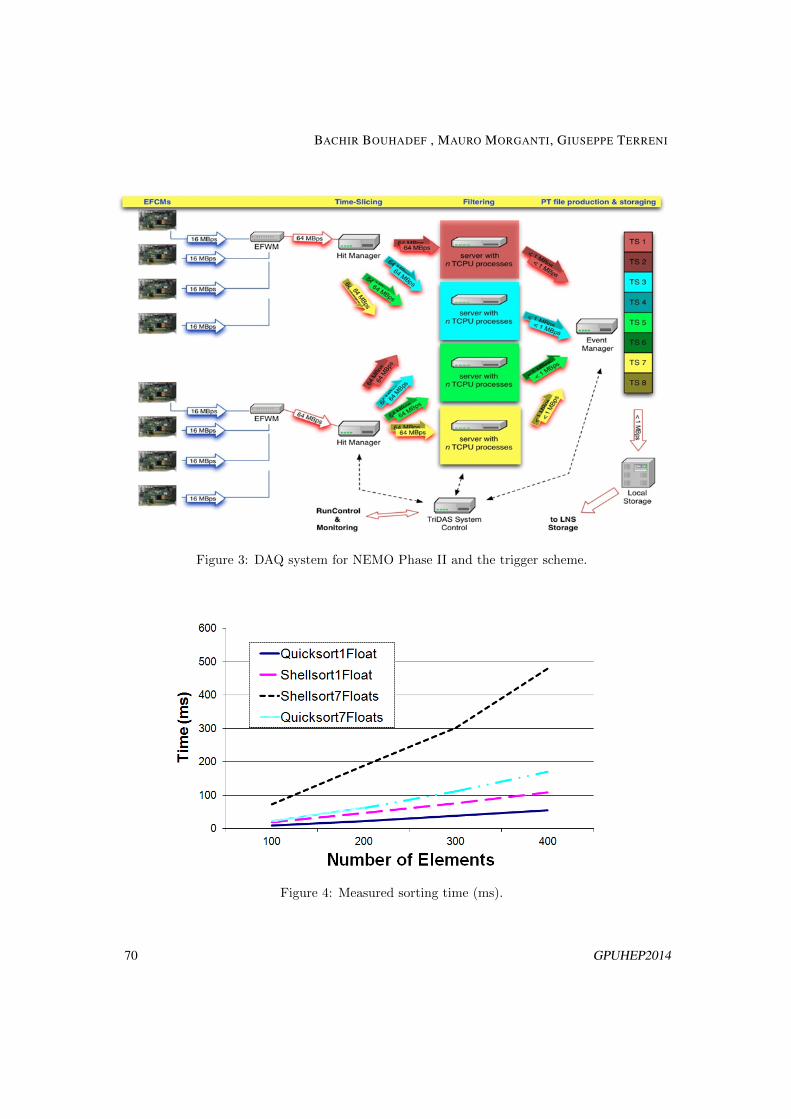
Figure 3: DAQ system for NEMO Phase II and the trigger scheme.

Figure 4: Measured sorting time (ms).

GPUHEP2014 7


70 GPUHEP2014

Track and Vertex Reconstruction on GPUs for

the Mu3e Experiment

Dorothea vom Bruch1 for the Mu3e collaboration

1Physikalisches Institut, Universitat Heidelberg, Im Neuenheimer Feld 226, 69120 Heidelberg,Germany


The Mu3e experiment searches for the lepton flavour violating decay µ → eee, aiming ata branching ratio sensitivity of 10−16. A high precision tracking detector combined withtiming detectors will measure the momenta, vertices and timing of the decay products ofmore than 109 muons/s stopped in the target. The trigger-less readout system will deliverabout 100 GB/s of data. The implementation of a 3D tracking algorithm on a GPU ispresented for usage in the online event selection. Together with a vertex fit this will allowfor a reduction of the output data rate to below 100 MB/s.

1 The Mu3e experiment

The Mu3e experiment [1] searches for the lepton flavour violating decay µ → eee. Within thestandard model, this process is allowed via neutrino oscillations. It is however suppressed toa branching fraction below 10−54. If lepton flavour violation is observed in the charged leptonsector, this is a clear indication for new physics. Many models beyond the standard model,such as supersymmetry, grand unified models or the extended Higgs sector predict lepton flavourviolation at a level to which future detectors are sensitive. The current limit on the µ → eeebranching fraction was set by the SINDRUM experiment to 10−12 [2]. The Mu3e experimentaims to improve this limit by four orders of magnitude and to reach a sensitivity of 10−16 at90 % CL.

To reach this sensitivity level, the distinction between signal and background events iscrucial. In the Mu3e experiment, muons will be stopped in a target and decay at rest. A signalevent consists of two positrons and one electron originating from one single vertex as shown inFigure 1a. They are coincident in time and the momentum sum is zero. The total energy ofthe event is equal to the rest mass of the muon.

One source of background is a radiative muon decay with internal conversionµ+ → e+e−e+νµνe. This process is shown in Figure 1b. Here, the decay products are alsocoincident in time and have a single vertex, however the momenta do not add up to zero andthe energy does not equal the muon rest mass. Combinatorial background stems from twoordinary muon decays µ+ → e+νeνµ taking place close to each other in space and time togetherwith an additional electron from photon conversion, Bhabha scattering etc. (see Figure 1c).When both the e+ and e− from Bhabha scattering are detected, only one additional muondecay is required and the probability of misreconstruction as signal event is higher.


e+

e+

e-

(a) Signal event (b) Internal conversion

e+

e+

e-

(c) Combinatorial background

Figure 1: Comparison of signal and background events.

Momentum, timing and vertex resolution are therefore the key parameters for the distinctionbetween signal and background events. To achieve the desired sensitivity, Mu3e aims for amomentum resolution < 0.5 MeV/c, a timing resolution of 100 ps and a vertex resolution of< 200 µm. These requirements guide the design of the Mu3e detector.

1.1 Detector design

Since the muons decay at rest in the target, the momentum of the decay electrons is at maximumhalf the muon mass (53 MeV/c). In this energy range, the momentum resolution is dominatedby multiple Coulomb scattering whose variance is inversely proportional to the momentum.Therefore the design of the Mu3e experiment is aimed at minimizing the material budget.Ultralight mechanics will be used for construction and a pixel tracking detector is built from highvoltage monolithic active pixels sensors [3, 4, 5] thinned to 50 µm, with a pixel size of 80×80 µm2.In addition, scintillating tiles and fibres are included for precise timing information. The muonsare stopped on the surface of a hollow double cone target, leading to a spread in the vertexlocations. A magnetic field of 1 T is applied so that the tracks are bent and recurling tracks aredetected by outer detector regions. This allows for a more precise momentum measurement.A schematic of the detector is shown in figure 2. To reach the sensitivity of 10−16 within areasonable time, muons at high rates are desired which will be provided by the Paul ScherrerInstitut. At the current beamlines, up to 108 µ/s are available. A future high intensity muonbeam line (HiMB) could deliver in excess of 2 · 109 µ/s.

2 Readout scheme

A triggerless readout is foreseen for the detector. At the above mentioned rates this results ina data rate of about 100 GB/s. Consequently, an online selection is required to cope with thisamount of data and reduce the rate by a factor of 1000. A schematic of the readout is shownin Figure 3. Zero-suppressed data are sent from the pixel sensors, the fibres and the tiles tofront-end FPGAs via flex print cables. The FPGAs merge the data and sort it into time slicesof 50 ns which are then transferred via optical links to the readout boards. Each readout boardreceives the information from each sub-component of the detector and then sends the completedetector information for one time slice to one computer of the filter farm via optical links. With

2 GPUHEP2014

DOROTHEA VOM BRUCH

72 GPUHEP2014

Target

Inner pixel layers

Scintillating bres

Outer pixel layers

Recurl pixel layers

Scintillator tiles

μ Beam

Figure 2: Schematic of the Mu3e detector design.

this procedure, each PC analyzes different time slices of full detector information. The GPUsof the filter farm PCs perform the online event selection by searching for 3 tracks originatingfrom one single vertex.

...

4860 Pixel Sensors

up to 56800 Mbit/s links

FPGA FPGA FPGA

...

142 FPGAs

ROBoard

ROBoard

ROBoard

ROBoard

1 6 Gbit/slink each

Group A Group B Group C Group D

GPUPC

GPUPC

GPUPC12 PCs

Subfarm A

...12 10 Gbit/s

links perRO Board

8 Inputseach

GPUPC

GPUPC

GPUPC12 PCs

Subfarm D

4 Subfarms

~ 4000Fibres

FPGA FPGA

...

48 FPGAs

~ 7000 Tiles

FPGA FPGA

...

48 FPGAs

ROBoard

ROBoard

ROBoard

ROBoard


ROBoard

ROBoard

ROBoard

ROBoard


DataCollection

Server

MassStorage

Gbit Ethernet

Figure 3: Readout scheme of the Mu3e detector design. [6]

3 Multiple scattering fit

Tracks are reconstructed based on the hits in the pixel detectors using a 3D tracking algorithmfor multiple scattering dominated resolution [7, 8]. Triplets of subsequent hits in three layers areselected and multiple scattering is assumed at the middle hit of the triplet. In the momentum

GPUHEP2014 3

TRACK AND VERTEX RECONSTRUCTION ON GPUS FOR THE MU3E EXPERIMENT

GPUHEP2014 73

region of interest the position resolution of the pixel detector (σpixel = 80/√

12 µm) is smallcompared to the effects of multiple scattering.

Figure 4 shows one triplet with the azimuthal scattering angle ΦMS in the x-y plane on theleft and the polar scattering angle ΘMS in the s-z plane on the right, where s is the 3D path

length. The combined χ2 =φ2MS

σ2MS

+θ2MS

σ2MS

is minimized during the non-iterative fitting procedure.

The variances of the scattering angles are obtained from multiple scattering theory. Severaltriplets grouped together form one track.

z

s

x

y

ΦMS

S01

S12

S12

S01

ΘMS

Figure 4: Sequence of three hits forming a triplet in the x-y plane on the left, and the s-z planeon the right with respective scattering angles.

4 Fit implementation on GPU

For online event selection, a basic version of the multiple scattering fit runs on the GPUs ofthe filter farm PCs. It has been implemented on Nvidia’s GeForce GTX 680 using the CUDAenvironment. Triplets are constructed from hits in the first three detector layers. The numberof possible hit combinations to form a triplet is proportional to n1 × n2 × n3 where ni is thenumber of hits in layer i. The main steps of the processing are:

• Sorting the hit array with respect to the z-coordinate

• Geometric filtering on ordered hits

• Triplet fitting and selection

Notice that in the final readout mechanism, the hit arrays will be sorted by the FPGAsin the PCs and geometrical selection cuts will be applied. The preselected arrays will then becopied via direct memory access to the GPUs to perform the fitting step. Currently the CPUsorts the hit arrays with respect to the z-coordinate, then the sorted hit arrays are copied tothe GPU global memory.

A preliminary kernel implementation gathers the hit filtering and triplet fitting. The selec-tion cuts require proximity in the x-y plane and in z for pairs of hits in layers one and two, andtwo and three respectively. If these cuts were passed, the fitting procedure is applied and hitsof triplets are saved in global memory with an atomic function given a successful fit completionand a certain χ2.

4 GPUHEP2014

DOROTHEA VOM BRUCH

74 GPUHEP2014

For the first kernel implementation, a 2D-grid is set up with n1 × n2 grid dimensions,each kernel loops over the n3 hits in layer three. Since the geometrical selection cuts and fitcompletion cuts introduce branch divergence, 87 % of the threads are idle in this configuration.

Consequently, an alternative implementation with two separate kernels was tested. Withinthe geometric kernel, only the geometry cuts are applied and triplets of hits passing these cutsare saved into an array in global memory. The grid dimensions for this kernel are the same asdescribed for the first implementation. Then, the fit kernel, which fits and selects hit triplets,is launched on the number of selected triplets using a 1D-grid associated with 128-block size.Consequently, one fit is performed per thread without any divergence. In addition, since theblock dimension is now a multiple of the warp size (32), no inherently idle threads are launchedin the grid.

In terms of run time, there is no significant improvement with the two kernel version com-pared to one kernel. However, only tasks for which the GPU is optimized are now performed inthe fitting kernel, so this is one step towards the final readout and selection chain of the filterfarm.

5 Performance

Figure 5: Compute utilization of the streamingmultiprocessors on the GTX 680 for the fittingkernel of the two kernel fit implementation.

Next we will focus on the triplet fitting per-formance, since it will be the processing stepdeployed on GPUs.Using Nvidia’s Visual Profiler tool, the per-formance of the different versions was stud-ied. The compute utilization of the stream-ing multiprocessors averages around 80 % forthe fitting kernel of the two kernel version, asshown in Figure 5.

The block size has been chosen to optimizethe number of warps per streaming multipro-cessor: 128 threads per block take advantageof all 64 warps in a streaming multiprocessor(see Figure 6 on the left). Since the fittingkernel requires 29 registers per thread, the

kernel implementation can make optimal use of these 64 warps per streaming multiprocessor(see Figure 6 on the right). Therefore, the compute efficiency is not limited by the block sizeor register count.

Currently, 1.4 ·1010 triplets/s are processed. This measurement is based on the wall time ofboth CPU and GPU, so that all sorting and selection times are included. Most of the time isspent on the first kernel applying the selection cuts. Therefore, further improvement is expectedwhen the pre-selection is outsourced to the FPGAs on the readout boards. Similarly, the ratioof copying data from CPU to GPU compared to computing time (40 %) will improve once moreselection criteria are applied before transferring the data to the PC.

GPUHEP2014 5

TRACK AND VERTEX RECONSTRUCTION ON GPUS FOR THE MU3E EXPERIMENT

GPUHEP2014 75

Figure 6: Warps per Streaming Multiprocessor (SM) as a function of the block size (left) andthe register count (right).

6 Summary and outlook

To achieve a sensitivity of 1016 in the measurement of the µ→ eee branching ratio, high rateson the order of 109µ/s are required, resulting in a data rate on the order of 100 GB/s in thedetector.

The implementation of the triplet fit on the GTX 680 can currently process 1.4 × 1010

triplets/s. For a muon rate of 108, about 1012 hit combinations are expected per second in thefirst three layers, therefore requiring 10 - 100 GPU computers in the filter farm. Faster filteringis required for the higher rate of 109µ/s. This can be achieved by sorting the data on FPGAsand further improving the performance of the fit, and as a result, reduce by a factor of 1000the data rate. In addition, a new vertex fit [9] will be implemented on the GPU in order toapply the selection criteria for a signal of 3 tracks originating from one single vertex.

References[1] A. Blondel et al. Research Proposal for an Experiment to Search for the Decay µ → eee. ArXiv e-prints,

January 2013.

[2] W. Bertl et al. Search for the decay µ+ → e+e+e−. Nucl. P, B 260(1):1 – 31, 1985.

[3] N. Berger et al. A Tracker for the Mu3e Experiment based on High-Voltage Monolithic Active Pixel Sensors.Nucl. Instr. Meth. A, 732:61–65, 2013.

[4] I. Peric. A novel monolithic pixelated particle detector implemented in high-voltage CMOS technology.Nucl.Instrum.Meth., A582:876, 2007.

[5] I. Peric et al. High-voltage pixel detectors in commercial CMOS technologies for ATLAS, CLIC and Mu3eexperiments. Nucl.Instrum.Meth., A731:131–136, 2013.

[6] S. Bachmann et al. The proposed trigger-less tbit/s readout for the mu3e experiment. Journal of Instru-mentation, 9(01):C01011, 2014.

[7] A. Schoning et al. A multiple scattering triplet fit for pixel detectors. publication in preparation.

[8] M. Kiehn. Track fitting with broken lines for the mu3e experiment. Diploma thesis, Heidelberg University,2012.

[9] S. Schenk. A Vertex Fit for Low Momentum Particles in a Solenoidal Magnetic Field with Multiple Scattering.Master’s thesis, Heidelberg University, 2013.

6 GPUHEP2014

DOROTHEA VOM BRUCH

76 GPUHEP2014

INTEL HPC portfolio

E. Politano1

1 INTELr


GPUHEP2014GPUHEP2014 77

GPUHEP2014

E. POLITANO

78 GPUHEP2014

GPUs for the realtime low-level trigger of the

NA62 experiment at CERN

R. Ammendola4, M. Bauce3,7, A. Biagioni3, S. Chiozzi1,5, A. Cotta Ramusino1,5, R. Fantechi2,M. Fiorini1,5,∗, A. Gianoli1,5, E. Graverini2,6, G. Lamanna2,8, A. Lonardo3, A. Messina3,7,I. Neri1,5, F. Pantaleo2,6, P. S. Paolucci3, R. Piandani2,6, L. Pontisso2, F. Simula3, M. Sozzi2,6,P. Vicini3

1INFN Sezione di Ferrara, Via Saragat 1, 44122 Ferrara, Italy2INFN Sezione di Pisa, Largo B. Pontecorvo 3, 56127 Pisa, Italy3INFN Sezione di Roma“La Sapienza”, P.le A. Moro 2, 00185 Roma, Italy4INFN Sezione di Roma “Tor Vergata”, Via della Ricerca Scientifica 1, 00133 Roma, Italy5University of Ferrara, Via Saragat 1, 44122 Ferrara, Italy6University of Pisa, Largo B. Pontecorvo 3, 56127 Pisa, Italy7University of Rome “La Sapienza”, P.le A.Moro 2, 00185 Roma, Italy8INFN Sezione di Frascati, Via E.Fermi 40, 00044 Frascati (Roma), Italy∗ Corresponding author. E-mail: [email protected]


A pilot project for the use of GPUs (Graphics processing units) in online triggering ap-plications for high energy physics experiments (HEP) is presented. GPUs offer a highlyparallel architecture and the fact that most of the chip resources are devoted to computa-tion. Moreover, they allow to achieve a large computing power using a limited amount ofspace and power. The application of online parallel computing on GPUs is shown for thesynchronous low level trigger of NA62 experiment at CERN. Direct GPU communicationusing a FPGA-based board has been exploited to reduce the data transmission latencyand results on a first field test at CERN will be highlighted. This work is part of a widerproject named GAP (GPU application project), intended to study the use of GPUs inreal-time applications in both HEP and medical imaging.

1 Introduction

The trigger system plays a fundamental role in any HEP experiment since it must decidewhether a particular event observed in a detector should be recorded or not, based on limitedinformation. Every experiment features a limited amount of DAQ bandwidth and disk spacefor data storage, the use of real-time selections is crucial to make the experiment affordablemaintaining at the same time its discovery potential. Online selection of important eventscan be performed by arranging the trigger system in a cascaded set of computational levels.The low-level (hereinafter referred to as L0) is usually realized in hardware, often based oncustom electronics devoted to the experiment and normally developed using programmablelogic (FPGA) that offer flexibility and possibility of reconfiguration. The upper trigger levels(L1 and L2) are implemented in software on a commodity PC farm for further reconstruction


and event building. In the baseline implementation, the FPGAs on the readout boards computesimple trigger primitives on the fly, such as hit multiplicities and rough hit patterns, which arethen timestamped and sent to a central trigger processor for matching and trigger decision.

This paper presents the idea of using GPUs for low-level triggering in HEP experiments.In fact, GPUs provide a huge computing power on a single device, thus allowing to take com-plex decisions with a significantly high speed. In particular, in the standard multi-level triggerarchitecture, GPUs can be easily exploited in the higher software levels, where the numberof computing farm nodes can be reduced and the capability of the processing system can beimproved without increasing the scale of the system itself. As an example, GPUs are currentlyunder study in the software trigger level of ATLAS experiment at CERN [1] and are imple-mented with encouranging results in tracking of Pb-Pb Events in the ALICE experiment [2].

Low-level triggers can also take advantage from the usage of GPUs, but a careful assessmentof their online performance is required especially in terms of computing power and latency. Infact, low level trigger systems are designed to perform very rough selection based on a sub-setof the available information, typically in a pipelined structure housed in custom electronics,in order to bring to a manageable level the high data rate that would otherwise reach thesoftware stages behind them. Due to small buffers size in the read-out electronics, such systemsusually require very low latency. A low total processing latency is usually not crucial in theapplications for which GPUs have been originally developed. On the contrary, for a GPU-base trigger system, data transfer latency to the GPU and its stability in time become a veryimportant issue.

In this paper we present recent results of the ongoing R&D on the use of GPUs in the lowesttrigger level of the NA62 Experiment at CERN, within the framework of the GAP project [3].Next section describes the idea of the adoption of GPUs in the NA62 L0 trigger while in theother subsection we address more specifically the latency control problem, and we show theresults on the solution that we are currently developing. This is based on a custom “smart”NIC that allows copying data directly into the GPU.

2 GPUs in the low-level trigger of the NA62 experiment

The NA62 experiment at CERN aims at measuring the branching ratio of the ultra-rare decayof the charged kaon into a pion and a neutrino-antineutrino pair. The goal is to collect ∼ 100events with a 10:1 signal to background ratio, using a high-energy (75 GeV/c) unseparatedhadron beam decaying in flight [4, 5]. In order to manage the 25 GB/s raw data stream due toa ∼ 10 MHz rate of particle decays illuminating the detectors, the NA62 trigger consists of threelevels as illustrated in the previous section: the L0 is based on FPGA boards which performdetector data readout [6], while the next two levels are developed on PCs, thus implementedin software. L0 must handle an input event rate of the order of 10 MHz and apply a rejectionfactor of around 10, in order to allow a maximum input rate of 1 MHz to the L1 trigger. Thelatter, together with the L2 trigger, must reduce the rate to about 10 kHz in order to permitpermanent data storage for later offline analysis. The maximum total latency allowed by theNA62 experiment for the L0 trigger is 1 ms.

A pilot project within NA62 is investigating the possibility of using a GPU system as L0trigger processor (GL0TP), exploiting the GPU computing power to process unfiltered datafrom the readout in order to implement more selective trigger algorithms. In the standard L0implementation, trigger primitives contributing to the final trigger decision are computed on

2 GPUHEP2014

R. AMMENDOLA, M. BAUCE, A. BIAGIONI, S. CHIOZZI, A. COTTA RAMUSINO, R. . . .

80 GPUHEP2014

Figure 1: Throughput as a function of thenumber of events for last generation GPUs.

Figure 2: Total latency (including data trans-fer and computing). Here the maximumthreshold does not take into account thedata transfer from readout, but it only esti-mates the total latency contribution withinthe GPU.

the readout board FPGAs, and are mostly based on event hit patterns. The use of GPUs inthis level would allow building more complex physics-related trigger primitives, such as energyor direction of the final state particles in the detectors, therefore leading to a net improvementof trigger conditions and data handling.

In particular, the reconstruction through GPUs of the ring-shaped hit patterns within theNA62 Ring Imaging Cherenkov (RICH) detector represents the first study case on the use ofGPUs at low-level trigger in the GAP project. The proposed GL0TP will operate in parasiticmode with respect to the main L0 trigger processor by processing data coming only from theRICH detector. Such detector, described in [7], provides a measurement of the velocity anddirection of the charged particles crossing its volume above the Cherenkov threshold. It cantherefore contribute to the computation of other physical quantities, such as the decay vertexof the K+ and the missing mass. On the basis of such information, highly selective triggeralgorithms can be implemented for several interesting K+ decay modes.

As highlighted in [8], several ring reconstruction algorithms have been studied in order toassess the best GPU-based implementation. In particular, the one based on a simple coordinatetransformation of the hits which reduces the problem to a least square procedure was foundto be the best ring-fitting algorithm in terms of computing throughput. This algorithm wasdeveloped and tested on different GPUs, such as the NVIDIA Tesla C1060, Tesla C2050 andGeForce GTX680. The computing performance of the C2050 and GTX680 proved to be a factor4 and 8 higher than that of the C1060, respectively.

Figure 1 shows the computing throughput for these devices as a function of the number ofevents processed in one batch. The effective computing power is seen to increase with the num-ber of events to be processed concurrently. The horizontal line shows the minimum throughput

GPUHEP2014 3

GPUS FOR THE REALTIME LOW-LEVEL TRIGGER OF THE NA62 EXPERIMENT AT CERN

GPUHEP2014 81

requirement for an online trigger based on the RICH detector of the NA62 experiment.Figure 2 points out the total computing latency that includes data transfer times to and

from the GPU and the kernel execution time. Here NVIDIA Tesla C2050 and GeForce GTX680devices have been used for the measurement. The significant reduction of the latency for thenewer GTX680 GPU is due to the faster data transfer allowed by the 3rd generation PCIExpressbus. As can be seen, the maximum threshold (green horizontal line) seems to be attainablewhen a reasonable number of events is processed in one batch.

In a standard GPU computing approach, data from the detector reach the Network InterfaceCard (NIC) which copies them periodically on a dedicated area in the PC RAM, from wherethey are then copied to the user space memory where applications can process them. Here asufficient data load of buffered events is usually prepared for the following stages, and theyare copied to GPU memory through the PCI express bus. The host (the PC on which theGPU card is plugged) has the role of starting the GPU kernel, which operates on the data.Computation results can then be sent back to the host for further processing or distribution tothe detectors, to ultimately trigger the read-out of the complete data event. In this system, themost important contribution to the total latency is due to the data transfer latency from theNIC to the GPU memory. Thus, in order to reduce the maximum total latency, an approachwill be described in detail in the following, i.e., the use of a direct data transfer protocol froma custom FPGA-based NIC to the GPU.

2.1 NaNet

NaNet is a modular design of a low-latency NIC with GPUdirect capability developed at INFNRome division, that is being integrated in the GPU-based low level trigger of the NA62 RICHdetector [9, 10]. Its design comes from the APEnet+ PCIe Gen 2 x8 3D NIC [11] and the boardsupports a configurable number of different physical I/O links (see Figure 3). The DistributedNetwork Processor (DNP) is the APEnet+ core logic, behaving as an off-loading engine for thecomputing node in performing inter-node communications [12]. NaNet is able to exploit theGPUDirect peer-to-peer (P2P) capabilities of NVIDIA Fermi/Kepler GPUs enabling a host PCto directly inject into its memory an UDP input data stream from the detector front-end, withrates compatible with the low latency real-time requirements of the trigger system.

To measure the data transmission latency a readout board (TEL62) has been employed tosend input data. In particular, data communication between the TEL62 readout boards and theL0 trigger processor (L0TP) happens over multiple GbE links using UDP streams. The mainrequisite for the communication system comes from the request for <1 ms and deterministicresponse latency of the L0TP, thus communication latency and its fluctuations are to be keptunder control. The requisite on bandwidth is 400÷700 MB/s, depending on the final choiceof the primitives data protocol which in turn depends on the amount of preprocessing to beactually implemented in the TEL62 FPGA. This means that, to extract primitives data fromthe readout board towards the L0TP in the final system, 4÷6 GbE links will be used.

NaNet latency was measured sending UDP packets from one of the host GbE ports to theNaNet GbE interface: using the x86 TSC register as a common reference time, a single-processtest could measure the time difference between the moment before the first UDP packet of abunch (needed to fill the receive buffer) is piped out through the host GbE port and when thesignal of a filled receive buffer reaches the application. Within this measurement setup (“systemloopback”), the latency of the send process is also taken into account.

Measurements in Figure 5 were thus taken; UDP packets with a payload size of 1168 Bytes

4 GPUHEP2014


82 GPUHEP2014

Figure 3: NaNet as a FPGA-based NIC im-plemented using an Altera development board(Stratix IVGX230 FPGA).

Figure 4: NaNet architecture schematic.

(16 events) were sent to a GPU memory receiving buffer of size variable between 1 and 64 timesthe UDP packet payload.

2.1.1 Synchronization of NaNet with the Timing Trigger and Control system atCERN

The Timing Trigger and Control (TTC) system distributes the system clock for the NA62experiment as well as the first level triggers and synchronization commands, which are alldistributed on a single optical fibre. In particular, a mezzanine card (TTCrq) [13], developedby the CERN microelectronics group, acts as an interface between the TTC system for NA62detectors and its receiving end users. The card delivers the clock together with control andsynchronization information to the front-end electronics controllers in the detector.

Synchronization of NaNet with the TTC system through the TTCrq, has been tested byfirstly realizing an interface board between NaNet and the TTCrq. This has been produced atPhysics Department at University of Ferrara (Italy) and connected to the High Speed MezzanineCard (HSMC) port B of the FPGA board. The whole TTCrq-interface-NaNet system (seeFigure 6) proved to correctly receive all the signals necessary to synchronise the detectors, i.e.clock, event counter reset and bunch counter reset (the last ones encoding start-of-burst andend-of-burst commands).

3 Conclusions

The GAP Project aims at studying the application of GPUs in real-time HEP trigger systemsand in medical imaging. In this paper the application to a low-level trigger system for the NA62experiment at CERN has been described: the critical point to be pursued is the reduction of

GPUHEP2014 5


GPUHEP2014 83

Figure 5: A comparison between NaNet com-munication latency and standard GbE inter-faces results.

Figure 6: The TTCrq-interface-NaNet systemtogether with a NVIDIA Tesla K20 GPU.

the contributions to the total latency due to data transfer from the detectors to the GPU. Anapproach based on a FPGA board to establish a peer-to-peer connection with the GPU is beingdeveloped. The reconstruction of photon rings in the RICH detector has been considered asfirst case of study on the use of GPUs at L0 in the NA62 experiment. Preliminary resultsshow that current GPUs are suitable for sustaining the event rates, while at the same timeminimizing the latency to an acceptable level.

Acknowledgment

The GAP project is partially supported by MIUR under grant RBFR12JF2Z “Futuro in ricerca2012”.

References

[1] P.J. Clark, C. Jones. D Emeilyanov, M. Rovatsou, A. Washbrook, and the ATLAS col-laboration, “Algorithm Acceleration from GPGPUs for the ATLAS Upgrade” Journal ofPhysics: Conference Series 331 (2011) 022031.

[2] D. Rohr, S. Gorbunov, A. Szostak, M. Kretz, T. Kollegger, T. Breitner and Torsten Alt,“ALICE HLT TPC Tracking of Pb-Pb Events on GPUs”, Journal of Physics: ConferenceSeries 396 (2012) 012044.

[3] http://web2.infn.it/gap

[4] M. Fiorini [NA62 Collaboration], “The NA62 experiment at CERN”, PoS HQL 2012(2012) 016.

[5] http://cern.ch/NA62/

6 GPUHEP2014


84 GPUHEP2014

[6] B. Angelucci, E. Pedreschi, M. Sozzi and F. Spinella, “TEL62: an integrated triggerand data acquisition board” Nuclear Science Symposium and Medical Imaging Confer-ence (NSS/MIC), 2011 IEEE.

[7] B. Angelucci, G. Anzivino, C. Avanzini, C. Biino, A. Bizzeti, F. Bucci, A. Cassese andP. Cenci et al., “Pion-muon separation with a RICH prototype for the NA62 experiment,”Nucl. Instrum. Meth. A 621 (2010) 205.

[8] R. Ammendola, A. Biagioni, L. Deri, M. Fiorini, O. Frezza, G. Lamanna, F. Lo Cicero,A. Lonardo, A. Messina, M. Sozzi, F. Pantaleo, P.S. Paolucci, D. Rossetti, F. Simula,L. Tosoratto and P. Vicini, “GPUs for Real Time processing in HEP trigger systems” Jour-nal of Physics: Conference Series 523 (2014) 012007 doi: 10.1088/1742-6596/523/1/012007and references therein.

[9] R. Ammendola, A. Biagioni, O. Frezza, G. Lamanna, A. Lonardo, F. Lo Cicero,P. S. Paolucci, F. Pantaleo, D. Rossetti, F. Simula, M. Sozzi, L. Tosoratto and P. Vicini,“NaNet: a flexible and configurable low-latency NIC for real-time trigger systems basedon GPUs” JINST 9 (2014) C02023, doi:10.1088/1748-0221/9/02/C02023.

[10] R. Ammendola, A. Biagioni, R. Fantechi, O. Frezza, G. Lamanna, F. L. Cicero, A. Lonardo,P. S. Paolucci, F. Pantaleo, R. Piandani, L. Pontisso, D. Rossetti, F. Simula, M. Sozzi,L. Tosoratto and P. Vicini, “NaNet:a low-latency NIC enabling GPU-based, real-time lowlevel trigger systems”, Journal of Physics: Conference Series, 513, (2014) 012018.

[11] R. Ammendola, A. Biagioni, O. Frezza, F. Lo Cicero, A. Lonardo, P. S. Paolucci, D. Ros-setti and F. Simula, L. Tosoratto and P. Vicini, “APEnet+: A 3D Torus network optimizedfor GPU-based HPC systems”, J. Phys. Conf. Ser. 396 (2012) 042059.

[12] A. Biagioni, F. L. Cicero, A. Lonardo, P. S. Paolucci, M. Perra, D. Rossetti, C. Sidore,F. Simula, L. Tosoratto and P. Vicini, “The Distributed Network Processor: a novel off-chipand on-chip interconnection network architecture”, arXiv:1203.1536.

[13] http://proj-qpll.web.cern.ch/proj-qpll/ttcrq.htm

GPUHEP2014 7


GPUHEP2014 85

A FPGA-based Network Interface Card with

GPUDirect enabling real-time GPU computing

in HEP experiments.

Alessandro Lonardoa∗, Fabrizio Amelia, Roberto Ammendolab, Andrea Biagionia, Angelo CottaRamusinoc, Massimiliano Fiorinic, Ottorino Frezzaa, Gianluca Lamannade, Francesca Lo Ciceroa,Michele Martinellia, Ilaria Neric, Pier Stanislao Paoluccia, Elena Pastorellia, Luca Pontissof ,Davide Rossettig, Francesco Simeonea, Francesco Simulaa, Marco Sozzif e, Laura Tosorattoa,Piero Vicinia

aINFN Sezione di Roma - Sapienza, P.le Aldo Moro, 2 - 00185 Roma, ItalybINFN Sezione di Roma - Tor Vergata, Via della Ricerca Scientifica, 1 - 00133 Roma, ItalycUniversita degli Studi di Ferrara and INFN Sezione di Ferrara, Polo Scientifico e Tecnologico,Via Saragat 1 - 44122 Ferrara, Italy

dINFN Laboratori Nazionali di Frascati, Via E. Fermi,40 - 00044 Frascati (Roma), ItalyeCERN, CH-1211 Geneva 23, Switzerlandf INFN Sezione di Pisa, Via F. Buonarroti 2 - 56127 Pisa, ItalygNVIDIA Corp, 2701 San Tomas Expressway, Santa Clara, CA 95050


The capability of processing high bandwidth data streams in real-time is a computationalrequirement common to many High Energy Physics experiments. Keeping the latencyof the data transport tasks under control is essential in order to meet this requirement.We present NaNet, a FPGA-based PCIe Network Interface Card design featuring RemoteDirect Memory Access towards CPU and GPU memories plus a transport protocol offloadmodule characterized by cycle-accurate upper-bound handling. The combination of thesetwo features allows to relieve almost entirely the OS and the application from data tranfermanagement, minimizing the unavoidable jitter effects associated to OS process scheduling.The design currently supports one GbE (1000Base-T) and three custom 34 Gbps APElinkI/O channels, but four-channels 10GbE (10Base-R) and 2.5 Gbps deterministic latencyKM3link versions are being implemented. Two use cases of NaNet will be discussed: theGPU-based low level trigger for the RICH detector in the NA62 experiment and the on-/off-shore data acquisition for the KM3Net-IT underwater neutrino telescope.

1 Introduction

In many fields of Experimental Physics ranging from Radio Astronomy to High Energy Physics,the GPU adoption effort that in High Performance Computing brings such outstanding results

∗Corresponding author. E-mail: [email protected]


is hampered by the real-time constraints that the processing of data streams outflowing fromexperimental apparatuses is often subject to. GPUs processing latency is mostly stable oncedata has landed in their own internal memories; a data transport mechanism with determin-istic or at least bound latency is then crucial in building a GPGPU system honouring theseconstraints.

Our NaNet design is one such mechanism, reusing several IPs developed for the APEnet+3D torus NIC [1] targeted at HPC hybrid clusters; its real-time features were achieved by addingdedicated modules and support of multiple link technologies, both standard and custom. Theresulting FPGA-based, low-latency PCIe NIC is highly configurable and modular, with RDMAand GPUDirect capabilities. It has been employed in widely varying configurations and physicaldevice implementations in two different High Energy Physics experiments: the NA62 experimentat CERN [2] and the KM3NeT-IT underwater neutrino telescope [3].

2 NaNet design overview

PCIe X8 Gen2 core

Network Interface

TX/RX Block

32bit Micro Controller

Custom Logic

memory controller

GPU I/O accelerator

On

Bo

ard

Me

mo

ry

Router

I/O

Inte

rfac

e

Physical Link Coding

Protocol Manager

NaNet Controller

AP

Elin

k

8B10B

Word Stuff

NaN

et-1

(G

bE)

TSE MAC

UDP

NaNet Ctrl N

aNet

3 C

han

nel

8B10B

TDMP

NaNet Ctrl

Link Ctrl

Figure 1: NaNet architecture schematic.

NaNet is a low-latency PCIe NIC support-ing standard — GbE (1000BASE-T) and10GbE (10Base-R) — and custom — 34 GbpsAPElink [4] and 2.5 Gbps deterministic la-tency optical KM3link [5] — network links.NaNet bridges the gap between real-time andGPGPU heterogeneous computing by inher-iting the GPUDirect P2P/RDMA capabil-ity from its HPC-dedicated sibling — theAPEnet+ 3D torus NIC — and enhancing itwith real-time-enabling features, e.g. a net-work stack protocol offload engine for sta-ble communication latency. NaNet design ispartitioned into 4 main modules: I/O In-terface, Router, Network Interface and PCIeCore (see Fig. 1). The I/O Interface moduleperforms a 4-stages processing on the datastream: following the OSI Model, the Phys-ical Link Coding stage implements the channel physical layer (e.g. 1000BASE-T) while theProtocol Manager stage handles, depending on the kind of channel, data/network/transportlayers (e.g. Time Division Multiplexing or UDP); the Data Processing stage implementsapplication-dependent reshuffling on data streams (e.g. performing de/compression) while theAPEnet Protocol Encoder performs protocol adaptation, encapsulating inbound payload datain APElink packet protocol — used in the inner NaNet logic — and decapsulating outboundAPElink packets before re-encapsulating their payload into output channel transport protocol(e.g. UDP). The Router module implements a parametric full crossbar switch responsible fordata routing, sustaining multiple data flows @2.8 GB/s.

The Network Interface block acts on the trasmitting side by forwarding PCIe-originated datato the Router ports and on the receiving side by providing support for RDMA in communicationsinvolving both the host and the GPU (via a dedicated GPU I/O Accelerator module). A Nios IIµcontroller handles configuration and runtime operations.

Finally, the PCIe Core module is built upon a powerful commercial core from PLDA that

2 GPUHEP2014

A FPGA-BASED NETWORK INTERFACE CARD WITH *GPUDIRECT ENABLING . . .

GPUHEP2014 87

sports a simplified but efficient backend interface and multiple DMA engines.

This general architecture has been specialized up to now into three configurations, namelyNaNet-1, NaNet3 and NaNet-10, to match the requirements of different experimental setups:NaNet-1 is implemented on the Altera Stratix IV FPGA Dev Kit; it sports a PCIe Gen2 x8 hostinterface, a GbE channel and three optional 34 Gbps APElink ones; NaNet3 is implementedon the Terasic DE5-net Stratix V FPGA Dev Kit; it supports a PCIe Gen2 x8 host interfacewhile the four SFP+ cages of the board are used for the KM3link channels which are 2.5 Gbpsoptical links with deterministic latency;NaNet-10 is another implementation on the TerasicDE5-net board; the PCIe Gen2 x8 host interface is the same as NaNet3 while the SFP+ portssupport four 10GbE channels.

3 NaNet-1: a NIC for NA62 GPU-based low-level trigger

The NA62 experiment at CERN aims at measuring the Branching Ratio of the ultra-raredecay of the charged Kaon into a pion and a neutrino-antineutrino pair. The NA62 goal isto collect ∼ 100 events with a 10:1 signal to background ratio, using a novel technique witha high-energy (75 GeV) unseparated hadron beam decaying in flight. In order to managethe 25 GB/s raw data stream due to a ∼ 10 MHz rate of particle decays illuminating thedetectors, the trigger system is designed as a set of three cascaded levels that decrease this rateby three orders of magnitude [6]. The low-level trigger (L0) is a synchronous real-time systemimplemented in hardware by means of FPGAs on the readout boards and reduces the streambandwidth tenfold: whether the data on the readout board buffers is to be passed on to thehigher levels has to be decided within 1 ms to avoid data loss. The upper trigger levels (L1and L2) are implemented in software on a commodity PC farm for further reconstruction andevent building. A pilot project within NA62 is investigating the possibility of using a GPGPUsystem as L0 trigger processor (GL0TP), exploiting the GPU computing power to processunfiltered data from the readout in order to implement more selective trigger algorithms. Inorder to satisfy the real-time requirements of the system, a fast, reliable and time-deterministicdedicated link must be employed. NaNet-1 has been designed and developed with the motivationof building a fully functional and network-integrated GL0TP prototype, albeit with a limitedbandwidth with respect to the experiment requirements, in order to demonstrate as soon aspossible the suitability of the approach and eventually evolve the design to incorporate betterI/O channels. NaNet-1 real-time characterization has been carefully assessed on dedicatedtestbeds [7, 8]. The results of this activity have driven the latest developments towards a lowerlatency design. Allocation of time-consuming RDMA related tasks has been moved from theNios II µcontroller to dedicated logic blocks. The Virtual Address Generator (VAG) includedin the NaNet Controller module is in charge of generating memory addresses of the receivingbuffers for incoming data, while a Translation Lookaside Buffer (TLB) module performs fastvirtual-to-physical address translations.

A bandwidth-downscaled GL0TP setup was realized in a loopback configuration by a hostsystem simulating TEL62 UDP traffic through one of its GbE ports towards a NaNet-1 NICstreaming the incoming data into a GPU memory circular list of receive buffers; once landed,buffers are consumed by a CUDA Kernel implementing the pattern matching algorithm. Com-munication and kernel processing tasks were serialized in order to perform the measure; in Fig. 2(left) the results for the K20Xm system are shown. During normal operation, this serializationconstraint can be relaxed, and kernel processing task overlaps with data communication. Ac-tually this is what was done to measure system throughput, with the results in Fig. 2 (right).

GPUHEP2014 3

ALESSANDRO LONARDO, FABRIZIO AMELI, ROBERTO AMMENDOLA, ANDREA . . .

88 GPUHEP2014

0

500

1000

1500

2000

2500

3000

16 32 64 128 256 512 1024 2048 4096

2K 4K 8K 16K 32K 64K 128K 256K

Lat

ency

[us

]

Receive Buffer Size [Number of Events]

Communication + Kernel Latencies (K20Xm)

Receive Buffer Size [Bytes]

Kernel Processing Latency (K20Xm)Total LatencyNaNet-1 Communication Latency

25

50

75

100

125

150

16 32 64 128 256 512 1024 2048 4096 0

0.25

0.5

0.75

1

1.25

1.5

1.75

2

2K 4K 8K 16K 32K 64K 128K 256K

Ban

dwid

th [

MB

/s]

ME

vent

s/s

Receive Buffer Size [Number of Events]

NaNet-1 Performance

Receive Buffer Size [Bytes]

M2070 - Bandwidth M2070 - ThroughputK20Xm - Bandwidth K20Xm - Throughput

Figure 2: (left) NaNet-1 latency over GbE towards GPU memory for varying datagram payloadsizes (nVIDIA Fermi K20Xm); (right) NaNet-1 GbE bandwidth towards GPU memory atvarying datagram payload sizes.

We see that using GPU receive buffer sizes ranging from 128 to 1024 events allows the systemto stay within the 1 ms time budget while keeping a ∼ 1.7 MEvents/s throughput.

Besides optimizing performances, we undertook several developments to cope with theNaNet-1 integration within the NA62 experiment. A Timing Trigger and Control (TTC) HSMCdaughtercard was designed to provide NaNet-1 with the capability of receiving either triggerand 40 MHz clock streams distributed from the experiment TTC system via optical cable: thiscommon reference clock was used to perform latency measurements discussed above. A decom-pressor stage was added in the I/O interface to reformat events data in a GPU-friendly fashionon the fly. Finally, a timeout was implemented in the NaNet Controller module that triggers theDMA of received data towards CPU/GPU memory on a configurable deadline rather than onthe filling of a buffer. The prototype to be deployed at the NA62 experiment site will integrateinto NaNet-1 a TTC HSMC daughtercard and a nVIDIA Kepler K20 GPU.

4 NaNet3: KM3NeT-IT neutrino telescope on-shore board

KM3NeT-IT is an underwater experimental apparatus for the detection of high energy neutrinosin the TeV÷PeV range by means of the Cerenkov technique. The KM3NeT-IT detection unitconsists of 14 floors vertically spaced 20 meters apart, with ∼8 m long floor arms bearing 6 glassspheres each called Optical Modules (OM); each OM contains one 10 inches photomultipliers(PMT) and front-end electronics that digitizes, formats and emits the PMT signal. All dataproduced by OMs and auxiliary floor instrumentation is collected by an off-shore electronicboard called Floor Control Module (FCM) contained in a vessel at the floor centre; the FCMmanages the communication between the on-shore laboratory and the underwater devices, alsodistributing the timing information and signals. Due to the distance between apparatus andshoreland the connecting medium is optical fiber.

The spatially distributed DAQ architecture requires a common clock distributed all overthe system to correlate signals, with respect to a fixed reference, coming from different partsof the apparatus. For this purpose data acquisition and transport electronics labels each signalwith a “time stamp”, i.e. hit arrival time. Time resolution is also fundamental for the trackreconstruction accuracy. These constraints pushed the choice of a synchronous link protocol

4 GPUHEP2014


GPUHEP2014 89

embedding clock and data with deterministic latency; Floors are independent from each other;each is connected to the on-shore laboratory by a bidirectional virtual point-to-point link.A single floor data stream delivered to shore has a rate of ∼300 Mbps, while shore-to-underwatercommunication data rate is much lower, consisting only of slow-control data for the apparatus.The small data rate per FCM compared with state-of-the-art technologies led us to designingNaNet3, an on-shore readout board able to manage multiple FCM data channels.This is a NaNet customization for the KM3NeT-IT experiment, with added support for asynchronous link protocol with deterministic latency at physical level and for a Time DivisionMultiplexing protocol at data level (see Fig. 1).

Figure 3: Deterministic latency of NaNet3

SerDes: phase alignment of the transmitting(upper) and receiving (central) clocks.

The first design stage for NaNet3 wasimplemented on the Terasic DE5-net board,which is based on an Altera Stratix-V GXFPGA with four SFP+ channels and a PCIex8 edge connector. To match time resolutionconstraint, time delta between wavefronts ofthree clocks must have ns precision: the firstclock is an on-shore reference one (comingfrom a GPS and redistributed), used for theoptical link transmission from NaNet3 to-wards the underwater FCM; the second clockis recovered from the incoming data streamby a Clock and Data Recovery (CDR) moduleat the receiving end of the FCM which usesit for sending its data payload from the ap-paratus back on-shore; a third clock is againrecovered by NaNet3 decoding the payload at

the end of the loop. The deterministic latency constraint must be enforced on the Stratix deviceas the FCM does on paths both ways to allow correct time stamping of events on the PMT.The established link is synchronous, i.e. clock rate is equal for both devices with fixed phasedisplacement. We developed a test setup to explore latency capabilities of a complete link chainleveraging on the fixed latency native mode of the Altera transceivers, on the NaNet3 board, andon the hardware fixed latency implementation for a Xilinx device on the FCM board [9]. Theexternal GPS-equivalent clock has been input to the NaNet3 to clock the transmitting side ofthe device. A sequence of dummy parallel data are serialised, 8b/10b-encoded and transmitted,together with the embedded serial clock, at 800 Mbps along the fiber towards the receiver sideof the FCM system. The FCM system recovers the received clock and transmits the receiveddata and recovered clock back to the NaNet3 board. The receive side of NaNet3 deserializesdata and produces the received clock.Testing the fixed latency features of the SerDes hardware implementation is straightforwardwhen taking into account that on every initialisation sequence, e.g. for a hardware reset or atSerDes hardware powerup, we should be able to measure the same phase shift between trans-mitted and received clock, equal to the fixed number of serial clock cycles shift used to correctlyalign the deserialised data stream. Fig. 3 shows a scope acquisition in infinite persistence modesampled over 12 h issuing every 10 s a new reset and align. The NaNet3 transmitter parallelclock (the upper line) maintains exactly the same phase difference with the receiver parallelclock (the central line) and with the FCM recovered clock (the lower line).

GPUHEP2014 5

ALESSANDRO LONARDO, FABRIZIO AMELI, ROBERTO AMMENDOLA, ANDREA . . .

90 GPUHEP2014

5 Conclusions and future work

Our NaNet design proved to be an efficient real-time communication channel between the NA62RICH readout system and GPU-based L0 trigger processor over a single GbE link. With four10 GbE ports, the currently under development NaNet-10 board will exceed the bandwidthrequirements for the NA62 RICH, enabling integration of other detectors in the GPU-basedL0 trigger. Along the same lines, the deterministic latency link of the NaNet3 customizationmakes it a viable solution for the data transport system of the KM3NeT-IT experiment whilethe GPUDirect RDMA features imported from NaNet will allow us later on to build a real-timeGPU-based platform, to investigate improved trigger and data reconstruction algorithms.

Acknowledgments

This work was partially supported by the EU Framework Programme 7 EURETILE project,grant number 247846; R. Ammendola and M. Martinelli were supported by MIUR (Italy)through the INFN SUMA project. G. Lamanna, I. Neri, L. Pontisso and M. Sozzi thank theGAP project, partially supported by MIUR under grant RBFR12JF2Z “Futuro in ricerca 2012”.

References

[1] R. Ammendola et al. APEnet+: a 3D Torus network optimized for GPU-based HPCsystems. Journal of Physics: Conference Series, 396(4):042059, 2012.

[2] Gianluca Lamanna. The NA62 experiment at CERN. Journal of Physics: ConferenceSeries, 335(1):012071, 2011.

[3] A Margiotta. Status of the KM3NeT project. Journal of Instrumentation, 9(04):C04020,2014.

[4] R Ammendola et al. APEnet+ 34 Gbps Data Transmission System and Custom Transmis-sion Logic. Journal of Instrumentation, 8(12):C12022, 2013.

[5] A. Aloisio et al. The NEMO experiment data acquisition and timing distribution systems.In Nuclear Science Symposium and Medical Imaging Conference (NSS/MIC), 2011 IEEE,pages 147–152, Oct 2011.

[6] B Angelucci et al. The FPGA based trigger and data acquisition system for the CERNNA62 experiment. Journal of Instrumentation, 9(01):C01055, 2014.

[7] R Ammendola et al. NaNet: a flexible and configurable low-latency NIC for real-time triggersystems based on GPUs. Journal of Instrumentation, 9(02):C02023, 2014.

[8] R. Ammendola et al. NaNet: a low–latency NIC enabling GPU–based, real–time low leveltrigger systems. Journal of Physics: Conference Series, 513(1):012018, 2014.

[9] R. Giordano and A. Aloisio. Fixed latency multi-gigabit serial links with Xilinx FPGA.IEEE Transaction On Nuclear Science, 58(1):194–201, 2011.

6 GPUHEP2014


GPUHEP2014 91

Chapter 3

GPU in Montecarlo and OfflineAnalysis

Convenors:

Soon Yung JunPiero ViciniMarco Sozzi

92 GPUHEP2014

Fast event generation on GPU

J. Kanzaki1

1 KEK, Japan

We use a graphics processing unit (GPU) for fast event generation of general StandardModel (SM) processes. The event generation system on GPU is developed based on theMonte Carlo integration and generation program BASES/SPRING in FORTRAN. Forcomputations of cross sections of physics processes all SM interactions are included in thehelicity amplitude computation package on GPU (HEGET) and phase space generationcodes are developed for efficient generation of jet associated processes. For the GPU versionof BASES/SPRING new algorithm is introduced in order to fully exploit the ability ofGPU performance and the improvement of performance in nearly two orders of magnitudeis achieved.

The generation system is tested for general SM processes by comparing with the Mad-Graph, which is widely used in HEP experiments, and integrated cross sections and distri-butions of generated events are found to be consistent. In order to realize smooth migrationto the GPU environment, a program that automatically converts FORTRAN amplitudeprograms generated by the MadGraph into CUDA programs is developed.



GPUHEP2014

J. KANZAKI

94 GPUHEP2014

First experience with portable high-performance

geometry code on GPU

John Apostolakis1, Marilena Bandieramonte1, Georgios Bitzes1, Gabriele Cosmo1, Johannes deFine Licht1∗, Laurent Duhem3, Andrei Gheata1, Guilherme Lima2, Tatiana Nikitina1, SandroWenzel1†

1CERN, 1211 Geneve 23, Switzerland2Fermilab, Kirk & Pine Rd, Batavia, IL 60510, USA3Intel, 2200 Mission College Blvd., Santa Clara, CA 95054-1549, USA


The Geant-Vector prototype is an effort to address the demand for increased performance inHEP experiment simulation software. By reorganizing particle transport towards a vector-centric data layout, the projects aims for efficient use of SIMD instructions on modernCPUs, as well as co-processors such as GPUs and Xeon Phi.

The geometry is an important part of particle transport, consuming a significant fraction ofprocessing time during simulation. A next generation geometry library must be adaptableto scalar, vector and accelerator/GPU platforms. To avoid the large potential effort goinginto developing and maintaining distinct solutions, we seek a single code base that can beutilized on multiple platforms and for various use cases.

We report on our solution: by employing C++ templating techniques we can adapt geom-etry operations to SIMD processing, thus enabling the development of abstract algorithmsthat compile to efficient, architecture-specific code. We introduce the concept of modu-lar “backends”, separating architecture specific code and geometrical algorithms, therebyallowing distinct implementation and validation. We present the templating, compila-tion and structural architecture employed to achieve this code generality. Benchmarks ofmethods for navigation in detector geometry will be shown, demonstrating abstracted al-gorithms compiled to scalar, SSE, AVX and GPU instructions. By allowing users to choosethe most suitable type of processing unit for an application or potentially dispatch workdynamically at runtime, we can greatly increase hardware occupancy without inflating thecode base. Finally the advantages and disadvantages of a generalized approach will bediscussed.

1 IntroductionRecent evolution of hardware has seen a reawakened focus on vector processing, a concept thathad otherwise lain dormant outside the world of video games while CPU clock speeds stillrode Moore’s law. Most notable is the surge of interest in general purpose GPU programming(GPGPU), but vector instruction sets have existed on convential CPUs since the introductionof 3DNow! by AMD [3] and SSE by Intel [4] in 1998 and 1999, respectively.

∗Presenting author ([email protected]).†Corresponding author ([email protected]).

1GPUHEP2014 95

To improve performance on modern hardware, it is essential to make use of their vectorprocessing capabilities to access memory efficiently, whether this means efficient cache accesson CPU or efficient use of memory bandwidth on GPU.

1.1 GeantV

The Geant Vector prototype (GeantV) [1] was started as a feasibility study of the potential foradding vectorization to detector simulation programs, in order to address an increasing needfor performance in HEP detector simulation software.

At the core of GeantV there is a scheduling engine orchestrating the progress of the sim-ulation. This scheduler works on particle data packed in structure of arrays (SOA) form forcache-efficiency and to accommodate SIMD memory access [7]; particles that require similartreatment are grouped into baskets, which can be dispatched to the relevant components forvectorized treatment [5]).

The GeantV R&D effort targets multiple platforms for vectorization, including SIMD in-structions on CPUs (SSE, AVX) and accelerators such as GPUs and the Xeon Phi (AVX512).Although sometimes limited by the state of compilers, the project pursues platform indepen-dence to avoid vendor lock-in.

1.2 VecGeom

Navigation and particle tracking in detector geometry is responsible for up to 30%–40% of timespent on particle transport in detector simulation (this fraction is highly experiment depen-dent) [2], thus being an important research topic for vectorization in the GeantV prototype.The main consumers of cycles are the four algorithms shown in Figure 1, which are implementedseparately for each geometrical shape.

VecGeom introduces vectorization techniques in the implementation of a new geometrymodeller. It is a continuation of the USolids [8] effort, a common library for geometricalprimitives, unifying and enhancing the implementations that currently exist in ROOT [9] andGeant4 [10]. The scalar interfaces of VecGeom are therefore made to be compliant with theones of USolids, allowing free interchangeability between the two. VecGeom and USolids areconverging to a single code base.

To accommodate the scheduler of GeantV mentioned above, VecGeom exposes vector signa-ture operating on baskets of particles. These signatures take SOA objects carrying informationon the particles in the basket, instead of a single set of parameters. Since these interfaces comein addition to the scalar ones, there is an issue of signature multiplication requiring a lot ofboilerplate code, which will be addressed in Section 2.3.

VecGeom does not rely on vectorization alone to achieve performance. In the spirit ofUSolids, the library employs the best available algorithms to solve the problems listed in Fig-ure 1. This can mean picking and optimizing the best algorithm between existing ones inROOT, Geant4 and USolids, or it can mean writing them from scratch if deemed relevant.When a new shape is implemented, performance is compared directly to that of the existinglibraries. Algorithms are not accepted before their scalar version (in addition to the vectorizedone) outperforms all existing implementations (more on different kernel versions follows in Sec-tion 2.1). After algorithmic optimization, the library uses a number of additional templatingtechniques for performance which are described in Section 2.1 and 2.4.

2 Templates for portability and performanceTemplating is at the heart of VecGeom, being involved in every aspect of optimization. Thephilosophy is that whenever the parameters of a performance-critical component can be resolved

2

JOHN APOSTOLAKIS, MARILENA BANDIERAMONTE, GEORGIOS BITZES, GABRIELE . . .

96 GPUHEP2014

A physics geometry package

Users define a geometrical hierarchy by placing daughter primitives in mother primitives

Primitives must provide a number of methods necessary for navigation in such a geometry

Existing implementations exist in ROOT and Geant4

8

??

(a) Determine if point isinside a volume.





8

??

(b) Intersection checkand distance to intersec-tion with volume.





8

??

(c) Minimum boundon distance to volumeboundary.





8

??

(d) Distance to exit cur-rent volume.

Figure 1: Primary problems solved by a geometry library during particle transport in simulation.

at compile-time, or even just if it has a finite set of configurations (see Section 2.4), templateswill be used to generate specialized machine code.

2.1 Thinking in kernelsThe approach taken by VecGeom to achieve portability and performance through templates is toseparate performance-critical functionality into small plug-and-play kernels. Each kernel shouldhave a single and well-defined purpose, delegating subtasks to separate kernels, promoting thesharing of kernels between algorithms. Kernels are built to operate on a single unit of input,meaning no explicit vectorization is typically done in them. Instead, vectorization can beconveyed by the types on which operations are performed (as this will often be a templateparameter), and is described in Section 3. Logical constructs such as branches have to beabstracted to higher level functions in order to accommodate this. To ensure that kernels canindeed be shared between different contexts, kernels can live either as free C-like functions oras static methods of enclosing classes, but should never relate to an object. When an object-abstraction is useful, classes can instead implement static methods and call them from withintheir own methods.

2.2 Architecture abstractionAn important motivation for taking the kernel approach is architecture abstraction. VecGeom isa performance-oriented library, and as such aims at maximizing hardware utilization by offeringto run scalar and SIMD code on CPU, and also run on accelerators. Rather than writing sep-arate implementations for each target architecture and multiplying the required maintenance,VecGeom has opted for a generalized approach. The difference between architectures is isolatedto memory management and the types that are operated on, with the latter being handled bythe kernels. For this, the concept of backends was introduced. Backends represent an architec-ture to which kernels should compile, and are encapsulated in C++ trait classes. These classescontain the relevant types to operate on, as well as some static members, such as a boolean totoggle early returns. Backends are used as a template parameter of kernels that operate on theprovided types, and by overloading higher level functions called on these types, the architecturespecific instructions necessary to perform operations is decided. An example of a backend classis shown in Listing 1.

3

FIRST EXPERIENCE WITH PORTABLE HIGH-PERFORMANCE GEOMETRY CODE ON GPU

GPUHEP2014 97

class VcBackend

public:

typedef Vc:: double_v double_t;

typedef Vc::int_v int_t;

typedef Vc:: double_m bool_t;

static constexpr bool earlyReturns

= true;

;

Listing 1: A C++ trait classrepresentation of a backend, providingtypes to operate on and allowing otherconfiguration options. Vc is used towrap vector instruction sets.

template <class B>

typename B:: double_t DistanceToPlane(

Vector3D <typename B::double_t > const &point ,

Vector3D <typename B:: double_t const &plane)

typename B:: double_t result;

result = point.dot(plane);

// If behind the point is considered inside

MaskedAssign(result < 0, 0, &result);

return result;

Listing 2: Kernel operating on a backend class, suchas the one shown in Listing 1.

2.3 Solving code multiplication

The introduction of the vector interfaces led to a multiplication of signatures necessary fora shape to implement, as each shape has to provide both the scalar and vector signatures.Because of the way kernels are designed, this quickly led to large amounts of boilerplate codethat simply called different instantiations of the the same family of templates. These were notonly cumbersome to write for each implemented shape, but also meant a lot of duplicate codeto maintain in the future. To improve this, the curiously recurring template pattern (named byJames Coplien [12]) is employed. This pattern allows a leaf class to inherit from a templatedauxiliary class, passing its own type as a template parameter. The auxiliary class will theninherit from the appropriate base class and implement a number of methods calling staticmethods of the class passed as a template parameter. This can be either the inheriting classitself or a separate class entirely. Using the interface of VecGeom shapes, this meant that only asingle templated method per algorithm had to be implemented for each shape. The boilerplatecode used to call different configurations was collected in a single global auxiliary class. Anexample of this technique is provided in Listing 3.

2.4 Shape specialization

VecGeom defines a set of geometrical shapes. Some parameters describing the shapes havea significant impact on the algorithms: an angle configuration can eliminate the need for atrigonometric function, or a tube with no inner radius can just be treated as a cylinder. Cre-ating separate shape classes for specific configurations would cause the number of primitivesto explode. Instead, VecGeom takes advantage of this behind the scenes by using the conceptof shape specialization. By having kernels template on one or more specialization parameters,blocks of code are tweaked or removed entirely from the implementation at compile time. Thissaves branch mispredictions and register allocation as compared to performing all branches atruntime. The concept is shown in Listing 4.

To avoid to expose end users to specialization, the instantiation of each configuration is doneby a factory method. This limits specialization to a finite phase space, but hides the specificsthrough polymorphism, handing the user an optimized object behind the base primitive’s in-terface. Specialization happens when shapes are placed into their frame of reference. Volumesinstantiated by other means are not specialized, and will instead branch at runtime.

Figure 2 shows relative benchmarks between the same kernel compiled for three differentscenarios: the unspecialized case where branches are taken at runtime, the specialized case

4


98 GPUHEP2014

template <class B, class S>

class Helper : public B

public:

virtual double Distance(Vector3D <double > ...) const

// Implement virtual methods by calling the

// implementation class methods

S:: template Distance <kScalar >(...);

virtual void Distance(SOA3D <double > ...,

double *distance) const

// Generate vector types from the input and loop

// over the kernel

S:: template Distance <kVector >(...);

;

Listing 3: Applying the curiously recurring templatepattern to eliminate boilerplate code. A shape inheritingfrom the helper class only needs to provide a single kernelper algorithm, as the helper will use it to implement allthe virtual function required by the interface.

template <bool hollow >

class TubeImplementation

public:

void Distance (...)

// Treat outer radius and

both ends

...

if (hollow)

// Treat inner radius

...

;

Listing 4: Change or removeblocks of code at compile-time.To avoid relying on the optimizer,an auxiliary function can also beintroduced to explicitly specializedifferent cases of a templateparameter.

where unused code has been optimized away at compile time, and the vectorized case treatingfour incoming rays in parallel using AVX instructions.

3 Running on multiple architectures

With the proposed kernel design, supporting multiple architecture means to provide the per-architecture backend trait class, and to write kernels in a generic fashion, letting types lead tothe underlying instructions. Mathematical functions typically work by simple overloading oninput types. Conditional statements need to be handled more carefully, as conditions evaluatedfrom the input can have different values for each value in the vectors being operated on. This canbe done using masked assignments and boolean aggregation: the overloaded masked assignmentfunction uses an input condition to only assign input elements to a new value if the conditionevaluates to true for the instance in question; the overloaded boolean aggregation functionsreduce an input condition by aggregators all, any or none. When the input is scalar, thesefunctions trivially assign the variable or return the conditional variable itself, respectively. Anexample of a kernel using a masked assignment is shown in Listing 2.

VecGeom uses the Vc [11] library to target CPU vector instructions. Vc provides typesstored as packed, aligned memory, which are loaded into vector registers. Depending on thesupported instruction set, this can compile to SSE, AVX or AVX512 intrinsics, operating on2, 4 or 8 doubles at a time, respectively. Since vectorization by Vc is explicit, kernels instanti-ated with these types are guaranteed to use appropriate vector intrinsics. Figure 2 includes abenchmark for a kernel compiled to AVX intrinsics by operating on Vc types.

Supporting CUDA is fairly straightforward, as the VecGeom kernel architecture fits wellinto a GPU design. Kernel functions are simply annotated with host and device whencompiling with nvcc, making them available to both CPU and GPU as needed. Additionally,the mask-based coding style described above means that branching is discouraged by design,showing how the generalized SIMD-oriented approach benefits multiple architectures.

5


GPUHEP2014 99

Unspecialized Specialized Vectorized0.000

0.001

0.002

0.003

0.004

0.005

0.006

0.007

Tim

e f

or

4096 invoca

tions

[s]

Tube (cylinder) distance benchmark

Figure 2: Relative benchmarks of the distance algorithmto a cylinder, which is the special case of a tube with noinner radius. All configurations are compiled from thesame kernel. Vectorized kernel compiled to AVX instruc-tions, treating four rays in parallel.

Use case: Brokering

19

1

4

1024

…

…

Input sizeGeneric kernel

Scalar instantiation

Vectorized instantiation

GPU instantiation

Clever brokering algorithms can take advantage of multiple architecture support

Delegation can happen at runtime

Algorithm only has to be designed once; various instantiations can easily be verified against each other

Figure 3: Methods targetingdifferent architectures areinstantiated from the sametemplated kernel.

Once kernels have been instantiated with different backends, it is easy to perform bench-marks such as the ones shown in Figure 4, comparing performance and scaling on differentarchitectures. This can also be used for verification purposes: once an algorithm is validatedon one architecture, other architectures can conveniently be validated against this result.

3.1 GPU support

The library support for GPUs was first implemented in CUDA. Although this opposes the desireto avoid vendor lock-in, it was considered the more productive way forward given the currentstate of CUDA and OpenCL compilers.

The support offered is two-fold: shape primitives and their respective kernels are providedas device functions that can be run from user code, and memory synchronization capabilitiesare offered to copy geometries built in main memory to GPU memory. Together this offersfull flexibility to integrate the GPU in user code, whether it be exclusively or as a target foroffloading.

An effort to investigate the use of this approach with OpenCL has been significantly ham-pered by the lack of support for polymorphism in the current specification.

3.2 Feasibility of architecture independence

Several advantages of architecture independent kernels have been discussed, such as maintain-ability, hardware utilization and cross-architecture benefits of SIMD data structures. Thereare of course disadvantages to this approach, the most prominent being loss of important ar-chitecture specific optimizations by restricting kernels to use higher-level abstractions. Thisis recognized in VecGeom by allowing implementation of template specializations of a givenbackend for kernels or overwriting methods (that are otherwise implemented by a helper as

6


100 GPUHEP2014

4 8 16 32 64 128 256 512 1024 2048 4096 8192Input size

0

1

2

3

4

5

6

7

8

9

10

Speedup

Performance of DistanceToIn algorithm for tubes

CPU SIMD instructionsCUDA

(a) Distance algorithm, 50 floating point operationsper kernel execution.

4 8 16 32 64 128 256 512 1024 2048 4096 8192Input size

0

1

2

3

4

5

6

7

8

9

10

Speedup

Performance of Inside algorithm for tubes

CPU SIMD instructionsCUDA

(b) Inside algorithm, 10 floating point operationsper kernel execution.

Figure 4: Relative benchmarks of generic kernels run on scalar, AVX and CUDA architectureson consumer-grade hardware (3.4 GHz Ivy Bridge Core i7 and GeForce GTX 680). Speedupwith respect to the scalar instantiation of the same kernel shown as the black dashed line.The GPU needs considerably more floating point operations than the CPU to efficiently hidememory latency.

demonstrated in Section 2.3) in leaf classes. In this way, the code base can be extended toinclude specific implementations without sacrificing the benefits of having general kernels.

Since kernels often template on one or more parameters, and to encourage compiler opti-mizations in general, all kernels are implemented in header files. In performance intensive code,function calls (virtual function calls in particular) have proven to be a significant performanceliability, amplified by the design that encourages high separation of functionality. Avoiding thiscomes with at least two (correlated) penalties, being compilation time and binary file size. Al-though this is typically an acceptable trade-off, the impact can be significant, and is monitoredas development progresses to ensure a desirable balance.

4 Summary

Through the philosophy of small, reusable and general kernels, and the creation of abstractbackends, VecGeom has achieved a small code base with a large degree of portability, support-ing both CPU and accelerators. Architecture specific optimizations remain possible by usingtemplate specialization and method overwriting.

Benchmarks were presented that demonstrate benefits of vectorization achieved in a generalfashion by employing the Vc library, and the gain in the performance obtain by specializingshapes at compile time to remove unused code (all configurations instantiated from the sametemplated kernel).

GPU support is offered through device instantiations of kernels and memory synchronizationAPI, allowing exclusive or offloading use by an external scheduler.

References[1] J. Apostolakis et al., Rethinking particle transport in the many-core era towards GEANT 5, 2012 J. Phys.:

Conf. Ser. 396 022014, doi:10.1088/1742-6596/396/2/022014.

7


GPUHEP2014 101

[2] J. Apostolakis et al., Vectorising the detector geometry to optimise particle transport, 2014 J. Phys.: Conf.Ser. 513 052038, doi:10.1088/1742-6596/513/5/052038.

[3] AMD, 3DNow! Technology Manual, 21928G/0, Rev. G, March 2000.

[4] Intel Corporation, Pentium III Processor for the PGA370 Socket at 500 MHz to 1.13 GHz, 245264-08,Rev. 8, June 2001.

[5] A. Gheata, Adaptative track scheduling to optimize concurrency and vectorization in GeantV, Proc. ACAT2014, forthcoming.

[6] Sandro Wenzel, Towards a generic high performance geometry library for particle transport simulation,Proc. ACAT 2014, forthcoming.

[7] Intel Corporation, Programming Guidelines for Vectorization, 2014.

[8] Marek Gayer et al., New software library of geometrical primitives for modeling of solids used in MonteCarlo detector simulations, 2012 J. Phys.: Conf. Ser. 396 052035, doi:10.1088/1742-6596/396/5/052035.

[9] R. Brun and F. Rademakers, ROOT: An object oriented data analysis framework, Nucl. Instrum. Meth. A389 (1997) 81.

[10] S. Agostinelli et al., Geant4 - a simulation toolkit, Nuclear Instruments and Methods A 506 (2003) 250-303.

[11] M. Kretz and V. Lindenstruth, Vc: A C++ library for explicit vectorization, Softw: Pract. Exper., 42:14091430. doi: 10.1002/spe.1149, December 2011.

[12] J. Coplien, Curiously Recurring Template Patterns, C++ Report, February 1995.

8


102 GPUHEP2014

Hybrid implementation of the VEGAS Monte-

Carlo algorithm

Gilles Grasseau1, Stanislav Lisniak1, David Chamont1

1LLR, Laboratoire Leprince-Ringuet, Ecole polytechnique, 91128 Palaiseau, France


Cutting edge statistical methods involving Monte-Carlo integrations are commonly used inthe LHC analysis chains. Dealing with high dimensionality integration, the computing timecan be a bottleneck to deploy such statistical methods at large scales. In this paper wepresent the first bricks to build an HPC implementation of the well known vegas algorithm.Thanks to the open programming standards

OpenCL and MPI, we target to deploy such tool on cluster of nodes handling various hardwarelike GPGPU or ’many-core’ computing accelerators.

1 Motivations

Multidimensional integration based on Monte-Carlo (MC) techniques [1] are widely used in HighEnergy Physics (HEP) and numerous other computing domains. In HEP, they naturally arisefrom the multidimensional probability densities or from the likelihoods often present in theanalysis. Due to computing intensive integrations and large data sets containing millions ofevents, the situation is difficult for an analysis team if the processing of all samples exceeds 2-3weeks (elapsed time).

Today, HPC programming requires dealing with computing accelerators

like GPGPU or ’many-core’ processors, but also taking into account the development portabil-ity and the hardware heterogeneities with the use of open programming standards like OpenCL.Among the available MC algorithms (miser, Markov Chain, etc.) the choice has been driven bythe popularity and the efficiency of the method. The ’vegas’ algorithm [2, 3] is frequently usedin LHC analyses as it is accessible from the root environment [4], while providing reasonablygood performance.

The parallel implementation of vegas for computing accelerators presents no major ob-stacle [5], even though some technical difficulties occur when dealing with portability andheterogeneity, mainly due to the lack of libraries and development tools (like

performance analysis tools).

Combining MPI and OpenCL, we present a scalable distributed implementation. Performancewill be shown on different platforms (NVidia K20, Intel Xeon Phi) but also on heterogeneousplatform mixing CPUs, and different kinds of computing accelerator cards.

The presented work is a canvas to integrate various multidimensional

functions for different analysis processes. It is planned to integrate and exploit this imple-mentation in the future analyses by the CMS (Compact Muon Solenoid) experiment at CERN.


2 Software design

2.1 Introduction to the VEGAS MC algorithm

The root-based MC integration environment is popular within the High Energy Physics com-munity. This environment actually provides an encapsulation of the GNU Scientific Library(GSL) MC integration functions [6]. GSL offers 3 kinds of MC algorithms : classical (or plain),miser, vegas. Since vegas converges more rapidly than the two other methods, and is widelyused in the CMS collaboration data analysis, we will focus on this MC integration method.

A High-dimensional integral I =∫dn~x f(~x) can be approximated by evaluating f(~x) at M

points ~x, drawn randomly in the domain Ω with the probability density p(~x):

I = fp =V

M

∑

~x

f(~x)

p(~x), V is the volume of Ω,

with its estimated variance σ2 :

σ2 =f2p − (fp)

2

M − 1' σ2, where f2p =

V

M

∑

~x

(f(~x)

p(~x))2.

The classical MC integration method (plain in GSL library) uses a uniform density probabilityp(~x) = cst which ensures the process’ convergence: limM→+∞ fp −→ I. Nevertheless, theconvergence is slow and requires a great number of points M to obtain a good approximationof I.

In the vegas algorithm, two main ideas are used to reduce the variance and, as a result,accelerate the convergence of the estimated integral I.

1. Importance sampling: the variance tends to zero if the probability density has the form

p(~x) ∝ |f(~x)| (quick justification for f(~x) > 0, f(~x)p(~x) = cst,⇒ σ2 = 0, see [1] for more

details) . In other words, this means that the function sampling must be concentrated onthe largest magnitudes of the function f(~x). Starting with p(~x) uniform, p(~x) gradually

approximates |f(~x)|cst , thanks to the contributions of the different function evaluations.

2. Stratified sampling: this other strategy samples the highest variance domains in Ω, thensubdivides it in sub-domains to decrease the local variance and thus the global variance of|f(~x)|. With this strategy, the system converges with a sub-domain partition of Ω whichminimizes the variance σ2. In GSL implementation, the probability distribution p(~x) isupdated with the local sub-domain variance σ2(~x); these sub-domains are called boxesand are used to discretize p(~x).

Depending on the number of points to evaluate (set by user), vegas chooses Importancesampling or Stratified Sampling according to the sampling density of the domain.

2.2 Parallelism and OpenCL considerations

The vegas algorithm can be sketched with 3 main embedded loops as shown in Fig.: 1. Theinternal loop evaluates the function f(~x) for M random points ~x, according to the probabilitydistribution pk−1(~x). The accumulated values of f(~x) give the estimated integral Ik. In thesame loop, the estimated variance σk

2, as well as the new probability distribution pk(~x), are

2 GPUHEP2014

GILLES GRASSEAU, STANISLAV LISNIAK, DAVID CHAMONT

104 GPUHEP2014

updated. Several evaluations of the Ik integral are performed in the intermediate loop, in orderto compute the Chi-square χ2 by degree of freedom, thus determining the consistency of thesampling. Finally, the outer-loop is used to control the integral convergence (I, σ2, χ2).

Compute: I =∫Ω f(~x) dnx, on

a d-dimensional integration domain ΩLoop until convergence (σ2, χ2)

Loop internal iteration kpk(~x)← 0;Loop over N points ~x ∈ Ω

~x← rand();f ← f + f(~x);update Ik, σk

2, pk(~x);End Loop

update I, σ2, χ2;End Loop

End Loop

Figure 1: the vegas algorithm. The integralI of f(~x) is evaluated on the d-dimensional do-main Ω. The standard deviation σ2 and the χ2

can be used as convergence criteria. pk(~x) is theprobability distribution discretized on a grid.

From the parallelization point of view, themost computing intensive loop, i.e. the in-ternal one, must be spread among differentcomputing units, handling the shared vari-ables Ik, σk

2, pk(~x) with care. It is well-known that opening a parallel region (withthe OpenMP formalism) on the internal loopis much less efficient than opening a parallelregion on the outer loop. In the same way,OpenCL (or CUDA ) kernels must be as large aspossible to avoid substantial overhead timeto launch kernels and unnecessary work tosplit the initial kernel in several kernels. It isworth mentioning, in our algorithm, the em-bedded loops must be split in two kernels atthe reduction step (Ik, . . .) to synchronize theglobal memory between the different work-groups. As a result, split kernels will generateunexpected overhead time to launch and syn-chronize : number convergence iterations×number internal iterations× 2 kernels.

Writing and managing a single kernelwhich takes into account all steps of the ve-gas algorithm, presents no difficulty. It only requires that each computing element evaluatesseveral points contributing to the integral. In addition it substantially increases the computingload per computing unit. However, the only way to synchronize the shared variables is to per-form the computations in a single work-group (or block in CUDA). Although this solution workswell on Intel Xeon Phi (thanks to OpenCL 1.2), it does not work properly on NVidia hardwarefor 2 reasons:

• The work-group size is limited (hardware limit, generally 1024).

• Two OpenCL kernels cannot be run simultaneously on NVidia GPGPUs (the situation iseven more dramatic, two OpenCL kernels cannot be run simultaneously on two differentGPGPUs in the same process).

With such limitation on NVidia OpenCL driver we were constrained to split the kernel andlose efficiency.

2.3 OpenCL and MPI event dispatchers

The expected speed-up factor of a single accelerator card will not be sufficient to minimize userwaiting time when dealing with data-sets containing each 106 events to process. The CMSanalysis team cannot afford to wait for long processing chains to end (each chain needs severalweeks to be processed). With this requirement, it is mandatory to use several accelerator cards

GPUHEP2014 3

HYBRID IMPLEMENTATION OF THE VEGAS MONTE-CARLO ALGORITHM

GPUHEP2014 105

simultaneously, and even more, using several nodes themselves handling several acceleratorcards to build a high performance computing application.

Platform 1

GPGPU GPGPU

clEvent clEvent

Device 1,2

Platform 2

CPU CPU CPU CPU

CPU CPU CPU CPU

CPU CPU CPU CPU

CPU CPU CPU CPU

clEvent

Device 1

Platform N

CPU CPU

CPU CPU

clEvent

clEvent

clEvent

clEvent

Device 1,2,3,4

MPI EventDispatcher

OpenCL EventDispatcher

Events

Events

Events Events

Figure 2: OpenCL dispatcher: the events are dis-patched to different device queues. The dif-ferent kernels to be processed are run asyn-chronously. The synchronization is performedthanks to OpenCL events

To gather the computing power available,a two-level event dispatcher has been imple-mented: the OpenCL event dispatcher dealingwith the distribution of events among sev-eral devices (i.e. several accelerator cards andCPUs) and the MPI event dispatcher to dis-tribute events among the computation nodes.

The OpenCL event dispatcher takes advan-tage of the OpenCL abstract model, in whichqueues manage kernels to be executed on thehosted devices. In this way, we can benefitdirectly of the CPUs power without adding amulti-thread programming paradigm to builda hybrid application.

The OpenCL dispatcher feeds the devicewith an event to be processed, as soon as aqueue is free. All copies from host node toaccelerator cards and all kernels are launchedasynchronously, with a dependence graphbuilt thanks to OpenCL events. The computa-tion of the integral is considered to be finishedwhen the copy of the result - from the deviceto the host - is completed.

The second dispatcher level, called MPI

event dispatcher aggregates computing powerform different nodes by distributing sets of events among several MPI processes (generally oneMPI process per node). In the same way as the OpenCL dispatcher, the master MPI process sendsa set of events to be processed, as soon as a worker MPI process is idle. Then, the MPI worker(or MPI master) delegates the treatment of its event set to the OpenCL dispatcher.

3 Performance studies

3.1 Benchmark environment

Product Version/Options

Compiler icc-13.0.1 / -O3

MPI OpenMPI 1.6.5OpenCL Intel 1.2OpenCL NVidia 1.1

Table 1: Compiler and libraryversions.

As far as the integration is concerned, we choose for thisbenchmark the special function sinus integral to test theadaptive scheme for an oscillating function, whose result isknown:

I =

∫ 2π

0

n∏

i=0

sin(xi)

xidnx ' 5.7360, withn = 5.

Often, the integration is done iteratively to control theconvergence towards acceptable values of the standard de-viation σ and chi-square χ2. In this test case, we want to

4 GPUHEP2014


106 GPUHEP2014

perform a fixed number of iterations, evaluating 5 × 105 points per integration. For these pa-rameters, vegas draws 2 points per box (discretized volume element of pk(~x)), this means thatonly 12 boxes are used per dimension for the grid integration domain (2× 125 = 497664).

Three kinds of clusters are available on our platform, called GridCL, for benchmarking:

• Two nodes connected with an InfiniBand link, each hosting 2 Intel Xeon E5-2650

processors (8 cores for each processor rated at 2.0 GHz). In addition, each node hosts 2NVidia K20M GPGPU cards.

• Same as above concerning the node characteristics. Each node hosts 2 Intel Xeon Phi

5110P accelerator cards.

• The last node based on two Intel Xeon E5-2650 v2 (Ivy Bridge) processors (8 cores foreach processor rated at 2.6 GHz) hosts 6 NVidia Titan GPU cards.

The software configuration used to build the vegas hybrid application is presented in Tab. 1.

3.2 Results

Speed-up GSL OCL OCL OCL OCL MPI

(1) (2) (3) (4) (5) (6)

# CPUs 32 32 - - 32 -# accelerators - - 1 2 2 2/6

K20M node 18.5 50.0 56.0 56.0 94.5 110Xeon Phi node 18.5 50.0 27.3 54.1 80.3 -Titan node 18.1 39.1 55.9 55.6 95.3 328

Table 2: Speed-up values obtained with different configu-rations (the reference time to calculate the speed-up val-ues is the computing time obtained with the GSL library):(1) using GSL library executed on 32 processors (in fact 16physical processors, 32 with hyper-threading), (2) OpenCLversion on the 32 processors, (3) OpenCL version on a sin-gle accelerator card, (4) OpenCL with 2 accelerator cards,(5) OpenCL with all devices including CPUs, (6) 2 MPI pro-cesses (6 MPI processes on the Titan node), each handlingone accelerator card (with OpenCL).

As shown in Tab. 2, the OpenCL

implementation of vegas presentsvery good performance on CPUs

(column 2). This improvement isnot only accountable to OpenCL par-allelization, but also to the Intel

OpenCL implementation which bothparallelizes and vectorizes the ker-nels, as Intel was claiming [7] (aspeed-up of 18.5 is obtained with 32MPI instantiations of the GSL imple-mentation - column 1).

The acceleration obtained withthe NVidia K20M card seems to begood, but compared with CPUs per-formance, the gain is not excel-lent. As announced in paragraphsection 2.2, no gain is obtainedwith two K20M devices (column 4),assuming that the NVidia OpenCL

driver does not handle simultaneously several cards properly. Fortunately, we can bypass thelack of functionality, by launching 2 MPI processes each handling one device (see column 6).

Concerning Intel Xeon Phi, the speed-up shows that we do not use theses acceleratorsoptimally. We will rely on the Intel performance analysis software VTune to highlight thebottleneck when we will start to optimize our kernels. However, the Intel OpenCL driver dealswith the 2 cards simultaneously (column 4). Considering all computing devices, good overallperformance is obtained (column 5), thanks to the efficiency of OpenCL CPUs.

Benchmarking the computing node holding 6 NVidia Titan cards, the performance profileis the same as above : moderated speed-up for one card (speed-up = 56). With all 6 cards the

GPUHEP2014 5

HYBRID IMPLEMENTATION OF THE VEGAS MONTE-CARLO ALGORITHM

GPUHEP2014 107

speed up value is identical due to the NVidia driver issue, while the speed-up reaches 328 with6 MPI processes.

The OpenCL and MPI event dispatchers provide good efficiency (see columns 5 and 6) evenif the efficiency decreases when using several nodes. A time sampling has been added intothe application to trace the event distribution, the overheads and the idle zones for futureoptimization work.

4 Conclusion

This preliminary version of our high performance MC integration implementation, based onOpenCL and MPI, already offers good efficiency on CPUs and OpenCL event dispatchers. Theapplication however still needs several improvements to extract more computing power fromaccelerator cards, and requires tuning load-balancing parameters to efficiently run on MPI eventdispatchers. Already substantial speed-up (> 300 - compared with sequential integrations basedon GSL library) has been reached on the GridCL node hosting 6 NVidia Titan cards.

Before improving the application with all potential identified optimizations, we are goingto focus our activity on a real application currently designed by the LLR CMS analysis team.Based on vegas integrations, the matrix-element methods (MEM) [8, 9], is a well known powerfulapproach in particle physics to extract maximal information from the events. Knowing thatMEM require a huge computing power (processing one event can take 60s), we aim to provide adrastic speed-up to the MEM processing chain.

Acknowledgments

This work has been funded by the P2IO LabEx (ANR-10-LABX-0038) in the framework In-vestissements d’Avenir (ANR-11-IDEX-0003-01) managed by the French National ResearchAgency (ANR).

References[1] Stefan Weinzierl. Introduction to Monte Carlo methods. ArXiv e-prints, 2000.

[2] G. Peter Lepage. A New Algorithm for Adaptive Multidimensional Integration. J.Comput.Phys., 27:192,1978.

[3] G. Peter Lepage. VEGAS: An Adaptive Multi-dimensional Integration Program. 1980. Cornell preprintCLNS 80-447.

[4] Rene Brun and Fons Rademakers. ROOT - An Object Oriented Data Analysis Framework. Nucl. Inst. &Meth. in Phys. Res. A, 389:81–86, 1997. http://root.cern.ch/.

[5] J. Kanzaki. Monte Carlo integration on GPU. European Physical Journal C, 71:1559, February 2011.

[6] M. Galassi et al. GNU Scientific Library Reference Manual. Network Theory Ltd, third edition edition,2009. http://www.gnu.org/software/gsl/.

[7] Intel developper note. Writing Optimal OpenCL Code with Intel OpenCL SDK. page 10, 2011. https:

//software.intel.com.

[8] Abazov VM et al. A precision measurement of the mass of the top quark. NATURE, 429:638–642, 2004.

[9] D. Schouten, A. DeAbreu, and B. Stelzer. Accelerated Matrix Element Method with Parallel Computing.ArXiv e-prints, July 2014.

6 GPUHEP2014


108 GPUHEP2014

GPUs for Higgs boson data analysis at the LHC

using the Matrix Element Method

Doug Schouten1, Adam DeAbreu2, Bernd Stelzer2

1TRIUMF, TRIUMF, 4004 Wesbrook Mall, Vancouver, BC, Canada2Department of Physics, Simon Fraser University, 8888 University Dr, Burnaby, BC, Canada


The matrix element method utilizes ab initio calculations of probability densities as power-ful discriminants to extract small signals from large backgrounds at hadron collider exper-iments. The computational complexity of this method for final states with many particlesand degrees of freedom sets it at a disadvantage compared to supervised classificationmethods such as decision trees, k nearest-neighbour, or neural networks. We will presenta concrete implementation of the matrix element technique in the context of Higgs bosonanalysis at the LHC employing graphics processing units. Due to the intrinsic paral-lelizability of multidimensional phase space integration, dramatic speedups can be readilyachieved, which makes the matrix element technique viable for general usage at colliderexperiments.

1 Introduction

The matrix element method (MEM) in experimental particle physics is a unique analysis tech-nique for characterizing collision events. When used to define a discriminant for event classifi-cation, it differs from supervised multivariate methods such as neural networks, decision trees,k-NN, and support vector machines in that it employs unsupervised ab initio calculations ofthe probability density Pi that an observed collision event with a particular final state arisesfrom 2 → N scattering process i. Furthermore, the strong connection of this technique to theunderlying particle physics theory provides key benefits compared to more generic methods:

1. the probability density Pi directly depends on the physical parameters of interest;

2. it provides a most powerful test statistic for discriminating between alternative hypothe-ses, namely Pi/Pj for hypotheses i and j, by the Neyman-Pearson lemma;

3. it avoids tuning on unphysical parameters for analysis optimization1;

4. it requires no training, thereby mitigating dependence on large samples of simulatedevents.

The MEM was first studied in [1] and was heavily utilized by experiments at the Tevatron forW helicity [2] and top mass [3, 4] measurements, and in the observation of single top production

1Rather, optimization is determined by theoretical physics considerations, such as inclusion of higher orderterms in the matrix element, or improved modeling of detector resolution.


[5], for example. It has also been used in Higgs searches at the Tevatron [6] and at the LargeHadron Collider (LHC) by both CMS [7] and ATLAS [8] collaborations. The MEM has alsobeen extended in a general framework known as MadWeight [11].

The MEM derives its name from the evaluation of Pi:

Pi =1

σi

∑

flavor

∫

Vn

M2i (Y)

f1(x1, Q2) f2(x2, Q

2)

|~q1| · |~q2|dΦn(q1 + q2; y1, .., yn), (1)

where Mi is the the Lorentz invariant matrix element for the 2→ n process i, Y is shorthandnotation for all the momenta ~y of each of the n initial and final state particles, f1 and f2 are theparton distribution functions (PDF’s) for the colliding partons, σ is the overall normalization(cross-section), and

dΦn(q1 + q2; y1, .., yn) = (2π)4δ4(q1 + q2 −n∑

i=1

yi)

n∏

i=1

d3yi(2π)32Ei

(2)

is the n-body phase space term. The momenta of the colliding partons are given by q1 and q2,and the fractions of the proton beam energy are x1 and x2, respectively. The sum in Equation(1) indicates a sum over all relevant flavor combinations for the colliding partons.

The association of the partonic momenta Y with the measured momenta X is given by atransfer function (TF), T (~x; ~y) for each final state particle. The TF provides the conditionalprobability density function for measuring ~x given parton momentum ~y. Thus,

pi =

∫Pi T (X;Y) dY, (3)

is the MEM probability density for an observed event to arise from process i assuming theparton → observable evolution provided by the TF’s. For well-measured objects like photons,muons and electrons, the TF is typically taken to be a δ-function. For unobserved particlessuch as neutrinos, the TF is a uniform distribution. The TF for jet energies is often modeledwith a double Gaussian function, which accounts for detector response (Gaussian core) andalso for parton fragmentation outside of the jet definition (non-Gaussian tail). To reduce thenumber of integration dimensions, the jet directions are assumed to be well-modeled so thatT (θx, φx; θy, φy) = δ(θx − θy)δ(φx − φy).

Despite the advantages provided by the MEM enumerated above, an important obstacle toovercome is the computational overhead in evaluating ≥ 1 multi-dimensional integrals for eachcollision event. For complex final states with many degrees of freedom (eg., many particleswith broad measurement resolution, or unobserved particles), the time needed to evaluate pican exceed many minutes. In realistic use cases, the calculations must be performed multipletimes for each event, such as in the context of a parameter estimation analysis where pi ismaximized with respect to a parameter of interest, or for samples of simulated events usedto study systematic biases with varied detector calibrations or theoretical parameters. Forlarge samples of events, the computing time can be prohibitive, even with access to powerfulcomputer clusters. Therefore, overcoming the computation hurdle is a relevant goal.

This paper presents an implementation of the MEM using graphics processing units (GPU’s).The notion of using GPU’s for evaluating matrix elements in a multidimensional phase spacehas been investigated previously [12], although not in the context of the MEM. In order toascertain the improvements in computing time when utilizing GPU’s, the MEM was applied

2 GPUHEP2014

DOUG SCHOUTEN, ADAM DEABREU, BERND STELZER

110 GPUHEP2014

in the context of a simplified ttH(→ bb) search in LHC Run II. Studying the ttH process isimportant in its own right [13, 14, 15, 16, 17]. Due to the complexity of the final state for thisprocess, it is also an interesting use case in which to study the feasibility of the MEM with theimprovements from highly parellelized multi-dimensional integration.

The note is organized as follows: in Section 2, the applicability of GPU architectures to thecomputational problem at hand is briefly outlined. In Section 3 a simplified ttH analysis ispresented, which will be used to benchmark the improved computational performance affordedby modern GPU’s. In Section 3.1 the specific implementation is outlined together with asummary of the results obtained from a number of GPU and CPU architectures.

2 Parallelized Integrand Evaluation

For dimensions ≥ 3, evaluation of multidimensional integrals is typically only feasible usingMonte Carlo methods. In these methods, the integrand

I =

∫

Vm

f(~x) d~x (4)

is approximated by a sum over randomly sampled points in the m-dimensional integrationvolume Vm

SN ≡ Vm1

N

N∑

i=1

f(~xi)

︸︷︷︸≡ f

, (5)

which converges to I by the law of large numbers. For all Monte Carlo integration algorithms,there is a trivial parallelization that can be achieved by evaluating the integrand f(xi) at pointsxii=1,..,N simultaneously, since the evaluation of the integrand at each point xi is independentof all other points xjj 6=i.

This mode of parallel evaluation is known as data parallelism, which is achieved by concur-rently applying the same set of instructions to each data element. In practice, evaluating thefunctions used in the MEM involves conditional branching, so that the integrand calculation ateach xi does not follow an identical control flow. Nevertheless, it is instructive to proceed withthe ansatz of strict data parallelism.

Data parallelism maps very well to the single instruction, multiple data (SIMD) architectureof graphics processing units (GPU’s). Modern GPU’s contain many individual compute unitsorganized in thread units. Within each thread unit, all threads follow the same instructionsequence2, and have access to a small shared memory cache in addition to the global GPUmemory.

The advent of general purpose programming on GPU’s (GPGPU) has vastly increased thecomputing capability available on a single workstation, especially for data parallel calculationssuch as in the MEM. Two languages have gained traction for GPGPU, namely CUDA [20](restricted to GPU’s manufactured by NVidia) and OpenCL [21]. Both languages are based onC/C++3.

2This has implications for code with complicated control flow, since threads will be locked waiting for otherthreads in the same unit to be syncronized in the instruction sequence. Careful tuning of the MEM functioncontrol flow and the thread unit sizes may improve the performance.

3In this work, the AMD Static C++ extensions to OpenCL [22] are used.

GPUHEP2014 3

GPUS FOR HIGGS BOSON DATA ANALYSIS AT THE LHC USING THE MATRIX . . .

GPUHEP2014 111

3 ttH(→ bb) Search

The fact that the Higgs coupling to the top quark is ≈ 1 hints at a special role played by thetop quark in electroweak symmetry breaking. Analysis of ttH(→ bb) production at the LHCcan provide a powerful direct constraint on the fermionic (specifically, the top) couplings ofthe Higgs boson, with minimal model-dependence. The dominant backgrounds to this process,assuming at least one leptonic top decay, arise from the irreducible ttbb background as wellas the ttcc and ttjj backgrounds via ‘fake’ b-tagged jets. The association of observed jets to

b

b

ν

ℓb

b

ℓ

ν

t

t

H

t

t

b

b

b

b

ν

ℓ

ℓ

νt

t

Figure 1: Representative Feynman diagrams for ttH(→ bb) production (left) and the irreduciblettbb background (right) in the dilepton channel.

the external lines of the leading order (LO) Feynman diagrams in Figure 1 also gives rise to acombinatoric dilution of the signal, since there is an increased probability that a random pairof b partons in a ttbb event will have mbb ′ ≈ mH . For the fully hadronic tt decay, there are4! × 4! / 2= 288 combinations, assuming fully efficient b-tagging. This benchmark study isperformed predominantly for the dileptonic tt decay mode, to showcase the application of themethod for a very complex final state and also to reduce the large QCD backgrounds.

For the dilepton channel, the observable signature of the final state is bb`¯ + /ET , where/ET = ~pνT + ~pνT . It is not possible to constrain the z components of the neutrino momenta, andusing transverse momentum balance removes only two of the remaining four degrees of freedomfrom the x and y components. Due to the broad resolution of the measured jet energy, thereare also four degrees of freedom for the energy of the four b quarks in the final state, so thatthe MEM evaluation implies an 8-dimensional integration:

pi =1

σi

∑

jet comb.

∑

flavor

∫M2

i (Y)f1(x1, Q

2) f2(x2, Q2)

|~q1| · |~q2|Φ · (6)

δ(pνx − /E

xT − pνx

)δ(pνy − /E

yT − pνy

)d3~pν d

3~pν

Njet=4∏

j=1

T (Ejetj ;Ej) · (E2

j sin θj) dEj ,

where Φ = (2π)4δ4(q1 +q2−∑ni=1 p

iy)∏ni=1

1(2π)32Ei

, and the integrals over the lepton momenta

are removed by assuming infinitesimal measurement resolution. The outer sum is over allpermutations of assigning measured jets to partons in the matrix element. A transformationto spherical coordinates has been performed d3~p → p2 sin(θ) dp dθ dφ for the jets, and E is setto |p|.

4 GPUHEP2014


112 GPUHEP2014

The behaviour of the matrix element function M(Y) is strongly influenced by whether ornot the internal propagators are on shell. It is difficult for numerical integration algorithms toefficiently map out the locations in momentum space of the external lines for which the internallines are on shell. Therefore, it is advantageous to transform integration over the neutrinomomenta to integrals over q2 (where q is the four momentum) of the top quark and W bosonpropagators, so that the poles in the integration volume are along simple hyperplanes. Thisleads to the following coupled equations:

/Ex = pνx + pνx/Ey = pνy + pνy

q2W+ = (E`+ + Eν)2 − (p`

+

x + pνx)2 − (p`+

y + pνy)2 − (p`+

z + pνz)2

q2W− = (E`− + Eν)2 − (p`

−x + pνx)2 − (p`

−y + pνy )2 − (p`

−z + pνz )2 (7)

q2t = (Eb + E`+ + Eν)2 − (pbx + p`

+

x + pνx)2 −(pby + p`

+

y + pνy)2 − (pbz + p`+

z + pνz)2

q2t = (Eb + E`− + Eν)2 − (pbx + p`

−x + pνx)2 −

(pby + p`−y + pνy)2 − (pbz + p`

−z + pνz)2,

which have been solved analytically in [23]. For the ttH(→ bb) process, there is an additionalvery narrow resonance from the Higgs propagator. For the same reasoning as above, the fol-lowing transformation of variables for E1 and E2 are employed, which are the energies of theb-quarks from the Higgs decay, respectively:

f = (E1 + E2)

m2H = (E1 + E2)2 − |~p1|2 − |~p2|2 − 2 |~p1| |~p2| cos ∆θ1,2, (8)

where |~p| =√E2 −m2. Figure 1 highlights the internal lines which are used in the integration.

3.1 Analysis and Results

The evaluation of the integrand in Equation (6) is broken into components for the matrixelement M(Y), the PDF’s, the TF’s and the phase space factor. Each of these components isevaluated within a single GPU “kernel” program for each phase space point. Code for evaluatingM is generated using a plugin developed for MadGraph [24]. This plugin allows one to exportcode for an arbitrary 2→ N process from MadGraph to a format compatible with OpenCL,CUDA, and standard C++. This code is based on HELAS functions [25, 26]. Compilation forthe various platforms is controlled with precompiler flags. Model parameters, PDF grids andphase space coordinates are loaded in memory and transferred to the device4 (GPU) whereafterthe kernel is executed. The PDF’s are evaluated within the kernel using wrapper code thatinterfaces with LHAPDF [27] and with the CTEQ [28] standalone PDF library. The PDF data isqueried from the external library and stored in (x,Q2) grids for each parton flavor (d, u, s, c, b),which are passed to the kernel program. The PDF for an arbitrary point is evaluted usingbilinear interpolation within the kernel. The precision of the interpolation is within 1% of the

4In the case of CPU-only computation, the transfer step is unnecessary.

GPUHEP2014 5


GPUHEP2014 113

Configuration Details Peak Power Cost (USD, 2014)CPU Intel Xeon CPU E5-2620 0 @ 2.00GHz (single core) using gcc 4.8.1 95W 400CPU (MP) Intel Xeon CPU E5-2620 0 @ 2.00GHz (six cores + hyperthreading) using AMD SDK 2.9 / OpenCL 1.2 95W 400GPU AMD Radeon R9 290X GPU (2,816 c.u.) using AMD SDK 2.9 / OpenCL 1.2 on Intel Xeon CPU E5-2620 295W 450GPUx same configuration as GPU, but with minor code modifications to accomodate GPU architecture

Table 1: Details of the hardware configurations used to benchmark the MEM for GPU and(multicore) CPU’s. The peak power is as reported by the manufacturer. The cost is listedin USD for the CPU or GPU only. For the GPU configuration, the code was identical tothat used for the CPU configurations. For the GPUx configuration, the code was modified toaccommodate the specific GPU architecture.

values directly queried from the PDF library. An event discriminant D is constructed as

D = log10

(pttHpttbb

)(9)

and evaluated for a sample of signal (ttH) and background (ttbb) events generated in Mad-Graph and interfaced with Pythia for the parton shower, [29] using the so-called Perugia tune[30]. Jets are reconstructed using the anti-kT algorithm described in [31] with width parameterd = 0.4. Any jets overlapping with leptons within d are vetoed, and b-tagging is performedby matching jets to the highest energy parton within ∆R =

√∆η2 + ∆φ2 < d. A transfer

function is defined for b-jets by relating the jet energy to the energy of the matched partonusing a double Gaussian distribution.

The analysis is performed at two levels, namely

1. parton level: using the parton momenta from MadGraph-generated events directly (byassuming δ-function TF’s for all final state particles), and averaging over all permutationsfor the assignment of the b partons in each event;

2. hadron level: using the outputs from Pythia and selecting events with four b-jets, aver-aging over all the permutations and integrating over the full 8-dimensional phase spaceas in Equation (6).

The convenient PyOpenCL and PyCUDA [32] packages are used to setup and launchOpenCL and CUDA kernels. Using OpenCL one can also compile the MEM source for a CPUtarget, and is thereby able to parallelize the MEM across multiple cores (see Table 1). In orderto perform the numerical integration, a modified Vegas implementation in Cython/Python [33]is used. This implementation has a number of improvements compared to previous versionsand, importantly, interfaces with the provided integrand function by passing the full grid ofphase space points as a single function argument. This allows one to pass the whole integrationgrid to the OpenCL or CUDA device at once, which facilitates the desired high degree of paral-lelism. The parton and hadron level MEM is performed with various hardware configurationsspecified in Table 1. In all configurations except the one labelled GPUx, the MEM code usedis identical. For the GPUx case, minor modifications were made to replace particular arrayvariables with sets of scalar variables.

3.1.1 Parton Level

Here, the evaluation is performed using the parton momenta, so that all the transfer functionsbecome δ-functions, and the evaluation of D does not involve any numberical integration. In

6 GPUHEP2014


114 GPUHEP2014

this benchmark, all possible combinations of b-quarks in the final state are summed. Thedistribution of D for the signal and background samples is shown in Figure 2. A comparisonof the time needed to evaluate pi for all events is shown in Table 2 for various CPU and GPUconfigurations.

Process CPU CPU (MP) GPU GPUx CPU / GPUx

signal 255 29 1.8 0.7 364

background 661 91 12 5.4 122

Table 2: Processing time, in seconds, required to evaluate the matrix elements for 105 eventsat parton level, for the various configurations detailed in Table 1. Using GPU’s reduces theprocessing time by a factor greater than 120× compared to a single CPU core for the ttbb matrixelement.

3.1.2 Hadron Level

The analysis at hadron level is closer to what can be optimally achieved in a real world colliderexperiment. Only the momenta of stable, interacting particles are accessible, and the jet energyresolution must be taken into account. The calculation of pi requires evaluating the eight-dimensional integral in Equation (6). The integration variable transformation for ttH and ttbbmatrix element integrals presented in Section 2 are used. At each phase space point in the sumof Equation (5), the /ET used in Equation (7) is defined as

/Ex,y = −

p`+x,y + p`

−x,y +

∑

j ∈ jets

pjx,y

. (10)

The processing times per event for the hadron level MEM calculation are shown in Table 3.The relative improvement for the GPU is significantly reduced compared to the parton levelanalysis. This arises from a number of differences for this scenario. First, the VEGAS stratifiedsampling and adaptive integration algorithm is run on the CPU in all cases, which damps theGPU improvements in the integrand evaluation. Second, in the evaluation of the integral ofEquation (6), significant additional complexity is demanded to solve Equations (7) and (8).Due to the cancellation of large coefficients in these solutions, double floating point precision isrequired, which reduces the GPU advantage since double precision calculations are performedsignificantly slower on most GPU’s. Furthermore, the number of intermediate variables issignificantly larger, which is found to increase the number of processor registers used. Since thenumber of registers available to each thread unit (or “wavefront” in the parlance of OpenCL)is limited to at most 256 for the GPU used in this study, the overall duty factor of the GPU issignificantly reduced, to as low as 10%, since the full number of threads available in each blockcould not be utilized. It is anticipated that careful tuning of the code to accommodate GPUarchitecture could greatly improve the relative performance.

3.2 Further Results in the Lepton + Jets Channel

A brief summary is given on the evaluation of the GPU performance on a recent implementationof the ttH(→ bb) search in the lepton + jets channel. The corresponding Feynman diagrams for

GPUHEP2014 7


GPUHEP2014 115

)ttbb / PttH(P10

log-20 -15 -10 -5 0 5 10

0.2

0.4

0.6

0.8

1

)ttbb / PttH(P10

log-20 -15 -10 -5 0 5 10

0.1

0.2

0.3

0.4

0.5

Figure 2: The event discriminant D for ttH (filled) and ttbb (dashed line) events at parton level(left) and at hadron level (right). The distributions are normalized to unit area.

Process CPU CPU (MP) GPU GPUx CPU / GPUx

signal 312 36.2 7.5 5.9 52.0

background 405 55.1 9.1 7.1 57.3

Table 3: Processing time required to evaluate the matrix elements for a single event at hadronlevel, for the various configurations detailed in Table 1. Note that this includes a full 8-dimensional integration over phase space for each event. Using GPU’s reduces the processingtime by at least 50×.

signal and background are shown in Figure 3. In this case, only a 6-dim phase space integralhas to be evaluated (instead of 8-dim in the case of the dilepton final state). The variable

q

q’

q

q’

Figure 3: Representative Feynman diagrams for ttH(→ bb) production (left) and the irreduciblettbb background (right) in the lepton + jets channel

transformation is much simpler. The results of the new study are summarized in Table 4.Using GPU’s reduces the processing time by at least 100× for the lepton + jets final state. Theoverall duty factor of the GPU is increased compared to the dilepton analysis to about 20%.

8 GPUHEP2014


116 GPUHEP2014

Process CPU CPU (MP) GPUx CPU / GPUx

signal ≈1000 91 7.9 125

background ≈3800 347 35 109

Table 4: Processing time required to evaluate the matrix elements for a single event at hadronlevel, for the various configurations detailed in Table 1. Note that this includes a full 6-dimensional integration over phase space for each event. Using GPU’s reduces the processingtime by at least 100×.

4 Conclusions

The matrix element method can be computationally prohibitive for complex final states. ThettH(→ bb) benchmark study in this paper has shown that by exploiting the parallel architec-tures of modern GPU’s, computation time can be reduced by a factor ≥ 100 for the matrixelement method, at about 10-20% utilization of the GPU. It is anticipated that careful codemodifications can add significant further improvements in speed. This can be the subject offuture study. However, even with the performance gains in this benchmark study, it is clear thatfor the MEM, the computing time required with O(10) GPU’s is equivalent to a medium-sizedcomputing cluster with O(400) cores (along with its required support and facilities infrastruc-ture). This provides the potential to apply the method generally to searches and measurementswith complex final states in experimental particle physics.

The programs described in this work are generic in nature, such that GPU-capable MEMcode can be readily derived for an arbitrary 2 → N process with only few modifications toaccommodate transformations of variables or transfer functions. It is envisaged that futurework can automate the inclusion of NLO matrix elements and transformations of variables (asin MadWeight) for the matrix element method, thereby providing an optimal methodologyfor classification and parameter estimation in particle physics.

References[1] Kunitaka Kondo. Dynamical Likelihood Method for Reconstruction of Events with Missing Momentum. I.

Method and Toy Models. J. Phys. Soc. Jap., 57(12):4126–4140, 1988.

[2] V.M. Abazov, et al. Helicity of the W boson in lepton + jets tt events. Phys. Lett. B, 617:1–10, 2005.

[3] Abulencia, A. et al. Precision measurement of the top-quark mass from dilepton events at cdf ii. Phys.Rev. D, 75:031105, Feb 2007.

[4] V.M. Abazov et al. A precision measurement of the mass of the top quark. Nature, 429:638–642, 2004.

[5] Aaltonen, T., et al. Observation of single top quark production and measurement of |Vtb| with CDF. Phys.Rev. D, 82:112005, Dec 2010.

[6] Aaltonen, T., et al. Search for a Standard Model Higgs Boson in WH → `νbb in pp Collisions at√s = 1.96

TeV. Phys. Rev. Lett., 103:101802, Sep 2009.

[7] Serguei Chatrchyan et al. Observation of a new boson at a mass of 125 GeV with the CMS experiment atthe LHC. Phys.Lett., B716:30–61, 2012.

[8] Search for the Standard Model Higgs boson in the H → WW (∗) → `ν`ν decay mode using MultivariateTechniques with 4.7 fb-1 of ATLAS data at

√s = 7 TeV. Technical Report ATLAS-CONF-2012-060,

CERN, Geneva, June 2012.

[9] F. Fiedler, A. Grohsjean, P. Haefner, and P. Schieferdecker. The Matrix Element Method and its Applicationto Measurements of the Top Quark Mass. NIM A, 624(1):203–218, 2010.

GPUHEP2014 9


GPUHEP2014 117

[10] A. Grohsjean. Measurement of the Top Quark Mass in the Dilepton Final State Using the Matrix ElementMethod. 2010.

[11] P. Artoisenet, V. Lemaitre, F. Maltoni, and O. Mattelaer. Automation of the matrix element reweightingmethod. JHEP, 12(68), 2010.

[12] K. Hagiwara, J. Kanzaki, Q. Li, N. Okamura, and T. Stelzer. Fast computation of MadGraph amplitudeson graphics processing unit (GPU). European Physical Journal C, 73:2608, 2013.

[13] F. Englert and R. Brout. Broken symmetry and the mass of gauge vector mesons. Phys. Rev. Lett.,13:321–323, Aug 1964.

[14] Higgs, Peter W. Broken Symmetries and the Masses of Gauge Bosons. Phys. Rev. Lett., 13:508–509, Oct1964.

[15] G. S. Guralnik, C. R. Hagen, and T. W. B. Kibble. Global conservation laws and massless particles. Phys.Rev. Lett., 13:585–587, Nov 1964.

[16] S. Dittmaier, S. Dittmaier, C. Mariotti, G. Passarino, R. Tanaka, et al. Handbook of LHC Higgs CrossSections: 2. Differential Distributions. 2012.

[17] C. Degrande, J.M. Gerard, C. Grojean, F. Maltoni, and G. Servant. Probing Top-Higgs Non-StandardInteractions at the LHC. JHEP, 1207:036, 2012.

[18] G. Peter Lepage. A new algorithm for adaptive multidimensional integration. Journal of ComputationalPhysics, 27(2):192 – 203, 1978.

[19] G. Peter Lepage. VEGAS: An Adaptive Multi-dimensional Integration Program. Technical Report CLNS80-447, Cornell, March 1980.

[20] John Nickolls, Ian Buck, Michael Garland, and Kevin Skadron. Scalable parallel programming with cuda.Queue, 6(2):40–53, March 2008.

[21] John E. Stone, David Gohara, and Guochun Shi. Opencl: A parallel programming standard for heteroge-neous computing systems. IEEE Des. Test, 12(3):66–73, May 2010.

[22] Ofer Rosenberg, Benedict R. Gaster, Bixia Zheng, Irina Lipov. OpenCL Static C++ Kernel LanguageExtension, 04 edition, 2012.

[23] Lars Sonnenschein. Algebraic approach to solve tt dilepton equations. Phys. Rev. D, 72:095020, Nov 2005.

[24] Alwall, Johan and Herquet, Michel and Maltoni, Fabio and Mattelaer, Olivier and Stelzer, Tim. MadGraph5 : Going Beyond. JHEP, 1106:128, 2011.

[25] H. Murayama, I. Watanabe, and Kaoru Hagiwara. HELAS: HELicity amplitude subroutines for Feynmandiagram evaluations. 1992.

[26] Priscila de Aquino, William Link, Fabio Maltoni, Olivier Mattelaer, and Tim Stelzer. ALOHA: AutomaticLibraries Of Helicity Amplitudes for Feynman Diagram Computations. Comput.Phys.Commun., 183:2254–2263, 2012.

[27] M.R. Whalley, D. Bourilkov, and R.C. Group. The Les Houches accord PDFs (LHAPDF) and LHAGLUE.2005.

[28] Lai, Hung-Liang and Guzzi, Marco and Huston, Joey and Li, Zhao and Nadolsky, Pavel M. and others.New parton distributions for collider physics. Phys.Rev., D82:074024, 2010.

[29] Torbjorn Sjostrand, Stephen Mrenna, and Peter Z. Skands. PYTHIA 6.4 Physics and Manual. JHEP,0605:026, 2006.

[30] Peter Zeiler Skands. Tuning Monte Carlo Generators: The Perugia Tunes. Phys.Rev., D82:074018, 2010.

[31] Matteo Cacciari, Gavin P. Salam, and Gregory Soyez. FastJet User Manual. Eur.Phys.J., C72:1896, 2012.

[32] Andreas Klockner, Nicolas Pinto, Yunsup Lee, B. Catanzaro, Paul Ivanov, and Ahmed Fasih. PyCUDAand PyOpenCL: A Scripting-Based Approach to GPU Run-Time Code Generation. Parallel Computing,38(3):157–174, 2012.

[33] G. Peter Lepage. vegas Documentation, 2.1.4 edition, 2014.

10 GPUHEP2014


118 GPUHEP2014

Fast 3D tracking with GPUs for analysis of an-

tiproton annihilations in emulsion detectors

Akitaka Ariga1

1Albert Einstein Center for Fundamental Physics, Laboratory for High Energy Physics, Uni-versity of Bern, Sidlerstrasse 5, 3012 Bern, Switzerland


Fast 3D particle tracking has been a challenge in particle physics for a long time. Inparticular, the data rate from emulsion detectors is recently about 10-100 TB/day fromone microscope. Real-time 3D volume processing and track reconstruction of such a hugedata need a large amount of computation, in which the GPU technology plays an essentialrole. A fast 4π solid angle particle tracking based on GPU technology has been developedfor the reconstruction of antiproton annihilations. The results in speed are comparedbetween the multithread CPU processing and the multi-GPU one. By employing multipleGPUs, about two orders of magnitude faster processing has been achieved with an excellenttracking performance in comparison with a single-thread CPU processing.

1 Introduction

The reconstruction of particle trajectory (or tracking) is one of the fundamental subjects inexperimental particle physics. Thanks to the development of detector technology, particledetectors are tend to employ more and more detector elements and to use higher dimensionaldata. The importance of 3D volume data processing is getting higher. Since 3D trackingrequires a few orders of magnitude larger computation than 2D tracking, it has been essentialto solve the computing issue with available computing resources.

Emulsion detector is one of the most classic detectors, however, physicists have attacked toestablish the fast 3D volume processing with this detector since many decades.

The basic detector element of emulsion detector is a silver bromide crystal with a typicaldiameter of 200 nm. The crystals are uniformly distributed in the gelatin medium. An emulsionvolume of 1 cc (' an emulsion film of 100 cm2) consists of about 1014 crystals and each crystalworks as an independent particle detector. The position resolution of emulsion detector is asgood as 50 nm.

In the past, the readout of 1014 detectors and the reconstruction of the 3D tracks in emulsiondetectors were impossible because of lack of technologies. Due to the difficulty of automation,the analysis had relied on human check on manual microscopes. Efforts to develop automatedscanning system has started in late 70’s. In order to read out the 3D information stored inemulsion films, scanning microscopes take tomographic images by moving focal plane, andthen the tomographic images are processed in real-time manner. This is illustrated in Fig. 1.The scanning speed progressed many orders of magnitudes after several generations [1, 2, 3].


Figure 1: Schematic of scanning microscopes

Figure 2: Evolution of scanning speed

The progress of speed in an unit of surface area scanned per hour is shown in Fig. 2, whichfeatures the different computing solutions available at those time. The data rate from camerais recently reached to of the order of 1 GBytes/s. To reconstruct 3D tracks in this amount ofdata, a powerful computing solution is mandatory.

GPU (Graphic Processing Unit) has been developed for the graphics, namely games. Yet,it is recently opened for general purpose computing. A GPU has a number of processors of theorder of thousand and it can process tasks in parallel with the processors (parallel processing).An application of GPUs is highly efficent as a computing solution for the case that the algorithmcan be parallelized, such as image processing or tracking.

On the other hand, emulsion detectors are intensively used in the field of antimatter physics,especially in the measurement of gravity for antimatter and matter-antimatter annihilationin the AEgIS experiment [4, 5, 6]. In such experimental conditions, the products from theannihilation vertex are emitted isotropically as shown in Fig. 3. However, the conventional

2 GPUHEP2014

AKITAKA ARIGA

120 GPUHEP2014

Figure 3: An antiproton annihilation vertex observed in the emulsion detector.

algorithms used in the systems in Fig. 2 reconstruct tracks in limited angular space of tanθ < 0.5(θ - angle from the normal of emulsion surface) or, in other word, only 1/8 of full angular space.Thus, a new tracking algorithm which covers full angular space is awaited to achieve a highdetection efficiency of antiproton annihilations.

A new algorithm is recently proposed and realized in [7] with a computing solution withGPUs, which is the basis of this article. In this paper, we shortly recall the main feature of thealgorithm and report updated results.

2 Tracking algorithm and GPU implementation

The scanning microscope takes a set of tomographic images of 40 layers (a view) through anemulsion layer of 50-micron thick as illustrated in Fig. 1. An image size is 1280 × 1024 pixels,corresponding to 300 µm × 250 µm. Fig. 4 shows the flow of data processing to obtain 3Dposition of grains. The volume data (a) is filtered in 3D (b) and then grains in the view arerecognized in 3D (c).

(a) (b) (c)

Figure 4: Processing of images. (a) Raw data image. (b) 3D-filtered image. (c) Recognized 3Dgrains marked with a red cross.

Any two combinations of grains in a limited volume define lines (or seeds) by connectingthe two grains (Fig. 5 (a)). A cylinder along each seeds is defined and the number of grains in

GPUHEP2014 3

FAST 3D TRACKING WITH GPUS FOR ANALYSIS OF ANTIPROTON ANNIHILATIONS IN . . .

GPUHEP2014 121

the cylinder is evaluated (Fig. 5 (b)). If the number of grains is bigger than a preset threshold(e.g. 5 grains), the seed is classified as a tracks. The algorithm can cover all angular acceptancewith this seed formation.

Z

X

(a) (b)

Figure 5: Schematic of tracking algorithm. (a) For each grain (for example, the blue dot), seedsfor a track (blue lines) are defined by looping for grains within a given distance. (b) For eachseed (blue line formed by blue and red dots), the number of grains along the seed is counted.If the number of grains is larger than a preset threshold, one can define it as a track.

The 3D volume processing (Fig. 4) and the processing of seeds (Fig.5 (b)) account for a largepart of computation time, however, they can be highly parallelized. These parts of algorithmare implemented with the GPU programming.

The further detail of the algorithm can be found in [7].

3 Performance test

The performance of tracking, especially in terms of speed, is compared between the CPUs pro-gramming and the GPUs programming. The code is written with C++ and with NVIDIACUDA libraries (version 5.5) [8] combined with CERN ROOT libraries [9]. A dedicated pro-cessing server (Linux Mint 15) equipped with a recent CPU (i7-3930K, 3.2 GHz, 6 cores, 12logical processors) with 3 state-of-the-art GPUs (NVIDIA GEFORCE TITAN, 837 MHz, 2688cores, 6.144 GBytes on-board memory [10]) and with a fast memory (DDR3-2400) has beentested for our purpose.

Obtained tracking time is summarized in Table 1 for a single CPU thread case, with andwithout a GPU. The performance is also checked in two different samples that have differentnumber of grains in the view. ”Cosmic sample” was exposed to cosmic rays and it has about5,000 grains per view. As underlined, the image filtering is the most dominant process for thiscase. On the other hand ”Antiproton sample” was exposed to the antiproton beam at CERNAD and has about 11,000 grains per view. In this case the 3D tracking process holds the majorprocessing time. For both cases, the processing time is remarkably accelerated by implementingGPU-based computing by factors of 40 and 26, respectively.

A multithread programming was then implemented on the basis of the single CPU threadprogramming. Each CPU thread is linked to one of the three GPU devices. One can use all the

4 GPUHEP2014

AKITAKA ARIGA

122 GPUHEP2014

Cosmic sample (few grains) Antiproton sample (more grains)Process CPU-based GPU-based Gain CPU-based GPU-based Gain

(s/view) (s/view) (s/view) (s/view)Image filtering 3.388 0.051 × 66 3.396 0.051 × 663D grain recognition 0.157 0.012 × 13 0.181 0.023 × 133D tracking 0.274 0.033 × 8.3 6.999 0.330 × 21Total processing time 3.819 0.096 × 40 10.576 0.404 × 26

Table 1: Processing time between the CPU-based and the GPU-based programs with a singleCPU thread.

GPUs by running several CPU-threads simultaneously. The result is shown in Figure 6. Theprocessing speed (or frequency) is almost proportional to the number of GPUs. The dashedlines shows a fitted tendency with the formula given in the figure. It is well understandable bytaking account the overhead time in the process. The frequency can reach up to 15 Hz, whichis far enough for the data taking limitation of 5 Hz with the conventional mechanical hardwarefor [3]. The gain in time for the antiproton sample between the single CPU thread process(0.096 Hz) and the multi-GPU process (8.7 Hz, 3 GPU and 15 CPU threads) is calculated tobe 91.

Number of threads

0 2 4 6 8 10 12 14 16

Vie

ws / s

ec (

Hz)

0

2

4

6

8

10

12

14

16

18

threadsN

processt+

overheadt

1freq =

CPUs (max. 6 cores)

Single GPU

2 GPUs

3 GPUs

Number of threads

0 2 4 6 8 10 12 14 16

Vie

ws / s

ec (

Hz)

0

1

2

3

4

5

6

7

8

9

10

CPUs (max. 6 cores)

Single GPU

2 GPUs

3 GPUs

Figure 6: Comparison of scanning speed as a number of views processed per sec, as a functionof number of threads. Left: cosmic-ray sample (less grains), right: antiproton sample (moregrains).

4 Summary

Fast 3D particle full-angle tracking has been for a long time a challenge when using nuclearemulsion detectors as high accuracy 3D tracking devices. Advances in the GPU technologyhave opened the way for the actual realization of real-time fast processing.

The proposed algorithm with full angular acceptance, required for the analysis of antiprotoninteractions, needs a large computing power compared to the conventional algorithms with a

GPUHEP2014 5

FAST 3D TRACKING WITH GPUS FOR ANALYSIS OF ANTIPROTON ANNIHILATIONS IN . . .

GPUHEP2014 123

narrower angular acceptance. Nevertheless, the processing speed reached to maximum 15 Hz,which is sufficiently high for the current data taking limitation of 5 Hz.

This new tracking algorithm can be employed by any applications using nuclear emulsiondetectors which needs a fast 4π tracking, as the AEgIS experiment at CERN which needs ahigh detection efficiency for antiproton annihilations.

The development of tracking system will further be extended for the next generation dataaquisition system which has about 2 GBytes/s output data rate (currently 0.25 GBytes/s).

Acknowledgments

The authors wish to warmly acknowledge the colleagues at LHEP : C. Amsler, T. Ariga, S.Braccini, A. Ereditato, J. Kawada, M. Kimura, I. Kreslo, C. Pistillo, P. Scampoli, J. Storeyand S. Tufanli.

References[1] K. Niwa, K. Hoshino and K. Niu, Auto scanning and measuring system for the emulsion chamber, in the

proceedings of the International Cosmic ray Symposium of High Energy Phenomena, Tokyo, Japan (1974),see pag. 149.S. Aoki et al., The fully automated emulsion analysis system, Nucl. Instrum. Meth. B 51 (1990) 466.T. Nakano, Automatic analysis of nuclear emulsion, Ph.D. Thesis, Nagoya University, Japan (1997).

[2] K. Morishima and T. Nakano, Development of a new automatic nuclear emulsion scanning system, S-UTS,with continuous 3D tomographic image read-out, JINST 5 2010 P04011

[3] N. Armenise et al., High-speed particle tracking in nuclear emulsion by last-generation automatic micro-scopes, Nucl. Instrum. Meth. A 551 (2005) 261;

[4] G. Drobychev et al., Proposal for the AEGIS experiment at the CERN antiproton decelerator, available atspsc-2007-017.pdf;AEGIS PROTO collaboration, Proposed antimatter gravity measurement with an antihydrogen beam, Nucl.Instrum. Meth. B 266 (2008) 351.

[5] C. Amsler, A. Ariga, T. Ariga, S. Braccini, C. Canali, et al., A new application of emulsions to measurethe gravitational force on antihydrogen, JINST 8 P02015 (2013) [arXiv:1211.1370].

[6] AEgIS collaboration, S. Aghion et al., Prospects for measuring the gravitational free-fall of antihydrogenwith emulsion detectors, JINST 8 P08013 (2013).

[7] A Ariga and T Ariga, Fast 4π track reconstruction in nuclear emulsion detectors based on GPU technology,JINST 9 P04002 (2014).

[8] NVIDIA CUDA web page: http://www.nvidia.com/cuda

[9] CERN ROOT, A Data Analysis Framework, web page: http://root.cern.ch/

[10] NVIDIA GEFORCE TITAN web page: http://www.geforce.com/hardware/desktop-gpus/geforce-gtx-titan

6 GPUHEP2014

AKITAKA ARIGA

124 GPUHEP2014

GPUs in gravitational wave data analysis

G. Debreczeni1

1 Wigner Research Centre for Physics of the Hungarian Academy of Sciences

Gravitational wave physics is in the doorstep of a new, very exciting era. When theadvanced Virgo and advanced LIGO detectors will start their operation, there will beconsiderable probability of performing the first direct detection of gravitational wavespredicted almost 100 years ago by Einsten’s theory of General Relativity. However theextraction of the faint signal from the noisy measurement data is a challanging task -and due to the high arithmetic density of the algorithms - requires special methods andtheir efficient, sophisticated implementation on high-end many-core architectures such asGPUs, APUs, MIC and FPGAs.. The operation-level paralellizability of the algorithmsexecuted so far on single CPU core results - has already resulted - in nearly 2 order ofmagnitude speedup of the analysis and can directly be trasnlated to detector sensitivity!As such, the developed and applied computational algorithms can be regarded as part ofthe instrument, thus giving thorough meaning to the notion of ”e-detectors”. In this talkwe will shortly present and discuss the many-core GPU algorithms used in gravitationalwave data analysis for extracting the continous waves emitted by isolated, spinning neutronstars and the chirp-like signals of binary NS-NS or NS-BH systems with an outlook forfuture possibilities.



GPUHEP2014

G. DEBRECZENI

126 GPUHEP2014

Accelerated Neutrino Oscillation Probability Cal-

culations and Reweighting on GPUs

Richard Graham Calland11University of Liverpool, Department of Physics, Oliver Lodge Bld, Oxford Street, Liverpool,L69 7ZE, UK


Neutrino oscillation experiments are reaching high levels of precision in measurements,which are critical for the search for CP violation in the neutrino sector. Inclusion of mat-ter effects increases the computational burden of oscillation probability calculations. Theindependency of reweighting individual events in a Monte Carlo sample lends itself to par-allel implementation on a Graphics Processing Unit. The library Prob3++ was ported tothe GPU using the CUDA C API, allowing for large scale parallelized calculations of neu-trino oscillation probabilities through matter of constant density, decreasing the executiontime of the oscillation probability calculations by 2 orders of magnitude, when compared toperformance on a single CPU core. Additionally, benefit can be realized by porting somesystematic uncertainty calculations to GPU, especially non-linear uncertainties evaluatedwith response functions. The implementation of a fast, parallel cubic spline evaluation ona GPU is discussed. The speed improvement achieved by using the GPU calculations withthe T2K oscillation analysis is also noted.

1 Neutrino Oscillation Probability for Long Baseline Ex-periments

It is established that neutrinos exhibit oscillation between flavour states [1][2]. The standardformalism describes this phenomena using a unitary transition matrix (PMNS) to compute theprobability of a neutrino να to change to νβ . A neutrino travelling a distance L (km) from itssource has a probability to change flavour defined as

P (να → νβ) = δαβ − 4∑

i>j

Re(U∗αiUβiUαjU

∗βj) sin2(

∆m2ijL

4E)

+2∑

i>j

Im(U∗αiUβiUαjU

∗βj) sin(

∆m2ijL

2E)

(1)

where E is the neutrino energy, Uflavour,mass is the mixing matrix, ∆m2ij is the difference

between mass states i,j and δαβ is the Kronecker delta function. However, when the neutrinopropagates through matter, an extra potential is added to the equation which manifests from theforward scattering of νe on the ambient electrons in matter. This extra potential term requiresthat the mass matrix of the Hamiltonian be re-diagonalized in order to find the eigenstates


0 0.2 0.4 0.6 0.8 1 1.2 1.4 1.6 1.8 2

) µν→ µν

P(

0.2

0.4

0.6

0.8

1

Energy (GeV)µν0 0.2 0.4 0.6 0.8 1 1.2 1.4 1.6 1.8 2

Eve

nts

(a.u

.)

0

2000

4000

6000

8000

10000

12000

14000No Oscillations

Oscillatedµν→µν

Figure 1: Effect of neutrino oscillation on a mock neutrino energy spectrum. Top plot showsthe νµ survival probability and the bottom plot shows the mock energy spectrum with andwithout the survival probability applied.

in matter. The extra computation required to calculate matter effects can be costly, howeverthere is an analytical solution prescribed in [3] which is used in the work presented here.

2 The Tokai-to-Kamioka Experiment

The Tokai-to-Kamioka (T2K) experiment [4] is a second generation long baseline neutrinooscillation experiment, designed to use an intense beam of neutrinos to make precision mea-surements of the θ23 mixing angle, and to look for θ13. The experiment, which is located inJapan, is comprised of 3 sections. The first is located on the east coast of Japan, where theJ-PARC accelerator produces a neutrino beam composed of mainly νµ by colliding protons ontoa graphite target. This beam is measured at the second stage, by a near detector (ND280) sit-uated 280 m from the neutrino source. ND280 can make characterisation measurements of thebeam before it has the chance to undergo neutrino oscillation. This stage is important becauseit can provide valuable constraints on the uncertainties in the neutrino beam flux and crosssection models. The final stage, takes place 295 km away at the Super-Kamiokande (SK) 50 ktwater Cherenkov detector, where neutrino oscillation parameters are measured by looking fora disappearance of νµ-like events and an appearance of νe-like events.

Due to the setup of the experiment, there are multiple samples from multiple detectors,which leads to a relatively complicated oscillation analysis involving many systematic uncer-tainties.

3 Event-by-event Reweighting

Neutrino oscillation analyses in T2K are performed using a large sample of Monte Carlo (MC)simulated events inside the near and far detectors to construct a PDF. The number of MC

2 GPUHEP2014

RICHARD GRAHAM CALLAND

128 GPUHEP2014

events is large due to the multiple interaction modes and reconstruction effects. The events areproduced assuming no neutrino oscillation has taken place, so the effect of neutrino oscillationmust be calculated as a weight for these MC events. This is visualized in Figure 1. In order toinfer the most probable values of the oscillation parameters, the PDF must be reweighted inorder to find the response of the detector simulation to varying values of oscillation parameters.This reweighting can be done in two ways. The first, and simplest, is to construct templatesfor the detector MC. This is essentially using a histogram with a suitable binning, filling thehistogram with the MC events and then using the bin centre to calculate a weight for the bin.An alternative method is to keep all MC event information inside memory, and calculating aweight for each MC event. These events can then be binned using the weights to computea binned likelihood in the same way as using templates. The obvious difference is that theevent-by-event method requires orders of magnitudes more calculations, because instead ofdoing computations per bin, we are instead doing them per event. The advantages of usingthis method, if one can overcome the computational challenges, are that there is no additionalloss of information by compiling events into bins; the shape information of the PDF is retainedinside the bin as described in Figure 2. In recent binning schemes used for T2K PDFs, itwas found that the difference in predicted number of events from reweighting differs by 1-2%between template and event-by-event methods.

Another advantage of the event-by-event method is in the case where one constructs multiplePDFs from the same set of MC events, as is the case for T2K, where different event topologiesare selected from the data based on a few selection criteria. As detector systematic uncertaintiesare varied, this can cause events to move between sample selections. This systematic effect caneasily be modelled using the event-by-event method, but it is difficult to do so with a templatemethod due to the loss of MC information about the event category of each event. This, alongwith parameters that may shift the kinematics of an event and cause the event to shift betweenbins in a histogram, is a strong justification to retain all the relevant information about MCevents and reweight each event individually.

4 Calculation on GPU

Using the event-by-event method to reweight PDFs (and thus calculate the likelihood) has theconsequence of increasing the number of calculations involved by orders of magnitude. In T2Kneutrino oscillation analyses, the two largest contributions to CPU time are the evaluation ofthe oscillation probability including matter effects, and the evaluation of cubic splines that areused to encode the non-linearity of the cross section model on the PDF. These two tasks wereoffloaded to a GPU using the CUDA toolkit version 5. For the oscillation probability calculation,the library Prob3++ [5] is used to calculate these probabilities on CPU. This library was portedto run on the GPU [6]. The structure of this calculation is as follows. First, the mass and mixingmatrices were computed on CPU and copied to GPU memory. Then, an array of neutrinoenergies taken from the MC was copied to the GPU memory. An array of the same length asthe energy array was allocated on GPU memory to store the results. A GPU algorithm (kernel)was then executed with each GPU thread operating on an element of the neutrino energy array.The kernel calculates a weight using the event energy and information from the mass and mixingmatrices. The resulting weight is saved to the corresponding element in the weights array, whichis copied back to CPU memory when the kernel has finished processing. The time taken toperform this oscillation probability calculation over varying numbers of events in a standalone

GPUHEP2014 3

ACCELERATED NEUTRINO OSCILLATION PROBABILITY CALCULATIONS AND . . .

GPUHEP2014 129

0.6 0.7

0.65

Reweightingfunction

Applied weight

Template method would use 0.65to reweight entire bin

Event-by-event method usesactual MC event value toreweight: more precision

Histogram bin

MC event

Figure 2: A comparison of template and event-by-event reweighting methods. When calculatingweights using a reweighting function, the template method uses the bin centre to calculate asingle weight for the whole bin. In contrast, the event-by-event method calculates a weight foreach event, using the events energy value. The template method loses information about theshape of the reweighting function, whereas the event-by-event method retains it.

program was studied, with results shown in Figures 3 and 4.

In addition to oscillation probability reweighting, the simulated MC events are also reweightedaccording to a neutrino cross section model. This model is encoded with cubic splines to effi-ciently describe the non-linearity of each parameter response without having to rerun the timeconsuming simulation for every iteration of the fit. When cross section parameters are varied,each response function must be evaluated to produce a new weight, on a per neutrino interac-tion mode, per event basis. To improve the performance, the array of spline objects used inthe CPU code were reformatted into a structure of arrays to better suit the GPU architecture.This structure is on the order of 1 Gb in size, and was copied only once to the GPU as aread-only resource. At each iteration of the analysis, the new parameter values were copied toGPU memory, and were used by the kernel to evaluate a single spline per GPU thread acrossmultiple threads simultaneously. Finally, the resulting weights of the splines were copied backto CPU memory, where they were applied to the events during the construction of the PDF.When compared to the performance of the original array of spline objects structure, the GPUimplementation saw a factor of 20 times speed up in a standalone benchmark. This benchmarkconsisted of evaluating a large number of splines both sequentially (CPU) and simultaneously(GPU) to compare execution times.

A validation study was performed for both the oscillation reweighting and the spline eval-uation GPU algorithms. It was found that the relative difference between GPU and CPUversions was on the order of 10−12 and 10−6 for oscillation reweighting and spline evaluationrespectively; both within acceptable tolerance for this application.

The benchmarks found in Figures 3 and 4 were executed on an Intel Xeon E5640 quad-coreprocessor clocked at 2.67 Ghz, using an NVIDIA M2070 GPU which has 448 cores clocked at

4 GPUHEP2014


130 GPUHEP2014

Number of Oscillation Weight Calculations1 10 210 310 410 510 610

Exe

cutio

n T

ime

(sec

onds

)

-510

-410

-310

-210

-110

1

10Single CoreCUDAOpenMP

Figure 3: Time taken to evaluate the oscillation probabilities of batches of events, as a functionof batch size. Single core CPU time is compared with the CUDA implementation, and also amulti-threaded version using OpenMP.

1.15 GHz. The code was compiled using the CUDA 5 toolkit and gcc version 4.6.3 with the-O2 optimization flag enabled. The OpenMP benchmark was restricted to 4 cores, using thesame hardware as the single core benchmark.

5 Conclusion

When offloading both oscillation probability calculations with matter effects, and evaluation ofresponse functions to GPU, the T2K neutrino oscillation analysis saw approximately 20 timesspeed up in total execution time compared to running everything on a single CPU core. Thereis much scope to further improve the acceleration of the T2K neutrino oscillation analysis withGPUs. The most obvious way is to perform all reweighting operations on the GPU, instead ofoffloading two components. However, this may require significant reworking of existing analysiscode. Since the generation of the results in this study, the oscillation probability code hasbeen improved to fit the mass and mixing matrices inside constant memory on the GPU. Thisincreased the maximum observed speed increase factor in the standalone benchmark from 130to 180.

6 Acknowledgments

The author would like to acknowledge the SES (Science Engineering South) Centre for Innova-tion service (CFI) Emerald HPC cluster, along with the HEP computing staff at the University

GPUHEP2014 5

ACCELERATED NEUTRINO OSCILLATION PROBABILITY CALCULATIONS AND . . .

GPUHEP2014 131

Number of Oscillation Weights Calculated1 10 210 310 410 510 610

Spe

edup

Fac

tor

Rel

ativ

e to

Sin

gle

Cor

e

-110

1

10

210

CUDA

OpenMP

Single Core

Figure 4: The speedup time relative to single core execution, which shows the speed increasefactor for the GPU and OpenMP implementations. The largest speed increase factor seenbetween CPU and CUDA implementations was 130.

of Liverpool for their support.

References[1] Y. Fukuda et al. Evidence for oscillation of atmospheric neutrinos. Phys. Rev. Lett., 81:1562–1567, Aug

1998.

[2] Q. R. Ahmad et al. Measurement of the Rate of νe + d → p + p + e− Interactions Produced by 8B SolarNeutrinos at the Sudbury Neutrino Observatory. Physical Review Letters, 87(7):071301, August 2001.

[3] V. Barger, K. Whisnant, S. Pakvasa, and R. J. N. Phillips. Matter effects on three-neutrino oscillations.Phys. Rev. D, 22:2718–2726, 1980.

[4] T2K Collaboration, K. Abe, N. Abgrall, H. Aihara, Y. Ajima, J. B. Albert, D. Allan, P.-A. Amaudruz,C. Andreopoulos, B. Andrieu, and et al. The T2K experiment. Nuclear Instruments and Methods inPhysics Research A, 659:106–135, December 2011.

[5] R. Wendell. Prob3++ software for computing three flavor neutrino oscillation probabilities. http://www.

phy.duke.edu/~raw22/public/Prob3++/, 2012.

[6] RG Calland, AC Kaboth, and D Payne. Accelerated event-by-event neutrino oscillation reweighting withmatter effects on a gpu. Journal of Instrumentation, 9(04):P04016, 2014.

6 GPUHEP2014


132 GPUHEP2014

Sampling secondary particles in high energy physics

simulation on the GPU

S.Y. Jun1

1 Fermilab, USA

We present a massively parallel application for sampling secondary particles in high en-ergy physics (HEP) simulation on a Graphics Processing Unit (GPU). HEP experimentsprimarily uses the Geant4 toolkit (Geant4) to simulate the passage of particles througha general-purpose detector, which requires intensive computing resources due to the com-plexity of the geometry as well as physics processes applied to particles copiously producedby primary collisions and secondary interactions. The combined composition and rejectionmethods to sample secondary particles often used in Geant4 may not be suitable for optimalperformance of HEP events simulation using recent hardware architectures of acceleratedor many-core processors owing to the stochastic nature of the Monte Carlo technique. Analternative approach based on a discrete inverse cumulative probability distribution is ex-plored to minimize the divergence in thread level parallelism as well as to vectorize physicsprocesses for spatial locality and instruction throughput. The inverse cumulative distribu-tion of the differential cross section associated with each electromagnetic physics processis tabulated based on algorithms excerpted from Geant4 and a simple random samplingtechnique with a linear interpolation is implemented for GPU. Validation and performanceevaluation with the alternative technique compared to the conventional composition andrejection method both on GPU and CPU are presented.



GPUHEP2014

S. Y. JUN

134 GPUHEP2014

Implementation of a Thread-Parallel, GPU-Friendly

Function Evaluation Library

M.D. Sokoloff1

1 University of Cincinnati, USA

GooFit is a thread-parallel, GPU-friendly function evaluation library, nominally designedfor use with the maximum likelihood fitting program MINUIT. In this use case, it provideshighly parallel calculations of normalization integrals and log (likelihood) sums. A keyfeature of the design is its use of the Thrust library to manage all parallel kernel launches.This allows GooFit to execute on any architecture for which Thrust has a backend, cur-rently, including CUDA for nVidia GPUs and OpenMP for single- and multi-core CPUs.Running on an nVidia C2050, GooFit executes as much as 300 times more quickly for acomplex high energy physics problem than does the prior (algorithmically equivalent) coderunning on a single CPU core. This talk will focus on design and implementation issues,in addition to performance.



GPUHEP2014

M. D. SOKOLOFF

136 GPUHEP2014

Discovering Matter-Antimatter Asymmetries with

GPUs

Stefanie Reichert1 on behalf of the LHCb collaboration

1School of Physics and Astronomy, The University of Manchester, Oxford Road, Manchester,M13 9PL, United Kingdom


The search for matter-antimatter asymmetries requires highest precision analyses and thusvery large datasets and intensive computing. This contribution discusses two complemen-tary approaches where GPU systems have been successfully exploited in this area. Bothapproaches make use of the CUDA Thrust library which can be used on supported GPUs.The first approach is a generic search for local asymmetries in phase-space distributionsof matter and antimatter particle decays. This powerful analysis method has never beenused to date due to its high demand in CPU time. The second approach uses the GooFitframework, which is a generic fitting framework that exploits massive parallelisation onGPUs.

1 Introduction

In the neutral charm meson system, the mass eigenstates or physical particles |D1,2〉 with massesm1,2 and widths Γ1,2 are a linear combination of the flavour eigenstates |D0〉 and |D0〉 whichgovern the interaction. The linear combination |D1,2〉 = p|D0〉 ± q|D0〉 depends on complexcoefficients q, p satisfying the normalisation condition |q|2 +|p|2 = 1. The flavour eigenstates aresubject to matter-antimatter transitions, so-called mixing, through box diagrams as illustratedin Fig. 1.

D0 D

0

W+

d, s, b

W−

d, s, b

c u

u c

D0 D

0

d, s, b

W± W±

d, s, b

c u

u c

Figure 1: (Left) Box diagram for D0 − D0 mixing via intermediate W± bosons and (right) viaintermediate quarks.

The D0− D0 oscillation is driven by a non-zero difference in masses and widths of the masseigenstates ∆m = m2−m1 and ∆Γ = Γ2−Γ1, respectively. The mixing parameters x and y aredefined as x = ∆m/Γ and y = ∆Γ/(2Γ) where Γ denotes the width average Γ = (Γ1 + Γ2)/2 of


the mass eigenstates. The mass eigenstates are eigenstates to the charge-parity (CP ) operatorif CP |D1,2〉 = ±|D1.2〉 is fulfilled. Three different types of CP violation can be distinguished.CP violation in decay is implied if the decay amplitude of a D0 to a final state f and theamplitude of the charge conjugated D0 → f decay differ. In case of |q/p| 6= 1, the CP operatortransforms the mass eigenstates to states which are not CP eigenstates. This phenomenon isknow as CP violation in mixing. Furthermore, CP violation in decay and mixing can interfere.In the charm sector, mixing is well established, while no evidence of CP violation has beenmeasured [1].

The mixing parameters in the charm sector are of the order O(10−3) due to the small massand width differences ∆m and ∆Γ of the mass eigenstates. Therefore, measurements of thecharm mixing parameters and searches for CP violation are experimentally challenging and arerequired to be performed on large datasets. The datasets recorded at the LHCb experiment [2]used for such measurements contain typically several millions of events. Most analysis methodsare CPU-expensive but are parallelisable and benefit from the massive parallelisation and speed-up provided by the usage of GPUs. In particular, the presented methods rely on the CUDAThrust library [3] providing similar functionalities as the C++ Standard Template Library(STL). Functions available in STL such as reduce are also part of the CUDA Thrust librarywhich also enables portability between GPUs and multicore CPUs.

2 Energy test for D0 → π+π−π0 using the CUDA Thrustlibrary

The energy test [4] is an unbinned model-independent statistical method to search for time-integrated CP violation in D0 → π+π−π0 decays (charge conjugate decays are implied unlessstated otherwise). The method relies on the comparison of two D0 and D0 flavour samplesand is sensitive to local CP asymmetries across phase-space. The phase-space is spanned bythe invariant mass squared of the daughter particles, e.g. by m2(π+π0) and m2(π−π0). TheD0 → π+π−π0 decay is required to originate from a D∗+ → D0π+ decay. By determining thecharge of the soft pion of the D∗+ → D0π+ decay, the data are split in two independent samplescontaining either D0 or D0 candidates. For both samples, a test statistic T is computed as

T ≈n∑

i

n∑

j>i

ψ (∆~xij)

n2 − n +

n∑

i

n∑

j>i

ψ (∆~xij)

n2 − n −n∑

i

n∑

j

ψ (∆~xij)

nn, (1)

where n(n) is the size of the D0(D0) sample, ψ (∆~xij) is a metric function and ∆~xij is thedistance in the 3-dimensional phase-space between events i and j. A Gaussian, given by

ψ (∆~xij) = e−∆~x2ij/2σ

2

, (2)

is chosen as metric function. The width σ is tunable and indicates the radius in which themethod is sensitive to local phase-space asymmetries. Thus, σ should be larger than the res-olution of ∆~xij and small enough to avoid a dilution of locally varying asymmetries. Thethree terms in Eq. 1 are the average distance in the D0, D0 and mixed sample. In case of largeCP asymmetries, the T -value increases. The T -value computation uses thrust::transform reduce

2 GPUHEP2014

STEFANIE REICHERT

138 GPUHEP2014

from the CUDA Thrust library to compute the sums in 1. The function thrust::transform reduceperforms a reduction operation, e.g. an addition, after an application of an operator to eachelement of an input sequence. In this analysis, for each point, the Gaussian metric functionhaving been initialised with the position of event i is evaluated with respect to the position ofevent j.

The measured T -value does not indicate the presence of CP violation on its own and needsto be compared with the hypothesis of no CP violation. So-called permutation samples are gen-erated where the flavour of each D0 and D0 candidate is reassigned randomly. The permutationsamples then reflect the no CP violation hypothesis. The T -value of each permutation sampleis calculated resulting in a distribution of T -values reflecting the no CP violation hypothesis. Ap-value for the no CP violation hypothesis is calculated as the fraction of permutation T -valuesgreater than the measured T -value. In case that the measured T -value lies outside the rangeof the permutation T -value distribution, the latter is fitted with a generalised extreme valuefunction [5, 6]

f(x;µ, σ, ξ) = N

[1 + ξ

(x− µσ

)](−1/ξ)−1

exp

−[1 + ξ

(x− µσ

)]−1/ξ, (3)

where N is the normalisation, µ the location, σ the scale and ξ the shape parameter. Thep-value is then defined as the fraction of the integral above the measured T -value. A statisticaluncertainty on the p-value is obtained by propagating the uncertainties on the fit parametersor in case of counting as a binomial standard deviation. On a sample of 700,000 candidates,which is of the same order as the analysed data set of 663, 000 selected events, the energytest with a single permutation requires approximately 10 hours of CPU time whereas the GPUimplementation of the energy test runs in 11 minutes. To obtain a reliable p-value, around1000 permutation samples reflecting the no CP violation hypothesis are required. The resultsof the energy test on a data sample of Lint = 2 fb−1 recorded at a centre-of-mass energy of8 TeV are summarised in Table 1 for various metric parameter values. Monte-Carlo studiesindicate that σ = 0.3 GeV2 yields the best sensitivity. The permutation T -value distributionand the measured T -value are illustrated in Fig. 2 along with the visualisation of the asymmetrysignificance which is obtained by assigning an asymmetry significance to each event similar tothe T -value extraction. The analysed data set are found to be consistent with a no CP violationhypothesis at a probability of (2.6± 0.5)% [7].

σ [GeV2] p-value0.2 (4.6± 0.6)× 10−2

0.3 (2.6± 0.5)× 10−2

0.4 (1.7± 0.4)× 10−2

0.5 (2.1± 0.5)× 10−2

Table 1: p-values for various metric parameter values. The p-values are obtained with thecounting method [7].

GPUHEP2014 3

DISCOVERING MATTER-ANTIMATTER ASYMMETRIES WITH GPUS

GPUHEP2014 139

]-6T value [100 5

Ent

ries

0

10

20

30

40

50 LHCb (a)

]4c/2) [GeV0π+π(2m0 1 2 3

]4 c/2)

[GeV

0 π− π(2m

0

1

2

3

Sign

ific

ance

-3

-2

-1

0

1

2

3LHCb(b)

Figure 2: (Left) Permutation T -value distribution and the resulting the fit function. Themeasured T -value is indicated by the vertical line. (Right) Visualisation of local asymmetrysignificances. The negative (positive) asymmetry significance is set for the D0 candidates havingnegative (positive) contribution to the measured T -value, respectively. The results are givenfor σ = 0.3 GeV2 [7].

3 Time-dependent amplitude analysis of D0 → K0Sπ

+π−

with GooFit

A time-dependent amplitude analysis of D0 → K0Sπ

+π− decays grants direct access to themixing parameters x and y and allows to search for CP violation in mixing. The three-bodydecay D0 → K0

Sπ+π− is treated as a two-body decay D0 → Rc through an intermediate

resonance R→ ab with the amplitude

MR = Z(J, L, l, ~p, ~q )BR→abL (|~q |) ·TR(mab)B

D→RcL (|~p |), (4)

where the angular distribution of the final state particles is denoted by Z(J = 0, L, l, ~p, ~q ) [8].For a D0 meson, J = 0, L and l are referring to the orbital angular momentum between R and cand between a and b, respectively. The momenta of c and a in the rest frame of the intermediateresonance R are denoted by ~p and ~q. The Blatt-Weißkopf barrier factors [9, 10] are denoted byBL(q). The dynamical function TR is the propagator for the chosen line shape of the resonance,e.g. the Gounaris-Sakurai propagator [11]. A model-dependence of the analysis arises fromthe choice of intermediate resonances and their line shapes. The two most common models arethe so-called isobar model where the line shapes of the resonances in Table 2. are relativisticBreit-Wigners with exception of the ρ(770) which is modelled by a Gounaris-Sakurai shape. Analternative model where the K0

Sπ± S-waves are described by the LASS parameterisation [12]

and the π+π− S-wave is formulated with the K-matrix algorithm LASS parameterisation andK-matrix algorithm preserve unitarity by construction in opposition to the unitarity-violatingBreit-Wigner line shapes.

4 GPUHEP2014

STEFANIE REICHERT

140 GPUHEP2014

Resonance R Mass [GeV] Width [GeV] SpinR→ π+π−

ρ(770) 0.776 0.146 1ω 0.783 0.008 1f0(980) 0.975 0.044 0f0(1370) 1.434 0.173 0f2(1270) 1.275 0.185 2σ1 0.528 0.512 1σ2 1.033 0.099 0

R→ K0Sπ

+

K∗(892)+ 0.894 0.046 1K∗0 (1430)+ 1.459 0.175 0K∗2 (1430)+ 1.426 0.099 2

R→ K0Sπ−

K∗(892)− 0.894 0.046 1K∗0 (1430)− 1.459 0.175 0K∗2 (1430)− 1.426 0.099 2K∗(1680)− 1.677 0.205 1

non-resonant K0Sπ

+π−

Table 2: Intermediate resonances contributing tothe isobar model with their mass, width and spin.The numbers and the model are taken from theD0mixDalitz model as implemented in EvtGen[13].

The analysis uses the GooFit [14]library to perform the time-dependentDalitz-plot (Tddp) amplitude analysisfit. The GooFit package is a par-allel fitting framework implemented inCUDA and using the Thrust library.GooFit can be run under OpenMP oron GPUs supporting CUDA. In thisframework, the most commonly used lineshapes for resonance are available, e.g.Breit-Wigner, Gounaris-Sakurai and theLASS parameterisation as well as theBlatt-Weißkopf barrier factors and an-gular functions. The K-matrix algo-rithm to describe the π+π− S-wave is un-der development. In GooFit, the classTddpPdf is dedicated to time-dependentamplitude analyses. The user definesthe resonances and line shapes enteringthe probability density function which isthen build in TddpPdf and is used asfit model to extract the mixing param-eters x and y. The TddpPdf class re-quires the invariant mass squared of twodaughter pair combinations, the D0 de-cay time and its uncertainty as well asthe event number as input. In addition to the amplitude model, background components, ef-ficiencies and resolutions can be included in the fit. The framework allows to veto certainregions in phase-space and the blinding of results. The Thrust library is used to computethe amplitudes of the intermediate resonances and the matrix elements contributing to thelogarithm of the likelihood. In addition, the computation of the normalisation integral of thefit model relies heavily on thrust::transform, thrust::transform reduce, thrust::make zip iteratorand thrust::make tuple. For example, thrust::transform reduce is used to loop over an inputsequence created by thrust::make zip iterator which yields a sequence of tuples from multipletuples returned by thrust::make tuple. For each element of this sequence, the phase-space in-tegral is computed which is then added to a complex number to yield the total phase-spaceintegral. Due to the parallelisation with the methods from the Thrust library, the fit runs overseveral hundred thousand or million of events in minutes instead of hours. In Fig. 3, the resultsof an amplitude analysis fit of a toy data sample generated according to the isobar model withx = y = 0.005 is shown.

GPUHEP2014 5

DISCOVERING MATTER-ANTIMATTER ASYMMETRIES WITH GPUS

GPUHEP2014 141

]4c/2) [GeV+π S0K(2m

0 1 2 3

]4 c/2)

[GeV

- π S0

K(2m

0

0.5

1

1.5

2

2.5

3

Can

dida

tes

1

10

210

310LHCb Simulation

]4c/2) [GeV+π S0K(2m

0 1 2 3

]4 c/2)

[GeV

- π S0

K(2m

0

0.5

1

1.5

2

2.5

3

Can

dida

tes

1

10

210

310LHCb Simulation

Figure 3: (Left) Toy data and (right) fit model of a toy data sample reflecting the 2012 datataking conditions of LHCb including an efficiency parametrisation. The sample is generatedaccording to the isobar model with x = y = 0.005.

4 Conclusion

Searches for CP violation and measurements of the mixing parameters in the charm sectorrequire large statistics which will keep increasing in the future. The search for time-integratedCP violation in D0 → π+π−π0 decays at LHCb with the energy test is the first analysis atLHCb exploiting the potential provided by GPUs. The energy test could be applied to datafor the first time due to the massive parallelisation and reduction of the computing time. Ameasurement of the mixing parameters x and y with a time-dependent amplitude analysis ofD0 → K0

Sπ+π− decays is currently ongoing with the GooFit package.

References[1] Y. Amhis et al. Averages of B-Hadron, C-Hadron, and tau-lepton properties as of early 2012 and online

update at http://www.slac.stanford.edu/xorg/hfag. arXiv: 1207.1158 [hep-ex], 2012.

[2] A.A. Alves Junior et al. The LHCb Detector at the LHC. JINST, 3:S08005, 2008.

[3] The Thrust libraries. https://thrust.github.io/.

[4] M. Williams. Observing CP Violation in Many-Body Decays. Phys.Rev., D84:054015, 2011.

[5] B. Aslan and G. Zech. New test for the multivariate two-sample problem based on the concept of minimumenergy. JSCS, 75(2):109, 2005.

[6] B. Aslan and G. Zech. Statistical energy as a tool for binning-free, multivariate goodness-of-fit tests,two-sample comparison and unfolding. Nucl. Instr. Meth. Phys. Res. A, 537(3):626, 2005.

[7] R. Aaij et al. Search for CP violation in D0 → π−π+π0 decays with the energy test. arXiv:1410.4170[hep-ex], 2014.

[8] J. Beringer et al. Review of Particle Physics (RPP). Phys.Rev., D86:010001, 2012.

[9] J. Blatt and V. Weisskopf. Theoretical Nuclear Physics. John Wiley & Sons, 1952.

[10] F. Von Hippel and C. Quigg. Centrifugal-barrier effects in resonance partial decay widths, shapes, andproduction amplitudes. Phys.Rev., D5:624, 1972.

[11] G.J. Gounaris and J.J. Sakurai. Finite width corrections to the vector meson dominance prediction forρ→ e+e−. Phys.Rev.Lett., 21:244, 1968.

[12] D. Aston et al. A Study of K−π+ Scattering in the Reaction K−p → K−π+n at 11-GeV/c. Nucl.Phys.,B296:493, 1988.

[13] D. J. Lange. The EvtGen particle decay simulation package. Nucl. Instrum. Meth., A462:152, 2001.

[14] The GooFit package. https://github.com/GooFit/GooFit.

6 GPUHEP2014

STEFANIE REICHERT

142 GPUHEP2014

Prospects of GPGPU in the Auger Offline Soft-

ware Framework

Tobias Winchen1, Marvin Gottowik1, Julian Rautenberg1 for the Pierre Auger Collaboration2,3

1 Bergische Universitat Wuppertal, Gaußstr. 20, 42119 Wuppertal, Germany2 Pierre Auger Observatory, Av. San Martın Norte 304, 5613 Malargue, Argentina.3 Full author list: http://www.auger.org/archive/authors_2014_09.html


The Pierre Auger Observatory is the currently largest experiment dedicated to unveil thenature and origin of the highest energetic cosmic rays. The software framework Offline hasbeen developed by the Pierre Auger Collaboration for joint analysis of data from differentdetector systems used in the observatory. While reconstruction modules are specific tothe Pierre Auger Observatory components of the Offline framework are also used by otherexperiments. The software framework has recently been extended to analyze also datafrom the Auger Engineering Radio Array (AERA), the radio extension of the Pierre AugerObservatory. The reconstruction of the data from such radio detectors requires the repeatedevaluation of complex antenna gain patterns which significantly increases the requiredcomputing resources in the joint analysis. In this contribution we explore the usability ofmassive parallelization of parts of the Offline code on the GPU. We present the result of asystematic profiling of the joint analysis of the Offline software framework aiming for theidentification of code areas suitable for parallelization on GPUs. Possible strategies andobstacles for the usage of GPGPU in an existing experiment framework are discussed.

1 Introduction

Although cosmic rays have been intensively studied for more than 100 years, fundamentalquestions about the phenomenon remain unclear. In particular, the origin, the accelerationmechanism, and the chemical composition of the highest energetic cosmic rays with energiesup to several hundred EeV (1 EeV = 1018 eV) remain open questions. As the flux of thehighest energy cosmic rays is of the order of one particle per square kilometer per century,direct observation is impracticable. Instead, the Earth’s atmosphere is used as a calorimeterin which the cosmic rays are detected indirectly by the particle cascades, or ‘air showers’, theyinduce. For detailed reviews on cosmic rays see e.g. references [1, 2].

The currently largest detector for cosmic rays at the highest energies is the Pierre AugerObservatory in Argentina. The Pierre Auger Observatory [3] is designed as a hybrid of twocomplementary detector systems. The ‘surface detector’ [4] consists of 1660 water-Cherenkovstations that sample the secondary particles at the ground level. The stations are arranged ina hexagonal grid that covers an area of 3000 km2. The surface detector array is surrounded by27 telescopes stationed at four sites to detect the fluorescence light emitted by air moleculesthat have been excited by the particle cascade. This ‘fluorescence detector’ [5] provides a


direct calorimetric measurement independent of hadronic interaction models and thus a betterenergy resolution than the surface detector. Furthermore, as it measures the development of theshower in the atmosphere, it is sensitive to the mass of the primary cosmic ray. However, thefluorescence detector can operate only during clear and moonless nights, whereas the surfacedetector has no principal constraint on the uptime.

As complementary detector without principal time constraints, the Auger Engineering RadioArray (AERA) [6] detects the radio pulses emitted by the particle cascades, due to geomagneticand charge-excess effects [7]. Currently, AERA consists of 124 stations in a hexagonal gridcovering an area of about 6 km2. Each station is equipped with an antenna designed forpolarized measurements from 30 to 80 MHz.

The Auger Offline Software Framework [8] provides the tools and infrastructure for the re-construction of events detected with the Pierre Auger Observatory. Components of the frame-work are also used by other experiments [9]. It is designed to support and incorporate the ideasof physicists for the projected lifetime of the experiment of more than 20 years. This is achievedby a strict separation of configuration, reconstruction modules, event and detector data, andutilities to be used in the algorithms. The reconstruction of radio events detected with AERA isfully integrated in the Auger Offline Software Framework which allows joint analyses of eventsfrom all detector systems [10]. The main reconstruction algorithm for the radio reconstructionand its performance profile is described in the next section.

2 Radio Reconstruction in the Auger Offline Framework

The main algorithm for the reconstruction of radio events implemented in several Offline mod-ules is depicted in Fig. 1. After a trigger, the voltage traces of the two channels at each stationare read out, and, after noise filtering and signal enhancing, processed as follows. First, as aninitial estimate of the event timing in each station, the maxima of the voltage traces is used.Second, from the timing information of the individual stations, the direction of the shower isobtained by triangulation. Third, the antenna pattern for this direction is evaluated, and theE-field trace at each station reconstructed from the voltage traces. Finally, the maximum of theenvelope of the E-field trace is used as updated timing information for a new iteration of theprocedure. On convergence, the timing information yields the incident direction of the primaryparticle whereas the E-field distribution on the ground allows a derivation of the energy andparticle type of the cosmic ray.

The execution of this algorithm in Offline requires an uncomfortable amount of time. Usingthe Linux kernel profiler ‘perf’ [11] we identified two main performance bottlenecks in this algo-rithm. First, about 15% of the computation time is spent in calculating Fourier transformationswith the FFTW library [12]. Second, about 25% of the time is used for the interpolation ofthe antenna patterns. All other parts of the algorithm use less than 5% of the time. Thesame bottlenecks are identified using ‘google-perftools’ [13] or ‘Intel VTune amplifier’ [14] asalternative profilers.

In the next sections we discuss the elimination of these bottlenecks by implementing therelevant parts on the GPU using the Cuda framework. In both cases we followed a minimuminvasive approach that leaves the general interfaces in Offline intact. To select between theCPU and GPU implementation, a preprocessor directive is used.

2 GPUHEP2014

TOBIAS WINCHEN, MARVIN GOTTOWIK, JULIAN RAUTENBERG

144 GPUHEP2014

Figure 1: Schematic of the individual steps in the Offline radio reconstruction.

3 Interpolations of Antenna Patterns

To reconstruct the electric field vector from the measured voltage traces the antenna patternin the direction of the electromagnetic wave must be known. The antenna pattern can beconveniently expressed as a two dimensional complex vector, the ‘vector effective length (VEL)’.For each antenna, the VEL is known for discrete frequencies and zenith and azimuth anglesfrom measurements or simulations. Between theses nodes the VEL has to be interpolated forarbitrary directions.

The interpolation of textures is a core task of graphics cards, which have dedicated circuitsfor the interpolation. The usage of these promises a great speedup, but is available for singleprecision data of limited size only. In the baseline implementation, the antenna pattern isevaluated in double precision. As a linear interpolation requires six elementary operations, themaximum relative uncertainty from the limited floating-point precision can be estimated as2.5×10−4 % in single precision. This is smaller than other uncertainties in the reconstructionand thus negligible here. The largest antenna pattern considered here consists of complex datafor the vector effective length at 98 frequencies, 31 zenith angles, and 49 azimuth angles. Insingle precision this corresponds to approximately 2.4 MB of data which is small compared to

GPUHEP2014 3

PROSPECTS OF GPGPU IN THE AUGER OFFLINE SOFTWARE FRAMEWORK

GPUHEP2014 145

DEVICEHOST

Copy Data

FFT

FFT

phase shift

Copy Data

Copy Data

Copy Data

Add to trace

(a) (b)DEVICEHOST

FFT

FFT

phase shift

Copy Data

Copy Data

Add to trace

Figure 2: Calculation of the Hilbert envelope (a) using the CuFFT wrapper only and (b) usinga dedicated kernel.

the total available memory size of a few GB on modern GPUs and much below the maximal sizeof a 3D texture of typically at least 2048×2048×2048 elements. The patterns for all antennasused in AERA can be stored simultaneously on the device.

To speed up the interpolation on the CPU, the pattern has already been buffered in thebaseline implementation for look up on repeated access. In the GPU implementation this isunnecessary. Here, the patterns are copied and converted to allow binding to texture memoryonly once on first access.

4 Fourier Transformations and Hilbert Envelopes

In the baseline implementation in Offline, calls to the FFTW library are wrapped in an object-oriented interface. The interface provides several distinct classes for the operation on real orcomplex data of given dimensionality. Shared functionality is implemented in a base class andpropagated by inheritance. In the radio reconstruction, the wrapper operates within a containerthat stores a trace simultaneously in the time and frequency domains. After modification ofeither, the other is updated in a lazy evaluation scheme.

To calculate the FFT on the GPU, FFTW calls are replaced by calls to the CUDA FFTlibrary (CuFFT). In contrast to the CPU implementation, all instances of the GPU implemen-tation share static memory on the GPU to avoid time consuming allocations. This is safe here asmemory copies are blocking and performed immediately before and after the FFT calculation.

However, in the reconstruction several FFTs are calculated in context of obtaining theHilbert envelope of the radio traces. The envelope E(t) of a trace x(t) is E(t) =

√x(t)2 +H(x(t)2)

with the Hilbert transform of the signal H(x(t)). The Hilbert transformation shifts the phase of

4 GPUHEP2014


146 GPUHEP2014

0

5

10

15

20

Baseline FFT Hilbert Interpolation 0

0.5

1

1.5

2

2.5

Tim

e/E

ve

nt

[s]

Sp

ee

du

p

Improvement

Time per Event Cluster

Time per Event Desktop

Speedup Cluster

Speddup Desktop

Figure 3: Summary of the speedup achieved in the individual improvements.

negative frequencies, i.e. for band-limited signal frequencies below the mid-frequency, by −90

and positive frequencies by +90. The GPU implementation as described above thus resultsin a non-optimal memory access pattern for the envelope calculation as shown in Fig. 2 (a).However, with a dedicated computing kernel not only can two memory copies be avoided, butalso the phase shift and summation are calculated in parallel (cf. Fig 2 (b)).

5 Discussion

The results obtained from the new GPU implementations are consistent with the results fromthe baseline implementation. While the FFTs yield identical results on CPU and GPU, theinterpolation is not only a different implementation but also only in single precision. Thisamounts to a relative difference in the directional antenna patterns between the individualimplementations of typically below ±0.8% and thus small compared to other uncertainties.

The performance improvements obtained by the modifications are summarized in Fig. 3.As test systems we used here a typical recent desktop PC and a combined CPU/GPU cluster.The desktop is equipped with an AMD A8-6600K processor and an NVIDIA GeForce 750Ti graphics card. The cluster contains 4 Intel Xeon X5650 CPUs and 4 NVIDIA Tesla M2090GPUs. On the desktop system the GPU implementation of FFT and the Hilbert transformationyield a speedup of 1.3, doing also the interpolations on the GPU increased this speedup toapproximately 2. On the cluster system the total achieved speedup is 1.5. The lower speedupon the cluster system is due to the higher relative performance of the cluster CPU and GPUcompared to the desktop system.

As only selected isolated parts of the code are moved to the GPU, the time used for comput-ing on the GPU is low compared to the time needed for memory copy, and also only 7% of thecopy-time is overlapped by computing time. However, increasing the GPU utilization would

GPUHEP2014 5

PROSPECTS OF GPGPU IN THE AUGER OFFLINE SOFTWARE FRAMEWORK

GPUHEP2014 147

require the traces to be kept permanently on the GPU so that more analysis steps can bene-fit from porting to the GPU. This, however, would require non-trivial changes in the Offline

framework, in particular, modifications of the internal structure and interfaces.

6 Conclusion

The calculation of Fourier transformations and the interpolation of antenna response patternshave been identified as bottlenecks in the AERA event reconstruction using a performanceprofiler. Eliminating both by re-implementating the calculation in CUDA while keeping thestructure of Offline intact yields a speedup of 1.49 to 2.04 depending on the test system. Thelargest speedup is obtained here on a typical desktop PC equipped with an entry level graphicscard. Considering the relative costs of about AC500 for a desktop PC and AC100 for an entrylevel GPU, even such selected applications of GPGPU in existing frameworks are a possibilityto be considered in planning future computing strategies.

References[1] K. Kotera and A. V. Olinto. The astrophysics of ultrahigh energy cosmic rays. Annual Review of Astronomy

and Astrophysics, 49:119–153, 2011.

[2] A. Letessier-Selvon and T. Stanev. Ultrahigh Energy Cosmic Rays. Reviews of Modern Physics, 83:907–942,2011.

[3] J. Abraham et al. (The Pierre Auger Collaboration). Properties and performance of the prototype instru-ment for the Pierre Auger Observatory. Nuclear Instruments and Methods in Physics Research Section A,523:50, 2004.

[4] I. Allekotte et al. (The Pierre Auger Collaboration). The Surface Detector System of the Pierre AugerObservatory. Nuclear Instruments and Methods in Physics Research Section A, 586:409–420, 2008.

[5] J. Abraham et al. (The Pierre Auger Collaboration). The Fluorescence Detector of the Pierre AugerObservatory. Nuclear Instruments and Methods in Physics Research Section A, 620:227–251, 2010.

[6] J. Neuser for the Pierre Auger Collaboration. Detection of Radio Emission from Air Showers in the MHzRange at the Pierre Auger Observatory. In Proceedings of the 6th international Conference on Acousticand Radio EeV Neutrino Detection Activities (ARENA), 2014.

[7] A. Aab et al. (The Pierre Auger Collaboration). Probing the radio emission from air showers with polar-ization measurements. Phys. Rev. D, 89:052002, Mar 2014.

[8] S. Argiro et al. The Offline Software Framework of the Pierre Auger Observatory. Nuclear Instrumentsand Methods in Physics Research Section A, 580:1485–1496, 2007.

[9] R. Sipos et al. The offline software framework of the na61/shine experiment. In Proceedigs of the Interna-tional Conference on Computing in High Energy and Nuclear Physics 2012 (CHEP2012), 2012.

[10] P. Abreu et al. (The Pierre Auger Collaboration). Advanced functionality for radio analysis in the Offlinesoftware framework of the Pierre Auger Observatory. Nuclear Instruments and Methods in Physics ResearchSection A, A635:92–102, 2011.

[11] The Linux Kernel Team. Perf wiki. https://perf.wiki.kernel.org/index.php/Main_Page, visited on2014-09-19.

[12] M. Frigo and S. G. Johnson. The design and implementation of FFTW3. Proceedings of the IEEE,93(2):216–231, 2005. Special issue on “Program Generation, Optimization, and Platform Adaptation”.

[13] Google Inc. gperftools - fast, multi-threaded malloc() and nifty performance analysis tools. https://code.google.com/p/gperftools/, visited on 2014-08-10.

[14] The Intel Corporation. Intel VTune Amplifier. https://software.intel.com/en-us/

intel-vtune-amplifier-xe, visited on 2014-08-02.

6 GPUHEP2014


148 GPUHEP2014

Chapter 4

GPU in Lattice QCD

Convenors:

Massimo D’Elia

GPUHEP2014 149

Designing and Optimizing LQCD codes using

OpenACC

Claudio Bonati1, Enrico Calore2, Simone Coscetti1, Massimo D’Elia1,3, Michele Mesiti1,3,Francesco Negro1, Sebastiano Fabio Schifano2,4, Raffaele Tripiccione2,4

1INFN - Sezione di Pisa, Largo Bruno Pontecorvo 3, 56127 Pisa, Italy2INFN - Sezione di Ferrara, via Saragat 1, 44122 Ferrara, Italy3Universita di Pisa, Largo Bruno Pontecorvo, 3, 56127 Pisa, Italy4Universita di Ferrara, via Saragat 1, 44122 Ferrara, Italy


An increasing number of massively parallel machines adopt heterogeneous node architec-tures combining traditional multicore CPUs with energy-efficient and fast accelerators.Programming heterogeneous systems can be cumbersome and designing efficient codes of-ten becomes a hard task. The lack of standard programming frameworks for acceleratorbased machines makes it even more complex; in fact, in most cases satisfactory performanceimplies rewriting the code, usually written in C or C++, using proprietary programminglanguages such as CUDA. OpenACC offers a different approach based on directives. Port-ing applications to run on hybrid architectures “only” requires to annotate existing codeswith specific “pragma” instructions, that identify functions to be executed on accelerators,and instruct the compiler on how to structure and generate code for specific target device.In this talk we present our experience in designing and optimizing a LQCD code tar-geted for multi-GPU cluster machines, giving details of its implementation and presentingpreliminary results.

1 Introduction

Lattice Quantum Chromodynamics (LQCD) simulations enable us to investigate aspects ofthe Quantum Chromodynamics (QCD) physics that would be impossible to systematicallyinvestigate in perturbation theory.

The computation time for LQCD simulations is a strong limiting factor, bounding for exam-ple the usable lattice size. Fortunately enough, the most time consuming kernels of the LQCDalgorithms are embarassingly parallel, however the challenge of designing and running efficientcodes is not easy to met.

In the past years commodity processors were not able to provide the required computationalpower for LQCD simulations, and several generations of parallel machines have been specificallydesigned and optimized for this purpose [1, 2]. Today, multi-core architecture processors areable to deliver several levels of parallelism providing high computing power that allow to tacklelarger and larger lattices, and computations are commonly performed using large computerclusters of commodity multi- and many-core CPUs. Moreover, the use of accelerators such asGPUs has been successfully explored to boost performamces of LQCD codes [3].


More generally, massively-parallel machines based on heterogeneous nodes combining tra-ditional powerful multicore CPUs with energy-efficient and fast accelerators are ideal targetsfor LQCD simulations and are indeed commonly used. Programming these heterogeneous sys-tems can be cumbersome, mainly because of the lack of standard programming frameworks foraccelerator based machines. In most of the cases, reasonable efficiency requires that the codeis re-written targeting a specific accelerator, using proprietary programming languages such asCUDA for nVIDIA GPUs.

OpenACC offers a different approach based on directives, allowing to port applicationsonto hybrid architectures by annotating existing codes with specific “pragma” directives. Aperspective OpenACC implementation of an LQCD simulation code would grant its portabilityacross different heterogeneous machines without the need of producing multiple versions usingdifferent languages. However the price to pay for code portability may be in terms of codeefficiency.

In this work we explore the possible usage of OpenACC for LQCD codes targeting het-erogeneous architectures, estimating the performance loss that could arise with respect to anarchitecture-specific optimized code. To pursue this goal, we wrote the functions accountingfor most of the execution time in an LQCD simulation using plain C and OpenACC directives.As well known, the most compute intensive computational kernel is the repeated application ofthe Dirac operator (the so called D slash operator /D). We wrote and optimized the correspond-ing routines and then compared the obtained performance of our C/OpenACC implementationwith an already existing state-of-the-art CUDA program [4].

In Sec. 2 and Sec. 3 we briefly review the OpenACC programming standard and the LQCDmethods respectively, while in Sec. 4 we provide the details of our implementation. In Sec. 5we present our performance results.

2 OpenACC

OpenACC is a programming framework for parallel computing aimed to facilitate code devel-opment on heterogeneous computing systems, and in particular to simplify porting of existingcodes. Its support for different architectures relies on compilers; although at this stage thefew available ones target mainly GPU devices, thanks to the OpenACC generality the samecode can be compiled for different architectures when the corresponding compilers and run-timesupports become available.

OpenACC, like OpenCL, provides a widely applicable abstraction of actual hardware, mak-ing it possible to run the same code across different architectures. Contrary to OpenCL, wherespecific functions (called kernels) have to be explicitly programmed to run in a parallel fashion(e.g. as GPU threads), OpenACC is based on pragma directives that help the compiler identifythose parts of the source code that can be implemented as parallel functions. Following pragmainstructions the compiler generates one or more kernel functions – in the OpenCL sense – thatrun in parallel as a set of threads.

OpenACC is similar to the OpenMP (Open Multi-Processing) language in several ways [5];both environments are directive based, but OpenACC targets accelerators in general, while atthis stage OpenMP targets mainly multi-core CPUs.

Regular C/C++ or Fortran code, already developed and tested on traditional CPU archi-tectures, can be annotated with OpenACC pragma directives (e.g. parallel or kernels clauses)to instruct the compiler to transform loop iterations into distinct threads, belonging to one or

2 GPUHEP2014

CLAUDIO BONATI, ENRICO CALORE, SIMONE COSCETTI, MASSIMO D’ELIA, . . .

152 GPUHEP2014

more functions to run on an accelerator.Various directives are available, allowing fine tuning of the application. As an example, the

number of threads launched by each device function and their grouping can be fine tuned by thevector, worker and gang directives, in a similar fashion as setting the number of work-items andwork-groups in OpenCL. Data transfers between host and device memories are automaticallygenerated, when needed, entering and exiting the annotated code regions. Even in this casedata directives are available to allow the programmer to obtain a finer tuning, e.g. increasingperformance by an appropriate ordering of the transfers. For more details on OpenACC see [6].

3 Lattice QCD

Lattice QCD (LQCD) is a nonperturbative regularization of Quantum Chromodynamics (QCD)which enables us to tackle some aspects of the QCD physics that would be impossible to sys-tematically investigate by using standard perturbation theory, like for instance the confinementproblem or chiral symmetry breaking.

The basic idea of LQCD is to discretize the continuum QCD on a four dimensional lattice,in such a way that continuum physics is recovered as the lattice spacing goes to zero. Fermionsare problematic in this respect: a famous no-go theorem by Nielsen and Ninomiya can bevulgarized by saying that in the discretization procedure some of the properties of the fermionswill be lost; they will be recovered only after the continuum limit is performed. Several ways tocircumvent this difficulty exist and this is the reason for the current lattice fermions zoology:Wilson, staggered, domain-wall and overlap fermions (see e.g. [7]). In the following we willspecifically refer to the staggered formulation, which is commonly adopted for the investigationof QCD thermodynamics.

The discretized problem can be studied by means of Monte-Carlo techniques and, in orderto generate configurations with the appropriate statistical weight, the standard procedure is theHybrid Monte Carlo algorithm (HMC, see e.g. [7]). HMC consists of the numerical integrationof the equations of motion, followed by an accept/reject step. The computationally moreintensive step of this algorithm is the solution of linear systems of the form /Dψ = η, where ηis a vector of Gaussian random numbers and /D is the discretized version of the Dirac matrix,whose dimension is given by the total lattice size, which is typically O(105− 106). By using aneven-odd sorting of the lattice sites, the matrix /D can be written in block form

/D =

(m Doe

Deo m

), D†

oe = −Deo ,

where m is the fermion mass. The even-odd preconditioned form of the linear system is (m2 −DeoDoe)ψe = ηe, where now ψe and ηe are defined on even sites only.

This is still a very large sparse linear problem, which can be conveniently solved by usingthe Conjugate Gradient method or, more generally, Krylov solvers. The common strategy ofthis class of solvers is the following: one starts from an initial guess solution, then iterativelyimproves its accuracy by using auxiliary vectors, obtained by applying Doe and Deo to thesolution of the previous step.

From this brief description of the target algorithm it should be clear that, in order to havegood performances, a key point is the availability of very optimized routines for the Doe andDeo operators. As a consequence these routines appear as natural candidates for a comparisonbetween different code implementations.

GPUHEP2014 3

DESIGNING AND OPTIMIZING LQCD CODES USING OPENACC

GPUHEP2014 153

Figure 1: Memory allocation diagrams for the data structures of vectors (left) and SU(3)matrices (right). Each vector or matrix component is a double precision complex value.

Before going on to present some details about the code and the performances obtained, wenotice that both Doe and Deo still have a natural block structure. The basic elements of theseoperators are SU(3) matrices and this structure can be used, e.g., to reduce the amount of datathat have to be transferred from the memory (the algorithm is strongly bandwidth limited).The starting point for the development of the OpenACC code was the CUDA code describedin [4], which adopts all these specific optimizations.

4 Code Implementation

We coded the Deo and the Doe functions using plain C; OpenACC directives instruct thecompiler to generate one GPU kernel function for each of them. The function bodies of theOpenACC version strongly resemble the corresponding CUDA kernel bodies, trying to ensurea fair comparison between codes which perform the same operations.

For both the CUDA and OpenACC versions, each GPU thread is associated to a singlelattice site; in the Deo function all GPU threads are associated to even lattice sites, while inthe Doe function all GPU threads are associated to odd lattice sites. Consequently each kernelfunction operates on half of the lattice points.

Data structures are allocated in memory following the SoA (Structure of Arrays) layout toobtain better memory coalescing for both vectors and matrices as shown in Fig. 1. The basicdata element of both the structures is the standard C99 double complex.

Listing 1 contains a code snippet showing the beginning of the CUDA function implementingthe Deo operation. Note in particular the mechanism to reconstruct the x, y, z, t coordinatesidentifying the lattice point associated to the current thread, given the CUDA 3-dimensionalthread coordinates (nt, nx, ny, nz are the lattice extents and nxh = nx/2).

Listing 1: CUDA

__global__ void Deo(const __restrict su3_soa_d * const u,__restrict vec3_soa_d * const out,

const __restrict vec3_soa_d * const in)

int x, y, z, t, xm, ym, zm, tm, xp, yp, zp, tp, idxh, eta;

4 GPUHEP2014


154 GPUHEP2014

vec3 aux_tmp;vec3 aux;

idxh = ((blockIdx.z * blockDim.z + threadIdx.z) * nxh * ny)+ ((blockIdx.y * blockDim.y + threadIdx.y) * nxh)+ (blockIdx.x * blockDim.x + threadIdx.x);

t = (blockIdx.z * blockDim.z + threadIdx.z) / nz;z = (blockIdx.z * blockDim.z + threadIdx.z) % nz;y = (blockIdx.y * blockDim.y + threadIdx.y);x = 2*(blockIdx.x * blockDim.x + threadIdx.x) + ((y+z+t) & 0x1);

...

Listing 2 shows the OpenACC version of the same part of the Deo function. The four forloops, each iterating over one of the four lattice dimensions, and the pragma directive precedingeach of them are clearly visible. In this case the explicit evaluation of the x, y, z, t coordinatesis not needed, since we use here standard loop indices; however we can still control the threadblocks size using the vector and gang clauses. In particular, DIM BLK X, DIM BLK Y andDIM BLK Z are the desired dimensions of the thread blocks. Since we execute the code on annVIDIA GPU, as for the CUDA case, also in this case, each GPU thread is actually addressedby 3 coordinates.

Listing 2: OpenACC

void Deo(const __restrict su3_soa * const u,__restrict vec3_soa * const out,

const __restrict vec3_soa * const in)

int hx, y, z, t;

#pragma acc kernels present(u) present(out) present(in)#pragma acc loop independent gang(nt)for(t=0; t<nt; t++)

#pragma acc loop independent gang(nz/DIM_BLK_Z) vector(DIM_BLK_Z)for(z=0; z<nz; z++)

#pragma acc loop independent gang(ny/DIM_BLK_Y) vector(DIM_BLK_Y)for(y=0; y<ny; y++)

#pragma acc loop independent vector(DIM_BLK_X)for(hx=0; hx < nxh; hx++)

...

We experimented with other potentially useful optimizations, e.g. combining the Deo andDoe routine in a single function Deoe and mapping it onto a single GPU kernel, but the per-formance was roughly one order of magnitude lower, mainly because of overheads associated toregister spilling.

5 Results and Conclusions

We prepared a benchmark code able to repeatedly call the Deo and the Doe functions, one afterthe other, using the OpenACC implementation or the CUDA one. The two implementations

GPUHEP2014 5

DESIGNING AND OPTIMIZING LQCD CODES USING OPENACC

GPUHEP2014 155

were compiled respectively with the PGI compiler, version 14.6, and the nVIDIA nvcc CUDAcompiler, version 6.0.

The benchmark code was run on a 324 lattice, using an nVIDIA K20m GPU; results areshown in Tab. 1, where we list the sum of the execution times of the Deo and Doe operations innanoseconds per lattice site, for different choices of thread block sizes. All computations wereperformed using double precision floating point values.

Deo + Doe Funtions

Block-size CUDA OpenACC

8,8,8 7.58 9.2916,1,1 8.43 16.1616,2,1 7.68 9.9216,4,1 7.76 9.9616,8,1 7.75 10.1116,16,1 7.64 10.46

Table 1: Execution time in (nsec per lattice site) of the Deo + Doe functions, for the CUDAand OpenACC implementations running on an nVIDIA K20m GPU and using floating pointdouble precision throughout.

Execution times have a very mild dependence on the block size and for the OpenACCimplementation are in general slightly higher; if one considers the best thread block sizes bothfor CUDA and OpenACC, the latter is ' 23% slower.

A slight performance loss with respect to CUDA is expected, given the higher level ofthe OpenACC language. In this respect, our results are very satisfactory, given the lowerprogramming efforts needed to use OpenACC and the increased code maintainability given bythe possibility to run the same code on CPUs or GPUs, by simply disabling or enabling pragmadirectives. Moreover, OpenACC code performance is expected to improve in the future alsodue to the rapid development of OpenACC compilers, which at the moment are yet in theirearly days.

The development of a complete LQCD simulation code fully based on OpenACC is now inprogress.

References[1] H. Baier, et al. Computer Science - Research and Development, 25(3-4):149–154, 2010. DOI:10.1007/s00450-

010-0122-4.

[2] F. Belletti, et al. Computing in Science and Engineering, 8(1):50–61, 2006. DOI:10.1109/MCSE.2006.4.

[3] G.I. Egri, et al. Computer Physics Communications, 177(8):631–639, 2007. DOI:10.1016/j.cpc.2007.06.005.

[4] C. Bonati, et al. Computer Physics Communications, 183(4):853–863, 2012. DOI:10.1016/j.cpc.2011.12.011.

[5] S. Wienke, et al. In Lecture Notes in Computer Science, volume 8632 LNCS, pages 812–823, 2014.DOI:10.1007/978-3-319-09873-9-68.

[6] http://www.openacc-standard.org/.

[7] T. DeGrand and C. DeTar. Lattice methods for quantum chromodynamics. World Scientific, 2006.

6 GPUHEP2014


156 GPUHEP2014

Conjugate gradient solvers on IntelR©Xeon Phi

TM

and NVIDIAR©GPUs

O. Kaczmarek1, C. Schmidt1, P. Steinbrecher1, M. Wagner2

1Fakultat fur Physik, Universitat Bielefeld, D-33615 Bielefeld, Germany2Physics Department, Indiana University, Bloomington, IN 47405, USA


Lattice Quantum Chromodynamics simulations typically spend most of the runtime ininversions of the Fermion Matrix. This part is therefore frequently optimized for variousHPC architectures. Here we compare the performance of the Intel

R©Xeon Phi

TM

to currentKepler-based NVIDIA

R©Tesla

TM

GPUs running a conjugate gradient solver. By exposingmore parallelism to the accelerator through inverting multiple vectors at the same time,we obtain a performance greater than 300 GFlop/s on both architectures. This more thandoubles the performance of the inversions. We also give a short overview of the KnightsCorner architecture, discuss some details of the implementation and the effort required toobtain the achieved performance.

1 Introduction

In finite temperature Quantum Chromodynamics (QCD) fluctuations of conserved charges,baryon number (B), electric charge (Q) and strangeness (S), are particular interesting observ-ables. They can be measured in experiments at the Relativistic Heavy Ion Collider (RHIC) andthe Large Hadron Collider (LHC) and have also been calculated in Lattice QCD (LQCD) withincreasing precision [1]. They are derived from generalized susceptibilities

χBQSmnk (T ) =1

V T 3

∂m+n+k lnZ∂ (µB/T )

m∂ (µQ/T )

n∂ (µS/T )

k

∣∣∣∣∣~µ=0

, (1)

where Z denotes the partition function of the medium at temperature T and volume V .

In LQCD the required derivatives of Z w.r.t. the chemical potentials µ can be obtained bystochastically estimating traces over combinations of the inverse and derivatives of the FermionMatrix M with a sufficiently large number of random vectors η, e.g.

Tr

(∂n1M

∂µn1M−1

∂n2M

∂µn2. . .M−1

)= limN→∞

1

N

N∑

k=1

η†k∂n1M

∂µn1M−1

∂n2M

∂µn2. . .M−1ηk . (2)

To control the errors we use 500-1500 random vectors on each gauge configuration. Dependingon the desired highest derivative degree this involves several inversion of the Fermion Matrixfor each random vector.


#rhs 1 2 3 4 5 6 8

Flop/byte (full) 0.73 1.16 1.45 1.65 1.80 1.91 2.08Flop/byte (r14) 0.80 1.25 1.53 1.73 1.87 1.98 2.14

Table 1: The arithmetic intensity of the HISQ Dslash for different number of right-hand sides(rhs) using full or reduced 14 float storage (r14) for the Naik links.

For reasons of the numerical costs, staggered fermions are the most common type of fermionsfor thermodynamic calculations on the lattice. We use the highly improved staggered fermion(HISQ) action [2]. In terms of the smeared links U and Naik links N the Dslash operator reads

wx = Dx,x′vx′ =

4∑

µ=0

[(Ux,µvx+µ − U†x−µ,µvx−µ

)+(Nx,µvx+3µ −N†x−3µ,µvx−3µ

)]. (3)

Here N and U are complex 3×3 matrices and v, w are complex 3-dimensional vectors. Withinthe inversion the application of the Dslash operator typically consumes more than 80% ofthe runtime. This part already has a low arithmetic intensity (see Tab. 1) and the averagearithmetic intensity (Flop/byte) is further decreased by the linear algebra operation in theconjugate gradient. Thus, the achievable performance is clearly bound by the available memorybandwidth. Given its massively parallel nature and the bandwidth hunger it is well suitable foraccelerators. Lattice QCD simulations make extensive use of GPUs for several years now [3].The MIC architecture is also gaining more attraction and codes are being optimized [4]. Acommon optimization to reduce memory accesses in LQCD is to exploit available symmetriesand reconstruct the gauge links from 8 or 12 floats instead of loading all 18 floats. For improvedactions these symmetries are often broken and thus we can only reconstruct the Naik links from9 or 13/14 floats.

For our and many other applications a large number of inversions are performed on a singlegauge configuration. In this case, one can exploit the constant gauge field by grouping therandom vectors in small bundles, thus applying the Dslash for multiple right-hand sides (rhs)at once: (

w(1)x , w(2)

x , . . . , w(n)x

)= Dx,x′

(v(1)x′ , v

(2)x′ , . . . , v

(n)x

). (4)

This increases the arithmetic intensity of the HISQ Dslash as the load of the gauge field occursonly once for the n rhs. Increasing the number of rhs from 1 to 4 already results in an improve-ment by a factor of more than 2. In the limiting case of assuming the gauge fields do not haveto be loaded at all, the highest arithmetic intensity that can be reached is ∼ 2.75. At n = 8we have reached already ∼ 75% of the limiting peak intensity, while for 1 rhs we only obtain25−30%. For an increasing number of rhs the memory transfers caused by loading the gaugefields are no longer dominating and thus also the impact of reconstructing the Naik links is lesspronounced. Note that all numbers given here, as well as the performance data in the following,are for single-precision computations. However, the arguments work also for double-precisionand the arithmetic intensity, in this case, is just half of the one in the single-precision case. Forthe full inverter the linear algebra operations in the conjugate gradient do not allow for thereuse of any constant fields. They therefore limit the achievable speedup.

We summarized some technical data of the accelerators we use for our comparison in Table 2.In the following we will only discuss our implementation for the Intel

R©Xeon Phi

TM

. Informationabout our GPU implementation can be found in [5].

2 GPUHEP2014

O. KACZMAREK, C. SCHMIDT, P. STEINBRECHER, M. WAGNER

158 GPUHEP2014

5110P 7120P K20 K40

Cores / SMX 60 61 13 15(Threads/Core) / (Cores/SMX) 4 4 192 192Clock Speed [MHz] 1053 1238/1333 706 745/810/875L1 Cache / Core [KB] 32 32 16-48 16-48L2 Cache [MB] 30 30.5 1.5 1.5Memory Size [GB] 8 16 5 12peak fp32/64 [TFlop/s] 2.02/1.01 2.42/1.21 3.52/1.17 4.29/1.43Memory Bandwidth [GB/s] 320 352 208 288

Table 2: The important technical data of the accelerators we have used in our benchmarks.

2 MIC

The IntelR©

Xeon PhiTM

is an in-order x86 based many-core processor [6]. The coprocessor runs aLinux µOS and can have up to 61 cores combined via a bidirectional ring (see Fig. 1). Therefore,the memory transfers are limited by concurrency reaching only 149 GB/s on a 7120P runninga stream triad benchmark [7]. Each core has a private L1 data and instruction cache and aglobally visible L2 cache. In the case of a local L2 cache miss, a core can cross-snoop another’score L2 cache and if the data is present avoid a direct memory access. Each core has thirty-

Core

TD

Core

TD

Core

TD

Core

TD

Core

TD

Core

TD

Core

TD

Core

TD

GDDR MCGDDR MCGDDR MCGDDR MC

GDDR MCGDDR MCGDDR MCGDDR MC

PCIe

Instruction Decode

SPU VPU

VectorRegisters

ScalarRegisters

32KB Ins.L1 Cache

512KB L2 Cache

32KB Dat.L1 Cache

microarchitecture

.

Figure 1: Visualization of the bidirectional ring on the die and the microarchitecture of onecore showing the Scalar Processing Unit (SPU), Vector Processing Unit (VPU) and the cachehierarchy. The latter is kept fully coherent through global distributed tag directories (TD).

two 512 bit zmm vector registers and 4 hardware context threads. To fully utilize the ManyIntegrated Core (MIC) it is, especially for memory-bound applications, necessary to run withfour threads per core. This offers more flexibility to the processor to swap the context of athread, which is currently stalled by a cache miss. The MIC has its own SIMD instructionset extension IMIC with support for fused multiply-add and masked instructions. The latterallows to conditionally execute vector instructions on single elements of a vector register. Thecoprocessor can stream data directly into memory without reading the original content of anentire cache line, thus bypassing the cache and increasing the performance of algorithms where

GPUHEP2014 3

CONJUGATE GRADIENT SOLVERS ON INTEL XEON PHI AND NVIDIA GPUS

GPUHEP2014 159

the memory footprint is too large for the cache.

Implementation: We have parallelized our program with OpenMP and vectorized it usinglow-level compiler functions called intrinsics. These are expanded inline and do not requireexplicit register management or instruction scheduling through the programmer as in pureassembly code. There are 512 bit intrinsics data types for single- and double-precision accuracyas well as for integer values. More than 32 variables of a 512 bit data type can be usedsimultaneously. With only 32 zmm registers available in hardware, the compiler is, in this case,forced to use “spills”, i.e. temporarily storing the contents of a register into L1 cache, andreloading the register when the data is required later, thereby increasing memory bandwidthpressure and cache pollution. When using intrinsics the software has to be designed in a registeraware manner; only the explicit management of the registers is taken over by the compiler. Wefound that the compiler is only able to optimize code over small regions. Thus, the order ofintrinsics can have an influence on the achieved performance, thereby making optimizationsmore difficult. Nonetheless, the use of intrinsics for the Dslash kernel is lightweight requiringonly a subset of 9 instructions. Due to the different links needed for the nearest and third-nearestneighbor term we implemented both in separate kernels, thereby reducing cache pollution andsimplifying cache reuse for the vectors. For the global sums inside the linear algebra kernels weuse the OpenMP reduction clause. In order to avoid explicit barriers, each thread repeats thecalculation of the coefficients necessary for the CG in a thread local variable.

Site fusion: One problem of using 512 bit registers involving SU(3) matrix-vector productsis that one matrix/vector does not fit into an integer number of zmm registers without padding.Because of this, it is more efficient to process several matrix-vector products at the same time

︸

︷︷

︸

sites

( ),,,

,,, ( )× matrix

real imag

vector

Figure 2: Visualization of a fused matrix-vector product using the 16-fold vectorization scheme.Each lane corresponds to one zmm register, which holds the same element of all 16 sites.

using a site fusion method. A naive single-precision implementation could be to create a “Structof Arrays” (SoA) object for 16 matrices as well as for 16 vectors. Such a SoA vector objectrequires 6 zmm registers when it is loaded from memory. One specific register then refers to thereal or imaginary part of the same color component gathered from all 16 vectors, thus eachvector register can be treated in a “scalar way” (see Fig. 2). These SoA objects are stored inan array using a site ordering technique. Our Dslash kernel runs best with streaming throughxy-planes and is specifically adapted for inverting multiple right-hand sides. Therefore, we usea 8-fold site fusion method, combining 8 sites of the same parity in x-direction, which makesthe matrix-vector products less trivial and requires explicit in-register align/blend operations.By doing so, we reduce the register pressure by 50% compared to the naive 16-fold site fusionmethod, leaving more space for the intermediate result of the right-hand sides for each direction

4 GPUHEP2014


160 GPUHEP2014

50

100

150

200

250

300

1 2 3 4 5

HISQ CG 323×8

GFlop/s

#rhs

fp32, ECC

16-fold

8-fold

Figure 3: Performance comparison of the 8-fold and 16-fold vectorization scheme measured on a5110P with enabled ECC. The dashed lines correspond to kernels without software prefetching.

µ. This is why the 8-fold site fusion is 55% faster compared to the 16-fold scheme at 4 rhs (seeFig. 3). For one right-hand side this optimization is insignificant since the 16-fold matrix-vectorproduct requires only 30 of the 32 in hardware available zmm registers.

Prefetching: For indirect memory access, i.e. if the array index is a non-trivial calculationor loaded from memory, it is not possible for the compiler to insert software prefetches. The MIChas a L2 hardware prefetcher which is able to recognize simple access pattern. We found that itdoes a good job for a linear memory access. Thus, there is no need for software prefetching byhand inside the linear algebra operations of the CG. However, the access pattern of the Dslashkernel is too complicated for the hardware prefetcher. Therefore, it is required to insert softwareprefetches using intrinsics. The inverter runs 2× faster with inserted software prefetches. Weunroll the loop over all directions and prefetch always one µ-term ahead. The first right-handside vector and link of the first µ-term are prefetched at the end of the previous site loopiteration. Considering that there is no reuse of gauge links, it is more efficient to prefetch theseinto the non-temporal cache. For the vectors we use temporal prefetch hints. It is importantto note that software prefeteches are dropped if they cause a page table walk and in order tocounterbalance the increased TLB pressure from the multiple right-hand sides, we store, foreach lattice site, all rhs contiguously in memory. This approach is 15% faster for large latticescompared to an implementation which stores each right-hand side in a separate array.

3 Comparison

For the Xeon PhiTM

we used the IntelR©

Compiler 14.0 and MPSS 3.3 with disabled instructioncache snooping, huge pages and a balanced processor affinity. For the GPU part we used theNVIDIA

R©CUDA 6.0 toolkit. For the K40 we enabled GPU boost at the highest possible clock

rate 875 MHz. In all benchmarks we left ECC enabled.

In the left panel of Fig. 4 we show the performance as a function of the number of rhs. Themaximum number of rhs is limited by memory requirements. We observe roughly the behavioras expected from the increased arithmetic intensity. Comparing the results using four right-hand sides to one right-hand side we find a speedup of roughly 2.05 for the full CG, very close tothe increase of 2.16 in arithmetic intensity for the Dslash. Despite the linear algebra operations

GPUHEP2014 5

CONJUGATE GRADIENT SOLVERS ON INTEL XEON PHI AND NVIDIA GPUS

GPUHEP2014 161

100

150

200

250

300

350

400

450

1 2 3 4 5 6 7 8

HISQ CG 643×16

GFlop/s

#rhs

fp32, ECC

K40

K20

7120P

5110P 100

150

200

250

300

350

400

450

163×4 32

3×8 48

3×12 32

3×64 64

3×16

HISQ CG 4 rhs

GFlop/s

fp32, ECC

K40

K20

7120P

5110P

Figure 4: Performance of the HISQ inverter on different accelerators for a 643×16 lattice as afunction of the number of rhs (left) and for 4 rhs as a function of the lattice size (right).

that limit the obtainable speedup this is still about 95% of the expected effect. Independent ofthe number of rhs the ordering with decreasing performance is K40, 7120P, 5110P, K20 withthe relative performance roughly given by 1.4, 1.2, 1.1, 1.0 (normalized to K20).

In the right panel we show the performance with 4 rhs as a function of the lattice size.Ignoring the smallest size, the K40 is always superior while the 7120P is faster than the K20.The 323×64 lattice seems to be more expedient for the SIMT model of the GPU.

Acknowledgments: We would like to thank IntelR©

for providing a Xeon PhiTM

system andespecially Jeongnim Kim for supporting this work. We acknowledge support from NVIDIA

R©

through the CUDA Research Center program.

References

[1] A. Bazavov et al., Phys. Lett. B 737, 210 (2014); Phys. Rev. Lett. 113, 072001 (2014);Phys. Rev. Lett. 111, 082301 (2013); Phys. Rev. Lett. 109, 192302 (2012).

[2] E. Follana et al. [HPQCD and UKQCD Collaborations], Phys. Rev. D 75, 054502 (2007);A. Bazavov et al. [MILC Collaboration], Phys. Rev. D 82, 074501 (2010).

[3] See e.g. F. T. Winter et al., arXiv:1408.5925 [hep-lat]; R. Babich et al., arXiv:1109.2935[hep-lat]; M. A. Clark et al., Comput. Phys. Commun. 181, 1517 (2010); G. I. Egri et al.,Comput. Phys. Commun. 177, 631 (2007).

[4] See e.g. B. Joo et al. ISC 2013, Lecture Notes in Computer Science, Vol, 7905, 40 (2013);R. Li and S. Gottlieb, arXiv:1411.2087 [hep-lat]; Y. C. Jang et al., arXiv:1411.2223 [hep-lat].

[5] O. Kaczmarek et al., arXiv:1409.1510 [hep-lat].

[6] IntelR©Xeon Phi Coprocessor System Software Developers Guide.

[7] J. D. McCalpin, http://www.cs.virginia.edu/stream/

6 GPUHEP2014


162 GPUHEP2014

QCDGPU: an Open-Source OpenCL Tool for

Monte Carlo Lattice Simulations on

Heterogeneous GPU Cluster

Vadim Demchik1, Natalia Kolomoyets1

1Dnipropetrovsk National University, Gagarin ave. 72, 49010 Dnipropetrovsk, Ukraine


QCDGPU is an open-source tool for Monte Carlo lattice simulations of the SU(N) gluo-dynamics and O(N) models. In particular, the package allows to study vacuum thermo-dynamics in external chromomagnetic fields, spontaneous vacuum magnetization at hightemperature in the SU(N) gluodynamics and other new phenomena. The QCDGPU codeis implemented in the OpenCL environment and tested on different OpenCL-compatibledevices. It supports single- and multi-GPU modes as well as GPU clusters. Also, theQCDGPU has a client-server part for distributed simulations over VPN. The core of MonteCarlo procedure is based on the PRNGCL library, which contains implementations of themost popular pseudorandom number generators. The package supports single-, mixed- andfull double-precision including pseudorandom number generation. The current version ofthe QCDGPU is available online.

1 Introduction

Intensive development of computational methods, along with a rapid progress of computertechnology has opened up the possibility of studying many problems of quantum field theorythat can not be resolved within the analytical approach. One of such computational meth-ods is lattice Monte Carlo (MC) method, which significantly expanded our understanding ofmany high-energy phenomena. Lattice MC simulations are based on the procedure of infinite-dimensional path integral calculation with the finite sums on a discrete space-time lattice. Dueto locality of basic algorithms, the method is well suited for massively parallel computationalenvironment. Therefore the advent of graphics processing units (GPU) as affordable computa-tional platform reasonably causes a great interest.

Historically, NVIDIA CUDA has become the first widespread platform for general purposecomputing on GPUs. However, the requirement of cross-platform compatibility yields to thedevelopment of the new open standard computational language OpenCL. Currently the shareof OpenCL usage reaches 30% of all scientific researches involving GPUs [1].

Nowadays, there are several software packages to provide MC lattice simulations on GPUs (forexample, [2], [3], [4], [5] and [6]). Nevertheless, existing software tools cannot cover manymodern high-energy physics problems like investigations of O(N) scalar models or study ofSU(N) vacuum in (chromo)magnetic fields. Therefore, we have developed a new software pack-age, QCDGPU to provide the possibility of such kind of explorations. The general aim of


the QCDGPU software [7] is the production of lattice gauge field configurations for O(N) andSU(N) (with or without (chromo)magnetic fields) models with further statistical processing ofmeasurable quantities on GPUs.

2 Structure of QCDGPU

A full platform-independence principle is taken as a basis while constructing the QCDGPUpackage. Correspondingly, OpenCL was chosen as a GPGPU platform for the package toprovide independence on GPU hardware vendors. Host code is implemented in C++ languagewith minimal external library dependence, which ensures it runs equally well on Windows andLinux operating systems.

Figure 1: Structure of the QCDGPU package

From the programming point of view the QCDGPU package is a set of independent modulesthat provide different functions. The structure of QCDGPU is shown as a schematic diagramin Fig. 1.

The core of the package is the CLInterface module which unifies the interaction of the hostcode with different computing devices. It performs initialization and finalization of computingdevices, prepares and adjusts memory objects and OpenCL-kernels for execution, controls andschedules the program flow, etc. All references to memory objects and kernels are organizedthrough integer identifiers. This approach removes direct dealing with OpenCL types andstructures, which essentially simplifies programming.

Another important function of the CLInterface module is a caching of previously compiledOpenCL programs to reduce startup time of their execution by creating .bin-files with compiledcode for a particular device with distinct computational parameters. The reason to imple-ment an external caching is caused by the fact that not all OpenCL SDK vendors providecorrect caching and tracking of dependent source code files. Compilation-specific and addi-tional parameters (like computing platform and device, program options, etc.) are written tothe corresponding .inf-files. The uniqueness and code modification is controlled by MD5-hashcalculation for each OpenCL source code. Any code or compiler parameters changing leads to a

2 GPUHEP2014

VADIM DEMCHIK, NATALIA KOLOMOYETS

164 GPUHEP2014

new rebuilding of the program with corresponding .bin- and .inf-files generation. These files arecreated for a new startup parameters set. If MD5 and other parameters fit the existing .inf-file,the CLInterface module uses the previously built program from .bin-file. If only MD5-hash ischanged (that means kernel source code update), old .bin and .inf files are overwritten. Sucha technique provides significant runtime speedup for real MC simulations, because usually alimited set of parameters is used to perform such computer experiments.

Moreover, instant profiling of kernels and host-device data transfer are also performed withthe module CLInterface. Due to a slightly slowing up of the package by profiling, it is turned offby default. Device errors handling is performed with CLInterface too. All errors are collectedin .log-file. In case of critical errors the program stops.

Model description block is represented by the SUNCL and ONCL modules, which describeSU(N) and O(N) models, correspondingly. The quantum fields in the SU(N) case are representedby N × N complex matrices living on lattice links. Not all the components of these matricesare independent, so it reduces desired storing data. In the O(N) model case the scalar fields areN -vectors placed in lattice sites. While organizing such matrices and vectors, it is taken intoaccount a common GPU memory architecture that is optimized for the storage of 4-vectors.Such storage format provides additional significant speedup for a program on all computingdevices. The whole lattice is a multidimensional set of data that is presented in the QCDGPUpackage in the following way. The first dimension (fastest index) enumerates lattice site. Thenext dimension contains the spatial directions of lattice links (in the case of O(N) models thisis absent). The last dimension (slowest index) is connected with the gauge group.

The lattice update is realized by decomposing sites in odd and even ones (checkerboardscheme), and, if necessary, into separate parts to handle big lattices. For SU(N) link updatea (pseudo)heat-bath algorithm [8, 9] is used, while for O(N) update an improved Metropolisalgorithm [10] is implemented.

Pseudorandom numbers for MC simulations are produced with the PRNGCL library [11].The most widely used generators in HEP lattice simulations are realized in it (RANMAR,RANECU, XOR7, XOR128, MRG32K3a and RANLUX with various luxury levels). Sincealmost all realized generators (apart from MRG32k3a) have not a general scheme for multi-thread execution, parallelization is made by the random seeding method – each computingthread uses its own seed table, which is uniquely initialized during startup. Initialization ofPRNG is made by one integer parameter RANDSERIES. If it is set to zero, system time ischosen for its value. PRNGCL library provides very important feature for MC simulations –repeatability of results on different hardware and operating systems. PRNGCL possesses thepossibility to produce pseudorandom numbers with single or double precision to study tinyeffects on a lattice.

The possibility to work with big lattices is implemented in QCDGPU through dividing thewhole lattice into several parts (Big lattice module). Each part can be simulated on one orseveral devices. In the case of a multi-GPU system or heterogeneous GPU cluster, dividingthe lattice into unequal parts provides the possibility to hide the differences in performance ofthe different devices. The slowest device gets the smallest lattice part, while the most powerfuldevice operates with biggest lattice portion. The division is implemented along the x spatialaxis, because the package is designed mainly for investigation of finite temperature effects,where Lt < Ls, Lt/s being the lattice size in the temporal and spatial directions, respectively.

GPUHEP2014 3

QCDGPU: AN OPEN-SOURCE OPENCL TOOL FOR MONTE CARLO LATTICE . . .

GPUHEP2014 165

In order to hide data transfer among computing devices, additional checkerboard decom-position is used: the odd and even parts of the lattice are updated alternately. In this case,the information exchange of lattice boundary layers is performed in asynchronous mode – whileeven sites are being updated, transfer of the information at the boundary layer sites takes placeand vice versa. That is why it is preferable to divide the lattice into an even number of parts.

In the Data analysis module the statistical analysis of the data collected during one programrun is performed. The averages and variances over each run of measured quantities are cal-culated here. The Data analysis module also provides data distribution analysis for particularmeasurements.

The Results checking module serves to control the correctness of obtained results. It comparesthe measurements on the last gauge configuration obtained on GPU with results of traditionalsequential approach on CPU. For deep debugging and dynamical comparison of results theResults checking module can independently produce lattice gauge configurations on the samepseudorandom numbers as the device. This module is turned off by default to speed up theprogram and can be activated.

One of the most widely spread error while developing lattice-based programs is incorrectlinking among different lattice sites. Obviously, such an error may bring unnecessary latticeconnections and lead to nonphysical results. To overcome such problems the QCDGPU packageprovides additional lattice initialization with the so-called GID update. Unlike “cold” (or-dered) and “hot” (disordered) starts, in this case the lattice is filled with predefined numbers(GID start), which are uniquely determined with each computing thread. Update is also per-formed with some predefined numbers instead of PRNs. To exclude rounding errors in theheat-bath procedure, the expression for the coefficients of the identity matrix of SU(2) sub-groups is changed and the obtained configuration is always accepted. This method provides agood possibility to compare MC simulation results with some alternative realization of the keyprocedures (for example, mathematical packages).

3 Run description

In actual calculations it is convenient to run QCDGPU in pair with an external program GPU-dispatcher, which prepares the init.dat file with run parameters (like lattice geometry, gaugegroup, precision and so on). init.dat is an ordinary text file containing those parameters in theform PARAMETER = value. The complete list of run parameters may be found in the poster [12].

The program QCDGPU is run in the standard way, QCDGPU root directory> ./QCDGPU

init.dat. During execution it creates several files programi.bin and programi.inf, where i isindex number of the binary file. The .bin files contain compiled OpenCL kernels. Additionalinformation needed for those programs is written in the .inf files.

The possibility of regular saving of the program state, including the state of pseudorandomnumber generators, is realized in QCDGPU for resuming the interrupted simulation. It allowsto interrupt the simulation at any time, and provides basic fault tolerance (power or hardwarefailure). Saving frequency can be set manually. Saved .qcg-file with the computational state isportable – the computation can be continued on another device.

The result of the program execution is written to the modeln-yy-Month-dd-hh-mm-ss.txt file,which contains run parameters, average over run values of measured quantities, their variances

4 GPUHEP2014


166 GPUHEP2014

over run, the table of averaged over configuration quantities. If Results checking module is onthen CPU comparison is included in the output file.

After program execution the file finish.txt is created. It prevents QCDGPU from prematurerun. To start the program one more time, this file must be removed. GPU-dispatcher createsa new init.dat file, removes finish.txt, and QCDGPU runs with new startup parameters. Suchasynchronous task scheduling via operating system tools causes extremely low CPU load instand-by mode.

Using QCDGPU in pair with GPU-dispatcher allows to perform MC simulations on severalhosts at the same time. Each copy of the main computational program is launched on the corre-sponding host, while parameters passing and launch control are carried out by GPU-dispatcher.It sequentially looks through folders and sets a new task for the first free host.

4 Performance results

To estimate the performance of the QCDGPU package, several devices were used: NVIDIAGeForce GTX970, NVIDIA GeForce GTX980 (NVIDIA CUDA SDK 7.0), AMD Radeon R9270X, AMD Radeon HD7970 (AMD APP SDK 3.0 Beta), Intel Xeon Phi 31S1P and IntelXeon CPU E5-2609 (Intel OpenCL SDK 1.2 4.6.0.92). In Table 1 the timings for one sweep inseconds are presented for SU(3) gauge theory for three lattice sizes for single, mixed and doubleprecisions. The mixed precision means that all calculations are done with double precisionexcept for PRNs production. Each sweep consists of the lattice update by multihit heat-bathmethod (10 hits are set) and measurement of the Wilson action.

Single Mixed Double

DeviceLattice

164 244 324 164 244 324 164 244 324

NVIDIA GTX980 0.01 0.04 0.13 0.02 0.08 0.25 0.03 0.20 0.69NVIDIA GTX970 0.01 0.06 0.18 0.02 0.10 0.34 0.04 0.27 0.94AMD R9 270X 0.02 0.10 0.32 0.05 0.22 0.68 0.14 0.82 2.65AMD HD7970 0.02 0.08 0.26 0.03 0.14 0.46 0.12 0.66 2.28E5-2609 CPU 0.19 0.93 2.89 0.23 1.14 3.56 0.59 3.60 11.77Intel Xeon Phi 0.47 2.29 7.18 0.57 2.65 8.20 1.81 11.3 36.9

Table 1: Timings (in seconds) of one sweep for SU(3) gluodynamics

It can be seen that the computing time depends linearly on the lattice volume for almost alldevices. Despite of significant difference in the peak performance for modern GPUs, QCDGPUshows much better ratio of double/single precision timings. The run on Intel Xeon Phi isperformed just to test compatibility of the QCDGPU package, the program is not optimizedfor Intel MIC architecture.

5 Conclusions

QCDGPU package is a new software tool for MC lattice simulations on OpenCL-compatiblecomputing devices. It provides a possibility to study vacuum thermodynamics in extreme

GPUHEP2014 5

QCDGPU: AN OPEN-SOURCE OPENCL TOOL FOR MONTE CARLO LATTICE . . .

GPUHEP2014 167

conditions and measuring of nonconventional quantities like Polyakov loop and action spatialdistribution, Cartesian components of SU(N) electromagnetic field tensor. QCDGPU is alsoapplicable for simulating scalar O(N) model in the quantum field theory on GPUs.

Underlying full platform-independence principle makes it possible the usage of the QCDGPUpackage on different OpenCL-compatible computing hardware as well as for most popular op-erating systems without any source code modifying. Additionally, the package almost does notload the central processor. Together with platform-independence it provides a great opportunityto use the package in local networks as a background software for lattice simulations.

The package demonstrates the best performance results in multi-GPU simulations for trivialparallelization of a task. This approach consists of whole lattice simulation with certain set ofadjustable parameters by each involved computing device. The main bottleneck of GPU com-puting is still relatively low throughput of host-to-device connection. Moreover, interconnectionbetween computing nodes in GPU cluster possesses even lower throughput then host-to-deviceconnection. Obviously, it is better to carry out simulations directly in device memory to elimi-nate data transfer to/from device. However, for large lattices this is impossible due to the lackof device memory and the only way is to separate lattices into several parts on one host system.

The package instantly provides data production with single, mixed and double precision.The usage of double precision on a regular basis may lead to unnecessary waste of computingtime. To overcome this issue internal pseudorandom number generators are built to provide dou-ble precision numbers from numbers with single precision by applying a special procedure [13].

Undoubtedly, QCDGPU package is continuously developing to provide additional featuresthat can improve performance and extend the class of tasks solvable with the package. One ofsuch features is autotuning of start-up parameters with internal micro-benchmarks of involvedcomputing devices.

The source codes of the current version of the QCDGPU package and some examples of resultfiles are publicly available [7].

References[1] High performance computing on graphics processing units, http://hgpu.org/.

[2] M. A. Clark, R. Babich, K. Barros, R. C. Brower and C. Rebbi, Comput. Phys. Commun. 181, 1517 (2010)[arXiv:0911.3191 [hep-lat]].

[3] N. Cardoso and P. Bicudo, Comput. Phys. Commun. 184, 509 (2013) [arXiv:1112.4533 [hep-lat]].

[4] M. Schrock and H. Vogt, PoS LATTICE 2012, 187 (2012) [arXiv:1209.4008 [hep-lat]].

[5] M. Bach, V. Lindenstruth, O. Philipsen and C. Pinke, Comput. Phys. Commun. 184, 2042 (2013)[arXiv:1209.5942 [hep-lat]].

[6] M. Di Pierro, PoS LATTICE 2013, 043 (2013).

[7] QCDGPU, https://github.com/vadimdi/QCDGPU

[8] A. D. Kennedy and B. J. Pendleton, Phys. Lett. B 156 393 (1985).

[9] N. N. Cabibbo and E. Marinari, Phys. Lett. B 119 387 (1982).

[10] M. Bordag, V. Demchik, A. Gulov and V. Skalozub, Int. J. Mod. Phys. A 27 1250116 (2012).

[11] V. Demchik, ch. 12 in “Numerical Computations with GPUs,” ed. V. Kindratenko, Springer (2014).

[12] N. Kolomoyets, V. Demchik, GPUHEP (2014), https://agenda.infn.it/getFile.py/access?contribId=8&sessionId=15&resId=0&materialId=poster&confId=7534.

[13] V. Demchik and A. Gulov, arXiv:1401.8230 [cs.MS], 1–4 (2014).

6 GPUHEP2014


168 GPUHEP2014

CL2QCD - Lattice QCD based on OpenCL

Owe Philipsen1, Christopher Pinke1, Alessandro Sciarra1, Matthias Bach2

1ITP, Goethe-Universität, Max-von-Laue-Str. 1, 60438 Frankfurt am Main2FIAS, Goethe-Universität, Ruth-Moufang-Str. 1, 60438 Frankfurt am Main


We present the Lattice QCD application CL2QCD, which is based on OpenCL and can

be utilized to run on Graphic Processing Units as well as on common CPUs. We focus

on implementation details as well as performance results of selected features. CL2QCD

has been successfully applied in LQCD studies at nite temperature and density and is

available at http://code.compeng.uni-frankfurt.de/projects/clhmc.

1 Lattice QCD at Finite Temperature

Lattice QCD (LQCD) successfully describes many aspects of the strong interactions and is theonly method available to study QCD from rst principles. The idea is to discretize space-timeon a N3

σ ×Nτ hypercube with lattice spacing a and treat this system with numerical methods.State-of-the-art lattice simulations require high-performance computing and constitute one ofthe most compute intensive problems in science. The discretization procedure is not uniqueand several dierent lattice theories of QCD have been developed. It is important, in general,to cross check each result using dierent formulations.

The QCD phase diagram is of great interest both theoretically and experimentally, e.g. atthe dedicated programs at RHIC at Brookhaven, LHC at CERN or at the future FAIR facilityin Darmstadt1. On the lattice, studies at nite temperature T are possible via the identicationT = (a(β)Nτ )

−1. Thus, scans in T require simulations at multiple values of the lattice couplingβ. In addition, to employ a scaling analysis, simulations on various spatial volumes N3

σ areneeded (to avoid nite size eects one typically uses Nσ/Nτ ≈ 3). Hence, studies at nite Tnaturally constitute a parallel simulation setup. Currently, these investigations are restrictedto zero chemical potential µ, as the sign-problem prevents direct simulations at µ > 0. Tocircumvent this issue one can use reweighting, a Taylor series approach or one can employ apurely imaginary chemical potential µI .

On the lattice, observables are evaluated by means of importance sampling methods bygenerating ensembles of gauge congurations Um using as probability measure the Boltzmann-weight p[U, φ] = exp −Se[U, φ]. Expectation values are then

〈K〉 ≈ 1

N

∑

m

K[Um] .

These ensembles are commonly generated using the Hybrid-Monte-Carlo (HMC) algorithm [1],which does not depend on any particular lattice formulation of QCD.

1See http://www.bnl.gov/rhic/, http://home.web.cern.ch/, and http://www.fair-center.de .


LOEWE -CSC SANAMGPU nodes 600 40 304GPUs/node 1 × AMD 5870 2 × AMD S10000 2 × AMD S10000CPUs/node 2 × Opteron 6172 2 × Intel Xeon E5-2630 v2 2 × Xeon E5-2650

Table 1: AMD based clusters where CL2QCD was used for production runs.

The fermions enter in the eective action Se via the fermion determinant detD, whichis evaluated using pseudo-fermions φ, requiring the inverse of the fermion matrix, D−1. Thefermion matrix D is specic to the chosen discretization. The most expensive ingredient tocurrent LQCD simulations is the inversion of the fermion-matrix

Dφ = ψ ⇒ φ = D−1 ψ ,

which is carried out with Krylov subspace methods, e.g. conjugate gradient (CG). During theinversion, the matrix-vector product Dφ has to be carried out multiple times. The performanceof this operation, like almost all LQCD operations, is limited by the memory bandwidth. Forexample, in the Wilson formulation, the derivative part of D, the so-called 6D, requires to readand write 2880 Bytes per lattice site in each call, while it performs only 1632 FLOPs per site,giving a rather low numerical density ρ (FLOPs per Byte) of ∼ 0.57. In the standard staggeredformulation, the situation is even more bandwidth-dominated. To apply the discretization ofthe Dirac operator on a fermionic eld (DKS φ) 570 FLOPs per each lattice site are performedand 1584 Bytes are read or written, with a consequent smaller ρ of ∼ 0.35. This emphasizesthat LQCD requires hardware with a high memory-bandwidth to run eectively, and that ameaningful measure for the eciency is the achieved bandwidth. In addition, LQCD functionsare local, i.e. they depend on a number of nearest neighbours only. Hence, they are very wellsuited for parallelization.

2 OpenCL and Graphic Cards

Graphics Processing Units (GPUs) surpass CPUs in peak performance as well as in memorybandwidth and can be used for general purposes. Hence, many clusters are today acceleratedby GPUs, for example LOEWE -CSC in Frankfurt [2] or SANAM [3] (see Table 1). GPUsconstitute an inherently parallel architecture. As LQCD applications are always memory-bandwidth limited (see above) they can benet from GPUs tremendously. Accordingly, inrecent years the usage of GPUs in LQCD simulations has increased. These eorts mainly rely onCUDA as computing language, applicable to NVIDIA hardware only2. A hardware independentapproach to GPU applications is given by the Open Computing Language (OpenCL)3, which isan open standard to perform calculations on heterogeneous computing platforms. This meansthat GPUs and CPUs can be used together within the same framework, taking advantage oftheir synergy and resulting in a high portability of the software. First attempts to do this inLQCD have been reported in [4].

An OpenCL application consists of a host program coordinating the execution of the actualfunctions, called kernels, on computing devices, like for instance GPUs or a CPUs. Although the

2See https://developer.nvidia.com/cuda-zone and https://github.com/lattice/quda for the QUDA library.3See https://www.khronos.org/opencl .

2 GPUHEP2014

OWE PHILIPSEN, CHRISTOPHER PINKE, ALESSANDRO SCIARRA, MATTHIAS BACH

170 GPUHEP2014

hardware has dierent characteristics, GPU programming shares many similarities with parallelprogramming of CPUs. A computing device consists of multiple compute units. When a kernelis executed on a computing device, actually a huge number of kernel instances is launched.They are mapped onto work-groups consisting of work-items. The work-items are guaranteedto be executed concurrently only on the processing elements of the compute unit (and shareprocessor resources on the device).

Compared to the main memory of traditional computing systems, on-board memory capac-ities of GPUs are low, though increasing more and more4. This constitutes a clear boundaryfor simulation setups. Also, communication between host system and GPU is slow, limitingworkarounds in case the available GPU memory is exceeded. Nevertheless, as nite T studies areusually carried out on moderate lattice sizes (in particular Nσ Nτ ), this is less problematicfor the use cases CL2QCD was developed for.

3 CL2QCD Features

CL2QCD is a Lattice QCD application based on OpenCL, applicable to CPUs and GPUs.Focusing on Wilson fermions, it constitutes the rst such application for this discretizationtype [5]. In particular, the so-called Twisted Mass Wilson fermions [6, 7], which ensure O(a)improvement at maximal twist, are implemented. Recently, the (standard) formulation of stag-gered fermions has been added. Improved gauge actions and standard inversion and integrationalgorithms are available, as well as ILDG-compatible IO5 and the RANLUX Pseudo-RandomNumber Generator (PRNG) [8]. More precisely, CL2QCD provides the following executables.

• HMC: Generation of gauge eld congurations for Nf = 2 Twisted Mass Wilson type orpure Wilson type fermions using the HMC algorithm [1].

• RHMC: Generation of gauge eld congurations for Nf staggered type fermions usingthe Rational HMC algorithm [9].

• SU3HEATBATH: Generation of gauge eld congurations for SU(3) Pure Gauge The-ory using the heatbath algorithm [10, 11, 12].

• INVERTER:Measurements of fermionic observables on given gauge eld congurations.

• GAUGEOBSERVABLES: Measurements of gauge observables on given gauge eldcongurations.

The host program of CL2QCD is set up in C++, which allows for independent program partsusing C++ functionalities and also naturally provides extension capabilities. Cross-platformcompilation is provided using the CMake framework.6 All parts of the simulation code arecarried out using OpenCL kernels in double precision. The OpenCL language is based onC99. In particular, concrete implementations of basic LQCD functionality like matrix-matrixmultiplication, but also more complex operations like the 6D or the (R)HMC force calculation,are found in the kernel les. The kernels are in a certain way detached from the host part asthe latter can continue independently of the status of the kernel execution. This nicely shows

4For instance, the GPUs given in Table 1 have on-board memory capacities of 1, 12 and 3 GB, respectively.5Via LIME, see http://usqcd.jlab.org/usqcd-docs/c-lime .6See http://www.cmake.org .

GPUHEP2014 3

LATTICE QCD BASED ON OPENCL

GPUHEP2014 171

163

×8

163

×16

163

×24

163

×32

243

×12

243

×16

323

×8

243

×24

323

×12

243

×32

323

×16

243

×48

323

×24

483

×80

100

200

Lattice Size

GB/s

AMD Radeon HD 7970AMD Radeon HD 5870

NVIDIA Tesla K40AMD FirePro S10000

0

50

100

GFLO

PS

Figure 1: Performace of Wilson 6D kernel for various lattice sizes on dierent devices in doubleprecision.

the separation into the administrative part (host) and the performance-critical calculations(kernels).

OpenCL kernels are compiled at runtime which is mandatory as the specic architecture isnot known a priori. On the one hand, this introduces an overhead, but on the other hand allowsto pass runtime parameters (like the lattice size) as compile time parameters to the kernels,saving arguments and enabling compiler optimization for specic parameter sets. In addition,the compiled kernel code is saved for later reuse, e.g. when resuming an HMC chain with thesame parameters on the same architecture. This reduces the initialization time. Kernel codeis common to GPUs and CPUs, device specics are incorporated using macros. It is ensuredthat that memory objects are treated in a Structure of arrays (SOA) fashion on GPUs, whichthere is crucial for optimal memory access as opposed to Array of structures (AOS).

In general, it is desireable to be able to test every single part of code on its own and tohave as little code duplication as possible. This is at the heart of the Test Driven Development[13] and Clean Code [14] concepts, which we follow during the development of CL2QCD. Unittests are implemented utilizing the BOOST7 and CMake unit test frameworks. Regressiontests for the OpenCL parts are mandatory due to the runtime compilation. In particular, asLQCD functions are local in the sense that they depend only on a few nearest neighbours, onecan calculate analytic results to test against and often the dependence on the lattice size iseasily predictable. Another crucial aspects to guarantee maintainability and portability of codeis to avoid dependence of the tests on specic environments. For example, this happens whenrandom numbers are used (e.g. for trial eld conguration). If this is the case, a test result thendepends not only on the used PRNG but also on the hardware in a multi-core architecture.

4 Performance of 6DOur Wilson 6D implementation, which is crucial for overall performance, shows very good per-formance on various lattice sizes (Figure 1) and outperforms performances reported in the

7See http://www.boost.org .

4 GPUHEP2014


172 GPUHEP2014

0 1000 2000 3000 4000 5000 6000 7000

A

B

C

6459

6469

2178

3458

3410

1021

1602

1592

553

Execution Time / s

AMD FirePro S10000AMD Radeon HD 5870

tmlqcd on 2 AMD Opteron 6172

Figure 2: HMC performance for dierent Setups A, B and C (setup A having the smallestfermion mass) for Nτ = 8, Nσ = 24. The HMC is compared on dierent GPUs and comparedto a reference code [15] running on one LOEWE -CSC node.

literature (see [5]). We are able to utilize ∼ 80% of the peak memory bandwidth on the AMDRadeon HD 5870, Radeon HD 7970 and FirePro S10000. Note that the code runs also onNVIDIA devices as shown in the gure, however, with lower performance since AMD was theprimary development platform and no optimization was carried out here.

The staggered DKS implementation, which plays the same role as 6D regarding the overallspeed of the code, shows also good performance on various lattice sizes. We are able to utilize∼ 70% of the peak memory bandwidth on the AMD Radeon HD 5870 and AMD Radeon HD7970. Due to its recent development, the implementation of the staggered code can be furtheroptimized. So far no other benchmark for a possible comparison is present in the literature.Again, the code runs also on NVIDIA devices, though also here the performance is lower forthe same reasons explained above regarding the Wilson 6D.

5 Algorithmic Performance

The full HMC application also performs very well compared to a reference CPU-based codetmLQCD [15] (see Figure 2). The tmLQCD performance was taken on one LOEWE -CSC node.Compared to tmLQCD, the older AMD Radeon HD 5870 is twice as fast. The newer AMDFirePro S10000 again doubles this performance. This essentially means that we gain a factorof 4 in speed, comparing a single GPU to a whole LOEWE -CSC node. In addition, it isinteresting to look at the price-per-op, which is much lower for the GPUs used then for theused CPUs.

As on-board memory is the biggest limiting factor on GPUs, using multiple GPUs is of greatinterest [16]. In CL2QCD it is possible to split the lattice in time direction [17].

6 Conclusions and Perspectives

We presented the OpenCL-based LQCD application CL2QCD. It has been successfully applied innite temperature studies on LOEWE -CSC and SANAM supercomputers (e.g. [18]), providinga well-suited basis for future applications. CL2QCD is available at

http://code.compeng.uni-frankfurt.de/projects/clhmc .

GPUHEP2014 5

LATTICE QCD BASED ON OPENCL

GPUHEP2014 173

Additional features will be added to CL2QCD according to the needs of the physical studies.In the near future, these will cover the extension of Wilson fermions to Nf = 2+1 avours andthe implementation of the clover discretization. Adding to that, optimizations of performancesof staggered fermions and the inclusion of improved staggered actions are planned.

7 Acknowledgments

O. P., C. P. and A.S. are supported by the Helmholtz International Center for FAIR within theLOEWE program of the State of Hesse. C.P. is supported by the GSI Helmholtzzentrum fürSchwerionenforschung. A.S. acknowledges travel support by the Helmholtz Graduate SchoolHIRe for FAIR.

References

[1] S. Duane, A. D. Kennedy, B. J. Pendleton, and D. Roweth. Hybrid Monte Carlo. Phys. Lett., B195:216222,1987.

[2] Matthias Bach, Matthias Kretz, Volker Lindenstruth, and David Rohr. Optimized HPL for AMD GPUand multi-core CPU usage. Comput. Sci., 26(3-4):153164, June 2011.

[3] David Rohr, Sebastian Kalcher, Matthias Bach, A. Alaqeeli, H. Alzaid, Dominic Eschweiler, Volker Lin-denstruth, A. Sakhar, A. Alharthi, A. Almubarak, I. Alqwaiz, and R. Bin Suliman. An Energy-EcientMulti-GPU Supercomputer. In Proceedings of the 16th IEEE International Conference on High Perfor-

mance Computing and Communications, HPCC 2014, Paris, France. IEEE, 2014.

[4] O. Philipsen, C. Pinke, C. Schäfer, L. Zeidlewicz, and M. Bach. LatticeQCD using OpenCL. PoS, LAT-TICE2011:044, 2011.

[5] Matthias Bach, Volker Lindenstruth, Owe Philipsen, and Christopher Pinke. Lattice QCD based onOpenCL. Comput.Phys.Commun., 184:20422052, 2013.

[6] A. Shindler. Twisted mass lattice QCD. Phys. Rept., 461:37110, 2008.

[7] R. Frezzotti and G.C. Rossi. Chirally improving Wilson fermions. 1. O(a) improvement. JHEP, 0408:007,2004.

[8] Martin Lüscher. A portable high-quality random number generator for lattice eld theory simulations.Computer Physics Communications, 79(1):100 110, 1994.

[9] M. A. Clark and A. D. Kennedy. Accelerating staggered-fermion dynamics with the rational hybridmonte carlo algorithm. Phys. Rev. D, 75:011502, Jan 2007.

[10] M. Creutz. Monte Carlo Study of Quantized SU(2) Gauge Theory. Phys. Rev., D21:23082315, 1980.

[11] Nicola Cabibbo and Enzo Marinari. A new method for updating SU(N) matrices in computer simulationsof gauge theories. Physics Letters B, 119(4-6):387 390, 1982.

[12] A.D. Kennedy and B.J. Pendleton. Improved heatbath method for monte carlo calculations in lattice gaugetheories. Physics Letters B, 156(5-6):393 399, 1985.

[13] Beck. Test Driven Development: By Example. Addison-Wesley Longman Publishing Co., Inc., Boston,MA, USA, 2002.

[14] Robert C. Martin. Clean Code: A Handbook of Agile Software Craftsmanship. Prentice Hall PTR, UpperSaddle River, NJ, USA, 1 edition, 2008.

[15] K. Jansen and C. Urbach. tmLQCD: a program suite to simulate Wilson Twisted mass Lattice QCD.Comput. Phys. Commun., 180:27172738, 2009.

[16] R. Babich et al. Scaling Lattice QCD beyond 100 GPUs. 2011.

[17] M. Bach, V. Lindenstruth, C. Pinke, and O. Philipsen. Twisted-Mass Lattice QCD using OpenCL. PoS,LATTICE2013:032, 2014.

[18] Owe Philipsen and Christopher Pinke. Nature of the roberge-weiss transition in Nf = 2 qcd with wilsonfermions. Phys. Rev. D, 89:094504, May 2014.

6 GPUHEP2014


174 GPUHEP2014

cuLGT: Lattice Gauge Fixing on GPUs

Hannes Vogt1, Mario Schrock2

1Institut fur Theoretische Physik, Universitat Tubingen, Germany2INFN Roma Tre, Italy


We adopt CUDA-capable Graphic Processing Units (GPUs) for Landau, Coulomb andmaximally Abelian gauge fixing in 3+1 dimensional SU(3) and SU(2) lattice gauge fieldtheories. A combination of simulated annealing and overrelaxation is used to aim for theglobal maximum of the gauge functional. We use a fine grained degree of parallelism toachieve the maximum performance: instead of the common 1 thread per site strategy weuse 4 or 8 threads per lattice site. Here, we report on an improved version of our publiclyavailable code (www.cuLGT.com) which again increases performance and is much easier toinclude in existing code. On the GeForce GTX 580 we achieve up to 470 GFlops (utilizing80% of the theoretical peak bandwidth) for the Landau overrelaxation code.

1 Introduction

In lattice QCD, gauge fixing is necessary to study the fundamental (gauge-variant) two pointfunctions of QCD and to compare with continuum results. Lattice gauge fixing is an optimiza-tion problem with very many degrees of freedom and many local maxima. Each local maximumcorresponds to a so-called Gribov copy. These Gribov copies may have an effect on gauge-variantquantities. One way to get a unique gauge copy is to search for the global maximum of thefunctional. This task is very time-consuming and an efficient implementation on modern hard-ware is desirable. Since the optimization algorithms are nicely parallelizable, graphic processingunits (GPUs) are perfectly suited for these algorithms. Here, we report on latest improvementsto cuLGT, a CUDA-based software for lattice gauge fixing that evolved from the first GPUgauge fixing code presented in [1]. In its first version, cuLGT offered standalone applicationsfor Landau, Coulomb and maximally Abelian gauge fixing in 3+1 dimensional SU(3) gaugetheories using a combination of overrelaxation and simulated annealing [2]. One of the aimsof cuLGT2 was to offer the possibility to integrate the gauge fixing routines in existing latticeQCD frameworks, like the MILC code [3]. In the following, we will restrict the discussion toLandau gauge and the overrelaxation algorithm. For a more complete treatment we refer tothe original work [2].

An alternative GPU gauge fixing software using a Fourier accelerated steepest descent al-gorithm is available from the authors of [4].


2 Lattice Gauge Fixing

On the lattice, a link variable Uµ(x) ∈ SU(Nc) transforms with respect to gauge transformationsg(x) ∈ SU(Nc) as

Uµ → Ugµ = g(x)Uµ(x)g†(x+ µ).

The continuum Landau gauge condition,

∂µAµ(x) = 0,

translates on the lattice to the discrete derivative

∆(x) =∑

µ

(Aµ(x)−Aµ(x− µ)) = 0, (1)

where the connection between the continuum gauge fields Aµ(x) and the lattice links is estab-lished by

Aµ(x) =1

2iag

[Uµ(x)− U†

µ(x)]traceless

.

In each local maximum of the Landau gauge fixing functional

FU [g] =1

NdNcV

∑

x

∑

µ

Re tr[g(x)Uµ(x)g†(x+ µ)

](2)

the lattice Landau gauge condition (1) is satisfied. In the normalization of (2), Nd = 4 denotesthe number of space-time dimensions and V = N3

sNt is the lattice volume. Instead of consid-ering the complete functional (2), we rewrite it in a sum of local terms by factoring out thegauge transformation at lattice point x,

FU [g] =1

2NdNcV

∑

x

Re tr [g(x)K(x)] .

Then, we optimize

Re tr [g(x)K(x)] = Re tr

[g(x)

∑

µ

[Uµ(x) + U†

µ(x− µ)]]. (3)

with respect to g(x). All other (inactive) gauge transformations are set to the identity. Thelocal functional (3) only depends on links that start or end at lattice site x.

The local maximum at each site can be found directly as

g(x) = K†(x)/√

detK†(x)

for the gauge group SU(2). For Nc > 2 one iterates over the SU(2) subgroups. To overcomethe problem of critical slowing down, the authors of [5] proposed to apply an overrelaxationupdate by replacing g(x) by gω(x) with ω ∈ [1, 2). Since only transformations at neighboringsites interfere, we can use a checkerboard layout and sweep first over the black and then overthe white lattice sites. The algorithm is then iterated until the discrete gauge condition (1) issatisfied up to a given numerical precision.

2 GPUHEP2014

HANNES VOGT, MARIO SCHROCK

176 GPUHEP2014

3 GPU optimizations

Most GPU applications in lattice QCD are bound by the bandwidth of global device memory.Therefore, the highest focus should be on ideal memory usage. For an overview of optimizationtechniques for lattice QCD we refer to [6]. In the following, we will shortly summarize theoptimizations that led to the performance of cuLGT1. In Sec. 4 we will report on the improvedcode cuLGT2.

3.1 Pre-cuLGT (first version)

For maximal throughput the memory access should be coalesced, i.e. consecutive threads shouldread from consecutive memory addresses. Therefore, we first reorder the lattice into its blackand white sublattices according to the checkerboard layout. Within each sublattice we orderdata such that the site index runs faster than Lorentz and matrix indices.

In order to save bandwidth we do not load full Nc ×Nc matrices from global memory, butonly parts of it. Then, we use the properties of the gauge group to reconstruct the full matrixin registers/local memory. For the gauge group SU(3) we use a 12 parameter representation,i.e. the first 2 rows of the matrix.

With these optimizations we already get a remarkable speedup of a factor of ∼ 30 over asingle core CPU implementation1 for the SU(3) overrelaxation code. The performance of 120GFlops is of course far away from the theoretical peak performance of this GPU, however thecorrect measure of the utilization of the GPU is the achieved memory throughput. Therefore,on the r.h.s. of Fig. 1 we show the throughput in percent of the theoretical peak bandwidth.For this version of the code we only use 20% of the theoretical bandwidth2.

3.2 cuLGT1

Register pressure turned out to be the main performance bottleneck in the first version of thecode. There we used one thread to calculate the update of a site. A simple calculation showsthat we would already need 144 registers for storing the 8 links that are involved in a siteupdate (and additional registers are needed for temporary storage in the computation). Sincethe register limit of GPUs of the Fermi generation is 63 registers (32 bit) per kernel, a lotof data is spilled to the slow global memory. To relax the register pressure we introduced a8-thread-per-site strategy in [2], where we keep one link (18 parameters) in each thread. Thecommunication among these 8 threads (summation of links to get K(x) and distribution of theresult g(x)) is done via shared memory. With this optimization we increase performance by afactor of three, using more than 60% of the bandwidth. This version of the code is currentlyavailable on our website.

4 cuLGT2

With the development of cuLGT2 we wanted to solve several structural problems of cuLGT1:(a) the parameterization of links was hard-coded, switching to other parameterization would

1We used our own reference CPU code which runs slightly faster than the publicly available MILC code [3].However, for a fair comparison of CPU vs. GPU performance we would need a highly optimized multi-threadedCPU code.

2With the 12 parameter representation.

GPUHEP2014 3

CULGT: LATTICE GAUGE FIXING ON GPUS

GPUHEP2014 177

0

100

200

300

400

500

(CPU)first version (2010)

cuLGT1 (2012)

cuLGT2 (2014)

0

20

40

60

80

100S

usta

ined

GF

lops

Thr

ough

put [

% o

f max

.]

Figure 1: Evolution of the performance of cuLGT from the first version to cuLGT2 for the SU(3)Landau gauge overrelaxation code (324 lattice in single precision) on a GeForce GTX 580. TheCPU performance is from a single core of an Intel Core i7-2600.

have needed a lot of code changes; (b) related to the former point, SU(2) and SU(3) implemen-tations needed a lot of code duplication; (c) switching from the 8-threads-per-site strategy to 4threads per site was not easily possible; (d) all these points prevented to implement a tool toautomatically choose the optimal kernel settings for different GPUs, a technique that is alreadysuccessfully used in the QUDA library [7].

To systematically solve these issues we decided to completely rewrite major parts of thecode. In the following, we leave out most details of the implementation but focus only on thelink management. This part might be useful for many other lattice GPU applications, sinceit allows developers to use high level constructs for writing GPU optimized code. A multi-GPU version of cuLGT2 is not yet available. We refer to cuLGT1 for lattice sizes that needmulti-GPU.

4.1 Link management

Already in cuLGT1 we used two separate classes to represent a link in global memory SU3<Link>

and local memory SU3<Matrix>. The former takes care of the memory pattern (details aboutavailable memory patterns in [2]) and allows to access a link by specifying the site and theLorentz index. The data is stored in a linear float or double array of length L = V Nd(2N

2c ),

where 2N2c is the number of parameters of the Nc × Nc complex matrix. For using the 12

parameter representation one just reads/stores the first two rows of the matrix. Other repre-sentations where the parameters are not just a subset of the full matrix, like the minimal 8parameter representation, are not provided. Changing the datatype of the global array was

4 GPUHEP2014


178 GPUHEP2014

also not possible3.

With cuLGT2, we decided to introduce an additional abstraction that easily allows changinghow links are represented in memory. An implementation of a ParameterizationType definesthe datatype and the number of elements. For transformations from one representation toanother we define a mediator that overloads the assignment operator for the specific types.Links in global memory (GlobalLink) are now defined with two template parameters to specifythe memory pattern and the parameterization. The LocalLink takes only the parameterizationtype as template parameter. Two examples for ParameterizationTypes for SU(3) are

class SU3Full

typedef float TYPE;const static int SIZE = 18;

class SU3Vector4

typedef float4 TYPE;const static int SIZE = 3;

on the l.h.s. a 18 parameter representation with floats, usually used in LocalLink; on ther.h.s. a 12 parameter representation as three float4, usually used in GlobalLink. A (simplified)example code to perform a gauge transformation is

1 typedef GlobalLink<GPUPattern,SU3Vector4> GLOBALLINK;2 typedef LocalLink<SU3Full> LOCALLINK;3 void transformLink(Site s, int dir, LOCALLINK gLeft, LOCALLINK gRight)4 5 GLOBALLINK global(s, dir);6 LOCALLINK local;7 local = global;8 local = gLeft*local*gRight.hermitian();9 global = local;

10

In line 1 and 2 the parameterizations for the GlobalLink and LocalLink are defined. Changingthe gauge group to SU(2) would only require to set appropriate SU(2) parameterizations here.In line 7 a GlobalLink is assigned to a LocalLink. The full matrix is implicitly reconstructed.In line 8 the link is transformed. LocalLink overloads the multiplication operator and definesa function to compute the hermitian conjugate. The actual implementation of these operationsis in the class of the ParameterizationType. In line 9 the modified link is written back toglobal memory, discarding the third line.

4.2 Performance

Although the primary design goal of cuLGT2 was not on performance improvements, we gota speedup compared to cuLGT1. The main improvement in Fig. 1 comes from the use of the4-threads-per-site strategy instead of 8 threads per site. In Fig. 2 we compare the performanceof the code on different GPUs. Only on the Tesla K20s 8-threads-per-site performs better. Wedo not yet know why this happens and why the result is that bad compared to the GTX Titan.Additional tuning is needed for the K20s.

3Using for example float4/double2 instead of float/double would improve bandwidth utilization for mem-ory accesses that cannot be coalesced, like access to links that are neighbors of the current site Uµ(x+ µ).

GPUHEP2014 5

CULGT: LATTICE GAUGE FIXING ON GPUS

GPUHEP2014 179

0

100

200

300

400

500

600

700

GTX 580GTX 680

GTX TitanTesla K20s

sust

aine

d G

Flo

ps

SPMPDP

Figure 2: Performance of the cuLGT2 SU(3) Landau gauge overrelaxation code (324 lattice)on different GPUs in SP (left), mixed precision (middle) and DP (right)

5 Summary

With the development of cuLGT2 we successfully solved several design issues of cuLGT1. Thegauge fixing software is now well modularized which allows us to run the gauge fixing routinesfrom the MILC code. Additionally, the software automatically chooses the optimal kernel setupfor different architectures at runtime by trying (a) 4 or 8 threads per site update, (b) differentregister limits by setting launchbounds() (c) switching texture loads on or off. With the4-threads-per-site strategy and the improved link management the performance of the codewas remarkably improved.

Acknowledgments

H.V. acknowledges support from the Evangelisches Studienwerk Villigst e.V.

References[1] Mario Schrock. The chirally improved quark propagator and restoration of chiral symmetry. Phys.Lett.,

B711:217–224, 2012.

[2] Mario Schrock and Hannes Vogt. Coulomb, Landau and Maximally Abelian Gauge Fixing in Lattice QCDwith Multi-GPUs. Comput.Phys.Commun., 184:1907–1919, 2013.

[3] MILC Code. http://www.physics.utah.edu/~detar/milc/.

[4] Nuno Cardoso, Paulo J. Silva, Pedro Bicudo, and Orlando Oliveira. Landau Gauge Fixing on GPUs.Comput.Phys.Commun., 184:124–129, 2013.

[5] Jeffrey E. Mandula and Michael Ogilvie. Efficient gauge fixing via overrelaxation. Phys.Lett., B248:156–158,1990.

[6] M.A. Clark, R. Babich, K. Barros, R.C. Brower, and C. Rebbi. Solving Lattice QCD systems of equationsusing mixed precision solvers on GPUs. Comput.Phys.Commun., 181:1517–1528, 2010.

[7] QUDA library. http://lattice.github.io/quda/.

6 GPUHEP2014


180 GPUHEP2014

Chapter 5

GPU in Other Applications

Convenors:

Felice PantaleoClaudio Bonati

GPUHEP2014 181

Novel GPU features: Performance and Produc-

tivity.

P. Messmer1

1 NVIDIA

The huge amount of computing power needed for signal processing and off-line simulationmakes High-Energy Physics an ideal target for GPUs. Since the first versions of CUDA,considerable progress has been made in demonstrating the benefit of GPUs for these pro-cessing pipelines and GPUs are now being deployed for production systems. However, earlyexperiments also showed some of the challenges encountered in HEP specific tasks, includ-ing memory footprint, complex control flow, phases of limited concurrency and portability.Many of these concerns have been addressed with recent changes to the GPU hardwareand software infrastructure: Unified memory, dynamic parallelism, and priority streamsare just some of the features at the developers disposal to fully take advantage of theavailable hardware. In addition, recently added boards like the TK1 processor for embed-ded high performance, low power applications enable now CUDA accelerated applicationsfrom the sensor to the offline simulations. In this talk I will present some of the latestadditions to the GPU hardware, provide an overview of the recent changes to the softwareinfrastructure and will walk through features added in the latest CUDA version.



GPUHEP2014

P. MESSMER

184 GPUHEP2014

Commodity embedded technology and mobile GPUs

for future HPC systems

F. Mantovani1

1 Barcelona Supercomputing Center, Spain

Around 2005-2008, (mostly) economic reasons led to the adoption of commodity GPU inhigh-performance computing. This transformation has been so effective that in 2013 theTOP500 list of supercomputers is still dominated by heterogeneous architectures basedon CPU+coprocessor. In 2013, the largest commodity market in computing is not theone of PCs or GPUs, but mobile computing, comprising smartphones and tablets, most ofwhich are built with ARM-based System On Chips (SoCs). This leads to the suggestionthat, once mobile SoCs deliver sufficient performance, mobile SoCs can help reduce thecost of HPC. Moreover mobile SoCs embed GPUs that are in many cases OpenCL/CUDAcapable, therefore most of the computing experience gained over these years can be highlybeneficial.

Since the end of 2011 the Mont-Blanc project is tackling the challenges related to the useof mobile SoCs in an HPC environment, developing a prototype, evaluating heterogeneousCPU+GPU architectures and porting libraries and scientific applications to ARM basedarchitectures. In view of the experiences within the Mont-Blanc project at the BarcelonaSupercomputing Center, this contribution will show preliminary results about performanceevaluation of heterogeneous CPU+GPU computation on mobile SoCs and will describepossibilities and challenges involved in developing high-performance computing platformsfrom low cost and energy efficient mobile processors and commodity components.



GPUHEP2014

F. MANTOVANI

186 GPUHEP2014

Using Graphics Processing Units to solve the clas-

sical N-Body Problem in Physics and Astrophysics

Mario Spera1,2

1INAF-Osservatorio Astronomico di Padova, Vicolo dell’Osservatorio 5, I-35122, Padova, Italy;2Sapienza, Universita di Roma, P.le A. Moro 5, I-00165 Rome, Italy;

[email protected] [email protected]


Graphics Processing Units (GPUs) can speed up the numerical solution of various problemsin astrophysics including the dynamical evolution of stellar systems; the performance gaincan be more than a factor 100 compared to using a Central Processing Unit only. In thiswork I describe some strategies to speed up the classical N -body problem using GPUs. Ishow some features of the N -body code HiGPUs as template code. In this context, I alsogive some hints on the parallel implementation of a regularization method and I introducethe code HiGPUs-R. Although the main application of this work concerns astrophysics, someof the presented techniques are of general validity and can be applied to other branches ofphysics such as electrodynamics and QCD.

1 Introduction

The N -body problem is the study of the motion of N point-like particles interacting throughtheir mutual forces that can be expressed according to a specific physical law. In particular,if the reciprocal interaction is well approximated by the Newton’s gravity law, we refer to theclassical, gravitational N -body problem. The differential equations that describe the kinematicsof the N -body system are

ri = −GN∑j=1j 6=i

mj

rij3rij

ri (t0) = ri,0 i = 1, 2, ..., N

ri (t0) = ri,0

(1)

where t is the time, ri, ri and ri are the position, the velocity and the acceleration of thei-th particle, respectively, G is the universal gravitational constant, mj indicates the mass ofthe particle j, ri,0 and ri,0 represent the initial position and velocity and rij is the mutualdistance between particle i and particle j. Although we know that the solution of the systemof equations (1) exists and is unique, we do not have its explicit expression. Therefore, thebest way to solve the N -body problem is numerical. The numerical solution of the systemof equations (1) is considered a challenge despite the considerable advances in both software


development and computing technologies; for instance, it is still not possible to study thedynamical evolution of stellar systems composed of more than ∼ 106 objects without the needof theoretical approximations. The numerical issues come mainly from two aspects:

• ultraviolet divergence (UVd): close encounters between particles (rij → 0) produce adivergent mutual force (Fij →∞). The immediate consequence is that the numerical timestep must be very small in order to follow the rapid changes of positions and velocitieswith sufficient accuracy, slowing down the integration.

• infrared divergence (IRd): to evaluate the acceleration of the i-th particle we need to takeinto account all the otherN−1 contributions because the gravitational force never vanishes(Fij → 0 ⇔ rij → ∞). This implies that the N -body problem has a computationalcomplexity of O

(N2).

To control the effects of the UVd and smooth the behavior of the force during close encounters,a parameter ε (softening parameter) is introduced in the gravitational potential. This leads toan approximate expression for the reciprocal attraction which is

Fi = −G mimj

(rij2 + ε2)32

rij. (2)

In this way, the UVd is artificially removed paying a loss of resolution at spatial scales compa-rable to ε and below. An alternative approach concerns the usage of a regularization method,that is a coordinate transformation that modifies the standard N -body Hamiltonian removingthe singularity for rij = 0. We briefly discuss this strategy in Sec. 3.

On the other hand, the issues that come from the IRd can be overcome using:

1. approximation schemes: the direct sum of inter-particle forces is replaced by anothermathematical expression with lower computational complexity. To this category belongs,for instance, the tree scheme, originally introduced by Barnes and Hut, which is one ofthe most known approximation strategies [1];

2. hardware acceleration: it is also possible to use more efficient hardware to speed up theforce calculation maintaining the O

(N2)

computational complexity of the problem.

For what concerns hardware advances, Graphics Processing Units (GPUs) can act as com-puting accelerators of the evaluation of the mutual forces. This approach is extremely efficientbecause a GPU is a highly parallel device which can have up to ∼ 3,000 cores and run up to∼ 80,000 virtual units (GPU threads) that can execute independent instructions at the sametime. Since the evaluations of mutual distances can be executed independently, a GPU per-fectly matches the structure of the N -body problem. Nowadays, the overwhelming majority ofN -body simulations are carried out exploiting the GPU acceleration.

2 The direct N-body code HiGPUs

In this section I give an overview of the most common strategies adopted to numerically solvethe N -body problem using a GPU. I describe the HiGPUs code as an example of GPU optimizedN -body code [2]. HiGPUs1 is a direct summation N -body code that implements a Hermite 6th

1http://astrowww.phys.uniroma1.it/dolcetta/HPCcodes/HiGPUs.html

2 GPUHEP2014

MARIO SPERA

188 GPUHEP2014

order time integrator. It is written combining utilities of C and C++ and it uses CUDA (orOpenCL), MPI and OpenMP to exploit GPU workstations as well as GPU clusters. The mainfeatures of HiGPUs and of other GPU optimized N -body codes are the following:

1. THE HERMITE ALGORITHM: the Hermite time integrators (4th, 6th and 8thorder) represent the state of the art of direct N -body simulations( [4], [3]). In particu-lar, the 4th order scheme is, by far, the most widely used algorithm in this context be-ing particularly efficient in terms of ratio between computing time and accuracy. The Her-mite integrators are based on Taylor series of positions and velocities and their most im-portant feature is that they have high accuracy even though they need to evaluate the dis-tances between particles just once per time step. This is a huge advantage in using Her-mite integrators if we consider that, for example, a standard Runge-Kutta method needsto evaluate accelerations 4 times per integration step and it is “only” 4th order accurate.

Figure 1: The effects of the Bfactor opti-mization on the performance of a GeForceGTX TITAN Black (measured in billionsof floating point operations per second,GFlops) as a function of the number of par-ticles that need to be updated (according tothe block time steps distribution). The re-sults were obtained using the N -body codeHiGPUs with N ' 260, 000.

2. BLOCK TIME STEPS: stars in an N -bodysystem can have very different accelerations; thiscorresponds to have a large variety of evolutionarytime-scales. In this context, it is convenient to as-sign to all the objects their own time step whichbecomes a function of the physical parameters thatdescribe the kinematic state of the correspondingparticle. In order to avoid time synchronizationissues among the N bodies and to simplify theparallelization process, the time step is forced tobe a power of two. Thus, particles are sub-dividedin several groups (blocks) that share the same timestep [4]. In this way we need to update positionsand velocities only of m ≤ N particles per timestep; in particular, bodies with smaller time stepswill be updated more often than particles with big-ger time steps for which the kinematic state will beestimated using Taylor expansions only. This im-plies that the computational complexity per timestep is reduced from O

(N2)

to O (mN).

3. THE Bfactor VARIABLE: another im-portant aspect concerns the GPU load. For exam-ple, a GeForce GTX TITAN Black GPU can runa maximum of 30,720 threads in parallel, there-fore we need to fittingly distribute the work loadto fully exploit this kind of GPU. When using theblock time steps strategy it is quite common to have m < 30, 720 therefore we introduce the vari-able Bfactor that can increase the number of running threads and further split and distributethe work load among the GPU cores. For instance, if we have m < 30, 720 and Bfactor= B werun mB threads and each thread calculates the accelerations due to N/B bodies. The optimalBfactor value must be determined step by step. We show in Fig. 1 the differences in terms ofGPU performance running a typical N -body simulation with and without the Bfactor variable.It is evident that, for a GeForce GTX TITAN Black, when the particles that must be updatedare m . 30, 720 we obtain significantly higher performance when the Bfactor optimization isturned on. A similar optimization strategy can be found in [5].

GPUHEP2014 3

USING GRAPHICS PROCESSING UNITS TO SOLVE THE CLASSICAL N -BODY . . .

GPUHEP2014 189

Figure 2: Left panel: speed up of the code HiGPUs as a function of the number of used GPUsfor different N -body systems with 3.2 × 104 . N . 8 × 106. The dashed line corresponds tothe maximum computing efficiency (linear speedup). Right panel: performance (in TFlops) ofHiGPUs running on single, different GPUs. For the scalability tests we used the IBM Data-Plex DX360M3 Linux Infiniband Cluster provided by the Italian supercomputing consortiumCINECA.

4. PRECISION: it is well known that the maximum theoretical performance of all theGPUs in double precision (DP) is lower than their capability to execute single precision (SP)operations. For N -body problems it is important to use DP to calculate reciprocal distancesand to cumulate accelerations in order to reduce round-off errors as much as possible. All theother instructions (square roots included) can be executed in SP to speed up the integration.Some authors use an alternative approach based on an emulated double precision arithmetic(also known as double-single precision or simply DS). In this strategy a DP variable is replacedwith two, properly handled, SP values; in this way only SP quantities are used against a slightlylarger number of operations that must be executed [6].

5. SHARED MEMORY: the GPU shared memory (SM) is a limited amount of memory(in general . 65kB) and it is shared between all the GPU threads in the same block and canbe used for fast data transactions (on average, SM is about 10 times faster than “standard”memory). During the evaluation of the N -body accelerations, the best strategy is to cyclicallyload SM until all the pair-wise forces are computed.

2.1 Performance results

Fig. 2 shows the scalability of the code HiGPUs on a GPU cluster (left panel) and its performanceusing single, different GPUs (right panel). Form Fig. 2, it is apparent that GPUs are extremelywell suited to solve the N -body problem: we reach a computing efficiency of ∼ 92% using 256GPUs and ∼ 8 million bodies and a sustained performance of ∼ 1.4 TFlops on just one GPU(GeForce GTX TITAN Black). More details can be found in [2] and [7].

4 GPUHEP2014

MARIO SPERA

190 GPUHEP2014

Figure 3: Left panel: trajectories obtained for the modified version of the Pythagorean 3-body problem, where the three particles are replaced with three binaries, using a regularizedalgorithm. Three binary systems, indicated with (1,2), (3,4) and (5,6), are initially placed atthe vertices of a right triangle with null velocities. During the dynamical evolution, the particles1, 2, 3 and 6 are ejected form the system with high velocities (outside directions are indicatedwith arrows) while particles 4 and 5 form a very hard binary. Right panel: relative energyvariation during the integration of the Pythagorean problem.

3 Regularization

Close encounters between (two or more) particles are critical in N -body simulations becauseof the UVd of the gravitational force. An attempt to remove the small-scale singularity of theinteraction potential is referred as an attempt of regularization. The Burdet-Heggie method( [8], [9]), the Kustaanheimo-Stiefel algorithm [10] or the Mikkola’s algorithmic formulation(MAR, [11]) are some of the most famous examples of regularization. In general, all thesemethods are quite expensive in terms of implementation effort and computing time but, if weuse them to integrate few bodies only, they become both faster and much more accurate thanstandard N -body integrators. It is not convenient to implement regularization methods on aGPU because of their mathematical construction and because they can integrate, in general,a maximum of few tens of bodies. Nevertheless, during the dynamical evolution of an N -body system, we can identify the groups of particles that are in tight systems or that areexperimenting a close encounter, and regularize them. This process can be done in parallelby the CPU, by means of OpenMP, establishing a 1 to 1 correspondence between groups thatmust be regularized and CPU threads. At the same time, given that the GPU kernels areasynchronous, the regularization process can be performed while the GPU works in background.This describes the parallel scheme adopted to implement the MAR in the code HiGPUs-R whichis still under development. A test application to demonstrate the advantages of regularization isshown in Fig. 3. It represents a modified version of the so called Pythagorean 3-body problem

GPUHEP2014 5

USING GRAPHICS PROCESSING UNITS TO SOLVE THE CLASSICAL N -BODY . . .

GPUHEP2014 191

(e.g. [12]) integrated with HiGPUs-R. Standard N -body integrators, such as the Hermite 4thorder scheme, cannot evolve this system, because either the time step becomes prohibitivelysmall throughout the dynamical evolution, or, if we fix a minimum time step, the solution iscompletely inaccurate. The only chance is to use a regularized code which is very fast (∼ 10seconds of simulations to obtain the trajectories in the left panel of Fig. 3) and maintains avery good total energy conservation (see the right panel of Fig. 3).

4 Conclusions

In this work I have presented and discussed the main strategies adopted to speed up the nu-merical solution of the N -body problem using GPUs. I have also shown the main advantages inusing regularization methods and described a new parallel scheme to implement the Mikkola’salgorithmic regularization in the context of a GPU N -body code. I have used the direct N -Body code HiGPUs as reference and I have given an overview of the code HiGPUs-R that is a newregularized version of HiGPUs. The development of fast and regularized N -body codes such asHiGPUs-R is of fundamental importance to investigate a large number of astrophysical problems(ranging from the dynamical evolution of star clusters to the formation of double black holebinaries).

5 Acknowledgments

MS thanks Michela Mapelli and Roberto Capuzzo Dolcetta for useful discussions, and acknowl-edges financial support from the MIUR through grant FIRB 2012 RBFR12PM1F.

References

[1] J. Barnes and P. Hut, Nature 324 446 (1986)

[2] R. Capuzzo-Dolcetta, M. Spera and D. Punzo, JCP 236 580 (2013)

[3] Nitadori, K., & Makino, J., New Astronomy 13 498 (2008)

[4] S.J. Aarseth, Gravitational N-body simulations: tools and algorithms, Cambridge Univ.Press, UK (2003)

[5] L. Nyland, M. Harris and J. Prins, GPU gems 3 31 677 (2007)

[6] E. Gaburov, S. Harfst and S. Portegies Zwart, New. Ast. 14 630 (2009)

[7] R. Capuzzo-Dolcetta, M. Spera, Comp. Phys. Comm. 184 2528 (2013)

[8] C.A. Burdet, Z. Angew. Math. Phys. 18 434 (1967)

[9] D.C. Heggie, Astr. and Space Science Lib. 39 34 (1973)

[10] P. Kustaanheimo and E. Stiefel, Jour. fur Reine und Angew. Math. 218 204 (1965)

[11] S. Mikkola and K. Tanikawa, Celest. Mech. Dyn. Astr. 74 287 (1999)

[12] S. Mikkola and S.J. Aarseth, Celest. Mech. Dyn. Astr. 57 439 (1993)

6 GPUHEP2014

MARIO SPERA

192 GPUHEP2014

Fast Cone-beam CT reconstruction using GPU

Giovanni Di Domenico1

1Dipartimento di Fisica e Scienza della Terra, via Saragat 1, 44122 Ferrara, Italy2INFN - Sezione di Ferrara, via Saragat 1, 44122 Ferrara, Italy


Fast 3D cone-beam CT reconstruction is required by many application fields like medicalCT imaging or industrial non-destructive testing. We have used GPU hardware and CUDAplatform to speed-up the Feldkamp Davis Kress (FDK) algorithm, which permits thereconstruction of cone-beam CT data. In this work, we present our implementation ofthe most time-consuming step of FDK algorithm: back-projection. We also explain therequired transformations to parallelize the algorithm for the CUDA architecture. Our FDKalgorithm implementation in addition allows to do a rapid reconstruction, which meansthat the reconstruction is completed just after the end of data acquisition.

1 Introduction

There are a lot of application areas that benefit of the GPU computing, among them we findthe image reconstruction in medical physics applications [1]. In the last years, the computa-tional complexity of image reconstruction has increased with the progress in imaging systemsand reconstruction algorithms. Moreover, fast image reconstruction is required in an imag-ing diagnostic department to allow the technologist to review the images while the patientis waiting or to obtain the output in real-time imaging applications. Many researchers haveworked to accelerate Cone-Beam CT (CBCT) reconstruction using various accelerators, suchas GPU [3, 4, 5, 6], Cell Broadband Engine (CBE) [7], and field programmable gate array(FPGA) [8]. The Common Unified Device Architecture (CUDA) [2] is a software developmentplatform, invented by nVIDIA, that allows us to write and execute general-purpose appli-cation on graphics processing unit (GPU). Scherl et al. [4] have developed one of the firstGPU-accelereted CT reconstruction using CUDA and they have compared the performanceresults of CUDA implementation with the CBE ones concluding that the CUDA-enable GPUis well suited for high-speed CBCT recontruction. In this paper, we propose a CUDA basedmethod capable of accelerating CBCT reconstruction based on FDK algorithm, showing someoptimization techniques for the backprojection step.

2 Theory

The ideal geometry for cone-beam CT, see Fig.1, is made by an x-ray source that moves on acircle through the x-y plane around z, the axis of rotation. The (u,v,w) denotes the rotatedreference frame, where β is the angle of rotation, Rs is the radius of the source circle, while Rdis the source to detector distance. The line from the x-ray source through the origin O hits the


detector at the origin of its 2D-coordinate system (u,v) and is orthogonal to the detector plane.The CT measurement can be converted to a form that is closely modeled by a line integral

Figure 1: Cone-beam CT geometry.

through the continuous object function

g(u, v, β) =

∫ ∞

0

f(~ro(β) + αθ)dα (1)

where f(~r) represents the object function, the x-ray attenuation coefficient, and the data func-

tion g(u, v, β) is the line integral through the object in the direction of unit vector θ from thesource location ~ro(β). For the model considered here, the detector is taken to be a flat panelarray with bin location (up, vp)

~do(up, vp, β) = (Rd −Rs)(−sinβ, cosβ, 0) + up(cosβ, sinβ, 0) + vp(0, 0, 1) (2)

The goal of image reconstruction is to find f(~r) from the knowledge of g(u, v, β).

2.1 FDK algorithm

The FDK algorithm [9] reconstructs the function f(~r) accurately only in the plane of trajectory.Outside of this plane, the algorithm approximate f(~r). The FDK algorithm applies a filteredbackprojection technique to solve the reconstruction task in a computationally efficient way.Due to its efficiency it has been implemented successfully on almost ever commercially availablemedical CT image system and still maintain its state of the art status in modern computedtomography. The FDK algorithm is organized in three steps:

2 GPUHEP2014

GIOVANNI DI DOMENICO

194 GPUHEP2014

1. cosine weighting:

g1(u, v, β) = g(u, v, β)Rd√

R2d + u2 + v2

(3)

2. ramp filtering:g2(u, v, β) = g1(u, v, β)⊗ hramp(u) (4)

3. backprojection:

f(x, y, z) =1

2

∫ 2π

0

(Rs

Rs − xsinβ + ycosβ)2g2(u, v, β)dβ (5)

Typically, the algorithm input data consist of K-projections, the size of each projection isNu ×Nv, the output data is N3-voxel volume V.

3 Materials and Methods

The CUDA programming model assumes that both the host (CPU) and the device (GPU)maintain their own separate memory spaces, referred to as host memory and device memory,respectively. Since a CUDA kernel works only on data present in device memory and due tothe limited GPU memory capacity, it is not easy to store the entire volume and the projectionsin device memory. For example: a 5123 voxel volume requires al least 512 MB of memoryspace, so we have decided to store the entire volume (or a 5123 portion if the volume size isgreater than 5123) in device memory and to load the projections into device memory whenneeded and remove it after its backprojection. Our first implementation of FDK algorithm

Figure 2: Overview of implemented naive method.

on CUDA-enabled GPU is a naive method, as shown in fig. 2, we transfer the first projection

GPUHEP2014 3

FAST CONE-BEAM CT RECONSTRUCTION USING GPU

GPUHEP2014 195

P1 to the device global memory and perform the cosine weighting, the ramp filtering and thebackprojection steps to the volume V in the device global memory. This operation is repeatedon the remaining projections to obtain the final accumulated volume. The naive code assignsin the backprojection step every voxel to a different CUDA threads. Two data sets have beenchosen for testing the naive implementation in CUDA:

- dataset 1 consists of 200 projections acquired on 360 circular scan trajectory. The sizeof each projection is 1024x512.

- dataset 2 consists of 642 projections acquired on 360 circular scan trajectory. The sizeof each projection is 256x192.

Reconstruction tests have been performed on a desktop PC: it is equipped with a Intel Core i7-3770 CPU, 16 GB main memory and a nVIDIA GeForce GTX-Titan with 4GB device memory.Our implementation runs on Linux with CUDA v5.5. The filtering step has been implementedby using the CUFFT library of CUDA package. Table 1 shows the execution time needed for theCUDA implementation of FDK algorithm compared with the OpenMP [10] implementation.

step1 [s] step2 [s] step3 [s] Total [s]CUDAdataset1 0.57 5.69 8.05 14.31dataset2 0.45 1.81 3.1 5.36OpenMPdataset1 0.67 5.09 206.95 212.71dataset2 0.21 1.26 80.96 82.43

Table 1: Execution time of CUDA implementation compared to OpenMP. step 1: cosine weight-ing, step 2: ramp filtering, step 3: backprojection.

The results obtained show a remarkable time speed-up in the backprojection step imple-mented in CUDA by factor ≈ 25 respect to the OpenMP implementation, while the other onesare comparable. Starting from these results we have worked on the optimization of the back-projection step, a memory intensive operation, by using the techniques suggested in the CUDAprogramming guide [2]. The two techniques used are:

1. Memory coalescing: we organize the threads inside a block to access contiguous memorylocation and each thread computes the backprojection of a given number of voxels alongz. This approach allows to save the number of add-multiply operations by incrementingthe (u,v) coordinates.

2. Global memory access reduction: we use kinds of memory that have a cache mecha-nism ( texture and constant memory). Moreover, texture memory has a GPU’s hardwarebilinear interpolation mechanism that speeds up the calculation of update voxel value.Also, we increase the number of projections processed by a single thread to reduce thenumber of access to volume global memory.

We have accomplished the task of backprojection optimization on CUDA-enabled GPU by usingRabbitCT [11] an open platform for worldwide comparison in backprojection performance. Wehave implemented two new versions for the backprojection kernel, the version v1 where we

4 GPUHEP2014


196 GPUHEP2014

introduce the use of constant and texture memory on GPU, and the version v2 where in additionwe load more projections in texture memory before the backprojection step. A processed datasetof a rabbit, suitable for cone beam 3D reconstruction, is available for testing the own kernelimplementation. It consist of N=496 projection images In, the size of a projection image is1248x960 pixels. The performance results of the new kernels respect to the naive kernel, namedv0, are shown in table 2. Both the new versions of backprojection kernel show an improvement

Version Size Time [s] Occupancy Error [HU] GUPsv0 512 10.32 84 0.03 6.01v1 512 4.77 89 0.16 12.90v2 512 3.0 95 0.16 20.67

Table 2: Comparison of execution time, percentage of GPU occupancy , reconstruction errorin Hounsfield Unit (HU), billion of voxel updates per second (GUPs), for the various version ofbackprojection kernel on the RabbiCT dataset.

in the execution time, the speed-up of version v1 is of a factor 2 and the speed-up of versionv2 is of a factor 3 with a moderate increase of reconstruction error. At the end of optimizationstep the new backprojection kernels have been integrated in CBCT reconstruction code.

4 Results and Discussion

The reconstructed images of dataset 1 obtained by using CUDA and OpenMP implementationof the FDK method are shown in figure 3. The maximum relative difference between the

Figure 3: Comparison between GPU and CPU reconstructed CBCT images of dataset 1.

corresponding pixels in the reconstructed volumes, defined in eq. 6, is less than 9.0× 10−3.

max(x,y,z)∈V

|ICUDA(x, y, z)− IOMP (x, y, z)|IOMP (x, y, z

(6)

GPUHEP2014 5

FAST CONE-BEAM CT RECONSTRUCTION USING GPU

GPUHEP2014 197

The total execution times of various CUDA implementation of FDK reconstruction softwareare in table 3 compared to the OpenMP implementation.

v0 [s] v1 [s] v2 [s] OpenMP [s]dataset1 14.31 8.49 7.68 212.7

Table 3: Total execution time of various versions of CUDA implementation of the FDK recon-struction algorithm compared with the OpenMP implementation.

Using GPU + CUDA in CBCT reconstruction we are able to accelerate the reconstructionprocess of a factor greater than 25. On dataset 1 the reconstruction time is less than 8 sfor a volume of 5123, and this result suggests CUDA implementation permits a real timereconstruction of CBCT data.

Acknowledgment


References[1] G. Pratx and L. Xing, Med. Phys. 38 2685 (2011).

[2] nVIDIA Corporation: CUDA C Programming guide Version v5.5 (July 2013).

[3] F. Xu, K. Mueller, Phys. Med. Biol. 52 3405 (2007).

[4] H. Scherl, B. Keck, M. Kowarschik, J. Hornegger, IEEE NSS Conf. Proc. 6 4464 (2007).

[5] G. Yan, J. Tian, S. Zhu, Y. Dai, C. Qin, J. X-ray Sci. 16 225 (2008).

[6] Y. Okitsu, F. Ino, K. Hagihara, Parallel Comput. 36 129 (2010).

[7] M. Kachelrieβ, M. Knaup, O. Bockenbach, Med. Phys. 34 1474 (2007).

[8] N. Gac, S. Mancini, M. Desvignes, Proc. 21st ACM Symp. Applied Computing 222 (2006).

[9] L.A. Feldkamp, L.C. Davis, J.W. Kress, J. Opt. Soc. Am. A1 612 (1984).

[10] B. Chapman, G. Jost, R. van der Pas, Using OpenMP. The MIT Press (2008).

[11] C. Rohkohl, B Keck, H.G. Hofmann,J. Hornegger, Med. Phys. 36 3940 (2009).

6 GPUHEP2014


198 GPUHEP2014

GPU-parallelized model fitting for realtime non-

Gaussian diffusion NMR parametric imaging

Marco Palombo1,2,3, Dianwen Zhang4, Xiang Zhu5, Julien Valette2,3, Alessandro Gozzi6, An-gelo Bifone6, Andrea Messina7, Gianluca Lamanna8,9, Silvia Capuani1,7

1IPCF-UOS Roma, Physics Department, ”Sapienza” University of Rome, Rome, Italy2CEA/DSV/I2BM/MIRCen, Fontenay-aux-Roses, France3CEA-CNRS URA 2210, Fontenay-aux-Roses, France, France4ITG, Beckman Institute, UIUC, Urbana, Illinois, United States5College of Economics and Management, CAU, Beijing, China6IIT, Center for Neuroscience and Cognitive Systems @ UniTn, Rovereto, Italy7Physics Department, ”Sapienza” University of Rome, Rome, Italy8INFN, Pisa Section, Pisa, Italy,9INFN, Frascati Section, Frascati (Rome), Italy


The application of graphics processing units (GPUs) for diffusion-weighted Nuclear-Magnetic-Resonance (DW-NMR) images reconstruction by using non-Gaussian diffusion models ispresented. The image processing based on non-Gaussian models (Kurtosis and StretchedExponential) currently are time consuming for any application in realtime diagnostics.Non-Gaussian diffusion imaging processing was implemented on the massively parallelarchitecture of GPUs, by employing a scalable parallel Levenberg-Marquardt algorithm(GPU-LMFit) optimized for the Nvidia CUDA platform. Our results demonstrate that itis possible to reduce the time for massive image processing from some hours to some sec-onds, finally enabling automated parametric non-Gaussian DW-NMR analyses in realtime.

1 Introduction

In this contribution we focused on the application of graphics processing units (GPUs) accel-erated computing in reconstruction of diffusion weighted Nuclear-Magnetic-Resonance (DW-NMR) images by using non-Gaussian diffusion models, such as the diffusional kurtosis imaging(DKI) [1] and the stretched exponential model imaging (STREMI) [2], which allow to increasethe sensitivity and specificity of the DW-NMR maps in healthy [3, 4, 5] and pathological sub-jects [6, 7]. However, the post-processing of DW-NMR images based on these models currentlyrequires too long times for any realtime diagnostics. Typically, for the elaboration of diffusionmaps, 106-107 voxels have to be managed. For each voxel a typical algorithm used to obtainnon-Gaussian maps calculates at least three parameters by non-linear functions optimization.This is computationally demanding and takes some hours on recent multi-core processors(i.e.CPU Intel Xeon E5 and E7) to obtain a whole brain map. The aim of this work is to implementnon-Gaussian diffusion imaging processing on the massively parallel architecture of GPUs and


optimize different aspects to enable on-line imaging.To achieve this goal, diffusion images were acquired in a fixed mouse brain and two differentalgorithm to reconstruct DKI and STREMI maps were implemented on GPU. Successively,diffusion images were processed and non-Gaussian diffusion maps were obtained by using boththe conventional currently used algorithm working on CPU and the new algorithms, based ona highly parallelized Levenberg-Marquardt (LM) method on GPU.More specifically, we are concerned with a model-based approach for extracting tissue struc-tural information from DW-NMR imaging data. Non-linear relations describing the DW-NMRsignal attenuation have to be fitted to experimental dataset voxel-by-voxel by using the LMalgorithm.Certain features of the proposed implementation make it a good candidate for a GPU-baseddesign: a) Independence between voxels across the three-dimensional brain volume allows voxel-based parallelization, b) Within each voxel, certain computation steps of data analysis are in-trinsically iterative and independent, allowing further parallelization (i.e. fitting parametersestimation), c) Relatively simple mathematical operations are needed and these can be handledeffectively by the GPU instruction set and d) Memory requirements are moderate during eachstep of the algorithm.

2 Theory

Non-Gaussian DW-NMR models. Describing water molecules displacement with a Gaus-sian Motion Propagator, NMR signal decay recorded using a diffusion-sensitized sequence maybe expressed as a b-value function according to the following equation [8]:

S(b) = S(0) exp(−bD) (1)

where D is the apparent diffusion coefficient and b = (Γδg)2∆eff with Γ the nuclear spingyromagnetic ratio, g the diffusion sensitizing gradient strength, δ the diffusion sensitizinggradient duration and ∆eff the effective diffusion time, depending on the particular diffusionsensitized sequence used. In 3D space, observing diffusion displacement in a generic directionand working in an anisotropic environment, D is no more a scalar, but a tensor (DT) andthe coupling of non diagonal terms in DT has to be taken into account. Nevertheless, due toproprieties of Fourier Transform and Gaussian Propagator, the mono-exponential form of thesignal decay can be conserved by introducing the so called b-factor [9]:

ln

(S(b)

S(0)

)= −

3∑

i,j=1

bi,jDi,j (2)

where bi,j = (Γδ)2∆eff

∫ tseq0

dt(∫ t0dt′g(t′)g(t′)T )i,j is the correspondent term of b-factor

matrix to the relative term of DT. Due to its propriety, DT is diagonalizable to obtain scalarinvariant quantities as MD and FA and the reference frame in which DT is diagonal.The formalism exposed is based on the assumption that molecular diffusion occurs in a ho-mogeneous environment, implying a linear relationship between mean square displacement anddiffusion time. However, in a complex system with pores and traps on many length scales, thissimple relation is lost and Eqs.1 and 2 are no longer valid [10, 11]. We refer to these casesas “non-Gaussian” diffusion process. In the last decade several different approaches have been

2 GPUHEP2014

MARCO PALOMBO, DIANWEN ZHANG, XIANG ZHU, JULIEN VALETTE, . . .

200 GPUHEP2014

introduced in NMR field to describe DW-NMR signal decay in case of non-Gaussian diffusion.Here we treat two of the most employed ones: (i) the DKI [1] and (ii) the STREMI [2, 10].(i) DKI is based on the assumption that DW-NMR signal can be described by the followingrelation [1]:

S(b)

S(0)=[

exp(−bDapp + b2Aapp

)]2+ η2

1/2

(3)

where η is the background noise, and Aapp = 16D

2appKapp, with Dapp and Kapp the apparent

diffusion coefficient and the apparent diffusional kurtosis, estimated in the direction parallel tothe orientation of diffusion sensitizing gradients, respectively.(ii) The STREMI assumes the following relation to describe the signal decay [2, 10]:

ln(S(b)

S(0)) = −

3∑

i=1

(b∗i )γiAi (4)

where Ai is the generalized diffusion coefficient estimated along the direction identified bythe ith eigenvector of DT, named ~εi; γi is the stretching exponent estimated along the ithdirection of DT reference frame (being between 0 and 1); and b∗i is the projection of bvalue

along ~εi (with components ε1i, ε2i, ε3i, in the laboratory reference frame), i.e. b∗i = ~b · ~εi.

3 Materials and Methods

DW-NMR data acquisition. An ex vivo healthy mouse brain, fixed in paraformaldehydeand stored in PBS [12], was scanned at 7.0T (BRUKER Biospec). An imaging version ofPGSTE sequence was performed with TE/TR = 25.77/4000ms, ∆/δ = 40/2ms, number ofaverages NA = 14; 16 axial slices with thickness STH = 0.75mm, field of view FOV = 6cm,matrix 128x128 with in plane resolution of 470µm2 were acquired with 10 b-values ranging from100 to 8000s/mm2 along 30 no-coplanar directions plus 5 b = 0s/mm2

DW-NMR data analysis. Both DKI parametric maps (Kapp-maps) and STREMI para-metric maps (γ-maps) were estimated in each direction parallel to the orientation of diffusionsensitizing gradient, but Kapp-maps were obtained by fitting on a voxel-by-voxel basis Eq.(3) tothe DW image signal intensities (for b ≤ 3000s/mm2), while γ-maps, were obtained by similarprocedure, using Eq.(4).Finally, the non-Gaussian diffusion parametric maps MK and Mγ were computed by averagingacross the 30 directions in the corresponding Kapp- and γ-maps, respectively.

GPU implementation. A modern GPU device can have a number of ”multiprocessors”(MP), each of which executes in parallel with the others. Using the Nvidia compute unifieddevice architecture (CUDA), multiple thread blocks (and thus multiple fittings) can executeconcurrently with many parallel threads on one multi-processor. Here we implemented anefficient and robust fitting algorithm, based on a highly parallelized LM method on GPU. TheLM algorithm is based on an iterative numerical optimization procedure that minimizes the sumof squared model residuals. The function we used to perform LM fittings on GPU device is thesingle precision GPU-LMFit function, introduced and described in details elsewhere [13]. GPU-LMFit uses a scalable parallel LM algorithm optimized for using the Nvidia CUDA platform.

GPUHEP2014 3

GPU-PARALLELIZED MODEL FITTING FOR REALTIME NON-GAUSSIAN DIFFUSION . . .

GPUHEP2014 201

Figure 1: Comparison between CPU and GPU non-Gaussian diffusion maps reconstruction.Reported maps were obtained by using the lsqcurvefit on Intel Xeon E5- E5430 CPU andGPU-LMFit on Nvidia Quadro K2000 GPU (see Table 1 for details).

The code kernel calls GPU-LMFit to perform the LM algorithm on each CUDA block, whichis mapped to a single voxel. Because the processing of different voxels is totally independent,the CUDA blocks do not need to synchronize, and the kernel launches as many blocks as voxelscontained in a particular slice to speed up performance.The code was optimized to be fully integrated within Matlab (The Mathworks, Natick, MA,USA) scripts.A multi-core central processing unit (CPU) Intel Xeon E5430 processor at 2.66GHz with 8thread, and a Nvidia GPU Quadro K2000, with 2Gb of dedicated memory, supporting 1024threads per block and a maximum number of 64 registers per thread, were used for the analysisand the cross-comparison of CPU and GPU performance. In particular, lsqcurvefit functionwith Parallel Computing Toolbox was used to test multi-core CPU performance.Each analyzed DW-NMR image dataset is of ∼ 150 Mb, and requires that the total numberof fittings to be performed to create a single image of the non-Gaussian parametric map is inthe range of (0.5− 5)x106. In the kernel function, we choose to distribute the computation in4096 CUDA blocks, each of which has 8 threads concurrently executing to compute a fitting.Therefore, the kernel function was called multiple times in the program to complete all fittingsfor an image, and each call to this function requires 7-15 Mb global memory on GPU.

4 Results and Discussion

Non-Gaussian diffusion parametric mapsMγ andMK, obtained by using lsqcurvefit on multipleCPU threads and GPU-LMFit on GPU, are displayed in Figure 1. The specific performancesof the CPU and GPU employed are reported in Table 1, while the cross-comparison betweenlsqcurvefit and GPU-LMFit results is reported in Figure 2.

The Figures 1 and 2 show that the GPU approach for STREMI is in agreement with con-ventional CPU one. Conversely, for DKI, GPU-LMFit slightly overestimates MK values withrespect to lsqcurvefit. However, it is important to note that MK-maps obtained by GPU-LMFit

4 GPUHEP2014


202 GPUHEP2014

Figure 2: Cross-comparison between lsqcurvefit and GPU-LMFit results. The frequency his-tograms of the difference between Mγ (left) and MK (right) values derived with GPU-LMFitand lsqcurvefit are computed from all the voxels of the parametric maps comprised within theex vivo mouse brain investigated.

show a contrast-to-noise ratio different from the lsqcurvefit ones (see Figure 1): they better dis-criminate between white and gray matter regions within mouse brain, even if they are moregrainy and noisy than the lsqcurvefit ones. The grainy and noisy characteristic of these mapscan be due to the single precision implementation of the GPU-LMFit function. Indeed, eachKapp-map is obtained by fitting, voxel-by-voxel, Eq.3 to get the two constants Dapp and Aapp.

Then, Kapp is estimated by keeping the ratio: Kapp =6Aapp

D2app

. It is therefore clear that using

single or double precision operators in Kapp estimation can make the difference. In particular,the lsqcurvefit is a double precision Matlab function, while the GPU-LMFit version used hereis single precision. Therefore, further developments are actually in progress to release a doubleprecision version of GPU-LMFit, in order to increase the quality of non-Gaussian diffusion mapsobtained on GPU.Finally, from Table 1 it is possible to appreciate the relative speed-up obtainable by using

GPU-LMFit, which for a medium level GPU like the Quadro K2000 is ∼ 240x. In terms ofcomputational time, this speed-up factor means that the GPU implementation reported hereallows to reduce the time for massive image processing from some hours to some seconds (see

Performance Parameters CPU GPUAverage Speed (fit/sec.) 50 12000Computational Time (sec.) 7200 30Speed-up factor 1 240

Table 1: Comparison of CPU and GPU performance in non-Gaussian diffusion maps recon-struction.

GPUHEP2014 5

GPU-PARALLELIZED MODEL FITTING FOR REALTIME NON-GAUSSIAN DIFFUSION . . .

GPUHEP2014 203

Table 1). Moreover, numerical simulations were performed on high level Nvidia GPU, theNvidia Titan, to test the additional speed-up factor obtainable by employing one of the mostpowerful GPU now available (results not reported here). Simulation results suggest that anadditional speed-up factor of 6.6x with respect to the Nvidia Quadro K2000 GPU is achievableby using the Nvidia Titan GPU. This demonstrates that automated parametric non-GaussianDW-NMR analysis in realtime is now really possible by using the GPU approach proposed inthis work.

5 Conclusion

In this contribution we focused on the application of GPUs in the reconstruction of DW-NMRimages based on non-Gaussian diffusion models. This application can benefit from the im-plementation on the massively parallel architecture of GPUs, optimizing different aspects andenabling online imaging. A pixel-wise approach by using a fast, accurate and robust parallel LMminimization optimizer, called GPU-LMFit, was implemented in CUDA and fully integrated inMatlab. Our results show that the GPU application proposed here can further improve the effi-ciency of the conventional LM model fittings, reducing the time for DW-NMR image-processingfrom hours to seconds, finally enabling automated parametric non-Gaussian DW-NMR analysisin realtime. Moreover, another important feature of the architecture of the proposed approachis that it can allow multiple GPUs applications [13], where the measured experimental data inthe host computer memory is separately passed to the global memories of multiple GPUs, andthen the host program launches the kernel functions on each GPU device. Therefore, anothernatural development of this work, behind the upgrade to the double precision version, is themultiple GPUs application in order to further improve the efficiency of the LM model fittingswith GPU-LMFit.

Acknowledgements

This work was partially supported by MIUR Futuro in Ricerca 2012 grant N: RBFR12JF2Z.

References[1] J.H. Jensen et al., Magn. Reson. Med. 53 (6) 1432 (2005).

[2] S. De Santis, et al., Magn. Reson. Med. 65 (4) 1043 (2010).

[3] M. Palombo, et al., J. Magn. Reson. 216 28 (2012).

[4] J. GadElkarim, et al., IEEE J. Emerg. Sel. Top. Circ. Syst. 3 432 (2013).

[5] M. Palombo, et al., Magn. Reson. Med.(2014), DOI: 10.1002/mrm.25308.

[6] S. Capuani, et al., Magn. Reson. Imag. 31 359 (2013).

[7] F. Grinberg, et al., PloS one 9(2) e89225 (2014).

[8] E.O. Stejskal, J.E. Tanner, J. Chem. Phys. 42(1) 288 (1965).

[9] P.J. Basser, et al., Biophys. J. 66(1) 259 (1994).

[10] M. Palombo, et al., J. Chem. Phys. 135 (3) 034504 (2011).

[11] M. Palombo, et al., Nature Sci. Rep. 3 2631 (2013).

[12] L. Dodero , et al., PloS one 8(10) e76655 (2013).

[13] X. Zhu , D. Zhang, PloS one 8(10) e76665 (2013).

6 GPUHEP2014


204 GPUHEP2014

Estimation of GPU acceleration in NMR medical

imaging reconstruction for realtime applications

Marco Palombo1,2,3, Matteo Bauce4, Andrea Messina4, Gianluca Lamanna5,6, Silvia Capuani1,4

1IPCF-UOS Roma, Physics Department, ”Sapienza” University of Rome, Rome, Italy2CEA/DSV/I2BM/MIRCen, Fontenay-aux-Roses, France3CEA-CNRS URA 2210, Fontenay-aux-Roses, France, France4Physics Department, ”Sapienza” University of Rome, Rome, Italy5INFN, Pisa Section, Pisa, Italy,6INFN, Frascati Section, Frascati (Rome), Italy


Introduction. Recently new Nuclear-Magnetic-Resonance (NMR) methods have been devel-oped to measure physical parameters that are directly correlated with properties of biologicaltissues, such as the Diffusional Kurtosis Imaging (DKI) [1] and the Stretched Exponential ModelImaging (STREMI) [2]. Such methods are based on non-Gaussian diffusion measurements.These techniques are particularly interesting because they allow to increase the sensitivity andspecificity of the NMR imaging for healthy and pathological cerebral conditions [3, 4, 5, 6].The DKI is essentially based on the assumption that DW-NMR signal can be described by thefollowing relation [1]:

S(b)

S(0)=[

exp(−bDapp + b2Aapp

)]2+ η2

1/2

(1)

where η is the background noise, Aapp = 16D

2appKapp, with Dapp and Kapp respectively the

apparent diffusion coefficient and the apparent diffusional kurtosis, estimated in the directionparallel to the orientation of diffusion sensitizing gradients, and b = (Γδg)2∆eff with Γ thenuclear spin gyromagnetic ratio, g the diffusion sensitizing gradient strength, δ the diffusionsensitizing gradient duration and ∆eff the effective diffusion time, depending on the particulardiffusion sensitized sequence used.On the contrary, the STREMI assumes the following relation to describe the signal decay [2, 7]:

S(b)

S(0)= exp [−(b)γA] (2)

where A is the generalized diffusion coefficient and γ is the stretching exponent, being between0 and 1.Currently, the post-processing of NMR images based on these new techniques requires a toolong time ( 2 hours on a multi-core Intel Xeon E5430 CPU) for any use in realtime diagnostics.In this contribution we focused on the application of graphics processing units (GPUs) acceler-ated computing to improve the speed in reconstruction of diffusion weighted nuclear magnetic


resonance (DW-NMR) images by using non-Gaussian diffusion models. The aim of this workis to use model-related numerical simulations of DW-NMR signal in realistic conditions, toestimate the possible speed-up factor achievable by using GPU computing for non-Gaussiandiffusion mapping.

Methods. Synthetic DW-NMR data generation. Brain regions characterized by highly co-herent axonal bundles, with different geometrical organization were considered to simulateDW-NMR signal from water molecules diffusing within a realistic medium. In human brainsuch a region can be identified by the Corpus Callosum (CC) that, according to the estimatedaxonal diameter distributions within it, can be mainly subdivided into two regions: the first,characterized by denser and smaller axons, includes the genu and splenium (GS-CC); the other,characterized by less dense and bigger axons, includes the body (B-CC).To simulate DW-signal, a Monte-Carlo (MC) simulation was implemented in C++. A total of104 point like spins were randomly placed in a 2D plane of 0.5x0.5 mm2, resembling a voxel ofthe DW-NMR image dataset. A random walk at a rate ∆t ∼ 2.5x10−5 s per step, with bulkdiffusivity (D0) set to 1.4x10−3 mm2/s and particle step size ∆x = (4D0∆t)1/2 was performedbetween randomly packed axons. Axonal diameter distribution and density were numericallyreproduced within each voxel of the synthetic image. Specifically, the chosen mean axon diam-eter ±SD and axon density percentage were: 2± 0.5 µm, ∼ 0.50, for G-CC and S-CC; 6± 1.5µm, ∼ 0.35 for B-CC. Assuming axons as infinitely long coaxial cylinders, the DW-NMR signaldecay for each voxel of the synthetic image due to a Pulsed Field Gradient Stimulated Echosequence (PGSTE) was simulated through spin phase accumulation. The DW-NMR signalfor the whole image was obtained by averaging the signal from each voxel. The parametersof the sequence were chosen to be similar to those of experiments we performed and reportelsewhere [5]. We simulated different synthetic images, at different resolutions: 32x32, 64x64,128x128, 256x256, 512x512, 1024x1024 and 2048x2048, to test the performance of CPU andGPU in analyzing images at different resolutions using a voxel-by-voxel fitting approach.Synthetic DW-NMR data analysis. DKI and STREMI metrics were estimated by fitting on avoxel-by-voxel basis Eqs.(1) and (2) to the synthetic DW image signal intensities, respectively.This procedure was performed for all the image resolution investigated.Here we used an efficient and robust fitting algorithm, named GPU-LMFit, based on a highlyparallelized Levenberg-Marquardt (LM) method on GPU, introduced and described in detailselsewhere [8]. GPU-LMFit uses a scalable parallel LM algorithm optimized for using the NvidiaCUDA platform. The code kernel calls GPU-LMFit to perform the LM algorithm on eachCUDA block, which is mapped to a single voxel. Because the processing of different voxels istotally independent, the CUDA blocks do not need to synchronize, and the kernel launches asmany blocks as voxels contained in a particular slice to speed up performance. The code wasoptimized to be fully integrated within Matlab (The Mathworks, Natick, MA, USA) scripts. Amulti-core central processing unit (CPU) Intel Xeon E5430 processor at 2.66GHz with 8 thread,an Nvidia GPU GeForce GT650m and an Nvidia GPU Titan were used for the analysis andthe cross-comparison of CPU and GPU performance. In particular, lsqcurvefit function withParallel Computing Toolbox was used to test multi-core CPU performance.

Results and Discussion. An example of two simulated voxels with realistic geometry andlocal magnetic field inhomogeneities; the resulting DW-NMR signal and the fitted curves isreported in Figure 1-a), b) and c). The results of the performance test, obtained for each

2 GPUHEP2014

MARCO PALOMBO, MATTEO BAUCE, ANDREA MESSINA, GIANLUCA LAMANNA, . . .

206 GPUHEP2014

synthetic image resolution, is instead reported in Figure 1-d).Numerical results reported in Figure 1-d) suggest that for typical clinical images, whose

resolution ranges from 64x64 to 256x256, an expected speed-up factor of ∼ 100x (for the NvidiaGeForce GT650m) and ∼ 1000x (for the Nvidia Titan) with respect to CPU performance isachievable by using massive parallel GPU computing to perform non-linear fitting of non-Gaussian diffusion models to DW-NMR dataset. Despite the results presented here are basedon a simplistic simulation, where several effects including noise are neglected, they are in goodagreement with experimental results. In real experiments, noise effects is not negligible, speciallyat high b-values, and can decrease the performance of both the CPU and GPU algorithms used.Indeed, high noise fluctuations in experimental data may introduce many spurious local minimain the likelihood function to be minimized in fitting routine. This implies that conventionalfitting pipeline, based on LM algorithm, often fail in finding the global minimum, becomingstrongly dependent on the fitting parameters initialization. Further investigations are thereforein progress in order to optimize the LM based fitting algorithms to make them less sensitive tonoise fluctuations.

Conclusion. In this contribution we focused on the application of GPUs in the reconstructionof DW-NMR images based on non-Gaussian diffusion models. By using model-related numericalsimulations, the performances of LM based fitting algorithm on CPU and GPU were tested forsynthetic images at different resolutions and on two different GPUs: a low and a high-levelNvidia GPU. Our numerical results suggest that the implementation of LM algorithm on GPUmakes it excellent for extensive GPU-based applications such as massive MRI processing, furtherimproving the efficiency of the conventional LM model fittings on CPU. Specifically, an expectedspeed-up factor of ∼ 100x (for the Nvidia GeForce GT650m) and ∼ 1000x (for the Nvidia Titan)with respect to CPU (Intel Xeon E5430) performance is achievable by using massive parallelGPU computing. These results strongly suggest the GPU computing as a powerful tool forenabling automated parametric non-Gaussian DW-NMR analysis in realtime.

Acknowledgements

This work was partially supported by MIUR Futuro in Ricerca 2012 grant N. RBFR12JF2Z.

References[1] J.H. Jensen et al., Magn. Reson. Med. 53 (6) 1432 (2005).

[2] S. De Santis, et al., Magn. Reson. Med. 65 (4) 1043 (2010).

[3] M. Palombo, et al., J. Magn. Reson. 216 28 (2012).

[4] J. GadElkarim, et al., IEEE J. Emerg. Sel. Top. Circ. Syst. 3 432 (2013).

[5] M. Palombo, et al., Magn. Reson. Med.(2014), DOI: 10.1002/mrm.25308.

[6] S. Capuani, et al., Magn. Reson. Imag. 31 359 (2013).

[7] M. Palombo, et al., J. Chem. Phys. 135 (3) 034504 (2011).

[8] X. Zhu , D. Zhang, PloS one 8(10) e76665 (2013).

GPUHEP2014 3

ESTIMATION OF GPU ACCELERATION IN NMR MEDICAL IMAGING . . .

GPUHEP2014 207

GS-CC

B-CC

Nvidia Titan

a)

a) b)

a) b)

c) d)

Figure 1: a-b) Local axonal geometry and magnetic field inhomogeneities strength spatialdistribution computed with ∆χH2O−TISSUE = −0.010 ppm (in IS) and static magnetic field of3.0 T, for a representative voxel selected within GS-CC and B-CC, respectively, depicted in theWM maps reported in insets. c) S(b)/S(0), as a function of b, for the two representative voxelsin GS-CC (circles) and B-CC (squares). Straight lines represent Eq.(1) (red) and (2) (blue),fitted to the simulated data. As comparison, dotted black lines represent the curves of equation−bDapp, with Dapp values estimated by the fitting procedures to the data until b ≤ 2000s/mm2. d) Performance test of the low-level, high-level Nvidia GPUs and high performanceCPU described in the main text, for different values of image resolutions (matrix dimension).

4 GPUHEP2014

MARCO PALOMBO, MATTEO BAUCE, ANDREA MESSINA, GIANLUCA LAMANNA, . . .

208 GPUHEP2014

Chapter 6

Poster Session

GPUHEP2014 209

CUDA Implementation of CG Inverters for the

Faddeev-Popov Matrix

Attilio Cucchieri1, Tereza Mendes1

1Instituto de Fısica de Sao Carlos, Universidade de Sao Paulo, Caixa Postal 369, 13560-970 SaoCarlos, SP, Brazil


The strong force is one of the four fundamental interactions of nature (along with gravity,electromagnetism and the weak nuclear force). It is the force that holds together protons andneutrons in the atomic nucleus. The strong interaction is described by Quantum Chromody-namics (QCD) [1], a quantum field theory with local gauge invariance, given by the SU(3)group symmetry. A unique feature of the strong force is that the particles that feel it directly(quarks and gluons) are completely hidden from us, i.e. they are never observed as free particles.This property is known as color confinement and makes QCD much harder to handle thanthe theories describing the weak and electromagnetic forces. Indeed, it is not possible to studyQCD analytically in the limit of small energies, or large spatial separations, which correspondsto several processes of interest, including the mechanism of color confinement. To gain insightinto these issues, physicists must rely on numerical simulations performed on supercomputers.These studies are carried out using the lattice formulation of QCD [2, 3, 4, 5, 6]. Similarstudies are done also for other non-Abelian SU(N) gauge theories.

A propagator of a field is a two-point function, i.e. a correlation function between valuesof the field at two different points in space-time [7]. In quantum mechanics, the propagatordetermines the evolution of the wave function of a system and, for a particle, it gives theprobability amplitude of propagating from a point in space-time to another [8]. More generally,Green’s functions (i.e. n-point functions) carry all the information about the physical andmathematical structure of a quantum field theory. Thus, the study of the long-range —orinfrared (IR)— behavior of propagators and vertices is an important step in our understandingof QCD. In particular, the confinement mechanism for color charges could manifest itself in theIR behavior of (some of) these Green’s functions.

For gauge theories, such as QCD, the local gauge invariance implies that Green’s functionsare usually gauge-dependent quantities and can be evaluated only after a specific gauge condi-tion is imposed. Among the possible choices, the so-called Landau (or Lorenz) gauge conditionis particularly interesting, since it preserves the relativistic covariance of the theory. The statusof lattice studies of IR propagators in Landau gauge has been reviewed in [9].

On the lattice, the minimal Landau gauge condition is usually implemented by (numer-ically) finding local minima of a functional [10]. As a consequence, in this gauge, the pathintegral over gauge-field configurations is restricted to the set of transverse configurations forwhich the so-called Landau-gauge Faddeev-Popov matrix (FP) is semi-positive-definite [11].


Thus, this matrix should encode all the relevant (non-perturbative) aspects of the theory, re-lated to the color-confinement mechanism.

For a given (thermalized and gauge-fixed) lattice gauge-field configuration Uµ(x) ∈ SU(N),with µ = 0, 1, 2 and 3, the FP matrixMU in minimal Landau gauge is defined by its action ona function γc(x) as (see, for example, [12] and [13])

(MUγ)b

(x) =∑

µ

Γbcµ (x) [ γc(x) − γc(x+ eµ) ] + Γbcµ (x− eµ) [ γc(x) − γc(x− eµ) ]

+f bdc[Adµ(x) γc(x+ eµ) − Adµ(x− eµ) γc(x− eµ)

].

Here, b, c, d = 1, . . . , N2− 1 are color indices, f bcd are the (anti-symmetric) structure constantsof the SU(N) gauge group, Adµ(x) are the gauge fields defined by the relation

Adµ(x)λd =Uµ(x)− U†

µ(x)

2iag0

∣∣∣∣∣traceless

,

where λd are the generators of the SU(N) group, g0 is the bare coupling constant, a is thelattice spacing and

Γbcµ (x) =1

8Tr(

λb,λc [Uµ(x) + U†

µ(x)]).

We note that, in the SU(2) case, one finds Γbcµ (x) = δbc TrUµ(x)/2 and f bcd=εbcd, where εbcd isthe completely anti-symmetric tensor. Also, note that the FP matrix MU becomes the latticeLaplacian if Γbcµ (x) = δbc and Adµ(x) = 0.

The inverse of the FP matrix enters the evaluation of several fundamental Green’s functionsof the theory, such as the ghost propagator, the ghost-gluon vertex, the Bose-ghost propagator,etc. These functions can be computed on the lattice through Monte Carlo simulations[14]. However, the numerical inversion of the FP matrix is rather time consuming, since itis a very large (sparse) matrix with an extremely small (positive) eigenvalue, thus requiringthe use of a parallel preconditioned conjugate-gradient (CG) algorithm [15]. Moreover,this inversion has to be done in double precision and, for each lattice configuration, one hasto consider hundreds of different sources, corresponding to different kinematic combinations.One should also stress that, in a lattice simulation, one cannot study momenta smaller than2π/L, where L is the lattice side. Thus, numerical studies of Green’s functions in the IR limit(small momenta) require very large lattice volumes and a careful extrapolation of the data tothe infinite-volume limit. In fact, inversion of the FP matrix is the performance bottleneck forthese numerical studies.

In this study we considered four preconditioned conjugate-gradient algorithms. In particular,for the preconditioner matrix P we used:

i) the diagonal elements (with respect to color and space-time indices) of the FP matrix,

ii) the diagonal elements (with respect to space-time indices only) of the FP matrix,

iii) the usual lattice Laplacian [16, 17],

2 GPUHEP2014

ATTILIO CUCCHIERI, TEREZA MENDES

212 GPUHEP2014

iv) the FP matrix with Adµ(x) = 0.

In the former two cases described above, the inversion of P can be done exactly and it does notrequire inter-GPU communication. On the other hand, for the latter two choices, we employeda (non-preconditioned) CG algorithm. We tested the above choices for the preconditioning stepusing double and single precision. For the last two cases (choices iii and iv) we also consideredtwo different stopping criteria for the CG algorithm used to invert the preconditioner matrixP. The code has been written using CUDA and MPI and tested on multiple GPUs (Tesla S1070and Tesla K20) interconnected by InfiniBand.

0

1

2

3

4

5

6

7

8

15 20 25 30 35

Tim

e (

s)

for

1 C

G ite

ration

L

Figure 1: Weak scaling using lattice volumes V = L4 = 164 and 324 with 1 and 16 Tesla S1070GPUs, respectively. The data correspond to the CG algorithm without preconditioning (+),with preconditioning iii (×), iv (∗), iii in single precision () and iv in single precision ().

Our results can be seen in the three plots in Figs. 1 and 2. In particular, we show theprocessing time for one CG iteration as a function of the lattice side for a fixed lattice vol-ume/number of GPUs ratio (weak scaling, Fig. 1) and as a function of the number of GPUsat a fixed lattice size L (strong scaling, Fig. 2). One clearly sees that the overhead due tothe inversion of the preconditioner matrix P is quite large for the cases iii and iv (see Fig. 1).However, this overhead can be drastically reduced by applying the preconditioner step in singleprecision (see again Fig. 1). Moreover, this reduction in the processing time for one CG itera-tion does not affect the convergence properties of the method, i.e. the number of CG iterationsnecessary to satisfy a given convergence criterion is essentially unchanged when moving fromdouble to single precision. From Fig. 2 we also see that the overhead due to inter-GPU com-munication is not particularly critical for the algorithms considered, even when the inversion ofthe preconditioner matrix P requires inter-GPU communication and for a rather small latticevolume, at least when going from 1 to 4 GPUs.

Of the four preconditioners considered here, the last two are quite effective in reducing thenumber of CG iterations, typically by a factor of 3–4. We plan to study other precondition-ers for the FP matrix, including the so-called even-odd preconditioning, and to fine-tune the

GPUHEP2014 3

CUDA IMPLEMENTATION OF CG INVERTERS FOR THE FADDEEV-POPOV MATRIX

GPUHEP2014 213

0

1

2

3

4

5

6

7

8

0 2 4 6 8 10 12 14 16

Tim

e (

s)

for

1 C

G ite

ration

# GPUs

0

2

4

6

8

10

12

1 2 3 4T

ime (

s)

for

1 C

G ite

ration

# GPUs

Figure 2: Strong scaling using lattice volume V = 324 with, respectively, 1,2,4,8,16 Tesla GPUs(left plot) and 1,2,4 Kepler GPUs (right plot). The data correspond to the CG algorithmwith preconditioning i (+), with preconditioning iv (×) and with preconditioning iii in singleprecision (∗).

implementation of the various algorithms.

We acknowledge FAPESP, PRP–USP and CNPq for financial support.

References[1] An Elementary Primer for Gauge Theory, K. Moriyasu, (World Scientific, Cingapura, 1983).

[2] Quarks, gluons and lattices, M. Creutz, (Cambridge University Press, Cambridge UK, 1983).

[3] Introduction to Quantum Fields on a Lattice, J. Smit, (Cambridge University Press, Cambridge UK, 2002).

[4] Lattice gauge theories. An introduction, H.J. Rothe, (World Scientific, Cingapura, 2005).

[5] Lattice Methods for Quantum Chromodynamics, T. DeGrand e C. DeTar, (World Scientific, Cingapura,2006).

[6] Quantum Chromodynamics on the Lattice, C. Gattringer e C.B. Lang, (Springer, Berlim D, 2010).

[7] Quantum and Statistical Field Theory, M. Le Bellac, (Oxford University Press, Oxford UK, 1995).

[8] Modern Quantum Mechanics, J.J. Sakurai, edited by San Fu Tuan, (revised edition, Addison-Wesley Pub-lishing Company, Reading MA, USA, 1994).

[9] A. Cucchieri and T. Mendes, PoS QCD-TNT09 026 (2009).

[10] L. Giusti, M.L. Paciello, C. Parrinello, S. Petrarca and B. Taglienti, Int. J. Mod. Phys. A16 3487 (2001).

[11] N. Vandersickel and D. Zwanziger, Phys. Rept. 520 175 (2012).

[12] D. Zwanziger, Nucl. Phys. B412 657 (1994).

[13] A. Cucchieri, T. Mendes and A. Mihara, Phys. Rev. D72 094505 (2005).

[14] A guide to Monte Carlo simulations in Statistical Physics, D.P. Landau e K. Binder, (Cambridge UniversityPress, Cambridge UK, 2000).

[15] Iterative methods for sparse linear systems, Y. Saad, (2nd edition, SIAM, Philadelphia, PA, 2003).

[16] S. Furui and H. Nakajima, Phys. Rev. D69 074505 (2004).

[17] A. Sternbeck, E.-M. Ilgenfritz, M. Muller-Preussker and A. Schiller, Phys. Rev. D72 014507 (2005).

4 GPUHEP2014

ATTILIO CUCCHIERI, TEREZA MENDES

214 GPUHEP2014

Implementation of a Data Transfer Method for

GPU-based Online Tracking for the PANDA Ex-

periment

L. Bianchi1

1 Forschungszentrum Jlich, Germany

The PANDA experiment (antiProton ANnihilation at DArmstadt) is a new hadron physicsexperiment currently being built at FAIR, Darmstadt (Germany). PANDA will studyfixed target collisions of phase space-cooled antiprotons of 1.5 to 15 GeV/c momentumwith protons and nuclei at a rate of 20 million events per second. To distinguish betweenbackground and signal events, PANDA will utilize a novel data acquisition mechanism.Instead of relying on fast hardware-level triggers initiating data recording, PANDA usesa sophisticated software-based event filtering scheme involving the reconstruction of thewhole incoming data stream in realtime. A massive amount of computing power is neededin order to sufficiently reduce the incoming data rate of 200 GB/s to 3 PB/year for per-manent storage and further offline analysis. An important part of the experiment’s onlineevent filter is online tracking, giving the base for higher-level discrimination algorithms.To cope with PANDA’s high data rate, we explore the feasibility of using GPUs for onlinetracking. This talk presents the status of the three algorithms currently investigated forPANDA’s GPU-based online tracking; a Hough transform, a track finder based on Rie-mann paraboloids, and a novel algorithm called the Triplet Finder. Their performancesand different optimizations are shown. Currently having a processing time of 20 s perevent, the Triplet Finder in particular is a promising algorithm making online tracking onGPUs feasible for PANDA.



GPUHEP2014

L. BIANCHI

216 GPUHEP2014

Photon Propagation with GPUs in IceCube

Dmitry Chirkin1 for the IceCube collaboration∗

1UW-Madison, Madison, WI, U.S.A.


A typical muon event in IceCube creates in excess of 107 Cherenkov photons in the sensitivewavelength range, presenting a considerable computational challenge when more than abillion of such muons need to be simulated to represent just a few days of the detectordata. However, we note that describing propagation of a large number of photons in atransparent medium is a computational problem of a highly parallel nature. All of thesimulated photons go through the same stages: they are emitted, they may scatter afew times, and they get absorbed. These steps, when performed in parallel on a largenumber of photons, can be done very efficiently on a GPU. The IceCube collaboration usesparallelized code that runs on both GPUs and CPUs to simulate photon propagation ina variety of settings, with significant gains in precision and, in many cases, speed of thesimulation compared to the table lookup-based code. The same code is also used for thedetector medium calibration and as a part of an event reconstruction tool.

1 Introduction

50 m

1450 m

2450 m

2820 m

IceCube Array 86 strings including 8 DeepCore strings 5160 optical sensors

DeepCore 8 strings-spacing optimized for lower energies480 optical sensors

Eiffel Tower

324 m

IceCube Lab

IceTop81 Stations324 optical sensors

Bedrock

Amanda II Array(precursor to IceCube)

IceCube (shown on the right, see [1]) isa cubic-kilometer-scale high-energy neu-trino observatory built at the geographicSouth Pole. IceCube uses the 2.8 kmthick glacial ice sheet as a medium forproducing Cherenkov light emitted bycharged particles created when neutri-nos interact in the ice or nearby rock.Neutrino interactions can create high-energy muons, electrons or tau leptons,which must be distinguished from abackground of downgoing atmosphericmuons based on the pattern of emittedCherenkov light. The photons that reachthe detector have wavelengths in the vis-ible range (300 to 550 nm), are emittedat the Cherenkov angle of about 41, andare subject to both scattering (with scattering length varying between values of 5 to 90 m withinthe detector volume) and absorption (20-280 m) [2]. Since scattering and absorption lengths

∗http://icecube.wisc.edu


are comparable to each other, and to the typical distances at which the events are observed(20-150 m), existing analytical approximations (single scattering or, on the other end, diffusive)cannot be used, and the photons must be propagated individually in the simulation. Results ofsuch propagation can optionally be tabulated, but the parameter space that must be exploredin such an approach is large (in 8 dimensions or more), necessitating certain simplifications.Additionally, the tables are slow to generate, quite large, and may still suffer from certain issues(e.g., related to binning or interpolation strategy).

2 Photon Propagation Software

The photon propagation code (PPC) [3] was initially written to study the feasibility of directphoton propagation for simulation of events in IceCube. The simple nature of photon propa-gation physics allowed us to focus on the code optimization, to make sure the simulation ranas fast as possible. The simulation was written in C++, then re-written entirely in Assemblyfor the 32-bit i686 architecture with SSE1 vector optimizations. The Assembly version of theprogram used the SSE instructions for updating photon direction when scattered and for locat-ing the optical sensors near the photon segment, while the calculation of the scattering anglewas performed by keeping all intermediate variables inside the registers of the float point unit(FPU) stack. The calculation speed improved by 25-37% compared to the C++ version.

Shortly thereafter we were able to demonstrate that significant acceleration of the photonpropagation by factors of 150 or more (compared to running on a single CPU core) is possi-ble by using graphics processing units (GPUs). We confirmed this with a version of softwarethat employs the Nvidia GPUs (graphics processing units) via the CUDA2 programming in-terface, and a second version that uses OpenCL3, supporting both Nvidia and AMD GPUs,and also multi-CPU environments. The IceCube collaboration also uses a software modulecalled CLSIM4 that was independently written for OpenCL, and verified to produce resultsstatistically indistinguishable from those produced with PPC.

The reason for the substantial acceleration of our simulation on GPUs is the highly parallelnature of the simulation of the photon propagation. All of the simulated photons go throughthe same steps before getting absorbed or hitting a sensor (see Figure 1): photon propaga-tion between the scattering points, calculation of the scattering angle and new direction, andevaluation of whether the current photon segment intersects with any of the optical sensorsof the detector array. The GPUs are designed to perform the same computational operationin parallel across multiple threads. Each thread works on its own photon for as long as thephoton exists. When the photon is absorbed or hits the detector the thread receives the newphoton from a pool of photons for as long as that pool is not empty. Although a single threadruns slower than a typical modern computer CPU core, running thousands of them in parallelresults in the much faster processing of photons from the same pool on the GPU.

1Streaming SIMD Extensions, an extension to the CPU instruction set that operates on vector data.2Compute Unified Device Architecture, a programming model by Nvidia that provides access to the comput-

ing features of their GPU cards.3Open Computing Language, a framework for accessing features of devices working on multiple data elements

in parallel. This includes devices like CPUs, GPUs, and accelerator cards from multiple manufacturers.4OpenCL-based photon-tracking simulation modeling scattering and absorption of light in ice or water.

2 GPUHEP2014

DMITRY CHIRKIN

218 GPUHEP2014

propagation steps

(between scatterings)

new photon created

(taken from the pool)

their execution

(no more photons)

threads complete

execution threads

photon absorbed

!"#$%&'()*&*"'

+$",&)'&*'-.#*%(/*"' 0!#&-"1$'&*'"$2&'#1-3$%'

(%*(-,-&$'&*'"$2&'#1-3$%'#1-3$%'

1)$14'5*%'

!"&$%#$1/*"'

6!&)'78#'

9)$14'5*%'

0!#&-"1$'&*'

-.#*%(/*"'

)!&' +*#&'

:!5$'1;1+$'*5'-'()*&*"'

Figure 1: Parallel nature of the photon propagation simulation: tracking of photons entailsthe computationally identical steps: propagation to the next scatter, calculation of the newdirection after scatter, and evaluation of intersection points of the photon track segment withthe detector array. These same steps are computed simultaneously for thousands of photons.

3 Simulation with photon propagation code

The direct photon simulation software is typically used in the two scenarios shown in Figure2. In the first scenario the in-situ light sources of the detector are simulated for calibrating thedetector and the properties of the surrounding ice. It is possible to very quickly re-simulatethe detector response to a variety of ice scattering and absorption coefficients which are finelytabulated in depth bins. This allows for these coefficients to be fit directly, by finding thecombination that is a best simultaneous fit to all of the in-situ light source calibration data[2]. For the 10 meter depth bins, 200 coefficients are fitted (with scattering and absorptiondefined in 100 layers spanning 1 km of depth of the detector), with nearly a million possible iceparameter configurations tested in less than a week on a single GPU-enabled computer. Thismethod is intractable with a table-based simulation, as each new parameter set would requiregeneration of the new set of parametrization tables, each generation taking on the order of aweek of computing time on a ∼ 100-CPU cluster.

Figure 2: Typical simulation scenar-ios: photons emitted by the detector aretracked as part of the calibration proce-dure (left). Cherenkov photons emitted bya passing muon and cascades along its trackare tracked to simulate the typical IceCubeevents (right).

In the second scenario the Cherenkov photonscreated by the passing muons and cascades aresimulated as part of the larger simulation of thedetector response to atmospheric and other fluxesof muons and neutrinos. The simulation is ableto account for some effects that are difficult toimplement with the table-based simulation, be-cause their simulation would lead to additionaldegrees of freedom, thus increasing the size of theparametrization effort and tables many-fold. Oneof these is the tilt of the ice layers, i.e., depen-dence of the ice parameters not only on the depth,but also on the xy surface coordinates [2]. An-other effect, recently discovered, is ice anisotropy[4], which manifests itself as a roughly 13% varia-tion in scattering length depending on the orien-tation.

GPUHEP2014 3

PHOTON PROPAGATION WITH GPUS IN ICECUBE

GPUHEP2014 219

4 IceCube GPUs

The IceCube collaboration operates or otherwise has access to multiple GPU clusters. Recentwork on fitting the ice was done at a cluster of 32 Nvidia 690 (2 GPUs each) and 32 AMD 7970cards (for 96 GPUs altogether). The fitting works by simulating several slightly different iceconfigurations, waiting for the results, and finding the best configuration. Then creating severalslightly modified configurations (based on the best configuration calculated in the previous step),and so on.

Card Performance TDPAMD 7970 1.77 250AMD 7950 1.57 200Nvidia 690 2 300Nvidia 680 1 195Nvidia 660 0.62 140Nvidia 650 ti 0.43 110Nvidia m2070 0.66 225

Table 1: Relative performance of thetested GPU cards. TDP is the manu-facturer’s specified maximum card heatgeneration in Watts.

We have studied the relative performance of dif-ferent GPU cards currently in use within our collab-oration and summarize our findings in Table 1.

To optimize the use of the GPU-enabled comput-ers further we employ the DAG5 tools. This involvesseparating simulation segments into tasks, and as-signing these tasks to DAG nodes. DAG assignsseparate tasks to different computer nodes; execu-tion of photon propagation simulation is performedon dedicated GPU nodes.

5 Concluding remarks

We report on a photon propagation tool that re-places the older table-based approach in certain sit-uations, while achieving more precision, better description of the physics of the process andshorter run time. This tool is capable of running on both CPU cores and GPU hardware,achieving significant speed up (factors in excess of ∼ 100) on the latter.

References

[1] M. G. Aartsen and others (IceCube collaboration). Evidence for high-energy extraterrestrialneutrinos at the icecube detector. Science, 342:1242856, 2013.

[2] M. G. Aartsen et al. (IceCube collaboration). Measurement of south pole ice transparencywith the icecube led calibration system. Nucl. Inst. Meth. A, 711:73–89, 2013.

[3] Dmitry Chirkin for the IceCube Collaboration. Photon tracking with gpus in icecube. Nucl.Inst. Meth. A, 725:141–143, 2013.

[4] Dmitry Chirkin for the IceCube Collaboration. Evidence of optical anisotropy of the southpole ice. proceedings to 33th ICRC, Rio de Janeiro, 2013, arXiv:1309.7010.

5Directed Acyclical Graph, used to represent dependencies in a software chain

4 GPUHEP2014

DMITRY CHIRKIN

220 GPUHEP2014

Studying of SU(N) LGT in External

Chromomagnetic Field with QCDGPU

Natalia Kolomoyets1, Vadim Demchik1

1Dnepropetrovsk National University, Gagarin ave. 72, 49010 Dnepropetrovsk, Ukraine


It is well-known that in extreme conditions the behavior of a system is different than instandard ones, see for example [1]. The presence of external (chromo)magnetic field is a par-ticular case of these nonstandard conditions. One of the most powerful methods to investigatequantum field theory (also in extreme conditions) is the lattice Monte Carlo (MC) approach,which allows to investigate problems which cannot be solved analytically. Lattice methods be-came popular with the increase in performance of computers and the use of GPUs significantlyincreases the computing performance.

Major research collaborations develop software for MC simulations (see, for example, [2] fora review) that is adopted for their tasks and hardware. However, due to the severe competitionbetween hardware manufacturers, cross-platform principles have to be considered while creatingsuch type of programs.

The open-source package QCDGPU is a package that enables to perform MC lattice simula-tions of SU(N) gauge theories and O(N) models on AMD and nVidia GPUs. The main featureof the package is the possibility of investigating physical phenomena in presence of an externalchromomagnetic field. All functions needed for MC simulations are performed on GPU. TheCPU part of the program computes averages of measured quantities over the MC run, preparesthe computational device, provides input/output functions, etc. The GPU kernels are imple-mented in OpenCL to enable execution on devices by various vendors. The host part of thecode is written in C++. The package is optimized for execution on GPUs, but can also run onCPUs.

QCDGPU performs gauge configuration production as well as the measurements of thelattice observables. In particular, the package allows to measure the most common latticeobservables: mean values of plaquette and action, the Wilson loop, the Polyakov loop, its squareand 4-th power. Also some nonconventional measurements are implemented: measurement ofcomponents of the Fµν tensor, spatial distribution of the Polyakov loop and action. The lastquantities are useful for the investigation of phenomena in presence of external chromomagneticfields.

The QCDGPU package allows to investigate SU(N) gluodynamics in n-dimensional space.By default the 4D hypercubic lattice is considered but the number n can be changed throughthe run parameters.

The standard Wilson action for lattice SU(N) theories is considered,

SW = β∑

x,ν>µ

(1− 1

NRe TrUµν(x)

),


summation is performed on all the lattice sites and on all the pairs of space-time directions µand ν, β = 2N/g2 is inverse coupling, Uµν(x) is the plaquette in the point x = (x, y, z, t),

Uµν(x) = Uµ(x)Uν(x+ µ)U†µ(x+ ν)U†ν (x), (1)

µ is the unit vector in direction µ. The field variables Uµ(x) are SU(N) matrices. For SU(2)and SU(3) groups the following symmetry properties are used to represent link variables:

SU(2) : U =

(u1 u2−u2∗ u1∗

)

SU(3) : U =

u1 u2 u3v1 v2 v3w1 w2 w3

, ~w = ~u ∗ × ~v ∗.

So SU(2) matrices are defined through 4 real numbers and SU(3) matrices are defined through12 reals instead of 18. Due to the GPU architecture, those matrices are represented as theappropriate number of 4-component vectors. For SU(2) this is one double4 (float4) structure,

U.uv1 = (Re u1, Im u1, Re u2, Im u2),

while in SU(3) case three such structures are needed for one matrix:

U.uv1 = (Re u1, Re u2, Re u3, Re v3);

U.uv2 = (Im u1, Im u2, Im u3, Im v3);

U.uv3 = (Re v1, Re v2, Im v1, Im v2).

Other matrix elements are calculated during execution, when they are needed.For link update the standard multi-hit heat-bath algorithm [3, 4] is implemented. To par-

allelize lattice update the checkerboard scheme is used.

One of the main purposes of QCDGPU is to enable the investigation of phenomena inexternal chromomagnetic field. The external Abelian chromomagnetic field is realized throughtwisted boundary conditions (t.b.c.) [5]. This approach is similar to one used in [6]. The fieldis introduced as additional flux through plaquettes. This allows to work with the external fieldas with a continuous quantity. The t.b.c. have the following form:

U ′µ(Nx − 1, y, z, t) = Uµ(Nx − 1, y, z, t)Ω, Ω = eiϕδµ2, ∀ y, z, t,

ϕ = a2NxH is the field flux in z direction through the Nx × 1 stripe of plaquettes, see Fig. 1.

twis

t

Figure 1: Chromomagnetic flux ϕ through a stripe of plaquettes

2 GPUHEP2014

NATALIA KOLOMOYETS, VADIM DEMCHIK

222 GPUHEP2014

This method is valid for values of the external field flux small enough to neglect the commutatorswith the external field.

The possibility of varying the external field flux in the QCDGPU package allows to studythe dependence of the deconfinement phase transition temperature, the gluon magnetic mass,etc., on the applied external field. One more problem that can be investigated with QCDGPUis the vacuum magnetization in SU(N) gluodynamics.

A general approach to investigate this phenomenon on the lattice is to find the (global)minimum of the action as function of the applied external field. A non-trivial minimum of theaction means that a non-zero chromomagnetic field exists in the ground state.

The possibility of vacuum magnetization was investigated recently for SU(3) lattice gluo-dynamics [5]. The simulations were performed on 4 × 163 lattice at β = 6. There are twoneutral chromomagnetic field components in this group. They correspond to the 3-rd and 8-thGell-Mann matrices. So the action was considered as function of two field variables. Threesections of this 2D surface were investigated: ϕ8 = 0, ϕ3 = 0 and ϕ8 = 6.17ϕ3, to compareresults with [7]. For the section ϕ8 = 0 the non-trivial minimum of the action was obtained at95% confidence level (Fig. 2).

0.002 0.006 0.010

2.43082

2.43080

2.43078

2.43076

2.43074

Figure 2: Dependence of action S on applied external field flux ϕ3 at ϕ8 = 0. The barscorrespond to the 95% CI in the bins, the horizontal stripe is zero level (mean value and 95% CI),the thick curve corresponds to the χ2-fit result. 95% CI for the position of the minimum isshown by the hatched background

From χ2 analysis the following estimates and 95% confidence interval (CI) were obtainedfor generated field:

ϕ3 =(7.48+11.3

−4.11)× 10−3 or H3 =

(488+734−268

)MeV2.

The estimated temperature is T ' 370 MeV.

Also the possibility of direct measurement of the Cartesian components of the SU(N) elec-tromagnetic field tensor Fµν is implemented in the QCDGPU package. The expansion of theplaquette (1) for small lattice spacing,

Uµν(n) = 1 + ia2F bµν(n)λb − 1

2a4F bµν(n)F b

′µν(n)λbλb

′+O(a5), (2)

GPUHEP2014 3

STUDYING OF SU(N) LGT IN EXTERNAL CHROMOMAGNETIC FIELD WITH QCDGPU

GPUHEP2014 223

where λb are the gauge group generators, is used to extract the field strength. This is done bymultiplying (2) by the generators λb, and taking the trace [8]:

a2F bµν = −iTr[Uµνλ

b]

+O(a4). (3)

This function of the QCDGPU package provides an alternative approach to investigate thevacuum magnetization phenomenon [8]. The method is based on a study of the distributionfunction of the total chromomagnetic field strength H. This total field consists of the condensed~Hc and “quantum” parts. The Cartesian components of ~H are obtained directly from MC runby Eq. (3). They are supposed to be Gaussian ones with mean values ~Hc and variance σ2. Thevariance can be obtained as usual sample variance over the MC run. Thus, the absolute valuesof the field ~H have the following distribution (in dimensionless units):

p(η) =16η

ζπ3/2e−ζ

2/4e−4η2/π sinh

2ζη√π,

η = H/H0, ζ = Hc

√2/σ, H0 = 4σ/

√2π is the mean value of H at Hc = 0. Consequently, the

mean value of η is

η =16

ζπ3/2e−ζ

2/4

∫ ∞

0

η2e−4η2/π sinh

2ζη√πdη = f(ζ).

This can be associated with its estimator from lattice simulations and f(ζ) must be invertednumerically to calculate the condensate field.

The open-source QCDGPU package is developed as a tool for MC lattice simulations ofSU(N) gluodynamics in external chromomagnetic field. The package performs gauge configu-rations production as well as measurements. All procedures for MC simulations are realizedin OpenCL and are optimized for execution on GPUs. CPU performs only averaging of mea-sured quantities over run and auxiliary work for the interaction with the compute device. Apartfrom common lattice quantities, QCDGPU provides measurement of several non-standard ones.This allows to investigate such problems as the dependence of different quantities on the appliedchromomagnetic field, spontaneous vacuum magnetization, etc. The introduction of fermionicfields is among the plans for future developments.

References[1] M. N. Chernodub, Phys. Lett. B 549 146 (2002), arXiv:hep-ph/0208105.

[2] V. Demchik and N. Kolomoyets, Comput. Sci. Appl. v. 1, no. 1, 13 (2014), arXiv:1310.7087 [hep-lat].

[3] A. D. Kennedy and B. J. Pendleton, Phys. Lett. B 156 393 (1985).

[4] N. N. Cabibbo and E. Marinari, Phys. Lett. B 119 387 (1982).

[5] V. I. Demchik, A. V. Gulov, N. V. Kolomoyets, to be published

[6] M. Vettorazzo and P. de Forcrand, Nucl. Phys. B 686 85 (2004), arXiv:hep-lat/0311006.

[7] V. V. Skalozub and A. V. Strelchenko, Eur. Phys. J. C 33, 105 (2004), arXiv:hep-ph/0208071.

[8] V. Demchik, A. Gulov and N. Kolomoyets, arXiv:hep-lat/1212.6185v1 (2012).

[9] P. Cea and L. Cosmai, arXiv:hep-lat/0101017.

4 GPUHEP2014

NATALIA KOLOMOYETS, VADIM DEMCHIK

224 GPUHEP2014

Fast algorithm for real-time rings reconstruction.

R. Ammendola1,M. Bauce2,3,4, A. Biagioni2, S.Capuani3,5, S. Chiozzi6,7, A. Cotta Ramusino6,7,G.Di Domenico6,7, R. Fantechi2,8, M. Fiorini6,7, S.Giagu2,3, A. Gianoli6,7, E. Graverini8,9, G.Lamanna8,10,∗, A. Lonardo2, A. Messina2,3, I. Neri6,7, M. Palombo5,11,12, F. Pantaleo9,10, P. S.Paolucci2, R. Piandani8,9, L. Pontisso8, M.Rescigno2, F. Simula2, M. Sozzi8,9, P. Vicini2

1INFN Sezione di Roma “Tor Vergata”, Via della Ricerca Scientifica 1, 00133 Roma, Italy2INFN Sezione di Roma“La Sapienza”, P.le A. Moro 2, 00185 Roma, Italy3University of Rome “La Sapienza”, P.le A.Moro 2, 00185 Roma, Italy4 CERN, Geneve, Switzerland5IPCF-UOS Roma, Physics Department, ”Sapienza” University of Rome, Rome, Italy6INFN Sezione di Ferrara, Via Saragat 1, 44122 Ferrara, Italy7University of Ferrara, Via Saragat 1, 44122 Ferrara, Italy8INFN Sezione di Pisa, Largo B. Pontecorvo 3, 56127 Pisa, Italy9University of Pisa, Largo B. Pontecorvo 3, 56127 Pisa, Italy10 INFN Sezione di Frascati, Italy11CEA/DSV/I2BM/MIRCen, Fontenay-aux-Roses, France12CEA-CNRS URA 2210, Fontenay-aux-Roses, France, France∗ Corresponding author. E-mail: [email protected]


The GAP project is dedicated to study the application of GPU in several contexts in whichreal-time response is important to take decisions. The definition of real-time depends onthe application under study, ranging from answer time of µs up to several hours in caseof very computing intensive task. During this conference we presented our work in lowlevel triggers [1] [2] and high level triggers [3] in high energy physics experiments, andspecific application for nuclear magnetic resonance (NMR) [4] [5] and cone-beam CT [6].Apart from the study of dedicated solution to decrease the latency due to data transportand preparation, the computing algorithms play an essential role in any GPU application.In this contribution, we show an original algorithm developed for triggers application, toaccelerate the ring reconstruction in RICH detector when it is not possible to have seedsfor reconstruction from external trackers.

1 Introduction

Low level trigger RICH reconstruction is very challenging. But the possibility to use in trig-ger decisions the information coming from Cherenkov rings, would be very useful in buildingstringent conditions for data selection. Standard algorithms are difficult to use in an on-lineenvironment: some of them requires an external seed, some of them is not adequate in terms ofresolution and noise immunity, all of them are too slow. In particular, in high intensity experi-ments high data rate requires fast data processing setting the maximum complexity allowed forthe on-line reconstruction algorithms. The recent development in high throughput processors


provides new opportunities in using information coming from rings in RICH detectors directly inthe first trigger level. The GPUs (Graphics Processing Units), in particular, are designed witha parallel architecture in order to exploit the huge computing power offered by a big number ofcomputing cores working together on the same problem. This kind of structure (the so calledSIMD (Single Instruction Multiple Data)) allows the design of new parallel algorithms suitablefor pattern recognition and ring fitting, with very high computing throughput and relativelysmall latency. In this paper we will discuss a new algorithm heavily based on the possibility torun concurrently several computing threads on the same processor. The GPU implementationof this algorithm and the results in terms of performances will be discussed.

2 Requests for an on-line ring reconstruction

Most of standard single ring algorithms [7] can not be trivially used in real-time application.The geometrical fits, like for instance Gauss-Newton, Chernov-Lesort and others, are veryaccurate, but most of them require an initial seed to start, while the algebraic fits, like forinstance Taubin, Crawford and others, are less accurate, but usually faster. In both cases it isnot easy to extend the ring reconstruction to a multi-ring problem. Specialized algorithms, likeHough transform, fitQun, APfit, based on likelihood and similar, are usually slow with respectto the requirements imposed by high intensity experiments. A good algorithm candidate to beused in low level trigger applications should have the following characteristics:

• seedless,

• multi-Ring reconstruction,

• fast enough to cope with event rate of tens of MHz,

• accurate (events reconstruction with offline resolution).

In addition, depending on the specific experiment requirements, noise immunity and stabilityof the fitting time with respect to the complexity should be required. Presently no suitablealgorithms are available on the market.

3 A physics case: the NA62 RICH

As physics case for the study described in this paper, we consider the NA62 RICH detector.The NA62 experiment at CERN [8] has the goal of measuring the branching ratio of the ultra-rare decay of the charged kaon into a pion and a neutrino anti-neutrino pair. The main interestin this decay is linked to the high precision theoretical prediction of its branching ratio, atthe level of few percent, since it is almost free of non-parametric theoretical uncertainties.Because of this, a precise measurement with a sample of 100 events would be a stringent testof the Standard Model, being also highly sensitive to new physics. The trigger is a key systemto obtain such a result. In its standard implementation, the FPGAs on the readout boardsof each sub-detector participating to the L0 trigger, compute simple trigger primitives. Themaximum latency allowed for the synchronous L0 trigger is related to the maximum data storageavailable on the data acquisition boards; its value was chosen to be rather large in NA62 (upto 1 ms). Such a time budget allows in principle the use of more complex but slower trigger

2 GPUHEP2014

R. AMMENDOLA, M. BAUCE, A. BIAGIONI, S. CAPUANI, S. CHIOZZI, A. COTTA . . .

226 GPUHEP2014

implementations at this level. This would have the benefit of increasing the trigger selectivityfor the K+ → π+νν process, and would allow the design of new trigger condition to collectadditional physics processes.

The NA62 RICH [9] is a 17 meters long, 4 meters in diameter, 1 atm Neon filled detector,used to distinguish pions and muons in the 15-35 GeV/c range. The Cherenkov light is focusedon two spots equipped with about 1000 small (16 mm in diameter) phototubes each. The ringmaximum radius is about 20 cm, while the average number of hits is 20 per ring. Typical NA62events are one charged particle in final state (K+ → π+π0 and K+ → µ+ν), but interestingthree tracks events are also possible (K+ → π+π+π−, Lepton Flavor Violation modes, etc.).

4 The Almagest

Most of the algorithms mentioned above are efficient for single rings. A strategy to implementa multi-rings reconstruction should use a two step process: first collect the hits (pattern recog-nition) from the same circle and then perform the fit. Obviously the pattern recognition is themost time consuming and difficult part. We present a new idea based on elementary geometryto address this problem.

In his treatise on astronomy, the Almagest, Ptolemy derived several geometrical results. Inparticular, in Euclidean geometry, one of Ptolemy’s theorems connects the lengths of the foursides and the two diagonals of a cyclic quadrilateral, that is quadrilateral whose vertexes alllie on a single circle. In a convex quadrilateral, if the sum of the products of its two pairs ofopposite sides is equal to the product of its diagonals, then the quadrilateral can be inscribed ina circle. In the particular case shown in figure 1, the theorem states that:

AC ·BD = AB · CD +BC ·DA

This is an useful condition for our problem, since it does not require any other information butthe distances between hits inside the RICH. Using this theorem it is possible to decide if a pointshould be considered for a single ring fit or not. Assuming that the maximum number of hitscoming from the NA62 RICH is 64, checking all the combinations of all the hits in groups offour (more than 600000), to decide if the points belong to the same ring, is unfeasible in on-linereconstruction.

To reduce the number of tests, one possibility is to choose few triplets, i.e. a set of three hitsassumed to belong to a single ring, and iterate through all the other hits while checking whetherPtolemy’s relation is satisfied. In this way, in the worst case scenario of a 64 hit NA62 event,the number of iterations for each triplet turns out to be 61. The hits collected in this phasewill be used to fit the ring with a classical single-fit algorithm (like the Taubin method). Theproblem converges only if the points of the starting triplet come from the same ring. Obviouslythe choice of the test triplets is decisive for the efficiency of the algorithm. Considering eventswith two or three rings like, for example, the one shown in figure 2, to maximize the probabilitythat all the points of a triplet belong to the same ring we decided to use 8 triplets and inparticular the ones obtained with three points from the top, bottom, right, left and from theU and V diagonal directions.

A key point of this approach is the possibility to run more than one “triplet” at the sametime. Modern processors offer the possibility to vectorialize the algorithms in order to exploitparallel computing. In particular the so called streaming processors have the SIMD (SingleInstruction Multiple Data) architecture that allow to run the same program on different sets

GPUHEP2014 3

FAST ALGORITHM FOR REAL-TIME RINGS RECONSTRUCTION.

GPUHEP2014 227

Figure 1: Ptolemy’s Theorem.

of data concurrently. Among SIMD processors, the GPUs (Graphics Processing Units) offer ahuge computing power, as will be discussed in the next section.

In figure 3 a preliminary result on the reconstruction efficiency for the multi-ring selection isshown. The rings are obtained using GEANT4 Montecarlo, including electromagnetic showers,delta rays and hadronic interaction. For this reason, additional spurious hits are possible. Theefficiency strongly depends on hits distribution: asymmetric hits distribution for a ring, forinstance, could introduce a bias in the triplets selection described above, as well as points tooclose each other could affect the single ring (Taubin) fit. Further cuts on hits distance andposition can improve the efficiency significantly. The average time to reconstruct a multi-ringevent is about 1 µs, using one single GPU.

5 The GPU

Graphic processors represent a viable way to fill the gap between a multi-level system, witha hardware-based lowest level trigger, and a system which would not require preliminary real-time hardware processing on partial event information. Indeed GPUs do provide large rawcomputing power even on a single device, thus allowing to take complex decisions within alatency that can match significant event rates. This computing power is given by the differentprocessor architecture with respect to the standard CPUs. In GPU more transistors are devotedto computing with respect to the CPU, the number of cores in a GPU can be easily of the order

4 GPUHEP2014


228 GPUHEP2014

Figure 2: Two rings reconstructed by Almagest’s algorithm (solid line). The dotted ring rep-resent the real ring position. The small circles represent the PMTs positions within the NA62RICH.

of few thousands, with respect to the few units in multi-cores CPU. In addition the computingdedicated structure of the GPU is obtained by reducing the cache dimension, increasing thememory bus and simplifying the control stage.

In recent times GPUs are used for General Purpose computing (GPGPU), and not only forgraphics applications. In the High Performance Computing sector there are two major GPUvendors: AMD and NVIDIA. For the moment we are concentrating on NVIDIA, because theycan be programmed at a lower level allowing better control of the hardware through the soft-ware. GPU parallelism, on Graphic cards produced by NVIDIA, is exposed for general-purposecomputing thanks to an architecture called Compute Unified Device Architecture (CUDA). TheCUDA architecture is built around a scalable array of multi-threaded Streaming Multiproces-sors (SMs). A SM is designed to execute hundreds of threads concurrently. Each thread isexecute on a single CUDA core. The CUDA cores share a very fast on-chip memory, to allowdata exchange and temporary caching. The computing power of recent GPUs can easily exceed4 Teraflops.

GPUHEP2014 5


GPUHEP2014 229

Figure 3: Preliminary efficiency of the algorithm as a function of the number of rings, for 4triplets (horizontal and vertical) and 8 triplets (horizontal, vertical and diagonals) version. Asexpected, the efficiency increases with the number of triplets considered.

6 GPU in real-time

The use of GPUs in lowest trigger levels requires a careful assessment of their real-time perfor-mance. A low total processing latency and its stability in time (on the scales of hard real-time1)are indeed requirements which are not of paramount importance in the applications for whichGPUs have been originally developed. This issue is related to the fact that in common usage ofGPUs as graphics co-processors in computers, data are transferred to the GPU - and results aretransferred back - through the PCIExpress computer bus. Moreover, in order to better exploitthe parallel architecture of GPUs, their computing cores should be saturated, thus requiringthe computation on a significant number of events after a buffering stage.

GAP (GPU Application Project) is focused on the use of GPU in real-time, both in HighEnergy Physics and medical imaging. We use two techniques to reduce the data transportationlatency: PFRING and NANET. The first is a new fast capture driver, designed to avoid anyredundant operation on the data received in a standard NIC (Network Interface Card)[10],while the second is a board named NANET [11], based on an FPGA, in which the possibilityto copy directly the data from the FPGA to the GPU is implemented. Preliminary results, onsingle ring search kernel [12], shows similar performance (figure 4 and figure 5). In the case of

1A system is defined as “hard” real-time if a task that temporally exceed its deadline causes irrecovarabledamage to the system.

6 GPUHEP2014


230 GPUHEP2014

PFRING we used a TESLA K20 board, while for the NANET test we used, a little bit older,TESLA M2070. The K20 is almost a factor of two faster than the M2070 in executing thekernel, but all the other components of the latency are almost the same (both boards are usedas X16 PCIExpress gen.2). The main component of the total latency is the gathering time

Figure 4: Total time (including data transfer and computing for a single ring kernel) as afunction of the rate, for a buffer of 256 events, for PFRING driver solution. The time isindependent on the MGP (the number of events per data packet from the detector).

needed to collect a sufficient number of events to better exploit the GPU computing power andto hide the overhead latency due to data transmission. Times of the order of 150/200 µs perevent is the limit of the present technology. The latency time fluctuation is well below the µs.This is very important in using GPU for synchronous low level trigger. The behaviour of theGPUs, with respect to the CPUs, is almost deterministic (the non-deterministic component isdue to the GPU-CPU interaction in data transfer and kernel loading) and very stable.

GPUHEP2014 7


GPUHEP2014 231

Figure 5: Total time (including data transfer and computing for a single ring kernel) as afunction of the buffer dimension, for NANET board solution.

7 Conclusions

We have presented a new algorithm for ring reconstruction. This algorithm, based on Ptolemy’stheorem on quadrilaterals, is suitable to be used for circular pattern recognition. A parallelimplementation of this algorithm is proposed to run on a GPU, the standard video processor.The computing power for this kind of device is huge for parallel application. Preliminary tests,using the NA62 RICH as physics case, are very encouraging. The maximum latency is in theorder of 150/200 µs, while the computing time is 50 ns for single ring, and 1 µs for multi-ringsevents. Rare events search experiment, like NA62, would benefit on the possibility to exploiton-line ring reconstruction to define selective trigger for data acquisition. A “demonstrator” isin preparation for testing, in parassitic way, during the next NA62 run.

Acknowledgment


8 GPUHEP2014


232 GPUHEP2014

References

[1] M. Fiorini et al. GPUs for the realtime low-level trigger of the NA62 experiment at CERN.GPU in HEP 2014 conference.

[2] A. Lonardo et al. A FPGA-based Network Interface Card with GPUDirect enabling real-time GPU computing in HEP experiments. GPU in HEP 2014 conference.

[3] M. Bauce et al. The GAP project: GPU applications for High Level Trigger and MedicalImaging GPU in HEP 2014 conference.

[4] M. Palombo et al. Estimation of GPU acceleration in NMR medical imaging reconstructionfor realtime applications. GPU in HEP 2014 conference.

[5] M. Palombo et al. GPU-parallelized model fitting for realtime non- Gaussian diffusion NMRparametric imaging. GPU in HEP 2014 conference.

[6] G. Di Domenico et al. Fast Cone-beam CT reconstruction using GPU GPU in HEP 2014conference.

[7] N. Chernov Circular and linear regression: Fitting circles and lines by least squares Mono-graphs on Statistics and Applied Probability (Chapman & Hall/CRC), Volume 117 (2010).

[8] NA62 Collaboration, NA62: Technical Design Document,https://cds.cern.ch/record/1404985, 2010.

[9] B. Angelucciet al., Nucl. Instrum. Meth. A 621 (2010) 205. (see also M.Piccini at the sameconference RICH2013)

[10] http://www.ntop.org

[11] R. Ammendola, A. Biagioni, O. Frezza, F. Lo Cicero, A. Lonardo, P. S. Paolucci, D. Ros-setti and F. Simula et al., J. Phys. Conf. Ser. 396 (2012) 042059.

[12] G. Collazuol, G. Lamanna, J. Pinzino and M. S. Sozzi, Nucl. Instrum. Meth. A 662 (2012)49.

GPUHEP2014 9


GPUHEP2014 233

Participants• Alves Junior, Antonio Augusto (INFN Roma1, Roma, Italy)

[email protected]

• Arezzini, Silvia (INFN Pisa, Pisa, Italy)[email protected]

• Ariga, Akitaka (University of Bern, Bern, Switzerland)[email protected]

• Bauce, Matteo, (INFN Roma1, Roma, Italy)[email protected]

• Belgiovine, Mauro (INFN Bologna, Bologna, Italy)[email protected]

• Berenyi,Daniel (Wigner Research Centre for Physics, Budapest, Hungary)[email protected]

• Bianchi, Ludovico (Forschungszentrum Julich, Julich, Germany)[email protected]

• Bonati, Claudio (INFN Pisa, Pisa, Italy)[email protected]

• Bouhadef Bachir (INFN Pisa, Pisa, Italy)[email protected]

• Bozza, Cristiano (University of Salerno, Fisciano, Italy)[email protected]

• Calderini, Giovanni (LPNHE Paris, Paris, France & Universiy of Pisa, Pisa, Italy)[email protected]

• Calland, Richard (University of Liverpool, Liverpool, United Kingdom)[email protected]

• Calore, Enrico (INFN Ferrara, Ferrara, Italy)[email protected]

• Campora Perez, Daniel Hugo (CERN, Geneva, Switzerland)[email protected]

• Cesini, Daniele (CNAF, Bologna, Italy)[email protected]

• Chamont, David (Lab. Leprince-Ringuet - IN2P3 - CNRS - Ecole polytechnique, Palaiseau,France)[email protected]

• Chirkin, Dmitry (University of Wisconsin-Madison, Madison, U.S.A.)[email protected]

GPUHEP2014 235

• Collazuol, Gianmaria (INFN Padova & University of Padova, Padova, Italy)[email protected]

• Corvo, Marco (Univesity of Ferara, Ferrara, Italy)[email protected]

• Coscetti, Simone (INFN Pisa, Pisa, Italy)[email protected]

• Cucchieri, Attilio University of Sao Paulo, Sao Carlos, Brazil)[email protected]

• Cwiek, Arkadiusz (National Centre for Nuclear Research, Warsaw, Poland)[email protected]

• D’Elia, Massimo (INFN Pisa & University of Pisa, Pisa, Italy)[email protected]

• Dankel, Maik (CERN, Steinfurt, Germany)[email protected]

• de Fine Licht, Johannes (CERN, Copenhagen, Denmark)[email protected]

• Debreczeni, Gergely (Wigner Research Centre for Physics, Budapest, Hungary)[email protected]

• Di Domenico, Giovanni (University of Ferrara, Ferrara, Italy)[email protected]

• Fiorini, Massimiliano (INFN Ferrara, Ferrara, Italy)[email protected]

• Gallorini, Stefano (INFN Padova, Padova, Italy)[email protected]

• Gianelle, Alessio (INFN Padova, Padova, Italy)[email protected]

• Grasseau, Gilles (Lab. Leprince-Ringuet - IN2P3 - CNRS - Ecole polytechnique, Palaiseau,France)[email protected]

• Herten, Andreas (Forschungszentrum Julich, Julich, Germany)[email protected]

• Howard, Jacob (University of Oxford, Oxford, United Kingdom)[email protected]

• Jun, Soon Yung (Fermilab, Batavia, U.S.A.)[email protected]

• Kaletta, Dietmar (University of Tuebingen, Tuebingen, Germany)[email protected]

236 GPUHEP2014

• Kanzaki, Junichi (KEK, Tsukuba, Japan)[email protected]

• Kisel, Ivan (Goethe University & Frankfurt Institute for Advanced Studies, Frankfurt am Main,Germany)[email protected]

• Kolomoyets, Natalia (Dnepropetrovsk National University, Dnepropetrovsk, Ukraine)[email protected]

• Lamanna, Gianluca (INFN Pisa, Pisa, Italy)[email protected]

• Lonardo, Alessandro (INFN Roma1, Roma, Italy)[email protected]

• Mantovani, Filippo (Barcelona Supercomputing Center, Barcelona, Spain)[email protected]

• Mazza,Simone Michele (INFN Milano, Milano, Italy)[email protected]

• Mesiti,Michele (INFN Pisa & University of Pisa, Pisa, Italy)[email protected]

• Messina, Andrea (INFN Roma1, Roma, Italy)[email protected]

• Messmer,Peter (NVIDIA, Zurich, Switzerland)[email protected]

• Mila,Giorgia (INFN Torino, Torino, Italy)[email protected]

• Minuti, Massimo (INFN Pisa, Pisa, Italy)[email protected]

• Morganti, Lucia (CNAF, Bologna, Italy)[email protected]

• Nagy-Egri,Mate Ferenc (Wigner Research Centre for Physics, Budapesz, Hungary)[email protected]

• Neri,Ilaria (INFN Ferrara & University of Ferrara, Ferrara, Italy)[email protected]

• Palombo, Marco (MIRcen, I2BM, DSV, CEA, Fontenay-aux-Roses, France; CNR Roma, Roma,Italy; Sapienza University of Rome, Rome, Italy)[email protected]

• Pantaleo, Felice (CERN, Geneva, Switzerland)[email protected]

GPUHEP2014 237

• Piandani, Roberto (INFN Pisa, Pisa, Italy)[email protected]

• Pinke, Christopher (Goethe University, Frankfurt am Main, Germany)[email protected]

• Pinzino, Jacopo (INFN Pisa & University of Pisa, Pisa, Italy)[email protected]

• Pontisso, Luca (INFN Rome, Rome, Italy)[email protected]

• Rei, Luca (INFN Genoa, Genoa, Italy)[email protected]

• Reichert, Stefanie (University of Manchester, Manchester, United Kingdom)[email protected]

• Reid, Ivan (Brunel University, Uxbridge, United Kingdom)[email protected]

• Rescigno, Marco, (INFN Roma1, Roma, Italy)[email protected]

• Rinaldi, Lorenzo (University of Bologna, Bologna, Italy)[email protected]

• Rodrguez, Juan Jose (CIEMAT, Madrid, Spain)[email protected]

• Ruggeri,Andrea (Computer Team Srl, Pisa, Italy)[email protected]

• Schroeck, Mario (INFN Roma3, Roma, Italy)[email protected]

• Sokoloff, Michael (University of Cincinnati, Cincinnati, U.S.A.)[email protected]

• Soldi, Dario (University of Torino, Bra, Italy)[email protected]

• Sozzi, Marco (INFN Pisa & Univerity of Pisa, Pisa, Italy)[email protected]

• Spera, Mario (INAF - Astronomical Observatory of Padova, Padova, Italy)[email protected]

• Steinbrecher, Patrick (University of Bielefeld, Bad Oeynhausen, Germany)[email protected]

• Stelzer, Bernd (Simon Fraser University, Vancouver, Canada)[email protected]

238 GPUHEP2014

• Tupputi, Salvatore Alessandro (CNAF, Bologna, Italy)[email protected]

• Vicini,Piero(INFN Roma1, Roma, Italy)[email protected]

• Vogt, Hannes (Universitaet Tuebingen, Tuebingen, Germany)[email protected]

• vom Bruch, Dorothea (University of Heidelberg, Heidelberg, Germany)[email protected]

• Winchen, Tobias (University of Wuppertal, Wuppertal, Germany)[email protected]

GPUHEP2014 239

[2] J. Apostolakis et al., Vectorising the detector geometry to optimise particle transport, 2014 J. Phys.: Conf.Ser. 513 052038, doi:10.1088/1742-6596/513/5/052038.

[3] AMD, 3DNow! Technology Manual, 21928G/0, Rev. G, March 2000.

[4] Intel Corporation, Pentium III Processor for the PGA370 Socket at 500 MHz to 1.13 GHz, 245264-08,Rev. 8, June 2001.

[5] A. Gheata, Adaptative track scheduling to optimize concurrency and vectorization in GeantV, Proc. ACAT2014, forthcoming.

[6] Sandro Wenzel, Towards a generic high performance geometry library for particle transport simulation,Proc. ACAT 2014, forthcoming.

[7] Intel Corporation, Programming Guidelines for Vectorization, 2014.

[8] Marek Gayer et al., New software library of geometrical primitives for modeling of solids used in MonteCarlo detector simulations, 2012 J. Phys.: Conf. Ser. 396 052035, doi:10.1088/1742-6596/396/5/052035.

[9] R. Brun and F. Rademakers, ROOT: An object oriented data analysis framework, Nucl. Instrum. Meth. A389 (1997) 81.

[10] S. Agostinelli et al., Geant4 - a simulation toolkit, Nuclear Instruments and Methods A 506 (2003) 250-303.

[11] M. Kretz and V. Lindenstruth, Vc: A C++ library for explicit vectorization, Softw: Pract. Exper., 42:14091430. doi: 10.1002/spe.1149, December 2011.

[12] J. Coplien, Curiously Recurring Template Patterns, C++ Report, February 1995.

8


102 GPUHEP2014

First experience with portable high-performance geometry ...

Documents

Transcript of First experience with portable high-performance geometry ...