
Firm Size as Determinant of the Nonlinear Relationship Between Bank Debt and Growth Opportunities:...
30
Emerging Markets Finance & Trade / January–February 2014, Vol. 50, Supplement 1, pp. 265–293. © 2014 M.E. Sharpe, Inc. All rights reserved. Permissions: www.copyright.com ISSN 1540–496X (print)/ISSN 1558–0938 (online) DOI: 10.2753/REE1540-496X5001S117 Firm Size as Determinant of the Nonlinear Relationship Between Bank Debt and Growth Opportunities: The Case of Chilean Public Firms Paolo Saona Hoffmann, Mauricio Jara Bertín, and Marta Moreno Warleta ABSTRACT: We analyze the extent to which firm size determines the relationship between growth opportunities and bank debt in the Chilean corporate sector. Using generalized method of moments (GMM) system estimator techniques in an unbalanced panel data of quoted firms, we provide evidence of a U-shaped relationship between growth opportunities and bank debt, which has a different behavior depending on the firm’s size. Smaller firms seek private debt sooner than larger firms do when growth opportunities increase. This finding is supported by the institutional characteristics of the Chilean financial system, the higher confidence of small firms in bank debt, and the bank-based orientation of the Chilean financial markets. KEY WORDS: bank debt, Chilean public firms, firm size, growth opportunities. Under imperfect capital market conditions, firm value is determined not only by investment decisions but also by debt choices and by the ownership of debt (Modigliani and Miller 1958). We focus on the analysis of bank debt decisions for the Chilean corporate sector. Chile is an emerging economy with a bank-based financial system. Although Chile’s financial markets have experienced great development over the past two decades, the main source of financial support for future growth opportunities is still bank debt, especially for smaller firms. Our goal is to expand on the work of Jara et al. (2012) by analyzing the extent to which firm size determines the nonmonotonic relationship between growth opportunities and bank debt in the Chilean context. Our paper extends the literature on bank debt choice in developed and emerging markets (Demirgüç-Kunt and Maksimovic 2002; Denis and Mihov 2003; Johnson 1997, 1998; López 2005). We also extend Chilean evidence (Jara and Sánchez 2012; Jara et al. 2012) in the following three aspects: (1) We consider specifically the effect of firm size on the bank debt decision, which seems to be largely relevant in emerging civil-law economies. (2) We use growth opportunities, which considers the replacement value of assets, as a better proxy for Tobin’s Q. This variable has not been used in empirical literature for the Chilean context. (3) We include a new dummy variable, IPSA, to dif- ferentiate those companies that belong to the market index of the most-traded firms as a proxy for reputation, which enhances the multivariate analysis. Paolo Saona Hoffmann ([email protected]) is a professor of finance in the Business and Econom- ics Department, Saint Louis University, Madrid, Spain. Mauricio Jara Bertín ([email protected]. cl) is a professor of finance in the Department of Business, Universidad de Chile, Santiago, Chile. Marta Moreno Warleta ([email protected]) is a professor of decision sciences in the Business and Economics Department, Saint Louis University, Madrid, Spain. The authors appreciate support from the Chilean Ministry of Education through the FONDECYT Initiation Project no. 11110021.
-
Upload
independent -
Category
Documents
-
view
3 -
download
0
Transcript of Firm Size as Determinant of the Nonlinear Relationship Between Bank Debt and Growth Opportunities:...
Emerging Markets Finance & Trade / January–February 2014, Vol. 50, Supplement 1, pp. 265–293.© 2014 M.E. Sharpe, Inc. All rights reserved. Permissions: www.copyright.com
ISSN 1540–496X (print)/ISSN 1558–0938 (online)DOI: 10.2753/REE1540-496X5001S117
Firm Size as Determinant of the Nonlinear Relationship Between Bank Debt and Growth Opportunities: The Case of Chilean Public FirmsPaolo Saona Hoffmann, Mauricio Jara Bertín, and Marta Moreno Warleta
ABSTRACT: We analyze the extent to which firm size determines the relationship between growth opportunities and bank debt in the Chilean corporate sector. Using generalized method of moments (GMM) system estimator techniques in an unbalanced panel data of quoted firms, we provide evidence of a U-shaped relationship between growth opportunities and bank debt, which has a different behavior depending on the firm’s size. Smaller firms seek private debt sooner than larger firms do when growth opportunities increase. This finding is supported by the institutional characteristics of the Chilean financial system, the higher confidence of small firms in bank debt, and the bank-based orientation of the Chilean financial markets.
KEY WORDS: bank debt, Chilean public firms, firm size, growth opportunities.
Under imperfect capital market conditions, firm value is determined not only by investment decisions but also by debt choices and by the ownership of debt (Modigliani and Miller 1958). We focus on the analysis of bank debt decisions for the Chilean corporate sector. Chile is an emerging economy with a bank-based financial system. Although Chile’s financial markets have experienced great development over the past two decades, the main source of financial support for future growth opportunities is still bank debt, especially for smaller firms. Our goal is to expand on the work of Jara et al. (2012) by analyzing the extent to which firm size determines the nonmonotonic relationship between growth opportunities and bank debt in the Chilean context.
Our paper extends the literature on bank debt choice in developed and emerging markets (Demirgüç-Kunt and Maksimovic 2002; Denis and Mihov 2003; Johnson 1997, 1998; López 2005). We also extend Chilean evidence (Jara and Sánchez 2012; Jara et al. 2012) in the following three aspects: (1) We consider specifically the effect of firm size on the bank debt decision, which seems to be largely relevant in emerging civil-law economies. (2) We use growth opportunities, which considers the replacement value of assets, as a better proxy for Tobin’s Q. This variable has not been used in empirical literature for the Chilean context. (3) We include a new dummy variable, IPSA, to dif-ferentiate those companies that belong to the market index of the most-traded firms as a proxy for reputation, which enhances the multivariate analysis.
Paolo Saona Hoffmann ([email protected]) is a professor of finance in the Business and Econom-ics Department, Saint Louis University, Madrid, Spain. Mauricio Jara Bertín ([email protected]) is a professor of finance in the Department of Business, Universidad de Chile, Santiago, Chile. Marta Moreno Warleta ([email protected]) is a professor of decision sciences in the Business and Economics Department, Saint Louis University, Madrid, Spain. The authors appreciate support from the Chilean Ministry of Education through the FONDECYT Initiation Project no. 11110021.
266 Emerging Markets Finance & Trade
Using an unbalanced panel data analysis, we verify our research hypothesis that there is a nonmonotonic relationship between growth opportunities and bank debt and that this nonmonotonic relationship is different depending on the size of the firm. We find evidence to support the assertion that small firms turn to bank debt sooner than large firms do as growth opportunities increase. This differential behavior occurs for several reasons: Small and large firms have asymmetric access to external sources other than bank debt; small and large firms have dissimilar likelihoods of insolvency; and the informational gap between firms and capital markets varies depending on firm size in the same way that the cost of debt varies. The results are consistent through a number of robustness tests. These findings might be the cornerstone for future policies related to the development of capital markets in Chile.
Literature Review
Chilean firms present a high ownership concentration, primarily in the hands of individual shareholders or conglomerates, which gives rise to pyramidal structures and the genera-tion of internal capital markets (Lefort and González 2008; Lefort and Walker 2000a). This is explained partially by the political process in the Chilean corporate sector at the second half of the 1980s (Hachette 2001; Larraín and Vergara 2000) and partially as a natural response to a French civil-law system characterized by weak legal protection of investors and creditors (Akisik 2013; Demirgüç-Kunt and Maksimovic 2002; La Porta et al. 1999; Lefort and González 2008; Lefort and Walker 2000b).1 Despite the great growth experienced by Chile’s capital markets in recent decades, the legal system has not given sufficient protection to the investor to avoid such high levels of ownership concentration. On the contrary, the Chilean legal system has traditionally operated in a reactive way toward increasing the flexibility of the capital markets (Iglesias 2000).
Therefore, the source of external funds is a very important decision for nonfinancial firms, especially in civil-law emerging markets. Law and finance literature predicts that both the legal origin and the institutional setting of the country are important factors due to international differences in quality of law and its enforcement that could shape the characteristics of debt contracts (Akisik 2013).2 These institutional features can help us to explain, among other things, why firms in emerging markets prefer alternative funding sources such as private bank debt (Demirgüç-Kunt and Maksimovic 1998; Djankov et al. 2008; La Porta et al. 1998). In this paper, we analyze how firm size affects the way growth opportunities are financed in the context of a South American emerging market such as Chile.
Nonlinear Relationship Between Bank Borrowing and Growth Opportunities
Theoretical perspectives suggest several reasons to obtain financing from different sources other than bank lending, but no consensus exists about the expected relationship between firm growth opportunities and the level of bank debt (Serrasqueiro and Nunes 2010). According to the pecking-order theory (Myers 1984; Myers and Majluf 1984), if companies choose to borrow from external sources, they have to decide whether it is more convenient to borrow from private lenders (banks and other financial institutions) or public lenders (corporate bonds). This choice between sources of debt can be influ-enced by several factors, such as the asymmetries of information and the agency cost of debt (Denis and Mihov 2003; James and Smith 2000; Jensen 1986; López 2005). For instance, public lenders suffer from a higher information gap than do private lenders
January–February 2014, Volume 50, Supplement 1 267
regarding the future prospects of the firm. This is because of the widespread ownership implicit in public debt (Bessler et al. 2011; Boyd and Prescott 1986). Conversely, due to the concentrated nature of bank debt, these lenders have much more incentive than do public lenders to be more informed about the companies they finance and to reduce ex-post information asymmetries through monitoring (Albring et al. 2011; Houston and James 1996; Meneghetti 2012; Nakamura 1993).
Several arguments based on asymmetric information approaches support a positive relationship between growth opportunities and bank debt. The degree of asymmetric information is usually associated with growth opportunities. The idea that firms with higher levels of growth opportunities prefer to borrow first from private lenders is widely supported by both monitoring and strategic information arguments (Rajan and Winton 1995). For instance, from the signaling perspective, De Andrés et al. (2005) suggest that the disciplining role of bank debt supports a positive relationship between the company’s growth opportunities and the level of bank debt. From a strategic perspective, public debt decisions necessarily imply greater information disclosure to public lenders. This could be extremely risky for firms with high levels of growth opportunities and asymmetric information since conveying more information to the market can jeopardize the strategic advantage of the firms’ portfolios of investment (Yosha 1995). Therefore, private debt seems to be the best solution to alleviate the problems of unequally distributed informa-tion (Denis and Mihov 2003).
The free cash flow hypothesis proposed by Jensen (1986) also predicts a positive relationship between bank debt and growth options. According to the free cash flow hypothesis, managers have incentives to use the free cash flow to undertake negative net present value (NPV) projects in order to enjoy both pecuniary and nonpecuniary benefits associated with the larger dimension of the firm (Jensen). Shareholders will persuade their managers to use higher levels of debt, particularly private debt, because managers will then be obligated to afford periodic payments that reduce the free cash flow available for the consumption of perquisites.
On the contrary, the bank’s hold-up problem described by Rajan (1992) arises when firms need to keep their growth opportunities information private. If banks have an infor-mational monopoly about firms, banks will have incentives to engage in opportunistic behavior and try to extract additional rents from these private information advantages (James 1987). Consequently, if hold-up problems are likely to exist, firms will prefer to borrow from public sources rather than from private sources (Yosha 1995).
In addition, Raddatz (2006) suggests that when financial markets are more developed, borrowers and lenders have better tools to deal with information asymmetries that arise from financial relations. The effect of growth opportunities and asymmetric information over bank debt levels will depend on the ability of public lenders to anticipate the agency problems of debt (assets substitution and underinvestment problems).3 Consequently, if public lenders are less sophisticated and, therefore, have less ability to anticipate the agency problems of debt, a negative relationship between growth opportunities and private debt should be expected. In this case, private creditors will try to prevent those subopti-mal investment policies through several mechanisms, such as restrictive debt covenants, the reduction of the stated periods of loan, credit rationing, and greater supervision and control. On the contrary, if public lenders are sophisticated, they can anticipate the agency problems of debt as well as can private lenders. Since public lenders are not able to monitor more effectively than private lenders (Kale and Meneghetti 2011), the only natural reaction to risky debt is to raise the cost of debt. As a result, firms could have incentives to raise private debt.
268 Emerging Markets Finance & Trade
As we stated above, evidence has not been conclusive with respect to the effect of growth opportunities on the choice of debt source. However, empirical literature suggests that this relationship could be nonmonotonic due to the underinvestment and overinvest-ment costs (Jara et al. 2012; Morgado and Pindado 2003). Therefore, if we consider the Chilean firms’ characteristics, the relationship between growth opportunities and bank debt is an empirical issue that leads to the expectation of a nonmonotonic relation whose behavior will depend on which force is stronger. Finally, we have to note that the strength of each force could be conditioned by a firm’s size, business risk, and ability to raise capital.
The Effect of Firm Size on Concentration of Bank Debt
According to the analysis developed in the previous section, firm size seems to be a determining factor not only of the volume of debt financing but also of the ownership of debt. In general, large firms have easier access to public debt markets than do small firms. These findings might be supported by the following three arguments (Andritzky 2003): (1) large firms have relatively lower bankruptcy costs, (2) large firms can diversify much more easily than small firms can, and (3) transaction costs for the issuance of public debt are relatively lower for big firms.
Ghosh (2007) suggests that the factors that influence the concentration of bank debt in total debt vary with firm size. Usually, large firms are more diversified and therefore have less volatile cash flow streams. Consequently, the likelihood of insolvency is lower, and so is the bankruptcy risk. As Rajan and Zingales (1995) mention, the size of the firm seems to be negatively related to the bankruptcy risk. For small firms, the conflicts between lenders and shareholders are higher because the managers of small firms are usually majority shareholders and are in a better position to modify the investment decision from one portfolio to another (Gaud et al. 2005). The model developed by Hackbarth (2009) shows that firms referred to as weak firms—the smallest firms—are forced to get “take it or leave it” credits from banks during the debt renegotiation processes. Large firms, on the contrary, are usually followed by external analysts and are subject to the scrutiny of stakeholders and prospect investors. Therefore, the information gap between large firms and capital markets, and more particularly, lenders, is lower. This argument supports the idea that small firms have higher restrictions to reaching external sources of funds other than bank debt in comparison to large firms (Barclay et al. 1995). Small firms will have higher barriers to issuing public debt (Hovakimian 2006). Therefore, small firms may find that private debt is less costly because this type of debt has a more concentrated nature. However, since the cost of borrowing in the market is high but fixed, it is appropriate only for high levels of debt. This explains why large companies have a greater propensity to issue public debt relative to smaller firms (Fitzpatrick and Ogden 2011).
In terms of prediction, Diamond (1991) and Rajan (1992) observe a nonmonotonic relationship between the quality of the company and the type of debt. The models that have been proposed in the literature generally predict that higher quality firms, usually large, will issue debt through the market, while lower quality firms, the small firms, will use bank debt. Moreover, companies with higher default risk will prefer to borrow through financial institutions since debt renegotiations can avoid inefficient liquidations (Detragiache et al. 2000).
As Diamond (1991) predicts, the effect of information asymmetries varies according to firm size. Small firms, often those without a well-established reputation and with no
January–February 2014, Volume 50, Supplement 1 269
easy access to public debt markets, choose high concentrations of bank debt; this occurs when the firm has valuable future growth opportunities. It might be expected that large companies finance their growth opportunities with a lower concentration of bank debt.4 Evidence indicates that firms of different sizes face changing borrowing opportunities as they grow. Fama (1985) shows that banks can use economies of scale in information production and bridge information asymmetries between borrowers and lenders. The monitoring view implies that a company with performance or investments that are dif-ficult for outsiders to observe will likely use banks as efficient monitors.
Hooks (2003) predicts that a firm with a high credit rating and a well-established repu-tation chooses to borrow directly from financial markets, issuing commercial papers or publicly traded bonds, because its reputation provides low information-cost access to these markets. Therefore, when small firms have growth opportunities, they will turn to bank debt sooner than large firms, which have more chances to issue other kinds of debt.
Briefly, according to the previous arguments, the hypothesis to be tested might be split into two parts. The first part is that there is a nonmonotonic relationship between growth opportunities and bank debt. The second is that the described nonmonotonic relationship will be different, depending on the size of the firm. For small firms, we should observe that they turn to bank debt sooner than do large firms as growth opportunities increase.
The consideration described above regarding the size of the firm and the concentra-tion of bank debt seems to be supported also by the arguments of the level of financial development of the country. The findings observed by Beck et al. (2008) point out that financial development disproportionately fosters the growth of small firms relative to larger firms. Furthermore, a greater degree of financial development reduces transaction costs, of which informational barriers are one, and this, in turn, promotes development of small firms and access to external sources of funds (Beck et al. 2008). Consequently, the negative relationship between firm size and the concentration of bank debt is more robust the lower the degree of financial development of the country where the firm operates.
In summary, the described nonmonotonic relationship could be expected in the Chilean context, where creditors’ legal protection fosters a bank-oriented financial system where banks play a leading role compared with capital markets when financing the investment portfolios of firms (Fernández 2005, 2006; Gallego and Loayza 2000; Hernández and Walker 1993). This nonmonotonic relationship might be determined also by the firm’s size because larger companies have a higher propensity to use public debt than do smaller firms. Consequently, large firms are more likely to issue bank debt later than smaller firms will when they have to finance their future growth opportunities. Therefore, when the level of growth opportunities is substantially high, smaller firms with a deficit of funds will first issue private debt through banks with a higher cost of capital because this is the smaller firms’ main source of external funds in Chile. Larger firms might use bank debt after exhausting public debt sources, taking advantage of the economies of scale of their larger size.
Variables and Methodology
Source of Information and Variables
To test empirically the research hypothesis, we use an unbalanced panel data of quoted nonfinancial Chilean firms on the Santiago de Chile Stock Exchange. The panel consists of 1,792 firm-year observations for the 1997 to 2008 period, comprising 223 firms with an average of 8.04 year-observations per firm. The data set has been obtained from the
270 Emerging Markets Finance & Trade
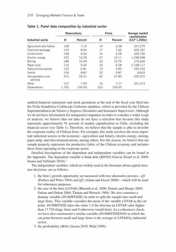
audited financial statements and stock quotations at the end of the fiscal year filed into the Ficha Estadística Codificada Uniforme database, which is provided by the Chilean Superintendencia de Valores y Seguros (Securities and Insurance Supervisor). Although we do not have information for nonquoted companies in order to consider a wider scope of analysis, we believe that our data do not have a selection bias because this study represents approximately 91 percent of market capitalization in Chile, excluding the financial sector (see Table 1). Therefore, we believe that the sample is able to describe the corporate reality of Chilean firms. For example, this study involves the most impor-tant industrial sectors in the economy—agriculture and fishery, electric energy, mining, paper pulp, and telecommunications, among others. For this reason, we believe that our sample properly represents the productive fabric of the Chilean economy and includes those firms operating in the corporate sector.
Detailed descriptions of the dependent and independent variables can be found in the Appendix. The dependent variable is bank debt (BDTD) (García-Teruel et al. 2009; Saona and Vallelado 2010).5
The independent variables, which are widely used in the literature about capital struc-ture decisions, are as follows:
1. the firm’s growth opportunity set measured with two alternative proxies—Q1 (Perfect and Wiles 1994) and Q2 (Adam and Goyal 2008)—which will be used for robustness purposes;
2. the size of the firm (LNTAB) (Bharath et al. 2009; Dennis and Sharpe 2005; Ozkan and Ozkan 2004; Titman and Wessels 1988). We also construct a dummy variable (DUMMYSIZE) in order to split the sample into small and large firms. This variable considers the mean of the variable LNTAB as the cut point. DUMMYSIZE takes the value 1 if the firm has an LNTAB value higher than 17.739 (large firm) and 0 otherwise (small firm). As a robustness check, we have also constructed a similar variable (DUMMYSIZEIND) in which the cut point between small and large firms is the average of LNTAB by industrial sector;
3. the profitability (ROA) (Saona 2010; Wald 1999);
Table 1. Panel data composition by industrial sector
Industrial sector
Observations Firms Average market capitalization (CLP 1,000s)N Percent N Percent
Agriculture and fishery 128 7.14 14 6.28 327,279Food and beverage 144 8.04 17 7.62 409,187Construction 108 6.03 14 6.28 209,736Electric energy 222 12.39 27 12.11 1,298,098Mining 188 10.49 24 10.76 276,666Paper pulp 119 6.64 14 6.28 2,168,117Telecommunications 122 6.81 13 5.83 349,232Textile 159 8.87 22 9.87 8,603Transportation and
services475 26.51 62 27.80 420,972
Other 127 7.09 16 7.17 201,073Observations 1,792 100.00 223 100.00

January–February 2014, Volume 50, Supplement 1 271
4. the collateral (FATA) defined as the assets subject to use in default and financial constraints. The collateral is usually related to the asset structure in a liquida-tion process. The larger the relative tangible assets are, the higher the guaran-tees of paying off the debt (C=rnigoj and Mramor 2009; Flannery and Rangan 2006; Rajan and Winton 1995);
5. the insolvency risk (SDROA) (C=rnigoj and Mramor 2009). This variable should have a negative relationship with the firm’s leverage;
6. the distance from the firm’s debt position to the industry average leverage (DIFD) (Elsas and Florysiak 2011; Flannery and Rangan 2006; Saona and Val-lelado 2012); and
7. the firm’s reputation (IPSA and LNAGE).
Finally, we included dummy variables for the industrial sector in which the firm oper-ates and temporal dummy variables. To reduce the effects of outliers, we have Winsorized all ratios/variables at the first and ninety-ninth percentiles. This technique replaces the values in the 1 percent uppermost and lowermost tails by the next value counting inward from the extremes.
Because it is expected that the current debt decisions depend also on the past decisions, an autoregressive equation model is used, taking the follow form:
BDTDit = β0 + β1BDTDit–1 + β2Qit + β3Qit2 + β4LNTABit + β5ROAit
+ β6FATAit + β7SDROAit + β8DIFDit + β9IPSAit + β10DUMMYTEMPt
+ β11DUMMYINDit + ηi + ηt + εit,
(1)
where ηi represents the individual effect of each firm i; ηt is the temporal effect for the t periods considered in this study; and εit is the stochastic error. The individual effect cor-responds to the characteristics of the firms considered individually, such as the managerial style, the patterns of financial decisions, and so on, which are assumed to be constant over time. The temporal effect includes all the elements that simultaneously, and with the same intensity, affect all firms in the sample, such as the macroeconomic variables and the legal and institutional setting. The stochastic error takes into account the measurement errors as well as the omission of some independent variables in our model. This model can be used to estimate the value at which bank debt is optimized relative to the growth opportunity set (critical value of growth opportunities). In this case, the critical value is the nonlinear combination –β2 /2β3.
To test the interaction effect of firm size and growth opportunities on bank debt, we use the following model:
BDTDit = β0 + β1BDTDit–1 + β2Qit + β3Qit * DUMMYSIZEit + β4Qit2 + β5Qit
2
* DUMMYSIZEit + β6DUMMYSIZEit + β7ROAit + β8FATAit + β9DSROA
+ β10DIFDit + β11IPSAit + β12DUMMYTEMPt + β13DUMMYINDit + ηi + ηt + εit.
(2)
Because of the construction of DUMMYSIZE (and DUMMYSIZEIND), the critical value of growth opportunities for large firms will be –(β2 + β3)/(2(β4 + β5)); for small firms it will take the form –β2 /2β4.
Methodology
Due to the panel structure of our data, which is a combination of cross-sectional and time-series information, we have estimated the model using the generalized method
272 Emerging Markets Finance & Trade
of moments (GMM). The panel data methodology allows us to control for two basic problems in this kind of study: the heterogeneity problem and the endogeneity problem (Arellano 2002).
The relationships between firms’ characteristics and financial decisions must be inter-preted carefully because of the possibility of observing spurious relations. One of the factors contributing to the appearance of spurious relations is the endogeneity problem. An exogenous variable is an independent variable whose value is not affected by the dependent variable, which is said to be endogenous. There is an endogeneity problem when one or more of the explanatory variables are not strictly exogenous. To control for this issue in Equations (1) and (2), we use the GMM system estimator proposed by Blundell and Bond (1998) and Bond (2002).
The GMM system estimator is an enhanced estimator of the first-difference GMM estimator, which is based on the endogeneity of the instruments and allows us to eliminate the bias derived from the fixed and specific effects of each firm considered individually.6 The joint endogeneity of the explanatory variables requires the application of instru-mental variables to obtain consistent estimators of the relevant coefficients. Due to the possible weakness of the instruments (Alonso-Borrego and Arellano 1999), the GMM system estimator returns the most efficient and consistent estimations. These estima-tors are derived under the following assumptions: (1) there is no serial correlation in the disturbance error and (2) there is no correlation between the disturbance term and the individual effect.
The selection of the instruments is central in handling the endogeneity problem. These instruments are based on the contemporary and lagged values of the independent variables that are not strictly exogenous. In our case, the only variable that presents this problem is the growth opportunity set. According to the previous empirical literature on capital structure decisions, the growth opportunity set seems to be an endogenous variable (Bevan and Danbolt 2004; Billett et al. 2007; Danbolt et al. 2002; Dang 2011; Goyal et al. 2002; Krishnaswami and Subramaniam 1999; López and Sogorb 2008; Moon and Tandon 2007; Saona 2010; Saona and Vallelado 2005; Serrasqueiro and Nunes 2010). We require at least two years’ lag to allow the explanatory variable to be introduced as an instrument. We test the validity of the instruments using the Hansen test for over-identifying restrictions, which checks the validity of the selected instruments (Arellano 2002; Hansen et al. 1996). Finally, we perform the Wald test of joint significance for all the dependent variables.
The consistency of the GMM system estimator depends on the absence of second-order serial autocorrelation in the residuals and on the validity of the instruments (Arel-lano 2002; Arellano and Bond 1991, 1998). The GMM system estimator addresses the serial autocorrelation by combining a system of regressions in levels and regressions expressed in first differences, each one of them properly instrumentalized. The instru-ments for the regression expressed in differences—those that by construction eliminate the firm-specific effect—correspond to the lagged levels of the dependent variables. For the regression in levels, the instruments are the lagged differences of the dependent vari-ables. These are suitable instruments under the assumption that the correlation between the dependent variables and the firm-specific effect is constant across time.
The AR1 and AR2 statistics measure first- and second-order serial correlation. Since first-difference transformations have been used, some level of first-order serial correla-tion is expected. However, this correlation does not invalidate the results (Gallego and Loayza 2000; López and Crisóstomo 2010; López and Rodríguez 2008).
January–February 2014, Volume 50, Supplement 1 273
Results
Descriptive Analysis
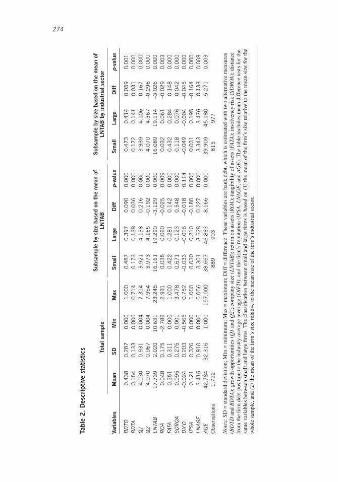
In Table 2, we observe that a typical Chilean firm has about 43.8 percent of its total financial debt issued with private institutions. Although aggregate results by Lefort and Walker (2000b) report slightly higher proportions of bank debt relative to total debt (46.0 percent, 47.0 percent, and 51.0 percent for 1990, 1994, and 1998, respectively), Saona and Vallelado (2010) report that the average proportion of private debt in total debt is about 41.0 percent in their sample of Chilean firms for the 1991–99 period. Our descriptive statistics concerning bank debt over total financial debt are similar also to the recent work by Jara and Sánchez (2012), who report an average ratio of 39.6 percent. Bank debt represents 15.4 percent of total assets, which is close to the results reported by Saona and Vallelado (2010) (12.0 percent) and Jara and Sánchez (2012) (12.4 percent). Concerning the two alternative measures of growth opportunities used in this study, Q1 and Q2, we observe that an average firm has future growth opportunities because the means for Q1 and Q2 are greater than one. The average profitability (ROA) is about 4.8 percent of total assets. Nevertheless, we observe a high standard deviation for this variable (SDROA), which means that there is a large dispersion: some firms make very high profits while others perform very poorly. In general, larger firms seem to have a lower insolvency risk than small firms.
The proxy used for collateral (FATA) indicates that, on average, 35.1 percent of total assets are fixed assets. In other words, a typical Chilean firm has more current assets than fixed assets. This is a source of inefficient liquidations. Finally, according to the statistics, an average firm has about forty-three years since its founding.
Table 2 includes also the difference-of-means test between small and large firms for all the variables under analysis. The mean for LNTAB is the cut point used to dif-ferentiate small firms from large firms. We use the mean of LNTAB by industrial sector to differentiate small and large firms within each sector. There is a statistically signifi-cant difference in the average bank debt (BDTD and BDTA) between small and large firms. Regardless of the measure used to differentiate between small and large firms, small firms have more bank debt than do the largest firms. This preliminary finding is consistent with the extant literature (Gander 2012; Ghosh 2007; Hooks 2003; Kale and Meneghetti 2011). We observe that large firms, on average, have more growth opportunities than do small firms, but smaller firms have almost double the size of collateral (FATA) as a proportion of total assets. Finally, we can say that large firms are older (AGE), and most of them are part of the index of the most-traded firms in the Chilean capital market (IPSA).
Multivariate Analysis
The Effect of Growth Opportunities on Concentration of Bank Debt
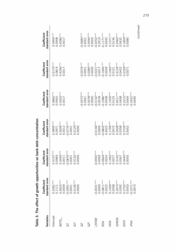
Table 3 describes the effect of growth opportunities on bank debt concentration. As one would expect, the one-period lagged dependent variable (BDTDt–1) is positively correlated with the current level of bank debt concentration. In fact, the average coefficient of this variable is 0.396, which means that the changes in the current bank debt concentration are explained in about 39.6 percent of cases by the changes in bank debt concentration in the previous period.
274 Emerging Markets Finance & Trade
Tabl
e 2
. D
escr
ipti
ve s
tati
stic
s Tota
l sam
ple
Sub
sam
ple
by s
ize
base
d on
the
mea
n of
LN
TAB
Sub
sam
ple
by s
ize
base
d on
the
mea
n of
LN
TAB
by
indu
stri
al s
ecto
r
Vari
able
sM
ean
SD
Min
Max
Sm
all
Larg
eD
iff
p-va
lue
Sm
all
Larg
eD
iff
p-va
lue
BD
TD0
.43
80
.28
70
.00
01
.00
00
.48
70
.39
70
.09
00
.00
00
.47
30
.41
40
.05
90
.00
1B
DTA
0.1
54
0.1
33
0.0
00
0.7
14
0.1
73
0.1
38
0.0
36
0.0
00
0.1
72
0.1
41
0.0
31
0.0
00
Q1
4.0
30
0.9
31
0.0
04
7.3
14
3.9
21
4.1
38
–0.2
16
0.0
00
3.9
39
4.1
06
–0.1
67
0.0
00
Q2
4.0
70
0.9
67
0.0
04
7.9
54
3.9
73
4.1
65
–0.1
92
0.0
00
4.0
70
4.3
67
–0.2
96
0.0
00
LNTA
B1
7.7
39
2.0
20
10
.63
12
3.2
45
16
.16
11
9.2
90
–3.1
29
0.0
00
16
.08
91
9.1
14
–3.0
26
0.0
00
RO
A0
.04
80
.17
5–2
.78
62
.93
10
.03
50
.06
0–0
.02
50
.00
90
.03
20
.06
1–0
.02
90
.00
3FA
TA0
.35
10
.31
10
.00
01
.00
00
.42
20
.28
10
.14
20
.00
00
.43
20
.28
40
.14
80
.00
0SD
RO
A0
.09
50
.27
50
.00
13
.47
80
.67
10
.12
30
.54
80
.00
00
.11
80
.07
60
.04
20
.00
0D
IFD
–0.0
24
0.2
03
–0.5
65
0.7
52
–0.0
33
–0.0
16
–0.0
18
0.1
14
–0.0
49
–0.0
04
–0.0
45
0.0
00
IPSA
0.1
21
0.3
26
0.0
00
1.0
00
0.0
30
0.2
10
–0.1
80
0.0
00
0.0
31
0.1
95
–0.1
64
0.0
00
LNAG
E3
.41
50
.91
00
.00
05
.05
63
.30
13
.52
8–0
.22
70
.00
03
.34
33
.47
6–0
.13
30
.00
8AG
E4
2.7
84
32
.31
61
.00
01
57
.00
03
8.6
67
46
.83
3–8
.16
60
.00
03
9.9
09
45
.18
0–5
.27
10
.00
3O
bser
vati
ons
1,7
92
88
99
03
81
59
77
Not
es:
SD =
sta
ndar
d de
viat
ion;
Min
= m
inim
um; M
ax =
max
imum
; Dif
f =
dif
fere
nce.
The
se v
aria
bles
are
ban
k de
bt, w
hich
is e
stim
ated
with
two
alte
rnat
ive
mea
sure
s (B
DT
D a
nd B
DTA
); g
row
th o
ppor
tuni
ties
(Q1
and
Q2)
; com
pany
siz
e (L
NTA
B);
ret
urn
on a
sset
s (R
OA
); ta
ngib
ility
of
asse
ts (
FATA
); in
solv
ency
ris
k (S
DR
OA
); d
ista
nce
from
the
firm
deb
t pos
ition
to th
e in
dust
ry a
vera
ge le
vera
ge (
DIF
D);
and
the
firm
’s r
eput
atio
n (I
PSA
, LN
AG
E, a
nd A
GE
). T
he ta
ble
incl
udes
mea
n di
ffer
ence
test
s fo
r th
e sa
me
vari
able
s be
twee
n sm
all a
nd la
rge
firm
s. T
he c
lass
ifica
tion
betw
een
smal
l and
larg
e fir
ms
is b
ased
on
(1)
the
mea
n of
the
firm
’s s
ize
rela
tive
to th
e m
ean
size
for
the
who
le s
ampl
e, a
nd (
2) th
e m
ean
of th
e fir
m’s
siz
e re
lativ
e to
the
mea
n si
ze o
f th
e fir
m’s
indu
stri
al s
ecto
r.
January–February 2014, Volume 50, Supplement 1 275
Tabl
e 3
. Th
e ef
fect
of
grow
th o
ppor
tuni
ties
on
bank
deb
t co
ncen
trat
ion
Vari
able
sC
oeffi
cien
t st
anda
rd e
rror
Coe
ffici
ent
stan
dard
err
orC
oeffi
cien
t st
anda
rd e
rror
Coe
ffici
ent
stan
dard
err
orC
oeffi
cien
t st
anda
rd e
rror
Coe
ffici
ent
stan
dard
err
or
Inte
rcep
t0
.22
81
***
0.1
17
10
.41
57
***
0.0
96
90
.38
95
***
0.0
97
10
.38
66
***
0.0
95
00
.51
70
***
0.0
81
90
.54
69
***
0.0
90
8B
DTD
t–1
0.3
65
3**
*0
.00
09
0.3
49
9**
*0
.00
11
0.3
69
9**
*0
.00
12
0.4
30
3**
*0
.00
17
0.4
29
6**
*0
.00
17
0.4
28
6**
*0
.00
17
Q1
–0.0
99
1**
*0
.00
01
–0.0
87
6**
*0
.00
01
–0.0
77
6**
*0
.00
01
Q12
0.0
13
6**
*0
.00
00
0.0
13
2**
*0
.00
00
0.0
12
9**
*0
.00
00
Q2
–0.0
57
3**
*0
.00
01
–0.0
57
6**
*0
.00
01
–0.0
68
4**
*0
.00
01
Q22
0.0
07
8**
*0
.00
00
0.0
08
5**
*0
.00
00
0.0
09
4**
*0
.00
00
LNTA
B–0
.00
31
***
0.0
00
9–0
.00
92
***
0.0
00
9–0
.01
44
***
0.0
00
9–0
.01
32
***
0.0
01
8–0
.02
21
***
0.0
01
7–0
.02
53
***
0.0
01
9R
OA
–0.0
81
1**
*0
.00
22
–0.0
66
4**
*0
.00
24
–0.0
80
5**
*0
.00
22
–0.1
08
6**
*0
.00
38
–0.1
06
6**
*0
.00
39
–0.1
17
1**
*0
.00
45
FATA
0.1
93
9**
*0
.00
58
0.1
99
2**
*0
.00
77
0.1
79
9**
*0
.00
72
0.1
50
9**
*0
.01
23
0.1
56
0**
*0
.01
21
0.1
37
1**
*0
.01
36
SDR
OA
0.3
47
3**
*0
.03
92
0.3
14
5**
*0
.03
67
0.2
62
8**
*0
.03
58
0.4
01
1**
*0
.04
58
0.3
13
4**
*0
.04
22
0.2
96
0**
*0
.04
32
DIF
D0
.27
52
***
0.0
05
30
.34
45
***
0.0
05
50
.27
09
***
0.0
05
20
.23
15
***
0.0
06
90
.23
39
***
0.0
07
10
.18
59
***
0.0
08
0IP
SA–0
.22
71
***
0.0
67
3–0
.20
22
***
0.0
69
4(c
ontin
ues)
276 Emerging Markets Finance & Trade
Vari
able
sC
oeffi
cien
t st
anda
rd e
rror
Coe
ffici
ent
stan
dard
err
orC
oeffi
cien
t st
anda
rd e
rror
Coe
ffici
ent
stan
dard
err
orC
oeffi
cien
t st
anda
rd e
rror
Coe
ffici
ent
stan
dard
err
or
LNAG
E–0
.02
86
***
0.0
02
2–0
.00
29
0.0
02
8AG
E
–0.0
00
5**
*0
.00
01
–0.0
01
0**
*0
.00
01
Indu
stry
dum
my
Yes
Yes
Yes
Yes
Yes
Yes
Tim
e du
mm
yYe
sYe
sYe
sYe
sYe
sYe
sA
R1
–5.4
90
0**
*–5
.44
00
***
–5.4
90
0**
*–5
.60
00
***
–5.5
90
0**
*–5
.61
00
***
AR
2–0
.77
–0.7
8–0
.77
–72
–0.7
2–0
.75
Sar
gan
15
1.4
2**
*(0
.00
0)
15
5.9
5**
*(0
.00
0)
15
4.3
7**
*(0
.00
0)
13
8.6
3**
*(0
.00
0)
14
2.2
6**
*(0
.00
0)
13
9.8
***
(0.0
00
)H
anse
n7
6.3
9(0
.62
4)
74
.29
(0.6
88
)7
6.0
7(0
.63
4)
76
.23
(0.6
29
)7
5.0
8(0
.66
4)
77
.58
(0.5
87
)W
ald
7.6
5E
+0
6**
*9
.49
E+0
6**
*8
.45
E+0
6**
*9
.95
E+0
6**
*1
.26
E+0
7**
*1
.07
E+0
7**
*O
bser
vati
ons
1,4
20
1,4
20
1,4
20
1,4
20
1,4
20
1,4
20
H0:
crit
ical
val
ue
= 0
3.6
43
***
3.3
18
***
3.0
14
***
3.6
73
***
3.3
88
***
3.6
38
***
Not
es:
Coe
ffici
ents
are
est
imat
ed f
rom
the
GM
M s
yste
m e
stim
ator
of
the
follo
win
g m
odel
:
BD
TD
it =
β0 +
β1Q
it–1
+ β
2Qit +
β3Q
it2 + β
4LN
TAB
it +
β 5R
OA
it +
β6F
ATA
it +
β7S
DR
OA
it +
β8D
IFD
it +
β9I
PSA
it +
β10
DU
MM
YT
EM
Pt +
β11
DU
MM
YIN
Dit +
ηi +
ηt +
εit
The
dep
ende
nt v
aria
ble
is b
ank
debt
ove
r to
tal d
ebt (
BD
TD
). B
DT
Dt–
1: th
e on
e-pe
riod
lagg
ed v
aria
ble
of B
DT
D; Q
1 an
d Q
2: g
row
th o
ppor
tuni
ties;
LN
TAB
: com
pany
si
ze; R
OA
: ret
urn
on a
sset
s; F
ATA
: tan
gibi
lity
of a
sset
s; S
DR
OA
: ins
olve
ncy
risk
; DIF
D: d
ista
nce
from
the
firm
deb
t pos
ition
to th
e in
dust
ry a
vera
ge le
vera
ge; I
PSA
, L
NA
GE
, and
AG
E: t
he fi
rm’s
rep
utat
ion.
We
cont
rol f
or in
dust
ry e
ffec
t and
tem
pora
l eff
ect.
To d
eal w
ith th
e po
tent
ial e
ndog
enei
ty p
robl
ems,
the
inst
rum
ents
sel
ecte
d ar
e ba
sed
in la
gged
val
ues
of r
ight
han
d va
riab
les
of th
e es
timat
ed m
odel
. AR
1 an
d A
R2
are
the
test
of
first
-ord
er a
nd s
econ
d-or
der
seri
al a
utoc
orre
latio
n of
the
resi
dual
s,
resp
ectiv
ely.
The
Sar
gan
and
Han
sen
cont
rast
s re
pres
ent t
he te
st o
f ov
erid
entif
ying
res
tric
tions
, asy
mpt
otic
ally
dis
trib
uted
as
a χ2 .
We
show
the
Wal
d te
sts
of s
igni
fican
ce
of th
e ex
plan
ator
y va
riab
les.
We
test
the
hypo
thes
is th
at th
e cr
itica
l val
ues
are
zero
thro
ugh
the
nonl
inea
r co
mbi
natio
ns te
st. S
tand
ard
erro
rs a
re g
iven
bel
ow e
ach
coef
-fic
ient
. ***
Sig
nific
ance
at <
1 p
erce
nt; *
* si
gnifi
canc
e at
< 5
per
cent
; * s
igni
fican
ce a
t < 1
0 pe
rcen
t.
Tabl
e 3
. C
onti
nued
January–February 2014, Volume 50, Supplement 1 277
Since the growth opportunities are typically unobservable by outsiders, a common practice is to rely on proxy variables. To minimize the bias caused by the measurement of growth opportunities in our results, we use two alternative proxies. Q1 considers the replacement value of total assets; Q2 considers the market value of the firm. These two are the usual approximations of the Tobin’s Q and may be used for robustness purposes as well.7
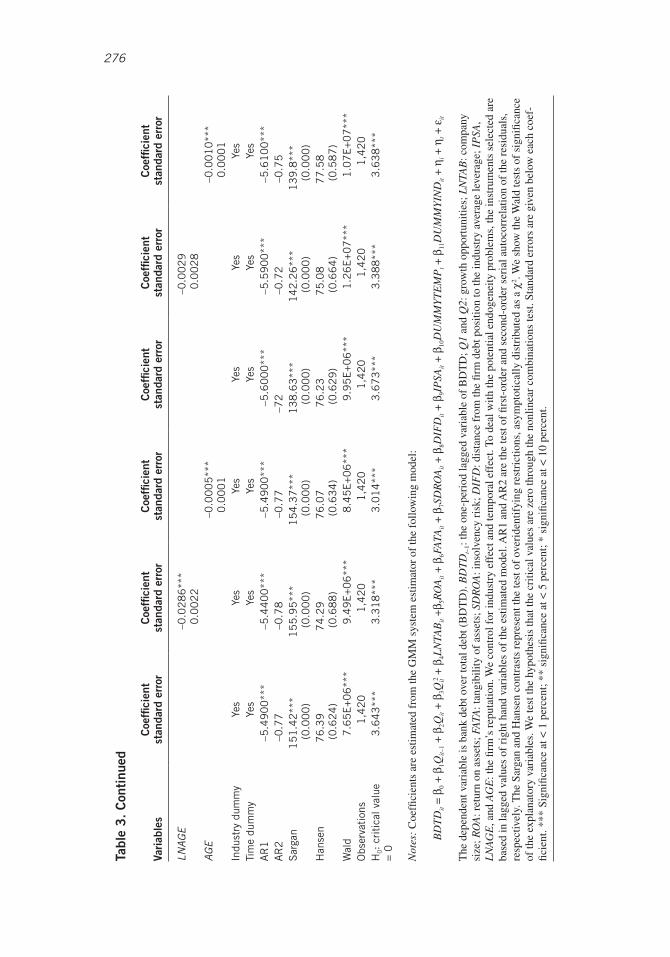
In all cases, for the whole sample in Table 3, we observe that there is a nonmonotonic U-shaped relationship between the growth opportunities and the level of bank debt for the two proxies of the growth opportunity set, Q1 and Q2. The relationship is negative for low levels of growth opportunities and positive once the critical level of growth opportunities is reached. The critical level of growth opportunities is recorded for each regression at the bottom of the table. The applied test on nonlinear restriction verifies that the estimated values are statistically different from zero. In fact, bank debt level is minimized when the average levels of growth opportunities are 3.33 and 3.57 for Q1 and Q2, respectively.
This finding is consistent with the hypothesis about the effect of growth opportunities on bank debt. The negative relationship between growth options and bank debt is sup-ported by the hold-up problem. Private creditors can take advantage of their informational monopoly and extract rents from the company and its future investment projects. To avoid the excessive power that banks can exert over the firm, managers will reduce the level of bank debt as growth opportunities increase. This argument comes from the side of the demand for external funds.
Once the critical point of growth opportunities is achieved (bottom line of Table 3), a positive relationship is observed between this variable and bank debt. This finding is sup-ported by the following arguments: First, the asymmetries of information generated by the growth opportunities might cause more severe agency problems. As a result, shareholders might use bank debt to reduce the informational gap of growth opportunities, and, by doing so, to more efficiently monitor the firm. Second, the strategic advantage of growth opportunities might be jeopardized if the information is shared with a large number of creditors, as occurs in the case of public debt. However, if these growth opportunities are financed through one or a few bank creditors, the strategic advantage is kept inside the firm and not disseminated to outsiders. In this case, the firm will prefer to finance the growth options with private debt and not spread the strategic information into the capital markets. Finally, when information about growth opportunities is asymmetrically distributed, managers might opportunistically use the free cash flow to undertake negative NPV projects. To avoid these agency problems, shareholders will persuade their managers to issue more debt, particularly bank debt. By doing this, shareholders force managers to afford periodic payments of both interest and principal, which reduces the free cash flow available for opportunistic behavior. Therefore, this last argument also supports a positive relationship between growth opportunities and bank debt.
Regarding the other variables included in the estimations, we observe that the larger the firm (LNTAB), the lower the proportion of bank debt. This finding is consistent with the additional sources of funds available for large firms. It has been widely recognized that large firms can take advantage of the economies of scale issuing corporate bonds, for instance, or additional equity in national markets and abroad (e.g., American Depository Receipts [ADRs]). In less integrated capital markets, smaller firms are usually constrained to issuing bank debt because they cannot take advantage of the economies of scale when issuing, for instance, public debt.
278 Emerging Markets Finance & Trade
Concerning the firm’s profitability (ROA), we observe a negative and statistically significant relationship with private debt. This finding is supported by the pecking order theory, which argues that firms will first use internally generated funds and will issue debt only when this internal source of funds is exhausted. More profitable firms are able to generate higher inflows, and therefore, their dependence on external sources of funds, such as banks, is lower.
The tangibility of assets, which might be used also as a proxy for collateral (FATA), shows a positive relationship with bank debt. Firms with a higher degree of information asymmetry (lower collateral in the form of fixed assets) will be less likely to issue debt privately. The idea that if a firm pledges collateral when taking a bank loan, the price at which it obtains credit will be lower and thus will improve debt capacity is widely accepted in the extensive empirical literature (Benmelech and Bergman 2009). Our find-ings seem to support this idea.
In Table 3, we observe a positive relationship between SDROA and bank debt. The explanation for this result is that in the Chilean corporate sector, shareholders are trying to transfer the insolvency risk to private creditors. This agency conflict is materialized in the asset substitution problem. We might say that high-risk companies are interested in sources of funds that can mitigate inefficient firm liquidation (De Andrés et al. 2005). Therefore, firms with more volatile returns will prefer bank debt rather than public or market debt in case they need to avoid liquidation.
The results show that the higher the difference between the firm’s leverage and its industry’s leverage (DIFD), the higher the proportion of bank debt. When the firm’s leverage is further from its industry’s leverage, bank debt is the resource used by the firm to finance its operations.
Finally, we have used a number of measures for a firm’s reputation (IPSA, LNAGE, AGE). IPSA is a dummy variable that indicates whether the company is one of the twenty most-traded firms in the Chilean corporate sector; AGE and LNAGE are the number of years since the founding of the company and its logarithmic transformation, respectively. The three proxies for reputation are negatively related with bank debt (note that AGE and LNAGE are not significant in the third and fifth regressions in Table 3, respectively). In general, we can suggest that there is a negative impact of a firm’s reputation on private debt. There seems to be a substitution effect of private debt by public debt when reputa-tion improves. In other words, firms use their reputation to access capital markets other than bank debt (Ang et al. 1982).
The Effect of Firm Size on the Relationship Between Growth Opportunities and Concentration of Bank Debt
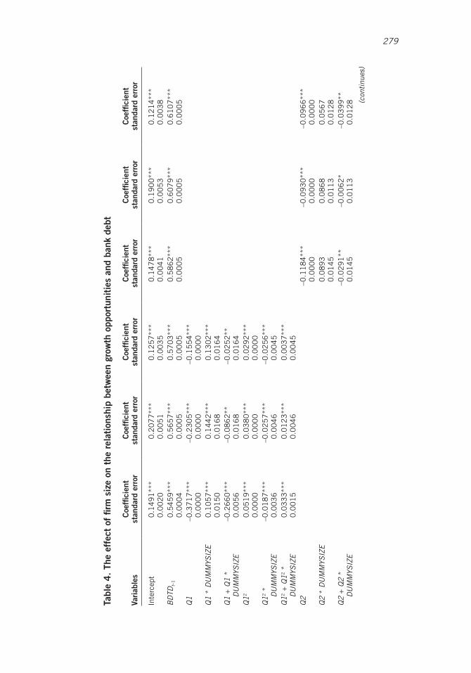
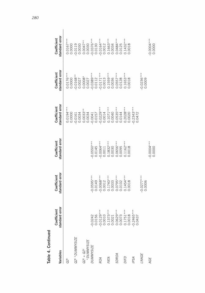
The most interesting result of this study is that we find empirical evidence that the behavior of small and large companies is not the same when they choose their financial resources. Although in both cases, the relationship between growth opportunities and bank debt is first negative and then positive, the critical level is reached sooner for small firms than for large firms. This finding is consistent for the two proxies of growth oppor-tunities used in this paper (see Table 4 for Q1 and Q2). In other words, the minimum of bank debt is obtained at lower levels of growth opportunities for smaller firms than for larger firms. To determine what the critical values are, we use the dummy variable for firm size (DUMMYSIZE, which takes value 1 when the size of the firm is greater than the mean value for LNTAB and 0 otherwise), which is interacted with the different
January–February 2014, Volume 50, Supplement 1 279
Tabl
e 4
. Th
e ef
fect
of
firm
siz
e on
the
rel
atio
nshi
p be
twee
n gr
owth
opp
ortu
niti
es a
nd b
ank
debt
Vari
able
sC
oeffi
cien
t
stan
dard
err
orC
oeffi
cien
t
stan
dard
err
orC
oeffi
cien
t
stan
dard
err
orC
oeffi
cien
t
stan
dard
err
orC
oeffi
cien
t
stan
dard
err
orC
oeffi
cien
t
stan
dard
err
or
Inte
rcep
t0
.14
91
***
0.0
02
0
0.2
07
7**
*0
.00
51
0.1
25
7**
*0
.00
35
0.1
47
8**
*0
.00
41
0.1
90
0**
*0
.00
53
0.1
21
4**
*0
.00
38
BD
TDt–
10
.54
59
***
0.0
00
40
.56
57
***
0.0
00
50
.57
03
***
0.0
00
50
.58
62
***
0.0
00
50
.60
79
***
0.0
00
50
.61
07
***
0.0
00
5Q
1–0
.37
17
***
0.0
00
0–0
.23
05
***
0.0
00
0–0
.15
54
***
0.0
00
0Q
1 *
DU
MM
YSIZ
E0
.10
57
***
0.0
15
00
.14
42
***
0.0
16
80
.13
02
***
0.0
16
4Q
1 + Q
1 *
DU
MM
YSIZ
E–0
.26
60
***
0.0
05
6–0
.08
62
**0
.01
68
–0.0
25
2**
0.0
16
4Q
120
.05
19
***
0.0
00
00
.03
80
***
0.0
00
00
.02
92
***
0.0
00
0Q
12 *
D
UM
MYS
IZE
–0.0
18
7**
*0
.00
36
–0.0
25
7**
*0
.00
46
–0.0
25
6**
*0
.00
45
Q12
+ Q
12 *
D
UM
MYS
IZE
0.0
33
3**
*0
.00
15
0.0
12
3**
*0
.00
46
0.0
03
7**
*0
.00
45
Q2
–0.1
18
4**
*0
.00
00
–0.0
93
0**
*0
.00
00
–0.0
96
6**
*0
.00
00
Q2
* D
UM
MYS
IZE
0.0
89
30
.01
45
0.0
86
80
.01
13
0.0
56
70
.01
28
Q2
+ Q
2 *
DU
MM
YSIZ
E–0
.02
91
**0
.01
45
–0.0
06
2*
0.0
11
3–0
.03
99
**0
.01
28 (c
ontin
ues)
280 Emerging Markets Finance & Trade
Vari
able
sC
oeffi
cien
t
stan
dard
err
orC
oeffi
cien
t
stan
dard
err
orC
oeffi
cien
t
stan
dard
err
orC
oeffi
cien
t
stan
dard
err
orC
oeffi
cien
t
stan
dard
err
orC
oeffi
cien
t
stan
dard
err
or
Q22
0.0
19
4**
*0
.00
00
0.0
17
6**
*0
.00
00
0.0
16
7**
*0
.00
00
Q22
*D
UM
MYS
IZE
–0.0
16
10
.00
34
–0.0
16
8**
0.0
02
7–0
.01
19
0.0
03
0Q
2 2 +
Q2
2
*DU
MM
YSIZ
E0
.00
33
**0
.00
34
0.0
00
8*
0.0
02
70
.00
47
**0
.00
30
DU
MM
YSIZ
E–0
.02
42
0.0
15
6–0
.05
95
***
0.0
14
9–0
.05
50
***
0.0
14
5–0
.00
41
0.0
15
7–0
.03
89
***
0.0
11
2–0
.03
76
***
0.0
13
0R
OA
–0.0
12
9**
*0
.00
10
–0.0
06
8**
*0
.00
12
–0.0
06
4**
*0
.00
11
–0.0
22
9**
*0
.00
14
–0.0
17
1**
*0
.00
13
–0.0
16
4**
*0
.00
12
FATA
0.1
37
3**
*0
.00
21
0.1
74
0**
*0
.00
33
0.1
83
2**
*0
.00
30
0.1
07
1**
*0
.00
40
0.1
55
9**
*0
.00
36
0.1
66
3**
*0
.00
34
SDR
OA
0.0
62
9**
*0
.00
73
0.0
79
5**
*0
.01
02
0.0
65
6**
*0
.00
95
0.0
53
5**
*0
.01
44
0.0
55
7**
*0
.01
28
0.0
48
4**
*0
.01
25
DIF
D0
.17
51
***
0.0
01
80
.14
54
***
0.0
01
80
.11
62
***
0.0
01
80
.20
28
***
0.0
02
00
.16
53
***
0.0
01
80
.14
32
***
0.0
01
8IP
SA–0
.24
65
***
0.0
43
7–0
.23
43
***
0.0
47
2LN
AGE
–0.0
27
7**
*0
.00
06
–0.0
23
6**
*0
.00
09
AGE
–0.0
00
4**
*0
.00
00
–0.0
00
4**
*0
.00
00
Tabl
e 4
. C
onti
nued
January–February 2014, Volume 50, Supplement 1 281
Indu
stry
dum
my
Yes
Yes
Yes
Yes
Yes
Yes
Tim
e du
mm
yYe
sYe
sYe
sYe
sYe
sYe
sA
R1
–5.7
50
0**
*–5
.76
00
***
–5.7
60
0**
*–5
.74
00
***
–5.7
60
0**
*–5
.76
00
***
AR
2–0
.46
–0.4
7–0
.47
–0.4
9–0
.48
–0.4
8S
arga
n (p
-val
ue)
23
2.6
3**
*(0
.00
0)
23
6.1
1**
*(0
.00
0)
23
6.0
2**
*(0
.00
0)
22
0.3
8**
*(0
.00
0)
22
2.6
3**
*(0
.00
0)
22
2.7
8**
*(0
.00
0)
Han
sen
(p-v
alue
)1
23
.57
(0.8
05
)1
23
.26
(0.8
11
)1
27
.69
(0.7
25
)1
22
.27
(0.8
28
)1
25
.82
(0.7
63
)1
30
.65
(0.6
59
)W
ald
1.0
4E
+0
8**
*8
.92
E+0
7**
*9
.26
E+0
7**
*1
.08
E+0
8**
*9
.93
E+0
7**
*1
.01
E+0
8**
*O
bser
vati
ons
1,4
20
1,4
20
1,4
20
1,4
20
1,4
20
1,4
20
Larg
e fir
ms’
cr
itic
al v
alue
3.9
97
3.5
01
3.4
44
4.4
77
4.0
72
4.2
11
Sm
all fi
rms’
cr
itic
al v
alue
3
.57
93
.03
12
.65
93
.05
82
.64
72
.89
7
H0:
diff
eren
ce
crit
ical
va
lue
= 0
0.4
18
***
0.4
70
***
0.7
86
***
1.4
18
***
1.4
25
***
1.3
14
***
Not
es:
Coe
ffici
ents
are
est
imat
ed f
rom
the
GM
M s
yste
m e
stim
ator
of
the
follo
win
g m
odel
:
BD
TD
it =
β0 +
β1 B
DT
Dit
–1 +
β2Q
it +
β3Q
it *
DU
MM
YSI
ZE
it +
β4Q
it2 + β
5Qit2 *
DU
MM
YSI
ZE
it +
β6 D
UM
MY
SIZ
Eit +
β7 R
OA
it +
β8 FA
TAit +
β9 Z
it +
β10
DIF
Dit
+ β
11 IP
SAit +
β12
DU
MM
YT
EM
Pt +
β13
DU
MM
YIN
Dit +
ηi +
ηt +
εit
The
dep
ende
nt v
aria
ble
is b
ank
debt
ove
r to
tal d
ebt (
BD
TD
). B
DT
Dt–
1: th
e on
e-pe
riod
lagg
ed v
aria
ble
of B
DT
D; Q
1 an
d Q
2: g
row
th o
ppor
tuni
ties;
LN
TAB
: com
pany
siz
e; R
OA
: re-
turn
on
asse
ts; F
ATA
: tan
gibi
lity
of a
sset
s; S
DR
OA
: ins
olve
ncy
risk
; DIF
D: d
ista
nce
from
the
firm
deb
t pos
ition
to th
e in
dust
ry a
vera
ge le
vera
ge; I
PSA
, LN
AG
E, a
nd A
GE
: the
firm
’s
repu
tatio
n; D
UM
MY
SIZ
E: a
dum
my
vari
able
for
the
size
of
the
com
pany
). W
e co
ntro
l for
indu
stry
eff
ect a
nd te
mpo
ral e
ffec
t. To
dea
l with
the
pote
ntia
l end
ogen
eity
pro
blem
s, th
e in
stru
men
ts s
elec
ted
are
base
d in
lagg
ed v
alue
s of
rig
ht h
and
vari
able
s of
the
estim
ated
mod
el. A
R1
and
AR
2 ar
e th
e te
st o
f fir
st-o
rder
and
sec
ond-
orde
r se
rial
aut
ocor
rela
tion
of th
e re
sidu
als,
res
pect
ivel
y. T
he S
arga
n an
d H
anse
n te
st r
epre
sent
s te
st o
f ov
erid
entif
ying
res
tric
tions
, asy
mpt
otic
ally
dis
trib
uted
as
a χ2 .
We
show
the
Wal
d te
sts
of s
igni
fican
ce o
f th
e ex
plan
ator
y va
riab
les.
We
test
the
hypo
thes
is th
at th
e cr
itica
l val
ues
for
larg
e an
d sm
all fi
rms
are
the
sam
e th
roug
hout
the
nonl
inea
r re
stri
ctio
ns te
st. S
tand
ard
erro
rs a
re g
iven
bel
ow
each
coe
ffici
ent.
***
Sign
ifica
nce
at <
1 p
erce
nt; *
* si
gnifi
canc
e at
< 5
per
cent
; * s
igni
fican
ce a
t < 1
0 pe
rcen
t.

282 Emerging Markets Finance & Trade
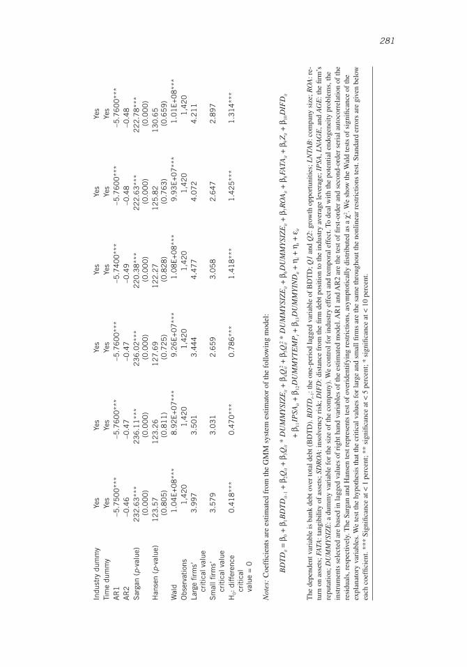
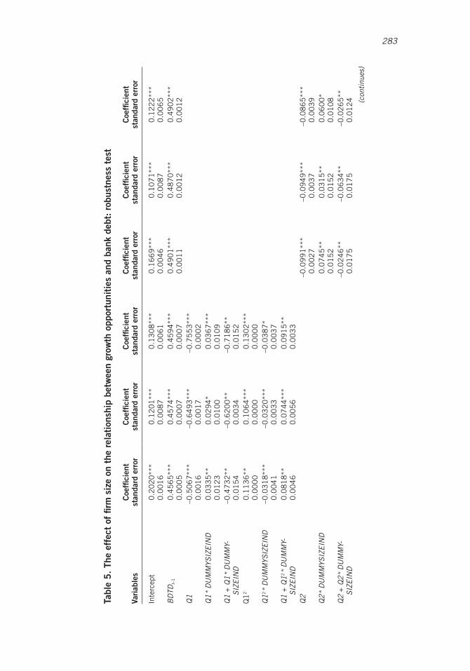
proxies for growth opportunities and their respective squared transformations (Q1, Q12, Q2, and Q22). We run nonlinear restriction tests to validate the addition of Q1 and Q1 * DUMMYSIZE and their squared transformations. The same tests apply for the Q2 variable. The results in Table 4 correspond to the estimations of Equation (2). We also test the null hypothesis, which states that the critical values for large and small firms are the same. The hypothesis is rejected in all the regressions shown in Table 4. Thus, we can accept the assertion that the critical value for small firms is achieved at statistically lower levels of growth opportunities than for large firms. Once this threshold is passed, the growth opportunities tend to be financed with higher levels of bank debt.
It is important to note that the divergence in the critical values of growth opportu-nities between large and small firms is due to inherent characteristics of the Chilean marketplace. There are several arguments supporting this idea. First, in general, larger firms have easier access to public debt markets than do smaller firms. This is because larger firms have relatively lower bankruptcy costs, can diversify more easily than smaller firms, and can take advantage of the economies of scale of the fixed flotation costs of public debt more easily than small firms (Saona 2011). Therefore, small firms must issue bank debt sooner than large companies to be able to finance their growth opportunity set. Second, according to Hackbarth (2009), in an institutional environment with weak protection of investors, small firms are forced to accept “take it or leave it” loans because the supply of alternative funds for this kind of firm is much less than for large and mature companies. Consequently, small firms must issue bank debt to finance their growth opportunities in situations where a large firm might still be able to issue financial securities other than private debt. Third, according to the institutional setting, Beck et al. (2008) argue that bank-based financial systems, such as the Chilean system, foster disproportionately the development of small firms relative to large firms. Therefore, the most important source of funds to finance the future growth opportunities of small firms is private borrowing.
Considering the other explanatory variables included in the specification of our model, we observe some other interesting findings. For instance, the DUMMYSIZE vari-able is in accordance with LNTAB (from Table 3), showing a negative and statistically significant coefficient. In other words, larger firms issue less bank debt than do small firms for financing their operations. The descriptive statistic also shows that small firms have about 48.7 percent of their debt issued through private banks while large firms have only 39.7 percent of their total debt issued with banks (see Table 2).
The other explanatory variables as well as the control variables show roughly the same results as those displayed in Table 3.
As a robustness test, we run the regressions of Equation (2) one more time, but in this case, we use DUMMYSIZEIND as a dummy variable for the firm size (Table 5). This dummy takes into consideration the average size of the firm relative to its indus-trial sector. This variable takes the value 1 when the size of the company is larger than the average firm size in its own industrial sector and 0 otherwise. The results are consistent with those shown in Table 4. Therefore, we can conclude that the major findings are robust regardless of the criteria used to differentiate between large and small companies. Once again, the nonlinear U-shaped relationship between the set of growth opportunities and private debt is observed. The bottom line of Table 5 shows that the critical values for small firms are different from those for large firms, support-ing the idea that small firms seek private loans sooner than do large firms as growth opportunities increase.
January–February 2014, Volume 50, Supplement 1 283
Tabl
e 5
. Th
e ef
fect
of
firm
siz
e on
the
rel
atio
nshi
p be
twee
n gr
owth
opp
ortu
niti
es a
nd b
ank
debt
: ro
bust
ness
tes
t
Vari
able
sC
oeffi
cien
t
stan
dard
err
orC
oeffi
cien
t
stan
dard
err
orC
oeffi
cien
t
stan
dard
err
orC
oeffi
cien
t
stan
dard
err
orC
oeffi
cien
t
stan
dard
err
orC
oeffi
cien
t
stan
dard
err
or
Inte
rcep
t0
.20
20
***
0.0
01
60
.12
01
***
0.0
08
70
.13
08
***
0.0
06
10
.16
69
***
0.0
04
60
.10
71
***
0.0
08
70
.12
22
***
0.0
06
5B
DTD
t–1
0.4
56
5**
*0
.00
05
0.4
57
4**
*0
.00
07
0.4
59
4**
*0
.00
07
0.4
90
1**
*0
.00
11
0.4
87
0**
*0
.00
12
0.4
90
2**
*0
.00
12
Q1
–0.5
06
7**
*0
.00
16
–0.6
49
3**
*0
.00
17
–0.7
55
3**
*0
.00
02
Q1
* D
UM
MYS
IZEI
ND
0.0
33
5**
0.0
12
30
.02
94
*0
.01
00
0.0
36
7**
*0
.01
09
Q1
+ Q
1 *
DU
MM
Y-SI
ZEIN
D–0
.47
32
**0
.01
54
–0.6
20
0**
0.0
03
4–0
.71
86
**0
.01
52
Q1
20
.11
36
**0
.00
00
0.1
06
4**
*0
.00
00
0.1
30
2**
*0
.00
00
Q12
* D
UM
MYS
IZEI
ND
–0.0
31
8**
*0
.00
41
–0.0
32
0**
*0
.00
33
–0.0
38
7*
0.0
03
7Q
1 + Q
12 *
DU
MM
Y-SI
ZEIN
D0
.08
18
**0
.00
46
0.0
74
4**
*0
.00
56
0.0
91
5**
0.0
03
3
Q2
–0.0
99
1**
*0
.00
27
–0.0
94
9**
*0
.00
37
–0.0
86
5**
*0
.00
39
Q2
* D
UM
MYS
IZEI
ND
0.0
74
5**
0.0
15
20
.03
15
**0
.01
52
0.0
60
0*
0.0
10
8Q
2 + Q
2 *
DU
MM
Y-SI
ZEIN
D–0
.02
46
**0
.01
75
–0.0
63
4**
0.0
17
5–0
.02
65
**0
.01
24 (c
ontin
ues)
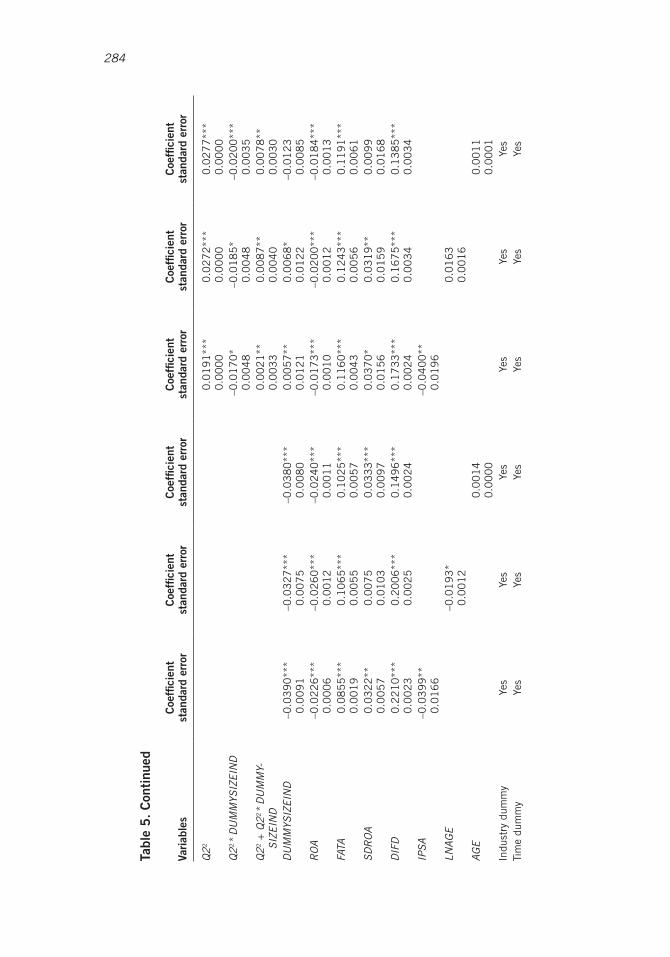
284 Emerging Markets Finance & Trade
Vari
able
sC
oeffi
cien
t
stan
dard
err
orC
oeffi
cien
t
stan
dard
err
orC
oeffi
cien
t
stan
dard
err
orC
oeffi
cien
t
stan
dard
err
orC
oeffi
cien
t
stan
dard
err
orC
oeffi
cien
t
stan
dard
err
or
Q2
20
.01
91
***
0.0
00
00
.02
72
***
0.0
00
00
.02
77
***
0.0
00
0Q
2 2 *
DU
MM
YSIZ
EIN
D–0
.01
70
*0
.00
48
–0.0
18
5*
0.0
04
8–0
.02
00
***
0.0
03
5Q
2 2 +
Q2
2 *
DU
MM
Y-SI
ZEIN
D0
.00
21
**0
.00
33
0.0
08
7**
0.0
04
00
.00
78
**0
.00
30
DU
MM
YSIZ
EIN
D–0
.03
90
***
0.0
09
1–0
.03
27
***
0.0
07
5–0
.03
80
***
0.0
08
00
.00
57
**0
.01
21
0.0
06
8*
0.0
12
2–0
.01
23
0.0
08
5R
OA
–0.0
22
6**
*0
.00
06
–0.0
26
0**
*0
.00
12
–0.0
24
0**
*0
.00
11
–0.0
17
3**
*0
.00
10
–0.0
20
0**
*0
.00
12
–0.0
18
4**
*0
.00
13
FATA
0.0
85
5**
*0
.00
19
0.1
06
5**
*0
.00
55
0.1
02
5**
*0
.00
57
0.1
16
0**
*0
.00
43
0.1
24
3**
*0
.00
56
0.1
19
1**
*0
.00
61
SDR
OA
0.0
32
2**
0.0
05
70
.00
75
0.0
10
30
.03
33
***
0.0
09
70
.03
70
*0
.01
56
0.0
31
9**
0.0
15
90
.00
99
0.0
16
8D
IFD
0.2
21
0**
*0
.00
23
0.2
00
6**
*0
.00
25
0.1
49
6**
*0
.00
24
0.1
73
3**
*0
.00
24
0.1
67
5**
*0
.00
34
0.1
38
5**
*0
.00
34
IPSA
–0.0
39
9**
0.0
16
6–0
.04
00
**0
.01
96
LNAG
E–0
.01
93
*0
.00
12
0.0
16
30
.00
16
AGE
0.0
01
40
.00
00
0.0
01
10
.00
01
Indu
stry
dum
my
Yes
Yes
Yes
Yes
Yes
Yes
Tim
e du
mm
yYe
sYe
sYe
sYe
sYe
sYe
s
Tabl
e 5
. C
onti
nued
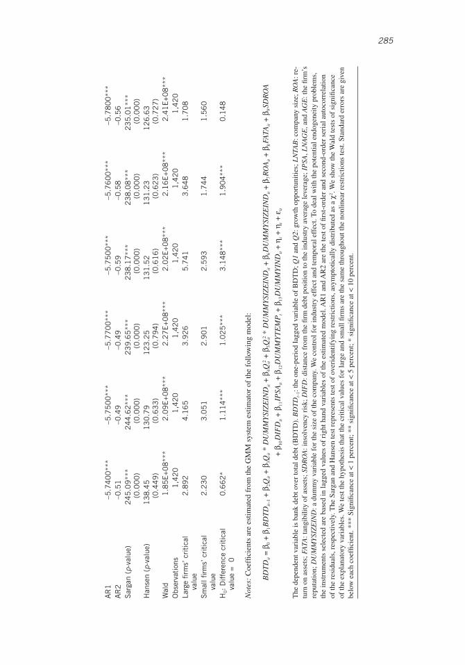
January–February 2014, Volume 50, Supplement 1 285
AR
1–5
.74
00
***
–5.7
50
0**
*–5
.77
00
***
–5.7
50
0**
*–5
.76
00
***
–5.7
80
0**
*A
R2
–0.5
1–0
.49
–0.4
9–0
.59
–0.5
8–0
.56
Sar
gan
(p-v
alue
)2
45
.09
***
(0.0
00
)2
44
.62
***
(0.0
00
)2
39
.65
***
(0.0
00
)2
38
.17
***
(0.0
00
)2
38
.08
***
(0.0
00
)2
35
.01
***
(0.0
00
)H
anse
n (p
-val
ue)
13
8.4
5(0
.44
9)
13
0.7
9(0
.63
3)
12
3.2
5(0
.79
4)
13
1.5
2(0
.61
6)
13
1.2
3(0
.62
3)
12
6.6
3(0
.72
7)
Wal
d1
.85
E+0
8**
*2
.09
E+0
8**
*2
.27
E+0
8**
*2
.02
E+0
8**
*2
.16
E+0
8**
*2
.41
E+0
8**
*O
bser
vati
ons
1,4
20
1,4
20
1,4
20
1,4
20
1,4
20
1,4
20
Larg
e fir
ms’
cri
tica
l va
lue
2.8
92
4.1
65
3.9
26
5.7
41
3.6
48
1.7
08
Sm
all fi
rms’
cri
tica
l va
lue
2.2
30
3.0
51
2.9
01
2.5
93
1.7
44
1.5
60
H0:
Dif
fere
nce
crit
ical
va
lue
=
00
.66
2*
1.1
14
***
1.0
25
***
3.1
48
***
1.9
04
***
0.1
48
Not
es:
Coe
ffici
ents
are
est
imat
ed f
rom
the
GM
M s
yste
m e
stim
ator
of
the
follo
win
g m
odel
:
BD
TD
it =
β0 +
β1 B
DT
Dit
–1 +
β2Q
it +
β3Q
it *
DU
MM
YSI
ZE
IND
it +
β4Q
it2 + β
5Qit2 *
DU
MM
YSI
ZE
IND
it +
β6 D
UM
MY
SIZ
EIN
Dit +
β7 R
OA
it +
β8 FA
TAit +
β9 SD
RO
A
+ β
10 D
IFD
it +
β11
IPSA
it +
β12
DU
MM
YT
EM
Pt +
β13
DU
MM
YIN
Dit +
ηi +
ηt +
εit
The
dep
ende
nt v
aria
ble
is b
ank
debt
ove
r to
tal d
ebt (
BD
TD
). B
DT
Dt–
1: th
e on
e-pe
riod
lagg
ed v
aria
ble
of B
DT
D; Q
1 an
d Q
2: g
row
th o
ppor
tuni
ties;
LN
TAB
: com
pany
siz
e; R
OA
: re-
turn
on
asse
ts; F
ATA
: tan
gibi
lity
of a
sset
s; S
DR
OA
: ins
olve
ncy
risk
; DIF
D: d
ista
nce
from
the
firm
deb
t pos
ition
to th
e in
dust
ry a
vera
ge le
vera
ge; I
PSA
, LN
AG
E, a
nd A
GE
: the
firm
’s
repu
tatio
n; D
UM
MY
SIZ
EIN
D: a
dum
my
vari
able
for
the
size
of
the
com
pany
. We
cont
rol f
or in
dust
ry e
ffec
t and
tem
pora
l eff
ect.
To d
eal w
ith th
e po
tent
ial e
ndog
enei
ty p
robl
ems,
th
e in
stru
men
ts s
elec
ted
are
base
d in
lagg
ed v
alue
s of
rig
ht h
and
vari
able
s of
the
estim
ated
mod
el. A
R1
and
AR
2 ar
e th
e te
st o
f fir
st-o
rder
and
sec
ond-
orde
r se
rial
aut
ocor
rela
tion
of th
e re
sidu
als,
res
pect
ivel
y. T
he S
arga
n an
d H
anse
n te
st r
epre
sent
s te
st o
f ov
erid
entif
ying
res
tric
tions
, asy
mpt
otic
ally
dis
trib
uted
as
a χ2 .
We
show
the
Wal
d te
sts
of s
igni
fican
ce
of th
e ex
plan
ator
y va
riab
les.
We
test
the
hypo
thes
is th
at th
e cr
itica
l val
ues
for
larg
e an
d sm
all fi
rms
are
the
sam
e th
roug
hout
the
nonl
inea
r re
stri
ctio
ns te
st. S
tand
ard
erro
rs a
re g
iven
be
low
eac
h co
effic
ient
. ***
Sig
nific
ance
at <
1 p
erce
nt; *
* si
gnifi
canc
e at
< 5
per
cent
; * s
igni
fican
ce a
t < 1
0 pe
rcen
t.
286 Emerging Markets Finance & Trade
Conclusions and Final Remarks
This paper goes one step beyond Jara et al.’s (2012) article, analyzing the extent to which firm size determines the nonmonotonic relationship between future growth opportunities and bank debt in the Chilean corporate sector. We use the agency theory and the asym-metries of information theory to ascertain how firm size determines the capital structure and particularly the bank debt decision.
The empirical analysis shows that the U-shaped relationship between growth oppor-tunities and bank debt is justified by the rent consumption done by banks, which use their informative advantage (hold-up problem) to create the negative relationship; the positive relation between growth options and private debt is justified by the overinvest-ment problems and by the disciplining role of debt in reducing the agency problems of debt. Moreover, we conclude that this nonmonotonic relationship has a different pattern depending on the size of the firm. Consistently, smaller firms resort to bank debt sooner than do larger firms as the growth opportunities set rises. Several factors support this find-ing: the higher transaction costs of public debt for smaller firms relative to larger firms, the lower availability of external sources other than private debt for small companies, the lesser reputation and credit quality of smaller companies, the higher insolvency risk for smaller firms, among others.
The results obtained in this paper suggest possible future changes in economic policies in order to develop the Chilean financial and corporate sectors. Policy makers should address future regulation in order to facilitate more diversified capital structures in Chil-ean firms, particularly in small firms. This will make access to external sources of funds other than bank debt easier, which will lower the cost of capital and prevent firms from rejecting profitable projects due to financial constraints.
Finally, a future research line derived from this paper might be addressed by a cross-country analysis, including other emerging economies, to study the extent to which country-level factors determine bank debt decisions.
Notes
1. This political process was known as “popular capitalism,” wherein several important firms were part of a privatization process. Some examples of these firms are LAN (now LATAM), Copec, Inforsa (now CMPC), Banco de Chile, Banco Santiago (now Banco Santander de Chile), CTC (now Telefónica Chile), Enersis, IANSA, and SOQUIMICH (Sociedad Química y Minera), among others.
2. Some of the main differences related to the country of legal origin are creditors’ rights (Levine 1998), quality of accounting standards and the accounting process in general, ownership structure (Himmelberg et al. 1999), market development, and per capita income (La Porta et al. 2000). In general, common-law systems provide greater investor protection than do French civil-law systems.
3. The ability of public lenders to anticipate the agency problems of debt is related to the degree of financial market development. According to the empirical literature about financial development, the Chilean capital markets are quite developed compared with capital markets of the United States and the most developed markets in South America (Beck et al. 2008; Beck et al. 2000; La Porta et al. 1998; World Economic Forum 2009, 2012). Although Chilean financial market development scores have experienced significant improvements (World Economic Forum 2009, 2012), recent financial scandals such as La Polar case cast doubts on the ability of Chile’s public lenders to anticipate properly the agency problems of debt.
4. Berger and Udell (2002) provide evidence that size reflects reputation in financing choices.5. Accounts payable, debt with related parties, and other non–interest-bearing debt in our records
represent about 18.4 percent of total assets. In their aggregate statistics, Lefort and Walker (2000b)
January–February 2014, Volume 50, Supplement 1 287
report that these types of debt represent about one-third of total assets. Lefort and Walker’s statistics are substantially higher than ours because their time span covers the decade of the 1990s, when high capital markets and economic growth were observed in Chile. The use of internal capital markets and a sharp increase in accounts payable occurred as a response to the pronounced growth and some financial restrictions originated by the Asian financial crisis in the middle of the 1990s.
6. For further detail about the differences and advantages of the GMM system estimator relative to the first-difference GMM estimator, see Roodman (2009).
7. The theoretical definition of Tobin’s Q coefficient is the ratio of market value of the firm to replacement cost of assets. Chung and Pruitt (1994) have compared the values of Q obtained by the method of Lindenberg and Ross (1981) with the market-to-book ratio, finding that at least 96.6 percent of the variability of Tobin’s Q is explained by the market-to-book ratio. A similar correlation coefficient (96 percent) is found by Perfect and Wiles (1994). The findings reported by Adam and Goyal (2008) show that, on a relative scale, the market-to-book assets ratio has the highest information content with respect to investment opportunities.
8. To avoid losing a few observations for year 1997, SDROAit is computed from year t to year t – 4.
References
Adam, T., and V. Goyal. 2008. “The Investment Opportunity Set and Its Proxy Variables.” Jour-nal of Financial Research 31, no. 1: 41–63.
Akisik, O. 2013. “Accounting Regulation, Financial Development, and Economic Growth.” Emerging Markets Finance & Trade 49, no. 1: 33–67.
Albring, S.M.; I.K. Khurana; A. Nejadmalayeri; and R. Pereira. 2011. “Managerial Compensa-tion and the Debt Placement Decision.” Journal of Corporate Finance 17, no. 5: 1445–1456.
Alonso-Borrego, C., and M. Arellano. 1999. “Symmetrically Normalized Instrumental-Variable Estimation Using Panel Data.” Journal of Business & Economic Statistics 17, no. 1: 36–49.
Andritzky, J. 2003. “Leverage, Industries, and Countries: Evidence from Seven Countries.” Working paper, Universität St. Gallen, November 17.
Ang, J.; J. Chua; and J. McConnell. 1982. “The Administrative Costs of Corporate Bankruptcy: A Note.” Journal of Finance 37, no. 1: 219–226.
Arellano, M. 2002. “Sargan’s Instrumental Variables Estimation and the Generalized Method of Moments.” Journal of Business & Economic Statistics 20, no. 4: 450–459.
Arellano, M., and S. Bond. 1991. “Some Tests of Specification for Panel Data: Monte Carlo Evidence and an Application to Employment Equations.” Review of Economic Studies 58, no. 2: 277–297.
———. 1998. “Dynamic Panel Data Estimation Using DPD98 for GAUSS: A Guide for Users.” Working paper, Institute of Financial Studies, London.
Azofra, V.; P. Saona; and E. Vallelado. 2004. “Estructura de propiedad y oportunidades de crecimiento como determinantes del endeudamiento de las empresas chilenas” [Ownership Structure and Growth Opportunities as Determinants of Debt in Chilean Companies]. Revista ABANTE 7, no. 2: 105–145.
Barclay M.; C. Smith; and R. Watts. 1995. “The Determinants of Corporate Leverage and Divi-dend Policies.” Journal of Applied Corporate Finance 7, no. 4: 4–19.
Beck T.; A. Demirgüç-Kunt; L. Laeven; and R. Levine. 2008. “Finance, Firm Size, and Growth.” Journal of Money, Credit and Banking 40, no. 7: 1379–1405.
Beck T.; A. Demirgüç-Kunt; and R. Levine. 2000. “A New Database on the Structure and Devel-opment of the Financial Sector.” World Bank Economic Review 14, no. 3: 597–605.
Benmelech E., and N.K. Bergman. 2009. “Collateral Pricing.” Journal of Financial Economics 91, no. 3: 339–360.
Berger, A., and G. Udell. 2002. “Small Business Credit Availability and Relationship Lend-ing: The Importance of Bank Organizational Structure.” Economic Journal 112, no. 477: F32–F53.
Bessler, W.; W. Drobetz; and M. Grüninger. 2011. “Information Asymmetry and Financing Decisions.” International Review of Finance 11, no. 1: 123–154.
Bevan, A.A., and J. Danbolt. 2004. “Testing for Inconsistencies in the Estimation of UK Capital Structure Determinants.” Applied Financial Economics 14, no. 1: 55–66.
288 Emerging Markets Finance & Trade
Bharath, S.T.; P. Pasquariello; and G. Wu. 2009. “Does Asymmetric Information Drive Capital Structure Decisions?” Review of Financial Studies 22, no. 8: 3211–3243.
Billett, M.; T. King; and D. Mauer. 2007. “Growth Opportunities and the Choice of Leverage, Debt Maturity, and Covenants.” Journal of Finance 62, no. 2: 697–730.
Blundell, R., and S. Bond. 1998. “Initial Conditions and Moment Restrictions in Dynamic Panel Data Models.” Journal of Econometrics 87, no. 1: 115–143.
Bond, S. 2002. “Dynamic Panel Data Models: A Guide to Micro Data Methods and Practice.” Portuguese Economic Journal 1, no. 2: 141–162.
Boyd, J.H., and E.C. Prescott. 1986. “Financial Intermediary-Coalitions.” Journal of Economic Theory 38, no. 2: 211–232.
Chung, K., and S. Pruitt. 1994. “A Simple Approximation of Tobin’s q.” Financial Management 23, no. 3: 70–74.
C=rnigoj, M; and D. Mramor. 2009. “Determinants of Capital Structure in Emerging European Economies: Evidence from Slovenian Firms.” Emerging Markets Finance & Trade 45, no. 1: 72–89.
Danbolt, J.; I. Hirst; and E. Jones. 2002. “Measuring Growth Opportunities.” Applied Financial Economics 12, no. 3: 203–212.
Dang, V.A. 2011. “Leverage, Debt Maturity and Firm Investment: An Empirical Analysis.” Jour-nal of Business Finance & Accounting 38, nos. 1–2: 225–258.
De Andrés, P.; F. López; J. Rodríguez; and E. Vallelado. 2005. “Determinants of Bank Debt in a Continental Financial System: Evidence from Spanish Companies.” Financial Review 40, no. 3: 305–333.
Demirgüç-Kunt, A., and V. Maksimovic. 1998. “Law, Finance, and Firm Growth.” Journal of Finance 53, no. 6: 2107–2137.
———. 2002. “Funding Growth in Bank-Based and Market-Based Financial Systems: Evidence from Firm-Level Data.” Journal of Financial Economics 65, no. 3: 337–363.
Denis, D., and V. Mihov. 2003. “The Choice Among Bank Debt, Non-Bank Private Debt and Public Debt: Evidence from New Corporate Borrowings.” Journal of Financial Economics 70, no. 1: 3–28.
Dennis, S.A., and I.G. Sharpe. 2005. “Firm Size Dependence in the Determinants of Bank Term Loan Maturity.” Journal of Business Finance & Accounting 32, nos. 1–2: 31–64.
Detragiache, E.; P. Garella; and L. Guiso. 2000. “Multiple Versus Single Banking Relationships: Theory and Evidence.” Journal of Finance 55, no. 3: 1133–1161.
Diamond, D. 1991. “Debt Maturity Structure and Liquidity Risk.” Quarterly Journal of Eco-nomics 106, no. 3: 709–737.
Djankov, S.; O. Hart; C. McLiesh; and A. Shleifer. 2008. “Debt Enforcement Around the World.” Journal of Political Economy 116, no. 6: 1105–1149.
Elsas, R., and D. Florysiak. 2011. “Heterogeneity in the Speed of Adjustment Toward Target Leverage.” International Review of Finance 11, no. 2: 181–211.
Fama, E. 1985. “What’s Different About Banks?” Journal of Monetary Economics 15, no. 1: 29–39.
Fernández, V. 2005. “Monetary Policy and the Banking Sector in Chile.” Emerging Markets Finance & Trade 41, no. 3: 5–36.
———. 2006. “Emerging Derivatives Markets: The Case of Chile.” Emerging Markets Fi-nance & Trade 42, no. 2: 63–92.
Fitzpatrick, J., and J.P. Ogden. 2011. “The Detection and Dynamics of Financial Distress.” International Review of Finance 11, no. 1: 87–121.
Flannery, M., and K. Rangan. 2006. “Partial Adjustment Toward Target Capital Structures.” Journal of Financial Economics 79, no. 3: 469–506.
Gallego, F., and N. Loayza. 2000. “Financial Structure in Chile: Macroeconomic Developments and Microeconomic Effects.” Economía Chilena 3, no. 2: 5–30.
Gander, J.P. 2012. “Firm Debt Structure, Firm Size and Risk Volatility in U.S. Industrial Firms.” Applied Financial Economics 22, no. 5: 387–393.
García-Teruel, P.J.; P. Martínez-Solano; and J.P. Sánchez-Ballesta. 2009. “Accruals Quality and Corporate Cash Holdings.” Accounting & Finance 49, no. 1: 95–115.
Gaud, P.; E. Jani; M. Hoesli; and A. Bender. 2005. “The Capital Structure of Swiss Companies: An Empirical Analysis Using Dynamic Panel Data.” European Financial Management 11, no. 1: 51–69.
January–February 2014, Volume 50, Supplement 1 289
Ghosh, S. 2007. “Bank Debt Use and Firm Size: Indian Evidence.” Small Business Economics 29, nos. 1–2: 15–23.
Goyal, V.; K. Lehn; and S. Racic. 2002. “Growth Opportunities and Corporate Debt Policy: The Case of the U.S. Defense Industry.” Journal of Financial Economics 64, no. 1: 35–59.
Hachette, D. 2001. “Privatizaciones: Reforma estructural pero inconclusa” [Privatization: Structural Reform but Unfinished]. In La transformación económica de Chile [The Economic Transformation of Chile], ed. F. Larraín and R. Vergara, pp. 111–153. Santiago: Center for Public Studies.
Hackbarth, D. 2009. “Determinants of Corporate Borrowing: A Behavioral Perspective.” Jour-nal of Corporate Finance 15, no. 4: 389–411.
Hansen, L.; J. Heaton; and A. Yaron. 1996. “Finite-Sample Properties of Some Alternative GMM Estimators.” Journal of Business & Economic Statistics 14, no. 3: 262–280.
Hernández, L., and E. Walker. 1993. “Estructura de financiamiento corporativo en Chile (1978–1990): Evidencia a partir de datos contables” [Corporate Financing Structure in Chile (1978–1990): Evidence from Accounting Data]. Estudios Públicos 51: 87–156.
Himmelberg, C.; R. Hubbard; and D. Palia. 1999. “Understanding the Determinants of Manage-rial Ownership and the Link Between Ownership and Performance.” Journal of Financial Economics 53, no. 3: 353–384.
Hooks, L.M. 2003. “The Impact of Firm Size on Bank Debt Use.” Review of Financial Econom-ics 12, no. 2: 173–189.
Houston, J., and C. James. 1996. “Bank Information Monopolies and the Mix of Private and Public Debt Claims.” Journal of Finance 51, no. 5: 1863–1889.
Hovakimian, A. 2006. “Are Observed Capital Structures Determined by Equity Market Tim-ing?” Journal of Financial and Quantitative Analysis 41, no. 1: 221–243.
Iglesias, A. 2000. “Pension Reform and Corporate Governance: Impact in Chile.” Revista ABANTE 3, 1: 109–141.
James, C. 1987. “Some Evidence on the Uniqueness of Bank Loans.” Journal of Financial Economics 19, no. 2: 217–236.
James, C., and D.C. Smith. 2000. “Are Banks Still Special? New Evidence on Their Role in the Corporate Capital-Raising Process.” Journal of Applied Corporate Finance 13, no. 1: 52–63.
Jara, M.; M. Moreno; and P. Saona. 2012. “Non-Linear Relationship Between Growth Opportu-nities and Bank Debt: A Panel Data Analysis of Chilean Firms.” Academia, Revista Latino-americana de Administración 50, no. 1: 44–65.
Jara, M., and S. Sánchez. 2012. “Factores determinantes del endeudamiento bancario en la empresa no financiera chilena” [Determinants of Bank Debt in Chilean Nonfinancial Compa-nies]. El Trimestre Económico 79, no. 313: 53–84.
Jensen, M. 1986. “Agency Cost of Free Cash Flow, Corporate Finance, and Takeovers.” Ameri-can Economic Review 72, no. 6: 323–329.
Johnson, S. 1997. “An Empirical Analysis of the Determinants of Corporate Debt Ownership Structure.” Journal of Financial and Quantitative Analysis 32, no. 1: 47–69.
———. 1998. “The Effect of Bank Debt on Optimal Capital Structure.” Financial Management 27, no. 1: 47–56.
Kale, J.R., and C. Meneghetti. 2011. “The Choice Between Public and Private Debt: A Survey.” IIMB Management Review 23, no. 1: 5–14.
Krishnaswami, S., and V. Subramaniam. 1999. “Information Asymmetry, Valuation, and the Corporate Spin-Off Decision.” Journal of Financial Economics 53, no. 1: 73–112.
La Porta, R.; F. Lopez-de-Silanes; and A. Shleifer. 1999. “Corporate Ownership Around the World.” Journal of Finance 54, no. 2: 471–517.
La Porta, R.; F. Lopez-de-Silanes; A. Shleifer; and R. Vishny. 1998. “Law and Finance.” Journal of Political Economy 106, no. 6: 1113–1155.
———. 2000. “Investor Protection and Corporate Governance.” Journal of Financial Econom-ics 58, nos. 1–2: 3–27.
Larraín, F., and R. Vergara. 2000. “Un cuarto de siglo de reformas fiscales” [A Quarter Cen-tury of Tax Reforms]. In La transformación económica de Chile [The Economic Transfor-mation of Chile], ed. F. Larraín and R. Vergara, pp. 70–107. Santiago: Center for Public Studies.
Lefort, F., and R. González. 2008. “Hacia un mejor gobierno corporativo en Chile” [Toward Better Corporate Governance in Chile]. Revista ABANTE 11, no. 1: 17–37.
290 Emerging Markets Finance & Trade
Lefort, F., and E. Walker. 2000a. “The Effects of Economic and Political Shocks on Corporate Governance Systems in Chile.” Revista ABANTE 2, no. 2: 183–206.
———. 2000b. “Ownership and Capital Structure of Chilean Conglomerates: Facts and Hypoth-eses for Governance.” Revista ABANTE 3, no. 1: 3–27.
Levine, R. 1998. “The Legal Environment, Banks, and Long-Run Economic Growth.” Journal of Money, Credit and Banking 30, no. 3: 596–613.
Lindenberg, E., and S. Ross. 1981. “Tobin’s q Ratio and Industrial Organization.” Journal of Business 54, no. 1: 1–32.
López, F. 2005. “Debt Ownership Structure and Legal System: An International Analysis.” Ap-plied Economics 37, no. 3: 355–365.
López, F., and V.L. Crisóstomo. 2010. “Do Leverage, Dividend Payout, and Ownership Concen-tration Influence Firms’ Value Creation? An Analysis of Brazilian Firms.” Emerging Markets Finance & Trade 46, no. 3: 80–94.
López, F., and J. Rodríguez. 2008. “Capital Structure and Institutional Setting: A Decomposi-tional and International Analysis.” Applied Economics 40, no. 14: 1851–1864.
López, J., and F. Sogorb. 2008. “Testing Trade-Off and Pecking Order Theories Financing SMEs.” Small Business Economics 31, no. 2: 117–136.
Meneghetti, C. 2012. “Managerial Incentives and the Choice Between Public and Bank Debt.” Journal of Corporate Finance 18, no. 1: 65–91.
Modigliani, F., and M. Miller. 1958. “The Cost of Capital, Corporation Finance and the Theory of Investment.” American Economic Review 48, no. 3: 261–297.
Moon, D., and K. Tandon. 2007. “The Influence of Growth Opportunities on the Relationship Between Equity Ownership and Leverage.” Review of Quantitative Finance and Accounting 29: 339–351.
Morgado, A., and J. Pindado. 2003. “The Underinvestment and Overinvestment Hypotheses: An Analysis Using Panel Data.” European Financial Management 9, no. 2: 163–177.
Myers, S. 1984. “The Capital Structure Puzzle.” Journal of Finance 39, no. 3: 575–593.Myers, S., and N. Majluf. 1984. “Corporate Financing and Investment Decisions When Firms
Have Information That Investors Do Not Have.” Journal of Financial Economics 13, no. 2: 187–221.
Nakamura, L. 1993. “Commercial Bank Information: Implications for the Structure of Bank-ing.” In Structural Change in Banking, ed. M. Klausner and L. White, pp. 131–160. Home-wood, IL: Business One/Irwin.
Ozkan, A., and N. Ozkan. 2004. “Corporate Cash Holdings: An Empirical Investigation of UK Companies.” Journal of Banking & Finance 28, no. 9: 2103–2134.
Perfect, S., and K. Wiles. 1994. “Alternative Constructions of Tobin’s q: An Empirical Compari-son.” Journal of Empirical Finance 1, nos. 3–4: 313–341.
Raddatz, C. 2006. “Liquidity Needs and Vulnerability to Financial Underdevelopment.” Journal of Financial Economics 80, no. 3: 677–722.
Rajan, R. 1992. “Insiders and Outsiders: The Choice Between Informed and Arm’s-Length Debt.” Journal of Finance 47, no. 4: 1367–1400.
Rajan, R., and A. Winton. 1995. “Covenants and Collateral as Incentives to Monitor.” Journal of Finance 50, no. 4: 1113–1146.
Rajan, R., and L. Zingales. 1995. “What Do We Know About Capital Structure? Some Evidence from International Data.” Journal of Finance 50, no. 5: 1421–1460.
Roodman, D. 2009. “How to Do xtabond2: An Introduction to ‘Difference’ and ‘System’ GMM in Stata.” Stata Journal 9, no. 1: 86–136.
Saona, P. 2010. “Growth Opportunities as Determinants of the Partial Adjustment Toward Target Debt Ratio: Evidence for the Chilean Case.” International Review of Business and Finance 2, no. 2: 179–207.
———. 2011. Endeudamiento bajo la teoría de agencia y el enfoque “Law & Finance”: Un estudio para Chile y España [Endebtedness Under the Agency Theory and the “Law & Fi-nance” Approach: A Study of Chile and Spain]. Saarbrücken: Editorial Académica Española.
Saona, P., and E. Vallelado. 2005. “Ownership Structure and Growth Opportunities as Deter-minants of Bank Debt: Evidence from Chilean Companies.” Management Research: The Journal of the Iberoamerican Academy of Management 3, no. 2: 119–134.
January–February 2014, Volume 50, Supplement 1 291
———. 2010. “Is the Use of Bank Debt as a Governance Mechanism Conditioned by the Finan-cial System? The Cases of Chile and Spain.” Applied Economics 42, no. 13: 1709–1726.
———. 2012. “Firms’ Capital Structure Under Akerlof’s Separating Equilibrium.” Spanish Journal of Finance and Accounting 41, no. 156: 471–495.
Serrasqueiro, Z., and P.M. Nunes. 2010. “Non-Linear Relationships Between Growth Op-portunities and Debt: Evidence from Quoted Portuguese Companies.” Journal of Business Research 63, no. 8: 870–878.
Titman, S., and R. Wessels. 1988. “The Determinants of Capital Structure Choice.” Journal of Finance 43, no. 1: 1–19.
Wald, J. 1999. “Capital Structure with Dividend Restrictions.” Journal of Corporate Finance 5, no. 2: 193–208.
World Economic Forum. 2009. The Global Competitiveness Report 2008–2009. Geneva.———. 2012. The Global Competitiveness Report 2012–2013. Geneva.Yosha, O. 1995. “Information Disclosure Costs and the Choice of Financing Source.” Journal of
Financial Intermediation 4, no. 1: 3–20.
Appendix
Dependent Variable
The dependent variable is bank debt, which is measured by private borrowing as a frac-tion of total financial liabilities. In private borrowing we have included the short- and long-term debt issued with banks and private institutions only. Following Azofra et al. (2004), in the denominator we consider only the financial liabilities, excluding accounts payable, debt with related parties, and other non-interest-bearing debt:
BDTD = BDit /TDit,
where BDit is the bank debt for firm i at year t and TDit is total financial liabilities for firm i at year t excluding accounts payable, debt with related parties, and other non-interest-bearing debt.
BDTA = BDit /TAit,
where TAit, is the total assets for firm i at year t.
Independent Variables
Growth Opportunities
Q1 = MkCptzit + TDit /Kit,
where MkCptzit is market capitalization computed as the product of the year-end closing price per share and the number of shares outstanding per firm; Kit is the replacement value of assets of firm i at year t, which is estimated in Perfect and Wiles (1994) as follows:
Kit = RNPit + RINVit + (TAit – BNPit – BINVit),
where RNPit is the replacement cost of net property, plant, and equipment (net fixed assets); RINVit is the replacement value of inventories; BNPit is the book value of net fixed assets; and BINVit is the book value of inventories.
RNPit = RNPit–1[(1 + φt)/(1 + δit)] + Iit
292 Emerging Markets Finance & Trade
for t > t0, where t0 is the first year observed for a given company in this study. RNPit0 = BNPit0. φt is the growth of capital goods prices in year t, which is defined by the gross domestic product (GDP) deflator. In other words, φt = (NomGDPt /RealGDPt)100, where NomGDPt is the nominal GDP and RealGDPt is the real GDP, both reported by the National Institute of Statistics of Chile. δit is the real depreciation rate, defined as δit = Depit /BNPit, where Depit is the book depreciation.
Iit is the new investment in property, plant, and equipment (capital expenditure), which is defined as Iit = BNPit – BNPit–1 + Depit.
RINV BINVWPI
WPI WPIit itt
t t
=+
−
2
1
,
where WPIt is the wholesale price index reported by the National Institute of Statistics of Chile. This estimation for the replacement value of inventories assumes that the inventory accounting method is the average cost. For this method, the value of inventories reported at time t is approximately equal to the average of the prices at t – 1 and t.
Q2 = MkCptzit + TDit /TAit.
Size of the Firm
LNTABit = ln(TAit)
DUMMYSIZE LNTAB
i
it=>( )1 17 739
0
for large firms
for small f
.
iirms LNTABit ≤( )
17 739.
DUMMYSIZEIND LNTAB LNTAB
i
it it=>1 for large firms mean of by industrial sector
for small firms mean of
( )≤0 LNTAB LNTit AABit by industrial sector( )
Profitability
ROAit = EBTit /TAit,
where EBTit is earnings before taxes.
Collateral
FATAit = BNPit /TAit.
Insolvency Risk
SDROAit is the standard deviation of ROAit from year t to year t – 6.8
Distance from the Firm’s Debt Position to the Industry Average Leverage
DIFDit = LEVit – LEVIindt,
where LEVit = TDit /TAit and LEVIindt = TDindt /TAindt, TDindt and TAindt are the total debt and total assets for firms belonging to the ind industrial sector at the year t, respectively.

January–February 2014, Volume 50, Supplement 1 293
Reputation
IPSA
it =1 if the firm belongs to the ISPA index
0 if the firmm does not belong to the IPSA index
where IPSA is the Indice de Precio Selectivo de Acciones, which is a market index that considers the forty most-traded companies in the Santiago Stock Exchange.
LNAGEit = ln(AGEit),
where AGEit is the number of years since the founding of the company.
To order reprints, call 1-800-352-2210; outside the United States, call 717-632-3535.

Copyright of Emerging Markets Finance & Trade is the property of M.E. Sharpe Inc. and itscontent may not be copied or emailed to multiple sites or posted to a listserv without thecopyright holder's express written permission. However, users may print, download, or emailarticles for individual use.