Bidding behavior in the Chilean electricity market∗

Javier Bustos Salvagno†

June 14, 2013

PRELIMINARY VERSION - PLEASE DO NOT CITE

Abstract

Auctions for long-term supply contracts in electricity markets were introduced

mainly in developing countries to encourage capacity investment and optimal risk

allocation. In order to understand generators' bidding behavior, this paper ex-

amines the Chilean experience from 2006 to 2011. Using a divisible good auction

model I provide a theoretical framework that explains bidding behavior in terms

of expected spot prices and contracting positions. The model is extended to

include evidence of potential strategic behavior on contracting decisions. Em-

pirical estimations con�rm main determinants of bidding behavior and indicate

heterogeneity in the marginal cost of over-contracting depending on size and in-

cumbency.

JEL Classi�cation : C72, D44, L13, L94

Keywords : Chile; Long-term contracts; Auctions; Electricity

1 Introduction

One of the main concerns in developing countries is how to acquire new power gen-

eration resources to ensure that enough capacity is built in a timely manner and at the

∗I am very grateful to Ian Gale, Axel Anderson, Luca Flabbi and Marius Schwartz for all theirhelp and support. I thanks Jorge Fernandez, Mauricio Tejada, Robert Lemke, Minbo Xu and Anas-tasiya Denisova for their valuable comments. This paper has also bene�ted from suggestions by theparticipants of the LACEA Meeting 2012, Midwest Economic Association Annual Meeting as well asseminar participants at Georgetown University, ILADES-Universidad Alberto Hurtado and Universi-dad de Santiago de Chile. All errors are mine.†Núcleo de Investigación Empresa, Sociedad y Tecnología (NEST). Facultad de Emprendimiento

y Negocios, Universidad Mayor, Chile. E-mail: rjb92@georgetown.edu

1

least possible cost.1 The typical obstacles procuring e�cient new power generation are

�nance limitations, spot market volatility and regulatory uncertainty. By providing

access to long-term contracts it can be possible to solve part of these problems. Since

generation investments involve large capital outlays and �nancing in developing coun-

tries is usually based on project �nance, long-term electricity forward contracts provide

revenue stability to investors. Also, regulatory uncertainty is reduced by auctioning

those long-term contracts.

This paper addresses the Chilean recent experience with auctions for long-term

supply contracts (LTC). LTC are forward contracts signed between electricity genera-

tors and distributors or large customers in which generators agree to supply power at

a �xed price for a long-term period (i.e. from 5 to 15 years). Contracts with distrib-

utors were historically under price-regulation by the energy authority. An alternative

regulatory scheme is to auction LTC and let average winning bids become �nal prices

for distributors' customers.

Although LTC auctions are generally seen as a signi�cant improvement in market

regulation, there are concerns with auction performance that require careful design.

There are also mixed results across countries.2 For instance, it is not clear how gen-

erators determine their bids. To what extent are bids in�uenced by a generator's own

technology or by the expected spot prices? Such distinction is key to determine, for

example, how consumer prices should be indexed over time. More generally, there are

questions about how competitive these auctions can be in markets with high concen-

tration like Chile. The existence of potential barriers to entry can limit LTC auctions'

e�ectiveness. It is also possible that auctions encourage generators' strategic behavior.

For all these reasons understanding bidding behavior is important.

The main goal of this paper is to provide a multi-unit theoretical approach to

bidding behavior in Chilean LTC auctions, and determine whether submitted bids

can be explained by contracting decisions, production technologies and forecasted spot

market prices. Once a model is available it is possible to test theoretical implications

with actual data, in particular, looking for heterogenous behavior across �rms. To my

knowledge, this is the �rst paper that tests theoretical implications with the Chilean

data and analyzes heterogenous behavior across bidders.3

1Chile has a power system of 16,900 MW while the single state of California has 67,000 MW.With annual demand growth of 5%, Chile will have to double the existing capacity in about 15 years.(Maurer and Barroso, 2011)

2Moreno et. al. (2010) describe the di�erent experiences of LTC auctions in Brazil and Chile.3Nevertheless, I will not make any assessment about how competitive Chilean auctions have been.

2

I use a model of a divisible good auction in the sense of the Wilson (1979) share

auction, adapting a framework developed by Hortaçsu (2002) and Hortaçsu and Puller

(2008). It is a �rst-price sealed-bid discriminatory auction. Generators bid for the

right to supply power to a distribution company in a future period. There are two

relevant features to highlight in this type of auction: the contracting capacity and the

cost of over-contracting of a given generator.

More important than the physical capacity at the moment of the auction is the

contracting capacity. Contracting capacity is the minimum uncommitted capacity a

generator has available in order to participate in an LTC auction. It is his own expected

generation, considering adverse scenarios (i.e. drought), net of already committed

capacity on other contracts.

If a �rm bids to supply more than his contracting capacity, it has to face the risk

of over-contracting and buying from other generators at the spot market in order to

honor his contract. Thus, due to future spot price uncertainty, I explicitly include in

the generator's pro�t function the cost of over-contracting. As a result, �rms submit

supply functions where the slope becomes steeper for quantities above their contract-

ing capacity. Supply functions have a change in slope because, as quantity supplied

increases, generators have to assume riskier forward positions to be closed in future

spot markets.

The �rst part of my analysis considers contracting capacities as given. However,

it is possible to have strategic considerations at the moment of choosing contracting

capacity.4 For that reason the basic model is extended to include that possibility. If

�rms choose their contracting capacities before submitting a bid function, I show there

are scenarios were �rms choose small contracting positions to behave as a monopolist

over the residual demand.

In terms of empirical results, I �nd evidence that contracting capacity constraints

and expected spot price are the main determinants of bidding behavior. I also �nd het-

erogeneity across bidders that can be explained by the cost of over-contracting. This

cost is larger for small incumbents and entrants. As it would be expected, assuming

riskier positions for these types of �rms is more costly than for larger and diversi-

�ed generators. Then the idea that LTC auctions would bring more competition to

concentrated markets by encouraging entry has to be revisited.

4This is possible because a LTC auction is usually performed with years in advance of actualdelivery. This feature can not be found in day-ahead power auctions, because capacity is not variablein the short term.

3

The Chilean experience is interesting not only because it represents a new case study

and provides new data to test our hypothesis, but also because the auctions' results have

been somewhat disappointing in terms of capacity expansion and entry in comparison

with other South-American countries (Moreno et al, 2010; Maurer and Barroso, 2011).

By providing a theoretical approach that �ts with the empirical evidence, it is possible

to present policy recommendations.

Section 2 includes a description of the power market in Chile, its regulation and

competition in generation. The main features of the Chilean LTC auctions are de-

scribed and results are presented. Section 3 includes the theoretical approach to un-

derstand actual bids. Section 4 analyzes the possibility of endogenous contracting

decisions. In Section 5, empirical evidence is presented. Section 6 includes conclusions

and summarizes. Tables and proofs are included in the Appendix.

2 The Chilean Power System

2.1 A brief description

Geographically, there are two main regional power markets: the SIC covering the

southern and central areas of the country, and the SING covering the northern part. 5

SIC's generating mix is mainly based on hydroelectric power while SING's is mainly

thermal. At SIC, 55% of demand comes from regulated customers while at SING 90%

comes from unregulated or �free customers�, particularly from the mining industry. 6

SIC is the bigger system with a total installed capacity of 12, 488 MW, serving 90%

of the population of the country and SING has 3,964 MW.7 The electricity generation

system has a large installed hydro-generation capacity (35% for the country as a whole,

but 45% in SIC), but as demand increases fossil fuels have become more important.

The generating mix in terms of installed capacity is shown in Table A1 of the Appendix.

The generation market exhibits high market concentration. In the Appendix, Table

A2-A shows installed capacity and Table A2-B market shares of the major generation

5SIC (Sistema interconectado Central) and SING (Sistema Interconectado del Norte Grande).6Large consumers are known as free customers because they are free to contract directly with

generators for power supply, while regulated customers are supplied by local distribution companiesand haven't any direct contact with generators. A consumer is considered large if she demands acapacity of 2 MW or more. Consumers between 0.5 MW and 2 MW can choose to be free customersor regulated customers.

7For comparison, the state of Maryland has 12, 516 MW.

4

groups in SIC: Endesa, Colbun, AES-Gener and Guacolda.8 In 2005, 90% of the

installed capacity and 95% of market share was in the hands of these four �rms, while

in 2011 those percentages were 80% and 83%. The same �rms dominated the generation

market since the privatization process. Even though recently new �rms entered the

market, none has more than 3% of SIC physical capacity.

Power regulation in Chile has been an object of study since the 1980s, when a

profound market-oriented reform was implemented earlier than even in more developed

countries.9 However, there has been little research on the second wave of reforms

implemented after 2004, when LTC auctions were introduced.10 Caravia and Saavedra

(2007) use uncertain supply and risk-averse generators to show that the auction winner

is the generating �rm that sets the spot market price.11 Roubik and Rudnick (2009)

assume that generators sign forward contracts following an optimal portfolio decision.

Since only the spot price uncertainty can be hedged with a LTC, spot price uncertainty

is the only relevant variable in generators' decisions. I also found evidence that the

expected spot price is one of the main variables that bidders consider, but the cost of

over-contracting is relevant too. In a di�erent venue, Lima (2010) develops a single-unit

IPV auction model, where each bidder can't fully meet the entire auctioned demand.

He �nds that by increasing the number of bidders, expected prices are reduced more

than by increasing incumbents' capacity. I don't test this theoretical implication but

the number of bidders is only part of the story. If entrants have signi�cantly higher

cost of over-contracting, the �nal e�ect on power prices is unclear.

2.2 Regulation in the power market

The Chilean regulation splits the industry into three sectors: generation, transmis-

sion and distribution. Transmission and distribution are seen as natural monopolies

and remain under price regulation. The regulatory agency is the CNE. 12 Since there

are no signi�cant economies of scale in generation, the Chilean law envisioned a com-

petitive environment among generators with open entry.

Generators operate in a spot market and in a forward market at the same time.

8Guacolda is the fourth �rm in size, but 50% of it belongs to AES-Gener.9As Pollitt (2004) mentions, �Chile's electricity reform has been hailed as a highly successful exam-

ple of electricity reform in a developing country and a model for other privatization in Latin Americaand around the world.�

10See Arellano (2008) for a description of these reforms and the reasons behind them.11In a marginal cost system, like the Chilean one, the �rm that sets the spot market price is the

one with the most expensive unit of generation in use to balance demand and supply.12National Energy Commission (Comisión Nacional de Energía).

5

The spot market works as a short-term market where demand and supply meet instan-

taneously. The forward market operates as a long-term market where generators and

customers contract supply and demand in advance. The spot market is organized by

an Independent System Operator (ISO). All generating plants report their operational

costs and the operator sets the order of generation following the least cost dispatch.

The ISO also audits those operational costs. There is no bidding in the spot market;

dispatch is based on audited costs.

A generator acts as two di�erent agents: a producer and a trader. As a producer

he will generate power only if the ISO calls him to produce electricity and this depends

on his cost of operation or marginal cost. This part of the market works as a price

regulated market that mimics perfect competition. Thus, the spot market price is equal

to the marginal cost of the most expensive unit of generation in use to balance supply

and demand. As a trader, the generator purchases power from the spot market, at the

spot market price, to supply his contracts with distributors and large customers. 13 He

has to buy from the spot market regardless of whether the ISO calls him to produce

electricity or not at that moment.

Since the producer's role is regulated by the ISO decisions, it will be possible to

focus on the trader's role. From the trader's perspective, spot price is an exogenous

variable.14

2.3 Chilean LTC auctions

Until 2005, all contracts with distribution companies for regulated customers had

prices regulated by CNE. That year, the government introduced a regulatory reform

that replaced contracts under price regulation with LTC auctions with the intention

of foster capacity expansion and optimize the risk allocation. According to the new

regulations, distribution companies15 have to contract their entire power demand in

advance. Generators bid for the right to supply a distributor's contract. Contracts are

allocated among generators through auctions with the following features:

• Contracts are allocated by minimum price.

13Neither distributors nor large customers can buy electricity directly from the spot market.14In Chile, there are generators who do not hold any contract (pure producers) but there are not

pure traders.15There are 5 major distribution groups all along the country - Chilectra, CGE, Chilquinta, EMEL

and SAESA - besides smaller distribution companies. In all auctions done so far, these smallercompanies joined with one of the 5 major groups in order to make their auctions more attractive topotential bidders.

6

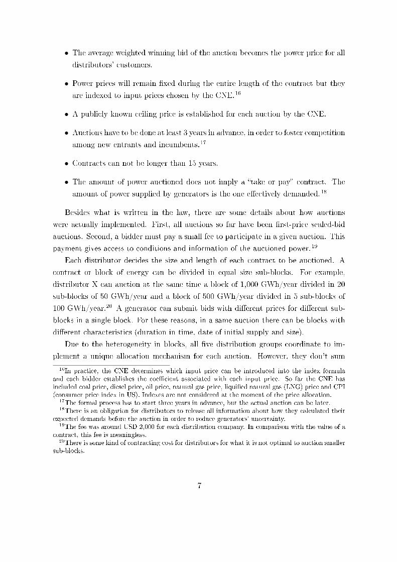
• The average weighted winning bid of the auction becomes the power price for all

distributors' customers.

• Power prices will remain �xed during the entire length of the contract but they

are indexed to input prices chosen by the CNE.16

• A publicly known ceiling price is established for each auction by the CNE.

• Auctions have to be done at least 3 years in advance, in order to foster competition

among new entrants and incumbents.17

• Contracts can not be longer than 15 years.

• The amount of power auctioned does not imply a �take or pay� contract. The

amount of power supplied by generators is the one e�ectively demanded. 18

Besides what is written in the law, there are some details about how auctions

were actually implemented. First, all auctions so far have been �rst-price sealed-bid

auctions. Second, a bidder must pay a small fee to participate in a given auction. This

payment gives access to conditions and information of the auctioned power. 19

Each distributor decides the size and length of each contract to be auctioned. A

contract or block of energy can be divided in equal size sub-blocks. For example,

distributor X can auction at the same time a block of 1,000 GWh/year divided in 20

sub-blocks of 50 GWh/year and a block of 500 GWh/year divided in 5 sub-blocks of

100 GWh/year.20 A generator can submit bids with di�erent prices for di�erent sub-

blocks in a single block. For these reasons, in a same auction there can be blocks with

di�erent characteristics (duration in time, date of initial supply and size).

Due to the heterogeneity in blocks, all �ve distribution groups coordinate to im-

plement a unique allocation mechanism for each auction. However, they don't sum

16In practice, the CNE determines which input price can be introduced into the index formulaand each bidder establishes the coe�cient associated with each input price. So far the CNE hasincluded coal price, diesel price, oil price, natural gas price, liqui�ed natural gas (LNG) price and CPI(consumer price index in US). Indexes are not considered at the moment of the price allocation.

17The formal process has to start three years in advance, but the actual auction can be later.18There is an obligation for distributors to release all information about how they calculated their

expected demands before the auction in order to reduce generators' uncertainty.19The fee was around USD 2,000 for each distribution company. In comparison with the value of a

contract, this fee is meaningless.20There is some kind of contracting cost for distributors for what it is not optimal to auction smaller

sub-blocks.

7

their demands in a unique supply contract/block. Rather, they coordinate on a sin-

gle mechanism for di�erent supply blocks that allocates the minimum bid for each

block for each distributor. A generator can bid di�erent prices to di�erent blocks and

sub-blocks, even if they belong to the same distributor.21

Finally, since several contracts with di�erent distributors were auctioned at the

same time, in order to foster competition the CNE allowed generators to de�ne a limit

for the amount of power that they can win in all the blocks auctioned simultaneously.

For example, a generator with a capacity on 1,000 GWh bidding for two di�erent

contracts of a 1,000 GWh each, can submit bids for the total amount of each contract

but the allocation mechanism will only assign 1,000 GWh to this generator. 22

2.4 LTC auctions' results

Between October 2006 and July 2011 there were seven auctions for SIC's supply. 23

Table 1 summarizes auction results.24 Prices are in USD/MWh.25 The average win-

ning price is a weighted average with the weights being equal to the fractions of the

individual's quantities submitted in each auction. For a more detailed description of

the results, please see Section 7.2 of the Appendix.

There are three main results to highlight. First, there was no entry until the 2009

auctions, when expected spot prices as well as ceiling prices were higher. 26 Entry

of new generators was marginal. Second, prices submitted by generators after 2009

almost doubled those of 2006. Third, bids have been quite close to the ceiling prices

in October 2007 and January 2008 when large portions of auctioned contracts didn't

receive any bids at all.27

21Section 7.4 of the Appendix includes an example of an o�cial page to submit bids.22In theory, this allows generators to alleviate their capacity constraints and act similarly across

di�erent contracts. For the interest of the current paper, this means that we do not need to considerany relationship between bids submitted to di�erent blocks. We can consider each block independently.

23The �rst SING auction took place in September 2009 so I will focus only on SIC auctions.24This table includes all auctioned contracts. In case the size of a contract increases in time, I use

the amount of power that was used as reference for the allocation in the auction.25Bids are submitted in USD/MWh but prices to regulated customers are converted to Chilean

pesos at the proper exchange rate.26Auctions' shares do not change signi�catively from market shares showed in Table A2-B.27The unsold portion of the auction has been positive almost in every auction. This means that

some contracts or portions of them did not receive any bid.

8

Table 1: Results of LTC auctions in SIC

Auction Size Blocks Ceiling P Winning bid Bidders UnsoldTWh/year number USD/MWh USD/MWh number portion

Oct-06 12.8 9 62.7 52.7 4 9.3%Feb-07 1.2 2 62.7 54.5 2 5.5%Oct-07 14.7 6 61.7 59.8 2 61.3%Jan-08 9.0 4 71.1 65.8 1 80.1%Jan-09 8.0 4 125.2 104.3 5 10.6%Jul-09 0.9 1 125.2 99.5 6 0.0%Mar-11 2.5 4 95.0 90.3 3 18.4%

Source: CNE

The rise in �nal prices could be explained by di�erent factors. First, it is possible

that low-cost power was committed in the �rst auctions, while the high-cost power was

committed in the last ones. Such an explanation is based on technological di�erences

across generation plants. A di�erent explanation is based on capacity constraints. It is

possible that as capacity constraints became binding, prices increased. The fact that in

2009 there was power auctioned to be supplied in 2010 gave short time for any capacity

expansion if the generator has no power left to supply. Only high-cost plants can be

installed in such a short time. Finally, expected spot prices were soaring due to high

input prices (i.e. coal, LNG, oil) during this period. In sum, it is an empirical question

whether submitted bids can be explained by production costs, capacity constraints and

forecasted prices or by strategic behavior.28 The next section builds up a theoretical

approach that will allow us to address these issues.

3 Theoretical Approach

In terms of related literature, multi-unit auctions can be traced back to the seminal

work of Wilson (1979).29 For a literature review on the theoretical and empirical

analysis of multi-unit auctions, see Hortaçsu (2011). Along this section I will follow

Hortaçsu (2002) and Hortaçsu and Puller (2008) methodology to analyze data on multi-

28It is possible that generators were expecting rises in input prices and for that reason decided notto participate in 2007 and 2008 auction until ceiling price was increased enough. This paper do notaccount for that dynamic perspective. I will assume each generator submit a bid function for eachcontract independently of past and future auctions.

29Back and Zender (1993), Wang and Zender (2000), Ausubel and Cramton (2002) develop thistheoretical framework further.

9

unit auctions.

3.1 Linear approximation for bids

Before introducing assumptions about bidding behavior I will start describing the

available data. From this analysis it is possible to �nd the best suitable theoretical

approach. I will use the data of 7 auctions from October 2006 to March 2011. There

were 11 bidders across all auctions. They submitted as bids 319 price - quantities

pairs, resulting in an average of 4.1 bids per generator. Each bidder submitted a �at

or an upward-sloping supply function. I include in Figure 1 an example of an actual

bid function.30 In this case, the generator is willing to supply 900 GWh/year at 50.6

USD/MWh and additional 150 GWh/year at 51.4 USD/MWh.

Figure 1: Example of a submitted bid function

From Figure 1 it can be seen that a linear approximation to actual bidding behavior

could �t well. For that reason in this section I will approximate the price-quantity pairs

submitted by generators by linear and continuous functions. In reality, generators

submit non-di�erentiable step functions. However, Kastl (2008) shows that as the

number of steps grows without bound, necessary conditions of bidding behavior in a

discrete strategy game converge to the same conditions for equilibrium for a game with

di�erentiable supply schedules.

30This schedule was submitted by the largest generator, Endesa, for a contract with the largestdistributor, Chilectra, in October 2006.

10

Now I will describe how I performed the linear approximations. When a distributor

auctioned two separate blocks of energy, I separated them as two di�erent contracts. 31

Then I run a linear regression for each bid function in the following way: pijk =

βitqijk +αik +υijk, where: (pijk, qijk) is the j -th price-quantity submitted by bidder i in

block k. The parameter β gives the slope, α the price-intercept and υ is the error term.

Table 2 shows the average, minimum and maximum intercept, slope and goodness of

�t.32 There are 57 bid functions.

Table 2: Linear approximation to bid functions over i and k (USD/MWh)

Min Mean Max

Intercept 41.91 79.09 128.53

Slope 0.000 0.004 0.048

R2 0.62 0.95 1

Since the goodness of �t measured by the average R2 is more than 95%33, a divisible-

good auction model that generates linear supply functions for each bidder as equilib-

rium bidding strategies would provide a good description of the data. Now it is possible

to use the data I obtained from the linear approximations and observe how intercepts

and slopes are distributed statistically.34

There could be unobservable factors that a�ect price-intercepts between auctions.

In order to control for that, Hortaçsu (2002)'s analysis of treasury bill auctions nor-

malizes price-intercepts by dividing them by the resale market price of the securities.

In LTC auctions there is not a resale value but we can use the expected spot price at

the moment of the auction.35

Figure 2 shows the distribution of normalized price-intercepts. It can be seen that

the distribution has a mode close to one.36 This last fact suggests that the bid function

31For example, in October 2006, the largest distribution company Chilectra auctioned 2 blocks:Chilectra 1 with a duration of 11 years and Chilectra 2 with 13 years.

32Bid functions with only two points are not included.33Log-normal and exponential approximations do not �t that well.34As Rostek, Weretka and Pycia (2010) mention, a linear approximation �nds empirical support in

�nancial, electricity, and other divisible good markets.35This expected spot price is based on CNE semiannual estimations (May and October). It considers

the expected spot price at the moment contract starts. For a detailed description of what I have usedas expected spot prices see section 7.3 in the Appendix.

36Di�erent normality tests do not reject the null hypothesis that price-intercepts follow a normaldistribution (Jarque-Bera test, Shapiro-Francia and Shapiro-Wilk tests). However, the test is very

11

Figure 2: Distribution of normalized price-intercepts

is determined by the private information of a bidder about expected spot prices.

Figure 3 shows the distribution of slopes of the linear approximations to the bid

functions.37 As expected, all slopes are non negative. The heterogeneity in slopes - a

large proportion of �at schedules - can be driven by bidder size or available capacity.

In sum, based on the analysis of real auctions' data, my theoretical approach will

consider a linear approximation to bid functions, with at least partial private informa-

tion about expected spot prices and heterogeneity in bidder's size.

3.2 A multi-unit model

This section includes a model that explains under which conditions it is possible to

have bidding behavior like that found in Chile's power industry. I will use a divisible

good auction in the sense of the Wilson (1979) share auction. It is a �rst-price sealed-

bid discriminatory auction.38 I will start assuming the simplest case with independent

private values but I will also consider a more general case. Since the expected spot price

is a function of all generators' decisions on investment, technologies and contracts, it

is possible to have a relevant �common value� component.

sensitive to any change in the series of expected spot prices used.37A slope of 0.001 indicates that each additional GWh increases the price by one dollar.38Chilean LTC auctions are all pay-as-you-bid auctions.

12

Figure 3: Distribution of slopes of �tted bid functions

Let us assume that there are N risk-neutral power generators.39 They bid for the

right to supply power to a distribution company in the next period. If they win any

units, they will have to buy power from the spot market in that period, irrespective

of whether they are called by the ISO to generate or not.40 All generators receive a

private signal of the expected spot price, ci. Spot prices depend on future prices of

inputs like coal, natural gas and diesel, but more importantly spot prices at SIC are

heavily in�uenced by the volatility of hydropower generation. Hence all �rms have to

forecast di�erent scenarios for future spot prices. It is expected that each generator will

have di�erent information about their own investment plans and contracting portfolios

as well. I assume that ci is identically and independently distributed according to the

cumulative distribution F (c), with density f(c) and it is continuous over [cL, cH ].

Generators are constrained by installed capacity when they produce electricity.

However, installed capacity does not completely constrain the generator when signing

a contract with a distributor. The generator (as a trader) can supply the distributor

by buying power at the spot market from any other generator that has been called to

produce by the ISO at that moment. Also, since auctions are carried years in advance

of the moment of actual delivery, generators have a chance to increase physical capacity

or adjust their contract portfolios.41

39Hortaçsu and Puller (2008) show that main results do not change by introducing risk-aversion inthis model.

40As I mentioned before, the generator has two roles, one as a producer and one as a trader. Here Iwill refer only to his trader role, submitting bids and signing forward contracts. Within �rms usuallydi�erent units are responsible for those roles.

41There have been cases where a generator dropped a free customer's contracts to adjust his overall

13

Then what generators have is a sales target or a �contract position� or �contracting

capacity� Ai to contract for future supply. Contracting capacity is the minimum un-

committed capacity a generator has available in order to participate in an LTC auction.

It is his own expected generation from existing and future plants net of existing con-

tracts with large customers or other distributors. If a �rm bids to supply more than

his contracting position, it has to face the risk of over-contracting and buying from

other generators at the spot market in order to honor his contract. Ai is the contract

position at the moment of the auction and I assume generators took it as given. Also,

Ai is common knowledge. The heterogeneity across bidders found in Figure 3can be

explained by di�erences in contracting capacity.

It is possible to show a numerical example of a contract decision. Assume three

generators, with di�erent technologies of generation. A low cost generator, G1, with

marginal cost of generation equal to 5; a medium cost generator, G2, with marginal

cost of 30; and a high cost G3 with marginal cost of 50. G1 and G2 have an expected

production of 100 units each, while G3 has only 50 units. There are three relevant

levels of demand, D, and demand is never larger than 250 units. If D ≤ 100 units, the

spot price is 5. If 100 < D ≤ 200, the spot price would be 30 and if 200 < D ≤ 250

the spot price would be 50. Now, due to price uncertainty, �rms may hedge risk with

a contract. Assume G1 and G2 sign a forward contract with �nal consumers for 100

units each (the same as the expected production) for a forward price of 30. In this case,

no matter what is the spot price, expected pro�ts are positive for both �rms. What

happens if G2 signs a contract of 120 units? This generator would be over-contracted.

Under such circumstances, G2 will have to increase his forward price to obtain the

same expected pro�ts as before: 30 for the �rst 100 units and 50 for the next 20.

Assume generators bid supply schedules that are continuously di�erentiable with

bounded derivatives. Si(p) ≡ S(p, ci, Ai) is the bidding function submitted by bidder

i, which maps price p into a supply curve given signal ci and contracting capacity Ai.

I am looking for a Bayesian-Nash equilibrium where bid functions are functions

of their private information, ci. Then, the optimal bidding strategy considers that

each bidder forms expectations about the market-clearing price, P c. In order to de�ne

the market-clearing price in the auction, we need a de�nition for �residual demand

function�. The total amount of electricity auctioned is Q =∑N

i=1 Si(Pc). Since P c

is the realized market-clearing price under the market-clearing condition, the residual

demand is RDi(p) = Q−∑N

j 6=i Sj(p).

contract portfolio.

14

The cumulative distribution function of the market-clearing price is H(p, Si(p), Ai)

from the perspective of �rm i, conditional on Ai and the fact that �rm i submits a

supply schedule Si(p) while his competitors are playing S(p, cj, Aj).

H(p, Si(p), Ai) = Pr[Si(p) ≤ Q−N∑j 6=i

Sj(p)] (1)

In terms of excess of demand (there is an excess of demand at price P c):

H(p, Si(p), Ai) = Pr[P c ≥ p|Si] (2)

The support of the market-clearing price distribution is [p, p]

3.2.1 Not constrained case: (Si ≤ Ai)

Consider �rst the case of a risk-neutral bidder not constrained by contracting ca-

pacity (Si ≤ Ai). Ex-post pro�ts are given by the area below the submitted supply

curve net of costs at the market-price level:

Π[Si(p), p] =

∫ Si(p)

0

[S−1(q)− ci]dq

=

∫ Si(p)

0

S−1(q)dq − Si(p)ci (3)

At the market-clearing price (ex-post pro�ts):

Π[Si(Pc), P c] =

∫ P c

p

Si(p)dp− Si(P c)ci (4)

The optimization problem that each non-constrained generator solves symmetri-

cally is:

maxSi

∫ p

p

Π[Si(p), p]dH(p, Si(p)) (5)

Integrating by parts:

maxSi

{[Πi(Si(p), p)H(p, Si(p))]pp −

∫ p

p

Π′(Si(p), p)H(p, Si(p))dp} (6)

15

Setting S(p) = 0 and considering that H(p, Si(p)) = 0:

maxSi

−∫ p

p

[S ′i(p)(p− ci)]H(p, Si(p))dp (7)

The integrand is a function of p, S ′ and S.

−∫ p

p

[S ′i(p)(p− ci)]H(p, Si(p))dp = F (p, S, S ′) (8)

The Euler-Lagrange necessary condition for the (pointwise) optimality of the supply

schedule Si(p) is given by FS = ddpFS′ . In our case this means:

Hs(p, Si(p))[S′(p− c)] = H(p, Si(p)) +Hp(p, Si(p))(p− c) +Hs(p, Si(p))[S

′(p− c)] (9)

The optimal supply schedule is implicitly de�ned by:

p = ci +

[H(p, Si(p))

−Hp(p, Si(p))

](10)

This condition is a mark-up condition, where the generator bids above the expected

spot price by an amount determined by the inverse hazard rate of the market-clearing

price distribution.42

3.2.2 Constrained case: (Si > Ai)

Now it is time to introduce available capacity explicitly in the generator's opti-

mization decision. The ex-post pro�ts for a risk-neutral bidder in this discriminatory

auction with available contracting capacity Ai are:

Πi[Si(p), Pc, Ai] =

[∫ P c

p

Si(p)dp− Si(P c)ci

]− θ

2(Si(P

c)− Ai)2 (11)

The cost of over-contracting is given by a quadratic expression multiplied by the pa-

rameter θ. θ is the marginal cost of over-contracting.

42The derivative of the pdf of the market-clearing price with respect to the price is negative.

16

The optimization problem that each generator solves is:

maxSi

∫ p

p

Π[Si(p), p, Ai]dH(p, Si(p)) (12)

Integrating by parts we obtain the following:

maxSi

−∫ p

p

[S ′i(p)(p− ci)− θ(Si(p)− Ai)S ′i(p)]H(p, Si(p))dp (13)

Solving the Euler-Lagrange condition, and since we are looking for the symmetric

equilibrium, we obtain:

p = ci +

[H(p, Si(p))

−Hp(p, Si(p))

]+ θ(Si − Ai) (14)

The bid function's slope is increasing in the marginal cost to over-contracting. This

result gives us the following Proposition.

Proposition 3.1 The optimal bidding strategy for a risk-neutral generator satis�es:

p =

ci +[

H(p,Si(p))−Hp(p,Si(p))

]if Si ≤ Ai

ci +[

H(p,Si(p))−Hp(p,Si(p))

]+ θ(Si − Ai) if Si > Ai

Proposition 3.1 explains why we can �nd changes in a bid function's slope. For

quantities below contracting capacity, the slope of the bid function is given by the

inverse hazard rate. For quantities above contracting capacity, the marginal cost of

over-contracting increases the slope.

The Euler equation does not necessarily imply a linear bid function as the one

depicted by the data analysis in the previous section. In order to obtain a linear bid

function, the inverse hazard rate H(p,Si(p))Hp(p,Si(p))

has to be a linear function of the quantity.

From now on I will assume the following condition holds, which is adequate to �t our

data:43

H(p, Si(p))

−Hp(p, Si(p))= λ(Si) = λ0 + λ1Si (15)

43Rostek, Weretka and Pycia (2010) shows that if H(p, Si(p)) has a convex support, any distributionthat belongs to the class of Generalized Pareto distributions exhibits a linear inverse hazard rate.

17

If we assume this simple case where the inverse hazard rate is a linear function,

Figure 4 depicts an example of such a bidding function.44

As I mentioned before, since the expected spot price is a function of all generators'

decisions on investment, technologies and contracts, it is possible to have a �common

value� situation. Instead of a full a�liated value model, it is possible to assume a

reduced form speci�cation of a common value model, where the marginal valuations

depend on the realization of the market clearing price. The market clearing price is

a statistic that aggregates the private information of all bidders. Then, the marginal

valuation or cost for the bidder is (1−π)ci +πP c, a convex combination of the private

signal ci and the market clearing price P c. The relative importance of each component

is given by π, where 0 ≤ π ≤ 1. If π = 0, this collapses to the IPV case. If π = 1, we

have a full CV model, with �at supply functions.45

Based on Hortaçsu (2002) and analogous to the previous development, we can set

a new optimal supply schedule.

Proposition 3.2 A risk-neutral generator with a common value component, will sub-

mit a supply schedule according to:

p =

ci + 1

1−π

[H(p,Si(p))−Hp(p,Si(p))

]+ π

1−π

[Hs(p,Si(p))−Hp(p,Si(p))

]Si if Si ≤ Ai

ci + 11−π

[H(p,Si(p))−Hp(p,Si(p))

]+ π

1−π

[Hs(p,Si(p))−Hp(p,Si(p))

]Si + θ(Si − Ai) if Si > Ai

Even with a common value component, it is possible to obtain linear bid functions

in equilibrium.46 The change in slope due to the possibility of over-contracting remains.

As can be seen, the above model can give an accurate representation of the actual data.

4 Endogenous Contracting Positions

4.1 Contracting positions in the data

From the theoretical framework developed above, it is possible to have an approxi-

mation to generators' contract capacities. From now on, I will assume that the contract

44In section 7.7 in the Appendix it has been included an example of an equilibrium with linear bidfunctions.

45Back and Zender (1993) showed in a CV model that if bidders have constant marginal valuations,they will submit a single price-quantity pair, constituting a �at supply function.

46 Hs(p,Si(p))−Hp(p,Si(p))

is a constant if the inverse hazard rate is linear.

18

Figure 4: Bidding function according to the model

capacity of each bidder, Ai, is equal to the amount of power o�ered until the bid func-

tion's slope changes. In case there is no change in the slope, I will approximate contract

capacity by the total amount of power o�ered for that contract. Then it would be pos-

sible to obtain estimates of S-A. This is an important assumption because it allows us

to approximate the amount of expected generation net of previous contracts without

data on contract positions that would not include strategic considerations.

It is possible to plot these implicit contracting positions and analyze behavior across

bidders and auctions. The �rst result is that there is plenty of heterogeneity across

contracts for the same bidder. This could be a result of di�erent contract sizes. For

that reason, the Figure 5 shows the amount of A in GWh and as a proportion of A/Q

for the larger incumbents.47

In case of the largest generator, Endesa, available capacity in 2006 auctions is, on

average, half of a contract's size. This proportion rises to 68% in 2007 and to 100% in

almost all contracts of 2009.48 In the case of Endesa, there is a homogenous contract

position across contracts in each auction. The same can be said about Guacolda's

contracting capacity.

The case of AES-Gener and Colbun is di�erent. Both exhibit more heterogeneity

in A as a proportion of size. In particular, it is interesting that Colbun shows very

47In the case of the entrants, they generally submitted contracting positions consistent with theirinstalled capacity.

48The increase in Endesa's contract position could be explained by a new coal plant in constructionsince October 2007.

19

Figure 5: Incumbents' contracting positions in GWh/year (1) and as percentage of Q(2).

low contracting positions in 2007 in comparison with other auctions and bidders. In

2008 auctions, AES-Gener and Colbun submitted very di�erent contracting positions

for contracts with the same distributor.

In July 2009, contracting positions fall for all generators. It is important to remem-

ber that this auction was held less than six months in advance of the starting date of

the auctioned contract. It is possible that the contract position was already full by

then and �rms didn't have time to expand it.

In sum, I found plenty of heterogeneity in the estimated values of A. For small gen-

20

erators49, contracting capacity follows the same pattern as physical capacity, while for

some large generators estimated contracting capacity can not be explained by changes

in physical capacity. So far contracting positions have been assumed exogenous. How-

ever, there is a possibility that A is chosen strategically. The next sub-section endo-

geneizes the value of A in order to �nd an explanation for these cases.

4.2 Choosing contracting positions

We have seen in the previous section that in October 2007, Colbun and Endesa

submitted very di�erent implicit contracting capacities for the same contract. The

largest generator Endesa had contracting capacities of 70% of the size of the auctioned

contracts while Colbun had only 5%. While Colbun is smaller than Endesa in terms

of capacity, it is the second largest generator. Also, in the previous auctions of 2006,

Colbun submitted bid functions with larger A and there is no evidence of Colbun

committing with other contracts since then. How we can explain this behavior?

In this section I will extend the model of section 3 in order to account for potential

strategic behavior on A that results in such an asymmetric equilibrium. In order to do

so, I assume that �rms �rst choose A and later they participate in an auction. This

is a game of two periods where, by solving backwards, the bidding strategy de�ned in

Proposition 3.2 is the equilibrium strategy for the last period. I assume a simpli�ed

version of the bid function of bidder i : P = ci + λ+ δSi + θ(Si − Ai) with Si ≥ Ai.

Now we need to �nd the equilibrium strategy for the level of contracting capacity.

For the sake of simplicity, I will assume there are only two strategic �rms, like in the

Endesa-Colbun case, regardless of other non-strategic �rms that take their contracting

capacity as exogenous. Both strategic �rms are large enough to not be restricted on

their contracting capacities but they can submit bid functions where A is below their

real contracting capacity.50

Figure 6 shows an example, where �rm i can choose between A and A′. These

determine supply functions S(P,A) and S(P,A′). The lowest price is the same in both

cases, Pmin. In case of rationing, the �rm will receive this price for any quantity below

Ai. Since �rms will participate in a discriminatory �rst-price auction in period 2, they

will choose A in order to maximize the area below the supply curve, with a lowest price

Pmin, net of the expected spot price ci. The only di�erence between bid functions is

49Typically with a few plants and a single generation technology.50It is implicitly assumed that there is no cost in adjusting the contract portfolio by subscribing or

dropping a forward contract with a large customer to cover the di�erence.

21

the contracting capacity involved.

Figure 6: Comparing di�erent available contracting capacities

For now let us assume both �rms are identical in order to provide a symmetric

benchmark. In terms of information available at the moment of choosing A, assume

that in period 1 �rms know the exogenous size of the contract to be auctioned Q and

their marginal cost of over-contracting, θ. Regarding the parameter λ, here it will be a

�xed mark-up over the expected spot price. λ is also known in period 1. If we interpret

this mark-up as the inverse hazard rate of section 3, conditions in the game will change.

For that reason I reserve a separate discussion about it in section 4.2.1.

Firms will form expectations about expected spot prices. There are two states:

high (cH) and low (cL). Firm i receives a signal of high expected spot prices with

probability ρ and �rm j with probability γ.

There will be only two potential levels of residual demand, high or low. The high

residual demand for �rm i is Q − βP while the low residual demand is Q − α − βP .The residual demand each bidder will have to face depends on the action the rival �rm

takes in terms of contracting capacity A. Before analyzing this interaction I need to

describe the set of possible actions.

Taking the expected residual demand, bidder i will have to choose a level for A

that goes from zero to A1. If a �rm chooses 0 ≤ Ai < A1 and obtains in the auction

a quantity S ≤ Ai, he will receive Pmin. For quantities above Ai, he will ask for a

higher price, so the slope of the supply function is increasing for S > Ai. The higher

amount of contracting capacity the �rm can choose is at the high residual demand

22

(α = 0) with price Pmin. Then, if �rm i chooses the higher amount of contracting

capacity, the optimal amount will be Ai = A1.51 We have two corner solutions and/or

an interior solution to the problem of maximizing expected pro�ts by choosing the

optimal contracting capacity. Figure 7 shows the two corner results with the two

possible residual demands.52

It is possible to prove that there are no interior solutions to the problem of maxi-

mizing expected pro�ts by choosing A. The next lemma shows that any Ai such that

0 < Ai < A1 is not optimal under the preceding assumptions.

Lemma 4.1 Assuming two bidders with two states of expected spot prices and two

levels of residual demand, a bidder i will have only two optimal levels of contracting

capacities: Ai = 0 or Ai = A1

The intuition of the proof is the following.53 Choosing A = 0 indicates the bidder

is acting as a monopolist over the residual demand. Then if it is not optimal to choose

a larger A, A = 0 is a superior option to any other A > 0 that implies an increasing

portion of the supply function. Choosing A = A1 indicates the bidder is acting as a

price-taker bidder that gets a �xed mark-up over his expected marginal cost. If A = 0

is not optimal, then any A < A1 is an inferior option with respect to A = A1. The

larger the A, the more �xed mark-up the �rm gets. In sum, we have two potential

actions, low A or high A as we can see in Figure 7.

If the residual demand is high, �rm i will obtain S1 if he chooses A1 and S3 if he

chooses Ai = 0. If the residual demand is low, �rm i will obtain S2 if he chooses A1

and S4 if he chooses Ai = 0. The possible values of S double when we account for the

two potential residual levels of expected spot prices. The lowest price in both supply

functions is Pmin = ci + λ+ δA1 since S1 = A1.54

In order to �nd the equilibrium strategies each �rm will follow, it is important to

determine how the decisions of each �rm about its own contracting capacity will a�ect

the rival's residual demand. If �rm 1 chooses A = A1, residual demand for �rm 2 will

be RD(α > 0). By choosing a larger contracting capacity, �rm 1 is reducing its rival's

market share. If both �rms choose A = 0, both �rms will face a high residual demand,

RD(α = 0). If both �rms choose A = A1, then both �rms will face the low residual

demand, RD(α > 0).

51Any other amount over this point is not optimal for a risk-neutral �rm.52I will assume that both bidders have enough contracting capacity to reach A1.53For a formal proof, see section 7.6.1 in the Appendix.54In case δ = 0, we have the case of a �at supply function until A. Then Pmin = ci + λ.

23

Figure 7: Cases for A0 = 0 and A1 > 0

Solving this game gives us three Bayesian Nash Equilibria.55 In what follows and

without loss of generality, I will present these equilibria for the case of δ = 0.56 This

includes the case of a �at portion of the supply function. In the Appendix, conditions

are shown for the general case.

If we assume complete symmetry between the two bidders, such that ρ = γ, we will

have �ve cases shown in Figure 8. For values of Q−λβ(3 + 2βθ) in Case 1 (below βcL)

the BNE is (A1, A1;A1, A1). Both �rms choose the higher level of contracting capacity

and both �rms end up facing the lower residual demand. The intuition behind this

result is based on the size of the residual demand. If the residual demand is small, the

best option for both bidders is to submit �at schedules.

For values of Q − λβ(3 + 2βθ) in Case 5 (above α + βcH) the BNE is (0, 0; 0, 0).

Both �rms choose the lowest level of contracting capacity and both �rms end up facing

the higher residual demand. Here, since the residual demand is large, both �rms will

choose to behave as a monopolist over the residual demand.

In case 2, there are two BNE: (A1, A1;A1, A1) and (A1, 0;A1, 0). In case 4, again we

have two BNE: (A1, 0;A1, 0) and (0, 0; 0, 0). Finally in case 3, the BNE is (A1, 0;A1, 0).

The only possibility of an asymmetric result has a �rm receiving a signal of high

expected spot prices and the rival a signal of low expected spot prices. Under those

55Strategies are de�ne in the following way: in case signal received is high spot price, choose AH ,in case signal is low spot price, choose AL

56Anwar (2007) shows that in an a�liated multi-unit model, there is an equilibrium where bidderswith constant marginal valuations submit �at price schedules.

24

Figure 8: Cases for BNE if ρ = γ

conditions and if we are in cases 2, 3 or 4, the high-price �rm will choose A = A1 and

the low-price �rm will choose A = 0. If Colbun was expecting low spot prices and

Endesa high spot prices, this result can explain their behavior in 2007 auction. Indeed,

submitted prices were lower for Colbun than for Endesa, while in previous auctions the

situation was the opposite.

If ρ < γ, we have two additional cases as is shown in Figure 9.57 Under this

assumption, we are more likely to have an asymmetric equilibrium.

Figure 9: Cases for BNE if ρ < γ

Here we are interested in asymmetric equilibria where �rms choose di�erent con-

tracting capacities. So far I have assumed both �rms are identical. I will consider two

di�erent kind of asymmetries: size and cost of over-contracting.

First, in the case of size asymmetries, I will assume �rm 1 is larger than �rm 2

and in case they choose A > 0, A1 > A2, i.e. A1 = A2 + ε where ε > 0. This means

that in case �rm 1 chooses A1, �rm 2 has to face a residual demand Q− (α+ ε)− βP .Under these assumptions there is only one asymmetric BNE, which is described in the

following proposition.

Proposition 4.1 Assuming �rm i can choose a bigger contracting capacity than �rm

j, Ai = Aj + ε where ε > 0 and ρ = γ, there is only one asymmetric equilibrium where

�rm i always chooses the lowest contracting capacity, (0, 0), and �rm 2 chooses the

highest (A1, 0), if the di�erence in contracting capacities ε is large enough.

Proof: See the Appendix

57Figure 9 shows the cases if γ − ρ < βα (cH − cL)

25

In this case the large �rm chooses to play as the monopolist over the residual

demand and the small �rms chooses to play as a price-taker if both receive a signal of

high expected spot prices. This does not explain the Endesa-Colbun case because the

largest �rm (Endesa) was the one choosing the largest contracting capacity.

A di�erent kind of asymmetric BNE can be found if we assume di�erent marginal

costs of over-contracting θ between �rms instead of di�erences in size.

Proposition 4.2 Assuming �rm i has a larger marginal cost of over-contracting than

�rm j, θi > θj and ρ = γ, there is an asymmetric equilibrium where �rm i always

chooses the highest contracting capacity (A1, A1) and �rm j always chooses the lowest

(0, 0), if the di�erence in the marginal cost of over-contracting, θ1−θ2, is large enough.

Proof: See the Appendix

This case can explain the 2007 auction. If Endesa had a larger cost of over-

contracting, it is possible that Colbun acted strategically and behaved like a monopolist

on the expected residual demand by choosing a smaller contracting capacity. 58

4.2.1 Mark-up as a function of contracting capacity

The previous analysis assumes a constant mark-up over the expected spot price

λ. In section 3 we saw that this mark-up corresponds to the inverse hazard rate and

depending on distributional assumptions could be a non-constant value. Decisions on

contracting capacity in period 1 a�ect the mark-up in period 2's auction, but the result

of the auction determines this mark-up. Then, λ will be a function of A. In particular,

a larger contracting capacity can have a negative impact on the mark-up. 59 In that

case, Pmin will no longer be the same for S(P, 0) and S(P,A1). It will be lower if the

generator chooses A1. This reduces the incentives to choose a larger A.

In case the relationship between mark-up and contracting position is linear, λ(A) =

a − bA where a, b > 0, Lemma 4.1 no longer applies. The optimal action is to choose

A = 0. For a more general relationship (e.g. quadratic), it is possible to have an

interior value A. In that case, it is possible to replicate the analysis of the previous

sub-section, but now with this two optimal levels of A: (0, A), where 0 < A < A1.

58Similar results can be found in January 2009 auction where the cost of over-contracting rises dueto the proximity of delivery in January 2010. AES-Gener and Colbun submitted contracting capacitiesof 8% and 20% respectively for a contract with Chilquinta, while Endesa had a 100% capacity forthe same one. However, they also submitted contracting capacities of 40% and 55% respectively fora contract with CGE. The inclusion of a second contract in the extension of the model could explainthis result.

59Estimations in section 7.5 in the Appendix show a negative e�ect of A over the mark-up.

26

Since we do not know the exact form of λ(A), there is no close form for A. However,

it is possible to recognize that a higher cost of over-contracting will increase A, under

certain parametric conditions. In that case, we will have a similar result as the one

stated in Proposition 4.2.

5 Empirical Evidence

Once we have a model of bidding behavior it is possible to use the data on bids to

estimate unobservable variables like the amount of mark-up. The empirical implemen-

tation of (10) and (14) requires the estimation of H(p, S(p)) and its partial derivative

for each bidder, in each auction. Unfortunately, the data on LTC auctions from 2006

to 2011 is not enough to estimate the inverse hazard rate by supply function. We have

7 di�erent auctions and only 64 supply functions for 11 bidders.

In this article I will pursue a di�erent goal. By imposing conditions on the inverse

hazard rate, I can use the model developed in section 3 to estimate the marginal cost of

over-contracting, θ, as well as the e�ect of expected spot price on submitted prices. This

is important because we can get an estimate of how important the expected spot price

(a variable that depends on the aggregate power system decisions) and the contracting

capacity (a variable that depends on physical, technological and commercial decisions of

each generator) are to explain submitted prices. I use all pairs of prices and quantities

in order to linearly estimate the e�ect of expected spot prices and over-contracting on

submitted prices.

I make two assumptions. First, I will assume the inverse hazard rate is a constant

mark-up. This assumption is not as strong as it sounds. The constant mark-up as-

sumption gives a �at bid function until S = A where its slope changes to θ > 0. A �at

portion of the bid function is consistent with the rules of the auction. Even if the gen-

erator bids an amount A for a price P, the allocation mechanism rations a proportion

below A at the same price.60 Again, I will denote the constant mark-up as λ.

Second, I will assume as in section 4 that the available contract capacity of each

bidder, Ai, is equal to the �at amount of power o�ered until the bid function's slope

changes. This assumption does not depend on any condition imposed on the inverse

hazard rate.

60For example, a bidder i submits a bid of 1,000 GWh for 70 USD/MWh and 500 GWh for 72USD/MWh for a contract of 1,500 GWh. If bidder j bids 500 GWh for 68 USD/MWh, the allocationmechanism will allocate only 500 GWh at 70 USD/MWh to bidder i.

27

Although the mark-up is assumed constant, it is a function we don't know. In order

to estimate θ we can follow two strategies. First, a parametric estimation by assuming

that λ is a polynomial function. Second, a semi-parametric linear estimation can be

used if we don't want to impose any structure on it. I will pursue both strategies. The

mark-up would be a function of the competitiveness of the auction. For that reason,

I include the number of bidders, N, and the size of the contract Q in GWh. Size of

blocks and sub-blocks are chosen by distributors so they are exogenous to generators.

I estimate the following equation, for i bidders, j units, t auctions.

Pijt = Ct + βλit + θ(S − A)ijt + αi + µj + ηXjt + εijt (16)

The endogenous variable is the submitted price, P, which includes modulation

factors. Among the exogenous variables, S − A is calculated as the amount o�ered

over the contract capacity. In order to account for size I create a second variable (in

percentages) that normalizes S − A by the physical capacity of the generator.61 C is

the expected spot price at the moment of the auction, based on information provided

by CNE.62 Fixed e�ects by generator are captured by αi

In order to account for heterogeneity across distributors, I include a dummy variable

for each distributor µj. There is heterogeneity across contracts too. For that reason I

also include two other regressors in X : the duration of the contract in years and the

time left for physical delivery in weeks. It would be expected that longer contracts

would be more coveted by bidders and a shorter time left for delivery would raise the

cost of over-contracting.

Table 3 shows summary statistics for the main variables in the regressions. The

over-contract proportion, (S-A)/Capacity, is particularly high for some small genera-

tors. It goes beyond 100% but in average is below 10%. Delivery time goes from 6

months to more than 3 years, but in average is 2 years.

5.1 Results

Table 4 shows the estimations for two parametric speci�cations: linear and polyno-

mial of grade two. The regressor S−A is in GWh (not normalized by physical capacity)

61As physical capacity I use the on-�rm energy of each plant as it is calculated by the IndependentSystem Operator. On-�rm energy is power that can be generated in dry periods and it is a relevantcapacity measure in systems with large portions of hydropower.

62Section 7.3 of the Appendix includes a detailed description of it. I have tried di�erent scenariosfor expected spot prices with the same results in terms of signi�cance.

28

Table 3: Summary statistics

Variables Obs Mean Std. Dv. Min Max

P 319 80.14 22.99 48.8 128.5C 319 74.37 16.51 55.0 95.0A 319 776.83 673.27 23.0 3,000.0S-A 319 603.36 605.30 0.0 3,500.0

(S-A)/Capacity 319 9.09 18.38 0.0 145.8Q 319 1,897.87 796.86 150.0 3,000.0N 319 3.64 1.42 1.0 6.0

Duration 319 12.99 1.48 10.0 15.0Delivery time 319 109.29 58.90 26.3 169.7

and in % (normalized by physical capacity). In both speci�cations, the variables that

a�ect signi�catively (and positively) the bidding price are the expected spot price C

and the over-contracting quantity S − A. The expected spot price has a coe�cient

ranging between 1.13 and 1.2. The cost of over-contracting is around 2 USD/GWh.63

Table 4 also uses the normalized regressor S − A, that shows the over-contractingquantity as a percentage of the physical capacity. Results are almost identical, but

here the cost of over-contracting is in terms of capacity percentages. Contracting one

percentage point over the physical capacity implies an increase of 185 USD/GWh in

the submitted price. Considering that some �rm are over-contracted for more than a

100%, the total cost of over-contracting can be particularly high.

In the polynomial regression, delivery time and duration have a negative e�ect on

prices as expected but they are not signi�cant. The e�ects on prices of the number of

bidders and the size of the contracts are also not signi�cant, but the number of bidders

become signi�cant in higher degree polynomials.

It is possible that above parametric speci�cations are not capturing the mark up

λ if the polynomial has a di�erent structure. Table 5 shows results for polynomials

of degree three and four. The cost of over-contracting does not change signi�catively.

The coe�cient of C gets closer to one as we increase the degree of the polynomial.

This could mean that a more �exible speci�cation for the mark-up can give better

estimations for this coe�cient. Also, the e�ect of the number of �rms is negative and

statistically signi�cant at the average value of N in polynomials of higher degree.64

63This value is signi�catively below the 3.8 USD/GWh shown in Table 2 as an average of all linearapproximations to the submitted bidding functions.

64It is possible to choose the best speci�cation by cross validation. Since results are very similaracross all polynomials, I prefer to show them all.

29

Table 4: Parametric Approach

Variable Linear PolynomialIn GWh In % In GWh In %

C 1.198*** 1.202*** 1.133*** 1.139***0.158 0.148 0.16 0.15

S − A 0.002** 0.186*** 0.002** 0.184***0.001 0.026 0.001 0.026

N 0.431 0.451 4.385 4.2661.095 1.03 2.713 2.552

Q 0.000 0.000 0.004 0.0050.001 0.001 0.004 0.004

N2 -0.947 -0.9150.556 0.523

Q2 -0.000 -0.0000.000 0.000

Delivery 0.002 0.000 -0.062 -0.0620.058 0.054 0.067 0.063

Duration -0.068 -0.012 -0.13 -0.0720.355 0.334 0.373 0.351

Constant -7.252 -8.382 4.369 2.85721.616 20.339 23.073 21.697

Obs 319 319 319 319R2 adjusted 0.925 0.933 0.926 0.934

(*) p < 0.05, (**) p < 0.01, (***) p < 0.001.

We have mentioned that a second strategy is to follow a semi-parametric estimation.

Robinson (1988) showed that despite the presence of a nonparametric component as

λ, θ can be estimated. In my setting λ is considered a nuisance function and I proceed

to estimate a partially linear model.65 Results are depicted in Table 6.

Semi-parametric estimations are less precise but they allow for more �exible mod-

eling strategies. The coe�cient of expected spot price is close to 0.9. The cost of

over-contracting is identical to the polynomial speci�cation.

In sum, under di�erent speci�cations we can assert three main results. First, the

expected spot price and the cost of over-contracting are the main determinants of

submitted prices. Second, expected spot prices have a close one-to-one relationship

with submitted prices. Third, the marginal cost of over-contracting is around 185 USD

65I use a constant normal kernel density estimator. Bandwidth was selected from Silverman (1986)for the optimal smoothing of a normal random variable's density.

30

Table 5: Parametric Approach with di�erent polynomials

Variable Grade 3 Grade 4In GWh In % In GWh In %

C 1.107*** 1.115*** 1.067*** 1.049***0.155 0.145 0.178 0.166

S − A 0.002*** 0.185*** 0.002** 0.186***0.001 0.025 0.001 0.025

N -42.308*** -42.328*** 44.128 55.93610.005 9.359 42.026 39.14

N2 14.703*** 14.642*** -38.767 -45.381*3.356 3.139 23.883 22.244

N3 -1.401*** -1.386*** 11.477* 12.937*0.313 0.292 5.466 5.091

N4 -1.002* -1.109**0.416 0.387

Delivery 0.009 0.012 0.131 0.1320.068 0.064 0.093 0.087

Duration -0.068 -0.002 -0.288 -0.2260.363 0.339 0.373 0.347

Constant 44.676 43.475 -6.208 -9.90623.798 22.254 30.916 28.792

Obs 319 319 319 319R2 adjusted 0.931 0.939 0.932 0.941

(*) p < 0.05, (**) p < 0.01, (***) p < 0.001.

per percentage point of physical capacity.

Figure 3 shows that there is plenty of heterogeneity across bidders. It is a relevant

question if the cost of over-contracting is di�erent across groups of bidders. I present

results in Table 7 for the linear and the polynomial of grade two speci�cation, but only

for a group of generators. The group includes the four largest incumbents (Endesa,

AES-Gener, Colbun and Guacolda). These are the historical incumbents of the indus-

try. It is expected that the cost of over-contracting of incumbents or big generators

would be lower than the average generator.

From Table 7 we can see that the marginal cost of over-contracting for incumbents

is below the average value in Tables 4, 5 and 6, and is not even signi�cant. The cost

of over-contracting is a bigger constraint for smaller incumbents and entrants. Table

8 introduce an interaction between (S − A) and a dummy variable for the top four

incumbents. As it can be seen, the cost of over-contracting is signi�cant for entrants but

31

Table 6: Semi-parametric estimation

Variable Robinson's EstimationIn GWh In %

C 0.888* 0.898**0.331 0.403

S − A 0.002** 0.185***0.001 0.024

Delivery 0.000 0.0001.36 1.268

Duration -0.128 -0.1010.384 0.358

(*) p < 0.05, (**) p < 0.01, (***) p < 0.001.

Table 7: Parametric estimation for incumbents

Variable Linear PolynomialIn GWh In % In GWh In %

C 1.19*** 1.19*** 1.162*** 1.158***0.152 0.152 0.155 0.155

S − A 0.001 0.162 0.001 0.1640.001 0.087 0.001 0.087

Obs 264 264 264 264R2 adjusted 0.921 0.921 0.92 0.92

(*) p < 0.05, (**) p < 0.01, (***) p < 0.001.

not for the top 4 incumbents. It is possible that entrants face a riskier scenario in case

of winning a LTC. Since they usually relay in a few units of production, any eventuality

(i.e. drought, earthquake, accident) can drive the entrant into bankruptcy. 66

The cost of over-contracting is related to the slope of the bid function. The average

slope of bid functions remain constant between October 2006 and Feb 2009. When

the time lag to start supplying the contracted amount of power is reduced to less

than 6 months, average slopes jump from 1.9 USD/GWh to 19 USD/GWh. As an

important part of available capacity was committed in previous auctions and there

was no time left to install new plants, it is to be expected that there would be a rise

66The biggest entrant in the 2008 auction, Campanario, went into bankruptcy in 2011 after severalmonths of negative cash �ow due to high spot prices and not enough own production to supply for itsLTC.

32

Table 8: Parametric estimation with incumbents' interactions

Variable Linear PolynomialIn GWh In % In GWh In %

C 1.199*** 1.198*** 1.132*** 1.134***-0.154 -0.149 -0.155 -0.151

S − A 0.010*** 0.189*** 0.010*** 0.186***-0.002 -0.028 -0.002 -0.027

(S − A) ∗ Inc -0.009*** -0.023 -0.009*** -0.018-0.002 -0.089 -0.002 -0.089

Obs 319 319 319 319R2 adjusted 0.929 0.933 0.930 0.934

(*) p < 0.05, (**) p < 0.01, (***) p < 0.001.

in the cost of over-contracting. This rise increases bid functions' slopes. Once time

to delivery increases back, slopes fall down. However, in my estimations I couldn't

�nd any evidence of delivery time as a signi�cant explanatory variable of prices. An

alternative explanation could be that in this auction we have three entrants and one

small incumbent. Since the marginal cost of over-contracting is higher for entrants and

small generators, the average slope is higher in that auction relative to others. Similar

results can be found if we perform an estimation by submitted schedule. 67

6 Summary

LTC auctions for power have become a new instrument to encourage investments in

generation and to reach a correct risk allocation. Since 2005, generators in Chile have

to compete in public auctions for the right to supply electricity to customers formerly

under price regulation. Long-term contract auctions imply di�erent incentives than

widely known short-term or day-ahead auctions. This article provides a multi-unit

model to understand bidding behavior, as well as to estimate the main determinants

of submitted prices. This is the �rst theoretical approach that �ts the actual Chilean

data. In particular, it is the �rst that considers the divisible-good dimension of LTC

auctions.

From my estimations, the key variables explaining bidding behavior are expected

67In the Appendix, section 7.5, Table A.4 shows that contracting capacity has a negative e�ecton the di�erence between price-intercepts (estimated by linear approximations in section 3.1) andexpected spot prices. This e�ect is larger for non-incumbents in Table A.5.

33

spot prices and generator's contracting capacity. There is an almost one-to-one re-

lationship between expected spot prices and submitted prices. This is an important

fact for contract indexation. Indexation should take into account the expected spot

price, not individual generators' technology. As a policy recommendation, it would be

bene�cial to increase the time between the moment of the auction and the moment

of physical delivery, not necessarily because a shorter time would increase prices, but

because increasing the time to deliver would make generators think more in terms of

expected spot prices than short-term �uctuations.

Our approach allows us to estimate the marginal cost of over-contracting. We

have calculated that the cost of over-contracting is around 185 USD per percentage

point over generator's physical capacity. Also we have found that this cost is more

important in smaller generators and new entrants. This is a point to keep in mind

about the impact of entry.

Estimations of contracting capacity seem to follow physical capacity in the majority

of the cases. Nevertheless, in some auctions we found large incumbent �rms who

show very reduced contracting capacities. This behavior can be explained by strategic

choices of contracting capacities. A generator can commit to a smaller size to act as a

monopolist over the expected residual demand.

This paper was written without considering the dynamic implications of having

sequential auctions. It is an important feature because the contracting decisions of

today will impact the contracting decisions of tomorrow. A �rm that contracts a

positive amount of electricity in period t will face a more constraining situation in

t + 1. Since results are public, this information is available for competitors and they

will behave accordingly. In LTC auctions there is a caveat. Since auctions are usually

performed with years in advance, a generator has a higher incentive to expand capacity

after winning a contract. Then the optimal contract position increases. The �nal e�ect

is unclear and remains to be explored in future research.

7 Appendix

7.1 Tables

Table A1: Installed Capacity in MW by Technology, December 2010

Table A2: Capacity installed by Generator

34

Technology Installed InstalledSIC Capacity [MW] Capacity [%]

Hydro with a dam 3,768.1 31.8%Hydro without a dam 1,573.7 13.3%

Coal / Petcoke 1,354.4 11.4%Natural Gas 2,721.0 23.0%

Oil 2,050.4 17.3%Biomass 217.0 1.8%Wind 160.5 1.4%

Total Capacity SIC 11,845.1 100.0%

Technology Installed InstalledSING Capacity [MW] Capacity [%]

Hydro without a dam 14.9 0.4%Coal / Petcoke 1,137.8 31.8%Natural Gas 2,073.9 58.0%

Oil 348.2 9.7%

Total Capacity SING 3,574.9 100.0%

Source: CNE

Generating Groups Capacity in 2005 Capacity in 2011MW % MW %

Endesa 4,171.73 50.3% 5,107.45 40.9%AES-Gener 1,160.37 14.0% 1,682.68 13.5%Colbún 1,840.40 22.2% 2,555.17 20.5%Guacolda 304.00 3.7% 608.00 4.9%Others 811.80 9.8% 2,534.59 20.3%

Total SIC 8,288.30 100.0% 12,487.89 100.0%

Source: CNE

Table A3: Market Share by Generator

7.2 Proofs of section 4

7.2.1 Lemma 4.1

In order to prove that there are only two optimum levels of contracting capacity A, we

�rst need to de�ne quantities and prices under the di�erent residual demand scenarios.

From Figure 7 we know there are four possible levels of S. Since Pmin = ci + λ+ δA1,

we have that:

35

Generating Groups Sales in 2005 Sales in 2011GWh % GWh %

Endesa 13,999.47 40.9% 17,495.75 40.5%AES-Gener 6,978.58 20.4% 5,944.27 13.8%Colbún 9,564.65 27.9% 10,431.13 24.2%Guacolda 2,083.82 6.1% 3,820.23 8.9%Others 1,611.96 4.7% 5,471.47 12.7%

Total SIC 34,238.48 100.0% 43,162.83 100.0%

Source: CNE

S1 = A1 =Q− β(ci + λ)

1 + βδ(17)

S2 =Q− α− β(ci + λ)

1 + βδ(18)

S3 =Q− β(ci + λ)

1 + β(δ + θ)(19)

S4 =Q− α− β(ci + λ)

1 + β(δ + θ)(20)

The pro�ts at A1 for �rm i depend on expected residual demand. If residual de-

mand is high then bidder i will o�er S1 and pro�ts will be Π(ci + λ + δA1, A1) =

λ(Q−β(ci+λ+δS1)). If residual demand is low then bidder i will o�er S2 and payo�s

will be λ(Q− α− β(ci + λ+ δS2)).

From the auction game we know that the positive slope portion of the bid function is

P = ci+λ+δSi+θ(Si−Ai). Then, if A = 0, P = ci+λ+(δ+θ)(Si). If residual demand

is high, S = S3 and pro�ts will be Π(P, 0) = λS3 + S3−A0

2(P − (ci +λi + δA1)). If resid-

ual demand is low, S = S4 and pro�ts will be Π(P, 0) = λS4+ S4−A0

2(P−(ci+λi+δA1)).

Now, let us assume there is a level of A = A where 0 < A < A1. In that case,

the price for a residual demand that intersects the bid function above A would be

P = ci + λ+ δS + θ(S − A). Then:

S =Q− α− β(ci + λ+ θA)

1 + β(δ + θ)

36

Pro�ts from S will be:

Π(P, S) = (Pmin − ci)S +1

2(S − A)(P − Pmin)

Maximizing this pro�ts with respect to A will give us the optimal amount of contracting

capacity as an interior solution. From the �rst order conditions we get that there is an

extreme point. However, this is a minimum according to the second order conditions. 68

What we have is that, under our assumptions, it is never optimal for a �rm to choose

a level of A di�erent from 0 or A1.

7.2.2 Symmetric equilibria

Before �nding conditions for an asymmetric equilibrium, I need to de�ne conditions

for a symmetric equilibrium. Equations 17 to 20 de�ne the four cases of quantities

supplied depending on the choose of A and the level of residual demand. When we

introduce the additional dimension of two levels of expected spot prices, we have eight

cases. Pro�ts associated with each case are de�ned as Πml for spot price m and case l.

It is possible to establish relationships between pro�ts. First, Πm3 < Πm1 if:

Q < cmβ + λβ +2λβ(δ + θ)[1 + β(δ + θ)]

θ − 2δβ(δ + θ)[1 + β(δ + θ)](21)

If δ = 0, this condition collapses to Q < cmβ + λβ[3 + 2βθ].

Second, Πm4 < Πm2 if:

Q < cmβ + λβ + α +2λβ(δ + θ)[1 + β(δ + θ)]

θ − 2δβ(δ + θ)[1 + β(δ + θ)](22)

If δ = 0, this condition collapses to Q < cmβ + λβ[3 + 2βθ] + α.

Firm i receives a signal of high expected spot prices with probability ρ and �rm j

receives a signal of high expected spot prices with probability γ. If �rm 1 chooses

A = A1, residual demand for �rm 2 will be RD(α > 0). If both �rms choose A = 0,

both �rms will face a high residual demand, RD(α = 0). If both �rms choose A = A1,

then both �rms will face the low residual demand, RD(α > 0). Considering these

assumptions, expected pro�ts will have the following form:

68A = A1 − λβ(1 + βθ) if δ = 0.

37

• For the case of �rm i choosing A = A1 if signal cH and A = A1 if signal cL and

�rm 2 choosing A = A1 if signal cH and A = A1 if cL:

Ui(A1, A1;A1, A1) = ργΠH2 + (1− ρ)[γΠL1 + (1− γ)ΠL2]

• For the case of �rm i choosing A = 0 if cH and A = 0 if cL and �rm 2 choosing

A = 0 if cH and A = 0 if cL:

Ui(0, 0; 0, 0) = ρ[γΠH3 + (1− γ)ΠH4] + (1− ρ)ΠL3

• For the case of �rm i choosing A = A1 if cH and A = 0 if cL and �rm 2 choosing

A = A1 if cH and A = 0 if cL:

Ui(A1, 0;A1, 0) = ργΠH2 + (1− ρ)ΠL3

Figure 8 de�ne �ve cases from four cutting values. Equations 21 and 22 give the cutting

values for cases 1 and 5. The other two come from the next condition: γΠm1 + (1 −γ)Πm2 > γΠm3 + (1− γ)Πm4 if:

Q < cmβ + λβ + (1− γ)α +2λβ(δ + θ)[1 + β(δ + θ)]

θ − 2δβ(δ + θ)[1 + β(δ + θ)](23)

In order to sustain (A1, A1;A1, A1) as a BNE we need that (23) is true for cL.69

(0, 0; 0, 0) as a BNE needs that (23) is not true for cH .70 Finally, the third symmetric

BNE is (A1, 0;A1, 0). The condition for it is:71

βcL < Q− λβ − 2λβ(δ + θ)[1 + β(δ + θ)]

θ − 2δβ(δ + θ)[1 + β(δ + θ)]< α + βcH (24)

7.2.3 Proposition 4.1

The only di�erence between �rms is the size of the maximum contract position they

can choose: A1 = A2 + ε where ε > 0. If δ = 0, the cuto� values of Figure 8 change

from (1− γ)α+ βcm to (1− γ)(α+ ε) + βcm. If A1 −A2 is large enough, it is possible

to have an asymmetric equilibrium where the big �rm �rms plays (0, 0) and the small

69If δ = 0 this means Q < βcL + (1− γ)α+ λβ[3 + 2βθ].70If δ = 0 this means Q > βcH + (1− γ)α+ λβ[3 + 2βθ]71If δ = 0 this means βcL < Q+ λβ[3 + 2βθ] < βcH + α.

38

�rm plays (A1, 0). The condition for such BNE is: Q+ λβ[3 + 2βθ] has to be between

α + βcH and (1− γ)(α + ε) + βcH . This means that:

ε >γ

1− γα

7.2.4 Proposition 4.2

The only di�erence between �rms is the cost of over-contracting θ. In this case I assume

θ1 > θ2. Then, if the di�erence is large enough we can have the following condition if

δ = 0.

Q− λβ(3 + 2βθ1) < βcL

α + βcH < Q− λβ(3 + 2βθ2)

If this is true, we can have an asymmetric equilibrium where �rm 1 chooses (A1, A1)

and �rm 2 chooses (0, 0).

8 References

• Arellano, M.S. (2008) The old and the new reform of Chile's power industry.

International Journal of Global Energy Issues 29, (1-2): 55.

• Ausubel L. and P. Cramton (2002) Demand Reduction and Ine�ciency in Multi-

Unit Auctions. Working Paper, University of Maryland.

• Back, K. and J. Zender (1993) Auctions of Divisible Goods: On The Rationale

for the Treasury Experiment. Review of Financial Studies, 6: 733-664.

• Caravia F. and E. Saavedra (2007) Subastando la Energía Eléctrica para Clientes

Regulados: Equilibrio con Información Completa y Aversión al Riesgo. Latin

American Journal of Economics-formerly Cuadernos de Economía , Instituto de

Economía. Ponti�cia Universidad Católica de Chile, 44 (129): 1.

• Hortaçsu, A. (2002) Bidding Behavior in Divisible Good Auctions: Theory and

Evidence from the Turkish Treasury Auction Market. Mimeo, Department of

Economics, University of Chicago.

• Hortaçsu, A. (2011) Recent progress in the empirical analysis of multi-unit auc-

tions. International Journal of Industrial Organization, 29(3): 345-349.

39

• Hortaçsu, A. and S.L. Puller (2008) Understanding Strategic Bidding in Multi-

Unit Auctions: A Case Study of the Texas Electricity Spot Market. The Rand

Journal of Economics, 39(1): 86.

• Kastl, J. (2008) On the Properties of Equilibria in Private Value Divisible Good

Auctions. Mimeo, Department of Economics, Stanford University.

• Lima, J.L. (2010) What really matters for competition in electricity forward-

contract auctions. Working Paper, Universidad de Chile.

• Maurer, L. and L. Barroso (2011) Electricity Auctions: An Overview of E�cient

Practices. World Bank Study, World Bank Press.

• Moreno, R., L. A. Barroso, H. Rudnick, S. Mocarquer, and B. Bezerra (2010)

Auction Approaches of Long-Term Contracts to Ensure Generation Investment in

Electricity Markets: Lessons from the Brazilian and Chilean Experiences. Energy

Policy, 38(10): 5758.

• Pollitt, M. (2004) Electricity reform in Chile: lessons for developing countries.

Journal of Network Industries, 5(3-4): 221-262.

• Robinson, P. (1988) Root-N-Consistent Semiparametric Regression. Economet-

rica, 56(4): 931-954

• Rostek M., M. Weretka and M. Pycia (2010) Design of Divisible Good Markets.

Working paper, University of California at Los Angeles.

• Roubik E. and H. Rudnick (2009) Assessment of generators strategic behavior in

long term supply contract auctions using portfolio concepts. Paper presented at

IEEE Bucharest Power Tech Conference.

• Silverman B. (1986) Density Estimation for Statistics and Data Analysis. Chap-

man and Hall, London.

• Wang J. and J.F. Zender (2002) Auctioning Divisible Goods. Economic Theory,

19(4):673-705.

• Wilson, R. (1979) Auctions of Shares. Quarterly Journal of Economics, 93: 675-

689.

40