�����������������

Citation: Alshoaibi, A.M.; Fageehi,

Y.A. Finite Element Simulation of a

Crack Growth in the Presence of a

Hole in the Vicinity of the Crack

Trajectory. Materials 2022, 15, 363.

https://doi.org/10.3390/ma15010363

Academic Editor: Alberto Sapora

Received: 17 December 2021

Accepted: 3 January 2022

Published: 4 January 2022

Publisher’s Note: MDPI stays neutral

with regard to jurisdictional claims in

published maps and institutional affil-

iations.

Copyright: © 2022 by the authors.

Licensee MDPI, Basel, Switzerland.

This article is an open access article

distributed under the terms and

conditions of the Creative Commons

Attribution (CC BY) license (https://

creativecommons.org/licenses/by/

4.0/).

materials

Article

Finite Element Simulation of a Crack Growth in the Presence ofa Hole in the Vicinity of the Crack TrajectoryAbdulnaser M. Alshoaibi * and Yahya Ali Fageehi

Mechanical Engineering Department, College of Engineering, Jazan University, Jazan 45142, Saudi Arabia;yfageehi@jazanu.edu.sa* Correspondence: alshoaibi@jazanu.edu.sa

Abstract: The aim of this paper was to present a numerical simulation of a crack growth path andassociated stress intensity factors (SIFs) for linear elastic material. The influence of the holes’ positionand pre-crack locations in the crack growth direction were investigated. For this purpose, ANSYSMechanical R19.2 was introduced with the use of a new feature known as Separating Morphing andAdaptive Remeshing Technology (SMART) dependent on the Unstructured Mesh Method (UMM),which can reduce the meshing time from up to several days to a few minutes, eliminating longpreprocessing sessions. The presence of a hole near a propagating crack causes a deviation in thecrack path. If the hole is close enough to the crack path, the crack may stop at the edge of the hole,resulting in crack arrest. The present study was carried out for two geometries, namely a cracked platewith four holes and a plate with a circular hole, and an edge crack with different pre-crack locations.Under linear elastic fracture mechanics (LEFM), the maximum circumferential stress criterion isapplied as a direction criterion. Depending on the position of the hole, the results reveal that thecrack propagates in the direction of the hole due to the uneven stresses at the crack tip, which areconsequences of the hole’s influence. The results of this modeling are validated in terms of crackgrowth trajectories and SIFs by several crack growth studies reported in the literature that showtrustworthy results.

Keywords: finite element method; linear elastic fracture mechanics; stress intensity factors; holes;ANSYS Mechanical R19.2; SMART crack growth

1. Introduction

Studying and evaluating mechanical and structural components’ integrity is a particu-larly important task in engineering. Internal crack growth is closely related to the qualityand stability of engineering structures, according to a great amount of engineering practice.As a result, crack propagation path prediction and crack stability analysis are essential forpredicting the integrity and durability of engineering structures. Many researchers havefocused on using analytical or computational formulations to investigate dynamic fracturemechanics. Numerous numerical approaches for simulating crack propagation have beenused, including the finite element method (FEM) [1], Discrete Element Method (DEM) [2–4],Element Free Galerkin method (EFGM) [5], extended finite element method (XFEM) [6,7],Cohesive Element Method (CEM) [8,9], Boundary Element Method (BEM) [10], meshlessmethod [11,12] and Phase-Field Method (PFM) [13]. Most fracture mechanics models in theliterature are developed within the framework of the finite element method (FEM), as thismethod is robust, reliable and deals with complex geometries [14–22]. Numerous fatiguecrack models have been developed during the last 30 years based on numerical simulationsto predict the fatigue life of practical engineering structures under service circumstances.Many three-dimensional software tools, including FRANC3D [23], ZENCRACK [24,25],ABAQUS [26,27], and BEASY [28], use these approaches. Damage tolerance analysis, basedon crack tip SIFs, has become one of the most widely used applications of LEFM [29]. The

Materials 2022, 15, 363. https://doi.org/10.3390/ma15010363 https://www.mdpi.com/journal/materials

Materials 2022, 15, 363 2 of 13

main LEFM characteristics associated with crack propagation are SIFs, energy release rate,and J-integral. In the linear formulation, the last two factors are equivalent and pertainto the SIFs, whereas the crack growth and the evaluation of the front shape are predicteddepending on the values of SIFs. The SIFs are used to determine the severity of the stresscaused by remote loading in the vicinity of the crack tip. During crack growth, the relatedinstantaneous value of SIFs would follow the changes in the crack geometry and stresses.The load, boundary conditions, crack propagation, geometry, and material properties allinfluence the stress intensity factor. For decades, FEM has been effectively used to analyzecracked structures. However, since a new mesh must be generated in the vicinity of a cracktip after every step of crack growth, the crack growth simulation is computationally veryintensive. The modeling procedures have been significantly simplified and the computationtime drastically reduced by the development of software such as the ANSYS workbench’ssmart crack growth module. In this study, FEM was used with Ansys Workbench software,and crack propagation was simulated using genuine SMART, which only allows meshadaptation in the vicinity of the crack. Crack propagation modeling is an incrementalprocedure in which a set of stages is repeated for each model progression. Each simulationincrement is based on previously computed results and represents one crack configuration.The main motivation for this study was to make a significant contribution to the use of AN-SYS as an efficient tool for modeling crack growth under mixed-mode loading conditionsand monitoring the effect of the holes and the crack position on the crack growth trajectory.

2. ANSYS SMART Crack Growth

ANSYS is a powerful software program for finite element analysis. Ansys Paramet-ric Design Language is used in this work to calculate SIFs, crack growth direction, andthe stresses and strain distribution for two geometries, namely a cracked plate with fourholes and a plate with a circular hole, and an edge crack with different pre-crack loca-tions. There are several experimental models for crack growth modeling that have beenpresented [30–32]; however, they are both costly and time-consuming. Incorporating a sim-ulation technique that includes numerical analysis and the usage of the ANSYS MechanicalR19.2 finite element method is an excellent way to save laboratory effort, time, and costs.Mesh generation is a critical step that influences the performance of finite element analysis.ANSYS Workbench provides a reliable and robust structural mesh generator capable ofgenerating a consistent mesh for the entire structure with minimal computational effort.The element size was optimized using a mesh sensitivity analysis, which improved theprecision of the results. The crack growth simulation and meshing processes in the ANSYSworkbench are automated as well as an accurate prediction of the SIFs. There are threetypes of cracks that ANSYS can model: arbitrary, semi-elliptical, and pre-meshed. Theunstructured mesh method (UMM) is used in the Separating, Morphing, Adaptive andRemeshing Technology (SMART) algorithm. At each solution step, SMART automaticallyupdates the mesh to reflect changes in crack geometry caused by crack growth. Insteadof using the enrichment technique, it uses a localized remesh function as the crack grows.Unlike the XFEM, SMART can be scaled up for larger projects since remeshing is limited toa small area around the crack tip at each iteration. After each iteration, remeshing aroundthe crack tip concentrates computing power where it is most needed, making SMARTsimulations faster and easier to scale up for larger projects. This approach does not neces-sitate the development of new elements, and conventional elements included in ANSYSMechanical can still be employed. The pre-meshed crack approach necessitates the useof a crack front as identified by the Smart Crack growth analysis tool. On each solutionstage, SMART automatically updates the mesh from crack geometry changes due to crackpropagation, decreasing the requirements for long pre-processing sessions. The crack tipmesh and the geometric edge that passes through the thickness were refined using thesphere of influence. The crack tip, the crack’s top surface, and the crack’s bottom surfaceare all included in the geometric regions. Each of these regions is connected to a set ofnodes that will be utilized for the simulation.

Materials 2022, 15, 363 3 of 13

For the static crack growth simulation, ANSYS Mechanical provides two commonfracture criteria, which are the J-integral and stress intensity factor. In this study, the stressintensity factor criterion was used, which states that the crack grows when the equivalentstress intensity factor exceeds the fracture toughness of the material. This computation isperformed along the distributed crack front, where the distribution of the stress intensityfactor controls the adapting crack front shape. The equivalent stress intensity factor isrepresented by [33], as follows:

∆Keq =12

cosθ

2[(∆KI(1 + cos θ))− 3∆KI I sin θ] (1)

where: ∆KI = the range of SIF in mode I loading and ∆KI I = the range of SIF in modeII loading.

The crack growth direction is identified by an angle determined from the originalcrack plane [34–36]. The ratio of stress intensity factor modes at the crack tip determinesthe direction of a mixed-mode crack. The maximum circumferential stress criterion isimplemented in the ANSYS software for mixed-mode loading. The formula for the crackpropagation direction in ANSYS is expressed as follows [33,37]:

θ = cos−1

3K2I I + KI

√K2

I + 8K2I I

K2I + 9K2

I I

(2)

where: KI = first mode of SIF and KII = second mode of SIF.

3. Results and Discussion3.1. A Cracked Plate with Four Holes

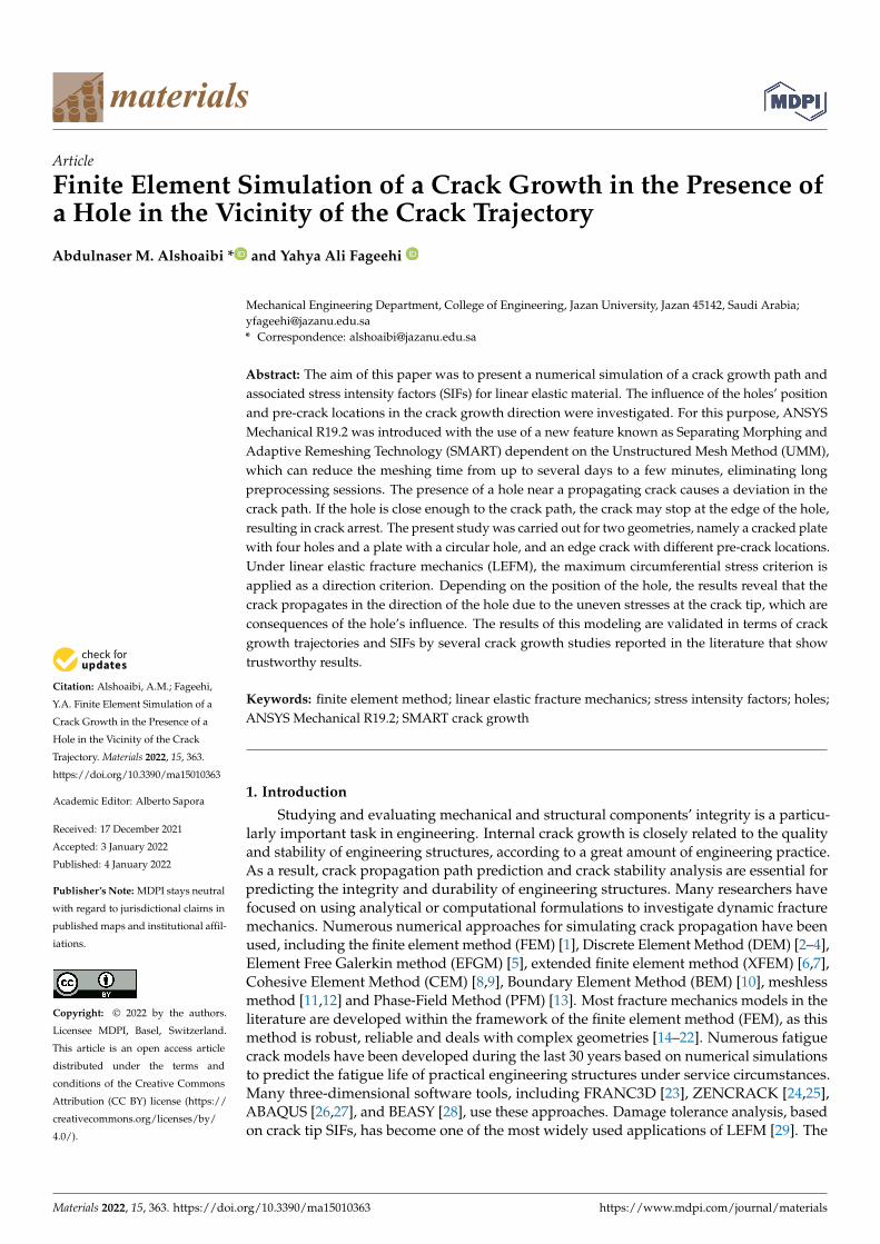
In this example, the crack growth path is deviated due to multiple holes in a relativelycomplicated shape. A square plate containing four holes of equal radii of 5 mm and a 6 mmlong edge crack is considered, as shown in Figure 1. The plate is 100 mm × 100 mm × 10 mmin size. The dimensions of the geometry are 100 mm × 100 mm with two different thick-nesses: 10 mm and 20 mm. Along the top and bottom edges of the plate, a uniformdistributed stress of σ = 10 MPa is applied. The material is Aluminium 7075-T6 with the fol-lowing properties: Modulus of elasticity, E = 72 GPa, Poisson’s ratio, υ = 0.33, Yield strength,σy = 469 MPa, Ultimate strength, σu = 538 MPa, Fracture toughness, KIC = 29 MPa

√mm.

Materials 2022, 15, x FOR PEER REVIEW 3 of 13

using the sphere of influence. The crack tip, the crack’s top surface, and the crack’s bottom surface are all included in the geometric regions. Each of these regions is connected to a set of nodes that will be utilized for the simulation.

For the static crack growth simulation, ANSYS Mechanical provides two common fracture criteria, which are the J-integral and stress intensity factor. In this study, the stress intensity factor criterion was used, which states that the crack grows when the equivalent stress intensity factor exceeds the fracture toughness of the material. This computation is performed along the distributed crack front, where the distribution of the stress intensity factor controls the adapting crack front shape. The equivalent stress intensity factor is rep-resented by [33], as follows:

[ ]1 cos ( (1 cos )) 3 sin2 2eq I IIK K Kθ θ θΔ = Δ + − Δ

(1)

where: ∆ = the range of SIF in mode I loading and ∆ = the range of SIF in mode II loading.

The crack growth direction is identified by an angle determined from the original crack plane [34–36]. The ratio of stress intensity factor modes at the crack tip determines the direction of a mixed-mode crack. The maximum circumferential stress criterion is im-plemented in the ANSYS software for mixed-mode loading. The formula for the crack propagation direction in ANSYS is expressed as follows [33,37]:

2 2 21

2 2

3 8cos

9II I I II

I II

K K K KK K

θ − + + = +

(2)

where: KI = first mode of SIF and KII = second mode of SIF.

3. Results and Discussion 3.1. A Cracked Plate with Four Holes

In this example, the crack growth path is deviated due to multiple holes in a relatively complicated shape. A square plate containing four holes of equal radii of 5 mm and a 6 mm long edge crack is considered, as shown in Figure 1. The plate is 100 mm × 100 mm x 10 mm in size. The dimensions of the geometry are 100 mm × 100 mm with two different thicknesses: 10 mm and 20 mm. Along the top and bottom edges of the plate, a uniform distributed stress of σ = 10 MPa is applied. The material is Aluminium 7075-T6 with the following properties: Modulus of elasticity, E = 72 GPa, Poisson’s ratio, υ = 0.33, Yield strength, σy = 469 MPa, Ultimate strength, σu = 538 MPa, Fracture toughness, KIC = 29 MPa √ .

Figure 1. Cracked plate with four holes and one edge crack. Figure 1. Cracked plate with four holes and one edge crack.

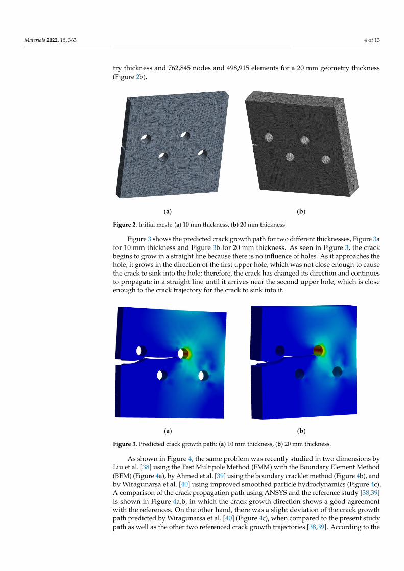
Figure 2 depicts the initial mesh generated by Ansys, which had a 1 mm elementsize and generated 693,495 nodes and 453,855 elements for a 10 mm (Figure 2a) geome-

Materials 2022, 15, 363 4 of 13

try thickness and 762,845 nodes and 498,915 elements for a 20 mm geometry thickness(Figure 2b).

Materials 2022, 15, x FOR PEER REVIEW 4 of 13

Figure 2 depicts the initial mesh generated by Ansys, which had a 1 mm element size and generated 693,495 nodes and 453,855 elements for a 10 mm (Figure 2a) geometry thickness and 762,845 nodes and 498,915 elements for a 20 mm geometry thickness (Figure 2b).

(a) (b)

Figure 2. Initial mesh: (a) 10 mm thickness, (b) 20 mm thickness.

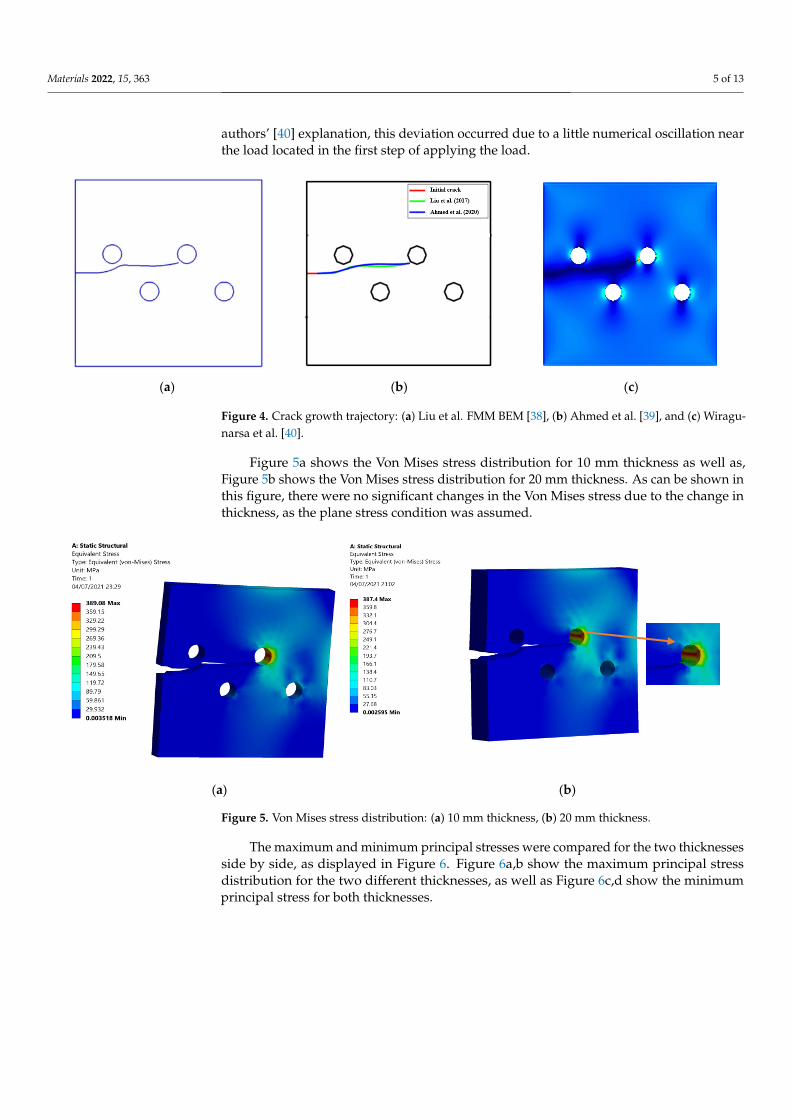
Figure 3 shows the predicted crack growth path for two different thicknesses, Figure 3a for 10 mm thickness and Figure 3b for 20 mm thickness. As seen in Figure 3, the crack begins to grow in a straight line because there is no influence of holes. As it approaches the hole, it grows in the direction of the first upper hole, which was not close enough to cause the crack to sink into the hole; therefore, the crack has changed its direction and continues to propagate in a straight line until it arrives near the second upper hole, which is close enough to the crack trajectory for the crack to sink into it.

(a) (b)

Figure 3. Predicted crack growth path: (a) 10 mm thickness, (b) 20 mm thickness.

As shown in Figure 4, the same problem was recently studied in two dimensions by Liu et al. [38] using the Fast Multipole Method (FMM) with the Boundary Element Method (BEM) (Figure 4a), by Ahmed et al. [39] using the boundary cracklet method (Figure 4b), and by Wiragunarsa et al. [40] using improved smoothed particle hydrodynamics (Figure 4c). A comparison of the crack propagation path using ANSYS and the reference study

Figure 2. Initial mesh: (a) 10 mm thickness, (b) 20 mm thickness.

Figure 3 shows the predicted crack growth path for two different thicknesses, Figure 3afor 10 mm thickness and Figure 3b for 20 mm thickness. As seen in Figure 3, the crackbegins to grow in a straight line because there is no influence of holes. As it approaches thehole, it grows in the direction of the first upper hole, which was not close enough to causethe crack to sink into the hole; therefore, the crack has changed its direction and continuesto propagate in a straight line until it arrives near the second upper hole, which is closeenough to the crack trajectory for the crack to sink into it.

Materials 2022, 15, x FOR PEER REVIEW 4 of 13

Figure 2 depicts the initial mesh generated by Ansys, which had a 1 mm element size and generated 693,495 nodes and 453,855 elements for a 10 mm (Figure 2a) geometry thickness and 762,845 nodes and 498,915 elements for a 20 mm geometry thickness (Figure 2b).

(a) (b)

Figure 2. Initial mesh: (a) 10 mm thickness, (b) 20 mm thickness.

Figure 3 shows the predicted crack growth path for two different thicknesses, Figure 3a for 10 mm thickness and Figure 3b for 20 mm thickness. As seen in Figure 3, the crack begins to grow in a straight line because there is no influence of holes. As it approaches the hole, it grows in the direction of the first upper hole, which was not close enough to cause the crack to sink into the hole; therefore, the crack has changed its direction and continues to propagate in a straight line until it arrives near the second upper hole, which is close enough to the crack trajectory for the crack to sink into it.

(a) (b)

Figure 3. Predicted crack growth path: (a) 10 mm thickness, (b) 20 mm thickness.

As shown in Figure 4, the same problem was recently studied in two dimensions by Liu et al. [38] using the Fast Multipole Method (FMM) with the Boundary Element Method (BEM) (Figure 4a), by Ahmed et al. [39] using the boundary cracklet method (Figure 4b), and by Wiragunarsa et al. [40] using improved smoothed particle hydrodynamics (Figure 4c). A comparison of the crack propagation path using ANSYS and the reference study

Figure 3. Predicted crack growth path: (a) 10 mm thickness, (b) 20 mm thickness.

As shown in Figure 4, the same problem was recently studied in two dimensions byLiu et al. [38] using the Fast Multipole Method (FMM) with the Boundary Element Method(BEM) (Figure 4a), by Ahmed et al. [39] using the boundary cracklet method (Figure 4b), andby Wiragunarsa et al. [40] using improved smoothed particle hydrodynamics (Figure 4c).A comparison of the crack propagation path using ANSYS and the reference study [38,39]is shown in Figure 4a,b, in which the crack growth direction shows a good agreementwith the references. On the other hand, there was a slight deviation of the crack growthpath predicted by Wiragunarsa et al. [40] (Figure 4c), when compared to the present studypath as well as the other two referenced crack growth trajectories [38,39]. According to the

Materials 2022, 15, 363 5 of 13

authors’ [40] explanation, this deviation occurred due to a little numerical oscillation nearthe load located in the first step of applying the load.

Materials 2022, 15, x FOR PEER REVIEW 5 of 13

[38,39] is shown in Figure 4a,b, in which the crack growth direction shows a good agree-ment with the references. On the other hand, there was a slight deviation of the crack growth path predicted by Wiragunarsa et al. [40] (Figure 4c), when compared to the pre-sent study path as well as the other two referenced crack growth trajectories [38,39]. Ac-cording to the authors’ [40] explanation, this deviation occurred due to a little numerical oscillation near the load located in the first step of applying the load.

(a) (b) (c)

Figure 4. Crack growth trajectory: (a) Liu et al. FMM BEM [38], (b) Ahmed et al. [39], and (c) Wira-gunarsa et al. [40].

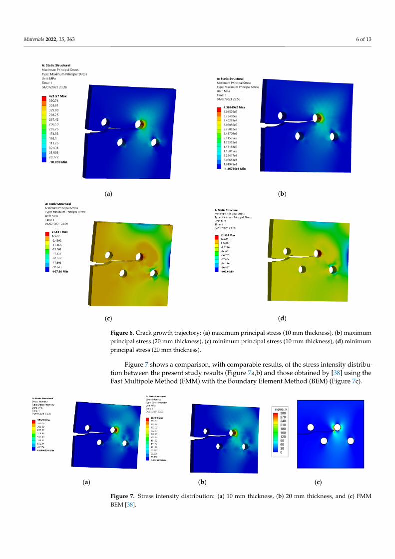
Figure 5a shows the Von Mises stress distribution for 10 mm thickness as well as, Figure 5b shows the Von Mises stress distribution for 20 mm thickness. As can be shown in this figure, there were no significant changes in the Von Mises stress due to the change in thickness, as the plane stress condition was assumed.

(a) (b)

Figure 5. Von Mises stress distribution: (a) 10 mm thickness, (b) 20 mm thickness.

The maximum and minimum principal stresses were compared for the two thick-nesses side by side, as displayed in Figure 6. Figure 6a,b show the maximum principal stress distribution for the two different thicknesses, as well as Figure 6c,d show the mini-mum principal stress for both thicknesses.

Figure 4. Crack growth trajectory: (a) Liu et al. FMM BEM [38], (b) Ahmed et al. [39], and (c) Wiragu-narsa et al. [40].

Figure 5a shows the Von Mises stress distribution for 10 mm thickness as well as,Figure 5b shows the Von Mises stress distribution for 20 mm thickness. As can be shown inthis figure, there were no significant changes in the Von Mises stress due to the change inthickness, as the plane stress condition was assumed.

Materials 2022, 15, x FOR PEER REVIEW 5 of 13

[38,39] is shown in Figure 4a,b, in which the crack growth direction shows a good agree-ment with the references. On the other hand, there was a slight deviation of the crack growth path predicted by Wiragunarsa et al. [40] (Figure 4c), when compared to the pre-sent study path as well as the other two referenced crack growth trajectories [38,39]. Ac-cording to the authors’ [40] explanation, this deviation occurred due to a little numerical oscillation near the load located in the first step of applying the load.

(a) (b) (c)

Figure 4. Crack growth trajectory: (a) Liu et al. FMM BEM [38], (b) Ahmed et al. [39], and (c) Wira-gunarsa et al. [40].

Figure 5a shows the Von Mises stress distribution for 10 mm thickness as well as, Figure 5b shows the Von Mises stress distribution for 20 mm thickness. As can be shown in this figure, there were no significant changes in the Von Mises stress due to the change in thickness, as the plane stress condition was assumed.

(a) (b)

Figure 5. Von Mises stress distribution: (a) 10 mm thickness, (b) 20 mm thickness.

The maximum and minimum principal stresses were compared for the two thick-nesses side by side, as displayed in Figure 6. Figure 6a,b show the maximum principal stress distribution for the two different thicknesses, as well as Figure 6c,d show the mini-mum principal stress for both thicknesses.

Figure 5. Von Mises stress distribution: (a) 10 mm thickness, (b) 20 mm thickness.

The maximum and minimum principal stresses were compared for the two thicknessesside by side, as displayed in Figure 6. Figure 6a,b show the maximum principal stressdistribution for the two different thicknesses, as well as Figure 6c,d show the minimumprincipal stress for both thicknesses.

Materials 2022, 15, 363 6 of 13Materials 2022, 15, x FOR PEER REVIEW 6 of 13

(a) (b)

(c) (d)

Figure 6. Crack growth trajectory: (a) maximum principal stress (10 mm thickness), (b) maximum principal stress (20 mm thickness), (c) minimum principal stress (10 mm thickness), (d) minimum principal stress (20 mm thickness).

Figure 7 shows a comparison, with comparable results, of the stress intensity distri-bution between the present study results (Figure 7a,b) and those obtained by [38] using the Fast Multipole Method (FMM) with the Boundary Element Method (BEM) (Figure 7c).

(a) (b) (c)

Figure 7. Stress intensity distribution: (a) 10 mm thickness, (b) 20 mm thickness, and (c) FMM BEM [38].

Figure 6. Crack growth trajectory: (a) maximum principal stress (10 mm thickness), (b) maximumprincipal stress (20 mm thickness), (c) minimum principal stress (10 mm thickness), (d) minimumprincipal stress (20 mm thickness).

Figure 7 shows a comparison, with comparable results, of the stress intensity distribu-tion between the present study results (Figure 7a,b) and those obtained by [38] using theFast Multipole Method (FMM) with the Boundary Element Method (BEM) (Figure 7c).

Materials 2022, 15, x FOR PEER REVIEW 6 of 13

(a) (b)

(c) (d)

Figure 6. Crack growth trajectory: (a) maximum principal stress (10 mm thickness), (b) maximum principal stress (20 mm thickness), (c) minimum principal stress (10 mm thickness), (d) minimum principal stress (20 mm thickness).

Figure 7 shows a comparison, with comparable results, of the stress intensity distri-bution between the present study results (Figure 7a,b) and those obtained by [38] using the Fast Multipole Method (FMM) with the Boundary Element Method (BEM) (Figure 7c).

(a) (b) (c)

Figure 7. Stress intensity distribution: (a) 10 mm thickness, (b) 20 mm thickness, and (c) FMM BEM [38].

Figure 7. Stress intensity distribution: (a) 10 mm thickness, (b) 20 mm thickness, and (c) FMMBEM [38].

Materials 2022, 15, 363 7 of 13

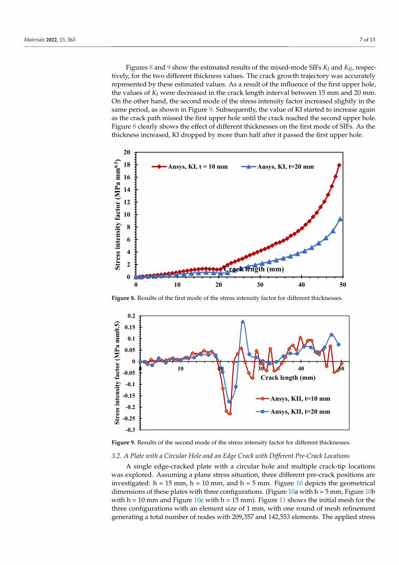
Figures 8 and 9 show the estimated results of the mixed-mode SIFs KI and KII, respec-tively, for the two different thickness values. The crack growth trajectory was accuratelyrepresented by these estimated values. As a result of the influence of the first upper hole,the values of KI were decreased in the crack length interval between 15 mm and 20 mm.On the other hand, the second mode of the stress intensity factor increased slightly in thesame period, as shown in Figure 9. Subsequently, the value of KI started to increase againas the crack path missed the first upper hole until the crack reached the second upper hole.Figure 8 clearly shows the effect of different thicknesses on the first mode of SIFs. As thethickness increased, KI dropped by more than half after it passed the first upper hole.

Materials 2022, 15, x FOR PEER REVIEW 7 of 13

Figures 8 and 9 show the estimated results of the mixed-mode SIFs KI and KII, respec-tively, for the two different thickness values. The crack growth trajectory was accurately represented by these estimated values. As a result of the influence of the first upper hole, the values of KI were decreased in the crack length interval between 15 mm and 20 mm. On the other hand, the second mode of the stress intensity factor increased slightly in the same period, as shown in Figure 9. Subsequently, the value of KI started to increase again as the crack path missed the first upper hole until the crack reached the second upper hole. Figure 8 clearly shows the effect of different thicknesses on the first mode of SIFs. As the thickness increased, KI dropped by more than half after it passed the first upper hole.

Figure 8. Results of the first mode of the stress intensity factor for different thicknesses.

Figure 9. Results of the second mode of the stress intensity factor for different thicknesses.

3.2. A Plate with a Circular Hole and an Edge Crack with Different Pre-Crack Locations A single edge-cracked plate with a circular hole and multiple crack-tip locations was

explored. Assuming a plane stress situation, three different pre-crack positions are inves-tigated: h = 15 mm, h = 10 mm, and h = 5 mm. Figure 10 depicts the geometrical dimensions of these plates with three configurations. (Figure 10a with h = 5 mm, Figure 10b with h = 10 mm and Figure 10c with h = 15 mm). Figure 11 shows the initial mesh for the three

0

2

4

6

8

10

12

14

16

18

20

0 10 20 30 40 50

Stre

ss in

tens

ity fa

ctor

(MPa

mm

0.5 )

Crack length (mm)

Ansys, KI, t = 10 mm Ansys, KI, t=20 mm

-0.3

-0.25

-0.2

-0.15

-0.1

-0.05

0

0.05

0.1

0.15

0.2

0 10 20 30 40 50

Stre

ss in

tens

ity fa

ctor

(MPa

mm

0.5)

Crack length (mm)

Ansys, KII, t=10 mm

Ansys, KII, t=20 mm

Figure 8. Results of the first mode of the stress intensity factor for different thicknesses.

Materials 2022, 15, x FOR PEER REVIEW 7 of 13

Figures 8 and 9 show the estimated results of the mixed-mode SIFs KI and KII, respec-tively, for the two different thickness values. The crack growth trajectory was accurately represented by these estimated values. As a result of the influence of the first upper hole, the values of KI were decreased in the crack length interval between 15 mm and 20 mm. On the other hand, the second mode of the stress intensity factor increased slightly in the same period, as shown in Figure 9. Subsequently, the value of KI started to increase again as the crack path missed the first upper hole until the crack reached the second upper hole. Figure 8 clearly shows the effect of different thicknesses on the first mode of SIFs. As the thickness increased, KI dropped by more than half after it passed the first upper hole.

Figure 8. Results of the first mode of the stress intensity factor for different thicknesses.

Figure 9. Results of the second mode of the stress intensity factor for different thicknesses.

3.2. A Plate with a Circular Hole and an Edge Crack with Different Pre-Crack Locations A single edge-cracked plate with a circular hole and multiple crack-tip locations was

explored. Assuming a plane stress situation, three different pre-crack positions are inves-tigated: h = 15 mm, h = 10 mm, and h = 5 mm. Figure 10 depicts the geometrical dimensions of these plates with three configurations. (Figure 10a with h = 5 mm, Figure 10b with h = 10 mm and Figure 10c with h = 15 mm). Figure 11 shows the initial mesh for the three

0

2

4

6

8

10

12

14

16

18

20

0 10 20 30 40 50

Stre

ss in

tens

ity fa

ctor

(MPa

mm

0.5 )

Crack length (mm)

Ansys, KI, t = 10 mm Ansys, KI, t=20 mm

-0.3

-0.25

-0.2

-0.15

-0.1

-0.05

0

0.05

0.1

0.15

0.2

0 10 20 30 40 50

Stre

ss in

tens

ity fa

ctor

(MPa

mm

0.5)

Crack length (mm)

Ansys, KII, t=10 mm

Ansys, KII, t=20 mm

Figure 9. Results of the second mode of the stress intensity factor for different thicknesses.

3.2. A Plate with a Circular Hole and an Edge Crack with Different Pre-Crack Locations

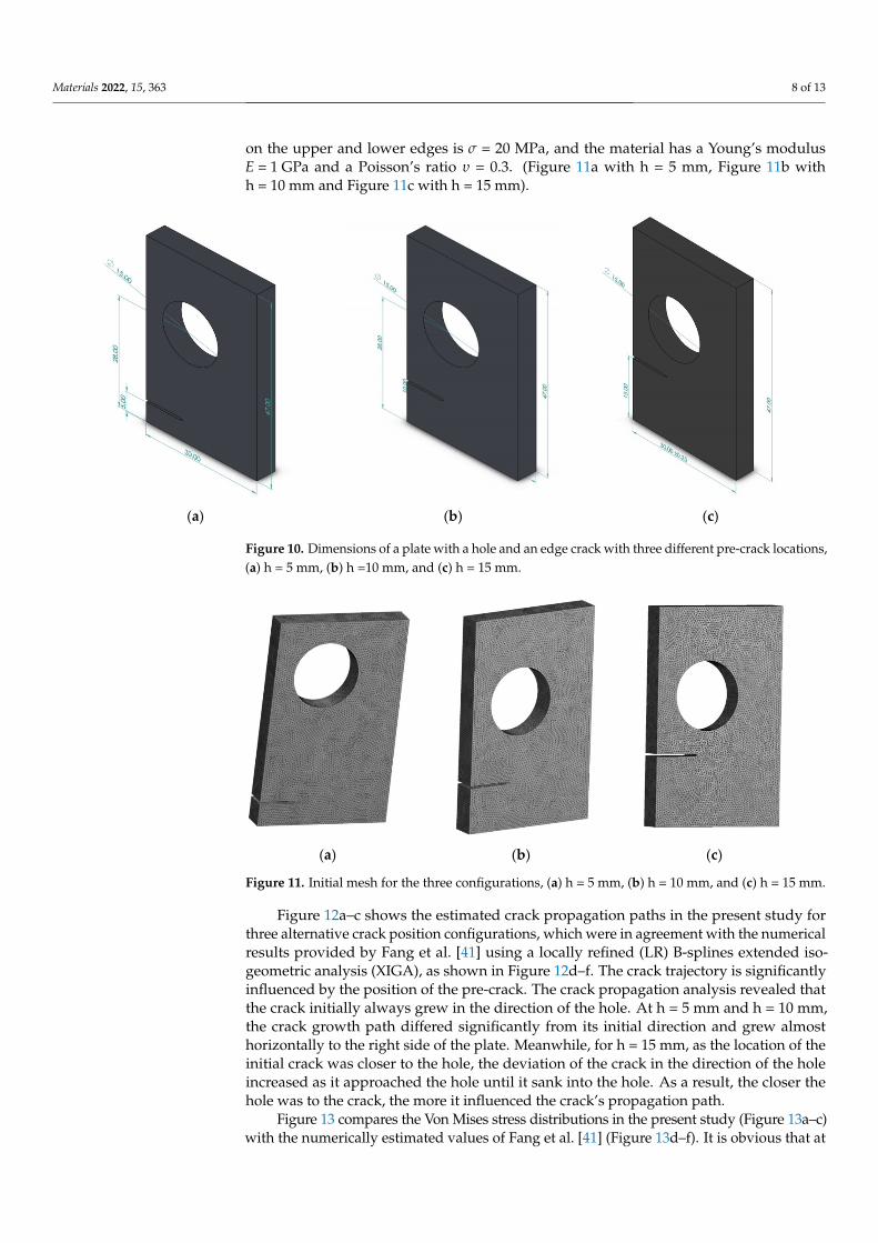
A single edge-cracked plate with a circular hole and multiple crack-tip locationswas explored. Assuming a plane stress situation, three different pre-crack positions areinvestigated: h = 15 mm, h = 10 mm, and h = 5 mm. Figure 10 depicts the geometricaldimensions of these plates with three configurations. (Figure 10a with h = 5 mm, Figure 10bwith h = 10 mm and Figure 10c with h = 15 mm). Figure 11 shows the initial mesh for thethree configurations with an element size of 1 mm, with one round of mesh refinementgenerating a total number of nodes with 209,357 and 142,553 elements. The applied stress

Materials 2022, 15, 363 8 of 13

on the upper and lower edges is σ = 20 MPa, and the material has a Young’s modulusE = 1 GPa and a Poisson’s ratio υ = 0.3. (Figure 11a with h = 5 mm, Figure 11b withh = 10 mm and Figure 11c with h = 15 mm).

Materials 2022, 15, x FOR PEER REVIEW 8 of 13

configurations with an element size of 1 mm, with one round of mesh refinement gener-ating a total number of nodes with 209,357 and 142,553 elements. The applied stress on the upper and lower edges is σ = 20 MPa, and the material has a Young’s modulus E = 1 GPa and a Poisson’s ratio υ = 0.3. (Figure 11a with h = 5 mm, Figure 11b with h = 10 mm and Figure 11c with h = 15 mm).

(a) (b) (c)

Figure 10. Dimensions of a plate with a hole and an edge crack with three different pre-crack loca-tions, (a) h = 5 mm, (b) h =10 mm, and (c) h = 15 mm.

(a) (b) (c)

Figure 11. Initial mesh for the three configurations, (a) h = 5 mm, (b) h = 10 mm, and (c) h = 15 mm.

Figure 12a–c shows the estimated crack propagation paths in the present study for three alternative crack position configurations, which were in agreement with the numer-ical results provided by Fang et al. [41] using a locally refined (LR) B-splines extended iso-geometric analysis (XIGA), as shown in Figure 12d-f. The crack trajectory is significantly influenced by the position of the pre-crack. The crack propagation analysis revealed that the crack initially always grew in the direction of the hole. At h = 5 mm and h = 10 mm, the crack growth path differed significantly from its initial direction and grew almost hor-izontally to the right side of the plate. Meanwhile, for h = 15 mm, as the location of the initial crack was closer to the hole, the deviation of the crack in the direction of the hole increased as it approached the hole until it sank into the hole. As a result, the closer the hole was to the crack, the more it influenced the crack’s propagation path.

Figure 10. Dimensions of a plate with a hole and an edge crack with three different pre-crack locations,(a) h = 5 mm, (b) h =10 mm, and (c) h = 15 mm.

Materials 2022, 15, x FOR PEER REVIEW 8 of 13

configurations with an element size of 1 mm, with one round of mesh refinement gener-ating a total number of nodes with 209,357 and 142,553 elements. The applied stress on the upper and lower edges is σ = 20 MPa, and the material has a Young’s modulus E = 1 GPa and a Poisson’s ratio υ = 0.3. (Figure 11a with h = 5 mm, Figure 11b with h = 10 mm and Figure 11c with h = 15 mm).

(a) (b) (c)

Figure 10. Dimensions of a plate with a hole and an edge crack with three different pre-crack loca-tions, (a) h = 5 mm, (b) h =10 mm, and (c) h = 15 mm.

(a) (b) (c)

Figure 11. Initial mesh for the three configurations, (a) h = 5 mm, (b) h = 10 mm, and (c) h = 15 mm.

Figure 12a–c shows the estimated crack propagation paths in the present study for three alternative crack position configurations, which were in agreement with the numer-ical results provided by Fang et al. [41] using a locally refined (LR) B-splines extended iso-geometric analysis (XIGA), as shown in Figure 12d-f. The crack trajectory is significantly influenced by the position of the pre-crack. The crack propagation analysis revealed that the crack initially always grew in the direction of the hole. At h = 5 mm and h = 10 mm, the crack growth path differed significantly from its initial direction and grew almost hor-izontally to the right side of the plate. Meanwhile, for h = 15 mm, as the location of the initial crack was closer to the hole, the deviation of the crack in the direction of the hole increased as it approached the hole until it sank into the hole. As a result, the closer the hole was to the crack, the more it influenced the crack’s propagation path.

Figure 11. Initial mesh for the three configurations, (a) h = 5 mm, (b) h = 10 mm, and (c) h = 15 mm.

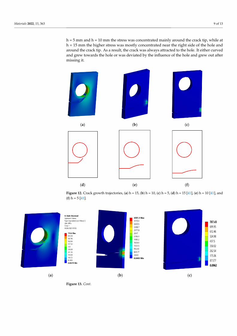
Figure 12a–c shows the estimated crack propagation paths in the present study forthree alternative crack position configurations, which were in agreement with the numericalresults provided by Fang et al. [41] using a locally refined (LR) B-splines extended iso-geometric analysis (XIGA), as shown in Figure 12d–f. The crack trajectory is significantlyinfluenced by the position of the pre-crack. The crack propagation analysis revealed thatthe crack initially always grew in the direction of the hole. At h = 5 mm and h = 10 mm,the crack growth path differed significantly from its initial direction and grew almosthorizontally to the right side of the plate. Meanwhile, for h = 15 mm, as the location of theinitial crack was closer to the hole, the deviation of the crack in the direction of the holeincreased as it approached the hole until it sank into the hole. As a result, the closer thehole was to the crack, the more it influenced the crack’s propagation path.

Figure 13 compares the Von Mises stress distributions in the present study (Figure 13a–c)with the numerically estimated values of Fang et al. [41] (Figure 13d–f). It is obvious that at

Materials 2022, 15, 363 9 of 13

h = 5 mm and h = 10 mm the stress was concentrated mainly around the crack tip, while ath = 15 mm the higher stress was mostly concentrated near the right side of the hole andaround the crack tip. As a result, the crack was always attracted to the hole. It either curvedand grew towards the hole or was deviated by the influence of the hole and grew out aftermissing it.

Materials 2022, 15, x FOR PEER REVIEW 9 of 13

Figure 13 compares the Von Mises stress distributions in the present study (Figure 13a–c) with the numerically estimated values of Fang et al. [41] (Figure 13d–f). It is obvious that at h = 5 mm and h = 10 mm the stress was concentrated mainly around the crack tip, while at h = 15 mm the higher stress was mostly concentrated near the right side of the hole and around the crack tip. As a result, the crack was always attracted to the hole. It either curved and grew towards the hole or was deviated by the influence of the hole and grew out after missing it.

(a) (b) (c)

(d) (e) (f)

Figure 12. Crack growth trajectories, (a) h = 15, (b) h = 10, (c) h = 5, (d) h = 15 [41], (e) h = 10 [41], and (f) h = 5 [41].

(a) (b) (c)

Figure 12. Crack growth trajectories, (a) h = 15, (b) h = 10, (c) h = 5, (d) h = 15 [41], (e) h = 10 [41], and(f) h = 5 [41].

Materials 2022, 15, x FOR PEER REVIEW 9 of 13

Figure 13 compares the Von Mises stress distributions in the present study (Figure 13a–c) with the numerically estimated values of Fang et al. [41] (Figure 13d–f). It is obvious that at h = 5 mm and h = 10 mm the stress was concentrated mainly around the crack tip, while at h = 15 mm the higher stress was mostly concentrated near the right side of the hole and around the crack tip. As a result, the crack was always attracted to the hole. It either curved and grew towards the hole or was deviated by the influence of the hole and grew out after missing it.

(a) (b) (c)

(d) (e) (f)

Figure 12. Crack growth trajectories, (a) h = 15, (b) h = 10, (c) h = 5, (d) h = 15 [41], (e) h = 10 [41], and (f) h = 5 [41].

(a) (b) (c)

Figure 13. Cont.

Materials 2022, 15, 363 10 of 13Materials 2022, 15, x FOR PEER REVIEW 10 of 13

(d) (e) (f)

Figure 13. Von Mises stress distribution, (a) h = 15, (b) h = 10, (c) h = 5, (d) h = 15 [41], (e) h = 10 [41], and (f) h = 5 [41].

Figures 14 and 15 illustrate the estimated results for KI. As shown in these figures, the case of a crack position with h = 15 has higher KI and KII results than the other two cases for the same crack length interval, demonstrating the influence of the hole on the increase of the SIFs when the crack grows towards it. As the KII values increase, the crack grows in a curvature trajectory until it falls into the hole, as shown in Figure 13a. In addi-tion, there was a minor effect of the hole at the onset of the crack trajectory in the other two configurations with h = 10 mm and h = 5 mm, which can also be noticed in the increase of KII; nevertheless, when the KI values were increased, the crack kept growing in a straight path, and this mode completely controlled the crack propagation trajectory with a reduc-tion in the KII values, as shown on Figure 13b,c.

Figure 14. Evaluated results of KI for three pre-crack positions.

0

400

800

1200

1600

2000

0 2 4 6 8 10 12 14 16 18

Stre

ss in

tens

ity fa

ctor

s (M

Pa m

m0.

5 )

Crack length (mm)

h = 15 mm, KIh = 10 mm, KIh = 5 mm KI

Figure 13. Von Mises stress distribution, (a) h = 15, (b) h = 10, (c) h = 5, (d) h = 15 [41], (e) h = 10 [41],and (f) h = 5 [41].

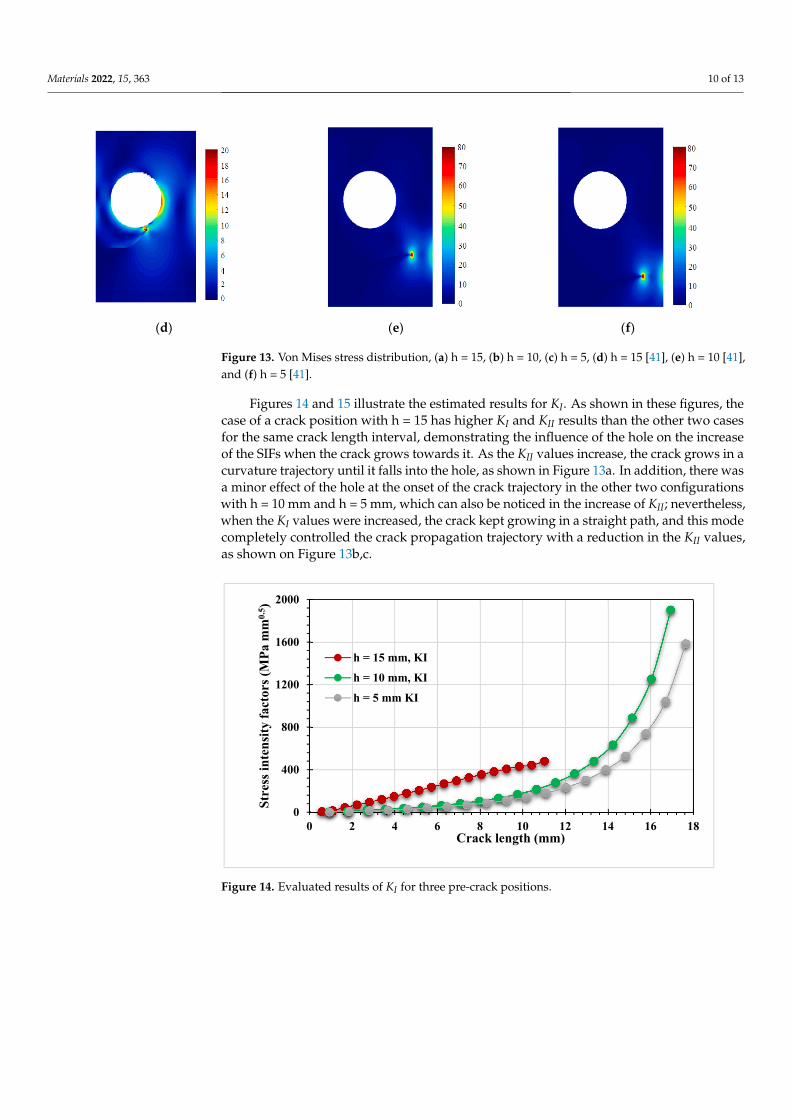
Figures 14 and 15 illustrate the estimated results for KI. As shown in these figures, thecase of a crack position with h = 15 has higher KI and KII results than the other two casesfor the same crack length interval, demonstrating the influence of the hole on the increaseof the SIFs when the crack grows towards it. As the KII values increase, the crack grows in acurvature trajectory until it falls into the hole, as shown in Figure 13a. In addition, there wasa minor effect of the hole at the onset of the crack trajectory in the other two configurationswith h = 10 mm and h = 5 mm, which can also be noticed in the increase of KII; nevertheless,when the KI values were increased, the crack kept growing in a straight path, and this modecompletely controlled the crack propagation trajectory with a reduction in the KII values,as shown on Figure 13b,c.

Materials 2022, 15, x FOR PEER REVIEW 10 of 13

(d) (e) (f)

Figure 13. Von Mises stress distribution, (a) h = 15, (b) h = 10, (c) h = 5, (d) h = 15 [41], (e) h = 10 [41], and (f) h = 5 [41].

Figures 14 and 15 illustrate the estimated results for KI. As shown in these figures, the case of a crack position with h = 15 has higher KI and KII results than the other two cases for the same crack length interval, demonstrating the influence of the hole on the increase of the SIFs when the crack grows towards it. As the KII values increase, the crack grows in a curvature trajectory until it falls into the hole, as shown in Figure 13a. In addi-tion, there was a minor effect of the hole at the onset of the crack trajectory in the other two configurations with h = 10 mm and h = 5 mm, which can also be noticed in the increase of KII; nevertheless, when the KI values were increased, the crack kept growing in a straight path, and this mode completely controlled the crack propagation trajectory with a reduc-tion in the KII values, as shown on Figure 13b,c.

Figure 14. Evaluated results of KI for three pre-crack positions.

0

400

800

1200

1600

2000

0 2 4 6 8 10 12 14 16 18

Stre

ss in

tens

ity fa

ctor

s (M

Pa m

m0.

5 )

Crack length (mm)

h = 15 mm, KIh = 10 mm, KIh = 5 mm KI

Figure 14. Evaluated results of KI for three pre-crack positions.

Materials 2022, 15, 363 11 of 13

Materials 2022, 15, x FOR PEER REVIEW 11 of 13

Figure 15. Evaluated results of KII for three pre-crack positions.

4. Conclusions In this study, a crack growth simulation was performed for a cracked plate with four

holes and a plate with a circular hole and for an edge crack with different pre-crack posi-tions, employing the ANSYS SMART fracture technology, which was recently introduced into the ANSYS Mechanical 19.2. The SMART crack propagation simulation was based on the Paris law and used a tetrahedral mesh for the crack fronts, which was automatically updated when the crack front changed according to the crack propagation. Due to uneven stresses at the crack tip caused by the hole, the crack grows towards the hole, as predicted. The holes act as a crack stopper, attracting a crack path that grows towards the hole, de-pending on the position of the hole and the initial position of the crack tip from the hole. Depending on the position of the hole, the direction of growth of the crack either deviates from the hole, which is known as the missed hole phenomenon, or it grows towards the hole and sinks into it, which is known as the sinking in hole phenomenon.

Author Contributions: Conceptualization, A.M.A.; methodology, A.M.A.; software, A.M.A.; vali-dation, A.M.A. and Y.A.F.; formal analysis, A.M.A.; investigation, A.M.A. and Y.A.F.; resources, A.M.A.; data curation, A.M.A. and Y.A.F.; writing—original draft preparation, A.M.A.; writing—review and editing, A.M.A. and Y.A.F.; visualization, A.M.A. and Y.A.F.; supervision, A.M.A.; pro-ject administration, A.M.A. and Y.A.F.; funding acquisition, A.M.A. and Y.A.F. All authors have read and agreed to the published version of the manuscript.

Funding: This research received no external funding.

Institutional Review Board Statement: Not applicable.

Informed Consent Statement: Not applicable.

Data Availability Statement: The data presented in this study are available upon request from the corresponding author.

Conflicts of Interest: The authors declare no conflict of interest.

References 1. Branco, R.; Antunes, F.; Costa, J. A review on 3D-FE adaptive remeshing techniques for crack growth modelling. Eng. Fract.

Mech. 2015, 141, 170–195. 2. Li, X.; Li, H.; Liu, L.; Liu, Y.; Ju, M.; Zhao, J. Investigating the crack initiation and propagation mechanism in brittle rocks using

grain-based finite-discrete element method. Int. J. Rock Mech. Min. Sci. 2020, 127, 104219. 3. Leclerc, W.; Haddad, H.; Guessasma, M. On the suitability of a Discrete Element Method to simulate cracks initiation and prop-

agation in heterogeneous media. Int. J. Solids Struct. 2017, 108, 98–114.

-20

-10

0

10

20

30

40

0 1 2 3 4 5 6 7 8 9 10 11 12 13 14 15 16 17 18 19 20

Stre

ss in

tens

ity fa

ctor

s (M

Pa m

m0.

5 )

Crack length (mm)

h = 15 mm, KII

h = 10 mm, KII

h = 5 mm, KII

Figure 15. Evaluated results of KII for three pre-crack positions.

4. Conclusions

In this study, a crack growth simulation was performed for a cracked plate with fourholes and a plate with a circular hole and for an edge crack with different pre-crack positions,employing the ANSYS SMART fracture technology, which was recently introduced into theANSYS Mechanical 19.2. The SMART crack propagation simulation was based on the Parislaw and used a tetrahedral mesh for the crack fronts, which was automatically updatedwhen the crack front changed according to the crack propagation. Due to uneven stressesat the crack tip caused by the hole, the crack grows towards the hole, as predicted. Theholes act as a crack stopper, attracting a crack path that grows towards the hole, dependingon the position of the hole and the initial position of the crack tip from the hole. Dependingon the position of the hole, the direction of growth of the crack either deviates from thehole, which is known as the missed hole phenomenon, or it grows towards the hole andsinks into it, which is known as the sinking in hole phenomenon.

Author Contributions: Conceptualization, A.M.A.; methodology, A.M.A.; software, A.M.A.; valida-tion, A.M.A. and Y.A.F.; formal analysis, A.M.A.; investigation, A.M.A. and Y.A.F.; resources, A.M.A.;data curation, A.M.A. and Y.A.F.; writing—original draft preparation, A.M.A.; writing—review andediting, A.M.A. and Y.A.F.; visualization, A.M.A. and Y.A.F.; supervision, A.M.A.; project administra-tion, A.M.A. and Y.A.F.; funding acquisition, A.M.A. and Y.A.F. All authors have read and agreed tothe published version of the manuscript.

Funding: This research received no external funding.

Institutional Review Board Statement: Not applicable.

Informed Consent Statement: Not applicable.

Data Availability Statement: The data presented in this study are available upon request from thecorresponding author.

Conflicts of Interest: The authors declare no conflict of interest.

References1. Branco, R.; Antunes, F.; Costa, J. A review on 3D-FE adaptive remeshing techniques for crack growth modelling. Eng. Fract. Mech.

2015, 141, 170–195. [CrossRef]2. Li, X.; Li, H.; Liu, L.; Liu, Y.; Ju, M.; Zhao, J. Investigating the crack initiation and propagation mechanism in brittle rocks using

grain-based finite-discrete element method. Int. J. Rock Mech. Min. Sci. 2020, 127, 104219. [CrossRef]3. Leclerc, W.; Haddad, H.; Guessasma, M. On the suitability of a Discrete Element Method to simulate cracks initiation and

propagation in heterogeneous media. Int. J. Solids Struct. 2017, 108, 98–114. [CrossRef]

Materials 2022, 15, 363 12 of 13

4. Shao, Y.; Duan, Q.; Qiu, S. Adaptive consistent element-free Galerkin method for phase-field model of brittle fracture. Comput.Mech. 2019, 64, 741–767. [CrossRef]

5. Kanth, S.A.; Harmain, G.; Jameel, A. Modeling of Nonlinear Crack Growth in Steel and Aluminum Alloys by the Element FreeGalerkin Method. Mater. Today Proc. 2018, 5, 18805–18814. [CrossRef]

6. Huynh, H.D.; Nguyen, M.N.; Cusatis, G.; Tanaka, S.; Bui, T.Q. A polygonal XFEM with new numerical integration for linearelastic fracture mechanics. Eng. Fract. Mech. 2019, 213, 241–263. [CrossRef]

7. Surendran, M.; Natarajan, S.; Palani, G.; Bordas, S.P. Linear smoothed extended finite element method for fatigue crack growthsimulations. Eng. Fract. Mech. 2019, 206, 551–564. [CrossRef]

8. Dekker, R.; van der Meer, F.; Maljaars, J.; Sluys, L. A cohesive XFEM model for simulating fatigue crack growth under mixed-modeloading and overloading. Int. J. Numer. Methods Eng. 2019, 118, 561–577. [CrossRef]

9. Rezaei, S.; Wulfinghoff, S.; Reese, S. Prediction of fracture and damage in micro/nano coating systems using cohesive zoneelements. Int. J. Solids Struct. 2017, 121, 62–74. [CrossRef]

10. Santana, E.; Portela, A. Dual boundary element analysis of fatigue crack growth, interaction and linkup. Eng. Anal. Bound. Elem.2016, 64, 176–195. [CrossRef]

11. Tanaka, S.; Suzuki, H.; Sadamoto, S.; Imachi, M.; Bui, T.Q. Analysis of cracked shear deformable plates by an effective meshfreeplate formulation. Eng. Fract. Mech. 2015, 144, 142–157. [CrossRef]

12. Khosravifard, A.; Hematiyan, M.; Bui, T.; Do, T. Accurate and efficient analysis of stationary and propagating crack problems bymeshless methods. Theor. Appl. Fract. Mech. 2017, 87, 21–34. [CrossRef]

13. Zhang, W.; Tabiei, A. An Efficient Implementation of Phase Field Method with Explicit Time Integration. J. Appl. Comput. Mech.2020, 6, 373–382.

14. Moës, N.; Dolbow, J.; Belytschko, T. A finite element method for crack growth without remeshing. Int. J. Numer. Methods Eng.1999, 46, 131–150. [CrossRef]

15. Sukumar, N.; Prévost, J.-H. Modeling quasi-static crack growth with the extended finite element method Part I: Computerimplementation. Int. J. Solids Struct. 2003, 40, 7513–7537. [CrossRef]

16. Alshoaibi, A.M.; Fageehi, Y.A. Simulation of Quasi-Static Crack Propagation by Adaptive Finite Element Method. Metals 2021,11, 98. [CrossRef]

17. Lin, X.; Smith, R. Finite element modelling of fatigue crack growth of surface cracked plates: Part I: The numerical technique. Eng.Fract. Mech. 1999, 63, 503–522. [CrossRef]

18. Muixí, A.; Marco, O.; Rodríguez-Ferran, A.; Fernández-Méndez, S. A combined XFEM phase-field computational model for crackgrowth without remeshing. Comput. Mech. 2021, 67, 231–249. [CrossRef]

19. Alshoaibi, A.M.; Fageehi, Y.A. 2D finite element simulation of mixed mode fatigue crack propagation for CTS specimen. J. Mater.Res. Technol. 2020, 9, 7850–7861. [CrossRef]

20. Alshoaibi, A.M.; Fageehi, Y.A. Numerical Analysis of Fatigue Crack Growth Path and Life Predictions for Linear Elastic Material.Materials 2020, 13, 3380. [CrossRef]

21. Alshoaibi, A.M. Computational Simulation of 3D Fatigue Crack Growth under Mixed-Mode Loading. Appl. Sci. 2021, 11, 5953.[CrossRef]

22. Alshoaibi, A.M. Numerical Modeling of Crack Growth under Mixed-Mode Loading. Appl. Sci. 2021, 11, 2975. [CrossRef]23. Carter, B.; Wawrzynek, P.; Ingraffea, A. Automated 3-D crack growth simulation. Int. J. Numer. Methods Eng. 2000, 47, 229–253.

[CrossRef]24. Hou, J.; Goldstraw, M.; Maan, S.; Knop, M.; Defence Science and Technology Organization Victoria (Australia) Aeronautical and

Maritime Research Laboratory. An Evaluation of 3D Crack Growth Using ZENCRACK; Department of Defence, DSTO: Victoria,Australia, 2001.

25. Shahani, A.; Farrahi, A. Experimental investigation and numerical modeling of the fatigue crack growth in friction stir spotwelding of lap-shear specimen. Int. J. Fatigue 2019, 125, 520–529. [CrossRef]

26. Malekan, M.; Khosravi, A.; St-Pierre, L. An Abaqus plug-in to simulate fatigue crack growth. Eng. Comput. 2021, 1–15. [CrossRef]27. Rocha, A.; Akhavan-Safar, A.; Carbas, R.; Marques, E.; Goyal, R.; El-zein, M.; da Silva, L. Numerical analysis of mixed-mode

fatigue crack growth of adhesive joints using CZM. Theor. Appl. Fract. Mech. 2020, 106, 102493. [CrossRef]28. Teh, S.; Andriyana, A.; Ramesh, S.; Putra, I.; Kadarno, P.; Purbolaksono, J. Tetrahedral meshing for a slanted semi-elliptical surface

crack at a solid cylinder. Eng. Fract. Mech. 2021, 241, 107400. [CrossRef]29. Paris, P.C. A Brief History of the Crack Tip Stress Intensity Factor and Its Application; Springer: Berlin/Heidelberg, Germany, 2014.30. Zhao, T.; Zhang, J.; Jiang, Y. A study of fatigue crack growth of 7075-T651 aluminum alloy. Int. J. Fatigue 2008, 30, 1169–1180.

[CrossRef]31. Singh, V.K.; Gope, P.C. Experimental evaluation of mixed mode stress intensity factor for prediction of crack growth by phoelastic

method. J. Fail. Anal. Prev. 2013, 13, 217–226. [CrossRef]32. Forth, S.C.; Newman, J.C., Jr.; Forman, R.G. On generating fatigue crack growth thresholds. Int. J. Fatigue 2003, 25, 9–15.

[CrossRef]33. Bjørheim, F. Practical Comparison of Crack Meshing in ANSYS Mechanical APDL 19.2. Master’s Thesis, University of Stavanger,

Vistavanger, Norway, 2019.

Materials 2022, 15, 363 13 of 13

34. Wawrzynek, P.; Carter, B.; Banks-Sills, L. The M-Integral for Computing Stress Intensity Factors in Generally Anisotropic Materials;National Aeronautics and Space Administration, Marshall Space Flight Center: Hanover, NH, USA, 2005.

35. Citarella, R.; Giannella, V.; Lepore, M.; Dhondt, G. Dual boundary element method and finite element method for mixed-modecrack propagation simulations in a cracked hollow shaft. Fatigue Fract. Eng. Mater. Struct. 2018, 41, 84–98. [CrossRef]

36. Dhondt, G.; Hackenberg, H.-P. Use of a rotation-invariant linear strain measure for linear elastic crack propagation calculations.Eng. Fract. Mech. 2021, 247, 107634. [CrossRef]

37. ANSYS. Academic Research Mechanical, Release 19.2, Help System. In Coupled Field Analysis Guide; ANSYS, Inc.: Canonsburg,PA, USA, 2020.

38. Liu, Y.; Li, Y.; Xie, W. Modeling of multiple crack propagation in 2-D elastic solids by the fast multipole boundary element method.Eng. Fract. Mech. 2017, 172, 1–16. [CrossRef]

39. Ahmed, T.; Yavuz, A.; Turkmen, H.S. Fatigue crack growth simulation of interacting multiple cracks in perforated plates withmultiple holes using boundary cracklet method. Fatigue Fract. Eng. Mater. Struct. 2021, 44, 333–348. [CrossRef]

40. Wiragunarsa, I.M.; Zuhal, L.R.; Dirgantara, T.; Putra, I.S. A particle interaction-based crack model using an improved smoothedparticle hydrodynamics for fatigue crack growth simulations. Int. J. Fract. 2021, 229, 229–244. [CrossRef]

41. Fang, W.; Chen, X.; Yu, T.; Bui, T.Q. Effects of arbitrary holes/voids on crack growth using local mesh refinement adaptive XIGA.Theor. Appl. Fract. Mech. 2020, 109, 102724. [CrossRef]