FINAL REPORT Application of Advanced Sensor Technology to DoD Soil Vapor

Intrusion Problems

ESTCP Project ER-200702

July 2012

James Reisinger David Burris Integrated Science & Technology, Inc. Edward Zellers University of Michigan.

i

REPORT DOCUMENTATION PAGE Form Approved OMB No. 0704·0188

The public reporting burden for this coll.etion of infOfmatlon is tstlm attd to av..-a~ 1 hour per response, including the time for reviewing in.ttnJction:, :earching exi:ting data :ourcc:. gathering and maintaining dle data needed, and COt'Tl)letiog and revtewing the collection of information. Send commtntc regarding thic burden utima1e or any other aspect of thic co llection of inform.-bon, including suggestions for reducing th-e burden, to the Department of Defense. Executive Servitas and Commu nie.ations Oir.etorate (0704·0188). R"pondents c.hould be aware that notwithstanding any othet prov1sion of law, no .,.,uon shall be subject to any penalty fo r failng to comply with a col!ection of information if it does not d isplay a curtentfy valid OMS control number. PLEASE DO NOT RETURN YOUR FORM TO THE ABOVE ORGANIZATION. 1. REPORT DATE 00-MM· YYYY) ,2. REPORT TYPE 3. DATES COVERED (From · To)

16-()7-2012 Final Report April 2007- July 2012

4 . TITLE AND SUBTITLE 5a. CONTRACT NUMBER

Application of Advanced Sensor Technology to DoD W912HQ-07-C-OOII Soil Vapor Intrusion Problems

5b. GRANT NUMBER

N/A

5c. PROGRAM ELEMENT NUMBER

N/A

6. AUTHOR(Sl 5d. PROJECT NUMBER Reisinger, H. James Burris, David R.

200702

Zellers, Edward T. 5e. TASK NUMBER

N/A

5f. WORK UNIT NUMBER

NIA

7. PERFORMING ORGANIZATION NAME(S) AND ADDRESS(ES) 8. PERFORMING ORGANIZATION

Integrated Science & Technology, Inc. University of Michigan REPORT NUMBER

4640 Cowan Road School of Public Health N/A

Acworth, GA 30101 109 South Observatory Street Ann Arbor, Ml 48109

9. SPONSORING/MONITORING AGENCY NAME(S) AND ADDRESS(ESJ 10. SPONSOR/MONITOR'S ACRONYM(S)

Environmental Security Technology Certification Program ESTCP SERDPIESTCP Support Office, HGL Il l 07 Sunset Hills Road, Suite 400 11 . SPONSORIMONITOR·s REPORT Reston, VA 20 190 NUMBER(S)

N/A

12. DISTRIBUTION/AVAILABILITY STATEMENT Approved for public release; distribution unlimited

13. SUPPLEMENTARY NOTES

NIA

14.ABSTRACT This study demonstrated the use of a unique prototype gas chromatograph with sensor array detection, the analytical components of which are microfabricated from Si (micro-GC), for analysis of indoor air concentrations of trichloroethylene (TCE) at low- and sub·ppb levels, related to vapor intrusion (VI) applications. The objectives of this study were to demonstrate the performance of the prototype micro-GC in two operating modes: portable mode for forensic and spatial monitoring; and fixed-location mode for longer term temporal monitoring (exposure estimation). Results from the micro·GC and from T0-15 reference samples were compared. Above the mitigation action level (MAL; 2.3 ppb), the micro-GC accurately determined TCE under complex field matrix conditions. Below the MAL, TCE micro-GC determinations were positively biased due to unresolved interferences. This study stands as the first of its kind, where micro-GC instrumentation was shown capable of sustained, reliable , automated measurements of a trace-level component (TCE) in a complex VOC mixture in real-world environments.

15. SUBJECT TERMS

vapor intrusion, micro-gas chromatograph, indoor air analysis

16. SECURITY CLASSIFICATION OF: 17. LIMITATION OF

a. REPORT b. ABSTRACT c. THIS PAGE ABSTRACT

u u u uu

18. NUMBER OF PAGES

116

19a. NAME OF RESPONSIBLE PERSON

H. James Reisinger 19b. TELEPHONE NUMBER 1/nclude area code)

(770)425-3080

Standard Form 298 (Rev. 8 /98) Prescribed by ANSI Std. Z39.18

ii

TABLE OF CONTENTS Page LIST OF FIGURES iv

LIST OF TABLES viii

LIST OF ACRONYMS ix

ACKNOWLEDGMENTS xii

EXECUTIVE SUMMARY xiii

1.0 INTRODUCTION 1

1.1 BACKGROUND 1 1.2 DEMONSTRATION OBJECTIVE 5 1.3 REGULATORY DRIVERS 5

2.0 TECHNOLOGY 8

2.1 TECHNOLOGY DEVELOPMENT 8 2.2 TECHNOLOGY DESCRIPTION 9 2.3 ADVANTAGES AND LIMITATIONS OF THE TECHNOLOGY 14

3.0 PERFORMANCE OBJECTIVES 16

3.1 TCE SENSITIVITY – PORTABLE µGC MODE 16 3.2 TCE SENSITIVITY – FIXED-LOCATION µGC MODE 17 3.3 µGC RESPONSE STABILITY 17 3.4 CORRELATION OF µGC AND TO-15 TCE FIELD SAMPLE RESULTS 17 3.5 QUALITATIVE PERFORMANCE OBJECTIVES 18

4.0 SITE DESCRIPTION 20 5.0 TEST DESIGN 22

5.1 CONCEPTUAL EXPERIMENTAL DESIGN 22 5.2 LABORATORY STUDY RESULTS 23 5.2.1 DEVELOPMENT AND CHARACTERIZATION 23 5.2.2 MULTIVARIATE CURVE RESOLUTION 52 5.3 FIELD TESTING 60 5.4 FIELD SAMPLING METHODS 61 5.5 FIELD SAMPLING RESULTS 62 5.5.1 BASIC PROTOTYPE PERFORMANCE 62

iii

5.5.2 PROTOTYPE TEMPORAL RESULTS 72 5.5.3 PROTOTYPE SPATIAL RESULTS 76

6.0 PERFORMANCE ASSESSMENT 79

6.1 TCE SENSITIVITY – PORTABLE µGC MODE 79 6.2 TCE SENSITIVITY – FIXED-LOCATION µGC MODE 79 6.3 µGC RESPONSE STABILITY 80 6.4 CORRELATION OF µGC AND TO-15 TCE FIELD SAMPLE RESULTS 80 6.5 QUALITATIVE PERFORMANCE OBJECTIVES 82

7.0 COST ASSESSMENT 83

7.1 COST MODEL 83 7.2 COST DRIVERS 89 7.3 COST ANALYSIS 90

8.0 IMPLEMENTATION ISSUES 93 9.0 REFERENCES 95 Appendix A – Points of Contact 102

iv

LIST OF FIGURES Page Figure 2.1. Fluidic diagram of µGC key components showing the front-end sampling and analytical subsystems. 10 Figure 2.2. Photographs of major components. 10 Figure 2.3. Schematics illustrating MPN chemiresistor processes. 12 Figure 2.4 Schematic illustrating response patterns generated from different MPN chemiresistors. 12 Figure 2.5. Chromatograms generated by SPIRON prototype µGC. 13 Figure 2.6. Photograph of prototype µGC and laptop. 13 Figure 4.1. Map of Hill AFB, Utah with surrounding communities. 20 Figure 5.1. Components of the multi-stage PCF module. 24 Figure 5.2. Fluidic diagram of µGC showing key components of the multi-stage PCF module. 25 Figure 5.3. Configuration used for testing breakthrough volumes for the pre-trap and sampler. 29 Figure 5.4. Configuration used for testing breakthrough volumes for the µF. 30 Figure 5.5. TCE breakthrough curves (1-ppb challenge concentration; 1 L/min) for pre-traps packed with 50 mg and 75 mg Carbopack-B. 31 Figure 5.6. Breakthrough curves for the pre-trap packed with 50 mg of Carbopack-B challenged with a mixture of 500 ppb each of cumene, 4-ethyltoluene, d-limonene, and 1,2,4- trichlorobenzene at 1 L/min. 32 Figure 5.7. Breakthrough curves for the high-volume sampler packed with 50 mg of Carbopack-X challenged with a mixture of 500 ppb each of 2-butanone, benzene, TCE, and n-heptane at 1 L/min. 33 Figure 5.8. Breakthrough curves for the high-volume sampler packed with 100 mg of Carbopack-X challenged with a mixture of 500 ppb each of 2-butanone, benzene, TCE, and n-heptane at 1 L/min. 34 Figure 5.9. Representative heating profile for the µF during desorption/ injection. 35

v

Figure 5.10. Desorption profiles of TCE from the sampler at different maximum desorption temperatures and flow rates: 180 ºC/20 mL/min, 180 ºC/30 mL/min, 225 ºC/10 mL/min, and 225 ºC/20 mL/min. 35 Figure 5.11. TCE breakthrough curves for the μF placed downstream from the sampler during desorption of TCE from the sampler at different maximum desorption temperatures and flow rates: 180 ºC/20 mL/min, 180 ºC/30 mL/min, 225 ºC/10 mL/min, and 225 ºC/20 mL/min. 36 Figure 5.12. Effect of flow rate on desorption (injection) bandwidth of TCE from the µF for 5.2 ng spikes of TCE alone and as a component of a mixture with 9 co-contaminants. 37 Figure 5.13. SEM images of sub-sections of the etched-Si channels used in the 3-m-long µcolumns of the SPIRON µGC prototype prior to sealing and coating with PDMS stationary phase: a) previous design with right-angle corners; b) current design with chamfered corners. 39 Figure 5.14. Golay plot generated with n-octane (1000:1 split, k = 3.7) using nitrogen as carrier gas by connecting the dual 3-m µcolumn ensemble between the injector and detector of a bench-scale GC. 39 Figure 5.15. TCE separation from 10 VOC interferences using a conventional (bench scale) GC inlet/injection port and FID, and the dual 3-m µcolumns of the current design. 40 Figure 5.16. Photographs showing physical aspects of the chemiresister array. 41 Figure 5.17. Prototype SPIRON µGC system and components: (a) layout diagram showing subsystems and fluidic pathways; (b) top view of Proto 1 with cover panel removed (iPhone included for scale); (c) µfocuser; (d) µcolumn; and (e) micro-scale chemiresistor array. 41 Figure 5.18. Operational mode fluidic flow paths for the SPIRON µGC. 44 Figure 5.19. SPIRON µGC prototype chromatograms (3 minutes) from the four CR microsensors and a downstream FID generated from the analysis of a 20-L air sample spiked with TCE and 11 VOC interferences. 45 Figure 5.20. CR array response patterns for TCE and proximate interferences (Figure 5.19 chromatogram above). 46 Figure 5.21. Calibration curves generated from sampling different volumes of test atmospheres of TCE in air. 48 Figure 5.22. Chromatograms from the four CR microsensors and generated from the analysis of a 20-L air sample spiked with TCE and 45 interferences. 51

vi

Figure 5.23. Experimental setup to generate data sets of binary mixtures: a) sample loading to sample loop; and b) transfer of sample from sample loop to the µGC prototype. 54 Figure 5.24. Idealized chromatograms illustrating a range of resolutions (R) and relative response ratios (RRR): a) range of R values with RRR=1:1 and b) range of RRRs with R=0.5. 55 Figure 5.25. Calibration curves for TCE and HEP with µGC CR array. 56 Figure 5.26. CR array response patterns for TCE and HEP (ρ = 0.80). 57 Figure 5.27. Example of EFA-ALS analysis (S/N ratio=10, R=0.5, RRR=1:1). 59 Figure 5.28. Photographs of: a) Layton, Utah ASU SERDP project study house and b) basement storage closet beneath stairs with significant VI entry location at crack between cement wall and poured concrete floor. 61 Figure 5.29. Field TCE calibration curves for a) Proto 1 and b) Proto 2. 63 Figure 5.30. Results of periodic analysis (standardization check) of the TCE tank standard (2-L sample; 9.6 ppb TCE) showing stability of responses and relative response patterns over the 3-week study (RSD = 17%). 65 Figure 5.31. Inter-prototype comparison of TCE concentrations for 23 side-by-side air samples. 66 Figure 5.32. (a) Representative chromatograms from the MPN-coated CR array for a measurement obtained from Proto 1 having a TCE concentration of 12 ppb; (b) Normalized response patterns (bar charts) for TCE and the selected (unknown) VOCs designated in (a). 67 Figure 5.33. Chromatograms obtained from Proto 2 for an indoor air sample containing TCE (50- second elution time). 68 Figure 5.34. Extracted subsections of several chromatograms from the OPH sensor of Proto 1 and corresponding normalized response patterns from the CR array (insets) for TCE peaks with and without co-eluting interferences, illustrating the utility of the pattern-matching criterion. 69 Figure 5.35. Correlation of the pooled measurements from the µGC prototypes with the corresponding canister samples analyzed by TO-15. 70 Figure 5.36. Comparison of TCE measurements from the prototypes and from the reference method (TO-15) for matched samples. 71

vii

Figure 5.37. Temporal variations in the TCE concentration (left-hand ordinate) determined by Proto 1, Proto 2, canister/TO-15, and portable GC-MS as a function of the differential pressure between the sub-slab headspace and the basement hallway. 73 Figure 5.38. Results of 48 hours of continuous, automated (unattended) TCE concentration measurements with Proto 1 (crawl space) and Proto 2 (hallway), along with discrete reference measurements by canister/TO-15 (crawl space) and portable GC-MS (hallway) as a function of the differential pressure between the sub-slab headspace and the basement hallway of ASU’s VI-study house. 75 Figure 5.39. Floor plan of ASU’s VI-study house showing the spatial distribution of TCE vapor concentrations. 77 Figure 5.40. Spatial distributions of TCE in the second Layton, Utah house without VI in which a non-VI source of TCE was placed 78 Figure 6.1. Correlation between TO-15 and µGC prototype TCE field sample results for TO-15 TCE results greater than 10 times µGC LOD. 81 Figure 6.2. Correlation between TO-15 and µGC prototype TCE field sample results for TO-15 TCE results less than 10 times µGC LOD. 81

viii

LIST OF TABLES Page Table 3.1 Quantitative Performance Objectives. 16 Table 3.2 Qualitative Performance Objectives 18 Table 5.1. Test compounds and their corresponding vapor pressures, pv, at 25 oC. 28 Table 5.2. Timetable for SPIRON µGC operation. 42 Table 5.3. Confusion matrix for single-vapor discrimination. 47 Table 5.4. Limits of detection for TCE from each sensor in the array for two assumed sample volumes (laboratory calibration). 49 Table 5.5. Short- and medium-term stability of TCE retention times and sensor responses. 50 Table 5.6. List of 46 test compounds and their vapor pressures used in complex mixture analysis. 52 Table 5.7. Conditions for binary mixture data generation. 56 Table 5.8. MCR analysis results for binary mixtures under various conditions of S/N ratio, resolution, and relative response ratio. 60 Table 5.9. Limit of Detection (LOD, ppb) for TCE with both prototypes in the field for assumed sample volumes of 4 L and 20 L 64 Table 5.10. Comparison of TCE measurements obtained concurrently from the µGC prototypes and from canister samples analyzed by GC-MS (reference method). 71 Table 7.1. Cost Model for short-term forensic-type application of µGC for VI. 87 Table 7.2. Cost Model for long-term monitoring application of µGC for VI. 88 Table 7.3. Cost Model for short-term forensic-type application for VI using conventional Summa canisters for TO-15. 91 Table 7.4. Cost Model for long-term monitoring application for VI using conventional Summa canisters for TO-15. 92

ix

LIST OF ACRONYMS AC alternating current AFB Air Force Base ALS alternating least square ASU Arizona State University C concentration profile matrix CEPA California Environmental Protection Agency cm centimeter CR chemiresistor COC constituent of concern C-B Carbopack B C-X Carbopack X C8 octanethiol DAQ data acquisition DC direct current DCE dichloroethylene DNAPL dense nonaqueous phase liquid DoD Department of Defense DPA 4-mercaptodiphenylacetylene DRIE deep-reactive-ion-etching E random error matrix ECD electron capture detector EDPCR extended disjoint principal components regression EFA evolving factor analysis ESTCP Environmental Security Technology Certification Program ETV Environmental Technology Verification FID flame ionization detector fwhm full width at half height GC gas chromatography GC/MS gas chromatography/mass spectrometry HMDS hexamethyldisiloxane HME methyl-6-mercaptohexanoate IDE interdigital electrodes I/O input/output IRIS USEPA Integrated Risk Information System IST Integrated Science and Technology kPA kilopascals L liter L/min liter per minute LOD limit of detection LSS least sensitive sensor m2/g square meters per gramCited on p. 23, but not defined MAL mitigation action level MCL maximum concentration level MCR multivariate curve resolution

x

LIST OF ACRONYMS - Continued MEMS micro-electrical-mechanical systems meso-GC intermediate scale gas chromatograph mg milligram mg/kg-d milligrams per kilogram per day mg/L milligrams per liter mL milliliter mm millimeter MPN thiolate-monolayer-protected gold nanoparticles mΩ milliohm N number (count) NAS Naval Air Station ng nanogram NS Naval station NYSDOH New York State Department of Health OPH 1-mercapto-6-phenoxyhexane OSWER USEPA Office of Solid Waste and Emergency Response pv vapor pressure PCB printed circuit board PCE tetrachloroethylene PCF preconcentrator/focuser PDMS polydimethylsiloxane PF preconcentration factor PI principal investigator PID proportional-integral-derivative PWHH peak width half height PRG preliminary remediation goals ppb parts per billion (by volume for vapor samples) ppb-L concentration in ppb if assumed 1 liter air sample volume ppm parts per million (by volume for vapor samples) ppt parts per trillion (by volume for vapor samples) PWM pulse-width-modulation QA/QC quality assurance/quality control r correlation coefficient r fidelity rc confusion R resolution RR recognition rate RRR relative response ratio RSL regional screening levels RSD relative standard deviation RTD resistive temperature device S spectra matrix SERDP Strategic Environmental Research and Development Program SIM selected ion monitoring

xi

LIST OF ACRONYMS - Continued S/N signal to noise ratio SVOCs semi-volatile organic compounds TCE trichloroethylene TO-15 Toxic Organics-15; USEPA air analytical method TO-17 Toxic Organics-17; USEPA air analytical method tR retention time s seconds USEPA U.S. Environmental Protection Agency VRS vapor removal system VI vapor intrusion VOCs volatile organic compounds W1/2 peak width at half height X matrix of sensor responses ºC/s degrees Celsius per second ρ correlation coefficient σ standard deviation µF micro-focuser µGC micro-gas chromatograph µg/m3 micrograms per cubic meter µm micron

xii

ACKNOWLEDGMENTS The inspiration behind this project was provided by Dr. Rob Hinchee (IST) and Kyle Gorder (Hill AFB). The logistical/technical assistance and encouragement of Kyle was crucial to this project and is gratefully acknowledged. Dr. Erik Dettenmaier’s (Hill AFB) technical assistance with field data collected with the HAPSITE GC/MS is also much appreciated. Dr. Paul Johnson’s (Arizona State University) technical advice and use of ASU’s SERDP VI- study house in Layton, Utah, as well as the technical assistance of Dr. Paul Dahlen (ASU), are very gratefully acknowledged. The University of Michigan “team” was vital to the development, fabrication, and lab and field testing of the SPIRON µGC prototypes, and contributions of the various team members are gratefully acknowledged. Dr. Hungwei Chang’s expertise was crucial in the fabrication of the µGC prototypes. Doctoral candidate Sun Kyu Kim’s efforts in the laboratory and field testing of the µGC prototypes were central to the success of this project. Ms. Thitiporn Sukaew led efforts towards the design and testing of the front-end multi-stage preconcentrator/focuser. Jonathan Bryant provided technical assistance for several aspects the project especially in the start-up of the field demonstration. Jung Hwan Seo and Prof. Katsuo Kurabayashi helped the design and model of the µfocuser. Katharine Beach fabricated the µfocusers and µcolumns. Gustavo Serrano, Forest Bohrer, Brendan Casey, Robert Gordenker, and Brad Richert contributed their technical expertise to various aspects of the project. The field efforts of David Wolf (IST) are also gratefully acknowledged. Engineering Research Centers Program of the National Science Foundation under Award Number ERC-9986866 (University of Michigan’s Center for Wireless Integrated MicroSystems) also supported this project. The micro-fabricated devices described in this report were made at University of Michigan’s Lurie Nanofabrication Facility, a member of the National Nanotechnology Infrastructure Network, which is supported by the National Science Foundation.

xiii

EXECUTIVE SUMMARY Soil and groundwater vapor intrusion (VI) of contaminants such as trichloroethylene (TCE) to indoor air and subsequent human exposure has become an issue of increasing concern over the past decade requiring development of methods to appropriately address it. This ESTCP project addresses this issue by applying advanced sensor technology to Department of Defense (DoD) soil VI problems. TCE is the constituent of concern (COC) for this project because it is frequently encountered at DoD sites. A crucial part of assessing TCE VI occurrence is determining TCE concentrations in indoor air. As indoor air contains many common volatile organic compounds (VOCs) in addition to TCE, an analytical methodology capable of accurate TCE determination in the presence of common VOCs is required. Conventional United States Environmental Protection Agency (USEPA) Method Toxic Organics-15 (TO-15; GC/MS)sampling and analysis can easily deal with complex mixtures, but it has limitations primarily due to protracted laboratory turnaround, multiple visits required to the site, costs, and difficulty discerning potential indoor TCE sources. Near-real-time on-site analysis can address potential indoor sources during the VI assessment. A commercially available portable GC/MS can provide a valuable alternative for near-real-time analysis of TCE in indoor air; however, this alternative has high capital costs, requires pressurized carrier gas, and can have significant instrument downtime, which is problematic when routine, dependable use is required. This ESTCP project applies a cost-effective potential alternative near-real-time on-site advanced sensor technology to DoD VI problems. The overall project objective is to evaluate the use of a micro-scale gas chromatograph (µGC) prototype to determine low TCE concentrations in indoor air typical of VI applications. The µGC prototype, dubbed “SPIRON” and developed by the University of Michigan, consists of front-end sampling and micro-analysis modules. The front-end sampling module uses conventional sorbents to load sufficient sample (excluding low volatility non-target compounds using a pre-trap and high volatility VOCs by selection of sorbent material; concentrating VOCs with vapor pressures similar to TCE) onto a µfocuser (µF). Rapid µF heating desorbs those compounds and injects the sample onto the separation µcolumns (2 3-meter µcolumns in series; each with independent temperature control). Scrubbed air is used as the carrier gas, thereby eliminating the need for an external gas supply. The µdetector consists of an array of four different chemiresistor microsensors, which provides compound-specific response patterns. All prototype functions are controlled by customized software. Data reduction is performed using conventional software. Laboratory investigations showed that TCE detection limits in the sub-ppb range could be obtained in a ~30-minute cycle time. Although the development of the µGC prototype was tailored to the quantification of TCE, the technology is applicable with modification to many VOCs. A field demonstration was conducted in the vicinity of Hill Air Force Base (AFB), Utah, primarily in a house with known TCE VI. Concurrent reference samples were analyzed principally by TO-15 and also with a portable HAPSITE GC/MS. Field calibrations showed detection limits similar to those in the laboratory. A range of TCE concentrations was induced by periodically creating a negative indoor air pressure relative to sub-slab, thus varying the extent of VI. Comparison with concurrent reference samples showed that µGC prototype TCE

xiv

accuracy was good above the TCE Mitigation Action Level (MAL; 2.3 parts per billion [ppb] for Hill AFB vicinity at the time of the field demonstration), but considerably less accurate below the MAL due to interfering VOCs at the lower concentration levels. Multivariate curve resolution holds promise in using relative response patterns and retention times to improve TCE accuracy. Temporal and spatial variations in TCE were measured with the µGC prototype. Temporal variations were effectively tracked by the µGC prototype, including a 48-hour unattended, automated run. The results indicate that remote, wireless operation of the µGC for long-term monitoring should be possible. Measurements of spatial variations showed higher TCE concentrations near the primary VI entry location in the basement; and in a separate house without TCE VI effectively located an emplaced indoor TCE source. These studies demonstrate the µGC prototype in real-world VI applications. The µGC prototype is not yet in commercial production and requires additional development to become a robust field analytical device capable of determination of TCE and other target analytes at ultra-low, but relevant concentration levels in the presence of interfering indoor air VOCs. As such, definitive µGC unit costs are not presently available. However, using cost estimates, the µGC for VI applications is anticipated to be more cost-effective with greater data value than the traditional TO-15 approach. The µGC is expected to provide a cost-effective alternative to current commercially available portable GC/MS technology. A primary implementation issue is that the µGC is not commercially available, it is currently in prototype. Although accurate TCE determinations were made in the higher concentration range examined, improvements are needed in the µGC’s ability to accurately determine TCE in the lower concentration range with indoor air VOCs present. Future work is needed to further reduce the size of the instrument, improve ease of use, improve instrument robustness, incorporate remote communication capability, and implement hardware and software refinements that will reduce the number of interferences and their influence on the accuracy of target-VOC determinations, and expand the range of VOCs measured. Project reports and peer-review publications will aid in transition to commercialization. This study stands as the first of its kind in which µGC instrumentation has been shown capable of sustained, reliable, automated measurements of a trace-level component (TCE) in a complex VOC mixture under field conditions. TCE measurements were obtained in the presence of up to ~50 background interferents at concentrations in the low-/sub-ppb concentration range. Temporal resolution was sufficiently high to detect transient concentration fluctuations. The capability to resolve TCE arising from VI versus non-VI sources was demonstrated. Although a consistent, significant positive bias was observed in the prototype data at lower TCE concentrations, due to unresolved co-elution, it did not impede the assessment-related decision making process to a significant extent. µGC technology holds great promise for environmental monitoring problems (including VI) where speciated VOC measurements are required. The µGC could be remote controlled wirelessly for long-term monitoring without an operator being present on-site. Future work directed at further reducing the size of the instrument and implementing a few hardware and software refinements will reduce the number of interferences

xv

and their influence on the accuracy of target-VOC determinations as well as expand the range of VOCs measured.

1

1.0 INTRODUCTION 1.1 BACKGROUND Indoor air vapor intrusion (VI) is the entry of volatile organic compounds (VOCs) into dwellings or occupied buildings overlying contaminated soils or groundwater. VI is an emerging problem, the extent of which has been more fully recognized by Department of Defense (DoD), regulators, private industry, and others over the past decade or more. DoD facilities currently known to have VI concerns include Hill Air Force Base (AFB), Altus AFB, Ft. Lewis, Paris Island, Naval Air Station (NAS) Jacksonville, McClellan AFB, Ft. Ord, NAS Moffett Field, DoDHG Novato, Naval Station (NS) Pearl Harbor, former Lowry AFB, and others. Trichloroethylene (TCE) is a common constituent of concern (COC) at DoD VI-impacted sites. In recognition of the growing concern regarding VI at DoD facilities, a handbook was released addressing various VI issues (DoD, 2009). Target regulatory action levels for some compounds of concern, such as TCE, are in the low parts per billion (ppb; by volume) to parts per trillion (ppt) range. The current method of sampling and analysis most prevalently used for indoor air VI is vapor sampling using Summa (or equivalent) canisters followed by laboratory analysis by United States Environmental Protection Agency (USEPA) Method Toxic Organics-15 (TO-15; gas chromatography/mass spectrometry [GC/MS]). This approach is costly, requires shipping to a laboratory, and an attendant turnaround time, thereby limiting VI assessment sampling frequency and data density. Many investigations rely on several 24-hour composite samples collected over time. Because COC concentrations may vary substantially over time, traditionally-designed sampling programs may not provide representative concentration estimates for exposure calculation. For forensic evaluations such as indoor source identification, cost and reduced data density from the traditional TO-15 approach are major limitations. In addition, results from TO-15 analysis are generally not available for several days (at the earliest) or weeks after the sample collection. The fact that several visits to the house are required over a span of time in which conditions may well have changed adds significantly to the challenge of forensic assessments. The indoor air TO-15 methodology typically results in relatively few data points that are of generally limited value in discerning potential indoor TCE sources. An alternative to canisters and TO-15 analysis is the use of sorbent tubes (which involves a known air volume pulled through the tubes using a pump) followed by TO-17 analysis (desorption followed by GC/MS). TO-17 is a suitable approach for VI investigations, but it is used less frequently. Another possible method is the diffusion-based passive sampler (e.g., Gong et al., 2008) in which access to the sorbent is limited and known (Fick’s Law). The TO-17 and diffusion-based passive sampler methods have many of the same drawbacks and limitations as the TO-15 method. In extreme VI cases (e.g., volatile liquid product in soil beneath a building), constituent vapors accumulate indoors at concentration levels that may pose acute health effects (or aesthetic odor problems). More typically, however, indoor air concentrations of the intruding VOCs are low but may pose unacceptable risks due to potential long-term chronic health effects. Evaluation of

2

potential chronic risk due to VI is complicated since accumulated vapors may be due to other sources, instead of or in addition to VI. Other potential vapor sources include “background” concentration levels either in ambient (outside) air or indoor sources (e.g., hobby craft products, household products, dry cleaned clothing). The following illustrates the contributions to observed indoor air concentrations:

Observed Indoor Conc. = Conc.vapor intrusion + Conc.ambient bkgd + Conc.indoor bkgd Determination of whether VI contributes to observed indoor VOC concentrations requires an evaluation of multiple lines of evidence. For example, groundwater and soil gas data can be used to assess the potential VI pathway (i.e., if the contaminant is not present in soil gas, the completed VI to indoor air pathway is not established) (USEPA, 2002). The presence of indoor chemical concentrations alone does not establish that the VI pathway to indoor air is completed. In 2002, USEPA Office of Solid Waste and Emergency Response (OSWER) issued “Draft Guidance for Evaluating Vapor Intrusion to Indoor Air Pathway from Groundwater and Soils (Subsurface Vapor Intrusion Guidance)” (USEPA, 2002), which states, “It is our judgment that indoor air sampling results can be misleading because it is difficult and sometimes impossible to eliminate or adequately account for contributions from ‘background’ sources.” In the years since the 2002 VI Guidance was issued, USEPA OSWER has gained considerably more experience and insight from numerous field investigations and has issued a review of its 2002 VI Guidance that is more positive in addressing background sources and is more strongly encouraging earlier indoor air sampling efforts in site screening investigations (USEPA, 2010a). Indoor air temporal and spatial variability was also a consideration in USEPA OSWER’s encouragement of more indoor air sampling. TCE, the COC for this demonstration project, is in a number of products found in homes, including typewriter correction fluid, paint removers/strippers, gun cleaning fluid, rust removers, adhesive glues, spot removers, cleaners for electronic equipment, wood stains/varnishes/finishers, degreasers, and other types of fluids (ATSDR, 1997; CDPHE, 2005). Thus, it is challenging to differentiate indoor TCE levels attributable to VI from those due to these “background” sources. In Massachusetts, the presence of TCE in shipped products has declined substantially in recent years (MTURI, 2008). A similar decline in use is likely for the United States as a whole; however, many older products containing TCE remain in households. Indoor air quality criteria vary from one regulatory jurisdiction to another and have also varied over time. At Hill AFB (project’s demonstration site), the mitigation action level (MAL) (concentration above which action is to be taken to mitigate VI) at the time of the field demonstration for TCE was 12.6 micrograms per cubic meter (µg/m3) (2.3 ppb). TCE risk values have changed since the field demonstration, so for continuity the report is written from the standpoint of values in place during the field demonstration and for clarity the new, lower values will also be noted. (Note: The current 2012 Hill AFB TCE MAL is 2.1 µg/m3 or 0.38 ppb, and is based upon the current noncarcinogenic Regional Screening Level [USEPA, 2012]; prior to 2009, the MAL was 2.4 µg/m3 or 0.43 ppb.) The 2002 USEPA TCE Target Indoor Air Concentrations for 10-6, 10-5, and 10-4 carcinogenic risk levels are 0.022, 0.22, and 2.2 µg/m3, respectively (0.004, 0.041, and 0.41 ppb) (USEPA, 2002). The California Human Health Screening Level for TCE in indoor air is 1.22 µg/m3 (0.22 ppb) based on a 10-6 carcinogenic risk

3

level; however, California uses a different cancer slope factor from USEPA (CEPA, 2005). Additionally, USEPA acknowledges that use of the conservative 10-6 carcinogenic risk level TCE Target Indoor Air Concentration is lower than typical background TCE indoor air levels (USEPA, 2005). The current USEPA Regions 3, 6 and 9 10-6 inhalation Regional Screening Level for TCE in residential air is also 1.2 µg/m3 (USEPA, 2010b) (Note: Since the recent update of TCE in USEPA’s Integrated Risk Information System [IRIS], the 10-6 risk inhalation Regional Screening Level for TCE is now 0.43 µg/m-3). In 1998, outdoor TCE air concentrations measured at 115 locations in 14 states ranged from 0.01 to 3.9 µg/m3 (0.002 to 0.71 ppb) with a mean of 0.88 µg/m3 (0.16 ppb) (Wu and Schaum, 2000). TCE air concentrations in urban areas were greater than rural areas. Annual outdoor TCE air concentrations have been decreasing over time, reflecting decreasing TCE usage. Results of a 2003 New York State Department of Health (NYSDOH) study of indoor air background TCE concentrations included 406 samples with 19% TCE detection and a 90th percentile concentration of 0.48 µg/m3 (0.09 ppb) (McDonald and Wertz, 2007). A Colorado indoor air chlorinated hydrocarbon background study reported results of 282 samples with 14 percent TCE detection and a 90th percentile concentration of 0.3 µg/m3 (0.06 ppb) (Kurtz and Folkes, 2002). Implementation of commonly applied VI mitigation measures cannot decrease indoor air contaminant concentrations from indoor sources. Lack of effectiveness of an installed mitigation system (subslab vapor recovery system) is suggestive of an indoor vapor source. A portable field instrument that rapidly measures low TCE concentrations can aid in identifying and locating indoor TCE sources because measurements can demonstrate concentration gradients that can lead to potential sources. Kuehster et al. (2004) conducted quarterly indoor sampling for VI in a number of houses at a chlorinated solvent site and observed considerable variation in 1,1-dichloroethylene (1,1-DCE) concentrations (there are few 1,1-DCE background sources, so concentrations are more likely due to VI). Their results suggested that more frequent sampling over long time periods would generate concentration data that would be more representative of exposure levels and provide for a more accurate assessment of potential risk due to VI. In a study at a tetrachloroethylene (PCE) and TCE VI site, Eklund and Simon (2007) observed that variable building ventilation caused significant changes in differential pressures (between building interior and exterior) and recommended that better time resolution of indoor air concentration data would be useful. Eklund and Simon (2007) state, “A field instrument with sufficient analytical sensitivity would allow measurements of changes in indoor air concentration as a function of changes in building operation.” Higher density indoor concentration data, in combination with differential pressure data, can provide a better understanding of exposure as a function of building heating, ventilation, and air conditioning operations. Observed concentrations over a time period of induced positive and negative pressure differentials can be used as a tool for discerning potential VI contributions from background contributions. Evaluating the indoor air VI pathway, unlike most other contaminant exposure pathways (soil and groundwater), involves sampling immediately outside and inside buildings, which can be invasive and inconvenient to the building occupants. The current TO-15 approach can be

4

particularly invasive because multiple trips to the residence can be required for assessment of the VI pathway and long-term monitoring. The repeated invasive nature of the current TO-15 approach can be problematic in terms of effective community relations and risk communications with the potentially affected community. The only currently available commercial field instrument that is sufficiently sensitive and selective for use in VI applications is the HAPSITE field portable GC/MS. Hill AFB personnel have been using the HAPSITE over the past several years in VI investigations and have found it to be useful in determining indoor air concentrations when properly calibrated for the compounds of interest (Kyle Gorder, Hill AFB, personal communication; ESTCP Project ER-201119; Gorder and Dettenmaier, 2011). They have found the HAPSITE to be particularly useful in locating indoor VOC sources that can complicate VI investigations. A well-trained and experienced operator is required to generate accurate and valid HAPSITE data for VI investigations. The HAPSITE can be used for long-term monitoring, but requires a larger external carrier gas cylinder, which may not be practical in a residential setting. The HAPSITE GC/MS is also costly, greater than the $100,000 range. The Hill AFB experience has been that the HAPSITE has required relatively frequent factory repairs, which reduces the availability of the instrument. Overall, Hill AFB has had a positive experience with HAPSITE, but relies on the traditional TO-15 approach for the bulk of its indoor air sampling program. At present, with the exception of the HAPSITE, there are no commercially available field instruments sufficiently sensitive, selective, and convenient to use for VI assessments and remediation monitoring. High sensitivity is required due to low Target Indoor Air Concentrations. A high degree of selectivity is required due to the potential presence of other VOCs in indoor air. A commercially available field analytical instrument would reduce the invasive nature of both VI pathway assessment and long-term exposure assessment. A survey of available and developing sensor technologies (IST, 2007) indicated that a portable µGC is likely the most suitable analyzer technology due to sensitivity and selectivity requirements of indoor air VI situations. This technology demonstration project sought to show the applicability of an innovative miniaturized instrument for in situ measurements of trace levels of TCE in residential buildings impacted by TCE. The instrument, developed at the University of Michigan and dubbed “SPIRON”, is a gas chromatograph whose principal components are microfabricated from Si (a micro-gas chromatograph [µGC]). Three SPIRON µGC field prototypes were fabricated, and two of those prototypes were involved in this field demonstration. The SPIRON µGC prototypes were demonstrated in two operational modes: 1) a portable µGC mode for near-real-time determinations of specific VOC (e.g., TCE) concentrations for identifying sources and distributions of VOCs in indoor environments (i.e., spatial, and potentially temporal, variations for forensic assessment) and 2) a fixed-location µGC mode for continuous monitoring of specific VOC concentrations over longer periods of time for assessing temporal variations. Field demonstration of the SPIRON µGC prototype was primarily in a house in the vicinity of Hill AFB where VI existed due to an underlying TCE groundwater plume. The Hill AFB field demonstration of the SPIRON µGC prototypes, with concurrent reference method TO-15 sampling/analysis, allowed for a thorough evaluation of the µGC in

5

real-world operational conditions (including the presence of common, potentially interfering compounds) in determining TCE concentrations in spatial and temporal sampling modes. 1.2 DEMONSTRATION OBJECTIVE SPIRON µGC prototypes tailored for the analysis of TCE were fabricated for this demonstration to be used in the following VI application modes: 1) portable µGC mode for near-real time contaminant source assessment (forensic) and spatial concentration distributions and 2) fixed-location µGC mode for long-term temporal concentrations (exposure estimation). The objective of the demonstration was to field validate the SPIRON µGC in its portable and fixed-location operational modes in addressing DoD indoor air TCE VI problems. An off-facility residential house in the vicinity of Hill AFB was chosen as the location for this demonstration. Several TCE groundwater plumes originating on Hill AFB have migrated off the facility into residential areas where TCE VI is known to occur. The fixed-location µGC mode field demonstration performance evaluation (temporal concentrations) was conducted in the VI-impacted house used for studying VI processes (SERDP ER-1686; Dr. Paul Johnson, Principal Investigator). The field demonstration for performance evaluation of the portable µGC mode (spatial concentrations) was conducted in the SERDP VI-study house as well as a second nearby house without TCE VI in which a TCE indoor source was emplaced. A more over-arching objective of this demonstration was to facilitate the continued development and improvements in µGC technology for environmental applications, including VI. The SPIRON µGC prototype was developed by University of Michigan and is not commercially available. A successful field µGC demonstration and positive response of the end-user and regulatory communities should facilitate technology transfer by encouraging analytical instrumentation manufacturers who are currently or considering pursuing µGC technologies to produce cost-effective µGCs for VI and other environmental applications. DoD facilities and the private sector would benefit by having access to powerful, low-cost field VOC analytical tools for VI specifically and other environmental applications in general. 1.3 REGULATORY DRIVERS An improved understanding of the indoor air VI pathway from groundwater and soils to potential exposed populations has emerged over the past decade or more. The response of federal and state regulatory agencies to VI concerns has been evolving in recent years, in an effort to better assess potential risks to human health and the environment and to mitigate or remediate situations in which unacceptable risk of exposure exists. In 2002, USEPA OSWER issued “Draft Guidance for Evaluating Vapor Intrusion to Indoor Air Pathway from Groundwater and Soils (Subsurface Vapor Intrusion Guidance)” (USEPA, 2002). Although USEPA’s VI Guidance is still in draft form, experience gained since 2002, while investigating VI sites, has led USEPA to recently review the 2002 Draft Guidance (USEPA, 2010). The review indicates that revision of the Guidance will include an increased emphasis on the analysis of indoor air, to be done earlier in the screening process and to address temporal and spatial variability in indoor air.

6

The 2002 TCE Target Indoor Air Concentrations corresponding to risk levels of 10-6, 10-5, and 10-4 were 0.022, 0.22, and 2.2 µg/m3, respectively (0.004, 0.041, and 0.41 ppb) given in the 2002 Subsurface Vapor Intrusion Guidance. These target values are based upon the “new provisional” inhalation TCE cancer slope factor (due to uncertainty concerning the TCE inhalation cancer slope factor, USEPA’s “new provisional” value is actually a range of two values, a conservative value of 0.4 [milligrams per kilogram per day (mg/kg-d)]-1 and a less conservative value of 0.02 [mg/kg-d]-1; Note: the “old withdrawn value” was 0.006 [mg/kg-d]-1). These target values will likely change as a result of further revision of the inhalation TCE cancer slope factor. USEPA acknowledges that use of the 10-6 risk level TCE Target Indoor Air Concentration is lower than typical background TCE indoor air levels (USEPA, 2005). Since the determination of source(s) chemicals in indoor air can be a complex and difficult task, a multiple lines of evidence approach is recommended to reach decisions based upon professional judgment (ITRC, 2007). USEPA has indicated that guidance regarding the use of the multiple lines of evidence approach will be issued (USEPA, 2009b). At the time of the field demonstration, TCE was not included in USEPA’s Integrated Risk Information System (IRIS; http://cfpub.epa.gov/ncea/iris/index.cfm). Since the field demonstration, the IRIS TCE toxicity review has been completed. To deal with situations where risk values not in IRIS, USEPA has issued a directive concerning the hierarchy of human health toxicity values used for risk assessments (USEPA, 2003). In this hierarchy, USEPA recommends that values from the highest tier possible be used. Tier 1 values are those in USEPA’s IRIS; Tier 2 values are those in which USEPA has issued Provisional Peer Reviewed Toxicity Values; and Tier 3 values are those from USEPA or non-USEPA sources that are transparent and peer reviewed. In January 2009, USEPA issued a memorandum on interim recommended TCE toxicity values to assess human health risk. This 2009 directive superseded USEPA 2002 draft guidance on the vapor intrusion pathway and was consistent with USEPA’s 2003 hierarchy guidance. It recommended that the California Environmental Protection Agency (CEPA) TCE risk value be used as the point of departure for determining preliminary remediation goals (PRG; now called Regional Screening Levels [RSL]) (USEPA, 2009a). In April 2009, USEPA withdrew its January 2009 memorandum and indicated recommendations would be re-evaluated (USEPA, 2009b). In California, the Indoor Air Human Health Screening Level is 1.22 µg/m3 (0.22 ppb) (CEPA, 2005), which is the 10-6 lifetime TCE excess inhalation cancer risk value based upon an external peer review of CEPA human health unit risk values. This value (1.2 µg/m3 TCE) was the 10-6 risk recommended PRG in the USEPA’s January 2009 memorandum (USEPA, 2009a). The USEPA Regions 3, 6, and 9 10-6 inhalation RSL for TCE in residential air at that time was also 1.2 µg/m3 (USEPA, 2010b). (Note: The current 2012 TCE inhalation RSL in residential air is 0.43 mg/m-3 for the 10-6 risk level, and 2.1 µg/m-3 for noncancer risk [HI = 1]). USEPA now uses RSLs rather than the indoor air target concentrations of the 2002 VI Guidance (personal communication, Henry Schuver, USEPA OSWER). Specific state guidance and MALs (concentrations above which action is to be taken to mitigate VI) vary from state to state. At Hill AFB, the TCE MAL at the time of the field demonstration was 12.6 µg/m3 (2.3 ppb; CEPA’s 10-5 risk value). (Note: Based upon the recent TCE inclusion in to USEPA’s IRIS and new RSLs, the current 2012 Hill AFB MAL is 2.1 µg/m-3 or 0.38 ppb. Prior to 2009, the TCE MAL was 2.4 µg/m3 or 0.43 ppb).

7

8

2.0 TECHNOLOGY A review of portable gas sensor technologies for the detection of TCE resulting from indoor air VI was conducted for this project and Hill AFB (IST, 2007). The review concluded that compound separation prior to gas detection was essential due to the complex low level compositional nature of indoor air. Thus, gas chromatography (GC), in some form, was the consensus. The most appropriate currently available off-the-shelf portable GC technology was the HAPSITE portable GC/MS (http://www.inficonenvironmentalmonitoring.com/en/ HAPSITEsmartplus/index.html). As a result of the review, Hill AFB purchased a HAPSITE GC/MS for VI investigations. Hill AFB’s experience has been positive and they currently have two HAPSITE GC/MS units. However, HAPSITE unit downtime for repairs has been a practical issue for Hill AFB. Factors such as the level of operator training required, cost, size of the unit, and the need for large carrier gas supply for long-term operation has made the HAPSITE GC/MS less than ideal for the type of long-term monitoring in VI projects. The review concluded that recent advances in microfabricated GC (µGC) technology made it a suitable choice for both the portable and fixed unit applications for this project’s indoor air TCE quantification. A carrier gas supply (e.g., N2) would not be needed for µGC approaches that utilized scrubbed ambient air as the carrier gas. µGC technologies have the advantage of smaller size and lower power requirements. The demonstration of µGC technology for the TCE analysis in indoor air samples would contribute to the evolution of µGC technology for environmental applications beyond VI. 2.1 TECHNOLOGY DEVELOPMENT Preliminary experiments on µGC technologies for analysis of low levels of TCE in indoor air were conducted at Honeywell Laboratories. Difficulties were encountered in achieving low detection limits. Alternative µGC research groups were therefore sought. Dr. Ted Zellers’ research group at the University of Michigan’s School of Public Health, Environmental Health Sciences was by the research team. Dr. Zellers is part of University of Michigan’s Center for Wireless Integrated Microsystems which has made considerable strides in advancing micro-electrical-mechanical systems (MEMS)-based technologies. University of Michigan is also home of the Lurie Nanofabrication Facility where MEMS-based components can be fabricated, thus facilitating the required custom fabrication and modification of microfabricated µGC components needed for this project. The University of Michigan research group was also chosen based upon their published progress in µGC development and emphasis on environmental VOC analysis. Phase I preliminary experiments were conducted using University of Michigan’s meso-scale GC and pre-prototype versions of the SPIRON µGC. The meso-GC incorporated the same detector, preconcentrator sorbents, and column stationary phase as the SPIRON µGC. The chemiresistor array detector sensitivity and the limited air sample throughput through the preconcentrator/focuser showed that a front-end high-volume sampler would be required to

9

obtain the detection limits needed for VI applications. In order to facilitate low level VOC detection, all current µGC designs (not just University of Michigan’s) require a front-end high-volume sampler to achieve required detection limits. The meso-GC experiments allowed preliminary optimization of parameters relevant to TCE analysis, including examination of simpler sampler design to determine design requirements for an effective high-volume sampler. The preliminary experiments with the meso-GC and bread-board SPIRON µGC systems demonstrated that it should be possible, with design improvements, to achieve the detection limits needed for VI applications with the µGC. The chemiresistor array response patterns for the four sensors in the array demonstrated that chemometrics would be of use to deconvolute overlapping compound peaks. The preliminary experiments also demonstrated the need to make the µGC more rugged and robust for dependable field operation and indicated issues with long-term stability and detector dependability. Phase II activities focused on improvements to the components (columns, preconcentrator/ focuser) of the SPIRON µGC, the front-end high-volume sampler, overall design/assembly of the field prototype µGC (fluidic/analytical, electronic subsystems), prototype control software, and chemometrics. These resulted in the construction of three µGC prototypes suitable for the field demonstration. Laboratory studies characterizing the prototype performance prior to the field demonstration are presented in Section 5.2: Laboratory Study Results. 2.2 TECHNOLOGY DESCRIPTION The front-end sampler and analytical subsystems comprise the basic components of the prototype µGC. Figure 2.1 is a fluidic diagram. The front-end sampler subsystem and the µfocuser (µF) are also referred to as the multi-stage preconcentrator/focuser (PCF) module because they involve air sampling and injection onto the analytical columns. Photographs of the key components and the PC-board mounted micro-analytical subsystem are shown in Figure 2.2. Laboratory development and characterization of the multi-stage PCF module and the SPIRON prototype µGC are presented in Sukaew et al., 2011 and Kim et al., 2011, respectively. Presented in this section is a general description of the technology. A more detailed description of the prototype µGC development and characterization is presented in Section 5.2: Laboratory Study Results.

10

Column#1 Column #2

CR array

Sample inlet

Pretrap

Sampler

Analytical subsystem

Front-end sampling subsystem

µF

Scrubber

Samplepump

Scrubber

Analyticalpump

Figure 2.1. Fluidic diagram of µGC key components showing the front-end sampling and analytical subsystems. The multi-stage PCF module consists of the front-end sampling subsystem (pre-trap and sampler) and µF. (See Figure 5.18 for fluidic flow routes during sampling, focusing, and stabilization/analysis operational modes.)

b)

c)

d) e)

f)

g)

a)

µF

1st µColumn

2nd µColumnCR

array

Figure 2.2. Photographs of major components: a) microfocusor (µF), b) 3-m microcolumn, c) microsensor array detector, d) integrated micro-analytical subsystem, e) high-volume sampler/pretrap, f) valve and valve manifold, g) miniature diaphragm pump.

11

The multi-stage PCF performs three vital functions: 1) prevents low vapor pressure compounds from entering analysis module, 2) traps TCE (and compounds within similar vapor pressure range from air sample), and 3) injects TCE and other trapped compounds into the analytical module. The pre-trap (Carbopack B) prevents VOCs with lower vapor pressures from entering the analytical module which, if allowed, would greatly increase sample run times and cause unacceptable baseline drift as the low vapor pressure components slowly desorb from the separation column. The high-volume sampler (Carbopack X) traps TCE (and other compounds in similar vapor pressure range) while allowing compounds with higher vapor pressures to flow through and not be trapped (thus simplifying the analysis for TCE). After sample collection onto the high-volume sampler, the flow is reversed with scrubbed ambient air flowing through the sampler to the µF (also containing Carbopack X). The sampler is heated to transfer the sampled compounds onto the µF. After sample transfer, the µF is rapidly heated to inject the sample on the analytical separation columns. The pre-trap and sampler are of conventional tubular design and the µF is microfabricated. The SPIRON prototype µGC has two 3-m microfabricated columns (µcolumns), both wall-coated with a polydimethylsiloxane (PDMS) stationary phase. Both µcolumns also have integrated thin-film heaters. The µF-injected compounds partition between the stationary phase and the mobile carrier gas (scrubbed ambient air) primarily due to compound functionality, compound vapor pressure, type of stationary phase, and temperature. This partitioning behavior causes the compounds to separate from each other as they travel down the column under the pressure-driven air flow provided by the on-board pump. The µcolumns are temperature programmed to facilitate the migration of compounds through the columns. As the compounds exit the columns, they pass across the microsensor array for detection. The microsensor array has four chemiresistors that employ thiolate-monolayer-protected gold nanoparticles (MPN) as sorptive interface layers coating indigital electrodes (IDE). The MPN’s are derived from different thiols, which allow each chemiresistor to respond with partial selectivity to different compounds. Each microsensor array has eight chemiresistors with two chemiresistors for each of the four MPNs (in practice, the better-performing of each chemiresistor type is used). The four thiol functionalities used in this study are: n-octane (C8), 4-mercaptodiphenylacetylene (DPA), 1-mercapto-6-phenoxyhexane (OPH), and methyl-6-mercaptohexanoate (HME). As each eluting vapor enters the detector cell that houses the sensor array, it rapidly and reversibly partitions into the MPN films, causing them to swell. The transient increase in the distance between the gold nanoparticles changes the film resistance, which is measured indirectly as a voltage change in the supporting circuitry. Figure 2.3 illustrates various processes of MPN chemiresistors as they function as a GC detector. Figure 2.4 illustrates a set of hypothetical responses (forming a collective pattern) generated from an array of MPN-coated chemiresistors.

12

Figure 2.3. Schematics illustrating MPN chemiresistor processes.

N

O

O

OH

CF3

F3C

O

C8

DPA

OPH

HFA

CCN

HME

N

O

O

OH

CF3

F3C

O

C8

DPA

OPH

HFA

CCN

HME

Figure 2.4 Schematic illustrating response patterns generated from different MPN chemiresistors. The SPIRON prototype µGC uses C8 (n-octane), DPA (4-mercaptodiphenylacetylene), OPH (1-mercapto-6-phenoxyhexane), and HME (methyl-6-mercaptohexanoate) thiol functionalities for its chemiresistor array. Quantification can be based on either peak height or peak area. Figure 2.5 shows the chromatographic traces generated by the SPIRON prototype µGC for an air sample containing 2-butanone, benzene, TCE, PCE, ethylbenzene, and m-xylene, as well as several of their response patterns. One of the SPIRON prototype µGCs (partially assembled) is shown in Figure 2.6.

13

0 0.5 1 1.5 2 2.5 3 3.5 Time (min)

C8

OPH

DPA

HME

TCEPCE2-butanone

benzene tolueneethylbenzene m-xylene

0

0.5

1

C8 OPH HME DPA

TCE

0

0.5

1

C8 OPH HME DPA

PCE

0

0.5

1

C8 OPH HME DPA

Benzene

Figure 2.5. Chromatograms generated by SPIRON prototype µGC. Histograms illustrate relative response patterns for TCE, PCE, and benzene. (Note: Microsensor arrays are custom-made, so compound response patterns are unique to a microsensor array; however, relative response patterns tend to be similar between different chemiresistor sensor arrays.)

Figure 2.6. Photograph of prototype µGC and laptop.

14

2.3 ADVANTAGES AND LIMITATIONS OF THE TECHNOLOGY Currently, cost-effective, sensitive, and compound-selective tools for efficient field investigation and assessment of VI problems do not exist. Mobile analytical laboratories (van, RV, trailer) are available and have been used successfully in field VI investigations, but they can be obtrusive and costly. The portable HAPSITE GC/MS has proven useful in VI applications but is costly, can have significant instrument downtime, and requires substantial operator training. The µGC provides substantial advantages over the commonly used traditional TO-15 analysis approach. The considerable limitations of the TO-15 approach (few data points, multiple site visits, difficulty as a forensic source assessment tool, limited exposure assessment capability, cost, and substantial time delay in obtaining analysis results) are overcome by the µGC. The µGC may outperform current portable GCs on the market in terms of ease-of-use, lower level of operator training required, sensitivity, selectivity, cost, and rapid analyses. The µGC is anticipated to lead to a paradigm shift in environmental, health and safety, and on-site VOC analysis at industrial operations. It should be noted that even with a commercially available µGC, TO-15 will still be needed in many VI applications. In terms of limitations, the µGC is currently in the prototype development stage and is not commercially available. This Environmental Security Technology Certification Program (ESTCP) project is anticipated to advance efforts to transition the µGC to commercialization by demonstration of field µGC prototypes in actual DoD VI situations, including use concurrent with the traditional TO-15 approach. Results of this technology demonstration should facilitate regulatory and practitioner acceptance of µGC data for VI and other environmental applications. Most importantly, the technology demonstration is anticipated to encourage analytical instrumentation manufacturers to produce commercial field-worthy µGCs. Practical application of new and evolving µGC technologies to VI (and other environmental applications) can only be realized through commercial production of µGCs that meets the needs of these applications. Another limitation of the µGC is that it does not produce a full scan in the sense that a GC/MS does (i.e., GC/MS is data-rich in terms of specific compound identification); however, the SPIRON µGC does function in a roughly similar manner through its multisensor array. The chemiresistor array detector contains of various sensors coated with films of thiolate-monolayer-protected gold nanoparticles (MPNs) with distinct thiolate ligands, each of which provides a partially selective response to individual compounds. This configuration results yields a chromatogram for each sensor in the chemiresistor array. By comparing the collective response pattern from all sensors in the array to a library of patterns generated during calibration, it is possible to identify individual compounds with a higher degree of certainty than if only one sensor/detector response was used. Additionally, chemometrics can be used with the differential sensor responses to deconvolute co-eluting peaks (generally effective for two co-eluting peaks). Chemiresistor sensors with greater or lesser sensitivity towards specific compound types can be developed to improve the utility of chemometric peak deconvolution methods. The MCR deconvolution methodology is not amenable to mixtures more complex than binary as the array response patterns do not generally provide enough diversity to permit reliable ternary mixture

15

analysis. The MCR deconvolution method requires that a portion of each partially overlapping composite be “free” of interference. An additional potential limitation for the portable application is the power requirements for the field µGC prototypes, which require alternating current (AC) power. For some homes, this may require long extension cords that can be cumbersome. Power optimization in future designs may facilitate battery operation. AC power for the fixed unit is expected for long-term operation in a single location. The use of this technology may require more sophisticated user training requirements (beyond that required for most field technicians), which will limit the personnel who could use the instrument. Training requirements will need to be sufficient to insure adequate quality assurance/quality control (QA/QC) to meet data quality objectives. It is anticipated that field personnel with bachelors degrees (science background) can be adequately trained to operate this instrument. Periodic refurbishing and recertification of the instrument would also require more highly trained personnel. While instrument operators will need to be trained, the level of training required will be considerably less than required for instruments such as the HAPSITE GC/MS. Another potential limitation since field demonstration is that the Hill AFB MAL has lowered from 2.3 ppb to 0.38 ppb, which would require field instrumentation to have sufficient accuracy to a lower level.

16

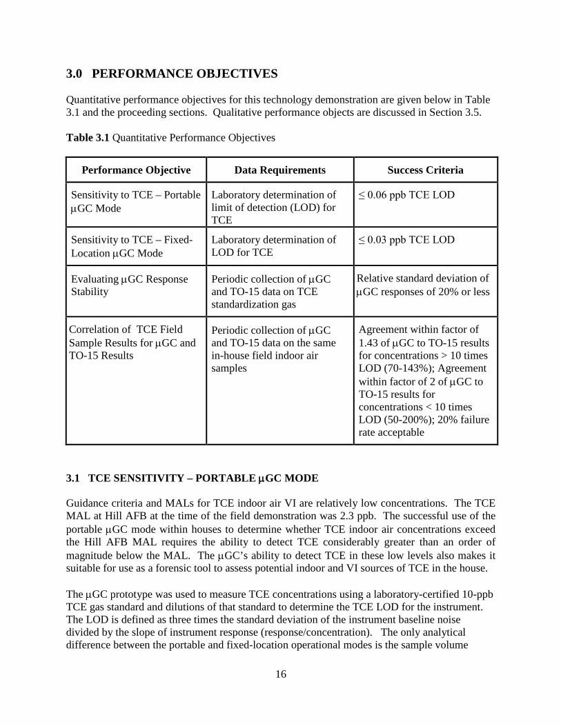
3.0 PERFORMANCE OBJECTIVES Quantitative performance objectives for this technology demonstration are given below in Table 3.1 and the proceeding sections. Qualitative performance objects are discussed in Section 3.5. Table 3.1 Quantitative Performance Objectives

Performance Objective Data Requirements Success Criteria

Sensitivity to TCE – Portable µGC Mode

Laboratory determination of limit of detection (LOD) for TCE

≤ 0.06 ppb TCE LOD

Sensitivity to TCE – Fixed-Location µGC Mode

Laboratory determination of LOD for TCE

≤ 0.03 ppb TCE LOD

Evaluating µGC Response Stability

Periodic collection of µGC and TO-15 data on TCE standardization gas

Relative standard deviation of µGC responses of 20% or less

Correlation of TCE Field Sample Results for µGC and TO-15 Results

Periodic collection of µGC and TO-15 data on the same in-house field indoor air samples

Agreement within factor of 1.43 of µGC to TO-15 results for concentrations > 10 times LOD (70-143%); Agreement within factor of 2 of µGC to TO-15 results for concentrations < 10 times LOD (50-200%); 20% failure rate acceptable

3.1 TCE SENSITIVITY – PORTABLE µGC MODE Guidance criteria and MALs for TCE indoor air VI are relatively low concentrations. The TCE MAL at Hill AFB at the time of the field demonstration was 2.3 ppb. The successful use of the portable µGC mode within houses to determine whether TCE indoor air concentrations exceed the Hill AFB MAL requires the ability to detect TCE considerably greater than an order of magnitude below the MAL. The µGC’s ability to detect TCE in these low levels also makes it suitable for use as a forensic tool to assess potential indoor and VI sources of TCE in the house. The µGC prototype was used to measure TCE concentrations using a laboratory-certified 10-ppb TCE gas standard and dilutions of that standard to determine the TCE LOD for the instrument. The LOD is defined as three times the standard deviation of the instrument baseline noise divided by the slope of instrument response (response/concentration). The only analytical difference between the portable and fixed-location operational modes is the sample volume

17

(sampling time) being shorter for the portable mode. This objective will be successfully achieved if the TCE LOD for the portable µGC unit is less than or equal to 0.06 ppb TCE. 3.2 TCE SENSITIVITY – FIXED-LOCATION µGC MODE Guidance criteria and MALs for TCE indoor air VI are relatively low concentrations. The TCE MAL at Hill AFB at the time of the field demonstration was 2.3 ppb. Successful fixed µGC mode operation within houses requires determination of TCE indoor air concentrations considerably greater than an order of magnitude lower than the Hill AFB MAL. TCE concentrations are expected to be lower in houses with vapor removal systems (VRSs), where the fixed-location µGC unit can also be used as a measure of VRS effectiveness and potential failure. Since the sampling time can be longer for the fixed-location µGC mode relative to the portable mode, a lower TCE LOD is expected. The µGC prototype will measure TCE concentrations using a laboratory-certified TCE gas standard and dilutions of that standard to determine the TCE LOD for the instrument. This objective will be successfully achieved if the TCE LOD for the fixed-location µGC mode is less than or equal to 0.03 ppb TCE. 3.3 µGC RESPONSE STABILITY Analyzing the TCE field standardization gas (10 ppb; concentration determined by supplier as well as by TO-15) provided a check on the stability of the µGC’s response to TCE. Periodic field standardization provided a continuing calibration check of the µGC. Good stability of µGC response to TCE is an important performance characteristic. If the µGC response to TCE varies over time in the field, the standardization could be used to make appropriate adjustments to the readings; thus, even with some variability in response, it can easily be assessed and corrected. Periodic standardization gas TO-15 analyses were also made. This objective was considered to have been achieved if the µGC response relative standard deviation was 20% or less. 3.4 CORRELATION OF µGC AND TO-15 TCE FIELD SAMPLE RESULTS TO-15 is the current standard practice for indoor air sample analysis to determine TCE concentrations. The agreement between the µGC field analysis TCE results and the laboratory TO-15 TCE results is a crucial aspect of the successful performance of the µGC. The value of the µGC for field TCE analysis would be considerably diminished if there was not sufficient agreement between the µGC and TO-15 (reference method) results. For both the portable and fixed-location µGC modes, periodic field indoor air samples were taken. As the µGC samples were collected, simultaneous TO-15 samples of the same parcel of room air were taken over a similar time interval. Note that true replicate indoor air sampling (µGC or TO-15) can be difficult due to temporal or spatial changes in concentrations; however, there can be reasonable certainty that the µGC and TO-15 sampling pairs were essentially sampling the same parcel of air. This is an important performance objective based upon the results from two different analytical methods, one field and one lab (reference method). Both

18

analytical methods have inherent errors associated with their determinations of TCE concentrations, and these inherent errors should be considered when evaluating success. The objective was considered to have been achieved if the µGC results were within a factor of 1.43 of their corresponding TO-15 results (means used for triplicate sets) for concentrations greater than 10 times the LOD (i.e., within 70 to 143%. As the LOD is approached, greater errors are expected. For concentrations less than 10 times the LOD, success was considered to be achieved if µGC results are within a factor of 2 of their corresponding TO-15 results (i.e., within 50 to 200%). A failure rate of 20% or less was considered to be acceptable. 3.5 QUALITATIVE PERFORMANCE OBJECTIVES Qualitative performance objectives for this technology demonstration are given below in Table 3.2. Table 3.2 Qualitative Performance Objectives

Performance Objective Data Requirements Success Criteria

Ease of Use Feedback from field team on usability of technology and time required

A single field technician able to effectively take measurements

Ease of Field Standardization & Blanks

Feedback from field technician on standardization and blank check procedures

Effective and time-efficient field standardization and blank checks

Rapid Site Assessment – Portable µGC Mode

Collection of field µGC TCE data in a forensic mode from multiple houses; collection of confirmation TO-15 data

Effective site assessment with µGC for TCE in one house within 1 day (planted TCE source location).

Long-term Operation Operational history in portable and fixed µGC modes under field conditions

Minimum continuous operation of approximately 1 month

Note: Remote communications capability was deleted from µGC fabrication to focus on critical analytical components; thus, an earlier remote wireless communications performance objective has been deleted. Remote wireless communications is not anticipated to be difficult. The ability to easily use the µGC in a field setting is an important qualitative performance criterion, as it would aid its eventual acceptance as a field tool. This would include the ease of conducting standardization and blank checks in the field. The µGC prototype developed in this project is a university-fabricated prototype as opposed to a commercial prototype, and there would be many features of a commercial prototype that would improve its “ease of use” in the

19

field. However, the field demonstration of this university-fabricated µGC prototype should provide some insights as the potential ease of use of a commercial unit. Rapid site assessment in a forensic approach is an important performance criterion in VI applications. The ability to locate an indoor TCE source in 1 day is one way to evaluate this performance criterion. Long-term operation is another important criterion for VI applications, particularly in a continuous monitoring mode. An important aspect of long-term operation is detector stability.

20

4.0 SITE DESCRIPTION Hill AFB has been an active facility since the early 1940s. It is located in northern Utah, about 30 miles north of Salt Lake City. Covering 6,670 acres, the base lies on a plateau roughly 300 feet above a valley floor. The base is surrounded by the communities of South Weber, Riverdale, Sunset, Clearfield, Clinton, Roy, and Layton. Adjacent land use is residential and mixed agricultural, commercial, and residential. Figure 4.1 is a map of Hill AFB, Utah and surrounding communities.

Hill AFBBoundary

ASU’s SERDP VI Study House

TCE EmplacedSource House

Figure 4.1. Map of Hill AFB, Utah with surrounding communities. Outline of base is in dashed green line. The blue areas are groundwater plumes, most with TCE contamination. Locations of the residential houses used in this demonstration are indicated. Aircraft maintenance activities at the base historically involved the use of TCE (and other solvents) to clean aircraft engine parts. Some the TCE used was disposed into the ground at various locations around the base. TCE is a dense non-aqueous phase liquid (DNAPL) that can migrate as a separate phase below the water table, making source area delineation and remediation challenging. TCE dissolves into groundwater (the pure compound TCE solubility in water is 1,280 milligrams per liter) resulting in TCE groundwater plumes with concentrations above the 5-ppb maximum contaminant level (MCL) that can be miles long. As the base is on a plateau, groundwater tends to flow off-base to the lower lying valley floor, leading to shallow groundwater contamination in the surrounding residential areas. Figure 4.1 shows contaminated groundwater plumes (most containing TCE) in blue.

21

Shallow groundwater contamination (often containing TCE) may lead to migration of VOC molecules from groundwater to the overlying unsaturated (vadose) zone and then it can potentially be present in soil vapor beneath houses. Neutral to negative pressures within houses relative to the pressures in the soil gas beneath the houses can lead to TCE (and potentially other VOCs present in groundwater and soil vapor) migration into the houses. The Arizona State University (ASU) SERDP VI-study house (Dr. Paul Johnson, ASU, principal investigator) is located in Layton, Utah above a shallow TCE groundwater plume that has migrated to the south of Hill AFB. The study house’s location is shown on Figure 4.1. The presence of TCE in shallow groundwater concentrations and active TCE VI into this house (historical observed indoor air TCE concentrations ranged up to the low single digit ppb range) was confirmed by ASU and Hill AFB personnel during selection of the house for the SERDP project. The vast majority of this demonstration was conducted in the ASU SERDP VI-study house. A second house in Layton, Utah without TCE VI was also used in this demonstration. At the second house, an indoor TCE source was intentionally emplaced (TCE source location initially unknown to the field µGC team). The location of this second Layton, Utah house is also shown on Figure 4.1.

22

5.0 TEST DESIGN 5.1 CONCEPTUAL EXPERIMENTAL DESIGN The primary goal of this project was to conduct a field performance evaluation of the SPIRON µGC. In conjunction with the field component, laboratory testing of the SPIRON µGC was also conducted to evaluate its performance under controlled laboratory conditions. Additional laboratory work was conducted after the field demonstration to better explore the potential for the use of multivariate curve resolution (MCR) to discriminate overlapping peaks and improve TCE quantification under certain conditions. This field demonstration was to evaluate the performance of the SPIRON µGC prototype in short-term portable forensic-type and longer-term fixed-location monitoring type applications to analyze indoor air TCE concentrations that may be the result of VI (or due to indoor TCE sources). The SPIRON µGC prototype (two prototypes were used in the field) was able to sample and analyze for TCE at a frequency substantially greater than is practicable using the TO-15 conventional approach. Periodic simultaneous sampling using µGC and TO-15 methodologies enabled comparison of TCE concentrations obtained by the two approaches. This field demonstration primarily took place in ASU’s SERDP VI-study house in Layton, Utah near Hill AFB (Dr. Paul Johnson, PI) for both the portable (spatial) and fixed-location (temporal) applications. Investigations showed that this house was impacted by TCE VI. An additional house in Layton, Utah (not impacted by TCE VI) was used for the portable application to locate an emplaced indoor TCE source. Potential TCE concentrations due to VI or indoor sources can vary greatly (from below to well above the detection limits of both the µGC and TO-15 methods). The value of this field demonstration for performance evaluation of the µGC prototypes was significantly enhanced by a relatively wide range of field TCE concentrations monitored by both the field µGC and TO-15 methods. ASU’s SERDP VI-study house ensured the availability of a wide range of TCE concentrations due to a significant TCE VI entry location (crack between concrete basement wall and poured concrete floor; in basement crawl space) and the ability to induce concentration changes by changing indoor pressure relative to subslab pressure (periodic operation of a box fan in an upstairs window). Additionally, using a house not impacted by TCE VI but with an emplaced indoor TCE source also provided a wide range of concentrations. The µGC prototypes were calibrated for TCE in the field in ASU’s SERDP VI-study house. The extent of response drift was assessed by periodic measurement of a TCE gas standard (also allowing for adjustments in TCE calibration factors). Periodic blanks were also analyzed. Since key performance criteria for this technology demonstration relied heavily upon the comparison between the field µGC and laboratory TO-15 results, both analytical methods were used periodically on the field TCE standard gas. A key feature of the portable µGC application is that the µGC is easily moved within the house from one location to another to gather data on spatial TCE concentration distributions. Sample turnaround times were relatively quick at 30 minutes or less per sample (actual sampling time depended the amount of preconcentration required). Rapidly obtaining spatial TCE distributions

23

is important in identifying source(s) of TCE within a dwelling. TCE concentrations tend to be highest near the source (VI or indoor), with an increasing concentration gradient as the source is approached. The portable µGC application (i.e., spatial concentration data) was conducted over several days at the ASU SERDP VI-study house and over 2 days at the Layton, Utah non-VI house with an emplaced indoor TCE source. Periodic concurrent sampling (generally within 6 inches) by µGC and TO-15 methods was conducted to enable comparison. Since two µGC prototypes were available in the VI-study house, the second µGC was periodically used to collect concurrent temporal data from a location in the basement during the portable µGC application. The demonstration of the fixed-location µGC application entailed continuous monitoring of TCE for assessing temporal variations in indoor air concentrations. The fixed µGCs were installed in a low traffic area and collected samples from either of two locations (in the basement crawl space under the stairway at a VI entry location and in the short hallway outside the crawl space doorway). Since two µGC prototypes were available, samples were sometimes collected from both locations or from the same location by both prototypes. Periodic concurrent sampling by µGC and TO-15 methods was conducted to allow for comparison. During a substantial part of the demonstration, Hill AFB also operated a HAPSITE GC/MS in automated mode in the short hallway outside of the closet doorway. Hallway µGC samples were often taken from the same sampling location (within 6 inches) and within the same sampling time window as the HAPSITE GC/MS (Hill AFB calibrated the HAPSITE with a certified standard gas mixture). This experimental setup allowed for comparison between all three analytical methods (µGC, TO-15, and HAPSITE). Most of the µGC sampling was manually initiated. For a 48-hour period, the µGC prototype sampling and analysis was conducted in an automated mode to demonstrate continuous automated sampling and analysis. 5.2 LABORATORY STUDY RESULTS The following sections described the development and characterization of the SPIRON prototype µGC in a laboratory setting as described in Sukaew et al. (2011) and Kim et al. (2011) as well as post-field demonstration examination of MCR with the prototype µGC as described in Kim and Zellers (in prep.). 5.2.1 DEVELOPMENT AND CHARACTERIZATION PCF Module Components. In considering the application of µGC to assess TCE contamination from VI in homes, it became apparent that the air sample volume required to achieve the sub-ppb detection limits demanded by this application would exceed the capacity of the µPCF devices (Tian et al., 2003 & 2005; Lu et al., 2005) used in previous University of Michigan µGC prototypes. In addition, any semi-volatile organic compounds (SVOCs) present in the air would tend to strongly adsorb to surfaces or only slowly desorb from the µPCF at normal desorption temperatures (Zhong et al., 2007). Thus, a high-volume sampler and a means of precluding SVOCs were required upstream from the µGC prototype in this project.

24

The pre-trap and sampler adsorbents used were graphitized carbons obtained from Supelco (Bellefonte, Pennsylvania). Carbopack B (C-B, specific surface area = 100 m2/g) and Carbopack X (C-X, 250 m2/g) were used in the pre-trap and sampler, respectively. Both pre-trap and sampler were constructed from thin-walled stainless-steel tubes (0.64-centimeter (cm) outer diameter (o.d.) ; 0.54-cm inner diameter (i.d.); 6 cm long). A 50-milligram (mg) bed of C-B was used in the pre-trap and a 100-mg bed of C-X was used in the sampler. Previous studies have demonstrated that small quantities of C-B can capture VOCs with vapor pressures up to ~28 torr from moderately large air volumes and release them efficiently with thermal desorption and C-X was capable of capturing and efficiently desorbing VOCs with vapor pressures up to ~95 torr (Lu and Zellers, 2001 and 2002; TCE: 69 torr). Both devices were heated with coils of insulated Cu wire and monitored with thermocouples held snugly against the tube walls. Figure 5.1 shows close-ups of the pre-trap and sampler tubes. Teflon® connectors were used for more rapid heating and cooling of the tubes (metal connectors act as heat sinks).

Figure 5.1. Components of the multi-stage PCF module: a) pre-trap packed with C-B, b) high-volume sampler packed with C-X, and c) µF packed with C-X. Pre-trap and sampler are shown with Teflon® connectors, resistive-coil heaters, and thermocouples. An enlarged image of the µF is shown to highlight the microfluidic features of the device. Figure 5.2 shows a block diagram of the essential analytical components and fluidic paths of the µGC prototype, including the PCF module. In operation, a commercial mini-pump (pump A; miniature diaphragm pump, NMS020, KNF Neuburger, Trenton, New Jersey) draws an air sample through the pre-trap and sampler at a high flow rate. Then, valve A actuates and a second pump (pump B; also a miniature diaphragm pump) draws scrubbed air through the sampler as it is resistively heated and backflushed to desorb and transfer the captured VOCs (including TCE) to the µF at a low flow rate (Note: valve B is closed during this process to prevent VOCs from entering the column). Then, the flow from pump B is reversed and air is backflushed through the µF as it is heated rapidly to inject the captured VOC mixture into the

25

dual-microcolumn separation module for separation and identification/quantification by the array of nanoparticle-coated chemiresistor sensors.

Valve B

1 Column1st

Chemiresistorarray

Pretrap

Sampler

Pump A

2 Columnnd

Sampleinlet

Pump B

µF

Valve A

Scrubber

Figure 5.2. Fluidic diagram of µGC showing key components of the multi-stage PCF module. The μF chip (see Figure 5.1) has dimensions of 9.76 × 4.18 × 0.6 millimeters (mm). Deep-reactive-ion-etching (DRIE) was used to form a 3.2 (w) × 3.45 (l) × 0.38 mm (h) cavity with additional tapered sections leading to the inlet and outlet ports at opposing ends of the Si substrate, a set of pillars near the inlet and outlet ports to retain the adsorbent within the cavity, and inlet and outlet channels one of which has a right-angle tee-branch. The device was capped with an anodically bonded Pyrex plate. Cr/Au contact pads were evaporated onto the backside of the substrate for bulk resistive heating, and a Ti/Pt resistive temperature device (RTD) was patterned near the contacts for monitoring temperature. C-X (~2.3 mg) was loaded into the μF using gentle suction. Deactivated fused-silica interconnection capillaries (0.25-mm i.d., 0.32-mm o.d., Restek Corp., Belafonte, Pennsylvania) were secured with adhesive (Duraseal 1531, Cotronics, Brooklyn, New York). Electrical connections to a custom printed circuit board (PCB) were made via Al wire-bonds. The specifications of the µF designed and fabricated during this project were due to the pressure drop caused by the previous µF design. A series of experiments was conducted to determine suitable sorbent quantities, flow rates, and timing for the PCF module. Several application-specific performance criteria were developed for the µGC which, in turn, led to the criteria used to specify the design and operating features of the PCF module components. Prioritizing these criteria, assessing the performance tradeoffs, and implementing the final specifications required a system-level approach for which no precedent was found in the literature. Therefore, the following rationale is a preface to the PCF component testing methods using this system-level approach. Defining the detection limit (limit of detection or LOD) for TCE and the time limit for each determination was necessary at the outset to specify the maximum air-sample volume and the corresponding volumetric flow rate of the sampling step. The target TCE LOD was 0.06 ppb. Preliminary tests performed with the chemiresistor sensor array gave an LOD for TCE of ~1.2 ppb assuming a 1-liter (L) air sample (i.e., “1.2 ppb-L,” or 6.2 nanogram [ng]). Thus, in order to

26

achieve an LOD of 0.06 ppb, it would require a sample volume of 20 L. Higher concentrations would require smaller volumes. Preliminary tests with the µGC separation module indicated that it would require ~3 minutes to separate TCE from the most critical co-contaminants, which are defined as those VOCs having chromatographic retention times similar to those of TCE. Since an analysis time of 15 to 30 minutes was considered acceptable for both short-term screening and long-term monitoring measurements, a sampling flow rate of 1 liter per minute (L/min) was deemed sufficient. Additionally, the fluidic restrictions of the system limited the sampling flow rate to the range of ~1 L/min. Defining the nature of potential interferences was then necessary to specify the types and amounts of adsorbent materials to use in the PCF components because the capacities, desorption efficiencies, and associated flow rates passing through these devices depend on these factors. The set of potential interferences (i.e., co-contaminants) considered in this study was determined from a set of field samples collected from Hill AFB VI-impacted homes. These were then parsed into three subsets according to vapor pressure (pv). Those with values of pv > 100 torr were designated as sufficiently volatile as to not be of concern; by proper adsorbent selection, these interferences would be largely unretained by the sampler. Those with pv values ranging from 3 to 100 torr and would be collected along with TCE (69 torr) in the sampler, transferred to the µF, and subsequently separated and detected. Those compounds with pv < 3 torr would be captured by the upstream pre-trap. Since environments with high humidity might be encountered, it was necessary to account for this potential co-factor as well. The flow rate achievable by the miniature diaphragm pumps is a function of the resistance to flow in the sampling train (www.knf.com/oemicro.htm). Another design constraint to address, therefore, was the pressure drop presented by each component in the PCF module. This generally dictated minimizing the masses of adsorbent materials. The size of the adsorbent granules was also a relevant variable, since packed beds of smaller granules lead to higher flow resistance. Minimizing the adsorbent masses would also reduce the power and time required for thermal desorption. The pre-trap required sufficient mass of a low-surface-area adsorbent to capture the less volatile co-contaminants while permitting the TCE to pass through unretained. Excluding such compounds from passing further downstream would prevent irreversible adsorption onto the higher-surface-area adsorbents in the sampler and µF and also would reduce the maximum temperature required for chromatographic separations and, thereby, the overall analytical cycle time. Experiments performed with the pre-trap focused on adjusting the mass of the selected adsorbent in order to optimize the tradeoff of low retention of TCE (pv = 69 torr) and high retention of the less volatile interferences at the flow rate dictated by the sampler, while also monitoring the pressure drop constraint imposed by the pump. It was also necessary to determine the capacity of the pre-trap for the less volatile co-contaminants to specify how often it would need to be thermally regenerated. The sampler required a sufficient mass of a higher-surface-area adsorbent to capture TCE quantitatively in the presence of co-contaminants at relevant concentrations, and the flow rate

27

through the sampler had to be high enough to keep the overall analytical cycle time under 30 minutes while capturing a sufficient mass of TCE to achieve the targeted LODs with the downstream detector. Rapid, quantitative transfer the captured TCE from the sampler to the µF was also required. Experiments with the sampler focused on optimizing the tradeoff between adsorption capacity for TCE and the flow rate (and associated pressure drop), as well as documenting sufficient capacity in the presence of co-contaminants and high humidity. The quantitative desorption of TCE at low flow rates also needed to be confirmed. The µF was required to capture TCE (quantitatively) along with any accompanying co-contaminants desorbed from the upstream sampler, and then to thermally desorb them to provide a focused injection into the separation module. The narrower the injection band, the greater the chromatographic efficiency of any separation. The microfabricated device used as the µF here is a refined version of devices used for both preconcentration and injection in previous University of Michigan µGC prototypes (Lu et al., 2005; Tian et al., 2005). Experiments performed with this device focused on documenting its capacity for quantitatively capturing the TCE desorbed from the upstream sampler in the presence of co-contaminants as a function of flow rate, and then exploring the effect of flow rate on the injection bandwidth of TCE. Following the series of experiments required to determine the nature and quantities of adsorbents to use in each of the three devices, the tolerable pressure drops, flow rate limitations, TCE dynamic adsorption capacity, humidity effects, desorption efficiencies, and desorption bandwidths in the presence of anticipated co-contaminants, a final test series was necessary to demonstrate that the assembled multi-stage PCF provided quantitative capture, transfer, and injection of TCE. Table 5.1 lists the VOCs used in the PCF module studies. They were culled from a set of 63 compounds detected by TO-15 in 12 air samples from residential homes in the vicinity of Hill AFB. Compounds > 100 torr were omitted since they would largely be unretained by the sampler.

28

Table 5.1. Test compounds and their corresponding vapor pressures, pv, at 25 oC (Howard and

Meyen, 1997).

No. Compound pv/torr No. Compound pv/torr

1. Benzene 95 17. n-Butyl acetate 15 2. Ethyl Acetate 94 18. n-Octane 14 3. 2-Butanone 89 19. Ethylbenzene 9.6 4. Acetonitrile 73 20. m-Xylene 8.3 5. Trichloroethylene 69 21. o-Xylene 6.6 6. Bromodichloromethane 65 22. Styrene 6.4 7. Ethanol 60 23. α-Pinene 4.8 8. 1,2-Dichloropropane 54 24. n-Nonane 4.5 9. n-Heptane 46 25. Cumene 3.5 10. 2-Propanol 44 26. 1-Propylbenzene 3.4 11. Methylmethacrylate 39 12. Toluene 28 27. 4-Ethyltoluene 3.0 13. 1,4-Dioxane 27 28. 1,3,5-Trimethylbenzene 2.5 14. 4-Methyl-2-pentanone 20 29. d-Limonene 2.0 15. Tetrachloroethylene 18 30. 1,2,4-Trichlorobenzene 0.5 16. 1,1,2-Trichloroethane 17 31. Naphthalene 0.085

Concentrations of TCE and co-contaminants found in the field samples were generally in the 0.01 to 10 ppb range. Therefore, testing was generally constrained to this concentration range. Test atmospheres were generated by injecting pre-determined volumes of liquid TCE (and interfering compounds, when necessary; chemicals purchased from Sigma-Aldrich/Fluka, Milwaulkee, Wisconsin or Acros/Fisher, Pittsburgh, Pennsylvania in >95% [most > 99%] purity and were used as received) into a Tedlar bag prefilled with a known volume of clean, dry air or N2 from compressed gas cylinders. Serial dilutions were made to achieve the targeted concentrations. For compounds with vapor pressures above ~3 torr, the concentrations in the bag can be estimated accurately from the injection and dilution volumes. For less volatile compounds, some loss is expected from condensation and adsorption to the bag walls. For tests performed at high humidity, dilution air was passed through a fritted bubbler filled with distilled water prior to filling the Tedlar bag. An additional volume of 0.5 milliliters (mL) of distilled water was added to the bag by syringe to maintain 100% RH, since water vapor permeates through Tedlar rapidly due to its size (Groves and Zellers, 1996). Little or no loss of test vapors to the liquid water was observed; however, breakthrough test fractions were normalized to the extant concentration in the bag, so this issue did not affect determinations of breakthrough volumes. All test atmospheres were at ambient room temperature. A lower-surface-area commercial graphitized carbon, Carbopack B (C-B, specific surface area = 100 m2/g), was chosen for use in the pre-trap to retain the low-pv interferences (Dettmer and Engewald, 2002). Another graphitized carbon, Carbopack X (C-X, specific surface area = 250 m2/g), was chosen for use in the sampler. Previous studies showed C-B and C-X to capture VOCs up to ~28 torr and ~95 torr, respectively, and efficiently thermally desorb those VOCs (Lu and Zellers, 2001 & 2002; TCE is 69 torr). Interferences with higher vapor pressures were

29

expected to pass through the sampler largely unretained. C-B and C-X (60/80 mesh) were obtained from Supelco (Bellefonte, Pennslyvania). Samples of C-B and C-X were sieved and the fractions with nominal diameters in the range of 180 to 212 μm (for C-B only) and 212 to 250 µm (for C-B and C-X) were isolated and packed in the appropriate device. Analyses were performed with a bench-scale GC (Agilent Model 6890). Where separations were required, a 15-m capillary column (320-μm i.d., 0.25-μm HP-1 stationary phase) was typically used with N2 carrier gas. For the final tests of the assembled module, a 6-m column was used instead to mimic the µcolumn length used in the µGC. One of two types of detectors was employed, depending on the nature of the analysis being performed. A flame ionization detector (FID) was used in pre-trap breakthrough tests and in some of the tests of the sampler, and an electron capture detector (ECD) was used to monitor TCE in those experiments where the concentrations of the co-contaminants did not need to be determined. Breakthrough fractions were determined by comparing the peak area of injected samples of the relevant compound from the challenge test atmosphere to that measured in the same injection volume downstream from the device under test. For those tests requiring TCE quantification, the ECD was calibrated by analyzing separate serially-diluted test atmospheres prepared in Tedlar bags that spanned the required range of injected masses. Figure 5.3 shows the apparatus used for the pre-trap and sampler tests; Figure 5.4 shows that used for the µF tests.

Pump A

Pump B

Sampler/pretrap

GC inlet

Sample loop

Test atmosphere

Column/detector

N2

Figure 5.3. Configuration used for testing breakthrough volumes for the pre-trap and sampler.

30

N2 N2

Pump A

Pump B

µF

Sampler

Column/detector

Sample loop

GC inlet

Injection port

N2

Figure 5.4. Configuration used for testing breakthrough volumes for the µF. The pressure drop across the coupled pre-trap and sampler devices was examined as a function of adsorbent mass over a range of flow rates using a differential pressure gauge (Magnehelic, Dwyer Instruments, Inc.) connected by a tee to the line connecting the pre-trap/sampler to the same type of diaphragm pump to be used in the field prototype µGC instruments (SN020, KNF Neuberger). The two devices were connected by large-bore tubing that presented minimal additional pressure drop at 1 L/min. The 25 most prevalent potentially interfering compounds with pv values in the 3 to 95 torr range (out of 28), identified in the field samples, were used in various combinations and subsets to assess the impact of co-contaminants on PCF performance. Four of these VOCs are chlorinated hydrocarbons (i.e., bromodichloromethane, 1,2-dichloropropane, tetrachloroethylene, and 1,1,2-trichloroethane), and the first two of these are difficult to resolve from TCE chromatographically. Therefore, in some of the breakthrough tests performed with a GC column downstream, only 23 co-contaminants were included. In those tests where the mixture was passed directly to an ECD without separation, only 21 of the co-contaminants were included in the test mixture (TCE as the only halogenated compound present). The test atmosphere was drawn through the sampler or pre-trap using pump A (UN86, KNF Neuberger) at 1 L/min and a fraction of the downstream air was drawn through a sampling loop (112-µL or 250-µL) by pump B (UN86, KNF Neuberger) (see Figure 5.3). At 1-minute intervals, the six-port valve was actuated to inject the contents of the loop to the injector of the GC. The sample volume required for the concentration downstream from the adsorbent tube to reach 10% of the inlet concentration, Vb10, was used as the metric of the dynamic adsorption capacity of the devices. Breakthrough tests were run in duplicate to assess the reproducibility of the results. Chemstation software (Rev.B.01.01, Agilent Technologies), GRAMS32 (version 6.0. ThermoScientific), and Microsoft Excel were used for data acquisition and processing.

31

To characterize the pressure drop constraint, initial range-finding tests were performed with 50 mg of the smaller-diameter fraction of C-B in the pre-trap (i.e., 180 to 212 µm) and 200 mg of C-X (212 to 250 µm) in the sampler. Although somewhat arbitrary, these adsorbent masses are consistent with those used in sampling tubes for USEPA Method TO-17. The pressure drop increased linearly with flow rate (slope = 0.054 L/min/kPa) to a maximum of 18 kPa at 0.95 L/min, which was the highest flow rate the pump could provide. This pressure-flow relationship is consistent with data provided by the pump manufacturer. Replacing the C-B with the same mass of the larger diameter C-B (i.e., 212-250 µm) permitted the desired flow rate of 1 L/min to be reached at a pressure drop of 16 kPa. With 100 mg C-X (212-250 µm) and 50 mg C-B (212-250 µm), a flow rate of 1 L/min could be achieved with a pressure drop of only 11 kPa. The first performance criterion for the pre-trap was that TCE not be retained to any significant extent. Breakthrough tests were performed at 1 L/min with pre-traps containing either 50 or 75 mg of C-B (212 to 250 µm) challenged with 1 ppb of TCE in air. A low TCE concentration was used to achieve the greatest sensitivity to small losses of vapor to the pre-trap adsorbent. Figure 5.5 shows that there is some retention of TCE over the first 1 to 2.5 minutes of exposure, but that the amount retained with the smaller bed mass is significantly less. Since the temporal resolution of these breakthrough measurements is limited, it is difficult to precisely quantify the loss of TCE, but a conservative estimate can be made by integrating the area above the breakthrough curves. For the 50-mg C-B bed, this yields 7.8 ng (1.5 ppb-L), and, for the 75-mg bed, it is 13 ng (2.5 ppb-L). For a 20-L sample, this would correspond to potential losses of 1.8 and 6.2 % of the TCE in the sample stream for the 50 and 75 mg beds, respectively. For a 5-L sample, this amounts to losses of 7 and 25%, respectively. Note that, in the presence of less-volatile co-contaminants, some displacement of TCE is likely to occur, reducing further the amount of TCE retained on the pre-trap. The losses of TCE to the 50-mg bed were considered acceptably small, and this mass of C-B was used in subsequent testing.

Bre

akth

roug

h (%

)

20

60

100

0 1 2 3 4 5 6

Sample volume (L)

80

40

Figure 5.5. TCE breakthrough curves (1-ppb challenge concentration; 1 L/min) for pre-traps packed with 50 mg (filled triangles) and 75 mg (open triangles) Carbopack-B.

32

The second performance criterion for the pre-trap is its ability to retain/remove low-volatility interferences. Based on prior studies (Lu and Zellers, 2001 & 2002), the pre-trap packed with C-B was expected to efficiently adsorb compounds with pv < 8 torr. However, initial tests of a 50-mg bed of C-B with a mixture containing a subset of four vapors with pv values ranging from 3.5 to 28 torr (i.e., 500 ppb each of toluene, PCE, m-xylene, and cumene) gave Vb10 values < 12 L (1 L/min) for all mixture components. Despite the high challenge concentrations used for this test, it was apparent that compounds with vapor pressures in this range would not be retained effectively, and that a lower ‘cut-off’ pv value would need to be defined. A mixture of each of the following less volatile co-contaminants was prepared, which spanned a range of pv values from 0.5 to 3.4 torr: cumene, 4-ethyltoluene, d-limonene, and 1,2,4-trichlorobenzene (Table 5.1). The nominal concentration of each component was 500 ppb, although fractional losses to the bag walls are to be expected for all of these compounds. Since all Vb10 determinations were referenced to the test-atmosphere peak areas, this factor did not preclude obtaining useful data. Figure 5.6 shows that while cumene (pv = 3.5 torr) gives a Vb10 value of only 8 L, the remaining compounds give Vb10 values ≥ 30 L. Thus, it appears that this trap can effectively retain compounds with pv ≤ 3 torr. The 4-ethyltoluene showed ~0.2% breakthrough at 28 L, suggesting that it would serve as a good ”sentinel” vapor for the capacity of the pre-trap, since all less volatile compounds should give larger breakthrough volumes. The pre-trap was re-conditioned at 250oC under N2 for 20 minutes, and the repeated breakthrough test gave similar results.

Bre

akth

roug

h (%

)

20406080

100

0 5 10 15 20 25 30

Sample volume (L) Figure 5.6. Breakthrough curves for the pre-trap packed with 50 mg of Carbopack-B challenged with a mixture of 500 ppb each of cumene (filled diamonds, pv = 3.4 torr), 4-ethyltoluene (open squares, pv = 3 torr), d-limonene (crosses, pv = 1.9 torr), and 1,2,4- trichlorobenzene (open triangles, pv = 0.5 torr) at 1 L/min, showing Vb10 > 30 L for all compounds except cumene for which Vb10 = 7 L. A subsequent experiment was performed with a mixture of 4-ethyltoluene, d-limonene, 1,2,4-trichlorobenzene, and naphthalene (pv range = 0.085 to 3.0 torr), which includes the least volatile non-target compounds found in the field samples. The nominal concentration of each component was 40 ppb. To minimize losses to fluidic interconnections in the test system, the pre-trap was connected directly to the Tedlar bag containing the test atmosphere by a short section of tubing, and a septum-capped tee-fitting was inserted just downstream. The test atmosphere was drawn through the pre-trap and 1-mL samples were collected periodically by gas-tight syringe and injected into the GC-FID.

33

Although a low level of the sentinel compound, 4-ethyltoluene, was detected in early samples, the amount decreased over the first 30 L, and the initial amounts were attributed to contamination of the syringe, which had been used to sample the challenge test atmosphere initially. The downstream levels did not increase to > 10% of the challenge concentration until the sample volume was 110 L when the test was concluded. This suggests that these compounds are retained effectively and that reconditioning of the pre-trap could be performed roughly every 5 to 6 operational cycles (assuming 20-L samples per cycle). To assess the dynamic capacity as a function of the mass of C-X packed in the sampler, a test atmosphere containing 500 ppb each of TCE, benzene, 2-butanone, and n-heptane (in air) was drawn through beds of 50, 100, and 200 mg at 1 L/min. With the 50-mg bed of C-X (see Figure 5.7), the TCE Vb10 was ~8 L, indicating that this is an insufficient mass. With the 100-mg bed of C-X (see Figure 5.8), the Vb10 for 2-butanone was about 8 L, but for TCE and all other mixture components the Vb10 was > 20 L. The 200-mg bed of C-X gave a Vb10 > 20 L for all vapors, indicating more than enough capacity. All breakthrough experiments were repeated with comparable results.

Bre

akth

roug

h (%

)

20

40

6080

100

0 5 10 15 20Sample volume (L)

Figure 5.7. Breakthrough curves for the high-volume sampler packed with 50 mg of Carbopack-X challenged with a mixture of 500 ppb each of 2-butanone (open diamonds), benzene (open squares), TCE (filled triangles), and n-heptane (open circles) at 1 L/min. Vb10 values < 10L for all compounds except n-heptane.

34

B

reak

thro

ugh

(%)

Sample volume (L)

100

20406080

0 5 10 15 20

Figure 5.8. Breakthrough curves for the high-volume sampler packed with 100 mg of Carbopack-X challenged with a mixture of 500 ppb each of 2-butanone (open diamonds), benzene (open squares), TCE (filled triangles), and n-heptane (open circles) at 1 L/min. Vb10 > 20 L for all vapors except 2-butanone. Subsequent testing was performed with 100 mg C-X beds using test atmospheres of 50 ppb of TCE in a mixture with similar concentrations of each of 23 interferent compounds with pv > 3 torr (Table 5.1, compounds 1-26, excluding 6 and 8). A Vb10 > 30 L was obtained for TCE. Repeating this test with saturated water vapor showed no reduction in the dynamic capacity for TCE. Thus, there appears to be sufficient capacity for TCE using the 100-mg C-X bed mass for the sampler. Medium-term aging effects were explored by first running a breakthrough test with the same 50 ppb mixture. Then a test atmosphere containing a mixture of 1 ppm each of TCE and 21 co-contaminants was prepared (excluding all chlorinated hydrocarbons) and a 10-mL aliquot (10 ppb-L) was spiked onto the sampler under a low flow of N2. The sampler was then heated to 220ºC and backflushed directly to the ECD at 20 mL/min. The peak measured by the ECD was due only to TCE. A set of 10 replicates of such spikes was analyzed. Then another breakthrough test was performed (50 ppb of TCE with 23 interferent compounds at 1 L/min), followed by another set of 20 replicate spiked analyses. This was followed by a final breakthrough test with the 50-ppb mixture. The peak areas observed from desorbed spikes were averaged and the relative standard deviation was only 8.5%, demonstrating reproducible sampler desorption and no evidence of aging or accumulation of residual vapors that might affect TCE desorption. Values of Vb10 for TCE in the 50-ppb samples, initially and after 10 and 20 spike replicates, were all >30 L, indicating no loss in capacity for TCE after repeated co-contaminant and temperature challenges. A maximum µF desorption temperature of 250°C was employed to desorb TCE rapidly and completely. This temperature was low enough to minimize the risk of thermal degradation of the C-X, which we have found to shed small particles after repeated thermal cycling at > 250°C in air. Figure 5.9 shows a representative initial 2 seconds of µF heating profile (440 degrees Celsius per second (°C/s) for 0.45 seconds, maintained between 225 and 250°C for 120 seconds, then cooled).

35

0

50

100

150

200

250

300

0 0.2 0.4 0.6 0.8 1.0 1.2 1.4 1.6 1.8 2.0Time (s)

Tem

pera

ture

(°C

)

0.45 s

Figure 5.9. Representative heating profile for the µF during desorption/ injection. Application of 36 V leads to an increase 25 to 225°C in 0.45 seconds (440°C/s). Subsequent application of 16 V maintains the µF between 225 and 250°C. Tests were performed to assess the effect of temperature and flow rate on the TCE desorption profile obtained from the sampler. Figure 5.10 compares the TCE desorption profiles for the most relevant subset of conditions with spiked samples corresponding to 10 ppb-L of TCE and each of the 25 interferences. At 180°C and 20 mL/min, it required between 4 and 5 minutes to completely desorb the TCE. By increasing the flow rate to 30 mL/min, TCE was completely desorbed in 3 minutes (Note: At 180 °C and 10 mL/min, it required > 8 minutes to completely desorb the TCE.). Increasing the maximum temperature to 225°C, at 10 mL/min, the TCE was desorbed within 5 minutes, and, at 20 mL/min, it was desorbed in 2.5 minutes.

Pea

k ar

ea (H

z-m

in)

50

150

250

0 1 2 3 4 50

200

100

20Time (min)

Figure 5.10. Desorption profiles of TCE (52-ng spikes) from the sampler at different maximum desorption temperatures and flow rates: 180ºC/20 mL/min (open circles), 180ºC/30 mL/min (filled circles), 225ºC/10 mL/min (open triangles), and 225ºC/20 mL/min (filled triangles).

36

µF TCE breakthrough profiles under these four sampler desorption conditions are shown in Figure 5.11. At 180°C and 30 mL/min, TCE was detected at ~1% of the challenge concentration within 1 minute, and, by 3 minutes, there was ~5% breakthrough. Although this extent of loss is not significant, raising the maximum temperature to 220°C and lowering the flow rate to 20 mL/min resulted in only 0.7% breakthrough at 3 minutes. This combination of temperature and flow rate thus appears to be the most acceptable. These results reveal that the capacity of the µF for TCE in complex mixtures is quite limited. In part, this is because the peak concentration generated from the sampler desorption profile is rather high; we estimate it to be on the order of 1 to 3 ppm for TCE (and all other co-contaminants). There is certain margin of safety built in to the conditions derived from these experiments by including in the test mixture realistic concentrations of the co-contaminants likely to be present with TCE.

5

10

15

20

0 1 2 3 4 5

( )

Bre

akth

roug

h (%

)

Time (min) Figure 5.11. TCE breakthrough curves for the μF placed downstream from the sampler during desorption of TCE (52-ng spikes) from the sampler at different maximum desorption temperatures and flow rates: 180ºC/20 mL/min (open circles), 180ºC/30 mL/min (filled circles), 225ºC/10 mL/min (open triangles), and 225ºC/20 mL/min (filled triangles). Decreasing the injection band width leads to increased chromatographic resolution by virtue of the reduced band dispersion at the outset of the separation and also to decreased LODs by virtue of the increased peak height. Thus, it is desirable to maximize the rate at which samples captured on the µF are desorbed and injected onto the separation column. In general, this calls for rapid heating and high flow rates through the µF (Lu and Zellers, 2001 & 2002; Whiting and Sacks, 2006; Sanchez and Sacks, 2003). As part of the µGC development effort, control circuitry was developed permitting the µF to be heated at a rate of ~375 oC/sec and then held at any set-point temperature. In light of the sampler tests, and the fact that field operation will entail performing desorptions in an air matrix, a decision was made to fix the maximum temperature of the µF at 225°C and to examine the effect of flow rate on the width of the desorption band of TCE. The maximum separation efficiency (i.e., smallest theoretical plate height) for the µcolumns is achieved with a flow rate of ~ 0.4

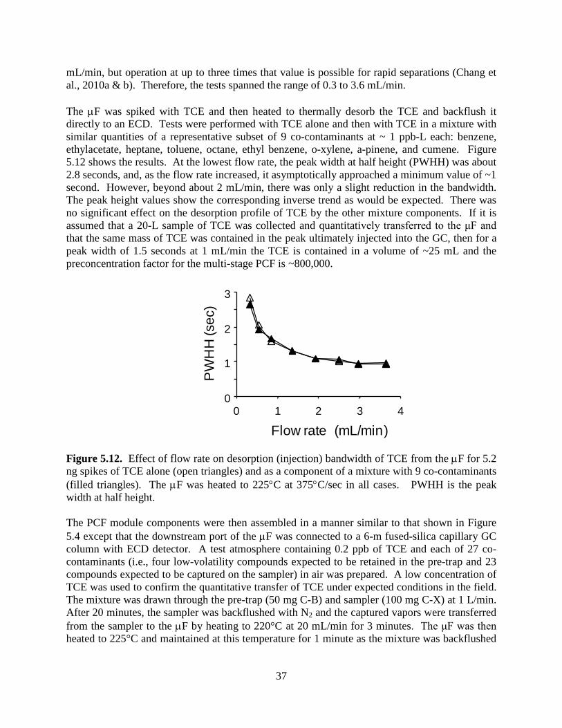
37

mL/min, but operation at up to three times that value is possible for rapid separations (Chang et al., 2010a & b). Therefore, the tests spanned the range of 0.3 to 3.6 mL/min. The µF was spiked with TCE and then heated to thermally desorb the TCE and backflush it directly to an ECD. Tests were performed with TCE alone and then with TCE in a mixture with similar quantities of a representative subset of 9 co-contaminants at ~ 1 ppb-L each: benzene, ethylacetate, heptane, toluene, octane, ethyl benzene, o-xylene, a-pinene, and cumene. Figure 5.12 shows the results. At the lowest flow rate, the peak width at half height (PWHH) was about 2.8 seconds, and, as the flow rate increased, it asymptotically approached a minimum value of ~1 second. However, beyond about 2 mL/min, there was only a slight reduction in the bandwidth. The peak height values show the corresponding inverse trend as would be expected. There was no significant effect on the desorption profile of TCE by the other mixture components. If it is assumed that a 20-L sample of TCE was collected and quantitatively transferred to the μF and that the same mass of TCE was contained in the peak ultimately injected into the GC, then for a peak width of 1.5 seconds at 1 mL/min the TCE is contained in a volume of ~25 mL and the preconcentration factor for the multi-stage PCF is ~800,000.

PW

HH

(sec

)

Flow rate (mL/min)

0

1

2

3

0 1 2 3 4

Figure 5.12. Effect of flow rate on desorption (injection) bandwidth of TCE from the µF for 5.2 ng spikes of TCE alone (open triangles) and as a component of a mixture with 9 co-contaminants (filled triangles). The µF was heated to 225°C at 375°C/sec in all cases. PWHH is the peak width at half height. The PCF module components were then assembled in a manner similar to that shown in Figure 5.4 except that the downstream port of the µF was connected to a 6-m fused-silica capillary GC column with ECD detector. A test atmosphere containing 0.2 ppb of TCE and each of 27 co-contaminants (i.e., four low-volatility compounds expected to be retained in the pre-trap and 23 compounds expected to be captured on the sampler) in air was prepared. A low concentration of TCE was used to confirm the quantitative transfer of TCE under expected conditions in the field. The mixture was drawn through the pre-trap (50 mg C-B) and sampler (100 mg C-X) at 1 L/min. After 20 minutes, the sampler was backflushed with N2 and the captured vapors were transferred from the sampler to the µF by heating to 220°C at 20 mL/min for 3 minutes. The μF was then heated to 225°C and maintained at this temperature for 1 minute as the mixture was backflushed

38

and injected onto a 6-m capillary column at 1 mL/min. The TCE eluted within 1 minute (room temperature) and was detected with the ECD. This experiment was performed in duplicate. The recovered peak area of TCE was evaluated against a calibration curve generated prior to these experiments for the ECD under the conditions of analysis. For the 20.0-L and 20.4-L samples of 0.2 ppb of TCE collected, the expected masses were 21 and 22 ng, respectively. From the recovered peaks areas, the masses were 26 and 21 ng, respectively. The corresponding sample transfer efficiencies were 120% and 95%, which gave an average of 107%. Developing an effective multi-stage PCF module suitable for use with a µGC for quantitative determinations of TCE at low concentrations in the presence of common airborne co-contaminants requires numerous tradeoffs in design and operation. Although the chemiresistor sensors used in the µGC are sensitive, preconcentration factors approaching 106 are necessary to detect TCE at the concentrations needed in this study. Achieving such low detection limits using micro-scale preconcentration components alone would not be possible, and interfacing with the macro-scale sampler is needed. µColumn Characterization. Each µcolumn chip has a 3 × 3 cm footprint and comprises a convolved square-spiral channel 3 m long with a rectangular cross section, 150 × 240 µm, formed in Si by DRIE and sealed by an anodically bonded Pyrex cover plate (Reidy et al., 2006; Kim et al., 2007). The peripheral inlet and outlet ports accommodate deactivated fused-silica capillaries (250 µm i.d.) sealed with epoxy (Hysol Epoxy Patch 1C, Henkel Corp., Rocky Hill, Connecticut). Two meander-line Cr/Au heaters and a Ti/Pt RTD evaporated onto the backside of the µcolumns were used for programmed heating during separations. In this study, one set of µcolumns was modified by chamfering the corners within the spiral using a different DRIE mask during fabrication and enlarging the heaters to improve the heat-transfer efficiency and uniformity. The µcolumns were individually pre-treated with HMDS, coated with a PDMS stationary phase from solution using a static deposition method, and then cross-linked using dicumyl peroxide (calc. avg. film thickness = 0.15 µm). Figure 5.13 shows SEM images of the two µcolumn types prior to sealing and coating. The maximum N produced by the µcolumns with chamfered corners is 4,550 plates/m, which is ~20% greater than that produced from µcolumns with right-angle corners. Figure 5.14 shows Golay Plots. For all Golay Plot separations, µcolumn temperatures were maintained ≤ 120°C to minimize stationary phase bleed. Figure 5.15 shows a representative chromatogram using the new µcolumn design (using a bench-scale GC injector and FID).

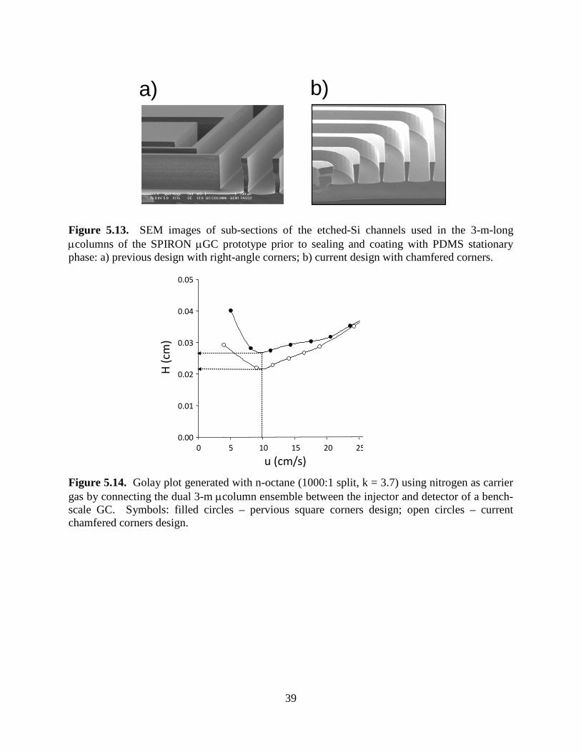
39

a) b)

Figure 5.13. SEM images of sub-sections of the etched-Si channels used in the 3-m-long µcolumns of the SPIRON µGC prototype prior to sealing and coating with PDMS stationary phase: a) previous design with right-angle corners; b) current design with chamfered corners.

u (cm/s)

0 5 10 15 20 25

H (c

m)

0.00

0.01

0.02

0.03

0.04

0.05

Figure 5.14. Golay plot generated with n-octane (1000:1 split, k = 3.7) using nitrogen as carrier gas by connecting the dual 3-m µcolumn ensemble between the injector and detector of a bench-scale GC. Symbols: filled circles – pervious square corners design; open circles – current chamfered corners design.

40

0.0 0.5 1.0 1.5 2.0 2.5

Time (min)

0.0 0.5 1.0 1.5 2.0 2.5

Time (min)

1

2

3

4

5

6

7 8

9 10

11TCE

Figure 5.15. TCE separation from 10 VOC interferences using a conventional (bench scale) GC inlet/injection port and FID, and the dual 3-m µcolumns of the current design. (0.1 µL injection of the neat mixture; inlet pressure: 4 psi; inlet temperature: 250oC; split ratio: 100:1. Temperature program of 1st µcolumn: hold at 25°C for 60 seconds, heat to 60°C at 70°C/min, heat to 100°C at 80°C/min, hold at 100°C for 30 seconds. Temperature program of 2nd µcolumn: hold at 25°C for 60 seconds, heat to 60°C at 70°C/min, heat to 120°C at 120 °C/min, hold at 120°C for 30 seconds. Compounds: 1, n-hexane; 2, benzene; 3, TCE; 4, toluene; 5, 2-hexanone; 6, PCE; 7, ethylbenzene; 8, o-xylene; 9, nonane; 10, cumene; 11, n-propylbenzene). Chemiresistor (CR) Array. Responses from MPN-coated CRs derive from the swelling induced changes in inter-particle distance as well as any changes in the dielectric constant accompanying reversible vapor sorption (Steinecker et al., 2007). The CR array used in the prototype is the same as that used in a meso-scale instrument reported on previously (Rairigh et al., 2009). The thiol coatings used are: C8 – octanethiol; DPA - 4-mercaptodiphenylacetylene; HME - methyl-6-mercaptohexanoate; and OPH - 1-mercapto-6-phenoxyhexane. The array chip has dimensions of 2.0 × 1.2 cm and consists of 8 Au/Cr IDEs deposited in a 4×2 pattern on a thermal-SiOx/Si substrate. Each IDE has 24 finger pairs (5 μm widths/spaces, 450 µm length, 410 µm overlap). A Macor® lid with inlet/outlet ports was sealed to the substrate using a gasket of VHB tape (3M, St. Paul, Minnesota) to create a detector cell volume of 1.6 μL (0.3 (w) × 0.4 (l) × 0.013 cm (h)). Deactivated fused-silica capillaries were sealed into the ports with Hysol epoxy. Two sensors were coated with each type of MPN by drop casting from solution with a 0.5-µL syringe to create multi-layer films with baseline resistances within the range of 1 to10 MΩ (Note: thicknesses were not determined). The CR array temperature was monitored via a calibrated on-chip RTD. Figure 5.16 shows aspects of CR array and µGC-installed CR array.

41

a) b) c) d)

CR

Figure 5.16. Photographs showing physical aspects of the chemiresister array: a) closeup of interdigital electrodes (which are coated with MPN to make chemiresisters), b) uncoated chemiresister array chip, c) chemiresister array with flow cell, and d) µGC-installed CR array. Device Mounting and System Integration. The assembled prototype has dimensions of 44 (w) × 25.5 (d) × 14.5 cm (h) and weighs 4.5 kilograms (kg). Photographs of the key fluidic and analytical components are provided below in Figure 5.17. A stainless-steel manifold was created with top-surface access ports designed to match those on each of six two-way latching micro-solenoid valves (Lee Co., Westbrook, Connectictut), which were bolted in place. The pre-trap and sampler were also mounted on the manifold using Teflon® Swagelok® fittings tapped into opposing sidewalls. The two miniature diaphragm pumps (NMS020, KNF Neuburger, Trenton, New Jersey) were located beside the manifold and connected to the appropriate ports via flexible tubing.

Figure 5.17. Prototype SPIRON µGC system and components: (a) layout diagram showing subsystems and fluidic pathways; (b) top view of Proto 1 with cover panel removed (iPhone included for scale); (c) µfocuser; (d) µcolumn; and (e) micro-scale chemiresistor array. The µF, CR array, and the dual-µcolumn separation module (Figure 5.17 b-e) were mounted and wire-bonded on separate carrier printed circuit boards (PCBs), which were mounted on standoffs

42

to the floor of the prototype. Cut-outs in the µcolumn PCB reduced the distances among these devices, which were connected by use of glass press-fits (Agilent Technologies). Two large cylindrical scrubbers (Restek), each containing Drierite and 5Å molecular sieves, and two smaller scrubbers containing activated charcoal (SKC Inc.) were mounted to the external walls of the prototype chassis and used to remove water vapor and background organic vapors, respectively, during focusing and analysis. Additional components included two power supplies and three cooling fans. Actuation and control circuitry utilized a custom pneumatic control circuit board and associated digital I/O card (USB-6501, National Instruments) for actuating the valves, pumps, and the heaters on the pre-trap and sampler, which were located beneath the manifold on the chassis floor. A second printed circuit board and associated 16-bit multi-functional DAQ card (USB-6218, National Instrument) for monitoring and controlling the devices in the analytical subsystem (i.e., the µF and µcolumn heaters and temperature sensors, and the sensors in the CR array) were located beneath the analytical subsystem components. A USB hub permitted connections to a laptop computer running a control program written in LabView® (Ver. 8.5, National Instruments). Device Control and System Operation. Each measurement cycle consisted of sampling, focusing, stabilization, and analysis steps. User-defined pump, valve, and heater actuation timing and temperature settings, as well as the temperature program for each µcolumn, could be entered at the start of a run through the graphic user interface of the custom instrument control program written in LabView® and automatically implemented. However, manual operation of each step was also possible and was often used during testing. Table 5.2 below is the timetable for a typical operating cycle. Table 5.2. Timetable for SPIRON µGC operation.

Component Sampling (5-26 min)

Focusing (3 min)

Stabilization (3 min)

Separation & Detection (3.5 min)

Manifold valve 1 On On Off Off Off Off Off Manifold valve 2 Off Off Off Off Off Off Off Manifold valve 3 Off On Off Off Off Off Off Manifold valve 4 Off Off Off Off Off Off Off Manifold valve 5 Off Off Off Off Off Off Off Manifold valve 6 Off Off On On On On On Analysis pump Off Off On On On On On Sampling pump On On Off Off Off Off Off

Pretrap Off Off Off Off Off Off Off Sampler Off On Off Off Off Off Off Focuser Off Off Off On Off Off Off Column Off Off On On On On On Sensor Off Off On On On On On

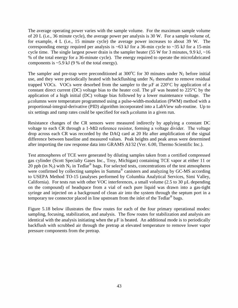
43

The average operating power varies with the sample volume. For the maximum sample volume of 20 L (i.e., 36 minute cycle), the average power per analysis is 30 W. For a sample volume of, for example, 4 L (i.e., 15 minute cycle) the average power increases to about 39 W. The corresponding energy required per analysis is ~63 kJ for a 36-min cycle to ~35 kJ for a 15-min cycle time. The single largest power drain is the sampler heater (55 W for 3 minutes, 9.9 kJ, ~16 % of the total energy for a 36-minute cycle). The energy required to operate the microfabricated components is ~5.9 kJ (9 % of the total energy). The sampler and pre-trap were preconditioned at 300oC for 30 minutes under N2 before initial use, and they were periodically heated with backflushing under N2 thereafter to remove residual trapped VOCs. VOCs were desorbed from the sampler to the µF at 220°C by application of a constant direct current (DC) voltage bias to the heater coil. The µF was heated to 225°C by the application of a high initial (DC) voltage bias followed by a lower maintenance voltage. The µcolumns were temperature programmed using a pulse-width-modulation (PWM) method with a proportional-integral-derivative (PID) algorithm incorporated into a LabView sub-routine. Up to six settings and ramp rates could be specified for each µcolumn in a given run. Resistance changes of the CR sensors were measured indirectly by applying a constant DC voltage to each CR through a 1-MΩ reference resistor, forming a voltage divider. The voltage drop across each CR was recorded by the DAQ card at 20 Hz after amplification of the signal difference between baseline and measured values. Peak heights and peak areas were determined after importing the raw response data into GRAMS AI/32 (Ver. 6.00, Thermo Scientific Inc.). Test atmospheres of TCE were generated by diluting samples taken from a certified compressed gas cylinder (Scott Specialty Gases Inc., Troy, Michigan) containing TCE vapor at either 11 or 20 ppb (in N2) with N2 in Tedlar® bags. For selected tests, concentrations of the test atmospheres were confirmed by collecting samples in Summa® canisters and analyzing by GC-MS according to USEPA Method TO-15 (analyses performed by Columbia Analytical Services, Simi Valley, California). For tests run with other VOC interferences, a small volume (2.5 to 30 µL depending on the compound) of headspace from a vial of each pure liquid was drawn into a gas-tight syringe and injected on a background of clean air into the system through the septum port in a temporary tee connector placed in line upstream from the inlet of the Tedlar® bags. Figure 5.18 below illustrates the flow routes for each of the four primary operational modes: sampling, focusing, stabilization, and analysis. The flow routes for stabilization and analysis are identical with the analysis initiating when the µF is heated. An additional mode is to periodically backflush with scrubbed air through the pretrap at elevated temperature to remove lower vapor pressure components from the pretrap.

44

Column#1 Column #2

CR array

Sample inlet

Pretrap

Sampler

Analytical subsystem

Front-end sampling subsystem

µF

Scrubber

Samplepump

Scrubber

Analyticalpump

a) Sampling

Column#1 Column #2

CR array

Sample inlet

Pretrap

Sampler

Analytical subsystem

Front-end sampling subsystem

µF

Scrubber

Samplepump

Scrubber

Analyticalpump

b) Focusing

Column#1 Column #2

CR array

Sample inlet

Pretrap

Sampler

Analytical subsystem

Front-end sampling subsystem

µF

Scrubber

Samplepump

Scrubber

Analyticalpump

c) Stabilization/Analysis

Figure 5.18. Operational mode fluidic flow paths for the SPIRON µGC: a) sampling, b) focusing, and c) stabilization/analysis. System Integration. Due to flow restrictions in the manifold, the maximum flow rate achievable during sampling was 0.78 L·min-1. Therefore, collecting the largest anticipated sample volume of 20 L required 26 minutes. Focusing at 18 mL·min-1 for 3 minutes was sufficient to transfer TCE quantitatively to the µF (i.e., subsequent blank analyses yielded no measurable TCE) without breakthrough of the µF adsorbent bed. For the stabilization step, the flow through the µcolumns and sensor array was set at 1.2 mL·min-1 and a minimum period of 3 minutes was required in order to regain stable sensor baseline signals. Although it required < 1 minute for TCE to elute during the analysis step, up to 3.5 minutes was allowed for elution of the remaining mixture components to illustrate their full or partial resolution. Thus, the maximum total sampling and analytical cycle time was ~36 minutes. Reconciling flow rates among the devices in the analytical subsystem required tradeoffs in the various aspects of performance. Previous work had shown that the injection band width of TCE from the µF decreased sharply between 0.2 and 1 mL·min-1 and then more gradually up to 2 mL·min-1, reaching a minimum full-width-at-half-maximum (fwhm) value of 1 s by FID. Although the optimal efficiency for the dual column ensemble occurs at 0.22 mL·min-1 in air or N2, the fwhm of the injection band at this low flow rate is > 2.7 s, which precludes the separation of TCE from early-eluting co-contaminants. Increasing the flow rate to 2 mL·min-1 minimizes the injection band width but also decreases N from 4,500 to ~700 plates/meter. The peak areas and fwhm values from the CR sensors have been shown to decrease sharply up to a flow rate of 1.0 mL·min-1, followed by a more gradual decrease up to 3.3 mL·min-1 (Zhong et al., 2009). Thus, although lower flow rates yield higher sensitivities, they also yield broader peaks and incur a very high sensitivity to flow rate, both of which are undesirable. Peak height shows a much smaller dependence on flow rate, which argues for using peak height as the sensitivity parameter

45

(Zhong et al., 2009). The analytical flow rate of 1.2 mL·min-1 adopted for all subsequent testing represents a compromise among the efficiency, resolution, speed, and sensitivity of the analysis. Chromatographic Resolution and Array Response Patterns. A subset of 11 VOCs with pv values ranging from 3.5 to 150 torr, bracketing that of TCE (pv = 69 torr), was selected to develop the separation conditions and to illustrate the performance of the prototype. The set of chromatograms in Figure 5.19 was generated from the analysis of a 20-L spiked air sample with the SPIRON µGC prototype. The mixture composition was adjusted so that the range of sampled masses (34 to 1700 ng) decreased with decreasing analyte volatility (increasing retention time), and peaks of comparable size were obtained for all components in the chromatograms. As shown, TCE was separated from the 11 interferences in 45 seconds and the entire mixture eluted in < 3 minutes. The temperature program used for each µcolumn was determined empirically. The temperature program of the 1st µcolumn was: hold at 25°C for 40 seconds, heat to 50°C at 1.25°C/s, heat to 120°C at 0.58°C/s, hold at 120°C for 60 seconds. The temperature program of the 2nd µcolumn was: hold at 25 °C for 45 seconds, heat to 60°C at 0.64°C/s, heat to 120°C at 0.75°C/s, hold at 120°C for 60 seconds. A more aggressive heating ramp (i.e., > 7.6°C⋅s-1) could be implemented after the first 45 seconds to reduce the analysis time, with a consequent loss of resolution of the later eluting compounds. This particular separation did not require the more elaborate temperature programming capability built in to the instrument.

50 100 150 200 0

C8

OPH

HME

FID1

23

5 6 7 8 9 10 11 12

TCE4

50 100 150 200 0

Time (s)

DPA

)

Figure 5.19. SPIRON µGC prototype chromatograms (3 minutes) from the four CR microsensors and a downstream FID generated from the analysis of a 20-L air sample spiked with TCE and 11 VOC interferences. Peak assignments are as follows: 1, 2-propanol; 2, n-hexane (HEX); 3, benzene (BEN); 4, TCE; 5, 4-methyl-2-pentanone (MIBK); 6, toluene (TOL); 7, perchloroethylene; 8, butylacetate; 9, ethylbenzene; 10, m-xylene; 11, nonane; 12, cumene.

46

The chromatogram from the HME-coated sensor shows an exceptionally large artifact peak at a retention time of ~25 seconds with a long tail that overlaps the TCE peak. This was eventually determined to be due to water vapor drawn in to the system during focusing by a small leak in the downstream Teflon® sampler fitting. Separate testing confirmed that the water sensitivity of the HME sensor is significantly greater that of the other sensors in the array, consistent with the data shown in Figure 5.19. Despite the overlap with the tail of this peak, it was possible to obtain sensitive and reproducible TCE responses from the HME sensor. The mixture component eluting most closely to TCE is benzene. For the measured retention time (tR) values of 39.1 and 45.3 seconds and fwhm values of 2.1 ± 0.3 and 2.0 ± 0.2 s (among all four sensors) for benzene and TCE, respectively, the resolution is 1.7. This is comparable to the resolution provided by the FID (top trace in Figure 5.19); however, since the latter was placed downstream from the CR array, it was subject to the band broadening associated with the array detector cell and interconnecting capillary (~40 cm). It is interesting to note the differences in the relative magnitudes of various peaks between the sensors and the FID. For example, the benzene:TCE peak area ratio of 3.9 for the FID reflects the low sensitivity of the FID to chlorinated hydrocarbons, whereas the ratio of 1.1 for the C8 sensor (similar to the other sensors) reflects the similarity in partition coefficients of the two vapors in the MPN films (Bohrer et al., 2011). Normalized CR array response patterns are presented in Figure 5.20 for TCE and the subset of four compounds eluting most closely to TCE. The TCE response pattern is quite distinct from those of n-hexane and MIBK but rather similar to those of benzene and toluene, consistent with previous reports of microsensor arrays employing polymer or MPN interface layers (Lu et al., 2006; Zhong et al., 2007).

HEX BEN TCE MIBK TOL Figure 5.20. CR array response patterns for TCE and proximate interferences (Figure 5.19 chromatogram above). The histogram bars correspond to: C8 – black, DPA – white, OPH – grey, HME – dotted filled. To assess the ability to recognize TCE and differentiate it from the other vapors in the set on the basis of its response pattern, retention time notwithstanding, Monte Carlo simulations coupled with extended disjoint principal components regression (EDPCR) analyses were performed with the relative response patterns generated from the data in Figure 5.20. The performance of the CR array in differentiating among TCE and several potential interfering VOCs eluting nearby was assessed using Monte Carlo simulations coupled with EDPCR classification models. Details of

47

this approach to array assessment have been published elsewhere (Hsieh and Zellers, 2004; Jin et al., 2008; Jin and Zellers, 2008) and are summarized in the following paragraph. Using the experimental sensitivity values, synthetic MPN-CR responses to each vapor were generated by randomly selecting a vapor concentration within the range of 5-10 × LOD, where the LOD was dictated by the least sensitive sensor in the array to ensure that all sensors contributed to the response patterns. The response was calculated from the calibration-curve regression equation for each sensor. Then, error was introduced by adding to the response a value obtained by multiplying that response value by a factor derived from randomly sampling a Gaussian distribution with a mean of zero and a standard deviation corresponding to the random sensitivity errors derived from the calibration data (see Figure 5.21) for each sensor for TCE (i.e., C8, 8.1%; DPA, 2.7%; OPH, 2.2%; HME, 9.5%). The error enhanced responses from all sensors were combined and the location of the resulting response vector was projected onto the principal component corresponding to the original calibrations for each vapor via EDPCR. The identity of the vapor assigned to this synthetic response vector was determined by the shortest Euclidean distance. This procedure was performed iteratively (i.e., 500 samples) to yield a statistical estimate of recognition rate (RR) for each vapor. The results of this analysis are given below in Table 5.3. For TCE, the RR value is only 80%, with the error being due almost entirely to confusion with benzene (i.e., excluding benzene, the RR value for TCE is > 99.5%). The RR values for n-hexane, benzene, MIBK, and toluene are 100, 83, 99, and 99%, respectively. The low value for benzene is due to its confusion with TCE. Thus, while this confirms the value of the CR array to help identify TCE (and other analytes), it also emphasizes the need for chromatographic separation in utilizing the CR array (or any other microsensor array) for multi-vapor analyses. Table 5.3. Confusion matrix for single-vapor discrimination.a

Compound HEX BEN TCE MIBK TOL

HEX 500 0 0 0 0 BEN 0 415 97 0 0 TCE 0 85 402 1 0

MIBK 0 0 1 496 5 TOL 0 0 0 3 495

Recognition rate (%) 100 83.0 80.4 99.2 99.0

a Based on Monte Carlo simulations and EDPCR classification models (see text); HEX = n-hexane, BEN = benzene, TCE = trichloroethylene, MIBK = 4-methyl-2-pentanone, TOL = toluene; actual identities are listed in the top row and assigned identities are listed in the first column; n = 500 iterations for each vapor. Calibration, Detection Limits, and Accuracy. Figure 5.21 shows a set of calibration curves for TCE obtained by collecting samples of different volumes from two test atmospheres. The atmospheres were generated in Tedlar® bags from a compressed gas cylinder containing a low

48

TCE concentration. The TCE bag concentrations were 0.83 and 18 ppb from duplicate TO-15 canister samples analyzed by GC-MS. Ambient temperature and relative humidity during testing were 25°C and 20%, respectively. Sample volumes of 2 to 8 L were collected and analyzed, resulting in a range of captured TCE masses from 9 to 390 ng and integrated vapor volumes of 1.7 to 72 ppb-L. As shown, responses (peak areas) vary linearly with concentration. The corresponding plots of peak height show similar relative sensitivities and the same degree of linearity. TCE LODs calculated on the basis of these data are presented in Table 5.4 for assumed sample volumes of 1 and 20 L. For the latter, the LODs range from 0.04 ppb (OPH) to 0.12 ppb (DPA). For reference, single-point estimates of the sensitivities for a subset of 12 vapors (see Figure 5.19 above) were used to derive rough estimates of their LODs. Using the sensor that provided the lowest LOD value in the array for a given vapor, these range from 0.010 ppb for m-xylene (OPH) to 15 ppb for 2-propanol (C8) assuming a 20-L sample (Note: n-nonane and cumene were excluded because of significant retention by the pre-trap, which also occurs to a lesser extent for compounds eluting after TCE).

0

5

10

15

20

25

30

0 20 40 60 80

Pea

k ar

ea (V

-sec

)

Volume of TCE Vapor (ppb-L)

HMEOPH

C8

DPA

42 44 46 48 50 52

C8

OPH

HME

DPA

Time (s)40

Figure 5.21. Calibration curves generated from sampling different volumes of test atmospheres of TCE in air. The net TCE volumes ranged from 1.7 to 72 ppb-L (9-390 ng): linear regression (forced zero) r2 values are all > 0.99. Concentrations were confirmed by independent GC-MS analysis. Inset shows chromatograms (encompassing elution time of TCE) from the analysis of a test atmosphere containing 0.12 ppb of TCE in air (sample volume: 20 L; TCE volume: 2.4 ppb-L; TCE mass: 13 ng). The inset of Figure 5.21 shows the raw response data from all four sensors for a 20-L sample collected from a test atmosphere containing 0.12 ppb TCE (concentration confirmed by GC-MS). Using the aforementioned calibration data, the average value obtained with the prototype using the peak areas from the four sensors was 0.12 ± 0.03 ppb and the average value using peak heights was 0.14 ± 0.04 ppb. An additional 4-L sample of a test atmosphere containing 11 ppb of TCE (also confirmed by GC-MS) gave an average of 11 ± 0.4 ppb on the basis of the peak

49

area calibrations and 12 ± 0.7 ppb on the basis of peak height. This degree of accuracy is sufficient for practical purpose. Table 5.4. Limits of detection for TCE from each sensor in the array for two assumed sample volumes. LOD = 3 σ /sensitivity, where σ = standard deviation of baseline noise determined for each sensor and sensitivity was taken as the slope of the calibration curve (in Figure 5.21).

Sensor LOD (ppb) . 1 L 20 L

C8 1.7 0.08 DPA 2.4 0.12 OPH 0.8 0.04 HME 1.4 0.07

The preconcentration factor (PF) achieved by use of the high-volume sampler can be evaluated by taking the ratio of the sample volume to the volume of the peak measured at the detector, assuming that the same mass of TCE is contained in both (i.e., that the transfer efficiency is 100%). This corresponds to the ratio of the atmospheric concentration to the concentration delivered to the sensor array. For a fwhm value of 2.0 s at 1.2 mL·min-1 (0.02 mL·s-1) the volume of the TCE peak is ~0.04 mL. For a 20-L sample volume, PF equals 500,000. Stability. Previous reports have noted that the responses from MPN-coated CR sensors can drift over time, often significantly (Zhong et al., 2009; Steinecker et al., 2011). The short-term stabilities of TCE retention times, responses, and response patterns were examined by replicate analyses of 2-L samples of 11 ppb of TCE (n = 10). Results are summarized below in Table 5.5. The retention times varied by ~ 1% (RSD) for all four sensors (tR = 45.3 sec), and the variation in peak areas ranged from 3.7% (OPH) to 9.1% (C8) (avg = 6.1%) for signal-to-noise ratios ranging from 25 (C8) to 94 (OPH). Similar results were obtained when using peak heights. The stability of the response pattern was assessed using the pairwise correlation coefficients (r) between the pattern for the first sample and those of each subsequent sample. The r values ranged from 0.97 to 1.00 (peak area or height) for the first nine replicates and decreased to 0.95 for the last sample due to an anomalously low response from the HME sensor. Another set of replicates (n=6) collected for mixtures of benzene, toluene, ethylbenzene, and m-xylene spiked into each 20-L air sample gave RSDs of 0.4 to 0.9% and 13 to 30% (average = 23%) for retention time and peak height, respectively. The relatively large variation in peak height values is attributed to the use of manual (syringe) injections to spike the air samples and to partial retention of the latter three compounds on the pre-trap adsorbent.

50

Table 5.5. Short- and medium-term stability of TCE retention times and sensor responses.

RSD (%)a .

Period Sensor Peak Area Peak Height tR Short-term

b C8 9.1 8.1 0.9

DPA 3.9 2.7 1.0 OPH 3.7 2.2 0.9 HME 5.6 9.5 0.9 average 5.6 5.6 1.0

Medium-termc C8 8.2 9.5 1.4

DPA 15 13 1.4 OPH 10 7.7 1.3 HME 10 9.4 1.4 average 11 9.9 1.4

a relative standard deviation b n = 10 replicates within a single day c n = 15 replicates over one month Medium-term stability was also examined by analyzing replicate 2-L samples of 11 ppb of TCE every few days for 4 weeks (Table 5.5). Within a given day, the RSD values among the responses (peak heights) from all sensors (n = 4) were < 9.3% and averaged 6.6% over the 15 days on which tests were run. Over the month, the RSDs of the grand averages of the 15 daily (average) values ranged from 7.7% (OPH) to 13% (DPA) among the four sensors. The largest amount of drift was observed over the first week, after which sensitivities changed by < 10%. Net drifts ranged from -26 to +15% of the starting sensitivity values. Accordingly, the pairwise correlations between the relative response pattern for TCE from the first day and those from subsequent samples decreased over the first week (i.e., from r = 1.00 to 0.95), but then stabilized over the subsequent 3 weeks (i.e., r > 0.99). Complex Mixture Analysis. To test the ability of the prototype µGC to analyze TCE in the presence of a large number of interferences, a mixture of 46 VOCs (Table 5.6) was introduced on a background of 20 L of clean air. Focusing, separation, and detection proceeded as described above and the µcolumn temperature programs were the same as those used to generate the chromatograms for the 12-component mixture (Figure 5.19). Figure 5.22 shows the traces with each of the 38 other compounds not (completely) retained in the pre-trap. The 38 compounds are designated by number on the figure. Eight of the 10 compounds with pv values < 3 torr were effectively captured by the pre-trap, while two broke through to the sampler and were focused and analyzed. As shown, TCE is completely resolved and elutes in 45 seconds, and the entire

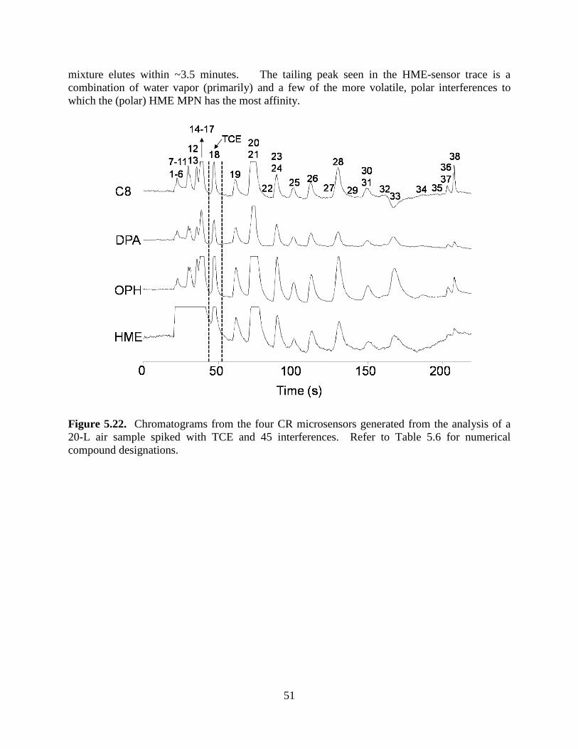
51

mixture elutes within ~3.5 minutes. The tailing peak seen in the HME-sensor trace is a combination of water vapor (primarily) and a few of the more volatile, polar interferences to which the (polar) HME MPN has the most affinity.

Figure 5.22. Chromatograms from the four CR microsensors generated from the analysis of a 20-L air sample spiked with TCE and 45 interferences. Refer to Table 5.6 for numerical compound designations.

52

Table 5.6. List of 46 test compounds and their vapor pressures (pv) used in complex mixture analysis.

ID Compound pv (torr) ID Compound pv (torr)

1. Pentane 514 24. n-Octane 14.1 2. 1,2-Dichloroethane 333 25. n-Butyl Acetate 15 3. Methylene Chloride 349 26. Chlorobenzene 11.8 4. Acetonitrile 73 27. Ethylbenzene 9.6

5. 2-Propanol (Isopropyl Alcohol) 44 28. m,p-Xylenes 8.29

6. Acrylonitrile 97 29. Bromoform 5 7. 2-Butanone (MEK) 89 30. o-Xylene 6.61 8. n-Hexane 150 31. Styrene 6.4 9. Ethanol 60 32. n-Nonane 4.45 10. Tetrahydrofuran (THF) 162 33. Cumene 3.5 11. Chloroform 200 34. alpha-Pinene 4.75 12. Acetone 231 35. n-Propylbenzene 3.42 13. 1,1,1-Trichloroethane 100 36. 1,2,4-Trimethylbenzene 2.1 14. Ethyl Acetate 93.7 37. 4-Ethyltoluene 3 15. Carbon Tetrachloride 113 38. 1,3,5-Trimethylbenzene 2.48 16. Benzene 95.2 39. d-Limonene 1.98 17. Cyclohexane 98 40. 1,2,4-Trichlorobenzene 0.5 18. Trichloroethylene (TCE) 69 41. 1,4-dichlorobenzene 1.76 19. 4-Methyl-2-pentanone 20 42. Naphthalene 0.08 20. 1,1,2-Trichloroethane 17 43. n-Decane 1.4 21. Toluene 28.4 44. n-Undecane 0.564 22. 2-Hexanone 12 45. n-Dodecane 0.21 23. Tetrachloroethylene (PCE) 18.6 46. n-Tridecane 0.081

The results suggest that multiple target compounds in the vapor pressure range of ~3 to 95 torr could be analyzed by the SPIRON µGC prototype. Some modifications to the pre-trap to ensure that the target compounds are transferred from the atmosphere to the sampler quantitatively would be needed. Additionally, column temperature program modifications may improve specific resolution of specific peaks. 5.2.2 MULTIVARIATE CURVE RESOLUTION Although a stand-alone chemiresistor array could differentiate among, perhaps, 20 or more vapors presented to the array individually, by use of pattern recognition methods, it is necessary to have an upstream chromatographic separation stage in order to determine the components of mixtures of three or more VOCs, because of inherent limitations on the degree of selectivity afforded by such arrays (Park et al., 1999; Zellers et al., 1995; Hsieh and Zellers, 2004; Jin and Zellers, 2008 and 2009). With upstream separation, the intractable problem of identifying and quantifying the components of an arbitrarily complex VOC mixture can be reduced into a time-resolved series of more manageable problems concerned with small subsets of that mixture.

53

Defining retention time windows within which specific VOCs are possibly present (Lu et al., 2003) facilitates this approach. Still, the likelihood of partial co-elutions within a window is rather high due to the short microcolumn length (6 meters) used in the prototype, and a means of analyzing the set of overlapping responses is needed; ideally one that minimizes computation and calibration complexity. As discussed below (Section 5.3), co-elutions of interfering compounds with TCE were apparent in some of the field samples. A simplified pattern fidelity test was used to detect such interferences in the field samples as a way of highlighting the value of sensor-array detection. However, the method was only partially successful. A more sophisticated deconvolution method, based on multivariate curve resolution (MCR), was piloted using data generated in the laboratory with one of the µGC prototypes to demonstrate the utility of MCR. This section describes the pilot study. MCR methods are often used to determine the components of mixtures with overlapping spectra in vibrational spectroscopy, and in chromatographic systems employing spectrometric detectors (e.g., GC-MS, HPLC-diode array, etc.) (Jaumot and Tauler, 2010; de Juan and Tauler, 2007; Manne, 1995; Maeder, 1987; Gampp et al., 1985; Amrhein et al., 1996; Tauler et al., 1995; Kowalski and Sharaf, 1982). Such methods can determine the number of components in overlapped chromatographic peak composites, and then can extract and recover the elution profile and spectrum of each component of the composite peak without prior knowledge of the mixture composition. Following MCR, the reconstituted spectra are then compared to those in a library in order to determine the identities and concentrations of the individual analytes. Various MCR algorithms have been introduced and applied, such as AutoBTEM for FT-IR, Raman, and IR imaging data (Xu et al., 2009), PARAFAC for GC×GC-TOFMS (Hoggard et al., 2009 and 2010), Evolving factor analysis (EFA) for hyphenated chromatography-spectrometer methods (Manne, 1995; Maeder, 1987; Gampp et al., 1985), and alternating least square (ALS) for multiple applications (Loszano et al., 2009; Szymanska et al., 2009; Carneiro et al., 2008). The study of Jin and Zellers (2009) was the first to consider using an MCR method to deconvolute overlapping peaks in GC-microsensor array systems. EFA-ALS Analysis. EFA performs factor analysis on a composite peak profile in sequential time segments. If the detector can differentiate components making up the composite peak, the rank of the corresponding data matrix will be equal to the number of components in the composite peak. By performing EFA in both the forward and backward directions, it is possible to locate the start and end of the peak profile of each component in the composite peak. ALS is an iterative least squares algorithm used to approximate the elution profile and/or spectrum of each component of a composite peak starting with an initial estimate of the profile or spectrum (Amrhein et al., 1996; Tauler et al., 1995; Tauler, 1995). Thus, EFA can be used to locate selective elution regions and to estimate the rank of the composite data matrix (i.e., number of components in a composite peak), and then ALS can be used to improve the accuracy of the recovered profile and/or spectrum. Once such information is extracted from a composite peak, pattern recognition is required to match the recovered spectrum with spectra of compounds in the library. Accurate recovery would normally lead to accurate recognition.

54

In their adaptation of such MCR methodology to chromatographic data obtained from microsensor arrays, Jin and Zellers (2009) used experimental sensitivity data derived from a previous study (Zhong, et al., 2007), but the peak shapes, relative responses, and resolutions they examined were generated by simulation assuming idealized Gaussian peaks. Here, the EFA-ALS method has been applied for the first time to a set of experimental data generated from an array of microsensors used as the detector in a µGC. The focus of this pilot study is on demonstrating the applicability of this hybrid MCR method to experimental data for qualitative (i.e., vapor recognition) analysis of a relevant pair of analytes: TCE and n-heptane (HEP). As discussed in Section 5.3, it was found that TCE and HEP partially co-eluted with each other under analytical conditions used in the field, and that some field samples also contained n-heptane. It was also found that their CR array response patterns were fairly similar, giving a correlation coefficient (ρ) of ~0.80.

Experimental Setup and Vapor Selection. One of the µGC prototypes was used for generating chromatograms for binary mixtures of TCE and n-heptane (HEP) in different relative concentrations. The experimental setup is shown in Figure 5-23. Prior to sampling by the µGC, an aliquot of a test atmosphere of these two vapors generated in a Tedlar bag was drawn into a sample loop connected to a six-port valve by suction flow generated by a pump. Then, the six-port valve was actuated to load the sample onto the preconcentration module of µGC with a flow of N2 provided from a regulated compressed cylinder. After drawing sufficient additional N2 to insure capture of the sample onto the high-volume sampler adsorbent, it was focused, injected, separated, and detected by the prototype. The voltage drops across individual sensors were recorded into a text file by the DAQ card at 20 Hz after amplification of the signal difference between baseline and measured values. Each text file was then imported into Grams 32 software (Thermogalactics, Inc., Salem, NH) to be converted to chromatograms and analyzed.

Sample

GC system

loop

N2

Pump

a)

Sample

GC system

loop

N2

Pump

b)

Figure 5.23. Experimental setup to generate data sets of binary mixtures: a) sample loading to sample loop; and b) transfer of sample from sample loop to the µGC prototype.

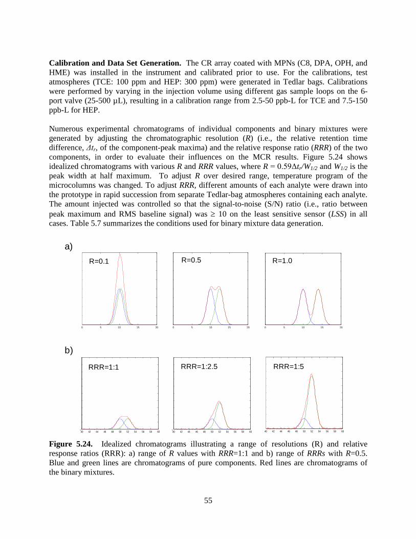
55

Calibration and Data Set Generation. The CR array coated with MPNs (C8, DPA, OPH, and HME) was installed in the instrument and calibrated prior to use. For the calibrations, test atmospheres (TCE: 100 ppm and HEP: 300 ppm) were generated in Tedlar bags. Calibrations were performed by varying in the injection volume using different gas sample loops on the 6-port valve (25-500 µL), resulting in a calibration range from 2.5-50 ppb-L for TCE and 7.5-150 ppb-L for HEP. Numerous experimental chromatograms of individual components and binary mixtures were generated by adjusting the chromatographic resolution (R) (i.e., the relative retention time difference, Δtr, of the component-peak maxima) and the relative response ratio (RRR) of the two components, in order to evaluate their influences on the MCR results. Figure 5.24 shows idealized chromatograms with various R and RRR values, where R = 0.59Δtr/W1/2 and W1/2 is the peak width at half maximum. To adjust R over desired range, temperature program of the microcolumns was changed. To adjust RRR, different amounts of each analyte were drawn into the prototype in rapid succession from separate Tedlar-bag atmospheres containing each analyte. The amount injected was controlled so that the signal-to-noise (S/N) ratio (i.e., ratio between peak maximum and RMS baseline signal) was ≥ 10 on the least sensitive sensor (LSS) in all cases. Table 5.7 summarizes the conditions used for binary mixture data generation.

0 5 10 15 200

10

20

30

40

50

60

70

80

Time

Sen

sor

resp

ons

e

R=0.1

R=0.1

0 5 10 15 200

10

20

30

40

50

60

70

80

Time

Sen

sor

resp

ons

e

R=0.6

R=0.5

0 5 10 15 200

10

20

30

40

50

60

70

80

Time

Sen

sor

resp

ons

e

R=1

R=1.0

40 42 44 46 48 50 52 54 56 58 600

20

40

60

80

100

120

140

160

180

200

40 42 44 46 48 50 52 54 56 58 600

20

40

60

80

100

120

140

160

180

200

40 42 44 46 48 50 52 54 56 58 600

20

40

60

80

100

120

140

160

180

200

RRR=1:1 RRR=1:5RRR=1:2.5

a)

b)

Figure 5.24. Idealized chromatograms illustrating a range of resolutions (R) and relative response ratios (RRR): a) range of R values with RRR=1:1 and b) range of RRRs with R=0.5. Blue and green lines are chromatograms of pure components. Red lines are chromatograms of the binary mixtures.

56

Table 5.7. Conditions for binary mixture data generation.

Sample Ra RRRb 1 0.1 1:1 2 0.5 1:1 3 0.5 1:2.5 4 0.5 1:5 5 0.5 1:10 6 1.0 1:1 7 1.0 1:2.5 8 1.0 1:5 9 1.0 1:10 10 0.1 1:1 11 0.5 1:1 12 1.0 1:1 13 0.5 1:10 14 0.5 1:5 15 0.5 1:2.5 16 0.5 1:1 17 0.5 2.5:1 18 0.5 5:1 19 0.5 10:1

a Resolution between two components. b Relative response ratio (TCE:HEP) based on the least sensitive sensor. Signal-to-noise ratio was ≥ 10 for all sensors in all cases. Calibration curves of injected mass vs. peak height gave forced-zero linear regression r2 values ≥ 0.98 for all sensors for both compounds (Figure 5.25). The normalized CR array response pattern for each vapor was derived from the slopes of the calibration curves and is presented in Figure 5.26. The TCE and HEP pair gave patterns with a correlation coefficient (used as an index of pattern similarity), ρ, of 0.80.

y = 0.118xr² = 0.999

y = 0.0667xr² = 0.992

y = 0.193xr² = 0.994

y = 0.0593xr² = 0.998

0

2

4

6

8

10

12

0 10 20 30 40 50 60 70

Sen

sor r

espo

nse

(V)

Concentration (ppb-L)

TCE y = 0.0734xr² = 0.996

y = 0.0182xr² = 0.988

y = 0.0636xr² = 0.995

y = 0.0116xr² = 0.986

0

2

4

6

8

10

12

0 50 100 150 200

Sen

sor r

espo

nse

(V)

Concentration (ppb-L)

HEP

Figure 5.25. Calibration curves for TCE and HEP with µGC CR array. Symbols: unfilled diamonds (C8), unfilled squares (DPA), unfilled triangles (OPH), and unfilled circles (HME).

57

TCE HEP Figure 5.26. CR array response patterns for TCE and HEP (ρ = 0.80). Bars are in the order of C8, DPA, OPH, and HME from the left hand side. The LOD of each sensor for each vapor was determined in order to insure that the minimum sampled mass was > LOD for the LSS in the array for a given analyte. The HME-coated sensor had the highest LOD for TCE (1.7 ppb assuming 1-L sample, equivalent to 8.8 ng) and HEP (8.9 ppb, equivalent to 36 ng). The ratio of peak areas for TCE and HEP from the HME sensor was ~4:1, with vapors at the same concentration. Two separate sample bags were generated for TCE (660 ppm) and HEP (2600 ppm), resulting in equivalent peak areas for the same sample volume from each bag. To vary the RRR, the sample volumes loaded into the instrument were adjusted accordingly by using different volumes of sample loop. For example, to achieve an RRR of 1:1, a TCE sample containing 34 ng TCE vapors (6.6 ppb-L, 660 ppm × 10 µL) and a HEP sample containing 107 ng (26 ppb-L, 2600 ppm × 10 µL) were loaded onto the sampler in the μGC one after the other using the sampling setup presented in Figure 5.23, and analyzed together. RRR values range from 1:10 (10 µL of 660 ppm TCE sample: 100 µL of 2600 ppm HEP sample) to 10:1 (100 µL of 660 ppm TCE sample: 10 µL of 2600 ppm HEP sample). By operating the dual-microcolumn ensemble isothermally at 30, 55, and 70 °C, a range of R values of 1.0, 0.5, and 0.1, respectively, were obtained. Multivariate Curve Resolution (EFA-ALS). A matrix of sensor responses (X) can be decomposed to a concentration profile matrix (C) at each value of retention time assuming a Gaussian elution profile, and the spectra (i.e. sensitivity) matrix (S) for each sensor with a random error matrix (E). It is created as shown in Eq. 1,

X=C·S+E (1)

To extract each component from a mixture having the matrix X, an estimate of the concentration profile matrix C should be obtained within the selective elution region (i.e., tail regions where there is no overlap) of each component using the EFA algorithm. In this study, an EFA algorithm developed by Maeder et al. (1985) was used. The estimate of C is then refined to minimize the random error (E) by iterative ALS calculations using the following equations:

Sest = (C’·C)-1C’·X (2)

Xest = C·Sest (3)

Cest = Xest·Sest(Sest’·Sest)·Sest-1 (4)

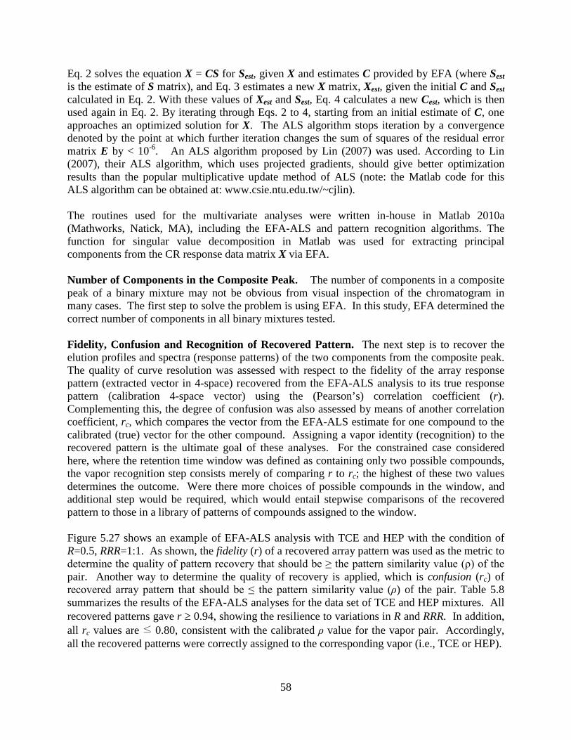
58

Eq. 2 solves the equation X = CS for Sest, given X and estimates C provided by EFA (where Sest is the estimate of S matrix), and Eq. 3 estimates a new X matrix, Xest, given the initial C and Sest calculated in Eq. 2. With these values of Xest and Sest, Eq. 4 calculates a new Cest, which is then used again in Eq. 2. By iterating through Eqs. 2 to 4, starting from an initial estimate of C, one approaches an optimized solution for X. The ALS algorithm stops iteration by a convergence denoted by the point at which further iteration changes the sum of squares of the residual error matrix E by < 10-6. An ALS algorithm proposed by Lin (2007) was used. According to Lin (2007), their ALS algorithm, which uses projected gradients, should give better optimization results than the popular multiplicative update method of ALS (note: the Matlab code for this ALS algorithm can be obtained at: www.csie.ntu.edu.tw/~cjlin). The routines used for the multivariate analyses were written in-house in Matlab 2010a (Mathworks, Natick, MA), including the EFA-ALS and pattern recognition algorithms. The function for singular value decomposition in Matlab was used for extracting principal components from the CR response data matrix X via EFA.

Number of Components in the Composite Peak. The number of components in a composite peak of a binary mixture may not be obvious from visual inspection of the chromatogram in many cases. The first step to solve the problem is using EFA. In this study, EFA determined the correct number of components in all binary mixtures tested. Fidelity, Confusion and Recognition of Recovered Pattern. The next step is to recover the elution profiles and spectra (response patterns) of the two components from the composite peak. The quality of curve resolution was assessed with respect to the fidelity of the array response pattern (extracted vector in 4-space) recovered from the EFA-ALS analysis to its true response pattern (calibration 4-space vector) using the (Pearson’s) correlation coefficient (r). Complementing this, the degree of confusion was also assessed by means of another correlation coefficient, rc, which compares the vector from the EFA-ALS estimate for one compound to the calibrated (true) vector for the other compound. Assigning a vapor identity (recognition) to the recovered pattern is the ultimate goal of these analyses. For the constrained case considered here, where the retention time window was defined as containing only two possible compounds, the vapor recognition step consists merely of comparing r to rc; the highest of these two values determines the outcome. Were there more choices of possible compounds in the window, and additional step would be required, which would entail stepwise comparisons of the recovered pattern to those in a library of patterns of compounds assigned to the window. Figure 5.27 shows an example of EFA-ALS analysis with TCE and HEP with the condition of R=0.5, RRR=1:1. As shown, the fidelity (r) of a recovered array pattern was used as the metric to determine the quality of pattern recovery that should be ≥ the pattern similarity value (ρ) of the pair. Another way to determine the quality of recovery is applied, which is confusion (rc) of recovered array pattern that should be ≤ the pattern similarity value (ρ) of the pair. Table 5.8 summarizes the results of the EFA-ALS analyses for the data set of TCE and HEP mixtures. All recovered patterns gave r ≥ 0.94, showing the resilience to variations in R and RRR. In addition, all rc values are ≤ 0.80, consistent with the calibrated ρ value for the vapor pair. Accordingly, all the recovered patterns were correctly assigned to the corresponding vapor (i.e., TCE or HEP).

59

In summary, despite the low dimensionality of the data obtained from the microsensor array detector, as compared to more conventional spectrometric GC detectors, the results obtained are extremely good. The hybrid MCR method employed, which combines EFA with ALS, showed the ability to accurately determine the number of components in a composite and recover response patterns from a mixture of two compounds with fairly similar response patterns under a range of chromatographic resolution and relative signal amplitudes. Similar tests are planned with other pairs of compounds. Additional issues to resolve prior to full implementation include devising a generalized means of defining retention time windows, determining the number and nature of vapors in the window to which recovered patterns must be compared, and quantifying responses from recovered components.

corr

el. c

oeff.

(r)

Figure 5.27. Example of EFA-ALS analysis (S/N ratio=10, R=0.5, RRR=1:1). a) Chromatograms of TCE (trichloroethylene), HEP (n-heptane), and their mixture from the least sensitive sensor (HME); b) chromatograms of the mixture from all four CR sensors; c) of true (calibrated) and recovered normalized response patterns for TCE and HEP; d) fidelity (r between true and recovered patterns) of recovered patterns of TCE and HEP and confusion (rc between true pattern of one compound and recovered pattern of the other compound). Numbers on the bars in d) are the values of r (two left-most bars) or rc (two right-most bars).

60

Table 5.8. MCR analysis results for binary mixtures under various conditions of S/N ratio, resolution, and relative response ratio.

ID S/Na Rb RRRc Fidelityd Confusione Recognitionf TCE HEP TCE HEP TCE HEP 1 10 0.1 1:1 0.98 1.00 0.72 0.59 'TCE' 'HEP' 2 0.5 1:1 0.99 1.00 0.70 0.61 'TCE' 'HEP' 3 1:2.5 0.99 1.00 0.76 0.64 'TCE' 'HEP' 4 1:5 0.94 1.00 0.72 0.52 'TCE' 'HEP' 5 1:10 0.97 1.00 0.67 0.53 'TCE' 'HEP' 6 1.0 1:1 0.95 1.00 0.61 0.38 'TCE' 'HEP' 7 1:2.5 0.99 1.00 0.61 0.55 'TCE' 'HEP' 8 1:5 0.95 1.00 0.69 0.59 'TCE' 'HEP' 9 1:10 0.98 1.00 0.59 0.47 'TCE' 'HEP' 10 10 0.1 1:1 0.98 1.00 0.72 0.59 'TCE' 'HEP' 11 0.5 0.99 1.00 0.70 0.61 'TCE' 'HEP' 12 1.0 0.95 1.00 0.61 0.38 'TCE' 'HEP' 13 10 0.5 1:10 0.97 1.00 0.67 0.53 'TCE' 'HEP' 14 1:5 0.94 1.00 0.72 0.52 'TCE' 'HEP' 15 1:2.5 0.99 1.00 0.76 0.64 'TCE' 'HEP' 16 1:1 0.99 1.00 0.70 0.61 'TCE' 'HEP' 17 2.5:1 0.98 0.99 0.71 0.67 'TCE' 'HEP' 18 5:1 1.00 1.00 0.76 0.79 'TCE' 'HEP' 19 10:1 1.00 0.98 0.68 0.79 'TCE' 'HEP'

a Minimum signal-to-noise ratio ; b Resolution; c Relative response ratio; d correlation coefficient between the recovered pattern and those stored in the library; e correlation coefficient between recovered pattern of one compound and that of the other compound stored in the library; f Vapor recognition after pattern matching. 5.3 FIELD TESTING Field testing was primarily conducted from July to September 2010. The field demonstration was conducted in the ASU SERDP VI-study house in Layton, Utah as described in Section 4.0 Site Description. Figure 5.28 Shows photographs of the study house. Preliminary field testing, including use of the HAPSITE portable GC/MS (courtesy of Kyle Gorder and Eric Dettenmair of Hill AFB), established that a crack in the basement in a small closet underneath the stairs was a significant TCE VI entry location (shown in Figure 5.28b along with the hallway outside of the closet). This proved useful to the µGC field demonstration since a wide range of indoor TCE concentrations could be established by inducing negative pressure in the house (relative to subslab) by using a fan in the upstairs window. During the field testing, the basement windows were opened periodically and outside air was drawn in to reduce TCE concentrations prior to subsequent measurements. The indoor temperature was 25 ± 3°C and relative humidity was within the range of 20 to 60%.

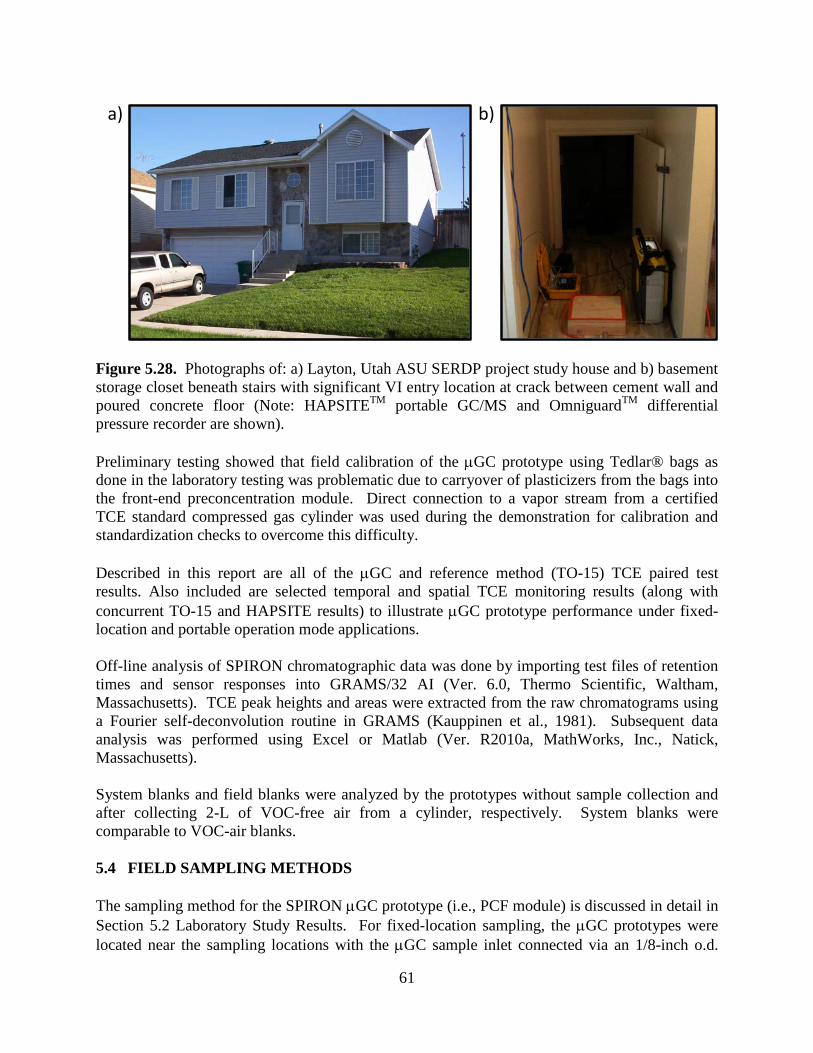
61

a) b)

Figure 5.28. Photographs of: a) Layton, Utah ASU SERDP project study house and b) basement storage closet beneath stairs with significant VI entry location at crack between cement wall and poured concrete floor (Note: HAPSITETM portable GC/MS and OmniguardTM differential pressure recorder are shown). Preliminary testing showed that field calibration of the µGC prototype using Tedlar® bags as done in the laboratory testing was problematic due to carryover of plasticizers from the bags into the front-end preconcentration module. Direct connection to a vapor stream from a certified TCE standard compressed gas cylinder was used during the demonstration for calibration and standardization checks to overcome this difficulty. Described in this report are all of the µGC and reference method (TO-15) TCE paired test results. Also included are selected temporal and spatial TCE monitoring results (along with concurrent TO-15 and HAPSITE results) to illustrate µGC prototype performance under fixed-location and portable operation mode applications. Off-line analysis of SPIRON chromatographic data was done by importing test files of retention times and sensor responses into GRAMS/32 AI (Ver. 6.0, Thermo Scientific, Waltham, Massachusetts). TCE peak heights and areas were extracted from the raw chromatograms using a Fourier self-deconvolution routine in GRAMS (Kauppinen et al., 1981). Subsequent data analysis was performed using Excel or Matlab (Ver. R2010a, MathWorks, Inc., Natick, Massachusetts). System blanks and field blanks were analyzed by the prototypes without sample collection and after collecting 2-L of VOC-free air from a cylinder, respectively. System blanks were comparable to VOC-air blanks. 5.4 FIELD SAMPLING METHODS The sampling method for the SPIRON µGC prototype (i.e., PCF module) is discussed in detail in Section 5.2 Laboratory Study Results. For fixed-location sampling, the µGC prototypes were located near the sampling locations with the µGC sample inlet connected via an 1/8-inch o.d.

62

stainless steel tubing (internal volume less than 0.5% of sample volume) to the sampling location. Generally, the µGC prototypes were placed in two locations: several inches from the storage closet floor crack and in the hallway outside of the storage closet several inches from the HAPSITE sampling location. For the portable mode sampling, the µGC was placed in the sampling location. TO-15 samples were taken with 6-L Summa canisters. Flow restriction was used to approximate the same sampling time window for the TO-15 samples as for the concurrent µGC samples. For samples taken from the storage closet location, a small length of 1/8-inch stainless steel tubing was used to sample from the same location that the µGC was sampling, otherwise the canister inlet was simply placed within several inches of the concurrent µGC sampling location. Differential pressure measurements were made using an OmniguardTM 4 differential pressure transducer and recorder. One side of the pressure transducer was connected to tubing (sealed in the floor) exposed to subslab vapor, and the other side was exposed to indoor air. 5.5 FIELD SAMPLING RESULTS The results of the µGC prototype field demonstration are presented in three sections. The first section presents the overall basic performance results of the µGC prototype including comparison with TO-15 results. The other two sections present representative temporal and spatial monitoring results. The field results are reported in Kim et al., In Review a & b. 5.5.1 BASIC PROTOTYPE PERFORMANCE Two SPIRON µGC prototypes were used in the field demonstration. In this report, they are referred to as “Proto 1” and “Proto 2.” The TCE standard tank was periodically sampled in the field and analyzed by TO-15 throughout the study period, and the TCE concentration was determined to be 9.6 ± 0.43 ppb (51.7 µg/m3, n = 7). This value was within 1% of the concentration determined by the tank supplier after correcting for the difference in atmospheric pressure between the test site (12.7 psi) and the site where the tank was prepared (14.4 psi) (i.e., 9.7 ppb, 52.3 µg/m3). For calibration, sample volumes ranging from 0.5 to 6 L and 0.5 to 8 L were collected for Proto 1 and Proto 2, respectively. The corresponding ranges of collected masses (integrated vapor volumes) were 26 to 310 ng (4.8 to 58 ppb∙L) and 26 to 414 ng (4.8 to 77 ppb∙L). With the amplification circuit configuration employed, the most TCE-sensitive sensors (i.e., HME and OPH) saturated at masses of ~330 ng (61 ppb∙L) and ~430 ng (80 ppb∙L) for Proto 1 and 2, respectively. Two full (i.e., 6 to 7 points) calibrations and seven single-point standardization checks (2-L tank sample) were performed over the primary 3-week study period (after preliminary field setup and sampling). One set of calibration curves is presented in Figure 5.29. The forced-zero linear regression r2 values are ≥ 0.98 for all sensors in both prototypes. Response patterns for TCE derived from the peak-height sensitivity values (Figure 5.29 insets) differ somewhat between the two instruments because of small differences in sensitivities among the MPN-coated CRs in the arrays installed in each prototype, a reflection of the prototype instruments being manually custom fabricated.

63

a)

y = 0.15x

y = 0.062x

y = 0.17x

y = 0.19x

0

2

4

6

8

10

12

0 20 40 60 80

peak

hei

ght(V

)

Volume of TCE Vapor (ppb-L)

b)

y = 0.10x

y = 0.068x

y = 0.099x

y = 0.15x

0

2

4

6

8

10

12

0 20 40 60 80 100

peak

hei

ght (

V)

Volume of TCE Vapor (ppb-L)

Figure 5.29. Field TCE calibration curves for a) Proto 1 and b) Proto 2. Symbols: × - OPH; - HME; ♦ - C8; – DPA. All regression lines have r2 values > 0.99, except HME in Proto 2 (r2 = 0.98). Insets show the normalized response pattern for TCE from the CR arrays (bars, from left to right are: C8, DPA, OPH, and HME). LODs for TCE calculated on the basis of these calibration data are presented in Table 5.9 for assumed sample volumes of 4 L (minimum volume collected during the field tests) and 20 L (maximum sample volume; preconcentrator was designed for this sample volume), since the LOD is inversely proportional to sample volume. LOD is calculated as 3σ/sensitivity, where σ is the standard deviation of baseline noise. For a 20-L sample, the lowest LOD among the individual sensors in the two prototypes is 0.021 ppb. Differences in LOD values for a given sensor type between the two prototypes arise from a combination of different sensitivities and baseline noise levels. Although the LOD for the array as a whole is dictated by the highest LOD among the sensors, it is possible to use only three of the four sensors and still perform effective vapor recognition from the array response patterns (Park et al., 1999; Cai and Zellers, 2002; Hsieh et al., 2004). Sample volumes collected for the tests described below were ≤ 10 L (typically 4 to 8 L) due to concerns over exceeding the dynamic range of the more sensitive sensors at larger sample volumes and analyte masses. For an 8-L sample (a common sample volume used in the field), the lowest LOD values were 0.052 ppb (HME in Proto 1) and 0.073 ppb (OPH in Proto 2). If the three most sensitive sensors are considered collectively (i.e., minimum required for pattern recognition), the LOD values were 0.18 ppb and 0.25 ppb for Proto 1 and 2, respectively (~10% of the MAL at the time of the field demonstration).

64

Table 5.9. Limit of Detection (LOD, ppb) for TCE with both prototypes in the field for assumed sample volumes of 4 L and 20 L (in parentheses). Calculations are based on sensitivities and noise levels obtained from the calibration curves shown in Figure 5.29. LOD = 3σ/sensitivity, where σ is the standard deviation of baseline noise, which ranged from 0.023 V (HME) to 0.077 V (DPA) for Proto 1 and from 0.030 V (OPH) to 0.085 (C8) for Proto 2. To convert from ppb to µg/m3, multiply by 5.4.

Sensor LOD (ppb) Proto 1 Proto 2

C8 0.37 (0.073) 0.65 (0.13) DPA 0.95 (0.19) 0.50 (0.099) OPH 0.11 (0.022) 0.15 (0.029) HME 0.11 (0.021) 0.30 (0.060)

Figure 5.30 summarizes the standardization data collected every few days for Proto 2 in the form of bar charts. Except for the last day (-32%), the variations in TCE sensitivity (Figure 5.30a, RSD = 17%) were ≤ 11% and there was no temporal trend in the sign or magnitude of the drift. The concentration-normalized response patterns in Figure 5.30b show that the pattern fidelity was good, as reflected in the r values relating the pattern on each day to that determined from the mid-study full calibration (i.e., day 12). Over the first week, the HME sensor response drifted downward, but then stabilized. As a result, the r value of 0.85 for the first day is anomalously low compared to all other days, for which r ≥ 0.95. With the possible exception of the first day, this indicates that fluctuations in sensitivity (Figure 5.30a) arise from a ”common mode” effect (e.g., shift in array temperature or pump flow rate during sampling). To account for the changes in apparent sensitivity, prototype responses obtained on a given day were corrected using the most recent standardization value; that is, measured values were multiplied by the ratio of the original calibration value to that of the standardization value. The same standardization method was applied to the data for Proto 1.

65

Figure 5.30. Results of periodic analysis (standardization check) of the TCE tank standard (2-L sample; 9.6 ppb TCE) showing stability of responses and relative response patterns over the 3-week study (RSD = 17%). a) Actual (absolute) responses from each sensor in the array; error (%) between each sample estimate of TCE concentration (average of four sensors) and that determined from the calibration performed on day 12 is shown above each set of responses. b) Normalized response patterns obtained by dividing each response by the maximum response among all four sensors; the correlation coefficient (r) derived from a comparison of the pattern on each day to that on day 15 is shown above each set of responses. Bars, from left to right, refer to the following nanoparticle sensor coatings: C8, DPA, OPH, and HME. A total of 23 indoor air samples analyzed concurrently by both prototypes while operating in close proximity gave TCE values > LOD. The range of concentrations among these samples was from 1 to 11.4 ppb. Figure 5.31 shows good consistency between the measurements from the two prototypes: the forced-zero, linear regression r2 value is 0.88 and the slope is 1.12. Proto 2 yielded slightly higher values than Proto 1 on average. These results show that TCE determinations by the two prototypes are comparable to each other.

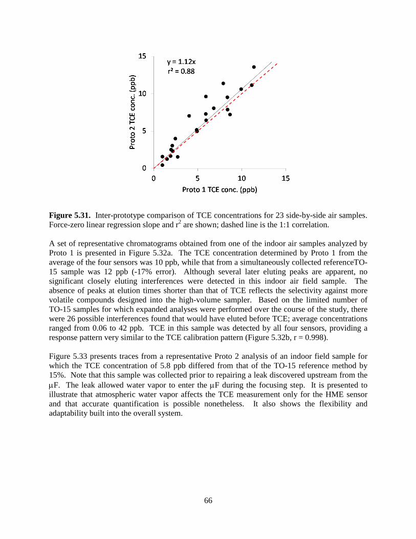
66

Figure 5.31. Inter-prototype comparison of TCE concentrations for 23 side-by-side air samples. Force-zero linear regression slope and r2 are shown; dashed line is the 1:1 correlation. A set of representative chromatograms obtained from one of the indoor air samples analyzed by Proto 1 is presented in Figure 5.32a. The TCE concentration determined by Proto 1 from the average of the four sensors was 10 ppb, while that from a simultaneously collected referenceTO-15 sample was 12 ppb (-17% error). Although several later eluting peaks are apparent, no significant closely eluting interferences were detected in this indoor air field sample. The absence of peaks at elution times shorter than that of TCE reflects the selectivity against more volatile compounds designed into the high-volume sampler. Based on the limited number of TO-15 samples for which expanded analyses were performed over the course of the study, there were 26 possible interferences found that would have eluted before TCE; average concentrations ranged from 0.06 to 42 ppb. TCE in this sample was detected by all four sensors, providing a response pattern very similar to the TCE calibration pattern (Figure 5.32b, r = 0.998). Figure 5.33 presents traces from a representative Proto 2 analysis of an indoor field sample for which the TCE concentration of 5.8 ppb differed from that of the TO-15 reference method by 15%. Note that this sample was collected prior to repairing a leak discovered upstream from the µF. The leak allowed water vapor to enter the µF during the focusing step. It is presented to illustrate that atmospheric water vapor affects the TCE measurement only for the HME sensor and that accurate quantification is possible nonetheless. It also shows the flexibility and adaptability built into the overall system.

67

Figure 5.32. (a) Representative chromatograms from the MPN-coated CR array for a measurement obtained from Proto 1 having a TCE concentration of 12 ppb; (b) Normalized response patterns (bar charts) for TCE and the selected (unknown) VOCs designated in (a). Bars in each chart correspond to specific sensors in the array, from left to right: C8, DPA, OPH, and HME. The pattern-matching correlation coefficients (r values) above each response pattern reflect the similarity/dissimilarity with the pattern for TCE determined from the calibration.

68

20 40 60 80 100 120 140 160 180

Time (s)

C8

DPA

OPH

HME

Figure 5.33. Chromatograms obtained from Proto 2 for an indoor air sample containing TCE (50- second elution time). Response patterns for the six most prominent additional peaks in the chromatograms of Figure 5.32a are presented in Figure 5.32b along with the r values derived from comparisons with the TCE calibration pattern, which range from r = 0.46 to 0.98. The identities of these compounds were not determined. As shown, the ability to differentiate TCE from interferences on the basis of response patterns varies. However, many patterns are sufficiently different from that of TCE to enhance the reliability of the TCE analysis significantly, particularly when considered in conjunction with the retention times. Stated differently, it is evident that these prototypes could be used to selectively determine other VOCs with proper calibration and adjustment of operating conditions.

The utility of the array response pattern is perhaps of greater value when interfering VOCs are present that fully or partially co-elute with TCE. For this preliminary study, we applied a simple pattern matching test to identify cases where there was reason to suspect the presence of one or more co-eluting co-contaminants; that is, for a set of peaks eluting at the retention time expected for TCE, if the correlation of the sample-pattern vector to the calibration-pattern vector for TCE yielded a value of r < 0.85, then it was assumed that one or more co-eluting interferences was present. Samples with r < 0.85 would therefore be expected to yield positively biased (apparent) TCE concentrations relative to those found with the reference method. Figure 5.34 presents extracted sections of three chromatograms from Proto 1 in which peaks were detected at the TCE retention time and patterns derived therefrom. For brevity only, a single representative sensor trace is presented along with the four-sensor response pattern (insets). The first panel (Figure 5.34a) shows a slightly tailing peak and a response pattern for which r = 0.997. The top of this peak does not show distortion, suggesting absence of a

69

significant co-eluting peak. The concentration determined with the prototype was 8.3 ppb, which is within 5% of that of the parallel sample analyzed by the reference method (i.e., 8.7 ppb). This first panel also shows the chromatographic trace of a 2-L VOC-free air blank for comparison; it shows no TCE response. The second panel (5.34b) shows a peak with some distortion (curvature as peak approaches its top) suggesting the presence of more than one component. Indeed, the response pattern gave an r = 0.830 and the TCE concentration estimated with the prototype had a positive bias of 52% (i.e., 4.1 ppb vs. 2.7 ppb for TO-15). For the third panel (5.34c), again some distortion is apparent in the peak, and the concentration estimate was positively biased by 64%. However, the response pattern gave an r = 0.984. In this case, it appears that the response pattern(s) of the co-eluting interference(s) was not sufficiently different from that of TCE to exceed the threshold for a mismatch.

60 70

Time (s)

60 70

Time (s)

r = 0.830 r = 0.984r = 0.997

a) b) c)

60 70

Time (s)

Figure 5.34. Extracted subsections of several chromatograms from the OPH sensor of Proto 1 and corresponding normalized response patterns from the CR array (insets) for TCE peaks with and without co-eluting interferences, illustrating the utility of the pattern-matching criterion. a) Chromatogram trace with no apparent interferences: pattern-matching r = 0.997; prototype TCE concentration = 8.3 ppb, reference method TCE concentration = 8.7 ppb (-5% error). Trace for a 2-L blank sample is shown in red superimposed on the trace for the TCE peak. b) Chromatogram trace with partially-co-eluting interference(s) indicated by the distortion in the peak shape: pattern-matching r = 0.830; prototype TCE concentration = 4.1 ppb; reference method TCE concentration = 2.7 ppb (+52% error). c) Chromatogram trace with partially-co-eluting interference(s) as indicated by the distortion in the peak shape: pattern matching r = 0.984; prototype TCE concentration = 2.3 ppb; reference method TCE concentration = 1.4 ppb (+64% error); lack of pattern mismatch indicates the presence of interferences with response patterns similar to that of TCE. All of the 60 TO-15 reference samples collected and analyzed during the study had detectable levels of TCE, with concentrations ranging from 0.047 to 16 ppb. Of these, 42 were above the LODs for at least three of the sensors: 30 for Proto 1 and 12 for Proto 2. Figure 5.35 plots the pooled TCE concentration estimates from the two prototypes against the matching reference values. The slope and (force-zero) linear regression r2 value are 0.90 and 0.87, respectively, indicating generally good agreement with the reference method. Above the MAL, 21 of the 26

70

TCE values were within 25% of the reference values. Deviations are larger and more prevalent below the MAL. (Note: Throughout this section, the MAL is for the time period of the field demonstration.) Overall, Figure 5.35 reveals a slight tendency toward underestimation at high concentrations and a stronger tendency toward overestimation at low concentrations for the prototypes.

Figure 5.35. Correlation of the pooled measurements from the µGC prototypes with the corresponding canister samples analyzed by TO-15. The black solid line is from linear regression with forced zero (slope and r2 shown), the red dotted line is the 1:1 correlation, and the blue dashed lines show the ± 25% limits around the 1:1 correlation. The 42 paired TO-15 and µGC samples in the above figure can be subdivided into data sets with values falling above and below the MAL as well as above and below the pattern matching threshold of r = 0.85, allowing for a more detailed assessment of performance. Results are summarized in Table 5.10 and the relevant plots are presented in Figure 5.36. For measurements ≥ MAL with patterns giving r > 0.85 (n=25), regression onto the reference measurements gave a slope of 0.90 (r2 = 0.72). Errors in measured TCE concentrations ranged from -43 to +50, averaging -6.6%. Over the same concentration range, there was just one sample that gave a pattern with r < 0.85, which had a large positive error in the TCE concentration estimate (i.e., 51%), implying a significant concentration of co-eluting interference(s) with pattern(s) different from that of TCE. Thus, pattern matching appears to add reliability over this range of concentrations.

Below the MAL, for the 11 samples with patterns giving r > 0.85 the correlation between prototype and reference TCE values was somewhat lower (i.e., linear regression r2 = 0.69) and all of the measurements were positively biased; the slope = 1.66 and the range of errors was 24-119%, averaging 74%. In this concentration range, the pattern matching criterion was not as effective in detecting the presence of co-eluting VOCs, which suggests that the interferences had response patterns similar to that of TCE. Still, for those samples not meeting the pattern

71

matching threshold (Table 5.10; r < 0.85, n = 5), the errors were generally much larger (i.e., range = 75 to 285%; average = 147%), indicating that the response pattern was useful in identifying the more extreme cases of co-eluting interferences. Table 5.10. Comparison of TCE measurements obtained concurrently from the µGC prototypes and from canister samples analyzed by GC-MS (reference method).

case conc. ra nb Difference (%)c min. max. avg.

1 > MALd > 0.85 25 -43 50 -6.6 2 > MAL < 0.85 1 51 51 51 3 < MAL > 0.85 11 24 119 74 4 < MAL < 0.85 5 75 285 147

a Correlation coefficient between response patterns from air samples and from calibration. b Number of samples. c Difference between TCE concentrations determined by prototypes and reference method. d Mitigation Action Level (2.3 ppb).

y = 0.90xr² = 0.72

0

10

20

0 10 20

Prot

otyp

e TC

E Co

nc. (

ppb)

TO-15 TCE Conc. (ppb)

y = 1.66xr² = 0.69

0

1

2

3

4

0 1 2 3

SPIR

ON

TCE

conc

. (pp

b)

TO-15 TCE Conc. (ppb)

y = 2.28xr² = 0.06

0

1

2

3

4

0 1 2 3

SPIR

ON

TCE

conc

. (pp

b)

TO-15 TCE Conc. (ppb)

a) b) c)

Figure 5.36. Comparison of TCE measurements from the prototypes and from the reference method (TO-15) for matched samples. In each panel, the black solid line is from linear regression with forced zero (slope and r2 shown), the red dotted line is the 1:1 correlation, and the blue dashed lines show the ± 25% limits around the 1:1 correlation. a) Subset of data with TCE concentrations > MAL and r > 0.850. b) Subset of data with TCE concentrations < MAL and r > 0.850. c) Subset of data with TCE concentrations < MAL and r < 0.850. Note that there was only one sample with a TCE concentration > MAL and r < 0.850.

72

5.5.2 PROTOTYPE TEMPORAL RESULTS Temporal variations in TCE concentrations were measured in ASU’s VI-study house on numerous days within the study period. This section presents representative temporal results illustrative of prototype performance. The prototypes were placed on a table in the main basement room, and short sections of stainless-steel tubing (1.6-mm i.d.) were affixed to the inlets and extended either to the primary VI entry point in the basement crawl space or to the center of the hallway adjacent to the crawl space near the portable GC-MS inlet (see Figure 5.28b). To obtain side-by-side reference samples in the crawl-space near the main VI entry point, canisters were also fitted with short sections of stainless steel tubing. Measurements were also collected every 2 hours with a portable GC-MS (HAPSITE, Inficon, East Syracuse, New York) positioned in the hallway adjacent to the primary VI entry location. Selected ion monitoring (SIM) mode was used, with TCE detected on the basis of peaks at 95, 130, and 132 m/z. The peak at 130 m/z was used for quantification and the TCE detection limit was < 0.2 ppb for the 0.1-L preconcentrated air samples. Calibration and quality control procedures followed documented protocols for USEPA Method TO-17. µGC prototype samples were collected within about 30 cm of the portable GC-MS inlet port. In order to vary the TCE concentrations for the µGC performance assessments, the extent of TCE VI was increased over scheduled time intervals in the house by temporarily reducing the indoor air pressure. This was achieved with a three-speed, box-style, exhaust fan placed in the window of one of the bedrooms on the second floor. The pressure differential between the hallway adjacent to the VI entry point and the sub-slab headspace was monitored using a logging pressure sensor (Omniguard 4, Omnitec Design, Inc., Lynnwood, Washington); and data were subsequently downloaded to a laptop computer. Prior to collecting air samples each day, the exhaust fan was turned on and several windows opened to draw outside air through the house to reduce any accumulated TCE. The fan was then turned off and the windows closed. Figure 5.37a presents the results of 12 hours of continuous monitoring from the crawl space with Proto 1 and Proto 2 (i.e., both prototypes sampling from the same location). A total of 22 measurements were collected with each prototype (Note: several data points overlap in the figure). Five reference canister samples were collected during this time period. As the figure shows, over the first 90 minutes, prior to the first induced pressure differential, the TCE concentration was stable and low, averaging 0.56 ppb and 0.26 ppb for Proto 1 and 2, respectively, and 0.14 ppb for the single canister/TO-15 sample. The exhaust fan was then turned on, stepped through low, medium, and high settings over ~ 1 hour, and then maintained at the high setting for 110 minutes. The net indoor pressure reduction was 0.013 inches of H2O. During the transition, the increase in TCE concentration coincided with the decrease in differential pressure for both prototype measurements and the canister/TO-15 value. Once the pressure stabilized over this first induced-VI interval, the two canister samples collected gave an average of 13 ppb TCE, while the concurrently collected individual measurements from Proto 1 and Proto 2 gave averages of 9.3 and 8.9 ppb of TCE, respectively (average error = -27%). The average TCE concentrations (n = 6) measured with Proto 1 and 2 during the depressurization event were 6.6 and 6.3 ppb, respectively.

73

5

0

-5

-10

-15

-20

5

0

-5

-10

-15

-20

5

0

-5

-10

-15

-200 2 4 6 8 10 12

Elapsed time (h)

TCE

conc

entr

atio

n (p

pb)

Differential pressure (“H2 O

, x 10-3)

a)

b)

c)

Figure 5.37. Temporal variations in the TCE concentration (left-hand ordinate) determined by Proto 1 (open triangles), Proto 2 (filled triangles), canister/TO-15 (open circles), and portable GC-MS (filled circles) as a function of the differential pressure (dotted lines) between the sub-slab headspace and the basement hallway (right-hand ordinate): (a) measurements collected from the crawl space near the primary VI entry location with and without pressure changes induced by an exhaust fan located on the second floor; (b) measurements collected from the crawl space (Proto 1 and canister/TO-15) and from the hallway adjacent to the crawl space (Proto 2 and portable GC-MS) with induced pressure changes; and (c) measurements collected from same locations as in (b) without induced pressure changes.

74

Upon stepping the fan speed down to the low setting, the differential pressure decreased and the TCE concentration quickly decreased to a level similar to that prior to the pressure reduction. At this point, several windows were opened in the basement and left open for 2 hours. They were then closed for another 2 hours. Over this 4-hour interval, the average TCE concentrations (n = 6) measured by Proto 1 and 2 were 0.44 and 0.56 ppb, respectively. The single canister sample collected during this interval gave a TCE concentration of 0.12 ppb, while the concurrent single prototype values were 0.25 and 0.28 ppb for Proto 1 and 2, respectively (average error = +117%). Note that the large positive errors in the prototype values observed at the lower concentrations (i.e., < 2.3 ppb, which is the MAL for this site at the time of the field demonstration) are attributable to interferences that could not be resolved either chromatographically or by pattern recognition methods. At t = 8.5 hours, the fan was again stepped up to full speed over ~ 3 hours and the TCE values again increased to values similar to those observed during the first induced-VI interval. The TCE concentration measured with Proto 2 was within 6% of the canister/TO-15 value of 12 ppb, while Proto 1 measured only 7.9 ppb, which may be due to a concentration gradient in the crawl space area. The two prototype measurements continued to track the TCE concentration changes well and are in reasonably good agreement with the each other and with the reference value. Figure 5.37b shows a series of measurements collected in a manner similar to those depicted in Figure 5.37a, with similar scheduled changes in differential pressure. In this case, however, Proto 1 and canister samples were collected from the crawl space and Proto 2 and portable GC-MS samples were collected from the adjacent hallway. Again, a total of 22 measurements were collected with each prototype. Five concurrent canister samples were also collected. Six measurements were collected with the portable GC-MS over the entire period, but they were not synchronized with the prototype measurements. Over the first 1.5 hours, TCE concentrations were low and stable. As the fan was stepped up to its highest setting over the next 2 hours and subsequently back down to its low setting over ~1.5 hours (see Figure 5.37b), the TCE concentrations measured with the prototypes increased and decreased accordingly. TCE concentration in the crawl space (Proto 1) was consistently higher than that in the hallway (Proto 2), and, in the interval corresponding to the largest pressure differential (-0.015″ H20), the concentration ratio was about 2.2 (i.e., 12 ppb vs. 5.6 ppb for Proto 1 and 2, respectively). The most closely time-matched GC-MS and Proto 2 values, taken during the transition periods, agreed to within 9% and the three concurrent canister/TO-15 and Proto 1 values tracked each other and agreed to within 22% on average. Interestingly, during the second reduced-pressure excursion, the TCE concentration did not increase nearly as much as during the first excursion. Both prototypes and both reference methods gave low TCE values and there was no significant concentration gradient evident between the crawl space and the hallway. We speculate that the soil immediately beneath the house was temporarily depleted of TCE. Regardless, the prototype measurements remained consistent with each other (i.e., 2.2 and 1.6 ppb, n = 11) and with the reference measurements (average = 2.7 ppb).

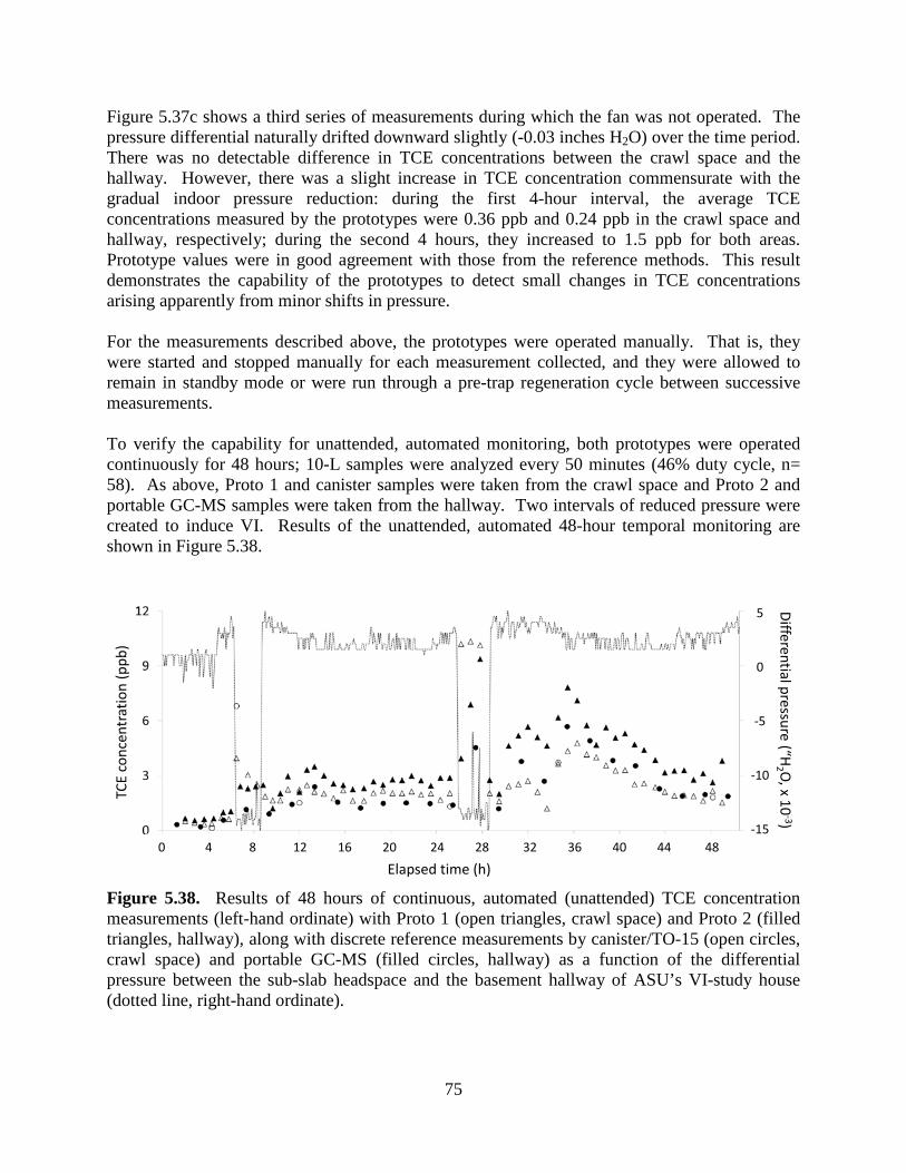
75

Figure 5.37c shows a third series of measurements during which the fan was not operated. The pressure differential naturally drifted downward slightly (-0.03 inches H2O) over the time period. There was no detectable difference in TCE concentrations between the crawl space and the hallway. However, there was a slight increase in TCE concentration commensurate with the gradual indoor pressure reduction: during the first 4-hour interval, the average TCE concentrations measured by the prototypes were 0.36 ppb and 0.24 ppb in the crawl space and hallway, respectively; during the second 4 hours, they increased to 1.5 ppb for both areas. Prototype values were in good agreement with those from the reference methods. This result demonstrates the capability of the prototypes to detect small changes in TCE concentrations arising apparently from minor shifts in pressure. For the measurements described above, the prototypes were operated manually. That is, they were started and stopped manually for each measurement collected, and they were allowed to remain in standby mode or were run through a pre-trap regeneration cycle between successive measurements. To verify the capability for unattended, automated monitoring, both prototypes were operated continuously for 48 hours; 10-L samples were analyzed every 50 minutes (46% duty cycle, n= 58). As above, Proto 1 and canister samples were taken from the crawl space and Proto 2 and portable GC-MS samples were taken from the hallway. Two intervals of reduced pressure were created to induce VI. Results of the unattended, automated 48-hour temporal monitoring are shown in Figure 5.38.

0 4 8 12 16 20 24 28 32 36 40 44 48

Elapsed time (h)

5

0

-5

-10

-15

TCE

conc

entr

atio

n (p

pb)

Differential pressure (“H2 O

, x 10-3)

Figure 5.38. Results of 48 hours of continuous, automated (unattended) TCE concentration measurements (left-hand ordinate) with Proto 1 (open triangles, crawl space) and Proto 2 (filled triangles, hallway), along with discrete reference measurements by canister/TO-15 (open circles, crawl space) and portable GC-MS (filled circles, hallway) as a function of the differential pressure between the sub-slab headspace and the basement hallway of ASU’s VI-study house (dotted line, right-hand ordinate).

76

The Proto 1 and canister/TO-15 measurements from the crawl space were similar, except for the pair of measurements collected during the pressure transition at t = 5.5 hours (6.8 and 3.9 ppb from the canister/TO-15 and Proto 1, respectively). Otherwise, the Proto 1 average was 63% higher than that of the canister/TO-15 average (n = 6), reflecting the positive bias at low concentrations by the prototypes. Proto 2 results were compared to the closest-matched portable GC-MS values (the largest sampling time difference was ~25 minutes, and most were within 10 to 15 minutes). The temporal trends in TCE concentration from the Proto 2 and portable GC-MS measurements were consistent, but the Proto 2 average of 3.4 ppb is 54% higher than that of the portable GC-MS (2.2 ppb) (n = 23). During the two reduced indoor-air pressure intervals, a concentration gradient from the crawl space to the hallway was evident, reflecting the enhanced TCE VI in the crawl space observed previously. At other times, and particularly from t = 30 to 48 hours, the gradient was from the hallway to the crawl space, suggesting that the crawl space (i.e., VI) was not the dominant source of TCE. As it turns out, at t = 10 hours on the first day, the garage door was closed, and it remained closed for the remaining 38 hours spanned by this survey. Subsequent sampling with the portable GC-MS confirmed that the TCE stored in the refrigerator in the garage was an unexpected non-VI source of contamination in the house that only became significant when the garage door was closed. Between the first and second reduced-pressure intervals, this source apparently contributed only slightly to the TCE concentration measured in the hallway, leading to similar levels in the crawl space and hallway. During the second pressure-reduction interval, the levels in the hallway were higher than expected, and, from t = 10 to 48 hours, the peak in TCE concentration in the hallway (Proto 2) reflects a more significant contribution from the TCE source in the garage. 5.5.3 PROTOTYPE SPATIAL RESULTS For the spatial concentration mapping survey in the ASU study house (results presented are representative of comparable spatial sampling efforts in the house), 15 measurements were collected with Proto 1 over a single day from multiple locations. Results are shown in Figure 5.39. Concentrations (from Proto 1) ranged from 0.51 to 3.8 ppb with a mean value of 1.3 ppb. The average TCE concentration in the basement was higher than that on the second floor (i.e., 2.2 ppb vs. 0.86 ppb, respectively) and the highest concentration was observed in the crawl space, consistent with TCE VI. The TCE concentration contours shown in Figure 5.39b convey the shallow gradients. Four of the five pairs of concurrently collected Proto 1 and canister/TO-15 values agreed to within 30%. Testing in a second Layton, Utah house without TCE VI was then conducted to demonstrate that a non-VI source could be detected and located by means of the spatial distribution of TCE concentrations determined with a µGC prototype. After venting the house for about 2 hours and placing the hidden TCE source, four measurements were collected on the second level, one in the stairwell, and four in the basement. Since this took most of the day, sampling had to be suspended, although the location of the TCE source was determined. On the second day, after venting the house in the morning and replacing the hidden TCE source in the same location, measurements were resumed, with two being collected from the second floor and eight from the basement. Results are shown in Figure 5.40.

77

Measurements from similar locations on different days were quite consistent. For the five Proto 1 measurements with concurrently collected canister samples, the Proto 1 values were ~2-fold higher on average (excluding one sub-ppb-level outlier with a 9-fold difference). On average, the TCE concentrations on the second floor (1.6 ppb, n = 6) were lower than those in the basement (2.9 ppb, n = 7), excluding the measurements from the basement bedroom in which the source was ultimately found. Interestingly, the second-floor measurement near the cabinet in which the TCE source had been stored prior to this study gave the highest value found on the second floor (i.e., 3.9 ppb), suggesting residual TCE in the gun cabinet where TCE-containing gun cleaner had previously been placed. The corner room in the basement showed much higher TCE concentrations (Figure 5.40), with an average of 21 ppb (n = 5); in the closet of this room where the source was located, the TCE concentration was determined to be 56 ppb by Proto 1 and confirmed by canister/TO-15 as 66 ppb.

Second floor

Basement

a)Stairs &

Entrance

Kitchen

Hallway

Bedroom Bedroom

Master bedroomBathroom

Living room

Dining room

Garage

Furnace room

Hallway

Stairs &Crawlspace

Bathroom

Room

0.561.2 (0.9) 0.64

0.72

0.87 (0.5)

0.800.56

0.51 2.1 (0.60)

1.4 (1.2)

1.9

3.8

2.9 (2.2)

0.91

* Fan

Closet

b)

Figure 5.39. Floor plan of ASU’s VI-study house showing the spatial distribution of TCE vapor concentrations: (a) sampling locations and corresponding TCE concentrations (ppb) determined by Proto 1 and by canister/TO-15 (in parentheses) and (b) kriged contour map of TCE concentrations (ppb) in the basement showing the gradient with distance from the primary VI entry location in the crawl space.

78

20 (21) 23

Door Closet

Desk

Boxes

23 28

20

56(66)

Stair

2.8 (0.31)

Sofa

Sofa

TV

2.7

23 3.1

2.4 (1.0)

2.8

3.6

20

Kitchen Dining room

Living room

Entrance

Bathroom

Bathroom

Bedroom

Bedroom

Bedroom

1.6

1.5

0.5 1.3

Fire place

0.9

1.8 (0.4) 3.9

Stair

Gun cabinet

a) Second floor

Folding bed Cabinet

Room LaundryRoom

Bathroom*

Basement

++

+

+

+

++

+

++ +

b) Second Floor

*

Basement

20

Figure 5.40. Spatial distributions of TCE in the second Layton, Utah house without VI in which a non-VI source of TCE was placed: (a) sampling locations and their corresponding TCE concentrations (ppb) determined by Proto 1 and by canister/TO-15 (in parentheses) (Note: samples collected on Day 2 are denoted with a “+”) and b) corresponding contour map of TCE concentrations (ppb) derived from the Proto 1 data. Lower left-most image shows an enlarged view of the bedroom in the basement and the closet in which the TCE source was hidden (indicated by “*”).

79

6.0 PERFORMANCE ASSESSMENT The performance assessment is based upon the field demonstration unless otherwise stated. Each performance objective is discussed individually. 6.1 TCE SENSITIVITY – PORTABLE µGC MODE The performance objective for the portable µGC mode sensitivity is the TCE LOD being less than or equal to 0.06 ppb TCE. LODs for Proto 1 and Proto 2 sensors are given in Table 5.9 (Section 5.5.1: Basic Prototype Performance). A 10-L sampling period will be used since shorter turnaround times are more appropriate for a more rapid portable sampling situation. The 10-L TCE LOD for Proto 1’s most sensitive sensor (HME) is 0.04 ppb. On the basis of the most sensitive sensor, the portable mode sensitivity performance objective would be met for Proto 1. For pattern recognition, it is possible to use three sensors, so the highest LOD of the most sensitive three sensors would give a Proto 1 LOD of 0.15 ppb (C8). On the basis of sufficient sensors for pattern recognition, Proto 1 would not meet the portable mode sensitivity performance objective. The 10-L TCE LOD for Proto 2’s most sensitive sensor (OPH) is 0.06 ppb. On the basis of the most sensitive sensor, the portable mode sensitivity performance objective would also be met for Proto 2. For pattern recognition, it is possible to use three sensors, so the highest LOD of the most sensitive three sensors would give a Proto 2 LOD of 0.2 ppb (DPA). On the basis of sufficient sensors for pattern recognition, Proto 2 would not meet the portable mode sensitivity performance objective. The portable µGC mode sensitivity performance objective was met for both prototypes based upon the most sensitive sensor for each. However, neither met the sensitivity performance objective if based upon the least sensitive of the three most sensitive sensors. 6.2 TCE SENSITIVITY – FIXED-LOCATION µGC MODE The performance objective for the fixed-location µGC mode sensitivity is the TCE LOD being less than or equal to 0.03 ppb TCE. A 20-L sampling period will be used due to less time constraints in the fixed location mode. The 20-L TCE LOD for Proto 1’s most sensitive sensor (HME) is 0.02 ppb. On the basis of the most sensitive sensor, the fixed-location mode sensitivity performance objective would be met for Proto 1. For pattern recognition, it is possible to use three sensors, so the highest LOD of the most sensitive three sensors would give a Proto 1 LOD of 0.07 ppb (C8). On the basis of sufficient sensors for pattern recognition, Proto 1 would not meet the fixed-location mode sensitivity performance objective. The 20-L TCE LOD for Proto 2’s most sensitive sensor (OPH) is 0.03 ppb. On the basis of the most sensitive sensor, the fixed-location mode sensitivity performance objective would also be met for Proto 2. For pattern recognition, it is possible to use three sensors, so the highest LOD of

80

the most sensitive three sensors would give a Proto 2 LOD of 0.1 ppb (DPA). On the basis of sufficient sensors for pattern recognition, Proto 2 would not meet the fixed-location mode sensitivity performance objective. The fixed-location µGC mode sensitivity performance objective was met for both prototypes based upon the most sensitive sensor for each. However, neither met the sensitivity performance objective if based upon the least sensitive of the three most sensitive sensors. 6.3 µGC RESPONSE STABILITY Performance evaluation of the µGC response stability is based upon the µGC responses to 2 L of the 9.6 ppb TCE gas standard (calibrations and standardization checks) over the primary 3-week field sampling period, with the goal of an RSD of 20% or less. Response stability for Proto 1 and Proto 2 were discussed in more detail above in Section 5.5.1 Basic Prototype Performance. The RSD for Proto 1 and Proto 2 TCE responses were 21% and 17%, respectively (Note: Excludes the few standardization checks where the prototype lid was closed since that increased the temperature within the prototype and changed detector sensitivity). Although there was some variability in µGC response to TCE, it was relatively modest with the average RSD between the two prototypes being 19%; thus, the µGC response stability performance objective was met. As a practical note, the chemiresistor sensor array temperature is a significant factor in response stability. Increased temperature control of the chemiresistor sensor array detector will likely improve response stability. 6.4 CORRELATION OF µGC AND TO-15 TCE FIELD SAMPLE RESULTS Assessment of the degree of agreement between the µGC and TO-15 field sample TCE results is separated into two categories: 1) those where the TO-15 value is greater than 10 times the µGC LOD and those where the TO-15 value is less than 10 times the µGC LOD. For the greater than 10 times LOD category, performance success is to be within a factor of 1.43 (70 to 143%), with a 20% failure rate as acceptable. For the less than 10 times LOD category, performance success is to be within a factor of 2 (50 to 200%), with a 20% failure rate as acceptable. Performance results of the greater than 10 times LOD category are shown in Figure 6.1. For this higher concentration range category, there were 26 sample pairs with five pairs with the µGC TCE concentration exceeding the corresponding TO-15 TCE concentration by greater than a factor of 1.43, a 19% failure rate. The five samples that did exceed the factor of 1.43 criteria were generally close to the criteria. For this higher concentration category, the µGC meets the performance evaluation criteria.

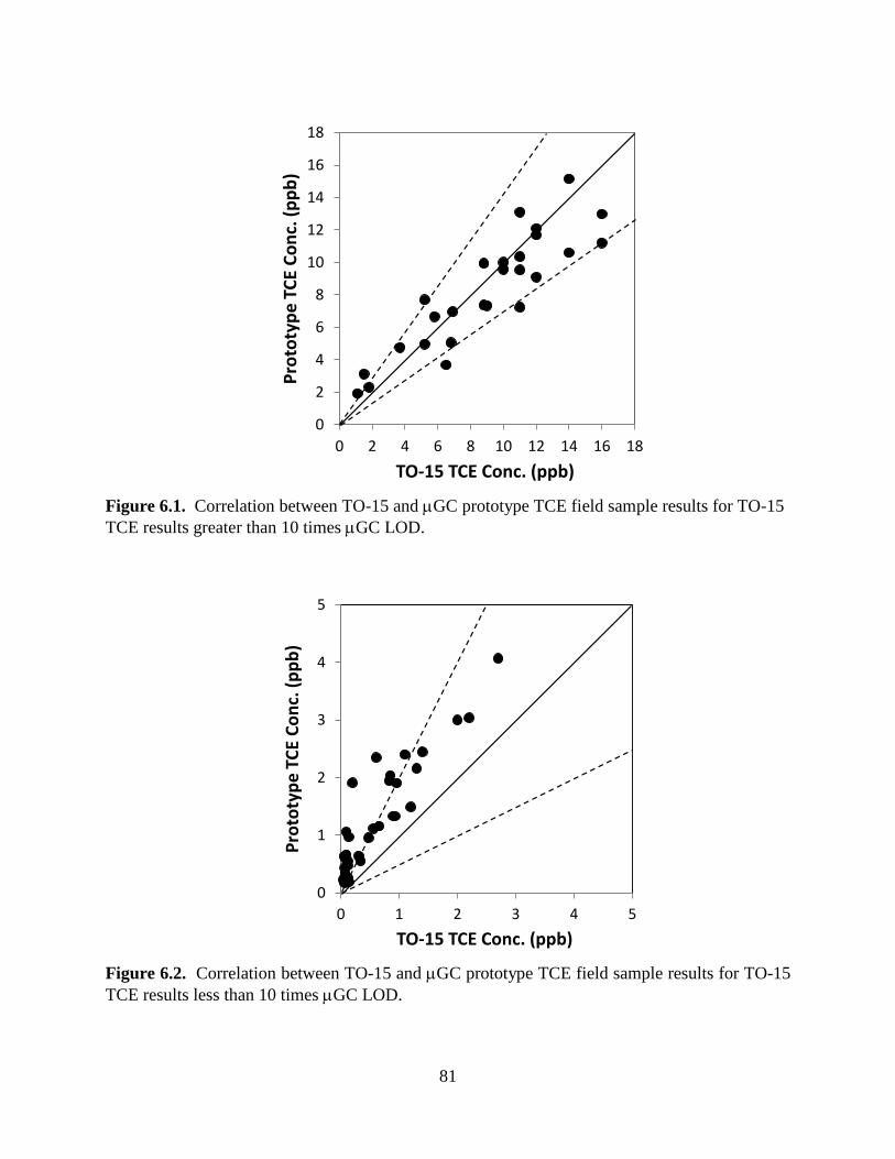
81

0

2

4

6

8

10

12

14

16

18

0 2 4 6 8 10 12 14 16 18

Prot

otyp

e TC

E Co

nc. (

ppb)

TO-15 TCE Conc. (ppb)

Figure 6.1. Correlation between TO-15 and µGC prototype TCE field sample results for TO-15 TCE results greater than 10 times µGC LOD.

0

1

2

3

4

5

0 1 2 3 4 5

Prot

otyp

e TC

E Co

nc. (

ppb)

TO-15 TCE Conc. (ppb)

Figure 6.2. Correlation between TO-15 and µGC prototype TCE field sample results for TO-15 TCE results less than 10 times µGC LOD.

82

Performance results of the less than 10 times LOD category are given above in Figure 6.2. The results show the positive bias in the lower concentration range due to co-eluting peaks as discussed in previous sections. Of the 33 sample pairs in this category, 19 samples were greater than the factor of 2 criteria, a failure rate of 58%. VOC-air (see Figure 5.34 for blank trace in chromatogram) and system blanks did not show detections of TCE. Sampler and µF heating temperatures easily eluted TCE and similar vapor pressure compounds. Co-eluting peaks contribute to the positive bias in the low concentration range as discussed above. For this lower concentration category, the µGC does not meet the performance evaluation criteria as the failure rate is greater than 20%.

6.5 QUALITATIVE PERFORMANCE OBJECTIVES Ease of Use: Experience of the field team showed that a single field technician could effectively use the µGC in a field setting. It is anticipated that improvements made during µGC commercialization would significantly improve its ease of use. Rapid reduction of raw µGC data will be improved during commercialization allowing rapid quantification of sample analyses. Field standardization and blanks were easily accomplished. Development of an automated standardization method will improved the µGC’s utility in long-term monitoring applications. Blanks using either VOC-free air or scrubbed room air were easily accomplished as well as system blanks (operation of entire analytical system without sample introduction). Rapid Site Assessment: Field experience demonstrated that rapid site assessment was possible for the portable µGC mode. The emplaced TCE source was located in 1 day, although a second day was utilized to improve data resolution and replicate sampling. Commercialization will substantially improve the ability of the µGC for rapid site assessment. Long-term Operation: The bulk of the µGC results reported were obtained over a 3-week period and µGC operation in the field was greater than 1 month. Long-term operation of the µGC was demonstrated. A continuous 48-hour automated operation of the µGC demonstrated the ability to operate it in an automated fashion without continuous operator attention. Wireless remote controlled operation of the µGC, as well as data retrieval, is anticipated to be fairly easily accomplished. The challenge will be to develop an automated standardization check method.

83

7.0 COST ASSESSMENT 7.1 COST MODEL The SPIRON µGC is a laboratory prototype and is not commercially available. Additional development is needed to bring a µGC like the SPIRON prototype to commercial production before being available for environmental applications such as VI. Thus, the cost of a potential commercial µGC for VI applications is currently unknown and can only be estimated. The potential market size of µGCs for environmental and similar applications (e.g., industrial hygiene, public health) is also not known, but it is potentially significant. In the cost model, the costs to design and fabricate the µGC prototypes would not be appropriate as it would be unrealistically high for a commercial production µGC. The potential costs of a commercial production µGC will have to be estimated. The development of a chemiresistor sensor with a greater sensitivity towards halogenated compounds (like TCE) for the chemiresistor array may improve the utility of multivariate curve resolution (MCR) for peak deconvolution (particularly if analyte peak interferences are non-halogenated). Improvements in chromatographic resolution in the separation columns would also improve analyte peak discrimination. An embedded microprocessor and data storage module within the µGC will allow for independent operation from a dedicated laptop computer and would allow wireless communication with a laptop. Data reduction (at least preliminary data reduction) could be done by the µGC microprocessor, which would facilitate the ease-of-use. Additional data reduction (e.g., MCR) could be done after data transfer to a laptop computer. Software necessary for interfacing with the µGC microprocessor (setting operating conditions externally) and for data reduction would simply need to be on a laptop that can wirelessly (or with USB) connected to the µGC. Assuming a more sensitive detector is not developed in the near-term, a front-end preconcentrator module will still be needed to achieve required detection limits. Many of the commercial µGC parts will be relatively inexpensive to produce in a mass production mode, especially the micro-fabricated components (µF, µcolumns, chemiresistor arrays). However, many of the conventional components will need to be customized for the smaller µGC size. The front-end preconcentrator module could be separate from the µGC (i.e., the µGC could be used independently since µF would be within the µGC), but be designed to interface with the µGC. Development costs will have to transfer in some fashion to the commercial µGC cost. USEPA’s Environmental Technology Verification (ETV) Program is designed to accelerate the entrance of new environmental technologies into domestic and international marketplaces. The ETV Program has been used for environmental sensors and field analytical technologies that have been successfully brought to market. This USEPA program would be appropriate for facilitating the entrance of a commercial µGC into environmental applications, and VI would a good test application.

84

A phased approach may be appropriate for the entrance of µGCs into environmental, industrial hygiene, or public health markets. Applications with simple sample matrices and higher concentrations (e.g., industrial hygiene applications) may be the suitable entry point for a commercial µGC, followed by increased sample matrix complexity and lower concentrations. Considering the uncertainties in the potential cost of the µGC (with front-end preconcentrator module), it may be reasonable to assume that the upper end potential cost might be similar to the cost of a lower cost tabletop GC. An SRI TO-14 Air Monitoring GC System costs ~$23,000 (http://www.srigc.com/2005catalog/cat22-23.htm). A range of potential µGC costs might be $5,000 to $25,000, so, for the purposes of this cost assessment, a conservative cost estimate of $20,000 will be the assumed. Experience with the SPIRON µGC prototypes during the field demonstration provided insights as to what might be needed in terms of periodic refurbishing (e.g., switch out the sorbent components of the front-end PCF module; changing the chemiresistor array) of the µGC (Note: All GCs require periodic repairs or component changes.). Refurbishing can be done by sending the device to a laboratory familiar with what is needed to refurbish the µGC, and testing can be performed to verify proper performance. However, field personnel knowledgeable of basic GC operation could conduct basic, routine refurbishing operations at the home office or lab. Experience from the demonstration showed that field replacement of the chemiresistor array was quite easy, as with the pre-trap and sampler sorbent tubes. Pumps can also be easily replaced if needed. The current replacement procedure of the µF takes considerable skill due to the current µGC design; however, design modifications should facilitate easy µF replacement. The short-term forensic-type µGC application likely will require a variety of different types of samples and have more physical handling of the µGC, which may require more frequent refurbishing. Therefore, an estimated refurbishing cost of $3,000 will be applied for every 40 days (conservative refurbishing cost estimate, may be lower) of field testing in the short-term application. Refurbishing costs will be incorporated into the daily usage fee. The long-term monitoring µGC application will likely have a more dependable and simpler type of air sample and will not require physically moving the µGC during monitoring; thus, this application will likely require less frequent refurbishing. For the long-term monitoring application, an estimated refurbishing cost of $3,000 will be applied every 4 months of field operation, and the refurbishing costs will be incorporated into the daily usage fee. A military facility could purchase the µGCs much as Hill AFB has done with their HAPSITE portable GC-MS units. Direct purchase may be the most cost-effective approach depending upon the nature and magnitude of their VI-related issues (if long-term monitoring was needed, purchase may likely be more appropriate). However, it may be more appropriate and useful to assume daily or monthly usage fees, in a similar fashion as an environmental consulting firm charges a usage fee for use of field instrumentation. The µGC is an analytical instrument, just as a table top GC is. The µGC is not like a handheld PID direct-reading instrument where only a very minimal amount of training/experience is necessary to operate it. Many environmental consulting firms have personnel with GC experience. Currently, there are also a few firms that

85

specialize in field analysis. The wireless communications nature of the µGC may also promote the involvement of environmental analytical laboratories. The traditional environmental chemistry labs may see a market in field analysis with the µGC. The daily and monthly rental charges for the SRI TO-14 Air Monitoring GC System are $175/day and $4,499/month, respectively (http://www.srigc.com/rentals.htm). The SRI rental charges can provide a rough comparison in establishing reasonable usage rates. A usage rate in the range of $175/day appears appropriate for the use of the µGC in a short-term forensic mode to assess potential indoor sources and/or VI entry locations. Assuming a 6-month usage cost recovery of the µGC purchase and an estimated refurbishing cost of $1000/30 field days of short-term application (i.e., estimated refurbishing cost is rolled into daily usage rate), a rate of $150/day will be assumed for short-term applications. However, for long-term monitoring applications, a ~$4,500/month (using short-term usage rate) or ~$4,500/month rate (SRI TO-14 Air Monitoring System) appears high for µGC usage. Long-term monitoring provides a dependable cost recovery route, so an 8-month cost recovery appears reasonable. An 8-month recovery of purchase price plus incorporating a refurbishing cost of $500/month yields a $3,000/month µGC monthly usage rate, which will be assumed for the long-term monitoring application. Calibration of the µGC prototype in the field using Tedlar® bags was problematic due to carryover of plasticizers into the front-end preconcentration module. Direct connection to the certified TCE standard compressed gas cylinder was used during the demonstration to overcome this difficulty. However, easier, accurate methods of calibration, avoiding the use of a large cumbersome compressed gas cylinder, are possible. One easy method would be to put a tee with a septum and scrubbed room air on the sample inlet line, and, using a gas-tight syringe, inject smaller known volumes of TCE standard vapor from a smaller, more manageable compressed air cylinder with a syringe sampling adaptor. A calibration curve could be generated using: 1 mL, 10 mL, and 100 mL gas-tight syringes. A 1,000-ppb certified TCE standard (lecture bottle size) with syringe sampling adaptor can provide ppb-L calibrations, with ppb concentration units obtained by incorporating sample volume. Likewise, sample blanks can be obtained using scrubbed room air, which would eliminate the need for a large VOC-free compressed air cylinder. System blanks (PCF module operation without an air sample) are also useful. The cost assessment will assume this easier and more cost-effective approach to calibration and blanks. Simple cost models for use of a commercially produced µGC for two VI applications are given below. One is a short-term forensic-type VI application and the other is a longer-term monitoring VI application. The short-term application involves mobilization activities in which the µGC is calibrated prior to field activities, in addition to system and VOC-free air blanks. It is assumed that the homeowner is asked to remove potential indoor VOC sources from the house prior to the site visit (with the understanding that the homeowner will likely not remove all potential VOC sources). The short-term application involves being at the home during two field days. Any additional potential indoor VOC will be identified and removed from the home during the first field day based upon the µGC results and observations. The second field day will focus on any remaining potential indoor TCE sources and on the potential for VI where induced negative

86

pressure within the house may be used to assist in determination of whether the home is impacted by VI. Other site-specific VI investigations can be accomplished as deemed necessary. Analysis of one each of TCE standardization gas sample and system and VOC-free air blank can be conducted each day. In the short-term µGC VI application, the µGC is being moved to take samples around the home, thus potentially exposing the µGC to a variety of conditions. Therefore, a shorter time period between µGC refurbishing is assumed (every 40 field days; could be substantially longer, but 40 days is assumed for usage rate estimation). The long-term application involves mobilization activities in which the µGC is calibrated prior to field activities, in addition to system and VOC-free air blanks. Removal of substantial VOC (including TCE) indoor air sources prior to long-term monitoring is assumed. It is also assumed that samples are taken from one location for a period of 3 months (for long-term exposure monitoring or remedial system performance evaluation). It is expected that samples will have relatively low concentrations for TCE and other VOCs (whereas the shorter-term forensic sampling can see a wide variety of sample types). Standardization gas checks and VOC-free air blanks will be taken four times during field operations (once during system setup, two intermittent, and once at system takedown), so a total of 4 visits to the house are anticipated over the 3-month period. It is assumed that the house has a wireless internet router and internet connection that can be used. The µGC can operate in automatic mode as well as by external commands (wireless). It is anticipated that the µGC will analyze 12 indoor air samples per day (greater sample density may be of little value). Additionally, the µGC can run several “system” blanks per day where automatic cleaning procedures are used on the front-end PCF module and an “injection” is made by the PCF module without sampling room air. The results of these simple cost models for the short-term and long-term applications are given below in Table 7.1 and 7.2, respectively.

87

Table 7.1. Cost Model for short-term forensic-type application of µGC for VI (assume two on-site days with removal of items emitting potential interferences before first day and additional items prior to second day).

Cost Element Data Tracked / Information Assessed Estimated Costs

Commercial µGC Unit Cost Estimate (daily

usage rate)

• Cost of roughly comparable commercial unit

• Potential commercial µGC cost range

• Conservative cost estimate

• Daily usage rate incorporating cost recovery and refurbishing cost estimates (including certified TCE std tank)

SRI TO-14 Air Monitoring GC ~$23,000

Pot. Commercial µGC cost range

~$5,000 to ~$25,000

Assumed conservative cost µGC estimate ~$20,000

Assumes 6 month usage cost recovery & $1,000 refurbishing cost/30 field days

$150/day usage rate

Assessment of Individual

House using µGC

• Personnel required and associated labor (includes mob/demob)

• µGC operation costs

• Field laptop computer usage fee

• Vehicle usage

• Miscellaneous costs

Lab field tech., 30 h $2,100

Project engineer, 3 h $300

µGC, 2 days $300

Field Laptop computer, 2 days, N/A

N/A

Vehicle, 2 days $120

Miscellaneous, N/A N/A

Reporting • Reporting requirements can vary

• Assume minimal reporting requirements

• Minimal turnaround time since do not have to wait for lab results

Lab field tech., 8 h

Project engineer, 2 h

$560

$200

Total Cost Estimate

$3,580

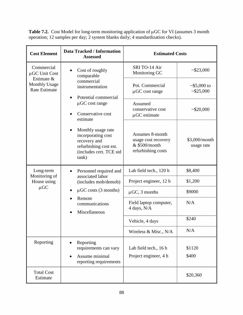
88

Table 7.2. Cost Model for long-term monitoring application of µGC for VI (assumes 3 month operation; 12 samples per day; 2 system blanks daily; 4 standardization checks).

Cost Element Data Tracked / Information Assessed Estimated Costs

Commercial µGC Unit Cost

Estimate & Monthly Usage Rate Estimate

• Cost of roughly comparable commercial instrumentation

• Potential commercial µGC cost range

• Conservative cost estimate

• Monthly usage rate incorporating cost recovery and refurbishing cost est. (includes cert. TCE std tank)

SRI TO-14 Air Monitoring GC ~$23,000

Pot. Commercial µGC cost range

~$5,000 to ~$25,000

Assumed conservative cost µGC estimate

~$20,000

Assumes 8-month usage cost recovery & $500/month refurbishing costs

$3,000/month usage rate

Long-term Monitoring of House using

µGC

• Personnel required and associated labor (includes mob/demob)

• µGC costs (3 months)

• Remote communications

• Miscellaneous

Lab field tech., 120 h $8,400

Project engineer, 12 h $1,200

µGC, 3 months $9000

Field laptop computer, 4 days, N/A

N/A

Vehicle, 4 days $240

Wireless & Misc., N/A N/A

Reporting • Reporting requirements can vary

• Assume minimal reporting requirements

Lab field tech., 16 h

Project engineer, 4 h

$1120

$400

Total Cost Estimate

$20,360

89

7.2 COST DRIVERS A key cost driver in selecting µGC technology (commercial production units) is the ability to accurately determine TCE concentrations in indoor air samples at relevant low concentrations with common indoor air VOCs present. This is the practical requirement that needs to be met for the application of µGC technology to VI applications to be cost-effective. Although a challenging task, this demonstration has shown that sufficient accuracy can be achieved for TCE due to indoor air VI in the several ppb range and higher. It is reasonable to expect that with further modifications/optimization the level at which TCE in indoor air can be accurately determined would be lowered by at least an order of magnitude. Examination of cost-effectiveness for commercialized µGC technology may be application-specific (see Section 7.3 Cost Analysis below). For a long-term monitoring application, µGC may be particularly cost effective. The need for long-term monitoring may be driven by: 1) desire of the impacted household to have it implemented; 2) requirement by regulatory agency; 3) and/or need to monitor the effectiveness of the VI abatement measures. There is currently no easily implemented, commonly available technology to conduct long-term monitoring such as provided by the µGC. Other portable GCs or the HAPSITE GC/MS would require large carrier gas tanks, which would be very cumbersome in a household setting. Hill AFB has found the HAPSITE GC/MS to be very useful for short-term, forensic-type applications. Commercial production µGC technology would lower the upfront capital costs for a military facility compared with the HAPSITE GC/MS, as well as reduce instrument downtime (most repairs or refurbishing tasks could be performed by field lab personnel). The HAPSITE GC/MS is not easily feasible for environmental consulting firms to purchase because it would be difficult to recover the capital costs and the servicing costs. A lower cost and more robust commercial production µGC would be much easier for environmental consulting firms (or environmental analytical laboratories) to purchase and recover the unit cost and maintain its operation. A likely scenario is to have the environmental consulting industry and/or the environmental analytical lab industry (it could reasonably be a partnership between the two industries) take the lead on field VOC analysis for indoor air VI. The environmental analytical chemistry labs may find the field analysis market advantageous to enter, certainly the involvement of those trained in analytical chemistry would improve data quality regardless of what field analytical methodology was used (with ubiquitous Internet connections, it would not be necessary to have on-site presence of analytical chemistry trained personnel).

90

7.3 COST ANALYSIS The current approach for indoor air VI investigations is to collect canister samples, followed by shipment to an environmental air analysis laboratory for TO-15 GC/MS analysis. A difficulty in making a direct comparison between using the µGC and using traditional TO-15 is that data density cannot be matched by traditional TO-15 (except at extraordinary cost). An advantage of TO-15 analysis is that compounds can be determined for a larger analyte list and concentrations can be determined with greater confidence. There are situations where traditional TO-15 is desirable and preferred by the regulatory agency. Considering that the two methods are so different, it is reasonable to expect that, even if µGC technology were used, then a minor amount of TO-15 confirmatory sampling might be appropriate. Long-term monitoring using TO-15 would be extremely invasive to the homeowner requiring a level of home access that is logistically unrealistic. In the short-term forensic-type investigation, the TO-15 is also problematic since results are not known for days if not weeks after the sampling event. This significantly reduces the results’ value. Hill AFB has overcome this difficulty by using the HAPSITE GC/MS (in much the same fashion as the µGC). The cost comparisons will use TO-15 and assume a short analyte list (five analytes max). The short-term forensic-type application will use six canisters per day with 3-day sample analysis turnaround times from the laboratory and 2 days spent on site. The resulting cost estimate for the short-term TO-15 approach is given in Table 7.3. The TO-15 cost estimate of $7,820 compares with $3,580 of the short-term µGC approach. Although not directly comparable, the TO-15 approach is $652/sample and the µGC approach (assuming 20 samples total) is $179/sample. The short-term TO-15 approach is largely impractical in terms of information gained since concentrations are not known during the investigation in the home; whereas the µGC approach provides near-real time concentrations that can dictate the investigation approach used within the home. Additionally, more samples can be taken and analyzed using the µGC approach. The cost comparison for the long-term monitoring type application will use an automated canister sampler capable of filling seven canisters with one canister taken per day (assumed for meeting monitoring objectives). This approach requires access to the home once per week, minimizing the intrusive nature of the investigation. The cost estimate for the long-term TO-15 approach is given in Table 7.4 and is $45,140, compared to the $20,360 cost estimate for the long-term monitoring µGC approach. The TO-15 approach only provides one sample per day, which does not provide information on changes in concentration within a 24-hour time period. The TO-15 approach provides concentrations for 120 samples whereas the µGC approach provides concentrations for 1,080 samples over the 3-month time period. Although not directly comparable, the TO-15 approach costs $376/sample and the µGC approach costs $19/sample. The µGC provides a cost and information advantage over the TO-15 approach when used for long-term monitoring. If a lower sampling density for TO-15 was adequate to meet sampling objectives, the TO-15 approach may be cost competitive.

91

Table 7.3. Cost Model for short-term forensic-type application for VI using conventional Summa canisters for TO-15 (assumes 2-day operation; 6 samples per day).

Cost Element Estimated Costs

Short-term Forensic Application using

ΤΟ−15

Field technician, 24 h $1,440

Project engineer, 12 h $1,200

TO-15 analyses, 12 total, short analyte list, 3-day turn around

$3,240

Vehicle, 2 days $120

Shipping $300

Reporting Field technician, 12 h

Project engineer, 8 h

$720

$800

Total Cost Estimate $7,820

92

Table 7.4. Cost Model for long-term monitoring application for VI using conventional Summa canisters for TO-15 (assumes 3 month operation; 1 sample per day).

Cost Element Estimated Costs

Long-term Monitoring of House using ΤΟ−15

Field technician, 150 h $9,000

Project engineer, 20 h $2,000

Canister sampler rental, 3 months

$6000

TO-15 analyses, 120 total, short analyte list, normal turn around (no sampling orifice assembly needed)

$24,000

Vehicle, 13 days $780

Shipping $1,600

Reporting Field technician, 16 h

Project engineer, 8 h

$960

$800

Total Cost Estimate $45,140

93

8.0 IMPLEMENTATION ISSUES A µGC prototype was used in this demonstration project for the detection of TCE in indoor air for VI applications. The µGC prototype was able to detect TCE due to VI in indoor air, with more accurate values obtained at the higher TCE levels and less accurate (positive bias) at the lower levels. Continued development is needed to improve the accuracy at the lower levels for routine application of µGC technology to VI applications. Although challenging, attaining dependable analytical accuracy in the lower levels should be achievable (increased chromatographic resolution, detector and data reduction modifications). The foremost, and overriding, implementation issue is that a fully developed, commercially available µGC that can be used in low concentration environmental applications such as VI is not currently available. Some µGCs (or partial µGCs) are available for petrochemical and natural gas industrial applications where quite high concentrations are the norm. The current project shows that it should be possible to produce a commercially available µGC for low concentration environmental applications and will hopefully encourage developments towards that goal. USEPA is currently in the process of revising its 2002 Draft Subsurface Vapor Intrusion Guidance with a final version to be released by November 2012 (USEPA, 2010a). Field data sets obtained since the 2002 Draft Subsurface Vapor Intrusion Guidance has shown that the extent of temporal and spatial variation of indoor VOC concentrations can differ greatly. USEPA (2010a) indicated that an increased emphasis on indoor air sampling will be included in the final version of the VI guidance. The final VI guidance will likely increase field analysis of indoor air samples of a temporal and spatial nature, for which a fully developed, commercially available µGC could be ideally suited. Generally taking USEPA guidance into consideration, state regulatory agencies determine VI investigation requirements for their states. The approach of state regulatory agencies towards VI has been evolving and is expected to continue to evolve as more experience is gained. Therefore, the adoption of VI investigation approaches reliant upon field analysis technologies such as the µGC may be largely driven by the guidance and expectations of state regulatory agencies. The prototype µGC was not capable of rapid data reduction in the field as currently configured. Microprocessor development is needed to store and process data as it is being gathered. Additionally, the development of easy-to-use software for interfacing with the µGC via remote communications, including robust data reduction, would facilitate implementation of µGC technology by reducing manpower requirements. Chemiresistor array stability also remains an issue. The results from this demonstration showed that, after some initial changes in sensor sensitivity, they tended to become stable (unknown for how long). These chemiresistor array results were encouraging. The chemiresistor array would benefit from the development of a sensor that was particularly sensitive to chlorinated compounds (such as TCE) to aid in the use of MCR to differentiate TCE from non-chlorinated compounds, which are likely causing interference. The relative response patterns for TCE and some of the common non-chlorinated compounds that elute near TCE are similar to each other,

94

so greater differentiation would be beneficial. The chemiresistor arrays are coated by hand, each individually; mass production will likely lead to more uniformity in chemiresistor array performance. Improvements in separation of compounds eluting near TCE would help offset the problem of similar response patterns and could be achieved by further optimization of stationary phase thickness, use of a different stationary phase, or cooling of the µcolumns to increase retention (and resolution) in the critical early part of the chromatograms. Another potential implementation issue since field demonstration is that the Hill AFB MAL has lowered from 2.3 ppb to 0.38 ppb, which will require field instrumentation to have sufficient accuracy to a lower level.

95

9.0 REFERENCES Amrhein, M., B. Srinivasan, D. Bonvin, and M.M. Schumacher, 1996, On the Rank Deficiency

and Rank Augmentation of the Spectral Measurement Matrix, Chemom. Intell. Lab. Syst., 33:17– 33.

ATSDR, 1997, Toxicological Profile for Trichloroethylene, Agency for Toxic Substances and

Disease Registry, www.atsdr.cdc.gov/toxprofiles/tp19.html. Bohrer, F.I., E. Covington, Ç. Kurdak and E.T. Zellers, 2011, Characterization of Dense Arrays

of Chemiresistor Vapor Sensors with Submicrometer Features and Patterned Nanoparticle Interface Layers, Anal. Chem., 83(10):3687-3695.

Cai, Q-Y. and E.T. Zellers, 2002, Dual-chemiresistor GC Detector Employing Monolayer-

protected Metal Nanocluster Interfaces, Anal. Chem., 71:3877-3886. Carneiro, R.L., J.W.B. Braga, R.J. Poppi and R. Tauler, 2008, Multivariate Curve Resolution of

pH Gradient Flow Injection Mixture Analysis with Correction of the Schlieren Effect, Analyst, 133:774–783.

CDPHE, 2005, Trichloroethylene Health Effects Fact Sheet, Colorado Department of Public

Health and Environment, www.cdphe.state.co.us/HM/tcef.pdf. CEPA, 2005, Use of California Human Health Screening Levels (CHHSLs) in Evaluation of

Contaminated Properties, California Environmental Protection Agency, http://www.calepa.ca.gov/Brownfields/documents/2005/CHHSLsGuide.pdf.

Chang, H., S.K. Kim, T. Sukaew, F. Bohrer, and E.T. Zellers, 2010, A Microfabricated Gas

Chromatograph for Sub-ppb Determinations of TCE in Vapor Intrusion Investigations, Proc. Solid-State Sensors, Actuators, and Microsystems Workshop, Hilton Head, South Carolina, pp. 278-281.

Chang, H., S.K. Kim, T. Sukaew, F.I. Bohrer, and E.T. Zellers, 2010, A Microfabricated Gas

Chromatograph for Parts-Per-Trillion Determinations of VOCs in Vapor Intrusion Investigations Proc. of Eurosensors XXIV, Linz, Austria, 2010, Procedia Engineering, 5:973-976.

de Juan, A. and R. Tauler, 2007, Factor Analysis of Hyphenated Chromatographic Data:

Exploration, Resolution and Quantification of Multicomponent Systems, J. Chromatog. A, 1158:184–195.

Dettmer, K. and W. Engewald, 2002, Adsorbent Materials Commonly Used in Air Analysis for

Adsorptive Enrichment and Thermal Desorption of Volatile Organic Compounds, Anal. Bioanal. Chem., 373:490-500.

DoD, 2009, DoD Vapor Intrusion Handbook, http://www.clu-in.org/download/char/

96

dodvihdbk200901.pdf. Eklund, B.M. and M.A. Simon, 2007, Concentration of Tetrachloroethylene in Indoor Air at a

Former Dry Cleaner Facility as a Function of Subsurface Contamination: A Case Study, J. Air and Waste Manag. Assoc., 57(6):753-760.

Gampp, H., M. Maeder,; C.J. Meyer, and A.D. Zuberbuehier, 1985, Calculation of Equilibrium

Constants from Multiwavelength Spectroscopic Data--III:: Model-free Analysis of Spectrophotometric and ESR Titrations, Talanta, 32:1133-1139.

Gong, Y., I. Eom, D. Lou, D. Hein, and J. Pawliszyn, 2008, Development and Application of a

Needle Trap Device for Time-Weighted Average Diffusive Sampling, Analytical Chemistry, 80:7275-7282.

Gorder, K. A. and E. M. Dettenmaier, 2011, Portable GC/MS Methods to Evaluate Sources of

cVOC Contamination in Indoor Air, Ground Water Monitoring and Remediation, 31:113-119.

Groves, W.A. and E. T. Zellers, 1996, Investigation of Organic Vapor Losses to Condensed

Water Vapor in Tedlar Bags Used for Exhaled Breath Sampling, Am. Ind. Hyg. Assoc. J., 57, 257-263.

Hoggard, J. C., J.H. Wahl, R.E. Synovec, G.M. Mong and C.G. Fraga, 2010, Impurity Profiling

of a Chemical Weapon Precursor for Possible Forensic Signatures by Comprehensive Two-Dimensional Gas Chromatography/Mass Spectrometry and Chemometrics, Anal. Chem., 82:689–698.

Hoggard, J.C., W.C. Siegler and R.E. Synovec, 2009, Toward Automated Peak Resolution in

Complete GC× GC–TOFMS Chromatograms by PARAFAC, J. Chem., 23:421–431. Howard P.H. and W.M. Meylan, Eds., 1997, Handbook of Physical Properties of Organic

Chemicals, CRC Press: Boca Raton, FL. Hsieh, M.-D. and E.T. Zellers, 2004, Limits of Recognition for Simple Vapor Mixtures

Determined with a Microsensor Array, Anal. Chem., 76:1885-1895. IST, 2007, Phase I Investigation of Advanced Gas Sensor Technologies Applicable to Hill Air

Force Base Indoor Air Intrusion Problems, Prepared by Integrated Science & Technology, Inc. for 75th CEV/EM, Hill AFB, Utah.

ITRC, 2007, Vapor Intrusion Pathway: A Practical Guideline, VI-1, Washington, DC: Interstate

Technology & Regulatory Council, Vapor Intrusion Team. www.itrcweb.org Jaumot, J. and R. Tauler, 2010, MCR-BANDS: A User Friendly MATLAB Program for the

Evaluation of Rotation Ambiguities in Multivariate Curve Resolution, Chemom. Intell. Lab. Syst., 103:96-107.

97

Jin, C., P. Kurzawski, A. Hierlemann and E.T. Zellers, 2008, Evaluation of Multi-Transducer

Arrays for the Determination of Organic Vapor Mixtures, Anal. Chem., 80:227-236. Jin, C. and E.T. Zellers, 2008, “Limits of Recognition for Binary and Ternary Vapor Mixtures

Determined with Multi-Transducer Arrays, Anal. Chem., 80:7283-7293. Jin, C. and E.T. Zellers, 2009, Chemometric Analysis of Gas Chromatographic Peaks Measured

with a Microsensor Array: Methodology and Performance Assessment, Sens. Actuators. B, 139:548-556.

Kauppinen, J.K., D.J. Moffatt, H.H. Mantsch and D.G.Cameron, 1981, Fourier Self-

Deconvolution: A Method for Resolving Intrinsically Overlapped Bands, Appl. Spectrosc., 35:271-276.

Kim, H.A. Astle, K. Najafi, L.P. Bernal and P.D. Washabaugh, 2007, IEEE 20th Int’l Conf.

Microelectromechanical System (MEMS): Kobe, Japan, January 21-25 2007, pp 131-134. Kim, S.K., H. Chang and E.T. Zellers, 2011, Microfabricated Gas Chromatograph for the

Selective Determination of Trichloroethylene Vapor at Sub-Parts-Per-Billion Concentrations in Complex Mixtures, Analytical Chemistry, 83(18):7198-7206.

Kim, S.K., H. Chang, J. Bryant, D.R. Burris and E.T. Zellers, In Review (a), Microfabricated Gas

Chromatograph for On-Site Determinations TCE Arising from Vapor Intrusion Studies, Part I: Field Evaluation, Environ. Sci. Technol., submitted.

Kim, S.K., D.R. Burris, H. Chang, J. Bryant-Genevier, K.A. Gorder, E.M. Dettenmaier, and E.T.

Zellers, In Review (b), Microfabricated Gas Chromatograph for On-Site Determinations TCE Arising from Vapor Intrusion Studies, Part II: Temporal/Spatial Monitoring, Environ. Sci. Technol., submitted.

Kim, S.K. and E.T. Zellers, In Preparation, Multivariate Curve Resolution of Partially Resolved

Analytes Measured with a Micro-Scale Gas Chromatograph with a Microsensor Array Detector.

Kowalski, B.R. and M.A. Sharaf, 1982, Quantitative Resolution of Fused Chromatographic

Peaks in Gas Chromatography/Mass Spectrometry, Anal. Chem., 54:1291-1296. Kuehster, T., D. Folkes, and E. Wannamaker, 2004, Seasonal Variation of Observed Indoor Air

Concentrations due to Vapor Intrusion (Redfield Site, Colorado), presentation at the Midwestern States Risk Assessment Symposium, Indianapolis, IN, August 26, 2004, www.envirogroup.com/publications.php.

Kurtz, J.P. and D.J. Folkes, 2002, Background Concentrations of Selected Chlorinated

Hydrocarbons in Residential Indoor Air, in the Proceedings of the 9th International

98

Conference on Indoor Air Quality and Climate, International Academy of Indoor Air Sciences, Monterey, CA, June 30 – July 5, 2002, www.envirogroup.com/ publications.php.

Lin, C.-J., 2007, Projected Gradient Methods for Nonnegative Matrix Factorization, Neural

Computation, 19:2756-2779. Lozano, V.A., R. Tauler, G.A. Ibanez and A.C. Olivieri, 2009, Standard Addition Analysis of

Fluoroquinolones in Human Serum in the Presence of the Interferent Salicylate Using Lanthanide-sensitized Excitation-time Decay Luminescence Data and Multivariate Curve Resolution, Talanta, 77:1715–1723.

Lu, C.-J. and E.T. Zellers, 2001, A Dual-Adsorbent Preconcentrator for a Portable Indoor VOC

Microsensor System, Analytical Chemistry, 73:3449-3457. Lu, C.-J. and E.T. Zellers, 2002, Multi-Adsorbent Preconcentrator/Focusing Module for

Portable-GC/Microsensor Array Analysis of Complex Vapor Mixtures, The Analyst, 127:1061-1068.

Lu, C.-J., W.H. Steinecker, W. Tian, M.C. Oborny, J.M. Nichols, N. Agah, J.A. Potkay, H.K.L.

Chan, J. Driscoll, R.D. Sacks, K.D. Wise, S.W. Pang, and E.T. Zellers, 2005, First-Generation Hybrid MEMS Gas Chromatograph, Lab on a Chip, 5:1123-1131.

Lu, C.-J., J.C. Jin, and E.T. Zellers, 2006, Chamber Evaluation of a Portable GC with Tunable

Retention and Microsensor-Array Detection for Indoor Air Quality Monitoring, J. Environ. Monit., 8:270-278.

Lu, C.-J., J.R.Whiting, D.Sacks and E.T. Zellers, 2003, Portable Gas Chromatograph with

Tunable Retention and Sensor Array Detection for Determination of Complex Vapor Mixtures, Anal. Chem., 75:1400-1409.

Manne, R., 1995, On the Resolution Problem in Hyphenated Chromatography, Chemom. Intell.

Lab. Syst., 27:89-93. Massachusetts Toxics Use Reduction Institute, 2008, Massachusetts Chemical Fact Sheet:

Trichloroethylene, www.turi.org/content/download/1517/.../TURI%20FS%2008537-final.pdf.

Maeder, M., 1987, Evolving Factor Analysis for the Resolution of Overlapping Chromatographic

Peaks, Anal. Chem., 59:527–530. McDonald, G.J. and W.E. Wertz, 2007, PCE, TCE, and TCA Vapors in Subslab Soil Gas and

Indoor Air: A Case Study in Upstate New York, Ground Water Monitoring and Remediation, 27(4):86-92.

99

Park, J., W.A. Groves and E.T. Zellers, 1999, Vapor Recognition with Small Arrays of Polymer-coated Microsensors: A Comprehensive Analysis, Anal. Chem., 71:3877-3886.

Rairigh, D.J., G.A. Warnell,, C. Xu,, E.T. Zellers and A.J. Mason, 2009, CMOS Baseline

Tracking and Cancellation Instrumentation for Nanoparticle-Coated Chemiresistors, IEEE Trans. Biomedical Circuits and Systems, 3:267-276.

Reidy, S., G. Lambertus, J. Reece and R. Sacks, 2006, High-Performance, Static-Coated Silicon

Microfabricated Columns for Gas Chromatography, Anal. Chem., 78, 2623-2630. Sanchez, J.M. and R.D. Sacks, 2003, Online Multibed Sorption Trap and Injector for the GC

Analysis of Organic vapors in Large-Volume Air Samples, Anal. Chem., 75:978-985. Steinecker, W.H., M.P. Rowe, and E.T. Zellers, 2007, Model of Vapor-Induced Resistivity

Changes in Gold-Thiolate Monolayer-Protected Nanoparticle Sensor Films, Analytical Chemistry, 79:4977-4986.

Steinecker, W.H., S.K. Kim, F.I. Bohrer, L.Farina, Ç. Kurdak, and E.T.Zellers, 2011, Electron-

Beam Patterned Monolayer-Protected Gold Nanoparticle Interface Layers on a Chemiresistor Vapor Sensor Array, IEEE Sens. J., 11:469-480.

Sukaew, T., H. Chang, G. Serrano and E.T. Zellers, 2011, Multi-Stage Preconcentrator/Focuser

Module Designed to Enable Trace Level Determinations of Trichloroethylene in Indoor Air with a Microfabricated Gas Chromatograph, Analyst, 136:1664-1674.

Szymanska, E., M. J. Markuszewski, Y. Vander Heyden and R. Kaliszan, 2009, Efficient

Recovery of Electrophoretic Profiles of Nucleoside Metabolites from Urine Samples by Multivariate Curve Resolution, Electrophoresis, 30:3573–3581.

Tauler, R., A.K. Smilde, and B.J.Kowalski, 1995, Selectivity, Local Rank, Three‐way Data

Analysis and Ambiguity in Multivariate Curve Resolution, J. Chemom., 9:31– 58. Tauler, R., 1995, Multivariate Curve Resolution Applied to Second Order Data, Chemom. Intell.

Lab. Syst., 30:133– 146. Tian, W., W.K.L. Chan, C. Lu, S.W. Pang, and E.T. Zellers, 2005, Multiple-Stage

Microfabricated Preconcentrator-Focuser for Micro Gas Chromatography System, J. of Microelectromechanical Systems, 14:498-507.

Tian, W., S.W. Pang, C. Lu, and E.T. Zellers, 2003, Microfabricated Preconcentrator-Focuser for

a Microscale Gas Chromatograph, J. of Microelectromechanical Systems, 12:264-272. USEPA, 2002, OSWER Draft Guidance for Evaluating the Vapor Intrusion to Indoor Air

Pathway from Groundwater and Soils (Subsurface Vapor Intrusion Guidance), EPA-D-02-004.

100

USEPA, 2003, Memorandum on Human Health Toxicity Values in Superfund Risk Assessments, OSWER Directive 9285.7-53.

USEPA, 2005, Trichloroethylene Inhalation Toxicity Values and Corresponding Risk Based

Indoor Air Concentrations, Region 8 Technical Publication, January 26, 2005, www.cleanairathens.org/assets/pdfs/EPA9_TCE_Toxicity.pdf.

USEPA, 2009a, Memorandum on Interim Recommended Trichloroethylene (TCE) Toxicity

Values to Assess Human Health Risk and Recommendations for the Vapor Intrusion Pathway Analysis, from Susan Parker Bodine, Assistant Administrator (OSWER), January 15, 2009.

USEPA, 2009b, Memorandum on Withdrawal of the January 15, 2009, OSWER Guidance

Entitled “Interim Recommended Trichloroethylene (TCE) Toxicity Values to Assess Human Health Risk and Recommendations for the Vapor Intrusion Pathway Analysis,” from Barry N. Breen, Acting Assistant Administrator (OSWER), April 9, 2009.

USEPA, 2010, Regions 3, 6 and 9 Risk-Based Regional Screening Levels;

www.epa.gov/reg3hwmd/risk/human/rb-concentration_table/Generic_Tables/pdf/ master_sl_table_bwrun_NOVEMBER2010.pdf.

USEPA, 2010, OSWER Review Document regarding the 2002 Draft Subsurface Vapor Intrusion

Guidance, www.epa.gov/oswer/vaporintrusion/documents/ review_of_2002_draft_vi_guidance_final.pdf

USEPA, 2012, Regional Screen Level (RSL) Residential Air Supporting Table, April, 2012; www.epa.gov/reg3hwmd/risk/human/rb-concentration_table/Generic_Tables/pdf/resair_sl_table_run_MAY2012.pdf.

Whiting, J.J. and R.D. Sacks, 2006, Evaluation of Split/Splitless Operation and Rapid Heating of

a Multi-Bed Sorption Trap used for Gas Chromatography Analysis of Large Volume Air Samples, J. Sep. Sci., 29:218-227.

Woodka, M.D., B.S. Brunschwig and N.S. Lewis, 2007, Use of Spatiotemporal Response

Information from Sorption-based Sensor Arrays to Identify and Quantify the Composition of Analyte Mixtures, Langmuir, 23:13232-13241.

Wu, C. and J. Schaum, 2000, Exposure Assessment of Trichloroethylene, Environ. Health

Perspectives, 108(Supp. 2):359-363. Xu, W., K. Chen, D. Liang and W. Chew, 2009, Hierarchical Band-target Entropy Minimization

Curve Resolution and Pearson VII Curve-fitting Analysis of Cellular Protein Infrared Imaging Spectra, Anal. Biochem., 387:42–53.

101

Zellers, E.T., S.A. Batterman, M. Han, and S. J.Patrash, 1995, Optimal Coating Selection for the Analysis of Organic Vapor Mixtures with Polymer-coated Surface Acoustic Wave Sensor Arrays, Anal. Chem., 67:1092-1106.

Zhong, Q,, W.H. Steinecker, and E.T. Zellers, 2009, Characterization of a High-Performance

Portable GC with a Chemiresistor Array Detector, The Analyst, 134:283-293. Zhong, Q, R.A. Veeneman, W.H. Steinecker, C. Jia, S.A. Batterman, and E.T. Zellers, 2007,

Rapid Determination of ETS Markers with a Prototype Field-Portable GC Employing a Microsensor Array Detector, J. Environ. Monitor., 9:440-448.

102

APPENDICES

Appendix A: Points of Contact

POINT OF CONTACT

Name

ORGANIZATION Name

Address

Phone Fax

E-mail Role in Project

H. James Reisinger

IST 4940 Cowan Rd.

Acworth, GA 30101

(770) 425-3080 ext. 102 (770) 425-0295 fax istatlanta@aol.com

Principal Investigator (PI)

David R. Burris, Ph.D.

IST 228 Harrison Ave., #102 Panama City, FL 32401

(850) 522-8005 (850) 522-8060 fax

istpanamacity@aol.com

Co-PI; U of MI Liaison;

Demonstration Coordinator

Edward T. Zellers, Ph.D.

University of Michigan Depart. of Environ.

Health Sciences School of Public Health

Room M6543 109 S. Observatory St. Ann Arbor, MI 48109

(734) 936-0766 (734) 763-8095 fax ezellers@umich.edu

Development, Fabrication and Testing of µGC

Kyle Gorder 75 CEG/CEVR, Environmental

Restoration Branch 7274 Wardleigh Road Hill AFB, UT 84056

(801) 775-2559 kyle.gorder@hill.af.mil

Hill AFB POC; Demonstration

Facilitator

Robert E. Hinchee, Ph.D.,

P.E.

IST 1509 Coastal Highway

Panacea, FL 32346

(850) 984-4460 (850) 984-4467 fax rob@hinchee.org

Advisor; Initial Project PI