1

Field Oriented Control of Induction Motors with Core Loss

Jorge Rivera, Christian Mora-Soto, Alberto De La Mora, Stefano Di Gennaro, Juan Raygoza

Abstract A novel nonlinear affine model for the induction motor with core loss is developed in the well known ( )d q reference frame. The core is represented with a resistance in parallel with the magnetization

inductance. Then, an optimal rotor flux modulus is calculated such that, the power loss due to stator, rotor and core resistances is minimized, and as a consequence the motor efficiency is raised; therefore this flux modulus is forced to be tracked by the induction motor along with a desired rotor velocity by means of a field oriented controller. A simulation study is carried on, where the superior performance of the proposed controller is put in evidence when compared to the same controller when not taking into account an optimal flux modulus.

1. Introduction

Induction motors are widely used in industrial applications due to its simple mechanical construction, low service requirements and lower cost with respect to DC motors that are also widely used in industry. On the other hand, induction motors constitute a classical test bench in the control theory field due to the fact that represents a coupled MIMO nonlinear system, resulting in a challenging control problem. Starting from the pioneering work of Blaschke [1], field oriented control has been a classical control technique for induction motors. This control technique consists in applying a nonlinear state transformation and feedback for asymptotic decoupling of the rotor velocity and rotor flux modulus along with PI controls loops for each channel [2]. Recently, various control approaches have been studied for performance improvement. Active research area include adaptive I/O feedback linearization [3], adaptive backstepping [4], [5], sliding mode [6], [7], [8], [9], [10], artificial neural networks [11], [12], among others. It is worth to mention that all of these works are based on a mathematical induction motor model that does not considers power core losses, implying that the induction motor presents a low efficiency performance. In order to achieve a high efficiency in power consumption one must consider the power core losses, and then to design a control law under conditions that results when minimizing the power core and copper losses. Nowadays, this results an important problem since in the last two decades has been a global need for better use of electric energy and considering that induction motors are the major electric energy consumers in industry, therefore, the efficiency improvement in induction motors has also been another active research area. In the effort of maximizing the motor efficiency, the main works are towards to a better physical design of the motor [13], [14], [15] and to improve its performance [16], [17], [18] by means of closed-loop controllers. In the case of closed-loop controller designs one must consider power core loss, where the main two approaches are the loss-model based and power-measure-based methods. In the first method, the losses are defined in terms of induction motors variables that are minimized by selecting a flux level that minimizes these losses using what is best known as loss model based controller [19], [20]. In the second approach, also known as search controllers, the flux is decreased until the electrical input power settles down to the lowest value for a given torque and velocity [21], [22], [23]. It is clear that the first method yields to better results since is based on mathematical analysis, while the second one can not be reliable since is realized by means of a experimental method. With respect to loss model based controllers, there are two main approaches for modeling the core, as a parallel resistance or as a series one. In the model with a parallel resistance, this is fixed in parallel with the magnetization inductance, increasing the four electrical dynamical equations to six

2

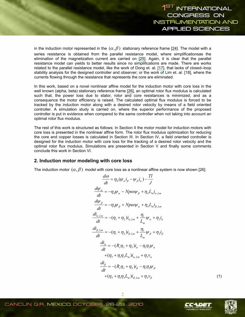
in the induction motor represented in the ( ) stationary reference frame [24]. The model with a

series resistance is obtained from the parallel resistance model, where simplificationsas the elimination of the magnetization current are carried on [25]. Again, it is clear that the parallel resistance model can yields to better results since no simplifications are made. There are works related to the parallel resistance model, like the work of Dong et. al. [17], that lacks of closed–loop stability analysis for the designed controller and observer; or the work of Lim et. al. [18], where the currents flowing through the resistance that represents the core are eliminated. In this work, based on a novel nonlinear affine model for the induction motor with core loss in the well known (alpha, beta) stationary reference frame [26], an optimal rotor flux modulus is calculated such that, the power loss due to stator, rotor and core resistances is minimized, and as a consequence the motor efficiency is raised. The calculated optimal flux modulus is forced to be tracked by the induction motor along with a desired rotor velocity by means of a field oriented controller. A simulation study is carried on, where the superior performance of the proposed controller is put in evidence when compared to the same controller when not taking into account an optimal rotor flux modulus. The rest of this work is structured as follows: In Section II the motor model for induction motors with core loss is presented in the nonlinear affine form. The rotor flux modulus optimization for reducing the core and copper losses is calculated in Section III. In Section IV, a field oriented controller is designed for the induction motor with core loss for the tracking of a desired rotor velocity and the optimal rotor flux modulus. Simulations are presented in Section V and finally some comments conclude this work in Section VI.

2. Induction motor modeling with core loss

The induction motor ( ) model with core loss as a nonlinear affine system is now shown [26].

0 ( )d Tl

i idt J

4 4 m Lm

dNp L i

dt

4 4 m Lm

dNp L i

dt

11 2 2( )Lm

Lmm

dii i

dt L

11 2 2( )Lm

Lmm

dii i

dt L

3 5 1 3( )s

diR i

dt

5 1 3 3( )m LmL i v

3 5 1 3( )s

diR i

dt

5 1 3 3( )m LmL i v (1)

3

where is the rotor velocity, v v are the stator voltages, i i are the stator currents, i i are

the rotor currents, Lm Lmi i are the magnetization currents and are the rotor fluxes. The

constant parameters are defined as follows:

0 1 2

3

2 ( )m c c

r m r m m

L Np R R

J L L L L L

3 4 5

1 cr

s m r m s m

RR

L L L L L L

with pN as the number of pole pairs, sR , rR and cR as the stator, rotor and core resistances

respectively, s mL Lls L and r mL Llr L as the stator and rotor inductances respectively,

sLl , rLl and mL as the stator leakage, rotor leakage and magnetizing inductances respectively.

Now, the induction motor model (1) will be transformed to ( )d q reference frame by means of the

following change of coordinates

d J

q

i ie

i i

(2)

d J

q

e

(3)

m m

m m

dL LJ

qL L

i ie

i i

(4)

dJ

q

vve

vv

(5)

where

cos sin

sin cosJe

with

arctan

Finally the full dynamic model of the induction motor in the frame of reference (d-q)

4 mm qL

pd

L in

(6)

0 q d

d Tli

dt J

(7)

4

4 4 m

dd m dL

dL i

dt

(8)

11 2 2

m

m m

dL dd qLdL

m

dii i i

dt L

(9)

1 2 2m

mm

qL

qqL dL

dii i i

dt (10)

3 5 1 3 5 1 3 3m

ds d d m d qdL

di R i L i v idt

(11)

3 5 5 1 3 3m

qs q m q dqL

diR i L i v i

dt (12)

The control problem is to force the rotor angular velocity and the rotor flux modulus d to track

some desired references r and d r , ensuring at the same time disturbance rejection. The

control problem will be solved in Section IV by means of a field oriented controller.

3. Optimal rotor flux calculation for maximum efficiency

The copper and core losses are obtained by the corresponding resistances and currents. Therefore, the power lost in copper and core is expressed as follows:

2 2 2 2 2 23 3 32 2 2L s d s q s r d r q r c d Rc q RcP R i i R i i R i i

where d ri and q ri are the currents flowing through the rotor, d Rci and q Rci are the currents

flowing through the resistance that represents the core. Since LP is a positive-definite function can

be considered as a cost function and then to be minimized with any desired variables, in this case the most suitable is the rotor flux, i. e.,

0L

d

P

The resulting rotor flux component is given of the following form

0 m

c m dr m cd dL

r c r c r

R Lr L iR L R Lri

R R R R R Rc

4. Field oriented control of induction motors with core loss

In this section, the posed control problem is solved along with the design of an observer for the estimation of unmesured variables.

5

4.1. Controller design

In order to solve the posed control problem using the super-twisting sliding mode approach, we first

derive the expression of the tracking error dynamics 1 rz , 2 m d oz which are the

output which we want force to zero. The error tracking dynamic for the rotor velocity results as

1 0 d q r

Tlz i

J (13)

Proposing a desired dynamic for 1z of the following form

1 0 1 1d q r

Tlz i k z

J

one can calculate qi as a reference signal, i. e., qri

1 1

0

TlrJ

qrd

k zi

(14)

in order to force the current component qi to track its reference current, one defines the following

trackng error

2 q qri i (15)

and tanking the derivative of this error

2 3 5 5 1 3 3ms q m q d qqLR i L i v i i r

Chosing qu as follows

3 5 5 1 3

3

ms q m d q qqL

q

R i L i i i r Vv

where qV is a PI control action, i.e.,

2 2q pq iqV K k

yielding to:

2 2 2pq iqK k

2 2

where 2 is the integral action and pqK y iqK constant parameters. Now, from (15) one can write

qi as follows

2q qri i

and when substituting it along with (14) in (13) yields to

1 1 1 0 2dz k z

Finally, collecting the equations

1 1 1 0 2dz k z

6

2 2 2pq iqK k

2 2

one can see that the determination of 1k , pqK and iqK is easily achieved in order to lead to

1 0z .

Let us consider the second output 2z , where its dynamic results as follows

2 4 4 md m drdLz L i (16)

note that the relative degree for 2z is three, therefore in order to cope with the relative degree of

1z , one proposes the following desired dynamic for 2z

2 4 4 2 2 3md m drdLz L i k z z

where the new variable 3z is calculated as:

3 4 4 2 2md m drdLz L i k z

Taking the derivative of 3z and assigning a desired dynamic

2 2

3 4 1 4 2 2 4 4 1 2 44 4d m m m m m dz i L L L L k L k

4 2 4 2 3 3m d m qLm dr drL i L i k k z (17)

then, one can calculate di as a reference current, i. e., dri

2 23 3 4 1 4 2 2 4 4 1 2 44 4

4 2

d m m m m m d

drm

k z i L L L L k L ki

L

4 2

4 2

m qLm dr dr

m

L i k

L

(18)

Defining the tracking error for the current d component

1 d dri i (19)

and by taking its derivative, i. e.,

1 3 5 1 3 5 1 3 3ms d d m d q ddLR i L i v i i r

one can calculate dv as follows

3 5 1 3 5 1 3

3

ms d d m q d ddLd

R i L i i i r Vv

where dV is a new control action of the PI type, i. e.,

1 1 1pd idK k

where

1 1

7

with 1 as an integral action and pdK y idK constant parameters. Now, from (19) one can write

1d dri i

and replacing it in (17) along with (18) yields to

3 3 3 4 2 1mz k z L

Finally, collecting the equations

2 2 2 3z k z z

3 3 3 4 2 1mz k z L

1 1 1pd idK K

1 1

one can see that the determination of 2k , 3k , pdK and idK is easily achieved in order to lead to

2 0z .

4.2. Observer design In this subsection, we consider and fix the drawbacks of the proposed controls action. The first problem is the measurability of the rotor fluxes and magnetization currents. This problem is solved using a sliding mode observer. The second problem concerns the estimation of the load torque, where a classical Luemberger observer is designed. The proposed sliding mode observer for rotor fluxes and magnetization currents is proposed based on (1) as follows:

ˆd

dt

4 4ˆ ˆ ˆm LmNp L i

ˆd

dt

4 4ˆ ˆ ˆm LmNp L i

ˆ Lmdidt 1

1 2 2ˆˆ( )mLm L ii

ˆ Lmdidt 1

1 2 2ˆˆ( )mLm L ii

ˆdidt

3 5 1 3 ˆˆ( )sR i 5 1 3 3ˆ( )m LmL vi

ˆdidt

3 5 1 3 ˆˆ( )sR i 5 1 3 3ˆ( )m LmL vi

where , , and are the observer design parameters, and and are the injected

8

inputs to the observer that will be defined in the following lines. Now one defines the estimation

errors, ˆ

, ˆ

, ˆLm Lm Lmii i

, ˆLm Lm Lmii i

, ˆpha ii i

and ˆii i

, whose dynamics can be expressed as:

4 4 Lmm

dNp L i

dt

4 4 Lmm

dNp L i

dt

11 2( )Lm

Lm

m

dii

dt L

11 2( )Lm

Lm

m

dii

dt L

3 5 1 3( )s

di R idt

5 1 3( ) LmmL i

3 5 1 3( )s

d i R idt

5 1 3( ) LmmL i (20)

Since the stator currents are measurable variables, one can chose the observer injection as

( )l sign i and

( )l sign i . Proposing the following candidate Lyapunov function

2 21( )

2oV i i

when taking its derivative along the trajectories of (20), one can easily determine the following

bounds, 1 3 5 1 3( ) Lmml L i and 1 3 5 1 3( ) Lmmel ta L i

that

guarantees the convergence of i and i

towards zero in finite time. When the sliding mode

occurs, i. e., 0i i

one can calculate the equivalent control for the injected signals from

0i and

0i as

1 3 5 1 3( ) Lmeq mL i

1 3 5 1 3( ) Lmeq mL i

then, the sliding mode dynamic can be obtained by replacing the calculated equivalent controls, resulting in the following linear time-variant dynamic:

( )oA

where

,TLm Lmi i

9

11 12

21 22

o oo

o o

A AA

A A

with

1 3 4

111 3 4

4

124

11 3

211

1 3

1 2

221 2

5 1 3

0

0

0

0

0

0

o

m

om

mo

m

o

m

NpA

Np

LA

L

LA

L

A

L

In order to chose the design parameters, we use the same ideas presented in [27], where a

polynomial with desired poles is proposed, 1 2 3 4( ) ( )( )( )( )dp s s p s p s p s p , such that,

the coefficients of the characteristic equation that results from the matrix oA are equalized with the

ones related with ( )dp s , i. e., ( ) ( )o ddet sI A p s , moreover, one can assume that the rotor

velocity is constant, therefore the design parameters are easily determined. This will guarantee that

( ) 0tlim t .

For the load torque estimation we consider that it is slowly varying, so one can assume it is

constant, i. e., 0Tl . This fact can be valid since the electric dynamic of the motor is faster than the mechanical one. Therefore one proposes the following observer based on rotor velocity and stator current measurements

ˆ

0 1

ˆˆˆ ˆ( ) ( )Tl

J

di i l

dt

2

ˆˆ( )

dTll

dt

Defining the estimation errors as ˆe and ˆTle Tl Tl one can determine the estimation

error dynamic

10

2

1

00Tl Tl

e i ileJ

ee l

(21)

10

When the estimation errors for the rotor fluxes in (20) are zero, equation (21) reduces to

1

2

1

0Tl Tl

eleJ

ee l

(22)

where 1l and 2l can easily be determined in order to yield to ( ) 0tlim e t and

( ) 0t Tllim e t .

5. Simulations

In this section we verify the performance of the proposed control scheme by means of numeric simulations.

We consider an induction motor with the following nominal parameters: 10 1rR , 14sR ,

1cR k , 3400 10 HsL , 3412 8 10 HrL

, 3377 10 HmL ,

20 01Kg mJ .

Hence, 1 27 932 96 H , 2 2 652 51 H , 13 43 47 H , 4 282 12 H and

5 43 478 26 H .

The gain parameters have been chosen for the controller as 1 10k , 2 5k , 3 10k ,

200idK , 100iqK . 10000pdK , 2100pqK ; for the robust differentiator, 1 1 10 ,

1 2 10 , 2 1 10 , 2 2 10 ; for the rotor fluxes and magnetization currents observer, 6l ,

6l , 0 005 , 0 005 , 0 001 , 0 001 , and for the load torque

observer, 1 70l and 2 70l . A load torque Tl of 5 Nm , with decrements of 1 Nm and

2 Nm at 8 s and 12 s respectively, has been considered in simulations. The reference velocity

signal increases from 0 to 188 5 rad s in the first 5 s and then remains constant, while the rotor

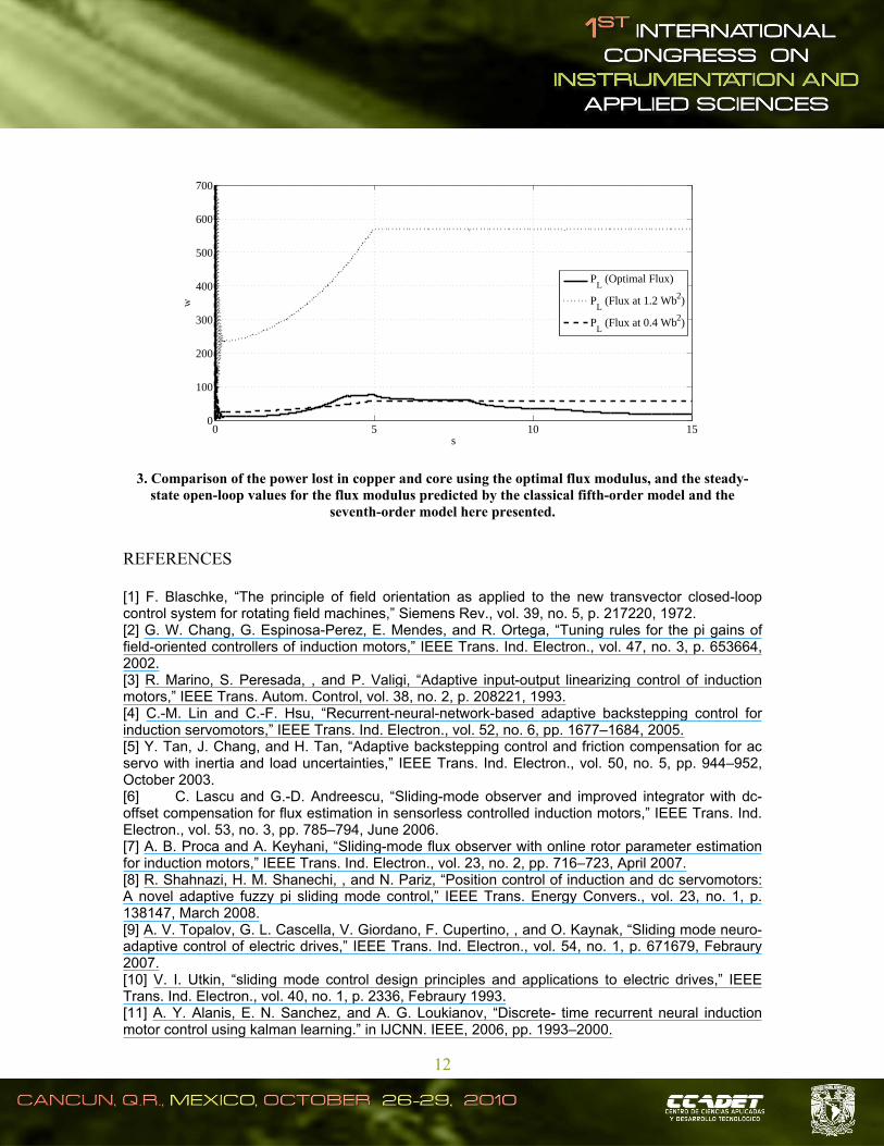
flux modulus reference signal is directly taken from the calculated optimal fluxes. A good tracking performance by the proposed controller can be appreciated in Figures 1 and 2. In Fig. 3 the power lost in copper and core is shown in the case of using the optimal flux modulus and the predicted open-loop steady state values in the cases of considering or not the core, this is a common practice when dealing with the control of the rotor flux in induction motors. From this figure one can observe a low power lost in copper and core when using the optimal flux, also one can note in Fig. 2 that the less is the load torque the lower is the flux level and as a consequence the power lost is reduced.

6. Conclusions

Based on an induction motor model with core loss in the ( )d q reference frame, an optimal

reference rotor flux has been determined for power lost minimization in copper and core. An observer-based controller, which guarantees asymptotic reference tracking for the velocity and optimal flux in presence of and unknown load torque, has been designed using a classical field oriented controller. The simulations show a great performance of the induction motor when tracking the optimal flux modulus instead of arbitrary constant flux modulus. Some interesting issues as the robustness of the controller with respect to plant parameter variations and real-time implementation

11

are currently under study.

0 5 10 150

20

40

60

80

100

120

140

160

180

200

s

rad/

s

ωω

r

1. Closed-loop velocity tracking of the proposed controller.

0 5 10 150

0.05

0.1

0.15

0.2

0.25

s

Wb2

ψm

ψmo

2. Closed-loop optimal flux modulus tracking of the proposed controller.

12

0 5 10 150

100

200

300

400

500

600

700

s

W

PL (Optimal Flux)

PL (Flux at 1.2 Wb2)

PL (Flux at 0.4 Wb2)

3. Comparison of the power lost in copper and core using the optimal flux modulus, and the steady-state open-loop values for the flux modulus predicted by the classical fifth-order model and the

seventh-order model here presented.

REFERENCES [1] F. Blaschke, “The principle of field orientation as applied to the new transvector closed-loop control system for rotating field machines,” Siemens Rev., vol. 39, no. 5, p. 217220, 1972. [2] G. W. Chang, G. Espinosa-Perez, E. Mendes, and R. Ortega, “Tuning rules for the pi gains of field-oriented controllers of induction motors,” IEEE Trans. Ind. Electron., vol. 47, no. 3, p. 653664, 2002. [3] R. Marino, S. Peresada, , and P. Valigi, “Adaptive input-output linearizing control of induction motors,” IEEE Trans. Autom. Control, vol. 38, no. 2, p. 208221, 1993. [4] C.-M. Lin and C.-F. Hsu, “Recurrent-neural-network-based adaptive backstepping control for induction servomotors,” IEEE Trans. Ind. Electron., vol. 52, no. 6, pp. 1677–1684, 2005. [5] Y. Tan, J. Chang, and H. Tan, “Adaptive backstepping control and friction compensation for ac servo with inertia and load uncertainties,” IEEE Trans. Ind. Electron., vol. 50, no. 5, pp. 944–952, October 2003. [6] C. Lascu and G.-D. Andreescu, “Sliding-mode observer and improved integrator with dc-offset compensation for flux estimation in sensorless controlled induction motors,” IEEE Trans. Ind. Electron., vol. 53, no. 3, pp. 785–794, June 2006. [7] A. B. Proca and A. Keyhani, “Sliding-mode flux observer with online rotor parameter estimation for induction motors,” IEEE Trans. Ind. Electron., vol. 23, no. 2, pp. 716–723, April 2007. [8] R. Shahnazi, H. M. Shanechi, , and N. Pariz, “Position control of induction and dc servomotors: A novel adaptive fuzzy pi sliding mode control,” IEEE Trans. Energy Convers., vol. 23, no. 1, p. 138147, March 2008. [9] A. V. Topalov, G. L. Cascella, V. Giordano, F. Cupertino, , and O. Kaynak, “Sliding mode neuro-adaptive control of electric drives,” IEEE Trans. Ind. Electron., vol. 54, no. 1, p. 671679, Febraury 2007. [10] V. I. Utkin, “sliding mode control design principles and applications to electric drives,” IEEE Trans. Ind. Electron., vol. 40, no. 1, p. 2336, Febraury 1993. [11] A. Y. Alanis, E. N. Sanchez, and A. G. Loukianov, “Discrete- time recurrent neural induction motor control using kalman learning.” in IJCNN. IEEE, 2006, pp. 1993–2000.

13

[12] ——, “Real-time discrete recurrent high order neural observer for induction motors.” in IJCNN. IEEE, 2008, pp. 1012–1018. [13] M. Deivasahayam, “Energy conservation through efficiency improvement in squirrel cage induction motors by using copper die cast,” in International Conference of energy efficiency in motor driven systems, 2005. [14] L. S and D. Pietro, “Copper die cast rotor efficiency improvement and economic consideration,” IEEE Trans Energy convers., vol. 10, no. 3, p. 419424, September 1995. [15] F. Parasiliti, M. Villani, C. Paris, and O. Walti, “Three-phase induction motor efficiency improvements with die-cast copper rotor cage and premium steel,” in Symposium on Power Electronics, Electrical Drives, Automation and Motion, 2004. [16] L. Liu, K. Zhang, and S. Zhang, “Optimal efficiency control of induction motor with core loss,” in Proceedings of 2009 IEEE International Conference on Applied Superconductivity and Electromagnetic Devices, 2009. [17] G. Dong and O. Ojo, “Efficiency optimizing control of induction motor using natural variables,” IEEE Trans. Ind. Electron., vol. 53, no. 6, pp. 1791–1798, December 2006. [18] S. L. andK. Nam, “Loss-minimising control scheme for induction motors,” IEE Proc.-Electr. Power Appl., vol. 151, no. 6, pp. 385–397, July 2004. [19] F. Fernandez-Bernal, A. Garcia-Cerrada, and R. Faure, “Model based loss minimization for dc and ac vector-controlled motors including core saturation,” IEEE Trans. Ind. Appl., vol. 36, no. 3, p. 755763, 2000. [20] I. Kioskeridis and N. Margaris, “Loss minimization in induction motor adjustable-speed drives,” IEEE Trans. Ind. Appl., vol. 43, no. 1, p. 226231, 1996. [21] C. Chakraborty, M. C. Ta, T. Uchida, and Y. Hori, “Fast search controllers for efficiency maximization of induction motor derives based on dc link power measurement,” in Proc. Power Conversion Conf., 2002. [22] G. Sousa, B. Bose, and J. Cleland, “Loss minimization in induction motor adjustable-speed drives,” IEEE Trans. Ind. Appl., vol. 42, no. 2, p. 192198, 1995. [23] D. Kirschen, D. Novotny, and T. Lipo, “On-line efficiency optimization of a variable frequency induction motor drive,” IEEE Trans. Ind. Appl., vol. 21, no. 4, p. 610615, 1985. [24] E. Levi, A. Boglietti, and M. Lazzar, “Performance deterioration in indirect vector controlled induction motor drives due to iron losses,” in Proc. Power Electronics Specialists Conf., 1995. [25] W. J. Jinh and K. Nam, “A vector control scheme for ev induction motors with series iron loss model,” IEEE Trans. Ind. Appl., vol. 45, no. 4, pp. 617–624, August 1998. [26] J. Rivera Dominguez, C. Mora-Soto, S. Ortega, J. J. Raygoza, and A. De La Mora, “Super-twisting control of induction motors with core loss,” in Variable Structure Systems (VSS), 2010 11th International Workshop on, jun. 2010, pp. 428 –433. [27] Y. Liu, X. Wu, J. Zhu, and J. Lew, “Omni-directional mobile robot controller design by trajectory linearization,” in Proceedings of the 2003 American Control Conference, 2003.