Fetal Brain Tissue Annotation and Segmentation Challenge Re
171
Author’s Original Version / manuscript under review Author’s Original Version / 07. Apr 2022 / Manuscript under review. 1 Fetal Brain Tissue Annotation and Segmentation Challenge Re- sults Kelly Payette a,b* , Hongwei Li c,d , Priscille de Dumast e,f , Rox- ane Licandro g,h , Hui Ji a,b , Md Mahfuzur Rahman Siddiquee i,j , Daguang Xu j , Andriy Myronenko j , Hao Liu k , Yuchen Pei k , Lisheng Wang k , Ying Peng l , Juanying Xie l , Huiquan Zhang l , Guiming Dong jj , Hao Fu jj , Guotai Wang jj , ZunHyan Rieu m , Donghyeon Kim m , Hyun Gi Kim n , Davood Karimi o , Ali Gholipour o , Helena R. Torres p,q,r,s , Bruno Oliveira p,q,r,s , João L. Vilaça p , Yang Lin kk , Netanell Avis- dris t,u , Ori Ben-Zvi u,v , Dafna Ben Bashat u,v,w , Lucas Fidon x , Michael Aertsen y , Tom Vercauteren x , Daniel Sobotka z , Georg Langs z , Mireia Alenyà aa , Maria Inmaculada Villanue- va bb,cc , Oscar Camara aa , Bella Specktor Fadida t , Leo Joskowicz t , Liao Weibin ll , Lv Yi ll , Li Xuesong ll , Moona Ma- zher dd , Abdul Qayyum ee , Domenec Puig dd , Hamza Kebiri e,f , Zelin Zhang ff , Xinyi Xu ff , Dan Wu ff , KuanLun Liao gg , YiXuan Wu gg , JinTai Chen gg , Yunzhi Xu ff , Li Zhao ff , Lana Vasung hh,ii , Bjoern Menze mm , Meritxell Bach Cuadra f,e , An- dras Jakab a,b a. Center for MR Research, University Children’s Hospital Zurich, University of Zurich, Zurich, Switzerland ; b. Neuroscience Center Zurich, University of Zurich, Zurich, Switzerland; c. Department of Quantitative Biomedicine, Univer- sity of Zurich, Zurich, Switzerland; d. Department of Informatics, Technical University of Munich, Munich, Germany; e. Medical Image Analysis Laboratory, Department of Diagnostic and Interventional Radiology, Lausanne University Hospital and University of Lausanne, Lausanne, Switzerland; f. CIBM, Center for Biomedical Imaging, Lausanne, Switzerland; g. Laboratory for Computational Neuroimaging, Athinoula A. Martinos Center for Biomedical Imaging, Massachu- setts General Hospital/Harvard Medical School, Charlestown, MA, USA; h. Department of Biomedical Imaging and Image-guided Therapy, Computational Imaging Research Lab (CIR), Medical University of Vienna, Vienna, Austria; i. Arizona State University; j. NVIDIA; k. Shanghai Jiaotong University; l. School of Computer Science, Shaanxi Normal University, Xi’an 710119, PR China; m. Research Institute, NEUROPHET Inc., Seoul 06247, Korea; n. Department of Radiology, The Catholic University of Korea, Eunpyeong St. Mary's Hospital, Seoul 06247, Korea; o. Boston Children’s Hospital and Harvard Medical School, Boston, MA, USA; p. 2Ai – School of Technology, IPCA, Barcelos, Portugal; q. Algoritmi Center, School of Engineering, University of Minho, Guimarães, Portugal; r. Life and Health Sciences Research Institute (ICVS), School of Medi- cine, University of Minho, Braga, Portugal; s. ICVS/3B’s - PT Government Associate Laboratory, Braga/Guimarães, Portugal; t. School of Computer Science and Engineering, The Hebrew University of Jerusalem, Israel; u. Sagol Brain Institute, Tel Aviv Sourasky Medical Center, Israel; v. Sagol School of Neurosci- ence, Tel Aviv University, Israel; w. Sackler Faculty of Medicine, Tel Aviv University, Israel; x. School of Biomedical Engineering & Imaging Sciences, King’s College London, London, SE1 7EU, UK; y. Department of Radiology, University Hospitals Leuven, 3000 Leuven, Belgium; z. Computational Imaging Research Lab, Department of Biomedical Imaging and Image-guided Therapy, Medical University of Vienna, Vienna, Austria; aa. BCN-MedTech, Department of Information and Communications Technologies, Universitat Pompeu Fabra, Barcelona, Spain; bb. Department of Information and Communications Tech- nologies, Universitat Pompeu Fabra, Barcelona, Spain; cc. Institut d’Investigacions Biomèdiques August Pi i Sunyer, Barcelona, Spain; dd. Depart- ment of Computer Engineering and Mathematics, University Rovira i Virgili,Spain; ee. Université de Bourgogne, France; ff. Key Laboratory for Bio- medical Engineering of Ministry of Education, Department of Biomedical Engineering, College of Biomedical Engineering & Instrument Science, Zhejiang University, Yuquan Campus, Hangzhou, China; gg. College of Computer Science, Zhejiang University, Hangzhou, China; hh. Division of Newborn Medicine, Department of Pediatrics, Boston Children’s Hospital; ii. Department of Pediat- rics, Harvard Medical School; jj. School of Mechanical and Electrical Engineering, University of Electronic Science and Technology of China, Chengdu, China; kk. Department of Computer Science, Hong Kong University of Science and Tech- nology; ll. School of Computer Science, Beijing Institute of Technology; mm. Department of Quantitative Biomedicine, University of Zurich, Zurich, Switzer- land Corresponding author: Kelly Payette, Email: [email protected] Highlights benchmark for future automatic multi-tissue fetal brain segmen- tation algorithms used the largest publicly available fetal brain dataset with man- ual annotations U-Net is the dominant method for automatic fetal brain seg- mentation results using the U-Net have reached a plateau challenge results analyzed from both technical and clinical per- spectives Abstract In-utero fetal MRI is emerging as an important tool in the diagnosis and analysis of the developing human brain. Automatic segmentation of the developing fetal brain is a vital step in the quantitative analysis of prenatal neurodevelopment both in the research and clinical context. However, manual segmentation of cerebral structures is time-consuming and prone to error and inter-observer variability. Therefore, we organized the Fetal Tissue Annotation (FeTA) Challenge in 2021 in order to encourage the development of automatic segmentation algorithms on an international level. The challenge utilized FeTA Dataset, an open dataset of fetal brain MRI reconstructions segmented into seven different tissues (external cerebrospinal fluid, grey matter, white matter, ventricles, cerebellum, brainstem, deep grey matter). 20 international teams participated in this challenge, submitting a total of 21 algorithms for evaluation. In this paper, we provide a detailed analysis of the results from both a technical and clinical perspective. All participants relied on deep learning methods, mainly U-Nets, with some variability present in the network architecture, optimization, and image pre- and post-processing. The majority of teams used existing medical imaging deep learning frameworks. The main differ- ences between the submissions were the fine tuning done during training, and the specific pre- and post-processing steps performed. The challenge results showed that almost all submissions performed similarly. Four of the top five teams used ensemble learning methods. However, one team’s algorithm performed significantly superior to the other submissions, and consisted of an asymmetrical U-Net network architecture. This paper provides a first of its kind benchmark for future automatic multi-tissue segmentation algorithms for the developing human brain in utero. Keywords: Multi-class Image Segmentation, Fetal Brain MRI, Congenital Disor- ders, Super-resolution reconstructions Graphical Abstract Introduction Fetal in-utero magnetic resonance imaging (MRI) is a powerful tool to in- vestigate the developing human brain in fetuses with and without pathological features (De Asis-Cruz et al., 2021; Hosny and Elghawabi, 2010). It can be used to portray the complex neurodevelopmental events during
-
Upload
khangminh22 -
Category
Documents
-
view
0 -
download
0
Transcript of Fetal Brain Tissue Annotation and Segmentation Challenge Re

Author’s Original Version / manuscript under review
Author’s Original Version / 07. Apr 2022 / Manuscript under review. 1
Fetal Brain Tissue Annotation and Segmentation Challenge Re-sults Kelly Payettea,b*, Hongwei Lic,d, Priscille de Dumaste,f, Rox-ane Licandrog,h, Hui Jia,b, Md Mahfuzur Rahman Siddiqueei,j, Daguang Xuj, Andriy Myronenkoj, Hao Liuk, Yuchen Peik, Lisheng Wangk, Ying Pengl, Juanying Xiel, Huiquan Zhangl, Guiming Dongjj, Hao Fujj, Guotai Wangjj, ZunHyan Rieum, Donghyeon Kimm, Hyun Gi Kimn, Davood Karimio, Ali Gholipouro, Helena R. Torresp,q,r,s, Bruno Oliveirap,q,r,s, João L. Vilaçap, Yang Linkk, Netanell Avis-drist,u, Ori Ben-Zviu,v, Dafna Ben Bashatu,v,w, Lucas Fidonx, Michael Aertseny, Tom Vercauterenx, Daniel Sobotkaz, Georg Langsz, Mireia Alenyàaa, Maria Inmaculada Villanue-vabb,cc, Oscar Camaraaa, Bella Specktor Fadidat, Leo Joskowiczt, Liao Weibinll, Lv Yill, Li Xuesongll, Moona Ma-zherdd, Abdul Qayyumee, Domenec Puigdd, Hamza Kebirie,f, Zelin Zhangff, Xinyi Xuff, Dan Wuff, KuanLun Liaogg, YiXuan Wugg, JinTai Chengg, Yunzhi Xuff, Li Zhaoff, Lana Vasunghh,ii, Bjoern Menzemm, Meritxell Bach Cuadraf,e, An-dras Jakaba,b
a. Center for MR Research, University Children’s Hospital Zurich, University of Zurich, Zurich, Switzerland ; b. Neuroscience Center Zurich, University of Zurich, Zurich, Switzerland; c. Department of Quantitative Biomedicine, Univer-sity of Zurich, Zurich, Switzerland; d. Department of Informatics, Technical University of Munich, Munich, Germany; e. Medical Image Analysis Laboratory, Department of Diagnostic and Interventional Radiology, Lausanne University Hospital and University of Lausanne, Lausanne, Switzerland; f. CIBM, Center for Biomedical Imaging, Lausanne, Switzerland; g. Laboratory for Computational Neuroimaging, Athinoula A. Martinos Center for Biomedical Imaging, Massachu-setts General Hospital/Harvard Medical School, Charlestown, MA, USA; h. Department of Biomedical Imaging and Image-guided Therapy, Computational Imaging Research Lab (CIR), Medical University of Vienna, Vienna, Austria; i. Arizona State University; j. NVIDIA; k. Shanghai Jiaotong University; l. School of Computer Science, Shaanxi Normal University, Xi’an 710119, PR China; m. Research Institute, NEUROPHET Inc., Seoul 06247, Korea; n. Department of Radiology, The Catholic University of Korea, Eunpyeong St. Mary's Hospital, Seoul 06247, Korea; o. Boston Children’s Hospital and Harvard Medical School, Boston, MA, USA; p. 2Ai – School of Technology, IPCA, Barcelos, Portugal; q. Algoritmi Center, School of Engineering, University of Minho, Guimarães, Portugal; r. Life and Health Sciences Research Institute (ICVS), School of Medi-cine, University of Minho, Braga, Portugal; s. ICVS/3B’s - PT Government Associate Laboratory, Braga/Guimarães, Portugal; t. School of Computer Science and Engineering, The Hebrew University of Jerusalem, Israel; u. Sagol Brain Institute, Tel Aviv Sourasky Medical Center, Israel; v. Sagol School of Neurosci-ence, Tel Aviv University, Israel; w. Sackler Faculty of Medicine, Tel Aviv University, Israel; x. School of Biomedical Engineering & Imaging Sciences, King’s College London, London, SE1 7EU, UK; y. Department of Radiology, University Hospitals Leuven, 3000 Leuven, Belgium; z. Computational Imaging Research Lab, Department of Biomedical Imaging and Image-guided Therapy, Medical University of Vienna, Vienna, Austria; aa. BCN-MedTech, Department of Information and Communications Technologies, Universitat Pompeu Fabra, Barcelona, Spain; bb. Department of Information and Communications Tech-nologies, Universitat Pompeu Fabra, Barcelona, Spain; cc. Institut d’Investigacions Biomèdiques August Pi i Sunyer, Barcelona, Spain; dd. Depart-ment of Computer Engineering and Mathematics, University Rovira i Virgili,Spain; ee. Université de Bourgogne, France; ff. Key Laboratory for Bio-medical Engineering of Ministry of Education, Department of Biomedical Engineering, College of Biomedical Engineering & Instrument Science, Zhejiang University, Yuquan Campus, Hangzhou, China; gg. College of Computer Science, Zhejiang University, Hangzhou, China; hh. Division of Newborn Medicine, Department of Pediatrics, Boston Children’s Hospital; ii. Department of Pediat-rics, Harvard Medical School; jj. School of Mechanical and Electrical Engineering, University of Electronic Science and Technology of China, Chengdu, China; kk. Department of Computer Science, Hong Kong University of Science and Tech-nology; ll. School of Computer Science, Beijing Institute of Technology; mm.
Department of Quantitative Biomedicine, University of Zurich, Zurich, Switzer-land
Corresponding author: Kelly Payette, Email: [email protected]
Highlights benchmark for future automatic multi-tissue fetal brain segmen-
tation algorithms
used the largest publicly available fetal brain dataset with man-ual annotations
U-Net is the dominant method for automatic fetal brain seg-mentation
results using the U-Net have reached a plateau
challenge results analyzed from both technical and clinical per-spectives
Abstract
In-utero fetal MRI is emerging as an important tool in the diagnosis and analysis of the developing human brain. Automatic segmentation of the developing fetal brain is a vital step in the quantitative analysis of prenatal neurodevelopment both in the research and clinical context. However, manual segmentation of cerebral structures is time-consuming and prone to error and inter-observer variability. Therefore, we organized the Fetal Tissue Annotation (FeTA) Challenge in 2021 in order to encourage the development of automatic segmentation algorithms on an international level. The challenge utilized FeTA Dataset, an open dataset of fetal brain MRI reconstructions segmented into seven different tissues (external cerebrospinal fluid, grey matter, white matter, ventricles, cerebellum, brainstem, deep grey matter). 20 international teams participated in this challenge, submitting a total of 21 algorithms for evaluation. In this paper, we provide a detailed analysis of the results from both a technical and clinical perspective. All participants relied on deep learning methods, mainly U-Nets, with some variability present in the network architecture, optimization, and image pre- and post-processing. The majority of teams used existing medical imaging deep learning frameworks. The main differ-ences between the submissions were the fine tuning done during training, and the specific pre- and post-processing steps performed. The challenge results showed that almost all submissions performed similarly. Four of the top five teams used ensemble learning methods. However, one team’s algorithm performed significantly superior to the other submissions, and consisted of an asymmetrical U-Net network architecture. This paper provides a first of its kind benchmark for future automatic multi-tissue segmentation algorithms for the developing human brain in utero.
Keywords: Multi-class Image Segmentation, Fetal Brain MRI, Congenital Disor-ders, Super-resolution reconstructions
Graphical Abstract
Introduction
Fetal in-utero magnetic resonance imaging (MRI) is a powerful tool to in-vestigate the developing human brain in fetuses with and without pathological features (De Asis-Cruz et al., 2021; Hosny and Elghawabi, 2010). It can be used to portray the complex neurodevelopmental events during

Author’s Original Version / manuscript under review
Author’s Original Version / 07. Apr 2022 / Manuscript under review. 2
human gestation, which remain to be completely characterized (Vasung et al., 2019). Clinically, it is becoming an important adjunct to ultrasound in the detection and diagnosis of congenital disorders (Hart et al., 2020), and can be used to aid during prenatal care (Gholipour et al., 2014).
Automated segmentation and quantification of the highly complex and rapidly changing brain morphology using MRI prior to birth has great potential to improve the diagnostic process, as manual segmentation is both time consuming and subject to human error and inter-rater variability. It is clinical-ly relevant to analyze the morphometry of the developing brain, where measures such as the volume or the shape can be objectively compared with population-based references of normative development. Many congenital and acquired disorders manifest in reduced brain volume or altered anatomi-cal structure of cerebral tissue compartments, for example, slower cortical growth (Clouchoux et al., 2013; Egaña-Ugrinovic et al., 2013) or reduced white matter volume (Rollins et al., 2021). Existing MRI based data of brain growth is mainly based on normally developing brains (Jarvis et al., 2019; Kyriakopou-lou et al., 2017; Prayer et al., 2006), leaving brain growth in various numerous pathologies and congenital disorders largely unexplored.
From a technical standpoint, there are many challenges that an automat-ic segmentation method of the fetal brain would need to overcome. The cerebral structures are constantly growing and developing in complexity throughout gestation, which results in a gradually changing appearance in shape, size, and image intensity on MRI. In addition, the quality of the images can be poor due to fetal and maternal movement and imaging artefacts (Glenn, 2010). The boundary between tissues is often unclear on MR images due to partial volume effects (Bach Cuadra et al., 2009). Furthermore, fetal brains with abnormal features can have radically different morphology than those in a non-pathological brain. This can make it challenging for an auto-matic method to correctly identify these structures.
Fetal MRI requires no special MRI equipment, is noninvasive, safe (Gow-land, 2011; Zvi et al., 2020), and its value in the diagnosis of certain central nervous system or somatic disorders is being increasingly recognized (Griffiths et al., 2019; Nagaraj et al., 2022). The development of ultra-fast MRI se-quences such as the single shot T2-weighted sequence have also led to the increasing popularity of fetal MRI as these images have excellent soft tissue contrast and reduced motion artefact (Gholipour et al., 2014). As a result, fetal MRI is more frequently performed at diagnostic and surgical centers worldwide. There is also an increase in the number of studies focused on developing computational tools to quantitatively analyze the fetal brain. Some studies have focused on segmenting a specific tissue for analysis, such as the cortical plate (Benkarim et al., 2018; de Dumast et al., 2020; Fetit et al., 2020; Hong et al., 2020). Other studies have developed multi-tissue segmen-tation algorithms using a limited in-house dataset (e.g., clinically acquired anisotropic coronal images of normal fetuses (Khalili et al., 2019), or images of a specific pathology (Sanroma et al., 2018), or with atlas based frameworks (Dittrich et al., 2011; Gholipour et al., 2017; Licandro et al., 2016)). However, the field of developing automated tools for fetal MRI has been understudied due to both challenges in imaging and the lack of public, curated, and anno-tated ground truth data. Such shared datasets are currently the backbone for developing computer-aided diagnostic support systems.
In this paper we describe the Fetal Brain Tissue Annotation and Segmen-tation Challenge (FeTA) and outline the challenge organization, the submitted segmentation frameworks, and a detailed evaluation of the challenge results, with reporting based on the BIAS method (Maier-Hein et al., 2020). The aim of the FeTA Challenge was to develop reliable, valid, and reproducible methods of analyzing high resolution reconstructed MR images of the developing fetal brain from gestational week 20-35. The FeTA Challenge used an expanded version of the original FeTA Dataset to develop automatic fetal brain tissue segmentation methods (Payette et al., 2021a). Our evaluation compares and analyzes the algorithms on a test dataset hidden to the participants. The submitted algorithms are also tested on various subsets of the testing dataset in order to determine whether they perform better or worse under various circumstances such as image quality or reconstruction method. Finally, we investigated two real life applications outside the scope of the FeTA Challenge evaluation: First, the performance of the submitted algorithms to estimate intracranial volume was evaluated, an application relevant to the characteri-zation of developmental delay in many conditions, such as intrauterine growth restriction or congenital heart defects (Polat et al., 2017; Sadhwani et al., 2022; Skotting et al., 2021). Second, we looked at the ability of the algo-rithms to segment younger (<29 weeks) versus older (≥29 weeks) fetal
brains). The algorithms developed as part of the FeTA Challenge will have the potential to help better understand the underlying causes of congenital disorders and ultimately to guide the development of perinatal guidelines and clinical risk stratification tools for early interventions, treatments, and care management decisions.
Materials and Methods Challenge Organization: The FeTA Challenge was held as part of the in-
ternational Medical Image Computing and Computer Assisted Intervention (MICCAI) 2021 Conference (https://feta.grand-challenge.org/). Participants were to create a fully automatic multi-class segmentation algorithm of the fetal brain (with optional inputs of gestational age and whether the brain was pathological or not). The training dataset was made available to the partici-pants on May 3rd, 2021 on Synapse (Payette and Jakab, 2021) to train their own methods. Participants were able to use other publicly available datasets for training if they wished to, as long as it was documented in their algorithm description. Participants created a Docker container which stored the algo-rithm, and submitted this container to the organizers by July 30, 2021. Organizers were allowed to submit containers, but were not eligible for prizes. This container was run by the challenge organizers locally on the hidden testing dataset in order to compare the algorithms. Re-submission of the Docker container was only allowed in cases of technical difficulties or bugs identified during evaluation. The top teams received their results on Septem-ber 1, 2021 in order to prepare presentations. The complete results and awards to the top three teams were presented on Oct 1, 2021 at the MICCAI Conference FeTA Challenge Session. Dockers of teams who provided permis-sion are available on Dockerhub (https://hub.docker.com/u/fetachallenge). For the complete overview of the challenge, see the final challenge proposal (Payette et al., 2021b).
Mission of the Challenge: The mission of the FeTA Challenge is to boost the development of accurate and automatic multi-class segmentation algo-rithms for the developing human brain with fetal MRI, and to create a benchmark for future algorithms. There were a total of eight classes: external cerebrospinal fluid (eCSF), grey matter (GM), white matter (WM), ventricles (including cavum), cerebellum, deep grey matter (deep GM), brainstem, and background. The target cohort for the FeTA Challenge were pregnant mothers who, after an initial ultrasound examination, were clinically referred for a fetal MRI. The acquired fetal MRI images were then reconstructed into a 3-dimensional volume using a super-resolution method (for details see Section 0). The task of the challenge was to segment these super-resolution volumes into different brain tissues. The challenge cohort was made up of two sub-groups: fetuses with normal and abnormal development of the nervous system, and covers a gestational age (GA) range of 20-35 weeks. The accuracy of the automatically generated fetal brain segmentations was evaluated in the challenge cohort in order to determine the optimal segmentation method for fetal brain MRI.
Challenge Dataset: For the challenge, a clinically acquired dataset from a single institution was used for both the training and testing data. 120 fetal MRI brain scans were acquired. Recorded gestational age was modified by a random value within the range of ±3 days to further anonymize the data. Several T2-weighted single shot Fast Spin Echo (ssFSE) images were acquired for each subject in all three planes with a reconstructed resolution of 0.5mm x 0.5mm x 3 to 5mm. The images were acquired on either a 1.5T or 3T clinical GE whole-body MRI scanners (Signa Discovery MR450 and MR750) using an 8-channel cardiac or body coil with the following sequence parameters: TR: 2000–3500 ms, TE: 120 ms (minimum), flip angle: 90°, sampling percentage 55%. Field of view (200–240 mm) and image matrix (1.5T: 256×224; 3T: 320×224) were adjusted depending on the gestational age and size of the fetus. The data was acquired at the University Children’s Hospital Zurich in Zurich, Switzerland by trained radiographers using clinically defined protocols.
For each subject, the acquired images were reviewed, and images of good quality, at least one image in each of the axial, sagittal, coronal planes with respect to the fetal brain, were chosen. A high-resolution fetal brain reconstruction was performed with the chosen scans using a super-resolution (SR) method (60 cases reconstructed with the mialSR method (Pierre Deman et al., 2020; Tourbier et al., 2019, 2015) and 60 cases reconstructed with the

Author’s Original Version / manuscript under review
Author’s Original Version / 07. Apr 2022 / Manuscript under review. 3
Simple IRTK method (Kuklisova-Murgasova et al., 2012)). Fetal brain masks were created where necessitated by the SR algorithm, either manually or with a custom MeVisLab module (Pierre Deman et al., 2020; Tourbier et al., 2015). Cases reconstructed with mialSR were reoriented prior to reconstruction through the MeVisLab module. Cases reconstructed with the Simple IRTK method were registered to an atlas after reconstruction (Serag et al., 2012). After reconstruction, each fetal brain volume had an isotropic resolution of approximately 0.5mmx0.5mmx0.5mm, with some deviation in exact dimen-sions between the SR methods. Each reconstructed image was then histogram-matched using Slicer (Kikinis et al., 2014), and zero-padded to be 256x256x256 voxels. For each reconstruction method, 40 cases were included in the training dataset available to the challenge participants (for a total of 80 cases), and 20 cases were included in testing dataset not available to the participants (for a total of 40 cases). Note that maternal tissue was excluded from the super-resolution reconstruction, only the fetal brain was recon-structed. Examples of non-pathological fetal brains across the range of gestational ages included in the dataset and their corresponding label maps can be seen in Figure 1.
The training and testing datasets consisted of fetuses with both typical and atypical features. In the group with atypical features, a variety of cerebral pathologies of varying severities were included (such as Chiari-II malformation or ventricular dysmorphology seen in ventriculomegaly). There were slightly more pathological than neurotypical cases, as in the clinic where the scans were performed it is more common to see pathologic brains (Figure 2). Fetus-es with a gestational age range of 20 to 35 gestational weeks were included (mean gestational age: 27.0±3.60 weeks), with the distribution of ages and pathologies equal between the training and testing datasets (see Figure 3). The gestational age and the label of “neurotypical/pathological” was made available to the participants. Each case’s label map was manually segmented by individuals with experience in segmenting medical images using the meth-od described in (Payette et al., 2021a). Each case consists of a 3D super-resolution reconstruction of a fetal brain (256x256x256 voxels) and the asso-ciated manually segmented label map. There is no overlap of subjects between the training and testing dataset, each dataset is unique. The dataset and affiliated custom license is publicly available on Synapse (Payette and Jakab, 2021).
Mothers of the healthy fetuses participating in the BrainDNIU study were prospectively informed about the inclusion in the FeTA Dataset by members of the research team and gave written consent for their participation. Moth-ers of all other fetuses included in the current work were scanned as part of their routine clinical care and gave informed written consent for the re-use of their data for research purposes. The ethical committee of the Canton of Zurich, Switzerland approved the prospective and retrospective studies that collected and analyzed the MRI data (Decision numbers: 2017-00885, 2016-01019, 2017-00167), and a waiver for an ethical approval was acquired for the release of a fully anonymous dataset for research purposes.
Participants were free to choose if they wanted to work with the data in a 2D or 3D format. A validation dataset was not provided to the participants, it was up to the team’s discretion to decide how to train their data and what to use for validation. The following section outlines the evaluation metrics used to determine the ranking of participants in the challenge.
Figure 1: Fetal Brain Segmentations by gestational age
Figure 2: Pathological fetal brain viewed in axial, sagittal, and coronal directions A):
mialSR reconstruction, 27.3 GA; B) Simple IRTK SR Reconstruction, 26.9 GA
Figure 3: Dataset Age Range: Histogram of the gestational age range of neurotypical and
pathological cases within the testing and training dataset for the FeTA Challenge.
Assessment Method - Evaluation Metrics: Three different metrics were chosen to compute the rankings of the FeTA Challenge: the Dice Similarity Coefficient (DSC), The Volume Similarity (VS), and the Hausdorff distance (HD). The DSC was chosen, as it is the most popular segmentation overlap metric for segmentation evaluation (Dice, 1945). However, we were also interested in assessing volume, as relevant biomarker for fetal development, and surface-based error. Therefore the HD (surface, (Hausdorff, 1991)), and VS (volume) metrics were chosen as well (Taha and Hanbury, 2015), and the final ranking will take all three metrics into account.
The DSC measures the amount of overlap between the manual segmen-tations (MS) label and the new segmentation (NS) generated by the participant’s algorithm, and is defined as
𝐷𝑆𝐶 = 2 |𝑀𝑆 ∩ 𝑁𝑆|
|𝑀𝑆| + |𝑁𝑆|
The VS is a volumetric metric that measures the similarity between the volume of the GT and NS label map and is defined as

Author’s Original Version / manuscript under review
Author’s Original Version / 07. Apr 2022 / Manuscript under review. 4
𝑉𝑆 = 1 − |𝑀𝑆𝑣𝑜𝑙 − 𝑁𝑆𝑣𝑜𝑙|
𝑀𝑆𝑣𝑜𝑙 + 𝑁𝑆𝑣𝑜𝑙
The HD is a distance metric that evaluates the distance between two fi-nite point sets A and B.
The Hausdorff distance (HD) is a spatial metric helpful in evaluating the contours of segmentations as well as the spatial positions of the voxels. The HD between two finite point sets A and B is defined as
𝐻𝐷(𝐴, 𝐵) = 𝑚𝑎𝑥 (ℎ(𝐴, 𝐵), ℎ(𝐵, 𝐴))
ℎ(𝐴, 𝐵) = ||𝑎 − 𝑏||
Note: The original challenge design had stated that the 95th percentile HD of maximum distances would be used to exclude possible outliers. How-ever, after the challenge it was discovered that there was an error in the implementation of the 95th percentile, and the values reported were close to the maximum HD, and therefore these are the scores reported in this paper. This makes the HD values reported within this report slightly more susceptible to outliers. However, as we take three different metrics into account for the final ranking, the overall impact of outliers is reduced. For each metric, the implementation described in (Taha and Hanbury, 2015) was used (Evalu-ateSegmentation Tool, v2017.04.25).
Assessment Method – Ranking: Each of the participating teams was ranked based on each evaluation metric, and then the final rankings com-bined the rankings from all of the metrics (DSC, HD95, VS). The DSC, HD95, and VS were calculated for each label within each of the corresponding pre-dicted label maps of the fetal brain volumes in the testing set. The mean and standard deviation of each label for all test cases was calculated, and the participating algorithms were ranked from low to high (HD95), where the lowest score received the highest scoring rank (best), and from high to low (DSC, VS), where the highest value received highest scoring rank (best) based on the calculated mean across all labels and test cases. If there were missing results, the worst possible value is used. For example, if a label does not exist in the NS label map but is present in the GT label map, it will receive a DSC and VS score of 0, and the HD95 score will be double the max value of the other algorithms submitted. This ranking procedure was developed in order to take three different metric types equally into account.
Assessment Method - Further Analysis: In addition to the ranking above, several other analyses were performed on the submitted algorithms. Per-label rankings of the entire dataset were analyzed. In addition, the algorithms were evaluated in the categories ‘Non Pathological cases’ and ‘Pathological cases’, SR reconstruction method (mialSR and Simple IRTK) as well as ‘Excel-lent Quality‘, ‘Good Quality‘ and ‘Poor Quality’, with the identical ranking methodology for each category. The pathology of each fetal brain was deter-mined by an experienced radiologist. The quality of the fetal brain SR reconstructions were determined based on ratings (Excellent, Good, Poor) from three independent raters, and the correlation of the reviewers was calculated using the Gwet AC coefficient using R (v4.0.2, (Gwet, 2019)). As the ratings are ordinal data, the median of the ratings were considered to be the final rating of the SR volume. The participating algorithms were also evaluated on the different SR reconstruction methods.
Intracranial volume was calculated and compared to the manual segmen-tation’s intracranial volume as well, but not used in the rankings. Intracranial volume was calculated by adding all labels except the background together.
An analysis of the performance of the algorithms based on gestational age was also performed, as the structure of the fetal brain changes greatly throughout development, especially in the cortex where there is increased cortical complexity, disappearance of transient subplate zone related to cortical maturation (blurring of white matter and grey matter border) and partial volumes (blurring of white matter/grey matter border in gyral crest, blurring of CSF/grey matter border because of narrow sulci). Because of this, the random error in segmentation of the grey matter between 29-35 GW might be increased. Therefore, in order to determine if gestational age im-
pacts the success of a segmentation algorithm, our testing dataset was split into two age groups (21-28 weeks, and 29-35 weeks), and the differences between these two groups was analyzed by looking for differences in the evaluation metrics between each label for each of the submitted algorithms.
Results Training and Testing Data: A Kolmogorov–Smirnov test was performed in
R v4.0.0 (R Core Team, 2020) in order to compare the distribution of GA and non-pathological/pathological fetal brains between the training and testing data. No significant differences were found between the training and testing datasets (GA: p = 0.88; pathology: p = 1).
Challenge Submission: In total, 21 teams submitted algorithms to the FeTA Challenge. One team’s Docker container was not able to be fixed prior to the deadline and was thereby excluded. One team (Ichi-love) submitted two algorithms, meaning the total number of participating teams was 20, and the total number of valid submissions was 21. Each team submitted a written description of their algorithm, which can be found in the Appendix. Each algorithm is summarized in Table 1, and the pre-processing and data augmen-tation used by each team is outlined in
Table 2. All teams submitted a deep learning-based method, most of which were variants based on the U-Net architecture (Çiçek et al., 2016; Ronneberger et al., 2015). The top five teams used similar loss functions (mainly the combination of Dice loss and cross-entropy loss), and four of the five (excluding Neurophet) used an ensemble learning method. Every method used a 3x3 (or 3x3x3) convolutional kernel except for one team (Physense-UPF) who used a 2x2x2 kernel. Most submissions (14 of 21) used a random initialization of network parameters. The networks were of varying depths, between 3 and 6 layers on each of the ascending and descending layers of the networks. Thirteen of the submitted networks were 3D networks, the re-mainder were 2D or 2.5D. Seven teams used cross-validation. A variety of different data augmentation strategies were used, and only two team did not employ data augmentation at all. Only four teams used external datasets, either during the training step or used pre-trained network backbones trained on publicly available datasets.
Metric Values and Rankings: Statistical analysis of the metrics of the challenge and images displayed in this section were created using the Chal-lengeR tool (Wiesenfarth et al., 2021). The individual metrics for each team (all labels combined) can be found in Figures 4-6. The final ranking of all teams and their average evaluation metrics can be found in Table 3. The full reports (DSC, HD95, VS of all labels combined) created by the ChallengeR Tool, includ-ing details on the statistical tests performed can be found in Sections 2-4 of the Appendix. In the significance maps displayed, the testing was done using a one-sided Wilcoxon signed rank test at a 5% significance level, with adjust-ments for multiple comparisons. In all cases, the x-axis in the boxplots are ranked according to the mean values of the respective evaluation metric, and the black bar indicates the median value.
The top three teams according to the DSC were NVAUTO, SJTU_EIEE_2-426Lab, and Neurophet. The top three teams according to the HD95 were NVAUTO, Hilab, and 2Ai. The top three teams according to the VS were ichil-ove-ax, NVAUTO, and SJTU_EIEE_2-426Lab. With a few exceptions, there was no statistically significant differences between the top 10-12 teams in all three metrics, suggesting that a plateau has been reached. The highest and lowest average DSC were: 0.786 (team NVAUTO) and 0.534 (team A3). The lowest and highest average HD95 were: 14.012 (team NVAUTO) and 39.608 (team A3). The highest and lowest average VS were: 0.888 (team ichilove-ax) and 0.791 (team A3). However, when the bootstrapping and significance maps are investigated, it is clear that NVAUTO is the top team for the DSC metric, placing first in 100% of the bootstrap sampling, and is statistically significant to all but one of the algorithms (Team pengyy). There is no differ-ence between teams in places 2 to 4 for the DSC metric in both the

Author’s Original Version / manuscript under review
Author’s Original Version / 07. Apr 2022 / Manuscript under review. 5
bootstrapping and statistical significance testing. The same trend appears when looking at the HD95 metric, with NVAUTO being the clear winner, and the teams in places 2 to 4 performing equivalently. Some differences exist in the VS metrics, with ichilove-ax as the first place, but with not as clear of a lead with no statistical difference from any of the top teams, and a less clear winner when looking at the bootstrapping.

Author’s Original Version / manuscript under review
Author’s Original Version / 07. Apr 2022 / Manuscript under review. 6
Table 1: Overview of algorithms submitted to the FeTA Challenge ordered from best to worst
Team Name Network Loss Function 2D/ 3D
Patch Size Post-Processing
Convolution Kernel Size
Optimizer Initialization Learning Rate
Cross-Validation
Epochs GPU Used # of Layers
# of Traina-ble Parameters
NVAUTO MONAI (SegRes-Net), OCR modules
Dice 3D 224x 224x 144 Ensemble learning
3x3x3 AdamW Random 0.0002, decrease to 0 at final epoch with cosine annealing scheduler
5-fold 300 4 x Nvidia V100 32GB
5 desc / 5 asc
75 819 624
SJTU_EIEE_2-426Lab
two steps: coarse to fine, 1. nnU-net and 3D UNet with residual architec-ture; 2. 5 3D Res-Unets
1. Cross-entropy and Dice; 2. Haus-dorff and Dice
3D 128x 128x 128 - nn-UNet. only
Ensemble learning
3x3x3 Adam Random 1. 1E-3; 2. 1E-4
No 1. 500; 2. 1000
Nvidia RTX 3090
6 desc / 6 asc
1. 2 235 680 (UNet); 31 199 584 (nnUNet) 2. 214 58 929 (first UNet); 85 823 969 (other 4 UNets)
pengyy nnU-Net Cross-entropy and Dice
3D 128x 128x 128 Ensemble learning
3x3x3 Stochastic Gradient Descent
Random 0.01 with reduction
10-fold 1000 Nvidia GeFor-ce RTX 3090
6 desc / 6 asc
72 142 688
Hilab nnU-Net Cross-entropy and Dice
3D 128x 128x 128 Ensemble learning
3x3x3 Stochastic Gradient Descent
Random 0.01 with decay
5-fold 400 Nvidia GeFor-ce RTX 2080 Ti
6 desc / 6 asc
30 847 564
Neurophet U-Net sum of Cross-entropy and Dice
3D 64x64x64 Isolated seg-mented voxels removed
3x3x3 AdamW Random 1.00E-05 No 500 3 x Tesla V100
5 desc / 5 asc
314 999 688
davoodkari-mi U-Net with addi-tional short and long skip connec-tions
Novel loss function derived from mean absolute error
3D 128x 128x 128 Label Fusion 3x3x3 Adam He 1E-4 with reduction
No 400 Nvidia GeFor-ce GTX 1080
5 desc / 5 asc
18 500 000
2Ai U-Net/nnU-Net Dice 3D 128x 128x 128 Isolated seg-mented voxels removed
3x3x3 Adam Xavier 1E-3 with decay
No 800 1 x GTX1070
6 desc / 6 asc
29 971 032
xlab U-Net/nnUnet Cross-entropy and Dice
2D No None 3x3 Adam Random 3.00E-04 5-fold 1000 Nvidia RTX 3090
5 desc / 5 asc
-

Author’s Original Version / manuscript under review
Author’s Original Version / 07. Apr 2022 / Manuscript under review. 7
Ichilove-ax Two step net-works. Dynamic U-Net with pre-trained ResNET34 network blocks (desc) and pix-elShuffle ICNR blocks (asc)
Lovasz-Softmax loss
2D No None 3x3 OneCycle ResNet34 - encoder, ICNR - Decoder
1.00E-03 No 60 1 x GTX1080Ti
4 desc / 4 asc
41 221 768
TRABIT DynU-Net from MONAI; 10 net-works
Label-set Loss function: Leaf-Dice and mar-ginalized cross entropy
3D 128x 160x 128 Ensemble learning
3x3x3 Stochastic Gradient Descent
He 0.01 with decay
No 2200 1 x Tesla V100-SXM2-32GB
6 desc / 6 asc
31 195 784
Ichilove-Combi Two step net-works. One for ROI, 3 for each axis (Coronal, Axial, Sagittal). Dynamic U-Net with pre-trained ResNET34 network blocks (desc) and pix-elShuffle ICNR blocks (asc)
Lovasz-Softmax loss
2D No Label Fusion 3x3 OneCycle ResNet34 - encoder, ICNR - Decoder
1.00E-03 No 60 1 x GTX1080Ti
4 desc / 4 asc
103 054 420
muw_dsobotka multi-task U-Net with two decoders (segmentation and reconstruction)
Homoscedastic uncertainty, cross-entropy, mean squared error
3D 128x 96x96 None 3x3x3 Adam Random 0.001 No 100 Nvidia GeFor-ce RTX 2080 Ti
3 desc / 3 asc
6 491 385
Physense-UPF Team
nnU-Net Cross-entropy and Generali-zed Dice
3D 128x128x128 None 2x2x2 Stochastic Gradient Descent
Random 0.01 5-fold 100 1x Nvidia GEFORCE GTX 1080 Ti
6 desc / 6 asc
31 199 584
SingleNets U-Net Soft Dice and Contour Dice
3D 96x96x96 Majority Voting, clipping using "skull" (background-foreground) network response with threshold 0.5
3x3x3 Adam Fine tuning from previ-ously trained networks on smaller training set
0.005 with reduction
No 100 Tesla M60 5 desc / 5 asc
4 727 841
Author’s Original Version / manuscript under review
Author’s Original Version / 07. Apr 2022 / Manuscript under review. 8
BIT_LILAB CNN-Transformer Hybrid (Trans-U-Net)
Cross-entropy and Dice
2D 16 x 16 None 3x3 Stochastic Gradient Descent
Pre-trained ResNet-50 and ViT
1E-2 with decay
No 150 4 x Nvidia GTX 1080Ti GPU
5 desc / 5 asc
54 000 000
Moona Mazher DenseNet Binary Cross-entropy
2D No Label Fusion 3x3 Adam Random 0.0003 5-fold 1000 4 x Nvidia V100
5 desc / 5 asc
49 510 728
MIAL U-Net hybrid loss (Dice and Cross-entropy)
2D 64x64 Majority Voting
3x3 Adam Random 0.001 with decay
5-fold 100 NVIDIA RTX 2070
5 desc / 5 asc
-
ZJUWULAB U-Net with conv downsampling instead of max pooling downsam-pling
L1 Regulariza-tion and feature-matching with a pre-trained VGG19 Network
2D No None 3x3 Adam Random 0.002 No 100 4 x RTX 3080Ti
5 desc / 5 asc
7 765 442
FeVer Res-Unet Dice 3D 48x224x224 Ensemble learning
3x3x3 QHAdam Random 0.005-0.0005
No 300 1 x RTX 3090
5 desc / 5 asc
2 369 496
Anonymous U-Net Focal Loss 2D No None 3x3 Adam Random 0.002 No 30, backbone frozen for 15
- - -
A3 V-Net with PReLU activation
Binary Cross-entropy
3D Crop-ped & pad-ded to 192x 192x 192; down-sampled to 128 x 128 x 128
None 3x3x3 Adam Random 1E-4 with reduction
No 200 2 x NVIDIA P100,
3 desc / 3 asc
283 886 304

Author’s Original Version / manuscript under review
Author’s Original Version / 07. Apr 2022 / Manuscript under review. 9
Table 2: Overview of the data augmentation, and pre-processing used in each submission.
Team Name Data Augmentation External Dataset used Pre-processing
NVAUTO Rotation, Flipping, Zoom, contrast adjustment, Gaussian noise, Gaussian smooth-ing
No Normalize images to zero mean
SJTU_EIEE_2-426Lab
Rotation, Scaling, Flipping No Normalize images to zero mean, cropping in 2nd stage
pengyy Rotation, scaling, elastic deformation, mirroring, Gaussian noise, Gamma Correc-tion
No resample dimensions to .5x.5x.5mm; z-score normalization
Hilab Pathological Cases copied 3 times in training data, rotation, scaling, Gaussian noise, Gaussian blur, brightness, contrast, simulation of low resolution, gamma augmentation, mirroring
No Cropping and normalization
Neurophet Affine, Blur No Intensity Normalization, classification of images into poor and good quality
davoodkarimi Flipping, rotation, elastic deformation, label perturbation and smoothing No Intensity Normalization
2Ai Flipping, rotation, scaling, grid distortion, optical distortion, elastic transfor-mations, noise, brightness, contrast, gamma transformations
No Image normalization (mean value zero)
xlab Mirroring, rotation, scaling, gamma correction, random elastic transformation No nnUNet standard preprocessing
Ichilove-ax Intensity, contrast, scaling, normalization, rotation, intensity inhomogeneity No No
TRABIT Flipping, zooming, rotation, Gaussian noise, spatial smoothing, gamma augmenta-tion
Uses external fetal brain atlases and neonatal MRI's segmented with dHCP
generated brain mask (from atlas + niftyReg), registered brain to atlas, resampled to 0.8mm isotropic; skull stripping; thresholding of intensity percen-tiles; z-score normalization
Ichilove-Combi Intensity, contrast, scaling, normalization, rotation, intensity inhomogeneity No No
muw_dsobotka Elastic deformation, flipping, rotation, contrast, Gaussian noise, Poisson noise No z-score normalized patches
Physense-UPF Team
Rotation, elastic deformation, scaling, Gaussian noise, Gaussian blur, gamma transform, mirror, brightness, contrast, low resolution simulation, zoom
No Cropping, resampling, normalization, classification of quality of images, regis-tration to Gholipour atlas
SingleNets Flipping, rotation, translation, scaling, Poisson noise, contrast, intensity No Thresholding, cropping, windowing, normalization, downscaling by 0.5 in all axes
BIT_LILAB Rotation and flipping Yes, Synapse multi-organ segmenta-tion dataset (for pre-training)
None
Moona Mazher Cropping, Flipping, Brightness and Contrast, Random Gamma No None
MIAL Flipping, Rotation No Intensity standardization
ZJUWULAB No yes, pre-trained VGG19network Normalize, colour map labels
FeVer Flipping, Mixup No Intensity-based image filtering, resampling voxels to have equal spacing, re-move slices with only background label
Anonymous No ResNet backbone pre-trained on Kinect400
Intensity re-scaling; ResNet backbone pre-trained on ImageNet
A3 Shifting, rotation, flipping No Image normalization (mean value zero)

Author’s Original Version / manuscript under review
Author’s Original Version / 07. Apr 2022 / Manuscript under review. 10
Figure 4: DSC values of FeTA Challenge participants a) Dot and box plot; b) Blob plot for visualizing ranking stability based on bootstrap sampling, black cross indicated the median rank for each algorithm and 95% bootstrap intervals across samples are indicated by black lines; c) Significance maps for visualizing ranking stability based on statistical significance (Yellow:
metrics from the algorithm on the x-axis were significantly superior to the algorithm on the y-axis, blue color indicates no significant difference). Figures were created using the Chal-lengeR Tool (Wiesenfarth et al., 2021).
Figure 5: HD95 values of FeTA Challenge participants a) Dot and box plot; b) Blob plot for visualizing ranking stability based on bootstrap sampling, black cross indicated the median rank for each algorithm and 95% bootstrap intervals across samples are indicated by black lines; c) Significance maps for visualizing ranking stability based on statistical significance
(Yellow: metrics from the algorithm on the x-axis were significantly superior to the algorithm on the y-axis, blue color indicates no significant difference.)

Author’s Original Version / manuscript under review
Author’s Original Version / 07. Apr 2022 / Manuscript under review. 11
Figure 6: VS values of FeTA Challenge participants a) Dot and box plot; b) Blob plot for visualizing ranking stability based on bootstrap sampling, black cross indicated the median rank for each algorithm and 95% bootstrap intervals across samples are indicated by black lines; c) Significance maps for visualizing ranking stability based on statistical significance (Yellow:
metrics from the algorithm on the x-axis were significantly superior to the algorithm on the y-axis, blue color indicates no significant difference.)
Table 3: Final FeTA Ranking; * indicates a tie
Ranking Team Name Average DSC Average HD95 (voxels) Average VS
1 NVAUTO 0.786 ± 0.161 14.012 ± 9.285 0.885 ± 0.156
2 SJTU_EIEE_2-426Lab 0.775 ± 0.173 14.671 ± 9.917 0.883 ± 0.166
3 Pengyy 0.774 ± 0.182 14.699 ± 10.049 0.875 ± 0.182
4 Hilab* 0.774 ± 0.181 14.569 ± 9.954 0.873 ± 0.180
4 Neurophet* 0.775 ± 0.171 15.375 ± 9.277 0.877 ± 0.165
6 davoodkarimi 0.771 ± 0.171 16.755 ± 11.443 0.882 ± 0.156
7 2Ai* 0.767 ± 0.170 14.625 ± 9.892 0.867 ± 0.166
7 xlab* 0.771 ± 0.183 15.262 ± 14.769 0.873 ± 0.182
9 ichilove-ax 0.766 ± 0.176 21.329 ± 13.241 0.888 ± 0.158
10 TRABIT 0.769 ± 0.174 14.901 ± 9.049 0.866 ± 0.173
11 ichilove-combi* 0.762 ± 0.188 16.039 ± 9.395 0.873 ± 0.183
11 muw_dsobotka* 0.765 ± 0.171 17.159 ± 11.905 0.874 ± 0.168
11 Physense-UPF Team* 0.767 ± 0.182 15.018 ± 10.145 0.863 ± 0.180
14 SingleNets 0.748 ± 0.172 26.121 ± 12.072 0.876 ± 0.154
15 BIT_LILAB 0.752 ± 0.190 18.162 ± 12.644 0.868 ± 0.183
16 Moona Mazher 0.755 ± 0.183 18.548 ± 12.739 0.866 ± 0.179
17 MIAL 0.740 ± 0.211 25.107 ± 19.425 0.845 ± 0.213
18 ZJUWULAB 0.703 ± 0.217 27.948 ± 22.400 0.835 ± 0.218
19 FeVer 0.683 ± 0.180 34.419 ± 15.990 0.828 ± 0.164
20 Anonymous 0.621 ± 0.192 37.385 ± 18.249 0.801 ± 0.181
21 A3 0.534 ± 0.178 39.608 ± 18.249 0.791 ± 0.199
Author’s Original Version / manuscript under review
Author’s Original Version / 07. Apr 2022 / Manuscript under review. 12
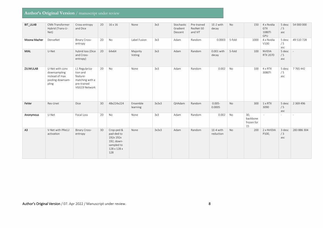
Figure 7: Ranking of each algorithm for each subset of data in Section 3.3.

Author’s Original Version / manuscript under review
Author’s Original Version / 07. Apr 2022 / Manuscript under review. 13
Figure 8: DSC per label for each team (teams ranked from best to worst are visualized from left to right on the x-axis of each graph)

Author’s Original Version / manuscript under review
Author’s Original Version / 07. Apr 2022 / Manuscript under review. 14
Figure 9: HD95 per label for each team (teams ranked from best to worst are visualized from left to right on the x-axis of each graph)

Author’s Original Version / manuscript under review
Author’s Original Version / 07. Apr 2022 / Manuscript under review. 15
Figure 10: VS per label for each team (teams ranked from best to worst are visualized from left to right on the x-axis of each graph)

Author’s Original Version / manuscript under review
Author’s Original Version / 07. Apr 2022 / Manuscript under review. 16
Table 4: Complete Rankings (DSC, HD95, VS combined) for each label; * indicates a tie, with the rank in brackets following the team name
Rank eCSF GM WM Ventricle Cerebel-lum Deep GM Brainstem
1 ichilove-ax pengyy NVAUTO NVAUTO NVAUTO SJTU_EIEE_2-426Lab
SJTU_EIEE_2-426Lab
2 ichilove-combi Hilab Hilab* (2) Hilab SJTU_EIEE_2-426Lab
TRABIT NVAUTO
3 Neurophet* (3)
NVAUTO pengyy* (2) pengyy TRABIT 2Ai xlab
4 Davoodkarimi* (3)
2Ai TRABIT Neurophet davoodkarimi NVAUTO* (4) Hilab
5 NVAUTO* (5) Physense-UPF Team
xlab SJTU_EIEE_2-426Lab
Neurophet Hilab* (4) pengyy
6 muw_dsobotka* (5)
davoodkarimi Physense-UPF Team
Davoodkarimi* (6)
ichilove-ax ichilove-combi* (6)
Neurophet
7 MIAL xlab SJTU_EIEE_2-426Lab
TRABIT* (6) 2Ai pengyy* (6) Physense-UPF Team
8 A3 SJTU_EIEE_2-426Lab* (8)
ichilove-combi xlab* (6) muw_dsobotka
xlab 2Ai
9 pengyy Neurophet* (8)
Neurophet ichilove-ax Hilab MIAL davoodkarimi
10 SingleNets TRABIT SingleNets* (10)
Physense-UPF Team
ichilove-combi Neurophet muw_dsobotka
11 Moona_Mazher* (11)
ichilove-ax Davoodkarimi* (10)
2Ai pengyy muw_dsobotka
ichilove-combi
12 BIT_LILAB* (11)
ichilove-combi* (12)
ichilove-ax muw_dsobotka
BIT_LILAB Physense-UPF Team
ichilove-ax
13 xlab muw_dsobotka* (12)
2Ai ichilove-combi Physense-UPF Team* (13)
Davoodkarimi* (13)
TRABIT
14 Hilab BIT_LILAB* (12)
BIT_LILAB Moona_Mazher* (14)
xlab* (13) BIT_LILAB* (13)
SingleNets* (14)
15 SJTU_EIEE_2-426Lab* (15)
SingleNets muw_dsobotka
BIT_LILAB* (14)
Moona_Mazher
SingleNets* (15)
Moona_Mazher* (14)
16 ZJUWULAB* (15)
ZJUWULAB Moona_Mazher
SingleNets SingleNets Moona_Mazher* (15)
BIT_LILAB
17 FeVer Moona_Mazher
ZJUWULAB MIAL* (17) ZJUWULAB A3 FeVer
18 2Ai MIAL MIAL ZJUWULAB* (17)
FeVer* (18) ichilove-ax MIAL
19 TRABIT FeVer Anonymous FeVer MIAL* (18) ZJUWULAB ZJUWULAB
20 Physense-UPF Team
Anonymous FeVer A3 Anonymous Anonymous * (20)
Anonymous * (20)
21 Anonymous A3 A3 Anonymous A3 FeVer* (20) A3* (20)

Author’s Original Version / manuscript under review
Author’s Original Version / 07. Apr 2022 / Manuscript under review. 17
Further Analysis: A variety of subsets of the data were created in order to determine if the algorithms perform better or worse based on various criteria such as image quality, SR method used, and normal vs pathological brains. The rankings of the teams based on the different subsets can be seen in Figure 7. A large amount of variability in the rankings is present depending on the subset of data being investigated. However, NVAUTO remains in the number 1 ranking spot in all subsets except two (Excellent Quality and IRTK_SR).
Per-Label Metric Values and Ranking: Each team’s algorithm was ana-lyzed separately per tissue label. The average DSC, HD95, and VS scores for each team and label can be found in Figures 8 - 10. The order of the teams on the x-axis in each graph is ordered from best to worst, left to right. When looking at the DSC, team NVAUTO placed first in all labels except eCSF (MIAL), deepGM (TRABIT), and brainstem (SJTU_EIEE_2-426Lab). When looking at the HD95, team NVAUTO placed first in all labels except eCSF (ichilove-combi), Ventricles (Hilab), and deepGM (SJTU_EIEE_2-426Lab). In the VS metric, almost every label had a different top team: eCSF (MIAL), GM (2Ai), WM (NVAUTO), Ventricles (NVAUTO), Cerebellum (ichilove-ax), deepGM (A3), and brainstem (SJTU_EIEE_2-426Lab).
Image Quality: The dataset was split into three subsets based on the quality of the SR reconstructions as determined by experienced raters (excel-lent quality SR: n=11 (mialSR/IRTK: 1/10); good quality SR: n=25 (mialSR/IRTK: 15/10); poor quality SR: n=4 (mialSR/IRTK: 4/0)). Each team’s algorithm was analyzed with the average metrics across all labels. The average DSC, HD95, and VS scores for each team and label can be found in Figure 11. The order of the teams on the x-axis in each graph is ordered from best to worst, left to right. Team pengyy performed the best (according to the DSC) when the fetal brain reconstructions were of excellent quality, while NVAUTO performed the best for good and poor quality reconstructions. Complete ranking information taking all three metrics into account based on SR reconstruction quality can be found in Figure 7.
Figure 11: DSC across all labels for each team, based on the quality of the SR reconstruc-tion (teams ranked from best to worst are visualized from left to right on the x-axis of
each graph)
SR Reconstruction: The dataset was split into two subsets based on SR reconstruction method used. Each team’s algorithm was analyzed with the average metrics across all labels. The average DSC, HD95, and VS scores for each team and label can be found in Figure 12. The order of the teams on the x-axis in each graph is ordered from best to worst, left to right. Team NVAUTO performed the best (according to the DSC) with the mialSRSR reconstruction, and Team SJTU_EIEE_2-426Lab performed the best (according to the DSC) with the IRTK SR reconstruction. Complete ranking information taking all
three metrics into account for each SR reconstruction can be found in Figure 7.
Figure 12: DSC across all labels for each team, based on the SR reconstruction used (teams ranked from best to worst are visualized from left to right on the x-axis of each
graph)
Pathology: The dataset was split into two subsets based on whether the fetal brain contained a pathology (n=25 (mialSR/IRTK: 14/11)) or not (neuro-logically normal, n=15 (mialSR/IRTK: 6/9)). Each team’s algorithm was analyzed with the average metrics across all labels. The average DSC, HD95, and VS scores for each team and label can be found in Figure 13. The order of the teams on the x-axis in each graph is ordered from best to worst, left to right. Team NVAUTO performed best for both pathological and non-pathological brains. No details of the specific pathologies were available to the challenge participants. Complete ranking information taking all three metrics into account for the pathological and non-pathological datasets can be found in Figure 7.
Figure 13: DSC across all labels for each team, based on whether the fetal brain was pathological or non-pathological (teams ranked from best to worst are visualized from
left to right on the x-axis of each graph)
Intracranial Volume: The intracranial volume of each case in the test set was calculated using all labels (excluding the background) and compared to the intracranial volumes determined by each participant in the challenge. While most methods had some outliers, all teams except for five had a medi-an percent difference from GT within ±1% (Figure 14).

Author’s Original Version / manuscript under review
Author’s Original Version / 07. Apr 2022 / Manuscript under review. 18
Figure 14: Percent difference in intracranial volume between the submitted algorithms and the reference label map.
Gestational Age Comparison in the GM: The evaluation metrics for the cortex (grey matter label) were calculated based on age of the fetus. The top-scoring teams for the younger fetuses (GA 21-28; n=28) were pengyy, NVAU-TO, and Hilab.
The top scoring teams for the older fetuses (GA 29-35; n=12) were xlab, pengyy, and Hilab. When all ages were combined together, the top teams for the GM label were pengyy, Hilab, and NVAUTO (see Table 4), showing that gestational age does play a small role in the success of the algorithms in segmenting the cortex. There are fewer cases included in the older group mainly due to the smaller gestational age range, and the fact that the majority of fetal scans at the center used to collect the data happen by the 32nd gestational week. The evaluation metrics of the GM from both the older and younger fetuses can be seen in Figure 15 and 16.
Figure 15: Evaluation metrics (DSC, HD95, VS) of the GM label from younger GA fetuses (21-28GA)
Figure 16: Evaluation metrics (DSC, HD95, VS) of the GM label from older GA fetuses (29-35GA)
Discussion and Conclusion In this paper we present the results of the first FeTA Challenge held at the
MICCAI 2021 conference. All submissions to the FeTA Challenge were deep-learning based submissions. Other machine-learning methods or purely atlas-based approaches were not submitted. This demonstrates that deep learning is currently the leading method for fetal brain medical image segmentation, and confirms its dominance in medical image segmentation more broadly. Indeed, the top three teams all had very similar network architectures. The majority of participating teams obtained very similar evaluation metrics; however, one team performed significantly better than all other teams on the complete testing dataset.
Top Methods: When all labels are combined together and the entire test-ing dataset is used, Team NVAUTO submitted the top algorithm of the challenge. They ranked first in two out of the three evaluation metrics (DCS and HD95), and came second in the third (VS). In addition, the bootstrapping and significance testing showed that NVAUTO was the clear winner in the DSC and HD95 coefficients. The VS metric was more ambiguous across all partici-pants, with no statistically significant difference among the first 9 teams. This suggests that while VS is a relevant biomarker, it is potentially not an ideal evaluation metric for this challenge as it is unable to show differences in the performance.
There were many methodological similarities among the top five ranking teams. All were 3D U-Nets, all used either a Dice or cross-entropy/Dice com-bination loss function, none used an external dataset, and all used standard data augmentation techniques such as rotation, flipping, scaling, addition of Gaussian noise, Gaussian smoothing, gamma correction, affine transfor-mations, and contrast adjustment. Four of the teams used Pytorch, while the fifth used MONAI, which is Pytorch-based (MONAI Consortium, 2020). All used the same convolution kernel size (3x3x3) with random initialization. Four out of five used an ensemble learning strategy, three teams out of the top five used cross-validation. The main differences in networks appeared to be in the training procedures, such as the number of epochs, and in how the learning rate was manipulated throughout training.
When looking at the changes in rankings based on different subsets of the data the interpretation of the results become challenging. As shown in Figure 7, the rankings change considerably depending on the data subset tested. This is relevant, as different centers have different data, different age ranges at which fetal MRI is acquired and one algorithm may not work well across all sites. As the submitted algorithms were all similar deep learning-based methods, this suggests that fine tuning the networks plays a key role in any potential practical application of these algorithms, depending on the specific clinical or research usage.

Author’s Original Version / manuscript under review
Author’s Original Version / 07. Apr 2022 / Manuscript under review. 19
Performance of Submitted Algorithms: As mentioned already, all sub-missions were deep learning-based submissions. To go one step further, it was not just that all submissions used deep learning, but 19 out of 21 submis-sions used some form of U- Net, consisting of a contracting and an expanding path forming a U-shaped network. During the former, higher resolution information is sacrificed for more context. However, U-Net has the capability, using skip connections, of combining this information with the corresponding output from the expanding path. There were many differences within each U-Net, but the overall shape and structure of the network remained consistent, including the depth of the network. Eight teams used the pre-existing medical imaging neural network frameworks nnU-Net (Isensee et al., 2021) or MONAI (MONAI Consortium, 2020). The main differences across the submissions were in how the training was performed (such as the use of cross-validation or changes in the learning rate decay), or in the pre-processing (patch size, how the data was normalized) and post-processing (such as ensemble learn-ing, removal of external label ‘blobs’). The plateauing of the top team entries is interesting as well, potentially suggesting that U-Nets have a performance limit in multi-class segmentation tasks with limited data.
The most likely labels to fail to be segmented (that is, where the algo-rithm was unable to detect any voxels with the specific tissue) were the brainstem and the cerebellum, in particular in the pathological cases. This could potentially be explained by unclear demarcations of the brainstem and cerebellum in pathological groups which contained some cases of the Chiari-II malformation. Overall, the most challenging labels to segment were cortical GM, deep GM, and the brainstem. This can be seen in Figure 8 - Figure 10, where these three tissue labels have worse performances than the other tissues, along with a larger distribution of evaluation metrics in each team. The potential reasons for this are multifold. The lateral and ventral borders of the deep GM and ventral portion of the brainstem are not well defined and are challenging for experienced radiologists to delineate. In the GM, the contrast between WM and GM changes throughout gestation due to neuronal migration and axonal outgrowth, while the surface pattern of the cortical GM becomes increasingly complex.
In general, the pathological brains were more challenging to segment than the non-pathological brains due to the larger variations in neuroanato-my. Selective data augmentation on these pathological cases could be a potential solution to this. The results of the image quality and SR reconstruc-tion methods are related to each other, as the majority of the low quality images were done with the mialSR method, and the excellent quality brain volumes included were reconstructed with the Simple IRTK method. We would like to emphasize this is not a comment on the SR methods them-selves, only a reflection of what cases were chosen for each reconstruction method. As expected, the low quality images, and therefore also the mialSR reconstructions were more challenging to accurately segment than the high quality and IRTK SR reconstructions, with lower DSC scores and a wider range of variability as can be seen in Figure 12.
Clinical Applications: Potential applications of the fully automatic and highly accurate fetal brain MRI segmentation algorithms are broad and span from neuroscience (characterizing spatio-temporal lateralization of the cortex (Kasprian et al., 2011; Vasung et al., 2020), virtopsies (identification and analysis of the details of demise (Rüegger et al., 2014)), surgery (clinical guidelines for early fetal surgery (Clewell et al., 1982; Meuli et al., 1997; Meuli and Moehrlen, 2013)), medicine (identification of biomarkers of outcome needed for stratification tools and development of early interventions (Rollins et al., 2021)), volumetric studies (Polat et al., 2017; Sadhwani et al., 2022) and development of new public health policies (prenatal programs focused on reduction of stress during pregnancy (van den Heuvel et al., 2021; Wu et al., 2020)).
Fetal MRI offers a unique possibility to study the human specific aspects of neurodevelopment. It remains the only non-invasive in vivo imaging modal-ity to study connectivity, function, and structural anatomy of the fetal brain in a single session (Jakab et al., 2021, 2015). From the perspective of neurosci-ence, it is critically important to study the relationship between brain structure and function. However, this requires parcellation of the brain and cortex into regions or areas (e.g. (Amunts et al., 2020; Desikan et al., 2006; Klein and Tourville, 2012)). A first crucial step toward this is to perform relia-ble segmentation of the developing cerebral cortex, which was the objective of this FeTA Challenge.
Furthermore, normative charts showing age-related changes in volume of different brain structures throughout the lifespan, similar to head circumfer-
ence in the pediatric population, have just started to emerge (Bethlehem et al., 2021). Nonetheless, in addition to obvious challenges of fetal MRI acquisi-tion, the harmonization of MRI acquisition protocols across sites and the development of robust and automatic algorithms for accurate and precise segmentation of fetal brain remain prerequisites for any future clinical appli-cation.
Limitations and Future Considerations: Some limitations of the challenge include the fact that all images included were acquired from a single center, and therefore algorithms developed with this dataset are unlikely to be generalizable to other centers. In addition, while the total number of cases included is relatively large for the type of dataset, it is relatively small when compared to other datasets used for training neural networks (Bakas et al., 2019; Menze et al., 2015). The manual segmentations included in both the training and testing dataset were not perfect, and therefore there are misla-beled voxels. Annotations were made mainly in the axial plane, leading to some noisy labels and discontinuity in the annotations in the coronal and sagittal planes. The manual annotations were especially challenging in the mialSR reconstructions, as it was the low resolution scans that underwent reorientation rather than the final reconstructed volume, resulting in a final reconstruction that was not exactly ‘in plane’ according to standard fetal atlases. This led to the phenomenon of participants’ algorithms performing quite well visually but receiving mid-range evaluation metrics. One team even performed their own revisions on the manual segmentations using their own in house experts, and then used them in their training dataset (Fidon et al., 2021). While organizing the challenge we were aware of these errors, and therefore included three different metrics in order to reduce the reliance on any one metric. Future work includes improving the manual segmentations included in the FeTA Dataset. Further research into inter-rater variability in fetal brain segmentations is also required to understand what values of evaluation metrics are considered ‘good enough’. Preliminary research has been done using a very small sample set (Payette et al., 2021a), but a more extensive study should be performed.
In the future, we aim to expand the FeTA Dataset to include data from multiple centers in order to increase the generalizability of algorithms trained using this dataset. We also hope to extend the number of different patholo-gies included, and to increase the number of cases at the outer range of the gestational ages, especially at older gestational ages.
Conclusion: The algorithms developed as part of the FeTA Challenge pro-vide a benchmark for future segmentation algorithms and can already be used to research fetal neurodevelopment. Our study found that most groups working on segmentation methods are using U-Nets, and that 3D U-Nets seem to be superior to 2D based on the evaluation metrics. In a dataset with large variation, such as the FeTA Dataset, the variation plays a role in the success of the algorithm. There was not one algorithm that was the ‘best’ when specific subsets of the data was analyzed, although there was a ‘best’ algorithm when the testing dataset was assessed as a whole. There are still many opportunities for improvement in developing multi-class segmentation techniques for the fetal brain throughout gestation, and therefore this chal-lenge is the starting point for further development of such algorithms.
CRediT Author Statements Kelly Payette: Conceptualization, Writing - Original Draft, Data Curation, Visualization, Software, Validation, Investigation
Hongwei Li: Writing - Review & Editing, Software, Validation, Conceptualiza-tion
Priscille de Dumast: Writing - Review & Editing, Conceptualization
Roxane Licandro: Writing - Review & Editing, Conceptualization
Hui Ji: Data Curation
Lana Vasung: Writing - Review & Editing, Conceptualization
Bjoern Menze: Supervision
Meritxell Bach Cuadra: Conceptualization, Writing - Review & Editing, Super-vision, Investigation

Author’s Original Version / manuscript under review
Author’s Original Version / 07. Apr 2022 / Manuscript under review. 20
Andras Jakab: Conceptualization, Writing - Review & Editing, Data Curation, Visualization, Supervision, Investigation
Md Mahfuzur Rahman Siddiquee, Daguang Xu, Andriy Myronenko, Hao Liu, Yuchen Pei, Lisheng Wang, Ying Peng, Juanying Xie, Huiquan Zhang, Guiming Dong, Hao Fu, Guotai Wang, ZunHyan (Clarence) Rieu, Donghyeon Kim, Hyun Gi Kim, Davood Karimi, Ali Gholipour, Helena R. Torres, Bruno Oliveira, João L. Vilaça, Yang Lin, Netanell Avisdris, Ori Ben-Zvi, Dafna Ben Bashat, Lucas Fidon, Michael Aertsen, Tom Vercauteren, Daniel Sobotka, Georg Langs, Mireia Alenyà, Maria Inmaculada Villanueva, Oscar Camara, Bella Specktor Fadida, Leo Joskowicz, Liao Weibin, Lv Yi, Li Xuesong, Moona Mazher, Abdul Qayyum, Domenec Puig, Hamza Kebiri, Zelin Zhang, Xinyi Xu, Dan Wu, KuanLun Liao, YiXuan Wu, JinTai Chen, Yunzhi Xu, Li Zhao: Data Curation, Writing - Original Draft, Review & Editing
Funding Sources and Acknowledgements
The authors would like to acknowledge funding from the following fund-ing sources: the OPO Foundation, the Prof. Dr. Max Cloetta Foundation, the Anna Müller Grocholski Foundation, the Foundation for Research in Science and the Humanities at the UZH, the EMDO Foundation, the Hasler Founda-tion, the FZK Grant, the Swiss National Science Foundation (project 205321-182602), the Forschungskredit (Grant NO. FK-21-125) from University of Zurich, the ZNZ PhD Grant, the EU H2020 Marie Sklodowska-Curie [765148], Austrian Science Fund FWF [P 35189], Vienna Science and Technology Fund WWTF [LS20-065], and the Austrian Research Fund Grant I3925-B27 in collab-oration with the French National Research Agency (ANR). We acknowledge access to the expertise of the CIBM Center for Biomedical Imaging, a Swiss research center of excellence founded and supported by Lausanne University Hospital (CHUV), University of Lausanne (UNIL), Ecole polytechnique fédérale de Lausanne (EPFL), University of Geneva (UNIGE) and Geneva University Hospitals (HUG). We would also like to acknowledge funding from the Euro-pean Union's Horizon 2020 research and innovation program under the Marie Sklodowska-Curie grant agreement TRABIT No 765148, as well as from core and project funding from the Wellcome [203148/Z/16/Z; 203145Z/16/Z; WT101957], and EP-SRC [NS/A000049/1; NS/A000050/1; NS/A000027/1]. TV is supported by a Medtronic / RAEng Research Chair [RCSRF1819\7\34]. The authors would also like to thank NVIDIA for providing access to computing resources.
This manuscript is the author’s original version.
References
Amunts, K., Mohlberg, H., Bludau, S., Zilles, K., 2020. Julich-Brain: A 3D probabilistic atlas of the human brain’s cytoarchitecture. Science 369, 988–992. https://doi.org/10.1126/science.abb4588
Bach Cuadra, M., Schaer, M., Andre, A., Guibaud, L., Eliez, S., Thiran, J.-P. (Eds.), 2009. Brain tissue segmentation of fetal MR images, in: Workshop on Image Analysis for Developing Brain, in 12th International Conference on Medical Image Computing and Computer Assisted Intervention. Presented at the Workshop on Image Analysis for Developing Brain, in 12th International Conference on Medical Image Computing and Computer Assisted Interven-tion, London, UK.
Bakas, S., Reyes, M., Jakab, A., Bauer, S., Rempfler, M., Crimi, A., Shinoha-ra, R.T., Berger, C., Ha, S.M., Rozycki, M., Prastawa, M., Alberts, E., Lipkova, J., Freymann, J., Kirby, J., Bilello, M., Fathallah-Shaykh, H., Wiest, R., Kirschke, J., Wiestler, B., Colen, R., Kotrotsou, A., Lamontagne, P., Marcus, D., Milchenko, M., Nazeri, A., Weber, M.-A., Mahajan, A., Baid, U., Gerstner, E., Kwon, D., Acharya, G., Agarwal, M., Alam, M., Albiol, Alberto, Albiol, Antonio, Albiol, F.J., Alex, V., Allinson, N., Amorim, P.H.A., Amrutkar, A., Anand, G., Andermatt, S., Arbel, T., Arbelaez, P., Avery, A., Azmat, M., B., P., Bai, W., Banerjee, S., Barth, B., Batchelder, T., Batmanghelich, K., Battistella, E., Beers, A., Belyaev, M., Bendszus, M., Benson, E., Bernal, J., Bharath, H.N., Biros, G., Bisdas, S., Brown, J., Cabezas, M., Cao, S., Cardoso, J.M., Carver, E.N., Casamitjana, A., Castillo, L.S., Catà, M., Cattin, P., Cerigues, A., Chagas, V.S., Chandra, S., Chang, Y.-J., Chang, S., Chang, K., Chazalon, J., Chen, S., Chen, W., Chen, J.W., Chen, Z., Cheng, K., Choudhury, A.R., Chylla, R., Clérigues, A., Colleman, S., Colmeiro, R.G.R., Combalia, M., Costa, A., Cui, X., Dai, Z., Dai, L., Daza, L.A., Deutsch, E., Ding, C., Dong, C., Dong, S., Dudzik, W., Eaton-Rosen, Z., Egan, G., Escudero,
G., Estienne, T., Everson, R., Fabrizio, J., Fan, Y., Fang, L., Feng, X., Ferrante, E., Fidon, L., Fischer, M., French, A.P., Fridman, N., Fu, H., Fuentes, D., Gao, Y., Gates, E., Gering, D., Gholami, A., Gierke, W., Glocker, B., Gong, M., González-Villá, S., Grosges, T., Guan, Y., Guo, S., Gupta, S., Han, W.-S., Han, I.S., Harmuth, K., He, H., Hernández-Sabaté, A., Herrmann, E., Himthani, N., Hsu, W., Hsu, C., Hu, Xiaojun, Hu, Xiaobin, Hu, Yan, Hu, Yifan, Hua, R., Huang, T.-Y., Huang, W., Van Huffel, S., Huo, Q., HV, V., Iftekharuddin, K.M., Isensee, F., Islam, M., Jackson, A.S., Jambawalikar, S.R., Jesson, A., Jian, W., Jin, P., Jose, V.J.M., Jungo, A., Kainz, B., Kamnitsas, K., Kao, P.-Y., Karnawat, A., Kellermeier, T., Kermi, A., Keutzer, K., Khadir, M.T., Khened, M., Kickingereder, P., Kim, G., King, N., Knapp, H., Knecht, U., Kohli, L., Kong, D., Kong, X., Koppers, S., Kori, A., Krishnamurthi, G., Krivov, E., Kumar, P., Kushibar, K., Lachinov, D., Lam-brou, T., Lee, J., Lee, C., Lee, Y., Lee, M., Lefkovits, S., Lefkovits, L., Levitt, J., Li, T., Li, Hongwei, Li, W., Li, Hongyang, Li, Xiaochuan, Li, Y., Li, Heng, Li, Zhenye, Li, Xiaoyu, Li, Zeju, Li, XiaoGang, Li, W., Lin, Z.-S., Lin, F., Lio, P., Liu, C., Liu, B., Liu, X., Liu, M., Liu, J., Liu, L., Llado, X., Lopez, M.M., Lorenzo, P.R., Lu, Z., Luo, L., Luo, Z., Ma, J., Ma, K., Mackie, T., Madabushi, A., Mahmoudi, I., Maier-Hein, K.H., Maji, P., Mammen, C.P., Mang, A., Manjunath, B.S., Marcinkiewicz, M., McDonagh, S., McKenna, S., McKinley, R., Mehl, M., Mehta, S., Mehta, R., Meier, R., Meinel, C., Merhof, D., Meyer, C., Miller, R., Mitra, S., Moiyadi, A., Molina-Garcia, D., Monteiro, M.A.B., Mrukwa, G., Myronenko, A., Nalepa, J., Ngo, T., Nie, D., Ning, H., Niu, C., Nuechterlein, N.K., Oermann, E., Oliveira, A., Oliveira, D.D.C., Oliver, A., Osman, A.F.I., Ou, Y.-N., Ourselin, S., Paragios, N., Park, M.S., Paschke, B., Pauloski, J.G., Pawar, K., Pawlowski, N., Pei, L., Peng, S., Pereira, S.M., Perez-Beteta, J., Perez-Garcia, V.M., Pezold, S., Pham, B., Phophalia, A., Piella, G., Pillai, G.N., Piraud, M., Pisov, M., Popli, A., Pound, M.P., Pourreza, R., Prasanna, P., Prkovska, V., Pridmore, T.P., Puch, S., Puybareau, É., Qian, B., Qiao, X., Rajchl, M., Rane, S., Rebsamen, M., Ren, H., Ren, X., Revanuru, K., Rezaei, M., Rippel, O., Rivera, L.C., Robert, C., Rosen, B., Rueckert, D., Safwan, M., Salem, M., Salvi, J., Sanchez, I., Sánchez, I., Santos, H.M., Sartor, E., Schellingerhout, D., Scheufele, K., Scott, M.R., Scussel, A.A., Sedlar, S., Serrano-Rubio, J.P., Shah, N.J., Shah, N., Shaikh, M., Shankar, B.U., Shboul, Z., Shen, Haipeng, Shen, D., Shen, L., Shen, Haocheng, Shenoy, V., Shi, F., Shin, H.E., Shu, H., Sima, D., Sinclair, M., Smedby, O., Snyder, J.M., Solta-ninejad, M., Song, G., Soni, M., Stawiaski, J., Subramanian, S., Sun, L., Sun, R., Sun, J., Sun, K., Sun, Y., Sun, G., Sun, S., Suter, Y.R., Szilagyi, L., Talbar, S., Tao, D., Tao, D., Teng, Z., Thakur, S., Thakur, M.H., Tharakan, S., Tiwari, P., Tochon, G., Tran, T., Tsai, Y.M., Tseng, K.-L., Tuan, T.A., Turlapov, V., Tustison, N., Vakalopoulou, M., Valverde, S., Vanguri, R., Vasiliev, E., Ventura, J., Vera, L., Vercauteren, T., Verrastro, C.A., Vidyaratne, L., Vilaplana, V., Vivekanandan, A., Wang, G., Wang, Q., Wang, C.J., Wang, W., Wang, D., Wang, R., Wang, Y., Wang, C., Wang, G., Wen, N., Wen, X., Weninger, L., Wick, W., Wu, S., Wu, Q., Wu, Y., Xia, Y., Xu, Y., Xu, X., Xu, P., Yang, T.-L., Yang, X., Yang, H.-Y., Yang, J., Yang, H., Yang, G., Yao, H., Ye, X., Yin, C., Young-Moxon, B., Yu, J., Yue, X., Zhang, S., Zhang, A., Zhang, K., Zhang, Xuejie, Zhang, Lichi, Zhang, Xiaoyue, Zhang, Y., Zhang, Lei, Zhang, J., Zhang, Xiang, Zhang, T., Zhao, S., Zhao, Y., Zhao, X., Zhao, L., Zheng, Y., Zhong, L., Zhou, C., Zhou, X., Zhou, F., Zhu, H., Zhu, J., Zhuge, Y., Zong, W., Kalpathy-Cramer, J., Farahani, K., Davatzikos, C., van Leemput, K., Menze, B., 2019. Identifying the Best Machine Learning Algorithms for Brain Tumor Segmentation, Progression Assessment, and Overall Survival Prediction in the BRATS Challenge. arXiv:1811.02629 [cs, stat].
Benkarim, O.M., Hahner, N., Piella, G., Gratacos, E., González Ballester, M.A., Eixarch, E., Sanroma, G., 2018. Cortical folding alterations in fetuses with isolated non-severe ventriculomegaly. Neuroimage Clin 18, 103–114. https://doi.org/10.1016/j.nicl.2018.01.006
Bethlehem, R. a. I., Seidlitz, J., White, S.R., Vogel, J.W., Anderson, K.M., Adamson, C., Adler, S., Alexopoulos, G.S., Anagnostou, E., Areces-Gonzalez, A., Astle, D.E., Auyeung, B., Ayub, M., Ball, G., Baron-Cohen, S., Beare, R., Bed-ford, S.A., Benegal, V., Beyer, F., Bae, J.B., Blangero, J., Cábez, M.B., Boardman, J.P., Borzage, M., Bosch-Bayard, J.F., Bourke, N., Calhoun, V.D., Chakravarty, M.M., Chen, C., Chertavian, C., Chetelat, G., Chong, Y.S., Cole, J.H., Corvin, A., Courchesne, E., Crivello, F., Cropley, V.L., Crosbie, J., Crossley, N., Delarue, M., Desrivieres, S., Devenyi, G., Biase, M.A.D., Dolan, R., Donald, K.A., Donohoe, G., Dunlop, K., Edwards, A.D., Elison, J.T., Ellis, C.T., Elman, J.A., Eyler, L., Fair, D.A., Fletcher, P.C., Fonagy, P., Franz, C.E., Galan-Garcia, L., Gholipour, A., Giedd, J., Gilmore, J.H., Glahn, D.C., Goodyer, I., Grant, P.E., Groenewold, N.A., Gunning, F.M., Gur, R.E., Gur, R.C., Hammill, C.F., Hansson, O., Hedden, T., Heinz, A., Henson, R., Heuer, K., Hoare, J., Holla, B., Holmes, A.J., Holt, R., Huang, H., Im, K., Ipser, J., Jack, C.R., Jackowski, A.P., Jia, T., Johnson, K.A., Jones, P.B., Jones, D.T., Kahn, R., Karlsson, H., Karlsson, L.,

Author’s Original Version / manuscript under review
Author’s Original Version / 07. Apr 2022 / Manuscript under review. 21
Kawashima, R., Kelley, E.A., Kern, S., Kim, K., Kitzbichler, M.G., Kremen, W.S., Lalonde, F., Landeau, B., Lee, S., Lerch, J., Lewis, J.D., Li, J., Liao, W., Linares, D.P., Liston, C., Lombardo, M.V., Lv, J., Lynch, C., Mallard, T.T., Marcelis, M., Markello, R.D., Mazoyer, B., McGuire, P., Meaney, M.J., Mechelli, A., Medic, N., Misic, B., Morgan, S.E., Mothersill, D., Nigg, J., Ong, M.Q.W., Ortinau, C., Ossenkoppele, R., Ouyang, M., Palaniyappan, L., Paly, L., Pan, P.M., Pantelis, C., Park, M.M., Paus, T., Pausova, Z., Binette, A.P., Pierce, K., Qian, X., Qiu, J., Qiu, A., Raznahan, A., Rittman, T., Rollins, C.K., Romero-Garcia, R., Ronan, L., Rosenberg, M.D., Rowitch, D.H., Salum, G.A., Satterthwaite, T.D., Schaare, H.L., Schachar, R.J., Schultz, A.P., Schumann, G., Schöll, M., Sharp, D., Shinoha-ra, R.T., Skoog, I., Smyser, C.D., Sperling, R.A., Stein, D.J., Stolicyn, A., Suckling, J., Sullivan, G., Taki, Y., Thyreau, B., Toro, R., Tsvetanov, K.A., Turk-Browne, N.B., Tuulari, J.J., Tzourio, C., Vachon-Presseau, É., Valdes-Sosa, M.J., Valdes-Sosa, P.A., Valk, S.L., Amelsvoort, T. van, Vandekar, S.N., Vasung, L., Victoria, L.W., Villeneuve, S., Villringer, A., Vértes, P.E., Wagstyl, K., Wang, Y.S., Warfield, S.K., Warrier, V., Westman, E., Westwater, M.L., Whalley, H.C., Witte, A.V., Yang, N., Yeo, B.T.T., Yun, H.J., Zalesky, A., Zar, H.J., Zettergren, A., Zhou, J.H., Ziauddeen, H., Zugman, A., Zuo, X.N., Aibl, Initiative, A.D.N., Inves-tigators, A.D.R.W.B., Asrb, Team, C., Cam-CAN, Ccnp, 3r-Brain, Cobre, Group, E.D.B.A. working, FinnBrain, Study, H.A.B., Imagen, K., Nspn, Oasis-3, Project, O., Pond, The PREVENT-AD Research Group, V., Alexander-Bloch, A.F., 2021. Brain charts for the human lifespan. https://doi.org/10.1101/2021.06.08.447489
Çiçek, Ö., Abdulkadir, A., Lienkamp, S.S., Brox, T., Ronneberger, O., 2016. 3D U-Net: learning dense volumetric segmentation from sparse annotation, in: International Conference on Medical Image Computing and Computer-Assisted Intervention. Springer, pp. 424–432.
Clewell, W.H., Johnson, M.L., Meier, P.R., Newkirk, J.B., Zide, S.L., Hen-dee, R.W., Bowes, W.A., Hecht, F., O’Keeffe, D., Henry, G.P., Shikes, R.H., 1982. A Surgical Approach to the Treatment of Fetal Hydrocephalus. New England Journal of Medicine 306, 1320–1325. https://doi.org/10.1056/NEJM198206033062202
Clouchoux, C., du Plessis, A.J., Bouyssi-Kobar, M., Tworetzky, W., McElhinney, D.B., Brown, D.W., Gholipour, A., Kudelski, D., Warfield, S.K., McCarter, R.J., Robertson, R.L., Evans, A.C., Newburger, J.W., Limperopoulos, C., 2013. Delayed Cortical Development in Fetuses with Complex Congenital Heart Disease. Cereb Cortex 23, 2932–2943. https://doi.org/10.1093/cercor/bhs281
De Asis-Cruz, J., Andescavage, N., Limperopoulos, C., 2021. Adverse Pre-natal Exposures and Fetal Brain Development: Insights From Advanced Fetal Magnetic Resonance Imaging. Biological Psychiatry: Cognitive Neuroscience and Neuroimaging. https://doi.org/10.1016/j.bpsc.2021.11.009
de Dumast, P., Kebiri, H., Atat, C., Dunet, V., Koob, M., Cuadra, M.B., 2020. Segmentation of the cortical plate in fetal brain MRI with a topological loss. arXiv:2010.12391 [cs, eess].
Desikan, R.S., Ségonne, F., Fischl, B., Quinn, B.T., Dickerson, B.C., Blacker, D., Buckner, R.L., Dale, A.M., Maguire, R.P., Hyman, B.T., Albert, M.S., Killiany, R.J., 2006. An automated labeling system for subdividing the human cerebral cortex on MRI scans into gyral based regions of interest. Neuroimage 31, 968–980. https://doi.org/10.1016/j.neuroimage.2006.01.021
Dice, L.R., 1945. Measures of the Amount of Ecologic Association Be-tween Species. Ecology 26, 297–302. https://doi.org/10.2307/1932409
Dittrich, E., Kasprian, G.J., Prayer, D., Langs, G., 2011. Atlas Learning in Fe-tal Brain Development. Topics in Magnetic Resonance Imaging 22, 107–111.
Egaña-Ugrinovic, G., Sanz-Cortes, M., Figueras, F., Bargalló, N., Gratacós, E., 2013. Differences in cortical development assessed by fetal MRI in late-onset intrauterine growth restriction. American Journal of Obstetrics and Gynecology 209, 126.e1-126.e8. https://doi.org/10.1016/j.ajog.2013.04.008
Fetit, A.E., Alansary, A., Cordero-Grande, L., Cupitt, J., Davidson, A.B., Ed-wards, A.D., Hajnal, J.V., Hughes, E., Kamnitsas, K., Kyriakopoulou, V., Makropoulos, A., Patkee, P.A., Price, A.N., Rutherford, M.A., Rueckert, D., 2020. A deep learning approach to segmentation of the developing cortex in fetal brain MRI with minimal manual labeling, in: Arbel, T., Ben Ayed, I., de Bruijne, M., Descoteaux, M., Lombaert, H., Pal, C. (Eds.), Proceedings of the Third Conference on Medical Imaging with Deep Learning, Proceedings of Machine Learning Research. PMLR, pp. 241–261.
Fidon, L., Aertsen, M., Emam, D., Mufti, N., Guffens, F., Deprest, T., Demaerel, P., David, A.L., Melbourne, A., Ourselin, S., Deprest, J., Vercau-
teren, T., 2021. Label-Set Loss Functions for Partial Supervision: Application to Fetal Brain 3D MRI Parcellation, in: de Bruijne, M., Cattin, P.C., Cotin, S., Padoy, N., Speidel, S., Zheng, Y., Essert, C. (Eds.), Medical Image Computing and Computer Assisted Intervention – MICCAI 2021. Springer International Publishing, Cham, pp. 647–657. https://doi.org/10.1007/978-3-030-87196-3_60
Gholipour, A., Estroff, J.A., Barnewolt, C.E., Robertson, R.L., Grant, P.E., Gagoski, B., Warfield, S.K., Afacan, O., Connolly, S.A., Neil, J.J., Wolfberg, A., Mulkern, R.V., 2014. Fetal MRI: A Technical Update with Educational Aspira-tions. Concepts Magn Reson Part A Bridg Educ Res 43, 237–266. https://doi.org/10.1002/cmr.a.21321
Gholipour, A., Rollins, C., Velasco-Annis, C., Ouaalam, A., Akhondi-Asl, A., Afacan, O., Ortinau, C., Clancy, S., Limperopoulos, C., Yang, E., Estroff, J., Warfield, S., 2017. A normative spatiotemporal MRI atlas of the fetal brain for automatic segmentation and analysis of early brain growth. Scientific Reports 7. https://doi.org/10.1038/s41598-017-00525-w
Glenn, O.A., 2010. MR imaging of the fetal brain. Pediatr Radiol 40, 68–81. https://doi.org/10.1007/s00247-009-1459-3
Gowland, P., 2011. Safety of Fetal MRI Scanning, in: Prayer, D. (Ed.), Fetal MRI. Springer, Berlin, Heidelberg, pp. 49–54. https://doi.org/10.1007/174_2010_122
Griffiths, P.D., Bradburn, M., Campbell, M.J., Cooper, C.L., Embleton, N., Graham, R., Hart, A.R., Jarvis, D., Kilby, M.D., Lie, M., Mason, G., Mandefield, L., Mooney, C., Pennington, R., Robson, S.C., Wailoo, A., 2019. MRI in the diagnosis of fetal developmental brain abnormalities: the MERIDIAN diagnos-tic accuracy study. Health Technol Assess 23, 1–144. https://doi.org/10.3310/hta23490
Gwet, K.L., 2019. irrCAC: Computing Chance-Corrected Agreement Coeffi-cients (CAC), R Package version 1.0.
Hart, A.R., Embleton, N.D., Bradburn, M., Connolly, D.J.A., Mandefield, L., Mooney, C., Griffiths, P.D., 2020. Accuracy of in-utero MRI to detect fetal brain abnormalities and prognosticate developmental outcome: postnatal follow-up of the MERIDIAN cohort. The Lancet Child & Adolescent Health 4, 131–140. https://doi.org/10.1016/S2352-4642(19)30349-9
Hausdorff, F., 1991. Set theory. American Mathematical Society (RI).
Hong, J., Yun, H.J., Park, G., Kim, S., Laurentys, C.T., Siqueira, L.C., Tarui, T., Rollins, C.K., Ortinau, C.M., Grant, P.E., Lee, J.-M., Im, K., 2020. Fetal Corti-cal Plate Segmentation Using Fully Convolutional Networks With Multiple Plane Aggregation. Frontiers in Neuroscience 14, 1226. https://doi.org/10.3389/fnins.2020.591683
Hosny, I.A., Elghawabi, H.S., 2010. Ultrafast MRI of the fetus: an increas-ingly important tool in prenatal diagnosis of congenital anomalies. Magn Reson Imaging 28, 1431–1439. https://doi.org/10.1016/j.mri.2010.06.024
Isensee, F., Jaeger, P.F., Kohl, S.A.A., Petersen, J., Maier-Hein, K.H., 2021. nnU-Net: a self-configuring method for deep learning-based biomedical image segmentation. Nat Methods 18, 203–211. https://doi.org/10.1038/s41592-020-01008-z
Jakab, A., Payette, K., Mazzone, L., Schauer, S., Muller, C.O., Kottke, R., Ochsenbein-Kölble, N., Tuura, R., Moehrlen, U., Meuli, M., 2021. Emerging magnetic resonance imaging techniques in open spina bifida in utero. Euro-pean Radiology Experimental 5, 23. https://doi.org/10.1186/s41747-021-00219-z
Jakab, A., Pogledic, I., Schwartz, E., Gruber, G., Mitter, C., Brugger, P.C., Langs, G., Schöpf, V., Kasprian, G., Prayer, D., 2015. Fetal Cerebral Magnetic Resonance Imaging Beyond Morphology. Semin. Ultrasound CT MR 36, 465–475. https://doi.org/10.1053/j.sult.2015.06.003
Jarvis, D.A., Finney, C.R., Griffiths, P.D., 2019. Normative volume meas-urements of the fetal intra-cranial compartments using 3D volume in utero MR imaging. Eur Radiol 29, 3488–3495. https://doi.org/10.1007/s00330-018-5938-5
Kasprian, G., Langs, G., Brugger, P.C., Bittner, M., Weber, M., Arantes, M., Prayer, D., 2011. The prenatal origin of hemispheric asymmetry: an in utero neuroimaging study. Cereb. Cortex 21, 1076–1083. https://doi.org/10.1093/cercor/bhq179
Khalili, N., Lessmann, N., Turk, E., Claessens, N., Heus, R. de, Kolk, T., Viergever, M.A., Benders, M.J.N.L., Išgum, I., 2019. Automatic brain tissue

Author’s Original Version / manuscript under review
Author’s Original Version / 07. Apr 2022 / Manuscript under review. 22
segmentation in fetal MRI using convolutional neural networks. Magn Reson Imaging. https://doi.org/10.1016/j.mri.2019.05.020
Kikinis, R., Pieper, S.D., Vosburgh, K.G., 2014. 3D Slicer: A Platform for Subject-Specific Image Analysis, Visualization, and Clinical Support, in: In-traoperative Imaging and Image-Guided Therapy. Springer, New York, NY, pp. 277–289. https://doi.org/10.1007/978-1-4614-7657-3_19
Klein, A., Tourville, J., 2012. 101 Labeled Brain Images and a Consistent Human Cortical Labeling Protocol. Frontiers in Neuroscience 6, 171. https://doi.org/10.3389/fnins.2012.00171
Kuklisova-Murgasova, M., Quaghebeur, G., Rutherford, M.A., Hajnal, J.V., Schnabel, J.A., 2012. Reconstruction of fetal brain MRI with intensity matching and complete outlier removal. Med Image Anal 16, 1550–1564. https://doi.org/10.1016/j.media.2012.07.004
Kyriakopoulou, V., Vatansever, D., Davidson, A., Patkee, P., Elkommos, S., Chew, A., Martinez-Biarge, M., Hagberg, B., Damodaram, M., Allsop, J., Fox, M., Hajnal, J.V., Rutherford, M.A., 2017. Normative biometry of the fetal brain using magnetic resonance imaging. Brain Struct Funct 222, 2295–2307. https://doi.org/10.1007/s00429-016-1342-6
Licandro, R., Langs, G., Kasprian, G.J., Sablatnig, R., Prayer, D., Schwartz, E., 2016. A Longitudinal Diffeomorphic Atlas-Based Tissue Labeling Frame-work for Fetal Brains using Geodesic Regression. Presented at the 21st Computer Vision Winter Workshop, Rimske Toplice, Slovenia.
Maier-Hein, L., Reinke, A., Kozubek, M., Martel, A.L., Arbel, T., Eisenmann, M., Hanbury, A., Jannin, P., Müller, H., Onogur, S., Saez-Rodriguez, J., van Ginneken, B., Kopp-Schneider, A., Landman, B.A., 2020. BIAS: Transparent reporting of biomedical image analysis challenges. Medical Image Analysis 66, 101796. https://doi.org/10.1016/j.media.2020.101796
Menze, B.H., Jakab, A., Bauer, S., Kalpathy-Cramer, J., Farahani, K., Kirby, J., Burren, Y., Porz, N., Slotboom, J., Wiest, R., Lanczi, L., Gerstner, E., Weber, M.-A., Arbel, T., Avants, B.B., Ayache, N., Buendia, P., Collins, D.L., Cordier, N., Corso, J.J., Criminisi, A., Das, T., Delingette, H., Demiralp, Ç., Durst, C.R., Dojat, M., Doyle, S., Festa, J., Forbes, F., Geremia, E., Glocker, B., Golland, P., Guo, X., Hamamci, A., Iftekharuddin, K.M., Jena, R., John, N.M., Konukoglu, E., Lash-kari, D., Mariz, J.A., Meier, R., Pereira, S., Precup, D., Price, S.J., Raviv, T.R., Reza, S.M.S., Ryan, M., Sarikaya, D., Schwartz, L., Shin, H.-C., Shotton, J., Silva, C.A., Sousa, N., Subbanna, N.K., Szekely, G., Taylor, T.J., Thomas, O.M., Tusti-son, N.J., Unal, G., Vasseur, F., Wintermark, M., Ye, D.H., Zhao, L., Zhao, B., Zikic, D., Prastawa, M., Reyes, M., Van Leemput, K., 2015. The Multimodal Brain Tumor Image Segmentation Benchmark (BRATS). IEEE Trans Med Imag-ing 34, 1993–2024. https://doi.org/10.1109/TMI.2014.2377694
Meuli, M., Meuli-Simmen, C., Hutchins, G.M., Seller, M.J., Harrison, M.R., Adzick, N.S., 1997. The spinal cord lesion in human fetuses with myelomenin-gocele: Implications for fetal surgery. Journal of Pediatric Surgery, Papers Presented at the 43rd Annual International Congress 32, 448–452. https://doi.org/10.1016/S0022-3468(97)90603-5
Meuli, M., Moehrlen, U., 2013. Fetal surgery for myelomeningocele: a critical appraisal. Eur J Pediatr Surg 23, 103–109. https://doi.org/10.1055/s-0033-1343082
MONAI Consortium, 2020. MONAI: Medical Open Network for AI. https://doi.org/10.5281/zenodo.4323058
Nagaraj, U.D., Venkatesan, C., Bierbrauer, K.S., Kline-Fath, B.M., 2022. Value of pre- and postnatal magnetic resonance imaging in the evaluation of congenital central nervous system anomalies. Pediatr Radiol 52, 802–816. https://doi.org/10.1007/s00247-021-05137-1
Payette, K., de Dumast, P., Kebiri, H., Ezhov, I., Paetzold, J.C., Shit, S., Iq-bal, A., Khan, R., Kottke, R., Grehten, P., Ji, H., Lanczi, L., Nagy, M., Beresova, M., Nguyen, T.D., Natalucci, G., Karayannis, T., Menze, B., Bach Cuadra, M., Jakab, A., 2021a. An automatic multi-tissue human fetal brain segmentation benchmark using the Fetal Tissue Annotation Dataset. Sci Data 8, 167. https://doi.org/10.1038/s41597-021-00946-3
Payette, K., Dumast, P. de, Jakab, A., Cuadra, M.B., Vasung, L., Licandro, R., Menze, B., Zurich), H.L., 2021b. Fetal Brain Tissue Annotation and Segmen-tation Challenge. https://doi.org/10.5281/zenodo.4573144
Payette, K., Jakab, A., 2021. Fetal Tissue Annotation Challenge - FeTA MICCAI 2021 [WWW Document]. URL http://dx.doi.org/10.7303/syn25649159 (accessed 2.22.22).
Pierre Deman, Sebastien Tourbier, Reto Meuli, Meritxell Bach Cuadra, 2020. meribach/mevislabFetalMRI: MEVISLAB MIAL Super-Resolution Recon-struction of Fetal Brain MRI v1.0. Zenodo. https://doi.org/10.5281/zenodo.3878564
Polat, A., Barlow, S., Ber, R., Achiron, R., Katorza, E., 2017. Volumetric MRI study of the intrauterine growth restriction fetal brain. Eur Radiol 27, 2110–2118. https://doi.org/10.1007/s00330-016-4502-4
Prayer, D., Kasprian, G., Krampl, E., Ulm, B., Witzani, L., Prayer, L., Brug-ger, P.C., 2006. MRI of normal fetal brain development. European Journal of Radiology, Fetal Imaging 57, 199–216. https://doi.org/10.1016/j.ejrad.2005.11.020
R Core Team, 2020. R: A Language and Environment for Statistical Com-puting. R Foundation for Statistical Computing, Vienna, Austria.
Rollins, C.K., Ortinau, C.M., Stopp, C., Friedman, K.G., Tworetzky, W., Gagoski, B., Velasco-Annis, C., Afacan, O., Vasung, L., Beaute, J.I., Rofeberg, V., Estroff, J.A., Grant, P.E., Soul, J.S., Yang, E., Wypij, D., Gholipour, A., Warfield, S.K., Newburger, J.W., 2021. Regional Brain Growth Trajectories in Fetuses with Congenital Heart Disease. Ann Neurol 89, 143–157. https://doi.org/10.1002/ana.25940
Ronneberger, O., Fischer, P., Brox, T., 2015. U-Net: Convolutional Net-works for Biomedical Image Segmentation, in: Navab, N., Hornegger, J., Wells, W.M., Frangi, A.F. (Eds.), Medical Image Computing and Computer-Assisted Intervention – MICCAI 2015, Lecture Notes in Computer Science. Springer International Publishing, Cham, pp. 234–241. https://doi.org/10.1007/978-3-319-24574-4_28
Rüegger, C.M., Bartsch, C., Martinez, R.M., Ross, S., Bolliger, S.A., Koller, B., Held, L., Bruder, E., Bode, P.K., Caduff, R., Frey, B., Schäffer, L., Bucher, H.U., 2014. Minimally invasive, imaging guided virtual autopsy compared to conventional autopsy in foetal, newborn and infant cases: study protocol for the paediatric virtual autopsy trial. BMC Pediatr 14, 15. https://doi.org/10.1186/1471-2431-14-15
Sadhwani, A., Wypij, D., Rofeberg, V., Gholipour, A., Mittleman, M., Rohde, J., Velasco-Annis, C., Calderon, J., Friedman, K.G., Tworetzky, W., Grant, P.E., Soul, J.S., Warfield, S.K., Newburger, J.W., Ortinau, C.M., Rollins, C.K., 2022. Fetal Brain Volume Predicts Neurodevelopment in Congenital Heart Disease. Circulation. https://doi.org/10.1161/CIRCULATIONAHA.121.056305
Sanroma, G., Benkarim, O.M., Piella, G., Lekadir, K., Hahner, N., Eixarch, E., González Ballester, M.A., 2018. Learning to combine complementary segmentation methods for fetal and 6-month infant brain MRI segmentation. Computerized Medical Imaging and Graphics 69, 52–59. https://doi.org/10.1016/j.compmedimag.2018.08.007
Serag, A., Aljabar, P., Ball, G., Counsell, S.J., Boardman, J.P., Rutherford, M.A., Edwards, A.D., Hajnal, J.V., Rueckert, D., 2012. Construction of a con-sistent high-definition spatio-temporal atlas of the developing brain using adaptive kernel regression. Neuroimage 59, 2255–2265. https://doi.org/10.1016/j.neuroimage.2011.09.062
Skotting, M.B., Eskildsen, S.F., Ovesen, A.S., Fonov, V.S., Ringgaard, S., Hjortdal, V.E., Lauridsen, M.H., 2021. Infants with congenital heart defects have reduced brain volumes. Sci Rep 11, 4191. https://doi.org/10.1038/s41598-021-83690-3
Taha, A.A., Hanbury, A., 2015. Metrics for evaluating 3D medical image segmentation: analysis, selection, and tool. BMC Med Imaging 15. https://doi.org/10.1186/s12880-015-0068-x
Tourbier, S., Bresson, X., Hagmann, P., Meuli, R., Bach Cuadra, M., 2019. sebastientourbier/mialsuperresolutiontoolkit: MIAL Super-Resolution Toolkit v1.0. Zenodo. https://doi.org/10.5281/zenodo.2598448
Tourbier, S., Bresson, X., Hagmann, P., Thiran, J.-P., Meuli, R., Cuadra, M.B., 2015. An efficient total variation algorithm for super-resolution in fetal brain MRI with adaptive regularization. Neuroimage 118, 584–597. https://doi.org/10.1016/j.neuroimage.2015.06.018
van den Heuvel, M.I., Hect, J.L., Smarr, B.L., Qawasmeh, T., Kriegsfeld, L.J., Barcelona, J., Hijazi, K.E., Thomason, M.E., 2021. Maternal stress during pregnancy alters fetal cortico-cerebellar connectivity in utero and increases child sleep problems after birth. Sci Rep 11, 2228. https://doi.org/10.1038/s41598-021-81681-y

Author’s Original Version / manuscript under review
Author’s Original Version / 07. Apr 2022 / Manuscript under review. 23
Vasung, L., Abaci Turk, E., Ferradal, S.L., Sutin, J., Stout, J.N., Ahtam, B., Lin, P.-Y., Ellen Grant, P., 2019. Exploring early human brain development with structural and physiological neuroimaging. Neuroimage 187, 226–254. https://doi.org/10.1016/j.neuroimage.2018.07.041
Vasung, L., Rollins, C.K., Yun, H.J., Velasco-Annis, C., Zhang, J., Wagstyl, K., Evans, A., Warfield, S.K., Feldman, H.A., Grant, P.E., Gholipour, A., 2020. Quantitative In vivo MRI Assessment of Structural Asymmetries and Sexual Dimorphism of Transient Fetal Compartments in the Human Brain. Cerebral Cortex 30, 1752–1767. https://doi.org/10.1093/cercor/bhz200
Wiesenfarth, M., Reinke, A., Landman, B.A., Eisenmann, M., Saiz, L.A., Cardoso, M.J., Maier-Hein, L., Kopp-Schneider, A., 2021. Methods and open-source toolkit for analyzing and visualizing challenge results. Sci Rep 11, 2369. https://doi.org/10.1038/s41598-021-82017-6
Wu, Y., Lu, Y.-C., Jacobs, M., Pradhan, S., Kapse, K., Zhao, L., Niforatos-Andescavage, N., Vezina, G., du Plessis, A.J., Limperopoulos, C., 2020. Associa-tion of Prenatal Maternal Psychological Distress With Fetal Brain Growth, Metabolism, and Cortical Maturation. JAMA Network Open 3, e1919940. https://doi.org/10.1001/jamanetworkopen.2019.19940
Zvi, E., Shemer, A., Toussia-Cohen, S., Zvi, D., Bashan, Y., Hirschfeld-Dicker, L., Oselka, N., Amitai, M.-M., Ezra, O., Bar-Yosef, O., Katorza, E., 2020. Fetal Exposure to MR Imaging: Long-Term Neurodevelopmental Outcome. AJNR Am J Neuroradiol 41, 1989–1992. https://doi.org/10.3174/ajnr.A6771

Author’s Original Version / manuscript under review
Author’s Original Version / 07. Apr 2022 / Manuscript under review. 24

Author’s Original Version / manuscript under review
Author’s Original Version / 07. Apr 2022 / Manuscript under review. 25
Overview of Challenge Participants Algorithm
1.1 2Ai
Team Members and Affiliations
Team Members: Helena R. Torres1,2,3,4, Bruno Oliveira1,2,3,4, Pedro Morais, Jaime C. Fonseca, João L. Vilaca1
Affiliations: 12Ai – School of Technology, IPCA, Barcelos, Portugal; 2Algoritmi Center, School of Engineering, University of Minho, Guimarães, Portugal; 3Life and Health Sciences Research Institute (ICVS), School of Medicine, University of Minho, Braga, Portugal; 4ICVS/3B’s - PT Government Associate Laboratory, Braga/Guimarães, Portugal
Model Description
In-utero MRI has been emerging as an important tool to evaluate fetal neurological development. Here, segmentation of fetal brain struc-tures can have an important role in the interpretation of the fetal MRI, allowing to aid in the quantification of the changing brain morphology and in the diagnosis of congenital disorders. Since manual segmentation is highly prone to observer variability and time-consuming, automatic methods for fetal tissue segmentation can bring added value to clinical practice. The main goal of the FeTA challenge is to potentiate the development of new methods for fetal tissue segmentation.
In the scope of the FeTA challenge, an automatic method to segment the different brain structures of the fetus was developed. As well-known, encoder-decoder deep convolutional neural networks have been showed the best performance for medical imaging segmentation. In this work, the U-Net method was adapted to perform fetal tissue segmentation [2, 4]. Concerning the model architecture, similar to U-NET, an encoder-decoder network was used. The encoding path is composed of down-sampling blocks and each block of the encoding path is composed of two convolutional layers, with each layer consisting of a convolution, followed by batch normalization and a leaky rectified linear unit (ReLU). The down-sampling is implemented using a stride convolution on the first layer of each encoding block. The initial num-ber of feature maps is defined to be 32, which is double in each down-sampling stride convolution operation. The decoding path corresponds to a symmetric expanding path and skip-connections are used to allow that the encoder and decoder share information. Overall, the number of trainable parameters was 29,971,032. Moreover, a Sigmoid activation layer was added to the end of the network to achieve the segmentation, which was performed through a one-hot labelling scheme using the Dice metric as loss function. Finally, a Xavier initialization of the model parameters was applied, in order to initialize the weights such that the variance of the activations were the same across every layer.
Concerning the input of the network, all training images of the FeTA challenge were used. A pre-processing of the images was applied, where image normalization was implemented in order to achieve zero mean intensity with unit variance. Moreover, the pixel size of the images was normalized to be the median value of the pixel size of all the images and a patch-based strategy was used, were a 3D patch with size 128x128x128 was applied. To overcome overfitting problems during training, data augmentation techniques were applied to the training images, namely spatial and intensity-based transformations [1]. Spatial transformations included random flip, rotation, scaling, grid distortion, optical distortion, and elastic transformations, whereas intensity transformations included random gaussian noise, brightness, contrast, and gamma transformations.
The network was trained during 800 epochs with a mini-batch size of 4 and using the Adam optimizer with an initial learning rate of 0.001 and a learning rate decay following the polinomial learning rate policy (lr=1- ((1-epoch)⁄(max_epoch) )^power) with the power of 0.9 [3]. The training time of the method was ≈6 days on a computer with a CPU: i7-7700HQ @3.56GHz, RAM: 16GBytes @1.2GHz, and GPU: GTX1070 @1.443GHz, using the PyTorch python library. Finally, the final segmentation was obtained by post-processing the output of the network by removing isolated segmented voxels.
References
[1] Buslaev, A., Iglovikov, V. I., Khvedchenya, E., Parinov, A., Druzhinin, M., & Kalinin, A. A. (2020). Albumentations: Fast and flexible image augmentations. Information (Switzerland), 11(2), 1–20. https://doi.org/10.3390/info11020125
[2] Isensee, F., Jaeger, P. F., Kohl, S. A. A., Petersen, J., & Maier-Hein, K. H. (2021). nnU-Net: a self-configuring method for deep learning-based biomedical image segmentation. Nature Methods, 18(2), 203–211. https://doi.org/10.1038/s41592-020-01008-z
[3] Kingma, D. P., & Ba, J. L. (2015). Adam: A method for stochastic optimization. 3rd International Conference on Learning Representa-tions, ICLR 2015 - Conference Track Proceedings, 1–15.
[4] Ronneberger, O., Fischer, P., & Brox, T. (2015). U-Net: Convolutional Networks for Biomedical Image Segmentation. Computer Vision and Pattern Recognition, 1–8.

Author’s Original Version / manuscript under review
Author’s Original Version / 07. Apr 2022 / Manuscript under review. 26
1.2 A3
Team Members and Affiliations
Team Members: Yunzhi Xu and Li Zhao
Affiliations: College of Biomedical Engineering & Instrument Science, Zhejiang University, Hangzhou, China
Model Description
Input: 3D volume with a shape of 128x128x128. The input data were preprocessed as follows.
Pre-processing: To improve the data balance, the background of the original data was cropped according to the edge of the brain in 3D. The border of the brain was selected by the non-zero pixels. The cropped images were zero-padded to a matrix size of 192x192x192. Then the images were down-sampled to 128x128x128 to fit in the memory of GPUs. Images were normalized, so the mean value was zero and the standard deviation equals one.
Model Architecture: The model was implemented based on V-net. Compared to the standard U-Net, a parametric rectified linear unit (PReLU) activation function. Starting number of features was 16 and was doubled in each descending layer. There are three layers of fea-ture extraction. Each layer was a res-net composed of two consecutive 3x3x3 convolutional kernels. Layer normalization was used instead of original batch normalization. A 2x2x2 max-pooling was performed instead of 3D convolution in the original V-net. A dropout rate of 0.5 was used before the first transpose convolution layer. The decoding path was symmetric with the encoding path with the halved number of filters for each layer.
Training Description
FeTA data were mixed in the training with 80% in the training and 20% in the validation. No additional data were used. Data augmentation was performed by randomly shifting the image up to 5 pixels in 3 directions, rotating the image up to 15 degrees along three axes, and flipping the brain in the left-right direction. Binary-cross-entropy was used as the loss function. Adam optimizer was used with a learning rate of 1e-4 with auto rate schedule using ReduceLROnPlateau. The model was trained in 200 epochs. Each epoch had 32 steps and a batch size of two. The algorithm was implemented using Tensorflow 2.4. The training was performed with two Nvidia P100 GPUs, 16 CPUs, and 118G Memory on Alibaba Cloud.

Author’s Original Version / manuscript under review
Author’s Original Version / 07. Apr 2022 / Manuscript under review. 27
1.3 BIT_LILAB
1.3.1 Team Members and Affiliations
Team Members: Weibin Liao, Yi Lv, Xuesong Li
Affiliations: School of Computer Science and Technology, Beijing Institute of Technology, Beijing, Chi-
na
1.3.2 Model Architecture
Our model structure is shown in the figure below, mainly referring to TransUNet [1]. This is a
CNN-Transformer hybrid model. The network is similar to a U-shaped structure, adding Transformer
layers with Multi-head Self-Attention mechanism to the encoder to encode the feature representation
of image patches. The motivation of using this hybrid architecture is that we can not only use the high-
resolution CNN feature map in the decoding path, but also use the global context information encoded
by Transformers [2].
In encoder, ResNet-50 [3] is used as the feature extractor of CNN to generate a feature map
for the input image. Transformer is used encoding feature representations from decomposed image
patches.
Decoder consists of multiple up-sampling block, where each block consists of a 2× upsampling opera-
tor, a 3×3 convolution layer, a ReLU layer and a Batch Normalization layer successively. The overall
architecture of our proposal network can be found in Figure 1. The detailed network architecture can
be found in Table 1.
Fig.1. Overall architecture of our proposal network.
Table 1. The design details of our proposed network. 𝐶𝑜𝑛𝑣 3 × 3 denotes a 3 × 3 convolutional layer. 𝐺𝑁 denotes Group Nor-
malization. 𝐵𝑁 denotes Batch Normalization. Each ResBlock in encoder is a residual block. The size of input image is
3×256×256.
Stage Block name Details Output Size
CNN Encoder
InitConv 𝐶𝑜𝑛𝑣 7 × 7, 𝐺𝑁, 𝑅𝑒𝐿𝑈 64 × 128 × 128
DownSample 𝑀𝑎𝑥𝑃𝑜𝑜𝑙 64 × 128 × 128
ResBlock1 {𝐺𝑁, 𝐶𝑜𝑛𝑣 1 × 1, 𝑅𝑒𝐿𝑈𝐺𝑁, 𝐶𝑜𝑛𝑣 3 × 3, 𝑅𝑒𝐿𝑈𝐺𝑁, 𝐶𝑜𝑛𝑣 1 × 1, 𝑅𝑒𝐿𝑈
× 3 128 × 64 × 64

Author’s Original Version / manuscript under review
Author’s Original Version / 07. Apr 2022 / Manuscript under review. 28
ResBlock2 {𝐺𝑁, 𝐶𝑜𝑛𝑣 1 × 1, 𝑅𝑒𝐿𝑈𝐺𝑁, 𝐶𝑜𝑛𝑣 3 × 3, 𝑅𝑒𝐿𝑈𝐺𝑁, 𝐶𝑜𝑛𝑣 1 × 1, 𝑅𝑒𝐿𝑈
× 4 256 × 32 × 32
ResBlock3 {𝐺𝑁, 𝐶𝑜𝑛𝑣 1 × 1, 𝑅𝑒𝐿𝑈𝐺𝑁, 𝐶𝑜𝑛𝑣 3 × 3, 𝑅𝑒𝐿𝑈𝐺𝑁, 𝐶𝑜𝑛𝑣 1 × 1, 𝑅𝑒𝐿𝑈
× 9 512 × 16 × 16
Transformer Encod-
er
Linear Projection 𝐶𝑜𝑛𝑣 3 × 3, 𝑟𝑒𝑠ℎ𝑎𝑝𝑒 1024 × 4096
Transformer 𝑇𝑟𝑎𝑛𝑠𝑓𝑜𝑟𝑚𝑒𝑟 𝐿𝑎𝑦𝑒𝑟 × 12 1024 × 4096
CNN Decoder
Feature Mapping 𝑟𝑒𝑠ℎ𝑎𝑝𝑒, 𝐶𝑜𝑛𝑣3 × 3 512 × 16 × 16
DeBlock1 𝐶𝑜𝑛𝑣 3 × 3, 𝑅𝑒𝐿𝑈, 𝐵𝑁 × 3 512 × 16 × 16
UpSample1 𝐶𝑜𝑛𝑣 3 × 3, 𝑈𝑝𝑠𝑎𝑚𝑝𝑙𝑖𝑛𝑔𝐵𝑖𝑙𝑖𝑛𝑒𝑎𝑟 256 × 32 × 32
DeBlock2 𝐶𝑜𝑛𝑣 3 × 3, 𝑅𝑒𝐿𝑈, 𝐵𝑁 × 2 256 × 32 × 32
UpSample2 𝐶𝑜𝑛𝑣 3 × 3, 𝑈𝑝𝑠𝑎𝑚𝑝𝑙𝑖𝑛𝑔𝐵𝑖𝑙𝑖𝑛𝑒𝑎𝑟 128 × 64 × 64
DeBlock3 𝐶𝑜𝑛𝑣 3 × 3, 𝑅𝑒𝐿𝑈, 𝐵𝑁 × 2 128 × 64 × 64
UpSample3 𝐶𝑜𝑛𝑣 3 × 3, 𝑈𝑝𝑠𝑎𝑚𝑝𝑙𝑖𝑛𝑔𝐵𝑖𝑙𝑖𝑛𝑒𝑎𝑟 64 × 128 × 128
DeBlock4 𝐶𝑜𝑛𝑣 3 × 3, 𝑅𝑒𝐿𝑈, 𝐵𝑁 × 2 64 × 128 × 128
EndConv 𝐶𝑜𝑛𝑣 1 × 1, 𝑆𝑜𝑓𝑡𝑚𝑎𝑥 3 × 256 × 256
1.3.3 Input and Output
Our model accepts 2D slices as input, and the 3D volume needs to be sliced in advance dur-
ing model training. When testing, the 3D volume image can be directly input, and the program will
automatically slice the volume image, predict each slice, and then stack it into a 3D volume image.
The input 2D slice resolution is 256 × 256, and the image patch size is fixed as 16 × 16.
1.3.4 Dataset
We used all 80 data in the dataset. Due to the different reconstruction methods of data (the
first 40 data are reconstructed by MialSRTK and the last 40 data are reconstructed by SimpleIRTK.
When using data, we make a simple division based on two different reconstruction methods. 60 data
(1-30, 41-70) are used as the training set, and 20 data (31-40, 71-80) are used as the test set. We
don’t differentiate the data for health conditions.
1.3.5 Preprocess and Data Augmentation
Due to we use 2D-input network, we need to preprocess 3D volume data into 2D slices. We
adopt two simple data augmentation strategies: random rotation and flipping. Randomly rotate the 2D
slice (-20, 20) degrees counterclockwise, or rotate it by 90 degrees, and then flip it up and down or left
and right. The probability of data augmentation is 0.5.
1.3.6 Pre-training
ResNet-50 and ViT are combined in the hybrid encoder, we use the pre-training model of the
backbone network provided by the author. We have also made some attempts on transfer learning:
We first train the model on the Synapse multi-organ segmentation dataset, and then transfer the pre-
training weights to the Fetal Tissue Annotation task. The results show that the model with pre-trained
weights can converge faster on the Fetal Tissue Annotation dataset.
1.3.7 Implementation Details
The input resolution and patch size are set as 256 × 256 and 16. Models are trained with SGD
optimizer with learning rate 0.01, momentum 0.9 and weight decay 1e-4. Batch size is 24, the max
epochs are 150 and the number of training iterations are 30k. Loss function is a composite loss func-
tion of Cross Entropy and Dice loss. All experiments are conducted using four Nvidia GTX 1080Ti
GPU. Training model takes about 10 hours at a time.

Author’s Original Version / manuscript under review
Author’s Original Version / 07. Apr 2022 / Manuscript under review. 29
The python package version we use is as follows: torch==1.4.0, torchvision==0.5.0, numpy==1.20.3,
tqdm==4.61.1, tensorboard==2.5.0, tensorboardX==2.2, ml-collections==0.1.0, medpy==0.4.0, Sim-
pleITK==2.0.2, scipy==1.6.3, h5py==3.2.1.
1.3.8 Other Trained Models
We also tried other two baseline models on this task.
The first is nnUNet [4]. nnU-Net is the first standardized deep learning benchmark in biomedi-
cal segmentation. Without manual effort, researchers can compare their algorithms against nnU-Net
on an arbitrary number of datasets to provide meaningful evidence for proposed improvements. We
use 3D full resolution U-Net for training in nnUNet. We also used all 80 data, including 64 data as
training data and 16 data as validation data. The test results show that nnUNet can reach the same
level as TransUNet in DSC and HD95.
The other is CoTr [5]. This is also a framework combining CNN and transformer for medical
image segmentation. Unlike TransUNet, CoTr can directly process 3D volume data. Unfortunately, the
results we reproduced are far lower than TransUNet and nnUNet, and do not show better results com-
pared with other CNN-based, Transformer-based and hybrid methods mentioned in this paper.
1.3.9 Reference
1. Chen, Jieneng, et al. "Transunet: Transformers make strong encoders for medical image segmenta-
tion." arXiv preprint arXiv:2102.04306 (2021).
2. Dosovitskiy, Alexey, et al. "An image is worth 16x16 words: Transformers for image recognition at
scale." arXiv preprint arXiv:2010.11929 (2020).
3. He, Kaiming, et al. "Deep residual learning for image recognition." Proceedings of the IEEE confer-
ence on computer vision and pattern recognition. 2016.
4. Isensee, Fabian, et al. "nnU-Net: a self-configuring method for deep learning-based biomedical
image segmentation." Nature methods 18.2 (2021): 203-211.
5. Xie, Yutong, et al. "CoTr: Efficiently Bridging CNN and Transformer for 3D Medical Image Segmen-
tation." arXiv preprint arXiv:2103.03024 (2021).

Author’s Original Version / manuscript under review
Author’s Original Version / 07. Apr 2022 / Manuscript under review. 30
1.4 Davoodkarimi
1.4.1 Team Members and Affiliations
Team Members: Davood Karimi, Ali Gholipour
Affiliations: Boston Children’s Hospital, Harvard Medical School
1.4.2 Model Description
An encoder-decoded fully-convolutional neural network. The backbone is similar to UNet. Ad-
ditional dense connections as well as short and long skip connections are included between the
different stages of the encoder and the decoder. All layers are followed by ReLU.
The model works on 1283-voxel patches. During training, patches are selected from training
images at random locations. During test, a sliding-window strategy is used to cover the entire volume.
We use a novel loss function derived from mean-absolute-error loss [4]. Additionally, we have a loss
term to constrain the relative volume of each of the segments/labels.
1.4.3 Training Method
All FeTA images (regardless of quality) were used in the same way. No additional datasets
were used in any way for training. We used 15 of the FeTA images (selected to be representative of
image quality and subject age distribution) for validation/testing. Once the final architecture/training
hyper-parameters were decided upon, the final model was trained on all 80 FeTA images.
The only pre-processing applied consisted of intensity normalization. Specifically, each image
was normalized via dividing by the image standard deviation.
Extensive image augmentation was used. Including simple geometric flips and rotations, as
well as elastic deformations [2]. In addition, label perturbation and smoothing were used. Test-time
image augmentation is also performed, but only includes flips; at test time no rotations or elastic de-
formations are used. Only a single model is trained. On a test image, the flips generate 8 labels that
can be combined using simple averaging or STAPLE [5] to obtain a final label prediction.
We initialize all parameters using He's method [1] and optimize using Adam optimizer [3] with
an initial learning rate of 10-4, with a batch size of 1. Learning rate was reduced by a factor of 0.9 after
every 2000 training iterations if the validation loss did not decrease. If the validation loss did not de-
crease after 3 consecutive evaluations, training was stopped. No pre-training is used. The model
training takes approximately 105 iterations, equivalent to 24 hours on a single GPU. All implementation
is done in TensorFlow 1.14. For data augmentation and other processing we used ITK.
1.4.4 References
1. He, K., Zhang, X., Ren, S., Sun, J.: Delving deep into rectifers: Surpassing human-level perfor-
mance on imagenet classication. In: Proceedings of the IEEE international conference on computer
vision. pp. 1026-1034 (2015)
2. Karimi, D., Samei, G., Kesch, C., Nir, G., Salcudean, S.E.: Prostate segmentation in mri using a
convolutional neural network architecture and training strategy based on statistical shape models.
International journal of computer assisted radiology and surgery 13(8), 1211-1219 (2018)
3. Kingma, D.P., Ba, J.: Adam: A method for stochastic optimization. arXiv preprint arXiv:1412.6980
(2014)
4. Wang, X., Hua, Y., Kodirov, E., Robertson, N.M.: Imae for noise-robust learning: Mean absolute
error does not treat examples equally and gradient magnitude's variance matters. arXiv preprint
arXiv:1903.12141 (2019)

Author’s Original Version / manuscript under review
Author’s Original Version / 07. Apr 2022 / Manuscript under review. 31
5. Warfield, S.K., Zou, K.H., Wells, W.M.: Simultaneous truth and performance level estimation (sta-
ple): an algorithm for the validation of image segmentation. IEEE transactions on medical imaging
23(7), 903-921 (2004)

Author’s Original Version / manuscript under review
Author’s Original Version / 07. Apr 2022 / Manuscript under review. 32
1.5 FeVer
1.5.1 Team Members and Affiliations
Team Members: KuanLun Liao1,3, YiXuan Wu2,3, and JinTai Chen1,3
Affiliations: 1Zhejiang University, College of Computer Science and Technology, Road 38 West
Lake District, Hangzhou 310058, P.R. China; 2Zhejiang University, School of Medicine, 866 Yuhang-
tang Rd, Hangzhou 310058, P.R. China; 3Real Doctor AI Research Centre, Zhejiang University,
Hangzhou, China
1.5.2 Data Processing
Data source: We use all 80 T2-weighted fetal brain reconstructions data [5]. Besides, we don't use any
other datasets. In order to preserve the internal structure and locality information of images, we use
the original 3D images as input.
Data pre-processing: For pre-processing, we first limit the pixel values to the range of (-200, 1000) to
removing the unused pixels. Then, since the spacing of each CT image is different, we resample the
slice spaces for all CT images to the same scale by using spline interpolation. What's more, in order to
utilize the data effectively, we remove the slices which corresponding labels only have background
information.
Data augmentation: For data augmentation, we randomly crop each image with slices of 48, and ran-
domly flip each image in the direction of up-and-down and left-and-right; besides, we also utilize the
method of mixup [7], which convexly combines random pairs of images and their associated labels.
1.5.3 Model Description
We adopt a modified 3D Res-UNet model architecture (https://github.com/pykao/Modified-3D-
UNet-Pytorch), which has a context pathway, a localization pathway and residual connections each
with five layers.
Context path: In the context pathway, each layer contains three 3 × 3 × 3 convolutions each followed
by a instance normalization, and then a leaky rectified linear unit (LeakyReLu); and every layer has a
dropout layer with the ratio equals to 0.3. The shortcut path with residual connection brings the fea-
tures of the nearby lower-level layers, alleviating the degradation problem and giving better
performance.
Localization path: In the localization pathway, each layer consists of an up-sampling block with multi-
plier of spatial size 2, in the following of two sequence of a 3×3×3 convolution, a 3d-InstanceNorm,
and then a leaky rectified linear unit (LeakyReLu). Besides, the upsample step is followed by a 3×3×3
convolution, a 3d-InstanceNorm, and then a leaky rectified linear unit (LeakyReLu).
Concat connection: The concat connections from layers of equal resolution in the context path provide
the essential high-resolution features to the localization path. What's more, the concat connections are
also utilized between different layers of the localization pathway to get the final predict.
InstanceNorm: In this work, we apply Instance Normalization [6] over a 5D input (a mini-batch of 3D
inputs with additional channel dimension), which give normalization to H and W and D at the dimen-
sion of pixel value. The mean and standard-deviation are calculated per-dimension separately for each
object in a mini-batch, giving a better outcome for the theme of semantic segmentation.

Author’s Original Version / manuscript under review
Author’s Original Version / 07. Apr 2022 / Manuscript under review. 33
Leaky ReLU: Unlike the architecture in original U-Net, we utilize LeakyReLu instead of ReLu to be the
activation function in our network. Leaky ReLU [3] is a type of activation function based on a ReLU,
but it has a small slope for negative values instead of a flat slope.
Optimizer: For optimization, we choose the QHAdam [2] to be the optimizer with default configurations
except for the weight decay rate 0.00001, which performs best in our task and settings.
Scheduler: For learning rate, we start with the value of 0.005, and choose the CosineAnnealingLR [1]
as the learning rate scheduler, setting the period at 50 iterations and the minimum learning rate at
0.0005.
Loss function: For loss function, we apply Dice-Loss function [4], a popular loss function for image
segmentation tasks based on the Dice coefficient, which is essentially a measure of overlap between
two samples. This measure ranges from 0 to 1 where a Dice coefficient of 1 denotes perfect and com-
plete overlap.
1.5.4 Training details
Parameter initialization: We initial the model parameters in a random way.
Parameter number: The architecture has 2,369,496 parameters in total.
Hyperparameter tuning: The hyperparameters are tuned by grid search.
batch size: {1, 2, 4}
learning rate: {0.01, 0.001, 0.005, 0.0001}
weight decay rate: {0.0001, 0.00001}
Splits of the datasets: We randomly divide 95% of the dataset as the training set and the remaining
5% as the validation set.
Batch size: We set the batch size as 4.
Ensemble of models: We divide the dataset as training set and validation set randomly for five times,
and use them to train different models respectively. Then, we choose the best two models among
these five models and utilize average value of these two models to be the final prediction for labels.
Training time: 40 hours per model on RTX 3090
Software libraries and packages:
Pytorch 1.8.0
Qhoptim 1.1.0
SimpleITK 2.0.0
Torchvision 0.9.0
Numpy 1.19.1
Pandas 1.1.3
Scipy 1.4.1
Scikit-learn 0.23.2
Tensorboard 2.2.2

Author’s Original Version / manuscript under review
Author’s Original Version / 07. Apr 2022 / Manuscript under review. 34
1.5.5 References
1. Loshchilov, I., Hutter, F.: Sgdr: Stochastic gradient descent with warm restarts. arXiv preprint
arXiv:1608.03983 (2016)
2. Ma, J., Yarats, D.: Quasi-hyperbolic momentum and adam for deep learning. arXiv preprint
arXiv:1810.06801 (2018)
3. Maas, A.L., Hannun, A.Y., Ng, A.Y., et al.: Rectifier nonlinearities improve neural network acoustic
models. In: Proc. icml. vol. 30, p. 3. Citeseer (2013)
4. Milletari, F., Navab, N., Ahmadi, S.A.: V-net: Fully convolutional neural networks for volumetric med-
ical image segmentation. In: 2016 fourth international conference on 3D vision (3DV). pp. 565-571.
IEEE (2016)
5. Payette, K., de Dumast, P., Kebiri, H., Ezhov, I., Paetzold, J.C., Shit, S., Iqbal, A., Khan, R., Kottke,
R., Grehten, P., et al.: An automatic multi-tissue human fetal brain segmentation benchmark using the
fetal tissue annotation dataset. Scientific Data 8(1), 1-14 (2021)
6. Ulyanov, D., Vedaldi, A., Lempitsky, V.: Instance normalization: The missing ingredient for fast styli-
zation. arXiv preprint arXiv:1607.08022 (2016)
7. Zhang, H., Cisse, M., Dauphin, Y.N., Lopez-Paz, D.: mixup: Beyond empirical risk minimization.
arXiv preprint arXiv:1710.09412 (2017)

Author’s Original Version / manuscript under review
Author’s Original Version / 07. Apr 2022 / Manuscript under review. 35
1.6 Hilab
1.6.1 Team Members and Affiliations
Team Members: Guiming Dong, Hao Fu, and Guotai Wang
Affiliations: School of Mechanical and Electrical Engineering, University of Electronic Science and
Technology of China, Chengdu, China
1.6.2 Model Description
Our method is based on nnU Net [1], and more details are described in the following. The
network architecture is showed in Figure 1.
Figure 1: Network Architecture as generated by nnU Net.
We use instance normalization [2] and Leaky ReLU [3] following every convolution layer. And
then, SGD optimizer with Nesterov momentum (μ = 0.99) is selected. Both cross entropy loss and
Dice loss are used for segmentation training.
Training inputs are patches which are randomly sampled from training cases and the patch
size of 128x128x128 is selected. Besides, the input data only has one modality.
Before fed into the network, all the training images need to be cropped according to the fore-
ground. We also use Z score (mean subtraction and division by standard deviation) per image
followed by cropping for data normalization.
Random initialization is selected for our model. Our framework is based on nn UNet [1], which
is publically available at https://github.com/MIC DKFZ/nnUNet
1.6.3 Training Method
During the training, we use all cases of FeTA dataset. We don’t use any external dataset. We
split the dataset into 5 folds so that we can run a 5 fold cross validation. During the validation, we
found that performance of the model on pathological cases is worse than that one on neurotypical
cases. So pathological cases are copied triple during the training. And then, an initial learning rate of
0.01 is used for learning network weights. The learning rate is decayed with following schedule [4]:
(1 − epoch/epoch_max)0.9. Batch size is set to 2.
The data augmentation techniques are as follows: Rotation and Scaling, Gaussian noise,
Gaussian blur, Brightness, Contrast, Simulation of low resolution, Gamma augmentation and Mirror-
ing. More details can be seen in [1].

Author’s Original Version / manuscript under review
Author’s Original Version / 07. Apr 2022 / Manuscript under review. 36
For FeTA challenge, we have trained 5 models via a 5 fold cross validation. And all the 5
models were selected to run ensembling.
Other details:
System version: Ubuntu 20.04
PyTorch version: pytorch1.6.0_py3.8_cuda10.2.89_cudnn7.6.5_0
Devices: NVIDIA GeForce RTX 2080 Ti
Training runs 400 epochs for each fold, and one epoch is defined as 250 iterations. Each
epoch costs about 460s.
1.6.4 References
1. Isensee, F., Jaeger, P.F., Kohl, S.A.A. et al. "nnU Net: a self configuring method for deep learning
based biomedical image segmentation." Nat Methods (2020).
2. D. Ulyanov, A. Vedaldi, and V. Lempitsky, “Instance normalization: The missing ingredient for fast
stylization,” arXiv preprint arXiv:1607.08022, 2016.
3. A. L. Maas, A. Y. Hannun, and A. Y. Ng, “Rectifier nonlinearities improve neural network acoustic
models,” in Proc. icml, vol. 30, no. 1, 2013, p. 3.
4. C. Chen, G. Papandreou, I. Kokkinos, K. Murphy, and A. L. Yuille, “Deeplab: Semantic image seg-
mentation with deep convolutional nets, atrous convolution, and fully connected crfs,” IEEE
transactions on pattern analysis and machine.

Author’s Original Version / manuscript under review
Author’s Original Version / 07. Apr 2022 / Manuscript under review. 37
1.7 Ichilove-ax and Ichilove-combi
1.7.1 Team Members and Affiliations
Team Members: Netanell Avisdris1,2, Ori Ben-Zvi2,3, Bella Fadida-Specktor, Prof. Leo Joskowicz, Prof.
Dafna Ben Bashat2,3,4
Affiliations: 1School of Computer Science and Engineering, The Hebrew University of Jerusalem, Isra-
el; 2Sagol Brain Institute, Tel Aviv Sourasky Medical Center, Israel, 3Sagol School of Neuroscience,
Tel Aviv University, Israel; 4Sackler Faculty of Medicine, Tel Aviv University, Israel
Note: Only ichilove-ax and ichilove-combi were entries in the FeTA Challenge
1.7.2 Model Description
The approach taken in our algorithm included: reformat the brain into three orthogonal plans of
2D slice-volumes (axial, sagittal and coronal); The algorithm composed of two stages: (1) detecting the
fetal brain ROI using 2D U-net (only on the axial slices); (2) performing 2D multi-class segmentation
on the cropped ROI using 2D U-net; and finally, merging all resulting segmentations into one, based
on majority voting.
We submitted four submissions, three where the segmentation obtained separately on each plane,
and one which merge all segmentations.
Ichilove-ax: First stage + segmentation in the axial plane of cropped ROI input volume
Ichilove-sag: First stage + segmentation in the sagittal plane of cropped ROI input volume
Ichilove-cor: First stage + segmentation in the coronal plane of cropped ROI input volume
Ichilove-combi : First stage + segmentation in three planes of cropped ROI input volume, each
segmentation performed twice, on the original volume, and on flipped volume, thus resulting in
six segmentations. The merging strategy between segmentation is voxel-wise majority voting.
Figure 1 shows schematic overview of the four submissions.
Figure 17: Schematic overview of 4 submissions: ichilove-{ax,sag,cor,combi}.

Author’s Original Version / manuscript under review
Author’s Original Version / 07. Apr 2022 / Manuscript under review. 38
1.7.3 Networks
Figure 18: Architecture of 2D Segmentation network
For all segmentation steps, we use modified 2D U-net with similar architecture to the one used
in [1] for fetal brain segmentation, where the encoder part composed of pre-trained ResNet34 network
blocks and the decoder consists of U-Net PixelShuffle ICNR blocks for each scale described in [2].
The encoder and decoder are connected with the fast.ai Dynamic U-Net [3].
Figure 3: Blocks of the segmentation network: a ResNet34 block for the first scale of the encoder (left), a U-Net ICNR block for
the decoder (right) and a comparison block between the classic U-Net and the U-Net ICNR blocks (middle).
To train the network, we used the OneCycle optimizer in [4] with a learning rate of 1e-3 for 30
epochs twice - the first time only the decoder layers (U-Net ICNR blocks), and the second time for the
entire network with batch size of 16 slices. The network was trained with Lovasz-Softmax loss [5].
For training, we used four augmentations: 1) intensity with a contrast in the range 0.3-1.7 and
brightness in the range 0.3-0.9 for training only; 2) scaling to size NxN and normalization in the range
[0,1] for both training and inference, where for the first stage N=256, and for second stage N=160; 3)
rotation in the range of 0-90 degrees, and; 4) Intensity Inhomogeneity Augmentation [6]. For the infer-

Author’s Original Version / manuscript under review
Author’s Original Version / 07. Apr 2022 / Manuscript under review. 39
ence, the slice output segmentation is computed by nearest-neighbor interpolation followed by zero-
padding (background class) to obtain the original slice size. From 60 provided volumes, we use 50
volumes for train 5 for validation and 5 for test.
1.7.4 References
1. Avisdris, N., et al., Automatic linear measurements of the fetal brain on MRI with deep neural net-
works. International Journal of Computer Assisted Radiology and Surgery, 2021.
2. Aitken, A., et al., Checkerboard artifact free sub-pixel convolution: A note on sub-pixel convolution,
resize convolution and convolution resize. arXiv preprint arXiv:1707.02937, 2017.
3. Howard, J. and S. Gugger, fastai: A Layered API for Deep Learning. Information, 2020. 11(2): p.
108.
4. Smith, L.N., A disciplined approach to neural network hyper-parameters: Part 1--learning rate, batch
size, momentum, and weight decay. arXiv preprint arXiv:1803.09820, 2018.
5. Berman, M., A.R. Triki, and M.B. Blaschko. The lovász-softmax loss: A tractable surrogate for the
optimization of the intersection-over-union measure in neural networks. in Proceedings of the IEEE
Conference on Computer Vision and Pattern Recognition. 2018.
6. Khalili, N., et al., Automatic brain tissue segmentation in fetal MRI using convolutional neural net-
works. Magnetic resonance imaging, 2019. 64: p. 77-89.

Author’s Original Version / manuscript under review
Author’s Original Version / 07. Apr 2022 / Manuscript under review. 40
1.8 Anonymous
One team participated in the FeTA Challenge, but declined to be a part of the paper. Therefore their
scores are included in all rankings for completeness, but the algorithm description is not included.

Author’s Original Version / manuscript under review
Author’s Original Version / 07. Apr 2022 / Manuscript under review. 41
1.9 MIAL
1.9.1 Team Members and Affiliations
Team Members: Priscille de Dumast2,1, Meritxell Bach Cuadra1,2
Affiliations: 1CIBM Center for Biomedical Imaging; 2Department of Radiology, Lausanne University
Hospital and University of Lausanne
Note: This team contains challenge organizers. While included in all rankings, this team was ineligible
for prizes.
1.9.2 Model Description
Our segmentation method is based on the well-established 2D U-Net [2] image segmentation
method that has been used in the past for 2D fetal brain MRI [1]. In our approach, two networks, with
identical architecture, are trained separately: one network is trained on the MIALSRTK reconstructed
images, and one network is trained on the IRTK reconstructed images.
We adopt a patch-based approach, feeding our networks with sub-image of 64x64 voxel size.
The 2D U-Net architecture is composed of encoding and de-coding paths. The encoding path consists
of 5 repetitions of the followings: two 3x3 convolutional layers, followed by a rectified linear unit (ReLu)
activation function and a 2x2 max-pooling down-sampling layer. Feature maps are hence doubled
from 32 to 512. In the expanding path, 2x2 up-sampled encoded features concatenated with the cor-
responding encoding path are 3x3 convolved and passed through ReLu. All convolutional layers
output are batch normalized. The network prediction is computed with a final 1x1 convolution.
Neural networks are implemented in TensorFlow (version 2.3).
1.9.3 Data
We proceed to a reconstruction-aware method. Each network was trained on 40 training cas-
es, according to the reconstruction method used, either IRTK or MIALSRTK.
Input sub-image patches are extracted using a 2.5D approach: overlapping patches from the three
orientations (axial, coronal and sagittal). Patches with tissue (positive patches) are duplicated once
with data augmentation performed by randomly flipping and rotating patches (by 𝑛 x 90°, n ∈ [0;3]).
Most negative patches (with positive intensities but no fetal brain tissue represented) were discarded
as only 1/8 are kept. Intensities of all image patches are standardized to have mean 0 and variance 1.
Final estimation of the segmentation is reconstructed using a majority voting approach from all proba-
bility maps.
1.9.4 Training
Both networks are trained using a hybrid loss ℒℎ𝑦𝑏𝑟𝑖𝑑 combining two terms:
ℒℎ𝑦𝑏𝑟𝑖𝑑 = (1 − 𝜆) ℒ𝑐𝑐𝑒 + 𝜆ℒ𝑑𝑖𝑐𝑒
where ℒ𝑐𝑐𝑒 is the categorical cross-entropy loss function, ℒ𝑑𝑖𝑐𝑒 is based on the dice similarity coefficient
and 𝜆 balances the contribution of the two terms of the loss. 𝜆 was set to 0.5.
Both networks were trained with an initial learning rate (LR) of 1 x 10⁻³. Mialsrtk network was trained
for 100 epochs with learning rate decay at epoch [23, 45] and irtk network was trained for 100 epochs
with learning rate decay at [24,44].
A 5-folds cross-validation approach was used to determine the hyperparameters (initial LR,
epochs for LR decay, and total number of epochs).
1.9.5 References
[1] Khalili, N., et al.: Automatic brain tissue segmentation in fetal MRI using convolutional neural net-
works. Magnetic Resonance Imaging 64, 77-89 (Dec 2019). https://doi.org/10.1016/j.mri.2019.05.020

Author’s Original Version / manuscript under review
Author’s Original Version / 07. Apr 2022 / Manuscript under review. 42
[2] Ronneberger, O., et al.: U-net: Convolutional networks for biomedical image segmentation. In:
Medical Image Computing and Computer-Assisted Intervention - MICCAI 2015. pp. 234-241. Springer
International Publishing, Cham (2015)

Author’s Original Version / manuscript under review
Author’s Original Version / 07. Apr 2022 / Manuscript under review. 43
1.10 Moona Mazher
1.10.1 Team Members and Affiliations
Team Members: Moona Mazher1, Abdul Qayyum2, Abdesslam BENZINOU2, Mohamed Abdel-
Nasser1,3 and Domenec Puig1
Affiliations: 1Department of Computer Engineering and Mathematics, University Rovira i Virgili, Spain; 2ENIB, UMR CNRS 6285 LabSTICC, Brest, 29238, France; 3Department of Electrical Engineering,
Faculty of Engineering, Aswan University, Egypt
1.10.2 Model Description
Main Contribution for Feta Segmentation Task:
1. We developed 2D Densely-based encoder network from scratch without using any pre-trained
module and it is composed of a different number of layers with feature reuse capability. The
efficient and lightweight 2D convolutional layer blocks with 2D up-sampling layers have been
built on the decoder side of the proposed model (see detail in Figure 1). The proposed dense
blocks used a successive number of feature maps in each encoder layer of the proposed
model.
2. Initially, we have used axial 2D slices for training our proposed model and models did not per-
form well. Later, the same proposed model is trained on three different views (axial, coronal,
and sagittal) of the 2D slices of the feta dataset and then combined these three output seg-
mentation maps to develop 3D segmentation volume (see detail in Figure 3).
Proposed Method Description: The different deep learning models based on ResNet, MobileNet, effi-
cientNet have been used to construct the encoder for the Feta challenge segmentation task. We have
tried different deep leaning based modules such as ResNet [1], MobileNet [2], efficientNet[3] for Feta
brain segmentation, and finally, the DenseNet [4] based module produced a better performance as
compared to other deep learning modules. Our proposed model is based on an encoder and decoder
module with a skip connection.
We have proposed a simple DenseNet module with a small number of blocks on the encoder
side and some efficient simple 2D convolutional layers module with 2D up-sampling layers including
regularization layers proposed at the decoder side. The DenseNet based deep learning with additional
tricks produced better segmentation performance on the Feta challenge dataset.
In the DenseNet module, the feature maps of all preceding layers are used as inputs, and their
feature maps are used as inputs into all subsequent layers. The dense module has many advantages
such as alleviates the vanishing-gradient problem, strengthen feature propagation, encourage feature
reuse, and substantially reduce the number of parameters. The proposed Dense feature maps module
adding only a small set of feature maps to the collective knowledge of the network and keeps the re-
maining feature maps unchanged—and the final layer makes a decision based on all feature-maps in
that are reused in the model. The proposed Dense module used a fewer number of parameters and
improved the flow of information and gradients throughout the network, which makes them easy to
train. Each layer has direct access to the gradients from the loss function and the original input signal,
leading to implicit deep supervision. This helps training of deeper network architectures. Further, we
also observe those dense connections have a regularizing effect, which reduces overfitting on tasks
with smaller training set sizes.
A detailed description of the proposed model with proposed layers is shown in Figure 1. We
have trained all layers’ weights from scratch using the Fetal Brain Tissue Annotation and Segmenta-
tion Challenge (FeTA) dataset. Pre-trained models and extra datasets are not used in this our
proposed solution.

Author’s Original Version / manuscript under review
Author’s Original Version / 07. Apr 2022 / Manuscript under review. 44
Figure 1: The proposed model configuration for Feta Segmentation (EB: Encoder Block).
The Dense-Layer (DL) consisted of two convolutional layers (Conv-BN-ReLU) with batch nor-
malization (BN) layer and ReLU activation function. The feature maps are concatenated and reuse
between each convolutional layer. The first convolutional layer used a 1x1 kernel and the second con-
volutional layer used a 3x3 kernel with a different number of feature maps. The feature maps of each
layer are concatenated to form the Dense layer is shown in Figure 2. The six number of Dense-layers
have been used to construct the encoder module of the proposed model with transition layer. We refer
to layers between encoder blocks as transition layers, which do convolution and pooling. The transition
layers used in our experiments consist of a batch normalization layer and a 1x1 convolutional layer
followed by a 2x2 average pooling layer. The transition layer helps to reduce the spatial size in each
encoder block in the proposed model. The transition layers have been used after each dense block in
the encoder module inside the proposed model. The transition layer with six dense layers is shown in
Figure 2.
Figure 2: The encoder module based on proposed DensNet blocks (DL: Dense Layer).
On the decoder side, the first up-sampling 2D layer is used with a simple and efficient 2D con-
volutional layers block (1x1conv,3x3conv, BN, and ReLU). The feature maps between encoder and

Author’s Original Version / manuscript under review
Author’s Original Version / 07. Apr 2022 / Manuscript under review. 45
decoder module are concatenated using skip connection based on second, third, and fourth up-blocks
and proposed 2D-convolutional layer block (3x3conv, BN, ReLU) to reconstruct the segmentation from
input images. The input features’ maps that are obtained from every encoder block are concatenated
with every decoder block feature’s map to reconstruct the semantic information. The regularization
layers (BN, ReLU) have been used after the concatenation of feature maps between 3x3 2D convolu-
tional and up-sampled layer feature maps for smooth training and optimization of the training process
of the proposed model. In the end, the 1x1 convolutional layer with a sigmoid layer is used to construct
the segmentation map. Each dense block used several features maps (96, 768, 2112, and 2208).
First, we used the proposed model for axial 2D slices of the Feta dataset, and the model pro-
duced the worst dice score especially for Ventricles, Cerebellum, Deep Grey Matter, Brainstem
classes. When we trained our model on coronal slices, the model provided optimal performance in
terms of validation Dice score for all classes in the dataset that’s the main motivation and reason to
use all three views 2D slices to trained the 2D deep learning model. We have trained the proposed
model for individual views of the 3D input volume and combined the output of the trained model on
each view (axial, coronal, and sagittal) to construct a 3D segmentation map. The combined output
developed by the proposed model with all three 2D views produced a better performance as compared
to individual 2D views. The proposed solution is shown in Figure 3. Note. We also trained three differ-
ent models on each view and could not get optimal performance on validation data as compared to the
trained single model on each view.
Figure 3: The proposed model using two separate views for Feta segmentation.
1.10.3 Training and Data Distribution used in Proposed Model
The Adam optimizers with a 0.0003 learning rate have been used for the training of our pro-
posed model. In our experiments, 24 batch sizes with 1000 epochs using early stop criteria have been
used for the training and optimization of the proposed model. First, the proposed model trained without
data augmentation and got a good score, and later we did some data augmentation techniques such

Author’s Original Version / manuscript under review
Author’s Original Version / 07. Apr 2022 / Manuscript under review. 46
as CenterCrop, HorizontalFlip (p=0.5), VerticalFlip (p=0.5), RandomBrightnessContrast (p=0.8), and
RandomGamma (p=0.8) during training the model that helps to improve a little performance. The bina-
ry cross-entropy loss function is used to compute the loss between ground-truth and predicted
segmentation mask.
The one-hot encoded ground-truth segmentation map was used to compute the binary cross-
entropy loss between ground truth and the predicted segmentation map.
Albumentations PyTorch segmentation library [5] used for data augmentation. The Pytorch library [6]
has been used for all model implementation, training, validation, and testing. The V 100 Tesla machine
with a single 12 GB GPU memory is used for training the proposed and state-of-the-art deep learning
models. The proposed model contains the total number of trainable parameters (49,510,728) and total
FLOPs (301846528).
The Feta dataset consisted of 80 subjects with a ground truth segmentation map. 80 % (64
subjects) data has been for training and 20% (16 subjects) for testing. The 5k fold cross-validation
technique was used for random splitting the data into training and validation. The 16384 (256*64)
number of images and masks in axial, coronal, and sagittal views are used for training the model 4096
(256*16) no. of images used for validation the proposed model. The standard normalization method to
normalize the dataset. The pandas, skimage, OpenCV, nibabel, simpleITK python-based libraries are
used for data preprocessing for training, validation, and testing the proposed model.
Note: There is no pre-trained model and an additional dataset has been used in our experiments.
1.10.4 References
[1] He, Kaiming, Xiangyu Zhang, Shaoqing Ren, and Jian Sun. "Identity mappings in deep residual
networks." In European conference on computer vision, pp. 630-645. Springer, Cham, 2016.
[2] Sandler, Mark, Andrew Howard, Menglong Zhu, Andrey Zhmoginov, and Liang-Chieh Chen. "Mo-
bilenetv2: Inverted residuals and linear bottlenecks." In Proceedings of the IEEE conference on
computer vision and pattern recognition, pp. 4510-4520. 2018.
[3] Tan, Mingxing, and Quoc Le. "Efficientnet: Rethinking model scaling for convolutional neural net-
works." In International Conference on Machine Learning, pp. 6105-6114. PMLR, 2019.
[4] Huang, Gao, Zhuang Liu, Laurens Van Der Maaten, and Kilian Q. Weinberger. "Densely connected
convolutional networks." In Proceedings of the IEEE conference on computer vision and pattern
recognition, pp. 4700-4708. 2017.
[5] https://albumentations.ai/docs/
[6] https://pytorch.org/

Author’s Original Version / manuscript under review
Author’s Original Version / 07. Apr 2022 / Manuscript under review. 47
1.11 muw_dsobotka
1.11.1 Team Members and Affiliations Model Description
Team Members: Daniel Sobotka, Georg Langs
Affiliations: Computational Imaging Research Lab, Department of Biomedical Imaging and
Image-guided Therapy, Medical University of Vienna, Vienna, Austria
1.11.2 Model Description
The proposed multi-task learning model is building on a 3D U-Net architecture [1] with a
shared encoder and two task specific decoders. The segmentation task TS generates the fetal tissue
annotations, where the image reconstruction task TR reconstructs the input image. In contrast to other
multi-task learning approaches, layer-wise feature fusion [2] is used to share features between the
image segmentation and image reconstruction decoders. The encoder of the network consists of three
down-sampling blocks and each task specific decoder of three up-sampling blocks. Each down-
sampling block contains two 3 x 3 x 3 convolutions followed by Rectified Linear Units (ReLU) and
Group Normalizations (GN) [6], as well as a 2 x 2 x 2 max pooling operation. The up-sampling path for
both, image segmentation and image reconstruction tasks uses nearest neighbor interpolation and is
symmetric to the down-sampling path. Neural Discriminative Dimensionality Reduction (NDDR) layers
[2] are used to utilize features learned from 𝑇𝑆 and 𝑇𝑅 and to learn layerwise feature fusion between
the two task specific decoders. There, features with the same spatial resolution from both, the image
segmentation and image reconstruction decoders, are concatenated followed by a 1 x 1 x 1 convolu-
tion, ReLu and GN. The loss function 𝐿 uses homoscedastic uncertainty [3] to balance the single-task
losses for the weights 𝑊 of the network:
𝐿(𝑊, 𝜎𝑆, 𝜎𝑅) = 1
2𝜎𝑆2 𝐿𝑆(𝑊) +
1
2𝜎𝑅2 𝐿𝑅(𝑊) + log(𝜎𝑆) + log(𝜎𝑅)
where 𝐿𝑆(𝑊) denotes the cross entropy loss for 𝑇𝑆. 𝐿𝑅(𝑊) is the mean squared error loss for 𝑇𝑅.
Based on preliminary results we set 𝜎𝑆 and 𝜎𝑅 to fixed values with a ratio 1:8. The network consists of
6491385 trainable parameters and uses 3D patches of size 128 x 96 x 96 as input with stride between
patches of size 64 x 48 x 48 and predicts 3D patches of size 128 x 96 x 96 combined at inference to
an fetal tissue annotation image of size 256 x 256 x 256. All the input patches were Z-score normal-
ized and the initialization of the model parameters was random. As baseline implementation the 3D-
UNet from [5] was used.
1.11.3 Training Method
The proposed network model was trained on all available 80 FeTa subjects with-out validation
and testing splitting and without additional external data. Further, the network was optimized using
Adam [4] with an initial learning rate of 0:001, batch size of 1 and a total of 100 epochs. Data augmen-
tation included elastic deformation with spline order 3, random flipping, random rotation by 90 degrees,
random rotation by ±15 degrees, random contrast, Gaussian noise and Poisson noise. As software
library PyTorch 1.3.1 with Python 3.7.3 was used and training of the network lasted around one week.
For the final selection of the here described model approximately 5 different models with different val-
ues of 𝜎𝑆 and 𝜎𝑅 have been trained.

Author’s Original Version / manuscript under review
Author’s Original Version / 07. Apr 2022 / Manuscript under review. 48
1.11.4 References
1. Cicek, O., Abdulkadir, A., Lienkamp, S.S., Brox, T., Ronneberger, O.: 3d u-net: learning dense vol-
umetric segmentation from sparse annotation. In: International conference on medical image
computing and computer-assisted intervention. pp. 424-432. Springer (2016)
2. Gao, Y., Ma, J., Zhao, M., Liu, W., Yuille, A.L.: Nddr-cnn: Layerwise feature fusing in multi-task cnns
by neural discriminative dimensionality reduction. In: Proceedings of the IEEE/CVF Conference on
Computer Vision and Pattern Recognition. pp. 3205-3214 (2019)
3. Kendall, A., Gal, Y., Cipolla, R.: Multi-task learning using uncertainty to weigh losses for scene ge-
ometry and semantics. In: Proceedings of the IEEE conference on computer vision and pattern
recognition. pp. 7482-7491 (2018)
4. Kingma, D.P., Ba, J.: Adam: A method for stochastic optimization. arXiv preprint arXiv:1412.6980
(2014)
5. Wolny, A., Cerrone, L., Vijayan, A., Tofanelli, R., Barro, A.V., Louveaux, M.,Wenzl, C., Strauss, S.,
Wilson-Sanchez, D., Lymbouridou, R., et al.: Accurate and versatile 3d segmentation of plant tissues
at cellular resolution. Elife 9, e57613 (2020)
6. Wu, Y., He, K.: Group normalization. In: Proceedings of the European conference on computer
vision (ECCV). pp. 3-19 (2018)

Author’s Original Version / manuscript under review
Author’s Original Version / 07. Apr 2022 / Manuscript under review. 49
1.12 Neurophet
1.12.1 Team Members and Affiliations
Team Members: ZunHyan Rieu1, Donghyeon Kim1, Hyun Gi Kim2
Affiliations: 1NEUROPHET, Republic of Korea; 2The Catholic University of Korea, Eunpyeong St.
Mary's Hospital, Republic of Korea
1.12.2 Model Description
The base segmentation architecture we used is U-Net, and we designed it to receive its input
patch 3D with the size of (64, 64, 64). We used patch-based training since the actual brain size MRI is
pretty small compared to its MRI dimensions (256, 256, 256). Our U-Net design consists of encoding
blocks of 5 followed by residual blocks. We applied a probability-based sampling method to avoid our
model being trained for non-label patches.
As for the loss function, we used the sum of cross-entropy loss function and dice loss function.
In cross-entropy loss function, specifically, we applied different weights in each class to define the
vague segmentation boundaries between ‘External Cerebrospinal Fluid' and 'Grey Matter, and 'Brain-
stem'. For the optimizer, we applied AdamW with the learning rate of 1E-5. To normalize the intensity
range of the given MRI dataset, we performed intensity normalization from 0 to 1 with a percentile
cutoff of (0, 99.8).
1.12.3 Training Method
Neither an additional dataset nor a pre-trained model was used for training. All case of FeTA
dataset was used for training. However, we performed a visual inspection to define the poor and good
quality images and distributed them equally to the train and validation. For the train and validation
dataset, we divided 80 subjects with a split ratio of 0.8 (training:64, validation:16).
To reduce the dependency on the training dataset, we performed the data augmentation (ran-
dom affine, random blur). For the hyper-parameter tuning, we applied the inferences for multiple patch
overlap combinations (8 x 8 x 8, 16 x 16 x 16, 32 x 32 x 32, 48 x 48 x 48) and chose the best out of it.
Once the output is generated, we removed the mislabeled outer blobs using the connected
component-based label noise removal method.
All preprocessing and architecture modeling, we used torchIO and scikit-image library.

Author’s Original Version / manuscript under review
Author’s Original Version / 07. Apr 2022 / Manuscript under review. 50
Inference Example

Author’s Original Version / manuscript under review
Author’s Original Version / 07. Apr 2022 / Manuscript under review. 51
1.13 NVAUTO
1.13.1 Team Members and Affiliations
Team Members: Md Mahfuzur Rahman Siddiquee1, Andriy Myronenko2, Daguang Xu2
Affiliations: 1Arizona State University; 2NVIDIA, Santa Clara, CA
1.13.2 Model Description
We implemented our approach with MONAI (https://github.com/Project-MONAI/MONAI) [1].
We use the encoder-decoder backbone based on [4] with an asymmetrically larger encoder to extract
image features and a smaller decoder to reconstruct the segmentation mask [6, 8, 9]. We have also
utilized the OCR module from [7].
Encoder part: The encoder part uses ResNet [2] blocks. We have used 5 stage of down-sampling,
each stage have 1, 2, 2, 4, and 4 convolutional blocks, respectively. We have used batch normaliza-
tion and ReLU. Each block's output is followed by additive identity skip connection. We follow a
common CNN approach to progressively downsize image dimensions by 2 and simultaneously in-
crease feature size by 2. For downsizing we use strided convolutions. All convolutions are 3x3x3 with
initial number of filters equal to 32. The encoder is trained with
224x224x144 input region.
Decoder part: The decoder structure is similar to the encoder one, but with a single block per each
spatial level. Each decoder level begins with upsizing with transposed convolution: reducing the num-
ber of features by a factor of 2 and doubling the spatial dimension, followed by an addition of encoder
output of the equivalent spatial level. The end of the decoder has the same spatial size as the original
image, and the number of features equal to the initial input feature size, followed by 1x1x1 convolution
into 8 channels and a softmax.
1.13.3 Training Method
Dataset: We have used the FeTA dataset [5] only for training the model. We have randomly split the
entire dataset into 5-folds and trained a model for each.
Loss: We have used Dice loss for training [3].
Optimization: We use AdamW optimizer with initial learning rate of 2E-4 and decrease it to zero at the
end of final epoch using Cosine annealing scheduler. We have used a batch-size of 4. The model is
trained of 4 GPUs, each GPU optimizing for batch-size of 1. However, we have calculated batch nor-
malization across all the GPUs. We have ensembled 10 models for the submission: 5 of these models
contain OCR module [7] and the rest do not. All the models were trained for 300 epochs.
Regularization: We use L2 norm regularization on the convolutional kernel parameters with a weight of
1E-5.
Data preprocessing and augmentation: We normalize all input images to have zero mean and unit std
(based on nonzero voxels only). We have applied random flip on each axis, random rotation, and ran-
dom zoom with probability of 0.5. We have also applied random contrast adjustment, random
Gaussian noise, and random Gaussian smoothing with probability of 0.2.

Author’s Original Version / manuscript under review
Author’s Original Version / 07. Apr 2022 / Manuscript under review. 52
1.13.4 Results on Cross-Validation
Our cross-validation results on the 5-folds can be found in Table 1.
Table 1. Average DICE among classes using 5-fold cross-validation. Fold 1 Fold 2 Fold 3 Fold 4 Fold 5 Average
0.8531 0.8515 0.8304 0.8284 0.8481 0.8423
1.13.5 References
1. Project-monai/monai, https://doi.org/10.5281/zenodo.5083813
2. He, K., Zhang, X., Ren, S., Sun, J.: Identity mappings in deep residual networks. In: European con-
ference on computer vision. pp. 630-645. Springer (2016)
3. Milletari, F., Navab, N., Ahmadi, S.A.: V-net: Fully convolutional neural networks for volumetric med-
ical image segmentation. In: 2016 fourth international conference on 3D vision (3DV). pp. 565-571.
IEEE (2016)
4. Myronenko, A.: 3D MRI brain tumor segmentation using autoencoder regularization. In: International
MICCAI Brainlesion Workshop. pp. 311-320. Springer (2018)
5. Payette, K., de Dumast, P., Kebiri, H., Ezhov, I., Paetzold, J.C., Shit, S., Iqbal, A., Khan, R., Kottke,
R., Grehten, P., et al.: An automatic multi-tissue human fetal brain segmentation benchmark using the
fetal tissue annotation dataset. Scientific Data 8(1), 1-14 (2021)
6. Ronneberger, O., Fischer, P., Brox, T.: U-net: Convolutional networks for biomedical image seg-
mentation. In: International Conference on Medical image computing and computer-assisted
intervention. pp. 234-241. Springer (2015)
7. Yuan, Y., Chen, X., Wang, J.: Object-contextual representations for semantic segmentation. In:
Computer Vision - ECCV 2020: 16th European Conference, Glasgow, UK, August 23-28, 2020, Pro-
ceedings, Part VI 16. pp. 173-190. Springer (2020)
8. Zhou, Z., Siddiquee, M.M.R., Tajbakhsh, N., Liang, J.: Unet++: A nested u-net architecture for med-
ical image segmentation. In: Deep learning in medical image analysis and multimodal learning for
clinical decision support, pp. 3-11. Springer (2018)
9. Zhou, Z., Siddiquee, M.M.R., Tajbakhsh, N., Liang, J.: Unet++: Redesigning skip connections to
exploit multiscale features in image segmentation. IEEE transactions on medical imaging 39(6), 1856-
1867 (2019)

Author’s Original Version / manuscript under review
Author’s Original Version / 07. Apr 2022 / Manuscript under review. 53
1.14 pengyy
1.14.1 Team Members and Affiliations
Team Members: Ying Peng1, Juanying Xie1, Huiquan Zhang1
Affiliations: 1School of Computer Science, Shaanxi Normal University, Xi’an 710119, PR China
1.14.2 Model Description
Our network is based on the residual 3D U-Net. The architecture of our network is shown in Fig-
ure 1. Residual blocks in the encoder consist of two convolution blocks and a shortcut connection. If
the number of input/output channels is different in a residual block, a non-linear projection is per-
formed by adding the 1×1×1 convolutional block to the shortcut connection, so as to match the
dimensions. Down-sampling in the encoder is done by a specific stride convolution. The decoder of
the network consists of a stack of Conv-IN-Leaky ReLU blocks. The 2×2×2 transposed convolutions
are used to realize up-sampling the feature maps at each layer of decoder. There are 32 channels of
feature map in our network initially. The feature map channels will be doubled by each down-sampling
operation in the encoder, until 320 feature maps at last. The feature maps will be halved by each
transposed convolution in the decoder. At last the size at the end of decoder is same as the spatial
size in the input end. Then is a convolution layer with 8 channels and the 1×1×1 convolution kernel
size and a Softmax function.
Figure 1: The architecture of 3D ResU-Net model.
1.14.3 Data Preprocessing
Since the images in the FeTA dataset have different scanning orientations, we reorient all im-
ages to the RAI orientation. At the same time we also resample the images to the isotropic resolution
of 0.5mm×0.5mm×0.5mm. The detail is that the third order spline interpolation and linear interpolation
are used to the images and labels, respectively. Finally, the Z-score (mean subtraction and division by
standard deviation) is used to normalize each image. We only use the official FeTA dataset to evalu-
ate the proposed method without using any other datasets.
3x3x3 Conv-IN-Leaky ReLU
Residual Block (stride 2)
Transposed Conv
Input (1x128x128x128)
1x1x1 Conv+Softmax
Skip Connection
Residual Block
(X2)
(X3)
(X3)
32x128x128x128
64x64x64x64
128x32x32x32
256x16x16x16
320x8x8x8
320x4x4x4
(X3)

Author’s Original Version / manuscript under review
Author’s Original Version / 07. Apr 2022 / Manuscript under review. 54
1.14.4 Implementation Details
The loss function used in our network is the one combining the cross-entropy and dice loss. The
optimizer is SGD (Stochastic Gradient Descent). The initial learning rate is 0.01, and the nesterov
momentum is 0.99. The mini-batch size is 2, and the number of epochs is 1000. The patch size is 128
× 128 × 128. 10-fold cross validation experiments are carried out by randomly partitioning the training
set into 10 folds. All our models are trained by starting from scratch, without using any pre-trained
model. To avoid overfitting, standard data augmentation techniques are used during training proce-
dure, such as random rotation, random scaling, random elastic deformation, mirroring, adding
Gaussian noise, and Gamma correction. The program is implemented on the basis of nnU-Net [1] and
the experimental environment is Python 3.7 with Pytorch 1.8. The nnU-Net repository is available at:
https://github.com/mic-dkfz/nnunet. All the experiments were conducted on GeForce RTX 3090 GPU
with 24 GB memory. Training each fold costs about 24 hours.
There are 10 models obtained by using 10-fold cross validation experiments. These 10 models
are ensemble together to predict the images in the test set. In particular, test time augmentation tech-
nique is employed by mirroring along all axes.
Our method is different from the original nnU-Net, due to the data are re-rotated and training data
are partitioned using different way.
1.14.5 References
[1] Isensee, F., Jaeger, P. F., Kohl, S. A., Petersen, J., & Maier-Hein, K. H. (2020). nnU-Net: a self-
configuring method for deep learning-based biomedical image segmentation. Nature Methods, 1-9.

Author’s Original Version / manuscript under review
Author’s Original Version / 07. Apr 2022 / Manuscript under review. 55
1.15 Physense-UPF Team
1.15.1 Team Members and Affiliations
Team Members: Mireia Alenyà1, Maria Inmaculada Villanueva2, Mateus Riva, Oscar Camara1
Affiliations: 1BCN-MedTech, Department of Information and Communications Technologies, Universi-
tat Pompeu Fabra, Barcelona, Spain; 2Department of Information and Communications Technologies,
Universitat Pompeu Fabra, Barcelona, Spain; 3Institut d’Investigacions Biomèdiques August Pi i
Sunyer, Barcelona, Spain
1.15.2 Model Description
The deep learning model used for this challenge was the nnU-Net, publicly available
https://github.com/MIC-DKFZ/nnUNet [1]. The network features that have improved the performance
the most have been the generalised Dice [2], which accounts for the volume of segmented structures
and the implementation of data augmentation. These two features are described in more detail in the
following sections.
Additionally, several attempts have been made in order to improve the segmentation accura-
cy, whether in the pre-processing stage or in the computation of the loss function. Those are described
in the section Report of all tested models.
The submitted model presents a modification in the computation of the loss function. It still us-
es Dice and cross entropy terms as the original network does, but the former has been modified to be
a generalised Dice as presented in [2]. This new Dice metric assesses multilabel segmentations with a
unique score, assigning a different weight for each structure according to its volume.
It is calculated as follows:
𝐷𝐼𝐶𝐸𝑚𝑙 = 2𝑇𝐶𝑚𝑙
𝑇𝐶𝑚𝑙 + 1, 𝑇𝐶𝑚𝑙 =
∑ ∝𝑙 ∑ min (𝐺𝑇𝑙𝑖 , 𝑋𝑙𝑖)𝑣𝑜𝑥𝑒𝑙𝑠,𝑖𝑙𝑎𝑏𝑒𝑙𝑠,𝑙
∑ ∝𝑙𝑙𝑎𝑏𝑒𝑙𝑠,𝑙 ∑ ∝𝑙𝑣𝑜𝑥𝑒𝑙𝑠,𝑖 max (𝐺𝑇𝑙𝑖 , 𝑋𝑙𝑖), ∝𝑙=
1
𝑉𝑙
where 𝑇𝐶𝑚𝑙 is the multilabel Tanimoto coefficient [2]; 𝐺𝑇𝑙𝑖 is the value of voxel 𝑖 for label 𝑙 in the
ground-truth segmentation; 𝑋𝑙𝑖 is the analogous for the predicted one; ∝𝑙 is the label-specific weighting
factor that affects how much each structure 𝑙 contributes to the overlap accumulated over all labels;
and 𝑉𝑙 is the volume of each label 𝑙.
To run five folds (switching subset of samples for training and validation in each of them), im-
plement cross validation and data augmentation are possible options already defined in the nnU-Net
codes.
Model architecture: The model architecture is based on an encoder–decoder with skip-connection ('U-
Net-like') and instance normalization, leaky ReLU and deep supervision [1]. Its scheme is shown in
Figure 1.

Author’s Original Version / manuscript under review
Author’s Original Version / 07. Apr 2022 / Manuscript under review. 56
Figure 1: nnU-Net architecture. Each box corresponds to a multi-channel feature map. The arrows denote different operations.
The number of channels is denoted on top of the box. The x-y-z-size is provided at the lower left edge of the box.
The loss function is based on Dice and cross-entropy, while the optimizer is the stochastic
gradient descent (SGD) with Nesterov momentum (μ = 0.99). Conv3d layers are of kernel size [3, 3,
3], stride [1, 1, 1] or [2, 2, 2] and padding [1, 1, 1]. LeakyReLU is applied with negative slope = 0.01
and Instance Normalization is applied with parameters: eps=1e-05, momentum=0.1, affine=True.
ConvTranspose3d layers present the following characteristics, depending on the level in which
they are applied:
(0): ConvTranspose3d(320, 320, kernel_size=[2, 2, 2], stride=[2, 2, 2], bias=False)
(1): ConvTranspose3d(320, 256, kernel_size=[2, 2, 2], stride=[2, 2, 2], bias=False)
(2): ConvTranspose3d(256, 128, kernel_size=[2, 2, 2], stride=[2, 2, 2], bias=False)
(3): ConvTranspose3d(128, 64, kernel_size=[2, 2, 2], stride=[2, 2, 2], bias=False)
(4): ConvTranspose3d(64, 32, kernel_size=[2, 2, 2], stride=[2, 2, 2], bias=False)
Inputs/outputs: Inputs and outputs have been FeTA images and labels in 3D. The used network is 3D-
nnU-Net with full resolution. The patch size has been: [128 128 128].
Pre-processing of inputs: Pre-processing done on the inputs is cropping, resampling (if necessary) and
data normalisation.
The parameters’ configuration is:
batch_size: 2
num pool per axis: [5, 5, 5]
patch size: array([128, 128, 128])
spacing: array([0.5, 0.5, 0.5])

Author’s Original Version / manuscript under review
Author’s Original Version / 07. Apr 2022 / Manuscript under review. 57
pool kernel sizes: [[2, 2, 2], [2, 2, 2], [2, 2, 2], [2, 2, 2], [2, 2, 2]]
convolution kernel sizes: [[3, 3, 3], [3, 3, 3], [3, 3, 3], [3, 3, 3], [3, 3, 3], [3, 3, 3]]
Initialization of model parameters: The initialization of model parameters is fully optimized by the net-
work after extracting the dataset fingerprint (a set of dataset-specific properties such as image sizes,
voxel spacings, intensity information etc). The initial loss rate is 0.01.
1.15.3 Training method:
To train the network, cases from 1 to 60 have been used while the 20 remaining have served
to test the network performance.
In the final version of the model no additional datasets have been used. The main reason for
this is that no public fetal datasets were known and neither were found.
Optimization: splits of the datasets (training, validation, testing), learning rate/batch size:
The submitted model includes the independent run of five different folds, in each of which different
samples have been used for training and validation (48 - 12) during training. Then, cross validation
between those five folds is applied.
Data augmentation strategies: The following data augmentation features have been applied:
Rotation along each axis, range (-15º,15º)
Elastic deformation
Scaling, range (0.85, 1.25)
Add Gaussian noise, range (0, 0.1)
Add Gaussian blur, range (0.5, 1)
Gamma Transform, range (0.7, 1.5)
Mirror along all axes
Additive brightness transform, range (0.75, 1.25)
Contrast transform, range (0.75, 1.25)
Simulate low resolution transform, zoom range (0.5, 1)
1.15.4 Report of all tested models:
Several models with different approaches have been trained, and then used to predict seg-
mentations, whose results were evaluated with the following metrics: Hausdorff Distance, Dice
coefficient and volume similarity index.
Changes in the network configuration:
Single label models (segmenting all 7 tissues separately) have been compared with multilabel
models, obtaining better results with the latter. Not only in terms of accuracy but also in terms
of computing time and memory optimization.
Options of network architecture: 3D-UNet with full resolution, 2D-UNet, 3D-UNet Cascade
have been tested. Best results were obtained with the 3D-UNet full resolution configuration.
Changes in the pre-processing stage:
Registration of FeTA images and labels to the publicly available Gholipour ATLAS has been
performed using the Advanced Normalization Tools (ANTs) software. FeTA data of subjects of

Author’s Original Version / manuscript under review
Author’s Original Version / 07. Apr 2022 / Manuscript under review. 58
GA higher than 27 has been registered to the ATLAS of GA 31 weeks, while FeTA data of
subjects of less or equal than 27 weeks has been registered to the ATLAS of 25 weeks. This
allows us to have all the input data in the same position and orientation by applying rigid trans-
formations. Results obtained with this implementation are worse than the ones with the
original images.
Addition of gestational age as an extra input channel in the medical images has been imple-
mented, but it has not supposed any improvements in the model performance.
Modifying the loss function:
The Dice loss term computation has been changed for the generalised Dice. This implementa-
tion led to an improvement in the performance of the model, so it is included in the version
submitted.
Spatial constraints by relational graphs [3] have been applied. To do so, the centroids of label
structures have been computed on ground-truth data and the L2 distances between the labels
of adjacent structures have been defined as prior distances. Differences between priors and
distances between predicted labels have been computed during training and have been in-
cluded as an additional term in the loss function.
o Centroids and respective L2 distances have been computed on the whole brain (cen-
troids of 7 labels computed).
o Centroids and distances have been computed on separated hemispheres (centroids
of 14 labels computed). To separate the labels according to hemispheres: (1) FeTA
data has been registered to the Gholipour ATLAS (Fetal Brain Atlas (harvard.edu)) by
applying a rigid transform using ANTs (GitHub - ANTsX/ANTs: Advanced Normaliza-
tion Tools (ANTs)); (2) After having all images aligned, labels of the right hemisphere
have been defined as label_number+7; (3) centroids have been computed on those
14 labels.
o None of those two approaches lead to an improvement of the model performance, so
they have not been included in the presented version.
Others:
Curriculum learning [4] methods impose a gradual and systematic way of learning, first train-
ing with best quality images before considering the low-quality ones. A qualitative
classification of the quality of the medical images was made between high=1, medium=2 and
low=3 by different members of the team. The data loader of the nnU-Net was modified accord-
ingly, in order to start training with the annotated high-quality images (easier to segment
correctly), continue with the medium and ending with the low-quality images (presenting more
difficulty or uncertainty). This implementation does not improve the performance of the model
either.
Other details: software libraries and packages used, including version, training time:
o Python 3.8 with an Anaconda virtual environment has been used. The nnU-Net runs in
the HPC cluster of Universitat Pompeu Fabra (UPF) using a GPU and the computing
platform is CUDA 10.2.
o The average training time was of ~48 hours to run 100 epochs of the model.
o Required Libraries:
nibabel 3.2.1
glob 0.7
os 0.1.4
numpy 1.20.3

Author’s Original Version / manuscript under review
Author’s Original Version / 07. Apr 2022 / Manuscript under review. 59
argparse 1.4.0
Pytorch 1.6
1.15.5 References
[1] Isensee, F., Jaeger, P. F., Kohl, S. A., Petersen, J., & Maier-Hein, K. H. (2020). nnU-Net: a self-
configuring method for deep learning-based biomedical image segmentation. Nature Methods, 1-9.
[2] Crum, W. R., Camara, O. & Hill, D. L. G. (2006). Generalized overlap measures for evaluation and
validation in medical image analysis. IEEE Trans. Med. Imaging 25, 1451–1461.
[3] Riva, M. (2018) A new calibration approach to graph-based semantic segmentation. Master’s the-
sis, Institute of Mathematics and Statistics.
[4] Y. Bengio, J. Louradour, R. Collobert, and J. Weston, “Curriculum learning,” in Proceedings of the
26th International Conference on Machine Learning, ser. ICML 2009. New York, NY, USA: ACM,
2009, pp. 41–48.

Author’s Original Version / manuscript under review
Author’s Original Version / 07. Apr 2022 / Manuscript under review. 60
1.16 SingleNets
1.16.1 Team Members and Affiliations
Team Members: Bella Specktor Fadida1, Leo Joskowicz1, Dafna Ben Bashat2,3, Netanell Avisdris1,2
Affiliations: 1School of Computer Science and Engineering, The Hebrew University of Jerusalem, Isra-
el; 2Sagol Brain Institute, Tel Aviv Sourasky Medical Center, Israel; 3Sackler Faculty of Medicine &
Sagol School of Neuroscience, Tel Aviv University, Israel
1.16.2 Background
Fetal brain structures segmentation is important for quantitative brain evaluation. Usually,
works on brain segmentation focus on a single brain structure or a general brain segmentation. A
question remains whether a method that is used for a single structure can be effectively used for multi-
structure segmentation.
Multiple works have been proposed for single structure fetal brain segmentation including a
work by Dudovitch et al [1] that reached a Dice score of 0.96 for whole brain segmentation using only
9 training cases.
Isensee et al. [2] observed that different frameworks should be used for segmenting different
structures. The authors propose a single network framework, a single network on downscaled data
framework and a cascaded framework of detection followed by segmentation. In [3] a novel contour
dice loss function was proposed for segmentation of fuzzy boundaries that was shown to be effective
for placenta segmentation.
1.16.3 Model Description
For brain structure multi-class prediction, we used 3D networks trained separately for each
brain sub-structure and for the background (“Skull” network). The network architecture was the same
for all networks and is similar to Dudovitch et al [1] (Figure 1). To combine the predictions, we used the
maximum network response for each voxel. Figure 2 illustrates our method.

Author’s Original Version / manuscript under review
Author’s Original Version / 07. Apr 2022 / Manuscript under review. 61
Fig. 1. Top: Architecture of 3D segmentation network. The number of output channels of each unit is indicated next to it. Bottom:
(a-f) network modules details.
Fig. 2 Illustration of multi-class fetal brain structure segmentation method using networks for each structure
Segmentation Frameworks: Single downscaled network for most structures. Data was downscaled by
a factor of 0.5 in all planes. Cascaded framework for CBM (Cerebellum) and BS (Brainstem). ROI
extraction was performed by a segmentation network on downscaled data by a factor of 0.5 and seg-
mentation network was trained on the original scale. Most networks used soft dice loss and some used
contour dice loss in combination with soft dice based on validation results. Table 1 summarizes net-
work configurations for each structure.
Table 1. Frameworks and loss functions for each one of the structures
Network framework Loss Function
Skull Single Contour Dice + Soft Dice
CSF Single Soft Dice

Author’s Original Version / manuscript under review
Author’s Original Version / 07. Apr 2022 / Manuscript under review. 62
GM Single Soft Dice
WM Single Soft Dice
LV Single Contour Dice + Soft Dice
CBM Cascade Soft Dice for both detection and seg-
mentation networks
SGM Single Soft Dice
BS Cascade Soft dice for detection, Contour
Dice + Soft Dice for segmentation
Preprocessing:
1. Bounding box around the data with voxel intensities above th=2.
2. Windowing on intensity values so that the top and bottom 1% intensities were discarded.
3. Data normalization to zero mean and std of 1.
4. Downscaling by 0.5 in all planes for increased input ROI (block size of [96,96,96] was used
due to GPU memory limitations).
Postprocessing: Voxels that were predicted as background by the Skull network were set to 0.
1.16.4 Contour Dice (CD) Loss Method – new formulation
We implemented a new version of Contour Dice (CD) loss which is closer to the definition of
Contour Dice metric used in previous works [4,5]. Formally, let 𝜕𝑇 and 𝜕𝑆 be the extracted surfaces of
the ground truth delineation and the network results, respectively and let 𝐵𝜕𝑇 and B∂S be their respec-
tive offset bands. The contour Dice loss of the offset bands is:
Contour Dice Loss (T,S) = −|∂T∩B∂S|+|∂S∩B∂T|
|∂T|+|∂S|
Although the Contour Dice is a non-differentiable function, in practice the contours 𝜕𝑇 and 𝜕𝑆 have a
width, and | ∂T| and | ∂T| are summations over contour voxels. The formula can therefore be directly
used as a loss function.
1.16.5 Training Details
For development, we randomly split the data to 55/25 training and validation examples. For
deployment, best network setups were retrained on 75 training cases.
We did not use metadata information at all during training. Initial learning rate of 0.005 was
used with learning rate drop. Models were trained with early stopping of 20 epochs. For all networks
we used block size of 96×96×96, batch size of 2 and the augmentations: flipping, rotation, translation,
scaling, Poisson noise, contrast, and intensity multiplication.
For Skull network we used CD loss with band size of 0 and for LV and BS segmentation net-
works we used band size of 3. Networks with Soft Dice loss were fine-tuned from previous best
networks.
Software Packages: For inference, we used cuda=9.0, tensorflow_gpu=1.8.0, Keras=2.1.5, ni-
babel=2.5.0, scipy=1.3.3, numpy=1.17.4, h5py=2.0, keras_contrib=2.0.8, SimpleITK=2.1.0 and
tqdm=4.48.2 packages. The training was performed on a cluster environment with cuda=10.0 and
tensorflow_gpu=1.14.0.
1.16.6 Results
To combine the networks, we tested two different approaches against one another:

Author’s Original Version / manuscript under review
Author’s Original Version / 07. Apr 2022 / Manuscript under review. 63
1. Stacking results one on top of the other where structures order is
CSF<GM<WM<LV<CBM<SGM<BS. Holes were filled with maximum network response.
2. Maximum networks response for each voxel.
Preliminary results on 55/25 training/validation split are depicted in Table 2. Figure 3 shows illustrative
results examples using each one of the approaches. Combining segmentation results of the structures
with maximum response approach resulted in better segmentation results compared to structures
stacking for almost all brain structures.
Table 2. Results comparison between stacking and max response
Figure 3. Results comparison between stacking approach (2nd column) and maximum response (3rd column). 4th column is the
ground truth
1.16.7 References
1. Dudovitch G, Link-Sourani D, Sira LB, Miller E, Bashat DB, Joskowicz L. Deep Learning Automatic
Fetal Structures Segmentation in MRI Scans with Few Annotated Datasets. Proc. Int. Conf. Medical
Image Computing and Computer-Assisted Interventions pp365-74, 2020.

Author’s Original Version / manuscript under review
Author’s Original Version / 07. Apr 2022 / Manuscript under review. 64
2. Isensee F, Jaeger PF, Kohl SA, Petersen J, Maier-Hein KH. nnU-Net: a self-configuring method for
deep learning-based biomedical image segmentation. Nature Methods 18(2):203-11, 2021.
3. Specktor Fadida B, Link Sourani D, Ferster-Kveller S, Ben Sira L, Miller E, Ben Bashat D, Jos-
kowicz L. A bootstrap self-training method for sequence transfer: State-of-the-art placenta
segmentation in fetal MRI. Perinatal, Preterm and Pediatric Image Analysis MICCAI workshop 2021.
4. Nikolov S, Blackwell S, Mendes R, De Fauw J, Meyer C, Hughes C, Askham H, Romera- Paredes
B, Karthikesalingam A, Chu C, Carnell D. Deep learning to achieve clinically applicable segmentation
of head and neck anatomy for radiotherapy. arXiv preprint arXiv:1809.04430, Sep 12, 2018.
5. Moltz JH, Hänsch A, Lassen-Schmidt B, Haas B, Genghi A, Schreier J, Morgas T, Klein J. Learning
a loss function for segmentation: a feasibility study. In Proc. IEEE 17th Int. Symp. on Biomedical Imag-
ing, pp. 357-360), 2020.

Author’s Original Version / manuscript under review
Author’s Original Version / 07. Apr 2022 / Manuscript under review. 65
1.17 SJTU_EIEE_2-426Lab
1.17.1 Team Members and Affiliations
Team Members Hao Liu, Yuchen Pei, Huai Chen, and Lisheng Wang
Affiliations: Team SJTU_EIEE_2-426LAB, Shanghai Jiao Tong University
1.17.2 Model Description
Data: For the task of fetal brain tissue segmentation, we propose a cumbersome coarse-to-fine seg-
mentation framework inspired by [1], which divides the segmentation process into two stages. In the
first stage, the coarse model segments all the 7 tissues at a time. Then in the second stage, with the
regions of interest (ROIs) determined by the coarse result from the first step, the segmentation of each
tissue is refined by a separate model, respectively. Specifically, we use nnU-Net [1] as well as a vanil-
la 3D U-Net [2] with residual architecture [3] (referred to below as Res-U-Net) for the coarse stage,
and then we train 5 3D Res-U-Net models separately to refine the segmentation of white matter, ven-
tricles, cerebellum, deep grey matter, and brainstem.
All the 3D Res-U-Net models we use share the similarly architecture. The detailed structure of
Res-U-Net in the coarse stage is shown in Figure 1.
Figure 1: The network architecture of the Res-U-Net for coarse segmentation. There are 8 filters in the first convolution layer
with a ratio of 2 between subsequent spatial levels and the last layer of the encoder has 128 filters.
Since we use small ROIs of corresponding tissues as the input of refinement networks, the
width (i.e., the number of filters in intermediate convolutional layers) of the refinement networks is
allowed to be larger. For the model to refine the segmentation of white matter, the width of the network
is two times than the coarse network and there is one more spatial level where convolution layers

Author’s Original Version / manuscript under review
Author’s Original Version / 07. Apr 2022 / Manuscript under review. 66
have 256 filters. The other refinement networks are four times wider than the coarse network and also
have an additional spatial level where convolution layers have 512 filters.
For the nnU-Net used in the first stage, we follow the default setting.
Loss Function: In the first stage, we use the combination of cross-entropy and dice loss to train the
multi-class segmentation networks. The weights of two losses are both 1. In the second stage, since
the 95th percentile Hausdorff Coefficient (HD95) is one of the evaluation metrics, we replace the
cross-entropy loss with a distance transform-based HD loss function [4] to reduce HD directly. At the
end of each training epoch, the weight for HD loss is modified to the ratio of the mean of the dice loss
term on the training data to that of the HD loss term.
Pre-processing: In the first stage, we first crop the nonzero regions of each fetal brain reconstructions
and then pad them into the size of 256×256×256. Then, they are normalized to zero mean and unit
variance and used as the input data of the 3D Res-U-Net. The preprocessing for nnU-Net is still left to
its default. In the second stage, we crop the ROIs of tissues according to the segmentation results in
the first stage. Specifically, the ROIs of white matter and ventricles are determined by the segmenta-
tion results of nnU-Net, while the ROIs of cerebellum and deep grey matter are selected on the basis
of the segmentation by Res-U-Net. With regard to brainstem, the union of the two coarse segmenta-
tion masks is used to crop the ROIs. Note that we do not refine the segmentation of external
cerebrospinal fluid and grey matter. All the cropped ROIs are slightly bigger than the bounding box
and the size of each dimension is evenly divisible by 32 since the input data will go through 5
downsampling layers. And in order to inherit the results in the first stage, we concatenate the cropped
ROIs and their corresponding segmentation predictions from the coarse models, which are used as
the input of the refinement networks in the second stage.
1.17.3 Training Method
Data: We split all the provided data randomly into 64 training cases and 16 test cases. And since our
coarse models in the first stage works poorly on the Case 5 and Case 7, we remove them from test
dataset and use the remaining 14 cases to select refinement models. We do not use any additional
datasets.
The data augmentations used for training the Res-U-Net in the first stage includes random ro-
tation, random scale and random flip in each dimension. And we use only random flip in the second
stage.
Training Details: All the training details mentioned below are for our Res-U-Net models and the nnU-
Net is trained with default setting. The optimizer of network parameters of all the Res-U-Net is per-
formed via Adam optimizer. All the model parameters are initialized randomly. Learning rate is
initialized as 1e-3 in the first stage and 1e-4 in the second stage. The weight decay is set as 1e-5 and
the batch size is 1. We train the network in the first stage for 500 epochs and the refinement networks
in the second stage for 1000 epochs at most. We only save the model with highest dice coefficient on
the test dataset in the first stage, while in the second stage, the models with the highest dice coeffi-
cient or the lowest HD are both saved. Our algorithm is implemented in Python 3.8.5 using Pytorch
1.7.1 framework. Experiments are performed on one NVIDIA RTX 3090 with 24GB of RAM memory.
1.17.4 Inference Strategy and Post-processing
We use two inference strategies in the refinement stage to improve the quality of segmenta-
tion. First, for each input volume, the result is produced by the mean of predictions by the two saved

Author’s Original Version / manuscript under review
Author’s Original Version / 07. Apr 2022 / Manuscript under review. 67
models. Second, for each case, we predict the results of 8 variants obtained through flips in each di-
mension, and then take the average of them as the final result.
The mask of refinement segmentation is generated by the threshold of 0.5. And if there is
overlap of segmentation masks for different tissues, the tissue with the maximum average volume on
the whole dataset is treated as the predicted label for the overlapping regions.
1.17.5 References
1. Huai, Chen & Wang, Xiuying & Huang, Yijie & Wu, Xiyi & Yu, Yizhou & Wang, Lisheng. (2019).
Harnessing 2D Networks and 3D Features for Automated Pancreas Segmentation from Volumetric CT
Images. 339-347. 10.1007/978-3-030-32226-7_38.
2. Isensee, Fabian & Jaeger, Paul & Kohl, Simon & Petersen, Jens & Maier-Hein, Klaus. (2021). nnU-
Net: a self-configuring method for deep learning-based biomedical image segmentation. Nature Meth-
ods. 18. 1-9. 10.1038/s41592-020-01008-z.
3. Ronneberger, Olaf & Fischer, Philipp & Brox, Thomas. (2015). U-Net: Convolutional Networks for
Biomedical Image Segmentation. LNCS. 9351. 234-241. 10.1007/978-3-319-24574-4_28.
4. He, Kaiming & Zhang, Xiangyu & Ren, Shaoqing & Sun, Jian. (2016). Deep Residual Learning for
Image Recognition. 770-778. 10.1109/CVPR.2016.90.
5. Karimi, Davood & Salcudean, Septimiu. (2019). Reducing the Hausdorff Distance in Medical Image
Segmentation with Convolutional Neural Networks. IEEE Transactions on Medical Imaging. PP. 1-1.
10.1109/TMI.2019.2930068.
Author’s Original Version / manuscript under review
Author’s Original Version / 07. Apr 2022 / Manuscript under review. 68
1.18 TRABIT
1.18.1 Team Members and Affiliations
Team Members: Lucas Fidon1, Michael Aertsen2, Suprosanna Shit3, Philippe Demaerel2, Sébastien
Ourselin1, Jan Deprest2,4,5, and Tom Vercauteren1
Affiliations: 1School of Biomedical Engineering & Imaging Sciences, King's College London, UK; 2Department of Radiology, University Hospitals Leuven, Belgium; 3Technical University of Munich,
Germany; 4Institute for Women's Health, University College London, UK; 5Department of Obstetrics
and Gynaecology, University Hospitals Leuven, Belgium
1.18.2 Objective
The Fetal Brain Tissue Annotation and Segmentation Challenge (FeTA) aims at comparing algo-
rithms for multi-class automatic segmentation of fetal brain 3D T2 MRI. Seven tissue types are
considered [13]:
1. extra-axial cerebrospinal fluid
2. cortical gray matter
3. white matter
4. ventricular system
5. cerebellum
6. deep gray matter
7. brainstem
This paper describes our method for our participation in the FeTA challenge 2021 (team name:
TRABIT).
The performance of convolutional neural networks for medical image segmentation is thought to
correlate positively with the number of training data [1]. The FeTA challenge does not restrict partici-
pants to using only the provided training data but also allows for using other publicly available sources.
Yet, open access fetal brain data remains limited. An advantageous strategy could thus be to expand
the training data to cover broader perinatal brain imaging sources. Perinatal brain MRIs, other than the
FeTA challenge data, that are currently publicly available, span normal and pathological fetal atlases
as well as neonatal scans [4,5,7,17]. However, perinatal brain MRIs segmented in different datasets
typically come with different annotation protocols. This makes it challenging to combine those datasets
to train a deep neural network.
We recently proposed a family of loss functions, the label-set loss functions [3], for partially super-
vised learning. Label-set loss functions allow to train deep neural networks with partially segmented
images, i.e. segmentations in which some classes may be grouped into super-classes. We propose to
use label-set loss functions [3] to improve the segmentation performance of a state-of-the-art deep
learning pipeline for multi-class fetal brain segmentation by merging several publicly available da-
tasets. To promote generalisability, our approach does not introduce any additional hyper-parameters
tuning.

Author’s Original Version / manuscript under review
Author’s Original Version / 07. Apr 2022 / Manuscript under review. 69
Figure 1: Overview of the training process with partial supervision. The 3D MRIs from datasets a. [13] and b. [4,5] are fully-
segmented while the 3D MRIs from dataset c. [7] were only segmented manually for white matter, ventricular system, cerebel-
lum, and the full brain. We propose to use a label-set loss function [3] to allow to train a 3D U-Net [2] with fully and partially
segmented 3D MRIs.
1.18.3 Materials and Methods
In this section, we give the detail of our segmentation pipeline and the data used for training
the deep neural networks. Our segmentation software will be publicly available.
FeTA challenge amended training data: The original FeTA challenge training data provides 80 fetal
brain 3D T2 MRIs with manual segmentations of all 7 target tissue types [13]. 40 fetal brain 3D MRIs
were reconstructed using MIAL [14] and 40 fetal brain 3D MRIs were reconstructed using Simple IRTK
[8].
For the 40 MIAL 3D MRIs, corrections of the segmentations were performed by authors MA,
LF, and PD using ITK-SNAP [18] to reduce the variability against the published segmentation guide-
lines that was released with the FeTA dataset [13]. Those corrections were performed as part of our
previous work [3] and are publicly available (DOI: 10.5281/zenodo.5148611). Two spina bifida cases
were excluded (sub-feta007 and sub-feta009) because we considered that the image quality did not
allow to segment them reliably for all the tissue types. Only the remaining 78 3D MRIs were used for
training.
Other public training data: We also included 18 average fetal brain 3D T2 MRIs from a neurotypical
fetal brain atlas (http://crl.med.harvard.edu/research/fetal_brain_atlas/) [5], 15 average fetal brain 3D
T2 MRIs from a spina bifida fetal brain atlas
(https://www.synapse.org/#!Synapse:syn25887675/wiki/611424) [4]. Segmentations for all 7 tissue

Author’s Original Version / manuscript under review
Author’s Original Version / 07. Apr 2022 / Manuscript under review. 70
types are available for all the atlas data. In addition, we used 112 neonatal brain MRIs from the devel-
oping human connectome project [7] (dHCP data release 2). We excluded the brain MRIs of babies
with a gestational age higher than 38 weeks. We started from the brain masks and the automatic
segmentations publicly available for the neonatal brain MRIs for white matter, ventricular system, and
cerebellum [9] and we modified them manually to match the annotation protocol of the FeTA dataset
[13] using ITK-SNAP [18]. Ground-truth segmentations for the other tissue types in the dHCP data
were not available for our training.
Pre-processing: A brain mask for the fetal brain 3D MRI is computed by affine registration of template
volumes from two fetal brain atlases [4,5]. We use all the template volumes with a gestational age that
does not differ to the gestation age of fetal brain by more than 1:5 weeks. The affine registrations are
computed using a symmetric block-matching approach [10] as implemented in NiftyReg [11]. The af-
fine transformations are initialized by a translation that aligns the centre of gravity of the non-zero
intensity regions of the two volumes. The brain mask is obtained by averaging the warped brain mask
and thresholding at 0.5.
After a brain mask has been computed, the fetal brain 3D MRI is registered rigidly to a neuro-
typical fetal brain atlas [5] and the 3D MRI resampled to a resolution of 0.8 mm isotropic. The rigid
registration is computed using NiftyReg [10,11] and the transformation is initialized by a translation
that aligns the centre of gravity of the brain masks.
Deep learning pipeline: We used an ensemble of 10 3D U-Nets [2]. We used the DynU-Net of MONAI
[12] to implement a 3D U-Net with one input block, 4 down-sampling blocks, one bottleneck block, 5
up-sampling blocks, 32 features in the first level, instance normalization [15], and leaky-ReLU with
slope 0.01. An illustration of the architecture is provided in Fig. 1. The CNN used has 31195784 train-
able parameters. The patch size was set to 128 x 160 x 128. All the pre-processed 3D MRIs on which
the pipeline was tested fitted inside a patch of size 128 x 160 x 128. Every input volume is skull
stripped after dilating the brain mask by 5 voxels and cropped or padded with zeros to fit the patch
size. The non-zeros image intensity values are clipped for the values above percentile 99.9, and nor-
malized to zeros mean and unit variance. Test-time augmentation [16] with all the combinations of
flipping along the three spatial dimensions is performed (8 predictions). The 8 score map predictions
are averaged to obtain the output of each CNN. Ensembling is obtained by averaging the softmax
predictions of the 10 CNNs. The deep learning pipeline was implemented using MONAI v5.2.0 by au-
thors LF and SS.
Loss function: We used the sum of two label-set loss functions as loss function: the Leaf-Dice loss [3]
and the marginalized cross entropy loss [3].
Optimization: For each network in the ensemble, the training dataset was split into 90% training and
10% validation at random. The random initialization of the 3D U-Net weights was performed using He
initialization [6]. We used SGD with Nesterov momentum, batch size 2, weight decay 3 x 10⁻⁵, initial
learning rate 0.01, and polynomial learning rate decay with power 0.9 for a total of 2200 epochs. The
CNN parameters used at inference corresponds to the last epoch. We used deep supervision with 4
levels during training. Training each 3D U-Net required 12GB of GPU memory and took on average 3
days. We have trained exactly 10 CNNs and used all of them for the ensemble submitted to the chal-
lenge.
Data augmentation: We used random zoom (zoom ratio range [0.7, 1.5] drawn uniformly at random;
probability of augmentation 0:3), random rotation (rotation angle range [-15°; 15°] for all dimensions

Author’s Original Version / manuscript under review
Author’s Original Version / 07. Apr 2022 / Manuscript under review. 71
drawn uniformly at random; probability of augmentation 0.3), random additive Gaussian noise (mean
0, standard deviation 0.1; probability of augmentation 0.3), random Gaussian spatial smoothing
(standard deviation range [0.5; 1.5] in voxels for all dimensions drawn uniformly at random; probability
of augmentation 0.2), random gamma augmentation (gamma range [0.7; 1.5] drawn uniformly at ran-
dom; probability of augmentation 0.3), and random flip along all dimension (probability of
augmentation 0.5 for each dimension).
Post-processing: The mean softmax prediction is resampled to the original 3D MRI using the inverse
of the rigid transformation computed in the pre-processing step to register the 3D MRI to the template
space. This image registration is computed using NiftyReg [11] with an interpolation order equal to 1.
After resampling, the final multi-class segmentation prediction is obtained by taking the argmax of the
mean softmax.
1.18.4 Conclusion
Partially supervised learning can be used to train deep neural networks using multiple publicly availa-
ble perinatal brain 3D MRI datasets that have different level of segmentations available. We used
label-set loss functions [3] to train an ensemble of 3D U-Nets using four publicly available datasets
[4,5,7,13]. We have submitted our segmentation algorithm to the FeTA challenge 2021.
1.18.5 Funding Sources
This project has received funding from the European Union's Horizon 2020 research and innovation
program under the Marie Sklodowska-Curie grant agreement TRABIT No 765148. This work was sup-
ported by core and project funding from the Wellcome [203148/Z/16/Z; 203145Z/16/Z; WT101957],
and EP-SRC [NS/A000049/1; NS/A000050/1; NS/A000027/1]. TV is supported by a Medtronic /
RAEng Research Chair [RCSRF1819\7\34].
1.18.6 References
1. Bakas, S., Reyes, M., Jakab, A., Bauer, S., Remper, M., Crimi, A., Shinohara, R.T., Berger, C., Ha,
S.M., Rozycki, M., et al.: Identifying the best machine learning algorithms for brain tumor segmenta-
tion, progression assessment, and overall survival prediction in the brats challenge. arXiv preprint
arXiv:1811.02629 (2018)
2. Cicek, O., Abdulkadir, A., Lienkamp, S.S., Brox, T., Ronneberger, O.: 3d u-net: learning dense vol-
umetric segmentation from sparse annotation. In: International conference on medical image
computing and computer-assisted intervention. pp. 424-432. Springer (2016)
3. Fidon, L., Aertsen, M., Emam, D., Mufti, N., Guffens, F., Deprest, T., Demaerel, P., David, A.L.,
Melbourne, A., Ourselin, S., et al.: Label-set loss functions for partial supervision: Application to fetal
brain 3d mri parcellation. arXiv preprint arXiv:2107.03846 (2021)
4. Fidon, L., Viola, E., Mufti, N., David, A., Melbourne, A., Demaerel, P., Ourselin, S., Vercauteren, T.,
Deprest, J., Aertsen, M.: A spatio-temporal atlas of the developing fetal brain with spina bifida aperta.
Open Research Europe (2021)
5. Gholipour, A., Rollins, C.K., Velasco-Annis, C., Ouaalam, A., Akhondi-Asl, A., Afacan, O., Ortinau,
C.M., Clancy, S., Limperopoulos, C., Yang, E., et al.: A normative spatiotemporal MRI atlas of the fetal
brain for automatic segmentation and analysis of early brain growth. Scientific reports 7(1), 1-13
(2017)
6. He, K., Zhang, X., Ren, S., Sun, J.: Delving deep into rectifiers: Surpassing human-level perfor-
mance on imagenet classification. In: Proceedings of the IEEE international conference on computer
vision. pp. 1026-1034 (2015)

Author’s Original Version / manuscript under review
Author’s Original Version / 07. Apr 2022 / Manuscript under review. 72
7. Hughes, E.J., Winchman, T., Padormo, F., Teixeira, R., Wurie, J., Sharma, M., Fox, M., Hutter, J.,
Cordero-Grande, L., Price, A.N., et al.: A dedicated neonatal brain imaging system. Magnetic reso-
nance in medicine 78(2), 794-804 (2017)
8. Kuklisova-Murgasova, M., Quaghebeur, G., Rutherford, M.A., Hajnal, J.V., Schnabel, J.A.: Recon-
struction of fetal brain mri with intensity matching and complete outlier removal. Medical image
analysis 16(8), 1550-1564 (2012)
9. Makropoulos, A., Robinson, E.C., Schuh, A., Wright, R., Fitzgibbon, S., Bozek, J., Counsell, S.J.,
Steinweg, J., Vecchiato, K., Passerat-Palmbach, J., et al.: The developing human connectome project:
A minimal processing pipeline for neonatal cortical surface reconstruction. Neuroimage 173, 88-112
(2018)
10. Modat, M., Cash, D.M., Daga, P., Winston, G.P., Duncan, J.S., Ourselin, S.: Global image registra-
tion using a symmetric block-matching approach. Journal of Medical Imaging 1(2), 024003 (2014)
11. Modat, M., Ridgway, G.R., Taylor, Z.A., Lehmann, M., Barnes, J., Hawkes, D.J., Fox, N.C.,
Ourselin, S.: Fast free-form deformation using graphics processing units. Computer methods and pro-
grams in biomedicine 98(3), 278-284 (2010)
12. MONAI Consortium: MONAI: Medical open network for AI (3 2020).
https://doi.org/10.5281/zenodo.4323058, https://github.com/Project-MONAI/MONAI
13. Payette, K., de Dumast, P., Kebiri, H., Ezhov, I., Paetzold, J.C., Shit, S., Iqbal, A., Khan, R., Kott-
ke, R., Grehten, P., et al.: An automatic multi-tissue human fetal brain segmentation benchmark using
the fetal tissue annotation dataset. Scientific
Data 8(1), 1-14 (2021)
14. Tourbier, S., Bresson, X., Hagmann, P., Thiran, J.P., Meuli, R., Cuadra, M.B.: An efficient total
variation algorithm for super-resolution in fetal brain mri with adaptive regularization. NeuroImage 118,
584-597 (2015)
15. Ulyanov, D., Vedaldi, A., Lempitsky, V.: Instance normalization: The missing ingredient for fast
stylization. arXiv preprint arXiv:1607.08022 (2016)
16. Wang, G., Li, W., Aertsen, M., Deprest, J., Ourselin, S., Vercauteren, T.: Aleatoric uncertainty es-
timation with test-time augmentation for medical image segmentation with convolutional neural
networks. Neurocomputing 338, 34-45 (2019)
17. Wu, J., Sun, T., Yu, B., Li, Z., Wu, Q., Wang, Y., Qian, Z., Zhang, Y., Jiang, L., Wei, H.: Age-
specific structural fetal brain atlases construction and cortical development quantification for chinese
population. NeuroImage p. 118412 (2021)
18. Yushkevich, P.A., Gao, Y., Gerig, G.: ITK-SNAP: an interactive tool for semiautomatic segmenta-
tion of multi-modality biomedical images. In: 2016 38th Annual International Conference of the IEEE
Engineering in Medicine and Biology Society (EMBC). pp. 3342-3345. IEEE (2016)

Author’s Original Version / manuscript under review
Author’s Original Version / 07. Apr 2022 / Manuscript under review. 73
1.19 Xlab
1.19.1 Team Members and Affiliations
Team Members: Yang Lin
Affiliations: Department of Computer Science, Hong Kong University of Science and Technology
1.19.2 Model description
The model uses the architecture similar to U-net [1]. The contracting path consists of five repe-
tition of two 3*3 convolutions, a rectified linear unit and a 2*2 max pooling with stride 2. In each down
sampling, the number of feature channels is doubled. The expansive path consists of an up sampling
of the feature map, a 2x2 convolution, a concatenation with the correspondingly cropped feature map
from the contracting path, and two 3x3 convolutions, each followed by a ReLU. The final layer is a 1x1
convolution mapping each 64- component feature vector to the desired number of classes. The differ-
ence is that padding is added in the convolutions, so that the size of the feature maps won’t change
inside each repetition, as a result, more information will be transferred to the next layer. And batch
norm is used instead of instance norm.
The preprocessing step is similar to nnUNet [2]. But more pre-process on the input images are
designed after observing the features of FeTA images.
1.19.3 Training method
All cases of FeTA are used in the training progress. The loss function is the combination of
dice loss and cross entropy loss. The datasets are split to training set and validation and 5-fold cross
validation is used. 5 models are generated in the 5-fold cross validation. Strategies includes mirroring,
random rotation, random scaling, gamma correction and random elastic transformation are used.
The training in done with CUDA 11.0, Ubuntu 20, python 3.8 and pytorch 1.8 and takes about 5 days
and has 1000 epochs.
1.19.4 Reference
[1] Olaf Ronneberger, Philipp Fischer, Thomas Brox. U-Net: Convolutional Networks for Biomedical
Image Segmentation.
[2] Isensee, F., Jaeger, P. F., Kohl, S. A., Petersen, J., & Maier-Hein, K. H. (2020). nnU-Net: a self-
configuring method for deep learning-based biomedical image segmentation. Nature Methods, 1-9.

Author’s Original Version / manuscript under review
Author’s Original Version / 07. Apr 2022 / Manuscript under review. 74
1.20 ZJUWULAB
1.20.1 Team Members and Affiliations
Team Members: Zelin Zhang1, Xinyi Xu1, Dan Wu1
Affiliations: 1Key Laboratory for Biomedical Engineering of Ministry of Education, Department of Bio-
medical Engineering, College of Biomedical Engineering & Instrument Science, Zhejiang University,
Yuquan Campus, Hangzhou, China
1.20.2 Model Description
Our segmentation network adopts a standard 2D Unet framework, but we replace all 2x max
pool down sampling layers with 2x convolution down sampling layers. Our loss function consists of two
parts: L1 regularization loss function and feature matching loss function. In the feature matching loss
function, we cascade the predicted output and corresponding label of the model with the original input
image respectively and input them into the pretrained vgg19 network to calculate the L1 loss from the
deep features output by each convolution layers, and finally carry out back propagation training model
after weighted average of all feature matching losses.
The input to our model is a series of 2D slices with the size of 256x256.
The input preprocessing includes 2 steps: 1) Normalize all voxel values of one case to the in-
terval [0, 255]; 2) Convert class mapping of 8 categories into color mapping (Each category
corresponds to the combination of three channels in the RGB color map, in which each channel has
only 0 and 1.); 3) Extract all 2D slices and convert to RGB images.
The initialization of the model adopts the method of random initialization.
The whole model is implemented under the framework of pytoch 1.0.
1.20.3 Training method
We used all cases to optimize our model. We did not use any additional public datasets. The
whole dataset is divided into training set, validation set and test set with the ratio of 7:2:1. We use the
Adam optimizer, the initialization learning rate is 0.002, and the batch size of training is 32. We did not
use any data augmentation methods. According to the divided validation set and test set, we select
the checkpoint with the best accuracy in 100 epochs as the final submitted model.
Other details: Pytorch 1.0; CUDA 10.1; SimpleITK 1.2.4; Nvidia GPU RTX 3080 ti x 4; Training time:
6.8h.

Author’s Original Version / manuscript under review
Author’s Original Version / 07. Apr 2022 / Manuscript under review. 75
2. Benchmarking report for multiTaskChallengeDice_combined
created by challengeR v1.0.2
17 December, 2021
This document presents a systematic report on the benchmark study “multiTaskChallengeDi-ce_combined”. Input data comprises raw metric values for all algorithms and cases. Generated plots are:
• Visualization of assessment data: Dot- and boxplot, podium plot and ranking heatmap
• Visualization of ranking stability: Blob plot, violin plot and significance map, line plot
Details can be found in Wiesenfarth et al. (2021).
2.1 Ranking
Algorithms within a task are ranked according to the following ranking scheme:
aggregate using function (“mean”) then rank
The analysis is based on 21 algorithms and 280 cases. 0 missing cases have been found in the data set.
Ranking:
Dice_mean rank
NVAUTO 0.7858525 1
SJTU_EIEE_2-426Lab 0.7753286 2
Neurophet 0.7745291 3
Pengyy 0.7744333 4
Hilab 0.7735193 5
davoodkarimi 0.7709845 6
Xlab 0.7709073 7
TRABIT 0.7685622 8
Physense-UPF Team 0.7674980 9
2Ai 0.7669346 10
ichilove-ax 0.7660280 11
muw_dsobotka 0.7648522 12
ichilove-combi 0.7619306 13
Moona_Mazher 0.7550563 14
BIT_LILAB 0.7518695 15
SingleNets 0.7478066 16
MIAL 0.7402952 17

Author’s Original Version / manuscript under review
Author’s Original Version / 07. Apr 2022 / Manuscript under review. 76
ZJUWULAB 0.7026920 18
FeVer 0.6826219 19
Anonymous 0.6207273 20
A3 0.5335483 21

Author’s Original Version / manuscript under review
Author’s Original Version / 07. Apr 2022 / Manuscript under review. 77
2.2 Visualization of raw assessment data
2.2.1 Dot- and boxplot
Dot- and boxplots for visualizing raw assessment data separately for each algorithm. Box-plots representing descriptive statistics over all cases (median, quartiles and outliers) are combined with horizontally jittered dots representing individual cases.

Author’s Original Version / manuscript under review
Author’s Original Version / 07. Apr 2022 / Manuscript under review. 78
2.2.2 Podium plot
Podium plots (see also Eugster et al., 2008) for visualizing raw assessment data. Upper part (spaghetti plot): Participating algorithms are color-coded, and each colored dot in the plot represents a metric value achieved with the respective algorithm. The actual metric value is encoded by the y-axis. Each podium (here: 𝑝=21) represents one possible rank, ordered from best (1) to last (here: 21). The assignment of metric values (i.e. colored dots) to one of the podiums is based on the rank that the respective algorithm achieved on the corresponding case. Note that the plot part above each podium place is further subdivided into 𝑝 “col-umns”, where each column represents one participating algorithm (here: 𝑝 = 21). Dots corresponding to identical cases are connected by a line, leading to the shown spaghetti structure. Lower part: Bar charts represent the relative frequency for each algorithm to achieve the rank encoded by the podium place.

Author’s Original Version / manuscript under review
Author’s Original Version / 07. Apr 2022 / Manuscript under review. 79
2.2.3 Ranking heatmap
Ranking heatmaps for visualizing raw assessment data. Each cell (𝑖, 𝐴𝑗) shows the absolute
frequency of cases in which algorithm 𝐴𝑗 achieved rank 𝑖.

Author’s Original Version / manuscript under review
Author’s Original Version / 07. Apr 2022 / Manuscript under review. 80
2.3 Visualization of ranking stability
2.3.1 Blob plot for visualizing ranking stability based on bootstrap sampling
Algorithms are color-coded, and the area of each blob at position (𝐴𝑖,rank 𝑗) is proportional to the relative frequency 𝐴𝑖 achieved rank 𝑗 across 𝑏 = 1000 bootstrap samples. The median rank for each algorithm is indicated by a black cross. 95% bootstrap intervals across boot-strap samples are indicated by black lines.
## Warning: `guides(<scale> = FALSE)` is deprecated. Please use `guides(<scale> = ## "none")` instead.

Author’s Original Version / manuscript under review
Author’s Original Version / 07. Apr 2022 / Manuscript under review. 81
2.3.2 Violin plot for visualizing ranking stability based on bootstrapping
The ranking list based on the full assessment data is pairwise compared with the ranking lists based on the individual bootstrap samples (here 𝑏 = 1000 samples). For each pair of rank-ings, Kendall’s 𝜏 correlation is computed. Kendall’s 𝜏 is a scaled index determining the correlation between the lists. It is computed by evaluating the number of pairwise concord-ances and discordances between ranking lists and produces values between −1 (for inverted order) and 1 (for identical order). A violin plot, which simultaneously depicts a boxplot and a density plot, is generated from the results.
Summary Kendall’s tau:
Task mean median q25 q75
dummyTask 0.9217905 0.9238095 0.8952381 0.952381

Author’s Original Version / manuscript under review
Author’s Original Version / 07. Apr 2022 / Manuscript under review. 82
2.3.3 Significance maps for visualizing ranking stability based on statistical significance
Significance maps depict incidence matrices of pairwise significant test results for the one-sided Wilcoxon signed rank test at a 5% significance level with adjustment for multiple test-ing according to Holm. Yellow shading indicates that metric values from the algorithm on the x-axis were significantly superior to those from the algorithm on the y-axis, blue color indi-cates no significant difference.

Author’s Original Version / manuscript under review
Author’s Original Version / 07. Apr 2022 / Manuscript under review. 83
2.3.4 Ranking robustness to ranking methods
Line plots for visualizing ranking robustness across different ranking methods. Each algo-rithm is represented by one colored line. For each ranking method encoded on the x-axis, the height of the line represents the corresponding rank. Horizontal lines indicate identical ranks for all methods.

Author’s Original Version / manuscript under review
Author’s Original Version / 07. Apr 2022 / Manuscript under review. 84
2.4 References
Wiesenfarth, M., Reinke, A., Landman, B.A., Eisenmann, M., Aguilera Saiz, L., Cardoso, M.J., Maier-Hein, L. and Kopp-Schneider, A. Methods and open-source toolkit for analyzing and visualizing challenge results. Sci Rep 11, 2369 (2021). https://doi.org/10.1038/s41598-021-82017-6
M. J. A. Eugster, T. Hothorn, and F. Leisch, “Exploratory and inferential analysis of benchmark experiments,” Institut fuer Statistik, Ludwig-Maximilians-Universitaet Muenchen, Germany, Technical Report 30, 2008. [Online]. Available: http://epub.ub.uni-muenchen.de/4134/.

Author’s Original Version / manuscript under review
Author’s Original Version / 07. Apr 2022 / Manuscript under review. 85
3. Benchmarking report for multiTaskChallengeHD_combined
created by challengeR v1.0.2
17 December, 2021
This document presents a systematic report on the benchmark study “multiTaskChal-lengeHD_combined”. Input data comprises raw metric values for all algorithms and cases. Generated plots are:
• Visualization of assessment data: Dot- and boxplot, podium plot and ranking heatmap
• Visualization of ranking stability: Blob plot, violin plot and significance map, line plot
Details can be found in Wiesenfarth et al. (2021).
3.1 Ranking
Algorithms within a task are ranked according to the following ranking scheme:
aggregate using function (“mean”) then rank
The analysis is based on 21 algorithms and 280 cases. 0 missing cases have been found in the data set.
Ranking:
Hausdorff_mean rank
NVAUTO 14.01218 1
Hilab 14.56878 2
2Ai 14.62533 3
SJTU_EIEE_2-426Lab 14.67063 4
pengyy 14.69852 5
TRABIT 14.90064 6
Physense-UPF Team 15.01775 7
xlab 15.26159 8
Neurophet 15.37497 9
ichilove-combi 16.03872 10
davoodkarimi 16.75480 11
muw_dsobotka 17.15931 12
BIT_LILAB 18.16190 13
Moona_Mazher 18.54792 14

Author’s Original Version / manuscript under review
Author’s Original Version / 07. Apr 2022 / Manuscript under review. 86
ichilove-ax 21.32919 15
MIAL 25.10674 16
SingleNets 26.12090 17
ZJUWULAB 27.94799 18
FeVer 34.41890 19
Anonymous 37.38550 20
A3 39.60763 21

Author’s Original Version / manuscript under review
Author’s Original Version / 07. Apr 2022 / Manuscript under review. 87
3.2 Visualization of raw assessment data
3.2.1 Dot- and boxplot
Dot- and boxplots for visualizing raw assessment data separately for each algorithm. Boxplots representing descriptive statistics over all cases (median, quartiles and outliers) are combined with horizontally jittered dots representing individual cases.

Author’s Original Version / manuscript under review
Author’s Original Version / 07. Apr 2022 / Manuscript under review. 88
3.2.2 Podium plot
Podium plots (see also Eugster et al., 2008) for visualizing raw assessment data. Upper part (spaghetti plot): Participating algorithms are color-coded, and each colored dot in the plot rep-resents a metric value achieved with the respective algorithm. The actual metric value is encoded by the y-axis. Each podium (here: 𝑝=21) represents one possible rank, ordered from best (1) to last (here: 21). The assignment of metric values (i.e. colored dots) to one of the podi-ums is based on the rank that the respective algorithm achieved on the corresponding case. Note that the plot part above each podium place is further subdivided into 𝑝 “columns”, where each column represents one participating algorithm (here: 𝑝 = 21). Dots corresponding to iden-tical cases are connected by a line, leading to the shown spaghetti structure. Lower part: Bar charts represent the relative frequency for each algorithm to achieve the rank encoded by the podium place.

Author’s Original Version / manuscript under review
Author’s Original Version / 07. Apr 2022 / Manuscript under review. 89
3.2.3 Ranking heatmap
Ranking heatmaps for visualizing raw assessment data. Each cell (𝑖, 𝐴𝑗) shows the absolute fre-
quency of cases in which algorithm 𝐴𝑗 achieved rank 𝑖.

Author’s Original Version / manuscript under review
Author’s Original Version / 07. Apr 2022 / Manuscript under review. 90
3.3 Visualization of ranking stability
3.3.1 Blob plot for visualizing ranking stability based on bootstrap sampling
Algorithms are color-coded, and the area of each blob at position (𝐴𝑖,rank 𝑗) is proportional to the relative frequency 𝐴𝑖 achieved rank 𝑗 across 𝑏 = 1000 bootstrap samples. The median rank for each algorithm is indicated by a black cross. 95% bootstrap intervals across bootstrap sam-ples are indicated by black lines.
## Warning: `guides(<scale> = FALSE)` is deprecated. Please use `guides(<scale> = ## "none")` instead.

Author’s Original Version / manuscript under review
Author’s Original Version / 07. Apr 2022 / Manuscript under review. 91
3.3.2 Violin plot for visualizing ranking stability based on bootstrapping
The ranking list based on the full assessment data is pairwise compared with the ranking lists based on the individual bootstrap samples (here 𝑏 = 1000 samples). For each pair of rankings, Kendall’s 𝜏 correlation is computed. Kendall’s 𝜏 is a scaled index determining the correlation between the lists. It is computed by evaluating the number of pairwise concordances and dis-cordances between ranking lists and produces values between −1 (for inverted order) and 1 (for identical order). A violin plot, which simultaneously depicts a boxplot and a density plot, is generated from the results.
Summary Kendall’s tau:
Task mean median q25 q75
dummyTask 0.9334476 0.9333333 0.9142857 0.952381

Author’s Original Version / manuscript under review
Author’s Original Version / 07. Apr 2022 / Manuscript under review. 92
3.3.3 Significance maps for visualizing ranking stability based on statistical significance
Significance maps depict incidence matrices of pairwise significant test results for the one-sided Wilcoxon signed rank test at a 5% significance level with adjustment for multiple testing accord-ing to Holm. Yellow shading indicates that metric values from the algorithm on the x-axis were significantly superior to those from the algorithm on the y-axis, blue color indicates no signifi-cant difference.

Author’s Original Version / manuscript under review
Author’s Original Version / 07. Apr 2022 / Manuscript under review. 93
3.3.4 Ranking robustness to ranking methods
Line plots for visualizing ranking robustness across different ranking methods. Each algorithm is represented by one colored line. For each ranking method encoded on the x-axis, the height of the line represents the corresponding rank. Horizontal lines indicate identical ranks for all methods.

Author’s Original Version / manuscript under review
Author’s Original Version / 07. Apr 2022 / Manuscript under review. 94
3.4 References
Wiesenfarth, M., Reinke, A., Landman, B.A., Eisenmann, M., Aguilera Saiz, L., Cardoso, M.J., Maier-Hein, L. and Kopp-Schneider, A. Methods and open-source toolkit for analyzing and visu-alizing challenge results. Sci Rep 11, 2369 (2021). https://doi.org/10.1038/s41598-021-82017-6
M. J. A. Eugster, T. Hothorn, and F. Leisch, “Exploratory and inferential analysis of benchmark experiments,” Institut fuer Statistik, Ludwig-Maximilians-Universitaet Muenchen, Germany, Technical Report 30, 2008. [Online]. Available: http://epub.ub.uni-muenchen.de/4134/.

Author’s Original Version / manuscript under review
Author’s Original Version / 07. Apr 2022 / Manuscript under review. 95
4. Benchmarking report for multiTaskChallengeVolSim_combined
created by challengeR v1.0.2
17 December, 2021
This document presents a systematic report on the benchmark study “multiTaskChallenge-VolSim_combined”. Input data comprises raw metric values for all algorithms and cases. Generated plots are:
• Visualization of assessment data: Dot- and boxplot, podium plot and ranking heatmap
• Visualization of ranking stability: Blob plot, violin plot and significance map, line plot
Details can be found in Wiesenfarth et al. (2021).
4.1 Ranking
Algorithms within a task are ranked according to the following ranking scheme:
aggregate using function (“mean”) then rank
The analysis is based on 21 algorithms and 280 cases. 0 missing cases have been found in the data set.
Ranking:
Volume_Similarity_mean rank
ichilove-ax 0.8879231 1
NVAUTO 0.8849992 2
SJTU_EIEE_2-426Lab 0.8829732 3
davoodkarimi 0.8817364 4
Neurophet 0.8767972 5
SingleNets 0.8758778 6
pengyy 0.8746371 7
muw_dsobotka 0.8736648 8
ichilove-combi 0.8732283 9
Hilab 0.8732049 10
xlab 0.8731572 11
BIT_LILAB 0.8675333 12
2Ai 0.8671930 13
TRABIT 0.8657770 14
Moona_Mazher 0.8657734 15
Physense-UPF Team 0.8633648 16
MIAL 0.8447757 17
ZJUWULAB 0.8353674 18
FeVer 0.8278280 19

Author’s Original Version / manuscript under review
Author’s Original Version / 07. Apr 2022 / Manuscript under review. 96
Anonymous 0.8012755 20
A3 0.7909992 21

Author’s Original Version / manuscript under review
Author’s Original Version / 07. Apr 2022 / Manuscript under review. 97
4.2 Visualization of raw assessment data
4.2.1 Dot- and boxplot
Dot- and boxplots for visualizing raw assessment data separately for each algorithm. Boxplots representing descriptive statistics over all cases (median, quartiles and outliers) are combined with horizontally jittered dots representing individual cases.

Author’s Original Version / manuscript under review
Author’s Original Version / 07. Apr 2022 / Manuscript under review. 98
4.2.2 Podium plot
Podium plots (see also Eugster et al., 2008) for visualizing raw assessment data. Upper part (spaghetti plot): Participating algorithms are color-coded, and each colored dot in the plot represents a metric value achieved with the respective algorithm. The actual metric value is encoded by the y-axis. Each podium (here: 𝑝=21) represents one possible rank, ordered from best (1) to last (here: 21). The assignment of met-ric values (i.e. colored dots) to one of the podiums is based on the rank that the respective algorithm achieved on the corresponding case. Note that the plot part above each podium place is further subdivided into 𝑝 “columns”, where each column represents one participating algorithm (here: 𝑝 = 21). Dots corre-sponding to identical cases are connected by a line, leading to the shown spaghetti structure. Lower part: Bar charts represent the relative frequency for each algorithm to achieve the rank encoded by the podium place.

Author’s Original Version / manuscript under review
Author’s Original Version / 07. Apr 2022 / Manuscript under review. 99
4.2.3 Ranking heatmap
Ranking heatmaps for visualizing raw assessment data. Each cell (𝑖, 𝐴𝑗) shows the absolute frequency of
cases in which algorithm 𝐴𝑗 achieved rank 𝑖.

Author’s Original Version / manuscript under review
Author’s Original Version / 07. Apr 2022 / Manuscript under review. 100
4.3 Visualization of ranking stability
4.3.1 Blob plot for visualizing ranking stability based on bootstrap sampling
Algorithms are color-coded, and the area of each blob at position (𝐴𝑖,rank 𝑗) is proportional to the relative frequency 𝐴𝑖 achieved rank 𝑗 across 𝑏 = 1000 bootstrap samples. The median rank for each algorithm is indicated by a black cross. 95% bootstrap intervals across bootstrap samples are indicated by black lines.
## Warning: `guides(<scale> = FALSE)` is deprecated. Please use `guides(<scale> = ## "none")` instead.

Author’s Original Version / manuscript under review
Author’s Original Version / 07. Apr 2022 / Manuscript under review. 101
4.3.2 Violin plot for visualizing ranking stability based on bootstrapping
The ranking list based on the full assessment data is pairwise compared with the ranking lists based on the individual bootstrap samples (here 𝑏 = 1000 samples). For each pair of rankings, Kendall’s 𝜏 correlation is computed. Kendall’s 𝜏 is a scaled index determining the correlation between the lists. It is computed by evaluating the number of pairwise concordances and discordances between ranking lists and produces values between −1 (for inverted order) and 1 (for identical order). A violin plot, which simultaneously de-picts a boxplot and a density plot, is generated from the results.
Summary Kendall’s tau:
Task mean median q25 q75
dummyTask 0.8657238 0.8666667 0.8380952 0.8952381
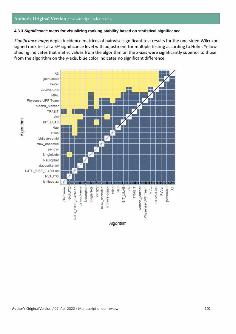
Author’s Original Version / manuscript under review
Author’s Original Version / 07. Apr 2022 / Manuscript under review. 102
4.3.3 Significance maps for visualizing ranking stability based on statistical significance
Significance maps depict incidence matrices of pairwise significant test results for the one-sided Wilcoxon signed rank test at a 5% significance level with adjustment for multiple testing according to Holm. Yellow shading indicates that metric values from the algorithm on the x-axis were significantly superior to those from the algorithm on the y-axis, blue color indicates no significant difference.

Author’s Original Version / manuscript under review
Author’s Original Version / 07. Apr 2022 / Manuscript under review. 103
4.3.4 Ranking robustness to ranking methods
Line plots for visualizing ranking robustness across different ranking methods. Each algorithm is represent-ed by one colored line. For each ranking method encoded on the x-axis, the height of the line represents the corresponding rank. Horizontal lines indicate identical ranks for all methods.
Author’s Original Version / manuscript under review
Author’s Original Version / 07. Apr 2022 / Manuscript under review. 104
4.4 References
Wiesenfarth, M., Reinke, A., Landman, B.A., Eisenmann, M., Aguilera Saiz, L., Cardoso, M.J., Maier-Hein, L. and Kopp-Schneider, A. Methods and open-source toolkit for analyzing and visualizing challenge results. Sci Rep 11, 2369 (2021). https://doi.org/10.1038/s41598-021-82017-6
M. J. A. Eugster, T. Hothorn, and F. Leisch, “Exploratory and inferential analysis of benchmark experi-ments,” Institut fuer Statistik, Ludwig-Maximilians-Universitaet Muenchen, Germany, Technical Report 30, 2008. [Online]. Available: http://epub.ub.uni-muenchen.de/4134/.

1
Appendix
Table of Contents
1. Overview of Challenge Participants Algorithm 2
1.1 2Ai 2
1.2 A3 3
1.3 BIT_LILAB 4
1.4 Davoodkarimi 6
1.5 FeVer 7
1.6 Hilab 9
1.7 Ichilove-ax and Ichilove-combi 11
1.8 Anonymous 14
1.9 MIAL 15
1.10 Moona Mazher 16
1.11 muw_dsobotka 19
1.12 Neurophet 20
1.13 NVAUTO 22
1.14 pengyy 24
1.15 Physense-UPF Team 26
1.16 SingleNets 29
1.17 SJTU_EIEE_2-426Lab 33
1.18 TRABIT 35
1.19 Xlab 39
1.20 ZJUWULAB 40
2. Benchmarking report for multiTaskChallengeDice_combined 41
2.1 Ranking 41
2.2 Visualization of raw assessment data 42
2.3 Visualization of ranking stability 45
2.4 References 49
3. Benchmarking report for multiTaskChallengeHD_combined 50
3.1 Ranking 50
3.2 Visualization of raw assessment data 51
3.3 Visualization of ranking stability 54
3.4 References 58
4. Benchmarking report for multiTaskChallengeVolSim_combined 59
4.1 Ranking 59
4.2 Visualization of raw assessment data 60
4.3 Visualization of ranking stability 63
4.4 References 67

2
1. Overview of Challenge Participants Algorithm
1.1 2Ai
Team Members and Affiliations
Team Members: Helena R. Torres1,2,3,4, Bruno Oliveira1,2,3,4, Pedro Morais, Jaime C. Fonseca, João L. Vilaca1
Affiliations: 12Ai – School of Technology, IPCA, Barcelos, Portugal; 2Algoritmi Center, School of Engineering, University of Minho, Guimarães,
Portugal; 3Life and Health Sciences Research Institute (ICVS), School of Medicine, University of Minho, Braga, Portugal; 4ICVS/3B’s - PT
Government Associate Laboratory, Braga/Guimarães, Portugal
Model Description
In-utero MRI has been emerging as an important tool to evaluate fetal neurological development. Here, segmentation of fetal
brain structures can have an important role in the interpretation of the fetal MRI, allowing to aid in the quantification of the changing brain
morphology and in the diagnosis of congenital disorders. Since manual segmentation is highly prone to observer variability and time-
consuming, automatic methods for fetal tissue segmentation can bring added value to clinical practice. The main goal of the FeTA challenge
is to potentiate the development of new methods for fetal tissue segmentation.
In the scope of the FeTA challenge, an automatic method to segment the different brain structures of the fetus was developed. As
well-known, encoder-decoder deep convolutional neural networks have been showed the best performance for medical imaging
segmentation. In this work, the U-Net method was adapted to perform fetal tissue segmentation [2, 4]. Concerning the model architecture,
similar to U-NET, an encoder-decoder network was used. The encoding path is composed of down-sampling blocks and each block of the
encoding path is composed of two convolutional layers, with each layer consisting of a convolution, followed by batch normalization and a
leaky rectified linear unit (ReLU). The down-sampling is implemented using a stride convolution on the first layer of each encoding block. The
initial number of feature maps is defined to be 32, which is double in each down-sampling stride convolution operation. The decoding path
corresponds to a symmetric expanding path and skip-connections are used to allow that the encoder and decoder share information.
Overall, the number of trainable parameters was 29,971,032. Moreover, a Sigmoid activation layer was added to the end of the network to
achieve the segmentation, which was performed through a one-hot labelling scheme using the Dice metric as loss function. Finally, a Xavier
initialization of the model parameters was applied, in order to initialize the weights such that the variance of the activations were the same
across every layer.
Concerning the input of the network, all training images of the FeTA challenge were used. A pre-processing of the images was
applied, where image normalization was implemented in order to achieve zero mean intensity with unit variance. Moreover, the pixel size of
the images was normalized to be the median value of the pixel size of all the images and a patch-based strategy was used, were a 3D patch
with size 128x128x128 was applied. To overcome overfitting problems during training, data augmentation techniques were applied to the
training images, namely spatial and intensity-based transformations [1]. Spatial transformations included random flip, rotation, scaling, grid
distortion, optical distortion, and elastic transformations, whereas intensity transformations included random gaussian noise, brightness,
contrast, and gamma transformations.
The network was trained during 800 epochs with a mini-batch size of 4 and using the Adam optimizer with an initial learning rate
of 0.001 and a learning rate decay following the polinomial learning rate policy (lr=1- ((1-epoch)⁄(max_epoch) )^power) with the power of
0.9 [3]. The training time of the method was ≈6 days on a computer with a CPU: i7-7700HQ @3.56GHz, RAM: 16GBytes @1.2GHz, and GPU:
GTX1070 @1.443GHz, using the PyTorch python library. Finally, the final segmentation was obtained by post-processing the output of the
network by removing isolated segmented voxels.
References
[1] Buslaev, A., Iglovikov, V. I., Khvedchenya, E., Parinov, A., Druzhinin, M., & Kalinin, A. A. (2020). Albumentations: Fast and flexible image
augmentations. Information (Switzerland), 11(2), 1–20. https://doi.org/10.3390/info11020125
[2] Isensee, F., Jaeger, P. F., Kohl, S. A. A., Petersen, J., & Maier-Hein, K. H. (2021). nnU-Net: a self-configuring method for deep learning-
based biomedical image segmentation. Nature Methods, 18(2), 203–211. https://doi.org/10.1038/s41592-020-01008-z
[3] Kingma, D. P., & Ba, J. L. (2015). Adam: A method for stochastic optimization. 3rd International Conference on Learning Representations,
ICLR 2015 - Conference Track Proceedings, 1–15.
[4] Ronneberger, O., Fischer, P., & Brox, T. (2015). U-Net: Convolutional Networks for Biomedical Image Segmentation. Computer Vision and
Pattern Recognition, 1–8.

3
1.2 A3
Team Members and Affiliations
Team Members: Yunzhi Xu and Li Zhao
Affiliations: College of Biomedical Engineering & Instrument Science, Zhejiang University, Hangzhou, China
Model Description
Input: 3D volume with a shape of 128x128x128. The input data were preprocessed as follows.
Pre-processing: To improve the data balance, the background of the original data was cropped according to the edge of the brain in 3D. The
border of the brain was selected by the non-zero pixels. The cropped images were zero-padded to a matrix size of 192x192x192. Then the
images were down-sampled to 128x128x128 to fit in the memory of GPUs. Images were normalized, so the mean value was zero and the
standard deviation equals one.
Model Architecture: The model was implemented based on V-net. Compared to the standard U-Net, a parametric rectified linear unit
(PReLU) activation function. Starting number of features was 16 and was doubled in each descending layer. There are three layers of feature
extraction. Each layer was a res-net composed of two consecutive 3x3x3 convolutional kernels. Layer normalization was used instead of
original batch normalization. A 2x2x2 max-pooling was performed instead of 3D convolution in the original V-net. A dropout rate of 0.5 was
used before the first transpose convolution layer. The decoding path was symmetric with the encoding path with the halved number of
filters for each layer.
Training Description
FeTA data were mixed in the training with 80% in the training and 20% in the validation. No additional data were used. Data
augmentation was performed by randomly shifting the image up to 5 pixels in 3 directions, rotating the image up to 15 degrees along three
axes, and flipping the brain in the left-right direction. Binary-cross-entropy was used as the loss function. Adam optimizer was used with a
learning rate of 1e-4 with auto rate schedule using ReduceLROnPlateau. The model was trained in 200 epochs. Each epoch had 32 steps and
a batch size of two. The algorithm was implemented using Tensorflow 2.4. The training was performed with two Nvidia P100 GPUs, 16 CPUs,
and 118G Memory on Alibaba Cloud.

4
1.3 BIT_LILAB
Team Members and Affiliations
Team Members: Weibin Liao, Yi Lv, Xuesong Li
Affiliations: School of Computer Science and Technology, Beijing Institute of Technology, Beijing, China
Model Architecture
Our model structure is shown in the figure below, mainly referring to TransUNet [1]. This is a CNN-Transformer hybrid model. The
network is similar to a U-shaped structure, adding Transformer layers with Multi-head Self-Attention mechanism to the encoder to encode
the feature representation of image patches. The motivation of using this hybrid architecture is that we can not only use the high-resolution
CNN feature map in the decoding path, but also use the global context information encoded by Transformers [2].
In encoder, ResNet-50 [3] is used as the feature extractor of CNN to generate a feature map for the input image. Transformer is
used encoding feature representations from decomposed image patches.
Decoder consists of multiple up-sampling block, where each block consists of a 2× upsampling operator, a 3×3 convolution layer, a ReLU
layer and a Batch Normalization layer successively. The overall architecture of our proposal network can be found in Figure 1. The detailed
network architecture can be found in Table 1.
Fig.1. Overall architecture of our proposal network.
Table 1. The design details of our proposed network. 𝐶𝑜𝑛𝑣 3 × 3 denotes a 3 × 3 convolutional layer. 𝐺𝑁 denotes Group Normalization. 𝐵𝑁
denotes Batch Normalization. Each ResBlock in encoder is a residual block. The size of input image is 3×256×256.
Stage Block name Details Output Size
CNN Encoder
InitConv 𝐶𝑜𝑛𝑣 7 × 7, 𝐺𝑁, 𝑅𝑒𝐿𝑈 64 × 128 × 128
DownSample 𝑀𝑎𝑥𝑃𝑜𝑜𝑙 64 × 128 × 128
ResBlock1 {𝐺𝑁, 𝐶𝑜𝑛𝑣 1 × 1, 𝑅𝑒𝐿𝑈𝐺𝑁, 𝐶𝑜𝑛𝑣 3 × 3, 𝑅𝑒𝐿𝑈𝐺𝑁, 𝐶𝑜𝑛𝑣 1 × 1, 𝑅𝑒𝐿𝑈
× 3 128 × 64 × 64
ResBlock2 {𝐺𝑁, 𝐶𝑜𝑛𝑣 1 × 1, 𝑅𝑒𝐿𝑈𝐺𝑁, 𝐶𝑜𝑛𝑣 3 × 3, 𝑅𝑒𝐿𝑈𝐺𝑁, 𝐶𝑜𝑛𝑣 1 × 1, 𝑅𝑒𝐿𝑈
× 4 256 × 32 × 32
ResBlock3 {𝐺𝑁, 𝐶𝑜𝑛𝑣 1 × 1, 𝑅𝑒𝐿𝑈𝐺𝑁, 𝐶𝑜𝑛𝑣 3 × 3, 𝑅𝑒𝐿𝑈𝐺𝑁, 𝐶𝑜𝑛𝑣 1 × 1, 𝑅𝑒𝐿𝑈
× 9 512 × 16 × 16
Transformer Encoder Linear Projection 𝐶𝑜𝑛𝑣 3 × 3, 𝑟𝑒𝑠ℎ𝑎𝑝𝑒 1024 × 4096
Transformer 𝑇𝑟𝑎𝑛𝑠𝑓𝑜𝑟𝑚𝑒𝑟 𝐿𝑎𝑦𝑒𝑟 × 12 1024 × 4096
CNN Decoder
Feature Mapping 𝑟𝑒𝑠ℎ𝑎𝑝𝑒, 𝐶𝑜𝑛𝑣3 × 3 512 × 16 × 16
DeBlock1 𝐶𝑜𝑛𝑣 3 × 3, 𝑅𝑒𝐿𝑈, 𝐵𝑁 × 3 512 × 16 × 16
UpSample1 𝐶𝑜𝑛𝑣 3 × 3, 𝑈𝑝𝑠𝑎𝑚𝑝𝑙𝑖𝑛𝑔𝐵𝑖𝑙𝑖𝑛𝑒𝑎𝑟 256 × 32 × 32
DeBlock2 𝐶𝑜𝑛𝑣 3 × 3, 𝑅𝑒𝐿𝑈, 𝐵𝑁 × 2 256 × 32 × 32
UpSample2 𝐶𝑜𝑛𝑣 3 × 3, 𝑈𝑝𝑠𝑎𝑚𝑝𝑙𝑖𝑛𝑔𝐵𝑖𝑙𝑖𝑛𝑒𝑎𝑟 128 × 64 × 64
DeBlock3 𝐶𝑜𝑛𝑣 3 × 3, 𝑅𝑒𝐿𝑈, 𝐵𝑁 × 2 128 × 64 × 64
UpSample3 𝐶𝑜𝑛𝑣 3 × 3, 𝑈𝑝𝑠𝑎𝑚𝑝𝑙𝑖𝑛𝑔𝐵𝑖𝑙𝑖𝑛𝑒𝑎𝑟 64 × 128 × 128

5
DeBlock4 𝐶𝑜𝑛𝑣 3 × 3, 𝑅𝑒𝐿𝑈, 𝐵𝑁 × 2 64 × 128 × 128
EndConv 𝐶𝑜𝑛𝑣 1 × 1, 𝑆𝑜𝑓𝑡𝑚𝑎𝑥 3 × 256 × 256
Input and Output
Our model accepts 2D slices as input, and the 3D volume needs to be sliced in advance during model training. When testing, the
3D volume image can be directly input, and the program will automatically slice the volume image, predict each slice, and then stack it into a
3D volume image. The input 2D slice resolution is 256 × 256, and the image patch size is fixed as 16 × 16.
Dataset
We used all 80 data in the dataset. Due to the different reconstruction methods of data (the first 40 data are reconstructed by
MialSRTK and the last 40 data are reconstructed by SimpleIRTK. When using data, we make a simple division based on two different
reconstruction methods. 60 data (1-30, 41-70) are used as the training set, and 20 data (31-40, 71-80) are used as the test set. We don’t
differentiate the data for health conditions.
Preprocess and Data Augmentation
Due to we use 2D-input network, we need to preprocess 3D volume data into 2D slices. We adopt two simple data augmentation
strategies: random rotation and flipping. Randomly rotate the 2D slice (-20, 20) degrees counterclockwise, or rotate it by 90 degrees, and
then flip it up and down or left and right. The probability of data augmentation is 0.5.
Pre-training
ResNet-50 and ViT are combined in the hybrid encoder, we use the pre-training model of the backbone network provided by the
author. We have also made some attempts on transfer learning: We first train the model on the Synapse multi-organ segmentation dataset,
and then transfer the pre-training weights to the Fetal Tissue Annotation task. The results show that the model with pre-trained weights can
converge faster on the Fetal Tissue Annotation dataset.
Implementation Details
The input resolution and patch size are set as 256 × 256 and 16. Models are trained with SGD optimizer with learning rate 0.01,
momentum 0.9 and weight decay 1e-4. Batch size is 24, the max epochs are 150 and the number of training iterations are 30k. Loss function
is a composite loss function of Cross Entropy and Dice loss. All experiments are conducted using four Nvidia GTX 1080Ti GPU. Training model
takes about 10 hours at a time.
The python package version we use is as follows: torch==1.4.0, torchvision==0.5.0, numpy==1.20.3, tqdm==4.61.1, tensorboard==2.5.0,
tensorboardX==2.2, ml-collections==0.1.0, medpy==0.4.0, SimpleITK==2.0.2, scipy==1.6.3, h5py==3.2.1.
Other Trained Models
We also tried other two baseline models on this task.
The first is nnUNet [4]. nnU-Net is the first standardized deep learning benchmark in biomedical segmentation. Without manual
effort, researchers can compare their algorithms against nnU-Net on an arbitrary number of datasets to provide meaningful evidence for
proposed improvements. We use 3D full resolution U-Net for training in nnUNet. We also used all 80 data, including 64 data as training data
and 16 data as validation data. The test results show that nnUNet can reach the same level as TransUNet in DSC and HD95.
The other is CoTr [5]. This is also a framework combining CNN and transformer for medical image segmentation. Unlike
TransUNet, CoTr can directly process 3D volume data. Unfortunately, the results we reproduced are far lower than TransUNet and nnUNet,
and do not show better results compared with other CNN-based, Transformer-based and hybrid methods mentioned in this paper.
Reference
1. Chen, Jieneng, et al. "Transunet: Transformers make strong encoders for medical image segmentation." arXiv preprint arXiv:2102.04306
(2021).
2. Dosovitskiy, Alexey, et al. "An image is worth 16x16 words: Transformers for image recognition at scale." arXiv preprint arXiv:2010.11929
(2020).
3. He, Kaiming, et al. "Deep residual learning for image recognition." Proceedings of the IEEE conference on computer vision and pattern
recognition. 2016.
4. Isensee, Fabian, et al. "nnU-Net: a self-configuring method for deep learning-based biomedical image segmentation." Nature methods
18.2 (2021): 203-211.
5. Xie, Yutong, et al. "CoTr: Efficiently Bridging CNN and Transformer for 3D Medical Image Segmentation." arXiv preprint arXiv:2103.03024
(2021).
6
1.4 Davoodkarimi
Team Members and Affiliations
Team Members: Davood Karimi, Ali Gholipour
Affiliations: Boston Children’s Hospital, Harvard Medical School
Model Description
An encoder-decoded fully-convolutional neural network. The backbone is similar to UNet. Additional dense connections as well as
short and long skip connections are included between the different stages of the encoder and the decoder. All layers are followed by ReLU.
The model works on 1283-voxel patches. During training, patches are selected from training images at random locations. During
test, a sliding-window strategy is used to cover the entire volume.
We use a novel loss function derived from mean-absolute-error loss [4]. Additionally, we have a loss term to constrain the relative volume of
each of the segments/labels.
Training Method
All FeTA images (regardless of quality) were used in the same way. No additional datasets were used in any way for training. We
used 15 of the FeTA images (selected to be representative of image quality and subject age distribution) for validation/testing. Once the final
architecture/training hyper-parameters were decided upon, the final model was trained on all 80 FeTA images.
The only pre-processing applied consisted of intensity normalization. Specifically, each image was normalized via dividing by the
image standard deviation.
Extensive image augmentation was used. Including simple geometric flips and rotations, as well as elastic deformations [2]. In
addition, label perturbation and smoothing were used. Test-time image augmentation is also performed, but only includes flips; at test time
no rotations or elastic deformations are used. Only a single model is trained. On a test image, the flips generate 8 labels that can be
combined using simple averaging or STAPLE [5] to obtain a final label prediction.
We initialize all parameters using He's method [1] and optimize using Adam optimizer [3] with an initial learning rate of 10-4, with
a batch size of 1. Learning rate was reduced by a factor of 0.9 after every 2000 training iterations if the validation loss did not decrease. If the
validation loss did not decrease after 3 consecutive evaluations, training was stopped. No pre-training is used. The model training takes
approximately 105 iterations, equivalent to 24 hours on a single GPU. All implementation is done in TensorFlow 1.14. For data augmentation
and other processing we used ITK.
References
1. He, K., Zhang, X., Ren, S., Sun, J.: Delving deep into rectifers: Surpassing human-level performance on imagenet classication. In:
Proceedings of the IEEE international conference on computer vision. pp. 1026-1034 (2015)
2. Karimi, D., Samei, G., Kesch, C., Nir, G., Salcudean, S.E.: Prostate segmentation in mri using a convolutional neural network architecture
and training strategy based on statistical shape models. International journal of computer assisted radiology and surgery 13(8), 1211-1219
(2018)
3. Kingma, D.P., Ba, J.: Adam: A method for stochastic optimization. arXiv preprint arXiv:1412.6980 (2014)
4. Wang, X., Hua, Y., Kodirov, E., Robertson, N.M.: Imae for noise-robust learning: Mean absolute error does not treat examples equally and
gradient magnitude's variance matters. arXiv preprint arXiv:1903.12141 (2019)
5. Warfield, S.K., Zou, K.H., Wells, W.M.: Simultaneous truth and performance level estimation (staple): an algorithm for the validation of
image segmentation. IEEE transactions on medical imaging 23(7), 903-921 (2004)

7
1.5 FeVer
Team Members and Affiliations
Team Members: KuanLun Liao1,3, YiXuan Wu2,3, and JinTai Chen1,3
Affiliations: 1Zhejiang University, College of Computer Science and Technology, Road 38 West
Lake District, Hangzhou 310058, P.R. China; 2Zhejiang University, School of Medicine, 866 Yuhangtang Rd, Hangzhou 310058, P.R. China; 3Real Doctor AI Research Centre, Zhejiang University, Hangzhou, China
Data Processing
Data source: We use all 80 T2-weighted fetal brain reconstructions data [5]. Besides, we don't use any other datasets. In order to preserve
the internal structure and locality information of images, we use the original 3D images as input.
Data pre-processing: For pre-processing, we first limit the pixel values to the range of (-200, 1000) to removing the unused pixels. Then, since
the spacing of each CT image is different, we resample the slice spaces for all CT images to the same scale by using spline interpolation.
What's more, in order to utilize the data effectively, we remove the slices which corresponding labels only have background information.
Data augmentation: For data augmentation, we randomly crop each image with slices of 48, and randomly flip each image in the direction of
up-and-down and left-and-right; besides, we also utilize the method of mixup [7], which convexly combines random pairs of images and their
associated labels.
Model Description
We adopt a modified 3D Res-UNet model architecture (https://github.com/pykao/Modified-3D-UNet-Pytorch), which has a
context pathway, a localization pathway and residual connections each with five layers.
Context path: In the context pathway, each layer contains three 3 × 3 × 3 convolutions each followed by a instance normalization, and then a
leaky rectified linear unit (LeakyReLu); and every layer has a dropout layer with the ratio equals to 0.3. The shortcut path with residual
connection brings the features of the nearby lower-level layers, alleviating the degradation problem and giving better performance.
Localization path: In the localization pathway, each layer consists of an up-sampling block with multiplier of spatial size 2, in the following of
two sequence of a 3×3×3 convolution, a 3d-InstanceNorm, and then a leaky rectified linear unit (LeakyReLu). Besides, the upsample step is
followed by a 3×3×3 convolution, a 3d-InstanceNorm, and then a leaky rectified linear unit (LeakyReLu).
Concat connection: The concat connections from layers of equal resolution in the context path provide the essential high-resolution features
to the localization path. What's more, the concat connections are also utilized between different layers of the localization pathway to get the
final predict.
InstanceNorm: In this work, we apply Instance Normalization [6] over a 5D input (a mini-batch of 3D inputs with additional channel
dimension), which give normalization to H and W and D at the dimension of pixel value. The mean and standard-deviation are calculated per-
dimension separately for each object in a mini-batch, giving a better outcome for the theme of semantic segmentation.
Leaky ReLU: Unlike the architecture in original U-Net, we utilize LeakyReLu instead of ReLu to be the activation function in our network.
Leaky ReLU [3] is a type of activation function based on a ReLU, but it has a small slope for negative values instead of a flat slope.
Optimizer: For optimization, we choose the QHAdam [2] to be the optimizer with default configurations except for the weight decay rate
0.00001, which performs best in our task and settings.
Scheduler: For learning rate, we start with the value of 0.005, and choose the CosineAnnealingLR [1] as the learning rate scheduler, setting
the period at 50 iterations and the minimum learning rate at 0.0005.
Loss function: For loss function, we apply Dice-Loss function [4], a popular loss function for image segmentation tasks based on the Dice
coefficient, which is essentially a measure of overlap between two samples. This measure ranges from 0 to 1 where a Dice coefficient of 1
denotes perfect and complete overlap.
Training details
Parameter initialization: We initial the model parameters in a random way.
Parameter number: The architecture has 2,369,496 parameters in total.
Hyperparameter tuning: The hyperparameters are tuned by grid search.
batch size: {1, 2, 4}

8
learning rate: {0.01, 0.001, 0.005, 0.0001}
weight decay rate: {0.0001, 0.00001}
Splits of the datasets: We randomly divide 95% of the dataset as the training set and the remaining 5% as the validation set.
Batch size: We set the batch size as 4.
Ensemble of models: We divide the dataset as training set and validation set randomly for five times, and use them to train different models
respectively. Then, we choose the best two models among these five models and utilize average value of these two models to be the final
prediction for labels.
Training time: 40 hours per model on RTX 3090
Software libraries and packages:
Pytorch 1.8.0
Qhoptim 1.1.0
SimpleITK 2.0.0
Torchvision 0.9.0
Numpy 1.19.1
Pandas 1.1.3
Scipy 1.4.1
Scikit-learn 0.23.2
Tensorboard 2.2.2
References
1. Loshchilov, I., Hutter, F.: Sgdr: Stochastic gradient descent with warm restarts. arXiv preprint arXiv:1608.03983 (2016)
2. Ma, J., Yarats, D.: Quasi-hyperbolic momentum and adam for deep learning. arXiv preprint arXiv:1810.06801 (2018)
3. Maas, A.L., Hannun, A.Y., Ng, A.Y., et al.: Rectifier nonlinearities improve neural network acoustic models. In: Proc. icml. vol. 30, p. 3.
Citeseer (2013)
4. Milletari, F., Navab, N., Ahmadi, S.A.: V-net: Fully convolutional neural networks for volumetric medical image segmentation. In: 2016
fourth international conference on 3D vision (3DV). pp. 565-571. IEEE (2016)
5. Payette, K., de Dumast, P., Kebiri, H., Ezhov, I., Paetzold, J.C., Shit, S., Iqbal, A., Khan, R., Kottke, R., Grehten, P., et al.: An automatic multi-
tissue human fetal brain segmentation benchmark using the fetal tissue annotation dataset. Scientific Data 8(1), 1-14 (2021)
6. Ulyanov, D., Vedaldi, A., Lempitsky, V.: Instance normalization: The missing ingredient for fast stylization. arXiv preprint arXiv:1607.08022
(2016)
7. Zhang, H., Cisse, M., Dauphin, Y.N., Lopez-Paz, D.: mixup: Beyond empirical risk minimization. arXiv preprint arXiv:1710.09412 (2017)

9
1.6 Hilab
Team Members and Affiliations
Team Members: Guiming Dong, Hao Fu, and Guotai Wang
Affiliations: School of Mechanical and Electrical Engineering, University of Electronic Science and
Technology of China, Chengdu, China
Model Description
Our method is based on nnU Net [1], and more details are described in the following. The network architecture is showed in
Figure 1.
Figure 1: Network Architecture as generated by nnU Net.
We use instance normalization [2] and Leaky ReLU [3] following every convolution layer. And then, SGD optimizer with Nesterov
momentum (μ = 0.99) is selected. Both cross entropy loss and Dice loss are used for segmentation training.
Training inputs are patches which are randomly sampled from training cases and the patch size of 128x128x128 is selected.
Besides, the input data only has one modality.
Before fed into the network, all the training images need to be cropped according to the foreground. We also use Z score (mean
subtraction and division by standard deviation) per image followed by cropping for data normalization.
Random initialization is selected for our model. Our framework is based on nn UNet [1], which is publically available at
https://github.com/MIC DKFZ/nnUNet
Training Method
During the training, we use all cases of FeTA dataset. We don’t use any external dataset. We split the dataset into 5 folds so that
we can run a 5 fold cross validation. During the validation, we found that performance of the model on pathological cases is worse than that
one on neurotypical cases. So pathological cases are copied triple during the training. And then, an initial learning rate of 0.01 is used for
learning network weights. The learning rate is decayed with following schedule [4]:
(1 − epoch/epoch_max)0.9. Batch size is set to 2.
The data augmentation techniques are as follows: Rotation and Scaling, Gaussian noise, Gaussian blur, Brightness, Contrast,
Simulation of low resolution, Gamma augmentation and Mirroring. More details can be seen in [1].
For FeTA challenge, we have trained 5 models via a 5 fold cross validation. And all the 5 models were selected to run ensembling.
Other details:
System version: Ubuntu 20.04
PyTorch version: pytorch1.6.0_py3.8_cuda10.2.89_cudnn7.6.5_0
Devices: NVIDIA GeForce RTX 2080 Ti
Training runs 400 epochs for each fold, and one epoch is defined as 250 iterations. Each epoch costs about 460s.
References
1. Isensee, F., Jaeger, P.F., Kohl, S.A.A. et al. "nnU Net: a self configuring method for deep learning based biomedical image segmentation."
Nat Methods (2020).
2. D. Ulyanov, A. Vedaldi, and V. Lempitsky, “Instance normalization: The missing ingredient for fast stylization,” arXiv preprint
arXiv:1607.08022, 2016.

10
3. A. L. Maas, A. Y. Hannun, and A. Y. Ng, “Rectifier nonlinearities improve neural network acoustic models,” in Proc. icml, vol. 30, no. 1, 2013,
p. 3.
4. C. Chen, G. Papandreou, I. Kokkinos, K. Murphy, and A. L. Yuille, “Deeplab: Semantic image segmentation with deep convolutional nets,
atrous convolution, and fully connected crfs,” IEEE transactions on pattern analysis and machine.

11
1.7 Ichilove-ax and Ichilove-combi
Team Members and Affiliations
Team Members: Netanell Avisdris1,2, Ori Ben-Zvi2,3, Bella Fadida-Specktor, Prof. Leo Joskowicz, Prof. Dafna Ben Bashat2,3,4
Affiliations: 1School of Computer Science and Engineering, The Hebrew University of Jerusalem, Israel; 2Sagol Brain Institute, Tel Aviv
Sourasky Medical Center, Israel, 3Sagol School of Neuroscience, Tel Aviv University, Israel; 4Sackler Faculty of Medicine, Tel Aviv University,
Israel
Note: Only ichilove-ax and ichilove-combi were entries in the FeTA Challenge
Model Description
The approach taken in our algorithm included: reformat the brain into three orthogonal plans of 2D slice-volumes (axial, sagittal
and coronal); The algorithm composed of two stages: (1) detecting the fetal brain ROI using 2D U-net (only on the axial slices); (2) performing
2D multi-class segmentation on the cropped ROI using 2D U-net; and finally, merging all resulting segmentations into one, based on majority
voting.
We submitted four submissions, three where the segmentation obtained separately on each plane, and one which merge all segmentations.
Ichilove-ax: First stage + segmentation in the axial plane of cropped ROI input volume
Ichilove-sag: First stage + segmentation in the sagittal plane of cropped ROI input volume
Ichilove-cor: First stage + segmentation in the coronal plane of cropped ROI input volume
Ichilove-combi : First stage + segmentation in three planes of cropped ROI input volume, each segmentation performed twice, on
the original volume, and on flipped volume, thus resulting in six segmentations. The merging strategy between segmentation is
voxel-wise majority voting.
Figure 1 shows schematic overview of the four submissions.
Figure 1: Schematic overview of 4 submissions: ichilove-{ax,sag,cor,combi}.

12
Networks
Figure 2: Architecture of 2D Segmentation network
For all segmentation steps, we use modified 2D U-net with similar architecture to the one used in [1] for fetal brain segmentation,
where the encoder part composed of pre-trained ResNet34 network blocks and the decoder consists of U-Net PixelShuffle ICNR blocks for
each scale described in [2]. The encoder and decoder are connected with the fast.ai Dynamic U-Net [3].
Figure 3: Blocks of the segmentation network: a ResNet34 block for the first scale of the encoder (left), a U-Net ICNR block for the decoder
(right) and a comparison block between the classic U-Net and the U-Net ICNR blocks (middle).
To train the network, we used the OneCycle optimizer in [4] with a learning rate of 1e-3 for 30 epochs twice - the first time only
the decoder layers (U-Net ICNR blocks), and the second time for the entire network with batch size of 16 slices. The network was trained
with Lovasz-Softmax loss [5].
For training, we used four augmentations: 1) intensity with a contrast in the range 0.3-1.7 and brightness in the range 0.3-0.9 for
training only; 2) scaling to size NxN and normalization in the range [0,1] for both training and inference, where for the first stage N=256, and
for second stage N=160; 3) rotation in the range of 0-90 degrees, and; 4) Intensity Inhomogeneity Augmentation [6]. For the inference, the
slice output segmentation is computed by nearest-neighbor interpolation followed by zero-padding (background class) to obtain the original
slice size. From 60 provided volumes, we use 50 volumes for train 5 for validation and 5 for test.
References
1. Avisdris, N., et al., Automatic linear measurements of the fetal brain on MRI with deep neural networks. International Journal of Computer
Assisted Radiology and Surgery, 2021.

13
2. Aitken, A., et al., Checkerboard artifact free sub-pixel convolution: A note on sub-pixel convolution, resize convolution and convolution
resize. arXiv preprint arXiv:1707.02937, 2017.
3. Howard, J. and S. Gugger, fastai: A Layered API for Deep Learning. Information, 2020. 11(2): p. 108.
4. Smith, L.N., A disciplined approach to neural network hyper-parameters: Part 1--learning rate, batch size, momentum, and weight decay.
arXiv preprint arXiv:1803.09820, 2018.
5. Berman, M., A.R. Triki, and M.B. Blaschko. The lovász-softmax loss: A tractable surrogate for the optimization of the intersection-over-
union measure in neural networks. in Proceedings of the IEEE Conference on Computer Vision and Pattern Recognition. 2018.
6. Khalili, N., et al., Automatic brain tissue segmentation in fetal MRI using convolutional neural networks. Magnetic resonance imaging,
2019. 64: p. 77-89.

14
1.8 Anonymous
One team participated in the FeTA Challenge, but declined to be a part of the paper. Therefore their scores are included in all rankings for
completeness, but the algorithm description is not included.

15
1.9 MIAL
Team Members and Affiliations
Team Members: Priscille de Dumast2,1, Meritxell Bach Cuadra1,2
Affiliations: 1CIBM Center for Biomedical Imaging; 2Department of Radiology, Lausanne University Hospital and University of Lausanne
Note: This team contains challenge organizers. While included in all rankings, this team was ineligible for prizes.
Model Description
Our segmentation method is based on the well-established 2D U-Net [2] image segmentation method that has been used in the
past for 2D fetal brain MRI [1]. In our approach, two networks, with identical architecture, are trained separately: one network is trained on
the MIALSRTK reconstructed images, and one network is trained on the IRTK reconstructed images.
We adopt a patch-based approach, feeding our networks with sub-image of 64x64 voxel size. The 2D U-Net architecture is
composed of encoding and de-coding paths. The encoding path consists of 5 repetitions of the followings: two 3x3 convolutional layers,
followed by a rectified linear unit (ReLu) activation function and a 2x2 max-pooling down-sampling layer. Feature maps are hence doubled
from 32 to 512. In the expanding path, 2x2 up-sampled encoded features concatenated with the corresponding encoding path are 3x3
convolved and passed through ReLu. All convolutional layers output are batch normalized. The network prediction is computed with a final
1x1 convolution.
Neural networks are implemented in TensorFlow (version 2.3).
Data
We proceed to a reconstruction-aware method. Each network was trained on 40 training cases, according to the reconstruction
method used, either IRTK or MIALSRTK.
Input sub-image patches are extracted using a 2.5D approach: overlapping patches from the three orientations (axial, coronal and sagittal).
Patches with tissue (positive patches) are duplicated once with data augmentation performed by randomly flipping and rotating patches (by
𝑛 x 90°, n ∈ [0;3]). Most negative patches (with positive intensities but no fetal brain tissue represented) were discarded as only 1/8 are kept.
Intensities of all image patches are standardized to have mean 0 and variance 1.
Final estimation of the segmentation is reconstructed using a majority voting approach from all probability maps.
Training
Both networks are trained using a hybrid loss ℒℎ𝑦𝑏𝑟𝑖𝑑 combining two terms:
ℒℎ𝑦𝑏𝑟𝑖𝑑 = (1 − 𝜆) ℒ𝑐𝑐𝑒 + 𝜆ℒ𝑑𝑖𝑐𝑒
where ℒ𝑐𝑐𝑒 is the categorical cross-entropy loss function, ℒ𝑑𝑖𝑐𝑒is based on the dice similarity coefficient and 𝜆 balances the contribution of
the two terms of the loss. 𝜆 was set to 0.5.
Both networks were trained with an initial learning rate (LR) of 1 x 10⁻³. Mialsrtk network was trained for 100 epochs with learning rate decay
at epoch [23, 45] and irtk network was trained for 100 epochs with learning rate decay at [24,44].
A 5-folds cross-validation approach was used to determine the hyperparameters (initial LR, epochs for LR decay, and total number
of epochs).
References
[1] Khalili, N., et al.: Automatic brain tissue segmentation in fetal MRI using convolutional neural networks. Magnetic Resonance Imaging 64,
77-89 (Dec 2019). https://doi.org/10.1016/j.mri.2019.05.020
[2] Ronneberger, O., et al.: U-net: Convolutional networks for biomedical image segmentation. In: Medical Image Computing and Computer-
Assisted Intervention - MICCAI 2015. pp. 234-241. Springer International Publishing, Cham (2015)

16
1.10 Moona Mazher
Team Members and Affiliations
Team Members: Moona Mazher1, Abdul Qayyum2, Abdesslam BENZINOU2, Mohamed Abdel-Nasser1,3 and Domenec Puig1
Affiliations: 1Department of Computer Engineering and Mathematics, University Rovira i Virgili, Spain; 2ENIB, UMR CNRS 6285 LabSTICC,
Brest, 29238, France; 3Department of Electrical Engineering, Faculty of Engineering, Aswan University, Egypt
Model Description
Main Contribution for Feta Segmentation Task:
1. We developed 2D Densely-based encoder network from scratch without using any pre-trained module and it is composed of a
different number of layers with feature reuse capability. The efficient and lightweight 2D convolutional layer blocks with 2D up-
sampling layers have been built on the decoder side of the proposed model (see detail in Figure 1). The proposed dense blocks
used a successive number of feature maps in each encoder layer of the proposed model.
2. Initially, we have used axial 2D slices for training our proposed model and models did not perform well. Later, the same proposed
model is trained on three different views (axial, coronal, and sagittal) of the 2D slices of the feta dataset and then combined these
three output segmentation maps to develop 3D segmentation volume (see detail in Figure 3).
Proposed Method Description: The different deep learning models based on ResNet, MobileNet, efficientNet have been used to construct
the encoder for the Feta challenge segmentation task. We have tried different deep leaning based modules such as ResNet [1], MobileNet
[2], efficientNet[3] for Feta brain segmentation, and finally, the DenseNet [4] based module produced a better performance as compared to
other deep learning modules. Our proposed model is based on an encoder and decoder module with a skip connection.
We have proposed a simple DenseNet module with a small number of blocks on the encoder side and some efficient simple 2D
convolutional layers module with 2D up-sampling layers including regularization layers proposed at the decoder side. The DenseNet based
deep learning with additional tricks produced better segmentation performance on the Feta challenge dataset.
In the DenseNet module, the feature maps of all preceding layers are used as inputs, and their feature maps are used as inputs
into all subsequent layers. The dense module has many advantages such as alleviates the vanishing-gradient problem, strengthen feature
propagation, encourage feature reuse, and substantially reduce the number of parameters. The proposed Dense feature maps module
adding only a small set of feature maps to the collective knowledge of the network and keeps the remaining feature maps unchanged—and
the final layer makes a decision based on all feature-maps in that are reused in the model. The proposed Dense module used a fewer
number of parameters and improved the flow of information and gradients throughout the network, which makes them easy to train. Each
layer has direct access to the gradients from the loss function and the original input signal, leading to implicit deep supervision. This helps
training of deeper network architectures. Further, we also observe those dense connections have a regularizing effect, which reduces
overfitting on tasks with smaller training set sizes.
A detailed description of the proposed model with proposed layers is shown in Figure 1. We have trained all layers’ weights from
scratch using the Fetal Brain Tissue Annotation and Segmentation Challenge (FeTA) dataset. Pre-trained models and extra datasets are not
used in this our proposed solution.
Figure 1: The proposed model configuration for Feta Segmentation (EB: Encoder Block).
The Dense-Layer (DL) consisted of two convolutional layers (Conv-BN-ReLU) with batch normalization (BN) layer and ReLU
activation function. The feature maps are concatenated and reuse between each convolutional layer. The first convolutional layer used a 1x1
kernel and the second convolutional layer used a 3x3 kernel with a different number of feature maps. The feature maps of each layer are
concatenated to form the Dense layer is shown in Figure 2. The six number of Dense-layers have been used to construct the encoder module
of the proposed model with transition layer. We refer to layers between encoder blocks as transition layers, which do convolution and

17
pooling. The transition layers used in our experiments consist of a batch normalization layer and a 1x1 convolutional layer followed by a 2x2
average pooling layer. The transition layer helps to reduce the spatial size in each encoder block in the proposed model. The transition layers
have been used after each dense block in the encoder module inside the proposed model. The transition layer with six dense layers is shown
in Figure 2.
Figure 2: The encoder module based on proposed DensNet blocks (DL: Dense Layer).
On the decoder side, the first up-sampling 2D layer is used with a simple and efficient 2D convolutional layers block
(1x1conv,3x3conv, BN, and ReLU). The feature maps between encoder and decoder module are concatenated using skip connection based
on second, third, and fourth up-blocks and proposed 2D-convolutional layer block (3x3conv, BN, ReLU) to reconstruct the segmentation from
input images. The input features’ maps that are obtained from every encoder block are concatenated with every decoder block feature’s
map to reconstruct the semantic information. The regularization layers (BN, ReLU) have been used after the concatenation of feature maps
between 3x3 2D convolutional and up-sampled layer feature maps for smooth training and optimization of the training process of the
proposed model. In the end, the 1x1 convolutional layer with a sigmoid layer is used to construct the segmentation map. Each dense block
used several features maps (96, 768, 2112, and 2208).
First, we used the proposed model for axial 2D slices of the Feta dataset, and the model produced the worst dice score especially
for Ventricles, Cerebellum, Deep Grey Matter, Brainstem classes. When we trained our model on coronal slices, the model provided optimal
performance in terms of validation Dice score for all classes in the dataset that’s the main motivation and reason to use all three views 2D
slices to trained the 2D deep learning model. We have trained the proposed model for individual views of the 3D input volume and combined
the output of the trained model on each view (axial, coronal, and sagittal) to construct a 3D segmentation map. The combined output
developed by the proposed model with all three 2D views produced a better performance as compared to individual 2D views. The proposed
solution is shown in Figure 3. Note. We also trained three different models on each view and could not get optimal performance on
validation data as compared to the trained single model on each view.

18
Figure 3: The proposed model using two separate views for Feta segmentation.
Training and Data Distribution used in Proposed Model
The Adam optimizers with a 0.0003 learning rate have been used for the training of our proposed model. In our experiments, 24
batch sizes with 1000 epochs using early stop criteria have been used for the training and optimization of the proposed model. First, the
proposed model trained without data augmentation and got a good score, and later we did some data augmentation techniques such as
CenterCrop, HorizontalFlip (p=0.5), VerticalFlip (p=0.5), RandomBrightnessContrast (p=0.8), and RandomGamma (p=0.8) during training the
model that helps to improve a little performance. The binary cross-entropy loss function is used to compute the loss between ground-truth
and predicted segmentation mask.
The one-hot encoded ground-truth segmentation map was used to compute the binary cross-entropy loss between ground truth
and the predicted segmentation map.
Albumentations PyTorch segmentation library [5] used for data augmentation. The Pytorch library [6] has been used for all model
implementation, training, validation, and testing. The V 100 Tesla machine with a single 12 GB GPU memory is used for training the proposed
and state-of-the-art deep learning models. The proposed model contains the total number of trainable parameters (49,510,728) and total
FLOPs (301846528).
The Feta dataset consisted of 80 subjects with a ground truth segmentation map. 80 % (64 subjects) data has been for training
and 20% (16 subjects) for testing. The 5k fold cross-validation technique was used for random splitting the data into training and validation.
The 16384 (256*64) number of images and masks in axial, coronal, and sagittal views are used for training the model 4096 (256*16) no. of
images used for validation the proposed model. The standard normalization method to normalize the dataset. The pandas, skimage,
OpenCV, nibabel, simpleITK python-based libraries are used for data preprocessing for training, validation, and testing the proposed model.
Note: There is no pre-trained model and an additional dataset has been used in our experiments.
References
[1] He, Kaiming, Xiangyu Zhang, Shaoqing Ren, and Jian Sun. "Identity mappings in deep residual networks." In European conference on
computer vision, pp. 630-645. Springer, Cham, 2016.
[2] Sandler, Mark, Andrew Howard, Menglong Zhu, Andrey Zhmoginov, and Liang-Chieh Chen. "Mobilenetv2: Inverted residuals and linear
bottlenecks." In Proceedings of the IEEE conference on computer vision and pattern recognition, pp. 4510-4520. 2018.
[3] Tan, Mingxing, and Quoc Le. "Efficientnet: Rethinking model scaling for convolutional neural networks." In International Conference on
Machine Learning, pp. 6105-6114. PMLR, 2019.
[4] Huang, Gao, Zhuang Liu, Laurens Van Der Maaten, and Kilian Q. Weinberger. "Densely connected convolutional networks." In Proceedings
of the IEEE conference on computer vision and pattern recognition, pp. 4700-4708. 2017.
[5] https://albumentations.ai/docs/
[6] https://pytorch.org/

19
1.11 muw_dsobotka
Team Members and Affiliations Model Description
Team Members: Daniel Sobotka, Georg Langs
Affiliations: Computational Imaging Research Lab, Department of Biomedical Imaging and
Image-guided Therapy, Medical University of Vienna, Vienna, Austria
Model Description
The proposed multi-task learning model is building on a 3D U-Net architecture [1] with a shared encoder and two task specific
decoders. The segmentation task TS generates the fetal tissue annotations, where the image reconstruction task TR reconstructs the input
image. In contrast to other multi-task learning approaches, layer-wise feature fusion [2] is used to share features between the image
segmentation and image reconstruction decoders. The encoder of the network consists of three down-sampling blocks and each task specific
decoder of three up-sampling blocks. Each down-sampling block contains two 3 x 3 x 3 convolutions followed by Rectified Linear Units (ReLU)
and Group Normalizations (GN) [6], as well as a 2 x 2 x 2 max pooling operation. The up-sampling path for both, image segmentation and
image reconstruction tasks uses nearest neighbor interpolation and is symmetric to the down-sampling path. Neural Discriminative
Dimensionality Reduction (NDDR) layers [2] are used to utilize features learned from 𝑇𝑆 and 𝑇𝑅 and to learn layerwise feature fusion between
the two task specific decoders. There, features with the same spatial resolution from both, the image segmentation and image
reconstruction decoders, are concatenated followed by a 1 x 1 x 1 convolution, ReLu and GN. The loss function 𝐿 uses homoscedastic
uncertainty [3] to balance the single-task losses for the weights 𝑊 of the network:
𝐿(𝑊, 𝜎𝑆 , 𝜎𝑅) = 1
2𝜎𝑆2 𝐿𝑆(𝑊) +
1
2𝜎𝑅2 𝐿𝑅(𝑊) + log(𝜎𝑆) + log(𝜎𝑅)
where 𝐿𝑆(𝑊) denotes the cross entropy loss for 𝑇𝑆. 𝐿𝑅(𝑊) is the mean squared error loss for 𝑇𝑅. Based on preliminary results we set 𝜎𝑆 and
𝜎𝑅 to fixed values with a ratio 1:8. The network consists of 6491385 trainable parameters and uses 3D patches of size 128 x 96 x 96 as input
with stride between patches of size 64 x 48 x 48 and predicts 3D patches of size 128 x 96 x 96 combined at inference to an fetal tissue
annotation image of size 256 x 256 x 256. All the input patches were Z-score normalized and the initialization of the model parameters was
random. As baseline implementation the 3D-UNet from [5] was used.
Training Method
The proposed network model was trained on all available 80 FeTa subjects with-out validation and testing splitting and without
additional external data. Further, the network was optimized using Adam [4] with an initial learning rate of 0:001, batch size of 1 and a total
of 100 epochs. Data augmentation included elastic deformation with spline order 3, random flipping, random rotation by 90 degrees,
random rotation by ±15 degrees, random contrast, Gaussian noise and Poisson noise. As software library PyTorch 1.3.1 with Python 3.7.3
was used and training of the network lasted around one week. For the final selection of the here described model approximately 5 different
models with different values of 𝜎𝑆 and 𝜎𝑅 have been trained.
References
1. Cicek, O., Abdulkadir, A., Lienkamp, S.S., Brox, T., Ronneberger, O.: 3d u-net: learning dense volumetric segmentation from sparse
annotation. In: International conference on medical image computing and computer-assisted intervention. pp. 424-432. Springer (2016)
2. Gao, Y., Ma, J., Zhao, M., Liu, W., Yuille, A.L.: Nddr-cnn: Layerwise feature fusing in multi-task cnns by neural discriminative dimensionality
reduction. In: Proceedings of the IEEE/CVF Conference on Computer Vision and Pattern Recognition. pp. 3205-3214 (2019)
3. Kendall, A., Gal, Y., Cipolla, R.: Multi-task learning using uncertainty to weigh losses for scene geometry and semantics. In: Proceedings of
the IEEE conference on computer vision and pattern recognition. pp. 7482-7491 (2018)
4. Kingma, D.P., Ba, J.: Adam: A method for stochastic optimization. arXiv preprint arXiv:1412.6980 (2014)
5. Wolny, A., Cerrone, L., Vijayan, A., Tofanelli, R., Barro, A.V., Louveaux, M.,Wenzl, C., Strauss, S., Wilson-Sanchez, D., Lymbouridou, R., et al.:
Accurate and versatile 3d segmentation of plant tissues at cellular resolution. Elife 9, e57613 (2020)
6. Wu, Y., He, K.: Group normalization. In: Proceedings of the European conference on computer vision (ECCV). pp. 3-19 (2018)

20
1.12 Neurophet
Team Members and Affiliations
Team Members: ZunHyan Rieu1, Donghyeon Kim1, Hyun Gi Kim2
Affiliations: 1NEUROPHET, Republic of Korea; 2The Catholic University of Korea, Eunpyeong St. Mary's Hospital, Republic of Korea
Model Description
The base segmentation architecture we used is U-Net, and we designed it to receive its input patch 3D with the size of (64, 64,
64). We used patch-based training since the actual brain size MRI is pretty small compared to its MRI dimensions (256, 256, 256). Our U-Net
design consists of encoding blocks of 5 followed by residual blocks. We applied a probability-based sampling method to avoid our model
being trained for non-label patches.
As for the loss function, we used the sum of cross-entropy loss function and dice loss function. In cross-entropy loss function,
specifically, we applied different weights in each class to define the vague segmentation boundaries between ‘External Cerebrospinal Fluid'
and 'Grey Matter, and 'Brainstem'. For the optimizer, we applied AdamW with the learning rate of 1E-5. To normalize the intensity range of
the given MRI dataset, we performed intensity normalization from 0 to 1 with a percentile cutoff of (0, 99.8).
Training Method
Neither an additional dataset nor a pre-trained model was used for training. All case of FeTA dataset was used for training.
However, we performed a visual inspection to define the poor and good quality images and distributed them equally to the train and
validation. For the train and validation dataset, we divided 80 subjects with a split ratio of 0.8 (training:64, validation:16).
To reduce the dependency on the training dataset, we performed the data augmentation (random affine, random blur). For the
hyper-parameter tuning, we applied the inferences for multiple patch overlap combinations (8 x 8 x 8, 16 x 16 x 16, 32 x 32 x 32, 48 x 48 x
48) and chose the best out of it.
Once the output is generated, we removed the mislabeled outer blobs using the connected component-based label noise removal
method.
All preprocessing and architecture modeling, we used torchIO and scikit-image library.
Inference Example

21

22
1.13 NVAUTO
Team Members and Affiliations
Team Members: Md Mahfuzur Rahman Siddiquee1, Andriy Myronenko2, Daguang Xu2
Affiliations: 1Arizona State University; 2NVIDIA, Santa Clara, CA
Model Description
We implemented our approach with MONAI (https://github.com/Project-MONAI/MONAI) [1]. We use the encoder-decoder
backbone based on [4] with an asymmetrically larger encoder to extract image features and a smaller decoder to reconstruct the
segmentation mask [6, 8, 9]. We have also utilized the OCR module from [7].
Encoder part: The encoder part uses ResNet [2] blocks. We have used 5 stage of down-sampling, each stage have 1, 2, 2, 4, and 4
convolutional blocks, respectively. We have used batch normalization and ReLU. Each block's output is followed by additive identity skip
connection. We follow a common CNN approach to progressively downsize image dimensions by 2 and simultaneously increase feature size
by 2. For downsizing we use strided convolutions. All convolutions are 3x3x3 with initial number of filters equal to 32. The encoder is trained
with
224x224x144 input region.
Decoder part: The decoder structure is similar to the encoder one, but with a single block per each spatial level. Each decoder level begins
with upsizing with transposed convolution: reducing the number of features by a factor of 2 and doubling the spatial dimension, followed by
an addition of encoder output of the equivalent spatial level. The end of the decoder has the same spatial size as the original image, and the
number of features equal to the initial input feature size, followed by 1x1x1 convolution into 8 channels and a softmax.
Training Method
Dataset: We have used the FeTA dataset [5] only for training the model. We have randomly split the entire dataset into 5-folds and trained a
model for each.
Loss: We have used Dice loss for training [3].
Optimization: We use AdamW optimizer with initial learning rate of 2E-4 and decrease it to zero at the end of final epoch using Cosine
annealing scheduler. We have used a batch-size of 4. The model is trained of 4 GPUs, each GPU optimizing for batch-size of 1. However, we
have calculated batch normalization across all the GPUs. We have ensembled 10 models for the submission: 5 of these models contain OCR
module [7] and the rest do not. All the models were trained for 300 epochs.
Regularization: We use L2 norm regularization on the convolutional kernel parameters with a weight of 1E-5.
Data preprocessing and augmentation: We normalize all input images to have zero mean and unit std (based on nonzero voxels only). We
have applied random flip on each axis, random rotation, and random zoom with probability of 0.5. We have also applied random contrast
adjustment, random Gaussian noise, and random Gaussian smoothing with probability of 0.2.
Results on Cross-Validation
Our cross-validation results on the 5-folds can be found in Table 1.
Table 1. Average DICE among classes using 5-fold cross-validation.
Fold 1 Fold 2 Fold 3 Fold 4 Fold 5 Average
0.8531 0.8515 0.8304 0.8284 0.8481 0.8423
References
1. Project-monai/monai, https://doi.org/10.5281/zenodo.5083813
2. He, K., Zhang, X., Ren, S., Sun, J.: Identity mappings in deep residual networks. In: European conference on computer vision. pp. 630-645.
Springer (2016)
3. Milletari, F., Navab, N., Ahmadi, S.A.: V-net: Fully convolutional neural networks for volumetric medical image segmentation. In: 2016
fourth international conference on 3D vision (3DV). pp. 565-571. IEEE (2016)
4. Myronenko, A.: 3D MRI brain tumor segmentation using autoencoder regularization. In: International MICCAI Brainlesion Workshop. pp.
311-320. Springer (2018)
5. Payette, K., de Dumast, P., Kebiri, H., Ezhov, I., Paetzold, J.C., Shit, S., Iqbal, A., Khan, R., Kottke, R., Grehten, P., et al.: An automatic multi-
tissue human fetal brain segmentation benchmark using the fetal tissue annotation dataset. Scientific Data 8(1), 1-14 (2021)

23
6. Ronneberger, O., Fischer, P., Brox, T.: U-net: Convolutional networks for biomedical image segmentation. In: International Conference on
Medical image computing and computer-assisted intervention. pp. 234-241. Springer (2015)
7. Yuan, Y., Chen, X., Wang, J.: Object-contextual representations for semantic segmentation. In: Computer Vision - ECCV 2020: 16th
European Conference, Glasgow, UK, August 23-28, 2020, Proceedings, Part VI 16. pp. 173-190. Springer (2020)
8. Zhou, Z., Siddiquee, M.M.R., Tajbakhsh, N., Liang, J.: Unet++: A nested u-net architecture for medical image segmentation. In: Deep
learning in medical image analysis and multimodal learning for clinical decision support, pp. 3-11. Springer (2018)
9. Zhou, Z., Siddiquee, M.M.R., Tajbakhsh, N., Liang, J.: Unet++: Redesigning skip connections to exploit multiscale features in image
segmentation. IEEE transactions on medical imaging 39(6), 1856-1867 (2019)

24
1.14 pengyy
Team Members and Affiliations
Team Members: Ying Peng1, Juanying Xie1, Huiquan Zhang1
Affiliations: 1School of Computer Science, Shaanxi Normal University, Xi’an 710119, PR China
Model Description
Our network is based on the residual 3D U-Net. The architecture of our network is shown in Figure 1. Residual blocks in the encoder
consist of two convolution blocks and a shortcut connection. If the number of input/output channels is different in a residual block, a non-
linear projection is performed by adding the 1×1×1 convolutional block to the shortcut connection, so as to match the dimensions. Down-
sampling in the encoder is done by a specific stride convolution. The decoder of the network consists of a stack of Conv-IN-Leaky ReLU blocks.
The 2×2×2 transposed convolutions are used to realize up-sampling the feature maps at each layer of decoder. There are 32 channels of
feature map in our network initially. The feature map channels will be doubled by each down-sampling operation in the encoder, until 320
feature maps at last. The feature maps will be halved by each transposed convolution in the decoder. At last the size at the end of decoder is
same as the spatial size in the input end. Then is a convolution layer with 8 channels and the 1×1×1 convolution kernel size and a Softmax
function.
Figure 1: The architecture of 3D ResU-Net model.
Data Preprocessing
Since the images in the FeTA dataset have different scanning orientations, we reorient all images to the RAI orientation. At the same
time we also resample the images to the isotropic resolution of 0.5mm×0.5mm×0.5mm. The detail is that the third order spline interpolation
and linear interpolation are used to the images and labels, respectively. Finally, the Z-score (mean subtraction and division by standard
deviation) is used to normalize each image. We only use the official FeTA dataset to evaluate the proposed method without using any other
datasets.
Implementation Details
The loss function used in our network is the one combining the cross-entropy and dice loss. The optimizer is SGD (Stochastic Gradient
Descent). The initial learning rate is 0.01, and the nesterov momentum is 0.99. The mini-batch size is 2, and the number of epochs is 1000. The
patch size is 128 × 128 × 128. 10-fold cross validation experiments are carried out by randomly partitioning the training set into 10 folds. All
our models are trained by starting from scratch, without using any pre-trained model. To avoid overfitting, standard data augmentation
techniques are used during training procedure, such as random rotation, random scaling, random elastic deformation, mirroring, adding
Gaussian noise, and Gamma correction. The program is implemented on the basis of nnU-Net [1] and the experimental environment is Python
3.7 with Pytorch 1.8. The nnU-Net repository is available at: https://github.com/mic-dkfz/nnunet. All the experiments were conducted on
GeForce RTX 3090 GPU with 24 GB memory. Training each fold costs about 24 hours.
3x3x3 Conv-IN-Leaky ReLU
Residual Block (stride 2)
Transposed Conv
Input (1x128x128x128)
1x1x1 Conv+Softmax
Skip Connection
Residual Block
(X2)
(X3)
(X3)
32x128x128x128
64x64x64x64
128x32x32x32
256x16x16x16
320x8x8x8
320x4x4x4
(X3)

25
There are 10 models obtained by using 10-fold cross validation experiments. These 10 models are ensemble together to predict the
images in the test set. In particular, test time augmentation technique is employed by mirroring along all axes.
Our method is different from the original nnU-Net, due to the data are re-rotated and training data are partitioned using different way.
References
[1] Isensee, F., Jaeger, P. F., Kohl, S. A., Petersen, J., & Maier-Hein, K. H. (2020). nnU-Net: a self-configuring method for deep learning-based
biomedical image segmentation. Nature Methods, 1-9.

26
1.15 Physense-UPF Team
Team Members and Affiliations
Team Members: Mireia Alenyà1, Maria Inmaculada Villanueva2, Mateus Riva, Oscar Camara1
Affiliations: 1BCN-MedTech, Department of Information and Communications Technologies, Universitat Pompeu Fabra, Barcelona, Spain; 2Department of Information and Communications Technologies, Universitat Pompeu Fabra, Barcelona, Spain; 3Institut d’Investigacions
Biomèdiques August Pi i Sunyer, Barcelona, Spain
Model Description
The deep learning model used for this challenge was the nnU-Net, publicly available https://github.com/MIC-DKFZ/nnUNet [1].
The network features that have improved the performance the most have been the generalised Dice [2], which accounts for the volume of
segmented structures and the implementation of data augmentation. These two features are described in more detail in the following
sections.
Additionally, several attempts have been made in order to improve the segmentation accuracy, whether in the pre-processing
stage or in the computation of the loss function. Those are described in the section Report of all tested models.
The submitted model presents a modification in the computation of the loss function. It still uses Dice and cross entropy terms as
the original network does, but the former has been modified to be a generalised Dice as presented in [2]. This new Dice metric assesses
multilabel segmentations with a unique score, assigning a different weight for each structure according to its volume.
It is calculated as follows:
𝐷𝐼𝐶𝐸𝑚𝑙 = 2𝑇𝐶𝑚𝑙
𝑇𝐶𝑚𝑙 + 1, 𝑇𝐶𝑚𝑙 =
∑ ∝𝑙 ∑ min (𝐺𝑇𝑙𝑖, 𝑋𝑙𝑖)𝑣𝑜𝑥𝑒𝑙𝑠,𝑖𝑙𝑎𝑏𝑒𝑙𝑠,𝑙
∑ ∝𝑙𝑙𝑎𝑏𝑒𝑙𝑠,𝑙 ∑ ∝𝑙𝑣𝑜𝑥𝑒𝑙𝑠,𝑖 max (𝐺𝑇𝑙𝑖 , 𝑋𝑙𝑖), ∝𝑙=
1
𝑉𝑙
where 𝑇𝐶𝑚𝑙 is the multilabel Tanimoto coefficient [2]; 𝐺𝑇𝑙𝑖 is the value of voxel 𝑖 for label 𝑙 in the ground-truth segmentation; 𝑋𝑙𝑖 is the
analogous for the predicted one; ∝𝑙 is the label-specific weighting factor that affects how much each structure 𝑙 contributes to the overlap
accumulated over all labels; and 𝑉𝑙 is the volume of each label 𝑙.
To run five folds (switching subset of samples for training and validation in each of them), implement cross validation and data
augmentation are possible options already defined in the nnU-Net codes.
Model architecture: The model architecture is based on an encoder–decoder with skip-connection ('U-Net-like') and instance normalization,
leaky ReLU and deep supervision [1]. Its scheme is shown in Figure 1.
Figure 1: nnU-Net architecture. Each box corresponds to a multi-channel feature map. The arrows denote different operations. The number
of channels is denoted on top of the box. The x-y-z-size is provided at the lower left edge of the box.
27
The loss function is based on Dice and cross-entropy, while the optimizer is the stochastic gradient descent (SGD) with Nesterov
momentum (μ = 0.99). Conv3d layers are of kernel size [3, 3, 3], stride [1, 1, 1] or [2, 2, 2] and padding [1, 1, 1]. LeakyReLU is applied with
negative slope = 0.01 and Instance Normalization is applied with parameters: eps=1e-05, momentum=0.1, affine=True.
ConvTranspose3d layers present the following characteristics, depending on the level in which they are applied:
(0): ConvTranspose3d(320, 320, kernel_size=[2, 2, 2], stride=[2, 2, 2], bias=False)
(1): ConvTranspose3d(320, 256, kernel_size=[2, 2, 2], stride=[2, 2, 2], bias=False)
(2): ConvTranspose3d(256, 128, kernel_size=[2, 2, 2], stride=[2, 2, 2], bias=False)
(3): ConvTranspose3d(128, 64, kernel_size=[2, 2, 2], stride=[2, 2, 2], bias=False)
(4): ConvTranspose3d(64, 32, kernel_size=[2, 2, 2], stride=[2, 2, 2], bias=False)
Inputs/outputs: Inputs and outputs have been FeTA images and labels in 3D. The used network is 3D-nnU-Net with full resolution. The patch
size has been: [128 128 128].
Pre-processing of inputs: Pre-processing done on the inputs is cropping, resampling (if necessary) and data normalisation.
The parameters’ configuration is:
batch_size: 2
num pool per axis: [5, 5, 5]
patch size: array([128, 128, 128])
spacing: array([0.5, 0.5, 0.5])
pool kernel sizes: [[2, 2, 2], [2, 2, 2], [2, 2, 2], [2, 2, 2], [2, 2, 2]]
convolution kernel sizes: [[3, 3, 3], [3, 3, 3], [3, 3, 3], [3, 3, 3], [3, 3, 3], [3, 3, 3]]
Initialization of model parameters: The initialization of model parameters is fully optimized by the network after extracting the dataset
fingerprint (a set of dataset-specific properties such as image sizes, voxel spacings, intensity information etc). The initial loss rate is 0.01.
Training method:
To train the network, cases from 1 to 60 have been used while the 20 remaining have served to test the network performance.
In the final version of the model no additional datasets have been used. The main reason for this is that no public fetal datasets
were known and neither were found.
Optimization: splits of the datasets (training, validation, testing), learning rate/batch size:
The submitted model includes the independent run of five different folds, in each of which different samples have been used for training and
validation (48 - 12) during training. Then, cross validation between those five folds is applied.
Data augmentation strategies: The following data augmentation features have been applied:
Rotation along each axis, range (-15º,15º)
Elastic deformation
Scaling, range (0.85, 1.25)
Add Gaussian noise, range (0, 0.1)
Add Gaussian blur, range (0.5, 1)
Gamma Transform, range (0.7, 1.5)
Mirror along all axes
Additive brightness transform, range (0.75, 1.25)
Contrast transform, range (0.75, 1.25)
Simulate low resolution transform, zoom range (0.5, 1)
Report of all tested models:
Several models with different approaches have been trained, and then used to predict segmentations, whose results were
evaluated with the following metrics: Hausdorff Distance, Dice coefficient and volume similarity index.
Changes in the network configuration:
Single label models (segmenting all 7 tissues separately) have been compared with multilabel models, obtaining better results
with the latter. Not only in terms of accuracy but also in terms of computing time and memory optimization.

28
Options of network architecture: 3D-UNet with full resolution, 2D-UNet, 3D-UNet Cascade have been tested. Best results were
obtained with the 3D-UNet full resolution configuration.
Changes in the pre-processing stage:
Registration of FeTA images and labels to the publicly available Gholipour ATLAS has been performed using the Advanced
Normalization Tools (ANTs) software. FeTA data of subjects of GA higher than 27 has been registered to the ATLAS of GA 31
weeks, while FeTA data of subjects of less or equal than 27 weeks has been registered to the ATLAS of 25 weeks. This allows us to
have all the input data in the same position and orientation by applying rigid transformations. Results obtained with this
implementation are worse than the ones with the original images.
Addition of gestational age as an extra input channel in the medical images has been implemented, but it has not supposed any
improvements in the model performance.
Modifying the loss function:
The Dice loss term computation has been changed for the generalised Dice. This implementation led to an improvement in the
performance of the model, so it is included in the version submitted.
Spatial constraints by relational graphs [3] have been applied. To do so, the centroids of label structures have been computed on
ground-truth data and the L2 distances between the labels of adjacent structures have been defined as prior distances.
Differences between priors and distances between predicted labels have been computed during training and have been included
as an additional term in the loss function.
o Centroids and respective L2 distances have been computed on the whole brain (centroids of 7 labels computed).
o Centroids and distances have been computed on separated hemispheres (centroids of 14 labels computed). To
separate the labels according to hemispheres: (1) FeTA data has been registered to the Gholipour ATLAS (Fetal Brain
Atlas (harvard.edu)) by applying a rigid transform using ANTs (GitHub - ANTsX/ANTs: Advanced Normalization Tools
(ANTs)); (2) After having all images aligned, labels of the right hemisphere have been defined as label_number+7; (3)
centroids have been computed on those 14 labels.
o None of those two approaches lead to an improvement of the model performance, so they have not been included in
the presented version.
Others:
Curriculum learning [4] methods impose a gradual and systematic way of learning, first training with best quality images before
considering the low-quality ones. A qualitative classification of the quality of the medical images was made between high=1,
medium=2 and low=3 by different members of the team. The data loader of the nnU-Net was modified accordingly, in order to
start training with the annotated high-quality images (easier to segment correctly), continue with the medium and ending with
the low-quality images (presenting more difficulty or uncertainty). This implementation does not improve the performance of the
model either.
Other details: software libraries and packages used, including version, training time:
o Python 3.8 with an Anaconda virtual environment has been used. The nnU-Net runs in the HPC cluster of Universitat
Pompeu Fabra (UPF) using a GPU and the computing platform is CUDA 10.2.
o The average training time was of ~48 hours to run 100 epochs of the model.
o Required Libraries:
nibabel 3.2.1
glob 0.7
os 0.1.4
numpy 1.20.3
argparse 1.4.0
Pytorch 1.6
References
[1] Isensee, F., Jaeger, P. F., Kohl, S. A., Petersen, J., & Maier-Hein, K. H. (2020). nnU-Net: a self-configuring method for deep learning-based
biomedical image segmentation. Nature Methods, 1-9.
[2] Crum, W. R., Camara, O. & Hill, D. L. G. (2006). Generalized overlap measures for evaluation and validation in medical image analysis. IEEE
Trans. Med. Imaging 25, 1451–1461.
[3] Riva, M. (2018) A new calibration approach to graph-based semantic segmentation. Master’s thesis, Institute of Mathematics and
Statistics.
[4] Y. Bengio, J. Louradour, R. Collobert, and J. Weston, “Curriculum learning,” in Proceedings of the 26th International Conference on
Machine Learning, ser. ICML 2009. New York, NY, USA: ACM, 2009, pp. 41–48.

29
1.16 SingleNets
Team Members and Affiliations
Team Members: Bella Specktor Fadida1, Leo Joskowicz1, Dafna Ben Bashat2,3, Netanell Avisdris1,2
Affiliations: 1School of Computer Science and Engineering, The Hebrew University of Jerusalem, Israel; 2Sagol Brain Institute, Tel Aviv
Sourasky Medical Center, Israel; 3Sackler Faculty of Medicine & Sagol School of Neuroscience, Tel Aviv University, Israel
Background
Fetal brain structures segmentation is important for quantitative brain evaluation. Usually, works on brain segmentation focus on
a single brain structure or a general brain segmentation. A question remains whether a method that is used for a single structure can be
effectively used for multi-structure segmentation.
Multiple works have been proposed for single structure fetal brain segmentation including a work by Dudovitch et al [1] that
reached a Dice score of 0.96 for whole brain segmentation using only 9 training cases.
Isensee et al. [2] observed that different frameworks should be used for segmenting different structures. The authors propose a
single network framework, a single network on downscaled data framework and a cascaded framework of detection followed by
segmentation. In [3] a novel contour dice loss function was proposed for segmentation of fuzzy boundaries that was shown to be effective
for placenta segmentation.
Model Description
For brain structure multi-class prediction, we used 3D networks trained separately for each brain sub-structure and for the
background (“Skull” network). The network architecture was the same for all networks and is similar to Dudovitch et al [1] (Figure 1). To
combine the predictions, we used the maximum network response for each voxel. Figure 2 illustrates our method.
Fig. 1. Top: Architecture of 3D segmentation network. The number of output channels of each unit is indicated next to it. Bottom: (a-f)
network modules details.

30
Fig. 2 Illustration of multi-class fetal brain structure segmentation method using networks for each structure
Segmentation Frameworks: Single downscaled network for most structures. Data was downscaled by a factor of 0.5 in all planes. Cascaded
framework for CBM (Cerebellum) and BS (Brainstem). ROI extraction was performed by a segmentation network on downscaled data by a
factor of 0.5 and segmentation network was trained on the original scale. Most networks used soft dice loss and some used contour dice loss
in combination with soft dice based on validation results. Table 1 summarizes network configurations for each structure.
Table 1. Frameworks and loss functions for each one of the structures
Network framework Loss Function
Skull Single Contour Dice + Soft Dice
CSF Single Soft Dice
GM Single Soft Dice
WM Single Soft Dice
LV Single Contour Dice + Soft Dice
CBM Cascade Soft Dice for both detection and
segmentation networks
SGM Single Soft Dice
BS Cascade Soft dice for detection, Contour
Dice + Soft Dice for segmentation
Preprocessing:
1. Bounding box around the data with voxel intensities above th=2.
2. Windowing on intensity values so that the top and bottom 1% intensities were discarded.
3. Data normalization to zero mean and std of 1.
4. Downscaling by 0.5 in all planes for increased input ROI (block size of [96,96,96] was used due to GPU memory limitations).
Postprocessing: Voxels that were predicted as background by the Skull network were set to 0.
Contour Dice (CD) Loss Method – new formulation
We implemented a new version of Contour Dice (CD) loss which is closer to the definition of Contour Dice metric used in previous
works [4,5]. Formally, let ∂T and ∂S be the extracted surfaces of the ground truth delineation and the network results, respectively and let
𝐵𝜕𝑇 and B∂S be their respective offset bands. The contour Dice loss of the offset bands is:
Contour Dice Loss (T,S) = −|∂T∩B∂S|+|∂S∩B∂T|
|∂T|+|∂S|
Although the Contour Dice is a non-differentiable function, in practice the contours ∂T and ∂S have a width, and |∂T| and |∂T| are
summations over contour voxels. The formula can therefore be directly used as a loss function.
Training Details
For development, we randomly split the data to 55/25 training and validation examples. For deployment, best network setups
were retrained on 75 training cases.

31
We did not use metadata information at all during training. Initial learning rate of 0.005 was used with learning rate drop. Models
were trained with early stopping of 20 epochs. For all networks we used block size of 96×96×96, batch size of 2 and the augmentations:
flipping, rotation, translation, scaling, Poisson noise, contrast, and intensity multiplication.
For Skull network we used CD loss with band size of 0 and for LV and BS segmentation networks we used band size of 3. Networks
with Soft Dice loss were fine-tuned from previous best networks.
Software Packages: For inference, we used cuda=9.0, tensorflow_gpu=1.8.0, Keras=2.1.5, nibabel=2.5.0, scipy=1.3.3, numpy=1.17.4,
h5py=2.0, keras_contrib=2.0.8, SimpleITK=2.1.0 and tqdm=4.48.2 packages. The training was performed on a cluster environment with
cuda=10.0 and tensorflow_gpu=1.14.0.
Results
To combine the networks, we tested two different approaches against one another:
1. Stacking results one on top of the other where structures order is CSF<GM<WM<LV<CBM<SGM<BS. Holes were filled with
maximum network response.
2. Maximum networks response for each voxel.
Preliminary results on 55/25 training/validation split are depicted in Table 2. Figure 3 shows illustrative results examples using each one of
the approaches. Combining segmentation results of the structures with maximum response approach resulted in better segmentation results
compared to structures stacking for almost all brain structures.
Table 2. Results comparison between stacking and max response
Figure 3. Results comparison between stacking approach (2nd column) and maximum response (3rd column). 4th column is the ground truth

32
References
1. Dudovitch G, Link-Sourani D, Sira LB, Miller E, Bashat DB, Joskowicz L. Deep Learning Automatic Fetal Structures Segmentation in MRI
Scans with Few Annotated Datasets. Proc. Int. Conf. Medical Image Computing and Computer-Assisted Interventions pp365-74, 2020.
2. Isensee F, Jaeger PF, Kohl SA, Petersen J, Maier-Hein KH. nnU-Net: a self-configuring method for deep learning-based biomedical image
segmentation. Nature Methods 18(2):203-11, 2021.
3. Specktor Fadida B, Link Sourani D, Ferster-Kveller S, Ben Sira L, Miller E, Ben Bashat D, Joskowicz L. A bootstrap self-training method for
sequence transfer: State-of-the-art placenta segmentation in fetal MRI. Perinatal, Preterm and Pediatric Image Analysis MICCAI workshop
2021.
4. Nikolov S, Blackwell S, Mendes R, De Fauw J, Meyer C, Hughes C, Askham H, Romera- Paredes B, Karthikesalingam A, Chu C, Carnell D.
Deep learning to achieve clinically applicable segmentation of head and neck anatomy for radiotherapy. arXiv preprint arXiv:1809.04430, Sep
12, 2018.
5. Moltz JH, Hänsch A, Lassen-Schmidt B, Haas B, Genghi A, Schreier J, Morgas T, Klein J. Learning a loss function for segmentation: a
feasibility study. In Proc. IEEE 17th Int. Symp. on Biomedical Imaging, pp. 357-360), 2020.

33
1.17 SJTU_EIEE_2-426Lab
Team Members and Affiliations
Team Members Hao Liu, Yuchen Pei, Huai Chen, and Lisheng Wang
Affiliations: Team SJTU_EIEE_2-426LAB, Shanghai Jiao Tong University
Model Description
Data: For the task of fetal brain tissue segmentation, we propose a cumbersome coarse-to-fine segmentation framework inspired by [1],
which divides the segmentation process into two stages. In the first stage, the coarse model segments all the 7 tissues at a time. Then in the
second stage, with the regions of interest (ROIs) determined by the coarse result from the first step, the segmentation of each tissue is
refined by a separate model, respectively. Specifically, we use nnU-Net [1] as well as a vanilla 3D U-Net [2] with residual architecture [3]
(referred to below as Res-U-Net) for the coarse stage, and then we train 5 3D Res-U-Net models separately to refine the segmentation of
white matter, ventricles, cerebellum, deep grey matter, and brainstem.
All the 3D Res-U-Net models we use share the similarly architecture. The detailed structure of Res-U-Net in the coarse stage is
shown in Figure 1.
Figure 1: The network architecture of the Res-U-Net for coarse segmentation. There are 8 filters in the first convolution layer with a ratio of 2
between subsequent spatial levels and the last layer of the encoder has 128 filters.
Since we use small ROIs of corresponding tissues as the input of refinement networks, the width (i.e., the number of filters in
intermediate convolutional layers) of the refinement networks is allowed to be larger. For the model to refine the segmentation of white
matter, the width of the network is two times than the coarse network and there is one more spatial level where convolution layers have
256 filters. The other refinement networks are four times wider than the coarse network and also have an additional spatial level where
convolution layers have 512 filters.
For the nnU-Net used in the first stage, we follow the default setting.
Loss Function: In the first stage, we use the combination of cross-entropy and dice loss to train the multi-class segmentation networks. The
weights of two losses are both 1. In the second stage, since the 95th percentile Hausdorff Coefficient (HD95) is one of the evaluation metrics,
we replace the cross-entropy loss with a distance transform-based HD loss function [4] to reduce HD directly. At the end of each training
epoch, the weight for HD loss is modified to the ratio of the mean of the dice loss term on the training data to that of the HD loss term.
Pre-processing: In the first stage, we first crop the nonzero regions of each fetal brain reconstructions and then pad them into the size of
256×256×256. Then, they are normalized to zero mean and unit variance and used as the input data of the 3D Res-U-Net. The preprocessing
for nnU-Net is still left to its default. In the second stage, we crop the ROIs of tissues according to the segmentation results in the first stage.

34
Specifically, the ROIs of white matter and ventricles are determined by the segmentation results of nnU-Net, while the ROIs of cerebellum
and deep grey matter are selected on the basis of the segmentation by Res-U-Net. With regard to brainstem, the union of the two coarse
segmentation masks is used to crop the ROIs. Note that we do not refine the segmentation of external cerebrospinal fluid and grey matter.
All the cropped ROIs are slightly bigger than the bounding box and the size of each dimension is evenly divisible by 32 since the input data
will go through 5 downsampling layers. And in order to inherit the results in the first stage, we concatenate the cropped ROIs and their
corresponding segmentation predictions from the coarse models, which are used as the input of the refinement networks in the second
stage.
Training Method
Data: We split all the provided data randomly into 64 training cases and 16 test cases. And since our coarse models in the first stage works
poorly on the Case 5 and Case 7, we remove them from test dataset and use the remaining 14 cases to select refinement models. We do not
use any additional datasets.
The data augmentations used for training the Res-U-Net in the first stage includes random rotation, random scale and random flip
in each dimension. And we use only random flip in the second stage.
Training Details: All the training details mentioned below are for our Res-U-Net models and the nnU-Net is trained with default setting. The
optimizer of network parameters of all the Res-U-Net is performed via Adam optimizer. All the model parameters are initialized randomly.
Learning rate is initialized as 1e-3 in the first stage and 1e-4 in the second stage. The weight decay is set as 1e-5 and the batch size is 1. We
train the network in the first stage for 500 epochs and the refinement networks in the second stage for 1000 epochs at most. We only save
the model with highest dice coefficient on the test dataset in the first stage, while in the second stage, the models with the highest dice
coefficient or the lowest HD are both saved. Our algorithm is implemented in Python 3.8.5 using Pytorch 1.7.1 framework. Experiments are
performed on one NVIDIA RTX 3090 with 24GB of RAM memory.
Inference Strategy and Post-processing
We use two inference strategies in the refinement stage to improve the quality of segmentation. First, for each input volume, the
result is produced by the mean of predictions by the two saved models. Second, for each case, we predict the results of 8 variants obtained
through flips in each dimension, and then take the average of them as the final result.
The mask of refinement segmentation is generated by the threshold of 0.5. And if there is overlap of segmentation masks for
different tissues, the tissue with the maximum average volume on the whole dataset is treated as the predicted label for the overlapping
regions.
References
1. Huai, Chen & Wang, Xiuying & Huang, Yijie & Wu, Xiyi & Yu, Yizhou & Wang, Lisheng. (2019). Harnessing 2D Networks and 3D Features for
Automated Pancreas Segmentation from Volumetric CT Images. 339-347. 10.1007/978-3-030-32226-7_38.
2. Isensee, Fabian & Jaeger, Paul & Kohl, Simon & Petersen, Jens & Maier-Hein, Klaus. (2021). nnU-Net: a self-configuring method for deep
learning-based biomedical image segmentation. Nature Methods. 18. 1-9. 10.1038/s41592-020-01008-z.
3. Ronneberger, Olaf & Fischer, Philipp & Brox, Thomas. (2015). U-Net: Convolutional Networks for Biomedical Image Segmentation. LNCS.
9351. 234-241. 10.1007/978-3-319-24574-4_28.
4. He, Kaiming & Zhang, Xiangyu & Ren, Shaoqing & Sun, Jian. (2016). Deep Residual Learning for Image Recognition. 770-778.
10.1109/CVPR.2016.90.
5. Karimi, Davood & Salcudean, Septimiu. (2019). Reducing the Hausdorff Distance in Medical Image Segmentation with Convolutional Neural
Networks. IEEE Transactions on Medical Imaging. PP. 1-1. 10.1109/TMI.2019.2930068.

35
1.18 TRABIT
Team Members and Affiliations
Team Members: Lucas Fidon1, Michael Aertsen2, Suprosanna Shit3, Philippe Demaerel2, Sébastien Ourselin1, Jan Deprest2,4,5, and Tom
Vercauteren1
Affiliations: 1School of Biomedical Engineering & Imaging Sciences, King's College London, UK; 2Department of Radiology, University Hospitals
Leuven, Belgium; 3Technical University of Munich, Germany; 4Institute for Women's Health, University College London, UK; 5Department of
Obstetrics and Gynaecology, University Hospitals Leuven, Belgium
Objective
The Fetal Brain Tissue Annotation and Segmentation Challenge (FeTA) aims at comparing algorithms for multi-class automatic
segmentation of fetal brain 3D T2 MRI. Seven tissue types are considered [13]:
1. extra-axial cerebrospinal fluid
2. cortical gray matter
3. white matter
4. ventricular system
5. cerebellum
6. deep gray matter
7. brainstem
This paper describes our method for our participation in the FeTA challenge 2021 (team name: TRABIT).
The performance of convolutional neural networks for medical image segmentation is thought to correlate positively with the number
of training data [1]. The FeTA challenge does not restrict participants to using only the provided training data but also allows for using other
publicly available sources. Yet, open access fetal brain data remains limited. An advantageous strategy could thus be to expand the training
data to cover broader perinatal brain imaging sources. Perinatal brain MRIs, other than the FeTA challenge data, that are currently publicly
available, span normal and pathological fetal atlases as well as neonatal scans [4,5,7,17]. However, perinatal brain MRIs segmented in
different datasets typically come with different annotation protocols. This makes it challenging to combine those datasets to train a deep
neural network.
We recently proposed a family of loss functions, the label-set loss functions [3], for partially supervised learning. Label-set loss
functions allow to train deep neural networks with partially segmented images, i.e. segmentations in which some classes may be grouped
into super-classes. We propose to use label-set loss functions [3] to improve the segmentation performance of a state-of-the-art deep
learning pipeline for multi-class fetal brain segmentation by merging several publicly available datasets. To promote generalisability, our
approach does not introduce any additional hyper-parameters tuning.

36
Figure 1: Overview of the training process with partial supervision. The 3D MRIs from datasets a. [13] and b. [4,5] are fully-segmented while
the 3D MRIs from dataset c. [7] were only segmented manually for white matter, ventricular system, cerebellum, and the full brain. We
propose to use a label-set loss function [3] to allow to train a 3D U-Net [2] with fully and partially segmented 3D MRIs.
Materials and Methods
In this section, we give the detail of our segmentation pipeline and the data used for training the deep neural networks. Our
segmentation software will be publicly available.
FeTA challenge amended training data: The original FeTA challenge training data provides 80 fetal brain 3D T2 MRIs with manual
segmentations of all 7 target tissue types [13]. 40 fetal brain 3D MRIs were reconstructed using MIAL [14] and 40 fetal brain 3D MRIs were
reconstructed using Simple IRTK [8].
For the 40 MIAL 3D MRIs, corrections of the segmentations were performed by authors MA, LF, and PD using ITK-SNAP [18] to
reduce the variability against the published segmentation guidelines that was released with the FeTA dataset [13]. Those corrections were
performed as part of our previous work [3] and are publicly available (DOI: 10.5281/zenodo.5148611). Two spina bifida cases were excluded
(sub-feta007 and sub-feta009) because we considered that the image quality did not allow to segment them reliably for all the tissue types.
Only the remaining 78 3D MRIs were used for training.
Other public training data: We also included 18 average fetal brain 3D T2 MRIs from a neurotypical fetal brain atlas
(http://crl.med.harvard.edu/research/fetal_brain_atlas/) [5], 15 average fetal brain 3D T2 MRIs from a spina bifida fetal brain atlas
(https://www.synapse.org/#!Synapse:syn25887675/wiki/611424) [4]. Segmentations for all 7 tissue types are available for all the atlas data.
In addition, we used 112 neonatal brain MRIs from the developing human connectome project [7] (dHCP data release 2). We excluded the
brain MRIs of babies with a gestational age higher than 38 weeks. We started from the brain masks and the automatic segmentations
publicly available for the neonatal brain MRIs for white matter, ventricular system, and cerebellum [9] and we modified them manually to
match the annotation protocol of the FeTA dataset [13] using ITK-SNAP [18]. Ground-truth segmentations for the other tissue types in the
dHCP data were not available for our training.
Pre-processing: A brain mask for the fetal brain 3D MRI is computed by affine registration of template volumes from two fetal brain atlases
[4,5]. We use all the template volumes with a gestational age that does not differ to the gestation age of fetal brain by more than 1:5 weeks.
The affine registrations are computed using a symmetric block-matching approach [10] as implemented in NiftyReg [11]. The affine
transformations are initialized by a translation that aligns the centre of gravity of the non-zero intensity regions of the two volumes. The
brain mask is obtained by averaging the warped brain mask and thresholding at 0.5.

37
After a brain mask has been computed, the fetal brain 3D MRI is registered rigidly to a neurotypical fetal brain atlas [5] and the 3D
MRI resampled to a resolution of 0.8 mm isotropic. The rigid registration is computed using NiftyReg [10,11] and the transformation is
initialized by a translation that aligns the centre of gravity of the brain masks.
Deep learning pipeline: We used an ensemble of 10 3D U-Nets [2]. We used the DynU-Net of MONAI [12] to implement a 3D U-Net with one
input block, 4 down-sampling blocks, one bottleneck block, 5 up-sampling blocks, 32 features in the first level, instance normalization [15],
and leaky-ReLU with slope 0.01. An illustration of the architecture is provided in Fig. 1. The CNN used has 31195784 trainable parameters.
The patch size was set to 128 x 160 x 128. All the pre-processed 3D MRIs on which the pipeline was tested fitted inside a patch of size 128 x
160 x 128. Every input volume is skull stripped after dilating the brain mask by 5 voxels and cropped or padded with zeros to fit the patch
size. The non-zeros image intensity values are clipped for the values above percentile 99.9, and normalized to zeros mean and unit variance.
Test-time augmentation [16] with all the combinations of flipping along the three spatial dimensions is performed (8 predictions). The 8
score map predictions are averaged to obtain the output of each CNN. Ensembling is obtained by averaging the softmax predictions of the 10
CNNs. The deep learning pipeline was implemented using MONAI v5.2.0 by authors LF and SS.
Loss function: We used the sum of two label-set loss functions as loss function: the Leaf-Dice loss [3] and the marginalized cross entropy loss
[3].
Optimization: For each network in the ensemble, the training dataset was split into 90% training and 10% validation at random. The random
initialization of the 3D U-Net weights was performed using He initialization [6]. We used SGD with Nesterov momentum, batch size 2, weight
decay 3 x 10⁻⁵, initial learning rate 0.01, and polynomial learning rate decay with power 0.9 for a total of 2200 epochs. The CNN parameters
used at inference corresponds to the last epoch. We used deep supervision with 4 levels during training. Training each 3D U-Net required
12GB of GPU memory and took on average 3 days. We have trained exactly 10 CNNs and used all of them for the ensemble submitted to the
challenge.
Data augmentation: We used random zoom (zoom ratio range [0.7, 1.5] drawn uniformly at random; probability of augmentation 0:3),
random rotation (rotation angle range [-15°; 15°] for all dimensions drawn uniformly at random; probability of augmentation 0.3), random
additive Gaussian noise (mean 0, standard deviation 0.1; probability of augmentation 0.3), random Gaussian spatial smoothing (standard
deviation range [0.5; 1.5] in voxels for all dimensions drawn uniformly at random; probability of augmentation 0.2), random gamma
augmentation (gamma range [0.7; 1.5] drawn uniformly at random; probability of augmentation 0.3), and random flip along all dimension
(probability of augmentation 0.5 for each dimension).
Post-processing: The mean softmax prediction is resampled to the original 3D MRI using the inverse of the rigid transformation computed in
the pre-processing step to register the 3D MRI to the template space. This image registration is computed using NiftyReg [11] with an
interpolation order equal to 1. After resampling, the final multi-class segmentation prediction is obtained by taking the argmax of the mean
softmax.
Conclusion
Partially supervised learning can be used to train deep neural networks using multiple publicly available perinatal brain 3D MRI datasets that
have different level of segmentations available. We used label-set loss functions [3] to train an ensemble of 3D U-Nets using four publicly
available datasets [4,5,7,13]. We have submitted our segmentation algorithm to the FeTA challenge 2021.
Funding Sources
This project has received funding from the European Union's Horizon 2020 research and innovation program under the Marie Sklodowska-
Curie grant agreement TRABIT No 765148. This work was supported by core and project funding from the Wellcome [203148/Z/16/Z;
203145Z/16/Z; WT101957], and EP-SRC [NS/A000049/1; NS/A000050/1; NS/A000027/1]. TV is supported by a Medtronic / RAEng Research
Chair [RCSRF1819\7\34].
References
1. Bakas, S., Reyes, M., Jakab, A., Bauer, S., Remper, M., Crimi, A., Shinohara, R.T., Berger, C., Ha, S.M., Rozycki, M., et al.: Identifying the best
machine learning algorithms for brain tumor segmentation, progression assessment, and overall survival prediction in the brats challenge.
arXiv preprint arXiv:1811.02629 (2018)
2. Cicek, O., Abdulkadir, A., Lienkamp, S.S., Brox, T., Ronneberger, O.: 3d u-net: learning dense volumetric segmentation from sparse
annotation. In: International conference on medical image computing and computer-assisted intervention. pp. 424-432. Springer (2016)
3. Fidon, L., Aertsen, M., Emam, D., Mufti, N., Guffens, F., Deprest, T., Demaerel, P., David, A.L., Melbourne, A., Ourselin, S., et al.: Label-set
loss functions for partial supervision: Application to fetal brain 3d mri parcellation. arXiv preprint arXiv:2107.03846 (2021)
4. Fidon, L., Viola, E., Mufti, N., David, A., Melbourne, A., Demaerel, P., Ourselin, S., Vercauteren, T., Deprest, J., Aertsen, M.: A spatio-
temporal atlas of the developing fetal brain with spina bifida aperta. Open Research Europe (2021)

38
5. Gholipour, A., Rollins, C.K., Velasco-Annis, C., Ouaalam, A., Akhondi-Asl, A., Afacan, O., Ortinau, C.M., Clancy, S., Limperopoulos, C., Yang,
E., et al.: A normative spatiotemporal MRI atlas of the fetal brain for automatic segmentation and analysis of early brain growth. Scientific
reports 7(1), 1-13 (2017)
6. He, K., Zhang, X., Ren, S., Sun, J.: Delving deep into rectifiers: Surpassing human-level performance on imagenet classification. In:
Proceedings of the IEEE international conference on computer vision. pp. 1026-1034 (2015)
7. Hughes, E.J., Winchman, T., Padormo, F., Teixeira, R., Wurie, J., Sharma, M., Fox, M., Hutter, J., Cordero-Grande, L., Price, A.N., et al.: A
dedicated neonatal brain imaging system. Magnetic resonance in medicine 78(2), 794-804 (2017)
8. Kuklisova-Murgasova, M., Quaghebeur, G., Rutherford, M.A., Hajnal, J.V., Schnabel, J.A.: Reconstruction of fetal brain mri with intensity
matching and complete outlier removal. Medical image analysis 16(8), 1550-1564 (2012)
9. Makropoulos, A., Robinson, E.C., Schuh, A., Wright, R., Fitzgibbon, S., Bozek, J., Counsell, S.J., Steinweg, J., Vecchiato, K., Passerat-
Palmbach, J., et al.: The developing human connectome project: A minimal processing pipeline for neonatal cortical surface reconstruction.
Neuroimage 173, 88-112 (2018)
10. Modat, M., Cash, D.M., Daga, P., Winston, G.P., Duncan, J.S., Ourselin, S.: Global image registration using a symmetric block-matching
approach. Journal of Medical Imaging 1(2), 024003 (2014)
11. Modat, M., Ridgway, G.R., Taylor, Z.A., Lehmann, M., Barnes, J., Hawkes, D.J., Fox, N.C., Ourselin, S.: Fast free-form deformation using
graphics processing units. Computer methods and programs in biomedicine 98(3), 278-284 (2010)
12. MONAI Consortium: MONAI: Medical open network for AI (3 2020). https://doi.org/10.5281/zenodo.4323058,
https://github.com/Project-MONAI/MONAI
13. Payette, K., de Dumast, P., Kebiri, H., Ezhov, I., Paetzold, J.C., Shit, S., Iqbal, A., Khan, R., Kottke, R., Grehten, P., et al.: An automatic multi-
tissue human fetal brain segmentation benchmark using the fetal tissue annotation dataset. Scientific
Data 8(1), 1-14 (2021)
14. Tourbier, S., Bresson, X., Hagmann, P., Thiran, J.P., Meuli, R., Cuadra, M.B.: An efficient total variation algorithm for super-resolution in
fetal brain mri with adaptive regularization. NeuroImage 118, 584-597 (2015)
15. Ulyanov, D., Vedaldi, A., Lempitsky, V.: Instance normalization: The missing ingredient for fast stylization. arXiv preprint arXiv:1607.08022
(2016)
16. Wang, G., Li, W., Aertsen, M., Deprest, J., Ourselin, S., Vercauteren, T.: Aleatoric uncertainty estimation with test-time augmentation for
medical image segmentation with convolutional neural networks. Neurocomputing 338, 34-45 (2019)
17. Wu, J., Sun, T., Yu, B., Li, Z., Wu, Q., Wang, Y., Qian, Z., Zhang, Y., Jiang, L., Wei, H.: Age-specific structural fetal brain atlases construction
and cortical development quantification for chinese population. NeuroImage p. 118412 (2021)
18. Yushkevich, P.A., Gao, Y., Gerig, G.: ITK-SNAP: an interactive tool for semiautomatic segmentation of multi-modality biomedical images.
In: 2016 38th Annual International Conference of the IEEE Engineering in Medicine and Biology Society (EMBC). pp. 3342-3345. IEEE (2016)

39
1.19 Xlab
Team Members and Affiliations
Team Members: Yang Lin
Affiliations: Department of Computer Science, Hong Kong University of Science and Technology
Model description
The model uses the architecture similar to U-net [1]. The contracting path consists of five repetition of two 3*3 convolutions, a
rectified linear unit and a 2*2 max pooling with stride 2. In each down sampling, the number of feature channels is doubled. The expansive
path consists of an up sampling of the feature map, a 2x2 convolution, a concatenation with the correspondingly cropped feature map from
the contracting path, and two 3x3 convolutions, each followed by a ReLU. The final layer is a 1x1 convolution mapping each 64- component
feature vector to the desired number of classes. The difference is that padding is added in the convolutions, so that the size of the feature
maps won’t change inside each repetition, as a result, more information will be transferred to the next layer. And batch norm is used instead
of instance norm.
The preprocessing step is similar to nnUNet [2]. But more pre-process on the input images are designed after observing the
features of FeTA images.
Training method
All cases of FeTA are used in the training progress. The loss function is the combination of dice loss and cross entropy loss. The
datasets are split to training set and validation and 5-fold cross validation is used. 5 models are generated in the 5-fold cross validation.
Strategies includes mirroring, random rotation, random scaling, gamma correction and random elastic transformation are used.
The training in done with CUDA 11.0, Ubuntu 20, python 3.8 and pytorch 1.8 and takes about 5 days and has 1000 epochs.
Reference
[1] Olaf Ronneberger, Philipp Fischer, Thomas Brox. U-Net: Convolutional Networks for Biomedical Image Segmentation.
[2] Isensee, F., Jaeger, P. F., Kohl, S. A., Petersen, J., & Maier-Hein, K. H. (2020). nnU-Net: a self-configuring method for deep learning-based
biomedical image segmentation. Nature Methods, 1-9.

40
1.20 ZJUWULAB
Team Members and Affiliations
Team Members: Zelin Zhang1, Xinyi Xu1, Dan Wu1
Affiliations: 1Key Laboratory for Biomedical Engineering of Ministry of Education, Department of Biomedical Engineering, College of
Biomedical Engineering & Instrument Science, Zhejiang University, Yuquan Campus, Hangzhou, China
Model Description
Our segmentation network adopts a standard 2D Unet framework, but we replace all 2x max pool down sampling layers with 2x
convolution down sampling layers. Our loss function consists of two parts: L1 regularization loss function and feature matching loss function.
In the feature matching loss function, we cascade the predicted output and corresponding label of the model with the original input image
respectively and input them into the pretrained vgg19 network to calculate the L1 loss from the deep features output by each convolution
layers, and finally carry out back propagation training model after weighted average of all feature matching losses.
The input to our model is a series of 2D slices with the size of 256x256.
The input preprocessing includes 2 steps: 1) Normalize all voxel values of one case to the interval [0, 255]; 2) Convert class
mapping of 8 categories into color mapping (Each category corresponds to the combination of three channels in the RGB color map, in which
each channel has only 0 and 1.); 3) Extract all 2D slices and convert to RGB images.
The initialization of the model adopts the method of random initialization.
The whole model is implemented under the framework of pytoch 1.0.
Training method
We used all cases to optimize our model. We did not use any additional public datasets. The whole dataset is divided into training
set, validation set and test set with the ratio of 7:2:1. We use the Adam optimizer, the initialization learning rate is 0.002, and the batch size
of training is 32. We did not use any data augmentation methods. According to the divided validation set and test set, we select the
checkpoint with the best accuracy in 100 epochs as the final submitted model.
Other details: Pytorch 1.0; CUDA 10.1; SimpleITK 1.2.4; Nvidia GPU RTX 3080 ti x 4; Training time: 6.8h.

41
2. Benchmarking report for multiTaskChallengeDice_combined
created by challengeR v1.0.2
12 April, 2022
This document presents a systematic report on the benchmark study “multiTaskChallengeDice_combined”. Input data comprises raw metric values for all algorithms and cases. Generated plots are:
• Visualization of assessment data: Dot- and boxplot, podium plot and ranking heatmap
• Visualization of ranking stability: Blob plot, violin plot and significance map, line plot
Details can be found in Wiesenfarth et al. (2021).
2.1 Ranking
Algorithms within a task are ranked according to the following ranking scheme:
aggregate using function (“mean”) then rank
The analysis is based on 21 algorithms and 280 cases. 0 missing cases have been found in the data set.
Ranking:
Dice_mean rank
NVAUTO 0.7858525 1
SJTU_EIEE_2-426Lab 0.7753286 2
Neurophet 0.7745291 3
Pengyy 0.7744333 4
Hilab 0.7735193 5
davoodkarimi 0.7709845 6
Xlab 0.7709073 7
TRABIT 0.7685622 8
Physense-UPF Team 0.7674980 9
2Ai 0.7669346 10
ichilove-ax 0.7660280 11
muw_dsobotka 0.7648522 12
ichilove-combi 0.7619306 13
Moona_Mazher 0.7550563 14
BIT_LILAB 0.7518695 15
SingleNets 0.7478066 16
MIAL 0.7402952 17
ZJUWULAB 0.7026920 18
FeVer 0.6826219 19
Anonymous 0.6207273 20
A3 0.5335483 21

42
2.2 Visualization of raw assessment data
Dot- and boxplot
Dot- and boxplots for visualizing raw assessment data separately for each algorithm. Boxplots representing descriptive statistics over all cases (median, quartiles and outliers) are combined with horizontally jittered dots representing individual cases.

43
Podium plot
Podium plots (see also Eugster et al., 2008) for visualizing raw assessment data. Upper part (spaghetti plot): Participating algorithms are color-coded, and each colored dot in the plot represents a metric value achieved with the respective algorithm. The actual metric value is encoded by the y-axis. Each podium (here: 𝑝=21) represents one possible rank, ordered from best (1) to last (here: 21). The assignment of metric values (i.e. colored dots) to one of the podiums is based on the rank that the respective algorithm achieved on the corresponding case. Note that the plot part above each podium place is further subdivided into 𝑝 “columns”, where each column represents one participating algorithm (here: 𝑝 = 21). Dots corresponding to identical cases are connected by a line, leading to the shown spaghetti structure. Lower part: Bar charts represent the relative frequency for each algorithm to achieve the rank encoded by the podium place.

44
Ranking heatmap
Ranking heatmaps for visualizing raw assessment data. Each cell (𝑖, 𝐴𝑗) shows the absolute frequency of cases in which algorithm 𝐴𝑗
achieved rank 𝑖.

45
2.3 Visualization of ranking stability
Blob plot for visualizing ranking stability based on bootstrap sampling
Algorithms are color-coded, and the area of each blob at position (𝐴𝑖 ,rank 𝑗) is proportional to the relative frequency 𝐴𝑖 achieved rank 𝑗 across 𝑏 = 1000 bootstrap samples. The median rank for each algorithm is indicated by a black cross. 95% bootstrap intervals across bootstrap samples are indicated by black lines.
## Warning: `guides(<scale> = FALSE)` is deprecated. Please use `guides(<scale> = ## "none")` instead.

46
Violin plot for visualizing ranking stability based on bootstrapping
The ranking list based on the full assessment data is pairwise compared with the ranking lists based on the individual bootstrap samples (here 𝑏 = 1000 samples). For each pair of rankings, Kendall’s 𝜏 correlation is computed. Kendall’s 𝜏 is a scaled index determining the correlation between the lists. It is computed by evaluating the number of pairwise concordances and discordances between ranking lists and produces values between −1 (for inverted order) and 1 (for identical order). A violin plot, which simultaneously depicts a boxplot and a density plot, is generated from the results.
Summary Kendall’s tau:
Task mean median q25 q75
dummyTask 0.9217905 0.9238095 0.8952381 0.952381

47
Significance maps for visualizing ranking stability based on statistical significance
Significance maps depict incidence matrices of pairwise significant test results for the one-sided Wilcoxon signed rank test at a 5% significance level with adjustment for multiple testing according to Holm. Yellow shading indicates that metric values from the algorithm on the x-axis were significantly superior to those from the algorithm on the y-axis, blue color indicates no significant difference.

48
Ranking robustness to ranking methods
Line plots for visualizing ranking robustness across different ranking methods. Each algorithm is represented by one colored line. For each ranking method encoded on the x-axis, the height of the line represents the corresponding rank. Horizontal lines indicate identical ranks for all methods.

49
2.4 References
Wiesenfarth, M., Reinke, A., Landman, B.A., Eisenmann, M., Aguilera Saiz, L., Cardoso, M.J., Maier-Hein, L. and Kopp-Schneider, A. Methods and open-source toolkit for analyzing and visualizing challenge results. Sci Rep 11, 2369 (2021). https://doi.org/10.1038/s41598-021-82017-6
M. J. A. Eugster, T. Hothorn, and F. Leisch, “Exploratory and inferential analysis of benchmark experiments,” Institut fuer Statistik, Ludwig-Maximilians-Universitaet Muenchen, Germany, Technical Report 30, 2008. [Online]. Available: http://epub.ub.uni-muenchen.de/4134/.

50
3. Benchmarking report for multiTaskChallengeHD_combined
created by challengeR v1.0.2
12 April, 2022
This document presents a systematic report on the benchmark study “multiTaskChallengeHD_combined”. Input data comprises raw metric values for all algorithms and cases. Generated plots are:
• Visualization of assessment data: Dot- and boxplot, podium plot and ranking heatmap
• Visualization of ranking stability: Blob plot, violin plot and significance map, line plot
Details can be found in Wiesenfarth et al. (2021).
3.1 Ranking
Algorithms within a task are ranked according to the following ranking scheme:
aggregate using function (“mean”) then rank
The analysis is based on 21 algorithms and 280 cases. 0 missing cases have been found in the data set.
Ranking:
Hausdorff_mean rank
NVAUTO 14.01218 1
Hilab 14.56878 2
2Ai 14.62533 3
SJTU_EIEE_2-426Lab 14.67063 4
pengyy 14.69852 5
TRABIT 14.90064 6
Physense-UPF Team 15.01775 7
xlab 15.26159 8
Neurophet 15.37497 9
ichilove-combi 16.03872 10
davoodkarimi 16.75480 11
muw_dsobotka 17.15931 12
BIT_LILAB 18.16190 13
Moona_Mazher 18.54792 14
ichilove-ax 21.32919 15
MIAL 25.10674 16
SingleNets 26.12090 17
ZJUWULAB 27.94799 18
FeVer 34.41890 19
Anonymous 37.38550 20
A3 39.60763 21

51
3.2 Visualization of raw assessment data
Dot- and boxplot
Dot- and boxplots for visualizing raw assessment data separately for each algorithm. Boxplots representing descriptive statistics over all cases (median, quartiles and outliers) are combined with horizontally jittered dots representing individual cases.

52
Podium plot
Podium plots (see also Eugster et al., 2008) for visualizing raw assessment data. Upper part (spaghetti plot): Participating algorithms are color-coded, and each colored dot in the plot represents a metric value achieved with the respective algorithm. The actual metric value is encoded by the y-axis. Each podium (here: 𝑝=21) represents one possible rank, ordered from best (1) to last (here: 21). The assignment of metric values (i.e. colored dots) to one of the podiums is based on the rank that the respective algorithm achieved on the corresponding case. Note that the plot part above each podium place is further subdivided into 𝑝 “columns”, where each column represents one participating algorithm (here: 𝑝 = 21). Dots corresponding to identical cases are connected by a line, leading to the shown spaghetti structure. Lower part: Bar charts represent the relative frequency for each algorithm to achieve the rank encoded by the podium place.

53
Ranking heatmap
Ranking heatmaps for visualizing raw assessment data. Each cell (𝑖, 𝐴𝑗) shows the absolute frequency of cases in which algorithm 𝐴𝑗 achieved
rank 𝑖.

54
3.3 Visualization of ranking stability
Blob plot for visualizing ranking stability based on bootstrap sampling
Algorithms are color-coded, and the area of each blob at position (𝐴𝑖 ,rank 𝑗) is proportional to the relative frequency 𝐴𝑖 achieved rank 𝑗 across 𝑏 = 1000 bootstrap samples. The median rank for each algorithm is indicated by a black cross. 95% bootstrap intervals across bootstrap samples are indicated by black lines.
## Warning: `guides(<scale> = FALSE)` is deprecated. Please use `guides(<scale> = ## "none")` instead.

55
Violin plot for visualizing ranking stability based on bootstrapping
The ranking list based on the full assessment data is pairwise compared with the ranking lists based on the individual bootstrap samples (here 𝑏 = 1000 samples). For each pair of rankings, Kendall’s 𝜏 correlation is computed. Kendall’s 𝜏 is a scaled index determining the correlation between the lists. It is computed by evaluating the number of pairwise concordances and discordances between ranking lists and produces values between −1 (for inverted order) and 1 (for identical order). A violin plot, which simultaneously depicts a boxplot and a density plot, is generated from the results.
Summary Kendall’s tau:
Task mean median q25 q75
dummyTask 0.9334476 0.9333333 0.9142857 0.952381

56
Significance maps for visualizing ranking stability based on statistical significance
Significance maps depict incidence matrices of pairwise significant test results for the one-sided Wilcoxon signed rank test at a 5% significance level with adjustment for multiple testing according to Holm. Yellow shading indicates that metric values from the algorithm on the x-axis were significantly superior to those from the algorithm on the y-axis, blue color indicates no significant difference.

57
Ranking robustness to ranking methods
Line plots for visualizing ranking robustness across different ranking methods. Each algorithm is represented by one colored line. For each ranking method encoded on the x-axis, the height of the line represents the corresponding rank. Horizontal lines indicate identical ranks for all methods.

58
3.4 References
Wiesenfarth, M., Reinke, A., Landman, B.A., Eisenmann, M., Aguilera Saiz, L., Cardoso, M.J., Maier-Hein, L. and Kopp-Schneider, A. Methods and open-source toolkit for analyzing and visualizing challenge results. Sci Rep 11, 2369 (2021). https://doi.org/10.1038/s41598-021-82017-6
M. J. A. Eugster, T. Hothorn, and F. Leisch, “Exploratory and inferential analysis of benchmark experiments,” Institut fuer Statistik, Ludwig-Maximilians-Universitaet Muenchen, Germany, Technical Report 30, 2008. [Online]. Available: http://epub.ub.uni-muenchen.de/4134/.

59
4. Benchmarking report for multiTaskChallengeVolSim_combined
created by challengeR v1.0.2
12 April, 2022
This document presents a systematic report on the benchmark study “multiTaskChallengeVolSim_combined”. Input data comprises raw metric values for all algorithms and cases. Generated plots are:
• Visualization of assessment data: Dot- and boxplot, podium plot and ranking heatmap
• Visualization of ranking stability: Blob plot, violin plot and significance map, line plot
Details can be found in Wiesenfarth et al. (2021).
4.1 Ranking
Algorithms within a task are ranked according to the following ranking scheme:
aggregate using function (“mean”) then rank
The analysis is based on 21 algorithms and 280 cases. 0 missing cases have been found in the data set.
Ranking:
Volume_Similarity_mean rank
ichilove-ax 0.8879231 1
NVAUTO 0.8849992 2
SJTU_EIEE_2-426Lab 0.8829732 3
davoodkarimi 0.8817364 4
Neurophet 0.8767972 5
SingleNets 0.8758778 6
pengyy 0.8746371 7
muw_dsobotka 0.8736648 8
ichilove-combi 0.8732283 9
Hilab 0.8732049 10
xlab 0.8731572 11
BIT_LILAB 0.8675333 12
2Ai 0.8671930 13
TRABIT 0.8657770 14
Moona_Mazher 0.8657734 15
Physense-UPF Team 0.8633648 16
MIAL 0.8447757 17
ZJUWULAB 0.8353674 18
FeVer 0.8278280 19
Anonymous 0.8012755 20
A3 0.7909992 21

60
4.2 Visualization of raw assessment data
Dot- and boxplot
Dot- and boxplots for visualizing raw assessment data separately for each algorithm. Boxplots representing descriptive statistics over all cases (median, quartiles and outliers) are combined with horizontally jittered dots representing individual cases.

61
Podium plot
Podium plots (see also Eugster et al., 2008) for visualizing raw assessment data. Upper part (spaghetti plot): Participating algorithms are color-coded, and each colored dot in the plot represents a metric value achieved with the respective algorithm. The actual metric value is encoded by the y-axis. Each podium (here: 𝑝=21) represents one possible rank, ordered from best (1) to last (here: 21). The assignment of metric values (i.e. colored dots) to one of the podiums is based on the rank that the respective algorithm achieved on the corresponding case. Note that the plot part above each podium place is further subdivided into 𝑝 “columns”, where each column represents one participating algorithm (here: 𝑝 = 21). Dots corresponding to identical cases are connected by a line, leading to the shown spaghetti structure. Lower part: Bar charts represent the relative frequency for each algorithm to achieve the rank encoded by the podium place.

62
Ranking heatmap
Ranking heatmaps for visualizing raw assessment data. Each cell (𝑖, 𝐴𝑗) shows the absolute frequency of cases in which algorithm 𝐴𝑗 achieved
rank 𝑖.

63
4.3 Visualization of ranking stability
Blob plot for visualizing ranking stability based on bootstrap sampling
Algorithms are color-coded, and the area of each blob at position (𝐴𝑖 ,rank 𝑗) is proportional to the relative frequency 𝐴𝑖 achieved rank 𝑗 across 𝑏 = 1000 bootstrap samples. The median rank for each algorithm is indicated by a black cross. 95% bootstrap intervals across bootstrap samples are indicated by black lines.
## Warning: `guides(<scale> = FALSE)` is deprecated. Please use `guides(<scale> = ## "none")` instead.

64
Violin plot for visualizing ranking stability based on bootstrapping
The ranking list based on the full assessment data is pairwise compared with the ranking lists based on the individual bootstrap samples (here 𝑏 = 1000 samples). For each pair of rankings, Kendall’s 𝜏 correlation is computed. Kendall’s 𝜏 is a scaled index determining the correlation between the lists. It is computed by evaluating the number of pairwise concordances and discordances between ranking lists and produces values between −1 (for inverted order) and 1 (for identical order). A violin plot, which simultaneously depicts a boxplot and a density plot, is generated from the results.
Summary Kendall’s tau:
Task mean median q25 q75
dummyTask 0.8657238 0.8666667 0.8380952 0.8952381

65
Significance maps for visualizing ranking stability based on statistical significance
Significance maps depict incidence matrices of pairwise significant test results for the one-sided Wilcoxon signed rank test at a 5% significance level with adjustment for multiple testing according to Holm. Yellow shading indicates that metric values from the algorithm on the x-axis were significantly superior to those from the algorithm on the y-axis, blue color indicates no significant difference.

66
Ranking robustness to ranking methods
Line plots for visualizing ranking robustness across different ranking methods. Each algorithm is represented by one colored line. For each ranking method encoded on the x-axis, the height of the line represents the corresponding rank. Horizontal lines indicate identical ranks for all methods.

67
4.4 References
Wiesenfarth, M., Reinke, A., Landman, B.A., Eisenmann, M., Aguilera Saiz, L., Cardoso, M.J., Maier-Hein, L. and Kopp-Schneider, A. Methods and open-source toolkit for analyzing and visualizing challenge results. Sci Rep 11, 2369 (2021). https://doi.org/10.1038/s41598-021-82017-6
M. J. A. Eugster, T. Hothorn, and F. Leisch, “Exploratory and inferential analysis of benchmark experiments,” Institut fuer Statistik, Ludwig-Maximilians-Universitaet Muenchen, Germany, Technical Report 30, 2008. [Online]. Available: http://epub.ub.uni-muenchen.de/4134/.