Fate and transport of oil in sediment laden marine waters

Available online at www.sciencedirect.com

Journal of Hydro-environment Research 5 (2011) 145e156www.elsevier.com/locate/jher

Research paper

Fate and transport of oil in sediment laden marine waters

Uditha C. Bandara, Poojitha D. Yapa*, Hao Xie1

Dept. of Civil and Envir. Engrg., Clarkson University, Potsdam, NY 13699, USA

Received 5 October 2010; revised 25 March 2011; accepted 26 March 2011

Abstract

Spilled oil when present in sediment-enriched waters, is known to interact with sediments. Oil droplets form aggregates with sediments due tocollision and dissolved oil partitions (absorption and adsorption) into sediments due to capillarity and surfactant ions. This may change the fateand transport of both oil and sediments. Interaction with sediments acts as a natural oil removal process. This has been recognized as a crucialcomponent in developing oil spill countermeasures. However, no comprehensive models are currently available to describe the process. Thispaper presents a novel numerical model developed to simulate oil-sediment interaction and transport in near-shore waters. The present modelsimulates, oil and sediment transport, oil-sediment aggregate (OSA) formation, oil partitioning into sediments, and sediment aggregation. Thecritical information provided by the model such as the fraction of oil removed due to sediment interaction would be useful in developing oil spillcountermeasures.

The model results are compared with the limited data from laboratory experiments and show a good agreement. Scenario simulations showedthat up to 65% of released oil may be removed from the water column as OSAs. They further showed that when oil droplets and sedimentparticles are smaller (less than 0.1 mm), the amount of OSAs formed is higher. According to the scenario simulations, the amount of oilpartitioned into sediments is 4e5 orders of magnitude smaller than the amount of OSAs formed.� 2011 International Association of Hydro-environment Engineering and Research, Asia Pacific Division. Published by Elsevier B.V. All rightsreserved.

Keywords: Coastal oil spills; Oil sediment interaction; Oil sediment aggregates; Oil partitioning; Sediment aggregation

1. Introduction

Offshore oil well blowout or pipe line ruptures could releaseoil to the marine environment (e.g. Deepwater Horizon Spill).A significant threat is posed by the oil tankers carrying millionsof gallons of oil in the ocean in the event of a breakdown (e.g.Exxon Valdez, Prestige). Such large releases would endangernot only the marine ecosystem but also the surface facilities andthe workers since oil is a fire hazard. In the long term, fishingand tourism industries can be severely damaged. The impact ofspilled oil on shoreline, fauna, and flora has been well empha-sized (Shailaja, 1988; Lytle and Peckarsky, 2001). Developingoil spill countermeasures and contingency plans therefore are

* Corresponding author.

E-mail address: [email protected] (P.D. Yapa).1 Present address: Department of Water Resources, Sacramanto, CA, USA.

1570-6443/$ - see front matter � 2011 International Association of Hydro-environment Engine

doi:10.1016/j.jher.2011.03.002

critical. Comprehensive oil spill models such as DeepBlow(Johansen, 2000) and CDOG (Zheng et al., 2003) have beendeveloped in the recent past to describe the fate and transport ofoil. Oil-sediment interaction has been identified as an importantprocess in near-shore oil transport (Payne et al., 1987; Owenset al., 1994; Lee, 2002; Muschenheim and Lee, 2002; Sterlinget al., 2004). Nevertheless, none of the existing modelsaccount for oil-sediment interaction. Thismay be reasonable forthe circumstances where the sediment concentration is too low.When sediment concentrations are moderate to high, oil sedi-ment interaction would be significant. Hence, the knowledge offraction of oil interacted with sediments and their eventualtransport and fate would become important in developing oilspill countermeasures and in contingency planning.

Oil may be interacted with sediment in two ways; oildroplets may form aggregates with sediments (Payne et al.,1987; Owens et al., 1994; Lee, 2002; Sterling et al., 2004)and the dissolved oil may be partitioned into sediments (Chao

ering and Research, Asia Pacific Division. Published by Elsevier B.V. All rights reserved.

mailto:[email protected]

http://dx.doi.org/10.1016/j.jher.2011.03.002


http://www.elsevier.com/locate/jher


146 U.C. Bandara et al. / Journal of Hydro-environment Research 5 (2011) 145e156

et al., 2002; Zhao et al., 1997). The fate and transport of oilcan be significantly changed due to these processes as sedi-ment carries oil with them. Oil on the other hand, whenpresents in large quantities, change the fate and transport ofsediment.

Higher turbulence in coastal waters enhances the process ofoil sediment collision resulting OSAs. The density of OSAsformed after collision is different from their parent particles(Lee, 2002; Sterling et al., 2004). Oil is typically buoyant whilesediment may either be negatively or neutrally buoyant in seawater depending on densities of their primary particles and thepacking nature. When OSAs are formed, they may stay fora long period of time in the water column, may rise to the seasurface, or may settle on the bed depending on the compositedensity. The process of OSA formation would not only changethe transport patterns of oil but acts as a natural oil removalprocess. For example, Mesocosm studies showed that about50% of the insoluble hydrocarbon fraction dispersed into watercolumn was removed by suspended sediments (Gearing et al.,1980). Laboratory and field experiments have shown that thedispersed oil attached to the mineral fines is more rapidlybiodegraded and removed from the environment (Weise et al.,1999). This knowledge has been useful in the developmentand evaluation of oil spill countermeasure strategies based onthe promotion of oil-sediment interaction (Lee, 2002).

Dissolved oil in the water column may be partitioned intosuspended sediments. Conversely, partitioned oil into sedi-ments may be desorbed into water column (Chao et al., 2002;Zhao et al., 1997). The impact of partitioned oil may besignificant when the quantity of spilled oil is large, despite thepercentage of dissolved oil being small. This also acts asa natural oil cleansing process as the oil partitioned sedimentwill eventually settle in the bed. For instance, following theTSESIS oil spill in the Baltic Sea, approximately 10e15% ofthe 300 tons of spilled oil were removed as partitioned intosediments (Johansson et al., 1980). Muschenheim and Lee(2002) postulate that partitioning of hydrocarbons onto sedi-ments as a major removal pathway of surface oil as opposed tooil-sediment aggregation.

The suspended sediment concentration is a key factor thatcontrols the formation of OSAs in natural water systems. Inmarine environments, suspended sediment concentrationchanges with time due to sediment deposition and resus-pension to and from the bed. Therefore, better simulation ofoil-sediment interaction and transport, requires accounting forsuspended sediment transport. Both cohesive and non-cohesive sediment may interact with oil droplets to formOSAs, the former being dominant (Sterling et al., 2004).Sediment when present in saline waters tends to becomecohesive (Krone, 1983; Hayter and Mehta, 1986; Lee, 2002).Collision of cohesive sediment particles results in aggregationwhich alters the hydrodynamic characteristics of sedimentsdue to change in their properties such as density and settlingvelocity (Krone, 1983; Hayter et al., 1995; McAnally andMehta, 2000; Bungartz and Wanner, 2004). As a result, therate of sediment removal from the water column may beincreased due to bed deposition. Further, due to the change in

the effective surface areas, the hydrocarbon partitioning ratesmay change (Lick and Lick, 1988). Therefore, accounting forthe aggregation of cohesive sediments is important inmodeling sediment transport (Krone, 1983; Hayter et al.,1995; Shrestha and Orlob, 1996; Lick and Lick, 1988;Winterwerp, 1998; McAnally and Mehta, 2000; Bungartzand Wanner, 2004; Krishnappan, 2007).

This paper presents a model developed to simulate oilsediment interaction and transport in coastal waters. Themodel simulates oil and sediment transport in the watercolumn and on the surface, oil dissolution into the watercolumn, formation of OSAs, oil partitioning into sediments,and sediment aggregation.

2. Model development

Oil may form aggregates with sediments due to collisioncaused by fluid shear, turbulence, and differences in settling/rising velocities (macroscopic scale). Dissolved oil can bepartitioned into the sediments depending on their physical andchemical properties (microscopic scale). Therefore, oil wheninteracted with sediments may exist as; (i) OSAs, and (ii) oilpartitioned into sediments in water column or on the surface.The objective of this paper is to model the fate and transport ofoil including the undergoing physico-chemical processes whenspilled in sediment rich waters.

The model is treated as a multi-species system with fivedifferent species, namely; (1) oil droplets, (2) sedimentparticles, (3) OSAs, (4) dissolved oil, and (5) oil partitionedsediment particles. The model considers the followingprocesses; (i) advection and diffusion of oil and sediments, (ii)dissolution of oil, (iii) aggregation of sediments, (iv) aggre-gation of oil-sediment particles, (v) oil partitioning, and (vi)deposition of sediment and OSAs. Bed load transport is notconsidered since the main focus in this work is on suspendedsediment transport.

3. Modeling transport and fate of species

Prediction of the fate and transport of oil attached sedimentrequires the integration of various governing physical andchemical processes. This can be achieved by using thefollowing three dimensional (3D) advection-diffusion equation.

vCi

vtþvðukCiÞ

vxk¼v

�Ek

vCi

vxk

�vxk

þwsi

vCi

vx3þSi;AggþSi;DeþSi;Abs ð1Þ

for i ¼ 1e5; correspond to five species mentioned above;k ¼ 1, 2, 3; correspond to directions x, y, and z;Ci ¼ volumetric concentration of the ith species;uk ¼ component of current velocity in x, y, and z directions;wsi ¼ buoyant/settling velocity of the ith species;Ek ¼ diffusion coefficient of kth direction; Si,Agg ¼ vCi/vtjAgg ¼ source/sink terms of the ith species due to aggrega-tion; Si,De ¼ vCi/vtjDe ¼ sink term due to deposition of the ith

147U.C. Bandara et al. / Journal of Hydro-environment Research 5 (2011) 145e156

species; and Si,Abs ¼ source/sink term for the ith species due topartitioning.

The seven terms of Eq. (1) from left to right can bedescribed as follows; (i) temporal variation of concentration,(ii) advection due to water current, (iii) diffusion caused byflow turbulence, (iv) vertical transport due to settling/buoyantvelocity, (v) gain/loss of concentration due to aggregation,(vi) loss from the water column due to bed deposition, and(vii) gain/loss of concentration due to partitioning. Eachspecies is divided into finite number of size classes (e.g.Nc ¼ 10). Eq. (1) is numerically implemented using theLagrangian Parcel (LP) method. A complete description of LPmethod can be found elsewhere (Yapa et al., 1996).

The boundary condition at the free surface stipulates thatthe net vertical sediment flux at the free surface is zero, giving�Ez

vCi

vyþCi �wsi

�¼ 0; at; z¼ zs ð2Þ

At the bed, net flux of the species can be described by

�Ez

vCi

vyþCi �wsi

�¼ vCi

vt

��De

; at; z¼ zb ð3Þ

3.1. Modeling effective density

Reliable estimation of effective density of species isimportant as it impacts the settling/buoyant velocity. Changein oil density is very small after a sub-sea oil spill. Density ofsuspended sediment flocs depends mainly on the density of theprimary particles forming the flocs and their packing nature.Floc densities change constantly due to aggregation process.When OSAs are formed, the combined density depends on thedensity and the composition of each constituent in the floc.

3.1.1. Modeling effective density of sedimentNumerous expressions for the effective density of sedi-

ments have been proposed (Kranenburg, 1994; McAnally,2000; Khelifa and Hill, 2006). Khelifa and Hill (2006) equa-tion is used in the present work, which calculates the effectivedensity more reasonably for a wide range of sediment sizes.

rf � rw ¼ ðrs � rwÞ�D

d50

�F�3

ð4Þ

where d50 ¼ median size of the primary particles; D ¼ flocsize; rf, rw, rs ¼ density of floc, water, and sediment respec-tively. F is the fractal dimension which describes the sedimentsize taking primary particle size d and packing nature intoaccount. F becomes 3 when the floc size becomes d while itreaches a lower value Fc when the floc size becomes Dfc. F canbe estimated using the following equation for intermediatevalues of floc sizes (Khelifa and Hill, 2006),

F¼ a

�D

d

�b

ð5Þ

and

a¼ 3 and b¼ logðFc=3Þlog�Dfc=d

� ð6Þ

Most commonly recommended values are; d ¼ 1.0 mm,Dfc ¼ 2000 mm, and Fc ¼ 2.0 (Winterwerp, 1998; McAnally,2000; Khelifa and Hill, 2006).

3.1.2. Modeling effective density of oil-sediment aggregatesThe density of a floc composed of primary particles of

densities rs and r0 can be calculated as (Sterling et al., 2005),

rf ¼ ð1� eÞðxoro þ xsrsÞ þ erw ð7Þwhere e ¼ porosity of the floc which is given by,

e¼ 1��D

d

�F�3

ð8Þ

and xo ( ¼ Vo/Vf), and xs ( ¼ Vs/Vf) are the volume fractionsof particle type o and s respectively. Then the effective densityof flocs can be calculated as,

rf � rw ¼ ð1� eÞðxoro þ xsrs � rwÞ ð9Þ

3.2. Modeling settling/buoyant velocity

Particle size, density, and ambient flow viscosity are the keyfactors affecting settling/buoyant velocity. Settling/buoyantvelocities of three species; oil droplets, sediment flocs, andOSAsaremodeled in the present work. Buoyant velocity of oil dropletsis modeled by using the approach by Zheng and Yapa (2000).

3.2.1. Modeling settling velocity of sedimentsEstimating settling velocity of sediment particles (ws) is

a rather complex task. Approaches to estimate ws are based onnumerous criterion such as sediment concentration and flowturbulence. Out of these, expressions given by Khelifa and Hill(2006) compares well with a large number of experimentaldata for sediment particle sizes ranging from 1.4 to25,500 mm. These are similar to the equations developed byWinterwerp (1998) and can be given as,

ws ¼ 1

18

ðrs � rwÞgm

d3�F50

DF�1

1þ 0:15Re0:687p

ð10Þ

where particle Reynolds number (Rep) is given as,Rep ¼ wsD/v ; g ¼ gravitational acceleration; v, m ¼ kinematicand dynamic viscosities of ambient water respectively.

3.2.2. Modeling settling velocity of oil-sediment aggregatesTheoretical formulations of settling velocity of OSAs are

rare. The only available study is that of Sterling et al. (2005)who used the Stokes law. Settling velocity of the aggregatescan be derived form the balance between gravitational anddrag forces as (Batchelor, 1982; Winterwerp, 1998),

p

6D3�rf � rw

�g¼ CD

1

2rwp

4D2w2

s ð11Þ


Drag coefficient, CD which matches with most experi-mental conditions is given by (Winterwerp, 1998),

CD ¼ 24

Re

�1þ 0:15Re0:687

� ð12ÞFor OSAs with fractal structures, Eqs. (9 and 12) can be

substituted into Eq. (11) which results;

ws ¼ 1

18

ðxsrs þ xoro � rwÞgm

d3�F50

DF�1

1þ 0:15Re0:687p

ð13Þ

For sediment only case, i.e. xo ¼ 0 and xs ¼ 1; Eq. (13)simplifies to Eq. (10) which is the settling velocity of sedi-ment flocs given by Winterwerp (1998).

4. Modeling aggregation

Aggregation of flocs takes place due to turbulent shear anddifferential settling/buoyant velocity. The term “floc” refers tosediment and OSAs in this work. Aggregation rate depends onthe collision frequency and the collision efficiency. Modelingaggregation becomes complicated due to presence of severalspecies in the system. Aggregation may take place betweensimilar type species (homo-aggregation; i.e. between species1e1, 2e2, etc) as well as between different types of species(hetero-aggregation; i.e. between species 1e2, 2e3, etc). Inthe present model four aggregation types; oil-sediment (type1e2), sedimentesediment (type 2e2), OSA-sediment (type3e2), and OSA-oil (type 3e1) are considered. Aggregation isrepresented by the fifth term of Eq. (1) which accounts for thegain/loss of each type due to aggregation with another. Notethat though we do not consider oileoil droplet aggregation(type 1e1), the term would appear in Eq. (1) when applied tooil droplets. This is because oil droplets may be lost fromspecies-1 by adding to species-3.

4.1. Collision frequency

Collision due to Brownian motion is neglected due to itsrelative insignificance in ocean systems (Krone, 1983; Hayteret al., 1995; Winterwerp, 1998). Collision due to differentialsettling and fluid shear are considered in the model. The ratesare estimated considering the different size classes anddifferent species using the following expressions (McAnallyand Mehta, 2000).

qDSik ;jl ¼p

4

�Dik þDjl

�2jws;ik �ws;jl j ð14Þ

qShik ;jl ¼"p

4

ffiffiffiffiffiffiffiffiffi2

15p

r # ffiffiffi3

y

r �Dik þDjl

�3 ð15Þ

where qDSik ;jl ; qShik ;jl

¼ collision frequency of size class k of speciesi with size class l of species j due to differential settling andfluid shear respectively; ws,ik, ws,jl ¼ settling/buoyant veloci-ties of size class k of species i and size class l of species jwhich are calculated using Eq. (10) or Eq. (13);Dik ;Djl ¼ diameters of floc class k of species i and class l of

species j respectively; 3 ¼ energy dissipation rate. Calculationof 3 is described in the following section.

4.1.1. Energy dissipation rateTerray et al. (1996) proposed the following scaling for 3

based on wind and wave parameters.

3¼

8>>>><>>>>:

u3�wkz

from the bottom to zt

0:3u2�wcHs

z2from zt to zb

3b from zb to the surface

ð16Þ

where z ¼ vertical coordinate; zb ¼ 0.6Hs; zt ¼ 6czb=u�a;3b ¼ the dissipation rate at the depth zb ¼ 0:3u2�wcHs=z

2b;

k ¼ von Karman constant ¼ 0.4; Hs ¼ significant wave height;c ¼ effective phase speed; u*a, u*w ¼ friction velocity in airand water respectively which can be calculated as follows.

u�a ¼ kWs

lnð10=z0Þ ¼�rw

rau2�w

�0:5

ð17Þ

u�w ¼ffiffiffiffiffira

rw

ru�a ð18Þ

where ra ¼ air density; z0 ¼ roughnesslength ¼ 1.38 � 10�4(Ws/cp)

2.66Hs; and Ws ¼ wind speed. Fora wind-driven wave, significant wave height Hs could beestimated as follows (Neumann and Pierson, 1966).

Hs ¼ 2:12� 10�2W2s ð19Þ

In the ocean, the wave phase speed cp is related to the waveperiod by,

cp ¼ gT

2pð20Þ

where T ¼ the period of wave. Neumann and Pierson (1966)suggested the following equation to calculate the averageperiod of the wind-driven waves.

T ¼ 0:812pWs

gð21Þ

Relationship between effective phase speed c and phasespeed of wave cp can be given as (Terray et al., 1996),

c

cp¼

8>><>>:

10u�acp

� 0:25u�acp

� 0:075

0:5u�acp

> 0:75ð22Þ

4.2. Collision efficiency

Collision efficiency (a) is the ratio of the number ofsuccessful aggregation to the total number of collision events.Aggregation depends on the physical and chemical propertiessuch as particle geometry, sediment cation exchange capacity,


salinity, and ambient water temperature (McAnally and Mehta,2000). McAnally and Mehta (2000) provided an expression forthe collision efficiency considering the effect of all thepossible controlling parameters. However, the usability of thisexpression is limited as some of the parameters such as cationexchange capacity is not readily available. Some researchersmeasured the collision efficiency experimentally (Sterlinget al., 2004), others used it as a calibration parameter(Maggi, 2005). In the present model, homogeneous collisionefficiency for sedimentesediment: 0.7 and heterogeneouscollision efficiency for oil-clay and oil-silica: 0.4 and 0.3respectively are used (Sterling et al., 2004).

4.3. Aggregation rate

Aggregation rate is defined as the product of the collisionfrequency and the collision efficiency. Rate of aggregation dueto differential velocities and fluid shear can be given respec-tively as follows (McAnally and Mehta, 2000; Sterling et al.,2005).

GDSik ;jl

¼ ap

4

�Dik þDjl

�2jws;ik �ws;jl j ð23Þ

GShik ;jl

¼ a

"p

4

ffiffiffiffiffiffiffiffiffi2

15p

r # ffiffiffi3

y

r �Dik þDjl

�3 ð24Þ

where GDSik ;jl

;GShik ;jl

¼ aggregation rate between size class k ofspecies i and size class l of species j due to differential settlingand fluid shear respectively. Total aggregation rate is thesummation of aggregation rates due to both mechanisms (Lickand Lick, 1988; McAnally and Mehta, 2000) which can beexpressed as,

Gik ;jl ¼ GDSik ;jl

þGShik ;jl

ð25ÞThus the time rate of change of volumetric concentration of

sediments due to aggregation, the fifth term of Eq. (1) can bemodeled using the following coagulation equation (Lick andLick, 1988; Maggi, 2005; Sterling et al., 2004; Krishnappan,2007) accounting for different size classes.

Si;Agg ¼ vCi

vt

��Agg

¼ 1

2

XNc

k¼1

XNc

l¼1

X5j¼1

Gik�jl;jlVik�jlVjl

�XNc

k¼1

Vik

XNc

l¼1

X5j¼1

Gik;jlVjl ð26Þ

which describes the time variation of the volumetric concen-tration of ith species, Ci. Aggregation is modeled using theLagrangian method known as Smoothed Particle Hydrody-namics (SPH) (Monaghan and Gingold, 1983; Monaghan,1988; Shen et al., 2000). A description of numerical imple-mentation is given in Appendix A.

5. Deposition

Once a species reaches closer to the bed, deposition isassumed to occur if the critical bed shear stress for deposition(tcd) is greater than the bed shear stress (tb). Although tcddepends on the properties of bed, such information has to beobtained from field data. The following experimental valuesfor tcd are used in this work (Krone, 1962).

tcd ¼�0:06 N=m2 C< 0:3g=l0:078N=m2 0:3< C< 10g=l

ð27Þ

Bed shear stress may be estimated as (Dean and Dalrymple,2004);

tb ¼ rwf

8ujuj ð28Þ

where u ¼ current velocity; f ¼ friction factor which can bedetermined as (Dean and Dalrymple, 2004),

fz0:1

�kexb

�3=4

for ke=xb > 0:02

1

2ffiffiffif

p þ ln1

2ffiffiffif

p ¼�0:35� 4

3ln

�kexb

�3=4

for ke=xb < 0:02

ð29Þfor ke/xb � 2200/Rb; where Rb ¼ uxb/v; ke ¼ 2d90;

xb ¼ A/sinh kh ¼ the horizontal excursion of the wave inducedwater particle motion at the bottom in the absence of theboundary layer; k ¼ 2p/L; L ¼ wave length; A ¼ waveamplitude.

6. Oil dissolution

A multi-component method is used for computing oildissolution in the present model. The amount of oil dissolvedinto water is given as (Yapa and Xie, 2006),

DMDi ¼ ADtKdi

�seiXiC

si �Cw

i

� ð30Þ

where subscript i refers to component i; DMDi ¼ the amountlost by dissolution; A ¼ surface area (m2); Kd

i ¼ dissolutionmass transfer coefficient (m/s); sei ¼ solubility enhancement;Xi ¼ oil phase mole fraction; Cs

i ¼ pure component solubility(mol/m3); and Cw

i ¼ bulk water phase concentration (mol/m3).The model assumes that Cw

i � Csi and thus Cw

i z0.

6.1. Calculation of dissolution mass transfer coefficient

Kdi is calculated as follows (Riazi and Edalat, 1996).

Kdi ¼

4:18� 10�9T0:67

V0:4Ai A

0:1i

ð31Þ

where VAi ¼ molar volume of oil at its normal boiling point(m3/mol); T ¼ temperature at seawater surface (K); andAi ¼ surface area of ith component (m2). VAi can be calculatedfrom Rackett equation (Reid et al., 1987)


VAi ¼�RTci

Pci

�Z½1þð1�TrbiÞ2=7�RA;i ð32Þ

where ZRA,i ¼ Rackett parameter; Trbi ¼ Tbi/Tci ¼ reducedboiling point (K); Tbi ¼ boiling point (K); Tci ¼ criticaltemperature (K); R ¼ 8.314 (J/(mol K)). Calculations of ZRA,iand Pci are given in the Appendix B. Cs

i is calculated using thefollowing empirical equation (Shiu et al., 1988).

Csi ¼ Cs

0i=ð1þQ=KiÞ ð33Þ

where Ki ¼ oil-water partition coefficient; Q ¼ the water-to-oil volume ratio; and Cs

0i ¼ the solubility in the water phaseat Q ¼ 0.

7. Oil partitioning

The partitioning of oil into sediment occurs due to affinityof surfactant ions (adsorption) and due to capillarity (absorp-tion). Zhao et al. (1997) carried out laboratory experimentsusing emulsified oil prepared by mixing kerosene and waterusing a cyclic pump. Experiments were carried out in openchannel uniform flow, using beaters with 3 revs/sec (180 rpm)and 5 revs/sec (300 rpm), and in static water in a beaker and50 cm high glass tub for different flow conditions. Theirexperiments showed that the adsorption of emulsified oil tosediment occurred within 2 min. Therefore, the kinetics ofadsorption of oil to sediment can be neglected. The equilib-rium partitioning of dissolved oil on sediment particles can becalculated as (Zhao et al., 1997),

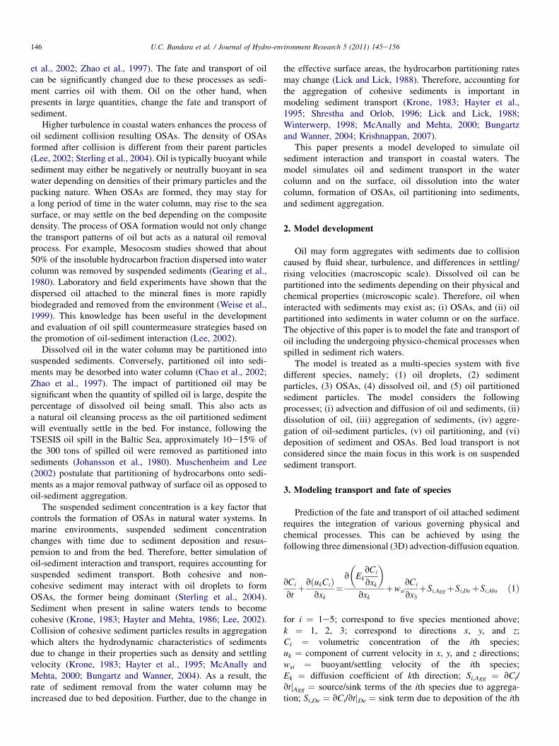
Fig. 1. Comparison of model prediction and experimental data of Sterling e

CPEq ¼ CA;S þCA;C ð34Þ

where CPEq¼ partitioned oil at equilibrium (mL/g);

CA,S ¼ surface adsorbed oil (mL/g); and CA,C ¼ capillaryabsorbed oil (mL/g). CA,S can be calculated by using Langmuiradsorption equation as (Zhao et al., 1997),

CA;S ¼ bkCDi

1þ kCDi

ð35Þ

where CDi ¼ the dissolved oil volume concentration afteradsorption reaches an equilibrium stage; and b, k ¼ adsorptioncoefficients. The unit of b is mL/g; CDi and k have no units.Zhao et al. (1997) conducted experimental studies on equi-librium adsorption of oil by using sediment with a concentra-tion of 10 kg/m3 and diameters of 0.213, 0.188, 0.159, 0.129,0.087, and 0.043 mm. They found the following relationshipsfor b and k through curve fitting.

b¼ 0:00019D�0:6215 ð36Þ

K ¼ 112:21� 68:31D ð37ÞCA,C is related to sediment particle size and can be calcu-

lated as follows (Zhao et al., 1997).

CA;C ¼ kmDm ð38Þ

where km,m ¼ constants. Chao et al. (1997) suggested valuesof 8.14 � 10�6 and �0.772 for km and m respectively based ontheir experiments. The following equation shows the massconservation of oil (Chao et al., 1997).

t al. (2004); (a) input condition at 0 min; (b) at 15 min; (c) at 30 min.


CDi ¼ CDi;0 �CSCPEq ð39Þ

where CDi,0 ¼ the initial volume concentration of dissolvedoil; and CS ¼ sediment concentration (g/mL).

When dissolved oil mixes with pure sediment, absorptionand adsorption will occur. On the other hand, when sedimentin clear water containing oil mixes, desorption will occur.Desorption is the reverse process of absorption and adsorption.The equilibrium desorption can be given as follows (Chaoet al., 1997).

CSCA;0 ¼ CDi þCSCPEq ð40Þ

where CA,0 ¼ the initial oil concentration in sediment sample.In reality, often absorption/adsorption and desorption occur

simultaneously since neither sediment is pure nor water isclear. With the initial oil concentration in water CDi,0 andinitial oil amount in sediment CA,0, the equilibrium of theabsorption/adsorption and desorption CPEq

, can be calculatedas follows combining Eqs. 34 through 40.

CPEq¼ 1

2

24�CDi;0

CS

þCA;0þ 1

kCS

þbþ kmDm

�

�ffiffiffiffiffiffiffiffiffiffiffiffiffiffiffiffiffiffiffiffiffiffiffiffiffiffiffiffiffiffiffiffiffiffiffiffiffiffiffiffiffiffiffiffiffiffiffiffiffiffiffiffiffiffiffiffiffiffiffiffiffiffiffiffiffiffiffiffiffiffiffiffiffiffiffiffiffiffiffiffiffiffi��CDi;0

CS

�CA;0� 1

kCS

þ bþ kmDm

�2

þ 4b

kCS

s 35 ð41Þ

8. Model validation

8.1. Oil-sediment aggregate formation

Sterling et al. (2004) conducted a series of batch mixinglaboratory experiments to estimate homogeneous and hetero-geneous collision efficiency values. They measured particlesize distributions (PSD) using a light scattering particleanalyzer and an electronic particle counter. A 40 L batch

Fig. 2. Comparison of model prediction and experimental data of the effect of

sediment particle sizes on equilibrium partitioning.

mixing tank filled with artificial sea water was used for theirexperiments. PSDs were measured for the systems of clay,silica, chemically dispersed crude oil, clay-crude oil, andsilica crude oil systems. The data are available only forclayecrude oil system. For this experiment they used a sedi-ment loading of 8.3 mg/L, oil loading of 12.5 mg/L, anda mean shear stress of 20 se1. The heterogeneous collisionefficiency (oil-sediment) was found to be 0.55. The compar-ison of the model simulated results with the experimental dataare shown in Fig. 1. Fig. 1 shows the volume fraction of PSDsmeasured at two time intervals. The initial condition is takento be PSD of OSAs at 0 min. Model is allowed to account forthe sediment aggregation as clay particles are known to becohesive. Although the simulated results are not a perfectmatch with the experimental data, the major behaviors arewell simulated. The reduction in smaller aggregates andincrease in larger aggregates with time, are in good agreementwith the model results.

8.2. Effect of sediment particle sizes on equilibriumpartitioning

To study the effect of sediment particle sizes on equilibriumpartitioning of oil, Zhao et al. (1997) carried out laboratoryexperiments with CDi,0 ¼ 0.004 kg/m3 and CS ¼ 10 kg/m3.They used sediments with ds ¼ 0.213, 0.188, 0.159, 0.129,0.087, and 0.043 mm. The measured equilibrium partitioning(CPEq

) of oil with the simulated results for these six cases areplotted in Fig. 2.

Simulated results show a good agreement with the experi-mental data when ds > 0.1 mm. When ds < 0.05 mm, thesimulated partitioning is higher than the measured one. Sedi-ments with particle sizes less than 0.05 mm are classified as silt.Thus the chemical and physical properties are different from theparticles larger than 0.1 mm. The equations used may notdescribe the chemical and physical properties of silt very well.

Fig. 3. Comparison of model prediction and experimental data of the effect of

initial oil concentration on equilibrium partitioning.

Fig. 4. Ambient current in X direction (m/s).

Table 2

Input parameters for simulations-effect of bubble/particle sizes, sediment

concentration.

Parameter Value

Spill duration 2 h

Simulation duration 72 h (3 days)

Spilled oil volume 500 m3

Oil density 893 kg/m3

Oil type Venezuelan

Water depth (h) 20 m

Depth of oil release 20 m

Ambient salinity 32 ppt

Ambient velocity profile Fig. 4


8.3. Effect of oil concentration on equilibriumpartitioning

Zhao et al. (1997) conducted laboratory experiments tostudy the effect of initial oil concentrations on equilibriumpartitioning. They tested sediments with ds ¼ 0.213, 0.166,0.129, 0.087, and 0.043 mm under different initial oil volumeconcentrations and CS ¼ 10 kg/m3. The comparison ofmeasured and the simulated results for the equilibrium parti-tioning (CPEq

) of oil with different sediment particle sizesunder different initial oil concentrations are plotted in Fig. 3.Lines show the model results while the experimental data areshown as discrete points. The comparisons show that thesimulated results agree well with the measured data.

9. Scenario simulations

The objective of developing the present model is to simu-late the interaction, transport, and fate of spilled oil in sedi-ment laden coastal waters. With such simulations one canpredict how much oil is removed from the water column due tooil-sediment interaction once spilled oil volume, PSDs of oiland sediments, water and hydrodynamic conditions areknown. This information would be useful in planning anddeveloping countermeasures for oil spills.

Table 1

Input data for scenario simulation-effect of droplet/particle sizes, sediment

concentration.

Case Median oil droplet

Diameter (mm)

Median sediment

Diameter (mm)

Reference sediment

Concentration (g/l)

1 100 63 1

2 100 500 1

3 500 63 1

4 500 500 1

5 100 63 10

6 100 500 10

7 500 63 10

8 500 500 10

The objectives of the scenario simulations are; to show themodel capabilities such as predicting the oil budget; toexamine the effect of oil and sediment PSDs, sedimentconcentration, and sediment aggregation on oil-sedimentinteractions. To demonstrate these effects eight cases aredeveloped. Table 1 shows the input data for the eight cases.

Oil droplet sizes are selected based on the reported exper-imental data in upper ocean (Delvigne, 1991; Li and Garrett,1998). Sediment particle sizes are selected to represent bothcohesive (silt) and non-cohesive (sand) particles. The observedsediment sizes in shallow water regions were found to bebetween 10 and 700 mm (van Rijn, 1984; Lou and Ridd, 1997;McAnally and Mehta, 2001). The horizontal and verticaldiffusion coefficients used are 0.001 and 0.0001 m2/s respec-tively. Suspended sediment concentrations are given as openboundary conditions along X and Z directions. The followingstandard Rouse profile is assumed to be the input sedimentconcentrations along the two boundaries (van Rijn, 1984,1986; Lou and Ridd, 1997).

c

ca¼a

z

�h� z

h� a

�zð42Þ

Fig. 5. Case 1: Oil budget for reference sediment concentration 1 g/l; median

oil droplet diameter ¼ 100 mm; median sediment particle size ¼ 63 mm.

Fig. 6. Case 1: Oil attached sediments vs oil partitioned sediments for refer-

ence sediment concentration 1 g/l; median oil droplet diameter ¼ 100 mm;

median sediment particle size ¼ 63 mm.


where h ¼ flow depth; a ¼ reference level; ca ¼ referenceconcentration; z ¼ Rouse parameter; z ¼ ws/ku* whereu* ¼ bed shear velocity; a ¼ 0.001;h ¼ 0.02 m (van Rijn,1984); ws ¼ 1 mm/s (Winterwerp, 1998). Reference sedi-ment concentrations are selected to represent the field valuesin near-shore regions, reported in the literature (Lou and Ridd,1997; Jankowski and Zielke, 2001; McAnally and Mehta,2001). Some key input parameters used in simulations arelisted in Table 2.

The calculated oil budget includes; (i) free oil droplets inthe water column; (ii) OSAs in the water column; (iii) free oildroplets on the water surface; (iv) OSAs on the water surface;(v) OSAs at the bed; (vi) partitioned oil into sediments. Eachcomponent is given as a volume percentage of the total oilvolume released. Sample results of oil budget for Case 1 areshown in Figs. 5 and 6. Fig. 5 shows variation of oil attachedsediments while Fig. 6 shows a comparison of oil attachedsediment with oil partitioned sediments. Fig. 6 reveals that theamount of partitioned oil into sediments is about 4e5 ordersmagnitude smaller than the amount of oil attached sediments.A summary of results after 72 h of simulation period is givenin Table 3. The amounts of oil partitioned sediment are

Table 3

Summary of oil budget after 72 h.

Case Maximum

oil-sediment

agg.(%)

Oil-sediment

agg. in water

column (%)

Oil-sediment

agg. at the

bed (%)

Free oil

at the

surface (%)

Oil-sediment

agg. at the

surface (%)

1 57 54 9 37 0

2 58 54 9 37 0

3 32 14 6 67 13

4 25 4 7 73 16

5 82 27 59 14 0

6 79 20 65 15 0

7 66 14 58 27 1

8 63 4 68 24 4

omitted from the results since they are negligible compared tooil attached sediments.

Cases 1 through 4 use the reference sediment concentration1 g/l which is a relatively low value in shallow water regions.Case 1 represents a mixture of silt and clay (63 mm) whileCase 2 represents fine sand (500 mm). The difference in oilbudget in two cases is small. The change in sediment sizeaffects the formation of OSAs in two ways. Larger sedimentparticles have higher settling velocities which enhances thepossibility of OSA formation. On the other hand, the numberdensity is smaller for larger sizes as the sediment concentra-tion is not changed. This reduces the OSA formation rate.Therefore, this implies that the two effect balance out eachother in this situation.

Comparison of Cases 1 and 3 shows a drastic change in theamount of OSAs formed (32% compared to 57%). Thissignificant difference is caused by the change in rise velocityand the number density. When oil droplet size is 63 mm (Case1), rise velocity is as low as 1 mm/s whereas it is about 5 cm/sfor a size of 500 mm (Case 3). Accordingly, time to reach thesea surface is few minutes for an oil droplet of size 500 mmwhile it is about 5 h for a size of 63 mm. Thus in Case 3, oilrapidly escapes sediment concentrated bottom layers reducingthe interaction with sediments. Further, oil droplet numberdensity is smaller for larger droplets for the same oil volume.Due to these two reasons smaller oil droplets tend formaggregates with sediment more than larger ones. Some oilattached sediment on the surface (13%) can be observed inCase 3 while there are none in Case 1. This is because whenthe dominant constituent of aggregates is oil, the combineddensity of the aggregate is less than that of ambient waterwhich allows them the rise to the surface.

Case 4 shows a lesser amount of formed OSAs (25%)compared to Case 3 (30%). This is due to the fact that sedi-ment number concentration is less when the sizes are larger fora given sediment concentration. Accordingly, a higherpercentage of free oil droplet can be observed on the watersurface (67%) in Case 3 compared to Case 4 (73%).

Cases 5 through 8 show the oil budget for reference sedimentconcentration of 10 g/l which is a relatively high value found inshallow water areas. Input conditions for these four cases aresimilar to the cases 1 through 4 except for the higher sedimentconcentration. Comparison of simulated results for Cases 5through 8 shows a similar behavior to Cases 1 through 4. Resultsfor lower sediment concentrations (Cases 1 through 4) differfrom the results for higher sediment concentrations in severalways. When the sediment concentration is higher the totalamount of OSA formed are higher as expected. It can also beobserved that the removal rate of suspended OSAs due to beddeposition is higher when the sediment concentration is higher.OSAs once formedmay not further interactwith sediments underlow sediment concentrations. This make sense from physicalpoint of view because when OSAs are formed the numberconcentration decreases and may even falls below the criticalconcentration required for aggregation. However, when thesediment concentration is higher, OSA formed has a higherchance for further aggregation with sediments increasing the


combined density. This increases the rate of removal of OSAsfrom the water column.

10. Summary

This paper presents a three dimensional numerical model tosimulate oil-sediment interaction and transport in coastalwaters. The model simulates; (i) oil and sediment transport,(ii) formation of OSAs, (iii) oil dissolution and partitioninginto sediments, and (iv) sediment aggregation. The presentmodel is developed as a multi-species system. The speciesconsidered are; oil, sediment, OSAs (both oil attached sedi-ments and oil partitioned sediments), and dissolved oil.Advection-diffusion equation is implemented using LPmethod to model the transport and fate of each species.Modeling components include; effective density and settlingvelocity of sediments and OSAs, aggregation of oil andsediments, oil dissolution into water column, oil partitioninginto sediments, aggregation of sediment, and bed deposition ofsediments and OSAs.

The model results compared well with the limited labora-tory experimental data. Scenario simulations reveal that up to82% of the total oil released can interact with sediments toform aggregates. Up to 65% of the total oil released may beremoved from the water column as OSAs. In contrast, theresults show that the amount of oil partitioned into sedimentsis 4e5 orders of magnitude smaller than the amount of OSAsformed.

Scenario simulations further show that the sedimentparticle and oil droplet sizes directly impact the OSA forma-tion rate. When smaller oil droplets (less than 0.1 mm) arepresent, predicted amounts of OSAs are higher. Smallerdroplets have smaller buoyant velocities. Having smallerbuoyant velocities allow oil droplets to stay longer in the watercolumn providing more time to interact with sediments. Whensediment sizes are larger than 0.5 mm, the amount of OSAformation is less compared to smaller sizes (less than 63 mm).Reduction in the number density of sediments due to increasedsizes causes this. In addition, higher removal rates of OSAsfrom water column due to bed deposition are predicted whenthe sediment concentration is higher.

Lack of knowledge on oil sediment aggregation collisionefficiencies, sediment aggregation efficiencies, and oil parti-tioning cause some uncertainty in the results. Further labora-tory and field experimental data would facilitate testing andimproving the model. Model developed in this work can alsobe applied to interaction of oil with marine snow.

Appendix A. Numerical implementation of aggregation

Appendix A. 1. Smoothed Particle Hydrodynamics (SPH)method

SPH method was first developed to solve problems inastrophysics involving moving fluid masses in 3D space(Monaghan, 1988). Since then the SPH method has been

applied to a variety of problems including modeling multi-phase flows (Valizadeh et al., 2008), flow through porousmedia (Tartakovsky et al., 2008), and river ice dynamics (Shenet al., 2000). The SPH method has several advantagesincluding: (i) meshless nature, (ii) no nonlinear terms involvedin the NaviereStokes equation, (iii) explicit mass andmomentum conservation, and (iv) convenient implementation.

The SPH method defines any physical property A ata location r to be interpolated as the weighted sum of the sameproperty of neighboring parcels in an appropriate range giving,

AðrÞzXNi

j¼1

mj

Aj

rjW�r� rj;hi

� ðA:1Þ

where Aj, rj, mj ¼ property, density, and mass of jth parcel;hi ¼ smoothing length; Ni ¼ number of parcels within therange of hi. The integration is over the entire 3D space. Thefunction W is the SPH smoothing kernel with a smoothinglength h. In other words h determines the influence range ofW.The interpolating kernel W must be differentiable and thederivatives should be continuous. Gaussian and spline func-tions are the most commonly used kernels. The present modeluses the following 3D Gaussian kernel.

W�r� rj;h

� ¼ 1

h2p3=2e��r�rjh

�2ðA:2Þ

Appendix A. 1.1. Modeling number densityModeling aggregation requires a good estimate of the

number/volume density as it controls the aggregation rate. Eq.(26) describes the rate of formation of sediment flocs or OSAswhich is a function of volume density of each particle type.Parcel number density, nj is related to the mass density rjaccording to,

rj ¼ mjnj ðA:3ÞBy using Eqs. (A. 3) and (A. 1) the number density ni at

parcel location r is given by,

niðrÞ ¼XNi

j¼1

W�r� rj;hi

� ðA:4Þ

Number density of ith parcel location can be converted intovolume density multiplying by the volume of the interpolatingdomain.

Appendix A.1.2. Smoothing LengthSelection of the smoothing length impacts the accuracy and

the efficiency of the model. The following equation is used todescribe the smoothing length which takes time variation in toaccount (Monaghan, 2005).

hnewi ¼ holdi

�roldi

rnewi

�1=3

ðA:5Þ

where hnewi ; holdi ¼ smoothing lengths of the present and theprevious time steps respectively of the ith parcel location;rnewi ; roldi ¼ mass density of the current and previous time


steps respectively of the ith parcel location. Mass density canbe obtained by using r for property A in Eq. (A. 1).

Particle mass mj changes due to flocculation/aggregationand oil dissolution and is updated during each time step. Theinitial smoothing length is calculated as follows (Liu et al.,2003).

h0i ¼ ð3=32pÞ1=3 XNi

j¼1

mj=roi

!1=3

ðA:6Þ

where roi ¼ initial number density of the ith parcel location.

Appendix B. Calculation of rackett parameter

Rackett Parameter is calculated using the following equa-tion (Yamada and Gunn, 1973)

ZRAi ¼ 0:29056� 0:08775ui ðB:1Þwhere ui ¼ acentric factor and is calculated as (Daubert

and Danner, 1989),

ui ¼ lnð101:325=PciÞ � 5:92714þ 6:09648=Trbi þ 1:28862 lnTrbi � 0:169347T6rbi

15:2518� 15:6875=Trbi � 13:4721 lnTrbi þ 0:43577T6rbi

ðB:2Þ

where Trbi ¼ Tbi/Tci ¼ reduced boiling point; Tbi ¼ boilingpoint (K); Tci ¼ critical temperature (K) and is calculated as(Daubert and Danner, 1989),

Tci ¼9:5233exp�� 9:3145� 10�4Tbi � 0:5444Si þ 6:4791

� 10�4TbiSi�T0:81067bi S0:53691i ðB:3Þ

where Si ¼ the specific gravity of component i at 15.5 C.Tbi can be calculated based on the molecular weight andspecific gravity of this component using the following equa-tion (Riazi and Daubert, 1987).

Tbi ¼3:76587exp�3:7741� 10�3Mi þ 2:98404Si � 4:25288

� 10�3MiSi�M0:40167

i S�1:58262i ðB:4Þ

where Mi ¼ molecular weight of component i (g/mol). Pci iscalculated as (Daubert and Danner, 1989),

Pci ¼31:9497� 106exp�� 8:505� 10�3Tbi � 4:8014Si

þ 5:7490� 10�3TbiSi�T�0:4844bi S4:0486i ðB:5Þ

References

Batchelor, G.K., 1982. The Theory of Homogeneous Turbulence. Cambridge

Univ. Press, Cambridge, England.

Bungartz, H., Wanner, S.C., 2004. Significance of particle interaction to the

modelling of cohesive sediment transport in rivers. Hydrological Process.

18, 1685e1702.

Chao, X., Shankar, N.J.,Wang, S.S.Y., 2002. Development and application of oil

spill model for singapore coastal waters. J. Hydraul. Eng. 129 (7), 495e503.

Chao, X., Zhao, W., Qiu, D., 1997. Study on the adsoprtion properties of oil by

sediment applying fractal theory. Shuili Xuebao (9).

Daubert, T.E., Danner, R.P., 1989. API Technical Data Book-Petroleum

Refining. American Petroleum Institute (API), Washington D. C.

Dean, R., Dalrymple, R.A., 2004. Water Wave Mechanics for Engineers and

Scientists. Wold Scientific, Singapore.

Delvigne, G.A.L., 1991. On scale modeling of oil droplet formation from

spilled oil. Proc. 1991 Oil Spill Conf., 501e526.Gearing, P.J., Gearing, J.N., Pruell, R.J.W., Quinn, T.L., James, G., 1980.

Partitioning of no. 2 fuel oil in controlled estuarine ecosystems. sediments

and suspended particulate matter. Environ. Sci. Tech. 14 (4), 299e309.

Hayter, E.J., Bergs, M.A., Gu, R., McCutcheon, S.C., Smith, S.J., Whiteley, H.

J., May 1995. HSCTM-2D, A Finite Element Model for Depth-Averaged

Hydrodynamics, Sediment and Contaminant Transport. Technical Report.

National Exposure Research Laboratory, Office of Research and Devel-

opment, U.S. Environmental Protecting Agency, Athens, Georgia 30605.

Hayter, E.J., Mehta, A.J., 1986. Modelling cohesive sediment transport in

estuarial waters. Appl. Mathe. Model. 10 (4), 294e303.

Jankowski, J.A., Zielke, W., 2001. The mesoscale sediment transport due to

technical activities in the deep sea. Hydrol. Proces 48, 3487e3521.

Johansen, O., 2000. Deepblow e a lagrangian plume model for deep water

blowouts. Spill Sci. Tech. Bull. 6 (2), 103e111.

Johansson, S.U., Larsson, U., Boehm, P., 1980. The tsesis oil spill: impact on

the pelagic ecosystem. Marine Pollut. Bull. 11 (14(4)), 284e293.

Khelifa, A., Hill, P., 2006. Models for effective density and settling velocity of

flocs. J. Hydraul. Res. 44 (3), 390e401.

Kranenburg, C., 1994. An Entrainment Model for Fluid Mud. Technical

Report 93e10. Fac. of Civil Eng., Delft Uni. of Technology, Delft, The

Netherlands.

Krishnappan, B.G., 2007. Recent advances in basic and applied research in cohe-

sive sediment transport in aquatic systems. Can. J. Civil Eng. 34 (6), 731e743.Krone, R., 1962. Flume Studies of the Transport of Sediment in Estuarial

Shoaling Processes. Final Rep., Hydraul. Eng. Lab. and Sanitary Eng. Res.

Lab., Univ. of California at Berkeley, Berkeley, Calif.

Krone, R., 1983. Cohesive sediment properties and transport processes. Front.

Hydraul, 66e78.

Lee, K., 2002. Oil-particle interactions in aquatic environments:influence on

the transport, fate, effect and remediation of oil spills. Spill Sci. Tech. Bull.

8 (1), 3e8.

Li, M., Garrett, C., 1998. The relationship between oil droplet size and upper

ocean turbulence. Marine Pollut. Bull. 36 (12), 961e970.

Lick, W., Lick, J., 1988. Aggregation and disaggregation of fine-grained lake

sediments. J.of Great Lakes Res. 14 (4), 514e523.

Liu, M.B., Liu, G.R., Lam, K.Y., Zong, Z., 2003. Smooth particle hydrody-

namics for numerical simulation of underwater explosion. Comp. Mech.

30, 106e118.

Lou, J., Ridd, P.V., 1997. Modelling of suspended sediment transport in coastal

areas under waves and currents. Est., Coast. Shelf Sci 45 (1), 1e16.

Lytle, D.A., Peckarsky, B.L., 2001. Spatial and temporal impacts of a diesel

fuel spill on stream invertebrates. Freshwater Biol. 46 (4), 693e704.

Maggi, F., September 2005. Flocculation Dynamics of Cohesive Sediment.

PhD thesis 05 e 1, Delft Univ. of Tech., Postbus 5, 2600 AA, Delft, The

Netherlands.

McAnally, W.H., May 2000. Aggregation and Deposition of Estuarial Fine

Sediment. Technical Report. U.S. Army Engineer Research and Devel-

opment Center, 3909 Halls ferry road, Vicksburg. MS 39180 e 6199.

McAnally, W.H., Mehta, A.J., 2000. Aggregation rate of fine sediment.

J. Hydraul. Eng. 126 (12), 883e892.

McAnally, W.H., Mehta, A.J., 2001. Collisional aggregation of fine estuarial

sediment. Coastal and estuarine fine sediment processes-Proce. Marine Sci.

3 (12), 19e40.


Monaghan, J.J., 1988. An introduction to sph. Comp. Phys. Comm. 48, 89e96.Monaghan, J.J., 2005. Smoothed particle hydrodynamics. Rep. Prog. Phys. 68,

1703e1759.

Monaghan, J.J., Gingold, R.A., 1983. Shock simulation by the particle method

sph. J. Comp. Phys. 52 (2), 374e389.Muschenheim, D.K., Lee, K., 2002. Removal of oil from the sea surface

through particulate interactions: review and prospectus. Spill Sci. Tech.

Bull. 8 (1), 9e18.Neumann, G., Pierson, W.J., 1966. Principles of Physical Oceanography.

Prentice-Hall, Englewood Cliffs, N.J.

Owens, E.H., Bragg, J.R., Humphrey, B., 1994. Clay-oil flocculation as

a natural cleaning process following oil spills:part 2 -implications of study

results in understanding past spills and for future response decisions.

Proceedings 20 (4), 25e37.

Payne, J., Kirstein, B., Clayton Jr., J.R., ClaryRedding, R., McNabb Jr., D.,

Farmer, G., September 1987. Integration of Suspended Particulate Matter

and Oil Transportation Study. Technical Report 14-12-0001-30146.

Science Application International Corporation, 10260, Campus Point

Drive, San Diego, CA 92121.

Reid, R.C., Prausnitz, J.M., Poling, B.E., 1987. Properties of Gases and

Liquids. McGraw e Hill, New York.

Riazi, M.R., Daubert, T.E., 1987. Characterization parameters for petroleum

fractions. Ind. Eng. Chem. Res. 26, 755e759.Riazi, M.R., Edalat, M., 1996. Prediction of the rate of oil removal from

seawater by evaporation and dissolution. J. Pet. Sci. Eng. 16, 291e300.

Shailaja,M.S., 1988. The influence of dissolved petroleumhydrocarbon residues

on natural phytoplankton biomass. Marine Environ. Res. 25 (4), 315e324.Shen, H.T., Su, J., Liu, L., 2000. Sph simulation of river ice dynamics.

J. Comp. Phys. 165, 752e770.

Shiu, W.Y., Maijanen, A., Anita, L.Y.N., Mackay, D., 1988. Preparation of

aqueous solutions of sparingly soluble organic substances: ii. multiple

component system hydrocarbon mixture and petroleum products. Environ.

Toxicol. Chem. 7, 125e137.

Shrestha, P.L., Orlob, G.T., 1996. Multiphase distribution of cohesive sedi-

ments and heavy metals in estuarine systems. J. Environ. Eng. 122 (8),

730e740.

Sterling, M.C., Bonner, J.S., Ernest, A.N.S., Pageb, C.A., Autenrieth, R.L.,

2005. Application of fractal flocculation and vertical transport model to

aquatic sol-sediment systems. Water Res. 39 (9), 1818e1830.

Sterling, M.C., Bonner, J.S., Page, C.A., Fuller, C.B., Ernest, A.N.S.,

Autenrieth, R.L., 2004. Modeling crude oil droplet-sediment aggregation

in nearshore waters. Environ. Sci. Tech. 38 (17), 4627e4634.

Tartakovsky, A.M., Tartakovsky, D.M., Meakin, P., Jul 2008. Stochastic lan-

gevin model for flow and transport in porous media. Phys. Rev. Lett. 101

(4), 044502.

Terray, E., Donelan, M., Agrawal, Y., Drennan, W., Kahma, K., Williams, A.I.,

Hwang, P., Kitaigorodskii, S., 1996. Estimates of kinetic energy dissipation

under breaking waves. J. Phys. Oceanography 26 (5), 792e807.Valizadeh, A., Shafieefar, M., Monaghan, J.J., Neyshaboori, S., 2008.

Modeling two-phase flows using sph method. J. Appl. Sci. 8 (21),

3817e3826.

van Rijn, L.C., 1984. Sediment transport, part ii: suspended load transport.

J. Hydraul. Eng. 110 (11), 1626e1638.

van Rijn, L.C., 1986. Mathematical modeling of suspended sediment in

nonuniform flows. J. Hydraul. Eng. 112 (6), 433e455.

Weise, A.M., Nalewajko, C., Lee, K., 1999. Oil-mineral fine interactions

facilitate oil biodegradation in seawater. Environ. Tech. 20 (4), 299e309.

Winterwerp, J.C., 1998. Simple model for turbulence induced flocculation of

cohesive sediment. J. Hydraul. Res. 36 (3), 309e326.Yamada, T., Gunn, R.D., 1973. J. Chem. Eng. Data 18, 234.

Yapa, P.D., Xie, H., January 2006. Modeling of Chemical Processes in Oil

Spills (Final Report). Technical Report 06e01. Depart. of Civil and

Environ. Eng., Clarkson Univ., Potsdam, NY.

Yapa, P.D., Zheng, L., Kobayashi, T., 1996. Application of linked-list approach

to pollutant transport models. J. Comput. Civil Eng. 4, 88e90.

Zhao, W., Chao, X., Huang, Q., 1997. Mathematical model and experimental

study on adsorption of oil by sediment. Shuili Xuebao (12).

Zheng, L., Yapa, P.D., 2000. Buoyant velocity of spherical and nonspherical

bubbles/droplets. J. Hydraul. Eng. 126 (11), 852e854.

Zheng, L., Yapa, P.D., Chen, F., 2003. A model for simulating deepwater oil

and gas blowouts e part I: theory and model formulation. J. Hydraul. Res.

41 (4), 339e351.

Fate and transport of oil in sediment laden marine waters

Documents

Transcript of Fate and transport of oil in sediment laden marine waters