HAL Id: hal-01606812https://hal.archives-ouvertes.fr/hal-01606812

Submitted on 18 Jul 2021

HAL is a multi-disciplinary open accessarchive for the deposit and dissemination of sci-entific research documents, whether they are pub-lished or not. The documents may come fromteaching and research institutions in France orabroad, or from public or private research centers.

L’archive ouverte pluridisciplinaire HAL, estdestinée au dépôt et à la diffusion de documentsscientifiques de niveau recherche, publiés ou non,émanant des établissements d’enseignement et derecherche français ou étrangers, des laboratoirespublics ou privés.

Fast determination of gas-liquid diffusion coefficient byan innovative double approach

Feishi S. Xu, Melanie Jimenez, Nicolas Dietrich, Gilles Hébrard

To cite this version:Feishi S. Xu, Melanie Jimenez, Nicolas Dietrich, Gilles Hébrard. Fast determination of gas-liquiddiffusion coefficient by an innovative double approach. Chemical Engineering Science, Elsevier, 2017,170, pp.68-76. �10.1016/j.ces.2017.02.043�. �hal-01606812�

1

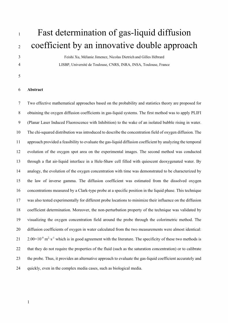
Fast determination of gas-liquid diffusion 1

coefficient by an innovative double approach 2

Feishi Xu, Mélanie Jimenez, Nicolas Dietrich and Gilles Hébrard 3

LISBP, Université de Toulouse, CNRS, INRA, INSA, Toulouse, France 4

5

Abstract 6

Two effective mathematical approaches based on the probability and statistics theory are proposed for 7

obtaining the oxygen diffusion coefficients in gas-liquid systems. The first method was to apply PLIFI 8

(Planar Laser Induced Fluorescence with Inhibition) to the wake of an isolated bubble rising in water. 9

The chi-squared distribution was introduced to describe the concentration field of oxygen diffusion. The 10

approach provided a feasibility to evaluate the gas-liquid diffusion coefficient by analyzing the temporal 11

evolution of the oxygen spot area on the experimental images. The second method was conducted 12

through a flat air-liquid interface in a Hele-Shaw cell filled with quiescent deoxygenated water. By 13

analogy, the evolution of the oxygen concentration with time was demonstrated to be characterized by 14

the law of inverse gamma. The diffusion coefficient was estimated from the dissolved oxygen 15

concentrations measured by a Clark-type probe at a specific position in the liquid phase. This technique 16

was also tested experimentally for different probe locations to minimize their influence on the diffusion 17

coefficient determination. Moreover, the non-perturbation property of the technique was validated by 18

visualizing the oxygen concentration field around the probe through the colorimetric method. The 19

diffusion coefficients of oxygen in water calculated from the two measurements were almost identical: 20

2.00×10-9 m2·s-1 which is in good agreement with the literature. The specificity of these two methods is 21

that they do not require the properties of the fluid (such as the saturation concentration) or to calibrate 22

the probe. Thus, it provides an alternative approach to evaluate the gas-liquid coefficient accurately and 23

quickly, even in the complex media cases, such as biological media. 24

2

1. Introduction 25

The quantification of mass transfer phenomenon is important in the industry. The determination of 26

physical properties in the transport process, such as the diffusion coefficient and liquid-side mass 27

transfer coefficient, would be helpful to understand the transport mechanism deeply. Concentrating on 28

the diffusion regime which is characterized by a diffusion coefficient D, it physically represents a 29

migration of molecules of a constituent under the effect of a potential chemical gradient. The first law 30

of diffusion was established by Fick (1855). By analogy with Fourier's law governing the transfer of 31

heat, the diffusive flux can be expressed as 32

𝐽 = −𝐷∇𝐶 33

where J is the diffusive flux (kg·m-2·s-1) and ∇𝐶 denotes the concentration gradient. The subsequent 34

researches in this domain are intensive and several measurement techniques have been developed: the 35

steady state method (Tham et al., 1967), capillary cell method (Gubbins et al., 1966; Malik and Hayduk, 36

1968), laminar jet method (Duda and Vrentas, 1968; Ferrell and Himmelblau, 1967), and absorption 37

measurement (Sovová and Procházka, 1976). Other techniques based on the Taylor dispersion (Baldauf 38

and Knapp, 1983), the use of polarographic sensors (Ho et al., 1986; Ju and Ho, 1985) and bubble size 39

calculation (de Blok and Fortuin, 1981; Wise and Houghton, 1966) can also be considered. However, 40

the classical determination methods present some limitations due to hydrodynamic perturbation, natural 41

convection, necessity of transparent liquids, long response time, impact of the liquid media, and so on 42

(Blackadder and Keniry, 1973, 1974). Furthermore, it has to be noted that most of the measurements 43

concern gas-gas or liquid-liquid systems and the knowledge of the case persisting in the gas-liquid 44

system is not sufficient. 45

More recently in laboratories, the technique by using microprobes has been adopted because of its 46

simplicity of experimental configuration (Bowyer et al., 2004; Jamnongwong et al., 2010). For instance, 47

Hebrard et al. (2009) assessed the impact of surfactants on the oxygen diffusion coefficient with a Clark-48

type probe in a stirred cell. This kind of technique always requires the insertion of measuring instruments 49

(ex. pressure, concentration meters) which may bring a perturbation to the system. Due to the non-50

3

intrusive advantages, optical techniques such as interferometry (Guo et al., 1999), are developed to 51

characterize the diffusive process. The technique of interferometry could quantify the transfer in a liquid 52

phase through the change of refractive index induced by the presence of dissolved gas (Roetzel et al., 53

1997; Wylock et al., 2011). However, the process for obtaining the relation between the refractive index 54

and dissolved gas concentration is always complicated and time-consuming. The planar laser-induced 55

fluorescence (PLIF) is another optical method widely applied to characterize the mass transfer in the 56

gas-liquid system (Bouche et al., 2013; Sancho et al., 2016; Stamatopoulos et al., 2015). The principle 57

of PLIF is to introduce a fluorescent dye into the liquid phase illuminated by a laser sheet. According to 58

the properties of different fluorescent dyes, the fluorescence intensities can be affected by one or 59

multiple the fluid conditions (the presence of specific gas, pH value, and temperature). The state of mass 60

transfer can thus be obtained from images of the studied solution in the enlightened area recorded by 61

cameras. Due to the advantages (ex. fast response, no flow disturbance, high resolution), several PLIF-62

based studies have been carried out to evaluate the gas-liquid diffusion coefficient (Bork et al., 2005; 63

Dietrich et al., 2015; Jimenez et al., 2012a, 2012b) with good accuracy. 64

Overall, techniques to measure the diffusion coefficient are diverse, each of which displays low 65

measurement uncertainties. Nevertheless, if a comparison is made between the diffusion coefficient 66

values obtained by these techniques, a big gap appears. For example, the values in the literature for the 67

diffusion coefficient of oxygen in water range between 0.7×10-9 m2·s-1 and 2.5×10-9 m2·s-1 for a given 68

temperature (20 °C). The empirical equations or semi-empirical ones, commonly used in the literature 69

and the industry, being established from these experimental results, it is not surprising that their validity 70

is, in some cases, questionable. 71

Therefore, the objective of this study is to provide new insight into this domain. Two different methods 72

are proposed to obtain the diffusion coefficient of oxygen in water in different devices. In the first 73

method, PLIF with inhibition (PLIFI) technique was used to measure the mass transfer in the wake of 74

an isolated bubble rising in a column. In the second one, a probe was used to measure the concentration 75

of dissolved oxygen passed through a flat air-liquid interface in a Hele-Shaw cell. With the experimental 76

data, both diffusion coefficients were calculated based on the effective mathematical models: the chi-77

4

squared distribution and the law of inverse gamma, respectively. The final coefficient could be 78

determined by comparing these two results. 79

2. Materials and Methods 80

2.1 First Method: PLIF with inhibition in a bubble column 81

PLIF is an optical technique which has already been proved powerful for the mass transfer visualization 82

(Asher, 2009; Jimenez et al., 2013). In PLIF with inhibition (PLIFI), the ability of some molecules called 83

“quenchers” to inhibit the fluorescence dye is considered. Oxygen, which is of prime interest in a series 84

of studies (Dani et al., 2007; Jimenez et al., 2013; Kück et al., 2010, 2012), has been known as an 85

excellent quencher. The quenching effect is usually considered to be a consequence of collisions 86

between molecules where the excess energy of the dye is absorbed by oxygen (Lakowicz, 1999). The 87

suitability of PLIFI is mainly because the technique is not only limited to visualization but also enables 88

an accurate quantification of the transferred mass. The quantification of the mass transfer is 89

straightforward since the fluorescence level is directly related to the oxygen concentration in the liquid 90

phase according to the (Stern and Volmer, 1919) equation: 91

𝐼!𝐼"=𝜏𝜏"=

11 + 𝐾#$[𝑄]

92

where Ksv is the Stern–Volmer constant (m3·kg-1), [Q] the quencher concentration (kg·m-3), τ and τ0 are 93

the lifetimes of the fluorescence molecule with/without inhibition, and IQ and I0 the fluorescence 94

intensities in the presence and absence of quencher, respectively. In the experiment, the fluorescence 95

intensities can be determined from the gray levels recorded by the camera. The parameters I0 and Ksv of 96

the Eq. (2) can be easily determined from an experimental calibration curve, in which the inverse of 97

different recorded fluorescence intensities IQ (or more precisely gray levels recorded by the camera) is 98

plotted as a function of uniform quencher concentration (oxygen in this study). 99

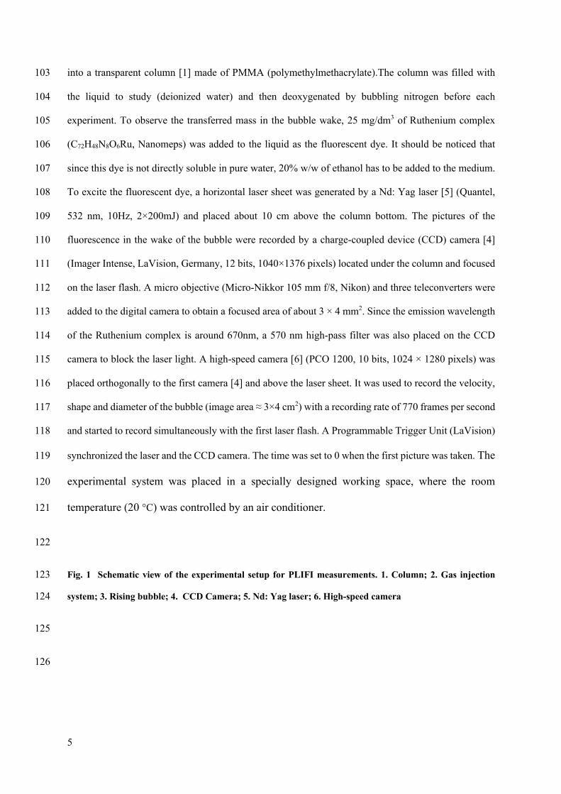
2.1.1 Experimental setup 100

The experimental setup was quite similar to the one presented by Francois et al., (2011) as depicted in 101

Fig. 1. A single air bubble [3] was generated by a peristaltic pump and injected through a capillary [2] 102

5

into a transparent column [1] made of PMMA (polymethylmethacrylate).The column was filled with 103

the liquid to study (deionized water) and then deoxygenated by bubbling nitrogen before each 104

experiment. To observe the transferred mass in the bubble wake, 25 mg/dm3 of Ruthenium complex 105

(C72H48N8O6Ru, Nanomeps) was added to the liquid as the fluorescent dye. It should be noticed that 106

since this dye is not directly soluble in pure water, 20% w/w of ethanol has to be added to the medium. 107

To excite the fluorescent dye, a horizontal laser sheet was generated by a Nd: Yag laser [5] (Quantel, 108

532 nm, 10Hz, 2×200mJ) and placed about 10 cm above the column bottom. The pictures of the 109

fluorescence in the wake of the bubble were recorded by a charge-coupled device (CCD) camera [4] 110

(Imager Intense, LaVision, Germany, 12 bits, 1040×1376 pixels) located under the column and focused 111

on the laser flash. A micro objective (Micro-Nikkor 105 mm f/8, Nikon) and three teleconverters were 112

added to the digital camera to obtain a focused area of about 3 × 4 mm2. Since the emission wavelength 113

of the Ruthenium complex is around 670nm, a 570 nm high-pass filter was also placed on the CCD 114

camera to block the laser light. A high-speed camera [6] (PCO 1200, 10 bits, 1024 × 1280 pixels) was 115

placed orthogonally to the first camera [4] and above the laser sheet. It was used to record the velocity, 116

shape and diameter of the bubble (image area ≈ 3×4 cm2) with a recording rate of 770 frames per second 117

and started to record simultaneously with the first laser flash. A Programmable Trigger Unit (LaVision) 118

synchronized the laser and the CCD camera. The time was set to 0 when the first picture was taken. The 119

experimental system was placed in a specially designed working space, where the room 120

temperature (20 °C) was controlled by an air conditioner. 121

122

Fig. 1 Schematic view of the experimental setup for PLIFI measurements. 1. Column; 2. Gas injection 123

system; 3. Rising bubble; 4. CCD Camera; 5. Nd: Yag laser; 6. High-speed camera 124

125

126

6

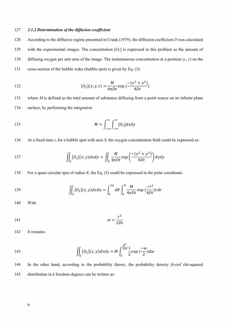
2.1.2 Determination of the diffusion coefficient 127

According to the diffusive regime presented in Crank (1979), the diffusion coefficient D was calculated 128

with the experimental images. The concentration [O2] is expressed in this problem as the amount of 129

diffusing oxygen per unit area of the image. The instantaneous concentration at a position (x, y) on the 130

cross-section of the bubble wake (bubble spot) is given by Eq. (3): 131

[𝑂%](𝑥, 𝑦, 𝑡) =𝑀

4𝜋𝐷𝑡exp(

−(𝑥% + 𝑦%)4𝐷𝑡

) 132

where M is defined as the total amount of substance diffusing from a point source on an infinite plane 133

surface, by performing the integration 134

𝑀 = = = [𝑂%]𝑑𝑥𝑑𝑦&

'&

&

'& 135

At a fixed time t, for a bubble spot with area S, the oxygen concentration field could be expressed as: 136

?[𝑂%](𝑥, 𝑦)𝑑𝑥𝑑𝑦 =?𝑀

4𝜋𝐷𝑡exp@

−(𝑥% + 𝑦%)4𝐷𝑡

A𝑑𝑥𝑑𝑦

)

) 137

For a quasi-circular spot of radius R, the Eq. (5) could be expressed in the polar coordinate: 138

?[𝑂%](𝑥, 𝑦)𝑑𝑥𝑑𝑦 =

)= 𝑑𝜃=

𝑀4𝜋𝐷𝑡

*

"exp(

−𝑟%

4𝐷𝑡)𝑟𝑑𝑟

%+

" 139

With 140

𝑤 =𝑟%

2𝐷𝑡141

It remains: 142

?[𝑂%](𝑥, 𝑦)𝑑𝑥𝑑𝑦 =

)𝑀=

12exp(

−𝑤2)𝑑𝑤

*!%,-

" 143

In the other hand, according to the probability theory, the probability density f(w)of chi-squared 144

distribution in k freedom degrees can be written as: 145

7

for𝑤 > 0:𝑓(𝑤) =M12N

.%

𝛤 M𝑘2N𝑤.%'/ exp M

−𝑤2N146

otherwise:𝑓(𝑤) = 0147

with Γ the gamma function. In our study, the freedom degrees k is 2 (x and y) and definitely 𝑤 > 0 (Eq. 148

(7)). Therefore, the Eq. (9) becomes: 149

𝑓(𝑤) =12exp(

−𝑤2)150

Comparing the forms of Eq. (8) and Eq. (10), the following equation can be derived: 151

∬ [𝑂%](𝑥, 𝑦)𝑑𝑥𝑑𝑦)

𝑀= = 𝑓(𝑤)𝑑𝑤

*!%,-

"152

It could provide the feasibility to determine the diffusion coefficient D from the proprieties of chi-153

squared distribution. It is known that in the case of 𝑘 = 2, the cumulative distribution function of chi-154

squared distribution has a simple form: 155

𝑃[𝑤 ≤ 𝜂|𝑤~𝜒%] = = 𝑓(𝑤)𝑑𝑤0

"156

= 1 − 𝑒'0/% 157

where P the probability in case𝑤 ≤ 𝜂 and w is distributed according to Chi-squared law. An example 158

of values of P versus η is given in Table 1. 159

Table 1 160 Relation between parameter η and P of chi-squared distribution 161

η P 1 0.3995 2 0.6321 3 0.7769 4 0.8647 5 0.9179 6 0.9502

162

8

Substituting Eq. (12) into Eq. (11), the relationship between the diffusing oxygen concentration field 163

and probability property of chi-squared distribution is given by the following equation: 164

∬ [𝑂%](𝑥, 𝑦)𝑑𝑥𝑑𝑦)

𝑀= 𝑃[𝑤 ≤ 𝜂|𝑤~𝜒%]165

where 166

𝜂 =𝑅%

2𝐷𝑡 167

For the quasi-circular spot, the spot area S is given: 168

𝑆 = 𝜋𝑅% = 2𝜋𝜂𝐷𝑡 169

From Eq.(15), for the constant D and a chosen η, the area of the spot 𝑆varies linearly with time t. 170

Through the special treatment of the experimental images pixel by pixel, the relationship between the 171

bubble area 𝑆 and time 𝑡 can be obtained. The diffusion coefficient D can be determined from the slope 172

of the curve S-t. 173

2.1.3 Image processing 174

In PLIFI, a typical optical experiment, various sources of noise are possible to occur on the image during 175

the measurement. Despite the uneven distribution of dye, the image of gas concentration or fluorescence 176

intensity presents an exponential decrease along the gas trajectory through the liquid. This phenomenon 177

is commonly referred to an attenuation of the laser light during diffusion named Lambert-Beers decay 178

or Beer-Lambert absorption. Such a phenomenon makes the background non- uniform and can 179

dramatically distort the results. A threshold λ was then set as defined in Eq. (16) to eliminate the influent 180

of background noise and determine the boundary between the background of the image and the 181

transferred mass by the bubble: 182

For[𝑂%] ≥ 𝜆 × 𝜎,[𝑂%]183

For[𝑂%] < 𝜆 × 𝜎,[𝑂%] = 0 184

𝜆 ∈ {0, 1, 2, 3, 4, 5} 185

9

where 𝜎 is the estimated standard deviation of the distribution of oxygen concentrations of the image 186

background. The choice of the threshold factor is crucial since it directly affects the quantification of 187

the total amount of the oxygen diffusion. Depending on the image quality, the threshold factor was 188

chosen for each image to minimize the noise and maximize the spot of mass transfer. For most cases, a 189

threshold factor of 3 is high enough (Jimenez et al., 2013). 190

After applying a noise threshold to the image, for a quasi-circular spot, the concentration value[𝑂%] on 191

the pixel (x, y) was estimated by: 192

[𝑂%](𝑥, 𝑦) = 𝐴exp−(𝑥 − 𝑋)% + (𝑦 − 𝑌)%

𝐵+ 𝑐 193

where A, B are the parameters representing the properties of Gaussian distribution, c the mean value of 194

the residual noise on the image and (X,Y) the center of the spot. With the solver fminsearch (Matlab 195

R2012a), these five parameters were determined by minimizing the error between measured value [𝑂%] 196

and the value from Eq. (17). For initialization, the parameters were set as follows: 197

o Initialization of A: Maximum value of [O2] on the spot 198

o Initialization of B: Variance of the Gaussian by placing on a fixed line passing through the 199

center of the spot 200

o Initialization of c: Minimum value of [O2] on the spot 201

o Initialization of (X, Y): Coordinates of the maximum [O2] 202

The diffusing oxygen concerning the bubble spot S and the total diffusing amount M on the image 203

(defined by Eq. (4)) can be calculated experimentally from: 204

?[𝑂%](𝑥, 𝑦)𝑑𝑥𝑑𝑦 =

)qq[𝑂%](𝑥, 𝑦)

23

𝛿% 205

𝑀 =qq[𝑂%](𝑥, 𝑦)4"5"

𝛿% 206

where 𝛿% is the area of a pixel(m2), XI (and YI ) the totals of pixels along x(and y)-direction on the image 207

(1040*1376 in this study), respectively. 208

10

According to the deduction in (2.1.2), the area of the circular spot S thus changes linearly with time if 209

the possibility parameter η is chosen and the coefficient D is constant. For obtaining this area S, the 210

following steps were preceded: 211

• Sum all the oxygen concentrations on the processed image where the noise has been removed; 212

• Sort the concentrations by ascending order; 213

• Perform a cumulative sum of these concentrations to achieve the proportion 𝑃 of the total sum 214

of the concentrations. The value of P was calculated with 𝜂 being selected arbitrarily (Eq. (12)); 215

• Determine the number of pixels forming the cumulative sum; 216

• Multiplied the number by 𝛿%, surface of a pixel, for having the spot area. 217

The relationship S-t was thus obtained. Base on Eq. (15), the diffusion coefficient can be determined. 218

2.2 Second method: Measurement by Probe in a Hele-Shaw cell 219

The previous parts have presented the determination of the diffusion coefficient by using the 220

visualization method PLIFI. This kind of measurement has to use powerful lasers, which is not 221

transportable enough for applying to large-scale facilities such as a sewage treatment plant. To overcome 222

this inconvenience, another method is present in this section. Based on the use of a Clark-type probe, 223

this method is portable and simple to implement in various fields. The functional principle of the probe 224

was introduced in Revsbech (1989). 225

2.2.1 Experimental setup 226

The experiment was applied through a flat air-liquid interface in a Hele-Shaw cell filled with quiescent 227

deoxygenated water with air flowing at a small flow rate at the interface to generate a diffusion of 228

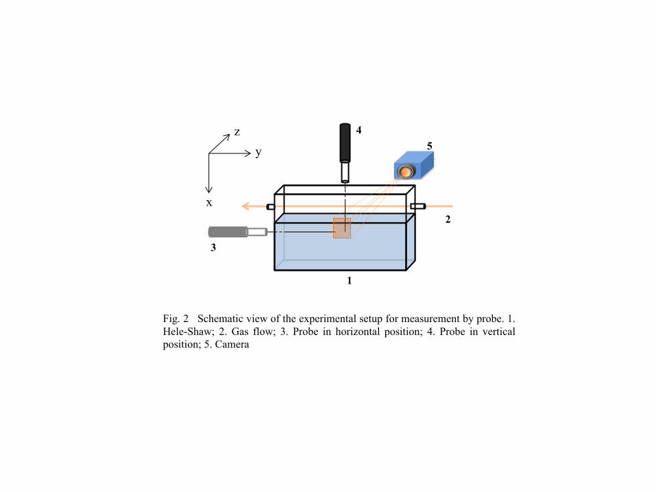
dissolved oxygen from the interface. The experimental setup is described in Fig. 2. It was composed of 229

a transparent Hele-Shaw cell and an optical system. The Hele-Shaw cell [1] was 12 cm high, 5 cm wide 230

and 0.2 cm thick. The cell sides were made of polymethyl methacrylate (PMMA) with two gas orifices 231

placed 1 cm below the top of the cell to allow the gas to flow [2]. 232

233

11

Fig. 2 Schematic view of the experimental setup for measurement by probe. 1. Hele-Shaw; 2. Gas flow; 3. 234

Probe in horizontal position; 4. Probe in vertical position; 5. Camera 235

236

237

This technique was tested experimentally for different probe locations. In fact, two types of cells of that 238

size were tested. The main difference between these two cells was the location of the additional openings 239

providing access to probes. The first cell had lateral openings allowing horizontal positioning of the 240

oxygen probe [3]. The second was designed with an opening on the upper part of the cell to position the 241

probe vertically [4]. As the measurement should be implemented far away from the cell edges to avoid 242

any renewal of the liquid at the interface, a type of specific oxygen sensor has been used. This kind of 243

probe has a metal reinforcement of constant cross section at its extremity (OX100 Needle Sensor 244

0.80×40 mm, Unisense). This reinforcement not only consolidates the probe but also makes it possible 245

to perform far away from the edges. Deoxygenated liquid (deionized water, 10 mL) was then inserted 246

smoothly into the cell to obtain a flat interface. A low flow rate of nitrogen (about 10L·h-1) which was 247

controlled by a rotameter, flowed over the liquid. The gas flow was switched from the nitrogen to the 248

air at the moment𝑡 = 0. The sensor recorded every second the level of dissolved oxygen concentrations 249

in the liquid. The distance between the probe tip and the gas-liquid interface was determined through a 250

camera [5] (with lens GuppyPro 105 mm). The experimental temperature was controlled at 20°C. 251

2.2.2 Determination of the diffusion coefficient 252

The configuration of the Hele-Shaw cell could be supposed as a two-dimensional (x-y) problem 253

(negligibility of the contribution along the z-axis) and an oxygen concentration gradient is imposed only 254

in the x-direction. If no convection is present along the x-axis, the equation of mass transfer in the Hele-255

Shaw cell can be deduced from Fick's law (Eq. (1)): 256

𝜕[𝑂%]𝜕𝑡

= 𝐷𝜕%[𝑂%]𝜕𝑥%

257

12

where [𝑂%] the oxygen concentration (kg·m-3), 𝑡 the time since the start of the transfer (s) and 𝐷 the 258

oxygen diffusivity in the liquid medium (m2·s-1). In our study, x represents the distance between the 259

probe tip and the gas-liquid interface (m). The gas flow rate being imposed along the y-axis and by 260

continuity in the liquid phase, it can be assumed that no convection is present along the x-axis far away 261

from the cell walls. 262

The duration of the experiments is relatively short (always less than 30 minutes) compared to the 263

duration of the diffusive phenomena. Thus a semi-infinite solution can be considered. 264

[𝑂%](𝑥, 𝑡) − [𝑂%]"[𝑂%]# − [𝑂%]"

= 1 − 𝑒𝑟𝑓(𝑥

2√𝐷𝑡) 265

where [𝑂%]" and [𝑂%]# are the concentrations of dissolved oxygen in a deoxygenated zone and in 266

saturation respectively (kg·m-3) and erf the error function defined as follows (Abramowitz and Stegun, 267

1964): 268

𝑒𝑟𝑓(𝑧) =2√𝜋

= exp(−𝑢%)𝑑𝑢6

" 269

Indeed, Eq. (20) connects ∂%[𝑂%]/ ∂𝑥% to ∂[𝑂%]/ ∂𝑡. Since a simple relation has been established to 270

connect ∂%[O]%/ ∂𝑥% to the diffusion coefficient (Jimenez et al., 2012b), the similar reasoning can be 271

conducted with ∂[𝑂%]/ ∂𝑡. 272

Substituting Eq.(22) in Eq. (21), the relation between ∂[𝑂%]/ ∂𝑡 and D is established: 273

∂[𝑂%]∂𝑡

= ([𝑂%]# − [𝑂%]")𝑥

2√𝜋𝐷1𝑡7/%

exp(−𝑥%

4𝐷𝑡) 274

Replace with 𝛼 = 1/2 and 𝛽 = 𝑥%/(4𝐷), the equation becomes: 275

∂[𝑂%]∂𝑡

=([𝑂%]# − [𝑂%]")

√𝜋𝛽8

1𝑡89/

exp(−𝛽𝑡) 276

In the other hand, according to the probability and statistics theory, the inverse gamma distribution's 277

probability density function is defined over the support 𝑤 > 0with defined parameters α and β 278

(Abramowitz and Stegun, 1964): 279

13

𝑓(𝑤) =𝛽8

𝛤(𝛼)1

𝑤89/ exp(−𝛽𝑤) 280

It is known that the mode of this function f(w) is located in: 281

𝑤 =𝛽

𝛼 + 1 282

From Eq. (24) and (25), it can be deduced that ∂[𝑂%]/ ∂𝑡 is proportional to 𝑓(𝑤) of the inverse gamma 283

distribution law. Their modes are thus located in the same coordinate. The moment 𝑡:;3 maximizing 284

∂[𝑂%]/ ∂𝑡 is defined by: 285

𝑡:;3 =𝛽

𝛼 + 1=

𝑥%

4𝐷(1/2 + 1)=

𝑥%

6𝐷 286

The distance x in this case corresponds to the distance between the tip of the probe and the gas-liquid 287

interface. The value of x is measured by the camera and the oxygen concentration profile [𝑂%(𝑥, 𝑡)] can 288

be measured simply by an oxygen probe. By investigating the derivative of the concentration profile 289

[𝑂%(𝑥, 𝑡)] with respect to t, the location 𝑡:;3 can be determined. Then based on Eq. (27), the diffusion 290

coefficient can be obtained without additional information on the liquid. It should be noted that for a 291

Clark type probe, the signal delivered (typically in mV or mg·L-1) is directly proportional to the oxygen 292

concentration. This proportionality allows obtaining 𝑡:;3 the moment when the signal of the probe 293

becomes maximum. It means that no calibration of the probes is required to measure the diffusion 294

coefficient. 295

296

3. Result and discussion 297

3.1 Result of PLIFI in the bubble column 298

Image processing and mass transfer quantification are realized for each spot recorded every 1/10s by the 299

CCD Camera after the bubble passing. A typical example of corrected images is given in Fig. 3 for the 300

bubble of equivalent bubble diameter 𝑑!" = 0.09𝑚𝑚. 301

14

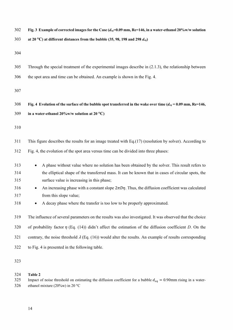
Fig. 3 Example of corrected images for the Case (deq=0.09 mm, Re=146, in a water-ethanol 20%w/w solution 302

at 20 °C) at different distances from the bubble (35, 98, 198 and 298 deq) 303

304

Through the special treatment of the experimental images describe in (2.1.3), the relationship between 305

the spot area and time can be obtained. An example is shown in the Fig. 4. 306

307

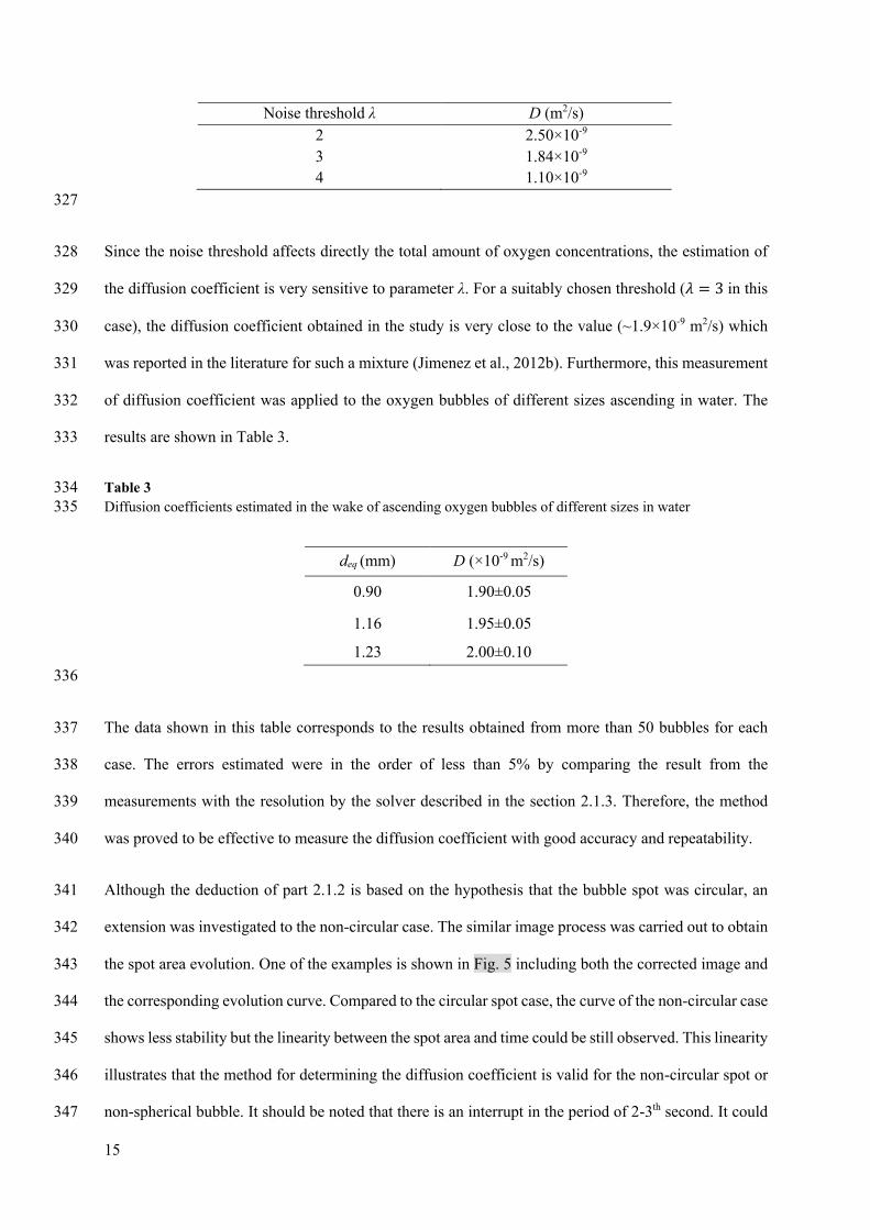
Fig. 4 Evolution of the surface of the bubble spot transferred in the wake over time (deq = 0.09 mm, Re=146, 308

in a water-ethanol 20%w/w solution at 20 °C) 309

310

This figure describes the results for an image treated with Eq.(17) (resolution by solver). According to 311

Fig. 4, the evolution of the spot area versus time can be divided into three phases: 312

• A phase without value where no solution has been obtained by the solver. This result refers to 313

the elliptical shape of the transferred mass. It can be known that in cases of circular spots, the 314

surface value is increasing in this phase; 315

• An increasing phase with a constant slope 2𝜋𝐷𝜂. Thus, the diffusion coefficient was calculated 316

from this slope value; 317

• A decay phase where the transfer is too low to be properly approximated. 318

The influence of several parameters on the results was also investigated. It was observed that the choice 319

of probability factor 𝜂 (Eq. (14)) didn’t affect the estimation of the diffusion coefficient D. On the 320

contrary, the noise threshold λ (Eq. (16)) would alter the results. An example of results corresponding 321

to Fig. 4 is presented in the following table. 322

323

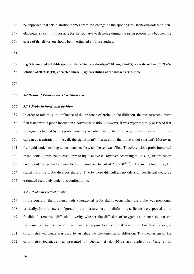
Table 2 324 Impact of noise threshold on estimating the diffusion coefficient for a bubble 𝑑!" = 0.90mm rising in a water-325 ethanol mixture (20%w) in 20 °C 326

15

Noise threshold λ D (m2/s) 2 2.50×10-9

3 1.84×10-9 4 1.10×10-9

327

Since the noise threshold affects directly the total amount of oxygen concentrations, the estimation of 328

the diffusion coefficient is very sensitive to parameter λ. For a suitably chosen threshold (𝜆 = 3 in this 329

case), the diffusion coefficient obtained in the study is very close to the value (~1.9×10-9 m2/s) which 330

was reported in the literature for such a mixture (Jimenez et al., 2012b). Furthermore, this measurement 331

of diffusion coefficient was applied to the oxygen bubbles of different sizes ascending in water. The 332

results are shown in Table 3. 333

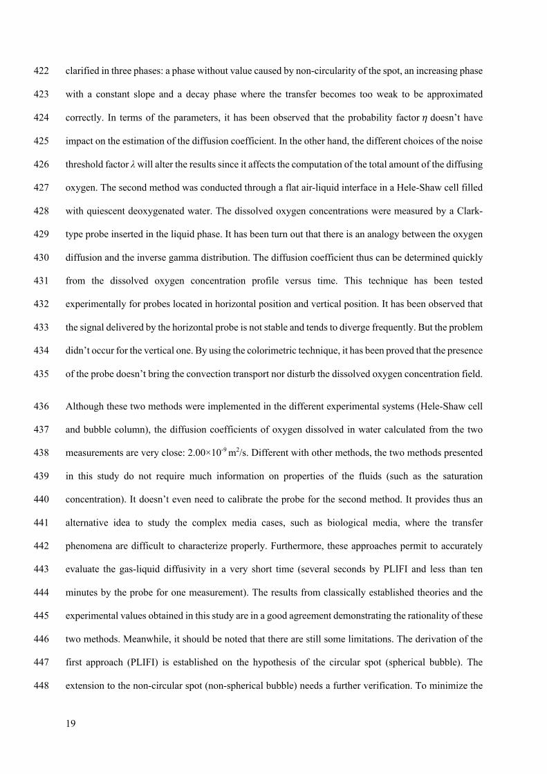
Table 3 334 Diffusion coefficients estimated in the wake of ascending oxygen bubbles of different sizes in water 335

deq (mm) D (×10-9 m2/s)

0.90 1.90±0.05

1.16 1.95±0.05

1.23 2.00±0.10 336

The data shown in this table corresponds to the results obtained from more than 50 bubbles for each 337

case. The errors estimated were in the order of less than 5% by comparing the result from the 338

measurements with the resolution by the solver described in the section 2.1.3. Therefore, the method 339

was proved to be effective to measure the diffusion coefficient with good accuracy and repeatability. 340

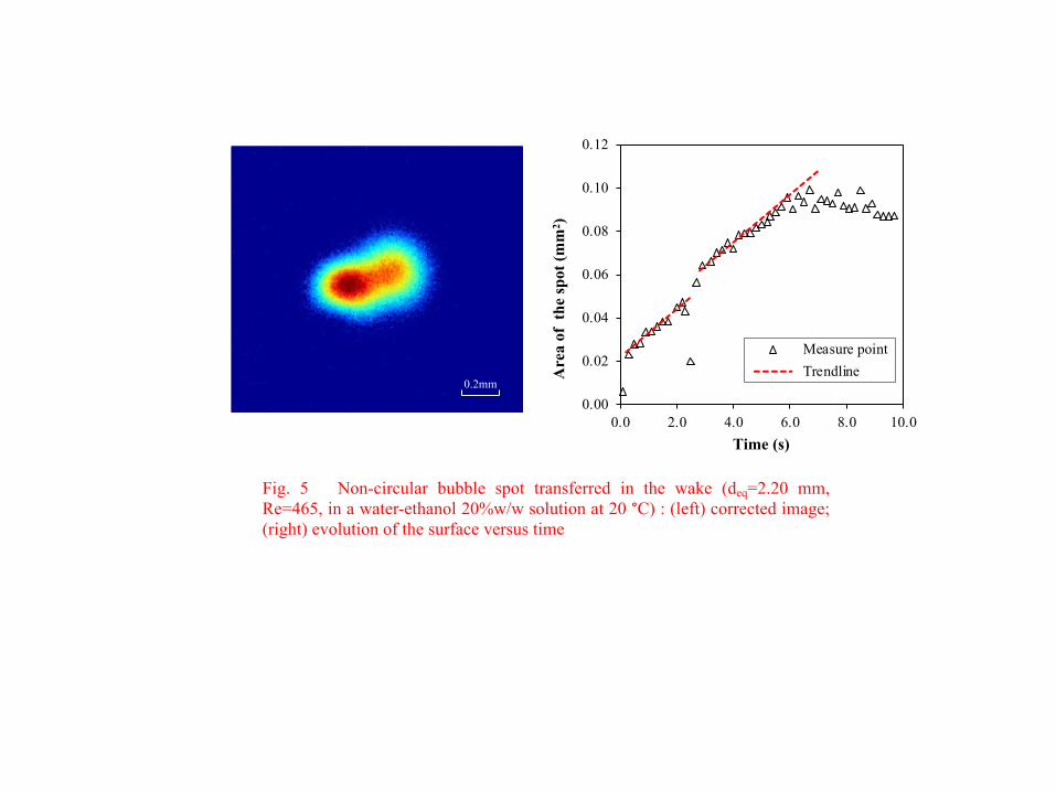
Although the deduction of part 2.1.2 is based on the hypothesis that the bubble spot was circular, an 341

extension was investigated to the non-circular case. The similar image process was carried out to obtain 342

the spot area evolution. One of the examples is shown in Fig. 5 including both the corrected image and 343

the corresponding evolution curve. Compared to the circular spot case, the curve of the non-circular case 344

shows less stability but the linearity between the spot area and time could be still observed. This linearity 345

illustrates that the method for determining the diffusion coefficient is valid for the non-circular spot or 346

non-spherical bubble. It should be noted that there is an interrupt in the period of 2-3th second. It could 347

16

be supposed that this distortion comes from the change of the spot shapes: from ellipsoidal to non-348

ellipsoidal since it is impossible for the spot area to decrease during the rising process of a bubble. The 349

cause of this distortion should be investigated in future studies. 350

351

Fig. 5 Non-circular bubble spot transferred in the wake (deq=2.20 mm, Re=465, in a water-ethanol 20%w/w 352

solution at 20 °C): (left) corrected image; (right) evolution of the surface versus time 353

354

3.2 Result of Probe in the Hele-Shaw cell 355

3.2.1 Probe in horizontal position 356

In order to minimize the influence of the presence of probe on the diffusion, the measurements were 357

first tested with a probe inserted in a horizontal position. However, it was experimentally observed that 358

the signal delivered by this probe was very sensitive and tended to diverge frequently (for a uniform 359

oxygen concentration in the cell, the signal in mV measured by the probe is not constant). Moreover, 360

the liquid tended to cling to the metal needle when the cell was filled. Therefore with a probe immersed 361

in the liquid, it must be at least 3 mm of liquid above it. However, according to Eq. (27), the inflection 362

point would range t = 12.5 min for a diffusion coefficient of 2.00×10-9 m2/s. For such a long time, the 363

signal from the probe diverges sharply. Due to these difficulties, no diffusion coefficient could be 364

estimated accurately under this configuration. 365

3.2.2 Probe in vertical position 366

In the contrary, the problems with a horizontal probe didn’t occur when the probe was positioned 367

vertically. In this new configuration, the measurements of diffusion coefficient were proved to be 368

feasible. It remained difficult to verify whether the diffusion of oxygen was planar so that the 369

mathematical approach is still valid in the proposed experimental conditions. For this purpose, a 370

colorimetric technique was used to visualize the phenomenon of diffusion. The mechanism of the 371

colorimetric technique was presented by Dietrich et al. (2013) and applied by Yang et al. 372

17

(2016a&2016b). In this study, resazurin was selected as the colorimetric indicator as its color can range 373

from colorless (without oxygen) to pink (when oxygen was present). This coloration can be visualized 374

and recorded using the camera. 375

An example of the recorded images is given in Fig. 6. It was shown that there is no evident convection 376

transport along the x-direction. Thus the influence of the vertical probe on the oxygen diffusion can be 377

neglected. However, this conclusion is only valid when the probe locates very close to the interface 378

(about 1 mm between the tip of the probe and the interface). For a longer distance (over 3 mm), the 379

presence of the probe will cause the perturbation of the diffusion. 380

381

Fig. 6 Visualization of the diffusion of oxygen by colorimetry with a probe inserted vertically close to the 382

interface (1.95mm, in a water solution consisting of 0.015 g/L resazurin, 20g/L glucose and 10g/L NaOH) 383

384

385

In our experiment, the probe was placed at 1.95 mm below the interface so that the non-convection 386

property is assuredly reasonable. The measurement of the diffusion coefficient of oxygen in water can 387

be conducted. The dissolved oxygen concentration profile as a function of time is depicted in Fig. 7. 388

This experimental profile was compared with an analytical profile (see Eq. (21)Erreur ! Source du 389

renvoi introuvable. with 𝐷 = 2 × 10'<m%/s, [𝑂%]# = 9mg/Land𝑥 = 1.95 × 10'7m). At the first 390

minutes (t ≤2 minutes on Fig. 7), the oxygen concentration presented as a constant since the air flow 391

didn’t arrive at the position of probe. After the probe detected the oxygen diffusion (2< t ≤8 minutes 392

on Fig 7), the trends of these two profiles were similar, with a slight discrepancy. This discrepancy can 393

be explained by experimental error on the initial time of the experiment (t = 0). As mentioned before, 394

for longer time (t > 8 min on Fig. 7), the profiles diverged. Several hypotheses can be put forward to 395

explain this phenomenon: sensitivity of the oxygen probe, perturbation of the diffusion of oxygen, etc. 396

However, the inflection point for estimating the diffusion coefficient is generally detected before this 397

18

divergence as shown in Fig. 8. The profile of the derivative ∂[O%]/ ∂t was obtained through a 6-order 398

polynomial regression of the concentration profiles. The moments 𝑡:;3 which maximize the derivative 399

∂[O%]/ ∂t were almost identical for the experimental and analytical profiles (𝑡:;3 = 5:25 min and 5:17 400

min, respectively). The value 𝑡:;3 led to the diffusion coefficients of 2×10-9 m2/s, which is consistent 401

with the literature (Roustan, 2003). 402

403

Fig. 7 Comparison of experimental and analytical concentration profiles 404

405

Fig. 8 Evolution of the derivative of dissolved oxygen concentration in water 𝝏[𝑶𝟐]/𝝏𝒕 with respect to time 406

(the maximum positions are indicated by vertical dotted lines) 407

408

409

Although the result above seems promising, it should be noted that the error of the result is more 410

significant (around 15%) than that from a measure of PLIF (around 5%). For reducing the error, it would 411

be wise to place two probes at slightly different depths in the liquid and determine the diffusion 412

coefficient by comparing the time 𝑡:;3 of the two probes. These perspective works can be implemented 413

in the future for extending and improving the technique. 414

4. Conclusion 415

In this paper, two effective mathematical approaches based on the probability and statistics theory have 416

been proposed to determine the oxygen diffusion coefficients in water. The first was to apply the 417

technique PLIFI (Planar Laser Induced Fluorescence with Inhibition) to quantify the mass transfer in 418

the wake of an isolated bubble (deq= 0.9-1.26 mm) rising in the column. The chi-squared distribution 419

was introduced to describe the diffusing oxygen concentration field, which was shown as the bubble 420

spot on the experimental images. As a result, the evolution of the spot area as a function of time can be 421

19

clarified in three phases: a phase without value caused by non-circularity of the spot, an increasing phase 422

with a constant slope and a decay phase where the transfer becomes too weak to be approximated 423

correctly. In terms of the parameters, it has been observed that the probability factor 𝜂 doesn’t have 424

impact on the estimation of the diffusion coefficient. In the other hand, the different choices of the noise 425

threshold factor λ will alter the results since it affects the computation of the total amount of the diffusing 426

oxygen. The second method was conducted through a flat air-liquid interface in a Hele-Shaw cell filled 427

with quiescent deoxygenated water. The dissolved oxygen concentrations were measured by a Clark-428

type probe inserted in the liquid phase. It has been turn out that there is an analogy between the oxygen 429

diffusion and the inverse gamma distribution. The diffusion coefficient thus can be determined quickly 430

from the dissolved oxygen concentration profile versus time. This technique has been tested 431

experimentally for probes located in horizontal position and vertical position. It has been observed that 432

the signal delivered by the horizontal probe is not stable and tends to diverge frequently. But the problem 433

didn’t occur for the vertical one. By using the colorimetric technique, it has been proved that the presence 434

of the probe doesn’t bring the convection transport nor disturb the dissolved oxygen concentration field. 435

Although these two methods were implemented in the different experimental systems (Hele-Shaw cell 436

and bubble column), the diffusion coefficients of oxygen dissolved in water calculated from the two 437

measurements are very close: 2.00×10-9 m2/s. Different with other methods, the two methods presented 438

in this study do not require much information on properties of the fluids (such as the saturation 439

concentration). It doesn’t even need to calibrate the probe for the second method. It provides thus an 440

alternative idea to study the complex media cases, such as biological media, where the transfer 441

phenomena are difficult to characterize properly. Furthermore, these approaches permit to accurately 442

evaluate the gas-liquid diffusivity in a very short time (several seconds by PLIFI and less than ten 443

minutes by the probe for one measurement). The results from classically established theories and the 444

experimental values obtained in this study are in a good agreement demonstrating the rationality of these 445

two methods. Meanwhile, it should be noted that there are still some limitations. The derivation of the 446

first approach (PLIFI) is established on the hypothesis of the circular spot (spherical bubble). The 447

extension to the non-circular spot (non-spherical bubble) needs a further verification. To minimize the 448

20

uncertainty of the result by the probe, a new configuration of two probes positioned at different depths 449

in the liquid should be tested. Further research will be implemented for investigating these problems and 450

making these techniques more powerful for diffusion characterization. 451

452

Nomenclature 453

Latin symbols

𝐶 Concentration (kg/m3)

𝐷 Diffusion coefficient (m2/s)

𝑑=> Equivalent bubble diameter (m)

𝐼" Fluorescence intensity without quencher, gray level

𝐼! Fluorescence intensity with quencher, gray level

𝐽 Diffusive flux (kg/m2.s)

𝑘 Freedom degrees

𝐾 Stern-Volmer constant (m3/kg)

𝑀 Quantity of mass per unit area (kg/m2)

[𝑂%] Oxygen concentration (kg/m3)

𝑃 Probability

[𝑄] Quencher concentration (kg/m3)

𝑅 Radius of the image spot (m)

𝑟 Radius (m)

𝑅𝑒 Reynolds number

𝑆 Surface of the spot in the image (m2)

𝑡 Time (s)

𝑥 Abscissa (m)

𝑦 Ordinate (m)

21

Greek symbols

𝛤 Gamma function

𝜆 Threshold factor

𝛿 Length of a pixel on the recorded image (m)

𝜎 Standard deviation

𝜏 Lifetime of the fluorescence molecule with inhibition (s)

𝜏" Lifetime of the fluorescence molecule without inhibition (s)

454

Figure List 455

Fig. 1 Schematic view of the experimental setup for PLIFI measurements

Fig. 2 Schematic view of the experimental setup for measurement by probe in Hele-Shaw

cell

Fig. 3 Example of corrected images for the Case (deq=0.09 mm, Re=146, in a water-

ethanol 20%w/w solution at 20 °C) at different distances from the bubble

Fig. 4 Evolution of the area of the bubble spot transferred in the wake over time (deq=0.09

mm, Re=146, in a water-ethanol 20%w/w solution at 20 °C)

Fig. 5 Non-circular bubble spot transferred in the wake (deq=2.20 mm, Re=465, in a

water-ethanol 20%w/w solution at 20 °C) : (left) corrected image; (right) evolution

of the surface versus time

Fig. 6 Visualization of the diffusion of oxygen by colorimetry with a probe inserted

vertically close to the interface (1.95mm, in a water solution consisting of 0.015 g/L

resazurin, 20g/L glucose and 10g/L NaOH)

Fig. 7 Comparison of experimental and analytical concentration profiles

Fig. 8 Evolution of the derivative of dissolved oxygen concentration in water 𝜕[𝑂%]/𝜕𝑡

with respect to time (the maximum positions are indicated by vertical dotted lines)

456

22

457

Reference 458

Abramowitz, M., and Stegun, I. (1964). Handbook of Mathematical Functions: With Formulars, Graphs, 459 and Mathematical Tables. Appl. Math. Ser. 460

Asher, W.E. (2009). The effects of experimental uncertainty in parameterizing air-sea gas exchange 461 using tracer experiment data. Atmos Chem Phys 9, 131–139. 462

Baldauf, W., and Knapp, H. (1983). Measurements of diffusivities in liquids by the dispersion method. 463 Chem. Eng. Sci. 38, 1031–1037. 464

Blackadder, D.A., and Keniry, J.S. (1973). Difficulties associated with the measurement of the diffusion 465 coefficient of solvating liquid or vapor in semicrystalline polymer. I. Permeation methods. J. Appl. 466 Polym. Sci. 17, 351–363. 467

Blackadder, D.A., and Keniry, J.S. (1974). Difficulties associated with the measurement of the diffusion 468 coefficient of solvating liquid or vapor in semicrystalline polymer. II. Sorption–desorption kinetics. J. 469 Appl. Polym. Sci. 18, 699–708. 470

de Blok, W.J., and Fortuin, J.M.H. (1981). Method for determining diffusion coefficients of slightly 471 soluble gases in liquids. Chem. Eng. Sci. 36, 1687–1694. 472

Bork, O., Schlueter, M., and Raebiger, N. (2005). The Impact of Local Phenomena on Mass Transfer in 473 Gas-Liquid Systems. Can. J. Chem. Eng. 83, 658–666. 474

Bouche, E., Cazin, S., Roig, V., and Risso, F. (2013). Mixing in a swarm of bubbles rising in a confined 475 cell measured by mean of PLIF with two different dyes. Exp. Fluids 54, 1–9. 476

Bowyer, W.J., Xu, W., and Demas, J.N. (2004). Determining oxygen diffusion coefficients in polymer 477 films by lifetimes of luminescent complexes measured in the frequency domain. Anal. Chem. 76, 4374–478 4378. 479

Crank, J. (1979). The Mathematics of Diffusion (Clarendon Press). 480

Dani, A., Guiraud, P., and Cockx, A. (2007). Local measurement of oxygen transfer around a single 481 bubble by planar laser-induced fluorescence. Chem. Eng. Sci. 62, 7245–7252. 482

Dietrich, N., Loubière, K., Jimenez, M., Hébrard, G., and Gourdon, C. (2013). A new direct technique 483 for visualizing and measuring gas–liquid mass transfer around bubbles moving in a straight millimetric 484 square channel. Chem. Eng. Sci. 100, 172–182. 485

Dietrich, N., Francois, J., Jimenez, M., Cockx, A., Guiraud, P., and Hébrard, G. (2015). Fast 486 Measurements of the Gas-Liquid Diffusion Coefficient in the Gaussian Wake of a Spherical Bubble. 487 Chem. Eng. Technol. 38, 941–946. 488

Duda, J.L., and Vrentas, J.S. (1968). Laminar liquid jet diffusion studies. AIChE J. 14, 286–294. 489

Ferrell, R.T., and Himmelblau, D.M. (1967). Diffusion coefficients of hydrogen and helium in water. 490 AIChE J. 13, 702–708. 491

Fick, A. (1855). Ueber diffusion. Ann. Phys. 170, 59–86. 492

23

Francois, J., Dietrich, N., Guiraud, P., and Cockx, A. (2011). Direct measurement of mass transfer 493 around a single bubble by micro-PLIFI. Chem. Eng. Sci. 66, 3328–3338. 494

Gubbins, K.E., Bhatia, K.K., and Walker, R.D. (1966). Diffusion of gases in electrolytic solutions. 495 AIChE J. 12, 548–552. 496

Guo, Z., Maruyama, S., and Komiya, A. (1999). Rapid yet accurate measurement of mass diffusion 497 coefficients by phase shifting interferometer. J. Phys. Appl. Phys. 32, 995. 498

Hebrard, G., Zeng, J., and Loubiere, K. (2009). Effect of surfactants on liquid side mass transfer 499 coefficients: A new insight. Chem. Eng. J. 148, 132–138. 500

Ho, C.S., Ju, L.-K., and Ho, C.-T. (1986). Measuring oxygen diffusion coefficients with polarographic 501 oxygen electrodes. II. Fermentation Media. Biotechnol. Bioeng. 28, 1086–1092. 502

Jamnongwong, M., Loubiere, K., Dietrich, N., and Hébrard, G. (2010). Experimental study of oxygen 503 diffusion coefficients in clean water containing salt, glucose or surfactant: Consequences on the liquid-504 side mass transfer coefficients. Chem. Eng. J. 165, 758–768. 505

Jimenez, M., Dietrich, N., and Hebrard, G. (2012a). A New Method for Measuring Diffusion Coefficient 506 of Gases in Liquids by Plif. Mod. Phys. Lett. B 26, 1150034. 507

Jimenez, M., Dietrich, N., Cockx, A., and Hébrard, and G. (2012b). Experimental study of O2 diffusion 508 coefficient measurement at a planar gas–liquid interface by planar laser-induced fluorescence with 509 inhibition. AIChE J. 59, 325–333. 510

Jimenez, M., Dietrich, N., and Hébrard, G. (2013). Mass transfer in the wake of non-spherical air 511 bubbles quantified by quenching of fluorescence. Chem. Eng. Sci. 100, 160–171. 512

Ju, L.-K., and Ho, C.S. (1985). Measuring oxygen diffusion coefficients with polarographic oxygen 513 electrodes: I. Electrolyte solutions. Biotechnol. Bioeng. 27, 1495–1499. 514

Kück, U.D., Schlüter, M., and Räbiger, N. (2010). Investigation on Reactive Mass Transfer at Freely 515 Rising Gas Bubbles. 516

Kück, U.D., Schlüter, M., and Räbiger, N. (2012). Local Measurement of Mass Transfer Rate of a Single 517 Bubble with and without a Chemical Reaction. J. Chem. Eng. Jpn. 45, 708–712. 518

Lakowicz, J.R. (1999). Advanced Topics in Fluorescence Quenching. In Principles of Fluorescence 519 Spectroscopy, (Springer US), pp. 267–289. 520

Malik, V.K., and Hayduk, W. (1968). A steady’state capillary cell method for measuring gas-liquid 521 diffusion coefficients. Can. J. Chem. Eng. 46, 462–466. 522

Revsbech, N.P. (1989). An oxygen microsensor with a guard cathode. Limnol. Oceanogr. 34, 474–478. 523

Roetzel, W., Blömker, D., and Czarnetzki, W. (1997). Messung binärer Diffusionskoeffizienten von 524 Gasen in Wasser mit Hilfe der holographischen Interferometrie. Chem. Ing. Tech. 69, 674–678. 525

Roustan, M. (2003). Transferts gaz-liquide dans les procédés de traitement des eaux et des effluents 526 gazeux. Libr. Lavoisier. 527

Sancho, I., Varela, S., Vernet, A., and Pallares, J. (2016). Characterization of the reacting laminar flow 528 in a cylindrical cavity with a rotating endwall using numerical simulations and a combined PIV/PLIF 529 technique. Int. J. Heat Mass Transf. 93, 155–166. 530

24

Sovová, H., and Procházka, J. (1976). A new method of measurement of diffusivities of gases in liquids. 531 Chem. Eng. Sci. 31, 1091–1097. 532

Stamatopoulos, K., Batchelor, H.K., Alberini, F., Ramsay, J., and Simmons, M.J.H. (2015). 533 Understanding the impact of media viscosity on dissolution of a highly water soluble drug within a USP 534 2 mini vessel dissolution apparatus using an optical planar induced fluorescence (PLIF) method. Int. J. 535 Pharm. 495, 362–373. 536

Stern, O., and Volmer, M. (1919). On the quenching time of fluorescence. Phys. Z 20, 183–188. 537

Tham, M.J., Bhatia, K.K., and Gubbins, K.F. (1967). Steady-state method for studying diffusion of gases 538 in liquids. Chem. Eng. Sci. 22, 309–311. 539

Wise, D.L., and Houghton, G. (1966). The diffusion coefficients of ten slightly soluble gasses in water 540 at 10–60°C. Chem. Eng. Sci. 21, 999–1010. 541

Wylock, C., Dehaeck, S., Cartage, T., Colinet, P., and Haut, B. (2011). Experimental study of gas–liquid 542 mass transfer coupled with chemical reactions by digital holographic interferometry. Chem. Eng. Sci. 543 66, 3400–3412. 544

Yang, L., Dietrich, N., Hébrard, G., Loubière, K., Gourdon, C., 2016a. Optical methods to investigate 545 the enhancement factor of an oxygen-sensitive colorimetric reaction using microreactors. AIChE J. 546 doi:10.1002/aic.15547 547

Yang, L., Dietrich, N., Loubière, K., Gourdon, C., Hébrard, G., 2016b. Visualization and 548 characterization of gas–liquid mass transfer around a Taylor bubble right after the formation stage in 549 microreactors. Chemical Engineering Science 143, 364–368. doi:10.1016/j.ces.2016.01.013 550

1

4

5

6

2

3

Fig. 1 Schematic view of the experimental setup for PLIFI measurements. 1.Column; 2. Gas injection system; 3. Rising bubble; 4. CCD Camera; 5. Nd:Yag laser; 6. High-speed camera

yx

z

z

x

y

1

2

3

45

Fig. 2 Schematic view of the experimental setup for measurement by probe. 1.Hele-Shaw; 2. Gas flow; 3. Probe in horizontal position; 4. Probe in verticalposition; 5. Camera

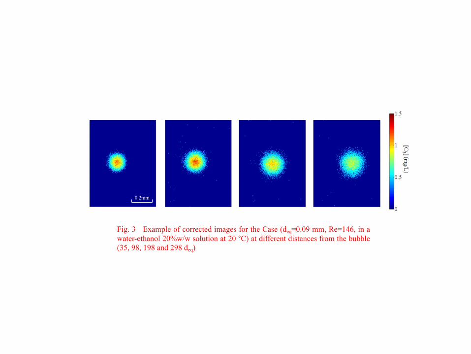
Fig. 3 Example of corrected images for the Case (deq=0.09 mm, Re=146, in awater-ethanol 20%w/w solution at 20 °C) at different distances from the bubble(35, 98, 198 and 298 deq)

0.2mm

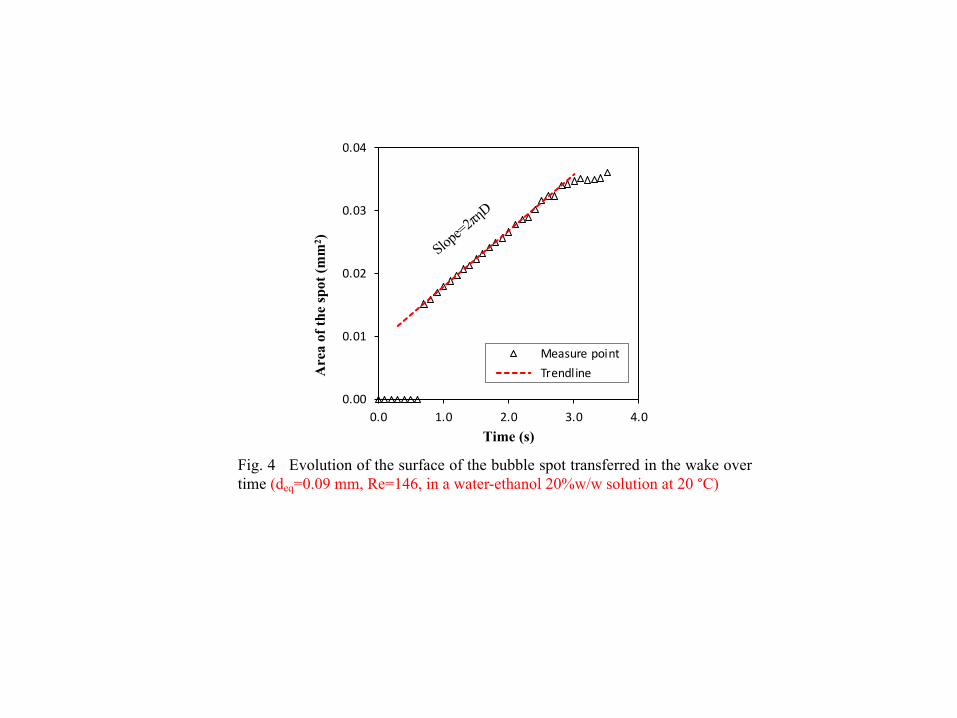
Fig. 4 Evolution of the surface of the bubble spot transferred in the wake overtime (deq=0.09 mm, Re=146, in a water-ethanol 20%w/w solution at 20 °C)

0.00

0.01

0.02

0.03

0.04

0.0 1.0 2.0 3.0 4.0

Are

a of

the

spot

(mm2 )

Time (s)

Measure point Trendline

Slope=2πηD

0.00

0.02

0.04

0.06

0.08

0.10

0.12

0.0 2.0 4.0 6.0 8.0 10.0

Are

a of

the

spot

(mm2 )

Time (s)

Measure point Trendline

Fig. 5 Non-circular bubble spot transferred in the wake (deq=2.20 mm,Re=465, in a water-ethanol 20%w/w solution at 20 °C) : (left) corrected image;(right) evolution of the surface versus time

0.2mm

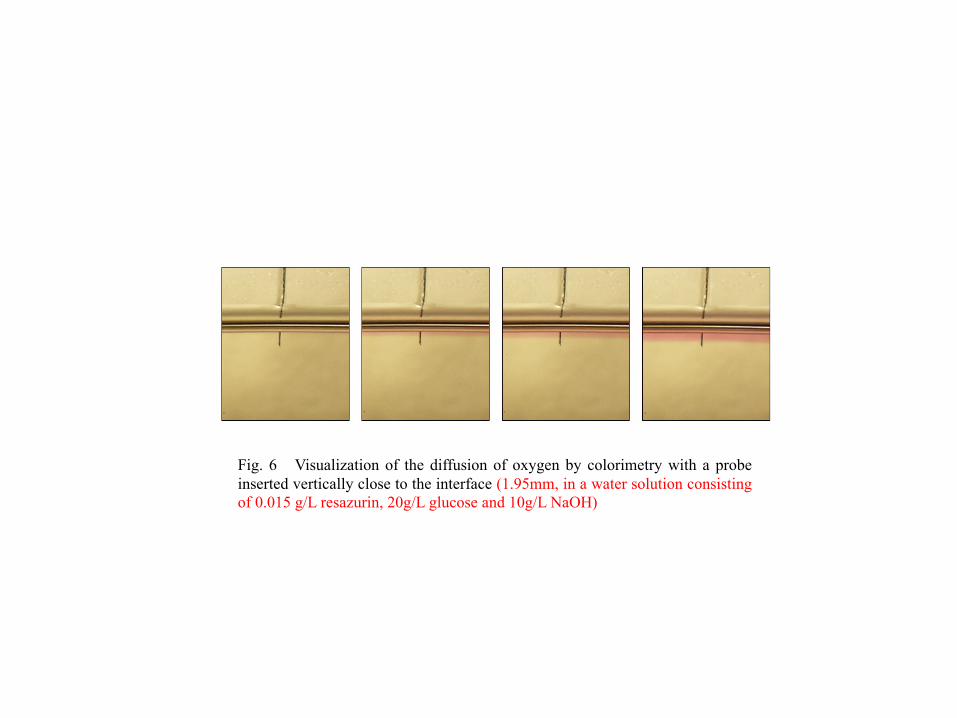
Fig. 6 Visualization of the diffusion of oxygen by colorimetry with a probeinserted vertically close to the interface (1.95mm, in a water solution consistingof 0.015 g/L resazurin, 20g/L glucose and 10g/L NaOH)

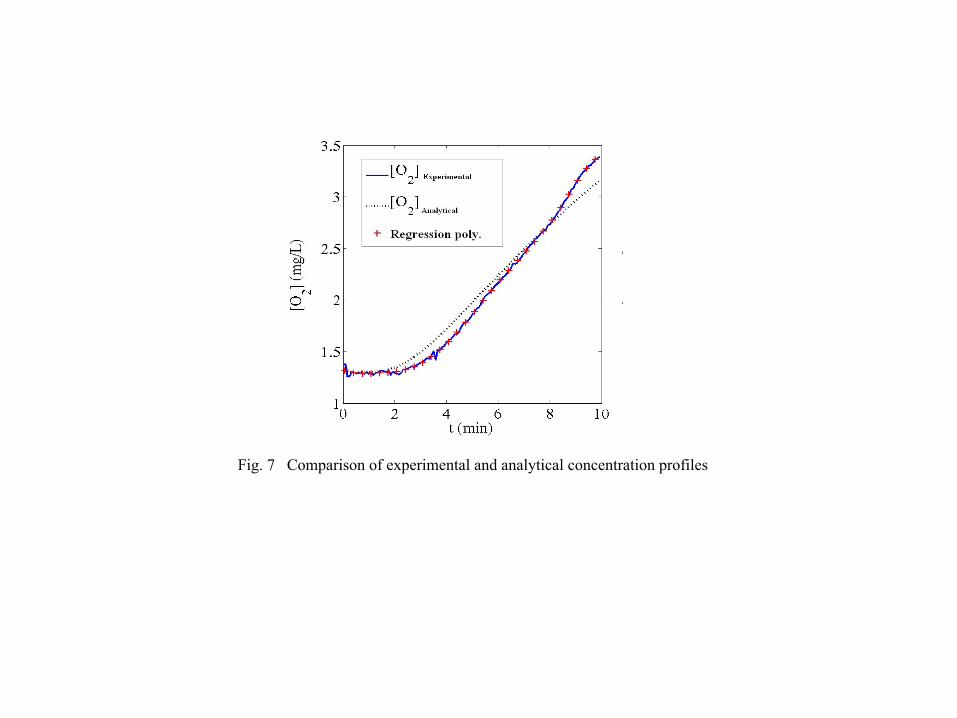
Fig. 7 Comparison of experimental and analytical concentration profiles

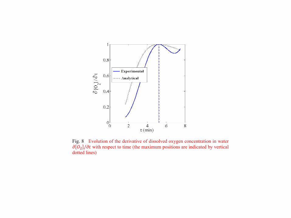
Fig. 8 Evolution of the derivative of dissolved oxygen concentration in water𝜕 𝑂! /𝜕𝑡 with respect to time (the maximum positions are indicated by verticaldotted lines)