Fast Algorithms for Segmented Regression

Jayadev AcharyaMIT

jayadev@csail.mit.edu

Ilias DiakonikolasUniversity of Southern California

ilias.d@ed.ac.uk

Jerry LiMIT

jerryzli@csail.mit.edu

Ludwig SchmidtMIT

ludwigs@mit.edu

July 15, 2016

Abstract

We study the fixed design segmented regression problem: Given noisy samples from a piece-wise linear function f , we want to recover f up to a desired accuracy in mean-squared error.

Previous rigorous approaches for this problem rely on dynamic programming (DP) and, whilesample efficient, have running time quadratic in the sample size. As our main contribution, weprovide new sample near-linear time algorithms for the problem that – while not being minimaxoptimal – achieve a significantly better sample-time tradeoff on large datasets compared to theDP approach. Our experimental evaluation shows that, compared with the DP approach, ouralgorithms provide a convergence rate that is only off by a factor of 2 to 4, while achievingspeedups of three orders of magnitude.

arX

iv:1

607.

0399

0v1

[cs

.LG

] 1

4 Ju

l 201

6

1 Introduction

We study the regression problem – a fundamental inference task with numerous applications thathas received tremendous attention in machine learning and statistics during the past fifty years (see,e.g., [MT77] for a classical textbook). Roughly speaking, in a (fixed design) regression problem,we are given a set of n observations (xi, yi), where the yi’s are the dependent variables and the xi’sare the independent variables, and our goal is to model the relationship between them. The typicalassumptions are that (i) there exists a simple function f that (approximately) models the underlyingrelation, and (ii) the dependent observations are corrupted by random noise. More specifically, weassume that there exists a family of functions F such that for some f ∈ F the following holds:yi = f(xi) + εi, where the εi’s are i.i.d. random variables drawn from a “tame” distribution such asa Gaussian (later, we also consider model misspecification).

Throughout this paper, we consider the classical notion of Mean Squared Error (MSE) to measurethe performance (risk) of an estimator. As expected, the minimax risk depends on the family F thatf comes from. The natural case that f is linear is fully understood: It is well-known that the least-squares estimator is statistically efficient and runs in sample-linear time. The more general case thatf is non-linear, but satisfies some well-defined structural constraint has been extensively studied in avariety of contexts (see, e.g., [GA73, Fed75, Fri91, BP98, YP13, KRS15, ASW13, Mey08, CGS15]).In contrast to the linear case, this more general setting is not well-understood from an information-theoretic and/or computational aspect.

In this paper, we focus on the case that the function f is promised to be piecewise linear with agiven number k of unknown pieces (segments). This is known as fixed design segmented regression,and has received considerable attention in the statistics community [GA73, Fed75, BP98, YP13].The special case of piecewise polynomial functions (splines) has been extensively used in the contextof inference, including density estimation and regression, see, e.g., [WW83, Fri91, Sto94, SHKT97,Mey08].

Information-theoretic aspects of the segmented regression problem are well-understood: Roughlyspeaking, the minimax risk is inversely proportional to the number of samples. In contrast, thecomputational complexity of the problem is poorly understood: Prior to our work, known algorithmsfor this problem with provable guarantees were quite slow. Our main contribution is a set of newprovably fast algorithms that outperform previous approaches both in theory and in practice. Ouralgorithms run in time that is nearly-linear in the number of data points n and the number ofintervals k. Their computational efficiency is established both theoretically and experimentally. Wealso emphasize that our algorithms are robust to model misspecification, i.e., they perform well evenif the function f is only approximately piecewise linear.

Note that if the segments of f were known a priori, the segmented regression problem couldbe immediately reduced to k independent linear regression problems. Roughly speaking, in thegeneral case (where the location of the segment boundaries is unknown) one needs to “discover” theright segments using information provided by the samples. To address this algorithmic problem,previous works [BP98, YP13] relied on dynamic programming that, while being statistically efficient,is computationally quite slow: its running time scales at least quadratically with the size n of thedata, hence it is rather impractical for large datasets.

Our main motivation comes from the availability of large datasets that has made computationalefficiency the main bottleneck in many cases. In the words of [Jor13]: “As data grows, it may bebeneficial to consider faster inferential algorithms, because the increasing statistical strength of thedata can compensate for the poor algorithmic quality.” Hence, it is sometimes advantageous to

sacrifice statistical efficiency in order to achieve faster running times because we can then achievethe desired error guarantee faster (provided more samples). In our context, instead of using a slowdynamic program, we employ a subtle iterative greedy approach that runs in sample-linear time.

Our iterative greedy approach builds on the work of [ADH+15, ADLS15], but the details ofour algorithms here and their analysis are substantially different. In particular, as we explain inthe body of the paper, the natural adaptation of their analysis to our setting fails to provide anymeaningful statistical guarantees. To obtain our results, we introduce novel algorithmic ideas andcarefully combine them with additional probabilistic arguments.

2 Preliminaries

In this paper, we study the problem of fixed design segmented regression. We are given samplesxi ∈ Rd for i ∈ [n] ( = {1, . . . , n}), and we consider the following classical regression model:

yi = f(xi) + εi . (1)

Here, the εi are i.i.d. sub-Gaussian noise variables with variance proxy σ2, mean E[εi] = 0, andvariance s2 = E[ε2i ] for all i.

1 We will let ε = (ε1, . . . , εn) denote the vector of noise variables. Wealso assume that f : Rd → R is a k-piecewise linear function. Formally, this means:

Definition 1. The function f : Rd → R is a k-piecewise linear function if there exists a partitionof the real line into k disjoint intervals I1, . . . , Ik, k corresponding parameters θ1, . . . ,θk ∈ Rd, anda fixed, known j such that for all x = (x1, . . . , xd) ∈ Rd we have that f(x) = 〈θi,x〉 if xj ∈ Ii. LetLk,j denote the space of k-piecewise linear functions with partition defined on coordinate j.

Moreover, we say f is flat on an interval I ⊆ R if I ⊆ Ii for some i = 1, . . . , k, otherwise, wesay that f has a jump on the interval I.

Later in the paper (see Section 6), we also discuss the setting where the ground truth f is notpiecewise linear itself but only well-approximated by a k-piecewise linear function. For simplicityof exposition, we assume that the partition coordinate j is 1 in the rest of the paper.

Following this generative model, a regression algorithm receives the n pairs (xi, yi) as input.The goal of the algorithm is then to produce an estimate f that is close to the true, unknown fwith high probability over the noise terms εi and any randomness in the algorithm. We measurethe distance between our estimate f and the unknown function f with the classical mean-squarederror:

MSE(f) =1

n

n∑i=1

(f(xi)− f(xi))2 .

Throughout this paper, we let X ∈ Rn×d be the data matrix, i.e., the matrix whose j-th rowis xTj for every j, and we let r denote the rank of X. We also assume that no xi is the all-zerosvector, since such points are trivially fit by any linear function.

The following notation will also be useful. For any function f : Rd → R, we let f ∈ Rn denotethe vector with components fi = f(xi) for i ∈ [n]. For any interval I, we let XI denote the datamatrix consisting of all data points xi for i ∈ I, and for any vector v ∈ Rn, we let vI ∈ R|I| be thevector of vi for i ∈ I.

1We observe that s2 is guaranteed to be finite since the εi are sub-Gaussian. The variance s2 is in general notequal to the variance proxy σ2, however, it is well-known that s2 ≤ σ2.

3

We remark that this model also contains the problem of (fixed design) piecewise polynomialregression as an important subcase. Indeed, imagine we are given x1, . . . , xn ∈ R and y1, . . . , yn ∈ Rso that there is some k-piece degree-d polynomial p so that for all i = 1, . . . , n we have yi = p(xi)+εi,and our goal is to recover p in the same mean-squared sense as above. We can write this problem as ak-piecewise linear fit in Rd+1, by associating the data vector vi = (1, xi, x

2i , . . . , x

di ) to each xi. If the

piecewise polynomial p has breakpoints at z1, . . . zk−1, the associated partition for the k-piecewiselinear function is I = {(−∞, z1), [z1, z2), . . . , (zk−2, zk−1], (zk−1,∞)}. If the piecewise polynomialis of the form p(x) =

∑d`=0 a

I`x` for any interval I ∈ I, then for any vector v = (v1, v2, . . . , vd+1) ∈

Rd+1, the ground truth k-piecewise linear function is simply the linear function f(v) =∑d+1

`=1 aI`−1v`

for v2 ∈ I. Moreover, the data matrix associated with the data points v is a Vandermonde matrix.For n ≥ d + 1 it is well-known that this associated Vandermonde matrix has rank exactly d + 1(assuming xi 6= xj for any i 6= j).

2.1 Our Contributions

Our main contributions are new, fast algorithms for the aforementioned segmented regression prob-lem. We now informally state our main results and refer to later sections for more precise theorems.

Theorem 2 (informal statement of Theorems 18 and 19). There is an algorithm GreedyMerge,which, given X (of rank r), y, a target number of pieces k, and the variance of the noise s2, runs intime O(nd2 log n) and outputs an O(k)-piecewise linear function f so that with probability at least0.99, we have

MSE(f) ≤ O

(σ2kr

n+ σ

√k

nlog n

).

That is, our algorithm runs in time which is nearly linear in n and still achieves a reasonable rateof convergence. While this rate is asymptotically slower than the rate of the dynamic programmingestimator, our algorithm is significantly faster than the DP so that in order to achieve a comparableMSE, our algorithm takes less total time given access to a sufficient number of samples. For moredetails on this comparision and an experimental evaluation, see Sections 2.2 and 7.

At a high level, our algorithm proceeds as follows: it first forms a fine partition of [n] and theniteratively merges pieces of this partitions until only O(k) pieces are left. In each iteration, thealgorithm reduces the number of pieces in the following manner: we group consecutive intervalsinto pairs which we call “candidates”. For each candidate interval, the algorithm computes an errorterm that is the error of a least squares fit combined with a regularizer depending on the varianceof the noise s2. The algorithm then finds the O(k) candidates with the largest errors. We do notmerge these candidates, but do merge all other candidate intervals. We repeat this process untilonly O(k) pieces are left.

A drawback of this algorithm is that we need to know the variance of the noise s2, or at leasthave a good estimate of it. In practice, we might be able to obtain such an estimate, but ideallyour algorithm would work without knowing s2. By extending our greedy algorithm, we obtain thefollowing result:

Theorem 3 (informal statement of Theorems 21 and 22). There is an algorithm BucketGreedyMerge,which, givenX (of rank r), y, and a target number of pieces k, runs in time O(nd2 log n) and outputs

4

an O(k log n)-piecewise linear function f so that with probability at least 0.99, we have

MSE(f) ≤ O

(σ2kr log n

n+ σ

√k

nlog n

).

At a high level, there are two fundamental changes to the algorithm: first, instead of mergingwith respect to the sum squared error of the least squares fit regularized by a term depending ons2, we instead merge with respect to the average error the least squares fit incurs within the currentinterval. The second change is more substantial: instead of finding the top O(k) candidates withlargest error and merging the rest, we now split the candidates into log n buckets based on thelengths of the candidate intervals. In this bucketing scheme, bucket α contains all candidates withlength between 2α and 2α+1, for α = 0, . . . , log n−1. Then we find the k+1 candidates with largesterror within each bucket and merge the remaining candidate intervals. We continue this processuntil we are left with O(k log n) buckets. Intuitively, this bucketing allows us to control the varianceof the noise without knowing s2 because all candidate intervals have roughly the same length.

A potential disadvantage of our algorithms above is that they produce O(k) or O(k log n) pieces,respectively. In order to address this issue, we also provide a postprocessing algorithm that convertsthe output of any of our algorithms and decreases the number of pieces down to 2k + 1 whilepreserving the statistical guarantees above. The guarantee of this postprocessing algorithm is asfollows.

Theorem 4 (informal statement of Theorems 23 and 24). There is an algorithm Postprocessingthat takes as input the output of either GreedyMerge or BucketGreedyMerge together witha target number of pieces k, runs in time O

(k3d2 log n

), and outputs a (2k + 1)-piecewise linear

function fp so that with probability at least 0.99, we have

MSE(fp) ≤ O

(σ2kr

n+ σ

√k

nlog n

).

Qualitatively, an important aspect this algorithm is that its running time depends only loga-rithmically on n. In practice, we expect k to be much smaller than n, and hence the running timeof this postprocessing step will usually be dominated by the running time of the piecewise linearfitting algorithm run before it.

2.2 Comparison to prior work

Dynamic programming. Previous work on segmented regression with statistical guarantees[BP98, YP13] relies heavily on dynamic programming-style algorithms to find the k-piecewise linearleast-squares estimator. Somewhat surprisingly, we are not aware of any work which explicitly givesthe best possible running time and statistical guarantee for this algorithm. For completeness, weprove the following result (Theorem 5), which we believe to be folklore. The techniques used in itsproof will also be useful for us later.

Theorem 5 (informal statement of Theorems 15 and 16). The exact dynamic program runs in timeO(n2(d2 +k)) and outputs an k-piecewise linear estimator f so that with probability at least 0.99 wehave

MSE(f) ≤ O

(σ2kr

n

).

5

We now compare our guarantees with those of the DP. The main advantage of our approachesis computational efficiency – our algorithm runs in linear time, while the running time of the DPhas a quadratic dependence on n. While our statistical rate of convergence is slower, we are ableto achieve the same MSE as the DP in asymptotically less time (and also in practice) if enoughsamples are available.

For instance, suppose we wish to obtain a MSE of η with a k-piecewise linear function, andsuppose for simplicity that d = O(1) so that r = O(1) as well. Then Theorem 5 tells us that theDP requires n = k/η samples and runs in time O(k3/η2). On the other hand, Theorem 2 tells usthat GreedyMerging requires n = O(k/η2) samples (ignoring log factors) and thus runs in timeO(k/η2). For non-trivial values of k, this is a significant improvement in time complexity.

This gap also manifests itself strongly in our experiments (see Section 7). When given the samenumber of samples, our MSE is a factor of 2-4 times worse than that achieved by the DP, but ouralgorithm is about 1, 000 times faster already for 104 data points. When more samples are availablefor our algorithm, it achieves the same MSE as the DP about 100 times faster.

Histogram Approximation Our results build upon the techniques of [ADH+15], who considerthe problem of histogram approximation. In this setting, one is given a function f : [n] → R, andthe goal is to find the best k-flat approximation to f in sum-squared error. This problem bearsnontrivial resemblance to the problem of piecewise constant regression, and indeed, the results in thispaper establish a connection between the two problems. The histogram approximation problem hasreceived significant attention in the database community (e.g. [JKM+98, GKS06, ADH+15]), andit is natural to ask whether these results also imply algorithms for segmented regression. Indeed, itis possible to convert the algorithms of [GKS06] and [ADH+15] to the segmented regression setting,but the corresponding guarantees are too weak to obtain good statistical results. At a high level,the algorithms in these papers can be adapted to output an O(k)-piecewise linear function f sothat

∑ni=1(yi − f(xi))

2 ≤ C ·∑n

i=1(yi − fLS(xi))2, where C > 1 is a fixed constant and fLS is the

best k-piecewise linear least-squares fit to the data. However, this guarantee by itself does not givemeaningful results for segmented regression.

As a toy example, consider the k = 1 case. Let x1, . . . ,xn ∈ Rn be arbitrary, let f(x) = 0 forall x, and εi ∼ N (0, 1), for i = 1, . . . , n. Then it is not too hard to see that the least squares fithas squared error

∑ni=1(yi − fLS(xi))

2 = Θ(n) with high probability. Hence the function g whichis constantly C/2 for all x achieves the approximation guarantee

n∑i=1

(yi − g(xi))2 ≤ C

n∑i=1

(yi − fLS(xi))2

described above with non-negligible probability. However, this function clearly does not convergeto f as n→∞, and indeed its MSE is always Θ(1).

To get around this difficulty, we must extend the algorithms presented in histogram approxi-mation literature in order to adapt them to the segmented regression setting. In the process, weintroduce new algorithmic ideas and use more sophisticated proof techniques to obtain a meaningfulrate of convergence for our algorithms.

2.3 Agnostic guarantees

We also consider the agnostic model, also known as learning with model misspecification. So far,we assumed that the ground truth is exactly a piecewise linear function. In reality, such a notion

6

is probably only an approximation. While the ground truth may be close to a piecewise linearfunction, generally we do not believe that it exactly follows a piecewise linear function. In this case,our goal should be to recover a piecewise linear function that is competitive with the best piecewiselinear approximation to the ground truth.

Formally, we consider the following problem. We assume the same generative model as in (1),however, we no longer assume that f is a piecewise linear function. Instead, the function f can nowbe arbitrary. We define

OPTk = ming∈Lk

MSE(g)

to be the error of the best fit k-piecewise linear function to f , and we let f∗ be any k-piecewiselinear function that achieves this minimum. Then the goal of our algorithm is to achieve an MSEas close to OPTk as possible. We remark that the qualitatively interesting regime is when OPTk issmall and comparable to the statistical error, and we encourage readers to think of OPTk as beingin that regime.

For clarity of exposition, we first prove non-agnostic guarantees. In Section 6, we then show howto modify these proofs to obtain agnostic guarantees with roughly the same rate of convergence.

2.4 Mathematical Preliminaries

In this section, we state some preliminaries that our analysis builds on.

Tail bounds. We require the following tail bound on sub-exponential random variables. Recallthat for any sub-exponential random variable X, the sub-exponential norm of X, denoted ‖X‖ψ1 ,is defined to be the smallest parameter K so that (E[|X|p])1/p ≤ Kp for all p ≥ 1 (see [Ver10]).Moreover, if Y is a sub-Gaussian random variable with variance σ2, then Y 2 − σ2 is a centeredsub-exponential random with ‖Y 2 − σ2‖ψ1 = O(σ2).

Fact 6 (Bernstein-type inequality, c.f. Proposition 5.16 in [Ver10]). Let X1, . . . , XN be centeredsub-exponential random variables, and let K = maxi ‖Xi‖ψ1 . Then for all t > 0, we have

Pr

[∣∣∣∣∣ 1√N

N∑i=1

Xi

∣∣∣∣∣ ≥ t

]≤ 2 exp

(−cmin

(t2

K2,t√N

K

)).

This yields the following straightforward corollary:

Corollary 7. Fix δ > 0 and let ε1, . . . , εn be as in (1). Recall that s = E[ε2i ]. Then, with probability1− δ, we have that simultaneously for all intervals I ⊆ [n] the following inequality holds:∣∣∣∣∣∑

i∈Iε2i − s2|I|

∣∣∣∣∣ ≤ O(σ2 · log(n/δ))√|I| . (2)

Proof. Let δ′ = O(δ/n2). For any interval I ⊆ [n], by Fact 6 applied to the random variables ε2i −s2for i ∈ I, we have that (2) holds with probability 1 − δ′. Thus, by a union bound over all O(n2)subintervals of [n], we conclude that Equation 2 holds with probability 1− δ.

7

Linear regression. Our analysis builds on the classical results for fixed design linear regression.In linear regression, the generative model is exactly of the form described in (1), except that fis restricted to be a 1-piecewise linear function (as opposed to a k-piecewise linear function), i.e.,f(x) = 〈θ∗,x〉 for some unknown θ∗.

The problem of linear regression is very well understood, and the asymptotically best estimatoris known to be the least-squares estimator.

Definition 8. Given x1, . . . ,xn and y1, . . . , yn, the least squares estimator fLS is defined to be thelinear function which minimizes

∑ni=1(yi − f(xi))

2 over all linear functions f . For any interval I,we let fLSI denote the least squares estimator for the data points restricted to I, i.e. for the datapairs {(xi, yi)}i∈I . We also let LeastSquares (X, y, I) denote an algorithm which solves linearleast squares for these data points, i.e., which outputs the coefficients of the linear least squares fitfor these points.

Following our previous definitions, we let fLS ∈ Rn denote the vector whose i-th coordinate isfLS(xi), and similarly for any I ⊆ [n] we let fLS

I ∈ R|I| denote the vector whose i-th coordinate fori ∈ I is fLSI (xi).

The following prediction error rate is known for the least-squares estimator:

Fact 9. Let x1, . . . ,xn and y1, . . . , yn be generated as in (1), where f is a linear function. LetfLS(x) be the least squares estimator. Then,

E[MSE(fLS)

]= O

(σ2r

n

).

Moreover, with probability 1− δ, we have

MSE(fLS) = O

(σ2

r + log 1/δ

n

).

Fact 9 can be proved with the following lemma, which we also use in our analysis. The lemmabounds the correlation of a random vector with any fixed r-dimensional subspace:

Lemma 10 (c.f. proof of Theorem 2.2 in [Rig15]). Fix δ > 0. Let ε1, . . . , εn be i.i.d. sub-Gaussianrandom variables with variance proxy σ2. Let ε = (ε1, . . . , εn), and let S be a fixed r-dimensionalaffine subspace of Rn. Then, with probability 1− δ, we have

supv∈S\{0}

|vT ε|‖v‖

≤ O(σ√r + log(1/δ)

).

This lemma also yields the two following consequences. The first corollary bounds the correlationbetween sub-Gaussian random noise and any linear function on any interval:

Corollary 11. Fix δ > 0 and v ∈ Rn. Let ε = (ε1, . . . , εn) be as in Lemma 10. Then with probabilityat least 1− δ, we have that for all intervals I, and for all non-zero linear functions f : Rd → R,

|〈εI ,fI + vI〉|‖fI + vI‖

≤ O(σ√r + log(n/δ)) .

8

Proof. Fix any interval I ⊆ [n]. Observe that any linear function on I can only take values inthe range {XIθ : θ ∈ Rd}, and hence the range of functions of the form f(xi) + v is at most anr-dimensional affine subspace. Thus, by Lemma 10, we know that for any linear function f ,

|〈εI ,fI + vI〉|‖fI + vI‖

≤ O(σ√r + log(n/δ)) .

with probability 1 − O(δ/n2). By union bounding over all O(n2) intervals, we achieve the desiredresult.

Corollary 12. Fix δ > 0 and v ∈ Rn. Let ε = (ε1, . . . , εn) be as in Lemma 10. Then with probabilityat least 1− δ, we have

supf∈Lk

|〈ε,fI + vI〉|‖fI + vI‖

≤ O

(σ

√kr + k log

n

δ

).

Proof. Fix any partition of [n] into k intervals I, and let SI be the set of k-piecewise linear functionswhich are flat on each I ∈ I. It is not hard to see that SI is a kr-dimensional linear subspace, andhence the set of all k-piecewise linear functions which are flat on each I ∈ I when translated by vis a kr-dimensional affine subspace. Hence Lemma 10 implies that

supf∈SI

|〈ε,fI + vI〉|‖fI + vI‖

≤ O

(σ

√kr + log

1

δ′

)

with probability at least 1−δ′. A basic combinatorial argument shows that there are(n+k−1k−1

)= nO(k)

such different partitions I. Let δ′ = δ/(n−kk

). Then the result follows by union bounding over all

the different possible partitions.

2.5 Runtime of linear least squares

The appeal of linear least squares is not only its statistical properties, but also that the estimatorcan be computed efficiently. In our algorithm, we invoke linear least squares multiple times as ablack-box subrountine. Primarily, we use the following theorem:

Fact 13. Let A ∈ Rn×d be an arbitrary data matrix, and let y be the set of responses. Then thereis an algorithm LeastSquares(A, y) that runs in time O(nd2) and computes the least squares fitto this data.

There has been work on faster, approximate algorithms that would suffice for our purposes intheory. These algorithms offer a better dependence on the dimension d in exchange for slightly morecomplicated approximation guarantees and somewhat more complicated algorithms (for instance,see [CW13]). However, the classical algorithms for least squares with time complexity O(nd2) aremore commonly used in practice. For this reason and to simplify our exposition, we thus present ourresults using the running time of the classical algorithms for least squares regression. Specifically,we write LeastSquares(X,y, I) to denote an algorithm that computes a least squares fit on agiven interval I ⊆ [n] and assume that LeastSquares(X,y, I) runs in time O(|I| · d2) for allI ⊆ [n].

9

3 Finding the least squares estimator via dynamic programming

In this section, we first present a dynamic programming approach (DP) to piecewise linear regression.We do not believe these results to be novel, but to the best of our knowledge, these results appearprimarily as folklore in the literature. For completeness, we demonstrate the fastest DP we areaware of, and we also prove its statistical guarantees. Not only will this serve as a good warm-upfor the later, more complex proofs, but we will also need a variant of this result in the later analyses.

3.1 The exact DP

We first describe the exact dynamic program. It will simply find the k-piecewise linear functionwhich minimizes the sum-squared error to the data. In other words, it outputs

arg minf∈Lk

n∑i=1

(yi − f(xi))2 = arg min

f∈Lk‖y − f‖2 ,

which is simply the least-squares fit to the data amongst all k-piecewise linear functions. Thedynamic program computes the estimator f as follows. For i = 1, . . . , n and j = 1, . . . , k, let A(i, j)denote the best error achievable by a j-piecewise linear function on the data pairs {(x`, y`)}i`=1,that is, the best error achievable by j pieces for the first i data points. Then it is not hard to seethat

A(i, j) = mini′<i

(err(X,y, {i′ + 1, . . . , i}) +A(i′, j − 1)

),

where for any interval I, we let err(X,y, I) denote the sum-squared error to the data of the bestleast squares fit to the data points {(x`, y`)}`∈I . That is, if fLSI is the least squares fit to the datain I, then err(X,y, I) = ‖yI − fLS

I ‖2.

The algorithm then uses dynamic programming to fill out this n × k sized table of A values,starting at i = 1 and j = 1. After having done so, the algorithm does one additional pass backwardsover the table to actually find the path through the table which achieves the best error. We canoptimize this by first computing the error quantities err(X,y, {i′+ 1, . . . , i}) for all i′ < i, and thenusing a lookup table to find their values while actually executing the DP. Given such a lookup table,the DP runs in time O(n2k). Naively, the construction of this look-up table would take time whichis O(n3d2) since there are O(n2) linear regression problems of size O(n), each of which takes O(nd2)time to solve.

However, we can speed this up. Consider a fixed interval I ⊂ [n]. Then the least squares fit onthis interval is of the form XT

I XIθI = XTI yI . Assuming the matrix XT

I XI is invertible, we havethat θI =

(XTI XI

)−1XTI yI . Moreover, the error of the fit is given by

‖XIθI − yI‖2 = (XIθI − yI)T (XIθI − yI)= θTI X

TI XIθI − 2yTXIθI + yTI yI

= yTI XI

[(XTI XI

)]−1XTI yI − 2yTI XIθI + yTI yI .

The main point is the following: given(XTI XI

)−1 and XTI yI , we can compute all the remaining

quantities in time which is O(d2). To compute(XTI XI

)−1 and XTI yI , we use the fact that our

regression instances are not arbitrary but very closely related. As a result, we can re-use computation

10

from previous regression instances that we have already solved in order to speed up later regressioninstances.

Concretely, the calculations above indicate that we need to compute XTI yI for all intervals

I ⊆ [n]. But these are all just sub-vectors of the vector XTy, which we compute once in timeO(nd) and then use later on in all of the remaining computations. More non-trivially, we alsoneed to compute (XIXI)

−1 for all I ⊆ [n]. However, observe that if we let I = {`, . . . , p − 1} for` < p, then XT

I∪{p}XI∪{p} = XTI XI + xpx

Tp , so that adding a single data point to the data matrix

corresponds to a rank-one update of the data matrix. Moreover, the effect of a rank-one update tothe inverse of the matrix is well-known:

Theorem 14 (Sherman-Morrison formula). SupposeM ∈ Rd×d is an invertible square matrix, andlet v ∈ Rd be such that 1 + vTM−1v 6= 0. Then

(M + vvT

)−1= M−1 −M

−1vvTM−1

1 + vTM−1v.

Thus, given M−1 and v satisfying these conditions, we may compute(M + vvT

)−1 in time O(d2).

Therefore, the dynamic program can do as follows: for each ` = 1, . . . , n, first compute(XTI XI

)−1for the interval I of length d starting at `, and then use the Sherman-Morrison update formula2 tocompute

(XTI XI

)−1 for every interval I starting at ` in total time O(nd2). Thus the algorithmtakes O(n2d2) time total to compute all of the

(XTI XI

)−1. As demonstrated earlier, this impliesthe following:

Theorem 15. The exact dynamic program runs in time O(n2(d2 + k)).

3.2 Error analysis for the exact DP

We now turn our attention to the learning rate of the exact DP. We show:

Theorem 16. Let δ > 0, and let fLS be the k-piecewise linear estimator returned by the exact DP.Then, with probability 1− δ, we we have that

MSE(fLS) ≤ O

(σ2

kr + k log nδ

n

).

Proof. We follow the proof technique for convergence of linear least squares as presented in [Rig15].Recall f is the true k-piecewise linear function. Then, by the definition of the least squares fit, wehave that

‖y − fLS‖2 ≤ ‖y − f‖2 = ‖ε‖2 .

By expanding out ‖y − fLS‖2, we have that

‖y − fLS‖2 = ‖f + ε− fLS‖2

= ‖fLS − f‖2 + 2 〈ε,f − fLS〉+ ‖ε‖2 . (3)

2In general, our matrices may not be invertible, or the update vector may not satisfy the condition in the Sherman-Morrison formula, but in practice it seems these issues don’t come up and thus we do not worry about them here.In general there are more complicated formulas for rank one updates for pseudo-inverses here but we will not coverthem for simplicity.

11

From these two calculations, we gather that

‖fLS − f‖2 ≤ 2 〈ε,f − fLS〉

≤ O

(σ

√kr + k log

n

δ

)· ‖fLS − f‖ ,

with probability 1−δ, where the last line follows from Corollary 12. A simple algebraic manipulationfrom this last inequality yields the desired statement.

The same proof technique can also be easily adapted to yield the following slight extension ofTheorem 16, which can be proven via a union bound over all sets of k disjoint intervals. We omita proof here for conciseness.

Lemma 17. Fix δ > 0. Then with probability 1− δ we have the following: for all disjoint sets of kintervals I1, . . . , Ik of [n] so that f is flat on each I`, the following inequality holds:

k∑`=1

‖fLSI`− fI`‖

2 ≤ O(σ2 k(r + log(n/δ))) .

4 A simple greedy merging algorithm

In this section, we give a novel greedy algorithm which runs much faster than the DP, but whichachieves a somewhat worse learning rate. However, we show both theoretically and experimentallythat the tradeoff between speed and statistical accuracy for this algorithm is markedly better thanit is for the exact DP.

4.1 The greedy merging algorithm

The overall structure of the algorithm is quite similar to [ADH+15], however, the merging criterionis different, and as explained above, the guarantees proved in that paper are insufficient to givenon-trivial learning guarantees for regression.

Our algorithm here also requires an additional input s2, which is defined to be the variance ofthe εi variables, i.e., s2 = E[ε2i ]. Requiring that we know s2 is a drawback, and in Section 5 we givea slightly more complicated algorithm which does not require knowledge of s.

We give the formal pseudocode for the procedure in Algorithm 1. In the pseudocode we providetwo additional tuning parameters τ, γ. This is because in general our algorithm cannot provide ak-histogram, but instead provides an O(k) histogram, which for most practical applications suffices.The tuning parameters allow us to trade off running time for fewer pieces. In the typical use casewe will have τ, γ = Θ(1), in which case our algorithm will output an O(k)-piecewise linear functionin time O(nd2 log n) time.

4.2 Runtime of GreedyMerging

In this section we prove that our algorithm has the following, nearly-linear running time. Theanalysis is similar to the analysis presented in [ADH+15].

Theorem 18. LetX and y be as in (1). Then GreedyMerging(τ, γ, s,X,y) outputs a((2 + 2

τ )k + γ)-

piecewise linear function and runs in time O(nd2 log(n/γ)).

12

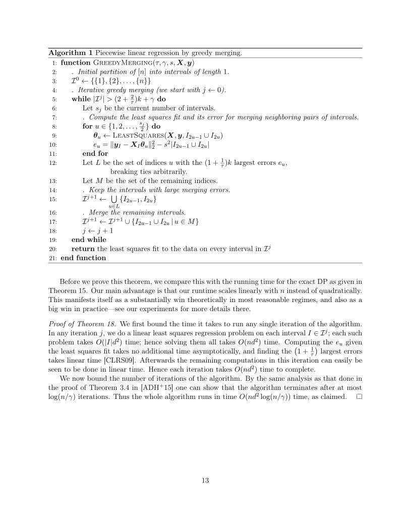
Algorithm 1 Piecewise linear regression by greedy merging.1: function GreedyMerging(τ, γ, s,X,y)2: . Initial partition of [n] into intervals of length 1.3: I0 ← {{1}, {2}, . . . , {n}}4: . Iterative greedy merging (we start with j ← 0).5: while |Ij | > (2 + 2

τ )k + γ do6: Let sj be the current number of intervals.7: . Compute the least squares fit and its error for merging neighboring pairs of intervals.8: for u ∈ {1, 2, . . . , sj2 } do9: θu ← LeastSquares(X,y, I2u−1 ∪ I2u)

10: eu = ‖yI −XIθu‖22 − s2|I2u−1 ∪ I2u|11: end for12: Let L be the set of indices u with the (1 + 1

τ )k largest errors eu,breaking ties arbitrarily.

13: Let M be the set of the remaining indices.14: . Keep the intervals with large merging errors.15: Ij+1 ←

⋃u∈L{I2u−1, I2u}

16: . Merge the remaining intervals.17: Ij+1 ← Ij+1 ∪ {I2u−1 ∪ I2u |u ∈M}18: j ← j + 119: end while20: return the least squares fit to the data on every interval in Ij21: end function

Before we prove this theorem, we compare this with the running time for the exact DP as given inTheorem 15. Our main advantage is that our runtime scales linearly with n instead of quadratically.This manifests itself as a substantially win theoretically in most reasonable regimes, and also as abig win in practice—see our experiments for more details there.

Proof of Theorem 18. We first bound the time it takes to run any single iteration of the algorithm.In any iteration j, we do a linear least squares regression problem on each interval I ∈ Ij ; each suchproblem takes O(|I|d2) time; hence solving them all takes O(nd2) time. Computing the eu giventhe least squares fit takes no additional time asymptotically, and finding the

(1 + 1

τ

)largest errors

takes linear time [CLRS09]. Afterwards the remaining computations in this iteration can easily beseen to be done in linear time. Hence each iteration takes O(nd2) time to complete.

We now bound the number of iterations of the algorithm. By the same analysis as that done inthe proof of Theorem 3.4 in [ADH+15] one can show that the algorithm terminates after at mostlog(n/γ) iterations. Thus the whole algorithm runs in time O(nd2 log(n/γ)) time, as claimed.

13

4.3 Analysis of GreedyMerging

Theorem 19. Let δ > 0, and let f be the estimator returned by GreedyMerging. Let m =(2 + 2

τ )k + γ be the number of pieces in f . Then, with probability 1− δ, we have that

MSE(f) ≤ O

(σ2(m(r + log(n/δ))

n

)+ σ

τ +√k√

nlog(nδ

)).

Proof. We first condition on the event that Corollaries 7, 11 and 12, and Lemma 17 all hold with errorparameter O(δ), so that together they all hold with probability at least 1− δ. Let I = {I1, . . . , Im}be the final partition of [n] that our algorithm produces. Recall f is the ground truth k-piecewiselinear function. We partition the intervals in I into two sets:

F = {I ∈ I : f is flat on I} ,J = {I ∈ I : f has a jump on I} .

We first bound the error over the intervals in F . By Lemma 17, we have∑I∈F‖fI − fI‖2 ≤ O(σ2|F|(r + log(n/δ))) , (4)

with probability at least 1−O(δ).We now turn our attention to the intervals in J and distinguish two further cases. We let J1

be the set of intervals in J which were never merged, and we let J2 be the remaining intervals. Ifthe interval I ∈ J1 was never merged, the interval contains one point, call it i. Because we mayassume that xi 6= 0, we know that for this one point, our estimator satisfies f(xi) = yi, since this isclearly the least squares fit for a linear estimator on one nonzero point. Hence Corollary 7 impliesthat the following inequality holds with probability at least 1−O(δ):∑

I∈J1

‖fI − fI‖2 =∑I∈J1

‖εI‖2

≤ σ2∑I∈J1

|I|+O(

logn

δ

)√∑I∈J1

|I|

≤ σ2

(m+O

(log

n

δ

)√m). (5)

We now finally turn our attention to the intervals in J2. Fix an interval I ∈ J2. By definition,the interval I was merged in some iteration of the algorithm. This implies that in that iteration,there were (1 + 1/τ)k intervals M1, . . . ,M(1+1/τ)k so that for each interval M`, we have

‖yI − fI‖2 − s2|I| ≤ ‖yM`− fLS

M`‖2 − s2|M`| . (6)

Since the true, underlying k-piecewise linear function f has at most k jumps, this means that thereare at least k/τ intervals of the M` on which f is flat. WLOG assume that these intervals areM1, . . . ,Mk/τ .

14

Fix any ` = 1, . . . , k/τ . Expanding out the RHS of (6) using the definition of yi gives∥∥yM`− fLS

M`

∥∥2 − s2|M`| =∥∥fM`

− fLSM`

∥∥2 + 2〈εM`,fM`

− fLSM`〉+ ‖εM`

‖2 − s2|M`|

=∥∥fM`

− fLSM`

∥∥2 + 2〈εM`,fM`

− fLSM`〉+

∑i∈M`

(ε2i − s2) .

Thus, we have that in aggregate,k/τ∑`=1

∥∥yM`− fLS

M`

∥∥2 − s2|M`| =k/τ∑`=1

∥∥fM`− fLS

M`

∥∥2 + 2

k/τ∑`=1

〈εM`,fM`

− fLSM`〉+

k/τ∑`=1

∑i∈M`

(ε2i − s2) .

(7)

We will upper bound each term on the RHS in turn. First, since the function f is flat on each M`

for ` = 1, . . . , k/τ , Lemma 17 implies

k/τ∑`=1

∥∥fM`− fLS

M`

∥∥2 ≤ O(σ2kτ

(r + log

n

δ

)), (8)

with probability at least 1−O(δ).Moreover, note that the function fLSM`

is a linear function on M` of the form fLSM`(x) = xT β,

where β ∈ Rd is the least-squares fit on M`. Because f is just a fixed vector, the vector fM`− fLS

M`

lives in the affine subspace of vectors of the form fM`+ (XM`

)η where η ∈ Rd is arbitrary. SoCorollary 12 and (8) imply that

k/τ∑`=1

〈εM`,fM`

− fLSM`〉 ≤

√√√√k/τ∑`=1

〈εM`,fM`

− fLSM`〉 · sup

η

|〈εM`,Xη〉|

‖Xη‖

≤ O(σ2k

τ

(r + log

n

δ

)). (9)

with probability 1−O(δ).By Corollary 7, we get that with probability 1−O(δ),

k/τ∑`=1

∑i∈M`

ε2i − s2|M`|

≤ O (σ logn

δ

)√n .

Putting it all together, we get thatk/τ∑i=1

(∥∥yM`− fLS

M`

∥∥2 − s2|M`|)≤ O

(k

τσ2(r + log

n

δ

))+O

(σ log

n

δ

)√n (10)

with probability 1 − O(δ). Since the LHS of (6) is bounded by each individual summand above,this implies that the LHS is also bounded by their average, which implies that

‖yI − fI‖2 − s2|I| ≤τ

k

k/τ∑i=1

(‖yM`

− fLSM`‖2 − s2|M`|

)≤ O

(σ2(r + log

(nδ

)))+O

(σ log

n

δ

) τ√nk

. (11)

15

We now similarly expand out the LHS of (6):

‖yI − fI‖2 − s2|I| = ‖fI + εI − fI‖2 − s2|I|

= ‖fI − fI‖2 + 2〈εI ,fI − fI〉+ ‖εI‖2 − s2|I| . (12)

From this we are interested in obtaining an upper bound on∑

i∈I(f(xi) − f(xi))2, hence we seek

to lower bound the second and third terms of (12). The calculations here will very closely mirrorthose done above.

By Corollary 11, we have that

2〈εI ,fI − fI〉 ≥ −O(σ

√r + log

(nδ

))‖fI − fI‖ ,

and by Corollary 7 we have

‖εI‖2 − s2|I| ≥ −O(σ log

n

δ

)√|I| ,

and so

‖yI − fI‖2 − s2|I| ≥ ‖fI − fI‖2 −O(σ

√r + log

(nδ

))‖fI − fI‖ −O

(σ log

n

δ

)√|I| . (13)

Putting (11) and (13) together yields that with probability 1−O(δ),

‖fI − fI‖2 ≤ O(σ2(r + log

(nδ

)))+O

(σ

√r + log

(nδ

))‖fI − fI‖+O

(σ log

n

δ

)(τ√nk

+√|I|).

Letting z2 = ‖fI − fI‖2, then this inequality is of the form z2 ≤ bz + c where b, c ≥ 0. In thisspecific case, we have that

b = O

(σ

√r + log

n

δ

), and

c = O(σ2(r + log

(nδ

)))+O

(σ log

n

δ

)(τ√nk

+√|I|)

We now prove the following lemma about the behavior of such quadratic inequalities:

Lemma 20. Suppose z2 ≤ bz + c where b, c ≥ 0. Then z2 ≤ O(b2 + c).

Proof. From the quadratic formula, the inequality implies that z ≤ b+√b2+4c2 . From this, it is

straightforward to demonstrate the desired claim.

Thus, from the lemma, we have

‖fI − fI‖2 ≤ O(σ2(r + log

(nδ

)))+O

(σ log

n

δ

)(τ√nk

+√|I|).

16

Hence the total error over all intervals in J2 can be bounded by:∑I∈J2

‖fI − fI‖2 ≤ O(kσ2

(r + log

(nδ

)))+O

(σ log

n

δ

)(τ√n+

∑I∈J

√|I|

)≤ O

(kσ2

(r + log

(nδ′

)))+O

(σ log

n

δ

)(τ√n+√kn). (14)

In the last line we use that the intervals I ∈ J2 are disjoint (and hence their cardinalities sum up toat most n), and that there are at most k intervals in J2 because the function f is k-piecewise linear.Finally, applying a union bound and summing (4), (5), and (14) yields the desired conclusion.

5 A variance-free merging algorithm

In this section, we give a variant of the above algorithm that does not require knowledge of thenoise variance s2. The formal pseudo code is given in Algorithm 2.

Algorithm 2 Variance-free greedy merging with bucketing.1: function BucketGreedyMerging(γ,X,y)2: . Initial histogram.3: Let I0 ← {{1}, {2}, . . . , {n}} be the initial partition of [n] into intervals of length 1.4: . Iterative greedy merging (we start with j = 0).5: while |Ij | > (2(k + 1) + γ) log n do6: Let sj be the current number of intervals.7: . Compute the least squares fit and its error for merging neighboring pairs of intervals.8: for u ∈ {1, 2, . . . , sj2 } do9: I ′u ← I2u−1 ∪ I2u

10: θu ← LeastSquares(X,y, I ′u)11: eu = 1

|I′u|‖yI −XIθu‖22

12: end for13: for α = 0, . . . , log(n)− 1 do14: Let Bα be the set of indices u so that 2α ≤ |I ′u| ≤ 2α+1

15: Let Lα be the set of indices u ∈ Bα with the k + 1 largest eu amongst u ∈ Bα,breaking ties arbitrarily.

16: Let Mα be the set of the remaining indices u in Bα.17: . Keep the intervals in each Bα with large merging errors.18: Ij+1 ←

⋃u∈Lα{I2u−1, I2u}

19: . Merge the remaining intervals in each Bα.20: Ij+1 ← Ij+1 ∪ {I ′u |u ∈Mα}21: end for22: j ← j + 123: end while24: return the least squares fit to the data on every interval in Ij25: end function

We now state the running time for BucketGreedyMerge. The running time analysis forBucketGreedyMerge is almost identical to that of GreedyMerge; hence we omit its proof.

17

Theorem 21. Let X and y be as in (1). Then BucketGreedyMerging(γ,X,y) outputs a(2(k + 1) + γ) log n-piecewise linear function and runs in time O(nd2 log(n/γ)).

5.1 Analysis of BucketGreedyMerge

This section is dedicated to the proof of the following theorem:

Theorem 22. Let f be them-piecewise linear function that is returned by BucketGreedyMerge,where m = (2(k + 1) + γ) log n. Then, with probability 1− δ, we have

MSE(f) ≤ O

(σ2(m(r + log(n/δ))

n

)+ σ

√k

nlog(nδ

)).

Proof. As in the proof of Theorem 19, we let I be the final partition of [n] that our algorithmproduces. We also similarly condition on the event that Corollaries 7 and 12 and Lemma 17 all holdwith parameter O(δ). We again partition I into two sets F and J as before, and further subdivideJ into J1 and J2. The error on F and J1 is the same as the error given in (4) and (5). The onlydifference is the error on intervals in J2.

Let I ∈ J2 be fixed. By definition, this means there was some iteration and a collection of somek + 1 disjoint intervals M1, . . . ,Mk+1 so that |M`|/2 ≤ |I| ≤ 2|M`| and

1

|I|

∥∥∥yI − fI∥∥∥2 ≤ 1

|M`|∥∥yM`

− fLSM`

∥∥2for all ` = 1, . . . , k + 1. Since f has at most k jumps, this means that there is at least one intervalM` so that f is flat on M`. WLOG assume that f is flat on M1. By the same kinds of calculationsdone in the proof of Theorem 19, we have that with probability 1− δ,∥∥yM1 − fLS

M1

∥∥2 ≤ O (σ2(r + logn

δ))

+ σ2|M1|+O(σ log(n/δ))√|M1|

and ∥∥∥yI − fI∥∥∥2 ≥ ∥∥∥fI − fI∥∥∥2 −O (σ√r + log(n/δ))∥∥∥yI − fI∥∥∥+ σ2|I| −O(σ log(n/δ))

√|I| ,

and putting these two equations together and rearranging, we have∥∥∥fI − fI∥∥∥2 ≤ O (σ2(r + log(n/δ)))

+ σ2 ·O(log(n/δ))

(|I|√|M`|

+√|I|

)+O

(σ√r + log(n/δ)

)∥∥∥yI − fI∥∥∥≤ O

(σ2(r + log(n/δ))

)+O

(σ2 log(n/δ)

√|I|)

+O(σ√r + log(n/δ)

)∥∥∥yI − fI∥∥∥ ,where in the last inequality we used that |M`| ≥ |I|/2. By Lemma 20, this implies that∥∥∥fI − fI∥∥∥2 ≤ O (σ2(r + log(n/δ))

)+O

(σ2 log(n/δ)

√|I|).

Since there are at most k elements in J2, and they are all disjoint, this yields that∑I∈J2

∥∥∥fI − fI∥∥∥2 ≤ O (kσ2 (r + logn

δ

))+O

(σ log

(nδ

)√kn)

(15)

and putting this equation together with (4) and (5) yields the desired conclusion.

18

5.2 Postprocessing

One unsatisfying aspect of BucketGreedyMerge is that it outputs O(k log n) pieces. Not onlydoes this increase the size of the representation nontrivially when n is large, but it also increases theerror rate: it is the reason why the first term in the error rate given in Theorem 22 has an additionallog n factor as opposed the rate in Theorem 19. In this section, we give an efficient postprocessingprocedure for BucketGreedyMerge which, when run on the output of BucketGreedyMerge,outputs an O(k) histogram with the same rate as before. In fact, the rate is slightly improved aswe are able to remove the log n factor mentioned above.

The postprocessing algorithm Postprocessing takes as input a partition I of [n] of sizeO(k log n) and a target number of pieces k. It then performs the following steps: starting fromthe O(k log n) partition I, run the dynamic program (DP) on intervals with breakpoints amongstthe breakpoints of I to find the 2k + 1 partition Ip (whose endpoints are also endpoints of I) thatminimizes the sum squared error to the data. The running time analysis is identical to that of theDP with two exceptions: first, we only need to fill out a O(k log n)×(2k+1) size table (as comparedto an n× k sized table). Second, we are no longer performing rank one updates because we insteadcompute updates in large chunks, we cannot use the Sherman-Morrison formula to speed up thecomputation of the least-squares fits. Hence, we obtain the following theorem:

Theorem 23. Given a partition I of [n] into O(k log n) pieces, Postprocessing(I, k) runs intime O(k3d2), and outputs a (2k+1)-piecewise linear function, where the O hides poly log(n) factors.

We now show that the algorithm still provides the same (in fact, slightly better) statisticalguarantees as the original partition:

Theorem 24. Fix δ > 0. Let fp be the estimator output by PostprocessedBucketGreedyMerge.Then, with probability 1− δ, we have

MSE(fp) ≤ O

(σ2k(r + log n

δ

)n

+ σ log(nδ

)√k

n

).

Proof. Let I and J be as in the proof of Theorem 22. Let Ip = {J1, . . . , J2k+1} be the intervals inthe partition that we return. We again condition on the event that Corollaries 7 and 12 and Lemma17 all hold with parameter O(δ). The following will then all hold with probability 1− δ.

Define the partition K to be the partition that contains every interval in J and exactly oneinterval between any two non-consecutive intervals in J (i.e., K merges all flat intervals). Moreover,let g be the (2k + 1)-piecewise linear function which is the least squares fit to the data on eachinterval in I ∈ K. This is clearly a possible solution for the dynamic program, and therefore wehave

‖f − y‖2 ≤ ‖g − y‖2

=∑

I∈K\J

‖gI − yI‖2 +∑I∈J‖gI − yI‖2 . (16)

We will expand and then upper bound the RHS of (16). First, by calculations similar to thoseemployed in the proof of Theorem 19, we have that∑

I∈K\J

‖gI − yI‖2 ≤ O(kσ2

(r + log

n

δ

))+∑

I∈K\J

‖εI‖2 ,

19

and from (15) and Corollary 12 we have∑I∈J‖gI − yI‖2 =

∑I∈J‖fI + εI − gI‖2

=∑I∈J‖fI − gI‖2 + 2

∑I∈J〈εI ,fI − gI〉+

∑I∈J‖εI‖2

≤ O(kσ2

(r + log

n

δ

))+O

(σ log

(nδ

)√kn)

+∑I∈J‖εI‖2 ,

so all together now we have∑I∈K‖gI − yI‖2 ≤ O

(kσ2

(r + log

n

δ

))+O

(σ log

(nδ

)√kn)

+ ‖ε‖2 .

Moreover, by the same kinds of calculations, we can expand out the LHS of (16):

‖f − y‖2 ≥ ‖f − f‖2 + 〈ε, f − f〉+ ‖ε‖2

≥ ‖f − f‖2 −O(√

k · σ√r + log

n

δ

)‖f − f‖+ ‖ε‖2

and hence, combining, cancelling, and moving terms around, we get that

‖f − f‖2 ≤ O(√

k · σ√r + log

n

δ

)(1 + ‖f − f‖

)+O

(σ log

(nδ

)√kn).

By Lemma 20, this implies that

‖f − f‖2 ≤ O(kσ2

(r + log

n

δ

)+ σ log

(nδ

)√kn),

with probability 1− δ, as claimed.

We remark that Postprocessing can also be run on the output of GreedyMerging todecrease the number of pieces from O(k) to 2k+ 1 if so desired. The proof that it maintains similarstatistical guarantees is almost identical to the one presented above.

6 Obtaining agnostic guarantees

In this section, we demonstrate how to show agnostic guarantees for the algorithms in the previoussections. Recall now f is arbitrary, and f∗ is a k-piecewise linear function which obtains thebest approximation in mean-squared error to f amongst all k-piecewise linear functions. For alli = 1, . . . , n, define ζi = f(xi)− f∗(xi) to be the error at data point i of the approximation, so thatfor all i, we have

yi = f∗(xi) + ζi + εi . (17)

By definition, we have that ‖ζ‖2 = n ·OPTk.As a warm-up, we first show the following agnostic guarantee for the exact DP:

20

Theorem 25. Fix δ > 0. Let fLS be the k-piecewise linear function returned by the exact DP.Then, with probability 1− δ, we have

MSE(fLS) ≤ O

(σ2kr + k log n

δ

n+ σ log

(1

δ

)√OPTk

n+ OPTk

)In the regimes that are most interesting, i.e., when OPTk is small, the middle term does not

contribute significantly to the error.

Proof. The overall proof structure stays the same. From the definition of the least-squares fit, wehave

‖y − fLS‖2 ≤ ‖y − f∗‖2

= ‖ε+ ζ‖2

= ‖ε‖2 + 2〈ε, ζ〉2 + n ·OPTk

≤ ‖ε‖2 +O

(σ log

1

δ

)(n ·OPTk)

1/2 + n ·OPTk ,

with probability 1−O(δ), where the last inequality follows from the r = 1 case of Lemma 10. TheLHS can be expanded out exactly as before in (3), and putting these two sides together we obtainthat

‖fLS − f‖2 ≤ 2〈ε,fLS − f〉+O

(σ log

1

δ

)(n ·OPTk)

1/2 + n ·OPTk

≤ O(σ

√kr + k log

n

δ

)· ‖fLS − f‖+O

(σ log

1

δ

)(n ·OPTk)

1/2 + n ·OPTk

with probability at least 1−O(δ) and so by Lemma 20 we obtain that

‖fLS − f‖2 ≤ O(σ2(kr + k log

n

δ

)+ σ log

(1

δ

)(n ·OPTk)

1/2 + n ·OPTk

).

Dividing both sides by n yields the desired conclusion.

Reviewing the proof, we observe the following general pattern: in all upper bounds we wishto obtain (generally for formulas which occur on the RHS of the equations above) we obtain newOPTk terms, whereas in the lower bounds (generally for formulas on the LHS of the equationsabove) nothing changes. In fact, all folllowing proofs exhibit this pattern. We first establish someuseful concentration bounds. By the same union-bound technique used throughout this paper, onecan show the following. We omit the proof for conciseness.

Lemma 26. Fix δ > 0. Let εi and ζi be as in (17), for i = 1, . . . , n. Then, with probability 1 − δ,we have that for all collections of k disjoint intervals J1, . . . , Jk, the following holds:

k∑`=1

〈εJ` , ζJ`〉 ≤ O(kσ log

n

δ

)·

(k∑`=1

‖ζJ`‖2

)1/2

≤ O(kσ log

n

δ

)· (n ·OPTk)

1/2

21

Observe that with this lemma, we can easily adapt the proof of Theorem 25 to show the followingagnostic version of Lemma 17:

Lemma 27. Fix δ > 0. Then with probability 1− δ, we have that for all disjoint sets of k intervalsJ1, . . . , Jk of [n] so that f∗ is flat on each J`, the following inequality holds:

k∑`=1

‖fLSJ`− fJ`‖

2 ≤ O(σ2(kr + k log

n

δ

)+ kσ log

(nδ

)(n ·OPTk)

1/2 + n ·OPTk

).

With this lemma, we can now prove the following theorem for our greedy algorithm, which showsthat in the presence of model misspecification, our algorithm still performs at a good rate:

Theorem 28. Let δ > 0, and let f be the estimator returned by GreedyMerging. Let m =(2 + 2

τ )k + γ be the number of pieces in f . Then, with probability 1− δ, we have that

MSE(f) ≤ O

(σ2(m(r + log(n/δ))

n

)+ σ

τ +√k√

nlog(nδ

)+ kσ log

(nδ

)√OPTk

n+ τ ·OPTk

).

Proof. As before, we condition on the event that Corollaries 7, 11, and 12, and Lemmas 26 and 27all hold with error parameter O(δ), so that together they all hold with probability at least 1 − δ.We also let I,F ,J1, and J2 denote the same quantities as before, except we define the partitionwith respect to the jumps of f∗ instead of f , since the latter does not have well-defined jumps. Forinstance, F is the set of intervals in I on which f∗ has no jumps.

We again bound the error on these three sets separately. First, by Lemma 27 we have that∑I∈F‖fI − fI‖2 ≤ O

(σ2(mr +m log

n

δ

)+mσ log

(nδ

)(n ·OPTk)

1/2 + n ·OPTk

). (18)

Second, we bound the error on J1. By modifying the calculations as those preceding (5) in thesame way as we did above in the proof of Theorem 25, we may show that∑

I∈J1

‖fI − fI‖2 ≤ σ2(k +O

(log

n

δ

)√m)

+O(kσ log

n

δ(n ·OPTk)

1/2)

+ n ·OPTk . (19)

Finally, we bound the error on J2. Fix an I ∈ J2, and let M1, . . . ,Mk/τ be as before. Recall thatthis proof had two components: an upper bound for the M1, . . . ,M` and a lower bound for I. Wefirst compute the upper bound. By following the calculations for (11) and using Lemma 27, we have

k/τ∑`=1

(‖yM`

− fLSM`‖2 − s2|M`|

)≤ O

(k

τσ2(r + log

(nδ

))+ σ log

(nδ

)√n

+k

τσ log

(nδ

)(n ·OPTk)

1/2 + n ·OPTk

)The lower bound is in fact unchanged: we may use (13) as stated. Putting these two terms togetherand simplifying as we did previously, we obtain that

‖fI − fI‖2 ≤ O(σ2(r + log

(nδ

))+ σ log

n

δ

(τ√n

k+√|I|)

+σ log(nδ

)(n ·OPTk)

1/2 +τ

kn ·OPTk

).

As before, summing up all the bounds we have achieved proves the desired claim.

22

102 103 104

10−2

10−1

100

n

MSE

102 103 104

2

4

6

8

10

n

Rel

ativ

eM

SEra

tio

102 103 104

10−4

10−2

100

n

Run

ning

tim

e(s

)

102 103 104

101

102

103

n

Spee

d-up

102 103 104

10−2

10−1

100

n

MSE

102 103 104

2

4

6

8

10

n

Rel

ativ

eM

SEra

tio

102 103 104

10−4

10−2

100

102

n

Run

ning

tim

e(s

)

Merging k Merging 2k Merging 4k Exact DP

102 103 104

102

103

n

Spee

d-up

Piecewise constant

Piecewise linear

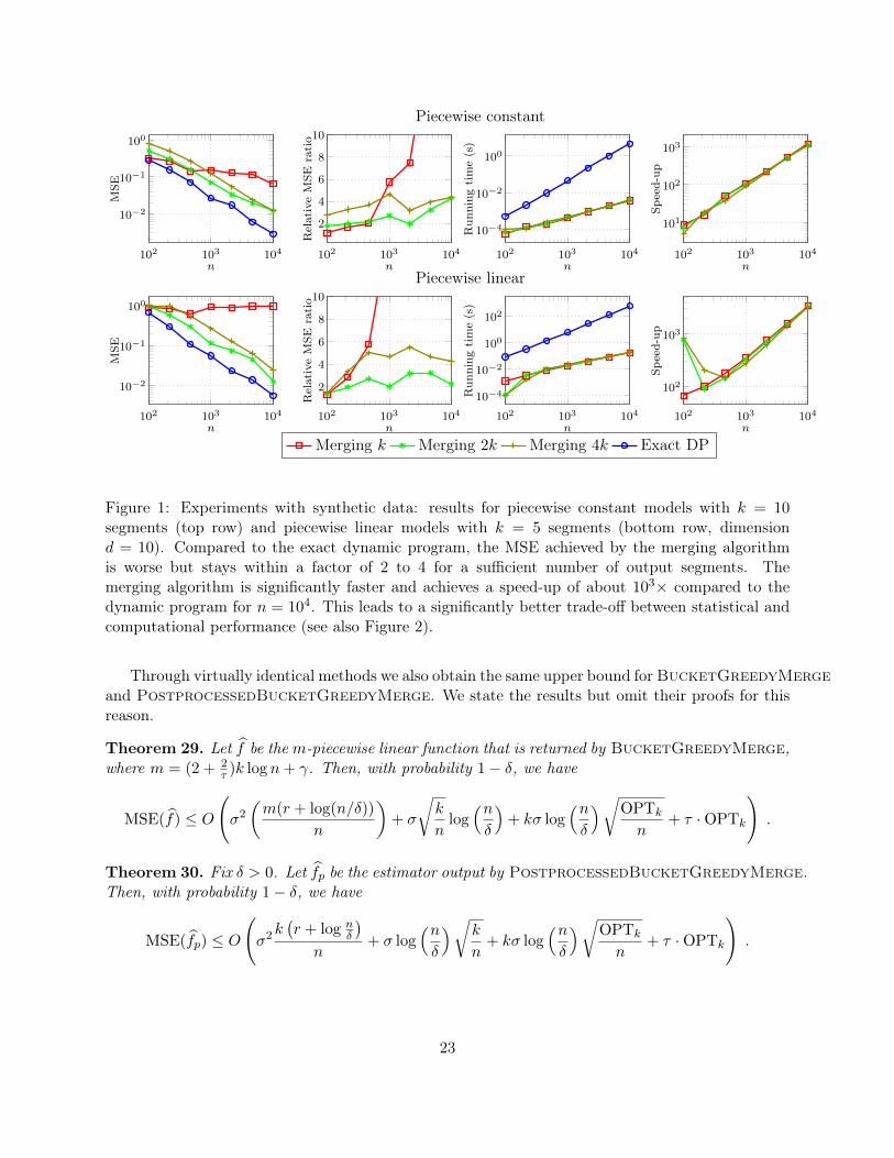
Figure 1: Experiments with synthetic data: results for piecewise constant models with k = 10segments (top row) and piecewise linear models with k = 5 segments (bottom row, dimensiond = 10). Compared to the exact dynamic program, the MSE achieved by the merging algorithmis worse but stays within a factor of 2 to 4 for a sufficient number of output segments. Themerging algorithm is significantly faster and achieves a speed-up of about 103× compared to thedynamic program for n = 104. This leads to a significantly better trade-off between statistical andcomputational performance (see also Figure 2).

Through virtually identical methods we also obtain the same upper bound for BucketGreedyMergeand PostprocessedBucketGreedyMerge. We state the results but omit their proofs for thisreason.

Theorem 29. Let f be them-piecewise linear function that is returned by BucketGreedyMerge,where m = (2 + 2

τ )k log n+ γ. Then, with probability 1− δ, we have

MSE(f) ≤ O

(σ2(m(r + log(n/δ))

n

)+ σ

√k

nlog(nδ

)+ kσ log

(nδ

)√OPTk

n+ τ ·OPTk

).

Theorem 30. Fix δ > 0. Let fp be the estimator output by PostprocessedBucketGreedyMerge.Then, with probability 1− δ, we have

MSE(fp) ≤ O

(σ2k(r + log n

δ

)n

+ σ log(nδ

)√k

n+ kσ log

(nδ

)√OPTk

n+ τ ·OPTk

).

23

10−4 10−2 10010−4

10−2

100

Time (s)M

SE

Piecewise constant

10−4 10−1 10210−4

10−2

100

Time (s)

MSE

Piecewise linear

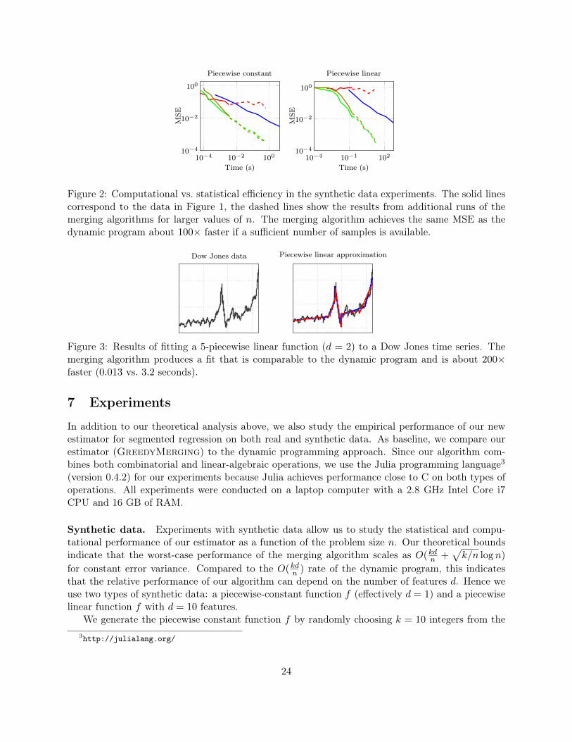
Figure 2: Computational vs. statistical efficiency in the synthetic data experiments. The solid linescorrespond to the data in Figure 1, the dashed lines show the results from additional runs of themerging algorithms for larger values of n. The merging algorithm achieves the same MSE as thedynamic program about 100× faster if a sufficient number of samples is available.

Dow Jones data Piecewise linear approximation

Figure 3: Results of fitting a 5-piecewise linear function (d = 2) to a Dow Jones time series. Themerging algorithm produces a fit that is comparable to the dynamic program and is about 200×faster (0.013 vs. 3.2 seconds).

7 Experiments

In addition to our theoretical analysis above, we also study the empirical performance of our newestimator for segmented regression on both real and synthetic data. As baseline, we compare ourestimator (GreedyMerging) to the dynamic programming approach. Since our algorithm com-bines both combinatorial and linear-algebraic operations, we use the Julia programming language3

(version 0.4.2) for our experiments because Julia achieves performance close to C on both types ofoperations. All experiments were conducted on a laptop computer with a 2.8 GHz Intel Core i7CPU and 16 GB of RAM.

Synthetic data. Experiments with synthetic data allow us to study the statistical and compu-tational performance of our estimator as a function of the problem size n. Our theoretical boundsindicate that the worst-case performance of the merging algorithm scales as O(kdn +

√k/n log n)

for constant error variance. Compared to the O(kdn ) rate of the dynamic program, this indicatesthat the relative performance of our algorithm can depend on the number of features d. Hence weuse two types of synthetic data: a piecewise-constant function f (effectively d = 1) and a piecewiselinear function f with d = 10 features.

We generate the piecewise constant function f by randomly choosing k = 10 integers from the3http://julialang.org/

24

set {1, . . . , 10} as function value in each of the k segments.4 Then we draw n/k samples from eachsegment by adding an i.i.d. Gaussian noise term with variance 1 to each sample.

For the piecewise linear case, we generate a n × d data matrix X with i.i.d. Gaussian entries(d = 10). In each segment I, we choose the parameter values βI independently and uniformlyat random from the interval [−1, 1]. So the true function values in this segment are given byfI = XIβI . As before, we then add an i.i.d. Gaussian noise term with variance 1 to each functionvalue.

Figure 1 shows the results of the merging algorithm and the exact dynamic program for samplesize n ranging from 102 to 104. Since the merging algorithm can produce a variable number of outputsegments, we run the merging algorithm with three different parameter settings corresponding to k,2k, and 4k output segments, respectively. As predicted by our theory, the plots show that the exactdynamic program has a better statistical performance. However, the MSE of the merging algorithmwith 2k pieces is only worse by a factor of 2 to 4, and this ratio empirically increases only slowlywith n (if at all). The experiments also show that forcing the merging algorithm to return at mostk pieces can lead to a significantly worse MSE.

In terms of computational performance, the merging algorithm has a significantly faster runningtime, with speed-ups of more than 1, 000× for n = 104 samples. As can be seen in Figure 2, thiscombination of statistical and computational performance leads to a significantly improved trade-offbetween the two quantities. When we have a sufficient number of samples, the merging algorithmachieves a given MSE roughly 100× faster than the dynamic program.

Real data. We also investigate whether the merging algorithm can empirically be used to findlinear trends in a real dataset. We use a time series of the Dow Jones index as input, and fit apiecewise linear function (d = 2) with 5 segments using both the dynamic program and our mergingalgorithm with k = 5 output pieces. As can be seen from Figure 3, the dynamic program producesa slightly better fit for the rightmost part of the curve, but the merging algorithm identifies roughlythe same five main segments. As before, the merging algorithm is significantly faster and achievesa 200× speed-up compared to the dynamic program (0.013 vs 3.2 seconds).

Acknowledgements

Part of this research was conducted while Ilias Diakonikolas was at the University of Edinburgh,Jerry Li was an intern at Microsoft Research Cambridge (UK), and Ludwig Schmidt was visitingthe EECS department at UC Berkeley.

Jayadev Acharya was supported by a grant from the MIT-Shell Energy Initiative. Ilias Di-akonikolas was supported in part by EPSRC grant EP/L021749/1, a Marie Curie Career Integra-tion Grant, and a SICSA grant. Jerry Li was supported by NSF grant CCF-1217921, DOE grantDE-SC0008923, NSF CAREER Award CCF-145326, and a NSF Graduate Research Fellowship.Ludwig Schmidt was supported by grants from the MIT-Shell Energy Initiative, MADALGO, andthe Simons Foundation.

4We also repeated the experiment for other values of k. Since the results are not qualitatively different, we onlyreport the k = 10 case here.

25

References

[ADH+15] J. Acharya, I. Diakonikolas, C. Hegde, J. Z. Li, and L. Schmidt. Fast and near-optimalalgorithms for approximating distributions by histograms. In PODS, pages 249–263,2015.

[ADLS15] J. Acharya, I. Diakonikolas, J. Zheng Li, and L Schmidt. Sample-optimal density esti-mation in nearly-linear time. CoRR, abs/1506.00671, 2015.

[ASW13] H. Avron, V. Sindhwani, and D. Woodruff. Sketching structured matrices for fasternonlinear regression. In NIPS, pages 2994–3002. 2013.

[BP98] J. Bai and P. Perron. Estimating and testing linear models with multiple structuralchanges. Econometrica, 66(1):47–78, 1998.

[CGS15] S. Chatterjee, A. Guntuboyina, and B. Sen. On risk bounds in isotonic and other shaperestricted regression problems. Annals of Statistics, 43(4):1774–1800, 08 2015.

[CLRS09] T. H. Cormen, C. E. Leiserson, R. L. Rivest, and C. Stein. Introduction to Algorithms.3rd edition, 2009.

[CW13] K. L. Clarkson and D. P. Woodruff. Low rank approximation and regression in inputsparsity time. In STOC, 2013.

[Fed75] P. I. Feder. On asymptotic distribution theory in segmented regression problems– iden-tified case. Annals of Statistics, 3(1):49–83, 01 1975.

[Fri91] J. H. Friedman. Multivariate adaptive regression splines. Annals of Statistics, 19(1):1–67, 03 1991.

[GA73] A. R. Gallant and Fuller W. A. Fitting segmented polynomial regression models whosejoin points have to be estimated. Journal of the American Statistical Association,68(341):144–147, 1973.

[GKS06] S. Guha, N. Koudas, and K. Shim. Approximation and streaming algorithms for his-togram construction problems. ACM Trans. Database Syst., 2006.

[JKM+98] H. V. Jagadish, Nick Koudas, S. Muthukrishnan, Viswanath Poosala, Kenneth C. Sevcik,and Torsten Suel. Optimal histograms with quality guarantees. In VLDB ’98, 1998.

[Jor13] M. I. Jordan. On statistics, computation and scalability. Bernoulli, 19(4):1378–1390, 092013.

[KRS15] R. Kyng, A. Rao, and S. Sachdeva. Fast, provable algorithms for isotonic regression inall lp-norms. In NIPS, pages 2701–2709, 2015.

[Mey08] M. C. Meyer. Inference using shape-restricted regression splines. Annals of AppliedStatistics, 2(3):1013–1033, 09 2008.

[MT77] F. Mosteller and J. W. Tukey. Data analysis and regression: a second course in statistics.Addison-Wesley, Reading (Mass.), Menlo Park (Calif.), London, 1977.

26

[Rig15] P. Rigollet. High dimensional statistics. 2015.

[SHKT97] C. J. Stone, M. H. Hansen, C. Kooperberg, and Y. K. Truong. Polynomial splines andtheir tensor products in extended linear modeling: 1994 wald memorial lecture. Annalsof Statistics, 25(4):1371–1470, 1997.

[Sto94] C. J. Stone. The use of polynomial splines and their tensor products in multivariatefunction estimation. Annals of Statistics, 22(1):pp. 118–171, 1994.

[Ver10] Roman Vershynin. Introduction to the non-asymptotic analysis of random matrices.Chapter 5 of: Compressed Sensing, Theory and Applications. Edited by Y. Eldar andG. Kutyniok. Cambridge University Press, 2012, 2010.

[WW83] E. J. Wegman and I. W. Wright. Splines in statistics. Journal of the American StatisticalAssociation, 78(382):pp. 351–365, 1983.

[YP13] Y. Yamamoto and P. Perron. Estimating and testing multiple structural changes inlinear models using band spectral regressions. Econometrics Journal, 16(3):400–429,2013.

27