Facility Location and Capacity Acquisition: An Integrated Approach

Vedat Verter Faculty of Business, University ofAlberta, Edmonton, Alberta, T6G 2R6, Canada

M. Cemal Dincer Department of Industrial Engineering, Bilkent University, 06533,

Bilkent, Ankara, Turkey

The facility location and capacity acquisition decisions are intertwined, especially within the international context where capacity acquisition costs are location dependent. A review of the relevant literature however, reveals that the facility location and the capacity acquisi- tion problems have been dealt with separately. Thus, an integrated approach for simulta- neous optimization of these strategic decisions is presented. Analytical properties of the arising model are investigated and an algorithm for solving the problem is devised. Encour- aging computational results are reported. 0 1995 John Wiley & Sons, Inc.

1. INTRODUCTION

A company might consider investing in the construction of new facilities for a variety of reasons, such as, increasing its production capacity of an existing product, or extending its product range by new product introduction, or entering new markets with the existing and/ or new products. Here facility refers to the smallest productive entity that manufactures a single commodity (or, at most a single family ofcommodities) . Aplant however, refers to a collection of facilities in the same location, and hence in general will be producing multiple commodities. Construction of a new facility therefore, might mean expansion of an exist- ing plant if it takes place at that site, or otherwise would require opening a new plant.

In many investment projects, decisions regarding the location and the size of a new facility to be established are interrelated since capacity acquisition costs are location de- pendent. A typical example is new facility investments in the international context, where subsidized financing as well as low tax rates are provided by the national governments to attract the multinational companies to locate production plants in their country. In this case, it is clear that not only the fixed costs that occur due to opening the new facility at a particular site but also the capacity acquisition costs that vary with the size of the new facility are location specific. In a recent review however, Verter and Dincer [ 201 pointed out that the facility location and the capacity acquisition problems have been dealt with separately in the literature. That is the capacity acquisition costs are not incorporated in the facility location models which implies an implicit assumption that they would be the same at all sites. Therefore, the information provided by a facility location model regarding the size of a new facility might be far from optimal when the above assumption is not valid.

Naval Research Logistics. Vol. 42, pp. 1141-1 160 (1995) Copyright 0 1995 by John Wiley & Sons, Inc. CCC 0894-069X/95/08 1 14 1-20

1142 NavalResearch Logistics, Vol. 42 ( 1995)

Whereas, the capacity expansion models dwell on a given set of existing plants which may not necessarily contain the optimal site to locate the new facility. Thus, separate treatment ofthe facility location and capacity acquisition decisions could be justified only under quite stringent assumptions.

The aim of this study therefore, is to present an integrated approach for the problem of simultaneously deciding the optimal location and size of each new facility to be established. Thus, the remainder of this article is organized as follows: Section 2 provides the problem definition and a model formulation. The relevant literature is reviewed in Section 3. Ana- lytical properties of the model for the uncapacitated version of the problem are explored in Section 4 which constitute the foundations of the algorithm presented in Section 5. Computational results obtained via the implementation of this algorithm are reported in Section 6. Section 7 justifies the applicability of the same algorithm (with a minor adjustment) for also solving the capacitated version of the problem. Finally, some conclud- ing remarks are provided which suggest directions for further research.

2. THE FACILITY LOCATION AND CAPACITY ACQUISITION PROBLEM

Given a set of alternative facility locations and a set of markets to be served, thefacility location and capacity acquisition problem involves simultaneously locating an undeter- mined number of new facilities, and deciding their size to minimize the total cost of serving the clients. For each alternative location the cost items are:

.Fixed setup cost of establishing a new facility at that site,

.Variable cost of capacity acquisition associated with the size of the new facility,

.Variable costs of operation and transportation for serving the markets. and

Fixed setup costs such as the acquisition of land and the construction of infrastructure will be incurred only if a new facility is opened. Capacity acquisition costs would normally represent economies of scale, and hence would be monotone increasing concave functions of the capacity to be built-in at each new facility. Although it is also possible that the oper- ation and transportation costs represent economies of scale, we presume that this would not have a considerable effect on the strategic location and sizing decisions. Therefore, variable costs of operation and transportation are assumed to be linear.

The facility location and capacity acquisition problem is by definition concerned with a single commodity. Furthermore, the problem is deterministic, static, and has no transship- ment points. Note that the problem boils down to the uncapacitated facility location prob- lem (UFLP) when the capacity acquisition costs are ignored. UFLP is shown to be NP- complete by Krarup and Pruzan [ 141 which in consequence means that the facility location and capacity acquisition problem also belongs to the NP-complete class of problems.

Let n denote the number of markets (indexed by j ) and m denote the number of al- ternative facility locations (indexed by i). The problem can be modeled as follows:

Verter and Dincer: Integration of Location and Capacity Decisions i 143

Minimize z = C. F, Y, tf; 2 X , + c c,X, , ( 1 )

subject to C XIJ = 4, j = 1, . . . , r ? , ( 2 )

OIX,I Y,DJ , i = 1 , . . . , m , j = 1 , . . . , n , ( 3 )

y, E yo, 11 , i = I , . . . , m, (4)

IEI [ ( J E J J E J 1 Id

where

I, J = the sets of alternative facility locations and markets respectively,

f ;( .) = the total capacity acquisition cost at facility i, F, = the fixed setup cost of opening facility i,

c,, = the unit cost of producing and shipping from facility i to market j , 0, = the demand of marketj,

and the decision variables are

X,j = the quantity shipped from facility i to marketj, Y, = 1 if facility i is opened, 0 otherwise.

It should be emphasized that F, excludes any costs associated with the capacity of facility i, and obviously will depend on whether the new facility is established at an existing plant or it requires construction of a new plant. Thus, the total cost that is incurred due to the location and sizing of the new facilities as well as the facility-market allocations is mini- mized, while constraints ( 2 ) guarantee that each market’s demand will be fully satisfied, and constraints ( 3) ensure that markets receive shipments only from open facilities.

The above mathematical program models the problem where there are no upper bounds on the capacity acquired at the new facilities, which we call the uncapacitated facility loca- tion and capacity acquisition problem (UFL&CAP). If the size of each new facility how- ever, is constrained due to a variety of reasons e.g., availability of land, then the following constraints are appended to the model:

C X , , r C A P i i = 1 , . . . , m J E J

where, CAP, is the maximum capacity that can be built-in at facility i. This version of the problem is called the capacitated facility location and capacity acquisition problem (CFL&CAP). It is evident that CFL&CAP boils down to the capacitated facility location problem (CFLP) when the capacity acquisition costs are ignored. Note that, it is possible to interpret CFLP as the problem of locating an undetermined number of new facilities where the capacity of each alternative facility is given, and hence capacity acquisition costs are incorporated in the fixed setup costs. It should be emphasized that however, for a new facility, such a predetermined size might be far from optimal.

3. REVIEW OF THE RELEVANT LITERATURE In this section the relevant literature is reviewed in order to provide the reader with

further insight about the problem we address here. Note that, the mathematical program

1144 Naval Research Logistics, Vol. 42 ( 1995 )

presented in Section 2 is also suitable for modeling the concave cost facility location prob- lem. It is possible to show this by redefining X ( .) as the total cost of operating facility i, and c, as the unit cost of transport from facility i to market j . If the parameters are defined as above then ( 1 )-( 5) constitutes the concave cost capacitated facility location model. Therefore, the techniques available for solving the concave cost facility location problem are also suitable for solving the facility location and capacity acquisition problem.

The literature on concave cost facility location however, is rather sparse. In their seminal work on UFLP, Efroymson and Ray [ 41 suggested that if the cost functions are piecewise linear then the concave cost uncapacitated facility location problem can be formulated as an UFLP by associating a separate “facility” with each segment, Khumawala and Kelly [ 131 suggested a heuristic approach to the uncapacitated case where operating costs are represented via power functions. The earliest algorithm that guarantees an optimal solu- tion with no further assumptions regarding the form of the concave cost functions is due to Soland [ 18 1 . He devised a branch-and-bound algorithm, where the nodal problems can be solved by inspection in the uncapacitated case. They are however, in the form of the standard transportation problem when there are capacity constraints on the volume of production. At each node, linear underestimates (chords) are used to approximate the concave operating costs (including the fixed costs), and hence a lower bound on the prob- lem solution is obtained by solving the associated linear program (LP). Branching involves partitioning the constraint space by the aid of the LP solution, and hence narrowing the relevant range of the concave cost functions in the subsequent nodal problems. Thus, the chord inscribed in a facility’s operating cost curve is replaced with two adjacent chords which results in a better approximation. Therefore, the algorithm generates progressively better lower bounds. Khumawala and Kelly [ 131 however, observed the efficiency of tan- gent line approximation in assigning the facilities to markets for a given set of open facili- ties. Whereas, in the presence of fixed setup costs of opening new facilities, Kelly and Khu- mawala [ 121 had to resort to a combination of the tangent line and chord approximations. Their algorithm for the capacitated problem seems to have less memory requirements than that of Soland [ 181 since only the previous solution needs to be retained at each iteration. Note that objective function approximation is a well-studied technique in the general area of global optimization. The reader is referred to Geoffrion [9] and Pardalos and Rosen [ 171 for the use of approximation methods in solving problems with nonlinear objective functions.

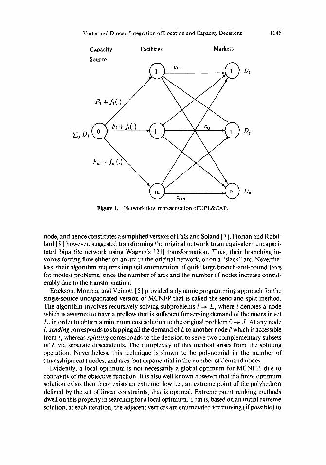
It is also possible to cast the facility location and capacity acquisition problem as a min- imum concave cost network flow problem (MCNFP). Figure 1 depicts a network flow representation of the UFL&CAP. Here, facilities acquire the necessary capacity from a single source by paying the associated costs, to be able to produce and ship the market demand. CFL&CAP can also be represented by the same network by imposing upper bounds on the flows from the capacity source to the facilities. Therefore, the techniques available for solving MCNFP are also suitable for solving our problem.

Guisewite and Pardalos [ 101 provided an extensive review of the solution techniques for MCNFP. There are a variety of algorithms based on branch-and-bound, dynamic pro- gramming, and extreme point ranking. Falk and Soland [ 71 presented a branch-and-bound algorithm for minimizing a separable nonconvex function over a linear polyhedron, e.g., MCNFP. At each node, a linear underestimate of the nonconvex function is minimized over the associated partition of the constraint space. Note that, Soland [ 181 involves mini- mization of the associated linear underestimate over the entire constraint space at each

Verter and Dincer: Integration of Location and Capacity Decisions I145

Capacity Facilities Markets

Figure 1. Network flow representation of UFL&CAP.

node, and hence constitutes a simplified version of Falk and Soland [ 71. Florian and Robil- lard [ 81 however, suggested transforming the original network to an equivalent uncapaci- tated bipartite network using Wagner’s [ 2 I ] transformation. Thus, their branching in- volves forcing flow either on an arc in the original network, or on a “slack” arc. Neverthe- less, their algorithm requires implicit enumeration of quite large branch-and-bound trees for modest problems, since the number of arcs and the number of nodes increase consid- erably due to the transformation.

Erickson, Monma, and Veinott [ 51 provided a dynamic programming approach for the single-source uncapacitated version of MCNFP that is called the send-and-split method. The algorithm involves recursively solving subproblems 1 --f L , where 1 denotes a node which is assumed to have a preflow that is sufficient for serving demand of the nodes in set L , in order to obtain a minimum cost solution to the original problem 0 --+ J . At any node I , sending corresponds to shipping all the demand of L to another node I‘which is accessible from I , whereas splitting corresponds to the decision to serve two complementary subsets of L via separate descendents. The complexity of this method arises from the splitting operation. Nevertheless, this technique is shown to be polynomial in the number of (transshipment) nodes, and arcs, but exponential in the number of demand nodes.

Evidently, a local optimum is not necessarily a global optimum for MCNFP, due to concavity of the objective function. It is also well known however that if a finite optimum solution exists then there exists an extreme flow i.e., an extreme point of the polyhedron defined by the set of linear constraints, that is optimal. Extreme point ranking methods dwell on this property in searching for a local optimum. That is, based on an initial extreme solution, at each iteration, the adjacent vertices are enumerated for moving (if possible) to

1146 Naval Research Logistics, Vol. 42 ( 1995 )

the best adjacent vertex. Guisewite and Pardalos [ 1 I ] provided a computational compari- son of the various local search algorithms for the single source uncapacitated MCNFP.

The review of the relevant literature reveals that although there exist a variety of tech- niques applicable for solving the facility location and capacity acquisition problem, the ones that exploit the problem structure are not that many. Furthermore, since Soland‘s [ 18 ] computational experiments were confined to the fixed-charge cost structure, and Kelly and Khumawala [ 121 provided only a numerical example, the computational performance of the existing algorithms that recognize the problem structure remains to be investigated for problems of the type commonly encountered in practice.

4. ANALYTICAL PROPERTIES OF THE UFL&CAP

Given that each market is accessible by at least one alternative new facility, there always exists a feasible solution to the UFL&CAP since there are no constraints on the capability of the new facilities to serve the market demand. Further, since the associated MCNFP does not contain any negative cost cycles, the UFL&CAP always has a finite optimum solution.

Efroymson and Ray [ 41 observed that for any given set of open facilities, the optimal allocation decisions for UFLP can be obtained by allowing each market to be supplied from the “closest” facility. Such a dominant facility has the least unit variable cost of serving the market among the open facilities. Existence of a dominant facility for each market leads to a significant increase in the computational efficiency of their branch-and-bound procedure. This is because dominance enables decomposition of a nodal problem into y1 easily solved subproblems. Note that, each market’s dominant facility among the set of open facilities is decided independent of the quantity demanded. Linearity of the variable supply costs is a sufficient condition for this property to be present which is called consistent dominance.

It is possible to show that a different version of the dominance property holds for UFL&CAP where the effective variable costs of serving the markets are no longer linear due to the presence of concave capacity acquisition costs. That is, for a given set of open facilities, the optimal sizing and allocation decisions for UFL&CAP can still be obtained by allowing each market to be served by its dominant facility. In this case however, “close- ness” of a facility to a market depends on the demand to be served in addition to the unit variable costs of production and transportation. Thus, the dominant facilities and hence the optimal facility-market allocations might differ due to variations in market demand while costs remain the same. We call this conditional dominance.

To formalize the conditional dominance property, let { 1, 2, , . . , m‘ be the set of open facilities to serve a single market j with demand Di = D. Further, let

g i ( X i ) =A(&) + c&, i = 1,2 , . . . , m’ ( 6 )

represent the total cost of providing Xi units of the commodity to market j from facility i (Xi 2 0). Note that, Cz, Xi = D, and g j ( .) are monotone increasing concave functions whenf; ( .) and cij are defined as in Section 2.

THEOREM 1 : Conditional dominance in the UFL&CAP: At the optimum solution of the UFL&CAP, market j will be fully served by a dominant facility that varies with 4, all other parameters remain the same.

Verter and Dincer: Integration of Location and Capacity Decisions 1147

0 D D j Figure 2. Conditional dominance for fixed-charge costs.

PROOF: It suffices to show that

Since the cost functions are concave,

Summing over the open facilities, and realizing that g, (0) = 0, m' m' v m' v

This proves ( 7 ) since C X j = D 0

Theorem 1 shows that market j will be fully served by the facility that has the minimum total cost of providing 0, among { 1,2, . . . , m' ) . For the ease of exposition, Figure 2 depicts

I148 Naval Research Logistics, Vol. 42 ( 1995)

the presence of conditional dominance for fixed-charge costs in the three-facility case. Al- though, facility 3 happens to be the dominant facility for serving marketj when 0, = D, it should be realized that first, facility 2 and then facility 1 become dominant as D, decreases. Clearly, in an UFL&CAP where there are more than one markets, each market's dominant facility depends on the total demand to be served rather than only the demand of that market, due to the scale economies in capacity acquisition costs.

The presence of conditional dominance is very useful in the characterization of the set of alternative sizes for a facility in the UFL&CAP. Since each market will be fully served by one facility at the optimum solution, each facility can fully serve all possible combina- tions of the markets. Thus, any feasible solution to the UFL&CAP that contains more than one facility serving a market qualifies to be nonoptimal irrespective of the costs incurred. Therefore, there are at most 2" alternative sizes for any facility i , despite the fact that the acquired capacity is represented by a continuous variable (i.e., C,,, X,) in the mathemat- ical model. Note that, this result is in parallel with Zangwill [ 221 stating that an extreme flow of the single-source uncapacitated MCNFP would include at most one arc (with a positive flow) entering each node. Zangwill's property however, does not provide any in- sight about the relation between the arcs included in an extreme flow and the market demand.

5. AN ALGORITHM FOR SOLVING THE UFL&CAP

In the UFL&CAP, the total capacity acquisition cost is a separable concave function. This enables utilization of an underestimate that is also separable in terms of the facilities. Thus, the cost of providing capacity at each facility, i.e., sum of the fixed setup and the capacity acquisition costs, is approximated by a piecewise linear concave function. At each iteration of the algorithm, a pseudofacility is associated with each segment of the current linear underestimate for each facility. Hence, the UFL&CAP is transformed to an equiva- lent UFLP on the basis of the piecewise linear approximation. Therefore, the algorithm devised for solving the UFL&CAP involves solving a sequence of UFLPs. Optimum solu- tion of an UFLP however, corresponds to an extreme flow of the network underlying the UFL&CAP (see Figure 1 ). This is because in an extreme flow of the network, there will be one facility serving each market, which is in parallel with the dominance property as dis- cussed in the previous section. At each iteration, the underestimate is improved by the aid of the optimum solution to the associated UFLP, and hence progressively better lower bounds are provided. Thus, we call this progressive piecewise linear underestimation tech- nique. The algorithm finds a global optimum of the UFL&CAP in a finite number of iter- ations since the number of the extreme flows of the underlying network is finite.

At an iteration of the algorithm, let mi denote the number of pseudo-facilities (indexed by k ) associated with facility i. Further let,

Fik = the fixed setup cost of opening pseudo-facility k of facility i, cik = the unit cost of capacity acquisition at pseudo-facility k of facility i ,

Rlk, Rik+, = the lower and upper bounds on the size of pseudo-facility k of facility i respectively.

Thus, mi represents the number of linear segments in the current approximation of the cost of providing capacity at facility i. Observe that the pseudo-facilities represent size

Verter and Dincer: Integration of Location and Capacity Decisions 1149

ranges for a facility, and hence at most one pseudo-facility associated with the facility must be open in a feasible solution to the UFL&CAP. For pseudo-facility k of facility i, Fjk is the intercept obtained by extending the associated linear segment back to the y-axis whereas, Rik and Rjk+, are the endpoints of the associated partition of the x-axis, and cjk is the slope of the linear segment. On the basis of the current approximation the UFL&CAP can be modeled by the following mathematical program:

subjectto 2 C X,,, = DJ, ;= 1,. . . , n , i E l k c K ,

0 I X j j k I YikDJ, j = 1,. . . , n, i = 1,. . . , m, k = I , . . . , m,, ( 1 1 )

YjkRIks C X l j k s Y A . R ; ~ + ~ , i = I , . . . ,m, k = 1,. . . , m i , (13) j E J

where

K, = the set of pseudo-facilities associated with facility i, c,Jh = the unit cost of serving marketj from pseudo-facility k of facility i i.e., ci,h = CIA + CI,,

and the decision variables are

XI,, = the quantity shipped from pseudo-facility k of facility i to marketj, Ylk = 1 if pseudo-facility k of facility i is opened, 0 otherwise.

The optimal value of zL constitutes a lower bound on the optimal solution value of the UFL&CAP. Constraints ( 10) ensure that each market’s demand will be fully satisfied, con- straints ( 1 1 ) guarantee that markets receive shipments only from open pseudo-facilities. Whereas, constraints ( 13) ensure that the total production of each open pseudo-facility is between its lower and upper bounds, and constraints ( 14) specify that at most one pseudo- facility can be open associated with each facility. Due to the concavity of the piecewise linear underestimates however, the constraints (13) and (14) are redundant in the above formulation. That is for each facility, cost minimization will automatically select the cor- rect pseudo-facility which corresponds to the size range that contains the optimal size of the facility. Evidently, the remaining integer program constitutes a classical model for an- UFLP with C :, mi “facilities” and n markets. As pointed out by Verter and Dincer [ 201 however, there are very efficient techniques available for solving the UFLP such as the dual-based optimization procedure of Erlenkotter [ 61.

1150 Naval Research Logistics, Vol. 42 ( 1995 )

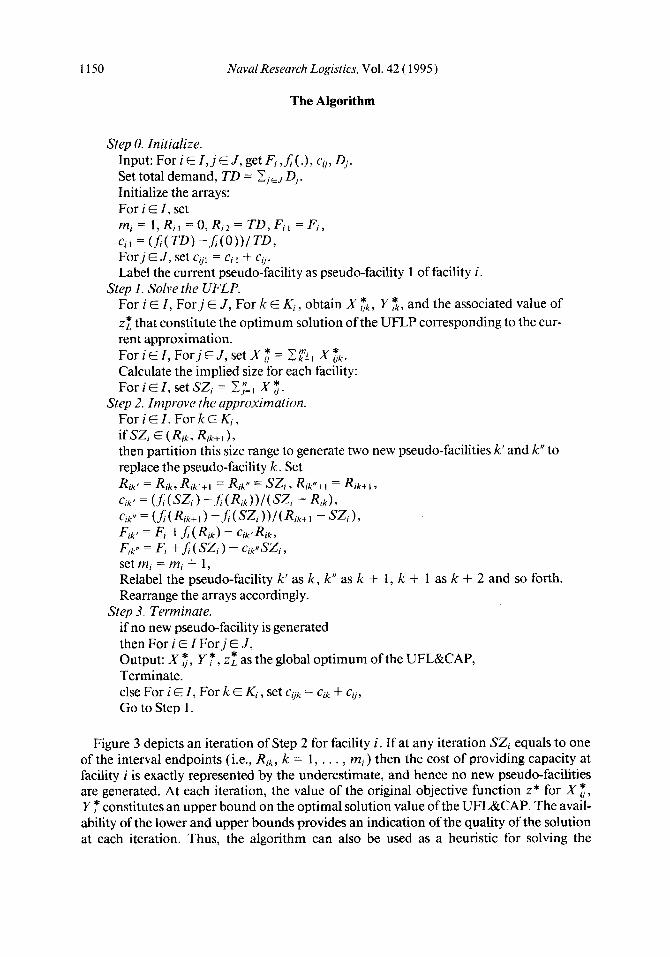
The Algorithm

Step 0. Initialize. Input: For i E I , jE J, get F ; , J ( . ) , cij, Dj. Set total demand, TD = C j E J 0,. Initialize the arrays: For i E I , set mi = 1, R ; , = 0, R j 2 = TD, F- I I = F. I ¶

Forj E J , set cijl = c, + cii. Label the current pseudo-facility as pseudo-facility 1 of facility i.

Step 1 . Solve the UFLP. For i E I , For j E J, For k E K;, obtain X ;k, Y 2, and the associated value of zz that constitute the optimum solution of the UFLP corresponding to the cur- rent approximation. For i E I , Forj E J , set X $ = 2 r~ x $ . Calculate the implied size for each facility: ForiEZ,setSZj= C&lX;.

Step 2. Improve the approximation. For i € I , Fork E Ki,

then partition this size range to generate two new pseudo-facilities k’ and k” to replace the pseudo-facility k. Set

ci1= (f;(TD)-f;(O))/TD,

ifSZ, E (Rik, R i k + l ) ,

R,k’ = R j k , R,k’+l = Ri,. = SZ,, R;kll+I = R ; k + l ,

cik‘= (f;(szi)-.L(Rik))/(SZi -Rik) ,

cik” = (f; ( R i k + l ) -f; (szt ) ) / ( R i k + I - szi ) 3

F;kI = F; + f ; ( R l k ) - ~ , k , R i k ,

F j k ~ = F, + f ; ( S z ; ) - ~ i k ~ ~ S Z j , set mi = mi + 1, Relabel the pseudo-facility k‘ as k , k“ as k + 1, k + 1 as k + 2 and so forth. Rearrange the arrays accordingly.

if no new pseudo-facility is generated then For i E I For j E J, Output: X 3, Y :, z: as the global optimum of the UFL&CAP, Terminate. else For i E I , For k E Ki , set cijk = Cik + cu, Go to Step 1.

Step 3. Terminate.

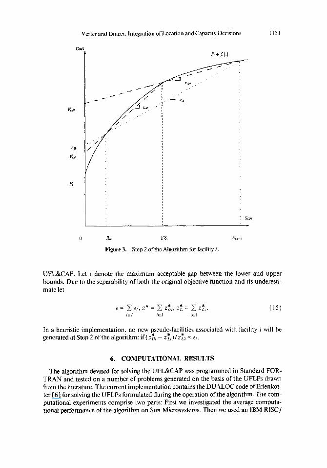
Figure 3 depicts an iteration of Step 2 for facility i. If at any iteration SZ, equals to one of the interval endpoints (i.e., Rjk, k = 1, . . . , mi) then the cost of providing capacity at facility i is exactly represented by the underestimate, and hence no new pseudo-facilities are generated. At each iteration, the value of the original objective function z* for X z , Y 7 constitutes an upper bound on the optimal solution value of the UFLKAP. The avail- ability of the lower and upper bounds provides an indication of the quality of the solution at each iteration. Thus, the algorithm can also be used as a heuristic for solving the

Verter and Dincer: Integration of Location and Capacity Decisions 1 I51

Rk SZ, Rk+l

Figure 3. Step 2 ofthe Algorithm for facility i.

UFL&CAP. Let t denote the maximum acceptable gap between the lower and upper bounds. Due to the separability of both the original objective function and its underesti- mate let

In a heuristic implementation, no new pseudo-facilities associated with facility i will be generated at Step 2 of the algorithm: if (2:; - z ~ , ) / z * , , I t, .

6. COMPUTATIONAL RESULTS

The algorithm devised for solving the UFL&CAP was programmed in Standard FOR- TRAN and tested on a number of problems generated on the basis of the UFLPs drawn from the literature. The current implementation contains the DUALOC code of Erlenkot- ter [6] for solving the UFLPs formulated during the operation ofthe algorithm. The com- putational experiments comprise two parts: First we investigated the average computa- tional performance of the algorithm on Sun Microsystems. Then we used an IBM RISC/

1152 Naval Research Logistics, Vol. 42 ( 1995)

Table 1. Computational results based on cap71 for /3 = 20.

Total

a 6) facilities set of open fac. pseudo-fac. iter. (set) Total cost # of open Change in the # of # of Sun time

1 .oo 0.95 0.90 0.85 0.80 0.75 0.70 0.65 0.60

2097975.8 1682095.1 141 1790.1 1242238.4 I 132823.2 1062582.4 1016944.7 987540.7 968374.6

11 9 6 9 9

10 10 10 I 1

0.23 1.97 2.39 4.29 2.07 1.20 1.15 1.1 1 0.59

6000 to compare the computational performance of the algorithm with that of the Balak- rishnan and Graves [ 11 algorithm for MCNFP. The demand, fixed setup cost, and variable operation and transportation cost data used in the computational experiments originates from the standard test problems of Kuehn and Hamburger [ 151 which are available via electronic mail from the OR-Library (see Beasley [ 3 ] ) . Concerning the capacity acquisi- tion costs, Luss [ 161 pointed out the common use of power functions in the literature as well as the empirical evidence regarding the validity of these functions in modeling indus- trial problems. Verter and Dincer [ 201 stated that the fixed charge cost function and the piecewise linear concave cost function are also popular in modeling the capacity acquisi- tion costs. Observe that the former constitutes a trivial case which can be solved in a single iteration by the algorithm. Whereas, in the latter case an equivalent UFLP can be formu- lated as described in the previous section that again can be solved in one iteration.

In the UFL&CAP the major trade off is between the cost of providing capacity and the operation and transportation costs at each facility. The UFLP named cup71 in the OR- Library will be used as a basis for an illustrative example. The problem contains 16 al- ternative facility locations and 50 markets. The fixed setup costs of opening a facility at any location is given as $7,500 except the already existing facility 1 1, i.e., F, I = 0. Further, let the capacity acquisition costs have the following form:

where a, E [0, 11 represents the economies of scale in capacity acquisition at facility i whereas, pi is a positive scalar for scaling the capacity acquisition cost with respect to the fixed setup cost at that facility. Without loss of generality it will be assumed that ai = a, pi = 0, for, i = 1, . . . , m in investigating the impact of scale economies on the location and sizing decisions. This assumption ensures that the location and sizing decisions are not biased toward establishment of a larger facility at a certain location. For p = 10, a = 1 the optimum solution to the cup71 constitutes opening facilities 1-4,6-9, and 11-13 for serv- ing the 50 markets. When there is economies of scale in capacity acquisition and hence p = 10, a = 0.8 however, facility 12 is closed in the optimum solution while its markets are allocated to facilities 4, 7, and 1 1. Although, the total operation and transportation cost of

Verter and Dincer: Integration of Location and Capacity Decisions 1153

Table 2. Computational results based on cap71 for = 30. Change in the Total

a ($1 facilities fac. pseudo-fac. iter. (set) Total cost # of open set of open # of # of Sun time

1 .oo 0.95 0.90 0.85 0.80 0.78 0.75 0.70 0.65 0.60

2680655.2 2046686.0 1633869.5 1380066.5 1223853.8 1179137.6 1125328.2 1058199.8 1014372.8 985928.7

11 6 5 5 5 6 9 9

10 10

16

43 41 43

121 46

{ 12,9, 1,4,6} 43 (2)

48 42 36 34

1 6 6 6 6 6 7 4 4 4

0.25 1.70 1.90 1.45 1.91 1.71 3.55 1.20 I .20 I .oo

0.55 96749 1.9 1 1 1121 33 3 0.78

serving facility 12’s markets by facilities 4, 7, and 11 is higher, this is more than compen- sated by the economies achieved by increasing the size of each of the three facilities.

Table 1 presents the effects of varying the degree of scale economies in cap71 for p = 20. Note that cy = I constitutes the case where the marginal cost of capacity acquisition is ( a positive) constant, and the total cost decreases as the economies of scale in capacity acqui- sition increases. The fourth column in the table depicts the changes in the set of open facilities as cy decreases. { . . . denotes the set of facilities that are closed due to a decrease in (Y whereas, [. . -1 denotes the set of facilities that are opened for the same reason. The total Sun time (including the input and output) relates to the total number of pseudo- facilities generated during the operation of the algorithm as well as the number of iterations in finding the optimum solution.

Table 2, presents the effects of increasing the weight of capacity acquisition costs with respect to the fixed setup costs in cap71. Note that fl = 30 is a sufficiently large factor since for example facility 3 incurrs a $87,3 19 capacity acquisition cost (for acquiring 2 1,379 units of capacity to serve 37% of the total market demand for 58,268 units) compared to the $7,500 fixed setup cost in the optimal solution for (Y = 0.8. As the capacity acquisition costs increase due to the increase in the scaling factor p, the effects of scale economies are magnified. This leads to drastic changes in facility sizes. Note that as scale economies in- creases at an equal rate at all facilities, its effect in decreasing the number of open facilities gradually vanishes. Increasing the fixed setup costs of opening facilities, results in larger economies of scale in capacity acquisition as depicted by Table 3. Apparently, the demand, and the operation and transportation cost data is the same for all the problems referred in Table 3.

The computational performance of the algorithm is encouraging. All of the test problems mentioned above were solved in at most 8 iterations. Furthermore, for p = 20, (Y = 0.95, the 25 facility locations problem cup101 was solved to optimality in seven iterations gen- erating 70 pseudo-facilities which took 6.44 seconds. Whereas, for the same values of a and p, finding an optimal solution to the 50 facility locations problem cap131 required nine iterations involving the generation of 104 pseudo-facilities in 7.99 seconds. Note that the number of markets is 50 in all the test problems which would require 2 50 iterations in the worst case. The above analysis also enabled us to observe the existence of a sequence in

1154 NuvulReseurch Logistics, Vol. 42 (1995)

Table 3. Computational results for increasing fixed setup costs for fl= 20,a = 0.95.

Total Problem Total cost # of open Change in the # of # of Sun time name Fl ($1 facilities set of open fac. pseudo-fac. iter. (sec)

cup71 7500 1682095.1 9 { 12,9> 46 5 1.97 cup72 12500 1708123.6 5 { 1,4,6,2) 37 5 1.35

35 6 1.05 24 4 0.66

cup73 17500 1727685.5 4 (71 cup74 25000 1745875.9 3 (81

closing (and then opening) facilities as the scale economies increases. For example, facili- ties 5 , 10, and 14-16 are closed in the optimum solution of cap71. Depending on the economies in building larger facilities, the following order can be observed in closing the facilities: 12,9, 1, 4, 6,2, 7, 8. Note that this example presumes the equality of scale econ- omies at all the alternative facility locations. Nevertheless, such an analysis is also possible without the equality assumption and would provide the decision maker with valuable in- formation about the priorities of the alternative facility locations. This is especially crucial when there is an upper bound on the number of facilities to be established due to a variety of reasons such as the scarcity of the financial resources or the strategic policies that dis- courage diversification of operations.

The 16 alternative facility locations and 50 markets UFL&CAP can be cast as a MCNFP with 67 nodes, 8 16 arcs, and 50 commodities where the required flow to each market from the capacity source is treated as a distinct commodity. In the equivalent MCNFP, the cost functions on the 16 arcs connecting the capacity source to the alternative facility locations are concave and the remaining cost functions are linear. (see Figure 1 .) Balakrishnan and Graves [ 11 developed a composite algorithm for the MCNFP with piecewise linear concave costs that generates both heuristic solutions and good lower bounds. Their algorithm is based on Lagrangian relaxation of the flow conservation constraints in a mixed-integer programming formulation of the MCNFP. A combination of dual ascent and subgradient optimization is used to generate Lagrangian lower bounds, and a local improvement pro- cedure is devised to construct locally optimal solutions from the Lagrangian solutions. The algorithm also contains a problem reduction stage for the improvement of the final lower bound.

In order to analyze the relative performance of our algorithm we generated six test prob- lems by using cap71 as a basis and varying the capacity acquisition cost functions. In each test problem, all piecewise linear concave cost functions have the same three cost ranges, and the total cost at the endpoint of each cost range is calculated using a power function in the form of ( 16). Table 4 depicts the range widths (in demand units) and the economies of scale parameters for the test problems. For example, in both wrcnfp 1 and mcnfp2 the range width to total demand ratios are 1 / 15,5 / 15, and 9 / 15 for the three cost ranges. The opti- mal solutions to these UFL&CAPs were found by the use of our progressive piecewise linear underestimation algorithm (without an a priori transformation to UFLP). In using the composite algorithm for solving the equivalent MCNFPs, the maximum number of subgradient iterations was set at 100. Other parameters of the algorithm were set as de- scribed in Balakrishnan and Graves [ 11. The current FORTRAN implementation of the composite algorithm however, assumes that the fixed cost for the first range would be zero for all arcs. Therefore, in order to incorporate the fixed costs of facility location in the

Verter and Dincer: Integration of Location and Capacity Decisions 1155

Table 4. Test Droblem SDecifications.

Problem name

Total Width of demand range 1

mcnfb 1 mcnfp2 mcnfi3 mcnfp4 mcnfp5 mcnli~6

58268 3885 58268 3885 58268 3885 58268 3885 58268 1942 58268 1942

Width of Width of range 2 range 3 19423 34960 19423 34960 11653 42730 11653 42730 971 1 46614 971 1 466 14

P a

30 0.80 30 0.75 30 0.80 30 0.75 30 0.80 30 0.75

equivalent MCNFPs, we divided range 1 into two subranges (and in effect, used four cost ranges) and fixed the width of the first subrange as one unit. Table 5 presents the results of our comparative experiments. The considerably higher computational effort required by the composite algorithm in providing acceptable heuristic solutions can be explained by the fact that it is designed for the more general MCNFP, and hence it does not exploit the structure of UFL&CAP.

7. ANALYTICAL PROPERTIES OF THE CFL&CAP

In the CFL&CAP there is an upper bound on the size of each new facility to be built at an alternative location. In terms of the underlying network (see Figure 1 ), these bounds impose constraints on the flows from the capacity source to the facilities. In consequence, the flow on each arc emanating from a facility is also constrained by the upper bound on the size of the facility. Thus, given that each market is accessible by at least one alternative new facility, the CFL&CAP has a feasible solution only if for each market, the set of facili- ties that have access to the market can acquire sufficient capacity for serving the demand. If a feasible solution to the problem exists however, then there exists a finite optimum solution.

The piecewise linear concave approximation to the total cost of providing capacity at the new facilities enables the transformation of the CFL&CAP to an equivalent CFLP. Therefore, the application of the progressive piecewise linear underestimation algorithm described in Section 5 for solving the CFL&CAP involves solving a sequence of CFLPs. Evidently, the UFLP solver used at every iteration of Step I needs to be replaced by a CFLP solver. Beasley [ 21 presented an efficient algorithm for solving sufficiently large CFLPs whereas, the cross decomposition method of Van Roy [ 191 remains to be the most efficient technique for solving moderate size problems.

Table 5. Results of Comparative Computational Experiments. Problem name mcnfpl mcnfp2 mcnfp3 mcnfp4 mcnfi5 mcnfd

Optimum

I2 13422.9 1 1 12492.2 12138 13.1 1 1 17358.4 121 1816.9 I 1 17549.2

sol. ($1 Total IBM time (sec)

0.42 0.4 1 0.38 0.39 0.39 0.43

Heuristic

11 12532.8 1221458.0 11 18225.2 1222351.4 1122758.4

Lower bound (9)

Total IBM time (sec)

I03941 1.6 1 1029 17.2 1195663.9 1 106340. I 1183563.4 957347.3

8 1.09 105.34 109.45 95.72

I 1 1.83 87.94

1156 Naval Research Logistics, Vol. 42 ( 1995)

Observe that the dominance property does not hold for CFLP, since more than one facility might serve a market in the optimal solution, due to presence of the capacity con- straints. Nevertheless, optimum solution of a CFLP corresponds to an extreme flow of the capacitated network underlying the CFL&CAP. In a capacitated network however, a flow is extremal only if at most one of the arcs entering each node has a flow that is strictly between its bounds. The implication of this for the CFLP, and hence for the CFL&CAP is that in the optimal solution although a market might be served by multiple facilities, all of these facilities except at most one will be fully utilizing their capacity in serving the market. Investigation of properties of the extreme flows of the underlying capacitated network pro- vides further insight about the analytical properties of the CFL&CAP. Since the number of extreme flows is finite, the algorithm will find an optimum solution to the CFL&CAP in a finite number of iterations. The following definitions facilitate the analysis:

DEFINITION I: A facility that fully serves a market’s demand is called a,full-sewer of the market.

DEFINITION 2: A facility that partially serves a market’s demand at its capacity limit is called apartial-server of the market.

DEFINITION 3: A facility that serves the remaining demand of a partially served market is called a remainder-server of the market.

In an extreme flow of the uncapacitated network associated with the UFLP, and hence the UFL&CAP, each market will have one full-server i.e., its dominant facility. This im- plies that each facility might be a full-server for all possible combinations of the markets. Thus, the acquired capacity at each facility can take 2” distinct values. That is at a new facility the optimal size is essentially determined by making a “fully serve/do not serve” decision associated with each market. Note that the number of values that the acquired capacity can take constitutes a worst case bound on the number of iterations of the algo- rithm required for solving the UFL&CAP.

In an extreme flow of the capacitated network associated with the CFLP, and hence the CFL&CAP, each market will have one of the following:

0 1 full-server, 0 I to m- 1 partial-servers and 1 remainder-server, 0 2 to m partial-servers.

This implies that each facility might be one of the following:

.A full-server for some combination of the markets,

.A remainder-server for some combination of the markets,

.A full-server for some combination of the markets, and a remainder-server for a disjoint combination of the markets,

.A partial-server for one of the markets.

Facility i being a remainder-server for market j implies that market j is being partially served by a combination of the remaining m- 1 facilities. Further, facility i being a full- server for market j is equivalent to facility i being a remainder-server of market j that is

Verter and Dincer: Integration of Location and Capacity Decisions 1157

partially served by none of the remaining m-1 facilities. Thus, there are actually 2"-' remainder values that a facility can serve. Hence the following can be stated:

PROPOSITION 1: In the CFL&CAP the acquired capacity at a facility can take at most ( 2'"-' + 1 )" t 1 distinct values.

PROOF For each of the n markets, a facility will either be a remainder-server provid- ing one of the 2m-' remainder values or not serve the market. Alternatively, the facility will be a partial-server for one of the markets, and hence its size will be CAP,. The former implies the first term whereas the latter implies the second term in the expression that constitutes an upper bound on the cardinality of the set of alternative sizes for a facility. I7

Let p denote the number of alternative partial-servers for a market given that one of the facilities is qualified as a remainder-server, and t equal 1 if there are capacity constraints 0 otherwise. The following theorem enables the perception of the UFL&CAP as a special case of the CFL&CAP in terms of the set of alternative sizes for a facility:

THEOREM 2: In the facility location and capacity acquisition problem, the acquired capacity at each facility can take at most ( 2 p + 1 )" + t distinct values.

PROOF Observe that t = 0 implies p = 0 and t = 1 implies p = rn - 1 . 0

Note that however, Proposition 1 provides a weak upper bound on the cardinality of the set of alternative sizes in the CFL&CAP. To show this, let 1c. denote the actual number of alternative sizes for a facility i.e., in the UFL&CAP 1c/ = 2".

PROPOSITION 2: In the CFL&CAP,

1c/ < ( 2 m - I + 1)" + 1. (17)

PROOF: Let Rj( S ) denote the remainder of the demand of market j being partially served by the facilities in the set S. If facility i serves R,( S ) and Ry( S') such that j # j ' then S n S' = where @ denotes the empty set. This is because if facility i' E S , that is i' is a partial-server of marketj, then i' QS', Thus the strict inequality holds. 0

It is possible to provide closed form expressions for 1c. in the CFL&CAP when n is small. L e t p = m - l , f o r n = 2 , p 2 1,

$ = 2 ( 2 P + 1 ) + i = l

1158 Naval Research Logistics, Vol. 42 ( 1995)

Whereas, for n = 3, p 2 2,

Ic/ = 4 ( 2 p + 1) + 2

The above expressions constitute enumeration of the possible sizes of a facility based on the properties stated in the proof of Proposition 2. Evidently, as the number of markets in the CFL&CAP increases, it becomes quite cumbersome to provide a closed form expres- sion for Ic/. Thus, for example in a CFL&CAP with four alternative facility locations three markets, the facilities can actually be of 170 different sizes compared to the upper bound of 729 provided by Proposition 1 . As in the uncapacitated case J. constitutes a worst case bound on the number of iterations of the algorithm required for solving CFL&CAP.

8. CONCLUDING REMARKS

This article presents an integrated approach for the facility location and capacity acqui- sition decisions. The arising model requires global minimization of a concave function over the constraint space which constitutes the set of feasible solutions to the problem. When the facility size is unconstrained, the algorithm devised for solving the problem in- volves solving a sequence of UFLPs. It is shown that the dominance property present in the UFLP also holds for the UFL&CAP, although in a conditional sense. The dominance property however, is instrumental in the characterization of the set of alternative sizes for a facility in the UFL&CAP. Note that the cardinality of this set provides a worst case bound on the number of iterations of the algorithm, required for solving the problem. The computational performance of the algorithm in solving the UFL&CAP is satisfactory. In the capacitated case however, the algorithm involves solving a sequence of CFLPs. Ai- though the dominance property does not hold for the CFLP, the set of alternative sizes for a facility can still be characterized. This provides a framework for the perception of the UFL&CAP as a special case of the CFL&CAP in terms of the alternative sizes of a facility. The computational performance of the algorithm in solving the CFL&CAP is currently an open question.

The proposed algorithm can also be used as a heuristic for solving large size facility location and capacity acquisition problems, since both lower and upper bounds on the optimum solution value are available at each iteration. Further, if it is to be assumed that the capacity acquisition costs are piecewise linear concave functions (as assumed in Balak- rishnan and Graves [l] for the arc flow costs in the MCNFP) then the set of alternative sizes provides valuable information for deciding the endpoints of the linear segments. At this stage, it is possible to relax the linearity assumption regarding the variable operation costs which was stated in Section 2 for the ease of exposition. Thus, the economies of scale in operation costs can also be incorporated in the model by redefining (.) as the total capacity acquisition and operation cost at facility i, and co as the unit cost of shipping from facility i to marketj.

Facility location problems attracted the attention of many operations researchers since

Verter and Dincer: Integration of Location and Capacity Decisions 1 I59

the seminal work of Efroymson and Ray [ 41. Despite abundance of the academic literature however, the papers describing real life applications of analytical approaches for locational decisions are not that many. In our view, this is primarily due to the strategic and complex nature of locational decisions, and hence the limitations of the available models in incor- porating all of the relevant factors. Thus, the present model is in need of two major exten- sions to enhance its capability in assisting the strategic decision-making process. First, the model should be generalized for also dealing with the facility relocation and capacity ex- pansion decisions via incorporation of the dynamic nature of the cost and demand pa- rameters. No need to say however, the arising dynamic model will be much more difficult to handle in terms of its computational complexity compared to the static model provided in this paper. Second, the model should be generalized for dealing with multiple com- modities which will enable simultaneous optimization of the plant location and sizing de- cisions. Note that however, there would normally be a set of alternative technologies for producing each family of commodities. Thus, such an extension constitutes a primary step in improving the model to also provide the optimal technology selection decisions. The more general model should be able to provide the optimal location of the plants, including their facility configuration (implying their product-mix) as well as the amount of capacity acquired in terms of each technology at each open plant. The authors’ current research focuses on the incorporation of the technology selection decisions in the model presented in this paper.

ACKNOWLEDGMENTS

The authors acknowledge the comments and suggestions of two anonymous referees which improved the article. In particular, one of the referees suggested a shorter proof for Theorem I. We are also grateful to Anant Balakrishnan and Steve Graves for enabling us to use their software for testing the relative performance of our algorithm.

REFERENCES

[ 11 Balakrishnan, A., and Graves, S. C., “A Composite Algorithm for a Concave-Cost Network Flow Problem,” Networks, 19, 175-202 (1989).

(21 Beasley, J. E., “An Algorithm for Solving Large Capacitated Warehouse Location Problems,” European Jozirnal of Operational Research. 33,3 14-325 ( 1988).

[3] Beasley, J . E., “OR-Library: Distributing Test Problems by Electronic Mail,” Juzimal of Oper- ationalResearch Society, 41, 1069-1072 ( 1990).

[4] Efroymson, M. A., and Ray, T. L., “A Branch-and-Bound Algorithm for Plant Location,” Op- erafions Research, 14,361-368 ( 1966).

[5] Erickson, R. E., Monma, C. L., and Veinott, A. F., “Send-and-Split Method for Minimum Concave Cost Network Flows,’’ Mathematics of Operations Research. 12,634-664 ( 1987 ).

[6] Erlenkotter, D., “A Dual Based Procedure for Uncapacitated Facility Location,” Operalions Research, 26,992- 1009 ( 1978).

[7] Falk, J. E., and Soland, R. M., “An Algorithm for Separable Nonconvex Programming Prob- lems,” Management Science, 15,550-569 ( 1969).

[8] Florian, M., and Robillard, P., “An Implicit Enumeration Algorithm for the Concave Cost Network Problem,” Management Science, 18, 184- 193 ( 197 I ) .

[9] Geoffrion, A. M., “Objective Function Approximation in Mathematical Programming,” Math- ematical Programming, 13,23-37 (1977).

[lo] Guisewite, G. M., and Pardalos, P. M., “Minimum Concave-Cost Network Flow Problems:

1160 NavalResearch Logistics, Vol. 42 ( 1995)

Applications, Complexity and Algorithms,” Annals of Operations Research, 25, 75- 100 (1990).

[ 1 1 J Guisewite, G. M., and Pardalos, P. M., “Algorithms for the Single-Source Uncapacitated Mini- mum Concave-Cost Network Flow Problem,” Journal of Global Optimization, 1, 245-265 (1991).

[ 121 Kelly, D. L., and Khumawala, B. M., “Capacitated Warehouse Location With Concave Costs,” Journal of Operational Research Society, 33,8 17-826 ( 1982).

[ 131 Khumawala, B. M., and Kelly, D. L., “Warehouse Location with Concave Costs,” ZNFOR, 12,

[ 141 Krarup, J., and Pruzan, P. M., “The Simple Plant Location Problem: Survey and Synthesis,” European Journal of Operational Research, 12,36-8 1 ( 1983).

[ 151 Kuehn, A. A., and Hamburger, M. J., “A Heuristic Program for Locating Warehouses,” Man- agement Science, 9,643-666 (1963).

[ 161 Luss, H., “Operations Research and Capacity Expansion Problems: A Survey,” Operations Re- search, 30,907-947 ( 1982).

[ 171 Pardalos, P. M., and Rosen, J. B., “Constrained global optimization: Algorithms and Applica- tions,” Lecture Notes in Computer Science 268, Springer-Verlag, New York, 1987.

[ 181 Soland, R. F., “Optimal Facility Location with Concave Costs,” Operations Research, 22,373- 385 (1974).

[ 191 Van Roy, T. J., “A Cross Decomposition Algorithm for Capacitated Facility Location,” Oper- ationsResearch, 34, 145-163 (1986).

[20] Verter, V., and Dincer, M. C., “An Integrated Evaluation of Facility Location, Capacity Acqui- sition and Technology Selection for Designing Global Manufacturing Strategies,” European Journal of Operational Research, 60, 1 - 18 ( 1992).

[21 J Wagner, H. M., “On a Class of Capacitated Transportation Problems,” A4anagement Science,

1221 Zangwill, W. I., “Minimum Concave Cost Flows in Certain Networks,” Management Science,

55-65 (1974).

5,304-318 (1959).

14,429-450 ( 1968).

Manuscript received September 28, 1992 Revised October 1994 Accepted October 29, 1994