Transportation, facility location and inventory issues in ...

Issues in distribution

network design

471

Transportation, facilitylocation and inventory issuesin distribution network design

An investigationVaidyanathan Jayaraman

Division of Business Administration, University of SouthernMississippi, Long Beach, Mississippi, USA

Introduction and backgroundIn this paper we consider the relationship between the management ofinventory, location of facilities and the determination of transportation policysimultaneously in a distribution network design environment. These areasinteract, for example, when alternatives exist for location of facilities and fortransporting replacement inventory from a manufacturing plant, and eachtransportation and location alternative necessitates different parameters forinventory management. These selections are often made on the basis of cost ortransit time. This paper will analyze the interdependence among the three areasand propose an integrated model for design of a distribution network thatrepresents their interdependence. The proposed model can be expected toprovide a more complete tradeoff that exists among the three components,hence leading to better solutions than those provided by existing mathematicalmodels.

Mathematical location models are designed to address a number of questionsincluding: How many facilities should be sited? Where should each facility belocated? How should customer demand be allocated to the facilities? We use theterm facility here in its broadest sense. It is meant to include entities such asfactories, schools, warehouses, retail outlets, hospitals, computer concentrators,emergency warning sirens, and day-care centers to name but a few that havebeen analyzed in the literature. In spatial analysis, proximity is a fundamentalmetric, many siting models seek to optimize it. However, rather than optimizing,decision makers often base decisions on the “satisfactory” rather than the bestpossible. The concept of coverage is this type of measure (Batta and Mannur,1990). Another important characteristic for a facility is its capacity. Whilefacilities are often assumed to be able to serve all demand assigned to them,congested systems or those with wide variation in workload may need toconsider capacity constraints that limit the total workload for which a facilitywill be responsible.

Almost every private and public sector that we can think of has been facedwith the task of locating facilities. The ability of a firm to produce and market

International Journal of Operations& Production Management,

Vol. 18 No. 5, 1998, pp. 471-494,© MCB University Press, 0144-3577

IJOPM18,5

472

its products effectively or to deliver high-quality services is dependent in parton the location of the firm’s facilities in relation to other facilities and itscustomers. The interested reader is encouraged to refer to (Daskin, 1995) and(Drezner, 1995) for a comprehensive survey on facility location. Several reviewarticles (Brandeau and Chiu, 1989; Schilling et al., 1993) have also beenpublished on the topic. Facility location models for distribution planning haveinspired a large body of literature that spans well over two decades (Aikens,1985). The distribution/location family of problems covers formulations whichrange in complexity from simple single commodity linear deterministic modelsto multicommodity nonlinear stochastic versions.

Transportation has been recognized for many years as being one of the mostimportant activities in the physical distribution function. The work of Baumoland Vinod (1970) is one of the first attempts to determine a shipper choice oftransportation option in a single market and could be viewed as a cost modelthat provides the total transportation and inventory cost associated with eachtransportation option. Buffa and Reynolds (1977) developed a model to includea number of transport-related variables. They identified the “failure to considerexplicitly transport cost as a determinant of inventory strategy” as a “majorshortcoming” of inventory models and concluded an existence of a correlationbetween purchase quantity and transportation mode decision.

Constable and Whybark (1978) proposed an alternative version of theinventory-theoretic model that explicitly included both carrying and back-ordercost. The model jointly determined the inventory reorder points, orderquantities, and transportation choices that provide minimum totaltransportation and inventory costs. Langley (1980) proposed the inclusion oftransportation cost functions in models that represent the simultaneousconsideration of several types of distribution activity and the dependence ofunit transportation cost on shipment size and concluded that a higher productvalue resulted in small optimal shipment size due to inventory carrying costeffects. Larson (1988) developed a model that simultaneously determined theoptimal transportation choice and shipping quantity through calculation of aneconomic transportation quantity. Carter and Ferrin (1995) presented postulatesthat compromises by the buyer, seller, and carrier can serve to improveprofitability for all parties.

Determining an optimal policy for an inventory system configuration is adifficult choice. Too often, the estimation of the costs of carrying inventory in adistribution system is limited because they are considered to be only a minorportion of the total distribution costs. However, inventory can represent asignificant proportion of distribution costs. Van Beek (1981) investigateddifferent strategies for locating inventories in a two-level distribution systemthat consisted of a central manufacturing plant, a central distribution centerand four local distribution centers. The objective of the model was to determinethe “best” distribution strategy that minimized the sum of inventory carryingand ordering cost over all stocking points in the system. Davis and Davidson(1991) observed a significant difference in cost between order sales and stock


network design

473

sales manufacturing in finished goods inventory for the auto industry aroundthe world and concluded that the opportunity to shrink this inventory holdsimmense potential. Rajagopalan and Kumar (1994) analyzed the issue ofproviding the customer with the option of purchasing from stock or by placingan order and found that the optimal quantity of stock to be held by the retailerdecreases when the option of placing an order is offered. The basic designproblem in any production and distribution network is to match supply anddemand at the output points of the system in the most economical way.

Most of the existing mathematical models have focused on individualcomponents of the network design like warehouse location. They fail to includeinventory cost as a component of their objective function and have assumed pre-specified transportation choices. The evaluation of strategic changes to adistribution system configuration involves the estimation of several costs andbenefit measures, including the impact on the amount of inventory carried inthe total distribution network. Perl and Sirisoponsilp (1989) proposed the onlyexisting work on the interdependence between location, transportation andinventory decisions. In their paper, they provide a schematic representation ofthe interdependence between facility location, transportation and inventorydecisions.

Strategic distribution center location decisions can include determinationand location of number of warehouses and plants, warehouse and plantcapacity load ratio, assignment of customer demands to open warehouses andassignment of open warehouses to open plants among others. In this paper, wewill use the term warehouse and distribution center interchangeably. Strategictransportation decisions include choice of transportation mode (rail, truck, air,ship) and choice of type of carriage (common, contract, private). Other decisionscan include the size of shipments (or shipment frequency), and assignment ofloads to vehicles. Inventory decisions are concerned with total inventory level inthe system, location of inventories, and levels of cycle stock at various locations.There is a strong interdependence among all three decisions. An increase in thenumber of distribution centers increases total system inventory. The location ofinventories also determines the transportation mode choices, type, and choiceof carrier. A decision to maintain good customer service would require the useof faster and more reliable transportation mode. A decision to change theaverage level of cycle stock held at a facility would lead to a change in shipmentsize. Due to recent trends in emerging technologies and competition, companiesare convinced that it is no longer valid to assume that a single unittransportation cost is sufficient when we analyze among distribution centerlocations, or to consider inventory decisions as related only to number andlocation of warehouses and independent from transportation decisions.

The model that is presented in this paper builds upon the initial model thatwas proposed by Perl and Sirisiponsilp (1980). There are some major differences.Their model was only a conceptual model. It provided an objective function thatincluded the trade-off between location, transportation and inventory-relatedissues. It did not contain any constraints by way of demand satisfaction of

IJOPM18,5

474

customer outlets and capacity restrictions established by warehouses andmanufacturing plants. Further it was proposed for a single product and was nottested numerically. Our discussion in this paper will focus on an integratedmathematical programming mixed-integer model. The design objectiverepresents a minimization of the total distribution cost associated with all threedecision components (facility locations, inventory parameters andtransportation alternative selection). It also represents multiple transportationoptions and explicitly requires that demands of customer outlets for all productsare satisfied by open distribution centers. Our problem, then, is tosimultaneously determine which transportation alternative and inventoryparameters together with the number and location of plants and distributioncenters would lead to the lowest total inventory, transportation and location cost.

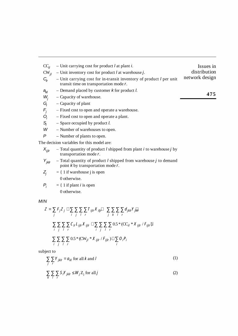
The mathematical model (FLITNET)In this section, we present a mixed integer programming model, FLITNET(Facility Location, Inventory, Transportation NETwork) that relates thetransportation mode attributes, the location of distribution centers and plants,and the inventory policy parameters subject to constraints imposed by thedistribution network design.

The FLITNET model’s total costs can be expressed as follows:

Annual Cost = Fixed cost to open and operate a warehouse +Transportation cost + Delivery cost + In-transit inventorycost + Plant cycle stock cost + Warehouse cycle stock cost+ Fixed cost to open and operate a plant

The following notation is used for the FLITNET model:

I – Set of potential plants.

J – Set of potential warehouses.

K – Set of customer demand outlets.

L – Set of products.

R – Set of different transportation modes.

Tijlr – Unit transportation cost for shipping product l between plant i andwarehouse j by transportation mode r.

Fijlr – Shipment frequency of using transportation mode r for product lfrom plant i to warehouse j.

djklr – Unit delivery cost for shipping product l between warehouse j anddemand point k using transportation mode r.

Lijlr – Average lead time for shipments of product l from plant i towarehouse j by transportation mode r.

CSijlr – Cycle stock cost at plant i associated with shipment of product l towarehouse j by transportation mode r.


network design

475

CCil – Unit carrying cost for product l at plant i.CWjl – Unit inventory cost for product l at warehouse j.Clr – Unit carrying cost for in-transit inventory of product l per unit

transit time on transportation mode r.

akl – Demand placed by customer k for product l.Wj – Capacity of warehouse.

Gi – Capacity of plant

Fj – Fixed cost to open and operate a warehouse.

Oi – Fixed cost to open and operate a plant.

Sl – Space occupied by product l. W – Number of warehouses to open.

P – Number of plants to open.

The decision variables for this model are:

Xijlr – Total quantity of product l shipped from plant i to warehouse j bytransportation mode r.

Yjklr – Total quantity of product l shipped from warehouse j to demandpoint k by transportation mode r.

Zj = { 1 if warehouse j is open

0 otherwise.

Pi = { 1 if plant i is open

0 otherwise.

MIN

subject to

(1)

(2)S Y W jl jklrrlk

j∑∑∑ ≤ Z for all j

Y a k ljklrrj

kl∑∑ = for all and

0 5. * ( * / )rlji

jl ijlr ijlr ii

iX F O P∑∑∑∑ ∑+CW

C L X X Flr ijlrrlji

ijlr ilrlji

ijlr ijlr∑∑∑∑ ∑∑∑∑+ +0 5. * ( * / )CC

Z F Z T X d Yjj

j ijlrrlji

iljr jklrrlkj

jklr= + + +∑ ∑∑∑∑ ∑∑∑∑

IJOPM18,5

476

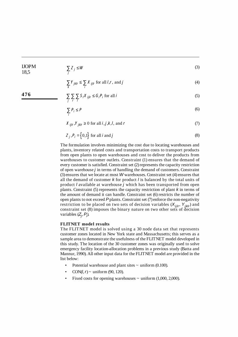
(3)

(4)

(5)

(6)

(7)

(8)

The formulation involves minimizing the cost due to locating warehouses andplants, inventory related costs and transportation costs to transport productsfrom open plants to open warehouses and cost to deliver the products fromwarehouses to customer outlets. Constraint (1) ensures that the demand ofevery customer is satisfied. Constraint set (2) represents the capacity restrictionof open warehouse j in terms of handling the demand of customers. Constraint(3) ensures that we locate at most W warehouses. Constraint set (4) ensures thatall the demand of customer k for product l is balanced by the total units ofproduct l available at warehouse j which has been transported from openplants. Constraint (5) represents the capacity restriction of plant k in terms ofthe amount of demand it can handle. Constraint set (6) restricts the number ofopen plants to not exceed P plants. Constraint set (7) enforce the non-negativityrestriction to be placed on two sets of decision variables (Xijlr, Yjklr) andconstraint set (8) imposes the binary nature on two other sets of decisionvariables (Zj, Pi).

FLITNET model resultsThe FLITNET model is solved using a 30 node data set that representscustomer zones located in New York state and Massachusetts; this serves as asample area to demonstrate the usefulness of the FLITNET model developed inthis study. The location of the 30 customer zones was originally used to solveemergency facility location-allocation problems in a previous study (Batta andMannur, 1990). All other input data for the FLITNET model are provided in thelist below:

• Potential warehouse and plant sites ~ uniform (0.100).

• CON(l, r) ~ uniform (90, 120).

• Fixed costs for opening warehouses ~ uniform (1,000, 2,000).

Z P i jj i, ,= { }0 1 for all and

X Y i j k l rijlr jklr, , , , ,≥ 0 for all and

P Pii

∑ ≤

S X G P illrj

ijlr i i∑∑∑ ≤ for all

Y X l r jjklrk

ijlri

∑ ∑≤ for all and , ,

Z Wjj

∑ ≤


network design

477

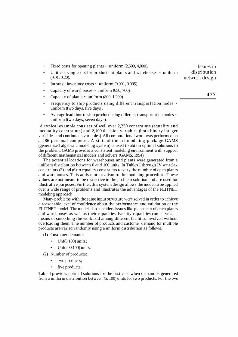
• Fixed costs for opening plants ~ uniform (2,500, 4,000).• Unit carrying costs for products at plants and warehouses ~ uniform

(0.01, 0.20).• Intransit inventory costs ~ uniform (0.001, 0.005).• Capacity of warehouses ~ uniform (650, 700).• Capacity of plants ~ uniform (800, 1,200).• Frequency to ship products using different transportation nodes ~

uniform (two days, five days).• Average lead time to ship product using different transportation nodes ~

uniform (two days, seven days).A typical example consists of well over 2,250 constraints (equality and

inequality constraints) and 2,100 decision variables (both binary integervariables and continuous variables). All computational work was performed ona 486 personal computer. A state-of-the-art modeling package GAMS(generalized algebraic modeling system) is used to obtain optimal solutions tothe problem. GAMS provides a consistent modeling environment with supportof different mathematical models and solvers (GAMS, 1994).

The potential locations for warehouses and plants were generated from auniform distribution between 0 and 100 units. In Tables I through IV we relaxconstraints (3) and (6) to equality constraints to vary the number of open plantsand warehouses. This adds more realism to the modeling procedure. Thesevalues are not meant to be restrictive in the problem solution and are used forillustrative purposes. Further, this system design allows the model to be appliedover a wide range of problems and illustrates the advantages of the FLITNETmodeling approach.

Many problems with the same input structure were solved in order to achievea reasonable level of confidence about the performance and validation of theFLITNET model. The model also considers issues like placement of open plantsand warehouses as well as their capacities. Facility capacities can serve as ameans of smoothing the workload among different facilities involved withoutoverloading them. The number of products and customer demand for multipleproducts are varied randomly using a uniform distribution as follows:

(1) Customer demand:• Unf(5,100) units;• Unf(200,100) units.

(2) Number of products:• two products;• five products.

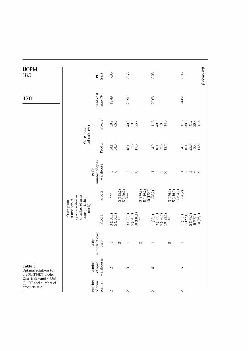
Table I provides optimal solutions for the first case when demand is generatedfrom a uniform distribution between (5, 100) units for two products. For the two

IJOPM18,5

478

Ope

n pl

ant

tran

spor

ts to

op

en w

areh

ouse

(num

ber

of u

nits

,tr

ansp

orta

tion

War

ehou

sem

ode)

load

rat

io (%

)N

umbe

rN

umbe

rN

ode

Nod

eof

ope

nof

ope

nnu

mbe

r of

ope

nnu

mbe

r of

ope

nFi

xed

cost

CPU

plan

tsw

areh

ouse

spl

ant

Prod

1Pr

od 2

war

ehou

sePr

od 1

Prod

2ra

tio (%

)(s

ec)

22

13

(230

,1)

***

334

.158

.219

.49

7.96

5 (2

36,1

)6

34.0

66.0

5**

*3

(393

,2)

5 (4

59,2

)2

31

3 (1

22,1

)**

*3

18.1

40.0

25.9

18.

635

(226

,1)

532

.559

.010

(118

,1)

1017

.625

.75

***

3 (2

70,2

)5

(410

,2)

10 (1

72,2

)2

41

1 (3

3,1)

1 (7

8,2)

14.

911

.629

.68

8.08

3 (1

22,1

)3

18.1

40.0

5 (2

26,1

)5

32.5

59.0

10 (8

5,1)

1012

.714

.05

***

3 (2

70,2

)5

(410

,2)

10 (9

4,2)

25

11

(33,

1)1

(78,

2)1

4.90

11.6

34.8

28.

063(

122,

1)3

18.1

40.0

5 (1

78,1

)5

25.6

41.2

6 (5

7,1)

68.

320

.310

(76,

1)10

11.3

11.6

(Con

tinue

d)

Table I.Optimal solutions to the FLITNET modelCase 1: demand ~ Unf(5, 100) and number ofproducts = 2


network design

479

Ope

n pl

ant

tran

spor

ts to

op

en w

areh

ouse

(num

ber

of u

nits

,tr

ansp

orta

tion

War

ehou

sem

ode)

load

rat

io (%

)N

umbe

rN

umbe

rN

ode

Nod

eof

ope

nof

ope

nnu

mbe

r of

ope

nnu

mbe

r of

ope

nFi

xed

cost

CPU

plan

tsw

areh

ouse

spl

ant

Prod

1Pr

od 2

war

ehou

sePr

od 1

Prod

2ra

tio (%

)(s

ec)

5**

*2

(90,

2)3

(214

,2)

5 (2

52,2

)6

(140

,2)

10 (7

8,2)

Not

es:

Fixe

d co

st r

atio

=Fi

xed

cost

of o

pen

war

ehou

ses

+ p

lant

s

Tot

al c

ost o

f opt

imal

sol

utio

n

War

ehou

se lo

ad r

atio

=T

otal

am

ount

of d

eman

d fo

r ea

ch p

rodu

ct b

y as

sign

ed c

usto

mer

s

Tot

al c

apac

ity o

f ope

n w

areh

ouse

for

each

pro

duct

Table I.

IJOPM18,5

480

Ope

n pl

ant t

rans

port

sto

ope

n w

areh

ouse

(num

ber

War

ehou

seof

uni

tslo

ad r

atio

tran

spor

tatio

n m

ode)

(%)

Nod

eN

ode

Fixe

dN

umbe

rN

umbe

rnu

mbe

rnu

mbe

rco

stof

ope

n of

ope

nof

ope

nof

ope

nra

tioCP

Upl

ants

war

ehou

ses

plan

tPr

od 1

Prod

2Pr

od 3

Prod

4Pr

od 5

war

ehou

sePr

od 1

Prod

2Pr

od 3

Prod

4Pr

od 5

(%)

(sec

)

34

11

(240

,1)

1 (3

33,2

)1

(254

,2)

1 (1

78,2

)1

(85,

3)1

9.00

12.5

9.50

8.70

8.40

9.52

19.0

14

***

5 (5

28,2

)**

*1

(53,

3)1

(124

,1)

413

.217

.016

.015

.817

.76

(353

.2)

4 (1

70,2

)1

(14,

3)4

(253

,3)

5 (8

1,1)

519

.820

.116

.318

.216

.75

(326

,2)

5 (3

70,3

)5

(165

,3)

6 (4

57,3

)6

12.9

13.1

15.8

16.0

17.0

6 (4

30,2

)5

4 (3

55,1

)4

(457

,2)

4 (4

29,2

)**

***

*5

(534

,1)

5 (1

5,2)

5 (4

38,2

)6

(346

,1)

6 (4

26,2

)3

51

1 (1

57,1

)1

(144

,2)

1 (1

60,2

)1

(148

,2)

1 (9

4,3)

15.

95.

46.

05.

58.

211

.06

18.5

14

(93,

2)4

(294

,2)

413

.217

.016

.015

.814

.24

***

5 (3

18,2

)**

*4

(170

,2)

1 (1

24,1

)6

(286

,2)

4 (2

53,3

)4

(293

,1)

519

.820

.116

.318

.216

.78

(256

,2)

5 (3

62,2

)4

(89,

3)5

(165

,3)

5 (8

1,1)

65.

610

.68.

49.

69.

36

(257

,2)

5 (3

70,3

)8

(210

,2)

6 (2

49,3

)8

10.4

9.6

11.0

9.6

11.5

8 (4

6,3)

8 (3

07,3

)

(Con

tinue

d)

Table II.Optimal solutions toFLITNET modelCase 2: demand ~ unf(5,100) and number ofproducts = 5


network design

481

Ope

n pl

ant t

rans

port

sto

ope

nw

areh

ouse

(num

ber

War

ehou

seof

uni

ts,

load

rat

iotr

ansp

orta

tion

mod

e)(%

)N

ode

Nod

eFi

xed

Num

ber

Num

ber

num

ber

num

ber

cost

of o

pen

of o

pen

of o

pen

of o

pen

ratio

CPU

plan

tsw

areh

ouse

spl

ant

Prod

1Pr

od 2

Prod

3Pr

od 4

Prod

5w

areh

ouse

Prod

1Pr

od 2

Prod

3Pr

od 4

Prod

5(%

)(s

ec)

54

(355

,1)

4 (4

57,2

)4

(336

,2)

***

***

5 (5

34,1

)5

(225

,2)

5 (4

38,2

)6

(150

,1)

6 (2

26,2

)8

(279

,1)

36

2**

*1

(144

,2)

***

1 (5

7,3)

***

15.

95.

45.

53.

64.

612

.16

18.3

42

(80,

2)2

(71,

3)4

(457

,2)

4 (2

53,3

)2

0.8

3.0

3.3

2.7

3.5

5 (4

63,2

)5(

255,

2)6

(286

,1)

5 (1

65,3

)4

13.2

17.0

16.4

17.7

17.7

8 (2

56,2

)6

(257

,2)

8 (2

10,2

)5

19.0

17.2

13.0

15.6

13.3

8 (4

6,3)

4**

***

*1

(22,

2)1

(39,

3)1

(124

,1)

65.

610

.68.

49.

69.

34

(222

,2)

2 (9

3,1)

4 (2

93,1

)8

10.4

9.6

11.0

9.6

11.5

4 (1

83,3

)5

(81,

1)5

((277

,3)

6 (2

49,3

)8

(307

,3)

(Con

tinue

d)

Table II.

IJOPM18,5

482

Ope

n pl

ant t

rans

port

sto

ope

nw

areh

ouse

(num

ber

War

ehou

seof

uni

ts,

load

rat

iotr

ansp

orta

tion

mod

e)(%

)N

ode

Nod

eFi

xed

Num

ber

Num

ber

num

ber

num

ber

cost

of o

pen

of o

pen

of o

pen

of o

pen

ratio

CPU

plan

tsw

areh

ouse

spl

ant

Prod

1Pr

od 2

Prod

3Pr

od 4

Prod

5w

areh

ouse

Prod

1Pr

od 2

Prod

3Pr

od 4

Prod

5(%

)(s

ec)

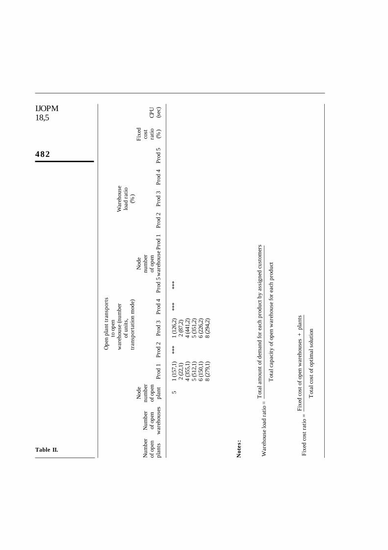
51

(157

,1)

***

1 (1

26,2

)**

***

*2

(22,

1)2

(87,

2)4

(355

,1)

4 (4

41,2

)5

(512

,1)

5 (3

51,2

)6

(150

,1)

6 (2

26,2

)8

(279

,1)

8 (2

94,2

)

Not

es:

Fixe

d co

st r

atio

=Fi

xed

cost

of o

pen

war

ehou

ses

+ p

lant

s

Tot

al c

ost o

f opt

imal

sol

utio

n

War

ehou

se lo

ad r

atio

=T

otal

am

ount

of d

eman

d fo

r ea

ch p

rodu

ct b

y as

sign

ed c

usto

mer

s

Tot

al c

apac

ity o

f ope

n w

areh

ouse

for

each

pro

duct

Table II.


network design

483

Ope

n pl

ant

tran

spor

ts to

op

en w

areh

ouse

(num

ber

of u

nits

,tr

ansp

orta

tion

War

ehou

sem

ode)

load

rat

io (%

)N

umbe

rN

umbe

rN

ode

Nod

eof

ope

nof

ope

nnu

mbe

r of

ope

nnu

mbe

r of

ope

nFi

xed

cost

CPU

plan

tsw

areh

ouse

spl

ant

Prod

1Pr

od 2

war

ehou

sePr

od 1

Prod

2ra

tio (%

)(s

ec)

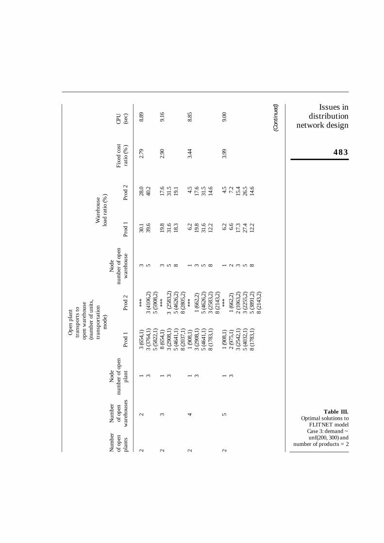
22

13

(654

,1)

***

330

.128

.02.

798.

893

3 (3

764,

1)3

(410

6,2)

539

.640

.25

(582

2,1)

5 (5

908,

2)2

31

8 (6

54,1

)**

*3

19.8

17.6

2.90

9.16

33

(290

8,1)

3 (2

583,

2)5

31.6

31.5

5 (4

641,

1)5

(462

6,2)

818

.319

.18

(203

7,1)

8 (2

805,

2)2

41

1 (9

08,1

)**

*1

6.2

4.5

3.44

8.85

33

(290

8,1)

1 (6

62,2

)3

19.8

17.6

5 (4

641,

1)5

(462

6,2)

531

.631

.58

(178

3,1)

3 (2

583,

2)8

12.2

14.6

8 (2

143,

2)2

51

1 (9

08,1

)**

*1

6.2

4.5

3.99

9.00

32

(975

,1)

1 (6

62,2

)2

6.6

7.2

3 (2

542,

1)2

(106

3,2)

317

.315

.45

(403

2,1)

3 (2

255,

2)5

27.4

26.5

8 (1

783,

1)5

(389

1,2)

812

.214

.68

(214

3,2)

(Con

tinue

d)

Table III.Optimal solutions to

FLITNET modelCase 3: demand ~unf(200, 300) and

number of products = 2

IJOPM18,5

484

Ope

n pl

ant

tran

spor

ts to

op

en w

areh

ouse

(num

ber

of u

nits

,tr

ansp

orta

tion

War

ehou

sem

ode)

load

rat

io (%

)N

umbe

rN

umbe

rN

ode

Nod

eof

ope

nof

ope

nnu

mbe

r of

ope

nnu

mbe

r of

ope

nFi

xed

cost

CPU

plan

tsw

areh

ouse

spl

ant

Prod

1Pr

od 2

war

ehou

sePr

od 1

Prod

2ra

tio (%

)(s

ec)

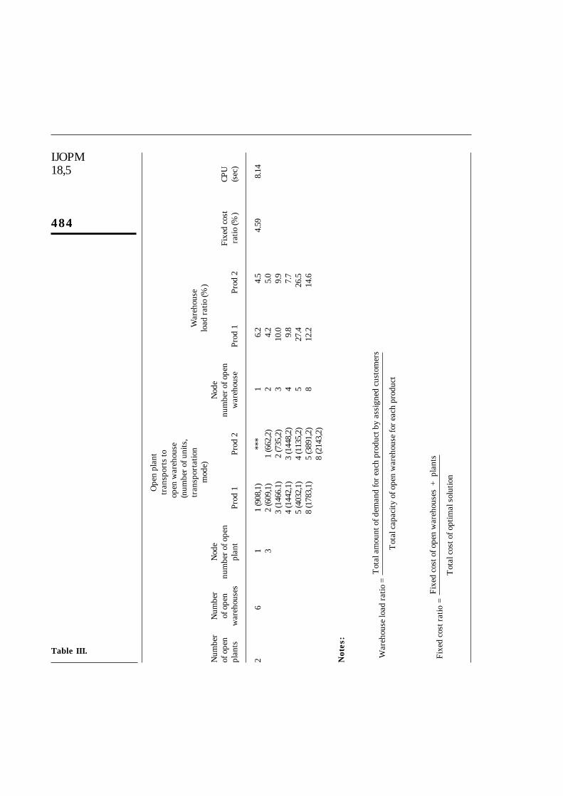
26

11

(908

,1)

***

16.

24.

54.

598.

143

2 (6

09,1

)1

(662

,2)

24.

25.

03

(146

6.1)

2 (7

35,2

)3

10.0

9.9

4 (1

442,

1)3

(144

8,2)

49.

87.

75

(403

2,1)

4 (1

135,

2)5

27.4

26.5

8 (1

783,

1)5

(389

1,2)

812

.214

.68

(214

3,2)

Not

es:

Fixe

d co

st r

atio

=Fi

xed

cost

of o

pen

war

ehou

ses

+ p

lant

s

Tot

al c

ost o

f opt

imal

sol

utio

n

War

ehou

se lo

ad r

atio

=T

otal

am

ount

of d

eman

d fo

r ea

ch p

rodu

ct b

y as

sign

ed c

usto

mer

s

Tot

al c

apac

ity o

f ope

n w

areh

ouse

for

each

pro

duct

Table III.


network design

485

Ope

n pl

ant t

rans

port

sto

ope

nw

areh

ouse

(num

ber

of u

nits

,W

areh

ouse

tran

spor

tatio

nlo

ad r

atio

mod

e)(%

)N

ode

Nod

eFi

xed

Num

ber

Num

ber

num

ber

num

ber

cost

of o

pen

of o

pen

of o

pen

of o

pen

ratio

CPU

plan

tsw

areh

ouse

spl

ant

Prod

1Pr

od 2

Prod

3Pr

od 4

Prod

5w

areh

ouse

Prod

1Pr

od 2

Prod

3Pr

od 4

Prod

5(%

)(s

ec)

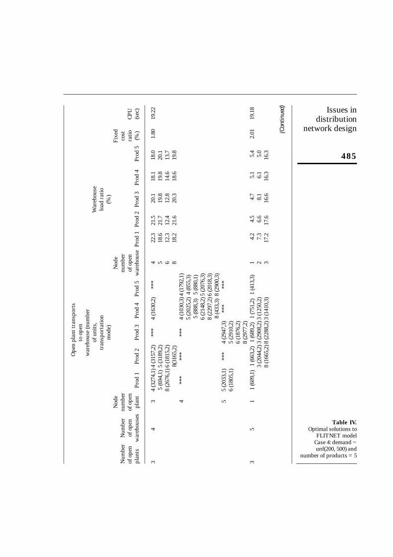
34

34

(327

4,1)

4 (3

157,

2)**

*4

(163

0,2)

***

422

.321

.520

.118

.118

.01.

8019

.22

5 (6

94,1

)5

(318

9,2)

518

.621

.719

.819

.820

.18

(267

6,1)

6 (1

815,

2)6

12.3

12.4

12.8

14.6

13.7

8(31

65,2

)8

18.2

21.6

20.3

18.6

19.8

4**

***

***

*4

(103

0,3)

4 (1

792,

1)5

(202

5,2)

4 (8

55,3

)5

(888

,3)

5 (8

80,1

)6

(214

8,2)

5 (2

076,

3)8

(229

7,2)

6 (2

018,

3)8

(433

,3)

8 (2

900,

3)5

5 (2

033,

1)**

*4

(294

7,3)

***

***

6 (1

805,

1)5

(291

0,2)

6 (1

876,

2)8

(297

7,2)

35

11

(609

,1)

1 (6

63,2

)1

(689

,2)

1 (7

51,2

)1

(413

,3)

14.

24.

54.

75.

15.

42.

0119

.18

3 (2

044,

2)3

(290

8,2)

3 (1

250,

2)2

7.3

6.6

8.1

6.1

5.0

8 (1

665,

2)8

(228

8,2)

3 (1

410,

3)3

17.2

17.6

16.6

16.3

16.3

(Con

tinue

d)

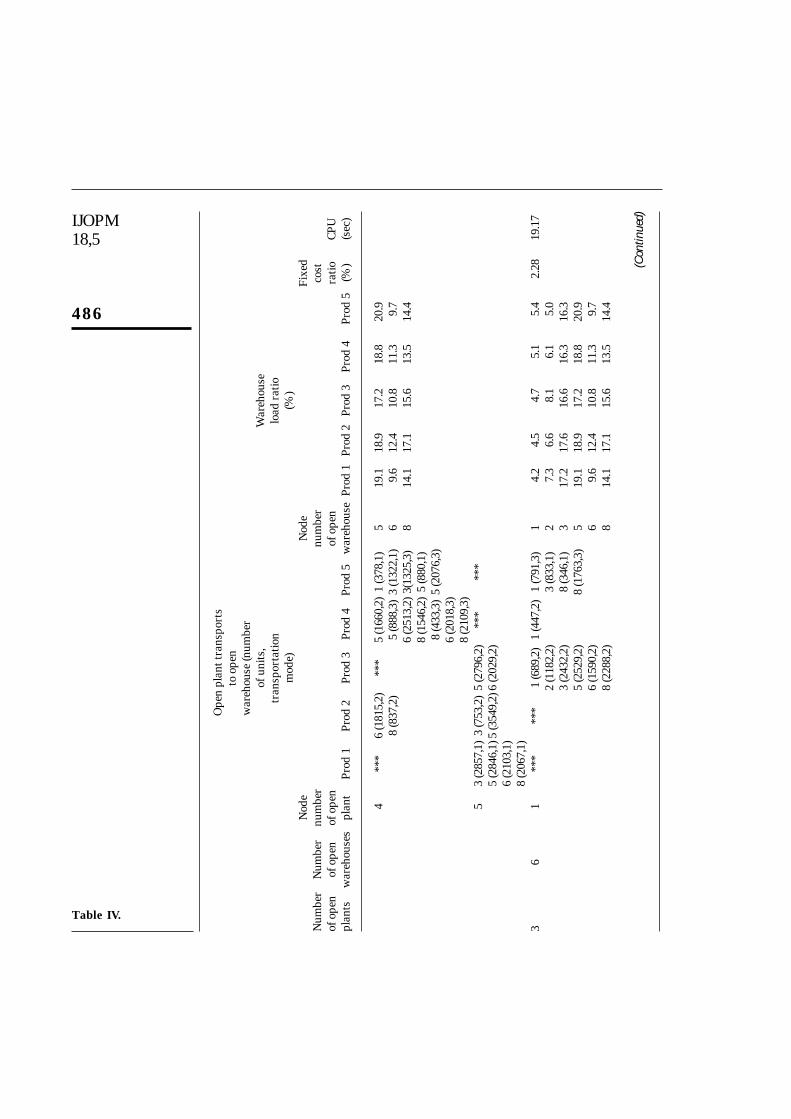
Table IV.Optimal solutions to

FLITNET modelCase 4: demand ~unf(200, 500) and

number of products = 5

IJOPM18,5

486

Ope

n pl

ant t

rans

port

sto

ope

nw

areh

ouse

(num

ber

of u

nits

,W

areh

ouse

tran

spor

tatio

nlo

ad r

atio

mod

e)(%

)N

ode

Nod

eFi

xed

Num

ber

Num

ber

num

ber

num

ber

cost

of o

pen

of o

pen

of o

pen

of o

pen

ratio

CPU

plan

tsw

areh

ouse

spl

ant

Prod

1Pr

od 2

Prod

3Pr

od 4

Prod

5w

areh

ouse

Prod

1Pr

od 2

Prod

3Pr

od 4

Prod

5(%

)(s

ec)

4**

*6

(181

5,2)

***

5 (1

660,

2)1

(378

,1)

519

.118

.917

.218

.820

.98

(837

,2)

5 (8

88,3

)3

(132

2,1)

69.

612

.410

.811

.39.

76

(251

3,2)

3(13

25,3

)8

14.1

17.1

15.6

13.5

14.4

8 (1

546,

2)5

(880

,1)

8 (4

33,3

)5

(207

6,3)

6 (2

018,

3)8

(210

9,3)

53

(285

7,1)

3 (7

53,2

)5

(279

6,2)

***

***

5 (2

846,

1)5

(354

9,2)

6 (2

029,

2)6

(210

3,1)

8 (2

067,

1)3

61

***

***

1 (6

89,2

)1

(447

,2)

1 (7

91,3

)1

4.2

4.5

4.7

5.1

5.4

2.28

19.1

72

(118

2,2)

3 (8

33,1

)2

7.3

6.6

8.1

6.1

5.0

3 (2

432,

2)8

(346

,1)

317

.217

.616

.616

.316

.35

(252

9,2)

8 (1

763,

3)5

19.1

18.9

17.2

18.8

20.9

6 (1

590,

2)6

9.6

12.4

10.8

11.3

9.7

8 (2

288,

2)8

14.1

17.1

15.6

13.5

14.4

(Con

tinue

d)

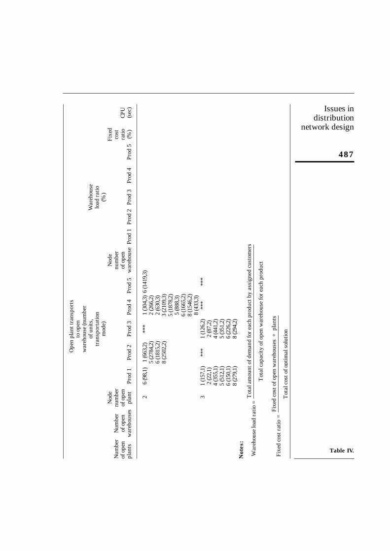
Table IV.


network design

487

Ope

n pl

ant t

rans

port

sto

ope

nw

areh

ouse

(num

ber

of u

nits

,W

areh

ouse

tran

spor

tatio

nlo

ad r

atio

mod

e)(%

)N

ode

Nod

eFi

xed

Num

ber

Num

ber

num

ber

num

ber

cost

of o

pen

of o

pen

of o

pen

of o

pen

ratio

CPU

plan

tsw

areh

ouse

spl

ant

Prod

1Pr

od 2

Prod

3Pr

od 4

Prod

5w

areh

ouse

Prod

1Pr

od 2

Prod

3Pr

od 4

Prod

5(%

)(s

ec)

26

(98,

1)1

(663

,2)

***

1 (3

04,3

)6

(141

9,3)

5 (2

784,

2)2

(266

,2)

6 (1

815,

2)2

(630

,3)

8 (2

502,

2)3

(210

9,3)

5 (1

878,

2)5

(888

,3)

6 (1

665,

2)8

(154

6,2)

8 (4

33,3

)3

1 (1

57,1

)**

*1

(126

,2)

***

***

2 (2

2,1)

2 (8

7,2)

4 (3

55,1

)4

(441

,2)

5 (5

12,1

)5

(351

,2)

6 (1

50,1

)6

(226

,2)

8 (2

79,1

)8

(294

,2)

Not

es:

Fixe

d co

st r

atio

=Fi

xed

cost

of o

pen

war

ehou

ses

+ p

lant

s

Tot

al c

ost o

f opt

imal

sol

utio

n

War

ehou

se lo

ad r

atio

=T

otal

am

ount

of d

eman

d fo

r ea

ch p

rodu

ct b

y as

sign

ed c

usto

mer

s

Tot

al c

apac

ity o

f ope

n w

areh

ouse

for

each

pro

duct

Table IV.

IJOPM18,5

488

cases (cases 1 and 2) when customer demand was low, warehouse capacity wasgenerated randomly on a uniform distribution between (2,600, 2,700) units andplant capacity was generated on a uniform distribution between (3,000, 4,000)units. When customer demand was high (cases 3 and 4), warehouse capacity wasgenerated randomly using a uniform distribution between (14,000, 15,000) unitsand plant capacity was generated uniformly between (19,000, 20,000) units.

In Table I when the decision is to open two plants and two warehouses, theoptimal solution is to open plants at nodes 1 and 5 and open warehouse at nodes3 and 5. Open plant 2 transports 230 units of product 1 using transportationmode 1 to open warehouse 3 while it transports 236 units of product 1 usingtransportation mode 1 to open warehouse 5. We also provide the warehouseload ratio for each product. The warehouse at node 4 operates at 92.3 per centof its capacity while the open warehouse at node 5 operates at 100 per cent of itscapacity. This ratio should provide more insights as one could also identify theservice differences for each product from each open warehouse. In Table I, wealso report the fixed cost ratio. Fixed costs to open plants and warehouses areimportant components of total cost that is incurred for the FLITNET model.The fixed cost ratio is found to be 19.49 per cent when the decision is to opentwo warehouses and plants. It took less than 8 seconds to obtain an optimalsolution to this problem.

When the decision is to open two plants and three warehouses, the optimalsolution is to open plants 1 and 5 while open warehouses 3, 5 and 10. Thewarehouse load ratio for node 6 drops to 32.5 per cent for product 1 and 59 percent for product 2 while for node 3 it drops to 18.1 per cent for product 1 and 40per cent for product 2 to accommodate open warehouse in node 10. The fixedcost ratio increases to 25.91 per cent. The FLITNET model also chooses the besttransportation alternative to transport products from manufacturing plants towarehouses. The operations manager can use these results to not only choosethe best location for plants and warehouses, but also pick the best mode fortransporting multiple products from the open plants to open warehouses whichin turn is distributed to customer retail outlets.

The CPU time (the time it takes to obtain an optimal solution: this includesgeneration, compilation and execution times) does not change dramatically andwe can obtain optimal solutions well within 9 seconds. Table I highlights thevalue of the FLITNET model through provision of warehouse load ratio and thefixed cost ratios as well as the location of open plants and warehouses.

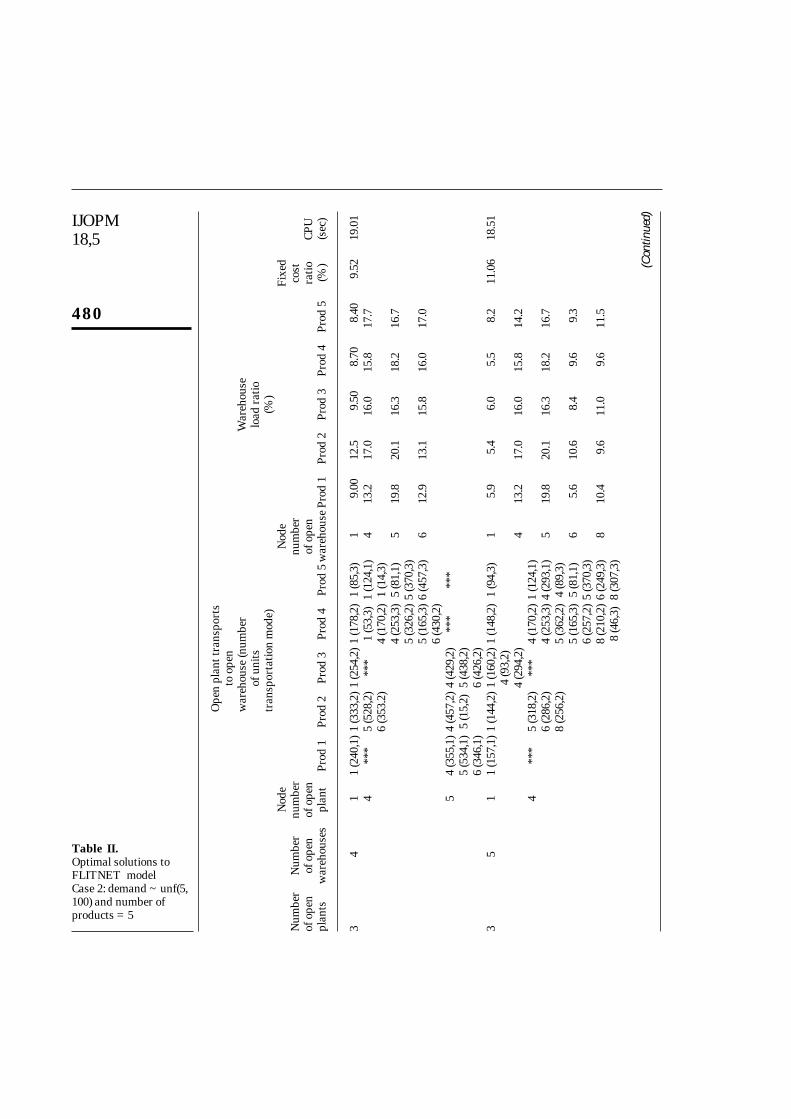
Table II presents optimal solution to the FLITNET model for the second casewhen demand is generated randomly from a uniform distribution between 5and 100 units for five products.

When the decision is to open three plant and four warehouses, the optimalsolution is to open plants at nodes 1 and 4 while warehouses are open at nodes1, 4, 5 and 6. The model considers a combination of all three transportationmodes to ship products from plants to warehouses. When the decision is to openthree plants and five warehouses, the model opens plants at nodes 1, 4 and 5while it opens warehouses at nodes 1, 4, 5, 6 and 8. However, when the decision


network design

489

is to open three plants and six warehouses, the optimal solution is to openplants at nodes 2, 4 and 5 while open warehouses at nodes 1, 2, 4, 5, 6 and 8. Themodel closes the plant at node 1 and replaces it with a plant at node 2 while wemove from a (three plants/five warehouses) scenario to a (three plants/sixwarehouses) scenario.

We present optimal solution to two other cases: Demand ~ Uniform (200,500) units for two products in Table III and Demand ~ Uniform (200, 500) unitsfor five products in Table IV.

In both cases, it was cheaper to open six warehouses to distribute products.Total transportation and inventory costs were also at a minimum when theoptimal solution was to operate with six warehouses.

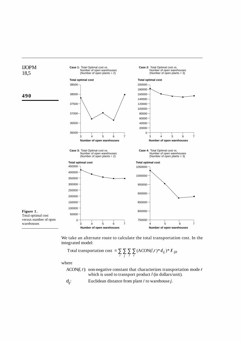
We compare the total costs with number of open warehouses (keeping thenumber of plants fixed) in Figure 1 for the FLITNET model.

For all the four cases, opening six warehouses produced the lowest optimaltotal cost. While cases 1 and 3 (customer demand for two types of products)require two plants to be opened, cases 2 and 4 (customer demand for five typesof products) require three plants to be opened.

The evaluation of strategic changes to an integrated distribution systemconfiguration involves estimation of several cost and benefit measures,including the impact on the amount of cycle stock that is carried in the network.The FLITNET model can help in evaluating the impact of cycle stock,inventory, and transportation cost as we change the number of openwarehouses and plants. Table V provides total cycle stock, inventory andtransportation costs for all four cases of the problem.

Table V confirms the hypothesis that the total cycle stock in the system willnot generally change as the number of warehouses increases, since eachwarehouse has a quantity of cycle stock averaging half a cycle’s time supply forthat specific warehouse. Moreover, cycle stock would vary between zero and afull cycle’s time supply when a shipment is received, and averages half a cycle’stime supply. This issue of cycle stock inventory is particularly important whenone is considering changes in the distribution configuration. The manager ofdistribution network operations must consider issues related to facilitylocation, transportation and inventory simultaneously before a decision couldbe made to decide on an efficient system configuration.

Total inventory and transportation cost as a percentage of total optimal cost are also provided for all the four cases of the problem. Total inventory cost remains a constant for each case of the problem when we change thenumber of open warehouses. In this problem we considered three modes oftransportation. Constable and Whybark (1978) argue that a “transportation costratio may provide a rational way of determining when organizational separationof the transportation and inventory decisions can be justified”. Langley (1980)concludes that while the magnitude of a constant per-unit transportation costwill have an impact on the total cost of the inventory policy, it will not have anyinfluence on an order quantity that will minimize the total cost function.

IJOPM18,5

490

We take an alternate route to calculate the total transportation cost. In theintegrated model:

whereACON(l, r): non-negative constant that characterizes transportation mode r

which is used to transport product l (in dollars/unit).dij: Euclidean distance from plant i to warehouse j.

Total transportation cost ACON= ∑∑∑∑ ( ( , )* )*l r d Xijrlji

ijlr

Figure 1.Total optimal costversus number of openwarehouses

Number of open warehouses

38500

38000

37500

37000

36500

360003 4 5 6 7

Total optimal cost

Case 1: Total Optimal cost vs.Number of open warehouses(Number of open plants = 2)

200000

180000

160000

140000

120000

100000

80000

60000

40000

20000

03 4 5 6 7

Total optimal cost


Number of open warehouses

450000

400000

350000

300000

250000

200000

150000

100000

50000

03 4 5 6 7

Total optimal cost


1050000

1000000

950000

900000

850000

800000

7500004 5 6 7

Total optimal cost


Number of open warehousesNumber of open warehouses


network design

491

This cost is proportional to the transportation mode used, the total quantity ofproducts transported from open plants to warehouses and the distance betweenmanufacturing plants and warehouses. In Table V, the total transportation costas a percentage of total optimal cost is compared to the number of openwarehouses keeping the number of open plants as a constant.

For a fixed number of open plants, when the decision is to increase the number of open warehouses, there is some added flexibility in distributing themultiple commodities from the set of open plants to the open warehouses. Thisleads to some decrease in the total transportation costs. The operations managercan perform such sensitivity analysis on the input parameters and makedecisions based on the outcome of the location, inventory and transportation parameters.

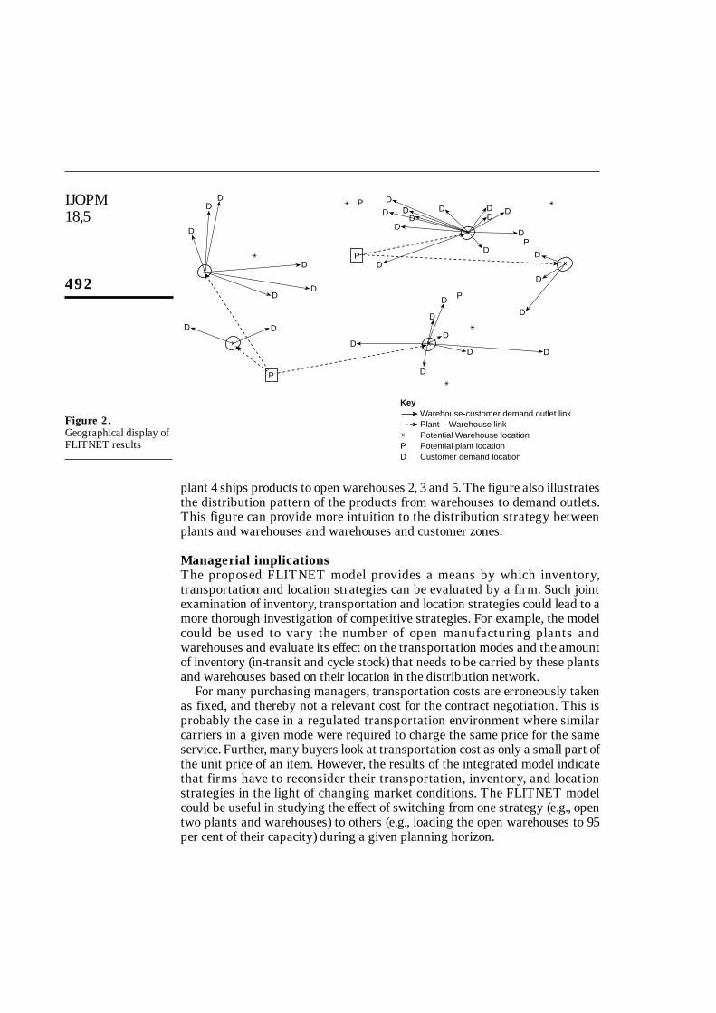
From the decision support system that was created for the model, ageographical display for one set of results of the FLITNET model is presentedin Figure 2. Demand outlets were generated from a uniform distributionbetween (0, 100) units for two products (case 1). The optimal solution was toopen two plants and five warehouses.

Plants are open at points 1 and 4 while warehouses are opened at points 1, 2,3, 5 and 10. Open plant 1 ships products to open warehouses 1, 3 and 10 while

Total inventory Total transportationNumber of Total cost as a cost as aopen cycle stock percentage of percentage ofwarehouses cost total optimal cost total optimal cost

Case 13 34.82 3.27 2.064 34.25 3.36 1.905 33.47 3.27 1.956 32.94 3.25 1.887 34.99 3.30 1.76Case 23 301.44 21.32 2.794 305.22 20.29 2.585 327.44 23.01 2.896 335.51 24.33 3.247 341.14 23.92 3.16Case 33 587.92 5.01 1.664 568.23 5.34 1.785 556.83 5.57 1.906 564.18 5.83 1.907 569.97 5.87 1.94Case 44 2,218.22 22.80 2.935 2,266.51 25.59 3.256 2,228.58 26.67 3.257 2,262.78 27.41 3.26

Table V.Total cycle stock,

inventory and transportation costs

IJOPM18,5

492

plant 4 ships products to open warehouses 2, 3 and 5. The figure also illustratesthe distribution pattern of the products from warehouses to demand outlets.This figure can provide more intuition to the distribution strategy betweenplants and warehouses and warehouses and customer zones.

Managerial implicationsThe proposed FLITNET model provides a means by which inventory,transportation and location strategies can be evaluated by a firm. Such jointexamination of inventory, transportation and location strategies could lead to amore thorough investigation of competitive strategies. For example, the modelcould be used to vary the number of open manufacturing plants andwarehouses and evaluate its effect on the transportation modes and the amountof inventory (in-transit and cycle stock) that needs to be carried by these plantsand warehouses based on their location in the distribution network.

For many purchasing managers, transportation costs are erroneously takenas fixed, and thereby not a relevant cost for the contract negotiation. This isprobably the case in a regulated transportation environment where similarcarriers in a given mode were required to charge the same price for the sameservice. Further, many buyers look at transportation cost as only a small part ofthe unit price of an item. However, the results of the integrated model indicatethat firms have to reconsider their transportation, inventory, and locationstrategies in the light of changing market conditions. The FLITNET modelcould be useful in studying the effect of switching from one strategy (e.g., opentwo plants and warehouses) to others (e.g., loading the open warehouses to 95per cent of their capacity) during a given planning horizon.

Figure 2.Geographical display ofFLITNET results

DD

D

D

DD

D

D

D

DD D D

D

D

D

DD

D

D

DD

D

D

DD

D

D

P

P

P

D

P

KeyWarehouse-customer demand outlet linkPlant – Warehouse linkPotential Warehouse location

P Potential plant locationD Customer demand location

P

x x

x

x

D

x


network design

493

It took less than 7 seconds to obtain optimal solutions to all instances of theFLITNET model. The evidence of these computational runs strongly suggeststhat the mixed integer linear programming formulation of the FLITNET modelis easily solvable by commercial software available on personal computers.Hence, we conclude that the FLITNET formulation is a computationallytractable model.

ConclusionThe design of an integrated distribution network encompasses decisions thatare among the most critical operational and logistical management decisionsthat face a firm. Such decisions affect costs, time, and quality of customerservice that should be carefully monitored. Existing analytical models fordistribution network design have focused only on individual components of thedesign problem. However, a full understanding of the simultaneous relationshipbetween facility location, inventory and transportation related issues is criticalfor the success of any firm.

This paper presented the FLITNET model for jointly examining the effectsof facility location, transportation modes, and inventory related issues on theoverall objective of minimizing the distribution design costs incurred by a firm.The integrated model permits a more comprehensive evaluation of the differenttrade-off that exists among the three strategic issues and has attempted toprovide insight into the inclusion of realistic transportation, inventory andlocation costs in a distribution network design model.

ReferencesAikens, C.H. (1985), “Facility location models for distributing planning”, European Journal of

Operational Research, Vol. 22, pp. 263-79.Batta, R. and Mannur, N. (1990), “Covering-location models for emergency situations that require

multiple response units”, Management Science, Vol. 36, pp. 16-23.Baumol, W. and Vinod, H. (1970), “An inventory theoretic model of freight transport demand”,

Management Science, Vol. 16, pp. 413-21. Brandeau, M. and Chiu, S. (1989), “An overview of representative problems in location research”,

Management Science, Vol. 35, pp. 645-73.Buffa, F. and Reynolds, J. (1977), “The inventory-transport model with sensitivity analysis by

indifference curves”, Transportation Journal, Vol. 17, pp. 83-90.Carter, J. and Ferrin, B. (1995), “The impact of transportation costs on supply chain management”,

Journal of Business Logistics, Vol. 16, pp. 189-211.Constable, G.K. and Whybark, D.C. (1978), “The interaction of transportation and inventory

decisions”, Decision Sciences, Vol. 9, pp. 688-99.Daskin, M. (1995), Network and Discrete Location, John Wiley & Sons, New York, NY.Davis, S. and Davidson, W. (1991), 2020 Vision, Simon & Schuster, New York, NY.Drezner, Z. (1995), Facility Location: A Survey of Applications and Methods, Springer-Verlag, New

York, NY. GAMS (Generalized Algebraic Modeling Systems) (1994), The Scientific Press.Langley, C.J. (1980), “The inclusion of transportation costs in inventory models: some

considerations”, Journal of Business Logistics, Vol. 2, pp. 106-25.

IJOPM18,5

494

Larson, P. (1988), “The economic transportation quantity”, Transportation Journal, Vol. 28, pp. 43-8.

Perl, J. and Sirisiponsilp, S. (1980), “Distribution networks: facility location, transportation andinventory”, International Journal of Physical Distribution & Materials Management, Vol. 18,pp. 18-26.

Rajagopalan, S. and Ravi Kumar, K. (1994), “Retail stocking decisions with order and stock sales”,Journal of Operations Management, Vol. 11, pp. 397-410.

Schilling, D., Jayaraman, V. and Barkhi, R. (1993), “A review of covering problems in facilitylocation”, Location Science, Vol. 1, pp. 25-55.

Van Beek, P. (1981) “Modelling and analysis of a multi-echelon inventory system: a case study”,European Journal of Operational Research, Vol. 6, pp. 380-85.

Transportation, facility location and inventory issues in ...

Documents

Transcript of Transportation, facility location and inventory issues in ...