Proceedings of the Asia Pacific Industrial Engineering & Management Systems Conference 2014

1

Competitive Facility Location Problem by Considering

Conditions of Government Regulation and Regional Saturation

Suprayogi† Institut Teknologi Bandung, Bandung, Indonesia

Email: yogi@mail.ti.itb.ac.id

Yosi A. Hidayat Institut Teknologi Bandung, Bandung, Indonesia

Email: yosi@mail.ti.itb.ac.id

Utaminingsih Linarti

Ahmad Dahlan University, Yogyakarta, Indonesia

Email: utaminingsih.linarti@ie.uad.ac.id

Abstract. This paper discusses a competitive facility location problem (CFLP). The CFLP is a facility

location problem incorporating the competition among the facilities belonging to different firms. Two

additional features are introduced, i.e., government regulation and regional saturation. The existence of

government regulation determines the feasibility of new facilities in a certain distance. The regional saturation

determine maximum number of facilities in a region. The CFLP is formulated as a bilevel mixed integer

nonlinear programming model. In order to find a solution, the model is converted into one-level mixed integer

nonlinear programming model. A solution is given for a real-case application.

Keywords: Competitive facility location problem, Attractiveness level, Regulation, Regional saturation,

Bilevel mixed integer nonlinear programming model

1. INTRODUCTION

This paper discusses a competitive facility location

problem (CFLP). According to Küçükaydin et al. (2011,

2012), the CFLP is a facility location problem

incorporating the competition among the facilities

belonging to different firms. The new facility or facilities to

be located by a firm have to compete with the facilities of

the other firm(s) that are already (or will be) present in the

market in order to capture market share.

Küçükaydin et al. (2011) present the CFLP in which a

firm enters a market by locating new facilities where there

are existing facilities belonging to a competitor. The firm

aims at finding the location and attractiveness of each

facility to be opened so as to maximize its profit. On the

other hand, the competitor can react by adjusting the

attractiveness of its existing facilities with the objective of

maximizing its own profit. The demand is assumed to be

aggregated at certain points and the facilities of the firm

can be located at predetermined candidate sites. The

behavior of the customers is modeled using the Huff’s

gravity-based rule where the fraction of customer at a

demand point that visits a certain facility is proportional to

the facility attractiveness and inversely proportional to the

distance between the facility site and demand point. The

CFLP is formulated as a bilevel mixed integer nonlinear

programming model. The firm entering the market is the

leader and the competitor is the follower. The model is

converted into one-level mixed integer nonlinear

programming model in order to find the optimal solution.

This paper can be considered as an extension work of

Küçükaydin et al. (2011). The CFLP discussed in this paper

is motivated by a real case faced by a firm to locate new

minimarkets. Two additional features are introduced, i.e.,

government regulation and regional saturation constraints.

The regulation limits the distance among minimarkets and

traditional markets. The regional saturation constraint

restricts number of facilities in a region. The regional

saturation index from Yang and Yang (2005) is used to

determine the maximum number of facilities.

1250

2

2. PROBLEM DEFINITION

In this section, we describe the CFLP faced by a firm

(called as leader). The leader owns a set of existing

minimarkets 𝐿. The leader has one main competitor firm

(called as follower) where the follower own a set of

existing minimarkets 𝑐. There is a set of other firms 𝑆

where each firm 𝑠 ∈ 𝑆 has a set of minimarkets 𝑃𝑠 . There

is a set of traditional markets 𝑇 where these traditional

market are owned by the local government (i.e., municipal

government).

Given a set of candidate sites 𝐵, the leader wants to

determine the location of new minimarkets to be opened

and the associated attractiveness levels that maximize the

total profit. The attractive level for each new minimarket

must not violate its maximum attractive level. Adding the

new minimarkets must satisfy the maximum number of

minimarkets in the region where this maximum number of

minimarkets is determined by the regional saturation index.

In addition, each new minimarket to be opened in a certain

site must have a distance satisfying the minimum distance

to the any traditional market established by the local

government.

The follower can react by adjusting the attractiveness

level of its existing minimarkets that maximize its own

profit. The new attractiveness level for each its existing

minimarket must be laid between its lower and upper

bounds. The lower bound of the existing minimarket is

represented by its current attractiveness level. It implies

that the follower cannot close the existing minimarkets. In

addition, the total cost incurred in adjusting the

attractiveness levels must fulfill the budget availability.

In this problem, it is assumed that other firms and the

local government do not react.

3. MATHEMATICAL MODEL

3.1 Notations

Sets:

𝑂 : set of demand points

𝐿 : set of existing minimarkets for the leader

𝐹 : set of existing minimarkets for the follower

𝑆 : set of other firms

𝑃𝑠 : set of existing minimarkets for the firm 𝑠 ∈ 𝑆

𝑇 : set of traditional markets

𝐵 : set of candidate sites of new minimarkets for the

leader

Parameters:

𝑏𝑜 : buying power at demand point 𝑜

𝑐𝑏 : unit attractiveness cost of the leader for a new

minimarket at site 𝑏

𝑐𝑓 : unit attractiveness cost of the follower for an

existing minimarket at site 𝑓

𝑓𝑏 : Annualized fixed cost of opening a new minimarket

for the leader at site 𝑏

𝑢𝑏 : maximum attractiveness level for a minimarket to be

opened at site 𝑏

𝑢𝑓′ : maximum attractiveness level of competitor’s

minimarket at site 𝑓

𝑑𝑜𝑠𝑝 : distance between demand point 𝑜 and existing

minimarket at site p of other firm 𝑠

dot : distance between demand point 𝑜 and traditional

market at site 𝑡 𝑑𝑜𝑏𝑀 : distance between demand point 𝑜 and candidate

site of leader’s new facility at site 𝑏

𝑑𝑜𝑙𝑀 : distance between demand point 𝑜 and leader’s

existing minimarket at site 𝑙

𝑑𝑜𝑓𝐶 : distance between demand point 𝑜 and follower’s at

site 𝑓

𝑑𝑏𝑡𝑀 : distance between candidate site for leader’s new

minimarket 𝑏 and traditional market at site 𝑡

dmin

: minimum distance allowed between a minimarket

and a traditional market

𝑞𝑙𝑀 : current attractiveness level of leader’s existing

minimarket at site 𝑙

�̃�𝑓𝐶 : current attractiveness level of follower’s minimarket

at site 𝑓

𝑞𝑠𝑝 : Attractiveness level of existing minimarket at point

𝑝 of other firm 𝑠

𝑞𝑡 : Attractiveness level of existing traditional market at

point t

: The distance sensitivity parameter > 0

𝑝𝑚𝑎𝑥: maximum number of new minimarkets

𝑎 : The total budget available for the follower

Decision variables:

𝑄𝑏𝑀 : attractiveness level of minimarket to be opened at

site 𝑏

𝑋𝑏𝑀 : binary variable which is equal to one if a new

minimarket for the leader is opened at site 𝑏, and

zero otherwise

𝑄𝑓𝐶 : new attractiveness level of follower’s competitor at

site 𝑓

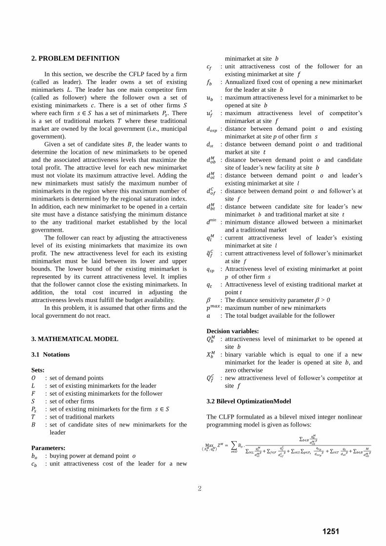
3.2 Bilevel OptimizationModel

The CLFP formulated as a bilevel mixed integer nonlinear

programming model is given as follows:

(

𝑞 )𝑍𝑀 ∑𝐵𝑜 .

∑𝑞

𝑏∈

∑𝑞

𝑙∈ ∑

𝑞

𝑓∈ ∑ ∑

𝑞

𝑝∈ 𝑠∈ ∑

𝑞

𝑡∈ ∑

𝑀

𝑏∈ 𝑜∈

1251

3

− ∑ 𝐹𝐶𝑏𝑀. 𝑋𝑏

𝑀𝑏∈ −∑ 𝐷𝐶𝑏

𝑀. 𝑞𝑏𝑀

𝑏∈ (1)

subject to

𝑞𝑏𝑀 ≤ 𝑈𝑏

𝑀 ∙ 𝑋𝑏 𝑀; ∀𝑏 ∈ 𝐵 (2)

∑ 𝑋𝑏 𝑀

𝑏∈ℬ ≤ 𝑃𝑚𝑎𝑥 (3)

min𝑡∈ {𝑑𝑏𝑡𝑀} ∙ 𝑋𝑏

𝑀 ≥ 𝑑𝑚𝑖𝑛; ∀𝑏 ∈ 𝐵 (4)

𝑞𝑏𝑀 ≥ 0; ∀𝑏 ∈ 𝐵 (5)

𝑋𝑏 𝑀 ∈ *0 1+; ∀𝑏 ∈ 𝐵 (6)

m (𝑞 )ZC ∑𝐵𝑜 ∙

∑ 𝑞

𝑓∈ℱ

∑𝑞

𝑙∈ℒ ∑

𝑞

𝑓∈ ∑ ∑

𝑞

𝑝∈ 𝑠∈ ∑

𝑞

𝑡∈𝒯 ∑

𝑞

𝑏∈ 𝑜∈

− ∑ 𝐷𝐶𝑓𝐶 ∙ (𝑞𝑓

𝐶 − �̃�𝑓𝐶)𝑓∈ℱ (7)

subject to:

𝑞𝑓𝐶 ≤ 𝑈𝑓

𝐶 ; ∀𝑓 ∈ 𝐹 (8)

𝑞𝑓𝐶 ≥ �̃�𝑓

𝐶; ∀𝑓 ∈ 𝐹 (9)

𝑞𝑓𝐶 ≥ 0; ∀𝑓 ∈ 𝐹 (10)

∑ 𝐷𝐶 𝑓 . (𝑞𝑓𝐶 − �̃�𝑓

𝐶) ≤ A𝑓 (11)

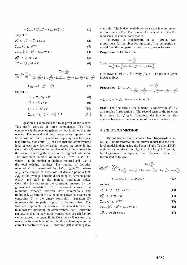
Equation (1) represents the total profit of the leader.

This profit consists of three components. The first

component is the revenue gained by new facilities that are

opened. The second and third components represent the

fixed cost and cost associated with opening new facilities,

respectively. Constraint (2) ensures that the attractiveness

level of each new facility cannot exceed the upper limit..

Constraint (3) restricts the number of facilities allowed in

the region reflecting the condition of regional saturation.

The maximum number of facilities 𝑃𝑚𝑎𝑥 is 𝑃 − 𝑇𝐹

where 𝑃 is the number of facilities required and 𝑇𝐹 is

the total existing facilities. The number of facilities

required 𝑃 is determined by (𝑅𝑇𝑜 ∙ 𝑃𝑔𝑜) 𝑅𝑆𝐼⁄ where

𝑅𝑇𝑜 is the number of households at demand point 𝑜 ∈ 𝑂 𝑃𝑔𝑜 is the average household spending at demand point

𝑜 ∈ 𝑂 and 𝑅𝑆𝐼 is the regional saturation index.

Constraint (4) represents the constraint imposed by the

government regulation. This constraint ensures the

minimum distance between new minimarkets and

traditional. Constraint (5) is the nonnegative constraint and

constraint (6) is the binary constraint. Equation (7)

represents the competitor’s profit to be maximized. The

first term represents the revenue. The second term is the

total cost for improving the attractiveness level. Constraint

(8) ensures that the new attractiveness level of each facility

cannot exceed the upper limit. Constraint (9) ensures that

new attractiveness level of each facility at least equal to the

current attractiveness level. Constraint (10) is nonnegative

constraint. The budget availability constraint is represented

in constraint (11). The model formulated in (7)-(11)

represents the competitor’s model.

Following to Küçükaydin et al. (2011), two

propositions for the objective function of the competitor’s

model (i.e., the competitor’s profit) are given as follows:

Proposition 1. The function

∑ 𝐵𝑜 .

∑ 𝑞

𝑑 ∈𝐹

∑𝑞

𝑑

∈𝐿 +∑ 𝑞

𝑑 ∈𝐹 +∑ ∑

𝑞

𝑑 ∈𝑆 ∈𝑆 +∑

𝑞

𝑑 ∈𝑇 +∑

𝑞

𝑑 ∈𝐵

𝑜∈

is concave in 𝑞𝑓𝐶 ≥ 0 for every 𝑓 ∈ 𝐹. The proof is given

in Appendix A.

Proposition 2. ∑ 𝐵𝑜 .

∑ 𝑞

𝑑 ∈𝐹

∑𝑞

𝑑

∈𝐿 +∑ 𝑞

𝑑 ∈𝐹 +∑ ∑

𝑞

𝑑 ∈𝑆 ∈𝑆 +∑

𝑞

𝑑 ∈𝑇 +∑

𝑞

𝑑 ∈𝐵

𝑜∈

− ∑ 𝐷𝐶𝑓𝐶. (𝑞𝑓

𝐶 − �̃�𝑓𝐶)𝑓∈ is concave in 𝑞𝐶 ≥ 0.

Proof. The first term of the function is concave in 𝑞𝐶 ≥ 0

as a result of proposition 1. The second term of the function

is a linear for 𝑞𝐶 ≥ 0 . Therefore, the function is also

concave because it is a summation of concave functions.

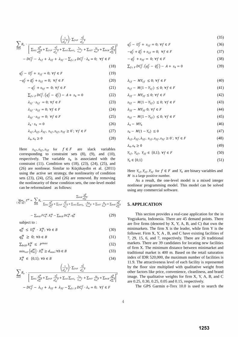
4. SOLUTION METHOD

The solution method is adopted from Küçükaydin et al.

(2011). The transformation the bilevel model into the one-

level model is done using the Karush Kuhn Tucker (KKT)

optimality conditions. Let 𝜆1𝑓 𝜆2𝑓, 𝜆3𝑓 for 𝑓 ∈ 𝐹 and 𝜆4

be Lagrangian multipliers, the one-level model is

formulated as follows:

(

𝑞 )𝑍𝑀 ∑𝐵𝑜 .

∑𝑞

𝑏∈

∑𝑞

𝑙∈ ∑

𝑞

𝑓∈ ∑ ∑

𝑞

𝑝∈ 𝑠∈ ∑

𝑞

𝑡∈ ∑

𝑞

𝑏∈ 𝑜∈

− ∑ 𝐹𝐶𝑏𝑀. 𝑋𝑏

𝑀𝑏∈ − ∑ 𝐷𝐶𝑏

𝑀. 𝑞𝑏𝑀

𝑏∈ (12)

subject to:

𝑞𝑏𝑀 ≤ 𝑈𝑏

𝑀 ∙ 𝑋𝑏 𝑀; ∀𝑏 ∈ 𝐵 (13)

𝑞𝑏𝑀 ≥ 0; ∀𝑏 ∈ 𝐵 (14)

∑ 𝑋𝑏 𝑀

𝑏∈ ≤ 𝑃𝑚𝑎𝑥 (15)

min𝑡∈ {𝑑𝑏𝑡𝑀} ∙ 𝑋𝑏

𝑀 ≥ 𝑑𝑚𝑖𝑛; ∀𝑏 ∈ 𝐵 (16)

𝑋𝑏 𝑀 ∈ *0 1+; ∀𝑏 ∈ 𝐵 (17)

1252

4

∑𝐵𝑜 ∙

(1

) ∙ ∑

𝑞

𝑓∈

* ∑𝑞

𝑙∈ ∑

𝑞

𝑓∈ ∑ ∑

𝑞𝑠𝑝

𝑑𝑜𝑠𝑝𝛽 𝑝∈𝑆𝑝𝑠∈𝑆 ∑

𝑞

𝑡∈ ∑

𝑞

𝑏∈ +

2

𝑜∈

− 𝐷𝐶𝑓𝐶 − 𝜆1𝑓 𝜆2𝑓 𝜆3𝑓 − ∑ 𝐷𝐶𝑓

𝐶 ∙ 𝜆4𝑓 0; ∀𝑓 ∈ 𝐹

(18)

𝑞𝑓𝐶 − 𝑈𝑓

𝐶 𝑠1𝑓 0; ∀𝑓 ∈ 𝐹 (19)

−𝑞𝑓𝐶 �̃�𝑓

𝐶 𝑠2𝑓 0; ∀𝑓 ∈ 𝐹 (20)

− 𝑞𝑓𝐶 𝑠3𝑓 0; ∀𝑓 ∈ 𝐹 (21)

∑ 𝐷𝐶𝑓𝐶 . (𝑞𝑓

𝐶 − �̃�𝑓𝐶) − 𝐴 𝑠4 0𝑓 (22)

𝜆1𝑓 ∙ 𝑠1𝑓 0; ∀𝑓 ∈ 𝐹 (23)

𝜆2𝑓 ∙ 𝑠2𝑓 0; ∀𝑓 ∈ 𝐹 (24)

𝜆3𝑓 ∙ 𝑠3𝑓 0; ∀𝑓 ∈ 𝐹 (25)

𝜆4 ∙ 𝑠4 0 (26)

𝜆1𝑓 𝜆2𝑓 𝜆3𝑓, 𝑠1𝑓 𝑠2𝑓 𝑠3𝑓 ≥ 0`; ∀𝑓 ∈ 𝐹 (27)

𝜆4 𝑠4 ≥ 0 (28)

Here 𝑠1𝑓 𝑠2𝑓 𝑠3𝑓 for 𝑓 ∈ 𝐹 are slack variables

corresponding to constraint sets (8), (9), and (10),

respectively. The variable 𝑠4 is associated with the

constraint (11). Condition sets (18), (23), (24), (25), and

(26) are nonlinear. Similar to Küçükaydin et al. (2011)

using the active set strategy, the nonlinearity of condition

sets (23), (24), (25), and (26) are removed. By removing

the nonlinearity of these condition sets, the one-level model

can be reformulated as follows:

(

)𝑍𝑀 ∑𝐵𝑜 .

∑𝑞

𝑏∈

∑𝑞

𝑙∈ ∑

𝑞

𝑓∈ ∑ ∑

𝑞

𝑝∈ 𝑠∈ ∑

𝑞

𝑡∈ ∑

𝑞

𝑏∈ 𝑜∈

− ∑ 𝐹𝐶𝑏𝑀. 𝑋𝑏

𝑀𝑏∈ − ∑ 𝐷𝐶𝑏

𝑀. 𝑞𝑏𝑀

𝑏∈ (29)

subject to :

𝑞𝑏𝑀 ≤ 𝑈𝑏

𝑀 ∙ 𝑋𝑏 𝑀; ∀𝑏 ∈ 𝐵 (30)

𝑞𝑏𝑀 ≥ 0; ∀𝑏 ∈ 𝐵 (31)

∑ 𝑋𝑏 𝑀

𝑏∈ ≤ 𝑃𝑚𝑎𝑥 (32)

min𝑡∈ {𝑑𝑏𝑡𝑀} ∙ 𝑋𝑏

𝑀 ≥ 𝑑𝑚𝑖𝑛; ∀𝑏 ∈ 𝐵 (33)

𝑋𝑏 𝑀 ∈ *0 1+; ∀𝑏 ∈ 𝐵 (34)

∑𝐵𝑜 ∙

(1

) ∙ ∑

𝑞

𝑓∈

* ∑𝑞

𝑙∈ ∑

𝑞

𝑓∈ ∑ ∑

𝑞𝑠𝑝

𝑑𝑜𝑠𝑝𝛽 𝑝∈𝑆𝑝𝑠∈𝑆 ∑

𝑞

𝑡∈ ∑

𝑞

𝑏∈ +

2

𝑜∈

− 𝐷𝐶𝑓𝐶 − 𝜆1𝑓 𝜆2𝑓 𝜆3𝑓 − ∑ 𝐷𝐶𝑓

𝐶 ∙ 𝜆4𝑓 0; ∀𝑓 ∈ 𝐹

(35)

𝑞𝑓𝐶 − 𝑈𝑓

𝐶 𝑠1𝑓 0; ∀𝑓 ∈ 𝐹 (36)

−𝑞𝑓𝐶 �̃�𝑓

𝐶 𝑠2𝑓 0; ∀𝑓 ∈ 𝐹 (37)

− 𝑞𝑓𝐶 𝑠3𝑓 0; ∀𝑓 ∈ 𝐹 (38)

∑ 𝐷𝐶𝑓𝐶 . (𝑞𝑓

𝐶 − �̃�𝑓𝐶) − 𝐴 𝑠4 0𝑓 (39)

𝜆1𝑓 − 𝑀𝑌1𝑓 ≤ 0; ∀𝑓 ∈ 𝐹 (40)

𝑠1𝑓 − 𝑀(1 − 𝑌1𝑓) ≤ 0; ∀𝑓 ∈ 𝐹 (41)

𝜆2𝑓 − 𝑀𝑌2𝑓 ≤ 0; ∀𝑓 ∈ 𝐹 (42)

𝑠2𝑓 − 𝑀(1 − 𝑌2𝑓) ≤ 0; ∀𝑓 ∈ 𝐹 (43)

𝜆3𝑓 − 𝑀𝑌3𝑓 0; ∀𝑓 ∈ 𝐹 (44)

𝑠3𝑓 − 𝑀(1 − 𝑌3𝑓) ≤ 0; ∀𝑓 ∈ 𝐹 (45)

𝜆4 − 𝑀𝑌4 (46)

𝑠4 − 𝑀(1 − 𝑌4) ≤ 0 (47)

𝜆1𝑓 𝜆2𝑓 𝜆3𝑓, 𝑠1𝑓 𝑠2𝑓 𝑠3𝑓 ≥ 0`; ∀𝑓 ∈ 𝐹 (48)

𝜆4 𝑠4 ≥ 0 (49)

𝑌1𝑓 𝑌2𝑓 𝑌3𝑓 ∈ *0 1+; ∀𝑓 ∈ 𝐹 (50)

𝑌4 ∈ *0 1+ (51)

Here 𝑌1𝑓 𝑌2𝑓 𝑌3𝑓 for 𝑓 ∈ 𝐹 and 𝑌4 are binary variables and

𝑀 is a large positive number.

As a result, the one-level model is a mixed integer

nonlinear programming model. This model can be solved

using any commercial software.

5. APPLICATION

This section provides a real-case application for the in

Yogyakarta, Indonesia. There are 45 demand points. There

are five firms (denoted by X, Y, A, B, and C) that own the

minimarkets. The firm X is the leader, while firm Y is the

follower. Firm X, Y, A , B, and C have existing facilities of

7, 29, 15, 6, and 7, respectively. There are 26 traditional

markets. There are 39 candidates for locating new facilities

of firm X. The minimum distance between minimarket and

traditional market is 400 m. Based on the retail saturation

index of IDR 520,000, the maximum number of facilities is

11.9. The attractiveness level of each facility is represented

by the floor size multiplied with qualitative weight from

other factors like price, convenience, cleanliness, and brand

image. The qualitative weights for firm X, Y, A, B, and C

are 0.25, 0.30, 0.25, 0.05 and 0.15, respectively.

The GPS Garmin e-Trex 10.0 is used to search the

1253

5

location point for every facility and demand point. The

distance between a facility and demand point or other

facilities is measured by straight-line from latitude and

longitude coordinate points.

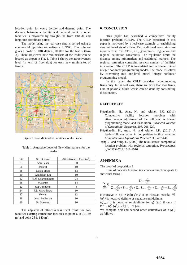
The model using the real-case data is solved using a

commercial optimization software LINGO. The solution

gives a profit of IDR 40,656,300,000 for the leader (firm

X). There are eleven new minimarkets of the leader can be

located as shown in Fig. 1. Table 1 shows the attractiveness

level (in term of floor size) for each new minimarket of

firm X.

Figure 1. New Minimarket Locations for the Leader

Table 1. Attractive Level of New Minimarkets for the

Leader

Site Street name Attractiveness level (m2)

1 Abu Bakar 30

4 Bantul 10

8 Gajah Mada 14

10 Gandekan Lor 10

12 HOS Cokroaminoto 24

18 Mataram 14

22 Kapt. Tendean 6

24 RE. Martadinata 10

27 Veteran 12

28 Jend. Sudirman 10

39 Dr. Soetomo 10

The adjusted of attractiveness level result for two

facilities existing competitor facilities at point 6 is 151,89

m2 and point 25 is 140 m

2.

6. CONCLUSION

This paper has described a competitive facility

location problem (CFLP). The CFLP presented in this

paper is motivated by a real-case example of establishing

new minimarkets of a firm. Two additional constraints are

introduced in this CFLP, i.e., government regulation and

regional saturation constraints. The regulation limits the

distance among minimarkets and traditional markets. The

regional saturation constraint restricts number of facilities

in a region. The CFLP is formulated into a bilevel mixed

integer nonlinear programming model. The model is solved

by converting into one-level mixed integer nonlinear

programming model.

In this paper, the CFLP considers two-competing

firms only. In the real case, there are more than two firms.

One of possible future works can be done by considering

this situation.

REFERENCES

Küçükaydin, H., Aras, N., and Altinel, I.K. (2011)

Competitive facility location problem with

attractiveness adjustment of the follower: A bilevel

programming model and its solution. European Journal

of Operational Research, 208, 206-220.

Küçükaydin, H., Aras, N., and Altinel, I.K. (2012) A

leader-follower game in competitive facility location,

Computers and Operations Research 39, 437-448.

Yang, J. and Yang, C. (2005) The retail stores’ competitive

location problem with regional saturation. Proceedings

of ICSSSM’05, 1511-1516.

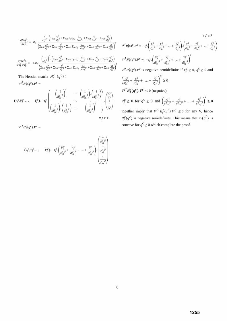
APPENDIX A

The proof of proposition 1

Sum of concave function is a concave function, quate to

show that terms :

∑𝐵𝑜 .

∑ 𝑞

𝑓∈

∑𝑞

𝑙∈ ∑

𝑞

𝑓∈ ∑ ∑

𝑞𝑠𝑝

𝑑𝑜𝑠𝑝𝛽 𝑝∈𝑆𝑝𝑠∈𝑆 ∑

𝑞

𝑡∈ ∑

𝑞

𝑏∈ 𝑜∈

is concave in 𝑞𝑓𝐶 ≥ 0 for 𝑓 F if its Hessian matriks 𝐻𝑓

𝐶 (𝑞𝐶) is negative definite or negative semidefinite.

𝐻𝑓𝐶 (𝑞𝐶) is negative semidefinite for 𝑞𝑓

𝐶 ≥ 0 if only if

𝑉𝐶 . 𝐻𝑓

𝐶. (𝑞𝐶) . 𝑉𝑓𝐶≤ 0, fF.

We compute first and second order derivatives of ZC(𝑞𝐶)

as follows :

1254

6

𝜕𝑓(𝑞𝐶)

𝜕𝑞𝑓𝐶

𝐵 .

1

𝐹 . (∑

𝑞

𝑙∈ ∑ ∑

𝑞

𝑝∈ 𝑠∈ ∑

𝑞

𝑡∈ ∑

𝑞

𝑏∈ )

(∑𝑞

𝑙∈ ∑

𝑞

𝑓∈ ∑ ∑

𝑞

𝑝∈ 𝑠∈ ∑

𝑞

𝑡∈ ∑

𝑞

𝑏∈ )

2

𝜕𝑓(𝑞𝐶)

𝜕𝑞𝑓𝐶 𝜕𝑞𝑓

𝐶 −2. 𝐵𝑜.

(1

)

2

. (∑𝑞

𝑙∈ ∑ ∑

𝑞

𝑝∈ 𝑠∈ ∑

𝑞

𝑡∈ ∑

𝑞

𝑏∈ )

(∑𝑞

𝑙∈ ∑

𝑞

𝑓∈ ∑ ∑

𝑞

𝑝∈ 𝑠∈ ∑

𝑞

𝑡∈ ∑

𝑞

𝑏∈ )

3

The Hessian matrix 𝐻𝑓𝐶 (𝑞𝐶) :

𝑽𝑪𝑻𝑯𝒇𝑪(𝒒𝑪). 𝑽𝑪

(𝑉1𝐶 𝑉2

𝐶 … 𝑉𝑓𝐶).− 𝑡𝑓

𝐶 .

(

(1

𝑑𝑜𝑓𝐶 𝛽)

2

⋯ (1

𝑑𝑜1𝐶 𝛽) . (

1

𝑑𝑜𝑓𝐶 𝛽)

⋮ ⋱ ⋮

(1

𝑑𝑜𝑓𝐶 𝛽) . (

1

𝑑𝑜1𝐶 𝛽) ⋯ (

1

𝑑𝑜𝑓𝐶 𝛽)

2

)

.

(

𝑉1𝐶

𝑉2𝐶

::𝑉𝑓𝐶)

∀ 𝑓 ∈ 𝐹

𝑽𝑪𝑻𝑯𝒇𝑪(𝒒𝑪). 𝑽𝑪

(𝑉1𝐶 𝑉2

𝐶 … 𝑉𝑓𝐶).− 𝑡𝑓

𝐶 . (𝑉1𝐶

𝑑𝑜1𝐶 𝛽

𝑉2𝐶

𝑑𝑜2𝐶 𝛽

… . 𝑉𝑓𝐶

𝑑𝑜𝑓𝐶 𝛽) .

(

1

𝑑𝑜1𝐶 𝛽

1

𝑑𝑜2𝐶 𝛽

:1

𝑑𝑜𝑓𝐶 𝛽)

∀ 𝑓 ∈ 𝐹

𝑽𝑪𝑻𝑯𝒇𝑪(𝒒𝑪). 𝑽𝑪 −𝑡𝑓

𝐶 . (𝑉1𝐶

𝑑𝑜1𝐶 𝛽

𝑉2𝐶

𝑑𝑜2𝐶 𝛽

… . 𝑉𝑓𝐶

𝑑𝑜𝑓𝐶 𝛽) . (

𝑉1𝐶

𝑑𝑜1𝐶 𝛽

𝑉2𝐶

𝑑𝑜2𝐶 𝛽

… . 𝑉𝑓𝐶

𝑑𝑜𝑓𝐶 𝛽)

𝑽𝑪𝑻𝑯𝒇𝑪(𝒒𝑪). 𝑽𝑪 −𝑡𝑓

𝐶 . (𝑉1𝐶

𝑑𝑜1𝐶 𝛽

𝑉2𝐶

𝑑𝑜2𝐶 𝛽

… . 𝑉𝑓𝐶

𝑑𝑜𝑓𝐶 𝛽)

2

𝑽𝑪𝑻𝑯𝒇𝑪(𝒒𝑪). 𝑽𝑪 is negative semidefinite if 𝑡𝑡

𝐶 ≥ 0, qC ≥ 0 and

(𝑉1

1

𝑉2

2 … .

𝑉

)

2

≥ 0

𝑽𝑪𝑻𝑯𝒇𝑪(𝒒𝑪). 𝑽𝑪 ≤ 0 (neg tive)

𝑡𝑓𝐶 ≥ 0 for q

C ≥ 0 and (

𝑉1

1

𝑉2

2 … .

𝑉

)

2

≥ 0

together imply that 𝑉𝐶 𝐻𝑓𝐶(𝑞𝐶). 𝑉𝐶 ≤ 0 for any V, hence

𝐻𝑓𝐶(𝑞𝐶) is negative semidefinite. This means that ZC(𝑞

𝐶) is

concave for qC ≥ 0 which complete the proof.

1255