EZ2: An extension of the EZ-diffusion model1

for Response Time and Accuracy 12

Raoul P. P. P. Grasman ∗, Eric–Jan Wagenmakers,3

Han L. J. van der Maas4

Department of Psychology, University of Amsterdam, Roetersstraat 15, 1018WB5

Amsterdam, the Netherlands6

∗ Corresponding author.Email addresses: rgrasman@uva.nl (Raoul P. P. P. Grasman),

e.j.wagenmakers@gmail.com (Eric–Jan Wagenmakers),

h.l.j.vandermaas@uva.nl (Han L. J. van der Maas).URL: http://users.fmg.uva.nl/rgrasman (Raoul P. P. P. Grasman).

1 Preparation of this article was sponsored in part by a VENI-grant from the

Netherland Organisation for Scienctific research (NWO) awarded to the correspond-

ing author.

Preprint submitted to Journal of Mathematical Psychology 29 August 2007

Abstract1

To simplify and popularize the use of the diffusion model for two-choice decision2

response times, Wagenmakers, van der Maas, and Grasman (2007) introduced the3

EZ diffusion model. The EZ diffusion model makes limiting simplifying assumptions4

that are violated in many cases of interest. The objective of the current paper is5

threefold: The first is to introduce the EZ2 diffusion model that addresses some of6

the drawbacks of the EZ diffusion model. Most notably we allow for the estimation7

of a response bias parameter. The second is to provide expressions for the mean8

and variance of the response times under the EZ2 model. The third objective is to9

provide a method and framework, and its software implementation, for estimating10

the parameters of models composed of EZ2 diffusions in a variety of experimental11

configurations. We illustrate the methodology with a lexical decision task data set.12

Key words: reaction time/response time, stochastic processes, diffusion model,13

estimation, response time mean, response time variance14

15

Preprint submitted to Journal of Mathematical Psychology 29 August 2007

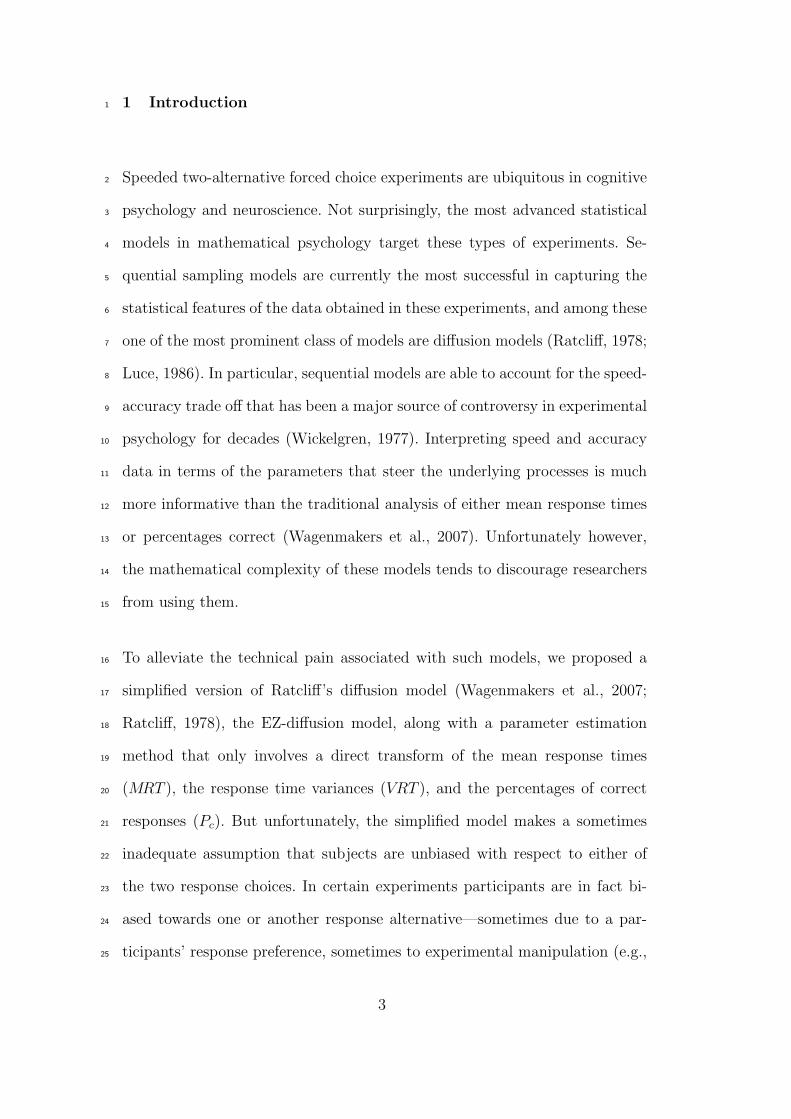
1 Introduction1

Speeded two-alternative forced choice experiments are ubiquitous in cognitive2

psychology and neuroscience. Not surprisingly, the most advanced statistical3

models in mathematical psychology target these types of experiments. Se-4

quential sampling models are currently the most successful in capturing the5

statistical features of the data obtained in these experiments, and among these6

one of the most prominent class of models are diffusion models (Ratcliff, 1978;7

Luce, 1986). In particular, sequential models are able to account for the speed-8

accuracy trade off that has been a major source of controversy in experimental9

psychology for decades (Wickelgren, 1977). Interpreting speed and accuracy10

data in terms of the parameters that steer the underlying processes is much11

more informative than the traditional analysis of either mean response times12

or percentages correct (Wagenmakers et al., 2007). Unfortunately however,13

the mathematical complexity of these models tends to discourage researchers14

from using them.15

To alleviate the technical pain associated with such models, we proposed a16

simplified version of Ratcliff’s diffusion model (Wagenmakers et al., 2007;17

Ratcliff, 1978), the EZ-diffusion model, along with a parameter estimation18

method that only involves a direct transform of the mean response times19

(MRT ), the response time variances (VRT ), and the percentages of correct20

responses (Pc). But unfortunately, the simplified model makes a sometimes21

inadequate assumption that subjects are unbiased with respect to either of22

the two response choices. In certain experiments participants are in fact bi-23

ased towards one or another response alternative—sometimes due to a par-24

ticipants’ response preference, sometimes to experimental manipulation (e.g.,25

3

presenting 75% words and 25% nonwords in a lexical decision experiment).1

A second limitation of the EZ-diffusion model is that tasks such as the lexi-2

cal decision task, are comprised of two conditions (a ‘word’ condition and a3

‘nonword’ condition) in which correct and error responses play reversed roles.4

These conditions are therefore logically intertwined and diffusion processes for5

each of these conditions logically share parameters. The EZ-model currently6

does not support these constraints, and handles each experimental condition7

separately. The purpose of the present article is to remove these limitations8

through the inclusion of the bias parameter in the EZ-diffusion model—i.e. its9

starting point.10

The EZ-diffusion method is easy by virtue of the availability of closed form ex-11

pressions of the mean, variance, and proportion correct under the assumption12

of an unbiased diffusion process (Wagenmakers, Grasman, & Molenaar, 2005).13

In order to be able to extend the model, in this article we derive equations14

for the mean and variance of the response times for arbitrary starting points15

of the diffusion. Although it is not possible to derive closed form expressions16

for the parameters in terms of proportion correct, mean and/or variance, the17

equations constitute a system that is much easier to solve numerically than18

the equations resulting from other approaches to parameter estimation. In ad-19

dition, the resulting formulas and estimation method make it easy to build20

models composed of diffusions for multiple experimental conditions in which21

parameters are constraint across conditions.22

The structure of this paper is as follows: In the next section, we first give23

a general description of the diffusion model as proposed by Ratcliff (1978).24

In section 3 we discuss parameter estimation techniques proposed previously,25

recapitulate the EZ-diffusion model, and indicate why an easier method of26

4

estimation of a more general model is still desirable. In section 4 we then1

introduce the EZ2-diffusion model, and derive equations for the moments of2

the response times, both conditionally and unconditionally on the correct-3

ness of the response. The solutions to these equations then form the basis for4

methods-of-moments estimation method put forward in section 5. That sec-5

tion also includes pointers to software we make available online—this includes6

a webpage application that allows researchers to tailor diffusion models ac-7

cording to their specific need, a tutorial for carrying out the estimation in an8

Excel sheet, and a package for use with R. We evaluate the performance of the9

estimators with simulation in section 6. In section 7 we illustrate the method10

with a data set consisting of responses in a lexical decision experiment. We11

conclude with a discussion of use of the derived equations for least squares12

estimation in the final section 8. The appendices contain a summary of the13

software made available through the internet.14

2 Ratcliff’s diffusion model15

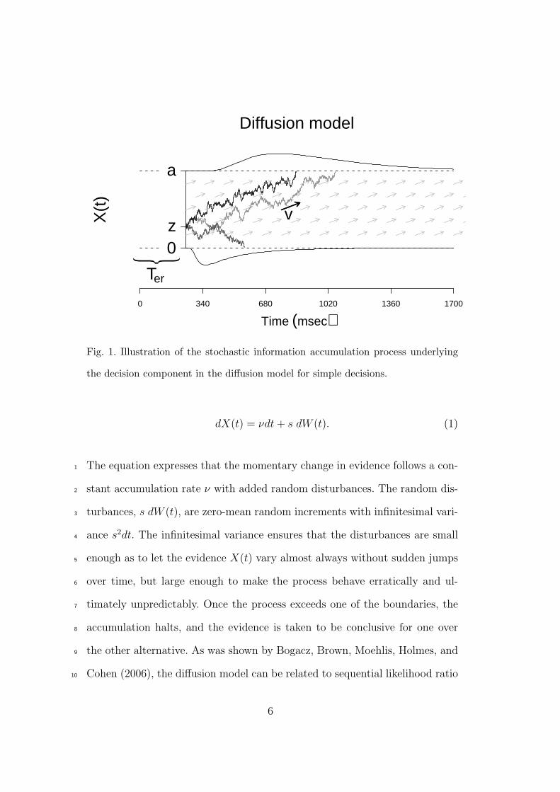
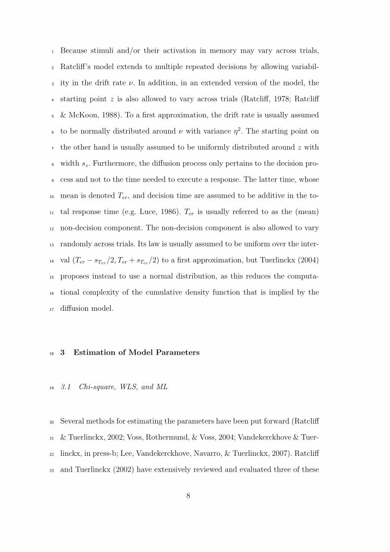
For a single decision, Ratcliff’s diffusion model can be conceived of as an in-16

formation accumulating process over a noisy channel. This process is modeled17

as the movements of a particle on the interval (0, a). Each of the boundaries18

of the interval is associated with one alternative (e.g., nonwords and words in19

a lexical decision task). The particle’s position X represents the evidence for20

one versus the other alternative. The initial position of the particle at time21

zero, denoted z, represents the bias towards either of the alternatives. The22

process is illustrated in Fig. 1. The particle’s movements are assumed to be23

governed by the stochastic differential equation24

5

X(t

)

0z

a

0 340 680 1020 1360 1700

Diffusion model

Time (msec)

{{

Ter

v

Fig. 1. Illustration of the stochastic information accumulation process underlying

the decision component in the diffusion model for simple decisions.

dX(t) = νdt+ s dW (t). (1)

The equation expresses that the momentary change in evidence follows a con-1

stant accumulation rate ν with added random disturbances. The random dis-2

turbances, s dW (t), are zero-mean random increments with infinitesimal vari-3

ance s2dt. The infinitesimal variance ensures that the disturbances are small4

enough as to let the evidence X(t) vary almost always without sudden jumps5

over time, but large enough to make the process behave erratically and ul-6

timately unpredictably. Once the process exceeds one of the boundaries, the7

accumulation halts, and the evidence is taken to be conclusive for one over8

the other alternative. As was shown by Bogacz, Brown, Moehlis, Holmes, and9

Cohen (2006), the diffusion model can be related to sequential likelihood ratio10

6

testing for optimal decision making under uncertainty.1

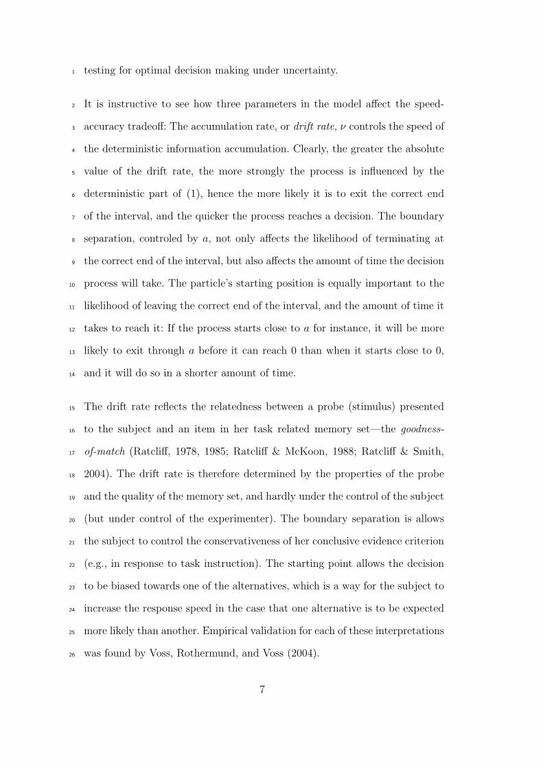
It is instructive to see how three parameters in the model affect the speed-2

accuracy tradeoff: The accumulation rate, or drift rate, ν controls the speed of3

the deterministic information accumulation. Clearly, the greater the absolute4

value of the drift rate, the more strongly the process is influenced by the5

deterministic part of (1), hence the more likely it is to exit the correct end6

of the interval, and the quicker the process reaches a decision. The boundary7

separation, controled by a, not only affects the likelihood of terminating at8

the correct end of the interval, but also affects the amount of time the decision9

process will take. The particle’s starting position is equally important to the10

likelihood of leaving the correct end of the interval, and the amount of time it11

takes to reach it: If the process starts close to a for instance, it will be more12

likely to exit through a before it can reach 0 than when it starts close to 0,13

and it will do so in a shorter amount of time.14

The drift rate reflects the relatedness between a probe (stimulus) presented15

to the subject and an item in her task related memory set—the goodness-16

of-match (Ratcliff, 1978, 1985; Ratcliff & McKoon, 1988; Ratcliff & Smith,17

2004). The drift rate is therefore determined by the properties of the probe18

and the quality of the memory set, and hardly under the control of the subject19

(but under control of the experimenter). The boundary separation is allows20

the subject to control the conservativeness of her conclusive evidence criterion21

(e.g., in response to task instruction). The starting point allows the decision22

to be biased towards one of the alternatives, which is a way for the subject to23

increase the response speed in the case that one alternative is to be expected24

more likely than another. Empirical validation for each of these interpretations25

was found by Voss, Rothermund, and Voss (2004).26

7

Because stimuli and/or their activation in memory may vary across trials,1

Ratcliff’s model extends to multiple repeated decisions by allowing variabil-2

ity in the drift rate ν. In addition, in an extended version of the model, the3

starting point z is also allowed to vary across trials (Ratcliff, 1978; Ratcliff4

& McKoon, 1988). To a first approximation, the drift rate is usually assumed5

to be normally distributed around ν with variance η2. The starting point on6

the other hand is usually assumed to be uniformly distributed around z with7

width sz. Furthermore, the diffusion process only pertains to the decision pro-8

cess and not to the time needed to execute a response. The latter time, whose9

mean is denoted Ter, and decision time are assumed to be additive in the to-10

tal response time (e.g. Luce, 1986). Ter is usually referred to as the (mean)11

non-decision component. The non-decision component is also allowed to vary12

randomly across trials. Its law is usually assumed to be uniform over the inter-13

val (Ter − sTer/2, Ter + sTer/2) to a first approximation, but Tuerlinckx (2004)14

proposes instead to use a normal distribution, as this reduces the computa-15

tional complexity of the cumulative density function that is implied by the16

diffusion model.17

3 Estimation of Model Parameters18

3.1 Chi-square, WLS, and ML19

Several methods for estimating the parameters have been put forward (Ratcliff20

& Tuerlinckx, 2002; Voss, Rothermund, & Voss, 2004; Vandekerckhove & Tuer-21

linckx, in press-b; Lee, Vandekerckhove, Navarro, & Tuerlinckx, 2007). Ratcliff22

and Tuerlinckx (2002) have extensively reviewed and evaluated three of these23

8

methods, namely, minimum chi-square, a weighted least squares method, and1

maximum likelihood.2

In the minimum chi-square (χ2) method, a number of quantiles are estimated3

from the data—usually the 1st, 3rd, 5th, 7th, and 9th deciles, (e.g., Ratcliff &4

Tuerlinckx, 2002)—independently for both error and correct responses. The5

cumulative distribution function (CDF) of the response times is evaluated at6

these quantiles, and the squared difference between the resulting predicted7

proportion of observations within the quantile bins and the quantile sizes are8

minimized by (iteratively) tuning the parameters.9

In the weighted least squares (WLS) method proposed by Ratcliff and Tuer-10

linckx (2002), the same quantiles as before are estimated from that data,11

but here the squared differences between these estimated quantiles and the12

quantiles predicted from the distribution plus the squared difference between13

observed and predicted accuracy is directly minimized. Note that this requires14

an numerical inversion of the CDF. Because the accuracy of the quantile esti-15

mates differs according to the rank (for instance the 5th decile is usually 2 es-16

timated with greater precision than the 1st or 9th), the quantiles’ contribution17

in determining the parameters is weighted with their asymptotic precision.18

The maximum likelihood (ML) method estimates the parameters by tuning the19

parameters until the likelihood of data set as observed is maximized. Ratcliff20

and Tuerlinckx (2002) computed the likelihood by numerically differentiating21

the cumulative distribution function. Instead, Vandekerckhove and Tuerlinckx22

(in press-b) use a multinomial likelihood function approach for binned response23

time data.24

2 At least for symmetric distributions.

9

Theoretically, there is a preference for ML estimators over other types of es-1

timators, because they are in very many cases asymptotically efficient—i.e.,2

they will achieve the greatest possible precision of any unbiased estimator,3

provided that the assumed family of distributions is correct, and suiTable4

amounts of observations are available (e.g., Silvey, 1970). In any real applica-5

tion the amount of observation is finite, and their number may not constitute a6

“suiTable amount”. It may therefore well be that other estimators outperform7

the maximum likelihood estimator when limited amounts of data are avail-8

able, or when there are other circumstances that undermine the assumptions9

under which the asymptotic properties hold—even if the assumed family of10

distributions is correct. 311

From the results of their simulations, Ratcliff and Tuerlinckx (2002) concluded12

that, although the ML estimators are more precise (essentially unbiased and13

small standard errors) than both the chi-square and WLS estimators, they are14

very sensitive to even the slightests of proportions of contaminants—response15

times that do not result from the diffusion process, e.g., due to an attentional16

lapse. The chi-square estimators on the other hand, were only slightly less17

precise than the ML estimators, substantially more robust than the ML esti-18

mators, and considerably more precise than the WLS estimators. The WLS19

estimators on their part were more robust than the chi-square estimators in20

face of contaminant response times. They therefore recommend the the chi-21

square fitting method.22

3 Note however, in finite samples the ML estimator is optimal in the Godambe-

Durbin sense, and is therefore still the preferred method of estimation (see, Go-

dambe, 1960).

10

3.2 EZ1

Despite the substantial payoff of the use of the diffusion model in terms of2

interpretability of the speed and accuracy data, the methodology has failed3

to catch on in a wider audience of researchers. This may have several causes:4

First of all, apparently the payoffs for analyzing response time data in terms of5

the diffusion model has thus far not balanced the amount of effort a researcher6

needs to invest in implementing one of the methods described above, and in7

gaining experience with this type of modeling and data analysis and the use of8

nonlinear estimation techniques (cf. Diederich & Busemeyer, 2003; Ratcliff &9

Tuerlinckx, 2002; Tuerlinckx, 2004; Wagenmakers et al., 2007). A second rea-10

son is the computational time that the methods described above require even11

on modern computers. Although this is not a principle barrier for application12

of the method, and arguably not even a practical one, it becomes problem-13

atic when a researcher wants to try different model configurations in complex14

designs with multiple partly constrained parameters with multiple subjects.15

Trying out different models can then become a nuisance, which makes it less16

appealing for a researcher to apply the diffusion model.17

The goal of introducing the EZ-diffusion model was to popularize the use of the18

diffusion model among a wider audience of researchers, by providing a method19

that is easily understood, easily implemented, and sTable, thus relying much20

less on user experience with nonlinear model fitting. This goal was reached21

by sacrificing a certain amount of detail of the original diffusion model, and22

setting much more modest aims in its range of applicability. Results obtained23

with the EZ-diffusion model may encourage users to pursue the analysis of24

their data with the full diffusion model.25

11

Two simplifications were introduced: First, in the EZ-model the starting point1

of the diffusion process is assumed to lie equidistant from both response thresh-2

olds. The EZ-diffusion model therefore is only suiTable in experiments where3

subjects do not have the ability to favor one response over another. The second4

simplification introduced in EZ is that none of the parameters are assumed5

to vary randomly (or non-randomly) over trials. The latter reduction in com-6

plexity limits the scope of the EZ-model to a somewhat more coarse grained7

analysis of the properties of the response time distribution, but is not very8

consequential with respect to the overall shape of the distribution. The first as-9

sumption however, constitutes a more profound limitation on the applicability10

of the EZ diffusion model.11

These simplifications leave us with three unknown parameters (i.e., the bound-12

ary separation a, the drift rate ν, and the non-decision time Ter). This allows13

us to use the expressions for the mean and variance of the response times,14

and the equation for probability of a correct response, given in Wagenmakers15

et al. (2005), to obtain a methods of moments estimator of the parameters by16

solving the equations in terms of these cumulants, and substituting the sample17

estimates for these cumulants.18

The simulations presented in Wagenmakers et al. (2007) showed that under19

the assumptions, these method of moments estimators performed quite well:20

there was no detecTable bias and standard errors where accepTable—even21

with a relatively modest amount of 50 trials. Performance was somewhat less22

favorable when the assumptions of lack of variability in either the drift rate or23

the starting point were violated, although this only was the case for variability24

in these parameters at the extreme end of empirical findings. Thus, overall the25

estimators were judged to be reasonably robust against these types of model26

12

mis specification.1

The major advantages of the EZ diffusion model are its simplicity and com-2

putational ease and speed, as well as its applicability to situations with few3

trials. A major disadvantage is however the assumption of a starting point4

that is equidistant from both decision thresholds. This assumption does not5

hold if participants are in some way biased toward one or the other response6

alternative, as is the case for instance in a lexical decision task with more7

words than nonwords (Wagenmakers, Ratcliff, Gomez, & McKoon, in press).8

A second disadvantage, although not a principle property, is that it applies9

only to a single experimental condition. That is, in a task with two types of10

stimuli, and two different responses associated with each stimulus type, the11

EZ-estimator applies only to one stimulus condition at a time. The result is12

that for each of these stimulus conditions a different set of estimates is ob-13

tained. This is unfortunate since the two conditions logically share at least one14

parameter if the two conditions are randomly intermixed—viz., the boundary15

separation a which reflects response conservativeness throughout the task.16

The latter problem becomes more prominent if we want to alleviate the former.17

Response bias should be independent of stimulus type, and hence the starting18

point should be the same in both experimental conditions. One straightforward19

way to force parameter equality across conditions is to use a least squares fit.20

This does however, preclude the possibility of finding closed form estimators21

for the parameters as there are more equations than parameters. For simplicity,22

in this paper we restrict attention to method of moments estimators and select23

at will as many moments equation as there are unknown parameters, and24

dispose of the remaining equations.25

13

4 Extension of EZ: EZ21

As was the case with the EZ-model, in EZ2 we also reduce the complexity of2

the full diffusion model by ignoring variability of any parameter across trials.3

In EZ2 however, we remove the limiting assumption of EZ that the starting4

point is equidistant from both decision boundaries. The model therefore only5

retains the parameters a, z, ν, and Ter. The parameter s, which determines the6

standard deviation of the noise process in (1), is as usual considered fixed.The7

diffusion constant, s, is often taken to be s = 0.1. We shall adhere to this8

convention.9

In this section, we proceed by finding closed form expressions for the mean and10

variance in terms of the parameters. In the next section, we then equate the11

sample values with these theoretical values and solve for the unknown param-12

eters. The ease of the EZ diffusion model lies in the complete analytical solu-13

tion of the parameters in terms of the sample statistics. Unfortunately, in the14

present case with an arbitrary starting point z, closed form solutions cannot15

be obtained. We therefore need to resort to numerical methods. Fortunately16

however, the resulting estimation procedure turns out to be simple enough to17

be computed in a web page. Alternatively, the method is straightforwardly im-18

plemented in an Excel (Microsoft, Inc., 2007) or Calc (OpenOffice.org, 2007)19

spreadsheet. This makes the EZ2 model still amenable to researchers without20

extensive backgrounds in numerical estimation procedures. Recent approaches21

to popularize the diffusion model by simplifying the fitting procedure for the22

full diffusion model, and by making available user friendlier software are pre-23

sented by Voss and Voss (in press) and by Vandekerckhove and Tuerlinckx (in24

press-a, in press-b). We next derive expressions for the cumulants of the RTs25

14

as a function of the parameters in the EZ2-model.1

4.1 Moments and Cumulants of Decision Times of Biased Processes2

We discuss two different cases: In the first case, we determine the mean and3

variance of the time that the process described by equation (1) exits the in-4

terval on either side—i.e., the cumulants of the correct and error decision5

times combined. In the second case we focus on the mean and variance of the6

time that the diffusion process exits through a particular interval—i.e., the7

cumulants of the correct or error decision time only.8

In this section we will switch to the terminology that is common in the litera-9

ture on stochastic processes, and will talk about a particle’s position and exit10

time rather than accumulated evidence and decision time.11

4.1.1 Cumulants of exit times independent of exit boundary12

As most of this case was already discussed in (Wagenmakers et al., 2005), we13

only briefly summarize the derivation here and quickly turn to the resulting14

expressions.15

The process in equation (1) is associated with a partial differential equation16

(PDE) that governs the evolution of the probability distribution of X(t) across17

time, given that the process started out from the point z:18

∂tp(x, t|z, 0) = ν ∂zp(x, t|z, 0) +s2

2∂2zp(x, t|z, 0). (2)

This equation is known as the backward Fokker-Planck equation, or Kolmogorov19

15

equation. The backward Fokker-Planck equation, as opposed to the associated1

forward Fokker-Planck equation, is the usual starting point for considerations2

about the exit times of a diffusion process.3

We consider the exit time T for the process. Let G(t, z) = Prob(T > t) denote4

the probability that a process that started at z exits the interval after time t.5

Then, since the process is still in the interval at time t if it leaves the interval6

after t, we have the equality7

G(t, z) =∫ a

0p(x, t|z, 0)dx.

Equation (2) then implies that G satisfies8

∂tG(t, z) = ν ∂zG(t, z) +s2

2∂2zG(t, z), (3)

with boundary conditions G(t, 0) = 0 = G(t, a) = 0, as both boundaries are9

absorbing (cf., Gardiner, 2004; Wagenmakers et al., 2005). The moments of10

the exit times are given by11

Tn(z) ≡ E{T n} =∫ ∞0

tn[∂t′P (T ≤ t′)]tdt

= −∫ ∞0

tn[∂t′G(t′, z)]tdt = n∫ ∞0

tn−1G(t, z)dt,

where the latter equality results from partial integration. The last equality can12

be applied in (3) to obtain the equation for the moments of the exit times:13

16

ν ∂zTn(z) +s2

2∂2zTn(z) = −nTn−1(z). (4)

Note that the equation is recursive in the moment order n. See Busemeyer1

and Townsend (1992) for an alternative derivation of the analogous equation2

for the more general Ornstein-Uhlenbeck process.3

A general solution can be obtained by direct integration of (4) (see Gardiner,4

2004), but we shall not do so here—the result is analogous however, to the5

derivation of the mean an variance of the correct responses that is outlined in6

the next section. For the first and second order moments the equations turn7

out to be analytically solvable, which allows us to obtain expressions for the8

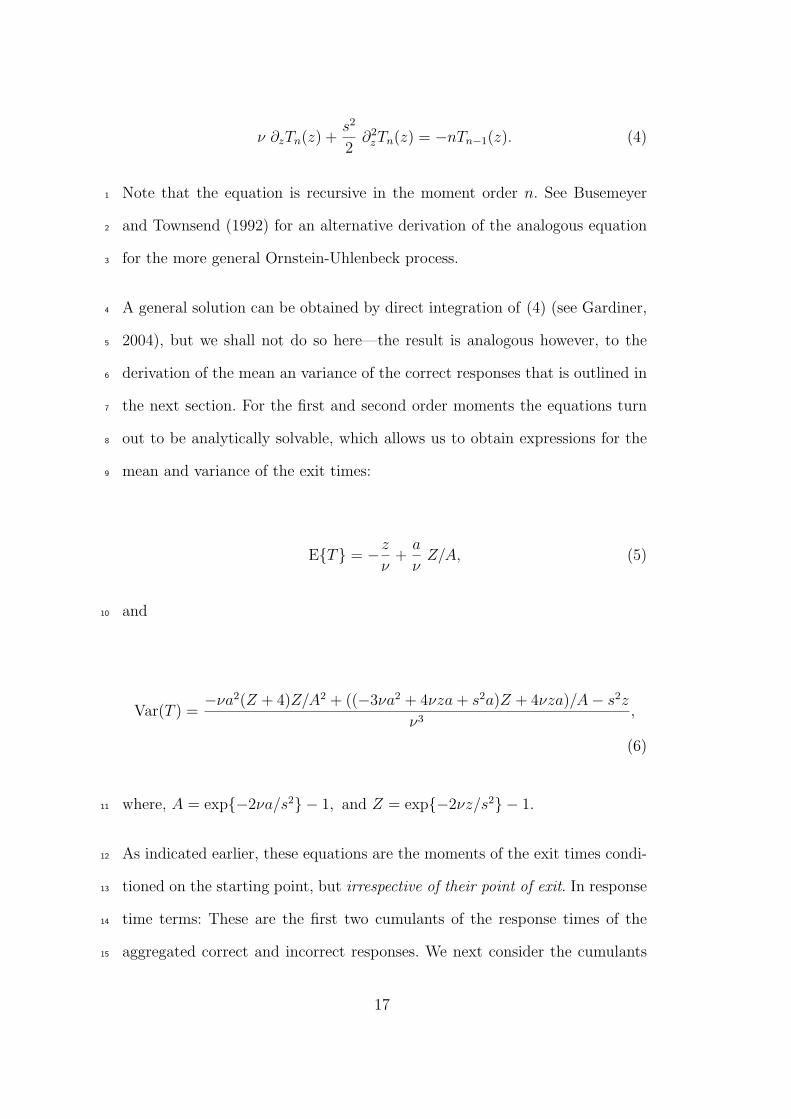
mean and variance of the exit times:9

E{T} = −zν

+a

νZ/A, (5)

and10

Var(T ) =−νa2(Z + 4)Z/A2 + ((−3νa2 + 4νza+ s2a)Z + 4νza)/A− s2z

ν3,

(6)

where, A = exp{−2νa/s2} − 1, and Z = exp{−2νz/s2} − 1.11

As indicated earlier, these equations are the moments of the exit times condi-12

tioned on the starting point, but irrespective of their point of exit. In response13

time terms: These are the first two cumulants of the response times of the14

aggregated correct and incorrect responses. We next consider the cumulants15

17

of the exit times given that the process exits through a particular end of the1

interval—i.e. of the responses conditioned on the correctness of the response.2

4.1.2 Mean and variance of exit times through the lower bound3

Before we proceed, consider again the backward Fokker-Planck equation in4

(2) associated with the decision proces. As indicated before, this equation is5

associated with the forward Fokker-Planck equation, which reads6

∂tp(x, t|z, 0) = −ν ∂xp(x, t|z, 0) +s2

2∂2xp(x, t|z, 0). (7)

This equation is in fact a completely equivalent, but slightly alternative spec-7

ification of the probability density p(x, t|z, t′). Both equations give rise to the8

same probability density function (Gardiner, 2004).9

The forward equation can be written10

∂tp(x, t|z, 0) + ∂xj(x, t|z, 0) = 0,

where j(x, t|z, 0) = νp(x, t|z, 0) − s2

2∂xp(x, t|z, 0). The function j(x, t; z, 0) is11

termed the probability current because mathematically, it behaves as a phys-12

ical current or flux (see Gardiner, 2004, sect. 5.2). The probability current13

describes how much of the probability per unit time flows through a particu-14

lar point x at time t, as the probability density p(x, t|z, 0) evolves over time.15

By convention, here the direction of flow is assumed to be pointing to the16

right. In particular, for the type of processes under consideration, j(0, t|z, 0)17

and j(a, t|z, 0) measure the amount of probability that leaks away per unit18

18

time at the end points of the interval. Clearly then, the probability of a par-1

ticle that started at z to leave the interval at the lower boundary after time t2

is3

g0(z, t) =∫ ∞t

j(0, t′|z, 0)dt′ = ν∫ ∞t

p(x, t′|z, 0)dt′ − s2

2∂x

∫ ∞t

p(x, t′|z, 0)dt′

= −∫ ∞t

∂t′p(x, t′|z, 0)dt′ (8)

(cf. Gardiner, 2004), where the first equality expresses the total amount of4

probability that leaks through a after time t. Therefore, the probability that5

the exit time of the particle is smaller than t given that it exits through 0 is6

P (T (0, z) < t) = g0(z, t)/g0(z, 0). (9)

The change of total probability that the particle is inside the interval at time t

is the total probability current that flows out of the interval at the boundaries

∂P (x(t) ∈ (0, a))

∂t= j(a, t)− j(0, t)

where the minus sign arises because the current is taken to point to the right.7

These equations imply that g0(z, t) satisfies the equation8

∂tg0(x, t) = −j(0, t|x, 0) = ν ∂zg0(z, t) +s2

2∂2zg0(z, t) (10)

As was the case for G(z, t) in the previous section, g0(z, t) gives rise to an9

equation for the moments of the exit times, given that the exit is at 0: The10

n-th order moment of T (z, 0), Tn(z, 0), is defined by11

19

Tn(z, 0) = −∫ ∞0

tn∂t′P (T (z, 0) > t′)|tdt = n∫ ∞0

tn−1∂t′g0(z, t′)|t/g0(z, 0)dt,

where the second equality result from partial integration.1

On the other hand, using the PDE for g0 above2

−g0(z, 0)Tn(z, 0) = −ν ∂z∫ ∞0

tng0(z, t)dt−s2

2∂2z

∫ ∞0

tng0(z, t)dt

Combining these equations, and defining π0(z) = g0(z, 0), we obtain3

ν ∂z(π0(z)Tn(z, 0)) +s2

2∂2z (π0(z)Tn(z, 0)) = −nπ0(z)Tn−1(z, 0). (11)

This equation recursively relates the moments of the exit times to each other,4

conditioned on the exit point 0. Note that the zeroth moment T0(z, 0) ≡ 1. It5

is clear that the boundary conditions for the solution π0(z)T (z, 0) are6

π0(a)T (a, 0) = π0(0)T (0, 0) = 0, (12)

which result directly from the boundary conditions of the backward Fokker-7

Planck equation in case of absorbing boundaries (the decision process termi-8

nates as soon as it hits one of the boundaries). Following Gardiner (2004, p.9

143), clearly T (0, 0) = 0, as a process starting at the boundary immediately10

terminates, and p0(a) = 0, as the chance that the process terminates at a if it11

started at the boundary 0 is zero.12

If t in (10) approaches 0, the equation reduces to an equation for g0(z, 0) =13

20

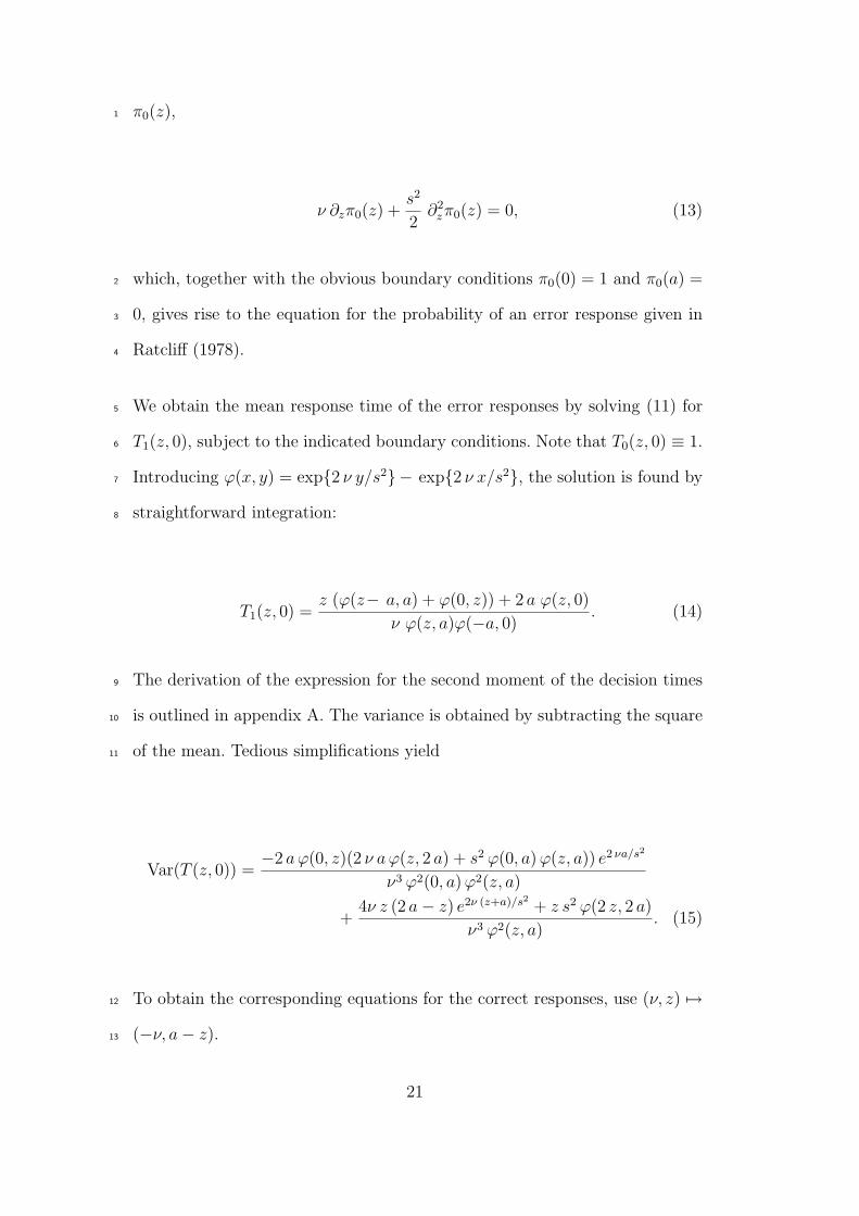
π0(z),1

ν ∂zπ0(z) +s2

2∂2zπ0(z) = 0, (13)

which, together with the obvious boundary conditions π0(0) = 1 and π0(a) =2

0, gives rise to the equation for the probability of an error response given in3

Ratcliff (1978).4

We obtain the mean response time of the error responses by solving (11) for5

T1(z, 0), subject to the indicated boundary conditions. Note that T0(z, 0) ≡ 1.6

Introducing ϕ(x, y) = exp{2 ν y/s2}− exp{2 ν x/s2}, the solution is found by7

straightforward integration:8

T1(z, 0) =z (ϕ(z− a, a) + ϕ(0, z)) + 2 a ϕ(z, 0)

ν ϕ(z, a)ϕ(−a, 0). (14)

The derivation of the expression for the second moment of the decision times9

is outlined in appendix A. The variance is obtained by subtracting the square10

of the mean. Tedious simplifications yield11

Var(T (z, 0)) =−2 aϕ(0, z)(2 ν aϕ(z, 2 a) + s2 ϕ(0, a)ϕ(z, a)) e2 νa/s

2

ν3 ϕ2(0, a)ϕ2(z, a)

+4ν z (2 a− z) e2ν (z+a)/s2 + z s2 ϕ(2 z, 2 a)

ν3 ϕ2(z, a). (15)

To obtain the corresponding equations for the correct responses, use (ν, z) 7→12

(−ν, a− z).13

21

Unconditional versus conditional cumulants We note a couple of dif-1

ferences between the conditional and uncondition mean and variance. First,2

both mean and variance of the exit time conditioned on the point of exit con-3

verge to an asymptotic value as the starting point approaches the other end.4

The unconditional mean and variance are both zero at either ends of the in-5

terval, which of course is to be expected. A second, perhaps more noteworthy,6

difference is that while the unconditional mean and variance are reflected in7

z = a/2 as the sign of ν is switched, the conditional mean and variance are8

even functions of ν. The latter implies that the conditional mean and variance9

do not provide information about the sign of ν, whereas the unconditional10

mean and variance do. If z = a/2 then both unconditional and conditional are11

even and neither contains information about the sign of ν. Only the proportion12

of correct responses provides information about the sign of ν.13

5 Method-of-Moments EZ2-diffusion Model Estimator14

To obtain method of moment estimators of the EZ2 model, we have to equate15

observed proportions of errors, response time means and/or variances to their16

theoretical expression just derived, and solve for the unknown parameters. In17

the EZ2 model the number of unknown parameters is less than the number18

of observable moments, and only a subset of the moments and their corre-19

sponding theoretical expressions is used. In principle any subset can be used.20

However, as indicated in the previous section, the conditional mean and vari-21

ance of correct responses do not provide information about the sign of ν.22

Therefore, if only the correct responses are used (or error responses for that23

matter), the proportion correct should also be used. In general it is advisable24

22

to include variance and error proportions.1

We consider as an example the common situation where there are two types of2

trials in which a correct response for one type of trial is an error response for3

the other and vice versa—a lexical decision task, say. We assume that the de-4

cision processes associated with the two conditions (i.e., words and nonwords)5

share the starting value z and the boundary separation a, which is appropriate6

if a participant cannot determine in advance what the condition of the next7

trial is. We further assume that the decision process associated with each type8

of condition has its own drift parameter–ν0 for nonwords and ν1 for words,9

say. In addition, both types of processes are hypothesized to have the same10

non-decision time Ter. Hence, there are five unknown parameters. In both the11

‘word’ and the ‘nonword’ condition, the proportion of errors, conditional and12

unconditional means, and conditional and unconditional variances can be cal-13

culated. This constitutes a total of ten observed moments. Because there are14

only five unknown parameters, only five observed moments and corresponding15

expressions for their theoretical values have to be used. To be able to estimate16

the sign of ν we have to include at least one proportion of errors or an un-17

conditional moment. To be able to estimate Ter we have to use at least one18

mean response time. However, because Ter is often not of primary interest, we19

can ignore this parameter if we do not use the means. Furthermore, it some-20

times seems reasonable to assume that error responses are more likely to be21

contaminated with responses that are not generated by the diffusion-process,22

and therefore to restrict the attention to correct responses. We are then left23

with 4 observed moments and 4 unknown parameters: A variance for the cor-24

rect response times for words, a variance for the correct response times for25

nonwords, a percentage of errors for the words and a percentage of errors for26

23

the nonwords, The non-linear system that needs to be solved then consists of1

4 equations. The simulations presented below focus on this setting.2

In contrast to the EZ-diffusion model, the equations for the EZ2-diffusion3

model cannot be inverted analytically. We therefore have to resort to numer-4

ical algorithms. Numerical methods to solve such nonlinear systems of equa-5

tions are discussed in Press, Flannery, Teukolsky, and Vetterling (1993). These6

generally involve defining a non-negative function, whose gradient involves the7

system (e.g., a least squares function) in a way that the gradient is zero if and8

only if the system is solved. The system is then solved by finding the minimum9

of the function using an optimization scheme. 4 We have considered several10

standard optimization algorithms; including the Nelder-Mead (or ‘simplex’)11

algorithm, the Hooke and Jeeves algorithm, and quasi Newton and Newton-12

Raphson algorithms (Hooke & Jeeves, 1961; Kaupe Jr., 1963; Gill, Wright,13

& Murray, 1986; Seber & Wild, 1989; Press et al., 1993). The algorithms did14

not differ very much, although the Hooke and Jeeves algorithm seemed to15

be slightly more accurate than the simplex algorithm, and is far simpler to16

implement than the other algorithms.17

We found the EZ estimates of ν, a, and Ter, together with z equal to half18

the estimate of a, to be effective starting values. We obtained two sets of EZ19

estimates—one based on the statistics from one condition and one based on20

the statistics from the other—and used both in a separate round of fitting21

the EZ2 model. We retained those estimates corresponding to the best fit22

according to the least squares distance measure.23

4 Note that although this may seem very similar to a least squares fit, it is in fact

not—the difference being that in order to solve the system, the minimum of the

objective function must be identically zero.

24

Note that there are logical constraints on the permitted parameter values,1

e.g., z is required lie in between 0 and a. Although general techniques exist to2

take these into account (e.g. Gill et al., 1986), we did not put any effort into3

imposing these constraints. In the simulations discussed in the next section4

we never encountered estimates that violated such natural constraints 5 , thus5

keeping the method simple.6

5.1 Diagnostic Checks and Model Evaluation7

Whenever we fit a model to a given data set, we need to evaluate the appro-8

priateness of the model by examining evidence of mismatch between model9

and data. Since EZ2 only takes error rates, response time means and response10

time variances as input, any set of such values gives parameter estimates. It11

is therefore very easy to forget about model checking, and start interpret-12

ing parameter estimates right away. One should however check whether the13

diffusion model is appropriate. A number of data checks were forwarded by14

Wagenmakers et al. (2007) to evaluate the appropriateness of the model. The15

most important one is to verify that the overall shape of the RT histograms16

is in accordance with the diffusion model—i.e., the histogram should be long17

tailed and skewed tot the right. The histogram may be visually compared to18

the density determined from the parameter estimates. Clearly this is not a19

rigorous test, but certainly a first requirement. Furthermore, the skew should20

increase with task difficulty. The skewness can be tested to deviate from zero21

5 This should not be surprising because both the variance formulas as well as the er-

ror proportion formula become negative when z is outside of (0, a), and the observed

values of course never are.

25

using the test by D’Agostino (1970), the skewness increase can be tested us-1

ing the bootstrap method proposed in (Muralhidar, 1993) or the test of Nath2

(1996). A second check is to see if the starting point is biased—if this is not3

the case one should prefer to stick to EZ to avoid the cost of estimating an4

unnecessary parameter.In a two-alternative forced choice task this check in-5

volves testing whether correct responses in one condition are faster than error6

responses, while the opposite is the case for the other condition. This consti-7

tutes a ‘stimulus category’ by ‘response correctness’ interaction with opposite8

effects (Wagenmakers et al., 2007). If there are, however, significant main ef-9

fects of the ‘response correctness’ factor, but insignificant interaction effects,10

this may imply that there is in fact no response bias, and that the difference11

between error and correct responses is due to variability in the drift rate co-12

efficient (Wagenmakers et al., 2007). In that case, neither the EZ nor the EZ213

model might be appropriate and one may have to resort to the full Ratcliff14

diffusion model (Ratcliff, 1978; Ratcliff & Rouder, 1998).15

6 Simulations16

To evaluate the moment estimators we conducted a simulation study under dif-17

ferent parameter setups and with different numbers of observations. To make18

results comparable, the setup of the simulations was as much the same as pos-19

sible as that of Wagenmakers et al. (2007). Overall the simulations show that20

when the starting point is not too close to the boundary separation parame-21

ter, the EZ2 estimators perform well when the number of trials per condition22

exceeds about 250, or when the number of trials per condition exceeds 12523

and drift rates are not very high. Overall it appears to be more difficult to es-24

26

timate parameter when the drift rates are very high and when the proportions1

of errors are very low.2

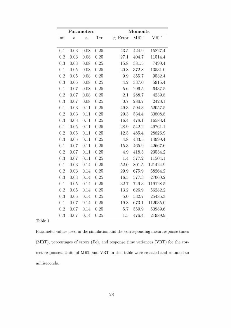
6.1 Setup3

We made every possible combination of ν1, ν2 ∈ {0.1, 0.2, 0.3} with ν1 al-4

ways strictly larger than ν2 (i.e., if ν2 = 0.1, then ν1 = 0.2 or ν1 = 0.3),5

a ∈ {0.08, 0.11, 0.14}, and z ∈ {0.03, 0.05, 0.07}. The choice for these values6

was motivated by estimates for these parameters that we encountered in the7

literature (cf. Wagenmakers et al., 2007). Because only the mean carries infor-8

mation about the parameter Ter, and results as soon as the other parameters9

are determined from the variances and error proportions, we only considered10

Ter = 0.250 as was done in the simulations in (Wagenmakers et al., 2007). Ta-11

ble 1 list the mean response times, the percentages of errors, and the response12

time variances corresponding to these parameter values.13

27

Parameters Moments

nu z a Ter % Error MRT VRT

0.1 0.03 0.08 0.25 43.5 424.9 15827.4

0.2 0.03 0.08 0.25 27.1 404.7 11514.4

0.3 0.03 0.08 0.25 15.8 381.5 7499.4

0.1 0.05 0.08 0.25 20.8 372.8 13531.0

0.2 0.05 0.08 0.25 9.9 355.7 9532.4

0.3 0.05 0.08 0.25 4.2 337.0 5915.4

0.1 0.07 0.08 0.25 5.6 296.5 6437.5

0.2 0.07 0.08 0.25 2.1 288.7 4239.8

0.3 0.07 0.08 0.25 0.7 280.7 2420.1

0.1 0.03 0.11 0.25 49.3 594.3 52057.5

0.2 0.03 0.11 0.25 29.3 534.4 30808.8

0.3 0.03 0.11 0.25 16.4 478.1 16583.4

0.1 0.05 0.11 0.25 28.9 542.2 49761.1

0.2 0.05 0.11 0.25 12.5 485.4 28826.9

0.3 0.05 0.11 0.25 4.8 433.5 14999.4

0.1 0.07 0.11 0.25 15.3 465.9 42667.6

0.2 0.07 0.11 0.25 4.9 418.3 23534.2

0.3 0.07 0.11 0.25 1.4 377.2 11504.1

0.1 0.03 0.14 0.25 52.0 801.5 121424.9

0.2 0.03 0.14 0.25 29.9 675.9 58264.2

0.3 0.03 0.14 0.25 16.5 577.3 27069.2

0.1 0.05 0.14 0.25 32.7 749.3 119128.5

0.2 0.05 0.14 0.25 13.2 626.9 56282.2

0.3 0.05 0.14 0.25 5.0 532.7 25485.3

0.1 0.07 0.14 0.25 19.8 673.1 112035.0

0.2 0.07 0.14 0.25 5.7 559.9 50989.6

0.3 0.07 0.14 0.25 1.5 476.4 21989.9Table 1

Parameter values used in the simulation and the corresponding mean response times

(MRT), percentages of errors (Pe), and response time variances (VRT) for the cor-

rect responses. Units of MRT and VRT in this table were rescaled and rounded to

milliseconds.

28

For each combination of parameters, we simulated 100 data sets, with N ∈1

{50, 250, 1000}, where N is the total number of trials. Each simulation con-2

sisted of two types of trials, each with N/2 replications. The parameters z and3

a had the same value in both conditions, but the boundary associations with4

correct and error responses in one condition were flipped in the other, as was5

the sign of the drift rate ν—i.e. if the drift rate was ν in one condition it was6

−ν in the other.7

A problem with small numbers of trials is the occurrence of perfect perfor-8

mance. Because the method only works if the proportion of errors is nonzero,9

if we encountered a data set with only correct responses, we simply discarded10

that data set. Hence, the results below are conditioned on the presence of error11

responses. Perfect performance can be dealt with as suggested in Wagenmak-12

ers et al. (2007). Here we did not do so, in order to be able to separate pure13

estimator bias from bias due to bias in the estimated moments.14

For each simulated data set, first EZ estimators for a, ν and Ter were obtained15

and, together with z equal to half the estimate of a, used as starting values16

for the iterative algorithm.17

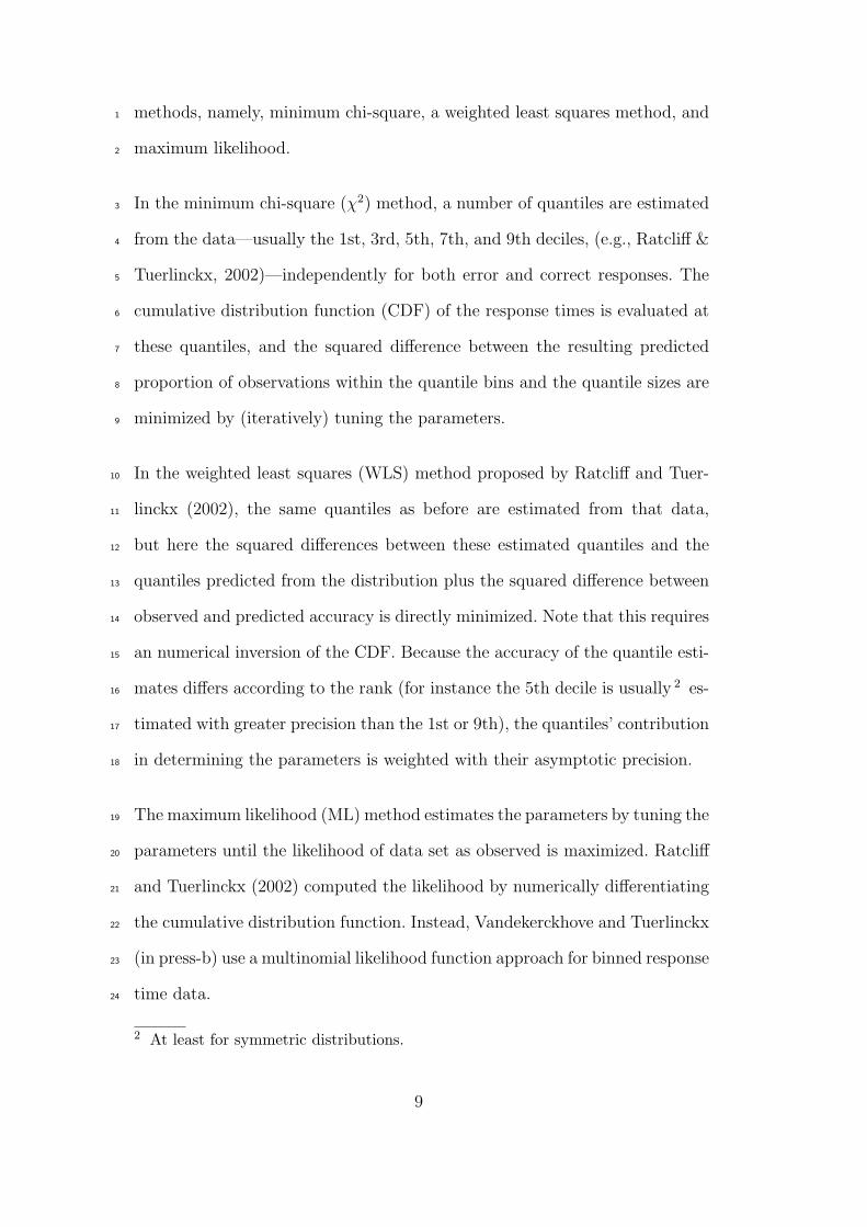
6.2 Results18

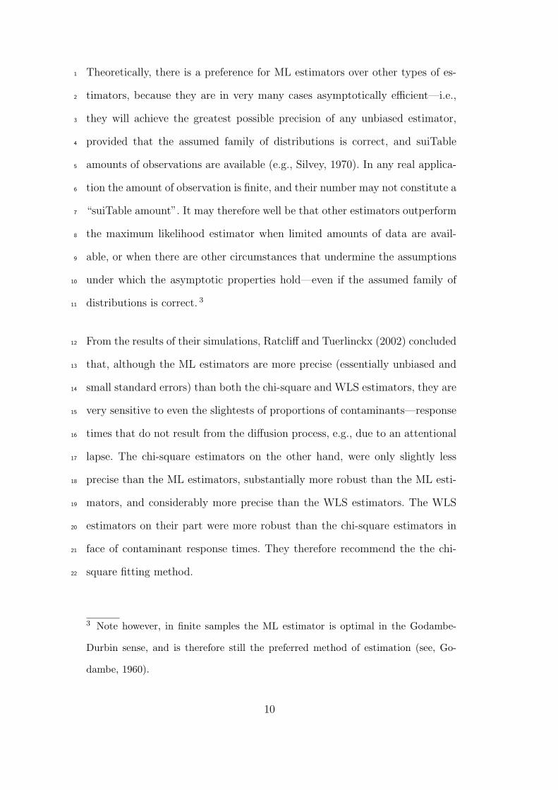
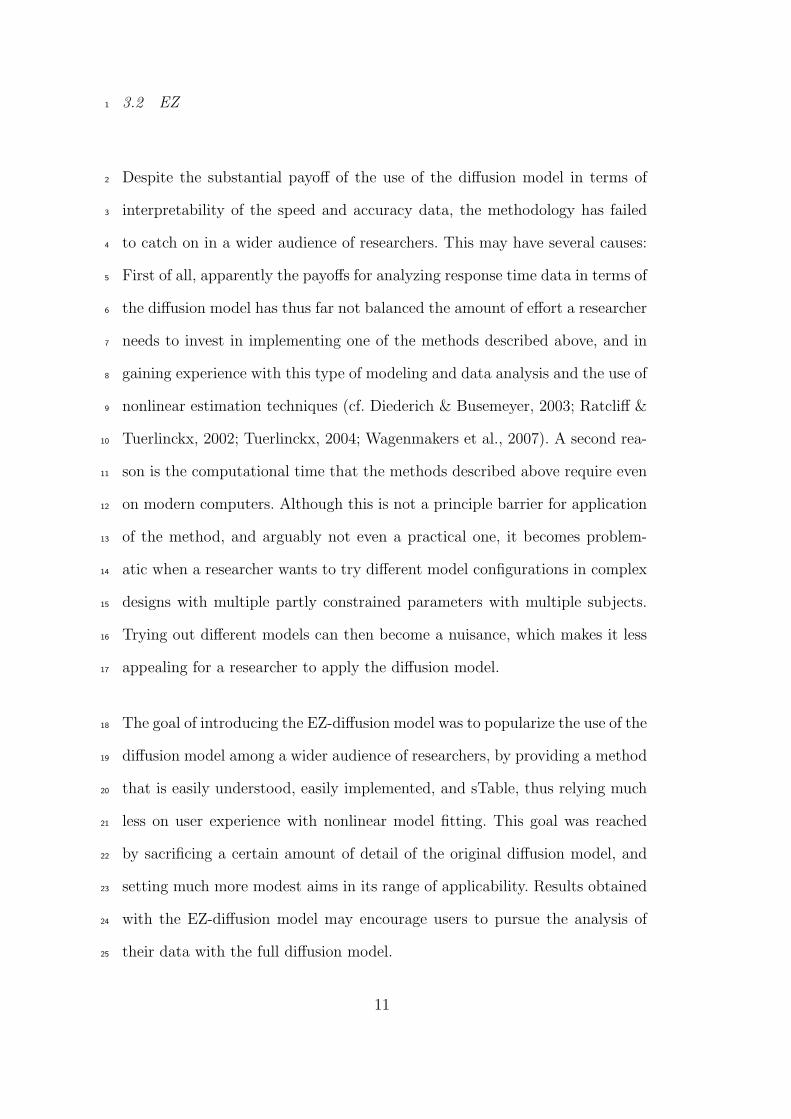
Figures 2 – 5 display the EZ2 results for the parameters a, z, ν1 and ν2 respec-19

tively in box-and-whisker plots. These estimates where based on the correct20

responses only. The results based on the pooled correct and error responses21

were very similar, and the conclusions to be drawn from these simulations22

are essentially the same. We therefore limit the discussion to the results dis-23

29

Estimator performance for a

N = 25 N = 125 N = 500

0.06

0.08

0.10

0.12

0.14

0.16

0.18

a

ν1 = 0.2, ν2 = 0.1, z = 0.03

N = 25 N = 125 N = 5000.

060.

080.

100.

120.

140.

160.

18a

ν1 = 0.3, ν2 = 0.1, z = 0.03

N = 25 N = 125 N = 500

0.06

0.08

0.10

0.12

0.14

0.16

0.18

a

ν1 = 0.3, ν2 = 0.2, z = 0.03

N = 25 N = 125 N = 500

0.06

0.08

0.10

0.12

0.14

0.16

0.18

a

ν1 = 0.2, ν2 = 0.1, z = 0.05

N = 25 N = 125 N = 500

0.06

0.08

0.10

0.12

0.14

0.16

0.18

a

ν1 = 0.3, ν2 = 0.1, z = 0.05

N = 25 N = 125 N = 500

0.06

0.08

0.10

0.12

0.14

0.16

0.18

a

ν1 = 0.3, ν2 = 0.2, z = 0.05

N = 25 N = 125 N = 500

0.06

0.08

0.10

0.12

0.14

0.16

0.18

a

ν1 = 0.2, ν2 = 0.1, z = 0.07

N = 25 N = 125 N = 500

0.06

0.08

0.10

0.12

0.14

0.16

0.18

a

ν1 = 0.3, ν2 = 0.1, z = 0.07

N = 25 N = 125 N = 500

0.06

0.08

0.10

0.12

0.14

0.16

0.18

a

ν1 = 0.3, ν2 = 0.2, z = 0.07

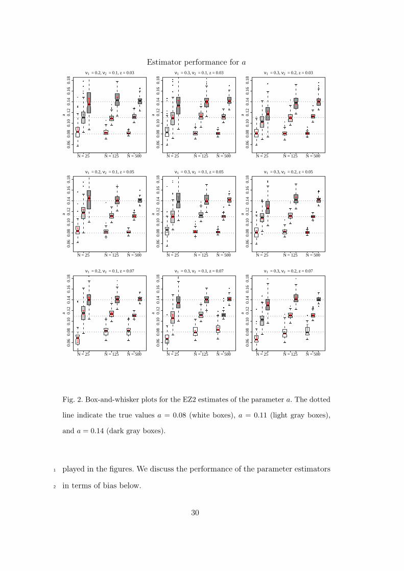
Fig. 2. Box-and-whisker plots for the EZ2 estimates of the parameter a. The dotted

line indicate the true values a = 0.08 (white boxes), a = 0.11 (light gray boxes),

and a = 0.14 (dark gray boxes).

played in the figures. We discuss the performance of the parameter estimators1

in terms of bias below.2

30

Estimator performance for z

N = 25 N = 125 N = 500

0.02

0.04

0.06

0.08

0.10

z

ν1 = 0.2, ν2 = 0.1, a = 0.08

N = 25 N = 125 N = 5000.

020.

040.

060.

080.

10z

ν1 = 0.3, ν2 = 0.1, a = 0.08

N = 25 N = 125 N = 500

0.02

0.04

0.06

0.08

0.10

z

ν1 = 0.3, ν2 = 0.2, a = 0.08

N = 25 N = 125 N = 500

0.02

0.04

0.06

0.08

0.10

z

ν1 = 0.2, ν2 = 0.1, a = 0.11

N = 25 N = 125 N = 500

0.02

0.04

0.06

0.08

0.10

z

ν1 = 0.3, ν2 = 0.1, a = 0.11

N = 25 N = 125 N = 500

0.02

0.04

0.06

0.08

0.10

z

ν1 = 0.3, ν2 = 0.2, a = 0.11

N = 25 N = 125 N = 500

0.02

0.04

0.06

0.08

0.10

z

ν1 = 0.2, ν2 = 0.1, a = 0.14

N = 25 N = 125 N = 500

0.02

0.04

0.06

0.08

0.10

z

ν1 = 0.3, ν2 = 0.1, a = 0.14

N = 25 N = 125 N = 500

0.02

0.04

0.06

0.08

0.10

z

ν1 = 0.3, ν2 = 0.2, a = 0.14

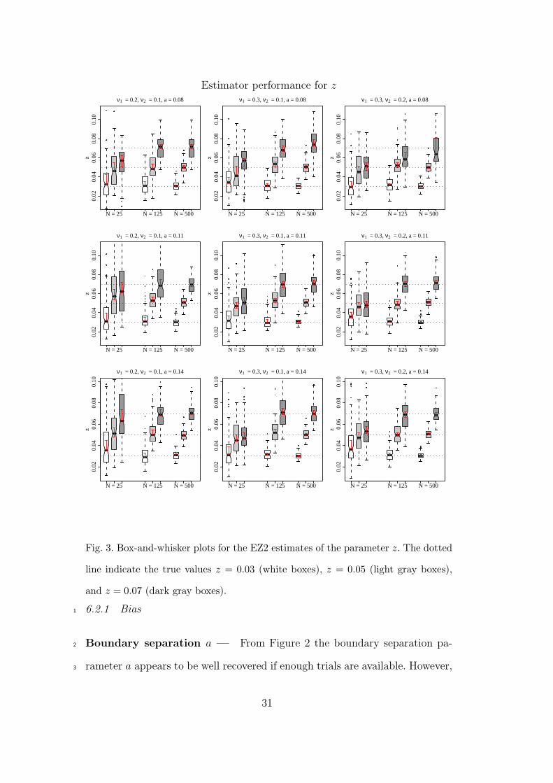
Fig. 3. Box-and-whisker plots for the EZ2 estimates of the parameter z. The dotted

line indicate the true values z = 0.03 (white boxes), z = 0.05 (light gray boxes),

and z = 0.07 (dark gray boxes).

6.2.1 Bias1

Boundary separation a — From Figure 2 the boundary separation pa-2

rameter a appears to be well recovered if enough trials are available. However,3

31

Estimator performance for ν1

N = 25 N = 125 N = 500

0.0

0.2

0.4

0.6

ν1

z = 0.03, a = 0.08

N = 25 N = 125 N = 5000.

00.

20.

40.

6ν1

z = 0.03, a = 0.11

N = 25 N = 125 N = 500

0.0

0.2

0.4

0.6

ν1

z = 0.03, a = 0.14

N = 25 N = 125 N = 500

0.0

0.2

0.4

0.6

ν1

z = 0.05, a = 0.08

N = 25 N = 125 N = 500

0.0

0.2

0.4

0.6

ν1

z = 0.05, a = 0.11

N = 25 N = 125 N = 500

0.0

0.2

0.4

0.6

ν1

z = 0.05, a = 0.14

N = 25 N = 125 N = 500

0.0

0.2

0.4

0.6

ν1

z = 0.07, a = 0.08

N = 25 N = 125 N = 500

0.0

0.2

0.4

0.6

ν1

z = 0.07, a = 0.11

N = 25 N = 125 N = 500

0.0

0.2

0.4

0.6

ν1

z = 0.07, a = 0.14

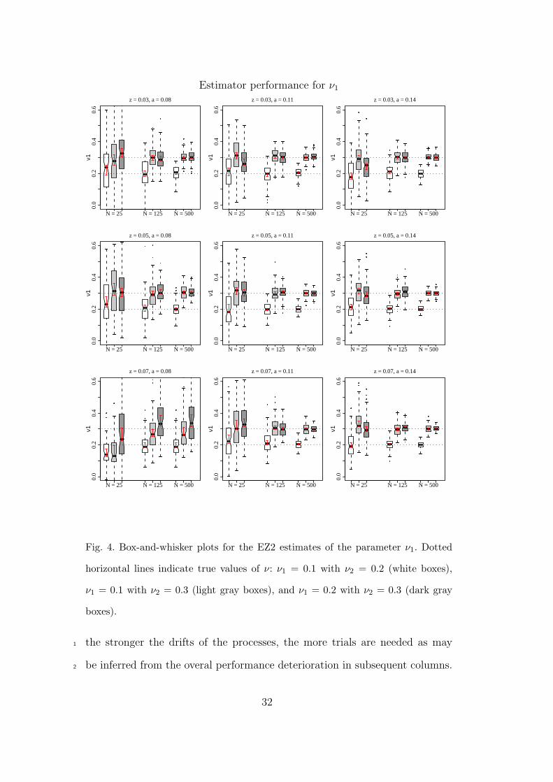
Fig. 4. Box-and-whisker plots for the EZ2 estimates of the parameter ν1. Dotted

horizontal lines indicate true values of ν: ν1 = 0.1 with ν2 = 0.2 (white boxes),

ν1 = 0.1 with ν2 = 0.3 (light gray boxes), and ν1 = 0.2 with ν2 = 0.3 (dark gray

boxes).

the stronger the drifts of the processes, the more trials are needed as may1

be inferred from the overal performance deterioration in subsequent columns.2

32

Estimator performance for ν2

N = 25 N = 125 N = 500

0.0

0.2

0.4

ν2

z = 0.03, a = 0.08

N = 25 N = 125 N = 5000.

00.

20.

4ν2

z = 0.03, a = 0.11

N = 25 N = 125 N = 500

0.0

0.2

0.4

ν2

z = 0.03, a = 0.14

N = 25 N = 125 N = 500

0.0

0.2

0.4

ν2

z = 0.05, a = 0.08

N = 25 N = 125 N = 500

0.0

0.2

0.4

ν2

z = 0.05, a = 0.11

N = 25 N = 125 N = 500

0.0

0.2

0.4

ν2

z = 0.05, a = 0.14

N = 25 N = 125 N = 500

0.0

0.2

0.4

ν2

z = 0.07, a = 0.08

N = 25 N = 125 N = 500

0.0

0.2

0.4

ν2

z = 0.07, a = 0.11

N = 25 N = 125 N = 500

0.0

0.2

0.4

ν2

z = 0.07, a = 0.14

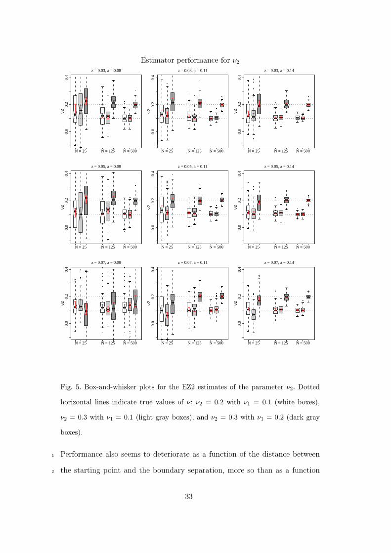
Fig. 5. Box-and-whisker plots for the EZ2 estimates of the parameter ν2. Dotted

horizontal lines indicate true values of ν: ν2 = 0.2 with ν1 = 0.1 (white boxes),

ν2 = 0.3 with ν1 = 0.1 (light gray boxes), and ν2 = 0.3 with ν1 = 0.2 (dark gray

boxes).

Performance also seems to deteriorate as a function of the distance between1

the starting point and the boundary separation, more so than as a function2

33

of boundary separation or starting point itself. Although the performance de-1

teriorates as the drift rate increases, eventually, if the number of responses in2

each condition are large enough, the estimates show no sign of bias, and seem3

to have a symmetrical distribution about the true value.4

Starting point z — The box-and-whisker plots in Figure 3 lead to similar5

conclusions about the starting point z: Higher drift rates cause bias in the6

estimates for few trials situations, but given enough trials this bias disappears.7

Also, the closer the starting point is to the upper boundary, the more trials8

are necessary to obtain unbiased estimates. This is especially noticeable from9

the top row of panels of Figure 3. In addition, proportionality of the distances10

from starting point to either boundaries seems to play a role: the interquartile11

range for more equidistant starting points seem to be narrower and more12

symmetrical around the true value. The middel and bottom rows of panels13

show that higher drift rates require more trials for unbiasedness.14

Drift rates ν1 and ν2 — As can be seen in the figures 4 and 5, the estima-15

tors for ν1 and ν2 also require more trials as its true value increases. Analogous16

to a and z, the ν estimators perform worst when a and z are very close to-17

gether. As indicated by the middle row of panels, performance is rather good18

even with few trials if the starting point is not too close to either boundary.19

The proportionality of the distances to both bound playing a more important20

role for ν1 and ν2 than for z as may be inferred from the bottom row panels.21

34

6.2.2 Simulation conclusions1

In conclusion, higher drift rates require more trials for unbiased estimation2

of any of the parameters. Furthermore, when z is closer to either boundary,3

performance of all estimators deteriorates, but this is more prominent for z4

very close to a than for z close to 0, which indicates that these two parameters5

tend to interfere with each other. The estimators have most difficulty when6

decision performance rate of a participant is almost perfect.7

It should however be noted that the cases in which the estimators perform8

worst, correspond to parameter values combinations that are at the extreme9

ends of what has been encountered model fits found in the literature (Wagen-10

makers et al., 2007). The estimators therefore all seem to be virtually unbiased11

in a great many experimental settings.12

7 Application to Lexical Decision Data13

For illustration purposes, we apply the EZ2 methods to empirical data. The14

complete task is described in Wagenmakers et al. (in press), here we only sum-15

marize the important features. The response time data were collected from 1916

individuals (university students) in a lexical decision task with 75% nonwords17

and 25% words, and word frequency was varied from ‘very low’ to ‘low’ to18

‘high’. The former imbalance presumably biases participants towards the non-19

word boundary, whereas the latter should affect drift rate for words but not20

for nonwords—that is, higher frequency words are presumably stronger repre-21

sented in memory and hence their drift rate should be higher. The nonwords22

consisted of pseudo-words that were formed by changing the vowels of existing23

35

words. Because ‘very low’, ‘low’, and ‘high’ frequency words were randomly1

intermixed, the bias should not be affected by word frequency, and boundary2

separation nor nonword drift rate should be affected by the word frequency.3

Two of the participants showed perfect performance in one of the conditions.4

Although this can be dealt with using the method suggested in Wagenmakers5

et al. (in press), since we only mean to illustrate the use of the method, we6

simply discarded these two cases from the analysis. In Wagenmakers et al. (in7

press), the data were judged to conforming to the diffusion model characteris-8

tics so that application of the EZ2 method is warranted. Individual variances9

(of correct responses only) and percentages of errors of 17 participants were10

fitted to a model in which the lower boundary corresponded to a word response11

and the upper boundary to a nonword response. The data from different word12

frequencies were fitted separately, so that for each word frequency we obtained13

a boundary separation (a), a starting point (z), a drift rate for words (ν1) and14

a drift rate for nonwords (ν0). The across participant means of the parameter15

estimates are given in Table 2, along with their standard errors in parentheses.16

Individual parameter estimates seemed approximately normal and no depar-17

tures from normal were indicated by a Shapiro test. A multivariate repeated18

measures omnibus Hotelling’s T 2 test revealed significant differences in param-19

eter vectors for the different word frequencies (F (8, 9) = 5.144, p = .0122).20

Post hoc these could only be attributed to differences between very low and21

high frequency words (F (4, 13) = 12.51, p = .0008) and between low and high22

frequency words (F (4, 13) = 7.509, p = .0023), but not between very low and23

low frequency words (F (4, 13) = .404, p = .316). Subsequent t-tests revealed24

significant differences only for the word drift rates (ν1) between low and high25

word frequencies (t(16) = 3.259, p = .005) and between very low and high26

word frequencies (t(16) = 5.731, p = .00003).27

36

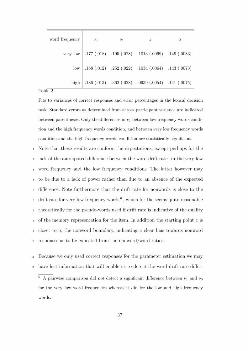
word frequency ν0 ν1 z a

very low .177 (.018) .195 (.028) .1013 (.0069) .149 (.0083)

low .168 (.012) .252 (.022) .1034 (.0064) .143 (.0073)

high .186 (.013) .362 (.028) .0939 (.0054) .141 (.0075)

Table 2

Fits to variances of correct responses and error percentages in the lexical decision

task. Standard errors as determined from across participant variance are indicated

between parentheses. Only the differences in ν1 between low frequency words condi-

tion and the high frequency words condition, and between very low frequency words

condition and the high frequency words condition are statistically significant.

Note that these results are conform the expectations, except perhaps for the1

lack of the anticipated difference between the word drift rates in the very low2

word frequency and the low frequency conditions. The latter however may3

to be due to a lack of power rather than due to an absence of the expected4

difference. Note furthermore that the drift rate for nonwords is close to the5

drift rate for very low frequency words 6 , which for the seems quite reasonable6

theoretically for the pseudo-words used if drift rate is indicative of the quality7

of the memory representation for the item. In addition the starting point z is8

closer to a, the nonword boundary, indicating a clear bias towards nonword9

responses as to be expected from the nonword/word ratios.10

Because we only used correct responses for the parameter estimation we may11

have lost information that will enable us to detect the word drift rate differ-12

6 A pairwise comparison did not detect a significant difference between ν1 and ν0

for the very low word frequencies whereas it did for the low and high frequency

words.

37

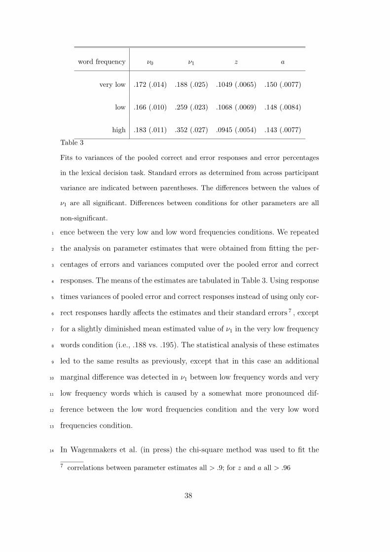
word frequency ν0 ν1 z a

very low .172 (.014) .188 (.025) .1049 (.0065) .150 (.0077)

low .166 (.010) .259 (.023) .1068 (.0069) .148 (.0084)

high .183 (.011) .352 (.027) .0945 (.0054) .143 (.0077)

Table 3

Fits to variances of the pooled correct and error responses and error percentages

in the lexical decision task. Standard errors as determined from across participant

variance are indicated between parentheses. The differences between the values of

ν1 are all significant. Differences between conditions for other parameters are all

non-significant.

ence between the very low and low word frequencies conditions. We repeated1

the analysis on parameter estimates that were obtained from fitting the per-2

centages of errors and variances computed over the pooled error and correct3

responses. The means of the estimates are tabulated in Table 3. Using response4

times variances of pooled error and correct responses instead of using only cor-5

rect responses hardly affects the estimates and their standard errors 7 , except6

for a slightly diminished mean estimated value of ν1 in the very low frequency7

words condition (i.e., .188 vs. .195). The statistical analysis of these estimates8

led to the same results as previously, except that in this case an additional9

marginal difference was detected in ν1 between low frequency words and very10

low frequency words which is caused by a somewhat more pronounced dif-11

ference between the low word frequencies condition and the very low word12

frequencies condition.13

In Wagenmakers et al. (in press) the chi-square method was used to fit the14

7 correlations between parameter estimates all > .9; for z and a all > .96

38

full diffusion model to the .1, .3, .5, .7, .9 quantiles that were averaged across1

participants. Qualitatively, the differences between the estimates given in that2

paper and the EZ2 estimates given here are not very large. All in all, the3

results show that for as far as the EZ2 parameters are concerned, conclusions4

that may drawn from the averaged EZ2 estimates pretty much confer to the5

conclusions that may be drawn from a full diffusion model fit to participant6

averaged data in this example.7

8 Discussion8

The aim of the present paper was three fold: First, we introduced the EZ2-9

diffusions model which, like the EZ-diffusion model, is a drastic simplification10

of Ratcliffs full diffusion model. It retains the most important features of the11

full diffusion model, and alleviates some of the more prominent drawbacks of12

the EZ-diffusion model. In particular, the EZ2 model includes the bias param-13

eter that is absent in the EZ-diffusion model. Second, we provided closed form14

formulas for the mean and variances of the response times under this model.15

These equations to our knowledge have not been available to the psychologi-16

cal community before. Lastly, based on the closed form equations, we provide17

method of moments estimators of the relevant parameters, which instigate a18

more general framework to model complex experimental designs. The frame-19

work is simple enough so that experimentalists without extensive statistical20

training are able to use the method with relatively little effort.21

Although for most interesting ranges of the parameters the simulations showed22

no signs of bias, for the more extreme ends of these ranges bias was in fact23

severe. Part of the problem in these extreme situations can be attributed to24

39

the difference in scale of response times variance and response accuracy: The1

response accuracy predicted from the estimated parameters correlated almost2

perfectly with the observed accuracies obtained from the simulation, whereas3

the correlation between the observed variances and the by the estimates pre-4

dicted variance was moderate. In addition, if we fitted standard deviations5

instead of variances by least squares, the problem was substantially dimin-6

ished. An unfortunate observation is that for every parameter estimator this7

bias was dependent on the values of other parameters. This implies that it8

can be difficult to assess the difference between two experimental conditions9

with respect to a single parameter. It is however not a problem unique to EZ210

estimates. One way out of this problem is to fit the model with constrained11

parameters and compare the fit to a model without constraints—i.e., to use12

model selection procedures.13

As indicated before, the currently proposed estimator straightforwardly gener-14

alizes to a least squares estimator that fits a composite model of EZ2 diffusions15

in different experimental conditions to the observed sample moments, using16

equations (5)-(14) as elementary building blocks. This is akin covariance struc-17

ture modeling as used, e.g., in linear structural relations modeling (LISREL,18

see Joreskog, 1981; Bollen, 1989). The straightforward method is ordinary19

least squares (OLS) estimation with more equations than unknown param-20

eters. OLS is however, generally dominated by its cousin generalized least21

squares (GLS) estimation (e.g., Browne, 1974, 1984) or generalized minimum22

chi-square estimation (Ferguson, 1996, chap. 23), in which squared differences23

between modeled and observed moments are weighted in accordance with their24

precision. GLS can result in asymptotically efficient (i.e., maximum likelihood25

equivalent) estimators (Browne, 1974, 1984). Such an approach could be vi-26

40

able in the current case: An estimate of the covariance matrix from which the1

precision can be calculated can be obtained by bootstrapping the mean and2

the variance of the response times if only correct responses are used, and the3

error rate, and mean and variance of the response times if pooled error and4

correct responses are used.5

Recently, Ratcliff and Tuerlinckx (2002) point out the importance of con-6

taminant response times. They showed in their simulations that outliers and7

contaminant responses in general can have important effects on parameter es-8

timates, and therefore propose to fit a mixture model in which the proportion9

of contaminants is estimated in addition to the other model parameters. In10

EZ2 is is not entirely straightforward perhaps to include a proportion of con-11

taminants parameter, although not entirely impossible 8 . Alternatively, one12

can try to find more robust estimators of the mean and variance. Such es-13

timators for skewed distribution are available (e.g., Wang & Raftery, 2002).14

Likewise, the EZ2 model can be augmented with a variance in the non-decision15

component that we have ignored all along. It remains to be evaluated if such16

additions are advantageous.17

EZ2 thus leaves room for future improvement; both in terms of (relatively18

8 One could modify the equations for the variance to (1 − ρ)V RT + ρ σc + p (1 −

p) (MRT − µc)2, where ρ would indicate the proportion of contaminants, and µc

and σc their mean and variance. This introduces 3 extra parameters and can only

be estimated if 3 more equations are available. This can be realized if multiple

conditions are analyzed in which these parameters are assumed to be constant. If

µc and σc are functionally dependent, as for instance is the case if a chi-square

distribution is assumed for the contaminants for instance, then the number of extra

parameters can be reduced by one parameter.

41

straightforward) generalizations to handling contaminants and non-decision1

time variability, as well as in terms of more complex generalizations to handling2

a complicated experimental designs with multiple factors, fit assessment and3

model selection.4

References5

Apostol, T. M. (1969). Calculus (Vol. 2). New York: Wiley.6

Bogacz, R., Brown, E., Moehlis, J., Holmes, P., & Cohen, J. D. (2006). The7

physics of optimal decision making: A formal analysis of models of per-8

formance in two-alternative forced choice tasks. Psychological Review,9

113 (4), 700–765.10

Bollen, K. A. (1989). Structural equations with latent variables (1st ed.). New11

York, USA: Wiley.12

Browne, M. W. (1974). Generalized least squares estimators in the analysis13

of covariance structures. South African Statistical Journal, 8, 1-24.14

Browne, M. W. (1984). Asymptotically distribution-free methods for the15

analysis of covariance structures. British Journal of Mathematical and16

Statistical Psychology, 37, 62–83.17

Busemeyer, J. R., & Townsend, J. T. (1992). Fundamental derivations from18

decision field theory. Mathematical Social Sciences, 23, 255–282.19

D’Agostino, R. B. (1970). Transformation to normality of the null distribution20

of g1. Biometrika, 57, 679–681.21

Diederich, A., & Busemeyer, J. R. (2003). Simple matrix methods for ana-22

lyzing diffusion models of choice probability, choice response time, and23

simple response time. Journal of Mathematical Psychology, 47, 304–322.24

42

Ferguson, T. S. (1996). A course in large sample theory (1 ed.). Boca Raton:1

Chapman & Hall/CRC.2

Gardiner, C. W. (2004). Handbook of stochastic methods (3 ed.). Berlin:3

Springer Verlag.4

Gill, P. E., Wright, M. H., & Murray, W. (1986). Nonlinear programming.5

Stanford: Stanford University Press.6

Godambe, V. P. (1960). An optimum property of regular maximum likelihood7

estimation. The Annals of Mathematical Statistics, 31 (4), 1208–1211.8

Hooke, R., & Jeeves, T. A. (1961). Direct search solution of numerical and9

statistical problems. Journal of the ACM, 8, 212–229.10

Joreskog, K. G. (1981). Analysis of covariance structures. Scandinavian11

Journal of Statistics, 8, 65-92.12

Kaupe Jr., A. F. (1963). Algorithm 178: Direct search. Communications of13

the ACM, 6, 313.14

Kreyszig, E. (1993). Advanced engineering mathematics. New York: Wiley.15

Lee, M., Vandekerckhove, J., Navarro, D., & Tuerlinckx, F. (2007). Hierarchi-16

cal bayesian modeling of human decision-making using Wiener diffusion.17

Manuscript submitted for publication.18

Luce, R. D. (1986). Response times. New York: Oxford University Press.19

Microsoft, Inc. (2007). Microsoft Office Excel [Computer software] (Microsoft20

Office 2007 ed.). Reddington, WA: Microsoft, Inc.21

Muralhidar, K. (1993). The bootstrap approach for testing skewness persis-22

tence. Management Science, 39 (4), 487–491.23

Nath, R. (1996). A note on testing for skewness persistence. Management24

Science, 42 (1), 138–141.25

OpenOffice.org. (2007). Calc [computer software] (2.2 ed.). World Wide Web:26

OpenOffice.org.27

43

Press, W. H., Flannery, B. P., Teukolsky, S. A., & Vetterling, W. T. (1993).1

Numerical recipes in c: the art of scientific computing (2nd ed.). Cam-2

bridge: Cambridge University Press.3

Ratcliff, R. (1978). A theory of memory retrieval. Psychological Review, 85,4

59–108.5

Ratcliff, R. (1985). Theoretical interpretations of the speed and accuracy of6

positive and negative responses. Psychological Review, 92, 212–225.7

Ratcliff, R., & McKoon, G. (1988). A retrieval theory of priming in memory.8

Psychological Review, 95.9

Ratcliff, R., & Rouder, J. N. (1998). Modeling response times for two–choice10

decisions. Psychological Science, 9, 347–356.11

Ratcliff, R., & Smith, P. L. (2004). A comparison of sequential sampling12

models for two–choice reaction time. Psychological Review, 111, 333–13

367.14

Ratcliff, R., & Tuerlinckx, F. (2002). Estimating parameters of the diffu-15

sion model: Approaches to dealing with contaminant reaction times and16

parameter variability. Psychonomic Bulletin & Review, 9, 438–481.17

Seber, G. A. F., & Wild, C. J. (1989). Nonlinear regression. New York: Wiley.18

Silvey, S. D. (1970). Statistical inference. Harmondsworth: Penguin.19

Tuerlinckx, F. (2004). The efficient computation of the distribution function20

of the diffusion process. Behavior Research Methods, Instruments, &21

Computers, 34.22

Vandekerckhove, J., & Tuerlinckx, F. (in press-a). Diffusion model analysis23

with MATLAB: a DMAT primer. Behavior Research Methods.24

Vandekerckhove, J., & Tuerlinckx, F. (in press-b). Fitting the Ratcliff diffusion25

model to experimental data. Psychonomic Bulletin & Review.26

Voss, A., Rothermund, K., & Voss, J. (2004). Interpreting the parameters of27

44

the diffusion model: An empirical validation. Memory & Cognition, 32,1

1206–1220.2

Voss, A., & Voss, J. (in press). Fast–dm: A free program for efficient diffusion3

model analysis. Behavior Research Methods.4

Wagenmakers, E.-J., Grasman, R. P. P. P., & Molenaar, P. C. M. (2005).5

On the relation between the mean and the variance of a diffusion model6

response time distribution. Journal of Mathematical Psychology, 49,7

195–204.8

Wagenmakers, E.-J., Ratcliff, R., Gomez, P., & McKoon, G. (in press). A9

diffusion model account of criterion manipulations in the lexical decision10

task. Journal of Memory and Language.11

Wagenmakers, E.-J., van der Maas, H. L. J., & Grasman, R. P. P. P. (2007). An12

EZ-diffusion model for response time and accuracy. Psychomic Bulletin13

and Review, 14, 3–22.14

Wang, N., & Raftery, A. E. (2002). Nearest-neighbor variance estimation15

(NNVE): Robust covariance estimation via nearest-neighbor cleaning.16

Journal of the American Statistical Association, 97, 994–1005.17

Wickelgren, W. A. (1977). Speed–accuracy tradeoff and information process-18

ing dynamics. Acta Psychologica, 41, 67–85.19

45

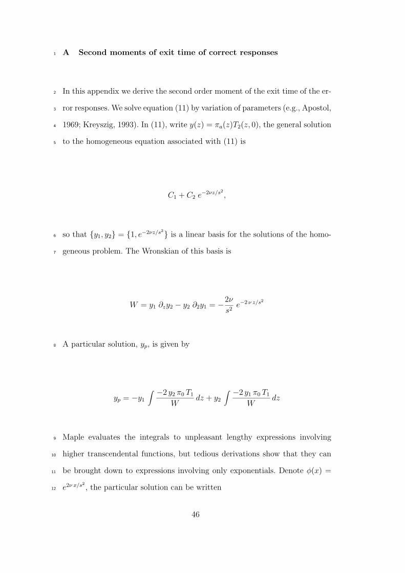
A Second moments of exit time of correct responses1

In this appendix we derive the second order moment of the exit time of the er-2

ror responses. We solve equation (11) by variation of parameters (e.g., Apostol,3

1969; Kreyszig, 1993). In (11), write y(z) = πa(z)T2(z, 0), the general solution4

to the homogeneous equation associated with (11) is5

C1 + C2 e−2νz/s2 ,

so that {y1, y2} = {1, e−2νz/s2} is a linear basis for the solutions of the homo-6

geneous problem. The Wronskian of this basis is7

W = y1 ∂zy2 − y2 ∂2y1 = −2ν

s2e−2 ν z/s2

A particular solution, yp, is given by8

yp = −y1

∫ −2 y2 π0 T1

Wdz + y2

∫ −2 y1 π0 T1

Wdz

Maple evaluates the integrals to unpleasant lengthy expressions involving9

higher transcendental functions, but tedious derivations show that they can10

be brought down to expressions involving only exponentials. Denote φ(x) =11

e2ν x/s2, the particular solution can be written12

46

yp =1

2

φ(−z)

ν4 (φ(a)− 1)2

((2 z ν s2 − s4 − 8φ(a) a ν2 z − 2 z2 ν2) φ(z)

+ (2 ν2z2 + 2νzs2 − 8aν2z − 4νas2 + s4) φ(a) + (−2 νzs2 − 2ν2z2 − s4) φ(2a)

+ (2ν2z2 + 4νas2 + s4 − 2νzs2) φ(x+ a)).

The general solution to (11) then is1

y = yp + C1 + C2 e−2νz/s2 .

The coefficients C1 and C2 are solved for by imposing the side conditions (12),2

and substituted back into the solution. Dividing y by πa(z) yields an expression3

for the second order moment T2(z, 0) which we do not give here. Instead, we4

gave the variance in (15), which results from subtracting the square of equation5

(14).6

B Estimation Software7

We provide several pointers to software implementations of the estimation8

procedure of the EZ2 diffusion model:9

B.1 Web Application10

A web application that can be used directly, can be found at http://users.11

fmg.uva.nl/rgrasman/jscript/EZ2_new.html. The application allows users12

to specify a model for complex experimental designs involving several EZ2-13

47

diffusions with separate and or shared parameters. To this end, the user i)1

creates a set of parameters, ii) chooses a multiple of the non-linear equations2

in (5), (6), (14), and (15) (i.e., one equation corresponding to each observed3

percentage of errors, response time variance and/or mean response time), iii)4

specifies the corresponding observed values, and iv) indicates on each equation5

parameters depends. The user can then specify starting values, or use EZ es-6

timators, and presses the ’solve’ button to find the estimates. The application7

can be used both for finding method-of-moment estimators (the number of8

non-linear equations equals the number of unknown parameters) or for (or-9

dinary) least squares estimation (the number of nonlinear equations exceeds10

the number of unknowns). The application also provides batch estimation11

functionality.12

Note that the application is written in JavaScript (ECMAScript) and DHTML.13

JavaScript is clearly not intended for heavy numerical computations, yet the14

application is sufficiently fast to gain some first hands-on experience with mod-15

eling this way. Performance speed varies considerably across browsers. Notably16

Firefox (versions 1.5 and 2.0, tested on a Windows XP machine) seems to be17

a bit slow. Microsoft’s Internet Explorer (IE6 & IE7 on Windows platform)18

is appreciably faster, as are Opera 9.0 and Safari 3.0 (both for Mac OS X &19

Windows).20

B.2 Estimation in an Excel Sheet21

An example Excel sheet, including a tutorial can be found at http://users.22

fmg.uva.nl/rgrasman/worknotes/EZ2inExcel.html.23

48

B.3 R Routines1

An R packages with non user-friendly R routines, including documentation,2

can be downloaded from http://users.fmg.uva.nl/rgrasman/rpages/EZ2.3

html.4

49