(This is a sample cover image for this issue. The actual cover is not yet available at this time.)

This article appeared in a journal published by Elsevier. The attachedcopy is furnished to the author for internal non-commercial researchand education use, including for instruction at the authors institution

and sharing with colleagues.

Other uses, including reproduction and distribution, or selling orlicensing copies, or posting to personal, institutional or third party

websites are prohibited.

In most cases authors are permitted to post their version of thearticle (e.g. in Word or Tex form) to their personal website orinstitutional repository. Authors requiring further information

regarding Elsevier’s archiving and manuscript policies areencouraged to visit:

http://www.elsevier.com/copyright

Author's personal copy

International Journal of Forecasting 28 (2012) 587–606

Contents lists available at SciVerse ScienceDirect

International Journal of Forecasting

journal homepage: www.elsevier.com/locate/ijforecast

A population dependent diffusion model with a stochastic extensionC. Michalakelis ∗, T. SphicopoulosDepartment of Informatics and Telecommunications, University of Athens, Greece

a r t i c l e i n f o

Keywords:Innovation diffusionHigh technology marketsTechnology estimation and forecasting‘‘Population’’ diffusion model (PDM)Stochastic diffusion models (SDM)

a b s t r a c t

Diffusion modeling is rather broad in nature, and is important in the areas of estimationand forecasting. Conventional models do not incorporate parameters that explicitly takeinto account the size of the population, or, equivalently, the size of the potential market.As a consequence, the models often fail to provide accurate forecasts, especially whenthe diffusion process is in the take-off stage. Furthermore, since diffusion is not a strictlydeterministic process, forecasts should provide a measure of the underlying uncertainty ofthe process by incorporating a stochastic process into the formulation of the models.

The aim of the present work is to fill this gap by proposing an aggregate diffusionmodel, the ‘‘population’’ diffusionmodel (PDM),which incorporates the potentially varyingmarket size as a function of the corresponding population. This model realization providesmore accurate estimations and future forecasts of the diffusion process, especially whencompared to the conventional aggregate diffusion models.

© 2012 Published by Elsevier B.V. on behalf of International Institute of Forecasters.

1. Introduction

In the context of the contemporary competitive globalmarket, there are tremendous pressures on companies andorganizations, due to exponential growth and the intro-duction of new technologies. Sustainable and disruptivetechnologies play a critical role in shaping the success ofcompanies.

The introduction of innovative products into a marketis frequently connected to heavy investments, requiringcritical business planning in order to meet marketdemand and competition. Industrial plans rolled out inan attempt to attract and retain customers must beforecasted precisely, in order to obtain the expected levelof adoptions and market shares. A failure to produceaccurate forecasts oftenhas dramatic results for the supply,whether oversupply and unnecessary over-investment, orunder-utilization of a firm’s capacities.

∗ Correspondence to: Department of Informatics and Telecommunica-tions, University of Athens, Panepistimioupolis, Illisia, Greece. Tel.: +30210 7275 319.

E-mail address:michalak@di.uoa.gr (C. Michalakelis).

The most representative case is probably the telecom-munications sector. It is one of the most significant con-temporary investments, which refers to new technologiesand services that are subject to competition. Privatizationand deregulation, alongwith the effects of increasing com-petition and the introduction of new services, will tend tointroduce new research problems. Diffusion forecasting isamong the most important of such problems, and aims toface the high level of uncertainty and the consequent needfor risk management.

Moreover, estimating and forecasting the diffusionpatterns of the innovations is considered important for allkinds of high technology markets. Characteristic examplesin the literature include the works of Teng, Grover, andGuttler (2002), who suggest general diffusion patterns forinformation technology innovations; and Linton (2002),who presents a thorough overview of the literature,before proposing a method for forecasting disruptiveand discontinuous innovations. In addition, Fildes andKumar (2002) review the telecommunications demandforecasting literature.

Although forecasting models for established productsand services are well developed, new opportunities haveemerged due to the nature of the high technology productmarket. Therefore, further methodological work should be

0169-2070/$ – see front matter© 2012 Published by Elsevier B.V. on behalf of International Institute of Forecasters.doi:10.1016/j.ijforecast.2012.03.002

Author's personal copy

588 C. Michalakelis, T. Sphicopoulos / International Journal of Forecasting 28 (2012) 587–606

carried out to identify the gaps that have opened up as aresult of changes in the market’s scope and structure.

The remainder of the paper is organised as follows. Sec-tion 2 provides a short presentation of the background todiffusion theory and models, together with the researchobjectives and contribution of the present work. Section 3describes the deterministic process for the ‘‘population’’diffusion model (PDM). The model’s evaluation results arepresented in Section 4. The stochastic analogue of the‘‘population’’ diffusion model (PDM) is presented in Sec-tion 5, and its evaluation results are illustrated in Section 6.The conclusions are presented in Section 7, together withtheir limitations and directions for future research.

2. Background and objectives

2.1. Models for innovation diffusion

One of the central themes of the innovation field isthe mathematical modeling of innovation diffusion, whichpertains to different types of innovations under differentassumptions. The main findings can be summarized asa bell-shaped curve depicting the frequency of adoptionagainst time and an S-shaped curve representing thecumulative number of adopters. During the initial stagesof the innovation life cycle (the introduction stage), therate of adoption is relatively low. This is followed by thetake-off stage, characterised by a high rate of adoption.Finally, the peak of the bell curve is reached, correspondingto the inflection point of the cumulative adoption. Afterthis point, the adoption rate decreases until the marketsaturation level is met asymptotically and the maximumnumber of adopters has been reached. This situationcorresponds to the end of the life cycle of the innovation,after which, in the case of high technology products, it isusually replaced by its descendant generation.

Apart from the pioneering work of Gompertz (1825),theworks of Bass (1969) and Rai (1999) represent the earlycontemporary efforts to capture the diffusion dynamics.These two works, together with the logistic family ofmodels (Bewley & Fiebig, 1988), such as the linear logisticor Fisher–Pry model (Fisher & Pry, 1971), are the mostwidely used diffusionmodels employed for estimating andforecasting market demand.

All of the above models provide ‘‘S-shaped curve’’estimations to describe the cumulative diffusion, which isused to estimate and forecast the diffusion of innovationsat the aggregate level. This approach describes the totalmarket response, in contrast to econometricmodels,whichfocus on the factors affecting the adoption of the studiedinnovation by individuals.

Aggregate models are generally able to provide reliableestimations of diffusion processes with respect to theadoption of innovations into a market of reference.One of their main fields of application is the sectorof high technology, and especially telecommunications.An informative review of the forecasting of demand intelecommunications is provided by Fildes and Kumar(2002). Moreover, important research results on thedevelopment and evaluation of diffusion models arepresented by Bewley and Fiebig (1988), Geroski (2000),

Jain and Rai (1988), Mahajan and Muller (1979), Mahajan,Muller, and Bass (1990), Michalakelis, Varoutas, andSphicopoulos (2008) and Skiadas (1987). Extensions ofthese models include cross-national influence (Kumar,Ganesh, & Echambadi, 1998; Kumar & Krishnan, 2002;Michalakelis, Dede, Varoutas, & Sphicopoulos, 2008) andmarketing variables (Mahajan & Peterson, 1979; Ruiz-Conde, Leeflang, & Wieringa, 2006), in an attempt todescribe the process of adoption inmore detail. Most of theresulting models are derived by incorporating functionaladjustments into the original formulation of a diffusionmodel’s equation.

2.2. Research objectives and contribution

None of the approaches described above, despite em-ploying a number of parameters and marketing variables,explicitly take into consideration the influence of thepopulation size on the diffusion process, and consequentlyincorporate it into the appropriate mathematical formula-tions. The market potential, or saturation level, used in theformulation of the models does not coincide with the ac-tual size of the market population, nor does it depend onit. Moreover, no relationship between these two quantitiesis derived. In fact, theymay lead to substantial divergencesin forecasting, especially at certain stages of the diffusionprocess, such as the take-off stage. This may turn out to bea major deficiency in the context of diffusion analysis, es-pecially in the case of rapid take-offs. The reason for this isthat the population size imposes a constraint on the furtheracceleration of the innovation diffusion. This is common inthe case of a technological product, where the probabilityof adopting another unit of the product decreases after thefirst adoption, although it is not totally eliminated. Mobilephones, broadband connections and personal computersare some representative examples. Conventional diffusionmodels do not usually provide accurate forecasts when thediffusion process accelerates fast, since their forecasts tendto diverge from the actual values recorded later, sometimessubstantially. For some important contributions to the taskof appraising the influence of the population on the diffu-sion process, see Gruber (2001) and Gruber and Verboven(2001).

Without limiting the value of the above contributions,the first objective of the present work is to study theinfluence of the target market’s size on the diffusionprocess, by developing an aggregate diffusion model thatincludes the population size of the market as an explicitparameter which influences both the diffusion rate andthe market potential. This is an important contribution,especially at the take-off stage of the diffusion life cycle,where the inflection point has not been reached. At thisparticular stage, the process is characterised by a highlevel of skewness and flexibility. In such cases, forecastingcan contain a high level of uncertainty and have a majoreffect on strategic planning. Since the life cycle of a typicalproduct is expected to be rather short, due to substitutionby its descendant generation, forecasting is usually basedon a limited amount of historical data.

A second objective is the development of a diffusionmodel that is capable of providing a flexible inflectionpoint

Author's personal copy

C. Michalakelis, T. Sphicopoulos / International Journal of Forecasting 28 (2012) 587–606 589

which is able to capture the flexibility and skewness ofthe process and which is affected by the market size andexpressed as a function of it. Since the inflection pointof the ‘‘traditional’’ diffusion models occurs at a certainlevel of capacity K (e.g., 50% of K for the logistic growthmodel), there is a need for a newmodel which can describethe diffusion process of high technology products, whichare usually characterized by asymmetric shapes and ahigh level of skewness. This is described in more detail inthe next section, where the development of the proposedmodel is presented.

The third objective of this research is to provide a mea-sure which can quantify the level of forecast uncertainty. Itis worthmentioning thatmost of the research in the litera-ture focuses on describing diffusion as a deterministic pro-cess in time. However, diffusion processes should often bemodeled as dynamic phenomena, which can be describedby stochastic differential equations. One work that raisedthis need is that of Eliashberg and Chatterjee (1986), whopresent some arguments on the necessity of using stochas-tic models, together with ways of introducing randomnessinto a diffusion process study. In the end, an estimation ofthe level of uncertainty in forecasts can provide valuableinput with respect to a firm’s available actions, predictionsfor the future and even expectations for competition.

Another important objective here is the application ofthe proposed diffusionmodel to a number of historical dataseries, in order to evaluate its performance and its abilityto provide accurate forecasts. This is especially importantwhen the peak point is not included in the observationsavailable, which usually limits the forecasting ability of theconventional models, due to the underlying uncertainty ofthe process.

Given the above considerations, the present work isdevoted to the construction of a new diffusion model, the‘‘population-diffusion model’’, or the PDM. The model turnsout to be able to capture the influence of the populationsize on the procedure of estimating and forecastingpenetration in the case of high technology products. Twoformulations of the model are constructed, presentedand evaluated: the deterministic model and its stochasticanalogue. Evaluation was performed using historical dataon mobile phone subscribers from 22 countries over thewider European area. The results demonstrate that notonly can the PDM provide accurate diffusion estimationsover a dataset that includes inflection points, but it canalso forecast future values quite accurately. In order tocompare the results of the PDM with the performancesof conventional diffusion models, the most representativecases of the latter (the logistic, Gompertz and Bassmodels) are also evaluated.Moreover, the evaluation of thestochastic realization provided a range of forecasted valuesthat are also quite accurate, since they indicate lower andupper bounds within which future recorded values areexpected to fall. The proposed diffusion model takes intoaccount the number of connections (services) providedto the customer, not the physical number of devices. Theprobability of purchasing the first connection is higherthan the probability of purchasing a second connection,and so on.

The data used to evaluate the PDM were extractedfrom the ITU (International Telecommunication Union)

database, describing the diffusion patterns of the countriesconsidered.

The accomplishment of the objectives of this workwill contribute significantly to both research and practice.Research will benefit from the provision of new directionsfor the development of a diffusion forecasting frameworkby incorporating a number of influential parameters. Thiswill help improve our understanding of the diffusionshapes in the high technology market, especially whencombined with our study of the underlying uncertainty.For practitioners, our research findings will be very usefulfor strategic planning and decision making, as they can beapplied in an increasingly competitive environment, sincemore accurate a priori estimates of the diffusion patterncan be derived, enhanced by the estimation of the level ofuncertainty provided by the stochastic analysis.

However, it should be clarified that the proposedmodeland the corresponding analysis do not attempt to providea method for the estimation of time-variant saturationlevels, based on the population size, but only show theeffect of the population size on the diffusion process.

3. Deterministic ‘‘population’’ diffusion model (PDM)

3.1. Development of the model

Aggregate diffusionmodels, which describe cumulativepenetration, are derived by a differential equation of thefollowing general form (Seber & Wild, 2003):

dN(t)dt

= d (N(t), p̄) · [f (K ,N(t))] . (1)

In the above equation, N(t) represents the total pene-tration at time t , while K is the saturation level, or themax-imum expected cumulative penetration of the innovation.d(N(t), p̄) is a functionwhich represents a factor of propor-tionality. The quantity f (K ,N(t)) represents the functionof the remaining market potential at time t , depending onthe saturation level of K and the number of adopters N(t)at this time t . Finally, p̄ is the vector of the model parame-ters, which are considered as constants over the period ofthe study.

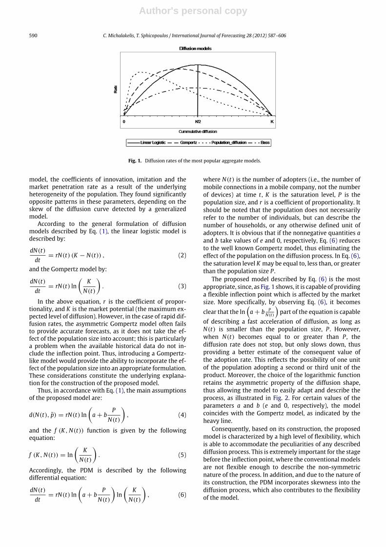
The most widely used aggregate diffusion modelsare the linear logistic and Bass models, which createsymmetric S-curves. In Fig. 1, the diffusion shapes of someof the most common models are illustrated for the samesaturation level of K , together with their inflection points,where the diffusion rate becomes equal to zero beforestarting to decrease. As was observed, the linear logisticand Bass models are described by a symmetric diffusionshape, with their inflection points at K/2. However, inthe case of high technology products, the correspondingdiffusion shapes are usually right skewed rather thansymmetric, since they follow a high initial rate of diffusion,slowing down after that. Therefore, symmetric modelsoften fail to describe such cases adequately.

The non-symmetric Gompertzmodel,which exposes aninflection point at the 37% of K , is sometimes consideredas more appropriate for describing a diffusion process.Bemmaor and Lee (2002) made an important contributionregarding the changes in parameter estimates of the Bass

Author's personal copy

590 C. Michalakelis, T. Sphicopoulos / International Journal of Forecasting 28 (2012) 587–606

Fig. 1. Diffusion rates of the most popular aggregate models.

model, the coefficients of innovation, imitation and themarket penetration rate as a result of the underlyingheterogeneity of the population. They found significantlyopposite patterns in these parameters, depending on theskew of the diffusion curve detected by a generalizedmodel.

According to the general formulation of diffusionmodels described by Eq. (1), the linear logistic model isdescribed by:

dN(t)dt

= rN(t) (K − N(t)) , (2)

and the Gompertz model by:

dN(t)dt

= rN(t) ln

KN(t)

. (3)

In the above equation, r is the coefficient of propor-tionality, and K is the market potential (the maximum ex-pected level of diffusion). However, in the case of rapid dif-fusion rates, the asymmetric Gompertz model often failsto provide accurate forecasts, as it does not take the ef-fect of the population size into account; this is particularlya problem when the available historical data do not in-clude the inflection point. Thus, introducing a Gompertz-like model would provide the ability to incorporate the ef-fect of the population size into an appropriate formulation.These considerations constitute the underlying explana-tion for the construction of the proposed model.

Thus, in accordance with Eq. (1), the main assumptionsof the proposed model are:

d(N(t), p̄) = rN(t) lna + b

PN(t)

, (4)

and the f (K ,N(t)) function is given by the followingequation:

f (K ,N(t)) = ln

KN(t)

. (5)

Accordingly, the PDM is described by the followingdifferential equation:

dN(t)dt

= rN(t) lna + b

PN(t)

ln

KN(t)

, (6)

where N(t) is the number of adopters (i.e., the number ofmobile connections in a mobile company, not the numberof devices) at time t , K is the saturation level, P is thepopulation size, and r is a coefficient of proportionality. Itshould be noted that the population does not necessarilyrefer to the number of individuals, but can describe thenumber of households, or any otherwise defined unit ofadopters. It is obvious that if the nonnegative quantities aand b take values of e and 0, respectively, Eq. (6) reducesto the well known Gompertz model, thus eliminating theeffect of the population on the diffusion process. In Eq. (6),the saturation level K may be equal to, less than, or greaterthan the population size P .

The proposed model described by Eq. (6) is the mostappropriate, since, as Fig. 1 shows, it is capable of providinga flexible inflection point which is affected by the marketsize. More specifically, by observing Eq. (6), it becomesclear that the ln

a + b P

N(t)

part of the equation is capable

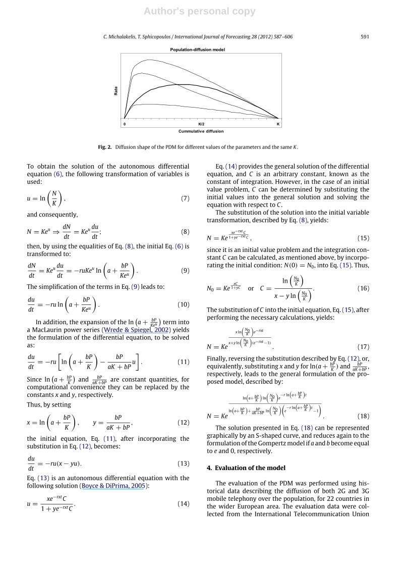
of describing a fast acceleration of diffusion, as long asN(t) is smaller than the population size, P . However,when N(t) becomes equal to or greater than P , thediffusion rate does not stop, but only slows down, thusproviding a better estimate of the consequent value ofthe adoption rate. This reflects the possibility of one unitof the population adopting a second or third unit of theproduct. Moreover, the choice of the logarithmic functionretains the asymmetric property of the diffusion shape,thus allowing the model to easily adapt and describe theprocess, as illustrated in Fig. 2. For certain values of theparameters a and b (e and 0, respectively), the modelcoincides with the Gompertz model, as indicated by theheavy line.

Consequently, based on its construction, the proposedmodel is characterized by a high level of flexibility, whichis able to accommodate the peculiarities of any describeddiffusion process. This is extremely important for the stagebefore the inflection point, where the conventionalmodelsare not flexible enough to describe the non-symmetricnature of the process. In addition, and due to the nature ofits construction, the PDM incorporates skewness into thediffusion process, which also contributes to the flexibilityof the model.

Author's personal copy

C. Michalakelis, T. Sphicopoulos / International Journal of Forecasting 28 (2012) 587–606 591

Fig. 2. Diffusion shape of the PDM for different values of the parameters and the same K .

To obtain the solution of the autonomous differentialequation (6), the following transformation of variables isused:

u = lnNK

, (7)

and consequently,

N = Keu ⇒dNdt

= Keududt

; (8)

then, by using the equalities of Eq. (8), the initial Eq. (6) istransformed to:

dNdt

= Keududt

= −ruKeu lna +

bPKeu

. (9)

The simplification of the terms in Eq. (9) leads to:

dudt

= −ru lna +

bPKeu

. (10)

In addition, the expansion of the lna +

bPKeuterm into

a MacLaurin power series (Wrede & Spiegel, 2002) yieldsthe formulation of the differential equation, to be solvedas:

dudt

= −rulna +

bPK

−

bPaK + bP

u

. (11)

Since lna +

bPK

and bP

aK+bP are constant quantities, forcomputational convenience they can be replaced by theconstants x and y, respectively.Thus, by setting

x = lna +

bPK

, y =

bPaK + bP

, (12)

the initial equation, Eq. (11), after incorporating thesubstitution in Eq. (12), becomes:

dudt

= −ru(x − yu). (13)

Eq. (13) is an autonomous differential equation with thefollowing solution (Boyce & DiPrima, 2005):

u =xe−rxtC

1 + ye−rxtC. (14)

Eq. (14) provides the general solution of the differentialequation, and C is an arbitrary constant, known as theconstant of integration. However, in the case of an initialvalue problem, C can be determined by substituting theinitial values into the general solution and solving theequation with respect to C .

The substitution of the solution into the initial variabletransformation, described by Eq. (8), yields:

N = Kexe−rxt C

1+ye−rxt C , (15)

since it is an initial value problem and the integration con-stant C can be calculated, as mentioned above, by incorpo-rating the initial condition: N(0) = N0, into Eq. (15). Thus,

N0 = KexC

1+yC or C =

ln

N0K

x − y ln

N0K

. (16)

The substitution of C into the initial equation, Eq. (15), afterperforming the necessary calculations, yields:

N = Ke

x ln

N0K

e−rxt

x+y ln

N0K

(e−rxt−1)

. (17)

Finally, reversing the substitution described by Eq. (12), or,equivalently, substituting x and y for ln(a+

bPK ) and bP

aK+bP ,respectively, leads to the general formulation of the pro-posed model, described by:

N = Ke

lna+ bP

K

ln

N0K

e−r ln

a+ bP

K

t

lna+ bP

K

+

bPaK+bP ln

N0K

e−r ln

a+ bP

K

t−1

. (18)

The solution presented in Eq. (18) can be representedgraphically by an S-shaped curve, and reduces again to theformulation of theGompertzmodel if a and bbecomeequalto e and 0, respectively.

4. Evaluation of the model

The evaluation of the PDM was performed using his-torical data describing the diffusion of both 2G and 3Gmobile telephony over the population, for 22 countries inthe wider European area. The evaluation data were col-lected from the International Telecommunication Union

Author's personal copy

592 C. Michalakelis, T. Sphicopoulos / International Journal of Forecasting 28 (2012) 587–606

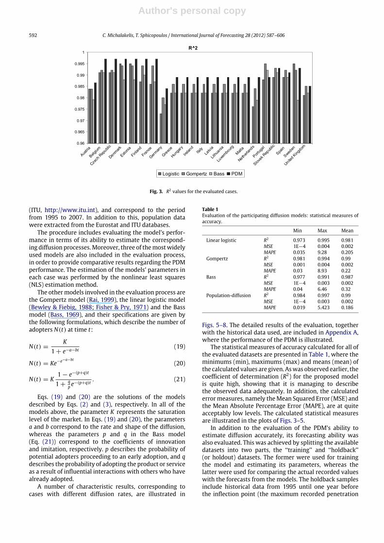
Fig. 3. R2 values for the evaluated cases.

(ITU, http://www.itu.int), and correspond to the periodfrom 1995 to 2007. In addition to this, population datawere extracted from the Eurostat and ITU databases.

The procedure includes evaluating the model’s perfor-mance in terms of its ability to estimate the correspond-ing diffusion processes.Moreover, three of themostwidelyused models are also included in the evaluation process,in order to provide comparative results regarding the PDMperformance. The estimation of the models’ parameters ineach case was performed by the nonlinear least squares(NLS) estimation method.

The othermodels involved in the evaluation process arethe Gompertz model (Rai, 1999), the linear logistic model(Bewley & Fiebig, 1988; Fisher & Pry, 1971) and the Bassmodel (Bass, 1969), and their specifications are given bythe following formulations, which describe the number ofadopters N(t) at time t:

N(t) =K

1 + e−a−bt(19)

N(t) = Ke−e−a−bt(20)

N(t) = K1 − e−(p+q)t

1 +qp e

−(p+q)t. (21)

Eqs. (19) and (20) are the solutions of the modelsdescribed by Eqs. (2) and (3), respectively. In all of themodels above, the parameter K represents the saturationlevel of the market. In Eqs. (19) and (20), the parametersa and b correspond to the rate and shape of the diffusion,whereas the parameters p and q in the Bass model(Eq. (21)) correspond to the coefficients of innovationand imitation, respectively. p describes the probability ofpotential adopters proceeding to an early adoption, and qdescribes the probability of adopting the product or serviceas a result of influential interactions with others who havealready adopted.

A number of characteristic results, corresponding tocases with different diffusion rates, are illustrated in

Table 1Evaluation of the participating diffusion models: statistical measures ofaccuracy.

Min Max Mean

Linear logistic R2 0.973 0.995 0.981MSE 1E−4 0.004 0.002MAPE 0.035 9.28 0.205

Gompertz R2 0.981 0.994 0.99MSE 0.001 0.004 0.002MAPE 0.03 8.93 0.22

Bass R2 0.977 0.991 0.987MSE 1E−4 0.003 0.002MAPE 0.04 6.46 0.32

Population-diffusion R2 0.984 0.997 0.99MSE 1E−4 0.003 0.002MAPE 0.019 5.423 0.186

Figs. 5–8. The detailed results of the evaluation, togetherwith the historical data used, are included in Appendix A,where the performance of the PDM is illustrated.

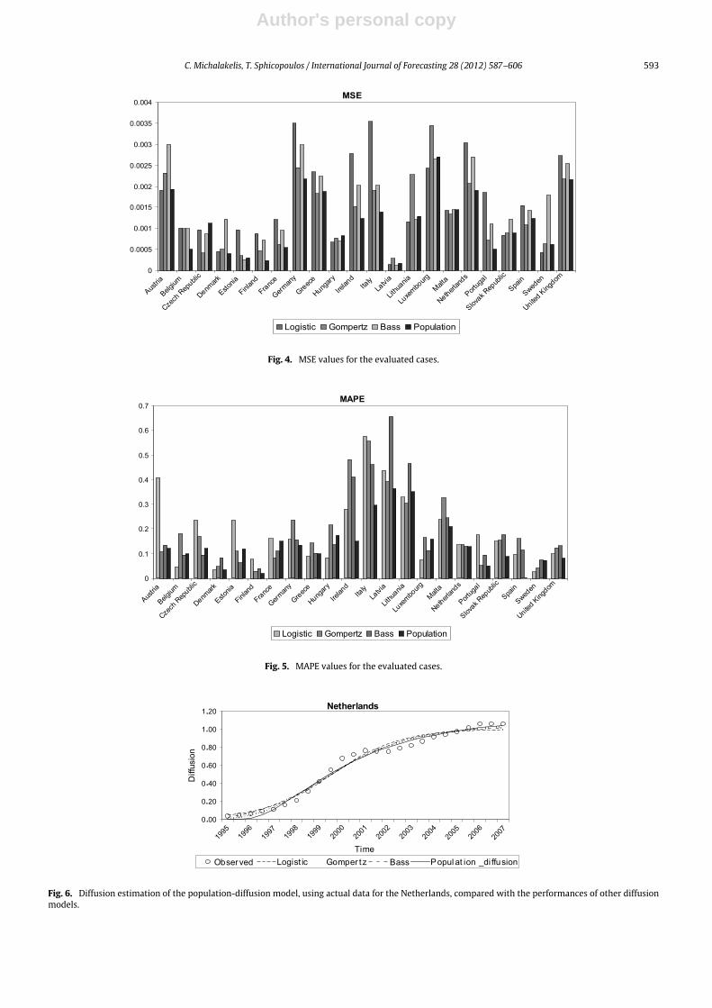
The statistical measures of accuracy calculated for all ofthe evaluated datasets are presented in Table 1, where theminimums (min), maximums (max) and means (mean) ofthe calculated values are given. Aswas observed earlier, thecoefficient of determination (R2) for the proposed modelis quite high, showing that it is managing to describethe observed data adequately. In addition, the calculatederrormeasures, namely theMean Squared Error (MSE) andthe Mean Absolute Percentage Error (MAPE), are at quiteacceptably low levels. The calculated statistical measuresare illustrated in the plots of Figs. 3–5.

In addition to the evaluation of the PDM’s ability toestimate diffusion accurately, its forecasting ability wasalso evaluated. This was achieved by splitting the availabledatasets into two parts, the ‘‘training’’ and ‘‘holdback’’(or holdout) datasets. The former were used for trainingthe model and estimating its parameters, whereas thelatter were used for comparing the actual recorded valueswith the forecasts from the models. The holdback samplesinclude historical data from 1995 until one year beforethe inflection point (the maximum recorded penetration

Author's personal copy

C. Michalakelis, T. Sphicopoulos / International Journal of Forecasting 28 (2012) 587–606 593

Fig. 4. MSE values for the evaluated cases.

Fig. 5. MAPE values for the evaluated cases.

Fig. 6. Diffusion estimation of the population-diffusion model, using actual data for the Netherlands, compared with the performances of other diffusionmodels.

Author's personal copy

594 C. Michalakelis, T. Sphicopoulos / International Journal of Forecasting 28 (2012) 587–606

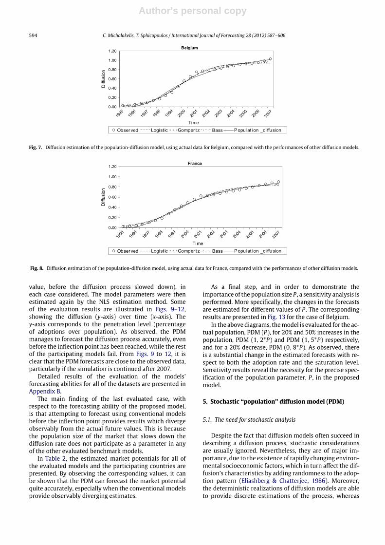
Fig. 7. Diffusion estimation of the population-diffusion model, using actual data for Belgium, compared with the performances of other diffusion models.

Fig. 8. Diffusion estimation of the population-diffusion model, using actual data for France, compared with the performances of other diffusion models.

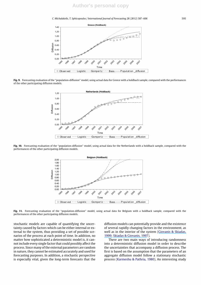
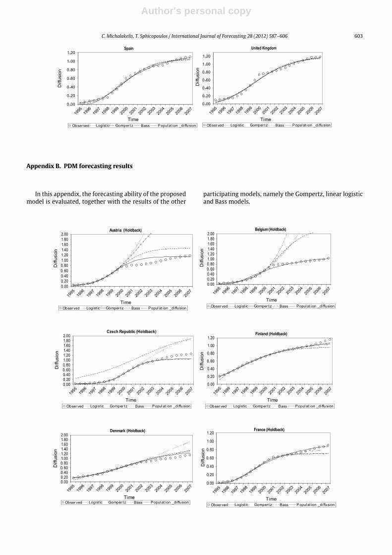
value, before the diffusion process slowed down), ineach case considered. The model parameters were thenestimated again by the NLS estimation method. Someof the evaluation results are illustrated in Figs. 9–12,showing the diffusion (y-axis) over time (x-axis). They-axis corresponds to the penetration level (percentageof adoptions over population). As observed, the PDMmanages to forecast the diffusion process accurately, evenbefore the inflection point has been reached, while the restof the participating models fail. From Figs. 9 to 12, it isclear that the PDM forecasts are close to the observed data,particularly if the simulation is continued after 2007.

Detailed results of the evaluation of the models’forecasting abilities for all of the datasets are presented inAppendix B.

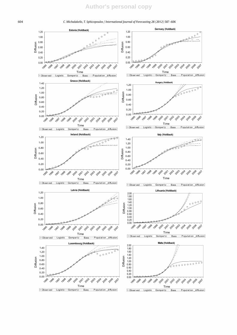
The main finding of the last evaluated case, withrespect to the forecasting ability of the proposed model,is that attempting to forecast using conventional modelsbefore the inflection point provides results which divergeobservably from the actual future values. This is becausethe population size of the market that slows down thediffusion rate does not participate as a parameter in anyof the other evaluated benchmark models.

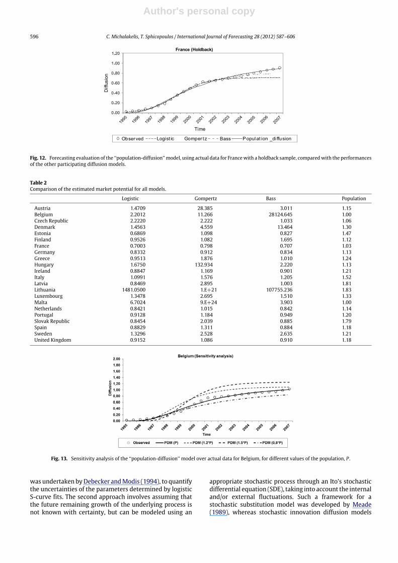
In Table 2, the estimated market potentials for all ofthe evaluated models and the participating countries arepresented. By observing the corresponding values, it canbe shown that the PDM can forecast the market potentialquite accurately, especially when the conventional modelsprovide observably diverging estimates.

As a final step, and in order to demonstrate theimportance of the population size P , a sensitivity analysis isperformed. More specifically, the changes in the forecastsare estimated for different values of P . The correspondingresults are presented in Fig. 13 for the case of Belgium.

In the above diagrams, themodel is evaluated for the ac-tual population, PDM (P), for 20% and 50% increases in thepopulation, PDM (1, 2∗P) and PDM (1, 5∗P) respectively,and for a 20% decrease, PDM (0, 8∗P). As observed, thereis a substantial change in the estimated forecasts with re-spect to both the adoption rate and the saturation level.Sensitivity results reveal the necessity for the precise spec-ification of the population parameter, P , in the proposedmodel.

5. Stochastic ‘‘population’’ diffusion model (PDM)

5.1. The need for stochastic analysis

Despite the fact that diffusion models often succeed indescribing a diffusion process, stochastic considerationsare usually ignored. Nevertheless, they are of major im-portance, due to the existence of rapidly changing environ-mental socioeconomic factors, which in turn affect the dif-fusion’s characteristics by adding randomness to the adop-tion pattern (Eliashberg & Chatterjee, 1986). Moreover,the deterministic realizations of diffusion models are ableto provide discrete estimations of the process, whereas

Author's personal copy

C. Michalakelis, T. Sphicopoulos / International Journal of Forecasting 28 (2012) 587–606 595

Fig. 9. Forecasting evaluation of the ‘‘population-diffusion’’ model, using actual data for Greece with a holdback sample, compared with the performancesof the other participating diffusion models.

Fig. 10. Forecasting evaluation of the ‘‘population-diffusion’’ model, using actual data for the Netherlands with a holdback sample, compared with theperformances of the other participating diffusion models.

Fig. 11. Forecasting evaluation of the ‘‘population-diffusion’’ model, using actual data for Belgium with a holdback sample, compared with theperformances of the other participating diffusion models.

stochastic models are capable of quantifying the uncer-tainty caused by factors which can be either internal or ex-ternal to the system, thus providing a set of possible sce-narios of the process at each point of time. In addition, nomatter how sophisticated a deterministic model is, it can-not include every single factor that could possibly affect theprocess. Sincemany of the external parameters are randomin nature, they cannot be estimated accurately and used forforecasting purposes. In addition, a stochastic perspectiveis especially vital, given the long-term forecasts that the

diffusionmodels can potentially provide and the existenceof several rapidly changing factors in the environment, aswell as in the interior of the system (Giovanis & Skiadas,1999; Skiadas & Giovanis, 1997).

There are two main ways of introducing randomnessinto a deterministic diffusion model in order to describethe uncertainties that accompany a diffusion process. Thefirst is based on the assumption that the parameters of anaggregate diffusion model follow a stationary stochasticprocess (Karmeshu & Pathria, 1980). An interesting study

Author's personal copy

596 C. Michalakelis, T. Sphicopoulos / International Journal of Forecasting 28 (2012) 587–606

Fig. 12. Forecasting evaluation of the ‘‘population-diffusion’’ model, using actual data for Francewith a holdback sample, comparedwith the performancesof the other participating diffusion models.

Table 2Comparison of the estimated market potential for all models.

Logistic Gompertz Bass Population

Austria 1.4709 28.385 3.011 1.15Belgium 2.2012 11.266 28124.645 1.00Czech Republic 2.2220 2.222 1.033 1.06Denmark 1.4563 4.559 13.464 1.30Estonia 0.6869 1.098 0.827 1.47Finland 0.9526 1.082 1.695 1.12France 0.7003 0.798 0.707 1.03Germany 0.8332 0.912 0.834 1.13Greece 0.9513 1.876 1.010 1.24Hungary 1.6750 132.934 2.220 1.13Ireland 0.8847 1.169 0.901 1.21Italy 1.0991 1.576 1.205 1.52Latvia 0.8469 2.895 1.003 1.81Lithuania 1481.0500 1.E+21 107755.236 1.83Luxembourg 1.3478 2.695 1.510 1.33Malta 6.7024 9.E+24 3.903 1.00Netherlands 0.8421 1.015 0.842 1.14Portugal 0.9128 1.184 0.949 1.20Slovak Republic 0.8454 2.039 0.885 1.79Spain 0.8829 1.311 0.884 1.18Sweden 1.3296 2.528 2.635 1.21United Kingdom 0.9152 1.086 0.910 1.18

Fig. 13. Sensitivity analysis of the ‘‘population-diffusion’’ model over actual data for Belgium, for different values of the population, P .

was undertaken byDebecker andModis (1994), to quantifythe uncertainties of the parameters determined by logisticS-curve fits. The second approach involves assuming thatthe future remaining growth of the underlying process isnot known with certainty, but can be modeled using an

appropriate stochastic process through an Ito’s stochasticdifferential equation (SDE), taking into account the internaland/or external fluctuations. Such a framework for astochastic substitution model was developed by Meade(1989), whereas stochastic innovation diffusion models

Author's personal copy

C. Michalakelis, T. Sphicopoulos / International Journal of Forecasting 28 (2012) 587–606 597

involving the introduction of stochasticity into the Bassand logistic diffusion models, respectively, were proposedby Skiadas and Giovanis (1997) and Giovanis and Skiadas(1999). In the context of the present work, a stochasticrealization of the PDM is constructed and evaluated basedon the second approach described above, providing avaluable way of measuring the uncertainty regarding theforecasted future values.

5.2. Model development

Stochastic differential equations (SDEs) are used quitefrequently, and in a wide range of fields of application.As was mentioned in the introductory section, the workpresented by Eliashberg and Chatterjee (1986) was one ofthe earliest studies to propose the need to employ SDEs inthe estimation and forecasting of diffusion processes.

This section is devoted to the development of amethod of stochastic analysis for aggregate models, andmore specifically for the proposed population diffusionmodel, PDM. The analysis is based on the addition ofa noise term to the initially developed model, which isrepresented by a Wiener process. Wiener processes playa vital role in stochastic calculus and diffusion processes.This analysis is important as a measure of the volatilityof the deterministic process, since diffusion is frequentlycharacterized by uncertainty.

Stochastic differential equations are ordinary differ-ential equations which are parameterized by means ofWiener processes (Gardiner, 2004; Oksendal, 2003), in ad-dition to time. AWiener process,Wt , is a non-differentiablerandom function of time t , which is obtained by samplingthe normal probability density:

1√2π t

e−W2t /2t . (22)

A general formulation of a stochastic differential equationis given by the following relationship:

dN = f (N, t)dt + g(N, t)dW (t). (23)

In Eq. (23), dW (t) is 1-dimensional ‘‘white noise’’, thetime derivative of the Wiener process, and f (N, t), g(N, t)are known functions (Evans, 2005). g(N, t) represents thevolatility, or the width of the noise of the process.

Recalling the general formulation of an aggregatediffusion model, as described by Eq. (1), the addition of astochastic term yields:

dN(t) = d(N(t), p̄)· {[f (K) − f (N(t))]dt + g · dW (t)}, (24)

or, equivalently:

dN(t) = d(N(t), p̄) · [f (K) − f (N(t))]dt+ d(N(t), p̄) · g · dW (t). (25)

The application of the formulations described in Eqs.(24) and (25) over the population model, as is describedby Eq. (6), provides its equivalent stochastic realization:

dN = rN lna + b

PN

lnKN

dt + gdW (t)

, (26)

which, after performing the expansion of terms, becomes:

dN = rN lna + b

PN

lnKN

dt

+ rN lna + b

PN

gdW (t). (27)

The stochastic differential equation described by Eq.(27) is a nonlinear stochastic differential equation. There-fore, in order to estimate its parameters, a suitable trans-formation should be applied so that the sde can be approx-imated by an equivalent linear sde, based on the availablediscrete time observations.

5.3. Local linearization

5.3.1. Function transformationA number of approaches are available in the literature

for the linearization of a nonlinear diffusion process(Bergstrom, 1990;Dembo&Zeitouni, 1987;Milstein, 1995;Nikolau, 2005; Ozaki, 1985; Singer, 1993). For the needs ofthe present work, the local linearization method proposedby Shoji and Ozaki (1998) is adopted, as it provides abetter performance and more accurate results. Accordingto thismethod, the original stochastic differential equationis locally approximated by a linear stochastic differentialequation, which is analytically tractable, since it can besolved easily and the solution is expressed as a sample pathof the stochastic process. Thus, the discretized process canbe obtained by the discretization of the sample path.

The basic idea of the local linearizationmethod is basedon approximating a stochastic differential equation of theform

dN = f (N, t)dt + σdW (t), (28)

using a linear differential equation

dN = LsNdt + σdW (t), (29)

with Ls being a real valued function and σ the volatility ofthe process.

The local linearization methodology is applied over thestochastic formulation of the population model expressedby Eq. (27). Again, as in the deterministic formulation ofthemodel and for the sake of computational simplification,the constants x and y are substituted for the constantquantities ln(a +

bPK ) and bP

aK+bP , respectively. Therefore,the corresponding stochastic differential equation thatdescribes the stochastic diffusion process becomes:

dNdt

= rN(x − yN) lnKN

dt

+ rN(x − yN)gdW (t). (30)

In order to express Eq. (30) in a more tractable form,similar to that of Eq. (28), which has a constant coefficientfor the diffusion term (volatility), a transformation nt =

ϕ(Nt) can be applied to Eq. (30). ϕ(Nt) must satisfy theordinary differential equation:

grN(x − yN)dϕdN

= σ , σ constant. (31)

Author's personal copy

598 C. Michalakelis, T. Sphicopoulos / International Journal of Forecasting 28 (2012) 587–606

The solution of Eq. (31) is:

ϕ =σ

grxln

Nx − yN

, (32)

and N can be obtained by

N =x

y + e−ngrxσ

. (33)

Thus, Eq. (32) is the transformation that should beapplied over Eq. (30) in order to derive a constant volatilitystochastic differential equation. The application of Ito’sformula (Evans, 2005;Oksendal, 2003; Shoji &Ozaki, 1998)gives:

dn =

rN(x − y) ln

KN

dϕdt

+g2r2N2

2(x − yN)2

d2ϕdN2

dt + σdW (t). (34)

ϕ(Nt) is twice continuously differentiable, with the firstand second derivatives being described by Eqs. (35) and(36), respectively:

dϕdN

=σ

gr(x − yN)N(35)

d2ϕdN2

= −σ

grx + 2yN

(x − yN)2N2. (36)

After substituting Eqs. (33), (35) and (36) into Eq. (34), thelatter becomes:

dn =

rN(x − y) ln

KN

σ

grN(x − yN)

+g2r2N2

2(x − yN)2

σ 2

gr

x − 2yN

N2(x − yN)2

dt

+ σdW (t) (37)

or

dn =

lnKN

−

σ 2gr2

lna + b

PK

− 2

bPaK + bP

N

dt + σdW (t). (38)

Therefore, the initial stochastic differential equation de-scribed by Eq. (27) can be expressed in the form

dn = f̃ dt + σdWt , (39)

where

f̃ =σ

glnKx

y + e−

ngrxσ

−

grσ2

x +

2yx

y + e−ngrxσ

. (40)

5.3.2. LinearizationThe linearization of Eq. (38) is derived by applying the

methodology proposed by Shoji and Ozaki (1998), whichyields

nt = ns +f̃Ls

(eLs(t−s)− 1)

+Ms

L2s

eLs(t−s)

− 1− Ls(t − s)

+ σ

t

seLs(t−u)dWu. (41)

In Eq. (41), f̃ is given by Eq. (40), and Ls andMs by

Ls =∂ f̃∂n

and (42)

Ms =σ 2

2∂2 f̃∂n2

+∂ f̃∂t

. (43)

The second part of the right-hand-side of Eq. (43) isequal to 0, since it is the case of an autonomous equation.Moreover, the integral term in Eq. (41) has a Normaldistribution, with mean 0 and variance given by

Vars(nt) = σ 2e2Ls(t−s)

− 12Ls

. (44)

After solving Eq. (41), corresponding values of Nt can becalculated by applying the relationship given by Eq. (33).

5.4. Parameter estimation of the discretized process

Since the discretized process locally follows a Gaussiandistribution, the log-likelihood can be obtained easily.Therefore, the maximum likelihood method can be usedto estimate the model’s parameters. The log-likelihoodfunction is given by

log(p(n1, n2, . . . , nk)) =

k−1j=1

log(p(nj+1|nj))

+ log(p(n1)). (45)

However, since nwas derived by applying the transfor-mation ϕ(t) to the initial stochastic differential equationof Eq. (27), the same transformation should be applied toEq. (45). This is necessary in order to remove the large vari-ance, caused by changes in the ns, and is achieved by ap-plying the transformation rule of a density function

p(N1,N2, . . . ,Nk) = p(n1, n2, . . . , nk)

×

∂(n1, n2, . . . , nk)

∂(N1,N2, . . . ,Nk)

, (46)

where ∂(n1,n2,...,nk)∂(N1,N2,...,Nk)

is the Jacobian, and is equivalent tok−1j=1

dϕdN

N=Nj

.

Author's personal copy

C. Michalakelis, T. Sphicopoulos / International Journal of Forecasting 28 (2012) 587–606 599

Finally, the log-likelihood for the stochastic population-diffusion model, based on the linearized approach of Eq.(41), is given by

log(p(N1,N2, . . . ,Nk))

= −12

k−1j=1

(nj+1 − Ej)2

Vj+ log(2πVj)

+ log(p(n1)) +

k−1j=1

log

dϕdNN=Nj

, (47)

where

Ej = nj +fLj

(eLj∆t− 1) +

Mj

L2j

(eLj∆t

− 1) − Lj∆t

(48)

Vj =(eLj∆t

− 1)2Lj

σ 2 (49)

Lj =∂ f∂n

(50)

Mj =σ 2

2∂2f∂n2

+∂ f∂t

and (51)

f = f̃∂ϕ

∂N+

g2

2∂2ϕ

∂n2. (52)

Explicit formulas for the calculation of the parameterthat maximizes the log-likelihood function do not alwaysexist, as is the case for the function in Eq. (47). Therefore,heuristic methods, such as Genetic Algorithms, are usuallyemployed for the estimation of a model’s parameters.Genetic algorithms, as posited by Goldberg (1989), aresearch algorithms based on the mechanisms of naturalselection and natural genetics. The key points of theprocess are reproduction, crossover and mutation, whichare performed according to a given probability, justas happens in the real world. Reproduction involvescopying (reproducing) solution vectors, crossover involvesswapping partial solution vectors, and mutation is theprocess of randomly changing a cell in the string ofthe solution vector, thus preventing the possibility ofthe algorithm being trapped. The process continues untilit reaches the optimal solution of the fitness function.Genetic algorithms have been applied for high technologydemand estimation (Venkatesan & Kumar, 2002).

In the context of the present work, the fitness functionto be optimized is the log-likelihood function, described byEq. (47), seeking to find its maximum value, based on thehistorical data. In order to evaluate the model’s accuracy,estimation was based on data from the period from 1994to 1999. After 1999, diffusion slowed down, as the mar-ket was about to reach saturation, and the rest of the mod-els evaluated estimated extremely high saturation levelswhich did not correspond to the actual values recorded inlater years.

The application of the genetic algorithms was basedon initial values equal to the ones estimated in thedeterministic case of the model. In addition, other,randomly chosen, initial values were also used, in order toavoid the algorithm getting trapped at local maxima. Afterperforming about 100,000 iterations, the process ended up

with a saturation level value (K ) of about 1.013. This canbe considered as quite a consistent result, since it doesnot diverge from the value calculated for the deterministicanalogue (1.031).

6. Results of the stochastic model

Forecasts of the stochastic model are provided by sim-ulating the solution given in the preceding section, basedon the parameters estimated by the maximum likelihoodmethod. Realizations of ∆Wt were generated using thewell-known Box–Muller method (Box & Muller, 1958).

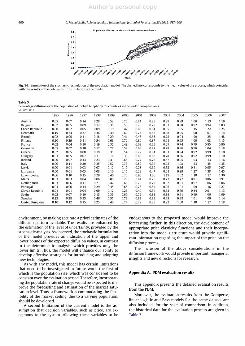
Themodel was evaluated for the case of Greece, and thecorresponding results are shown in Fig. 14. As observed,the stochastic formulation of themodel indicates the upperand lower bounds of the expected demand values. How-ever, the deterministic analysis only provides the lowervalues. This simulation is performed using parameter val-ues estimated using data for the period from 1995 to 1999(holdback sample). The important outcome that accompa-nies the results is the estimation of the uncertainty of theforecasted values, together with the possible values diffu-sion can take, according to the diffusion dynamics. As ob-served, the deviation from the mean value can be quitehigh. In the case of Greece, the deterministic PDM fore-casted a saturation level of 1.24. However, the stochasticanalysis revealed that possible values vary from about 1.06to 1.35. This stochastic analysis, together with the corre-sponding results, can be a valuable guide for the construc-tion of business plans and investments, since it provides ameasure of the deviation of the future expectations.

7. Conclusions and future work

The aim of this research was to contribute to the ex-isting knowledge regarding diffusion estimation and fore-casting, for both research and practice. This was attemptedby developing a diffusion model which explicitly incor-porates the size of the market, as expressed by the cor-responding population. The two formulations of the pro-posed PDM, both deterministic and stochastic, providequite accurate results in terms of diffusion estimation andforecasting, especiallywhen the rest of the aggregatemod-els failed to do so, such as when the diffusion is describedby a high adoption rate.

In such cases, the widely used diffusion models cannotpredict the saturation level accurately, mainly because thepopulation is not taken into account. The proposed modelwas evaluated using historical data from 22 Europeancountries, and provided accurate forecasts, even from theearly stages of the corresponding diffusion processes.

This study helped to move the consideration of innova-tion diffusion towards the development of a diffusion fore-casting framework, incorporating a number of driving fac-tors and decision variables, and also helped increase theunderstanding of high technology market trends. More-over, the estimation of the underlying level of uncertaintywill stimulate further research, in order to produce moreaccurate forecasts.

Themodel provides critical inputs for strategic planningand decision making, in an increasingly competitive

Author's personal copy

600 C. Michalakelis, T. Sphicopoulos / International Journal of Forecasting 28 (2012) 587–606

Fig. 14. Simulation of the stochastic formulation of the population model. The dashed line corresponds to the mean value of the process, which coincideswith the results of the deterministic formulation of the model.

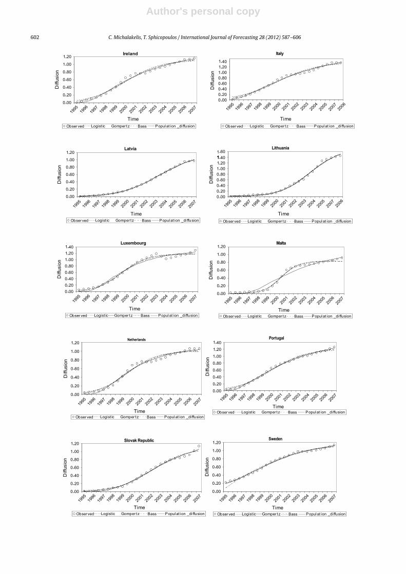
Table 3Percentage diffusion over the population of mobile telephony for countries in the wider European area.Source: ITU.

1995 1996 1997 1998 1999 2000 2001 2002 2003 2004 2005 2006 2007

Austria 0.05 0.07 0.14 0.28 0.52 0.76 0.81 0.83 0.89 0.98 1.06 1.13 1.19Belgium 0.02 0.05 0.09 0.17 0.31 0.55 0.75 0.78 0.83 0.88 0.92 0.94 1.03Czech Republic 0.00 0.02 0.05 0.09 0.19 0.42 0.68 0.84 0.95 1.05 1.15 1.22 1.25Denmark 0.15 0.24 0.27 0.36 0.49 0.63 0.74 0.83 0.88 0.95 1.00 1.07 1.14Estonia 0.02 0.05 0.11 0.18 0.29 0.41 0.48 0.65 0.78 0.94 1.09 1.25 1.48Finland 0.20 0.29 0.41 0.54 0.63 0.72 0.80 0.87 0.91 0.95 1.00 1.08 1.15France 0.02 0.04 0.10 0.19 0.35 0.49 0.62 0.65 0.69 0.74 0.79 0.85 0.90Germany 0.05 0.07 0.10 0.17 0.28 0.59 0.68 0.72 0.78 0.86 0.96 1.04 1.18Greece 0.02 0.05 0.08 0.19 0.35 0.54 0.72 0.84 0.81 0.84 0.92 0.99 1.10Hungary 0.03 0.05 0.07 0.11 0.16 0.30 0.49 0.68 0.78 0.86 0.92 0.99 1.10Ireland 0.00 0.07 0.13 0.23 0.41 0.65 0.77 0.76 0.87 0.95 1.03 1.13 1.16Italy 0.00 0.11 0.20 0.35 0.52 0.73 0.89 0.94 0.98 1.08 1.23 1.35 1.35Latvia 0.00 0.01 0.03 0.07 0.12 0.17 0.28 0.39 0.52 0.66 0.81 0.95 0.97Lithuania 0.00 0.01 0.05 0.08 0.10 0.15 0.29 0.47 0.61 0.89 1.27 1.38 1.45Luxembourg 0.06 0.10 0.15 0.29 0.46 0.70 0.93 1.06 1.19 1.02 1.10 1.17 1.30Malta 0.03 0.03 0.04 0.06 0.09 0.29 0.61 0.70 0.73 0.77 0.81 0.86 0.91Netherlands 0.03 0.06 0.11 0.21 0.42 0.68 0.76 0.75 0.82 0.91 0.97 1.06 1.06Portugal 0.03 0.06 0.14 0.29 0.45 0.65 0.78 0.84 0.96 1.01 1.09 1.16 1.27Slovak Republic 0.01 0.01 0.04 0.09 0.12 0.23 0.40 0.54 0.68 0.79 0.84 0.91 1.13Spain 0.02 0.07 0.10 0.15 0.35 0.60 0.72 0.81 0.88 0.91 0.99 1.06 1.09Sweden 0.22 0.28 0.35 0.46 0.57 0.72 0.81 0.89 0.98 0.98 1.01 1.06 1.14United Kingdom 0.10 0.12 0.15 0.25 0.46 0.74 0.79 0.83 0.92 1.00 1.10 1.17 1.18

environment, by making accurate a priori estimates of thediffusion pattern available. The results are enhanced bythe estimation of the level of uncertainty, provided by thestochastic analysis. As observed, the stochastic formulationof the model provides an indication of the upper andlower bounds of the expected diffusion values, in contrastto the deterministic analysis, which provides only thelower limits. Thus, the model will enhance our ability todevelop effective strategies for introducing and adoptingnew technologies.

As with any model, this model has certain limitationsthat need to be investigated in future work, the first ofwhich is the population size, which was considered to beconstant over the evaluation period. Therefore, incorporat-ing the population rate of changewould be expected to im-prove the forecasting and estimation of the market satu-ration level. Thus, a framework accommodating the flex-ibility of the market ceiling, due to a varying population,should be developed.

A second limitation of the current model is the as-sumption that decision variables, such as price, are ex-ogenous to the system. Allowing these variables to be

endogenous to the proposed model would improve theforecasting further. In this direction, the development ofappropriate price elasticity functions and their incorpo-ration into the model’s structure would provide signifi-cant information regarding the impact of the price on thediffusion process.

The inclusion of the above considerations in thediffusion framework would provide important managerialinsights and new directions for research.

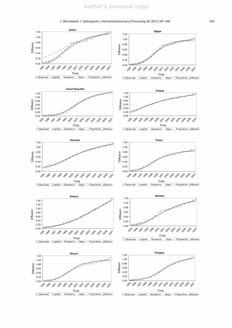
Appendix A. PDM evaluation results

This appendix presents the detailed evaluation resultsfrom the PDM.

Moreover, the evaluation results from the Gompertz,linear logistic and Bass models for the same dataset arealso included, for the sake of comparison. In addition,the historical data for the evaluation process are given inTable 3.

Author's personal copy

C. Michalakelis, T. Sphicopoulos / International Journal of Forecasting 28 (2012) 587–606 601

Author's personal copy

602 C. Michalakelis, T. Sphicopoulos / International Journal of Forecasting 28 (2012) 587–606

Author's personal copy

C. Michalakelis, T. Sphicopoulos / International Journal of Forecasting 28 (2012) 587–606 603

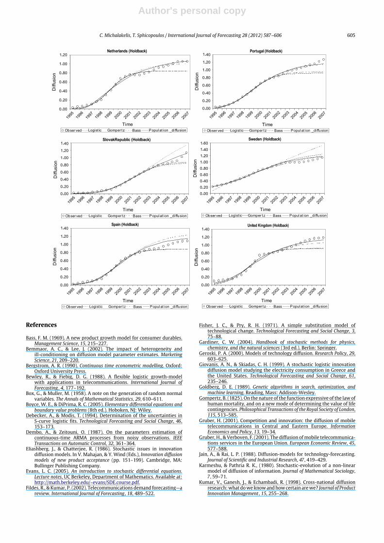
Appendix B. PDM forecasting results

In this appendix, the forecasting ability of the proposedmodel is evaluated, together with the results of the other

participating models, namely the Gompertz, linear logisticand Bass models.

Author's personal copy

604 C. Michalakelis, T. Sphicopoulos / International Journal of Forecasting 28 (2012) 587–606

Author's personal copy

C. Michalakelis, T. Sphicopoulos / International Journal of Forecasting 28 (2012) 587–606 605

References

Bass, F. M. (1969). A new product growth model for consumer durables.Management Science, 15, 215–227.

Bemmaor, A. C., & Lee, J. (2002). The impact of heterogeneity andill-conditioning on diffusion model parameter estimates. MarketingScience, 21, 209–220.

Bergstrom, A. R. (1990). Continuous time econometric modelling. Oxford:Oxford University Press.

Bewley, R., & Fiebig, D. G. (1988). A flexible logistic growth-modelwith applications in telecommunications. International Journal ofForecasting , 4, 177–192.

Box, G., & Muller, M. (1958). A note on the generation of random normalvariables. The Annals of Mathematical Statistics, 29, 610–611.

Boyce, W. E., & DiPrima, R. C. (2005). Elementary differential equations andboundary value problems (8th ed.). Hoboken, NJ: Wiley.

Debecker, A., & Modis, T. (1994). Determination of the uncertainties inS-curve logistic fits. Technological Forecasting and Social Change, 46,153–173.

Dembo, A., & Zeitouni, O. (1987). On the parameters estimation ofcontinuous-time ARMA processes from noisy observations. IEEETransactions on Automatic Control, 32, 361–364.

Eliashberg, J., & Chatterjee, R. (1986). Stochastic issues in innovationdiffusion models. In V. Mahajan, & Y. Wind (Eds.), Innovation diffusionmodels of new product acceptance (pp. 151–199). Cambridge, MA:Bullinger Publishing Company.

Evans, L. C. (2005). An introduction to stochastic differential equations.Lecture notes, UC Berkeley, Department of Mathematics. Available at:http://math.berkeley.edu/~evans/SDE.course.pdf.

Fildes, R., & Kumar, P. (2002). Telecommunications demand forecasting—areview. International Journal of Forecasting , 18, 489–522.

Fisher, J. C., & Pry, R. H. (1971). A simple substitution model oftechnological change. Technological Forecasting and Social Change, 3,75–88.

Gardiner, C. W. (2004). Handbook of stochastic methods for physics,chemistry, and the natural sciences (3rd ed.). Berlin: Springer.

Geroski, P. A. (2000). Models of technology diffusion. Research Policy, 29,603–625.

Giovanis, A. N., & Skiadas, C. H. (1999). A stochastic logistic innovationdiffusion model studying the electricity consumption in Greece andthe United States. Technological Forecasting and Social Change, 61,235–246.

Goldberg, D. E. (1989). Genetic algorithms in search, optimization, andmachine learning. Reading, Mass: Addison-Wesley.

Gompertz, B. (1825). On the nature of the function expressive of the law ofhumanmortality, and on a newmode of determining the value of lifecontingencies. Philosophical Transactions of the Royal Society of London,115, 513–585.

Gruber, H. (2001). Competition and innovation: the diffusion of mobiletelecommunications in Central and Eastern Europe. InformationEconomics and Policy, 13, 19–34.

Gruber, H., & Verboven, F. (2001). The diffusion ofmobile telecommunica-tions services in the European Union. European Economic Review, 45,577–588.

Jain, A., & Rai, L. P. (1988). Diffusion-models for technology-forecasting.Journal of Scientific and Industrial Research, 47, 419–429.

Karmeshu, & Pathria R. K., (1980). Stochastic-evolution of a non-linearmodel of diffusion of information. Journal of Mathematical Sociology,7, 59–71.

Kumar, V., Ganesh, J., & Echambadi, R. (1998). Cross-national diffusionresearch:what doweknowandhowcertain arewe? Journal of ProductInnovation Management , 15, 255–268.

Author's personal copy

606 C. Michalakelis, T. Sphicopoulos / International Journal of Forecasting 28 (2012) 587–606

Kumar, V., & Krishnan, T. V. (2002). Multinational diffusion models: analternative framework.Marketing Science, 21, 318–330.

Linton, J. D. (2002). Forecasting the market diffusion of disruptiveand discontinuous innovation. IEEE Transactions on EngineeringManagement , 49, 365–374.

Mahajan, V., & Muller, E. (1979). Innovation diffusion and new productgrowth-models in marketing. Journal of Marketing , 43, 55–68.

Mahajan, V., Muller, E., & Bass, F. M. (1990). New product diffusion-models in marketing—a review and directions for research. Journal ofMarketing , 54, 1–26.

Mahajan, V., & Peterson, R. A. (1979). First-purchase diffusion-models ofnew-product acceptance. Technological Forecasting and Social Change,15, 127–146.

Meade, N. (1989). Technological substitution—framework of stochastic-models. Technological Forecasting and Social Change, 36, 389–400.

Michalakelis, C., Dede, G., Varoutas, D., & Sphicopoulos, T. (2008). Impactof cross-national diffusion process in telecommunications demandforecasting. Telecommunication Systems, 39, 51–60.

Michalakelis, C., Varoutas, D., & Sphicopoulos, T. (2008). Diffusionmodels of mobile telephony in Greece. Telecommunications Policy, 32,234–245.

Milstein, G. N. (1995). Numerical integration of stochastic differentialequations. Dordrecht: Kluwer.

Nikolau, J. (2005). Methods for simulating non-linear stochastic differen-tial equations in R1. Journal of Statistical Computation and Simulation,75(8), 595–609.

Oksendal, B. (2003). Stochastic differential equations: an introduction withapplications (6th ed.). Berlin: Springer.

Ozaki, T. (1985). Non-linear time series models and dynamical systems.In E. J. Hannan (Ed.), Handbook of statistics, vol. 5 (pp. 25–83).Amsterdam: North-Holland.

Rai, L. P. (1999). Appropriate models for technology substitution. Journalof Scientific and Industrial Research, 58, 14–18.

Ruiz-Conde, E., Leeflang, P. S. H., & Wieringa, J. E. (2006). Marketing vari-ables in macro-level diffusion models. Journal für Betriebswirtschaft ,56, 155–183.

Seber, G. A. F., & Wild, C. J. (2003). Nonlinear regression. Hoboken, NewJersey: Wiley.

Shoji, I., & Ozaki, T. (1998). Estimation for nonlinear stochastic differentialequations by a local linearization method. Stochastic Analysis andApplications, 16, 733–752.

Singer, H. (1993). Continuous-timedynamical systemswith sampleddata,errors of measurement and unobserved components. Journal of TimeSeries Analysis, 14, 527–545.

Skiadas, C. H. (1987). Two simple-models for the early and middle stageprediction of innovation diffusion. IEEE Transactions on EngineeringManagement , 34, 79–84.

Skiadas, C. H., & Giovanis, A. N. (1997). A stochastic Bass innovationdiffusion model for studying the growth of electricity consumptionin Greece. Applied Stochastic Models and Data Analysis, 13, 85–101.

Teng, J. T. C., Grover, V., & Guttler, W. (2002). Information technology in-novations: general diffusion patterns and its relationships to innova-tion characteristics. IEEE Transactions on Engineering Management , 49,13–27.

Venkatesan, R., & Kumar, V. (2002). A genetic algorithms approach togrowth phase forecasting ofwireless subscribers. International Journalof Forecasting , 18, 625–646.

Wrede, R., & Spiegel, M. (2002). Theory and problems of advanced calculus(2nd ed.). New York: McGraw-Hill.

Christos Michalakelis holds a degree in Mathematics (University ofAthens, Department of Mathematics), an M.Sc. degree in SoftwareEngineering (The University of Liverpool, UK), and an M.Sc. degreein ‘‘Administration and Economics of Telecommunication Networks’’from the National and Kapodistrian University of Athens (Departmentof Informatics and Telecommunications, Interfaculty course of theDepartments of Informatics and Telecommunications and EconomicSciences). He also holds a Ph.D. degree in the area of technoeconomics,and with a focus on the demand estimation and forecasting of hightechnology products.

He is currently a Lecturer on telecommunications technoeconomicsin the Department of Informatics and Telematics at the HarokopioUniversity of Athens. Previously, he was with the Greek Ministry ofEducation for 7 years, in the Managing Authority of Operational Programfor Education and Initial Vocational Training, as an IT manager. Mr.Michalakelis has participated in a number of projects concerning thedesign and implementation of database systems, and now participatesin several technoeconomic activities for telecommunications, networksand services, such the CELTIC/ECOSYS project pricing and regulation. Hehas also developed or made a major contribution to the development of anumber of information systems and applications.

Mr. Michalakelis’ research interests include the study of the diffusionof high technology products and services, the application of economictheories to telecommunications, and the wider area of informatics andprice modeling and indexing. He has authored a number of paperspresented at conferences, and has published many papers in scientificjournals and books. He serves as a reviewer for a number of scientificjournals.

Thomas Sphicopoulos received a degree in physics from AthensUniversity in 1976, the D.E.A. degree and a Doctorate in Electronics,both from the University of Paris VI, in 1977 and 1980 respectively,and the Doctorat Es Science from the Ecole Polytechnique Federale deLausanne in 1986. From 1976 to 1977, he worked in Thomson CSF CentralResearch Laboratories on microwave oscillators. From 1977 to 1980, hewas an Associate Researcher in Thomson CSF Aeronautics InfrastructureDivision. In 1980, he joined the Electromagnetism Laboratory of theEcole Polytechnique Federal de Lausanne, where he researched appliedelectromagnetism. Since 1987, he has been at Athens University, engagedin research on broadband communications systems. He was elected anAssistant Professor of Communications in the Department of Informatics& Telecommunications in 1990, an Associate Professor in 1993, and aProfessor in the same department in 1998.

His main scientific interests are optical communication systemsand networks, and technoeconomics. He has led about 50 national andEuropean R & D projects.

Professor Sphicopoulos has published more than 150 articles inscientific journals and conference proceedings, and is an advisor forseveral organizations.