An Extension of the Double Vasicek Model to

Account for Stochastic Risk Premia

Riccardo RebonatoOxford University

October 30, 2014

Abstract

We present a stochastic-market-risk extension of a popular doubly-mean-reverting Vasicek model.

The model straddles the P and Q measures. By allowing for a sto-chastic market price of risk, we break the determninisitc link between thereturn-predicting factor and the market-price of risk, but we retain, onaverage, the observed regularities reported in the literature.

We also show how the model can be calibrated.

1 Why Do We Need Another Affine Model?

A classic empirical investigation of the properties of the yield curve looks at theexcess returns reaped by investing, year after year, for 1 year in an n-maturitybond, funding the position by paying the 1-year rate, unwinding the portfolioafter one year, recording the profit or loss, and repeating the strategy.1

Empirical regression studies suggest that excess returns should be linearlyrelated to some return-predicting factor. In earlier studies, this factor was iden-tified as the slope of the yield curve. More recent work suggests that a morecomplex (tent-shaped) pattern of forward rates may have a greater explanatorypower. See eg, . In what follows, we assume that, even if the slope does nottells the whole story, it has at least a significant explanatory power.

This return-predicting factor can be used in many ways. It can be useddirectly from the linear regressions (ie, without the intermediate processing ofthe fitting to an affine model), for instance to estimate whether the current shapeof the yield curve predicts attractive excess returns from a buy-long-fund-shortstrategy. Or it can be mapped onto the state variables of a (typically affine)model in order to obtain the model-implied dynamics in the risk-neutral (Q) andreal-world (P) measures. See, eg, Cochrane and Piazzesi (2005, 2008), D’Amico,Kim and Wei, (2010), Adrian, Crump and Moench (2013).

1This work reflects the ideas of the author, and not necessarily those of his employer.

1

Figure 1: Fig 1 shows the time series of the nominal, real and inflation excessreturns from May 2013 (10 year).

Of course, the outcome of a regression always contains the all-importanterror term — which, for the problem at hand, will be substantial. However,when the regression coefficients are mapped onto the affine model parameters(the reversion-speed matrix and the reversion-level vector) a ‘hard’ deterministicrelationship is established between the risk premium and the return-predictingfactor. If this is, say, the slope, it means that, according to the model, whenthe yield curve has a certain steepness, the market price of risk can have oneand only one value.

This can be undesirable. Suppose that we want to estimate the excess returnembedded in a market-observable n-year yield in order to distill the ‘market ex-pectation’ of the same yield. If the yield curve is steep, the predicted riskpremium will always be high, and for an observed nominal yield, the imputedexpectation of yields will always be low — often implausibly saw. For instance,Fig (1) shows the time series of the 10-year nominal and real ex ante expectedexcess returns from May 2013 to late summer 2014. The top curve shows thenominal expected excess return, and the corresponding real quantity. (The in-flation excess return is just the difference between the two.) As the ten yieldthroughout this period just barely exceeded 3%, and averaged approximately2.5%, it is clear that nominal term premia around 6% imply negative expecta-tions for the 10 year yield! The same consideration applies to real yields.

The surprising behaviour of the term premium (which implies strongly neg-ative rate expectations) stems from the high steepness of the yield curve in late2013, which implies, via the above-mentioned regression results and the inflexi-ble link between the market price of risk and the slope, implausibly high excessreturns. Needless to say, any estimate of expected rates based on these modelshave no credibility.

2

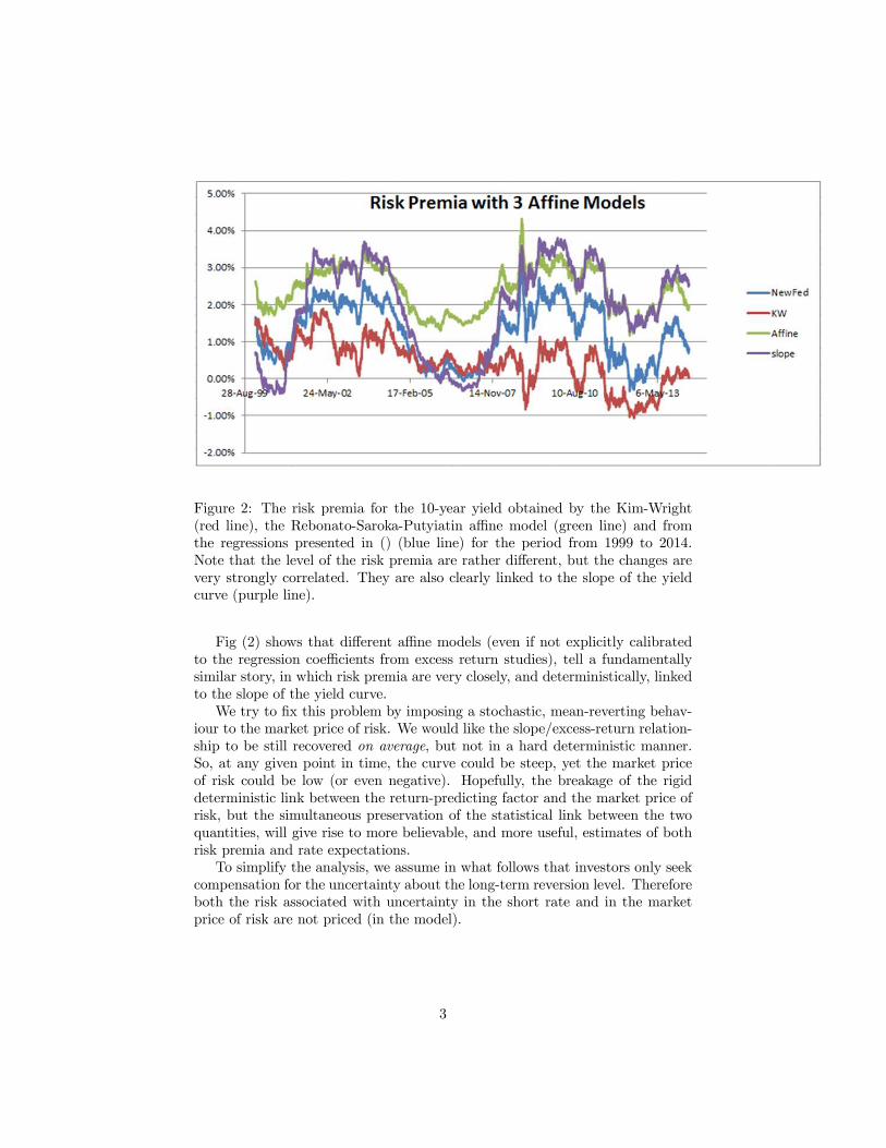
Figure 2: The risk premia for the 10-year yield obtained by the Kim-Wright(red line), the Rebonato-Saroka-Putyiatin affine model (green line) and fromthe regressions presented in () (blue line) for the period from 1999 to 2014.Note that the level of the risk premia are rather different, but the changes arevery strongly correlated. They are also clearly linked to the slope of the yieldcurve (purple line).

Fig (2) shows that different affine models (even if not explicitly calibratedto the regression coefficients from excess return studies), tell a fundamentallysimilar story, in which risk premia are very closely, and deterministically, linkedto the slope of the yield curve.

We try to fix this problem by imposing a stochastic, mean-reverting behav-iour to the market price of risk. We would like the slope/excess-return relation-ship to be still recovered on average, but not in a hard deterministic manner.So, at any given point in time, the curve could be steep, yet the market priceof risk could be low (or even negative). Hopefully, the breakage of the rigiddeterministic link between the return-predicting factor and the market price ofrisk, but the simultaneous preservation of the statistical link between the twoquantities, will give rise to more believable, and more useful, estimates of bothrisk premia and rate expectations.

To simplify the analysis, we assume in what follows that investors only seekcompensation for the uncertainty about the long-term reversion level. Thereforeboth the risk associated with uncertainty in the short rate and in the marketprice of risk are not priced (in the model).

3

2 The Model

The model is as follows:

drQt = κ

Pr [θt − rt] dt+ σrdz

rt (1)

dθQt = κ

Pθ

��θPt − θt

�dt+ λθtσθdt+ σθdz

rt (2)

dλθt = κλ

��λt − λt

�dt+ σλdz

rt (3)

where rt , θt and λt are the time-t value of the short rate, of its instantaneousreversion level (the ‘target rate’) and the market price of risk, respectively; σr,

σθ and σλ are the associated volatilities: �θPt and �λt are the reversion levels ofthe ‘target rate’ and of the market price of risk, respectively; and the incrementsdzrt , dz

θt and dzλt suitably correlated (see below). The model is fully specified

once the initial state, r0, θ0 and λ0 is given.This model is a variation on the theme of the well-known Naik (200X) and

similar ‘monetary’ models, in which the short rate is attracted to a mean-reverting target rate. (In more complex models, the target rate can in turnbe attracted to a mean-reverting process — we do not pursue this avenue here,in order to limit the number of parameters, and to ficus on the ability of themodel to capture the essence of the problem at hand.) For this interpretationto hold, it is usually assumed that, at least in the objective measure, κPr > κ

Pθ

and σr < σθ.Since we have assumed that investors only seek compensation for the uncer-

tainty about the long-term reversion level. It is for this reason that the reversionspeed, κPr , of the short rate is the same in the real-world and in the risk-neutral

measures. Also, the long-term reversion level, �θPt , of the ‘target rate’ (θt) is in

the real-world measure. The increment, dθQt , is then in the risk-neutral measurebecause we are adding the risk compensation, λθtσθ. We could equivalently havewritten

dθQt = κ

Pθ

��θQt − θt

�dt+ σθdz

rt (4)

with�θQt =

σθ

κPθλθt (5)

This immediately tells us that, the higher the volatility of the target rate (σθ,the source of uncertainty for which, in our model, investors seek compensation),the higher the risk-adjusted reversion level of the target rate. This makes sense.Also, the lower the reversion speed of the target rate to its reversion level, themore the target rate will be allowed to wander, creating uncertainty for thebond holders, who will ask for more yield compensation (ie, for a higher riskpremium). This also makes sense.

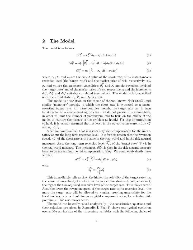
The model can be easily solved analytically — the constitutive equations andtheir solutions are given in Appendix I. Fig (3) shows one typical evolutionover a 30-year horizon of the three state variables with the following choice of

4

parameters: r0 = −0.0042, θ0 = 0.0344, λ0 = 0.0744, κr = 0.3437, κθ = 0.085,

κλ = 0.2816, σr = 0.0050, σθ = 0.0157, σλ = 0.1200, �θP

t = 0.0350,�λt = 0.1287,

ρrθ = 0.6, ρrλ = −0.05, ρθλ = 0.64.

Figure 3: A typical evolution over a 30-year horizon of the three state variables.

3 Qualitative Behaviour of the Model

In this section we want to get a feel for the qualitative behaviour of the model,and to check whether it does behaves as it is designed to.

First of all, we show a sample of 32 paths showing the evolution over 10years for the market price of risk are shown in Fig 4. (�λt = 0.1287, λ0 = 0.0744,r0 = −0.0042, θ0 = 0.0344, �θPt = 0.0350; see the calibration section for theparameter choice.)

One of the distinguishing features of the approach presented here is its in-principle ability to generate a positive correlation between the slope of the yieldcurve and the market price of risk. Can the model actually fulfill this promisewith a reasonable set of parameters?

This is indeed the case. As Figs (5) and (6) show, one of the most appealingfeatures of the model is that, for a suitable choice of the correlation matrixamong the three state variables, the model can easily produce a strong positivestochastic relationship between the slope of the yield curve and the market priceof risk.

(The slope of the yield curve was proxied as above by the difference betweenthe short rate and the reversion level). At any point in time, the market price

5

Figure 4: A sample of 32 paths showing the evolution over 10 years for themarket price of risk. Model parameters as in the text

6

Figure 5: A time series of the lope and of the market price of risk over a 30-yearperiod. Same parameters as for Fig Paths.

Figure 6: Same as Fig mpr1

7

of risk can be high or low even if the slope is low or high, respectively. However,the positive relationship between the market price of risk and the slope is onaverage recovered.

More precisely, as for the reversion speed and volatility of the market priceof risk, the higher its volatility, and the lower its reversion speed, the greaterits potential for assuming values other than what implied by the deterministicdynamics, and to break the deterministic relationship between excess returnsand the return-predicting factor.

4 Calibration of the Model

To determine the model parameters, we calibrate separately to the degrees offreedom that control the covariance matrix (or the swaption prices), and tothose that affect the shape of the yield curve. As we know, the latter have noeffect on the model covariance structure, and the former have a modest effect(through convexity) on the shape of the yield curve.

So, starting with the covariance structure, for the model to make financialsense, we should have a high reversion speed of the short rate to the targetrate, κPr > κ

θr, and a lower volatility for the short rate than for the target

rate, σr < σθ. A priori, we cannot say much about the relative volatility ofthe market price of risk and of the target rate, and we will therefore let thecalibration to the yield covariance matrix give us some guidance. Note however,that the market price of risk, which is a Sharpe-Ratio-like quantity, is one orderof magnitude larger than a typical rate, and therefore, in order to produce ameaningful dispersion, its absolute volatility should turn out significantly largerthan the volatilities of the short rate or the target rate.

Let’s move to the parameters which affect the shape of the yield curve.Roughly speaking, the strategy here is to subtract long-term expectations (asper blue dots in Fig (7) from visible long yields, in order to obtain an idea ofthe (P-measure) reversion level of the target rate. This that be gleaned froma variety of sources. See, eg, Christensen and Kwan (2014), who discuss theexpectations of federal funds rates from different surveys and from the FOMCparticipants’ funds rate projections. For our purposes the right-hand panel ofFig (7) (labelled ‘Longer Run’) serves our purposes well, as it embodies theexpectations of the FOMC participants of the long-term level of the target rate.

We would like the real-world long-term reversion level, �θPt , to be loosely anchoredin our optimization to this real-world expectation.

This strategy should be contrasted with the more usual model approach,which consists of subtracting from the visible yields today’s deterministic esti-mate of the excess return — which, as discussed, in market conditions such asthose prevailing in the early 2010s can give an implausibly low for estimate ofthe market expectations.

The considerations presented in Naik () can also give us an idea about the

8

Figure 7: Overview of FOMC participants’ assessments of appropriate monetarypolicy.

9

reversion level to which the market price of risk should be attracted — and thisshould not be too different from the Sharpe Ratio for the long-duration strategy.This is another anchor that we can use to guide the optimization process.

5 Results

Figs 8 and ?? show the market and the model yield covariance matrices for yieldsform 1 to 10 years (US$, market covariance matrix sampled over 2000 businessdays, before and up to September 2014) and Figs 10 and ?? show the samequantities for matrices for yields form 1 to 20 years. The model yield covariancematrix was obtained with a constrained choice of parameters, and the optimalset of volatility and reversion speeds obtained using yields of maturities out to10, 20 and 30 year were as follows:

10y 20y 30yσr 0.0051 0.0050 0.0055σθ 0.0161 0.0157 0.0153σλ 0.1200 0.1200 0.1200κr 0.4105 0.3437 0.2737κθ 0.1001 0.0850 0.0667κλ 0.4224 0.2816 0.2816

(6)

It is reassuring to see that calibrating the model to different sets of dataproduced very similar solutions.

The quality of the global fits to the whole covariance matrix, while notspectacular, at least suggests that there is a solution in the neighbourhood ofthe anchor parameters values (the values, that is, compatible with the finan-cial ‘story’ that underpins the model) that is compatible with the empiricalcovariance structure.

The fits to the yield curve obtained by keeping the reversion-speed matrixand the volatility matrix fixed to the values obtained in the calibration to thecovariance matrix, and by varying the initial state vector, −→x 0, and the reversion

levels, �θPt and �λ, are then shown in Figs 12, 13 and 14. (The US$ curve usedwas the Treasury curve for May 2014.)

In all cases, the fit to the market yields is excellent, and the resulting pa-rameters (not reported for the sake of brevity) very similar, irrespective of thefinal yield maturity to which the model was calibrated.

6 Comments on the Solution

A few comments are in order.First of all, it may seem that one has five degrees of freedom to fit the yield

curve. This may seem extravagant. However, there are strong constraints onthe acceptable values of the parameters.

10

Figure 8: The market US$ covariance matrices for yields form 1 to 10 years,sampled over 2000 business days, before and up to May 2014.

Figure 9: The model yield covariance matrices for yields form 1 to 10 yearsobtained with the parameters reported in the text.

11

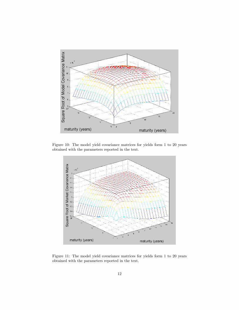
Figure 10: The model yield covariance matrices for yields form 1 to 20 yearsobtained with the parameters reported in the text.

Figure 11: The model yield covariance matrices for yields form 1 to 20 yearsobtained with the parameters reported in the text.

12

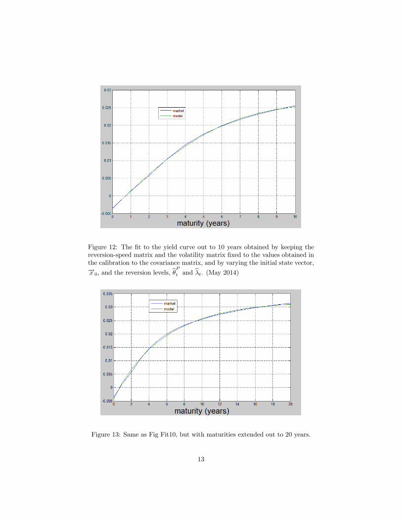
Figure 12: The fit to the yield curve out to 10 years obtained by keeping thereversion-speed matrix and the volatility matrix fixed to the values obtained inthe calibration to the covariance matrix, and by varying the initial state vector,−→x 0, and the reversion levels, �θPt and �λt. (May 2014)

Figure 13: Same as Fig Fit10, but with maturities extended out to 20 years.

13

Figure 14: Same as Fig Fit10, but with maturities extended out to 30 years.

First, the initial value of the short rate must be very close to the observableFed-funds rate. This virtually eliminates one degree of freedom.2

Second, we have an idea from the central bank forward guidance of the real-

world reversion level, �θPt (this, again, can be provided by the right-hand panelof Figure 7); this is a powerful constraint on the plausible range of values of thisparameter.

Third, as mentioned above, the reversion level of the market price of riskshould be approximately equal to the Sharpe ratio from bearing ‘duration risk’.This, in turn, is available from the empirical regression studies mentioned in theopening section, which point to Sharpe ratios in the region 0.2-04, dependingon the precise period.

As a result of these ‘priors’ (some of which are rather sharply peaked), weare left with a far more limited ability to overfit than the original number offree parameters may have made us fear.

What about the solution itself?The first observation is that, in the neighbourhood of the parameters space

that we have restricted as above, there lies an acceptable simultaneous solutionboth to the yield curve and to the covariance matrix.

We also find the predictions about the magnitude of the expectation andrisk-premium contribution to the observed market yields eminently reasonable

2 In the presence of a hard zero-bound (about which the model knows nothing about) onemay wish to adopt a slightly negative ‘shadow rate’, as discussed in Christensen and Rudebush(2013).

14

Figure 15: The best-fit model yield curve (labelled ‘Q-measure’) with the para-meteres discussed in the text, and the best-fit yield curve after subtracting theterm premia.

— indeed, as shown in Fig (2), more convincing that the estimate produced by themore complex models discussed in the Introduction. The origin of this enhancedplausibility is to be found in the breakage of the deterministic link between theslope of the yield curve and the market price of risk enforced by other models.Without our imposing that this should be the case (today’s value of the marketprice of risk, λ0, is one of the parameters we do not tamper with), we find theresult that today’s level of the market price of risk is significantly below itsreversion level (and very significantly below the historical Sharpe Ratio). As forthe reversion level of the market price of risk (which was also left unconstrained

in the optimization), this turned out to be ( �λ = 0.128) towards the lowerend of historical estimates of the Sharpe Ratio for the ‘long-duration’ bond-holding strategy. This could well be consistent with the mid-2010s idea of a‘New Normal’, according to which real returns in all asset classes, and in fixed-income products in particular, will, on the secular horizon, turn out to be lowerthan they have been in the past. See in this respect Fig 15, which shows thebest-fit model yield curve (labelled ‘Q-measure’), and the best-fit yield curveafter subtracting the term premia.

15

7 Appendix I — Solving the Model

Given a process for a vector, −→x t, of generic state variables

d−→x t = K−→θ −−→x t

�dt+ Sd−→z t (7)

such thatrt = ur +

−→g T−→x t (8)

the bond price, PTt = P (τ) , is given by

PTt = eATt +

−→BT−→x t (9)

with ATt and−→BT obtained as the solutions of the of Ordinary Differential Equa-

tionsdA (τ)

dτ= −ur +

−→BT

K−→θ +

1

2

−→BTSST

−→B (10)

d−→B (τ)

dτ= −−→g −KT

−→B (11)

with the initial conditions

A (0) = 0 (12)−→B (0) =

−→0 (13)

Assuming K invertible and diagonalizable as K = LLL−1, we derived

−→B (τ) =

e−K

T τ− In

� �KT −1−→g (14)

−→BT = −→g TK−1

�e−Kτ − In

�(15)

A (τ) = Int1 + Int2 + Int3 (16)

withInt1 = −urT (17)

Int2 =−→g T

LL−1D (T )LL−1

−→θ −

−→θ T�

(18)

Int3 = Inta3 + Int

b3 + Int

c3 + Int

d3 (19)

Inta3 =1

2−→g TK−1LF (T )L−1LT−→g (20)

Intb3 = −1

2−→g TK−1C

�L−1

TD (T )L−1LT−→g (21)

Intc3 = −1

2−→g TK−1LD (T )L−1C

�KT −1−→g (22)

Intd3 =1

2−→g TK−1C

�KT −1−→g T (23)

16

with M = L−1C�L−1

T, F = [fij ]n, and

fij = mij1− e(lii+ljj)T

lii + ljj(24)

D (T ) = diag

�1− eliiT

lii

�

n

(25)

C = SST (26)

In the case of the model at hand, these equations specialize as follows. Letthe model be

drt = κr (θt − rt) dt+ σrdzrt (27)

dθt = κθ (Θ∞− θt) dt+ λ

θtσθdt+ σθdzθt =�

κθΘ∞− κθθt + λ

θtσθ�dt+ σθdzθt (28)

dλθt = κλ

Λ∞ − λθt

�dt+ σλdzλt (29)

withE [drdθ] = ρrθ (30)

E [drdλ] = ρrλ (31)

E [dθdλ] = ρθλ (32)

Then, after numbering the state variables as λθt = x1t , θt = x

t2 and rt = x

t3, one

has

K =

κλ 0 0−σθ κθ 00 −κr κr

(33)

−→θ =

Λ∞

Θ∞ + σθΛ∞

κθ

Θ∞ + σθΛ∞

κθ

(34)

The affine transformation from the state variables to the short rate is given by

ur = 0 (35)

−→g T = [0, 0, 1] (36)

For the matrix S one can follow the same procedure shown above for the Trebly-Mean-Reverting Affine model. Indeed, one obtains

S =

s11 0 0s21 s22 0s31 s32 s33

(37)

withs11 = σλ (38)

17

s21 = σθρλθ (39)

s22 = σθ

�1− ρ2λθ (40)

s31 = σrρλr (41)

s32 = σrρθr − ρλθρλr�

1− ρ2λθ(42)

s33 = σr

�1− ρ2λr −

(ρθr − ρλθρλr)2

1− ρ2λθ(43)

8 References

Adrian T, Crump R K, Moench E, (2013), Pricing the Term Structure withLinear Regressions, Federal Reseve Bank of New York, Staff Report No 340,August 2008, Revcised 2013, available at

http://www.newyorkfed.org/research/staff_reports/sr340.pdf, last accessed15th October, 2014

Cochrane J H, Piazzesi M, (2005), Bond Risk Premia, American EconomicReview, Vol 95, no 1, 138-160

Cochrane J H, Piazzesi M, (2008), Decomposing the Yield Curve, Universityof Chicago and NBR working paper, March 2008

D’Amico S, Kim D H, Min Wei, (2010), Tips from TIPS: The InformationalContent of Treasury Inflation Protected Security Prices, working paper, Financeand Economics Discussion Series, Federal Reserve Board, Washington, DC

18