Experiments on the Role of the Number of Alternatives in Choice

1

Experiments on the Role of the Number of

Alternatives in Choice

Elena Reutskaja c. Sardenya 116, 5-2

Barcelona 08018, Spain E-mail: [email protected]

Tel: +34 675 733 821

Department of Economics and Business Universitat Pompeu Fabra

Dissertation submitted for the degree of

Doctor of Philosophy

Universitat Pompeu Fabra Barcelona, Spain

October, 2008

2

©2008 – Elena Reutskaja

All rights reserved.

5

Thesis advisors Author

Robin M. Hogarth Elena Reutskaja

Rosemarie Nagel

Experiments on the Role of the Number of Alternatives

in Choice

Abstract

Whereas people are typically thought to be better off with more choices, large sets may

lead to “choice paralysis”. This thesis explores the processes underlying the choice from

multiple alternatives in different settings. First, we propose that satisfaction is an inverted U-

shaped function of the number of alternatives. This proposition is derived theoretically by

considering the benefits and costs of different numbers of alternatives, and validated in several

behavioral experiments. Second, we investigate the computational processes used to make

choices from multiple alternatives under extreme time pressure using an eye-tracking

technique. We find that choices are well-described by a sequential search model, in which

people randomly fixate on items, measure their values, and choose the best item seen. Third,

we study the neural bases of choice from multiple alternatives using fMRI. The results

demonstrate that brain activity is modulated by the number of choice items and by the

subjective choice experience of people.

iii

6

Table of Contents

v

Title Page . . . . . . . . . . . . . . . . . . . . . . . . . . . . . . . . . . . . . . . . . . . . . . . . . . . . . . . Abstract . . . . . . . . . . . . . . . . . . . . . . . . . . . . . . . . . . . . . . . . . . . . . . . . . . . . . . . . Table of Contents . . . . . . . . . . . . . . . . . . . . . . . . . . . . . . . . . . . . . . . . . . . . . . . . Acknowledgments . . . . . . . . . . . . . . . . . . . . . . . . . . . . . . . . . . . . . . . . . . . . . . . .

Introduction . . . . . . . . . . . . . . . . . . . . . . . . . . . . . . . . . . . . . . . . . . . . . . . . . .

1. Satisfaction in Choice as a Function of the Number of Alternatives:

When “Goods Satiate” but “Bads Escalate” 1.1 Introduction . . . . . . . . . . . . . . . . . . . . . . . . . . . . . . . . . . . . . . . . . . . . . . . 1.2 Theoretical Framework . . . . . . . . . . . . . . . . . . . . . . . . . . . . . . . . . . . . . . 1.3 Study 1 . . . . . . . . . . . . . . . . . . . . . . . . . . . . . . . . . . . . . . . . . . . . . . . . . . .

1.3.1 Method . . . . . . . . . . . . . . . . . . . . . . . . . . . . . . . . . . . . . . . . . . . . . 1.3.2 Results . . . . . . . . . . . . . . . . . . . . . . . . . . . . . . . . . . . . . . . . . . . . . 1.3.3 Discussion of Study 1. . . . . . . . . . . . . . . . . . . . . . . . . . . . . . . . . .

1.4 Study 2 . . . . . . . . . . . . . . . . . . . . . . . . . . . . . . . . . . . . . . . . . . . . . . . . . . . 1.4.1 Method . . . . . . . . . . . . . . . . . . . . . . . . . . . . . . . . . . . . . . . . . . . . . 1.4.2 Results . . . . . . . . . . . . . . . . . . . . . . . . . . . . . . . . . . . . . . . . . . . . . 1.4.3 Eye-tracking data . . . . . . . . . . . . . . . . . . . . . . . . . . . . . . . . . . . . .

1.5 Study 3 . . . . . . . . . . . . . . . . . . . . . . . . . . . . . . . . . . . . . . . . . . . . . . . . . . . 1.5.1 Method . . . . . . . . . . . . . . . . . . . . . . . . . . . . . . . . . . . . . . . . . . . . . 1.5.2 Results . . . . . . . . . . . . . . . . . . . . . . . . . . . . . . . . . . . . . . . . . . . . . 1.5.3 Discussions of Studies 2 and 3 . . . . . . . . . . . . . . . . . . . . . . . . . . .

1.6 Study 4 . . . . . . . . . . . . . . . . . . . . . . . . . . . . . . . . . . . . . . . . . . . . . . . . . . . 1.6.1 Method . . . . . . . . . . . . . . . . . . . . . . . . . . . . . . . . . . . . . . . . . . . . . 1.6.2 Results . . . . . . . . . . . . . . . . . . . . . . . . . . . . . . . . . . . . . . . . . . . . . 1.6.3 Discussion of Study 4 . . . . . . . . . . . . . . . . . . . . . . . . . . . . . . . . .

1.7 Study 5 . . . . . . . . . . . . . . . . . . . . . . . . . . . . . . . . . . . . . . . . . . . . . . . . . . . 1.7.1 Method . . . . . . . . . . . . . . . . . . . . . . . . . . . . . . . . . . . . . . . . . . . . . 1.7.2 Results . . . . . . . . . . . . . . . . . . . . . . . . . . . . . . . . . . . . . . . . . . . . 1.7.3 Discussion of Study 5 . . . . . . . . . . . . . . . . . . . . . . . . . . . . . . . . .

1.8 General Discussion . . . . . . . . . . . . . . . . . . . . . . . . . . . . . . . . . . . . . . . . References . . . . . . . . . . . . . . . . . . . . . . . . . . . . . . . . . . . . . . . . . . . . . . . . . . Appendix 1.A: Gender effects for four dependent variables . . . . . . . . . . . Appendix 1.B: Complexity effects for four dependent variables . . . . . . . .

i iii iv vii

1

5 5 9

14 14 16 22 24 25 27 29 32 32 32 33 35 35 36 36 38 38 38 41 43

47 51 52

iv

7

v

2. Economic Decision Making Under Conditions of Extreme Time

Pressure and Option Overload: An Eye-Tracking Study . . . . . . 2.1 Introduction . . . . . . . . . . . . . . . . . . . . . . . . . . . . . . . . . . . . . . . . 2.2 Experimental Design . . . . . . . . . . . . . . . . . . . . . . . . . . . . . . . . . 2.3 Performance of the Choice Process . . . . . . . . . . . . . . . . . . . . . .

2.3.1 Result 1. Choice efficiency is comparable across choice sets . . . . . . . . . . . . . . . . . . . . . . . . . . . . . . . . . . . . . . . . . . . . . .

2.4 Model . . . . . . . . . . . . . . . . . . . . . . . . . . . . . . . . . . . . . . . . . . . . . 2.5 Tests of the Model’s Key Elements . . . . . . . . . . . . . . . . . . . . . .

2.5.1 Result 2. Fixation durations decrease slightly with set size, but are mostly constant across the search process. .

2.5.2 Result 3. The number of items seen increases with set size, but the percentage of items seen decreases with set size . . . . . . . . . . . . . . . . . . . . . . . . . . . . . . . . . . . . . . . . . .

2.5.3 Result 4. The sequential search is mostly independent of value . . . . . . . . . . . . . . . . . . . . . . . . . . . . . . . . . . . . . . . . .

2.5.4 Result 5. The probability of stopping the search (and choosing) increases as Ct increases . . . . . . . . . . . . . . . . .

2.5.5 Result 6. The probability that the last new seen item is chosen increases with Vt - Ct-1 . . . . . . . . . . . . . . . . . . . . .

2.5.6 Result 7. Usually there is at most one refixation before a choice is made . . . . . . . . . . . . . . . . . . . . . . . . . . . . . . . . .

2.5.7 Result 8. The efficiencies of refixated items are high . . . 2.5.8 Result 9. There is imperfect recall about the identity of

the best previously seen item . . . . . . . . . . . . . . . . . . . . . . 2.6 Decision Biases . . . . . . . . . . . . . . . . . . . . . . . . . . . . . . . . . . . . . .

2.6.1 Result 10. There are location driven biases on the initial fixation that have substantial impact on final choices . . .

2.7 Discussion . . . . . . . . . . . . . . . . . . . . . . . . . . . . . . . . . . . . . . . . . . References . . . . . . . . . . . . . . . . . . . . . . . . . . . . . . . . . . . . . . . . . . . . .

3. Neural Signatures of Choice-Overload and Choice Set-Value in

the Human Brain . . . . . . . . . . . . . . . . . . . . . . . . . . . . . . . . . . . . . . . . . . 3.1 Introduction . . . . . . . . . . . . . . . . . . . . . . . . . . . . . . . . . . . . . . . . . 3.2 Theoretical Framework . . . . . . . . . . . . . . . . . . . . . . . . . . . . . . . . 3.3 Experiment . . . . . . . . . . . . . . . . . . . . . . . . . . . . . . . . . . . . . . . . . 3.4 Results . . . . . . . . . . . . . . . . . . . . . . . . . . . . . . . . . . . . . . . . . . . .

3.4.1 Behavioral and eye-tracking results . . . . . . . . . . . . . . . . 3.4.2 Brain-imaging results . . . . . . . . . . . . . . . . . . . . . . . . . . . .

3.4.2.1 Physical reaction to the number of choice options . . . . . . . . . . . . . . . . . . . . . . . . . . . . . . . . .

3.4.2.2 Neural correlates of perceived difficulty and subjective set value . . . . . . . . . . . . . . . . . . . . . . .

3.4.2.3 Neural correlates of the availability of a clear favorite alternative in the set and of choice “freedom” . . . . . . . . . . . . . . . . . . . . . . . . . . . . . .

53 53 57 60

62 63 67

67

68

71

71

74

77 79

80 81

83 87 93

97 97

100 106 113 113 117

119

123

128

8

vi

3.5 Discussion . . . . . . . . . . . . . . . . . . . . . . . . . . . . . . . . . . . . . . . . . References . . . . . . . . . . . . . . . . . . . . . . . . . . . . . . . . . . . . . . . . . . . . . Appendix 3.A: Equipment and acquisition of biological data . . . . . . Appendix 3.B: Descriptive statistics of liking ratings . . . . . . . . . . . . Appendix 3.C: ROI analysis . . . . . . . . . . . . . . . . . . . . . . . . . . . . . . .

130 137 142 144 145

9

Acknowledgements

I owe my deepest gratitude to my supervisors Robin Hogarth and Rosemarie Nagel.

They were all to me: wise teachers, true friends and caring academic parents. I am indebted to

Robin Hogarth, under whose supervision I chose this topic and began the thesis and who

motivated and encouraged me during the entire process of thesis-writing. He provided me with

sound advice, great ideas and, not least, with simple human support. This thesis would have

been impossible without him. I am deeply thankful to Rosemarie Nagel who always inspired

and encouraged me, who opened a door for me to the amazing world of neuroeconomics, and

with whom I spent many months at Caltech struggling to understand the most complicated and

incredible thing in the world - the human brain.

I specially thank my co-authors Axel Lindner, Colin Camerer, Antonio Rangel, and

Johannes Pulst-Korenberg for their great ideas, hard work, and contributions to this thesis.

I also would like to thank all my teachers, who were supporting me along the way and

who taught me how to become a scientist. I am grateful to Stephen Peek and Laurence W.

Roberts for their support at Utica College of Syracuse University; Axel Sell and Hagen

Lichtenberg for their help at University of Bremen; professors from Belarussian State

Polytechnic Academy; Antonio Aznar for providing support with eye-tracking experiment;

Jeaninne Horowitz and Augusto Rupérez-Micola for sharing teaching experience; Fabrizio

Germano for helping me out during job market; Albert Satorra, Jaume Garcia, Antonio

Ladron, Sheena Iyengar, Ralph Hertwig, Barbara Fasolo, Giorgio Coricelli, Joseph Wang,

Abel Lucena, Anna Torres, Michael Greenacre, Nick Longford and Marc Le Menestrel for

fruitful discussions and advices on previous version of the thesis.

vii

10

I express my appreciation to Marta Araque, Marta Aragay, Gemma Burballa, Mireia

Monroig, Xavier Bonet, and Laurel Auchampaugh for efficient assistance with administrative

things. I acknowledge the DAAD scholarship, FSA scholarship, UPF teaching Assistantship,

and grants from Spanish Ministry of Education and HFSP, which gave me an opportunity to

receive my education.

During all these years I was surrounded by my great friends, who helped me daily and

who, apart from being supportive colleagues, reminded me that there exists enjoyable life

outside of academia. I would like to thank you all: Berkay Ozcan, Rosa Loveira, Natalia

Guseva, Taka Isshiki, Vlad Leetventchouk, Oxana Panina, Merce Roca, Eduardo Melero,

Yulia Kasperskaya, Irina Cojuharenco, Natalia Karelaia, Guzel Bilialova, Elena and Marek

Jarosincki, Sofia Bauducco, Riccardo Pedersini, Carlos Trujillo, Meghana Bhatt, Hilke

Plassman, Tomomi Tanaka, Piya Sereevinyayut, Ana Paula Cusolito, Elcio Mendonça, Ines

Buono, and all others who were by my side and whose names I could have left out.

It is difficult to overstate my gratitude to my parents who surrounded me with love,

support and encouragement at all times. And last but not least Andriy Ivchenko, not only for

his inspiration, help and patience, but also for the very special person he is.

To all my teachers, friends and family I dedicate this thesis.

viii

1

Introduction

Let no one say that taking action is hard.

Action is aided by courage, by the moment, by impulse,

and the hardest thing in the world is making a decision

Franz Grillparzer (1791-1872),

Austrian author

In today’s world, people face a great numbers of choice alternatives involving both

small and large stakes, e.g., from chocolates and cereals to health plans and pension schemes.

The every-day decisions in a typical supermarket involve choosing a yogurt out of 150 types

of yogurts or a bottle of wine out of 3600 sorts of wines. Yet, although both classic economics

and psychology emphasize the benefits of more choice (see, e.g., Langer & Rodin, 1976;

Zuckerman et al., 1978; Ryan & Deci, 2000), having many alternatives can lead to choice

paralysis and less satisfaction with decisions (Schwartz, 2000; 2004; Iyengar & Lepper, 2000;

Iyengar, Wells, & Schwartz, 2006). So how much choice is enough?

This thesis explores how people make choices from sets with multiple alternatives and

investigates the mechanisms underlying the choice overload phenomenon. There are several

gaps in the previous research that this thesis aims to fill. First, previous literature focused

mostly on studying choices from limited (up to 5 options) and extensive (25-30 options)

numbers of alternatives. Very few sources include choice sets with an intermediate number of

options. We emphasize that it is also important to predict human behavior and satisfaction

when one faces intermediate sets. This thesis studies choices from small, intermediate and

extensive sets of alternatives. We explore how satisfaction and actual behavior changes as a

function of the number of items in the set.

Second, previous research focused mostly on outcomes of choice behavior (e.g., the

number of choices made, quality of decisions, etc.). Little attention was paid to understanding

2

the processes underlying choice from multiple alternatives. This occurs mainly because there

are few tools which can be used for uncovering such processes. In this thesis we aim to

explore the processes driving choice behavior from multiple alternatives. To shed light on

mechanisms underlying choice behavior, we use various experimental methods including eye-

tracking and functional magnetic resonance imaging (fMRI) techniques. The use of both

behavioral and biological data provide a powerful tool for exploring and understanding the

actual processes that individuals use to make choice decisions.

In the first chapter we provide and test an explicit theoretical rationale for how

satisfaction from choice varies as a function of set size. We propose that satisfaction from

choice is an inverted U-shaped function of the number of alternatives. We derive this

proposition theoretically by considering the benefits and costs of different numbers of

alternatives. We suggest that both benefits and costs increase with the number of alternatives,

but while the former increase and “satiate” the latter increase and “escalate”. We assume that

satisfaction is defined as net benefits (i.e., benefits less costs), and therefore, is an inverted U-

shaped function of a set size. We further provide experimental verification of our proposition.

Moreover, hypothesizing differences in cognitive costs, we demonstrate how these affect the

relative location of the function’s peak. We conduct eye-tracking and questionnaire studies to

verify our conjecture about cognitive costs. We demonstrate effects of psychic costs by

showing that satisfaction is diminished if people are made aware of the existence of other

choice sets. Furthermore, effects due to gender further demonstrate the role of individual

differences.

In the second chapter we study the computational processes people use to make real

choices among familiar snack foods under extreme time pressure and option overload.

Surprisingly, given the speed of the process and the fact that subjects only fixate on a subset of

3

the items, we find that average choice efficiencies in all choice sets are large (about 80%).

This suggests that subjects are able to make good decisions in every day conditions (e.g., at a

supermarket aisle) even under severe time pressure. To explore why this is the case we use the

eye-tracking data to characterize in detail the computational process used to make the

decisions. We find that choices are well-described by a sequential search model in which

subjects randomly fixate on items in order to measure their values as long as they have time

and then choose the best item that they have seen. Although the process works well in many

circumstances, we also find that it exhibits significant display-driven biases that can be

potentially exploited by sellers to manipulate choice.

The third chapter aims to investigate the neural bases of choice overload phenomena.

In our fMRI experiment, subjects faced different-sized choice sets of landscape photographs

from which they had to choose their most preferred one. One of these choices was then used to

produce a consumer product with an imprint of the respective photograph (e.g., a mug, a T-

shirt, etc.). Our results demonstrate that brain activity was modulated by the number of choice

items available to the participants and by subjective perceptions about choice experience.

While activity in some brain areas (such as the MOG, IOG, LG, SMA and PMd) increased

linearly with the number of alternatives, activity in other brain regions (such as the NA,

Caudate, ACC, MFG, and POG) followed an inverted U-pattern, with the increase of the

choice set size. Areas exhibiting fMRI-activity which was correlated with the subjective

choice set value were mapped within the posterior parietal cortex, which is known to respond

in monkeys and humans to value and choice behavior. We further demonstrate how two other

variables - “freedom” of choice and availability of a strongly preferred item - mediate neural

representations of choice from multiple alternatives.

4

The findings are of significant theoretical and practical interest. Knowing how the

structure of the consumer’s environment and the computational processes people use affect

choice behavior and satisfaction can allow marketers to develop tools that can benefit both

consumers and companies.

5

Chapter 1

Satisfaction in Choice as a Function of the

Number of Alternatives: When “Goods

Satiate” but “Bads Escalate”1

1.1 Introduction

In today’s world, people face an embarrassment of riches in the form of the numbers of

alternatives available for choice involving both small and large stakes, e.g., from chocolates

and yogurts to health plans and pension schemes. And yet, although both economic theory and

the psychological literature emphasize the benefits of more choice (see, e.g., Langer & Rodin,

1976; Zuckerman et al., 1978; Ryan & Deci, 2000), having many alternatives can be

dysfunctional (Schwartz, 2000; 2004; Iyengar, Wells, & Schwartz, 2006). Rather than

choosing from many options, people sometimes incur costs by foregoing or delaying decisions

(Iyengar, Huberman, & Jiang, 2004). At the same time, some studies report greater

satisfaction when choice involves limited numbers of alternatives (say six as opposed to thirty,

Iyengar & Lepper, 2000).

1 This work is done in collaboration with Robin M. Hogarth (ICREA & Universitat Pompeu Fabra). The research was supported by the Spanish Ministerio de Educación y Ciencia, grant number SEJ2006-14098 (to R. M. Hogarth). The authors are grateful for helpful comments from Barbara Fasolo, Ralph Hertwig, Barbara Kahn, Antonio Ladrón de Guevara, Abel Lucena, Rosemarie Nagel, Albert Satorra on earlier versions of this chapter. We express our special appreciation to José Antonio Aznar for his help in conducting the eye-tracking study.

6

Our goal in this paper is to illuminate how satisfaction from choice varies as a function

of set size (i.e., the number of alternatives faced). We define satisfaction in two ways. One is

satisfaction from the ultimate choice (i.e., “outcome satisfaction”); the other is satisfaction

from the process of choosing itself (i.e., “process satisfaction”). Whereas most decision

research correctly focuses on actual choices, satisfaction also merits attention. At the

individual level, for example, Iyengar, Wells, and Schwartz (2006) have demonstrated that,

even while doing better, so-called “maximizers” may feel worse because of “not always

wanting what they get.” In addition, organizations are typically interested in having satisfied

clients or customers in the belief that satisfaction leads to further beneficial interactions.

We note, first, that at an empirical level, the set sizes examined in previous studies

favoring choice are typically limited (up to 6 options) while the sets claimed to be

demotivating are typically large (24-30 options) (Iyengar & Lepper, 2000; Kahn & Wansink,

2004). Curiously, little attention has been paid to choices that also involve intermediate

numbers of alternatives (e.g., between 10 and 20 options). Indeed, we know of only one study.

Shah and Wolford (2007) found that people were more likely to buy pens when confronted

with intermediate numbers of alternatives (10 as opposed to 2 or 20). Second, at a theoretical

level we note that authors of these empirical studies have not provided an explicit underlying

rationale for the phenomena.

This paper provides and tests an explicit theoretical rationale for how satisfaction from

choice varies as a function of set size. In particular, we emphasize not only levels of

satisfaction associated with small and large set sizes but also what occurs at intermediate

levels. We further indicate how characteristics of both individuals and tasks (e.g., types of

choice alternatives) affect the relation between satisfaction and set size.

7

In addition to intrinsic theoretical interest, there are significant practical implications.

From the marketing point of view it is crucial to understand how the structure of the

consumer’s environment (e.g., the number and characteristics of choice alternatives) affects

satisfaction. Knowing this can allow marketers to develop tools that can benefit both

consumers and companies. From the viewpoint of public policy, it is also important to

understand how the relation between satisfaction and set size affects choice for major

decisions such as pension schemes and health plans (see, e.g., Botti & Iyengar, 2006).

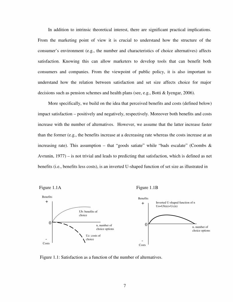
More specifically, we build on the idea that perceived benefits and costs (defined below)

impact satisfaction – positively and negatively, respectively. Moreover both benefits and costs

increase with the number of alternatives. However, we assume that the latter increase faster

than the former (e.g., the benefits increase at a decreasing rate whereas the costs increase at an

increasing rate). This assumption – that “goods satiate” while “bads escalate” (Coombs &

Avrunin, 1977) – is not trivial and leads to predicting that satisfaction, which is defined as net

benefits (i.e., benefits less costs), is an inverted U-shaped function of set size as illustrated in

Figure 1.1A Figure 1.1B

Figure 1.1: Satisfaction as a function of the number of alternatives.

Ub: benefits of choice

Uc: costs of choice

n, number of choice options

0

Benefits

+

- Costs

Inverted U-shaped function of n Uo=Ub(n)+Uc(n)

n, number of choice options

0

Benefits

+

- Costs

8

Two clear implications of this function are that, first, greater outcome and process

satisfaction will be experienced from choices made from intermediate as opposed to large or

small set sizes; and second, changes in perceived costs and benefits will shift the position of

the peak of the satisfaction function. For example, holding benefits constant, lower costs will

shift the peak to the right. We emphasize the explicit nature of our theoretical rationale and, in

particular, the predicted shape of the satisfaction function. More critically, it can be falsified

empirically.

In our experimental work, we explicitly manipulate cognitive costs imposed on decision-

makers by varying the visual attributes of choice alternatives and demonstrate how this affects

the shape of the satisfaction function. We further emphasize the importance of perceptions of

costs and benefits. Thus, even if the same choice set is viewed by different groups of people,

the satisfaction function could reflect characteristics such as gender, culture, or knowledge.

However, whereas the peak and position of the satisfaction function may change, there will

still be an inverted-U relation between satisfaction and the number of alternatives.

This paper is organized as follows. The next section elaborates on the theoretical

framework. This is followed by the presentation of five empirical studies. Study 1 explores the

shape of the satisfaction function and examines the effect of costs due to visual characteristics

of choices. The goal of Studies 2 (eye-tracking experiment) and 3 (questionnaire) is to

illuminate the asymmetry in costs between visual attributes which contribute to the changes in

the satisfaction function demonstrated in Study 1. Study 4 tests the influence of visual

properties of alternatives on choice set attractiveness. Study 5 manipulates perceived psychic

costs and demonstrates the effect of individual characteristics on the resulting function. We

conclude by discussing implications.

9

1.2 Theoretical Framework

The proliferation of choice alternatives can be thought of as implying benefits and costs

at two levels. One is at the level of the collective or society, the other at that of the individual.

For the former, the existence of many alternatives is clearly advantageous in that it enables

satisfying a multiplicity of different individual preferences. In addition, many choices can lead

to the benefits of competition, e.g., lower prices and greater quality (Loewenstein, 1999).

Moreover, perceived quality – and more purchases – can sometimes be achieved by companies

that offer greater variety within brands (Berger, Draganska, & Simonson, 2007). Finally, the

mere fact of having choice alternatives can enhance psychological well-being and thus also

social welfare (see, e.g., Langer & Rodin, 1976).

At the individual level, however, the perceived benefits and costs of choice depend on

both situational and psychological factors. One way of conceptualizing how these affect

satisfaction is to specify how their associated benefits and costs vary as the number of

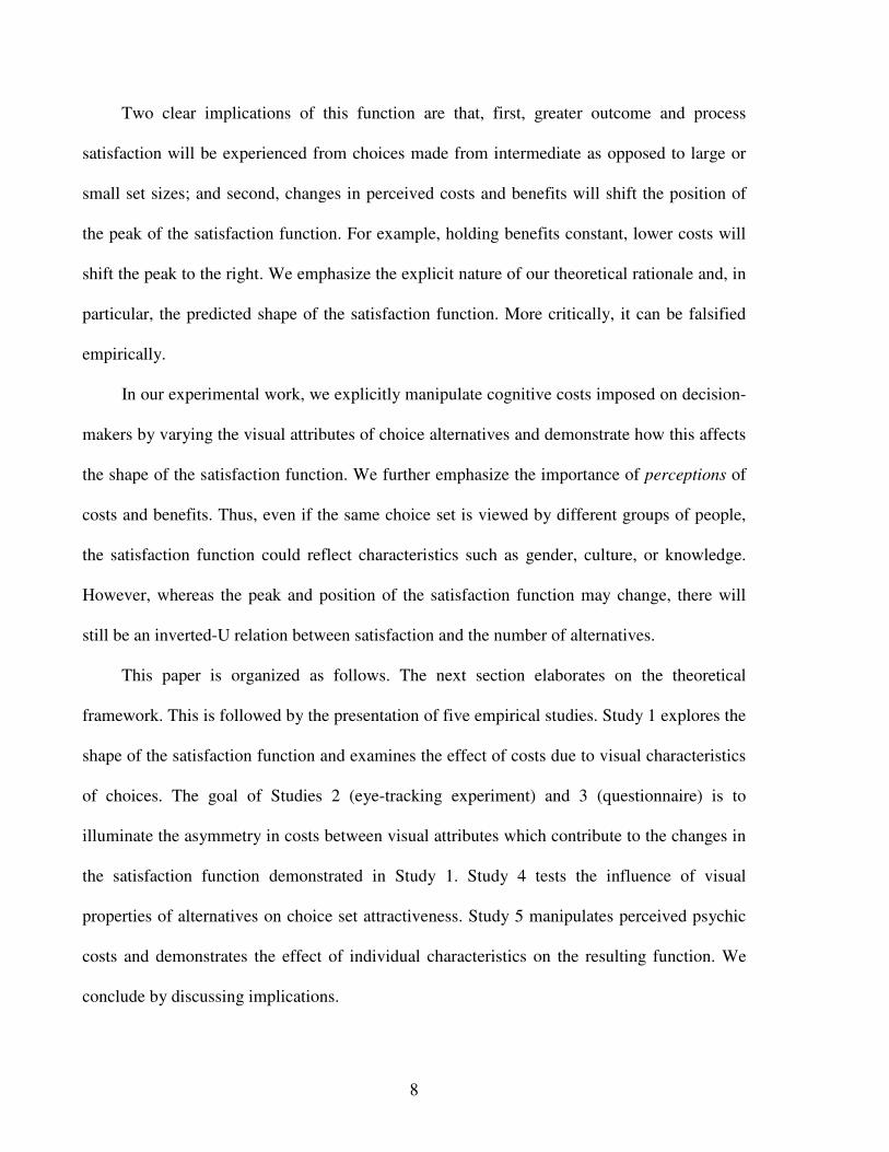
alternatives in the choice set increases. This is illustrated in Table 1.1 where we, first,

decompose situational and psychological costs, and, second, indicate how associated costs and

benefits increase with set size.

We decompose situational factors into two components: time and economic. For the

individual, we assume that, ceteris paribus, the cost of time to make a decision increases

linearly with the number of alternatives examined. As to the economic factor – or more

broadly the economist’s notion of utility – we assume that benefits increase with the number

of alternatives but at a decreasing rate, consistent with the notion of diminishing marginal

utility (Horowitz, List, & McConnell, 2007).

10

Table 1.1: Benefits and costs of choice as a function of number of alternatives

Factors Benefits Costs

Time

Increasing

(linear) Situational

Economic

Increasing

(decreasing rate)

Cognitive

Increasing

(increasing rate) Psychological

Psychic

Increasing

(decreasing rate)

Increasing

(increasing rate)

At the psychological level, the cognitive costs of processing alternatives increase with

the number of alternatives but at an increasing rate. This is in line with well-known limitations

on human cognitive capacity (Newell & Simon, 1972).

At the psychic level, we postulate both benefits and costs. By the former we mean the

positive affect that is generated by having more choice. In general, there is an attraction to

having more alternatives (see, e.g., Iyengar & Lepper, 2000). As a thought experiment,

contrast the emotional feelings experienced when entering a grocery store offering only a few

options as opposed to entering a well-stocked competitor). Moreover, having more alternatives

is associated with greater perceived decision freedom (Steiner, 1970; Reibstein, Youngblood,

& Fromkin, 1975; Walton & Berkowitz, 1979), and gives people a feeling of autonomy and

11

self-control thereby also facilitating intrinsic motivation (Zuckerman et al., 1978; Ryan &

Deci, 2000).

By psychic costs we mean psychological costs that are emotional as opposed to cognitive

in nature. These could be caused by discomfort due to uncertainty concerning preferences,

lack of expertise, concern or regret about making an incorrect decision, emotional costs of

making trade-offs, and so on (see, e.g., Loewenstein, 1999). Close consideration of the

alternatives may also induce “attachment” to the options in the choice set such that people feel

the “loss” of the items they have not chosen (Carmon, Wertenbroch, & Zeelenberg, 2003).

Also, the more options foregone, the greater the post-choice discomfort experienced. Having

too many alternatives may turn “freedom” of choice into “tyranny” (Schwartz, 2000).

Summing the situational and psychological benefits and costs of choice, our assumptions

imply that both increase with set size. However, we assume that the benefits increase more

slowly than the costs (“goods satiate” but “bads escalate,” Coombs & Avrunin, 1977). In our

experimental work, we do not test the separate shapes of the cost and benefit functions

explicitly but rather focus on the “net” effect of the two.

Equating satisfaction with the net difference between benefits and costs, we predict that

satisfaction is an inverted-U shaped function of the number of alternatives2. We therefore

state our first hypothesis:

Hypothesis 1: Both outcome and process satisfaction are inverted U-shaped functions of

the number of alternatives in the choice set.

2 Desmeules (2002) suggested that, when evaluating alternatives cognitively, the consumption experience might have an inverted U-shaped relation across set size. However, his proposition was neither formalized nor tested empirically

12

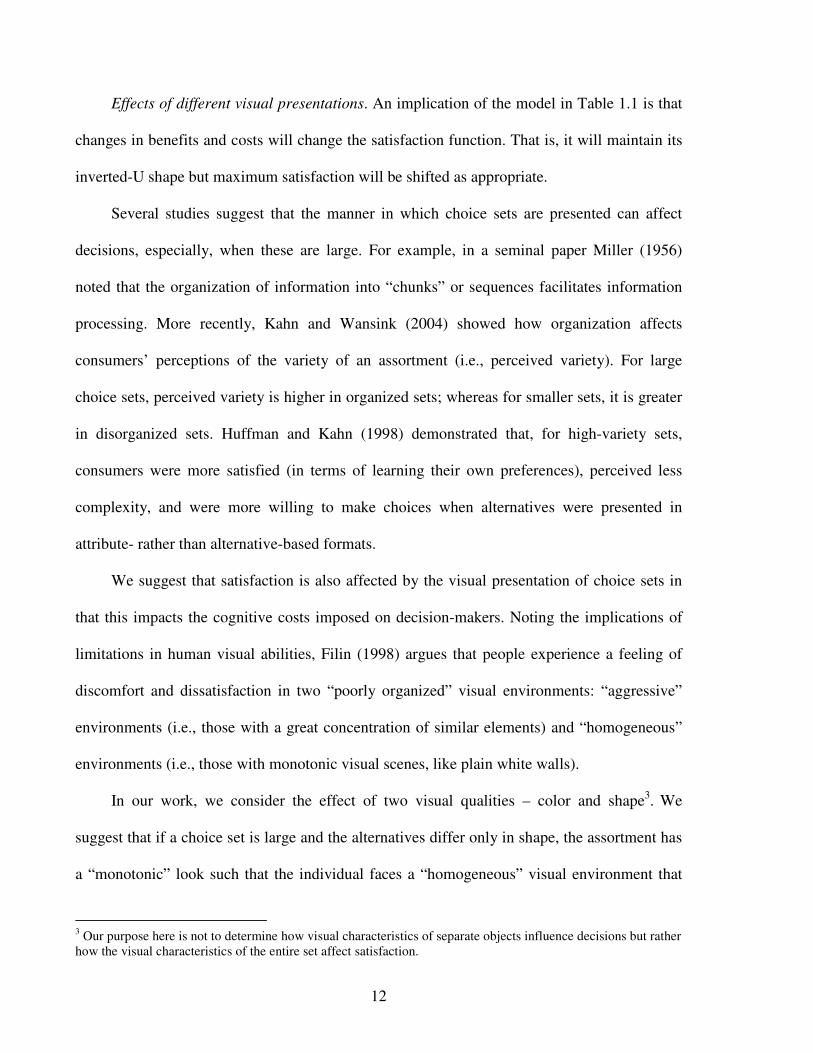
Effects of different visual presentations. An implication of the model in Table 1.1 is that

changes in benefits and costs will change the satisfaction function. That is, it will maintain its

inverted-U shape but maximum satisfaction will be shifted as appropriate.

Several studies suggest that the manner in which choice sets are presented can affect

decisions, especially, when these are large. For example, in a seminal paper Miller (1956)

noted that the organization of information into “chunks” or sequences facilitates information

processing. More recently, Kahn and Wansink (2004) showed how organization affects

consumers’ perceptions of the variety of an assortment (i.e., perceived variety). For large

choice sets, perceived variety is higher in organized sets; whereas for smaller sets, it is greater

in disorganized sets. Huffman and Kahn (1998) demonstrated that, for high-variety sets,

consumers were more satisfied (in terms of learning their own preferences), perceived less

complexity, and were more willing to make choices when alternatives were presented in

attribute- rather than alternative-based formats.

We suggest that satisfaction is also affected by the visual presentation of choice sets in

that this impacts the cognitive costs imposed on decision-makers. Noting the implications of

limitations in human visual abilities, Filin (1998) argues that people experience a feeling of

discomfort and dissatisfaction in two “poorly organized” visual environments: “aggressive”

environments (i.e., those with a great concentration of similar elements) and “homogeneous”

environments (i.e., those with monotonic visual scenes, like plain white walls).

In our work, we consider the effect of two visual qualities – color and shape3. We

suggest that if a choice set is large and the alternatives differ only in shape, the assortment has

a “monotonic” look such that the individual faces a “homogeneous” visual environment that

3 Our purpose here is not to determine how visual characteristics of separate objects influence decisions but rather how the visual characteristics of the entire set affect satisfaction.

13

imposes costs of discomfort (i.e., cognitive costs increase). Provision of colors, however, may

resolve the problem of monotonicity by making the items more distinct thereby reducing costs

for the human visual system.

Indeed, Spring, and Jennings (1993) claim that hue is recognized pre-attentively, while

complex shape is a non-preattentive stimulus that requires more time to be processed. Thus,

the detection of hue should not depend on the size of the set in which it is presented. On the

other hand, since complex shape is a non-preattentive stimulus, the time and effort involved in

processing shapes should be particularly high in larger sets4.

We therefore propose that, when the set of alternatives is large, the cost of choice is

higher for sets with alternatives differing in shape than for those differing in color. As a result,

we expect people to be more satisfied when they are presented with large sets with options that

differ in color as opposed to shape. In other words, the peak of the satisfaction function for

colors will lie to the right of that for shapes. More formally, we state:

Hypothesis 2: Visual presentation of sets affects satisfaction. People experience higher

satisfaction when the alternatives in large choice sets are different in color but not in shape.

However, for small choice sets, they are equally satisfied when alternatives are presented in

either different colors or shapes.

We emphasize that we limit our analysis and predictions in this paper to situations where

people actually make choices as opposed to avoiding them. Moreover, we focus on situations

where people do not have well-established preferences prior to choosing. In addition, we have

simplified the discussion of the benefits and costs of different numbers of alternatives by

ignoring possible interactions between different components. However, we believe that the

4 Corbetta, Miezin, Dobmeyer, Shulman, and Petersen (1991) have also shown that attention to shape and attention to color can activate different regions of the brain.

14

simple structure implied by Table 1.1 should be investigated prior to considering such factors.

This is the purpose of the present paper.

1.3 Study 1

The aim of Study 1 was to explore how satisfaction from choice varies as a function of

the number of alternatives and to examine how changes in cognitive costs affect satisfaction.

In this laboratory experiment, participants were given a picture representing a set of gift boxes

with a certain number of alternatives (5, 10, 15, or 30). They were asked to choose one gift

box they would buy to pack a present for a friend and to report their levels of satisfaction. We

manipulated cognitive costs imposed on individuals by varying two visual attributes of the gift

boxes – color and shape.

1.3.1 Method

Choice sets. Choice sets consisted of 5, 10, 15, or 30 gift boxes. The gift boxes differed

from each other on two visual attributes: color and/or shape. Three types of sets were created

representing gift boxes of: (1) the same shape and different colors (SSDC sets); (2) the same

color and different shapes (SCDS sets); (3) and different colors and different shapes (DCDS

sets). The gift boxes did not contain anything and, except for visual attributes, were said to be

identical. We refer to the SSDC and SCDS sets as “simple” since they vary on only one

attribute and to the DCDS sets as “complex” since alternatives differ on two dimensions. No

choice sets contained identical alternatives and all sets were organized (e.g., by shading of

colors).

15

Participants and procedure. The 120 participants were students and professors at

several universities in Barcelona, Spain (53% females, mean age of 23.7 years). All spoke

English and received no financial remuneration.

The participants were randomly divided into 12 experimental groups formed by crossing

two between-participant factors – number of choice options with four levels (5, 10, 15 or 30),

and three types of choice sets, SSDC, SCDS, and DCDS.

The experimenter invited one participant at a time into the experimental laboratory and

showed him/her a picture representing a set of gift boxes. (Participants were unaware of the

existence of other choice sets.) Each participant had to examine the picture and state which

box s/he would buy to pack a present for a friend. After choosing, participants answered a

paper-based questionnaire, evaluating satisfaction from the choice and providing demographic

characteristics.

Dependent measures. Satisfaction can result from both the outcome of choice (i.e., the

option chosen) and the process of choice itself (Steiner, 1980; Iyengar & Lepper, 2000). We

therefore assessed both sources. We measured outcome satisfaction by participants’ answers

to the question “How much do you like the gift box you decided to pick?” Response to the

question “How much did you enjoy making the choice (the decision process)?” was used to

measure process satisfaction. We also asked two further questions. First, “Did you find it

difficult to make your decision of which gift box to purchase?” Responses were provided on a

scale ranging from 1 (“not at all”) to 10 (“extremely”). Second, “Do you feel you had the right

amount of options to choose from?” Responses were provided on a nine-point scale where 1

16

= “No, I had too few choice options,” 5 = “Yes, I had just the right number of choice options,”

and 9 = “No, I had too many choice options.”5

1.3.2 Results

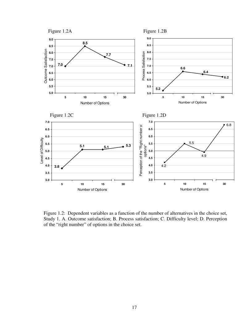
Satisfaction from the choice function. The results of Study 1 strongly support our first

hypothesis. Self-reported satisfaction – both outcome and process – is an inverted U-shaped

function of the number of alternatives as shown in Figures 1.2A and 1.2B. The participants

reported lower outcome and process satisfaction from limited (5) and extensive (30) options,

and higher satisfaction from medium-sized sets (10 and 15 options). The 10-option set was

found to be the most satisfying. Difficulty of choosing also increased with the set size (see

Figure 1.2C). Participants further believed that the “right number of options” was 10 or 15

(see Figure 1.2D). Recall that on this scale five was “ideal” with one being “too few” and nine

“too many.” The 30-option set was considered to be overwhelming, while the 5-item set was

perceived as offering too little choice. Outcome and process satisfaction showed significant

positive correlation (r =0.41, p < 0.001).

We tested the inverted-U relationship between satisfaction and number of alternatives in

two different ways: using regression analysis with the second degree polynomial and using

ANOVA and t-tests. Both tests confirmed that satisfaction follows an inverted U pattern when

the number of alternatives in the set increases.

5 Most of the measures used in this experiment were similar to those used by Iyengar and Lepper (2000) in their study 3 which motivated the current research.

17

Figure 1.2: Dependent variables as a function of the number of alternatives in the choice set, Study 1. A. Outcome satisfaction; B. Process satisfaction; C. Difficulty level; D. Perception of the “right number” of options in the choice set.

7.1

7.7

8.5

7.0

5.0

5.5

6.0

6.5

7.0

7.5

8.0

8.5

9.0

5 10 15 30

Number of Options

Ou

tco

me

Sa

tisfa

ctio

n

6.2

6.4

6.6

5.2

5.0

5.5

6.0

6.5

7.0

7.5

8.0

8.5

9.0

5 10 15 30

Number of Options

Pro

cess S

atisfa

ction

5.35.15.1

3.8

3.0

3.5

4.0

4.5

5.0

5.5

6.0

6.5

7.0

5 10 15 30

Number of Options

Level of D

ifficulty

6.8

5.5

4.9

4.2

3.0

3.5

4.0

4.5

5.0

5.5

6.0

6.5

7.0

5 10 15 30

Number of Options

Perc

eption o

f th

e "

Rig

ht num

ber of

options"


Figure 1.2C Figure 1.2D

18

First, outcome and process satisfaction were each regressed on the number of

alternatives (represented by both linear and quadratic terms) controlling for visual

characteristics of the sets. Both models –outcome and process satisfaction models – were

significant [F(4, 115) =6.33 p = 0.000; F(4, 115) = 4.49, p = 0.002, respectively]. This

analysis supported the inverted U-shape relation between satisfaction and set size in that- in

both the outcome and process satisfaction models - the linear (t = 3.21, p = 0.002; t = 3.07, p

=0.003, respectively) and quadratic (t = -3.51, p = 0.001; t = -2.87, p = 0.005, respectively)

terms were significant with appropriate signs. Participants facing SSDC sets also expressed

significantly higher outcome and process satisfaction than those facing DCDS sets (t = 3.37, p

= 0.001; t = 2.65, p = 0.009, respectively).

Second, ANOVA (see Table 1.2) indicates that the size of the choice set significantly

affects satisfaction for all four dependent measures. Statistical tests of the nature of these

differences (i.e., whether satisfaction functions have inverted U shapes) are presented in Table

1.3. This shows, for example, that for “outcome satisfaction” (Figure 1.2A), the mean

satisfaction for 10 options (8.5) is significantly greater than both those for 5 and 15 options

(i.e., 7.0 and 7.7, respectively), and that satisfaction for 15 options significantly exceeds that

for 30 (i.e., 7.7 vs. 7.1).

Visual presentation. Study 1 also aimed to test whether two visual attributes – color and

shape – affect satisfaction from different set sizes, a question motivated by our assertion that

colors imply less cognitive costs than shapes. We therefore analyzed the responses of the 80

participants who faced SCDS and SSDC sets.

19

Table 1.2: Significance of the set size effect on dependent variables

Statistics

Study 5

Dependent variable Study 1

Unaware group Aware group

Outcome Satisfaction F(3, 116) = 8.92

p = .000

F(3, 116)= 3.35

p = .022

F(3, 116)= 2.90

p = .038

Process

Satisfaction

F(3, 116)= 4.07

p = .009

F(3, 116) = 2.22

p = .089

F(3, 116) = 2.84

p = .041

Difficulty level F(3, 116) = 2.77

p = .045

F(3, 116) = 4.41

p = .006

F(3, 116) = 0.66

p = .580

Perception of the right

number of options

F(3, 116) = 10.21

p = .000

F(3, 116)= 2.78

p = .044

F(3, 116)= 3.98

p = .010

Table 1.3: Increases/ declines of means among choice sets with different numbers of alternatives

*** p < .01 ** p < .05 * p < .10

Measure Sample 5 vs 10 5 vs 15 5 vs 30 10 vs 15 10 vs 30 15 vs 30

Study 1 +1.53*** +0.73** +0.13 -0.80** -1.40*** -0.60*

Study 5 Unaware group

+0.14 +1.20*** +0.60 +1.06** +0.46 -0.60

Satisfaction from the gift box picked

Study 5 Aware Group

+1.20** +1.40* +0.60 +0.20 -0.60 -0.80

Experiment 1 +1.37*** +1.23*** +0.97** -0.14 -0.40 -0.26


+0.37 +1.40** +0.60 +1.03* +0.23 -0.80

Satisfaction from the decision-making process Study 5

Aware Group +1.03* +1.63*** +1.73*** +0.60 +0.73 +0.13

Experiment 1 +1.27** +1.27** +1.47** 0 +0.20 +0.20


+1.70** +0.27 +1.88*** -1.43** +0.17 +1.6** Difficulty level

Study 5 Aware Group

+0.10 +0.80 +0.64 +0.70 +0.54 -0.16

20

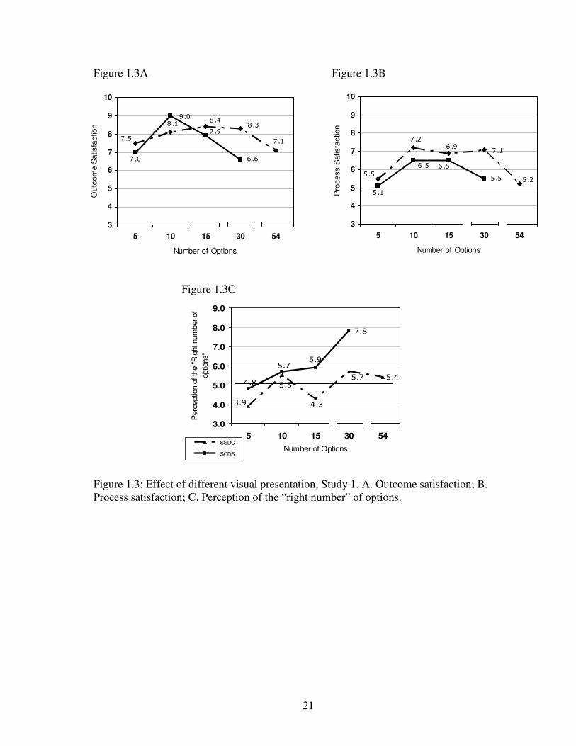
ANOVA supported our second hypothesis. Participants facing large sets (i.e., 30

options) with alternatives varying in color reported significantly higher outcome satisfaction

[F(1, 72) = 10.93, p = .002] than those encountering sets with items differing in shape (Figure

1.3A). For the small and medium-sized sets, however, this difference was not significant [F(1,

72) = 0.95, p = .334; F(1, 72) = 3.06, p = .084; F(1, 72) = 0.95 , p = .334 for 5-, 10- , and 15-

option sets respectively]. Moreover, the participants facing SSDC sets were significantly more

satisfied with the process of choosing than those who encountered SCDS sets over the entire

range of set sizes [F(1, 75) = 4.15, p = .045] – see Figure 1.3B.

Visual format also affected participants’ beliefs about the right number of options in the

set. When facing SSDC sets, the participants believed that 15- or even 30-option sets

contained “about the right number of options” [F( 1, 72) = 1.65, p = .203; F( 1, 72) = 1.65, p

= .203 respectively]. However, 30 options in the SCDS sets were viewed as “more than the

right amount” [F(1, 72) = 26.40, p = .000] – see Figure 1.3C.

Our results and analysis demonstrate that satisfaction is an inverted U-shaped function

of the number of alternatives for the SCDS sets. For the SSDC sets, however, this inverted U-

shape relation is not evident as the function did not decrease significantly after the peak. To

verify whether satisfaction would fall if the size of the SSDC set would become “too large,”

we conducted an additional treatment (with procedure identical to the others) where 34 new

participants faced an extensive SSDC set of 54 gift boxes. Results indicated that, from the 30

to 54 option set, both outcome and process satisfaction did indeed decrease significantly

(from 8.3 to 7.1 [ t = -2.31, p = .024], and from 7.1 to 5.2 [t = -2.52, p = .014], respectively –

see Figures 1.3A and B).

21

Figure 1.3A

Figure 1.3B

Figure 1.3C

Figure 1.3: Effect of different visual presentation, Study 1. A. Outcome satisfaction; B. Process satisfaction; C. Perception of the “right number” of options.

6.6

7.1

8.38 .4

8 .1

7 .5

9.0

7 .9

7 .0

3

4

5

6

7

8

9

10

5 10 15 30 54

Number of Options

Outc

om

e S

atis

factio

n

5.5 5 .2

7 .16 .9

7 .2

5 .5

6 .5 6 .5

5 .1

3

4

5

6

7

8

9

10

5 10 15 30 54

Number of Options

Pro

cess S

atis

factio

n7.8

5.45.7

4.3

5.5

3.9

5.75.9

4.8

3.0

4.0

5.0

6.0

7.0

8.0

9.0

5 10 15 30 54

Number of Options

Perc

eptio

n o

f th

e "

Rig

ht num

ber

of

optio

ns"

SSDC

SCDS

22

Gender and complexity. ANOVA revealed significant gender differences in outcome

satisfaction (controlling for set size). Compared to men, women reported higher outcome

satisfaction [F(1, 115) = 4.07, p = .046].

ANOVA also showed that participants facing simple sets (i.e., with items differing in

one attribute only) were significantly more satisfied with the outcome than those encountering

complex choice sets (i.e., with items differing in two attributes) controlling for set size [F(1,

115) = 9.81, p = .002]. No significant gender or complexity effects were found for the other

dependent variables. For detailed results on gender and complexity effects see Appendices

1.A and 1.B.

1.3.3 Discussion of Study 1

Study 1 demonstrated that satisfaction with both outcome and process is an inverted U-

shaped function of the number of items in the set. In other words, the data support Hypothesis

1.

Study 1 also supported Hypothesis 2 in that the peak of the function for colors was

shifted to the right. This, we had argued, was due to lower cognitive costs for colors as

opposed to shapes. However, we did not verify independently that the cognitive costs

associated with colors and shapes differed. Therefore, in Studies 2 and 3 (below), we

specifically investigate these costs using questionnaire and eye-tracking methodologies.

In Study 1 outcome and process satisfaction were positively correlated. However,

whereas outcome satisfaction in the 30-option case decreased to a level comparable to the 5-

option case, process satisfaction was significantly greater for the 30- than for the 5-option

sets. These results are in line with previous research. Iyengar and Lepper (2000) demonstrated

23

that when selecting and sampling a chocolate from either extensive (30 options) or limited (6

options) choice sets, subjects enjoyed the decision-making process more but, at the same time,

reported lower satisfaction with selection in the 30- than in the 6-option condition. Study 1

demonstrated that process satisfaction does not increase indefinitely. Rather, it decreases

when the choice set size is made significantly large. In our case, process satisfaction in the 54-

item SSDC set decreased to the level of that in the 5-option case.

Study 1 suggests that the satisfaction function may depend on gender. For males the

function lies below that of females. Two explanations come to mind. First, there is evidence

that women are used to paying more attention to detailed information than men and this habit

might lower the costs of choice in some tasks (Meyers-Levy & Maheswaran, 1991). Second,

females may simply care more about items such as gift boxes than males. For a different kind

of choice (e.g., beer or cell telephones), one might find the reverse effect. Whether gender

effects can be generalized across different conditions remains unclear and is an interesting

topic for further research.

The findings of Study 1 also demonstrated that participants reported lower outcome and

process satisfaction when encountering complex rather than simple sets over the entire range

of set sizes. This finding is consistent with our model. As the complexity of the sets increases,

both the psychological costs and benefits rise. If the shift in costs is greater than that in

benefits, the resulting satisfaction function shifts downwards. However, because we only

observed “net effects” of perceived benefits and costs, we were unable to test this implication

explicitly. The separation of effects of costs and benefits is critical for understanding the

underlying processes of choice and should be investigated in further research.

The finding that the peak of the satisfaction function for colors was positioned to the

right of that for shapes was consistent with our assertion that colors impose less cognitive

24

costs than shapes. However, this assumption was not explicitly tested in Study 1. Moreover,

implicit in the design of Study 1 are the assumptions that participants’ preferences for colors

and shapes are equally well-established and that individual boxes in the SSDC sets were as

attractive as those in the SCDS sets. Better established preferences for colors as opposed to

shapes, as well as the presence of more appealing colors than shapes in large sets, could

provide two alternative explanations for the rightward shift of the satisfaction function peak

for the SSDC sets.

We therefore explicitly designed two studies to test the following hypothesis and rule out

these two alternative explanations:

Hypothesis 3: The cognitive costs for alternatives differing in shape are greater than

those for alternatives differing in color.

1.4 Study 2

The primary goal of this study was to test whether cognitive costs for options differing

in shape are higher than those for options differing in color and to illuminate participants’

evaluations of individual boxes. We conceptualized the cognitive costs of choosing as having

two components: (1) “preference uncertainty” costs incurred when people decide how much

they like what they have observed (i.e., when establishing preferences); and (2) “processing”

costs that involve perceiving the objects that are evaluated. We also aimed to tease apart these

two types of cognitive costs and to verify whether they differ depending on color and shape.

In this study participants had to examine and evaluate – in terms of liking – 120 gift

boxes, one at a time. Time, individual ratings of the boxes and eye-movements of participants

were recorded while they examined the boxes and made their judgments (for more detailed

25

discussion of eye-tracking methodology, see Chandon, Hutchinson, Bradlow, & Young

(2007).

1.4.1 Method

Procedure, participants and stimuli. Fifteen students at a university in Barcelona, Spain

participated (27% males, mean age of 25.6 years). Each received 10 euro for participating.

One at a time, each participant had to examine sequentially pictures of gift boxes on a

computer screen and state how much s/he liked the boxes (for packing a present for a friend).

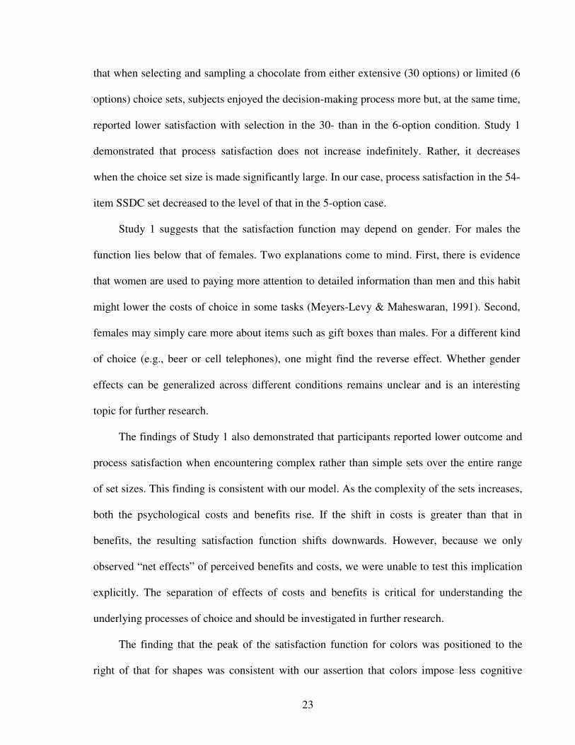
Each participant was told to imagine that any present would fit into the boxes. The computer

screen participants faced was divided into halves: on the left was the image of the box; on the

right, a 10-point rating scale. An example of the computer screen is presented in Figure 1.4.

The boxes were presented to participants one at a time and were identical to those in

Study 1. Participants had a maximum of seven seconds6 to examine each box and to rate how

much they liked it. However, they could use less time and proceed to the next trial.

Each participant was presented with four blocks of 30 boxes (i.e., 30 trials) each, and

thus had to make 120 judgments in total (i.e., 4 x 30). Within one block, boxes varied on only

one attribute – color or shape. Each participant faced two blocks with boxes differing in color,

and two blocks with boxes differing in shape. For example, in the first block (“Same Color

Different Shapes” – SCDS – condition) the participant would have to evaluate 30 boxes one at

a time that would be blue in color, but of different shapes. In the second block, the same

shapes as in the first block would be presented to the participant in the color red (SCDS

6 Note that Reutskaja, Pulst-Korenberg, Nagel, Camerer, and Rangel (2008) show that participants are able to make high quality decisions from 16 alternatives even within three seconds. In the current experiment, participants had seven seconds to evaluate each alternative.

26

condition). In the third block, the participant would face 30 oval boxes of different colors

(“Same Shape Different Colors”, SSDC condition), and so on. The order of the blocks as well

as that of presenting the stimuli was randomized.

Figure 1.4: Sample of a screen participants faced in the eye-tracking experiment.

Participants’ eye-movements were tracked while they examined and evaluated the

images of the boxes. Prior to viewing the stimuli, each participant went through a calibration

procedure that required looking at moving dots on the screen, and through a short training

session during which they evaluated six boxes that were not used in the actual study. We used

the VSG2/5 Workstation & Videoeyetracker which recorded the positioning of the eye gazes

on the screen and pupil dilations of participants every 20 milliseconds.

Dependent measures. We used both behavioral and eye-tracking measures.

27

Behavioral measures. We assessed the total cost of processing and determining

preferences about each box by measuring the total time spent on each trial. The average total

time spent on processing the boxes and establishing preferences in the SCDS condition was

then compared to that in the SSDC condition.

We also assessed how much participants liked each box by their responses to the

question “How much do you like the gift box presented on the screen?” Responses were given

on a 10-point scale ranging from 1 (“not at all”) to 10 (“extremely). We then compared the

average liking ratings given to the boxes in the SCDS and SSDC conditions.

Eye-tracking measures. The eye-tracker recorded the eye-movements of the participants

every 20 ms while they were processing and evaluating the images. This allowed separating

processing from preference uncertainty costs. Specifically, processing costs were measured by

the time participants spent looking at the part of the screen where the image of the box was

presented for the first time, while preference uncertainty costs were measured by the time

spent on further gazes at the image of the box as well as at the part of the screen with the scale.

1.4.2 Results

Behavioral data. Each of fifteen participants had to make 120 choices in total. We

dropped one trial (of one participant) from the analysis as the corresponding data were not

recorded for technical reasons. As a result, we analyze data obtained from 1,799 (i.e., 120 x

15-1) trials.

The results strongly support Hypothesis 3. On average, participants spent 3.13 seconds

per trial. The average total time spent per trial was 253 ms higher in the SCDS than in the

SSDC blocks. To test the significance of this effect in the presence of high individual

28

variability, we regressed response time on dummy variables for both type of blocks and

individual participants. This revealed a significant block effect (t = 3.54, p < .001) controlling

for individual effects – see Table 1.4. In short, the total costs of determining preferences and

processing alternatives differing in shape are greater than for those differing in color.

Table 1.4: Regression analysis of the effect of attribute (color/shape) on response time

Dependent Variable

Response Time (ms) St. Error

Color -252.78 71.32***

Participant1 -1,278.18 0.00***

Participant2 202.66 0.00***

Participant3 -912.66 0.00***

Participant4 -215.56 0.30***

Participant5 -1,428.32 0.00***

Participant6 -617.56 0.00***

Participant7 -343.80 0.00***

Participant8 -795.25 0.00***

Participant9 -712.42 0.00***

Participant10 -810.35 0.00***

Participant11 -844.23 0.00***

Participant12 -18.80 0.00***

Participant13 -797.93 0.00***

Participant14 477.47 0.00***

Constant 3,793.85 35.66***

Observations 1799

R-squared 0.44

Notes: (1) *** p < .01; ** p < .05; * p < .10 (2) Color is the dummy: Color=1 if box is in the SSDC block, and Color=0, if box is in the

SCDS block

(3) Participanti is the dummy indicating participant i (1≤ i ≤15).

29

Consistent with our assumption, the liking ratings assigned to items in the SCDS blocks did

not differ significantly from those in the SSDC blocks (t = 1.89, p = .08, with liking ratings of

items in the SSDC blocks being slightly lower than those in the SCDS blocks). We tested this

effect by regressing the liking rating of the box on block type controlling for individual

effects, see Table 1.5.

1.4.3 Eye-tracking data

We excluded the eye-tracking data of three (of the fifteen) participants because of

unacceptable rates of erroneous trials (more than 20%). In addition, several trials were not

properly recorded due to technical reasons and had to be deleted. As a result, our analysis is

based on the data from 1,283 trials.

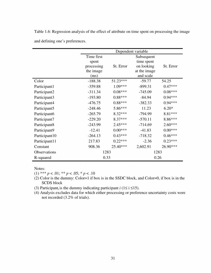
Results show that time for processing items was 188 ms higher for the SCDS blocks than

for the SSDC blocks. To test this effect, we regressed time first spent processing the image on

block type controlling for individual effects. This was significant (t = 3.72; p < .010) – see

model on left of Table 1.6. However, when subsequent time spent looking at the image and

scale was regressed on block type, there was no significant effect (t = 1.10; p = .294) – see

model on right of Table 1.6.

Overall, the results suggest that the processing costs for colors are greater than those for

shapes, but “preference uncertainty” costs are equal for the two attributes. To test further the

finding regarding preference uncertainty costs, we conducted a questionnaire study.

30

Table 1.5: Regression analysis of the effect of attribute (color/shape) on liking rating of the image

Dependent Variable

Liking Rating of the Image St. Error

Color -0.62 0.33* Participant1 0.71 0.00*** Participant2 -1.13 0.00*** Participant3 -0.57 0.00*** Participant4 1.04 0.00*** Participant5 -0.79 0.00*** Participant6 1.04 0.00*** Participant7 -2.88 0.00*** Participant8 -1.26 0.00*** Participant9 1.62 0.00*** Participant10 -1.08 0.00*** Participant11 1.08 0.00*** Participant12 -0.66 0.00*** Participant13 0.37 0.00*** Participant14 0.59 0.00*** Constant 5.80 0.17*** Observations 1797

R-squared 0.22


SCDS block

(3) Participanti is the dummy indicating participant i (1≤ i ≤15). (4) Two trials in which participants failed to indicate their ratings were coded as missing.

31

Table 1.6: Regression analysis of the effect of attribute on time spent on processing the image

and defining one’s preferences.

Dependent variable

Time first spent

processing the image

(ms)

St. Error

Subsequent time spent on looking

at the image and scale

St. Error

Color -188.38 51.23*** -59.77 54.25

Participant1 -359.88 1.09*** -899.31 0.47***

Participant2 -311.34 0.08*** -745.09 0.08***

Participant3 -193.80 0.88*** -84.94 0.94***

Participant4 -476.75 0.88*** -382.33 0.94***

Participant5 -248.46 5.86*** 11.23 6.20*

Participant6 -265.79 8.32*** -794.99 8.81***

Participant7 -229.20 8.37*** -570.11 8.86***

Participant8 -243.99 2.45*** -714.69 2.60***

Participant9 -12.41 0.00*** -41.83 0.00***

Participant10 -264.13 0.43*** -718.32 0.46***

Participant11 217.83 0.22*** -2.36 0.23***

Constant 908.36 25.40*** 2,602.91 26.90***

Observations 1283 1283

R-squared 0.33 0.26


SCDS block

(3) Participanti is the dummy indicating participant i (1≤ i ≤15). (4) Analysis excludes data for which either processing or preference uncertainty costs were

not recorded (3.2% of trials).

32

1.5 Study 3

In Study 3, we sought to understand people’s perceived preferences for colors and

shapes in general as well as in the context of gift boxes. For this we used a questionnaire.

1.5.1 Method

Procedure. The questionnaire assessed participants’ preferences for colors and shapes.

Participants had to state what color/shape they liked most both overall (i.e., answer the

question “What is your favorite color/shape?”) and in the context of gift boxes (i.e., answer the

question “If you think of the ideal gift box: What color/shape would you prefer this box to be,

which you would receive/give from/to a friend)?”)7. Participants could either state their

preferred color or shape, or respond “I do not know.”

Participants. Respondents were 106 students at a university in Barcelona, Spain (58%

females, mean age of 19.4 years). Each received 3 euro for participating.

Dependent measures. We calculated the number of “do not know” responses to questions

regarding color and shape preferences both overall and in the context of the gift boxes. We

assume that the greater the number of “do not know” responses, the less defined are

preferences for colors or shapes.

1.5.2 Results

In general, participants had better established preferences for colors than for shapes.

7 In fact, participants were asked many questions. Here we simply report responses that are pertinent to this paper.

33

More participants failed to report a favorite shape as opposed to a favorite color (t = 4.97, p

<0.001) (Responses were coded as “1” if participant responded “I don’t know”, and “0”

otherwise). However, in the context of gift boxes, these differences disappeared. Participants

had equally well determined preferences for colors and shapes independently of whether the

box was to be given or received (t = 0.22, ns, t = 0.00, ns, respectively).

1.5.3 Discussions of Studies 2 and 3

We used behavioral and biological measures to explain the asymmetry between the two

attributes of interest – color and shape. First, Study 2 demonstrated that cognitive costs – as

measured by response times – were greater for shapes than for colors. This is consistent with

our theoretical framework and can explain the shift of the peak of the function in Study 1.

Second, Study 2 revealed that this difference in time is attributed to processing rather than

preference uncertainty costs. In Study 2 participants processed items differing in color in less

time than those differing in shape.

Third, the eye-tracking data showed that the time spent on defining preferences

regarding the boxes did not differ between the SCDS and SSDC conditions. This finding was

replicated in the questionnaire, which demonstrated that people have equally well established

preferences for colors and shapes in the context of gift boxes. These results support the notion

that the shift of the peak of the satisfaction function in Study 1 cannot be explained by

differences in preference uncertainty costs, that is, for defining preferences. Nor can the shift

be explained by the fact that items in the SCDS sets were less appealing to the participants.

Indeed, the eye-tracking study demonstrated that items presented in the SCDS and SSDC sets

34

were seen as equally attractive by participants (with, if anything, a slight – significant at 10%

– liking bias for the SCDS images).

Our eye-tracking study and questionnaire have important theoretical and practical

implications. First, measuring the cognitive costs for the two different attributes served as an

empirical verification of our theoretical framework. We demonstrated that colors are less

taxing than shape thereby inducing the shift of the satisfaction function found in Study 1.

Second, comparison between two widely used visual attributes – color and shape – has

practical implications for people offering choices. The results suggest that presenting

alternatives of large sets in different colors can create “comfortable” visual environments

thereby attracting more people, and positively influencing outcome and process satisfaction.

As a result, people may be able to obtain high benefits from larger set sizes without losing

satisfaction.

Study 1 demonstrated that visual presentation of assortment influences satisfaction. More

specifically, participants reported significantly higher levels of satisfaction when the

alternatives in the large choice sets were different in color but not in shape (Hypothesis 2).

However, does this mean that the sets with alternatives different in color are also more

attractive than those that vary in shape? This question becomes relevant when people choose

between different sets of offerings rather than selecting an item from a given set.

As a corollary to Hypothesis 2, therefore, we suggest that since visual “comfort” is

more pleasing for the eyes (and less “costly” to process), one should also expect large SSDC

sets to be more appealing than large SCDS sets. Also – and once again – since the costs of

choice from small sets are not unduly taxing, we would not expect such effects with small sets.

More formally, we state:

35

Hypothesis 4: Visual properties of the set affect its attractiveness. More people are

attracted to large sets when alternatives differ in color as opposed to shape. No such effects

exist for small sets.

We conducted Study 4 to test this hypothesis

1.6 Study 4

1.6.1 Method

Procedure. The design of Study 4 was similar to that of Study1. The main difference

was that, first, participants had to decide which of the sets of gift boxes they liked the most:

that in “shop A” which offered gift boxes varying in shape (SCDS set) or that in “shop B”

which offered boxes differing in color (SSDC set). Participants were given pictures

representing each of the two sets. The choice sets were identical to those of Study 1. Both sets

offered to a particular individual were of the same size involving 5, 10, 15, or 30 alternatives.

Participants were 48 undergraduate students (mean age of 19.2 years, 54% females) at a

Spanish University. Participants were not remunerated. Groups of 12 participants were

assigned at random to each of four groups evaluating the different-sized options.

First, participants had to choose which choice set – shop A or B – they preferred and

answer a questionnaire assessing their satisfaction with each set and the difficulty of choosing

between them. Second, the participants were left with the picture of the choice set they had

selected and asked to choose a gift box and complete the same questionnaire as in Study 1.

Measures. First, we simply counted the numbers of participants who chose each “shop”

for the different set sizes. Second, we assessed participants’ satisfaction with each choice set

36

and the difficulty of choosing between them by asking “How much do you like the assortment

in shop A?”, “How much do you like the assortment in shop B?”, and “How difficult was it

for you to decide to which shop to go?” Responses were provided on a 10-point scale ranging

from one (“Not at all”) to 10 (“Extremely”). Third, satisfaction measures concerning choices

of boxes were identical to those used in Experiment 1.

1.6.2 Results

When facing medium or large choice sets (i.e., sets containing 10, 15 or 30 alternatives)

25 out of 36 participants preferred the options in shop B where boxes varied in color but not

in shape thereby indicating that the former are more attractive [p(x ≤ 11) = .025, binomial

test]. For small sets (5 options), there was no significant difference [p(x ≤ 5) = .387].

However, this lack of a significant difference could simply be due to the small sample of

participants (12) facing 5-alternative sets. We therefore recruited 19 additional participants for

a 5-option set treatment of this study. Results showed that of the 31 participants who faced 5-

alternative sets, 15 preferred the SSDC sets. In other words, there was no significant

difference in choices between the SCDS and SSDC sets [p(x ≤ 15) = 0.500, binomial test].

Finally, participants reported greater satisfaction levels from the SSDC than SCDS sets

when the number of alternatives in the set exceeded 10 (t = 1.98, p = .056), but similar

satisfaction levels for 5-option sets (t = 0.98, p = .381).

1.6.3 Discussion of Study 4

The results of Study 4 provide support for Hypothesis 4. Sets of alternatives differing in

color were more attractive than those differing in shape when the sets were large, while both

37

were seen as equally appealing when set size was small. This is consistent with the arguments

provided above. Namely, the costs of processing alternatives differing in color are lower for

the human visual system than those associated with shape.

Study 1 demonstrated that visual properties of the alternatives in the set affect perceived

costs and benefits and therefore influence the peak of the satisfaction function. However, can

individual characteristics also affect perceived costs and benefits of choice? We took the

opportunity to investigate this issue in a slightly different experimental setting.

In our initial setting, participants face a given set of choice alternatives and are unaware

of the possible existence of other sets. However, would satisfaction be affected if participants

were aware of the existence of choice sets different from theirs? Clearly, people do not only

engage in evaluating trade-offs between the alternatives they face, but also compare their own

possibilities with those of others. Indeed, as originally demonstrated by Festinger (1954),

when objective measures are not available, people tend to judge their own possibilities by

comparison with those of others. Thus, if when presented with a set of alternatives, a person

is made aware of the existence of other alternatives, he or she may well feel at a disadvantage

and thereby incur psychic costs.

The framework in Table 1.1 suggests how awareness about choice sets different from

one’s own will affect the relation between satisfaction and set size. Specifically, the psychic

costs incurred before even viewing the choice set would imply a downward shift of the cost

curve by a fixed amount and thus also a downward shift of the resulting satisfaction function.

More formally, we hypothesize:

Hypothesis 5: Individuals, who are aware of the existence of choice sets different from

theirs and from which they cannot choose, are less satisfied with their choice than those who

do not possess such knowledge.

38

To test this hypothesis we conducted Study 5.

1.7 Study 5

1.7.1 Method

Study 5 involved two groups of participants. In one, the treatment was identical to the

experiment in Study 1. We call this the “unaware” group. The treatment of the second group –

the “aware” group – was identical but with two exceptions. First, unlike Study 1, where only

one participant at a time was invited into the experimental laboratory, several participants

followed the experimental procedure simultaneously in the same room. Second, participants of

Study 5 were explicitly told that their colleagues had been given choice sets differing from

their own in size and visual properties of the alternatives. The participants were unaware how

many different choice sets there were, which choice set was larger or smaller and could only

see the sets offered to their colleagues from a distance. After being given a picture

representing a choice set, participants followed the same procedure as in Study 1.

Participants. 240 students and professors (50% females, mean age of 22.7 years) from

several universities in Belarus (66%) and Ukraine (34%) took part in the experiment. They

received no financial remuneration. Study 5 was conducted in Russian.

1.7.2 Results

Consistent with the findings of Study 1, outcome satisfaction was found to follow an

inverted U-shape for the unaware group – see Figure 1.5 and Tables 1.2 and 1.3.

39

Compared to the unaware group, the aware participants were less satisfied with their

ultimate choice (“awareness” dummy F(1, 235) = 7.18, p = .008), and with the process of

choosing (F(1, 235) = 4.96, p = .027), thereby providing support for Hypothesis 5. That is, the

satisfaction function for aware participants was shifted downwards in comparison with the

unaware group.

We also explored the influence of “cultural background” on the four variables of interest

by comparing the responses of “unaware” group of study 5 and those of participants in Study

1.

Though the satisfaction function of the Eastern European “unaware” group had an

inverted U-shape, participants from Belarus and Ukraine reported the highest satisfaction with

the gift box picked from 15- and 30-option sets whereas Western Europeans (group in Study

1) were most satisfied with the box chosen from medium-sized sets. The peak of the function,

therefore, was shifted toward a greater number of alternatives in the Eastern European sample

[F(4, 232) = 4.10, p = .003, Chow test], sets with 15 options being seen as the most satisfying.

Interestingly, the Eastern European participants also reported the lowest difficulty levels when

choosing from such sets, and considered that the 15-option set included exactly the “right

number of boxes.”

Gender and complexity. We found significant gender and complexity effects for several

dependent variables in the Eastern European unaware group (see Appendices 1.A and 1.B).

Eastern European females reported significantly higher satisfaction levels than men both with

the box picked and with the decision process. Across all set sizes, satisfaction with the box

picked was lower for participants facing complex as opposed to simple sets.

40

Figure 1.5A.

Figure 1.5B

Figure 1.5C

Figure 1.5D

Figure 1.5: Effect of “awareness” on choice experience, Study 5. A. Outcome satisfaction; B. Process satisfaction; C. Difficulty level; D. Perception of the “right number” of options in the choice set.

7,7

6,8

7,67,4

6,2

7,3

8,3

7,1

4,0

4,5

5,0

5,5

6,0

6,5

7,0

7,5

8,0

8,5

9,0

5 10 15 30

Number of Options

Outc

om

e S

atis

factio

n

6.46.3

5.7

4.7

6.4

6.2

7.2

5.8

4.0

4.5

5.0

5.5

6.0

6.5

7.0

7.5

8.0

8.5

9.0

5 10 15 30

Number of OptionsP

rocess S

atis

factio

n

4.34.4

3.73.6

5.25.1

3.6

3.43.0

3.5

4.0

4.5

5.0

5.5

6.0

6.5

7.0

5 10 15 30

Number of Options

Le

ve

l o

f D

ifficu

lty

Aw are group

Unaw are Group

3.6

4.1

5.0

4.0

4.2

2.7

3.9

3.2

2.0

2.5

3.0

3.5

4.0

4.5

5.0

5.5

6.0

6.5

5 10 15 30

Number of Options

Perc

eptio

n o

f th

e "

Rig

ht num

ber

of

optio

ns"

41

Visual presentation. In line with the findings of Study 1 (and Hypothesis 2), ANOVA

yielded differences in satisfaction of the Eastern European “unaware” participants due to the

visual layout of alternatives. Eastern Europeans reported higher satisfaction both with the gift

box picked [F(1, 72) = 4.02, p = .049], and with the decision process [F(1, 72) = 3.13, p =

.081], when facing large sets (30 options) in the SSDC as opposed to SCDS format. Moreover,

participants felt they had fewer options when facing SSDC sets rather than the same sized

SCDS sets [F(1, 75) = 8.26, p = .01] – see Figure 1.6.

1.7.3 Discussion of study 5

The outcome satisfaction curve of the unaware participants replicated the results of

Study 1 thereby providing additional support for Hypotheses 1 and 2. Consistent with

Hypothesis 5, the results of Study 5 also demonstrated that knowledge of the existence of

choice sets different from one’s own decreases both process and outcome satisfaction. As

argued above, the effect of telling participants explicitly that others can choose from different

sets imposes additional “fixed” psychic costs even before the choice is made. Holding benefits

constant, this initial increase in psychic costs results in a downward shift of the satisfaction

function.

Finally, we note the behavior of the aware group in Study 5 replicates Study 1 in a

different cultural sample (in Eastern as opposed to Western Europe). However there was a

difference. Participants from Eastern Europe were more satisfied with larger choice sets as

opposed to their Western counterparts, that is, the peak of satisfaction function for former lies

to the right of that for the latter (compare Figures 1.2 and 1.5). The reason for this finding is

not apparent and requires further investigation.

42

Figure 1.6A

Figure 1.6B

Figure 1.6C

Figure 1.6: Effect of different visual presentation, Study 5. A. Outcome satisfaction; B. Process Satisfaction; C. Perception of the “right number” of options in the set.

8,6

8,87,7

6,27,3

7,5

9,1

7,7

3

4

5

6

7

8

9

10

5 10 15 30

Number of Options

Ou

tcom

e S

atis

faction

5,4

7,16,8

5,7

5,3

6,7

8,1

6,5

3

4

5

6

7

8

9

10

5 10 15 30

Number of OptionsP

roce

ss s

atisfa

ctio

n

4,24,0

5,0

2,92,8

6,15,6

3,9

2

3

4

5

6

7

8

9

5 10 15 30

Number of Options

Perc

eptio

n o

f th

e "

Rig

ht num

ber

of

optio

ns"

SSDC

SCDS

43

1.8 General Discussion

This paper has explored the nature of satisfaction from choice as a function of

characteristics of choice sets. Building upon the theoretical insights of Coombs and Avrunin

(1977), we suggested that as the number of alternatives increases, so do the benefits and costs.

However, whereas the former “satiate,” the latter “escalate.” The net effect is that satisfaction

is an inverted U-shaped function of set size. Our studies provided support for this proposition.

At a theoretical level, our goal was to make explicit the implications of perceptions of

costs and benefits of the choice process. To test our theoretical framework we manipulated

differences in cognitive costs by contrasting satisfaction from choice when sets varied in color

as opposed to shape. We further assessed the asymmetry for colors and shapes using

behavioral and biological measures and demonstrated that alternatives differing in shapes are

more taxing. As a result, and as a direct verification of our theoretical framework in a

between-participants design, larger sets with alternatives differing in color were viewed as

being both more satisfying and attractive than those with alternatives varying in shape. That

is, the location of the peak of the satisfaction function was influenced by visual presentation

of the choice set.

Costs as well as benefits of choice may also depend on individual characteristics. First,

awareness of the existence of other choice sets influenced resulting satisfaction. We suggested

that when other sets are salient people incur additional psychic costs which, in turn, result in a

downward shift of the satisfaction function.

Second, we found that gender and culture may also affect perceptions of costs and

benefits. For the choices examined here, the satisfaction curve for women lay above that for

men. In addition, the peak of the curve of Eastern European participants was shifted to the

44

right of that for Western Europeans. We had no explicit hypotheses concerning these findings

but suggest that they provide a useful springboard for future research. In particular, we

suspect that type of choice could moderate these kinds of individual results. Though the

benefits and costs may depend on different factors, we stress again that the inverted U-shape

relation between satisfaction and choice set size was replicated in different settings.

We now outline implications and suggestions for further research.

First, in our experimental tasks, participants were required to make a choice. In many

situations, however, people may decide to avoid or defer choice (see, e.g., Dhar, 1997) and it

is also important to predict this phenomenon. One way of thinking about this within the

framework of Table 1.1 is to predict that choice is deferred or avoided when expected

satisfaction is negative, that is, when perceived costs exceed benefits. For example, imagine

the effect of imposing time limits on an important choice such that cognitive and psychic

costs increase rapidly and the person decides to defer choice (i.e., satisfaction becomes

negative). Similarly, when the perceived costs are higher than expected benefits of evaluating

the entire set people may also shift to using simplifying strategies (see, e.g., Payne, Bettman,

& Johnson, 1993). An advantage of our framework is that we can specify the expected effects

of different variables in this process as well as predict differences due, for example, to

severity of time limits or importance of the decision.

Second, we did not vary economic considerations in our experimental work. However,

our framework suggests how these might affect the satisfaction function. On the one hand,

there would be a desire to see more alternatives as decisions become more important. At the

same time, however, important choices could induce greater psychic costs as people become

more concerned about knowing their preferences and the possible regret of making errors

(thereby reducing the number of alternatives they would like to see). When economic stakes

45

are high, we would particularly expect to see expertise have a large effect on the location of

the peak of the satisfaction function. Thus, for example, in choosing a pension plan, we would

predict that the ideal number of alternative portfolios for a specialist (e.g., a security analyst)

would far exceed that of a financial novice. More generally, we believe much could be gained

by linking our framework to the literature on expertise.

Third, in our study participants were making choices for themselves. An intriguing

change to the implied costs might occur if they were making choices on behalf of others, that

is, as an agent. For example, if a financial specialist were selecting a portfolio for a friend as

opposed to herself, would she be willing to examine more alternatives? To the extent that this

would make the person feel more responsible, it follows that she probably would (see, e.g.,

Tetlock, 1991).

Fourth, the optimal number of alternatives (for satisfaction) in our studies was found to

be 10 or 15. These numbers are exactly the same as those reported by Miller (1956) for the

“channel capacity” of visual positioning, that is, the number of visual positions the human eye

can distinguish without making errors. It is unclear whether this is a coincidence. However, it

suggests investigating whether satisfaction is an inverted U-shaped function of the number of

alternatives when these are not characterized visually but by, say, tone, taste, or odor.

Building upon our theoretical framework, we would still expect satisfaction to be an inverted

U-shaped function of the numbers of these stimuli. Miller (1956) argued that the “span of

absolute judgment” is greater for visual stimuli than for tones or taste stimuli. Therefore, as

the costs of processing the latter are higher, we would also expect the location of the peaks of

the satisfaction functions for these to lie to the left of those for visual stimuli.

46

Fifth, in this experimental work we simplified by focusing on simple objects that

differed on only one or two attributes. Clearly, an important next step will be to extend the

approach adopted here to more complex products in naturally-occurring field studies.

In summary, we have presented a simple theoretical rationale that makes explicit the

reasons underlying the inverted U-shaped function that describes the relation between

satisfaction (both outcome and process) and the number of alternatives in a choice set. At one

level, good “common sense” suggests that people will be unsatisfied and confused by having

“too many” choice alternatives. Indeed, at an anecdotal level it is interesting to note that the

German retail chain ALDI carries 35 times less products that its rivals – traditional

supermarkets – but sells more of each product than its competitors (Kumar, 2006). Whereas it

would be foolish to generalize from this specific case, it is clearly an important matter to

understand when there are “too many alternatives” and how different variables contribute to

the satisfaction that people experience from choice. Our goal has been to help elucidate this

issue.

47

References

Berger, J., Draganska, M., & Simonson, I. (2007) The Influence of product variety on brand

perception and choice. Marketing Science, 26 (4), July–August, 460–472.

Botti, S., & Iyengar, S. S. (2006). The dark side of choice: When choice impairs social welfare.

Journal of Public Policy and Marketing, 25 (1) Spring, 24–38.

Carmon, Z., Wertenbroch, K., & Zeelenberg, M. (2003). Option attachment: When deliberating

makes choosing feel like losing. Journal of Consumer Research, 30(1), 15-29.

Chandon, P., Hutchinson, J. W., Bradlow, E.T. & Young, S. (2007). Measuring the value of point-

of-purchase marketing with commercial eye-tracking data, In Michel Wedel and Rik Pieters

(Eds.), Visual Marketing: From Attention to Action. Mahwah, New Jersey: Lawrence

Erlbaum Associates.

Coombs, C. H., & Avrunin, G. S. (1977). Single-peaked functions and the theory of preference.

Psychological Review, 84(2), 216-230.

Corbetta, M., Miezin F.M., Dobmeyer, S., Shulman G.L., & Petersen, S.E. (1991). Selective and

divided attention during visual discriminations of shape, color and speed: Functional anatomy

by positron emission tomography. The Journal of Neuroscience, 11(8), August, 2383-2402.

Desmeules, R. (2002). The impact of variety on consumer happiness: Marketing and the tyranny

of freedom. Academy of Marketing Science Review [Online], 12. Retrieved May 15, 2004,

from http://www.amsreview.org/articles/desmeules12-2002.pdf

Dhar, R. P. (1997). Context and task effects on choice deferral. Marketing Letters, 8(1), 119-130.

Festinger, L. (1954). A theory of social comparison processes. Human Relations, 7(1), 117-140.

Filin, V. A. (1998). Videoecology: Good and bad for the eye. Moscow: TASS-Advertising.

48

Huffman, C., & Kahn, B. E. (1998). Variety for sale: Mass customization or mass confusion?

Journal of Retailing, 74(4), 491-513.

Horowitz, J. List J., & McConnell K.E. (2007). A test of diminishing marginal value. Economica,

74, 650–663.

Iyengar, S. S., Jiang, W., & Huberman, G. (2004). How much choice is too much? Contributions

to 401 (k) retirement plans. In O. S. Mitchell, & S. Utkus (Eds.), Pension design and

structure: New lessons from behavioral finance (pp. 83-96). Oxford: Oxford University

Press.

Iyengar, S. S., & Lepper, M. R. (2000). When choice is demotivating: Can one desire too much of

a good thing? Journal of Personality and Social Psychology, 79(6), 995-1006.

Iyengar, S. S., & Lepper, M. R. (1999). Rethinking the value of choice: A cultural perspective on

intrinsic motivation. Journal of Personality and Social Psychology, 76(3), 349-366.

Iyengar, S. S., Wells, R. E., & Schwartz, B. (2006). Doing better but feeling worse. looking for

the "best" job undermines satisfaction. Psychological Science, 17(2), 143-150.

Kahn, B. E., & Wansink, B. (2004). The influence of assortment structure on perceived variety

and consumption quantities. Journal of Consumer Research, 30(4), 519-533.

Kumar, N. (2006), Strategies to fight low-cost rivals. Harvard Business Review, 84 (December),

104-12.

Langer, E. J., & Rodin, J. (1976). The effects of choice and enhanced personal responsibility for

the aged: A field experiment in an institutional setting. Journal of Personality and Social

Psychology, 34(2), 191-198.

Loewenstein, G. (1999). Is more choice always better? Social Security Brief, 7 (October), 1-8.

Meyers-Levy, J., & Maheswaran, D. (1991). Exploring differences in males' and females'

processing strategies. The Journal of Consumer Research, 18(1), 63-70.

49

Miller, G. A. (1956). The magical number seven, plus or minus two: Some limits on our capacity

for information processing. Psychological Review, 63(2), 81-97.

Newell, A., & Simon, H. A. (1972). Human Problem Solving. Englewood Cliffs, NJ: Prentice-

Hall.

Payne, J. W., Bettman, J. R., & Johnson, E. J. (1993). The adaptive decision maker. Cambridge:

Cambridge University Press.

Reibstein, D. J., Youngblood, S. A., & Fromkin, H.L. (1975). Number of choices and

perceived decision freedom as a determinant of satisfaction and consumer behavior.

Journal of Applied Psychology, 60(4), 434-437.

Reutskaja, E., & Hogarth, R. M. (2006, May). Satisfaction in choice as a function of the

number of alternatives: when "goods satiate" but "bads escalate". UPF working papers.

http://www.econ.upf.edu/en/research/onepaper.php?id=903

Reutskaja, E., Pulst-Korenberg, J., Nagel, R., Camerer, C., & Rangel, A. (2008). Economic

decision making under Conditions of Extreme Time Pressure and Option Overload: An

Eye-Tracking Study . Working paper. Pasadena.

Ryan, R. M., & Deci, E. L. (2000). Self-determination theory and the facilitation of intrinsic

motivation, social development, and well-being. American Psychologist, 55(1), 68-78.

Schwartz, B. (2000). Self-determination. The tyranny of freedom. The American Psychologist,

55(1), 79-88.

Schwartz, B. (2004). The paradox of choice: Why more is less. New York: Eco/HarperCollins

Publishers.

Shah, A. M. & Wolford, G. (2007). Buying behavior as a function of parametric variation of

number of choices, Psychological Science, 18, 369-370.

50

Spring, M. B., & Jennings, M. C. (1993). Virtual reality and abstract data: Virtualizing

information. Virtual Reality World, 1(1), c-m.

Steiner, I.D. (1970). Perceived freedom. In L. Berkowitz (Ed.), Advances in Experimental

Social Psychology: Vol. 5. New York: Academic Press.

Steiner, I. D. (1980). Attribution of choice. In M. Fishbein (Ed.), Progress in social

psychology. Hillsdale, N.J.: Lawrence Erlbaum Associates.

Taylor, S. E., & Brown, J. D. (1988). Illusion and well-being: A social-psychological

perspective on mental health. Psychological Bulletin, 103 (2), 193-210.

Tetlock, P. E. (1991). An alternative metaphor in the study of judgment and choice: People as

politicians. Theory and Psychology, 1(4), 451-475.

Walton, J., & Berkowitz, E. (1979). The effects of choice complexity and decision Freedom on

consumer choice behavior. In W. Wilkie & A. Abor, (Eds.), Advances in Consumer

Research: Vol. 06. Association for Consumer Research, (pp. 206-208).

Zuckerman, M., Porac, J., Lathin, D., Smith, R., & Deci, E. L. (1978). On the importance of

self-determination for intrinsically motivated behavior. Personality and Social

Psychology Bulletin, 4(3), 443-446.

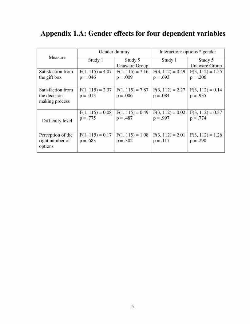
51

Appendix 1.A: Gender effects for four dependent variables

Gender dummy Interaction: options * gender Measure

Study 1

Study 5 Unaware Group

Study 1

Study 5 Unaware Group

Satisfaction from the gift box

F(1, 115) = 4.07 p = .046

F(1, 115) = 7.16 p = .009

F(3, 112) = 0.49 p = .693

F(3, 112) = 1.55 p = .206

Satisfaction from the decision-making process

F(1, 115) = 2.37 p = .013

F(1, 115) = 7.87 p = .006

F(3, 112) = 2.27 p = .084

F(3, 112) = 0.14 p = .935

Difficulty level

F(1, 115) = 0.08 p = .775

F(1, 115) = 0.49 p = .487

F(3, 112) = 0.02 p = .997

F(3, 112) = 0.37 p = .774

Perception of the right number of options

F(1, 115) = 0.17 p = .683

F(1, 115) = 1.08 p = .302

F(3, 112) = 2.01 p = .117

F(3, 112) = 1.26 p = .290

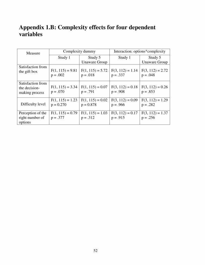
52

Appendix 1.B: Complexity effects for four dependent

variables

Complexity dummy Interaction: options*complexity

Measure Study 1

Study 5

Unaware Group Study 1

Study 5

Unaware Group

Satisfaction from the gift box F(1, 115) = 9.81

p = .002 F(1, 115) = 5.72 p = .018

F(3, 112) = 1.14 p = .337

F(3, 112) = 2.72 p = .048

Satisfaction from the decision-making process

F(1, 115) = 3.34 p = .070

F(1, 115) = 0.07 p = .791

F(3, 112) = 0.18 p = .908

F(3, 112) = 0.26 p = .853

Difficulty level F(1, 115) = 1.23 p = 0.270

F(1, 115) = 0.02 p = 0.878

F(3, 112) = 0.09 p = .966

F(3, 112) = 1.29 p = .282

Perception of the right number of options

F(1, 115) = 0.79 p = .377

F(1, 115) = 1.03 p = .312

F(3, 112) = 0.17 p = .915

F(3, 112) = 1.37 p = .256

53

Chapter 2

Economic Decision Making Under

Conditions of Extreme Time Pressure and

Option Overload: An Eye-Tracking Study8

2.1 Introduction

Consider the problem of a consumer in a modern supermarket. The typical store sells

more than 40,000 items and in many product categories it offers hundreds of options.9 The

typical consumer is also time-constrained and cannot afford to too much time making each

selection. This situation gives rise to the two questions studied in this paper: Can consumers

make good choices under extreme time pressure and option overload? Can the computational

processes that they use to solve this problem be exploited by sellers in order to manipulate

their choices?

We study these two questions by setting up an experimental version of the consumer’s

supermarket problem. Hungry subjects are presented with sets of 4, 9 or 16 familiar snack

items (e.g., Snickers candy bars and Lay’s chips) and are asked to make a choice within 3

seconds. Items are displayed using pictures of the actual packages of items. Besides choices

and reaction times, we also record the entire process of visual search using eye-tracking.

8 This work was done in collaboration with Rosemarie Nagel (Univeristat Pompeu Fabra); Johannes Pulst-Korenberg, Colin Camerer, and Antonio Rangel (California Institute ofTechnology) Financial support from HFSP (RN and CFC), the Moore Foundation (AR and CFC), the Spanish Ministry of Education (RN, SEJ2005-08391), and the Barcelona CREA program (RN) is gratefully acknowledged. 9 http://www.supermarketguur.com/page.cfm/284

54

With respect to the first question, we find that average choice efficiencies in all choice

sets are quite large (about 80%). This is especially surprising given that the eye-tracking data

shows that subjects do not look at all of the items in the 9 and 16 items choice sets, and that

fixations are largely random and independent of value. Our results suggest that subjects are

able to make good decisions in every day conditions (e.g., a supermarket aisle) even under

conditions of options overload and extreme time pressure.

In order to understand how consumers manage this feat we open the black-box of

decision making and study the computational processes used by subjects to make these types

of choices. We propose a “bounded rationality” model of the computational process used to

make these fast decisions and test the key assumptions of the model using the eye-tracking

evidence.

The basic idea of the model is simple: subjects randomly fixate on items in order to

measure their values, as long as they have time, and then choose the best item within the set

that was seen. Time pressure matters because people are only able to fixate on a subset of

items (in the larger choice sets) so they are not always able to find the best item in the set. The

key assumptions of the model are largely supported by the eye-tracking and behavioral data.

Looking at the computational process of generating choices is unusual in neoclassical

economics. Traditional economists build their models and interpret their data using the

concept of revealed preference, which is silent about the actual computational processes used

to make choices. This is true even in many behavioral economic models (e.g., prospect theory

or quasi-hyperbolic-discounting) in which subjects are assumed to act as-if they were

maximizing an objective function, but in which the computational process of generating the

choices is not spelled out. Although this view has worked extremely well in many

applications, this paper is built on the premise that there are domains, such as the problem of

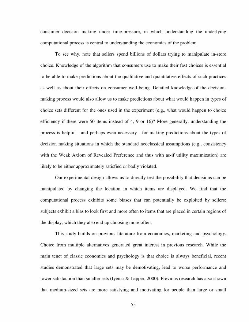
55

consumer decision making under time-pressure, in which understanding the underlying

computational process is central to understanding the economics of the problem.

To see why, note that sellers spend billions of dollars trying to manipulate in-store

choice. Knowledge of the algorithm that consumers use to make their fast choices is essential

to be able to make predictions about the qualitative and quantitative effects of such practices

as well as about their effects on consumer well-being. Detailed knowledge of the decision-

making process would also allow us to make predictions about what would happen in types of

choice sets different for the ones used in the experiment (e.g., what would happen to choice

efficiency if there were 50 items instead of 4, 9 or 16)? More generally, understanding the

process is helpful - and perhaps even necessary - for making predictions about the types of

decision making situations in which the standard neoclassical assumptions (e.g., consistency

with the Weak Axiom of Revealed Preference and thus with as-if utility maximization) are

likely to be either approximately satisfied or badly violated.

Our experimental design allows us to directly test the possibility that decisions can be

manipulated by changing the location in which items are displayed. We find that the

computational process exhibits some biases that can potentially be exploited by sellers:

subjects exhibit a bias to look first and more often to items that are placed in certain regions of

the display, which they also end up choosing more often.

This study builds on previous literature from economics, marketing and psychology.

Choice from multiple alternatives generated great interest in previous research. While the

main tenet of classic economics and psychology is that choice is always beneficial, recent

studies demonstrated that large sets may be demotivating, lead to worse performance and

lower satisfaction than smaller sets (Iyenar & Lepper, 2000). Previous research has also shown

that medium-sized sets are more satisfying and motivating for people than large or small

56

offerings (Reutskaja & Hogarth, 2006; Shah & Wolford, 2007). However, previous studies

usually allow decision-makers to use unlimited amount of time to make their choices. We

emphasize, however,that many every-day situations involve decisions made under extreme

time pressure and mechanisms underlying choice in such situation are not well-understood.

This paper also builds on the ideas of Payne, Bettman & Johnson (1993) which, using a

precursor technology to eye-tracking called MouseLab , showed that individuals who are

under high cognitive strain (perhaps due to information overload), or under time pressure, shift

to simpler computational models (see also Maule &. Edland, 1997; Bettman, Luce & Payne,

1998). We build our computational ‘bounded rationality’ model on this insight.

In economics, several groups have used eye-tracking to study the computational

process used to make strategic decisions. Using MouseLab, Johnson, Camerer, Sankar &

Rymon (2002) showed that the pattern of offers in bargaining experiments could be explained

to a large extent by a failure to carry out full “backward induction” since in many trials

subjects simply did not look ahead to future amounts. Camerer & Johnson (2004) established a

related result for the case of “forward induction”. Costa-Gomes, Crawford & Broseta (2001)

used this same technique to measure steps of strategic thinking in normal-form games (see

also Costa-Gomes, & Crawford, 2006). Using modern eye-tracking techniques, Wang, Spezio

& Camerer (2008) studied strategic information transmission and found that a combination of

lookup information and pupil dilation could help predict an unobservable private information

state.

Several studies in marketing have used eye-tracking to study how consumers choose

products from different types of displays. Russo, & Rosen (1975) started this literature by

studying how subjects moved their eyes while making hypothetical choices out of 6-item text-

based descriptions of cars, and arguing, much as we do in this paper, that the pattern of eye-

57

fixations provides a window into the computational process used to make choices (see also

Russo, & Leclerc,1994). Using more modern eye-tracking techniques, Van der Lans (2006)

studied how subjects locate brands within a display, but the experiment included no choice.

The closest study to the current paper is Chandon, Hutchinson & Young (2002) who look at

the hypothetical choices of consumers facing familiar consumer products out of large choice

sets without time pressure (their average reaction time is 25s). They find, like we do, that

visual attention plays a critical role in choice. Several additional studies in marketing have

also used eye-tracking to study which features of ads receive most attention, but they involve

no real decision-making (Loshe, 1997; Maughan, Gutnikov & Stevens, 2007; Pieters,

Rosbergen & Wedel, 1999; Pieters & Wedel, 2004). Some of these studies have found, as we

do, that display location impacts fixations. Note, however, that none of these papers has

studied real choice under time pressure and option overload. We emphasize that both the

model and the eye tracking evidence that we present are new to this literature.

The paper is organized as follows. Section 2.2 describes the experimental design.

Section 2.3 describes results about the performance of the choice process. Section 2.4 provides

a model of the computational process generating the choice. Section 2.5 tests the key

assumptions of the model using the eye-tracking data. Section 2.6 explores the qualitative and

quantitative nature decision bias implicit in the model. Section 2.7 concludes.

2.2 Experimental Design

The aim of this laboratory experiment was to study economic decision-making under

conditions of extreme time pressure and overload.

58

Forty-one Caltech undergraduates participated in the study. Individuals were excluded

if they had a history of eating disorders, had dieted in the past year, were vegetarian, disliked

junk food, or were pregnant. The selection criteria were designed to recruit individuals who

liked junk food and were not trying to control their diet. Subjects received 35 US dollars for

participating and provided informed consent prior to their participation. Participants were

asked to eat and then fast for three hours prior to the experiment. No deception was used.

At the beginning of the instruction period participants were told that they will have to

stay in the lab for an additional 30 minutes at the end of the experiment. During this time they

were allowed to eat the food item that they chose in a randomly selected trial according to the

rules described below, but no other foods or drinks were allowed. Subjects made choices out

of a set of 70 popular snacks such as candy bars (e.g., Snickers Bar) and potato chips (e.g.,

Lay’s).

Participants performed two tasks: (1) a liking-rating task, and (2) a choice task.

During the liking-rating task subjects had to answer the question “How much would

you like to eat this item at the end of the experiment?” on a scale of -5 (“not at all”) to 5 (“very

much”), with 0 denoting indifference. The liking-rating trials started with a 1s central fixation

cross, followed by a 3s presentation of a high-resolution picture of the item to be rated.

Pictures were 400x300 pixels in size and showed both the package and the food. Then subjects

entered their liking-rating at their own pace using the keyboard. The items were shown in

random order. There was a 1s inter-trial interval with an empty screen.

During the choice tasks subjects were shown 75 choice sets consisting of either of 4,

9, or 16 snack food items (25 of each of the three sizes). The items were presented

simultaneously on a computer screen (see Figure 2.1 for examples). The sets were presented

in such a way that the average distance among items was equalized across set sizes. The

59

identity and location of items was fully randomized. The order of the choice sets was also

randomized. As perceived variety may be affected by the number of identical items within a

set (Kahn & Wansink, 2004), we constructed sets such that no identical items were ever

present in the same choice set.

Figure 2.1: Examples of screenshots for the set sizes 4, 9, and 16.

Before the appearance of each set, the subject was shown a black screen with a central

white fixation cross. The subject had to maintain continuous fixation on the cross for two

seconds before the choice set was displayed. This was enforced with an eye-tracker and it was

implemented to eliminate “anticipatory fixations”.

Each choice set was presented for a maximum of 3s. Participants, however, could

make their choices in less than three seconds. Two seconds into the choice period subjects

heard a beep indicating that participant had exactly one second left until the choice set would

vanish. Subjects indicated their choice by pressing the keyboard while fixating on an item.

Prior to making actual choices, subjects went through 12 practice rounds to familiarize

themselves with the procedure.

Set size 4 Set size 9 Set size 16

60

At the end of the experiment a trial was selected at random and the subjects were

given the chance to eat the food that they choose in that trial. Subjects were penalized with a

loss of $3 if they failed to make a choice within three seconds in the selected trial.

The entire choice process was monitored with an eye-tracker (Tobii 1750, Sweden),

which recorded the positioning of the eye gazes on the screen every 20 ms with an

approximate resolution of 0.25 square inches.

After the experiment subjects answered a questionnaire regarding their consumption

habits of the snack food items. The experiment, including the instruction period, lasted an

average of 60 minutes, including the 30 minutes that a participant had to spend in an adjacent

room while eating his food.

2.3 Performance of the Choice Process

We begin the analysis of the experimental data by investigating the performance of the

choice process. We are interested in two questions: Are subjects able to make good choices

under conditions of time pressure? Does the quality of their choices deteriorate with the size of

the choice set?

In order to measure the performance of the choice process one needs to have an

independent measure of what is the best choice that can be made out of every budget set. Our

liking ratings provide such a measure. Conceptually, the liking ratings are forecasts of the

experienced utility that subjects expect to get from consuming each item. In the absence of

noise, the optimal choice in any given trial is to pick the available item(s) with the highest

possible liking-rating. Thus, one can think of the liking-ratings as a utility index over items.

61

Given this, we can define the efficiency of a choosing item i out of the set S as follows:

Efficiency (i|S)= l(i) − l(imin )

l(imax ) − l(imin ),

where imax is an item in S with a maximal liking-rating, and imin is an item in S with a minimal

liking rating, and l(.) denotes the liking-rating. Note that Efficiency=1 when a best item is

chosen, and Efficiency=0 when a worse item is selected.

Is this a satisfactory measure of performance? The main question studied here is

whether time pressure and overload interferes with a subject’s ability to select the best

alternative option. An alternative measure could have been obtained by giving subjects the

same choice sets at the end of the experiment, observing which choices they would have made

in the absence of any time pressure, and then comparing those choices with the ones made

under time pressure. We acknowledge that, in comparison to this alternative measure, our

concept of efficiency has two important shortcomings. First, it is sensitive to monotonic

nonlinear transformations of the liking-rating measure. Second, it is probably measured with

noise both across subjects, since they are likely to interpret the scale differently, and within

subjects, as they map their “feelings” about the items to the scale.

Given this caveats, why did we chose our alternative measure of performance? First,

in several previous experiments we have found that liking-ratings and “revealed preference”

measures such as willingness-to-pay (elicited with an incentive compatible Becker-DeGroot-

Marshak procedure) are extremely highly correlated within subjects (Armel & Rangel, 2008;

Armel, Beaumel & Rangel, 2008; Plassmann, O'Doherty & Rangel, 2007). In fact, the high-

efficiencies described below also suggest that the liking-ratings are good measures of the

62

value that options are assigned during the choice process. Second, our measure can be

obtained more quickly from subjects, which has experimental advantages. Third, our measure

provides a natural continuous measure of efficiency, whereas the alternative described above

only provides a 0-1 measure. Finally, and most importantly, qualitatively our results are robust

to monotonic transformations of the liking-rating function.

In the analyses that follow we use the following measurable notions of visual attention:

fixation, initial fixation, and refixation. A fixation occurs when a subject looks at an item for a

continuous period of time (typically a few hundred milliseconds). Note that during a fixation

subjects might look at different parts of the picture (these small eye movements within a

fixation are known as microfixations). A fixation on an item is an initial fixation if that is the

first time that the subject fixates on an item during a trial. If not, it is called a refixation.

2.3.1 Result 1. Choice efficiency is comparable across choice sets

Figure 2.2A shows that the average efficiency of choices is quite high and does not

vary with the set size: it is 85% for N = 4 and 83% for N = 9 and 16, which are insignificantly

different (lowest p = 0.24). Furthermore, if the liking-ratings are measured with noise, these

efficiency measures are biased downwards.

Given the extreme time pressure, and the fact that subjects are only able to see a subset

of the items during the search process (see Result 3 below), the high performance in the larger

sets is quite surprising and leads to a natural question: What properties of the choice processes

and situations are responsible for generating these high efficiencies? The answer to this

question turns out to be rather simple ex-post. As a result of simple combinatorics, in a

randomly chosen budget set the difference between the best item and the next-best items

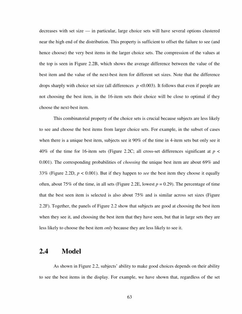
63

decreases with set size — in particular, large choice sets will have several options clustered

near the high end of the distribution. This property is sufficient to offset the failure to see (and

hence choose) the very best items in the larger choice sets. The compression of the values at

the top is seen in Figure 2.2B, which shows the average difference between the value of the

best item and the value of the next-best item for different set sizes. Note that the difference

drops sharply with choice set size (all differences p <0.003). It follows that even if people are

not choosing the best item, in the 16-item sets their choice will be close to optimal if they

choose the next-best item.

This combinatorial property of the choice sets is crucial because subjects are less likely

to see and choose the best items from larger choice sets. For example, in the subset of cases

when there is a unique best item, subjects see it 90% of the time in 4-item sets but only see it

40% of the time for 16-item sets (Figure 2.2C; all cross-set differences significant at p <

0.001). The corresponding probabilities of choosing the unique best item are about 69% and

33% (Figure 2.2D, p < 0.001). But if they happen to see the best item they choose it equally

often, about 75% of the time, in all sets (Figure 2.2E, lowest p = 0.29). The percentage of time

that the best seen item is selected is also about 75% and is similar across set sizes (Figure

2.2F). Together, the panels of Figure 2.2 show that subjects are good at choosing the best item

when they see it, and choosing the best item that they have seen, but that in large sets they are

less likely to choose the best item only because they are less likely to see it.

2.4 Model

As shown in Figure 2.2, subjects’ ability to make good choices depends on their ability

to see the best items in the display. For example, we have shown that, regardless of the set

64

Figure 2.2A

0.1

.2.3

.4.5

.6.7

.8.9

1

Choic

e e

ffic

iency

4 9 16

Set size

Figure 2.2B

0.5

11

.52

Vm

ax-V

(se

co

nd

be

st)

4 9 16Set size

Figure 2.2C

0.1

.2.3

.4.5

.6.7

.8.9

1%

of

tim

e b

est

item

wa

s f

ixa

ted

up

on

4 9 16Set size

Figure 2.2D

0.1

.2.3

.4.5

.6.7

.8.9

1%

of

be

st

ch

oic

es

4 9 16Set size

Figure 2.2E

0.1

.2.3

.4.5

.6.7

.8.9

1%

of

be

st

ch

oic

es w

he

n b

est

ite

m w

as s

ee

n

4 9 16Set size

Figure 2.2F

0.1

.2.3

.4.5

.6.7

.8.9

1%

of

be

st

ch

oic

es o

ut

of

the

se

en

se

t

4 9 16Set size

Figure 2.2: A. Choice efficiency; B. Difference in the liking-rating between the best and second best alternative in the choice set; C. Fraction of trials (with a unique best item) in which the best item was fixated upon; D. Fraction of trials (with a unique best item) in which the best item was chosen; E. Fraction of trials (with a unique best item) in which the best item was chosen conditional on the best

item being seen; F. Fraction of trials in which the best item seen in the trial was chosen. In all of the figures error bars denote standard error measures.

65

size, efficiency is high when the best items are seen, but not when they are not. This raises a

natural and important question: What is the computational process used by the subjects to

make choices under time pressure and why do fixations play such an important role?

In this section we propose a simple model of the computational process used by the

subjects that we then test in detail using a combination of eye-tracking and choice data.

Subjects search through the choice set using a sequence of distinct fixations and

sequential fixations within each trial. Let Ft denote the identity of the item seen in fixation t.

We assume that during each fixation t the brain computes several variables: 1) A value Vt to

the item that it is looking at; 2) a cached value Ct equal to the maximum value of all items

seen previously (including the current one); and 3) a label for the identity of the best item seen

so far which we denote by kt . Note that Ct = max (Ct-1,Vt) and so kt=Ft if Ct-1<Vt and kt=kt-1

otherwise. We assume that C0 = V1.

We assume that the identity of all initial fixations is random with respect to the item’s

value (i.e., subjects attentional processes are not able to guide the fixation to the best items

unless they have been previously seen in the trial). This does not rule out the possibility that

they might be influenced by other variables such as the location in the display (see section 2.6)

or by their location relative to previously seen items (in our data most eye movements are left-

to-right and up-to-down and that barely any are in a diagonal direction).

At the end of every fixation the brain decides whether to stop the search process and

choose the best item seen so far, with probability pt, or continue the search by looking at a new

item, with probability 1-pt. We assume that pt increases with the time elapsed within the trial

(and thus with the fixation number) as well as with the cached value Ct.

It is straightforward to see that the number of fixations plays a crucial role in this

model: on average subjects make good choices when they see a lot of items, but not when they

66

see few items. This naturally raises the question of fixation duration. We assume that fixation

duration is fixed and independent of values and set size. This assumption is based on the idea

that there is a biological limitation to how fast the brain can fixate on an item and extract value

and that subjects move near that threshold when making decisions under extreme time

pressure.

How does the model account for the key features in Figure 2.2? Given the fixed

fixation duration, the percentage of items seen decreases across choice sets. Since subjects

cannot choose an item that they do not see, this implies that the probability of choosing the

best items out of the entire choice set decreases with the set size. However, since there is

perfect maximization within the seen set, set size does not matter conditional on having gone

through a search process that fixated on the best item.

Note that this simple model makes several extreme simplifications that are only

approximations to our data and that should be explored and relaxed further in future work.

First, we assume the cached value at every step is computed by a perfect maximization

algorithm. This is probably not true given extensive evidence on biologically based “soft-

maximization” and binary choice with errors (for recent reviews see Wilcox, 2008; Rangel,

2008).

Second, the value assigned to an item is assumed to be independent of the length of the

fixation. This is a reasonable approximation because the items are familiar and fixation times

did not vary significantly across items. Note, however, that previous work has shown that

fixation times can affect valuation and choices (Armel, Beaumel & Rangel, 2008; Armel &

Rangel, 2008; Karjbich, Armel & Rangel, 2008).

Third, we have assumed that there is perfect memory of which item had the highest

value, as well as of the items’ actual value and location. This implies that the only purpose of a

67

refixation (going back to a previously seen item) is to select or choose a previously best seen

item, but not to see it again to recall a value. This “perfect recall” assumption is unlikely to

hold in more complicated choice settings and would be an especially interesting complication

to study. Interestingly, the extreme time pressure feature of our experiments might actually

help recall in the sense that a rapid choice time makes short-term memory more effective. It is

even conceivable that an extension of the model proposed, which includes memory decay,

would predict that allowing longer choice times hurts choice quality (if the bad effects of

memory decay outweigh the benefits from having more time to look or deliberate).

2.5 Tests of the Model’s Key Elements

The goal of this section is to use eye-tracking data to test the main assumptions of the

model. The first three results test the assumed properties of the fixation process that drives the

search for the best item.

2.5.1 Result 2. Fixation durations decrease slightly with set size, but are

mostly constant across the search process

Figure 2.3A and Figure 2.3B show statistics on the duration of fixations. Fixations are

around 320 ms for the smallest choice set (N = 4) and 260 ms for the largest choice set (N =

16). These are consistent with typical fixation times in other studies (e.g., Salvucci, &

Goldberg, 2000; Wang et al., 2008). The differences in fixation duration are small in

magnitude, but are highly significant across choice set sizes (for all comparisons, p < 0.001).

The differences in fixation durations are interesting for two reasons. First, it implies that the

number of seen items increases with set size, which has implications for the performance of

68

the choice process. Second, it suggests that the amount of attention allocated to each item is

adjusted endogenously (and most likely automatically and unconsciously) in response to

changes in set size. This finding is consistent with a view of psychological processes in which

scarce computing resources are allocated in a sensible way (Becker, 1965). Consistent with

this view, Figure 2.3B also shows that the fixation durations also drop a bit around the 8th

fixation for sets of 9 and 16 items. This is around the time that the beep sounds, as if people

are responding to the external reminder that time is running short.

2.5.2 Result 3. The number of items seen increases with set size, but the

percentage of items seen decreases with set size

The decision time constraint, together with the magnitude of the increase in set sizes

and decreases in fixation times, imply that people see more items in larger sets, but overall see

a smaller percentage of items in larger sets (Figures 2.4A and 2.4B; all cross-set differences

are significant at p < 0.05 one-tailed). This implies that subjects should be less likely to find

the best item in the largest choice sets, which is consistent with the results shown in Figure

2.3.

Interestingly, because of the combinatorics of large choice sets described in Section

2.3, the efficiency of the cached (highest-value) item does not decrease with set size because

of the smaller percentage of items seen in larger choice sets. This fact is shown in Figure 2.4C,

which plots the efficiency of the cached value (i.e. the efficiency value of the highest item

seen so far) across the order of fixations.10 As shown in the figure, the cached-efficiency starts

10 The efficiency of an item within a choice set is defined exactly as before.

69

Figure 2.3A

01

00

20

03

00

40

0F

ixa

tio

n d

ura

tio

n,

ms

4 9 16Set size

Figure 2.3B

01

00

20

03

00

40

0

1 2 3 4 5 6 7 8 9 1 2 3 4 5 6 7 8 9 1 2 3 4 5 6 7 8 9

Set size4

Set size9

Set size16

Fix

atio

n d

ura

tio

n,

ms

Fixation order

Figure 2.3: A. Average fixation duration; B. Average fixation duration as a function of fixation order.

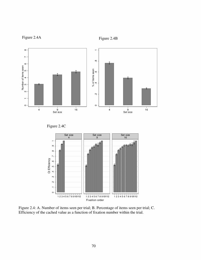
70

01

23

45

67

8N

um

be

r o

f ite

ms s

ee

n

4 9 16Set size

0.2

.4.6

.81

% o

f ite

ms s

ee

n

4 9 16Set size

0.1

.2.3

.4.5

.6.7

.8.9

1

1 2 3 4 5 6 7 8 9101112 1 2 3 4 5 6 7 8 9101112 1 2 3 4 5 6 7 8 9101112

Set size4

Set size9

Set size16

Ct

Eff

icie

ncy

Fixation order Figure 2.4: A. Number of items seen per trial; B. Percentage of items seen per trial; C. Efficiency of the cached value as a function of fixation number within the trial.


Figure 2.4C

71

at 50%, consistent with an initial random fixation, and exceeds 90% in all choice sets by the

fifth fixation.

Another important assumption of the model is that fixations are “random” with respect

to value. An alternative hypothesis would have been that subjects are able to process values in

peripheral vision and that this allows them to direct their fixations to items with higher relative

value.11 The following result shows that the alternative hypothesis is largely incorrect.

2.5.3 Result 4. The sequential search is mostly independent of value

Figure 2.5 shows the efficiency of items across the sequence of new fixations for

different set sizes (excluding refixations to previously seen items). If people managed to

always switch their attention to better and better items, there would be an increase in

efficiency across fixations, but there is not. Interestingly, efficiencies are generally slightly

greater than 50% (averaging 0.56, p < 0.001). This suggests that sequential search is mostly

independent of value, although it might be the case that due to some processing in peripheral

vision sufficiently undesirable items are slightly less likely to be fixated on.

Another key feature of the model, which is tested in the next result, is that the search is

more likely to stop when the cached value Ct is high (controlling for time and other factors).

2.5.4 Result 5. The probability of stopping the search (and choosing)

increases as Ct increases.

Figure 2.6 shows that the percentage of fixations which are the last new fixation

11 Note that, in the alternative hypothesis, peripheral attention and direct fixations might not be perfect substitutes if the peripheral value computations can be used to guide the fixations but not to assign values to items that can be used in the process of choice.

72

within a trial (i.e, there may be later refixations to chose an item that was seen previously)

depends on the cached value Ct. The identity of the last new fixation is important because it

marks the end of the search process prior to choice. The figure shows the likelihoods of ending 0

.1.2

.3.4

.5.6

.7.8

.91

1 2 3 4 5 6 7 8 9 101112 1 2 3 4 5 6 7 8 9 101112 1 2 3 4 5 6 7 8 9 101112

Set size4

Set size9

Set size16

Fix

atio

n e

ffic

ien

cy

Fixation order

Figure 2.5: Fixation efficiency by fixation order within the trial (new fixations only, excluding refixations).

the initial search process (before refixation) as a function of the cached value during for

fixations that end during the first 1500 ms (“first half of the trial”), and fixations that end

during the second 1500 ms (“second half of the trial”). To explain, consider the data for set

size of 4 (the left panel if Figure 2.6). In the first half of the trial (solid line) the percentage of

current fixations which are the last one is around 10% when Ct is negative (i.e., in 90% of the

trials they go on to look at new items). However, when the cached value is 5 (the highest

possible value), about 65% of the fixations are the last new one (i.e., they are twice as likely to

stop searching as they are to keep looking).

73

0.2

.4.6

.81

-5 -4 -3 -2 -1 0 1 2 3 4 5 -5 -4 -3 -2 -1 0 1 2 3 4 5 -5 -4 -3 -2 -1 0 1 2 3 4 5

Set size4

Set size9

Set size16

Second half of the trial First half of the trial

% o

f tim

e f

ixa

tio

n is t

he

la

st

ne

w f

ixa

tio

n

Ct

Figure 2.6: Fraction of fixations which are the last new fixation within a trial as a function of the cached value Ct. Values are presented separately for the first 1500ms (first half of the trial) and the last 1500ms (second half of the trial).

The stopping probabilities are lower for the larger choice sets, which is not surprising

since subjects are able to see all four items in the N=4 case rapidly. For the first half of the

trial (solid lines) the probability that a fixation is the last new one is low, but does increase

with Ct. For the second half of the trial, the probability that a fixation is the last new one is

much higher and highly dependent on the set size. In all cases, however, the probability of

stopping the search increases as Ct increases.

A limitation of the previous analysis is that the cached value is likely to be correlated

with the number of fixations, the length of time into the trial, and other variables. To address

this problem we performed a logit regression of the probability that the current fixation is the

last new fixation on a number of control variables (see Table 2.1). We found that after

controlling for other potentially confounding variables the stopping probability is strongly

74

increasing in the cached maximum value Ct. The analysis also shows that stopping probability

is lower for the larger choice sets (as Figure 2.6 shows), is higher for the second half of the

trial, is increasing in the number of fixations, and is also strongly influenced by the “beep”

sound which signals one second to go in the trial.

The effect of the “beep” is interesting because it illustrates how a small change in the

design of the choice process can have a large influence in behavior of economic agents with

biologically driven limitations on rationality. If subjects had a perfect clock in their heads the

beep would have no effect, but it does.

Another key assumption of the model is that subjects optimize within the set of items

that they have seen. In particular, this implies that if the value of the last item that they see

during the search (call it Vt ) is better than the value of those items that they saw earlier

(measured by the cached value Ct-1), then subjects are more likely to choose the last seen item.

The following result shows that this prediction is consistent with the data.

2.5.5 Result 6. The probability that the last new seen item is chosen

increases with Vt - Ct-1.

Figure 2.7 depicts the probability of choosing the item seen in the last new fixation as a

function of Vt - Ct-1 (the leap in value from the best of those previously-seen to the new value).

The figure shows that this probability is strongly increasing in Vt - Ct-1, has a logistic shape,

and is approximately 50% when Vt = Ct- 1. This clearly shows that the subject is optimizing

within each fixation between the previously best seen item and the current item. The figure

also shows that these stopping probability graphs are almost identical across choice sets,

which suggests that the comparison process is remarkably independent of the set size.

75

Table 2.1: Fixed effects logit regression. The independent variable is the probability that a given fixation is the last new fixation.

Model 1 Model 2

Fixation Order 0.405*** (0.000)

0.389*** (0.000)

Time > 1500 1.012*** (0.000)

1.002*** (0.000)

Beep On - 0.916** (0.011)

Ct 0.497*** (0.000)

0.498*** (0.000)

Set size 9 -1.313*** (0.000)

-1.305*** (0.000)

Set size 16 -1.609*** (0.000)

-1.603*** (0.000)

Individual dummies included yes yes Constant -2.026***

(0.000) -2.003***

(0.000)

N 11,458 11,458

Log pseudo-likelihood -4910.8 -4902.8

Pseudo R2 0.252 0.259

***, **, * denote significance at the 1%, 5%, and 10% level, respectively. p-values are in parenthesis. Standard errors are adjusted for clustering on subjects. Analysis is based only on fixations prior to the first refixation. Dependent variable =1 if fixation is the last new fixation (before the refixation start) and is =0 otherwise. Time > 1500 =1 if the fixation ended after the trial time reached 1500 ms, =0 otherwise. Beep On =1 if the beep was heard before the current fixation commenced, =0 otherwise. Set size 9 =1 if the choice set size is 9; =0 otherwise. Set size 16 =1 if the choice set size is16; =0 otherwise.

76

0.5

1

-10 -5 0 5 10 -10 -5 0 5 10 -10 -5 0 5 10

Set size4

Set size9

Set size16

% o

f tim

e w

he

n la

st

fixa

tio

n is c

ho

se

n

Vt-C(t-1)

Figure 2.7: Fraction of trials in which the last new fixation is chosen as a function of Vt - Ct-1.

The logistic nature of the curves depicted in Figure 2.7 could result from one of two

sources. First, they might be due to measurement error on the liking-ratings. Second, they

could reflect true biological randomness in the choice process. Although there is mounting

evidence from neuroeconomics that there is true biological randomness in the optimization

process (for a review see Rangel, 2008), the methods used in this paper do not allow us to

separate these two sources.

As before, a limitation of the previous analysis is that the surprise variable Vt - Ct-1

might be correlated with the number of fixations and other factors. To address this, Table 2.2

reports the results of a logit regression of the probability of choosing the last-seen item as a

function of Vt -Ct-1 and other control variables. We found that after controlling for other

potentially confounding variables the stopping probability is significantly increasing in Vt -Ct-1,

77

is independent of the set size, and is an order of magnitude larger in the second half or the trial

(after 1500ms).

Finally, we consider the assumption that subjects have perfect recall about the identity

and value of the previously best-seen item. This assumption implies that after they decide to

stop the search process, they can immediately refixate to the best item previously seen and

choose it (keep in mind that choices are actually made by pressing the ENTER key during a

final fixation). The next three results explore this assumption.

2.5.6 Result 7. Usually there is at most one refixation before a choice is

made

According to the model, a choice is made in one of two ways: either the subject stops

the search process by choosing the item seen in the last new fixation (for example, if it has the

maximum possible value), or the subject stops the search process and refixates to the best

previously seen item. In the first case there are no refixations. In the second case there is

exactly one refixation. Figure 2.8 shows a histogram of the number of refixations that occur

before a choice is made, conditional on a refixation taking place at all. Across all three set

sizes there is a sharp spike at 1—i.e., on average, about 80% of the time there is a single

refixation to the chosen item, and no further refixations.

Note that there is a right tail in the number of additional post-refixation fixations in the

16-item sets, but the effect is small. This is consistent with imperfections in working memory

that are further explored in Result 9.

78

Table 2.2: Fixed effects logit regression. The independent variable is the probability that the

items seen in the last new fixation is chosen (in which case there are no refixations).

Model 1 Model 2

Fixation Order -0.221*** (0.000)

-0.251*** (0.000)

Time > 1500 2.344*** (0.000)

2.313*** (0.000)

Beep On

0.248 (0.236)

Vt-Ct-1 0.377*** (0.000)

0.377*** (0.000)

Set size 9 -0.111 (0.435)

-0.120 (0.395)

Set size 16 0.134 (0.342)

0.136 (0.334)

Individual dummies included yes yes

Constant 0.285** (0.035)

0.365*** (0.008)

N 2904 2904

Log pseudo-likelihood -1402.6219 -1258.6836

Pseudo R2 0.3341 0.3345

***, **, * denote significance at the 1%, 5%, and 10% level, respectively. p-values are in parenthesis. Standard errors are adjusted for clustering on subjects. Analysis is based only on fixations prior to the first refixation. Dependent variable =1 if the last new fixation is chosen, =0 if there are refixations after it. Time > 1500 =1 if the fixation ended after the trial time reached 1500 ms, =0 otherwise. Beep On =1 if the beep was heard before the current fixation commenced, =0 otherwise. Set size 9 =1 if the choice set size is 9; =0 otherwise. Set size 16 =1 if the choice set size is16; =0 otherwise.

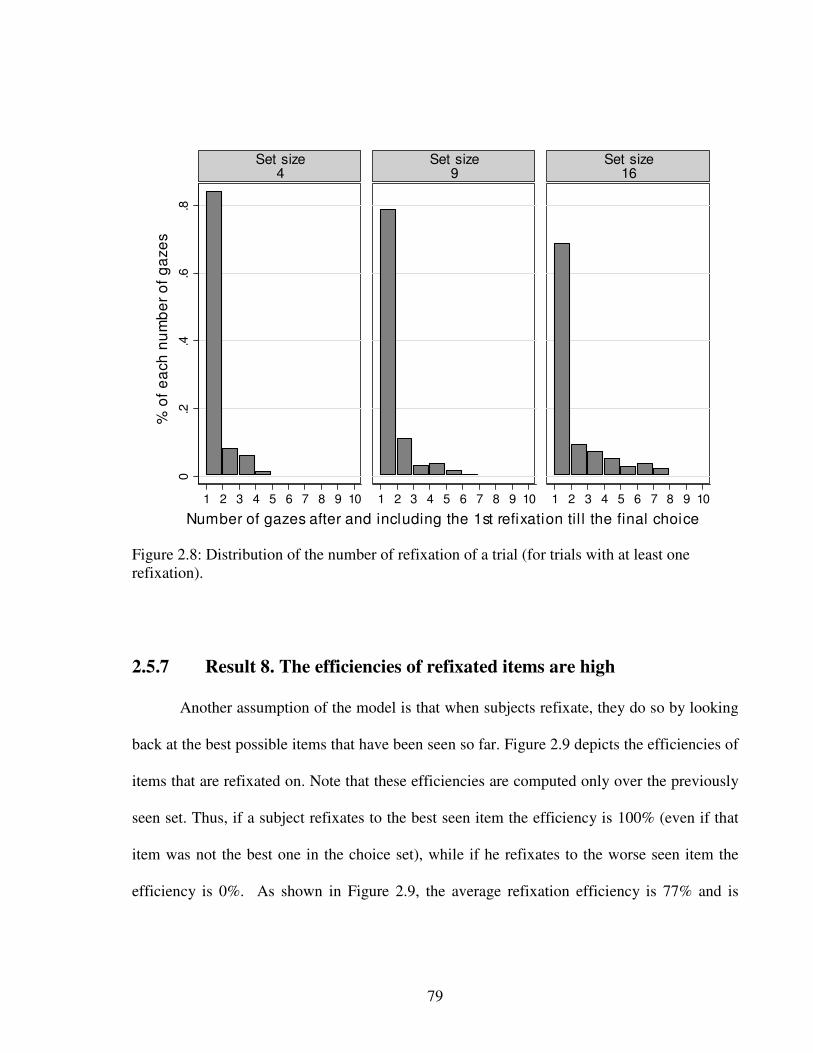
79

0.2

.4.6

.8

1 2 3 4 5 6 7 8 9 10 1 2 3 4 5 6 7 8 9 10 1 2 3 4 5 6 7 8 9 10

Set size4

Set size9

Set size16%

of

ea

ch

nu

mb

er

of

ga

ze

s

Number of gazes after and including the 1st refixation til l the final choice

Figure 2.8: Distribution of the number of refixation of a trial (for trials with at least one refixation).

2.5.7 Result 8. The efficiencies of refixated items are high

Another assumption of the model is that when subjects refixate, they do so by looking

back at the best possible items that have been seen so far. Figure 2.9 depicts the efficiencies of

items that are refixated on. Note that these efficiencies are computed only over the previously

seen set. Thus, if a subject refixates to the best seen item the efficiency is 100% (even if that

item was not the best one in the choice set), while if he refixates to the worse seen item the

efficiency is 0%. As shown in Figure 2.9, the average refixation efficiency is 77% and is

80

quantitatively very similar across the choice set sizes. Again, this suggests that perfect recall is

a good approximation, but leaves open the possibility for some imperfect working memory.

0.1

.2.3

.4.5

.6.7

.8.9

1

Refixation e

ffic

iency in the s

een s

et

4 9 16

Set size

Figure 2.9: Refixation efficiency as a function of set size.

Given that the previous two results suggest that imperfect working memory might be

playing a small role, we decided to perform an additional and independent test of the perfect

recall assumption.

2.5.8 Result 9. There is imperfect recall about the identity of the best

previously seen item.

Figure 2.10 depicts the results of two tests of the perfect recall hypothesis. The top

panel shows the fraction of trials in which the first refixation is made to the best previously

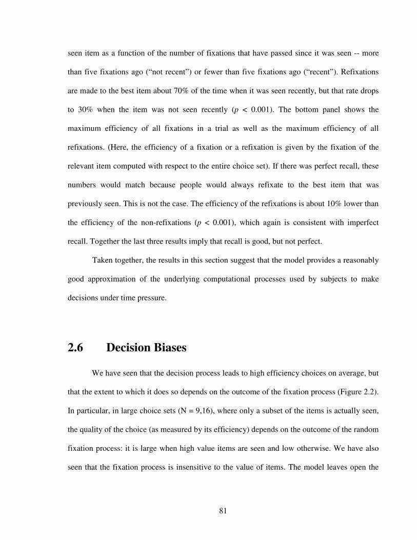
81

seen item as a function of the number of fixations that have passed since it was seen -- more

than five fixations ago (“not recent”) or fewer than five fixations ago (“recent”). Refixations

are made to the best item about 70% of the time when it was seen recently, but that rate drops

to 30% when the item was not seen recently (p < 0.001). The bottom panel shows the

maximum efficiency of all fixations in a trial as well as the maximum efficiency of all

refixations. (Here, the efficiency of a fixation or a refixation is given by the fixation of the

relevant item computed with respect to the entire choice set). If there was perfect recall, these

numbers would match because people would always refixate to the best item that was

previously seen. This is not the case. The efficiency of the refixations is about 10% lower than

the efficiency of the non-refixations (p < 0.001), which again is consistent with imperfect

recall. Together the last three results imply that recall is good, but not perfect.

Taken together, the results in this section suggest that the model provides a reasonably

good approximation of the underlying computational processes used by subjects to make

decisions under time pressure.

2.6 Decision Biases

We have seen that the decision process leads to high efficiency choices on average, but

that the extent to which it does so depends on the outcome of the fixation process (Figure 2.2).

In particular, in large choice sets (N = 9,16), where only a subset of the items is actually seen,

the quality of the choice (as measured by its efficiency) depends on the outcome of the random

fixation process: it is large when high value items are seen and low otherwise. We have also

seen that the fixation process is insensitive to the value of items. The model leaves open the

82

Figure 2.10A

0.1

.2.3

.4.5

.6.7

.8.9

1

% o

f tim

e 1

st re

fixation is to the b

est item

seen

<=5 >5

Number of gazes back the refixated item w as seen

Figure 2.10B

0.1

.2.3

.4.5

.6.7

.8.9

1M

axim

um

Eff

icie

ncy

Fixations Refixations

Figure 2.10: A. Fraction of trials in which the first refixation is to the best item that has been seen as a function of the number of items since it was last seen; B. Maximum fixation and refixation efficiency within a trial.

83

possibility, however, that the fixation process might be affected by other variables such as the

location in the display. (Note that value and location are uncorrelated in our experiment since

the items were randomly allocated to locations). This opens the possibility of systematic

decision-making biases that, in principle, could be exploited by sellers to manipulate choices.

As the following result shows, these biases exist and are quantitatively important.

2.6.1 Result 10. There are location driven biases on the initial fixation

that have substantial impact on final choices

Figure 2.11 shows the initial fixations in a gray-scaled “heat map” format. The total

number of initial fixations on each item is shown numerically in the locations of those items

(numerical entries can take a maximum value of 25, the number of trials for each set size, and

are averaged across subjects box-by-box). The lightest color is associated with the highest

average of initial fixations, and the darkest color is associated with the lowest averages.

About half the initial fixations in the 4-item set are in the upper left, and 95% of the

initial fixations in the larger sets are to the central item (for 9 item sets) or to the central four

items (for 16 item sets). A t-test of the number of initial fixations to the most seen location

versus the average of the other locations is significant at p < 0.001 for all set sizes.

The size of the first-fixation bias is quite large and is driven by the position of the

central fixation cross on which subjects need to maintain fixation before the items appear. In

the case of 9 items, the fixation cross lies exactly at the center of the middle item, which

explains the extreme bias. In the case of 4 and 16 items, it lies on the middle of the screen. The

subjects’ first fixation is typically to the item that lies just North-West of the fixation cross.

84

Figure 2.11A

Figure 2.11B

Figure 2.11C

Figure 2.11: Total number of initial fixations at each display location (out of a maximum of 25 and averaged across subjects box-by-box). Analysis includes initial fixations only. Trials with only one fixation are included. Lighter cells indicate greater number of fixations. A. 4-item sets; B. 9-item sets; C. 16-item sets.

85

Figure 2.12 shows the same type of statistics for the total number of fixations at each

location. If the initial fixation effect completely wears off these numbers should be the same in

all cells for each choice set size, but they are not. About a third of the fixations are in the

upper-left for N=4, and in the center item for N = 9 (compared to random base rates of 25%

and 11% respectively) and almost half of them are in the center four boxes for N = 16 (base

rate 25%).12

The combination of these initial fixation biases, and the sequential search model,

imply that initial fixations should have an impact on final choices, and they do. Figure 2.13

shows the choice frequencies. There is a small tendency to choose the upper items in N = 4,

and much bigger biases in the other cases (60% above average for choosing the middle in N =

9 and 25% above average for the central four boxes in the case of N = 16).13

Another way to measure the extent of the influence of display biases on choices is to

ask what would happen if a retailer, for example, put the worst items (as judged by individual

consumer ratings) in the locations at which they are likely to be seen first, or put the best items

in those locations. How much would final choices vary in efficiency? Our design provides a

ready answer to this question because items were randomly allocated items to locations across

trials. For each subject, we weight the likelihood that they will choose an item in a particular

location by their total percentage of fixations in that location, and compute the expected

12 In the case of N=4, a t-test of the total number of fixations to the upper vs lower half of the display is significant at p<0.001. In the case of N=9, a t-test of the total number of fixations to the center location versus the mean of all other locations is significant at p<0.001. In the case of N=16, a t-test of the average total number of fixations in the middle locations versus the average of the external locations is is significant at p<0.001. 13 In the case of N=4, a t-test of the total number of choices of items in the upper vs lower half of the display is significant at p<0.051. In the case of N=9, a t-test of the total number of choices of items displayed in the center location versus the mean of all other locations is significant at p<0.001. In the case of N=16, a t-test of the total number of choices made from items in the middle locations versus the mean of the external locations is significant at p<0.001.

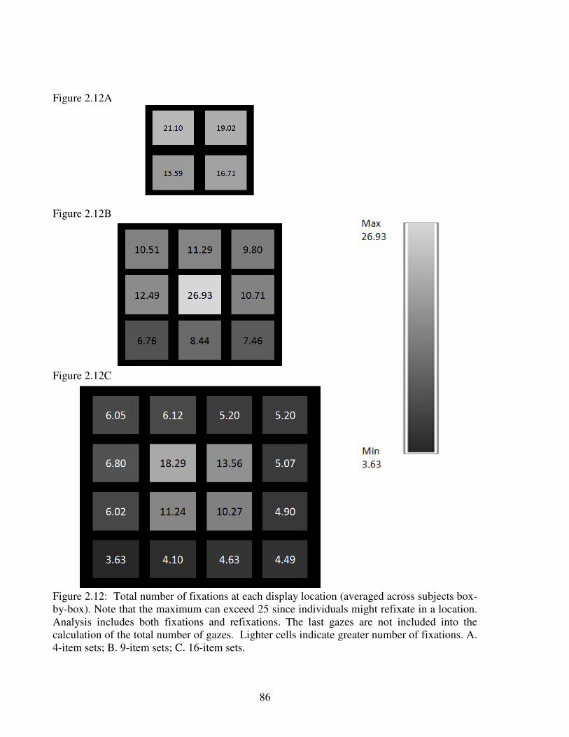
86

Figure 2.12A

Figure 2.12B

Figure 2.12C

Figure 2.12: Total number of fixations at each display location (averaged across subjects box-by-box). Note that the maximum can exceed 25 since individuals might refixate in a location. Analysis includes both fixations and refixations. The last gazes are not included into the calculation of the total number of gazes. Lighter cells indicate greater number of fixations. A. 4-item sets; B. 9-item sets; C. 16-item sets.

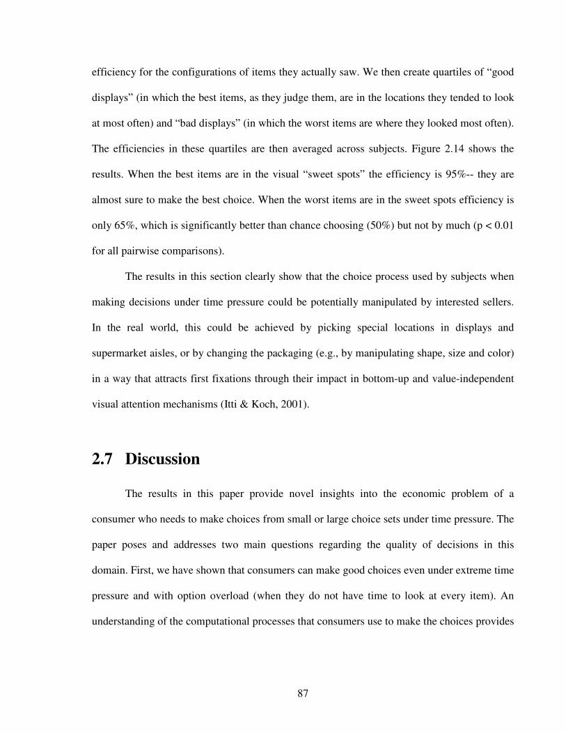
87

efficiency for the configurations of items they actually saw. We then create quartiles of “good

displays” (in which the best items, as they judge them, are in the locations they tended to look

at most often) and “bad displays” (in which the worst items are where they looked most often).

The efficiencies in these quartiles are then averaged across subjects. Figure 2.14 shows the

results. When the best items are in the visual “sweet spots” the efficiency is 95%-- they are

almost sure to make the best choice. When the worst items are in the sweet spots efficiency is

only 65%, which is significantly better than chance choosing (50%) but not by much (p < 0.01

for all pairwise comparisons).

The results in this section clearly show that the choice process used by subjects when

making decisions under time pressure could be potentially manipulated by interested sellers.

In the real world, this could be achieved by picking special locations in displays and

supermarket aisles, or by changing the packaging (e.g., by manipulating shape, size and color)

in a way that attracts first fixations through their impact in bottom-up and value-independent

visual attention mechanisms (Itti & Koch, 2001).

2.7 Discussion

The results in this paper provide novel insights into the economic problem of a

consumer who needs to make choices from small or large choice sets under time pressure. The

paper poses and addresses two main questions regarding the quality of decisions in this

domain. First, we have shown that consumers can make good choices even under extreme time

pressure and with option overload (when they do not have time to look at every item). An

understanding of the computational processes that consumers use to make the choices provides

88

Figure 2.13A

Figure 2.13B

Figure 2.13C

Figure 2.13: Total number of times the item displayed at each location was chosen (averaged across subjects box-by-box). Lighter cells indicate greater number of fixations. A. 4-item sets; B. 9-item sets; C. 16-item sets.

89

0.1

.2.3

.4.5

.6.7

.8.9

1C

ho

ice

eff

icie

ncy

Q1 Q2 Q3 Q4Weighted fixation efficiency

Figure 2.14: Choice efficiency as a function of weighted fixation efficiency (by quartile).

an insight for why this is the case. In small choice sets (N = 4) subjects are able to see most of

the items and choose the best one about 80% of the time. In contrast, in large choice sets (N =

9,16) subjects are only able to see a small fraction of the items and thus are able to choose the

best one only about half as frequently. It follows that the performance of the computational

process used to make choices deteriorates as the number of options increases. However,

combinatorics come to the rescue: in larger choice sets there are many alternatives close to the

best one which are seen and chosen with high-frequency. This is the key reason why

performance (as measured by average efficiency) does not deteriorate with set size.

Second, we have seen that choices are heavily influenced by the outcome of the

fixations, and that these fixations can be affected by variables such as display location, that are

90

not correlated with values. We have also shown that this feature of the choice process could

potentially be exploited by sellers through a clever selection of packaging and in-store

displays. We have also shown that these effects are quantitatively large. For example: in the

case of N=9 an item in the center of the display was almost 60% more likely to be selected

than similar items displayed in other locations.

These two regularities are consistent with a simple model of sequential search with

perfect recall in which search is value-independent (subjects cannot deliberately guide their

visual attention to high-value items) but is also display-dependent (they look first at the center

and upper-left). To economists, the sequential search model might seem so natural as to be

obvious. However, many studies of visual attention suggest a surprisingly different model of

parallel search. Parallel search is implied by hundreds of experimental studies showing a

phenomenon called the “pop-out effect” (Treisman, 1985). In these studies subjects are

instructed to search for a particular item in a set (e.g., “Is there a T in the set of letters?”).

Empirically, when items are visually distinctive in terms of easily-processed features that are

noticed “pre-attentively” (e., choosing an X from a set of X’s and O’s), the time taken for a

correct response is completely invariant to the number of items N. The fact that response

times are invariant to the set size N suggests that people are looking at all of the items

simultaneously (searching in parallel). If searching for the best item in a choice set exhibits a

similar pop out effect, time-constrained subjects will always choose the best items even in

large choice sets, and display locations will not matter. Both of our central findings are the

opposite of these predictions, which implies that search is clearly not parallel as shown in

many earlier studies. Our point here is simply that the sequential search model is not the only

conceivable model of visual search for choice, so establishing that model as a sensible one is

not simply confirming the obvious.

91

A comparison with previous research illustrates some differences between choice with

and without time pressure. Karjbich et al. (2008) have studied decision-making using eye-

tracking from sets of binary options using a similar set of stimuli. They find that subjects often

make repeated fixations to the same item before making a choice, and their fixations are

almost 80% longer than the ones in this paper. One potential explanation for the difference

with our results is that longer fixations are useful to improve the estimates of value. This is

consistent with the findings of Armel et al (2008) and Armel & Rangel (2008). Similarly,

repeated fixations might be useful to improve the comparison of values. If this is correct, the

brain might compute noisier estimates of value (due to the shorter fixations) and might make

more errors when comparing items, when making decisions under time pressure.

One natural question for future research is how well does the model and biases that we

have identified extend to other decision-making situations. We hypothesize that similar

computational processes might be used by consumers in situations without time pressure in

which they are overwhelmed by a large amount of information. A typical example would be

the selection of an investment portfolio out of the long list of options offered by the typical

investment company. Consumers might only end up considering a fraction of these options,

and “marketing” factors such as location in display, color, and font-size and style might affect

which ones are actually considered.

Another important question for future research is the extent to which consumers can

defend themselves from the biases identified here. Our hypothesis is that this might be

possible, but that it might require costly training before the choice situation, and costly

deployment of attentional control at the time of decision-making. For example, consumers

might have to train themselves to look at random locations in displays and to ignore certain

features of packaging such as color. Furthermore, deploying such rules might be hard in

92

practice since they require overruling powerful bottom-up attentional mechanisms (Itti &

Koch, 2001).

Our findings are related to the “choice overload” literature in psychology which

showed that large sets could be demotivating and dissatisfying for the consumers (Iyengar &

Lepper, 2000; Iyengar, Huberman & Jiang, 2004; Reutskaja & Hogarth, 2006). Interestingly,

these effects are normally studied in no-time-pressure conditions in which subjects can take as

long as they want to make a choice. The typical explanation given to these results is that large

choice sets and unfamiliarity leads to doubts about the quality of the choice to which people

react by deferring or avoiding making a choice at all (also, see Dhar, 1997). In contrast to

these findings, we forced individuals to make a decision in every trial, which rules out the

postponement of choice.

More generally, we hope that this paper illustrates the value for economists trying to

understand the actual computational processes that individuals use to make different types of

decisions. As described in the introduction, this approach has already generated important

insights in behavioral game-theory but it has not been as widely applied in economics to

individual decision-making process. The recent maturing of new technologies such as eye-

tracking and functional magnetic resonance imaging (fMRI) has made the development and

testing of these types of models feasible and relatively low cost.

93

References

Armel, C., Beaumel, A. & Rangel, A. (2008).The impact of computational time and

experience on decision values. American Economic Review, forthcoming.

Armel, C., & Rangel, A. (2008). Biasing simple choices by manipulating relative visual

attention. Working paper, Pasadena.

Becker, G. (1965). A theory of the allocation of time. Economic Journal, 75, 493-517.

Bettman, J. R., Luce, M. F. & Payne, J. W. (1998). Constructive consumer choice processes.

Journal of Consumer Research, 25, 187-217.

Camerer, C. F., & Johnson, E. (2004). Thinking backward and forward in games. In I. Brocas

& J. Carrillo.(Eds.), Psychology and Economics. Oxford: Oxford University Press.

Chandon, P., Hutchinson, J. W. & Young, S. H. (2002). Unseen is unsold: assessing visual

equity with commercial eye-tracking data. Working paper, Fontainebleau.

Costa-Gomes, M., & Crawford, V. P. (2006). Cognition and behavior in two-person guessing

games: an experimental stud. American Economic Review, 96, 1737-1768.

Costa-Gomes, M., Crawford, V. P., & Broseta, B. (2001). Cognition and behavior in normal-

form games: an experimental study. Econometrica, 69, 1193-1235.


Itti, L., & Koch, C. (2001). Computational modelling of visual attention, Nature Reviews

Neuroscience,2, 194-203.




Press.

94

Iyengar, S. S., & Lepper, M. R. (2000). When choice is demotivating: Can one desire too

much of a good thing? Journal of Personality and Social Psychology, 79(6), 995-1006.

Johnson, E., Camerer, C. F., Sankar, S., & Rymon, T. (2002). Detecting failures of backward

induction: monitoring information search in sequential barganing. Journal of Economic

Theory, 104, 16-47.

Kahn, B. E., & Wansink, B. (2004). The influence of assortment structure on perceived variety

and consumption quantities. Journal of Consumer Research, 30(4), 519-533.

Karjbich, I., Armel, C., & Rangel, A. (2008). The role of visual attention in the computation

and comparison of economic values. Working Paper, Pasadena.

Loshe, G. L. (1997). Consumer eye movement patterns on yellow page advertising. Journal of

Advertising, 26, 61-73.

Maughan, L., Gutnikov, S. & Stevens, R. (2007). Like more, look more. Look more, like

more: The evidence from eye-tracking. The Journal of Brand Management, 14, 335-

342.

Maule, J., & Edland , A. (1997). The effects of time pressure on human judgment and

decision-making. In R. Ranyard, W. R. Crozier, & O. Svenson (Eds.), Decision-

Making: Cognitive Models and Explanations. London: Routledge.

Payne, J. W., Bettman, J. R., & Johnson, E. J. (1993). The adaptive decision maker. Cambridge:

Cambridge University Press.

Pieters, R., Rosbergen, E., & Wedel, M. (1999). Visual attention to repeated print advertising:

A test of scanpath theory. Journal of Marketing Research, 36, 424-438.

Pieters, R., & Wedel, M. (2004). Attention capture and transfer in advertising: brand, pictorial

and text-size effects. Journal of Marketing, 68, 36-50.

95

Plassmann, H., O'Doherty, J. , & Rangel, A. (2007). Orbitofrontal cortex encodes willingness

to pay in everyday economic transactions. Journal of Neuroscience, 27, 9984-8.

Rangel, A. (2008). The Computation and Comparison of Value in Goal-Directed Choice. In P.

W. Glimcher, C. F. Camerer, E. Fehr, & R. A. Poldrack (Eds.), Neuroeconomics:

Decision Making and the Brain. New York: Elsevier.

Reutskaja, E., & Hogarth, R. M. (2006, May). Satisfaction in choice as a function of the

number of alternatives: when "goods satiate" but "bads escalate". UPF Working

Papers. http://www.econ.upf.edu/en/research/onepaper.php?id=903

Russo, J. E., & Leclerc, F. (1994). An eye-fixation analysis of choice processes for consumer

nondurables. Journal of Consumer Research, 21, 274-90.

Russo, J. E., & Rosen, L. D. (1975). An eye fixation analysis of multialternative choice.

Memory & Cognition, 3, 267-276.

Salvucci, D. D., & Goldberg, J. H. (2000). Identifying fixations and saccades in eye-tracking

protocols. In Proceedings of the 2000 Symposium on Eye Tracking Research and

Applications. New York, NY: ACM, (p.71-78).


number of choices, Psychological Science, 18, 369-370.

Treisman, A. (1985). Preattentive processing in vision. Computer Vision, Graphics and Image

Processing, 31, 156-177.

Van der Lans, R. (2006). Brand Search. Thesis. Tilburg: Universitiet van Tilburg.

Wang, J. T., Spezio, M. & Camerer, C. F. (2008). Pinocchio's pupil: using eyetracking and

pupil dilation to understand truth-telling and deception in games. Working Paper,

Pasadena.

96

Wilcox, N. (2008). Stochastic models for binary discrete choice under risk: A critical primer

and econometric comparison. In J. Cox, & G. W. Harrison (Eds.), Research in

Experimental Economics. Vol 12. Risk Aversion in Experiments.. Greenwich, CT: JAI

Press.

97

Chapter 3

Neural Signatures of Choice-Overload and

Choice Set-Value in the Human Brain14

3.1 Introduction

A main tenet of classic economic theory is that more choice is always desirable.

However, contrary to this proposition, empirical evidence suggests that people often prefer to

choose from small as opposed to large sets of alternatives. There is a growing body of

research suggesting that extensive choice may be costly and demotivating (Shafir, Simonson,

& Tversky, 1993; Dhar 1997; Loewenstein, 2000; Schwartz, 2000; Iyengar & Lepper, 2000;

Iyengar, Huberman, & Jiang, 2004; Iyengar, Wells, & Schwartz, 2006; Reutskaja & Hogarth,

2006; Shah & Wolford, 2007).

However, in spite of great interest in the problem of choice overload, there are at least

two gaps in the previous literature that we aim to fill. First, previous behavioral research

focused mostly on outcomes of choice behavior (e.g., number of choices made, quality of

decisions, etc.). Very few sources study processes underlying choice overload phenomena

(e.g., Iyengar & Lepper, 2000; Reutskaja & Hogarth, 2006; Reutskaja et al., 2008). This

occurs mainly because of the difficulty in measuring “behavioral processes”. Measures that

14 This work was done in collaboration with Rosemarie Nagel (Univeristat Pompeu Fabra); Colin Camerer, and Richard A. Andersen (California Institute of Technology), and Axel Lindner (Hertie Institute for Clinical Brain Research). Financial support from HFSP (to Rosemarie Nagel and Colin F. Camerer), and the Spanish Ministry of Education (to Rosemarie Nagel, SEJ2005-08391), and the Barcelona CREA program (Rosemarie Nagel) is gratefully acknowledged.

98

intend to explore the processes of choice usually rely on self-reports which can have

considerable drawbacks (e.g., subjectivity, limited memory of subjects, etc.). On the other

hand, biological measures that are collected via eye-tracking and brain-imaging techniques can

help to uncover the processes underlying choice behavior and inform predictions of human

decision making. To shed light on the mechanisms driving choice behavior, we used

functional magnetic resonance imaging (fMRI) to measure participants´ brain activity when

they were making choices from different-sized sets.

Second, in spite of great attention paid to the choice overload problem in behavioral,

economics and marketing research the neural bases of this phenomenon are still unknown.

Several sources report how primate and human brain activity is modulated by different

numbers of items. Tasks used in these studies involved both the simple presentation of

different numbers of items and choice from different sized sets (e.g., Nieder, Freedman, &

Miller, 2002; Mash et al., 2007; Churchland, Kiani, & Shadlen, 2008). However, it is worth

noting that the number of items subjects are exposed to in these studies is rather limited, i.e.,

typically from 2 to 5 items. How brain activity is modulated by large numbers of alternatives

(e.g., more than 20) has not yet been studied.

The aim of this paper is to investigate the neural correlates of choice behavior when

people are exposed to multiple alternatives. Specifically, we explore the neural processes

underlying choice overload phenomena by studying the brain activity of 19 subjects who face

choice from limited (6), medium (12) and large (24) sets of landscape photographs and receive

one of the chosen pictures printed on a product of their choice. We explore both the physical

reaction of people to the increase of the choice set size and the neural representations of

“subjective” choice experience. The physical reaction is influenced by the actual number of

choice items in the set and is independent of the perceptions of subjects. Subjective set value,

99

on the other hand, is affected by participants´ subjective choice experience rather than by

actual number of items.

We find that while activity in some brain areas [such as the middle occipital gyrus

(MOG), lingual gyrus (LG), inferior occipital gyrus (IOG), dorsal premotor cortex (PMd), and

supplementary motor area (SMA)] increases linearly with the number of alternatives, activity

in other brain regions [such as the nucleus accumbens (NA), caudate, anterior cingulate cortex

(ACC), medial frontal gyrus (MFG), and posterior orbitofrontal cortex (POG)] follows an

inverted-U-pattern with the increase of the choice set size. Most likely, the former activity

resembles the costs one incurs when choosing from different sized sets, while the later activity

represents “motivation” for choosing. These data are consistent with the behavioral findings,

which show that people buy more when confronted with medium-sized than small or large

sets, i.e., medium-sized sets are more “motivating” (Shah & Wolford, 2007). Our study

provides first evidence of the neural bases of choice overload in the brain.

Moreover, we find that brain activity is modulated not only by the actual number of

choice items present in the choice set, but also by the subjective choice experience of

participants. Similar to findings from previous behavioral studies (Reutskaja & Hogarth,

2006), participants generally considered that medium choice sets were of “optimal” size,

while they rated smaller sets as having too few items and the larger sets as having too many.

Activity in the superior parietal lobule (SPL) was correlated with such subjective value of the

choice set. This pattern of fMRI-activity provides the first insight into how the brain combines

the quality of choices from a set with the difficulty of making these choices into a signal that

can be interpreted as the value of a choice set.

Choice experience and behavior were further shown to be affected by the amount of

control or freedom people have over their decision and by the availability of an “ideal” item in

100

the set (see Botti & Iyengar, 2006; Chernev, 2003). In our experiment, we manipulate these

two important variables and explore the neural activity associated with this manipulation. Our

results suggest that both “freedom” of choice and availability of a strongly preferred item

modulate neural representations of choice from multiple alternatives.

We emphasize that knowledge of the processes underlying choice overload behavior is

a powerful tool that can provide hints to theorists and practitioners on how to optimize choice

assortments for consumers. Understanding how consumers’ minds decide what is “enough”

should help design marketing policies which are beneficial both for consumers and retailers

(e.g. developing choice sets which include large variety without hurting consumers´ choice

performance and shopping experience).

The paper is organized as follows. First, we start by examining the existing literature in

the fields of both behavioral research and neuroscience that is relevant for the choice overload

phenomena. Afterwards, we present the experimental design. Then we report the main

findings of our study and conclude by discussing the results and their implications.

3.2 Theoretical Framework

Whereas classical economics and psychology argue that choice is always beneficial, a

number of recent studies suggest that it is not always the case, and large choice offerings may

lead to choice paralysis. Iyengar and Lepper (2000) demonstrated that large assortments can

be demotivating. In their field study, although customers were more attracted to an array with

24 as opposed to six different jams, they purchased less from the larger than from smaller set.

In addition, other studies by these researchers showed that people consume more and even

101

perform better on intellectual tasks (writing essays) when facing limited rather than extensive

sets of options. Moreover, increasing the number of alternatives in the choice set or having

items with similar attractiveness may make people defer choice or simply choose a default

option (Shafir et al., 1993; Dhar, 1997).

Furthermore, having many choice alternatives affects not only people´s behavior, but

also their feelings and subjective perceptions of choice. The perceived difficulty of choice, for

example, increases with the number of items in the choice set (Iyengar & Lepper, 2000;

Reutskaja & Hogarth, 2006). People also experience post-choice discomfort, especially when

the choice set is large. For example, people may feel “attached” to forgone alternatives and,

therefore, experience “loss” of non-chosen items (Carmon, Wertenbroch, & Zeelenberg,

2003). Self-reported satisfaction with both the outcome and process of choosing is also

affected by the number of items in the set (Reutskaja & Hogarth, 2006).

There is, therefore, a limit to how much choice is good or “enough”. However, what

are the processes that underlie choice and determine the optimal choice set size? Reutskaja and

Hogarth (2006) propose a theoretical model that describes processes which underlie choice

behavior from different sized sets. They suggest that choice has both benefits and costs which

increase with the number of items in the set. However, with the number of choice options the

benefits increase at a decreasing rate, i.e., “benefits satiate”, while the costs increase at an

increasing rate, i.e., “costs escalate”. Satisfaction both with the chosen alternative and the

process of choosing as well as motivation for choosing should be the sum of these costs and

benefits. When the choice set is small, the benefits of choice outweigh the costs, but when

choice set becomes large, the reverse happens. Therefore, satisfaction as well as motivation for

choosing should be an inverted-U shape function of the number of alternatives in the choice

set. The empirical evidence suggests that it is indeed the case, and both satisfaction and

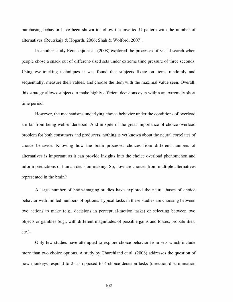
102

purchasing behavior have been shown to follow the inverted-U pattern with the number of

alternatives (Reutskaja & Hogarth, 2006; Shah & Wolford, 2007).

In another study Reutskaja et al. (2008) explored the processes of visual search when

people chose a snack out of different-sized sets under extreme time pressure of three seconds.

Using eye-tracking techniques it was found that subjects fixate on items randomly and

sequentially, measure their values, and choose the item with the maximal value seen. Overall,

this strategy allows subjects to make highly efficient decisions even within an extremely short

time period.

However, the mechanisms underlying choice behavior under the conditions of overload

are far from being well-understood. And in spite of the great importance of choice overload

problem for both consumers and producers, nothing is yet known about the neural correlates of

choice behavior. Knowing how the brain processes choices from different numbers of

alternatives is important as it can provide insights into the choice overload phenomenon and

inform predictions of human decision-making. So, how are choices from multiple alternatives

represented in the brain?

A large number of brain-imaging studies have explored the neural bases of choice

behavior with limited numbers of options. Typical tasks in these studies are choosing between

two actions to make (e.g., decisions in perceptual-motion tasks) or selecting between two

objects or gambles (e.g., with different magnitudes of possible gains and losses, probabilities,

etc.).

Only few studies have attempted to explore choice behavior from sets which include

more than two choice options. A study by Churchland et al. (2008) addresses the question of

how monkeys respond to 2- as opposed to 4-choice decision tasks (direction-discrimination

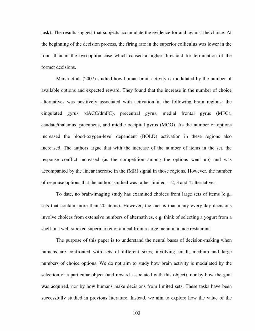
103

task). The results suggest that subjects accumulate the evidence for and against the choice. At

the beginning of the decision process, the firing rate in the superior colliculus was lower in the

four- than in the two-option case which caused a higher threshold for termination of the

former decisions.

Marsh et al. (2007) studied how human brain activity is modulated by the number of

available options and expected reward. They found that the increase in the number of choice

alternatives was positively associated with activation in the following brain regions: the

cingulated gyrus (dACC/dmFC), precentral gyrus, medial frontal gyrus (MFG),

caudate/thalamus, precuneus, and middle occipital gyrus (MOG). As the number of options

increased the blood-oxygen-level dependent (BOLD) activation in these regions also

increased. The authors argue that with the increase of the number of items in the set, the

response conflict increased (as the competition among the options went up) and was

accompanied by the linear increase in the fMRI signal in those regions. However, the number

of response options that the authors studied was rather limited -- 2, 3 and 4 alternatives.

To date, no brain-imaging study has examined choices from large sets of items (e.g.,

sets that contain more than 20 items). However, the fact is that many every-day decisions

involve choices from extensive numbers of alternatives, e.g. think of selecting a yogurt from a

shelf in a well-stocked supermarket or a meal from a large menu in a nice restaurant.

The purpose of this paper is to understand the neural bases of decision-making when

humans are confronted with sets of different sizes, involving small, medium and large

numbers of choice options. We do not aim to study how brain activity is modulated by the

selection of a particular object (and reward associated with this object), nor by how the goal

was acquired, nor by how humans make decisions from limited sets. These tasks have been

successfully studied in previous literature. Instead, we aim to explore how the value of the

104

entire set is represented in the human brain, and how this representation is affected by the

number of choice items, choice “freedom” and the availability of a strongly preferred

alternative in a set.

Previous behavioral studies demonstrate that people often make more choices and

experience greater satisfaction when choosing from intermediate numbers of items as opposed

to small or large sets of alternatives. Therefore, we first expect to see the set size

representation in the areas that were associated with reward and value in choice tasks in

previous literature. These are the striatum, orbitofrontal, cingulate and parietal cortex (Platt &

Glimcher1999; O’Doherty, 2004; Williams et al., 2004; Marsh et al., 2007; Plassmann et al.,

2008). Some of these areas relate to representation of the value of single items or actions.

However, it is not clear yet whether these areas also represent the value of an entire set, i.e.,

not only the value of a single item but the integrated value of the set consisting of many

separate options.

Second, one brain area may be of special interest for our task, namely the anterior

cingulate cortex (ACC). Previous literature suggests that apart from being associated with

functions such as error monitoring or reward, the ACC might be an area that represents the

“net” value of an action, which is based on accumulated evidence and cost-benefit analysis

(Kennerley et al., 2006; Rushworth et al., 2007; Rushworth & Behrens, 2008). In their work

Rushworth & Behrens (2008) argue that:

“…it is possible that the ACC represents the integrated value of a course of action to reflect both the action’s intrinsic costs and benefits” (p.395), and “…ACC activity preceding a decision encodes the integrated value of an action, whether in terms of immediate gains and costs or in terms of information to aid future decision making. On the observation of an outcome, ACC activity encodes the degree to which the resulting information should influence future decisions.” (p.396)

105

If choice satisfaction and behavior is a sum of costs and benefits (as proposed by

Reutskaja & Hogarth, 2006), and the ACC is the area that is associated with the integrated

value of a course of action, then we would especially expect the activity in the ACC to follow

an inverted-U pattern as the number of choice option increases. Interestingly, Marsh et al.

(2007) found that activity in the dorsal ACC (dACC) increased linearly with the number of

choice items. However, their choice sets were not extensive and contained at most four

alternatives. We suggest that when the choice set size becomes large enough, the cost of

choice may overweigh its benefits, and the activity in the dACC should level off.

In addition, the amount of choice considered “enough” may be affected by other

variables, for example, by choice set presentation and “freedom” of choice. Previous research

suggests that availability of a highly-preferred item in a large choice set can simplify choice

(Chernev, 2003). In this paper we also examine how the presence of a strongly preferred item

in the set influences participants’ choices and brain activity associated with their decisions.

We expect activity in areas associated with reward and value processing to be greater when

people face choice sets with a strongly preferred item compared to the case when such an

alternative is absent.

The literature further suggests that when choice becomes difficult, people can prefer to

defer the choice or “choose not to choose” (Dhar, 1997). In our experiment we investigate the

neural bases of human decision-making when participants face “free” (i.e., decide what to pick

by themselves) as opposed to “forced” choices (i.e., when the item is selected for the

participants). More specifically, we would expect to see different patterns of brain activity for

free and forced choice conditions in areas which are associated with reward and value

processing (see above). While medium sized sets should be more “rewarding” than small or

large sets when participants face “free” choices, large sets might be more “rewarding” than

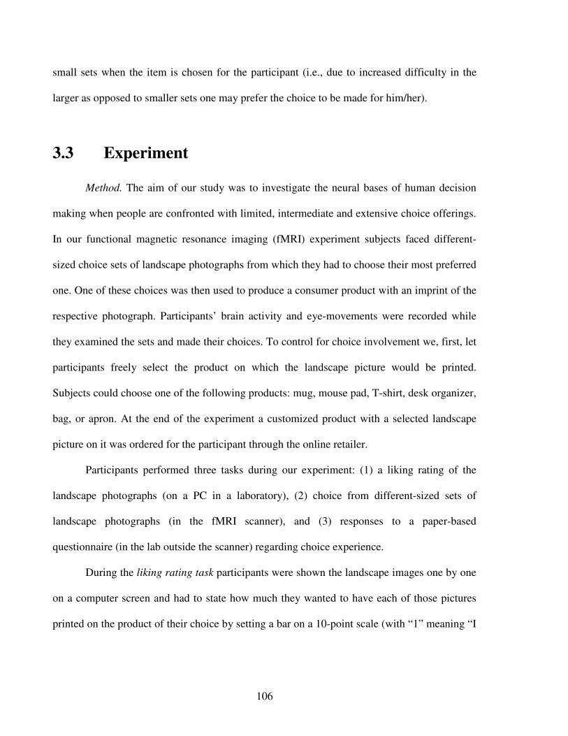
106

small sets when the item is chosen for the participant (i.e., due to increased difficulty in the

larger as opposed to smaller sets one may prefer the choice to be made for him/her).

3.3 Experiment

Method. The aim of our study was to investigate the neural bases of human decision

making when people are confronted with limited, intermediate and extensive choice offerings.

In our functional magnetic resonance imaging (fMRI) experiment subjects faced different-

sized choice sets of landscape photographs from which they had to choose their most preferred

one. One of these choices was then used to produce a consumer product with an imprint of the

respective photograph. Participants’ brain activity and eye-movements were recorded while

they examined the sets and made their choices. To control for choice involvement we, first, let

participants freely select the product on which the landscape picture would be printed.

Subjects could choose one of the following products: mug, mouse pad, T-shirt, desk organizer,

bag, or apron. At the end of the experiment a customized product with a selected landscape

picture on it was ordered for the participant through the online retailer.

Participants performed three tasks during our experiment: (1) a liking rating of the

landscape photographs (on a PC in a laboratory), (2) choice from different-sized sets of

landscape photographs (in the fMRI scanner), and (3) responses to a paper-based

questionnaire (in the lab outside the scanner) regarding choice experience.

During the liking rating task participants were shown the landscape images one by one

on a computer screen and had to state how much they wanted to have each of those pictures

printed on the product of their choice by setting a bar on a 10-point scale (with “1” meaning “I

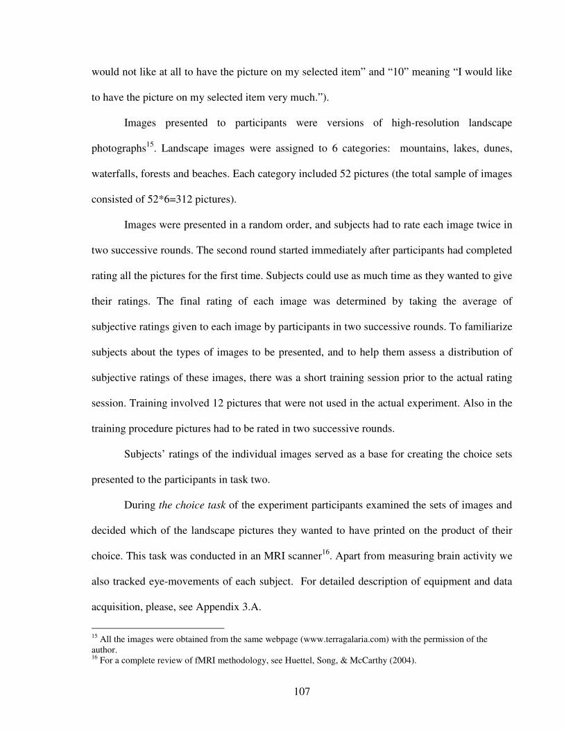
107

would not like at all to have the picture on my selected item” and “10” meaning “I would like

to have the picture on my selected item very much.”).

Images presented to participants were versions of high-resolution landscape

photographs15. Landscape images were assigned to 6 categories: mountains, lakes, dunes,

waterfalls, forests and beaches. Each category included 52 pictures (the total sample of images

consisted of 52*6=312 pictures).

Images were presented in a random order, and subjects had to rate each image twice in

two successive rounds. The second round started immediately after participants had completed

rating all the pictures for the first time. Subjects could use as much time as they wanted to give

their ratings. The final rating of each image was determined by taking the average of

subjective ratings given to each image by participants in two successive rounds. To familiarize

subjects about the types of images to be presented, and to help them assess a distribution of

subjective ratings of these images, there was a short training session prior to the actual rating

session. Training involved 12 pictures that were not used in the actual experiment. Also in the

training procedure pictures had to be rated in two successive rounds.

Subjects’ ratings of the individual images served as a base for creating the choice sets

presented to the participants in task two.

During the choice task of the experiment participants examined the sets of images and

decided which of the landscape pictures they wanted to have printed on the product of their

choice. This task was conducted in an MRI scanner16. Apart from measuring brain activity we

also tracked eye-movements of each subject. For detailed description of equipment and data

acquisition, please, see Appendix 3.A.

15 All the images were obtained from the same webpage (www.terragalaria.com) with the permission of the author. 16 For a complete review of fMRI methodology, see Huettel, Song, & McCarthy (2004).

108

Table 3.1 summarizes choice conditions subjects faced during this task. The choice sets

differed on two dimensions: the number of alternatives and the availability of a clear favorite

item in the set. With regard to the number of alternatives, choice sets presented to participants

included 6, 12 or 24 visible images of the same category. With regard to the availability of a

clear favorite item in a set, there were two types of sets: choice sets with a clear favorite item

(CF sets; the difference in rating between the first and the second best item in these sets was

large), and choice sets with no clear favorite alternative (NF sets; the difference between the

first and the second best item in the sets was small and not pronounced). To create the CF and

NF we used subjective ratings of images made by participants in the liking rating task of the

experiment.

In addition, in some trials subjects could select a photograph by themselves (“free”

choice trials), while in other trials a landscape picture from a set was selected by the computer

for the participant (“forced” choice trials). Thereby the computer would always select a

“good” or preferred picture ranked as 1st or 2nd in the “forced” set.

All forced choice sets (FO) were sets without a clear favorite picture, while free sets

could be both, with (CF) or without (NF) clear favorite alternative.

Choice sets were presented on an otherwise black screen with a central, white fixation

cross. Items of the choice sets could be randomly placed at 15 possible positions to each side

of the fixation cross. On both sides these positions were arranged in five rows and three

columns. Depending on the condition, a certain number of visible landscape images was

placed at these positions (with an equal amount placed to the right and to the left side of the

fixation cross). Scrambled images were presented at the remaining locations in order to

diminish global visual differences between sets (luminance, color, image density etc.).

109

Table 3.1: Experimental conditions and number of trials in each condition during the choice task in fMRI scanner.

Free choice

(the choice has to be made by the subjects)

Forced choice (FO) (the choice is made for

the subjects by a computer)

Number of

visible

landscape

pictures (other blurred)

Sets with clear

favorite item (CF) Sets with no clear

favorite item (NF) Sets with no clear

favorite item

6 8 trials 8 trials 8 trials



Examples of the computer screens presented to the participants during the fMRI

experiment are shown in Figure 3.1.

No choice set included identical alternatives. Moreover, within each experimental

session/run an item was shown only once and, across sessions, choice sets would always

comprise different items.

Each trial in the choice task consisted of three stages: an exposure stage (10 sec) –

during which participants were exposed to the set of the images for the first time17; a delay

stage (13-14 sec) - during which subjects saw a black screen with the central fixation cross

and had to maintain fixation on it; and a response stage (3 sec) – during which the screen with

the same choice stimuli appeared for the second time and subjects had to indicate the selected

item. The three-stage paradigm which subjects faced in the fMRI scanner (exposure, delay and

response period) was borrowed from Rosenbaum (1980) and allows teasing apart brain

17 Choice set presentation was followed by a brief random-dot mask that was presented for 0.5 seconds. The mask aimed to prevent specific after-images of the choice stimuli.

110

Figure 3.1A

Figure 3.1B Figure 3.1C

Figure 3.1: Examples of screenshots for the set containing: A. 6 items; B. 12 items; C. 24 items.

111

activity related to viewing/choosing and physical selection of a chosen item (i.e., movement

itself and its preparation). Between each trial subjects saw a black screen with the fixation

cross on it (13 sec) and had to maintain gaze on that fixation cross. The black fixation screens

between trials were considered the baseline in our analysis. The exact timeline of the choice

task is presented in Figure 3.2.

Subjects selected an item using the thumb of their right hand on an MRI-compatible

button-box (see full description of equipment in Appendix 3.A). To familiarize themselves

with the task, subjects went through a short training prior to starting the actual choice session.

During training we presented only choice sets that were not used in the actual experiment.

The landscape picture selected (by or for participants) in each trial affected the image

that a participant received printed on the product that s/he had selected. In particular, at the

end of the experiment, the computer selected one trial at random from all the trials that a

participant faced during the experiment. The landscape that was chosen in that trial was then

used to produce a featured product (i.e., printed on a product of the participant’s choice). This

product was sent to the participant about a week after the experiment18.

We used an event-related fMRI-design for the imaging part of the experiment. This

choice task of the experiment consisted of four runs (sessions) with short breaks between runs

(< 5 minutes). Each participant went through 72 trials (i.e., faced 72 different choice sets and

had to make either a free or forced selection in each of them) with 18 trials in each run. The

design was entirely balanced with 24 trials of each set type (i.e., 24 forced sets, 24 free CF

sets, and 24 free NF sets). Participants faced eight trials of each set size for each choice set

18 If a participant did not make a choice in a trial, the computer deducted $3 from the experimental payoff if the trial with no choice was selected at the end. To create a featured product, a new trial would be then again selected at random and the picture chosen in that trial would be printed on the good selected. However, this never happened during the experiment.

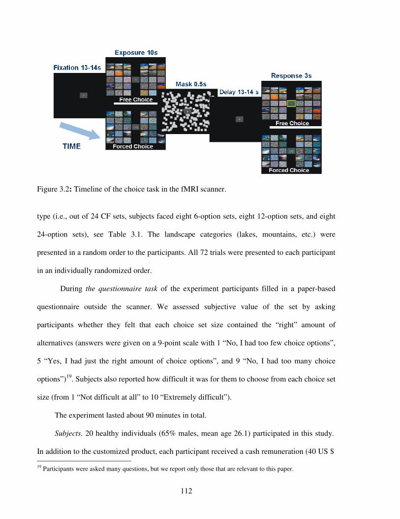
112

Figure 3.2: Timeline of the choice task in the fMRI scanner.

type (i.e., out of 24 CF sets, subjects faced eight 6-option sets, eight 12-option sets, and eight

24-option sets), see Table 3.1. The landscape categories (lakes, mountains, etc.) were

presented in a random order to the participants. All 72 trials were presented to each participant

in an individually randomized order.

During the questionnaire task of the experiment participants filled in a paper-based

questionnaire outside the scanner. We assessed subjective value of the set by asking

participants whether they felt that each choice set size contained the “right” amount of

alternatives (answers were given on a 9-point scale with 1 “No, I had too few choice options”,

5 “Yes, I had just the right amount of choice options”, and 9 “No, I had too many choice

options”)19. Subjects also reported how difficult it was for them to choose from each choice set

size (from 1 “Not difficult at all” to 10 “Extremely difficult”).

The experiment lasted about 90 minutes in total.

Subjects. 20 healthy individuals (65% males, mean age 26.1) participated in this study.

In addition to the customized product, each participant received a cash remuneration (40 US $ 19 Participants were asked many questions, but we report only those that are relevant to this paper.

113

if they chose a desk organizer, bag, or apron; and 50US $ if they chose a mug, mouse pad, or

T-shirt). All subjects were right-handed and had normal (or corrected to normal) vision.

Participants signed the informed consent form prior to participating in the experiment. The

study was performed in accordance with the declaration of Helsinki and the Caltech

Institutional Review Board guidelines20.

3.4 Results

In this paper we focus our analysis on the exposure period of the choice task. Presenting

data obtained during the delay and response phases is beyond the scope of this paper.

3.4.1 Behavioral and eye-tracking results

Before turning to brain activity, we first describe the eye-tracking and behavioral

results. Overall, subjects indicated that they liked the selection of images that they were

choosing from (on the 10-point scale: M = 7.16, SD=1.57) and found the process of choosing

enjoyable (on the 10-point scale: M = 7.32, SD=1.33). Several subjects also indicated verbally

or in their written comments that the experiment was “engaging”, “cool”, and “interesting”.

These data confirm that subjects were not indifferent to the images they were exposed to, and

that the choice task was engaging (with the exception of one subject)21. For the descriptive

statistics of the liking ratings of individual images, refer to Appendix 3.B.

20 One subject went through the rating procedure, but could not enter the MRI scanner due to unexpected claustrophobia. That subject therefore could not participate in the rest of the experiment and is not counted here. She received the show-up fee for the first part of the experiment ($20) and was not included in the analysis. 21 One subject reported verbally that he was indifferent about landscape images, was not interested in choosing any of them, and even rejected to receive the customized item at the end of the experiment. His ratings of the

114

The data demonstrate that the number of saccadic eye-movements as well as subjective

choice experience was influenced by the number of alternatives in the set. The number of

saccades per second increased with the number of items in the set in the exposure period, see

Figure 3.3. Subjects made significantly more eye-movements in the 12- as opposed to 6-item

set condition (t = 10.11, p < 0.001). The number of saccades per second increased further in

the 24 as opposed to 12-item sets (t = 6.68, p < 0.001). Moreover, subjects made significantly

more saccades per second in free than in forced choice trials regardless of the set size (t =

4.38, p <0.001). Previous research has demonstrated that the number of eye-movements

correlates with shifts of attention (for further discussion, see Wedel & Pieters, 2007).

Therefore, one may conclude that “attention load” increases with the set size, and is higher in

the free than in the forced choice trials. These data confirm that subjects were more involved

in the task and also had to “work harder” to make the selection in the free than in forced

choice trials.

Subjects’ perception regarding the value of the set was also affected by the number of

alternatives which the set contained. Recall, that a subjective set value was measured by

responses given on a 9-point scale (where “1” meant subjects felt they had too few, “5” - just

the “right” amount, and “9” - too many options to choose from). For easier visualization of the

results, we transformed the original scale into the new one by doing the following calculation:

[5-(“Subject´s Perception of Set Value” -5)]. On the new scale “5” would represent the

“optimal” set size, or the highest value of the set, while every number below 5 would show

landscape indicated the same: there was no variability in the liking ratings of different images that he reported. Over 84% of images were given a rating of “0” (meaning, the subject did not like the images at all), and the rest 16% of ratings were distributed between 0 and 1.8 on the 10-point scale (M = 0.1, SD = 0.28). The data clearly indicated that the task was not engaging for that particular subject. Therefore, the data from that subject was not included in further analysis (behavioral or fMRI), and analysis was performed on the data obtained from the remaining19 participants.

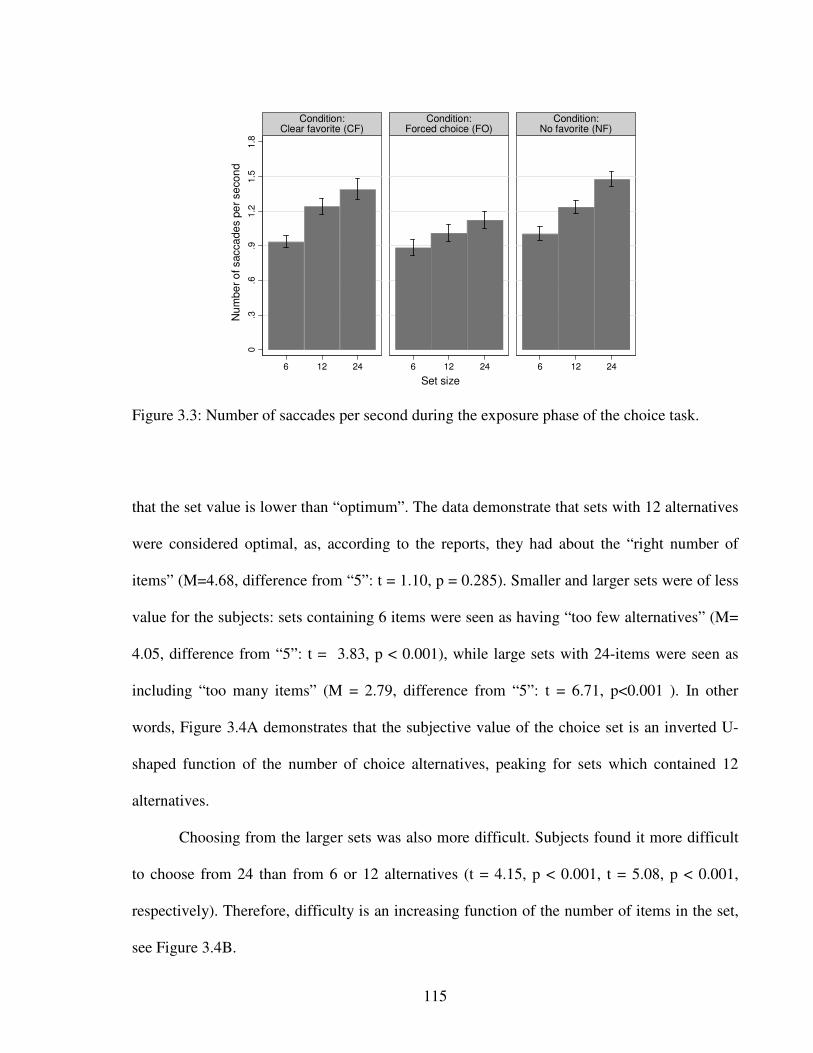
115

0.3

.6.9

1.2

1.5

1.8

6 12 24 6 12 24 6 12 24

Condition:Clear favorite (CF)

Condition:Forced choice (FO)

Condition:No favorite (NF)

Nu

mbe

r o

f sacca

de

s p

er

se

con

d

Set size

Figure 3.3: Number of saccades per second during the exposure phase of the choice task.

that the set value is lower than “optimum”. The data demonstrate that sets with 12 alternatives

were considered optimal, as, according to the reports, they had about the “right number of

items” (M=4.68, difference from “5”: t = 1.10, p = 0.285). Smaller and larger sets were of less

value for the subjects: sets containing 6 items were seen as having “too few alternatives” (M=

4.05, difference from “5”: t = 3.83, p < 0.001), while large sets with 24-items were seen as

including “too many items” (M = 2.79, difference from “5”: t = 6.71, p<0.001 ). In other

words, Figure 3.4A demonstrates that the subjective value of the choice set is an inverted U-

shaped function of the number of choice alternatives, peaking for sets which contained 12

alternatives.

Choosing from the larger sets was also more difficult. Subjects found it more difficult

to choose from 24 than from 6 or 12 alternatives (t = 4.15, p < 0.001, t = 5.08, p < 0.001,

respectively). Therefore, difficulty is an increasing function of the number of items in the set,

see Figure 3.4B.

116

Figure 3.4A

01

23

45

Perc

eptio

n o

f se

t valu

e

6 12 24Set size

Figure 3.4B

01

23

45

67

89

10

Difficu

lty o

f cho

osin

g

6 12 24Set size

Figure 3.4: Subjective ratings of participants regarding their choice experience. A. Choice set value by set size; B. Difficulty of choosing by set size.

117

3.4.2. Brain-imaging results

We performed functional image analyses both at the individual- and group- level.

On the individual level we used two different models to account for different aspects of

fMRI-response characteristics.

In model 1, on the individual subject level (1st level) 9 experimental conditions were

modeled separately [3 tasks (CF, NF, and FO choice) x 3 task stages (exposure and mask,

delay, and response periods)] in the general linear model (GLM). The model also included

three further parameters which served as additional parametric modulators for each of the 3x3

regressors of the GLM: number of items in the choice set (linear and squared term), and liking

rating of the chosen item (linear term). We used a polynomial of the second order to model the

response function because, based on the behavioral ratings from previous research and our

own results, we expected to find an inverted-U response of the brain activity to the number of

items the subjects faced.

For the group-level (2nd level) analysis we explicitly masked the brain with the task

related areas. On the group-level, contrast images for the various conditions were analyzed

using t-tests and multiple regression analysis. In this analysis we always present the results for

three statistical thresholds: p < 0.01, p < 0.005 and p < 0.001 (uncorrected) to emphasize the

spatial specificity of our results.

The 2nd level analyses of the results of model 1 allowed us to map brain regions which

showed: first, an inverted U-pattern in response to the number of items in the set (i.e., the

squared signal component was significantly larger than the linear signal component); second,

an increasing trend in response to the number of items in the set (i.e., the presence of a linear

signal component that significantly differs from baseline); third, significant differences in

118

activity in free (NF) as opposed to forced trials (FO); fourth, significant differences in activity

when subjects faced CF as opposed to NF sets; and finally, significant correlation with the

liking-rating of the item chosen in each individual trial.

In model 2, on the individual subject level the GLM included regressors for each of our

3x3 experimental conditions [3 tasks (CF, NF, and FO choices) x 3 choice sets (6-,12-, and 24-

item sets)] and for each stage of the task (exposure and mask, delay, and response period).

The 2nd level analyses of model 2 allowed mapping brain regions that were significantly

correlated with: first, the number of saccades; second, subjective ratings given by the subjects

about the value of the set; and third, subjective ratings of difficulty of choosing from each set.

Thus, while the analysis of the model 1 captured aspects directly related to the task itself

– the number of alternatives in the set, the value of the selected item in each trial etc. – the

model 2 would rather focus on aspects that were not only task-related but also differed

between individual subjects, namely the number of saccades per condition and the subjective

ratings about set value or difficulty of choosing. Note, that capturing all of these aspects in a

single model either would have reduced the statistical power (due to pooling) or, alternatively,

would have led to an overfitting of the data. In order to still allow a direct comparison of the

results obtained with the two models, we did an additional descriptive ROI-based statistics

described below.

In addition, we extracted normalized beta weights for the exposure-period regressors of

the second model for a 3mm-radius sphere that was centered on functionally defined regions

of interest (ROIs): those regions that exhibited significant fMRI-signal components correlated

with either the linear term, the squared term (both model 1) or the amount rating (model 2).

After extracting the normalized beta weights, we performed multiple correlations of

these beta values with: first, subjective ratings of the choice set value; second, subjective

119

ratings of difficulty; third, number of saccades; fourth, linear term for the number of items in

the set; and finally, the squared term for the number of items. In addition, the statistical

comparison for CF > NF and NF > FO conditions within ROIs was based on those extracted

beta values. More precisely, we performed paired t-tests across individual subject’s beta

values for the respective conditions (one-tailed).

We first determined the task-related areas, i.e. areas that were involved in all free

choice tasks relative to the baseline condition during the exposure period (contrast: Free

Choice (both CF and NF) > Baseline). Task related areas are shown in Figures 3.5, 3.6 and

3.7. Overall, the whole brain analysis of the fMRI data revealed that parietal, occipital,

anterior cingulate, premotor, prefrontal and orbitofrontal components as well as basal ganglia,

were activated. Activation of each particular area was modulated by the specific tasks in each

condition and is described in detail below.

3.4.2.1 Physical reaction to the number of choice options.

BOLD activation in the occipital cortex [lingual gyrus (LG; BA 18) also encroaching

fusiform gyrus ; inferior occipital gyrus (IOG; BA 19); and middle occipital gyrus, (MOG; BA

19)], parietal cortex (SPL; BA7), and premotor cortex [bilateral activity both in dorsal

premotor cortex (PMd, bilateral; BA 6), and supplementary motor area (SMA, bilateral)]

increased linearly in response to the increase of the number of items in the set (i.e., activity

was modulated by the linear parameter of the number of items in the set; Linear > Baseline

contrast, model 1), see Figure 3.5A-E22. Most of the areas activated in that contrast have been

shown to be modulated by motor planning and execution and processing of visual scenes in

primates and humans (see e.g., Andersen & Buneo, 2002; Grill-Spector & Malach, 2004;

22 Appendix 3C shows exact coordinates of the brain regions and statistics associated with their activity.

120

Orban, Van Essen, & Vanduffel, 2004; Medendorp et al., 2008). Therefore, the increased

activation in these areas might reflect costs of facing the large choice sets.

Figure 3.5: Brain activation in Linear > Baseline (A-E) and Quadratic > Linear (F-J) contrasts, model 1.

While activity in some brain regions increased linearly with the number of choice

alternatives, BOLD activation in the other regions has an inverted “quadratic” response to the

increase of the choice set size. Activation in the anterior cingulated cortex (ACC; BA 32),

dorsal striatum (bilateral activity in the caudate with some encroachments into the putamen),

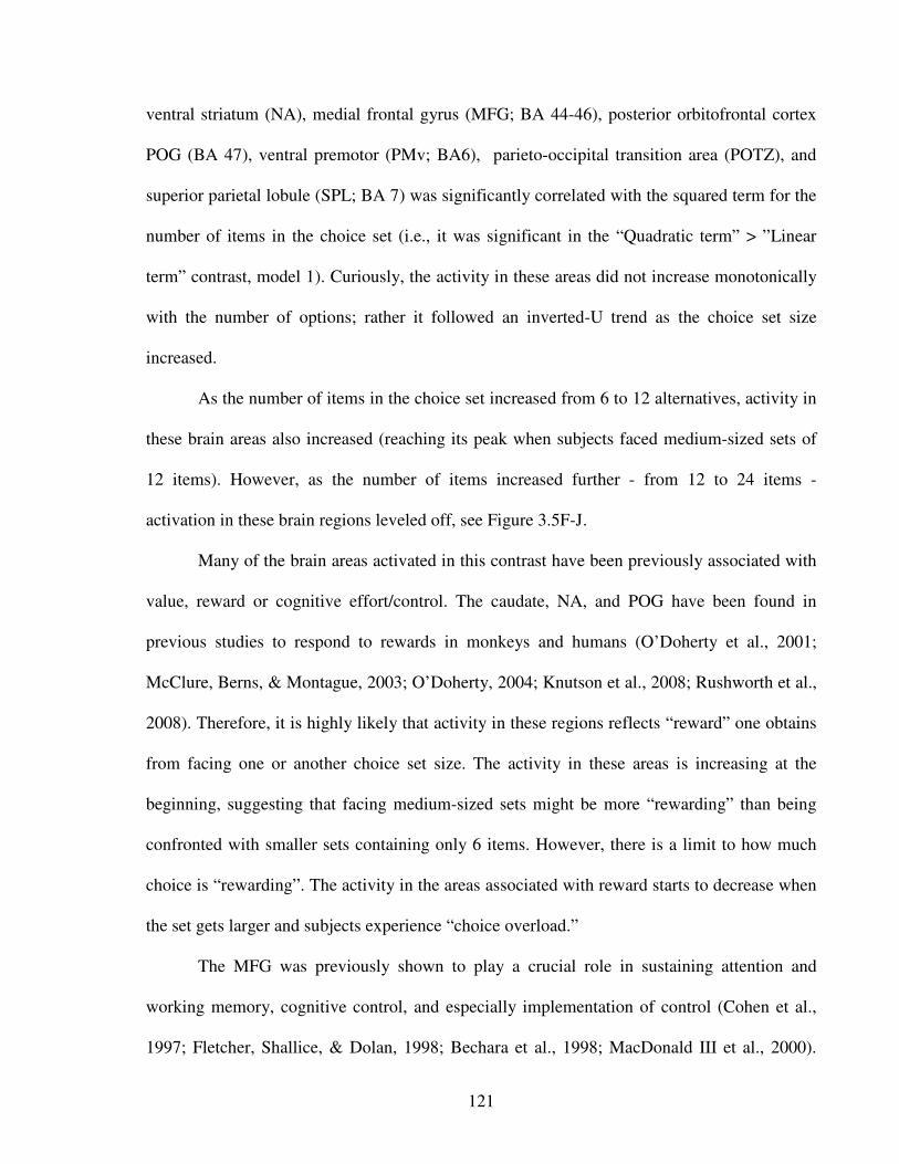
121

ventral striatum (NA), medial frontal gyrus (MFG; BA 44-46), posterior orbitofrontal cortex

POG (BA 47), ventral premotor (PMv; BA6), parieto-occipital transition area (POTZ), and

superior parietal lobule (SPL; BA 7) was significantly correlated with the squared term for the

number of items in the choice set (i.e., it was significant in the “Quadratic term” > ”Linear

term” contrast, model 1). Curiously, the activity in these areas did not increase monotonically

with the number of options; rather it followed an inverted-U trend as the choice set size

increased.

As the number of items in the choice set increased from 6 to 12 alternatives, activity in

these brain areas also increased (reaching its peak when subjects faced medium-sized sets of

12 items). However, as the number of items increased further - from 12 to 24 items -

activation in these brain regions leveled off, see Figure 3.5F-J.

Many of the brain areas activated in this contrast have been previously associated with

value, reward or cognitive effort/control. The caudate, NA, and POG have been found in

previous studies to respond to rewards in monkeys and humans (O’Doherty et al., 2001;

McClure, Berns, & Montague, 2003; O’Doherty, 2004; Knutson et al., 2008; Rushworth et al.,

2008). Therefore, it is highly likely that activity in these regions reflects “reward” one obtains

from facing one or another choice set size. The activity in these areas is increasing at the

beginning, suggesting that facing medium-sized sets might be more “rewarding” than being

confronted with smaller sets containing only 6 items. However, there is a limit to how much

choice is “rewarding”. The activity in the areas associated with reward starts to decrease when

the set gets larger and subjects experience “choice overload.”

The MFG was previously shown to play a crucial role in sustaining attention and

working memory, cognitive control, and especially implementation of control (Cohen et al.,

1997; Fletcher, Shallice, & Dolan, 1998; Bechara et al., 1998; MacDonald III et al., 2000).

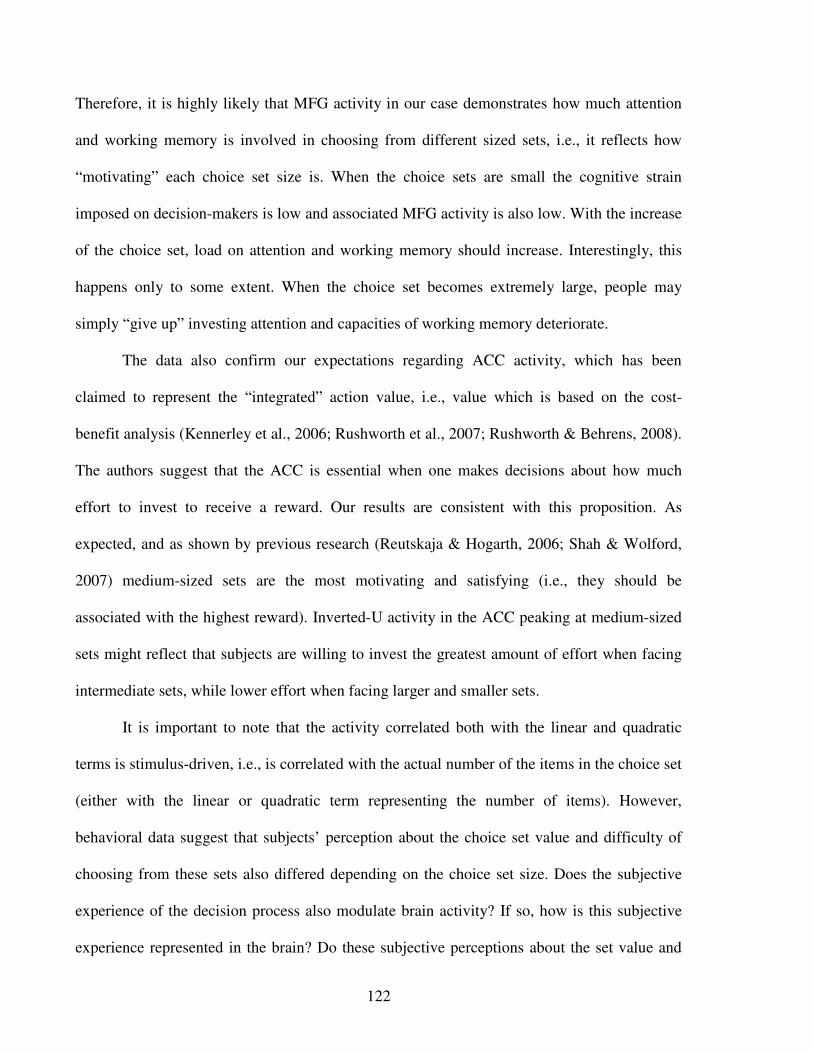
122

Therefore, it is highly likely that MFG activity in our case demonstrates how much attention

and working memory is involved in choosing from different sized sets, i.e., it reflects how

“motivating” each choice set size is. When the choice sets are small the cognitive strain

imposed on decision-makers is low and associated MFG activity is also low. With the increase

of the choice set, load on attention and working memory should increase. Interestingly, this

happens only to some extent. When the choice set becomes extremely large, people may

simply “give up” investing attention and capacities of working memory deteriorate.

The data also confirm our expectations regarding ACC activity, which has been

claimed to represent the “integrated” action value, i.e., value which is based on the cost-

benefit analysis (Kennerley et al., 2006; Rushworth et al., 2007; Rushworth & Behrens, 2008).

The authors suggest that the ACC is essential when one makes decisions about how much

effort to invest to receive a reward. Our results are consistent with this proposition. As

expected, and as shown by previous research (Reutskaja & Hogarth, 2006; Shah & Wolford,

2007) medium-sized sets are the most motivating and satisfying (i.e., they should be

associated with the highest reward). Inverted-U activity in the ACC peaking at medium-sized

sets might reflect that subjects are willing to invest the greatest amount of effort when facing

intermediate sets, while lower effort when facing larger and smaller sets.

It is important to note that the activity correlated both with the linear and quadratic

terms is stimulus-driven, i.e., is correlated with the actual number of the items in the choice set

(either with the linear or quadratic term representing the number of items). However,

behavioral data suggest that subjects’ perception about the choice set value and difficulty of

choosing from these sets also differed depending on the choice set size. Does the subjective

experience of the decision process also modulate brain activity? If so, how is this subjective

experience represented in the brain? Do these subjective perceptions about the set value and

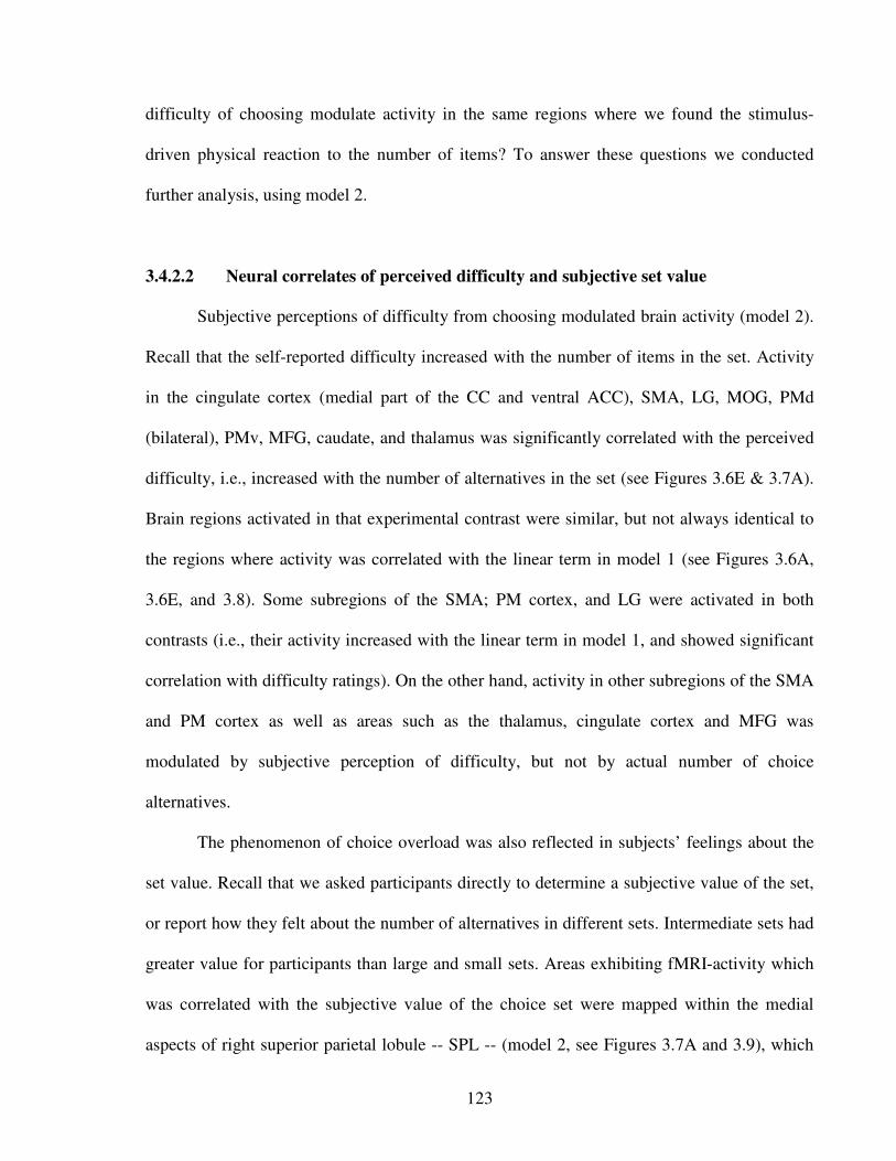
123

difficulty of choosing modulate activity in the same regions where we found the stimulus-

driven physical reaction to the number of items? To answer these questions we conducted

further analysis, using model 2.

3.4.2.2 Neural correlates of perceived difficulty and subjective set value

Subjective perceptions of difficulty from choosing modulated brain activity (model 2).

Recall that the self-reported difficulty increased with the number of items in the set. Activity

in the cingulate cortex (medial part of the CC and ventral ACC), SMA, LG, MOG, PMd

(bilateral), PMv, MFG, caudate, and thalamus was significantly correlated with the perceived

difficulty, i.e., increased with the number of alternatives in the set (see Figures 3.6E & 3.7A).

Brain regions activated in that experimental contrast were similar, but not always identical to

the regions where activity was correlated with the linear term in model 1 (see Figures 3.6A,

3.6E, and 3.8). Some subregions of the SMA; PM cortex, and LG were activated in both

contrasts (i.e., their activity increased with the linear term in model 1, and showed significant

correlation with difficulty ratings). On the other hand, activity in other subregions of the SMA

and PM cortex as well as areas such as the thalamus, cingulate cortex and MFG was

modulated by subjective perception of difficulty, but not by actual number of choice

alternatives.

The phenomenon of choice overload was also reflected in subjects’ feelings about the

set value. Recall that we asked participants directly to determine a subjective value of the set,

or report how they felt about the number of alternatives in different sets. Intermediate sets had

greater value for participants than large and small sets. Areas exhibiting fMRI-activity which

was correlated with the subjective value of the choice set were mapped within the medial

aspects of right superior parietal lobule -- SPL -- (model 2, see Figures 3.7A and 3.9), which

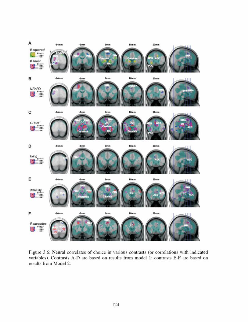
124

Figure 3.6: Neural correlates of choice in various contrasts (or correlations with indicated variables). Contrasts A-D are based on results from model 1; contrasts E-F are based on results from Model 2.

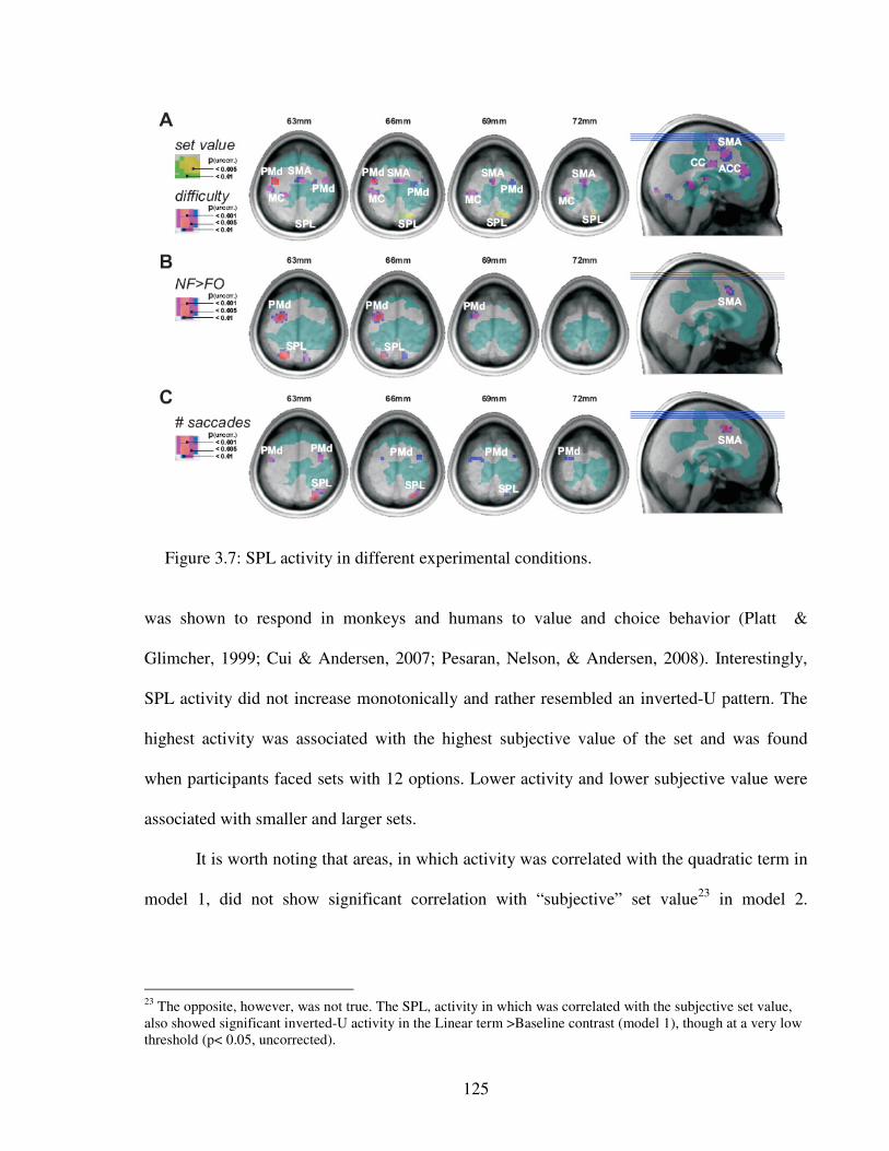
125

Figure 3.7: SPL activity in different experimental conditions.

was shown to respond in monkeys and humans to value and choice behavior (Platt &

Glimcher, 1999; Cui & Andersen, 2007; Pesaran, Nelson, & Andersen, 2008). Interestingly,

SPL activity did not increase monotonically and rather resembled an inverted-U pattern. The

highest activity was associated with the highest subjective value of the set and was found

when participants faced sets with 12 options. Lower activity and lower subjective value were

associated with smaller and larger sets.

It is worth noting that areas, in which activity was correlated with the quadratic term in

model 1, did not show significant correlation with “subjective” set value23 in model 2.

23 The opposite, however, was not true. The SPL, activity in which was correlated with the subjective set value, also showed significant inverted-U activity in the Linear term >Baseline contrast (model 1), though at a very low threshold (p< 0.05, uncorrected).

126

Therefore, our data suggest that the “subjective” set value might be represented in a separate

brain region, namely SPL.

Our data also demonstrate that the number of saccades increased with the number of

items in the choice set. Areas exhibiting fMRI-activity which was correlated with the number

of saccadic eye-movements included the SMA, PMd, MOG, IOG, LG, PO, medial parts of

CC, and lateral parts of SPL (analysis based on model 2), see Figure 3.6F. Eye-movements

have been shown to reflect covert attention (for further discussion see Wedel & Pieters, 2008).

Figure 3.8: Comparison of brain activity in the following contrasts: Linear term > Baseline ( # linear, model 1); Squared term > Linear term (# squared, model 1); significant correlation with difficulty (difficulty, model 2); significant correlation with subjective ratings of the set value (set value, model 2); subjective correlation with the number of saccades (# saccades, model 2).

Moreover, brain regions where activity was correlated with the number of saccades

were almost identical to those where activity was correlated with the linear term in model 1

(i.e., see Figures 3.6A, 3.6F, and 3.8). Some subregions of the SMA; PM cortex, LG; and CC

were also mapped at locations similar to those of regions, in which activity was correlated

127

with difficulty ratings (see Figures 3.6E and 3.6F; 3.7A and 3.7C; 3.8). Therefore, activity in

the areas listed above, which is increasing with the number of items, might represent cost of

facing different-sized sets and reflect attention load that increases with the number of options

in the set.

Activation in the ACC, dPM and STS was correlated with the liking rating of the

chosen item (analysis based on model 1), i.e., activation in these areas increased with the

Figure 3.9: Choice set value representation within the SPL.

rating of the chosen item, see Figure 3.6D. Interestingly, this activation was detected during

the exposure period, relatively long time before the subjects revealed their actual selection

(i.e., around 15 seconds prior to the selection).

128

The results show that both the actual number of items in the set as well as perceptions

of choice experience modulate brain activation. Until now we conducted analyses independent

of whether the subjects faced forced or free choice trials or whether the choice set contained

their strongly preferred item. The marketing and behavioral literature, however, suggests that

these two variables may affect perception of variety. Our behavioral results also showed that

the participants did not treat sets in free vs. forced as well as in CF vs. NF trials as identical,

and it is also important to understand the neural correlates of these differences. In the

following section we discuss how availability of a clear item in the set and choice freedom

affect neural representations of choice from multiple alternatives.

3.4.2.3 Neural correlates of the availability of a clear favorite alternative in the set

and of choice “freedom”.

Brain activity was modulated by the presence of the favorite item in the set (overall).

Many of the areas that showed an inverted-U activity in the free choice tasks also showed

significant activation in the CF > NF contrast, compare Figures 3.6A and 3.6C [as a test, note

the areas that showed significant activation in the CF > NF contrast are almost all in good

statistical correspondence with the areas that showed an inverted-U activity].

The most pronounced activity that shows the difference in the CF > NF contrast was

found in the caudate (bilateral), an area that has been associated with reward in previous

research (Knutson et al., 2001; O’Doherty et al., 2001). However, this activity is not restricted

to the caudate only, rather it invades other neighboring components of the basal ganglia (e.g.,

the pallidum).

We also compared fMRI-signal change in task-related ROIs which were significantly

correlated with the quadratic term in model 1. The analysis revealed significantly higher

129

activation in the CF as opposed to the NF sets for each area that has been found to correlate

with the quadratic term (see Figure 3.5F-J). In many cases BOLD activity associated with

choosing from the large CF sets was often as high as that associated with choosing from the

medium-sized NF sets.

This finding goes in line with previous research in marketing, which showed that an

“ideal point availability” simplifies choice from large sets (e.g., see Chernev, 2003). Our

results offer putative neural bases for this proposition. When the set contains an optimal item,

it is also associated with greater activity in areas, which have been shown to reflect reward or

value processing compared to the case when an optimal item is absent.

This finding implies that large sets are not always “bad” or “overwhelming”. Large sets

could be as rewarding as medium-sized set, if an “ideal” option is present in the set. The data

suggest that the benefits of having an “ideal” item within the set might compensate the costs of

overwhelming set size.

Brain activity was also modulated by choice “freedom”. Activity in the posterior

parietal cortex (PPC region) [bilateral activation in the medial aspects of superior parietal

lobule (SPL)], PMd, SMA and MFG was significantly higher in the free choice as opposed to

the forced choice trials, see Figures 3.6B and 3.7B. (NF > FO contrast, model 1).

It is worth noting, that some areas, in which activity followed an increasing linear

pattern and was correlated with difficulty, also showed greater activation in the free as

opposed to the forced choice trials, see Figure 3.6A, B, E. We also compared percent signal

change for task-related ROIs, which were significantly correlated with the linear term in

model 1, in the free and forced trials. Brain activity for each of these ROIs was significantly

higher in the NF condition than that in the FO condition with the exception of a non-

130

significant difference in activity in LG (see Figure 3.5A-E). Overall, our findings suggest that

“free” choices are also more difficult and demanding for the human brain.

Interestingly, the activity in regions, which followed an inverted U-trend in free choice

trials, had a linearly increasing trend in the forced choice condition (see Figure 3.5F-J). If

activity in regions such as the NA, caudate, and POG is modulated by “reward” (which is

highly likely in our case), then the activity in these regions should increase with the number of

choice items in the forced trials. In the small sets, the benefits of having a freedom of choice

are greater than the costs of choosing, therefore, small “free” choices are more rewarding than

small forced choices. However, when the choice set is large, difficulty of choosing might

outweigh the benefits of freedom of choice. When the set size increases from medium to large

size, ”reward” associated with free choices decreases, while “reward” associated with forced

choices “increases”.

ACC activity, which is increasing with the number of items in the forced sets, might

also reflect the highest net value from larger than from smaller forced sets. Indeed, when the

choice is done by someone else the probability of obtaining a better option from a large set

might be greater than from a smaller set (simply, because there are more options which are

closer to the one´s preferences), and the underlying cost-benefit analysis in the ACC might

reflect these calculation.

3.5 Discussion

In this paper we explored the neural bases of human decision making when people are

confronted with choices from different-sized sets. Our data demonstrates that brain activity

was modulated by the number of choice alternatives available to the participants, by subjective

131

perceptions about choice experience, by availability of a strongly preferred item as well as by

the “freedom of choice”.

BOLD activation in the LG, IOG, MOG, SPL, PMd, and SMA, showed a linear

increase when the number of options in the choice set increased. The increasing activity by the

set size in those areas is to be expected, as these areas were shown to be involved in

preparation and execution of movements and saccades in previous research. As the number of

items in the set increases, task demand imposed on a human being should also rise: e.g., one

needs to make more saccadic eye-movements and put greater effort in movement planning,

which might be reflected in visual and motor processes. Therefore, we argued that linearly

increasing activity in these areas might reflect the “cost” of having more choice. Activity in

most of these areas was not only correlated with the actual number of choice items, but also

with subjective difficulty ratings that participants assigned to different-sized sets. Our data

also show a clear evidence of choice overload phenomenon in the brain. Activity in the ACC,

caudate, NA, MFG, and POG followed an inverted U-pattern with the increase in the number

of choice alternatives. The activity in these regions increased when the set size increased from

6 to 12 items, and then leveled off when the set sized increased further from 12 to 24

alternatives.

Interestingly, many of the brain areas demonstrating an inverted-U activity in response

to the number of items in our task, have been associated with the processing of reward or

cognitive effort in previous research. Therefore, we attributed activity in these regions to the

“net reward”, one obtains from facing one or another choice set size. The subjective set value,

on the other hand, was mapped within the SPL, and followed and inverted-U pattern.

We also found, that two other variables – “freedom” of choice and availability of

strongly preferred set might affect neural representations of choice from multiple alternatives.

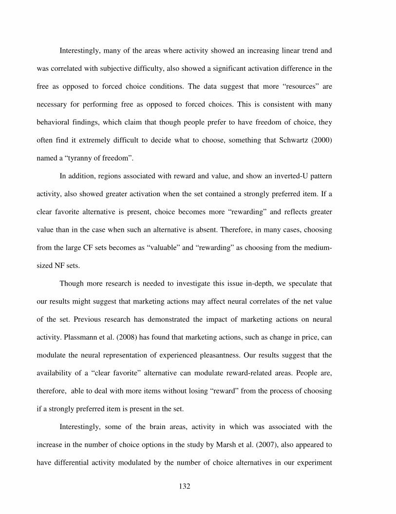
132

Interestingly, many of the areas where activity showed an increasing linear trend and

was correlated with subjective difficulty, also showed a significant activation difference in the

free as opposed to forced choice conditions. The data suggest that more “resources” are

necessary for performing free as opposed to forced choices. This is consistent with many

behavioral findings, which claim that though people prefer to have freedom of choice, they

often find it extremely difficult to decide what to choose, something that Schwartz (2000)

named a “tyranny of freedom”.

In addition, regions associated with reward and value, and show an inverted-U pattern

activity, also showed greater activation when the set contained a strongly preferred item. If a

clear favorite alternative is present, choice becomes more “rewarding” and reflects greater

value than in the case when such an alternative is absent. Therefore, in many cases, choosing

from the large CF sets becomes as “valuable” and “rewarding” as choosing from the medium-

sized NF sets.

Though more research is needed to investigate this issue in-depth, we speculate that

our results might suggest that marketing actions may affect neural correlates of the net value

of the set. Previous research has demonstrated the impact of marketing actions on neural

activity. Plassmann et al. (2008) has found that marketing actions, such as change in price, can

modulate the neural representation of experienced pleasantness. Our results suggest that the

availability of a “clear favorite” alternative can modulate reward-related areas. People are,

therefore, able to deal with more items without losing “reward” from the process of choosing

if a strongly preferred item is present in the set.

Interestingly, some of the brain areas, activity in which was associated with the

increase in the number of choice options in the study by Marsh et al. (2007), also appeared to

have differential activity modulated by the number of choice alternatives in our experiment

133

(e.g., dACC, caudate, MFG). Moreover, Marsh et al. (2007) also found that the caudate,

dACC and FMG responded similarly to the change in the number of decision items, i.e. the

activity in these regions increased with the number of response options. These authors suggest

that these brain regions might function “in coordinated fashion” (p. 986, Marsh et al., 2007).

Our data are compatible with this suggestion. These three brain areas also responded similarly

to the choice task in our experiment. However, in comparison to the study of Marsh (2007),

activity in these regions was not monotonically increasing with the number of choice items,

rather it followed an inverted-U trend. We stress that our results are not contradictory to those

of Marsh et al. (2007) and rather support them when the choice sets are small [recall that in

Marsh et al. (2007) study the number of items increased from two to four only]. As we

expected, our data suggest that the areas where activity showed significant correlation with the

quadratic term of the number of items, might also reflect how “rewarding” the entire choice

set is. In addition to simply being associated with a reward from a single item or stimulus (a

result reported in previous research), our results might suggest that the activity in these areas is

also mediated by the objective “net value” from facing the entire set (i.e., not a value of a

single item, but an integrated value of several items at a time). This is the first study, to the

best of our knowledge, which explicitly demonstrates this function of these areas.

Two brain regions, namely the ACC and SPL, deserve special attention. The data

confirmed our expectation that the ACC followed an inverted-U pattern with the increase of

the number of items in the set. We based our proposition on the claims that the ACC plays a

crucial role in “naturalistic situations” when the environment is changing, and is important for

action selection, i.e., when one makes decisions about how much effort to invest to receive a

reward (Walton et al., 2007; Kennerley et al., 2006; Rushworth et al., 2007). Therefore, the

134

ACC might be making cost-benefit analysis prior to a decision. Our results were consistent

with this proposition.

Activity in the dACC may represent the “net” reward or value of the set, which is

based on the underlying costs and benefits of each particular set. This is consistent with the

cost-benefit model of choice proposed by Reutskaja and Hogarth (2006). We further speculate

that the neural correlates of decision processes in the brain also consider when the effort does

not pay off. Therefore, when confronted with large sets “the brain” simply does not waste

precious resources and does not put a lot of effort in choosing.

On the other hand, it is important to note that different parts of the ACC were

associated with different tasks in our experiment. While activation in the dorsal part of the

ACC showed an inverted U-trend, activation of the more ventral part of the ACC was

correlated with the subjective difficulty ratings in our task.

SPL activation was associated with the subjective perception of choice set value in our

experiment. Apart from that, we found that SPL activation was modulated by the number of

items in the set, number of saccades, and choice “freedom”. First, SPL activation was higher

in free as opposed to forced choice trials. There may be two possible explanations for the

distinction in SPL activity in NF and FO sets: different number of saccades and degree of

choice “freedom”. The SPL was previously shown to be involved in saccadic eye-movement

planning and execution (Andersen & Buneo, 2002; Medendorp et al., 2008). As people make

more eye-movements in free than in forced choice condition, higher SPL activity is expected

in the former than in the later condition. However, it is highly unlikely that saccadic eye-

movements explain the difference in SPL activity in this contrast. The data show, that SPL

activity in these regions is not correlated with the number of saccades, i.e. activation of the

SPL in the NF > FO contrast was mapped mostly within its medial aspects, while more lateral

135

parts of SPL were correlated with the number of saccades (Figures 3.7A; 3.7C; and 3.8).

Therefore, we can rule out this explanation. On the other hand the degree of choice “freedom”

may explain this difference.

Therefore, based on evidence from previous research and results from this experiment,

we emphasize the role the SPL plays in the choice processes, and suggest that activity within

the medial SPL is “choice-related” and plays a major role in mediating voluntary behavioral

choices. It is highly likely that the activity in the SPL also reflects “how much choice is

enough.”

Our data suggest that the sub-regions of the parietal cortex might have different

specializations: while the medial part of the SPL might play a significant role in mediating

“choice” processes the more lateral SPL might be more related to eye movements planning.

Finally, our data can help understand whether “hot” or “cold” systems are involved in

decision-making in choice overload situations. Behavioral research suggests that choice

behavior and experience is a result of costs and benefits underlying choice (Loewenstein,

1999; Reutskaja & Hogarth, 2006). Costs associated with choice overload can be both

“psychic” and “cognitive”. While “psychic” costs are more emotional in nature (e.g., stress

and discomfort), “cognitive” costs (e.g., difficulty to make rational trade-offs) belong more to

the “cold” system of the human being. Interestingly, most of the task-related areas in our

experiment were in good special correspondence with regions that have been associated with

“cognitive” rather than “emotional” processes in previous research. Moreover, there was no

significant activity found in the amygdala or insula, i.e. areas that were highly associated with

emotional experiences during decision-making tasks in previous research (e.g, Paulus et al.,

2003; De Martino et al., 2006 ). Activity in such “analytic” areas as the MFG, dACC or SPL,

however, was modulated by the number of items in the set and by subjective experiences of

136

the participants. It is worth mentioning, that some areas that showed significant activation in

our tasks are thought to be correlated with “positive” rather than “negative” emotional states

(such as “reward” in the NA, Caudate, or POG)24. Therefore, our results suggest that while

positive sides of choice might be experienced with both the “heart” and “mind”, the costs of

choice might be more cognitive (i.e., based on calculations and physical requirements) than

emotional in nature.

In this paper we presented the first experiment which aimed to explore the neural

correlates of the choice overload phenomena. The results of our experiment showed that brain

activity was modulated by the number of choices available to the participants, by subjective

perceptions about the choices and choice experience, by availability of a clear favorite item as

well as by the “freedom of choice”. Though there is still a long journey to the final destination

of understanding of “how much choice is enough”, we believe that the data presented shed

light on the mechanisms underlying choice from sets with multiple alternatives, and inform

predictions of human decision making in choice overload situations.

24 We also found the ventral ACC to be modulated by difficulty ratings. As this area is known as “emotional” ACC (Bush et al., 2000; Rogers, et al 2004 ), it is likely that some costs may be emotional in nature. However, no other areas known for processing negative emotions were associated with costs of choosing..

137

References

Andersen, R. A. & Buneo, C.A. (2002). Intentional maps in posterior parietal cortex. Annual

Review of Neuroscience, 25, 189–220.

Bechara, A., Damasio, H., Tranel, D., Anderson, S. W. (1998). Dissociation of working memory

from decision making within the human prefrontal cortex. Journal of Neuroscience, 18, 428–

437.

Botti, S., & Iyengar, S. S. (2006). The dark side of choice: When choice impairs social welfare.

Journal of Public Policy and Marketing, 25 (1) Spring, 24–38.

Carmon, Z., Wertenbroch, K., & Zeelenberg, M. (2003). Option attachment: When deliberating

makes choosing feel like losing. Journal of Consumer Research, 30(1), 15-29.

Chernev, A. (2003). When more is less and less is more: The role of ideal point availability and

assortment in consumer choice. Journal of Consumer Research, 30 (September), 170-183

Churchland, A. K., Kiani, R., & Shadlen, M. N. (2008). Decision-making with multiple

alternatives. Nature Neuroscience, 11(6), 693-702.

Cohen, J. D., Perlstein, W. M., Braver, T. S., Nystrom, L. E., Noll, D. C., Jonides, J., & Smith,

E. E. (1997). Temporal dynamics of brain activation during a working memory task.

Nature, 386, 604-608.

De Martino, B., Kumaran, D., Seymour, B., & Dolan, R. J. (2006). Frames, biases, and

rational decision-making in the human brain. Science, 313(5787), 684-687.


Cui, H., & Andersen, R. A. (2007). Posterior parietal cortex encodes autonomously selected

motor plans. Neuron, 56(3), 552-559.

138

Fletcher, P. C., Shallice, T., & Dolan, R. J. (1998). The functional roles of prefrontal cortex in

episodic memory. Brain, 121, 1239–1248.

Grill-Spector K, & Malach, R. (2004). The human visual cortex. Review. Annual Review of

Neuroscience, 27, 649-77.

Huettel, S., Song, A., & McCarthy, G. (2004). Functional magnetic resonance imaging.

Sunderland, MA: Sinauer Associates Inc.




Press.

Iyengar, S. S., & Lepper, M. R. (2000). When choice is demotivating: Can one desire too much of

a good thing? Journal of Personality and Social Psychology, 79(6), 995-1006.

Iyengar, S. S., Wells, R. E., & Schwartz, B. (2006). Doing better but feeling worse. looking for

the "best" job undermines satisfaction. Psychological Science, 17(2), 143-150.

Kennerley, S. W., Walton, M. E., Behrens, T. E. J., Buckley, M. J., & Rushworth M. F. S. (2006).

Optimal decision making and the anterior cingulate cortex. Nature Neuroscience, 9 (7), 940-

947.

Knutson, B., Adams, C. M., Fong, G. W., & Hommer, D. (2001). Anticipation of increasing

monetary reward selectively recruits nucleus accumbens. Journal of Neuroscience, 21,

RC159.

Knutson, B, Wimmer, G. E, Rick, S., Hollon, N. G., Prelec, D., & Loewenstein, G. (2008).

Neural antecedents of the endowment effect. Neuron, 58(June 12), 814–822.

Loewenstein, G. (1999). Is more choice always better? Social Security Brief, 7 (October), 1-8.

139

Lindner, A., Iyer, A., Kagan, I., & Andersen, R.A. (2008) Where to reach and what to avoid:

Distinct roles of human posterior parietal cortex in movement preparation. Working Paper,

Pasadena.

Marsh, A. A., Blair, K. S., Vythilingam, M., Busis, S., & Blair, R. J. R. (2007). Response options

and expectations of reward in decision-making: The differential roles of dorsal and rostral

anterior cingulate cortex. NeuroImage, 35, 979–988.

MacDonald III, A. W., Cohen, J. D., Stenger, V. A., & Carter, C. S. (2000). Dissociating the role

of the dorsolateral prefrontal and anterior cingulate cortex in cognitive control. Science, 288,

1835-1838.

McClure, S. M., Berns, G. S., & Montague, P. R. (2003). Temporal prediction errors in a passive

learning task activate human striatum. Neuron, 38, 339–346.

Medendorp, W., Beurze, S ., Van Pelt, S., & Van Der Werf J. (2008). Behavioral and cortical

mechanisms for spatial coding and action planning. Cortex, 44 (5) , 587 – 597.

Nieder, A., Freedman, D. J., & Miller, E. K. (2002). Representation of the Quantity of Visual

Items in the Primate Prefrontal Cortex. Science, 297(5587), 1708-1711.

O'Doherty, J., Kringelbach, M. L., Rolls, E. T., Hornak, J., & Andrews, C. (2001). Abstract

reward and punishment representations in the human orbitofrontal cortex. Nature

Neuroscience, 4(1), 95-102.

O'Doherty, J. P. (2004). Reward representations and reward-related learning in the human brain:

insights from neuroimaging. Current Opinion in Neurobiology, 14(6), 769-776.

Orban, G. A., Van Essen, D., & Vanduffel, W. (2004). Comparative mapping of higher visual

areas in monkeys and humans. Review. Trends in Cognitive Sciences, 8(7), 315-324.

140

Paulus, M. P., Rogalsky, C., Simmons, A., Feinstein, J. S., & Stein, M. B. (2003). Increased

activation in the right insula during risk-taking decision making is related to harm avoidance

and neuroticism. NeuroImage, 19, 1439–1448.

Pesaran, B., Nelson, M. J., & Andersen, R. A. (2008). Free choice activates a decision circuit

between frontal and parietal cortex. Nature, 453(7193), 406-409.

Platt, M. L., & Glimcher, P. W. (1999). Neural correlates of decision variables in parietal cortex.

Nature, 400(6741), 233-238.

Plassmann, H., O'Doherty, J., Shiv, B., & Rangel, A. (2008). Marketing actions can modulate

neural representations of experienced pleasantness. Proceedings of the National Academy of

Sciences of the United States of America, 105(3), 1050-1054.

Reutskaja, E., & Hogarth, R. M. (2006). Satisfaction in choice as a function of the number of

alternatives: when "goods satiate" but "bads escalate". UPF working papers.

http://www.econ.upf.edu/en/research/onepaper.php?id=903

Reutskaja, E., Pulst-Korenberg, J., Nagel, R., Camerer, C., & Rangel, A. (2008). Economic

decision-making under conditions of extreme time pressure and option overload: an eye-

tracking study. Working paper, Pasadena.

Rosenbaum, D. (1980). Human movement initiation: specification of arm, direction, and

extent. Journal of experimental psychology. General, 109(4), 444-474.

Rushworth, M. F. S., Behrens, T. E. J., Rudebeck P. H., & Walton, M. E. (2007). Contrasting

roles for cingulate and orbitofrontal cortex in decisions and social behavior. Review.

Trends in Cognitive Sciences,11 (4), 168-176.

Rushworth, M. F. S., & Behrens, T. E. J. (2008). Choice, uncertainty and value in prefrontal

and cingulate cortex. Nature Neuroscience, 11 (4), 389 – 397.

141

Schwartz, B. (2000). Self-determination. The tyranny of freedom. The American Psychologist,

55(1), 79-88.

Shafir, E., Tversky, A. & Simonson, I. (1993). Reason-based choice. Cognition, 49(1-2), 11-

36.


number of choices. Psychological Science, 18, 369-370.

Walton, M. E., Devlin, J. T., & Rushworth, M. F. S. (2004). Interactions between decision

making and performance monitoring within prefrontal cortex. Nature Neuroscience,

7(11), 1259-1265.

Wedel, M., & Pieters, R. (2007). Visual Marketing: From Attention to Action. New York:

Lawrence Erlbaum.

Williams, Z. M., Bush, G., Rauch, S. L., Cosgrove, G. R., & Eskandar, E. N. (2004). Human

anterior cingulate neurons and the integration of monetary reward with motor

responses. Nature Neuroscience, 7(12), 1370-1375.

142

Appendix 3.A: Equipment and acquisition of biological

Data

Eye- and finger-tracking analysis. Eye-movements of participants were recorded by the

ViewPoint Eye Tracker (Arrington Research Inc., Scottsdale, USA) and registered by fMRI-

compatible eye-camera (Resonance Technology Inc., USA) while participants were

performing the task in the fMRI scanner. Eye-movements were recorded at 60HZ frequency.

Saccades were detected using an absolute velocity threshold (>20deg/sec).

Finger responses were recorded using an MRI-compatible diamond-shaped four button

response-box (Current Designs, Philadelphia) which was placed at a comfortable position

near the subject’s belly. Subjects could move the cursor (i.e. the green frame) up, down, left

or right by pressing the corresponding buttons. Subjects could not make diagonal movements.

Reaction time was defined by the amount of time that elapsed until subjects started to move

the cursor towards the item of their choice since the appearance of the response screen.Eye-

movements and finger responses were analyzed using Matlab7.1.

Image acquisition and fMRI analysis. A 3-tesla Siemens TRIO scanner and an 8-channel

head coil (Siemens, Erlangen, Germany) were used to acquire MRI-images. T1-weighted MP-

rage anatomical scan (176 slices, slice thickness=1mm, gap=0mm, in-plane voxel

size=1x1mm, TR=1500ms, TE=3.05ms, FOV=256x256, resolution = 256x256) as well as

T2*-weighted gradient-echo planar imaging scans (EPIs: slice thickness=3.5mm, gap=0mm,

in-plane voxel size=3x3mm, TR=2000ms, TE=30ms, flip angle=90°, FOV=192x192,

resolution=64x64, 32 axial slices) were obtained for each subject, providing an almost entire

coverage of the cerebral cortex as well as most sub-cortical structures (for several subjects

only the posterior parts of cerebellum were not covered, and there were also dropouts in the

143

frontal part of the brain for several participants). In total, 1512 EPIs per subject were collected

during three consecutive runs lasting about 13 min each.

We used SPM 5 (Wellcome Department of Cognitive Neurology, London) to perform

functional image analysis. First, images of each subject were realigned to the first scan. We

co-registered T1 anatomical images the mean image of the functional scans and then aligned

to the SPM T1-template in MNI space (Montreal Neurological Institute, mean brain). For

spatial normalization we applied the resulting non-linear 3D-transformation to all images.

Finally we performed spatial smoothing of the functional images with a Gaussian filter

(7x7x7 mm³ full-width at half-maximum) and high pass filtering (cut-off period 128 ms). We

did not perform slice-time correction since scans were acquired in an interleaved fashion.

144

Appendix 3.B: Descriptive statistics of liking ratings

Ratings of the landscape images

The liking ratings of the landscape images given by19 subjects followed normal

distribution (M=4.45, SD=2.18). Subjects took on average 2835 ms to rate each image in the

first round of ratings. That was on average 594 ms longer than the mean time spent per image

in the second round (t=8.21, p=0.000). The data also shows that time spent per image

increased significantly with the liking rating of the image, i.e. with every point increase in the

liking rating subjects spent 94ms longer on evaluating the image (t=2.71, p=0.014; analysis is

performed by regressing time spent on evaluating the image on liking rating assigned to the

image, controlling for individual differences by including dummies for each subjects).

The liking ratings showed significant correlation between rounds 1 and 2, suggesting

that subjects had similar preferences for the same picture and rated the same image similarly

in both rounds. Moreover, liking ratings did not differ significantly in the first and second

round (t= 1.65, p= 0.116; analysis is performed by regressing liking rating on round dummy,

controlling for individual differences by including dummies for each subject).The liking

ratings also decreased as the trial time progressed. However, the absolute amount of the

decrease in rating with the progress of the rating task is almost negligible (decrease of 0.001;

t=2.00, p= 0.061; analysis is performed by regressing liking rating on order of rating,

controlling for individual differences by including dummies for each subject).

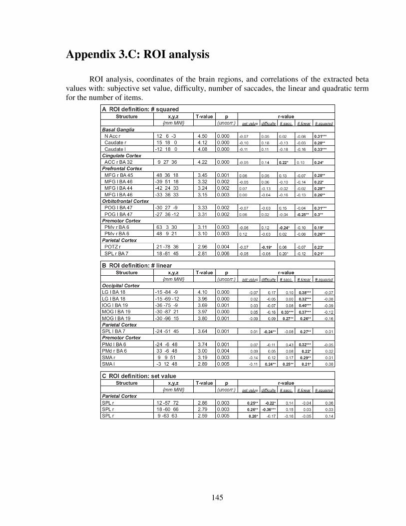
145

Appendix 3.C: ROI analysis

ROI analysis, coordinates of the brain regions, and correlations of the extracted beta values with: subjective set value, difficulty, number of saccades, the linear and quadratic term for the number of items.

Experiments on the Role of the Number of Alternatives in Choice

Documents

Transcript of Experiments on the Role of the Number of Alternatives in Choice