Rank-order conjoint experiments: efficiency and designs

Bart Vermeulen, Peter Goos and Martina Vandebroek

DEPARTMENT OF DECISION SCIENCES AND INFORMATION MANAGEMENT (KBI)

Faculty of Business and Economics

KBI 0734

Rank-order conjoint experiments: efficiency and design

Bart Vermeulen ∗

Peter Goos †

Martina Vandebroek ‡

Abstract

In a rank-order conjoint experiment, the respondent is asked to rank a numberof alternatives instead of choosing the preferred one, as is the standard procedure inconjoint choice experiments. In this paper, we study the efficiency of those experi-ments and propose a D-optimality criterion for rank-order conjoint experiments tofind designs yielding the most precise parameter estimators. For that purpose, anexpression of the Fisher information matrix for the rank-ordered multinomial logitmodel is derived which clearly shows how much additional information is providedby each extra ranking step made by the respondent. A simulation study shows thatBayesian D-optimal ranking designs are slightly better than Bayesian D-optimalchoice designs and (near-)orthogonal designs and perform considerably better thanother commonly used designs in marketing in terms of estimation and predictionaccuracy. Finally, it is shown that improvements of about 50% to 60% in estimationand prediction accuracy can be obtained by ranking a second alternative. If the re-spondent ranks a third alternative, a further improvement of 30% in estimation andprediction accuracy is obtained.

∗Corresponding author. Bart Vermeulen is funded by project G.0611.05 of the Fund for ScientificResearch Flanders. Department of Decision Sciences and Information Management, Faculty of Busi-ness and Economics, Katholieke Universiteit Leuven, Naamsestraat 69, 3000 Leuven, Belgium, e-mail:bart.vermeulen@econ.kuleuven.be, tel: +32 16 32 69 63, fax: +32 16 32 66 24

†Faculty of Applied Economics, Universiteit Antwerpen‡Faculty of Business and Economics, University Center for Statistics, Katholieke Universiteit Leuven

1

1 Introduction

A conjoint choice experiment measures the importance of the features of a good or service

in making a purchase decision. This is achieved by asking each respondent to choose

his/her preferred alternative from a number of choice sets. A rank-order conjoint ex-

periment measures the importance of the features of a good or service by asking the

respondent to rank a certain number of alternatives within the choice sets. Data from

a rank-order experiment can be analyzed by the rank-ordered multinomial logit model

or exploded logit model (Beggs et al., 1981, Hausman and Ruud, 1987 and Allison and

Christakis, 1994), which is an extension of the multinomial logit model, and provides a

better view on the preferences of a consumer than data from a choice experiment.

The design of an experiment has a significant impact on the accuracy of the estimated

parameters of the fitted model. Choosing the appropriate alternatives and grouping them

in choice sets in the best possible way according to an optimality criterion yields an opti-

mal design which guarantees precise parameter estimates and therefore an accurate view

on the preferences of the customer. We propose to use the D-optimality criterion which

focuses on the accuracy of the estimates of the rank-ordered multinomial logit model its

parameters. The central question is then whether the corresponding Bayesian D-optimal

ranking design results in significantly more precise estimates and predictions than com-

monly used design strategies in marketing. Additionally, we value the contribution of

each extra ranking step to the estimation and prediction accuracy.

In the next section, we introduce the rank-ordered multinomial logit model. In section 3,

we derive the Bayesian ranking D-optimality criterion and present the benchmark designs.

In section 4, we compare the design generated using the new criterion with benchmark

designs, which are commonly used in marketing, in terms of the newly developed design

optimality criterion. Furthermore, in section 4, we use a simulation study to compare the

precision of the estimators and the prediction accuracy of the designs. Finally, we examine

2

how much improvement is obtained by each extra ranking step in terms of estimation and

prediction accuracy.

2 The rank-ordered multinomial logit model

Any rank order can be regarded as a sequence of choices made by the respondent. This

was used as the starting point for the extension of the multinomial logit model to the

rank-ordered multinomial logit model by Beggs et al. (1981). In their approach, each

ranking of a choice set is converted into a number of independent pseudo-choices. In this

way, each ranking of alternatives in a choice set is considered as a sequential and condi-

tional choice task. The alternative ranked first is perceived as the preferred alternative

of the entire choice set. Alternatives ranked next are viewed as the preferred alternatives

of the choice sets consisting of all alternatives except the ones with a better ranking. In

the resulting rank-ordered multinomial logit model, a ranking of a set of J alternatives is

thus seen as a series of J − 1 choices.

The rank of an alternative is determined by its utility. The utility of alternative i in

choice set k experienced by respondent n is modeled as

ukin = x′kiβ + εkin. (1)

The deterministic part, x′kiβ, of the utility consists of a p-dimensional vector β, which

is assumed to be common for all respondents and which represents the importance of

the attributes for the consumer in determining the utility, and a p-dimensional vector xki

containing the levels of the attributes. The error term εkin, which forms the stochastic

part of the utility, captures the unobserved influences on this utility. The error terms are

assumed to be identically and independently distributed according to an extreme value

distribution.

3

The probability of ranking an alternative first in a choice set k with J alternatives cor-

responds to the logit probability of choosing this alternative as the preferred one. The

probability of ranking an alternative second corresponds to the logit probability of choos-

ing this alternative from the profiles remaining after the removal of the first-ranked alter-

native. This can be said for the J − 1 rankings made by the respondent. Because of the

assumed independence between these choice tasks, the likelihood of a certain ranking of

the alternatives in the entire choice set k is thus the product of J logit probabilities. This

likelihood can be written as

J∏j=1

exp(x′kjβ)

∑Jj′=1 δkjj′ exp(x

′kj′β)

, (2)

where the dummy variable δkjj′ equals zero when alternative j′ in choice set k has a better

ranking than alternative j, and one otherwise. For a respondent who ranks K choice sets,

the likelihood function for the rank-ordered multinomial logit model is given by

L(β) =K∏

k=1

J∏j=1

exp(x′kjβ)

∑Jj′=1 δkjj′ exp(x

′kj′β)

. (3)

The maximum likelihood estimate β for the parameter vector β is obtained by maximiz-

ing the likelihood function (3).

As the rank-order conjoint experiment requires the respondents to provide more infor-

mation about their preferences than the classical conjoint choice experiment, it results in

more accurate parameter estimates when the same number of choice sets is used. Stated

differently, to achieve a desired degree of precision of the estimates, less choice sets are

required in a rank-order conjoint experiment (Chapman and Staelin, 1982). The major

disadvantage of using a rank-order conjoint experiment is the weak link with reality: in

real life, respondents choose the alternative they like most and hardly ever select a second

best item. According to Bateman et al. (2002) and Chapman and Staelin (1982), lower

4

rankings are less reliable if the number of alternatives to rank is large. In this paper, we

therefore limit ourselves to three or four alternatives in a choice set.

3 Designs for the rank-ordered multinomial logit model

This section is devoted to the derivation of the Bayesian D-optimality criterion for the

rank-ordered multinomial logit model and the corresponding D-error. In addition, we

discuss how to create efficient designs using this D-optimality criterion. Finally, bench-

mark designs, with which the Bayesian D-optimal ranking design will be compared, are

introduced.

3.1 Bayesian D-optimal designs for rank-order conjoint experi-

ments

The issue of finding optimal designs for rank-order experiments has not yet been explored

in the literature on conjoint experiments. Till now, the applications measuring prefer-

ences by means of a rank-order conjoint experiment have used random designs (see, e.g.,

Boyle et al. (2001)), nearly orthogonal designs (see, e.g., Baarsma (2003)), and fractional

factorial designs (Gustafsson et al. (1999)). Although several design selection criteria

have been proposed in the literature on experimental designs, none of them has ever been

applied to generate an optimal design for a rank-order conjoint experiment. In this article,

we show how optimal designs for this type of experiment can be found and we use the

D-optimality criterion to do so.

A D-optimal design minimizes the determinant of the variance-covariance matrix on the

unknown parameters β and thereby minimizes the volume of the confidence ellipsoids

around them. As the variance-covariance matrix is inversely proportional to the Fisher

information matrix, a D-optimal design also maximizes the information content of the

experiment. In order to construct a D-optimal design for a rank-order conjoint exper-

5

iment, an expression for the Fisher information matrix on the unknown parameters in

the corresponding model is required. Starting from (3), it is not hard to show that the

information matrix for an experiment with K choice sets of size three can be written as

Irank(β) =K∑

k=1

X′k(Pk − pkp

′k)Xk +

K∑

k=1

3∑i=1

Pki1X′(i)k(P(i)k − p(i)kp

′(i)k)X(i)k

= Ichoice(β) +K∑

k=1

3∑i=1

Pki1X′(i)k(P(i)k − p(i)kp

′(i)k)X(i)k,

(4)

where

Ichoice(β) =K∑

k=1

X′k(Pk − pkp

′k)Xk (5)

denotes the information matrix of a conjoint choice experiment with choice sets of size

three (see, e.g., Sandor and Wedel, 2001), and,

• Pki1 represents the probability of ranking alternative i (i = 1, 2, 3) in choice set k

first,

• pk is a 3-dimensional vector of which the ith element is Pki1 (i = 1, 2, 3),

• Pk is a diagonal matrix with the elements of pk on its diagonal,

• p(i)k is a 2-dimensional vector containing the probabilities of ranking alternative i′

second (i′= 1, 2, 3 and i′ 6= i), given that i was ranked first,

• P(i)k is a diagonal matrix with the elements of p(i)k on its diagonal,

• Xk is the (3 × p) design matrix containing all attribute levels of the profiles in

choice set k, and

• X(i)k is the (2 × p) design matrix containing all attribute levels of the profiles in

choice set k, except those of the first-ranked profile i.

The information matrix for a rank-ordered multinomial logit model corresponding to

a rank-order conjoint experiment with choice sets of size three is thus a sum of two

6

parts: (i) the information matrix corresponding to an ordinary conjoint choice experi-

ment with choice sets of three alternatives, and (ii) a weighted sum of the information

matrices corresponding to three ordinary conjoint choice experiments with choice sets of

size two. Each of the latter information matrices gives the information content of the

choice sets after removing one of the alternatives. The weight of the ith such information

matrix is the probability that alternative i is ranked first. The expression for the infor-

mation matrix of a rank-order experiment proves that asking the respondents to rank

the alternatives in a choice set provides extra information. This is because the difference

Irank(β)− Ichoice(β) =∑K

k=1

∑3i=1 Pki1X

′(i)k(P(i)k−p(i)kp

′(i)k)X(i)k is a nonnegative definite

matrix, which ensures that the amount of information in a ranking experiment is larger

than in a choice experiment. In other words, for a given choice set, it is always better to

rank. By means of equation (4), the extra amount of information can be quantified easily.

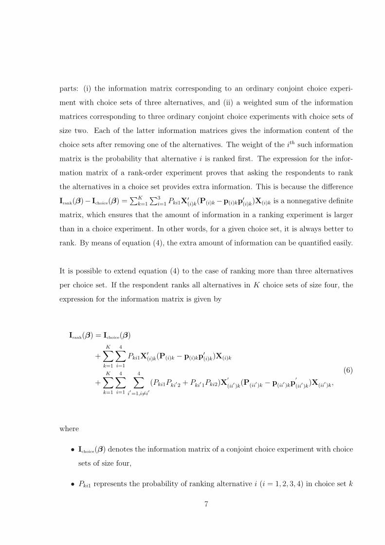
It is possible to extend equation (4) to the case of ranking more than three alternatives

per choice set. If the respondent ranks all alternatives in K choice sets of size four, the

expression for the information matrix is given by

Irank(β) = Ichoice(β)

+K∑

k=1

4∑i=1

Pki1X′(i)k(P(i)k − p(i)kp

′(i)k)X(i)k

+K∑

k=1

4∑i=1

4∑

i′=1,i 6=i′(Pki1Pki′2 + Pki′1Pki2)X

′(ii′)k

(P(ii′ )k − p(ii′ )kp′(ii′)k

)X(ii′ )k,

(6)

where

• Ichoice(β) denotes the information matrix of a conjoint choice experiment with choice

sets of size four,

• Pki1 represents the probability of ranking alternative i (i = 1, 2, 3, 4) in choice set k

7

first,

• pk is a 4-dimensional vector of which the ith element is Pki1 (i = 1, 2, 3, 4),

• Pk is a diagonal matrix with the elements of pk on its diagonal,

• Pki′2 represents the probability of ranking alternative i

′(i′= 1, 2, 3, 4 and i′ 6= i)

in choice set k second given that i was ranked first,

• p(i)k is a 3-dimensional vector of which the ith element is Pki′2 (i′= 1, 2, 3, 4 and i′ 6=

i),

• P(i)k is a diagonal matrix with the elements of p(i)k on its diagonal,

• p(ii′ )k is a 2-dimensional vector containing the probabilities of ranking alternative

i′′

third (i′′

= 1, 2, 3, 4, i′′ 6= i and i′′ 6= i′) given that i and i′ have been ranked

first and second or vice versa,

• P(ii′ )k is a diagonal matrix with the elements of p(ii′ )k on its diagonal,

• Xk is the (4 × p) design matrix containing all attribute levels of the profiles in

choice set k,

• X(i)k is the (3 × p) design matrix containing all attribute levels of the profiles in

choice set k, except those of the first-ranked profile i, and

• X(ii′ )k is the (2 × p) design matrix containing all attribute levels of the profiles in

choice set k, except those of the first- and second-ranked profiles i and i′.

Expression (6) illustrates again that asking respondents to rank the alternatives of a choice

set provides the researcher with more information than a choice experiment.

Ideally, the information content of the rank-order experiment is as large as possible. In

the experimental design literature, the most commonly used measure for the information

content of a design is the determinant of the information matrix. A design that maximizes

8

this quantity is called D-optimal. A D-optimal design can also be found by minimizing

the pth root of the determinant of the inverse of the information matrix. This criterion is

usually referred to as the D-error and is defined as

D-error = {det(Irank(X,β)−1)} 1p . (7)

In this article, we will use the D-error to quantify the performance of a design in the D-

optimality criterion. The design having the smallest D-error is then the D-optimal design.

As can be seen in (4), (6) and (7), the information matrix and the D-error depend on

the parameters in β which are unknown at the moment of designing the experiment. To

circumvent this problem, we use the Bayesian approach of Sandor and Wedel (2001, 2005)

and Kessels et al. (2006a) assuming a prior distribution f(β) on the unknown parameters

for the purpose of designing a rank-order experiment. The Bayesian version of the D-error

is given by

Db-error = Eβ[{det(Irank(X, β)−1)} 1p ] =

∫

<p

{ det(Irank(X,β)−1)} 1p f(β)dβ. (8)

Since there is no analytical way to compute the integral in (8), it has to be approximated

by taking a number of draws from the prior distribution f(β) and averaging the D-error

over all draws. The design which minimizes the average D-error over all draws is called

the Bayesian D-optimal ranking design.

The designs discussed in this paper involve three three-level and two two-level attributes

which are effects-type coded. This implies that the number of parameters, p, contained

within β, equals 8. As a Bayesian approach is used to circumvent the dependence of the

optimal design on the unknown parameter vector β, a prior distribution on β has to be

specified. We used as prior distribution an 8-dimensional normal distribution with mean

[−0.5; 0; −0.5; 0; −0.5; 0; −0.5; −0.5] and variance 0.5∗I8 with I8 being the

9

8-dimensional unity matrix. This prior distribution, which follows the recommendations

formulated by Kessels et al. (2006c), assumes the utility of a good or service increases

with the attribute levels.

To construct a Bayesian D-optimal ranking design, we implemented the adaptive algo-

rithm developed by Kessels et al. (2006b), using a systematic sample of 100 draws from the

prior distribution f(β). This systematic sample was generated using a Halton sequence

(Train, 2003).

3.2 Benchmark designs

In order to evaluate the performance of the Bayesian D-optimal ranking designs, we

compared them to four types of benchmark designs: Bayesian D-optimal designs for a

conjoint choice experiment (Kessels et al. (2006a) describe extensively how to generate

these designs) and three sorts of standard designs generated by Sawtooth Software. This

software offers the user three options to construct designs: (near-)orthogonal designs (la-

belled ’complete enumeration’ in Sawtooth), random designs and designs with a balanced

attribute level overlap in one choice set (denoted as ’balanced overlap’ in Sawtooth). To

construct a (near-)orthogonal design, all candidate profiles obtained by all possible com-

binations of attribute levels are considered. The alternatives are selected and grouped in

choice sets so that the attribute level overlap within one choice set is minimal and so that

the design is as close as possible to an orthogonal design. The random method leads to al-

ternatives with randomly drawn attribute levels and possibly results in a strong attribute

level overlap within a choice set. Contrary to the (near-)orthogonal design which severely

restricts the overlap of attribute levels within a choice set, the third option, balanced

overlap, allows a moderate attribute level overlap. In this sense, this option is the middle

course between the orthogonal design and the random design.

10

4 Evaluating the Bayesian D-optimal ranking design

In this section, we compare the different designs in terms of the Db-error and describe the

findings of a simulation study by which the performance of the designs in terms of esti-

mation and prediction accuracy was examined. In addition, we measure the improvement

achieved by including extra ranking steps in the experiment. In the simulation study, we

considered two cases: ranking nine choice sets of size four and ranking twelve choice sets

of size three. Each of the cases assumes 50 respondents participated in the experiment. As

an illustration, the Bayesian D-optimal ranking design and the four benchmark designs

for the case of nine choice sets of size four are included in appendix.

4.1 Measurement of the estimation and prediction accuracy

Based on simulated observations for all choice sets of the different designs discussed above,

we estimated the parameters of the rank-ordered multinomial logit model and used the

estimates to calculate the probabilities of choosing an alternative of a choice set. Com-

paring the estimated parameters with their true values, i.e. the ones used to generate the

data, and comparing the estimated probabilities with the probabilities calculated using

the true parameter values allows us to evaluate the estimation and prediction accuracy, re-

spectively. The metrics we used for that purpose are the expected mean squared errors for

estimation and prediction, denoted by EMSEβ(β) and EMSEp(β), and are computed

as

EMSEβ(β) =

∫

<p

(β − β)′(β − β)f(β)dβ, (9)

and

EMSEp(β) =

∫

<p

(p(β)− p(β))′(p(β)− p(β))f(β)dβ, (10)

where f(β) is the distribution of the parameter estimates, β and β are the vectors contain-

ing the true and estimated parameter values and p(β) and p(β) are vectors containing

the true and the predicted probabilities of choosing an alternative of a choice set in a

random design. For the results reported in this paper, (9) and (10) were approximated

11

using 1000 draws from f(β). This was done for 75 values of β drawn from the prior

distribution used to generate the Bayesian D-optimal ranking design. The smaller the

value of EMSEβ(β) and EMSEp(β), the more accurate the parameter estimators and

predictions respectively.

4.2 Performance of Bayesian D-optimal ranking designs

The next section considers the scenarios when the respondents do and do not rank all

alternatives of a choice set. We refer to a rank-order experiment where all alternatives in a

set are ranked as a full rank-order experiment. An experiment where only the subset of the

better alternatives of each choice set is ranked, is called a partial rank-order experiment.

4.2.1 Full rank-order experiments

In this section, we examine whether a Bayesian D-optimal ranking design performs better

in terms of estimation and prediction accuracy than the benchmark designs in case of a

full rank-order experiment. Table 1 compares the five different designs in terms of the

Db-error calculated for 100 values of β drawn from the prior distribution. This table

displays a slightly smaller Db-error for the Bayesian D-optimal ranking design than for

the Bayesian D-optimal choice design. The difference between the Db-errors for the D-

optimal ranking and the random design and the difference between the former design and

the design with balanced attribute level overlap are considerably larger, which suggests a

poor estimation performance of the random and balanced design.

The accuracies of the estimated parameters and the predicted probabilities, as measured

by the EMSEβ(β) and EMSEp(β), are shown in Figures 1 to 4 for both cases considered.

As expected, the Bayesian D-optimal ranking design results in the most precise estimates

compared to the four other designs, which can be seen in Figures 1 and 3. The difference

with the design characterized by balanced attribute level overlap and with the random

design is considerably larger than the difference with the Bayesian choice design and

12

Db-error whenranking the complete

choice setChoice set size = 4 Choice set size = 3

D-opt. rank. 0.1181 0.1458D-opt. choice 0.1210 0.1467Balanced overlap 0.1439 0.1755(Near-)Orthogonal 0.1301 0.1629Random 0.1421 0.2276

Table 1: Db-errors when ranking nine choice sets of four alternatives and twelve choice sets ofthree alternatives for the Bayesian D-optimal ranking design, the Bayesian D-optimalchoice design and three standard designs

Figure 1: Estimation accuracy, as measured by EMSEβ(β), for the five different designs ifthe respondents rank all four alternatives of nine choice sets

the (near-)orthogonal design. Figures 2 and 4 reveal that the smallest predictive error

is achieved also by using the Bayesian ranking design closely followed by the Bayesian

choice design and the (near-)orthogonal design.

13

Figure 2: Prediction accuracy, as measured by EMSEp(β), for the five different designs if therespondents rank all four alternatives of nine choice sets

Figure 3: Estimation accuracy, as measured by EMSEβ(β), for the five different designs ifthe respondents rank all three alternatives of twelve choice sets

14

Figure 4: Prediction accuracy, as measured by EMSEp(β), for the five different designs if therespondents rank all three alternatives of twelve choice sets

4.2.2 Partial rank-order experiments

So far, we have assumed that each respondent completes the ranking of all alternatives

in a choice set. In practice, it can happen that respondents are asked to rank only the

subset of the best alternatives in a choice set. That is why we discuss in this section the

partial rank-order experiment. Remark that the partial rank-order experiment where the

respondents rank only one alternative of each choice set corresponds to a conjoint choice

experiment.

Table 2 illustrates that the Bayesian D-optimal choice design outperforms the Bayesian D-

optimal ranking design and the three standard designs in terms of the Db-error. However,

the difference between the Bayesian ranking and choice design is rather small. Compared

to the scenario where the respondents rank the two best alternatives of nine choice sets of

size four, the choice of only the preferred alternative leads to a slightly larger difference

in Db-error between the ranking and choice design.

15

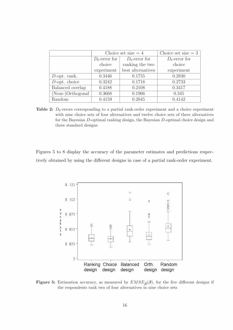
Choice set size = 4 Choice set size = 3Db-error for Db-error for Db-error for

choice ranking the two choiceexperiment best alternatives experiment

D-opt. rank. 0.3446 0.1755 0.2830D-opt. choice 0.3242 0.1718 0.2733Balanced overlap 0.4188 0.2108 0.3417(Near-)Orthogonal 0.3668 0.1966 0.345Random 0.4159 0.2045 0.4142

Table 2: Db-errors corresponding to a partial rank-order experiment and a choice experimentwith nine choice sets of four alternatives and twelve choice sets of three alternativesfor the Bayesian D-optimal ranking design, the Bayesian D-optimal choice design andthree standard designs

Figures 5 to 8 display the accuracy of the parameter estimates and predictions respec-

tively obtained by using the different designs in case of a partial rank-order experiment.

Figure 5: Estimation accuracy, as measured by EMSEβ(β), for the five different designs ifthe respondents rank two of four alternatives in nine choice sets

16

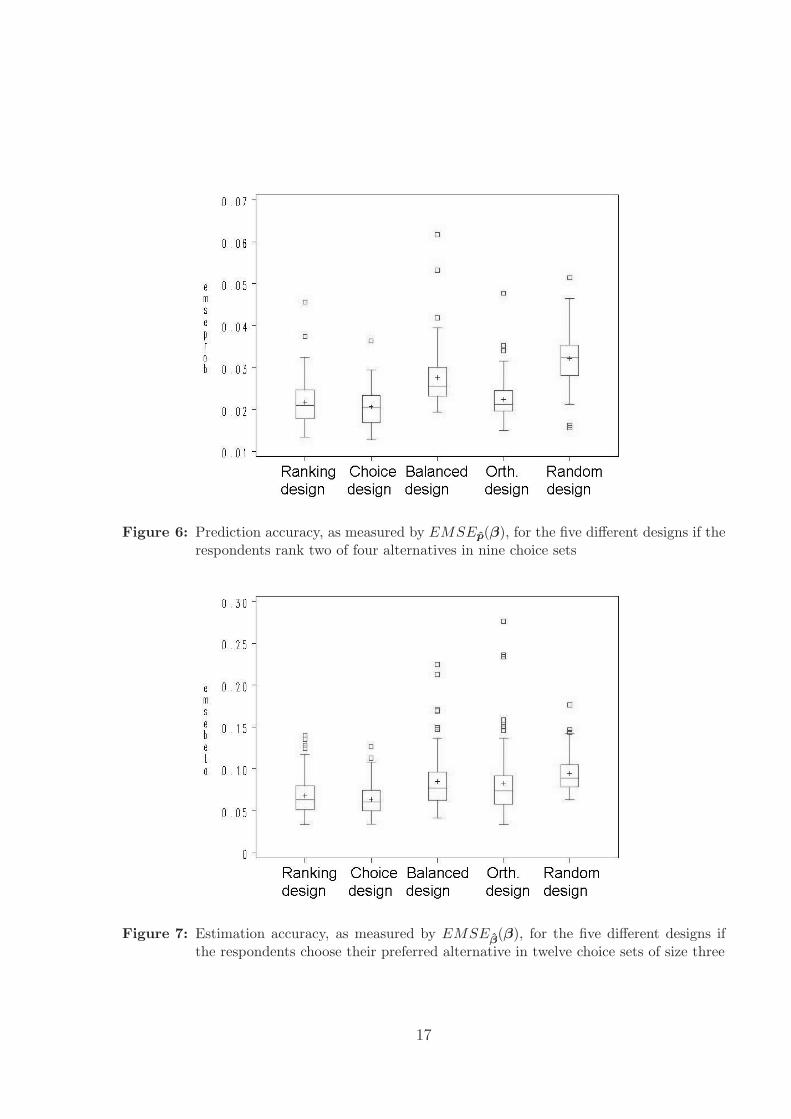
Figure 6: Prediction accuracy, as measured by EMSEp(β), for the five different designs if therespondents rank two of four alternatives in nine choice sets

Figure 7: Estimation accuracy, as measured by EMSEβ(β), for the five different designs ifthe respondents choose their preferred alternative in twelve choice sets of size three

17

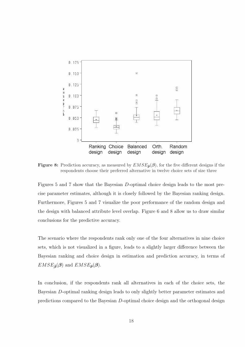
Figure 8: Prediction accuracy, as measured by EMSEp(β), for the five different designs if therespondents choose their preferred alternative in twelve choice sets of size three

Figures 5 and 7 show that the Bayesian D-optimal choice design leads to the most pre-

cise parameter estimates, although it is closely followed by the Bayesian ranking design.

Furthermore, Figures 5 and 7 visualize the poor performance of the random design and

the design with balanced attribute level overlap. Figure 6 and 8 allow us to draw similar

conclusions for the predictive accuracy.

The scenario where the respondents rank only one of the four alternatives in nine choice

sets, which is not visualized in a figure, leads to a slightly larger difference between the

Bayesian ranking and choice design in estimation and prediction accuracy, in terms of

EMSEβ(β) and EMSEp(β).

In conclusion, if the respondents rank all alternatives in each of the choice sets, the

Bayesian D-optimal ranking design leads to only slightly better parameter estimates and

predictions compared to the Bayesian D-optimal choice design and the orthogonal design

18

but does considerably better than the other standard designs used in marketing. Even

when the respondents do not rank all alternatives, we notice that the Bayesian D-optimal

ranking design results in more precise estimates and predictions than the random design

and the design with balanced attribute level overlap and yields only slightly less precise

estimates and predictions than the Bayesian D-optimal choice design. This leads to the

conclusion that a D-optimal choice design is also an appropriate design for the rank-order

conjoint experiment. A striking feature of the optimal designs compared to the standard

designs is that they never lead to very imprecise estimates or predictions. This can be seen

best from Figures 3, 5, 7 and 8 where the three standard designs all produce very large

EMSEβ(β) and EMSEp(β) values occasionally. This is unlike the optimal designs and

confirms earlier results by Woods et al. (2006) in the context of industrial experiments

involving non-normal responses.

We were able to draw similar conclusions for full and partial rank-order experiments with

two three-level attributes and one two-level attribute with nine and twelve choice sets of

size four and three, respectively.

4.2.3 The improvement in estimation and prediction accuracy by including

extra ranking steps

Tables 3 and 4 exhibit the benefits in terms of precision of the parameter estimates and

predicted probabilities by including an extra ranking step in case of nine choice sets of

size four.

Table 3 shows that there is a 60% improvement in estimation accuracy if the respondents

indicate which alternatives they like second best, in addition to the one they like best.

This implies that ranking two of four alternatives in nine choice sets requires 38% less

respondents than a choice experiment in order to have the same precision of parameter

estimates. If the respondents rank also the third alternative of four in each choice set

(and thus provide a full ranking of each choice set), a further improvement of some 30% is

19

obtained. This means that the number of respondents can be reduced further by another

23% to obtain the same estimation accuracy as the scenario where the respondents only

rank two of four alternatives. The EMSEp(β) values in Table 4 show that we can extend

these conclusions to the prediction accuracy. An accuracy gain of about 60% is acquired

by ranking a second alternative. If the respondents rank the full choice set, the predictions

are about 25% more accurate compared to the situation where the respondents rank only

two alternatives.

Improvement in EMSEβ

after assigning after assigningsecond rank third rank

D-opt. rank. 62.29% 30.45%D-opt. choice 58.07% 23.09%Balanced overlap 63.07% 34.23%(Near-)Orthogonal 64.78% 31.35%Random 61.69% 30.70%

Table 3: Improvement in the accuracy of the estimators of the model parameters, as measuredby EMSEβ(β), in case of a full and partial rank-order experiment with choice setsof size four for the five different designs

Improvement in EMSEp

after assigning after assigningsecond rank third rank

D-opt. rank. 57.96% 30.73%D-opt. choice 54.75% 23.70%Balanced overlap 58.41% 31.66%(Near-)Orthogonal 58.57% 27.79%Random 66.72% 27.80%

Table 4: Improvement in the accuracy of the predictions, as measured by EMSEp(β), in caseof a full and partial rank-order conjoint experiment with choice sets of size four forthe five different designs

For the case of twelve choice sets with three alternatives each, represented in Table 5, we

can draw similar conclusions: if the respondents rank the full choice set, an improvement

20

of about 50% is obtained in terms of estimation and prediction accuracy.

Improvement inEMSEβ EMSEp

D-opt. rank. 54.91% 52.45%D-opt. choice 50.12% 48.02%Balanced overlap 53.59% 49.26%(Near-)Orthogonal 54.47% 52.71%Random 49.06% 46.37%

Table 5: Improvement in the accuracy of the estimators of the model parameters and predic-tions, as measured by EMSEβ(β) and EMSEp(β), in case of a full and rank-orderexperiment with choice sets of size three for the five different designs

Because of those considerable improvements in estimation and prediction error, it is worth-

while to use rank-order conjoint experiments instead of conjoint choice experiments.

5 Conclusion

In a rank-order conjoint experiment, the respondent is asked to rank a number of al-

ternatives in each choice set. This way of performing a conjoint experiment offers the

important advantage that extra information is extracted about the preferences of the re-

spondent which results in better estimated part-worths and better predicted probabilities.

Although rank-ordered conjoint experiments are a popular instrument to measure con-

sumer preferences, the literature on experimental design for these experiments is very

scarce. In this paper, we try to fill this gap by proposing a D-optimality criterion focus-

ing on the precision of the estimates for the parameters of the ranked-ordered multinomial

logit model. To achieve this goal, the Fisher information matrix for this model was given.

This matrix clearly shows the additional information yielded by each extra ranking step

and is used to construct Bayesian D-optimal ranking designs. We compared these de-

signs with four benchmarks and concluded that the Bayesian D-optimal ranking design

21

performs slightly better in terms of the D-optimality criterion than its competitors if all

alternatives of a choice set are ranked. It is, however, closely followed by the Bayesian

D-optimal choice design.

We also used a simulation study to compare the Bayesian D-optimal ranking designs with

the four benchmark designs in terms of the estimation and predictive accuracy. We con-

clude that the Bayesian D-optimal ranking designs result in the most accurate estimates

and predictions if the respondents rank all alternatives. It should be pointed out, however,

that the Bayesian ranking and choice designs exhibit only minor differences. This allows

us to conclude that the Bayesian D-optimal conjoint choice designs are also appropriate

designs for rank-order conjoint experiments.

When examining the improvements in the precision of the estimates and predictions

yielded by each extra ranking step, we observed that a major gain in estimation and

predictive accuracy is achieved by including a second ranking step. Including a third

ranking step still offers a considerable improvement in estimation and predictive accu-

racy. Based on these substantial improvements in efficiency, we strongly recommend the

use of rank-order conjoint experiments instead of conjoint choice experiments.

6 Acknowledgments

We are grateful to Qi Ding for his contribution to the development of the adaptive algo-

rithm. He was funded by project NB/06/05 of the National Bank of Belgium.

22

Appendix

I. Bayesian D-optimal ranking design

Choice set Profile Attr. 1 Attr. 2 Attr. 3 Attr. 4 Attr. 51 1 3 1 3 1 1

2 3 3 2 1 23 1 2 1 2 24 2 1 2 2 1

2 1 3 2 1 2 22 2 2 3 1 13 2 3 2 1 24 1 1 2 2 1

3 1 3 1 1 2 22 1 3 1 1 13 1 2 3 1 24 2 2 2 2 1

4 1 1 3 2 1 22 1 2 3 2 13 3 2 1 1 14 2 1 1 2 2

5 1 3 2 2 1 12 1 2 2 2 23 2 1 3 1 24 3 3 1 2 1

6 1 2 3 1 1 22 3 1 3 2 13 1 1 2 1 24 2 2 2 2 1

7 1 2 2 1 2 12 1 1 3 1 23 1 3 3 2 14 3 2 2 1 2

8 1 2 2 3 1 22 1 1 1 2 23 3 3 2 2 14 2 3 1 1 1

9 1 2 1 2 2 22 1 2 1 1 23 1 3 3 2 14 3 1 2 1 1

23

II. Bayesian D-optimal choice design

Choice set Profile Attr. 1 Attr. 2 Attr. 3 Attr. 4 Attr. 51 1 3 2 1 2 1

2 2 2 2 1 13 1 3 3 1 24 2 1 2 2 2

2 1 2 3 2 2 22 3 2 1 1 23 1 2 3 2 14 3 1 3 1 1

3 1 1 1 3 2 22 3 2 2 1 23 2 1 3 1 14 2 3 1 2 1

4 1 2 1 2 1 12 1 2 2 2 23 3 3 1 1 24 2 1 3 2 1

5 1 1 1 3 1 22 3 3 2 1 13 1 1 2 2 14 2 2 1 2 2

6 1 3 1 3 1 22 2 2 1 2 13 1 2 1 1 24 1 3 2 2 1

7 1 2 2 2 1 12 3 1 1 2 23 2 3 3 1 14 1 2 2 1 2

8 1 1 1 1 2 22 2 1 2 1 23 2 3 1 1 24 3 2 3 2 1

9 1 2 2 3 1 22 3 1 2 2 13 1 1 1 1 24 1 3 1 2 1

24

III. (Near-)Orthogonal design

Choice set Profile Attr. 1 Attr. 2 Attr. 3 Attr. 4 Attr. 51 1 2 1 3 2 1

2 3 2 2 1 13 3 3 2 2 24 1 3 1 1 2

2 1 1 1 3 1 12 2 2 1 2 23 2 2 3 1 24 3 3 2 2 1

3 1 1 1 1 2 12 2 2 2 1 13 1 1 1 2 24 3 3 3 1 2

4 1 2 1 2 1 22 3 3 1 1 13 1 2 3 2 14 3 1 3 2 2

5 1 1 2 2 2 22 3 1 3 1 23 2 3 1 1 14 2 3 2 2 1

6 1 3 2 1 2 22 2 3 3 2 23 3 1 2 1 14 1 2 1 1 1

7 1 2 1 1 2 12 1 1 2 1 23 3 2 3 2 14 1 3 2 1 2

8 1 2 2 1 1 22 1 3 3 2 13 3 1 2 2 24 1 2 3 1 1

9 1 3 1 3 1 12 1 2 2 2 23 2 3 1 2 24 2 3 1 1 1

25

IV. Balanced overlap design

Choice set Profile Attr. 1 Attr. 2 Attr. 3 Attr. 4 Attr. 51 1 3 2 2 2 2

2 2 1 1 1 13 1 2 1 1 14 1 3 3 2 2

2 1 3 2 3 1 22 2 3 2 2 13 2 1 3 2 14 1 1 1 1 2

3 1 2 2 2 2 12 3 3 2 1 23 3 1 3 2 24 3 3 1 1 1

4 1 3 3 1 2 22 1 2 2 1 13 2 3 1 2 24 3 1 3 1 1

5 1 2 2 2 1 22 1 3 1 2 23 2 3 3 1 14 1 1 2 2 1

6 1 1 1 3 1 22 2 2 1 2 23 1 1 1 1 14 3 2 2 2 1

7 1 3 2 3 2 22 2 3 3 1 13 1 2 3 2 14 1 1 2 1 2

8 1 2 1 3 1 22 3 1 2 1 13 2 3 1 2 24 1 2 3 2 1

9 1 3 3 1 1 12 1 3 1 1 23 2 1 2 2 14 3 2 2 2 2

26

V. Random design

Choice set Profile Attr. 1 Attr. 2 Attr. 3 Attr. 4 Attr. 51 1 2 2 3 2 2

2 2 1 3 2 23 2 2 1 1 24 1 3 3 2 1

2 1 3 2 3 1 22 1 3 3 2 23 3 3 2 1 14 1 3 1 2 1

3 1 2 3 2 1 22 1 3 1 1 13 1 2 2 1 14 1 2 1 2 2

4 1 2 2 3 1 12 1 1 3 1 13 1 3 3 1 24 2 2 2 2 1

5 1 1 3 3 1 22 2 1 2 1 23 3 3 3 2 24 1 2 3 1 2

6 1 2 3 2 2 22 2 1 1 1 13 2 1 3 2 24 2 2 3 1 2

7 1 2 1 2 2 22 1 2 1 1 23 2 1 3 1 14 3 1 1 2 2

8 1 1 3 1 2 22 1 1 3 2 13 2 1 1 1 24 2 3 2 2 1

9 1 2 3 2 1 12 1 3 2 1 13 1 1 3 2 14 3 3 2 2 1

27

ReferencesAllison, P.D. and Christakis, N.A. (1994), Logit models for sets of ranked items, Socio-logical Methodology, 24, 199-228

Baarsma, B.E. (2003), The valuation of the Ijmeer Nature Reserve using conjoint analysis,Environmental and Resource Economics, 25, 343-356

Bateman, I.J., Carson, R.T., Day, B., Hanemann, M., Hanley, N., Hett, J., Jones-Lee,M., Loomes, G., Mourato, S., Ozdemiroglu, E., Pearce, D.W., Sugden, R. and Swanson,J. (2002), Economic valuation with stated preference techniques. A Manual, Cheltenham,Edward Elgar

Beggs, S., Cardell, S. and Hausman, J. (1981), Assessing the potential demand for electriccars, Journal of Econometrics, 16, 1-19

Boyle, K.J., Holmes, T.P., Teisl, M.F. and Roe, B. (2001), A comparison of conjointanalysis response formats, American Journal of Agricultural Economics, 83, 441-454

Chapman, R.G. and Staelin, R. (1982), Exploiting rank ordered choice set data withinthe stochastic utility model, Journal of Marketing Research, 19, 288-301

Gustafsson, A., Ekdahl, F. and Bergman, B. (1999), Conjoint analysis: a useful toolin the design process, Total Quality Management, 10, 327-343

Hausman, J.A. and Ruud, P.A. (1987), Specifying and testing econometric models forrank-ordered data, Journal of Econometrics, 34, 83-104

Kessels, R., Goos, P. and Vandebroek, M. (2006a), A comparison of criteria to designefficient choice experiments, Journal of Marketing Research, 43, 409-419

Kessels, R., Jones, B., Goos, P. and Vandebroek, M. (2006b), An efficient algorithmfor constructing Bayesian optimal choice designs, Research Report KBI 0616, Departmentof Decision Sciences and Information Management, Katholieke Universiteit Leuven, 29pp.

Kessels, R., Jones, B., Goos, P. and Vandebroek, M. (2006c), Recommendations on the useof Bayesian optimal designs for choice experiments, Research Report KBI 0617, Depart-ment of Decision Sciences and Information Management, Katholieke Universiteit Leuven,18pp.

Sandor, Z. and Wedel, M. (2001), Designing conjoint choice experiments using manager’sprior beliefs, Journal of Marketing Research, 38, 430-444

Sandor, Z. and Wedel, M. (2005), Heterogeneous conjoint choice designs, Journal of Mar-

28

keting Research, 42, 210-218

Train, K. (2003), Discrete Choice Methods with Simulations, Cambridge University Press

Woods, D.C., Lewis, S.M., Eccleston, J.A. and Russel, K.G. (2006), Designs for gen-eralized linear models with several variables and model uncertainty, Technometrics, 48,284-292

29