Paper ID #15686

Experiments for a Unit Operations in Food Engineering Course

Dr. Polly R. Piergiovanni, Lafayette College

Polly R. Piergiovanni is a Professor of Chemical Engineering at Lafayette College. Besides chemicalengineering courses, she teaches an engineering course to nonengineering students. Her current researchinterests include critical thinking evident in student writing and assessing learning in experiential learningactivities.

Mr. John H Jarboe

Lafayette College class of 2016 chemical engineering student

c©American Society for Engineering Education, 2016

Experiments for a Unit Operations in Food Engineering Course Abstract: A series of hands-on activities were developed to accompany a Unit Operations in Food Engineering course. The activities covered mechanical properties, the mechanical energy balance, and heat transfer. Each experiment was completed in a two-hour class period. Equipment for one group of students would cost approximately $50, assuming basic laboratory equipment is available. Total expenditures on supplies for the three labs were less than $100. Learning objectives, proposed assessment of student learning and specific details of the experiments are included for each experiment. Background Information: Junior chemical engineering students at Lafayette College take a Transport Phenomena course in the fall semester, where they learn the theory of momentum and heat transfer. In the spring, the students enroll in Applied Fluid Dynamics and Heat Transfer. This course covers practical applications of the theory, such as pump and heat exchanger sizing. The course has two weekly one-hour lecture times and one two-hour problem solving time. The students are also simultaneously enrolled in a Unit Operations laboratory where traditional experiments on pumps, heat exchangers and packed beds are performed. Due to enrollment growth, two sections of the applied course are offered each year, and due to student interest, one section focuses on unit operations in the food industry. The experiments described below were offered in the food unit operations section of the course – not as part of the Unit Operations laboratory course. Twelve to sixteen students enroll in this section each year. The course begins with information on physical properties of foods, including rheology, and electrical and mechanical properties. While these are not covered in a traditional unit operations course, they are a necessary foundation for this course, and are useful for any chemical engineer. The first experiment covers mechanical properties important to the food industry, providing background for the rest of the course. The next portion of the course covers the mechanical energy balance. Since most foods are non-Newtonian, the experiment introduced students to the categories and characterization of non-Newtonian fluids and the necessary modifications to the mechanical energy balance. The third portion of the class covers heat transfer in food preservation and cooking unit operations. The students were intrigued by the idea that during cooking and baking, the temperature of the food does not exceed the boiling point of water. This was illustrated and modeled with an experiment.

Experiments: Mechanical Properties of Foods During class, students learned the biochemistry of gluten formation along with how the amount of moisture, kneading process and resting time influence the strength of the gluten strands. During the two hour portion of class, groups of two students prepared gluten dough and used a device to hang a piece of dough and suspend weights from it (see Figure 1). The length of the dough was measured as a function of time or suspended mass to determine material properties of gluten. The learning objectives for this experiment are listed in Table 1, and the assessment questions are listed in Table 2. While this experiment may not be applicable to the traditional unit operations course, material characterization is an important concept for chemical engineers. An understanding of stress and strain may also help students understand viscometer operation as well.

 Figure 1. Apparatus used for testing mechanical properties. The gluten is connected to the S-hook and the hanging tray. As more washers are added to the tray, the gluten stretches. Its length is measured on the scale behind the tray.

 

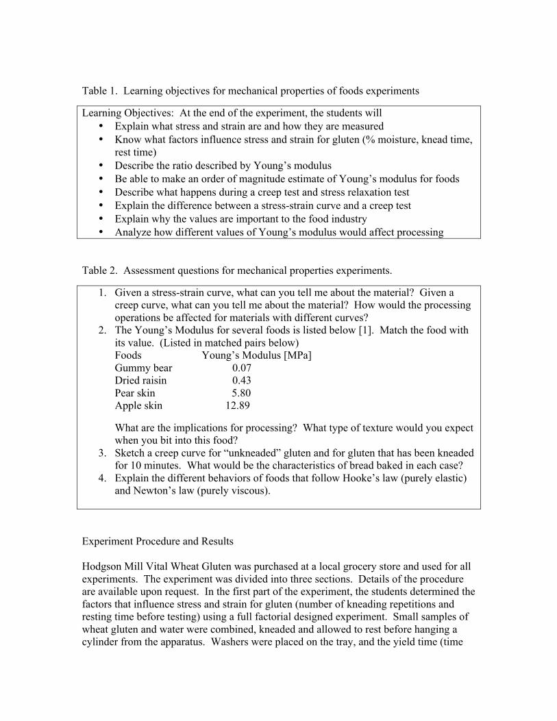
Table 1. Learning objectives for mechanical properties of foods experiments

Learning Objectives: At the end of the experiment, the students will • Explain what stress and strain are and how they are measured • Know what factors influence stress and strain for gluten (% moisture, knead time,

rest time) • Describe the ratio described by Young’s modulus • Be able to make an order of magnitude estimate of Young’s modulus for foods • Describe what happens during a creep test and stress relaxation test • Explain the difference between a stress-strain curve and a creep test • Explain why the values are important to the food industry  • Analyze how different values of Young’s modulus would affect processing  

Table 2. Assessment questions for mechanical properties experiments.

1. Given a stress-strain curve, what can you tell me about the material? Given a creep curve, what can you tell me about the material? How would the processing operations be affected for materials with different curves?

2. The Young’s Modulus for several foods is listed below [1]. Match the food with its value. (Listed in matched pairs below) Foods Young’s Modulus [MPa]  Gummy bear 0.07  Dried raisin 0.43  Pear skin 5.80  Apple skin 12.89    What are the implications for processing? What type of texture would you expect when you bit into this food?  

3. Sketch a creep curve for “unkneaded” gluten and for gluten that has been kneaded for 10 minutes. What would be the characteristics of bread baked in each case?

4. Explain the different behaviors of foods that follow Hooke’s law (purely elastic) and Newton’s law (purely viscous).

Experiment Procedure and Results Hodgson Mill Vital Wheat Gluten was purchased at a local grocery store and used for all experiments. The experiment was divided into three sections. Details of the procedure are available upon request. In the first part of the experiment, the students determined the factors that influence stress and strain for gluten (number of kneading repetitions and resting time before testing) using a full factorial designed experiment. Small samples of wheat gluten and water were combined, kneaded and allowed to rest before hanging a cylinder from the apparatus. Washers were placed on the tray, and the yield time (time

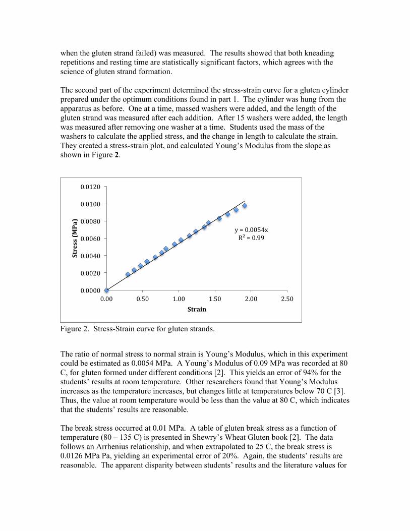
when the gluten strand failed) was measured. The results showed that both kneading repetitions and resting time are statistically significant factors, which agrees with the science of gluten strand formation. The second part of the experiment determined the stress-strain curve for a gluten cylinder prepared under the optimum conditions found in part 1. The cylinder was hung from the apparatus as before. One at a time, massed washers were added, and the length of the gluten strand was measured after each addition. After 15 washers were added, the length was measured after removing one washer at a time. Students used the mass of the washers to calculate the applied stress, and the change in length to calculate the strain. They created a stress-strain plot, and calculated Young’s Modulus from the slope as shown in Figure 2.

 Figure 2. Stress-Strain curve for gluten strands.

The ratio of normal stress to normal strain is Young’s Modulus, which in this experiment could be estimated as 0.0054 MPa. A Young’s Modulus of 0.09 MPa was recorded at 80 C, for gluten formed under different conditions [2]. This yields an error of 94% for the students’ results at room temperature. Other researchers found that Young’s Modulus increases as the temperature increases, but changes little at temperatures below 70 C [3]. Thus, the value at room temperature would be less than the value at 80 C, which indicates that the students’ results are reasonable. The break stress occurred at 0.01 MPa. A table of gluten break stress as a function of temperature (80 – 135 C) is presented in Shewry’s Wheat Gluten book [2]. The data follows an Arrhenius relationship, and when extrapolated to 25 C, the break stress is 0.0126 MPa Pa, yielding an experimental error of 20%. Again, the students’ results are reasonable. The apparent disparity between students’ results and the literature values for

y  =  0.0054x  R²  =  0.99  

0.0000  

0.0020  

0.0040  

0.0060  

0.0080  

0.0100  

0.0120  

0.00   0.50   1.00   1.50   2.00   2.50  

Stress  (M

Pa)  

Strain  

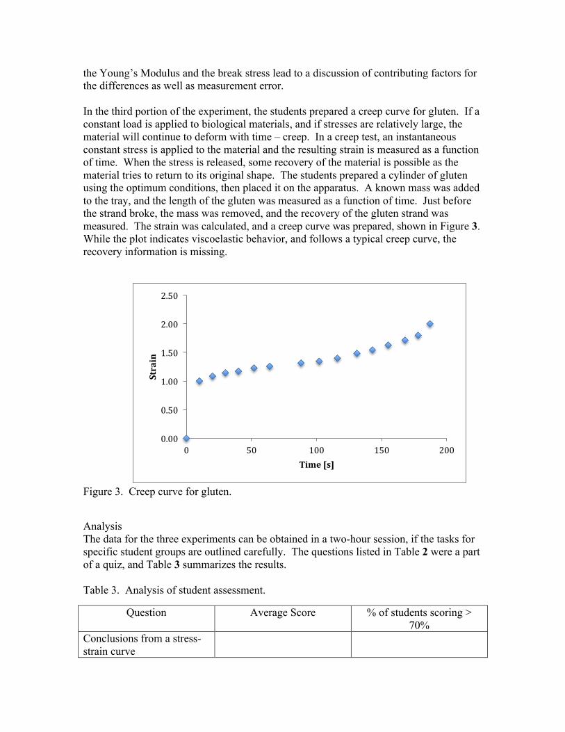
the Young’s Modulus and the break stress lead to a discussion of contributing factors for the differences as well as measurement error. In the third portion of the experiment, the students prepared a creep curve for gluten. If a constant load is applied to biological materials, and if stresses are relatively large, the material will continue to deform with time – creep. In a creep test, an instantaneous constant stress is applied to the material and the resulting strain is measured as a function of time. When the stress is released, some recovery of the material is possible as the material tries to return to its original shape. The students prepared a cylinder of gluten using the optimum conditions, then placed it on the apparatus. A known mass was added to the tray, and the length of the gluten was measured as a function of time. Just before the strand broke, the mass was removed, and the recovery of the gluten strand was measured. The strain was calculated, and a creep curve was prepared, shown in Figure 3. While the plot indicates viscoelastic behavior, and follows a typical creep curve, the recovery information is missing.

 Figure 3. Creep curve for gluten.

Analysis The data for the three experiments can be obtained in a two-hour session, if the tasks for specific student groups are outlined carefully. The questions listed in Table 2 were a part of a quiz, and Table 3 summarizes the results. Table 3. Analysis of student assessment.

Question   Average Score   % of students scoring > 70%  

Conclusions from a stress-strain curve

0.00  

0.50  

1.00  

1.50  

2.00  

2.50  

0   50   100   150   200  

Strain  

Time  [s]  

Conclusions from a creep curve

Matching foods with Young’s Modulus

Implications of Young’s Modulus on food processing

Creep curve for kneaded and unkneaded gluten

Hooke’s Law and Newton’s Law food behavior

Mechanical Energy Balance and Non-Newtonian Foods Many food products are non-Newtonian fluids. To apply the mechanical energy balance, a generalized Reynolds number and modified friction loss relationships must be used. While centrifugal pumps are common, they cannot pump certain types of non-Newtonian fluids. Centrifugal pumps are suitable for fluids with low viscosity – the velocity produces high liquid shear. However, as the viscosity increases, there is generally a small reduction in flow, a decrease in head, and an increase in power required [4]. Positive displacement pumps are generally used with highly viscous fluids, Compared to a centrifugal pump, the speed is lower and the pump imparts less shear. This experiment was developed to introduce students to these concepts. The learning objectives are shown in Table 4 and the assessment questions are shown in Table 5. Ketchup was used as an easily available non-Newtonian fluid. Table 4. Learning objectives for pumping non-Newtonian fluids.

Learning Objectives: At the end of the experiment, the students will be able to

• Explain how non-Newtonian fluids’ viscosity is characterized  • Describe how a shear thinning fluid behaves when pumped  • Explain why different pump types are used for non-Newtonian fluids  • Create a pump characteristic curve (Head vs. flow, Power vs. flow)  • Explain the difference in the curves for Newtonian and non-Newtonian fluids  • Compare friction losses for the two types of fluids  • Apply the mechanical energy balance to various pumping situations for both

Newtonian and non-Newtonian fluids. Table 5. Assessment questions for the mechanical energy balance

1. You have been given a new fluid that exhibits the following behavior. What type of fluid is it?  

2. Given the data for the fluid below, find the values that characterize its viscosity. 3. The efflux tank is filled with a shear thinning fluid. At time = 0, the plug is

removed, and the fluid starts to exit the tank. What happens to the shear rate during the first few seconds? What happens to the viscosity of the fluid?  

4. Why are centrifugal pumps not used for highly viscous fluids? Sometimes, however, a centrifugal pump is perfect for a shear thinning liquid – why?  

5. A fluid must be pumped from position A to position B as shown in the diagram below. Calculate the pump work needed if the fluid is water. Calculate the pump work needed if the fluid is ketchup. Properties of the fluids are included.

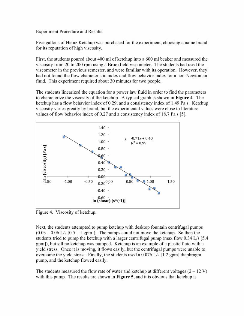
Experiment Procedure and Results Five gallons of Heinz Ketchup was purchased for the experiment, choosing a name brand for its reputation of high viscosity. First, the students poured about 400 ml of ketchup into a 600 ml beaker and measured the viscosity from 20 to 200 rpm using a Brookfield viscometer. The students had used the viscometer in the previous semester, and were familiar with its operation. However, they had not found the flow characteristic index and flow behavior index for a non-Newtonian fluid. This experiment required about 30 minutes for two people. The students linearized the equation for a power law fluid in order to find the parameters to characterize the viscosity of the ketchup. A typical graph is shown in Figure 4. The ketchup has a flow behavior index of 0.29, and a consistency index of 1.49 Pa s. Ketchup viscosity varies greatly by brand, but the experimental values were close to literature values of flow behavior index of 0.27 and a consistency index of 18.7 Pa s [5].

 Figure 4. Viscosity of ketchup.

Next, the students attempted to pump ketchup with desktop fountain centrifugal pumps (0.03 – 0.06 L/s [0.5 – 1 gpm]). The pumps could not move the ketchup. So then the students tried to pump the ketchup with a larger centrifugal pump (max flow 0.34 L/s [5.4 gpm]), but sill no ketchup was pumped. Ketchup is an example of a plastic fluid with a yield stress. Once it is moving, it flows easily, but the centrifugal pumps were unable to overcome the yield stress. Finally, the students used a 0.076 L/s [1.2 gpm] diaphragm pump, and the ketchup flowed easily. The students measured the flow rate of water and ketchup at different voltages (2 – 12 V) with this pump. The results are shown in Figure 5, and it is obvious that ketchup is

y  =  -­‐0.71x  +  0.40  R²  =  0.99  

-­‐0.60  

-­‐0.40  

-­‐0.20  

0.00  

0.20  

0.40  

0.60  

0.80  

1.00  

1.20  

1.40  

-­‐1.50   -­‐1.00   -­‐0.50   0.00   0.50   1.00   1.50  

ln  (viscosity)  [Pa  s]  

ln  (shear)  [s^(-­‐1)]  

pumped at a lower flow rate than water. The apparatus has pressure sensors across two elbows so friction losses could also be measured.

 Figure 5. Flow rate of ketchup and water as a function of voltage.

Table 6. Analysis of student assessment.

Question   Average Score   % of students scoring > 70%  

Fluid behavior determination

Characterize viscosity 73.1% 54% Efflux tank 87.2% 77% Centrifugal pump 92.3% 85% Pumping ketchup 88.7% 77%

0  

0.01  

0.02  

0.03  

0.04  

0.05  

0.06  

0.07  

0.08  

0.09  

0   5   10   15  

Mass  Flow

 [kg/s]  

Voltage  [V]  

Ketchup  

Water  

Unsteady State Conduction In a previous course, the students had learned about Fourier’s Law of Conduction, and performed an experiment to understand a solution to !"

!"=  𝛼 !!!

!!! . They had a general

understanding of unsteady state conduction and the solution for an infinite rod heated at one end. In this course the students are expected to use solutions of the equations for practical applications. Specifically, in the food engineering course, the students examined the rate of heating of an individual gnocchi. The learning objectives for this experiment are listed in Table 7 and Table 8 lists the assessment questions.

Table 7. Learning objectives for unsteady state conduction

Learning Objectives: At the end of the experiment, the students will • Be able to use composition equations to estimate physical property data • Describe how gnocchi heat up when placed in boiling water and know how much

water they gain as they cook. • Determine if the presence of salt in the water has a statistically significant effect on

the final temperature or the time to reach 98 C • Explain discrepancies in the temperature profile with different unsteady state

models of heat transfer and determine which one fits best • Calculate how long gnocchi should be boiled to obtain their preferred texture.

Table 8. Assessment questions for the unsteady state conduction experiment.

1. Use the composition equations below to estimate the thermal diffusivity of canned peas.

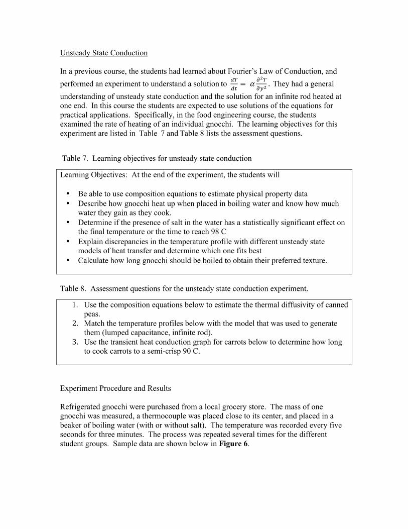
2. Match the temperature profiles below with the model that was used to generate them (lumped capacitance, infinite rod).  

3. Use the transient heat conduction graph for carrots below to determine how long to cook carrots to a semi-crisp 90 C.  

Experiment Procedure and Results Refrigerated gnocchi were purchased from a local grocery store. The mass of one gnocchi was measured, a thermocouple was placed close to its center, and placed in a beaker of boiling water (with or without salt). The temperature was recorded every five seconds for three minutes. The process was repeated several times for the different student groups. Sample data are shown below in Figure 6.

 Figure 6. Unsteady state gnocchi conduction. BPE indicates that salt was added to the water.

In order to model the unsteady state conduction, thermal properties for gnocchi needed to be estimated. Students used equations from ASHRAE to estimate thermal properties, based on temperature and amount of protein, fat, carbohydrate, fiber, ash and moisture [6]. The amount of water has the most significant effect on the properties, and must be found experimentally. Finally, the students were able to obtain an estimate for the thermal diffusivity. Next, the dimensionless temperature, Θ, was calculated. The Fourier number was calculated for two models (infinite rod and lumped capacitance) and the theoretical line was plotted along with the experimental data. While neither model was perfect (see Figure 7 and Figure 8), the exercise helped students understand the assumptions behind the equations.

0  

20  

40  

60  

80  

100  

120  

0   50   100   150   200   250  

Temp  [C]  

Time  [s]  

5.5  g  Gnocchi  

5.4  g  Gnocchi  

5.6  g  Gnocchi  

BPE  5.4  g  Gnocchi  

BPE  5.5  g  Gnocchi  

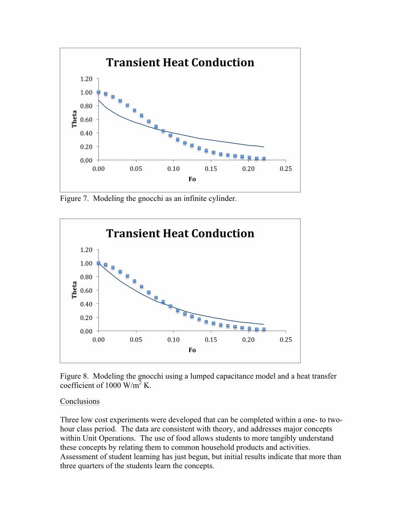
 Figure 7. Modeling the gnocchi as an infinite cylinder.

 

 

Figure 8. Modeling the gnocchi using a lumped capacitance model and a heat transfer coefficient of 1000 W/m2 K.

Conclusions Three low cost experiments were developed that can be completed within a one- to two-hour class period. The data are consistent with theory, and addresses major concepts within Unit Operations. The use of food allows students to more tangibly understand these concepts by relating them to common household products and activities. Assessment of student learning has just begun, but initial results indicate that more than three quarters of the students learn the concepts.

0.00  

0.20  

0.40  

0.60  

0.80  

1.00  

1.20  

0.00   0.05   0.10   0.15   0.20   0.25  

Theta  

Fo  

Transient  Heat  Conduction  

0.00  

0.20  

0.40  

0.60  

0.80  

1.00  

1.20  

0.00   0.05   0.10   0.15   0.20   0.25  

Theta  

Fo  

Transient  Heat  Conduction  

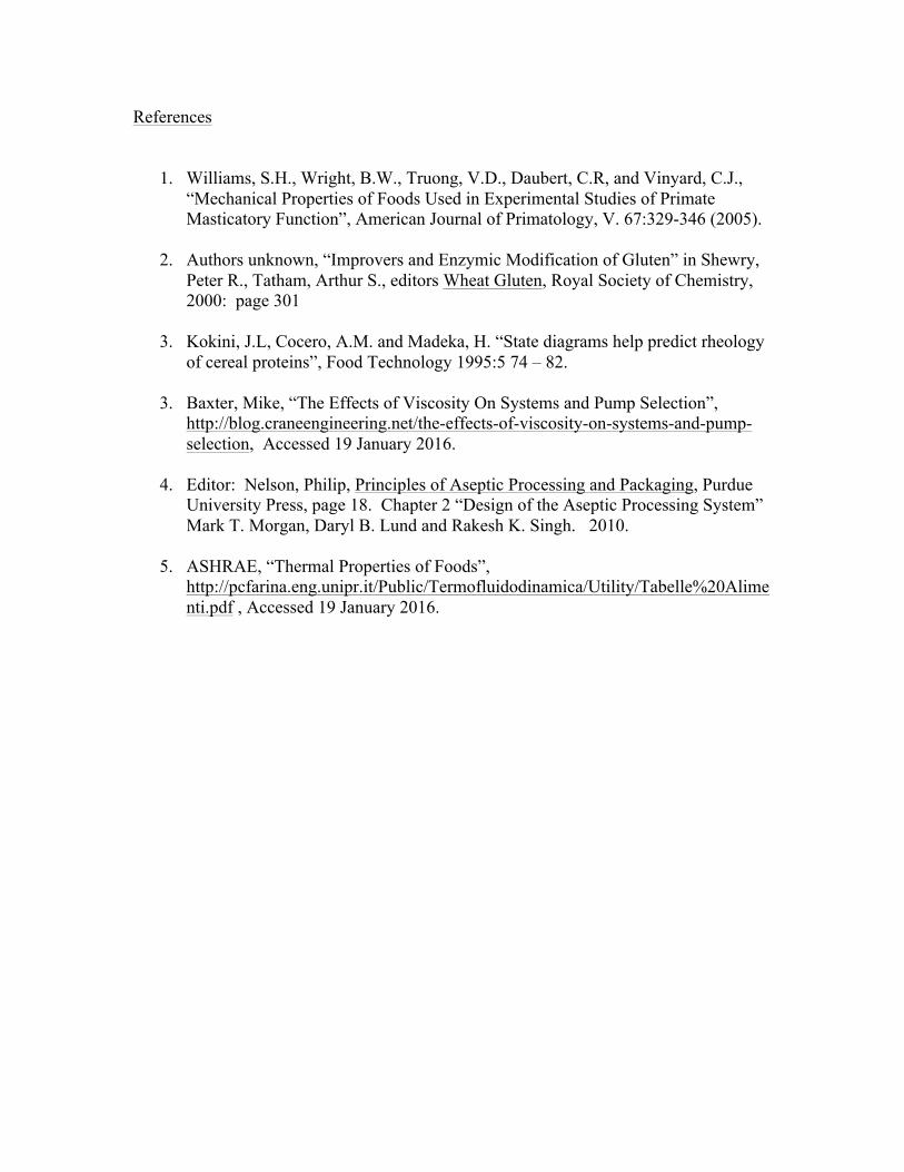
References

1. Williams, S.H., Wright, B.W., Truong, V.D., Daubert, C.R, and Vinyard, C.J., “Mechanical Properties of Foods Used in Experimental Studies of Primate Masticatory Function”, American Journal of Primatology, V. 67:329-346 (2005).

2. Authors unknown, “Improvers and Enzymic Modification of Gluten” in Shewry, Peter R., Tatham, Arthur S., editors Wheat Gluten, Royal Society of Chemistry, 2000: page 301

3. Kokini, J.L, Cocero, A.M. and Madeka, H. “State diagrams help predict rheology

of cereal proteins”, Food Technology 1995:5 74 – 82.

3. Baxter, Mike, “The Effects of Viscosity On Systems and Pump Selection”, http://blog.craneengineering.net/the-effects-of-viscosity-on-systems-and-pump-selection, Accessed 19 January 2016.

4. Editor: Nelson, Philip, Principles of Aseptic Processing and Packaging, Purdue University Press, page 18. Chapter 2 “Design of the Aseptic Processing System” Mark T. Morgan, Daryl B. Lund and Rakesh K. Singh. 2010.

5. ASHRAE, “Thermal Properties of Foods”, http://pcfarina.eng.unipr.it/Public/Termofluidodinamica/Utility/Tabelle%20Alimenti.pdf , Accessed 19 January 2016.