Experimental, numerical and analytical studies of abrasive wear: correlation between wear mechanisms...
365
EXPERIMENTAL, NUMERICAL, AND ANALYTICAL STUDIES ON THE SEISMIC RESPONSE OF STEEL-PLATE CONCRETE (SC) COMPOSITE SHEAR WALLS by Siamak Epackachi December 2014 A dissertation submitted to the Faculty of the Graduate School of the University at Buffalo, the State University of New York in partial fulfillment of the requirements for the degree of Doctor of Philosophy Department of Civil, Structural and Environmental Engineering
Transcript of Experimental, numerical and analytical studies of abrasive wear: correlation between wear mechanisms...

EXPERIMENTAL, NUMERICAL, AND ANALYTICAL STUDIES
ON THE SEISMIC RESPONSE OF STEEL-PLATE CONCRETE (SC)
COMPOSITE SHEAR WALLS
by
Siamak Epackachi
December 2014
A dissertation submitted to the
Faculty of the Graduate School of the
University at Buffalo, the State University of New York
in partial fulfillment of the requirements for the
degree of
Doctor of Philosophy
Department of Civil, Structural and Environmental Engineering


i
ACKNOWLEDGMENT
This research was conducted as part of a NEES research project on conventional and composite
structural walls with low aspect ratios. The project was funded by the U.S. National Science
Foundation under Grant No. 0829978. This financial support is gratefully acknowledged.
I thank my advisor, Professor Andrew Whittaker, for his guidance, support, and patience over the
course of the past four years. Professor Whittaker was my advisor in both life and academia and I
plan to collaborate with him in the future. I thank Professor Amit Varma from Purdue University,
for his support and guidance during the research project. I thank and acknowledge the important
contributions of my dissertation committee members, Professor Amjad Aref and Professor
Mettupalayam Sivaselvan.
I acknowledge and thank the following individuals and groups for their contributions to my
research product: Mr. Nam H. Nguyen at the University at Buffalo and Mr. Efe Kurt at Purdue
University, and the technicians and staff of the Bowen Laboratory at Purdue University, and
LPCiminelli Inc.
I thank the staff of the Structural Engineering and Earthquake Simulation Laboratory at the
University at Buffalo, specifically, Mr. Chris Budden, Mr. Jeff Cizdziel, Mr. Duane Kozlowski
(deceased), Mr. Lou Moretta, Mr. Mark Pitman, Mr. Robert Staniszewski, Mr. Scot Weinreber,
and Mr. Chris Zwierlein for their assistance in constructing and testing the composite walls. I am
most grateful to the faculty in Civil Engineering for making my journey through UB an incredible
experience, which has reinforced my commitment to lifelong learning. I thank all of my friends in
Ketter Hall and hope that our friendships will continue and flourish through future collaborations.
I wish to express my love and gratitude to my wife Ghazaleh for her continous encouragement,
patience, and support over the course of my studies and to my young daughter Fatemeh for her
presence that has always reminded me what is most important in life. I thank my parents, my
parents-in-law, and my sister-in-law for their support and patience during my studies. My family
has been an endless source of peace and inspiration, and their unequivocal support made my studies
possible.

ii
������������ � ���
������� ������� ����

iii
TABLE OF CONTENTS
ACKNOWLEDGMENT ............................................................................................................................. i
TABLE OF CONTENTS .......................................................................................................................... iii
LIST OF FIGURES ................................................................................................................................... ix
LIST OF TABLES ................................................................................................................................... xvi
ABSTRACT ............................................................................................................................................. xvii
GLOSSARY............................................................................................................................................ xviii
1. INTRODUCTION ............................................................................................................................. 1-1
1.1 General ............................................................................................................................................ 1-1
1.2 Research Objectives ........................................................................................................................ 1-4
1.3 Research Outline .............................................................................................................................. 1-6
2. LITERATURE REVIEW ................................................................................................................. 2-1
2.1 Overview ......................................................................................................................................... 2-1
2.2 Review of Experimental Studies on SC walls ................................................................................. 2-1
2.3 Review of Studies on Finite Element (Micro) Modeling of SC Walls .......................................... 2-28
3. PRELIMINARY DESIGN AND ANALYSIS OF SC WALLS ..................................................... 3-1
3.1 Introduction ..................................................................................................................................... 3-1
3.2 Preliminary Design of Test Specimens ............................................................................................ 3-1
3.3 Cross-Sectional Analysis of SC Walls ............................................................................................ 3-3
3.3.1 Introduction .............................................................................................................................. 3-3
3.3.2 XTRACT Analysis of SC walls ............................................................................................... 3-4
3.3.2.1 Material Properties ............................................................................................................ 3-4
3.3.2.2 Flexural Strengths of SC Walls ......................................................................................... 3-6
3.4 Pre-Test Finite Element Analysis of SC Walls ................................................................................ 3-8
3.5 Design of the SC Wall Base Connection and the Foundation Block ............................................. 3-10

iv
4. EXPERIMENTAL PROGRAM ...................................................................................................... 4-1
4.1 Introduction ..................................................................................................................................... 4-1
4.2 Description of the SC Wall Specimens ........................................................................................... 4-1
4.3 Construction of the Test Specimens and the Foundation Block ...................................................... 4-3
4.3.1 Wall Specimen Construction .................................................................................................... 4-4
4.3.2 Foundation Construction .......................................................................................................... 4-6
4.4 Material Testing ............................................................................................................................... 4-7
4.4.1 Studs and Tie Rods ................................................................................................................... 4-7
4.4.2 Steel Faceplates ........................................................................................................................ 4-7
4.4.3 Infill Concrete and Foundation................................................................................................. 4-8
4.5 Test Setup ...................................................................................................................................... 4-10
4.5.1 Installation of the Foundation Block ...................................................................................... 4-10
4.5.2 Installation of the SC Wall Panels .......................................................................................... 4-10
4.6 Loading Protocol ........................................................................................................................... 4-11
4.7 Instrumentation of Test Specimens ............................................................................................... 4-16
4.7.1 Krypton LEDs ........................................................................................................................ 4-16
4.7.2 Rosette Strain Gages .............................................................................................................. 4-18
4.7.3 LVDTs, Temposonic Displacement Transducers, and String Potentiometers ....................... 4-20
5. EXPERIMENTAL RESULTS ......................................................................................................... 5-1
5.1 Introduction ..................................................................................................................................... 5-1
5.2 Test Result ....................................................................................................................................... 5-1
5.3 Damage to SC Walls ........................................................................................................................ 5-2
5.4 Load-Displacement Cyclic Response .............................................................................................. 5-5
5.5 Post Peak Response of SC Walls ..................................................................................................... 5-9
5.6 Energy Dissipation and Viscous Damping .................................................................................... 5-10
5.7 Strain and Stress Fields in the Steel Faceplates ............................................................................. 5-12
5.8 Vertical Strain in the Steel Faceplates ........................................................................................... 5-15
5.9 Load Transfer in the SC Walls ...................................................................................................... 5-18

v
5.10 Lateral Displacement Profile ....................................................................................................... 5-21
5.11 Displacement Components .......................................................................................................... 5-21
5.12 Displacement Ductility of the SC Walls ...................................................................................... 5-24
5.13 Averaged Secant Stiffness ........................................................................................................... 5-26
6. NUMERICAL ANALYSIS OF SC WALLS ................................................................................... 6-1
6.1 Introduction ..................................................................................................................................... 6-1
6.2 ABAQUS Analysis .......................................................................................................................... 6-1
6.2.1 Concrete Material Model ......................................................................................................... 6-1
6.2.1.1 Stress-Strain Relationship ................................................................................................. 6-2
6.2.1.2 Yield Function .................................................................................................................. 6-2
6.2.1.3 Flow Rule .......................................................................................................................... 6-3
6.2.1.4 Damage and Stiffness Degradation ................................................................................... 6-4
6.2.1.5 Modeling Parameters ........................................................................................................ 6-4
6.2.2 Steel Material Model ................................................................................................................ 6-6
6.2.3 Contact and Constraint Modeling............................................................................................. 6-6
6.2.4 Elements, Loading, and Boundary Conditions ......................................................................... 6-6
6.2.5 ABAQUS Analysis Results ...................................................................................................... 6-7
6.3 VecTor2 Analysis .......................................................................................................................... 6-12
6.3.1 SC Wall Modeling .................................................................................................................. 6-12
6.3.2 VecTor2 Modeling of the SC Walls ....................................................................................... 6-14
6.3.2.1 Material Model................................................................................................................ 6-14
6.3.2.2 Elements, Loading, and Boundary Conditions ............................................................... 6-15
6.3.3 VecTor2 Analysis Results ...................................................................................................... 6-17
6.3.3.1 Load-Displacement Monotonic Response ...................................................................... 6-17
6.3.3.2 Crack Patterns in the Infill Concrete ............................................................................... 6-18
6.3.3.3 Strain Distributions ......................................................................................................... 6-18
6.3.3.4 Stress Distribution ........................................................................................................... 6-19
6.3.3.5 Load-Displacement Cyclic Response ............................................................................. 6-21
6.4 LS-DYNA Analysis ....................................................................................................................... 6-21
6.4.1 Concrete Material Model ....................................................................................................... 6-22
6.4.1.1 Plasticity Model Definition in the Winfrith Model ......................................................... 6-23

vi
6.4.1.2 Crack Analysis in the Winfrith Model ............................................................................ 6-25
6.4.1.3 Values of Parameters Input to the Winfrith Model ......................................................... 6-27
6.4.2 Steel Material Model .............................................................................................................. 6-28
6.4.3 Contact and Constraint Modeling........................................................................................... 6-29
6.4.4 Elements ................................................................................................................................. 6-29
6.4.4.1 Mesh Convergence Study ............................................................................................... 6-30
6.4.5 Loading and Boundary Conditions......................................................................................... 6-31
6.4.6 LS-DYNA Analysis Results ................................................................................................... 6-34
6.4.6.1 Load-Displacement Cyclic Response ............................................................................. 6-34
6.4.6.2 Hysteretic Damping ........................................................................................................ 6-35
6.4.6.3 Steel Faceplate Contribution to the Total Load .............................................................. 6-36
6.4.6.4 Damage to SC walls ........................................................................................................ 6-41
6.4.7 Validation of the DYNA Model ............................................................................................. 6-41
6.5 Exploration of Modeling Assumptions and Design Decisions ...................................................... 6-44
6.5.1 Load Transfer Mechanism in SC Walls ................................................................................. 6-44
6.5.2 Friction ................................................................................................................................... 6-47
6.5.3 Studs Attaching the Baseplate to the Infill Concrete .............................................................. 6-48
6.5.4 Axial and Shearing Forces Transferred by Connectors .......................................................... 6-50
7. A PARAMETRIC STUDY: DESIGN OF SC WALLS ................................................................. 7-1
7.1 Introduction ..................................................................................................................................... 7-1
7.2 DYNA Modeling of SC Walls ......................................................................................................... 7-1
7.2.1 Design Variables ...................................................................................................................... 7-1
7.2.2 Material Models ....................................................................................................................... 7-2
7.2.3 Contact, Element, Loading, and Boundary Condition ............................................................. 7-4
7.3 Monotonic Analysis Results ............................................................................................................ 7-4
7.3.1 Aspect Ratio ............................................................................................................................. 7-8
7.3.2 Reinforcement Ratio ................................................................................................................ 7-9
7.3.3 Concrete Compressive Strength ............................................................................................. 7-10
7.4 Shearing Strength .......................................................................................................................... 7-11
7.4.1 Depth of the Neutral Axis ...................................................................................................... 7-12
7.4.2 Average Shear Stress in the Compression Strut ..................................................................... 7-13
7.4.3 Average Shear Stress in the Steel Faceplates ......................................................................... 7-13

vii
7.5 Stiffness Prediction ........................................................................................................................ 7-16
7.6 Steel Faceplate Contribution to the Total Shear Load ................................................................... 7-19
7.7 Shearing Response of SC Walls .................................................................................................... 7-19
8. ANALYTICAL MODELING OF RECTANGULAR SC WALL PANELS ................................ 8-1
8.1 Introduction ..................................................................................................................................... 8-1
8.2 Simplified Monotonic Analysis of SC Walls .................................................................................. 8-1
8.2.1 Shearing Force-Shearing Strain Relationship .......................................................................... 8-3
8.2.1.1 Concrete Cracking: Break Point A.................................................................................... 8-3
8.2.1.2 Steel Faceplate Yielding: Break Point B ........................................................................... 8-4
8.2.1.3 Concrete Crushing: Break Point C .................................................................................... 8-9
8.2.2 Moment-Curvature Relationship ............................................................................................ 8-10
8.2.2.1 Cracking of the Infill Concrete ....................................................................................... 8-10
8.2.2.2 Steel Faceplate Yielding at the Tension End of the Wall Panel...................................... 8-11
8.2.2.3 Steel Faceplate Yielding at the Compression End of the Wall Panel ............................. 8-13
8.2.2.4 Peak Compressive Stress in the Infill Concrete .............................................................. 8-15
8.2.3 Concrete Behavior .................................................................................................................. 8-18
8.2.4 Steel Material ......................................................................................................................... 8-21
8.2.5 Flexure-Shear Interaction ....................................................................................................... 8-21
8.2.6 Vertical Discretization of the SC Wall Panel ......................................................................... 8-23
8.2.7 Validation of the Simplified Procedure .................................................................................. 8-23
8.2.8 Force-Displacement Response of Multi-Story SC Walls ....................................................... 8-27
8.3 Simulation of Cyclic Response ...................................................................................................... 8-30
8.3.1 Description of the IKP Model ................................................................................................ 8-30
8.3.2 Validation of the Cyclic Analysis .......................................................................................... 8-32
8.4 Initial Stiffness of SC Walls with a Baseplate Connection ........................................................... 8-39
9. SUMMARY AND CONCLUSIONS ................................................................................................ 9-1
9.1 Summary .......................................................................................................................................... 9-1
9.2 Conclusions ..................................................................................................................................... 9-3
9.2.1 Experimental Study .................................................................................................................. 9-3
9.2.2 Numerical and Analytical Studies ............................................................................................ 9-4

viii
10. REFERENCES ................................................................................................................................ 10-1
APPENDIX A. CAD DRAWINGS OF THE SPECIMENS AND FOUNDATION BLOCK........... A-1
APPENDIX B. PHOTOGRAPHS OF TEST SPECIMENS ............................................................... B-1
B.1 SC1 ................................................................................................................................................. B-1
B.2 SC2 ............................................................................................................................................... B-21
B.3 SC3 ............................................................................................................................................... B-34
B.4 SC4 ............................................................................................................................................... B-47
B.5 Damage to the Infill Concrete of SC2 .......................................................................................... B-60
B.6 Damage to the Infill Concrete of SC4 .......................................................................................... B-62
APPENDIX C. ROSETTE GAGES SPECIFICATIONS ................................................................... C-1
APPENDIX D. MATLAB CODE FOR CYCLIC ANALYSIS OF SC WALLS ............................... D-1

ix
LIST OF FIGURES
Figure 1-1 Modular box units (Fukumuto et al. [32]) .................................................................. 1-1�
Figure 1-2 Submerged tunnel application of SC panels [119] ..................................................... 1-2�
Figure 1-3 SC wall panels with corrugated steel faceplates wall (Wright et al. [115]) ............... 1-2�
Figure 1-4 SC wall alternatives with reinforced concrete infill [125] ......................................... 1-3�
Figure 1-5 Bi-Steel construction [86] .......................................................................................... 1-4�
Figure 1-6 SC wall pier construction studied herein .................................................................. 1-5�
Figure 2-1 Load transfer mechanisms at peak strength (Suzuki et al. [81]) ................................ 2-2�
Figure 2-2 Types of connectors used in experimental study (Fukumoto et al. [32]) ................... 2-3�
Figure 2-3 Analytical model proposed by Fukumoto et al. [32].................................................. 2-4�
Figure 2-4 Overview of the 1/10-scale CIS specimen [98] ......................................................... 2-5�
Figure 2-5 Test specimens (Takeda et al. [83]) ........................................................................... 2-7�
Figure 2-6 Results of the feasibility study (Takeuchi et al. [84]) ................................................ 2-7�
Figure 2-7 Three types of SC wall experiments (Takeuchi et al. [84]) ....................................... 2-8�
Figure 2-8 SC wall specimens (Usami et al. [90]) ....................................................................... 2-8�
Figure 2-9 Buckling stress of the steel faceplates (Usami et al. [90]) ......................................... 2-9�
Figure 2-10 SC wall specimen (Sasaki et al. [71]) .................................................................... 2-10�
Figure 2-11 Load transfer mechanisms in flanged SC walls (Suzuki et al. [82]) ...................... 2-10�
Figure 2-12 Load transfer mechanism of an SC panel under .................................................... 2-11�
Figure 2-13 Proposed details for SC construction (Takeuchi et al. [85]) .................................. 2-11�
Figure 2-14 Types of connection of an SC wall to its foundation (Tsuda et al. [89]) ............... 2-12�
Figure 2-15 Proposed joint-bar connection (Tsuda et al. [89]) .................................................. 2-13�
Figure 2-16 Test specimens (Ozaki et al. [62]) .......................................................................... 2-14�
Figure 2-17 Axial and shear responses of SC wall box units (Emori et al. [26]) ...................... 2-16�
Figure 2-18 Effects of composite action on axial and shear responses (Emori et al. [26]) ....... 2-16�
Figure 2-19 Composite shear walls (Zhao et al. [124]) ............................................................. 2-17�
Figure 2-20 SC panel (Ozaki et al. [63]).................................................................................... 2-18�
Figure 2-21 Isolated SC wall specimens (Eom et al. [27]) ........................................................ 2-21�
Figure 2-22 Coupled SC wall specimens (Eom et al. [27]) ....................................................... 2-21�
Figure 2-23 Test specimen (Varma et al. [100]) ........................................................................ 2-23�
Figure 2-24 Moment-curvature relationship of a composite beam section (Varma et al. [92]) 2-24�
x
Figure 2-25 SC wall test setup (Nie et al. [41]) ......................................................................... 2-25�
Figure 2-26 Test setup for pure shear loading (Hong et al. [36]) .............................................. 2-27�
Figure 2-27 Schematic drawing of the gap element (Link et al. [47]) ....................................... 2-28�
Figure 2-28 Finite element modeling of SC wall box units (Emori et al. [26]) ......................... 2-29�
Figure 2-29 ABAQUS model of I-shaped SC walls (Ali et al. [8]) ........................................... 2-30�
Figure 2-30 Post cracking mechanisms (Danay [25])................................................................ 2-32�
Figure 2-31 Finite element model of CIS structure (Varma et al. [98]) .................................... 2-34�
Figure 3-1 Elevation of SC walls ................................................................................................. 3-3�
Figure 3-2 XTRACT model of SC1............................................................................................. 3-5�
Figure 3-3 Moment-curvature relationships for the SC walls ..................................................... 3-7�
Figure 3-4 ABAQUS modeling of SC1 ....................................................................................... 3-9�
Figure 3-5 ABAQUS-predicted force-displacement relationships of SC walls ........................ 3-10�
Figure 3-6 Stresses in the steel faceplate of SC1 at the point of maximum resistance.............. 3-10�
Figure 3-7 SC wall connection to the foundation block ............................................................ 3-11�
Figure 4-1 Locations of studs (×) and tie rods ( ) attached to the steel faceplates ..................... 4-2�
Figure 4-2 Elevation view and cross section through specimen SC1 .......................................... 4-3�
Figure 4-3 Construction of the steel shells [44] ........................................................................... 4-5�
Figure 4-4 Assembled steel shells for SC wall construction [44] ................................................ 4-5�
Figure 4-5 Built-up steel anchorage and foundation formwork................................................... 4-6�
Figure 4-6 Foundation construction. ............................................................................................ 4-7�
Figure 4-7 Coupon test fixture ..................................................................................................... 4-8�
Figure 4-8 Stress-strain relationships of the faceplate coupons................................................... 4-8�
Figure 4-9 Concrete cylinder test ................................................................................................. 4-9�
Figure 4-10 Instrumentation of a concrete cylinder ..................................................................... 4-9�
Figure 4-11 Concrete cylinder after the test .............................................................................. 4-10�
Figure 4-12 Test setup .............................................................................................................. 4-11�
Figure 4-13 Plan view of the test fixture .................................................................................. 4-12�
Figure 4-14 Specimen SC1 ....................................................................................................... 4-12�
Figure 4-15 Deformation history for unidirectional cyclic loading of reinforced concrete structural
elements (ACI 374.1-05 [4]) ...................................................................................................... 4-13�
Figure 4-16 Determination of the yield displacement [4] ......................................................... 4-13�
xi
Figure 4-17 Yield or reference displacement calculation ......................................................... 4-14�
Figure 4-18 Deformation history for SC walls ......................................................................... 4-15�
Figure 4-19 Krypton cameras [73] ............................................................................................ 4-16�
Figure 4-20 Krypton LEDs on SC walls ................................................................................... 4-17�
Figure 4-21 Rectangular rosette strain gage (Vishay Precision Group [111]).......................... 4-18�
Figure 4-22 Rosette strain gages on SC walls .......................................................................... 4-19�
Figure 4-23 Layout of the linear potentiometers (SP), Temposonic displacement transducers (TP),
and linear variable displacement transducers (LPH and LPV) .................................................. 4-21�
Figure 5-1 Damage to SC walls at the end of testing .................................................................. 5-3�
Figure 5-2 Damage to the infill concrete of SC2 and SC4 .......................................................... 5-4�
Figure 5-3 Damage to SC walls ................................................................................................... 5-6�
Figure 5-4 Location of the studs and tie rods attached to the steel faceplates ............................. 5-7�
Figure 5-5 Cyclic force-displacement relationships and backbone curves for the SC walls ....... 5-8�
Figure 5-6 Damage to SC walls ................................................................................................... 5-9�
Figure 5-7 Cyclic backbone curves for the SC walls ................................................................. 5-10�
Figure 5-8 Damage to SC4 at 1.6% drift angle .......................................................................... 5-11�
Figure 5-9 Cumulative energy dissipation capacities of SC walls ............................................ 5-11�
Figure 5-10 Equivalent viscous damping ratios......................................................................... 5-12�
Figure 5-11 Measured shear force – displacement relationships in steel faceplates ................. 5-14�
Figure 5-12 Distribution of the strains and Von-Mises stress in steel faceplate of SC1 ........... 5-16�
Figure 5-13 Deformed shapes of the steel faceplate in SC3 ...................................................... 5-17�
Figure 5-14 Measured vertical strain distribution in the steel faceplate of SC4 over the length of
the wall ....................................................................................................................................... 5-18�
Figure 5-15 Reporting levels for the steel faceplates................................................................. 5-19�
Figure 5-16 Ratio of the horizontal shear force resisted by the steel faceplates to ................... 5-20�
Figure 5-17 Lateral displacement profile along the height of the wall ...................................... 5-21�
Figure 5-18 Components of the lateral displacement at top of the wall .................................... 5-22�
Figure 5-19 Definition of the horizontal strips for the shear displacement calculation............. 5-23�
Figure 5-20 Contribution of the lateral displacement components to the total displacement ... 5-24�
Figure 5-21 Alternate definitions of the yield and maximum displacements ........................... 5-25�
Figure 5-22 Averaged secant stiffness of the SC walls ............................................................. 5-26�
xii
Figure 6-1 Deviatoric plane of the yield surface [77] .................................................................. 6-3�
Figure 6-2 Plastic potential function [77] .................................................................................... 6-4�
Figure 6-3 Uniaxial and cyclic stress-strain relationships of concrete [77] ................................. 6-5�
Figure 6-4 ABAQUS model of SC2 ............................................................................................ 6-7�
Figure 6-5 ABAQUS-predicted and measured force-displacement relationships ....................... 6-8�
Figure 6-6 Failures of the ABAQUS analyses ........................................................................... 6-10�
Figure 6-7 VecTor2 models ....................................................................................................... 6-16�
Figure 6-8 Analysis and test results for SC1 ............................................................................. 6-17�
Figure 6-9 VecTor2-predicted cracking pattern at peak load of SC1 under monotonic loading
.................................................................................................................................................... 6-18�
Figure 6-10 Horizontal strain distribution at peak load (unit: millistrains) ............................... 6-18�
Figure 6-11 Vertical strain distribution at peak load (unit: millistrains) ................................... 6-19�
Figure 6-12 Shear strain distribution at peak load (unit: millistrains) ....................................... 6-19�
Figure 6-13 Horizontal stress distribution at peak load in infill concrete (unit: ksi) ................. 6-20�
Figure 6-14 Vertical stress distribution at peak load in infill oncrete (unit: ksi) ....................... 6-20�
Figure 6-15 Shear stress distribution at peak load in infill concrete (unit: ksi) ......................... 6-20�
Figure 6-16 VecTor2- predicted and measured cyclic force-displacement relationships .......... 6-22�
Figure 6-17 Crack opening displacement [72] ........................................................................... 6-26�
Figure 6-18 Post-cracked tensile stress-displacement relationship [72] .................................... 6-27�
Figure 6-19 Schematic description of the connection between the steel faceplate and the infill
concrete ...................................................................................................................................... 6-30�
Figure 6-20 Effect of mesh size on monotonic response ........................................................... 6-31�
Figure 6-21 Modeling the connection between the SC wall and the foundation block ............. 6-32�
Figure 6-22 Initial stiffness (K) calculation ............................................................................... 6-32�
Figure 6-23 Contours of vertical displacement as a function of spring stiffness at 1.17% drift ratio
(units: lb and inches) .................................................................................................................. 6-33�
Figure 6-24 LS-DYNA model of SC2 ....................................................................................... 6-33�
Figure 6-25 Predicted and measured lateral load-displacement relationships ........................... 6-35�
Figure 6-26 Equivalent viscous damping ratio .......................................................................... 6-36�
Figure 6-27 Predicted and measured cyclic force-displacement relationships in steel faceplates
.................................................................................................................................................... 6-38�

xiii
Figure 6-28 DYNA-predicted and measured Von-Mises stress distribution in steel faceplates 6-39�
Figure 6-29 DYNA-predicted and LED-measured deformed shapes of the steel faceplate in SC3
.................................................................................................................................................... 6-40�
Figure 6-30 Damage and distribution of Von-Mises stress in the steel faceplates .................... 6-42�
Figure 6-31 Damage to the infill concrete ................................................................................. 6-43�
Figure 6-32 Predicted and measured damage to SC2 ................................................................ 6-44�
Figure 6-33 Contribution of the steel faceplates to the total shear load .................................... 6-45�
Figure 6-34 DYNA-predicted cyclic force-displacement relationships in SC1 ........................ 6-47�
Figure 6-35 Influence of the assumption of perfect bond on in-plane response ........................ 6-48�
Figure 6-36 Plastic strain distribution in steel faceplates .......................................................... 6-48�
Figure 6-37 DYNA models for studs attached to the baseplate ................................................. 6-49�
Figure 6-38 Damage to infill concrete in Models A and B ........................................................ 6-50�
Figure 6-39 Lateral load-displacement relationships for Models A and B ................................ 6-50�
Figure 6-40 Maximum axial and shear force ratios for the connectors ..................................... 6-52�
Figure 6-41 Schematic representation of development length (adapted from Zhang et al. [123])
.................................................................................................................................................. . 6-53�
Figure 7-1 LS-DYNA models ...................................................................................................... 7-5�
Figure 7-2 Tri-linear approximation of the DYNA-predicted force-displacement relationship for
HAN10-4...................................................................................................................................... 7-6�
Figure 7-3 Relationship between peak lateral (shear) strength and the design variables ............ 7-8�
Figure 7-4 Effect of aspect ratio on the in-plane response of SC walls ....................................... 7-9�
Figure 7-5 Effect of reinforcement ratio on the in-plane response of the SC walls .................. 7-10�
Figure 7-6 Effect of concrete compressive strength on the in-plane response of the SC walls . 7-11�
Figure 7-7 Load transfer in the infill concrete ........................................................................... 7-12�
Figure 7-8 Relationship between the factors and the design variables for neutral axis depth ... 7-14�
Figure 7-9 Relationship between the factors and the design variables for average shear stress 7-15�
Figure 7-10 Relationship between the normalized average shear stress in the steel faceplates and
aspect ratio ................................................................................................................................. 7-15�
Figure 7-11 Relationship between the stiffness reduction coefficients and wall aspect ratio ... 7-18�
Figure 7-12 Contributions of the steel faceplates to the total lateral load ................................. 7-19�
Figure 7-13 Tri-linear shear force-displacement relationship for SC walls .............................. 7-20�

xiv
Figure 7-14 Analytical and numerical shear force-displacement relationships ......................... 7-21�
Figure 8-1 Simplified monotonic analysis of SC walls ............................................................... 8-2�
Figure 8-2 In-plane shear response of an SC wall ....................................................................... 8-4�
Figure 8-3 Stress definitions ........................................................................................................ 8-5�
Figure 8-4 Moment-curvature calculation at the onset of concrete cracking ............................ 8-10�
Figure 8-5 Moment-curvature calculation at the onset of steel faceplate yielding at the tension end
of the wall .................................................................................................................................. 8-12�
Figure 8-6 Moment-curvature calculation at the onset of the steel faceplate yielding on the
compression side of the wall ...................................................................................................... 8-13�
Figure 8-7 Moment-curvature calculation at maximum concrete compressive strain of εc0
.... 8-15�
Figure 8-8 Moment-curvature relationship for an SC wall panel .............................................. 8-17�
Figure 8-9 Unconfined uniaxial compressive stress-strain relationships for the infill concrete 8-21�
Figure 8-10 Effective yield stress of the steel faceplates ........................................................... 8-23�
Figure 8-11 Force-displacement relationships of SC walls with differing numbers of sub-elements
.................................................................................................................................................... 8-24�
Figure 8-12 Force-displacement relationship for 10-in. thick walls with 3.8% reinforcement ratio
.................................................................................................................................................... 8-24�
Figure 8-13 Force-displacement relationship for-10 in. thick walls with 5.0% reinforcement ratio
.................................................................................................................................................... 8-25�
Figure 8-14 Force-displacement relationship for 20-in. thick walls with 1.9% reinforcement ratio
.................................................................................................................................................... 8-25�
Figure 8-15 Force-displacement relationship for 20-in. thick walls with 5.0% reinforcement ratio
.................................................................................................................................................... 8-25�
Figure 8-16 Force-displacement relationship for 30-in. thick walls with 2.1% reinforcement ratio
.................................................................................................................................................... 8-26�
Figure 8-17 Force-displacement relationship for 30-in. thick walls with 5.0% reinforcement ratio
.................................................................................................................................................... 8-26�
Figure 8-18 Analytically- and DYNA-predicted force-displacement relationships for 10-in. thick
wall with 3.8% reinforcement ratio ........................................................................................... 8-27�
Figure 8-19 Elevation view of three-story SC walls subject to uniform and triangular loadings
.................................................................................................................................................... 8-28�

xv
Figure 8-20 Displacement calculation in three-story SC wall ................................................... 8-29�
Figure 8-21 Analytically- and numerically-predicted responses of a three-story SC wall ........ 8-30�
Figure 8-22 Pinching model proposed by Ibarra et al. [39] ....................................................... 8-31�
Figure 8-23 Deterioration modes available with the IKP model ............................................... 8-31�
Figure 8-24 Cyclic force-displacement relationship of LAN10-5 ............................................. 8-32�
Figure 8-25 Modifications to the IKP model ............................................................................. 8-34�
Figure 8-26 Cyclic modeling of SC walls using the MIKP model ............................................ 8-37�
Figure 8-27 SC wall model for initial stiffness calculation ....................................................... 8-39�
Figure 8-28 Plan view of an SC wall ......................................................................................... 8-41�
Figure 8-29 Elevation view of an SC wall ................................................................................. 8-41�
Figure 8-30 Cross-section view of an SC wall .......................................................................... 8-42�
Figure 8-31 Plan view of tested SC walls .................................................................................. 8-45�

xvi
LIST OF TABLES
Table 2-1 Test specimens (Emori et al. [26]) ............................................................................ 2-15�
Table 3-1 Concrete material properties for XTRACT analysis ................................................... 3-5�
Table 3-2 Steel material properties for XTRACT analysis ......................................................... 3-5�
Table 4-1 Test specimen configurations ...................................................................................... 4-1�
Table 4-2 Loading protocol ....................................................................................................... 4-15�
Table 5-1 Results summary for SC1 through SC4....................................................................... 5-2�
Table 5-2 Sequence of damage to SC walls................................................................................. 5-7�
Table 5-3 Displacement ductility calculation ............................................................................ 5-25�
Table 6-1 Modeling assumptions for selected ABAQUS analyses of the SC walls .................... 6-9�
Table 6-2 Concrete material properties input to VecTor2 model .............................................. 6-15�
Table 6-3 Steel material properties input to VecTor2 model .................................................... 6-15�
Table 6-4 Concrete material properties input to the DYNA model .......................................... 6-28�
Table 6-5 Steel material properties input to the DYNA model ................................................ 6-29�
Table 6-6 Mesh sizes for SC wall models ................................................................................ 6-30�
Table 7-1 Properties of the DYNA models.................................................................................. 7-3�
Table 7-2 Material properties for the DYNA analysis ................................................................. 7-4�
Table 7-3 Analysis results ............................................................................................................ 7-7�
Table 7-4 Modification factors .................................................................................................. 7-16�
Table 7-5 Numerical and analytical predictions of the yield and peak lateral strengths ........... 7-18�
Table 8-1 Calculation of the shear response of an SC wall panel ............................................... 8-9�
Table 8-2 Calculation of the flexural response of an SC wall panel considering steel hardening
................................................................................................................................................ 8-19�
Table 8-3 Calculation of the flexural response of an SC wall panel without steel hardening ... 8-20�
Table 8-4 Values of the stress block parameters ....................................................................... 8-21�
Table 8-5 Calculated backbone parameters ............................................................................... 8-35�
Table 8-6 Calculated pinching, deterioration, and rate parameters ........................................... 8-36�
Table 8-7 Input parameters for the stiffness calculation of the baseplate connection ............... 8-45�
Table 8-8 Values of measured and predicted initial stiffness of the SC walls .......................... 8-49�
xvii
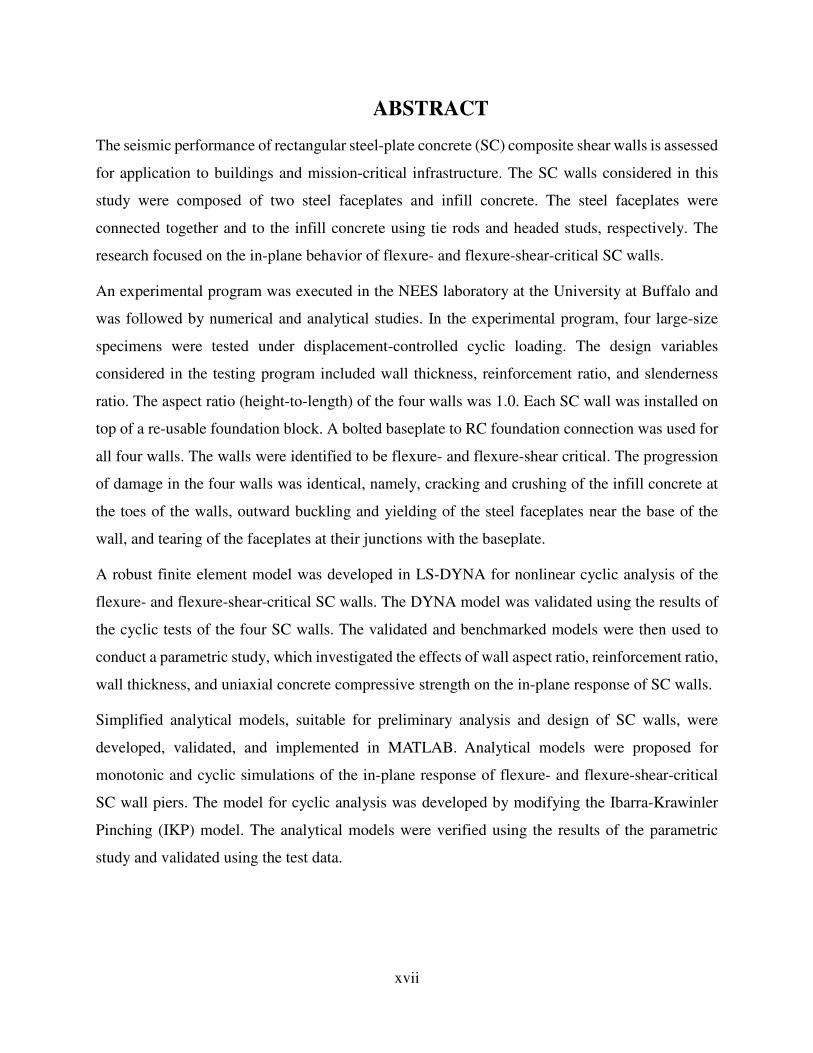
ABSTRACT
The seismic performance of rectangular steel-plate concrete (SC) composite shear walls is assessed
for application to buildings and mission-critical infrastructure. The SC walls considered in this
study were composed of two steel faceplates and infill concrete. The steel faceplates were
connected together and to the infill concrete using tie rods and headed studs, respectively. The
research focused on the in-plane behavior of flexure- and flexure-shear-critical SC walls.
An experimental program was executed in the NEES laboratory at the University at Buffalo and
was followed by numerical and analytical studies. In the experimental program, four large-size
specimens were tested under displacement-controlled cyclic loading. The design variables
considered in the testing program included wall thickness, reinforcement ratio, and slenderness
ratio. The aspect ratio (height-to-length) of the four walls was 1.0. Each SC wall was installed on
top of a re-usable foundation block. A bolted baseplate to RC foundation connection was used for
all four walls. The walls were identified to be flexure- and flexure-shear critical. The progression
of damage in the four walls was identical, namely, cracking and crushing of the infill concrete at
the toes of the walls, outward buckling and yielding of the steel faceplates near the base of the
wall, and tearing of the faceplates at their junctions with the baseplate.
A robust finite element model was developed in LS-DYNA for nonlinear cyclic analysis of the
flexure- and flexure-shear-critical SC walls. The DYNA model was validated using the results of
the cyclic tests of the four SC walls. The validated and benchmarked models were then used to
conduct a parametric study, which investigated the effects of wall aspect ratio, reinforcement ratio,
wall thickness, and uniaxial concrete compressive strength on the in-plane response of SC walls.
Simplified analytical models, suitable for preliminary analysis and design of SC walls, were
developed, validated, and implemented in MATLAB. Analytical models were proposed for
monotonic and cyclic simulations of the in-plane response of flexure- and flexure-shear-critical
SC wall piers. The model for cyclic analysis was developed by modifying the Ibarra-Krawinler
Pinching (IKP) model. The analytical models were verified using the results of the parametric
study and validated using the test data.

xviii
GLOSSARY
The following definitions are used in Chapter 8 of this dissertation.
cA Cross-sectional area of infill concrete
rA Cross-sectional area of threaded bar
sA Cross-sectional area of steel faceplates
sbA Effective cross-sectional area of baseplate for a section cut parallel to the width of baseplate
sbA′ Effective cross-sectional area of baseplate for a section cut between two threaded bars parallel
to the length of baseplate
a Ratio of the hardening modulus to the elastic modulus of the steel faceplates
B Width of baseplate
c Depth to the neutral axis
d Rate parameter in IKP model
id′ Distance between the center of ith row of threaded bars and the neutral axis
id Distance between the center of ith row of threaded bars and the wall centerline
unld Unloading stiffness rate parameter
reld Reloading stiffness rate parameter
ad Accelerated stiffness rate parameter
cE Elastic modulus of concrete (ksi)
sE Elastic modulus of steel (ksi)
cr
cE Elastic modulus of cracked concrete = 0.7Ec
iE Hysteretic energy dissipated in ith cycle
tE Hysteretic energy dissipation capacity
cF ′ Compressive force on infill concrete
cF Peak force
sF Compressive and tensile forces in the steel faceplates
yF Yield force in the IKP model
yF+
Yield force in the first quadrant
yF−
Yield force in the third quadrant
t
yF Force corresponding to yielding of steel faceplates at the tension end of the wall

xix
c
yF Force corresponding to yielding of steel faceplates at the compression end of the wall
rF Residual force
maxF + Maximum force achieved in previous cycles in first quadrant
maxF − Maximum force achieved in previous cycles in third quadrant
bf Maximum bearing stress on foundation
cf Concrete stress
sf Steel stress
cf ′ Uniaxial compressive stress of concrete (ksi)
yf Yield stress of steel faceplates (ksi)
uf Ultimate stress of steel faceplates (ksi)
eyf Effective yield stress of steel faceplates (ksi)
′y
f Average of yield and ultimate stress of steel (ksi)
rf Modulus of rupture of concrete (ksi)
sxf Horizontal stress in steel faceplates
syf Vertical stress in steel faceplates
sxyf Shear stress in steel faceplates
cxf Horizontal stress in infill concrete
cyf Vertical stress in infill concrete
cxyf Shear stress in infill concrete
cG Elastic shear modulus of concrete (ksi)
sG Elastic shear modulus of steel (ksi)
H Height of wall panel
rh Level of the resultant of the lateral loads applied above an SC panel in multi-story SC walls
cI Moment of inertia of infill concrete
sI Moment of inertia of steel faceplates
sbI Moment of inertia of baseplate about an axis parallel to the width of baseplate
sbI′ Moment of inertia of part of baseplate between two threaded bars about an axis parallel to the
length of baseplate
kRatio of the yield strain of the steel faceplates to the concrete strain corresponding to the peak
stress
fk Pinching parameter in MIKP model

xx
dk Pinching parameter in the MIKP model
ξ Pinching parameter in the MIKP model
bK Lateral stiffness of the wall connection (kips/in)
fK Flexural stiffness of the wall panel (kips/in)
sK Shear stiffness of the wall panel (kips/in)
tK Lateral stiffness of the wall panel (kips/in)
eK Elastic shear stiffness of the SC wall (kips/rad)
crK Shear stiffness of the SC wall after concrete cracking (kips/rad)
yK Shear stiffness of the SC wall after yielding of steel faceplates (kips/rad)
peK Effective stiffness of the wall panel (kips)
Kα Shear stiffness of the steel faceplates (kips/rad)
Kβ Shear stiffness of the diagonally cracked infill concrete (kips/rad)
Kθ Rotational stiffness of the spring (kip-in/rad)
unlK Unloading stiffness in the IKP model
relK Reloading stiffness in the IKP model
unlK′ Unloading stiffness in the MIKP model
relK′ Reloading stiffness in the MIKP model
L Length of wall
bL Length of baseplate
cL Distance between the edge of the baseplate and end of the wall
rL Total length of threaded bar from top of the baseplate to the nut-washer assembly at the bottom
tLLongitudinal spacing between the center of the first row of threaded bars at the tension end of
the wall and the end of the wall
tL′ Lateral spacing between the center of threaded bars on sides of the wall and face of the wall
M Bending moment applied to the SC wall cross-section
iM Bending moment in the ith sub element
crM Flexural strength of the SC wall at concrete cracking
tyM Flexural strength of the SC wall at yielding of steel faceplates at the tension end of the wall
cyM
Flexural strength of the SC wall at yielding of steel faceplates at the compression end of the
wall
cM Flexural strength of the SC wall at the maximum concrete compressive strain equal to 0cε

xxi
uM Flexural strength of the SC wall at concrete crushing
xN Normal force along the length of the wall applied to the SC wall cross-section
yN Normal force along the height of the wall applied to the SC wall cross-section
m Number of sub-elements along the height of a panel
rm Number of rows of threaded bars within the length of the wall
n Modular ratio
rn Number of threaded bars at the first row at the tension end of the wall
n′ Coefficient of concrete stress-strain relationship
r Coefficient of concrete stress-strain relationship
S Longitudinal spacing of threaded bars
ct Thickness of the infill concrete
st Thickness of each steel faceplate
pt Thickness of the baseplate
1T Tensile force in each threaded bar at the first row of the bars at the tension end of the wall
iT Tensile force in each threaded bar at the ith row
V Shearing force applied to the SC wall cross-section
crV Shearing strength of the SC wall at concrete cracking
yV Shearing strength of the SC wall at yielding of the steel faceplates
uV Shearing strength of the SC wall at concrete crushing
niV In-plane shear strength of the SC wall specified by AISC N690s1
iV Shearing force in the ith sub element
x Ratio of the concrete strain to strain corresponding to peak stress
iy Distance between the center of the ith sub element and the top of the wall
iy∆ Height of the ith sub element
1∆ Uplift of the baseplate at the irst row of threaded bars at the tension end of the wall
b∆ Lateral displacement due to base rotation
f∆ Flexural displacement at the top of the panel
fj∆ Flexural displacement at the top of the jth panel
i∆ Uplift of the baseplate at the ith row of threaded bars

xxii
s∆ Shear displacement at the top of the panel
1s∆ Downward deflection of the baseplate at the first row of threaded bars at the tension end of
the wall
si∆ Downward deflection of the baseplate at the ith row of threaded bars
sj∆ Shear displacement at the top of the jth panel
t∆ Total displacement at the top of the panel
crθ Angle of the inclination of the diagonal cracking in infill concrete
iγ Shear strain in the ith sub-element
crγ Shear strain of the SC wall at concrete cracking
yγ Shear strain of the SC wall at yielding of the steel faceplates
sc
xyγ Shear strain of the SC wall
uγ Shear strain in the SC wall at concrete crushing
,1unlγ Deterioration parameter for the first unloading branch
,2unlγ Deterioration parameter for the second unloading branch
,1relγ Deterioration parameter for the first reloading branch
aγ Accelerated stiffness deterioration parameter
τ Average shear stress in the steel faceplates
sν Poisson’s ratio for steel
η Strength-adjusted reinforcement ratio
ρ Reinforcement ratio
ρ Strength-adjusted reinforcement ratio
ρ′ Modulus-adjusted reinforcement ratio
λ Aspect ratio of a wall panel
crε Concrete cracking strain
cε Concrete strain
sε Steel strain
0cε Strain at peak stress of concrete
shε Steel strain at hardening
scxε Normal strain along the length of the wall
sc
yε Normal strain along the height of the wall
xxiii
yε Steel strain at yielding
uε Steel strain at peak stress
α Ratio of neutral axis depth to length of the wall
sα Ratio of post-yield stiffness to elastic stiffness in the IKP model
1sα Ratio of wall stiffness after yielding of steel faceplates at the tension end of wall to effective
stiffness in the MIKP model
2sα Ratio of wall stiffness after yielding of steel faceplates at the compression end of wall to
effective stiffness in the MIKP model
cα Ratio of post-capping stiffness to elastic stiffness
crφ Curvature of the SC wall cross-section at concrete cracking
tyφ Curvature of the SC wall cross-section at yielding of steel faceplates at the tension end of wall
cyφ
Curvature of the SC wall cross-section at yielding of steel faceplates at the compression end
of wall
cφ Curvature of the SC wall cross-section at maximum concrete compressive strain equals to 0cε
uφ Curvature of the SC wall cross-section at concrete crushing
iφ Curvature in the ith sub-element
θ Rotation of the baseplate
β Deterioration parameter
1β Stress block coefficient
2β Stress block coefficient
yδ Yield displacement in the IKP model
cδ Displacement corresponding to the peak force in the IKP model
rδ Displacement corresponding to the residual force in the IKP model
t
yδ Yield displacement corresponding to the yielding of steel faceplates at the tension end of the
wall
c
yδ Yield displacement corresponding to the yielding of steel faceplates at the compression end
of the wall
perlδ Maximum residual displacement in the previous cycle, same quadrant

1-1
1. INTRODUCTION
1.1 General
Steel-plate concrete (SC) composite walls consisting of steel faceplates, infill concrete, and
connectors used to anchor the steel faceplates together and to the infill concrete, have potential
advantages over conventional reinforced concrete and steel plate shear walls in terms of
constructability and seismic performance.
SC panels enable modular construction leading to potential time and cost savings over
conventional reinforced concrete walls. Double skin SC wall shells can be fabricated offsite,
assembled on site, and filled on-site with concrete to create monolithic structure. The use of steel
faceplates eliminates the need for on-site formwork, and the faceplates serve as primary
reinforcement.
SC wall construction has received attention from the research and design professional communities
but the number of applications to date is limited. Most proposals for SC wall construction have
involved two steel faceplates with infill concrete. Fukumuto et al. [32] proposed SC construction
in the form of modular box units, as reproduced in Figure 1-1. Another proposal from 1987 used
SC panels for submerged tunnels [87, 119], as cartooned in Figure 1-2.
Figure 1-1 Modular box units (Fukumuto et al. [32])

1-2
Figure 1-2 Submerged tunnel application of SC panels [119]
�������������� ���������������������������������������������� ���������������������
�������������� ��������������������� !�"������������������� ��������� �#��������$���������%��
������������������%���������������%&� ������!�
Figure 1-3 SC wall panels with corrugated steel faceplates wall (Wright et al. [115])
'�����(����������������������������������(������������������������#��������)�%��������������
��������������� ����������������������������������������� ��������� �����������������������(����
����� ������������%��*������ ���������������+���������,!�

1-3
(a) RC wall on one side of the steel plate
(b) RC walls on both sides of the steel plate
(c) Steel plate wall encased in RC wall
Figure 1-4 SC wall alternatives with reinforced concrete infill [125]
The proposed applications of SC walls seen in Figure 1-3 and Figure 1-4 provide possible
incremental advances over more conventional framing systems. The proposal of Figure 1-3
attaches the SC wall panels to an existing steel frame, and duplicates gravity load resistance, which
is not economical. The alternatives of Figure 1-4 seek to overcome the known challenges with
steel plate shear walls, which require stiffening to prevent elastic buckling, and capacity-protected
vertical (column) and horizontal (beam) steel boundary elements. The cost associated with
overcoming these challenges has precluded their use in the building and nuclear industries.
A proprietary composite product, Bi-Steel, was proposed by British Steel (later Corus) [16] for
flooring systems, beams and columns, fire resisting systems and building cores. A Bi-Steel panel
consists of two steel faceplates and steel bars that are friction welded to the faceplates at both ends.
Bi-Steel panels are welded together and filled with concrete on site. Figure 1-5 presents Bi-Steel
construction details.

1-4
(a) Internal construction (b) Shear walls
Figure 1-5 Bi-Steel construction [86]
The use of SC wall construction in nuclear power plants has been studied for nearly 20 years, with
an emphasis on elastic response in design basis shaking. Safety-related nuclear applications have
involved steel faceplates and infill (unreinforced) concrete, where the faceplates provide formwork
and reinforcement, and the SC walls provide both gravity and earthquake resistance, without the
introduction of internal steel framing for gravity-load resistance. Application of SC walls to
containment internal structures and shield buildings in nuclear power plants has begun in the
United States and China, with US applications based substantially on the work of Varma and his
co-workers at Purdue University (e.g., [93, 95, 96, 100, 123]). SC walls have not been used for
earthquake-resistant building construction, in part because there is little data on the seismic
performance of these walls at deformation levels expected in buildings subjected to maximum
earthquake shaking.
To date, design of SC walls (for nuclear applications) has been based in part on proprietary test
data and the limited data available in the literature. Most of the experiments were conducted at
small scales and focused on the essentially elastic range of response. The small-scale tests can not
represent reality well because construction materials and conditions are generally very different
from those used for field applications. Prior numerical studies have primarily focused on response
in the elastic range. The simulation of cyclic nonlinear response, and the loss of stiffness and
strength due to damage, have not been thoroughly investigated. The available physics-based
equations address only the pure shear response of SC walls, and flexural and shear-flexure
responses have not been studied.
1.2 Research Objectives
The focus of the research project presented in this dissertation is flexure- and flexure-shear critical
SC wall piers. The SC wall piers studied in this dissertation consist of two steel faceplates, infill
1-5
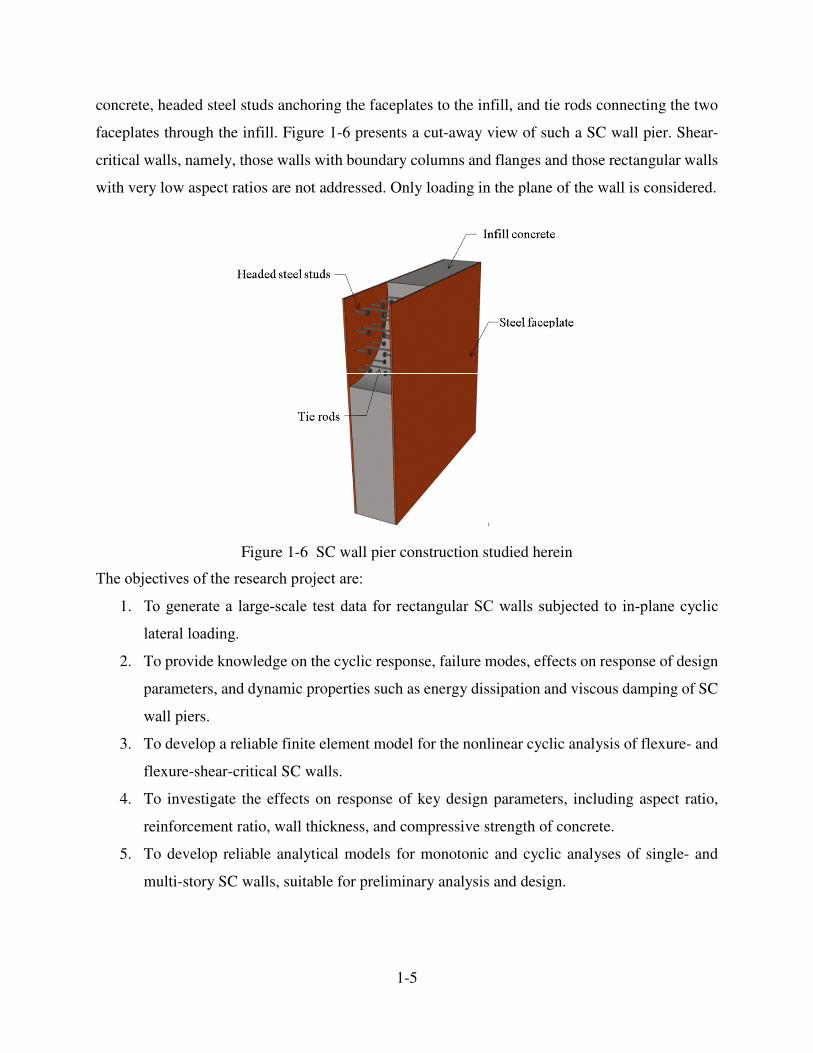
concrete, headed steel studs anchoring the faceplates to the infill, and tie rods connecting the two
faceplates through the infill. Figure 1-6 presents a cut-away view of such a SC wall pier. Shear-
critical walls, namely, those walls with boundary columns and flanges and those rectangular walls
with very low aspect ratios are not addressed. Only loading in the plane of the wall is considered.
Figure 1-6 SC wall pier construction studied herein
"����%-����(��� ���������������-�������.
1. "������������� ����������� ��������� ��� ���������������������%-������ ��� ���������&�����
���������������!�
2. To provide knowledge on the cyclic response, failure modes, effects on response of design
parameters, and dynamic properties such as energy dissipation and viscous damping of SC
wall piers.
3. To develop a reliable finite element model for the nonlinear cyclic analysis of flexure- and
flexure-shear-critical SC walls.
4. To investigate the effects on response of key design parameters, including aspect ratio,
reinforcement ratio, wall thickness, and compressive strength of concrete.
5. To develop reliable analytical models for monotonic and cyclic analyses of single- and
multi-story SC walls, suitable for preliminary analysis and design.

1-6
1.3 Research Outline
This dissertation is organized in nine chapters, a list of references, and four appendices. Chapter 2
presents a literature review. Chapter 3 provides information on the pre-test analysis and
preliminary design of the SC wall specimens. The details of the experimental program including
descriptions of the four specimens, the construction of the foundation block and the wall panels,
material testing, test setup, loading protocol, and instrumentation are presented in Chapter 4.
Results of the tests are provided in Chapter 5. In Chapter 6, a finite element model for nonlinear
cyclic analysis of flexure- and flexure-shear-critical SC walls is developed and validated. Chapter
7 presents the results of a parametric study to investigate the effects on response of design
parameters including aspect ratio, reinforcement ratio, wall thickness, and compressive strength of
infill concrete. Simplified models for the monotonic and cyclic analyses of flexure- and flexure-
shear-critical single- and multi-story SC walls and for the prediction of initial stiffness of an SC
wall with a baseplate connection are developed in Chapter 8. Chapter 9 summarizes the research
and identifies the key conclusions. A list of references follows Chapter 9. Appendix A includes
CAD drawings of the SC specimens, foundation block, and the SC wall connection to the block.
Photographs of the specimens at different drift ratios and of the damage to the infill concrete of
SC2 and SC4 at the end of testing are presented in Appendix B. Specifications for the rosette gages
used to measure strains in the steel faceplates are provided in Appendix C. The MATLAB code
for the Modified-Ibarra-Krawinkler-Pinching (MIKP) model for the cyclic analysis of SC walls is
provided in Appendix D.

2-1
2. LITERATURE REVIEW
2.1 Overview
This chapter reviews the literature on experimental and numerical studies on steel-plate concrete
(SC) composite shear walls. Section 2.2 summarizes the experimental and analytical studies.
Section 2.3 reviews finite element (numerical) studies of the behavior of SC walls.
2.2 Review of Experimental Studies on SC walls
Suzuki et al. [81] proposed an analytical method to predict the peak strength of rectangular SC
panels under combined bending, axial, and shear loads. These SC panels were equipped with
flange plates. They assumed that the load was resisted at peak strength by a diagonal tension field
in the steel faceplates and diagonal compression field in the infill concrete, as cartooned in
Figure 2-1. Figure 2-1(a) shows the compression field in the infill concrete; α �is the angle of the
compression field to the horizontal. The tension field of Figure 2-1(d) is characterized by two
parameters and β ξ , where β is the angle of the tension field to the horizontal and hξ is the
height of the faceplate over which the tension field is developed. The resultant load in the tension
field is decomposed into two forces T and T� , where T is the tensile force resisted by the steel
faceplates and the two components of T� along the height (Ty� in Figure 2-1(b)) and length (Tx
� in
Figure 2-1(c)) of the panel are resisted by the infill concrete and the steel flange plates,
respectively. Figure 2-1(b) shows the force Ty� resisted by the infill concrete and the reaction force
F generated at the corners of the infill concrete. Figure 2-1(c) shows the force Tx� resisted by one
of the flange plates and the tensile and compressive reactions K and J , respectively. Figure 2-1(f)
illustrates the equilibrium of the internal forces in the steel faceplates and flange plates,
K, J, F, and T , and the external forces in the steel faceplates and flange plates, s s sN , Q , and M .
Figure 2-1(e) presents the equilibrium of the internal force in the infill concrete, C , with the
external forces in the concrete, c c cN , Q , and M .

2-2
Figure 2-1 Load transfer mechanisms at peak strength (Suzuki et al. [81])
Suzuki et al. tested four SC walls to validate the proposed method. The ratio of predicted to
measured peak shear strengths varied from 0.7 to 1. More accurate predictions were obtained for
the shear-critical SC panels. The proposed method underestimated the peak shear strength of the
flexure-critical panels.
Fukumoto et al. [32] tested 1/4-scale steel plate, plain concrete, and composite shear walls under
axial and shear loads to study the effects of composite action between the steel faceplates and the
infill concrete, slenderness ratio, and stiffening methods for the steel faceplates, on the response
of SC walls. The composite walls were constructed by assembling welded steel boxes and infilling

2-3
them with concrete. Figure 2-2 presents the three types of connectors considered in that study,
namely, vertical steel insert plates, steel angles, and headed studs.
Figure 2-2 Types of connectors used in experimental study (Fukumoto et al. [32])
The experimental studies showed that the axial and shear responses of SC walls are substantially
affected by composite action of the steel faceplate and the infill concrete; the axial and shear
strengths of the composite wall were 14% and 40% greater than the corresponding superposed
strengths of the steel plate and plain concrete walls, respectively.
The initial stiffness of the SC walls under axial compression was not affected by the presence of
the vertical insert plates. The tangent stiffness beyond the elastic range decreased as the spacing
of the insert plates increased. Using a smaller spacing for the insert plates increased the axial
strength but did not have a significant effect on the shear strength. The shear load-displacement
relationships of SC walls was affected by the type of connector used.
Fukumoto et al. proposed an analytical model to predict the monotonic response of SC walls. The
proposed method (Figure 2-3) assumed that the shear load was resisted by tensile ties in the steel
faceplates oriented at 45° to the horizontal and diagonally inclined compression struts in the infill
concrete.

2-4
(a) Tensile ties in the steel faceplate (b) Compression struts in the infill concrete
Figure 2-3 Analytical model proposed by Fukumoto et al. [32]
They calculated the shear strength of an SC wall as:
sc s cQ Q Q= + �
1 2[ ( ) ( )]cos 45s s s s s s s sQ t B Bσ ε σ ε ′= + ��
1 2 2[( 1) ( ) ( ) ( )]cosc c c c c c c c c c cQ t n B n B Bσ ε σ ε σ ε θ′= + + + �
(2-1)
where θ is the inclination angle of the compression struts; 1 sB and 2 sB are the effective widths
of the main tie and the sub ties in the steel faceplates, respectively (see Figure 2-3); and 1 cB , and
2 cB are the effective widths of the main strut and sub struts in the infill concrete, respectively. As
seen in Figure 2-3, the main tie in the steel faceplate is a single diagonal connecting two opposite
corners of the SC panel and the sub ties are parallel to the main tie. The main strut in the infill
concrete is assumed to form between the vertical insert plates, as presented in Figure 2-3. The
modeling parameters θ , 1 sB , 2 sB , 1 cB , and 2 cB are calculated as:
1tan [( 1) / ]n l hθ −= + � (2-2)
1 ( / 4)cos 45sB h l= − �� (2-3)
2 / 4cos 45sB l= �� (2-4)
1 2
sin
2( 1)c c
hB B
n
θ= =
+(2-5)
where st is the sum of the steel faceplate thicknesses; ct is the thickness of the infill concrete; h
and l are the height and length of SC wall, respectively; sσ and cσ are the stresses in the steel

2-5
faceplates and infill concrete, respectively; sε and cε are the axial strain in the main steel tie and
the axial strains in the main and inner sub struts of the infill concrete, respectively; and sε′ and cε′
are the axial strains in the sub ties and outer sub struts of the steel faceplates and infill concrete,
respectively. The outer and inner sub struts (braces in Figure 2-3) in the infill concrete are located
in Figure 2-3. There was a good agreement between the measured and predicted shear strengths
but the displacement corresponding to the peak shear load was underestimated.
Akiayama et al. [7] tested a 1/10-scale model of a pressurized water reactor containment internal
structure (CIS) consisting of primary and secondary shield SC walls, a reinforced concrete base
mat, upper and lower loading slabs, steam generator compartments, pressurizer compartment, and
a number of partition walls. The thickness of the SC walls and steel faceplates were 4.3 in. and
0.06 in., respectively. The experimental program included two types of tests, namely, cyclic quasi-
static horizontal loading and vibration tests. The ratio of the cyclic horizontal load applied to the
upper slab to that applied to the lower slab was fixed at 2.6. The CIS specimen is presented in
Figure 2-4.
Figure 2-4 Overview of the 1/10-scale CIS specimen [98]
On the basis of their test results, they proposed empirical equations to predict the resistance of an
SC wall at the onset of concrete cracking, steel faceplate yielding, and peak strength. Their
equation to predict the peak shear strength is:
0.57 4.5u y s c cV f A f A′= + � (2-6)
where sA � and cA � are the cross-sectional areas of the steel faceplates and infill concrete,
respectively; and yf and cf ′ are the yield strength of the steel faceplates and the compressive

2-6
strength of the infill concrete, respectively. The equivalent viscous damping of the specimen,
calculated using hysteresis loops from the cyclic test, was 5% prior to the yielding of the steel
faceplates and up to 20% after the yielding of the steel faceplates.
Wright et al. [119] conducted 53 tests on 1/3-scale double skin composite beam, column, and
beam-column specimens to investigate the effects on response of connector spacing, thickness of
the steel faceplates, concrete strength, length of the connectors, load eccentricity, and axial load
variation. A 5.9 × 5.9 in. cross-section was used for all specimens. The length of the specimens
varied between 60 in. and 90 in. The specimens were simply supported at their ends and subjected
to two concentrated out-of-plane loads, 7 in. away from the mid-span of the specimen. Wright et
al. suggested the results of those beam and column tests could be indicative of composite wall
behavior assuming a plane strain state. The peak shear and axial strengths, and damage were
reported. Wright et al. [118] used the experimental results to develop a design guideline for
composite elements. Empirical equations were provided to characterize the strength and stiffness
of composite sections. The proposed empirical equations were validated using results of tests of
eleven large-scale beam, column and beam-column specimens. Recommendations were made for
the construction and detailing of the double skin composite structures.
Takeda et al. [83] tested seven composite wall panels subjected to cyclic, in-plane, pure shear
loading to investigate the effects of thickness of the steel faceplates, partitioning webs, and the use
of studs, on the shear response of the SC panels. The length and height of the panels were 47 in.
and the thickness of all specimens was 7.8 in. The specimens were composed of two steel
faceplates, infill concrete, headed steel studs anchoring the faceplates to the infill, and the
partitioning webs connecting the steel faceplates together. The test specimens are shown in
Figure 2-5.
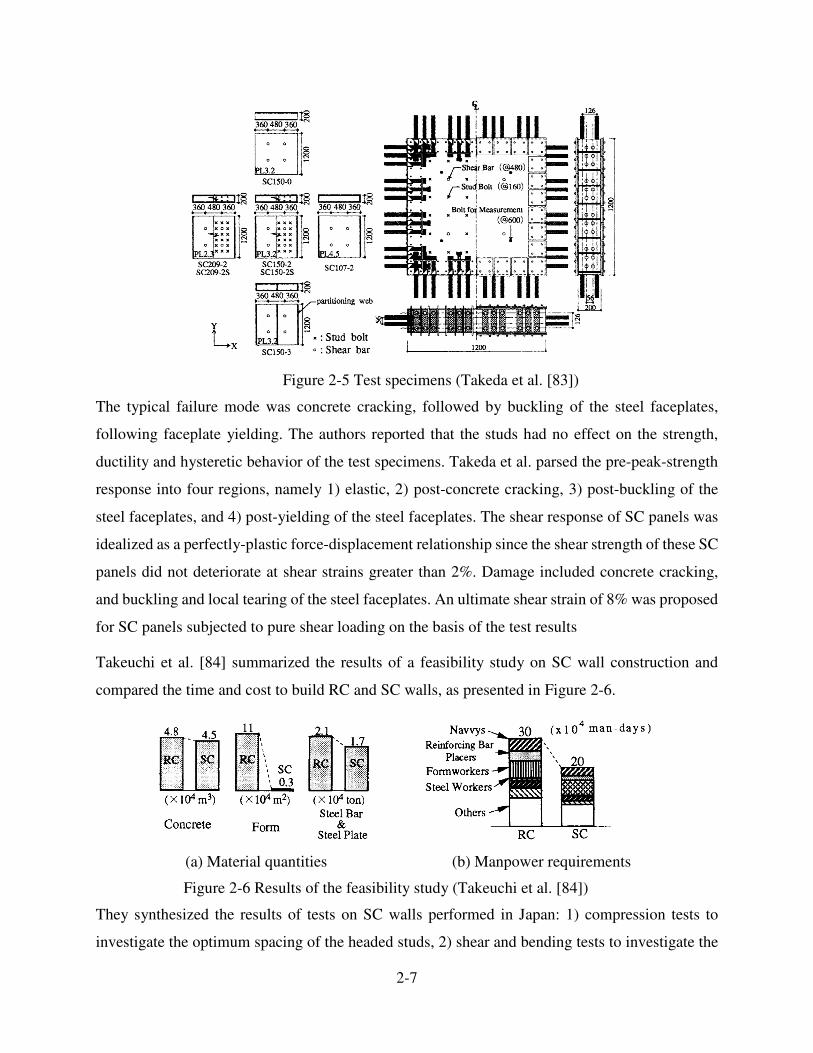
2-7
Figure 2-5 Test specimens (Takeda et al. [83])
The typical failure mode was concrete cracking, followed by buckling of the steel faceplates,
following faceplate yielding. The authors reported that the studs had no effect on the strength,
ductility and hysteretic behavior of the test specimens. Takeda et al. parsed the pre-peak-strength
response into four regions, namely 1) elastic, 2) post-concrete cracking, 3) post-buckling of the
steel faceplates, and 4) post-yielding of the steel faceplates. The shear response of SC panels was
idealized as a perfectly-plastic force-displacement relationship since the shear strength of these SC
panels did not deteriorate at shear strains greater than 2%. Damage included concrete cracking,
and buckling and local tearing of the steel faceplates. An ultimate shear strain of 8% was proposed
for SC panels subjected to pure shear loading on the basis of the test results
Takeuchi et al. [84] summarized the results of a feasibility study on SC wall construction and
compared the time and cost to build RC and SC walls, as presented in Figure 2-6.
(a) Material quantities (b) Manpower requirements
Figure 2-6 Results of the feasibility study (Takeuchi et al. [84])
They synthesized the results of tests on SC walls performed in Japan: 1) compression tests to
investigate the optimum spacing of the headed studs, 2) shear and bending tests to investigate the

2-8
in-plane shear and flexural responses of H-shaped (flanged) SC walls with web reinforcement
ratios ranging between 0.7% and 2%, and 3) tests to study the effect on response of the connection
of an SC wall to its foundation. The test specimens are described in Figure 2-7.
(a) Compression test (b) Shear and bending test (c) Wall-foundation joint test
Figure 2-7 Three types of SC wall experiments (Takeuchi et al. [84])
Four 1/5-scale SC walls were subjected to cyclic compressive loading by Usami et al. [90] with
particular attention being paid to the buckling characteristics of the steel faceplates. The specimens
were composed of two steel faceplates, two steel flange plates, infill concrete, and headed studs.
The faceplate slenderness ratio varied between 20 and 50. Drawings of the test specimens are
reproduced in Figure 2-8.
Figure 2-8 SC wall specimens (Usami et al. [90])
Usami’s study indicated that the axial load-displacement relationship of an SC wall did not change
abruptly at the onset of buckling and yielding of the steel faceplates. They proposed that the Euler

2-9
equation for elastic buckling of a column with a fixed-pinned boundary condition would accurately
predict the buckling stress of the steel faceplates using / sB t as the slenderness ratio for cases with
buckling stress less than 0.6 yf , where B is the spacing between the studs, st is the thickness of
each steel faceplate, and yf is the yield stress of the steel faceplates. The Euler equation over-
predicted buckling stress when it exceeded 0.6 yf . Test results and the proposed relationship
between buckling stress of the steel faceplates and slenderness ratio are presented in Figure 2-9.
Figure 2-9 Buckling stress of the steel faceplates (Usami et al. [90])
Sasaki et al. [71] tested seven flanged SC wall specimens with aspect ratios ranging between 1/3
and 1/2 to investigate the effects of aspect ratio, reinforcement ratio, axial load, and the use of
headed studs attached to the end plates of the web wall (see the plan view of the SC wall in
Figure 2-10) on the flexural-shear response of SC walls. A faceplate slenderness ratio of 33 was
used. Damage to the SC walls included concrete cracking, yielding and buckling of the steel
faceplates, and concrete crushing. On the basis of the test data, the lateral stiffness and peak shear
strength of an SC wall increases with decreasing shear span-to-depth ratio and increasing
reinforcement ratio. The peak shear strength increased, but the initial stiffness did not, as the axial
load was increased. The use of headed studs at the connection of the flange walls and the web wall
had no effect on response. A comparison of the responses of SC and RC walls with a shear span-
to-depth ratio of 0.8 and a reinforcement ratio of 1.7% indicated that the peak shear strength and
the displacement at peak strength were substantially greater for the SC wall than for the RC wall.

2-10
Figure 2-10 SC wall specimen (Sasaki et al. [71])
Suzuki et al. [82] proposed an analytical method to predict the peak shear strength of H-shaped
(flanged) SC walls by assuming that the shear load was resisted by a combination of arch and truss
mechanisms as presented in Figure 2-11. The study indicated that the orientation of the concrete
strut affected the contributions of the truss- and arch-action mechanisms to the peak shear strength
but that the peak shear strength of SC wall was not significantly influenced. The concrete strut,
shown in Figure 2-11(b), is oriented at )�/ to the horizontal.
(a) Truss mechanism
(b) Arch mechanism
Figure 2-11 Load transfer mechanisms in flanged SC walls (Suzuki et al. [82])

2-11
Takeuchi et al. [85] proposed an analytical method to simulate the pure shear behavior of SC walls
in three regions, namely, 1) elastic, 2) post-concrete cracking, and 3) post-steel buckling.
Figure 2-12 presents the load transfer mechanism in an SC panel subjected to a lateral loading.
Takeuchi et al. proposed an ultimate shear strain of 0.06% for the analysis of SC panels on the
basis of available results on pure shear testing of SC panels. Figure 2-13 presents the SC
construction considered by Takeuchi et al. [85].
(a) Elastic (b) Post-concrete cracking (c) Post-steel faceplate yielding
Figure 2-12 Load transfer mechanism of an SC panel under
pure shear loading (Takeuchi et al. [85])
(a) SC wall panel (b) SC floor (c) Pipe supports
(d) SC wall joints
Figure 2-13 Proposed details for SC construction (Takeuchi et al. [85])
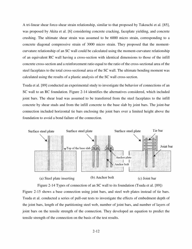
2-12
A tri-linear shear force-shear strain relationship, similar to that proposed by Takeuchi et al. [85],
was proposed by Akita et al. [6] considering concrete cracking, faceplate yielding, and concrete
crushing. The ultimate shear strain was assumed to be 6000 micro strain, corresponding to a
concrete diagonal compressive strain of 3000 micro strain. They proposed that the moment-
curvature relationship of an SC wall could be calculated using the moment-curvature relationship
of an equivalent RC wall having a cross-section with identical dimensions to those of the infill
concrete cross-section and a reinforcement ratio equal to the ratio of the cross-sectional area of the
steel faceplates to the total cross-sectional area of the SC wall. The ultimate bending moment was
calculated using the results of a plastic analysis of the SC wall cross-section.
Tsuda et al. [89] conducted an experimental study to investigate the behavior of connections of an
SC wall to an RC foundation. Figure 2-14 identifies the alternatives considered, which included
joint bars. The shear load was assumed to be transferred from the steel faceplates to the infill
concrete by shear studs and from the infill concrete to the base slab by joint bars. The joint-bar
connection included horizontal tie bars enclosing the joint bars over a limited height above the
foundation to avoid a bond failure of the connection.
(a) Steel plate inserting (b) Anchor bolt (c) Joint bar
Figure 2-14 Types of connection of an SC wall to its foundation (Tsuda et al. [89])
Figure 2-15 shows a base connection using joint bars, and steel web plates instead of tie bars.
Tsuda et al. conducted a series of pull-out tests to investigate the effects of embedment depth of
the joint bars, length of the partitioning steel web, number of joint bars, and number of layers of
joint bars on the tensile strength of the connection. They developed an equation to predict the
tensile strength of the connection on the basis of the test results.

2-13
The global response of SC walls equipped with the proposed joint-bar connection was investigated
by testing four walls under cyclic lateral loading. The aspect ratio of the walls varied from 0.62 to
1.23. The test results were used to develop an analytical method to predict the shear and flexural
responses of SC walls.
Figure 2-15 Proposed joint-bar connection (Tsuda et al. [89])
Ozaki et al. [64] investigated the effect of web openings on the cyclic shear response of SC walls
by testing six SC panels with through-thickness circular and square openings at the center of the
web, and one solid SC panel. The ratio of the surface area of the opening to the surface area of the
SC panel was 0.15. The presence of the opening had no effect on the shear strain of the SC panels
at the onset of concrete cracking and steel faceplate yielding. The shear strain at the peak shear
resistance of the SC walls with openings was a factor of 2 to 3 than that of the solid SC wall. On
the basis of the test data, Ozaki et al. developed an analytical method to predict the response of SC
panels with openings by applying reduction factors on the stiffness and strength of solid SC panels,
where the reductions factors were derived as a function of the dimensions of the opening. Finite
element analyses were conducted to convert the proposed reduction factors for the effect of
reinforcement around the opening.

2-14
Ozaki et al. [62] tested flanged SC walls with different aspect and reinforcement ratios under lateral
loading to investigate the in-plane response of shear-critical and flexure-critical SC walls. Five
shear-critical SC specimens with aspect ratios ranging from 0.5 to 0.85 and reinforcement ratios
ranging from 0.7% to 2% were tested. The SC specimens were connected to their foundation by
extending the steel faceplates and the infill concrete into the foundation concrete. The
reinforcement ratio had a small effect on the initial stiffness and cracking strength of the shear-
critical SC walls but it significantly affected the yield and the peak shear strengths. The
displacements corresponding to the yield and peak shear strengths were not affected by the
reinforcement ratio. Ozaki et al. proposed that the tensile and shear stresses in the concrete at the
onset of cracking were 1.2 cf ′ and cf ′ (units in kg and cm), respectively. Four flexure-critical
SC walls with aspect ratios of 0.7 and 0.85, and a reinforcement ratio of 2%, were tested. The
flexure-critical SC walls were connected to their foundations using baseplates and anchor bars.
The design parameters considered in this part of the study were aspect ratio, axial force, and SC
wall connection to the foundation block. Ozaki et al. proposed that the flexural strength of flexure-
critical SC walls be calculated using the results of a plastic analysis of the SC wall cross-section.
Drawing of the test specimens are reproduced in Figure 2-16.
(a) Shear-critical specimen (b) Flexure-critical specimen
Figure 2-16 Test specimens (Ozaki et al. [62])

2-15
Emori et al. [26] tested three 1/4-scale SC wall box units (specimens 200K, 100K, and 67K in
Table 2-1) under shear and axial compressive loads. The SC wall box units were constructed by
assembling and welding the prefabricated steel box units consisting of two steel faceplates and
vertical and horizontal partition plates, and filling the boxes with concrete. Headed studs and tie
rods were not used. To investigate the effect of composite action on the response of the SC wall
boxes, one steel plate box specimen (100S in Table 2-1) and two concrete solid specimens (0C and
1C in Table 2-1) were included in the test program. In Table 2-1, the width-to-thickness ratio is
the spacing between the partition plates divided by the thickness of each steel faceplate.
Results of the shear and axial compression tests are presented in Figure 2-17. The width-to-
thickness ratio, /s
b t , had a significant effect on the axial strength but only a minor effect on the
shear strength. The pre-peak shear response and the displacement corresponding to the peak shear
strength were significantly affected by the width-to-thickness ratio.
Table 2-1 Test specimens (Emori et al. [26])
Width-to-thickness
ratio ( /s
b t )
Cross-sections
(SC) (S) (C)
200 -
For compression test
For shear test
100
67 - -
The results of the axial and shear tests of the composite panels, steel plate boxes, and concrete
panel were used to study the effect of composite action on the shear and axial responses of SC
walls. Figure 2-18 shows that the shear and axial compressive responses of the SC walls were
affected by composite action. The axial and shear strengths of the SC walls were 15% and 43%
greater than the corresponding superposed strengths of the steel boxes and concrete panels,
respectively. These results showed that composite action, which delayed local buckling of the steel

2-16
faceplates and confined the infill concrete, had significant effect on the behavior of the composite
panels.
(a) Compression test (b) Shear test
Figure 2-17 Axial and shear responses of SC wall box units (Emori et al. [26])
(a) Compression test (b) Shear test
Figure 2-18 Effects of composite action on axial and shear responses (Emori et al. [26])
Zhao et al. [124] tested two 1/2-scale three-story composite shear walls consisting of a single steel
faceplate welded to the surrounding steel frame and a precast reinforced concrete panel bolted to
the steel faceplate. In one specimen, termed a traditional composite wall, the reinforced concrete
panel was in direct contact with the boundary steel beams and columns. In the second, termed an
innovative composite wall, a 1.25 in. gap between the reinforced concrete panel and the
surrounding steel frame was maintained to avoid early cracking and crushing of the concrete. The

2-17
innovative composite wall exhibited similar responses to that of a stiffened steel plate shear wall
at small lateral displacements. Upon closing the gap between the reinforced concrete panel and the
boundary steel framing, the reinforced concrete panel contributed to the lateral resistance of the
composite wall. Schematic drawings of the test specimens are reproduced in Figure 2-19. Both
specimens resisted lateral loading greater than 80% of the peak strength up to a drift ratio of 5%.
The rate of the post-peak strength deterioration of the traditional composite wall was greater than
that of the innovative composite wall because the gap between the reinforced concrete panel and
the boundary columns and beams delayed severe damage to the concrete wall. Importantly, the
lateral stiffness and peak shear strength were not significantly affected by the presence of the gap
since the contribution of the concrete panel to the total strength and lateral stiffness was estimated
to be less than 20%. Zhao et al. proposed that the shear strength of the reinforced concrete panel
could be ignored in the calculation of the peak shear strength of the composite wall but that its
stiffness should be included in calculations of force-displacement response.
Figure 2-19 Composite shear walls (Zhao et al. [124])

2-18
Ozaki et al. [63] tested nine SC panels subjected to cyclic in-plane shear loading to investigate the
effects of steel faceplate thickness, axial compressive loading, and partitioning webs on the shear
response of SC panels. Figure 2-20 presents a cut-away view of the SC panel.
Figure 2-20 SC panel (Ozaki et al. [63])
On the basis of the test results, the greater the steel faceplate thickness, the greater the elastic shear
stiffness, the post-cracking shear stiffness, and the yield and peak strengths of SC wall but the
lower the shear strain at peak strength. The elastic shear stiffness was not influenced by the axial
compressive force. However, as the axial compressive force increased, the post-cracking shear
stiffness decreased slightly. An increase in the axial compressive force increased the shear strength
at the onset of concrete cracking but it had no effect on the yield and peak shear strengths for the
range of axial loads applied ( 0�to 0.07
c cA f ′ �
�where cA is the cross-sectional area of the infill
concrete and cf ′ is the compressive strength of the concrete). The partitioning webs in the
specimens tested by Ozaki et al. had no impact on the yield and peak shear strengths of the SC
panels.
Ozaki et al. parsed the in-plane response of SC walls in shear into three regions: 1) elastic, 2)
concrete cracking, and 3) steel faceplate yielding. In the elastic range, the infill concrete and the
steel faceplates were modeled using an isotropic elastic and isotropic elastic plane-stress behaviors,
respectively. They proposed that the shear stress, cτ , in an SC wall at the onset of concrete cracking
could be calculated as:
2 2
c t t aτ σ σ σ= + � (2-7)
2-19
where aσ is the axial compressive stress on the infill concrete and t
σ is the tensile strength of the
infill concrete. Substituting 0.33 (unit:MPa)t c
fσ ′= , as proposed by Collins et al. [24], into (2-7)
results the shear stress of SC walls at the onset of concrete cracking as:
0.33 (0.33 )c c c a
f fτ σ′ ′= + �� (2-8)
The shear strength of SC wall at the onset of steel faceplate yielding and the peak shear strength
were calculated as:
2 2 2
( )
23
y wc sy
c s
f Ak G GQ
G k G
+=
+�� (2-9)
( )u w p yQ A A f= + ��� (2-10)
where cG and s
G are the elastic shear moduli of the infill concrete and steel faceplates,
respectively; yf is the yield stress of the steel faceplates; w
A is the cross-sectional area of the steel
faceplates; and k is calculated as:
1 (1 )s dx
k pν= + − ��� (2-11)
where dxp is the ratio of the cross-sectional area of the horizontal partitioning webs to the cross-
sectional area of the steel faceplates and sν is Poisson’s ratio for the steel faceplates.
Booth et al. [15] tested two full-scale, simply supported, 22-ft long beams to study the out-of-plane
behavior of composite walls. The specimens were subjected to thermal and mechanical loadings.
The mechanical loading included two concentrated loads applied at third points of the beam. The
effect of thermal loading on the shear and flexural responses was studied. The concrete cracking
patterns at different thermal and mechanical loading conditions were documented. Exposure of the
beams to an elevated temperature leaded to severe concrete cracking; the out-of-plane flexural
stiffness of the cracked specimens was reduced to 14% of that of the un-cracked specimens. Booth
et al. developed a 2D fiber-based finite element model assuming 1) 2D plane stress behavior for
the steel faceplates and infill concrete, 2) plane section remains plane, and 3) perfect bond between
the steel faceplates and the infill concrete. Booth’s model successfully predicted the flexural
stiffness of the SC walls at ambient conditions but the temperature-induced deformations could

2-20
not be predicted accurately due to the simplified modeling assumptions. Booth et al. then
conducted further research [94] to improve the analytical approach for predicting the behavior of
SC walls subjected to combined thermal and mechanical loadings.
Eom et al. [27] tested three 1/3-scale solid SC walls and two 1/4-scale coupled SC walls under
cyclic lateral loading. The walls had rectangular and T-shaped (flanged) cross sections. The SC
walls were flexure-critical with aspect ratios of 3.7 and 2.7 for the solid and coupled walls,
respectively. The spacing of the tie rods connecting the two steel faceplates, divided by the
thickness of each steel faceplate was 30 and 50 for the solid and coupled walls, respectively. The
steel faceplates were CJP-welded to a baseplate in one solid SC wall: specimen DSCW1N
presented in Figure 2-21. Due to the premature fracture of the welded connection of the faceplates
to the baseplate at 1.5% drift ratio, and prior to flexural yielding of the steel faceplates, triangular
rib plates were welded to the both ends of the SC wall cross section (specimen DSCW1H in
Figure 2-21) and specimen was re-tested. The addition of the rib plates did not significantly
improve the response of the SC wall and so the rib-plates were removed and the specimen was
strengthened by fillet welding cover plates to the steel faceplates, flange plates, and the baseplate
(specimen DSCW1C in Figure 2-21) and re-tested. The coupled wall specimens DSCW4 and
DSCW5 were strengthened to avoid the premature failure seen in the solid walls through the
addition of cover plates, which are identified in Figure 2-22.
The test results indicated that the addition of cover plates at the base of the SC walls significantly
improved the shear response and avoided the premature fracture of the welded connection of the
faceplates to the baseplate. The SC walls failed due to the steel faceplate buckling and crushing of
the infill concrete above the cover plates. Eom et al. proposed an analytical method to predict the
shear strength of rectangular and T-shaped SC walls on the basis of a plastic analysis of an SC
wall cross-section. Perfect bond between the steel faceplates and infill concrete was assumed and
the effect of axial load was considered.

2-21
(a) DSCW1 (b) DSCW2 (c) DSCW3
Figure 2-21 Isolated SC wall specimens (Eom et al. [27])
(a) DSCW4 (b) DSCW5
Figure 2-22 Coupled SC wall specimens (Eom et al. [27])

2-22
Hong et al. [35] tested nine SC beams subjected to concentrated out-of-plane loads at different
locations along the beam span to investigate the out-of-plane behavior of SC walls. The design
parameters considered in the investigation were shear-to-span ratio, steel faceplate thickness, and
shear reinforcement ratio, /sv
A sb , where svA is the cross-sectional area of the shear reinforcement,
s is the spacing of the reinforcement, and b is the width of the beam. Shear reinforcement
consisted of two #5-leg ties at 15 in. on center. Headed studs, tie rods, and H-shaped steel profiles
were used as connectors. Load-deflection curves for the beams, cracking patterns in the infill
concrete, and strain distributions in the steel faceplates were documented.
Similar to the analytical approach proposed by Ozaki et al. [63], Varma et al. [100] developed
mechanics-based equations to predict the in-plane shear response of SC walls. Concrete cracking
was assumed to occur when the shear force exceeded the cracking threshold corresponding to a
principal tensile stress of 2c
f ′ (psi), which indirectly accounted for the effects of restrained
shrinkage in the infill concrete. The infill concrete was assumed to behave as an orthotropic elastic
material with a) no stiffness perpendicular to the direction of cracking and b) 70% of the elastic
compression modulus ( cE ) in the orthogonal direction. The stiffness of the cracked SC wall was
calculated assuming orthotropic behavior of the infill concrete and isotropic elastic plane stress
behavior of the steel faceplates. Varma et al. assumed that the peak shear strength of SC walls
corresponded to the onset of the yielding of the steel faceplates.
The proposed method was used to predict the in-plane shear response of the SC walls tested by
Ozaki et al. [63]. The method successfully predicted the initial stiffness of the SC walls but the
peak shear strength was underestimated because the peak shear strength was associated with the
onset of steel faceplate yielding.
Varma et al. [100] tested a large-scale flanged SC wall subjected to lateral loading to validate the
proposed analytical method. The web and flanges of the SC wall were designed to resist shear
force and bending moments, respectively. The reinforcement ratio ( 2 / )s
t T= and the slenderness
ratio ( / )s
s t of the SC wall were 4.2% and 11.3, respectively, where st is the thickness of each
steel faceplate, T is the thickness of the web of the SC wall, and s is the spacing of the studs.
Good agreement was obtained between the analytical and test results. A photograph of the
specimen is shown in Figure 2-23.
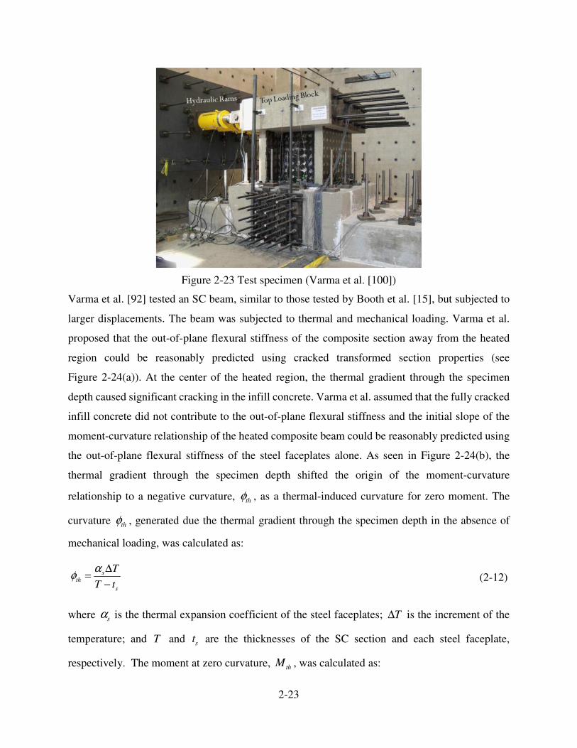
2-23
Figure 2-23 Test specimen (Varma et al. [100])
Varma et al. [92] tested an SC beam, similar to those tested by Booth et al. [15], but subjected to
larger displacements. The beam was subjected to thermal and mechanical loading. Varma et al.
proposed that the out-of-plane flexural stiffness of the composite section away from the heated
region could be reasonably predicted using cracked transformed section properties (see
Figure 2-24(a)). At the center of the heated region, the thermal gradient through the specimen
depth caused significant cracking in the infill concrete. Varma et al. assumed that the fully cracked
infill concrete did not contribute to the out-of-plane flexural stiffness and the initial slope of the
moment-curvature relationship of the heated composite beam could be reasonably predicted using
the out-of-plane flexural stiffness of the steel faceplates alone. As seen in Figure 2-24(b), the
thermal gradient through the specimen depth shifted the origin of the moment-curvature
relationship to a negative curvature, thφ , as a thermal-induced curvature for zero moment. The
curvature thφ , generated due the thermal gradient through the specimen depth in the absence of
mechanical loading, was calculated as:
sth
s
T
T t
αφ
∆=
−��� (2-12)
where sα is the thermal expansion coefficient of the steel faceplates; T∆ is the increment of the
temperature; and T and st are the thicknesses of the SC section and each steel faceplate,
respectively. The moment at zero curvature, thM , was calculated as:

2-24
th s s thM E I φ= ��� (2-13)
where s sE I is the flexural rigidity of the steel faceplates.
(a) Away from heating region (b) At center of heated region
Figure 2-24 Moment-curvature relationship of a composite beam section (Varma et al. [92])
Varma et al. derived an equation to predict the out-of-plane flexural stiffness of SC section using
the cracked transformed composite section properties. The simplest form of the derived equation
[92] is:
cr tr s s c cEI E I E Iβ− = + ��� (2-14)
where c cE I is the flexural rigidity of the infill concrete; and β is 0.48 0.1ρ′ + , where ρ ′ is the
stiffness normalized reinforcement ratio and was calculated as:
2 s s
c
t E
T Eρ ′ = ��� (2-15)
They proposed Equation (2-16) to predict the out-of-plane flexural stiffness of SC walls taking
into account the reduction of stiffness due to concrete cracking and thermal effects.
( )(1 )150
eff s s c c s s
TEI E I E I E I
Fβ
∆= + − ≥
���� (2-16)
Equation (2-16) calculates the out-of-plane flexural stiffness of the composite section at
temperatures greater than 150 F� �to be that of the steel faceplates only.
Nie et al. [41] tested twelve SC walls subjected to high axial and cyclic lateral loads to investigate
the effects of reinforcement ratio, concrete strength, thicknesses of the steel face and flange plates,
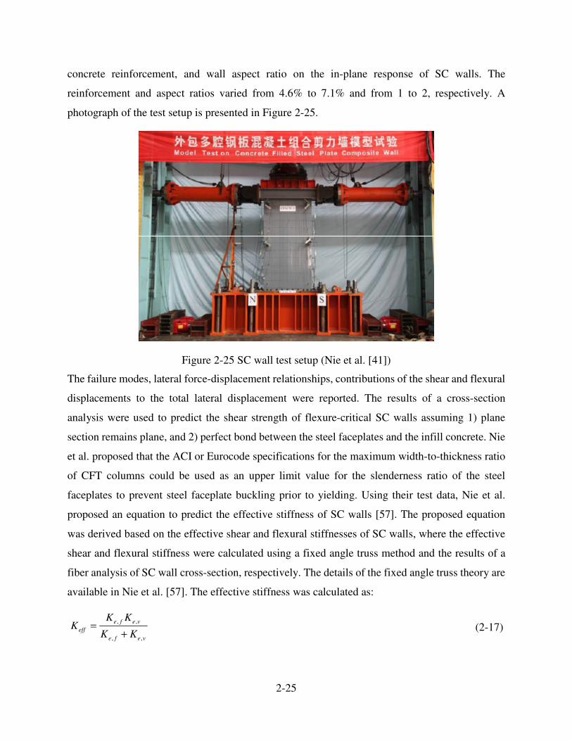
2-25
concrete reinforcement, and wall aspect ratio on the in-plane response of SC walls. The
reinforcement and aspect ratios varied from 4.6% to 7.1% and from 1 to 2, respectively. A
photograph of the test setup is presented in Figure 2-25.
Figure 2-25 SC wall test setup (Nie et al. [41])
The failure modes, lateral force-displacement relationships, contributions of the shear and flexural
displacements to the total lateral displacement were reported. The results of a cross-section
analysis were used to predict the shear strength of flexure-critical SC walls assuming 1) plane
section remains plane, and 2) perfect bond between the steel faceplates and the infill concrete. Nie
et al. proposed that the ACI or Eurocode specifications for the maximum width-to-thickness ratio
of CFT columns could be used as an upper limit value for the slenderness ratio of the steel
faceplates to prevent steel faceplate buckling prior to yielding. Using their test data, Nie et al.
proposed an equation to predict the effective stiffness of SC walls [57]. The proposed equation
was derived based on the effective shear and flexural stiffnesses of SC walls, where the effective
shear and flexural stiffness were calculated using a fixed angle truss method and the results of a
fiber analysis of SC wall cross-section, respectively. The details of the fixed angle truss theory are
available in Nie et al. [57]. The effective stiffness was calculated as:
, ,
, ,
e f e v
eff
e f e v
K KK
K K=
+��� (2-17)

2-26
where , , and e f e vK K �are the effective flexural and shear stiffnesses of SC walls and were expressed
as:
3
, 3(0.5 ) /e f s s c cK E I E I Hβ= + �� (2-18)
, 4
2 sin cos
(2 sin )
s s c ce v
s c
t EK
t n T H
γ θ θ
θ=
+� (2-19)
where s sE I and c c
E I are the flexural rigidities of the steel faceplates and infill concrete,
respectively; H is the height of the SC wall; and s
t T are the thicknesses of each steel faceplate
and the SC wall, respectively; cθ is the angle of concrete cracking; and n is the modular ratio.
Parameters γ and β are calculated using equations available in Nie et al. [57].
Sener et al. [74, 75] summarized available test data on the out-of-plane shear and flexural behaviors
of SC beams provided by Japanese, Korean, and US researchers for the purpose of characterizing
the out-of-plane response of SC walls. Design variables included loading configuration, width of
the beams, steel faceplate thickness, reinforcement ratio and faceplate slenderness ratios, shear
span-to-depth ratio, inclusion of shear reinforcement, and spacing of shear studs. The measured
out-of-plane shear and the flexural strengths of 48 SC beam specimens were compared with the
predictions provided by the design codes in Japan for SC (JEAC 4618 [40]), South Korea for SC
(KEPIC SNG [79]), and US for RC (ACI 349 [3]). The shear and flexural strengths were
overestimated using the Japanese and Korean SC specifications. Sener et al. showed that the ACI
specifications for reinforced concrete beams could be used to estimate the out-of-plane monotonic
shear and flexural strengths of SC beams, by equating SC beams to a doubly reinforced concrete
beams.
Zhang et al. [122, 123] and Varma et al. [101] investigated the effect of the use of shear studs on
local buckling of steel faceplates and composite action in SC walls. On the basis of the available
test data and the results of finite element analyses, they proposed that stud spacing should be
selected to 1) prevent the elastic local bulking of steel faceplates, and 2) provide adequate
development length for steel faceplates, where the development length was defined as the length
over which the steel faceplate could develop its yield strength under the axial tensile loading. Based
on these two criteria, the maximum stud spacing was proposed to be:

2-27
min 1.0 , n d
y s y
Q LEs
f t f
φ� �= � �
� �� �
�� (2-20)
where E and yf are the elastic modulus and yield stress of the steel faceplates, respectively; φ is
a reduction factor, taken as 0.65 for stud shank failure; nQ is the shear capacity of a single stud;
and dL is the development length taken at least three times the wall thickness to provide 75% to
90% partial composite action. The finite element analyses conducted by Zhang et al. [122, 123]
indicated that the partial composite action was affected by the reinforcement and faceplate
slenderness ratios. As the reinforcement ratio and stud spacing were decreased, the degree of
composite action increased.
Hong et al. [36] summarized analytical studies on the in-plane shear behavior of SC walls and
proposed two analytical models to predict the shear force and deformation capacities of SC walls
having vertical ribs. Seven SC panels subjected to pure shear load were tested to validate the
accuracy of the proposed model. Four of the seven specimens were reinforced with vertical ribs.
A photograph of the test setup is presented in Figure 2-26. A comparison of the analytical and
experimental results indicated that the proposed model could not predict the shear response of SC
walls. The ratio of the measured to the predicted peak shear strengths of SC panels varied from 0.4
to 1.35. In that study, they tested six low aspect ratio flanged SC walls under lateral loading. Four
walls were reinforced with vertical ribs. The predicted and measured pre-peak shear responses of
two specimens compared favorably and measured peak shear strengths were slightly under-
predicted.
Figure 2-26 Test setup for pure shear loading (Hong et al. [36])

2-28
2.3 Review of Studies on Finite Element (Micro) Modeling of SC Walls
Link et al. [47] developed a finite element model to simulate the out-of-plane behavior of SC walls
used in offshore structures. An orthotropic constitutive model and an elastic-plastic model were
used to model the infill concrete and the steel faceplates, respectively. Friction between the steel
faceplates and the infill concrete was modeled using Lagrangian multiplier gap elements presented
in Figure 2-27. Results of the in-plane and out-of-plane shear responses of SC beams tested by
Stephens et al. [80] and Hassinen et al. [34] were used to validate the finite element model. The
pre- and post-peak out-of-plane responses of the SC beams were successfully predicted using the
model.
Figure 2-27 Schematic drawing of the gap element (Link et al. [47])
Uy et al. [91] developed a finite strip model to simulate elastic local buckling of steel faceplates
in composite members, where the finite strip model was developed as a special form of the finite
element model. Finite element models simulate plate buckling using polynomials in the
longitudinal and transverse directions whereas the finite strip model uses a harmonic series in the
longitudinal direction and a polynomial in the transverse direction to describe the buckling
displacements. The proposed model was validated using available analytical solutions in the
literature. Design curves for buckling coefficients and slenderness ratios of the steel faceplates
used in profiled composite beams, slabs, walls and composite beams and columns with different
boundary conditions were provided.
Emori et al. [26] proposed a 2D finite element model to simulate the shear response of SC wall
box units using two laminated steel and concrete plates. Friction between the steel faceplates and
the infill concrete and steel partition plates was modeled using axial and shear springs. The
compressive stress in cracked concrete at a given compressive strain was assumed to be 70% of

2-29
that of un-cracked concrete to account for the effect of concrete cracking on the compressive stress-
strain relationship of concrete. The shear responses of the SC wall tested by these authors,
presented in Section 2.2, were used to validate the proposed finite element model. Good agreement
was achieved between the measured and predicted shear responses of the SC walls. The developed
finite element model is presented in Figure 2-28.
(a) Finite element layered model (b) Modeling of the partition plates and friction
Figure 2-28 Finite element modeling of SC wall box units (Emori et al. [26])
Zhou et al. [127] developed a 2D finite element model in OpenSees to simulate the cyclic response
of SC walls. Membrane elements with plane stress behavior were used to model the infill concrete
and the steel faceplates. The finite element model did not include the connectors, and the steel
faceplates were tied to the infill concrete where the studs were attached to the steel faceplates. The
Cyclic-Softened-Membrane-Model (CSMM) developed by Mansour et al. [53, 54] was used to
model the infill concrete and a J2 plasticity model was used to model the steel faceplates. The
CSMM model used to simulate the response of the infill concrete was validated using data for test
of an RC shear wall [126]. The SC wall model was not validated. Zhou et al. conducted a
parametric study to investigate the effects of wall thickness and faceplate slenderness ratio on the
in-plane shear response of SC walls.
Ali et al. [8] developed an ABAQUS model to simulate the cyclic behavior of I-shaped (flanged)
SC walls. The concrete damage plasticity (CDP) and bilinear kinematic hardening models were
used to model the infill concrete and the steel faceplates, respectively. The flange wall was tied to
the web. Contact between the steel faceplates and the infill concrete was considered. The infill
concrete and the steel faceplates were modeled using solid elements. The model was validated
using the data from cyclic loading test of four I-shaped SC walls. The model accurately predicted
the backbone curve of the measured cyclic force-displacement relationship. The pinched behavior
seen in the experiments was not captured because the bilinear kinematic model could not recover
Composite
panelSteel Concrete

2-30
the nonlinear buckled response of the steel faceplates. The ABAQUS-predicted post-peak response
was not presented. The ABAQUS model is presented in Figure 2-29.
Figure 2-29 ABAQUS model of I-shaped SC walls (Ali et al. [8])
Vecchio et al. [109] applied the Distributed-Stress-Field-Model (DSFM) to SC walls subjected to
axial and in-plane monotonic and cyclic shear loads using the two-dimensional nonlinear finite
element analysis program, VecTor2 [104, 105]. The strains in the steel faceplates were calculated
assuming perfect bond between the steel faceplates and the infill concrete. The steel faceplates was
assumed to buckle when the principal compressive stress in the faceplate elements exceeded the
critical buckling stress proposed by Usami et al. [90]. The adequacy of the model was investigated
by simulating the monotonic and cyclic responses of the SC walls tested by Sasaki et al. [71],
Usami et al. [90], and Ozaki et al. [62, 63]. The DFSM predicted the reported shear strengths to
within 5% but the stiffness at displacements less than those associated with peak strength was
significantly overestimated (Vecchio et al. [109]).
The dynamic response of RC and the SC walls were investigated by Chaudhary et al. [21] using
modal and response-history analyses by ABAQUS. The infill concrete and the steel faceplates
were modeled using 3D solid elements. A smeared crack model and a J2 plasticity model were
used to model the infill concrete and the steel faceplates, respectively. The elastic dynamic
response of the RC model was validated using the measured natural frequency of a flanged RC
shear wall tested by Nuclear Power Engineering Corporation [59]. The SC wall model was not

2-31
validated. Three types of shear walls were analyzed, namely, a RC shear wall, and two SC walls
with a web reinforcement ratio equal to that used in RC wall. Two SC wall models were studied
to investigate the effect of the connection between the steel faceplates and infill concrete on
dynamic response: models with flexible and rigid connections between the steel faceplates and
infill concrete.
Varma et al. [99] developed an ABAQUS model to simulate the out-of-plane shear behavior of SC
walls. The Brittle-Cracking (BC) model and an elastic-plastic model with isotropic hardening were
used to simulate the behavior of the infill concrete and the steel faceplates, respectively. The BC
model was used because of its advanced cracking features and element deletion option. This
material model assumes linear elastic behavior for concrete in compression. The model was
validated using the results of eight large-scale simply-supported SC beams under monotonic out-
of-plane loading [99]. Shear studs were not used in five of the specimens. The effects of
reinforcement ratio, beam width, steel faceplate thickness, and shear span-to-depth ratio, on out-
of-plane shear response were investigated. There was good agreement between the analysis and
the test results for one specimen without shear studs. The peak shear strengths of the SC beams
with shear studs were underestimated by a factor of 1.2. On the basis of the analysis and test results,
Varma et al. concluded that the ACI equations for the shear strength of RC beams could be
reasonably used to predict the out-of-plane monotonic shear strength of SC beams.
Danay [25] developed an analytical solution to predict the strain and stress fields in the steel
faceplate and the infill concrete, the shear forces resisted by the studs, crack spacing, and crack
opening in SC walls under in-plane, bi-axial, tensile and in-plane tensile-compressive loadings.
The connectors between the steel faceplates and the infill concrete were modeled using shear
springs distributed uniformly over the surface area of the steel faceplates. The proposed analytical
model was validated using data from the pure shear loading tests of Ozaki et al. [63]. The post-
cracking behavior of SC walls under tensile and shear loadings are presented in Figure 2-30.
Xiaowei et al. [120] conducted a numerical study on SC walls under axial compressive and cyclic
lateral loadings to investigate the influences of axial compressive force and steel faceplate
thickness on the global response of SC walls. Smeared-crack solid elements and piece-wise-linear
plastic shell elements with isotopic hardening were used to model the infill concrete and the steel
faceplates, respectively. Hard contact between the steel faceplates and the infill concrete was
assumed to avoid penetration of the steel faceplates into the infill concrete. Friction between the
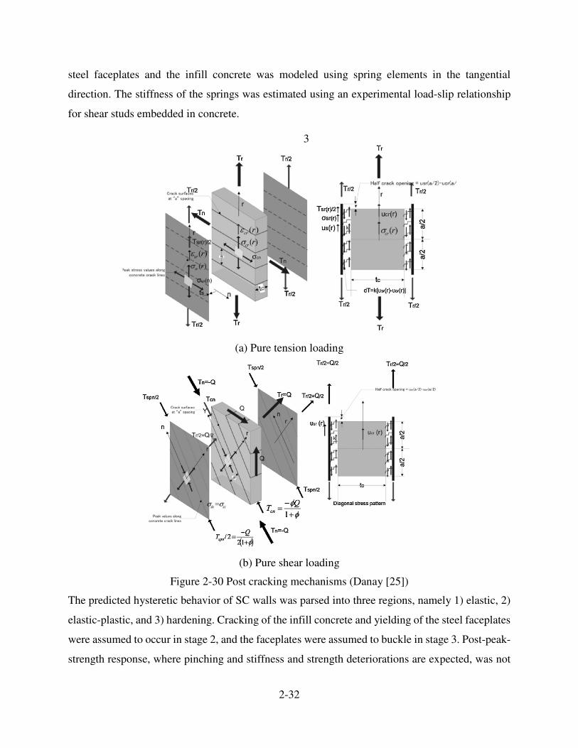
2-32
steel faceplates and the infill concrete was modeled using spring elements in the tangential
direction. The stiffness of the springs was estimated using an experimental load-slip relationship
for shear studs embedded in concrete.
3
(a) Pure tension loading
(b) Pure shear loading
Figure 2-30 Post cracking mechanisms (Danay [25])
The predicted hysteretic behavior of SC walls was parsed into three regions, namely 1) elastic, 2)
elastic-plastic, and 3) hardening. Cracking of the infill concrete and yielding of the steel faceplates
were assumed to occur in stage 2, and the faceplates were assumed to buckle in stage 3. Post-peak-
strength response, where pinching and stiffness and strength deteriorations are expected, was not
2-33
considered. Data from tests of four SC walls under axial and lateral loadings were used to validate
the model. The proposed model successfully predicted the shear strengths of the walls but
underestimated the displacements at peak force. Xiaowei et al. generated bending moment-axial
force interaction curves for SC walls using the results of the finite element analysis.
Varma et al. [100] proposed a mechanics-Based-Model (MBM) to predict the in-plane response of
SC panels under shear forces, as presented in Section 2.2. This simplified model: 1) assumed linear
elastic behavior for concrete in compression, and 2) did not consider the post-cracking and the
post-faceplate yielding regimes of response. To address these limitations, Varma et al. [97]
developed a layered composite shell finite element model using ABAQUS to extend the simplified
model and to predict the response of SC walls under monotonic loading. Multi-axial plasticity with
Von-Mises yield surface and kinematic hardening was used to model the steel faceplates. A
smeared crack model was used for the infill concrete. The experimental data of Ozaki et al. [63]
were used to validate the numerical model. Both the MBM and ABAQUS model under-predicted
the peak shear strength of SC walls. Analytical and numerical models were used to generate in-
plane force, and in-plane force and out-of-plane moment interaction curves. Based on the analysis
and test results, a simple design approach was proposed for SC walls subjected to a combined in-
plane forces and out-of-plane bending moments.
Varma et al. [98] developed a finite element model to simulate the monotonic and cyclic responses
of the 1/10-scale model of a pressurized water reactor containment internal structure (CIS) tested
by Akiayama et al. [7]. The CIS structure consisting of primary and secondary shield walls, two
reinforced concrete slabs, stream generator compartments, pressurizer compartment, and a number
of partition and wing walls was modeled in ABAQUS. The CDP model was used for concrete and
steel elements were modeled using the multi-axial plasticity model with combined hardening. The
shear studs and tie rods were modeled using beam and connector elements. The components of the
finite element model are presented in Figure 2-31.

2-34
(a) Infill concrete and basemat (b) Steel faceplates
(c) Reinforced concrete slabs (d) Tie bars
Figure 2-31 Finite element model of CIS structure (Varma et al. [98])
To investigate the effect of shear connectors on the lateral load response of the CIS structure, two
ABAQUS models were analyzed assuming: 1) perfect bond between the steel faceplates and the
infill concrete, and 2) partial bond by explicitly modeling the shear connectors. The predicted
monotonic force-displacement relationships were most similar, indicating that shear connectors
had no significant effect on the monotonic response of the CIS structure noting that the faceplate
slenderness ratio was 40. The models successfully predicted the peak shear strength but the pre-
peak stiffness was slightly underestimated. Cyclic analysis was conducted assuming perfect bond
between the steel faceplates and infill concrete, based on the results of the monotonic analysis. The
monotonic analysis model was updated to include cyclic damage and deterioration rules in the
concrete material model and ductile damage and fracture criteria in the steel material model. The
updated ABAQUS model successfully predicted the peak shear strength but the pinched response
and stiffness deterioration were not captured.

2-35
Kurt et al. [45] conducted LS-DYNA analyses of rectangular and flanged SC walls subjected to a
monotonic in-plane shear loading. The DYNA-predicted force-displacement relationship matched
the measured monotonic response up to peak strength. A parametric study was conducted to
investigate the effect of wall thickness and aspect ratio on the behavior of SC walls. This study
showed that the shear strength of a rectangular SC wall with an aspect ratio (i.e., height-to-length)
greater than 1.0 is governed by the moment capacity of the cross-section at the base of the wall.
For SC walls with an aspect ratio of less than 1.0, Kurt et al. concluded that the smaller the aspect
ratio, the greater the shear strength, with a maximum strength less than the pure in-plane shear
strength calculated as s yA f , where s
A and yf are the cross-sectional area and the yield stress of
the steel faceplates, respectively. Guidelines for connecting SC walls to RC foundation were
proposed.

3-1
3. PRELIMINARY DESIGN AND ANALYSIS OF SC WALLS
3.1 Introduction
The experimental program was developed assuming a maximum of four steel-plate concrete (SC)
composite shear walls were to be tested as part of a research project on conventional and innovative
structural walls with a low aspect ratio. Given that the focus was low aspect ratio, rectangular walls
that were flexure- and flexure-shear critical, an aspect ratio (height/length) of 1.0 was chosen for
the walls.
Choosing an aspect ratio of 1.0 for all four specimens, SC1, SC2, SC3 and SC4, allowed other
important design parameters to be varied. Ranges on key design parameters were identified,
considering the capacities of the equipment and facilities in the laboratory at the University at
Buffalo. After examining many alternatives, one steel faceplate thickness and two total thicknesses
(steel faceplates and infill concrete) were selected. Studs and tie rods were used in SC1 and SC3
but only tie rods were used in SC2 and SC4, in part to permit the removal of the faceplates from
SC2 and SC4, to allow examination of the damage to the infill concrete.
Section 3.2 provides the design basis for the test specimens. Section 3.3 presents the cross-
sectional analysis of the walls. Section 3.4 presents the results of a preliminary finite element
analysis conducted to predict the force-displacement relationships for the SC walls under
monotonic loading. Section 3.5 presents the designs of the SC wall connection to the foundation
and of the re-usable foundation block.
3.2 Preliminary Design of Test Specimens
The test specimens were designed with considerations of a draft version of AISC N690s1 [5].
Section N9.1.1c of AISC N690s1 limits the reinforcement ratio to the range of 1.5% to 5%, where
the reinforcement ratio is defined as the cross-sectional area of the faceplates divided by the cross-
sectional area of the SC wall web. Using 3/16 in. thick steel faceplates and total wall thicknesses
of 12 inches and 9 inches, the reinforcement ratios of SC1/SC2 and SC3/SC4 were 3.1% and 4.2%,
respectively.
Sections N9.3 and N9.4b of AISC N690s1 determine the maximum stud spacing to be the smaller
of the spacing required to a) limit the width-to-thickness ratio to 1.0 /s y
E f to prevent local
3-2
buckling of the steel faceplates before yielding, and b) develop the yield strength of the steel
faceplates over a development length, dL , where the development length of steel faceplates is
considered to be no more than three times the wall thickness. Grade 36 ASTM A572 steel with a
yield stress of 36 ksi was assumed for the design of the steel faceplates. The expected yield stress
( 1.4 36 ksi 50.4 ksi= × = ) of the steel faceplates was used to calculate the stud spacing, where the
factor of 1.4 was taken from the AISC Seismic Provisions 2005 [2]. The maximum spacing of the
studs according to the width-to-thickness ratio criterion is:
1
290003 /16 4.5 in.
50
ss
y
Es t
f≤ = = for SC1, SC2, SC3, and SC4
Assuming that the development length equals to three times the wall thickness, the maximum
spacing of the studs according to the development length criterion is:
2
3 12 54.4 in.
3 /16 50
d n
s y
L Qs
t f
× ×≤ = =
× for SC1 and SC2, and
2
3 9 53.8 in.
3 /16 50
d n
s y
L Qs
t f
× ×≤ = =
× for SC3 and SC4
where nQ is the shear capacity of a headed stud. For a 3/8 in. diameter headed stud, the shear
capacity per the Appendix D of ACI 349-06 [3], is:
20.7 0.7 (3 / 8) 65 5 kips4
stud
n sc uQ A Fπ
= = × × =
The stud spacing, calculated as a smaller of 1s and 2s , equaled 4.4 in. and 3.8 in. for SC1 and SC2,
and SC3 and SC4, respectively. Only tie rods (i.e., no studs) were used in SC2 and SC4. The studs
were spaced 4 in. on center in SC1. A stud spacing of 4.5 in. was used for SC3 to investigate the
effect on response of using a spacing greater than that specified by the AISC N690s1.
Tie rods are used to connect the two steel faceplates and provide structural integrity and the out-
of-plane shear reinforcement. AISC N690s1 specifies a maximum tie rod spacing equal to the wall
thickness. A tie rod spacing equal to one half of the AISC-specified maximum spacing was used
for SC2 and SC4 because no studs were used in these walls, although out-of-plane loads were not

3-3
imposed. In the other two specimens, the tie rod spacing was set equal to the thickness of the wall.
The tie rods were spaced at 12in., 6 in., 9 in., and 4.5 in. for SC1, SC2, SC3, and SC4, respectively.
A schematic of the walls is presented in Figure 3-1.
Figure 3-1 Elevation of SC walls
3.3 Cross-Sectional Analysis of SC Walls
3.3.1 Introduction
The flexural strengths of the SC walls were estimated using the cross-section program XTRACT
[19], which is a fiber-based cross-sectional analysis software. This calculation was made to
establish the lateral strength of the walls, assuming they were flexure-critical. Moment-curvature
relationships and axial force-bending moment interaction diagrams of a concrete, steel, reinforced
concrete, and composite sections can be calculated using XTRACT. Two concrete material models
can be accommodated: unconfined and confined. The input parameters for unconfined concrete
are uniaxial compressive and tensile strengths; post-crushing strength; concrete strains
corresponding to yield, crushing, spalling, and failure; and Young’s modulus. The yield strain is
typically taken as the strain corresponding to 0.4c
f ′ , where cf ′ is the uniaxial compressive strength
of the concrete. Typical values of the crushing and spalling strains are 0.003 and 0.006,
respectively, per Section R10.2.3 of ACI 318-11[1]. The properties of confined concrete, including
the concrete strength and crushing strain, are calculated automatically using the Mander model

3-4
[52] and information on the detailing of the cross section. The stress-strain relationship of the rebar
is characterized in three regions: 1) elastic, 2) the yield plateau, and 3) strain hardening. A
parabolic curve is used for the strain hardening branch. The input parameters for the steel material
are yield and ultimate stresses, strains at the onset of hardening and ultimate stress, and Young’s
modulus.
XTRACT discretizes a cross-section into a series of fibers. Finer meshes lead to more accurate
analysis. Each fiber within the discretized cross section is associated with a uniaxial steel or
concrete material. There are two types of analyses available in XTRACT: displacement-controlled
and force-controlled. In displacement-controlled analysis, the curvature is incremented and the
fiber strains relative to the strain at the centroid of the cross section (an arbitrary strain) at each
value of the curvature are calculated assuming plane section remains plane. The stress in each fiber
is calculated using the calculated fiber strain and its uniaxial stress-strain material model. The
resisting axial force and bending moment are calculated by integrating the fiber stresses across the
cross section. The absolute value of the strain at the centroid of the cross section is calculated by
solving the equilibrium equations. The curvature is incremented until the concrete or steel strain
reaches a specified failure strain. In force-controlled analysis, the force or moment is incremented.
The force-controlled analysis of the cross section in each load step is based on a Newton-Raphson
iteration process.
3.3.2 XTRACT Analysis of SC walls
3.3.2.1 Material Properties
Trial designs of specimens SC1 and SC3 were modeled in XTRACT. The flexural strengths were
calculated for two of the four SC walls, SC1 and SC3, since the geometrical properties of SC1 and
SC2, and SC3 and SC4, were nominally identical. Nominal material properties were used. Element
sizes of 2 in. and 1 in. were used for infill concrete and steel faceplates, respectively, on the basis
of preliminary analysis. The XTRACT model of SC1 is presented in Figure 3-2.

3-5
Figure 3-2 XTRACT model of SC1
Table 3-1 and Table 3-2 presents the concrete and steel material properties input to the XTRACT
model, respectively. In Table 3-1, cE is the Young’s modulus of the infill concrete; c
f ′ is the
uniaxial concrete compressive strength; rf is the concrete stress corresponding to the spalling; ycε
is the strain at 0.4c
f ′ ; ucε is the strain corresponding to peak stress; and spε and fε are the spalling
and failure strains, respectively. In Table 3-2, sE is Young’s modulus of the steel faceplates; yf
and uf are the yield and ultimate stresses of the steel faceplates, respectively; sh
ε is the strain at
the onset of hardening; and usε is the strain at the ultimate stress.
Table 3-1 Concrete material properties for XTRACT analysis
cE
cf ′
rf ycε
ucε spε fε
(ksi) (ksi) (ksi) (%) (%) (%) (%)
3605 4 0.4 0.04 0.2 1.0 1.0
Table 3-2 Steel material properties for XTRACT analysis
sE yf u
fsh
ε usε
(ksi) (ksi) (ksi) (%) (%)
29000 36 55 1.5 15.0
Young’s modulus of the infill concrete was calculated using (3-1), according to Section 8.5.1 of
ACI 318-11 [1]:
57000c c
E f ′= � (3-1)
The strain corresponding to peak stress was calculated using (3-2) proposed by Chang et al. [20]:

3-6
1/4( )
4000
cuc
fε
′= � (3-2)
The concrete stress corresponding to spalling was calculated using the concrete stress-strain
relationship proposed by Tsai [88] :
( )
1 ( )1 1
c c r
nxf f
r xn x
r r
′=
+ − +− −
(3-3)
where x is the concrete strain normalized by ucε , and n and r are the coefficients of the concrete
stress-strain relationship and calculated using (3-4) and (3-5), proposed by Chang et al. [20]:
3/8
46
( )c
nf
=′
(3-4)
1.9750
cf
r′
= − � (3-5)
where ycε corresponds to a concrete stress of 0.4c
f ′ . The spalling and failure strains were assumed
to be 1%, noting that the flexural strength is not affected by concrete spalling and failure since it
is achieved when the concrete strain reaches εc0
: the concrete strain at cf ′ . The properties for
ASTM A36 steel were taken from Brockenbrough et al. [18].
3.3.2.2 Flexural Strengths of SC Walls
The assumptions made to calculate the flexural strength of the SC walls were: (1) plane sections
remain plane after bending; (2) flexure-shear interaction is ignored; (3) the effect of confinement
on the behavior of the infill concrete is not considered; and (4) the steel faceplates and the infill
concrete are perfectly bonded.
Figure 3-3 presents the moment-curvature relationships for SC1 and SC3. The XTRACT-predicted
flexural strengths of SC1 and SC3 were 20610 kips-in. and 19650 kips-in., respectively. The shear
strengths of SC1 and SC3 corresponding to these flexural strengths were 344 kips and 328 kips,
respectively.

3-7
To determine whether the specimens were likely to be flexure-critical or shear-critical, the
maximum shear resistance of the walls was calculated using (3-6) to (3-8) that are based on the
draft Appendix N9 to AISC N690s1 [5], Ozaki et al. [65], and Varma et al. [100]:
1n y sV kf A= (3-6)
2n s yV A f= � (3-7)
3n s yV A fα= � (3-8)
where k is 1.11 5.16ρ− , and ρ is the strength-adjusted reinforcement ratio and calculated as:
31.6
s y
c c
A f
A fρ =
′�
(3-9)
Figure 3-3 Moment-curvature relationships for the SC walls
where sA and c
A are the cross-sectional areas of the steel faceplates and the infill concrete,
respectively. In (3-8), α is calculated as:
23
K K
K K
α β
α β
α+
=+
� (3-10)
where
� �!���� �!���0 �!���$ �!���) �!���� �!���1
���(��������2��!
�
����
�����
�����
0����
0����
���2��0
��$2��)
3���2��040�1���*�!��
3��$2��)4��1���*�!��
3-8
s sK G Aα = (3-11)
1
2(1 ) 4s
cr
s s c c
K
A E A E
β ν=
−+
�(3-12)
where sG is the elastic shear modulus of the steel faceplates, s
ν is Poisson’s ratio of the steel
faceplates, and cr
cE is Young’s modulus of the cracked infill concrete and taken as 0.7 cE ���
The maximum shear resistance of the walls per the draft Appendix N9 to AISC N690s1 [5], Ozaki
et al. [65], and Varma et al. [100] is 870/855/815 kips for SC1/SC2 and 840/855/780 kips for
SC3/SC4. The SC walls were identified to be flexure-critical since the shear strength associated to
the flexural strength of the walls was less than their maximum shear resistance.
3.4 Pre-Test Finite Element Analysis of SC Walls
The general-purpose finite element code ABAQUS [76, 77] was used to verify the XTRACT-
predicted peak shear strengths and to estimate the shear force-lateral displacement relationships
for the four walls. The ABAQUS model of SC1 is shown in Figure 3-4.
The model took advantage of symmetry to reduce the computational effort. As seen in Figure 3-4,
the model included one steel faceplate, infill concrete, a baseplate attached to the steel faceplate,
a steel plate embedded in the foundation, studs and tie rods, a loading plate attached to the actuator,
and threaded bars used to secure the baseplate to the foundation. The foundation was not included
in the model since preliminary analyses indicated that the foundation block was effectively rigid
and had no effect on the response of the SC walls.
The Concrete-Damage-Plasticity (CDP) model was used for the infill concrete and the J2 plasticity
model with isotropic hardening was used for the steel faceplates. Friction between the infill
concrete and the steel faceplate, and buckling of the steel faceplate were considered. Beam
elements were used to represent the studs and tie rods. Solid elements were used to model the infill
concrete, baseplate, steel plate, loading plate, and post-tensioning bars. Shell elements were used
for the steel faceplate. The infill concrete was modeled with 1 × 1 × 1 in. elements and the steel
faceplate was modeled with 0.5 × 0.5 in. elements. Nominal material properties were used for the
pre-test ABAQUS calculations.

3-9
The predicted shear force-lateral displacement relationships of SC1 through SC4 are presented in
Figure 3-5. In this figure, drift ratio is defined the lateral displacement devided by the vertical
distance between the line of loading and the top of the foundation block (= 60 inches). The peak
resistances of 300 kips for SC1/SC2 and 250 kips for SC3/SC4 agreed reasonably well with the
estimate of shear corresponding to flexural strengths (= 344 kips for SC1/SC2 and 328 kips for
SC3/SC4), which ignored flexure-shear interaction.
Figure 3-4 ABAQUS modeling of SC1
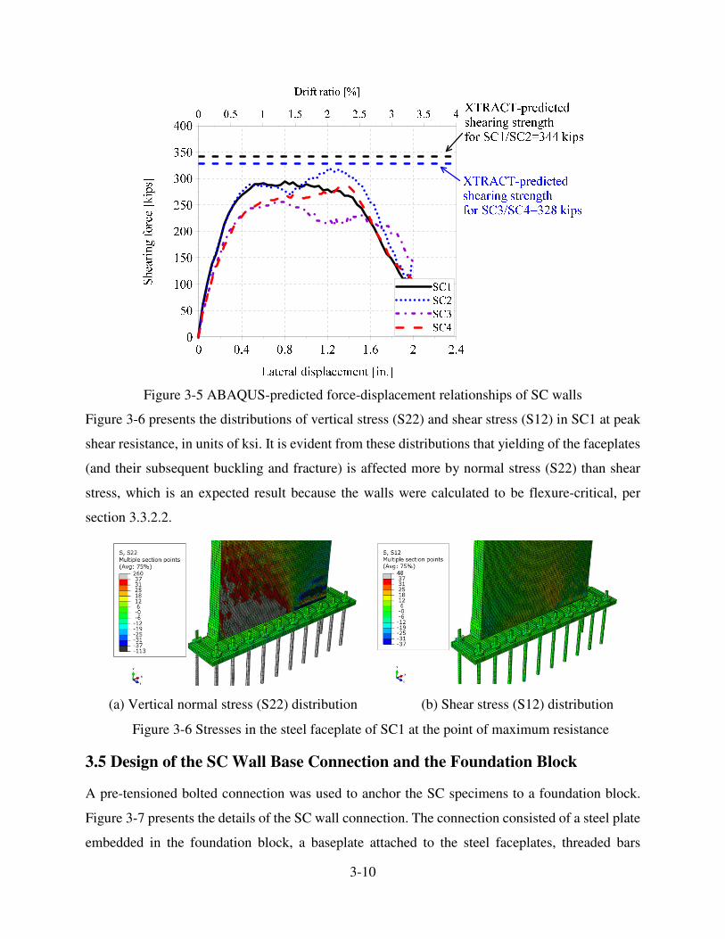
3-10
Figure 3-5 ABAQUS-predicted force-displacement relationships of SC walls
Figure 3-6 presents the distributions of vertical stress (S22) and shear stress (S12) in SC1 at peak
shear resistance, in units of ksi. It is evident from these distributions that yielding of the faceplates
(and their subsequent buckling and fracture) is affected more by normal stress (S22) than shear
stress, which is an expected result because the walls were calculated to be flexure-critical, per
section 3.3.2.2.
(a) Vertical normal stress (S22) distribution (b) Shear stress (S12) distribution
Figure 3-6 Stresses in the steel faceplate of SC1 at the point of maximum resistance
3.5 Design of the SC Wall Base Connection and the Foundation Block
A pre-tensioned bolted connection was used to anchor the SC specimens to a foundation block.
Figure 3-7 presents the details of the SC wall connection. The connection consisted of a steel plate
embedded in the foundation block, a baseplate attached to the steel faceplates, threaded bars

3-11
securing the baseplate to the foundation block, headed studs attached to the baseplate, shear lugs
attached to the steel plate embedded in the foundation block, and a steel anchorage securing the
threaded bars to the foundation block. Post-tensioned Dwyidag bars were used to anchor the
foundation block to the strong floor. The baseplate, threaded bars, and the Dwyidag bars were
sized to remain elastic, with a margin, under the maximum predicted shear force of 350 kips
(Section 3.3.2.2).
Figure 3-7 SC wall connection to the foundation block
The dimensions and detailing of the SC wall connection and the foundation block were based on
the results of the finite element analysis of the SC walls and analysis of strut-and-tie models,
respectively, as described in Nguyen [56]. The CAD drawings of the details of the foundation
block and the SC wall connection are provided in Appendix A.
The design of the studs that attached the infill concrete to the baseplate followed the steps
enumerated below:
1. The contribution of the steel faceplates and the infill concrete to the total shear load (from
Section 3.3.2.2) was calculated using the elastic shear stiffness of the steel faceplates (3-13)
and the post-cracked shear stiffness of the infill concrete (3-14), as proposed by Varma et al.
[100].
s sK G Aα = (3-13)

3-12
1
2(1 ) 4s
cr
s s c c
K
A E A E
β ν=
−+ (3-14)
where sA and
cA are the cross-sectional areas of the steel faceplates and infill concrete,
respectively; sG is the elastic shear modulus of the steel faceplates;
sν is Poisson’s ratio of the
steel faceplates; and cr
cE is the Young’s modulus of the cracked infill concrete, taken as 0.7 .cE
The shear stiffness of the steel faceplates and the infill concrete were 250960 kips/rad and
230040 kips/rad , respectively, using the nominal material properties of the steel faceplates
and the infill concrete, as specified in Section 3.3.2.1.
2. The contributions of the steel faceplates and the infill concrete to the total shear load were
calculated as:
250960350 182 kips
250960 230040
230040350 168 kips
250960 230040
S SC
C SC
KV V
K K
KV V
K K
α
α β
β
α β
= = =+ +
= = =+ +
where SV and C
V are the shear forces resisted by the steel faceplates and the infill concrete,
respectively, and SCV is the XTRACT-predicted peak shear force for SC1.
3. Using 5/8-in. diameter shear studs with a shear capacity (Appendix D of ACI 349-06 [3]) of:
20.7 0.7 (5 / 8) 65 14 kips4
stud
n sc uQ A Fπ
= = × × =
eighteen number 5/8-in. diameter studs were required to resist a shear force of 250 kips (equals
to ~1.5×168 kips, where 1.5 provides a margin on capacity).
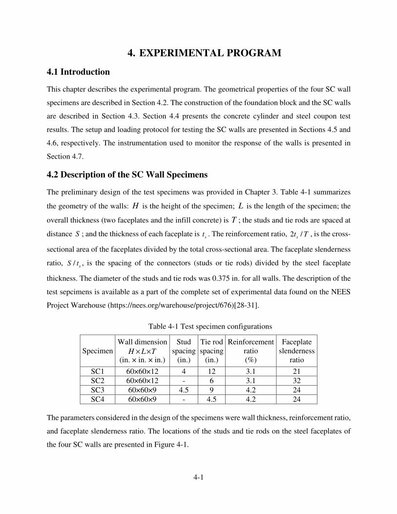
4-1
4. EXPERIMENTAL PROGRAM
4.1 Introduction
This chapter describes the experimental program. The geometrical properties of the four SC wall
specimens are described in Section 4.2. The construction of the foundation block and the SC walls
are described in Section 4.3. Section 4.4 presents the concrete cylinder and steel coupon test
results. The setup and loading protocol for testing the SC walls are presented in Sections 4.5 and
4.6, respectively. The instrumentation used to monitor the response of the walls is presented in
Section 4.7.
4.2 Description of the SC Wall Specimens
The preliminary design of the test specimens was provided in Chapter 3. Table 4-1 summarizes
the geometry of the walls: H is the height of the specimen; L is the length of the specimen; the
overall thickness (two faceplates and the infill concrete) is T ; the studs and tie rods are spaced at
distance S ; and the thickness of each faceplate is st . The reinforcement ratio, 2 /st T , is the cross-
sectional area of the faceplates divided by the total cross-sectional area. The faceplate slenderness
ratio, / sS t , is the spacing of the connectors (studs or tie rods) divided by the steel faceplate
thickness. The diameter of the studs and tie rods was 0.375 in. for all walls. The description of the
test sepcimens is available as a part of the complete set of experimental data found on the NEES
Project Warehouse (https://nees.org/warehouse/project/676)[28-31].
Table 4-1 Test specimen configurations
Specimen
Wall dimension
H L T× ×(in. × in. × in.)
Stud
spacing
(in.)
Tie rod
spacing
(in.)
Reinforcement
ratio
(%)
Faceplate
slenderness
ratio
SC1 60×60×12 4 12 3.1 21
SC2 60×60×12 - 6 3.1 32
SC3 60×60×9 4.5 9 4.2 24
SC4 60×60×9 - 4.5 4.2 24
The parameters considered in the design of the specimens were wall thickness, reinforcement ratio,
and faceplate slenderness ratio. The locations of the studs and tie rods on the steel faceplates of
the four SC walls are presented in Figure 4-1.

4-2
(a) SC1 (b) SC2
(c) SC3 (d) SC4
Figure 4-1 Locations of studs (×) and tie rods ( ) attached to the steel faceplates
Each SC wall was installed on top of a re-usable foundation block. The base of each wall included
a 1-in. thick A572 Gr.50 steel baseplate to which the faceplates were CJP groove welded. Two
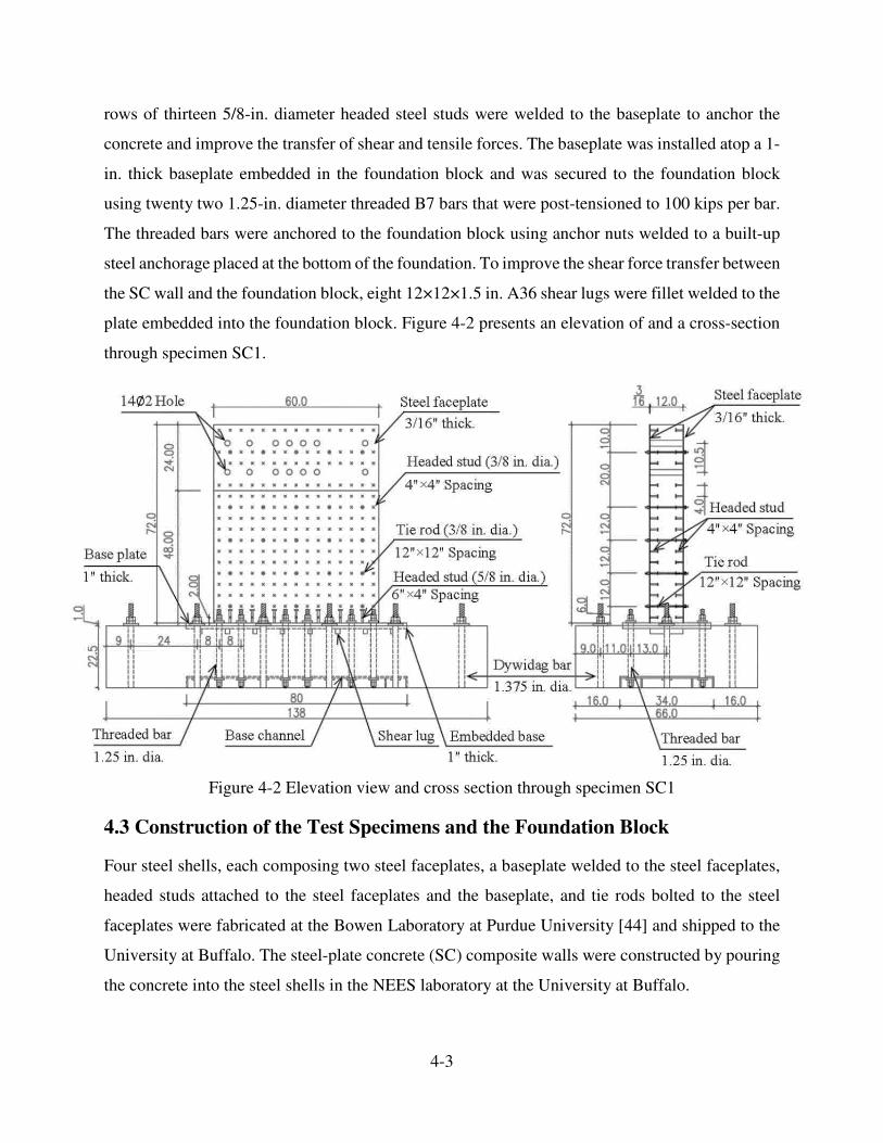
4-3
rows of thirteen 5/8-in. diameter headed steel studs were welded to the baseplate to anchor the
concrete and improve the transfer of shear and tensile forces. The baseplate was installed atop a 1-
in. thick baseplate embedded in the foundation block and was secured to the foundation block
using twenty two 1.25-in. diameter threaded B7 bars that were post-tensioned to 100 kips per bar.
The threaded bars were anchored to the foundation block using anchor nuts welded to a built-up
steel anchorage placed at the bottom of the foundation. To improve the shear force transfer between
the SC wall and the foundation block, eight 12×12×1.5 in. A36 shear lugs were fillet welded to the
plate embedded into the foundation block. Figure 4-2 presents an elevation of and a cross-section
through specimen SC1.
Figure 4-2 Elevation view and cross section through specimen SC1
4.3 Construction of the Test Specimens and the Foundation Block
Four steel shells, each composing two steel faceplates, a baseplate welded to the steel faceplates,
headed studs attached to the steel faceplates and the baseplate, and tie rods bolted to the steel
faceplates were fabricated at the Bowen Laboratory at Purdue University [44] and shipped to the
University at Buffalo. The steel-plate concrete (SC) composite walls were constructed by pouring
the concrete into the steel shells in the NEES laboratory at the University at Buffalo.

4-4
4.3.1 Wall Specimen Construction
Two 3/16 × 60 × 72 in. steel faceplates were fabricated for each specimen as follows [44]:
1. Drill fourteen 2-in. diameter holes at the top of the steel faceplates (Figure 4-2) to create
sleeves through which threaded bars were to be passed (Figure 4-3(a)).
2. Draw a grid on the surface of the steel faceplates to locate the points of the attachments of
the connectors to the steel faceplates (Figure 4-3(a)).
3. Use a center punch to mark the steel faceplates at the locations of the attachments of the
studs/tie rods to the faceplates. These marks were used to locate studs/tie rods after grinding
of the steel faceplate and to prevent movement of the stud when using the stud gun.
4. Grind the steel faceplates at the points of the attachments of the studs to create a smooth
surface (Figure 4-3(a)).
5. Weld the studs to the steel faceplates using a stud gun (Figure 4-3(b)).
6. Check the quality of the stud welds by a 90-degree bend test on a single welded stud
(Figure 4-3(c)).
7. Drill 7/16-in. diameter holes through the steel faceplates at the tie rod locations.
8. Insert the tie rods through the drilled holes, and install and tighten nuts on both sides of each
faceplate (Figure 4-3(d)).
9. Weld two rows of fifteen 0.675-in. diameter headed studs to the baseplate (Figure 4-3(e)).
10. Bevel one edge of the steel faceplate in preparation for its CJP welding to the baseplate
(Figure 4-3(f)).
11. CJP groove weld each steel faceplate to the baseplate (Figure 4-3(g)).
Figure 4-4 is a photograph of the assembled steel shells of SC1, SC3, and SC4.
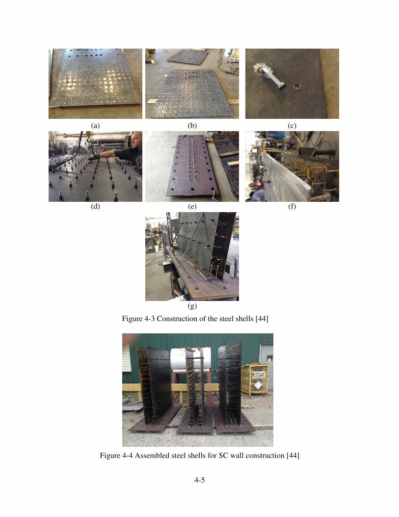
4-5
(a) (b) (c)
(d) (e) (f)
(g)
Figure 4-3 Construction of the steel shells [44]
Figure 4-4 Assembled steel shells for SC wall construction [44]

4-6
4.3.2 Foundation Construction
A steel anchorage built from channel sections was placed at the bottom of the foundation to anchor
the threaded bars to the foundation block. The detailing of this element and its construction are
described in Nguyen [56]. Figure 4-5 is a photograph of the anchor block in the formwork for the
foundation. Nuts for 1.25-in. diameter B7 bars were tack welded to the underside of the channel
(not seen in Figure 4-5) to permit tightening of the B7 anchor bolts from the top of the foundation.
One of the bolts is seen in the figure. Each bolt was isolated from the surrounding concrete by a
PVC sleeve.
Figure 4-5 Built-up steel anchorage and foundation formwork
Prior to placing the rebar cage into the foundation formwork, wooden plugs were attached at 24
inches on center to the soffit of the formwork at the location of the 2-in. diameter PVC sleeves to
prevent movement of the sleeves during the installation of the rebar cage and the pouring of
concrete. The rebar cage was then placed into the foundation formwork and the PVC sleeves were
installed. The 1.25-in. diameter threaded B7 bars were passed through the (22) sleeves and screwed
into the tack-welded nuts noted above. A steel plate was placed on the rebar cage, centered on the
anchor block below, and over the B7 anchor bolts, and leveled. The concrete was poured into the
formwork. The foundation block was water-cured for seven days after casting. Figure 4-6 shows
steps in the construction of the foundation.
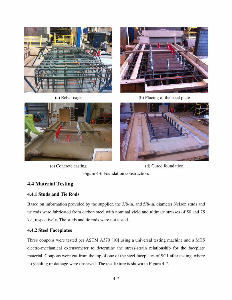
4-7
(a) Rebar cage (b) Placing of the steel plate
(c) Concrete casting (d) Cured foundation
Figure 4-6 Foundation construction.
4.4 Material Testing
4.4.1 Studs and Tie Rods
Based on information provided by the supplier, the 3/8-in. and 5/8-in. diameter Nelson studs and
tie rods were fabricated from carbon steel with nominal yield and ultimate stresses of 50 and 75
ksi, respectively. The studs and tie rods were not tested.
4.4.2 Steel Faceplates
Three coupons were tested per ASTM A370 [10] using a universal testing machine and a MTS
electro-mechanical extensometer to determine the stress-strain relationship for the faceplate
material. Coupons were cut from the top of one of the steel faceplates of SC1 after testing, where
no yielding or damage were observed. The test fixture is shown in Figure 4-7.

4-8
(a) Universal testing machine (b) MTS extensometer
Figure 4-7 Coupon test fixture
The measured stress-strain relationships of the coupons are presented in Figure 4-8. The yield and
ultimate strengths of the steel faceplates were 38 and 55 ksi, respectively. The measured strain at
the peak stress and the failure strain were 0.25 and 0.4, respectively.
4.4.3 Infill Concrete and Foundation
The uniaxial compressive strengths and Young’s modulus of the infill concrete and the foundation
concrete were calculated using the measured stress-strain relationships obtained from concrete
cylinder tests. Testing followed ASTM C39-02 [9]. Cylinders were tested at 7, 14, 21, 28 days
after concrete casting and on the days of the SC wall tests (=58, 75, 133, and 154 days after
concrete casting, respectively, for SC1, SC2, SC3, and SC4). Cylinder tests were performed using
a Forney compression testing machine, as shown in Figure 4-9.
Figure 4-8 Stress-strain relationships of the faceplate coupons

4-9
Figure 4-9 Concrete cylinder test
Figure 4-10 presents a photograph of the instrumentation used for the cylinder tests. One steel ring
and four steel supports were mounted on a cylinder, 5 in. from its ends, to support four equally
spaced LVDTs that were used to measure the relative axial displacement along the 10 in. gage
length.
Figure 4-10 Instrumentation of a concrete cylinder
The calculated Young’s modulus and measured uniaxial compressive strengths of the concrete,
calculated as averages from the concrete cylinders cracked on the day of testing, were 3000 ksi

4-10
and 4.4 ksi for SC1/SC2, and 3300 ksi and 5.3 ksi for SC3/SC4. Figure 4-11 shows a concrete
cylinder after testing.
Figure 4-11 Concrete cylinder after the test
4.5 Test Setup
4.5.1 Installation of the Foundation Block
A re-usable foundation block was used to test all four SC walls. The foundation block was placed
on four shims to a) level the block, and b) provide a gap for grouting. The steel top plate was
leveled using the shims. The gap between the block and the story floor was filled with a high-
strength cementitious grout. After the grout had cured, 14 Dwyidag bars were installed to anchor
the block to the strong floor, and tensioned to 100 kips per bar, for a total preload of the foundation
block on the strong floor of 1400 kips.
4.5.2 Installation of the SC Wall Panels
Each SC wall panel was installed on the steel top plate of the foundation block. After plumbing
the wall, the B7 threaded bars that joined the wall’s baseplate to the steel top plate and reaction
block were tensioned to 100 kips per bar, for a total preload of 2200 kips. The two loading brackets,
one on each side of the wall, were installed and anchored to the wall using fourteen 1.25-in.
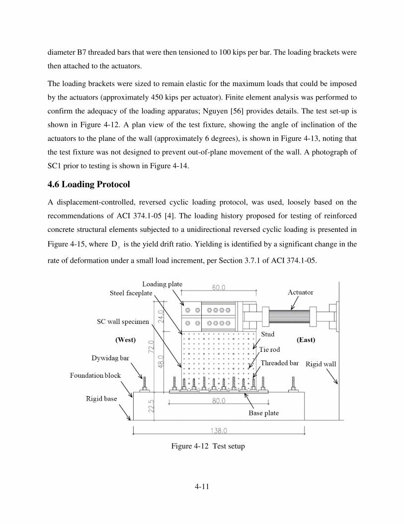
4-11
diameter B7 threaded bars that were then tensioned to 100 kips per bar. The loading brackets were
then attached to the actuators.
The loading brackets were sized to remain elastic for the maximum loads that could be imposed
by the actuators (approximately 450 kips per actuator). Finite element analysis was performed to
confirm the adequacy of the loading apparatus; Nguyen [56] provides details. The test set-up is
shown in Figure 4-12. A plan view of the test fixture, showing the angle of inclination of the
actuators to the plane of the wall (approximately 6 degrees), is shown in Figure 4-13, noting that
the test fixture was not designed to prevent out-of-plane movement of the wall. A photograph of
SC1 prior to testing is shown in Figure 4-14.
4.6 Loading Protocol
A displacement-controlled, reversed cyclic loading protocol, was used, loosely based on the
recommendations of ACI 374.1-05 [4]. The loading history proposed for testing of reinforced
concrete structural elements subjected to a unidirectional reversed cyclic loading is presented in
Figure 4-15, where Dy is the yield drift ratio. Yielding is identified by a significant change in the
rate of deformation under a small load increment, per Section 3.7.1 of ACI 374.1-05.
Figure 4-12 Test setup

4-12
Figure 4-13 Plan view of the test fixture
Figure 4-14 Specimen SC1
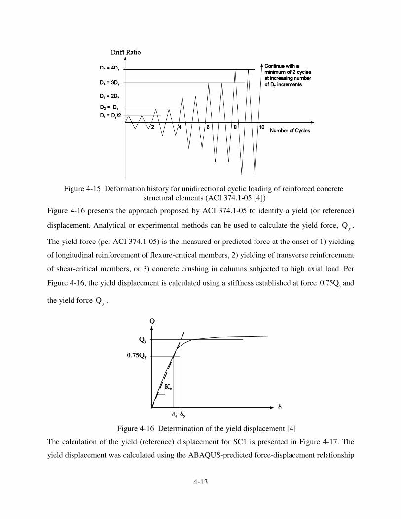
4-13
Figure 4-15 Deformation history for unidirectional cyclic loading of reinforced concrete
structural elements (ACI 374.1-05 [4])
Figure 4-16 presents the approach proposed by ACI 374.1-05 to identify a yield (or reference)
displacement. Analytical or experimental methods can be used to calculate the yield force, Q y .
The yield force (per ACI 374.1-05) is the measured or predicted force at the onset of 1) yielding
of longitudinal reinforcement of flexure-critical members, 2) yielding of transverse reinforcement
of shear-critical members, or 3) concrete crushing in columns subjected to high axial load. Per
Figure 4-16, the yield displacement is calculated using a stiffness established at force 0.75Qy and
the yield force Q y .
Figure 4-16 Determination of the yield displacement [4]
The calculation of the yield (reference) displacement for SC1 is presented in Figure 4-17. The
yield displacement was calculated using the ABAQUS-predicted force-displacement relationship

4-14
(see Section 3.4). Assuming that yielding of the SC walls corresponded to the onset of the yielding
of the steel faceplates, the yield displacement and its corresponding force for SC1 were estimated
to be 0.14 in. and 150 kips, respectively. A yield (reference) displacement of 0.14 in. was used to
generate the loading protocol for testing all four SC walls.
Two additional loading steps, at displacements of 10% and 75% of the reference displacement,
were added to the deformation history of Figure 4-15 to capture SC wall response before and after
cracking of the infill concrete.
Table 4-2 presents the loading protocol used to test the SC walls. The loading protocol consisted
of 15 load steps with two cycles in each step. Two cycles of loading were imposed at displacements
equal to fractions and multiples of the reference displacement (= 0.14 inch): 0.1, 0.5, 0.75, 1, 2 ...
12. In Table 4-2, drift ratio at any load step was calculated by dividing the peak displacement of
that load step to the distance between the base of the wall and the centerline of horizontal loading
(= 60 inches).
Figure 4-17 Yield or reference displacement calculation
In each loading cycle, a push was imposed first, followed by a pull, where push was defined as
the loading in the positive direction, to the West (denoted as WL+), and pull was defined as the
loading in the negative direction, to the East (denoted as EL-). The East and West directions are
identified in Figure 4-12. Testing was terminated after steel faceplate fracture and crushing of the
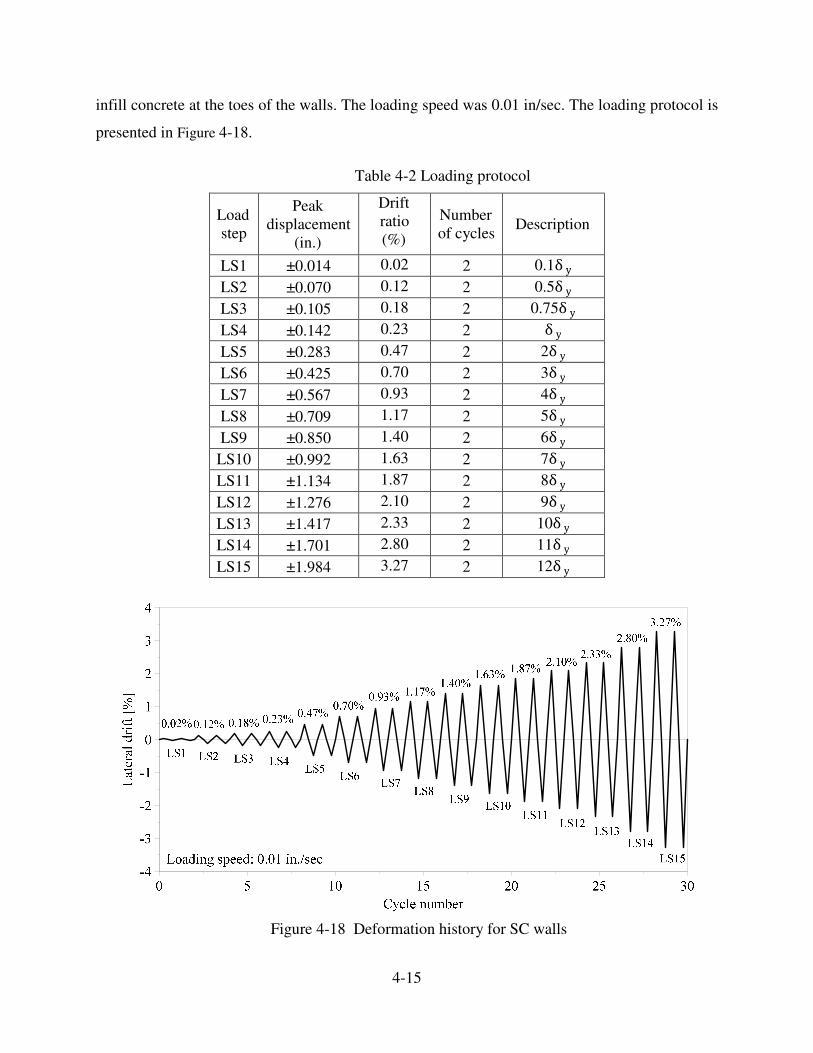
4-15
infill concrete at the toes of the walls. The loading speed was 0.01 in/sec. The loading protocol is
presented in Figure 4-18.
Table 4-2 Loading protocol
Load
step
Peak
displacement
(in.)
Drift
ratio
(%)
Number
of cyclesDescription
LS1 ±0.014 0.02 2 0.1� �
LS2 ±0.070 0.12 2 0.5� �
LS3 ±0.105 0.18 2 0.75� �
LS4 ±0.142 0.23 2 � �
LS5 ±0.283 0.47 2 2� �
LS6 ±0.425 0.70 2 3� �
LS7 ±0.567 0.93 2 4� �
LS8 ±0.709 1.17 2 5� �
LS9 ±0.850 1.40 2 6� �
LS10 ±0.992 1.63 2 7� �
LS11 ±1.134 1.87 2 8� �
LS12 ±1.276 2.10 2 9� �
LS13 ±1.417 2.33 2 10� �
LS14 ±1.701 2.80 2 11� �
LS15 ±1.984 3.27 2 12� �
Figure 4-18 Deformation history for SC walls
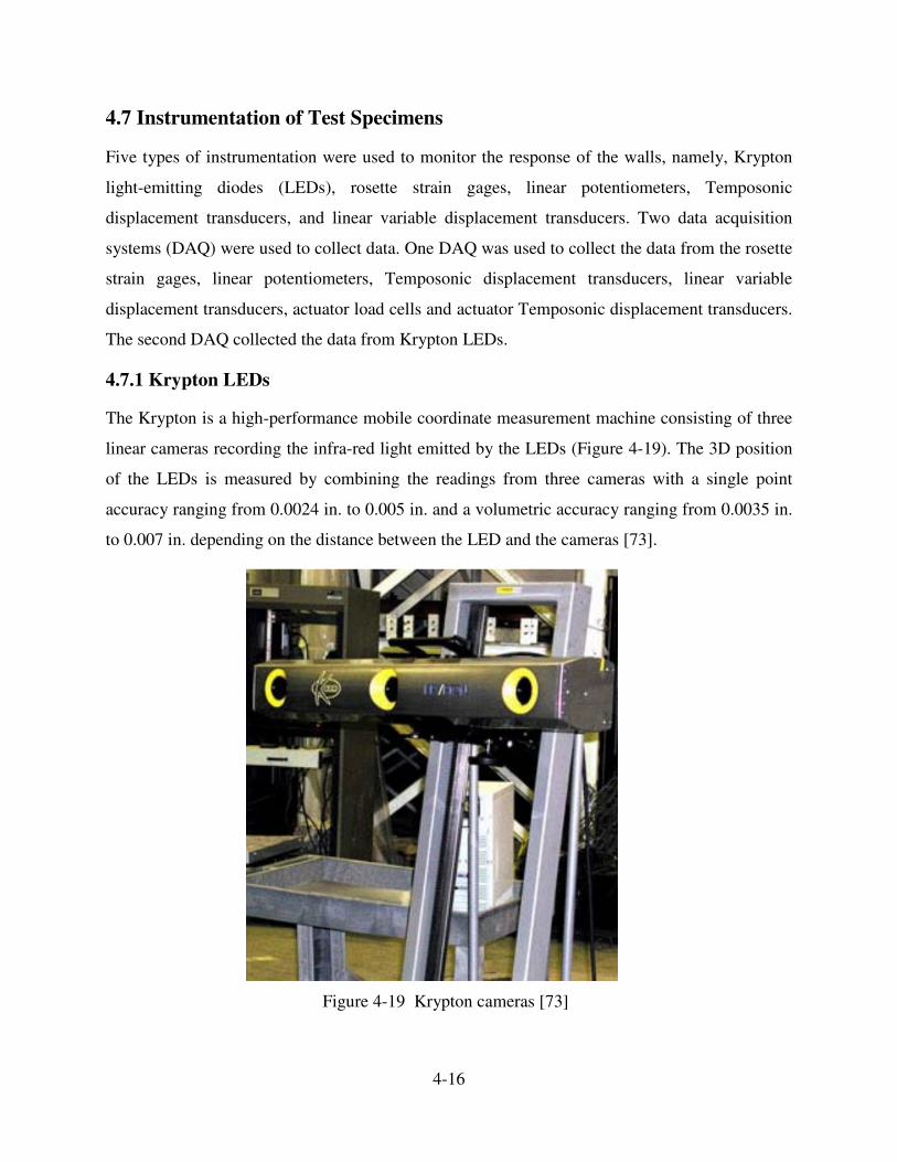
4-16
4.7 Instrumentation of Test Specimens
Five types of instrumentation were used to monitor the response of the walls, namely, Krypton
light-emitting diodes (LEDs), rosette strain gages, linear potentiometers, Temposonic
displacement transducers, and linear variable displacement transducers. Two data acquisition
systems (DAQ) were used to collect data. One DAQ was used to collect the data from the rosette
strain gages, linear potentiometers, Temposonic displacement transducers, linear variable
displacement transducers, actuator load cells and actuator Temposonic displacement transducers.
The second DAQ collected the data from Krypton LEDs.
4.7.1 Krypton LEDs
The Krypton is a high-performance mobile coordinate measurement machine consisting of three
linear cameras recording the infra-red light emitted by the LEDs (Figure 4-19). The 3D position
of the LEDs is measured by combining the readings from three cameras with a single point
accuracy ranging from 0.0024 in. to 0.005 in. and a volumetric accuracy ranging from 0.0035 in.
to 0.007 in. depending on the distance between the LED and the cameras [73].
Figure 4-19 Krypton cameras [73]

4-17
To measure the in-plane and out-of-plane displacements of SC walls, 179, 158, 146, and 146
Krypton LEDs were attached to one steel faceplate of SC1, SC2, SC3, and SC4, respectively. The
locations of the LEDs on the SC walls are presented in Figure 4-20.
(a) SC1
(b) SC2
Figure 4-20 Krypton LEDs on SC walls

4-18
(c) SC3 and SC4
Figure 4-20 Krypton LEDs on SC walls (cont.)
4.7.2 Rosette Strain Gages
Three independent axial strains at different orientations at a point are required to determine the
state of in-plane strain. The normal and shear strains are calculated using the three measured
strains, the orientations of the uniaxial gages, and the strain transformation equations. Figure 4-21
presents the rosette strain gage, used for the experiments, manufactured by Vishay Precision Group
Inc [111]. The specifications for the gage are provided in Appendix C.
Figure 4-21 Rectangular rosette strain gage (Vishay Precision Group [111])
Fifteen, 11, 17, and 17 rosette strain gages were installed at three levels on one steel faceplate of
SC1 through SC4, respectively, to measure strains at discrete locations. The rosette strain gages
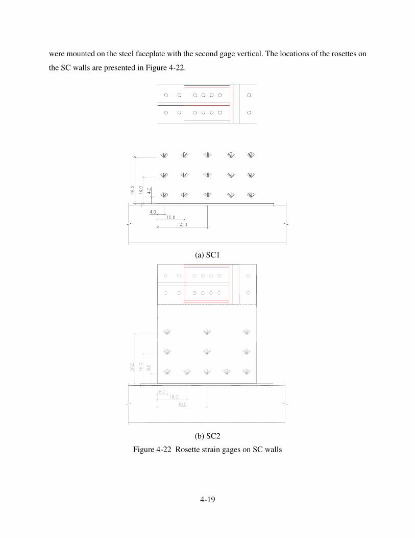
4-19
were mounted on the steel faceplate with the second gage vertical. The locations of the rosettes on
the SC walls are presented in Figure 4-22.
(a) SC1
(b) SC2
Figure 4-22 Rosette strain gages on SC walls

4-20
(c) SC3 and SC4
Figure 4-22 Rosette strain gages on SC walls (cont.)
4.7.3 LVDTs, Temposonic Displacement Transducers, and String Potentiometers
The horizontal and vertical movements of the foundation block relative to the strong floor were
monitored using two horizontal linear variable displacement transducers (LVDTs) attached to the
bottom corners of the foundation block and one vertical LVDT attached at the bottom center of
the foundation block.
Nineteen string potentiometers and 7 Temposonic displacement transducers were attached to the
ends of a wall to measure in-plane displacement along the height of the wall. Four string
potentiometers were attached to the corners of one steel faceplate to measure the out-of-plane
movement of the SC wall. Figure 4-23 presents the locations of the string potentiometers,
Temposonic transducers, and LVDTs attached on the ends of the wall.

4-21
Figure 4-23 Layout of the linear potentiometers (SP), Temposonic displacement
transducers (TP), and linear variable displacement transducers (LPH and LPV)
References

5-1
5. EXPERIMENTAL RESULTS
5.1 Introduction
Information on the test specimens, materials, loading protocol, test setup, and instrumentation was
provided in Chapter 4. This chapter summarizes the results of testing of the four SC walls in the
NEES laboratory at the University at Buffalo.
The initial stiffness of the SC walls, the forces and displacements corresponding to the onset of
buckling and yielding of the steel faceplates, to the peak load, and at the end of the tests are
presented in Section 5.2. The progression of damage to the SC walls, including the cracking and
crushing of the infill concrete, and buckling and fracture of the steel faceplates, are presented in
Section 5.3. The cyclic force-displacement relationships are presented in Section 5.4. Section 5.5
discusses the post-peak response of the SC walls, focusing on the influence of stud spacing. Energy
dissipation and equivalent viscous damping ratios are calculated in Section 5.6. Section 5.7
presents the strain and stress fields in the steel faceplates and the contribution of the steel faceplates
to the total shear load. The variation of vertical strain in the steel faceplates along the length of the
wall, near the base, at different drift ratios, is presented in Section 5.8. Section 5.9 discusses load
transfer mechanisms in the SC walls. The lateral displacement profiles along the height of the SC
walls are presented in Section 5.10. Section 5.11 identifies the contributions of shear, flexure, and
base rotation to the total lateral displacement. The displacement ductility of the SC walls is
established in Section 5.12. Cyclic secant stiffness is presented in Sections 5.13.
5.2 Test Result
Key test results are provided in Table 5-1. The initial stiffness of the SC walls, calculated at drift
ratios less than 0.02%, are presented in the second column of the table. The values of the forces
and displacements corresponding to the onset of faceplate buckling are listed in the third and fourth
columns, respectively. The fifth and sixth columns in the table present computed data at the onset
of faceplate yielding, where forces and displacements were calculated using rosette strain gage
data and assuming a Von-Mises yield criterion. The seventh and eighth columns present peak loads
and the corresponding drift ratios for both EL- and WL+ directions, where the EL- and WL+
directions were identified in Figure 4-12. The last column in the table lists the post-peak loads at
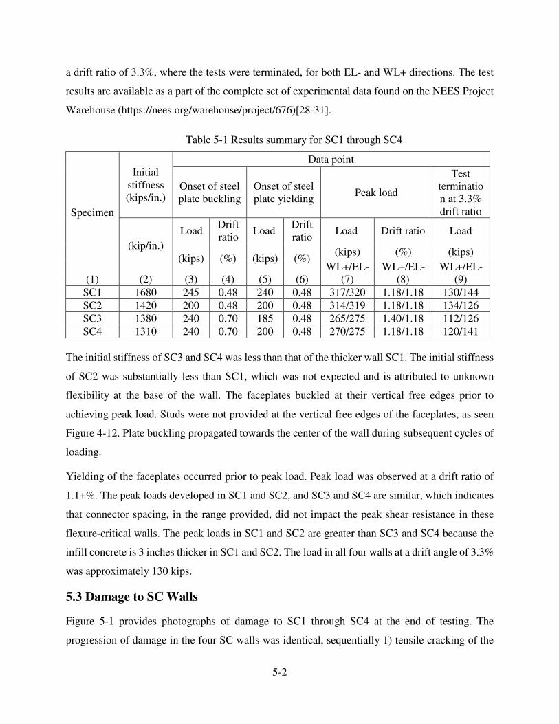
5-2
a drift ratio of 3.3%, where the tests were terminated, for both EL- and WL+ directions. The test
results are available as a part of the complete set of experimental data found on the NEES Project
Warehouse (https://nees.org/warehouse/project/676)[28-31].
Table 5-1 Results summary for SC1 through SC4
Specimen
Initial
stiffness
(kips/in.)
Data point
Onset of steel
plate buckling
Onset of steel
plate yielding Peak load
Test
terminatio
n at 3.3%
drift ratio
(kip/in.)
Load Drift
ratio Load
Drift
ratio Load Drift ratio Load
(kips) (%) (kips) (%) (kips) (%) (kips)
WL+/EL- WL+/EL- WL+/EL-
(1) (2) (3) (4) (5) (6) (7) (8) (9)
SC1 1680 245 0.48 240 0.48 317/320 1.18/1.18 130/144
SC2 1420 200 0.48 200 0.48 314/319 1.18/1.18 134/126
SC3 1380 240 0.70 185 0.48 265/275 1.40/1.18 112/126
SC4 1310 240 0.70 200 0.48 270/275 1.18/1.18 120/141
The initial stiffness of SC3 and SC4 was less than that of the thicker wall SC1. The initial stiffness
of SC2 was substantially less than SC1, which was not expected and is attributed to unknown
flexibility at the base of the wall. The faceplates buckled at their vertical free edges prior to
achieving peak load. Studs were not provided at the vertical free edges of the faceplates, as seen
Figure 4-12. Plate buckling propagated towards the center of the wall during subsequent cycles of
loading.
Yielding of the faceplates occurred prior to peak load. Peak load was observed at a drift ratio of
1.1+%. The peak loads developed in SC1 and SC2, and SC3 and SC4 are similar, which indicates
that connector spacing, in the range provided, did not impact the peak shear resistance in these
flexure-critical walls. The peak loads in SC1 and SC2 are greater than SC3 and SC4 because the
infill concrete is 3 inches thicker in SC1 and SC2. The load in all four walls at a drift angle of 3.3%
was approximately 130 kips.
5.3 Damage to SC Walls
Figure 5-1 provides photographs of damage to SC1 through SC4 at the end of testing. The
progression of damage in the four SC walls was identical, sequentially 1) tensile cracking of the

5-3
concrete at both ends of the wall, 2) outward buckling and yielding of the steel faceplates at the
base of the wall, 3) crushing and spalling of concrete at the toes of the wall, and 4) tearing of the
steel faceplates along their welded connection to the baseplate.
(a) SC1
(b) SC2
(c) SC3
Figure 5-1 Damage to SC walls at the end of testing
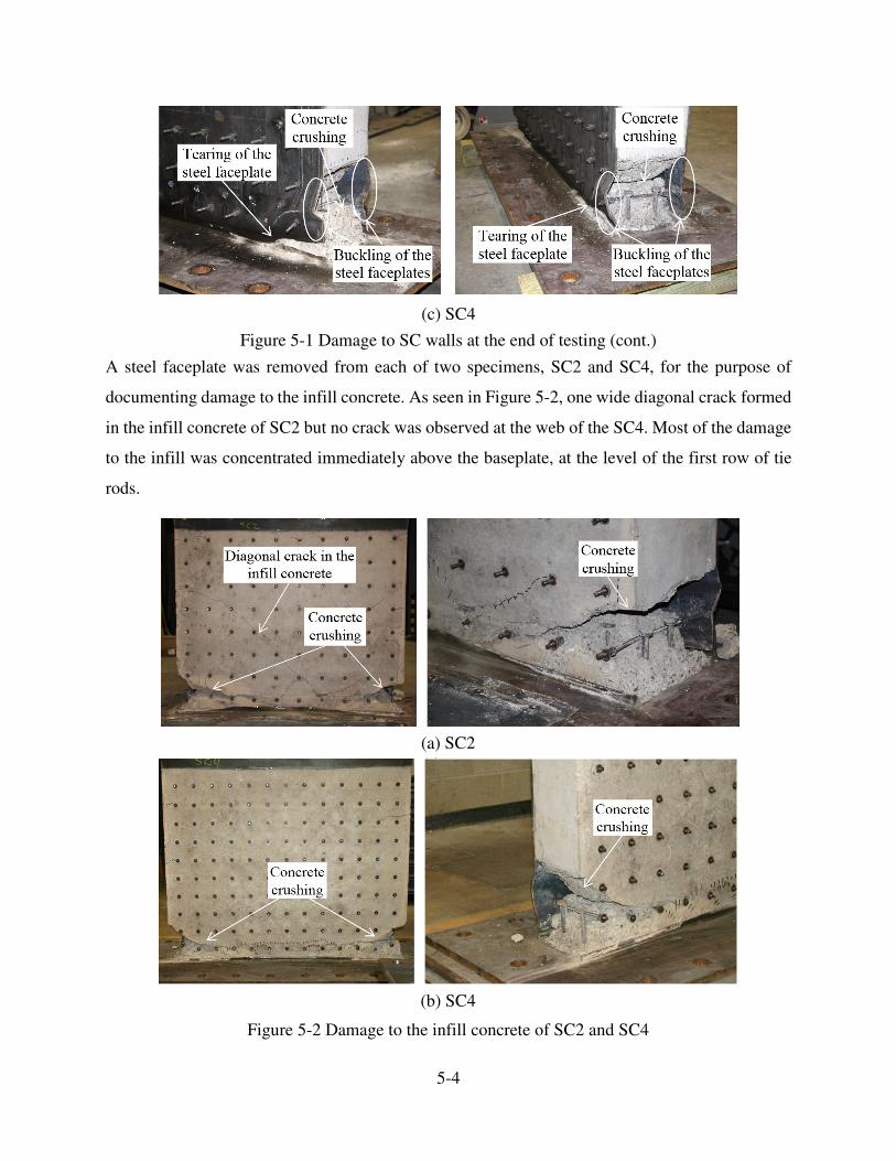
5-4
(c) SC4
Figure 5-1 Damage to SC walls at the end of testing (cont.)
A steel faceplate was removed from each of two specimens, SC2 and SC4, for the purpose of
documenting damage to the infill concrete. As seen in Figure 5-2, one wide diagonal crack formed
in the infill concrete of SC2 but no crack was observed at the web of the SC4. Most of the damage
to the infill was concentrated immediately above the baseplate, at the level of the first row of tie
rods.
(a) SC2
(b) SC4
Figure 5-2 Damage to the infill concrete of SC2 and SC4

5-5
Figure 5-3 presents the damage to SC1 through SC4 at different drift ratios. More photographs of
damage to the SC walls and to the infill concrete of SC2 and SC4 at each loading step and at the
end of the testing are provided in Appendix B. In Figure 5-3, LS denotes the load step, and CI and
CII represent the first and second cycles in each load step, respectively. The sequence of the
damage to the SC walls is presented in Table 5-2. Concrete cracking, steel faceplate buckling, and
concrete crushing in the four SC walls occurred at drift ratios of 0.12%, 0.47%, and 1.17%
respectively. Local tearing of the steel faceplates at their connection to the headed studs occurred
at a drift ratio of 1.6% for SC1. Tearing of the faceplates along their welded connection to the
baseplate begun at drift ratios of 1.4% for SC3 and SC4, 1.6% for SC2, and 2.3% for SC1. One tie
rod in SC4 fractured at a drift ratio of 2.1%.
Tearing of the steel faceplates initiated immediately above the welded connection of the faceplates
to the baseplate in SC2, SC3, and SC4. In SC1, the steel faceplates fractured first at connections
to the headed studs. The lower corners of the steel faceplates, where the faceplates were expected
to buckle, were restrained by headed studs in SC1 and tie rods in the other SC walls (see
Figure 5-4). Headed studs anchor the faceplates to the infill concrete, enable composite action, and
delay out-of-plane buckling of the faceplates. Crushed concrete around a stud cannot anchor a stud
and local damage around the stud will affect the buckling resistance of the faceplate. (The use of
tie rods near the base of the wall will significantly reduce the outward movement of the tie rod
(and the faceplate) after concrete crushing, at the location of the tie rod, and consequently improve
the response by delaying inelastic buckling of the faceplate).
5.4 Load-Displacement Cyclic Response
The load-displacement relationships for SC1 through SC4 are presented in Figure 5-5. Points A,
B, C, D, E, F, and G in Figure 5-5 represent the onset of concrete cracking, yielding of the steel
faceplates, buckling of the steel faceplates, concrete crushing, fracture of the steel faceplates at
their connection to the headed studs, tearing of the steel faceplate above the welded connection of
the faceplates to the baseplate, and fracture of tie rod, respectively. The load was calculated by
resolving the sum of the forces in the actuator load cells into the plane of the wall. The
displacement was measured by a Temposonic displacement transducer attached to the side of the
wall at the level of the actuators (60 in. above the base of the wall).

5-6
�(a) SC1
�(b) SC2
�(c) SC3
(d) SC4
1. Concrete cracking; 2. Steel faceplate buckling; 3. Concrete crushing; 4. Fracture of the steel
faceplate at the level of the stud; 5. Fracture of the steel faceplate above the welded connection;
6. Fracture of the tie rod
Figure 5-3 Damage to SC walls

5-7
Figure 5-4 Location of the studs and tie rods attached to the steel faceplates
Table 5-2 Sequence of damage to SC walls
Load
step
Drift
ratio Specimen Damage
LS2 0.12% SC1 through SC4 Concrete cracking at toes of the wall
LS5 0.47% SC1 through SC4 Buckling of the steel faceplates
LS8 1.17% SC1 through SC4 Concrete crushing at toes of the wall
LS9 1.40% SC3 and SC4 Tearing of the steel faceplates immediately above the
welded connection of the faceplates to the baseplate
LS10 1.63%
SC1 Local tearing of the steel faceplates at the connection
point to the steel studs
SC2
Horizontal tearing of the steel faceplates immediately
above the welded connection of the faceplates to the
baseplate
LS12 2.10% SC4 Fracture of tie rod
LS13 2.33% SC1
Horizontal tearing of the steel faceplates at the level of
the steel studs and immediately above the welded
connection of the faceplates to the baseplate
The peak load, observed at a relatively high drift ratio of 1.17+%, were 325 kips and 275 kips for
SC1/SC2, and SC3/SC4, respectively. The pinched behavior was attributed to the damage to the
infill concrete and steel faceplates, including concrete crushing and tearing of the steel faceplates,
and flexibility at the base of the wall. The rates of the post-peak strength and stiffness deterioration
were similar in SC2, SC3, and SC4. The rate of strength deterioration in SC1 post-peak-strength
was much lower than in other walls up to point F in SC1 (2.33% drift ratio), where the steel
faceplates fractured above their welded connection to the baseplate.

5-8
(a) SC1 (b) SC2
(c) SC3 (d) SC4
Figure 5-5 Cyclic force-displacement relationships and backbone curves for the SC walls
The onset of yielding of the steel faceplates was determined using the rosette strain gage data and
assuming a Von-Mises yield criterion. As seen in Figure 5-5, yielding of the steel faceplates
occurred prior to their buckling for SC1 and SC2. Buckling and yielding of the steel faceplates
occurred at the same drift ratio for SC3 and SC4. Concrete crushing occurred at a drift ratio
corresponding to the peak shear strength for the four SC walls. The pre-peak-strength response of
SC walls could be approximated by a tri-linear force-displacement relationship to consider three
stages of response, namely 1) elastic, 2) cracking of the infill concrete, and 3) buckling of the steel
faceplates.
�0!) ��!� ��!0 ��!1 � �!1 �!0 �!� 0!)
5���������������������!
�)��
�$��
�0��
����
�
���
0��
$��
)���) �$ �0 �� � � 0 $ )
6�� ���������7
�
�
6
8
#
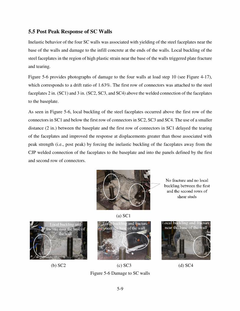
5-9
5.5 Post Peak Response of SC Walls
Inelastic behavior of the four SC walls was associated with yielding of the steel faceplates near the
base of the walls and damage to the infill concrete at the ends of the walls. Local buckling of the
steel faceplates in the region of high plastic strain near the base of the walls triggered plate fracture
and tearing.
Figure 5-6 provides photographs of damage to the four walls at load step 10 (see Figure 4-17),
which corresponds to a drift ratio of 1.63%. The first row of connectors was attached to the steel
faceplates 2 in. (SC1) and 3 in. (SC2, SC3, and SC4) above the welded connection of the faceplates
to the baseplate.
As seen in Figure 5-6, local buckling of the steel faceplates occurred above the first row of the
connectors in SC1 and below the first row of connectors in SC2, SC3 and SC4. The use of a smaller
distance (2 in.) between the baseplate and the first row of connectors in SC1 delayed the tearing
of the faceplates and improved the response at displacements greater than those associated with
peak strength (i.e., post peak) by forcing the inelastic buckling of the faceplates away from the
CJP welded connection of the faceplates to the baseplate and into the panels defined by the first
and second row of connectors.
(a) SC1
(b) SC2 (c) SC3 (d) SC4
Figure 5-6 Damage to SC walls
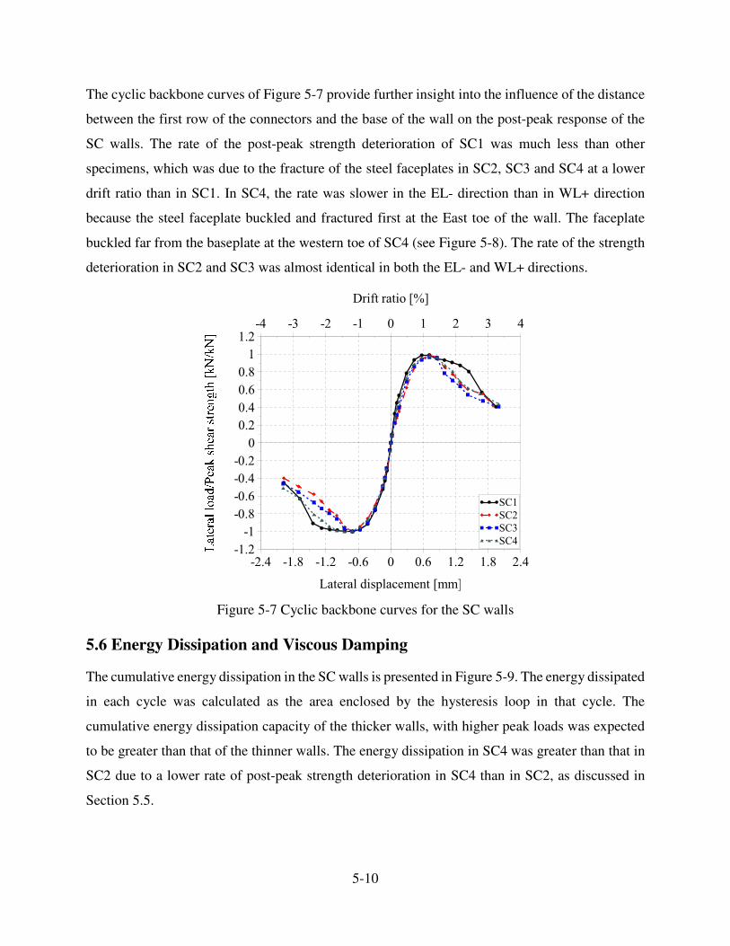
5-10
The cyclic backbone curves of Figure 5-7 provide further insight into the influence of the distance
between the first row of the connectors and the base of the wall on the post-peak response of the
SC walls. The rate of the post-peak strength deterioration of SC1 was much less than other
specimens, which was due to the fracture of the steel faceplates in SC2, SC3 and SC4 at a lower
drift ratio than in SC1. In SC4, the rate was slower in the EL- direction than in WL+ direction
because the steel faceplate buckled and fractured first at the East toe of the wall. The faceplate
buckled far from the baseplate at the western toe of SC4 (see Figure 5-8). The rate of the strength
deterioration in SC2 and SC3 was almost identical in both the EL- and WL+ directions.
Figure 5-7 Cyclic backbone curves for the SC walls
5.6 Energy Dissipation and Viscous Damping
The cumulative energy dissipation in the SC walls is presented in Figure 5-9. The energy dissipated
in each cycle was calculated as the area enclosed by the hysteresis loop in that cycle. The
cumulative energy dissipation capacity of the thicker walls, with higher peak loads was expected
to be greater than that of the thinner walls. The energy dissipation in SC4 was greater than that in
SC2 due to a lower rate of post-peak strength deterioration in SC4 than in SC2, as discussed in
Section 5.5.
�0!) ��!� ��!0 ��!1 � �!1 �!0 �!� 0!)
5���������������������
��!0
��
��!�
��!1
��!)
��!0
�
�!0
�!)
�!1
�!�
�
�!0
���
��0
��$
��)
�) �$ �0 �� � � 0 $ )
6�� ���������7

5-11
(a) West toe of the SC wall (b) East toe of the SC wall
Figure 5-8 Damage to SC4 at 1.6% drift angle
Figure 5-9 Cumulative energy dissipation capacities of SC walls
Equation (5-1) [23] was used to calculate the equivalent viscous damping, , in the SC walls:
1
4
Deq
S
E
Eξ
π= � (5-1)
where D
E is the energy dissipated in a vibration cycle and S
E �is the corresponding strain energy.
Figure 5-10 presents the equivalent viscous damping ratios calculated from experimental data for
drift ratios up to 3.3%. The vertical dashed red line represents the drift ratio corresponding to peak
strength. In the pre-peak-strength region, the equivalent viscous damping ratios for the walls are
virtually identical. For drift ratios between 50% and 100% of those associated with peak strength,
ζeq
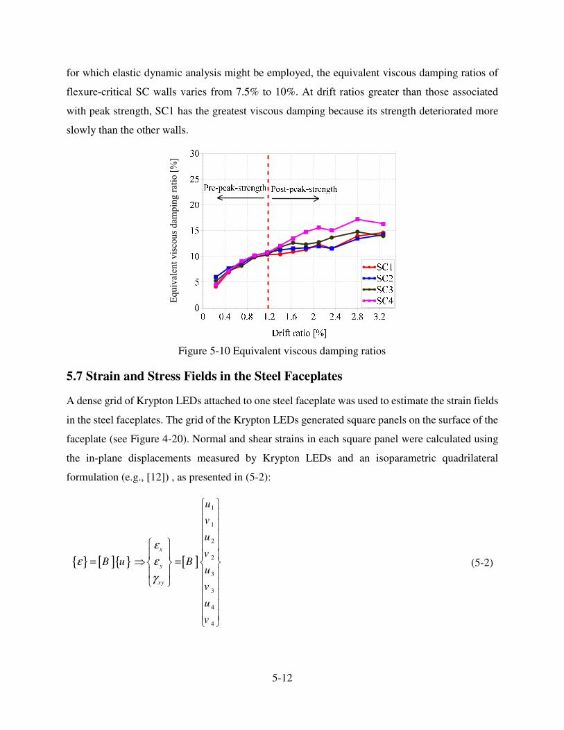
5-12
for which elastic dynamic analysis might be employed, the equivalent viscous damping ratios of
flexure-critical SC walls varies from 7.5% to 10%. At drift ratios greater than those associated
with peak strength, SC1 has the greatest viscous damping because its strength deteriorated more
slowly than the other walls.
Figure 5-10 Equivalent viscous damping ratios
5.7 Strain and Stress Fields in the Steel Faceplates
A dense grid of Krypton LEDs attached to one steel faceplate was used to estimate the strain fields
in the steel faceplates. The grid of the Krypton LEDs generated square panels on the surface of the
faceplate (see Figure 4-20). Normal and shear strains in each square panel were calculated using
the in-plane displacements measured by Krypton LEDs and an isoparametric quadrilateral
formulation (e.g., [12]) , as presented in (5-2):
{ } [ ]{ } [ ]
1
1
2
2
3
3
4
4
x
y
xy
u
v
u
vB u B
u
v
u
v
ε
ε
γ
ε
� �
� �
=� � � � �
�
=
(5-2)
9:��(
����
�(�
������
��
���
���
�7

5-13
where { }ε is a vector of the in-plane normal and shear strains; iu and i
v are the measured
horizontal and vertical nodal displacements at the four corners of each panel, respectively; and
[ ]B is the strain-displacement matrix and is derived using the shape functions presented in (5-3).
1(1 )(1 )
4i
N s t= ± ± , 1,..., 4i = (5-3)
where ( ),s t is the new coordinate system to which was mapped from the ( ),x y coordinate
system. The strains in the other steel faceplate were directly measured using rosette strain gages
installed at three elevations, with the second gage vertical. The three strains measured by each
rosette were transformed to normal and shear strains using (5-4) to (5-6).
x a c b
ε ε ε ε= + − (5-4)
y bε ε= (5-5)
xy c aγ ε ε= − � (5-6)
where aε , b
ε , and cε are the strains measured by the first, second, and third strain gages,
respectively; xε and yε are the transformed normal strains parallel to the length and height of the
specimen, respectively; and xyγ is the engineering shear strain.
The measured shear forces, corresponding to the level of the first row of strain gages and first row
of LED panels above the baseplate, were calculated as the product of the average shear strain
(calculated using either the rosettes strain gages or from the LED displacements), an assumed
value of G (=11155 ksi) for the steel faceplates, and a total faceplate area of 22.5 inches, prior to
the steel faceplate yielding.
Figure 5-11 presents the shear force-displacement relationships for the steel faceplates at small
values of drift ratio, and prior to steel faceplate yielding, calculated using the displacements
measured by the LEDs (solid blue line) and strains measured by rosettes (solid red line).
Figure 5-11 shows that the LED- and rosette-measured shear force-displacement relationships are
virtually identical.
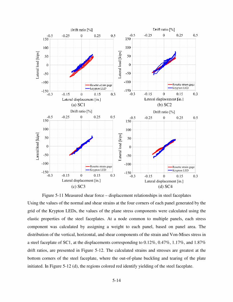
5-14
(a) SC1 (b) SC2
(c) SC3 (d) SC4
Figure 5-11 Measured shear force – displacement relationships in steel faceplates
Using the values of the normal and shear strains at the four corners of each panel generated by the
grid of the Krypton LEDs, the values of the plane stress components were calculated using the
elastic properties of the steel faceplates. At a node common to multiple panels, each stress
component was calculated by assigning a weight to each panel, based on panel area. The
distribution of the vertical, horizontal, and shear components of the strain and Von-Mises stress in
a steel faceplate of SC1, at the displacements corresponding to 0.12%, 0.47%, 1.17%, and 1.87%
drift ratios, are presented in Figure 5-12. The calculated strains and stresses are greatest at the
bottom corners of the steel faceplate, where the out-of-plane buckling and tearing of the plate
initiated. In Figure 5-12 (d), the regions colored red identify yielding of the steel faceplate.
5��
����
����
�*�
5��
����
����
�*�
��!$ ��!�� � �!�� �!$
5������ ���������� ���!
����
����
���
�
��
���
���
;����� ����� ����
<�&��� 596
��!� ��!0� � �!0� �!�
6�� � ����� �7
��!$ ��!�� � �!�� �!$
5������ ���������� ���!
����
����
���
�
��
���
���
;����� ����� ����
<�&��� 596
��!� ��!0� � �!0� �!�
6�� � ����� �7
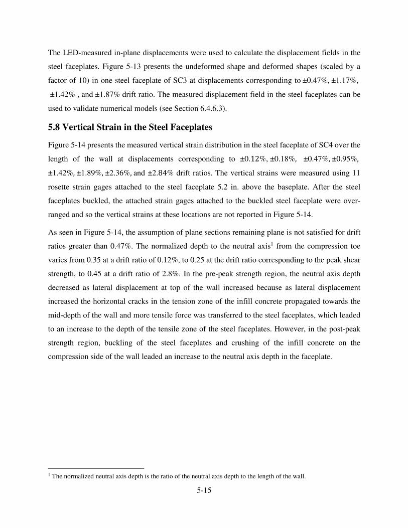
5-15
The LED-measured in-plane displacements were used to calculate the displacement fields in the
steel faceplates. Figure 5-13 presents the undeformed shape and deformed shapes (scaled by a
factor of 10) in one steel faceplate of SC3 at displacements corresponding to�±0.47%,�±1.17%,
±1.42% , and ±1.87% drift ratio. The measured displacement field in the steel faceplates can be
used to validate numerical models (see Section 6.4.6.3).
5.8 Vertical Strain in the Steel Faceplates
Figure 5-14 presents the measured vertical strain distribution in the steel faceplate of SC4 over the
length of the wall at displacements corresponding to ±0.��%, ±0.18%�� ±0.47%��±0.95%��
±1.42%��±1.89%��±2.36%��and ±2.��% drift ratios. The vertical strains were measured using 11
rosette strain gages attached to the steel faceplate 5.2 in. above the baseplate. After the steel
faceplates buckled, the attached strain gages attached to the buckled steel faceplate were over-
ranged and so the vertical strains at these locations are not reported in Figure 5-14.
As seen in Figure 5-14, the assumption of plane sections remaining plane is not satisfied for drift
ratios greater than 0.47%. The normalized depth to the neutral axis1 from the compression toe
varies from 0.35 at a drift ratio of 0.12%, to 0.25 at the drift ratio corresponding to the peak shear
strength, to 0.45 at a drift ratio of 2.8%. In the pre-peak strength region, the neutral axis depth
decreased as lateral displacement at top of the wall increased because as lateral displacement
increased the horizontal cracks in the tension zone of the infill concrete propagated towards the
mid-depth of the wall and more tensile force was transferred to the steel faceplates, which leaded
to an increase to the depth of the tensile zone of the steel faceplates. However, in the post-peak
strength region, buckling of the steel faceplates and crushing of the infill concrete on the
compression side of the wall leaded an increase to the neutral axis depth in the faceplate.
1 The normalized neutral axis depth is the ratio of the neutral axis depth to the length of the wall.
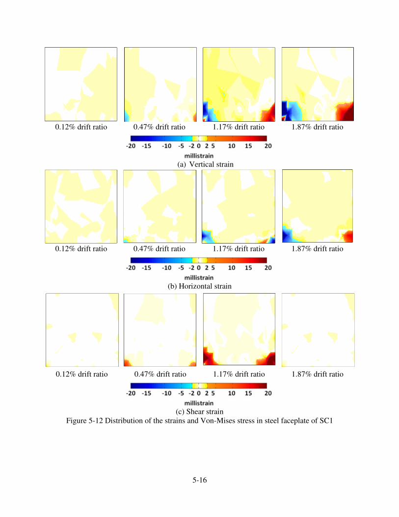
5-16
0.12% drift ratio 0.47% drift ratio 1.17% drift ratio 1.87% drift ratio
(a) Vertical strain
0.12% drift ratio 0.47% drift ratio 1.17% drift ratio 1.87% drift ratio
(b) Horizontal strain
0.12% drift ratio 0.47% drift ratio 1.17% drift ratio 1.87% drift ratio
(c) Shear strain
Figure 5-12 Distribution of the strains and Von-Mises stress in steel faceplate of SC1
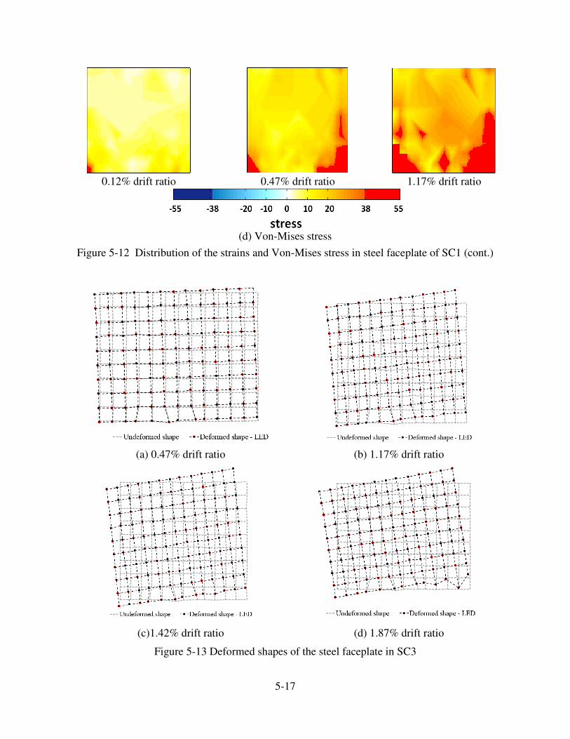
5-17
0.12% drift ratio 0.47% drift ratio 1.17% drift ratio
(d) Von-Mises stress
Figure 5-12 Distribution of the strains and Von-Mises stress in steel faceplate of SC1 (cont.)
(a) 0.47% drift ratio (b) 1.17% drift ratio
(c)1.42% drift ratio (d) 1.87% drift ratio
Figure 5-13 Deformed shapes of the steel faceplate in SC3

5-18
(a) Loading towards the West direction
(b) Loading towards the East direction
Figure 5-14 Measured vertical strain distribution in the steel faceplate of SC4 over the length
of the wall
5.9 Load Transfer in the SC Walls
To investigate load transfer between the steel faceplate and the infill concrete, the strain field in
the steel faceplates and the horizontal shear force resisted by the steel faceplates were evaluated at
different elevations over the height of the wall using nodal displacements measured by the LEDs.
The square grid of Krypton LEDs installed on one faceplate per wall enabled calculation of the
strain field in the elastic range of response. The horizontal and vertical displacements from each
LED were used to calculate the three in-plane strain components using an isoparametric
quadrilateral formulation (e.g., Bathe [12]). The normal and shear stresses were then calculated
�
�

5-19
using an elastic constitutive stress-strain relationship. The horizontal shear force resisted by the
steel faceplates was calculated by integrating the shear stress along the length of the faceplate and
multiplying by 2.
The horizontal shear forces resisted by the steel faceplates were calculated at the five levels along
the height of the wall identified in Figure 5-15. Figure 5-16 presents results for cycles 3 through 8
and prior to faceplate yielding.
Force ratio is defined as the horizontal shear force resisted by the steel faceplates divided by the
total applied lateral force (measured by the actuator load cells, resolved into the plane of the wall).
The force ratio varies from 25% to 75%, and from 30% to 90%, for SC1/SC2 and SC3/SC4,
respectively. The force ratios in SC3 and SC4 were greater than those in SC1 and SC3, supporting
the intuitive statement that the higher the reinforcement ratio, the greater the steel faceplate
contribution to the total shear force.
(a) SC1 (b) SC2 (c) SC3 (d) SC4
Figure 5-15 Reporting levels for the steel faceplates
The force ratios increased in SC1, SC3, and SC4 from the top of each specimen (level 5, see
Figure 5-15) to the foundation. The shear force was transferred from the infill concrete to the steel
faceplates through the connectors and interface friction between the infill concrete and steel
faceplate, along the height of the wall. In SC2, the specimen with the highest plate slenderness
ratio (=32), the greatest contribution of the steel faceplate to the total shear force before yielding
of the faceplate was observed at level 3: the mid-height of the specimen.
1234
5

5-20
(a) SC1 (b) SC2
(c) SC3 (d) SC4
Figure 5-16 Ratio of the horizontal shear force resisted by the steel faceplates to
the total applied load
The total horizontal shear force transferred by a row of connectors was calculated as the difference
between the horizontal shear forces resisted by the steel faceplate above and below the row, which
neglects interface friction. The shear forces resisted by the second, third, and fourth rows of the
connectors were estimated to be 11/14/20 kips, 7/6/13 kips, 27/4/5 kips, and 13/10/16 kips for SC1
through SC4, respectively, in cycles 2 through 8. The shear strengths of one anchor were 4.3 kips
and 16.5 kips for steel failure and concrete pryout, respectively, per Appendix D of ACI 318-11
� � 0 $ ) � 1
5�(�� =�!
�
�!�
�!0
�!$
�!)
�!�
�!1
�!�
�!�
�!�
�#���
���
���
��
��2����
� �
���
�*�
2*�
�&��� $
�&��� )
�&��� �
�&��� 1
�&��� �
�&��� �
#���
���
���
��
��2����
� �
���
�*�
2*�
� � 0 $ ) � 1
5�(�� =�!
�
�!�
�!0
�!$
�!)
�!�
�!1
�!�
�!�
�!�
�
�&��� $
�&��� )
�&��� �
�&��� 1
�&��� �
�&��� �
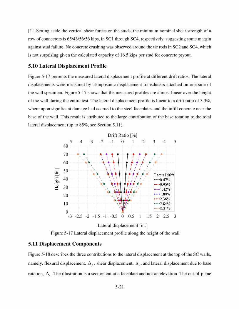
5-21
[1]. Setting aside the vertical shear forces on the studs, the minimum nominal shear strength of a
row of connectors is 65/43/56/56 kips, in SC1 through SC4, respectively, suggesting some margin
against stud failure. No concrete crushing was observed around the tie rods in SC2 and SC4, which
is not surprising given the calculated capacity of 16.5 kips per stud for concrete pryout.
5.10 Lateral Displacement Profile
Figure 5-17 presents the measured lateral displacement profile at different drift ratios. The lateral
displacements were measured by Temposonic displacement transducers attached on one side of
the wall specimen. Figure 5-17 shows that the measured profiles are almost linear over the height
of the wall during the entire test. The lateral displacement profile is linear to a drift ratio of 3.3%,
where upon significant damage had accrued to the steel faceplates and the infill concrete near the
base of the wall. This result is attributed to the large contribution of the base rotation to the total
lateral displacement (up to 85%, see Section 5.11).
Figure 5-17 Lateral displacement profile along the height of the wall
5.11 Displacement Components
Figure 5-18 describes the three contributions to the lateral displacement at the top of the SC walls,
namely, flexural displacement, f∆ , shear displacement, s∆ , and lateral displacement due to base
rotation, r∆ . The illustration is a section cut at a faceplate and not an elevation. The out-of-plane
�$ �0!� �0 ��!� �� ��!� � �!� � �!� 0 0!� $
5���������������������!
�
��
0�
$�
)�
��
1�
��
���� �) �$ �0 �� � � 0 $ ) �
6�� ��;������7
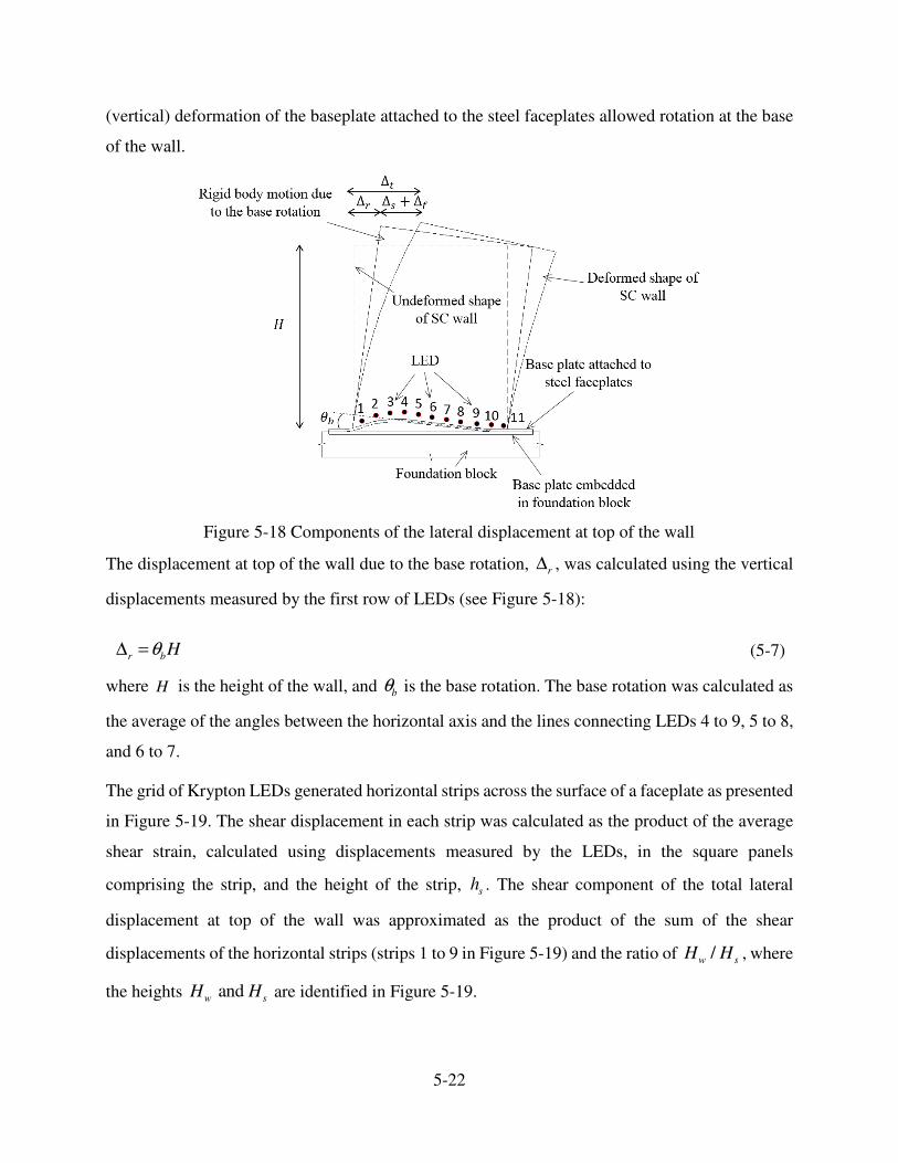
5-22
(vertical) deformation of the baseplate attached to the steel faceplates allowed rotation at the base
of the wall.
Figure 5-18 Components of the lateral displacement at top of the wall
The displacement at top of the wall due to the base rotation, r∆ , was calculated using the vertical
displacements measured by the first row of LEDs (see Figure 5-18):
r bHθ∆ = � (5-7)
where H is the height of the wall, and bθ is the base rotation. The base rotation was calculated as
the average of the angles between the horizontal axis and the lines connecting LEDs 4 to 9, 5 to 8,
and 6 to 7.
The grid of Krypton LEDs generated horizontal strips across the surface of a faceplate as presented
in Figure 5-19. The shear displacement in each strip was calculated as the product of the average
shear strain, calculated using displacements measured by the LEDs, in the square panels
comprising the strip, and the height of the strip,� sh . The shear component of the total lateral
displacement at top of the wall was approximated as the product of the sum of the shear
displacements of the horizontal strips (strips 1 to 9 in Figure 5-19) and the ratio of /w s
H H ,�where
the heights� and w s
H H �are identified in Figure 5-19.
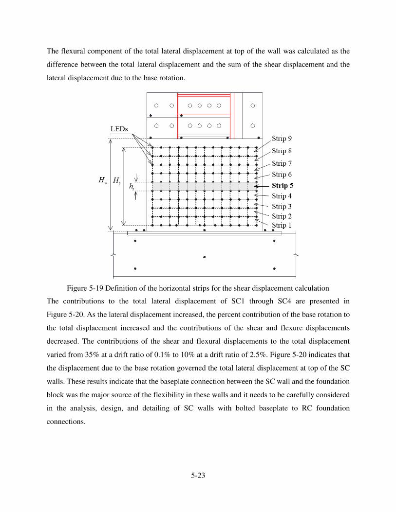
5-23
The flexural component of the total lateral displacement at top of the wall was calculated as the
difference between the total lateral displacement and the sum of the shear displacement and the
lateral displacement due to the base rotation.
Figure 5-19 Definition of the horizontal strips for the shear displacement calculation
The contributions to the total lateral displacement of SC1 through SC4 are presented in
Figure 5-20. As the lateral displacement increased, the percent contribution of the base rotation to
the total displacement increased and the contributions of the shear and flexure displacements
decreased. The contributions of the shear and flexural displacements to the total displacement
varied from 35% at a drift ratio of 0.1% to 10% at a drift ratio of 2.5%. Figure 5-20 indicates that
the displacement due to the base rotation governed the total lateral displacement at top of the SC
walls. These results indicate that the baseplate connection between the SC wall and the foundation
block was the major source of the flexibility in these walls and it needs to be carefully considered
in the analysis, design, and detailing of SC walls with bolted baseplate to RC foundation
connections.

5-24
(a) SC1 (b) SC2
(c) SC3 (d) SC4
Figure 5-20 Contribution of the lateral displacement components to the total displacement
5.12 Displacement Ductility of the SC Walls
Displacement ductility, defined as the ratio of the maximum displacement to the yield
displacement, represents the ability of the structure to undergo large plastic deformation in the
inelastic range without substantial loss of strength [66]. There are a number of definitions of the
yield and maximum displacements, both of which are needed to calculate displacement ductility.
Figure 5-21 presents alternate definitions of the yield and maximum displacements per Park [66],
proposed for reinforced concrete elements. In this study, the yield displacement, yδ , is defined as
the yield displacement of an equivalent elastic-plastic system with the same peak resistance and
energy absorption capacity as the real system: the third panel in Figure 5-21(a). Two definitions
were considered for the maximum displacement, namely, the displacements corresponding to the
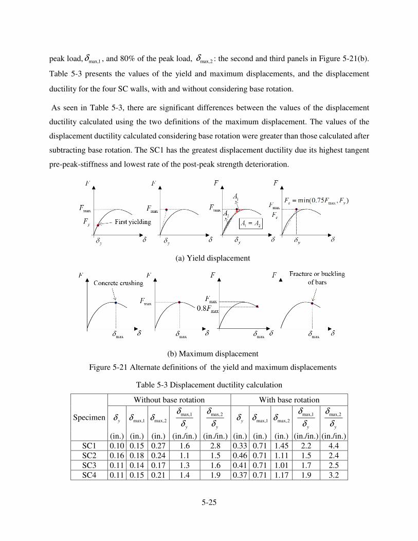
5-25
peak load, max,1δ , and 80% of the peak load, max,2δ : the second and third panels in Figure 5-21(b).
Table 5-3 presents the values of the yield and maximum displacements, and the displacement
ductility for the four SC walls, with and without considering base rotation.
As seen in Table 5-3, there are significant differences between the values of the displacement
ductility calculated using the two definitions of the maximum displacement. The values of the
displacement ductility calculated considering base rotation were greater than those calculated after
subtracting base rotation. The SC1 has the greatest displacement ductility due its highest tangent
pre-peak-stiffness and lowest rate of the post-peak strength deterioration.
(a) Yield displacement
(b) Maximum displacement
Figure 5-21 Alternate definitions of the yield and maximum displacements
Table 5-3 Displacement ductility calculation
Specimen
Without base rotation With base rotation
yδ max,1δ max,2δmax,1
y
δ
δmax,2
y
δ
δ yδ max,1δ max,2δ max,1
y
δ
δmax,2
y
δ
δ
(in.) (in.) (in.) (in./in.) (in./in.) (in.) (in.) (in.) (in./in.) (in./in.)
SC1 0.10 0.15 0.27 1.6 2.8 0.33 0.71 1.45 2.2 4.4
SC2 0.16 0.18 0.24 1.1 1.5 0.46 0.71 1.11 1.5 2.4
SC3 0.11 0.14 0.17 1.3 1.6 0.41 0.71 1.01 1.7 2.5
SC4 0.11 0.15 0.21 1.4 1.9 0.37 0.71 1.17 1.9 3.2

5-26
5.13 Averaged Secant Stiffness
Figure 5-22 presents the average secant stiffness of the specimens at different drift ratios. The
vertical dashed red lines represent the drift ratio corresponding to the peak shear resistance of the
SC walls. The average secant stiffness at ith load step, sec
iK , was calculated as:
1 2sec i ii 1 2
i i
(i 1, 2,.., )V V
K m+
= =∆ + ∆
� (5-8)
where 1 2
i i and ∆ ∆ represent the maximum lateral displacement at the first and second cycles of the
ith load step, respectively; 1 2
i i and V V are the corresponding shear forces for 1 2
i i and ,∆ ∆
respectively; and m is the number of load steps. Figure 5-22 indicates that the SC1 had the greatest
secant stiffness in the pre-peak-strength region, as the initial stiffness of this specimen was greater
than the other specimens. The variation of the secant stiffness for other three specimens, SC2, SC3,
and SC4, were virtually identical in pre- and post-peak strength regions.
Figure 5-22 Averaged secant stiffness of the SC walls
�(��
����
���
���� �
��*
�2��!

6-1
6. NUMERICAL ANALYSIS OF SC WALLS
6.1 Introduction
This chapter describes the nonlinear finite element modeling of flexure- and flexure-shear-critical
rectangular SC walls using the general-purpose finite element codes ABAQUS [76, 77], VecTor2
[114], and LS-DYNA [48, 49]. Sections 6.2 and 6.3 describe the ABAQUS and VecTor2 modeling
assumptions and analysis results, respectively. Section 6.4 includes information on the finite
element model developed in LS-DYNA to simulate the nonlinear cyclic response of flexure- and
flexure-shear critical SC walls. The developed finite element model was validated using data from
testing of the four large-scale rectangular SC walls presented in Chapter 5. DYNA analysis results
are presented, including global force-displacement responses, equivalent viscous damping ratio,
strain and stress distributions in the steel faceplates, estimates of the contribution of the steel
faceplates and infill concrete to the lateral resistance of the walls, and damage to the steel
faceplates and infill concrete. Section 6.5 uses the validated DYNA model to investigate load
transfer mechanisms in SC walls and axial and shear forces transferred by the connectors, and the
effects on global response of a) the interface friction between the steel faceplates and the infill
concrete, and b) the distribution of the shear studs attached to baseplate.
6.2 ABAQUS Analysis
This section discusses the numerical modeling of SC walls using the general-purpose finite
element code ABAQUS [76, 77]. The Concrete-Damage-Plasticity (CDP) model was used for the
infill concrete and the J2 plasticity model with isotropic hardening was used for the steel faceplates.
Friction between the infill concrete and the steel faceplates, and buckling of the steel faceplates
were considered. The following subsections describe the modeling assumptions and the ABAQUS
analysis results.
6.2.1 Concrete Material Model
The CDP model was used to simulate the behavior of the infill concrete. Although this material
model was primarily developed for cyclic and dynamic analyses of concrete structures, it is also
used for modeling of the quasi-brittle materials, such as rock, mortar, and ceramics. The CDP
model cannot be used to simulate the response of concrete members under high confining pressure
(e.g., greater than four or five times of uniaxial compressive strength of concrete [77]). Different
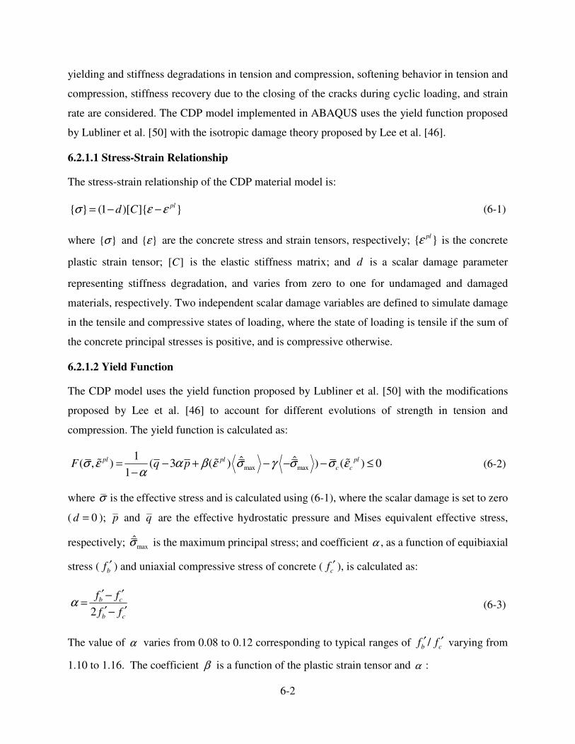
6-2
yielding and stiffness degradations in tension and compression, softening behavior in tension and
compression, stiffness recovery due to the closing of the cracks during cyclic loading, and strain
rate are considered. The CDP model implemented in ABAQUS uses the yield function proposed
by Lubliner et al. [50] with the isotropic damage theory proposed by Lee et al. [46].
6.2.1.1 Stress-Strain Relationship
The stress-strain relationship of the CDP material model is:
{ } (1 )[ ]{ }pl
d Cσ ε ε= − − (6-1)
where { }σ and { }ε are the concrete stress and strain tensors, respectively; { }plε is the concrete
plastic strain tensor; [ ]C is the elastic stiffness matrix; and d is a scalar damage parameter
representing stiffness degradation, and varies from zero to one for undamaged and damaged
materials, respectively. Two independent scalar damage variables are defined to simulate damage
in the tensile and compressive states of loading, where the state of loading is tensile if the sum of
the concrete principal stresses is positive, and is compressive otherwise.
6.2.1.2 Yield Function
The CDP model uses the yield function proposed by Lubliner et al. [50] with the modifications
proposed by Lee et al. [46] to account for different evolutions of strength in tension and
compression. The yield function is calculated as:
max max
1 ˆ ˆ( , ) ( 3 ( ) ) ( ) 01
pl pl pl
c cF q pσ ε α β ε σ γ σ σ εα
= − + − − − ≤−
� � � (6-2)
where σ is the effective stress and is calculated using (6-1), where the scalar damage is set to zero
( 0d = ); p and q are the effective hydrostatic pressure and Mises equivalent effective stress,
respectively; maxσ̂ is the maximum principal stress; and coefficient α , as a function of equibiaxial
stress ( bf ′ ) and uniaxial compressive stress of concrete ( cf ′ ), is calculated as:
2
b c
b c
f f
f fα
′ ′−=
′ ′−(6-3)
The value of α varies from 0.08 to 0.12 corresponding to typical ranges of /b cf f′ ′ varying from
1.10 to 1.16. The coefficient β is a function of the plastic strain tensor and α :

6-3
( )( ) (1 ) (1 )
( )
plpl c c
pl
t t
σ εβ ε α α
σ ε= − − +
��
�(6-4)
where cσ and
tσ are the effective compressive and tensile cohesion stresses, respectively. The
coefficient γ is a function of the constant cK that controls the shape of the yield surface in the
deviatoric plane. Coefficient γ is used when maxˆ 0σ < and is calculated as:
3(1 )
2 1
c
c
K
Kγ
−=
−(6-5)
Figure 6-1 indicates that as cK increases from 0.6 to 1.0, the shape of the deviatoric plane of the
yield surface tends to a circle, as is assumed in the classical Drucker-Prager yield surface.
Figure 6-1 Deviatoric plane of the yield surface [77]
6.2.1.3 Flow Rule
The plastic strain orientation is defined using a non-associated flow rule in the CDP model. The
Drucker-Prager hyperbolic function, ( )G σ , is used as the potential function. The increment of
plastic strain is a function of the derivative of the plastic function with respect to the effective
stress. The plastic strain increment and the plastic function are calculated as:
( )pl G σε λ
σ
∂=
∂�� (6-6)
2 2( tan ) tantG f q pχ ψ ψ= + − (6-7)
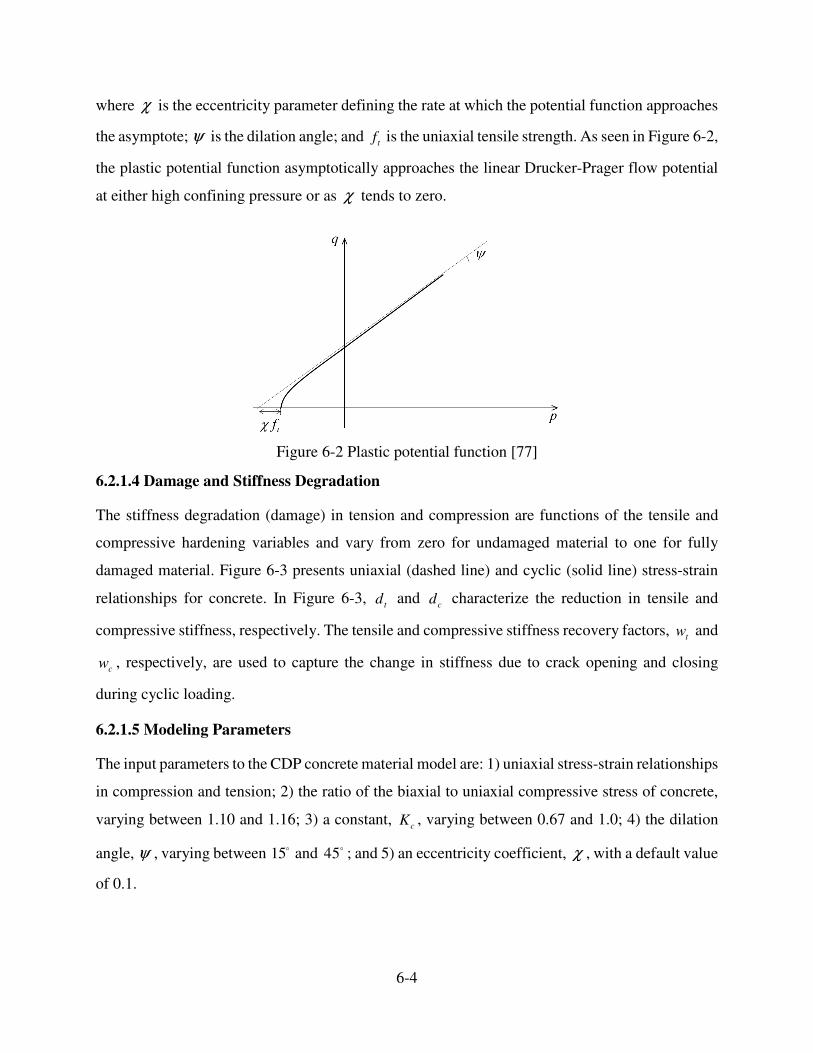
6-4
where χ is the eccentricity parameter defining the rate at which the potential function approaches
the asymptote; ψ is the dilation angle; and tf is the uniaxial tensile strength. As seen in Figure 6-2,
the plastic potential function asymptotically approaches the linear Drucker-Prager flow potential
at either high confining pressure or as χ tends to zero.
Figure 6-2 Plastic potential function [77]
6.2.1.4 Damage and Stiffness Degradation
The stiffness degradation (damage) in tension and compression are functions of the tensile and
compressive hardening variables and vary from zero for undamaged material to one for fully
damaged material. Figure 6-3 presents uniaxial (dashed line) and cyclic (solid line) stress-strain
relationships for concrete. In Figure 6-3, t
d and cd characterize the reduction in tensile and
compressive stiffness, respectively. The tensile and compressive stiffness recovery factors, tw and
cw , respectively, are used to capture the change in stiffness due to crack opening and closing
during cyclic loading.
6.2.1.5 Modeling Parameters
The input parameters to the CDP concrete material model are: 1) uniaxial stress-strain relationships
in compression and tension; 2) the ratio of the biaxial to uniaxial compressive stress of concrete,
varying between 1.10 and 1.16; 3) a constant, cK , varying between 0.67 and 1.0; 4) the dilation
angle, ψ , varying between 15� and 45� ; and 5) an eccentricity coefficient, χ , with a default value
of 0.1.
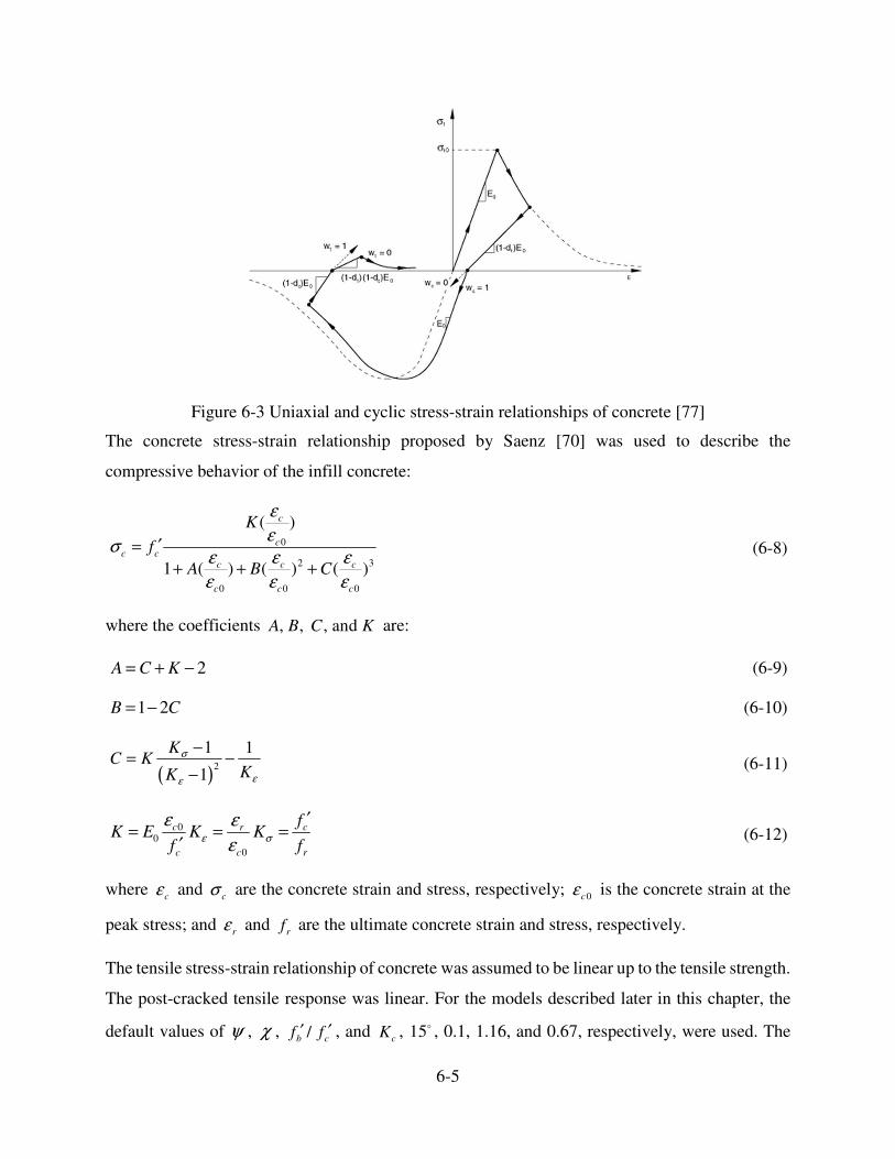
6-5
Figure 6-3 Uniaxial and cyclic stress-strain relationships of concrete [77]
The concrete stress-strain relationship proposed by Saenz [70] was used to describe the
compressive behavior of the infill concrete:
0
2 3
0 0 0
( )
1 ( ) ( ) ( )
c
cc c
c c c
c c c
K
f
A B C
ε
εσ
ε ε ε
ε ε ε
′=
+ + +(6-8)
where the coefficients , , , and A B C K are:
2A C K= + − (6-9)
1 2B C= − (6-10)
( )2
1 1
1
KC K
KK
σ
εε
−= −
−(6-11)
00
0
c cr
c c r
fK E K K
f fε σ
ε ε
ε
′= = =
′(6-12)
where c
ε and cσ are the concrete strain and stress, respectively;
0cε is the concrete strain at the
peak stress; and r
ε and r
f are the ultimate concrete strain and stress, respectively.
The tensile stress-strain relationship of concrete was assumed to be linear up to the tensile strength.
The post-cracked tensile response was linear. For the models described later in this chapter, the
default values of ψ , χ , /b cf f′ ′ , and cK , 15� , 0.1, 1.16, and 0.67, respectively, were used. The
6-6
damage parameters in tension and compression varied from 0.0 at peak stress to 1.0 at ultimate
strain. Concrete stress-strain relationships derived from concrete cylinder tests were used to
calculate uniaxial compressive strength and Young’s modulus of the infill concrete for SC1
through SC4.
6.2.2 Steel Material Model
A J2 plasticity model with isotropic hardening was used to simulate the nonlinear behavior of the
steel faceplates. The input parameters of this model are: 1) Young’s modulus; 2) Poisson’s ratio,
and 3) the uniaxial stress-strain relationship. The average stress-strain relationship, obtained from
coupon tests, was used to calculate the material properties of the steel faceplates.
6.2.3 Contact and Constraint Modeling
Contact between the infill concrete and the steel faceplates, the infill concrete and the baseplate,
and the baseplate and the steel plate embedded in the foundation block was considered using a)
hard contact in the normal direction to avoid penetration of slave nodes through master segments,
and b) a Surface-To-Surface penalty-based formulation in the transverse direction to simulate
interfacial friction. A Node-To-Surface constraint was used to tie the steel faceplates to the
baseplate and to join the studs and tie rods to the steel faceplates. The studs and tie rods were
coupled to the infill concrete elements using the Embedded-Constraint available in ABAQUS [77].
Slip between the connectors and the infill concrete was neglected.
6.2.4 Elements, Loading, and Boundary Conditions
Beam elements (B31) were used to represent the studs and tie rods. Eight-node solid elements with
full integration (C3D8) were used to model the infill concrete. Four-node shell elements with full
integration (S4) were used for the steel faceplates. Solid elements with reduced integration
(C3D8R) were used to model the connection between the SC wall and its foundation block,
including two 1-in. thick baseplates and the 22 1.25-in. diameter threaded B7 bars that secured the
baseplate to the foundation block. The loading plates, post-tensioned threaded rods used to attach
the loading plate to the SC walls, and the post-tensioning bars connecting the SC wall to the
foundation block were modeled using eight-node solid elements with reduced integration
(C3D8R). The infill concrete was modeled using 1 × 1 × 1 in. solid elements and the steel
faceplates were modeled using 0.5 × 0.5 in. shell elements.

6-7
The SC walls were subjected to quasi-static cyclic loading (see Chapter 4) using two horizontally
inclined actuators and loading plates that were attached to each specimen by 14 post-tensioned
threaded rods. In the finite element model, the reversed cyclic loading was simulated by imposing
horizontal nodal displacements at the center line of the loading plate, 60 in. above the baseplate.
Since preliminary analysis indicated that the foundation block was effectively rigid, the block was
not included in the finite element model. The model took advantage of symmetry to reduce the
computational effort. The ABAQUS model of SC2 is presented in Figure 6-4.
(a) Steel faceplate, connectors,
baseplates, and threaded bars (b) Infill concrete
(c) Loading plate and
threaded bars
Figure 6-4 ABAQUS model of SC2
6.2.5 ABAQUS Analysis Results
Figure 6-5 presents the results of monotonic ABAQUS analysis together with the first quadrant of
the measured cyclic force-displacement relationships of SC1 through SC4. ABAQUS successfully
predicted the initial stiffness and peak shear strengths of the SC walls. As seen in Figure 6-5, the
post-peak strength predicted by ABAUQS was greater than that measured in the tests for SC2,
SC3, and SC4. This outcome was expected since monotonic response (ABAQUS-predicted
response) is expected to overestimate cyclic response (test result) for a given post-peak
displacements. The rate of strength deterioration in SC1 at displacements greater than that
accounted with peak-strength was lower than that in the other walls due to the use of a smaller
distance between the first row of connectors and the baseplate in SC1. However, the use of smaller
distance between the first row of connector and the baseplate had no substantial effect on the
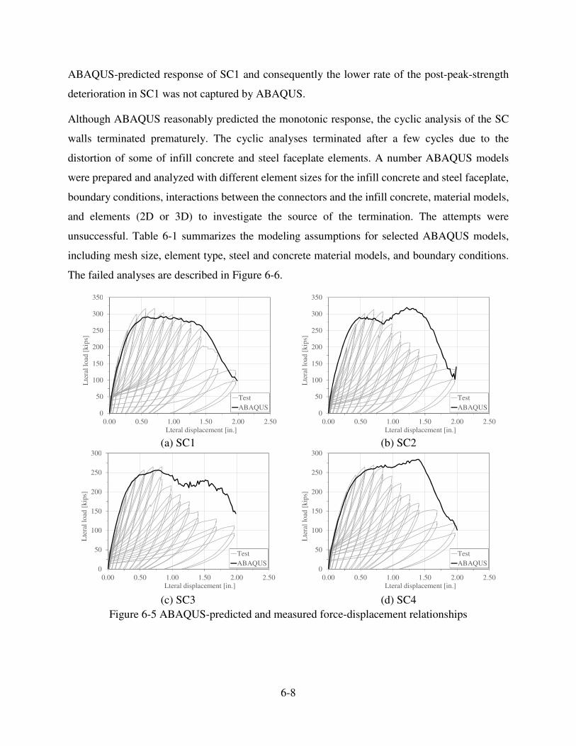
6-8
ABAQUS-predicted response of SC1 and consequently the lower rate of the post-peak-strength
deterioration in SC1 was not captured by ABAQUS.
Although ABAQUS reasonably predicted the monotonic response, the cyclic analysis of the SC
walls terminated prematurely. The cyclic analyses terminated after a few cycles due to the
distortion of some of infill concrete and steel faceplate elements. A number ABAQUS models
were prepared and analyzed with different element sizes for the infill concrete and steel faceplate,
boundary conditions, interactions between the connectors and the infill concrete, material models,
and elements (2D or 3D) to investigate the source of the termination. The attempts were
unsuccessful. Table 6-1 summarizes the modeling assumptions for selected ABAQUS models,
including mesh size, element type, steel and concrete material models, and boundary conditions.
The failed analyses are described in Figure 6-6.
(a) SC1 (b) SC2
(c) SC3 (d) SC4
Figure 6-5 ABAQUS-predicted and measured force-displacement relationships
0
50
100
150
200
250
300
350
0.00 0.50 1.00 1.50 2.00 2.50
Lte
ral
load [
kip
s]
Lteral displacement [in.]
Test
ABAQUS0
50
100
150
200
250
300
350
0.00 0.50 1.00 1.50 2.00 2.50
Lte
ral
load [
kip
s]
Lteral displacement [in.]
Test
ABAQUS
0
50
100
150
200
250
300
0.00 0.50 1.00 1.50 2.00 2.50
Lte
ral
load
[k
ips]
Lteral displacement [in.]
Test
ABAQUS0
50
100
150
200
250
300
0.00 0.50 1.00 1.50 2.00 2.50
Lte
ral
load
[k
ips]
Lteral displacement [in.]
Test
ABAQUS
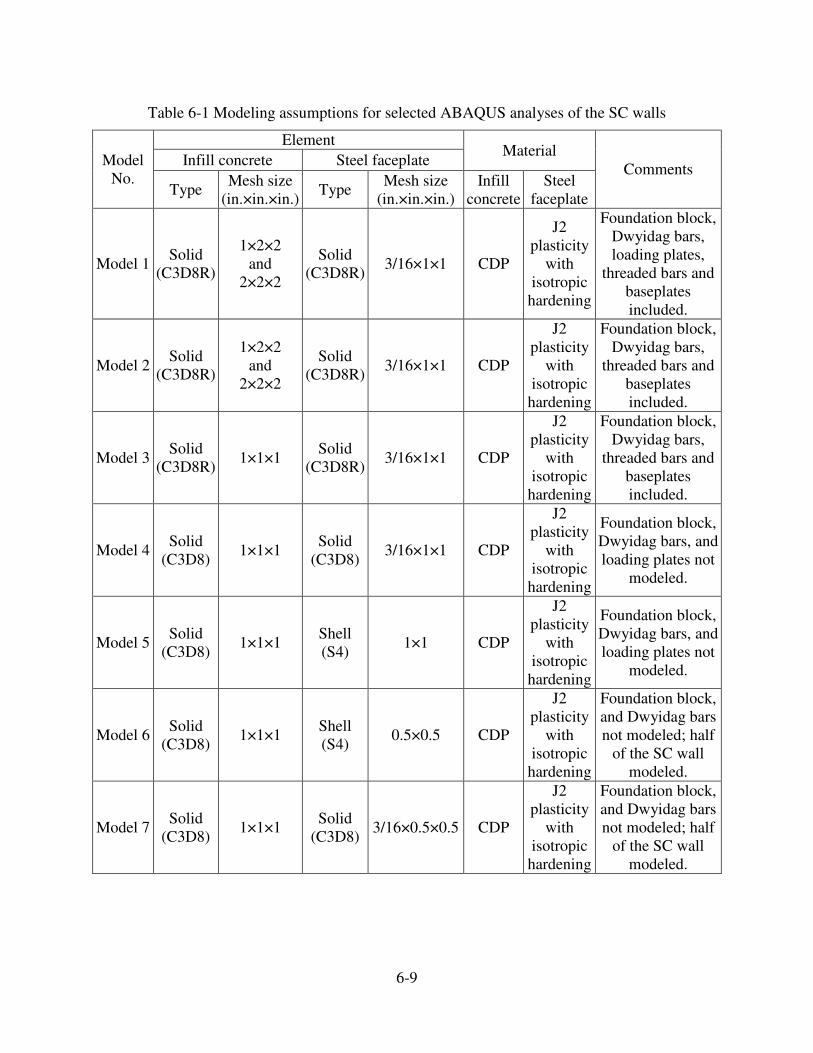
6-9
Table 6-1 Modeling assumptions for selected ABAQUS analyses of the SC walls
Model
No.
Element Material
Comments Infill concrete Steel faceplate
Type Mesh size
(in.×in.×in.)Type
Mesh size
(in.×in.×in.)
Infill
concrete
Steel
faceplate
Model 1Solid
(C3D8R)
1×2×2
and
2×2×2
Solid
(C3D8R)3/16×1×1 CDP
J2
plasticity
with
isotropic
hardening
Foundation block,
Dwyidag bars,
loading plates,
threaded bars and
baseplates
included.
Model 2Solid
(C3D8R)
1×2×2
and
2×2×2
Solid
(C3D8R)3/16×1×1 CDP
J2
plasticity
with
isotropic
hardening
Foundation block,
Dwyidag bars,
threaded bars and
baseplates
included.
Model 3Solid
(C3D8R)1×1×1
Solid
(C3D8R)3/16×1×1 CDP
J2
plasticity
with
isotropic
hardening
Foundation block,
Dwyidag bars,
threaded bars and
baseplates
included.
Model 4Solid
(C3D8) 1×1×1
Solid
(C3D8) 3/16×1×1 CDP
J2
plasticity
with
isotropic
hardening
Foundation block,
Dwyidag bars, and
loading plates not
modeled.
Model 5Solid
(C3D8) 1×1×1
Shell
(S4) 1×1 CDP
J2
plasticity
with
isotropic
hardening
Foundation block,
Dwyidag bars, and
loading plates not
modeled.
Model 6Solid
(C3D8) 1×1×1
Shell
(S4) 0.5×0.5 CDP
J2
plasticity
with
isotropic
hardening
Foundation block,
and Dwyidag bars
not modeled; half
of the SC wall
modeled.
Model 7Solid
(C3D8) 1×1×1
Solid
(C3D8) 3/16×0.5×0.5 CDP
J2
plasticity
with
isotropic
hardening
Foundation block,
and Dwyidag bars
not modeled; half
of the SC wall
modeled.

6-10
(a) Model 1 (b) Model 2
(c) Model 3 (d) Model 4
Figure 6-6 Failures of the ABAQUS analyses

6-11
(e) Model 5 (f) Model 6
(g) Model 7
Figure 6-6 Failures of the ABAQUS analyses (cont.)

6-12
6.3 VecTor2 Analysis
VecTor2 is a two dimensional nonlinear finite element program used to simulate the in-plane
response of reinforced concrete structures. VecTor2 is based on the Modified-Field- Compression-
Theory (MCFT) [110] and the Distributed-Stress-Field-Model (DSFM) [102]. The DSFM was
proposed by Vecchio et al. [102] as an alternative to MCFT. It incorporates a smeared rotating
crack model that considers slip deformations across crack surfaces and reorientation of the cracks
during cyclic loading.
The material models available in VecTor2 consider the important behaviors of concrete and steel,
such as compression softening, which is the effect on uniaxial concrete compressive strength of
transverse tensile strains; tension stiffening, which captures the tensile stiffness of intact concrete
between cracks; dowel action of reinforcing bars crossing cracks; the Bauschinger effect for
reinforcement; buckling of reinforcement; concrete confinement; concrete dilation; bond slip; and
deformations across cracks.
6.3.1 SC Wall Modeling
Vecchio et al. (2011) adopted the DSFM for the analysis of SC walls subjected to axial, and in-
plane monotonic and cyclic shear loadings. They proposed the following relationship for the
response of an SC element:
[ ] [ ][ ] 0Dσ ε σ� �= − � � (6-13)
where [ ]ε and [ ]σ are the strain and stress vectors; 0σ� �� � is a prestress vector; [ ]D is composite
material stiffness matrix, calculated as the sum of the stiffness matrices of the infill concrete, the
steel faceplates, and the steel reinforcement as:
[ ] [ ] [ ] [ ]1
2
2 2 2
nc c s
c ri s
ic s c s c s
t t tD D D D
t t t t t t=
= + ++ + +
� (6-14)
where [ ]cD is the stiffness matrix of the infill concrete, ct and st are the thicknesses of the infill
concrete and each steel faceplate, [ ]riD is the stiffness matrix of each reinforcement component
with angle iα to the horizontal, and [ ]sD is the stiffness matrix for the steel faceplates. Matrices
[ ]cD and [ ]riD are calculated using equations available in [102]. Compression softening, tension

6-13
stiffening, dilation, and confinement are considered in the derivation of the concrete stiffness
matrix. The Bauschinger effect and dowel action are considered in the calculation of the
reinforcement stiffness matrix. The matrix [ ]sD is calculated as:
[ ] [ ] [ ]1
2
0 0
0 0
0 0
sT
s s s s
s
E
D T E T
G
� �� �
= � �� �� �
(6-15)
where 1sE and 2s
E are the secant moduli of the steel faceplates in the principal stress directions,
respectively; s
G is the shear modulus; and [ ]sT is a matrix that transforms the principal coordinate
system back to the global coordinate system and calculated as:
[ ]
2 2
2 2
2 2
cos sin cos sin
sin cos cos sin
2cos sin 2cos sin cos sin
sT
ε ε ε ε
ε ε ε ε
ε ε ε ε ε ε
θ θ θ θ
θ θ θ θ
θ θ θ θ θ θ
� �� �
= −� �� �− −� �
(6-16)
The secant and shear moduli of the steel faceplates are calculated as:
1 ( 1, 2)sis
si
fE i
ε= = (6-17)
1 2
1 2
s ss
s s
E EG
E E=
+(6-18)
where and ( 1,2)si sif iε = are the principal strains and their corresponding stresses, respectively.
The steel stresses are determined using the calculated principal strains and the uniaxial stress-strain
relationship of the steel.
The prestress vector, 0σ� �� � , is defined as:
[ ] [ ] [ ]0
1
( ) ( ) ( )n
e p s e p e p
c c c c ri ri ri s s s
i
D D Dσ ε ε ε ε ε ε ε=
� � � � � � � � � � � � � � � �= + + + + + +� � � � � � � � � � � � � � � �� (6-19)
where e
cε� �� � , e
riε� �� � , and e
sε� �� � are the elastic offset strain vectors in the concrete, reinforcement,
and the steel faceplates, respectively; p
cε� �� � , p
riε� �� � , and p
sε� �� � are the plastic offset strain vectors
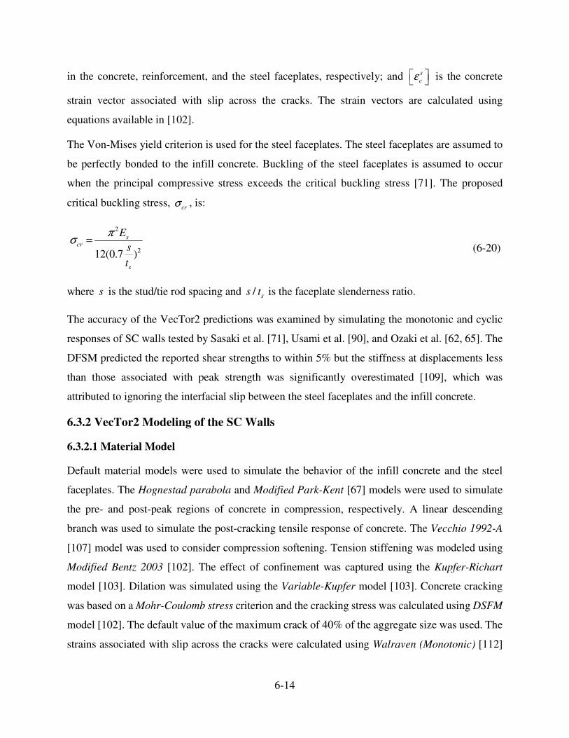
6-14
in the concrete, reinforcement, and the steel faceplates, respectively; and s
cε� �� � is the concrete
strain vector associated with slip across the cracks. The strain vectors are calculated using
equations available in [102].
The Von-Mises yield criterion is used for the steel faceplates. The steel faceplates are assumed to
be perfectly bonded to the infill concrete. Buckling of the steel faceplates is assumed to occur
when the principal compressive stress exceeds the critical buckling stress [71]. The proposed
critical buckling stress, crσ , is:
2
212(0.7 )
scr
s
E
s
t
πσ =
(6-20)
where s is the stud/tie rod spacing and / ss t is the faceplate slenderness ratio.
The accuracy of the VecTor2 predictions was examined by simulating the monotonic and cyclic
responses of SC walls tested by Sasaki et al. [71], Usami et al. [90], and Ozaki et al. [62, 65]. The
DFSM predicted the reported shear strengths to within 5% but the stiffness at displacements less
than those associated with peak strength was significantly overestimated [109], which was
attributed to ignoring the interfacial slip between the steel faceplates and the infill concrete.
6.3.2 VecTor2 Modeling of the SC Walls
6.3.2.1 Material Model
Default material models were used to simulate the behavior of the infill concrete and the steel
faceplates. The Hognestad parabola and Modified Park-Kent [67] models were used to simulate
the pre- and post-peak regions of concrete in compression, respectively. A linear descending
branch was used to simulate the post-cracking tensile response of concrete. The Vecchio 1992-A
[107] model was used to consider compression softening. Tension stiffening was modeled using
Modified Bentz 2003 [102]. The effect of confinement was captured using the Kupfer-Richart
model [103]. Dilation was simulated using the Variable-Kupfer model [103]. Concrete cracking
was based on a Mohr-Coulomb stress criterion and the cracking stress was calculated using DSFM
model [102]. The default value of the maximum crack of 40% of the aggregate size was used. The
strains associated with slip across the cracks were calculated using Walraven (Monotonic) [112]

6-15
model. The Nonlinear w/Plastic Offsets model [102] was used to simulate the hysteretic response
of concrete.
Table 6-2 presents the concrete material properties used as input to the VecTor2 model, where tf
is the tensile stress of the infill concrete, 0cε is the concrete strain at peak stress,
cν is Poisson’s
ratio, and c
γ is the concrete density.
Table 6-2 Concrete material properties input to VecTor2 model
cf ′tf cE 0cε
cν c
γ
(ksi) (ksi) (ksi) (in./in.) 3(lb/ft )
4.4 0.4 3000 0.0025 0.2 150
Table 6-3 presents the steel material properties input to VecTor2 model, where yf and
uf are the
yield and tensile stresses of the steel faceplates, respectively; shε and
uε are the steel strains at the
onset of the strain hardening and peak stress, respectively; s
ν is Poisson’s ratio; and / ss t is the
faceplate slenderness ratio.
Table 6-3 Steel material properties input to VecTor2 model
yfuf sE shε
uε
sν
/ ss t
(ksi) (ksi) (ksi) (in/in) (in/in) (in/in)
38 55 29000 0.003 0.03 0.3 30
6.3.2.2 Elements, Loading, and Boundary Conditions
The monotonic and reversed cyclic loading of the test specimens were simulated by imposing
nodal horizontal displacements 60 in. above the base of the wall.
Three sets of VecTor2 models were analyzed: A) including the foundation, B) a rigid connection
of the walls to an infinitely stiff base, and C) including the foundation flexibility by using four-
node membrane elements to represent the steel baseplate, and truss elements with tension- and
compression-only behaviors to represent the post-tensioned threaded bars used to secure the
baseplate to the foundation block. The VecTor2 models are presented Figure 6-7.

6-16
(a) Model A (b) Model B
(b) Model C
Figure 6-7 VecTor2 models
Two axial behaviors were assigned to each truss element connecting the SC wall to the base:
compression-only and tension-only. To prevent the penetration of wall elements into the stiff base,
a compression-only behavior with very large stiffness and strength was used. The properties of the
tension-only behavior, including cross-sectional area (=20.02 in ) and elasticity modulus (=580
ksi), were back-calculated from the measured initial stiffness of SC1.
Two inch × 2 in. elements were used for Models B and C. The mesh size in model A which
included the foundation block, was increased to 4 in. due to a limit on the number of available
elements in VecTor2. The height of the Model C was set at 72 in., including 12 in. above the
loading level, and identical to the constructed walls.

6-17
6.3.3 VecTor2 Analysis Results
6.3.3.1 Load-Displacement Monotonic Response
Figure 6-8 presents the VecTor2-predicted monotonic force-displacement relationships (solid
black line for Model A, dashed blue line for Model B, and dashed red line for Model C) together
with the measured cyclic force-displacement relationship (solid gray line) for SC1. The initial
stiffness was substantially overestimated by Model A (including the foundation block) and Model
B (rigid base) because these models did not include the baseplate connection between the SC wall
and the foundation block. The peak strength was significantly overestimated by Model A due to
the use of a coarse mesh, which delayed the onset of damage (cracking) to the infill concrete.
However, both the rigid- and flexible-base models, B and C, respectively, successfully predicted
the peak shear resistance of SC1. The rate of post-peak strength deterioration predicted by all three
models was substantially greater than that observed in the test. The discrepancies between the
numerically-predicted and experimentally-measured post peak responses might be attributed to: 1)
the effect of concrete confinement is neglected by VecTor2 analysis, which uses 2D elements for
the steel faceplates and the infill concrete, 2) VecTor2 assumes perfect bond between the steel
faceplates and infill concrete, and 3) the SC wall connection including the baseplate and the
threaded bars could not be explicitly modeled using VecTor2.
Figure 6-8 Analysis and test results for SC1
0
50
100
150
200
250
300
350
400
450
0.00 0.50 1.00 1.50 2.00 2.50
Late
ral
load
[kip
s]
Lateral displacement [in.]
Test
Model A
Model B
Model C

6-18
6.3.3.2 Crack Patterns in the Infill Concrete
Figure 6-9 presents the predicted deformed shape of SC1 (scaled by a factor of 7) and the crack
patterns at peak load. The critical crack width was set to 0.0022, where the critical crack width is
defined as the displacement at which the tensile normal stress across the crack is zero. The
calculation of the crack width is presented in Section 6.4.1.2.
(a) Model A (b) Model B (c) Model C
Figure 6-9 VecTor2-predicted cracking pattern at peak load of SC1 under monotonic loading
6.3.3.3 Strain Distributions
The distributions of horizontal, vertical, and shear strains in SC1 at peak load are presented in
Figure 6-10, Figure 6-11, and Figure 6-12, respectively. The high vertical and shear strains are
concentrated near the base of the wall.
(a) Model A (b) Model B (c) Model C
Figure 6-10 Horizontal strain distribution at peak load (unit: millistrains)

6-19
(a) Model A (b) Model B (c) Model C
Figure 6-11 Vertical strain distribution at peak load (unit: millistrains)
(a) Model A (b) Model B (c) Model C
Figure 6-12 Shear strain distribution at peak load (unit: millistrains)
6.3.3.4 Stress Distribution
The distributions of the horizontal, vertical, and shear stresses in the infill concrete of SC1 at peak
load are presented in Figure 6-13, Figure 6-14, and Figure 6-15, respectively. Figure 6-14 provides
an estimate of the depth of the compression zone in the infill concrete at the peak load (= 0.3L ,
where L is the length of the wall). The stress distribution in the infill concrete of SC1, presented
in Figure 6-15, indicates that the applied lateral load in the infill was transferred to the foundation
by a diagonal compression strut.

6-20
(a) Model A (b) Model B (c) Model C
Figure 6-13 Horizontal stress distribution at peak load in infill concrete (unit: ksi)
(a) Model A (b) Model B (c) Model C
Figure 6-14 Vertical stress distribution at peak load in infill oncrete (unit: ksi)
(a) Model A (b) Model B (c) Model C
Figure 6-15 Shear stress distribution at peak load in infill concrete (unit: ksi)
6-21
6.3.3.5 Load-Displacement Cyclic Response
Figure 6-16 presents the VecTor2-predicted and the measured cyclic force-displacement
relationships for SC1. Similar to the predictions of monotonic response, Models A and B
substantially overestimated the initial stiffness. The rate of post-peak strength deterioration in the
predicted cyclic responses of the Models A and B is greater than that of the measured cyclic
response. Models A and B predicted more damage than Model C because these models did not
include the baseplate connection, and thus were stiffer, which led to premature concrete cracking,
and buckling and yielding of the steel faceplates. As seen in Figure 6-16, the VecTor2 models
captured the pinching behavior by considering opening, closing, and re-opening of cracks in the
infill concrete caused by load reversals. Analysis of Model C terminated at the peak shear force
due to the significant distortion of a number of the wall elements, as presented in Figure 6-16(c).
Different mesh sizes, boundary conditions, and material models were analyzed but these attempts
were unsuccessful.
6.4 LS-DYNA Analysis
This section describes a finite element model in LS-DYNA that simulates the nonlinear cyclic
response of flexure- and flexure-shear-critical SC walls. LS-DYNA is a general-purpose finite
element program for the static and dynamic analysis of structures. The finite element model is
validated using data from testing of the four large-scale rectangular SC walls described in Chapters
4 and 5. The following subsections present the modeling assumptions and the finite element
predictions, including global force-displacement responses, equivalent viscous damping ratio,
damage to the steel faceplates and infill concrete, strain and stress distributions in the steel
faceplates, estimates of the contribution of the steel faceplates and infill concrete to the lateral
resistance of the walls, and axial and shear forces transferred by connectors. The impacts of
interface friction between the steel faceplates and the infill concrete, and of the distribution of
shear studs on the baseplate, to the global response of the SC walls are also presented.
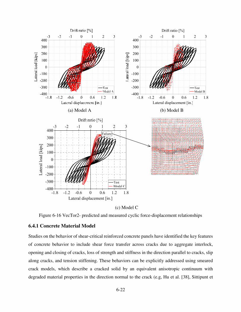
6-22
(a) Model A (b) Model B
(c) Model C
Figure 6-16 VecTor2- predicted and measured cyclic force-displacement relationships
6.4.1 Concrete Material Model
Studies on the behavior of shear-critical reinforced concrete panels have identified the key features
of concrete behavior to include shear force transfer across cracks due to aggregate interlock,
opening and closing of cracks, loss of strength and stiffness in the direction parallel to cracks, slip
along cracks, and tension stiffening. These behaviors can be explicitly addressed using smeared
crack models, which describe a cracked solid by an equivalent anisotropic continuum with
degraded material properties in the direction normal to the crack (e.g, Hu et al. [38], Sittipunt et
��!� ��!0 ��!1 � �!1 �!0 �!�
5���������������������!
�)��
�$��
�0��
����
�
���
0��
$��
)��
"��
3�����8
�$ �0 �� � � 0 $
6�� ���������7
6-23
al. [78], Vecchio et al. [106, 108], Bessason et al. [13], Hristovski et al. [37], and Orakcal et al.
[60]).
The smeared crack Winfrith model (MAT085) in LS-DYNA, developed by Broadhouse [17], was
used to model the infill concrete. The Broadhouse model provides information on the orientation
of the cracking planes (up to three orthogonal cracks for each element) and the width of the cracks
[72]. It assumes elastic-perfectly plastic behavior in compression [17] and its yield surface is based
on the four-parameter plastic surface of Ottosen model [61]. The yield surface expands as the
hydrostatic pressure increases and its radii at the compressive and tensile meridia are determined
using the compressive and tensile strengths of concrete [17]. The model considers shear stress
across the crack due to the aggregate interlock. Tension stiffening is considered using a linear
decay for the post-cracked tensile stress-strain relationship. Rather than using truss or beam
elements to model reinforcement, the Winfrith model smears the rebar. The Winfrith model can
incorporate strain-rate effects [49].
6.4.1.1 Plasticity Model Definition in the Winfrith Model
The four-parameter plastic surface proposed by Ottosen [61] is used as the failure surface in the
Winfrith model. The Ottosen failure surface is expressed as:
22 11 2 2
( , ,cos3 ) 1( )c c c
JJ IF I J a b
f f fθ λ= + + −
′ ′ ′(6-21)
where 1I is the first invariant of the stress tensor; 2J is the second invariant of the deviatoric stress
tensor; cos3θ is an invariant as a function of the second and third invariants of the deviatoric
stress tensor and θ is the Lodge angle, where the Lodge angle, varying between 0 and > / 3 , is
used to represent the yield surface on the planeπ − ; λ is a function of cos3θ ; and cf ′ is the
uniaxial compressive strength of concrete.
The four parameters of the Ottosen model are and a b , which control the quadratic shape of the
meridian curves of the failure surface, and 1 2 and k k , which control the noncircular shape of the
failure surface on the deviatoric plane, from a nearly triangular shape to a circular shape with
increasing the hydrostatic pressure [22]. The parameter λ can be calculated as:

6-24
1
1 2
1
1 2
1 cos [ cos ( cos3 )]
3
1cos [ cos ( cos3 )]
3 3
k k
k k
θλ
πθ
−
−
�
= � − −
for cos3 0θ ≥
(6-22)
for cos3 0θ <
The stress tensor and the deviatoric stress tensor are:
11 12 13
21 22 23
31 32 33
ij
σ σ σ
σ σ σ σ σ
σ σ σ
� �� �= = � �� �� �
(6-23)
11 12 13 11 12 13
21 22 23 21 22 23
31 32 33 31 32 33
ij
S S S P
S S S S S P
S S S P
σ σ σ
σ σ σ
σ σ σ
−� � � �� � � �= = = −� � � �� � � �−� � � �
(6-24)
where P is the hydrostatic stress and is calculated as 11 22 33( ) / 3σ σ σ+ + .
The first invariant of the stress tensor, and the second and third invariants of the deviatoric stress
tensor are:
1 11 22 33iiI σ σ σ σ= = + + (6-25)
2 2 2 2 2 2
2 11 22 33 12 13 230.5 ( 2 2 2 ) / 2
ij ijJ S S S S S S S S= = + + + + + (6-26)
11 12 13
3 21 22 23
31 32 33
/ 3ij jk ki
S S S
J S S S S S S
S S S
= = (6-27)
Cosine3θ , which is a function of the second and third invariants of the deviatoric stress tensor, is
calculated as:
3
3/2
2
3 3cos3
2
J
Jθ =
(6-28)
The four parameters of the Ottosen model are calculated using the results of uniaxial tensile and
compressive tests, and biaxial and triaxial tests as:
1. Uniaxial compressive stress of concrete, cf ′ ( 60θ = � and cos3 1θ = − ).

6-25
2. Uniaxial tensile stress of concrete, tf ( 0θ = � and cos3 1θ = + ).
3. Biaxial compressive stress of concrete, bcf ′ ( 0θ = � and cos3 1θ = + ); the Winfrith model
uses the results of the biaxial tests of Kupfer et al. [42, 43]; 1 2 1.16 cfσ σ ′= = and
3and 0σ = .
4. The triaxial stress state ( 1 2( / 3 , 2 / ) ( 5,4)c cI f J f′ ′ = − ) on the compressive meridian
( 60θ = � and cos3 1θ = − ) provides the best fit to the test results of Balmer [11] and Richart
et al. [69].
In the Winfrith concrete model, the four parameters of the Ottosen model are internally calculated
as [72]:
a bβ γ= + (6-29)
2
2
1 / 3 / 3 /
/ 3 3 / 3
R Rb
R
αγ α γ α
α β α αβ
+ − −=
− −(6-30)
11
2
1cos( cos ( ))
3
cK
k−
=(6-31)
1
2
1 2cos(3 tan ( ))
3 3
dk
c
−= − (6-32)
where , , and α β γ are non-dimensional constants and equal to 1.16, 0.59, and -0.61, respectively;
R is the ratio of the uniaxial tensile to compressive stress of concrete; and the coefficients and c d
are calculated as:
23(1 / 3)c bR R a
R= − − (6-33)
3 3
3
b ad
+ −= (6-34)
6.4.1.2 Crack Analysis in the Winfrith Model
DYNA provides information on crack locations, orientations, and widths [49]. The cracks can be
displayed on the deformed shape of the concrete elements. A minimum crack width can be set to

6-26
eliminate minor cracks. The post-cracking analysis of concrete is affected by whether strain-rate
effects are included. If considered, the input parameter for crack analysis is the specific fracture
energy; if not, the input parameter is the crack width. The specific fracture energy, fG , is the
energy required to propagate a tensile crack of unit area (CEB [14]) and the crack width is the
displacement at which the tensile stress normal to the crack is zero. The crack width or the crack
opening displacement (COD) is presented in Figure 6-17, where L is the crack length.
Figure 6-17 Crack opening displacement [72]
The cracking formulation used in the Winfrith model is based on Wittmann et al. [113]. Wittman
et al. tested a large number of concrete samples to provide a data base for the specific fracture
energy, crack opening displacement, and peak load of the concrete samples as a function of
aggregate size, concrete compressive stress, loading rate, water-to-cement ratio, and test specimen
size.
Figure 6-18 presents the post-cracked tensile stress-displacement relationships of the concrete
corresponding to two cases: 1) including the strain-rate effect (left figure) and 2) ignoring the
strain-rate effect (right figure).
Fracture energy is calculated as the area under the tensile stress-displacement curve [113]. In the
absence of experimental data, f
G , can be estimated using Equation 2.1-7 or Table 2.1.4 of the
CEB-FIP Model Code [14].

6-27
(a) with the strain-rate effect (b) without the strain-rate effect
Figure 6-18 Post-cracked tensile stress-displacement relationship [72]
6.4.1.3 Values of Parameters Input to the Winfrith Model
The input parameters for the Winfrith model in LS-DYNA are: 1) mass density, 2) Young’s
modulus, 3) Poisson’s ratio, 4) uniaxial compressive strength, 5) uniaxial tensile strength, 6)
fracture energy or crack width depending on the choice of strain-rate option, and 7) aggregate size.
Young’s modulus and Poisson’s ratio are used to predict elastic response. Uniaxial compressive
and tensile strengths are used to define the failure surface. Fracture energy or crack width are used
in the crack analysis, and aggregate size is used to calculate the shear capacity across the crack
surface.
The input parameters for smeared reinforcement are: 1) Young’s modulus, 2) hardening modulus,
3) ultimate strain, 4) yield stress, and 5) reinforcement ratio in the global X, Y, and Z directions,
where the reinforcement ratio is calculated by dividing the area of the reinforcement by the total
cross-sectional area of the element in the chosen direction.
The uniaxial compressive stress and Young’s modulus for the infill concrete in SC1 through SC4
were calculated using the measured stress-strain relationships obtained from concrete cylinder tests
conducted at the time of testing of each SC wall. The tensile stress and fracture properties of the
concrete were calculated using CEB-FIP Model Code [14], which calculates lower and upper
bounds on the tensile strength ( and tl tu
f f ) based on the uniaxial compressive strength as:

6-28
2/30.14( ) (unit:ksi)1.45
ctl
ff
′= (6-35)
2/30.27( ) (unit:ksi)1.45
ctu
ff
′= (6-36)
The lower and upper bounds on the tensile strength of concrete were 290/560 psi and 330/640 psi,
for SC1/SC2 and SC3/SC4, respectively. The tensile strength of concrete was assumed to be 350
psi and 400 psi for SC1/SC2 and SC3/SC4, respectively.
The fracture energies for the 0.75 in. maximum aggregate size used for the construction of SC1
through SC4, calculated using Table 2.1.4 of CEB-FIP Model Code, were 0.44 and 0.48 lbf/in. for
SC1/SC2 and SC3/SC4, respectively. The strain-rate effect was not considered because the testing
of the SC walls was quasi-static. As presented in Figure 6-18(b), the Winfrith model assumes a
linear decay for the post-cracked tensile stress-displacement relationship of the concrete if the
strain-rate effect is ignored. In this case, the crack width needs to be provided for the post-crack
analysis. The crack width at zero stress, calculated using the equation provided in Figure 6-18(b),
was 0.0025 in. for all walls. Table 6-4 presents the concrete material properties input to the DYNA
model.
Table 6-4 Concrete material properties input to the DYNA model
Model
Mass density2
4
lbf.sec( )
in
Young’s
modulus
(ksi)
Poisson’s
ratio
Uniaxial
compressive
strength
(ksi)
Uniaxial
tensile
strength
(ksi)
Crack
width
(in.)
Agg.
Size
(in.)
SC1/SC2 42.25 10
−× 3000 0.18 4.40 0.35 0.0025 0.75
SC3/SC4 42.25 10
−× 3300 0.18 5.30 0.40 0.0025 0.75
6.4.2 Steel Material Model
A plastic-damage model, Mat-Plasticity-With-Damage (MAT081) with isotropic hardening, was
used to simulate the nonlinear behavior of the steel faceplates and the connectors. Damage was
assumed to begin after the equivalent plastic strain reached the strain corresponding to the peak
stress of the stress-strain relationship. At fracture, the damage index equaled 1.0. The average
stress-strain relationship, derived from coupon tests, was used to model the steel faceplates (see
the coupon test results in Figure 4-8). Manufacturer-provided information on the yield and ultimate
strengths of studs and tie rods were used. Fracture was ignored for the studs and the tie rods.
Table 6-5 presents the steel material properties input to the DYNA model.

6-29
Table 6-5 Steel material properties input to the DYNA model
Material
Mass density2
4
lbf.sec( )
in
Young’s
modulus
(ksi)
Poisson’s
ratio
Yield
strength
(ksi)
Ultimate
strength
(ksi)
Failure
strain
(%)
Fracture
strain
(%)
Faceplate 47.34 10
−× 29000 0.30 38 55 30 40
Connectors 47.34 10
−× 29000 0.30 50 75 - -
6.4.3 Contact and Constraint Modeling
Friction between the infill concrete and the steel faceplates, the infill concrete and the baseplate,
and the baseplate and the steel plate embedded in the foundation block were considered using the
Contact-Automatic-Surface-To-Surface formulation available in LS-DYNA [48]. This contact
avoids any penetration of a slave node through a master segment using a penalty-based approach
(LS-DYNA [48]). The coefficient of friction for steel on concrete was conservatively assumed to
be 0.5 based on Rabbat et al. [68] who showed that the coefficient of friction between a steel plate
and cast-in-place concrete varied between 0.57 and 0.7. The impact of this assumption on response
is identified later in this chapter. The contact formulation allowed for compression and tangential
loads to be transferred between the contact surfaces: steel faceplates and infill concrete. A physical
gap between the shell elements of the steel faceplate and solid elements of the infill concrete was
considered because DYNA determines the contact surface of the shell element by normal
projection of its mid-plane by a distance equal to half thickness of the shell. The steel faceplates
were tied to the baseplate using the kinematic constraint Contact-Tied-Shell-Edge-To-Surface
available in LS-DYNA [48]. The studs and tie rods were coupled to the infill concrete elements
using the Constrained-Lagrange-In-Solid formulation available in LS-DYNA [48] and slip
between the connectors and the infill concrete was neglected. A schematic drawing of the
connection between the steel faceplate and infill concrete is presented in Figure 6-19.
6.4.4 Elements
Beam elements were used to represent the studs and tie rods. Eight-node solid elements were used
to model the infill concrete and the baseplates, and four-node shell elements were used for the steel
faceplates. The post-tensioning bars connecting the SC wall to the foundation block were modeled
using spring elements (see Figure 6-21). The constant stress formulation (ELFORM=1 in LS-
DYNA [48]) and Belytschko-Tsay formulation (LS-DYNA [48]) were used for solid elements and
shell elements, respectively. The cross section integrated beam element (Hughes-Liu beam in LS-
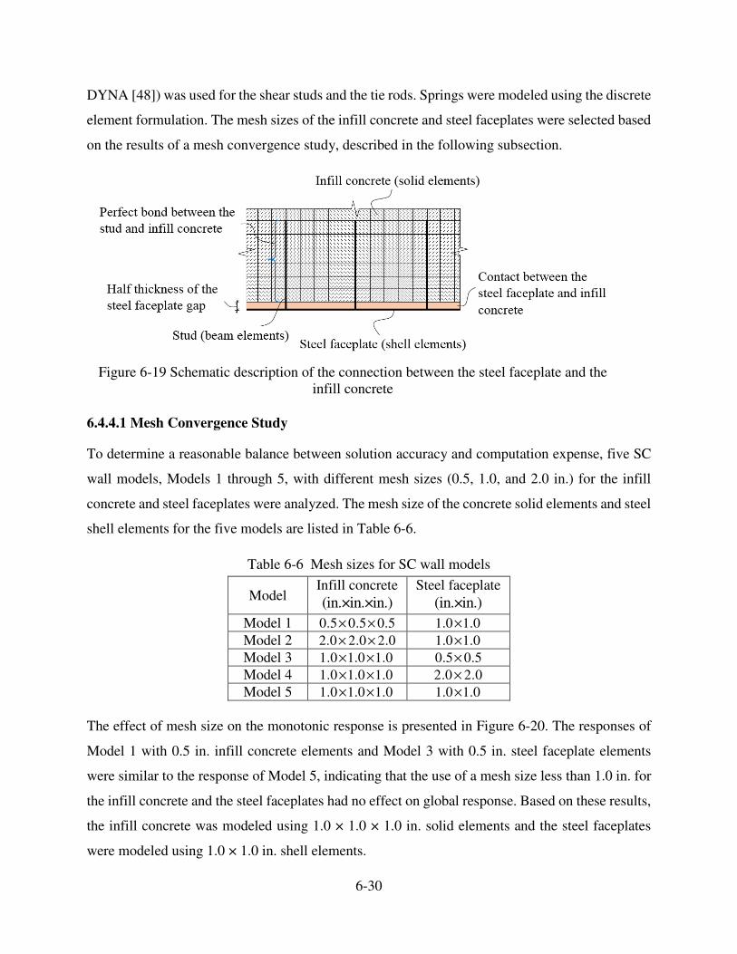
6-30
DYNA [48]) was used for the shear studs and the tie rods. Springs were modeled using the discrete
element formulation. The mesh sizes of the infill concrete and steel faceplates were selected based
on the results of a mesh convergence study, described in the following subsection.
Figure 6-19 Schematic description of the connection between the steel faceplate and the
infill concrete
6.4.4.1 Mesh Convergence Study
To determine a reasonable balance between solution accuracy and computation expense, five SC
wall models, Models 1 through 5, with different mesh sizes (0.5, 1.0, and 2.0 in.) for the infill
concrete and steel faceplates were analyzed. The mesh size of the concrete solid elements and steel
shell elements for the five models are listed in Table 6-6.
Table 6-6 Mesh sizes for SC wall models
Model Infill concrete
(in.×in.×in.)
Steel faceplate
(in.×in.)
Model 1 0.5 0.5 0.5× × 1.0 1.0×
Model 2 2.0 2.0 2.0× × 1.0 1.0×Model 3 1.0 1.0 1.0× × 0.5 0.5×Model 4 1.0 1.0 1.0× × 2.0 2.0×Model 5 1.0 1.0 1.0× × 1.0 1.0×
The effect of mesh size on the monotonic response is presented in Figure 6-20. The responses of
Model 1 with 0.5 in. infill concrete elements and Model 3 with 0.5 in. steel faceplate elements
were similar to the response of Model 5, indicating that the use of a mesh size less than 1.0 in. for
the infill concrete and the steel faceplates had no effect on global response. Based on these results,
the infill concrete was modeled using 1.0 × 1.0 × 1.0 in. solid elements and the steel faceplates
were modeled using 1.0 × 1.0 in. shell elements.

6-31
(a) Including infill concrete elements with
0.5, 1.0, and 2.0 in. mesh size
(b) Including steel faceplate elements with
0.5, 1.0, and 2.0 in. mesh size
Figure 6-20 Effect of mesh size on monotonic response
6.4.5 Loading and Boundary Conditions
The reversed cyclic loading of the test specimens was simulated by imposing horizontal
displacements at the nodes of the infill concrete and steel faceplate elements, located at the level
of the centerline of the loading plates, 60 in. above the baseplate.
Figure 6-21 presents the technique used for modeling the connection between an SC wall and its
foundation using two 1-in. thick baseplates and 22 linear springs to represent the 1.25-in. diameter
threaded B7 bars that secured the baseplate to the foundation block. The stiffness of the linear
springs was back-calculated from the measured initial stiffness of the SC walls. Figure 6-22
presents the measured cyclic response of SC3 together with the DYNA-predicted monotonic
responses corresponding to different spring stiffness at the base of the wall. Figure 6-22 indicates
that the initial stiffness of SC3 was successfully predicted using a stiffness of 61 10 lbf/in× per
spring.
The effect of spring stiffness on the deformation of the SC walls is presented in Figure 6-23. The
greater the stiffness of the linear springs, the smaller the vertical displacement of the SC walls and
the smaller the gap opening between the baseplate attached to the faceplates and the steel plate tied
to the stiff base. Similar analyses were conducted on the other SC walls to estimate the stiffness
of the linear springs representing the post-tensioned threaded bars. The stiffness of each spring for
SC1, SC2, and SC4, was 72 10× ,
61 10× , 61.5 10 lbf/in× , respectively.

6-32
Since preliminary analysis indicated that the foundation block was effectively rigid, it was not
included in the finite element model. The LS-DYNA model of SC2 is presented in Figure 6-24.
Figure 6-21 Modeling the connection between the SC wall and the foundation block
Figure 6-22 Initial stiffness (K) calculation
0
50
100
150
200
250
300
350
0.00 0.50 1.00 1.50 2.00 2.50
Lat
eral
lo
ad [
kip
s]
Lateral displacement [in.]
Test
K=1E4
K=1E5
K=1E6
K=1E7
K=1E8
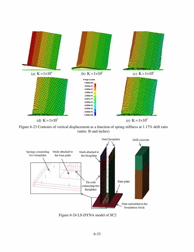
6-33
(a) 4K 1 10= × (b)
5K 1 10= × (c) 6K 1 10= ×
(d) 7K 1 10= × (e)
8K 1 10= ×
Figure 6-23 Contours of vertical displacement as a function of spring stiffness at 1.17% drift ratio
(units: lb and inches)
Figure 6-24 LS-DYNA model of SC2

6-34
6.4.6 LS-DYNA Analysis Results
The following sections describe the DYNA analysis results, including the global force-
displacement responses, equivalent viscous damping ratio, damage to the steel faceplates and infill
concrete, strain and stress distributions in the steel faceplates, and estimates of the contribution of
the steel faceplates and infill concrete to the lateral resistance of the walls.
6.4.6.1 Load-Displacement Cyclic Response
The DYNA-predicted and measured force-displacement relationships for SC1 through SC4 are
presented in Figure 6-25. In this figure, displacement is the horizontal movement of the wall in its
plane at the level of the actuators; drift ratio is defined as the horizontal displacement divided by
the distance between the base of the wall and the centerline of horizontal loading (= 60 inches).
There was good agreement between the measured and predicted cyclic responses of SC walls,
noting that initial stiffness was captured exactly through the choice of the axial stiffness of the
springs at the base (see Section 6.4.5).
The predictions of the peak shear resistance and the rate of the reloading/unloading stiffness
compared favorably with the test results. The predicted post-peak responses agreed well with the
experimental results for SC2 and SC4 but were slightly under-estimated and over-estimated in SC1
and SC3, respectively. This outcome was attributed to damage to the infill concrete and its effect
on the headed studs. Crushed concrete cannot anchor a stud and the buckling resistance of the
faceplate is consequently reduced. If threaded (tie) rods are used to provide composite action and
join the faceplates, outward movement of the tie rod (and the faceplate), at the location of the tie
rod, is by-and-large prevented and faceplate buckling resistance is preserved. The local crushing
of concrete was not addressed in the numerical model because beam elements were used to model
the studs and these were coupled to the concrete elements. Pinching was successfully simulated
using 1) the smeared crack concrete model that considers opening, closing and re-opening of the
cracks induced by load reversals, and 2) the steel material model, which considers the out-of-plane
buckling and fracture in the steel faceplates.

6-35
(a) SC1 (b) SC2
(c) SC3 (d) SC4
Figure 6-25 Predicted and measured lateral load-displacement relationships
6.4.6.2 Hysteretic Damping
Equivalent viscous damping is routinely used to model components and structures responding in
the linearly elastic range [23]. The measured hysteretic damping ratio at different drift ratios were
presented at Chapter 5. The equivalent viscous damping ratio, calculated from experimental and
numerical (DYNA) data for drift ratios up to 2% for SC1 through SC4, are presented in
Figure 6-26. For drift ratios between 50 percent and 100% of those associated with peak strength,
for which elastic dynamic analysis might be employed, the equivalent viscous damping ratios,
calculated using the experimental and numerical data, were almost identical; the ratio exceeds 6%
for both datasets. At drift ratios greater than those associated with peak strength, the DYNA
5��
����
����
�*�
5��
����
����
�*�

6-36
simulations showed more pinching of the hysteresis loops for SC1 through SC4 than was measured
and so underpredicted the dissipated energy in a given vibration cycle.
(a) SC1 (b) SC2
(c) SC3 (d) SC4
Figure 6-26 Equivalent viscous damping ratio
6.4.6.3 Steel Faceplate Contribution to the Total Load
A dense grid of Krypton LEDs was attached to one steel faceplate and rosette strain gages were
installed at three elevations on the other faceplate to measure the strain fields in the steel faceplates.
The grid of the Krypton LEDs generated square panels on the surface of the faceplate of the four
walls. The rosette strain gages were mounted on the steel faceplate with the second gage vertical.
In Section 5.7, the normal and shear strains in each panel were calculated using in-plane
displacements measured by the Krypton LEDs and an isoparametric quadrilateral formulation. The
three strains measured by each rosette were transformed to normal and shear strains.
9:��(
����
�(���
����
��
���
���
�7
9:��(
����
�(���
����
��
���
���
�7

6-37
Figure 6-27 presents information from the DYNA analyses and experiments for SC1 through SC4:
the measured cyclic force-displacement relationship for the steel faceplates provided at small
values of drift ratio prior to steel faceplate yielding using strains measured by rosettes (solid red
line) and displacements measured by LEDs (solid blue line), the DYNA-predicted cyclic force-
displacement relationship of SC wall (solid gray line), and the DYNA-predicted backbone curve
of the force-displacement relationship for the steel faceplates (dashed black line). The predicted
and measured shear forces resisted by the steel faceplates are at the level of the first row of strain
gages above the baseplate. As presented in Chapter 6, the measured shear force in the steel
faceplates was calculated as the product of the average shear strain (calculated using either the
rosettes strain gages or from the LED displacements), an assumed value of G for the steel
faceplates, and a total faceplate area of 22.5 inches, prior to steel faceplate yielding. Figure 6-27
indicates that the DYNA model successfully predicted the shear force in the steel faceplates.
The accuracy of the DYNA-predicted nonlinear response of the steel faceplates over the height of
the wall was investigated further using 1) calculations of the Von-Mises stress distributions in the
steel faceplates of SC1 and SC3, and 2) analysis of the deformed shape of the steel faceplates of
SC3 at increasing levels of drift ratio.
For each square panel generated by the grid of the Krypton LEDs, the strains and stresses were
calculated at its corners using an isoparametric quadrilateral formulation. At a node common to
multiple panels, each stress component was calculated by assigning a weight to each panel, based
on panel area. The DYNA-predicted Von-Mises stress distribution in one steel faceplate of SC1
and SC3 are presented in Figure 6-28 together with the Von-Mises stress distribution calculated
using the LED-measured displacements.
There was reasonable agreement between the numerical and experimental results at the locations
of greatest strain. The discrepancies between the numerical and experimental results were
attributed in part to the use of polynomial functions to interpolate between the measured strains at
the nodes of the grid (more accurate estimation of the strain fields in the steel faceplates could be
obtained by using a smaller spacing for the LEDs and/or by adding one LED at the center of the
panel.)

6-38
(a) SC1 (b) SC2
(c) SC3 (d) SC4
Figure 6-27 Predicted and measured cyclic force-displacement relationships in steel faceplates
5��
����
����
�*�
5��
����
����
�*�

6-39
(SC1 – LED) (SC1 – DYNA) (SC3 – LED) (SC3 – DYNA)
(a) Analysis and test data at 0.12 % drift ratio
(SC1 – LED) (SC1 – DYNA) (SC3 – LED) (SC3 – DYNA)
(b) Analysis and test data at 0.18 % drift ratio
(SC1 – LED) (SC1 – DYNA) (SC3 – LED) (SC3 – DYNA)
(c) Analysis and test data at 0.23 % drift ratio
0 4 8 12 16 20 24 28 32 36 40 ksi
Figure 6-28 DYNA-predicted and measured Von-Mises stress distribution in steel faceplates
Figure 6-29 presents the undeformed shape and predicted and measured deformed shapes (scaled
by a factor of 10) in one steel faceplate of SC3 at displacements corresponding to
0.23%, 0.47%, and 0.70%± ± ± drift ratio. The measured and DYNA-predicted displacement
fields in the steel faceplate are very similar.

6-40
(a) at +0.23% (left panel) and -0.23% (right panel) drift ratio
(a) at +0.47% (left panel) and -0.47% (right panel) drift ratio
(a) at +0.70% (left panel) and -0.70% (right panel) drift ratio
Figure 6-29 DYNA-predicted and LED-measured deformed shapes of the steel faceplate in SC3

6-41
6.4.6.4 Damage to SC walls
Figure 6-30 and Figure 6-31 present the extent of damage to the steel faceplates and the infill
concrete of SC1 through SC4, respectively, at 0.7%, 1.2%, and 2.8% drift ratios. The predicted
damage and a photograph of the recorded damage to SC2 are presented in Figure 6-32(a). The
damage to the SC walls, including the tensile cracking and crushing of the concrete at both ends
of the wall, and outward buckling and tearing of the steel faceplates at the base of the wall were
captured quite well by the finite element model.
The damage to the infill concrete of specimen SC2 is presented in Figure 6-32(b). Analysis of the
DYNA model predicted damage to the infill concrete above the baseplate at the level of the heads
of studs attached to the baseplate, which was observed in the experiment, as seen in the left panel.
Erosion of concrete was not considered in the DYNA analysis because the Winfrith model assumes
an element to have failed, with no tensile strength and stiffness, when three orthogonal cracks have
formed in it. The elements of the steel faceplates were eroded when the plastic strain reached the
rupture strain measured in the coupon tests (=40%, see Section 4.4.2). This assumption was
confirmed using numerical and experimental results. Preliminary analysis was conducted
assuming no fracture in the steel faceplates and the history of the equivalent plastic strain of the
steel faceplate elements near the vicinity of the tearing of the steel faceplates was monitored during
the cyclic analysis. The fracture strain was then calculated as the value of the effective plastic
strain of the critical steel faceplate elements corresponding to the cycle when the tearing of the
steel faceplate occurred in the experiment.
Figure 6-32(a) and Figure 6-32(b) show that the extent of damage to the steel faceplate and the
infill concrete predicted by DYNA was similar to that observed in the test.
6.4.7 Validation of the DYNA Model
The DYNA model of flexure-critical SC walls is considered to have been validated through
comparisons of predictions and measurements at the global and local levels, including cyclic force-
displacement relationships, equivalent damping ratios, shear forces in the steel faceplates, the
deformed shapes of the steel faceplates, and the Von-Mises stress distributions in the steel
faceplates.
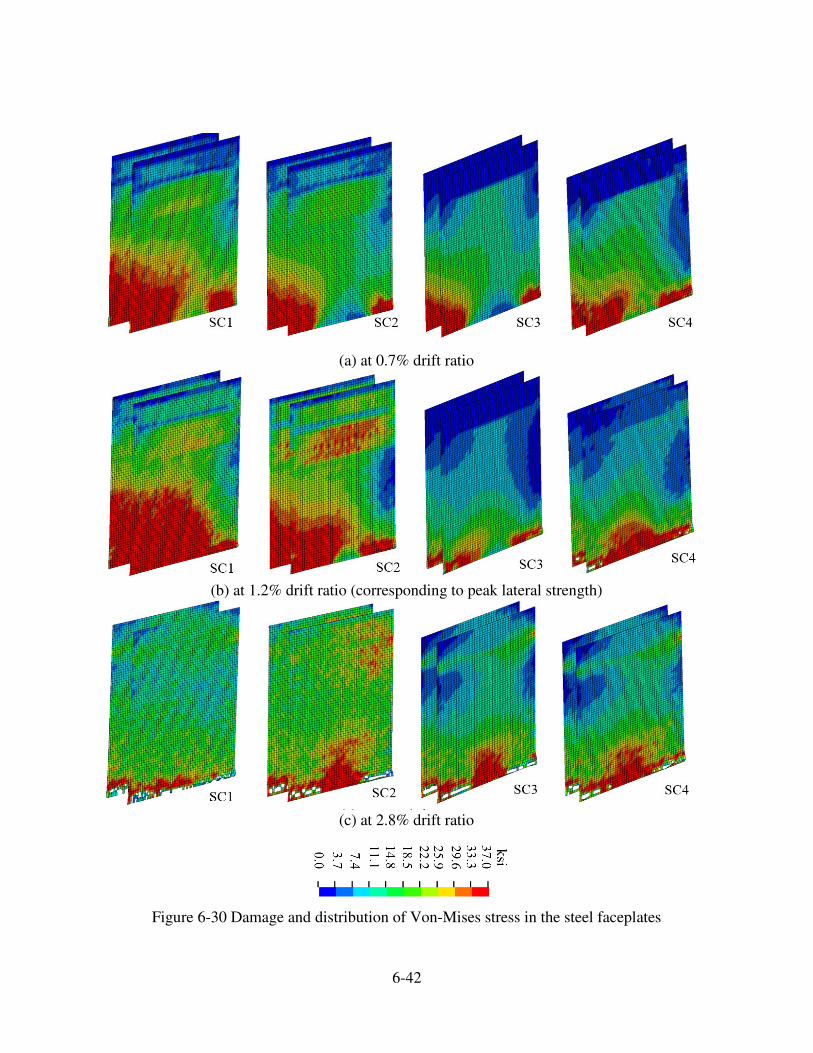
6-42
(a) at 0.7% drift ratio
(b) at 1.2% drift ratio (corresponding to peak lateral strength)
(c) at 2.8% drift ratio
Figure 6-30 Damage and distribution of Von-Mises stress in the steel faceplates

6-43
(a) at 0.7% drift ratio
(b) at 1.2% drift ratio (corresponding to peak lateral strength)
(c) at 2.8% drift ratio
Figure 6-31 Damage to the infill concrete
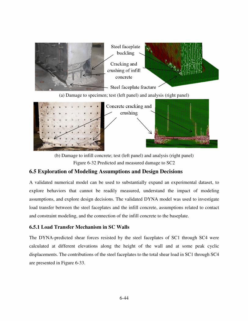
6-44
(a) Damage to specimen; test (left panel) and analysis (right panel)
(b) Damage to infill concrete; test (left panel) and analysis (right panel)
Figure 6-32 Predicted and measured damage to SC2
6.5 Exploration of Modeling Assumptions and Design Decisions
A validated numerical model can be used to substantially expand an experimental dataset, to
explore behaviors that cannot be readily measured, understand the impact of modeling
assumptions, and explore design decisions. The validated DYNA model was used to investigate
load transfer between the steel faceplates and the infill concrete, assumptions related to contact
and constraint modeling, and the connection of the infill concrete to the baseplate.
6.5.1 Load Transfer Mechanism in SC Walls
The DYNA-predicted shear forces resisted by the steel faceplates of SC1 through SC4 were
calculated at different elevations along the height of the wall and at some peak cyclic
displacements. The contributions of the steel faceplates to the total shear load in SC1 through SC4
are presented in Figure 6-33.

6-45
(a) SC1
(b) SC2
(c) SC3
Figure 6-33 Contribution of the steel faceplates to the total shear load

6-46
(d) SC4
Figure 6-33 Contribution of the steel faceplates to the total shear load (cont.)
The DYNA model assumed full composite action at the top of the SC wall because no slip was
observed between the steel faceplates and infill concrete at the level of the loading plates. This was
expected because a high normal pressure was applied to the steel faceplates and infill concrete by
the post-tensioning of the loading plates to the specimen.
Figure 6-33 shows that at small drift ratios, and prior to peak load, the shear force resisted by the
steel faceplates increased down the height of the wall due to the transfer of shear force from the
infill concrete to the steel faceplates through the shear connectors. At peak load, the shear forces
resisted by the steel faceplates at different levels along the height of the wall were approximately
identical. In the post-peak strength region, the increasing damage to the steel faceplates, including
out-of-plane buckling and tearing near the base of the wall, resulted in a significant reduction in
the percentage contribution of the steel faceplates to the total resistance.
Figure 6-34 presents the DYNA-predicted cyclic force-displacement relationships of the infill
concrete and steel faceplates in SC1. The horizontal shear forces resisted by the steel faceplates
and the infill concrete were calculated 1 in. above the baseplate. The horizontal shear force resisted
by the infill concrete 1 in. above the baseplate was calculated as the difference between the total
shear force in the SC wall and the shear force resisted by the steel faceplates, calculated as the
product of the average predicted shear stresses in the faceplates and a total faceplate area of 22.5
in2.

6-47
The highly pinched hysteresis loops in the infill concrete was associated with damage to the infill
concrete, including concrete cracking and crushing at the toes of the walls. The hysteresis loops
for the steel faceplates were pinched due to tearing and buckling.
Figure 6-34 DYNA-predicted cyclic force-displacement relationships in SC1
6.5.2 Friction
To investigate the influence of friction between the steel faceplates and the infill concrete on in-
plane response, the DYNA models of SC1 and SC3 were re-analyzed with the coefficient of
friction set to zero. The global responses were essentially identical to those reported previously for
a coefficient of friction of 0.5, and expected because the normal stresses acting on the faceplate-
to-concrete interface were negligible.
Figure 6-35 reproduces the predicted cyclic response of the SC1 and SC3 of Figure 6-25 (Model
1) together with the results of analysis assuming perfect bond between the infill concrete and
faceplates (Model 2). The pre-peak-strength response of these flexure-critical SC walls was not
significantly affected by the assumption of perfect bond but counter-intuitive differences were
evident in the post-peak behavior. Perfect bond did not allow the faceplates to buckle,
concentrating inelastic deformation near the base of the wall, and leading to their premature
fracture.

6-48
(a) SC1 (b) SC3
Figure 6-35 Influence of the assumption of perfect bond on in-plane response
Figure 6-36 presents fringes of plastic strain from the cyclic analysis of SC1 at a drift ratio of
1.5%: a drift ratio greater than that associated with peak strength. At 1.5% drift ratio, the plastic
strain in some steel faceplate elements near the base of the wall in Model 2 exceeded the rupture
strain whereas the plastic strains in the buckled steel faceplate of Model 1 were smaller than the
rupture strain.
(a) Model 1 (a) Model 2
Figure 6-36 Plastic strain distribution in steel faceplates
6.5.3 Studs Attaching the Baseplate to the Infill Concrete
The tests of SC1 through SC4 revealed a failure plane at the level of the heads of the vertical studs
that connected the infill concrete to the baseplate (see Figure 5-2). The heads of the studs occupied
��!� ��!0 ��!1 � �!1 �!0 �!�
5������ ���������� ���!
�)��
�$��
�0��
����
�
���
0��
$��
)��
5��
����
����
�*�
3���� �
3���� 0
�$ �0 �� � � 0 $
6�� � ����� �7
5��
����
����
�*�

6-49
5% and 7% of the shear area of the infill concrete in SC1/SC2 and SC3/SC4, respectively. Two
DYNA models of SC2 (A and B), with different stud spacing, were prepared and analyzed to study
the effect of stud spacing on the global and local responses of the flexure-critical walls. For Model
A, studs were placed in 2 rows at 4 in on center (the as-tested condition); the studs were placed in
2 rows at 12 in on center for Model B. Finely meshed elements were used for the infill concrete
surrounding the connectors; 3D solid elements were used to model the studs attached to the
baseplate. Models A and B are presented in Figure 6-37.
Figure 6-38 presents the predicted tensile cracking of the infill concrete of the two DYNA models
at drift ratios of 0.5% and 1.0%. Cracks formed in the horizontal plane defined by the heads of the
studs in Model A at smaller drift ratios than in Model B. Figure 6-39 presents the predicted shear
force-drift ratio relationships for the two models, which were identical up to a drift ratio of 0.5%,
noting that baseplate flexibility contributes much of the total flexibility at this drift ratio.
As seen in Figure 6-39, the shear force in Model B is greater than that in Model at drift ratios
greater than 0.5%, suggesting that an increase in stud spacing (Model B) may improve
performance (and reduce cost), noting that this analysis did not determine the minimum number
of studs or shear connectors required for adequate performance.
(a) Model A (b) Model B
Figure 6-37 DYNA models for studs attached to the baseplate

6-50
(a) Model A; 0.5% drift ratio (left panel) and 1.0% drift ratio (right panel)
(a) Model B; 0.5% drift ratio (left panel) and 1.0% drift ratio (right panel)
Figure 6-38 Damage to infill concrete in Models A and B
Figure 6-39 Lateral load-displacement relationships for Models A and B
6.5.4 Axial and Shearing Forces Transferred by Connectors
The maximum ratios of the axial and shear forces resisted by the connectors (calculated by DYNA
analysis) to their corresponding nominal strengths are presented in Figure 6-40. For each
5��
����
����
�*�

6-51
connector, two ratios were calculated; the top and bottom values present the axial force (A) and
shear force (S) ratios, respectively. The maximum axial and shear force ratios were not necessarily
calculated at the same time instant.
The nominal axial and shear strengths of the connectors were calculated using Appendix D of ACI
318-11 (ACI [1]). Considering the steel and concrete breakout strengths of the connector in
tension, and the steel and concrete pryout strengths of the connector in shear, the nominal tensile
and shear strengths of the connector were calculated 8.3 kips.
The shear studs were designed using the approach proposed by Zhang et al. [122], wherein the
stud spacing selected to avoid local buckling in steel faceplates and to ensure good composite
action in the SC wall: the sum of the shear stud capacities over the development length should be
greater than the faceplate yield strength over the tributary area defined by the line connecting shear
studs (see Figure 6-41). A development length, DL , was defined as the length over which the steel
faceplate developed its yield strength in axial tension: similar to the concept of rebar development
length (ACI 318 [1] and ACI 349 [3])[122]. In Figure 6-41, the studs are spaced at distances lS
along the length of the wall and tS over the height of the wall; nQ is the shear capacity of a single
anchor; φ is a reduction factor taken as 0.65 for studs in SC walls by Zhang et al. [122]; pt is the
thickness of each faceplate; and yf is the nominal yield strength of the steel faceplate.
Zhang et al. [122] observed that good composite action (75 to 90%) between the steel faceplates
and infill concrete could be achieved if the stud spacing was selected based on a development
length less than three times the wall thickness. They also recommended that the faceplate
slenderness ratio be limited to 1.0 /s yE f to prevent elastic buckling, where sE and yf are the
Young’s modulus and yield stress of the steel faceplate, respectively.

6-52
(a) SC1 (b) SC2
(c) SC3 (d) SC4
Figure 6-40 Maximum axial and shear force ratios for the connectors

6-53
Figure 6-41 Schematic representation of development length (adapted from Zhang et al. [123])
The spacing and diameter of the shear studs used in SC1 through SC4 were based on these local
buckling and composite action criteria. The development length, taken as three times of the wall
thickness, was 36 in and 27 in for SC1/SC2, and SC3/SC4, respectively.
Post-test numerical analysis suggested that the design of these shear studs was conservative. In the
two thicker walls, the axial force ratio was less than 0.2 except for the two rows of connectors
closest to the base of the wall: see Figure 6-40. The high axial force ratio (=0.93) in the first row
of connectors above the baseplate is attributed to the connectors resisting out-of-plane buckling of
the steel faceplates.

7-1
7. A PARAMETRIC STUDY: DESIGN OF SC WALLS
7.1 Introduction
This chapter summarizes a limited parametric study on the in-plane monotonic response of SC
walls using LS-DYNA [48, 49]. The results of finite element analysis of 36 rectangular SC walls
are used to investigate the effects on the in-plane response of SC walls of aspect ratio,
reinforcement ratio, wall thickness, and uniaxial compressive strength of concrete. The baseline
model was validated and benchmarked in Chapter 6 using data from the tests of large-scale
rectangular SC walls presented in Chapter 4.
Section 7.2 describes the DYNA modeling assumptions. Analysis results are presented in Section
7.3. Sections 7.4 and 7.5 present equations to predict the shear strength and stiffness of SC walls,
respectively. The contributions of the infill concrete and the steel faceplates to the total shear load
at the onset of the steel faceplate yielding and at peak shear strength are presented in Section 7.6.
A tri-linear shear force-displacement relationship for the monotonic in-plane response of SC walls
is proposed based on the results of the study in Section 7.7.
7.2 DYNA Modeling of SC Walls
The general purpose finite element code LS-DYNA [48, 49] was used to simulate the nonlinear
response of 36 rectangular SC walls subjected to monotonic loading. Validation and benchmarking
of the baseline model were presented in Chapter 6. The following subsections describe the
modeling assumptions and the key analysis results.
7.2.1 Design Variables
There are a number of parameters that affect the response of SC walls, including wall aspect ratio,
reinforcement ratio, slenderness ratio of the steel faceplates, wall thickness, axial force, and
material strengths. To reduce the number of simulations required for the parametric study, the
number of design variables was limited to four: 1) aspect ratio (0.5, 1.0 and 2.0), 2) reinforcement
ratio (2% to 5%), 3) wall thickness (10 in., 20 in., and 30 in.), and 4) compressive strength of infill
concrete (4 ksi and 7 ksi). The effects of axial force, slenderness ratio of the steel faceplates
(stud/tie rod spacing), and steel yield and tensile strengths were not considered but will be
investigated in the near future. As such the parametric study is limited in scope.
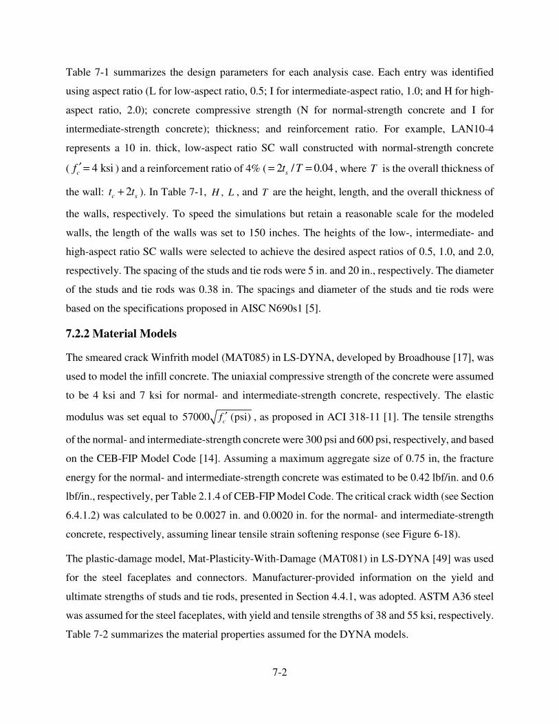
7-2
Table 7-1 summarizes the design parameters for each analysis case. Each entry was identified
using aspect ratio (L for low-aspect ratio, 0.5; I for intermediate-aspect ratio, 1.0; and H for high-
aspect ratio, 2.0); concrete compressive strength (N for normal-strength concrete and I for
intermediate-strength concrete); thickness; and reinforcement ratio. For example, LAN10-4
represents a 10 in. thick, low-aspect ratio SC wall constructed with normal-strength concrete
( 4 ksicf ′ = ) and a reinforcement ratio of 4% ( 2 / 0.04st T= = , where T is the overall thickness of
the wall: 2c st t+ ). In Table 7-1, , H L , and T are the height, length, and the overall thickness of
the walls, respectively. To speed the simulations but retain a reasonable scale for the modeled
walls, the length of the walls was set to 150 inches. The heights of the low-, intermediate- and
high-aspect ratio SC walls were selected to achieve the desired aspect ratios of 0.5, 1.0, and 2.0,
respectively. The spacing of the studs and tie rods were 5 in. and 20 in., respectively. The diameter
of the studs and tie rods was 0.38 in. The spacings and diameter of the studs and tie rods were
based on the specifications proposed in AISC N690s1 [5].
7.2.2 Material Models
The smeared crack Winfrith model (MAT085) in LS-DYNA, developed by Broadhouse [17], was
used to model the infill concrete. The uniaxial compressive strength of the concrete were assumed
to be 4 ksi and 7 ksi for normal- and intermediate-strength concrete, respectively. The elastic
modulus was set equal to 57000 (psi)c
f ′ , as proposed in ACI 318-11 [1]. The tensile strengths
of the normal- and intermediate-strength concrete were 300 psi and 600 psi, respectively, and based
on the CEB-FIP Model Code [14]. Assuming a maximum aggregate size of 0.75 in, the fracture
energy for the normal- and intermediate-strength concrete was estimated to be 0.42 lbf/in. and 0.6
lbf/in., respectively, per Table 2.1.4 of CEB-FIP Model Code. The critical crack width (see Section
6.4.1.2) was calculated to be 0.0027 in. and 0.0020 in. for the normal- and intermediate-strength
concrete, respectively, assuming linear tensile strain softening response (see Figure 6-18).
The plastic-damage model, Mat-Plasticity-With-Damage (MAT081) in LS-DYNA [49] was used
for the steel faceplates and connectors. Manufacturer-provided information on the yield and
ultimate strengths of studs and tie rods, presented in Section 4.4.1, was adopted. ASTM A36 steel
was assumed for the steel faceplates, with yield and tensile strengths of 38 and 55 ksi, respectively.
Table 7-2 summarizes the material properties assumed for the DYNA models.

7-3
Table 7-1 Properties of the DYNA models
Concrete
strengtht s
Reinforcement
ratio
(psi) (in.) (%)
1 LAN10-4 4000 0.50 75 × 150 × 10 3/16 3.8
2 LAH10-4 7000 0.50 75 × 150 × 10 3/16 3.8
3 LAN10-5 4000 0.50 75 × 150 × 10 1/4 5.0
4 LAH10-5 7000 0.50 75 × 150 × 10 1/4 5.0
5 LAN20-2 4000 0.50 75 × 150 × 20 3/16 1.9
6 LAH20-2 7000 0.50 75 × 150 × 20 3/16 1.9
7 LAN20-5 4000 0.50 75 × 150 × 20 1/2 5.0
8 LAH20-5 7000 0.50 75 × 150 × 20 1/2 5.0
9 LAN30-2 4000 0.50 75 × 150 × 30 5/16 2.1
10 LAH30-2 7000 0.50 75 × 150 × 30 5/16 2.1
11 LAN30-5 4000 0.50 75 × 150 × 30 3/4 5.0
12 LAH30-5 7000 0.50 75 × 150 × 30 3/4 5.0
13 IAN10-4 4000 1.00 150 × 150 × 10 3/16 3.8
14 IAH10-4 7000 1.00 150 × 150 × 10 3/16 3.8
15 IAN10-5 4000 1.00 150 × 150 × 10 1/4 5.0
16 IAH10-5 7000 1.00 150 × 150 × 10 1/4 5.0
17 IAN20-2 4000 1.00 150 × 150 × 20 3/16 1.9
18 IAH20-2 7000 1.00 150 × 150 × 20 3/16 1.9
19 IAN20-5 4000 1.00 150 × 150 × 20 1/2 5.0
20 IAH20-5 7000 1.00 150 × 150 × 20 1/2 5.0
21 IAN30-2 4000 1.00 150 × 150 × 30 5/16 2.1
22 IAH30-2 7000 1.00 150 × 150 × 30 5/16 2.1
23 IAN30-5 4000 1.00 150 × 150 × 30 3/4 5.0
24 IAH30-5 7000 1.00 150 × 150 × 30 3/4 5.0
25 HAN10-4 4000 2.00 300 × 150 × 10 3/16 3.8
26 HAH10-4 7000 2.00 300 × 150 × 10 3/16 3.8
27 HAN10-5 4000 2.00 300 × 150 × 10 1/4 5.0
28 HAH10-5 7000 2.00 300 × 150 × 10 1/4 5.0
29 HAN20-2 4000 2.00 300 × 150 × 20 3/16 1.9
30 HAH20-2 7000 2.00 300 × 150 × 20 3/16 1.9
31 HAN20-5 4000 2.00 300 × 150 × 20 1/2 5.0
32 HAH20-5 7000 2.00 300 × 150 × 20 1/2 5.0
33 HAN30-2 4000 2.00 300 × 150 × 30 5/16 2.1
34 HAH30-2 7000 2.00 300 × 150 × 30 5/16 2.1
35 HAN30-5 4000 2.00 300 × 150 × 30 3/4 5.0
36 HAH30-5 7000 2.00 300 × 150 × 30 3/4 5.0
Low
-asp
ect
ratio
SC
wal
ls In
term
edia
te-a
spec
t ra
tio
SC
wal
ls
H
igh-a
spec
t ra
tio
SC
wal
ls
H � L×TNo.
SC wall
typeModel
Aspect
ratio(in.×in.×in.)

7-4
Table 7-2 Material properties for the DYNA analysis
Material
Young’s
modulus
(ksi)
Poison
ratio
Uniaxial
compressive
strength
(ksi)
Uniaxial
tensile
strength
(ksi)
Yield
strength
(ksi)
Ultimate
strength
(ksi)
Crack
width
(in.)
Agg.
Size
(in.)
Infill
concrete
Normal
strength 3600 0.18 4.0 0.3 - - 0.0027 0.75
Intermediate
strength 4800 0.18 7.0 0.6 - - 0.002 0.75
Faceplate 29000 0.30 - - 36 55 - -
Connectors 29000 0.30 - - 50 75 - -
7.2.3 Contact, Element, Loading, and Boundary Condition
Friction between the infill concrete and the steel faceplates, the infill concrete and the baseplate,
and the baseplate and the steel plate embedded in the foundation block were considered using the
Contact-Automatic-Surface-To-Surface formulation, with a coefficient of friction 0.5 (see Section
6.4.3). The steel faceplates were tied to the baseplate using the kinematic constraint Contact-Tied-
Shell-Edge-To-Surface. The studs and tie rods were coupled to the infill concrete elements using
Constrained-Lagrange-In-Solid.
Beam elements were used to represent the studs and tie rods. Eight-node solid elements were used
to model the infill concrete, and four-node shell elements were used for the steel faceplates. The
infill concrete was modeled with 1 in. × 1 in. × 1 in. elements and the steel faceplates were modeled
with 1 in. × 1 in. elements. The constant stress formulation (ELFORM=1 in LS-DYNA [48]) and
Belytschko-Tsay formulation (LS-DYNA [48]) were used for solid elements and shell elements,
respectively. The cross section integrated beam element (Hughes-Liu beam in LS-DYNA [48])
was used for shear studs and tie rods. The walls were rigidly connected to an infinitely stiff base.
Three LS-DYNA models, with aspect ratios of 0.5, 1.0, and 2.0, are presented in Figure 7-1.
7.3 Monotonic Analysis Results
Key analysis results are summarized in Table 7-3, including the contributions of the steel
faceplates and the infill concrete to the total shear force at yield of the wall, and at peak force, and
their corresponding drift ratios, and the flexural strengths and their corresponding maximum shear
forces. The DYNA-predicted yield force and displacement correspond to the onset of Von-Mises
yielding of the steel faceplates. The drift ratio at the peak shear force was calculated using a tri-

7-5
linear idealization of the DYNA-predicted force-displacement relationship by an equal-energy
method [51]. Figure 7-2 presents the idealization of the DYNA predicted force-displacement
relationship for HAN10-4.
(a) LAN20-2 ( / 0.5H L = )
(b) IAH10-4 ( / 1.0H L = ) (c) HAH30-5 ( / 2.0H L = )
Figure 7-1 LS-DYNA models
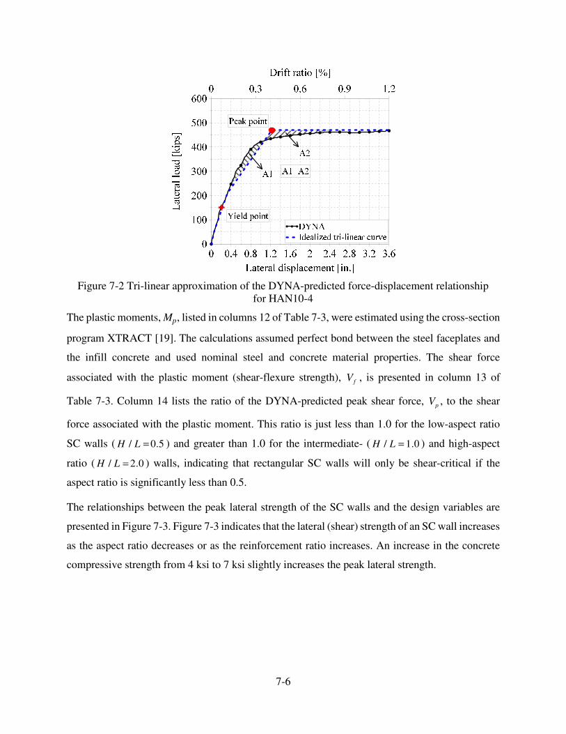
7-6
Figure 7-2 Tri-linear approximation of the DYNA-predicted force-displacement relationship
for HAN10-4
The plastic moments, Mp, listed in columns 12 of Table 7-3, were estimated using the cross-section
program XTRACT [19]. The calculations assumed perfect bond between the steel faceplates and
the infill concrete and used nominal steel and concrete material properties. The shear force
associated with the plastic moment (shear-flexure strength), fV , is presented in column 13 of
Table 7-3. Column 14 lists the ratio of the DYNA-predicted peak shear force, pV , to the shear
force associated with the plastic moment. This ratio is just less than 1.0 for the low-aspect ratio
SC walls ( / 0.5H L = ) and greater than 1.0 for the intermediate- ( / 1.0H L = ) and high-aspect
ratio ( / 2.0H L = ) walls, indicating that rectangular SC walls will only be shear-critical if the
aspect ratio is significantly less than 0.5.
The relationships between the peak lateral strength of the SC walls and the design variables are
presented in Figure 7-3. Figure 7-3 indicates that the lateral (shear) strength of an SC wall increases
as the aspect ratio decreases or as the reinforcement ratio increases. An increase in the concrete
compressive strength from 4 ksi to 7 ksi slightly increases the peak lateral strength.
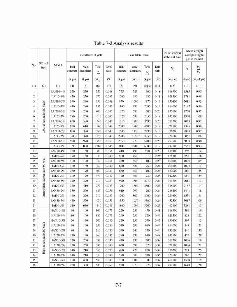
7-7
Table 7-3 Analysis results
Plastic moment
at the wall base
Total Total
(kips) (kips) (kips) (%) (kips) (kips) (kips) (%) (kip-in.) (kips) (kips/kips)
(1) (2) (3) (4) (5) (6) (7) (8) (9) (kips) (11) (12) (13) (14)
1 LAN10-4% 320 230 550 0.048 775 725 1500 0.18 118900 1585 0.95
2 LAI10-4% 450 220 670 0.043 1000 680 1680 0.18 128300 1711 0.98
3 LAN10-5% 340 290 630 0.048 870 1000 1870 0.19 150800 2011 0.93
4 LAI10-5% 470 280 750 0.043 1160 930 2090 0.19 164000 2187 0.96
5 LAN20-2% 560 240 800 0.043 1020 680 1700 0.20 132000 1760 0.97
6 LAI20-2% 780 230 1010 0.043 1420 630 2050 0.19 142500 1900 1.08
7 LAN20-5% 660 580 1240 0.048 1710 1980 3690 0.20 301700 4023 0.92
8 LAI20-5% 950 610 1560 0.048 2300 1900 4200 0.19 328100 4375 0.96
9 LAN30-2% 850 390 1240 0.043 1640 1150 2790 0.18 216200 2883 0.97
10 LAI30-2% 1200 370 1570 0.043 2200 1050 3250 0.19 229600 3061 1.06
11 LAN30-5% 980 970 1950 0.053 2350 3050 5400 0.20 452500 6033 0.90
12 LAI30-5% 1390 890 2280 0.048 3180 2900 6080 0.19 492100 6561 0.93
13 IAN10-4% 150 150 300 0.051 410 490 900 0.23 118900 793 1.14
14 IAI10-4% 170 160 330 0.040 560 450 1010 0.25 128300 855 1.18
15 IAN10-5% 160 190 350 0.051 450 650 1100 0.23 150800 1005 1.09
16 IAI10-5% 180 180 360 0.040 630 620 1250 0.24 164000 1093 1.14
17 IAN20-2% 230 170 400 0.053 650 450 1100 0.26 132000 880 1.25
18 IAI20-2% 300 170 470 0.037 770 460 1230 0.25 142500 950 1.29
19 IAN20-5% 320 390 710 0.053 970 1300 2270 0.24 301700 2011 1.13
20 IAI20-5% 360 410 770 0.043 1200 1300 2500 0.23 328100 2187 1.14
21 IAN30-2% 350 270 620 0.056 910 790 1700 0.24 216200 1441 1.18
22 IAI30-2% 440 270 710 0.037 1200 800 2000 0.24 229600 1531 1.31
23 IAN30-5% 460 570 1030 0.053 1350 1950 3300 0.24 452500 3017 1.09
24 IAI30-5% 510 630 1140 0.045 1800 1900 3700 0.25 492100 3281 1.13
25 HAN10-4% 60 100 160 0.073 220 250 470 0.41 118900 396 1.19
26 HAI10-4% 80 100 180 0.073 290 230 520 0.46 128300 428 1.22
27 HAN10-5% 70 130 200 0.080 220 350 570 0.42 150800 503 1.13
28 HAI10-5% 90 140 230 0.080 330 330 660 0.44 164000 547 1.21
29 HAN20-2% 80 130 210 0.080 330 240 570 0.40 132000 440 1.30
30 HAI20-2% 120 140 260 0.087 380 230 610 0.48 142500 475 1.28
31 HAN20-5% 120 260 380 0.080 470 730 1200 0.38 301700 1006 1.19
32 HAI20-5% 120 260 380 0.080 630 690 1320 0.37 328100 1094 1.21
33 HAN30-2% 140 210 350 0.073 480 420 900 0.39 216200 721 1.25
34 HAI30-2% 140 210 350 0.080 590 380 970 0.35 229600 765 1.27
35 HAN30-5% 180 400 580 0.087 700 1100 1800 0.37 452500 1508 1.19
36 HAI30-5% 250 380 630 0.067 920 1050 1970 0.37 492100 1640 1.20
Shear strength
coresponding to
plastic moment
No.SC wall
typeModel
Hig
h-a
spec
t ra
tio
SC
wal
ls
Lateral force at yield
L
ow
-asp
ect
rati
o S
C w
alls
I
nte
rmed
iate
-asp
ect
rati
o S
C w
all
Peak lateral force
Steel
faceplates
Infill
concrete
Drift
ratio
Infill
concrete
Steel
faceplates
Drift
ratio �
�� �
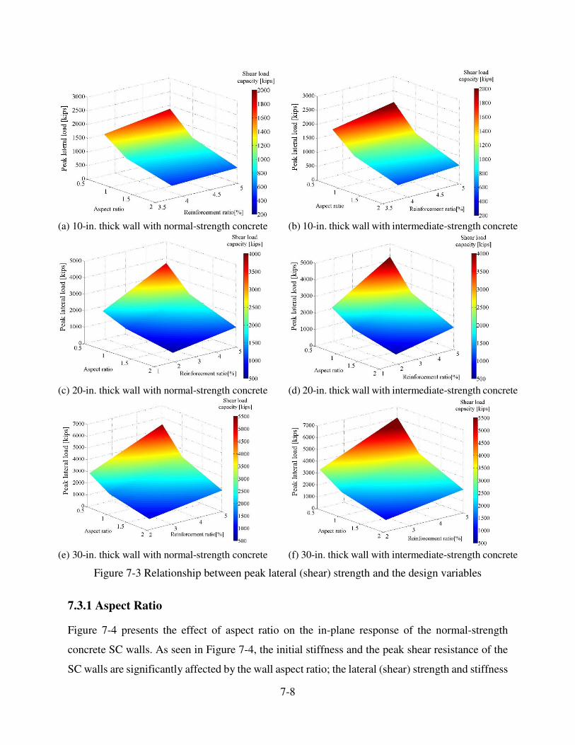
7-8
(a) 10-in. thick wall with normal-strength concrete (b) 10-in. thick wall with intermediate-strength concrete
(c) 20-in. thick wall with normal-strength concrete (d) 20-in. thick wall with intermediate-strength concrete
(e) 30-in. thick wall with normal-strength concrete (f) 30-in. thick wall with intermediate-strength concrete
Figure 7-3 Relationship between peak lateral (shear) strength and the design variables
7.3.1 Aspect Ratio
Figure 7-4 presents the effect of aspect ratio on the in-plane response of the normal-strength
concrete SC walls. As seen in Figure 7-4, the initial stiffness and the peak shear resistance of the
SC walls are significantly affected by the wall aspect ratio; the lateral (shear) strength and stiffness
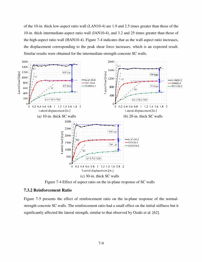
7-9
of the 10-in. thick low-aspect ratio wall (LAN10-4) are 1.9 and 2.5 times greater than those of the
10-in. thick intermediate-aspect ratio wall (IAN10-4), and 3.2 and 25 times greater than those of
the high-aspect ratio wall (HAN10-4). Figure 7-4 indicates that as the wall aspect ratio increases,
the displacement corresponding to the peak shear force increases, which is an expected result.
Similar results were obtained for the intermediate-strength concrete SC walls.
(a) 10-in. thick SC walls (b) 20-in. thick SC walls
(c) 30-in. thick SC walls
Figure 7-4 Effect of aspect ratio on the in-plane response of SC walls
7.3.2 Reinforcement Ratio
Figure 7-5 presents the effect of reinforcement ratio on the in-plane response of the normal-
strength concrete SC walls. The reinforcement ratio had a small effect on the initial stiffness but it
significantly affected the lateral strength, similar to that observed by Ozaki et al. [62].

7-10
(a) 10-in. thick SC walls (b) 20-in. thick SC walls
(c) 30-in. thick SC walls
Figure 7-5 Effect of reinforcement ratio on the in-plane response of the SC walls
Figure 7-5 indicates that the effect of the reinforcement ratio on the lateral (shear) strength
increases as the aspect ratio decreases or as the wall thickness increases. The displacement at the
peak shear force was not substantially affected by the reinforcement ratio. Similar results were
obtained for intermediate-strength concrete SC walls.
7.3.3 Concrete Compressive Strength
Figure 7-6 presents the effect of concrete compressive strength on the in-plane response of the SC
walls. Similar to reinforcement ratio, concrete compressive strength affected the lateral (shear)
strength. The initial stiffness was not substantially affected.
Figure 7-6 indicates that the influence of concrete compressive strength on the peak lateral load
increases as the aspect ratio decreases. The displacement at peak lateral load was not substantially
influenced by concrete compressive strength. Similar results were obtained for intermediate-
strength concrete SC walls.

7-11
(a) 10-in. thick SC walls (b) 20-in. thick SC walls
(c) 30-in. thick SC walls
Figure 7-6 Effect of concrete compressive strength on the in-plane response of the SC walls
7.4 Shearing Strength
Figure 7-7 presents the shear stress distribution in the infill concrete of IAN20-2. In Figure 7-7,
cθ is the angle of the primary compression strut to the horizontal. The lateral load applied at top
of the wall is transferred to its foundation by a diagonal compression strut in the infill concrete and
plane stress behavior of the steel faceplates. The shear force resisted by the infill concrete at the
base of the wall can be calculated as the product of the average horizontal shear stress over the
horizontal projection of the depth of the compression strut, the neutral axis depth in the infill
concrete, cd in Figure 7-7, and the thickness of the infill concrete. The shear force resisted by the
steel faceplates can be calculated as the product of the average shear stress in the faceplates and
the cross-sectional area of the faceplates.

7-12
Figure 7-7 Load transfer in the infill concrete
In the following subsection, the results of the analyses are used to investigate the effects of the
design variables on the depth of the neutral axis in the infill concrete, and the average shear stress
in the concrete compression strut and in the steel faceplates.
7.4.1 Depth of the Neutral Axis
At the yield point, the depth to the neutral axis from the extreme fiber in compression is influenced
by aspect ratio and reinforcement ratio (and axial load, but that is not addressed in this study). At
peak load, the concrete compressive strength also plays a role.
On the basis of the finite element analysis results of 36 DYNA models, (7-1) and (7-2) are proposed
to estimate the depth to the neutral axis at the yield load and peak lateral (shear) strength,
respectively, of an SC wall:
( )AR RR
yc y yd Lα α= (7-1)
( )AR RR CS
pc p p pd Lα α α= (7-2)
where ycd and
pcd are the neutral axis depths at the yield load and the peak lateral strength,
respectively; L is the length of the wall; and , , , , and AR RR AR RR CS
y y p p pα α α α α are factors that
account for the design variables. The subscripts y and p identify the yield load and the peak
lateral strengths, respectively. The superscripts AR , RR , and CS identify the influence of aspect
ratio, reinforcement ratio, and concrete compressive strength, respectively.
7-13
Figure 7-8 presents the relationships between the modification factors, used for the calculation of
the neutral axis depth, and the design variables. In Figure 7-8(a) and Figure 7-8(b), β is the wall
aspect ratio. In Figure 7-8 (c) and Figure 7-8(d), ρ is the reinforcement ratio. These figures
indicate that the neutral axis depth in the infill concrete increases as the wall aspect ratio decreases
or as the reinforcement ratio increases.
7.4.2 Average Shear Stress in the Compression Strut
The average shear stress in the compression strut at the yield load is influenced by the aspect ratio
and the concrete strength. At peak lateral strength, it is affected only by the aspect ratio.
On the basis of the finite element analysis results, (7-3) and (7-4) are proposed to calculate the
average shear stress in the compression strut at the yield load and the peak lateral strength,
respectively:
AR C
c
S
cy y y fτ γ γ ′= (7-3)
AR
cp p cfτ γ= ′ (7-4)
where cyτ and
cpτ are the average shear stresses in the compression strut at the yield load and the
peak lateral strength, respectively; and AR
yγ , AR
pγ , and CS
yγ are factors that account for the design
variables. Figure 7-9 presents the relationship between the aspect ratio coefficients, AR
yγ and AR
pγ
, and the wall aspect ratio at the yield load and the peak lateral strength. As seen in Figure 7-9, the
greater the aspect ratio, the lower the horizontal shear stress in the compression strut.
7.4.3 Average Shear Stress in the Steel Faceplates
The results of the finite element analysis indicated that the normalized average shear stress in the
steel faceplates at the yield load and peak lateral strength is affected by wall aspect ratio only,
where the normalized average shear stress in the steel faceplates was calculated by dividing the
force resisted by the steel faceplates by the corresponding axial strength (s yA f ), where sA and
yf
are the cross-sectional area and the yield stress of the steel faceplates, respectively. Figure 7-10
presents the relationship between the normalized average shear stress in the steel faceplates and
wall aspect ratio.

7-14
(a) Coefficient ��� (b) Coefficient ��
��
(c) Coefficient ��� (d) Coefficient ��
��
Figure 7-8 Relationship between the factors and the design variables for neutral axis depth
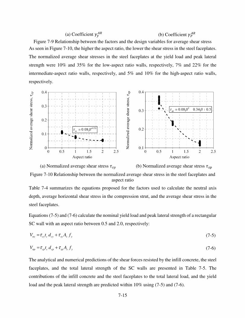
7-15
(a) Coefficient ��� (b) Coefficient ��
��
Figure 7-9 Relationship between the factors and the design variables for average shear stress
As seen in Figure 7-10, the higher the aspect ratio, the lower the shear stress in the steel faceplates.
The normalized average shear stresses in the steel faceplates at the yield load and peak lateral
strength were 10% and 35% for the low-aspect ratio walls, respectively, 7% and 22% for the
intermediate-aspect ratio walls, respectively, and 5% and 10% for the high-aspect ratio walls,
respectively.
(a) Normalized average shear stress �� (b) Normalized average shear stress ���
Figure 7-10 Relationship between the normalized average shear stress in the steel faceplates and
aspect ratio
Table 7-4 summarizes the equations proposed for the factors used to calculate the neutral axis
depth, average horizontal shear stress in the compression strut, and the average shear stress in the
steel faceplates.
Equations (7-5) and (7-6) calculate the nominal yield load and peak lateral strength of a rectangular
SC wall with an aspect ratio between 0.5 and 2.0, respectively:
ny cy c cy sy s yV t d A fτ τ= + (7-5)
np cp c cp sp s yV t d A fτ τ= + (7-6)
The analytical and numerical predictions of the shear forces resisted by the infill concrete, the steel
faceplates, and the total lateral strength of the SC walls are presented in Table 7-5. The
contributions of the infill concrete and the steel faceplates to the total lateral load, and the yield
load and the peak lateral strength are predicted within 10% using (7-5) and (7-6).

7-16
Table 7-4 Modification factors
Parameter Point
Design variable
Aspect ratio Reinforcement ratio Concrete
strength
Calculation of the
neutral axis depth in
the infill concrete
Yield load� 0.46 0.67AR
yα β −= 20.01 0.15
0.31
RRyα ρ ρ= − +
+-
Peak load� 0.57 0.67AR
pα β −=2
0.02 0.2
+0.08
RR
pα ρ ρ= − + 4CSp
cfα =
′
Calculation of the
average shear stress
in the infill concrete
Yield load� 0.037 0.10ARyγ β=− + -
4CSy
cfγ =
′
Peak load� 0.058 0.26AR
Pγ β= − + - -
Calculation of the
average shear stress
in the steel faceplates
Yield load� 0.52 0.08syτ β −=
Peak load� 20.08 0.34 0.5spτ β β= − +
7.5 Stiffness Prediction
On the basis of the results of the analyses, (7-7) and (7-8) are proposed to calculate the pre-yield
and post-yield stiffness of rectangular SC walls, where the pre-yield stiffness is the secant stiffness
established at the force corresponding to the onset of the yielding of the steel faceplates and the
post-yield stiffness is the slope of a line segment passing through the yield and peak points of the
force-displacement relationship.
c c s
cr cr el elK K Kα= + (7-7)
c c s s
y y el y elK K Kα α= + (7-8)
where c
elK and s
elK are the elastic stiffness of the infill concrete and the steel faceplates,
respectively; c
crα is calculated by dividing the contribution of the infill concrete to the pre-yield
stiffness of SC wall to the elastic stiffness of the infill concrete; and c
yα and s
yα are calculated by
dividing the contributions of the infill concrete and the steel faceplates, respectively, to the post-
yield stiffness of the SC wall, to their corresponding elastic stiffness. The elastic stiffness of the
infill concrete and the steel faceplates were calculated as:
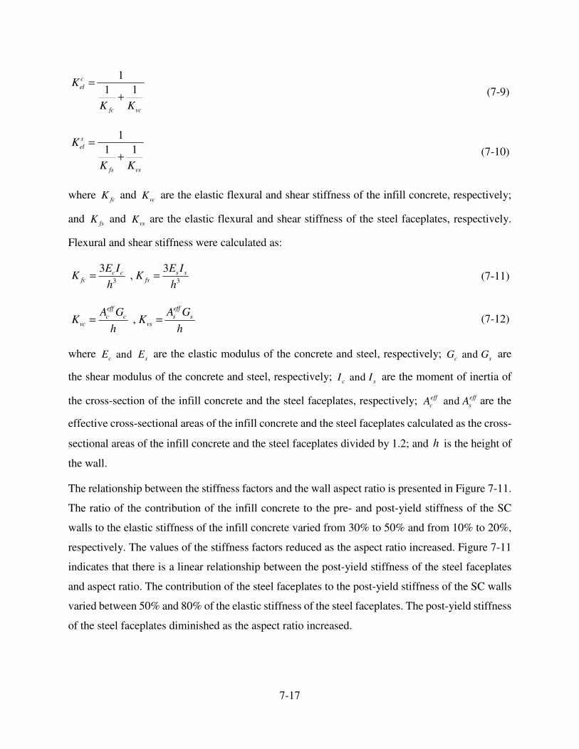
7-17
1
1 1c
el
fc vc
K
K K
=
+ (7-9)
1
1 1s
el
fs vs
K
K K
=
+ (7-10)
where fcK and
vcK are the elastic flexural and shear stiffness of the infill concrete, respectively;
and fsK and
vsK �are the elastic flexural and shear stiffness of the steel faceplates, respectively.
Flexural and shear stiffness were calculated as:
3 3
3 3 , c c s s
fc fs
E I E IK K
h h= = (7-11)
, eff eff
c c s svc vs
A G A GK K
h h= = (7-12)
where and c s
E E are the elastic modulus of the concrete and steel, respectively; and c s
G G are
the shear modulus of the concrete and steel, respectively; and c s
I I are the moment of inertia of
the cross-section of the infill concrete and the steel faceplates, respectively; and eff ff
c s
eA A are the
effective cross-sectional areas of the infill concrete and the steel faceplates calculated as the cross-
sectional areas of the infill concrete and the steel faceplates divided by 1.2; and h is the height of
the wall.
The relationship between the stiffness factors and the wall aspect ratio is presented in Figure 7-11.
The ratio of the contribution of the infill concrete to the pre- and post-yield stiffness of the SC
walls to the elastic stiffness of the infill concrete varied from 30% to 50% and from 10% to 20%,
respectively. The values of the stiffness factors reduced as the aspect ratio increased. Figure 7-11
indicates that there is a linear relationship between the post-yield stiffness of the steel faceplates
and aspect ratio. The contribution of the steel faceplates to the post-yield stiffness of the SC walls
varied between 50% and 80% of the elastic stiffness of the steel faceplates. The post-yield stiffness
of the steel faceplates diminished as the aspect ratio increased.

7-18
Table 7-5 Numerical and analytical predictions of the yield and peak lateral strengths
Figure 7-11 Relationship between the stiffness reduction coefficients and wall aspect ratio
DYNA AnalyticalAnalytical/
DYNADYNA Analytical
Analytical/
DYNADYNA Analytical
Analytical/
DYNADYNA Analytical
Analytical/
DYNADYNA Analytical
Analytical/
DYNADYNA Analytical
Analytical/
DYNA
(kips) (kips) (kips/kips) (kips) (kips) (kips/kips) (kips) (kips) (kips/kips) (kips) (kips) (kips/kips) (kips) (kips) (kips/kips) (kips) (kips) (kips/kips)
(1) (2) (3) (4) (5) (6) (7) (8) (9) (10) (11) (12) (13) (14) (15) (16) (17) (18) (19) (20) (21)
1 LAN10-4% 320 338 1.06 230 225 0.98 550 563 1.02 775 754 0.97 725 702 0.97 1500 1456 0.97
2 LAI10-4% 450 448 0.99 220 225 1.02 670 672 1.00 1000 998 1.00 680 702 1.03 1680 1700 1.01
3 LAN10-5% 340 361 1.06 290 299 1.03 630 660 1.05 870 814 0.94 1000 936 0.94 1870 1750 0.94
4 LAI10-5% 470 477 1.02 280 299 1.07 750 776 1.04 1160 1077 0.93 930 936 1.01 2090 2013 0.96
5 LAN20-2% 560 537 0.96 240 225 0.94 800 762 0.95 1020 1038 1.02 680 702 1.03 1700 1740 1.02
6 LAI20-2% 780 711 0.91 230 225 0.98 1010 936 0.93 1420 1374 0.97 630 702 1.11 2050 2076 1.01
7 LAN20-5% 660 721 1.09 580 599 1.03 1240 1320 1.06 1710 1628 0.95 1980 1872 0.95 3690 3500 0.95
8 LAI20-5% 950 954 1.00 610 599 0.98 1560 1553 1.00 2300 2154 0.94 1900 1872 0.99 4200 4026 0.96
9 LAN30-2% 850 836 0.98 390 374 0.96 1240 1210 0.98 1640 1662 1.01 1150 1170 1.02 2790 2832 1.02
10 LAI30-2% 1200 1106 0.92 370 374 1.01 1570 1480 0.94 2200 2198 1.00 1050 1170 1.11 3250 3368 1.04
11 LAN30-5% 980 1082 1.10 970 898 0.93 1950 1980 1.02 2350 2442 1.04 3050 2808 0.92 5400 5250 0.97
12 LAI30-5% 1390 1431 1.03 890 898 1.01 2280 2329 1.02 3180 3230 1.02 2900 2808 0.97 6080 6039 0.99
13 IAN10-4% 150 136 0.91 150 156 1.04 300 292 0.97 410 446 1.09 490 474 0.97 900 920 1.02
14 IAI10-4% 170 180 1.06 160 156 0.98 330 336 1.02 560 590 1.05 450 474 1.05 1010 1064 1.05
15 IAN10-5% 160 145 0.91 190 208 1.10 350 353 1.01 450 481 1.07 650 633 0.97 1100 1113 1.01
16 IAI10-5% 200 192 0.96 190 208 1.10 390 400 1.02 630 636 1.01 620 633 1.02 1250 1269 1.02
17 IAN20-2% 230 216 0.94 170 156 0.92 400 372 0.93 650 613 0.94 450 474 1.05 1100 1088 0.99
18 IAI20-2% 300 286 0.95 170 156 0.92 470 442 0.94 770 812 1.05 460 474 1.03 1230 1286 1.05
19 IAN20-5% 320 290 0.91 390 416 1.07 710 706 0.99 970 962 0.99 1300 1265 0.97 2270 2227 0.98
20 IAI20-5% 360 383 1.06 410 416 1.02 770 799 1.04 1200 1272 1.06 1300 1265 0.97 2500 2538 1.02
21 IAN30-2% 350 336 0.96 270 260 0.96 620 596 0.96 910 982 1.08 790 791 1.00 1700 1773 1.04
22 IAI30-2% 440 444 1.01 270 260 0.96 710 704 0.99 1200 1299 1.08 800 791 0.99 2000 2090 1.04
23 IAN30-5% 460 434 0.94 570 625 1.10 1030 1059 1.03 1350 1443 1.07 1950 1898 0.97 3300 3340 1.01
24 IAI30-5% 530 575 1.08 610 625 1.02 1140 1199 1.05 1800 1908 1.06 1900 1898 1.00 3700 3806 1.03
25 HAN10-4% 60 56 0.93 100 109 1.09 160 164 1.03 220 214 0.97 250 251 1.00 470 465 0.99
26 HAI10-4% 80 74 0.92 100 109 1.09 180 182 1.01 290 284 0.98 230 251 1.09 520 534 1.03
27 HAN10-5% 60 59 0.99 140 145 1.03 200 204 1.02 220 231 1.05 350 334 0.96 570 566 0.99
28 HAI10-5% 80 78 0.98 150 145 0.97 230 223 0.97 330 306 0.93 330 334 1.01 660 640 0.97
29 HAN20-2% 80 88 1.10 120 109 0.90 200 197 0.98 330 295 0.89 240 251 1.04 570 546 0.96
30 HAI20-2% 120 117 0.97 120 109 0.90 240 225 0.94 380 390 1.03 230 251 1.09 610 641 1.05
31 HAN20-5% 110 119 1.08 270 290 1.07 380 408 1.07 470 463 0.98 730 669 0.92 1200 1131 0.94
32 HAI20-5% 175 157 0.90 285 290 1.02 460 446 0.97 630 612 0.97 690 669 0.97 1320 1281 0.97
33 HAN30-2% 130 137 1.06 190 181 0.95 320 318 1.00 480 472 0.98 420 418 0.99 900 890 0.99
34 HAI30-2% 180 182 1.01 200 181 0.90 380 363 0.95 590 625 1.06 380 418 1.10 970 1043 1.07
35 HAN30-5% 180 178 0.99 400 434 1.09 580 612 1.06 700 694 0.99 1100 1003 0.91 1800 1697 0.94
36 HAI30-5% 220 235 1.07 460 434 0.94 680 670 0.98 920 918 1.00 1050 1003 0.96 1970 1921 0.98
No.
Lo
w-a
spec
t ra
tio S
C w
alls
H
igh
-asp
ect
ratio
SC
wal
ls
Model SC wall
type
Total shear forceShear force resisted by infill
concrete
Data point at yeild load
Shear force resisted by steel
faceplateTotal shear force
Shear force resisted by steel
faceplate
Shear force resisted by infill
concrete
Data point at peak load
In
term
edia
te-a
spec
t ra
tio
SC
wal
ls
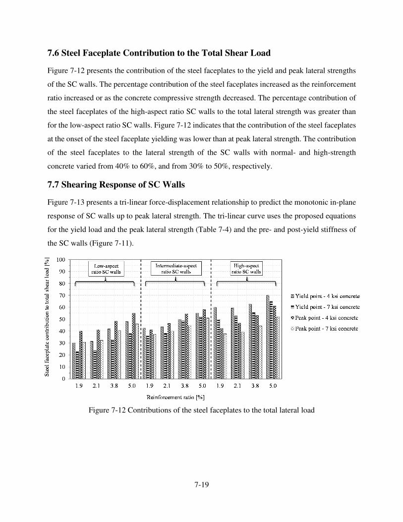
7-19
7.6 Steel Faceplate Contribution to the Total Shear Load
Figure 7-12 presents the contribution of the steel faceplates to the yield and peak lateral strengths
of the SC walls. The percentage contribution of the steel faceplates increased as the reinforcement
ratio increased or as the concrete compressive strength decreased. The percentage contribution of
the steel faceplates of the high-aspect ratio SC walls to the total lateral strength was greater than
for the low-aspect ratio SC walls. Figure 7-12 indicates that the contribution of the steel faceplates
at the onset of the steel faceplate yielding was lower than at peak lateral strength. The contribution
of the steel faceplates to the lateral strength of the SC walls with normal- and high-strength
concrete varied from 40% to 60%, and from 30% to 50%, respectively.
7.7 Shearing Response of SC Walls
Figure 7-13 presents a tri-linear force-displacement relationship to predict the monotonic in-plane
response of SC walls up to peak lateral strength. The tri-linear curve uses the proposed equations
for the yield load and the peak lateral strength (Table 7-4) and the pre- and post-yield stiffness of
the SC walls (Figure 7-11).
Figure 7-12 Contributions of the steel faceplates to the total lateral load

7-20
Figure 7-13 Tri-linear shear force-displacement relationship for SC walls
The analytical and numerical shear force-displacement relationships for all 36 models are
presented in Figure 7-14. The proposed equations accurately recover the DYNA-predicted
monotonic response of the SC walls with different aspect ratios, reinforcement ratios, concrete
compressive strengths, and wall thicknesses.
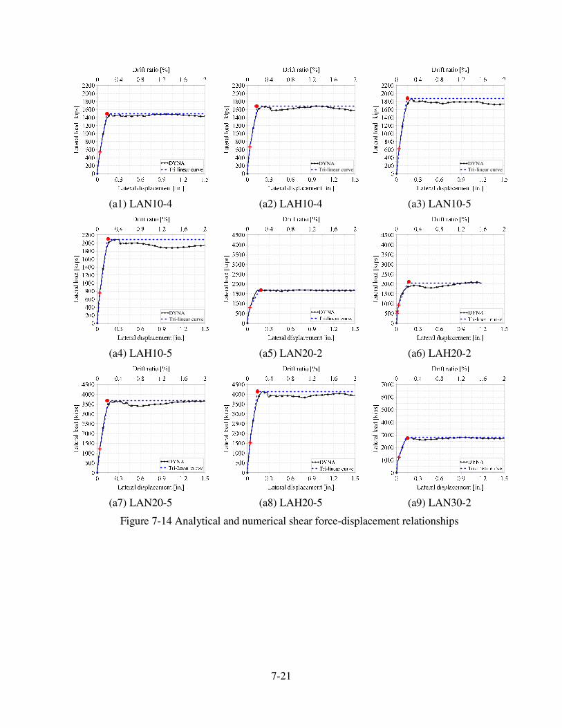
7-21
(a1) LAN10-4 (a2) LAH10-4 (a3) LAN10-5
(a4) LAH10-5 (a5) LAN20-2 (a6) LAH20-2
(a7) LAN20-5 (a8) LAH20-5 (a9) LAN30-2
Figure 7-14 Analytical and numerical shear force-displacement relationships
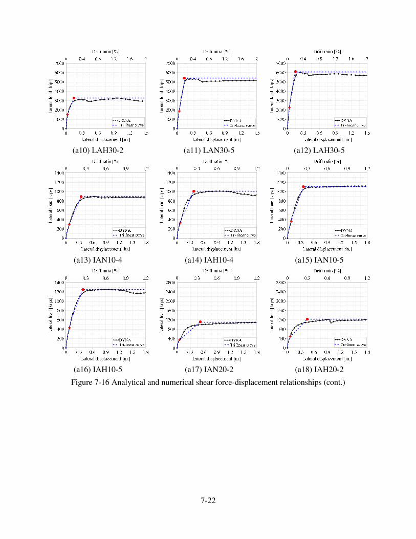
7-22
(a10) LAH30-2 (a11) LAN30-5 (a12) LAH30-5
(a13) IAN10-4 (a14) IAH10-4 (a15) IAN10-5
(a16) IAH10-5 (a17) IAN20-2 (a18) IAH20-2
Figure 7-16 Analytical and numerical shear force-displacement relationships (cont.)
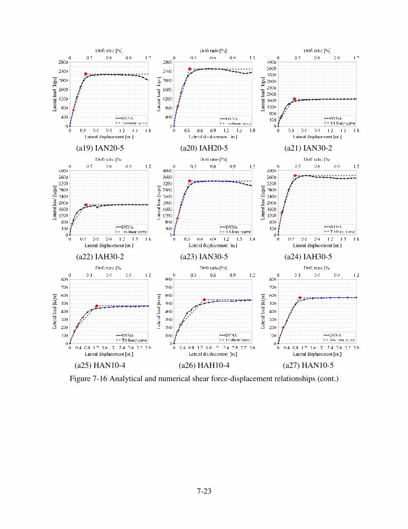
7-23
(a19) IAN20-5 (a20) IAH20-5 (a21) IAN30-2
(a22) IAH30-2 (a23) IAN30-5 (a24) IAH30-5
(a25) HAN10-4 (a26) HAH10-4 (a27) HAN10-5
Figure 7-16 Analytical and numerical shear force-displacement relationships (cont.)
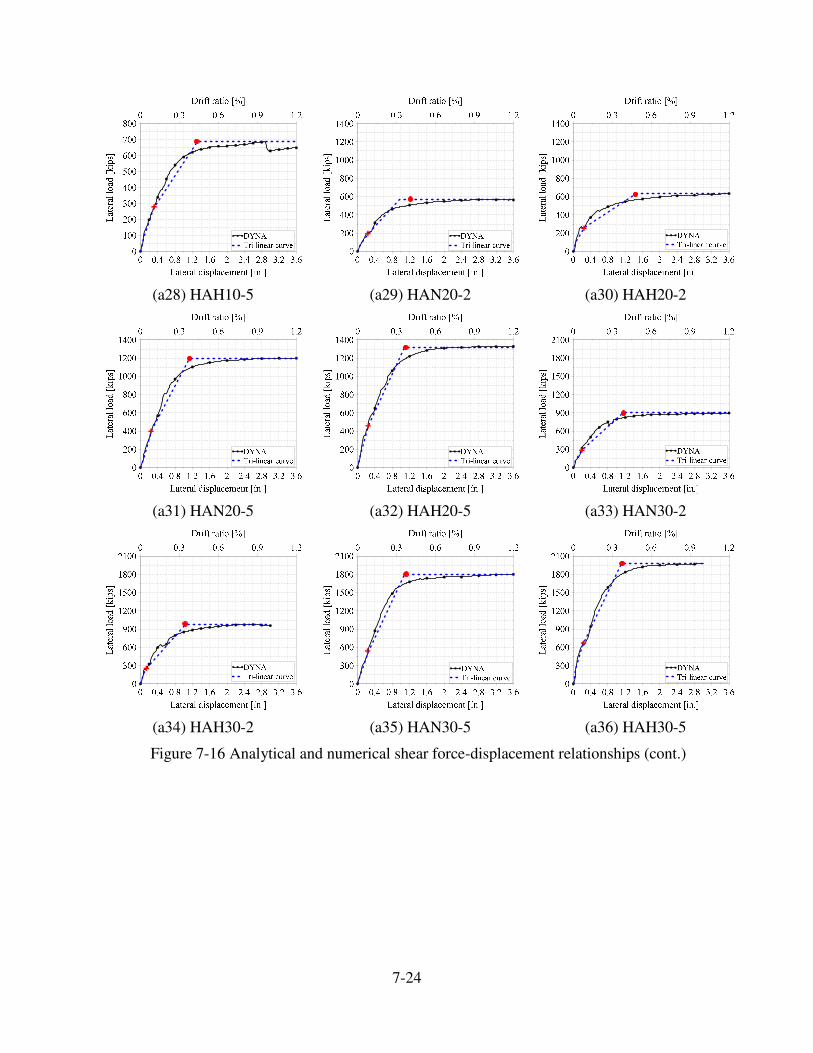
7-24
(a28) HAH10-5 (a29) HAN20-2 (a30) HAH20-2
(a31) HAN20-5 (a32) HAH20-5 (a33) HAN30-2
(a34) HAH30-2 (a35) HAN30-5 (a36) HAH30-5
Figure 7-16 Analytical and numerical shear force-displacement relationships (cont.)

8-1
8. ANALYTICAL MODELING OF RECTANGULAR SC
WALL PANELS
8.1 Introduction
A complete family of seismic analysis and design tools for a structural component or system would
include micro-models suitable for finite element analysis of individual components, macro-models
suitable for analysis of a framing system, and simplified models suitable for preliminary analysis
and design upon which macro-models can later be based.
This chapter presents simplified models for stiffness prediction, and monotonic and cyclic analyses
of flexure- and flexure-shear-critical rectangular SC walls. Section 8.2 presents a reliable and
straightforward method to calculate the monotonic force-displacement response of an SC wall.
The proposed analytical model is validated using results of finite element analyses of SC walls
with three aspect ratios (= 0.5, 1 and 2), reinforcement ratios ranging from 2% to 5%, wall
thicknesses of 10 in. and 20 in., and concrete compressive strengths of 4 ksi and 7 ksi. Section 8.3
presents analytical simulations of the cyclic response of SC walls using the Modified Ibarra-
Krawinler Pinching (MIKP) model [39]. Section 8.4 presents an analytical approach to predict the
initial stiffness of an SC wall with baseplate connection. A glossary of terms used in this chapter
is provided on pages xviii through xxiii.
8.2 Simplified Monotonic Analysis of SC Walls
Xu et al. [121] calculated the lateral force-displacement relationship for an RC column assuming
concentrated hinges and addressing coupling between axial force, shear force and bending
moment. Nonlinear response was simulated using flexural and shear springs at the ends of the
column. Backbone curves were established in flexure and shear for the nonlinear springs that were
assigned to the sub-elements comprising the column. The Modified-Compression-Field-Theory
(MCFT), as developed by Vecchio et al. [110], was used to establish the moment-curvature and
shear force-shear strain relationships for each sub-element. The flexural and shear deformations at
the top of the column, calculated by integrating the curvature and shear strain in each section along
the column height, are used to obtain the moment-rotation and the shear force-shear displacement
relationships for the flexural and shear springs, respectively.
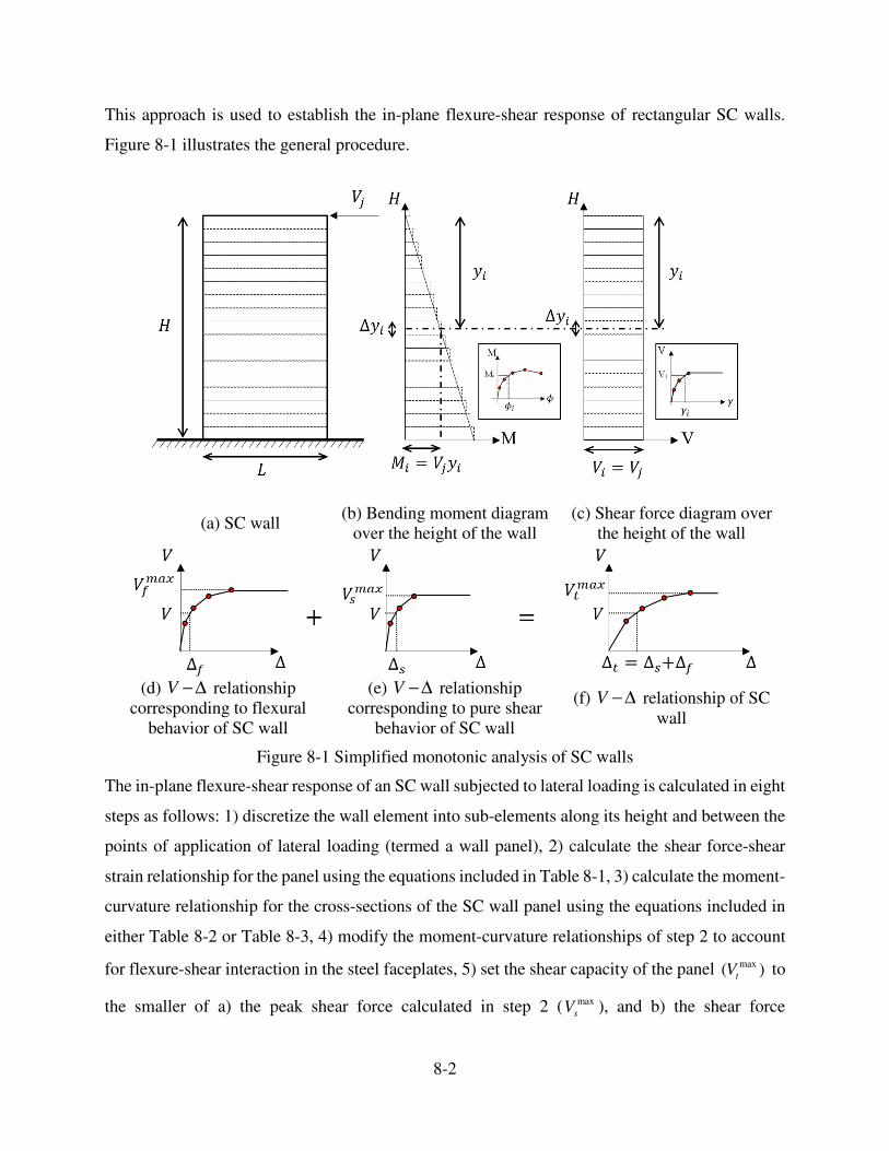
8-2
This approach is used to establish the in-plane flexure-shear response of rectangular SC walls.
Figure 8-1 illustrates the general procedure.
(a) SC wall (b) Bending moment diagram
over the height of the wall
(c) Shear force diagram over
the height of the wall
(d) V −∆ relationship
corresponding to flexural
behavior of SC wall
(e) V −∆ relationship
corresponding to pure shear
behavior of SC wall
(f) V −∆ relationship of SC
wall
Figure 8-1 Simplified monotonic analysis of SC walls
The in-plane flexure-shear response of an SC wall subjected to lateral loading is calculated in eight
steps as follows: 1) discretize the wall element into sub-elements along its height and between the
points of application of lateral loading (termed a wall panel), 2) calculate the shear force-shear
strain relationship for the panel using the equations included in Table 8-1, 3) calculate the moment-
curvature relationship for the cross-sections of the SC wall panel using the equations included in
either Table 8-2 or Table 8-3, 4) modify the moment-curvature relationships of step 2 to account
for flexure-shear interaction in the steel faceplates, 5) set the shear capacity of the panel max( )tV to
the smaller of a) the peak shear force calculated in step 2 ( max
sV ), and b) the shear force
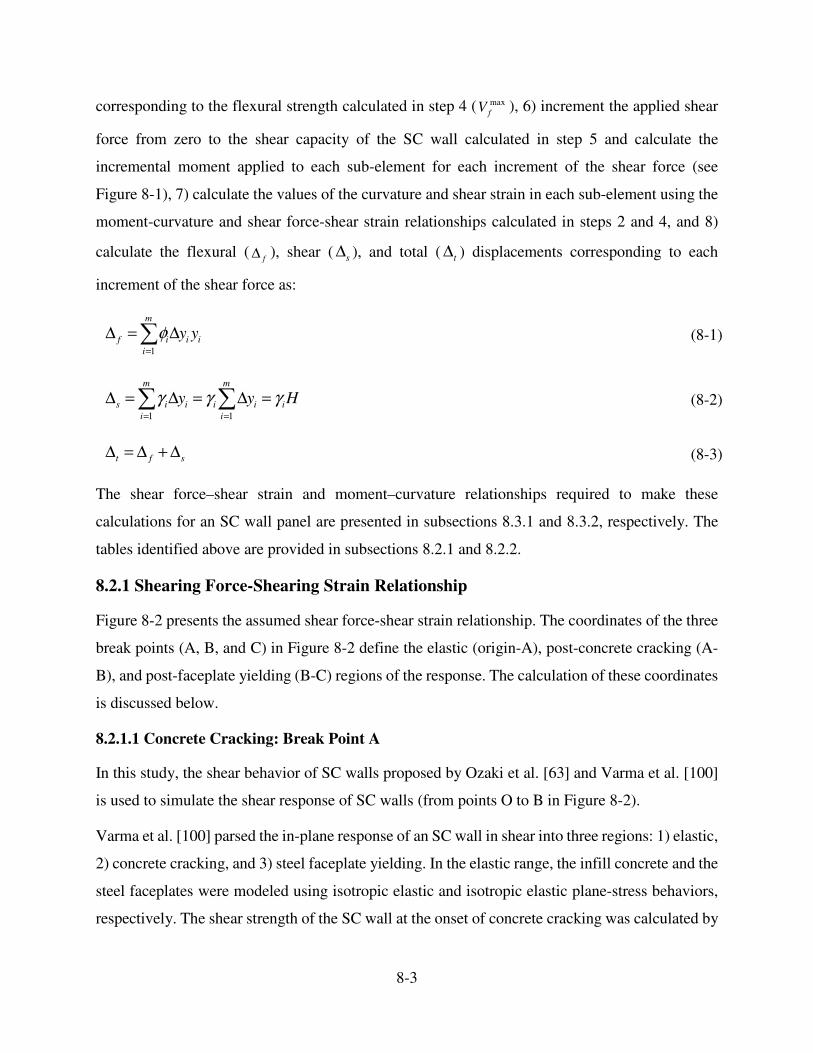
8-3
corresponding to the flexural strength calculated in step 4 ( max
fV ), 6) increment the applied shear
force from zero to the shear capacity of the SC wall calculated in step 5 and calculate the
incremental moment applied to each sub-element for each increment of the shear force (see
Figure 8-1), 7) calculate the values of the curvature and shear strain in each sub-element using the
moment-curvature and shear force-shear strain relationships calculated in steps 2 and 4, and 8)
calculate the flexural (f∆ ), shear ( s∆ ), and total ( t∆ ) displacements corresponding to each
increment of the shear force as:
1
m
f i i i
i
y yφ=
∆ = ∆� (8-1)
1 1
m m
s i i i i i
i i
y y Hγ γ γ= =
∆ = ∆ = ∆ =� � (8-2)
t f s∆ = ∆ + ∆ � (8-3)
The shear force–shear strain and moment–curvature relationships required to make these
calculations for an SC wall panel are presented in subsections 8.3.1 and 8.3.2, respectively. The
tables identified above are provided in subsections 8.2.1 and 8.2.2.
8.2.1 Shearing Force-Shearing Strain Relationship
Figure 8-2 presents the assumed shear force-shear strain relationship. The coordinates of the three
break points (A, B, and C) in Figure 8-2 define the elastic (origin-A), post-concrete cracking (A-
B), and post-faceplate yielding (B-C) regions of the response. The calculation of these coordinates
is discussed below.
8.2.1.1 Concrete Cracking: Break Point A
In this study, the shear behavior of SC walls proposed by Ozaki et al. [63] and Varma et al. [100]
is used to simulate the shear response of SC walls (from points O to B in Figure 8-2).
Varma et al. [100] parsed the in-plane response of an SC wall in shear into three regions: 1) elastic,
2) concrete cracking, and 3) steel faceplate yielding. In the elastic range, the infill concrete and the
steel faceplates were modeled using isotropic elastic and isotropic elastic plane-stress behaviors,
respectively. The shear strength of the SC wall at the onset of concrete cracking was calculated by
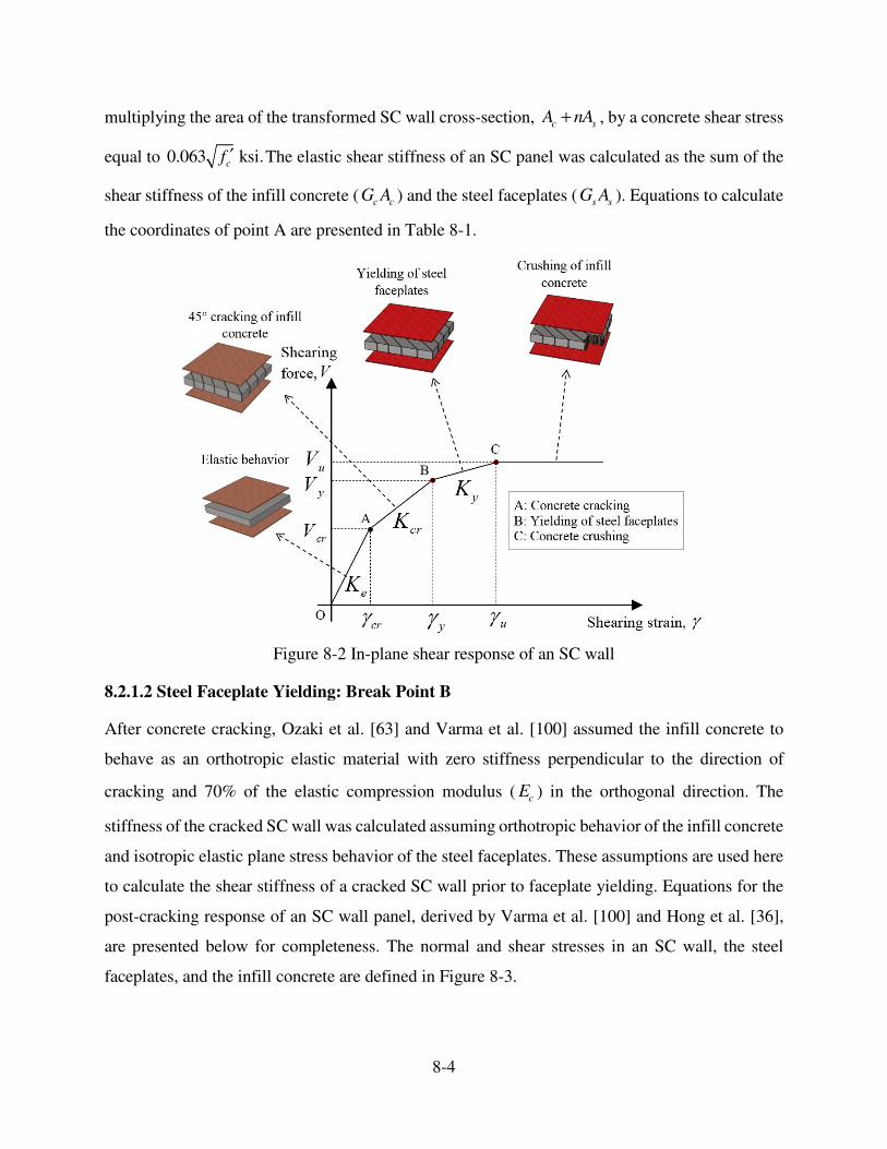
8-4
multiplying the area of the transformed SC wall cross-section, c sA nA+ , by a concrete shear stress
equal to 0.063 ksi.cf ′ The elastic shear stiffness of an SC panel was calculated as the sum of the
shear stiffness of the infill concrete ( c cG A ) and the steel faceplates ( s sG A ). Equations to calculate
the coordinates of point A are presented in Table 8-1.
Figure 8-2 In-plane shear response of an SC wall
8.2.1.2 Steel Faceplate Yielding: Break Point B
After concrete cracking, Ozaki et al. [63] and Varma et al. [100] assumed the infill concrete to
behave as an orthotropic elastic material with zero stiffness perpendicular to the direction of
cracking and 70% of the elastic compression modulus ( cE ) in the orthogonal direction. The
stiffness of the cracked SC wall was calculated assuming orthotropic behavior of the infill concrete
and isotropic elastic plane stress behavior of the steel faceplates. These assumptions are used here
to calculate the shear stiffness of a cracked SC wall prior to faceplate yielding. Equations for the
post-cracking response of an SC wall panel, derived by Varma et al. [100] and Hong et al. [36],
are presented below for completeness. The normal and shear stresses in an SC wall, the steel
faceplates, and the infill concrete are defined in Figure 8-3.

8-5
Figure 8-3 Stress definitions
The normal and shear stresses in the cracked infill concrete are calculated assuming orthotropic
behavior:
[ ] [ ][ ]1
cx x
cy c y
cxy xy
f
f T K T
fσ ε
ε
ε
γ
−
� � � �
′=� � � � � �
(8-4)
where [ ]cK ′ is the post-cracking stiffness matrix of the concrete with respect to the principal stress
and strain directions; the principal stress directions were assumed to coincide with the principal
strain directions; [ ]Tσ
is the transformation matrix that relates the principal stresses to the X-Y
stresses; and [ ]Tε
is the transformation matrix that relates the principal strains to the X-Y strains.
Matrices [ ]cK ′ , [ ]Tσ
, and [ ]Tε
are expressed as:
[ ]0 0 0
0 0
0 0 0
cr
c cK E
� �� �′ = � �� �� �
(8-5)
[ ]
2 2
2 2
2 2
cos sin 2sin cos
sin cos 2sin cos
sin cos sin cos cos sin
cr cr cr cr
cr cr cr cr
cr cr cr cr cr
Tσ
θ θ θ θ
θ θ θ θ
θ θ θ θ θ θ
� �� �
= −� �� �− −� �
(8-6)
[ ]
2 2
2 2
2 2
cos sin sin cos
sin cos sin cos
2sin cos 2sin cos cos sin
cr cr cr cr
cr cr cr cr
cr cr cr cr cr
Tε
θ θ θ θ
θ θ θ θ
θ θ θ θ θ θ
� �� �
= −� �� �− −� �
(8-7)

8-6
Assuming cracking in the infill concrete at 45�, and substituting (8-5), (8-6), and (8-7) into (8-4),
the stress-strain relationship of the cracked infill concrete is calculated as:
1 1 1
1 1 14
1 1 1
cx xcr
ccy y
cxy xy
fE
f
f
ε
ε
γ
� � � �−� � � �= −� � � �� � � �− −� � � �
(8-8)
The normal and shear stresses in the steel faceplates are calculated assuming isotropic elastic plane
stress behavior:
[ ]sx x
sy s y
sxy xy
f
f K
f
ε
ε
γ
� � � �
=� � � � � �
(8-9)
where [ ]sK is the elastic stiffness matrix of the steel faceplates, and is calculated as:
[ ] 2
1 0
1 01
10 0
2
s
ss s
s
s
EK
ν
νν
ν
� �� �� �
= � �− � �−� �� �
(8-10)
The equilibrium equations for an SC wall panel subjected to normal forces and x yN N , and shear
force V , in a matrix form can be expressed as:
cx sx x
c cy s sy y
cxy sxy
f f N
A f A f N
f f V
� � � � � �
+ =� � � � � �
� � �
(8-11)
Substituting (8-8), (8-9), and (8-10) into (8-11), and assuming that the normal forces are zero:
2
1 1 1 1 0 0
1 1 1 1 0 04 1
1 1 1 10 0
2
s xcr
c c s ss y
s
s xy
A E A E
V
ν ε
ν εν
ν γ
� �� �� �� � � �−� � � �� �� � � �− + =� � � � � �� �� � −� � � �� �− − −� � � �� �� �
� �� �
(8-12)
Solving (8-12) yields the normal and shear strains in an SC wall panel as:

8-7
2 (1 )x y xy
s
αε ε γ
α ν β= =
+ +(8-13)
11( )
2 1
(1 )
xy s s
s
G A Vγ
ν β α
−= +
++
(8-14)
where parameters and α β are:
4
cr
c cA Eα = (8-15)
21
s s
s
A Eβ
ν=
−(8-16)
The in-plane stresses in the infill concrete are calculated by substituting the calculated normal and
shear strains of (8-13) and (8-14) into (8-8):
2 (1 )1 1 1 1 1 1
1 1 1 1 1 14 2 (1 )
1 1 1 1 1 11
s
cx xcr
ccy y xy
c s
cxy xy
fE
fA
f
α
α ν βε
α αε γ
α ν βγ
� � + + � � � �− −� � � � � � � �= − = −� � � � � �� � � � + + � � � �− − − −� � � � � � �
(8-17)
A simpler form of the in-plane stresses in the infill concrete is:
cx
cy
c
cxy
K
K Kf
KVf
A K Kf
K
K K
β
α β
β
α β
β
α β
� �−
+ � �
= −� � � �+
�
+ �
(8-18)
where the parameters and K Kα β are calculated as:
s sK G Aα = (8-19)
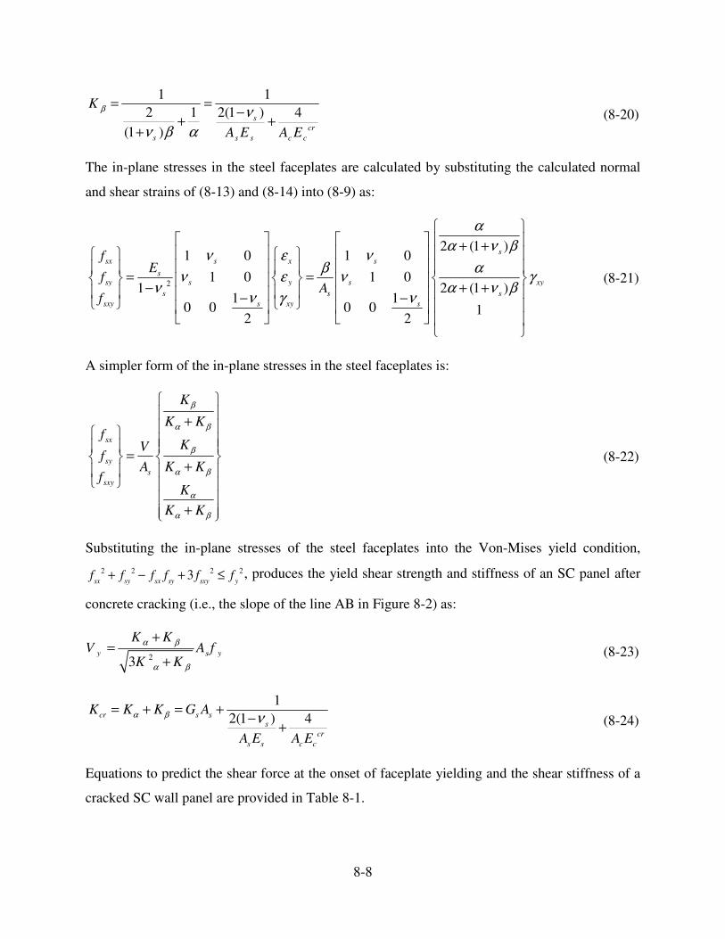
8-8
1 1
2 1 2(1 ) 4
(1 )s
cr
s s s c c
K
A E A E
β ν
ν β α
= =−
+ ++
(8-20)
The in-plane stresses in the steel faceplates are calculated by substituting the calculated normal
and shear strains of (8-13) and (8-14) into (8-9) as:
2
2 (1 )1 0 1 0
1 0 1 01 2 (1 )
1 10 0 0 0 1
2 2
s
sx s x s
ssy s y s xy
s s s
sxy s xy s
fE
fA
f
α
α ν βν ε ν
β αν ε ν γ
ν α ν βν γ ν
� �� � � � + +� � � � � � � �� � � �
= =� � � � � �� � � �− + + � � � �− − � � � � � �� � � �
�
(8-21)
A simpler form of the in-plane stresses in the steel faceplates is:
sx
sy
s
sxy
K
K Kf
KVf
A K Kf
K
K K
β
α β
β
α β
α
α β
� �
+ � �
=� � � �+
�
+ �
(8-22)
Substituting the in-plane stresses of the steel faceplates into the Von-Mises yield condition,
fsx
2 + fsy
2 − fsx
fsy
+ 3 fsxy
2 ≤ fy
2 , produces the yield shear strength and stiffness of an SC panel after
concrete cracking (i.e., the slope of the line AB in Figure 8-2) as:
23y s y
K KV A f
K K
α β
α β
+=
+(8-23)
1
2(1 ) 4cr s ss
cr
s s c c
K K K G A
A E A E
α β ν= + = +
−+ (8-24)
Equations to predict the shear force at the onset of faceplate yielding and the shear stiffness of a
cracked SC wall panel are provided in Table 8-1.

8-9
Table 8-1 Calculation of the shear response of an SC wall panel
Limit state Shearing force (kips) Shearing stiffness (kips/rad)
Concrete
cracking 0.063 ( )cr c c sV f A nA′= + = +e s s c cK G A G A
Yielding of
the steel
faceplates1,223
α β
α β
+=
+y s y
K KV A f
K Kα β= +crK K K
Concrete
crushing3
211 ( ) ( 1)
2η
� �′= + + −� �� �
� �u c c
H HV A f
L L 0.006 ( )
−=
−− +
u y
yy crcr
e cr
V VK
V VV
K K
1s sK G Aα =
22(1 ) 4
1/ ( )s
cr
s s c c
KA E A E
β
ν−= +
3 /s y c cA f A fη ′=
8.2.1.3 Concrete Crushing: Break Point C
Akita et al. [6] estimated the ultimate shear strain for an SC wall in pure shear to be 6000 micro
strain on the basis of test data. Tsuda et al. [89] and Hong et al. [36] used this value to characterize
the response of SC walls in pure shear.
Hong et al. (2014) used the equations derived by Nielsen et al. [58] to predict the peak shear
capacity of an SC wall. Those equations are available in section 4.9 of [58] and are not repeated
here.
The post-yield stiffness of an SC wall (i.e., the slope of line BC in Figure 8-2) can be calculated
as:
u y
y
u y
V VK
γ γ
−=
−
(8-25)
where uγ is 6000 microstrain, as proposed by Akita et al. [6], and yγ can be calculated using the
elastic and post-cracking shear stiffness and strengths of an SC panel as:
y crcry
e cr
V VV
K Kγ
−= + (8-26)
Table 8-1 summarizes the calculation of the shear response of an SC wall panel.

8-10
8.2.2 Moment-Curvature Relationship
The moment-curvature relationship for an SC panel was established at the points of 1) concrete
cracking, 2) yielding of the steel faceplates at the tension end of the wall, 3) yielding of the steel
faceplates at the compression end of the wall, and 4) maximum concrete compressive strain equal
to εc0
: the concrete strain at cf ′ .
Assumptions were made to calculate flexural strength, consistent with the development of a
simplified procedure: (1) plane sections remain plane after bending, (2) flexure-shear interaction
is considered in the calculation of the stress in the steel faceplates but its effect on the response of
the infill concrete is ignored, (3) the tensile strength of concrete is zero, (4) the flexural strength
of the infill concrete is derived using an equivalent rectangular stress block, (5) the steel faceplates
and infill concrete are perfectly bonded, and (6) the effects of axial force are ignored.
8.2.2.1 Cracking of the Infill Concrete
Figure 8-4 presents calculations of the flexural strength of an SC wall at the onset of concrete
cracking.
(a) Wall cross section
(b) Vertical strain profile
(c) Vertical stress profile in the infill
concrete
(d) Vertical stress profile in the steel
faceplates
Figure 8-4 Moment-curvature calculation at the onset of concrete cracking

8-11
The elastic vertical stresses of the infill concrete and the steel faceplates are:
c c crf E ε= (8-27)
s s crf E ε= (8-28)
where crε is calculated as:
rcr
cE
fε = (8-29)
The compressive and tensile forces in the infill concrete and the steel faceplates are:
1 12
2 4c cc cc crF t L Af E ε′ = = (8-30)
1 122
2 4s s cs s r sF AELf t ε= = (8-31)
The flexural strength and curvature of the cross-section of an SC wall panel at the onset of concrete
cracking are:
1( ) 2 3 ( ) ( )
6 6
rcr c s c sc scr csL E
f LM F F L A A A AE nε′= + = + = + (8-32)
2
2r
c
ccr rf
L LEφ
ε= = (8-33)
8.2.2.2 Steel Faceplate Yielding at the Tension End of the Wall Panel
Figure 8-5 presents calculations of the flexural strength of an SC wall panel at the onset of yielding
of the steel faceplates at the tension end of the wall.
At the onset of the steel faceplate yielding at the tension end of the wall, the maximum vertical
strain in the infill concrete is:
1c y y
c
L c
αε ε ε
α= =
− −(8-34)
The compressive force in infill concrete is:
/ 2 / 2 / 21
c cc c cc c c y ccF f A f E Et c t c t cα
ε εα
′ = = =−
= (8-35)

8-12
(a) Wall cross section
(b) Vertical strain profile
(c) Vertical stress profile in the infill
concrete
(d) Vertical stress profile in the steel
faceplates
Figure 8-5 Moment-curvature calculation at the onset of steel faceplate yielding at the tension end
of the wall
The compressive and tensile forces in the steel faceplates are:
1 / 2 / 21
2 2 2 / 2s cs s s s s s y sst c t cF A cf f E tEα
ε εα
=−
= = = (8-36)
2 ( ) / 22y ssF f t L c−= (8-37)
Solving the equilibrium equation of the vertical forces, 1 2c s sF F F′+ = , for α :
1
t
y
c
L
ρα
ρ ρ
′= =
′ ′+ +(8-38)
The flexural strength of an SC panel at the onset of the steel faceplate yielding at the tension end
of the wall is:
2 1( 6 / 3) )( / / 3)( 2t
s sy cM F F ccF LL ′ + −= + + (8-39)
Substituting (8-35), (8-36), and (8-37) into (8-39) gives the flexural strength of an SC wall as:
3 22 3
)2 ( 1)
(1
t
y y s LM f Aα α ρ
ρ α
′− −=
′ −(8-40)
The curvature of the cross-section at the onset of steel faceplate yielding at the tension end of the
wall is:

8-13
)(1
t
y
y y
L c Lφ
ε
α
ε= =
−−(8-41)
8.2.2.3 Steel Faceplate Yielding at the Compression End of the Wall Panel
Figure 8-6 presents calculations of the flexural strength of an SC wall panel at the onset of yielding
of the steel faceplates at the compression end of the wall.
(a) Wall cross section
(b) Vertical strain profile
(c) Vertical stress profile in the infill
concrete
(d) Vertical stress profile in the steel
faceplates
Figure 8-6 Moment-curvature calculation at the onset of the steel faceplate yielding on the
compression side of the wall
At the onset of the steel faceplate yielding, the maximum vertical tensile strain in the steel
faceplates is:
1s y y
L c
c
αε ε ε
α
− −= = (8-42)
The steel stress sf , identified in Figure 8-6, is:
( )ys ssf aE ε ε−= (8-43)
The compressive forces in the steel faceplates and the infill concrete are:
1 2c c cF f ctβ β′ ′= (8-44)
12
2 s
s
yt fF
c= (8-45)
The tensile forces in the steel faceplates are:

8-14
2 2 ( 2 )s s yF t L c f= − (8-46)
3
2 ( 2 )
2
s ss
t L c fF
−= (8-47)
Solving the equilibrium equation of the vertical forces, 1 1 2 3c s s s sF F F F F+ = + + , provides the
value of α at the onset of the steel faceplate yielding at the compression end of the wall:
1 2 2 11
2 2 2
c
y
a ac
L a
γα
γ
� �− + += = � �� �− + +� �
(8-48)
where the γ is calculated as:
1 2
y
cfn
f
β βγ
ρ
′=
′(8-49)
The flexural strength of an SC panel at the onset of steel faceplate yielding at the compression end
of the wall is:
21 2 3
2 2 2( ) ( ) ( ) ( )2 2 2 3 3 2 2 2 2 3
c s s s
c
y
cL L c L L L c L L cF F c c F FM
β − −′ − + − + + − + − + −= (8-50)
Substituting (8-44), (8-45), (8-46), and (8-47) into (8-50) enables the calculation of the flexural
strength of an SC wall panel at the onset of steel faceplate yielding at the compression end of the
wall:
221 2
1 4( ) ((1 )( ) )
2 3 12c cy ys
c af A L AM f L a
β αβ β α α α
α
−′ + − − += (8-51)
The curvature at the onset of steel faceplate yielding at the compression end of the wall is:
yc
y
y
c L
εφ
α
ε= = (8-52)
If the strain-hardening modulus of the steel is set equal to zero ( 0a = ), the normalized neutral axis
depth and the flexural strength of the SC panel are simplified to:
1
2α
γ=
+c
y (8-53)

8-15
21 2
1 4( ) (1 )
2 3
c e
y c c s yM f A L LA fβ α
β β α α α−
′= + − (8-54)
8.2.2.4 Peak Compressive Stress in the Infill Concrete
Figure 8-7 presents the calculations of the flexural strength of an SC wall when the maximum
concrete compressive strain is equal to εc0
.
(a) Wall cross section
(b) Vertical strain profile
(c) Vertical stress profile in the infill
concrete
(d) Vertical stress profile in the steel
faceplates
Figure 8-7 Moment-curvature calculation at maximum concrete compressive strain of εc0
The maximum vertical strain in the steel faceplates when the maximum concrete compressive
strain equals εc0
is:
0 0
1s c c
L c
c
αε ε ε
α
− −= =
(8-55)
The parameter k , identified in Figure 8-7, is calculated as:
0
y
c
kε
ε= (8-56)
The stresses 1 2 and s sf f in Figure 8-7 are:
0 01 ) 1( )( c ys s s cf a kE aEε ε ε− = −= (8-57)

8-16
02
1)( ( )s y cs s sf aE aE k
αε ε ε
α
−− = −= (8-58)
The compressive and tensile forces in the steel faceplates and the infill concrete are:
1 2c c cF f ctβ β′ ′= (8-59)
2
01 1(11 1
1 )2
) ( 22
2s s s s c skF f k c t aE c tε= − = − (8-60)
2 (1 ) 2 sysF k c tf= − (8-61)
3
1
22ys sf kF c t= (8-62
4 2 ( ( 1) )ys sF t L kf c= − + (8-63)
2 05 2 ( ( 1) ) ( ( ( 1)1 1
)2
)s s cs s sF f t L k c aE t L k ckα
εα
= − + = − +−
− (8-64)
Solving the equilibrium equation of the vertical forces, 1 2 3 3 4 5c s s s s s sF F F F F F F′+ + + = + + ,
produces the value of α when the maximum concrete compressive strain equals εc0
:
( )2
0
21 1 2 2
4 2 4c
a a aa a a
k k kc
L a
γ
αγ
� �− − + + + − + − + +� �
� �= =
− + +
(8-65)
The flexural strength of an SC panel when the maximum concrete compressive strain equals εc0
is:
21 2
3 4
5
(1 ) (1 )( ) ( ) ( )
2 2 2 3 2 2
2 ( 1) ((1 ) (1 ) ) ( )
3 3 2 2
( 1) ( )
2 3
c s s
s s
u
s
cL L k c L k cF F F
kc L L k cF k c kc kc k
M
c F
L L k cF
β − −′ − + − + − +
− +� �− + + − − + + − +� �
� �
− +−
=
(8-66)
and substituting (8-59) through (8-64) into (8-66) gives:

8-17
222
1 2
1 ( )( ) ((1 )( ) )
2 3 12u c c s yM f L
k af A L A a
k
β α αβ β α α α
α
−′ + − − + − += (8-67)
The corresponding curvature is:
0 0u
c c
c Lφ
α
ε ε= = (8-68)
If the strain-hardening modulus of the steel is set equal to zero ( 0a = ), the normalized neutral axis
depth and the flexural strength of an SC panel when the maximum concrete compressive strain is
equal to εc0
are simplified to:
1
2α
γ=
+u (8-69)
2
21 2
1( ) (1 )
2 3
e
u c c s y
kM f A L A f L
β α αβ β α α α
−′= + − − (8-70)
The moment-curvature relationship for the cross-section can be represented by the piecewise linear
relationship of Figure 8-8.
Figure 8-8 Moment-curvature relationship for an SC wall panel
Table 8-2 summarizes the flexural strength calculations for an SC wall panel considering strain-
hardening of the steel faceplates. Table 8-3 presents the corresponding equations assuming elastic-
perfectly plastic behavior for the steel faceplates. Preliminary analysis showed that hardening had

8-18
no significant effect on the values of the moments and curvatures, and that the flexural response
of an SC wall panel can be reasonably calculated assuming elastic-perfectly plastic behavior for
the steel.
8.2.3 Concrete Behavior
The concrete stress-strain relationship proposed by Tsai [88] is used to describe the behavior of
the infill concrete:
1 ( )1 1
c
r
c
f n x
r xfn x
r r
′=
′′+ − +
− −
�(8-71)
Chang et al. [20] proposed (8-72) to calculate the strain corresponding to peak stress, and (8-73)
and (8-74) to establish the shape of the stress-strain relationship:
1/ 4
0
( )
4000
cc
fε
′= (8-72)
3/8
46
( )c
nf
′ =′
(8-73)
1.9750
cf
r′
= − � (8-74)
Figure 8-9 presents the stress–strain relationships for unconfined uniaxial compressive strengths
of 3, 4, 5, 6, and 7 ksi, which is considered a practical range for infill concrete in SC walls, noting
that the strain limit for calculations is εc0
.
Figure 8-6 and Figure 8-7 present the calculation of the equivalent rectangular stress block
parameters corresponding to two limit states: 1) yielding of the steel faceplates on the compression
side of the wall, and 2) maximum concrete compressive strain equal to εc0
. The values of 1β and
2β �corresponding to these limit states, presented in Table 8-4,�are calculated assuming that the
equivalent rectangular stress block recovered the area under the stress-strain relationship and the
location of its resultant. Values of the two stress block parameters are presented for 3 ≤ ′fc
≤ 7 ksi
and faceplate yield strengths of 36, 45, and 60 ksi. Values for other combinations of ′fc
and fy
can be interpolated.

8-19
Tab
le 8
-2C
alcu
lati
on o
f th
e fl
exura
lre
sponse
of
an S
C w
all
pan
elco
nsi
der
ing s
teel
har
den
ing
Lim
it s
tate
Concr
ete
crac
kin
g
Yie
ldin
g o
f th
e
stee
l fa
cepla
tes
at
the
tensi
on e
nd o
f
the
wal
l1
Yie
ldin
g o
f th
e
stee
l fa
cepla
tes
at
the
com
pre
ssio
n
end o
f th
e w
all2
,
Max
imum
concr
ete
com
pre
ssiv
e st
rain
equal
to
,
1 2
8-20
Tab
le 8
-3 C
alcu
lati
on o
f th
e fl
exura
l re
sponse
of
an S
C w
all
pan
el w
ithout
stee
l har
den
ing
Lim
it s
tate
Concr
ete
crac
kin
g
Yie
ldin
g o
f th
e st
eel
face
pla
tes
at t
he
tensi
on e
nd o
f th
e
wal
l
Yie
ldin
g o
f th
e st
eel
face
pla
tes
at t
he
com
pre
ssio
n e
nd o
f
the
wal
l ,
Max
imum
concr
ete
com
pre
ssiv
e st
rain
equal
to
,
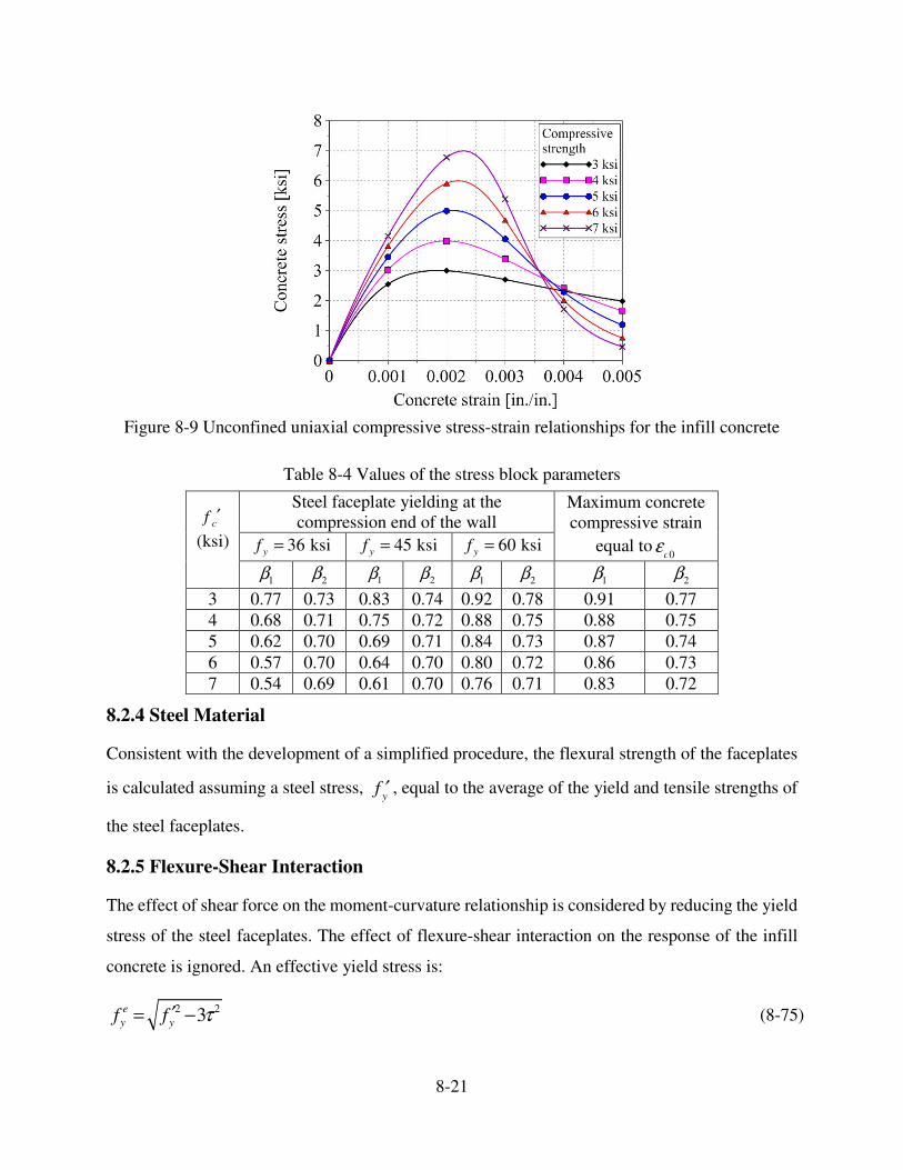
8-21
Figure 8-9 Unconfined uniaxial compressive stress-strain relationships for the infill concrete
Table 8-4 Values of the stress block parameters
′cf
(ksi)
Steel faceplate yielding at the
compression end of the wall Maximum concrete
compressive strain
equal to εc0
36 ksiyf = 45 ksiyf = 60 ksiyf =
1β 2β
3 0.77 0.73 0.83 0.74 0.92 0.78 0.91 0.77
4 0.68 0.71 0.75 0.72 0.88 0.75 0.88 0.75
5 0.62 0.70 0.69 0.71 0.84 0.73 0.87 0.74
6 0.57 0.70 0.64 0.70 0.80 0.72 0.86 0.73
7 0.54 0.69 0.61 0.70 0.76 0.71 0.83 0.72
8.2.4 Steel Material
Consistent with the development of a simplified procedure, the flexural strength of the faceplates
is calculated assuming a steel stress, ′fy
, equal to the average of the yield and tensile strengths of
the steel faceplates.
8.2.5 Flexure-Shear Interaction
The effect of shear force on the moment-curvature relationship is considered by reducing the yield
stress of the steel faceplates. The effect of flexure-shear interaction on the response of the infill
concrete is ignored. An effective yield stress is:
2 23
e
y yf f τ′= − � (8-75)
1β 2β 1β 2β 1β 2β
8-22
which is based on the Von-Mises yield condition and assumes zero horizontal stress along the
length of the steel faceplates.
The equivalent shear stress in the steel faceplates, τ in (8-75), is calculated by dividing the shear
force associated with the flexural resistance of the steel faceplates, by the cross-sectional area of
the faceplates. The shear force associated with the flexural resistance of the steel faceplates can be
calculated by dividing the flexural strength of the steel faceplates, s y sA f L′ ′′ in Table 8-3, by the
moment-to-shear ratio of the SC wall panel ( / )M V . Substituting / ( / )y sf L M Vτ ′ ′′= into (8-75):
2( 1 )e
y yf f ζ′= − � (8-76)
where ζ is:
2
2
3 33( )( ) 1
3( 2)
k VL
M
γζ
γ
+ −= ≤
+(8-77)
and γ is calculated using equation included in Table 8-2. The effective yield stress of the steel
faceplates is a function of the concrete uniaxial compressive strength, the yield stress of the steel
faceplates, the reinforcement ratio, and the normalized moment-to-shear ratio ( /M VL ��. Note that
the normalized moment-to-shear ratio is identical to the wall aspect ratio ( /H L ) for a single story
wall panel of height H and length L. The influence of the normalized moment-to-shear ratio and
concrete strength on fy
e is presented in Figure 8-10.
Results are presented in Figure 8-10 for a wall panel that is 60 in. long, 10 in. thick, and constructed
with 0.25- in. thick steel faceplates that have a yield strength of 36 ksi. Figure 8-10 indicates that
a) the yield stress is significantly reduced for aspect ratio less than one on account of flexure-shear
interaction, and b) the reduction in yield stress diminishes with increasing concrete compressive
strength because flexure-shear interaction decreases with an increase in the shear load resisted by
the infill concrete.
1 Equations (8-76) and (8-77) indicate that the effective yield stress of the steel faceplates is a function of γ and the
normalized moment-to-shear ratio ( /M VL ). The parameter γ is calculated using concrete uniaxial compressive
strength, yield stress of the steel faceplates, and reinforcement ratio (see Table 8-2).

8-23
Figure 8-10 Effective yield stress of the steel faceplates
8.2.6 Vertical Discretization of the SC Wall Panel
The vertical discretization of an SC wall panel will affect the calculation of response because the
effects of flexure-shear interaction change continuously. Results are presented in Figure 8-11 for
wall panels that are 150 in. long, 10 in. thick, with 0.19-in. thick steel faceplates having a yield
strength of 36 ksi, and aspect ratios of 0.5, 1.0, and 2.0. The results of Figure 8-11 indicate that the
use of 10 sub-elements between points of application of lateral load is sufficient for analysis:
increasing the number of sub-elements to 20 and 50 does not measurably change the results.
8.2.7 Validation of the Simplified Procedure
The simplified monotonic analysis procedure is validated using results of finite element analysis
of 36 rectangular SC wall, as presented in Chapter 7. The four design variables considered were
1) aspect ratio (0.5, 1.0 and 2.0), 2) reinforcement ratio (2% to 5%), 3) wall thickness (10, 20 and
30 inches), and 4) concrete compressive strength (4 ksi and 7 ksi). Validation of the baseline
model, as presented in Chapter 6, was performed by simulation of the nonlinear cyclic in-plane
behavior of four large-scale rectangular SC walls tested at the University at Buffalo.
Figure 8-12 through Figure 8-17 present the DYNA-predicted shear force-displacement
relationships together with those predicted using the proposed method calculated using 75 sub-
elements over the height of the wall panel. The proposed method accurately predicts the monotonic
in-plane response of the SC walls with different aspect ratios, reinforcement ratios, concrete

8-24
strengths, and wall thicknesses up to the point of maximum shear resistance. The peak shear
resistance of the low-aspect ratio walls is slightly over-estimated.
(a) Aspect ratio of 0.5 (b) Aspect ratio of 1.0
(c) Aspect ratio of 2.0
Figure 8-11 Force-displacement relationships of SC walls with differing numbers of sub-elements
Figure 8-12 Force-displacement relationship for 10-in. thick walls with 3.8% reinforcement ratio
5��
����
�����
��*�

8-25
Figure 8-13 Force-displacement relationship for-10 in. thick walls with 5.0% reinforcement ratio
Figure 8-14 Force-displacement relationship for 20-in. thick walls with 1.9% reinforcement ratio
Figure 8-15 Force-displacement relationship for 20-in. thick walls with 5.0% reinforcement ratio

8-26
Figure 8-16 Force-displacement relationship for 30-in. thick walls with 2.1% reinforcement ratio
Figure 8-17 Force-displacement relationship for 30-in. thick walls with 5.0% reinforcement ratio
Figure 8-18 presents the components of displacement for the analytically derived and DYNA-
predicted force-displacement relationships for the 10-in. thick rectangular SC walls with a
reinforcement ratio of 3.8% and aspect ratios of 0.5, 1.0, and 2.0. The shear displacements
dominate for an aspect ratio of 0.5 and the flexural displacements dominate for aspect ratios greater
than 1.0, which are expected outcomes. The lateral displacement corresponding to shear strength
is underestimated because the stiffness reduction due to the out-of-plane buckling of the steel
faceplates is not considered in the simplified procedure but is captured in the DYNA analysis.
These results further confirmed the utility of the proposed simplified method for the monotonic
analysis of rectangular SC wall panels.
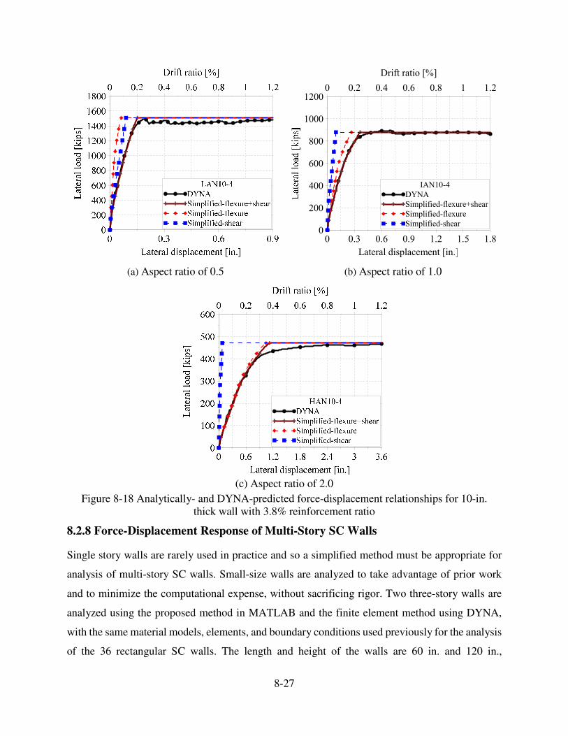
8-27
(a) Aspect ratio of 0.5 (b) Aspect ratio of 1.0
(c) Aspect ratio of 2.0
Figure 8-18 Analytically- and DYNA-predicted force-displacement relationships for 10-in.
thick wall with 3.8% reinforcement ratio
8.2.8 Force-Displacement Response of Multi-Story SC Walls
Single story walls are rarely used in practice and so a simplified method must be appropriate for
analysis of multi-story SC walls. Small-size walls are analyzed to take advantage of prior work
and to minimize the computational expense, without sacrificing rigor. Two three-story walls are
analyzed using the proposed method in MATLAB and the finite element method using DYNA,
with the same material models, elements, and boundary conditions used previously for the analysis
of the 36 rectangular SC walls. The length and height of the walls are 60 in. and 120 in.,
� �!$ �!1 �!� �!0 �!� �!�
5���������������������!
�
0��
)��
1��
���
����
�0��
?�=���)
6@=�
����� ���� ��A���B����
����� ���� ��A���
����� ��������
� �!0 �!) �!1 �!� � �!0
6�� ���������7

8-28
respectively. The thickness of the walls is 12 in.; the thickness of each steel faceplate is 0.19 in.
Beams and columns are not included in the models. The SC walls are subjected to uniform and
triangular distributions of lateral loads, as shown in Figure 8-19.
Figure 8-19 Elevation view of three-story SC walls subject to uniform and triangular loadings
The shear force-shear strain relationship for each panel of the three-story walls (P1, P2, and P3
presented in Figure 8-19) is calculated using the equations of Table 8-3. The moment-curvature
relationship for each panel is calculated using an effective yield stress [(8-76)] that is a function of
the moment-to-shear ratio ( /M VL ), which in turn depends on the vertical distribution of lateral
loads above the panel.
The moment-to-shear ratio for P1 in both SC walls is presented below to illustrate the calculation.
The level of the resultant of the lateral loads applied above P1 for the SC walls subjected to uniform
and triangular distributions of lateral loads are calculated using (8-78) and (8-79), respectively:
3 22r
F H F H F Hh H
F F F
× + × + ×= =
+ +� (8-78)
3 0.67 2 0.332.34
0.67 0.33r
F H F H F Hh H
F F F
× + × + ×= =
+ +� (8-79)
The moment-to-shear ratio for P1 is calculated as /rh L = 1.33 (2 / )H L and = 1.56 (2.34 / )H L
for the SC walls subjected to uniform and triangular distributions of lateral loads, respectively.

8-29
The flexural displacement at the top of each 40-in. tall panel is calculated using (8-1) with iy as
the distance between the center of ith sub-element of the panel and top of the three-story SC wall.
Seventy five sub-elements are used for each of the three panels. The shear displacement at top of
each panel is calculated using (8-2). The total displacement at the top of the wall is:
1 1 2 2 3 3( ) ( ) ( )t s f s f s f∆ = ∆ + ∆ + ∆ + ∆ + ∆ + ∆ � (8-80)
where the rotation at the top of each wall panel is:
1
1
mj j
j j i i
i
yθ θ φ−
=
= + ∆� � (8-81)
where i and j denote the sub-element and story numbers, respectively, and 0 0θ = . The
displacement components and rotations at the tops of the panels are defined in Figure 8-20.
Figure 8-20 Displacement calculation in three-story SC wall
Responses per (8-80) are presented in Figure 8-21. The proposed method reasonably predict the
monotonic response of this three-story SC wall subjected to both uniform and triangular loadings.
The initial stiffness is accurately predicted and the peak shear strength is estimated with an error
of less than 10%.

8-30
Figure 8-21 Analytically- and numerically-predicted responses of a three-story SC wall
8.3 Simulation of Cyclic Response
The Ibarra-Krawinkler Pinching (IKP) model proposed by Ibarra et al. [39] is used to simulate the
cyclic hysteretic response of SC walls. This model incorporates alternate cyclic deterioration
modes [39]. Ibarra et al. successfully simulated the inelastic behavior of two tested RC columns
subjected to axial and cyclic lateral loadings using this model. Gulec et al. [33] used this model to
simulate the cyclic behavior of seven low aspect ratio reinforced concrete walls.
8.3.1 Description of the IKP Model
The hysteretic model proposed by Ibarra et al. [39] is defined using the piece-wise linear backbone
curve presented in Figure 8-22(a) and the basic hysteretic rules presented in Figure 8-22(b). The
backbone curve consists of a bilinear curve in the pre-peak-strength region and a linear curve in
the post-peak-strength response. The unloading branch of the cyclic response is simulated using a
linear curve. The reloading branch consists of two segments. The first reloading path (paths 3-4
and 7-8 in Figure 8-22(b)) is directed towards a break point (points 4 and 8) and the second path
(paths 4-5 and 8-9) connects the break point to the point corresponding to the maximum
displacement of the earlier cycles in the same quadrant (points 2 and 6 in Figure 8-22(b)). The
break point is a function of the maximum force ( ) and residual displacement ( ) achieved
in the previous cycle in the same quadrant, and is established using displacement and force
coordinates equal to and , respectively.
maxF δ perl
(1 )δ− d perlkmaxfk F

8-31
(a) Backbone curve (b) Hysteretic model
Figure 8-22 Pinching model proposed by Ibarra et al. [39]
Four models of deterioration modes are considered in the IKP model, namely, the basic-strength,
post-capping strength, unloading stiffness, and accelerated stiffness, as cartooned in Figure 8-23.
Details are available in Ibarra et al. [39].
(a) Basic strength (b) Post-capping strength (c) Unloading-stiffness (d) Accelerated stiffness
Figure 8-23 Deterioration modes available with the IKP model
Ibarra et al. used an energy-based deterioration parameter to control deterioration. This parameter
is based on the hysteretic energy dissipated in cyclic excursions and is calculated as:
1
( )di
n
t j
i
E
E E
β
=
=
−� (8-82)

8-32
8.3.2 Validation of the Cyclic Analysis
The accuracy of the predictions of IKP model is validated using the results of finite element cyclic
analysis of 12 DYNA models selected from the 36 models used for monotonic analyses. The
models selected for cyclic analyses are LAN10-5, LAI10-5, LAN20-2, LAI20-2, IAN10-5, IAI10-
5, IAN20-2, IAI20-2, HAN10-5, HAI10-5, HAN20-2, and HAI20-2. The wall length in the DYNA
model used for the cyclic analysis is set equal to 60 in. to reduce the computational effort. The
same material models, elements, and boundary condition used for the monotonic analyses are
adopted for the cyclic analyses.
Figure 8-24 presents the cyclic force-displacement relationship for LAN10-5. Pinching of the
force-displacement response is evident in the post-peak-strength cycles.
The degree of pinching in the response of an SC wall is expected to be less than that of an RC wall
having a cross-section with 1) identical dimensions to those of the infill concrete cross-section,
and 2) a reinforcement ratio equal to the ratio of the cross-sectional area of the steel faceplates to
the total cross-sectional area of the SC wall, since the cyclic response is governed by the hysteretic
behavior of the steel faceplates after significant damage occurs in the infill concrete. The cyclic
response of SC walls cannot be accurately simulated using the pinching model proposed originally
by Ibarra et al. [39].
A modification to the original IKP model is proposed for SC walls using 1) a tri-linear curve for
the pre-peak-strength response that characterized the yielding of the steel faceplates at the tension
Figure 8-24 Cyclic force-displacement relationship of LAN10-5

8-33
and compression ends of the wall, and crushing of the infill concrete, 2) a bilinear curve for the
unloading branch, and 3) a tri-linear curve for the re-loading branch. These modifications to the
backbone curve and hysteretic force-displacement relationship of the IKP model are presented in
Figure 8-25. Figure 8-25(a) presents the proposed backbone curve for cyclic simulations.
Figure 8-25(b) presents the backbone curve of the IKP model (dotted line), the hysteretic force-
displacement relationship proposed by Ibarra et al. (solid line), and the modified hysteretic force-
displacement relationship (dashed line).
The unloading and reloading branches of the modified hysteretic force-displacement relationship
consisted of two segments with stiffness ,1unlk′ and ,2unlk′ , and three segments with stiffness ,1relk ′ ,
,2relk′ , and ,3relk′ , respectively. The first unloading path targets the force equal to a fraction,ξ , of
the maximum force, maxF , achieved in the same quadrant in the previous cycle. The first control
point of the reloading branch (points a and d in Figure 8-25(b)) on the force axis is established
using the coordinate of the residual displacement in the previous cycle and the value of stiffness
,1relk ′ . The calculated force corresponding to this point should not exceed maxfk F (see
Figure 8-25(b)). The second part of the reloading branch targets the second control point of the
reloading branch (points b and e in Figure 8-25(b)) with the displacement and force coordinates
of (1 )d perlk δ− and maxfk F , respectively. The third part of the reloading branch targets the
maximum displacement achieved in the previous cycle.
The Modified IKP (MIKP) model is implemented in MATLAB [55] and used to simulate the
DYNA-predicted cyclic responses of selected SC walls. The MATLAB code is provided in
Appendix D. The backbone curve in the pre-peak-strength region is calculated using the approach
proposed for the monotonic analysis of SC walls, as described in Section 8.3. The slope of the
backbone curve in the post-peak-strength response and pinching, deterioration, and rate parameters
are calculated using the results of finite element analysis of the 12 DYNA models. The basic
strength and post-capping strength deterioration modes are not considered since these modes
simulate the degradation of the backbone curve under cyclic loading. The calculated values of the
parameters for the backbone curve are presented in Table 8-5. The cyclic force-displacement
relationship of a rectangular SC wall is defined using 1) the displacements and forces in the pre-
peak-strength region predicted by the proposed method for monotonic analysis, 2) the slope of the

8-34
backbone curve in the post-peak-strength region, and 3) the values of the pinching, deterioration,
and rate parameters, as described below.
(a) Backbone curve
(b) Cyclic response
Figure 8-25 Modifications to the IKP model
In Table 8-5, the effective stiffness, p
eK , is defined as the ratio of the force associated with the
yielding of the steel faceplates on the tension end of the wall to its corresponding displacement.
The shear forces and displacements corresponding to flexural strength, cF and cδ , are presented
in columns three and four of Table 8-5. The backbone curve is fully defined by the displacements

8-35
and forces corresponding to the pre-peak-strength control points, namely, the yielding of the steel
faceplates at the tension and compression ends of the wall (presented in Figure 8-25(a)), and the
slope of the backbone curve in the post-peak-strength region. The ratios of the displacement and
force at the control points to the displacement and force at peak strength are presented in columns
5 through 8 of Table 8-5, where the forces and displacements are calculated using the method
proposed previously for monotonic analysis. The ratio of post-peak stiffness to effective stiffness
is presented in column 9.
Table 8-5 Calculated backbone parameters
Specimen
p
eK cFcδ
t
y
c
F
F
c
y
c
F
F
δ
δ
t
y
c
δ
δ
c
y
c
αc
kips( )
in.(kips) (in.)
kips( )kips
kips( )kips
in.( )in.
in.( )in.
(%)
(1) (2) (3) (4) (5) (6) (7) (8) (9)
LAN10-5 15196 751 0.12 0.59 0.87 0.24 0.39 -18
LAI10-5 16743 862 0.11 0.56 0.87 0.26 0.46 -31
LAN20-2 16806 750 0.12 0.58 0.95 0.22 0.48 -16
LAI20-2 19138 846 0.12 0.57 0.94 0.21 0.52 -21
IAN10-5 4018 447 0.20 0.64 0.93 0.35 0.59 -8
IAI10-5 4470 503 0.20 0.59 0.90 0.33 0.63 -12
IAN20-2 4533 415 0.20 0.60 0.96 0.27 0.71 -13
IAI20-2 5430 450 0.20 0.57 0.95 0.24 0.78 -12
HAN10-5 692 230 0.57 0.65 0.93 0.38 0.63 -16
HAI10-5 757 259 0.57 0.60 0.90 0.36 0.68 -17
HAN20-2 722 212 0.57 0.60 0.96 0.31 0.81 -17
HAI20-2 800 229 0.60 0.57 0.95 0.27 0.88 -19
Table 8-6 presents the values of the pinching ( fk , dk ,ξ ), deterioration ( ,1unlγ , ,2unlγ , ,1relγ , aγ ), and
rate parameters ( ,1unld , ,2unld , ,1reld , ad ) calibrated from the DYNA-predicted force-displacement
relationships. The hysteretic energy dissipation capacity corresponding to each deterioration mode
is calculated by multiplying the calculated deterioration parameters by the product of the peak
force and its corresponding displacement (= c cF δ ). Table 8-6 shows that the pinching parameter,
fk , is affected by the reinforcement ratio and the moment-to-shear ratio. The other two pinching
parameters, dk and ξ , presented in the third and fourth columns of Table 8-6, are not affected by
the design variables considered in this study. The deterioration parameters and rate parameter

8-36
corresponding to the reloading stiffness ( ,1relk ′ presented in Figure 8-25(b)) deterioration mode are
influenced by the moment-to-shear ratio. The analysis results are not substantially affected by the
rate parameters corresponding to the unloading stiffness and accelerated stiffness modes and the
best results are obtained by setting these parameters equal to 1.0.
Table 8-6 Calculated pinching, deterioration, and rate parameters
Specimen fk dk ξ ,1unlγ ,2unlγ ,1relγ γ a ,1unld ,2unld ,1reldad
LAN10-5 0.60 0.30 0.50 25 20 20 20 1 1 0.45 1
LAI10-5 0.60 0.30 0.50 25 20 20 20 1 1 0.45 1
LAN20-2 0.40 0.30 0.50 25 20 20 20 1 1 0.45 1
LAI20-2 0.40 0.30 0.50 25 20 20 20 1 1 0.45 1
IAN10-5 0.40 0.30 0.50 40 35 20 40 1 1 0.35 1
IAI10-5 0.40 0.30 0.50 40 35 20 40 1 1 0.35 1
IAN20-2 0.30 0.30 0.50 40 35 20 40 1 1 0.35 1
IAI20-2 0.30 0.30 0.50 40 35 20 40 1 1 0.35 1
HAN10-5 0.30 0.30 0.50 40 35 20 40 1 1 0.25 1
HAI10-5 0.30 0.30 0.50 40 35 20 40 1 1 0.25 1
HAN20-2 0.30 0.30 0.50 40 35 20 40 1 1 0.25 1
HAI20-2 0.30 0.30 0.50 40 35 20 40 1 1 0.25 1
On the basis of the finite element analyses of the 12 DYNA models selected from the 36 models,
the post-peak stiffness of the backbone curve can be considered to be 15% to 20% of the effective
stiffness of the rectangular SC wall, as presented in the last column of Table 8-5. The calculated
values of the pinching, deterioration, and rate parameters of Table 8-6 can be used to simulate the
hysteretic response of rectangular SC walls with an aspect ratio between 0.5 to 2, a reinforcement
ratio between 2% and 5%, and low axial loads.
Figure 8-26 presents the analytical- and DYNA-predicted force-displacement relationships for the
twelve SC walls: SC walls with aspect ratios of 0.5, 1.0, and 2.0, thickness of 10 in. and 20 in.,
and reinforcement ratios of 2% and 5%.
The MIKP model reasonably simulates the cyclic response of the SC walls: the post-peak pinched
behavior, the continuity of the response in the pre- and post-peak-strength regions, and the
unloading branch of the cyclic force-displacement relationship are captured well.
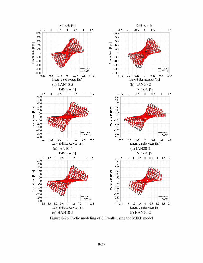
8-37
(a) LAN10-5 (b) LAN20-2
(c) IAN10-5 (d) IAN20-2
(e) HAN10-5 (f) HAN20-2
Figure 8-26 Cyclic modeling of SC walls using the MIKP model
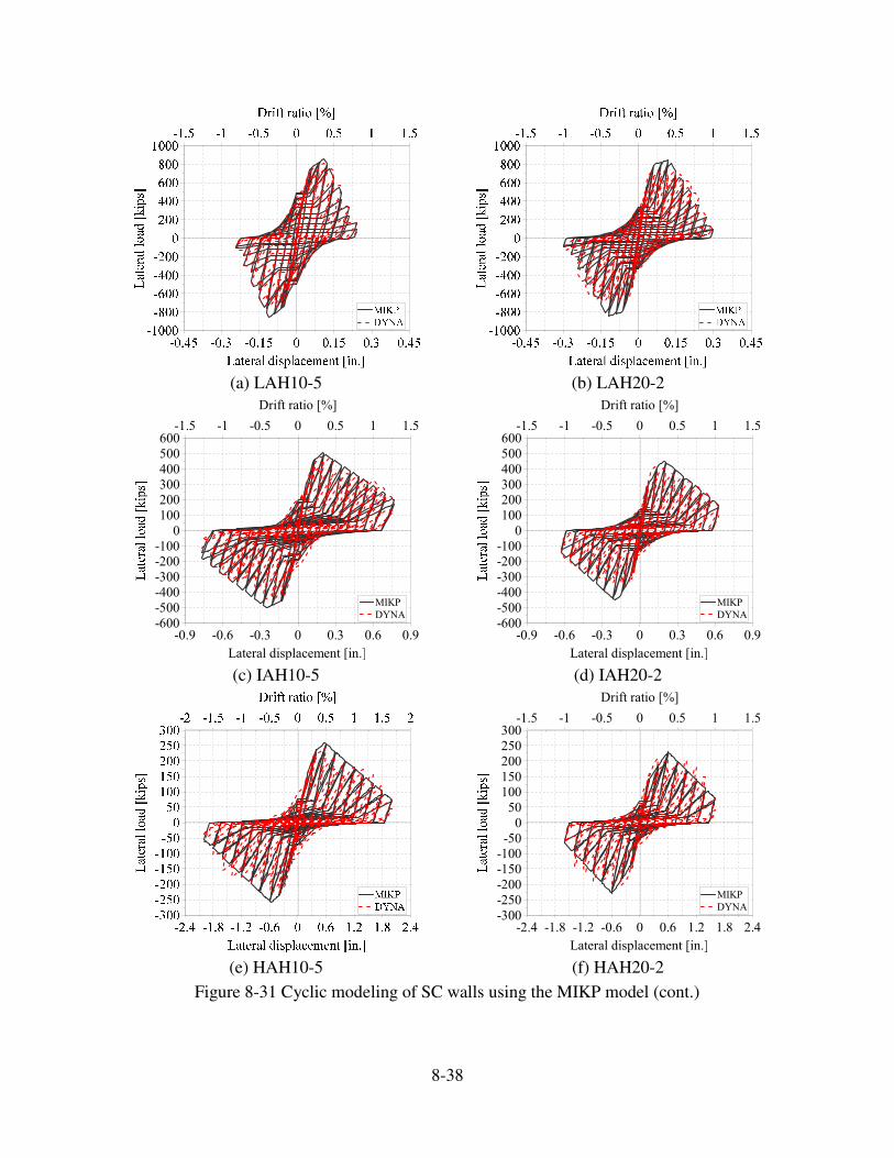
8-38
(a) LAH10-5 (b) LAH20-2
(c) IAH10-5 (d) IAH20-2
(e) HAH10-5 (f) HAH20-2
Figure 8-31 Cyclic modeling of SC walls using the MIKP model (cont.)
��!� ��!1 ��!$ � �!$ �!1 �!�
5���������������������!
�1��
����
�)��
�$��
�0������
�
���
0��$��
)��
���
1��
3?<C
6@=�
��!� �� ��!� � �!� � �!�
6�� ���������7
��!� ��!1 ��!$ � �!$ �!1 �!�
5���������������������!
�1��
����
�)��
�$��
�0������
�
���
0��$��
)��
���
1��
3?<C
6@=�
��!� �� ��!� � �!� � �!�
6�� ���������7
�0!) ��!� ��!0 ��!1 � �!1 �!0 �!� 0!)
5���������������������!
�$��
�0��
�0��
����
�������
�
��
������
0��
0��
$��
3?<C
6@=�
��!� �� ��!� � �!� � �!�
6�� ���������7

8-39
8.4 Initial Stiffness of SC Walls with a Baseplate Connection
The experimental study of the four SC walls, described in Chapter 5, indicated that the rotation of
the base connection governed their total lateral displacement. This result identifies the importance
of characterizing the stiffness of the connection of an SC wall to its foundation.
In this section, an analytical approach is proposed to characterize the rotational flexibility of an
SC wall with a baseplate connection. The method is validated using data from the tests presented
in Chapter 5.
To calculate the initial stiffness of an SC wall with a baseplate connection, the wall was modeled
as a cantilever beam with a rotational spring at its base. A schematic drawing of the model is
presented in Figure 8-27. �
Figure 8-27 SC wall model for initial stiffness calculation
The total lateral displacement at top of the wall, t∆ , is calculated as:
t b f s∆ = ∆ + ∆ + ∆ � (8-83)
The initial stiffness of the SC wall can be calculated as:
1 1 1 1
t b f sK K K K= + + � (8-84)
The initial flexural and shear stiffness of the SC wall can be estimated as:

8-40
3
3g
f
EIK
H= � (8-85)
g
s
GAK
Hκ= (8-86)
where gEI is the flexural rigidity of the SC wall and is calculated as the sum of the flexural
rigidities of the steel faceplates ( s sE I ) and the infill concrete ( c cE I ), and gGA is the shear rigidity
of the SC wall, calculated as the sum of the shear rigidities of the steel faceplates ( s sG A ) and the
infill concrete ( c cG A ).
Assuming that the moment-rotation relationship of the spring at the wall base is M Kθθ= , the
lateral stiffness bK is calculated as:
2/bK K Hθ= � (8-87)
Substituting (8-85), (8-86), and (8-87) into (8-84), the lateral stiffness of the SC wall is calculated
as:
2 3 11 1( )
3t
g g
K H H HGA k EIθ
κ −= + + � (8-88)
An analytical method is developed to characterize the rotational stiffness of a baseplate connection
of a rectangular SC wall to its foundation block. The following assumptions are made: (1) the SC
wall is modeled as a cantilever beam with elastic behavior, (2) the neutral axis is located at the
compressive toe of the wall, (3) the effects of axial force are insignificant, (4) the effect of post-
tensioning the threaded bars is small1, and (5) the configuration of the threaded bars in the
baseplate connection is that presented in Figure 8-28.
1 The analytical calculations presented later in this section show that the base rotation is signifacntly affected by the
out-of-plane deformation of the baseplate and not by the extension of the threaded bars. Accordingly, the post-
tensioning of a baseplate to its foundation using threaded bars will have no significant effect on the rotational stiffness
of the baseplate connection.
�

8-41
Figure 8-28 Plan view of an SC wall
Figure 8-29 and Figure 8-30 present elevation and cross-section views, respectively. These figures
show the deformations of the threaded bars and baseplate, and the distribution of tensile forces in
threaded bars and bearing stress on the foundation.
Figure 8-29 Elevation view of an SC wall

8-42
Figure 8-30 Cross-section view of an SC wall
The deflection of the baseplate at the level of the first row of threaded bars, 1s∆ (see Figure 8-29),
and at the level of the ith row of threaded bars, si∆ (see Figure 8-30), can be calculated using (8-89)
and (8-90), respectively.
1 11
3
3r r
ss sb s sb
t t
n T n T
E I G A
L L
∆ = + �(8-89)
3
3i i
sis sb s sb
t t
T T
E I G A
L L
∆ = +′ ′
′ ′
�(8-90)
where sbI ,
sbA , sbI ′ , and
sbA′ can be calculated as:
3
=12
p
sb
BtI � (8-91)
5
6sb pA Bt= � (8-92)
3
=12
p
sb
StI ′ � (8-93)

8-43
5
6sb pA St′ = � (8-94)
The tensile force in each threaded bar at the level of the ith row of threaded bars can be calculated
as:
( )( )s ri i si
r
E AT
L= ∆ − ∆ � (8-95)
where i si∆ − ∆ represents the actual elongation of threaded bar (see Figure 8-29 and Figure 8-30)
and /s r rE A L is the axial stiffness of the threaded bar. Given the value of 1∆ for the baseplate, the
vertical displacement of the baseplate at the level of the ith row of threaded bars, i∆ , can be
calculated as:
1
1
ii
d
d
′∆ = ∆
′� (8-96)
Substituting (8-95) into (8-89) and (8-90) results the equations to calculate baseplate deformation
at the levels of the first and ith rows of threaded bars as:
1 1 1 1
1 1 1 1 1
3
( )( ) ( )( )
( )3 1
s r s rr s r s
r rs s s
s sb s sb
t t
E A E An n
L L
E I G A
L L
ψψ
ψ
∆ − ∆ ∆ − ∆
∆ = + = ∆ − ∆ ∆ = ∆+
� (8-97)
3
( )( ) ( )( )
( )3 1
s r s ri si i si
r rsi i si si i
s sb s sb
t t
E A E A
L L
E I G A
L L
ξξ
ξ
∆ − ∆ ∆ − ∆
∆ = + = ∆ − ∆ ∆ = ∆′ ′ +
′ ′
� (8-98)
where the parameters ψ and ξ can be calculated as:
2 2 (1 )( )
3
t r r t r r s
r sb sb
L n A L n A
L I A
νψ
� �+= +� �
� �� (8-99)
2 2 (1 )( )
3
t r t r s
r sb sb
L A L A
L I A
νξ
� �′ ′ += +� �′ ′� �
� (8-100)

8-44
Substituting (8-98) into (8-95) yeilds the equations to calculate the tensile force in each threaded
bar at the levels of the first and ith rows of bars as:
11 ( )
1
s r
r
E AT
L ψ
∆=
+� (8-101)
( )1
s r ii
r
E AT
L ξ
∆=
+� (8-102)
Equilibrium of the vertical forces can be expressed as:
( ) 1 2 10 / 2 2 2 2ver b c r m mF f L B n T T T T += = + + + +� � � (8-103)
The bending moment of the vertical forces (i.e., tensile forces of the threaded bars and compressive
force of the bearing stress) at the wall centerline can be calculated as:
1 1 2 2 3 3 1 12 2 2 2 ( / 2)( / 2 / 3)r m m m m b c b cM n T d T d T d T d T d f L B L L+ += + + + − − + −� � (8-104)
The rotational stiffness of the baseplate connection is:
1 1/K Mdθ′= ∆ � (8-105)
The rotational stiffness of a baseplate connection can be calculated in seven steps using (8-96)
through (8-105): 1) set the vertical displacement of the baseplate at the level of the first row of
threaded bars at the tension end of the wall, 1∆ (see Figure 8-29), equal to a small value (� 1%
length of the wall), 2) calculate the vertical displacement of the baseplate at the level of the ith row
of threaded bars, i∆ , using (8-96), 3) calculate the values of ψ and ξ using (8-99) and (8-100),
respectively, 4) calculate the tensile force in each threaded bar at the levels of the first and ith rows
of threaded bars, 1T and
iT , using (8-101) and (8-102), respectively, 5) calculate the maximum
bearing stress, bf in Figure 8-29, using (8-103), 6) calculate the bending moment of the vertical
forces at the wall centerline corresponding to uplift 1∆ , using (8-104), and 7) calculate the
rotational stiffness of baseplate connection, kθ , using (8-105) .
The results of the four SC wall tests are used to validate the proposed method noting that the
threaded bars were post-tensioned in the experiments. Figure 8-31 presents a plan view of the
constructed SC walls.
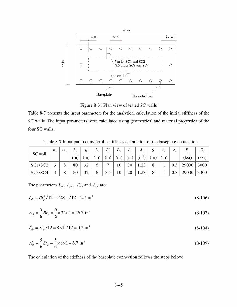
8-45
Figure 8-31 Plan view of tested SC walls
Table 8-7 presents the input parameters for the analytical calculation of the initial stiffness of the
SC walls. The input parameters were calculated using geometrical and material properties of the
four SC walls.
Table 8-7 Input parameters for the stiffness calculation of the baseplate connection
SC wall rn rm bL B tL tL ′
cL rL rA S ptsν sE cE
(in) (in) (in) (in) (in) (in) (in2) (in) (in) (ksi) (ksi)
SC1/SC2 3 8 80 32 6 7 10 20 1.23 8 1 0.3 29000 3000
SC3/SC4 3 8 80 32 6 8.5 10 20 1.23 8 1 0.3 29000 3300
The parameters sbI ,
sbA , sbI ′ , and
sbA′ are:
3 3 4 = /12 32 1 /12 2.7 insb pI Bt = × = � (8-106)
25 532 1 26.7 in
6 6sb pA Bt= = × × = � (8-107)
3 3 4 = /12 8 1 /12 0.7 insb pI St′ = × = � (8-108)
25 58 1 6.7 in
6 6sb pA St′ = = × × = � (8-109)
The calculation of the stiffness of the baseplate connection follows the steps below:

8-46
Step 1: An uplift 1∆ is assumed for the baseplate at the level of the first row of the threaded bars
at the tension end of the wall.
Step 2: The vertical displacement of the baseplate at the level of the ith row of threaded bars, i∆ ,
is:
1 1 2 3 9 , ( 66 in., 60 in., 54 in., ..., 2 in.)66
ii
dd d d d
′′ ′ ′ ′∆ = ∆ = = = = � (8-110)
Step 3: The value of ψ for SC1 through SC4 is:
2 22 (1 ) 6 3 1.23 6 2 3 1.23 (1 0.3)( ) ( ) 5.1
3 20 3 2.7 26.7
t r r t r r s
r sb sb
L n A L n A
L I A
νψ
� � � �+ × × × × × += + = + =� � � �
� �� �� (8-111)
The value of ξ for SC1 and SC2 is:
2 22 (1 ) 7 1.23 7 2 1.23 (1 0.3)( ) ( ) 10.6
3 20 3 0.7 6.7
t r t r s
r sb sb
L A L A
L I A
νξ
� �′ ′ � �+ × × × += + = + =� � � �′ ′ ×� �� �
� (8-112)
The value of ξ for SC3 and SC4 is:
2 22 (1 ) 8.5 1.23 8.5 2 1.23 (1 0.3)( ) ( ) 18.2
3 20 3 0.7 6.7
t r t r s
r sb sb
L A L A
L I A
νξ
� � � �′ ′ + × × × += + = + =� � � �
′ ′ ×� �� �� (8-113)
The contributions of the axial extension of the threaded bars to 1∆ per (8-97) is less than 15% for
SC1 through SC4 and less than 8% to to i
∆ per (8-98) for the remaining bars in the walls. Since
the contribution is very small, the fourth assumption on page 8-40 is not substantially violated if
the baseplate is post-tensioned to the foundation block.
Step 4: Assuming that the axial stiffness of the threaded bar is rK , the tensile force in each threaded
bar at the level of the first row of threaded bars is:
1 11
1 6.1
rr
KT K
ψ
∆ ∆= =
+� (8-114)
The tensile force in each threaded bar at the level of the ith row of threaded bars in SC1 and SC2
is:

8-47
1 11.6
i r ii r
KT K
ξ
∆ ∆= =
+� (8-115)
The tensile force in each threaded bar at the level of the ith row of threaded bars in SC3 and SC4
is:
1 19.2
i r ii r
KT K
ξ
∆ ∆= =
+� (8-116)
Step 5: The equilibrium of the vertical forces is:
1 2 90 3 2 22
b cver
f L BF T T T= + + + =� � (8-117)
Substituting (8-114) and (8-115) into (8-117) produces the maximum bearing stress in SC1 and
SC2:
10.007c rf K= ∆ (8-118)
The maximum bearing stress in SC3 and SC4 is:
10.0054c rf K= ∆ (8-119)
Step 6: The bending moment of the vertical forces at the wall centerline corresponding to uplift
1∆ is:
1 1 2 2 6 6 9 93 2 2 2 ( )( / 2 / 3)2
b cb c
f L BM T d T d T d T d L L= + + − − − + −� �
(8-120)
Substituting (8-114) and (8-115), and (8-118) into (8-120) produces the bending moment in SC1
and SC2:
165.6 rM K= ∆ (8-121)
The bending moment in SC3 and SC4 is:
153.8 rM K= ∆ (8-122)
Step 7: The rotational stiffness of the baseplate connection is calculated by substituting (8-121)
into (8-105). The rotational stiffness of the connection in SC1 and SC2 is:
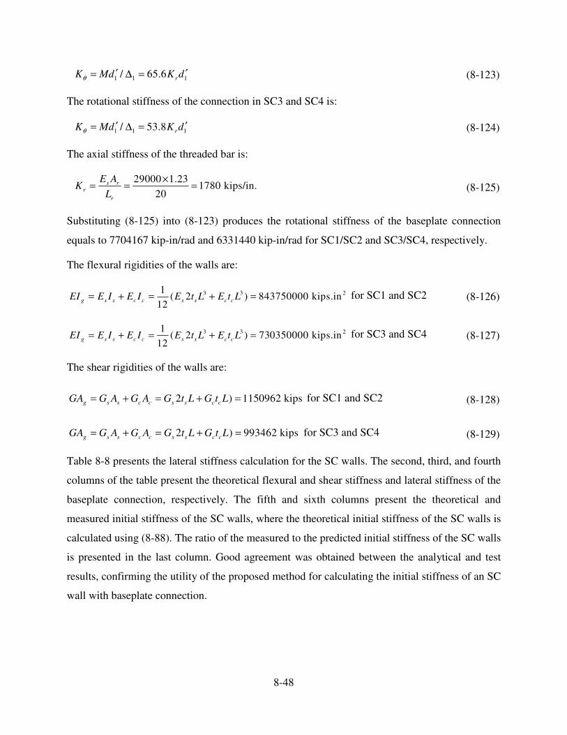
8-48
1 1 1/ 65.6 rK Md K dθ′ ′= ∆ = � (8-123)
The rotational stiffness of the connection in SC3 and SC4 is:
1 1 1/ 53.8 rK Md K dθ′ ′= ∆ = � (8-124)
The axial stiffness of the threaded bar is:
29000 1.23
1780 kips/in.20
s rr
r
E AK
L
×= = = � (8-125)
Substituting (8-125) into (8-123) produces the rotational stiffness of the baseplate connection
equals to 7704167 kip-in/rad and 6331440 kip-in/rad for SC1/SC2 and SC3/SC4, respectively.
The flexural rigidities of the walls are:
23 31( 2 )
12843750000 kips.ing s s c c s s c cEI E I E I E t L E t L= + = + = for SC1 and SC2� (8-126)
23 31( 2 )
12730350000 kips.ing s s c c s s c cEI E I E I E t L E t L= + = + = for SC3 and SC4� (8-127)
The shear rigidities of the walls are:
1150962 kips2 )g s s c c s s c cGA G A G A G t L G t L= + = + = for SC1 and SC2� (8-128)
2 ) 993462 kipsg s s c c s s c cGA G A G A G t L G t L= + = + = for SC3 and SC4� (8-129)
Table 8-8 presents the lateral stiffness calculation for the SC walls. The second, third, and fourth
columns of the table present the theoretical flexural and shear stiffness and lateral stiffness of the
baseplate connection, respectively. The fifth and sixth columns present the theoretical and
measured initial stiffness of the SC walls, where the theoretical initial stiffness of the SC walls is
calculated using (8-88). The ratio of the measured to the predicted initial stiffness of the SC walls
is presented in the last column. Good agreement was obtained between the analytical and test
results, confirming the utility of the proposed method for calculating the initial stiffness of an SC
wall with baseplate connection.

8-49
Table 8-8 Values of measured and predicted initial stiffness of the SC walls
Wall 3
3g
EI
H
gGA
Hκ2
K
H
θtK expK exp
t
K
K (kip/in) (kip/in) (kip/in) (kip/in) (kip/in)
SC1 11719 15986 2140 1625 1680 1.03
SC2 11719 15986 2140 1625 1420 0.88
SC3 10144 13798 1758 1350 1380 1.02
SC4 10144 13798 1758 1350 1310 0.97
�
9-1
9. SUMMARY AND CONCLUSIONS
9.1 Summary
The seismic behavior of intermediate-to-low aspect ratio, rectangular steel-plate concrete (SC)
composite shear walls was investigated as part of a NSF-funded NEESR project on conventional
and composite structural walls. The SC wall piers studied here were composed of steel faceplates,
infill concrete, headed steel studs anchoring the faceplates to the infill, and tie rods connecting the
two faceplates through the infill. The focus was the in-plane behavior of flexure- and flexure-shear
critical SC walls. Composite walls with boundary columns and flanges, and wall piers with very
low-aspect ratios (height-to-length less than 0.5), were not studied. The research project included
experimental, numerical and analytical studies.
The experimental study investigated the cyclic inelastic behavior of SC walls. Four large walls,
SC1 through SC4, were constructed in the Bowen Laboratory at Purdue University and the NEES
laboratory at the University at Buffalo, and at the University at Buffalo. The aspect ratio (height-
to-length, H/L) of all four walls was 1.0. The specimens were anchored to a concrete basemat with
a pre-tensioned bolted connection that was designed to be stronger than the walls. The connection
consisted of a steel plate embedded in the foundation block, a baseplate attached to the steel
faceplates, threaded bars securing the baseplate to the foundation block, headed studs attached to
the baseplate, shear lugs attached to the steel plate embedded in the foundation block, and a steel
anchorage securing the threaded bars to the foundation block. Post-tensioned Dwyidag bars were
used to anchor the foundation block to the strong floor. The design parameters considered in the
experimental investigation were wall thickness (9 in. and 12 in.), reinforcement ratio (3.1% and
4.2%), and faceplate slenderness ratio (21, 24, and 32). Studs and tie rods were used as shear
connectors in SC1 and SC3. Only tie rods were used in SC2 and SC4. Trial designs for the walls
and the re-usable foundation block were prepared and analyzed by hand, using XTRACT for
detailed cross-section analysis, and using ABAQUS to explore design alternatives and develop
force-displacement relationships.
The progression of damage with increasing cyclic lateral displacements in the four walls was
similar: tensile cracking of concrete, tensile yielding of the steel faceplates, crushing of concrete
at the toes of the wall, outward local buckling of the steel faceplates, and fracture of the steel

9-2
faceplates. The test results were used to characterize cyclic force-displacement relationships; post-
peak response focusing on the influence of the stud spacing; energy dissipation and equivalent
viscous damping ratios; strain and stress fields in the steel faceplates; the contribution of the steel
faceplates to the total lateral load; contributions of shear, flexure, and base rotation to the total
lateral displacement; and displacement ductility.
A finite element model for the nonlinear cyclic analysis of flexure- and flexure-shear-critical SC
walls was developed and validated using the test data. The finite element codes ABAQUS,
VecTor2, and LS-DYNA were evaluated. Only DYNA recovered the measured cyclic responses
well. Measured global and local responses of the walls were used to validate the DYNA model.
The validated model was used to investigate the influence of interface friction between the steel
faceplates and the infill concrete, and the distribution of the shear studs attached to baseplate, on
the cyclic response of SC walls.
A limited parametric study on the in-plane monotonic response of SC walls was conducted using
the validated and benchmarked DYNA model. The parametric study included 36 DYNA analyses
of SC walls with aspect ratios of 0.5, 1.0, and 2.0, reinforcement ratios of 1.9%, 2.1%, 3.8%, and
5%, wall thicknesses of 10 in., 20 in., and 30 in., and uniaxial concrete compressive strengths of 4
ksi and 7 ksi. The effects of axial force, slenderness ratio of the steel faceplates, and steel faceplate
material characteristics were not studied. The results of the parametric study were used to
investigate load transfer mechanisms in SC walls and the relative contributions of the infill
concrete and the steel faceplates to the lateral resistance at the onset of the faceplate yielding and
at peak lateral strength. The monotonic response was characterized using a tri-linear force-
displacement relationship.
Analytical models for calculating the monotonic and cyclic responses of single and multi-story SC
wall panels were developed, verified and validated. These models could be used for preliminary
analysis and design of structures including SC walls. The analytical models were verified using
the results of the parametric DYNA study. The Ibarra-Krawinkler Pinching model was modified
to predict the cyclic response of SC walls, and the results of cyclic finite element analysis of 12
models of SC walls were used to establish backbone curve, pinching, deterioration, and rate
parameters for the modified IKP model. An analytical model for predicting the rotational stiffness
of a baseplate connection was developed and validated using test data.

9-3
9.2 Conclusions
This section presents the key conclusions of the experimental, numerical, and analytical studies.
9.2.1 Experimental Study
1. The four walls sustained peak lateral loads close to those predicted by pre-test calculations
using commercially available software.
2. Faceplate slenderness ratio did not influence the peak resistance of SC walls in range of
slenderness ratio studied (21 to 32). The rate of strength deterioration was affected by the
faceplate slenderness ratio, with slightly better performance observed for values of the ratio
less than the limit proposed in the draft appendix to AISC N690.
3. Damage to flexure-critical SC walls in the pre-peak-strength region included concrete
cracking at toes of the wall at drift ratios less than 0.15% and steel faceplate buckling at
0.5% drift ratio. Concrete crushing occurred at peak load. Tearing of the steel faceplates
occurred in the post-peak-strength region of the SC wall response.
4. Pinched hysteresis and loss of stiffness and strength were observed in all four walls at
lateral displacements greater than those corresponding to peak load. Pinching in the
hysteretic response of the SC walls was attributed to the cracking and crushing of the infill
concrete, tearing of the steel faceplates, and flexibility at the base of the wall due to the
baseplate connection.
5. The damage to the infill concrete was concentrated around the level of the first row of
connectors in all four walls.
6. The distance between the first row of connectors and the base of an SC wall has a
significant influence on the post-peak behavior. The use of a smaller distance between the
first row of connectors and the baseplate forced the buckling of the faceplates away from
the CJP welded connection of the faceplates to the baseplate and avoided premature
fracture of the welded connection.
7. Tie rods instead of shear studs are recommended near the base of an SC wall to improve
seismic response, where the faceplates are likely to buckle and high tensile forces are
imposed on the connectors.

9-4
8. The equivalent viscous damping for flexure-critical SC walls can be assumed to be 5% at
displacements less than that at peak strength and 10% for greater displacements.
9. The displacement due to the base rotation governed the total lateral displacement for the
SC walls with a bolted baseplate to RC foundation connection, indicating the importance
of addressing foundation flexibility in design and analysis of SC walls.
9.2.2 Numerical and Analytical Studies
1. Models of SC walls can be prepared in LS-DYNA to reliably compute monotonic and
cyclic responses that are flexure- or flexure-shear-critical. For this purpose: 1) the smeared
crack Winfrith model, MAT085, can be used for the infill concrete; in the absence of
experimental data, the specific fracture energy can be estimated for a given aggregate size
using CEB-FIP Model Code [14]; 2) the plastic-damage model, MAT081, can be used for
the faceplates; 3) beam, shell, and solid elements can be used to model connectors, steel
faceplates, and infill concrete, respectively, and a mesh size of 1 in. is appropriate for the
solids and shells; and 4) the tie constraint can be used to attach the studs and tie rods to the
steel faceplates and the baseplate and the Lagrange-In-Solid constraint can be used to attach
the connectors to the infill concrete elements.
2. The DYNA model can be used to predict damage to the infill concrete and the steel
faceplates and thus can be used to develop robust fragility functions for seismic
probabilistic risk assessment.
3. The assumption of perfect bond between the steel faceplates and the infill concrete does
not significantly affect the pre-peak-strength response of the SC walls in the range of
faceplate slenderness studied here. The post-peak resistance of SC walls is underpredicted
if perfect bond is assumed due to premature fracture of the faceplates. Perfect bond should
not be assumed for finite element analysis.
4. In-plane cyclic response of SC wall is not affected by the choice of the coefficient of
friction between the infill concrete and the steel faceplates.
5. The initial stiffness of SC walls constructed with a baseplate connection to an RC
foundation may be substantially affected by the flexibility of the connection, with a
potential significant impact on the dynamic response of the supported structure.
6. The shear capacity of SC walls is significantly affected by the aspect ratio: the higher the
aspect ratio, the lower the shear capacity.

9-5
7. The contribution of the steel faceplates to the total lateral strength increases as the
reinforcement ratio and/or the wall aspect ratio increases.
8. SC wall piers with aspect ratios of 0.5 and less are shear-critical and SC wall piers with
aspect ratios greater than 0.5 are flexure-critical.
9. The shearing force resisted by the infill concrete at the peak lateral strength in the wall pier
varied from 7% to 15%, 4% to 8% and 2% to 4% of the axial strength of the infill concrete
( g cA f ′ ) for aspect ratios of 0.5, 1.0, and 2.0, respectively.
10. The shear forces resisted by the steel faceplates at peak lateral strength were 35%, 22%,
and 10% of s yA f for SC wall piers with aspect ratios of 0.5, 1.0, and 2.0, respectively.

10-1
10. REFERENCES
[1] ACI 318 Committee. (2011). "Building code requirements for structural concrete (ACI 318-
11) and commentary." American Concrete Institute, Farmington Hills, MI.
[2] AISC-341 (2010). "Seismic provisions for structural steel buildings." American Institute of
Steel Construction, Chicago, IL.
[3] ACI 349 Committee. (2006). "Code requirements for nuclear safety-related concrete structures
(ACI 349�06) and commentary." American Concrete Institute, Farmington Hills, MI.
[4] ACI 374 Committee. (2005). “Acceptance criteria for moment frames based on structural
testing and commentary." American Concrete Institute, Farmington Hills, MI.
[5] AISC (2014) "Specification for safety-related steel structures for nuclear facilities, Supplement
No. 1." N690s1, American Institute of Steel Construction, Chicago, IL.
[6] Akita, S., Ozaki, M., Niwa, N., Matsuo, I., and Hara, K. (2001). "Study on steel plate reinforced
concrete bearing wall for nuclear power plants (part #2): analytical method to evaluate response
of SC walls." 16th International Conference on Structural Mechanics in Reactor Technology
(SMiRT16), International Association for Structural Mechanics in Reactor Technology
(IASMiRT), Washington DC, USA.
[7] Akiyama, H., Sekimoto, H., Tanaka, M., Inoue, K., Fukihara, M., and Okuda, Y. (1989).
"1/10th scale model test of inner concrete structure composed of concrete filled steel bearing wall."
10th International Conference on Structural Mechanics in Reactor Technology (SMiRT10),
International Association for Structural Mechanics in Reactor Technology (IASMiRT), Anaheim,
California, USA, 73-78.
[8] Ali, A., Kim, D., and Cho, S. G. (2013). "Modeling of nonlinear cyclic load behavior of I-
shaped composite steel-concrete shear walls of nuclear power plants." Nuclear Engineering and
Technology, 45(1), 89-98.
[9] ASTM C39 (2002). "Standard test method for compressive strength of cylindrical concrete
specimens." American Society for Testing and Materials, West Conshohocken, PA.
[10] ASTM A370 (1997). "Standard test methods and definitions for mechanical testing of steel
products." American Society for Testing and Materials, West Conshohocken, PA.
[11] Balmer, G. G. (1949). "Shearing strength of concrete under high triaxial stress - computation
of Mohr's envelope as a curve." Structural Research Laboratory Report SP-23, Denver, Colorado.

10-2
[12] Bathe, K. J. (1982). "Finite element procedures in engineering analysis." Prentice Hall, Engle
Wood Cliffs, New Jersey.
[13] Bessason, B., and Sigfusson, T. (2001). "Capacity and earthquake response analysis of RC-
shear walls." Nordic Concrete Research, 27, 1-14.
[14] Comité Euro-International du Béton (CEB-FIP). (1993). "CEB-FIP model code 1990."
Thomas Telford, London.
[15] Booth, P. N., Varma, A. H., Malushte, S. R., and Johnson, W. H. (2007). "Response of
modular composite walls to combined thermal and mechanical load." 19th International
Conference on Structural Mechanics in Reactor Technology (SMiRT19), International Association
for Structural Mechanics in Reactor Technology (IASMiRT), Toronto, Canada.
[16] Bowerman, H., Coyle, N., and Chapman, J. C. (2002). "An innovative steel/concrete
construction system." The Structural Engineer, 80(20), 33-38.
[17] Broadhouse, B. J. (1986). "DRASTIC-A compute code for dynamic analysis of stress
transients in reinforced concrete." Safety and Engineering Science Devision, AEE, Winfrith,
AEEW – R2124.
[18] Brockenbrough, R. L., and Merritt, F. S. (1999). "Structural steel designer's handbook."
McGraw-Hill, New York.
[19] Chadwell, C. B., and Imbsen, R. A. (2002). "XTRACT-cross section analysis software for
structural and earthquake engineering." TRC, Rancho Cordova, CA.
[20] Chang, G. A., and Mander, J. B. (1994). "Seismic energy based fatigue damage analysis of
bridge columns: part I-evaluation of seismic capacity." Report No. NCEER-94-0006, National
Center for Earthquake Engineering Research, Buffalo, NY.
[21] Chaudhary, S., Ali, A., Kim, D., and Cho, S. G. (2011). "Seismic analysis of steel concrete
composite walls of nuclear power plant structures." 21th International Conference on Structural
Mechanics in Reactor Technology (SMiRT21), International Association for Structural Mechanics
in Reactor Technology (IASMiRT), New Delhi, India.
[22] Chen, W. F., and Han, D. J. (2007). "Plasticity for structural engineers." J. Ross Publishing,
New York.
[23] Chopra, A. K. (2012). "Dynamics of structures: Theory and applications to earthquake
engineering (4th Edition)." Prentice Hall, Englewood Cliffs, New Jersey.

10-3
[24] Collins, M. P., and Mitchell, D. (1991). "Prestressed concrete structures." Prentice Hall,
College Division.
[25] Danay, A. (2012). "Response of steel-concrete composite panels to in-plane loading." Nuclear
Engineering and Design, 242, 52-62.
[26] Emori, K. (2002). "Compressive and shear strength of concrete filled steel box wall." Steel
Structures (Korean Journal), 2(1), 29-40.
[27] Eom, T. S., Park, H. G., Lee, C. H., Kim, J. H., and Chang, I. H. (2009). "Behavior of double
skin composite wall subjected to in-plane cyclic loading." Journal of Structural Engineering,
135(10), 1239-1249.
[28] Epackachi, S., Nguyen, H. N., Kurt, E. G., Pitman, M., Weinreber, S., Whittaker, A. S. and
Varma, A., 2014, "Steel-plate composite shear wall - specimen No. 1 (SC1)," Network for
Earthquake Engineering Simulation (distributor), Dataset, DOI:10.4231/D3BG2H97F.
[29] Epackachi, S., Nguyen, H. N., Kurt, E. G., Pitman, M., Weinreber, S., Whittaker, A. S. and
Varma, A., 2014, “Steel-plate composite shear wall - specimen No. 2 (SC2)," Network for
Earthquake Engineering Simulation (distributor), Dataset, DOI: 10.4231/D36T0GW54.
[30] Epackachi, S., Nguyen, H. N., Kurt, E. G., Pitman, M., Weinreber, S., Whittaker, A. S. and
Varma, A., 2014, “Steel-plate composite shear wall - specimen No. 3 (SC3)," Network for
Earthquake Engineering Simulation (distributor), Dataset, DOI: 10.4231/D3319S315.
[31] Epackachi, S., Nguyen, H. N., Kurt, E. G., Pitman, M., Weinreber, S., Whittaker, A. S. and
Varma, A., 2014, “Steel-plate composite shear wall - specimen No. 4 (SC4)," Network for
Earthquake Engineering Simulation (distributor), Dataset, DOI: 10.4231/D3Z892F6J.
[32] Fukumoto, T., Kato, B., and Sato, K. (1987). "Concrete filled steel bearing walls." IABSE
Symposium, Paris-Versailles.
[33] Gulec, C. K., and Whittaker, A. S. (2011). "Hysteretic modeling of squat reinforced concrete
shear walls." 21th International Conference on Structural Mechanics in Reactor Technology
(SMiRT21), International Association for Structural Mechanics in Reactor Technology
(IASMiRT), New Delhi, India.
[34] Hassinen, P., Kouhi, J., Zimmerman, T. J. E., and Stephens, M. J. (1989). "Static and cyclic
load tests of a composite ice-resisting wall." Rep. No. 965, Technical Research Center of Finland,
Helsinki, Finland.
10-4
[35] Hong, S. G., Kim, W., Lee, K. J., Hong, N. K., and Lee, D. H. (2010). "Out-of-plane shear
strength of steel-plate-reinforced concrete walls dependent on bond behavior." Journal of Disaster
Research, 5(4), 385-394.
[36] Hong, S. G., Lee, S. J., and Lee, M. J. (2014). "Steel plate concrete walls for containment
structures in Korea: in-plane shear behavior." Infrastructure Systems for Nuclear Energy, 237-257.
[37] Hristovski, V. T., and Noguchi, H. (2002). "Finite element modeling of RC members
subjected to shear." Third DIANA World Conference, Tokyo, Japan, 175-183.
[38] Hu, H. T., and Schnobrich, W. C. (1990). "Nonlinear analysis of cracked reinforced concrete."
ACI Structural Journal, 87(2), 199-207.
[39] Ibarra, L. F., Medina, R. A., and Krawinkler, H. (2005). "Hysteretic models that incorporate
strength and stiffness deterioration." Earthquake Engineering and Structural Dynamics, 34(12),
1489-1511.
[40] JEAC 4618 (2009). "Technical code for seismic design of steel plate reinforced concrete
structures: buildings and structures." Japanese Electric Association Nuclear Standards Committee,
Tokyo, Japan.
[41] Jian-Guo, N., Hong-Song, H., Jian-Sheng, F., Mu-Xuan, T., Sheng-Yong, L., and Fu-Jun, L.
(2013). "Experimental study on seismic behavior of high-strength concrete filled double-steel-
plate composite walls." Journal of Constructional Steel Research, 88, 206-219.
[42] Kupfer, H. B., Hubert, K. H., and Hubert, R. (1969). "Behavior of concrete under biaxial
stresses." ACI Structural Journal, 66(8), 656-666.
[43] Kupfer, H. B., and Gerstle, K. H. (1973). "Behavior of concrete under biaxial
stresses." Journal of the Engineering Mechanics Division, 99(4), 853-866.
[44] Kurt, E. G. (2015). "Seismic assessment of steel-plate concrete composite walls." Ph.D.
dissertation, Purdue University, West Lafayette, IN.
[45] Kurt, E. G., Varma, A. H., Booth, P., and Whittaker, A. S. (2013). "SC wall piers and basemat
connections: numerical investigation of behavior and design." 22nd International Conference on
Structural Mechanics in Reactor Technology (SMiRT22), International Association for Structural
Mechanics in Reactor Technology (IASMiRT), San Francisco, California, US.
[46] Lee, J., and Fenves, G. L. (1998). "Plastic-damage model for cyclic loading of concrete
structures." Journal of Engineering Mechanics, 124(8), 892-900.

10-5
[47] Link, R. A., and Elwi, A. E. (1995). "Composite concrete-steel plate walls: analysis and
behavior." Journal of Structural Engineering, 121(2), 260-271.
[48] LS-DYNA (2012). "Keyword User’s Manual, Volume I." Version 971 R6.0.0, Livermore,
CA, USA.
[49] LS-DYNA (2012). "Keyword User’s Manual, Volume II." Version 971 R6.0.0, Livermore,
CA, USA.
[50] Lubliner, J., Oliver, J., Oller, S., and Onate, E. (1989). "A plastic-damage model for concrete."
International Journal of Solids and Structures, 25(3), 299-326.
[51] Mahin, S. A., and Bertero, V. V. (1981). "An evaluation of inelastic seismic design spectra."
Journal of the Structural Division, 107(9), 1777-1795.
[52] Mander, J. B., Priestley, M. J. N., and Park, R. (1988). "Observed stress-strain behavior of
confined concrete." Journal of Structural Engineering, 114(8), 1827-1849.
[53] Mansour, M., and Hsu, T. T. C. (2005). "Behavior of reinforced concrete elements under
cyclic shear. I: experiments." Journal of Structural Engineering, 131(1), 44-53.
[54] Mansour, M., and Hsu, T. T. C. (2005). "Behavior of reinforced concrete elements under
cyclic shear. II: theoretical model." Journal of Structural Engineering, 131(1), 54-65.
[55] MATLAB (2012). "Version 7.13.0.564." MathWorks Inc., Natick, MA.
[56] Nguyen, N. H. (2015). "In-plane shear behavior of steel-plate concrete composite walls."
Ph.D. dissertation in preparation, University at Buffalo, Buffalo, NY.
[57] Nie, J. G., Ma, X. W., Tao, M. X., Fan, J. S., and Bu, F. M. (2014). "Effective stiffness of
composite shear wall with double plates and filled concrete." Journal of Constructional Steel
Research, 99, 140-148.
[58] Nielsen, M. P., and Hoang, L. C. (2010). "Limit analysis and concrete plasticity." CRC Press,
Boca Raton, FL.
[59] Nuclear Power Engineering Corporation (1994). "Specification report of seismic shear wall
ISP on NUPEC’S seismic ultimate dynamic response test." NU-SSWIP-D009, Tokyo, Japan.
[60] Orakcal, K., Ulugtekin, D., and Massone, L. M. (2012). "Constitutive modeling of reinforced
concrete panel behavior under cyclic loading." 15th World Conference on Earthquake
Engineering, Lisbon, Portugal.
[61] Ottosen, N. S. (1977). "A failure criterion for concrete." Journal of the Engineering Mechanics
Division, 103(4), 527-535.

10-6
[62] Ozaki, M., Akita, S., Niwa, N., Matsuo, I., and Usami, S. (2001). "Study on steel-plate
reinforced concrete bearing wall for nuclear power plants part 1: shear and bending loading tests
of SC walls." 16th International Conference on Structural Mechanics in Reactor Technology
(SMiRT16), International Association for Structural Mechanics in Reactor Technology
(IASMiRT), Washington DC, USA.
[63] Ozaki, M., Akita, S., Osuga, H., Nakayama, T., and Adachi, N. (2004). "Study on steel plate
reinforced concrete panels subjected to cyclic in-plane shear." Nuclear Engineering and Design,
228(1-3), 225-244.
[64] Ozaki, M., Osuga, H., Nakayama, T., and Adachi, N. (2001). "Study on steel plate reinforced
concrete panels having an opening subjected to cyclic in-plane shear." 16th International
Conference on Structural Mechanics in Reactor Technology (SMiRT16), International Association
for Structural Mechanics in Reactor Technology (IASMiRT), Washington DC, USA.
[65] Ozaki, M., Akita, S., Osuga, H., Nakayama, T., and Adachi, N. (2004). "Study on steel plate
reinforced concrete panels subjected to cyclic in-plane shear." Nuclear Engineering and Design,
228(1), 225-244.
[66] Park, R. (1988). "Ductility evaluation from laboratory and analytical testing." Ninth World
Conference on Earthquake Engineering, Tokyo-Kyoto, Japan.
[67] Park, R., Priestley, M. J. N., and Gill, W. D. (1982). "Ductility of square-confined concrete
columns." 108 (ST4), 929-950.
[68] Rabbat, B. G., and Russell, H. G. (1985). "Friction coefficient of steel on concrete or grout."
Journal of Structural Engineering, 111(3), 505-515.
[69] Richart, F. E., Braendtzaeg, A., and Brown, R. L. (1928). "A study of the failure of concrete
under combined compressive stress." University of Illinois, Engineering Experimental Station
Bulletin, 185, 103.
[70] Saenz, L. P. (1964). "Discussion of equation for the stress-strain curve of concrete, by P.
Desay and S. Krishan’." ACI Journal, 61(9), 1229-1235.
[71] Sasaki, N., Akiyama, H., Narikawa, M., Hara, K., Takeuchi, M., and Usami, S. (1995). "Study
on a concrete filled steel structure for nuclear power plants (part #2): shear and bending loading
tests on wall member." 13th International Conference on Structural Mechanics in Reactor
Technology (SMiRT13), International Association for Structural Mechanics in Reactor
Technology (IASMiRT), Porto Alegre, Brazil, 27-32.
10-7
[72] Schwer, L. (2011). "The Winfrith concrete model: beauty or beast? Insights into the Winfrith
concrete model." 8th European LS-DYNA Users Conference, Strasbourg, France.
[73] SEESL (2008). "Online lab manual of the structural engineering and earthquake simulation
laboratory." University at Buffalo.
[74] Sener, K., Varma, A. H., Malushte, S. R., and Coogler, K. (2013). “Experimental database of
SC composite specimens tested under out-of-plane shear loading." 22nd International Conference
on Structural Mechanics in Reactor Technology (SMiRT22), International Association for
Structural Mechanics in Reactor Technology (IASMiRT), San Francisco, California, US.
[75] Sener, K. C., and Varma, A. H. (2014). "Steel-plate composite walls: experimental database
and design for out-of-plane shear." Journal of Constructional Steel Research, 100, 197-210.
[76] SIMULIA (2012). "ABAQUS analysis user’s manual." Version 6.12, Dassault Systèmes
Simulia Corp., Providence, Rhode Island, USA.
[77] SIMULIA (2012). " ABAQUS theory manual." Version 6.12, Dassault Systèmes Simulia
Corp., Providence, Rhode Island, USA.
[78] Sittipunt, C., and Wood, S. L. (1995). "Influence of web reinforcement on the cyclic response
of structural walls." ACI Structural Journal, 92(6), 745-756.
[79] SNG, K. (2010). "SNG steel plate concrete structures." Board of KEPIC Policy Structural
Committee, Seoul, Korea.
[80] Stephens, M. J., and Zimmerman, T. J. E. (1990). "The strength of composite ice-resisting
walls subjected to combined loads." The First ISOPE European Offshore Mechanics Symposium.
International Society of Offshore and Polar Engineers, Trondheim, Norway.
[81] Suzuki, H., and Kato, B. (1984). "Shear strengths of concrete-filled steel box elements."
Composite and Mixed Construction (ASCE), Seattle, Washington, US, 254-266.
[82] Suzuki, N., Akiyama, H., Narikawa, M., Hara, K., Takeuchi, M., and Matsuo, I. (1995).
"Study on a concrete filled steel structure for nuclear power plants (part #4): analytical method to
estimate shear strength." 13th International Conference on Structural Mechanics in Reactor
Technology (SMiRT13), International Association for Structural Mechanics in Reactor
Technology (IASMiRT), Porto Alegre, Brazil, 33-38.
[83] Takeda, T., Yamaguchi, T., Nakayama, T., Akiyama, K., and Kato, Y. (1995). "Experimental
study on shear characteristics of concrete filled steel plate wall." 13th International Conference on

10-8
Structural Mechanics in Reactor Technology (SMiRT13), International Association for Structural
Mechanics in Reactor Technology (IASMiRT), Porto Alegre, Brazil, 3-14.
[84] Takeuchi, M., Akiyama, H., Narikawa, M., Hara, K., Tsubota, H., and Matsuo, I. (1995).
"Study on a concrete filled steel structure for nuclear power plants (part #1): outline of the structure
and the mock-up test." 13th International Conference on Structural Mechanics in Reactor
Technology (SMiRT13), International Association for Structural Mechanics in Reactor
Technology (IASMiRT), Porto Alegre, Brazil, 15-20.
[85] Takeuchi, M., Narikawa, M., Matsuo, I., Hara, K., and Usami, S. (1998). "Study on a concrete
filled structure for nuclear power plants." Nuclear Engineering and Design, 179(2), 209-223.
[86] Tata Steel Inc., Netherlands, www.tatasteelconstruction.com
[87] Tomlinson, M., Chapman, M., and Wright, H. D. (1989). "Shell composite construction for
shallow draft immersed tube tunnels." ICE International Conference on Immersed Tube Tunnels
Techniques, Manchester, UK.
[88] Tsai, W. T. (1988). "Uniaxial compressional stress�strain relation of concrete." Journal of
Structural Engineering, 114(9), 2133–2136.
[89] Tsuda, K., Tatsuo, N., Eto, H., Akiayama, K., Shimizu, A., Tanouchi, K., and Aoyama, H.
(2001). "Experimental study on steel plate reinforced concrete shear walls with joint bars." 16th
International Conference on Structural Mechanics in Reactor Technology (SMiRT16),
International Association for Structural Mechanics in Reactor Technology (IASMiRT),
Washington DC, USA.
[90] Usami, S., Akiyama, H., Narikawa, M., Hara, K., Takeuchi, M., and Sasaki, N. (1995). "Study
on a concrete filled steel structure for nuclear power plants (part #2): compressive loading tests on
wall members." 13th International Conference on Structural Mechanics in Reactor Technology
(SMiRT13), International Association for Structural Mechanics in Reactor Technology
(IASMiRT), Porto Alegre, Brazil, 21-26.
[91] Uy, B., and Bradford, M. A. (1996). "Elastic local buckling of steel plates in composite steel-
concrete members." Engineering Structures, 18(3), 193-200.
[92] Varma, A. H., Malushte, S., Sener, K., Booth, P. N., and Coogler, K. (2011). "Steel-plate
composite (SC) walls: analysis and design including thermal effects." 21th International
Conference on Structural Mechanics in Reactor Technology (SMiRT21), International Association
for Structural Mechanics in Reactor Technology (IASMiRT), New Delhi, India.
10-9
[93] Varma, A. H., Malushte, S., Sener, K., and Lai, Z. (2013). "Steel-plate composite (SC) walls
for safety related nuclear facilities: design for in-plane force and out-of-plane moments." Nuclear
Engineering and Design, 269(1).
[94] Varma, A. H., Malushte, S. R., Sener, K. C., and Booth, P. N. (2009). "Analysis and design
of modular composite walls for combined thermal and mechanical loading." 20th International
Conference on Structural Mechanics in Reactor Technology (SMiRT19), International Association
for Structural Mechanics in Reactor Technology (IASMiRT), Espoo, Finland.
[95] Varma, A. H., Malushte, S. R., Sener, K. C., and Booth, P. N. (2012). "Analysis
recommendations for steel-composite (SC) walls of safety-related nuclear facilities." Structures
Congress 2012, ASCE, 1871-1880.
[96] Varma, A. H., Malushte, S. R., Sener, K. C., and Lai, Z. (2014). "Steel-plate composite (SC)
walls for safety related nuclear facilities: Design for in-plane forces and out-of-plane moments."
Nuclear Engineering and Design, 269(1), 240-249.
[97] Varma, A. H., Malushte, S. R., Sener, K. C., and Lai, Z. (2014). "Steel-plate composite (SC)
walls for safety related nuclear facilities: Design for in-plane forces and out-of-plane moments."
Nuclear Engineering and Design, 269, 240-249.
[98] Varma, A. H., Sener, K., and Inductries, M. H. (2013). "Lateral load behavior of a
containment internal structure consisting of composite SC walls." 22nd International Conference
on Structural Mechanics in Reactor Technology (SMiRT22), International Association for
Structural Mechanics in Reactor Technology (IASMiRT), San Francisco, California, US.
[99] Varma, A. H., Sener, K., Zhang, K., Coogler, K., and Malushte, S. (2011). "Out-of-plane
shear behavior of SC composite structures." 21th International Conference on Structural
Mechanics in Reactor Technology (SMiRT21), International Association for Structural Mechanics
in Reactor Technology (IASMiRT), New Delhi, India.
[100]Varma, A. H., Zhang, K., Chi, H., Booth, P. N., and Baker, T. (2011). "In-plane shear
behavior of SC composite walls: theory vs. experiment." 21th International Conference on
Structural Mechanics in Reactor Technology (SMiRT21), International Association for Structural
Mechanics in Reactor Technology (IASMiRT), New Delhi, India.
[101]Varma, A. H., Zhang, K., and Malushte, S. R. (2013). "Local buckling of SC composite walls
at ambient and elevated temperatures." 22nd International Conference on Structural Mechanics in

10-10
Reactor Technology (SMiRT22), International Association for Structural Mechanics in Reactor
Technology (IASMiRT), San Francisco, California, US.
[102]Vecchio, F. J. (2000). "Disturbed stress field model for reinforced concrete: formulation."
Journal of Structural Engineering, 126(9), 1070-1077.
[103]Vecchio, F. J. (1992). "Finite element modeling of concrete expansion and confinement."
Journal of Structural Engineering, 118(9), 2390-2406.
[104]Vecchio, F. J. (1989). "Nonlinear finite element analysis of reinforced concrete membranes."
ACI Structural Journal, 86(1), 26-35.
[105]Vecchio, F. J. (1990). "Reinforced concrete membrane element formulations." Journal of
Structural Engineering, 116(3), 730-750.
[106]Vecchio, F. J. (1999). "Towards cyclic load modeling of reinforced concrete." ACI Structural
Journal, 96(2), 193-202.
[107]Vecchio, F. J., and Collins, M. P. (1993). "Compression response of cracked reinforced
concrete." Journal of Structural Engineering, 119(12), 3590-3610.
[108]Vecchio, F. J., and DeRoo, A. (1995). "Smeared crack modelling of concrete tension
splitting." Journal of Engineering Mechanics, 121(6), 702-708.
[109]Vecchio, F. J., and McQuade, I. (2011). "Towards improved modeling of steel-concrete
composite wall elements." Nuclear Engineering and Design, 241(8), 2629-2642.
[110]Vecchio, F. J., and Collins, M. P. (1986). "Modified compression-field theory for reinforced
concrete elements subjected to shear." ACI Structural Journal, 83(2), 219-231.
[111] Vishay Precision Group. (2010). "General purpose strain gages-rectangular rosette."
Document Number: 11095Raleigh, NC.
[112] Walraven, J. C. (1981). "Fundamental analysis of aggregate interlock." Journal of the
Structural Division, 107(11), 2245-2270.
[113]Wittmann, F. H., Rokugo, K., Bruehwiler, E., Mihashi, H., and Simonin, P. (1988). "Fracture
energy and strain softening of concrete as determined by means of compact tension specimens."
Materials and Structures, 21(121), 21-32.
[114]Wong, P. S., Vecchio, F. J., and Trommels, H. (2013). "VecTor2 and Formworks User’s
Manual, Second Edition." University of Toronto, Toronto, Canada.
[115]Wright, H. D. (1995). "The behavior of composite walling under construction and service
loading." Journal of Constructional Steel Research, 35(3), 257-273.

10-11
[116]Wright, H. D., Evans, H. R., and Gallocher, S. C. (1992). "Composite walling." Engineering
Foundation Conference, Missouri, USA.
[117]Wright, H. D., Hossain, K. M. A., and Gallocher, S. C. (1994). "Composite walls as shear
elements in tall structures." ASCE Structures Congress XII, Atlanta, GA, USA, 140-145.
[118]Wright, H. D., Oduyemi, T. O. S., and Evans, H. R. (1991). "The design of double skin
composite elements." Journal of Constructional Steel Research, 19(2), 111-132.
[119]Wright, H. D., Oduyemi, T. O. S., and Evans, H. R. (1991). "The experimental behavior of
double skin composite elements." Journal of Constructional Steel Research, 19(2), 97-110.
[120]Xiaowei, M., Jianguo, N., and Muxuan, T. (2013). "Nonlinear finite-element analysis of
double-skin steel-concrete composite shear wall structures." IACSIT International Journal of
Engineering and Technology, 5(6), 648-652.
[121]Xu, S. Y., and Zhang, J. (2011). "Hysteretic shear-flexure interaction model of reinforced
concrete columns for seismic response assessment of bridges." Earthquake Engineering and
Structural Dynamics, 40(3), 315-337.
[122]Zhang, K., Varma, A., and Gallocher, S. (2013). "Partial composite action in SC composite
walls for nuclear structures." 22nd International Conference on Structural Mechanics in Reactor
Technology (SMiRT22), International Association for Structural Mechanics in Reactor
Technology (IASMiRT), San Francisco, California, US.
[123]Zhang, K., Varma, A. H., Malushte, S. R., and Gallocher, S. (2014). "Effect of shear
connectors on local buckling and composite action in steel concrete composite walls." Nuclear
Engineering and Design, 269, 231-239.
[124]Zhao, Q., and Astaneh-Asl, A. (2004). "Cyclic behavior of traditional and innovative
composite shear walls." Journal of Structural Engineering, 130(2), 271-284.
[125]Zhao, Q. a. A.-A. A. (2004). "Cyclic behavior of traditional and innovative composite shear
walls." Journal of Structural Engineering, 130(2), 271--284.
[126]Zhong, J. X. (2005). "Model-based simulation of reinforced concrete plane stress structures."
University of Houston.
[127]Zhou, J., Mo, Y. L., Sun, X., and Li, J. "Seismic performance of composite steel plate
reinforce concrete shear wall." 12th International Conference on Engineering, Science,
Construction, and Operations in Challenging Environments-Earth and Space 2010, American
Society of Civil Engineers, 3002-3010.

A-1
APPENDIX A. CAD DRAWINGS OF THE SPECIMENS
AND FOUNDATION BLOCK
Figure A-1 Elevation view of specimen SC1

A-2
Figure A-2 Elevation view of specimen SC2

A-3
Figure A-3 Elevation view of specimen SC3

A-4
Figure A-4 Elevation view of specimen SC4

A-5
Figure A-5 Cross-section through the foundation block
Figure A-6 Cross-section through the foundation block

A-6
Figure A-7 Plan view of the baseplate
Figure A-8 Loading plate and loading bracket

A-7
Figure A-9 Plan view of baseplate and top of the foundation block
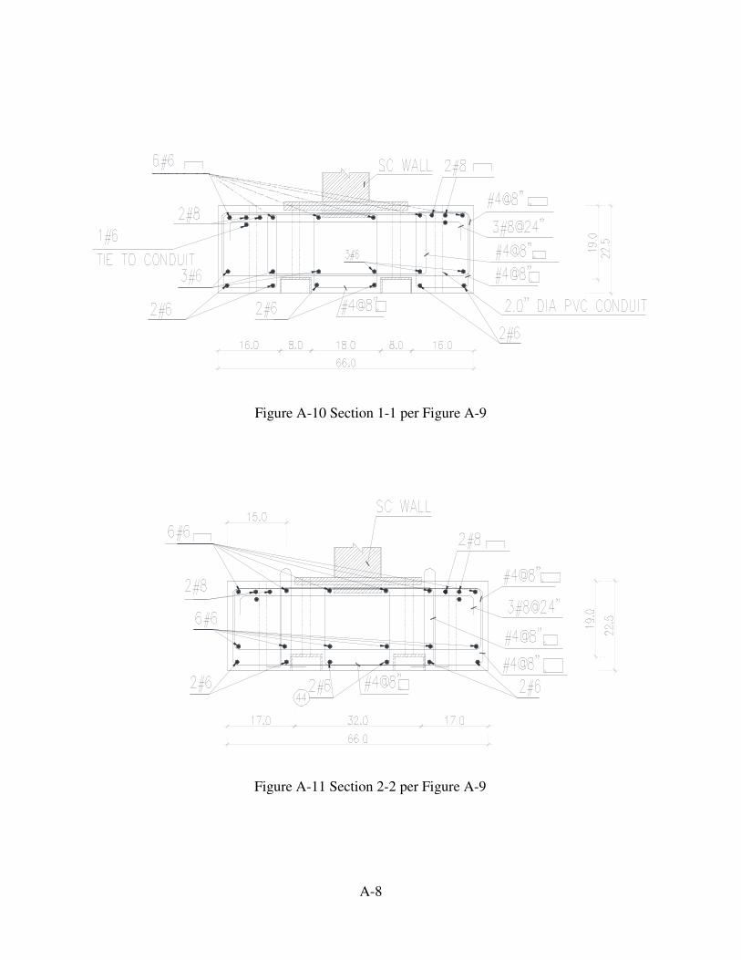
A-8
Figure A-10 Section 1-1 per Figure A-9
Figure A-11 Section 2-2 per Figure A-9

A-9
Figure A-12 Section 3-3 per Figure A-9
Figure A-13 Section 4-4 per Figure A-9

B-1
APPENDIX B. PHOTOGRAPHS OF TEST SPECIMENS
B.1 SC1
Figure B-1 SC1 before testing
Figure B-2 SC1 before testing

B-2
Figure B-3 SC1 before testing
Figure B-4 SC1 before testing

B-3
Figure B-5 Damage to SC1 at 0.47% drift ratio
Figure B-6 Damage to SC1 at 0.47% drift ratio

B-4
Figure B-7 Damage to SC1 at 0.7% drift ratio
Figure B-8 Damage to SC1 at 0.7% drift ratio

B-5
Figure B-9 Damage to SC1 at 0.7% drift ratio
Figure B-10 Damage to SC1 at 0.7% drift ratio

B-6
Figure B-11 Damage to SC1 at 0.93% drift ratio
Figure B-12 Damage to SC1 at 0.93% drift ratio

B-7
Figure B-13 Damage to SC1 at 1.17% drift ratio
Figure B-14 Damage to SC1 at 1.17% drift ratio

B-8
Figure B-15 Damage to SC1 at 1.40% drift ratio
Figure B-16 Damage to SC1 at 1.40% drift ratio

B-9
Figure B-17 Damage to SC1 at 1.63% drift ratio
Figure B-18 Damage to SC1 at 1.63% drift ratio

B-10
Figure B-19 Damage to SC1 at 1.87% drift ratio
Figure B-20 Damage to SC1 at 1.87% drift ratio

B-11
Figure B-21 Damage to SC1 at 2.10% drift ratio
Figure B-22 Damage to SC1 at 2.10% drift ratio

B-12
Figure B-23 Damage to SC1 at 2.33% drift ratio
Figure B-24 Damage to SC1 at 2.33% drift ratio

B-13
Figure B-25 Damage to SC1 at 2.33% drift ratio
Figure B-26 Damage to SC1 at 2.33% drift ratio

B-14
Figure B-27 Damage to SC1 at 2.8% drift ratio
Figure B-28 Damage to SC1 at 2.8% drift ratio

B-15
Figure B-29 Damage to SC1 at 2.8% drift ratio
Figure B-30 Damage to SC1 at 2.8% drift ratio

B-16
Figure B-31 Damage to SC1 at 2.8% drift ratio
Figure B-32 Damage to SC1 at 2.8% drift ratio

B-17
Figure B-33 Damage to SC1 at 3.3% drift ratio
Figure B-34 Damage to SC1 at 3.3% drift ratio

B-18
Figure B-35 Damage to SC1 at 3.3% drift ratio
Figure B-36 Damage to SC1 at the end of testing
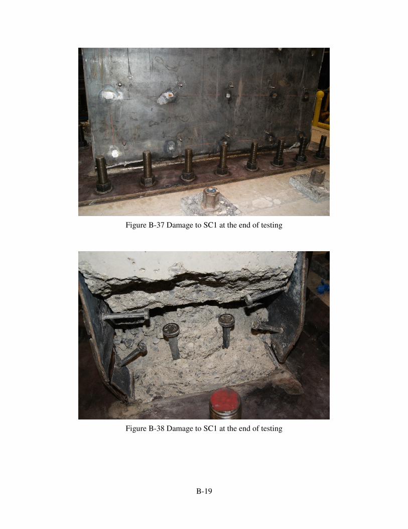
B-19
Figure B-37 Damage to SC1 at the end of testing
Figure B-38 Damage to SC1 at the end of testing

B-20
Figure B-39 Damage to SC1 at the end of testing
Figure B-40 Damage to SC1 at the end of testing

B-21
B.2 SC2
Figure B-41 Damage to SC2 at 0.47% drift ratio
Figure B-42 Damage to SC2 at 0.47% drift ratio

B-22
Figure B-43 Damage to SC2 at 0.70% drift ratio
Figure B-44 Damage to SC2 at 0.70% drift ratio

B-23
Figure B-45 Damage to SC2 at 0.93% drift ratio
Figure B-46 Damage to SC2 at 0.93% drift ratio
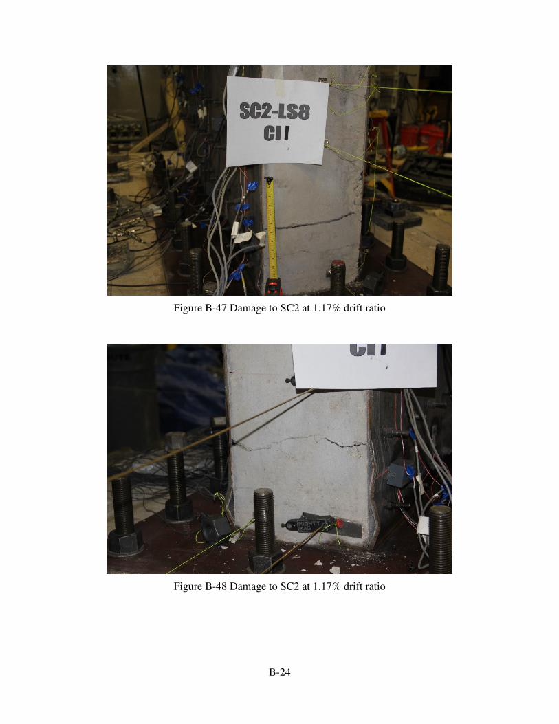
B-24
Figure B-47 Damage to SC2 at 1.17% drift ratio
Figure B-48 Damage to SC2 at 1.17% drift ratio

B-25
Figure B-49 Damage to SC2 at 1.40% drift ratio
Figure B-50 Damage to SC2 at 1.40% drift ratio
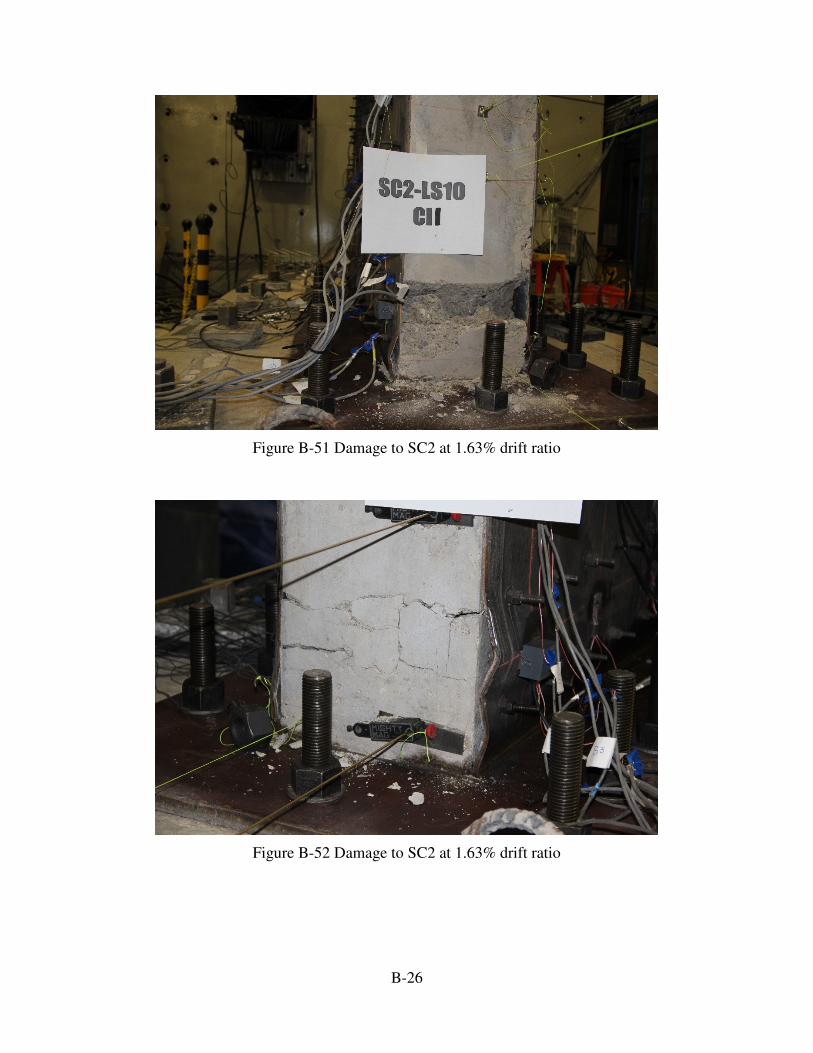
B-26
Figure B-51 Damage to SC2 at 1.63% drift ratio
Figure B-52 Damage to SC2 at 1.63% drift ratio

B-27
Figure B-53 Damage to SC2 at 1.63% drift ratio
Figure B-54 Damage to SC2 at 1.63% drift ratio

B-28
Figure B-55 Damage to SC2 at 2.10% drift ratio
Figure B-56 Damage to SC2 at 2.10% drift ratio

B-29
Figure B-57 Damage to SC2 at 2.33% drift ratio
Figure B-58 Damage to SC2 at 2.33% drift ratio
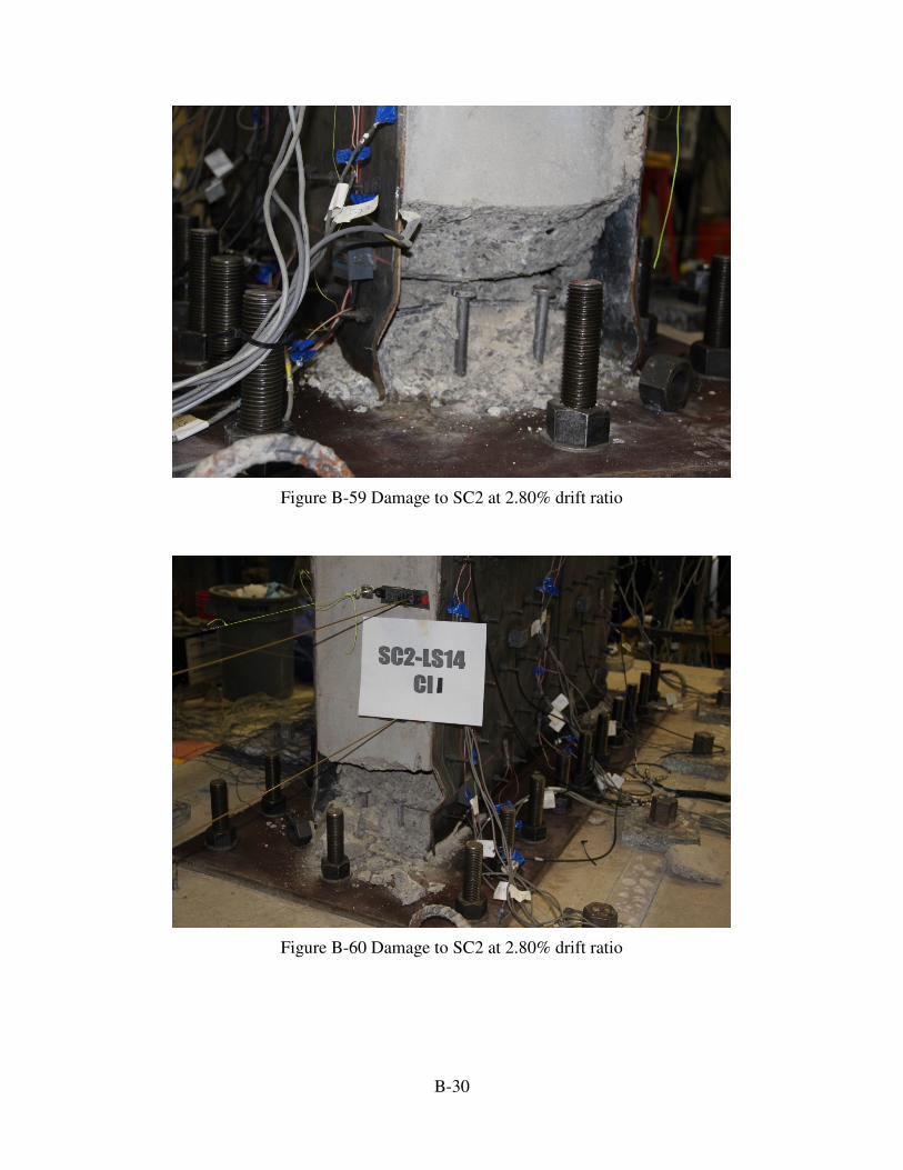
B-30
Figure B-59 Damage to SC2 at 2.80% drift ratio
Figure B-60 Damage to SC2 at 2.80% drift ratio
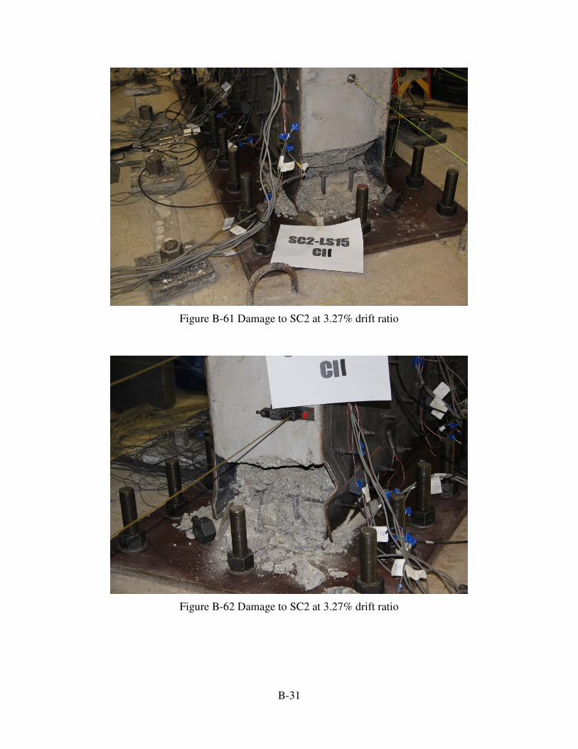
B-31
Figure B-61 Damage to SC2 at 3.27% drift ratio
Figure B-62 Damage to SC2 at 3.27% drift ratio

B-32
Figure B-63 Damage to SC2 at the end of testing
Figure B-64 Damage to SC2 at the end of testing

B-33
Figure B-65 Damage to SC2 at the end of testing
Figure B-66 Damage to SC2 at the end of testing
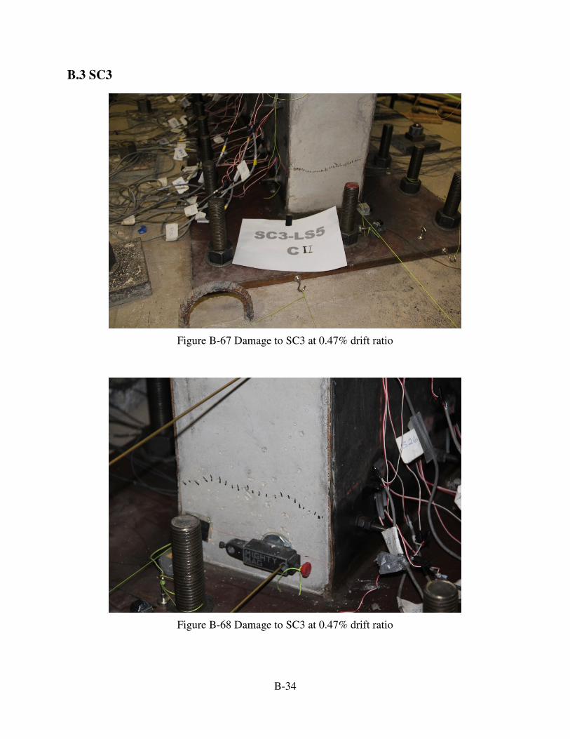
B-34
B.3 SC3
Figure B-67 Damage to SC3 at 0.47% drift ratio
Figure B-68 Damage to SC3 at 0.47% drift ratio

B-35
Figure B-69 Damage to SC3 at 0.70% drift ratio
Figure B-70 Damage to SC3 at 0.70% drift ratio

B-36
Figure B-71 Damage to SC3 at 0.93% drift ratio
Figure B-72 Damage to SC3 at 0.93% drift ratio

B-37
Figure B-73 Damage to SC3 at 1.17% drift ratio
Figure B-74 Damage to SC3 at 1.17% drift ratio
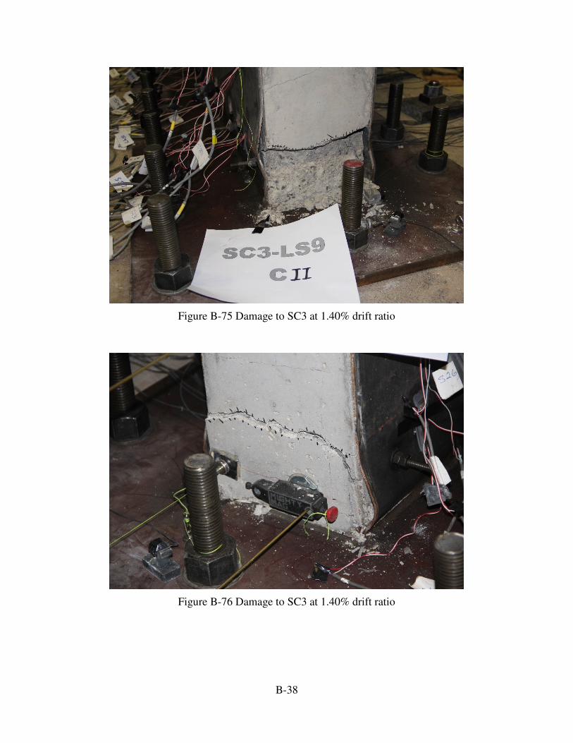
B-38
Figure B-75 Damage to SC3 at 1.40% drift ratio
Figure B-76 Damage to SC3 at 1.40% drift ratio

B-39
Figure B-77 Damage to SC3 at 1.63% drift ratio
Figure B-78 Damage to SC3 at 1.63% drift ratio

B-40
Figure B-79 Damage to SC3 at 1.87% drift ratio
Figure B-80 Damage to SC3 at 1.87% drift ratio

B-41
Figure B-81 Damage to SC3 at 2.10% drift ratio
Figure B-82 Damage to SC3 at 2.10% drift ratio

B-42
Figure B-83 Damage to SC3 at 2.33% drift ratio
Figure B-84 Damage to SC3 at 2.33% drift ratio

B-43
Figure B-85 Damage to SC3 at 2.80% drift ratio
Figure B-86 Damage to SC3 at 2.80% drift ratio

B-44
Figure B-87 Damage to SC3 at 3.27% drift ratio
Figure B-88 Damage to SC3 at 3.27% drift ratio

B-45
Figure B-89 Damage to SC3 at the end of testing
Figure B-90 Damage to SC3 at the end of testing
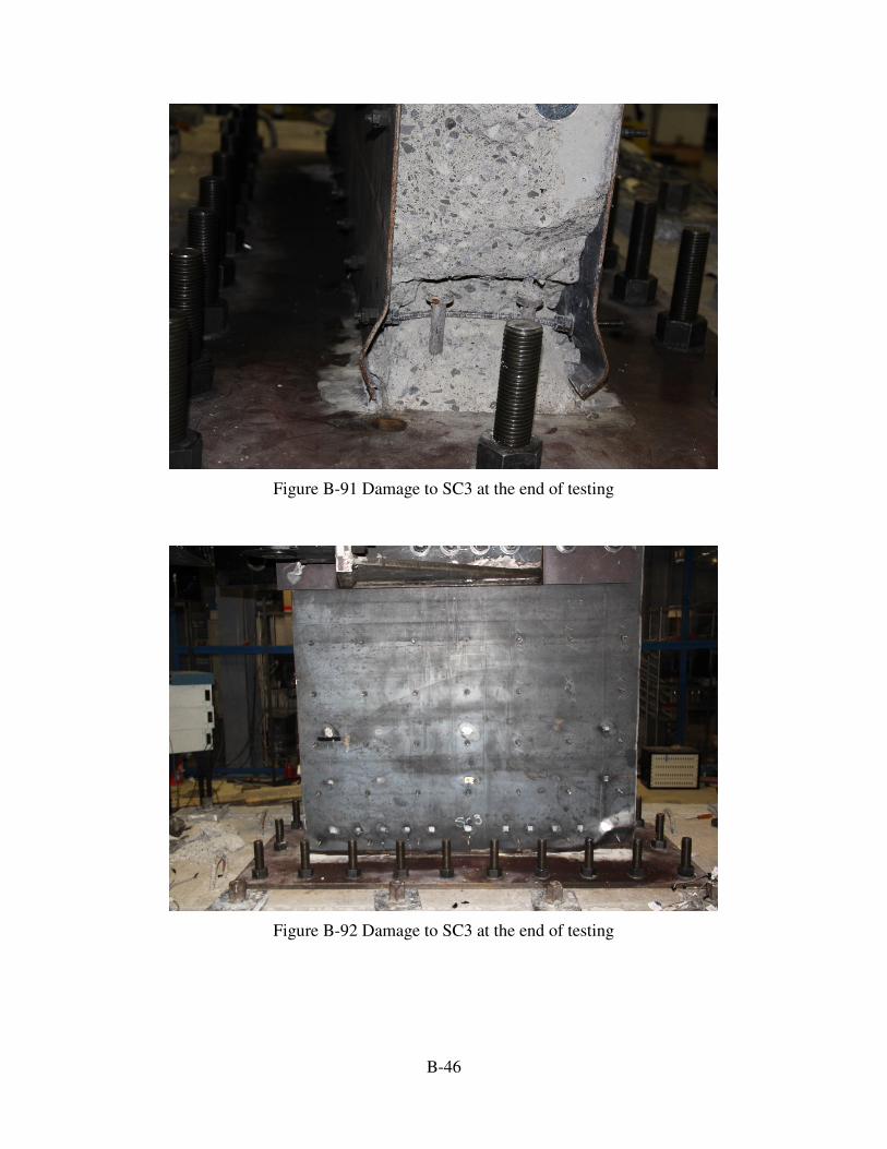
B-46
Figure B-91 Damage to SC3 at the end of testing
Figure B-92 Damage to SC3 at the end of testing

B-47
B.4 SC4
Figure B-93 Damage to SC4 at 0.47% drift ratio
Figure B-94 Damage to SC4 at 0.47% drift ratio

B-48
Figure B-95 Damage to SC4 at 0.70% drift ratio
Figure B-96 Damage to SC4 at 0.70% drift ratio
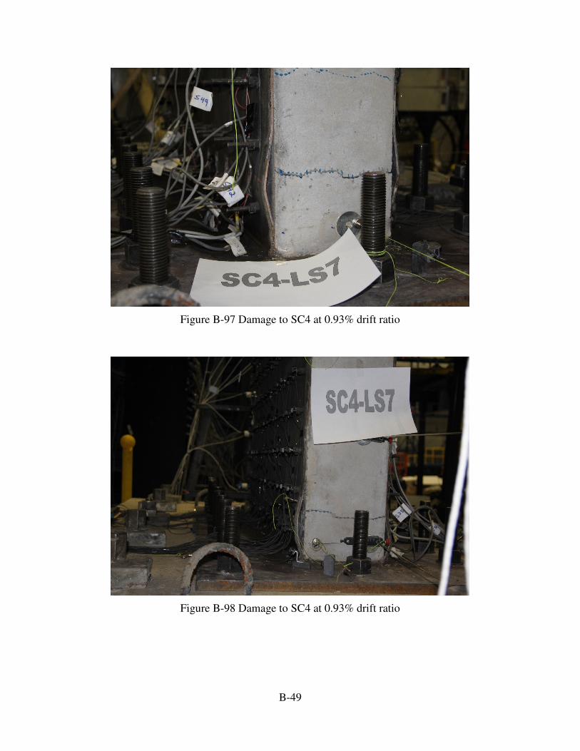
B-49
Figure B-97 Damage to SC4 at 0.93% drift ratio
Figure B-98 Damage to SC4 at 0.93% drift ratio

B-50
Figure B-99 Damage to SC4 at 1.17% drift ratio
Figure B-100 Damage to SC4 at 1.17% drift ratio

B-51
Figure B-101 Damage to SC4 at 1.40% drift ratio
Figure B-102 Damage to SC4 at 1.40% drift ratio
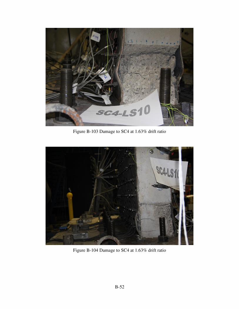
B-52
Figure B-103 Damage to SC4 at 1.63% drift ratio
Figure B-104 Damage to SC4 at 1.63% drift ratio
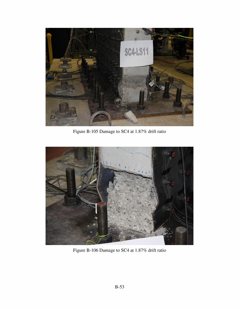
B-53
Figure B-105 Damage to SC4 at 1.87% drift ratio
Figure B-106 Damage to SC4 at 1.87% drift ratio

B-54
Figure B-107 Damage to SC4 at 2.10% drift ratio
Figure B-108 Damage to SC4 at 2.10% drift ratio
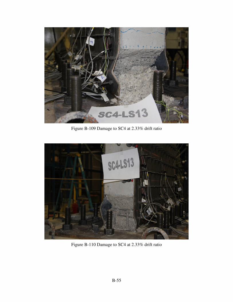
B-55
Figure B-109 Damage to SC4 at 2.33% drift ratio
Figure B-110 Damage to SC4 at 2.33% drift ratio
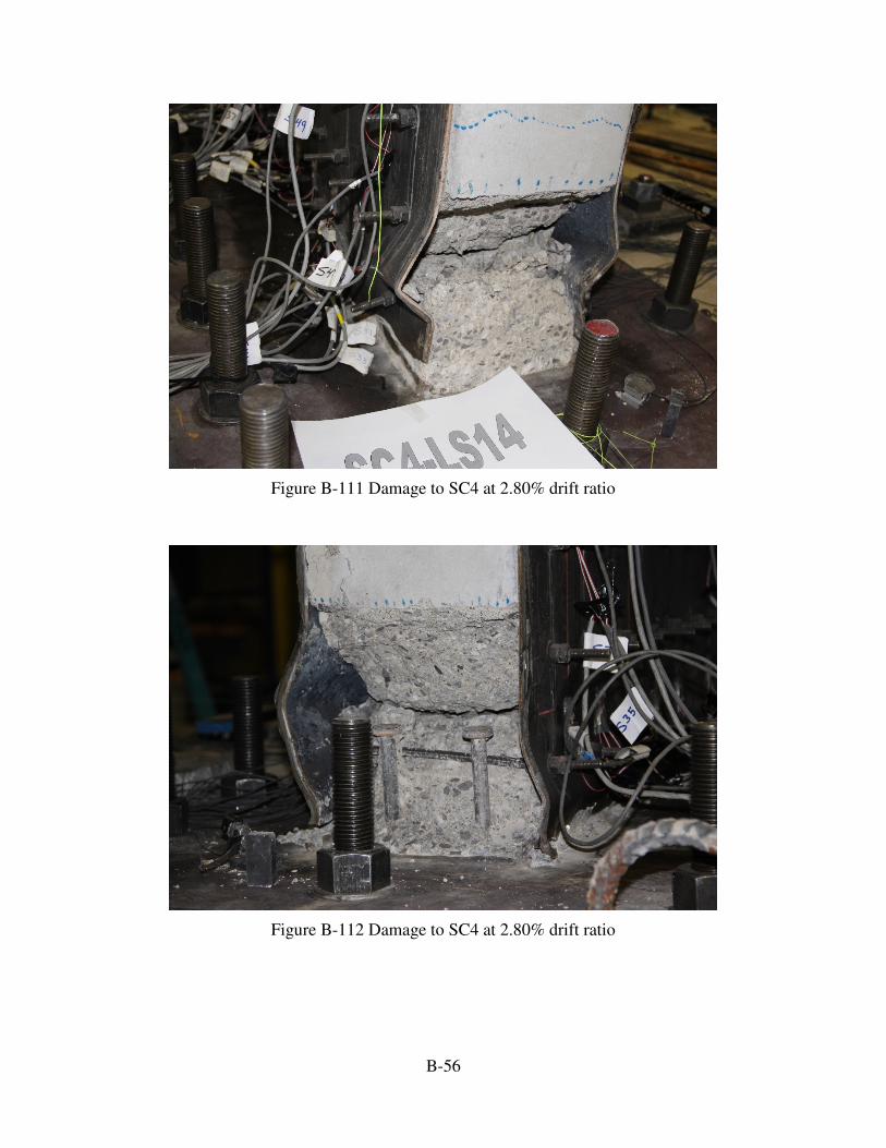
B-56
Figure B-111 Damage to SC4 at 2.80% drift ratio
Figure B-112 Damage to SC4 at 2.80% drift ratio

B-57
Figure B-113 Damage to SC4 at 3.27% drift ratio
Figure B-114 Damage to SC4 at 3.27% drift ratio

B-58
Figure B-115 Damage to SC4 at the end of testing
Figure B-116 Damage to SC4 at the end of testing

B-59
Figure B-117 Damage to SC4 at the end of testing
Figure B-118 Damage to SC4 at the end of testing
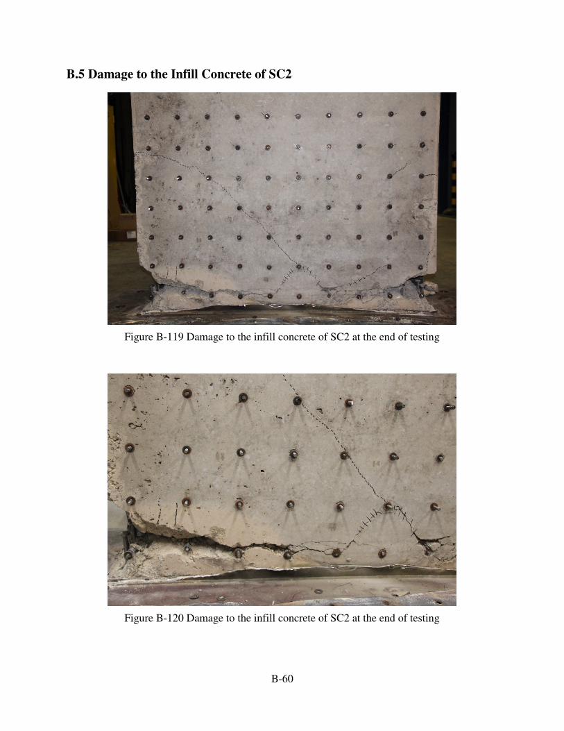
B-60
B.5 Damage to the Infill Concrete of SC2
Figure B-119 Damage to the infill concrete of SC2 at the end of testing
Figure B-120 Damage to the infill concrete of SC2 at the end of testing

B-61
Figure B-121 Damage to the infill concrete of SC2 at the end of testing
Figure B-122 Damage to the infill concrete of SC2 at the end of testing

B-62
B.6 Damage to the Infill Concrete of SC4
Figure B-123 Damage to the infill concrete of SC4 at the end of testing
Figure B-124 Damage to the infill concrete of SC4 at the end of testing

B-63
Figure B-125 Damage to the infill concrete of SC4 at the end of testing
Figure B-126 Damage to the infill concrete of SC4 at the end of testing
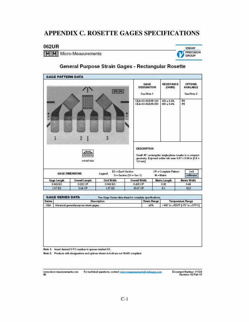
C-1
APPENDIX C. ROSETTE GAGES SPECIFICATIONS
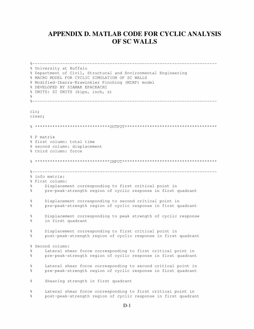
D-1
APPENDIX D. MATLAB CODE FOR CYCLIC ANALYSIS
OF SC WALLS
%--------------------------------------------------------------------------
% University at Buffalo
% Department of Civil, Structural and Environmental Engineering
% MACRO MODEL FOR CYCLIC SIMULATION OF SC WALLS
% Modified-Ibarra-Krawinkler Pinching (MIKP) model
% DEVELOPED BY SIAMAK EPACKACHI
% UNITS: SI UNITS (kips, inch, s)
%
%--------------------------------------------------------------------------
clc;
clear;
% ******************************OUTPUT*************************************
% F matrix
% first column: total time
% second column: displacement
% third column: force
% ******************************INPUT**************************************
%--------------------------------------------------------------------------
% info matrix:
% First column:
% Displacement corresponding to first critical point in
% pre-peak-strength region of cyclic response in first quadrant
% Displacement corresponding to second critical point in
% pre-peak-strength region of cyclic response in first quadrant
% Displacement corresponding to peak strength of cyclic response
% in first quadrant
% Displacement corresponding to first critical point in
% post-peak-strength region of cyclic response in first quadrant
% Second column:
% Lateral shear force corresponding to first critical point in
% pre-peak-strength region of cyclic response in first quadrant
% Lateral shear force corresponding to second critical point in
% pre-peak-strength region of cyclic response in first quadrant
% Shearing strength in first quadrant
% Lateral shear force corresponding to first critical point in
% post-peak-strength region of cyclic response in first quadrant

D-2
% Third column:
% Displacement corresponding to first critical point in
% pre-peak-strength region of cyclic response in third quadrant
% Displacement corresponding to second critical point in
% pre-peak-strength region of cyclic response in third quadrant
% Displacement corresponding to peak strength of cyclic response
% in third quadrant
% Displacement corresponding to first critical point in
% post-peak-strength region of cyclic response in third quadrant
% Fourth column:
% Lateral shear force corresponding to first critical point in
% pre-peak-strength region of cyclic response in third quadrant
% Lateral shear force corresponding to second critical point in
% pre-peak-strength region of cyclic response in third quadrant
% Shearing strength in third quadrant
% Lateral shear force corresponding to first critical point in
% post-peak-strength region of cyclic response in third quadrant
%--------------------------------------------------------------------------
info=[ ...;
0.2044 155 0.2044 155
0.3866 234 0.3866 234
0.5700 259 0.5700 259
2.0000 75 1.9600 61
];
%--------------------------------------------------------------------------
% info2 matrix:
% Values of the pinching and deterioration parameters.
% First to seventh values of matrix correspond to the parameters
% presented at second to eighth columns of Table 8-8
%--------------------------------------------------------------------------
info2=[ ...;
0.3 ...
0.3 ...
0.5 ...
40 ...
35 ...
20 ...
40 ...
];
%--------------------------------------------------------------------------
% info3 matrix:
% Values of rate parameters.

D-3
% First to fourth values of matrix correspond to the parameters
% presented at ninth to twelfth columns of Table 8-8
%--------------------------------------------------------------------------
info3=[ ...;
1 ...
1 ...
0.25 ...
1 ...
];
%--------------------------------------------------------------------------
% a matrix represent loading protocol
% first column: load step number
% second column: total time for each load step
% third column: maximum displacement for each load step
% fourth column: time increment for each load step
% fifth column: number of cycles per load step
%--------------------------------------------------------------------------
a=[1 0.1 0.12 0.01 2
2 0.2 0.24 0.01 2
3 0.4 0.48 0.01 2
4 0.6 0.72 0.01 2
5 0.8 0.96 0.01 2
6 1 1.2 0.01 2
7 1.2 1.44 0.01 2
8 1.4 1.68 0.01 2
9 1.6 1.92 0.01 2
10 1.8 2.16 0.01 2
11 2 2.4 0.01 2
12 2.2 2.64 0.01 2
13 2.4 2.88 0.01 2
14 2.6 3.12 0.01 2
15 2.8 3.36 0.01 2
16 3 3.6 0.01 2
17 3.2 3.84 0.01 2
18 3.4 4.08 0.01 2
];
% *************************************************************************
%----PARAMETERS-----------------------------------
fypos=info(1,2);
xypos=info(1,1);
fyneg=info(1,4);
xyneg=info(1,3);
fyypos=info(2,2);
xccpos=info(2,1);
fyyneg=info(2,4);
xccneg=info(2,3);
fupos=info(3,2);

D-4
xcpos=info(3,1);
funeg=info(3,4);
xcneg=info(3,3);
frrpos=info(4,2);
xsspos=info(4,1);
frrneg=info(4,4);
xssneg=info(4,3);
frpos=0.2*fypos;
frneg=0.2*fyneg;
mmpos=(info(4,2)-info(3,2))/(info(4,1)-info(3,1));
mmneg=(info(4,4)-info(3,4))/(info(4,3)-info(3,3));
xspos=(frpos-info(3,2))/mmpos+info(3,1);
xsneg=(frneg-info(3,4))/mmneg+info(3,3);
%----PINCHING MODEL-----------------------------
kf=info2(1,1);
kd=info2(1,2);
facfp=info2(1,3);
flagl=1;
%----Deterioration parameters-----------------------------
% (BASIC STRENGTH DETERIORATION)
etots=10000;
erates=1;
% (POST CAPPING DETERIORATION)
etotc=10000;
eratec=1;
% (UNLOADING STIFFNESS DETERIORATION)
etotk=info2(1,4);
eratek=info3(1,1);
% (UNLOADING STIFFNESS DETERIORATION)
etotkk=info2(1,5);
eratekk=info3(1,2);
% (UNLOADING STIFFNESS DETERIORATION)
etotkkk=info2(1,6);
eratekkk=info3(1,3);
% (ACCELERATED STIFFNESS DETERIORATION)
etota=info2(1,7);
eratea=info3(1,4);
% (DETERIORATION FLAG)
detflag=2;

D-5
%--------------------------------------------------
FOUT=[kf kd facfp etotk etotkk etota];
%--------------------------------------------------
etots=etots*fupos*xcpos;
etotc=etotc*fupos*xcpos;
etotk=etotk*fupos*xcpos;
etotkk=etotkk*fupos*xcpos;
etotkkk=etotkkk*fupos*xcpos;
etota=etota*fupos*xcpos;
%----STIFFNESS VALUES-----------------------------
kepos=fypos/xypos;
keneg=fyneg/xyneg;
kcpos=(fyypos-fypos)/(xccpos-xypos);
kcneg=(fyyneg-fyneg)/(xccneg-xyneg);
kccpos=(fupos-fyypos)/(xcpos-xccpos);
kccneg=(funeg-fyyneg)/(xcneg-xccneg);
kspos=(frrpos-fupos)/(xsspos-xcpos);
ksneg=(frrneg-funeg)/(xssneg-xcneg);
ksspos=(frpos-frrpos)/(xspos-xsspos);
kssneg=(frneg-frrneg)/(xsneg-xssneg);
krpos=0;
krneg=0;
kunl=0.5*(kepos+keneg);
kunll=kunl;
krelp=kunl;
kreln=kunl;
%----REFERNCE POINT VALUES-----------------------------
sloppos=(frrpos-fupos)/(xsspos-xcpos);
frefpos=fupos-sloppos*xcpos;
slopneg=(frrneg-funeg)/(xssneg-xcneg);
frefneg=funeg-slopneg*xcneg;
[x,y]=size(a);
b(1,1)=0;
b(1,2)=0;
b(1,3)=0;
ind=1;
for i=1:x
stepc=1/(4*a(i,2)/a(i,4));
step=a(i,3)/(4*a(i,2)/a(i,4))/a(i,5);
for j=1:a(i,5)
for k=a(i,4):a(i,4):a(i,2)
ind=ind+1;
b(ind,1)=b(ind-1,1)+stepc;
b(ind,2)=b(ind-1,2)+step;
b(ind,3)=k;
end

D-6
for k=a(i,2)-a(i,4):-a(i,4):-a(i,2)
ind=ind+1;
b(ind,1)=b(ind-1,1)+stepc;
b(ind,2)=b(ind-1,2)+step;
b(ind,3)=k;
end
for k=-a(i,2)+a(i,4):a(i,4):0
ind=ind+1;
b(ind,1)=b(ind-1,1)+stepc;
b(ind,2)=b(ind-1,2)+step;
b(ind,3)=k;
end
end
end
[x,y]=size(b);
%----INITIALIZATION--------------------------------
stat=1;
ind=1;
F(1,1:13)=0;
fneg=-fyneg;
fpos=fypos;
delneg=-xyneg;
delpos=xypos;
delresneg=0;
delrespos=0;
sume=0;
epos=0;
eneg=0;
betaposs=0;
betanegs=0;
betaposc=0;
betanegc=0;
betaposk=0;
betanegk=0;
betaposkk=0;
betanegkk=0;
betaposkkk=0;
betanegkkk=0;
betaposa=0;
betanega=0;
% Increment of dissipated ennergy at positive side
einc0=0;
% Increment of dissipated ennergy at negative side
einc1=0;
%----------------------------------------------------------
coind=0;
for i=2:x
coind=coind+1;
if(coind==28)
tt=1;

D-7
end
if(i==29)
ttt=1;
end
F(i,1)=b(i,2);
F(i,2)=b(i,3);
XOLD=b(i-1,3);
X=b(i,3);
FOLD=F(i-1,3);
if((stat~=5)&&(stat~=25)&&(stat~=6)&&(stat~=26)&&(stat~=7)&&(stat~=27))
if(abs(X)>=abs(XOLD))
if((stat==1)&&(X>0))
XLB=0;
XUB=xypos;
FLB=0;
FUB=fypos;
KLB=kepos;
KUP=kcpos;
statLB=1;
statUB=2;
elseif((stat==1)&&(X<0))
XLB=0;
XUB=-xyneg;
FLB=0;
FUB=-fyneg;
KLB=keneg;
KUP=kcneg;
statLB=21;
statUB=22;
elseif((stat==21)&&(X<0))
XLB=0;
XUB=-xyneg;
FLB=0;
FUB=-fyneg;
KLB=keneg;
KUP=kcneg;
statLB=21;
statUB=22;
elseif((stat==21)&&(X>0))
XLB=0;
XUB=xypos;
FLB=0;
FUB=fypos;
KLB=kepos;
KUP=kcpos;
statLB=1;
statUB=2;
elseif(stat==2)
XLB=xypos;
XUB=xccpos;
FLB=fypos;
FUB=fyypos;

D-8
KLB=kcpos;
KUP=kccpos;
statLB=2;
statUB=200;
elseif(stat==22)
XLB=-xyneg;
XUB=-xccneg;
FLB=-fyneg;
FUB=-fyyneg;
KLB=kcneg;
KUP=kccneg;
statLB=22;
statUB=2200;
elseif(stat==200)
XLB=xccpos;
XUB=xcpos;
FLB=fyypos;
FUB=fupos;
KLB=kccpos;
KUP=kspos;
statLB=200;
statUB=3;
elseif(stat==2200)
XLB=-xccneg;
XUB=-xcneg;
FLB=-fyyneg;
FUB=-funeg;
KLB=kccneg;
KUP=ksneg;
statLB=2200;
statUB=23;
elseif(stat==3)
XLB=xcpos;
XUB=xsspos;
FLB=fupos;
FUB=frrpos;
KLB=kspos;
KUP=ksspos;
statLB=3;
statUB=300;
elseif(stat==23)
XLB=-xcneg;
XUB=-xssneg;
FLB=-funeg;
FUB=-frrneg;
KLB=ksneg;
KUP=kssneg;
statLB=23;
statUB=2300;
elseif(stat==300)
XLB=xsspos;
XUB=xspos;
FLB=frrpos;
FUB=frpos;
KLB=ksspos;
KUP=krpos;
statLB=300;

D-9
statUB=4;
elseif(stat==2300)
XLB=-xssneg;
XUB=-xsneg;
FLB=-frrneg;
FUB=-frneg;
KLB=kssneg;
KUP=krneg;
statLB=2300;
statUB=24;
elseif(stat==4)
XLB=xspos;
XUB=1e20*xspos;
FLB=frpos;
FUB=frpos;
KLB=krpos;
KUP=krpos;
statLB=4;
statUB=4;
elseif(stat==24)
XLB=-xsneg;
XUB=-1e20*xsneg;
FLB=-frneg;
FUB=-frneg;
KLB=krneg;
KUP=krneg;
statLB=24;
statUB=24;
end
if (abs(X)<=abs(XUB))
F(i,3)=(X-XLB)*KLB+FLB;
stat=statLB;
%---------------Hysteretic Energy--------------------------
if(F(i,3)>=0)
efalg=0;
einc0=0.5*(F(i,3)+FOLD)*(X-XOLD);
else
efalg=1;
einc1=0.5*(F(i,3)+FOLD)*(X-XOLD);
end
%----------------------------------------------------------
else
F(i,3)=(X-XUB)*KUP+FUB;
stat=statUB;
%---------------Hysteretic Energy--------------------------
if(F(i,3)>=0)
efalg=0;
einc0=0.5*(F(i,3)+FUB)*(X-XUB)+0.5*(FUB+FOLD)*(XUB-XOLD);
else
efalg=1;
einc1=0.5*(F(i,3)+FUB)*(X-XUB)+0.5*(FUB+FOLD)*(XUB-XOLD);
end
%----------------------------------------------------------
end
else
if (stat==1)
if(X>=0)

D-10
F(i,3)=kepos*X;
stat=1;
%---------------Hysteretic Energy--------------------------
efalg=0;
einc0=0.5*(F(i,3)+FOLD)*(X-XOLD);
%----------------------------------------------------------
else
F(i,3)=keneg*X;
stat=21;
%---------------Hysteretic Energy--------------------------
efalg=2;
einc0=-0.5*FOLD*XOLD;
einc1=0.5*F(i,3)*X;
%----------------------------------------------------------
end
elseif (stat==21)
if(X<=0)
F(i,3)=keneg*X;
stat=21;
%---------------Hysteretic Energy--------------------------
efalg=1;
einc1=0.5*(F(i,3)+FOLD)*(X-XOLD);
%----------------------------------------------------------
else
F(i,3)=kepos*X;
stat=1;
%---------------Hysteretic Energy--------------------------
efalg=3;
einc1=-0.5*FOLD*XOLD;
einc0=0.5*F(i,3)*X;
%----------------------------------------------------------
end
else
if(FOLD>=0)
F(i,3)=FOLD+(X-XOLD)*kunl;
stat=5;
delpos=XOLD;
fpos=FOLD;
del5m=XOLD;
f5m=FOLD;
%---------------Hysteretic Energy--------------------------
efalg=0;
einc0=0.5*(F(i,3)+FOLD)*(X-XOLD);
%----------------------------------------------------------
else
F(i,3)=FOLD+(X-XOLD)*kunl;
stat=25;
delneg=XOLD;
fneg=FOLD;
del25m=XOLD;
f25m=FOLD;
%---------------Hysteretic Energy--------------------------
efalg=1;
einc1=0.5*(F(i,3)+FOLD)*(X-XOLD);
%----------------------------------------------------------
end
end
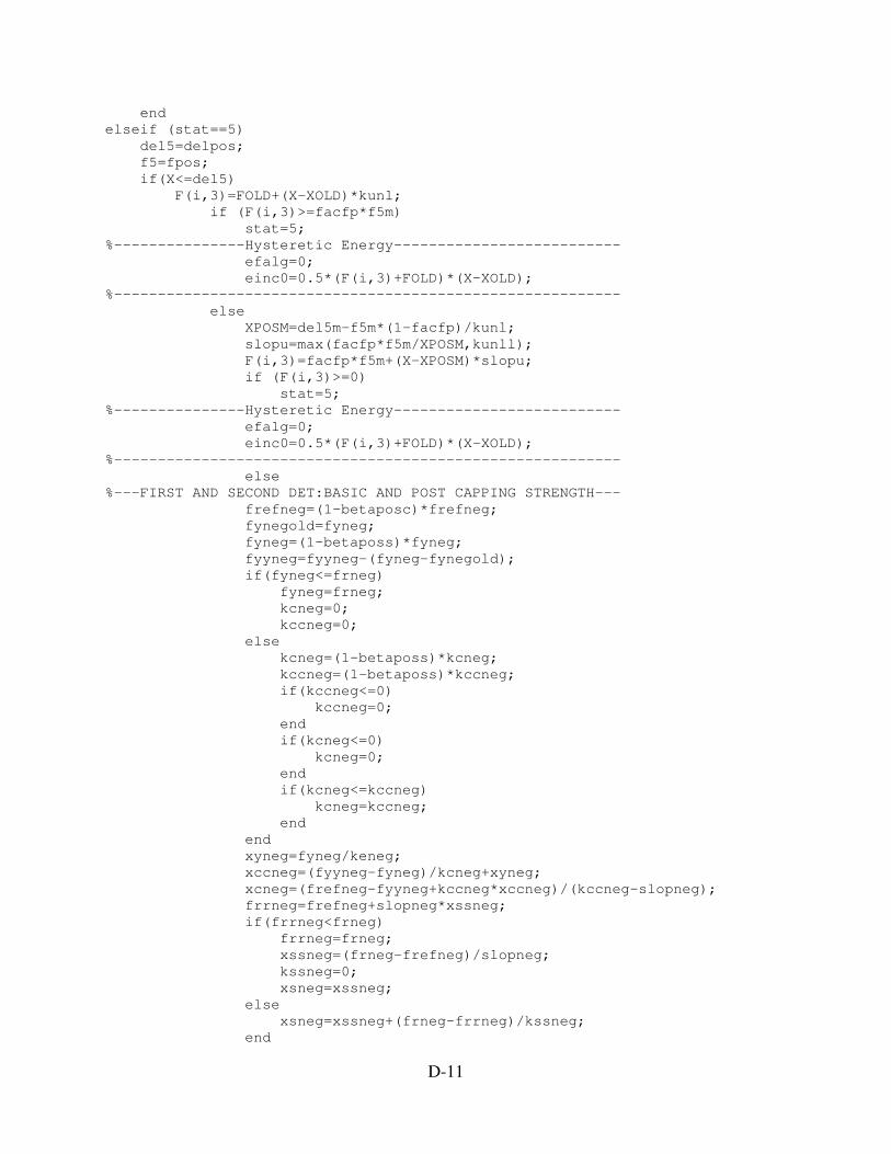
D-11
end
elseif (stat==5)
del5=delpos;
f5=fpos;
if(X<=del5)
F(i,3)=FOLD+(X-XOLD)*kunl;
if (F(i,3)>=facfp*f5m)
stat=5;
%---------------Hysteretic Energy--------------------------
efalg=0;
einc0=0.5*(F(i,3)+FOLD)*(X-XOLD);
%----------------------------------------------------------
else
XPOSM=del5m-f5m*(1-facfp)/kunl;
slopu=max(facfp*f5m/XPOSM,kunll);
F(i,3)=facfp*f5m+(X-XPOSM)*slopu;
if (F(i,3)>=0)
stat=5;
%---------------Hysteretic Energy--------------------------
efalg=0;
einc0=0.5*(F(i,3)+FOLD)*(X-XOLD);
%----------------------------------------------------------
else
%---FIRST AND SECOND DET:BASIC AND POST CAPPING STRENGTH---
frefneg=(1-betaposc)*frefneg;
fynegold=fyneg;
fyneg=(1-betaposs)*fyneg;
fyyneg=fyyneg-(fyneg-fynegold);
if(fyneg<=frneg)
fyneg=frneg;
kcneg=0;
kccneg=0;
else
kcneg=(1-betaposs)*kcneg;
kccneg=(1-betaposs)*kccneg;
if(kccneg<=0)
kccneg=0;
end
if(kcneg<=0)
kcneg=0;
end
if(kcneg<=kccneg)
kcneg=kccneg;
end
end
xyneg=fyneg/keneg;
xccneg=(fyyneg-fyneg)/kcneg+xyneg;
xcneg=(frefneg-fyyneg+kccneg*xccneg)/(kccneg-slopneg);
frrneg=frefneg+slopneg*xssneg;
if(frrneg<frneg)
frrneg=frneg;
xssneg=(frneg-frefneg)/slopneg;
kssneg=0;
xsneg=xssneg;
else
xsneg=xssneg+(frneg-frrneg)/kssneg;
end

D-12
funeg=fyyneg+kccneg*(xcneg-xccneg);
if((abs(delneg)>=xyneg)&&(abs(delneg)<=xccneg))
fneg=-(fyneg+kcneg*(abs(delneg)-xyneg));
elseif((abs(delneg)>xccneg)&&(abs(delneg)<=xcneg))
fneg=-(fyyneg+kccneg*(abs(delneg)-xccneg));
elseif((abs(delneg)>xcneg)&&(abs(delneg)<=xssneg))
fneg=-(funeg+ksneg*(abs(delneg)-xcneg));
elseif((abs(delneg)>xssneg)&&(abs(delneg)<=xsneg))
fneg=-(frrneg+kssneg*(abs(delneg)-xssneg));
else
fneg=-((abs(delneg)-xsneg)*krneg+frneg);
end
%---THIRD DET: UNLOADING STIFFNESS------------------------
kunl=(1-betaposk)*kunl;
%---FOURTH DET: ACCELERATED STIFF------------------------
delneg=(1+betaposa)*delneg;
if((abs(delneg)>=xyneg)&&(abs(delneg)<=xccneg))
fneg=-(fyneg+kcneg*(abs(delneg)-xyneg));
elseif((abs(delneg)>=xccneg)&&(abs(delneg)<=xcneg))
fneg=-(fyyneg+kccneg*(abs(delneg)-xccneg));
elseif((abs(delneg)>xcneg)&&(abs(delneg)<=xssneg))
fneg=-(funeg+ksneg*(abs(delneg)-xcneg));
elseif((abs(delneg)>xssneg)&&(abs(delneg)<=xsneg))
fneg=-(frrneg+kssneg*(abs(delneg)-xssneg));
else
fneg=-((abs(delneg)-xsneg)*krneg+frneg);
end
%---FIFTH DET: UNLOADING STIFFNESS-------------------------
kunll=(1-betaposkk)*kunll;
%---SIXTH DET: UNLOADING STIFFNESS-------------------------
krelp=(1-betaposkkk)*krelp;
%---------------------------------------------------------
delrespos=XOLD-FOLD/kunll;
if (delrespos<0)
delrespos=0;
end
stat=26;
if(flagl==0)
m26=kf*abs(fneg)/(delrespos-delneg);
F(i,3)=(X-delrespos)*m26;
else
m26=kf*abs(fneg)/(delrespos-delneg);
if(krelp<m26)
m266=m26;
else
y0=-krelp*delrespos;
if(abs(y0)>abs(kf*fneg))
m266=abs(kf*fneg)/delrespos;
m26=0;
else
m266=krelp;
m26=(abs(kf*fneg)-abs(y0))/(-delneg);
end
end
y0n=-m266*delrespos;
F(i,3)=(X-delrespos)*m266;

D-13
end
%---------------Hysteretic Energy--------------------------
efalg=2;
einc0=-0.5*FOLD*(XOLD-delrespos);
einc1=0.5*F(i,3)*(X-delrespos);
%----------------------------------------------------------
end
end
else
if(del5<=xccpos)
if(X<=xccpos)
F(i,3)=f5+kcpos*(X-del5);
stat=2;
%---------------Hysteretic Energy--------------------------
efalg=0;
einc0=0.5*(F(i,3)+f5)*(X-del5)+0.5*(f5+FOLD)*(del5-XOLD);
%----------------------------------------------------------
else
F(i,3)=fyypos+kccpos*(X-xccpos);
stat=200;
%---------------Hysteretic Energy--------------------------
efalg=0;
einc0=0.5*(F(i,3)+fyypos)*(X-xccpos)+0.5*(fyypos+f5)*(xccpos-
del5)+0.5*(f5+FOLD)*(del5-XOLD);
%----------------------------------------------------------
end
elseif(del5<=xcpos)
if(X<=xcpos)
F(i,3)=f5+kccpos*(X-del5);
stat=200;
%---------------Hysteretic Energy--------------------------
efalg=0;
einc0=0.5*(F(i,3)+f5)*(X-del5)+0.5*(f5+FOLD)*(del5-XOLD);
%----------------------------------------------------------
else
F(i,3)=fupos+kspos*(X-xcpos);
stat=3;
%---------------Hysteretic Energy--------------------------
efalg=0;
einc0=0.5*(F(i,3)+fupos)*(X-xcpos)+0.5*(fupos+f5)*(xcpos-
del5)+0.5*(f5+FOLD)*(del5-XOLD);
%----------------------------------------------------------
end
elseif(del5<=xsspos)
if(X<=xsspos)
F(i,3)=f5+kspos*(X-del5);
stat=3;
%---------------Hysteretic Energy--------------------------
efalg=0;
einc0=0.5*(F(i,3)+f5)*(X-del5)+0.5*(f5+FOLD)*(del5-XOLD);
%----------------------------------------------------------
else
F(i,3)=frrpos+ksspos*(X-xsspos);
stat=300;
%---------------Hysteretic Energy--------------------------
efalg=0;

D-14
einc0=0.5*(F(i,3)+frrpos)*(X-xsspos)+0.5*(frrpos+f5)*(xsspos-
del5)+0.5*(f5+FOLD)*(del5-XOLD);
%----------------------------------------------------------
end
elseif(del5<=xspos)
if(X<=xspos)
F(i,3)=f5+ksspos*(X-del5);
stat=300;
%---------------Hysteretic Energy--------------------------
efalg=0;
einc0=0.5*(F(i,3)+f5)*(X-del5)+0.5*(f5+FOLD)*(del5-XOLD);
%----------------------------------------------------------
else
F(i,3)=frpos+krpos*(X-xspos);
stat=4;
%---------------Hysteretic Energy--------------------------
efalg=0;
einc0=0.5*(F(i,3)+frpos)*(X-xspos)+0.5*(frpos+f5)*(xspos-
del5)+0.5*(f5+FOLD)*(del5-XOLD);
%----------------------------------------------------------
end
else
F(i,3)=f5+krpos*(X-del5);
stat=4;
%---------------Hysteretic Energy--------------------------
efalg=0;
einc0=0.5*(F(i,3)+f5)*(X-del5)+0.5*(f5+FOLD)*(del5-XOLD);
%----------------------------------------------------------
end
end
elseif (stat==25)
del25=delneg;
f25=fneg;
if(X>=del25)
F(i,3)=FOLD+(X-XOLD)*kunl;
if (F(i,3)<=facfp*f25m)
stat=25;
%---------------Hysteretic Energy--------------------------
efalg=1;
einc1=0.5*(F(i,3)+FOLD)*(X-XOLD);
%----------------------------------------------------------
else
XNEGM=del25m-f25m*(1-facfp)/kunl;
slopu=max(facfp*f25m/XNEGM,kunll);
F(i,3)=facfp*f25m+(X-XNEGM)*slopu;
if (F(i,3)<=0)
stat=25;
%---------------Hysteretic Energy--------------------------
efalg=1;
einc1=0.5*(F(i,3)+FOLD)*(X-XOLD);
%----------------------------------------------------------
else
%---FIRST AND SECOND DET:BASIC AND POST CAPPING STRENGTH---
frefpos=(1-betanegc)*frefpos;
fyposold=fypos;
fypos=(1-betanegs)*fypos;
fyypos=fyypos-(fypos-fyposold);

D-15
if(fypos<=frpos)
fypos=frpos;
kcpos=0;
kccpos=0;
else
kcpos=(1-betanegs)*kcpos;
kccpos=(1-betanegs)*kccpos;
if(kccpos<=0)
kccpos=0;
end
if(kcpos<=0)
kcpos=0;
end
if(kcpos<=kccpos)
kcpos=kccpos;
end
end
xypos=fypos/kepos;
xccpos=(fyypos-fypos)/kcpos+xypos;
xcpos=(frefpos-fyypos+kccpos*xccpos)/(kccpos-sloppos);
frrpos=frefpos+sloppos*xsspos;
if(frrpos<frpos)
frrpos=frpos;
xsspos=(frpos-frefpos)/sloppos;
ksspos=0;
xspos=xsspos;
else
xspos=xsspos+(frpos-frrpos)/ksspos;
end
fupos=fyypos+kccpos*(xcpos-xccpos);
if((delpos>=xypos)&&(delpos<=xccpos))
fpos=fypos+kcpos*(delpos-xypos);
elseif((delpos>xccpos)&&(delpos<=xcpos))
fpos=fyypos+kccpos*(delpos-xccpos);
elseif((delpos>xcpos)&&(delpos<=xsspos))
fpos=fupos+kspos*(delpos-xcpos);
elseif((delpos>xsspos)&&(delpos<=xspos))
fpos=frrpos+ksspos*(delpos-xsspos);
else
fpos=(delpos-xspos)*krpos+frpos;
end
%---THIRD DET: UNLOADING STIFFNESS------------------------
kunl=(1-betanegk)*kunl;
%---FOURTH DET: ACCELERATED STIFF------------------------
delpos=(1+betanega)*delpos;
if((delpos>=xypos)&&(delpos<=xccpos))
fpos=fypos+kcpos*(delpos-xypos);
elseif((delpos>=xccpos)&&(delpos<=xcpos))
fpos=fyypos+kccpos*(delpos-xccpos);
elseif((delpos>xcpos)&&(delpos<=xsspos))
fpos=fupos+kspos*(delpos-xcpos);
elseif((delpos>xsspos)&&(delpos<=xspos))
fpos=frrpos+ksspos*(delpos-xsspos);
else
fpos=(delpos-xspos)*krpos+frpos;
end
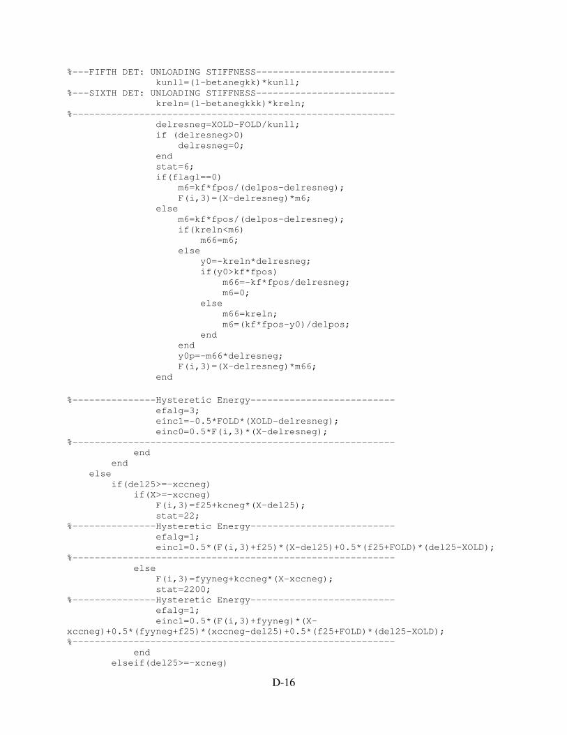
D-16
%---FIFTH DET: UNLOADING STIFFNESS-------------------------
kunll=(1-betanegkk)*kunll;
%---SIXTH DET: UNLOADING STIFFNESS-------------------------
kreln=(1-betanegkkk)*kreln;
%----------------------------------------------------------
delresneg=XOLD-FOLD/kunll;
if (delresneg>0)
delresneg=0;
end
stat=6;
if(flagl==0)
m6=kf*fpos/(delpos-delresneg);
F(i,3)=(X-delresneg)*m6;
else
m6=kf*fpos/(delpos-delresneg);
if(kreln<m6)
m66=m6;
else
y0=-kreln*delresneg;
if(y0>kf*fpos)
m66=-kf*fpos/delresneg;
m6=0;
else
m66=kreln;
m6=(kf*fpos-y0)/delpos;
end
end
y0p=-m66*delresneg;
F(i,3)=(X-delresneg)*m66;
end
%---------------Hysteretic Energy--------------------------
efalg=3;
einc1=-0.5*FOLD*(XOLD-delresneg);
einc0=0.5*F(i,3)*(X-delresneg);
%----------------------------------------------------------
end
end
else
if(del25>=-xccneg)
if(X>=-xccneg)
F(i,3)=f25+kcneg*(X-del25);
stat=22;
%---------------Hysteretic Energy--------------------------
efalg=1;
einc1=0.5*(F(i,3)+f25)*(X-del25)+0.5*(f25+FOLD)*(del25-XOLD);
%----------------------------------------------------------
else
F(i,3)=fyyneg+kccneg*(X-xccneg);
stat=2200;
%---------------Hysteretic Energy--------------------------
efalg=1;
einc1=0.5*(F(i,3)+fyyneg)*(X-
xccneg)+0.5*(fyyneg+f25)*(xccneg-del25)+0.5*(f25+FOLD)*(del25-XOLD);
%----------------------------------------------------------
end
elseif(del25>=-xcneg)

D-17
if(X>=-xcneg)
F(i,3)=f25+kccneg*(X-del25);
stat=2200;
%---------------Hysteretic Energy--------------------------
efalg=1;
einc1=0.5*(F(i,3)+f25)*(X-del25)+0.5*(f25+FOLD)*(del25-XOLD);
%----------------------------------------------------------
else
F(i,3)=funeg+ksneg*(X-xcneg);
stat=23;
%---------------Hysteretic Energy--------------------------
efalg=1;
einc1=0.5*(F(i,3)+funeg)*(X-xcneg)+0.5*(funeg+f25)*(xcneg-
del25)+0.5*(f25+FOLD)*(del25-XOLD);
%----------------------------------------------------------
end
elseif(del25>=-xssneg)
if(X>=-xssneg)
F(i,3)=f25+ksneg*(X-del25);
stat=23;
%---------------Hysteretic Energy--------------------------
efalg=1;
einc1=0.5*(F(i,3)+f25)*(X-del25)+0.5*(f25+FOLD)*(del25-XOLD);
%----------------------------------------------------------
else
F(i,3)=frrneg+kssneg*(X-xssneg);
stat=2300;
%---------------Hysteretic Energy--------------------------
efalg=1;
einc1=0.5*(F(i,3)+frrneg)*(X-
xssneg)+0.5*(frrneg+f25)*(xssneg-del25)+0.5*(f25+FOLD)*(del25-XOLD);
%----------------------------------------------------------
end
elseif(del25>=-xsneg)
if(X>=-xsneg)
F(i,3)=f25+kssneg*(X-del25);
stat=2300;
%---------------Hysteretic Energy--------------------------
efalg=1;
einc1=0.5*(F(i,3)+f25)*(X-del25)+0.5*(f25+FOLD)*(del25-XOLD);
%----------------------------------------------------------
else
F(i,3)=frneg+krneg*(X-xsneg);
stat=24;
%---------------Hysteretic Energy--------------------------
efalg=1;
einc1=0.5*(F(i,3)+frneg)*(X-xsneg)+0.5*(frneg+f25)*(xsneg-
del25)+0.5*(f25+FOLD)*(del25-XOLD);
%----------------------------------------------------------
end
else
F(i,3)=f25+krneg*(X-del25);
stat=24;
%---------------Hysteretic Energy--------------------------
efalg=1;
einc1=0.5*(F(i,3)+f25)*(X-del25)+0.5*(f25+FOLD)*(del25-XOLD);
%----------------------------------------------------------
D-18
end
end
elseif (stat==26)
if(X<(1-kd)*delresneg)
m27=((1-kf)*fneg+(delneg-(1-kd)*delresneg)*m26)/(delneg-(1-
kd)*delresneg);
if(flagl==0)
facx=((delrespos-(1-kd)*delresneg)/(delrespos-delneg))*kf*fneg;
else
facx=y0n+(1-kd)*delresneg*m26;
end
F(i,3)=m27*(X-(1-kd)*delresneg)+facx;
stat=27;
%---------------Hysteretic Energy--------------------------
efalg=1;
einc1=0.5*(F(i,3)+facx)*(X-(1-
kd)*delresneg)+0.5*(facx+FOLD)*((1-kd)*delresneg-XOLD);
%----------------------------------------------------------
else
if(X<=XOLD)
stat=26;
if(flagl==0)
F(i,3)=m26*(X-XOLD)+FOLD;
else
if(X>=-1e-6)
F(i,3)=m266*(X-XOLD)+FOLD;
else
F(i,3)=m26*(X-XOLD)+FOLD;
end
end
%---------------Hysteretic Energy--------------------------
efalg=1;
einc1=0.5*(F(i,3)+FOLD)*(X-XOLD);
%----------------------------------------------------------
else
F(i,3)=FOLD+(X-XOLD)*kunl;
stat=25;
del25m=XOLD;
f25m=FOLD;
%---------------Hysteretic Energy--------------------------
efalg=1;
einc1=0.5*(F(i,3)+FOLD)*(X-XOLD);
%---------------------------------------------------------
end
end
elseif (stat==27)
if(X<=delneg)
if(X>=-xccneg)
F(i,3)=-fyneg+kcneg*(X+xyneg);
stat=22;
%---------------Hysteretic Energy--------------------------
efalg=1;
einc1=0.5*(F(i,3)+fneg)*(X-delneg)+0.5*(fneg+FOLD)*(delneg-
XOLD);
%----------------------------------------------------------
elseif(X>=-xcneg)
F(i,3)=-fyyneg+kccneg*(X+xccneg);
D-19
stat=2200;
%---------------Hysteretic Energy--------------------------
efalg=1;
einc1=0.5*(F(i,3)+fneg)*(X-delneg)+0.5*(fneg+FOLD)*(delneg-
XOLD);
%----------------------------------------------------------
elseif(X>=-xssneg)
F(i,3)=-funeg+ksneg*(X+xcneg);
stat=23;
%---------------Hysteretic Energy--------------------------
efalg=1;
einc1=0.5*(F(i,3)+fneg)*(X-delneg)+0.5*(fneg+FOLD)*(delneg-
XOLD);
%----------------------------------------------------------
elseif(X>=-xsneg)
F(i,3)=-frrneg+kssneg*(X+xssneg);
stat=2300;
%---------------Hysteretic Energy--------------------------
efalg=1;
einc1=0.5*(F(i,3)+fneg)*(X-delneg)+0.5*(fneg+FOLD)*(delneg-
XOLD);
%----------------------------------------------------------
else
F(i,3)=-frneg+krneg*(X+xsneg);
stat=24;
%---------------Hysteretic Energy--------------------------
efalg=1;
einc1=0.5*(F(i,3)+fneg)*(X-delneg)+0.5*(fneg+FOLD)*(delneg-
XOLD);
%----------------------------------------------------------
end
else
if(X<=XOLD)
F(i,3)=m27*(X-XOLD)+FOLD;
stat=27;
%---------------Hysteretic Energy--------------------------
efalg=1;
einc1=0.5*(F(i,3)+FOLD)*(X-XOLD);
%----------------------------------------------------------
else
F(i,3)=FOLD+(X-XOLD)*kunl;
stat=25;
del25m=XOLD;
f25m=FOLD;
%---------------Hysteretic Energy--------------------------
efalg=1;
einc1=0.5*(F(i,3)+FOLD)*(X-XOLD);
%---------------------------------------------------------
end
end
elseif (stat==6)
if(X>(1-kd)*delrespos)
m7=((1-kf)*fpos+(delpos-(1-kd)*delrespos)*m6)/(delpos-(1-
kd)*delrespos);
if(flagl==0)
facx=((-delresneg+(1-kd)*delrespos)/(-delresneg+delpos))*kf*fpos;
else
D-20
facx=y0p+(1-kd)*delrespos*m6;
end
F(i,3)=m7*(X-(1-kd)*delrespos)+facx;
stat=7;
%---------------Hysteretic Energy--------------------------
efalg=0;
einc0=0.5*(F(i,3)+facx)*(X-(1-
kd)*delrespos)+0.5*(facx+FOLD)*((1-kd)*delrespos-XOLD);
%----------------------------------------------------------
else
if(X>=XOLD)
stat=6;
if(flagl==0)
F(i,3)=m6*(X-XOLD)+FOLD;
else
if(X<=1e-6)
F(i,3)=m66*(X-XOLD)+FOLD;
else
F(i,3)=m6*(X-XOLD)+FOLD;
end
end
%---------------Hysteretic Energy--------------------------
efalg=0;
einc0=0.5*(F(i,3)+FOLD)*(X-XOLD);
%----------------------------------------------------------
else
F(i,3)=FOLD+(X-XOLD)*kunl;
stat=5;
del5m=XOLD;
f5m=FOLD;
%---------------Hysteretic Energy--------------------------
efalg=0;
einc0=0.5*(F(i,3)+FOLD)*(X-XOLD);
%---------------------------------------------------------
end
end
elseif (stat==7)
if(X>delpos)
if(X<=xccpos)
F(i,3)=fypos+kcpos*(X-xypos);
stat=2;
%---------------Hysteretic Energy--------------------------
efalg=0;
einc0=0.5*(F(i,3)+fpos)*(X-delpos)+0.5*(fpos+FOLD)*(delpos-
XOLD);
%----------------------------------------------------------
elseif(X<=xcpos)
F(i,3)=fyypos+kccpos*(X-xccpos);
stat=200;
%---------------Hysteretic Energy--------------------------
efalg=0;
einc0=0.5*(F(i,3)+fpos)*(X-delpos)+0.5*(fpos+FOLD)*(delpos-
XOLD);
%----------------------------------------------------------
elseif(X<=xsspos)
F(i,3)=fupos+kspos*(X-xcpos);
stat=3;

D-21
%---------------Hysteretic Energy--------------------------
efalg=0;
einc0=0.5*(F(i,3)+fpos)*(X-delpos)+0.5*(fpos+FOLD)*(delpos-
XOLD);
%----------------------------------------------------------
elseif(X<=xspos)
F(i,3)=frrpos+ksspos*(X-xsspos);
stat=300;
%---------------Hysteretic Energy--------------------------
efalg=0;
einc0=0.5*(F(i,3)+fpos)*(X-delpos)+0.5*(fpos+FOLD)*(delpos-
XOLD);
%----------------------------------------------------------
else
F(i,3)=frpos+krpos*(X-xspos);
stat=4;
%---------------Hysteretic Energy--------------------------
efalg=0;
einc0=0.5*(F(i,3)+fpos)*(X-delpos)+0.5*(fpos+FOLD)*(delpos-
XOLD);
%----------------------------------------------------------
end
else
if(X>=XOLD)
F(i,3)=m7*(X-XOLD)+FOLD;
stat=7;
%---------------Hysteretic Energy--------------------------
efalg=0;
einc0=0.5*(F(i,3)+FOLD)*(X-XOLD);
%----------------------------------------------------------
else
F(i,3)=FOLD+(X-XOLD)*kunl;
stat=5;
del5m=XOLD;
f5m=FOLD;
%---------------Hysteretic Energy--------------------------
efalg=0;
einc0=0.5*(F(i,3)+FOLD)*(X-XOLD);
%---------------------------------------------------------
end
end
end
if (efalg==0)
sume=sume+einc0;
epos=epos+einc0;
if(epos<0)
epos=0;
end
elseif(efalg==1)
sume=sume+einc1;
eneg=eneg+einc1;
if(eneg<0)
eneg=0;
end
elseif(efalg==2)
sume=sume+einc0;

D-22
epos=epos+einc0;
if(epos<0)
epos=0;
end
if (detflag==1)
betaposs=(sume/etots)^erates;
betaposc=(sume/etotc)^eratec;
betaposa=(sume/etota)^eratea;
betaposk=(sume/etotk)^eratek;
betaposkk=(sume/etotkk)^eratekk;
betaposkkk=(sume/etotkkk)^eratekkk;
if(betaposs<=0)
betaposs=0;
elseif(betaposs>=1)
betaposs=1;
end
if(betaposc<=0)
betaposc=0;
elseif(betaposc>=1)
betaposc=1;
end
if(betaposa<=0)
betaposa=0;
elseif(betaposa>=1)
betaposa=1;
end
if(betaposk<=0)
betaposk=0;
elseif(betaposk>=1)
betaposk=1;
end
if(betaposkk<=0)
betaposkk=0;
elseif(betaposkk>=1)
betaposkk=1;
end
if(betaposkkk<=0)
betaposkkk=0;
elseif(betaposkkk>=1)
betaposkkk=1;
end
else
if(sume>=etots)
betaposs=1;
elseif((epos)/(etots-sume)>=1)
betaposs=1;
else
betaposs=((epos)/(etots-sume))^erates;
end
if(sume>=etotc)
betaposc=1;
elseif((epos)/(etotc-sume)>=1)
betaposc=1;
else
betaposc=((epos)/(etotc-sume))^eratec;
end

D-23
if(sume>=etota)
betaposa=1;
elseif((epos)/(etota-sume)>=1)
betaposa=1;
else
betaposa=((epos)/(etota-sume))^eratea;
end
if(sume>=etotk)
betaposk=1;
elseif((epos)/(etotk-sume)>=1)
betaposk=1;
else
betaposk=((epos)/(etotk-sume))^eratek;
end
if(sume>=etotkk)
betaposkk=1;
elseif((epos)/(etotkk-sume)>=1)
betaposkk=1;
else
betaposkk=((epos)/(etotkk-sume))^eratekk;
end
if(sume>=etotkkk)
betaposkkk=1;
elseif((epos)/(etotkkk-sume)>=1)
betaposkkk=1;
else
betaposkkk=((epos)/(etotkkk-sume))^eratekkk;
end
end
epos=0;
eneg=einc1;
sume=sume+einc1;
elseif(efalg==3)
sume=sume+einc1;
eneg=eneg+einc1;
if(eneg<0)
eneg=0;
end
if (detflag==1)
betanegs=(sume/etots)^erates;
betanegc=(sume/etotc)^eratec;
betanega=(sume/etota)^eratea;
if(betanegs<=0)
betanegs=0;
elseif(betanegs>=1)
betanegs=1;
end
if(betanegc<=0)
betanegc=0;
elseif(betanegc>=1)
betanegc=1;
end
if(betanega<=0)
D-24
betanega=0;
elseif(betanega>=1)
betanega=1;
end
if(betanegk<=0)
betanegk=0;
elseif(betanegk>=1)
betanegk=1;
end
if(betanegkk<=0)
betanegkk=0;
elseif(betanegkk>=1)
betanegkk=1;
end
if(betanegkkk<=0)
betanegkkk=0;
elseif(betanegkkk>=1)
betanegkkk=1;
end
else
if(sume>=etots)
betanegs=1;
elseif((eneg)/(etots-sume)>=1)
betanegs=1;
else
betanegs=((eneg)/(etots-sume))^erates;
end
if(sume>=etotc)
betanegc=1;
elseif((eneg)/(etotc-sume)>=1)
betanegc=1;
else
betanegc=((eneg)/(etotc-sume))^eratec;
end
if(sume>=etota)
betanega=1;
elseif((eneg)/(etota-sume)>=1)
betanega=1;
else
betanega=((eneg)/(etota-sume))^eratea;
end
if(sume>=etotk)
betanegk=1;
elseif((eneg)/(etotk-sume)>=1)
betanegk=1;
else
betanegk=((eneg)/(etotk-sume))^eratek;
end
if(sume>=etotkk)
betanegkk=1;
elseif((eneg)/(etotkk-sume)>=1)
betanegkk=1;
else
betanegkk=((eneg)/(etotkk-sume))^eratekk;
end
if(sume>=etotkkk)
betanegkkk=1;

D-25
elseif((eneg)/(etotkkk-sume)>=1)
betanegkkk=1;
else
betanegkkk=((eneg)/(etotkkk-sume))^eratekkk;
end
end
epos=einc0;
eneg=0;
sume=sume+einc0;
end
%{
F(i,4)=stat;
F(i,5)=betaposkkk;
F(i,6)=betanegkkk;
F(i,7)=betaposkk;
F(i,8)=betaposa;
F(i,9)=betanegs;
F(i,10)=betanegc;
F(i,11)=betanegk;
F(i,12)=betanegkk;
F(i,13)=betanega;
%}
end
plot(F(:,2),F(:,3));