�����������������

Citation: Zhang, Y.; Zou, Y. Study on

Corrective Abrasive Finishing for

Workpiece Surface by Using

Magnetic Abrasive Finishing

Processes. Machines 2022, 10, 98.

https://doi.org/10.3390/

machines10020098

Academic Editors: Kai Cheng,

Zewei Yuan and Mark J. Jackson

Received: 31 December 2021

Accepted: 26 January 2022

Published: 27 January 2022

Publisher’s Note: MDPI stays neutral

with regard to jurisdictional claims in

published maps and institutional affil-

iations.

Copyright: © 2022 by the authors.

Licensee MDPI, Basel, Switzerland.

This article is an open access article

distributed under the terms and

conditions of the Creative Commons

Attribution (CC BY) license (https://

creativecommons.org/licenses/by/

4.0/).

machines

Article

Study on Corrective Abrasive Finishing for Workpiece Surfaceby Using Magnetic Abrasive Finishing ProcessesYulong Zhang 1 and Yanhua Zou 2,*

1 Graduate School of Engineering, Utsunomiya University, 7-1-2 Yoto, Utsunomiya 321-8585, Japan;dt187178@cc.utsunomiya-u.ac.jp

2 School of Engineering, Course of Mechanical Engineering Systems, Utsunomiya University, 7-1-2 Yoto,Utsunomiya 321-8585, Japan

* Correspondence: yanhua@utsunomiya-u.ac.jp; Tel.: +81-28-689-6057

Abstract: In order to improve the plane quality of the workpiece shape accuracy, a correction abrasivefinishing method is proposed. This method is used to achieve the effect of correcting the workpiecesurface by changing the finishing conditions of different areas according to the profile of the initialsurface, such as feed speed. In previous research, the feasibility and effectiveness of this methodwere proven. In this research, a theoretical analysis of this method was carried out and the extensionof this method to the processing of larger planes was studied. Through a series of experiments onan aluminum plate (A5052), it was proven that the shape accuracy of the workpiece surface can beeffectively corrected by accurately controlling the feed speed. The experimental results showed thatthe extreme difference of the workpiece can be reduced from 4.81 µm to 2.65 µm within the processedarea of 30 mm by 10 mm.

Keywords: corrective finishing; magnetic abrasive finishing; surface profile; shape accuracy; speedcontrolled; aluminum alloy (A5052)

1. Introduction

With the rapid development of electronic technology, optical technology and aerospacetechnology, the requirements for workpiece surface accuracy in many fields are higher andhigher. For these components, their surfaces are required to be smooth, have low roughness,and have high geometric accuracy. The magnetic abrasive finishing (MAF) process is animportant non-traditional finishing process [1,2]. The MAF process uses magnetic particlesto form a flexible brush structure under the action of a magnetic field, mixing abrasiveparticles with magnetic particles, and using the motor to drive the magnetic brush to rotateso as to drive the abrasive particles to move relative to the workpiece and to realize thefinishing of the workpiece [3].

Shinmura et al. proposed and designed a plane MAF device, analyzed the processprinciple of plane MAF, and discussed the effect of the supply weight of finishing fluid andmagnetic abrasion on the finishing depth and surface roughness [4]. Yamaguchi studiedthe use of magnetic grinding technology to process the inside of a round tube [5]. In orderto solve the disadvantage of a weak magnetic force when processing thick tubes, Zou et al.proposed a processing method that could improve the magnetic force and made it possibleto process the inside of thick non-ferromagnetic tubing [6]. Because the magnetic brushformed in the magnetic field has a certain flexibility and can conform to the shape of theworkpiece, it is applied to the processing of various irregular shapes, such as the innerand outer surfaces of a tube, irregular surfaces, and so on. In order to improve processingefficiency, researchers combined MAF with other processing methods. Based on the MAFprinciples, additional ultrasonic vibration is used to achieve a high-quality workpiecesurface [7,8]. Mulik et al. employed ultrasonic vibration in the horizontal direction of theworkpiece using an ultrasonic power, a piezoelectric transducer, and a horn device [9].

Machines 2022, 10, 98. https://doi.org/10.3390/machines10020098 https://www.mdpi.com/journal/machines

Machines 2022, 10, 98 2 of 17

A high-frequency electrical signal was generated by ultrasonic power and transformedinto a horizontal mechanical vibration by the transducer. In order to further improve theprocessing efficiency of magnetic grinding, Zou et al. made different attempts and proposeda variety of processing methods. They proposed a processing method combining the MAFprocess with electrolytic technology [10–12] and a processing method that combined MAFwith fixed abrasive polishing technology [13]. They analyzed the process mechanisms andfinishing characteristics and proved that the purpose of improving processing efficiency canbe achieved by these methods through experiments. They also proposed a MAF processusing an alternating magnetic field. Compared with a static magnetic field, the MAFprocess using an alternating magnetic field can achieve higher finishing efficiency andsurface quality [14–16].

With the continuous development and improvement of MAF technology, higherrequirements for this technology are put forward. In order to make the magnetic fieldof finishing tools more uniform, a lot of research was carried out to change the shape ofthe magnetic pole, such as adding grooves, improving finishing tracks, and so on. Sincethe magnetic abrasive finishing process is a machining process using a magnetic brushwith flexible machining behavior, the process can be used for finishing free-form surfacesand improving surface accuracy without destroying the profile of the workpiece [17–19].However, because the magnetic brush is not a uniform finishing tool, further research isstill needed to maintain the geometric accuracy of the workpiece or correct the geometry,which is also the research content of this subject. Zou et al. calculated the trajectory toelevate the surface quality of plane magnetic abrasive finishing. The finishing trajectorycould be predicted by combining the revolution motion of the magnetic brush, the polerotation motion, and the linear reciprocating motion of the workpiece to investigate thefinishing results [20,21]. They conducted further studies on this method and proved thatthe revolution radius was an important factor affecting the surface flatness and proposedan effective method for evaluating the surface topography [22].

Through a series of experiments and theoretical analysis, this research uses magneticabrasive finishing technology to realize the plane correction of the workpiece. In order tofurther solve the problem of uniformity of finishing, a method of forming a small magneticbrush with a small magnetic pole is proposed in this research. According to the initialprofile of the surface, the finishing in different positions is controlled at different feed speeds.Through the analysis and finishing of the collected surface profile data, and according to thefinishing characteristics of the magnetic brush, the feed speed distribution in the finishingprocess is planned to make the effective finishing time at different positions different, andfinally to improve the surface flatness.

2. Processing Principle2.1. Processing Principle of Magnetic Abrasive Finishing

MAF is a precision finishing process, which realizes the finishing of the workpiece bydriving the abrasive particles to move relative to the workpiece through a flexible magneticbrush formed by magnetic particles under the action of a magnetic field. Figure 1 is aschematic diagram of the principle of the MAF process. The magnetic pole and magneticparticles are magnetized under the action of the magnet and the magnetic particles arearranged in order to form a brush-like structure. The abrasive particles are mixed withinthe brush-like structure and driven to rotate and to move relative to the workpiece, togetherwith the magnet, magnetic pole, and magnetic brush, by the motor, so the workpiece canbe finished.

Figure 1 shows the schematic diagram of the magnetic force acting on a magneticparticle at point A in a magnetic field. Fx and Fy can be calculated by Equations (1) and(2) [3,4].

Fx = Vχµ0H(

∂H∂x

)(1)

Machines 2022, 10, 98 3 of 17

Fy = Vχµ0H(

∂H∂y

)(2)

where x is the direction of the line of magnetic force, y is the direction of the magneticequipotential line, V is the volume of magnetic particle, χ is the susceptibility of particles,µ0 is the permeability of vacuum, H is the magnetic field intensity at point A, ∂H/∂x and∂H/∂y are gradients of magnetic field intensity in x and y directions, respectively.

Machines 2022, 9, x FOR PEER REVIEW 3 of 18

Figure 1. Schematic of finishing principle.

Figure 1 shows the schematic diagram of the magnetic force acting on a magnetic

particle at point A in a magnetic field. �� and �� can be calculated by Equations (1) and (2)

[3,4].

�� � �χ�� ��� (1)

�� � �χ�� ��� (2)

where � is the direction of the line of magnetic force, � is the direction of the magnetic

equipotential line, � is the volume of magnetic particle, � is the susceptibility of particles,

�� is the permeability of vacuum, is the magnetic field intensity at point A, �/ ∂� and

�/ ∂� are gradients of magnetic field intensity in � and � directions, respectively.

2.2. Processing Principle of Corrective Magnetic Abrasive Finishing

Based on Preston’s Law (Preston, 1927), the Integrated Material Removal Rate

(IMRR) is proportional to the polishing tool pressure on the surface of the workpiece and

the relative velocity between the tool and the workpiece [23]. The material removal

amount satisfies the following formula:

�� � ����, �����, ����, (3)

where �� is the amount of material removal, � is the removal factor, ��, �� is the coordi-

nate of a point on the plane. The ���, �� is the pressure at the point ��, ��, ���, �� is the

resultant velocity of the tool relative to the workpiece, and �� is the finishing time. When

the magnetic field strength, the composition of the abrasion liquid and the working gap

are constant, the amount of material removal is dependent on ���, �� and �� [24].

Previous studies have proven that the planar quality of the processed area can be

improved by controlling the feed speed of the workpiece, but only a single track was fin-

ished [25]. Now the finishing area needs to be extended to a larger planar area. Assuming

that the initial profile of the workpiece is shown in Figure 2, and its profile curves are

shown as in the figure in the direction �, due to the flexibility of the magnetic brush, the

workpiece can be finished and its roughness can be reduced while maintaining the origi-

nal profile of the workpiece. However, from another point of view, can magnetic abrasive

finishing technology be used to reduce the height difference of the surface and improve

its flatness? A simple method that is easy to think of is to change the processing time or

feed speed at different positions. For example, where the surface is high, the feed speed is

slower and the processing time is longer. On the contrary, where the surface is low, the

Feed motion

Magnetic particles

Abrasive

particles ��

� ��

�

�

Rotation

Workpiece

Magnetic

pole

Figure 1. Schematic of finishing principle.

2.2. Processing Principle of Corrective Magnetic Abrasive Finishing

Based on Preston’s Law (Preston, 1927), the Integrated Material Removal Rate (IMRR)is proportional to the polishing tool pressure on the surface of the workpiece and therelative velocity between the tool and the workpiece [23]. The material removal amountsatisfies the following formula:

dM = kP(x, y)V(x, y)dt, (3)

where dM is the amount of material removal, k is the removal factor, (x, y) is the coordinateof a point on the plane. The P(x, y) is the pressure at the point (x, y), V(x, y) is the resultantvelocity of the tool relative to the workpiece, and dt is the finishing time. When the magneticfield strength, the composition of the abrasion liquid and the working gap are constant, theamount of material removal is dependent on V(x, y) and dt [24].

Previous studies have proven that the planar quality of the processed area can beimproved by controlling the feed speed of the workpiece, but only a single track wasfinished [25]. Now the finishing area needs to be extended to a larger planar area. Assumingthat the initial profile of the workpiece is shown in Figure 2, and its profile curves areshown as in the figure in the direction x, due to the flexibility of the magnetic brush, theworkpiece can be finished and its roughness can be reduced while maintaining the originalprofile of the workpiece. However, from another point of view, can magnetic abrasivefinishing technology be used to reduce the height difference of the surface and improveits flatness? A simple method that is easy to think of is to change the processing time orfeed speed at different positions. For example, where the surface is high, the feed speed isslower and the processing time is longer. On the contrary, where the surface is low, the feedspeed is faster and the processing time is shorter. In other words, the purpose of correctingthe plane can be realized by controlling the motion conditions during finishing.

Machines 2022, 10, 98 4 of 17

Machines 2022, 9, x FOR PEER REVIEW 4 of 18

feed speed is faster and the processing time is shorter. In other words, the purpose of

correcting the plane can be realized by controlling the motion conditions during finishing.

However, for the magnetic brush, the processing efficiency of the point with different

positions from the center point is different. There are many reasons, such as the different

linear velocity of rotation, different magnetic field intensities and many other factors.

Therefore, it is not an easy thing to plan the processing speed well. In order to prove the

effectiveness of the corrective MAF method, theoretical analysis and experimental verifi-

cation are carried out, and it was proved that the surface range can be reduced from 14.317

μm to 2.18 μm by the experiments [19]. However, only a single trajectory was carried out

in the previous study, and further discussion and research are still needed if this finishing

is to be extended to the larger plane range.

Figure 2. The principle of corrective magnetic abrasive finishing.

At present, the amount of material removal is usually described according to Pres-

ton’s Equation [26]. The Preston equation is related to the pressure, relative velocity and

residence time in the contact area [27], as shown in Equation (3).

If the density of the workpiece is �, the contact area between the workpiece and the

magnetic brush is �, and the removal depth of the material is ℎ. Then � � ���ℎ, which is

substituted into Equation (3), meaning the following equation will be obtained:

�� � ���ℎ � ���ℎ � ����, �����, ����, (4)

where �ℎ is the removal depth at ��, �� on the workpiece surface at �� time. The material

removal curve generated within dwell time t is expressed as:

ℎ��, �� � !" # ����, �����, ����$

� , (5)

In the finishing process, the movement of the particles consists of a circular motion

and feed motion relative to the workpiece. When the feed speed is very small, the particle

velocity can be approximately equal to the linear velocity of the circular motion. To sim-

plify the model, in this research, it is considered that the velocity of the particle relative to

the workpiece is approximately equal to %&. Where % is the angular velocity of circular

motion, & is the distance between the particle and the axis of rotation, which is the radius

of the circular motion. Therefore, when the angular velocity % is constant, ���, �� is al-

most unchanged. From Equation (5), it can be seen that the amount of material removal

only depends on the finishing time �. The processing time is inversely proportional to the

feed speed ', so the corrective finishing of the workpiece can be realized by controlling

the feed speed. Then the key is how to calculate the feed speed according to the profile

curves.

x

y

h

Δy

Profile curves Surface:h(x,y)

N

S

Figure 2. The principle of corrective magnetic abrasive finishing.

However, for the magnetic brush, the processing efficiency of the point with differentpositions from the center point is different. There are many reasons, such as the differentlinear velocity of rotation, different magnetic field intensities and many other factors.Therefore, it is not an easy thing to plan the processing speed well. In order to provethe effectiveness of the corrective MAF method, theoretical analysis and experimentalverification are carried out, and it was proved that the surface range can be reduced from14.317 µm to 2.18 µm by the experiments [19]. However, only a single trajectory wascarried out in the previous study, and further discussion and research are still needed ifthis finishing is to be extended to the larger plane range.

At present, the amount of material removal is usually described according to Preston’sEquation [26]. The Preston equation is related to the pressure, relative velocity and residencetime in the contact area [27], as shown in Equation (3).

If the density of the workpiece is ρ, the contact area between the workpiece and themagnetic brush is A, and the removal depth of the material is h. Then M = dρAh, which issubstituted into Equation (3), meaning the following equation will be obtained:

dM = dρAh = ρAdh = kP(x, y)V(x, y)dt, (4)

where dh is the removal depth at (x, y) on the workpiece surface at dt time. The materialremoval curve generated within dwell time t is expressed as:

h(x, y) =1

ρA

∫ t

0kP(x, y)V(x, y)dt, (5)

In the finishing process, the movement of the particles consists of a circular motionand feed motion relative to the workpiece. When the feed speed is very small, the particlevelocity can be approximately equal to the linear velocity of the circular motion. To simplifythe model, in this research, it is considered that the velocity of the particle relative to theworkpiece is approximately equal to ωr. Where ω is the angular velocity of circular motion,r is the distance between the particle and the axis of rotation, which is the radius of thecircular motion. Therefore, when the angular velocity ω is constant, V(x, y) is almostunchanged. From Equation (5), it can be seen that the amount of material removal onlydepends on the finishing time t. The processing time is inversely proportional to the feedspeed v, so the corrective finishing of the workpiece can be realized by controlling the feedspeed. Then the key is how to calculate the feed speed according to the profile curves.

2.3. Calculation of Feed Speed Array

First of all, the initial profile data of the workpiece need to be measured. In thisresearch, the initial height H0(Si) at position Si is obtained by Surftest (SV-624-3D, Mitutoyo,

Machines 2022, 10, 98 5 of 17

2200 Shimogurimachi, Utsunomiya City, Tochigi Prefecture 321-0923). Si is the abscissa ofthe i-th sampling point in the x-direction. Then, it is necessary to calculate the feed speedv(Si) at different positions. To facilitate the processing of data, the original data are filteredand H(Si) is obtained after filtering with:

H(Si) =∑i+m−1

i H0(Si)

m, (6)

Here, the method of mean filtering is adopted. Where Si is the position of the i-thsampling point and m is the width of the data to be filtered, which is the number of data tobe averaged every time. Then, in order to calculate the processing time and feed speed,it is necessary to set the height h0 of the target finishing line. Therefore removed heightsequence h(Si) at each position can be calculated according to:

h(Si) = H(Si)− h0, (7)

Thereby, the processed height transformation sequence is obtained. Assuming thefinishing efficiency is η µm min−1, then the finishing time t(Si) for each position is:

t(Si) =h(Si)

η, (8)

Then, assuming that it needs n loops to finish the workpiece, the displacement changeis ∆S, the speed at each position is:

v(Si) =2n∆St(Si)

, (9)

Because the composite velocity of the particles is the vector sum of the rotation speedand the feed speed, and the rotation speed is much faster than the feed speed, the influenceof the feed speed on the composite velocity is ignored here. The feed speed only changesthe finishing time. Then, at high places, the speed v(Si) is slow, the time t(Si) is long, andin low places, the speed v(Si) is fast and the time t(Si) is short. Reorganizing the aboveequations yields:

v(Si) = 2n∆S/[h(Si)/η] = 2nη∆S/h(Si), (10)

It can be seen that when the finishing parameters are unchanged, η is a constant.Therefore, v(Si) is inversely proportional to h(Si).

v(Si)h(Si) = v(Si + 1)h(Si + 1) = 2nη∆S, (11)

This is:v(Si + 1) = v(Si)h(Si)/h(Si + 1), (12)

To facilitate the calculation, v(S1) should be obtained first, and then all regionalvelocity arrays v(Si) can be solved according to the above recurrence in Equation (12). Itcan be seen that the feed speed is inversely proportional to the initial height. Therefore, bycontrolling the feed speed, the profile characteristics of the surface can be improved.

Figure 3a shows a profile curve after filtering. If the finishing efficiency η is known,the relationship between the processing time curve and the position can be calculatedaccording to Equation (8), as shown in Figure 3b. Then, according to Equations (9) and (12),the speed sequence can be calculated, as shown in Figure 3c.

Machines 2022, 10, 98 6 of 17

Machines 2022, 9, x FOR PEER REVIEW 6 of 18

according to the speed curve shown in Figure 3c. However, the curve of velocity versus

the position needs to be converted to a curve of velocity versus time. In this way, due to

the control error, it may not be able to accurately correspond to the displacement and

velocity.

Another way is to control the position of the motor, dividing the speed curve into

several segments, and calculating the average speed of each segment, as shown in Figure

3c, which is the speed curve segmented according to 1 mm for one segment. It can be seen

that the velocity curve is basically the same as before the segmentation. In fact, the original

velocity curve is also equivalent to the curve obtained by 0.01 mm in each section, because

the data sampling interval is 0.01 mm. For this equidistant scheme, the smaller the dis-

tance of the partitions, the closer the resulting curve is to the target velocity curve.

But when the division is too small, the speed of the motor will change frequently,

which requires high performance from the motor. Therefore, the standard of the segmen-

tation curve can be changed according to the characteristics of the workpiece profile curve.

In this study, the segments are divided according to the height variation range of the pro-

file curve. A certain fixed height difference is used as the standard for dividing the area.

When the height change is less than this value, it is regarded as an area. In order to facili-

tate the use of this area division method, it can be performed after filtering. A practical

example of the division result is shown in Figure 3a. Here, Δℎ is set to 2 μm.

Figure 3. The curves of dividing the height, time and speed into segments.

The number of changes of the speed curve obtained is reduced according to the sec-

ond method, which is convenient for control. After segmentation, the average height of

each segment is calculated to obtain the approximate curve of the workpiece surface.

Then, according to this curve, the processing time curve is calculated. Thus, the finishing

speed curve after segmentation is calculated as shown in Figure 3d.

0

1

2

3

4

5

6

7

0 10 20 30 40 50 60Pro

cess

ing t

ime

t (m

in)

Position S (mm)

(b)The curve of processing time

0.0

0.1

0.2

0.3

0.4

0.5

0.6

0.7

0.00 20.00 40.00 60.00

Fee

d s

pee

d v

(mm

/s)

Position S (mm)

(c) The curve of feed speed by every milimeter

0.0

0.1

0.2

0.3

0.4

0.5

0.6

0.00 20.00 40.00 60.00

Fee

d s

pee

d v

(mm

/s)

Position S (mm)

(d) The curve of feed speed by segments

0

2

4

6

8

10

12

14

0 10 20 30 40 50 60

Hei

ght

H(μ

m)

Position S (mm)

(a) Cut the profile curve into segments

Figure 3. The curves of dividing the height, time and speed into segments.

So now the key problem is how to make the control system control the motor to moveaccording to the feed speed curve. The specific realization method is determined by theactual mechanical structure and motor control mode. One way to achieve this is to directlycontrol the speed of the motor by using analog quantities, which can make the motor runaccording to the speed curve shown in Figure 3c. However, the curve of velocity versus theposition needs to be converted to a curve of velocity versus time. In this way, due to thecontrol error, it may not be able to accurately correspond to the displacement and velocity.

Another way is to control the position of the motor, dividing the speed curve intoseveral segments, and calculating the average speed of each segment, as shown in Figure 3c,which is the speed curve segmented according to 1 mm for one segment. It can be seenthat the velocity curve is basically the same as before the segmentation. In fact, the originalvelocity curve is also equivalent to the curve obtained by 0.01 mm in each section, becausethe data sampling interval is 0.01 mm. For this equidistant scheme, the smaller the distanceof the partitions, the closer the resulting curve is to the target velocity curve.

But when the division is too small, the speed of the motor will change frequently, whichrequires high performance from the motor. Therefore, the standard of the segmentationcurve can be changed according to the characteristics of the workpiece profile curve. In thisstudy, the segments are divided according to the height variation range of the profile curve.A certain fixed height difference is used as the standard for dividing the area. When theheight change is less than this value, it is regarded as an area. In order to facilitate the useof this area division method, it can be performed after filtering. A practical example of thedivision result is shown in Figure 3a. Here, ∆h is set to 2 µm.

The number of changes of the speed curve obtained is reduced according to the secondmethod, which is convenient for control. After segmentation, the average height of eachsegment is calculated to obtain the approximate curve of the workpiece surface. Then,according to this curve, the processing time curve is calculated. Thus, the finishing speedcurve after segmentation is calculated as shown in Figure 3d.

Machines 2022, 10, 98 7 of 17

3. Experimental Stage3.1. Experimental Setup

Figure 4 is the system structure diagram of the experimental setup. It includes debug-ging computer, motion control circuit board, X-Y stage driver, linear slide driver, and DCmotor driver. The computer programs the STM32 circuit board by USB to control the pro-cessing position, feed speed and rotation speed. The STM32 control board communicateswith the X-Y stage driver through the RS232 interface to control the processing position andtrajectory. The STM32 control board communicates with the linear motor driver throughthe RS485 interface to realize the control of the feed speed. The STM32 control board usesDAC to directly output analog signals to control the speed of the DC motor.

Machines 2022, 9, x FOR PEER REVIEW 7 of 18

3. Experimental Stage

3.1. Experimental Setup

Figure 4 is the system structure diagram of the experimental setup. It includes de-

bugging computer, motion control circuit board, X-Y stage driver, linear slide driver, and

DC motor driver. The computer programs the STM32 circuit board by USB to control the

processing position, feed speed and rotation speed. The STM32 control board communi-

cates with the X-Y stage driver through the RS232 interface to control the processing po-

sition and trajectory. The STM32 control board communicates with the linear motor driver

through the RS485 interface to realize the control of the feed speed. The STM32 control

board uses DAC to directly output analog signals to control the speed of the DC motor.

YA

PC Control UnitSTM32

Linear slider Driver

DC MotorDriver

X-Y Stage Driver

Linear sliderX-Y Stage

DCMotor

X

DAC RS-485+DIORS-232

USB

Workpiece

M

Figure 4. Schematic of experimental setup.

A photo of the experimental setup used in this research is shown in Figure 5. The X-

Y stage is used to control the processing position of the workpiece. The DC motor drives

the magnetic poles and the magnetic brush rotation to process the workpiece. The linear

feed motor realizes the control of the feed speed by changing its speed to realize variable

speed processing. The height adjustment device is used to adjust the processing gap,

which can be accurate to 0.1 mm.

Figure 4. Schematic of experimental setup.

A photo of the experimental setup used in this research is shown in Figure 5. TheX-Y stage is used to control the processing position of the workpiece. The DC motor drivesthe magnetic poles and the magnetic brush rotation to process the workpiece. The linearfeed motor realizes the control of the feed speed by changing its speed to realize variablespeed processing. The height adjustment device is used to adjust the processing gap, whichcan be accurate to 0.1 mm.

3.2. Magnetic Field Analysis

Figure 6 shows the simulation results of the magnetic field around the magnetic poleusing Magnet 7 software. It can be seen from Figure 6a that the magnetic field at the lowerend of the magnetic pole is stronger. In order to more specifically reflect the change of themagnetic field intensity, the curves of the magnetic field intensity were drawn respectivelyon a line segment with a length of 10 mm at a distance of 0 mm and 0.2 mm from the lowersurface of the magnetic pole. It can be seen from Figure 6b that there is an obvious edgeeffect on the surface of the magnetic pole, and the magnetic field intensity in the center ismuch smaller than that at the edges. However, at a distance of 0.2 mm from the surface ofthe magnetic pole, as shown in Figure 6c, the magnetic field is relatively uniform. This isconducive to the uniform pressure of the magnetic brush.

Machines 2022, 10, 98 8 of 17Machines 2022, 9, x FOR PEER REVIEW 8 of 18

Figure 5. Experimental setup.

3.2. Magnetic Field Analysis

Figure 6 shows the simulation results of the magnetic field around the magnetic pole

using Magnet 7 software. It can be seen from Figure 6a that the magnetic field at the lower

end of the magnetic pole is stronger. In order to more specifically reflect the change of the

magnetic field intensity, the curves of the magnetic field intensity were drawn respec-

tively on a line segment with a length of 10 mm at a distance of 0 mm and 0.2 mm from

the lower surface of the magnetic pole. It can be seen from Figure 6b that there is an obvi-

ous edge effect on the surface of the magnetic pole, and the magnetic field intensity in the

center is much smaller than that at the edges. However, at a distance of 0.2 mm from the

surface of the magnetic pole, as shown in Figure 6c, the magnetic field is relatively uni-

form. This is conducive to the uniform pressure of the magnetic brush.

Magnetic pole Magnet

Workpiece

Magnetic plate (iron plate)

(a)

(c) Start=(−5,−0.2,0), End=(+5,−0.2,0)

Distance (mm)

Val

ue

of

|B| (

T)

1.4 1.3 1.2 1.1 1.0 0.9 0.8 0.7 0.6 0.5 0.4 0.3 0.2 0.1

10

9.5

9.0

8.5

8.0

7.5

7.0

6.5

6.0

5.5

5.0

4.5

4.0

3.5

3.0

2.5

1.5

1.0

0.5

0

2.0

(b) Start=(−5,0,0), End=(+5,0,0)

Distance (mm)

Val

ue

of

|B| (

T)

2.3

1.9

1.5

0.9 0.7 0.5 0.3 0.1

10

9.5

9.0

8.5

8.0

7.5

7.0

6.5

6.0

5.5

5.0

4.5

4.0

3.5

3.0

2.5

1.5

1.0

0.5

0

2.0

2.1

1.7

1.3 1.1

DC motor

Linear slider

Magnetic pole

Clearance

adjustment

X-Y stage

Workpiece

Magnet

Gap display

Figure 5. Experimental setup.

Machines 2022, 9, x FOR PEER REVIEW 8 of 18

Figure 5. Experimental setup.

3.2. Magnetic Field Analysis

Figure 6 shows the simulation results of the magnetic field around the magnetic pole

using Magnet 7 software. It can be seen from Figure 6a that the magnetic field at the lower

end of the magnetic pole is stronger. In order to more specifically reflect the change of the

magnetic field intensity, the curves of the magnetic field intensity were drawn respec-

tively on a line segment with a length of 10 mm at a distance of 0 mm and 0.2 mm from

the lower surface of the magnetic pole. It can be seen from Figure 6b that there is an obvi-

ous edge effect on the surface of the magnetic pole, and the magnetic field intensity in the

center is much smaller than that at the edges. However, at a distance of 0.2 mm from the

surface of the magnetic pole, as shown in Figure 6c, the magnetic field is relatively uni-

form. This is conducive to the uniform pressure of the magnetic brush.

Magnetic pole Magnet

Workpiece

Magnetic plate (iron plate)

(a)

(c) Start=(−5,−0.2,0), End=(+5,−0.2,0)

Distance (mm)

Val

ue

of

|B| (

T)

1.4 1.3 1.2 1.1 1.0 0.9 0.8 0.7 0.6 0.5 0.4 0.3 0.2 0.1

10

9.5

9.0

8.5

8.0

7.5

7.0

6.5

6.0

5.5

5.0

4.5

4.0

3.5

3.0

2.5

1.5

1.0

0.5

0

2.0

(b) Start=(−5,0,0), End=(+5,0,0)

Distance (mm)

Val

ue

of

|B| (

T)

2.3

1.9

1.5

0.9 0.7 0.5 0.3 0.1

10

9.5

9.0

8.5

8.0

7.5

7.0

6.5

6.0

5.5

5.0

4.5

4.0

3.5

3.0

2.5

1.5

1.0

0.5

0

2.0

2.1

1.7

1.3 1.1

DC motor

Linear slider

Magnetic pole

Clearance

adjustment

X-Y stage

Workpiece

Magnet

Gap display

Figure 6. The simulations with magnetic particles and with the magnetic plate under the workpiece.(a) The magnetic field distribution near the magnetic pole; (b) The magnetic field intensity |B| at adistance of 0 mm from the magnetic pole; (c) The magnetic field intensity |B| at a distance of 0.2 mmfrom the magnetic pole.

Machines 2022, 10, 98 9 of 17

Figure 7 shows the results of measuring the magnetic field near the magnetic poleusing the Tesla meter. Within 10 mm on both sides of the magnetic pole, the distancesbetween the sensor and the surface of the magnetic pole are set to 0 mm, 0.5 mm and1.0 mm. It can be seen from the measurement results that as the distance increases, themagnetic field strength becomes weaker and weaker. However, due to the small magneticpole diameter, the edge effect of magnetic field strength is weakened.

Machines 2022, 9, x FOR PEER REVIEW 9 of 18

Figure 6. The simulations with magnetic particles and with the magnetic plate under the workpiece.

(a) The magnetic field distribution near the magnetic pole; (b) The magnetic field intensity |B| at a

distance of 0 mm from the magnetic pole; (c) The magnetic field intensity |B| at a distance of 0.2

mm from the magnetic pole.

Figure 7 shows the results of measuring the magnetic field near the magnetic pole

using the Tesla meter. Within 10 mm on both sides of the magnetic pole, the distances

between the sensor and the surface of the magnetic pole are set to 0 mm, 0.5 mm and 1.0

mm. It can be seen from the measurement results that as the distance increases, the mag-

netic field strength becomes weaker and weaker. However, due to the small magnetic pole

diameter, the edge effect of magnetic field strength is weakened.

Figure 7. The measured results of magnetic field.

3.3. Force Analysis

In order to better analyze the characteristics of the magnetic pole, a device is designed

to measure the pressure distribution of the magnetic brush during processing. The meas-

urement method is shown in Figure 8. The pressure sensor used here is the LMA-A-5N

small pressure sensor from KYOWA. The pressure can be converted into an electrical sig-

nal by the sensor, which is amplified by an amplifier and sends the data to a recording

instrument. In this research, the amplifier used is the CDV-700A (KYOWA, Chofugaoka

3-5-1, Chofu, Tokyo, 182-8520), and the data logging instrument is the LOGGER GL240

(Graphtec Corporation, 58/3-5 4th Floor, Sukhumvit 63 (Ekkamai) Rd., Phra Khanong-

Nuea, Wattana, Bangkok 10110, Thailand).

050

100150200250300350400450

Val

ue

of

|B| (

mT

)

Position (mm)

0mm 0.5mm 1mm

−10.0 −5.0 0.0 5.0 10.0

Figure 7. The measured results of magnetic field.

3.3. Force Analysis

In order to better analyze the characteristics of the magnetic pole, a device is designedto measure the pressure distribution of the magnetic brush during processing. The mea-surement method is shown in Figure 8. The pressure sensor used here is the LMA-A-5Nsmall pressure sensor from KYOWA. The pressure can be converted into an electrical signalby the sensor, which is amplified by an amplifier and sends the data to a recording instru-ment. In this research, the amplifier used is the CDV-700A (KYOWA, Chofugaoka 3-5-1,Chofu, Tokyo, 182-8520), and the data logging instrument is the LOGGER GL240 (GraphtecCorporation, 58/3-5 4th Floor, Sukhumvit 63 (Ekkamai) Rd., Phra Khanong-Nuea, Wattana,Bangkok 10110, Thailand).

Machines 2022, 9, x FOR PEER REVIEW 10 of 18

Figure 8. Schematic diagram of pressure measuring device structure.

Figure 9 shows the measurement results of the pressure exerted by the magnetic

brush on the workpiece. When the gap is 0.2 mm, the pressure near the magnetic brush is

between 0.463 N and 0.716 N.

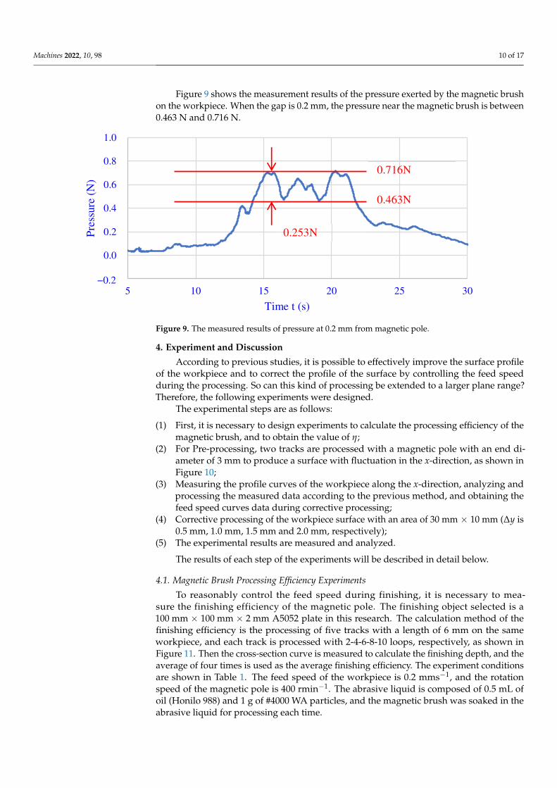
Figure 9. The measured results of pressure at 0.2 mm from magnetic pole.

4. Experiment and Discussion

According to previous studies, it is possible to effectively improve the surface profile

of the workpiece and to correct the profile of the surface by controlling the feed speed

during the processing. So can this kind of processing be extended to a larger plane range?

Therefore, the following experiments were designed.

The experimental steps are as follows:

(1) First, it is necessary to design experiments to calculate the processing efficiency of

the magnetic brush, and to obtain the value of ?;

N

S

LOGGER GL240

CDV-700A

LMA-A-5N

-0.2

0.0

0.2

0.4

0.6

0.8

1.0

5 10 15 20 25 30

Pre

ssur

e (N

)

Time t (s)

0.716N

0.463N

0.253N

−0.2

Figure 8. Schematic diagram of pressure measuring device structure.

Machines 2022, 10, 98 10 of 17

Figure 9 shows the measurement results of the pressure exerted by the magnetic brushon the workpiece. When the gap is 0.2 mm, the pressure near the magnetic brush is between0.463 N and 0.716 N.

Machines 2022, 9, x FOR PEER REVIEW 10 of 18

Figure 8. Schematic diagram of pressure measuring device structure.

Figure 9 shows the measurement results of the pressure exerted by the magnetic

brush on the workpiece. When the gap is 0.2 mm, the pressure near the magnetic brush is

between 0.463 N and 0.716 N.

Figure 9. The measured results of pressure at 0.2 mm from magnetic pole.

4. Experiment and Discussion

According to previous studies, it is possible to effectively improve the surface profile

of the workpiece and to correct the profile of the surface by controlling the feed speed

during the processing. So can this kind of processing be extended to a larger plane range?

Therefore, the following experiments were designed.

The experimental steps are as follows:

(1) First, it is necessary to design experiments to calculate the processing efficiency of

the magnetic brush, and to obtain the value of ?;

N

S

LOGGER GL240

CDV-700A

LMA-A-5N

-0.2

0.0

0.2

0.4

0.6

0.8

1.0

5 10 15 20 25 30

Pre

ssur

e (N

)

Time t (s)

0.716N

0.463N

0.253N

−0.2

Figure 9. The measured results of pressure at 0.2 mm from magnetic pole.

4. Experiment and Discussion

According to previous studies, it is possible to effectively improve the surface profileof the workpiece and to correct the profile of the surface by controlling the feed speedduring the processing. So can this kind of processing be extended to a larger plane range?Therefore, the following experiments were designed.

The experimental steps are as follows:

(1) First, it is necessary to design experiments to calculate the processing efficiency of themagnetic brush, and to obtain the value of η;

(2) For Pre-processing, two tracks are processed with a magnetic pole with an end di-ameter of 3 mm to produce a surface with fluctuation in the x-direction, as shown inFigure 10;

(3) Measuring the profile curves of the workpiece along the x-direction, analyzing andprocessing the measured data according to the previous method, and obtaining thefeed speed curves data during corrective processing;

(4) Corrective processing of the workpiece surface with an area of 30 mm × 10 mm (∆y is0.5 mm, 1.0 mm, 1.5 mm and 2.0 mm, respectively);

(5) The experimental results are measured and analyzed.

The results of each step of the experiments will be described in detail below.

4.1. Magnetic Brush Processing Efficiency Experiments

To reasonably control the feed speed during finishing, it is necessary to mea-sure the finishing efficiency of the magnetic pole. The finishing object selected is a100 mm × 100 mm × 2 mm A5052 plate in this research. The calculation method of thefinishing efficiency is the processing of five tracks with a length of 6 mm on the sameworkpiece, and each track is processed with 2-4-6-8-10 loops, respectively, as shown inFigure 11. Then the cross-section curve is measured to calculate the finishing depth, and theaverage of four times is used as the average finishing efficiency. The experiment conditionsare shown in Table 1. The feed speed of the workpiece is 0.2 mms−1, and the rotationspeed of the magnetic pole is 400 rmin−1. The abrasive liquid is composed of 0.5 mL ofoil (Honilo 988) and 1 g of #4000 WA particles, and the magnetic brush was soaked in theabrasive liquid for processing each time.

Machines 2022, 10, 98 11 of 17

Machines 2022, 9, x FOR PEER REVIEW 11 of 18

(2) For Pre-processing, two tracks are processed with a magnetic pole with an end diam-

eter of 3 mm to produce a surface with fluctuation in the x-direction, as shown in

Figure 10;

(3) Measuring the profile curves of the workpiece along the x-direction, analyzing and

processing the measured data according to the previous method, and obtaining the

feed speed curves data during corrective processing;

(4) Corrective processing of the workpiece surface with an area of 30 mm C 10 mm (∆�

is 0.5 mm, 1.0 mm, 1.5 mm and 2.0 mm, respectively);

(5) The experimental results are measured and analyzed.

The results of each step of the experiments will be described in detail below.

Figure 10. Schematic diagram of processing position.

4.1. Magnetic Brush Processing Efficiency Experiments

To reasonably control the feed speed during finishing, it is necessary to measure the

finishing efficiency of the magnetic pole. The finishing object selected is a 100 mm × 100

mm × 2 mm A5052 plate in this research. The calculation method of the finishing efficiency

is the processing of five tracks with a length of 6 mm on the same workpiece, and each

track is processed with 2-4-6-8-10 loops, respectively, as shown in Figure 11. Then the

cross-section curve is measured to calculate the finishing depth, and the average of four

times is used as the average finishing efficiency. The experiment conditions are shown in

Table 1. The feed speed of the workpiece is 0.2 mms−1, and the rotation speed of the mag-

netic pole is 400 rmin−1. The abrasive liquid is composed of 0.5 mL of oil (Honilo 988) and

1 g of #4000 WA particles, and the magnetic brush was soaked in the abrasive liquid for

processing each time.

x

y

Δy

Length:30 mm

Start

Width:10 mm

Pre-processing tracks

Figure 10. Schematic diagram of processing position.

Machines 2022, 9, x FOR PEER REVIEW 12 of 18

Figure 11. Evaluation of finishing efficiency.

Table 1. Experimental conditions of evaluating finishing efficiency.

Workpiece A5052 plate (100 mm × 100 mm × 2 mm)

Magnetic pole Nd-Fe-B rare earth permanent magnet (Φ1 × 35 mm)

Magnetic abrasive 0.02 g of 149 μm iron powder

Abrasion liquid 0.5 mL of oil (Honilo 988) and 1 g of #4000 WA particles

Clearance 0.2 mm

Finishing distance 6 mm

Finishing loops 2-4-6-8-10 loops

Feed speed 0.2 mm s−1

Rotation speed 400 r min−1

Figure 12 is the average value of the finishing depth of each group according to the

finishing method described above. As the times of reciprocating finishing increase, the

finishing depth becomes deeper. Moreover, the finishing depth has a linear relationship

with the number of reciprocations. After calculation, the average height reduction of the

one loop process is about 1.88 μm.

Figure 12. The relationship between reciprocating times and processing depth.

4.2. Pre-Processing Experiment

Pre-processing is processing two traces using a magnetic pole with an end face di-

ameter of 3 mm. Figure 13 shows a photo of the workpiece after pre-processing. Then, the

profile of the workpiece is measured along the direction perpendicular to the prepro-

cessing. Many curves are measured at an interval of 1 mm by Surftest (SV-624-3D). The

2.373

6.824

10.454

13.963

18.779

0

5

10

15

20

0 2 4 6 8 10 12Dth

: F

inis

hin

g d

epth

(μ

m)

Tms: Times of reciprocating finishing

2 Loops

4 Loops

6 Loops

8 Loops

10 Loops

Measuring

Figure 11. Evaluation of finishing efficiency.

Figure 12 is the average value of the finishing depth of each group according to thefinishing method described above. As the times of reciprocating finishing increase, thefinishing depth becomes deeper. Moreover, the finishing depth has a linear relationshipwith the number of reciprocations. After calculation, the average height reduction of theone loop process is about 1.88 µm.

Machines 2022, 10, 98 12 of 17

Table 1. Experimental conditions of evaluating finishing efficiency.

Workpiece A5052 plate (100 mm × 100 mm × 2 mm)

Magnetic pole Nd-Fe-B rare earth permanent magnet (Φ1 × 35 mm)

Magnetic abrasive 0.02 g of 149 µm iron powder

Abrasion liquid 0.5 mL of oil (Honilo 988) and 1 g of #4000 WA particles

Clearance 0.2 mm

Finishing distance 6 mm

Finishing loops 2-4-6-8-10 loops

Feed speed 0.2 mm s−1

Rotation speed 400 r min−1

Machines 2022, 9, x FOR PEER REVIEW 12 of 18

Figure 11. Evaluation of finishing efficiency.

Table 1. Experimental conditions of evaluating finishing efficiency.

Workpiece A5052 plate (100 mm × 100 mm × 2 mm)

Magnetic pole Nd-Fe-B rare earth permanent magnet (Φ1 × 35 mm)

Magnetic abrasive 0.02 g of 149 μm iron powder

Abrasion liquid 0.5 mL of oil (Honilo 988) and 1 g of #4000 WA particles

Clearance 0.2 mm

Finishing distance 6 mm

Finishing loops 2-4-6-8-10 loops

Feed speed 0.2 mm s−1

Rotation speed 400 r min−1

Figure 12 is the average value of the finishing depth of each group according to the

finishing method described above. As the times of reciprocating finishing increase, the

finishing depth becomes deeper. Moreover, the finishing depth has a linear relationship

with the number of reciprocations. After calculation, the average height reduction of the

one loop process is about 1.88 μm.

Figure 12. The relationship between reciprocating times and processing depth.

4.2. Pre-Processing Experiment

Pre-processing is processing two traces using a magnetic pole with an end face di-

ameter of 3 mm. Figure 13 shows a photo of the workpiece after pre-processing. Then, the

profile of the workpiece is measured along the direction perpendicular to the prepro-

cessing. Many curves are measured at an interval of 1 mm by Surftest (SV-624-3D). The

2.373

6.824

10.454

13.963

18.779

0

5

10

15

20

0 2 4 6 8 10 12Dth

: F

inis

hin

g d

epth

(μ

m)

Tms: Times of reciprocating finishing

2 Loops

4 Loops

6 Loops

8 Loops

10 Loops

Measuring

Figure 12. The relationship between reciprocating times and processing depth.

4.2. Pre-Processing Experiment

Pre-processing is processing two traces using a magnetic pole with an end face diam-eter of 3 mm. Figure 13 shows a photo of the workpiece after pre-processing. Then, theprofile of the workpiece is measured along the direction perpendicular to the preprocessing.Many curves are measured at an interval of 1 mm by Surftest (SV-624-3D). The data ob-tained are used to calculate the speed curves of the correction finishing. The preprocessingconditions of the experiments are shown in Table 2.

Machines 2022, 9, x FOR PEER REVIEW 13 of 18

data obtained are used to calculate the speed curves of the correction finishing. The pre-

processing conditions of the experiments are shown in Table 2.

Figure 13. The workpiece after pre-processing.

Table 2. Experimental conditions of preparation finishing.

Workpiece A5052 plate (100 mm × 100 mm × 2 mm)

Magnetic pole Nd-Fe-B rare earth permanent magnet (Φ3 × 35 mm)

Magnetic abrasive 0.5 g of 149 μm iron powder

Abrasion liquid 0.5 mL of oil (Honilo 988) and 1 g of #4000 WA particles

Clearance 0.2 mm

Finishing distance 80 mm

Finishing time 40 min

Feed speed 0.5 mms−1

Rotation speed 400 rmin−1

Figure 14a shows the 3D figure and Figure 14b shows a cross-sectional curve of the

surface profile of the workpiece after pre-processing. Since the pre-processing is processed

by using a uniform feed speed, the cross-sectional curves at different positions are almost

the same.

Figure 14. The measurement result of the workpiece surface after pre-processing: (a) The 3D figure

after pre-processing; (b) A cross-sectional curve after pre-processing.

(a) The 3D figure after pre-processing

4.81 μm

15.000 30.000[mm] 0.000 4.018 mm/cm.×2.489

−8

.61

1.5

55

9.2

23

[μm

] 2

.00

0 μ

m/c

m.×

50

00

.00

0 (b) A cross-sectional curve after pre-processing

80 m

m

10 mm

Measuring

direction

Pre-processing

direction

30 mm

Figure 13. The workpiece after pre-processing.

Machines 2022, 10, 98 13 of 17

Table 2. Experimental conditions of preparation finishing.

Workpiece A5052 plate (100 mm × 100 mm × 2 mm)

Magnetic pole Nd-Fe-B rare earth permanent magnet (Φ3 × 35 mm)

Magnetic abrasive 0.5 g of 149 µm iron powder

Abrasion liquid 0.5 mL of oil (Honilo 988) and 1 g of #4000 WA particles

Clearance 0.2 mm

Finishing distance 80 mm

Finishing time 40 min

Feed speed 0.5 mms−1

Rotation speed 400 rmin−1

Figure 14a shows the 3D figure and Figure 14b shows a cross-sectional curve of thesurface profile of the workpiece after pre-processing. Since the pre-processing is processedby using a uniform feed speed, the cross-sectional curves at different positions are almostthe same.

Machines 2022, 9, x FOR PEER REVIEW 13 of 18

data obtained are used to calculate the speed curves of the correction finishing. The pre-

processing conditions of the experiments are shown in Table 2.

Figure 13. The workpiece after pre-processing.

Table 2. Experimental conditions of preparation finishing.

Workpiece A5052 plate (100 mm × 100 mm × 2 mm)

Magnetic pole Nd-Fe-B rare earth permanent magnet (Φ3 × 35 mm)

Magnetic abrasive 0.5 g of 149 μm iron powder

Abrasion liquid 0.5 mL of oil (Honilo 988) and 1 g of #4000 WA particles

Clearance 0.2 mm

Finishing distance 80 mm

Finishing time 40 min

Feed speed 0.5 mms−1

Rotation speed 400 rmin−1

Figure 14a shows the 3D figure and Figure 14b shows a cross-sectional curve of the

surface profile of the workpiece after pre-processing. Since the pre-processing is processed

by using a uniform feed speed, the cross-sectional curves at different positions are almost

the same.

Figure 14. The measurement result of the workpiece surface after pre-processing: (a) The 3D figure

after pre-processing; (b) A cross-sectional curve after pre-processing.

(a) The 3D figure after pre-processing

4.81 μm

15.000 30.000[mm] 0.000 4.018 mm/cm.×2.489

−8

.61

1.5

55

9.2

23

[μm

] 2

.00

0 μ

m/c

m.×

50

00

.00

0 (b) A cross-sectional curve after pre-processing

80 m

m

10 mm

Measuring

direction

Pre-processing

direction

30 mm

Figure 14. The measurement result of the workpiece surface after pre-processing: (a) The 3D figureafter pre-processing; (b) A cross-sectional curve after pre-processing.

4.3. Corrective Finishing Experiments

A photo of the processed workpiece is shown in Figure 15. It can be seen from thepicture that as the step size of ∆y decreases, the surface becomes more uniform. The tracesof the transition between the two processing tracks are also reduced. When ∆y is 0.5 mmor 1.0 mm, the traces of this transition are not obvious. When ∆y is 0.5 mm, the tracesof this transition are almost indistinguishable with the naked eye. However, in terms ofprocessing time, a long processing time is required at 0.5 mm spacing, so the efficiency isslightly lower. The measurement results will be compared below.

Figure 16 is a 3D figure of the processed workpiece surface measured by a roughnessmeasuring instrument (Surftest: SV-624-3D). The measurement method is to measure agroup of section curves at 0.5 mm intervals to draw 3D figures. It can be seen from thefigure that when ∆y is 2 mm and 1.5 mm, there are obvious transition traces. When thespacing is 1 mm and 0.5 mm, the traces are not very obvious and the two traces producedby the pre-processing are no longer obvious. The surface was processed to be smooth.

In order to be able to see the difference in experimental results more clearly, thecross-sections of the processing area were measured along the x and y directions. Themeasurement results are shown in Figures 17 and 18.

Machines 2022, 10, 98 14 of 17

Machines 2022, 9, x FOR PEER REVIEW 14 of 18

4.3. Corrective Finishing Experiments

A photo of the processed workpiece is shown in Figure 15. It can be seen from the

picture that as the step size of ∆y decreases, the surface becomes more uniform. The traces

of the transition between the two processing tracks are also reduced. When Δy is 0.5 mm

or 1.0 mm, the traces of this transition are not obvious. When Δy is 0.5 mm, the traces of

this transition are almost indistinguishable with the naked eye. However, in terms of pro-

cessing time, a long processing time is required at 0.5 mm spacing, so the efficiency is

slightly lower. The measurement results will be compared below.

Figure 15. The photograph of the surface of the workpiece after processing.

Figure 16 is a 3D figure of the processed workpiece surface measured by a roughness

measuring instrument (Surftest: SV-624-3D). The measurement method is to measure a

group of section curves at 0.5 mm intervals to draw 3D figures. It can be seen from the

figure that when ∆y is 2 mm and 1.5 mm, there are obvious transition traces. When the

spacing is 1 mm and 0.5 mm, the traces are not very obvious and the two traces produced

by the pre-processing are no longer obvious. The surface was processed to be smooth.

In order to be able to see the difference in experimental results more clearly, the cross-

sections of the processing area were measured along the x and y directions. The measure-

ment results are shown in Figures 17 and 18.

As shown in Figure 17, the x-direction is the direction measured along the processing

feed direction. It can be seen that the surface was significantly improved compared with

before processing, and the surface of Δy = 1.0 mm and 0.5 mm is relatively flat. This is

because when ∆y is equal to 1.0 mm and 0.5 mm, the processing time is relatively long,

and when ∆y is equal to 1.5 mm and 2.0 mm, the processing time is relatively short.

The y-direction is the direction measured along the translation direction of the trajec-

tory, as shown in Figure 18. In this direction, the transition of the processing track during

translation can be clearly seen. For example, when Δy = 2.0 mm, there are five obvious

transition intervals. When Δy = 1.5 mm, there are six obvious transition intervals. When

Δy = 1.0 mm and 0.5 mm, the transition becomes inconspicuous. With the decrease in Δy,

the transition is no longer obvious, and the surface is almost flat. This shows that the

smaller Δy is, the better the processing effect is. However, when Δy decreases, the time of

the processing becomes longer. For example, when Δy = 2.0 mm, six lines need to be pro-

cessed. The processing time of each line is about 1 min, so the processing time is 6 min.

When Δy = 1.0 mm, 11 lines need to be processed, so the processing time is 11 min. When

Δy = 0.5 mm, 21 lines need to be processed, so the processing time is 21 min.

x

y

∆� � 2.0 mm

∆� � 1.5 mm

∆� � 1.0 mm

∆� � 0.5 mm

Figure 15. The photograph of the surface of the workpiece after processing.

Machines 2022, 9, x FOR PEER REVIEW 15 of 18

Figure 16. Three-dimensional figures of the processed surface: (a) The 3D figure after processing at

∆y = 2.0 mm; (b) The 3D figure after processing at ∆y = 1.5 mm; (c) The 3D figure after processing at

∆y = 1.0 mm; (d) The 3D figure after processing at ∆y = 0.5 mm.

(a) ∆� � 2.0 mm (b) ∆� � 1.5 mm

(c) ∆� � 1.0 mm (d) ∆� � 0.5 mm

∆� � 2.0 mm

3.19 μm

(a)

15.000 30.000[mm] 0.000 4.018 mm/cm.×2.489

−8

.61

0

0.3

06

9.2

23

[μm

] 2

.00

0 μ

m/c

m.×

50

00

.00

0 ∆� � 1.5mm

3.15 μm

(b)

15.000 30.000[mm] 0.000 4.018 mm/cm.×2.489

−8

.61

0

0.3

06

9.2

23

[μm

] 2

.00

0 μ

m/c

m.×

50

00

.00

0

∆� � 0.5 mm

2.65 μm

15.000 30.000[mm] 0.000 4.018 mm/cm.×2.489

−8

.61

0

0.3

06

9.2

23

[μm

] 2

.00

0 μ

m/c

m.×

50

00

.00

0 (d) ∆� � 1.0 mm

2.94 μm

(c)

15.000 30.000[mm] 0.000 4.018 mm/cm.×2.489

−8

.61

0

0.3

06

9.2

23

[μm

] 2

.00

0 μ

m/c

m.×

50

00

.00

0

Figure 16. Three-dimensional figures of the processed surface: (a) The 3D figure after processing at∆y = 2.0 mm; (b) The 3D figure after processing at ∆y = 1.5 mm; (c) The 3D figure after processing at∆y = 1.0 mm; (d) The 3D figure after processing at ∆y = 0.5 mm.

Machines 2022, 10, 98 15 of 17

Machines 2022, 9, x FOR PEER REVIEW 15 of 18

Figure 16. Three-dimensional figures of the processed surface: (a) The 3D figure after processing at

∆y = 2.0 mm; (b) The 3D figure after processing at ∆y = 1.5 mm; (c) The 3D figure after processing at

∆y = 1.0 mm; (d) The 3D figure after processing at ∆y = 0.5 mm.

(a) ∆� � 2.0 mm (b) ∆� � 1.5 mm

(c) ∆� � 1.0 mm (d) ∆� � 0.5 mm

∆� � 2.0 mm

3.19 μm

(a)

15.000 30.000[mm] 0.000 4.018 mm/cm.×2.489

−8

.61

0

0.3

06

9.2

23

[μm

] 2

.00

0 μ

m/c

m.×

50

00

.00

0 ∆� � 1.5mm

3.15 μm

(b)

15.000 30.000[mm] 0.000 4.018 mm/cm.×2.489

−8

.61

0

0.3

06

9.2

23

[μm

] 2

.00

0 μ

m/c

m.×

50

00

.00

0

∆� � 0.5 mm

2.65 μm

15.000 30.000[mm] 0.000 4.018 mm/cm.×2.489

−8

.61

0

0.3

06

9.2

23

[μm

] 2

.00

0 μ

m/c

m.×

50

00

.00

0 (d) ∆� � 1.0 mm

2.94 μm

(c)

15.000 30.000[mm] 0.000 4.018 mm/cm.×2.489

−8

.61

0

0.3

06

9.2

23

[μm

] 2

.00

0 μ

m/c

m.×

50

00

.00

0

Figure 17. The cross-section curves of the surface along the x-direction after processing: (a) Thecross-section curves at ∆y = 2.0 mm; (b) The cross-section curves at ∆y = 1.5 mm; (c) The cross-sectioncurves at ∆y = 1.0 mm; (d) The cross-section curves at ∆y = 0.5 mm.

Machines 2022, 9, x FOR PEER REVIEW 16 of 18

Figure 17. The cross-section curves of the surface along the x-direction after processing: (a) The

cross-section curves at ∆y = 2.0 mm; (b) The cross-section curves at ∆y = 1.5 mm; (c) The cross-section

curves at ∆y = 1.0 mm; (d) The cross-section curves at ∆y = 0.5 mm.

Figure 18. The cross-section curves of the surface along the y-direction after processing: (a) The

cross-section curves at ∆y = 2.0 mm; (b) The cross-section curves at ∆y = 1.5 mm; (c) The cross-section

curves at ∆y = 1.0 mm; (d) The cross-section curves at ∆y = 0.5 mm.

5. Conclusions

In this research, a surface corrective processing method is proposed and can be sum-

marized as follows:

(1) In the feed direction (�-direction), variable speed finishing has an obvious effect on

the surface correction. However, when Δ� decreases, the processing time becomes

longer, so the correction effect is better.

(2) When correcting the surface of the workpiece through speed control, the smaller the

step length of the processing track, the smaller the trace of surface transition, but it

takes a longer processing time. This experiment proves that the processing effect at

Δ� �1.0 mm is almost the same as that at Δ� � 0.5 mm, but the processing time is

reduced by half. In variable speed correction finishing, there is a certain correction

effect under different Δ� conditions, but when Δ� is large, it will produce transition

traces to the profile in the �-direction. When Δ� drops to 1.0 mm, the transition traces

are almost gone.

(3) The experimental results show that the speed control method can be used to correct

the surface profile of the workpiece. The extreme difference can be reduced from 4.81

μm to 2.65 μm within a processed area of 30 mm by 10 mm.

Author Contributions: Conceptualization, Y.Z. (Yulong Zhang) and Y.Z. (Yanhua Zou); Data cura-

tion, Y.Z. (Yulong Zhang); Formal analysis, Y.Z. (Yulong Zhang); Funding acquisition, Y.Z. (Yanhua

Zou); Investigation, Y.Z. (Yulong Zhang) and Y.Z. (Yanhua Zou); Methodology, Y.Z. (Yulong

Zhang) and Y.Z. (Yanhua Zou); Project administration, Y.Z. (Yanhua Zou); Validation, Y.Z. (Yulong

Zhang) and Y.Z. (Yanhua Zou); Writing—original draft, Y.Z. (Yulong Zhang) and Y.Z. (Yanhua

(a) ∆� � 2.0 mm

1.92 μm

5.000 10.000[mm] 0.000 0.628 mm/cm.×15.928

−9

.43

6

0.5

19

8.3

97

[μm

] 2

.00

0 μ

m/c

m.×

50

00

.00

0 (b) ∆� � 1.5 mm

1.31 μm

5.000 10.000[mm] 0.000 0.628 mm/cm.×15.928

−9

.43

6

0.5

19

8.3

97

[μm

] 2

.00

0 μ

m/c

m.×

50

00

.00

0

(c) ∆� � 1.0 mm

1.05 μm

5.000 10.000[mm] 0.000 0.628 mm/cm.×15.928

−9

.43

6

0.5

19

8.3

97

[μm

] 2

.00

0 μ

m/c

m.×

50

00

.00

0

(d) ∆� � 1.5 mm

1.14 μm

5.000 10.000[mm] 0.000 0.628 mm/cm.×15.928

−9

.43

6

0.5

19

8.3

97

[μm

] 2

.00

0 μ

m/c

m.×

50

00

.00

0

Figure 18. The cross-section curves of the surface along the y-direction after processing: (a) Thecross-section curves at ∆y = 2.0 mm; (b) The cross-section curves at ∆y = 1.5 mm; (c) The cross-sectioncurves at ∆y = 1.0 mm; (d) The cross-section curves at ∆y = 0.5 mm.

Machines 2022, 10, 98 16 of 17

As shown in Figure 17, the x-direction is the direction measured along the processingfeed direction. It can be seen that the surface was significantly improved compared withbefore processing, and the surface of ∆y = 1.0 mm and 0.5 mm is relatively flat. This isbecause when ∆y is equal to 1.0 mm and 0.5 mm, the processing time is relatively long, andwhen ∆y is equal to 1.5 mm and 2.0 mm, the processing time is relatively short.

The y-direction is the direction measured along the translation direction of the trajec-tory, as shown in Figure 18. In this direction, the transition of the processing track duringtranslation can be clearly seen. For example, when ∆y = 2.0 mm, there are five obvioustransition intervals. When ∆y = 1.5 mm, there are six obvious transition intervals. When∆y = 1.0 mm and 0.5 mm, the transition becomes inconspicuous. With the decrease in∆y, the transition is no longer obvious, and the surface is almost flat. This shows that thesmaller ∆y is, the better the processing effect is. However, when ∆y decreases, the timeof the processing becomes longer. For example, when ∆y = 2.0 mm, six lines need to beprocessed. The processing time of each line is about 1 min, so the processing time is 6 min.When ∆y = 1.0 mm, 11 lines need to be processed, so the processing time is 11 min. When∆y = 0.5 mm, 21 lines need to be processed, so the processing time is 21 min.

5. Conclusions

In this research, a surface corrective processing method is proposed and can be sum-marized as follows:

(1) In the feed direction (x-direction), variable speed finishing has an obvious effect on thesurface correction. However, when ∆y decreases, the processing time becomes longer,so the correction effect is better.

(2) When correcting the surface of the workpiece through speed control, the smaller thestep length of the processing track, the smaller the trace of surface transition, but ittakes a longer processing time. This experiment proves that the processing effect at∆y = 1.0 mm is almost the same as that at ∆y = 0.5 mm, but the processing time isreduced by half. In variable speed correction finishing, there is a certain correctioneffect under different ∆y conditions, but when ∆y is large, it will produce transitiontraces to the profile in the y-direction. When ∆y drops to 1.0 mm, the transition tracesare almost gone.

(3) The experimental results show that the speed control method can be used to correctthe surface profile of the workpiece. The extreme difference can be reduced from4.81 µm to 2.65 µm within a processed area of 30 mm by 10 mm.

Author Contributions: Conceptualization, Y.Z. (Yulong Zhang) and Y.Z. (Yanhua Zou); Data curation,Y.Z. (Yulong Zhang); Formal analysis, Y.Z. (Yulong Zhang); Funding acquisition, Y.Z. (Yanhua Zou);Investigation, Y.Z. (Yulong Zhang) and Y.Z. (Yanhua Zou); Methodology, Y.Z. (Yulong Zhang) and Y.Z.(Yanhua Zou); Project administration, Y.Z. (Yanhua Zou); Validation, Y.Z. (Yulong Zhang) and Y.Z.(Yanhua Zou); Writing—original draft, Y.Z. (Yulong Zhang) and Y.Z. (Yanhua Zou); Writing—review& editing, Y.Z. (Yulong Zhang) and Y.Z. (Yanhua Zou). All authors have read and agreed to thepublished version of the manuscript.

Funding: This research received no external funding.

Conflicts of Interest: The authors declare no conflict of interest.

References1. Patil, M.G.; Chandra, K.; Misra, P.S. Magnetic abrasive finishing–A Review. In Advanced Materials Research; Trans Tech Publications

Ltd.: Stafa-Zurich, Switzerland, 2012; Volume 418, pp. 1577–1581.2. Qian, C.; Fan, Z.; Tian, Y.; Liu, Y.; Han, J.; Wang, J. A review on magnetic abrasive finishing. Int. J. Adv. Manuf. Technol. 2020,

112, 619–634. [CrossRef]3. Shinmura, T.; Takazawa, K.; Hatano, E.; Matsunaga, M.; Matsuo, T. Study on magnetic abrasive finishing. CIRP Ann. 1990,

39, 325–328. [CrossRef]4. Shinmura, T.; Aizawa, T. Study on magnetic abrasive finishing process-development of plane finishing apparatus using a

stationary type electromagnet. Bull. Jpn. Soc. Precis. Eng. 1989, 23, 236–239.

Machines 2022, 10, 98 17 of 17

5. Yamaguchi, H.; Shinmura, T. Study of an internal magnetic abrasive finishing using a pole rotation system: Discussion of thecharacteristic abrasive behavior. Precis. Eng. 2000, 24, 237–244. [CrossRef]

6. Zou, Y.H. A new internal magnetic deburring process using a magnetic machining jig-Precise deburring of a drilled hole on theinside of a SUS304 stainless steel tube. J. Jpn. Soc. Abras. Technol. 2007, 51, 696.

7. Misra, A.; Pandey, P.M.; Dixit, U.S. Modeling of material removal in ultrasonic assisted magnetic abrasive finishing process. Int. J.Mech. Sci. 2017, 131, 853–867. [CrossRef]

8. Qu, S.; Wang, Z.; Zhang, C.; Ma, Z.; Zhang, T.; Chen, H.; Wang, Z.; Yu, T.; Zhao, J. Material removal profile predictionand experimental validation for obliquely axial ultrasonic vibration-assisted polishing of K9 optical glass. Ceram. Int. 2021,47, 33106–33119. [CrossRef]

9. Mulik, R.S.; Pandey, P.M. Ultrasonic assisted magnetic abrasive finishing of hardened AISI 52100 steel using unbonded SiCabrasive. Int. J. Refract. Met. Hard Mater. 2011, 29, 68–77. [CrossRef]

10. Sun, X.; Zou, Y.H. Development of magnetic abrasive finishing combined with electrolytic process for finishing SUS304 stainlesssteel plane. Int. J. Adv. Manuf. Technol. 2017, 92, 3373–3384. [CrossRef]

11. Zou, Y.H.; Xing, B.J.; Sun, X. Study on the magnetic abrasive finishing combined with electrolytic process—Investigation ofmachining mechanism. Int. J. Adv. Manuf. Technol. 2020, 108, 1675–1689. [CrossRef]

12. Xing, B.J.; Zou, Y.H. Investigation of finishing aluminum alloy A5052 using the magnetic abrasive finishing combined withelectrolytic process. Machines 2020, 8, 78. [CrossRef]

13. Zou, Y.H.; Satou, R.; Yamazaki, O.; Xie, H.J. Development of a New Finishing Process Combining a Fixed Abrasive Polishing withMagnetic Abrasive Finishing Process. Machines 2021, 9, 81. [CrossRef]

14. Wu, J.Z.; Zou, Y.H.; Sugiyama, H. Study on finishing characteristics of magnetic abrasive finishing process using low-frequencyalternating magnetic field. Int. J. Adv. Manuf. Technol. 2016, 85, 585–594. [CrossRef]

15. Zou, Y.H.; Xie, H.J.; Dong, C.; Wu, J. Study on complex micro surface finishing of alumina ceramic by the magnetic abrasivefinishing process using alternating magnetic field. Int. J. Adv. Manuf. Technol. 2018, 97, 2193–2202. [CrossRef]

16. Xie, H.J.; Zou, Y.H.; Dong, C.W.; Wu, J.Z. Study on the magnetic abrasive finishing process using alternating magnetic field:Investigation of mechanism and applied to aluminum alloy plate. Int. J. Adv. Manuf. Technol. 2019, 102, 1509–1520. [CrossRef]

17. Lin, C.T.; Yang, L.D.; Chow, H.M. Study of magnetic abrasive finishing in free-form surface operations using the Taguchi method.Int. J. Adv. Manuf. Technol. 2007, 34, 122–130. [CrossRef]

18. Zhang, M.D.; Lv, M.; Chen, H.L. Theoretical research on polishing free-form surface with magnetic abrasive finishing. In KeyEngineering Materials; Trans Tech Publications Ltd.: Stafa-Zurich, Switzerland, 2009; Volume 392, pp. 404–408.

19. Maksarov, V.V.; Keksin, A.I. Technology of magnetic-abrasive finishing of geometrically-complex products. In IOP ConferenceSeries: Materials Science and Engineering; IOP Publishing: Bristol, UK, 2018; Volume 327, p. 042068.

20. Zou, Y.H.; Jiao, A.Y.; Toshio, A. Study on plane magnetic abrasive finishing process-experimental and theoretical analysis onpolishing trajectory. In Advanced Materials Research; Trans Tech Publications Ltd.: Stafa-Zurich, Switzerland, 2010; Volume 126,pp. 1023–1028.

21. Jiao, A.Y.; Quan, H.J.; Li, Z.Z.; Zou, Y.H. Study on improving the trajectory to elevate the surface quality of plane magneticabrasive finishing. Int. J. Adv. Manuf. Technol. 2015, 80, 1613–1623. [CrossRef]

22. Zou, Y.H.; Xie, H.J.; Zhang, Y.L. Study on surface quality improvement of the plane magnetic abrasive finishing process. Int. J.Adv. Manuf. Technol. 2020, 109, 1825–1839. [CrossRef]

23. Preston, F.W. The Theory and Design of Plate Glass Polishing Machines. J. Soc. Glass Technol. 1927, 11, 214–256.24. Oh, J.H.; Lee, S.H. Prediction of surface roughness in magnetic abrasive finishing using acoustic emission and force sensor data

fusion. Proc. Inst. Mech. Eng. Part B J. Eng. Manuf. 2011, 225, 853–865. [CrossRef]25. Zhang, Y.L.; Zou, Y.H. Study of corrective abrasive finishing for plane surfaces using magnetic abrasive finishing processes.

Nanotechnol. Precis. Eng. 2021, 4, 033001. [CrossRef]26. Kim, D.W.; Kim, S.W. Static tool influence function for fabrication simulation of hexagonal mirror segments for extremely large

telescopes. Opt. Express 2005, 13, 910–917. [CrossRef] [PubMed]27. Michaeli, W.; Heßner, S.; Klaiber, F.; Forster, J. Geometrical accuracy and optical performance of injection moulded and injection-

compression moulded plastic parts. CIRP Ann. 2007, 56, 545–548. [CrossRef]