BioMed CentralBMC Bioinformatics

ss

Open AcceSoftwareHarshlight: a "corrective make-up" program for microarray chipsMayte Suárez-Fariñas†1, Maurizio Pellegrino†1, Knut M Wittkowski2 and Marcelo O Magnasco*1

Address: 1Center for Studies in Physics and Biology, The Rockefeller University, 1230 York Ave, Box 212, New York, NY 10021, USA and 2General Clinical Research Center, The Rockefeller University, 1230 York Ave, Box 327, New York, NY 10021, USA

Email: Mayte Suárez-Fariñas - mayte@babel.rockefeller.edu; Maurizio Pellegrino - mpellegri@rockefeller.edu; Knut M Wittkowski - kmw@rockefeller.edu; Marcelo O Magnasco* - magnasco@rockefeller.edu

* Corresponding author †Equal contributors

AbstractBackground: Microscopists are familiar with many blemishes that fluorescence images can havedue to dust and debris, glass flaws, uneven distribution of fluids or surface coatings, etc. Microarrayscans do show similar artifacts, which might affect subsequent analysis. Although all but the starkestblemishes are hard to find by the unaided eye, particularly in high-density oligonucleotide arrays(HDONAs), few tools are available to help with the detection of those defects.

Results: We develop a novel tool, Harshlight, for the automatic detection and masking of blemishesin HDONA microarray chips. Harshlight uses a combination of statistic and image processingmethods to identify three different types of defects: localized blemishes affecting a few probes,diffuse defects affecting larger areas, and extended defects which may invalidate an entire chip.

Conclusion: We demonstrate the use of Harshlight can materially improve analysis of HDONAchips, especially for experiments with subtle changes between samples. For the widely used MAS5algorithm, we show that compact blemishes cause an average of 8 gene expression values per chipto change by more than 50%, two of them by more than twofold; our masking algorithm restoresabout two thirds of this damage. Large-scale artifacts are successfully detected and eliminated.

BackgroundAnalysis of hybridized microarrays starts with scanningthe fluorescent image. The quality of data scanned from amicroarray is affected by a plethora of potential con-founders, which may act during printing/manufacturing,hybridization, washing, and reading. For high-density oli-gonucleotide arrays (HDONAs) such as Affymetrix Gene-Chip® oligonucleotide (Affy) arrays, each chip contains anumber of probes specifically designed to assess the over-all quality of the biochemistry, whose purpose is, e.g., toindicate problems with the biotinylated B2 hybridization.Affymetrix software and packages from Bioconductor

project for R [1] provide for a number of criteria and toolsto assess overall chip quality, such as percent present calls,scaling factor, background intensity, raw Q, and degrada-tion plots. However, these criteria and tools have littlesensitivity to detect localized artifacts, like specks of duston the face of the chip, which can substantially affect thesensitivity of detecting physiological (i.e., small) differ-ences. In the absence of readily available safeguards toindicate potential physical blemishes, researchers areadvised to carefully inspect the chip images visually [2,3].Unfortunately, it is impossible to visually detect any butthe starkest artifacts against the background of hundreds

Published: 10 December 2005

BMC Bioinformatics 2005, 6:294 doi:10.1186/1471-2105-6-294

Received: 18 August 2005Accepted: 10 December 2005

This article is available from: http://www.biomedcentral.com/1471-2105/6/294

© 2005 Suárez-Fariñas et al; licensee BioMed Central Ltd. This is an Open Access article distributed under the terms of the Creative Commons Attribution License (http://creativecommons.org/licenses/by/2.0), which permits unrestricted use, distribution, and reproduction in any medium, provided the original work is properly cited.

Page 1 of 11(page number not for citation purposes)

BMC Bioinformatics 2005, 6:294 http://www.biomedcentral.com/1471-2105/6/294

of thousands of randomly allocated probes with high var-iance in affinity.

In [4] a simple method to "harshlight" blemishes inHDONAs chips was presented. The method produces anError Image (E) for each chip, which indicates the devia-tion of this chip's log-intensities from the other chips inthe experiment. Formally, E is calculated as E(i) = L(i) -median jL(j) where L(j) is the log-intensity matrix of chip i.Given that the intensity of each cell is highly determinedby the sequence of the probe [5], this deviation should benear zero except for the probes belonging to the probe setsrelated to genes that are differentially expressed. In earlierAffymetrix chips, the probe pairs corresponding to a singleprobeset were located in adjacent positions on the array,but now probe pairs are randomly distributed on the chip[6], so that no obvious pattern should be discernable in E.

In about 25% of the chips we have seen, the error imageshows artifacts with strikingly obvious patterns, whichoften hint to the physical cause of the blemish. While thismakes such blemishes visible to the human eye, manuallymasking the defects is impractical except for small sets ofchips and introduces undesirable subjectivity. Thus, wedeveloped an R-package with subroutines in C, to auto-matically spot suspicious patterns in the error image (E)using a battery of diagnostic tests based on both imageprocessing and statistical approaches.

For testing and developing purposes, several sets of chipswere used, including chips from Affymetrix SpikeIn(HUG133 and HUG95) experiments [6] and from threeother experiments undertaken at Rockefeller Universityfacilities, for a total of 158 chips. These include a varietyof experimental sets: HGU133a chips on embryonic stemcell samples [7], two clinical studies on psoriasis [8],undertaken using blood and skin samples (Haider A., per-sonal communication), and a study on microglia cells(Kreek M.J., personal communication).

ImplementationIn [4] two broad categories of common defects were iden-tified in Affymetrix GeneChips: compact and diffusedefects. Compact defects are characterized by a small ormedium size region where all the probes are blemished,often due to mechanical and optical causes, like a piece ofdirt on the face of the chip (see solid circles, Figure 1A).Diffuse defects are characterized by clouds with a highdensity of blemished probes presumably due to defects inthe hybridization stage or to uneven scanner position,illumination, as those circled in dashed lines in Figure 1A.We have found evidence that these defects are probesequence dependent, suggesting hybridization problems(see Supplementary Information: SIprobecomposi-tion.pdf).

In this manuscript we shall also deal with extendeddefects, usually affecting a large area of the chip, as theone showed in Figure 1B. (see Ben Bolstad's homepage formore examples [9]).

We have developed pattern recognition methods specifi-cally tailored to each type of defect. We will describe themand how they are deployed in the next sections.

General structureHaving a batch of chips from a single experiment, theerror image E is obtained for each chip as described above.Our algorithm detects patterns of outliers in these errorimages, so it is important to notice that henceforth, unlessotherwise noted, we shall refer exclusively to the errorimages. In a typical experiment, only a small number ofgenes are expected to be differentially expressed. Thus,most pixels in E should be close to zero. Since probesbelonging to a probe set are randomly distributed over thechip, variance in gene expression should not lead to spa-tially correlated patterns. Therefore any discernable pat-tern of outliers in E signals a defect. Harshlightautomatically identifies those patterns and returns thebatch of masked chips. The user may choose whether theintensity values of defective probes are to be substitutedby missing values or by the median of the intensity valuesof the other chips (default).

The program's structure is outlined in Figure 2. Initially, Eis scanned for the presence of an extended defect and ifone is found, the chip is discarded; otherwise, the routinecontinues by searching for compact and diffuse defects,masking them and making sure they do not belong to adiffuse defect thought a contiguity test. Once the compactdefects are recognized, they are masked and the programsproceeds looking for areas of diffuse defects.

Extended defectsDefects covering a large area (extended defects), can causesubstantial variation in the overall intensity from oneregion of the chip to another, thereby compromising theassumption that most cells have only a small deviationfrom the median. To quantify such variation, we decom-posed the error image E as:

E = BE + ηE

where BE and ηE represent, respectively, the background

and features of the error image E. Please note that BE is a

background in an image analysis sense, and it should notbe confused with the optical background of the originalchip image that is addressed in background correctionprocedures; BE is not related to the "dark" area of the orig-

inal image and in fact can have either sign. sSimilarly, the

Page 2 of 11(page number not for citation purposes)

BMC Bioinformatics 2005, 6:294 http://www.biomedcentral.com/1471-2105/6/294

"features" of the error image are its local spatial variations,and also can have either sign. Ideally, in an unblemished

chip, the features ηE originate in differentially expressed

genes, which are expected to be spatially randomly dis-

tributed with mean zero and variance . Assuming

background and features to be uncorrelated, this allowsthe variance of E to be decomposed as:

To estimate , the image is smoothed with a median

filter[10], a technique commonly used in image process-ing to eliminate single-pixel noise. The median filtered

image , created trough a sliding median kernel, is anestimator of the background BE as is defined by

= median(Ej, j � Θi)

where Θi are the pixels in the window centered in i. In ourcase, the mask used is a circular window with a userdefined radius (default = 10 pixels). At the edges of the

image, the part of the mask that lies outside of the chipborders is filled with the image mirrored at the border.

Since the background is locally constant, we have approx-imately:

where nδ is the number of pixels in the window, which is

equal to 102π ≈ 314 in the case of a circular window with

radius δ = 10. Thus, is a good approximation of the

background variance.

In an unblemished chip, the variance of the deviations

from the median chip, , is mainly due to the variance

of the features η, and the background BE should suffer

small variations across the chip, i.e. >> . How-

ever, in an image such that in Figure 1B there is a large var-iation of the background from one region to another.Thus, the proportion of variations in E explained by the

σηE

2

σ σ σηE B2 2 2= +

E

σBE

2

E

Ei

σ σσ

ση

δ δE B BE E

2 22

2= + →→∞n

σE2

σE2

ση2 σBE

2

Three types of defectsFigure 1Three types of defects. A. Solid circles mark compact defects and dashed circles outline areas with diffuse defects. B. A chip with a large defect that invalidates its further use.

Page 3 of 11(page number not for citation purposes)

BMC Bioinformatics 2005, 6:294 http://www.biomedcentral.com/1471-2105/6/294

background, namely / , quantifies the extent of

such defect. If this quantity is bigger than a certain thresh-old, the chip should be discarded.

This kind of extended defect was rare; we only found threeseriously flawed chips among the 158 chips we analyzed.The percentage of the estimated variance explained by the

background / varied across chip collections; chips

handled by our local facility had a median of 3% andalways had <9% variations. The SpikeIn experiments hadsubstantially larger ratios, and in the case of SpikeIn95,three outlier chips at 33%, 36% and 60% (the chip in Fig-ure 1B). No chip in our collection has ratios between 17%

and 33%, so any number in that range seems a reasonablethreshold given our limited statistics. Since typically

ση~0.4 in log2 units, chips with large ratios can be mate-

rially distorted; the background of the chip in Figure 1B

has σB = 0.5, so the intensities in the bright region are

more than double the intensities in the dark area.

We do not have enough data to ascertain what causesextended defects; since the chips are scanned by a laser-scanning system, extended defects are not caused bychanges in illumination level or other simple physicalcauses. We therefore do not currently know what anappropriate remedy would be, so if an extended defect isdetected analysis is stopped for this chip, and suggest tothe user the chip should be discarded.

Compact defectsIf the chip passed the previous test, analysis continues.First the chip is searched for compact defects, defined assmall connected clusters of outliers in the error image E.As probe pairs are randomly distributed, differential geneexpression leads to spatially uncorrelated variations. Ingood chips, the outlier pixels of E should not be con-nected, so connected outlier pixels indicate compactdefects.

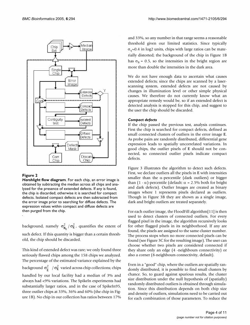
Figure 3 illustrates the algorithm to detect such defects.First, we declare outliers all the pixels in E with intensitiessmaller than the α-percentile (dark outliers) or biggerthan (1 - α)-percentile (default: α = 2.5% both for brightand dark defects). Outlier Images are created as binaryimages where 1 represents pixels declared as outliers.Though in Figure 3B they are shown as a single image,dark and bright outliers are treated separately.

For each outlier image, the FloodFill algorithm[11] is thenused to detect clusters of connected outliers. For everyflagged pixel in the image, the algorithm recursively looksfor other flagged pixels in its neighborhood. If any arefound, the pixels are assigned to the same cluster number.The process stops when no more connected pixels can befound (see Figure 3C for the resulting image). The user canchoose whether two pixels are considered connected ifthey share only an edge (4 -neighbours connectivity) oralso a corner (8-neighbours connectivity, default).

Even in a "good" chip, where the outliers are spatially ran-domly distributed, it is possible to find small clusters bychance. So, to guard against spurious results, the clustersize distribution under the null hypothesis of (spatially)randomly distributed outliers is obtained through simula-tion. Since this distribution depends on both chip sizeand density of outliers, simulations need to be carried outfor each combination of those parameters. To reduce the

σBE

2 σE2

σE2 σE

2

Harshlight flow diagramFigure 2Harshlight flow diagram. For each chip, an error image is obtained by subtracting the median across all chips and ana-lyzed for the presence of extended defects. If any is found, the chip is discarded; otherwise it is searched for compact defects. Isolated compact defects are then subtracted from the error image prior to searching for diffuse defects. The expression values within compact and diffuse defects are then purged from the chip.

Page 4 of 11(page number not for citation purposes)

BMC Bioinformatics 2005, 6:294 http://www.biomedcentral.com/1471-2105/6/294

computational burden at the procedure's runtime, we car-ried out simulations for common chips' designs (534 ×534, 640 × 640, and 712 × 712) and selected proportionof outliers (0.01, 0.02, 0.05, 0.10, 0.20, 0.25, 0.30, and0.40). An example of this distribution is the lower curvein Figure 4. By default, if the user's chip dimensions orspecified proportion of outliers are not among those tab-ulated, distribution values are interpolated from the table.However the user may override interpolation and run-time simulations will be executed.

After each cluster is defined, the significance of its size scan be easily computed as 1-F(s), where F is the cumula-tive distribution of cluster size under the null hypothesisin a chip of the same dimension and proportion of out-liers. If the size significance is bigger than a user-defined

threshold (default α = 0.01), the cluster is discarded andnot considered as a blemish (Figure 3D). In addition, itssize is also compared to the minimum cluster sizeaccepted (user defined, default = 15 pixels): again, if thecluster is not large enough it is not considered. The collec-tion of chips we have examined displays a large numberof compact defects, many of them quite large.

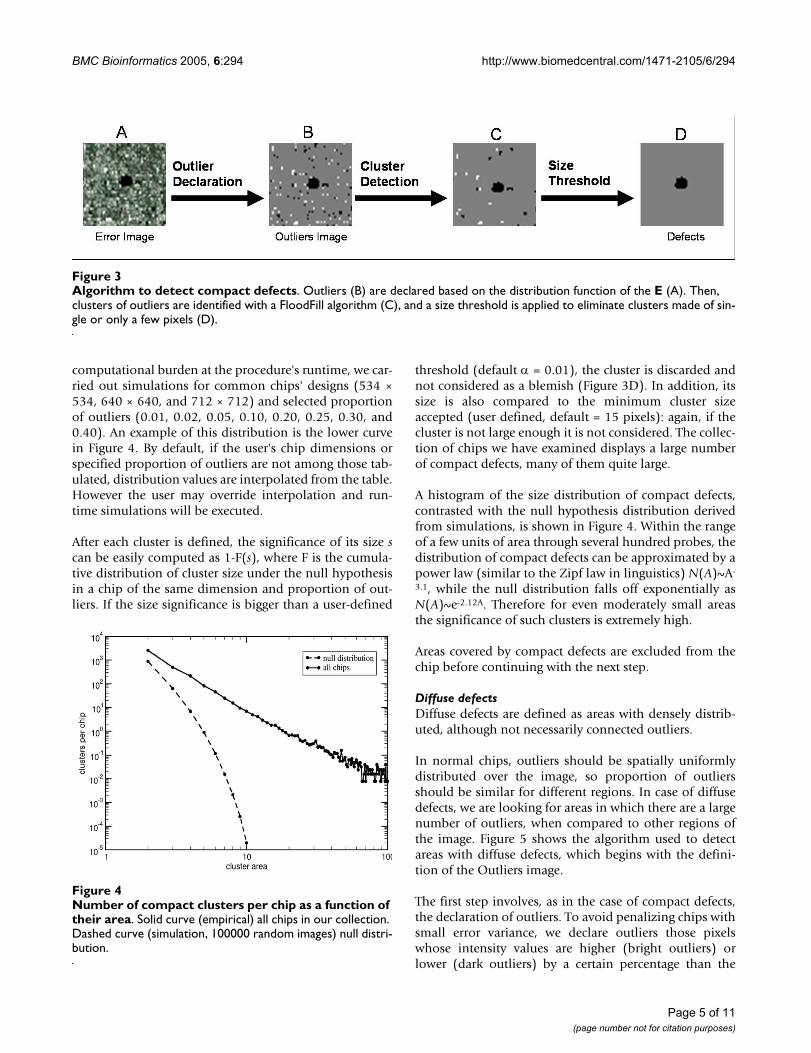
A histogram of the size distribution of compact defects,contrasted with the null hypothesis distribution derivedfrom simulations, is shown in Figure 4. Within the rangeof a few units of area through several hundred probes, thedistribution of compact defects can be approximated by apower law (similar to the Zipf law in linguistics) N(A)~A-

3.1, while the null distribution falls off exponentially asN(A)~e-2.12A. Therefore for even moderately small areasthe significance of such clusters is extremely high.

Areas covered by compact defects are excluded from thechip before continuing with the next step.

Diffuse defectsDiffuse defects are defined as areas with densely distrib-uted, although not necessarily connected outliers.

In normal chips, outliers should be spatially uniformlydistributed over the image, so proportion of outliersshould be similar for different regions. In case of diffusedefects, we are looking for areas in which there are a largenumber of outliers, when compared to other regions ofthe image. Figure 5 shows the algorithm used to detectareas with diffuse defects, which begins with the defini-tion of the Outliers image.

The first step involves, as in the case of compact defects,the declaration of outliers. To avoid penalizing chips withsmall error variance, we declare outliers those pixelswhose intensity values are higher (bright outliers) orlower (dark outliers) by a certain percentage than the

Algorithm to detect compact defectsFigure 3Algorithm to detect compact defects. Outliers (B) are declared based on the distribution function of the E (A). Then, clusters of outliers are identified with a FloodFill algorithm (C), and a size threshold is applied to eliminate clusters made of sin-gle or only a few pixels (D).

Number of compact clusters per chip as a function of their areaFigure 4Number of compact clusters per chip as a function of their area. Solid curve (empirical) all chips in our collection. Dashed curve (simulation, 100000 random images) null distri-bution.

Page 5 of 11(page number not for citation purposes)

BMC Bioinformatics 2005, 6:294 http://www.biomedcentral.com/1471-2105/6/294

expected intensity. In terms of the E, this criterion (alsoused in[12]) implies that if pixels with x% of decrease inintensities are considered dark outliers, the dark outlierimage can be defined as:

Both Outlier Images (one for dark outliers, one for thebright ones, overlaid in Figure 5A), are scanned with a cir-cular sliding window of user-defined radius (defaultradius δ = 10). The borders are duplicated as described forthe extended defects. For every pixel i in the Outlier image,the proportion of outliers in the surrounding circular win-dow Θi is computed as:

A binomial test is then used to decide whether pi is largerthan the overall proportion po of outliers in the image, i.e.to test pi>povs. pi = po.. A new image (Figure 5B) is then cre-ated as

where bα(p,n) is the α-percentile of the binomial distribu-tion. D gives a better representation of the regions withhigh proportion of outliers, since the disconnected pixelsin the Outlier Image appear now more connected (see Fig-ure 5B).

The FloodFill algorithm is then used to detect connectedflagged pixels (Di = 1) as before, and clusters of small sizeare discarded. The user can set the size limit of the clusters,but the default value is three times the area of the slidingwindow.

Finally, to better outline the area of blemishes, the imageundergoes a closing procedure. This is a technique com-monly used in image processing to close up breaks in thefeatures of an image (see for example [10]). In our case, acircular kernel is centered in each pixel of the image(radius = radius of the kernel used to detect the diffusedefects, see later). Its centre is flagged if any of the pixelsof the kernel is flagged.

This procedure (dilation) causes the borders of the defectsto grow, eventually filling empty spaces inside the fea-tures. However, in order to maintain the original outerborders of the features, another circular kernel is appliedto the image. This time, the centre of the window isflagged only if all of the pixels inside the window areflagged. This procedure (erosion) reverses any extensionbeyond the compact hull of the original cluster.

We suggest that all probes in the closed area should bemasked, but the user can choose to mask only the outlierprobes.

Contiguity testIt can happen that in a region with diffuse defects (as theone shown in Figure 6A) some blemished pixels can beclustered together, with sufficiently large size to bedetected as compact defects (Figure 6C). If they were elim-inated in the compact detection step, they could affect therecognition of diffuse regions. To avoid misrecognition of

Oif x

otherwiseii=

≤ − +

1 1

02E log ( )

pn

Oi ii i

=∈∑1

δ Θ

Dii oif p b p n

otherwise=

>

−1

01 α δ( , )

Algorithm to detect areas with diffuse defectsFigure 5Algorithm to detect areas with diffuse defects. The Outlier Image is obtained as for the analysis of the compact defects. A circular kernel is then applied to each pixel in the image to detect areas in which the observed number of outliers exceeds the expected number, based on a binomial test. The defected areas thus determined undergo a round of cluster detection and size threshold, in order to eliminate small areas. The final step involves a dilation and erosion of the defects, in order to better outline the areas.

Page 6 of 11(page number not for citation purposes)

BMC Bioinformatics 2005, 6:294 http://www.biomedcentral.com/1471-2105/6/294

parts of diffuse defects as compact defects, a "contiguitytest" is applied after the compact defects are detected. Toperform the test, a "closing" procedure is applied to thebinary image representing the compact defects (Figure6D).

Real compact defects are isolated and highly connectedclusters, so that after the closing procedure their arearemains substantially the same. On the contrary, probesdeclared as compact defects that are part of diffuse defectsare close to one another, and therefore after the closingprocedure the area covered by the resulting cluster isappreciably bigger than the area covered by the compactdefects alone. Comparing the extension of the areasbefore and after the procedure gives us an idea of howmany compact defects there are in a specific region. Theratio between these two areas (Figure 6C and 6D) repre-sents the density of compact defects in the region (Figure6E). If this value is smaller than a threshold (default =50%), the compact defects in the region are probably partof diffuse defects and shall not be eliminated when thecompact detection procedure ends.

Harshlight packageThe package was implemented in R in compliance withthe CRAN guidelines. Computationally intensive routineswere implemented in C (R shared library builder 1.29 andGCC version 3.2.3) through the R interface for better effi-ciency.

The main Harshlight function accepts a Bioconductorobject from the class affyBatch. For each batch of chipsanalyzed, the program returns two outputs: a file report inPostScript format and a new affyBatch object. The reportshows, for each chip analyzed, the number and type ofdefects found, the percentage of the area eliminated afterthe analysis, an image is produced for each kind of defect,showing the areas where the blemishes are found. The

output affyBatch object is identical to the input, exceptthat the values within defects are declared missing. Ifsome downstream subroutine does not allow for missingdata, the user may choose to have missing data be substi-tuted with the median of the other chips' intensity valuesfor the blemished probe; this is a neutral substitutionstrategy, since it sets the error image values to zero on theblemished probe without affecting any other value. Ingeneral, the efficacy of an imputation method depends onwhat analysis is used downstream of it; because of this,only the median substitution method has been built intoHarshlight. Other imputation methods can be still used, asfunctions taking an Affybatch object with missing values.

Other parameters to the function Harslight including inthe implementation of the algorithm are summarized inTable 1. The choice of the default parameter values isbased on our experience, but may depend on the individ-ual lab or chip type. Still, using a uniform set of parame-ters for all chips in a given experiment avoids spuriouseffects that might be caused by manually excluding areason the chip from analysis. Some parameters are robust, inthe sense that the results are not affected by small changes.For instance, the kernel radii are robust, and so weselected the smallest value that performs well, so as tominimize running time. Other parameters, on the otherhand, define the nature of what is being found; the defaultvalues we provide work well for our chip collection, andare provided as adjustable to allow for flexibility.

Results and DiscussionWe have built an algorithm upon a recently-developedmethodology to visualize artifacts on HDONA microar-rays, which automatically masks areas affected by theseartifacts; we present an implementation of the algorithmin an R package, called Harshlight. The algorithm com-bines image analysis techniques with statisticalapproaches to recognize three types of defects frequent in

Compact defects or part of a diffuse one?Figure 6Compact defects or part of a diffuse one?. A. E. B. Zoomed area with a diffuse defect. C defects "harshlighted" as com-pact. D. Region delimited by the closing procedure. C. Density of the area, more than half of the probes in the region are not defective, so the region is probably considered to contain a diffuse defect.

Page 7 of 11(page number not for citation purposes)

BMC Bioinformatics 2005, 6:294 http://www.biomedcentral.com/1471-2105/6/294

Affymetrix microarray chips: extended, compact, and dif-fuse defects. The algorithm was tested on 158 chips, from5 different experiments, including the two AffymetrixSpikeIn experiments. Output reports for all chips can befound online at[13].

That blemishes exist in fair abundance is clear from thoseoutput reports as well as from Figure 4. We shall nowdemonstrate that these blemishes affect the gene expres-sion values and that Harshlight can restore this damage.

Different summarization algorithms are expected to resistblemishes differently, based on their statistical construc-tion. We shall concentrate here on two popular algo-rithms, MAS5 and GCRMA. MAS5 is the "official"algorithm supplied by Affymetrix and by far the mostwidespread; GCRMA is an open-source method availablein the Bioconductor suite, based on robust averaging tech-niques and sequence-dependent affinity corrections [14].The robust averaging employed in GCRMA should conferstrong immunity to outliers. We shall show below thatMAS5 is strongly affected by blemishes, and that GCRMAis affected to a smaller, yet still relevant extent.

We quantified the ability of Harshlight to apply "correctivemake-up" using two distinct strategies: first, by artificiallyblemishing a "clean" dataset and verifying how much thevalues are affected and how well they are restored, andsecond, by using a case where nominal concentrations areknown, the Affymetrix SpikeIn experiments.

For the first strategy, we wrote a simple utility we dubbed"AffyPox", which pockmarks a collection of chips withsimulated defects with characteristics similar to thosefound in the test chips (Figure 4). Compact defects weresimulated as randomly located circles of radius between 4and 6 pixels, each defect having equal probability of being"bright" or "dark". The probes within the circle are line-arly compressed into the lower (upper) 20% of the inten-

sity range for dark (bright) defects. Further informationon Affypox is available on the program's vignette. For ourstarting point, we took the most unblemished dataset inour collection, and we then further selected from thisdataset the 8 chips with the smallest number of blem-ishes. Then we generated 10 artificial compact defects perchip as described above, covering less than 0.2% of theoverall surface area. Since for both GCRMA and MAS5 thebackground and normalization process couple all thegenes together, all genes' expression values are affected,most of them only by a minute amount, and a few by con-siderable amounts: there were 20 genes' expression valuesper chip affected by more than twofold in MAS5, while 3genes per chip had more than 50% change in GCRMA.Harshlight detected and excised all 80 artificial defects inaddition to two "false positive" defects, and reduced thenumber of genes affected at high fold changes, by a factorof approximately 3 in the case of MAS5, and about 2 in thecase of GCRMA, as shown in Figure 7; GCRMA appears toresist blemishes better than MAS5, but at the same timethe damage appears harder to undo. As with any restora-tion process, a large number of genes is restored, some areuntouched, and a few are changed for the worse, as shownin Figure 8.

For the second strategy, we used a well-known compari-son suite, AffyComp, which was developed to quantify theperformance of various summarization algorithms [15]on the Affymetrix SpikeIn datasets, where nominal con-centrations are given for a number of genes which were"spiked in" in a Latin square experimental design. This isnow an aggregate comparison, in which all defect typesdetected by Harshlight are excised, and the overall effect onthe statistical performance of the summarization algo-rithm is quantified by means of Return Operator Curves(ROC). We performed this analysis for the most recentdataset, SpikeIn133, and again we compared the perform-ance of MAS5 and GCRMA. We modified the MAS5implementation in Bioconductor so that it accepts missing

Table 1: Default values for the parameters used in the program

Defects Parameter Value

Extended Radius of the median filter 10 pixelsThreshold for the proportion of variance explained by the Background 30%

Compact Quantile for the definition of outliers 5th, two tailsMinimum size of clusters 15 pixelsConnectivity definition 8-neighbours

Probability value 0.01Diffuse Threshold for bright defects 40% more than original value

Threshold for dark defects 35% more than original valuep-value threshold for binomial test. 0.001

Radius of sliding window 10 pixelsConnectivity definition 8-neighbours

Minimum size of clusters 3π*diff. radius

Page 8 of 11(page number not for citation purposes)

BMC Bioinformatics 2005, 6:294 http://www.biomedcentral.com/1471-2105/6/294

values, and compared our two substitution strategies,missing values vs. neutral replacement (i.e., substitutionwith the median of the other chips' values for that probe).As GCRMA is not as easily modified to allow for missingdata, we could only use median substitution withGCRMA. Figure 9 shows the ROC curves summarizing thefalse positive/true positive behavior of the algorithm. Inall cases, preprocessing the SpikeIn133 dataset withHarshlight results in a significant increase of performanceof the algorithm, which is actually quite substantial forthe case of MAS5, where >5% extra true positives arefound at large false positive numbers, for both substitu-tion methods.

In earlier chips the probesets were laid contiguously inspace, so it was possible to detect localized defects byobserving that the probeset had an "outlier" pattern [16].However, the entire probeset would have to be discarded,and the gene expression information would be lost. Cor-related location in space precludes use of Harshlight onthose earlier chips (e.g., HUGeneFL). The random alloca-tion of probe pairs in newer generations of chips permitsrobust methods like GCRMA to partly resist damage byblemishes; and, in conjunction with a method like Harsh-light, to restore the expression values for many affectedgenes.

While we have developed this method on the basis of ourerror image detection of outliers, in principle the residualsof any model such as [16] or GCRMA could be used to

identify individual probes on a chip as outliers. To facili-tate the integration of various methods, Harshlight acceptserror images generated by other programs; if none are pro-vided, then the error images are computed. We have, how-ever, not yet explored the appropriate null hypothesis forthese methods.

ConclusionWe have presented an R package that provides a way toautomatically "harshlight" artifacts on the surface ofHDONA microarray chips. The algorithm is based on sta-tistical and image processing approaches in order to safelyidentify blemishes of different nature and correct theintensity values of the batch of chips provided by the user.The corrections made by Harshlight improve the reliabilityof the expression values when the chips are further ana-lyzed with other programs, such as GCRMA and MAS5.

It has been shown that microarray results are affected ifblemished chips enter the pipeline of the analysis; blem-ished probes may have values differing from the correct

Restoration effectsFigure 8Restoration effects. Comparing the log fold changes in the MAS5 algorithm before and after restoration. Vertical axis, log fold change between the original expression values and the restored values (Orig vs median). Horizontal axis, log fold change between the original and blemished chips (Orig vs pox). Notice three straight lines through the plot. A diago-nal line represents changed expression values that were not restored by Harshlight. A vertical line shows a few cases in which Harshlight incorrectly affected the expression values. Most points lie near the horizontal axis, showing that Harsh-light restored values closer to the original.

MAS5 and GCRMA analysisFigure 7MAS5 and GCRMA analysis. After artificially blemishing a collection of chips we excised the blemishes with Harshlight using median substitution. We compare the expression val-ues of the blemished chips vs. the original, and the expres-sion values after restoration with Harshlight vs. the originals. Left, GCRMA shows a substantial improvement; right, MAS5 shows a dramatic improvement.

Page 9 of 11(page number not for citation purposes)

BMC Bioinformatics 2005, 6:294 http://www.biomedcentral.com/1471-2105/6/294

value by much more than the typical error, so blemishesare expected to have a particularly strong impact on exper-iments trying to discriminate subtle differences betweensamples or in a clinical diagnosis context. We presentHarshlight in the hope it shall be a useful tool in qualityassessment of microarray chips and will help improvemicroarray analysis.

Availability and requirements• Project name: Harshlight

• Project home page: http://asterion.rockefeller.edu/Harshlight

• Operating system(s): Platform independent, testedupon Red Hat Linux and is being under testing on Win-dows XP systems

• Programming language: R, C

• Other requirements: R 1.8.0 or higher

• License: GNU, GPL

• Any restrictions to use by non-academics: licenseneeded

Authors' contributionsMSF developed the method, designed and carried out thestatistical analysis, and drafted the manuscript. MP wroteand implemented the algorithm, and helped to draft themanuscript. KMW developed the method and partici-pated in the design of the statistical approach. MOM con-ceived and coordinated the study, participated in itsdesign, and helped to draft the manuscript. All authorsread and approved the final manuscript.

Additional material

Additional File 1SIprobecomposition. nucleotide composition analysis of unblemished and blemished probes.Click here for file[http://www.biomedcentral.com/content/supplementary/1471-2105-6-294-S1.pdf]

Additional File 2Harshlight R package for LinuxClick here for file[http://www.biomedcentral.com/content/supplementary/1471-2105-6-294-S2.gz]

Receiver Operator Curves generated by the AffyComp suite for the SpikeIn133 dataset at 2-fold changesFigure 9Receiver Operator Curves generated by the AffyComp suite for the SpikeIn133 dataset at 2-fold changes. A. The MAS5 algorithm shows noticeable improvement when Harshlight is used to excise blemishes, both for missing value substi-tutions as well as for median substitution: approximately 2 extra true positives per chip are discovered. B. The GCRMA algo-rithm shows a slight improvement of about 0.5 extra true positives per chip under median substitution.

Page 10 of 11(page number not for citation purposes)

BMC Bioinformatics 2005, 6:294 http://www.biomedcentral.com/1471-2105/6/294

Publish with BioMed Central and every scientist can read your work free of charge

"BioMed Central will be the most significant development for disseminating the results of biomedical research in our lifetime."

Sir Paul Nurse, Cancer Research UK

Your research papers will be:

available free of charge to the entire biomedical community

peer reviewed and published immediately upon acceptance

cited in PubMed and archived on PubMed Central

yours — you keep the copyright

Submit your manuscript here:http://www.biomedcentral.com/info/publishing_adv.asp

BioMedcentral

AcknowledgementsM.S.F. acknowledges a Woman in Science fellowship from RU. K.M.W. was supported in part by GCRC grant M01-RR00102 from the National Center for Research Resources at the NIH. We would like to thank Steffen Bohn for helpful comments and discussion.

References1. Ihaka R, Gentleman R: R: A language for data analysis and

graphics. Journal of Computational and Graphical Statistics 1996,5(3):299-314.

2. Parmigiani G, Garrett ES, Irizarry RA, Zeger SL: The analysis ofgene expression data: methods and software. In Statistics forbiology and health Edited by: Dietz K, Gail M, Krickeberg K, Samet J,Tsianis A. New York , Springer; 2003:455.

3. Affymetrix I: GeneChip Expression Analysis: Data AnalysisFundamentals. 2004.

4. Suárez-Fariñas M, Haider A, Wittkowski KM: "Harshlighting"small blemishes on microarrays. BMC BIOINFORMATICS 2005,6:65:.

5. Naef F, Magnasco MO: Solving the riddle of the bright mis-matches: labeling and effective binding in oligonucleotidearrays. Phys Rev E Stat Nonlin Soft Matter Phys 2003, 68(1 Pt1):011906. Epub 2003 Jul 16..

6. AffyWebdata: Affymetrix website. [http://www.affymetrix.com/support/technical/sample_data/datasets.affx].

7. Suárez-Fariñas M, Noggle S, Heke M, Hemmati-Brivanlou A, Mag-nasco MO: How to compare microarray studies: The case ofhuman embryonic stem cells. Submmitted 2005.

8. Wittkowski KM, Lee E, Nussbaum R, Chamian FN, Krueger JG:Combining several ordinal measures in clinical studies. StatMed 2004, 23(10):1579-1592.

9. Bolstad B: Ben Bolstad website. [http://stat-www.berkeley.edu/users/bolstad/PLMImageGallery].

10. Russ JC: The Image Processing Handbook. 4th edition (July2002) edition. Boca Raton , CRC Press; 2002.

11. Thomas H. Cormen, Leiserson CE, Rivest RL, Stein C: Introductionto Algorithms. 2nd edition edition. Boston , The MIT Press; 2001.

12. Irizarry RA, Warren D, Spencer F, Biswal S, Frank BC: Multiple LabComparisons of Microarray Platforms. Dept of BiostatisticsWorking Papers, Johns Hopkins University 2004.

13. website H: Harshlight website. [http://asterion.rockefeller.edu/Harshlight].

14. Wu Z, Irizarry RA, Gentleman R, Martinez Murillo F, Spencer F: AModel Based Background Adjustement for OligonucleotideExpression Arrays. Journal of American Statistical Association 2004,99(468):909-917.

15. Cope LM, Irizarry RA, Jaffee HA, Wu ZJ, Speed TP: A benchmarkfor affymetrix GeneChip expression measures. BIOINFOR-MATICS 2004, 20(3):323-331.

16. Li C, Wong WH: Model-based analysis of oligonucleotidearrays: Expression index computation and outlier detection.P NATL ACAD SCI USA P NATL ACAD SCI USA 2001, 98(1):31-36.

Page 11 of 11(page number not for citation purposes)