Finishing LineSchedulingin the steelindustry

H. OkanoA. J. Davenport

M. TrumboC. Reddy

K. YodaM. Amano

A new solution for large-scale scheduling in the steelmakingindustry, called Finishing Line Scheduling (FLS), is described.FLS in a major steel mill is a task to create productioncampaigns (specific production runs) for steel coils on fourcontinuous processes for a one-month horizon. Two processflows are involved in FLS, and the balancing of the twoprocess flows requires resolving conflicts of due dates. Thereare also various constraints along the timeline for each processwith respect to sequences of campaigns and coils. The twotypes of constraints—along process flows and timelines—makethe FLS problem very complex. We have developed a high-performance solution for this problem as follows: Inputcoils are clustered by two clustering algorithms to reduce thecomplexity and size of the problem. Campaigns are created foreach process from downstream to upstream processes, whilepropagating upward the process timings of the clusters. Timinginconsistencies along the process flows are then repaired byscheduling downward. Finally, coils are sequenced within eachcampaign. The FLS system enabled a steel mill to expand itsscheduling horizon from a few days to one month, and toimprove decision frequency from monthly to daily.

1. IntroductionIn a major steel mill in Japan, production schedulingfor steel sheet products, also called coil products, wasconducted by skilled human experts, and the schedulinghorizon was limited to a few days. The steel mill hadfinished automating the scheduling of primary steelmaking,which covers the upstream processes of coil production,but their problem was how to determine accurate duedates for slabs for a longer horizon in order to utilize theautomated scheduler more efficiently. Slabs created by theupstream processes are transformed to hot coils at a hotstrip mill (HSM) and to cold coils at a cold mill (CM),and are finished with annealing and galvanizing processes(Figure 1). The whole scheduling task for coil productionafter the HSM, from the CM onward, is called FinishingLine Scheduling (FLS). In order to determine accurate duedates for slabs, therefore, the HSM and the finishing linesmust be scheduled for a longer scheduling horizon. Thesteel mill first examined the feasibility of the existing

capacity planning tools for the FLS and found them notapplicable. The steel mill then created a special-purposescheduling system, called the FLS system, with the supportof an IBM team including the authors.

A schedule for the finishing lines consists of productioncampaigns 1 on each process and a coil sequence withineach campaign. The schedule involves horizontal flows ofproduction campaigns along timelines on each processand vertical flows of coils from upstream to downstreamprocesses (Figure 2). For simplicity, in Figure 2, arrowsare drawn for only a few pairs of coils, and only twocampaign sequences are drawn for each process. There areactually more arrows, and there may be more than twomachines of the same type, called lines, for each process.Each coil has several properties: width, thickness, length,campaign type, release date, due date, priority, grade, andso on. Among the coil properties, those other than release

1 The production campaign is a production run with specific start and end times inwhich coils of a particular type are processed continuously on a process line.

�Copyright 2004 by International Business Machines Corporation. Copying in printed form for private use is permitted without payment of royalty provided that (1) eachreproduction is done without alteration and (2) the Journal reference and IBM copyright notice are included on the first page. The title and abstract, but no other portions, of thispaper may be copied or distributed royalty free without further permission by computer-based and other information-service systems. Permission to republish any other portion of

this paper must be obtained from the Editor.

0018-8646/04/$5.00 © 2004 IBM

IBM J. RES. & DEV. VOL. 48 NO. 5/6 SEPTEMBER/NOVEMBER 2004 H. OKANO ET AL.

811

and due dates, priority, and grade are all process-dependent. Note that campaign types on one processare not related to those on other processes. As shownin Figure 2, therefore, two coils in the same campaignon CM may (usually) be assigned to different campaigns

on lower stream processes. The number of coils assignedto a campaign is typically about 50 to 500. The task ofsequencing the coils assigned to each campaign taking intoaccount the several constraints between coils is called thesequencing (Figure 3). In this task, the vertical relationships

Figure 1

Process flow of primary steelmaking and coil making. Four processes targeted for scheduling in the finishing lines are shown. Work in

process (WIP) indicates that there is inventory stored at each location in the flow.

Hot strip mill

(HSM)WIP

coil

Cold mill

(CM)WIP

coil

Slab

Continuous

annealing

line (CAL) WIP

coil

Electro-

galvanizing

line (EGL)

Continuous galvanizing

line (CGL)

Continuous

caster

Primary steel making

Basic

oxygen

furnace

Finishing lines

Figure 2

Schematic rendering of schedules for four processes. Rectangles shown for the four processes represent campaigns, and the objects drawn

in the campaigns represent coils. Arrows between coils show that they are the same coils which should be processed from top to bottom.

Thick arrows represent coils going from CM to CGL, while thin arrows represent coils going from CM to CAL, then to EGL.

Cold mill

(CM)

Continuous

annealing

line (CAL)

Electro-

galvanizing

line (EGL)

Continuous

galvanizing

line (CGL)

WIP

WIP

day 1, day 2, … day 30+

WIP

WIP

HSM

H. OKANO ET AL. IBM J. RES. & DEV. VOL. 48 NO. 5/6 SEPTEMBER/NOVEMBER 2004

812

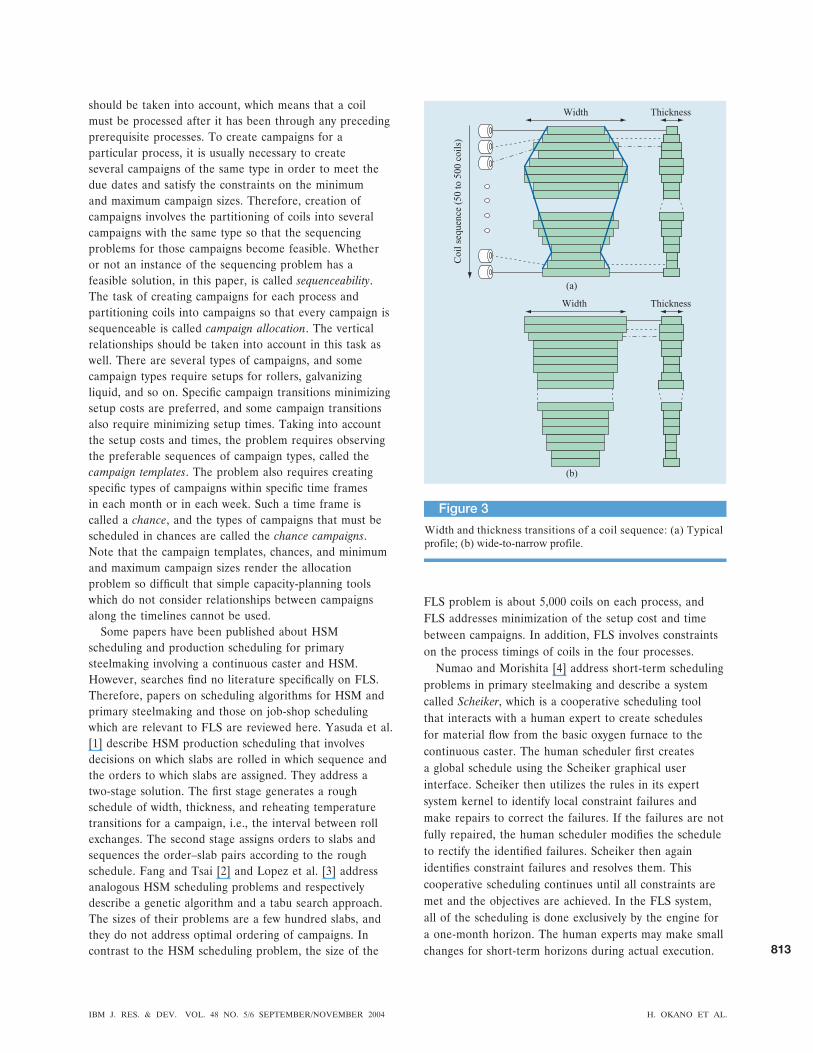
should be taken into account, which means that a coilmust be processed after it has been through any precedingprerequisite processes. To create campaigns for aparticular process, it is usually necessary to createseveral campaigns of the same type in order to meet thedue dates and satisfy the constraints on the minimumand maximum campaign sizes. Therefore, creation ofcampaigns involves the partitioning of coils into severalcampaigns with the same type so that the sequencingproblems for those campaigns become feasible. Whetheror not an instance of the sequencing problem has afeasible solution, in this paper, is called sequenceability.The task of creating campaigns for each process andpartitioning coils into campaigns so that every campaign issequenceable is called campaign allocation. The verticalrelationships should be taken into account in this task aswell. There are several types of campaigns, and somecampaign types require setups for rollers, galvanizingliquid, and so on. Specific campaign transitions minimizingsetup costs are preferred, and some campaign transitionsalso require minimizing setup times. Taking into accountthe setup costs and times, the problem requires observingthe preferable sequences of campaign types, called thecampaign templates. The problem also requires creatingspecific types of campaigns within specific time framesin each month or in each week. Such a time frame iscalled a chance, and the types of campaigns that must bescheduled in chances are called the chance campaigns.Note that the campaign templates, chances, and minimumand maximum campaign sizes render the allocationproblem so difficult that simple capacity-planning toolswhich do not consider relationships between campaignsalong the timelines cannot be used.

Some papers have been published about HSMscheduling and production scheduling for primarysteelmaking involving a continuous caster and HSM.However, searches find no literature specifically on FLS.Therefore, papers on scheduling algorithms for HSM andprimary steelmaking and those on job-shop schedulingwhich are relevant to FLS are reviewed here. Yasuda et al.[1] describe HSM production scheduling that involvesdecisions on which slabs are rolled in which sequence andthe orders to which slabs are assigned. They address atwo-stage solution. The first stage generates a roughschedule of width, thickness, and reheating temperaturetransitions for a campaign, i.e., the interval between rollexchanges. The second stage assigns orders to slabs andsequences the order–slab pairs according to the roughschedule. Fang and Tsai [2] and Lopez et al. [3] addressanalogous HSM scheduling problems and respectivelydescribe a genetic algorithm and a tabu search approach.The sizes of their problems are a few hundred slabs, andthey do not address optimal ordering of campaigns. Incontrast to the HSM scheduling problem, the size of the

FLS problem is about 5,000 coils on each process, andFLS addresses minimization of the setup cost and timebetween campaigns. In addition, FLS involves constraintson the process timings of coils in the four processes.

Numao and Morishita [4] address short-term schedulingproblems in primary steelmaking and describe a systemcalled Scheiker, which is a cooperative scheduling toolthat interacts with a human expert to create schedulesfor material flow from the basic oxygen furnace to thecontinuous caster. The human scheduler first createsa global schedule using the Scheiker graphical userinterface. Scheiker then utilizes the rules in its expertsystem kernel to identify local constraint failures andmake repairs to correct the failures. If the failures are notfully repaired, the human scheduler modifies the scheduleto rectify the identified failures. Scheiker then againidentifies constraint failures and resolves them. Thiscooperative scheduling continues until all constraints aremet and the objectives are achieved. In the FLS system,all of the scheduling is done exclusively by the engine fora one-month horizon. The human experts may make smallchanges for short-term horizons during actual execution.

Width and thickness transitions of a coil sequence: (a) Typical

profile; (b) wide-to-narrow profile.

Figure 3

Width Thickness

Coil

sequence (

50 t

o 5

00 c

oil

s)

Width Thickness

(a)

(b)

IBM J. RES. & DEV. VOL. 48 NO. 5/6 SEPTEMBER/NOVEMBER 2004 H. OKANO ET AL.

813

Lee et al. [5] address integrated scheduling at continuouscasters and HSMs. They address two techniques for casterscheduling and a third approach for integrated caster andHSM scheduling. The first of these generates casterschedules by clustering similar orders and then findinga sequence of these clusters using a heuristic searchalgorithm based on the beam and branch-and-boundsearch. These sequences are further improved by agenetic algorithm. The second approach is based on asolution framework, called asynchronous teams or A-teams[6, 7], which can exploit several solution techniques forfinding multiple Pareto-optimal solutions. The thirdapproach is based on clustering and a heuristic search.An analogous approach using A-teams was also describedby Gao et al. [8]. In contrast, the FLS problem involvestwice as many processes as their problem does, and has abranch of the process flow which their problem does notaddress.

Wein and Chevalier [9] discuss dynamic decision policiesfor assigning due dates, releasing jobs from a backlog,and sequencing jobs. Their problem assumes that thejob shop is modeled as a multiclass queuing network,and the objective is to minimize both the work-in-process(WIP) inventory and the due date lead time (DDLT, thedue date minus arrival date) of jobs. They proposed atwo-step approach. The first step releases and sequencesjobs, ignoring DDLT and focusing instead on efficientsystem performance. DDLT is then taken into account inthe second step to set the due dates. In FLS, coils (jobs)are grouped into campaigns whose lengths vary fromabout a few hours to a week. Each coil in a campaign isassociated with a release date from the preceding processand a due date for the succeeding process, and its DDLTis sometimes shorter than the campaign length. Therefore,once coils are assigned to campaigns, the time windows ofcampaigns are relatively short, and thus the sequence ofcampaigns is so restricted that the simple queuing networkmodel does not apply. Therefore, the assignment of coilsinto campaigns and campaign sequencing in FLS shouldbe solved at the same time.

Leachman et al. [10] address a large-scale andmultiple-process scheduling problem in semiconductormanufacturing. Their scheduling algorithm for eachprocess refers only to the WIP at hand, and the systemis controlled by determining target cycle times and WIPlevels for individual processes and by periodically releasingnew jobs into the fabrication line. In their problem, eachdevice is typically scheduled to be set up once per shift,which means that the campaign lengths are only one shiftlong. In contrast, in FLS, campaigns can be longer thanthe size of the WIP that exists when campaigns begin.Therefore, we use off-line scheduling algorithms that referto all of the coils that will be released during a one-monthhorizon, not only to the WIP at hand.

In this paper, we describe a four-step approach forthe FLS problem: 1) Input coils are clustered by twoclustering algorithms to reduce the complexity and sizeof the problem. 2) Campaigns are created for eachprocess from downstream to upstream processes, whilepropagating the process timings of the clusters upward.3) Timing inconsistencies along the process flows arethen repaired by scheduling downward. 4) Finally, coilsare sequenced within each campaign. Campaign allocation,Steps 2 and 3, addresses resolving of the due date conflictson the CM. Note that the process flow branches at theCM to CGL-bound and EGL-bound (Figure 1), and thatthe CM has to produce CGL- and EGL-bound coils inproper proportion, taking into account the due dates atthe lower stream processes. Our algorithm propagatestime windows upward to provide the CM with the timingrequirements on the lower stream processes so that theCM can be scheduled accordingly.

The remainder of the paper is organized as follows: TheFLS problem is presented in the next section. The solutionframework for the FLS system and numerical experimentsare described in Section 3. Details of each of thealgorithmic components are presented in Sections 4through 7. Finally, our conclusions are summarized inSection 8.

2. The FLS problemThe input data to the problem is the number of WIP coilson each of the four continuous processes and the numberof coils that will be released from HSM to CM during thescheduling horizon. The problem is to create productioncampaigns to which coils are assigned for each line of theprocesses, and to sequence coils within each campaign sothat productivity and product quality are maximized andtardiness is minimized.

Productivity means gross production per month dividedby cost, where the term gross indicates the exclusion ofparts of sheets which cannot be delivered because oftrimming or scars. Maximization of gross production permonth is addressed in the FLS problem as minimizationof the gaps between campaigns, and maximization ofproductivity is addressed directly as campaign templatesand indirectly as sequencing penalties. The gaps betweencampaigns include setup times and downtimes of processesdue to both planned maintenance and lack of WIPinventory. When the WIP inventory in front of a processfor each of the campaign types is less than the minimumcampaign size, the process has to stop until enough WIP issupplied from upstream processes. Such a situation lowersproductivity; therefore, the upstream processes shouldtake into account the amount of WIP at lower streamprocesses. Setups of campaigns that require extra costsfor changing of galvanizing liquid are undesirable, andcampaign templates are designed by the human experts in

H. OKANO ET AL. IBM J. RES. & DEV. VOL. 48 NO. 5/6 SEPTEMBER/NOVEMBER 2004

814

the steel mill to avoid such expensive setups. For example,a setup that requires changing only one galvanizing pot ispreferred to a setup that requires changing many. Thecampaign templates are sequences of campaign types anddowntimes that require only small setups. (Downtime istreated as a special campaign type.) Sequencing penaltiesinclude width differences between consecutive coils torepresent minimization of trim loss. Note that thecontinuous process is a process in which all of the inputcoils within a campaign are welded together to make along strip, processed at one time, and cut into coils afterprocessing. When the widths of consecutive coils differconsiderably, two corners of the wider coil are cut off tocreate a smooth profile (Figure 4). Therefore, in orderto increase productivity, it is preferable to make widthprofiles of campaigns as smooth as possible. (In addition,when the difference in widths or thickness is very large,the welded juncture is weak, limiting the allowabledifferences of width and thickness.) There are alsoconstraints on minimum campaign sizes, which are set todecrease the number of changes of rollers or galvanizingliquid.

Product quality is improved when the steel sheets areproperly galvanized and are not scarred. Maximization ofproduct quality is the production of as much high-gradeproduct as possible without any problems. Note that eachorder is associated with a grade, and high-grade products(for example, for the outer panels of cars) are moreexpensive than low-grade products. Once a steel sheetfor a high-grade product develops problems, it must bereassigned to a lower-grade order, whose profit margin islower than those of high-grade orders. Also, in continuousprocesses, the rollers are worn by processing coils;processing narrower and wider coils in that order causes atransferring of scars, called edge marks, to the wider coils atthe positions of both sides of the narrower coils (Figure 4).Therefore, in order to increase product quality, the widthprofiles of campaigns for high-grade products should bewide-to-narrow [Figure 3(b)]. Also, campaigns for high-grade products should not be placed immediately afterdowntimes, when the process machines are not yet stable.This preference is reflected in the campaign templates.There are constraints on maximum campaign sizes, whichare set to avoid scars due to worn rollers and to keepproduct quality high.

Minimization of tardiness means that as many productsas possible should be shipped before the due date.

Input and outputThe input data of the FLS problem is the following:

● A set of processes P � {CM, CAL, EGL, CGL} indexedby p.

● A set of lines Lp on process p indexed by l.

● A set of coils Cp on process p indexed by i.● The previous campaign on each line of the processes.● Any planned downtimes.

The previous campaign is a pre-allocated campaignwhich should be followed by newly created campaigns;planned downtimes are time periods in which campaignscannot be created.

Associated with each coil i are

● A campaign type ci.● A set of assignable lines Li � Lp.● A processing time li.● A priority: high or low.● A release date ri if coil i has no preceding process.● A due date di if coil i has no succeeding process.● A corresponding coil ui in the preceding process.● A lead time l(ui , i) to be allocated after the preceding

process.● Any process-dependent sequencing properties.

The preceding process is the process immediatelyupstream in the finishing lines from which coil i comes;the succeeding process is the process immediatelydownstream to which coil i goes. Each coil is assignable toonly specific lines Li. The process-dependent sequencingproperties include width, thickness, annealingtemperatures, and surface treatment types.

Associated with each campaign type c are the minimumlength minc and the maximum length maxc. For each line,the following constraints are given: campaign template,

Figure 4

Edge marks and trim loss.

Process

direction

Rollers

Steel sheet

ScarsTrim loss

Trim

loss

Steel sheet

Welded

juncture

Process

direction

Steel sheet

Edge marks

Steel sheet

Rollers

IBM J. RES. & DEV. VOL. 48 NO. 5/6 SEPTEMBER/NOVEMBER 2004 H. OKANO ET AL.

815

chance campaigns, chance positions, and sequencingconstraints. The campaign template is defined as a graphwith campaign types as nodes and campaign transitions asdirected edges. The chances for campaign type c are timewindows at specific positions in the timeline: [ESTc

t , LFTct]

for the tth chance. 2 Sequencing constraints include theallowable differences of width and thickness, width profile,setup costs between coils, and transition speed of theannealing furnace temperature. Most of these constraintscan be represented as a distance function between eachpair of coils.

The output data for the FLS solution is

● A set of campaigns Kl on each line l.● A set of coils Ck assigned to each campaign k.● A start time �k for each campaign k.● A start time �i for each coil i.

With respect to the output data, the ordering ofcampaigns on line l is denoted by �l and the ordering ofcoils for campaign k is denoted by �k.

Constraints and preferencesThe output schedule should satisfy the following constraintsand preferences (the latter are marked with an asterisk):

ESTi � � i

�ui� lui

� l(ui , i) � � i

��k ( j)� l

�k ( j) � ��k ( j�1)

�k1� lk1

� l(k1 , k2) � �k2,

k1� � l( j), k2� � l( j � 1)coil i must be assigned to

a campaign of type ci

coil i must be scheduledon line � Li

ESTc(k)t

� �k � LFTc(k)t � lk

for any chance t� i � li � LFTi

minc(k) � lk � maxc(k)

for all campaigns kcampaign orderings

follow campaigntemplates

coil orderings followsequencingconstraints

[release date][vertical relationship][continuous sequence]

[setup time betweencampaigns]

[campaign type]

[assignable line]

[chance campaign][due date]*

[min–max campaign sizes]*

[campaign templates]*

[sequencing constraints]*

for each coil i and each line l of processes, where l(ui, i)denotes the lead time between coil i and its preceding coilui, l(k1, k2) denotes the setup time between two campaigns

k1 and k2, and c(k) and lk respectively denote a campaigntype and the length of campaign k. Note that preferencesmay be violated when there is no feasible schedule. Thedue date constraint is marked as a preference becausethere may be no feasible schedule that satisfies both thedue dates and the other constraints. The campaigntemplates are shown as a preference for the samereason.

ObjectivesThe objectives to be minimized for the FLS problem areshown in Table 1, in which the elements are listedbasically in the order of importance assigned by humanexperts. The first three objectives (marked with �) arecounted as weighted sums. Tardiness for coils withdifferent priorities is treated with different weights. Theother objectives are considered in the order shown.When an input coil (or cluster) has an EST at a muchlater position, the makespan 3 is determined by that coil,disregarding the other parts of the schedule. From apractical point of view, schedules with fewer gaps at earlyparts of the horizon are preferred, and the makespan isnot very important. The minimization of gaps betweencampaigns reflects this preference (Figure 5). Thesequencing constraint violation is listed last becausedetailed coil sequences are required for a horizon of onlya few days. Except for the first few days in the beginningof a schedule, the primary objective in terms ofsequencing is to guarantee sequenceability, which is notexplicitly shown in Table 1.

System targetsThe targets of the FLS system are as follows: 1) Createa one-month schedule within one hour of running time;2) minimize tardiness; 3) maximize productivity; and 4)maximize product quality. The first target makes the sizeof the problem very large. The number of coils to beprocessed by all of the continuous processes in one monthis 20 to 25 thousand. The issue arising here is how toreduce the problem complexity and size by clustering thecoils or by decomposing the problem without significantlyaffecting the solution quality. The second target involvesa tradeoff between tardiness and the constraints incampaign allocation. Tardiness can be minimized bycreating small campaigns or by ignoring the campaigntemplates. However, setup costs will become large in sucha schedule. The third target involves a line balancingproblem. As shown in Figure 1, the process flow in thesteel mill branches after CM, with one branch going toEGL and the other to CGL. Unless CM produces EGL-bound and CGL-bound coils in proper proportions, either

2 The terms EST and LFT respectively indicate earliest start time and latest finishtime.

3 The term makespan indicates the duration from the beginning of the schedulinghorizon to the completion of the last coil on each line.

H. OKANO ET AL. IBM J. RES. & DEV. VOL. 48 NO. 5/6 SEPTEMBER/NOVEMBER 2004

816

EGL or CGL may be starved for coils and stop. Suchstops (downtimes) should be avoided because they lowerproductivity. The consideration of the different productflows to avoid downtimes is called line balancing. Thefourth target relates to the sequencing constraints andalso to the maximum campaign size and the campaigntemplates.

3. Solution frameworkIn order to reduce the problem complexity and size, theFLS system incorporates two types of clustering: outlierand performance. Dimensions, time windows, and otherparameters usually constrain the neighborhood of coilsthat can be scheduled together, and many of theseneighborhoods are large for most typical coils. Such coilsare likely to be sequenceable even if they are randomlyassigned to campaigns. In contrast, coils with a smallneighborhood or no neighbors, the outlier coils, should beput into campaigns along with near-neighbor coils whichconnect them to normal ones. By creating clusters ofoutlier and connecting coils, it is possible to separate thesequenceability problem from campaign allocation, andthe problem complexity is reduced. This type of clustering

is called outlier clustering. Normal coils and the outlierclusters are further clustered by performance clusteringin order to reduce the problem size.

The FLS problem has two interrelated problems:horizontal and vertical. The horizontal problem involvescampaign allocation and sequencing, and the verticalproblem involves line balancing and vertical relationships.Handling them at the same time, however, is not practicalbecause of the complexity. The FLS system thus adoptsa horizontal engine for campaign allocation which runsindependently for each process. The vertical problem isaddressed by time window propagation and upward anddownward scheduling. A time window [ESTi, LFTi] isassumed for each cluster i, which means that cluster ishould be scheduled at the earliest start time (EST) orlater, but (preferably) no later than the latest finish time(LFT). The time windows are set based on the release anddue dates and the lead times, as shown in Figure 6(a).The time window propagation defines a narrowed and non-overlapping time window for each cluster [Figure 6(b)],so that the horizontal engine for each processcan work independently without worrying about thevertical relationships. For example, after creating the

Figure 5

Example of gap penalty. The bottom schedule is the best and has the smallest gap penalty. Coils or clusters marked with X have earliest

start times (ESTs) at their positions, and they cannot be moved earlier.

100 200 300 400

150 200 250 400

190 210 400

100/1002 � 100/3002 � 0.0111

50/1502 � 150/2502 � 0.00462

10/1902 � 190/2102 � 0.00459

X

X

X

X X X X

X X X X

X X X X

Table 1 Objectives to be minimized for the FLS problem.

�p�P� i�Cpmax {� i � li � LFTi , 0} [tardiness]�

�p�P� l�Lp�k�Kl

max, {minc(k) � lk , 0} [minimum campaign size violation]�

�p�P� l�Lp� j[�k2

� (�k1� lk1

)]/�k1

2 , k1 � � l( j), k2 � � l( j � 1) [minimize gaps between campaigns]�

�p�P� l�Lpcampaign template violation [campaign template violation]

�p�P� l�Lp�k�Kl

max{lk � maxc(k) , 0} [maximum campaign size violation]

�p�P� l�Lpsequencing penalty [sequencing constraint violation]

IBM J. RES. & DEV. VOL. 48 NO. 5/6 SEPTEMBER/NOVEMBER 2004 H. OKANO ET AL.

817

line schedule for CM, the process timings of the clusterson CM are propagated downward, as illustrated inFigure 7.

The line balancing problem and tardiness minimizationrequire resolving conflicts of due dates on CM. These areaddressed in two steps: upward and downward scheduling.In upward scheduling, campaign allocation is performedfrom downstream to upstream processes, one by one,using the ESTs of initial time windows for the inputclusters. As processes are scheduled, the process timingsof clusters on lower stream processes are propagatedupward to set the LFTs for the preceding clusters. Whencampaigns are allocated for CM, the timing requirementson all of the lower stream processes are represented aspropagated time windows, and thus the horizontal enginecan take line balancing into account by referring to

the propagated time windows. Note that, when upwardscheduling is completed, there may be vertical relationshipviolations because the campaign allocation uses the initialtime windows and they do not include margins forpreceding processes. The purpose of the upward schedulingis not to obtain feasible solutions, but to obtain LFTs onthe CM that reflect the timing requirements on the lowerstream processes. A feasible solution is then created byscheduling downward for the CGL, CAL, and EGL.

Sequencing for each campaign is performed aftercreating the campaigns. Sequencing problems are soprocess-dependent that the FLS system adopts differentsequencing engines for each of the processes. The solutionframework of the FLS system is summarized as follows: 1)upward scheduling for downstream-to-upstream processes,2) downward scheduling for upstream-to-downstreamprocesses, and 3) sequencing for each campaign, wherethe upward and downward scheduling are performed foreach process by the horizontal engine. This horizontalengine consists of the following steps:

1. Outlier clustering.2. Performance clustering.3. Campaign allocation.4. Time window propagation.

Theoretically, the whole problem can be represented as asingle optimization problem, but handling such a hugeproblem is not practical with respect to both developmentand maintenance. We thought it would be preferable todecompose the problem into smaller components forwhich detailed heuristics can be captured easily.Therefore, we designed the campaign allocation step torun independently for each of the processes. The listedalgorithmic components are described in the following

Figure 6

(a) Initial time windows for a cluster on three processes. The

earliest start times (ESTs) are calculated from upstream to down-

stream processes, and the latest finish times (LFTs) are calculated

in the opposite direction. (b) Propagated time windows for a cluster

on three processes. The propagated time windows are calculated

inside their initial time windows so that they do not overlap one

another. The initial time windows are those depicted in Part (a).

CM

CAL

EGL

TimeESTi � ri

ESTi � ri

LFTi'' � di''

LFTi � di

ESTi'

ESTi

ESTi

ESTi''

LFTi

LFTi

LFTi'

LFTi

pi

pi' pi'

pi''Lead time

Lead time

Lead timeLead time

Lead time

Initial time windows

Total lead time

(a)

(b)

CM

CAL

EGL

Lead time

Initial time windows Propagated time windows

Time

Figure 7

Propagated time windows for a cluster after scheduling CM. The

scheduled time on CM of cluster i, i, is propagated downward to

recalculate the time windows on CAL and EGL.

LFTi � di

ESTi

ESTi

LFTi

Fixed

length

Initial time windows Propagated time windows

TimeScheduled time on CM

�

CM

CAL

EGL

Lead time

Lead time

ESTi � ri

H. OKANO ET AL. IBM J. RES. & DEV. VOL. 48 NO. 5/6 SEPTEMBER/NOVEMBER 2004

818

sections except for the time window propagation, whichhas already been discussed. The inputs for the steps ofcampaign allocation and time window propagation areclusters, not coils. In their descriptions, however, thenotations for coils defined in the subsection on input andoutput are used for clusters.

Numerical experimentsNumerical experiments were conducted using a probleminstance made for evaluation. The problem setting is asfollows: There are two lines for each process: CM, CGL,CAL, and EGL. For each line of CM, 120 clusters werereleased at random between day 1 and day 15. The lengthof each cluster on CM is three hours. WIP clustersamounting to ten days are supplied for each CM line.The clusters on CM lines were associated with succeedingprocess lines equally among each line of CGL and CAL.The clusters bound for CAL were also associated withsucceeding process lines equally among each of the EGLlines. The length of each cluster on CGL, CAL, and EGLis six hours. WIP clusters amounting to five days weresupplied for each of the CGL, CAL, and EGL lines. Thelead time between processes was set to one day. The totallead time for EGL clusters, i.e., LFT on EGL minus ESTon CM (Figure 6), was set to 12 days, and the total leadtime for CGL clusters, i.e., LFT on CGL minus EST onCM, was set to eight days.

The clusters on CM were randomly associated with oneof the campaign types A, B, C, D, and E. No campaigntemplate was specified for CM. The setup time betweenCM campaigns was set to zero. The clusters on CGL wererandomly associated with one of the campaign types G, H,I, and chance. The H type is for high-grade products,which should not be placed immediately after G orchance. The setup time between G, H, I, and chance wasset to eight hours. Clusters amounting to three days wereassociated with the chance, and their time windows wereset between day 11 and day 15. The clusters on CAL wereassociated with one of the campaign types P and Q. Nosetup time was specified for switching between them. Theclusters on EGL were randomly associated with one of thecampaign types V, W, X, Y, Z, and chance. The campaigntemplate was specified as V 3 W 3 X 3 Y 3 Z. Thesetup times from Z to V and between the chance and theothers was set to eight hours. The campaign templates forCGL and EGL were represented as the distance matricesshown in Tables 2 and 3, where the distance is a virtualcost between campaign types. The distance matrix definesa directed graph, consisting of nodes as the campaigntypes and weighted arcs as transitions between them, inwhich minimum cost paths represent the campaigntemplate. There were no planned downtimes in thisexperiment. The maximum campaign sizes for CM, CGL,and EGL were one day, 14 days, and two days, respectively.

The maximum campaign size was not specified for CAL.The minimum campaign size was set to 12 hours for all ofthe processes.

Figure 8 shows the results of the numerical experiments.In the upward scheduling shown in Figure 8(a), EGL andCGL were first scheduled with initial time windows set totheir clusters. Let �EGL and �CGL denote scheduled timesof the clusters on EGL and CGL, respectively. CAL wasthen scheduled with the clusters associated with LFTspropagated upward from EGL as LFTCAL � �EGL � DAY.CM was scheduled last, with the clusters associated withthe LFTs propagated upward from CGL and CAL asLFTCM � min{�EGL � 2DAY, �CAL � DAY} andLFTCM � �CGL � DAY. In the downward scheduling,the length of the time window on each process was set tofour days (Figure 7). Figure 8(a) shows the result of theupward scheduling. The slanted vertical lines in the figurerepresent points at which two connected clusters involve avertical relationship violation, which may happen becausethe LFTs are not always observed. Note that, in this step,clusters are tentatively sequenced within each campaignin order to check the vertical consistency. After thedownward scheduling, the violations were repairedand a feasible solution was obtained [Figure 8(b)].

A naive solution that schedules only downward involvesgaps (downtimes) on CAL between day 4 and day 5[Figure 8(c)]. The proposed solution that schedulesupward and downward does not involve gaps on CALand EGL [Figure 8(b)]. This is because, in the proposedsolution, the CM could consider the timing requirementsof lower stream processes. When the extent of vertical

Table 2 Distance matrix for the campaign types on CGL.

G H I Chance

G 0 10 5 10

H 10 0 1 10

I 10 1 0 10

Chance 10 10 10 0

Table 3 Distance matrix for the campaign types on EGL.

V W X Y Z Chance

V 0 1 10 10 10 10

W 10 0 1 10 10 10

X 10 10 0 1 10 10

Y 10 10 10 0 1 10

Z 1 10 10 10 0 10

Chance 10 10 10 10 10 0

IBM J. RES. & DEV. VOL. 48 NO. 5/6 SEPTEMBER/NOVEMBER 2004 H. OKANO ET AL.

819

Figure 8

(a) Schedule obtained by upward scheduling. The slanted vertical lines represent vertical relationship violations. (b) Schedule obtained by

the proposed solution method. Timing requirements of the lower stream processes are propagated upward [Part (a)], and then the vertical

relationship violations are resolved by downward scheduling. (c) Schedule obtained by using downward scheduling only. Observe the

undesirable gaps between campaigns on CAL and EGL.

(a)

(b)

(c)

1CM

2CM

1CGL

2CGL

1CAL

2CAL

1EGL

2EGL

A A A A A A A A AB B B B B B B B B BC C C C C C C C C C CD D D D D D D D D D DE E E E E E E E

A A A A A A A A AB B B B B B B B B B BC C C C C C C CD D D D D D D D D DE E E E E E E E E E E E

G GI I I IH H H

G GI I I IH H H

P P P P P PQ Q Q Q Q

P P P PQ Q Q

V V V VW W W WX X X XY Y Y YZ Z

V V V VW W WX X X XY Y Y YZ Z Z Z

1 2 3 4 5 6 7 8 9 10 11 12 13 14 15 16 17 18 19 20 21 22 23 24 25 26 27 28 29 30 31 32 33

1CM

2CM

1CGL

2CGL

1CAL

2CAL

1EGL

2EGL

A A A A A A A A AB B B B B B B B B BC C C C C C C C C C CD D D D D D D D D D DE E E E E E E E

A A A A A A A A AB B B B B B B B B B BC C C C C C C CD D D D D D D D D DE E E E E E E E E E E E

G GI I IH H H

G GI I I IH H H H

P P P P P P P P P PQ Q Q Q Q Q Q Q Q

P P P P P P PQ Q Q Q Q Q

V V V V V VW W W W W WX X X X XY Y Y Y YZ Z Z Z Z

V V V VW W W WX X X X X X X XY Y Y Y Y Y YZ Z Z Z Z

1 2 3 4 5 6 7 8 9 10 11 12 13 14 15 16 17 18 19 20 21 22 23 24 25 26 27 28 29 30 31 32 33

1CM

2CM

1CGL

2CGL

1CAL

2CAL

1EGL

2EGL

A A A A A AB B B B B BC C C C C C C CD D D D D D D D DE E E E E E

A A A A A AB B B B B B B B BC C C C C CD D D D D D DE E E E E E E

G G GI I I I IH H H H

G G GI I I I IH H H H H

P P P P P P P P P P PQ Q Q Q Q Q Q Q

P P P P P P P P PQ Q Q Q Q Q

V V V V V VW W W W W W WX X X X X XY Y Y Y YZ Z Z Z Z ZChance

Chance

Chance

Chance

Chance

Chance

Cha

nce

V V V V V V VW W W W W WX X X X X X X XY Y Y Y Y Y Y YZ Z Z Z Z Z

1 2 3 4 5 6 7 8 9 10 11 12 13 14 15 16 17 18 19 20 21 22 23 24 25 26 27 28 29 30 31 32 33

H. OKANO ET AL. IBM J. RES. & DEV. VOL. 48 NO. 5/6 SEPTEMBER/NOVEMBER 2004

820

relationship violations is small, as in the schedule shownin Figure 8(a), the downward scheduling step may bereplaced by local search on the violated clusters.

Comparison with capacity planning approachIn the proposed solution, schedules are created by runningthe campaign allocation engine for each process asdepicted in Figure 9(a). The campaign allocation enginecan take into account the campaign templates, such as “Hshould be placed after I,” while the vertical relationshipsare addressed by the time window propagation. Analternative approach we have considered is off-the-shelfcapacity planning programs. Placing daily buckets for eachprocess, such tools can iteratively assign associated coilsto the buckets in the ascending order of their due dates[Figure 9(b)]. For example, a coil processed by CM, CAL,and EGL is assigned to the earliest assignable buckets atCM, CAL, and EGL at the same time. Campaigns canbe created afterward according to the contents of thebuckets. A drawback of this approach is that it cannotconsider the constraints along timelines, that is, thecampaign templates. We considered applying local searchfor the created campaigns, but such an approach seemedto make the solution complicated. Therefore, we gaveup this approach and sought for other approacheswhich are suitable to address the constraints alongtimelines.

4. Outlier clusteringThe FLS system performs the allocation of coils tocampaigns independently of the sequencing of coils withina campaign. However, within a campaign, there areconstraints that must be satisfied with respect to the waythat coils can be sequenced. These constraints are usuallybased on the dimensions of the coils, such as widthand thickness, but may take into account line-specificcharacteristics as well, such as the annealing temperaturefor CAL. The majority of coils have properties such thatit is, in general, fairly easy to satisfy the sequencingconstraints. However, there are often a small numberof coils within certain campaigns which have atypicalproperties, such as very wide or very narrow coils.Such coils usually cause problems during sequencing,since the number of coils with which they canfeasibly be sequenced is quite small. We call theseoutlier coils.

Figure 10

(a) Width/thickness plot of coils of a particular campaign type,

showing middle range of coils (oval area) and outliners (points

outside the oval). (b) Output of outlier clustering. The shaded ovals

represent clusters connecting outlier coils to middle-range coils.

Thic

kness

Width

Thic

kness

Width

A

BC

(a)

(b)

Comparison of (a) the proposed solution (upward and downward

scheduling using a horizontal scheduler); (b) the capacity planning

approach (put clusters into the daily buckets in order of due dates).

CM

CAL

EGL1

2

3

4

5

CM

CAL

EGL

3 4

(b)

(a)

2

1

Figure 9

IBM J. RES. & DEV. VOL. 48 NO. 5/6 SEPTEMBER/NOVEMBER 2004 H. OKANO ET AL.

821

In order to avoid possible sequencing problems withoutlier coils after allocation, the horizontal engine runsan “outlier clustering” algorithm before allocation,which associates outlier coils with other coils that canbe sequenced with them. All of the coils within an outliercluster are then allocated to the same campaign duringthe allocation phase of the engine. Figure 10(a) illustratesa typical distribution of coils with respect to their widthand thickness properties. The majority of the coils liewithin what we call a “middle range,” presented within theoval area on the graph. Coils within the middle range arecompatible with many other coils with respect to how theirwidth and thickness properties satisfy the sequencingconstraints with other coils. Thus, whatever the campaignto which the middle-range coils are allocated, theexpectation is that it should not be too difficult to feasiblysequence these coils. Coils outside the middle range areoutlier coils, which will be hard to sequence. The primarygoal of outlier clustering is to form clusters which connectoutlier coils to coils in the middle range. The output ofoutlier clustering for the example illustrated in Figure 10(a)is presented in Figure 10(b). The shaded ovals representclusters of outlier coils created by the outlier clusteringalgorithm. The directed arcs in the solution graph representa feasible direction of sequencing between two coils.(Note that the sequencing constraints are asymmetrical,since in general wide to narrow sequences of coils arepreferred. In order to guarantee that clusters aresequenceable, therefore, we sequence coils withinclusters.) Three outlier clusters were created here. ClusterA forms a path of coils away from the middle-range coilstoward the narrowest coil. Such a cluster would probablybe placed at the end of a sequence of coils in a campaign.Cluster B forms a path connecting coils from and back to

the middle range. Cluster C connects the widest coils tothe middle range.

Transition graphThe primary data structure for representing coils andconstraints in outlier clustering is the transition graph. Atransition graph is associated with a particular campaigntype on a particular process. A transition graph for acampaign type is constructed from all of the coils withthe same campaign type on a particular process.

In the transition graph, nodes represent coils. Nodesare labeled with the priority of the coil: high or low. Adirected edge from node A to node B indicates that itis feasible to sequence the coil represented by node Adirectly before the coil represented by node B in somecampaign with respect to the sequencing constraints.For all of the processes, these include width andthickness constraints, feasibility with respect to assignablelines (LA � LB � �), and overlaps of time windows([ESTA, LFTA] � [ESTB, LFTB] � �). For the annealingline, the temperature constraint is also checked. Edgesare included for only feasible transitions. Each edge islabeled with a transition cost, which lies in the rangebetween 0.0 and 1.0. When this cost is 0.0, the two coilsrepresented by the adjacent nodes have exactly the sameproperties, such as width and thickness. When the costis 1.0, the difference between the width and thicknessproperties is the maximum allowable while still ensuringfeasibility. For example, when the widths of coils B andC are 1,020 mm and 1,000 mm, respectively, and themaximum widening and narrowing allowances are 20 mmand 30 mm, respectively, the transition cost from B to Cwith respect to width is 20/30 � 0.67, and that from C toB is 20/20 � 1.0.

An example of a transition graph is illustrated inFigure 11. The maximum widening and narrowingallowances are the same as for the example above, andthe maximum allowable thickness difference is 0.4 mm.The transition costs shown in the figure are theaverage values of the costs with respect to widthand thickness.

Greedy clustering algorithmA simple greedy algorithm is used to perform outlierclustering. The algorithm works by first creating a priorityqueue, where each entry in the queue contains thefollowing information about each coil: 1) the coilidentifier, 2) the scheduling priority of the coil, 3) whetherthe entry is for an incoming or outgoing connection forthis coil, and 4) the number of possible incoming oroutgoing connections to other coils. The priority queuesorts these entries in order of decreasing schedulingpriority, followed by increasing number of incoming or

Figure 11

Example of a transition graph for outlier clustering. High-priority

coils are represented by shaded nodes, low-priority coils by light

nodes. Edge weights represent transition costs with respect to se-

quencing constraints.

Width

Thic

kness

950 980 1,000 1,020 1,050

0.5

0.8

1.2

AB

C

D

E

F

0.5

0.8

1.00.8

1.0

0.90.7

0.70.9

1.0

H. OKANO ET AL. IBM J. RES. & DEV. VOL. 48 NO. 5/6 SEPTEMBER/NOVEMBER 2004

822

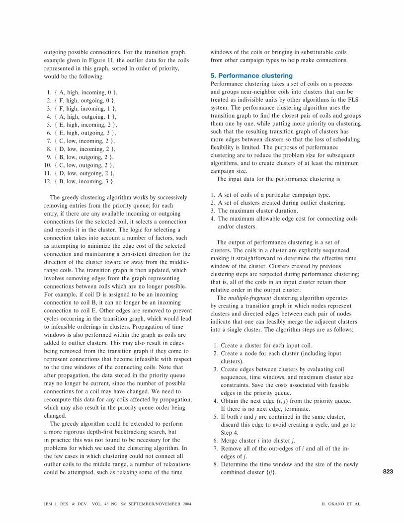
outgoing possible connections. For the transition graphexample given in Figure 11, the outlier data for the coilsrepresented in this graph, sorted in order of priority,would be the following:

1. { A, high, incoming, 0 },2. { F, high, outgoing, 0 },3. { F, high, incoming, 1 },4. { A, high, outgoing, 1 },5. { E, high, incoming, 2 },6. { E, high, outgoing, 3 },7. { C, low, incoming, 2 },8. { D, low, incoming, 2 },9. { B, low, outgoing, 2 },

10. { C, low, outgoing, 2 },11. { D, low, outgoing, 2 },12. { B, low, incoming, 3 }.

The greedy clustering algorithm works by successivelyremoving entries from the priority queue; for eachentry, if there are any available incoming or outgoingconnections for the selected coil, it selects a connectionand records it in the cluster. The logic for selecting aconnection takes into account a number of factors, suchas attempting to minimize the edge cost of the selectedconnection and maintaining a consistent direction for thedirection of the cluster toward or away from the middle-range coils. The transition graph is then updated, whichinvolves removing edges from the graph representingconnections between coils which are no longer possible.For example, if coil D is assigned to be an incomingconnection to coil B, it can no longer be an incomingconnection to coil E. Other edges are removed to preventcycles occurring in the transition graph, which would leadto infeasible orderings in clusters. Propagation of timewindows is also performed within the graph as coils areadded to outlier clusters. This may also result in edgesbeing removed from the transition graph if they come torepresent connections that become infeasible with respectto the time windows of the connecting coils. Note thatafter propagation, the data stored in the priority queuemay no longer be current, since the number of possibleconnections for a coil may have changed. We need torecompute this data for any coils affected by propagation,which may also result in the priority queue order beingchanged.

The greedy algorithm could be extended to performa more rigorous depth-first backtracking search, butin practice this was not found to be necessary for theproblems for which we used the clustering algorithm. Inthe few cases in which clustering could not connect alloutlier coils to the middle range, a number of relaxationscould be attempted, such as relaxing some of the time

windows of the coils or bringing in substitutable coilsfrom other campaign types to help make connections.

5. Performance clusteringPerformance clustering takes a set of coils on a processand groups near-neighbor coils into clusters that can betreated as indivisible units by other algorithms in the FLSsystem. The performance-clustering algorithm uses thetransition graph to find the closest pair of coils and groupsthem one by one, while putting more priority on clusteringsuch that the resulting transition graph of clusters hasmore edges between clusters so that the loss of schedulingflexibility is limited. The purposes of performanceclustering are to reduce the problem size for subsequentalgorithms, and to create clusters of at least the minimumcampaign size.

The input data for the performance clustering is

1. A set of coils of a particular campaign type.2. A set of clusters created during outlier clustering.3. The maximum cluster duration.4. The maximum allowable edge cost for connecting coils

and/or clusters.

The output of performance clustering is a set ofclusters. The coils in a cluster are explicitly sequenced,making it straightforward to determine the effective timewindow of the cluster. Clusters created by previousclustering steps are respected during performance clustering;that is, all of the coils in an input cluster retain theirrelative order in the output cluster.

The multiple-fragment clustering algorithm operatesby creating a transition graph in which nodes representclusters and directed edges between each pair of nodesindicate that one can feasibly merge the adjacent clustersinto a single cluster. The algorithm steps are as follows:

1. Create a cluster for each input coil.2. Create a node for each cluster (including input

clusters).3. Create edges between clusters by evaluating coil

sequences, time windows, and maximum cluster sizeconstraints. Save the costs associated with feasibleedges in the priority queue.

4. Obtain the next edge (i, j) from the priority queue.If there is no next edge, terminate.

5. If both i and j are contained in the same cluster,discard this edge to avoid creating a cycle, and go toStep 4.

6. Merge cluster i into cluster j.7. Remove all of the out-edges of i and all of the in-

edges of j.8. Determine the time window and the size of the newly

combined cluster {ij}.

IBM J. RES. & DEV. VOL. 48 NO. 5/6 SEPTEMBER/NOVEMBER 2004 H. OKANO ET AL.

823

9. Re-evaluate all of the in-edges and out-edges of {ij},remove infeasible edges, and update the priorityqueue costs for feasible edges.

10. Go to Step 4.

Note that the multiple-fragment algorithm is a well-knownheuristic for the traveling salesperson problem (TSP), whichstarts with each point as a fragment consisting of a singlepoint and patches the closest pairs of fragments one byone without making any points of degree three or smallloops (see for example [11]).

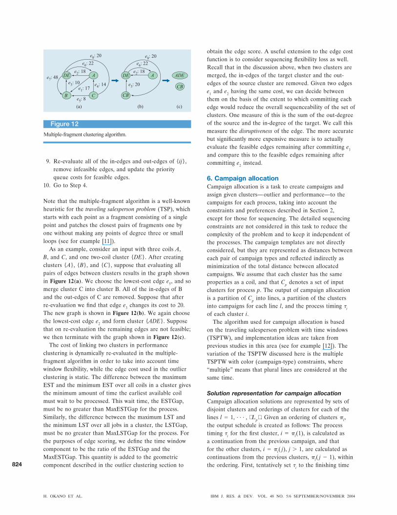
As an example, consider an input with three coils A,B, and C, and one two-coil cluster {DE}. After creatingclusters {A}, {B}, and {C}, suppose that evaluating allpairs of edges between clusters results in the graph shownin Figure 12(a). We choose the lowest-cost edge e5, and somerge cluster C into cluster B. All of the in-edges of Band the out-edges of C are removed. Suppose that afterre-evaluation we find that edge e3 changes its cost to 20.The new graph is shown in Figure 12(b). We again choosethe lowest-cost edge e2 and form cluster {ADE}. Supposethat on re-evaluation the remaining edges are not feasible;we then terminate with the graph shown in Figure 12(c).

The cost of linking two clusters in performanceclustering is dynamically re-evaluated in the multiple-fragment algorithm in order to take into account timewindow flexibility, while the edge cost used in the outlierclustering is static. The difference between the maximumEST and the minimum EST over all coils in a cluster givesthe minimum amount of time the earliest available coilmust wait to be processed. This wait time, the ESTGap,must be no greater than MaxESTGap for the process.Similarly, the difference between the maximum LST andthe minimum LST over all jobs in a cluster, the LSTGap,must be no greater than MaxLSTGap for the process. Forthe purposes of edge scoring, we define the time windowcomponent to be the ratio of the ESTGap and theMaxESTGap. This quantity is added to the geometriccomponent described in the outlier clustering section to

obtain the edge score. A useful extension to the edge costfunction is to consider sequencing flexibility loss as well.Recall that in the discussion above, when two clusters aremerged, the in-edges of the target cluster and the out-edges of the source cluster are removed. Given two edgese1 and e2 having the same cost, we can decide betweenthem on the basis of the extent to which committing eachedge would reduce the overall sequenceability of the set ofclusters. One measure of this is the sum of the out-degreeof the source and the in-degree of the target. We call thismeasure the disruptiveness of the edge. The more accuratebut significantly more expensive measure is to actuallyevaluate the feasible edges remaining after committing e1

and compare this to the feasible edges remaining aftercommitting e2 instead.

6. Campaign allocationCampaign allocation is a task to create campaigns andassign given clusters— outlier and performance—to thecampaigns for each process, taking into account theconstraints and preferences described in Section 2,except for those for sequencing. The detailed sequencingconstraints are not considered in this task to reduce thecomplexity of the problem and to keep it independent ofthe processes. The campaign templates are not directlyconsidered, but they are represented as distances betweeneach pair of campaign types and reflected indirectly asminimization of the total distance between allocatedcampaigns. We assume that each cluster has the sameproperties as a coil, and that Cp denotes a set of inputclusters for process p. The output of campaign allocationis a partition of Cp into lines, a partition of the clustersinto campaigns for each line l, and the process timing �i

of each cluster i.The algorithm used for campaign allocation is based

on the traveling salesperson problem with time windows(TSPTW), and implementation ideas are taken fromprevious studies in this area (see for example [12]). Thevariation of the TSPTW discussed here is the multipleTSPTW with color (campaign-type) constraints, where“multiple” means that plural lines are considered at thesame time.

Solution representation for campaign allocationCampaign allocation solutions are represented by sets ofdisjoint clusters and orderings of clusters for each of thelines l � 1, . . . , Lp . Given an ordering of clusters �l,the output schedule is created as follows: The processtiming �i for the first cluster, i � �l(1), is calculated asa continuation from the previous campaign, and thatfor the other clusters, i � �l( j), j � 1, are calculated ascontinuations from the previous clusters, �l( j � 1), withinthe ordering. First, tentatively set �i to the finishing time

Figure 12

Multiple-fragment clustering algorithm.

e8: 20 e

8: 20

e6: 22 e

6: 22

e2: 18

e3: 10

e1: 17

e5: 8

e4: 14

e2: 18

e3: 20

e7: 48 ADE

CB

(a) (b) (c)

DE A

B C

DE A

CB

H. OKANO ET AL. IBM J. RES. & DEV. VOL. 48 NO. 5/6 SEPTEMBER/NOVEMBER 2004

824

of the previous cluster. If the campaign types of theprevious and current clusters are different, the setup timebetween them is added to �i. If �i ESTi, �i is reset toESTi. If i is associated with chance terms and �i is notcontained in any of the chance terms, the closest chanceterm after �i is found. Let t be the EST of the closestchance term after �i. If t � �i � �, �i remains as it is;otherwise �i is moved to t, where the threshold � is atuning parameter. The gaps created between clusters byEST or chance terms are filled with other clusters duringthe local search phase described later.

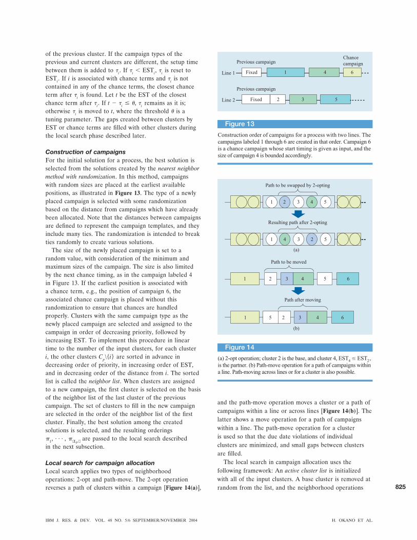
Construction of campaignsFor the initial solution for a process, the best solution isselected from the solutions created by the nearest neighbormethod with randomization. In this method, campaignswith random sizes are placed at the earliest availablepositions, as illustrated in Figure 13. The type of a newlyplaced campaign is selected with some randomizationbased on the distance from campaigns which have alreadybeen allocated. Note that the distances between campaignsare defined to represent the campaign templates, and theyinclude many ties. The randomization is intended to breakties randomly to create various solutions.

The size of the newly placed campaign is set to arandom value, with consideration of the minimum andmaximum sizes of the campaign. The size is also limitedby the next chance timing, as in the campaign labeled 4in Figure 13. If the earliest position is associated witha chance term, e.g., the position of campaign 6, theassociated chance campaign is placed without thisrandomization to ensure that chances are handledproperly. Clusters with the same campaign type as thenewly placed campaign are selected and assigned to thecampaign in order of decreasing priority, followed byincreasing EST. To implement this procedure in lineartime to the number of the input clusters, for each clusteri, the other clusters Cp\{i} are sorted in advance indecreasing order of priority, in increasing order of EST,and in decreasing order of the distance from i. The sortedlist is called the neighbor list. When clusters are assignedto a new campaign, the first cluster is selected on the basisof the neighbor list of the last cluster of the previouscampaign. The set of clusters to fill in the new campaignare selected in the order of the neighbor list of the firstcluster. Finally, the best solution among the createdsolutions is selected, and the resulting orderings�1, . . . , � Lp are passed to the local search describedin the next subsection.

Local search for campaign allocationLocal search applies two types of neighborhoodoperations: 2-opt and path-move. The 2-opt operationreverses a path of clusters within a campaign [Figure 14(a)],

and the path-move operation moves a cluster or a path ofcampaigns within a line or across lines [Figure 14(b)]. Thelatter shows a move operation for a path of campaignswithin a line. The path-move operation for a clusteris used so that the due date violations of individualclusters are minimized, and small gaps between clustersare filled.

The local search in campaign allocation uses thefollowing framework: An active cluster list is initializedwith all of the input clusters. A base cluster is removed atrandom from the list, and the neighborhood operations

Figure 13

Construction order of campaigns for a process with two lines. The

campaigns labeled 1 through 6 are created in that order. Campaign 6

is a chance campaign whose start timing is given as input, and the

size of campaign 4 is bounded accordingly.

Previous campaign

Previous campaign

Chance

campaign

1 6

32

Line 1

Line 2

Fixed

Fixed

4

5

Figure 14

(a) 2-opt operation; cluster 2 is the base, and cluster 4, EST4 � EST

2,

is the partner. (b) Path-move operation for a path of campaigns within

a line. Path-moving across lines or for a cluster is also possible.

Path to be swapped by 2-opting

Resulting path after 2-opting

1 2 3 4 5

1 4 3 2 5

Path to be moved

Path after moving

1 6

1 6

2 3 4 5

2 3 45

(a)

(b)

IBM J. RES. & DEV. VOL. 48 NO. 5/6 SEPTEMBER/NOVEMBER 2004 H. OKANO ET AL.

825

with respect to the base are examined. That is, candidate2-opt and path-move operations, which cut edges thathave the base as one of the ends are examined one byone. While examining the neighborhood operations, thefirst one that reduces the objective value is accepted,and the remaining candidate neighborhoods are discarded.After each application of the neighborhood operations(that is, when the operations have reduced the objectivevalue), the clusters at both ends of the two cut edges in2-opting or the four cut edges in path-moving are insertedinto the active cluster list. The local search continues untilthe list becomes empty. The objective function is definedon the basis of the objectives described in Section 2,except for the sequencing constraint. The candidates fora 2-opt with a base are created as follows: The partnerclusters for the base are first chosen from clusters withinthe same campaign, whose ESTs are earlier than the baseand which are placed after the base. The candidate pathsto be reversed by 2-opting are the paths from the baseto each of the partners. Note that the rule for choosingpartners is designed to minimize tardiness by 2-opting.The candidates for a path-move with a base are created asfollows: The partner clusters for the base are first chosenas the base itself and the last clusters of the campaigns onthe same line placed after the base. The candidate pathsto be moved are the paths from the base to each of thepartners, that is, either the base itself, the latter half ofthe campaign from the base, or consecutive campaigns.The destinations considered for the candidate paths arethe transition points of the campaigns. As campaigns aremoved by local search, the distances between campaignsare minimized, and the orderings of the campaigns aregradually refined so that the campaign templates aresatisfied.

7. SequencingFinding the minimum cost ordering �k of coils Ck assignedto each campaign k is called sequencing. The sequencing isdone for every campaign in the FLS system, and it is alsocalled from a schedule-editing program used by the humanexperts. The FLS system creates a layout of campaignsand orderings of coils for a one-month horizon, and theschedule for a few days from the beginning is passed tothe human experts. The human experts finally fix theorderings of the coils considering the situations changedafter running the FLS system, such as priority changesand delays or failures in coil making in the precedingprocesses. Therefore, the sequencing program should befast enough that a sequence of a few hundreds of coilscan be obtained within a minute. Note that the input forsequencing is not clusters, but coils. Thus, the scalabilityof the sequencing programs (sequencers) cannot beensured by the performance clustering described inSection 5.

In this task, detailed sequencing constraints whichdiffer greatly for different processes should be taken intoaccount, and so different sequencers were implementedfor each of the processes. Although the detailedconstraints differ greatly for each process, they share thesame type of constraints regarding allowable differences ofwidth and thickness. For most of the campaign types onevery process, the overall profile of widths should be wideto narrow in order to avoid edge marks, as described inSection 2 [see Figure 3(b)]. For campaign types orprocesses whose wide-to-narrow preference is strong, thesequencing problem resembles the simple sorting problem;for those whose wide-to-narrow preference is weak, itresembles the traveling salesperson problem with timewindows (TSPTW). We selected the TSPTW as a basemodel for all of the sequencers, and implemented process-dependent constraints on top of the base program.

In the next two subsections, the base TSPTW programand the proximity search method used in the baseprogram are described. The detailed description of theCGL sequencer, which is regarded as the most difficultprocess in the finishing lines in terms of sequencing,appears in another report [13].

TSPTW-based sequencingThe TSPTW is a well-known problem for which variousheuristics have been proposed by many researchers [12].In particular, the subject problem has a distinct structuresimilar to that of the geometric TSP, which is known tobe easier than non-metric TSPs. Note that polynomial-time approximation schemes are known for the formerproblem, whereas no performance guarantee is possiblefor the latter class of problems. Note also that for theTSPTW, even finding a feasible solution is known to beNP-hard, but in practice it is as easy as the TSP when thetime windows are wide. In the sequencing problem, theTSP “cities” to be visited are coils each having a specificwidth and thickness. In terms of both width and thickness,distance and maximum difference between each pair ofcoils are defined. By mapping the coils on a plane ofwidth and thickness as shown in Figures 10(a) and 10(b),the sequencing can be seen as a problem to find theminimum-cost path that visits all of the coils on theplane. The time windows of the coils are relatively widecompared to the campaign length, so that the geometriccharacteristics are dominant in sequencing.

The algorithm used in the base program for sequencinghas the same structure as that used for campaignallocation described in Section 6, consisting of aconstruction heuristic and local search. The solutionrepresentation is an ordering �k. The process timing �i ofeach coil i is calculated by scanning �k from the beginningto the end as �

�k(j) � max{EST�k(j), �

�k(j�1) � l�k(j�1)}. As

described in Section 2, there must be no gaps in process

H. OKANO ET AL. IBM J. RES. & DEV. VOL. 48 NO. 5/6 SEPTEMBER/NOVEMBER 2004

826

timing between consecutive coils. The objective functionis defined to penalize such gaps so that gaps are filledduring the local search. The objective function is a linearcombination of penalties for gaps, tardiness, edge marks,transition costs, and various process-dependent constraints.

The construction heuristic used for the sequencers isthe addition heuristic. In this heuristic, the first and thelast coils, �k(1) and �k( Ck ), are determined first, andthe current solution is created from those coils. The coilnearest to the current solution is then selected from amongthe unvisited coils and inserted into the position in thecurrent solution which least increases the objectivevalue. This continues until all of the coils have beenadded. This procedure can be efficiently implementedusing a priority queue to hold the nearest unvisited coilfrom each of the coils in the current solution. The localsearch used for the sequencers applies the 2-opt andpath-move operations in the same way as in campaignallocation. The structure of the local search is also thesame as for campaign allocation; i.e., an active list of basecoils is used. A significant difference from the campaignallocation is the use of the geometric characteristics, asdescribed in the next subsection.

Using the geometric structureIn the sequencers, queries for the nearest-neighbor coilsor for near-neighbor coils within some radius from a givencoil are used many times. For this purpose, we use a two-dimensional k-d tree [14] where the dimensions representwidth and thickness. Before the k-d tree is created, thedimensions of the input coils are normalized by theaverage allowable differences of width and thickness sothat the rectangle of the allowable differences on thewidth/thickness plane becomes a square. This rectangleis called the transition rectangle (Figure 15).

When the allowable differences of width and thicknessare a and b, respectively, the search radius is set to(r/2)�a 2 � b 2 for finding the near-neighbor coils. Thetuning parameter r is a radius factor used to limit thesearch area. The coils found by the k-d tree inside thecircle are examined one by one to check whether atransition from the search point (center of the circle)is permissible, taking into account all of the properties.Figure 16 shows the performance of the CGL sequencerplotted against the radius factor. (A computer with a1-GHz processor and a 512-MB memory was used.) Thefigure shows that the implementation using the k-dtree is efficient, and it is possible to meet the timerequirements by setting the search radius appropriately.

O(1)-time feasibility check in sequencingIn the construction and local search heuristics of thesequencers, the objective function takes O(n) time to

evaluate the exact cost of a coil sequence, where n � Ckis the number of coils in the sequence. The same amountof time is required even if a coil sequence is updatedonly locally because a local change might affect thewhole sequence for some constraints such as tardiness,temperature transitions, wide-to-narrow constraint, and soon. For example, it must scan the sequence forward andbackward to compute the target furnace temperature forthe continuous annealing line. Though such a linear timealgorithm might seem practical, the reality is that theobjective function is evaluated within a loop of O(n) orhigher complexity, thus making the whole computationalcost more than quadratic, which is impractical.

To make the computation faster, we adopted a two-stage evaluation: 1) In the first stage, the cost of the newsequence is “estimated” in O(1) time. 2) If the estimated

Figure 15

Transition rectangle.

Width

Thic

kness

b

a

2

1 a2 � b2

Search

point

Figure 16

Performance of the sequencer.

0

10

20

30

40

50

60

70

80

0 100 200 300 400 500

Tim

e (s

)

Number of coils

k-d tree (radius factor � 2.0)

k-d tree (radius factor � 1.0)

k-d tree (radius factor � 0.5)

IBM J. RES. & DEV. VOL. 48 NO. 5/6 SEPTEMBER/NOVEMBER 2004 H. OKANO ET AL.

827

cost is lower than the cost of the original sequence, thecost of the new sequence is then exactly evaluated usingO(n) time; otherwise, the new sequence is discardedwithout actually evaluating the objective function. Notethat, for time windows, an O(1)-time feasibility checkalgorithm which does not reject feasible solutionsis already known [15], whereas in our logic, whichconsiders various constraints, the first stage may rejectfeasible solutions in rare cases. Most of the neighborhoodsolutions examined in local search will be worse than thecurrent one, especially when the search is near a localoptimal solution. Therefore, rejecting obviously worsesolutions in the first stage can greatly speed up thesequencers.

To estimate the new sequence in O(1) time, wepropagate information forward and backward through thesequence and store additional information for each of thecoils. Given the changed parts of the sequence, the cost ofthe sequence is estimated in the first stage by referringonly to the additional information around the changedparts. As a result, we were able to make the sequencers15 to 50 times faster without making the solution qualityworse.

8. ConclusionsA new solution for the finishing line scheduling (FLS)problem in a major steel mill has been described. Theproduction schedules for finishing lines involve varioustypes of production campaigns because the number ofkinds of steel sheet products produced in the steel mill isvery large. Therefore, minimization of the setup cost andtime between campaigns is one of the main requirementsof the FLS problem. The problem also requires ensuringthe timing consistencies of coils across four processes.Capacity planning tools are not applicable to this problembecause of these complex constraints. To the best of ourknowledge, there is no prior study in the literature thataddresses the FLS problem as of the time at which thispaper is being written.

Issues in designing the solution were the complexityand size of the problem. In order to reduce the problemcomplexity, we separated the problems of sequenceabilityand timing consistency from campaign allocation by usingoutlier clustering for sequenceability, and by using timewindow propagation and upward and downward schedulingfor timing consistency. In order to reduce the problem sizefor campaign allocation, we introduced performanceclustering. The scalability of the sequencers was ensuredby the radius factor and the O(1)-time feasibility check.These approaches made it possible to scale our solutionup to large amounts of input data, which, in the case ofthe subject steel mill, comes to 20 to 25 thousand coils,while satisfying the one-hour limit for running time.

By using the FLS system, the steel mill can providethe primary production scheduling system with accuratedue dates of coils for a one-month horizon. The systemsintegration has just been completed, and the cost savingshave not yet been determined. The expected meritsyielded by the FLS system are the following: plan leadtime reduction, inventory reduction, workforce reduction,capability for quick rescheduling, and accurate due datequotation, where the plan lead time means the timerequired from order input to production, the inventorymeans the number of work-in-process (WIP) coils, and theworkforce is for sequencing and for the creation of chancetables. The steel mill created rough production campaignsof daily buckets for a one-month horizon, called a chancetable, to use for due date quotation or for workforceplanning. Since the FLS system can automatically create aproduction schedule more precise than the chance table,creation of the chance table itself is no longer necessary.The FLS system has allowed the steel mill to createschedules with a one-month horizon every day, and hasincreased the potential decision frequency from monthlyto daily.

AcknowledgmentsThe authors would like to express sincere gratitude to Mr.Yuhichi Shibata at IBM Business Consulting Services forhis valuable comments and suggestions on the manuscript.

References1. H. Yasuda, H. Tokuyama, K. Tarui, Y. Tanimoto, and M.

Nagano, “Two-Stage Algorithm for Production Schedulingof Hot Strip Mill,” Oper. Res. 32, 695–707 (1984).

2. H.-L. Fang and C.-H. Tsai, “A Genetic AlgorithmApproach to Hot Strip Mill Rolling SchedulingProblems,” Proceedings of the International Conference onTools with Artificial Intelligence, IEEE, Piscataway, NJ,1998, pp. 264 –271.

3. L. Lopez, M. W. Carter, and M. Gendreau, “The HotStrip Mill Production Scheduling Problem: A Tabu SearchApproach,” Eur. J. Oper. Res. 106, 317–335 (1998).

4. M. Numao and S. Morishita, “Co-operative Schedulingand Its Application to Steelmaking Industries,” IEEETrans. Indust. Electron. 38, 150 –155 (1991).

5. H.-S. Lee, S. S. Murthy, S. W. Haider, and D. V. Morse,“Primary Production Scheduling at SteelmakingIndustries,” IBM J. Res. & Dev. 40, 231–252 (1996).

6. S. N. Talukdar, L. Baerentzen, A. Gove, and P. S.de Souza, “Asynchronous Teams: Cooperation Schemesfor Autonomous Agents,” J. Heuristics 4, 295–321 (1998).

7. S. N. Talukdar, P. S. de Souza, and S. Murthy,“Organizations for Computer-Based Agents,” Int. J. Eng.Intell. Syst. 1, 75– 87 (1993).

8. H. Gao, J. Zeng, and G. Sun, “Multi-Agent Approach forPlanning and Scheduling of Integrated Steel Processes,”Proceedings of the IEEE International Conference onSystems, Man, and Cybernetics, 2002, pp. 427– 432.

9. L. M. Wein and P. B. Chevalier, “A Broader View of theJob-Shop Scheduling Problem,” Manage. Sci. 38, 1018 –1033 (1992).

10. R. C. Leachman, J. Kang, and V. Lin, “Slim: Short CycleTime and Low Inventory in Manufacturing at Samsung

H. OKANO ET AL. IBM J. RES. & DEV. VOL. 48 NO. 5/6 SEPTEMBER/NOVEMBER 2004

828

Electronics,” Interfaces 32, 61–77 (2002).11. J. L. Bentley, “Fast Algorithms for Geometric Traveling

Salesman Problems,” ORSA J. Computing 4, 387– 411(1992).

12. D. S. Johnson and L. A. McGeoch, “The TravelingSalesman Problem: A Case Study,” Local Search inCombinatorial Optimization, E. H. L. Aarts and J. K.Lenstra, Eds., John Wiley and Sons, Inc., New York,1997, pp. 215–310.

13. H. Okano, T. Morioka, and K. Yoda, “A HeuristicSolution for the Continuous Galvanizing Line SchedulingProblem in a Steel Mill,” Research Report RT-0478, 2002;IBM Tokyo Research Laboratory, 1623-14 Shimo-tsuruma,Yamato-shi, Kanagawa-ken 242-8502, Japan.

14. J. L. Bentley, “K-d Trees for Semidynamic Point Sets,”Proceedings of the Sixth Annual ACM Symposium onComputational Geometry, 1990, pp. 187–197.

15. G. A. P. Kindervater and M. W. Savelsbergh, “Vehicle

Combinatorial Optimization, E. H. L. Aarts and J. K.Lenstra, Eds., John Wiley and Sons, Inc., New York,1997, pp. 337–360.

Received October 15, 2003; accepted for publication May

Hiroyuki Okano IBM Research Division, IBM TokyoResearch Laboratory, 1623-14 Shimo-tsuruma, Yamato-shi,Kanagawa-ken 242-8502, Japan (okanoh@jp.ibm.com). Mr.Okano joined the IBM Tokyo Research Laboratory in 1990after receiving B.S. (1988) and M.S. (1990) degrees ininformation science from the Tokyo University of Agricultureand Technology. After five years of research on userinterfaces and systems software, Mr. Okano joined theoperations research group and started work on combinatorialoptimization. Since then, he has been working on developingsolutions to several optimization problems in logistics and themanufacturing industry. His research interests includescheduling and optimization, local search techniques, andstochastic sensitivity analysis.

Andrew J. Davenport IBM Research Division, IBMThomas J. Watson Research Center, P.O. Box 218, YorktownHeights, New York 10598 (davenport@us.ibm.com). Dr.Davenport received his M.Sc. and Ph.D. degrees in computerscience from the University of Essex, United Kingdom. Hespent four years working as a Research Scientist in theEnterprise Integration Laboratory at the University ofToronto, Canada, where he focused on developing newconstraint programming technologies to solve complexplanning and scheduling problems in industry. In 1999 hejoined the IBM Research Division, where he is a ResearchStaff Member in the Department of Mathematical Sciences.He is currently working on projects applying constraintprogramming, mathematical optimization, and artificialintelligence technologies to a range of customer problems inelectronic commerce, production planning, and scheduling.

Mark Trumbo Dragonfly Consulting, 3-320 Chapel Street,Ottawa, Ontario K1N 7Z3 Canada (marktrumbo@rogers.com).Mr. Trumbo joined IBM in 1988 after receiving a B.S.E.E.degree from the University of Washington; he joined theManufacturing Research Department at the IBM Thomas J.Watson Research Center in 1990. After receiving an M.A.Sc.degree from Simon Fraser University in 1994, Mr. Trumboreturned to the IBM Research Division to concentrate onplanning and scheduling for the steel industry; over the courseof several years, he successfully implemented inventoryapplication, slab design, and cast design systems for a majorJapanese steel producer. Now an independent consultant, Mr.Trumbo continues to collaborate closely with IBM Researchand IBM Global Services to provide solutions for customersin the metals industry.

Chandra Reddy IBM Research Division, IBM Thomas J.Watson Research Center, P.O. Box 218, Yorktown Heights, NewYork 10598 (creddy@us.ibm.com). Dr. Reddy joined IBM in1998 after receiving a Ph.D. degree in computer science fromOregon State University. Since then, he has been working ondeveloping solutions to several optimization and schedulingproblems arising in the steel industry. Several of thesesolutions have been successfully deployed and are inproduction at two of the world�s leading steel makers. Hisresearch prior to joining IBM focused on both theoretical andpractical aspects of machine learning of compact hierarchicalcontrol knowledge for planning and problem solving. Dr.Reddy�s research interests include scheduling and optimization,machine learning for planning and classification, data mining,and artificial intelligence.

IBM J. RES. & DEV. VOL. 48 NO. 5/6 SEPTEMBER/NOVEMBER 2004 H. OKANO ET AL.

829

Routing: Handling Edge Exchanges,” Local Search in

28, 2004; Internet publication September 17, 2004

Kunikazu Yoda IBM Research Division, IBM TokyoResearch Laboratory, 1623-14 Shimo-tsuruma, Yamato-shi,Kanagawa-ken 242-8502, Japan (yoda@jp.ibm.com). Mr. Yodareceived a B.S. degree in applied mathematics and physicsand an M.S. degree in applied systems science from KyotoUniversity in 1994 and 1996, respectively. He joined the IBMResearch Division in 1996, initially working on data mining.He was subsequently involved in a variety of projectsincluding network security, optimization, autonomiccomputing, and grid computing. Mr. Yoda�s research interestslie in the area of reliable distributed systems, fault-tolerantdistributed algorithms, and discrete algorithms in optimizationproblems.

Masami Amano IBM Research Division, IBM TokyoResearch Laboratory, 1623-14 Shimo-tsuruma, Yamato-shi,Kanagawa-ken 242-8502, Japan (amanom@jp.ibm.com). Mr.Amano received B.S. and M.S. degrees in information sciencefrom Kyoto University. He joined the IBM Research Divisionin 2001 to work on optimization technologies such asproduction scheduling and transportation scheduling. Hiscurrent interest is optimization for supply chain managementin the manufacturing industry.

H. OKANO ET AL. IBM J. RES. & DEV. VOL. 48 NO. 5/6 SEPTEMBER/NOVEMBER 2004

830