experiment and simulations Ing. Martin Doubek
175
Czech Technical University in Prague Faculty of Mechanical Engineering Department of Physics Doctoral thesis Thermophysical properties of refrigerants: experiment and simulations Ing. Martin Doubek Doctoral Study Program: Mechanical Engineering Thesis supervisor: Doc. Ing. Václav Vacek, CSc. Dissertation thesis for obtaining the academic title of "Doctor" abbreviated to "Ph.D." Prague December 2018 Study Field: Mathematical and Physical Engineering
-
Upload
khangminh22 -
Category
Documents
-
view
0 -
download
0
Transcript of experiment and simulations Ing. Martin Doubek
Czech Technical University in Prague
Faculty of Mechanical Engineering
Department of Physics
Doctoral thesis
Thermophysical properties of refrigerants:experiment and simulations
Ing. Martin Doubek
Doctoral Study Program: Mechanical Engineering
Thesis supervisor: Doc. Ing. Václav Vacek, CSc.
Dissertation thesis for obtaining the academic title of "Doctor"abbreviated to "Ph.D."
Prague December 2018
Study Field: Mathematical and Physical Engineering


DisclaimerProhlašuji, že jsem tuto disertacní práci vypracoval samostatne pod vedením vedoucího práce
a na zarízení, které bylo realizováno z grantových prostredku Ústavu fyziky Fakulty strojníCVUT v Praze a je majetkem ústavu. Pri vypracování své doktorské práce jsem použil literaturuuvedenou v seznamu na konci této práce. Nemám závažný duvod proti užití tohoto školního dílave smyslu § 60 zákona c. 121/2000 Sb., o právu autorském, o právech souvisejících s právemautorským a o zmene nekterých zákonu (autorský zákon)
V Praze dne: ............ ........................Martin Doubek
Abstract
This PhD thesis focuses on thermodynamics of pure refrigerants and refrigerants mixturesincluding mixtures of unlike fluids. The vapour-liquid equilibrium of these mixtures is studiedalong with speed of sound in both phases. The thesis consists of two parts: the first part isdedicated to design of a high accuracy speed of sound measurement apparatus which is used toobtain unique thermodynamic data. The second part deals with prediction models in form ofequations of state. The research is driven by ongoing development of new refrigerant blends forcommercial applications and by future needs of the cooling and monitoring systems for particledetectors at CERN.
The prediction of thermodynamic properties of fluid mixtures, especially mixtures of unlikefluids (natural refrigerants + fluorocarbons) is a challenging task. Currently only complexcontribution methods can provide reasonable accuracy for new blends where no experimentaldata exists. This work presents newly developed correlations for prediction of binary interactioncoefficient for SAFT-BACK model which has never been used for such mixtures. ThreeSAFT models are scrutinized in terms of prediction of vapour liquid equilibrium and speed ofsound using extensive data sets for natural refrigerants, fluorocarbons and their mixtures. Thecombination of the SAFT-BACK model with developed correlations creates prediction modelfor new refrigerant blends that uses only few fitting parameters.
Abstrakt
Predkládaná doktorská práce je studií termodynamických vlastností cistých chladiv a smesíchladiv vcetne smesí nestejnorodých látek. Podrobne je studována rovnováha kapalina-pára arychlost zvuku v obou fázích techto smesí. První cást práce se zabývá návrhem zarízení provelmi presné merení rychlosti zvuku, které je použito pro získání unikátních termodynamickýchdat. Druhá cást je venována výpoctum rychlosti zvuku a rovnováhy kapalina-pára cistých látek ismesí pomocí stavových rovnic. Hlavní motivací pro tento výzkum je soucasný vývoj novýchsmesí chladiv v komercním sektoru a potreby chladicích a monitorovacích systému cásticovýchdetektoru v CERN v Ženeve.
Výpocty vlastností smesí ruznorodých látek (prírodní chladiva + fluorovaná chladiva) jsounárocný úkol. Složité kontribucní modely jsou v soucasné dobe jedinou volbou pro presnévýpocty smesí, ke kterým neexistují experimentální data. V rámci predkládané práce jsouvyvinuty nové korelace pro odhad binárních interakcních koeficientu pro model SAFT-BACK,který pro podobné smesi ješte nikdy nebyl použit. Tri SAFT modely jsou dukladne testovány naexperimentálních datech rovnováhy kapalina-pára a rychlosti zvuku v obou fázích prírodníchchladiv, fluorovaných chladiv a jejich smesí. Výsledkem spojení modelu SAFT-BACK s novevyvinutými korelacemi je predikcní model pro výpocty nových smesí chladiv, který vyžadujejen malý pocet parametru.

Acknowledgements
I wish to express my deepest gratitude to my family for all the support that made it possiblefor me to pursue the doctoral degree.
Contents
Nomenclature xi
1 Introduction 21.1 Refrigerant blends . . . . . . . . . . . . . . . . . . . . . . . . . . . . . . . . . . . . . . . . 21.2 Importance of speed of sound in Thermodynamics . . . . . . . . . . . . . . . . . . . . . . . 41.3 Uses of speed of sound in refrigeration . . . . . . . . . . . . . . . . . . . . . . . . . . . . . 41.4 Refrigerant blends at CERN . . . . . . . . . . . . . . . . . . . . . . . . . . . . . . . . . . 61.5 Motivation . . . . . . . . . . . . . . . . . . . . . . . . . . . . . . . . . . . . . . . . . . . . 8Bibliography . . . . . . . . . . . . . . . . . . . . . . . . . . . . . . . . . . . . . . . . . . . . . 10
2 Prior art 112.1 Thermodynamic models . . . . . . . . . . . . . . . . . . . . . . . . . . . . . . . . . . . . 11
2.1.1 Introduction . . . . . . . . . . . . . . . . . . . . . . . . . . . . . . . . . . . . . . . 112.1.2 Speed of sound . . . . . . . . . . . . . . . . . . . . . . . . . . . . . . . . . . . . . 112.1.3 Equations of state . . . . . . . . . . . . . . . . . . . . . . . . . . . . . . . . . . . . 122.1.4 Empirical equations of state . . . . . . . . . . . . . . . . . . . . . . . . . . . . . . 132.1.5 Virial equations of state . . . . . . . . . . . . . . . . . . . . . . . . . . . . . . . . 142.1.6 Cubic equations . . . . . . . . . . . . . . . . . . . . . . . . . . . . . . . . . . . . . 152.1.7 Volume-translated cubic equation of state . . . . . . . . . . . . . . . . . . . . . . . 182.1.8 Helmholtz-energy equations of state . . . . . . . . . . . . . . . . . . . . . . . . . . 202.1.9 Acoustic models . . . . . . . . . . . . . . . . . . . . . . . . . . . . . . . . . . . . 212.1.10 SAFT equations of state . . . . . . . . . . . . . . . . . . . . . . . . . . . . . . . . 23
2.2 Binary interaction parameters . . . . . . . . . . . . . . . . . . . . . . . . . . . . . . . . . . 252.2.1 Correlations for estimation of interaction coefficients . . . . . . . . . . . . . . . . . 26
2.3 Speed of sound measurement and fluid analysis . . . . . . . . . . . . . . . . . . . . . . . . 292.4 Commercially available instruments . . . . . . . . . . . . . . . . . . . . . . . . . . . . . . 332.5 Summary . . . . . . . . . . . . . . . . . . . . . . . . . . . . . . . . . . . . . . . . . . . . 37Bibliography . . . . . . . . . . . . . . . . . . . . . . . . . . . . . . . . . . . . . . . . . . . . . 38
3 Speed of sound measurement 443.1 Speed of sound measurement techniques . . . . . . . . . . . . . . . . . . . . . . . . . . . . 44
3.1.1 Resonance methods . . . . . . . . . . . . . . . . . . . . . . . . . . . . . . . . . . . 443.1.2 Interferometric method . . . . . . . . . . . . . . . . . . . . . . . . . . . . . . . . . 503.1.3 Time of flight . . . . . . . . . . . . . . . . . . . . . . . . . . . . . . . . . . . . . . 51
3.2 Instrumentation for speed of sound measurement . . . . . . . . . . . . . . . . . . . . . . . 523.3 Sound transmission losses . . . . . . . . . . . . . . . . . . . . . . . . . . . . . . . . . . . 55
3.3.1 Piezoelectric transducers . . . . . . . . . . . . . . . . . . . . . . . . . . . . . . . . 573.3.2 Electrostatic transducers . . . . . . . . . . . . . . . . . . . . . . . . . . . . . . . . 60
Bibliography . . . . . . . . . . . . . . . . . . . . . . . . . . . . . . . . . . . . . . . . . . . . . 63
viii
4 Problem statement and goals 664.1 Problem statement . . . . . . . . . . . . . . . . . . . . . . . . . . . . . . . . . . . . . . . 664.2 Goals . . . . . . . . . . . . . . . . . . . . . . . . . . . . . . . . . . . . . . . . . . . . . . 66
5 Development of high accuracy speed-of-sound measurement apparatus 685.1 Setup Overview . . . . . . . . . . . . . . . . . . . . . . . . . . . . . . . . . . . . . . . . . 685.2 Mechanical design . . . . . . . . . . . . . . . . . . . . . . . . . . . . . . . . . . . . . . . 695.3 Electronics . . . . . . . . . . . . . . . . . . . . . . . . . . . . . . . . . . . . . . . . . . . 705.4 Design optimization for mixtures . . . . . . . . . . . . . . . . . . . . . . . . . . . . . . . . 745.5 Calibration and measurement procedure . . . . . . . . . . . . . . . . . . . . . . . . . . . . 755.6 Measurement uncertainty . . . . . . . . . . . . . . . . . . . . . . . . . . . . . . . . . . . . 755.7 Measured data . . . . . . . . . . . . . . . . . . . . . . . . . . . . . . . . . . . . . . . . . . 775.8 Comparison of measured data . . . . . . . . . . . . . . . . . . . . . . . . . . . . . . . . . 80Bibliography . . . . . . . . . . . . . . . . . . . . . . . . . . . . . . . . . . . . . . . . . . . . . 82
6 Thermodynamic Models 836.1 Peng-Robinson equation of state . . . . . . . . . . . . . . . . . . . . . . . . . . . . . . . . 836.2 Volume-translated Peng-Robinson equation of state . . . . . . . . . . . . . . . . . . . . . . 84
6.2.1 Volume translation by Magoulas and Tassios . . . . . . . . . . . . . . . . . . . . . 846.2.2 Volume translation by Ahlers and Gmehling . . . . . . . . . . . . . . . . . . . . . . 846.2.3 Volume translation by Lin and Duan . . . . . . . . . . . . . . . . . . . . . . . . . . 85
6.3 SoftSAFT . . . . . . . . . . . . . . . . . . . . . . . . . . . . . . . . . . . . . . . . . . . . 866.4 sPC-SAFT . . . . . . . . . . . . . . . . . . . . . . . . . . . . . . . . . . . . . . . . . . . . 896.5 SAFT-BACK . . . . . . . . . . . . . . . . . . . . . . . . . . . . . . . . . . . . . . . . . . 916.6 Speed of sound and molecular relaxation . . . . . . . . . . . . . . . . . . . . . . . . . . . . 94
6.6.1 Relaxation times . . . . . . . . . . . . . . . . . . . . . . . . . . . . . . . . . . . . 976.7 Vapour-liquid equilibrium . . . . . . . . . . . . . . . . . . . . . . . . . . . . . . . . . . . 98Bibliography . . . . . . . . . . . . . . . . . . . . . . . . . . . . . . . . . . . . . . . . . . . . . 103
7 Evaluations of models 1067.1 Introduction . . . . . . . . . . . . . . . . . . . . . . . . . . . . . . . . . . . . . . . . . . . 1067.2 Fluids . . . . . . . . . . . . . . . . . . . . . . . . . . . . . . . . . . . . . . . . . . . . . . 1067.3 Model parameter fitting . . . . . . . . . . . . . . . . . . . . . . . . . . . . . . . . . . . . . 1087.4 Model evaluations - saturation properties of pure fluids . . . . . . . . . . . . . . . . . . . . 1107.5 Model evaluations - Speed of sound . . . . . . . . . . . . . . . . . . . . . . . . . . . . . . 1127.6 Mixtures . . . . . . . . . . . . . . . . . . . . . . . . . . . . . . . . . . . . . . . . . . . . . 1167.7 Correlations of binary interaction coefficients . . . . . . . . . . . . . . . . . . . . . . . . . 1197.8 Speed of sound in mixtures . . . . . . . . . . . . . . . . . . . . . . . . . . . . . . . . . . . 123Bibliography . . . . . . . . . . . . . . . . . . . . . . . . . . . . . . . . . . . . . . . . . . . . . 125
8 Summary and conclusions 1308.1 Development of high accuracy speed-of-sound measurement apparatus . . . . . . . . . . . . 1308.2 Evaluations of models . . . . . . . . . . . . . . . . . . . . . . . . . . . . . . . . . . . . . . 1308.3 Applications . . . . . . . . . . . . . . . . . . . . . . . . . . . . . . . . . . . . . . . . . . . 131Bibliography . . . . . . . . . . . . . . . . . . . . . . . . . . . . . . . . . . . . . . . . . . . . . 132
9 Annexes 1349.1 Vapour liquid equilibrium plots . . . . . . . . . . . . . . . . . . . . . . . . . . . . . . . . . 1349.2 Speed of sound plots . . . . . . . . . . . . . . . . . . . . . . . . . . . . . . . . . . . . . . 140
9.2.1 vapour phase . . . . . . . . . . . . . . . . . . . . . . . . . . . . . . . . . . . . . . 1419.2.2 Liquid phase . . . . . . . . . . . . . . . . . . . . . . . . . . . . . . . . . . . . . . 150
9.3 Mixtures . . . . . . . . . . . . . . . . . . . . . . . . . . . . . . . . . . . . . . . . . . . . . 153
Nomenclature
Subscripts
a Acoustic
c Critical
LJ Lennard Jones
m Mixture
p At constant pressure
RA Rackett
r Reduced
S At constant entropy
T At constant temperature
v At constant volume
Superscripts′ Liquid phase′′ Vapor phase
0 Ideal gas contribution or reference state
calc Calculated
exp Experimental
HC Hard chain
id Ideal
p Perturbation term
r Residual part
ref Reference
Lower Case
a Cubic equation parameter [Pa.kmol−2.m6]
a Helmholtz energy [J]
ai Einstein coefficient [K]
b Cubic equation parameter [m3.kmol−1]
c Volume shift [m3.mol−1]
c Molar heat capacity [J.mol−1.K−1]
xi

d Segment diameter [m]
f Frequency [Hz]
g Imaginary part of resonance frequency [Hz]
g Radial distribution function [−]
h Thermal accomodation coefficient [−]
k Thermal conductivity (chapter 3) [W.m−2.K−1]
kB Boltzmann constant [J.K−1]
kij Pair interaction coefficient [−]
la Accomodation length [m]
m Average length of chains [−]
n Number of components in a mixture [−]
p Pressure [Pa]
r Radius [m]
t time [s]
ttime Ultrasound time of flight (chapter 4) [s]
u Pair potential energy [J]
uA Uncertainity type A (chapter 4) [various]
uB Uncertainity type B (chapter 4) [various]
v Molar volume [m3.mol−1]
w Speed of sound [m.s−1]
x Mole fraction [1]
Greek Letters
α Dimensionless Helmholtz Energy [1]
α Helmholtz energy [1]
α Cubic equation alpha function [−]
αs Attenuation (chapter 3) [1.m−1]
β Adiabatic compressibility [1.Pa−1]
δ Reduced density [1]
ε Interaction strength [J]
εAB Association energy parameter [Pa.m3]
η Packing fraction [1]
γ Heat capacity ratio [1]
κ Scaling factor [−]
κAB Association volume [m3.mol−1]
λ Wave length [m]
µ Chemical potental [J/particle]
µ Dynamic viscosity [Pa.s]
ν Eigenvalue of resonance modes [−]
ω Complex angular frequency [Hz]
ω Accentric factor [−]
φ Attenuation coefficient (chapter 3) [−]
ρ Molar density [mol.m−3]
σ Molecule diameter [Å]
τ Relaxation time [s]
τ Inverse reduced temperature [1]
τRC Time constant [s]
ϕ Energy loss coefficient (chapter 3) [−]
ϕ Fugacity [Pa]
ζ Dimensionless speed of sound [1]
Upper Case
B Second virial coefficient [m−3.mol−1]
C Third virial coefficient [m−6.mol−2]
D Distance [m]
Dp Thickness [m]
Dt Thermal diffusivity [m2.s−1]
I Wave intensity (chapter 3) [W.m−2]
L Length [m]
M Molar mass [kg.mol−1]
N Frequency constants of piezo crystals (chapter 3) [Hz.m]
N Number of particles/molecules [−]
Q Charge [C]
Qf Resonance quality factor [1]
R Reflection coefficient (chapter 3) [−]
R Universal gas constant [J.mol−1.K−1]
S Entropy [J.K−1]
T Temperature [K]
Tp Transmission coefficient (chapter 3) [−]
U Expanded uncertainity (chapter 4) [various]

U Voltage [V ]
Z Acustic impedance (chapter 3) [Pa.s.m−3]
Z Compressibility factor [1]
Publications
I am author or co-author of folllowing publications that present results described in this thesis and that can befound in the references:
1. M. Doubek and V. Vacek, Speed of Sound Data in Pure Refrigerants R-116 and R-218 and TheirMixtures: Experiment and Modeling, Journal of Chemical & Engineering Data, 2016, 61(12), pp.4046-4056
2. M. Doubek, V. Vacek, G. Hallewell and B. Pearson, Speed-of-sound based sensors for environmentalmonitoring, IEEE SENSORS, Orlando FL, 2016, pp. 1-3
3. M. Doubek, M. Haubner, V. Vacek, M. Battistin, G. Hallewell, S. Katunin, D. Robinson, Measurementof heat transfer coefficient in two phase flows of radiation-resistant zeotropic C2F6/C3F8 blends,International Journal of Heat and Mass Transfer, 2017, 113, pp. 246-256
4. M. Alhroob, M. Battistin, S. Berry, . . . M. Doubek et al., Custom ultrasonic instrumentation forflow measurement and real-time binary gas analysis in the CERN ATLAS experiment, Journal ofInstrumentation, 2017, 12, C01091, ISSN 1748-0221
5. M. Alhroob, M. Battistin, S. Berry, . . . M. Doubek et al., Custom real-time ultrasonic instrumentationfor simultaneous mixture and flow analysis of binary gases in the CERN ATLAS experiment, NuclearInstruments and Methods in Physics Research Section A: Accelerators, Spectrometers, Detectors andAssociated Equipment, 2017, 845(11), pp. 273-277
6. M. Battistin, S. Berry, A. Bitadtze, . . . M. Doubek et al., The thermosiphon cooling system of the atlasexperiment at the cern large hadron collider. International Journal of Chemical Reactor Engineering,2015, ISSN (Online) 1542-6580, ISSN (Print) 2194-5748
7. R. Bates, M. Battistin, S. Berry, . . . M. Doubek et al., The cooling capabilities of C2F6 / C3F8 saturatedfluorocarbon blends for the atlas silicon tracker. Journal of Instrumentation, 2015, 10(03), P03027
8. M. Alhroob, R. Bates M. Battistin, . . . M. Doubek et al., Development of a custom on-line ultrasonicvapour analyser and flow meter for the atlas inner detector, with application to cherenkov and gaseouscharged particle detectors, Journal of Instrumentation, 2015, 10(03):C03045
9. M. Doubek, M. Haubner, D: Houška et al. Experimental investigation and modelling of flow boilingheat transfer of C3F8/C2F6 blends, In: Proceedings of the 13th International Conference on HeatTransfer, Fluid Mechanics and Thermodynamics 2017. Pretoria: University of Pretoria, pp. 355-364.
10. M. Doubek and V. Vacek, Experimental study of refrigerants and their mixtures, Paper and Posterpresentation, Proceedings of 13th International Conference on Properties and Phase Equilibria forProducts and Process Design, 22–26 May 2016, Granja – Portugal.
11. M. Doubek and V. Vacek, Thermodynamic properties of fluorocarbons: Simulations and experiment. Inproceedings of the 24th IIR International Congress of Refrigeration, number ID:340, 2015, Yokohama,Japan, ISBN : 9782362150128
1
Chapter 1 Introduction
1 Introduction
All refrigerants were pure fluids in the past (R-11, R-22, carbon dioxide) but blends have been slowlyintroduced along the way. Either to replace phased-out pure refrigerants that were no longer allowed due totheir high environmental impact (high Global Warming Potential GWP or Ozone Depletion Potential ODP).Or to provide certain performance characteristics that could not be achieved with pure fluids. In either case,the composition of refrigerant blends is carefully formulated to meet complex requirements on evaporationand condensation temperatures, energy efficiency, miscibility with oils, low environmental impact and manyothers.
Modern refrigerant blends are often mixtures of very different components (natural refrigerant, hydro-fluorocarbons HFCs, hydrofluoroolefins HFOs etc.) in order to provide desired properties, namely the lowenvironmental impact. Modelling is always used before any experimental testing to formulate new blends orto study effect of changes in composition on behaviour and cooling performance. Unfortunately, modellingof such complex mixtures is a difficult task. Accurate models of the pure fluids coupled with appropriatemixing rules are required along with large and accurate experimental data sets that are needed for modelfitting and model evaluations.
Apart from the fact that the speed of sound is needed to obtain the ideal gas heat capacity of the refrigerantsand that it plays important role during the development of the thermodynamic models, it can be also used forfluid analysis. Relatively simple and inexpensive yet accurate instruments for speed of sound measurementcoupled with appropriate model can be used for online monitoring of blend composition. Such blend analysisis useful in an experimental circuit during blend development and testing but it can be also employed tomonitor blend composition during cooling plant operation since the composition can change in time due toleaks and/or wrong filling procedures.
1.1 Refrigerant blends
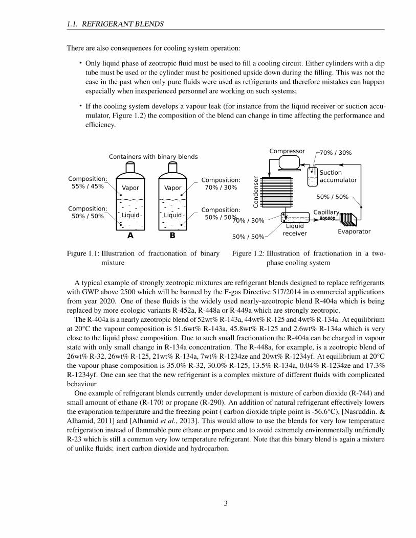
Zeotropic mixtures have different composition of vapour phase and liquid phase, Figure 1.1. The zeotropicbehaviour is called fractionation in the refrigeration industry. It is most pronounced when components ofhighly different volatilities are combined in a blend. For simplicity, let’s consider a binary zeotropic blend.The more volatile component, in other words the component with higher vapour pressure, will be prevalentin the gas phase at a vapour-liquid equilibrium. The vapour phase of the equilibrium state will have thereforedifferent composition than the liquid. The difference in composition will be higher for components withhighly different volatilities (vapour pressures) as is shown in the Figure 1.1 where the blend B componentshave a higher difference in vapour pressures.
The fractionation of zeotropic blends has following consequences for cooling system design:
• The fractionation precludes the zeotropic blends from use in systems where a pool boiling occurs, forinstance in flooded evaporators or in suction line heat exchangers;
• The boiling temperature is higher at the input of the evaporator and lower at the evaporator exit. Thiseffect is called evaporator glide, and it is caused by the different volatility and thus different rate ofboiling of the blend constituents.
2
1.1. REFRIGERANT BLENDS
There are also consequences for cooling system operation:
• Only liquid phase of zeotropic fluid must be used to fill a cooling circuit. Either cylinders with a diptube must be used or the cylinder must be positioned upside down during the filling. This was not thecase in the past when only pure fluids were used as refrigerants and therefore mistakes can happenespecially when inexperienced personnel are working on such systems;
• If the cooling system develops a vapour leak (for instance from the liquid receiver or suction accu-mulator, Figure 1.2) the composition of the blend can change in time affecting the performance andefficiency.
Liquid
Vapor
Containers with binary blends
Composition:50% / 50%
Composition:70% / 30%
Liquid
Vapor
Composition:50% / 50%
Composition:55% / 45%
A B
Figure 1.1: Illustration of fractionation of binarymixture
Evaporator
Capillary
Cond
ense
r
Compressor
Liquidreceiver
Suctionaccumulator
70% / 30%
70% / 30%
50% / 50%
50% / 50%
Figure 1.2: Illustration of fractionation in a two-phase cooling system
A typical example of strongly zeotropic mixtures are refrigerant blends designed to replace refrigerantswith GWP above 2500 which will be banned by the F-gas Directive 517/2014 in commercial applicationsfrom year 2020. One of these fluids is the widely used nearly-azeotropic blend R-404a which is beingreplaced by more ecologic variants R-452a, R-448a or R-449a which are strongly zeotropic.
The R-404a is a nearly azeotropic blend of 52wt% R-143a, 44wt% R-125 and 4wt% R-134a. At equilibriumat 20°C the vapour composition is 51.6wt% R-143a, 45.8wt% R-125 and 2.6wt% R-134a which is veryclose to the liquid phase composition. Due to such small fractionation the R-404a can be charged in vapourstate with only small change in R-134a concentration. The R-448a, for example, is a zeotropic blend of26wt% R-32, 26wt% R-125, 21wt% R-134a, 7wt% R-1234ze and 20wt% R-1234yf. At equilibrium at 20°Cthe vapour phase composition is 35.0% R-32, 30.0% R-125, 13.5% R-134a, 0.04% R-1234ze and 17.3%R-1234yf. One can see that the new refrigerant is a complex mixture of different fluids with complicatedbehaviour.
One example of refrigerant blends currently under development is mixture of carbon dioxide (R-744) andsmall amount of ethane (R-170) or propane (R-290). An addition of natural refrigerant effectively lowersthe evaporation temperature and the freezing point ( carbon dioxide triple point is -56.6°C), [Nasruddin. &Alhamid, 2011] and [Alhamid et al., 2013]. This would allow to use the blends for very low temperaturerefrigeration instead of flammable pure ethane or propane and to avoid extremely environmentally unfriendlyR-23 which is still a common very low temperature refrigerant. Note that this binary blend is again a mixtureof unlike fluids: inert carbon dioxide and hydrocarbon.
3
1.2. IMPORTANCE OF SPEED OF SOUND IN THERMODYNAMICS
1.2 Importance of speed of sound in Thermodynamics
The speed of sound plays an important role in the thermodynamics, fluid mechanics and gas dynamics. Ittells us how fast a mechanical perturbation propagates in a substance. The first recorded attempt to measurethe speed of sound in air dates back to 1635 when Pierre Gassendi fired a cannon and recorded the timeelapsed between the muzzle flash and the sound. His effort led to a number around 447 meters per second. In1864 Henro Regnault, French scientist and photographer, carried out more scientific experiment where thehuman reaction time no longer played role. Henro used a recording device with a pen connected to a soundsensitive diaphragm, chronograph with rotating paper cylinder and electric trigger circuit. The result wasspeed of sound in air around 335 meters per second. In fact, Henro devised this experiment in his studiesof specific heat (ratio of heat capacities) of gases and he eventually measured speed of sound in five othergases [Poncet & Dahlberg, 2011]. The speed of sound in water was measured in 1826 on Geneva Lake (LacLéman) during the famous experiment where a bell suspended under water from a boat was struck with ahammer and a gunpowder was ignited at the same time providing a light signal for a second boat in a distanceto start a stopwatch. When the bell sound was heard with an underwater hearing device on the second boatthe elapsed time on stopwatch was noted down.
Isaac Newton derived equation for the speed of sound from a propagation of a pressure wave in his Principia.Unfortunately, he incorrectly assumed that sound propagation is a isothermic process. The compression andexpansion of the air due to the propagating sound wave is too fast for any heat transfer to take place thereforeit is adiabatic process. The speed of sound calculated by Newton differed from experiments by more than20% [Ampel & Uzzle, 1993].
Valuable thermodynamic properties such as the ideal heat capacity can be derived from measurements ofthe speed of sound. In fact, the speed of sound measurements and molecular simulations are the only waysto obtain the ideal gas heat capacity of complex molecules. The ideal gas heat capacities of all refrigerantsincluding nitrogen and carbon dioxide were obtained from speed of sound measurements.
Speed of sound data can be also used to obtain inter-molecular potential energy through virial equation ofstate. The acoustic virial equation is used to derive coefficients of classical virial equation and the ideal gasheat capacity ratio due to the fact that the speed of sound measurements can be carried out at extremely highaccuracy (below 0.01%) unlike, for instance density or heat capacity measurements.
Since relatively complex manipulations are needed to obtain the speed of sound from equations of statesthe comparison of calculated speed of sound with precise measurements is often used as a benchmark intesting and development of new equations of state. Both heat capacities (cp and cv) and derivative of pressure(∂p∂ρ ) are needed in order to calculate the speed of sound which puts the equation of state to a tough test.
The experimental work in the field of speed of sound measurement is still very much alive and in the past50 years new and highly precise methods have been developed and are widely used. It is the high accuracyand relative simplicity of speed of sound measurement that are driving the interest.
1.3 Uses of speed of sound in refrigeration
Analysis of fluid mixtures based on the speed of sound has a long history. In the 1913 the German chemistFritz Haber invented a whistle that could be used to detect methane in mines [Stoltzenberg, 2004]. Lampswere used to detect presence of methane at that time since the lamp flame created a mild corona in presenceof methane but this wasn’t very safe detection method for obvious reasons. The Fritz’s invention was takingadvantage of the fact that the speed of sound is higher in methane than in air (343.3 vs 445.4m.s−1 atatmospheric pressure and 20C). Two whistles were first tuned with air to the same audible frequency sothat when later a small amount of methane changed the pitch of one of the whistles, noticeable beats were
4
1.3. USES OF SPEED OF SOUND IN REFRIGERATION
produced. Levels from 1% of methane in air were indicated [Wikipedia, 2015]. Unfortunately, the whistlewasn’t robust enough to be used in the harsh environment of mines.
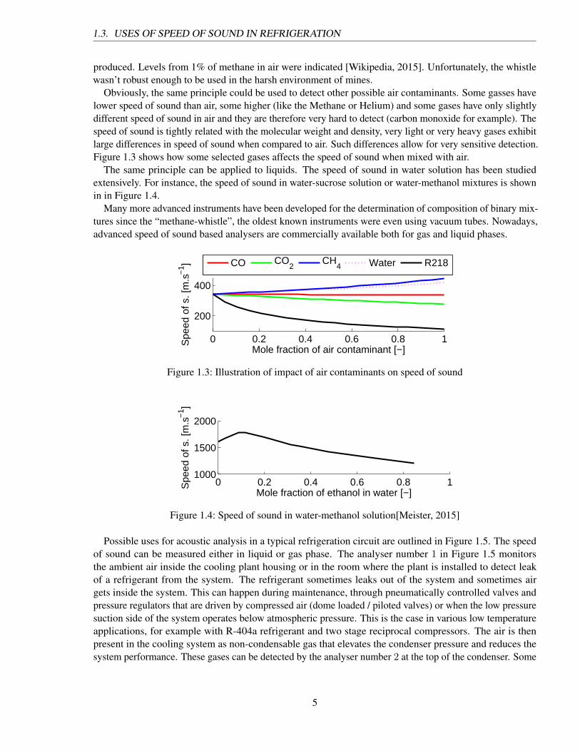
Obviously, the same principle could be used to detect other possible air contaminants. Some gasses havelower speed of sound than air, some higher (like the Methane or Helium) and some gases have only slightlydifferent speed of sound in air and they are therefore very hard to detect (carbon monoxide for example). Thespeed of sound is tightly related with the molecular weight and density, very light or very heavy gases exhibitlarge differences in speed of sound when compared to air. Such differences allow for very sensitive detection.Figure 1.3 shows how some selected gases affects the speed of sound when mixed with air.
The same principle can be applied to liquids. The speed of sound in water solution has been studiedextensively. For instance, the speed of sound in water-sucrose solution or water-methanol mixtures is shownin in Figure 1.4.
Many more advanced instruments have been developed for the determination of composition of binary mix-tures since the “methane-whistle”, the oldest known instruments were even using vacuum tubes. Nowadays,advanced speed of sound based analysers are commercially available both for gas and liquid phases.
0 0.2 0.4 0.6 0.8 1
200
400
Spe
ed o
f s. [
m.s
−1 ]
Mole fraction of air contaminant [−]
CO CO2
CH4 Water R218
Figure 1.3: Illustration of impact of air contaminants on speed of sound
0 0.2 0.4 0.6 0.8 11000
1500
2000
Spe
ed o
f s. [
m.s
−1 ]
Mole fraction of ethanol in water [−]
Figure 1.4: Speed of sound in water-methanol solution[Meister, 2015]
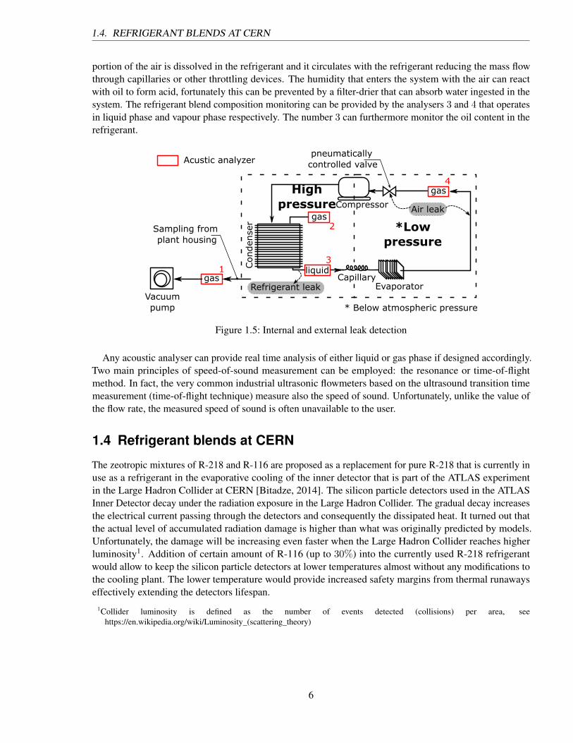
Possible uses for acoustic analysis in a typical refrigeration circuit are outlined in Figure 1.5. The speedof sound can be measured either in liquid or gas phase. The analyser number 1 in Figure 1.5 monitorsthe ambient air inside the cooling plant housing or in the room where the plant is installed to detect leakof a refrigerant from the system. The refrigerant sometimes leaks out of the system and sometimes airgets inside the system. This can happen during maintenance, through pneumatically controlled valves andpressure regulators that are driven by compressed air (dome loaded / piloted valves) or when the low pressuresuction side of the system operates below atmospheric pressure. This is the case in various low temperatureapplications, for example with R-404a refrigerant and two stage reciprocal compressors. The air is thenpresent in the cooling system as non-condensable gas that elevates the condenser pressure and reduces thesystem performance. These gases can be detected by the analyser number 2 at the top of the condenser. Some
5
1.4. REFRIGERANT BLENDS AT CERN
portion of the air is dissolved in the refrigerant and it circulates with the refrigerant reducing the mass flowthrough capillaries or other throttling devices. The humidity that enters the system with the air can reactwith oil to form acid, fortunately this can be prevented by a filter-drier that can absorb water ingested in thesystem. The refrigerant blend composition monitoring can be provided by the analysers 3 and 4 that operatesin liquid phase and vapour phase respectively. The number 3 can furthermore monitor the oil content in therefrigerant.
Refrigerant leak EvaporatorCapillary
Con
den
ser
Compressor
pneumatically controlled valve
Vacuum pump
Sampling from plant housing
Air leak
*Low pressure
High pressure
* Below atmospheric pressure
gas
gasliquid
gas
Acustic analyzer
1
2
3
4
Figure 1.5: Internal and external leak detection
Any acoustic analyser can provide real time analysis of either liquid or gas phase if designed accordingly.Two main principles of speed-of-sound measurement can be employed: the resonance or time-of-flightmethod. In fact, the very common industrial ultrasonic flowmeters based on the ultrasound transition timemeasurement (time-of-flight technique) measure also the speed of sound. Unfortunately, unlike the value ofthe flow rate, the measured speed of sound is often unavailable to the user.
1.4 Refrigerant blends at CERN
The zeotropic mixtures of R-218 and R-116 are proposed as a replacement for pure R-218 that is currently inuse as a refrigerant in the evaporative cooling of the inner detector that is part of the ATLAS experimentin the Large Hadron Collider at CERN [Bitadze, 2014]. The silicon particle detectors used in the ATLASInner Detector decay under the radiation exposure in the Large Hadron Collider. The gradual decay increasesthe electrical current passing through the detectors and consequently the dissipated heat. It turned out thatthe actual level of accumulated radiation damage is higher than what was originally predicted by models.Unfortunately, the damage will be increasing even faster when the Large Hadron Collider reaches higherluminosity1. Addition of certain amount of R-116 (up to 30%) into the currently used R-218 refrigerantwould allow to keep the silicon particle detectors at lower temperatures almost without any modifications tothe cooling plant. The lower temperature would provide increased safety margins from thermal runawayseffectively extending the detectors lifespan.
1Collider luminosity is defined as the number of events detected (collisions) per area, seehttps://en.wikipedia.org/wiki/Luminosity_(scattering_theory)
6
1.4. REFRIGERANT BLENDS AT CERN
Subcooling
Condenser
Liquid pump
Compressor
Glycolbath dummy
load
EXV
BPR
Electric heater
Stave
Capillaries
PR
Speed-of-soundanalyser
R-116 R-218
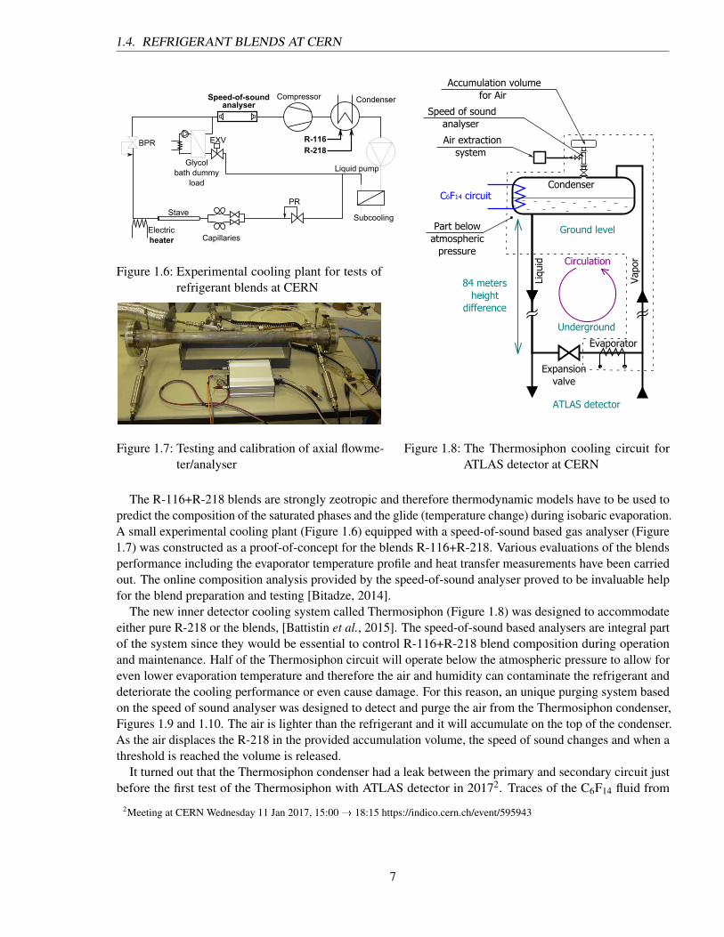
Figure 1.6: Experimental cooling plant for tests ofrefrigerant blends at CERN
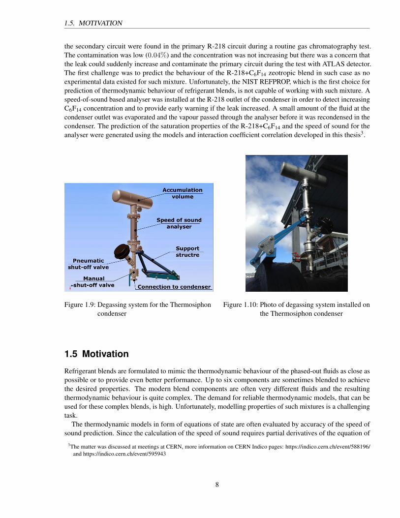
Figure 1.7: Testing and calibration of axial flowme-ter/analyser
Part below
atmospheric pressure
Air extraction system
CondenserC6F14 circuit
Ground level
Evaporator
84 metersheight
difference
Circulation
Liqu
id
Vapo
r
Expansionvalve
Underground
Accumulation volume for Air
ATLAS detector
Speed of soundanalyser
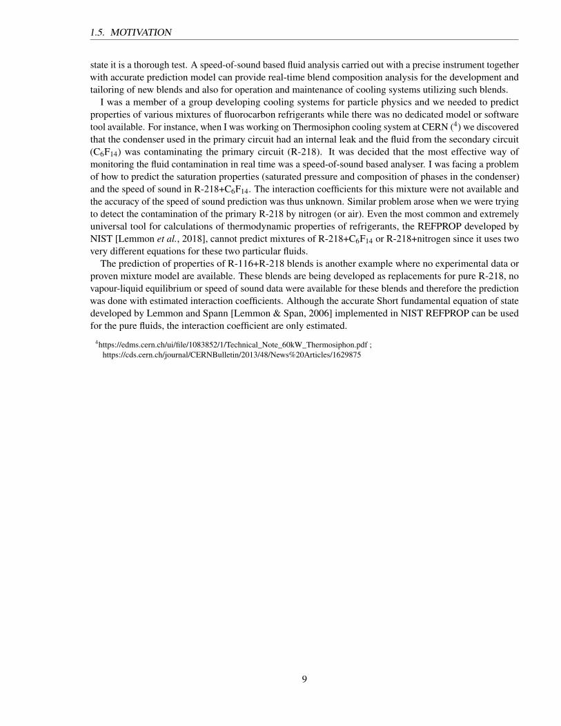
Figure 1.8: The Thermosiphon cooling circuit forATLAS detector at CERN
The R-116+R-218 blends are strongly zeotropic and therefore thermodynamic models have to be used topredict the composition of the saturated phases and the glide (temperature change) during isobaric evaporation.A small experimental cooling plant (Figure 1.6) equipped with a speed-of-sound based gas analyser (Figure1.7) was constructed as a proof-of-concept for the blends R-116+R-218. Various evaluations of the blendsperformance including the evaporator temperature profile and heat transfer measurements have been carriedout. The online composition analysis provided by the speed-of-sound analyser proved to be invaluable helpfor the blend preparation and testing [Bitadze, 2014].
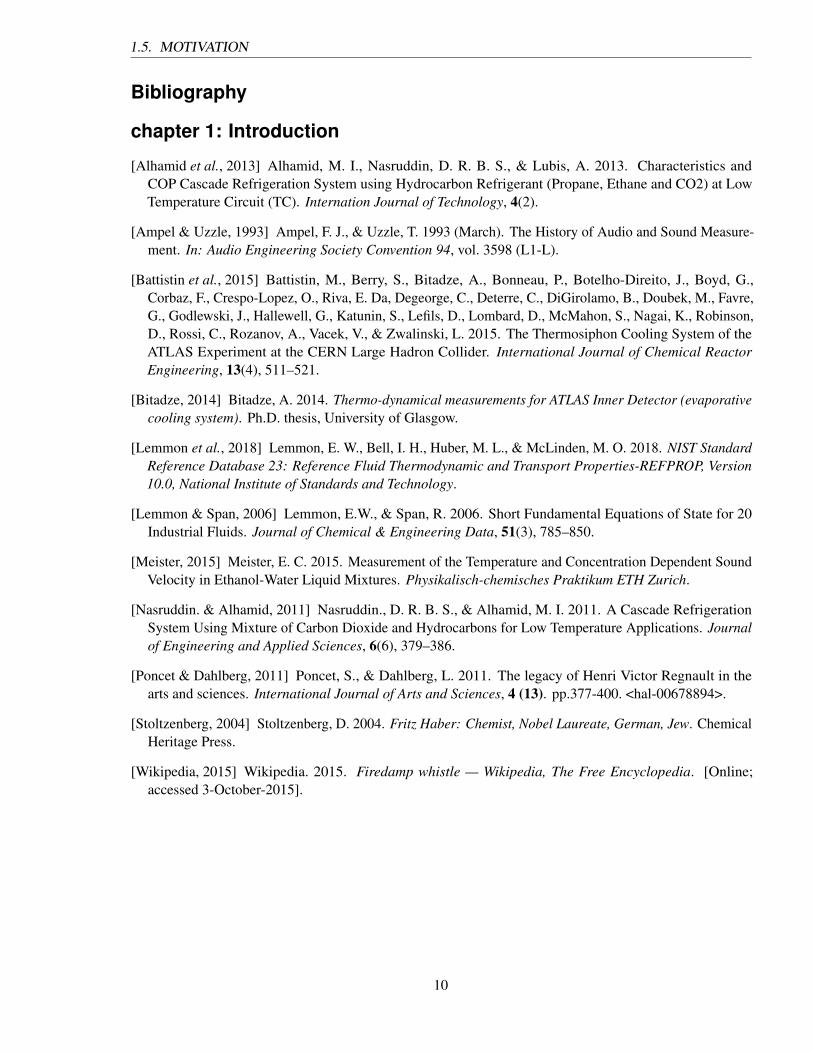
The new inner detector cooling system called Thermosiphon (Figure 1.8) was designed to accommodateeither pure R-218 or the blends, [Battistin et al., 2015]. The speed-of-sound based analysers are integral partof the system since they would be essential to control R-116+R-218 blend composition during operationand maintenance. Half of the Thermosiphon circuit will operate below the atmospheric pressure to allow foreven lower evaporation temperature and therefore the air and humidity can contaminate the refrigerant anddeteriorate the cooling performance or even cause damage. For this reason, an unique purging system basedon the speed of sound analyser was designed to detect and purge the air from the Thermosiphon condenser,Figures 1.9 and 1.10. The air is lighter than the refrigerant and it will accumulate on the top of the condenser.As the air displaces the R-218 in the provided accumulation volume, the speed of sound changes and when athreshold is reached the volume is released.
It turned out that the Thermosiphon condenser had a leak between the primary and secondary circuit justbefore the first test of the Thermosiphon with ATLAS detector in 20172. Traces of the C6F14 fluid from
2Meeting at CERN Wednesday 11 Jan 2017, 15:00 18:15 https://indico.cern.ch/event/595943
7
1.5. MOTIVATION
the secondary circuit were found in the primary R-218 circuit during a routine gas chromatography test.The contamination was low (0.04%) and the concentration was not increasing but there was a concern thatthe leak could suddenly increase and contaminate the primary circuit during the test with ATLAS detector.The first challenge was to predict the behaviour of the R-218+C6F14 zeotropic blend in such case as noexperimental data existed for such mixture. Unfortunately, the NIST REFPROP, which is the first choice forprediction of thermodynamic behaviour of refrigerant blends, is not capable of working with such mixture. Aspeed-of-sound based analyser was installed at the R-218 outlet of the condenser in order to detect increasingC6F14 concentration and to provide early warning if the leak increased. A small amount of the fluid at thecondenser outlet was evaporated and the vapour passed through the analyser before it was recondensed in thecondenser. The prediction of the saturation properties of the R-218+C6F14 and the speed of sound for theanalyser were generated using the models and interaction coefficient correlation developed in this thesis3.
Figure 1.9: Degassing system for the Thermosiphoncondenser
Figure 1.10: Photo of degassing system installed onthe Thermosiphon condenser
1.5 Motivation
Refrigerant blends are formulated to mimic the thermodynamic behaviour of the phased-out fluids as close aspossible or to provide even better performance. Up to six components are sometimes blended to achievethe desired properties. The modern blend components are often very different fluids and the resultingthermodynamic behaviour is quite complex. The demand for reliable thermodynamic models, that can beused for these complex blends, is high. Unfortunately, modelling properties of such mixtures is a challengingtask.
The thermodynamic models in form of equations of state are often evaluated by accuracy of the speed ofsound prediction. Since the calculation of the speed of sound requires partial derivatives of the equation of
3The matter was discussed at meetings at CERN, more information on CERN Indico pages: https://indico.cern.ch/event/588196/and https://indico.cern.ch/event/595943
8
1.5. MOTIVATION
state it is a thorough test. A speed-of-sound based fluid analysis carried out with a precise instrument togetherwith accurate prediction model can provide real-time blend composition analysis for the development andtailoring of new blends and also for operation and maintenance of cooling systems utilizing such blends.
I was a member of a group developing cooling systems for particle physics and we needed to predictproperties of various mixtures of fluorocarbon refrigerants while there was no dedicated model or softwaretool available. For instance, when I was working on Thermosiphon cooling system at CERN (4) we discoveredthat the condenser used in the primary circuit had an internal leak and the fluid from the secondary circuit(C6F14) was contaminating the primary circuit (R-218). It was decided that the most effective way ofmonitoring the fluid contamination in real time was a speed-of-sound based analyser. I was facing a problemof how to predict the saturation properties (saturated pressure and composition of phases in the condenser)and the speed of sound in R-218+C6F14. The interaction coefficients for this mixture were not available andthe accuracy of the speed of sound prediction was thus unknown. Similar problem arose when we were tryingto detect the contamination of the primary R-218 by nitrogen (or air). Even the most common and extremelyuniversal tool for calculations of thermodynamic properties of refrigerants, the REFPROP developed byNIST [Lemmon et al., 2018], cannot predict mixtures of R-218+C6F14 or R-218+nitrogen since it uses twovery different equations for these two particular fluids.
The prediction of properties of R-116+R-218 blends is another example where no experimental data orproven mixture model are available. These blends are being developed as replacements for pure R-218, novapour-liquid equilibrium or speed of sound data were available for these blends and therefore the predictionwas done with estimated interaction coefficients. Although the accurate Short fundamental equation of statedeveloped by Lemmon and Spann [Lemmon & Span, 2006] implemented in NIST REFPROP can be usedfor the pure fluids, the interaction coefficient are only estimated.
4https://edms.cern.ch/ui/file/1083852/1/Technical_Note_60kW_Thermosiphon.pdf ;https://cds.cern.ch/journal/CERNBulletin/2013/48/News%20Articles/1629875
9
1.5. MOTIVATION
Bibliography
chapter 1: Introduction
[Alhamid et al., 2013] Alhamid, M. I., Nasruddin, D. R. B. S., & Lubis, A. 2013. Characteristics andCOP Cascade Refrigeration System using Hydrocarbon Refrigerant (Propane, Ethane and CO2) at LowTemperature Circuit (TC). Internation Journal of Technology, 4(2).
[Ampel & Uzzle, 1993] Ampel, F. J., & Uzzle, T. 1993 (March). The History of Audio and Sound Measure-ment. In: Audio Engineering Society Convention 94, vol. 3598 (L1-L).
[Battistin et al., 2015] Battistin, M., Berry, S., Bitadze, A., Bonneau, P., Botelho-Direito, J., Boyd, G.,Corbaz, F., Crespo-Lopez, O., Riva, E. Da, Degeorge, C., Deterre, C., DiGirolamo, B., Doubek, M., Favre,G., Godlewski, J., Hallewell, G., Katunin, S., Lefils, D., Lombard, D., McMahon, S., Nagai, K., Robinson,D., Rossi, C., Rozanov, A., Vacek, V., & Zwalinski, L. 2015. The Thermosiphon Cooling System of theATLAS Experiment at the CERN Large Hadron Collider. International Journal of Chemical ReactorEngineering, 13(4), 511–521.
[Bitadze, 2014] Bitadze, A. 2014. Thermo-dynamical measurements for ATLAS Inner Detector (evaporativecooling system). Ph.D. thesis, University of Glasgow.
[Lemmon et al., 2018] Lemmon, E. W., Bell, I. H., Huber, M. L., & McLinden, M. O. 2018. NIST StandardReference Database 23: Reference Fluid Thermodynamic and Transport Properties-REFPROP, Version10.0, National Institute of Standards and Technology.
[Lemmon & Span, 2006] Lemmon, E.W., & Span, R. 2006. Short Fundamental Equations of State for 20Industrial Fluids. Journal of Chemical & Engineering Data, 51(3), 785–850.
[Meister, 2015] Meister, E. C. 2015. Measurement of the Temperature and Concentration Dependent SoundVelocity in Ethanol-Water Liquid Mixtures. Physikalisch-chemisches Praktikum ETH Zurich.
[Nasruddin. & Alhamid, 2011] Nasruddin., D. R. B. S., & Alhamid, M. I. 2011. A Cascade RefrigerationSystem Using Mixture of Carbon Dioxide and Hydrocarbons for Low Temperature Applications. Journalof Engineering and Applied Sciences, 6(6), 379–386.
[Poncet & Dahlberg, 2011] Poncet, S., & Dahlberg, L. 2011. The legacy of Henri Victor Regnault in thearts and sciences. International Journal of Arts and Sciences, 4 (13). pp.377-400. <hal-00678894>.
[Stoltzenberg, 2004] Stoltzenberg, D. 2004. Fritz Haber: Chemist, Nobel Laureate, German, Jew. ChemicalHeritage Press.
[Wikipedia, 2015] Wikipedia. 2015. Firedamp whistle — Wikipedia, The Free Encyclopedia. [Online;accessed 3-October-2015].
10
Chapter 2 Prior art
2 Prior art
2.1 Thermodynamic models
2.1.1 Introduction
Primary interest of this work is in models of vapour-liquid equilibrium and the speed of sound that requireonly few fluid-specific parameters and that can be applied to refrigerants and their blends including mixturesof unlike fluids. In addition, the models must work well in both vapour and liquid phases. Models developedspecifically for a homogeneous family of fluids, hydrocarbons for example, exhibit large deviations whenused to model the behaviour of other types of fluids (e.g. fluorinated refrigerants).
The selection criteria for appropriate models were following:
• The models must predict the vapour-liquid equilibrium of mixtures i.e. saturated pressure and compo-sition of phases of zeotropic mixtures at given temperature.
• The models must be able to predict the speed of sound in mixtures consisting of more than twocomponents. The models must be usable for both phases and also for saturation.
• It should be relatively simple to obtain the fitting parameters for the model, the model should beflexible, i.e. it should be easily applicable to new fluids and mixtures.
2.1.2 Speed of sound
The small signal (linear) theory yields following equation for propagation of a sound wave:
w2 =(∂p
∂ρ
)S
. (2.1)
In other words the square of the speed of sound w is equal to the partial derivative of pressure p withrespect to the density ρ at constant entropy S . The constant entropy signifies that the sound propagation isadiabatic process. In ideal case, the sound propagation is accompanied by small changes in temperature (dueto compression and expansion of the gas) but no heat exchange takes place since those changes are too fast.The equation can be transformed from adiabatic to isothermic using thermodynamic manipulations:
w2 = cpcv
(∂p
∂ρ
)T
. (2.2)
The partial derivative of pressure with respect to the density at constant temperature is easier to work withthan the derivative in previous equation. It is apparent that the speed of sound depends on the heat capacitiescp and cv or to be more precise on the ratio of the heat capacities.
The simplest approach is to assume the ideal gas with constant heat capacities which are not function oftemperature cid0
p , cid0v . Using ideal gas equation in the following form pM = ρRT , one can write:
11

2.1. THERMODYNAMIC MODELS
w2 =cid0p
cid0v
RT
M. (2.3)
This is a well-known equation for the speed of sound in the ideal gas. The cid0p and cid0
v are related throughMayer’s relation cid0
p − cid0v = R and the cid0
p depends on the number of atoms in the gas molecule. Thenumber of atoms dictates the rotational and translational degrees of freedom of a molecule and the ideal gasheat capacities are cid0
v = 23R,
32Ror 3R for monoatomic, diatomic or polyatomic gas respectively.
The real heat capacities are, however, functions of the temperature due to the contribution of vibrationaldegrees of freedom. The statistical theory yields equation for the ideal gas heat capacity cidp = f(T ):
cidpR
= crotp + ctransp + cvibp = 4 +3∗ξ−3−nrot∑
i=1
bi
(aiT
)2 exp(aiT
)[exp
(aiT
)− 1
]2 , (2.4)
where crotp , ctransp , cvibp are the contributions of rotational, translational and vibrational motions of themolecule to the heat capacity, ξ is the number of atoms in a molecule and nrot is the number of rotationaldegrees of freedom of the molecule. The term in the summation is also called Einstein equation and thecoefficients ai[K] are called vibrational temperatures.
2.1.3 Equations of state
Classical equations of state model the relation between intensive properties: pressure p, molar volume v ordensity ρ and temperature T . The pressure explicit equations of state are usually in a form of:
• Power series in v
• Cubic equation
• Empirical form
The power series, for example virial equation of state, do not usually model the vapour-liquid transition. Thecubic equations of state are very popular for their simplicity and accuracy in pressure calculations adequatefor engineering purposes although they exhibit significant deviation in liquid density calculations. Empiricalequations can provide high accuracy but they require large number of fluid-specific parameters that must befitted to extensive experimental datasets.
Modern equations of state are in so called Helmholtz energy form. The dimensionless Helmholtz energy ais expressed as function of temperature T and number density ρ. The pressure p, heat capacities cp, cv andfinally the speed of sound w can be then expressed through partial derivatives of Helmholtz energy as shownin Equations 2.5 to 2.8:
p(T,ρ) = ρ2(∂a
∂ρ
)T
, (2.5)
w =√cpcv
(∂p
∂ρ
)T
, (2.6)
12
2.1. THERMODYNAMIC MODELS
cresv = −R
2T(∂aid
∂T
)ρ
+ T 2(∂2ar
∂T 2
)ρ
, (2.7)
cp = cv +R
(1 + ρ
(∂ar
∂ρ
)T
+ ρT(∂2ar
∂T∂ρ
))2
1 + 2ρ(∂ar
∂ρ
)T
+ ρ2(∂2ar
∂ρ2
)T
. (2.8)
The compressibility factor Z can be also obtained from Helmholtz energy:
Z = p
ρRT= 1 + ρ
(∂ar
∂ρ
)T
. (2.9)
2.1.4 Empirical equations of state
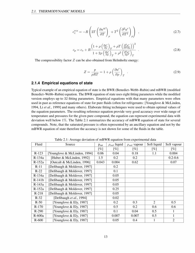
Typical example of an empirical equation of state is the BWR (Benedict–Webb–Rubin) and mBWR (modifiedBenedict–Webb–Rubin) equation. The BWR equation of state uses eight fitting parameters while the modifiedversion employs up to 32 fitting parameters. Empirical equations with that many parameters were oftenused in past as reference equations of state for pure fluids (often for refrigerants: [Younglove & McLinden,1994, Li et al., 1999] and many others). Elaborate fitting techniques were used to obtain optimal values ofthe equation parameters. The resulting reference equation provide very good accuracy over wide range oftemperature and pressures for the given pure compound, the equation can represent experimental data withdeviation well below 1%. The Table 2.1 summarizes the accuracy of mBWR equation of state for severalcompounds. Note, that the saturated pressure is often represented by an ancillary equation and not by themBWR equation of state therefore the accuracy is not shown for some of the fluids in the table.
Table 2.1: Average deviation of mBWR equation from experimental dataFluid Source psat ρsat liquid ρsat vapour SoS liquid SoS vapour
[%] [%] [%] [%] [%]R-123 [Younglove & McLinden, 1994] 0.06 0.04 0.18 1.1 0.004R-134a [Huber & McLinden, 1992] 1.5 0.2 0.2 0.2-0.6R-152a [Outcalt & McLinden, 1996] 0.043 0.004 0.62 0.07R-11 [Defibaugh & Moldover, 1997] 0.2R-22 [Defibaugh & Moldover, 1997] 0.1
R-134a [Defibaugh & Moldover, 1997] 0.05R-141b [Defibaugh & Moldover, 1997] 0.05R-143a [Defibaugh & Moldover, 1997] 0.05R-152a [Defibaugh & Moldover, 1997] 0.25R-218 [Defibaugh & Moldover, 1997] 0.05R-32 [Defibaugh et al., 1994] 0.02R-50 [Younglove & Ely, 1987] 0.2 0.3 2 0.5R-170 [Younglove & Ely, 1987] 0.5 0.2 0.6 0.6R-290 [Younglove & Ely, 1987] 0.1 0.04 0.5 1R-600a [Younglove & Ely, 1987] 0.007 0.007 0.5 1R-600 [Younglove & Ely, 1987] 0.05 0.4 1 2
13
2.1. THERMODYNAMIC MODELS
2.1.5 Virial equations of state
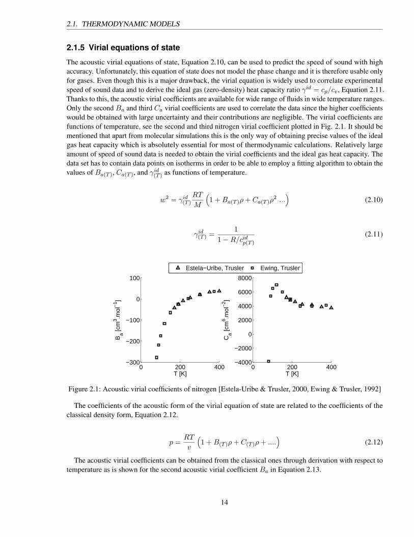
The acoustic virial equations of state, Equation 2.10, can be used to predict the speed of sound with highaccuracy. Unfortunately, this equation of state does not model the phase change and it is therefore usable onlyfor gases. Even though this is a major drawback, the virial equation is widely used to correlate experimentalspeed of sound data and to derive the ideal gas (zero-density) heat capacity ratio γid = cp/cv, Equation 2.11.Thanks to this, the acoustic virial coefficients are available for wide range of fluids in wide temperature ranges.Only the second Ba and third Ca virial coefficients are used to correlate the data since the higher coefficientswould be obtained with large uncertainty and their contributions are negligible. The virial coefficients arefunctions of temperature, see the second and third nitrogen virial coefficient plotted in Fig. 2.1. It should bementioned that apart from molecular simulations this is the only way of obtaining precise values of the idealgas heat capacity which is absolutely essential for most of thermodynamic calculations. Relatively largeamount of speed of sound data is needed to obtain the virial coefficients and the ideal gas heat capacity. Thedata set has to contain data points on isotherms in order to be able to employ a fitting algorithm to obtain thevalues of Ba(T ), Ca(T ), and γid(T ) as functions of temperature.
w2 = γid(T )RT
M
(1 +Ba(T )ρ+ Ca(T )ρ
2 ...)
(2.10)
γid(T ) = 11−R/cidp(T )
(2.11)
0 200 400−300
−200
−100
0
100
T [K]
Ba [c
m3 .m
ol−
1 ]
Estela−Uribe, Trusler Ewing, Trusler
0 200 400−4000
−2000
0
2000
4000
6000
8000
T [K]
Ca [c
m6 .m
ol−
2 ]
Figure 2.1: Acoustic virial coefficients of nitrogen [Estela-Uribe & Trusler, 2000, Ewing & Trusler, 1992]
The coefficients of the acoustic form of the virial equation of state are related to the coefficients of theclassical density form, Equation 2.12.
p = RT
v
(1 +B(T )ρ+ C(T )ρ+ ....
)(2.12)
The acoustic virial coefficients can be obtained from the classical ones through derivation with respect totemperature as is shown for the second acoustic virial coefficient Ba in Equation 2.13.
14
2.1. THERMODYNAMIC MODELS
12Ba = B + PaT
(dB
dT
)+QaT
2(d2B
dT 2
)(2.13)
where:
Pa = (γid − 1) , (2.14)
Qa =
(γid − 1
)2
2 γig . (2.15)
It should be mentioned that unlike other equations of state, the virial equation can be directly derived fromstatistical mechanics. The second, third, fourth, etc. virial coefficients represent the contributions of two-body,three-body, etc. interactions. However, the virial expansion is usually truncated after the second or thirdcoefficient even in the classical density form.
It is possible to use combination rules in order to obtain virial coefficients for mixture. The combinationrules that can be employed are following:
M =n∑i=1
xiMi , (2.16)
c0p
R=
n∑i=1
xic0pi
R, (2.17)
B =n∑i=1
n∑j=1
xixjBij , (2.18)
C =n∑i=1
n∑j=1
n∑k=1
xixjxkCijk , (2.19)
where Bii and Ciii are virial coefficients of the pure component i and the Bij and Cijk (i 6= j 6= k) are thecross coefficients. These coefficients are fluid specific, i.e. the coefficient is unique function of temperaturefor each pair of fluids i and j. Only few of these coefficients are available in literature and they cannot beomitted when reasonable accuracy is required. This is a significant limitation which renders the acousticvirial equation of state impractical for prediction of the speed of sound in various gas mixtures.
2.1.6 Cubic equations
Cubic equations are based on the Van der Wallse equation of state published in 1873 and they are widelyused due to their simplicity and good performance. There is a vast list of various cubic equations of statewith multitude of modifications. The cubic equations of state provide good accuracy (often better than 1%)
15
2.1. THERMODYNAMIC MODELS
in terms of saturated pressure and vapour phase density but they fall short in predicting the PVT propertiesnear critical region and the liquid density. The cubic equations usually underpredict the liquid density byapproximately 10% but this deviation can reach up to 20% in some cases. Consequently, the predictionaccuracy of the speed of sound in those regions is also poor. Generally, cubic equation of state can be writtenin following form:
p = RT
v − b− a
v(v − b) + c(v − d), (2.20)
where p is pressure, T is temperature, v is molar volume and R is the universal gas constant. Theparameters a, b and c can be fitted to vapour pressure data or they can be obtained from critical constraint bysetting ∂p
∂v = ∂2p∂v2 = 0. Unfortunately, the ability of the cubic equations to predict the liquid density cannot
be improved by adjusting the values of the parameters since an improvement in the density prediction leadsto poor performance in the critical region [Twu et al., 2002].
Redlich and Kwong [Redlich & Kwong, 1949] modified the Van der Waalse equation (1949) of state into afollowing form:
p = RT
v − b− a√
T
1v(v − b)
. (2.21)
The modification introduced temperature dependence of the parameter a. Subsequent cubic equations ofstate brought more and more complicated functions for the parameter a, so called alpha functions.
Another notable successful cubic equation of state was proposed by [Soave, 1972]. The temperature-dependent parameter a can be expressed as alpha function multiplied by the value of the a at the criticalpoint:
a = αac . (2.22)
The Soave alpha function has following form:
α =(1 +m
(1−
√Tr))2
. (2.23)
The Tr is the reduced temperature and m is a coefficient fitted to vapour-pressures of light hydrocarbons:
m = 0.480 + 1.57ω − 0.176ω2, (2.24)
where ω is the acentric factor.Another widely-used cubic equation of state is the Peng-Robinson (1976) equation, for details and
background on this equation of state see the recent publication dealing with cubic equations [Lopez-Echeverryet al., 2017]. It was originally developed for petrochemical industry but it is nowadays often used also forrefrigerants. The pressure form of the Peng-Robinson equation of state is following:
p = RT
v − b−
a(T )
v(v + b) + c(v − b), (2.25)
16
2.1. THERMODYNAMIC MODELS
where
α =(1 +m
(1−
√Tr))2
, (2.26)
m = 0.37464 + 1.54226ω − 0.26992ω2 . (2.27)
The a and b can be obtained from the critical constrains:
a = 0.45724R2T 2c
pc, (2.28)
b = 0.07780RTcpc
. (2.29)
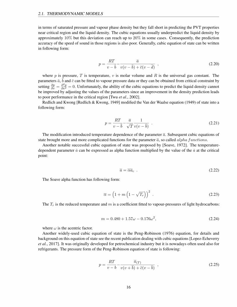
Comparison of the Redlich-Kwong, Soave and Peng-Robinson alpha functions can be found in Figure2.2. Many more complicated empirical alpha functions with additional fitting parameters are available inliterature. These complex functions are designed to better represent the saturated pressures of various fluids,they can use multiple parameters which are fitted directly to the vapour pressure data of the fluid.
0 2 4 6 8 100
1
2
3
4
α
Tr
Redlich and KwongSoavePeng−Robinson
Figure 2.2: Comparison of the alpha functions
Other modifications include Patel-Teja (1982) cubic equation of state, Equation 2.30. The Patel-Teja modelincludes an additional parameter c, Equation 2.31. This parameter is obtained from so called apparent criticalcompressibility factor ξc in Equation 2.32 (it is not equal to the true compressibility factor). Its value wasempirically correlated to acentric factor in order to improve liquid volumes accuracy, Equation 2.33.
p = RT
V − b− a
V 2 +(b+ c
)V − bc
(2.30)
c = Ωc
(RTcPc
)(2.31)
Ωc = 1− 3ξc (2.32)
ξc = 0.329032− 0.0767992ω + 0.0211947ω2 (2.33)
Accuracy of various cubic equations of state are summarized in Table 2.2 in the next section.
17
2.1. THERMODYNAMIC MODELS
2.1.7 Volume-translated cubic equation of state
The volume translation has been proposed in order to improve the accuracy of the cubic equation in predictingthe saturated liquid phase density. The translation is in fact a correction factor c that shifts the predictedvolumes [Péneloux et al., 1982]. Volume-translated Peng-Robinson equation of state has following form:
p = RT
v + c− b−
a(T )
(v + c)(v + c+ b) + c(v + c− b). (2.34)
The volume shift does not impact the saturated pressure and the impact on the saturated vapour densityis negligible since the correction is small when compared with the vapour phase volume. The simplestcorrection factor is temperature-independent and it is equal to the difference between the calculated vcalc andexperimental vexp molar volume at reduced temperature Tr of 0.7:
c = vcalc − vexp|Tr=0.7 . (2.35)
The constant translation for hydrocarbons was correlated to the Rackett compressibility factor ZRA byPeneloux [Péneloux et al., 1982] in following way:
c = 0.40768(0.29441− ZRA) . (2.36)
Peneloux demonstrated that the correction results in average deviation of 5% between the predictedsaturated liquid densities and the experimental values for hydrocarbons. Although this volume translationgives good results for reduced temperature below 0.6, it fails for temperatures close to the critical point.Many more sophisticated functions for the volume translation have been proposed since the first work byPeneloux. These corrections are often function of reduced temperature or some arbitrary distance fromcritical point. The most common approaches can be split into two groups:
• Correlations with fluid-specific fitting parameters, that have to be obtained by fitting techniques foreach fluid. For example [Tsai & Y, 1998].
• Volume translations that employ correlations fitted over extensive set of fluids where the fluid propertiessuch as the molecular weight, critical pressure, temperature and acentric factor are used as parameters.For example [Hemptinne & Ungerer, 1995].
Unfortunately, some of the volume translations cause nonphysical behaviour like prediction of negative heatcapacities or crossing of isotherms but only few publications address this issue. I will focus on the secondcategory from the short list above, since this approach eliminates the need for fluid-specific parameters.
The translation functions are often designed so that the shift is defined by the difference between thepredicted critical volume vcalcc and experimental critical volume vexpc :
cc = vcalcc − vexpc . (2.37)
A Gaussian-like temperature-dependent function f(Tc) is then used to obtain the translation function c:
c = f(Tc) · cc . (2.38)
18
2.1. THERMODYNAMIC MODELS
0.5 1 1.50
0.5
1
Tr [−]
Shi
ft [−
]
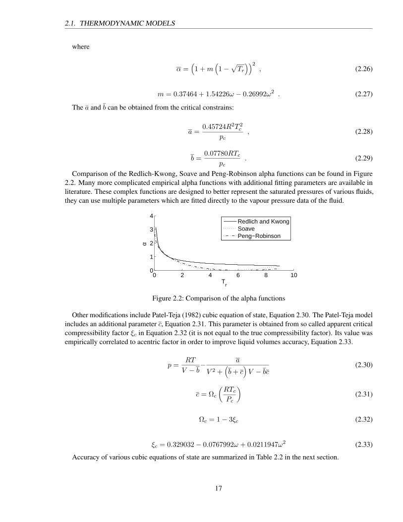
Magoulas and Tassios Ahlers and Gmehling
Figure 2.3: Gaussian volume translations according to [Magoulas & Tassios, 1990] and [Ahlers & Gmehling,2001]
The function f(Tc) has maximum equal to one at critical temperature Tr = 1. The correction is thereforesmall far from critical point but equal to the critical volume shift cc at the critical point. Two examples of thef − function from different translation correlation are showed in Figure 2.3. Other f − functions havebeen also evaluated (parabolic, exponential) but they have not gained that much popularity.
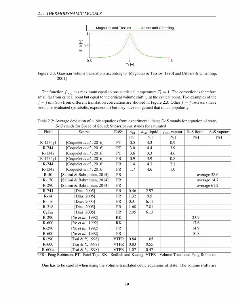
Table 2.2: Average deviation of cubic equations from experimental data; EoS stands for equation of state,SoS stands for Speed of Sound; Subscript sat stands for saturated
Fluid Source EoS* psat ρsat liquid ρsat vapour SoS liquid SoS vapour[%] [%] [%] [%] [%]
R-1234yf [Coquelet et al., 2016] PT 0.5 4.3 0.9R-744 [Coquelet et al., 2016] PT 3.0 4.4 3.9R-134a [Coquelet et al., 2016] PT 3.6 3.3 4.6
R-1234yf [Coquelet et al., 2016] PR 0.9 3.9 0.8R-744 [Coquelet et al., 2016] PR 1.4 4.3 2.1R-134a [Coquelet et al., 2016] PR 1.7 4.6 1.0R-50 [Salimi & Bahramian, 2014] PR average 28.6R-170 [Salimi & Bahramian, 2014] PR average 14.7R-290 [Salimi & Bahramian, 2014] PR average 61.2R-744 [Dias, 2005] PR 0.46 2.97R-14 [Dias, 2005] PR 1.32 9.5R-116 [Dias, 2005] PR 0.31 6.11R-218 [Dias, 2005] PR 1.68 7.81C4F10 [Dias, 2005] PR 2.05 6.13R-290 [Ye et al., 1992] RK 23.9R-600 [Ye et al., 1992] RK 17.6R-290 [Ye et al., 1992] PR 14.9R-600 [Ye et al., 1992] PR 10.8R-290 [Tsai & Y, 1998] VTPR 0.84 1.05R-600 [Tsai & Y, 1998] VTPR 0.83 0.55R-600a [Tsai & Y, 1998] VTPR 1.07 0.47
*PR - Peng Robinson, PT - Patel Teja, RK - Redlich and Kwong, VTPR - Volume Translated Peng Robinson
One has to be careful when using the volume-translated cubic equations of state. The volume shifts are
19
2.1. THERMODYNAMIC MODELS
often designed to improve the prediction of the saturated density but the equations of state have not beentested in the one-phase regions where some nonphysical behaviour can be encountered. It is usually notrecommended to use the volume translated cubic equations above the critical point or in the dense fluidregion. Three selected correlation for the volume translation are discussed in section 6.2. Accuracy ofvolume-translated cubic equations of state together with other types of cubic equations are summarized inTable 2.2.
2.1.8 Helmholtz-energy equations of state
Modern equations of state are formulated in Helmholtz energy form as explicit functions of temperature anddensity. Such equations are replacing the mBWR equation of state as the reference high-accuracy equationof state for pure fluids. Models with up to 50 fitting parameters can represent the experimental densitymeasurement with accuracy of 0.1% over wide range of temperature and pressures, [Lemmon & Roland,2006].
Good example of equation of state in the Helmholtz energy form is the Short fundamental equation of stateby Lemmon and Span [Lemmon & Roland, 2006]. This model uses 12 fitting parameters and it is optimizedfor industrial use as it offers fast computations at expense of small loss of accuracy. The equation of stateitself is formulated in dimensionless Helmholtz energy α(τ,δ) = a(T,ρ)
RT as a function of reduced temperatureτ = Tc/T and reduced density δ = ρ/ρc . Two formulations are available; one for non-polar fluids (Equation2.39) and one for polar fluids (Equation 2.40).
So called Multi-fluid models can combine equations of state in the Helmholtz energy form for differentpure fluids into a model that describes a mixture. Perhaps the best known representative of this approach isthe GERG (Groupe European de Recherches Gazires) model, which has been originally developed for naturalgas and it was the first application of the Multifluid approach [Kunz & European Gas Research Group, 2007].
αr(τ,δ) = n1δτ0.25 + n2δτ
1.125 + n3δτ1.5 + n4δ
2τ1.375 + n5δ3τ0.25 + n6δ
7τ0.85
+ n7δ2τ0.625exp(−ρ) + n8δ
5τ1.75exp(−ρ) + n9δτ3.625exp(−ρ2)
+ n10δ4τ3.625exp(−ρ2) + n11δ
3τ14.5exp(−ρ3) + n12δ2τ0.625exp(−ρ) (2.39)
αr(τ,δ) = n1δτ0.25 + n2δτ
1.125 + n3δτ1.5 + n4δ
3τ0.25 + n5δ7τ0.875 + n6δτ
2.375exp(−ρ)+ n7δ
2τ2.0exp(−ρ) + n8δ5τ2.125exp(−ρ) + n9δτ
3.5exp(−ρ2)+ n10δτ
6.5exp(−ρ2) + n11δ4τ4.75exp(−ρ2) + n12δ
2τ12.5exp(−ρ3) (2.40)
The model combines empirical equations of state explicit in the Helmholtz energy of natural gas compo-nents such as methane, nitrogen, carbon dioxide, propane, water and others. The Equation 2.41 shows thetypical expression for the dimensionless Helmholtz energy α of a mixture. It is composed of the ideal gasHelmholtz energy αid, the residual part αr0j and the mixture departure function αrij . The Fij is an adjustablefactor fitted to data for binary mixtures. Finally, the x is the vector of molar composition of the mixture. Theindividual parts of the dimensionless Helmholtz energy are then expressed as sums of polynomial terms andexponential expressions even though they can come from different models.
α(δ,τ,x) = αid(ρ,T,x) +N∑i=1
xiαroj(δ,τ) +
N∑i=1
N∑j=i+1
xixjFijαroj(δ,τ) (2.41)
20
2.1. THERMODYNAMIC MODELS
The speed of sound can be expressed using derivatives of the dimensionless Helmholtz energy:
w = RT +RT
2δ(∂αr
∂δ
)τ
+ δ2(∂2αr
∂δ2
)τ
−
[1 + δ
(∂αr
∂δ
)τ
+ δτ(∂2αr
∂δ∂τ
)τ
]2τ2[(
∂2αid
∂δ2
)δ
+(∂2αr
∂δ2
)δ
] . (2.42)
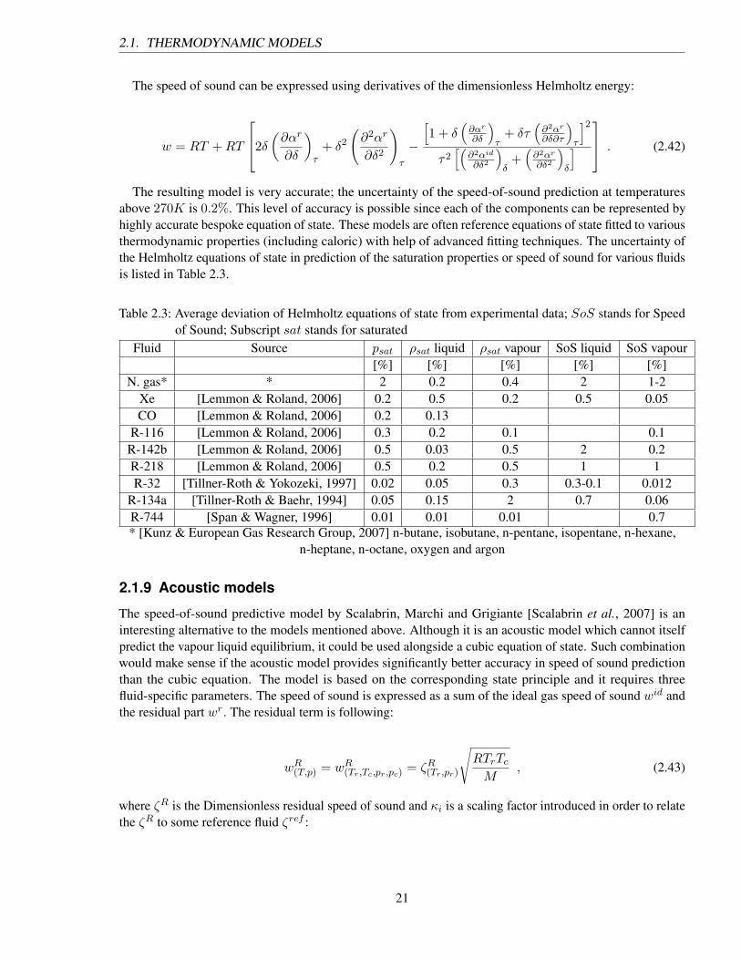
The resulting model is very accurate; the uncertainty of the speed-of-sound prediction at temperaturesabove 270K is 0.2%. This level of accuracy is possible since each of the components can be represented byhighly accurate bespoke equation of state. These models are often reference equations of state fitted to variousthermodynamic properties (including caloric) with help of advanced fitting techniques. The uncertainty ofthe Helmholtz equations of state in prediction of the saturation properties or speed of sound for various fluidsis listed in Table 2.3.
Table 2.3: Average deviation of Helmholtz equations of state from experimental data; SoS stands for Speedof Sound; Subscript sat stands for saturated
Fluid Source psat ρsat liquid ρsat vapour SoS liquid SoS vapour[%] [%] [%] [%] [%]
N. gas* * 2 0.2 0.4 2 1-2Xe [Lemmon & Roland, 2006] 0.2 0.5 0.2 0.5 0.05CO [Lemmon & Roland, 2006] 0.2 0.13
R-116 [Lemmon & Roland, 2006] 0.3 0.2 0.1 0.1R-142b [Lemmon & Roland, 2006] 0.5 0.03 0.5 2 0.2R-218 [Lemmon & Roland, 2006] 0.5 0.2 0.5 1 1R-32 [Tillner-Roth & Yokozeki, 1997] 0.02 0.05 0.3 0.3-0.1 0.012
R-134a [Tillner-Roth & Baehr, 1994] 0.05 0.15 2 0.7 0.06R-744 [Span & Wagner, 1996] 0.01 0.01 0.01 0.7* [Kunz & European Gas Research Group, 2007] n-butane, isobutane, n-pentane, isopentane, n-hexane,
n-heptane, n-octane, oxygen and argon
2.1.9 Acoustic models
The speed-of-sound predictive model by Scalabrin, Marchi and Grigiante [Scalabrin et al., 2007] is aninteresting alternative to the models mentioned above. Although it is an acoustic model which cannot itselfpredict the vapour liquid equilibrium, it could be used alongside a cubic equation of state. Such combinationwould make sense if the acoustic model provides significantly better accuracy in speed of sound predictionthan the cubic equation. The model is based on the corresponding state principle and it requires threefluid-specific parameters. The speed of sound is expressed as a sum of the ideal gas speed of sound wid andthe residual part wr. The residual term is following:
wR(T,p) = wR(Tr,Tc,pr,pc) = ζR(Tr,pr)
√RTrTcM
, (2.43)
where ζR is the Dimensionless residual speed of sound and κi is a scaling factor introduced in order to relatethe ζR to some reference fluid ζref :
21
2.1. THERMODYNAMIC MODELS
κ =ζR(Tr,pr)
ζR(Tr,pr)|ref. (2.44)
It turned out that the scaling parameter can be considered constant:
κ(Tr)|sat =κ(TrPr)|liq,vap = const. (2.45)
The final term for the residual contribution is evaluated as interpolation of two dimensionless speeds ofsound of two fluids:
ζR(Tr,pr,κ) = ζR1(Tr,pr) + κ− κ1κ2 − κ1
[ζR2(Tr,pr) − ζ
R1(Tr,pr)
]. (2.46)
The resulting speed of sound is then obtained by summation of the ideal and residual part:
w(T,Tc,p,pc,x) = wid(T,x) + ζR(T,Tc,p,pc,x)
√RT
M. (2.47)
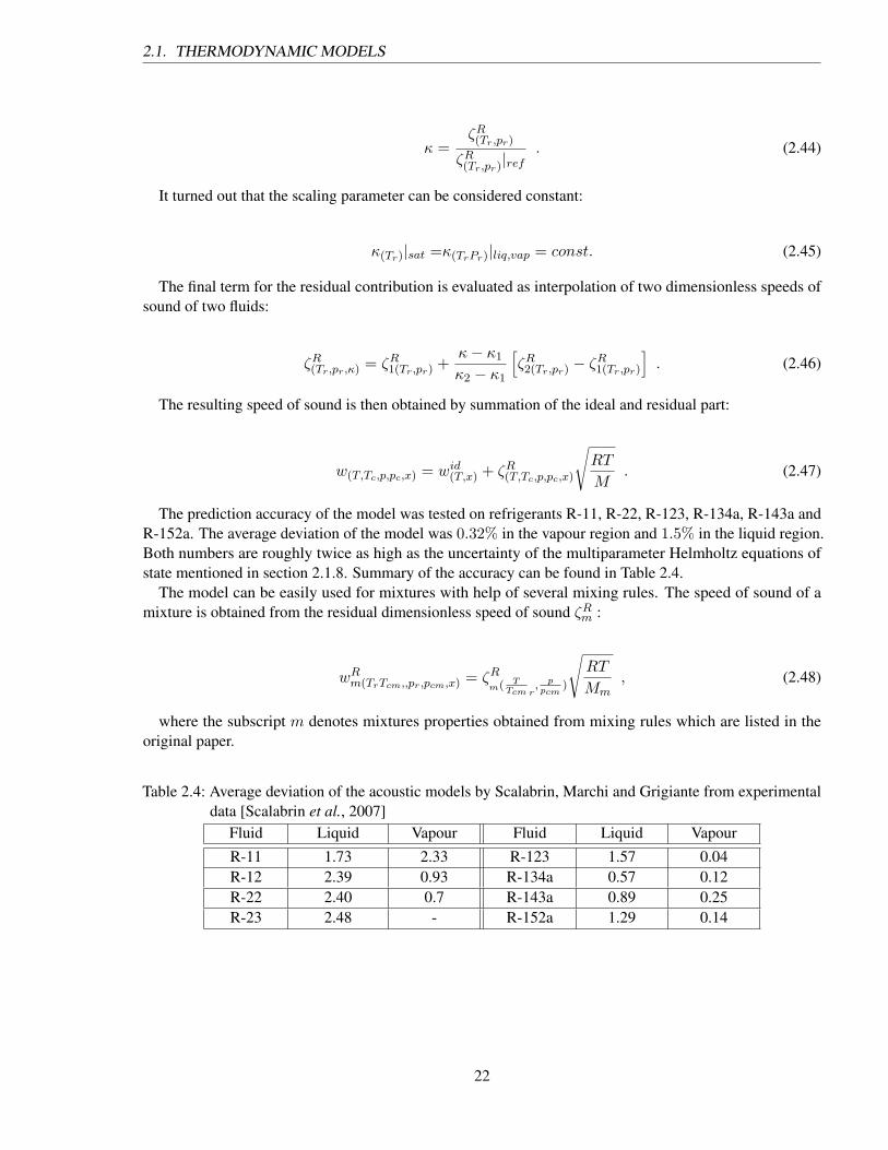
The prediction accuracy of the model was tested on refrigerants R-11, R-22, R-123, R-134a, R-143a andR-152a. The average deviation of the model was 0.32% in the vapour region and 1.5% in the liquid region.Both numbers are roughly twice as high as the uncertainty of the multiparameter Helmholtz equations ofstate mentioned in section 2.1.8. Summary of the accuracy can be found in Table 2.4.
The model can be easily used for mixtures with help of several mixing rules. The speed of sound of amixture is obtained from the residual dimensionless speed of sound ζRm :
wRm(TrTcm,,pr,pcm,x) = ζRm( T
Tcm r, ppcm
)
√RT
Mm, (2.48)
where the subscript m denotes mixtures properties obtained from mixing rules which are listed in theoriginal paper.
Table 2.4: Average deviation of the acoustic models by Scalabrin, Marchi and Grigiante from experimentaldata [Scalabrin et al., 2007]
Fluid Liquid Vapour Fluid Liquid VapourR-11 1.73 2.33 R-123 1.57 0.04R-12 2.39 0.93 R-134a 0.57 0.12R-22 2.40 0.7 R-143a 0.89 0.25R-23 2.48 - R-152a 1.29 0.14
22
2.1. THERMODYNAMIC MODELS
2.1.10 SAFT equations of state
The SAFT (Statistical Associating Fluid Theory) models were developed by applying the perturbation theoryto the equations of state of a monomer fluid. The perturbations accounts for chain formation (monomerchains), and additional terms can be added to account for association (hydrogen bonding) or polar molecules.The equations of state are in the Helmholtz energy form.
The SAFT approach has become quite popular in the last two decades since it offers good accuracy for abroad range of fluids; from simple organic or inorganic molecules to complex polymers. A great advantage ofthese models is the small number of fitting parameters: three or four parameters are needed for a combinationof the monomer term with the chain perturbation or five to six parameters are used when the association termis included. Only a small number of vapour pressure data points and saturated liquid density data points aretherefore needed in order to obtain the model parameters through a fitting procedure. A group contributionmethods have been developed for selected SAFT equations of state in order to estimate the model parameterswhen no experimental data are available.
The idea behind the perturbation theory is following: the molecular pair potential energy u is divided intothe reference term u0 and the perturbation term up, Equation 2.49. The reference term is often a hard-spherefluid (repulsive forces) and the perturbation represents the attractive forces, this model was originally used byZwanzig [Zwanzig, 1954].
u(r) = u0(r) + up(r) (2.49)
The thermodynamic models must respect associativity of fluids in order to accurately model many organicmolecules and also water, which is strongly affected by hydrogen bonding. The association forces (hydrogenbonding, dipole-dipole interaction and lone-pairs of electrons) between molecules are strong and they resultin formation of clusters of molecules having strong impact on the thermodynamic behaviour.
The association can also be modeled using perturbation theory by adding a correction (perturbation) termsto a reference non-associating fluid. One molecule can have number of different bonding sites which representdifferent kinds of associations (hydrogen bonding, dipole-dipole interactions, lone-pairs of electrons...).
The simplest first order association perturbation theory assumes that there is no interaction between theintramolecular bonds (bonding sites). A geometrical limitation allows only one molecule per one bondingsite. Molecules with one bonding site can create only dimers, molecules with two bonding sites can createchains or rings and molecules with more bonding sites can create branched chains and other structures.Chains of different length are present in a fluid, however, at equilibrium some average length of chains isestablished. The number of monomers per chain m[−] depends on the strength of association.
The Wertheim’s perturbation theory (described for example in [Blas & Vega, 2001]) incorporates theforces of association directly in the pair potential which therefore consists of the reference pair potential u0
and a sum of association forces between the association sites. The theory can be applied to the hard sphere,square-well or Lennard-Jones segments since the reference part of the pair potential and the associationforces are treated separately.
The SAFT equations of state are in the Helmholtz energy form, the real gas Helmholtz energy a iscomposed of several contributions, typically these contributions are:
ar = aseg + achain + aassoc . (2.50)
• ar is the residual Helmholtz energy defined as a− aig = ar
• aseg is the term that accounts for the hard sphere segment-segment interactions; aseg = f(m, ρ, T, σ, ε)
23
2.1. THERMODYNAMIC MODELS
• achain is the term that represents the covalent bonds between the segments that form the chains;achain = f(m, ρ, d)
• aassoc is the term that describes the change of Helmholtz energy due to the site-site segment interactionssuch as hydrogen bonding; aassoc = (ρ, T, d, εAB, κAB)
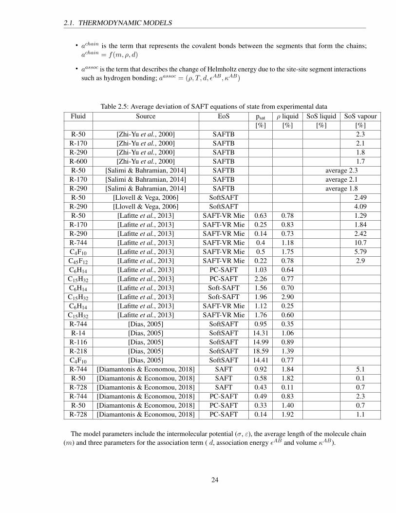
Table 2.5: Average deviation of SAFT equations of state from experimental dataFluid Source EoS psat ρ liquid SoS liquid SoS vapour
[%] [%] [%] [%]R-50 [Zhi-Yu et al., 2000] SAFTB 2.3R-170 [Zhi-Yu et al., 2000] SAFTB 2.1R-290 [Zhi-Yu et al., 2000] SAFTB 1.8R-600 [Zhi-Yu et al., 2000] SAFTB 1.7R-50 [Salimi & Bahramian, 2014] SAFTB average 2.3R-170 [Salimi & Bahramian, 2014] SAFTB average 2.1R-290 [Salimi & Bahramian, 2014] SAFTB average 1.8R-50 [Llovell & Vega, 2006] SoftSAFT 2.49R-290 [Llovell & Vega, 2006] SoftSAFT 4.09R-50 [Lafitte et al., 2013] SAFT-VR Mie 0.63 0.78 1.29R-170 [Lafitte et al., 2013] SAFT-VR Mie 0.25 0.83 1.84R-290 [Lafitte et al., 2013] SAFT-VR Mie 0.14 0.73 2.42R-744 [Lafitte et al., 2013] SAFT-VR Mie 0.4 1.18 10.7C4F10 [Lafitte et al., 2013] SAFT-VR Mie 0.5 1.75 5.79C45F12 [Lafitte et al., 2013] SAFT-VR Mie 0.22 0.78 2.9C6H14 [Lafitte et al., 2013] PC-SAFT 1.03 0.64C15H32 [Lafitte et al., 2013] PC-SAFT 2.26 0.77C6H14 [Lafitte et al., 2013] Soft-SAFT 1.56 0.70C15H32 [Lafitte et al., 2013] Soft-SAFT 1.96 2.90C6H14 [Lafitte et al., 2013] SAFT-VR Mie 1.12 0.25C15H32 [Lafitte et al., 2013] SAFT-VR Mie 1.76 0.60R-744 [Dias, 2005] SoftSAFT 0.95 0.35R-14 [Dias, 2005] SoftSAFT 14.31 1.06R-116 [Dias, 2005] SoftSAFT 14.99 0.89R-218 [Dias, 2005] SoftSAFT 18.59 1.39C4F10 [Dias, 2005] SoftSAFT 14.41 0.77R-744 [Diamantonis & Economou, 2018] SAFT 0.92 1.84 5.1R-50 [Diamantonis & Economou, 2018] SAFT 0.58 1.82 0.1R-728 [Diamantonis & Economou, 2018] SAFT 0.43 0.11 0.7R-744 [Diamantonis & Economou, 2018] PC-SAFT 0.49 0.83 2.3R-50 [Diamantonis & Economou, 2018] PC-SAFT 0.33 1.40 0.7R-728 [Diamantonis & Economou, 2018] PC-SAFT 0.14 1.92 1.1
The model parameters include the intermolecular potential (σ, ε), the average length of the molecule chain(m) and three parameters for the association term ( d, association energy εAB and volume κAB).
24
2.2. BINARY INTERACTION PARAMETERS
Multitude of publications evaluating different SAFT equations of state in terms of modelling of vapour-liquid equilibrium can be found in available literature. A number of publications have also dealt withspeed-of-sound prediction by various SAFT equations of state. Some comparisons with experimental speed-of-sound data can also be found among evaluations of the prediction accuracy of various thermodynamicproperties in papers that present thorough studies of SAFT equations, for instance [Liang et al., 2012]. Asmaller number of papers deal only with the speed-of-sound predictions, for instance [Lafitte et al., 2013].
2.2 Binary interaction parameters
One or more additional model parameters are introduced in order to provide better accuracy when theequations of state are used for mixtures. These parameters are called binary interaction parameters and theyare employed in the mixing and combination rules which transform the model parameters of pure fluids intoparameters of mixtures. The values of these binary interaction parameters are fitted to experimental data andthey are specific to a certain pair of fluids (binary mixture).
Usually only one parameter is employed but some more advance models can use two or three parameters toimprove accuracy. The parameter values can be either constant or temperature-dependent for higher accuracymodels. For instance, the simplest mixing and combination rules for the parameters a and b corresponding topure fluid i of the Peng-Robinson cubic equation of state can be following:
am =∑i
∑j
xixjaij , (2.51)
bm =∑i
∑j
xixjbij . (2.52)
aij =√aiajkij (2.53)
bij = 12(bi + bj) (2.54)
The mixture parameters am and bm are evaluated from the ai and bi parameters corresponding to each purefluid i in the mixture based on the vector of mole fractions x. The interaction parameter kij is used to adjustvalue of aij which is assigned to each pair ij of fluid in a mixture, hence the binary interaction parameter.
The value of the interaction parameters is unity (or zero if used as aij = √aiaj (1− kij)) when noexperimental data are available and the model is used in purely predictive mode. Otherwise the valuesare obtained by fitting (optimization) to vapour-liquid equilibrium data of binary mixtures consisting oftemperature, saturated pressure and composition of both phases. Not many data are usually available forless-known mixtures therefore obtaining the values of the coefficient might prove difficult, this is especiallythe case when one wants to analyze the behaviour of the interaction parameters as a function of temperature.Unfortunately, these parameters have dramatic impact on the accuracy of the equations of state for calculationof saturation properties of mixtures.
25
2.2. BINARY INTERACTION PARAMETERS
Several methods for estimation of interaction parameters have been developed, the two main approachesare:
• group contribution methods
• correlations
The several group contribution methods have been developed for selected equations of state. The principle ofthe methods is that the interaction coefficient is composed of contributions from functional groups that canbe found in the interacting molecules. For instance, in (linear) fluorocarbons the functional groups can be :CH3which are the extremities of the molecules and CH2 in the middle of the molecules, and the CH4 forthe lowest fluorocarbon R-14. The PPR78 is a predictive model that combines the Peng-Robinson equationof state with predictive contribution method for the interaction coefficients [Jaubert & Mutelet, 2004]. Themodel is aimed to predict the vapour-liquid equilibrium of hydrocarbons, some gases and also water, it isnot intended for refrigerants although few refrigerants were added to the predictive model in the extendedversion of the model.
The correlations are based on relations between various properties (critical temperature, pressure etc.) andthe interaction coefficients. At the end both methods can overlap since complicated correlations are veryclose to the simple contribution methods.
2.2.1 Correlations for estimation of interaction coefficients
The interaction coefficient kij of hydrocarbon mixtures can be estimated with correlation proposed by Chuehand Prausnitz [Chueh & Prausnitz, 1967]:
kij = 1−
2√v
1/3ci · v1/3
cj
v1/3ci − v
1/3cj
n . (2.55)
Where vc is the critical volume and n is the number of components in the mixture.Similar correlation was developed by Gao et al. [Gao et al., 1992] on experimental data of light hydrocar-
bons mixtures:
kij =
1−2√T
1/2ci · v1/2
cj
Tci − Tcj
Zcij , (2.56)
where Zcij is the average critical compressibility factor:
Zcij = Zci + Zcj2 . (2.57)
Another correlation described in [Wong & Sandler, 1992] have following form:
kij = 1−2(b− a
RT
)ij
2(bii − aii
RT
)ij
+ 2(bjj − ajj
RT
)ij
. (2.58)
Note that the predicted coefficient kij is temperature-dependent. The aii and bii are simply the parametersof the Peng Robinson equation of state.
26
2.2. BINARY INTERACTION PARAMETERS
Unfortunately, most of the correlations were developed for hydrocarbons, only few correlations exist forrefrigerants and their usability for mixtures of unlike refrigerants is very limited.
All of the correlations above use fluid properties such as the critical volume and temperature and one couldthink that they can be used for any fluid but this is not true. Such correlations provide reasonable resultsonly for the groups of fluids for which they were developed and even then, the results are not very good.Correlations that use fluid-specific or type-specific constants to obtain the binary interaction coefficientsperform much better.
Relatively recent work [Fateen et al., 2013] proposed correlation in Equation 2.59. This correlation wasdeveloped for mixtures of hydrocarbons and other fluids. The obtained interaction coefficient is function oftemperature and pressure.
k12 =1− 12b2b1
√a1a2− 1
2b1b2
√a2a1
+ 12b2RT√a1a2
θ1
T θ2r1P
θ3r1
(2.59)
The parameters θ1,θ2 and θ3 are chosen based on the types of fluids involved (alkanes/alkenes, nitro-gen/aromatics etc.).
Simple correlation that employs fluid-specific constants was developed for Peng-Robinson equation ofstate and thirteen refrigerants by Chen et al. [Chen et al., 2008]. The fluid-specific constants k are used toobtain the interaction coefficient kij by summation:
kij = ki + kj . (2.60)
One of the most universal correlations that was developed for Peng Robinson equation of state and variousmixtures of refrigerants can be found in [Zhang et al., 2016].
Fairly extensive set of binary blends including HFO, HFC, PFC and natural refrigerants was used todevelop the correlation. Each fluid was assigned the constant ki which is the contribution of component i tokij . Second constant wi used in the correlation is the contribution coefficient of the component j mixing withthe component i, i.e., all other pure components mixing with the component i have the same contributioncoefficient wi. The binary interaction coefficient kij is then determined as the sum of the contributioncoefficient of each pure component times its contribution:
kij = wjki + wikj . (2.61)
Another correlation in Equation 2.62 developed by Hu et al. [Hu et al., 2012] employs fluid-specificcoefficients but also fluid properties (acentric factor ω, critical pressure Pc and critical temperature Tc) , thecorrelation was developed using 62 binary mixtures of 15 refrigerants including natural fluids.
kij =(ωjP
0.5c,j
Tc,j
)ki −
(ωiP
0.5c,i
Tc,i
)ki with i < j (2.62)
The accuracy of the correlations is summarized in Table 2.6 and Figure 2.4, both are adopted from [Zhanget al., 2016]. One can use these correlations to obtain interaction coefficient of binary mixtures of fluidsfrom the data set used to develop them. It is however not possible to use these correlations to predictinteraction coefficient of new fluids (for example newly developed HFO refrigerants such is the CF3I) sincethe fluid-specific coefficients are not known.
27
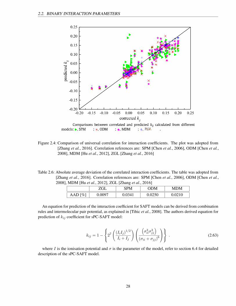
2.2. BINARY INTERACTION PARAMETERS
Figure 2.4: Comparison of universal correlation for interaction coefficients. The plot was adopted from[Zhang et al., 2016]. Correlation references are: SPM [Chen et al., 2006], ODM [Chen et al.,2008], MDM [Hu et al., 2012], ZGL [Zhang et al., 2016]
Table 2.6: Absolute average deviation of the correlated interaction coefficients. The table was adopted from[Zhang et al., 2016]. Correlation references are: SPM [Chen et al., 2006], ODM [Chen et al.,2008], MDM [Hu et al., 2012], ZGL [Zhang et al., 2016]
ZGL SPM ODM MDMAAD [%] 0.0097 0.0341 0.0250 0.0210
An equation for prediction of the interaction coefficient for SAFT models can be derived from combinationrules and intermolecular pair potential, as explained in [Tihic et al., 2008]. The authors derived equation forprediction of kij coefficient for sPC-SAFT model:
kij = 1−
27(
(IiIj)1/2
Ii + Ij
)(σ3iiσ
3jj
)(σii + σjj)6
. (2.63)
where I is the ionisation potential and σ is the parameter of the model, refer to section 6.4 for detaileddescription of the sPC-SAFT model.
28
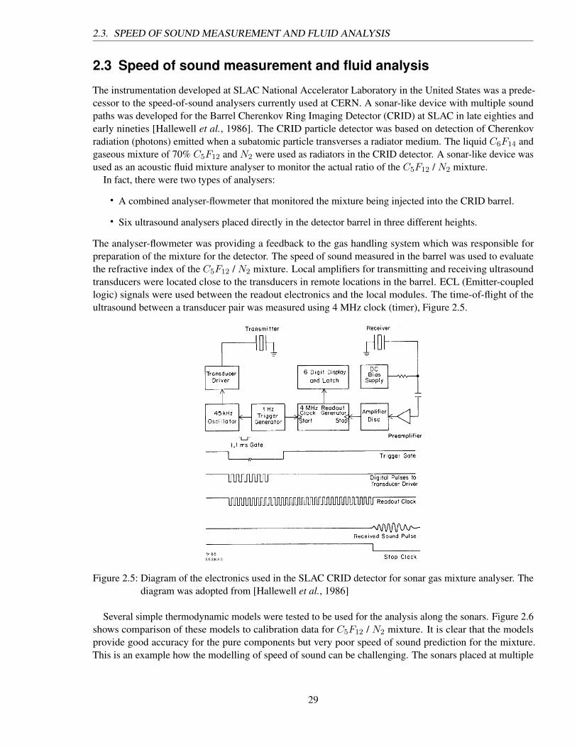
2.3. SPEED OF SOUND MEASUREMENT AND FLUID ANALYSIS
2.3 Speed of sound measurement and fluid analysis
The instrumentation developed at SLAC National Accelerator Laboratory in the United States was a prede-cessor to the speed-of-sound analysers currently used at CERN. A sonar-like device with multiple soundpaths was developed for the Barrel Cherenkov Ring Imaging Detector (CRID) at SLAC in late eighties andearly nineties [Hallewell et al., 1986]. The CRID particle detector was based on detection of Cherenkovradiation (photons) emitted when a subatomic particle transverses a radiator medium. The liquid C6F14 andgaseous mixture of 70% C5F12 and N2 were used as radiators in the CRID detector. A sonar-like device wasused as an acoustic fluid mixture analyser to monitor the actual ratio of the C5F12 / N2 mixture.
In fact, there were two types of analysers:
• A combined analyser-flowmeter that monitored the mixture being injected into the CRID barrel.
• Six ultrasound analysers placed directly in the detector barrel in three different heights.
The analyser-flowmeter was providing a feedback to the gas handling system which was responsible forpreparation of the mixture for the detector. The speed of sound measured in the barrel was used to evaluatethe refractive index of the C5F12 / N2 mixture. Local amplifiers for transmitting and receiving ultrasoundtransducers were located close to the transducers in remote locations in the barrel. ECL (Emitter-coupledlogic) signals were used between the readout electronics and the local modules. The time-of-flight of theultrasound between a transducer pair was measured using 4 MHz clock (timer), Figure 2.5.
Figure 2.5: Diagram of the electronics used in the SLAC CRID detector for sonar gas mixture analyser. Thediagram was adopted from [Hallewell et al., 1986]
Several simple thermodynamic models were tested to be used for the analysis along the sonars. Figure 2.6shows comparison of these models to calibration data for C5F12 / N2 mixture. It is clear that the modelsprovide good accuracy for the pure components but very poor speed of sound prediction for the mixture.This is an example how the modelling of speed of sound can be challenging. The sonars placed at multiple
29
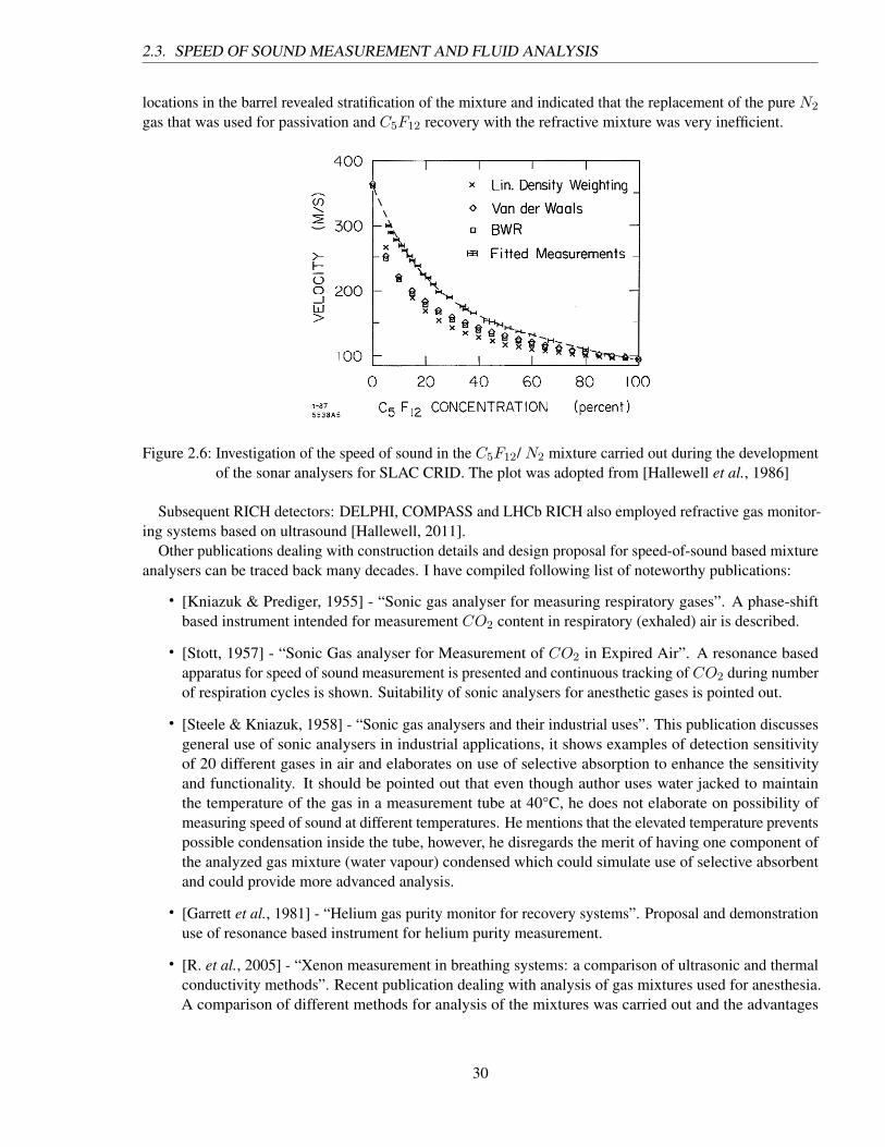
2.3. SPEED OF SOUND MEASUREMENT AND FLUID ANALYSIS
locations in the barrel revealed stratification of the mixture and indicated that the replacement of the pure N2gas that was used for passivation and C5F12 recovery with the refractive mixture was very inefficient.
Figure 2.6: Investigation of the speed of sound in the C5F12/ N2 mixture carried out during the developmentof the sonar analysers for SLAC CRID. The plot was adopted from [Hallewell et al., 1986]
Subsequent RICH detectors: DELPHI, COMPASS and LHCb RICH also employed refractive gas monitor-ing systems based on ultrasound [Hallewell, 2011].
Other publications dealing with construction details and design proposal for speed-of-sound based mixtureanalysers can be traced back many decades. I have compiled following list of noteworthy publications:
• [Kniazuk & Prediger, 1955] - “Sonic gas analyser for measuring respiratory gases”. A phase-shiftbased instrument intended for measurement CO2 content in respiratory (exhaled) air is described.
• [Stott, 1957] - “Sonic Gas analyser for Measurement of CO2 in Expired Air”. A resonance basedapparatus for speed of sound measurement is presented and continuous tracking of CO2 during numberof respiration cycles is shown. Suitability of sonic analysers for anesthetic gases is pointed out.
• [Steele & Kniazuk, 1958] - “Sonic gas analysers and their industrial uses”. This publication discussesgeneral use of sonic analysers in industrial applications, it shows examples of detection sensitivityof 20 different gases in air and elaborates on use of selective absorption to enhance the sensitivityand functionality. It should be pointed out that even though author uses water jacked to maintainthe temperature of the gas in a measurement tube at 40°C, he does not elaborate on possibility ofmeasuring speed of sound at different temperatures. He mentions that the elevated temperature preventspossible condensation inside the tube, however, he disregards the merit of having one component ofthe analyzed gas mixture (water vapour) condensed which could simulate use of selective absorbentand could provide more advanced analysis.
• [Garrett et al., 1981] - “Helium gas purity monitor for recovery systems”. Proposal and demonstrationuse of resonance based instrument for helium purity measurement.
• [R. et al., 2005] - “Xenon measurement in breathing systems: a comparison of ultrasonic and thermalconductivity methods”. Recent publication dealing with analysis of gas mixtures used for anesthesia.A comparison of different methods for analysis of the mixtures was carried out and the advantages
30

2.3. SPEED OF SOUND MEASUREMENT AND FLUID ANALYSIS
and disadvantages of the methods is discussed. The conclusion is that the acoustic analysis of themixtures is more precise than the tested instrument based on thermal conductivity. The disadvantageof the acoustic method is that it is not gas specific as it assumes binary mixture of two gases if a thirdgas is included the analysis cannot distinguish it. Author offers techniques (water trap, soda-lime toeliminate CO2) to overcome this disadvantage.
Steven Garett published numerous papers and developed number of instruments together with his colleagues:[Golden et al., 1998b], [Garrett, 2009], [Garrett, 2008] or [Golden et al., 1998a]. He presented use of hisinstrument for detection of hydrogen and methane from metabolic processes of anaerobic bacteria [Horta &Garrett, 2005].
Other publications from other authors that deal with construction or theoretical concept of speed-of-soundbased instruments include:
• [Valdes & Cadet, 1991] - “Ultrasonic Time-of-Flight Method for On-Line Quantitation of in SituGenerated Arsine”. Composition monitoring system based on an ultrasonic flow cell is used to monitorAsH2 +H2 and Ar +He mixtures that are utilized during semiconductor manufacturing.
• [Giacobbe, 1993] - “Precision measurement of acoustic velocities in pure gases and gas mixtures”.A design of precise instrument for measurement of speed of sound. The instrument performance isevaluated with 10 gases at two different temperatures. An accuracy from±0.15% to ±0.1% in case ofrepeated measurements is concluded.
• [Joos et al., 1993] - “An ultrasonic sensor for the analysis of binary gas mixtures”. Authors discussin detail sensitivity of ratio determination for binary mixtures. Authors conclude that the developedinstrument is suited for use in fruit-storage halls and greenhouses where it can monitor the CO2 contentin local atmosphere.
• [Löfqvist et al., 2003] - “Speed of sound measurements in gas-mixtures at varying composition usingan ultrasonic gas flow meter with silicon based transducers”. An ultrasonic flow meter, perhaps somecommercially available type but it is not specified, is used to demonstrate measurement of the speed ofsound and subsequent determination of binary mixture composition of three mixtures.
• [Liu et al., 2015], [Kosterev et al., 2010] - Relatively unique construction of speed of sound sensoris described. The sensor is intended as supplementary unit in a gas analyser on a principle of quartz-enhanced photoacoustic spectroscopy, Figure 2.7. The speed of sound is determined from a phase shiftof continuous sine wave of variable frequency from 1 kHz to 50 kHz. The microphone that detects thephase shift are located at the ends of a U-shaped tube with constant flow of gas. The sensor was testedwith number of gas mixtures and the results were compared to predictions. The standard deviation ofthe measured errors was found to be < 1 on a range from 260m/s to 1010m/s.
One of the most in-depth publication is [Hallewell et al., 1986] called “A Sonar-Based Technique for theRatiometric Determination of Binary Gas Mixtures”. In this 49-pages long paper (including the annexes)the theoretical background of sonic analyser, hardware construction and also experimental measurementsare covered. A study on speed of sound in pure components and mixtures with three different equationsof state (Ideal gas, Van der Waalse, BWR) is presented along with error analysis. The theoretical sectionis accompanied by measurement of speed of sound in pure gases and following mixtures: Ne + He,CH4 + C4H10, CH4 + C2H6, N2 + C4H10, and N2 + C5F12. The developed instrument was intendedto be used at Stanford Linear Accelerator Center (SLAC) in Cerenkov Ring Imaging Detector. It can beincorporated into a control loop in the gas handling units to enable effective monitoring of the gases mixturesthat are essential for the detector operation.
31
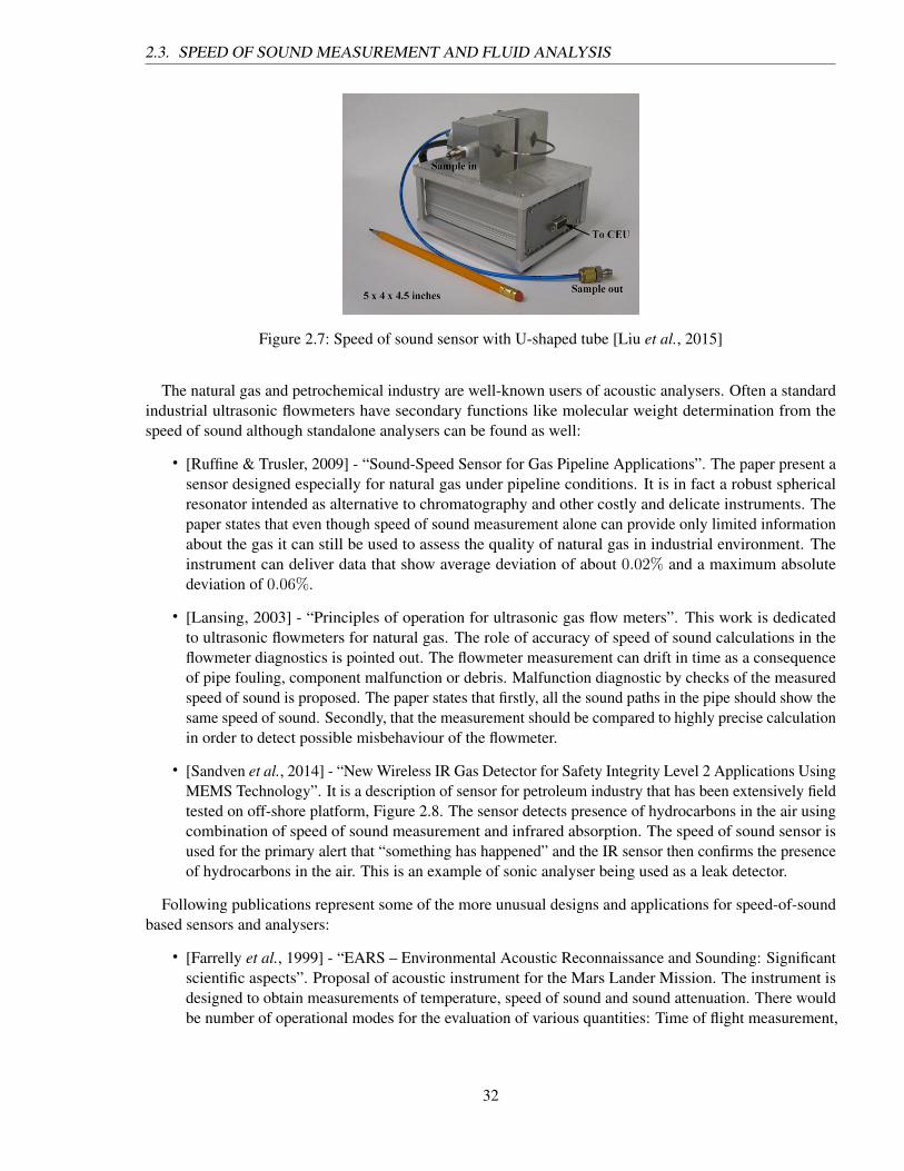
2.3. SPEED OF SOUND MEASUREMENT AND FLUID ANALYSIS
Figure 2.7: Speed of sound sensor with U-shaped tube [Liu et al., 2015]
The natural gas and petrochemical industry are well-known users of acoustic analysers. Often a standardindustrial ultrasonic flowmeters have secondary functions like molecular weight determination from thespeed of sound although standalone analysers can be found as well:
• [Ruffine & Trusler, 2009] - “Sound-Speed Sensor for Gas Pipeline Applications”. The paper present asensor designed especially for natural gas under pipeline conditions. It is in fact a robust sphericalresonator intended as alternative to chromatography and other costly and delicate instruments. Thepaper states that even though speed of sound measurement alone can provide only limited informationabout the gas it can still be used to assess the quality of natural gas in industrial environment. Theinstrument can deliver data that show average deviation of about 0.02% and a maximum absolutedeviation of 0.06%.
• [Lansing, 2003] - “Principles of operation for ultrasonic gas flow meters”. This work is dedicatedto ultrasonic flowmeters for natural gas. The role of accuracy of speed of sound calculations in theflowmeter diagnostics is pointed out. The flowmeter measurement can drift in time as a consequenceof pipe fouling, component malfunction or debris. Malfunction diagnostic by checks of the measuredspeed of sound is proposed. The paper states that firstly, all the sound paths in the pipe should show thesame speed of sound. Secondly, that the measurement should be compared to highly precise calculationin order to detect possible misbehaviour of the flowmeter.
• [Sandven et al., 2014] - “New Wireless IR Gas Detector for Safety Integrity Level 2 Applications UsingMEMS Technology”. It is a description of sensor for petroleum industry that has been extensively fieldtested on off-shore platform, Figure 2.8. The sensor detects presence of hydrocarbons in the air usingcombination of speed of sound measurement and infrared absorption. The speed of sound sensor isused for the primary alert that “something has happened” and the IR sensor then confirms the presenceof hydrocarbons in the air. This is an example of sonic analyser being used as a leak detector.
Following publications represent some of the more unusual designs and applications for speed-of-soundbased sensors and analysers:
• [Farrelly et al., 1999] - “EARS – Environmental Acoustic Reconnaissance and Sounding: Significantscientific aspects”. Proposal of acoustic instrument for the Mars Lander Mission. The instrument isdesigned to obtain measurements of temperature, speed of sound and sound attenuation. There wouldbe number of operational modes for the evaluation of various quantities: Time of flight measurement,
32
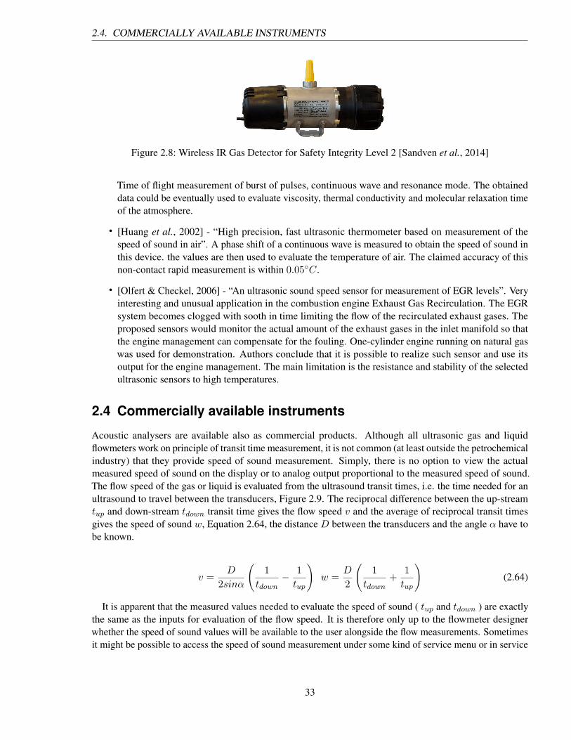
2.4. COMMERCIALLY AVAILABLE INSTRUMENTS
Figure 2.8: Wireless IR Gas Detector for Safety Integrity Level 2 [Sandven et al., 2014]
Time of flight measurement of burst of pulses, continuous wave and resonance mode. The obtaineddata could be eventually used to evaluate viscosity, thermal conductivity and molecular relaxation timeof the atmosphere.
• [Huang et al., 2002] - “High precision, fast ultrasonic thermometer based on measurement of thespeed of sound in air”. A phase shift of a continuous wave is measured to obtain the speed of sound inthis device. the values are then used to evaluate the temperature of air. The claimed accuracy of thisnon-contact rapid measurement is within 0.05C.
• [Olfert & Checkel, 2006] - “An ultrasonic sound speed sensor for measurement of EGR levels”. Veryinteresting and unusual application in the combustion engine Exhaust Gas Recirculation. The EGRsystem becomes clogged with sooth in time limiting the flow of the recirculated exhaust gases. Theproposed sensors would monitor the actual amount of the exhaust gases in the inlet manifold so thatthe engine management can compensate for the fouling. One-cylinder engine running on natural gaswas used for demonstration. Authors conclude that it is possible to realize such sensor and use itsoutput for the engine management. The main limitation is the resistance and stability of the selectedultrasonic sensors to high temperatures.
2.4 Commercially available instruments
Acoustic analysers are available also as commercial products. Although all ultrasonic gas and liquidflowmeters work on principle of transit time measurement, it is not common (at least outside the petrochemicalindustry) that they provide speed of sound measurement. Simply, there is no option to view the actualmeasured speed of sound on the display or to analog output proportional to the measured speed of sound.The flow speed of the gas or liquid is evaluated from the ultrasound transit times, i.e. the time needed for anultrasound to travel between the transducers, Figure 2.9. The reciprocal difference between the up-streamtup and down-stream tdown transit time gives the flow speed v and the average of reciprocal transit timesgives the speed of sound w, Equation 2.64, the distance D between the transducers and the angle α have tobe known.
v = D
2sinα
(1
tdown− 1tup
)w = D
2
(1
tdown+ 1tup
)(2.64)
It is apparent that the measured values needed to evaluate the speed of sound ( tup and tdown ) are exactlythe same as the inputs for evaluation of the flow speed. It is therefore only up to the flowmeter designerwhether the speed of sound values will be available to the user alongside the flow measurements. Sometimesit might be possible to access the speed of sound measurement under some kind of service menu or in service
33
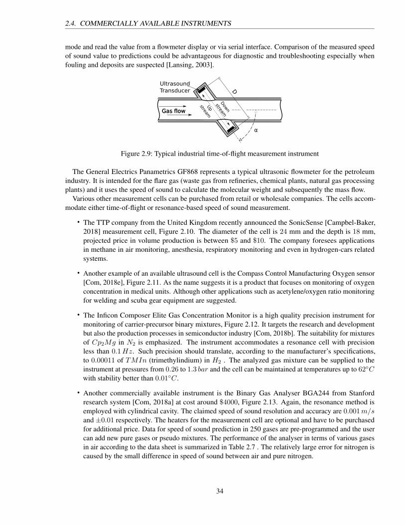
2.4. COMMERCIALLY AVAILABLE INSTRUMENTS
mode and read the value from a flowmeter display or via serial interface. Comparison of the measured speedof sound value to predictions could be advantageous for diagnostic and troubleshooting especially whenfouling and deposits are suspected [Lansing, 2003].
UltrasoundTransducer
Gas flow
Up
stream
Dow
n
streamGas flow
D
α
Figure 2.9: Typical industrial time-of-flight measurement instrument
The General Electrics Panametrics GF868 represents a typical ultrasonic flowmeter for the petroleumindustry. It is intended for the flare gas (waste gas from refineries, chemical plants, natural gas processingplants) and it uses the speed of sound to calculate the molecular weight and subsequently the mass flow.
Various other measurement cells can be purchased from retail or wholesale companies. The cells accom-modate either time-of-flight or resonance-based speed of sound measurement.
• The TTP company from the United Kingdom recently announced the SonicSense [Campbel-Baker,2018] measurement cell, Figure 2.10. The diameter of the cell is 24 mm and the depth is 18 mm,projected price in volume production is between $5 and $10. The company foresees applicationsin methane in air monitoring, anesthesia, respiratory monitoring and even in hydrogen-cars relatedsystems.
• Another example of an available ultrasound cell is the Compass Control Manufacturing Oxygen sensor[Com, 2018e], Figure 2.11. As the name suggests it is a product that focuses on monitoring of oxygenconcentration in medical units. Although other applications such as acetylene/oxygen ratio monitoringfor welding and scuba gear equipment are suggested.
• The Inficon Composer Elite Gas Concentration Monitor is a high quality precision instrument formonitoring of carrier-precursor binary mixtures, Figure 2.12. It targets the research and developmentbut also the production processes in semiconductor industry [Com, 2018b]. The suitability for mixturesof Cp2Mg in N2 is emphasized. The instrument accommodates a resonance cell with precisionless than 0.1Hz. Such precision should translate, according to the manufacturer’s specifications,to 0.00011 of TMIn (trimethylindium) in H2 . The analyzed gas mixture can be supplied to theinstrument at pressures from 0.26 to 1.3 bar and the cell can be maintained at temperatures up to 62Cwith stability better than 0.01C.
• Another commercially available instrument is the Binary Gas Analyser BGA244 from Stanfordresearch system [Com, 2018a] at cost around $4000, Figure 2.13. Again, the resonance method isemployed with cylindrical cavity. The claimed speed of sound resolution and accuracy are 0.001m/sand ±0.01 respectively. The heaters for the measurement cell are optional and have to be purchasedfor additional price. Data for speed of sound prediction in 250 gases are pre-programmed and the usercan add new pure gases or pseudo mixtures. The performance of the analyser in terms of various gasesin air according to the data sheet is summarized in Table 2.7 . The relatively large error for nitrogen iscaused by the small difference in speed of sound between air and pure nitrogen.
34
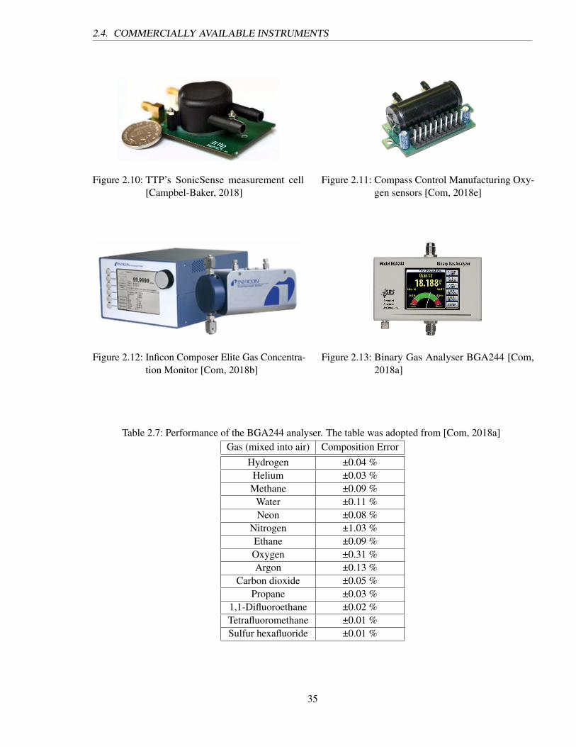
2.4. COMMERCIALLY AVAILABLE INSTRUMENTS
Figure 2.10: TTP’s SonicSense measurement cell[Campbel-Baker, 2018]
Figure 2.11: Compass Control Manufacturing Oxy-gen sensors [Com, 2018e]
Figure 2.12: Inficon Composer Elite Gas Concentra-tion Monitor [Com, 2018b]
Figure 2.13: Binary Gas Analyser BGA244 [Com,2018a]
Table 2.7: Performance of the BGA244 analyser. The table was adopted from [Com, 2018a]Gas (mixed into air) Composition Error
Hydrogen ±0.04 %Helium ±0.03 %Methane ±0.09 %
Water ±0.11 %Neon ±0.08 %
Nitrogen ±1.03 %Ethane ±0.09 %Oxygen ±0.31 %Argon ±0.13 %
Carbon dioxide ±0.05 %Propane ±0.03 %
1,1-Difluoroethane ±0.02 %Tetrafluoromethane ±0.01 %Sulfur hexafluoride ±0.01 %
35
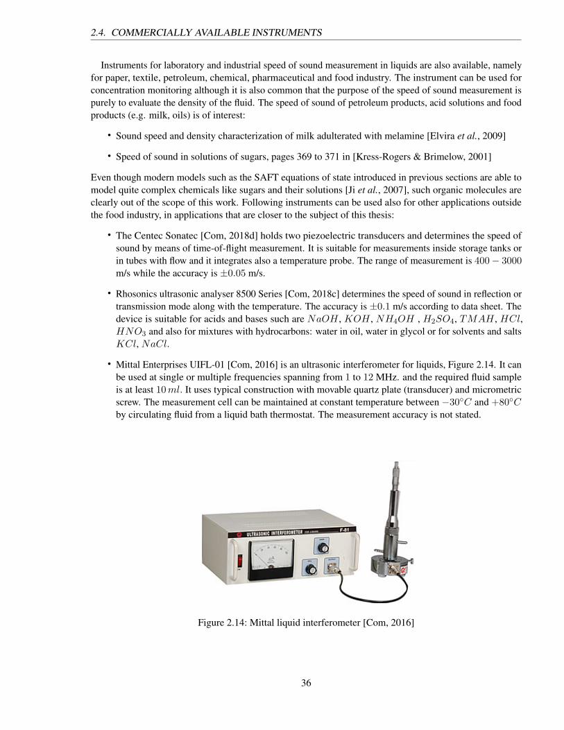
2.4. COMMERCIALLY AVAILABLE INSTRUMENTS
Instruments for laboratory and industrial speed of sound measurement in liquids are also available, namelyfor paper, textile, petroleum, chemical, pharmaceutical and food industry. The instrument can be used forconcentration monitoring although it is also common that the purpose of the speed of sound measurement ispurely to evaluate the density of the fluid. The speed of sound of petroleum products, acid solutions and foodproducts (e.g. milk, oils) is of interest:
• Sound speed and density characterization of milk adulterated with melamine [Elvira et al., 2009]
• Speed of sound in solutions of sugars, pages 369 to 371 in [Kress-Rogers & Brimelow, 2001]
Even though modern models such as the SAFT equations of state introduced in previous sections are able tomodel quite complex chemicals like sugars and their solutions [Ji et al., 2007], such organic molecules areclearly out of the scope of this work. Following instruments can be used also for other applications outsidethe food industry, in applications that are closer to the subject of this thesis:
• The Centec Sonatec [Com, 2018d] holds two piezoelectric transducers and determines the speed ofsound by means of time-of-flight measurement. It is suitable for measurements inside storage tanks orin tubes with flow and it integrates also a temperature probe. The range of measurement is 400− 3000m/s while the accuracy is ±0.05 m/s.
• Rhosonics ultrasonic analyser 8500 Series [Com, 2018c] determines the speed of sound in reflection ortransmission mode along with the temperature. The accuracy is ±0.1 m/s according to data sheet. Thedevice is suitable for acids and bases such are NaOH , KOH , NH4OH , H2SO4, TMAH , HCl,HNO3 and also for mixtures with hydrocarbons: water in oil, water in glycol or for solvents and saltsKCl, NaCl.
• Mittal Enterprises UIFL-01 [Com, 2016] is an ultrasonic interferometer for liquids, Figure 2.14. It canbe used at single or multiple frequencies spanning from 1 to 12 MHz. and the required fluid sampleis at least 10ml. It uses typical construction with movable quartz plate (transducer) and micrometricscrew. The measurement cell can be maintained at constant temperature between −30C and +80Cby circulating fluid from a liquid bath thermostat. The measurement accuracy is not stated.
Figure 2.14: Mittal liquid interferometer [Com, 2016]
36

2.5. SUMMARY
Figure 2.15: Centec Sonatec [Com, 2018d] Figure 2.16: Rhosonics ultrasonic analyser 8500 Se-ries [Com, 2018c]
2.5 Summary
The basic form of equations of state is used to calculate the pressure or Helmholtz energy from the temperatureand density. The pressure as well as any other thermodynamic property can be obtained from derivation of theHelmholtz energy. The speed of sound requires derivative of pressure or Helmholtz energy including the heatcapacities which are itself derivatives of pressure or Helmholtz energy but they also include the ideal gas heatcapacity that needs to be evaluated experimentally. The prediction of saturated pressure and vapour densityand speed of sound can be carried out with relatively simple cubic equations of state at reasonable accuracyof around 2%. The simple equation does not provide good accuracy neither for the liquid density nor for theliquid speed of sound, the deviations from experimental data are around 10% in both cases. The complexequations such as the BWR or modern Helmholtz energy equations of state which can provide accuracy betterthan 1% are difficult to use especially for new fluids (large experimental data sets needed for complicatedfitting procedure). The SAFT approach sits in the middle, only few fluid-specific fitting constants are requiredwhile the achieved accuracy is good even in liquid phase, the deviations are often close to 1%. But the resultsdiffer for different fluids and different SAFT models. To achieve good accuracy for mixtures it is necessaryto use binary interaction coefficients which are seldomly available for unusual mixture. Good estimationmodels are thus extremely useful. The section dedicated to speed-of-sound measuring instruments shows thatthere is a multitude of applications described in scientific literature. Multiple instruments for industrial speedof sound measurement exist namely in the food and petrochemical industry. To my knowledge, none of theinstruments are directly intended for refrigeration applications. In my opinion, the main limitation is lack ofreliable and speed of sound prediction models.
37
2.5. SUMMARY
Bibliography
chapter 2: Prior art
[Com, 2016] 2016. Ultrasonic Interferometer For Liquids. Mittal enterprises, New PatelNagar, Delhi, 110008 India, http://www.mittalenterprises.com/products/index/ultrasonic-interferometer-for-liquids_3238.html.
[Com, 2018a] 2018a (October). Binary Gas Analyzer BGA244. SRS Stanford Research Systems, 1290-DReamwood Ave. Sunnyvale CA 94089 USA, http://thinksrs.com/products/BGA244.htm.
[Com, 2018b] 2018b (October). Composer Elite Gas Concentration Monitor. INFICON HoldingAG, Hintergasse 15B CH-7310 Bad Ragaz Switzerland, http://products.inficon.com/en\protect\discretionary\char\hyphenchar\fontus/Product/Detail/Composer\protect\discretionary\char\hyphenchar\fontElite.
[Com, 2018c] 2018c (October). Composer Elite Gas Concentration Monitor. INFICON HoldingAG, Hintergasse 15B CH-7310 Bad Ragaz Switzerland, http://products.inficon.com/en\protect\discretionary\char\hyphenchar\fontus/Product/Detail/Composer\protect\discretionary\char\hyphenchar\fontElite.
[Com, 2018d] 2018d (October). Determination of Concentration by Sound Velocity. Centec,Wilhelm-Röntgen-Strasse 10 63477 Maintal Germany, http://www.centec.de/sensors/power-plants/sonatec/.
[Com, 2018e] 2018e (September). Oxygen sensor. Compass Controls Manufacturing Inc., 9645 LackmanRd Lenexa, KS 66219 USA, http://compassmanufacturing.com/monitoring.html.
[Ahlers & Gmehling, 2001] Ahlers, J., & Gmehling, J. 2001. Development of an universal group contri-bution equation of state: I. Prediction of liquid densities for pure compounds with a volume translatedPeng-Robinson equation of state. Fluid Phase Equilibria, 191(1), 177 – 188.
[Blas & Vega, 2001] Blas, F. J., & Vega, L. F. 2001. Thermodynamic properties and phase equilibria ofbranched chain fluids using first- and second-order Wertheim’s thermodynamic perturbation theory. TheJournal of Chemical Physics, 115(8), 3906–3915.
[Campbel-Baker, 2018] Campbel-Baker, A. 2018 (January). Press Release SonicSense. TTP plc., MelbournScience Park Melbourn Hertfordshire SG8 6EE UK, http://www.ttp.com/news/2014/01/sonic_sense.
[Chen et al., 2006] Chen, J., Chen, Z., & Hu, P. 2006. J. Univ. Sci. Technol. China, 36, 656–659. cited By 1.
[Chen et al., 2008] Chen, J.-X., Hu, P., & Chen, Z.-S. 2008. Study on the Interaction Coefficients inPR Equation with vdW Mixing Rules for HFC and HC Binary Mixtures. International Journal ofThermophysics, 29(6), 1945–1953.
38
2.5. SUMMARY
[Chueh & Prausnitz, 1967] Chueh, P. L., & Prausnitz, J. M. 1967. Vapor-liquid equilibria at high pressures:Calculation of partial molar volumes in nonpolar liquid mixtures. AIChE Journal, 13(6), 1099–1107.
[Coquelet et al., 2016] Coquelet, Ch., Houriez, C., & El Abbadi, J. 2016. Prediction of thermodynamicproperties of refrigerant fluids with a new three-parameter cubic equation of state. International Journalof Refrigeration, 69, 418–436.
[Defibaugh & Moldover, 1997] Defibaugh, D. R., & Moldover, M. R. 1997. Compressed and SaturatedLiquid Densities for 18 Halogenated Organic Compounds. Journal of Chemical & Engineering Data,42(1), 160–168.
[Defibaugh et al., 1994] Defibaugh, D. R., Morrison, G., & Weber., L. A. 1994. Thermodynamic Propertiesof Difluoromethane. Journal of Chemical & Engineering Data, 39(2), 333–340.
[Diamantonis & Economou, 2018] Diamantonis, N., & Economou, I. 2018. Evaluation of SAFT and PC-SAFT EoS for the calculation of thermodynamic derivative properties of fluids related to carbon captureand sequestration. 05.
[Dias, 2005] Dias, A. M. A. 2005. Thermodynamic Properties of Blood Substituting Liquid Mixtures. Ph.D.thesis.
[Elvira et al., 2009] Elvira, L., Rodriguez, J., & Lynnworth, L. C. 2009. Sound speed and density charac-terization of milk adulterated with melamine. The Journal of the Acoustical Society of America, 125(5),EL177–EL182.
[Estela-Uribe & Trusler, 2000] Estela-Uribe, J. F., & Trusler, J. P. M. 2000. Acoustic and Volumetric VirialCoefficients of Nitrogen. International Journal of Thermophysics, 21(5), 1033–1044.
[Ewing & Trusler, 1992] Ewing, M. B., & Trusler, J. P. M. 1992. Second acoustic virial coefficients ofnitrogen between 80 and 373 K. Physica A: Statistical Mechanics and its Applications, 184(3), 415 – 436.
[Farrelly et al., 1999] Farrelly, F. A., Flamini, E., Petri, A., Pitolli, L., & Pontuale, G. 1999 (September).EARS - Environmental Acoustic Reconnaissance and Sounding: Significant scientific aspects. In: 2ndInternational Workshop on "The Italian role and perspectives for the exploration of Mars".
[Fateen et al., 2013] Fateen, S.-E. K., Khalil, M. M., & Elnabawy, A. O. 2013. Semi-empirical correlationfor binary interaction parameters of the Peng-Robinson equation of state with the van der Waals mixingrules for the prediction of high-pressure vapor-liquid equilibrium. Journal of Advanced Research, 4(2),137 – 145.
[Gao et al., 1992] Gao, G., Daridon, J.-L., Saint-Guirons, H., Xans, P., & Montel, F. 1992. A simplecorrelation to evaluate binary interaction parameters of the Peng-Robinson equation of state: binary lighthydrocarbon systems. Fluid Phase Equilibria, 74, 85 – 93.
[Garrett, 2008] Garrett, S. L. 2008. Sonic gas analyzer for hydrogen and methane. The Journal of theAcoustical Society of America, 123(5), 3372–3372.
[Garrett, 2009] Garrett, S. L. 2009 (January). Sonic Gas Analysis. In: ETHOS Conference proceedings.Session 5: Science of Stoves.
[Garrett et al., 1981] Garrett, S. L., Swift, G. W., & Packard, R. E. 1981. Helium gas purity monitor forrecovery systems. Physica B+C, 107(1), 601 – 602.
39
2.5. SUMMARY
[Giacobbe, 1993] Giacobbe, F. W. 1993. Precision measurement of acoustic velocities in pure gases and gasmixtures. The Journal of the Acoustical Society of America, 94(3), 1200–1210.
[Golden et al., 1998a] Golden, M. V., Keoliarr, R. M., & Garrett, S. L. 1998a. Sonic Gas Analysis. Pages1705–1706 of: Proceedings 16th International Congress on Acoustics and 135th Meeting AcousticalSociety of America, vol. III.
[Golden et al., 1998b] Golden, M. V., Keolian, R. M., & Garrett, S. L. 1998b. Sonic gas analyzers. TheJournal of the Acoustical Society of America, 103(5), 2944–2944.
[Hallewell, 2011] Hallewell, G. 2011. Aspects de lutilisation de fluides fluorocarbures saturees dans laphysique des hautes energies. Université de la Méditerranée Aix-Marseille II. Habilitation a diriger desrecherches.
[Hallewell et al., 1986] Hallewell, G., Crawford, G., Mcshurley, D., Oxoby, G., & Reif, R. 1986. A Sonar-Based Technique for the Ratiometric Determination of Binary Gas Mixtures. SLAC - PUB, 4122(October).
[Hemptinne & Ungerer, 1995] Hemptinne, J. C., & Ungerer, P. 1995. Accuracy of the volumetric predictionsof some important equations of state for hydrocarbons, including a modified version of the Lee-Keslermethod. Fluid Phase Equilibria, 106(1), 81 – 109.
[Horta & Garrett, 2005] Horta, M. A., & Garrett, S. L. 2005. Sonic gas analyzer for microbiologicalmetabolic measurements. The Journal of the Acoustical Society of America, 118(3), 1945–1945.
[Hu et al., 2012] Hu, P., Chen, L.-X., & Chen, Z,-S. 2012. A modified differential-model for interactionparameters in PR EoS with vdW mixing rules for mixtures containing HFCs and HCs. Fluid PhaseEquilibria, 324, 64 – 69.
[Huang et al., 2002] Huang, K. N., Huang, C. F., Li, Y. C., & Young, M. S. 2002. High Precision, FastUltrasonic Thermometer Based on Measurement of the Speed of Sound in Air. Review of ScientificInstruments, 73(4022).
[Huber & McLinden, 1992] Huber, M. L., & McLinden, M. O. 1992. Thermodynamic Properties of R134a(1,1,1,2-tetrafluoroethane). International Refrigeration and Air Conditioning Conference.
[Jaubert & Mutelet, 2004] Jaubert, J.-N., & Mutelet, F. 2004. VLE predictions with the Peng-Robinsonequation of state and temperature dependent kij calculated through a group contribution method. FluidPhase Equilibria, 224(2), 285 – 304.
[Ji et al., 2007] Ji, Peijun, Feng, Wei, & Tan, Tianwei. 2007. Density Calculation of Sugar Solutions withthe SAFT Model. Journal of Chemical & Engineering Data, 52(1), 135–140.
[Joos et al., 1993] Joos, M., Müller, H., & Lindner, G. 1993. An ultrasonic sensor for the analysis of binarygas mixtures. Sensors and Actuators B: Chemical, 16(1), 413 – 419.
[Kniazuk & Prediger, 1955] Kniazuk, M., & Prediger, F. R. 1955. Sonic gas analyzer for measuring respira-tory gases. ISA Proc., II(55-9-2). 5 pages.
[Kosterev et al., 2010] Kosterev, A. A., Dong, L., Thomazy, D., Tittel, F.K., & Overby, S. 2010. QEPAS forChemical Analysis of Multi-Component Gas Mixtures. Appl Phys B, 101, 649–659.
40
2.5. SUMMARY
[Kress-Rogers & Brimelow, 2001] Kress-Rogers, E., & Brimelow, C.J.B. 2001. Instrumentation and Sensorsfor the Food Industry. Woodhead Publishing Series in Food Science, Technology and Nutrition. Woodhead.
[Kunz & European Gas Research Group, 2007] Kunz, O., & European Gas Research Group. 2007. TheGERG-2004 Wide Range Equation of State for Natural Gases and Other Mixtures: GERG TM15 2007.Fortschrittberichte VDI / 6: Energietechnik. VDI-Verlag.
[Lafitte et al., 2013] Lafitte, T., Apostolakou, A., Avendano, C., Galindo, A., Adjiman, C. S., Müller, E. A.,& Jackson, G. 2013. Accurate statistical associating fluid theory for chain molecules formed from Miesegments. The Journal of Chemical Physics, 139(15), 154504.
[Lansing, 2003] Lansing, J. 2003 (September). Principles of Operation for Ultrasonic Gas Flow Meters.Pages 50 – 60 of: American School of Gas Measurement Technology, vol. 38. American School of GasMeasurement Technology, Houston, texas.
[Lemmon & Roland, 2006] Lemmon, E. W., & Roland, S. 2006. Short Fundamental Equations of State for20 Industrial Fluids. Journal of Chemical & Engineering Data, 51(3), 785–850.
[Löfqvist et al., 2003] Löfqvist, T., Sokas, K., & Delsing, J. 2003. Speed of Sound Measurements in Gas-Mixtures at Varying Composition Using an Ultrasonic Gas Flow Meter With Silicon Based Transducers.Tech. rept. 11th Conference on Flow Measurement Groningen, NETHERLANDS.
[Li et al., 1999] Li, J., Tillner-Roth, R., Sato, H., & Watanabe, K. 1999. An Equation of State for 1,1,1-Trifluoroethane (R-143a). International Journal of Thermophysics, 20(6), 1639–1651.
[Liang et al., 2012] Liang, X., Maribo-Mogensen, B., Thomsen, K., Yan, W., & Kontogeorgis, G. M. 2012.Approach to Improve Speed of Sound Calculation within PC-SAFT Framework. Industrial & EngineeringChemistry Research, 51(45), 14903–14914.
[Liu et al., 2015] Liu, K., Dong, L., & Tittel, F. K. 2015. Compact Sound-Speed Sensor for Quartz EnhancedPhotoacoustic Spectroscopy Based Applications. Review Of Scientific Instruments, 86(044903).
[Llovell & Vega, 2006] Llovell, F., & Vega, L. F. 2006. Prediction of Thermodynamic Derivative Propertiesof Pure Fluids through the Soft-SAFT Equation of State. The Journal of Physical Chemistry B, 110(23),11427–11437. PMID: 16771416.
[Lopez-Echeverry et al., 2017] Lopez-Echeverry, J. S., Reif-Acherman, S., & Araujo-Lopez, E. 2017. Peng-Robinson equation of state: 40 years through cubics. Fluid Phase Equilibria, 447, 39 – 71.
[Magoulas & Tassios, 1990] Magoulas, K., & Tassios, D. 1990. Thermophysical properties of n-Alkanesfrom C1 to C20 and their prediction for higher ones. Fluid Phase Equilibria, 56(Supplement C), 119 –140.
[Olfert & Checkel, 2006] Olfert, J. S., & Checkel, M. D. 2006. An Ultrasonic Sound Speed Sensor ForMeasuring EGR Levels. Proc. IMechE, 221(November). Part D J. Automobile Engineering.
[Outcalt & McLinden, 1996] Outcalt, S. L., & McLinden, M. O. 1996. A Modified Benedict-Webb-RubinEquation of State for the Thermodynamic Properties of R152a (1,1-difluoroethane). Journal of Physicaland Chemical Reference Data, 25(2), 605–636.
[Péneloux et al., 1982] Péneloux, A., Rauzy, E., & Fréze, R. 1982. A consistent correction for Redlich-Kwong-Soave volumes. Fluid Phase Equilibria, 8(1), 7 – 23.
41
2.5. SUMMARY
[R. et al., 2005] R., King, M., Bretland, A., Wilkes, & J., Dingley. 2005. Xenon measurement in breathingsystems: a comparison of ultrasonic and thermal conductivity methods. Anaesthesia, 60(12), 1226–1230.
[Redlich & Kwong, 1949] Redlich, )., & Kwong, J. N. S. 1949. On the Thermodynamics of Solutions. V.An Equation of State. Fugacities of Gaseous Solutions. Chemical Reviews, 44(1), 233–244. PMID:18125401.
[Ruffine & Trusler, 2009] Ruffine, L., & Trusler, J. P. M. 2009. Sound-Speed Sensor for Gas PipelineApplications. Int. J. Thermophys, 30(January), 1106 –1117.
[Salimi & Bahramian, 2014] Salimi, M., & Bahramian, A. 2014. The Prediction of the Speed of Sound inHydrocarbon Liquids and Gases: The Peng-Robinson Equation of State Versus SAFT-BACK. PetroleumScience and Technology, 32(4), 409–417.
[Sandven et al., 2014] Sandven, K., Sagberg, H., Fismen, B., & Aakvaag, N. 2014. New Wireless IR GasDetector for Safety Intergrity Level 2 Applications Using Mems Technology. In: ISA 59th AnalysisDivision Symposium. International Society of Automation, Baton Rouge, LA USA. Session 05-2.
[Scalabrin et al., 2007] Scalabrin, G., Marchi, P., & Grigiante, M. 2007. Speed of sound predictive modelingin a three-parameter corresponding states format: Application to pure and mixed haloalkanes. ExperimentalThermal and Fluid Science, 31(3), 261 – 278.
[Soave, 1972] Soave, G. 1972. Equilibrium constants from a modified Redlich-Kwong equation of state.Chemical Engineering Science, 27(6), 1197 – 1203.
[Span & Wagner, 1996] Span, R., & Wagner, W. 1996. A New Equation of State for Carbon DioxideCovering the Fluid Region from the Triple-Point Temperature to 1100 K at Pressures up to 800 MPa.Journal of Physical and Chemical Reference Data, 25(6), 1509–1596.
[Steele & Kniazuk, 1958] Steele, D. I., & Kniazuk, M. 1958. Sonic gas Analyzers and their Industrial Uses.Industrial Electronics, IRE Transactions on, PGIE-6(May), 64–67.
[Stott, 1957] Stott, F. D. 1957. Sonic Gas Analyzer for Measurement of CO2 in Expired Air. Review ofScientific Instruments, 28(11), 914–915.
[Tihic et al., 2008] Tihic, A., Kontogeorgis, G., Michelsen, M. L., von Solms, N., & Constantinou, L. 2008.Group Contribution sPC-SAFT Equation of State. Ph.D. thesis.
[Tillner-Roth & Baehr, 1994] Tillner-Roth, R., & Baehr, H. D. 1994. An International Standard Formulationfor the Thermodynamic Properties of 1,1,1,2-Tetrafluoroethane (HFC-134a) for Temperatures from 170 Kto 455 K and Pressures up to 70 MPa. Journal of Physical and Chemical Reference Data, 23(5), 657–729.
[Tillner-Roth & Yokozeki, 1997] Tillner-Roth, R., & Yokozeki, A. 1997. An International Standard Equationof State for Difluoromethane (R-32) for Temperatures from the Triple Point at 136.34 K to 435 K andPressures up to 70 MPa. Journal of Physical and Chemical Reference Data, 26(6), 1273–1328.
[Tsai & Y, 1998] Tsai, J.-C., & Y, P. Chen. 1998. Application of a volume-translated Peng-Robinsonequation of state on vapor-liquid equilibrium calculations. Fluid Phase Equilibria, 145(2), 193 – 215.
[Twu et al., 2002] Twu, C. H., Sim, W. D., & Tassone, V. 2002. Getting a Handle on Advanced CubicEquations of State. Chemical Engineering Progress, 98(22), 58–56.
42
2.5. SUMMARY
[Valdes & Cadet, 1991] Valdes, J. L., & Cadet, G. 1991. Ultrasonic time-of-flight method for on-linequantitation of in situ generated arsine. Analytical Chemistry, 63(4), 366–369.
[Wong & Sandler, 1992] Wong, D. S. H., & Sandler, S. I. 1992. A theoretically correct mixing rule for cubicequations of state. AICh, 38(5), 671–680.
[Ye et al., 1992] Ye, S., Lagourette, B., Alliez, J., Saint-Guirons, H., Xans, P., & Montel, F. 1992. Compari-son with experimental data of ultrasound velocity in pure hydrocarbons calculated from equations of state.Fluid Phase Equilibria, 74, 157 – 175.
[Younglove & Ely, 1987] Younglove, B. A., & Ely, J. F. 1987. Thermophysical Properties of Fluids. II.Methane, Ethane, Propane, Isobutane, and Normal Butane. Journal of Physical and Chemical ReferenceData, 16(4), 577–798.
[Younglove & McLinden, 1994] Younglove, B. A., & McLinden, M. O. 1994. An International Stan-dard Equation of State for the Thermodynamic Properties of Refrigerant 123 (2,2-Dichloro-1,1,1-Trifluoroethane). Journal of Physical and Chemical Reference Data, 23(5), 731–779.
[Zhang et al., 2016] Zhang, H., Gong, M., Li, H., Zhao, Y., Zhong, Q., Dong, X., Shen, J., & Wu, J. 2016. Asimple model for temperature-independent kij of the PR-vdW model for mixtures containing HCs, HFCs,PFCs, HFOs, CO2, RE170 and R13I1. Fluid Phase Equilibria, 425, 374 – 384.
[Zhi-Yu et al., 2000] Zhi-Yu, Z., Ji-Chu, Y., & Yi-Gui, L. 2000. The use of statistical associating fluid theoryto improve the BACK equation of state: I. Pure fluids. Fluid Phase Equilibria, 172(2), 111 – 127.
[Zwanzig, 1954] Zwanzig, R. W. 1954. High-Temperature Equation of State by a Perturbation Method. I.Nonpolar Gases. The Journal Of Chemical Physics, 22(8), 1420–1426.
43
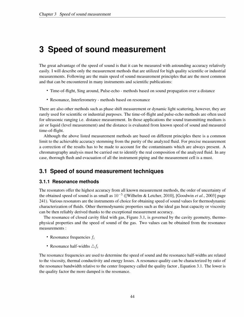
Chapter 3 Speed of sound measurement
3 Speed of sound measurement
The great advantage of the speed of sound is that it can be measured with astounding accuracy relativelyeasily. I will describe only the measurement methods that are utilized for high quality scientific or industrialmeasurements. Following are the main speed of sound measurement principles that are the most commonand that can be encountered in many instruments and scientific publications:
• Time-of-flight, Sing around, Pulse-echo - methods based on sound propagation over a distance
• Resonance, Interferometry - methods based on resonance
There are also other methods such as phase shift measurement or dynamic light scattering, however, they arerarely used for scientific or industrial purposes. The time-of-flight and pulse-echo methods are often usedfor ultrasonic ranging i.e. distance measurement. In those applications the sound transmitting medium isair or liquid (level measurement) and the distance is evaluated from known speed of sound and measuredtime-of-flight.
Although the above listed measurement methods are based on different principles there is a commonlimit to the achievable accuracy stemming from the purity of the analyzed fluid. For precise measurementa correction of the results has to be made to account for the contaminants which are always present. Achromatography analysis must be carried out to identify the real composition of the analyzed fluid. In anycase, thorough flush and evacuation of all the instrument piping and the measurement cell is a must.
3.1 Speed of sound measurement techniques
3.1.1 Resonance methods
The resonators offer the highest accuracy from all known measurement methods, the order of uncertainty ofthe obtained speed of sound is as small as 10−5 ([Wilhelm & Letcher, 2010], [Goodwin et al., 2003] page241). Various resonators are the instruments of choice for obtaining speed of sound values for thermodynamiccharacterization of fluids. Other thermodynamic properties such as the ideal gas heat capacity or viscositycan be then reliably derived thanks to the exceptional measurement accuracy.
The resonance of closed cavity filed with gas, Figure 3.1, is governed by the cavity geometry, thermo-physical properties and the speed of sound of the gas. Two values can be obtained from the resonancemeasurements :
• Resonance frequencies fi
• Resonance half-widths4fi
The resonance frequencies are used to determine the speed of sound and the resonance half-widths are relatedto the viscosity, thermal conductivity and energy losses. A resonance quality can be characterized by ratio ofthe resonance bandwidth relative to the center frequency called the quality factor , Equation 3.1. The lower isthe quality factor the more damped is the resonance.
44

3.1. SPEED OF SOUND MEASUREMENT TECHNIQUES
0.9
Frequency (arbitrary units)
Ampl
itude
(ar
bitr
ary
units
)
f
Δf
0.6 0.3 0
0
1
2
3
4
Figure 3.1: Resonance Figure 3.2: Wave guide construction [Gillis, 1994]
Qf = f
4f(3.1)
The uncertainty of the obtained ideal gas heat capacity depends on the uncertainty of the molar mass andmainly on contamination of the measured fluid [Wilhelm & Letcher, 2010]. In order to achieve the bestresults for the speed of sound, the resonators are designed so that a narrow frequency-amplitude peaks areobtained. The opposite approach is taken when the focus is on transport properties and the geometry of thecavity is designed so that it produces wide peaks allowing for more precise determination of the haft-widths[Assael et al., 2014]. Sound frequency of several kilohertz is used for gases, liquids are measured at severalmegahertz. The diameter of the spherical cavity or the length of the cylindrical resonator is selected so thatconvenient resonance frequencies at the lower modes are obtained. Common values are approximately 10cm, such size ensures that the low-order resonance modes occur at audio frequencies.
The rest of this section will describe resonators and techniques for speed of sound measurement in gasessince the instrument developed in this work is intended for gases. The resonance cavity is filled with measuredvapour and equipped with two transducers, an acoustic emitter (loudspeaker) and microphone. Arrangementwith only one transducer is also possible especially for cylindrical resonators. In this case the transducer isbeing excited and its admittance i.e. the driving current is measured instead of measuring the cavity responsewith a microphone. The transducers have to be able to withstand the pressures and temperatures in the cavityand they should be corrosion resistant and chemically inert. Although, wave guides (Figure 3.2) that connectthe cavity with external transducers can be used to keep the transducers at room temperature, atmosphericpressure and to separated them from the measured gas. The heat dissipation of the transducers has to beminimal and they have to allow for installation that disturbs the cavity surface as little as possible. Both theloudspeaker and the microphone can be custom made elements.
The signal-to-noise ratio depends on the sensitivity of the transducers and it will generally suffer at lowand high pressures. A precise frequency generator is used to excite the loudspeaker. The excitation signalmight need high voltage DC bias or a large amplitude depending on what type of transducer is used.
The signal from the microphone is amplified and a band-pass filter can be used to eliminate unwantedlow and high frequency components. The amplitude and phase of the received signal is compared with theexcitation signal by a dedicated amplitude and phase detector or lock-in amplifier, Figure 3.3. The frequencysweep is usually carried out in a few steps in a narrow range of frequencies around the resonance frequency.Sweep back and forth should point out to possible temperature drifts.
45
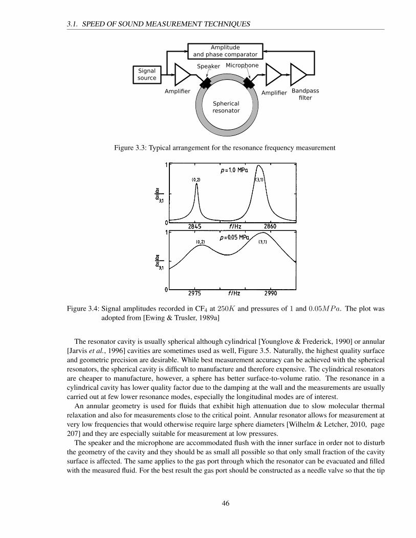
3.1. SPEED OF SOUND MEASUREMENT TECHNIQUES
Sphericalresonator
MicrophoneSpeaker
Amplifier
Signal source
Amplitude and phase comparator
Amplifier Bandpassfilter
Figure 3.3: Typical arrangement for the resonance frequency measurement
Figure 3.4: Signal amplitudes recorded in CF4 at 250K and pressures of 1 and 0.05MPa. The plot wasadopted from [Ewing & Trusler, 1989a]
The resonator cavity is usually spherical although cylindrical [Younglove & Frederick, 1990] or annular[Jarvis et al., 1996] cavities are sometimes used as well, Figure 3.5. Naturally, the highest quality surfaceand geometric precision are desirable. While best measurement accuracy can be achieved with the sphericalresonators, the spherical cavity is difficult to manufacture and therefore expensive. The cylindrical resonatorsare cheaper to manufacture, however, a sphere has better surface-to-volume ratio. The resonance in acylindrical cavity has lower quality factor due to the damping at the wall and the measurements are usuallycarried out at few lower resonance modes, especially the longitudinal modes are of interest.
An annular geometry is used for fluids that exhibit high attenuation due to slow molecular thermalrelaxation and also for measurements close to the critical point. Annular resonator allows for measurement atvery low frequencies that would otherwise require large sphere diameters [Wilhelm & Letcher, 2010, page207] and they are especially suitable for measurement at low pressures.
The speaker and the microphone are accommodated flush with the inner surface in order not to disturbthe geometry of the cavity and they should be as small all possible so that only small fraction of the cavitysurface is affected. The same applies to the gas port through which the resonator can be evacuated and filledwith the measured fluid. For the best result the gas port should be constructed as a needle valve so that the tip
46
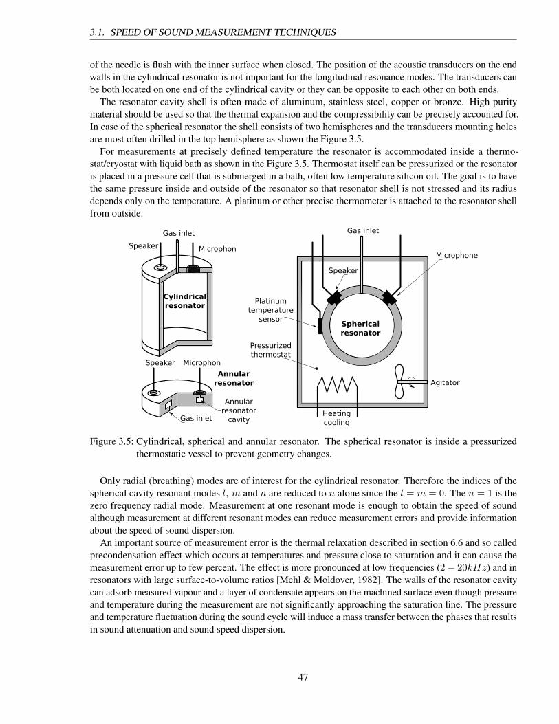
3.1. SPEED OF SOUND MEASUREMENT TECHNIQUES
of the needle is flush with the inner surface when closed. The position of the acoustic transducers on the endwalls in the cylindrical resonator is not important for the longitudinal resonance modes. The transducers canbe both located on one end of the cylindrical cavity or they can be opposite to each other on both ends.
The resonator cavity shell is often made of aluminum, stainless steel, copper or bronze. High puritymaterial should be used so that the thermal expansion and the compressibility can be precisely accounted for.In case of the spherical resonator the shell consists of two hemispheres and the transducers mounting holesare most often drilled in the top hemisphere as shown the Figure 3.5.
For measurements at precisely defined temperature the resonator is accommodated inside a thermo-stat/cryostat with liquid bath as shown in the Figure 3.5. Thermostat itself can be pressurized or the resonatoris placed in a pressure cell that is submerged in a bath, often low temperature silicon oil. The goal is to havethe same pressure inside and outside of the resonator so that resonator shell is not stressed and its radiusdepends only on the temperature. A platinum or other precise thermometer is attached to the resonator shellfrom outside.
Sphericalresonator
Agitator
Heatingcooling
Platinumtemperature
sensor
Gas inlet
Cylindricalresonator
Microphone
Speaker
MicrophonSpeaker
Gas inlet
Pressurized thermostat
Gas inlet
MicrophonSpeaker
Annular resonator
cavity
Annularresonator
Figure 3.5: Cylindrical, spherical and annular resonator. The spherical resonator is inside a pressurizedthermostatic vessel to prevent geometry changes.
Only radial (breathing) modes are of interest for the cylindrical resonator. Therefore the indices of thespherical cavity resonant modes l, m and n are reduced to n alone since the l = m = 0. The n = 1 is thezero frequency radial mode. Measurement at one resonant mode is enough to obtain the speed of soundalthough measurement at different resonant modes can reduce measurement errors and provide informationabout the speed of sound dispersion.
An important source of measurement error is the thermal relaxation described in section 6.6 and so calledprecondensation effect which occurs at temperatures and pressure close to saturation and it can cause themeasurement error up to few percent. The effect is more pronounced at low frequencies (2− 20kHz) and inresonators with large surface-to-volume ratios [Mehl & Moldover, 1982]. The walls of the resonator cavitycan adsorb measured vapour and a layer of condensate appears on the machined surface even though pressureand temperature during the measurement are not significantly approaching the saturation line. The pressureand temperature fluctuation during the sound cycle will induce a mass transfer between the phases that resultsin sound attenuation and sound speed dispersion.
47

3.1. SPEED OF SOUND MEASUREMENT TECHNIQUES
A first order acoustic model is usually used for the spherical resonators . The natural (observed) frequencyfn of the n− th radial mode is expressed as
fn = f0n − i g0n . (3.2)
The imaginary part g represents losses and it is related to the resonance half-widths that were explained inthe Figure 3.1. The equation can be expressed using perturbation terms (4f − i g)j :
fn = ν0nw
2πr +∑j
(4f − i g)j . (3.3)
Where the ν0nw2πa is the unperturbed resonance frequency f0
n. The ν0n is tabulated eigenvalue correspondingto the resonance mode, r is the sphere radius and w is the speed of sound. The diameter of the cavity has tobe known as a function of temperature and pressure, it can be either calculated using a model or obtainedfrom calibration carried out with a well-known gas. The perturbations (corrections) account for a shift in theresonance frequency and contribute to the resonance half-width.
A model based solely on the unperturbed resonance frequency would provide measurement accuracy in theorder of 0.01% [Hess, 1989]. A resonance model that employs the perturbations can increase the accuracyup to 0.0001% [Hess, 1989].
The most often used perturbations are:
1. Thermal boundary layer: For many gases the most important perturbation. The boundary condition ofthe radial modes requires temperature to be continuous at the gas/wall interface. The sound propagation,which is otherwise adiabatic process, becomes isothermal process at the wall, [Hess, 1989].
2. Bulk absorption and molecular relaxation: The correction terms incorporate viscous diffusivity andvibrational-relaxation contribution to the bulk diffusivity [Trusler, 1984, page 179]. In case ofnegligible sound speed dispersion this term influences only the resonance half-widths.
3. Openings in the resonator cavity wall for filling ports and transducers. The opening can be divided intocylindrical (tube of certain diameter and length) and annular ( slits around the transducers).
4. Shell motion: The elastic response: (breathing) of the resonator spherical isotropic shell to an internalacoustic mode. This perturbation contributes mainly to the resonance frequency shift [Trusler, 1984,page 180]. The breathing frequency of the resonator is found experimentally with helium making useof its very high speed of sound. Measured perturbations of the radial resonant frequency are comparedto frequencies far and close to the resonator shell breathing frequency [Boyes, 1992, page 12].
5. Geometric imperfection: The inner cavity is never an ideal sphere. An imperfection arises from themachining and polishing process. Also the cavity is always assembled from two hemispheres thereforeit is not ideally symmetric due to a step at the hemispheres joint.
The thermal boundary layer correction can be calculated from Equation 3.4. The first term in the equation isthe loss at a plane surface, the second term accounts for the curvature of the actual resonator surface. The last,third, term is the correction for the temperature jump effect that is a result of different thermal conductivityof a gas near the wall.
(4f − i g) = − (1 + i) γ − 12a
√Dtf0,nπ
+ i(γ − 1)Dt
2πa2 + (γ − 1) f0,nlaa
(3.4)
48
3.1. SPEED OF SOUND MEASUREMENT TECHNIQUES
where γ is the ratio of heat capacities, Dt is the thermal diffusivity coefficient:
Dt = γM
ρCp. (3.5)
and la is the accommodation length:
la = k
p
√πMT
2R(2− h) /hCv/R+ 1/2 . (3.6)
where p is the pressure, k is the thermal conductivity andM is the molar mass. The thermal accommodationcoefficient h spans from 0 to 1. It is a ratio of energy actually transported over the vapour-solid interface andenergy that would be transported over the interface if all molecules were in thermal equilibrium. The valuesof the coefficient are 0.91 for an aluminum resonator and 1 for a stainless steel resonator of diameter 40 and45mm respectively [Boyes, 1992].
A simple equation can be used for the cylindrical resonator provided only longitudinal resonance modesare considered:
w = 2Lfn
n = 1, 2, 3... . (3.7)
The n corresponds to the resonant mode and L is the resonator length. The speed of sound w obtainedfrom the Equation 3.7 can be corrected for various effects in similar way as described above for the sphericalresonator:
wcorr = w
(1− δw) , (3.8)
δ = φ+ ϕ
2πf . (3.9)
The correction coefficient δ is composed of two components [Younglove & Frederick, 1990]:
• φ is the attenuation coefficient for the wall losses:
φ = 1r.w
(µ
ρ
)0.5+ (γ − 1)
(k
e.Cp
)0.5 (πf)0.5 . (3.10)
• ϕ is accounting for the energy loss at the end walls of the cylinder:
ϕ = 1L.u
(γ − 1)(
k
e.Cp
)0.5
(πf)0.5 . (3.11)
Where µ is the viscosity, γ is the ratio of heat capacities, k is the thermal conductivity, ρ is the density, r isthe cylinder radius and L is the cylinder length (L is a function of the temperature and also pressure).
49
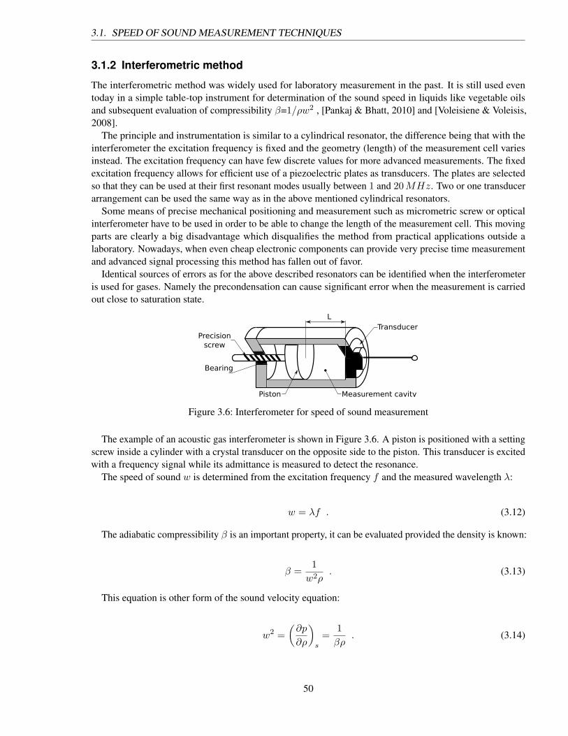
3.1. SPEED OF SOUND MEASUREMENT TECHNIQUES
3.1.2 Interferometric method
The interferometric method was widely used for laboratory measurement in the past. It is still used eventoday in a simple table-top instrument for determination of the sound speed in liquids like vegetable oilsand subsequent evaluation of compressibility β=1/ρw2 , [Pankaj & Bhatt, 2010] and [Voleisiene & Voleisis,2008].
The principle and instrumentation is similar to a cylindrical resonator, the difference being that with theinterferometer the excitation frequency is fixed and the geometry (length) of the measurement cell variesinstead. The excitation frequency can have few discrete values for more advanced measurements. The fixedexcitation frequency allows for efficient use of a piezoelectric plates as transducers. The plates are selectedso that they can be used at their first resonant modes usually between 1 and 20MHz. Two or one transducerarrangement can be used the same way as in the above mentioned cylindrical resonators.
Some means of precise mechanical positioning and measurement such as micrometric screw or opticalinterferometer have to be used in order to be able to change the length of the measurement cell. This movingparts are clearly a big disadvantage which disqualifies the method from practical applications outside alaboratory. Nowadays, when even cheap electronic components can provide very precise time measurementand advanced signal processing this method has fallen out of favor.
Identical sources of errors as for the above described resonators can be identified when the interferometeris used for gases. Namely the precondensation can cause significant error when the measurement is carriedout close to saturation state.
Transducer
Piston
Bearing
Precisionscrew
L
Measurement cavity
Figure 3.6: Interferometer for speed of sound measurement
The example of an acoustic gas interferometer is shown in Figure 3.6. A piston is positioned with a settingscrew inside a cylinder with a crystal transducer on the opposite side to the piston. This transducer is excitedwith a frequency signal while its admittance is measured to detect the resonance.
The speed of sound w is determined from the excitation frequency f and the measured wavelength λ:
w = λf . (3.12)
The adiabatic compressibility β is an important property, it can be evaluated provided the density is known:
β = 1w2ρ
. (3.13)
This equation is other form of the sound velocity equation:
w2 =(∂p
∂ρ
)s
= 1βρ
. (3.14)
50
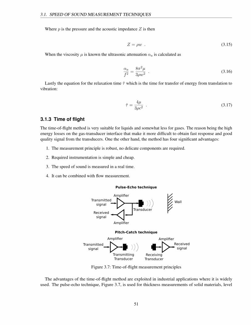
3.1. SPEED OF SOUND MEASUREMENT TECHNIQUES
Where p is the pressure and the acoustic impedance Z is then
Z = ρw . (3.15)
When the viscosity µ is known the ultrasonic attenuation αa is calculated as
αaf2 = 8π2µ
3ρw2 . (3.16)
Lastly the equation for the relaxation time τ which is the time for transfer of energy from translation tovibration:
τ = 4µ3ρc2 . (3.17)
3.1.3 Time of flight
The time-of-flight method is very suitable for liquids and somewhat less for gases. The reason being the highenergy losses on the gas-transducer interface that make it more difficult to obtain fast response and goodquality signal from the transducers. One the other hand, the method has four significant advantages:
1. The measurement principle is robust, no delicate components are required.
2. Required instrumentation is simple and cheap.
3. The speed of sound is measured in a real time.
4. It can be combined with flow measurement.
Amplifier
Amplifier
Transmitted signal
Receivedsignal
Transducer
Wall
Transmitted signal
Receivedsignal
TransmittingTransducer
ReceivingTransducer
AmplifierAmplifier
Pulse-Echo technique
Pitch-Catch technique
Figure 3.7: Time-of-flight measurement principles
The advantages of the time-of-flight method are exploited in industrial applications where it is widelyused. The pulse-echo technique, Figure 3.7, is used for thickness measurements of solid materials, level
51
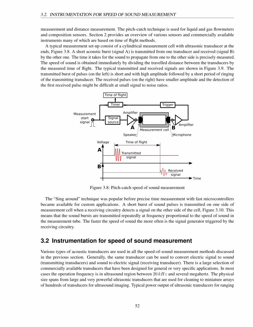
3.2. INSTRUMENTATION FOR SPEED OF SOUND MEASUREMENT
measurement and distance measurement. The pitch-catch technique is used for liquid and gas flowmetersand composition sensors. Section 2 provides an overview of various sensors and commercially availableinstruments many of which are based on time of flight methods.
A typical measurement set-up consist of a cylindrical measurement cell with ultrasonic transducer at theends, Figure 3.8. A short acoustic burst (signal A) is transmitted from one transducer and received (signal B)by the other one. The time it takes for the sound to propagate from one to the other side is precisely measured.The speed of sound is obtained immediately by dividing the travelled distance between the transducers bythe measured time of flight. The typical transmitted and received signals are shown in Figure 3.9. Thetransmitted burst of pulses (on the left) is short and with high amplitude followed by a short period of ringingof the transmitting transducer. The received pulses (on the right) have smaller amplitude and the detection ofthe first received pulse might be difficult at small signal to noise ratios.
Measurementstartsignal
A B
A
B
Time of flight
Transmitted signal
Time
Voltage
Received signal
Measurement cell
MicrophoneSpeaker
Amplifier
Signal source
Trigger
Amplifier
Timer
Time of flight
Figure 3.8: Pitch-catch speed of sound measurement
The “Sing around” technique was popular before precise time measurement with fast microcontrollersbecame available for custom applications. A short burst of sound pulses is transmitted on one side ofmeasurement cell when a receiving circuitry detects a signal on the other side of the cell, Figure 3.10. Thismeans that the sound bursts are transmitted repeatedly at frequency proportional to the speed of sound inthe measurement tube. The faster the speed of sound the more often is the signal generator triggered by thereceiving circuitry.
3.2 Instrumentation for speed of sound measurement
Various types of acoustic transducers are used in all the speed-of-sound measurement methods discussedin the previous section. Generally, the same transducer can be used to convert electric signal to sound(transmitting transducers) and sound to electric signal (receiving transducer). There is a large selection ofcommercially available transducers that have been designed for general or very specific applications. In mostcases the operation frequency is in ultrasound region between 20 kHz and several megahertz. The physicalsize spans from large and very powerful ultrasonic transducers that are used for cleaning to miniature arraysof hundreds of transducers for ultrasound imaging. Typical power output of ultrasonic transducers for ranging
52
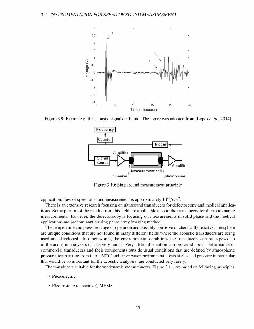
3.2. INSTRUMENTATION FOR SPEED OF SOUND MEASUREMENT
Figure 3.9: Example of the acoustic signals in liquid. The figure was adopted from [Lopes et al., 2014]
Measurement cell
MicrophoneSpeaker
Amplifier
Signal source
Trigger
Amplifier
Counter
Frequency
Figure 3.10: Sing around measurement principle
application, flow or speed of sound measurement is approximately 1W/cm2.There is an extensive research focusing on ultrasound transducers for defectoscopy and medical applica-
tions. Some portion of the results from this field are applicable also to the transducers for thermodynamicmeasurements. However, the defectoscopy is focusing on measurements in solid phase and the medicalapplications are predominantly using phase array imaging method.
The temperature and pressure range of operation and possibly corrosive or chemically reactive atmosphereare unique conditions that are not found in many different fields where the acoustic transducers are beingused and developed. In other words, the environmental conditions the transducers can be exposed toin the acoustic analysers can be very harsh. Very little information can be found about performance ofcommercial transducers and their components outside usual conditions that are defined by atmosphericpressure, temperature from 0 to +50C and air or water environment. Tests at elevated pressure in particular,that would be so important for the acoustic analysers, are conducted very rarely.
The transducers suitable for thermodynamic measurements, Figure 3.11, are based on following principles:
• Piezoelectric
• Electrostatic (capacitive), MEMS
53
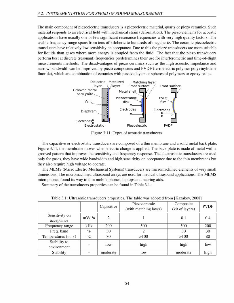
3.2. INSTRUMENTATION FOR SPEED OF SOUND MEASUREMENT
The main component of piezoelectric transducers is a piezoelectric material, quartz or piezo ceramics. Suchmaterial responds to an electrical field with mechanical strain (deformation). The piezo elements for acousticapplications have usually one or few significant resonance frequencies with very high quality factors. Theusable frequency range spans from tens of kilohertz to hundreds of megahertz. The ceramic piezoelectrictransducers have relatively low sensitivity on acceptance. Due to this the piezo transducers are more suitablefor liquids than gases where more energy is coupled from the fluid. The fact that the piezo transducersperform best at discrete (resonant) frequencies predetermines their use for interferometric and time-of-flightmeasurements methods. The disadvantages of piezo ceramics such as the high acoustic impedance andnarrow bandwidth can be improved by piezo composites and PVDF (ferroelectric polymer polyvinylidenefluoride), which are combination of ceramics with passive layers or spheres of polymers or epoxy resins.
Grooved metal back plate
Dielectric layer
Vent
Electrodes
Diaphram
Metal shell
Piezoceramicdisk
Electrostatic Piezoelectric
Electrodes
Metalized layer Front surface
Matching layer
PVDF film
PVDF
Front surface
Electrodes
Figure 3.11: Types of acoustic transducers
The capacitive or electrostatic transducers are composed of a thin membrane and a solid metal back plate,Figure 3.11, the membrane moves when electric charge is applied. The back plate is made of metal with agrooved pattern that improves the sensitivity and frequency response. The electrostatic transducers are usedonly for gases, they have wide bandwidth and high sensitivity on acceptance due to the thin membranes butthey also require high voltage to operate.
The MEMS (Micro Electro Mechanical Systems) transducers are micromachined elements of very smalldimensions. The micromachined ultrasound arrays are used for medical ultrasound applications. The MEMSmicrophones found its way to thin mobile phones, laptops and hearing aids.
Summary of the transducers properties can be found in Table 3.1.
Table 3.1: Ultrasonic transducers properties. The table was adopted from [Kazakov, 2008]
CapacitivePiezoceramic
(with matching layer)Composite
(kit of layers)PVDF
Sensitivity onacceptance
mV/Ðà 2 1 0.1 0.4
Frequency range kHz 200 500 500 200Freq. band % 30 2 30 30
Temperatures (màõ) °C 80 >100 >100 80Stability to
environment- low high high low
Stability - moderate low moderate high
54
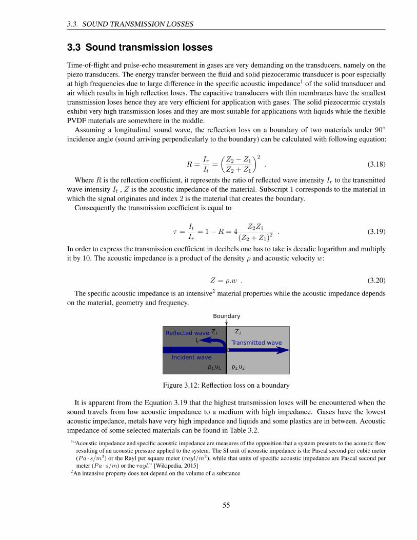
3.3. SOUND TRANSMISSION LOSSES
3.3 Sound transmission losses
Time-of-flight and pulse-echo measurement in gases are very demanding on the transducers, namely on thepiezo transducers. The energy transfer between the fluid and solid piezoceramic transducer is poor especiallyat high frequencies due to large difference in the specific acoustic impedance1 of the solid transducer andair which results in high reflection loses. The capacitive transducers with thin membranes have the smallesttransmission loses hence they are very efficient for application with gases. The solid piezocermic crystalsexhibit very high transmission loses and they are most suitable for applications with liquids while the flexiblePVDF materials are somewhere in the middle.
Assuming a longitudinal sound wave, the reflection loss on a boundary of two materials under 90incidence angle (sound arriving perpendicularly to the boundary) can be calculated with following equation:
R = IrIt
=(Z2 − Z1Z2 + Z1
)2. (3.18)
Where R is the reflection coefficient, it represents the ratio of reflected wave intensity Ir to the transmittedwave intensity It , Z is the acoustic impedance of the material. Subscript 1 corresponds to the material inwhich the signal originates and index 2 is the material that creates the boundary.
Consequently the transmission coefficient is equal to
τ = ItIr
= 1−R = 4 Z2Z1
(Z2 + Z1)2 . (3.19)
In order to express the transmission coefficient in decibels one has to take is decadic logarithm and multiplyit by 10. The acoustic impedance is a product of the density ρ and acoustic velocity w:
Z = ρ.w . (3.20)
The specific acoustic impedance is an intensive2 material properties while the acoustic impedance dependson the material, geometry and frequency.
Boundary
Transmitted wave
Z1 Z2
ρ1,u1 ρ2,u2
I
Ir
ItIncident wave
Reflected wave
Figure 3.12: Reflection loss on a boundary
It is apparent from the Equation 3.19 that the highest transmission loses will be encountered when thesound travels from low acoustic impedance to a medium with high impedance. Gases have the lowestacoustic impedance, metals have very high impedance and liquids and some plastics are in between. Acousticimpedance of some selected materials can be found in Table 3.2.
1“Acoustic impedance and specific acoustic impedance are measures of the opposition that a system presents to the acoustic flowresulting of an acoustic pressure applied to the system. The SI unit of acoustic impedance is the Pascal second per cubic meter(P a · s/m3) or the Rayl per square meter (rayl/m2), while that units of specific acoustic impedance are Pascal second permeter (P a · s/m) or the rayl.” [Wikipedia, 2015]
2An intensive property does not depend on the volume of a substance
55
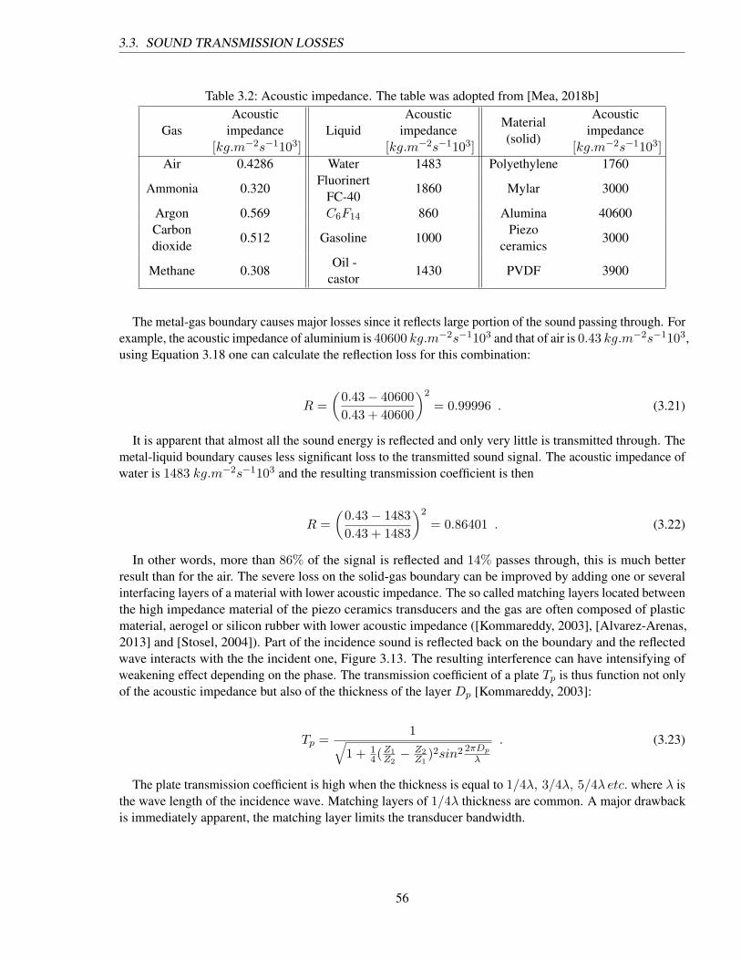
3.3. SOUND TRANSMISSION LOSSES
Table 3.2: Acoustic impedance. The table was adopted from [Mea, 2018b]
GasAcoustic
impedance[kg.m−2s−1103]
LiquidAcoustic
impedance[kg.m−2s−1103]
Material(solid)
Acousticimpedance
[kg.m−2s−1103]Air 0.4286 Water 1483 Polyethylene 1760
Ammonia 0.320Fluorinert
FC-401860 Mylar 3000
Argon 0.569 C6F14 860 Alumina 40600Carbondioxide
0.512 Gasoline 1000Piezo
ceramics3000
Methane 0.308Oil -
castor1430 PVDF 3900
The metal-gas boundary causes major losses since it reflects large portion of the sound passing through. Forexample, the acoustic impedance of aluminium is 40600 kg.m−2s−1103 and that of air is 0.43 kg.m−2s−1103,using Equation 3.18 one can calculate the reflection loss for this combination:
R =(0.43− 40600
0.43 + 40600
)2= 0.99996 . (3.21)
It is apparent that almost all the sound energy is reflected and only very little is transmitted through. Themetal-liquid boundary causes less significant loss to the transmitted sound signal. The acoustic impedance ofwater is 1483 kg.m−2s−1103 and the resulting transmission coefficient is then
R =(0.43− 1483
0.43 + 1483
)2= 0.86401 . (3.22)
In other words, more than 86% of the signal is reflected and 14% passes through, this is much betterresult than for the air. The severe loss on the solid-gas boundary can be improved by adding one or severalinterfacing layers of a material with lower acoustic impedance. The so called matching layers located betweenthe high impedance material of the piezo ceramics transducers and the gas are often composed of plasticmaterial, aerogel or silicon rubber with lower acoustic impedance ([Kommareddy, 2003], [Alvarez-Arenas,2013] and [Stosel, 2004]). Part of the incidence sound is reflected back on the boundary and the reflectedwave interacts with the the incident one, Figure 3.13. The resulting interference can have intensifying ofweakening effect depending on the phase. The transmission coefficient of a plate Tp is thus function not onlyof the acoustic impedance but also of the thickness of the layer Dp [Kommareddy, 2003]:
Tp = 1√1 + 1
4(Z1Z2− Z2
Z1)2sin2 2πDp
λ
. (3.23)
The plate transmission coefficient is high when the thickness is equal to 1/4λ, 3/4λ, 5/4λ etc. where λ isthe wave length of the incidence wave. Matching layers of 1/4λ thickness are common. A major drawbackis immediately apparent, the matching layer limits the transducer bandwidth.
56
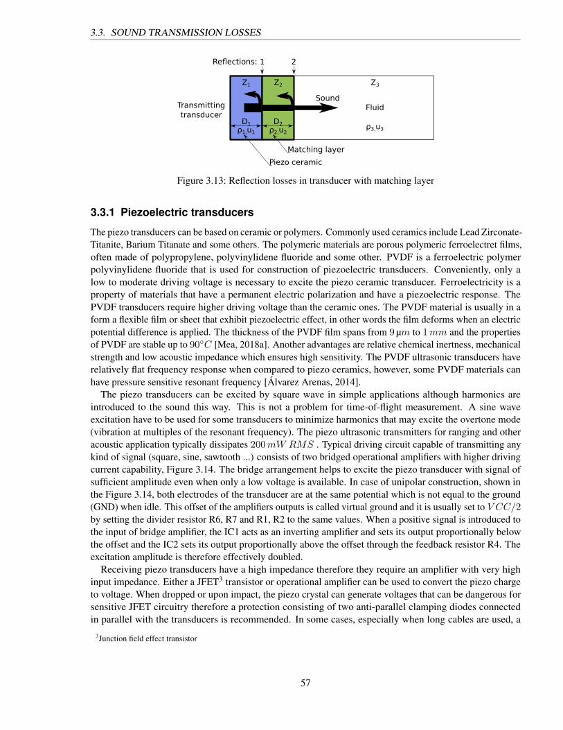
3.3. SOUND TRANSMISSION LOSSES
Piezo ceramic
Transmittingtransducer
Matching layer
Fluid
Reflections: 1 2
Sound
Z1 Z2
ρ1,u1 ρ2,u2
Z3
ρ3,u3D1 D2
Figure 3.13: Reflection losses in transducer with matching layer
3.3.1 Piezoelectric transducers
The piezo transducers can be based on ceramic or polymers. Commonly used ceramics include Lead Zirconate-Titanite, Barium Titanate and some others. The polymeric materials are porous polymeric ferroelectret films,often made of polypropylene, polyvinylidene fluoride and some other. PVDF is a ferroelectric polymerpolyvinylidene fluoride that is used for construction of piezoelectric transducers. Conveniently, only alow to moderate driving voltage is necessary to excite the piezo ceramic transducer. Ferroelectricity is aproperty of materials that have a permanent electric polarization and have a piezoelectric response. ThePVDF transducers require higher driving voltage than the ceramic ones. The PVDF material is usually in aform a flexible film or sheet that exhibit piezoelectric effect, in other words the film deforms when an electricpotential difference is applied. The thickness of the PVDF film spans from 9 µm to 1mm and the propertiesof PVDF are stable up to 90C [Mea, 2018a]. Another advantages are relative chemical inertness, mechanicalstrength and low acoustic impedance which ensures high sensitivity. The PVDF ultrasonic transducers haverelatively flat frequency response when compared to piezo ceramics, however, some PVDF materials canhave pressure sensitive resonant frequency [Álvarez Arenas, 2014].
The piezo transducers can be excited by square wave in simple applications although harmonics areintroduced to the sound this way. This is not a problem for time-of-flight measurement. A sine waveexcitation have to be used for some transducers to minimize harmonics that may excite the overtone mode(vibration at multiples of the resonant frequency). The piezo ultrasonic transmitters for ranging and otheracoustic application typically dissipates 200mW RMS . Typical driving circuit capable of transmitting anykind of signal (square, sine, sawtooth ...) consists of two bridged operational amplifiers with higher drivingcurrent capability, Figure 3.14. The bridge arrangement helps to excite the piezo transducer with signal ofsufficient amplitude even when only a low voltage is available. In case of unipolar construction, shown inthe Figure 3.14, both electrodes of the transducer are at the same potential which is not equal to the ground(GND) when idle. This offset of the amplifiers outputs is called virtual ground and it is usually set to V CC/2by setting the divider resistor R6, R7 and R1, R2 to the same values. When a positive signal is introduced tothe input of bridge amplifier, the IC1 acts as an inverting amplifier and sets its output proportionally belowthe offset and the IC2 sets its output proportionally above the offset through the feedback resistor R4. Theexcitation amplitude is therefore effectively doubled.
Receiving piezo transducers have a high impedance therefore they require an amplifier with very highinput impedance. Either a JFET3 transistor or operational amplifier can be used to convert the piezo chargeto voltage. When dropped or upon impact, the piezo crystal can generate voltages that can be dangerous forsensitive JFET circuitry therefore a protection consisting of two anti-parallel clamping diodes connectedin parallel with the transducers is recommended. In some cases, especially when long cables are used, a
3Junction field effect transistor
57
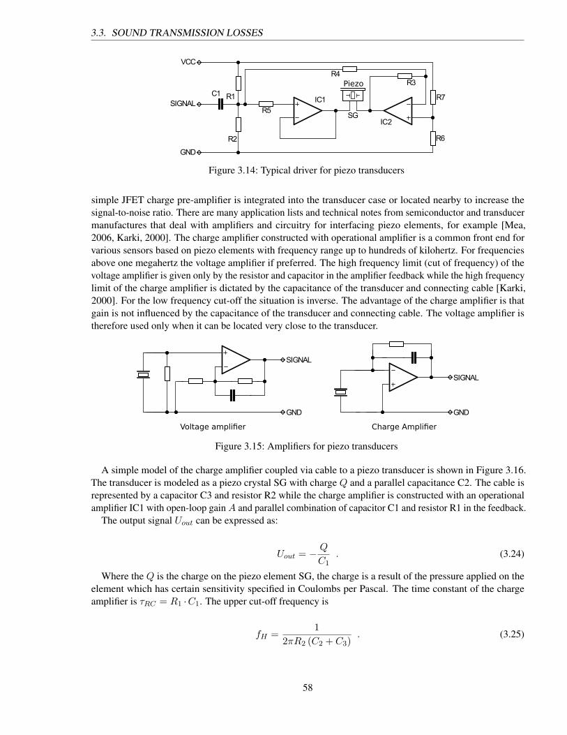
3.3. SOUND TRANSMISSION LOSSES
SGIC
R3R4
R6
R7
R5
GND
SIGNAL
VCC
IC1R1
R2
C1Piezo
2
Figure 3.14: Typical driver for piezo transducers
simple JFET charge pre-amplifier is integrated into the transducer case or located nearby to increase thesignal-to-noise ratio. There are many application lists and technical notes from semiconductor and transducermanufactures that deal with amplifiers and circuitry for interfacing piezo elements, for example [Mea,2006, Karki, 2000]. The charge amplifier constructed with operational amplifier is a common front end forvarious sensors based on piezo elements with frequency range up to hundreds of kilohertz. For frequenciesabove one megahertz the voltage amplifier if preferred. The high frequency limit (cut of frequency) of thevoltage amplifier is given only by the resistor and capacitor in the amplifier feedback while the high frequencylimit of the charge amplifier is dictated by the capacitance of the transducer and connecting cable [Karki,2000]. For the low frequency cut-off the situation is inverse. The advantage of the charge amplifier is thatgain is not influenced by the capacitance of the transducer and connecting cable. The voltage amplifier istherefore used only when it can be located very close to the transducer.
SIGNAL
GND
Voltage amplifier
SIGNAL
GND
Charge Amplifier
Figure 3.15: Amplifiers for piezo transducers
A simple model of the charge amplifier coupled via cable to a piezo transducer is shown in Figure 3.16.The transducer is modeled as a piezo crystal SG with charge Q and a parallel capacitance C2. The cable isrepresented by a capacitor C3 and resistor R2 while the charge amplifier is constructed with an operationalamplifier IC1 with open-loop gain A and parallel combination of capacitor C1 and resistor R1 in the feedback.
The output signal Uout can be expressed as:
Uout = − Q
C1. (3.24)
Where the Q is the charge on the piezo element SG, the charge is a result of the pressure applied on theelement which has certain sensitivity specified in Coulombs per Pascal. The time constant of the chargeamplifier is τRC = R1 ·C1. The upper cut-off frequency is
fH = 12πR2 (C2 + C3) . (3.25)
58
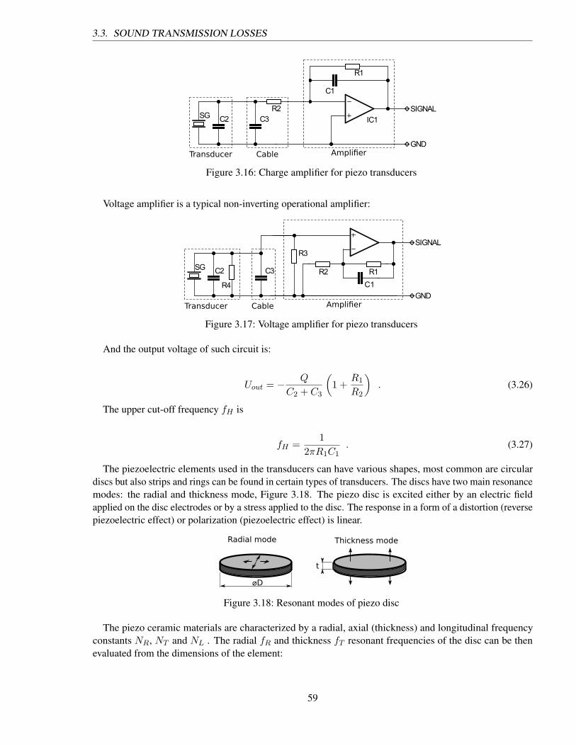
3.3. SOUND TRANSMISSION LOSSES
SIGNAL
GND
IC1SG
R1
C1
C2 C3R2
Transducer Cable Amplifier
Figure 3.16: Charge amplifier for piezo transducers
Voltage amplifier is a typical non-inverting operational amplifier:
SG C2 C3
Transducer Cable Amplifier
SIGNAL
GNDR4 C1
R2 R1
R3
Figure 3.17: Voltage amplifier for piezo transducers
And the output voltage of such circuit is:
Uout = − Q
C2 + C3
(1 + R1
R2
). (3.26)
The upper cut-off frequency fH is
fH = 12πR1C1
. (3.27)
The piezoelectric elements used in the transducers can have various shapes, most common are circulardiscs but also strips and rings can be found in certain types of transducers. The discs have two main resonancemodes: the radial and thickness mode, Figure 3.18. The piezo disc is excited either by an electric fieldapplied on the disc electrodes or by a stress applied to the disc. The response in a form of a distortion (reversepiezoelectric effect) or polarization (piezoelectric effect) is linear.
Radial mode Thickness mode
D
t
Figure 3.18: Resonant modes of piezo disc
The piezo ceramic materials are characterized by a radial, axial (thickness) and longitudinal frequencyconstants NR, NT and NL . The radial fR and thickness fT resonant frequencies of the disc can be thenevaluated from the dimensions of the element:
59
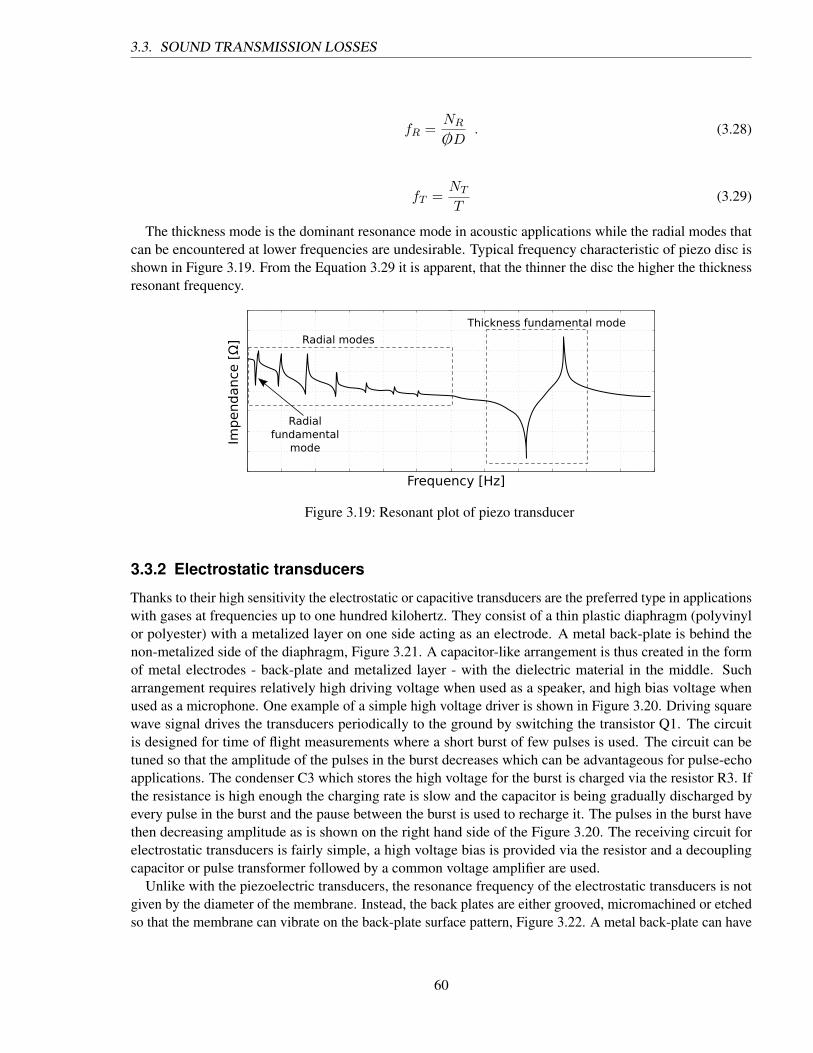
3.3. SOUND TRANSMISSION LOSSES
fR = NR
/OD. (3.28)
fT = NT
T(3.29)
The thickness mode is the dominant resonance mode in acoustic applications while the radial modes thatcan be encountered at lower frequencies are undesirable. Typical frequency characteristic of piezo disc isshown in Figure 3.19. From the Equation 3.29 it is apparent, that the thinner the disc the higher the thicknessresonant frequency.
Frequency [Hz]
Impendan
ce [Ω
] Radial modes
Thickness fundamental mode
Radialfundamental
mode
Figure 3.19: Resonant plot of piezo transducer
3.3.2 Electrostatic transducers
Thanks to their high sensitivity the electrostatic or capacitive transducers are the preferred type in applicationswith gases at frequencies up to one hundred kilohertz. They consist of a thin plastic diaphragm (polyvinylor polyester) with a metalized layer on one side acting as an electrode. A metal back-plate is behind thenon-metalized side of the diaphragm, Figure 3.21. A capacitor-like arrangement is thus created in the formof metal electrodes - back-plate and metalized layer - with the dielectric material in the middle. Sucharrangement requires relatively high driving voltage when used as a speaker, and high bias voltage whenused as a microphone. One example of a simple high voltage driver is shown in Figure 3.20. Driving squarewave signal drives the transducers periodically to the ground by switching the transistor Q1. The circuitis designed for time of flight measurements where a short burst of few pulses is used. The circuit can betuned so that the amplitude of the pulses in the burst decreases which can be advantageous for pulse-echoapplications. The condenser C3 which stores the high voltage for the burst is charged via the resistor R3. Ifthe resistance is high enough the charging rate is slow and the capacitor is being gradually discharged byevery pulse in the burst and the pause between the burst is used to recharge it. The pulses in the burst havethen decreasing amplitude as is shown on the right hand side of the Figure 3.20. The receiving circuit forelectrostatic transducers is fairly simple, a high voltage bias is provided via the resistor and a decouplingcapacitor or pulse transformer followed by a common voltage amplifier are used.
Unlike with the piezoelectric transducers, the resonance frequency of the electrostatic transducers is notgiven by the diameter of the membrane. Instead, the back plates are either grooved, micromachined or etchedso that the membrane can vibrate on the back-plate surface pattern, Figure 3.22. A metal back-plate can have
60
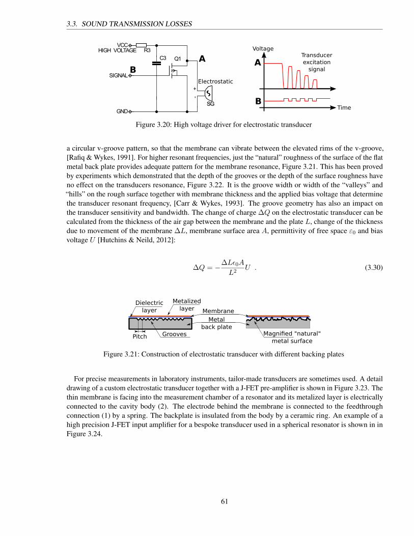
3.3. SOUND TRANSMISSION LOSSES
R3C3 Q1
VCC
SIGNAL
GND
+-
SG
HIGH VOLTAGE
Electrostatic
ATransducer excitation
signal
Voltage
AB
BTime
Figure 3.20: High voltage driver for electrostatic transducer
a circular v-groove pattern, so that the membrane can vibrate between the elevated rims of the v-groove,[Rafiq & Wykes, 1991]. For higher resonant frequencies, just the “natural” roughness of the surface of the flatmetal back plate provides adequate pattern for the membrane resonance, Figure 3.21. This has been provedby experiments which demonstrated that the depth of the grooves or the depth of the surface roughness haveno effect on the transducers resonance, Figure 3.22. It is the groove width or width of the “valleys” and“hills” on the rough surface together with membrane thickness and the applied bias voltage that determinethe transducer resonant frequency, [Carr & Wykes, 1993]. The groove geometry has also an impact onthe transducer sensitivity and bandwidth. The change of charge ∆Q on the electrostatic transducer can becalculated from the thickness of the air gap between the membrane and the plate L, change of the thicknessdue to movement of the membrane ∆L, membrane surface area A, permittivity of free space ε0 and biasvoltage U [Hutchins & Neild, 2012]:
∆Q = −∆Lε0AL2 U . (3.30)
Metal back plate
Dielectric layer
Metalized layer
Pitch Grooves
Membrane
Magnified "natural" metal surface
Figure 3.21: Construction of electrostatic transducer with different backing plates
For precise measurements in laboratory instruments, tailor-made transducers are sometimes used. A detaildrawing of a custom electrostatic transducer together with a J-FET pre-amplifier is shown in Figure 3.23. Thethin membrane is facing into the measurement chamber of a resonator and its metalized layer is electricallyconnected to the cavity body (2). The electrode behind the membrane is connected to the feedthroughconnection (1) by a spring. The backplate is insulated from the body by a ceramic ring. An example of ahigh precision J-FET input amplifier for a bespoke transducer used in a spherical resonator is shown in inFigure 3.24.
61

3.3. SOUND TRANSMISSION LOSSES
Figure 3.22: Resonant frequency of two electrostatic transducers with different back-plates [Carr & Wykes,1993]
Figure 3.23: Custom made electrostatic transducer.The figure was adopted from [Ewing &Trusler, 1989b]
Figure 3.24: Input amplifier for electrostatic trans-ducer used in spherical resonator. Thefigure was adopted from [Perkins &McLinden, 2015]
62

3.3. SOUND TRANSMISSION LOSSES
Bibliography
chapter 3: Speed of sound measurement
[Mea, 2006] 2006 (March). Interfacing Piezo Film to Electronics. Rev b edn. MEAS MeasurementSpecialties, 1000 Lucas Way, Hampton, VA 23666. Application Note 01800004-000.
[Mea, 2018a] 2018a. Piezoelectric films technical information. PIEZOTECH S.A.S. Polymeres pyro etpiezoelectriques [Online; accessed 01-January-2016] https://www.piezotech.fr.
[Mea, 2018b] 2018b. Tables of Acoustic Properties of Materials. Onda, 592 Weddell Drive, Suite 7,Sunnyvale, California 94089, USA, http://www.ondacorp.com/tecref_acoustictable.shtml.
[Alvarez-Arenas, 2013] Alvarez-Arenas, T. E. Gomez. 2013. Air-Coupled Piezoelectric Transducers withActive Polypropylene Foam Matching Layers. Sensors, 13(5), 5996.
[Assael et al., 2014] Assael, M. J., Goodwin, A. R. H., Vesovic, V., & Wakeham, W. A. (eds). 2014.Experimental Thermodynamics Volume IX. The Royal Society of Chemistry.
[Boyes, 1992] Boyes, S. J. 1992 (February). The speed of sound in gases with application to equations ofstate and sonic nozzles. Ph.D. thesis.
[Carr & Wykes, 1993] Carr, H., & Wykes, C. 1993. Diagnostic measurements in capacitive transducers. In:[Carr & Wykes, 1993], 13–30.
[Ewing & Trusler, 1989a] Ewing, M. B., & Trusler, J. P. M. 1989a. Speeds of sound in CF4 between 175and 300 K measured with a spherical resonator. The Journal of Chemical Physics, 90(2), 1106–1115.
[Ewing & Trusler, 1989b] Ewing, M. B., & Trusler, J. P. M. 1989b. Speeds of sound in CF4 between 175and 300 K measured with a spherical resonator. The Journal of Chemical Physics, 90(2), 1106–1115.
[Gillis, 1994] Gillis, K.A. 1994. Thermodynamic properties of two gaseous halogenated ethers from speed-of-sound measurements: Difluoromethoxy-difluoromethane and 2-difluoromethoxy-1,1,1-trifluoroethane.International Journal of Thermophysics, 15(5), 821–847.
[Goodwin et al., 2003] Goodwin, A. R. H, Marsh, K. N., & Wakeham, W. A. (eds). 2003. Measurement ofthe thermodynamic properties of single phases. Experimental thermodynamics, vol. VI. Elsevier. ISBN0-444-50931-3.
[Hess, 1989] Hess, P. 1989. Photoacoustic, Photothermal and Photochemical Processes in Gases. Vol. 46.Springer Berlin Heidelberg.
[Hutchins & Neild, 2012] Hutchins, D. A., & Neild, A. 2012. Airborne ultrasound transducers. WoodheadPublishing Limited.
63

3.3. SOUND TRANSMISSION LOSSES
[Jarvis et al., 1996] Jarvis, G. K., Johnson, K. A., & Walmsley, S. L. 1996. An Annular Resonator Used ToMeasure the Speed of Sound in Gaseous Fluoroalkanes: Trifluoromethane and Hexafluoroethane. Journalof Chemical & Engineering Data, 41(2), 222–230.
[Karki, 2000] Karki, J. 2000 (September). Signal Conditioning Piezoelectric Sensors. Texas Instruments.Application Report SLOA033A.
[Kazakov, 2008] Kazakov, V. V. 2008 (October 27-31). On particularities of choice of ultrasonic transducersfeatures at air location. XX Session of the Russian Acoustical Society.
[Kommareddy, 2003] Kommareddy, V. K. R. 2003. Air-coupled Ultrasonic Measurements in Composites.Ph.D. thesis, Iowa state university. Retrospective Theses and Dissertations. Paper 236.
[Lopes et al., 2014] Lopes, A. F.G., Talavera-Prieto, M. del Carmen, Ferreira, A. G.M., Santos, J. B., Santos,M. J., & Portugal, A. T.G. 2014. Speed of sound in pure fatty acid methyl esters and biodiesel fuels. Fuel,116(Complete), 242–254.
[Álvarez Arenas, 2014] Álvarez Arenas, T. E. Gómez. 2014 (May). Pressure sensitivity response ofpolymeric ferroelectret foam films. Pages 1–4 of: Applications of Ferroelectrics, International Work-shop on Acoustic Transduction Materials and Devices Workshop on Piezoresponse Force Microscopy(ISAF/IWATMD/PFM), 2014 Joint IEEE International Symposium on the.
[Mehl & Moldover, 1982] Mehl, J. B., & Moldover, M. R. 1982. Precondensation phenomena in acousticmeasurements. The Journal of Chemical Physics, 77(1), 455–465.
[Pankaj & Bhatt, 2010] Pankaj, K. S., & Bhatt, S. C. 2010. Investigation of Acoustical Parameters ofPolyvinyl Acetate. Applied Physics Research, 2(1), 35–45.
[Perkins & McLinden, 2015] Perkins, Richard A., & McLinden, Mark O. 2015. Spherical resonatorfor vapor-phase speed of sound and measurements of 1,1,1,2,2,3,3-heptafluoro-3-methoxypropane(RE347mcc) and trans-1,3,3,3-tetrafluoropropene [R1234ze(E)]. The Journal of Chemical Thermo-dynamics, 91(Supplement C), 43 – 61.
[Rafiq & Wykes, 1991] Rafiq, M., & Wykes, C. 1991. The performance of capacitive ultrasonic transducersusing v-grooved backplates. Meas. Sci. Technol., 2, 168–174.
[Stosel, 2004] Stosel, R. 2004. Air-Coupled Ultrasound Inspection as a New Non-Destructive Testing Toolfor Quality Assurance. Ph.D. thesis, Stuttgart university, Institut für Kunststofftechnik.
[Trusler, 1984] Trusler, J. P. M. 1984 (March). The speed of sound in gases. Ph.D. thesis, University ofLondon, department of chemistry.
[Voleisiene & Voleisis, 2008] Voleisiene, B., & Voleisis, A. 2008. Ultrasound velocity measurements inliquid media. Ultragarsas (ultrasound), 63(4), 7–19. ISSN 1392-2114.
[Wikipedia, 2015] Wikipedia. 2015. Acoustic impedance — Wikipedia, The Free Encyclopedia. [Online; ac-cessed 23-February-2016] https://en.wikipedia.org/w/index.php?title=Acoustic_impedance&oldid=688890317.
[Wilhelm & Letcher, 2010] Wilhelm, E., & Letcher, T. M. (eds). 2010. Heat Capacities. The Royal Societyof Chemistry.
64

3.3. SOUND TRANSMISSION LOSSES
[Younglove & Frederick, 1990] Younglove, B. A., & Frederick, N. V. 1990. Sound speed measurementson gas mixtures of natural gas components using a cylindrical resonator. International Journal ofThermophysics, 11(5), 897–910.
65

Chapter 4 Problem statement and goals
4 Problem statement and goals
4.1 Problem statement
A universal thermodynamic model (not necessarily but likely an equation of state) that would combineaccurate prediction of the speed of sound and saturation properties of mixtures of unlike components acrosswide range of conditions does not exist. The very accurate equations of state carefully developed for purefluid are available only for common fluids (including widely-used refrigerants). It takes a significant effortand large experimental data sets to fit such equations to new or less-common fluids. Unfortunately, sufficientdata sets are seldomly available for such fluids. Universal models with few fluid-specific parameters (fittingparameters) such as the cubic equation of state or SAFT model can be used relatively easily for many differentfluids although their accuracy varies widely. It is often the case that some models are applicable to blends offluids from one family (hydrocarbons, hydrofluorocarbons) but fail when used for fluids from other families.At the same time the accuracy of many existing models in terms of prediction of speed of sound in bothphases and also under saturated conditions is largely unknown for many common fluids.
When using the equations of state for mixtures, another parameters called binary interaction coefficientsare needed to accurately predict saturation properties. For the most common mixtures (fluid pairs) andcommon equations of state these parameters are usually known, either they have been obtained by fittingexperimental data or from molecular simulations. Since the values are unique for fluid pairs and the givenmodel, there are many combinations for which the parameters are unknown, either because there are noexperimental data or no one has ever fitted the parameters of the specific model (equation of state). Somemore or less universal methods exists to estimate the interaction coefficients for some equations of state butthe applications are often very limited and the accuracy is questionable.
4.2 Goals
In the previous sections I have outlined the scope and the motivation for this work. The problems addressed inthis thesis are concentrated around the speed of sound measurement and real application of the thermodynamicmodelling of cooling fluids used for particle detectors and high tech electronics cooling. The thesis consistsof the experimental and theoretical parts.
The goals of the experimental part are:
• to design an apparatus for high accuracy speed of sound measurement that can provide high accuracyat lower complexity;
• to carry out speed of sound measurements in binary mixtures of R-116, R-218 and nitrogen since nosuch data exist in available literature and the mentioned binary mixtures have direct applications in thecooling systems of particle detectors.
The theoretical part includes modelling of vapour liquid equilibrium of pure fluid and various refrigerantmixtures with emphasis on the accuracy of the speed of sound prediction, the specific goals are:
• to benchmark various thermodynamic models on representative sets of pure fluids and mixtures inorder to find the applicability range of the saturated properties and speed of sound predictions;
66
4.2. GOALS
• to develop new correlations for the prediction of binary interaction coefficients for mixtures of unlikefluids with emphasis on fluorocarbons that will allow to work more accurately with blends for whichno experimental data or molecular simulation exist. The correlations shall be applicable to modelfor which no group-contribution methods (that would allow the estimation of the binary interactioncoefficients) are available. The developed correlation will therefore be the only way for prediction ofthe interaction coefficients for this model.
67
Chapter 5 Development of high accuracy speed-of-sound measurement apparatus
5 Development of high accuracyspeed-of-sound measurement apparatus
I began the development of the apparatus together with the data acquisition in my Bachelor thesis [Doubek,2012], I have continued the work in my Master’s thesis [Doubek, 2014] and this chapter describes the latestdevelopment that lead to the current instrument that can be used for mixtures and that delivers accuracy closeto resonators as shown in chapter 5.8.
The goal from the very beginning was to develop an instrument for high-accuracy measurement of speedof sound in gases over wide range of temperature and pressure. The time-of-flight measurement methodwas selected for the measurement apparatus due to its relative simplicity and low cost. The developed setupincludes control system that allows for semi-automated measurement of the speed of sound along isochorsbut also along isotherms due to a precise temperature control. The speed of sound data on isotherms areessential for the derivation of ideal gas heat capacities.
The use of capacitive ultrasound transducers was inevitable due to their high sensitivity on acceptance.Standard piezoelectric transducers were also tested but they have very low sensitivity, exhibit long ringingand generally are not suitable for applications in gases where a high precision triggering on the receivedsignal is needed. Senscomp 600 transducers (previously made by Polaroid) were selected to be used from thefew available models. This type of transducers is most sensitive at 50 kHz although the frequency responseis fairly flat between 40 kHz and 100 kHz. The gold-plated membrane ensures good corrosion and chemicalresistance.
I have used the ELMB data acquisition system for temperature and pressure sensor readout together withmy custom made electronics which takes care of the actual speed of sound measurement. The SCADAsoftware running on dedicated computer is in charge of data visualization and archiving as well as temperatureregulation and other control functions.
5.1 Setup Overview
The new setup allows for preparation of binary mixtures directly inside the measurement cell. Two gascylinders provide the pure gases (mixture components) A and B, Figure 5.1. Since the setup is intended forrefrigerants the pressures inside the gas cylinders are not supposed to be very high and therefore pressureregulators on the cylinders are not needed. Omitting the pressure regulator eliminates complicated purgingprocedures to prevent gas contamination from air or other gases trapped inside the regulators. Since thepressures inside the gas cylinders were expected to be different in each cylinder (mixing of two differentrefrigerants at room temperature) there was a risk of contamination of the gas inside the cylinder at the lowerpressure due to wrong manipulation with valves in the setup. Two accumulators (coils of 1.5 meters of12mm tubing) were provided for each gas to store some amount of the pure gas so that the gas cylinderscould be shut off with cylinder valves during the preparation of the mixtures. With this arrangement onlythe gas inside the accumulator would be contaminated while the gas in the cylinder would remain intact.The pressure inside each accumulator was monitored with a pressure sensor. The high precision Keller 33Xpressure sensor was used to monitor the pressure inside the measurement cell. The temperature inside the cellwas monitored by Pt1000 Class A sensors manufactured by IST Innovative Sensor. The rotary oil vacuum
68
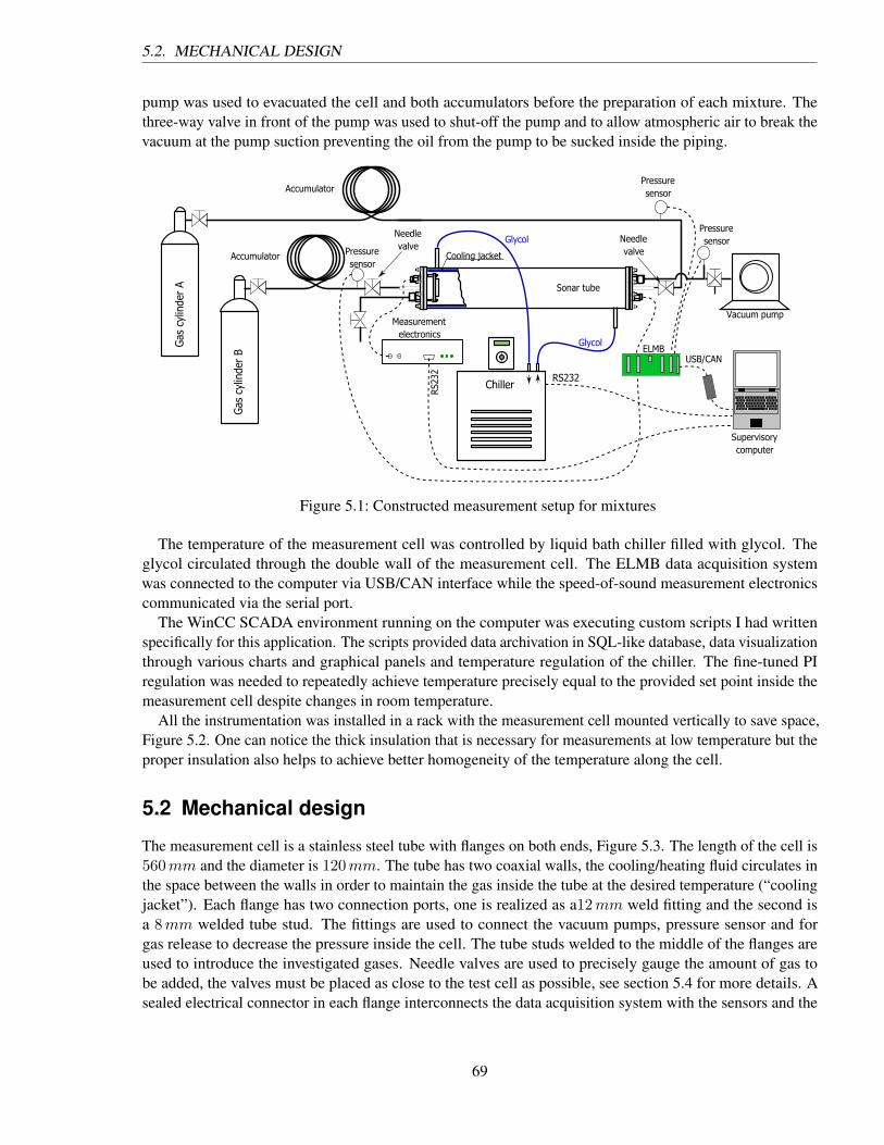
5.2. MECHANICAL DESIGN
pump was used to evacuated the cell and both accumulators before the preparation of each mixture. Thethree-way valve in front of the pump was used to shut-off the pump and to allow atmospheric air to break thevacuum at the pump suction preventing the oil from the pump to be sucked inside the piping.
RS232
Pressure sensor
ELMB
Supervisorycomputer
USB/CAN
Vacuum pump
Chiller
Sonar tube
Measurement electronics
RS23
2
Glycol
Glycol
Needle valve
Cooling jacket
Gas
cyl
inde
r A
Pressure sensor
Needle valve
Gas
cyl
inde
r B
Accumulator
Accumulator Pressure sensor
Figure 5.1: Constructed measurement setup for mixtures
The temperature of the measurement cell was controlled by liquid bath chiller filled with glycol. Theglycol circulated through the double wall of the measurement cell. The ELMB data acquisition systemwas connected to the computer via USB/CAN interface while the speed-of-sound measurement electronicscommunicated via the serial port.
The WinCC SCADA environment running on the computer was executing custom scripts I had writtenspecifically for this application. The scripts provided data archivation in SQL-like database, data visualizationthrough various charts and graphical panels and temperature regulation of the chiller. The fine-tuned PIregulation was needed to repeatedly achieve temperature precisely equal to the provided set point inside themeasurement cell despite changes in room temperature.
All the instrumentation was installed in a rack with the measurement cell mounted vertically to save space,Figure 5.2. One can notice the thick insulation that is necessary for measurements at low temperature but theproper insulation also helps to achieve better homogeneity of the temperature along the cell.
5.2 Mechanical design
The measurement cell is a stainless steel tube with flanges on both ends, Figure 5.3. The length of the cell is560mm and the diameter is 120mm. The tube has two coaxial walls, the cooling/heating fluid circulates inthe space between the walls in order to maintain the gas inside the tube at the desired temperature (“coolingjacket”). Each flange has two connection ports, one is realized as a12mm weld fitting and the second isa 8mm welded tube stud. The fittings are used to connect the vacuum pumps, pressure sensor and forgas release to decrease the pressure inside the cell. The tube studs welded to the middle of the flanges areused to introduce the investigated gases. Needle valves are used to precisely gauge the amount of gas tobe added, the valves must be placed as close to the test cell as possible, see section 5.4 for more details. Asealed electrical connector in each flange interconnects the data acquisition system with the sensors and the
69
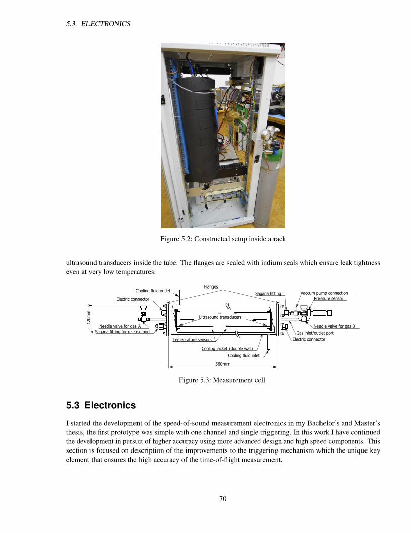
5.3. ELECTRONICS
Figure 5.2: Constructed setup inside a rack
ultrasound transducers inside the tube. The flanges are sealed with indium seals which ensure leak tightnesseven at very low temperatures.
560mm
120m
m
Pressure sensor
Electric connectorGas inlet/outlet port
Cooling fluid inlet
Cooling jacket (double wall)
Ultrasound transducers
Temeprature sensors
Flanges
Sagana fitting for release port
Cooling fluid outlet
Needle valve for gas BNeedle valve for gas A
Sagana fitting Vaccum pump connectionElectric connector
Figure 5.3: Measurement cell
5.3 Electronics
I started the development of the speed-of-sound measurement electronics in my Bachelor’s and Master’sthesis, the first prototype was simple with one channel and single triggering. In this work I have continuedthe development in pursuit of higher accuracy using more advanced design and high speed components. Thissection is focused on description of the improvements to the triggering mechanism which the unique keyelement that ensures the high accuracy of the time-of-flight measurement.
70
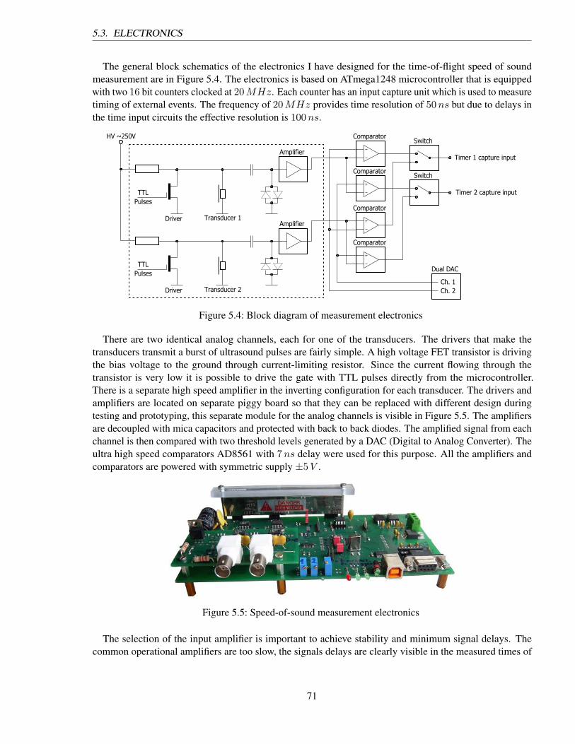
5.3. ELECTRONICS
The general block schematics of the electronics I have designed for the time-of-flight speed of soundmeasurement are in Figure 5.4. The electronics is based on ATmega1248 microcontroller that is equippedwith two 16 bit counters clocked at 20MHz. Each counter has an input capture unit which is used to measuretiming of external events. The frequency of 20MHz provides time resolution of 50ns but due to delays inthe time input circuits the effective resolution is 100ns.
HV ~250V
Transducer 1
Amplifier
Driver
SwitchComparator
Dual DAC
Ch. 1Ch. 2
Comparator
Timer 1 capture input
Timer 2 capture input
Transducer 2
Amplifier
Driver
TTLPulses
TTLPulses
Comparator
Comparator
Switch
Figure 5.4: Block diagram of measurement electronics
There are two identical analog channels, each for one of the transducers. The drivers that make thetransducers transmit a burst of ultrasound pulses are fairly simple. A high voltage FET transistor is drivingthe bias voltage to the ground through current-limiting resistor. Since the current flowing through thetransistor is very low it is possible to drive the gate with TTL pulses directly from the microcontroller.There is a separate high speed amplifier in the inverting configuration for each transducer. The drivers andamplifiers are located on separate piggy board so that they can be replaced with different design duringtesting and prototyping, this separate module for the analog channels is visible in Figure 5.5. The amplifiersare decoupled with mica capacitors and protected with back to back diodes. The amplified signal from eachchannel is then compared with two threshold levels generated by a DAC (Digital to Analog Converter). Theultra high speed comparators AD8561 with 7ns delay were used for this purpose. All the amplifiers andcomparators are powered with symmetric supply ±5V .
Figure 5.5: Speed-of-sound measurement electronics
The selection of the input amplifier is important to achieve stability and minimum signal delays. Thecommon operational amplifiers are too slow, the signals delays are clearly visible in the measured times of
71
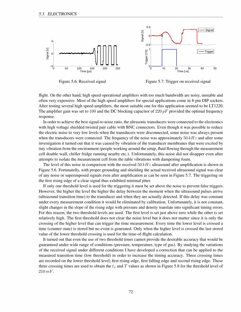
5.3. ELECTRONICS
0 50 100 150 200 250−5
0
5
Sig
nal [
V]
Time [µs]
Figure 5.6: Received signal
-5.0
0
5.0
Sig
nal [V
] Signal
0 10 20 30 40 500
1
Time [s]
Trig
ge
r [1
/0]
Trigger
Figure 5.7: Trigger on received signal
flight. On the other hand, high speed operational amplifiers with too much bandwidth are noisy, unstable andoften very expensive. Most of the high speed amplifiers for special applications come in 8-pin DIP sockets.After testing several high speed amplifiers, the most suitable one for this application seemed to be LT1220.The amplifier gain was set to 100 and the DC blocking capacitor of 220 pF provided the optimal frequencyresponse.
In order to achieve the best signal-to noise ratio, the ultrasonic transducers were connected to the electronicswith high voltage shielded twisted pair cable with BNC connectors. Even though it was possible to reducethe electric noise to very low levels when the transducers were disconnected, some noise was always presentwhen the transducers were connected. The frequency of the noise was approximately 50 kHz and after someinvestigation it turned out that it was caused by vibration of the transducer membranes that were excited bytiny vibration from the environment (people working around the setup, fluid flowing through the measurementcell double wall, chiller fridge running nearby etc.). Unfortunately, this noise did not disapper even afterattempts to isolate the measurement cell from the table vibrations with dampening foam.
The level of this noise in comparison with the received 50 kHz ultrasound after amplification is shown inFigure 5.6. Fortunatelly, with proper grounding and shielding the actual received ultrasound signal was clearof any noise or superimposed signals even after amplification as can be seen in Figure 5.7. The triggering onthe first rising edge of a clear signal thus exhibited minimal jitter.
If only one threshold level is used for the triggering it must be set above the noise to prevent false triggers.However, the higher the level the higher the delay between the moment when the ultrasound pulses arrive(ultrasound transition time) to the transducer and when they are actually detected. If this delay was constantunder every measurement condition it would be eliminated by calibration. Unfortunately, it is not constant,slight changes in the slope of the rising edge with pressure and density translate into significant timing errors.For this reason, the two threshold levels are used. The first level is set just above zero while the other is setrelatively high. The first threshold does not clear the noise level but it does not matter since it is only thecrossing of the higher level that can trigger the time measurement. Every time the lower level is crossed atime (counter state) is stored but no event is generated. Only when the higher level is crossed the last storedvalue of the lower threshold crossing is used for the time-of-flight calculation.
It turned out that even the use of two threshold times cannot provide the desirable accuracy that would beguaranteed under wide range of conditions (pressure, temperature, type of gas). By studying the variationsof the received signal under different conditions I have developed a correction that can be applied to themeasured transition time (low threshold) in order to increase the timing accuracy. Three crossing timesare recorded on the lower threshold level; first rising edge, first falling edge and second rising edge. Thesethree crossing times are used to obtain the tx and T values as shown in Figure 5.8 for the threshold level of210mV .
72
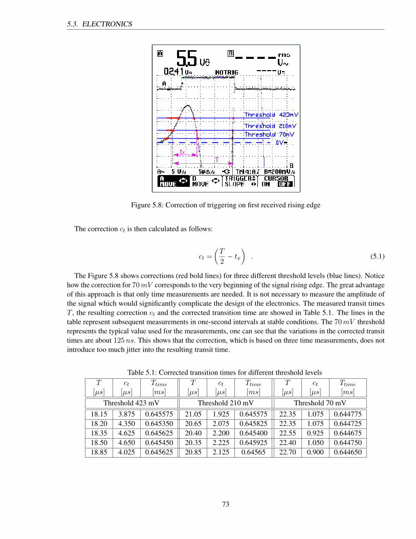
5.3. ELECTRONICS
txT
Figure 5.8: Correction of triggering on first received rising edge
The correction ct is then calculated as follows:
ct =(T
2 − tx)
. (5.1)
The Figure 5.8 shows corrections (red bold lines) for three different threshold levels (blue lines). Noticehow the correction for 70mV corresponds to the very beginning of the signal rising edge. The great advantageof this approach is that only time measurements are needed. It is not necessary to measure the amplitude ofthe signal which would significantly complicate the design of the electronics. The measured transit timesT , the resulting correction ct and the corrected transition time are showed in Table 5.1. The lines in thetable represent subsequent measurements in one-second intervals at stable conditions. The 70mV thresholdrepresents the typical value used for the measurements, one can see that the variations in the corrected transittimes are about 125ns. This shows that the correction, which is based on three time measurements, does notintroduce too much jitter into the resulting transit time.
Table 5.1: Corrected transition times for different threshold levelsT
[µs]ct
[µs]Ttime[ms]
T[µs]
ct[µs]
Ttime[ms]
T[µs]
ct[µs]
Ttime[ms]
Threshold 423 mV Threshold 210 mV Threshold 70 mV18.15 3.875 0.645575 21.05 1.925 0.645575 22.35 1.075 0.64477518.20 4.350 0.645350 20.65 2.075 0.645825 22.35 1.075 0.64472518.35 4.625 0.645625 20.40 2.200 0.645400 22.55 0.925 0.64467518.50 4.650 0.645450 20.35 2.225 0.645925 22.40 1.050 0.64475018.85 4.025 0.645625 20.85 2.125 0.64565 22.70 0.900 0.644650
73
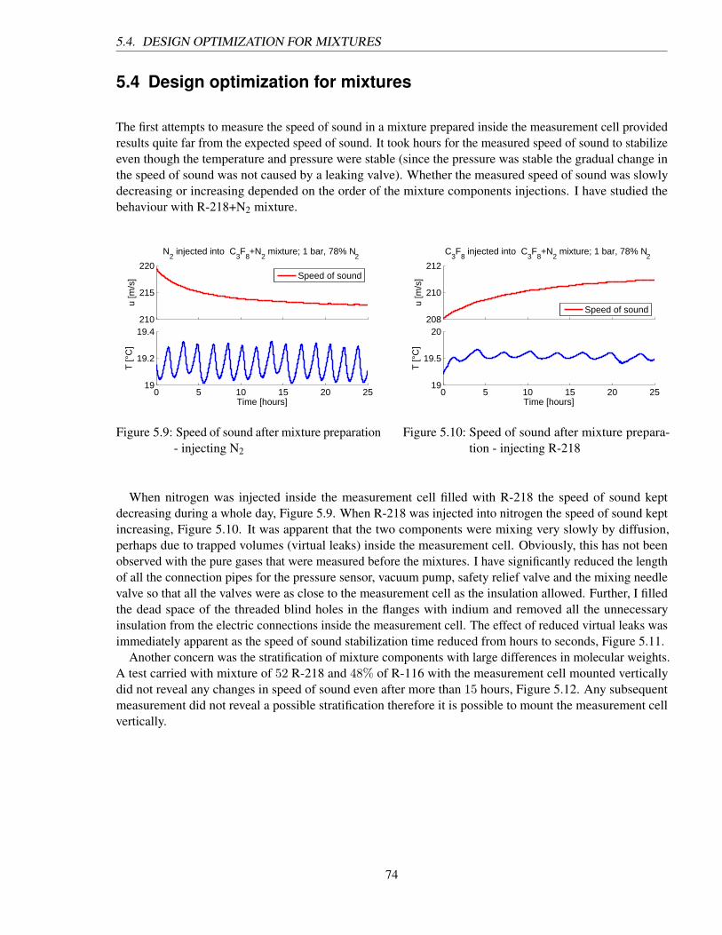
5.4. DESIGN OPTIMIZATION FOR MIXTURES
5.4 Design optimization for mixtures
The first attempts to measure the speed of sound in a mixture prepared inside the measurement cell providedresults quite far from the expected speed of sound. It took hours for the measured speed of sound to stabilizeeven though the temperature and pressure were stable (since the pressure was stable the gradual change inthe speed of sound was not caused by a leaking valve). Whether the measured speed of sound was slowlydecreasing or increasing depended on the order of the mixture components injections. I have studied thebehaviour with R-218+N2 mixture.
210
215
220
u [m
/s]
N2 injected into C
3F
8+N
2 mixture; 1 bar, 78% N
2
Speed of sound
0 5 10 15 20 2519
19.2
19.4
T [°
C]
Time [hours]
Figure 5.9: Speed of sound after mixture preparation- injecting N2
208
210
212
u [m
/s]
C3F
8 injected into C
3F
8+N
2 mixture; 1 bar, 78% N
2
Speed of sound
0 5 10 15 20 2519
19.5
20
T [°
C]
Time [hours]
Figure 5.10: Speed of sound after mixture prepara-tion - injecting R-218
When nitrogen was injected inside the measurement cell filled with R-218 the speed of sound keptdecreasing during a whole day, Figure 5.9. When R-218 was injected into nitrogen the speed of sound keptincreasing, Figure 5.10. It was apparent that the two components were mixing very slowly by diffusion,perhaps due to trapped volumes (virtual leaks) inside the measurement cell. Obviously, this has not beenobserved with the pure gases that were measured before the mixtures. I have significantly reduced the lengthof all the connection pipes for the pressure sensor, vacuum pump, safety relief valve and the mixing needlevalve so that all the valves were as close to the measurement cell as the insulation allowed. Further, I filledthe dead space of the threaded blind holes in the flanges with indium and removed all the unnecessaryinsulation from the electric connections inside the measurement cell. The effect of reduced virtual leaks wasimmediately apparent as the speed of sound stabilization time reduced from hours to seconds, Figure 5.11.
Another concern was the stratification of mixture components with large differences in molecular weights.A test carried with mixture of 52 R-218 and 48% of R-116 with the measurement cell mounted verticallydid not reveal any changes in speed of sound even after more than 15 hours, Figure 5.12. Any subsequentmeasurement did not reveal a possible stratification therefore it is possible to mount the measurement cellvertically.
74
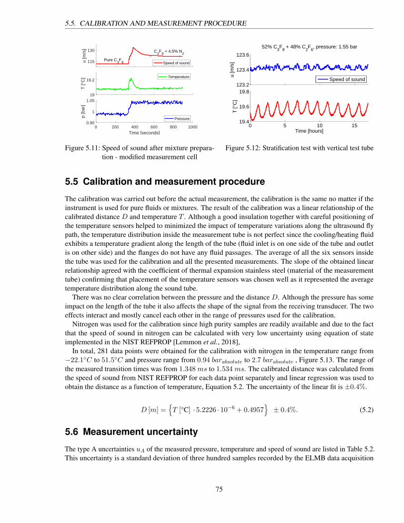
5.5. CALIBRATION AND MEASUREMENT PROCEDURE
115
130
u [m
/s]
Speed of sound
19
19.2T
[°C
] Temperature
0 200 400 600 800 1000Time [seconds]
0.95
1
1.05
p [b
ar]
Pressure
Pure C3F
8
C3F
8 + 4.5% N
2
Figure 5.11: Speed of sound after mixture prepara-tion - modified measurement cell
123.2
123.4
123.6
u [m
/s]
52% C3F
8 + 48% C
2F
6, pressure: 1.55 bar
Speed of sound
0 5 10 1519.4
19.6
19.8
T [°
C]
Time [hours]
Figure 5.12: Stratification test with vertical test tube
5.5 Calibration and measurement procedure
The calibration was carried out before the actual measurement, the calibration is the same no matter if theinstrument is used for pure fluids or mixtures. The result of the calibration was a linear relationship of thecalibrated distance D and temperature T . Although a good insulation together with careful positioning ofthe temperature sensors helped to minimized the impact of temperature variations along the ultrasound flypath, the temperature distribution inside the measurement tube is not perfect since the cooling/heating fluidexhibits a temperature gradient along the length of the tube (fluid inlet is on one side of the tube and outletis on other side) and the flanges do not have any fluid passages. The average of all the six sensors insidethe tube was used for the calibration and all the presented measurements. The slope of the obtained linearrelationship agreed with the coefficient of thermal expansion stainless steel (material of the measurementtube) confirming that placement of the temperature sensors was chosen well as it represented the averagetemperature distribution along the sound tube.
There was no clear correlation between the pressure and the distance D. Although the pressure has someimpact on the length of the tube it also affects the shape of the signal from the receiving transducer. The twoeffects interact and mostly cancel each other in the range of pressures used for the calibration.
Nitrogen was used for the calibration since high purity samples are readily available and due to the factthat the speed of sound in nitrogen can be calculated with very low uncertainty using equation of stateimplemented in the NIST REFPROP [Lemmon et al., 2018],
In total, 281 data points were obtained for the calibration with nitrogen in the temperature range from−22.1C to 51.5C and pressure range from 0.94 barabsolute to 2.7 barabsolute , Figure 5.13. The range ofthe measured transition times was from 1.348 ms to 1.534 ms. The calibrated distance was calculated fromthe speed of sound from NIST REFPROP for each data point separately and linear regression was used toobtain the distance as a function of temperature, Equation 5.2. The uncertainty of the linear fit is ±0.4%.
D [m] =T [°C] · 5.2226 · 10−6 + 0.4957
± 0.4%. (5.2)
5.6 Measurement uncertainty
The type A uncertainties uA of the measured pressure, temperature and speed of sound are listed in Table 5.2.This uncertainty is a standard deviation of three hundred samples recorded by the ELMB data acquisition
75
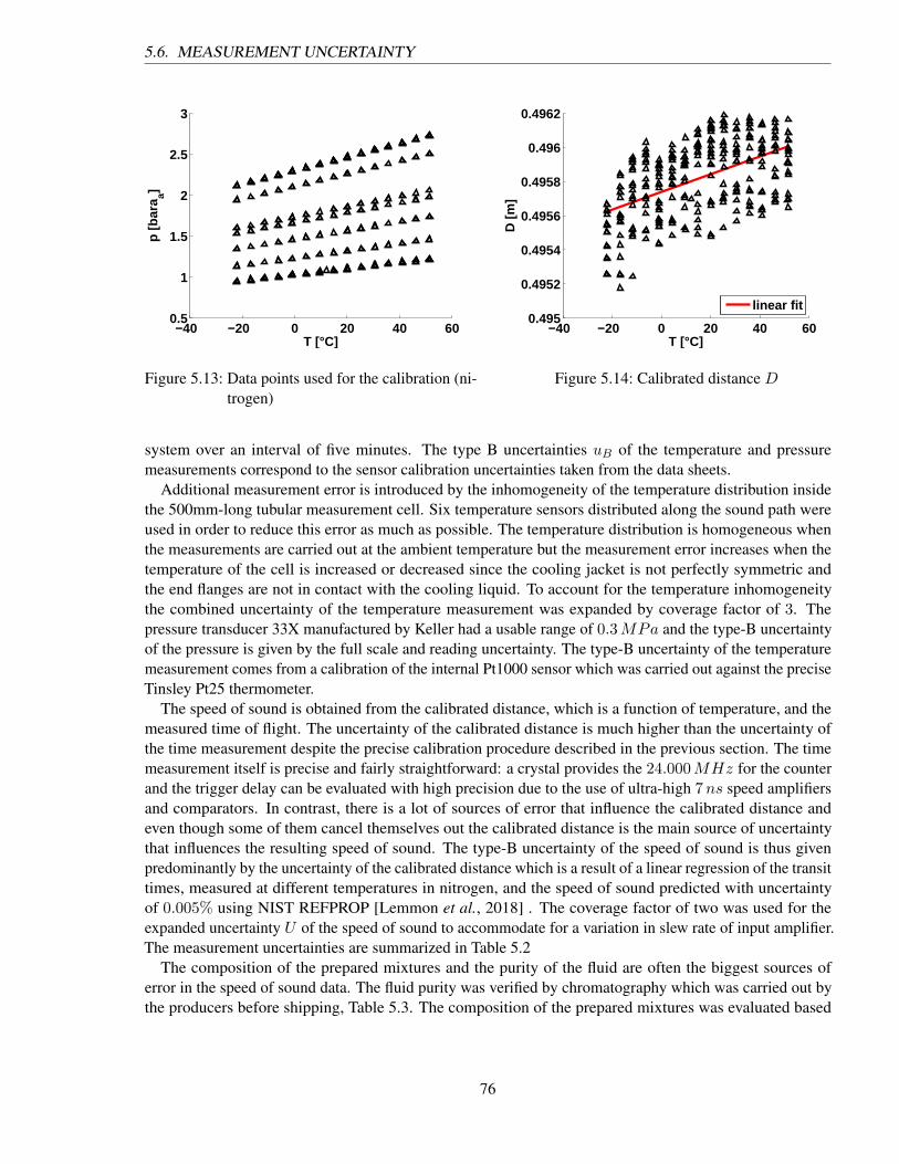
5.6. MEASUREMENT UNCERTAINTY
−40 −20 0 20 40 600.5
1
1.5
2
2.5
3
T [°C]
p [b
ara
a]
Figure 5.13: Data points used for the calibration (ni-trogen)
−40 −20 0 20 40 600.495
0.4952
0.4954
0.4956
0.4958
0.496
0.4962
T [°C]
D [m
]
linear fit
Figure 5.14: Calibrated distance D
system over an interval of five minutes. The type B uncertainties uB of the temperature and pressuremeasurements correspond to the sensor calibration uncertainties taken from the data sheets.
Additional measurement error is introduced by the inhomogeneity of the temperature distribution insidethe 500mm-long tubular measurement cell. Six temperature sensors distributed along the sound path wereused in order to reduce this error as much as possible. The temperature distribution is homogeneous whenthe measurements are carried out at the ambient temperature but the measurement error increases when thetemperature of the cell is increased or decreased since the cooling jacket is not perfectly symmetric andthe end flanges are not in contact with the cooling liquid. To account for the temperature inhomogeneitythe combined uncertainty of the temperature measurement was expanded by coverage factor of 3. Thepressure transducer 33X manufactured by Keller had a usable range of 0.3MPa and the type-B uncertaintyof the pressure is given by the full scale and reading uncertainty. The type-B uncertainty of the temperaturemeasurement comes from a calibration of the internal Pt1000 sensor which was carried out against the preciseTinsley Pt25 thermometer.
The speed of sound is obtained from the calibrated distance, which is a function of temperature, and themeasured time of flight. The uncertainty of the calibrated distance is much higher than the uncertainty ofthe time measurement despite the precise calibration procedure described in the previous section. The timemeasurement itself is precise and fairly straightforward: a crystal provides the 24.000MHz for the counterand the trigger delay can be evaluated with high precision due to the use of ultra-high 7ns speed amplifiersand comparators. In contrast, there is a lot of sources of error that influence the calibrated distance andeven though some of them cancel themselves out the calibrated distance is the main source of uncertaintythat influences the resulting speed of sound. The type-B uncertainty of the speed of sound is thus givenpredominantly by the uncertainty of the calibrated distance which is a result of a linear regression of the transittimes, measured at different temperatures in nitrogen, and the speed of sound predicted with uncertaintyof 0.005% using NIST REFPROP [Lemmon et al., 2018] . The coverage factor of two was used for theexpanded uncertainty U of the speed of sound to accommodate for a variation in slew rate of input amplifier.The measurement uncertainties are summarized in Table 5.2
The composition of the prepared mixtures and the purity of the fluid are often the biggest sources oferror in the speed of sound data. The fluid purity was verified by chromatography which was carried out bythe producers before shipping, Table 5.3. The composition of the prepared mixtures was evaluated based
76
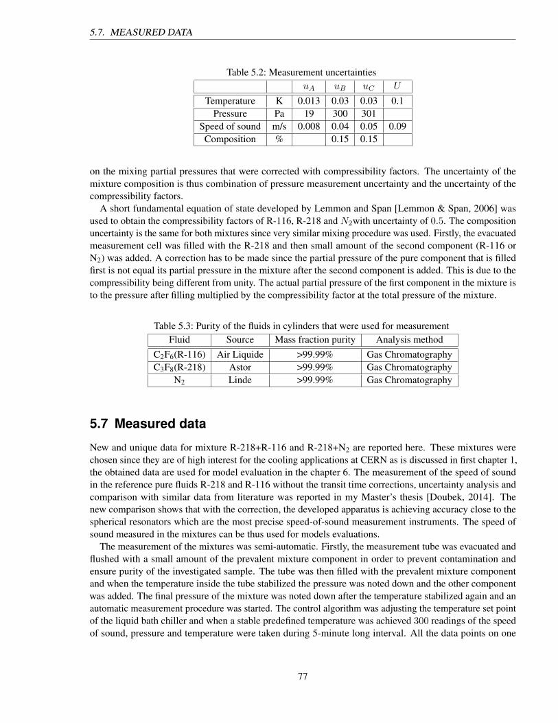
5.7. MEASURED DATA
Table 5.2: Measurement uncertaintiesuA uB uC U
Temperature K 0.013 0.03 0.03 0.1Pressure Pa 19 300 301
Speed of sound m/s 0.008 0.04 0.05 0.09Composition % 0.15 0.15
on the mixing partial pressures that were corrected with compressibility factors. The uncertainty of themixture composition is thus combination of pressure measurement uncertainty and the uncertainty of thecompressibility factors.
A short fundamental equation of state developed by Lemmon and Span [Lemmon & Span, 2006] wasused to obtain the compressibility factors of R-116, R-218 and N2with uncertainty of 0.5. The compositionuncertainty is the same for both mixtures since very similar mixing procedure was used. Firstly, the evacuatedmeasurement cell was filled with the R-218 and then small amount of the second component (R-116 orN2) was added. A correction has to be made since the partial pressure of the pure component that is filledfirst is not equal its partial pressure in the mixture after the second component is added. This is due to thecompressibility being different from unity. The actual partial pressure of the first component in the mixture isto the pressure after filling multiplied by the compressibility factor at the total pressure of the mixture.
Table 5.3: Purity of the fluids in cylinders that were used for measurementFluid Source Mass fraction purity Analysis method
C2F6(R-116) Air Liquide >99.99% Gas ChromatographyC3F8(R-218) Astor >99.99% Gas Chromatography
N2 Linde >99.99% Gas Chromatography
5.7 Measured data
New and unique data for mixture R-218+R-116 and R-218+N2 are reported here. These mixtures werechosen since they are of high interest for the cooling applications at CERN as is discussed in first chapter 1,the obtained data are used for model evaluation in the chapter 6. The measurement of the speed of soundin the reference pure fluids R-218 and R-116 without the transit time corrections, uncertainty analysis andcomparison with similar data from literature was reported in my Master’s thesis [Doubek, 2014]. Thenew comparison shows that with the correction, the developed apparatus is achieving accuracy close to thespherical resonators which are the most precise speed-of-sound measurement instruments. The speed ofsound measured in the mixtures can be thus used for models evaluations.
The measurement of the mixtures was semi-automatic. Firstly, the measurement tube was evacuated andflushed with a small amount of the prevalent mixture component in order to prevent contamination andensure purity of the investigated sample. The tube was then filled with the prevalent mixture componentand when the temperature inside the tube stabilized the pressure was noted down and the other componentwas added. The final pressure of the mixture was noted down after the temperature stabilized again and anautomatic measurement procedure was started. The control algorithm was adjusting the temperature set pointof the liquid bath chiller and when a stable predefined temperature was achieved 300 readings of the speedof sound, pressure and temperature were taken during 5-minute long interval. All the data points on one
77
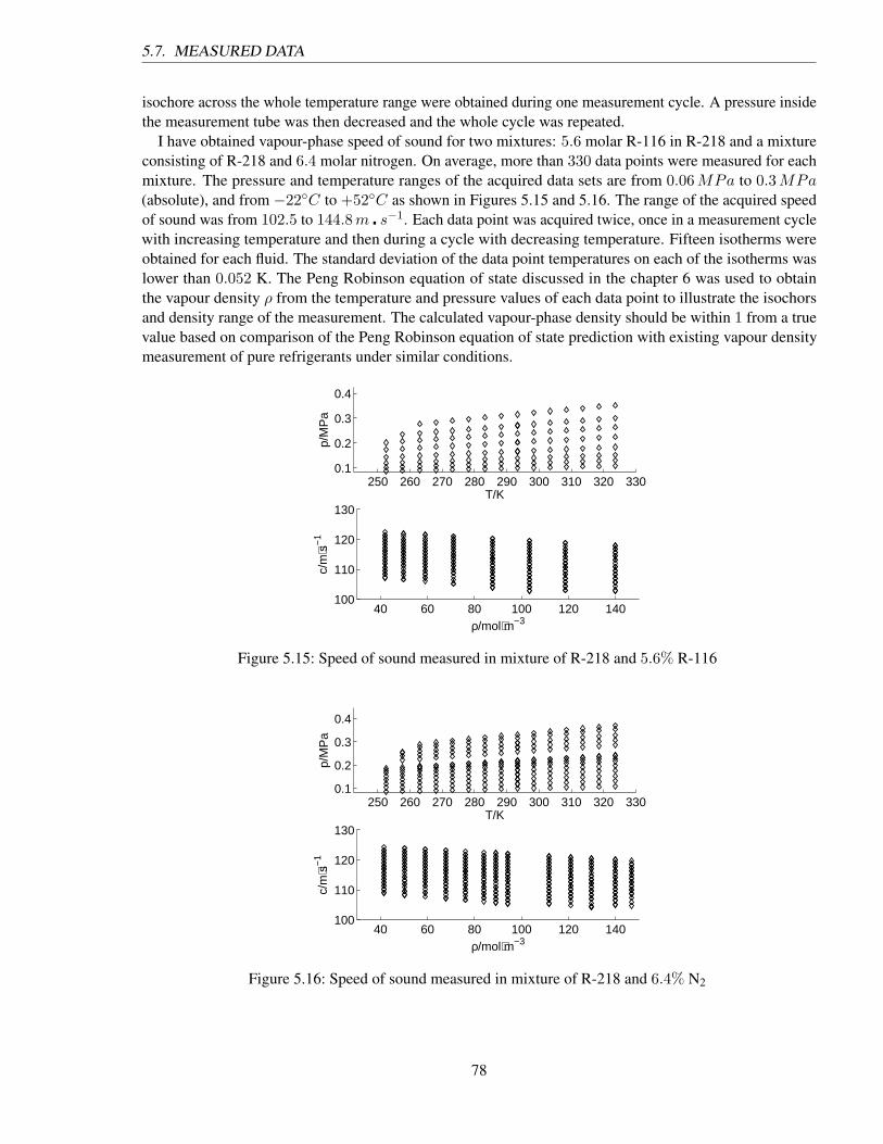
5.7. MEASURED DATA
isochore across the whole temperature range were obtained during one measurement cycle. A pressure insidethe measurement tube was then decreased and the whole cycle was repeated.
I have obtained vapour-phase speed of sound for two mixtures: 5.6 molar R-116 in R-218 and a mixtureconsisting of R-218 and 6.4 molar nitrogen. On average, more than 330 data points were measured for eachmixture. The pressure and temperature ranges of the acquired data sets are from 0.06MPa to 0.3MPa(absolute), and from −22C to +52C as shown in Figures 5.15 and 5.16. The range of the acquired speedof sound was from 102.5 to 144.8m s−1. Each data point was acquired twice, once in a measurement cyclewith increasing temperature and then during a cycle with decreasing temperature. Fifteen isotherms wereobtained for each fluid. The standard deviation of the data point temperatures on each of the isotherms waslower than 0.052 K. The Peng Robinson equation of state discussed in the chapter 6 was used to obtainthe vapour density ρ from the temperature and pressure values of each data point to illustrate the isochorsand density range of the measurement. The calculated vapour-phase density should be within 1 from a truevalue based on comparison of the Peng Robinson equation of state prediction with existing vapour densitymeasurement of pure refrigerants under similar conditions.
250 260 270 280 290 300 310 320 3300.1
0.2
0.3
0.4
T/K
p/M
Pa
40 60 80 100 120 140100
110
120
130
ρ/mol⋅m−3
c/m
⋅s−
1
Figure 5.15: Speed of sound measured in mixture of R-218 and 5.6% R-116
250 260 270 280 290 300 310 320 3300.1
0.2
0.3
0.4
T/K
p/M
Pa
40 60 80 100 120 140100
110
120
130
ρ/mol⋅m−3
c/m
⋅s−
1
Figure 5.16: Speed of sound measured in mixture of R-218 and 6.4% N2
78

5.7. MEASURED DATA
As is customary, the measured data were correlated with the acoustic virial equation, Equation 2.10. Thezero-density heat capacity ratio γid0 was determined from a linear extrapolation of the measured speedof sound to zero density and the value of the second acoustic virial coefficient Ba was obtained for eachisotherm. The results are listed in Table 5.4. The average deviation of the obtained fit is 0.008. The fittedacoustic virial equation allows for interpolation between the measured data points since the fitted acousticvirial coefficients Ba are smooth function of temperature, as can be seen in Figure 5.17.
Table 5.4: Second acoustic virial coefficients obtained from correlation of the measured dataT
[K]Ba [1e6 ∗m3/mol]
R-218 R-116 5.6% R-218
94.4% R-116
93.6% R-2186.4% N2
252.0 -1327.3 -606.67 -1292 -1203262.0 -1206 -558.23 -1178 -1086272.0 -1103.8 -515.18 -1079 -996282.0 -1014.2 -476.14 -990 -916292.0 -934.34 -440.73 -914 -847302.0 -863.47 -408.81 -840 -777312.0 -800.33 -379.79 -777 -718322.0 -741.14 -351.99 -722 -664
240 260 280 300 320 340−14
−12
−10
−8
−6
−4
−2
T/K
10−
4 Ba/m
3 ⋅mol
−1
C3F
8C
3F
8 + C
2F
6C
3F
8 + N
2C
2F
6
Figure 5.17: Acoustic virial coefficients obtained through regression of the experimental data
79
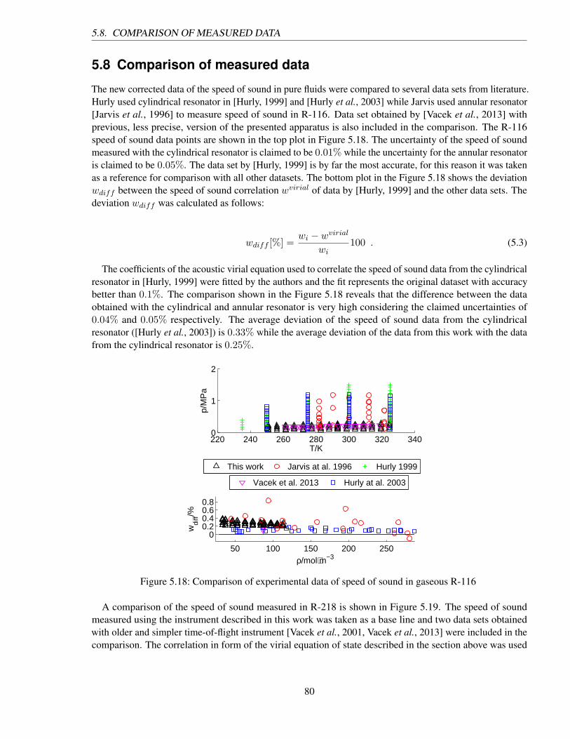
5.8. COMPARISON OF MEASURED DATA
5.8 Comparison of measured data
The new corrected data of the speed of sound in pure fluids were compared to several data sets from literature.Hurly used cylindrical resonator in [Hurly, 1999] and [Hurly et al., 2003] while Jarvis used annular resonator[Jarvis et al., 1996] to measure speed of sound in R-116. Data set obtained by [Vacek et al., 2013] withprevious, less precise, version of the presented apparatus is also included in the comparison. The R-116speed of sound data points are shown in the top plot in Figure 5.18. The uncertainty of the speed of soundmeasured with the cylindrical resonator is claimed to be 0.01% while the uncertainty for the annular resonatoris claimed to be 0.05%. The data set by [Hurly, 1999] is by far the most accurate, for this reason it was takenas a reference for comparison with all other datasets. The bottom plot in the Figure 5.18 shows the deviationwdiff between the speed of sound correlation wvirial of data by [Hurly, 1999] and the other data sets. Thedeviation wdiff was calculated as follows:
wdiff [%] = wi − wvirial
wi100 . (5.3)
The coefficients of the acoustic virial equation used to correlate the speed of sound data from the cylindricalresonator in [Hurly, 1999] were fitted by the authors and the fit represents the original dataset with accuracybetter than 0.1%. The comparison shown in the Figure 5.18 reveals that the difference between the dataobtained with the cylindrical and annular resonator is very high considering the claimed uncertainties of0.04% and 0.05% respectively. The average deviation of the speed of sound data from the cylindricalresonator ([Hurly et al., 2003]) is 0.33% while the average deviation of the data from this work with the datafrom the cylindrical resonator is 0.25%.
220 240 260 280 300 320 3400
1
2
T/K
p/M
Pa
This work Jarvis at al. 1996 Hurly 1999
50 100 150 200 250
00.20.40.60.8
wdi
ff/%
ρ/mol⋅m−3
Vacek et al. 2013 Hurly at al. 2003
Figure 5.18: Comparison of experimental data of speed of sound in gaseous R-116
A comparison of the speed of sound measured in R-218 is shown in Figure 5.19. The speed of soundmeasured using the instrument described in this work was taken as a base line and two data sets obtainedwith older and simpler time-of-flight instrument [Vacek et al., 2001, Vacek et al., 2013] were included in thecomparison. The correlation in form of the virial equation of state described in the section above was used
80
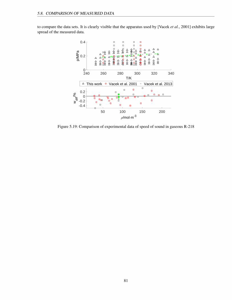
5.8. COMPARISON OF MEASURED DATA
to compare the data sets. It is clearly visible that the apparatus used by [Vacek et al., 2001] exhibits largespread of the measured data.
240 260 280 300 320 340T/K
0
0.2
0.4
p/M
Pa
This work Vacek et al. 2001 Vacek et al. 2013
50 100 150 200
/mol m-3
-0.4-0.2
00.2
wdi
ff/%
Figure 5.19: Comparison of experimental data of speed of sound in gaseous R-218
81
5.8. COMPARISON OF MEASURED DATA
Bibliography
chapter 5: Development of high accuracy speed-of-soundmeasurement apparatus
[Doubek, 2012] Doubek, M. 2012. Studie zarizeni pro merení rychlosti zvuku v plynne fazi. Bachelor’sthesis, Czech Technical University, Faculty of Mechanical Engineering.
[Doubek, 2014] Doubek, M. 2014. Thermophysical properties of fluids experiment and simulations. Master’sthesis, Czech Technical University, Faculty of Mechanical Engineering.
[Hurly, 1999] Hurly, J. J. 1999. Thermophysical Properties of Gaseous CF4 and C2F6 from Speed-of-SoundMeasurements. International Journal of Thermophysics, 20(2), 455–484.
[Hurly et al., 2003] Hurly, J. J., Gillis, K. A., Mehl, J. B., & Moldover, M. R. 2003. The Viscosity ofSeven Gases Measured with a Greenspan Viscometer. International Journal of Thermophysics, 24(6),1441–1474.
[Jarvis et al., 1996] Jarvis, G. K., Johnson, K. A., & Walmsley, S. L. 1996. An Annular Resonator Used ToMeasure the Speed of Sound in Gaseous Fluoroalkanes: Trifluoromethane and Hexafluoroethane. Journalof Chemical & Engineering Data, 41(2), 222–230.
[Lemmon & Span, 2006] Lemmon, E. W., & Span, R. 2006. Short Fundamental Equations of State for 20Industrial Fluids. Journal of Chemical & Engineering Data, 51(3), 785–850.
[Lemmon et al., 2018] Lemmon, E. W., Bell, I. H., Huber, M. L., & McLinden, M. O. 2018. NIST StandardReference Database 23: Reference Fluid Thermodynamic and Transport Properties-REFPROP, Version10.0, National Institute of Standards and Technology.
[Vacek et al., 2001] Vacek, V., Hallewell, G., & Lindsay, S. 2001. Velocity of sound measurements ingaseous per-fluorocarbons and their mixtures. Fluid Phase Equilibria, 185(1), 305 – 314. Proceedings ofthe 14th symposium on thermophysical properties.
[Vacek et al., 2013] Vacek, V., Vítek, M., & Doubek, M. 2013. Velocity of sound in Perfluoropropane(C3F8), Perfluoroethane (C2F6) and their mixtures. Fluid Phase Equilibria, 351, 53 – 60. Special Issuecovering the Eighteenth Symposium on Thermophysical Properties.
82
Chapter 6 Thermodynamic Models
6 Thermodynamic Models
6.1 Peng-Robinson equation of state
I have included the Peng Robinson equation of state in the tested models since it is widely used and it can beconsidered as the reference model. It exhibits the common drawback of cubic equations of state in that itunderestimates the liquid density by up to 10%. Nevertheless, the Peng-Robinson equation of state providesgood accuracy in the vapour region and good prediction of saturated pressure of pure fluids and mixtures.The pressure-specific form of the equation of state is discussed in chapter 2.
Since I used the same framework of Helmholtz-energy partial derivatives for all the thermodynamicmodels which are introduced in this section, I worked with the Helmholtz-energy form of the Peng-Robinsonequation of state, Equation 6.1, instead of the usual pressure-specific form.
ar
RT= ln
( 11− bρ
)− a
2√
2RTln
1 +(√
2 + 1)bρ
1−(√
2− 1)bρ
(6.1)
When the cubic equations are used for mixtures the am and bm coefficients have to be obtained usingsimple Van der Waalse mixing rules:
am =∑i
∑j
xixjaij , (6.2)
bm =∑i
∑j
xixjbij , (6.3)
aij =√aiaj(1− kij) , (6.4)
bij = 12(bi + bj) . (6.5)
The Van der Waalse mixing rules are suitable only for mixtures of non-polar or slightly polar fluids. Thebinary interaction parameter kij in Equation 6.4 is used to improve the vapour-liquid equilibrium prediction.Some authors proposed composition-dependent mixing rules to improve the accuracy of prediction of thevapour-liquid equilibrium of mixtures, temperature-dependent coefficients, rules for polar fluids [Iwai et al.,1988] and also rules for associating fluids [Medeiros & Tellez-Arredondo, 2008]. I chose to use the simplestrules since the more complicated mixing rules often provide better results for certain fluids but they are lessuniversal.
83
6.2. VOLUME-TRANSLATED PENG-ROBINSON EQUATION OF STATE
6.2 Volume-translated Peng-Robinson equation of state
The volume translation technique for the cubic equations of state is introduced in chapter 2. I have includedthe volume-translated Peng-Robinson equation of state in the tested models since it promises to overcomethe main drawback of the cubic equations while still keeping the model equations and derivatives relativelysimple. Unfortunately, the volume-translated models often exhibit over-crossing of isotherms at highpressures rendering the models suitable only for modelling of phase-equilibrium but not for one-phaseregions. A simple mixing rule is used for the volume translation of a mixture:
cm =n∑i
xici . (6.6)
6.2.1 Volume translation by Magoulas and Tassios
This temperature-dependent volume translation represented by Equations 6.7 to 6.10 was developed forn-alkanes by [Magoulas & Tassios, 1990]. The focus was on prediction of the saturated pressure, liquidvolume and enthalpy of vapourization. The volume translation provides improvement in prediction of thesaturated pressure especially at low pressures.
cc = RTcPc
(0.3074− Zc) (6.7)
co = RTcPc
(−0.014471 + 0.067498ω − 0.084852ω2 + 0.067298ω3 − 0.017366ω4
)(6.8)
β = −10.244700− 28.631200ω (6.9)
c = c0 + (cc − c0)e(β|1−Tr|) (6.10)
6.2.2 Volume translation by Ahlers and Gmehling
The Volume translation by Ahlers and Gmehling [Ahlers & Gmehling, 2001] (equations 6.11 to 6.17) wasdeveloped on a dataset containing various fluids, from simple molecules like CO2 to complex moleculesincluding refrigerants. Average deviation of 2.47% was achieved with this correlation in prediction of thesaturated liquid density. However, the authors point out that the volume translation cannot be used in widerpressure range due to the nonphysical over-crossing isotherms at high pressures. This is especially the casefor the critical isotherm and for large molecules where, in both cases, the volume translation (correction) isthe biggest.
c = C − 0.35cc0.35 + (η|α− Tr|)γ
(6.11)
84
6.2. VOLUME-TRANSLATED PENG-ROBINSON EQUATION OF STATE
cc = RTcPc
(0.3074− Zc) (6.12)
C = 0.252RTcPc
(−0.4024− 1.5448Zc) (6.13)
η = 26.966− 74.458Zc (6.14)
γ = 12.67− 107.21Zc + 246.78Z2C (6.15)
m = 0.37464 + 1.54226ω − 0.26992ω2 (6.16)
α =[1 +m
(1−
√Tr)]2
(6.17)
6.2.3 Volume translation by Lin and Duan
This third presented correlation for volume translation selected from broad variety of correlations availablein contemporary literature was developed on significantly larger data-set then the previous two. The data-setincludes, among others, 35 Halogenated hydrocarbons. The correlation achieved the average deviation of1.37% between the predicted saturated liquid density and experimental data [Lin & Duan, 2005]. Whatis more, the authors even tested the correlation on mixtures and achieved significant improvement overthe standard Peng-Robinson equation of state. The correlation represented by equations 6.18 to 6.21 wasdeveloped as a function of critical parameters.
cc = RTcPc
(0.3074− Zc) (6.18)
γ = 0.1735− 2.8431e[−64.2184(0.3074−Zc)] (6.19)
β = −99.2558 + 301.6201Zc (6.20)
c = c0[γ + (1− γ)e(β|1−Tr|)
](6.21)
85
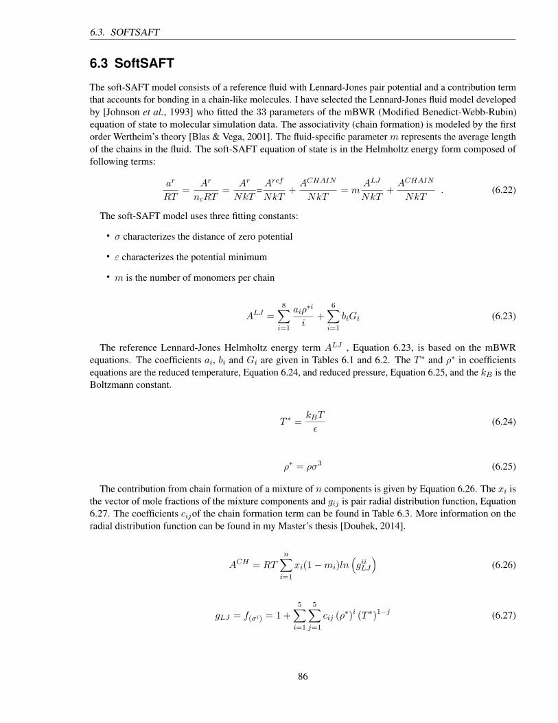
6.3. SOFTSAFT
6.3 SoftSAFT
The soft-SAFT model consists of a reference fluid with Lennard-Jones pair potential and a contribution termthat accounts for bonding in a chain-like molecules. I have selected the Lennard-Jones fluid model developedby [Johnson et al., 1993] who fitted the 33 parameters of the mBWR (Modified Benedict-Webb-Rubin)equation of state to molecular simulation data. The associativity (chain formation) is modeled by the firstorder Wertheim’s theory [Blas & Vega, 2001]. The fluid-specific parameter m represents the average lengthof the chains in the fluid. The soft-SAFT equation of state is in the Helmholtz energy form composed offollowing terms:
ar
RT= Ar
ncRT= Ar
NkT=Aref
NkT+ ACHAIN
NkT= m
ALJ
NkT+ ACHAIN
NkT. (6.22)
The soft-SAFT model uses three fitting constants:
• σ characterizes the distance of zero potential
• ε characterizes the potential minimum
• m is the number of monomers per chain
ALJ =8∑i=1
aiρ∗i
i+
6∑i=1
biGi (6.23)
The reference Lennard-Jones Helmholtz energy term ALJ , Equation 6.23, is based on the mBWRequations. The coefficients ai, bi and Gi are given in Tables 6.1 and 6.2. The T ∗ and ρ∗ in coefficientsequations are the reduced temperature, Equation 6.24, and reduced pressure, Equation 6.25, and the kB is theBoltzmann constant.
T ∗ = kBT
ε(6.24)
ρ∗ = ρσ3 (6.25)
The contribution from chain formation of a mixture of n components is given by Equation 6.26. The xi isthe vector of mole fractions of the mixture components and gij is pair radial distribution function, Equation6.27. The coefficients cijof the chain formation term can be found in Table 6.3. More information on theradial distribution function can be found in my Master’s thesis [Doubek, 2014].
ACH = RTn∑i=1
xi(1−mi)ln(giiLJ
)(6.26)
gLJ = f(σi) = 1 +5∑i=1
5∑j=1
cij (ρ∗)i (T ∗)1−j (6.27)
86
6.3. SOFTSAFT
Table 6.1: SoftSAFT model coefficients ai and bii ai
1 x1T∗ + x2
√T ∗ + x3 + x4/T
∗ + x5/T∗2
2 x6T∗ + x7 + x8/T
∗ + x9/T∗2
3 x10T∗ + x11 + x12/T
∗
4 x135 x14/T
∗ + x15/T∗2
6 x16/T∗
7 x17/T∗ + x18/T
∗2
8 x19/T∗2
i bi
1 x20/T∗2 + x21/T
∗3
2 x22/T∗2 + x23/T
∗3
3 x24/T∗2 + x25/T
∗3
4 x26/T∗2 + x28/T
∗3
5 x28/T∗2 + x29/T
∗3
6 x30/T∗2 + x31/T
∗3 + x32/T∗4
Table 6.2: SoftSAFT model coefficients Gii Gi
1 (1− F ) / (2γ)2 −
(Fρ∗2 − 2G1
)/ (2γ)
3 −(Fρ∗4 − 2G2
)/ (2γ)
4 −(Fρ∗6 − 2G3
)/ (2γ)
5 −(Fρ∗8 − 2G4
)/ (2γ)
6 −(Fρ∗10 − 2G5
)/ (2γ)
F = exp(−γρ∗2)
Table 6.3: SoftSAFT model coefficients ciji/j 1 2 3 4 51 0.493043466 2.152834989 -15.95568233 24.03599967 -8.6437958512 -0.470319831 1.147164749 37.88982802 -84.66712149 39.643914113 5.032548624 -25.91539923 -18.86225131 107.6370738 -66.602649744 -7.363315043 51.55356534 -40.51936926 -38.79669265 44.60513925 2.90436073 -24.41881287 31.50018677 -5.336892037 -9.518344018
87
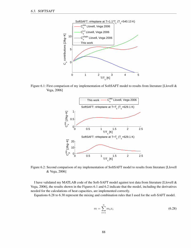
6.3. SOFTSAFT
0 1 2 3 4 5
0
5
10
SoftSAFT: nHeptane at T=1.1*Tc (T
c=540.13 K)
T/Tc [K]
Cv c
ontr
ibut
ions
[J/k
g−K
]
Cvres Llovell, Vega 2006
CvLJ Llovell, Vega 2006
Cvchain Llovell, Vega 2006
This work
Figure 6.1: First comparison of my implementation of SoftSAFT model to results from literature [Llovell &Vega, 2006]
0 0.5 1 1.5 2 2.50
0.5
1
SoftSAFT: nHeptane at T=Tc (T
c=629.1 K)
T/Tc [K]
Cvre
s [J/k
g−K
]
This work Cvres Llovell, Vega 2006
0 0.5 1 1.5 2 2.50
10
20
SoftSAFT: nHeptane at T=Tc (T
c=629.1 K)
T/Tc [K]
Cpre
s [J/k
g−K
]
Figure 6.2: Second comparison of my implementation of SoftSAFT model to results from literature [Llovell& Vega, 2006]
I have validated my MATLAB code of the Soft-SAFT model against test data from literature [Llovell &Vega, 2006], the results shown in the Figures 6.1 and 6.2 indicate that the model, including the derivativesneeded for the calculations of heat capacities, are implemented correctly.
Equations 6.28 to 6.30 represent the mixing and combination rules that I used for the soft-SAFT model.
m =n∑i=1
mixi (6.28)
88
6.4. SPC-SAFT
σ3m =
n∑i=1
n∑j=1
xixjσ3ij (6.29)
εmσ3m =
n∑i=1
n∑j=1
xixjεijσ3ij (6.30)
Conventional (Lorentz-Berthold) combination rules with one binary interaction parameter kij were usedfor the size and energy parameters:
σij = σii + σjj2 , (6.31)
εij = (1− kij) (εiiεjj)1/2 . (6.32)
6.4 sPC-SAFT
The PC-SAFT equation of state was originally published by Gross and Sadowski [Gross & Sadowski, 2001].The molecules are considered to be chains of spheres interacting with the square-well potential. The potentialis divided into a reference repulsive part and a perturbation part that accounts for the attractive interactions.The hard-chain fluid is characterized by the sphere-segments diameter σ and by the average number ofsegments in the chain m. The interaction between two chain-like molecules is considered to be the sum of thewhole interaction between individual atoms - spherical segments. The chain molecules are also consideredto be spherical, the first and second order perturbation terms are used to account for attractive interactionsbetween the chain molecules. A group contribution method has been developed for the sPC-SAFT equationof state [Tihic et al., 2008]. The method provides a relatively good estimate of the fitting parameters namelyfor polymer molecules.
The residual Helmholtz free energy Ar (Equation 6.33) consists of two terms: the hard-chain referencepart Ahc and the perturbation part Apert which is further split into the first and second order perturbations A1
and A2.
ar
RT= Ar
nRT= Ar
NkBT=Ahc
NkBT+ Apert
NkBT= Ahc
NkBT+ A1NkBT
+ A2NkBT
(6.33)
The PC-SAFT model uses three fitting parameters:
• σ - characterizes the distance of zero potential
• ε - characterizes the potential minimum
• m - is the number of monomers per chain
89
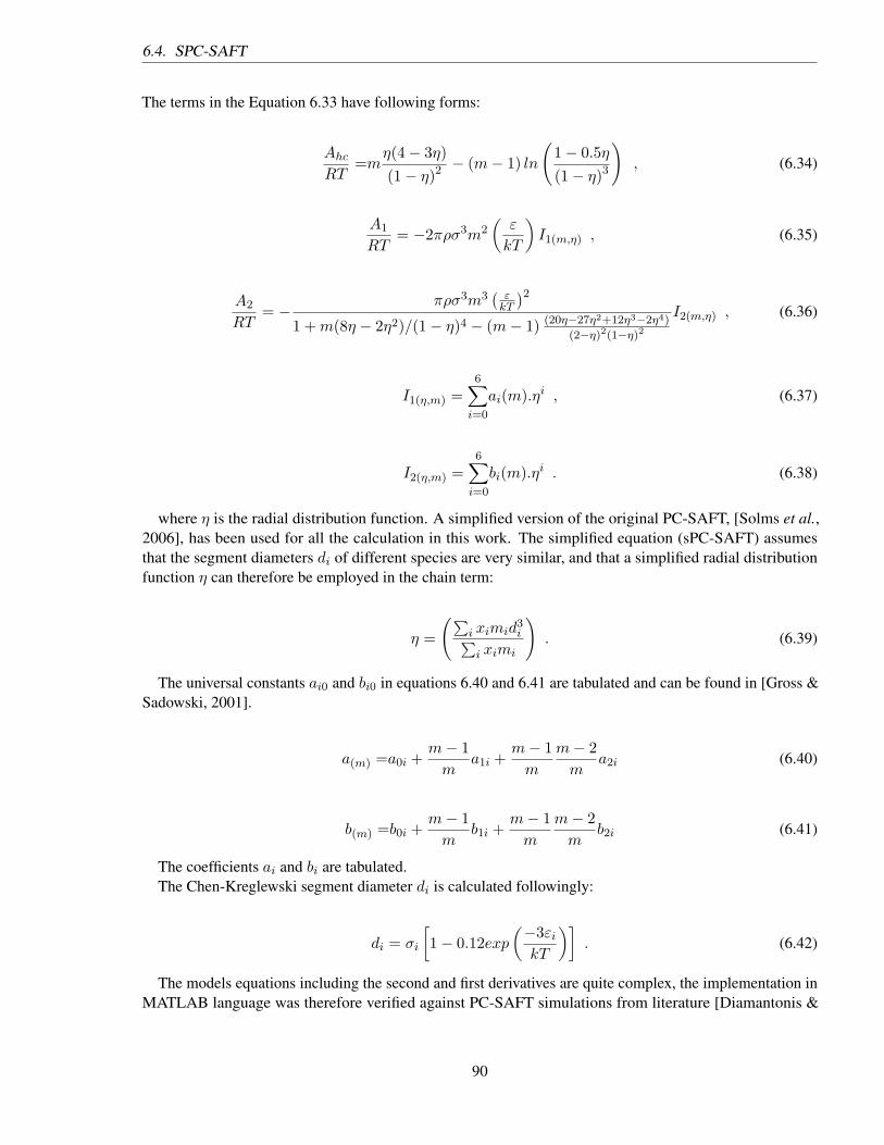
6.4. SPC-SAFT
The terms in the Equation 6.33 have following forms:
AhcRT
=mη(4− 3η)(1− η)2 − (m− 1) ln
(1− 0.5η(1− η)3
), (6.34)
A1RT
= −2πρσ3m2(ε
kT
)I1(m,η) , (6.35)
A2RT
= −πρσ3m3 ( ε
kT
)21 +m(8η − 2η2)/(1− η)4 − (m− 1) (20η−27η2+12η3−2η4)
(2−η)2(1−η)2
I2(m,η) , (6.36)
I1(η,m) =6∑i=0ai(m).ηi , (6.37)
I2(η,m) =6∑i=0bi(m).ηi . (6.38)
where η is the radial distribution function. A simplified version of the original PC-SAFT, [Solms et al.,2006], has been used for all the calculation in this work. The simplified equation (sPC-SAFT) assumesthat the segment diameters di of different species are very similar, and that a simplified radial distributionfunction η can therefore be employed in the chain term:
η =(∑
i ximid3i∑
i ximi
). (6.39)
The universal constants ai0 and bi0 in equations 6.40 and 6.41 are tabulated and can be found in [Gross &Sadowski, 2001].
a(m) =a0i + m− 1m
a1i + m− 1m
m− 2m
a2i (6.40)
b(m) =b0i + m− 1m
b1i + m− 1m
m− 2m
b2i (6.41)
The coefficients ai and bi are tabulated.The Chen-Kreglewski segment diameter di is calculated followingly:
di = σi
[1− 0.12exp
(−3εikT
)]. (6.42)
The models equations including the second and first derivatives are quite complex, the implementation inMATLAB language was therefore verified against PC-SAFT simulations from literature [Diamantonis &
90
6.5. SAFT-BACK
200 250 300 350 400 450 50050
100150200250
sPC−SAFT: CO2 at 12 MPa
Temperature [K]
Cpre
s [J/k
g−K
]
This work Diamantois, Economou, 2011
200 250 300 350 400 450 5000
2
4
sPC−SAFT: CO2 at 10 MPa
Temperature [K]
Cvre
s [J/k
g−K
]
Figure 6.3: Comparison of my implementation of sPC-SAFT model to results from literature [Diamantonis& Economou, 2011]
Economou, 2011]. Figure 6.3 shows that the model works correctly, including the derivatives for calculationsof heat capacities.
Conventional combination rules with one binary interaction parameter kij were used for the mixtures,equations 6.43 and 6.44.
σij = σii + σjj2 (6.43)
εij = (1− kij) (εiiεjj)1/2 (6.44)
Note that the term for the equations for the segment diameter di and packing fraction η already takes intoaccount the species in the mixture.
6.5 SAFT-BACK
The BACK (Boublik–Alder–Chen–Kreglewski) equation of state [Boublik, 2007] is an augmented van derWaals equation of state. The equation of state was developed on a statistical description of non-sphericalconvex molecules. It has been proven that BACK is quite suitable for simple non-associating fluids such asmethane, nitrogen, hydrogen and their mixtures. The BACK equation of state provides good prediction evenclose to the critical point and in the supercritical region. The statistical association fluid theory was applied tothis equation to obtain a model for more complex molecules and associating fluids [Zhi-Yu et al., 2000]. Asa result, the molecule is modeled as a chain of hard convex body segments. The residual Helmholtz energy,Equation 6.45, is divided into four parts: the hard convex body contribution Ahc, the chain formation termAchain,hcb, the dispersion term Adis and the dispersion due to chain formation Achain,dis. The SAFT-BACKmodel uses four fitting parameters:
91
6.5. SAFT-BACK
• α - geometry of a hard convex body (nonsphericity)
• m - segment number
• u0 - segment dispersion parameter (energetic parameter)
• υ00 - segment volume parameter
ares
RT= Ares
nRT= Ares
NkBT=Ahcb
NkBT+ Achain,hcb
NkBT+ Adis
NkBT+ Achain,dis
NkBT(6.45)
The first term is the Helmholtz energy of a hard convex body as defined by Boublik [Boublik, 2007]:
Ahcb
NkBT=m
[α2
(1− η)2 −α2 − 3α
1− η − (1− α2)ln (1− η − 3α)]. (6.46)
The m is the segment parameter number, η is the packing fraction and α is a parameter related to geometryof hard a convex body. The packing factor is defined in following way:
η=16πNAVmρd
3 . (6.47)
The segment diameter d is calculated using the model parameter u0 called the segment dispersion and σwhich is evaluated from another model parameter ν00 called segment volume parameter:
d=σ
[1− 0.12exp
(− 3u0
kBT
)], (6.48)
σ = 3
√6 ν00
πNAV. (6.49)
Next term is the contribution from the chain of hard convex bodies:
Ahcb
NkBT= (1−m) lnghcb . (6.50)
where the ghcb is the mean radial distribution function:
ghcb(d) = 11− η + 3α (1 + α) η
(1− η)2 (1 + 3α)+ 2α2η2
(1− η)3 (1 + 3α). (6.51)
The dispersion term comes from work of Aldler [Alder et al., 1972]:
Adis
NkBT= m
∑i
∑j
Dij
(u
kBT
)i( η√2π/6
)j. (6.52)
92
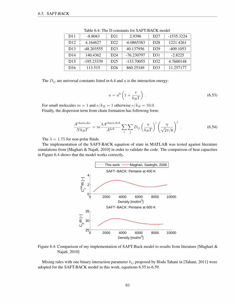
6.5. SAFT-BACK
Table 6.4: The D constants for SAFT-BACK modelD11 -8.8043 D21 2.9396 D27 -1535.3224D12 4.164627 D22 -6.0865383 D28 1221.4261D13 -48.203555 D23 40.137956 D29 -409.1053D14 140.4362 D24 -76.230797 D31 -2.8225D15 -195.23339 D25 -133.70055 D32 4.7600148D16 113.515 D26 860.25349 D33 11.257177
The Dij are universal constants listed in 6.4 and u is the interaction energy:
u = u0(
1 + e
kBT
). (6.53)
For small molecules m = 1 and e/kB = 1 otherwise e/kB = 10.0.Finally, the dispersion term from chain formation has following form:
Achain,dis
NkBT= m
λAchain,hcb
Ahcb
∑i
∑j
Dij
(u
kBT
)i( η√2π/6
)j. (6.54)
The λ = 1.75 for non-polar fluids.The implementation of the SAFT-BACK equation of state in MATLAB was tested against literature
simulations from [Maghari & Najafi, 2010] in order to validate the code. The comparison of heat capacitiesin Figure 6.4 shows that the model works correctly.
0 2000 4000 6000 8000 100000
2
4SAFT−BACK: Pentane at 400 K
Density [mol/m3]
Cvre
s /R [−
]
This work Maghari, Sadeghi, 2006
0 2000 4000 6000 8000 1000025
30
35SAFT−BACK: Pentane at 600 K
Density [mol/m3]
Cp/R
[−]
Figure 6.4: Comparison of my implementation of SAFT-Back model to results from literature [Maghari &Najafi, 2010]
Mixing rules with one binary interaction parameter kij proposed by Hoda Tahani in [Tahani, 2011] wereadopted for the SAFT-BACK model in this work, equations 6.55 to 6.59.
93

6.6. SPEED OF SOUND AND MOLECULAR RELAXATION
m =n∑i=1
mixi (6.55)
αm =∑nj=1 αimixi∑nj=1mixi
(6.56)
(uokB
)m
=n∑i=1
n∑j=1
xixjεij
(uokB
)ij
(6.57)
(uokB
)ij
=√(
uokB
)i
(uokB
)j
(1− kij) (6.58)
The mixing rule for the segment diameter is following:
dm =(∑n
j=1 d3imixi∑n
j=1mixi
)1/3
, (6.59)
where di is the segment diameter d of mixture component i.
6.6 Speed of sound and molecular relaxation
The actual measured speed of sound in polyatomic gases is a function of frequency since the sound-wavepropagation is not purely isoentropic. The dispersion effects cause an increase in entropy and result insound absorption and speed of sound shift (dispersion). The so called molecular relaxation is characterizedby molecular relaxation time τ and it causes the strongest speed of sound dispersion among the variousphenomena that affect the speed of sound. The sound absorption due to the molecular relaxation is highestwhen the sound frequency ω = 2πf approaches the relaxation frequency (ωτ = 1) and it is zero at low orhigh frequencies, this enables the experimental investigation of the relaxation times. Note that the absorptiondue to the molecular relaxation superimposes on the classical absorption (dissipation of sonic energy intoheat given by the Stokes-Kirchhoff relation) due to the viscosity and heat conduction. The sound intensity ILin the distance L decreases from the source intensity I0 in following manner:
IL = I0e−2αaL , (6.60)
where αa is the attenuation coefficient that consist of viscous and thermal contribution and it can beevaluated from the viscosity, density, coefficient of thermal expansion, specific heats, speed of sound andfrequency. The equations of states discussed in section 2.1 give so called zero-frequency speed of soundwhich is a speed of sound that would correspond to a sound wave with frequency of zero hertz. One canimagine this values as an extrapolation of sound speed measured at various frequencies. The variationbetween the zero-hertz frequency speed of sound and infinite-frequency speed of sound is usually around10%.
94
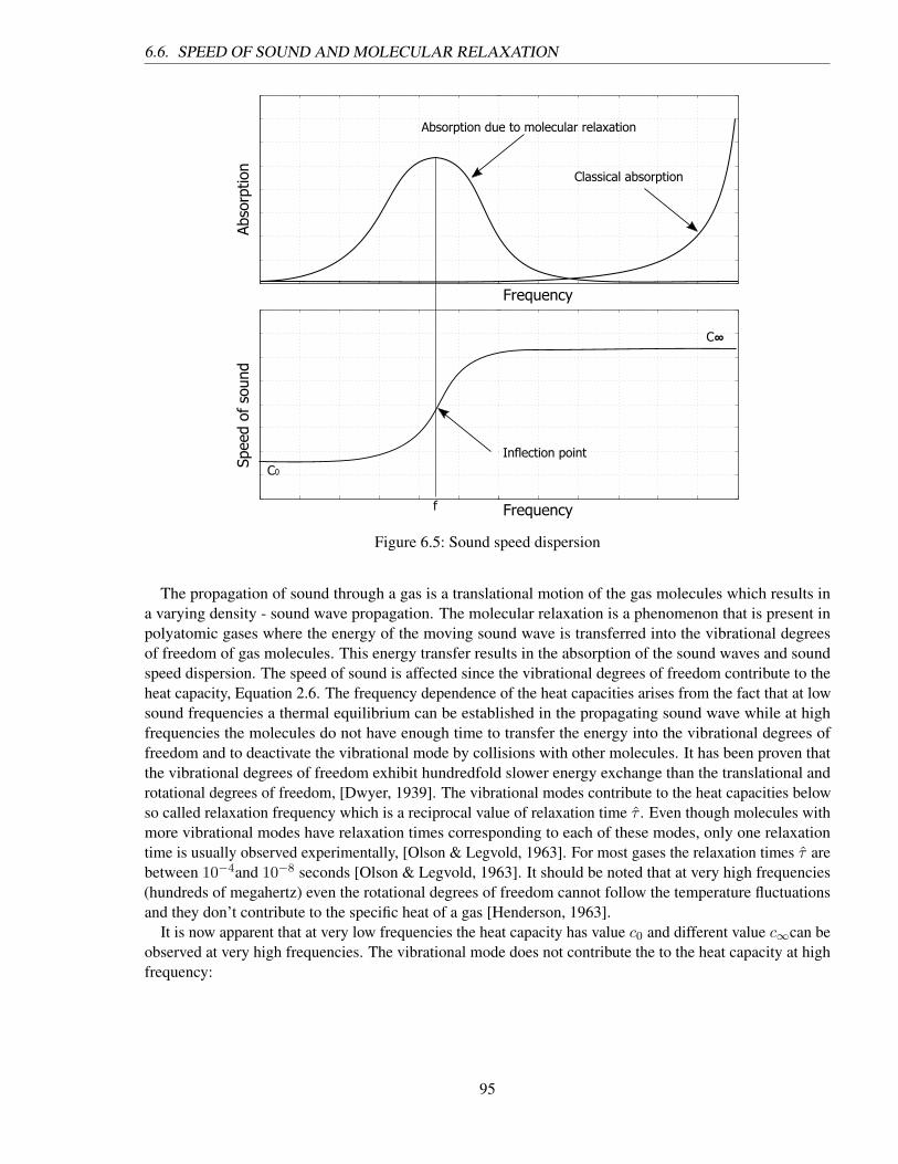
6.6. SPEED OF SOUND AND MOLECULAR RELAXATION
Frequency
Abso
rptio
n
Classical absorption
Frequency
Spee
d of
sou
nd
C∞
Inflection point
C0
Absorption due to molecular relaxation
f
Figure 6.5: Sound speed dispersion
The propagation of sound through a gas is a translational motion of the gas molecules which results ina varying density - sound wave propagation. The molecular relaxation is a phenomenon that is present inpolyatomic gases where the energy of the moving sound wave is transferred into the vibrational degreesof freedom of gas molecules. This energy transfer results in the absorption of the sound waves and soundspeed dispersion. The speed of sound is affected since the vibrational degrees of freedom contribute to theheat capacity, Equation 2.6. The frequency dependence of the heat capacities arises from the fact that at lowsound frequencies a thermal equilibrium can be established in the propagating sound wave while at highfrequencies the molecules do not have enough time to transfer the energy into the vibrational degrees offreedom and to deactivate the vibrational mode by collisions with other molecules. It has been proven thatthe vibrational degrees of freedom exhibit hundredfold slower energy exchange than the translational androtational degrees of freedom, [Dwyer, 1939]. The vibrational modes contribute to the heat capacities belowso called relaxation frequency which is a reciprocal value of relaxation time τ . Even though molecules withmore vibrational modes have relaxation times corresponding to each of these modes, only one relaxationtime is usually observed experimentally, [Olson & Legvold, 1963]. For most gases the relaxation times τ arebetween 10−4and 10−8 seconds [Olson & Legvold, 1963]. It should be noted that at very high frequencies(hundreds of megahertz) even the rotational degrees of freedom cannot follow the temperature fluctuationsand they don’t contribute to the specific heat of a gas [Henderson, 1963].
It is now apparent that at very low frequencies the heat capacity has value c0 and different value c∞can beobserved at very high frequencies. The vibrational mode does not contribute the to the heat capacity at highfrequency:
95
6.6. SPEED OF SOUND AND MOLECULAR RELAXATION
cv∞ = cv0 − cv vib . (6.61)
The heat capacity can be expressed as a function of the complex frequency ω :
cvω = cv∞ + cv vib1 + iωτ
. (6.62)
In fact, there are multiple vibrational modes and each has a corresponding relaxation time τi
cvω = cv∞ +∑i
cv vibi1 + iωτi
. (6.63)
However, as mentioned above only one relaxation time is usually observed experimentally. The real partof the heat capacity is equal to
cvω = c2vo + ω2τ2c2
v∞cvo + ω2τ2cv∞
. (6.64)
The relations above apply to pure gas. Unfortunately, the processes in a mixture of relaxing gasses arenot fully understood. Several thorough investigations of the sound dispersion in moist air can be foundin scientific literature, for instance [Dean, 1979]. Number of models have been proposed to evaluate therelaxation time and consequently the sound absorption and dispersion of a mixture ( for instance [Liu et al.,2017] and [Zhang et al., 2014]). Many of this models are very complex and are out of the scope of this work,which is focused es on easy-to-use reliable models. The simplest approach is to use following mixing rulesfor binary mixture of relaxing (component A) and nonrelaxing gas:
cmixvω = cmixv∞ + xcAv vib1 + iωτA
. (6.65)
Where x is the mole fraction of the relaxing component A. In similar manner, the simplest approach leadsto the following term for the specific heat of mixture of two relaxing gases with one dominant relaxationtime:
cmixvω = cmixv∞ + xcAv vib1 + iωτA
+ (x− 1)cBv vib1 + iωτ
. (6.66)
Fortunately, the dispersion effect due to the molecular relaxation can be avoided by carefully choosing thesound frequency for the speed of sound measurements. A frequency sweep can be used to evaluate the soundattenuation and if a peak is found a much higher or lower frequency can be used to measure the speed ofsound to avoid the dispersion region. A wide-range of frequencies from several kilohertz to one megahertzcan be used with the time-of-flight measurement methods.
96
6.6. SPEED OF SOUND AND MOLECULAR RELAXATION
6.6.1 Relaxation times
The vibrational relaxation times increase with the temperature and decrease with pressure. The speed ofsound against frequency divided by pressure is used on the horizontal axis (units are then cycle per second-atmosphere) and the square of sound velocity is plotted on the vertical axis of plots describing the relaxationbehaviour. The Landau-Teller relation can be used to express the relaxation time τ as a function of pressurep and temperature T :
τ = K1pe
( K23√T
), (6.67)
where K1and K2 are the fluid specific constants. The relaxation times are usually obtained experimentallyfrom an inflection in the sound absorption curve. Relaxation times τ for selected fluids are listed in table6.5, the relaxation frequency f = 1/τ is also included since it gives better picture about the gas behaviourfor our purposes. As a reminder, the relaxation frequency corresponds to the sound absorption peak causedby molecular relaxation. Most of the simple gases such as nitrogen (R-728) and oxygen exhibit very longrelaxation times. However, the CO2 (R-744) and methane (R-50) exhibit relaxation and strong ultrasoundabsorption at very inconvenient frequencies. The sound dispersion with these two gases can be expectedwhen common measurement techniques are employed. One can see that most of the refrigerants have shortrelaxation times and therefore the sound dispersion is not a concern with usual speed of sound measurementtechniques that work with ultrasound at few tens of kilohertz.
97
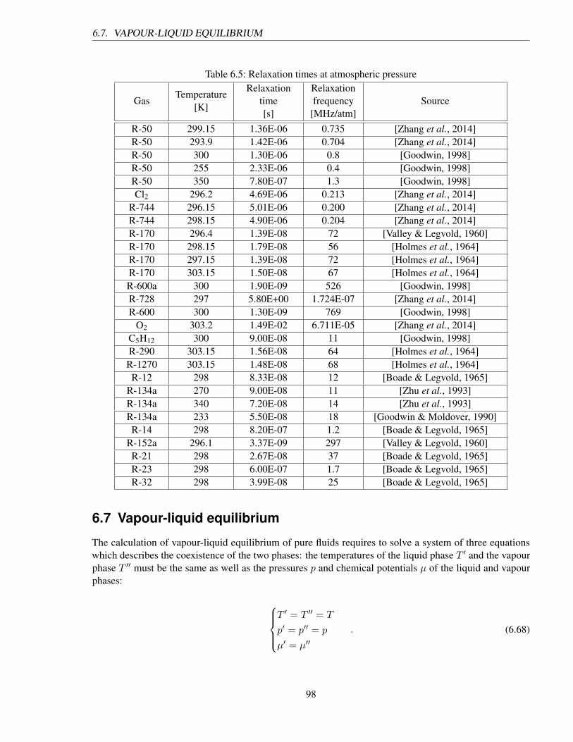
6.7. VAPOUR-LIQUID EQUILIBRIUM
Table 6.5: Relaxation times at atmospheric pressure
GasTemperature
[K]
Relaxationtime[s]
Relaxationfrequency
[MHz/atm]Source
R-50 299.15 1.36E-06 0.735 [Zhang et al., 2014]R-50 293.9 1.42E-06 0.704 [Zhang et al., 2014]R-50 300 1.30E-06 0.8 [Goodwin, 1998]R-50 255 2.33E-06 0.4 [Goodwin, 1998]R-50 350 7.80E-07 1.3 [Goodwin, 1998]Cl2 296.2 4.69E-06 0.213 [Zhang et al., 2014]
R-744 296.15 5.01E-06 0.200 [Zhang et al., 2014]R-744 298.15 4.90E-06 0.204 [Zhang et al., 2014]R-170 296.4 1.39E-08 72 [Valley & Legvold, 1960]R-170 298.15 1.79E-08 56 [Holmes et al., 1964]R-170 297.15 1.39E-08 72 [Holmes et al., 1964]R-170 303.15 1.50E-08 67 [Holmes et al., 1964]R-600a 300 1.90E-09 526 [Goodwin, 1998]R-728 297 5.80E+00 1.724E-07 [Zhang et al., 2014]R-600 300 1.30E-09 769 [Goodwin, 1998]
O2 303.2 1.49E-02 6.711E-05 [Zhang et al., 2014]C5H12 300 9.00E-08 11 [Goodwin, 1998]R-290 303.15 1.56E-08 64 [Holmes et al., 1964]R-1270 303.15 1.48E-08 68 [Holmes et al., 1964]R-12 298 8.33E-08 12 [Boade & Legvold, 1965]
R-134a 270 9.00E-08 11 [Zhu et al., 1993]R-134a 340 7.20E-08 14 [Zhu et al., 1993]R-134a 233 5.50E-08 18 [Goodwin & Moldover, 1990]R-14 298 8.20E-07 1.2 [Boade & Legvold, 1965]
R-152a 296.1 3.37E-09 297 [Valley & Legvold, 1960]R-21 298 2.67E-08 37 [Boade & Legvold, 1965]R-23 298 6.00E-07 1.7 [Boade & Legvold, 1965]R-32 298 3.99E-08 25 [Boade & Legvold, 1965]
6.7 Vapour-liquid equilibrium
The calculation of vapour-liquid equilibrium of pure fluids requires to solve a system of three equationswhich describes the coexistence of the two phases: the temperatures of the liquid phase T ′ and the vapourphase T ′′ must be the same as well as the pressures p and chemical potentials µ of the liquid and vapourphases:
T ′ = T ′′ = T
p′ = p′′ = p
µ′ = µ′′. (6.68)
98
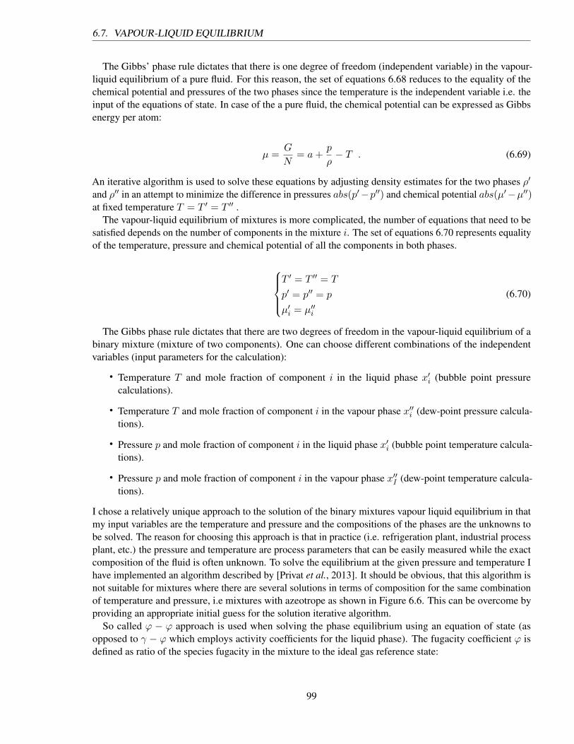
6.7. VAPOUR-LIQUID EQUILIBRIUM
The Gibbs’ phase rule dictates that there is one degree of freedom (independent variable) in the vapour-liquid equilibrium of a pure fluid. For this reason, the set of equations 6.68 reduces to the equality of thechemical potential and pressures of the two phases since the temperature is the independent variable i.e. theinput of the equations of state. In case of the a pure fluid, the chemical potential can be expressed as Gibbsenergy per atom:
µ = G
N= a+ p
ρ− T . (6.69)
An iterative algorithm is used to solve these equations by adjusting density estimates for the two phases ρ′
and ρ′′ in an attempt to minimize the difference in pressures abs(p′−p′′) and chemical potential abs(µ′−µ′′)at fixed temperature T = T ′ = T ′′ .
The vapour-liquid equilibrium of mixtures is more complicated, the number of equations that need to besatisfied depends on the number of components in the mixture i. The set of equations 6.70 represents equalityof the temperature, pressure and chemical potential of all the components in both phases.
T ′ = T ′′ = T
p′ = p′′ = p
µ′i = µ′′i
(6.70)
The Gibbs phase rule dictates that there are two degrees of freedom in the vapour-liquid equilibrium of abinary mixture (mixture of two components). One can choose different combinations of the independentvariables (input parameters for the calculation):
• Temperature T and mole fraction of component i in the liquid phase x′i (bubble point pressurecalculations).
• Temperature T and mole fraction of component i in the vapour phase x′′i (dew-point pressure calcula-tions).
• Pressure p and mole fraction of component i in the liquid phase x′i (bubble point temperature calcula-tions).
• Pressure p and mole fraction of component i in the vapour phase x′′I (dew-point temperature calcula-tions).
I chose a relatively unique approach to the solution of the binary mixtures vapour liquid equilibrium in thatmy input variables are the temperature and pressure and the compositions of the phases are the unknowns tobe solved. The reason for choosing this approach is that in practice (i.e. refrigeration plant, industrial processplant, etc.) the pressure and temperature are process parameters that can be easily measured while the exactcomposition of the fluid is often unknown. To solve the equilibrium at the given pressure and temperature Ihave implemented an algorithm described by [Privat et al., 2013]. It should be obvious, that this algorithm isnot suitable for mixtures where there are several solutions in terms of composition for the same combinationof temperature and pressure, i.e mixtures with azeotrope as shown in Figure 6.6. This can be overcome byproviding an appropriate initial guess for the solution iterative algorithm.
So called ϕ − ϕ approach is used when solving the phase equilibrium using an equation of state (asopposed to γ − ϕ which employs activity coefficients for the liquid phase). The fugacity coefficient ϕ isdefined as ratio of the species fugacity in the mixture to the ideal gas reference state:
99
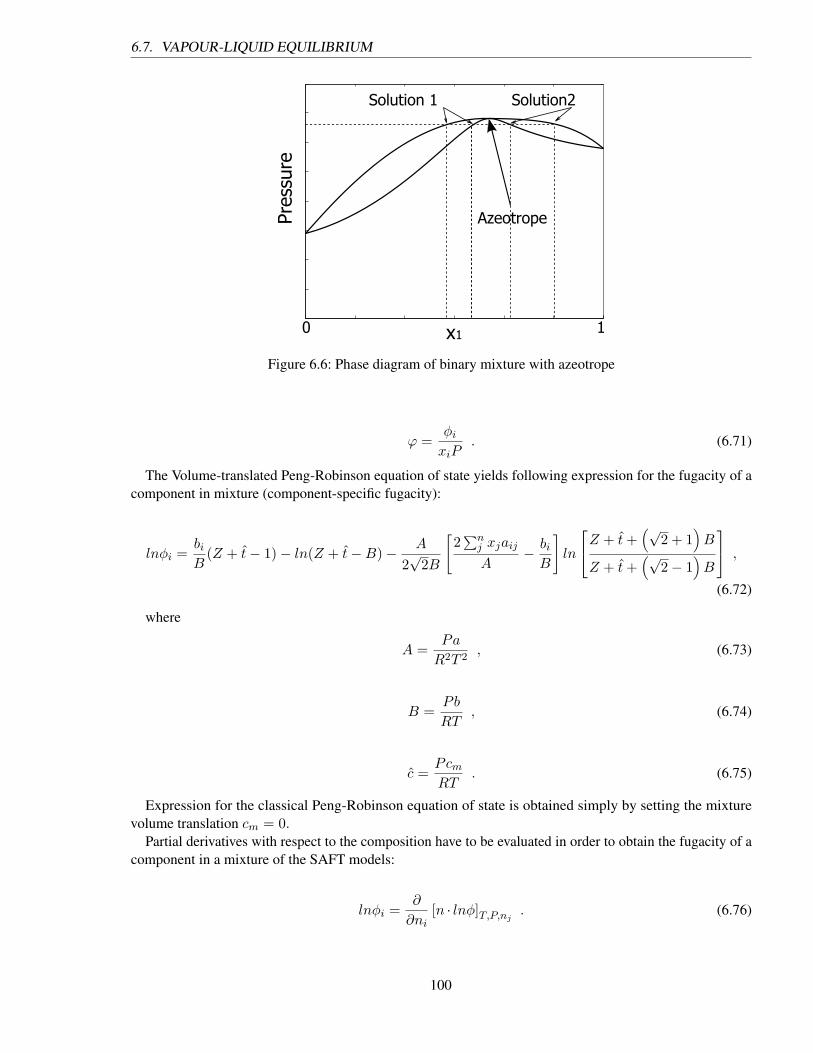
6.7. VAPOUR-LIQUID EQUILIBRIUM
x1
Pres
sure
Azeotrope
0 1
Solution 1 Solution2
Figure 6.6: Phase diagram of binary mixture with azeotrope
ϕ = φixiP
. (6.71)
The Volume-translated Peng-Robinson equation of state yields following expression for the fugacity of acomponent in mixture (component-specific fugacity):
lnφi = biB
(Z + t− 1)− ln(Z + t−B)− A
2√
2B
[2∑nj xjaij
A− biB
]ln
Z + t+(√
2 + 1)B
Z + t+(√
2− 1)B
,
(6.72)
where
A = Pa
R2T 2 , (6.73)
B = Pb
RT, (6.74)
c = PcmRT
. (6.75)
Expression for the classical Peng-Robinson equation of state is obtained simply by setting the mixturevolume translation cm = 0.
Partial derivatives with respect to the composition have to be evaluated in order to obtain the fugacity of acomponent in a mixture of the SAFT models:
lnφi = ∂
∂ni[n · lnφ]T,P,nj . (6.76)
100
6.7. VAPOUR-LIQUID EQUILIBRIUM
Where n is the total number of moles, ni is the number of moles of the component i and nj is the numberof moles of other components j. Since the equations of SAFT models are quite complex, the partial derivationwith respect to composition are usually solved numerically: [Rand, 2004]:
lnφi = (1 + dxi)lnφ+dni − (1− dxi)lnφ−dni2dxi
. (6.77)
I have used following expressions to obtain the component-specific fugacity from the SAFT equations ofstate from partial derivative of Helmholtz energy with respect to the composition:
lnφi = µresikT− lnZ , (6.78)
µresikT
= ares + (Z − 1) +[∂ares
∂xi
]T,ρ,xj 6=i
−∑
xk
[∂ares
∂x
]T,ρ,xk 6=j
. (6.79)
To solve the vapour-liquid equilibrium of a binary mixture using the ϕ−ϕ approach and with the pressureP and temperature T as the input variables one has to solve following set of equations [Privat et al., 2013]:
x′1ϕ
′1 = x′′1ϕ
′′1
(1− x′1)ϕ′2 = (1− x′′1)ϕ′′2. (6.80)
The fugacity coefficients ϕ are obtained from equations of state:
ϕ′i = ϕ(T,ρ′,x′i) . (6.81)
The vapour and liquid phase densities ρ′′ and ρ′ are obtained from the known pressure and temperature fora given composition in each step of the iterative algorithm:
P = P(T,ρ′,x′) = P(T,ρ′′,x′′) . (6.82)
The set of equations 6.80 can be rewritten in a matrix notation:
[ϕ′1 −ϕ′′1−ϕ′2 ϕ′′2
] [x′1x′′1
]=[
0ϕ′′2 − ϕ′2
]. (6.83)
This can be written in a matrix notation and we get a classical linear form:
[A(x)
][x] =
[B(x)
]. (6.84)
A simple iteration algorithm can be employed to solve the linear form. Firstly, an initial guess of thevector of vapour and liquid x1 compositions is used for the first iteration. Subsequent iterations update thecomposition vector using following iteration scheme:
101
6.7. VAPOUR-LIQUID EQUILIBRIUM
[xk+1
]=[A(x)
]−1 [B(x)
]. (6.85)
The iterations are stopped when a convergence criterion is fulfilled:
δ =[∣∣x′′1ϕ′′1 − x′1F ′1∣∣+ ∣∣(1− x′′1)ϕ′′2 − (1− x′1)F ′2∣∣] ≤ 10−5 . (6.86)
The important properties of the iteration algorithm for a solution of vapour-liquid equilibrium are:
• The algorithm is robust with respect the to initial guess of the composition vector. The iteration willconverge even with an initial guess far from the solution;
• The algorithm is relatively slow. It can take more than ten thousand iterations to converge when thetemperature is close to the critical temperature of the mixture;
• A trivial solution is reached when the temperature is above the critical temperature of the mixture.
The algorithm is also slow (it requires large number of iterations) when solving the equilibrium at temperatureabove the critical point of some of the components. Trying to solve the equilibrium of a mixture above itscritical point will lead to unphysical results.
102
6.7. VAPOUR-LIQUID EQUILIBRIUM
Bibliography
chapter 6: Thermodynamic Models
[Ahlers & Gmehling, 2001] Ahlers, J., & Gmehling, J. 2001. Development of an universal group contri-bution equation of state: I. Prediction of liquid densities for pure compounds with a volume translatedPeng-Robinson equation of state. Fluid Phase Equilibria, 191(1), 177 – 188.
[Alder et al., 1972] Alder, B. J., Young, D. A., & Mark, M. A. 1972. Studies in Molecular Dynamics. X.Corrections to the Augmented van der Waals Theory for the Square Well Fluid. The Journal of ChemicalPhysics, 56(6), 3013–3029.
[Blas & Vega, 2001] Blas, F. J., & Vega, L. F. 2001. Thermodynamic properties and phase equilibria ofbranched chain fluids using first- and second-order Wertheim’s thermodynamic perturbation theory. TheJournal of Chemical Physics, 115(8), 3906–3915.
[Boade & Legvold, 1965] Boade, R. R., & Legvold, S. 1965. Sound Dispersion in Binary Mixtures ofHalomethane Gases. The Journal of Chemical Physics, 42(2), 569–573.
[Boublik, 2007] Boublik, T. 2007. BACK equation of state for simple compounds. Journal of MolecularLiquids, 134(1), 151 – 155. EMLG/JMLG 2005 Special Issue.
[Dean, 1979] Dean, E. A. 1979. Atmospheric Effects on the Speed of Sound. Battelle Columbus LabsDurham Nc.
[Diamantonis & Economou, 2011] Diamantonis, N. I., & Economou, I. G. 2011. Evaluation of StatisticalAssociating Fluid Theory (SAFT) and Perturbed Chain-SAFT Equations of State for the Calculation ofThermodynamic Derivative Properties of Fluids Related to Carbon Capture and Sequestration. Energy &Fuels, 25(7), 3334–3343.
[Doubek, 2014] Doubek, M. 2014. Thermophysical properties of fluids experiment and simulations. Master’sthesis, Czech Technical University, Faculty of Mechanical Engineering.
[Dwyer, 1939] Dwyer, R. J. 1939. The Persistence of Molecular Vibration in Collisions. The Journal ofChemical Physics, 7(1), 40–44.
[Goodwin, 1998] Goodwin, A. R. H. 1998 (February). Thermophysical Properties of Chlorine from Speed-of-Sound Measurements. Ph.D. thesis, University of London.
[Goodwin & Moldover, 1990] Goodwin, A. R. H., & Moldover, M. R. 1990. Thermophysical propertiesof gaseous refrigerants from speed of sound measurements. I. Apparatus, model, and results for 1,1,1,2-tetrafluoroethane R134a. The Journal of Chemical Physics, 93(4), 2741–2753.
[Gross & Sadowski, 2001] Gross, J., & Sadowski, G. 2001. Perturbed-Chain SAFT: An Equation of StateBased on a Perturbation Theory for Chain Molecules. Industrial & Engineering Chemistry Research,40(4), 1244–1260.
103
6.7. VAPOUR-LIQUID EQUILIBRIUM
[Henderson, 1963] Henderson, M. C. 1963. Sound in Air: Absorption and Dispersion. Sound: Its uses andControl, 2(6), 28–36.
[Holmes et al., 1964] Holmes, R., Jones, G. R., & Pusat, N. 1964. Vibrational Relaxation in Propane,Propylene, and Ethane. The Journal of Chemical Physics, 41(8), 2512–2516.
[Iwai et al., 1988] Iwai, Y., Margerum, M. R., & Lu, B. C.-Y. 1988. A new three-parameter cubic equationof state for polar fluids and fluid mixtures. Fluid Phase Equilibria, 42, 21 – 41.
[Johnson et al., 1993] Johnson, J. K., Zollweg, J. A., & Gubbins, K. E. 1993. The Lennard-Jones equationof state revisited. Molecular Physics, 78(3), 591–618.
[Lin & Duan, 2005] Lin, H., & Duan, Y.-Y. 2005. Empirical correction to the Peng-Robinson equation ofstate for the saturated region. Fluid Phase Equilibria, 233(2), 194 – 203.
[Liu et al., 2017] Liu, T., Wang, S., & Zhu, M. 2017. Decomposition of effective specific heat of molecularrelaxation for gas detection in a mixture. The Journal of the Acoustical Society of America, 141(3),1844–1851.
[Llovell & Vega, 2006] Llovell, F., & Vega, L. F. 2006. Prediction of Thermodynamic Derivative Propertiesof Pure Fluids through the Soft-SAFT Equation of State. The Journal of Physical Chemistry B, 110(23),11427–11437. PMID: 16771416.
[Maghari & Najafi, 2010] Maghari, Ali, & Najafi, Mohsen. 2010. On the Calculation of Surface Tensionsof n-Alkanes Using the Modified SAFT-BACK-DFT Approach. Journal of Solution Chemistry, 39(1),31–41.
[Magoulas & Tassios, 1990] Magoulas, K., & Tassios, D. 1990. Thermophysical properties of n-Alkanesfrom C1 to C20 and their prediction for higher ones. Fluid Phase Equilibria, 56(Supplement C), 119 –140.
[Medeiros & Tellez-Arredondo, 2008] Medeiros, M., & Tellez-Arredondo, P. 2008. Cubic Two-State Equa-tion of State for Associating Fluids. Ind. Eng. Chem. Res, 47(15), 5723–5733.
[Olson & Legvold, 1963] Olson, J. R., & Legvold, S. 1963. Sound Dispersion in Substituted Methane-inertGas Mixtures. The Journal of Chemical Physics, 39(11), 2902–2908.
[Privat et al., 2013] Privat, R., Jaubert, J.-N., & Privat, Y. 2013. A simple and unified algorithm to solvefluid phase equilibria using either the gamma-phi or the phi-phi approach for binary and ternary mixtures.Computers & Chemical Engineering, 50, 139 – 151.
[Rand, 2004] Rand, M. 2004 (12). Practical Equation of State for Non-Spherical and Asymetric Systems.Dissertation thesis, University of Stellenbosch.
[Solms et al., 2006] Solms, N., Kouskoumvekaki, I. A., Michelsen, M. L., & Kontogeorgis, G. M. 2006.Capabilities, limitations and challenges of a simplified PC-SAFT equation of state. Fluid Phase Equilibria,241(1), 344 – 353. A Festschrift in Honor of John M. Prausnitz.
[Tahani, 2011] Tahani, H. 2011 (November). Determination of the Velocity of Sound in Reservoir FluidsUsing an Equation of State. Submitted for the degree of Doctor of Philosophy in Petroleum Engineering,Heriot-Watt University, Institute of Petroleum Engineering.
104

6.7. VAPOUR-LIQUID EQUILIBRIUM
[Tihic et al., 2008] Tihic, Amra, Kontogeorgis, Georgios M., von Solms, Nicolas, Michelsen, Michael L., &Constantinou, Leonidas. 2008. A Predictive Group-Contribution Simplified PC-SAFT Equation of State:Application to Polymer Systems. Industrial & Engineering Chemistry Research, 47(15), 5092–5101.
[Valley & Legvold, 1960] Valley, L. M., & Legvold, S. 1960. Sound Dispersion in Ethane and 1,1-Difluoroethane. The Journal of Chemical Physics, 33(2), 627–629.
[Zhang et al., 2014] Zhang, K.-S., Ou, W., Jiang, X., Long, F., & Hu, M. 2014. Calculation of vibrationalrelaxation times in multi-component excitable gases. Journal of the Korean Physical Society, 65(7),1028–1035.
[Zhu et al., 1993] Zhu, M. S., Han, L. Z., Zhang, K. Z., & Zhou, T. Y. 1993. Sound velocity and ideal-gasspecific heat of gaseous 1,1,1,2-tetrafluoroethane (R134a). International Journal of Thermophysics, 14(5),1039–1050.
105
Chapter 7 Evaluations of models
7 Evaluations of models
7.1 Introduction
This thesis focuses on fluids that are used in cooling of particle physics experiments, this include fluorocarbonsand carbon dioxide. The higher fluorocarbons are used as heat transfer liquids (mono-phase coolants) inradiation environments and so far only one suitable ecological friendly replacement called Novec 6491 havebeen identified. The carbon dioxide can be used as refrigerant and also as heat transfer fluid but the design ofthe pumping system is significantly more complex and expensive than for Novec or fluorocarbons liquids.The carbon dioxide triple point is relatively high (-56°C) and it presents a limitation for the lowest achievableevaporation temperature. Mixtures or R-744 with other fluids namely hydrocarbons are being tested toimprove certain properties and efficiency for cooling systems and heat pumps and to lower the minimumevaporation temperature, for example [Sarkar & Bhattacharyya, 2009] or [Zhang et al., 2017]. The mixturesof hydrocarbons with fluorocarbons are interesting for various applications spanning from solvent separation,organic Rankine cycles and most importantly for mixed-gases Joule-Thomson refrigerators (for example[Gong et al., 2004]).
7.2 Fluids
I have included following types of refrigerants in the evaluations of the thermodynamic models:
• Saturated fluorocarbons from CF4 (R-14) to C6F14
• Hydrocarbons from R-50 (ethane) to R-600 (nbutane)
• Nitrogen R-728
• Carbon dioxide R-744
• Heat transfer fluid Novec 649
Although fluorocarbons have very high GWP they are still used for special applications where more ecologicalfluids cannot be used for some reasons. The fluorocarbons have applications as solvents in microelectronicindustry, as fire extinguishing gases, blood substitutes (!) and as refrigerants. Needles to say that they arebeing replaced with more ecological fluids wherever possible. The saturated fluorocarbons are non-toxic,odorless, inert and they do not conduct electricity. Their chemical formula is CnF2n+2, starting from CF4(Tetrafluoromethane R-14), continuing through C2F6 (Hexafluoroethane R-116), C3F8 (OctafluoropropaneR-218) and so on. Since the fluorocarbons do not contain chlorine or bromine they have zero ozone depletingpotential. Their GWP is high, 12010 and 8690 for R-116 and R-218 respectively. The fluids up to C4F10 canbe considered refrigerants as they can be used in evaporative cooling circuits while the fluids with highercarbon numbers are used as heat transfer liquids. The fluorocarbons can be found in numerous commerciallyavailable refrigerant blends:
1Heat transfer fluid manufactured by 3M
106
7.2. FLUIDS
• R-508A: 39% R-23 and 61% R-116
• R-508B: 46% R-23 and 54% R-116
• R-403A: 5% R-290 75% R-22 and 20% R-218
• R-403B: 5% R-290 56% R-22 and 39% R-218
• R-412A: 10% R-22 5% R-218 and 25% R-142b
• R-413A: 9% R-218 88% R-134a 3% R-600a
• R-509A: 44% R-22 and 56% R-218
The C-F bond is very strong and notably it is the only bond in the fluorocarbon molecules. As a result themolecules are radiation hard. This has two consequences; on one hand the molecules have extremely longatmospheric life time, thousands of years, on the other hand they are suitable for uses in particle detectors ascooling fluid or radiation gases. The strong bond prevents formation of acids and toxic products in the coolingsystem even after long exposure to radiation. The R-218 proved to be a suitable refrigerant for multipleevaporative cooling circuits that removes heat from particle detector installed in the Large Hadron Colliderat CERN, [Attree et al., 2008] and [Haug, 2005]. Thanks to the favorable saturated pressure the R-218 isemployed in oil-free cooling systems with water-cooled condensers capable of dealing with loads up to tensof kilowatts at evaporation temperatures down to -32°C. I did not include fluorocarbons with carbon numberabove six since they are not used as refrigerants nor as heat transfer fluids. The lowest saturated fluorocarbonwith carbon number 1 is R-14. The R-116, R-218 refrigerants have carbon number two and three respectively,higher fluorocarbons are not assigned with refrigerant designation. Some higher fluorocarbons such is theC6F14 are sometimes referred to by commercial name FC-722.
The saturated hydrocarbons (alkenes) CnH2n+2 are used as ecological refrigerants with very low GWP(<26). Unfortunately, the flammability is limiting their use inside buildings and other closed spaces. But theycan be added in small amounts to other non flammable refrigerants in order to create blends with interestingproperties. One example is already mentioned low-temperature blend of carbon dioxide with small amountof ethane that is currently being developed. The saturated hydrocarbons start with methane R-50 (carbonnumber 1) and the series progresses with ethane R-170, propane R-290 and (n)butane R-600 and so on. Ihave not included hydrocarbons with higher carbon numbers since the normal boiling point is getting toohigh for refrigeration applications.
Nitrogen is rarely used as refrigerant outside cryogenic applications but it can be used in mixtures to modelbehaviour of air-contaminated refrigerants. The speed of sound in mixtures of fluorocarbons with nitrogen(R-728) are interesting since they can model air contamination of refrigerants and provide models for leakdetection systems utilizing speed of sound measurement.
The carbon dioxide is a popular ecological refrigerant with two significant limitations: firstly, criticaltemperature is relatively low (31°C) which means that in hotter climates the refrigeration/air-conditioningsystems with R-744 must run in trans-critical mode. Secondly, the triple point of carbon dioxide relativelyhigh (-56°C). The carbon-dioxide molecule is very stable and it is thus radiation hard. Many new systemsdesigns utilizing the R-744 are emerging nowadays including slush circuits and oil-less systems.
The Novec 649 is a new low GWP (<2) fluoroketone heat transfer fluid with properties closely matchingthe C6F14 fluorocarbon in every respect (density, viscosity etc.) but the molecules are quite different. Thefluid is relatively radiation hard and it is used in some new low-temperature cooling system for particledetectors in order to replace the environmentally unfriendly C6F14 .
2The C6F14 is produced under this name by 3M
107
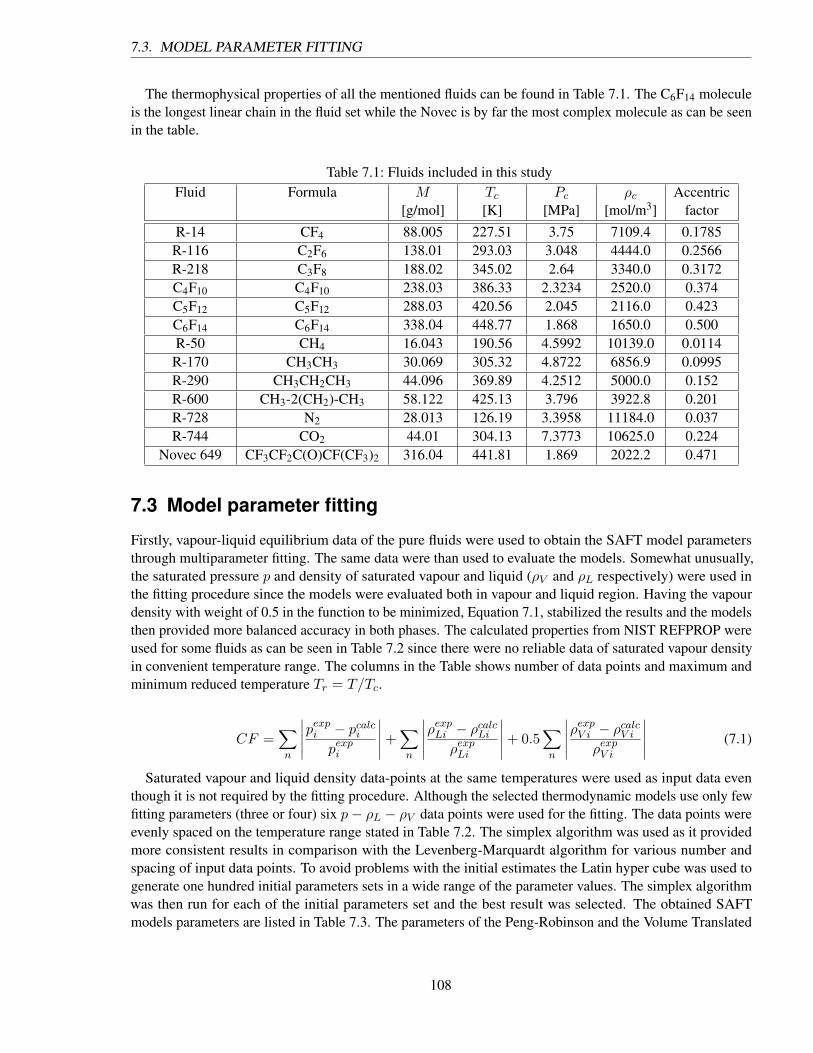
7.3. MODEL PARAMETER FITTING
The thermophysical properties of all the mentioned fluids can be found in Table 7.1. The C6F14 moleculeis the longest linear chain in the fluid set while the Novec is by far the most complex molecule as can be seenin the table.
Table 7.1: Fluids included in this studyFluid Formula M
[g/mol]Tc[K]
Pc[MPa]
ρc[mol/m3]
Accentricfactor
R-14 CF4 88.005 227.51 3.75 7109.4 0.1785R-116 C2F6 138.01 293.03 3.048 4444.0 0.2566R-218 C3F8 188.02 345.02 2.64 3340.0 0.3172C4F10 C4F10 238.03 386.33 2.3234 2520.0 0.374C5F12 C5F12 288.03 420.56 2.045 2116.0 0.423C6F14 C6F14 338.04 448.77 1.868 1650.0 0.500R-50 CH4 16.043 190.56 4.5992 10139.0 0.0114R-170 CH3CH3 30.069 305.32 4.8722 6856.9 0.0995R-290 CH3CH2CH3 44.096 369.89 4.2512 5000.0 0.152R-600 CH3-2(CH2)-CH3 58.122 425.13 3.796 3922.8 0.201R-728 N2 28.013 126.19 3.3958 11184.0 0.037R-744 CO2 44.01 304.13 7.3773 10625.0 0.224
Novec 649 CF3CF2C(O)CF(CF3)2 316.04 441.81 1.869 2022.2 0.471
7.3 Model parameter fitting
Firstly, vapour-liquid equilibrium data of the pure fluids were used to obtain the SAFT model parametersthrough multiparameter fitting. The same data were than used to evaluate the models. Somewhat unusually,the saturated pressure p and density of saturated vapour and liquid (ρV and ρL respectively) were used inthe fitting procedure since the models were evaluated both in vapour and liquid region. Having the vapourdensity with weight of 0.5 in the function to be minimized, Equation 7.1, stabilized the results and the modelsthen provided more balanced accuracy in both phases. The calculated properties from NIST REFPROP wereused for some fluids as can be seen in Table 7.2 since there were no reliable data of saturated vapour densityin convenient temperature range. The columns in the Table shows number of data points and maximum andminimum reduced temperature Tr = T/Tc.
CF =∑n
∣∣∣∣∣pexpi − pcalci
pexpi
∣∣∣∣∣+∑n
∣∣∣∣∣ρexpLi − ρcalcLi
ρexpLi
∣∣∣∣∣+ 0.5∑n
∣∣∣∣∣ρexpV i − ρcalcV i
ρexpV i
∣∣∣∣∣ (7.1)
Saturated vapour and liquid density data-points at the same temperatures were used as input data eventhough it is not required by the fitting procedure. Although the selected thermodynamic models use only fewfitting parameters (three or four) six p− ρL − ρV data points were used for the fitting. The data points wereevenly spaced on the temperature range stated in Table 7.2. The simplex algorithm was used as it providedmore consistent results in comparison with the Levenberg-Marquardt algorithm for various number andspacing of input data points. To avoid problems with the initial estimates the Latin hyper cube was used togenerate one hundred initial parameters sets in a wide range of the parameter values. The simplex algorithmwas then run for each of the initial parameters set and the best result was selected. The obtained SAFTmodels parameters are listed in Table 7.3. The parameters of the Peng-Robinson and the Volume Translated
108
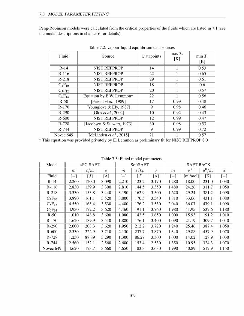
7.3. MODEL PARAMETER FITTING
Peng-Robinson models were calculated from the critical properties of the fluids which are listed in 7.1 (seethe model descriptions in chapter 6 for details).
Table 7.2: vapour-liquid equilibrium data sources
Fluid Source Datapointsmax Tr
[K]min Tr
[K]R-14 NIST REFPROP 14 1 0.53R-116 NIST REFPROP 22 1 0.65R-218 NIST REFPROP 29 1 0.61C4F10 NIST REFPROP 18 1 0.6C5F12 NIST REFPROP 20 1 0.57C6F14 Equation by E.W. Lemmon* 22 1 0.56R-50 [Friend et al., 1989] 17 0.99 0.48R-170 [Younglove & Ely, 1987] 9 0.98 0.46R-290 [Glos et al., 2004] 10 0.92 0.43R-600 NIST REFPROP 12 0.99 0.47R-728 [Jacobsen & Stewart, 1973] 30 0.98 0.53R-744 NIST REFPROP 9 0.99 0.72
Novec 649 [McLinden et al., 2015] 21 1 0.57* This equation was provided privately by E. Lemmon as preliminary fit for NIST REFPROP 8.0
Table 7.3: Fitted model parametersModel sPC-SAFT SoftSAFT SAFT-BACK
m ε/kb σ m ε/kb σ m v00 u0/kb α
Fluid [−] [J] [Å] [−] [J] [Å] [−] [ml/mol] [K] [−]R-14 2.260 120.0 3.090 2.210 123.2 3.170 1.280 18.00 231.0 1.030
R-116 2.830 139.9 3.300 2.810 144.5 3.350 1.480 24.26 311.7 1.050R-218 3.330 153.8 3.440 3.190 162.9 3.500 1.620 29.24 381.2 1.090C4F10 3.890 161.1 3.520 3.800 170.5 3.540 1.810 33.66 431.1 1.080C5F12 4.550 165.4 3.530 4.480 176.2 3.530 2.040 36.07 479.1 1.090C6F14 4.930 172.2 3.620 4.460 191.1 3.760 1.980 41.95 537.6 1.180R-50 1.010 148.8 3.690 1.080 142.5 3.650 1.000 15.93 191.2 1.010
R-170 1.620 189.9 3.510 1.880 176.1 3.400 1.090 21.19 309.7 1.040R-290 2.000 208.3 3.620 1.950 212.2 3.720 1.240 25.46 387.4 1.050R-600 2.330 222.9 3.710 2.130 237.7 3.870 1.340 29.88 457.9 1.070R-728 1.250 88.89 3.290 1.300 86.27 3.300 1.000 14.02 128.9 1.030R-744 2.560 152.1 2.560 2.680 153.4 2.530 1.350 10.95 324.3 1.070
Novec 649 4.620 173.7 3.660 4.650 183.3 3.630 1.990 40.89 517.9 1.150
109
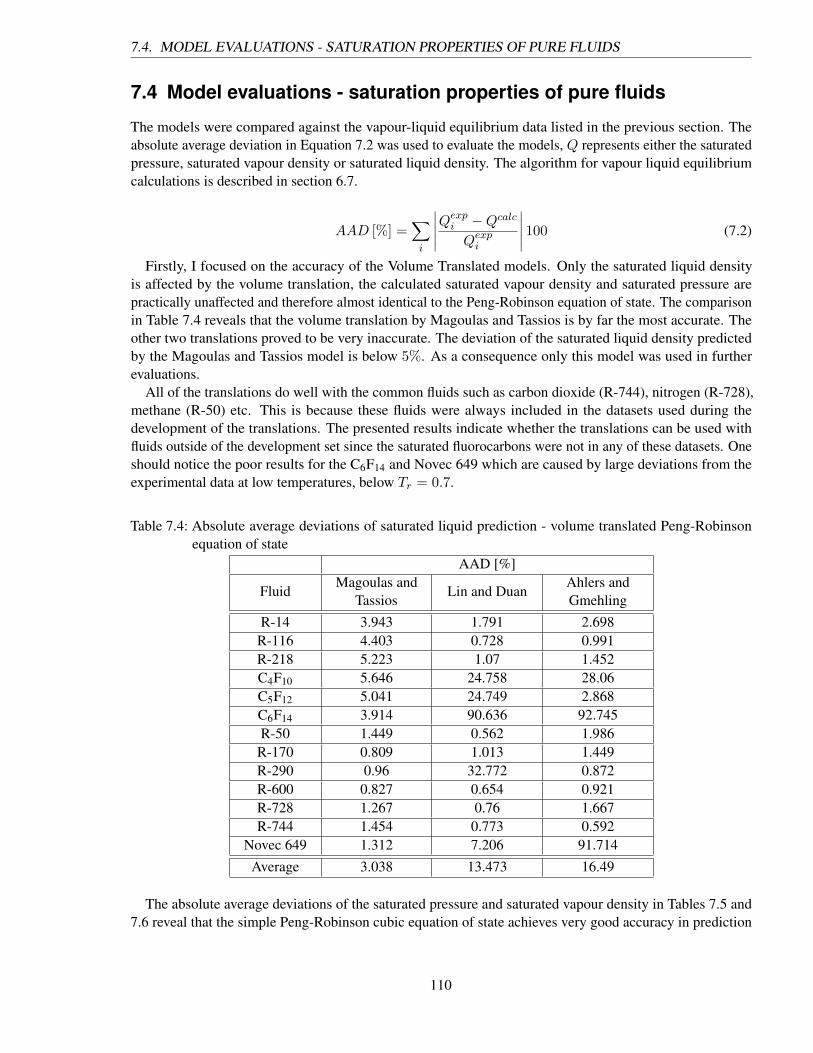
7.4. MODEL EVALUATIONS - SATURATION PROPERTIES OF PURE FLUIDS
7.4 Model evaluations - saturation properties of pure fluids
The models were compared against the vapour-liquid equilibrium data listed in the previous section. Theabsolute average deviation in Equation 7.2 was used to evaluate the models, Q represents either the saturatedpressure, saturated vapour density or saturated liquid density. The algorithm for vapour liquid equilibriumcalculations is described in section 6.7.
AAD [%] =∑i
∣∣∣∣∣Qexpi −Qcalc
Qexpi
∣∣∣∣∣ 100 (7.2)
Firstly, I focused on the accuracy of the Volume Translated models. Only the saturated liquid densityis affected by the volume translation, the calculated saturated vapour density and saturated pressure arepractically unaffected and therefore almost identical to the Peng-Robinson equation of state. The comparisonin Table 7.4 reveals that the volume translation by Magoulas and Tassios is by far the most accurate. Theother two translations proved to be very inaccurate. The deviation of the saturated liquid density predictedby the Magoulas and Tassios model is below 5%. As a consequence only this model was used in furtherevaluations.
All of the translations do well with the common fluids such as carbon dioxide (R-744), nitrogen (R-728),methane (R-50) etc. This is because these fluids were always included in the datasets used during thedevelopment of the translations. The presented results indicate whether the translations can be used withfluids outside of the development set since the saturated fluorocarbons were not in any of these datasets. Oneshould notice the poor results for the C6F14 and Novec 649 which are caused by large deviations from theexperimental data at low temperatures, below Tr = 0.7.
Table 7.4: Absolute average deviations of saturated liquid prediction - volume translated Peng-Robinsonequation of state
AAD [%]
FluidMagoulas and
TassiosLin and Duan
Ahlers andGmehling
R-14 3.943 1.791 2.698R-116 4.403 0.728 0.991R-218 5.223 1.07 1.452C4F10 5.646 24.758 28.06C5F12 5.041 24.749 2.868C6F14 3.914 90.636 92.745R-50 1.449 0.562 1.986R-170 0.809 1.013 1.449R-290 0.96 32.772 0.872R-600 0.827 0.654 0.921R-728 1.267 0.76 1.667R-744 1.454 0.773 0.592
Novec 649 1.312 7.206 91.714Average 3.038 13.473 16.49
The absolute average deviations of the saturated pressure and saturated vapour density in Tables 7.5 and7.6 reveal that the simple Peng-Robinson cubic equation of state achieves very good accuracy in prediction
110
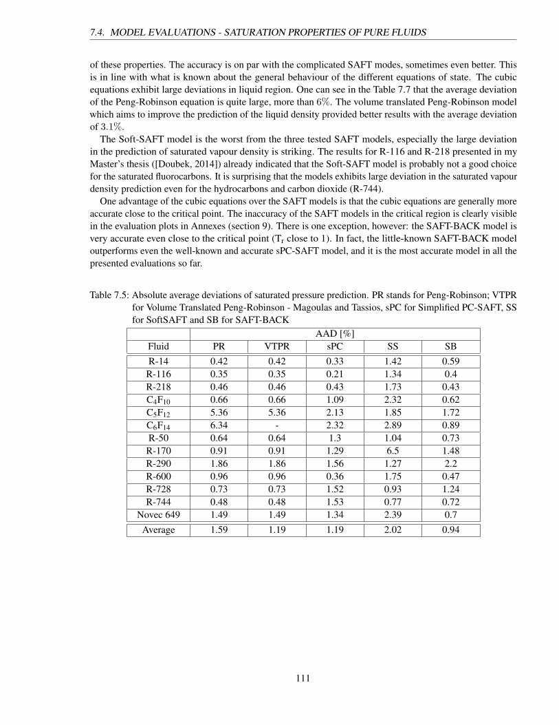
7.4. MODEL EVALUATIONS - SATURATION PROPERTIES OF PURE FLUIDS
of these properties. The accuracy is on par with the complicated SAFT modes, sometimes even better. Thisis in line with what is known about the general behaviour of the different equations of state. The cubicequations exhibit large deviations in liquid region. One can see in the Table 7.7 that the average deviationof the Peng-Robinson equation is quite large, more than 6%. The volume translated Peng-Robinson modelwhich aims to improve the prediction of the liquid density provided better results with the average deviationof 3.1%.
The Soft-SAFT model is the worst from the three tested SAFT models, especially the large deviationin the prediction of saturated vapour density is striking. The results for R-116 and R-218 presented in myMaster’s thesis ([Doubek, 2014]) already indicated that the Soft-SAFT model is probably not a good choicefor the saturated fluorocarbons. It is surprising that the models exhibits large deviation in the saturated vapourdensity prediction even for the hydrocarbons and carbon dioxide (R-744).
One advantage of the cubic equations over the SAFT models is that the cubic equations are generally moreaccurate close to the critical point. The inaccuracy of the SAFT models in the critical region is clearly visiblein the evaluation plots in Annexes (section 9). There is one exception, however: the SAFT-BACK model isvery accurate even close to the critical point (Tr close to 1). In fact, the little-known SAFT-BACK modeloutperforms even the well-known and accurate sPC-SAFT model, and it is the most accurate model in all thepresented evaluations so far.
Table 7.5: Absolute average deviations of saturated pressure prediction. PR stands for Peng-Robinson; VTPRfor Volume Translated Peng-Robinson - Magoulas and Tassios, sPC for Simplified PC-SAFT, SSfor SoftSAFT and SB for SAFT-BACK
AAD [%]Fluid PR VTPR sPC SS SBR-14 0.42 0.42 0.33 1.42 0.59
R-116 0.35 0.35 0.21 1.34 0.4R-218 0.46 0.46 0.43 1.73 0.43C4F10 0.66 0.66 1.09 2.32 0.62C5F12 5.36 5.36 2.13 1.85 1.72C6F14 6.34 - 2.32 2.89 0.89R-50 0.64 0.64 1.3 1.04 0.73
R-170 0.91 0.91 1.29 6.5 1.48R-290 1.86 1.86 1.56 1.27 2.2R-600 0.96 0.96 0.36 1.75 0.47R-728 0.73 0.73 1.52 0.93 1.24R-744 0.48 0.48 1.53 0.77 0.72
Novec 649 1.49 1.49 1.34 2.39 0.7Average 1.59 1.19 1.19 2.02 0.94
111
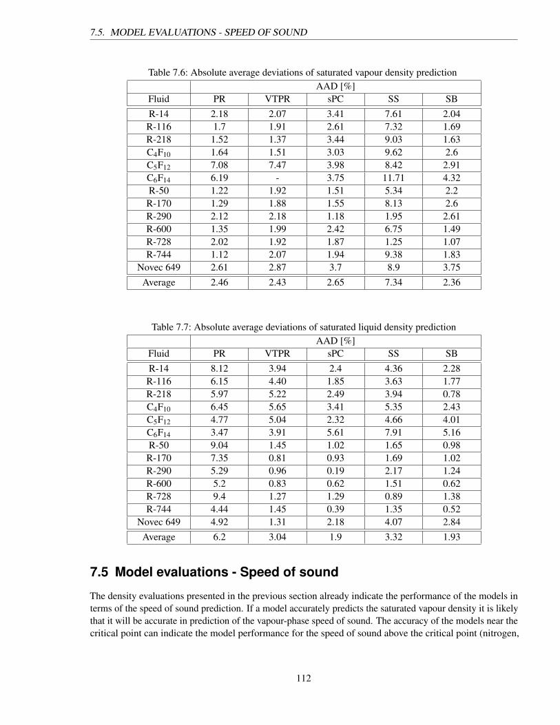
7.5. MODEL EVALUATIONS - SPEED OF SOUND
Table 7.6: Absolute average deviations of saturated vapour density predictionAAD [%]
Fluid PR VTPR sPC SS SBR-14 2.18 2.07 3.41 7.61 2.04
R-116 1.7 1.91 2.61 7.32 1.69R-218 1.52 1.37 3.44 9.03 1.63C4F10 1.64 1.51 3.03 9.62 2.6C5F12 7.08 7.47 3.98 8.42 2.91C6F14 6.19 - 3.75 11.71 4.32R-50 1.22 1.92 1.51 5.34 2.2
R-170 1.29 1.88 1.55 8.13 2.6R-290 2.12 2.18 1.18 1.95 2.61R-600 1.35 1.99 2.42 6.75 1.49R-728 2.02 1.92 1.87 1.25 1.07R-744 1.12 2.07 1.94 9.38 1.83
Novec 649 2.61 2.87 3.7 8.9 3.75Average 2.46 2.43 2.65 7.34 2.36
Table 7.7: Absolute average deviations of saturated liquid density predictionAAD [%]
Fluid PR VTPR sPC SS SBR-14 8.12 3.94 2.4 4.36 2.28
R-116 6.15 4.40 1.85 3.63 1.77R-218 5.97 5.22 2.49 3.94 0.78C4F10 6.45 5.65 3.41 5.35 2.43C5F12 4.77 5.04 2.32 4.66 4.01C6F14 3.47 3.91 5.61 7.91 5.16R-50 9.04 1.45 1.02 1.65 0.98
R-170 7.35 0.81 0.93 1.69 1.02R-290 5.29 0.96 0.19 2.17 1.24R-600 5.2 0.83 0.62 1.51 0.62R-728 9.4 1.27 1.29 0.89 1.38R-744 4.44 1.45 0.39 1.35 0.52
Novec 649 4.92 1.31 2.18 4.07 2.84Average 6.2 3.04 1.9 3.32 1.93
7.5 Model evaluations - Speed of sound
The density evaluations presented in the previous section already indicate the performance of the models interms of the speed of sound prediction. If a model accurately predicts the saturated vapour density it is likelythat it will be accurate in prediction of the vapour-phase speed of sound. The accuracy of the models near thecritical point can indicate the model performance for the speed of sound above the critical point (nitrogen,
112
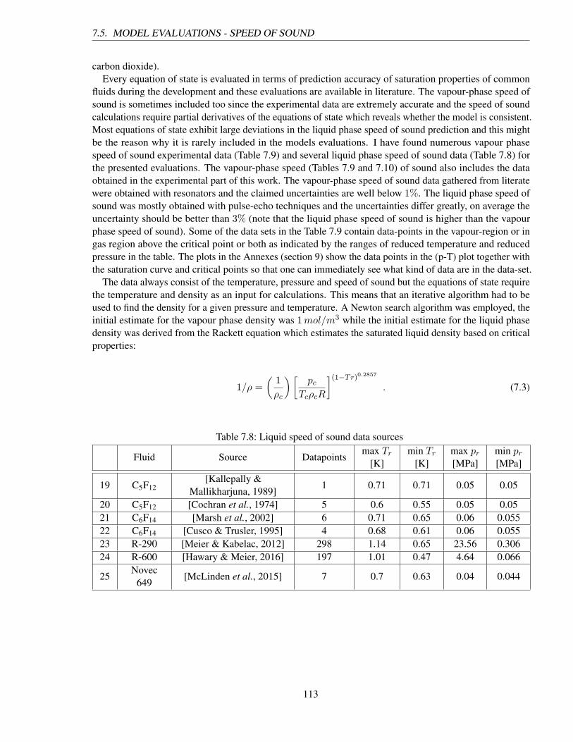
7.5. MODEL EVALUATIONS - SPEED OF SOUND
carbon dioxide).Every equation of state is evaluated in terms of prediction accuracy of saturation properties of common
fluids during the development and these evaluations are available in literature. The vapour-phase speed ofsound is sometimes included too since the experimental data are extremely accurate and the speed of soundcalculations require partial derivatives of the equations of state which reveals whether the model is consistent.Most equations of state exhibit large deviations in the liquid phase speed of sound prediction and this mightbe the reason why it is rarely included in the models evaluations. I have found numerous vapour phasespeed of sound experimental data (Table 7.9) and several liquid phase speed of sound data (Table 7.8) forthe presented evaluations. The vapour-phase speed (Tables 7.9 and 7.10) of sound also includes the dataobtained in the experimental part of this work. The vapour-phase speed of sound data gathered from literatewere obtained with resonators and the claimed uncertainties are well below 1%. The liquid phase speed ofsound was mostly obtained with pulse-echo techniques and the uncertainties differ greatly, on average theuncertainty should be better than 3% (note that the liquid phase speed of sound is higher than the vapourphase speed of sound). Some of the data sets in the Table 7.9 contain data-points in the vapour-region or ingas region above the critical point or both as indicated by the ranges of reduced temperature and reducedpressure in the table. The plots in the Annexes (section 9) show the data points in the (p-T) plot together withthe saturation curve and critical points so that one can immediately see what kind of data are in the data-set.
The data always consist of the temperature, pressure and speed of sound but the equations of state requirethe temperature and density as an input for calculations. This means that an iterative algorithm had to beused to find the density for a given pressure and temperature. A Newton search algorithm was employed, theinitial estimate for the vapour phase density was 1mol/m3 while the initial estimate for the liquid phasedensity was derived from the Rackett equation which estimates the saturated liquid density based on criticalproperties:
1/ρ =( 1ρc
)[pc
TcρcR
](1−Tr)0.2857
. (7.3)
Table 7.8: Liquid speed of sound data sources
Fluid Source Datapointsmax Tr
[K]min Tr
[K]max pr[MPa]
min pr[MPa]
19 C5F12[Kallepally &
Mallikharjuna, 1989]1 0.71 0.71 0.05 0.05
20 C5F12 [Cochran et al., 1974] 5 0.6 0.55 0.05 0.0521 C6F14 [Marsh et al., 2002] 6 0.71 0.65 0.06 0.05522 C6F14 [Cusco & Trusler, 1995] 4 0.68 0.61 0.06 0.05523 R-290 [Meier & Kabelac, 2012] 298 1.14 0.65 23.56 0.30624 R-600 [Hawary & Meier, 2016] 197 1.01 0.47 4.64 0.066
25Novec
649[McLinden et al., 2015] 7 0.7 0.63 0.04 0.044
113

7.5. MODEL EVALUATIONS - SPEED OF SOUND
Table 7.9: vapour speed of sound data sources
Fluid Source Datapointsmax Tr
[K]min Tr
[K]max pr[MPa]
min pr[MPa]
1 R-14 [Hurly, 1999] 81 1.87 1.32 0.4 0.0272 R-14 [Ewing & Trusler, 1989] 59 1.32 0.77 0.27 0.0213 R-116 This work 174 1.11 0.86 0.1 0.0234 R-116 [Hurly et al., 2003] 171 1.62 0.72 0.49 0.0335 R-218 [Vacek et al., 2001] 64 0.88 0.74 0.15 0.0046 R-218 This work 180 0.94 0.73 0.11 0.0247 C4F10 [Vacek et al., 2000] 26 0.78 0.66 0.04 0.0048 R-50 [Goodwin, 1988] 47 1.84 1.34 1.56 0.019 R-50 [Friend et al., 1989] 140 2.1 0.63 2.17 0.02210 R-50 [Younglove & Ely, 1987] 133 2.62 1.05 0.09 0.002
11 R-170[Estrada-Alexanders &
Trusler, 1997]187 1.47 0.72 2.15 0.003
12 R-290 [He et al., 2002] 24 0.87 0.79 0.16 0.04813 R-290 [Trusler & Zarari, 1996] 68 1.01 0.61 0.2 0.00214 R-728 [Gomes & Trusler, 1998] 68 2.77 1.98 8.86 0.029
15 R-728[Estela-Uribe & Trusler,
2000]58 3.17 1.35 0.42 0.007
16 R-728 [Boyes, 1992] 71 2.57 2.34 1.96 0.01517 R-744 [Liu et al., 2014] 61 1.48 0.72 1.92 0.042
18Novec
649[McLinden et al., 2015] 75 1.13 0.74 0.93 0.029
The Table 7.10 reveals that all the models perform very well in in the vapour phase speed of soundprediction, the average deviations are below 1%. Even the SoftSAFT model which did not perform well insaturated vapour density prediction delivers average deviation below 1%. It means that the derivatives neededto calculate the speed of sound are correct even though the saturated vapour density exhibits larger deviations.The deviation of the data obtained in the experimental part of this work (datasets 3 and 6 in Tables 7.9 and7.10) is comparable with the deviations of vapour-phase speed of sound data for other fluids in the table.Since the other data were obtained with spherical resonators it is another confirmation that the developedmeasurement technique is very accurate.
The liquid phase results in Table 7.11 indicate very poor accuracy of the Peng-Robinson equations of statewhich is no surprise but the volume-translated model is even worse. The reason is that the translated modelsare developed with strong focus on the saturated density and they can exhibit very strange behaviour in thecompressed liquid region. The SAFT-BACK model stands out in terms of prediction accuracy in the vapourand liquid phases. It is already clear that the little known and rarely used SAFT-BACK model is clearlysuperior to the other models in the presented tests. Especially the accuracy for C6F14 and Novec 649 whereall other models fail is impressive. It is true that the SAFT-BACK model has certain advantage in that it usesfour fluid-specific parameters unlike the other SAFT models which use only three.
114
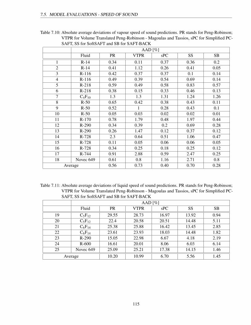
7.5. MODEL EVALUATIONS - SPEED OF SOUND
Table 7.10: Absolute average deviations of vapour speed of sound predictions. PR stands for Peng-Robinson;VTPR for Volume Translated Peng-Robinson - Magoulas and Tassios, sPC for Simplified PC-SAFT, SS for SoftSAFT and SB for SAFT-BACK
AAD [%]Fluid PR VTPR sPC SS SB
1 R-14 0.34 0.11 0.37 0.36 0.22 R-14 0.41 1.12 0.26 0.41 0.053 R-116 0.42 0.37 0.37 0.1 0.144 R-116 0.49 0.39 0.54 0.69 0.145 R-218 0.59 0.49 0.58 0.83 0.576 R-218 0.38 0.15 0.33 0.46 0.137 C4F10 1.3 1.3 1.31 1.24 1.268 R-50 0.65 0.42 0.38 0.43 0.119 R-50 0.52 1 0.28 0.43 0.110 R-50 0.05 0.03 0.02 0.02 0.0111 R-170 0.78 1.79 0.48 1.97 0.4412 R-290 0.34 0.39 0.2 0.69 0.2813 R-290 0.26 1.47 0.12 0.37 0.1214 R-728 2.3 0.64 0.51 1.06 0.4715 R-728 0.11 0.05 0.06 0.06 0.0516 R-728 0.34 0.25 0.18 0.25 0.1217 R-744 0.91 2.88 0.59 2.47 0.2518 Novec 649 0.61 0.8 1.16 2.71 0.8
Average 0.56 0.73 0.40 0.70 0.28
Table 7.11: Absolute average deviations of liquid speed of sound predictions. PR stands for Peng-Robinson;VTPR for Volume Translated Peng-Robinson - Magoulas and Tassios, sPC for Simplified PC-SAFT, SS for SoftSAFT and SB for SAFT-BACK
AAD [%]Fluid PR VTPR sPC SS SB
19 C5F12 29.55 28.73 16.97 13.92 0.9420 C5F12 22.4 20.58 20.51 14.48 5.1121 C6F14 25.38 25.88 16.42 13.45 2.8522 C6F14 23.61 23.93 18.03 14.48 1.8223 R-290 15.05 22.98 6.67 4.18 2.1924 R-600 16.61 20.01 8.06 6.03 6.1425 Novec 649 25.09 25.21 17.38 14.15 1.46
Average 10.20 10.99 6.70 5.56 1.45
115
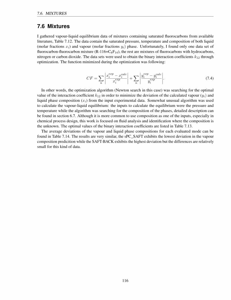
7.6. MIXTURES
7.6 Mixtures
I gathered vapour-liquid equilibrium data of mixtures containing saturated fluorocarbons from availableliterature, Table 7.12. The data contain the saturated pressure, temperature and composition of both liquid(molar fractions xi) and vapour (molar fractions yi) phase. Unfortunately, I found only one data set offluorocarbon-fluorocarbon mixture (R-116+C6F14), the rest are mixtures of fluorocarbons with hydrocarbons,nitrogen or carbon dioxide. The data sets were used to obtain the binary interaction coefficients k12 throughoptimization. The function minimized during the optimization was following:
CF =∑n
∣∣∣∣∣xexpi − xcalci
xexpi
∣∣∣∣∣+∑n
∣∣∣∣∣yexpi − ycalci
yexpi
∣∣∣∣∣. (7.4)
In other words, the optimization algorithm (Newton search in this case) was searching for the optimalvalue of the interaction coefficient k12 in order to minimize the deviation of the calculated vapour (yi) andliquid phase composition (xi) from the input experimental data. Somewhat unusual algorithm was usedto calculate the vapour-liquid equilibrium: the inputs to calculate the equilibrium were the pressure andtemperature while the algorithm was searching for the composition of the phases, detailed description canbe found in section 6.7. Although it is more common to use composition as one of the inputs, especially inchemical process design, this work is focused on fluid analysis and identification where the composition isthe unknown. The optimal values of the binary interaction coefficients are listed in Table 7.13.
The average deviations of the vapour and liquid phase compositions for each evaluated mode can befound in Table 7.14. The results are very similar, the sPC_SAFT exhibits the lowest deviation in the vapourcomposition predicition while the SAFT-BACK exhibits the highest deviation but the differences are relativelysmall for this kind of data.
116
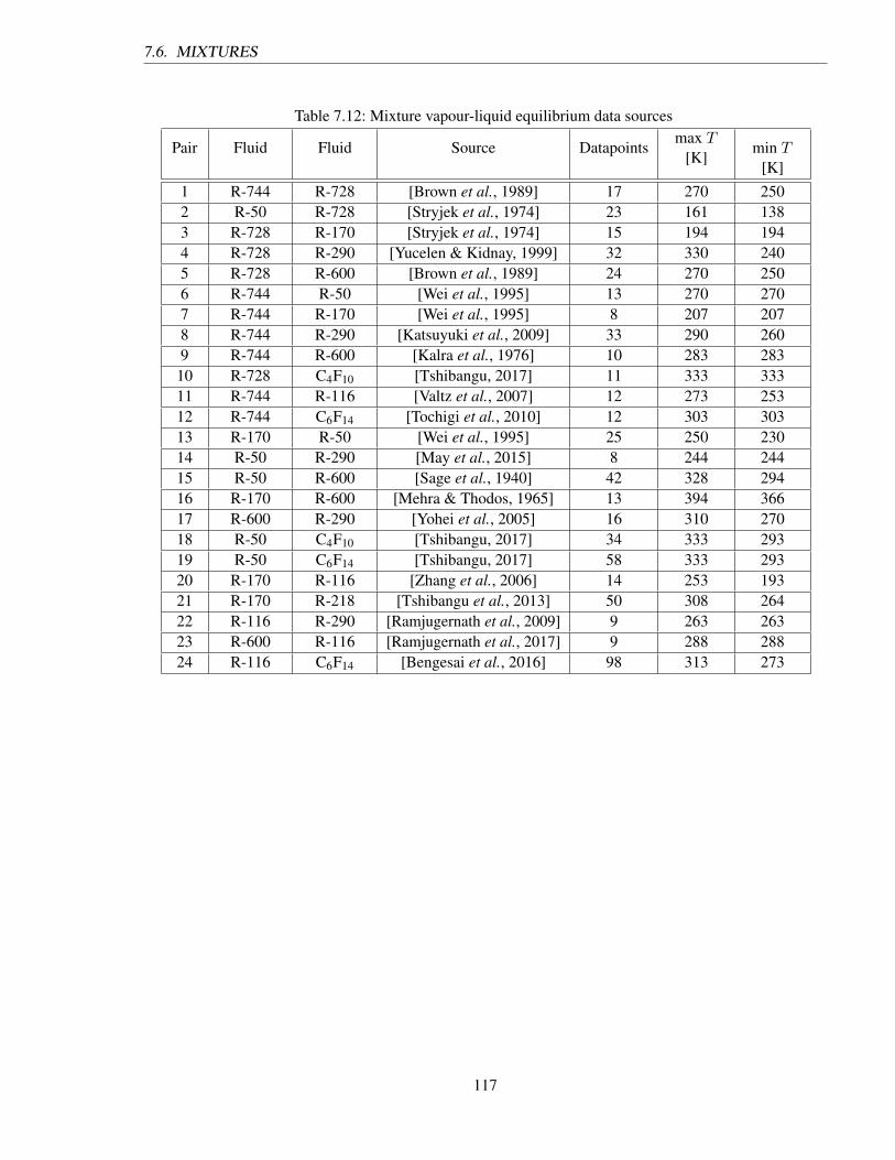
7.6. MIXTURES
Table 7.12: Mixture vapour-liquid equilibrium data sources
Pair Fluid Fluid Source Datapointsmax T
[K]min T
[K]1 R-744 R-728 [Brown et al., 1989] 17 270 2502 R-50 R-728 [Stryjek et al., 1974] 23 161 1383 R-728 R-170 [Stryjek et al., 1974] 15 194 1944 R-728 R-290 [Yucelen & Kidnay, 1999] 32 330 2405 R-728 R-600 [Brown et al., 1989] 24 270 2506 R-744 R-50 [Wei et al., 1995] 13 270 2707 R-744 R-170 [Wei et al., 1995] 8 207 2078 R-744 R-290 [Katsuyuki et al., 2009] 33 290 2609 R-744 R-600 [Kalra et al., 1976] 10 283 283
10 R-728 C4F10 [Tshibangu, 2017] 11 333 33311 R-744 R-116 [Valtz et al., 2007] 12 273 25312 R-744 C6F14 [Tochigi et al., 2010] 12 303 30313 R-170 R-50 [Wei et al., 1995] 25 250 23014 R-50 R-290 [May et al., 2015] 8 244 24415 R-50 R-600 [Sage et al., 1940] 42 328 29416 R-170 R-600 [Mehra & Thodos, 1965] 13 394 36617 R-600 R-290 [Yohei et al., 2005] 16 310 27018 R-50 C4F10 [Tshibangu, 2017] 34 333 29319 R-50 C6F14 [Tshibangu, 2017] 58 333 29320 R-170 R-116 [Zhang et al., 2006] 14 253 19321 R-170 R-218 [Tshibangu et al., 2013] 50 308 26422 R-116 R-290 [Ramjugernath et al., 2009] 9 263 26323 R-600 R-116 [Ramjugernath et al., 2017] 9 288 28824 R-116 C6F14 [Bengesai et al., 2016] 98 313 273
117
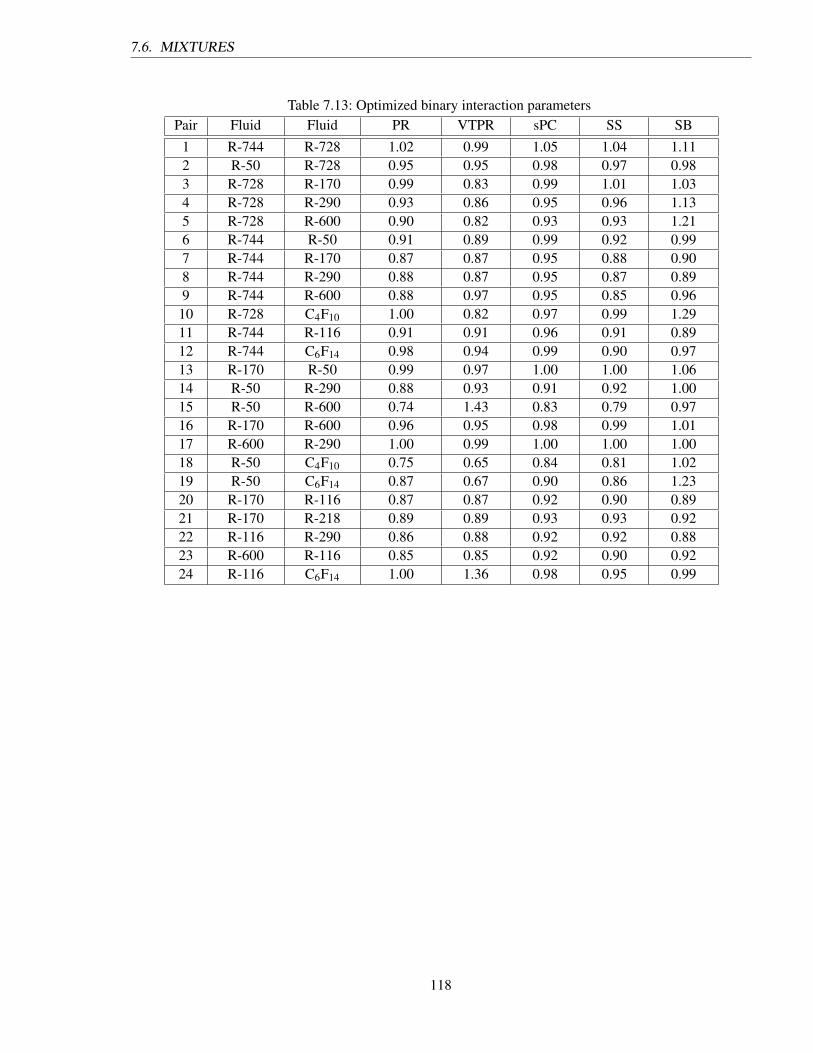
7.6. MIXTURES
Table 7.13: Optimized binary interaction parametersPair Fluid Fluid PR VTPR sPC SS SB
1 R-744 R-728 1.02 0.99 1.05 1.04 1.112 R-50 R-728 0.95 0.95 0.98 0.97 0.983 R-728 R-170 0.99 0.83 0.99 1.01 1.034 R-728 R-290 0.93 0.86 0.95 0.96 1.135 R-728 R-600 0.90 0.82 0.93 0.93 1.216 R-744 R-50 0.91 0.89 0.99 0.92 0.997 R-744 R-170 0.87 0.87 0.95 0.88 0.908 R-744 R-290 0.88 0.87 0.95 0.87 0.899 R-744 R-600 0.88 0.97 0.95 0.85 0.9610 R-728 C4F10 1.00 0.82 0.97 0.99 1.2911 R-744 R-116 0.91 0.91 0.96 0.91 0.8912 R-744 C6F14 0.98 0.94 0.99 0.90 0.9713 R-170 R-50 0.99 0.97 1.00 1.00 1.0614 R-50 R-290 0.88 0.93 0.91 0.92 1.0015 R-50 R-600 0.74 1.43 0.83 0.79 0.9716 R-170 R-600 0.96 0.95 0.98 0.99 1.0117 R-600 R-290 1.00 0.99 1.00 1.00 1.0018 R-50 C4F10 0.75 0.65 0.84 0.81 1.0219 R-50 C6F14 0.87 0.67 0.90 0.86 1.2320 R-170 R-116 0.87 0.87 0.92 0.90 0.8921 R-170 R-218 0.89 0.89 0.93 0.93 0.9222 R-116 R-290 0.86 0.88 0.92 0.92 0.8823 R-600 R-116 0.85 0.85 0.92 0.90 0.9224 R-116 C6F14 1.00 1.36 0.98 0.95 0.99
118
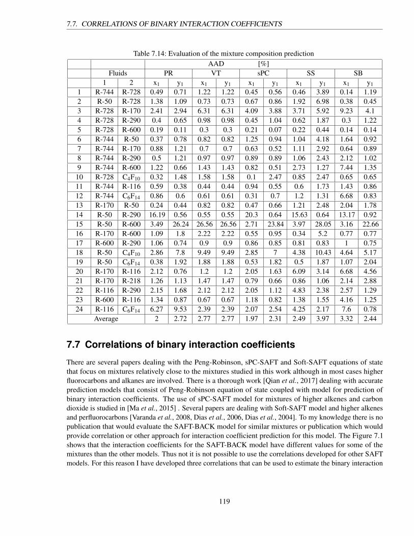
7.7. CORRELATIONS OF BINARY INTERACTION COEFFICIENTS
Table 7.14: Evaluation of the mixture composition predictionAAD [%]
Fluids PR VT sPC SS SB1 2 x1 y1 x1 y1 x1 y1 x1 y1 x1 y1
1 R-744 R-728 0.49 0.71 1.22 1.22 0.45 0.56 0.46 3.89 0.14 1.192 R-50 R-728 1.38 1.09 0.73 0.73 0.67 0.86 1.92 6.98 0.38 0.453 R-728 R-170 2.41 2.94 6.31 6.31 4.09 3.88 3.71 5.92 9.23 4.14 R-728 R-290 0.4 0.65 0.98 0.98 0.45 1.04 0.62 1.87 0.3 1.225 R-728 R-600 0.19 0.11 0.3 0.3 0.21 0.07 0.22 0.44 0.14 0.146 R-744 R-50 0.37 0.78 0.82 0.82 1.25 0.94 1.04 4.18 1.64 0.927 R-744 R-170 0.88 1.21 0.7 0.7 0.63 0.52 1.11 2.92 0.64 0.898 R-744 R-290 0.5 1.21 0.97 0.97 0.89 0.89 1.06 2.43 2.12 1.029 R-744 R-600 1.22 0.66 1.43 1.43 0.82 0.51 2.73 1.27 7.44 1.3510 R-728 C4F10 0.32 1.48 1.58 1.58 0.1 2.47 0.85 2.47 0.65 0.6511 R-744 R-116 0.59 0.38 0.44 0.44 0.94 0.55 0.6 1.73 1.43 0.8612 R-744 C6F14 0.86 0.6 0.61 0.61 0.31 0.7 1.2 1.31 6.68 0.8313 R-170 R-50 0.24 0.44 0.82 0.82 0.47 0.66 1.21 2.48 2.04 1.7814 R-50 R-290 16.19 0.56 0.55 0.55 20.3 0.64 15.63 0.64 13.17 0.9215 R-50 R-600 3.49 26.24 26.56 26.56 2.71 23.84 3.97 28.05 3.16 22.6616 R-170 R-600 1.09 1.8 2.22 2.22 0.55 0.95 0.34 5.2 0.77 0.7717 R-600 R-290 1.06 0.74 0.9 0.9 0.86 0.85 0.81 0.83 1 0.7518 R-50 C4F10 2.86 7.8 9.49 9.49 2.85 7 4.38 10.43 4.64 5.1719 R-50 C6F14 0.38 1.92 1.88 1.88 0.53 1.82 0.5 1.87 1.07 2.0420 R-170 R-116 2.12 0.76 1.2 1.2 2.05 1.63 6.09 3.14 6.68 4.5621 R-170 R-218 1.26 1.13 1.47 1.47 0.79 0.66 0.86 1.06 2.14 2.8822 R-116 R-290 2.15 1.68 2.12 2.12 2.05 1.12 4.83 2.38 2.57 1.2923 R-600 R-116 1.34 0.87 0.67 0.67 1.18 0.82 1.38 1.55 4.16 1.2524 R-116 C6F14 6.27 9.53 2.39 2.39 2.07 2.54 4.25 2.17 7.6 0.78
Average 2 2.72 2.77 2.77 1.97 2.31 2.49 3.97 3.32 2.44
7.7 Correlations of binary interaction coefficients
There are several papers dealing with the Peng-Robinson, sPC-SAFT and Soft-SAFT equations of statethat focus on mixtures relatively close to the mixtures studied in this work although in most cases higherfluorocarbons and alkanes are involved. There is a thorough work [Qian et al., 2017] dealing with accurateprediction models that consist of Peng-Robinson equation of state coupled with model for prediction ofbinary interaction coefficients. The use of sPC-SAFT model for mixtures of higher alkenes and carbondioxide is studied in [Ma et al., 2015] . Several papers are dealing with Soft-SAFT model and higher alkenesand perfluorocarbons [Varanda et al., 2008, Dias et al., 2006, Dias et al., 2004]. To my knowledge there is nopublication that would evaluate the SAFT-BACK model for similar mixtures or publication which wouldprovide correlation or other approach for interaction coefficient prediction for this model. The Figure 7.1shows that the interaction coefficients for the SAFT-BACK model have different values for some of themixtures than the other models. Thus not it is not possible to use the correlations developed for other SAFTmodels. For this reason I have developed three correlations that can be used to estimate the binary interaction
119
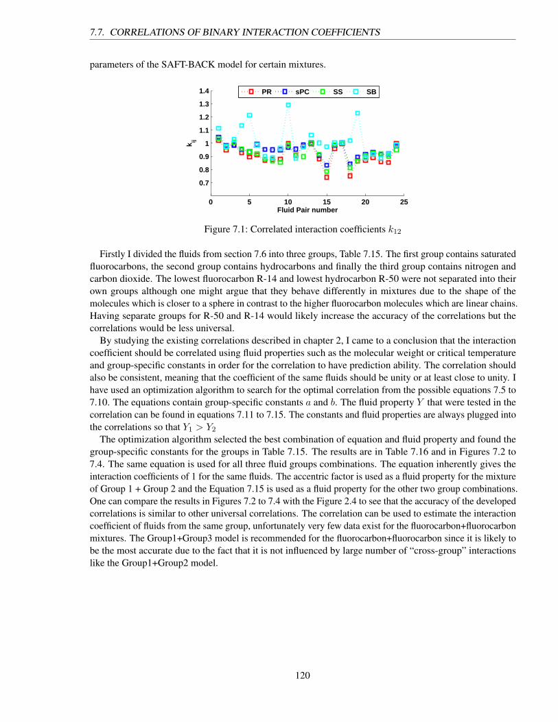
7.7. CORRELATIONS OF BINARY INTERACTION COEFFICIENTS
parameters of the SAFT-BACK model for certain mixtures.
0 5 10 15 20 25
0.7
0.8
0.9
1
1.1
1.2
1.3
1.4
Fluid Pair number
k ij
PR sPC SS SB
Figure 7.1: Correlated interaction coefficients k12
Firstly I divided the fluids from section 7.6 into three groups, Table 7.15. The first group contains saturatedfluorocarbons, the second group contains hydrocarbons and finally the third group contains nitrogen andcarbon dioxide. The lowest fluorocarbon R-14 and lowest hydrocarbon R-50 were not separated into theirown groups although one might argue that they behave differently in mixtures due to the shape of themolecules which is closer to a sphere in contrast to the higher fluorocarbon molecules which are linear chains.Having separate groups for R-50 and R-14 would likely increase the accuracy of the correlations but thecorrelations would be less universal.
By studying the existing correlations described in chapter 2, I came to a conclusion that the interactioncoefficient should be correlated using fluid properties such as the molecular weight or critical temperatureand group-specific constants in order for the correlation to have prediction ability. The correlation shouldalso be consistent, meaning that the coefficient of the same fluids should be unity or at least close to unity. Ihave used an optimization algorithm to search for the optimal correlation from the possible equations 7.5 to7.10. The equations contain group-specific constants a and b. The fluid property Y that were tested in thecorrelation can be found in equations 7.11 to 7.15. The constants and fluid properties are always plugged intothe correlations so that Y1 > Y2
The optimization algorithm selected the best combination of equation and fluid property and found thegroup-specific constants for the groups in Table 7.15. The results are in Table 7.16 and in Figures 7.2 to7.4. The same equation is used for all three fluid groups combinations. The equation inherently gives theinteraction coefficients of 1 for the same fluids. The accentric factor is used as a fluid property for the mixtureof Group 1 + Group 2 and the Equation 7.15 is used as a fluid property for the other two group combinations.One can compare the results in Figures 7.2 to 7.4 with the Figure 2.4 to see that the accuracy of the developedcorrelations is similar to other universal correlations. The correlation can be used to estimate the interactioncoefficient of fluids from the same group, unfortunately very few data exist for the fluorocarbon+fluorocarbonmixtures. The Group1+Group3 model is recommended for the fluorocarbon+fluorocarbon since it is likely tobe the most accurate due to the fact that it is not influenced by large number of “cross-group” interactionslike the Group1+Group2 model.
120
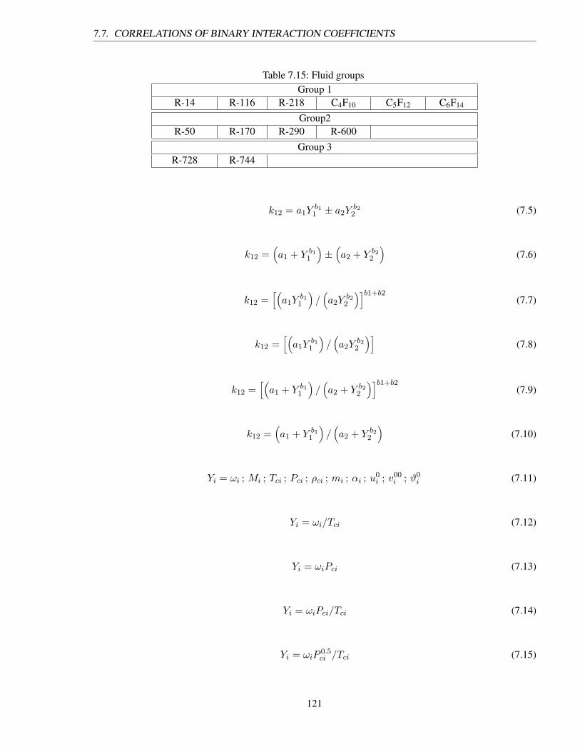
7.7. CORRELATIONS OF BINARY INTERACTION COEFFICIENTS
Table 7.15: Fluid groupsGroup 1
R-14 R-116 R-218 C4F10 C5F12 C6F14
Group2R-50 R-170 R-290 R-600
Group 3R-728 R-744
k12 = a1Yb1
1 ± a2Yb2
2 (7.5)
k12 =(a1 + Y b1
1
)±(a2 + Y b2
2
)(7.6)
k12 =[(a1Y
b11
)/(a2Y
b22
)]b1+b2(7.7)
k12 =[(a1Y
b11
)/(a2Y
b22
)](7.8)
k12 =[(a1 + Y b1
1
)/(a2 + Y b2
2
)]b1+b2(7.9)
k12 =(a1 + Y b1
1
)/(a2 + Y b2
2
)(7.10)
Yi = ωi ; Mi ; Tci ; Pci ; ρci ; mi ; αi ; u0i ; v00
i ; ϑ0i (7.11)
Yi = ωi/Tci (7.12)
Yi = ωiPci (7.13)
Yi = ωiPci/Tci (7.14)
Yi = ωiP0.5ci /Tci (7.15)
121

7.7. CORRELATIONS OF BINARY INTERACTION COEFFICIENTS
Table 7.16: Developed correlations for SAFT-BACK interaction coefficientsMixture Group1+Group2 Group1+Group3 Group2+Group2
Correlation[(a1 + Y b1
1
)/(a2 + Y b2
2
)]b1+b2
Property Yi = ωi Yi = ωiP0.5ci /Tci Yi = ωiP
0.5ci /Tci
First group constant a1 2.8079 1.4008 -0.9836First group constant b1 1.7085 0.3141 0.0067
Second group constant a2 2.1551 1.3729 -1.0592Second group constant b2 0.0755 0.8598 0.1560
0.85 0.9 0.95 1 1.05 1.1 1.15 1.2 1.25Fitted k
ij
0.9
1
1.1
1.2
Co
rrel
ated
kij
Group1: a=2.8079 , b=1.7085 Group2: a=2.1551 , b=0.0755
R-744+R-728
R-50+R-728R-728+R-170
R-728+R-290
R-728+R-600
R-744+R-50
R-744+R-170R-744+R-290
R-744+R-600
R-170+R-50
R-50+R-290
R-50+R-600
R-170+R-600R-600+R-290
ideal fitsame fluids Kij=1
same groupsdifferent groups
Figure 7.2: Correlation of interaction coefficients kij for fluids from Group1 and Group2
0.9 1 1.1 1.2 1.3 1.4Fitted k
ij
0.9
1
1.1
1.2
1.3
1.4
Co
rrel
ated
kij
Group1: a=1.4008 , b=0.3141 Group3: a=1.3729 , b=0.8598
R-744+R-728
R-728+C4F10
R-744+R-116
R-744+C6F14R-116+C6F14
ideal fitsame fluids Kij=1
same groupsdifferent groups
Figure 7.3: Correlation of interaction coefficients kij for fluids from Group1 and Group3
122
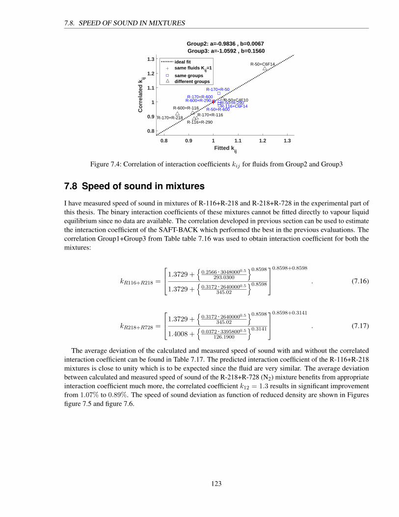
7.8. SPEED OF SOUND IN MIXTURES
0.8 0.9 1 1.1 1.2 1.3Fitted k
ij
0.8
0.9
1
1.1
1.2
1.3
Co
rrel
ated
kij
Group2: a=-0.9836 , b=0.0067 Group3: a=-1.0592 , b=0.1560
R-170+R-50
R-50+R-290
R-50+R-600
R-170+R-600R-600+R-290 R-50+C4F10
R-50+C6F14
R-170+R-116R-170+R-218
R-116+R-290
R-600+R-116 R-116+C6F14
ideal fitsame fluids Kij=1
same groupsdifferent groups
Figure 7.4: Correlation of interaction coefficients kij for fluids from Group2 and Group3
7.8 Speed of sound in mixtures
I have measured speed of sound in mixtures of R-116+R-218 and R-218+R-728 in the experimental part ofthis thesis. The binary interaction coefficients of these mixtures cannot be fitted directly to vapour liquidequilibrium since no data are available. The correlation developed in previous section can be used to estimatethe interaction coefficient of the SAFT-BACK which performed the best in the previous evaluations. Thecorrelation Group1+Group3 from Table table 7.16 was used to obtain interaction coefficient for both themixtures:
kR116+R218 =
1.3729 +
0.2566 · 30480000.5
293.0300
0.8598
1.3729 +
0.3172 · 26400000.5
345.02
0.8598
0.8598+0.8598
. (7.16)
kR218+R728 =
1.3729 +
0.3172 · 26400000.5
345.02
0.8598
1.4008 +
0.0372 · 33958000.5
126.1900
0.3141
0.8598+0.3141
. (7.17)
The average deviation of the calculated and measured speed of sound with and without the correlatedinteraction coefficient can be found in Table 7.17. The predicted interaction coefficient of the R-116+R-218mixtures is close to unity which is to be expected since the fluid are very similar. The average deviationbetween calculated and measured speed of sound of the R-218+R-728 (N2) mixture benefits from appropriateinteraction coefficient much more, the correlated coefficient k12 = 1.3 results in significant improvementfrom 1.07% to 0.89%. The speed of sound deviation as function of reduced density are shown in Figuresfigure 7.5 and figure 7.6.
123
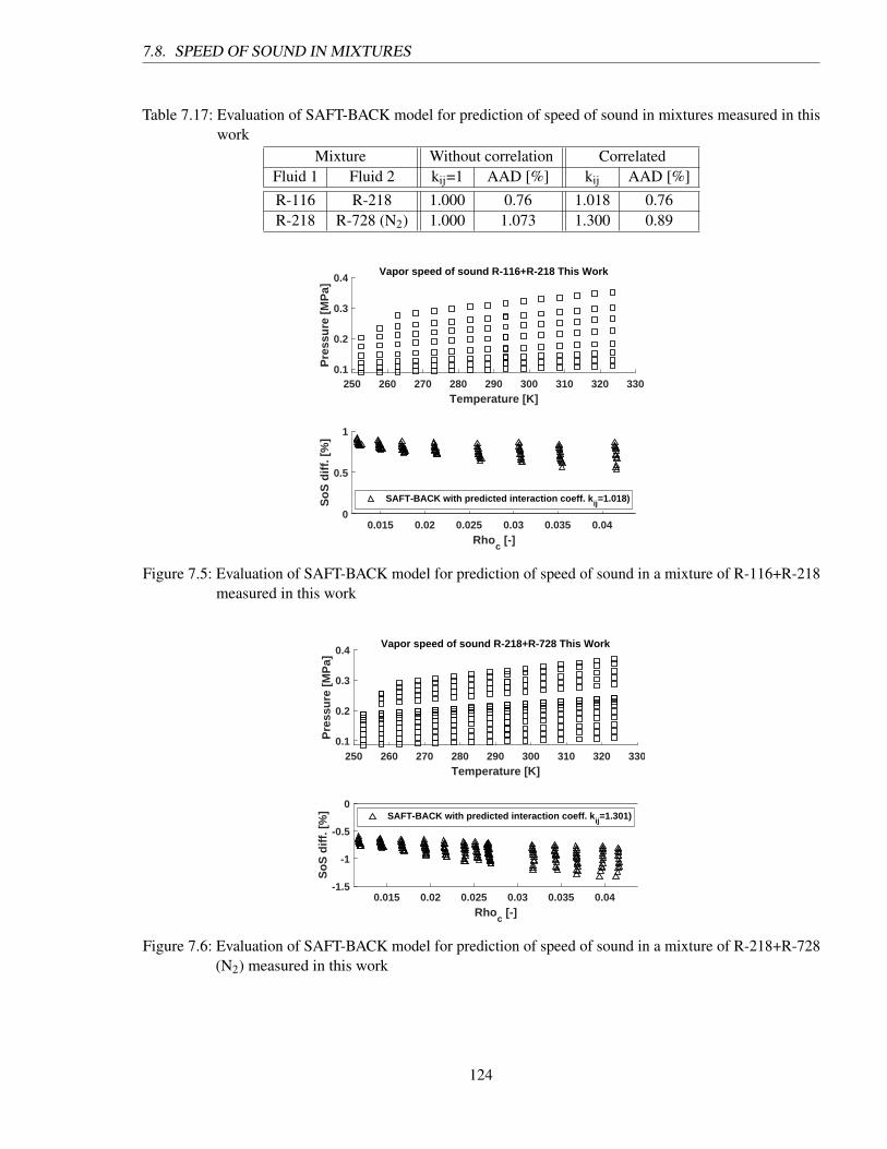
7.8. SPEED OF SOUND IN MIXTURES
Table 7.17: Evaluation of SAFT-BACK model for prediction of speed of sound in mixtures measured in thiswork
Mixture Without correlation CorrelatedFluid 1 Fluid 2 kij=1 AAD [%] kij AAD [%]R-116 R-218 1.000 0.76 1.018 0.76R-218 R-728 (N2) 1.000 1.073 1.300 0.89
250 260 270 280 290 300 310 320 330Temperature [K]
0.1
0.2
0.3
0.4
Pre
ssu
re [
MP
a]
Vapor speed of sound R-116+R-218 This Work
0.015 0.02 0.025 0.03 0.035 0.04Rho
c [-]
0
0.5
1
So
S d
iff.
[%
]
SAFT-BACK with predicted interaction coeff. kij=1.018)
Figure 7.5: Evaluation of SAFT-BACK model for prediction of speed of sound in a mixture of R-116+R-218measured in this work
250 260 270 280 290 300 310 320 330Temperature [K]
0.1
0.2
0.3
0.4
Pre
ssu
re [
MP
a]
Vapor speed of sound R-218+R-728 This Work
0.015 0.02 0.025 0.03 0.035 0.04Rho
c [-]
-1.5
-1
-0.5
0
So
S d
iff.
[%
] SAFT-BACK with predicted interaction coeff. kij=1.301)
Figure 7.6: Evaluation of SAFT-BACK model for prediction of speed of sound in a mixture of R-218+R-728(N2) measured in this work
124
7.8. SPEED OF SOUND IN MIXTURES
Bibliography
chapter 7: Evaluations of models
[Attree et al., 2008] Attree, D, Anderson, B, Anderssen, E C, Akhnazarov, V, Apsimon, R J, Barclay, P,Batchelor, L E, Bates, R L, Battistin, M, Bendotti, J, Berry, S, Bitadze, A, Bizzel, J P, Bonneau, P, Bosteels,M, Butterworth, J M, Butterworth, S, Carter, A A, Carter, J R, Catinaccio, A, Corbaz, F, Danielsson,H O, Danilevich, E, Dixon, N, Dixon, S D, Doherty, F, Dorholt, O, Doubrava, M, Egorov, K, Einsweiler,K, Falou, A C, Feraudet, P, Ferrari, P, Fowler, K, Fraser, J T, French, R S, Galuska, M, Gannaway, F,Gariano, G, Gibson, M D, Gilchriese, M, Giugni, D, Godlewski, J, Gousakov, I, Gorski, B, Hallewell, G D,Hartman, N, Hawkings, R J, Haywood, S J, Hessey, N P, Ilyashenko, I, Infante, S, Jackson, J N, Jones, T J,Kaplon, J, Katunin, S, Lindsay, S, Luisa, L, Massol, N, McEwan, F, McMahon, S J, Menot, C, Mistry, J,Morris, J, Muskett, D M, Nagai, K, Nichols, A, Nicholson, R, Nickerson, R B, Nielsen, S L, Nordahl,P E, Olcese, M, Parodi, M, Perez-Gomez, F, Pernegger, H, Perrin, E, Rossi, L P, Rovani, A, Ruscino, E,Sandaker, H, Smith, A, Sopko, V, Stapnes, S, Stodulski, M, Tarrant, J, Thadome, J, Tovey, D, Turala, M,Tyndel, M, Vacek, V, van der Kraaij, E, Viehhauser, G H A, Vigeolas, E, Wells, P S, Wenig, S, & Werneke,P. 2008. The evaporative cooling system for the ATLAS inner detector. Journal of Instrumentation, 3(07),P07003.
[Bengesai et al., 2016] Bengesai, P. N., Nelson, W. M.l, & Naidoo, P.and Ramjugernath, D. 2016. PhaseEquilibria for Perfluoroethane + (n-Perfluorohexane or n-Perfluorooctane) Binary Systems: Measurementand Modeling. Journal of Chemical & Engineering Data, 61(9), 3363–3370.
[Boyes, 1992] Boyes, S.J. 1992. The speed of sound in gases with application to equations of state andsonic nozzles. Ph.D. thesis, University of London.
[Brown et al., 1989] Brown, T. S., Niesen, V. G., Sloan, E. D., & Kidnay, A. J. 1989. Vapor-liquid equilibriafor the binary systems of nitrogen, carbon dioxide, and n-butane at temperatures from 220 to 344 K. FluidPhase Equilibria, 53, 7 – 14. Proceedings of the Fifth International Conference.
[Cochran et al., 1974] Cochran, M. A., North, A. M., & Pethrick, R. A. 1974. Ultrasonic studies of perfluoro-n-alkanes. J. Chem. Soc., Faraday Trans. 2, 70, 1274–1279.
[Cusco & Trusler, 1995] Cusco, L., & Trusler, J. P. M. 1995. Identification of environmentally acceptablelow-sound speed liquids. International Journal of Thermophysics, 16(3), 675–685.
[Dias et al., 2004] Dias, A. M. A., Pamies, J. C., Coutinho, J. A.P., Marrucho, I. M., & Vega, L. F. 2004.SAFT Modeling of the Solubility of Gases in Perfluoroalkanes. The Journal of Physical Chemistry B,108(4), 1450–1457.
[Dias et al., 2006] Dias, A. M. A., Carrier, H., Daridon, J. L., Pamies, J. C., Vega, L. F., Coutinho, J. A. P.,& Marrucho, I. M. 2006. VaporâLiquid Equilibrium of Carbon DioxideâPerfluoroalkane Mixtures:âExperimental Data and SAFT Modeling. Industrial & Engineering Chemistry Research, 45(7), 2341–2350.
125
7.8. SPEED OF SOUND IN MIXTURES
[Doubek, 2014] Doubek, M. 2014. Thermophysical properties of fluids experiment and simulations. Master’sthesis, Czech Technical University, Faculty of Mechanical Engineering.
[Estela-Uribe & Trusler, 2000] Estela-Uribe, J. F., & Trusler, J. P. M. 2000. Acoustic and Volumetric VirialCoefficients of Nitrogen. International Journal of Thermophysics, 21(5), 1033–1044.
[Estrada-Alexanders & Trusler, 1997] Estrada-Alexanders, A. F., & Trusler, J. P. M. 1997. The speed ofsound and derived thermodynamic properties of ethane at temperatures between 220 K and 450 K andpressures up to 10.5 MPa. The Journal of Chemical Thermodynamics, 29(9), 991 – 1015.
[Ewing & Trusler, 1989] Ewing, M. B., & Trusler, J. P. M. 1989. Speeds of sound in CF4 between 175 and300 K measured with a spherical resonator. The Journal of Chemical Physics, 90(2), 1106–1115.
[Friend et al., 1989] Friend, G. D., Ely, J. F., & Ingham, H. 1989. Thermophysical Properties of Methane.18(04), 583–638.
[Glos et al., 2004] Glos, S., Kleinrahm, R., & Wagner, W. 2004. Measurement of the (p,Ï,T) relation ofpropane, propylene, n-butane, and isobutane in the temperature range from (95 to 340) K at pressures upto 12 MPa using an accurate two-sinker densimeter. The Journal of Chemical Thermodynamics, 36(12),1037 – 1059.
[Gomes & Trusler, 1998] Gomes, M. F. C., & Trusler, J. P. M. 1998. The speed of sound in nitrogen attemperatures betweenT=250 K andT=350 K and at pressures up to 30 MPa. The Journal of ChemicalThermodynamics, 30(5), 527 – 534.
[Gong et al., 2004] Gong, M., Wu, J., Luo, E., Qi, Y., & Zhou, Y. 2004. Study of the single-stage mixed-gases refrigeration cycle for cooling temperature-distributed heat loads. International Journal of ThermalSciences, 43(1), 31 – 41.
[Goodwin, 1988] Goodwin, A. R. H. 1988. Thermophysical properties from speed of sound. Ph.D. thesis,University of London.
[Haug, 2005] Haug, F. 2005. Studies on cooling of the TOTEM particle detector at the LHC. 12.
[Hawary & Meier, 2016] Hawary, A. E., & Meier, K. 2016. Measurements of the Speed of Sound in Liquidn-Butane. Journal of Chemical & Engineering Data, 61(11), 3858–3867.
[He et al., 2002] He, M. G., Liu, Z. G., & Yin, J. M. 2002. Measurement of Speed of Sound with a SphericalResonator: HCFC-22, HFC-152a, HFC-143a, and Propane. International Journal of Thermophysics,23(6), 1599–1615.
[Hurly, 1999] Hurly, J. J. 1999. Thermophysical Properties of Gaseous CF4 and C2F6 from Speed-of-SoundMeasurements. International Journal of Thermophysics, 20(2), 455–484.
[Hurly et al., 2003] Hurly, J. J., Gillis, K. A., Mehl, J. B., & Moldover, M. R. 2003. The Viscosity ofSeven Gases Measured with a Greenspan Viscometer. International Journal of Thermophysics, 24(6),1441–1474.
[Jacobsen & Stewart, 1973] Jacobsen, R. T., & Stewart, R. B. 1973. Thermodynamic Properties of NitrogenIncluding Liquid and Vapor Phases from 63K to 2000K with Pressures to 10,000 Bar. Journal of Physicaland Chemical Reference Data, 2(4), 757–922.
126
7.8. SPEED OF SOUND IN MIXTURES
[Kallepally & Mallikharjuna, 1989] Kallepally, N. L., & Mallikharjuna, S. K. 1989. Ultrasonic velocity inand adiabatic compressibility for some fluorocarbon liquid mixtures. Journal of Chemical & EngineeringData, 34(1), 19–21.
[Kalra et al., 1976] Kalra, H., Krishnana, T. R., & Robinson, D. B. 1976. Equilibrium-phase properties ofcarbon dioxide-butane and nitrogen-hydrogen sulfide systems at subambient temperatures. Journal ofChemical & Engineering Data, 21(2), 222–225.
[Katsuyuki et al., 2009] Katsuyuki, T., Yukihiro, H., Ryo, A., Yohei, K., & Kenich, F. 2009. Measurementsof the VaporâLiquid Equilibrium for the CO2 + R290 Mixture. Journal of Chemical & Engineering Data,54(3), 1029–1033.
[Liu et al., 2014] Liu, Q., Feng, X., An, B., & Duan, Y. 2014. Speed of Sound Measurements Using aCylindrical Resonator for Gaseous Carbon Dioxide and Propene. Journal of Chemical & EngineeringData, 59(9), 2788–2798.
[Ma et al., 2015] Ma, M., Chen, S., & Abedi, J. 2015. Binary interaction coefficients of asymmetric CH4,C2H6, and CO2 with high n-alkanes for the simplified PC-SAFT correlation and prediction. Fluid PhaseEquilibria, 405, 114 – 123.
[Marsh et al., 2002] Marsh, J. N., Hall, Ch. S., Wickline, S. A., & Lanza, G. M. 2002. Temperaturedependence of acoustic impedance for specific fluorocarbon liquids. The Journal of the Acoustical Societyof America, 112(6), 2858–2862.
[May et al., 2015] May, E. F., Guo, J. Y., Oakley, J. H., Hughes, T. J., Graham, B. F., Marsh, K. N., & Huang,S. H. 2015. Reference Quality VaporâLiquid Equilibrium Data for the Binary Systems Methane + Ethane,+ Propane, + Butane, and + 2-Methylpropane, at Temperatures from (203 to 273) K and Pressures to 9MPa. Journal of Chemical & Engineering Data, 60(12), 3606–3620.
[McLinden et al., 2015] McLinden, M. O., Perkins, R. A., Lemmon, E. W., & Fortin, T. J. 2015. Thermody-namic Properties of 1,1,1,2,2,4,5,5,5-Nonafluoro-4-(trifluoromethyl)-3-pentanone: Vapor Pressure, (p,Ï, T) Behavior, and Speed of Sound Measurements, and an Equation of State. Journal of Chemical &Engineering Data, 60(12), 3646–3659.
[Mehra & Thodos, 1965] Mehra, V. S., & Thodos, G. 1965. Vapor-Liquid Equilibrium in the Ethane-n-Butane System. Journal of Chemical & Engineering Data, 10(4), 307–309.
[Meier & Kabelac, 2012] Meier, K., & Kabelac, S. 2012. Thermodynamic Properties of Propane. IV. Speedof Sound in the Liquid and Supercritical Regions. Journal of Chemical & Engineering Data, 57(12),3391–3398.
[Qian et al., 2017] Qian, J.-W., Privat, R., Jaubert, J.-N., Coquelet, Ch., & Ramjugernath, D. 2017. Fluid-phase-equilibrium prediction of fluorocompound-containing binary systems with the predictive E-PPR78model. International Journal of Refrigeration, 73, 65 – 90.
[Ramjugernath et al., 2009] Ramjugernath, D., Valtz, A., Coquelet, C., & Richon, D. 2009. IsothermalVaporâLiquid Equilibrium Data for the Hexafluoroethane (R116) + Propane System at Temperatures from(263 to 323) K. Journal of Chemical & Engineering Data, 54(4), 1292–1296.
[Ramjugernath et al., 2017] Ramjugernath, D., Valtz, A., Richon, D., Williams-Wynn, M. D., & Coquelet,C. 2017. Isothermal VaporâLiquid Equilibrium Data for the Hexafluoroethane (R116) + n-Butane Systemat Temperatures from 273 to 323 K. Journal of Chemical & Engineering Data, 62(10), 3483–3487.
127
7.8. SPEED OF SOUND IN MIXTURES
[Sage et al., 1940] Sage, B. H., Budenholzer, R. A., & Lacey, W. N. 1940. Phase Equilibria in HydrocarbonSystems Methaneân-Butane System in the Gaseous and Liquid Regions. Industrial & EngineeringChemistry, 32(9), 1262–1277.
[Sarkar & Bhattacharyya, 2009] Sarkar, J., & Bhattacharyya, S. 2009. Assessment of blends of CO2 withbutane and isobutane as working fluids for heat pump applications. International Journal of ThermalSciences, 48(7), 1460 – 1465.
[Stryjek et al., 1974] Stryjek, R., Chappelear, P. S., & Kobayashi, R. 1974. Low-temperature vapor-liquidequilibriums of nitrogen-methane system. Journal of Chemical & Engineering Data, 19(4), 334–339.
[Tochigi et al., 2010] Tochigi, K., Namae, T., Suga, T., Matsuda, H., Kurihara, K., Ramos, M. C., & McCabe,C. 2010. Measurement and prediction of high-pressure vaporâliquid equilibria for binary mixtures ofcarbon dioxide+n-octane, methanol, ethanol, and perfluorohexane. The Journal of Supercritical Fluids,55(2), 682 – 689. 100th year Anniversary of van der Waals’ Nobel Lecture.
[Trusler & Zarari, 1996] Trusler, J. P. M., & Zarari, M. P. 1996. The speed of sound in gaseous propaneat temperatures between 225 K and 375 K and at pressures up to 0.8 MPa. The Journal of ChemicalThermodynamics, 28(3), 329 – 335.
[Tshibangu, 2017] Tshibangu, M. M. 2017. Investigation Of Perfluorocarbons As Potential Physical SolventsFor Flue Gas Cleaning. Ph.D. thesis, University of KwaZulu-Natal.
[Tshibangu et al., 2013] Tshibangu, M. M., Courtial, X., Coquelet, C., Naidoo, P., & Ramjugernath, D.2013. Isothermal VaporâLiquid Equilibrium Data and Modeling for the Ethane (R170) + Perfluoropropane(R218) System at Temperatures from (264 to 308) K. Journal of Chemical & Engineering Data, 58(5),1316–1320.
[Vacek et al., 2000] Vacek, V., Hallewell, G., Ilie, S., & Lindsay, S. 2000. Perfluorocarbons and their use incooling systems for semiconductor particle detectors. Fluid Phase Equilibria, 174(1), 191 – 201.
[Vacek et al., 2001] Vacek, V., Hallewell, G., & Lindsay, S. 2001. Velocity of sound measurements ingaseous per-fluorocarbons and their mixtures. Fluid Phase Equilibria, 185(1), 305 – 314. Proceedings ofthe 14th symposium on thermophysical properties.
[Valtz et al., 2007] Valtz, A., Coquelet, Ch., & Richon, D. 2007. Vaporâliquid equilibrium data for thehexafluoroethane + carbon dioxide system at temperatures from 253 to 297 K and pressures up to 6.5 MPa.258(09), 179–185.
[Varanda et al., 2008] Varanda, F. R., Vega, L. F., Coutinho, J. A.P., & Marrucho, I. M. 2008. Liquidâliquidequilibrium of substituted perfluoro-n-octane+n-octane systems. Fluid Phase Equilibria, 268(1), 85 – 89.
[Wei et al., 1995] Wei, M. S.-W., Brown, T. S., Kidnay, A. J., & Sloan, E. D. 1995. Vapor + Liquid Equilibriafor the Ternary System Methane + Ethane + Carbon Dioxide at 230 K and Its Constituent Binaries atTemperatures from 207 to 270 K. Journal of Chemical & Engineering Data, 40(4), 726–731.
[Yohei et al., 2005] Yohei, K., Kenichi, F., & Yukihiro, H. 2005. VaporâLiquid Equilibrium (VLE) Propertiesfor the Binary Systems Propane (1) + n-Butane (2) and Propane (1) + Isobutane (3). Journal of Chemical& Engineering Data, 50(2), 579–582.
128
7.8. SPEED OF SOUND IN MIXTURES
[Younglove & Ely, 1987] Younglove, B. A., & Ely, J. F. 1987. Thermophysical Properties of Fluids. II.Methane, Ethane, Propane, Isobutane, and Normal Butane. Journal of Physical and Chemical ReferenceData, 16(4), 577–798.
[Yucelen & Kidnay, 1999] Yucelen, B., & Kidnay, A. J. 1999. VaporâLiquid Equilibria in the Nitrogen +Carbon Dioxide + Propane System from 240 to 330 K at Pressures to 15 MPa. Journal of Chemical &Engineering Data, 44(5), 926–931.
[Zhang et al., 2017] Zhang, Xianping, Wang, Fang, Liu, Zhiming, Gu, Junjie, Zhu, Feiyu, & Yuan, Qiuyan.2017. Performance Research on Heat Pump Using Blends of R744 with Eco-friendly Working Fluid.Procedia Engineering, 205, 2297 – 2302. 10th International Symposium on Heating, Ventilation and AirConditioning, ISHVAC2017, 19-22 October 2017, Jinan, China.
[Zhang et al., 2006] Zhang, Y., Gong, M.-Q., Zhu, H.-B., & Wu, J.-F. 2006. Vaporâliquid equilibriummeasurements and correlations for an azeotropic system of ethane+hexafluoroethane. Fluid PhaseEquilibria, 240(1), 73 – 78.
129

Chapter 8 Summary and conclusions
8 Summary and conclusions
8.1 Development of high accuracy speed-of-sound measurementapparatus
The experimental part of this thesis presents the time-of-flight based instrument for speed of sound measure-ment I have developed. The instrument was adopted for mixtures so that two gases can be mixed directlyinside the measurement chamber. A custom electronics I have designed and continuously improved is usedfor the speed of sound measurement. I have implemented a new triggering technique which eliminates errorsin the transit time measurements to achieve the best accuracy. The comparison of the speed of sound I havemeasured in pure R-116 and R-218 with the most accurate data from literature, which were measured withextremely precise but expensive and difficult to build spherical resonators, indicated mutual deviation smallerthan 0.4%. Although only the extremely accurate data from spherical resonators can be used to safely deriveother thermodynamic properties such as the heat capacities, the deviation of 0.4% is smaller than deviationsbetween experimental data and the speed of sound calculated by commonly used equations of state forrefrigerants.
8.2 Evaluations of models
I have compiled numerous experimental data from literature in order to evaluate the selected thermodynamicmodels for accuracy in terms of prediction of saturation properties and speed of sound in both phases. Theevaluation focused on fluorocarbons and their mixtures with unlike fluids including carbon dioxide (R-744)that will be used in most of the new cooling applications at CERN. The evaluation of thermodynamic modelsfor speed of sound prediction demonstrated that the simple cubic equations such as the Peng-Robinsonequation of state can be used for the vapour-phase speed of sound prediction, for prediction of the saturatedpressure and phase compositions. A well-known fact that the cubic equations fail to predict the correct liquiddensity and consequently the liquid speed of sound was confirmed. The volume translated Peng-Robinsonequation of state somewhat improves the accuracy for saturated liquid density prediction but otherwise isvery unreliable with large deviations in speed of sound prediction in both liquid and vapour regions. Thewell-known sPC-SAFT proved to be a universal model with good accuracy in all the evaluated disciplines.The Soft-SAFT model exhibited large deviation in the vapour density and cannot be recommended forfluorocarbons. The little-known SAFT-BACK model was by far the best model with a small deviation below2% even in the liquid region and close to the critical point where other models failed. The only disciplinewhere the model gave slightly worse results was the saturated vapour phase composition of mixtures. This isbecause the predicted vapour phase composition of R-744+C6F14 and C6F14+R-116 mixtures deviate fromthe experimental data (see figures in annexes). These deviations are most likely caused by the mixing andcombination rules. Unfortunately, there is no proposal for different mixing rules for this model. The nextstep in the development of the very accurate universal model for speed of sound prediction in mixtures canbe thus development of better mixing rules for the SAFT-BACK model.
I have used the vapour-equilibrium data of mixtures containing saturated fluorocarbons, hydrocarbons,nitrogen and carbon dioxide to obtain the binary interaction coefficients of the evaluated models. The
130
8.3. APPLICATIONS
obtained coefficients of the SAFT-BACK model are especially valuable since they have not been reportedin the available literature. Further, I have developed correlations for estimation of the binary interactioncoefficients for the SAFT-BACK model since there is no publications dealing with prediction of thosecoefficients. The correlation was shown to provide significant improvement for the speed of sound predictionfor the R-218+R-728 mixture which was measured in the experimental part of the thesis. The correlationalso correctly predicts the interaction coefficient very close to unity for R-116+R-218 mixture since it is amixture of very similar fluids.
As a result, this work provides unique model parameters of 13 refrigerants for the very accurate butlittle-known SAFT BACK model and binary interaction coefficients of 24 mixtures and 3 correlations thatcan be used to predict the interaction coefficients for mixtures of saturated fluorocarbons, hydrocarbons,nitrogen and carbon dioxide. Neither the fluid parameters for the saturated fluorocarbons nor any of thebinary interaction coefficients have been published in the available literature so far.
8.3 Applications
The developed instrument was used to obtain the speed of sound in R-116+R-218 and R-218+R-728 mixturesover wide range of temperatures and pressures, the obtained data were published in Journal of ChemicalEngineering Data ([Doubek & Vacek, 2016b]) and in proceedings of the Proceedings of 13th InternationalConference on Properties and Phase Equilibria for Products and Process Design ([Doubek & Vacek, 2016a])and 24th IIR International Congress of Refrigeration ([Doubek & Vacek, 2015]). These mixtures areinteresting for the cooling systems currently used at CERN for particle detectors ([Battistin et al., 2015]). TheR-116+R-218 blend might be used as a replacement for pure R-218 in the refrigeration systems in order todecrease evaporation temperatures to protect the particle detectors from thermal runaways as they accumulatemore and more radiation damage, [Bates et al., 2015] and . The R-218+R-728 mixture is interesting for leakdetection and modelling of performance of contaminated refrigerants. The nitrogen (R-728) can representair mixing with a refrigerant during operation of the cooling plant. In all cases, accurate speed-of-soundmeasurements and prediction models provide valuable tool for online composition monitoring of refrigerantblends and real-time leak and contamination detection. I have participated in several projects that benefitedfrom the speed-of-sound based analysis of refrigerants as is demonstrated in number of publications: Themeasurement of R-116+R-218 heat transfer ([Doubek et al., 2017b] and [Doubek et al., 2017a]) benefitedfrom concentration monitoring based on speed of sound which was used to adjust the blend compositionin order to evaluate impact of the increasing R-116 level. The Thermosiphon cooling system at CERN iscurrently using speed-of-sound based analyser I helped to develop to detect refrigerant contamination byair ([Alhroob et al., 2017a], [Alhroob et al., 2015] and [Alhroob et al., 2017b]), the developed simulationsmodels can be used to further increase the detection accuracy.
The measurement apparatus and the simulation models presented in this work can also be used forcommercial refrigerants, especially for modern ecological blends or for monitoring and leak detectionsystems in industrial refrigeration plants. I have described several such applications as a co-author of thecontribution presented on the IEEE SENSORS 2016 conference ([Doubek et al., 2016]).
131
8.3. APPLICATIONS
Bibliography
chapter 8: Summary and conclusions
[Alhroob et al., 2015] Alhroob, M., Battistin, M., Berry, S., Doubek, M., et al. 2015. Development of acustom on-line ultrasonic vapour analyzer and flow meter for the ATLAS inner detector, with applicationto Cherenkov and gaseous charged particle detectors. Journal of Instrumentation, 10(03), C03045.
[Alhroob et al., 2017a] Alhroob, M., Battistin, M., Berry, S., Doubek, M., et al. 2017a. Custom real-timeultrasonic instrumentation for simultaneous mixture and flow analysis of binary gases in the CERNATLAS experiment. Nuclear Instruments and Methods in Physics Research Section A: Accelerators, Spec-trometers, Detectors and Associated Equipment, 845, 273 – 277. Proceedings of the Vienna Conferenceon Instrumentation 2016.
[Alhroob et al., 2017b] Alhroob, M., Battistin, M., Berry, S., Doubek, M., et al. 2017b. Custom ultrasonicinstrumentation for flow measurement and real-time binary gas analysis in the CERN ATLAS experiment.Journal of Instrumentation, 12(01), C01091.
[Bates et al., 2015] Bates, R., Battistin, M., Berry, S., Doubek, M., et al. 2015. The cooling capabilities ofC2F6/C3F8 saturated fluorocarbon blends for the ATLAS silicon tracker. Journal of Instrumentation,10(03), P03027.
[Battistin et al., 2015] Battistin, M., Berry, S., Bitadze, A., Doubek, M., et al. 2015. The ThermosiphonCooling System of the ATLAS Experiment at the CERN Large Hadron Collider. International Journal ofChemical Reactor Engineering, 13(4), 511–521.
[Doubek & Vacek, 2015] Doubek, M., & Vacek, V. 2015 (August). Thermodynamic properties of fluorocar-bons: simulations and experiment. In: Proceedings of the 24th IIR International Congress of Refrigeration.IIF, Yokohama, Japan.
[Doubek & Vacek, 2016a] Doubek, M., & Vacek, V. 2016a (05). Experimental study of refrigerants andtheir mixtures. In: Proceedings of 13th International Conference on Properties and Phase Equilibria forProducts and Process Design.
[Doubek & Vacek, 2016b] Doubek, M., & Vacek, V. 2016b. Speed of Sound Data in Pure RefrigerantsR-116 and R-218 and Their Mixtures: Experiment and Modeling. Journal of Chemical & EngineeringData, 61(12), 4046–4056.
[Doubek et al., 2016] Doubek, M., Vacek, V., Hallewell, G., & Pearson, B. 2016 (Oct). Speed-of-soundbased sensors for environmental monitoring. Pages 1–3 of: 2016 IEEE SENSORS.
[Doubek et al., 2017a] Doubek, M., Haubner, M., Houska, D., Vacek, V., Battistin, M., Hallewell, G.,Katunin, S., & Robinson, D. 2017a (July). Experimental investigation and modelling of flow boiling heattransfer of C3F8/C2F6 blends. In: proceedings of the 13th International Conference on Heat Transfer.
132
8.3. APPLICATIONS
[Doubek et al., 2017b] Doubek, M., Haubner, M., Vacek, V., Battistin, M., Hallewell, G., Katunin, S., &Robinson, D. 2017b. Measurement of heat transfer coefficient in two phase flows of radiation-resistantzeotropic C2F6/C3F8 blends. International Journal of Heat and Mass Transfer, 113, 246 – 256.
133

Chapter 9 Annexes
9 Annexes
The annexes include detailed plots comparing the evaluated models to experimental data. The differencesvisible in the plots indicate accurcies of the models which were summarized in form of absolute averagedeviations in the tables in chapter 7.
9.1 Vapour liquid equilibrium plots
The vapour liquid evaluations consisted of saturated pressure, liquid density and vapour density comparisons.It is particularly interesting to see how the deviations between the models and the experimental data increasesin proximity of the critical point (Tr = 1).
0.55 0.6 0.65 0.7 0.75 0.8 0.85 0.9 0.95 1−5
0
5
Pre
ssur
e di
ff. [%
]
Tc [−]
R−14 (NIST REFPROP)
sPC−S Soft−S S−BACK PR. VTPR−MT
0.55 0.6 0.65 0.7 0.75 0.8 0.85 0.9 0.95 1−50
0
50
Den
sity
diff
. [%
]
Tc [−]
Vapor
0.55 0.6 0.65 0.7 0.75 0.8 0.85 0.9 0.95 1
−40
−20
0
Den
sity
diff
. [%
]
Tc [−]
Liquid
Figure 9.1: R-14 vapour-liquid equilibrium evaluation
134
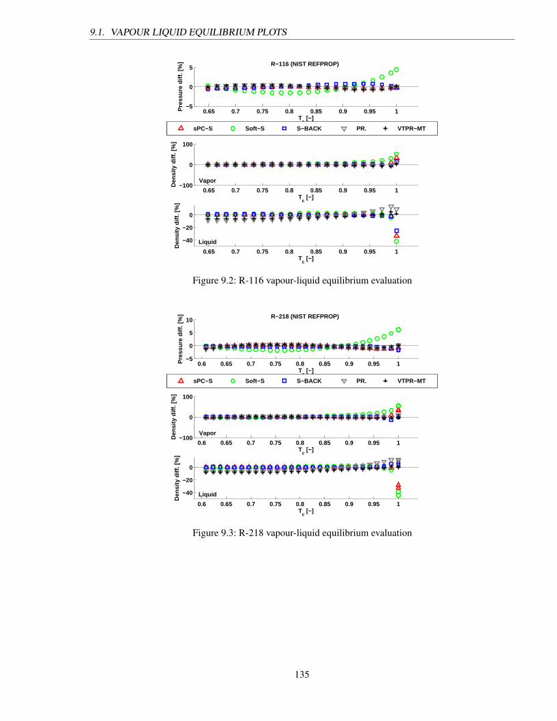
9.1. VAPOUR LIQUID EQUILIBRIUM PLOTS
0.65 0.7 0.75 0.8 0.85 0.9 0.95 1−5
0
5
Pre
ssur
e di
ff. [%
]
Tc [−]
R−116 (NIST REFPROP)
sPC−S Soft−S S−BACK PR. VTPR−MT
0.65 0.7 0.75 0.8 0.85 0.9 0.95 1−100
0
100
Den
sity
diff
. [%
]
Tc [−]
Vapor
0.65 0.7 0.75 0.8 0.85 0.9 0.95 1
−40
−20
0
Den
sity
diff
. [%
]
Tc [−]
Liquid
Figure 9.2: R-116 vapour-liquid equilibrium evaluation
0.6 0.65 0.7 0.75 0.8 0.85 0.9 0.95 1−5
0
5
10
Pre
ssur
e di
ff. [%
]
Tc [−]
R−218 (NIST REFPROP)
sPC−S Soft−S S−BACK PR. VTPR−MT
0.6 0.65 0.7 0.75 0.8 0.85 0.9 0.95 1−100
0
100
Den
sity
diff
. [%
]
Tc [−]
Vapor
0.6 0.65 0.7 0.75 0.8 0.85 0.9 0.95 1
−40
−20
0
Den
sity
diff
. [%
]
Tc [−]
Liquid
Figure 9.3: R-218 vapour-liquid equilibrium evaluation
135
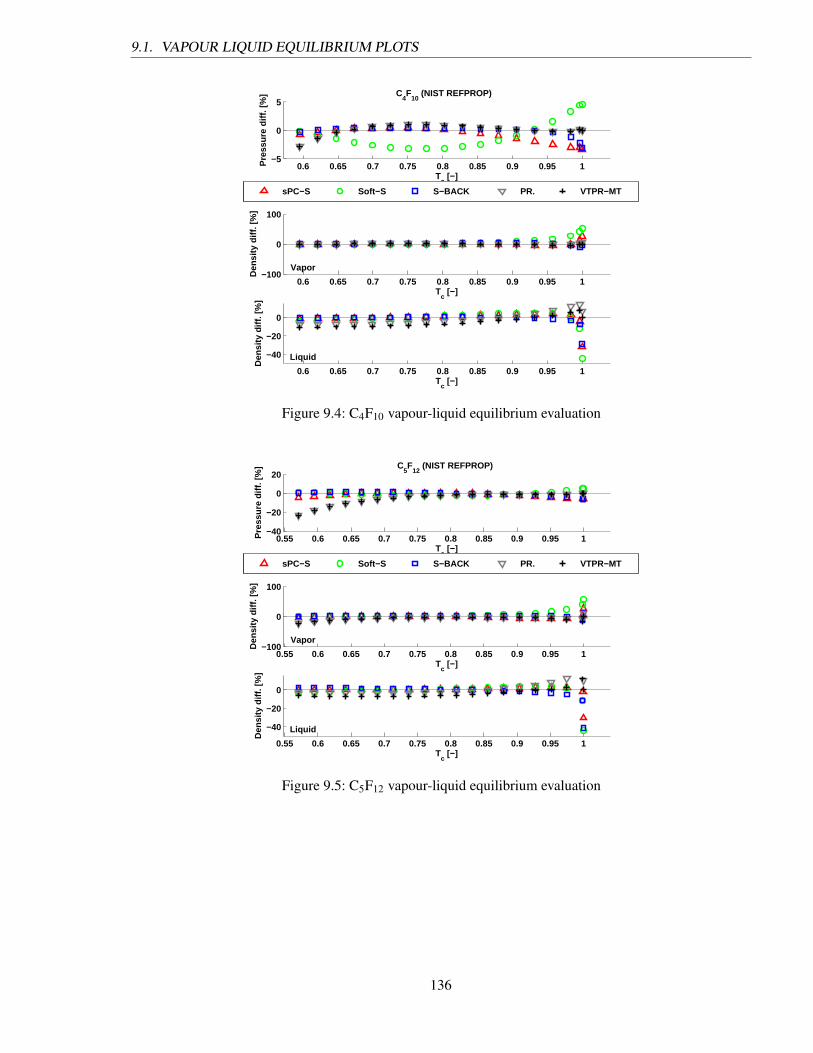
9.1. VAPOUR LIQUID EQUILIBRIUM PLOTS
0.6 0.65 0.7 0.75 0.8 0.85 0.9 0.95 1−5
0
5
Pre
ssur
e di
ff. [%
]
Tc [−]
C4F
10 (NIST REFPROP)
sPC−S Soft−S S−BACK PR. VTPR−MT
0.6 0.65 0.7 0.75 0.8 0.85 0.9 0.95 1−100
0
100
Den
sity
diff
. [%
]
Tc [−]
Vapor
0.6 0.65 0.7 0.75 0.8 0.85 0.9 0.95 1
−40
−20
0
Den
sity
diff
. [%
]
Tc [−]
Liquid
Figure 9.4: C4F10 vapour-liquid equilibrium evaluation
0.55 0.6 0.65 0.7 0.75 0.8 0.85 0.9 0.95 1−40
−20
0
20
Pre
ssur
e di
ff. [%
]
Tc [−]
C5F
12 (NIST REFPROP)
sPC−S Soft−S S−BACK PR. VTPR−MT
0.55 0.6 0.65 0.7 0.75 0.8 0.85 0.9 0.95 1−100
0
100
Den
sity
diff
. [%
]
Tc [−]
Vapor
0.55 0.6 0.65 0.7 0.75 0.8 0.85 0.9 0.95 1
−40
−20
0
Den
sity
diff
. [%
]
Tc [−]
Liquid
Figure 9.5: C5F12 vapour-liquid equilibrium evaluation
136

9.1. VAPOUR LIQUID EQUILIBRIUM PLOTS
0.65 0.7 0.75 0.8 0.85 0.9 0.95 1T
c [-]
-5
0
5
10
Pre
ssu
re d
iff.
[%
] C6F
14 (Equation by E.W. Lemmon)
sPC-S Soft-S S-BACK PR. VTPR-MT
0.65 0.7 0.75 0.8 0.85 0.9 0.95 1T
c [-]
-200
2040
Den
sity
dif
f. [
%]
Vapor
0.65 0.7 0.75 0.8 0.85 0.9 0.95 1T
c [-]
-40
-20
0D
ensi
ty d
iff.
[%
]
Liquid
Figure 9.6: C6F14 vapour-liquid equilibrium evaluation
0.55 0.6 0.65 0.7 0.75 0.8 0.85 0.9 0.95 1−4
−2
0
2
Pre
ssur
e di
ff. [%
]
Tc [−]
R−50 (Friend et al. 1989)
sPC−S Soft−S S−BACK PR. VTPR−AG
0.55 0.6 0.65 0.7 0.75 0.8 0.85 0.9 0.95 1−50
0
50
Den
sity
diff
. [%
]
Tc [−]
Vapor
0.55 0.6 0.65 0.7 0.75 0.8 0.85 0.9 0.95 1
−40
−20
0
Den
sity
diff
. [%
]
Tc [−]
Liquid
Figure 9.7: R-50 vapour-liquid equilibrium evaluation
137
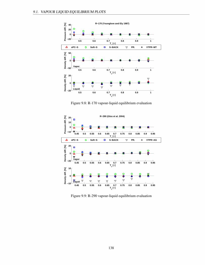
9.1. VAPOUR LIQUID EQUILIBRIUM PLOTS
0.5 0.6 0.7 0.8 0.9 1−20
0
20
40
Pre
ssur
e di
ff. [%
]
Tc [−]
R−170 (Younglove and Ely 1987)
sPC−S Soft−S S−BACK PR. VTPR−MT
0.5 0.6 0.7 0.8 0.9 1−50
0
50
Den
sity
diff
. [%
]
Tc [−]
Vapor
0.5 0.6 0.7 0.8 0.9 1−20
0
20
Den
sity
diff
. [%
]
Tc [−]
Liquid
Figure 9.8: R-170 vapour-liquid equilibrium evaluation
0.45 0.5 0.55 0.6 0.65 0.7 0.75 0.8 0.85 0.9 0.95−10
0
10
20
Pre
ssur
e di
ff. [%
]
Tc [−]
R−290 (Glos et al. 2004)
sPC−S Soft−S S−BACK PR. VTPR−AG
0.45 0.5 0.55 0.6 0.65 0.7 0.75 0.8 0.85 0.9 0.95−20
0
20
Den
sity
diff
. [%
]
Tc [−]
Vapor
0.45 0.5 0.55 0.6 0.65 0.7 0.75 0.8 0.85 0.9 0.95−10
0
10
Den
sity
diff
. [%
]
Tc [−]
Liquid
Figure 9.9: R-290 vapour-liquid equilibrium evaluation
138
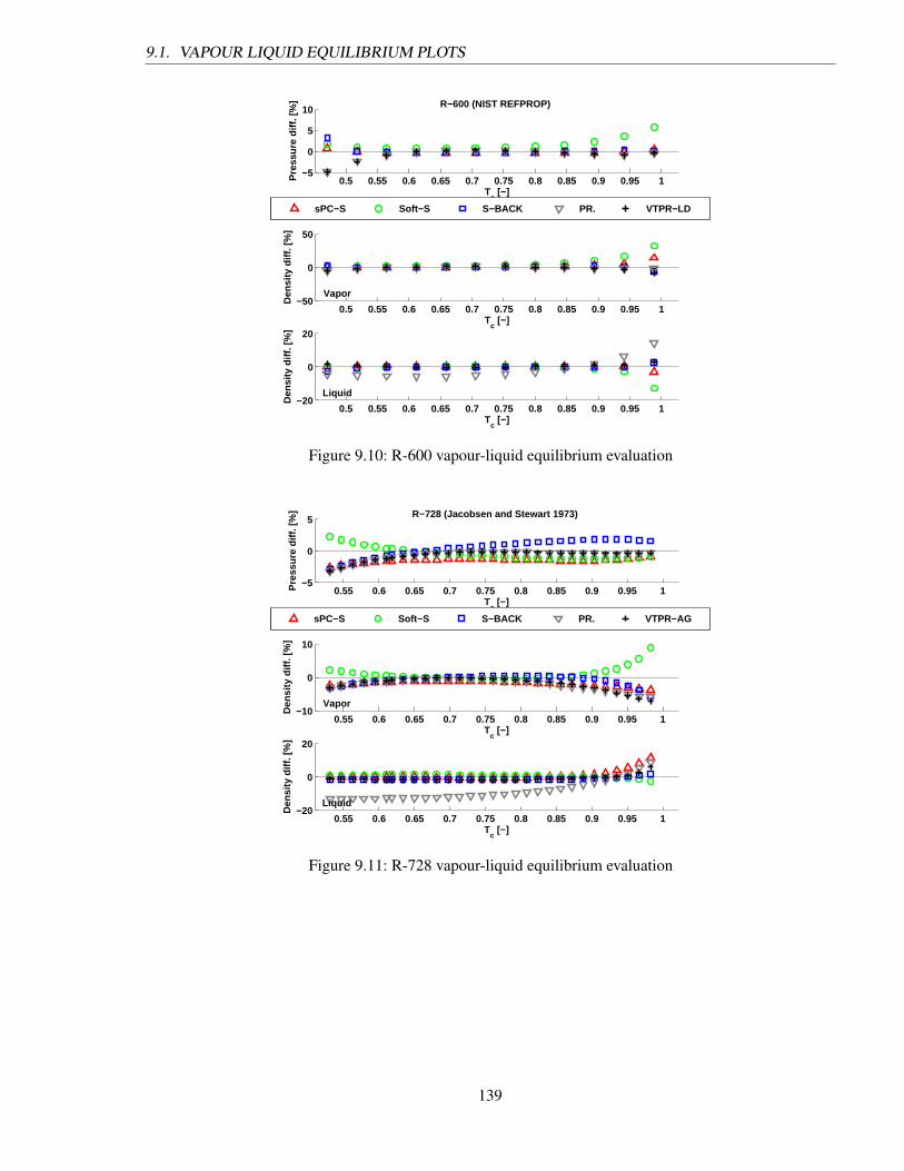
9.1. VAPOUR LIQUID EQUILIBRIUM PLOTS
0.5 0.55 0.6 0.65 0.7 0.75 0.8 0.85 0.9 0.95 1−5
0
5
10
Pre
ssur
e di
ff. [%
]
Tc [−]
R−600 (NIST REFPROP)
sPC−S Soft−S S−BACK PR. VTPR−LD
0.5 0.55 0.6 0.65 0.7 0.75 0.8 0.85 0.9 0.95 1−50
0
50
Den
sity
diff
. [%
]
Tc [−]
Vapor
0.5 0.55 0.6 0.65 0.7 0.75 0.8 0.85 0.9 0.95 1−20
0
20
Den
sity
diff
. [%
]
Tc [−]
Liquid
Figure 9.10: R-600 vapour-liquid equilibrium evaluation
0.55 0.6 0.65 0.7 0.75 0.8 0.85 0.9 0.95 1−5
0
5
Pre
ssur
e di
ff. [%
]
Tc [−]
R−728 (Jacobsen and Stewart 1973)
sPC−S Soft−S S−BACK PR. VTPR−AG
0.55 0.6 0.65 0.7 0.75 0.8 0.85 0.9 0.95 1−10
0
10
Den
sity
diff
. [%
]
Tc [−]
Vapor
0.55 0.6 0.65 0.7 0.75 0.8 0.85 0.9 0.95 1−20
0
20
Den
sity
diff
. [%
]
Tc [−]
Liquid
Figure 9.11: R-728 vapour-liquid equilibrium evaluation
139
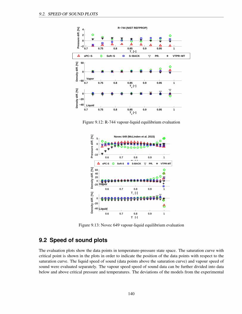
9.2. SPEED OF SOUND PLOTS
0.7 0.75 0.8 0.85 0.9 0.95 1−2
0
2
4
Pre
ssur
e di
ff. [%
]
Tc [−]
R−744 (NIST REFPROP)
sPC−S Soft−S S−BACK PR. VTPR−MT
0.7 0.75 0.8 0.85 0.9 0.95 1−50
0
50
Den
sity
diff
. [%
]
Tc [−]
Vapor
0.7 0.75 0.8 0.85 0.9 0.95 1
−40
−20
0
Den
sity
diff
. [%
]
Tc [−]
Liquid
Figure 9.12: R-744 vapour-liquid equilibrium evaluation
0.6 0.7 0.8 0.9 1T
c [-]
-10
-5
0
5
Pre
ssu
re d
iff.
[%
]
Novec 649 (McLinden et al. 2015)
sPC-S Soft-S S-BACK PR. VTPR-MT
0.6 0.7 0.8 0.9 1T
c [-]
-200
204060
Den
sity
dif
f. [
%]
Vapor
0.6 0.7 0.8 0.9 1T
c [-]
-40
-20
0
Den
sity
dif
f. [
%]
Liquid
Figure 9.13: Novec 649 vapour-liquid equilibrium evaluation
9.2 Speed of sound plots
The evaluation plots show the data points in temperature-pressure state space. The saturation curve withcritical point is shown in the plots in order to indicate the position of the data points with respect to thesaturation curve. The liquid speed of sound (data points above the saturation curve) and vapour speed ofsound were evaluated separately. The vapour speed speed of sound data can be further divided into databelow and above critical pressure and temperatures. The deviations of the models from the experimental
140

9.2. SPEED OF SOUND PLOTS
speed of sound are plotted as function of reduced density. The combination of the pressure-temperature plotand the density-deviation plot provides comprehensive overview of the input data used for the evaluation.
9.2.1 vapour phase
100 150 200 250 300 350 400 4500
1
2
3
4
Pre
ssur
e [M
Pa]
Temperature [K]
R−14 (Hurly1999)
Data points Critical point Saturation curve
0.01 0.02 0.03 0.04 0.05 0.06 0.07 0.08 0.09−4
−2
0
2
SoS
diff
. [%
]
Rhoc [−]
sPC−S Soft−S S−BACK PR. VTPR−MT
Figure 9.14: Speed of sound evaluation No1: R-14
120 140 160 180 200 220 240 260 280 300 3200
1
2
3
4
Pre
ssur
e [M
Pa]
Temperature [K]
R−14 (Ewing and Trusler 1989)
Data points Critical point Saturation curve
0.01 0.02 0.03 0.04 0.05 0.06 0.07 0.08 0.09 0.1−10
−5
0
5
SoS
diff
. [%
]
Rhoc [−]
sPC−S Soft−S S−BACK PR. VTPR−MT
Figure 9.15: Speed of sound evaluation No2: R-14
141
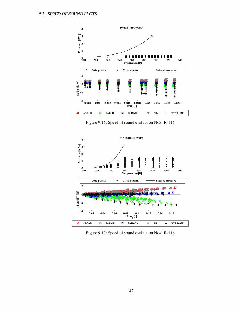
9.2. SPEED OF SOUND PLOTS
180 200 220 240 260 280 300 320 3400
1
2
3
4
Pre
ssur
e [M
Pa]
Temperature [K]
R−116 (This work)
Data points Critical point Saturation curve
0.008 0.01 0.012 0.014 0.016 0.018 0.02 0.022 0.024 0.026−2
−1
0
1S
oS d
iff. [
%]
Rhoc [−]
sPC−S Soft−S S−BACK PR. VTPR−MT
Figure 9.16: Speed of sound evaluation No3: R-116
150 200 250 300 350 400 450 5000
1
2
3
4
Pre
ssur
e [M
Pa]
Temperature [K]
R−116 (Hurly 2003)
Data points Critical point Saturation curve
0.02 0.04 0.06 0.08 0.1 0.12 0.14 0.16−4
−2
0
2
SoS
diff
. [%
]
Rhoc [−]
sPC−S Soft−S S−BACK PR. VTPR−MT
Figure 9.17: Speed of sound evaluation No4: R-116
142
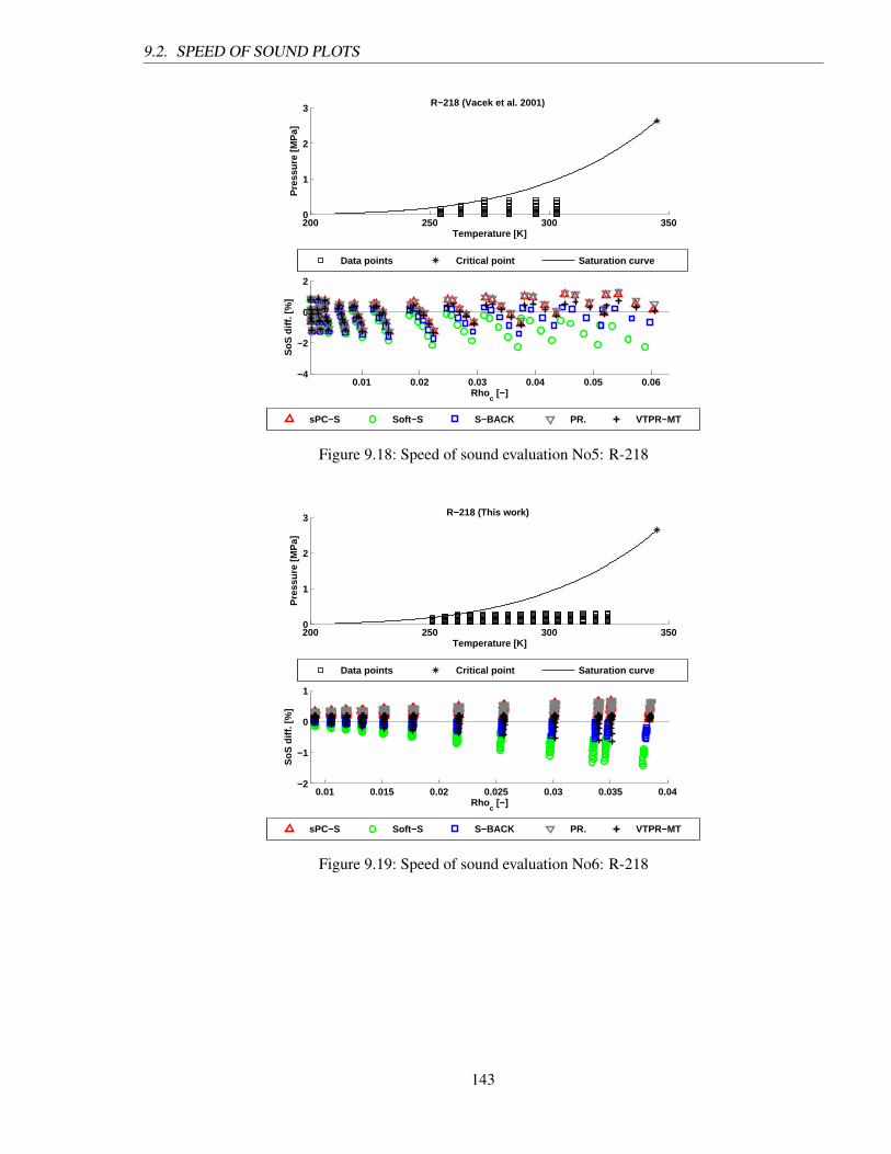
9.2. SPEED OF SOUND PLOTS
200 250 300 3500
1
2
3
Pre
ssur
e [M
Pa]
Temperature [K]
R−218 (Vacek et al. 2001)
Data points Critical point Saturation curve
0.01 0.02 0.03 0.04 0.05 0.06−4
−2
0
2S
oS d
iff. [
%]
Rhoc [−]
sPC−S Soft−S S−BACK PR. VTPR−MT
Figure 9.18: Speed of sound evaluation No5: R-218
200 250 300 3500
1
2
3
Pre
ssur
e [M
Pa]
Temperature [K]
R−218 (This work)
Data points Critical point Saturation curve
0.01 0.015 0.02 0.025 0.03 0.035 0.04−2
−1
0
1
SoS
diff
. [%
]
Rhoc [−]
sPC−S Soft−S S−BACK PR. VTPR−MT
Figure 9.19: Speed of sound evaluation No6: R-218
143
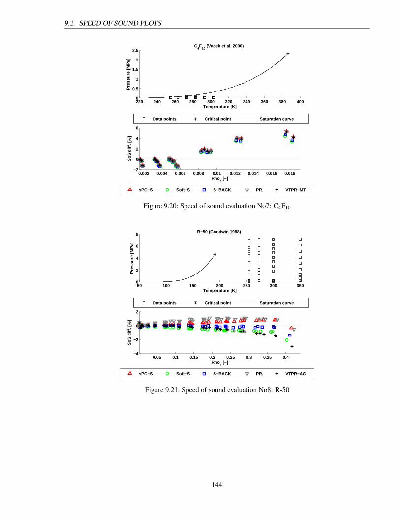
9.2. SPEED OF SOUND PLOTS
220 240 260 280 300 320 340 360 380 4000
0.5
1
1.5
2
2.5
Pre
ssur
e [M
Pa]
Temperature [K]
C4F
10 (Vacek et al. 2000)
Data points Critical point Saturation curve
0.002 0.004 0.006 0.008 0.01 0.012 0.014 0.016 0.018−2
0
2
4
6S
oS d
iff. [
%]
Rhoc [−]
sPC−S Soft−S S−BACK PR. VTPR−MT
Figure 9.20: Speed of sound evaluation No7: C4F10
50 100 150 200 250 300 3500
2
4
6
8
Pre
ssur
e [M
Pa]
Temperature [K]
R−50 (Goodwin 1988)
Data points Critical point Saturation curve
0.05 0.1 0.15 0.2 0.25 0.3 0.35 0.4−4
−2
0
2
SoS
diff
. [%
]
Rhoc [−]
sPC−S Soft−S S−BACK PR. VTPR−AG
Figure 9.21: Speed of sound evaluation No8: R-50
144
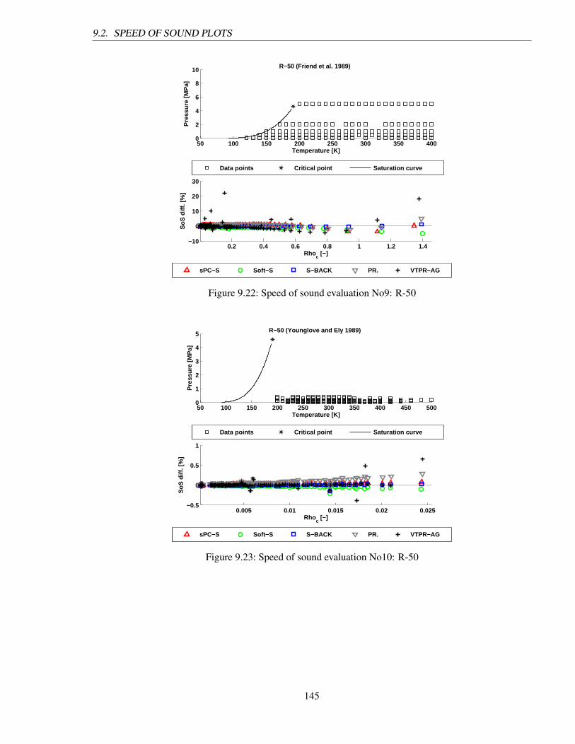
9.2. SPEED OF SOUND PLOTS
50 100 150 200 250 300 350 4000
2
4
6
8
10
Pre
ssur
e [M
Pa]
Temperature [K]
R−50 (Friend et al. 1989)
Data points Critical point Saturation curve
0.2 0.4 0.6 0.8 1 1.2 1.4−10
0
10
20
30S
oS d
iff. [
%]
Rhoc [−]
sPC−S Soft−S S−BACK PR. VTPR−AG
Figure 9.22: Speed of sound evaluation No9: R-50
50 100 150 200 250 300 350 400 450 5000
1
2
3
4
5
Pre
ssur
e [M
Pa]
Temperature [K]
R−50 (Younglove and Ely 1989)
Data points Critical point Saturation curve
0.005 0.01 0.015 0.02 0.025−0.5
0
0.5
1
SoS
diff
. [%
]
Rhoc [−]
sPC−S Soft−S S−BACK PR. VTPR−AG
Figure 9.23: Speed of sound evaluation No10: R-50
145
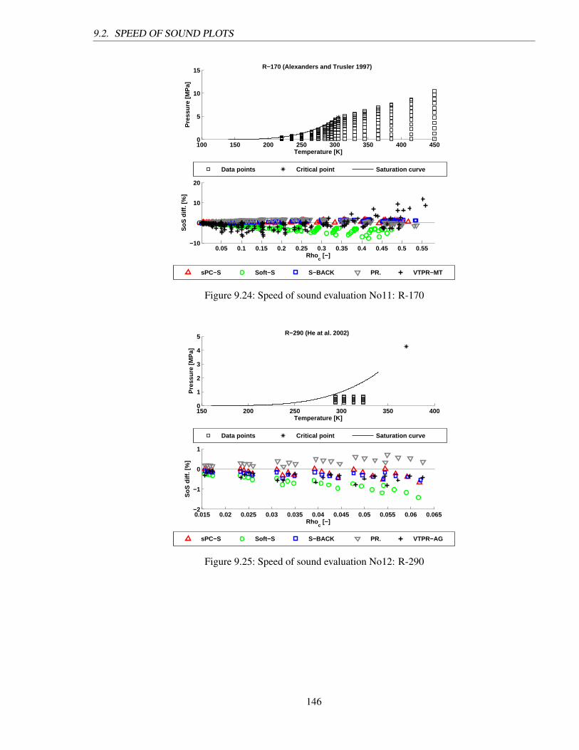
9.2. SPEED OF SOUND PLOTS
100 150 200 250 300 350 400 4500
5
10
15
Pre
ssur
e [M
Pa]
Temperature [K]
R−170 (Alexanders and Trusler 1997)
Data points Critical point Saturation curve
0.05 0.1 0.15 0.2 0.25 0.3 0.35 0.4 0.45 0.5 0.55−10
0
10
20S
oS d
iff. [
%]
Rhoc [−]
sPC−S Soft−S S−BACK PR. VTPR−MT
Figure 9.24: Speed of sound evaluation No11: R-170
150 200 250 300 350 4000
1
2
3
4
5
Pre
ssur
e [M
Pa]
Temperature [K]
R−290 (He at al. 2002)
Data points Critical point Saturation curve
0.015 0.02 0.025 0.03 0.035 0.04 0.045 0.05 0.055 0.06 0.065−2
−1
0
1
SoS
diff
. [%
]
Rhoc [−]
sPC−S Soft−S S−BACK PR. VTPR−AG
Figure 9.25: Speed of sound evaluation No12: R-290
146
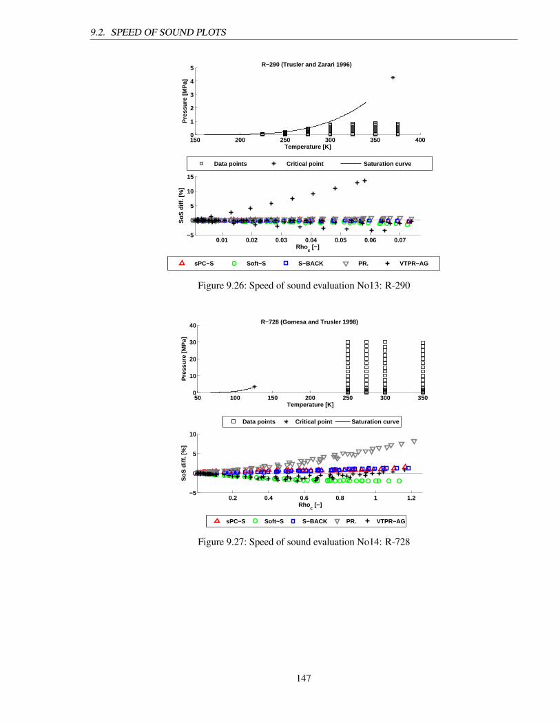
9.2. SPEED OF SOUND PLOTS
150 200 250 300 350 4000
1
2
3
4
5
Pre
ssur
e [M
Pa]
Temperature [K]
R−290 (Trusler and Zarari 1996)
Data points Critical point Saturation curve
0.01 0.02 0.03 0.04 0.05 0.06 0.07−5
0
5
10
15S
oS d
iff. [
%]
Rhoc [−]
sPC−S Soft−S S−BACK PR. VTPR−AG
Figure 9.26: Speed of sound evaluation No13: R-290
50 100 150 200 250 300 3500
10
20
30
40
Pre
ssur
e [M
Pa]
Temperature [K]
R−728 (Gomesa and Trusler 1998)
Data points Critical point Saturation curve
0.2 0.4 0.6 0.8 1 1.2−5
0
5
10
SoS
diff
. [%
]
Rhoc [−]
sPC−S Soft−S S−BACK PR. VTPR−AG
Figure 9.27: Speed of sound evaluation No14: R-728
147
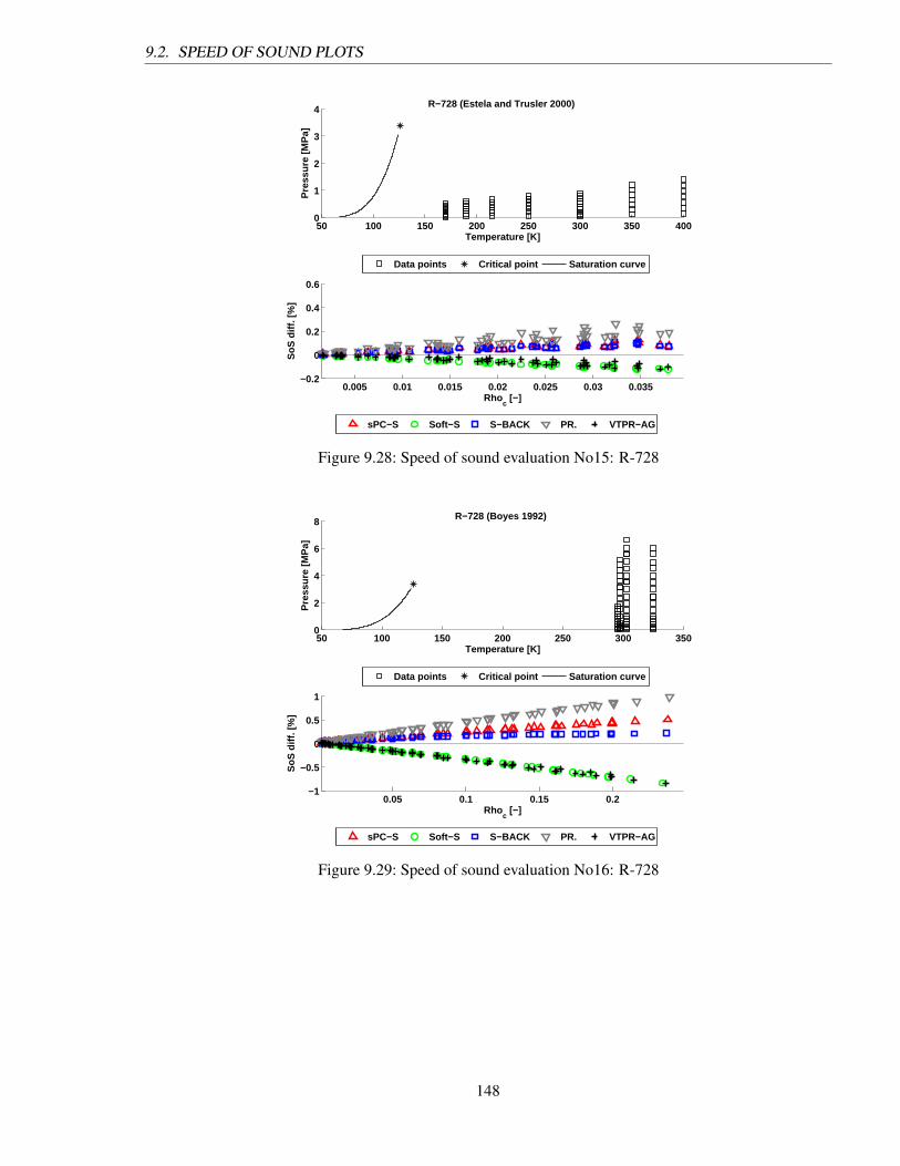
9.2. SPEED OF SOUND PLOTS
50 100 150 200 250 300 350 4000
1
2
3
4
Pre
ssur
e [M
Pa]
Temperature [K]
R−728 (Estela and Trusler 2000)
Data points Critical point Saturation curve
0.005 0.01 0.015 0.02 0.025 0.03 0.035−0.2
0
0.2
0.4
0.6S
oS d
iff. [
%]
Rhoc [−]
sPC−S Soft−S S−BACK PR. VTPR−AG
Figure 9.28: Speed of sound evaluation No15: R-728
50 100 150 200 250 300 3500
2
4
6
8
Pre
ssur
e [M
Pa]
Temperature [K]
R−728 (Boyes 1992)
Data points Critical point Saturation curve
0.05 0.1 0.15 0.2−1
−0.5
0
0.5
1
SoS
diff
. [%
]
Rhoc [−]
sPC−S Soft−S S−BACK PR. VTPR−AG
Figure 9.29: Speed of sound evaluation No16: R-728
148

9.2. SPEED OF SOUND PLOTS
220 240 260 280 300 320 3400
2
4
6
8
Pre
ssur
e [M
Pa]
Temperature [K]
R−744 (Liu et al. 2014)
Data points Critical point Saturation curve
0.01 0.015 0.02 0.025 0.03 0.035 0.04 0.045−10
−5
0
5S
oS d
iff. [
%]
Rhoc [−]
sPC−S Soft−S S−BACK PR. VTPR−MT
Figure 9.30: Speed of sound evaluation No17: R-744
250 300 350 400 450 500 550Temperature [K]
0
1
2
Pre
ssu
re [
MP
a]
Novec 649 (McLinden et al. 2015)
Data points Critical point Saturation curve
0.05 0.1 0.15 0.2 0.25 0.3 0.35 0.4Rho
c [-]
-10
-5
0
5
So
S d
iff.
[%
]
sPC-S Soft-S S-BACK PR. VTPR-MT
Figure 9.31: Speed of sound evaluation No18: Novec 649
149

9.2. SPEED OF SOUND PLOTS
9.2.2 Liquid phase
240 260 280 300 320 340 360 380 400 420 4400
0.5
1
1.5
2
2.5
Pre
ssur
e [M
Pa]
Temperature [K]
C5F
12 (Kallepally et al. 1989)
Data points Critical point Saturation curve
2.55 2.6 2.65 2.7 2.75 2.8 2.85 2.9 2.95−10
0
10
20
30
SoS
diff
. [%
]
Rhoc [−]
sPC−S Soft−S S−BACK PR. VTPR−MT
Figure 9.32: Speed of sound evaluation No19: C5F12
200 250 300 350 400 4500
0.5
1
1.5
2
2.5
Pre
ssur
e [M
Pa]
Temperature [K]
C5F
12 (Cochrana et al. 1974)
Data points Critical point Saturation curve
2.8 2.9 3 3.1 3.2 3.3−10
0
10
20
30
SoS
diff
. [%
]
Rhoc [−]
sPC−S Soft−S S−BACK PR. VTPR−MT
Figure 9.33: Speed of sound evaluation No20: C5F12
150
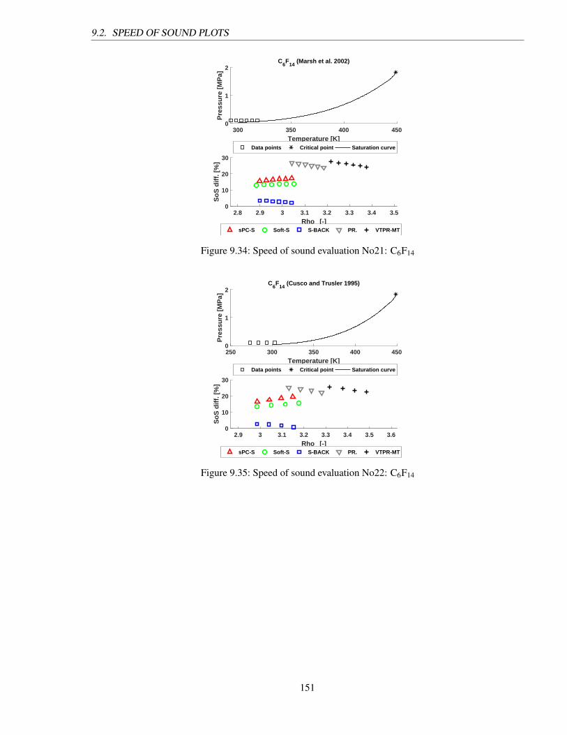
9.2. SPEED OF SOUND PLOTS
300 350 400 450Temperature [K]
0
1
2
Pre
ssu
re [
MP
a]
C6F
14 (Marsh et al. 2002)
Data points Critical point Saturation curve
2.8 2.9 3 3.1 3.2 3.3 3.4 3.5Rho
c [-]
0
10
20
30
So
S d
iff.
[%
]
sPC-S Soft-S S-BACK PR. VTPR-MT
Figure 9.34: Speed of sound evaluation No21: C6F14
250 300 350 400 450Temperature [K]
0
1
2
Pre
ssu
re [
MP
a]
C6F
14 (Cusco and Trusler 1995)
Data points Critical point Saturation curve
2.9 3 3.1 3.2 3.3 3.4 3.5 3.6Rho
c [-]
0
10
20
30
So
S d
iff.
[%
]
sPC-S Soft-S S-BACK PR. VTPR-MT
Figure 9.35: Speed of sound evaluation No22: C6F14
151
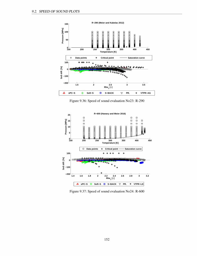
9.2. SPEED OF SOUND PLOTS
150 200 250 300 350 400 4500
50
100
150
Pre
ssur
e [M
Pa]
Temperature [K]
R−290 (Meier and Kabelac 2012)
Data points Critical point Saturation curve
1.5 2 2.5 3 3.5−200
−100
0
100S
oS d
iff. [
%]
Rhoc [−]
sPC−S Soft−S S−BACK PR. VTPR−AG
Figure 9.36: Speed of sound evaluation No23: R-290
150 200 250 300 350 400 4500
5
10
15
20
Pre
ssur
e [M
Pa]
Temperature [K]
R−600 (Hawary and Meier 2016)
Data points Critical point Saturation curve
1.4 1.6 1.8 2 2.2 2.4 2.6 2.8 3 3.2−200
−100
0
100
SoS
diff
. [%
]
Rhoc [−]
sPC−S Soft−S S−BACK PR. VTPR−LD
Figure 9.37: Speed of sound evaluation No24: R-600
152
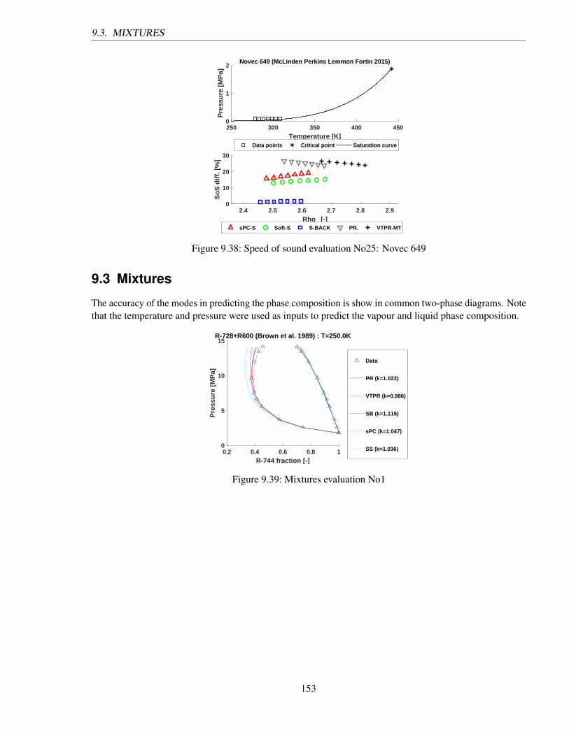
9.3. MIXTURES
250 300 350 400 450Temperature [K]
0
1
2
Pre
ssu
re [
MP
a]
Novec 649 (McLinden Perkins Lemmon Fortin 2015)
Data points Critical point Saturation curve
2.4 2.5 2.6 2.7 2.8 2.9Rho
c [-]
0
10
20
30
So
S d
iff.
[%
]
sPC-S Soft-S S-BACK PR. VTPR-MT
Figure 9.38: Speed of sound evaluation No25: Novec 649
9.3 Mixtures
The accuracy of the modes in predicting the phase composition is show in common two-phase diagrams. Notethat the temperature and pressure were used as inputs to predict the vapour and liquid phase composition.
0.2 0.4 0.6 0.8 1R-744 fraction [-]
0
5
10
15
Pre
ssu
re [
MP
a]
R-728+R600 (Brown et al. 1989) : T=250.0K
Data
PR (k=1.022)
VTPR (k=0.986)
SB (k=1.115)
sPC (k=1.047)
SS (k=1.036)
Figure 9.39: Mixtures evaluation No1
153
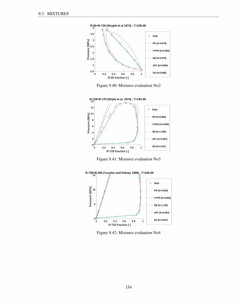
9.3. MIXTURES
0 0.2 0.4 0.6 0.8 1R-50 fraction [-]
0.5
1
1.5
2
2.5
3
3.5
4
Pre
ssu
re [
MP
a]
R-50+R-728 (Stryjek et al 1974) : T=138.4K
Data
PR (k=0.879)
VTPR (k=0.955)
SB (k=0.975)
sPC (k=0.984)
SS (k=0.985)
Figure 9.40: Mixtures evaluation No2
0 0.2 0.4 0.6 0.8 1R-728 fraction [-]
0
2
4
6
8
10
12
14
Pre
ssu
re [
MP
a]
R-728+R-170 (Strjek et al. 1974) : T=194.3K
Data
PR (k=0.985)
VTPR (k=0.829)
SB (k=1.028)
sPC (k=0.987)
SS (k=1.007)
Figure 9.41: Mixtures evaluation No3
0 0.2 0.4 0.6 0.8 1R-728 fraction [-]
0
5
10
15
Pre
ssu
re [
MP
a]
R-728+R-290 (Yucelen and Kidnay 1999) : T=240.0K
Data
PR (k=0.929)
VTPR (k=0.860)
SB (k=1.135)
sPC (k=0.953)
SS (k=0.957)
Figure 9.42: Mixtures evaluation No4
154
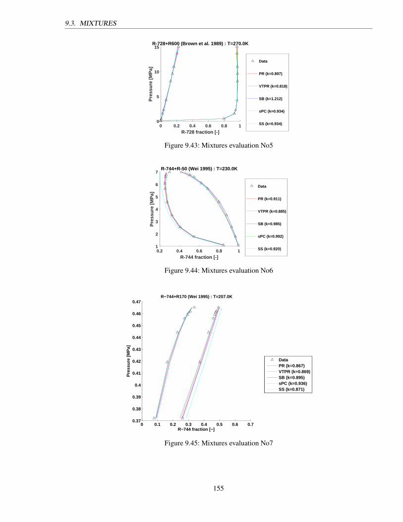
9.3. MIXTURES
0 0.2 0.4 0.6 0.8 1R-728 fraction [-]
0
5
10
15
Pre
ssu
re [
MP
a]
R-728+R600 (Brown et al. 1989) : T=270.0K
Data
PR (k=0.897)
VTPR (k=0.818)
SB (k=1.212)
sPC (k=0.934)
SS (k=0.934)
Figure 9.43: Mixtures evaluation No5
0.2 0.4 0.6 0.8 1R-744 fraction [-]
1
2
3
4
5
6
7
Pre
ssu
re [
MP
a]
R-744+R-50 (Wei 1995) : T=230.0K
Data
PR (k=0.911)
VTPR (k=0.885)
SB (k=0.985)
sPC (k=0.992)
SS (k=0.920)
Figure 9.44: Mixtures evaluation No6
0 0.1 0.2 0.3 0.4 0.5 0.6 0.70.37
0.38
0.39
0.4
0.41
0.42
0.43
0.44
0.45
0.46
0.47
R−744 fraction [−]
Pre
ssur
e [M
Pa]
R−744+R170 (Wei 1995) : T=207.0K
DataPR (k=0.867)VTPR (k=0.869)SB (k=0.895)sPC (k=0.936)SS (k=0.871)
Figure 9.45: Mixtures evaluation No7
155
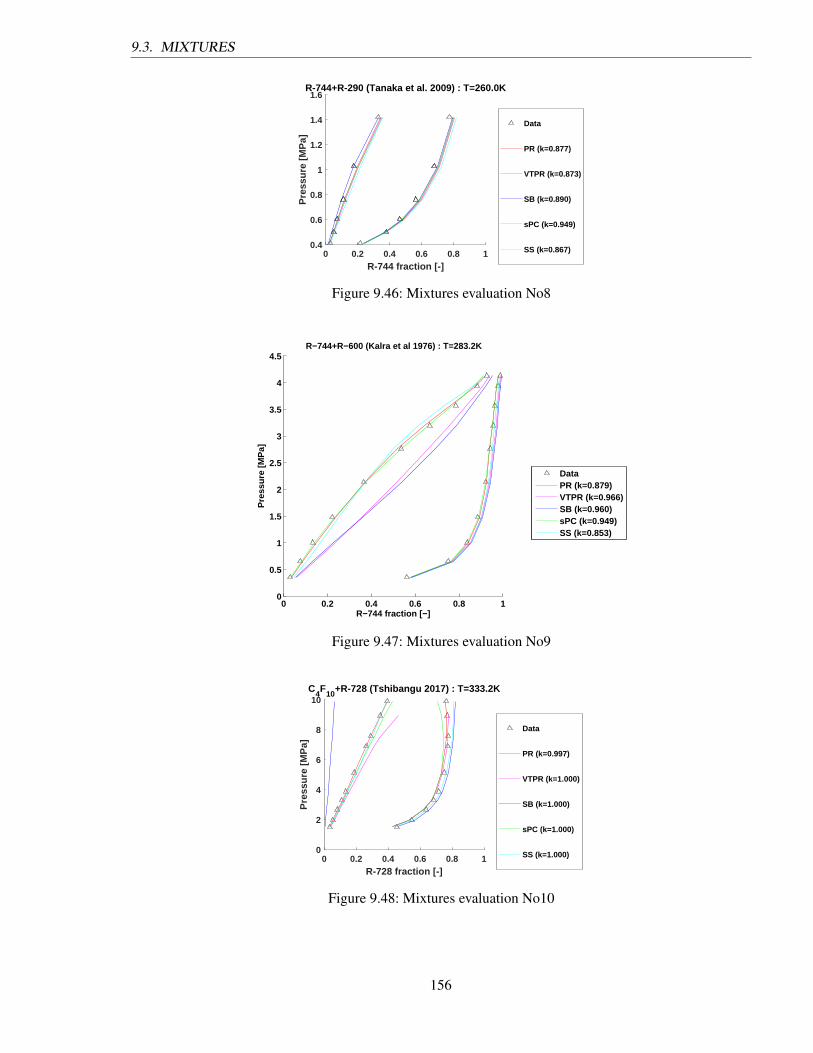
9.3. MIXTURES
0 0.2 0.4 0.6 0.8 1R-744 fraction [-]
0.4
0.6
0.8
1
1.2
1.4
1.6
Pre
ssu
re [
MP
a]
R-744+R-290 (Tanaka et al. 2009) : T=260.0K
Data
PR (k=0.877)
VTPR (k=0.873)
SB (k=0.890)
sPC (k=0.949)
SS (k=0.867)
Figure 9.46: Mixtures evaluation No8
0 0.2 0.4 0.6 0.8 10
0.5
1
1.5
2
2.5
3
3.5
4
4.5
R−744 fraction [−]
Pre
ssur
e [M
Pa]
R−744+R−600 (Kalra et al 1976) : T=283.2K
DataPR (k=0.879)VTPR (k=0.966)SB (k=0.960)sPC (k=0.949)SS (k=0.853)
Figure 9.47: Mixtures evaluation No9
0 0.2 0.4 0.6 0.8 1R-728 fraction [-]
0
2
4
6
8
10
Pre
ssu
re [
MP
a]
C4F
10+R-728 (Tshibangu 2017) : T=333.2K
Data
PR (k=0.997)
VTPR (k=1.000)
SB (k=1.000)
sPC (k=1.000)
SS (k=1.000)
Figure 9.48: Mixtures evaluation No10
156
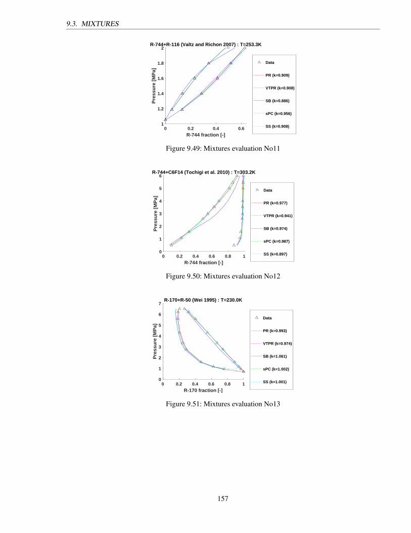
9.3. MIXTURES
0 0.2 0.4 0.6R-744 fraction [-]
1
1.2
1.4
1.6
1.8
2
Pre
ssu
re [
MP
a]
R-744+R-116 (Valtz and Richon 2007) : T=253.3K
Data
PR (k=0.909)
VTPR (k=0.908)
SB (k=0.886)
sPC (k=0.956)
SS (k=0.908)
Figure 9.49: Mixtures evaluation No11
0 0.2 0.4 0.6 0.8 1R-744 fraction [-]
0
1
2
3
4
5
6
Pre
ssu
re [
MP
a]
R-744+C6F14 (Tochigi et al. 2010) : T=303.2K
Data
PR (k=0.977)
VTPR (k=0.941)
SB (k=0.974)
sPC (k=0.987)
SS (k=0.897)
Figure 9.50: Mixtures evaluation No12
0 0.2 0.4 0.6 0.8 1R-170 fraction [-]
0
1
2
3
4
5
6
7
Pre
ssu
re [
MP
a]
R-170+R-50 (Wei 1995) : T=230.0K
Data
PR (k=0.993)
VTPR (k=0.974)
SB (k=1.061)
sPC (k=1.002)
SS (k=1.001)
Figure 9.51: Mixtures evaluation No13
157
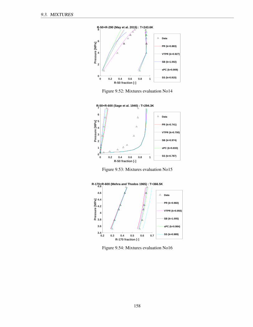
9.3. MIXTURES
0 0.2 0.4 0.6 0.8 1R-50 fraction [-]
0
2
4
6
8
Pre
ssu
re [
MP
a]
R-50+R-290 (May et al. 2015) : T=243.6K
Data
PR (k=0.883)
VTPR (k=0.927)
SB (k=1.002)
sPC (k=0.909)
SS (k=0.915)
Figure 9.52: Mixtures evaluation No14
0 0.2 0.4 0.6 0.8 1R-50 fraction [-]
0
1
2
3
4
5
6
7
Pre
ssu
re [
MP
a]
R-50+R-600 (Sage et al. 1940) : T=294.3K
Data
PR (k=0.741)
VTPR (k=0.700)
SB (k=0.974)
sPC (k=0.833)
SS (k=0.787)
Figure 9.53: Mixtures evaluation No15
0.2 0.3 0.4 0.5 0.6 0.7R-170 fraction [-]
3.4
3.6
3.8
4
4.2
4.4
4.6
4.8
Pre
ssu
re [
MP
a]
R-170+R-600 (Mehra and Thodos 1965) : T=366.5K
Data
PR (k=0.960)
VTPR (k=0.955)
SB (k=1.005)
sPC (k=0.984)
SS (k=0.989)
Figure 9.54: Mixtures evaluation No16
158

9.3. MIXTURES
0 0.2 0.4 0.6 0.8 1R-600 fraction [-]
0.1
0.15
0.2
0.25
0.3
0.35
0.4
Pre
ssu
re [
MP
a]
R-600+R-290 (Yohei et al 2005) : T=270.0K
Data
PR (k=0.997)
VTPR (k=0.995)
SB (k=1.004)
sPC (k=1.001)
SS (k=1.000)
Figure 9.55: Mixtures evaluation No17
0 0.2 0.4 0.6 0.8R-50 fraction [-]
0
2
4
6
8
10
Pre
ssu
re [
MP
a]
C4F
10+R-50 (Tshibangu 2017) : T=333.0K
Data
PR (k=0.751)
VTPR (k=0.649)
SB (k=1.021)
sPC (k=0.842)
SS (k=0.814)
Figure 9.56: Mixtures evaluation No18
0 0.2 0.4 0.6 0.8 1R-50 fraction [-]
0
1
2
3
4
5
6
7
Pre
ssu
re [
MP
a]
C6F
14+R-50 (Tshibangu 2017) : T=333.4K
Data
PR (k=0.865)
VTPR (k=0.666)
SB (k=1.230)
sPC (k=0.896)
SS (k=0.863)
Figure 9.57: Mixtures evaluation No19
159
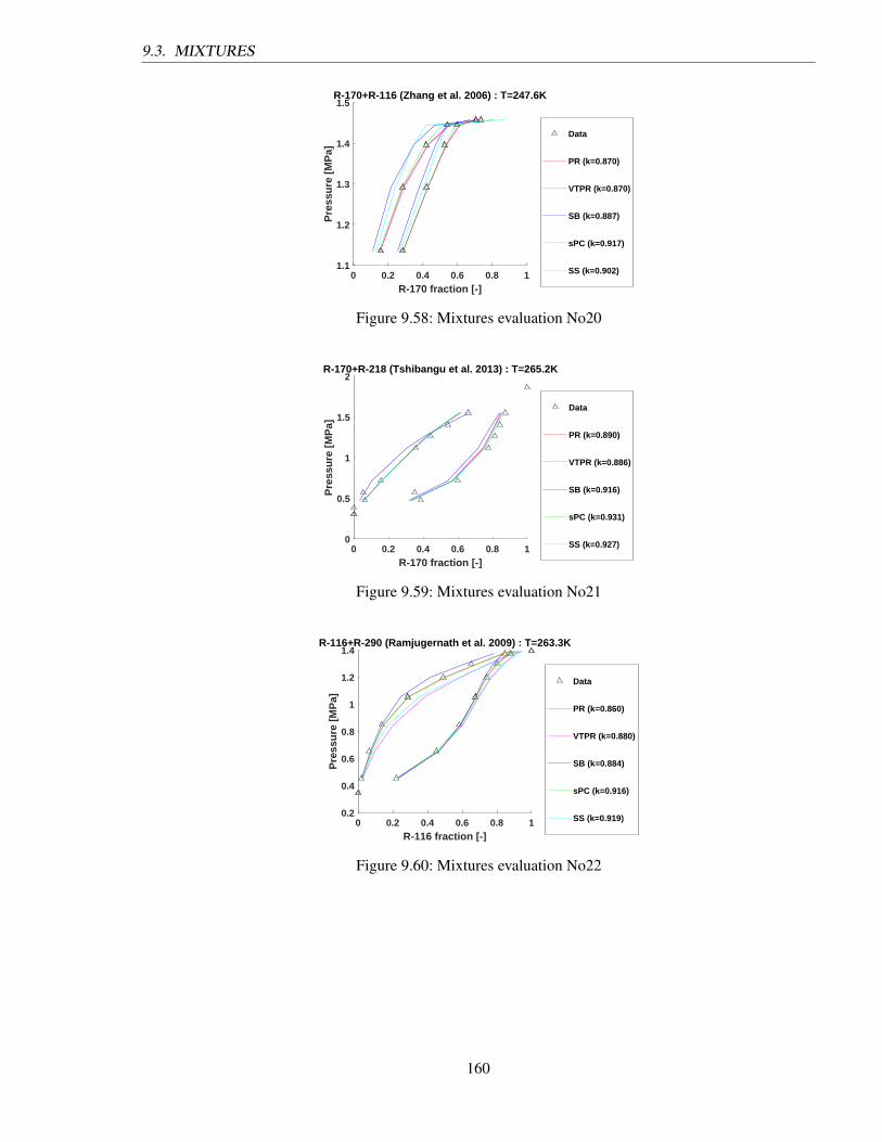
9.3. MIXTURES
0 0.2 0.4 0.6 0.8 1R-170 fraction [-]
1.1
1.2
1.3
1.4
1.5
Pre
ssu
re [
MP
a]
R-170+R-116 (Zhang et al. 2006) : T=247.6K
Data
PR (k=0.870)
VTPR (k=0.870)
SB (k=0.887)
sPC (k=0.917)
SS (k=0.902)
Figure 9.58: Mixtures evaluation No20
0 0.2 0.4 0.6 0.8 1R-170 fraction [-]
0
0.5
1
1.5
2
Pre
ssu
re [
MP
a]
R-170+R-218 (Tshibangu et al. 2013) : T=265.2K
Data
PR (k=0.890)
VTPR (k=0.886)
SB (k=0.916)
sPC (k=0.931)
SS (k=0.927)
Figure 9.59: Mixtures evaluation No21
0 0.2 0.4 0.6 0.8 1R-116 fraction [-]
0.2
0.4
0.6
0.8
1
1.2
1.4
Pre
ssu
re [
MP
a]
R-116+R-290 (Ramjugernath et al. 2009) : T=263.3K
Data
PR (k=0.860)
VTPR (k=0.880)
SB (k=0.884)
sPC (k=0.916)
SS (k=0.919)
Figure 9.60: Mixtures evaluation No22
160
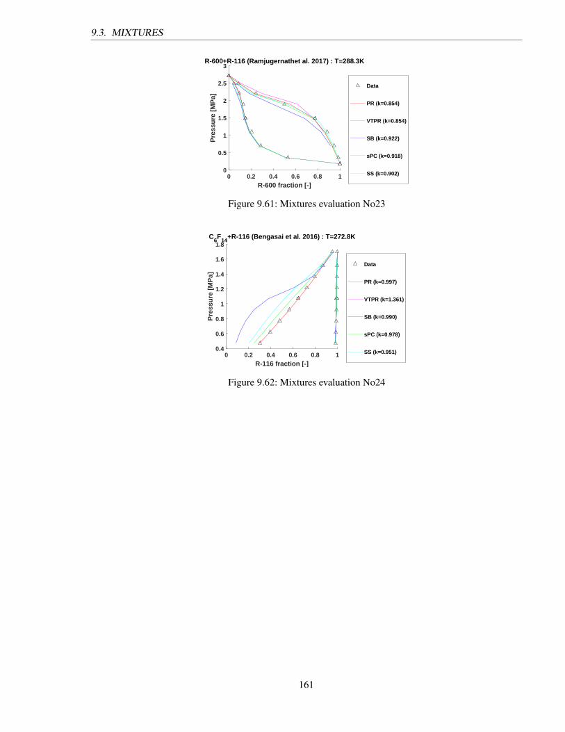
9.3. MIXTURES
0 0.2 0.4 0.6 0.8 1R-600 fraction [-]
0
0.5
1
1.5
2
2.5
3
Pre
ssu
re [
MP
a]
R-600+R-116 (Ramjugernathet al. 2017) : T=288.3K
Data
PR (k=0.854)
VTPR (k=0.854)
SB (k=0.922)
sPC (k=0.918)
SS (k=0.902)
Figure 9.61: Mixtures evaluation No23
0 0.2 0.4 0.6 0.8 1R-116 fraction [-]
0.4
0.6
0.8
1
1.2
1.4
1.6
1.8
Pre
ssu
re [
MP
a]
C6F
14+R-116 (Bengasai et al. 2016) : T=272.8K
Data
PR (k=0.997)
VTPR (k=1.361)
SB (k=0.990)
sPC (k=0.978)
SS (k=0.951)
Figure 9.62: Mixtures evaluation No24
161