Exchange Rate Volatility in Post-floating Regime in India

Advances in Economics and Business 3(9): 360-370, 2015 http://www.hrpub.org DOI: 10.13189/aeb.2015.030902

Exchange Rate Volatility in Post-floating Regime in India

Priyadarshi Dash

Research and Information System for Developing Countries (RIS), India

Copyright © 2015 by authors, all rights reserved. Authors agree that this article remains permanently open access under the terms of the Creative Commons Attribution License 4.0 International License

Abstract Exchange rate reflects the fundamentals of an economy in terms of relative export price and indicators of external stability. Volatility in nominal exchange rate spills over to the real sectors of the economy affecting output, employment and price stability. From this point of view, an assessment of exchange rate volatility assumes importance in studies on monetary and macroeconomics. This paper contains econometric analyses of the movements in INR-USD bilateral exchange rate in the post-floating period covering period from 1993 to 2009. Results of the GARCH, VAR and cointegrating VECM models confirm the existence of substantial volatility in the nominal INR-USD exchange rate evolving unilaterally and jointly with INR exchange rates against other international currencies such as EUR, JPY and CNY. Prima facie, this amounts to justify the relevance of managed float regimes for India as an intermediate solution to curb excessive volatility in nominal exchange rate.

Keywords Floating Exchange Rate, Volatility, GARCH, VAR, VECM

JEL Classification: F31, C32, E44

1. Introduction “Instability of exchange rates is a symptom of instability

in the underlying economic structure….A flexible exchange rate need not be an unstable exchange rate. If it is, it is primarily because there is underlying instability in the economic conditions” (Friedman [14]). Exchange rate volatility may have perverse effects on economic activities irrespective of the sources of instability. It leads to terms of trade deterioration, encourages speculation in foreign exchange markets and generates uncertainty in the economy. Durable and persistent spells of volatility in home currency against major invoicing currencies of the world generates destabilizing effects and downgrades export competitiveness. More particularly, the risk of volatility exposure remains a concern in presence of high capital mobility. Over the past decade and half, India witnessed a dramatic surge in capital inflows resulting in several bouts of INR appreciation. In response, the Reserve Bank of India (RBI) had to intervene frequently by purchasing USD from the market. Despite repeated recourse to intervention as a disciplining tool for restoring stability in the exchange rate, the RBI has reiterated its commitment to the market-based exchange rate system which is in place since March 1993. This is to remind here that India’s exchange rate system underwent a paradigm shift in 1991 with two consecutive (distressed) devaluations of INR in July 1991. Thereafter, dual exchange rates prevailed as a transition arrangement for the next two years. Subsequently, India adopted a de facto managed floating exchange rate regime in 1993 with unification of the two dual rates.

Advances in Economics and Business 3(9): 360-370, 2015 361

Figure 1. Volatility in Monthly REER (INR) and Foreign Exchange Reserves

As shown in Fig. 1, both nominal INR-USD exchange rate and reserves show erratic volatility in the post-floating period. And, volatility in exchange rate seems to have followed the same path as volatility in reserve flows. Mostly, large oscillations were observed in the first eight years after introduction of the managed float regime. Although it continued to exacerbate in subsequent years, the volatility cycles trimmed in the latter period. These volatility peaks are prominently illustrated in return series of the bilateral INR exchange rates. All the bilateral INR exchange rates exhibit substantial volatility in the INR-USD, INR-GBP and INR-JPY rates in the post-floating period (Fig. 2 through Fig. 4). This prompts us to empirically examine the presence and severity of volatility in select bilateral INR exchange rates for the post-reform period. Primarily, the emphasis is on assessing whether any discernible pattern in observed exchange rate movements has emerged after adoption of the managed float regime or not. In addition, the cross-currency movements among various bilateral INR exchange rates are also captured. The scheme for the rest of the paper is as follows. Section 2 presents the views surrounding the choice of exchange rate regime for a country from theory and available empirical evidence. Section 3 describes the data and econometric methodology employed for the study. Section 4 covers the discussion of the results of the empirical model. Section 5 concludes.

Figure 2. Volatility in Exchange Rate Return (INR-USD)

Figure 3. Volatility in Exchange Rate Return (INR-GBP)

362 Exchange Rate Volatility in Post-floating Regime in India

Figure 4. Volatility in Exchange Rate Return (INR-JPY)

2. Justification for Choice of Exchange Rate Regime in Economic Theory

As per the RBI, the managed floating regime has emerged successful in managing volatility and ensuring price stability over the past decade. This seems to be quite consistent with the stated objectives of exchange rate management and mimic trends and practices in other emerging markets. In addition, strengthening the capacity to intervene in foreign exchange market remained as one of the prime objectives of exchange rate management in the 1990s (Ramachandran and Srinivasan [26]). As far as appropriateness of exchange rate regime is concerned, Jalan [19] propagates flexible rate as the only sustainable way of having a less crisis-prone exchange rate regime. However, he discards the idea of having a completely free float without intervention. It seems consistent with the prevalent view of a gradualist approach to capital account liberalization and exchange rate management. As India is on the transition path to full financial liberalization, the RBI should adopt further liberalization programme, being mindful of the potential for exchange rate volatility and international migration (Jayakumar et al. [20]). The central bank has reiterated its commitment to floating exchange rate after China announced the flexibility of its exchange rate in 2005. To quote RBI, “the exchange rate policy in recent years has been guided by the broad principles of careful monitoring and management of exchange rates with flexibility without a fixed target or a pre-announced target or a band, coupled with the ability to intervene if and when necessary.” In recent years, capital flows have become the dominant source of exchange rate volatility in India. Despite moderation in forward premia the effects of improved supply of foreign capital on exchange rate remains a crucial concern whereas another strand attributes this pressure of appreciation to flexibility of INR. As exchange rate volatility impairs financial stability and affects growth process, it is imperative to ensure a credible and predictable exchange rate regime that discourages adverse market expectations and provides less incentive for competitive reserve accumulation.

The central theme related to the debate on exchange rate is

the choice of exchange rate regime. Despite wider adoption of flexible regimes across many countries of the world after 1973, there was hardly any change in reserve holding pattern in both the developed and developing countries. Rising oil prices helped the oil-exporting countries in the Middle East in accumulating a disproportionately larger fraction of global reserves in the 1970s defeating the very purpose of flexible exchange rate. These contradictions and paradoxes surrounding exchange rate management policy became live again during the financial crises of the 1990s. Many crisis-affected economies went to the extent of abandoning managed floating regime and shifting to rigid regimes like currency board or basket peg. If not the ‘fear of floating’, they seem to have realized the negative repercussions of extreme exchange rate volatility and its consequent effects on output and growth.

Flexible exchange regime relieves the central bank from the responsibility of clearing the foreign exchange market at a pre-determined rate. Under this regime, the spot rate varies as per the swings in demand and supply conditions in the market. And, change in reserve levels becomes zero and the cost of adjustment gets reflected in change in relative prices and terms of trade. However, in practice countries have maintained de facto managed floating regimes and used intervention for correcting temporary misalignments in the exchange rate. As such, interventions have been need-based and primarily targeted for addressing volatility in the nominal exchange rate. What remains unanswered in the emerging markets and developing countries are the following: are interventions meant to maintain a target exchange rate or to curb excessive volatility around a band? Is stability in exchange rate an overarching macroeconomic policy goal for developing countries?

Prior to 1971, most countries of the world adhered to the Bretton Woods system which was characterized by fixed pegs of home currencies against the USD which, in turn, was pegged to gold. At that time, this was considered as the most organized system of exchange rate arrangement in the world. Under this system the exchange rate was allowed to vary within a narrow band of 2.5 per cent around the central parity with rights vested in individual countries to alter the peg in event of fundamental misalignments. However, the commitment to fixed peg was officially dismantled after the collapse of the Bretton Woods era in 1971. In subsequent period, countries were open to choose from a variety of exchange rate arrangements involving fixed, floating and several other intermediate regimes. Several patterns in global exchange rate systems emerged over these years. Traditionally, gold standard used to be the model exchange rate regime during the pre-Bretton Woods period. During the interwar period, a brief spell of floating rates ended up in destabilizing speculation and beggar-thy-neighbour devaluations. The historical performance of different regimes present mixed results implying the significance of county-specific factors in explaining the relative superiority of any particular regime over others. Frankel [13] lists the


following advantages and disadvantages of fixed and floating exchange rate regimes. Fixed rate provides a nominal anchor to monetary policy, encourage trade and investment, and precludes competitive depreciation and speculative bubbles. Similarly, the floating rate ensures independence of monetary policy, allows automatic adjustment to trade shocks, retains seigniorage and lender of last resort capability, and avoids speculative attacks. Bordo [4] suggests the merits of intermediate regimes for emerging markets that have not yet attained sufficient financial maturity to float their currencies.

Although the choice of appropriate regime remains unsettled, several attempts were made in the past in reaching some sort of operational suitability of those regimes to countries having varying initial conditions and readiness to float. These issues surfaced with veracity after the devastating consequences of the East Asian financial crisis in 1997. The crisis-hit countries such as Indonesia, Malaysia, Korea, the Philippines and Thailand had to confront with a number of trade-offs while considering any particular exchange rate. In the post-crisis period, the choice between the two corner solutions- fixed peg and floating- dominated the contemporary thinking on exchange rate policy. The preference for extreme regimes was given legitimacy against the worst memories of steep and abrupt devaluations of most regional currencies during the crisis. By using a flexibility index, Baig [2] observes that exchange rates in the region have become more flexible now than the pre-crisis years and weight to the USD has diminished in respective country currency baskets.

As far as individual currencies are concerned, Korean won, Philippine peso and Thai baht have displayed greater overall stability in the post-crisis period. In general, emerging markets have tended to emulate exchange rate policies of the advanced economies which proved ineffective in terms of implementation. Many observers held the soft peg regimes responsible for the crisis. Given divergent viewpoints on causes and consequences of the East Asian crisis, Cavoli and Rajan [8] find greater acceptability of flexible exchange rate as one of the crucial post-crisis developments in policies of the crisis-hit economies, particularly in Korea, Thailand, Indonesia and the Philippines. Based on Ghosh et al. [15], the evidence on preference for corner solutions seems to be pretty clear. A look at de facto regimes shows that the number of countries falling under the pegged and floating regimes has increased from 37.1 per cent in 1990-99 to 46.2 per cent in 2000-09 and from 13.2 per cent in 1990-99 to 17.2 per cent in 2000-09 respectively. Likewise, in case of de jure classification, the number of countries in both the categories increased from 30.8 per cent in 1990-99 to 37.1 per cent in 2000-09 and from 23.3 per cent in 1990-99 to 25.8 per cent in 2000-09 respectively. Compared to de jure regimes, there has been a rise in de facto regimes in the recent years. Another striking finding is that the difference between de jure and de facto categories for floating regimes is larger than pegged and intermediate regimes in both the

sub-periods- 1990-99 and 2000-07. The arguments in favour of corner solutions and possible vanishing of intermediate exchange rates assumed centre stage in all policy debates in the post-crisis Asia and Latin America. Amidst the growing distaste for intermediate regimes the benefits of these regimes in preventing misalignments and providing flexibility to cope with shocks was not entirely ignored. Bubula and Otker-Robe [5] analyses the merits of the bipolar view by presenting evidence on frequency of currency crises under various possible exchange rate regimes.

On the question of crisis-proneness, it was found that the pegged regimes have become more prone to crises than floating regimes and extreme regimes are not entirely crisis-free. A peg cannot be viable under capital mobility unless the country makes an irrevocable commitment to the peg and is prepared to support it absolutely. To name a few, the currency board arrangement of Argentina came under severe pressure in 2001 and ended up with a float at end-2001; Hong Kong SAR currency board came under severe attack during the Asian crisis of 1998; and that of Bosnia and Herzegovina in 1999. Similar extent of crisis proneness was observed across different categories of intermediate regimes. The proportion of countries adopting intermediate regimes went on shrinking in favour of extreme regimes in the 2000s (Bubula and Otker-Robe[6]).

On the much-debated supremacy of floating rates over the fixed rate, there have been strong criticisms to Johnson [22] position of a universal favour for flexible exchange rate. The illusory position taken by the protagonists on the market clearing role of exchange rate under flexible exchange regime and its implications on prices, employment and other macroeconomic variables are refuted. Also, the exchange rate in most countries is linked to cost of living, prices, wages, credit conditions, taxes and so on. Hence, it would be dangerous to claim the benefits of extra autonomy in flexible exchange regimes. In the 1980s and 1990s, fixed exchange rates became a central component in many disinflation programs. Fixed exchange rate regime can be characterized by the ‘weakest commitment’ and the ‘strongest commitment’. In this regard, Cukierman et al. [9] identify two types of policymakers: dependable, who follow the prior announcements and the others, who are not bound by such announcements. People prima facie form expectations on the belief that policymakers are dependable. Among many other reasons, the cost of reneging to prior announcements is found to be a key reason which holds policymakers back from making strong commitments on their pre-announced exchange rate policies.

Another dimension to this debate is the timing and transition path from the fixed to the floating regime. The transition would be smoother when exchange rate is under speculative pressure or in a phase of strengthening. Distressed exits from pegged regimes to other regimes during crisis periods are example of such responses. Detragiache et al. [10] lists the various types of exits took place from heavily managed to more flexible regimes over a


twenty years period from 1980 to 2001. Half of those exit episodes was orderly and did not lead to any currency crises or high inflation over the next 12 months after the exit. Out of a sample of 156 managed floating cases, for 32 cases flexibility was introduced in an orderly manner and the remaining 31 were disorderly exits. As expected, exit cases were mostly concentrated in the non-emerging developing economies. Duttagupta et al. [11] explore the factors, degree of operational preparedness and capital mobility that influence the pace of exit and sequencing of exchange rate flexibility and capital account liberalization. Sound macroeconomic and structural policies are necessary conditions for achieving orderly exits from pegs and for smooth operation of any exchange rate regime. Containing exchange rate exposures in all sectors of the economy is critical for a successful transition to a flexible regime.

Orderly exits to less flexible regimes are associated with a build-up of international reserves and decline in foreign liabilities of the banking system. In contrast, orderly exits to more flexible regimes are associated with increase in fiscal vulnerability and trade openness. Emerging markets appear to be more prone to both crises and orderly shifts to more flexible regimes (Duttagupta and Otker-Robe [12]). Hakura [17] provides a systematic analysis of the association between evolving monetary and fiscal policy frameworks and moves towards more flexible exchange rate regimes. The study delves to analyze whether the association is different for crisis-driven transitions as compared to voluntary transitions. Overall, the no. of emerging markets with free floats has risen from virtually zero in the early 1990s to more than one-third in recent years. To a large extent, these transitions are accompanied by improved inflation performance. Though exchange rate volatility escalated immediately after transitions, it returned to the pre-crisis level soon.

In addition to the choice between two corner solutions, the ‘hollow middle’ hypothesis dominated the crisis-inspired literature on exchange rates in East Asia and elsewhere. The empirical finding on this subject is mixed and context-specific. Hernandez and Montiel [18] notice a different behavior pattern in the exchange rates in the crisis-hit countries that have introduced flexible exchange regimes in the post-crisis period which is quite far from being symptomatic of the pure floaters. Many countries face problems in meeting their prior exchange rate commitments, particularly developing countries. Alesina and Wagner [1] identify certain institutional characteristics that prevent them from reneging on prior announcements. Interestingly, countries having good institutions display a substantial degree of fear of floating. At the same time, countries with large foreign currency denominated liabilities would prefer to peg their currencies in order to minimize the adverse balance sheet effects. By employing a set of institutional and governance indicators such as operations risk index (ORI), political risk index (PRI), fear of floating, measure of cheating and others, the study aims to capture the politics

involved in determining the course of actions on exchange rate. The seminal piece by Calvo and Reinhart [7] titled ‘fear of floating’ has drawn attention of the policymakers to the exchange rate choice. However, it is not clear that how far the fear of floating proposition fits to the contemporary reality? The major finding of the study is that countries very often fail to adhere to the prior announcement to float. Likewise, Calvo and Reinhart [7] notice an all-pervasive fear of floating in countries across regions and level of development and warn the blind replication of floating regimes in the developing countries.

This debate on choice of exchange rate system adds a different flavor if it is studied from the perspective of currency crisis models. Currency crisis models not only illustrate theoretical predictions of the success or failure of speculative attacks on exchange rate commitment but also highlight the causes of the ineffectiveness of different exchange rate regimes. Krugman [24], the first generation currency crisis model, makes a realistic assessment of the inability to defend the exchange rate peg in view of unsustainable fiscal deficits. It applies strongly to the developing countries running persistent government deficits as they show greater inclination towards hoarding reserves and borrowing abroad. However, the subsequent developments in currency crisis models notably the works of Obstfeld, Aghion, Calvo, Reinhart, Eichengreen, Ghosh and others focus on the moral hazard associated with government guarantees and the expectations formed about government behaviour in case of initial symptoms of speculative attacks are made public. In the second- and third-generation models the role of expectations and frictions in banking and financial markets explain the government’s inability to manage the exchange rate (Glick [16]). Fear of fully floating and impossible trinity favours a prudent management of exchange rate around a band or a target. The third generation models complicate the transmission channels of the currency devaluation or overvaluation by linking it to the financial openness, credit constraints and real sector costs. Regardless of the theoretical predictions, the governments seem to lean more to short-term management of exchange rate rather than sticking to a system as such. Moreover, a spell of financial crises in the 1990s and 2000s does not allow the governments to exhaust their foreign exchange reserve stock and at the same time constrains them to limited manipulation of domestic interest rates as interest rate differential weakens the desired effect of interest rate change.

3. Econometric Model The study is based on the premise that nominal exchange

rates exhibit substantial volatility and vary with respect to time. This, in turn, implies that the likelihood of central bank intervention will remain high, hence an upward pressure on


reserve level. A battery of econometric models like GARCH, VAR and VECM are estimated on exchange rate data drawn from the Reserve Bank of India monthly bulletins. For daily data, the study period covers from March 2, 1993 to August 31, 2009 and for the monthly data, it spans from March 1992 to July 2009. The present study tests three related hypotheses representing the major origins of exchange rate volatility.

Hypothesis 1: Major Bilateral INR Exchange Rates Unilaterally Exhibit Significant Extent of Volatility in the Post-floating Period

GARCH models are generally used for forecasting financial series based on current as well as past innovations. In these models, the conditional variance is explained by the lagged values of endogenous variables, past realization of conditional variances, and other exogenous variables. Following Bollerslev [3] the basic GARCH model can be expressed as the following. Let ‘ tε ’ denote a real-valued discrete-time stochastic process and ‘ tψ ’ represent the information set through time ‘t’. A simple GARCH (p, q) model is specified as the following:

tε ׀ 1 ~ (0, )ψ − tt N h

20

1 1α α ε β− −

= == + +∑ ∑

q p

t i t i i t ii i

h h

20 ( ) ( )t tA L B L hα ε= + + (1)

where

0

0, 00, 0, 1,...........,0, 1,..........,

i

i

p qi q

i pα αβ

≥ ≥> ≥ =≥ =

For p =0, the process reduces to the ARCH (q) process, and when p = q = 0, tε is simply white noise. In the ARCH (q) process, the conditional variance is expressed as a linear function of the past sample variances only, whereas the GARCH (p, q) process allows lagged conditional variance terms to enter in the equation as well mimicking some sort of adaptive learning mechanism. The model seems to be consistent with our hypothesis that past expectations explaining the future course of exchange rate movements. For the INR-JPY daily exchange rates, GARCH-M (1.1) model is found to be the better representation of the data generating process in which the conditional variance enters as an independent variable in the mean equation. IGARCH (1.1) model is employed for the INR-EUR daily exchange rate. For monthly data estimations, EGARCH (1.1) models provide consistent results. The motivation for EGARCH models lies in the probable asymmetric response of exchange rate to positive and negative news and developments. Originally propounded by Nelson [25], the model suggests that volatility tends to rise in response to ‘bad news’ and fall in response to ‘good news’. This is in contrast with the

simple GARCH models which consider the magnitude of lagged residuals only, not their sign. In contrast, EGARCH models capture the asymmetric effects by incorporating both

the size and sign of the lagged errors. The term 1

1

t

t

εσ

−

−

in

equation (5) accounts for the asymmetric effects. The model can be expressed as the following:

GARCH (1.1):

Mean Equation:

0 1 1 2 2 3 1 4 2t t t t t tV V Vγ γ γ γ ε γ ε ε− − − −= + + + + +

Variance Equation: 2 2 21 1t t tσ ω αε βσ− −= + + (2)

GARCH–M (1.1):

Mean Equation:

0 1 1 2 2 3 1 4 2 5t t t t t t tV V Vγ γ γ γ ε γ ε γ σ ε− − − −= + + + + + +

Variance Equation:

2 2 21 1 08t t t tDσ ω αε βσ γ− −= + + + (3)

IGARCH (1.1):

Mean Equation: 0 1 1 2 1t t t tV Vγ γ γ ε ε− −= + + +

Variance Equation:

2 2 21 1 08t t t tDσ αε βσ γ− −= + + (4)

EGARCH (1.1):

Mean Equation:

0 1 1 2 2 3 1 4 2t t t t t tV V Vγ γ γ γ ε γ ε ε− − − −= + + + + +

Variance Equation:

1 12 21

1 1log( ) log( ) t t

t tt t

ε εσ β σ α γσ σ

− −−

− −

= + +

(5)

Hypothesis 2: All the Major INR Exchange Rates Evolve Jointly Over Time and Exert Significant Influence on Each Other

The empirical test to hypothesis 1 reveals the existence of time-varying volatility in four major INR exchange rates. However, this univariate analysis seems quite restrictive given the fact that it does not account for the changes in other bilateral INR exchange rates particularly INR-GBP, INR-EUR and INR-JPY. Since all these currencies are widely traded in foreign exchange markets across the world, the possibility of volatility spillover in home currency against these currencies looks imminent. In order to capture the contemporaneous effects, VAR models are estimated with four bilateral exchange rates such as INR-USD, INR-GBP, INR-EUR and INR-JPY as endogenous variables


on daily data for the period from 1993 to 2009. The VAR model is given by:

1 1 2 2 ..........t t t p t p tY v A y A y A y u− − −= + + + + + … (6)

Where tY = (logdollar, logsterling, logyen) for the full period and (logdollar, logsterling, logeuro, logyen) for the sub-period.

A1, A2,……….., Ap are parameters

tu is a white noise error term that satisfies the following:

( ) 0tE u =

( ) ,t tE u u′ = Σ and ( ) 0t sE u u′ = for t s≠

Hypothesis 3: Cross-Movements in Bilateral USD Exchange Rates Against Leading International Currencies Exert Significant Effects on the INR-USD Bilateral Exchange Rates

This hypothesis is a corollary of the previous one that includes the effects of cross-currency movements between USD and other major international currencies. Following the analogy developed in the previous section, the four major exchange rates such as EUR-USD, JPY-USD, CNY-USD and GBP-USD may have a larger impact on volatility in INR than originating from its own demand-supply mismatch. All these four exchange rate series are found integrated of order one. And, Johansen (1995) technique suggests the presence of cointegration among these four exchange rates. The trace statistic fails to reject the null hypothesis of at least one cointegrating vector among these exchange rates. Accordingly, a cointegrating VECM model is estimated.

4. Discussion of Empirical Results The GARCH model results on daily data show a strong

presence of volatility in the INR-GBP, INR-JPY and INR-EUR spot rates explained by their past volatility. The ARCH and GARCH coefficients for all the three series are significant and the sum of α and β coefficients close to one (Table 1). As robustness check, the GARCH model results on monthly data confirm the existence of substantial volatility and leverage effects in the exchange rate return series (Table 2). The predictions of conditional variance for all the three exchange rates (monthly data) indicate that the estimated volatility approximates the observed volatility. It also shows the severity of variability in exchange rate returns. The rising volatility invites more capital flows as the scope for arbitrage becomes high.

Table 1. Volatility in Bilateral Exchange Rates (Daily Data)

Variable INR-GBP INR-JPY INR-EUR GARCH

(1,1) GARCH-M

(1,1) IGARCH

(1,1) (1) (2) (3) (4)

Mean Equation Constant 0.0157** -0.0726** 0.0199*** AR(1) 0.4713** -0.4672* 0.9935*** AR(2) -0.7394*** 0.4730** - MA(1) -0.4824** 0.4222* -0.9974*** MA(2) 0.7229*** -0.5083** -

tσ - 0.0822* - Variance Equation

Constant -0.0086*** 0.0195*** - α 0.0574*** 0.0896*** 0.0338*** β 0.9192*** 0.8812*** 0.9662***

D08 - 0.0982** -0.0056*** LB Q-Statistic (Sq.

Residuals, Lag =20)

8.32 180.34 23.65

LM Test for ARCH (Residuals) 0.0180 0.0047 -0.0178

GED Parameter / T-Dif. df 6.22*** 4.70*** 15.99***

Log Likelihood -3423.0 -4416.2 -2548.3 N 4067 4067 2589

Table 2. Volatility in Exchange Rate Return (Monthly Data): EGARCH (1, 1) Model

Variable INR-USD INR-GBP INR-JPY (1) (2) (3) (5)

Mean Equation AR(1) 0.565*** -0.3596* -0.9575*** AR(2) - 0.5469*** - MA(1) -0.1878 0.2441 0.9653*** MA(2) - -0.7037*** -

Variance Equation EARCH 0.1665** -0.0034 0.1836**

EARCH_A 1.0727*** 0.8338*** 0.3898*** EGARCH 0.8294*** 0.2392 0.2591 Constant 0.2374*** 1.4338*** 1.7569***

Model Diagnostics Log-Likelihood -344.58 -488.01 -541.5

Wald (Chi) 17.45*** 106.35*** 66.31*** F-test (standardized

residuals) 0.27 0.67 0.29

Portmanteau (Q) 63.65** 25.11 50.08 Portmanteau (Q) (Squared Residuals) 42.12 23.83 38.68

Skewness-Kurtosis Normality Test 35.85*** 2.23 9.53***

Shapiro-Francia ‘W’ Normality Test 5.85*** 0.95 2.49***

Obs. 208 208 208

Notes: ‘***’, ‘**’ and ‘*’ show significance at 1%, 5% and 10% respectively. For Portmanteau (Q), Skewness-Kurtosis and Shapiro-Francia tests, those represent rejection of the null hypothesis.


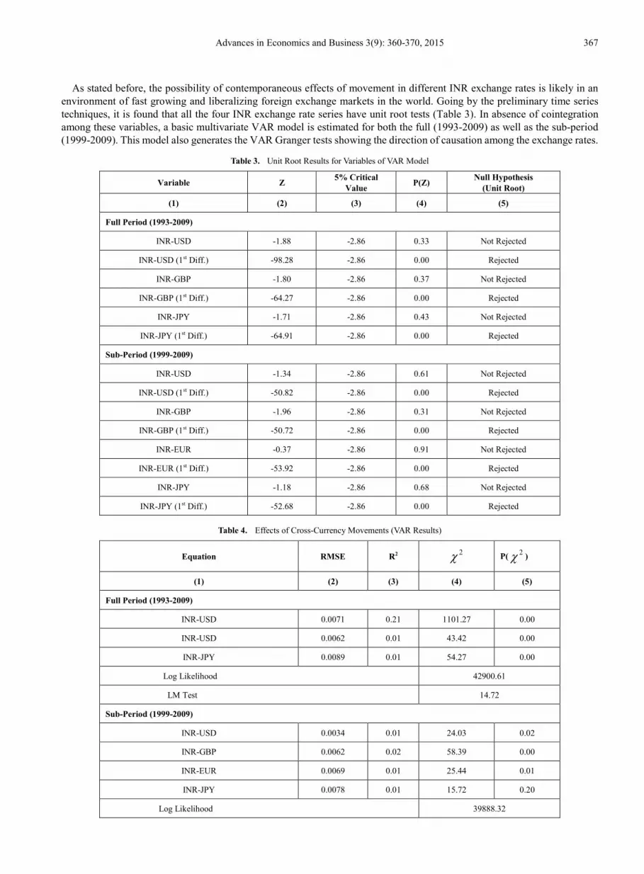
As stated before, the possibility of contemporaneous effects of movement in different INR exchange rates is likely in an environment of fast growing and liberalizing foreign exchange markets in the world. Going by the preliminary time series techniques, it is found that all the four INR exchange rate series have unit root tests (Table 3). In absence of cointegration among these variables, a basic multivariate VAR model is estimated for both the full (1993-2009) as well as the sub-period (1999-2009). This model also generates the VAR Granger tests showing the direction of causation among the exchange rates.

Table 3. Unit Root Results for Variables of VAR Model

Variable Z 5% Critical Value P(Z) Null Hypothesis

(Unit Root)

(1) (2) (3) (4) (5)

Full Period (1993-2009)

INR-USD -1.88 -2.86 0.33 Not Rejected

INR-USD (1st Diff.) -98.28 -2.86 0.00 Rejected

INR-GBP -1.80 -2.86 0.37 Not Rejected

INR-GBP (1st Diff.) -64.27 -2.86 0.00 Rejected

INR-JPY -1.71 -2.86 0.43 Not Rejected

INR-JPY (1st Diff.) -64.91 -2.86 0.00 Rejected

Sub-Period (1999-2009)

INR-USD -1.34 -2.86 0.61 Not Rejected

INR-USD (1st Diff.) -50.82 -2.86 0.00 Rejected

INR-GBP -1.96 -2.86 0.31 Not Rejected

INR-GBP (1st Diff.) -50.72 -2.86 0.00 Rejected

INR-EUR -0.37 -2.86 0.91 Not Rejected

INR-EUR (1st Diff.) -53.92 -2.86 0.00 Rejected

INR-JPY -1.18 -2.86 0.68 Not Rejected

INR-JPY (1st Diff.) -52.68 -2.86 0.00 Rejected

Table 4. Effects of Cross-Currency Movements (VAR Results)

Equation RMSE R2 2χ P( 2χ )

(1) (2) (3) (4) (5)

Full Period (1993-2009)

INR-USD 0.0071 0.21 1101.27 0.00

INR-USD 0.0062 0.01 43.42 0.00

INR-JPY 0.0089 0.01 54.27 0.00

Log Likelihood 42900.61

LM Test 14.72

Sub-Period (1999-2009)

INR-USD 0.0034 0.01 24.03 0.02

INR-GBP 0.0062 0.02 58.39 0.00

INR-EUR 0.0069 0.01 25.44 0.01

INR-JPY 0.0078 0.01 15.72 0.20

Log Likelihood 39888.32


Table 5. Wald Test for Granger Causality (Full Period, 1993-2009)

Dependent Variable Null Hypothesis 2χ Result

INR-USD

INR-GBP does not Granger-Cause INR-USD 37.1*** Rejected

INR-JPY does not Granger-Cause INR-USD 19.3*** Rejected

Both INR-GBP and INR-JPY do not Granger-cause INR-USD 70.8*** Rejected

INR-GBP

INR-USD does not Granger-cause INR-GBP 12.3** Rejected

INR-JPY does not Granger-cause INR-GBP 14.4*** Rejected

Both INR-USD and INR-JPY do not Granger-cause INR-GBP 25.6*** Rejected

INR-JPY

INR-USD does not Granger-cause INR-JPY 5.9 Not Rejected

INR-GBP does not Granger-cause INR-JPY 3.9 Not Rejected

Both INR-USD and INR-GBP do not Granger-cause INR-JPY 10.8 Not Rejected

Except INR-USD equation for the full period, all other VAR equations are found jointly significant suggesting contemporaneous and lagged effects of different INR exchange rates on each other. Further, the Granger causality tests substantiate this co-movement and reverse causation in the exchange rates. For the full period, INR-GBP and INR-JPY rates individually and jointly Granger-cause the INR-USD exchange rate. During the sub-period 1999-2009 the INR-GBP and the rest three rates together (INR-GBP, INR-EUR and INR-JPY) Granger-cause the INR-USD exchange rate. The Granger effects hold good for the INR-GBP and INR-EUR rates. Granger causality was not established for the INR-JPY exchange rate both during the full and the sub-period (Table 5 & 6).

Table 6. Wald Test for Granger Causality (Sub-Period, 1999-2009)

Dependent Variable Null Hypothesis 2χ Result

INR-USD

INR-GBP does not Granger-cause INR-USD 10.7** Rejected

INR-EUR does not Granger-cause INR-USD 2.5 Not Rejected

INR-JPY does not Granger-cause INR-USD 3.7 Not Rejected

All three do not Granger-cause INR-USD 21.0** Rejected

INR-GBP

INR-USD does not Granger-cause INR-GBP 5.7 Not Rejected

INR-EUR does not Granger-cause INR-GBP 10.0** Rejected

INR-JPY does not Granger-cause INR-GBP 9.9** Rejected

All three do not Granger-cause INR-GBP 41.9*** Rejected

INR-EUR

INR-USD does not Granger-cause INR-EUR 2.0 Not Rejected

INR-GBP does not Granger-cause INR-EUR 10.5** Rejected

INR-JPY does not Granger-cause INR-EUR 1.5 Not Rejected

All three do not Granger-cause INR-EUR 15.0* Rejected

INR-JPY

INR-USD does not Granger-cause INR-JPY 2.1 Not Rejected

INR-GBP does not Granger-cause INR-JPY 1.3 Not Rejected

INR-EUR does not Granger-cause INR-JPY 3.7 Not Rejected

All three do not Granger-cause INR-JPY 9.1 Not Rejected

Table 7. Cointegration among Bilateral Dollar Exchange Rates

Variable β α (1) (2) (3)

EUR-USD 1.00 0.0012

JPY-USD 0.37 0.0014 CNY-USD -1.51*** -0.0008*** GBP-USD -0.79** 0.0023***

INR-USD -2.23*** 0.0011**

Note: *** and ** denote significance at 1and 5 per cent levels of significance respectively.


The significant coefficients in the cointegrating equations reiterate the maintained hypothesis that possible long-run relationship among the USD exchange rates exists. For instance, the evolution of EUR-USD exchange rate, the two leading reserve currencies of the world, signals a strong impact on the other USD exchange rates. The results show an elastic response of the CNY-USD and INR-USD exchange rates to changes in the EUR-USD exchange rate (Table 7). In addition, the lower values of ‘α’ coefficients indicate that the error correction process is slow and not robust implying duration and persistence of volatility in the USD exchange rates. This, in turn, signals a high degree of uncertainty in INR-USD exchange rate.

Table 8. VECM Results

Equation (In First Difference) RMSE 2R

2χ

(1) (2) (3) (4)

EUR-USD 0.007 0.02 62.5***

JPY-USD 0.007 0.02 42.8**

CNY-USD 0.001 0.07 190.7***

GBP-USD 0.007 0.03 69.3***

INR-USD 0.004 0.05 134.3***

Log likelihood 52740.8

N 2518

Note: *** and ** denote 1 and 5 per cent levels of significance respectively.

The forecast error variance decomposition shows that more than 80 per cent variation in INR-USD exchange rate is explained by self-induced shocks (Table 9).

Table 9. Forecast Error Variance Decomposition (FEVD) (Response Variable:-Rupee-Dollar)

Step Impulse Variable

EUR-USD JPY-USD CNY-USD GBP-USD INR-USD

(1) (2) (3) (4) (5) (6)

1 0.056 0.022 0.004 0.023 0.895

2 0.082 0.022 0.003 0.022 0.870

3 0.103 0.019 0.003 0.022 0.853

4 0.108 0.017 0.003 0.023 0.849

5 0.108 0.014 0.004 0.020 0.854

6 0.113 0.011 0.005 0.018 0.853

7 0.117 0.010 0.005 0.016 0.852

Given the empirical results discussed above, one wonders

how to prescribe any remedy to the extent of volatility in INR corresponding to the cross-currency movements between the leading international currencies. The cointegration results indicate the growing integration of foreign exchange markets worldwide and therefore the scope for speculation over the evolution of exchange rates. Interestingly, the INR-USD and CNY-USD movements are sensitive to the changes in EUR-USD implying greater exposure of Chinese and Indian currencies to the developments in the foreign exchange markets of the United States and Europe. As higher growth prospects would attract foreign investment to India and China, the higher the exposure of INR and CNY to the EUR-USD movements, the higher would be the overall risk to external stability in these two countries. In this environment, the predictions of second- and third-generation currency models will largely hold.

5. Conclusions This paper presents the empirical results on volatility in

Indian currency i.e. INR in the post-floating period. From the GARCH models, it is evident that all the three bilateral INR exchange rates such as INR-GBP, INR-JPY and INR-EUR are volatile and past volatility explains the future movements. There is evidence of strong leverage effect in exchange rate movements implying asymmetric response to the positive and negative news in the economy. INR exchange rates against other international currencies other than USD exert significant influence on the evolution of INR-USD exchange rate. Further, INR-USD exchange rate exhibits an elastic response to changes in the EUR-USD rate. In terms of policy, these findings provide legitimacy to the present policy of managed float regime in India. However, the results need to be supplemented by the relation between the exchange rate and other macroeconomic variables.


REFERENCES [1] Alesina, Alberto and Wagner, Alexander (2003): Choosing

(And Reneging on) Exchange Rate Regimes. NBER Working Paper No. 9809, June.

[2] Baig, Taimur (2001): Characterizing Exchange Rate Regimes in Post-Crisis East Asia. IMF Working Paper No. 152, October.

[3] Bollerslev,Tim (1986): Generalized Autoregressive Conditional Heteroscedasticity. Journal of Econometrics. Vol. 31(3): 307-327.

[4] Bordo, Michael D (2003): Exchange Rate Regime Choice in Historical Perspective. IMF Working Paper No. 160.

[5] Bubula, Andrea and Otker-Robe, Inci (2003): Are Pegged and Intermediate Exchange Rate Regimes More Crisis Prone?. IMF Working Paper No. 223.

[6] Bubula, Andrea and Otker-Robe, Inci (2002): The Evolution of Exchange Rate Regimes since 1990: Evidence from De Facto Policies. IMF Working Paper No. 155.

[7] Calvo, G.A and Reinhart, Carmen M. (2002): Fear of Floating. Quarterly Journal of Economics. Vol. 117 (2): 379-408.

[8] Cavoli, Tony and Rajan, Ramkishen S. (2005): Have Exchange Rate Regimes in Asia Becomes More Flexible Post Crisis? Revisiting the Evidence. Working Paper No. 06. School of Economics, University of Adelaide.

[9] Cukierman, Alex., Kiguel, M.A. and Liviatan, N. (1992): How Much to Commit to An Exchange Rate Rule: Balancing Credibility and Flexibility. Policy Research Working Paper No. 931, The World Bank.

[10] Detragiache, Enrica., Mody A. and Okada, E. (2005): Exits from Heavily Managed Exchange Rate Regimes. IMF Working Paper No. 39.

[11] Duttagupta, Rupa., Fernandez, Gilda and Karacadag, Cem. (2004): From Fixed to Float: Operational Aspects of Moving Toward Exchange Rate Flexibility. IMF Working Paper No. 126.

[12] Duttagupta, Rupa and Otker-Robe, Inci (2003): Exits from Pegged Regimes: An Empirical Analysis. IMF Working Paper No. 147.

[13] Frankel, Jacob A (2003): Experience and Lessons from Exchange Rate Regimes in Emerging Economies. NBER Working Paper No.10032, October.

[14] Friedman, Milton (1953): The Case for Flexible Exchange Rates in Essays in Positive Economics. University of Chicago Press, 1953.

[15] Ghosh, Atish., Ostry J. D. and Tsangarides, C. (2010): Exchange Rate Regimes and the Stability of the International Monetary System. IMF Occasional Paper No. 270.

[16] Glick, Reuven and Hutchison, Michael. (2011): Currency Crises. Federal Reserve Bank of San Francisco Working Paper No.22, September.

[17] Hakura, Dalia S (2005): Are Emerging Market Countries Learning to Float. IMF Working Paper No. 98, May.

[18] Hernandez, Leonardo and Montiel, Peter (2001): Post-Crisis Exchange Rate Policy In Five Asian Countries: Filling in the “Hollow Middle?, IMF Working Paper No. 170, November.

[19] Jalan, Bimal (2002): Exchange Rate Management: An Emerging Consensus. Address at the 14th National Assembly of the Forex Association of India, Mumbai, August 14.

[20] Jayakumar, Vivekanand., Yoo, T.H. and Choi, Y.J. (2005): Exchange Rate System in India: Recent Reforms, Central Bank Policies and Fundamental Determinants of the Rupee-Dollar Rates. KIEP Working Paper No. 6.

[21] Johansen, S (1995): Likelihood-Based Inference in Cointegrated Vector Auto- Regressive Models. Oxford University Press, Oxford.

[22] Johnson, Harry G (1969): The Case for Flexible Exchange Rates. Federal Reserve Bank of St. Louis Review, Vol.51(6):12-24.

[23] Klein, Michael W and Shambaugh, Jay C. (2008): The Dynamics of Exchange Rate Regimes: Fixes, Floats and Flips. Journal of International Economics, Vol. 75: 70-92.

[24] Krugman, Paul (1979): A Model of Balance of Payments Crises. Journal of Money, Credit and Banking. Vol. 11: 311-325.

[25] Nelson, Daniel B (1991): Conditional Heteroscedasticity in Asset Returns: A New Approach. Econometrica. Vol. 59: 347-370.

[26] Ramachandran, M. and Srinivasan, Naveen (2007): Asymmetric Exchange Rate Intervention and International Reserve Accumulation in India. Economics Letters. Vol. 94 (2): 259-265.

[27] Taylor, Mark P and Sarno, Lucio (1998): The Behaviour of Real Exchange Rates during the Post-Bretton Woods Period. Journal of International Economics, Vol. 46: 281-312.

Exchange Rate Volatility in Post-floating Regime in India

Documents

Transcript of Exchange Rate Volatility in Post-floating Regime in India