Energy Harvesting by Floating Flaps Aerospace Engineering

Energy Harvesting by Floating Flaps

José Pedro de Sousa Ferreira

Thesis to obtain the Master of Science Degree in

Aerospace Engineering

Supervisors: Prof. Roeland De BreukerProf. Afzal Suleman

Examination Committee

Chairperson: Prof. Fernando José Parracho LauSupervisor: Prof. Afzal Suleman

Member of the Committee: Prof. Pedro Vieira Gamboa

November 2017

To my parents,Maria and José

Abstract

The increasing demand for energy efficiency have led to the development of an autonomous flap, which

encompasses an energy harvesting system to power sensors and actuators that ultimately perform

active gust alleviation. In this context, this thesis presents a novel mechanism for an electromagnetic

energy harvesting concept which transduces self-induced aeroelastic oscillations into electricity. The

onset of flutter is calculated using the p-k method, and a time-domain simulation is carried out to account

for inertial and electromagnetic non-linearities and assess the power harvested. To this end, a 3D-

printed aeroelastic model for wind tunnel testing is developed to experimentally evaluate the energy

harvesting mechanism. Experimental ground vibration tests have been performed to characterize the

structural model and demonstrate the efficiency of the proposed mechanism. Next, wind tunnel tests

were carried out to demonstrate the feasibility of the concept in a simulated environment. With a weight

penalty of 0.6 % when compared to a standard energy harvesting mechanism with a reciprocating shaft,

Free-Floating Flaps fitted with the novel mechanism showed a 40 % decrease in structural damping and

45 % increase in power generation. It was also experimentally demonstrated that the onset of flutter is

controllable by adjusting the generator external resistance. Future applications of such mechanism in full

scale wind turbine rotors are considered, and aircraft applications are also investigated with promising

results suggesting substantial fuel savings.

Keywords

Aeroelasticity; Electromagnetic Energy Harvesting; Free-Floating Flaps; Wind Tunnel Flutter Testing; 3D

Printing.

i

Resumo

O crescente desenvolvimento de soluções energeticamente auto-suficientes resultou num protótipo de

uma superfície de controlo autónoma, incorporando um sistema de armazenamento de energia que

alimenta sensores e actuadores na mitigação activa de cargas aerodinâmicas. Neste âmbito, esta dis-

sertação propõe um mecanismo inovador para o armazenamento de energia através da transdução

electromagnética de vibrações induzidas por fenómenos aeroelásticos em electricidade. O ponto de

flutter é calculado de acordo com o método p-k, e uma simulação no domínio temporal incorpora não-

linearidades inerciais e electromagnéticas na estimação da energia produzida. Um modelo experimental

pioneiro integralmente produzido com recurso à impressão 3D é desenvolvido para testar o mecanismo

de armazenamento energético. Testes de vibração são realizados com vista à caracterização estrutu-

ral do modelo, seguidos de testes em túnel de vento para provar a aplicabilidade do mecanismo. Os

resultados mostram que, com um acréscimo de 0.6 % relativamente à massa de um mecanismo não

optimizado, superfícies de controlo livres de oscilar em torno do seu eixo (n.b. do inglês Free-Floating

Flaps - FFF) equipadas com o mecanismo inovador apresentam uma redução de 40 % no amorteci-

mento estrutural e um aumento de 45 % na energia produzida. Comprovou-se ainda experimentalmente

que a velocidade de flutter é controlável através do ajuste da resistência aos terminais do gerador. Por

fim, um estudo preliminar de futuras aplicações em estruturas aeroespaciais revelou resultados promis-

sores conducentes a poupanças de combustível significativas.

Palavras-Chave

Aeroelasticidade; Armazenamento de Energia Electromagnética; Mecanismos de Superfícies de Con-

trolo; Testes de Flutter em Túnel de Vento; Impressão 3D.

iii

Acknowledgments

This research project consists in the accomplishment to which I have always looked forward since

the beginning of my academic path in 2012. I am absolutely thankful for having done exactly what I

have idealized: a full scientific research, from numerical study to production and experimental testing.

In that sense, I would like to express my gratitude to Prof. Roeland De Breuker for having accepted me

as a guest researcher in the Aerospace Structures and Computational Mechanics department at Delft

University of Technology for the last 6 months. He passed me the passion for adaptive structures and

morphing solutions and provided me with all the necessary means to carry out this investigation.

A very special note goes to Dr. Jurij Sodja for his permanent support and commitment to the project.

I greatly thank him for all the everlasting meetings we shared, for having trust in me whilst critically

discussing every choice I made, and for being constantly available to brainstorm new ideas.

I would also like to express my sincere gratitude to my supervisor at IST, Prof. Afzal Suleman, for

having made this project come true. His valuable and insightful guidance were of critical importance,

alongside his demanding character and availability even when we were an ocean apart.

A special thanks goes to Megan Walker, for having introduced me to the perks of 3D printing and

for her kindness and fruitful discussions in those regards. Also, to Dr. Calvin Rans who allowed me to

use the 3D printer, and to Prof. Pim Groen for the usage of the electromagnetic shaker and compliant

instruments. Moreover, I keep a special debt of gratitude to the technicians in the Delft Aerospace

Structures and Materials Laboratory, namely to Kees Paalvast, Gertjan Mulder and Misja Huizinga, for

all the support during manufacturing and testing. Lastly, I want to thank Frederico Afonso for his guidance

in applying the results of this research to the aeronautical paradigm.

To my colleagues in Delft, specially to my friends Diogo, Eduardo and Pedro with whom I was fortu-

nate to share housing, I would like to show my appreciation for receiving me. It was a pleasure to share

that time with you. Also, I could not forget to mention all the amazing friends I made during the last years

of pursuing this degree: you have turned a harsh path into a pleasureful journey. Moreover, to all my

friends in Portugal, that despite being far from me, always cared and supported my choices. You have

helped turning my life abroad a bit easier.

To you, Cristina, for all the love and support you gave me. For helping me seeing the light when it

darkens. For being who you are. I could not have asked for anyone better.

Finally, I am deeply grateful to my family. To my grandparents, who have been introduced to the

wonders of video conference, shortening a 2000 km distance at the speed of light. But above all, to

my beloved parents, who have always unconditionally supported and guided me in all circumstances,

putting me in front of any personal objective. This is for you. This is ultimately yours.

v

Contents

Abstract . . . . . . . . . . . . . . . . . . . . . . . . . . . . . . . . . . . . . . . . . . . . . . . . i

Resumo . . . . . . . . . . . . . . . . . . . . . . . . . . . . . . . . . . . . . . . . . . . . . . . . . iii

Acknowledgments . . . . . . . . . . . . . . . . . . . . . . . . . . . . . . . . . . . . . . . . . . v

List of Figures . . . . . . . . . . . . . . . . . . . . . . . . . . . . . . . . . . . . . . . . . . . . . xi

List of Tables . . . . . . . . . . . . . . . . . . . . . . . . . . . . . . . . . . . . . . . . . . . . . xv

List of Algorithms . . . . . . . . . . . . . . . . . . . . . . . . . . . . . . . . . . . . . . . . . . . xvii

List of Acronyms . . . . . . . . . . . . . . . . . . . . . . . . . . . . . . . . . . . . . . . . . . . xix

List of Symbols . . . . . . . . . . . . . . . . . . . . . . . . . . . . . . . . . . . . . . . . . . . . xxi

1 Introduction 1

1.1 Motivation . . . . . . . . . . . . . . . . . . . . . . . . . . . . . . . . . . . . . . . . . . . . . 1

1.2 Overview . . . . . . . . . . . . . . . . . . . . . . . . . . . . . . . . . . . . . . . . . . . . . 2

1.3 Objectives . . . . . . . . . . . . . . . . . . . . . . . . . . . . . . . . . . . . . . . . . . . . . 2

1.4 Methodology . . . . . . . . . . . . . . . . . . . . . . . . . . . . . . . . . . . . . . . . . . . 3

1.5 Thesis Outline . . . . . . . . . . . . . . . . . . . . . . . . . . . . . . . . . . . . . . . . . . 4

2 Literature Review 5

2.1 Energy Harvesting Mechanisms . . . . . . . . . . . . . . . . . . . . . . . . . . . . . . . . 5

2.2 Load Alleviation . . . . . . . . . . . . . . . . . . . . . . . . . . . . . . . . . . . . . . . . . . 7

2.2.1 Passive . . . . . . . . . . . . . . . . . . . . . . . . . . . . . . . . . . . . . . . . . . 7

2.2.2 Active . . . . . . . . . . . . . . . . . . . . . . . . . . . . . . . . . . . . . . . . . . . 8

2.3 Flow-Induced Vibrations Energy Harvesting . . . . . . . . . . . . . . . . . . . . . . . . . . 9

2.3.1 Turbulence . . . . . . . . . . . . . . . . . . . . . . . . . . . . . . . . . . . . . . . . 9

2.3.2 Vortex-Induced Vibrations . . . . . . . . . . . . . . . . . . . . . . . . . . . . . . . . 10

2.3.3 Galloping . . . . . . . . . . . . . . . . . . . . . . . . . . . . . . . . . . . . . . . . . 11

2.3.4 Flutter and Limit-Cycle Oscillations . . . . . . . . . . . . . . . . . . . . . . . . . . . 12

3 Numerical Modeling 15

3.1 System Modeling . . . . . . . . . . . . . . . . . . . . . . . . . . . . . . . . . . . . . . . . . 15

3.2 Numerical Approach . . . . . . . . . . . . . . . . . . . . . . . . . . . . . . . . . . . . . . . 17

vii

3.2.1 Flutter Determination Model . . . . . . . . . . . . . . . . . . . . . . . . . . . . . . . 17

3.2.2 Time-Domain Model . . . . . . . . . . . . . . . . . . . . . . . . . . . . . . . . . . . 18

3.3 Verification . . . . . . . . . . . . . . . . . . . . . . . . . . . . . . . . . . . . . . . . . . . . 19

3.3.1 Flutter Determination Model . . . . . . . . . . . . . . . . . . . . . . . . . . . . . . . 20

3.3.2 Time-Domain Model . . . . . . . . . . . . . . . . . . . . . . . . . . . . . . . . . . . 22

3.4 Feasibility Study . . . . . . . . . . . . . . . . . . . . . . . . . . . . . . . . . . . . . . . . . 24

4 Concept Development 28

4.1 Requirements and Overview . . . . . . . . . . . . . . . . . . . . . . . . . . . . . . . . . . 28

4.2 CAD Modeling . . . . . . . . . . . . . . . . . . . . . . . . . . . . . . . . . . . . . . . . . . 29

4.3 Manufacturing . . . . . . . . . . . . . . . . . . . . . . . . . . . . . . . . . . . . . . . . . . . 32

4.3.1 3D Printing . . . . . . . . . . . . . . . . . . . . . . . . . . . . . . . . . . . . . . . . 32

4.3.2 Composites . . . . . . . . . . . . . . . . . . . . . . . . . . . . . . . . . . . . . . . . 35

4.3.3 Off-the-shelf Components . . . . . . . . . . . . . . . . . . . . . . . . . . . . . . . . 36

4.4 Assembly . . . . . . . . . . . . . . . . . . . . . . . . . . . . . . . . . . . . . . . . . . . . . 36

5 Experimental Setup 37

5.1 Framework . . . . . . . . . . . . . . . . . . . . . . . . . . . . . . . . . . . . . . . . . . . . 37

5.2 Data Acquisition . . . . . . . . . . . . . . . . . . . . . . . . . . . . . . . . . . . . . . . . . 39

5.3 Vibration Tests . . . . . . . . . . . . . . . . . . . . . . . . . . . . . . . . . . . . . . . . . . 40

5.3.1 Apparatus . . . . . . . . . . . . . . . . . . . . . . . . . . . . . . . . . . . . . . . . . 40

5.3.2 Procedure . . . . . . . . . . . . . . . . . . . . . . . . . . . . . . . . . . . . . . . . . 42

5.4 Wind Tunnel Tests . . . . . . . . . . . . . . . . . . . . . . . . . . . . . . . . . . . . . . . . 43

5.4.1 Apparatus . . . . . . . . . . . . . . . . . . . . . . . . . . . . . . . . . . . . . . . . . 44

5.4.2 Procedure . . . . . . . . . . . . . . . . . . . . . . . . . . . . . . . . . . . . . . . . . 45

5.5 Physical Model Characterization . . . . . . . . . . . . . . . . . . . . . . . . . . . . . . . . 46

5.5.1 Stiffness . . . . . . . . . . . . . . . . . . . . . . . . . . . . . . . . . . . . . . . . . . 46

5.5.2 Damping . . . . . . . . . . . . . . . . . . . . . . . . . . . . . . . . . . . . . . . . . 47

6 Results 52

6.1 Data Post-Processing . . . . . . . . . . . . . . . . . . . . . . . . . . . . . . . . . . . . . . 52

6.2 Vibration Tests . . . . . . . . . . . . . . . . . . . . . . . . . . . . . . . . . . . . . . . . . . 53

6.2.1 Validation . . . . . . . . . . . . . . . . . . . . . . . . . . . . . . . . . . . . . . . . . 54

6.2.2 Mode Analysis by Impulse Excitations . . . . . . . . . . . . . . . . . . . . . . . . . 55

6.2.3 Energy Harvesting by Forced Harmonic Excitations . . . . . . . . . . . . . . . . . 59

6.3 Wind Tunnel Tests . . . . . . . . . . . . . . . . . . . . . . . . . . . . . . . . . . . . . . . . 62

6.3.1 Validation . . . . . . . . . . . . . . . . . . . . . . . . . . . . . . . . . . . . . . . . . 64

6.3.2 Flutter Speed Control . . . . . . . . . . . . . . . . . . . . . . . . . . . . . . . . . . 67

viii

6.3.3 Energy Harvesting . . . . . . . . . . . . . . . . . . . . . . . . . . . . . . . . . . . . 71

6.4 Concept Applicability . . . . . . . . . . . . . . . . . . . . . . . . . . . . . . . . . . . . . . . 73

7 Conclusion 76

7.1 Achievements . . . . . . . . . . . . . . . . . . . . . . . . . . . . . . . . . . . . . . . . . . . 76

7.2 Recommendations . . . . . . . . . . . . . . . . . . . . . . . . . . . . . . . . . . . . . . . . 77

7.3 Future Work . . . . . . . . . . . . . . . . . . . . . . . . . . . . . . . . . . . . . . . . . . . . 80

Bibliography 81

A Numerical Model 85

A.1 System Modeling . . . . . . . . . . . . . . . . . . . . . . . . . . . . . . . . . . . . . . . . . 85

A.2 Equations of Motion . . . . . . . . . . . . . . . . . . . . . . . . . . . . . . . . . . . . . . . 86

A.2.1 Inertia Terms . . . . . . . . . . . . . . . . . . . . . . . . . . . . . . . . . . . . . . . 86

A.2.2 Damping Terms . . . . . . . . . . . . . . . . . . . . . . . . . . . . . . . . . . . . . 86

A.2.3 Stiffness Terms . . . . . . . . . . . . . . . . . . . . . . . . . . . . . . . . . . . . . . 90

A.2.4 Generalized Aerodynamic Forces . . . . . . . . . . . . . . . . . . . . . . . . . . . . 91

A.2.5 Matrix assembly . . . . . . . . . . . . . . . . . . . . . . . . . . . . . . . . . . . . . 92

A.3 P-k method . . . . . . . . . . . . . . . . . . . . . . . . . . . . . . . . . . . . . . . . . . . . 93

A.4 State Space Model . . . . . . . . . . . . . . . . . . . . . . . . . . . . . . . . . . . . . . . . 95

B Calibration 98

B.1 Pitch Sensor . . . . . . . . . . . . . . . . . . . . . . . . . . . . . . . . . . . . . . . . . . . 98

B.2 Flap Sensor . . . . . . . . . . . . . . . . . . . . . . . . . . . . . . . . . . . . . . . . . . . . 98

B.3 Generator . . . . . . . . . . . . . . . . . . . . . . . . . . . . . . . . . . . . . . . . . . . . . 98

B.4 Pitot Tube . . . . . . . . . . . . . . . . . . . . . . . . . . . . . . . . . . . . . . . . . . . . . 100

ix

List of Figures

2.1 Energy harvesting sources for MEMS usage. Source: Thomas et al. [2006] . . . . . . . . 6

2.2 Wind tunnel concept for the energy harvesting mechanism by Bernhammer et al. [2017b] 14

3.1 3DOF wing section. Adapted from: Conner et al. [1997] . . . . . . . . . . . . . . . . . . . 15

3.2 Electric circuit for energy harvesting . . . . . . . . . . . . . . . . . . . . . . . . . . . . . . 16

3.3 One-Way Bearing mechanism CAD model . . . . . . . . . . . . . . . . . . . . . . . . . . . 19

3.4 Two-Way Bearing mechanism CAD model . . . . . . . . . . . . . . . . . . . . . . . . . . . 19

3.5 2DOF undamped system flutter plots . . . . . . . . . . . . . . . . . . . . . . . . . . . . . . 20

3.6 3DOF undamped system root locus plot . . . . . . . . . . . . . . . . . . . . . . . . . . . . 21

3.7 3DOF damped system root locus plot . . . . . . . . . . . . . . . . . . . . . . . . . . . . . 21

3.8 Time marching model benchmark with the p-k method . . . . . . . . . . . . . . . . . . . . 23

3.9 Time simulation for the modeled mechanisms and a Gear Ratio of 25 . . . . . . . . . . . 23

3.10 Flap flutter plots with changing electromagnetic damping . . . . . . . . . . . . . . . . . . . 25

3.11 Heave flutter plots with changing electromagnetic damping . . . . . . . . . . . . . . . . . 26

3.12 Flutter onset controllability . . . . . . . . . . . . . . . . . . . . . . . . . . . . . . . . . . . . 26

3.13 Total damping with varying resistance . . . . . . . . . . . . . . . . . . . . . . . . . . . . . 26

3.14 Voltage and Power outputs with varying Gear Ratio for the One-Way Bearing mechanism 27

4.1 Main wing cross-section CAD model . . . . . . . . . . . . . . . . . . . . . . . . . . . . . . 30

4.2 Flap mechanism CAD model . . . . . . . . . . . . . . . . . . . . . . . . . . . . . . . . . . 30

4.3 Wing assembly CAD model . . . . . . . . . . . . . . . . . . . . . . . . . . . . . . . . . . . 32

4.4 Wind tunnel setup CAD model . . . . . . . . . . . . . . . . . . . . . . . . . . . . . . . . . 32

4.5 3D printing setup . . . . . . . . . . . . . . . . . . . . . . . . . . . . . . . . . . . . . . . . . 33

4.6 Main wing half after a 24-hour print job . . . . . . . . . . . . . . . . . . . . . . . . . . . . . 33

4.7 Test parts . . . . . . . . . . . . . . . . . . . . . . . . . . . . . . . . . . . . . . . . . . . . . 33

4.8 Hook mechanism (f) . . . . . . . . . . . . . . . . . . . . . . . . . . . . . . . . . . . . . . . 33

4.9 Flap sensor support (E) . . . . . . . . . . . . . . . . . . . . . . . . . . . . . . . . . . . . . 33

xi

4.10 Printing flap bottom halves . . . . . . . . . . . . . . . . . . . . . . . . . . . . . . . . . . . 35

4.11 Flap bottom halves after treatment . . . . . . . . . . . . . . . . . . . . . . . . . . . . . . . 35

4.12 Main wing pockets and tip connections . . . . . . . . . . . . . . . . . . . . . . . . . . . . . 35

4.13 Top endplate . . . . . . . . . . . . . . . . . . . . . . . . . . . . . . . . . . . . . . . . . . . 35

4.14 Wing model assembly . . . . . . . . . . . . . . . . . . . . . . . . . . . . . . . . . . . . . . 36

4.15 Flap pulley system . . . . . . . . . . . . . . . . . . . . . . . . . . . . . . . . . . . . . . . . 36

5.1 Test workbench schematics. Adapted from: Gjerek et al. [2014] . . . . . . . . . . . . . . 38

5.2 Close-up to Excitation Target . . . . . . . . . . . . . . . . . . . . . . . . . . . . . . . . . . 39

5.3 Impulse Excitation Test setup . . . . . . . . . . . . . . . . . . . . . . . . . . . . . . . . . . 41

5.4 Forced Harmonic Excitation Test setup . . . . . . . . . . . . . . . . . . . . . . . . . . . . . 41

5.5 Forced Harmonic Excitation Test schematics . . . . . . . . . . . . . . . . . . . . . . . . . 41

5.6 Close-up to Load Cell . . . . . . . . . . . . . . . . . . . . . . . . . . . . . . . . . . . . . . 42

5.7 Graphical Interface for the Frequency Sweep Test . . . . . . . . . . . . . . . . . . . . . . 43

5.8 Wind Tunnel setup . . . . . . . . . . . . . . . . . . . . . . . . . . . . . . . . . . . . . . . . 44

5.9 Test Section back view . . . . . . . . . . . . . . . . . . . . . . . . . . . . . . . . . . . . . . 44

5.10 Wind Tunnel Test schematics . . . . . . . . . . . . . . . . . . . . . . . . . . . . . . . . . . 45

5.11 Graphical Interface for the Flutter Test . . . . . . . . . . . . . . . . . . . . . . . . . . . . . 46

5.12 Heave Stiffness Characterization . . . . . . . . . . . . . . . . . . . . . . . . . . . . . . . . 47

5.13 Curve fitting optimization procedure for Heave Damping Characterization . . . . . . . . . 48

6.1 Heave time response . . . . . . . . . . . . . . . . . . . . . . . . . . . . . . . . . . . . . . . 55

6.2 Pitch time response . . . . . . . . . . . . . . . . . . . . . . . . . . . . . . . . . . . . . . . 55

6.3 Flap time response . . . . . . . . . . . . . . . . . . . . . . . . . . . . . . . . . . . . . . . . 55

6.4 Voltage time response . . . . . . . . . . . . . . . . . . . . . . . . . . . . . . . . . . . . . . 55

6.5 Modal Analysis for an Impulse Excitation in OC conditions . . . . . . . . . . . . . . . . . . 57

6.6 Experimental FRF for both mechanisms in OC conditions for 2DOF and 3DOF systems . 58

6.7 Experimental FRF for the Standard mechanism under OC and SC conditions . . . . . . . 58

6.8 Experimental FRF for both mechanisms under SC conditions . . . . . . . . . . . . . . . . 59

6.9 Modal Analysis for Forced Harmonic Vibrations in OC conditions . . . . . . . . . . . . . . 61

6.10 Energy Harvested under Forced Harmonic Vibrations for Setup I . . . . . . . . . . . . . . 62

6.11 One-Way Bearing mechanism experimental effect on Voltage Production . . . . . . . . . 62

6.12 Flutter plots for the 2DOF system . . . . . . . . . . . . . . . . . . . . . . . . . . . . . . . . 65

6.13 Flutter plots for the 3DOF system - Standard mechanism . . . . . . . . . . . . . . . . . . 66

6.14 Flutter onset controllability for Setup II with One-Way Bearing mechanism . . . . . . . . . 68

xii

6.15 Comparison between damping characteristics for Setup I Standard mechanism and Setup

II One-Way Bearing mechanism . . . . . . . . . . . . . . . . . . . . . . . . . . . . . . . . 69

6.16 Influence of endplates on flutter speed control for Setup I with One-Way Bearing mechanism 70

6.17 Energy Harvested at the flutter point for Setup I . . . . . . . . . . . . . . . . . . . . . . . . 71

6.18 Energy Harvested at the flutter point for Setup II . . . . . . . . . . . . . . . . . . . . . . . 72

6.19 One-Way Bearing mechanism experimental effect on Voltage Production . . . . . . . . . 73

6.20 Numerical Simulation on One-Way Bearing mechanism with GR of 25 . . . . . . . . . . . 74

A.1 Generator schematic . . . . . . . . . . . . . . . . . . . . . . . . . . . . . . . . . . . . . . . 89

A.2 Flowchart for the interpolation methodology . . . . . . . . . . . . . . . . . . . . . . . . . . 94

A.3 One-Way Bearing mechanism algorithm variables . . . . . . . . . . . . . . . . . . . . . . 96

A.4 Matlab/Simulink® model for the One-Way Bearing mechanism . . . . . . . . . . . . . . . . 97

B.1 Pitch Sensor Calibration . . . . . . . . . . . . . . . . . . . . . . . . . . . . . . . . . . . . . 99

B.2 Flap Sensor Calibration . . . . . . . . . . . . . . . . . . . . . . . . . . . . . . . . . . . . . 99

B.3 Generator Calibration . . . . . . . . . . . . . . . . . . . . . . . . . . . . . . . . . . . . . . 99

B.4 Pitot Tube Calibration . . . . . . . . . . . . . . . . . . . . . . . . . . . . . . . . . . . . . . 100

xiii

List of Tables

2.1 Comparison between the three transduction mechanisms. Adapted from: Le et al. [2015] 6

3.1 2DOF undamped system data . . . . . . . . . . . . . . . . . . . . . . . . . . . . . . . . . 20

3.2 Comparison between the 2DOF undamped system flutter calculation codes . . . . . . . . 20

3.3 3DOF undamped system data . . . . . . . . . . . . . . . . . . . . . . . . . . . . . . . . . 21

3.4 Comparison between the 3DOF undamped system flutter calculation codes . . . . . . . . 21

3.5 3DOF damped system data . . . . . . . . . . . . . . . . . . . . . . . . . . . . . . . . . . . 22

3.6 Comparison between the 3DOF damped system flutter calculation codes . . . . . . . . . 22

3.7 Parametric study on the Gear Ratio for mechanism comparison . . . . . . . . . . . . . . . 27

4.1 Overview of relevant aeroelastic wind tunnel testing articles . . . . . . . . . . . . . . . . . 29

4.2 Off-the-shelf components list . . . . . . . . . . . . . . . . . . . . . . . . . . . . . . . . . . 36

5.1 Pitch and Flap Torsional Stiffness . . . . . . . . . . . . . . . . . . . . . . . . . . . . . . . . 48

5.2 Heave properties . . . . . . . . . . . . . . . . . . . . . . . . . . . . . . . . . . . . . . . . . 50

5.3 Pitch properties . . . . . . . . . . . . . . . . . . . . . . . . . . . . . . . . . . . . . . . . . . 50

5.4 Flap properties . . . . . . . . . . . . . . . . . . . . . . . . . . . . . . . . . . . . . . . . . . 50

5.5 Model Properties . . . . . . . . . . . . . . . . . . . . . . . . . . . . . . . . . . . . . . . . . 51

6.1 Wind tunnel tests validation results . . . . . . . . . . . . . . . . . . . . . . . . . . . . . . . 67

xv

List of Algorithms

1 Release Mechanism . . . . . . . . . . . . . . . . . . . . . . . . . . . . . . . . . . . . . . . 96

2 Free-spinning shaft decay . . . . . . . . . . . . . . . . . . . . . . . . . . . . . . . . . . . . 96

xvii

List of Acronyms

DOF Degree Of Freedom

OC Open-Circuit

SC Short-Circuit

LCO Limit-Cycle Oscillations

MEMS Micro-Electro-Mechanical Systems

FFF Free-Floating Flap

RPM Rotations Per Minute

FRF Frequency Response Function

FFT Fast Fourier Transform

DC Direct Current

PM Permanent Magnet

QEP Quadratic Eigenvalue Problem

FCL First Companion Linearization

MAC Modal Assurance Criterion

RMS Root Mean Square

UAV Unmanned Aerial Vehicle

CFRP Carbon-Fiber Reinforced Polymer

HAWT Horizontal-Axis Wind Turbine

FIV Flow-Induced Vibrations

VIV Vortex-Induced Vibrations

xix

List of Symbols

Greek symbols

α Pitch or torsional motion, with origin at the elastic axis / shear center, and defined positive for

clockwise rotation

β Flap, aileron, rudder or control surface motion, with origin at the hinge line, and defined positive

for clockwise rotation

β′ Flap angular velocity as it enters the generator

β∗ Flap angular velocity after the release mechanism

ε Electromotive force

η Mechanical efficiency

γ Damping ratio, real part of v

κ Decay ratio of the release mechanism numerical model

µ Mass ratio of a cylinder of air having a diameter equal to the wing chord over the mass of the

wing

µ0 Magnetic permeability of vacuum

ω Frequency, real part of v

ωi Natural frequency modal value

Φ Magnetic flux

φ Induction coefficient of the generator

ρ Mass of air per unit of volume

σ Ratio of natural frequencies

xxi

ξ State vector for the equations of motion

ξ Dimensionless state vector for the equations of motion

ξ∗ Pk-method dimensionless state vector amplitude

λ∗ New state variable for FCL. First derivative in time of ξ∗

θ Input rotational velocity of generator

ζi Damping coefficient modal value

Roman symbols

[A] State matrix of the state space model

a Elastic Axis location with respect to the mid-chord point

Ar Area ratio of the wind tunnel

[B] Input matrix of the state space model

B Total magnetic field

b Half chord of the wing

[C] Output matrix of the state space model

c Hinge line location with respect to the mid-chord point

Ci Modal damping

C Theodorsen function

[C] Damping matrix

[D] Feedthrough matrix of the state space model

Di Initial Value Problem constant

∆p Dynamic pressure, difference between total and static pressure

bk Least squares optimization parameters for the curve fitting procedure

E Specific energy

Fel Force created by the electromechanical coupling of generator

GR Gear ratio

xxii

h Heave, plunge or bending motion, with origin at the elastic axis, and defined positive for a down-

ward vertical movement

H(2)j Hankel function of the second kind

Hv FRF estimator

I Current

Iα Moment of inertia of wing-flap about a

Iβ Moment of inertia of flap about c

[I] Identity matrix

k Reduced frequency

Ki Modal Stiffness

[K] Stiffness matrix

L Inductance

l Coil length of the generator

m Mass of the wing-flap system

Mα,Mβ Moment input in the pitch and flap modes, respectively

Mb Mass of batteries for energy harvesting

Mf Mass of fuel not burnt due to using the energy harvesting mechanism

[M] Inertia matrix

M0 Empty mass of the airframe

ms Mass of the wing supports for the aeroelastic experiment

MTOW Maximum takeoff mass of the aircraft

L Force input in the heave mode

P Power

p Dimensionless eigenvalue

p0 Ambient pressure

xxiii

[Q] Generalized forces matrix

R Resistance

r Internal resistance of the generator due to brushes for current rectifying

Rg Specific gas constant for dry air

rα Radius of gyration of wing-flap divided by b

rβ Reduced radius of gyration of flap divided by b

S Cross-sectional area

Sα Static moment of wing-flap relative to a

Sβ Static moment of flap relative to c

Sxx, Syy Power spectral density of the input and output signal, respectively

Syx Cross spectral density from output to input

T Absolute temperature

t Time

Tl Geometric terms of Theodorsen model

U Stream velocity

u Input vector of the state space model

V Reduced stream velocity

v Complex eigenvalue

V Voltage

X State vector of the state space model

xα Center of gravity of wing-flap with respect to the elastic axis

xβ Center of gravity of the wing-flap with respect to the hinge line

Y Output vector of the state space model

Z Impedance

[Z] Companion matrix

xxiv

Subscripts

0 Initial value

aero Aerodynamic component of matrix

b Battery component of specific energy

crit Critical damping

el Electromagnetic component of damping

encl Enclosed component of current

eq Equivalent component of resistance and impedance

f Fuel component of specific energy

flap Flap component of inertia, as if there would be no release mechanism nor gearbox

GB Gearbox component of inertia

i Modal component h, α or β

∞ Free-stream component

j jth order of Hankel function

k kth geometric term of Theodorsen model

l lth optimization parameter

st Structural component of damping

T Total damping

TS Tunnel section component of area and velocity

visc Viscous component of damping

WT Wind tunnel component of area and velocity

Superscripts[ ¯. . .]

Reduced matrix

[ ¯. . .∗]

Pk-method reduced matrix

.. Second derivative in time

. First derivative in time

xxv

1 | Introduction

In this chapter, the design principles on energy harvesting and subsequent justification are explained

alongside with a brief description of the main objectives for the research project. The relevant literature

review and proposed methodology are introduced and an overview of the thesis layout is presented.

1.1 Motivation

With the ever growing demand for energy efficient aircraft systems, there has been an increased

research activity in the search for novel energy harvesting solutions. This is motivated by the increasingly

expensive fossil fuels and by the need to reduce operational costs. The potential of renewable energy

power generators has seen a marked increased in proposed solutions in the aeronautical industry.

The usage of natural energy sources in ways that one could transform it into a usable energetic

resource is a game-changer solution in the global energy panorama. According to Eurostat1 data on

renewable energy for the 28 member states of the European Union, 26.7 % of the total primary energy

production from all sources comes from renewable in 2015, having grown at an average rate of 5.5 %

per year in the previous 10 years. This undoubtedly shows the potential of energy harvesting, not only

in the macro scale but also for smaller applications which would allow remote pieces of equipment to be

completely self-sustained and maintenance-free for longer periods of time.

Self-powered micro-generators by means of energy harvesting are one of the clever solutions allow-

ing low-power embedded sensors and actuators to work in stand-alone systems. This has a wide range

of applications, such as in the development of Structural Health Monitoring (SHM) systems which would

enable the active and autonomous tracking of all loads, counter-acting the harmful ones.

As broadly acknowledged, one of the key features of designing new aeronautical applications is mak-

ing sure that the structure copes with the applied stresses, both instantaneously and during its lifetime.

To accomplish so, predetermined inspections for maintenance and repairs are mandatory, leading to

large off-duty periods. As such, energy harvesters for SHM may enable the reduction of maintenance

1Statistics on renewable energy: http://ec.europa.eu/eurostat/statistics-explained/index.php/Renewable_energy_statistics

Energy Harvesting by Floating Flaps 1

http://ec.europa.eu/eurostat/statistics-explained/index.php/Renewable_energy_statistics

http://ec.europa.eu/eurostat/statistics-explained/index.php/Renewable_energy_statistics

Chapter 1 Introduction

time by using both active load alleviation techniques and sensing to assess the structural integrity of

autonomous structures at remote locations. This kind of embedded systems would allow the harvesting

of structural vibrations, creating new perspectives in terms of wing design for Unmanned Aerial Vehicles

(UAV) and blade design for offshore wind turbines.

1.2 Overview

Amongst the wide range of possibilities for energy harvesting, the one that mostly fits aeronautical

purposes is the harnessing of vibrations induced by the fluid-structure interaction, a common denomi-

nator in every dynamic fluid-immersed structure. Therefore, finding a way of transforming kinetic energy

into a usable resource such as electricity is the key for a sustainable and potentially efficient application.

On the other hand, the concerns about loads across the wing box and the way it withstands them

have always been a critical point in a new component design, specially nowadays that a transition from

metallic components to composites is taking place. The structure is designed to cope not only with

steady loads but also with dynamic loads such as turbulence or gusts, which instantaneously create

peaks and put its structural integrity on the line. Intuitively, in order to withstand the referred peaks,

one has to increase structure robustness at the cost of weight. Nevertheless, active methods for load

alleviation are a good alternative to this problem which have been widely studied in the past century,

contributing to the wing weight diminishing. The first application of such system at the initial design

stage is presented by Payne [1986], as the Airbus Industrie A320 incorporates an active control system

which actuates the outboard wing spoilers and ailerons to perform the task.

More recent research has been able to accomplish faster actuation speeds using smart materials as

actuators in flexible high aspect ratio wings. The concept of a wing with one Free-Floating Flap (FFF)

is introduced by Heinze and Karpel [2006] for gust alleviation within flutter constraints. Later, a new

aeroservoelastic approach based on FFF actuated by piezoelectric tabs is proposed by Bernhammer

et al. [2013], evidencing superior effectiveness in gust alleviation and flutter suppression.

Considering these instabilities, namely the aeroelastic flutter, and in case of bounded into Limit-

Cycle Oscillations (LCO), an energy harvesting mechanism could be developed such that vibrations

may be transformed into electricity to power instrumentation. A first concept for this solution is presented

by Bernhammer et al. [2017a,b], where an electromechanical harvester feeds a battery which powers

actuators and sensors that perform SHM duties and actively control the LCO.

1.3 Objectives

Energy harvesting by means of exploiting aeroelastic instabilities in streamlined bodies is an ever-

changing field with a wide range of possibilities yet to be explored. Regardless the harvesting method, it

2 Energy Harvesting by Floating Flaps

Introduction Chapter 1

has several potential applications and advantages: once mastered the solution, designing such compo-

nents has no longer to be limited by the strict aeroelastic boundaries that no structure should go beyond.

Additionally, this would provide structure active control and sensing, allowing for longer due periods and

offshore operations in stand-alone systems.

In this way, the work developed by Bernhammer et al. [2017a,b] highlights a feasible application for

this solution in offshore Horizontal-Axis Wind Turbines (HAWT). Not only is this mechanism able to be

self-sustained by harvesting the LCO when the flutter boundary is exceeded, as it also manages to

actively alleviate the gust loads across the blades. Moreover, it was developed as a plug-in device in

order to be easily replaced in case of damage. Its electromechanical harvester, a generator that uses the

FFF oscillating movement to power the batteries, is the key feature of this solution. Overall, it exploits a

phenomenon that frequently occurs in the operational envelope of HAWT, with increasing significance as

the blade length increases, to boost its structural integrity in an efficient and autonomous way. However,

and as acknowledged in the referred papers, when a gearbox is introduced to increase the generator

performance, the flap mechanism is negatively affected and thereby the whole system performance

downgrades. As such, the purpose of this investigation is to develop a harvester that would be able to

increase the produced energy by optimizing the rotational mechanism, and prove it both numerically and

experimentally. Moreover, the premise of flutter speed controllability is also investigated experimentally.

In the end, a preliminary evaluation of integrating the novel mechanism in airframes is carried out.

1.4 Methodology

The procedures presented hereafter are intended to result in a comprehensive approach to improve

an energy harvesting mechanism that exploits self-induced aeroelastic vibrations.

Firstly, a numerical study is carried out to confirm the feasibility of such solution. The physical reality

is numerically described and two methods are used to calculate the instability boundary and the time-

domain response of the system. For the former, an eigenvalue problem in the frequency domain is

solved based on the p-k method to determine the flutter onset; nonetheless, and due to the non-linear

behavior of the new proposed mechanism that allows for shaft free-spinning, a time-domain simulation

is also performed. After numerical methodology verification, a feasibility study is performed.

Afterwards, an experimental apparatus that may verify the predictions made in the feasibility study

is developed. A wind tunnel model is completely developed to evaluate the performance of the novel

mechanism. Two test campaigns are planned: vibration and wind tunnel tests. The former aims to the

structural characterization of the model by defining its resonance modes. The latter focuses on the flutter

boundary and aeroelastic behavior. In the end, both experiments are used to test the energy harvesting

performance by measuring the generated voltage and power. Then, the effectiveness of the system is

assessed and future applications to the aerospace sector evaluated.


Chapter 1 Introduction

1.5 Thesis Outline

As per the organizational structure, this dissertation is divided into the following chapters:

Chapter 1 - Introduction: In this section, the main motivating factors for the investigation are pre-

sented. Following such, a brief overview on the topic is made, as well as the objectives intended to be

achieved on this project. In the end, a summary of the methodology applied to obtain such results is

presented alongside a brief outline of the document.

Chapter 2 - Literature Review: The chapter has its goal on the presentation of relevant investigation

done in the fields of knowledge of this research. Initially, some definitions are presented according to

distinct authors to better understand the multiple functional areas of this solution. Then, an organiza-

tional description of the mainstream energy harvesting methods for aeronautical applications is done,

with special focus on the ones adopted for this project.

Chapter 3 - Numerical Modeling: This explores into the equations of motion for the 3DOF wing

section to estimate the flutter boundaries of the system and its time response. To do so, two numerical

models are developed and applied, using both eigenvalue analysis and time-domain simulation. The

models undergo a verification process and, in the end, a feasibility study is carried out.

Chapter 4 - Concept Development: A concept model is developed in order to verify the predictions

made in the previous chapter. Firstly, an overview on similar test workbenches is performed to size

the experimental model. Then, the idea is generated leading to a conceptual CAD model. Using rapid

prototyping techniques such as 3D printing, the fully-custom wind tunnel model is manufactured.

Chapter 5 - Experimental Setup: This chapter describes the framework used to carry out the

experimental tests, as well as the instruments and systems that help on such task. The experimental

apparatus is presented for both vibration and wind tunnel tests. Also, the calibration procedures for

sensors and structural properties of the model are presented.

Chapter 6 - Results: The results obtained for both vibration and wind tunnel tests are presented.

The former aims at the structural characterization of the 3DOF system, leading to a forced harmonic

excitation to simulate LCO and evaluate the energy produced. The latter characterizes the flutter onset

of the wind tunnel model and test the energy harvesting performance at the flutter point. Considering

those results, the effectiveness of future applications to the aerospace sector are numerically evaluated.

Chapter 7 - Conclusion: Considering the results obtained, the main forthcomings of the energy

harvesting system tested are presented. A summary of the main breakthroughs achieved by the numer-

ical and experimental approaches to the problem is given. Moreover, considerations and remarks about

the manufacturing and testing campaign is carried out. In the end, detailed recommendations for future

work and implementation in aeronautical platforms are provided.


2 | Literature Review

This chapter is intended to clearly expose the research previously done and the ideas that motivated

and inspired the mechanism. As it combines several areas of knowledge, a brief description of key

definitions is made alongside a review on the investigation developed with special insight on the most

recent breakthroughs.

2.1 Energy Harvesting Mechanisms

From thermal to solar and kinetic, several are the usable types of energy available for harvesting

solutions, as depicted in Figure 2.1. Even in the kinetic group, options such as the wind energy, hydro-

electricity or tidal power are already well explored areas with proven feasibility and actual applications

in the global energy panorama. On a similar route, the vibration-based energy sources are currently

attracting the attention of the scientific community due to the possibility of harnessing energy for Micro-

Electro-Mechanical Systems (MEMS) with the purpose of sensing and acting in autonomous units.

This phenomenon is present in every fluid-immersed structure in which there is relative motion be-

tween solids and fluids. Structural oscillations have always been considered as a negative issue due to

adding fatigue cycles and therefore diminishing the component lifetime. In addition, if misjudged in the

design phase, vibrations may grow unbounded leading to catastrophic failure. As such, exploiting this

ever-present phenomena is a smart way of using a mostly undesirable feature for beneficial purposes.

To do so, mechanisms able to convert one type of energy into another - transducers - are used.

This feature transforms mechanical vibrations into electric power by means of inertia-based generators.

According to literature, authors as Beeby et al. [2006], Le et al. [2015], Wei and Jing [2017] suggest

that transduction mechanisms shall be categorized into electrostatic, piezoelectric and electromagnetic.

The first one is based on the energy generation by a capacitor for which the capacitance alters as it

oscillates; the piezoelectric uses the ability of producing electricity when mechanically stretched; and

the electromagnetic is used to convert a vibration-induced movement between the magnetic flux and the

conductor to produce electricity. An overview may be evaluated in Table 2.1.


Chapter 2 Literature Review

Figure 2.1: Energy harvesting sources for MEMS usage. Source: Thomas et al. [2006]

Table 2.1: Comparison between the three transduction mechanisms. Adapted from: Le et al. [2015]

(a)

Electrostatic Piezoelectric

Advantages

+ Very high output voltage + High output voltage+ Harvesting on low frequencies + High electric capacitor

+ Simple implementation and integration + Simple use

+ Coupling coefficient easy to adjust+ Robustness

+ Large Temperature range

Disadvantages

- Needs a polarization source. - The conversion properties of the- Complex power circuit management micro-generator are intimately related

- Mechanical guiding to those of the piezoelectric element.- Low capacitor (sensible to parasitic capacitor)

- Low efficiency at low frequencies- No information about lifetime- Insufficient knowledge on temperature resistance

(b)

Electromagnetic

Advantages

+ High output current+ Robustness

+ Proven long lifetime+ Proven feasibility with similar mechanisms

Disadvantages

- Low output voltage, problem of electronic management- Bulky

- Requirement of precision machining- Insufficient knowledge on temperature resistance- Low efficiency at low frequencies and small sizes

- Problem of electromagnetic compatibility


Literature Review Chapter 2

2.2 Load Alleviation

Generally, wings are designed to withstand a predetermined load condition. Depending on the role of

the lifting surface and the structure it will serve - either aircraft, helicopters or wind turbines -, wings may

be oversized using a safety factor so that they can cope with sudden plunges that instantaneously create

peaks in the stress distribution. By gathering statistical data about turbulence intensity on flyable zones,

i.e. outside stormy areas, civil and military aircraft must accomplish regulation 14 CFR Part 25.341 for

Gust and Turbulence Loads emitted by the FAA1; or its european counterpart, the CS-25 Amendment

12 by EASA . By doing so, it is assured that the structure can deal with the majority of the gusts during

its lifetime. However, and alongside the inherent weight penalty due to the increased robustness, it has

a considerable impact in structure’s fatigue lifetime. In fact, and as proved in early flight tests done by

Jonge and Nederveen [1980] for metallic airframe components, the fatigue lifetime is indeed positively

affected by gust alleviation mechanisms.

Such mechanisms can be divided into two classes: in case of a structure designed such that a

certain input deploys an inherent structural reaction in the wing, it is classified as a passive solution; for

systems with active sensing and actuation, it is classified as an active solution.

2.2.1 Passive

A passive load alleviation solution reflects the clever design of the wing structure such that the peak

load is inherently redistributed in order to diminish the stress distribution and root bending moment.

Comparing with its active counterpart, a passive control system is usually simpler and more reliable,

though not so effective.

In case of being hit by a vertical gust, the wing load is suddenly increased and so is the bending

moment. By carefully designing the wing structural elements accounting for the shear flow distribution

and its dynamic response, the bending effect may be coupled with the twist response such that the

effective angle of attack is reduced, hence reducing the load peak. In this way, load increasing due to

gusts is passively mitigated by the structure itself with no need for control surface deflection.

With the advent of composite materials applied to both wind turbines and the aeronautical sector

by the major aircraft manufacturers, passive gust alleviation techniques applied to traditional metallic

structures had to be completely adapted to new materials. The investigation done by Perron and Drela

[2013] depicts the study on bend-twist coupling of composite beams for passive gust attenuation which

is capable of achieving reductions in peak bending moments from 20 % to 45 %, while achieving weight

savings of 2 % to 4 %. The benefits of this solution are more significant for heavier and larger aircraft,

1The Federal Aviation Administration (FAA), in the domain of the U.S. Department of Transportation, is the entity responsiblefor governing the entire aviation sector in the United States. The regulations are present in the Title 14 of the Code of FederalRegulations (CFR), section 25.341 for discrete loads and continuous turbulence dynamic load conditions.



considering the top values on the latter intervals. These solutions lay on the aforementioned wing tip

increased twist for the critical load case which ultimately reduces the root bending moment.

As per the adaptive wing tip twist mechanism, the investigation developed by Guo et al. [2015]

introduces a passive mechanism which allows the wing tip portion rotation in between predetermined

limits such that gust loads may be alleviated by reducing its angle of attack. This is a separate wing

segment fixed to the wingtip of the front spar through a shaft and torque spring that numerically proved

to reduce the wing root bending moment by 14 % in the most critical load case for a 200-seater aircraft.

2.2.2 Active

Regarding the active load attenuation systems, they react to inputs which detect sudden gusts and

actuate control surfaces to mitigate the load peak effects. In the case of aviation, plunges are sensed by

accelerometers in the forward fuselage, which are interpreted by a control system that triggers ailerons

or spoilers to reduce the stress distribution and root bending moments.

This solution has been widely studied in the past century with the introduction of enabling technolo-

gies such as computer control and fly-by-wire, contributing to wing weight savings and longer service

lives. The first application of such a system was performed in the Airbus® Industrie A320 which incorpo-

rates an active control system that actuates the outboard wing spoilers and ailerons to perform the task.

Payne [1986] presents the research behind this technological breakthrough, including the calculations

supporting the achieved target of 15 % load alleviation in the wing root bending moment.

More recently, the usage of smart materials as actuators has been able to lead the research into

faster actuation speeds and new alleviation techniques. Heinze and Karpel [2006] introduced the con-

cept of a flexible high aspect ratio wing with one FFF equipped with a small tab at the trailing edge.

Actuated by piezoelectric fibers, this research showed that simple control laws could be used to alleviate

sudden gust excitations by decreasing in 25 % the wingtip acceleration. Furthermore, this mechanism

was also used to exploit a whole new set of load sources - the aeroelastic instabilities.

In the field of wind energy, a lot of effort has been put onto this subject so far. Due to the unstable

flow conditions wind turbines have to cope with, and in case of offshore applications which demand for

even higher maintenance-free periods, several active load alleviation mechanisms have been proposed.

Interesting investigation is presented by Ng et al. [2015] in which a floating HAWT is tested with trailing

edge flaps for load alleviation, reaching a root bending moment reduction of 13 %. Furthermore, other

active solutions may be applied such as individual pitch control to the blades: Navalkar et al. [2016]

show how well these two active solutions work together. However, and as demonstrated by Ng et al.

[2016] for land-based HAWT, the power required for active pitch control is higher than in FFF. This same

paper also conducts a novel investigation in which the combined effect of both passive and active load

alleviation solutions is estimated to reach a 35 % blade root bending moment reduction.



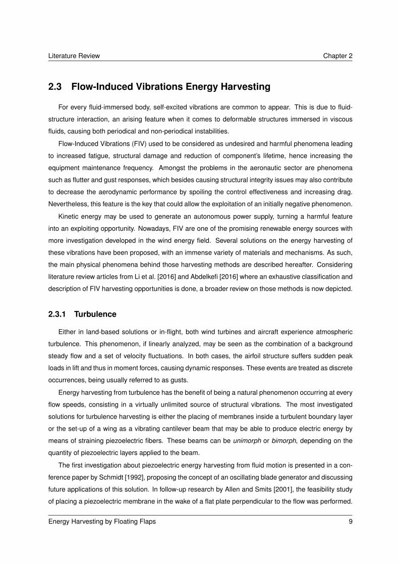
2.3 Flow-Induced Vibrations Energy Harvesting

For every fluid-immersed body, self-excited vibrations are common to appear. This is due to fluid-

structure interaction, an arising feature when it comes to deformable structures immersed in viscous

fluids, causing both periodical and non-periodical instabilities.

Flow-Induced Vibrations (FIV) used to be considered as undesired and harmful phenomena leading

to increased fatigue, structural damage and reduction of component’s lifetime, hence increasing the

equipment maintenance frequency. Amongst the problems in the aeronautic sector are phenomena

such as flutter and gust responses, which besides causing structural integrity issues may also contribute

to decrease the aerodynamic performance by spoiling the control effectiveness and increasing drag.

Nevertheless, this feature is the key that could allow the exploitation of an initially negative phenomenon.

Kinetic energy may be used to generate an autonomous power supply, turning a harmful feature

into an exploiting opportunity. Nowadays, FIV are one of the promising renewable energy sources with

more investigation developed in the wind energy field. Several solutions on the energy harvesting of

these vibrations have been proposed, with an immense variety of materials and mechanisms. As such,

the main physical phenomena behind those harvesting methods are described hereafter. Considering

literature review articles from Li et al. [2016] and Abdelkefi [2016] where an exhaustive classification and

description of FIV harvesting opportunities is done, a broader review on those methods is now depicted.

2.3.1 Turbulence

Either in land-based solutions or in-flight, both wind turbines and aircraft experience atmospheric

turbulence. This phenomenon, if linearly analyzed, may be seen as the combination of a background

steady flow and a set of velocity fluctuations. In both cases, the airfoil structure suffers sudden peak

loads in lift and thus in moment forces, causing dynamic responses. These events are treated as discrete

occurrences, being usually referred to as gusts.

Energy harvesting from turbulence has the benefit of being a natural phenomenon occurring at every

flow speeds, consisting in a virtually unlimited source of structural vibrations. The most investigated

solutions for turbulence harvesting is either the placing of membranes inside a turbulent boundary layer

or the set-up of a wing as a vibrating cantilever beam that may be able to produce electric energy by

means of straining piezoelectric fibers. These beams can be unimorph or bimorph, depending on the

quantity of piezoelectric layers applied to the beam.

The first investigation about piezoelectric energy harvesting from fluid motion is presented in a con-

ference paper by Schmidt [1992], proposing the concept of an oscillating blade generator and discussing

future applications of this solution. In follow-up research by Allen and Smits [2001], the feasibility study

of placing a piezoelectric membrane in the wake of a flat plate perpendicular to the flow was performed.



This would eventually have led to the experimental studies carried out by Goushcha et al. [2015] with

thin flexible cantilever beams covered by piezoelectric materials inside turbulent boundary layers. Here,

the effects of turbulence parameters such as mean local velocity, turbulence intensity and turbulence

scale were thoroughly explored and considered to reasonably estimate the power output.

Examples of recent research on wing-like cantilever beam prototypes have acknowledged the po-

tential of this solution in a broader scale. According to Abdelkefi et al. [2014], a unimorph cantilever

beam with a square cross-section tip mass has been proved to have increased harvested power with

upstream turbulence. This experiment recurred to an upstream mesh at the wind tunnel to simulate the

atmospheric turbulence. Moreover, in the work developed by Erturk and Inman [2009], a piezoelectric

bimorph prototype is experimentally validated for energy harvesting under base excitations.

Interestingly, the piezoelectric effect may also be used to suppress turbulence-induced vibrations as

suggested by Silva and Marqui [2013], which in turn could be used for a two-way smart solution capable

of harvesting energy from vibrations after suppressing the most harmful ones - a solution somehow

foreseen in the revolutionary article by Crawley and Luis [1987] suggesting piezoelectric actuators as

elements of smart structures.

2.3.2 Vortex-Induced Vibrations

Bluff bodies in steady flow conditions can usually undergo two types of dynamic instabilities, in which

Vortex-Induced Vibrations (VIV) is the first one to be explained.

Considering the classical example of a fluid-immersed cylinder at low Reynolds number, the stream-

lines are perfectly symmetric, fulfilling the potential flow theory. As the Reynolds number increases, the

symmetry is spoiled and the von Kármán vortex street is created in the back of the body, as noticed

by Mathis et al. [1984]. This phenomenon is ruled by parameters such as the diameter, flow viscosity

and velocity alongside mass and damping coefficients, as claimed by Barrero-Gil et al. [2012]; or by the

status of the boundary layer (laminar or turbulent). Nonetheless, this vortex shedding is always present

as an unsteady flow created by low pressure vortices periodically detached. In case of not being formed

symmetrically, the vortices create different lift forces in both sides of the body, forcing it to move towards

the low pressure zone at the same frequency of the shed vortices. As it approaches one of the the

natural frequencies of the structure, large and possibly harmful resonance vibrations may occur in a

phenomenon called lock-in.

Despite being potentially dangerous for structural integrity, if properly controlled and damped, this

aerodynamic feature may be used to harness kinetic energy from vibrations. This possibility has been

investigated for different fluids such as water and air. The water harvesting possibilities are immense,

mainly due to this phenomenon being widely present on offshore oil rigs and floating wind turbines.

Even so, the VIVACE concept proposed by Bernitsas et al. [2008] went further in presenting the first-



ever solution successfully using VIV to convert hydrokinetic energy in electricity. Featuring high energy

density whilst having low-maintenance requirements and a 20-year lifespan, it has shown the feasibility

of VIV-based solutions operating in a wide range of stream velocities. Follow-up research have shown

the possibility of increasing even more these results. On the paper by Meliga et al. [2011], a coupled

flow-cylinder system is tested to assess the possibility of a feedback control velocity mechanism at the

surface wall being used to optimize the amount of energy harvested, leading to an increase of 3.5 %.

Nonetheless, a very ingenious solution has literally come out of the water and, as a land-based

wind-powered energy source, is preparing to revolutionize the wind energy sector. The Spanish start-

up Vortex Bladeless2 has brought the energy harvesting by VIV out of the academia and proposed a

bladeless wind turbine to penetrate the market. This cylinder-shaped structure vibrates due to VIV and

harness energy by electromagnetic induction. According to field tests with scaled models, this new

solution is expected to achieve staggering results when compared with traditional wind turbines: 80 %

off maintenance costs, 40 % reduction in global power generation costs and carbon footprint. Their most

powerful model has 12.5 m height and produces a nominal power of 4 kW.

2.3.3 Galloping

Under steady flow conditions, galloping is the second type of dynamic instability that a bluff body

may suffer from. Unlike the resonance-related VIV, galloping has similitude with the aeroelastic flutter.

At a certain critical speed, total damping goes null and vibrations start growing exponentially. These

self-excited vibrations are known to occur in asymmetrically-iced electric conductors in high voltage

transmission lines, altering the aerodynamics of the wire. As a result of wake instability, the galloping

mechanism lies on steady and moderately strong crosswinds hitting the asymmetric cylinder causing a

negative pressure differential and therefore an oscillating movement. This phenomenon was addressed

in the book by Hartog [1985], where the first-ever mathematical formulation on the subject was made.

Nonetheless, galloping is a high-amplitude and low-frequency periodic oscillation, several times lower

than the vortex-shedding frequency. If not damped, it may reach a maximum amplitude equivalent to

the object span, which also scales with increasing velocity. Comparing with the VIV, this phenomenon is

independent from the synchronization between structural and vortex-shedding frequencies.

This phenomenon may be classified into vertical, horizontal and torsional galloping. The first two

ones are similar enough to depend only on the ice build up zone, causing the movement to occur

either on the vertical or horizontal plane. As per torsional galloping, a more complex movement is

considered; in fact, it can also be named as torsional flutter, a well-studied aeroelastic instability both in

the aeronautics and civil engineering sectors.

The first research milestones are being achieved in this prominent field of investigation. Proposed

2Vortex Bladeless webpage: http://www.vortexbladeless.com/


http://www.vortexbladeless.com/


by Barrero-Gil et al. [2010], the paper considers the first-ever energy harvesting solution by means of

transverse galloping whilst analyzing relevant relationships between cross-section geometry, incoming

flow velocity and maximum efficiency. Wind tunnel tests were performed in the research by Jung and Lee

[2011] to test the feasibility of a slightly different galloping mechanism, this time induced by the wake of

a cylinder, achieving interesting results for reduced speeds. Further developments have also considered

the replacement of electromechanical harvester for piezoelectric ones, as exposed by Abdelkefi et al.

[2012] on their numerical study about the efficiency of several cross-sections in a wide range of speeds.

2.3.4 Flutter and Limit-Cycle Oscillations

Aeroelasticity is the branch which studies the interactions between inertial, elastic and aerodynamic

forces in fluid-immersed elastic bodies, as introduced by Bisplinghoff et al. [1955]. It may be divided into

the areas of static and dynamic phenomena.

Concerning static aeroelasticity, it studies the steady response of an elastic body in a fluid flow,

which may be of two types: divergence and control reversal. The first one occurs when an elastic

lifting body deflects due to aerodynamic loads, increasing the effective angle of attack. This would

continually increase the load such that the twisting effect is augmented, leading to possible wing failure.

As per control reversal, it usually occurs at the tip of poorly torsionally stiffened wings under high speed

conditions. A deflected control surface will then suffer so much pressure that it will force the wing to

twist, starting to lose efficiency. Eventually, a point at which the deflected control surface leads to the

opposite response of that wanted by the pilot is reached.

On the other hand, dynamic aeroelasticity deals with structural vibration responses such as buffeting

and flutter. The first one is a high-frequency irregular motion of a structure caused by flow separation.

Buffeting was firstly noticed when tail portions undergone this phenomenon due to being placed inside

the main wing wake. As to its other counterpart, flutter is a self-excited aeroelastic instability which

usually arises in linear systems that transfer energy from the fluid flow to the elastic structure, charac-

terized by coupled bending and torsional modes interaction. On the approach of a threshold speed, flow

perturbations may create vibrations which are inherently damped by the aeroelastic structure. However,

as speed increases, the structure’s natural negative damping is outpaced by the aerodynamic positive

one, leading to ever-increasing harmonic oscillations. Therefore, the flutter speed may be seen as the

stability boundary where fluid-immersed structures go from a negative to a positive damping scenario,

changing the system’s natural frequencies.

As for non-linear systems in a fluid-structure interaction, stable LCO may occur after the flutter point

as thoroughly exposed in the book by Nayfeh and Mook [2008]. Mathematically speaking, a limit cycle is

a trajectory where energy is kept constant, meaning that a null energy balance is reached. These cycles

may be divided into stable, unstable or semi-stable depending on whether the neighboring trajectories



converge or spiral into the limit cycle as time approaches positive or negative infinity. Stable LCO are

the ones appearing on this dynamic aeroelastic instability, applying self-sustained oscillations with the

presence of an attractor - the trajectory is closed and periodic, and perturbations to it will converge to

the limit cycle as time tends to infinity. However, and despite being stable, the system will not tend to its

original state of equilibrium. This poses a problem because it may lead to bounded oscillations around

an ever-diverging equilibrium point, leading to catastrophic failure. Moreover, the excessive amplitude

of the LCO by itself may also lead to immediate failure. It is also worth noting that, if damping is kept

null, the flutter behavior is by default an LCO. Notwithstanding, as the speed increases, damping grows

and the system goes into flutter, whereas with LCO the amplitude of oscillations will increase without

exploding.

Nonetheless, exploiting these stable properties of LCO is the key for a new set of energy harvesting

opportunities. As investigated by Patil et al. [2001], who studied the LCO implications in high aspect

ratio wings, this kind of vibrations may even be noticed below the flutter speed threshold in case of

the steady state condition being disturbed. This led to the conclusion that LCO may appear at all

velocities depending only on the disturbance magnitude. It was also confirmed that stall limits post-flutter

oscillations and that LCO faces period doubling followed by loss of periodicity when speed increases.

Later, the introduction of FFF for gust alleviation with flutter constraints by Heinze and Karpel [2006]

opened the doors for the research done in the past years.

In the paper by Bernhammer et al. [2013], a new aeroservoelastic approach based on FFF actuated

by piezoelectric tabs is tested in wind tunnel, showing a 80 % increase in the flutter speed. Moreover, the

controller tested also evidenced a significant reduction on the model root bending moment, being able

to reduce the dynamic response to external excitations by a factor of 2. This corroborates the superior

effectiveness of FFF in gust alleviation and flutter suppression, and proposes follow-up research in the

applicability of this solution to control LCO.

Following the previous research, a new setup is numerically and experimentally tested by Bernham-

mer et al. [2017a], this time with an electromagnetic energy harvesters at the flap hinge. The model

consists of a cantilever wing with two FFF, each one with a dynamo connected to the flap hinge. This ex-

periment showed numerically that changing the resistance at the generator terminals may be a suitable

tool for controlling the stability of the system, but failed to do so experimentally due to too high resistance

in the wiring cables. For this same reason, no power was harvested. However, voltage was generated by

the flaps rotation, which achieved 0.035 V in the outer flap and 0.015 V in the inner; the values mismatch

due to different interaction with the structural modes. The values were that low because the generator

was operating far from its optimal speed and, as such, future work recommendations suggested the im-

plementation of a gearbox and a study on an energy harvesting and load alleviation integrated system.

Moreover, it is also proved that increasing the flutter speed augments the energy harvested. Also, in



low-amplitude LCO, the losses in lift are no more than 2 %.

As a follow-up research, the paper by Bernhammer et al. [2017b] depicts an experimental and nu-

merical simulation of an autonomous flap for wind turbines which deliberately induces flutter at low

speed and within its operational envelope such that an electromagnetic energy harvesting system may

use the energy generated to actively alleviate the incoming gusts. High-amplitude LCO are achieved by

using structural limiters, whereas low-amplitude ones perform the task by actuating trailing edge tabs

mounted on the FFF. As suggested in the previous paper, a gearbox was installed to increase the en-

ergy harvested. However, this ended up increasing the torque necessary to move the flap, feature that

was even worsen by the low wind speed velocity and the diminished aerodynamic force it provides. The

reason was attributed to mechanical friction in the gearbox which was a consequence of downsizing the

mechanism to a wind tunnel model scale, stating that a gear ratio of 80 apparently increased the friction

torque 80 times. As such, power measurements were not performed directly from the airflow excita-

tion. Instead, the system undergone a flap excitation at the first flutter frequency to mimic LCO. With 4

generators installed as depicted in Figure 2.2, the system produces 564 mW at optimal conditions in a

high-amplitude LCO. The sensors and actuators consume 42.7 mW at the same conditions, meaning

that the autonomous flap is self-sufficient.

In the end, the purpose of this project is increasing the performance of energy harvesters by develop-

ing a disruptive mechanism that mitigates the drawbacks of adding a gearbox. Moreover, experimentally

testing the controllability of the flutter speed by changing the resistance at the generator terminals is

also an objective. Doing so not only for a FFF but also in a torsionally stiffened flap is yet another goal.

(a) CAD model (b) Wind tunnel model

Figure 2.2: Wind tunnel concept for the energy harvesting mechanism by Bernhammer et al. [2017b]


3 | Numerical Modeling

In this chapter, the equations of motion for a 3DOF system are derived to assess the flutter speed.

To do so as long as the system can be modeled as linear, the p-k method is chosen. When dealing with

non-linearities, the system response is modeled in time domain to account for the inertial influence of a

release mechanism. Both models pass through a verification process. In the end, a feasibility study is

carried out to prove the applicability of the solution.

3.1 System Modeling

The numerical formulation used in the computational simulations is completely derived in Appendix

A. As such, only the initial and final steps of the deductions are presented in this section.

The numerical model based on the theory presented by Theodorsen [1934] in his report on aeroe-

lastic flutter may be idealized as the classical 3DOF spring-damper airfoil system depicted in Figure 3.1.

For a better insight on the notation used, please consult the Appendix A.1.

Figure 3.1: 3DOF wing section. Adapted from: Conner et al. [1997]

One can simply derive the equations of motion using either the standard spring-damper system

equation or the Euler-Lagrange equation, obtaining the following fully defined system:


Chapter 3 Numerical Modeling

mh+ Sαα+ Sβ β + Chh+Khh = L

Sαh+ Iαα+[Iβ + (c− a)bSβ

]β + Cαα+Kαα = Mα

Sβh+[Iβ + (c− a)bSβ

]α+ Iβ β + Cβ β +Kββ = Mβ

(3.1)

A careful insight on the reasoning behind the inertia, damping and stiffness terms may be respectively

consulted in the Appendix Sections A.2.1, A.2.2 and A.2.3. However, it is worth noting the inclusion of a

non-usual term in the flap damping part, namely the electromagnetic damping value estimator.

In the numerical model, a viscous damping model is used, meaning that each mode is characterized

by a damping value which is a fraction of the critical damping and stays in phase with the velocity for

each degree of freedom. To this standard modal damping model, the electromagnetic damping value is

added considering that it only affects the flap mode as shown in the following equation.

Ch 0 0

0 Cα 0

0 0 Cβ

=

2m0ωhζh 0 0

0 2Iαωαζα 0

0 0 2Iβωβζβ

+

0 0 0

0 0 0

0 0 Cel

(3.2)

In El-Hami et al. [2001], a first approximation to model the electromagnetic damping is proposed by

considering the electromechanical properties of a generator. As such, and considering that the model

will use a brushed Permanent Magnet (PM) Direct Current (DC) motor as generator, the circuit may be

modeled as depicted in Figure 3.2. The variable resistanceR is used to control the damping properties of

the system and maximize the power output. Moreover, note that the battery would also have an internal

resistance placed in series. Following such, and considering that power at the generator terminals is

simply given by the Ohm’s Law variant, one can conclude that the flap damping component may be

given by Equation 3.3. The complete deduction may be consulted in Appendix A.2.2.

Cel =(GR· < φ >)2

Req(3.3)

Figure 3.2: Electric circuit for energy harvesting

As such, and considering the equations of motion exposed in Equation A.3, the 3DOF system is

numerically represented by the following equation.

[M]ξ+ [C]ξ+ [K]ξ = Q (3.4)


Numerical Modeling Chapter 3

Also, the vector of generalized forces Q contains the whole set of forces applied to the system.

Depending on the goal of the study, the system may be simulated under a forced harmonic vibration, or

with a complete aerodynamic model to simulate the fluid-structure interaction and calculate the flutter

point. In the last case, the Theodorsen model for unsteady aerodynamics is used.

3.2 Numerical Approach

In this section, two approaches to the problem are exposed. Firstly, a standard flutter determination

procedure using the p-k method is presented in order to determine the flutter onset. However, it is insuffi-

cient to completely model the inertial effects of a gearbox coupled to the flap hinge and the development

of new mechanisms that would minimize such drawbacks. Hence, the second approach consists in a

time-domain simulation using a state-space model under forced harmonic vibrations - a similar condition

to that of Theodorsen model that considers aerodynamic forces with harmonic behavior.

3.2.1 Flutter Determination Model

For flutter modeling purposes, phenomenon which is predicted to occur at leveled flight, the only

external forces applied to the system are the ones related with its aerodynamics. Therefore, and as

described by Theodorsen [1934] in its model for unsteady aerodynamics, its contribution for the fluid-

structure interaction may be approximated as a purely harmonic function in the form of Equation 3.5. This

would then complete Equation 3.4, closing the system of equations and fully defining the 3DOF system.

The complete deduction on the generalized aerodynamic forces according to Theodorsen model and

the final matrix assembly are respectively presented in Appendices A.2.4 and A.2.5.

Q = [Maero]ξ+ [Caero]ξ+ [Kaero]ξ (3.5)

Introduced by Hassig [1971], the p-k method consists in a good approximation of the true damping

value when assumed that aerodynamic forces are properly approximated by purely harmonic functions.

This means that the computation of aerodynamic matrices, initially dependent on the dimensionless

eigenvalue p, can be expressed in the terms pertinent to the aerodynamic force as p ' ik.

The aforementioned equations with both structural and aerodynamic properties pose a Quadratric

Eigenvalue Problem (QEP) due to the damping term associated to ξ. It is possible to reduce the

order of the differential equation by introducing a new state variable λ∗, using the First Companion

Linearization (FCL) method. This originates a companion matrix [Z] that gathers all the 3DOF system

features. The eigenvalue problem is then solved according to Equation 3.6. Mode switching is avoided

by using the Modal Assurance Criterion (MAC) and the flutter onset interpolated when one of the modes

goes unstable. The deduction performed for the p-k method may be evaluated in Appendix A.3.



([Z]− p[I])

ξ∗λ∗

= 0 (3.6)

It is worth noting that although the p-k method outputs flutter diagrams close to the ones of real sys-

tems, it is only exact at the flutter point. Additionally, it can also predict the divergence speed where one

of the mode branches hits the null frequency. Ultimately, and most importantly, this method inherently

allows for the usage of electrodynamic damping which is the key feature on testing. In the end, this

model is developed using Python® programming language.

3.2.2 Time-Domain Model

Frequency-domain flutter detection algorithms may successfully detect the flutter boundary for com-

plex systems but are unable to simulate the time response for underlying non-linear features as gear-

boxes and release mechanisms. The model developed to simulate those features is presented hereafter

and the full deduction and algorithms proposed are depicted in Appendix A.4.

Firstly, one should note that inertia only plays a role in the flap motion when the system accelerates.

For geared systems, the inertia of an underlying shaft is given by Equation 3.7, meaning that the larger

the Gear Ratio (GR), the larger the moment of inertia. Recalling the work developed by Bernhammer

et al. [2017b], the struggle in dealing with a GR of 80:1 laid not only on friction, but mainly on the

shaft increased inertia. In order to avoid this feature, innovative mechanisms that somehow reduce the

influence of inertia and electromagnetic damping in the main shaft of the system shall be developed.

Iβ = Iflap +GR2 · IGB (3.7)

One of the possible solutions is a mechanism that somehow resembles the one of the bicycles: a

One-Way Bearing mechanism. It is, in fact, a bearing that only transmits the stroke in one direction,

consisting of a release mechanism; when the shaft rotates in the opposite direction, the input to the

generator free-spins according to an exponential decay ruled by friction and electromagnetic damping.

It can be modeled in time domain according to Algorithms 1 and 2, and the resultant plot evaluated in

Figure A.3. A more complex version, the Two-Way Bearing mechanism, is also developed.

Figures 3.3 and 3.4 show the physical concepts, where the metallic component is the one-way bear-

ing and the red one is the generator. In the Two-Way Bearing mechanism, the shaft connected to the

generator is the main axle. When it rotates, it transmits the reciprocating motion to the other shaft by

means of a conveyor belt. Each one-way bearing would then allow for rotation in one direction: when

the blue gear rotates, the yellow one is stopped; when the yellow gear rotates in the opposite direction,

the gears force the blue to rotate in its initial direction. This Two-Way Bearing system is therefore able

to convert both strokes of the circular reciprocating motion into a circular linear motion.



Figure 3.3: One-Way Bearing mechanism CAD model Figure 3.4: Two-Way Bearing mechanism CAD model

As a time-marching solution is required to solve such type of problem, a state space model is devel-

oped. To incorporate frequency-domain complex matrices defined by Theodorsen [1934] in that model,

one would have to follow a certain methodology. Ways of doing such include the Jones’ Approximation

by Jones [1938], the Finite State Induced Flow model by Peters et al. [1995], and the Minimum-State

method for the Rational Function Approximation method by Karpel [1990, 1999]. However, applying one

of those algorithms to the state space model was out of the scope of this thesis. As such, a solution

that equally represents the physical reality of the aerodynamic forces was applied: a harmonic function

is considered as the force input of the system, mimicking the unsteady aerodynamics oscillatory behav-

ior. In the end, the state space model based on the equations of motion shown in 3.4 is presented in

Equation 3.8. The state vectors and matrices content may be evaluated in Equation A.44.

X = [A]X+ [B]uY = [C]X+ [D]u

(3.8)

The time-domain simulation for the One-Way Bearing mechanism developed in Matlab/Simulink®

R2015a is presented in Figure A.4. For comparison purposes, two other models were developed for

the Standard mechanism (simply a shaft directly connected to a gearbox), and the Two-Way Bearing

mechanisms.

3.3 Verification

In order to enable the usage of the results obtained, one has firstly to compare them with others

obtained by the same or similar methods, and only after extrapolate it in the form of a feasibility study.

As such, both models pass through a set of benchmark tests. Firstly, the flutter detection code

according the p-k method is compared against peer-reviewed case studies in literature. Afterwards, this

same model is used to validate the time-domain code by comparing their response for the same input.



3.3.1 Flutter Determination Model

The flutter model verification is performed by benchmarking the code output. This is done for in-

creasingly complex systems: first a 2DOF system, then with the undamped full system and in the end

with the damped 3DOF system.

2DOF Undamped System

The first set of verification benchmark is performed according to data given in the book by Hodges

and Pierce [2011, p.229] for a 2DOF undamped system which data is available in Table 3.1.

The results obtained are shown in Figure 3.5 and plotted against the reference. Also, the numerical

flutter points are presented in Table 3.2 for further comparison. In both situations, the p-k method with

Theodorsen model is used. Note that the reduced damping ratio is given by γ/ωα. According to Figure

3.5, it is possible to see that the outputs perfectly match, predicting flutter for the pitch mode. This holds

true for both the flutter onset values and plots, and therefore the example is verified.

Table 3.1: 2DOF undamped system data

a µ xα r2α σh

-0.2 20 0.1 0.24 0.4

Table 3.2: Comparison between the 2DOF undamped system fluttercalculation codes

Own code in Hodges Difference [%]V 2.18393 2.18035 0.164

ω/ωα 0.648990 0.650154 0.179

Reduced Velocity [-]0 0.5 1 1.5 2 2.5

Red

uced

Dam

ping

Rat

io [-

]

-0.5

-0.4

-0.3

-0.2

-0.1

0

0.1

HeavePitchin Hodges

(a) Damping plot

Reduced Velocity [-]0 0.5 1 1.5 2 2.5

Dim

ensi

onle

ss F

requ

ency

[-]

0.3

0.4

0.5

0.6

0.7

0.8

0.9

1

1.1

HeavePitchin Hodges

(b) Frequency plot

Figure 3.5: 2DOF undamped system flutter plots

3DOF Undamped System

The second example, set for a 3DOF undamped system, is performed according the model tested

by Edwards [1977, pp.50-52] which data is available in Table 3.3.

Results obtained are shown in Figure 3.6 and plotted against outputs from the referred source. This

time, a root locus is presented instead of the two standard flutter plots. This is because it was the original



representation form in the reference aforementioned, so it was kept unchanged. Also, a comparative

assessment is present in Table 3.4.

By analyzing Figure 3.6, one can conclude that the outputs match, predicting flutter for the heave

mode. This remains true for both the flutter point and plots, and the example is therefore verified.

It is worth nothing that not all the values in Table 3.4 show the same numerical precision. This is due

to the ones exhibiting less precision being taken from the referred source. The remaining values for the

reference were extrapolated from the results available.

3DOF Damped System

The last step of the verification process is to add the viscous damping contribution. It is done ac-

cording to data in the paper by Conner et al. [1997, pp.94-100], where stiffness values are per unit

span.

The results obtained are shown in Figure 3.7 and plotted against outputs from the referred paper.

Due to the same reason of the previous example, a root locus plot is presented. Furthermore, output

benchmark is performed in Table 3.6.

In the end, Figure 3.7 shows that the outputs match, predicting flutter for the heave mode and thus

verifying the example. Moreover, it is of critical importance to refer that the support mass ms is added

to the wing-flap mass, thus originating a new heave modal mass value. Again, some values in Table 3.6

do not show the same numerical precision due to the reasons mentioned in the previous example.

Reduced Damping Ratio [-]-0.35 -0.3 -0.25 -0.2 -0.15 -0.1 -0.05 0 0.05

Dim

ensi

onle

ss F

requ

ency

[-]

0

0.5

1

1.5

2

2.5

3

3.5

HeavePitchFlapin Edwards

Figure 3.6: 3DOF undamped system root locus plot

Damping Ratio [-]-2 -1.5 -1 -0.5 0

Fre

quen

cy [H

z]

0

2

4

6

8

10

12

14

16

18 HeavePitchFlapin Conner

Figure 3.7: 3DOF damped system root locus plot

Table 3.3: 3DOF undamped system data

a c µ σh σβ

-0.4 0.6 40 0.5 3.0xα xβ r2

α r2β

0.2 0.0125 0.25 0.00625

Table 3.4: Comparison between the 3DOF undamped system fluttercalculation codes

Own code in Edwards Difference [%]V 3.01525 3.00 1 0.50

ω/ωα 0.705928 0.707579 0.233



Table 3.5: 3DOF damped system data

a c µ ms xα xβ rα rβ

-0.5 0.5 25.1 0.9497 kg 0.434 0.01996 0.7321 0.11397span Kh Kβ Kα ζh ζβ ζα

0.52 m 2818.8 kg/m/s2 37.3 kgm/s2 3.9 kgm/s2 0.0113 0.0115 0.01626

Table 3.6: Comparison between the 3DOF damped system flutter calculation codes

Own code in Conner Difference [%]U∞ [m/s] 24.03144 23.9 1 0.55ω [Hz] 6.050204 6.10 1 0.82

3.3.2 Time-Domain Model

The state space model in time domain is verified by benchmarking it against the same initial condi-

tions for the frequency-domain code.

Ideally, one would expect to compare the time-domain model with other examples in the literature.

All the aeroelastic data sets available for benchmark use aerodynamic forces as part of the equations of

motion as done for the p-k method. However, and as explained before, the aerodynamics is not included

in the state space model; instead, an harmonic force is used to determine the resonance frequencies

and test the harvesting mechanism. As such, the solution that arises is a comparison with the time

response calculated using the eigenvalue problem.

Considering the modal eigenvalue vi and the correspondent eigenvector ψi, the time response is:

ξi(t) =∑

i=mode

Dievitψi (3.9)

where the constant Di for the Initial Value Problem with Dirichelet boundary conditions is calculated

according to the following equation.

h

α

β

t=0

=

ψh ψα ψβDh

Dα

Dβ

(3.10)

Thus, using an initial condition of dimensionless heave h/b = 0.1 whilst considering null velocity and

therefore no aerodynamics influence on the equations of motion, time responses are plotted in Figure

3.8. The state space model response is obtained for the same initial condition with fixed-step Dormand-

Prince (Runge-Kutta 5th order) integration method and time step of 10-4 seconds. By analyzing the plots

one verifies that time responses overlap and the state space model is verified.1Results from the reference itself, not extrapolated



As a last verification step, a full simulation is performed to check the model performance in predicting

the behavior of the One- and Two-Way Bearing mechanisms. This time, no benchmark is performed.

Figure 3.9 shows that the mechanisms successfully convert a reciprocating circular motion into an almost

linear one for a GR of 25. Also, it is possible to see that the Two-Way Bearing mechanism achieves larger

angular velocity and has smaller fluctuations around the steady state value. Therefore, the voltage

it produces is the closest to DC. Nonetheless, the less complex One-Way Bearing mechanism also

performs quite well in these regards, being close to the results of its counterpart.

(a) Time response for heave perturbation (b) Zoom into the final transient period

Figure 3.8: Time marching model benchmark with the p-k method

Time [s]0 5 10 15

Gen

erat

or A

ngul

ar V

eloc

ity [r

ad/s

]

-10

-8

-6

-4

-2

0

2

4

6

8

10

StandardOne-Way BearingTwo-Way Bearing

(a) Time response for harmonic force input

Time [s]14 14.1 14.2 14.3 14.4 14.5 14.6 14.7 14.8 14.9 15

Gen

erat

or A

ngul

ar V

eloc

ity [r

ad/s

]

0

1

2

3

4

5

6

StandardOne-Way BearingTwo-Way Bearing

(b) Zoom into the positive stroke

Figure 3.9: Time simulation for the modeled mechanisms and a Gear Ratio of 25



3.4 Feasibility Study

Having performed the numerical model verification, it is possible to proceed with simulations that pre-

dict the system response and thus prove the feasibility of new solutions in order to allow for experimental

testing. As such, the effect of electromagnetic damping in the system is firstly shown in order to assess

the flutter speed controllability by means of resistance changing at the generator terminals. Afterwards,

the performance of two mechanisms that reduce the inertial effects of a gearbox in the overall system

and thereby improve the energy harvesting potential is assessed. In the end, the mechanism that would

fit the experimental model is developed based on this study.

Using the flutter determination model, one can study the influence of placing a generator at the flap

hinge and how it affects damping. Throughout this study, the aeroelastic properties of the model by

Conner et al. [1997] presented in Table 3.5 are used. The generator properties were gathered from

Bernhammer et al. [2017a], where the brushes resistance r is assumed to be null and the induction

coefficient φ is 0.96 Vs/rad. In this way, the flutter plots obtained for a range of resistances from Open-

Circuit (OC) to Short-Circuit (SC) conditions are presented in Figure 3.10, for the flap degree of freedom.

As predicted before, the heave mode goes unstable, and no flap branch overtakes the stability thresh-

old. Starting close to the OC condition and decreasing resistance down to 30 Ω, one can notice that

damping increases according to Figure 3.10a whilst frequency decreases in Figure 3.10b. This is the

expected behavior for the diminishing of the resistance, as described in Equation 3.3.

As the resistance keeps decreasing, an interesting saddle point in this tendency occurs around 25 Ω:

damping stops its decreasing trend and starts increasing again as depicted in Figure 3.10c, whilst the

mode frequency starts tending to zero (Figure 3.10d). With the resistance approaching SC conditions,

one notes that the damping value keeps increasing until reaching the edge of stability (Figure 3.11a),

whilst the frequency stays null in Figure 3.11b.

The fact of the flap damping having stopped increasing at certain point is in fact intriguing, and may

evidence an interesting phenomenon at the total damping level. But first, and in order to assess whether

or not the heave mode is affected by the same feature, the flutter plots for a resistance range up to 20 Ω

are presented in Figure 3.11. These plots qualitatively match the results obtained by Bernhammer et al.

[2017a] for the same range of resistances applied to the generator: the flutter speed increases as the

resistance decreases and the damping increase.

However, if the resistance keeps increasing, that does not occur anymore. As the heave mode

is always responsible for the flutter instability, one can plot the evolution of flutter speed with varying

resistance which would shed some light not only over the intriguing saddle point but also over the flutter

onset controllability. As seen in Figure 3.12, it is actually possible to control and therefore postpone the

flutter onset by changing the resistance value. Nevertheless, a strange increase in the flutter speed and



(a) Damping plot for resistance range of 30 Ω to 10 kΩ (b) Frequency plot for resistance range of 30 Ω to 10 kΩ

(c) Damping plot for resistance range of 20 Ω to 30 Ω (d) Frequency plot for resistance range of 20 Ω to 30 Ω

(e) Damping plot for resistance range of 0.1 Ω to 20 Ω (f) Frequency plot for resistance range of 0.1 Ω to 20 Ω

Figure 3.10: Flap flutter plots with changing electromagnetic damping



(a) Damping plot for resistance range of 0.1 Ω to 20 Ω (b) Frequency plot for resistance range of 0.1 Ω to 20 Ω

Figure 3.11: Heave flutter plots with changing electromagnetic damping

Resistance [+]10-3 10-2 10-1 100 101 102 103 104 105

Flu

tter

Spe

ed [m

/s]

24

24.1

24.2

24.3

Flu

tter

Fre

quen

cy [H

z]

6

6.02

6.04

6.06Short-CircuitOpen-Circuit

Figure 3.12: Flutter onset controllability

Resistance [+]10 20 30 40 50 60 70 80 90 100

Fla

p D

ampi

ng [N

ms/

rad]

0

0.02

0.04

0.06

0.08

0.1

0.12

0.14

0.16

Total DampingCritical Damping

Figure 3.13: Total damping with varying resistance

frequency occurs above approximately 25 Ω, resembling the same phenomenon described in the flap

damping behavior. As such, a careful reflection shall be elaborated.

Analyzing damping properties of the system may well help understanding this phenomenon. Consid-

ering total damping as CT = Cst + Cel − Caero and comparing with the flap critical value Ccrit = 2Iβωβ ,

one can conclude on whether or not the system is overdamped. This conclusion may be drawn only

based on the flap mode because the remaining are well below their critical damping threshold.

Still in Figure 3.12, it is worth noting that the OC and SC conditions respectively correspond also to

the limit cases of 3DOF without electromagnetic damping and 2DOF system without the flap. As to Fig-

ure 3.13, it plots the comparison between the total damping and its critical value. It reveals that below 25

Ω the electromagnetic damping makes the system overdamped. As such, a prominent conclusion may

be drawn: for over damped systems, the flutter speed increases with rising electromagnetic damping;

for systems below that threshold, the flutter speed decreases.



With the simulation on the flutter speed controllability performed and the possibility of postponing

flutter under certain conditions verified, the time-domain model is used to evaluate the performance

of the new mechanisms proposed and choose one to equip the experimental model. The simulation

is computed for a time window of 30 seconds and a forced harmonic excitation inputed to the heave

degree of freedom. The Root Mean Square (RMS) of the signal positive stroke is performed and the

power output is calculated according to Equation A.25. The results for both One- and Two-Way Bearing

mechanisms in comparison with the Standard one are shown in Table 3.7.

Table 3.7: Parametric study on the Gear Ratio for mechanism comparison

GearRatio

StandardOne-WayBearing

Increase[%]

Two-WayBearing

Increase[%]

Voltage [V]1

0.01524 0.02302 51.1 0.02317 52.0Power [mW] 0.0595 0.115 93.9 0.1168 96.2Voltage [V]

100.1517 0.2299 51.6 0.2325 53.3

Power [mW] 5.825 11.18 91.9 11.38 95.4Voltage [V]

250.3766 0.7147 89.8 0.7422 97.1

Power [mW] 35.14 105.1 199.1 112.3 219.6

In the end, one can conclude that only for large GR does the Two-Way Bearing mechanism capitalize.

For low GR, the performance difference is negligible. Therefore, and considering that only small GR

would be used in the experimental tests, the One-Way Bearing mechanism poses the best trade-off.

In Figure 3.14, one can see that the voltage curve is approximately linear as predicted in Equation

A.24, and the power curve quadratic as in Equation A.25. Moreover, the level of voltage and power output

is in the required range for small sensors and actuators for general usage, namely in wind turbines as

described in Bernhammer et al. [2017b], and possibly in Unmanned Aerial Vehicles (UAV). Note that the

power output is for an external load of 5 Ω and was not optimized for the maximum power condition.

Gear Ratio0 5 10 15 20 25

Vol

tage

[V]

0

0.5

1

Pow

er[m

W]

0

100

200

Figure 3.14: Voltage and Power outputs with varying Gear Ratio for the One-Way Bearing mechanism


4 | Concept Development

In this chapter, a description of the methodology applied to develop a feasible experimental model to

test the premises presented in the Feasibility Study is depicted.

Firstly, a brief overview on similar experimental test workbenches is performed to evaluate the feasi-

bility of such model. Then, the requirements are defined and the idea is generated grounded on those

foundations. Afterwards, a conceptual CAD model is developed to check the dimensional compatibility

between the developing structure and off-the-shelf components. In the end, the manufacturing solutions

are presented and 3D printing is used to materialize the concept development.

4.1 Requirements and Overview

The main purpose of the whole modeling procedure is simulating the behavior of a flutter-induced vi-

bration harvesting system. The entity responsible for such feature is the electromagnetic transducer, and

therefore the available generator size is the main design driver: its size will determine flap’s thickness,

which would set the maximum thickness for a given airfoil.

The generator chosen for this application is the VEM VEBEMH DC Motor, able to deliver 12 V at

10000 RPM. Weighting 126 g and having 26 mm of diameter, it consists in the best trade-off between

mass, cost and performance for an off-the-shelf component.

Previous peer-reviewed articles have already shown the feasibility of some concepts that can be

used as sizing references for the upcoming model. Moreover, the adaptable test setup developed by

Gjerek et al. [2014] is also presented because, despite having evaluated a 2DOF system, it studies

the aeroelastic behavior and experimental feasibility of thicker airfoils, which may be of interest for this

procedure. Hence, a descriptive comparison is depicted in Table 4.1.

As may be noticeable, the thicker the airfoil, the larger the acceptable generator diameter for the same

chord. However, one can not blindly increase the chord until fitting the transducer: the aspect ratio and

blockage ratio of the wind tunnel model are crucial parameters to perform valid testing. Moreover, and

in order to use the test workbench by Gjerek et al. [2014], the maximum acceptable distance between

the leading edge and the elastic axis is 90 mm, because a larger gap would place the former out of


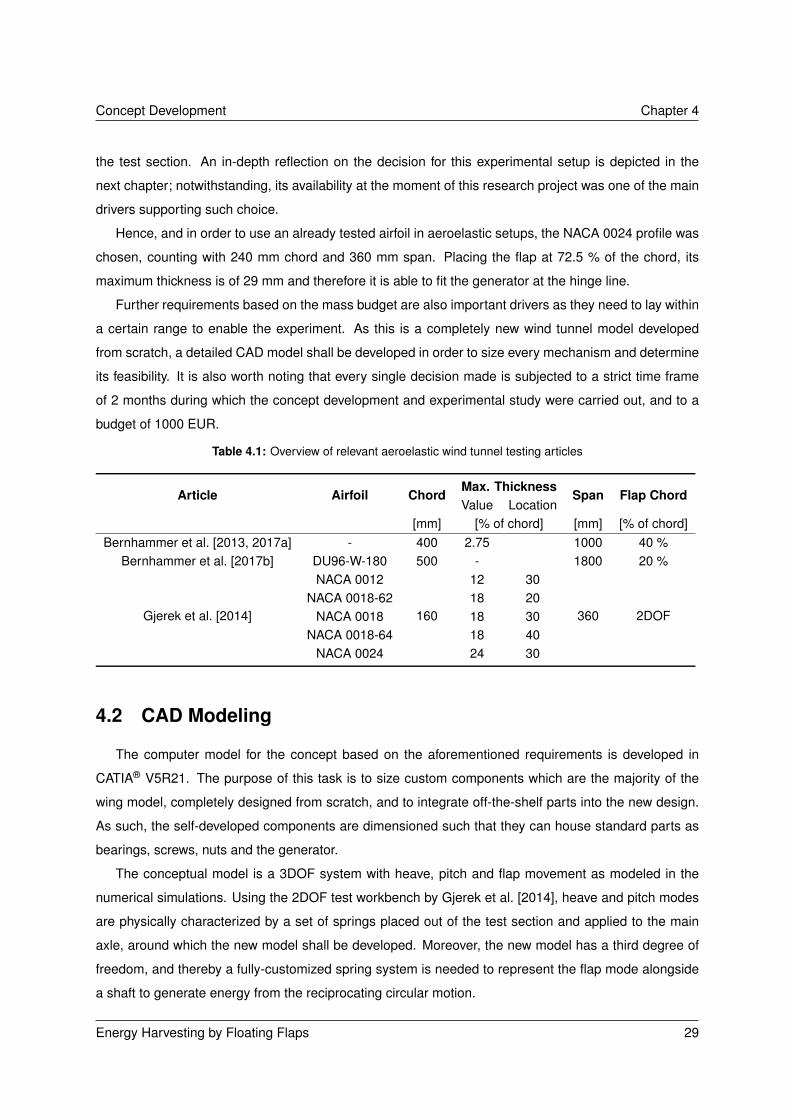
Concept Development Chapter 4

the test section. An in-depth reflection on the decision for this experimental setup is depicted in the

next chapter; notwithstanding, its availability at the moment of this research project was one of the main

drivers supporting such choice.

Hence, and in order to use an already tested airfoil in aeroelastic setups, the NACA 0024 profile was

chosen, counting with 240 mm chord and 360 mm span. Placing the flap at 72.5 % of the chord, its

maximum thickness is of 29 mm and therefore it is able to fit the generator at the hinge line.

Further requirements based on the mass budget are also important drivers as they need to lay within

a certain range to enable the experiment. As this is a completely new wind tunnel model developed

from scratch, a detailed CAD model shall be developed in order to size every mechanism and determine

its feasibility. It is also worth noting that every single decision made is subjected to a strict time frame

of 2 months during which the concept development and experimental study were carried out, and to a

budget of 1000 EUR.

Table 4.1: Overview of relevant aeroelastic wind tunnel testing articles

Article Airfoil ChordMax. Thickness

Span Flap ChordValue Location

[mm] [% of chord] [mm] [% of chord]Bernhammer et al. [2013, 2017a] - 400 2.75 1000 40 %

Bernhammer et al. [2017b] DU96-W-180 500 - 1800 20 %

Gjerek et al. [2014]

NACA 0012

160

12 30

360 2DOFNACA 0018-62 18 20

NACA 0018 18 30NACA 0018-64 18 40

NACA 0024 24 30

4.2 CAD Modeling

The computer model for the concept based on the aforementioned requirements is developed in

CATIA® V5R21. The purpose of this task is to size custom components which are the majority of the

wing model, completely designed from scratch, and to integrate off-the-shelf parts into the new design.

As such, the self-developed components are dimensioned such that they can house standard parts as

bearings, screws, nuts and the generator.

The conceptual model is a 3DOF system with heave, pitch and flap movement as modeled in the

numerical simulations. Using the 2DOF test workbench by Gjerek et al. [2014], heave and pitch modes

are physically characterized by a set of springs placed out of the test section and applied to the main

axle, around which the new model shall be developed. Moreover, the new model has a third degree of

freedom, and thereby a fully-customized spring system is needed to represent the flap mode alongside

a shaft to generate energy from the reciprocating circular motion.


Chapter 4 Concept Development

Despite engineering design being a highly iterative process in which success comes after countless

failures, solely the final concept is presented in this section. It is the result of a broad range of hindrances:

from time constraints to manufacturing impossibilities, passing by unavailable components and strict

dimensional requirements. Overall, it demands for a huge dose of creative thinking to overcome every

single hurdle that may appear. The result is presented hereafter, and the solutions achieved for the main

components exhibited.

Figure 4.1: Main wing cross-section CAD model Figure 4.2: Flap mechanism CAD model

Figure 4.1 presents the main wing cross-section. One can depict the following design breakthroughs:

A Skin-rib blended wing: motivated by the possibility of using rapid prototyping techniques to pro-

duce the model, the development of a skin-rib blended structure diminishes the complexity of

building an airfoil and decreases the production time. At the same time, it increases the structural

properties by having a seamless surface. The aerodynamic loads are transmitted by a 2 mm thick

skin and through 6 ribs to the main spar (C). Each rib has variable thickness, depending on where

it is located: at the tip, it has to withstand fastened screws that connect the wing tip (B) to the main

wing, and thus the rib thickness is of 4 mm; centered at the flap axle support (E), it has to carry

the flap transverse loads and therefore the rib thickness is of 5 mm; at the generator support (D),

having to transmit its weight load, with thickness of 3mm; the remaining ribs are symmetrically

placed with respect to the referred ones. Ribs design is ruled by weight saving and its primary

concern is redirecting the skin-to-spar load path.

B Wing tip: as the last wing component, it fixes the spar in place by screwing this light grey-colour

component to the wing. Using four M3 bolts in each tip, and by fixing compliant nuts incorporated in

pockets placed at the main wing, a durable and removable solution is achieved. Whenever access

to the main spar is needed, these tips are removed.

C Main Spar: it is the previously mentioned shaft around which the whole model should be built as

it transmits the heave and pitching movements from the wing to the spring system.

D Generator (support): as a cantilever support, the sizing was done considering the whole flap

system mass instead of solely the generator’s. This is because the model is vertically oriented,



meaning that the majority of the weight may lay on this support. As such, it has seamless edges

with the largest boolean radius possible to reduce the stress concentration factor. Moreover, the

support is sized to match the four M2 holes the DC motor has by default.

E Flap sensor (support): this flap axle support is one of the two hinges that allows flap angular

motion. It houses a bearing (H) in one side, and on the other it fixes a potentiometer. The latter

would be connected to the flap bottom shaft (J) and measure the flap deflection. Again, it was

designed to fit that specific type of potentiometer.

In Figure 4.2, one can see the uncovered flap layout and the One-Way Bearing mechanism, enabling

the evaluation of the main design:

F. Flap shaft adapter: custom part that connects the One-Way Bearing mechanism (G) output with

10 mm diameter to the generator (D) input shaft with diameter of 2.5 mm.

G. One-Way Bearing mechanism: innovative component that transforms the reciprocating circular

motion from the flap top shaft (I) into a linear circular one. The golden-color shaft holds inside

a one-way bearing encompassed by two regular bearings. The input shaft is connected to the

bearings with 6 mm inner and 10 mm outer diameter: the one-way bearing converts the motion

and the regular ones work as inertia wheels. Then, the converted moment is transmitted to the

golden shaft to input the generator.

H. Regular bearing: placed in both two supports to allow for the flap angular motion. The supports

are custom sized to fit these off-the-shelf bearings with 6 mm inner and 13 mm outer diameter.

I. Flap top shaft: fixed to the flap wall by a fixator (N), it transmits the angular motion of the airframe

with respect to the hinge support (E,H), being used to produce energy in the generator (D).

J. Flap bottom shaft: similar to the top shaft (I) but shorter in length, this is used to measure the flap

deflection as it inputs the potentiometer (E).

K. Flap cover fixator: using the same solution described in (B), two flat head M3 screws fix the 2 mm

thick flap cover in place. The nut is placed in a pocket, providing a durable and reversible solution

for this component which is removed every time the mechanism is changed.

L. Flap cover hook mechanism: this mechanism complements the aforementioned fixator (K) by

holding the flap in place near the trailing edge. The flap cover, not shown in the figures, has a

compliant hole through which the hook slides in, consisting of a strong fixating mechanism. It also

works as a rib, structurally reinforcing the flap in the transverse direction.

M. Flap half-span rib: structural appendix to strengthen the flap cover in the transverse direction by

preventing it to bend at half-span.

N. Flap shaft fixator: using M3 screws, the shafts (I,J) are fixed to the flap airframe and transmit

the angular motion. In order to avoid freeplay, bolts fix the screws in place. The edges are again

provided with a seamless boolean surface to minimize the torsion effect.



In the end, a final overview on the wing model may be seen in Figure 4.3. It is worth noting the

screws that fix the wing tip (B) to the main wing (A), and the flap spring system developed to embody

the torsional stiffness of that degree of freedom: it consists of a pulley with two tensioned linear springs

and a set of 3 holes in each side to enhance the tension controllability by varying the spring elongation.

This can also be depicted in Figure 4.15.

Finally, in Figure 4.4 one can see the wind tunnel testing layout. The model is placed vertically in

an acrylic test section that also holds the spring systems for heave and pitch. Carbon-Fiber Reinforced

Polymer (CFRP) endplates are placed in the model. The test section is connected to a nozzle that

connects to the wind tunnel facility described in Chapter 5.4.1

Figure 4.3: Wing assembly CAD model Figure 4.4: Wind tunnel setup CAD model

4.3 Manufacturing

In this section, the materialization of the concept is described. As referred before, time limitations

required this wing model to be produced as swiftly as possible. Thereby production lines were completely

avoided and the waiting time reduced to its minimum by choosing for rapid prototyping and 3D printing.

This means that the great majority of the wing model and components to attach to the original setup

were custom manufactured in less than two weeks, consisting of a major step to move from modeling to

testing in short time. The remaining was either produced in composite or bought in modeling stores.

4.3.1 3D Printing

The 3D printing process is carried out at Delft University of Technology using the Formlabs® Form2

machine. Its additive manufacturing process consists in stereolithography (SLA), where the photopoly-

merization of a liquid polymer leads to a solid object: a light-emitting device as a laser illuminates a

translucent tank filled with liquid resin; the solidified model is progressively pulled up by a lifting platform.

The printing models are generated by the software PreForm® 2.11.3, which uses .stl files rendered in

CATIA® to create support struts for printing. An overview of this setup may be evaluated in Figure 4.5.



Figure 4.5: 3D printing setup Figure 4.6: Main wing half after a 24-hour print job

The print job was carried out using the Formlabs® Grey V2 resin1, using the layer thickness of 50 µm

for the best trade-off between fastness and accuracy, in a printing bay of 145 × 145 × 175 mm3. The

most complex parts, such as the main wing halves and flaps, had to be halved in two parts and took

approximately 24 hours each to print. The final result of one of those prints may be evaluated in Figure

4.6, where it is possible to see the massive wing model supported by tiny struts fixed to the platform,

and the resin tank in the bottom. Curiously, it is even possible to spot the ribs beneath the wing skin.

Figure 4.7: Test parts

Figure 4.8: Hook mechanism (f)

Figure 4.9: Flap sensor support (E)

1Resin data sheet: https://formlabs.com/media/upload/Clear-DataSheet.pdf


https://formlabs.com/media/upload/Clear-DataSheet.pdf


Prior to the final model printing, some test parts were printed to test its feasibility in real scale. In

Figure 4.7, some of those models are presented:

a Generator support #1: prototype to fix the generator to the main wing. The diameter of this part

has to be such that it allows the generator to slide in but not to rotate, posing a tolerance problem.

b Generator support #2: the chosen prototype to fix the generator. As described in Section 4.2, the

support (E) uses the M2 screw holes in the generator to hold it in position.

c Bearing support tolerances: in order to achieve the best fit for the 13 mm diameter regular bear-

ing (H), several geometrical parameters are tested to acknowledge the printing tolerance needed

to achieve a proper fit to the bearing.

d Nut pocket tolerances: similar to the previous ones, but to house the nuts that hold the flap (K),

the wing and wing tip (A,B) in place.

e Main wing split tolerance: consisting in a quarter of the wing cross-section, this skin portion is

used to test the fitting tolerances between the bottom and top wing halves.

f Hook mechanism model: to ensure that the flap fixator and hook mechanism (K,L) are a feasible

solution, a cross-section model of the flap is printed as can also be seen in Figure 4.8. Here one

can see the nut pocket in the fixator and the fitting of the hook mechanism.

Moreover, in Figure 4.9 one can evaluate another test part custom built to hold both the bearing and flap

sensor (E).

With the test printing procedure performed and the tolerance parameters tuned, the final model

printing campaign starts, counting with 8 print jobs to manufacture the several wing and flap halves, as

well as other parts to connect external components to the test setup. In Figure 4.10, it is possible to see

the flap bottom halves just after being printed. Note that they had to be diagonally placed to fit in the

printing bay, and the supporting struts are connected to the internal surface of the flap in order not to

spoil the aerodynamic properties. After undergoing a sanding treatment, the halves are glued and the

result may be evaluated in Figure 4.11. In the end, the flap half-span rib (M) displayed in Figure 4.2 is

glued on the halves joint.

Regarding the nut pockets used to fix parts of the wing together, one must say that a metal-to-metal

screw/nut pair is the best trade-off for 3D-printed objects. Even if the tap was sculpted during the print

job, factors as thermal expansion or fatigue may spoil it after few usage cycles. The solution presented

in Figure 4.12 with black squares and arrows allow the nut to slide in a quadrangular pocket-shaped

hole that will hold it as the screw is tightened. Regarding the white arrows, they point to the holes that

would receive the sliding-in connection pins from the wing tip (B). As such, the wing-tip coupling process

consists in sliding the tip pins through the marked holes and use M3 screws and nuts to lock both parts

in place.



Figure 4.10: Printing flap bottom halves

Figure 4.11: Flap bottom halves after treatment

Figure 4.12: Main wing pockets and tip connections

4.3.2 Composites

The only composite panel used in this model is for manufacturing the endplates. With the requirement

of lightness and flexural rigidity such that its natural frequency lay outside the range of the structural fre-

quencies, the CFRP TEPEX® dynalite 201-C200(4)/50%2 with thickness of 1 mm is used to manufacture

endplates with 1.2 times the chord length and almost 4 times the maximum airfoil thickness. The size is

limited by the experimental test section dimensions and the expected pitch angle the model will exhibit

in a flutter test. The parts were modeled in CATIA®, and the composite endplates were hand-drilled and

cut according to the technical drawing in Figure 4.13a. The final result may be seen in Figure 4.13b.

200

2 90

1R

13

3

5

2.9

6

38

100

100

80

84.5

7 .57.5

42.5535.4516

25.69

116

(a) Technical drawing (b) Final product

Figure 4.13: Top endplate

2Composite data sheet: http://bond-laminates.com/fileadmin/user_upload/MDS_201-C200_x_-50__SSe_170710.pdf


http://bond-laminates.com/fileadmin/user_upload/MDS_201-C200_x_-50__SSe_170710.pdf


4.3.3 Off-the-shelf Components

The remaining components around which the 3D-printed model is designed were bought in a mod-

eling shop. Their description and function are depicted in Table 4.2, as well as references to the mech-

anism parts explained in Figure 4.2.

Table 4.2: Off-the-shelf components list

Part FunctionAERONAUT 7739/86 Stainless Steel Pipe

6/5.4 mmFlap shaft (I,J)

GRAUPNER Brass Pipe 11/10 mm One-Way Bearing mechanism external pipe (G)RABOESCH Connector 6.0 mm

Flap shaft adapter (F)RABOESCH Connector 2.3 mmRABOESCH Connector 3.0 mm

2 Bearings 13/6 mm Regular bearing (H)2 Bearings 10/6 mm One-Way Bearing mechanism inertial bearings (G)

RCP-racing One-way bearing One-Way Bearing mechanism (G)VEM VEBEMH DC motor Generator (D)

4.4 Assembly

The final assembly may be evaluated hereafter. In Figure 4.14, one can see the whole model as-

sembled with the One-Way Bearing mechanism. On the other hand, Figure 4.15 shows a top view of

the model which exhibits the flap pulley system.

Figure 4.14: Wing model assembly Figure 4.15: Flap pulley system


5 | Experimental Setup

The experimental model developed in the previous chapter is proposed to be tested in the setup

presented by Gjerek et al. [2014], where a comprehensive approach to determine flutter stability bound-

aries is firstly introduced. The detailed experimental apparatus for both vibration and wind tunnel tests

is presented, as well as the calibration procedure for sensors and structural parameters.

5.1 Framework

The experimental framework used to test the developed airfoil mechanism is thoroughly described in

the paper by Gjerek et al. [2014]. Nevertheless, the major features that corroborate its good function-

ality are highlighted in this section. Data that fully describe electrical components as sensors and the

generator are determined by means of calibration and may be consulted in Appendix B.

This setup was chosen for several reasons. Firstly, it allows for a wide range of possibilities when

it comes to structural parameters of a typical wing section according to aeroelasticity theory. In fact,

it reveals to be adaptable from a 2DOF system to a 3DOF airfoil. Secondly, the paper has shown the

possibility of choosing amongst an acceptable range of symmetrical airfoil options, making it possible

to optimize the final choice with respect to the generator size whilst keeping track of the blockage ratio

for wind tunnel testing. Moreover, the test structure is likely to be used in vibration tests, with hammer-

and shaker-based impulses, with little change in the original setup. Finally and foremost, the setup was

available at the time of this study at Delft University of Technology and allowed to perform both vibration

and wind tunnel tests in the same framework, which deeply increases the quality of the results.

The test bench, which is in reality a wind tunnel test section, is an acrylic hollow square-prism with

dimensions of 0.35 × 0.4 × 1.0 m3. It holds a support system for a 2DOF rigid wing model, upgraded to

fit 3DOF. The model is vertically placed to prevent both heave, pitch and flap modes from the influence

of gravity. Figure 5.1 depicts the overall schematics of the workbench mechanisms and sensors.

To reproduce the heave movement of the airfoil, a pair of leaf springs defines the plunge stiffness.

This is adjustable by changing the spring effective length, leading to a stiffness range from 200 N/m to

2600 N/m. The response is measured by the displacement sensor Sentech LVDT 75DC (Sentech Inc.,


Chapter 5 Experimental Setup

Glenside, PA) with sensitivity of 0.7874 V/mm as detailed in its technical data sheet, and voltage supply

of ±15 V.

Regarding the pitch degree of freedom, the elastic axis is defined by the wing support axis around

which the airfoil rotates. It is vertically placed across the test section and supported at the end by ball

bearings. At the top end, the pitch stiffness adjustment system consists of a pulley and two preloaded

linear springs combined to act as a torsional spring, tunable in a range from 0.6 Nm/rad to 4.4 Nm/rad.

At the bottom end is placed the rotation angle sensor Midori MAC QP-2HC (Midori America Corp.,

Fullerton, CA) with sensitivity of 43.22 mV/deg (Appendix B.1) and voltage supply of 5 V.

With respect to the flap motion, the hinge is made of two shafts supported by two ball bearings. The

top shaft connects to the generator at the bottom end and to the torsional spring at the top; this system

also uses a pulley-spring combination (Figure 4.15) to achieve the desired stiffness. The bottom shaft

connects to the flap angle sensor (Figure 4.14), a standard potentiometer with an angular range of 217.5

deg, sensitivity of 21.45 mV/deg (Appendix B.2), and voltage supply of 5 V.

The wing model is the 3D-printed prototype developed in the previous chapter. A NACA 0024 airfoil

with chord of 0.24 m and span of 0.36 m is mounted on the wing support axis and fixed at 40 % chord

length. The flap houses a generator for energy harvesting purposes, the VEM VEBEMH DC Motor with

induction coefficient of 18.741 mVs/rad (Appendix B.3), with the hinge line located at 72.5 % chordwise.

Two mechanisms for energy harvesting are tested, the Standard and One-Way Bearing; as well as two

flap configurations, the Setup I with some flap torsional stiffness and the Setup II with none (FFF).

Figure 5.1: Test workbench schematics. Adapted from: Gjerek et al. [2014]

For the purpose of forced excitations, the excitation target is repositioned with respect to the reference

paper in order to fit the devices available. In Figure 5.2 one can see that a stinger may excite the model

through a custom-build 3D-printed connector. This piece slides into the metallic support for the linear


Experimental Setup Chapter 5

springs, having been designed to fit a nut inside which position is determined by the pulley used. The

stinger directly fits into a hole designed with its negative shape. The conically-shaped external contour

uniformly distributes the load from the stinger to the metallic support, solely exciting the heave mode.

Figure 5.2: Close-up to Excitation Target

It is worth noting that throughout the experimental testing none of the center of mass and inertia ad-

justment systems were used. Inertial properties were kept constant, except for the parameters affected

by the swap between Standard and One-Way Bearing mechanisms which mainly affect damping and

inertia moment at the flap level. However, all damping and inertial components had to be recalculated

from the vibration to the wind tunnel tests due to the placement of endplates onto the model.

5.2 Data Acquisition

The whole data acquisition procedure is carried out using the National Instruments eight-slot USB

2.0 chassis NI cDAQ-9172, compatible with input and output modules and with LabVIEW® connectivity.

Onto the chassis are placed two NI 9215 input modules and one NI 9263 output module.

The NI 9215 is a 4-channel 16-bit ±10 V analog input module used in the BNC variant. Overall, it

was used to measure the following quantities:

• Heave displacement [mm]

• Pitch deflection [Deg]

• Flap deflection [Deg]

• Generator output voltage [V]

• Function generator input voltage [V]

• Shaker input voltage [V]

• Input load force [N]

Furthermore, the NI 9263 is a 4-channel ±10 V analog output module used in the screw-terminal



variant. It was used to generate the input voltage function [V] that would control the function generator

in the vibration tests.

In order to communicate with the hardware and develop an automated data acquisition system, the

LabVIEW® 2017 software and the NI DAQmx 17.1 driver were used. At a sampling frequency of 1 kHz,

100 samples are logged at each reading with an acquisition mode of continuous sampling. Note that the

frequency range of interest is up to 10 Hz, so the Nyquist frequency threshold is well above the required.

Two fully custom virtual interfaces were developed to match the requirements of an automated data

acquisition system not only for both vibration and wind tunnel experiments but also for calibration pur-

poses such as the viscous damping characterization or the wind tunnel area ratio calculation. With the

procedure details for each routine developed in LabVIEW® 2017 left for the upcoming sections, Figures

5.7 and 5.11 show the graphical interface developed for these experiments.

5.3 Vibration Tests

This type of testing uses the framework described in the previous sections to determine the fre-

quency response of the system by means of modal analysis and assess its energy harvesting potential.

Using the same setup for vibration and wind tunnel tests therefore consists in a good practice for model

characterization and results inter-comparability.

The modal analysis of a complex system outputs the coupled natural frequencies for each vibration

mode after an impulse excitation. These vibration modes fully characterize the model and allow to

perform code validation. On the other hand, the energy harvesting capabilities are tested with a forced

harmonic excitation in which a frequency sweep will reveal the optimal condition for voltage production;

the mechanisms are then compared at that point.

5.3.1 Apparatus

The experimental apparatus for the impulse and shaker tests is similar, only differing in the excitation

mode and therefore on the force generation method. In the impulse excitation, the load is generated by

the experiment operator as depicted in Figure 5.3, whereas in the shaker test a completely automated

frequency sweep is run as shown in Figure 5.4 and controlled by the LabVIEW® interface.

As such, in order to close the data acquisition loop, a detailed connection schematics is depicted in

Figure 5.5 alongside the full instrumentation list for the forced harmonic excitation test. Note that for the

impulse test none of the shaker-dependent instrumentation is necessary as the force is generated by

hand.

To generate the input force that triggers the system response, the Brüel & Kjœr Vibration Exciter

Type 4809 is used. A custom-made circular load cell is placed between the stinger and the shaker in



Figure 5.3: Impulse Excitation Test setup Figure 5.4: Forced Harmonic Excitation Test setup

Test Section

Heave Sensor

Pitch Sensor

Flap Sensor

Generator Output

Power Source

±15 V

+5 V

+5 V

Shaker

Shaker

Input

Load Cell

Peekel

Amplifier

B&K

Amplifier

Function

Generator

Data

Acquisition

I

O

I

o o o o

o o o o

o o o o

Function

Input

+

_ R

Figure 5.5: Forced Harmonic Excitation Test schematics

order to measure the input force, as can be seen in Figure 5.6. The stinger would fix into the 3D-printed

Connector to transmit the force into the model (Figure 5.2).

The circular load cell was manufactured at Delft University of Technology and is made of 4 strain

gages to measure the force in the axial direction. Overall, it consists of a full Wheatstone bridge with

resistance of 120 Ω.

Due to strain gage low output voltage, the load cell signal needs amplification. As such, it goes into

the Peekel Instruments Compact Amplifier System PICAS. The signal that goes into the data acquisition

input module is the load cell amplified voltage with sensitivity of 99.02 mV/N.

Returning to the shaker, more precisely to the input signal that controls its frequency. Firstly, the

output module generates an analog signal that inputs the Hewlett-Packard 3310B Function Generator in

order to control the generated frequency for the Frequency Sweep Test.

The output of the Function Generator will then input the Brüel & Kjœr Power Amplifier Type 2706. The



signal is now at the desired frequency and correctly amplified to control the vibration exciter, consisting

of the Shaker Input.

Figure 5.6: Close-up to Load Cell

5.3.2 Procedure

The experimental procedure for both vibration tests consists in executing a predetermined step list

for the Standard mechanism and then perform the same for the One-Way Bearing, undergoing OC and

SC conditions. This is only done for the Setup I flap configuration. Final results are obtained after

post-processing the acquired data according the methodology proposed in Section 6.1.

Impulse Excitations

The procedure for structural characterization by hammer testing is described as follows:

I Hit the Target depicted in Figure 6.5 with the Rubber Tip to excite both heave and pitch modes.

II Check the quality of the recorded impulse force that has to resemble a sharp peak load: there

should be no double hit present.

III Repeat the previous steps 10 times for each right-to-left and left-to-right direction.

IV Repeat the previous steps for both 2DOF and 3DOF systems (Standard and One-Way Bearing

mechanisms undergoing SC and OC conditions).

The LabVIEW® virtual instrument created to acquire data from these measurements resembles the one

presented in Figure 5.7 without Sweep Settings controls, Function and Shaker Input graphs.

Forced Harmonic Excitations

The procedure for determining the energy harvesting optimal frequency and voltage production per-

formance is carried out with constant shaker input voltage amplitude and is depicted next:



I Run a frequency sweep from 0 Hz to 30 Hz for 200 seconds in OC conditions and record the

frequency at which the voltage production is maximum.

II Redo the same procedure for a narrower frequency sweep that includes the previously determined

frequency (e.g. from 0 Hz to 10 Hz) and update the optimal value.

III Run a last frequency sweep with range of ±1 Hz around the optimal frequency previously deter-

mined.

IV At the optimal point, record the time response for 80 seconds at constant frequency, and for a

comprehensive range of resistance values at the generator terminal from SC to OC conditions.

V Repeat the previous steps for both Standard and One-Way Bearing mechanisms.

The LabVIEW® virtual instrument developed to automatically control the frequency sweep and acquire

data is presented in Figure 5.7.

Figure 5.7: Graphical Interface for the Frequency Sweep Test

5.4 Wind Tunnel Tests

Experimental flutter tests performed in wind tunnels aim at the aeroelastic characterization of the

physical model. By defining the instability boundaries of the system, one is able to extrapolate those

conclusions to larger scale models.

The instability threshold is defined by the system damping. It occurs when the damping provided

by the structure and the electromagnetic mechanism matches the one of the external forces, such as

the aerodynamics. After reaching the point of marginal stability, the energy harvesting capabilities are

tested in the same way as done for the vibration tests.



5.4.1 Apparatus

The wind tunnel testing campaign is carried out in the low-speed W-Tunnel at Delft University of

Technology. It is an open-jet wind tunnel facility with cross-section of 0.4 × 0.4 m2 and maximum

velocity of 35 m/s controlled by an induction motor that drives a fan.

As the framework used during the vibration test is 5 cm thinner in width than the wind tunnel open

end, it is connected to the latter by means of an adapter which gradually makes the transition from the

tunnel cross-section to the test section. This is depicted in Figures 5.8 and 5.9 as a general and back

views, and in Figure B.4a as a more detailed view of the contraction in the adapter.

Figure 5.8: Wind Tunnel setup Figure 5.9: Test Section back view

With respect to the wind stream velocity measurement, it is based on the dynamic pressure value

obtained by the pressure difference between total and static pressure ports in a pitot tube. To do so,

digital pressure gauges are used, namely the Mensor DPG 2400 during the whole experiment, and the

Mensor DPG 2100 when an extra sensor is needed for calibration purposes. Moreover, to determine the

velocity based on the dynamic pressure, one has also to compute the air density which depends on the

altitude and room temperature. As to the altitude, it is assumed to be Medium Sea Level; with respect

to temperature, it is measured with the RS 1319A Type K thermometer. Having these two variables as

input, the velocity at the test section is calculated based on measurements taken upstream. As such,

velocity is calculated based on Bernoulli’s equation:

v = Ar

√2∆p

p0·RgT (5.1)

where Ar is the area ratio between the place at which the pressure measurement is taken and the test

section, ∆p is the dynamic pressure, p0 is the ambient pressure, Rg is the specific gas constant for dry



air, and T is the absolute room temperature. An overall view of the aforementioned sensors positioning

in the setup is given in Figure B.4a. The area ratio is estimated to be Ar ' 1.101 and is determined by

means of calibration instead of using the mass conservation law, as described in Appendix B.4.

Regarding the data acquisition loop and sensor linking, the detailed connection schematics for the

flutter test is depicted in Figure 5.10. In this test, there is no need for force generation, therefore the data

acquisition system gets much simpler. However, note that velocity measurements are independent from

the data acquisition system as it is manually input into the LabVIEW® virtual instrument.

Test Section

Heave Sensor

Pitch Sensor

Flap Sensor

Generator Output

Power Source

±15 V

+5 V

+5 V

Data

Acquisition

I o o o o +

_ R

Wind Tunnel

Thermometer

Pitot Tube Velocity

Figure 5.10: Wind Tunnel Test schematics

5.4.2 Procedure

The wind tunnel experimental procedure consists in executing a predetermined step list for the Stan-

dard mechanism and then perform the same for the One-Way Bearing. It is done for both Setup I and II

flap configurations, meaning that the springs providing torsional stiffness to the flap mode are removed

as the configuration changes. Final results are also obtained after post-processing the acquired data

according to the methodology proposed in Section 6.1.

The experiment aims at determining the flutter speed by slowly increasing the airspeed, having the

numerical flutter value as reference. The flutter onset is the point at which an induced excitation (e.g. an

impulse force that excites at least one mode) does not fade out, maintaining a self-sustained oscillation

for the data acquisition period. During such time interval, the time response is recorded in order to

determine the energy harvesting performance. The detailed procedure is presented as follows:

I Set wind tunnel the induction motor Rotations Per Minute (RPM) and let the pressure and temper-

ature measurements stabilize.

II Excite one or more modes in several ways and record the time response for 10 times.

III Repeat the previews steps until reaching the flutter onset for both 2DOF and 3DOF systems (Stan-

dard and One-Way Bearing mechanisms undergoing SC and OC conditions).



IV For the 3DOF systems and at the flutter point, record the time response during 80 seconds and for

a comprehensive range of resistance values at the generator terminal from SC to OC conditions.

V Repeat the previous step for both Standard and One-Way Bearing mechanisms.

The LabVIEW® virtual instrument developed to automatically acquire the flutter test data is presented

in Figure 5.11.

Figure 5.11: Graphical Interface for the Flutter Test

5.5 Physical Model Characterization

Prior to the experimental campaign, a set of measurements have to be carried out in order to ensure

that the physical reality is correctly represented by the acquired data. As such, the procedure applied to

determine physical properties as stiffness and damping for the 3DOF system is described in this section.

5.5.1 Stiffness

The model stiffness properties are defined thanks to the adaptive design of the test workbench.

As such, and in order to accurately determine these features, the procedure used to calculate them is

described next.

With respect to the heave degree of freedom, the paper by Gjerek et al. [2014] states that stiffness

is tunable in a range from 200 N/m to 2600 N/m by adjusting the effective length of a pair of leaf springs.

The accurate stiffness value for a determined spring length is calculated as depicted in Figure 5.12a: a

certain load is applied and the heave sensor reads the corresponding displacement of the leaf spring

tip; the procedure is done in load and unload cycles. Performing these measurements for a set of spring



length values leads to Figure 5.12b which represents the range of heave stiffness values that may be of

interest for this study.

Tip Displacement [mm]0 2 4 6 8 10 12

For

ce [N

]

0

1

2

3

4

5

6

7

8 ExperimentalLinear Regression

y = 0.6761 x R2 = 0.9921

(a) Stiffness curve

Spring Length [mm]150 160 170 180 190 200 210 220 230 240

Hea

ve S

tiffn

ess

[N/m

]600

800

1000

1200

1400

1600

1800

2000

2200

2400

ExperimentalExponential Regression

(b) Stiffness range

Figure 5.12: Heave Stiffness Characterization

With respect to the pitch and flap degrees of freedom, the torsional stiffness is generated by two

linear springs attached to a pulley. As such, and depending on both linear springs stiffness and pulley

radii, several levels of torsional stiffness are achievable.

The linear springs stiffness value is determined by subjecting it to a tensile test in a Zwick® 1455

machine with automated data acquisition system. The output follows the same pattern as in Figure

5.12a and the stiffness value for every single linear spring is calculated. With respect to the pulley, and

in order to provide different stiffness values, there are five models available with different values. The

available possibilities for pitch and flap torsional stiffness are available in Table 5.1.

In the end, the heave stiffness value chosen is of 676.1 N/m, the pitch one is 1.033 Nm/rad and the

flap 0.178 Nm/rad. This choice is a trade-off between the availability of the pulleys, the effort to keep

the pitch-to-heave natural frequency ratio as close to 3 as possible, as it resembles the one of aircraft

wings.

5.5.2 Damping

Damping properties for the 3DOF system are determined by individually exciting each degree of

freedom while having the remaining blocked. This would allow to determine the uncoupled natural

frequencies and damping ratios, aligning with the viscous damping model presented in Section A.2.2.

This method is suggested by Gjerek et al. [2014] as the damping characterization procedure for the test

workbench used.

Time response is recorded for each degree of freedom and damping ratio obtained after filtering the

signal with the lowpass filter referred in Section 6.1. The process is repeated for left-to-right and right-



Table 5.1: Pitch and Flap Torsional Stiffness

PitchSpring ID I II III IV

Linear Stiffness [N/mm] 1.320 1.314 2.694 2.709

FlapSpring ID i ii iii iv

Linear Stiffness [N/mm] 0.4530 0.4392 0.4523 0.4452

PulleyPulley ID 1 2 3 4 5

Radius [mm] 14.0 19.8 24.3 28.0 30.5

Spring PairLinear Stiffness Torsional Stiffness

[N/m] [Nm/rad]I,II 2634 0.516 1.033 1.549 2.065 2.450I,III 4014 0.787 1.574 2.360 3.147 3.734

III,IV 5403 1.059 2.118 3.177 4.236 5.026i,ii 892.5 0.175 0.350 0.525 0.700 0.830i,iii 905.6 0.178 0.355 0.533 0.710 0.842i,iv 898.5 0.176 0.352 0.528 0.704 0.836

to-left impulses, 10 times each, in order to enrich the signal frequency range. An optimization code in

Matlab® is run to fit the experimental data to the following equation using the Least Square Method:

e−b1t[b3 cos (2πb2t+ b5) + b4 sin (2πb2t+ b6)

]+ b7 (5.2)

where bi are the optimization parameters. The parameter b1 matches the damping ratio γ ≈ log(hi/hi+1)/(2π),

and b2 the mode natural frequency in Hz. The curve fitting result may be evaluated in Figure 5.13 for the

heave mode.

Time [s]0 0.2 0.4 0.6 0.8 1 1.2 1.4 1.6

Hea

ve D

ispl

acem

ent [

mm

]

-10

-8

-6

-4

-2

0

2

4

6

8

10Experimental DataLowpass-Filtered DataFitted Curve

Figure 5.13: Curve fitting optimization procedure for Heave Damping Characterization

According to the following expressions it is possible to determine the viscous damping values for the

model (Equation 5.3), and update the inertia matrix with experimental results (Equation 5.4).



Ch =2γhKh

γ2h + ω2

h

, Cα =2γαKα

γ2α + ω2

α

, Cβ =2γβKβ

γ2β + ω2

β

(5.3)

m+ms =Kh

γ2h + ω2

h

, Iα =Kα

γ2α + ω2

α

, Iβ =Kβ

γ2β + ω2

β

(5.4)

The results computed for the heave mode are presented in Table 5.2. Total heave mass has slightly

increased due to the endplates, and thereby its natural frequency has decreased. In the end, viscous

damping decreases 25.4 % when endplates are installed. Comparing with the CAD model, the experi-

mental values present a difference of less than 1 % . This consists in a great validation for the predictions

carried out using the 3D model.

Concerning the pitch mode, the results may be evaluated in Table 5.3. The moment of inertia has

significantly increased as a consequence of the endplates. Despite having only 1 mm thickness, the

endplates increase the inertia of this degree of freedom due to its large area in the direction perpen-

dicular to rotation. Therefore its natural frequency has decreased along with the viscous damping. The

comparison with the values estimated by the CAD model is also of great quality, showing good accuracy

of the 3D model.

At last, the flap damping data is presented in Table 5.4. The moment of inertia is not affected by

the placement of endplates as it only resembles the movement of the control surface about its hinge.

Nonetheless, it is worth noting that both mechanisms have behaved differently during the damping

characterization, which was totally expected in beforehand given that the One-Way Bearing mechanism

was developed to reduce the inertial effects of the back-and-forth shaft rotation. It led to an almost 40 %

reduction in viscous damping.

Moreover, one should note that the difference between computed and experimental values for the

One-Way Bearing mechanism is noticeably larger than the remaining. Although the CAD model is able

to predict these values based on its mass properties, the One-Way Bearing mechanism has an important

dynamic feature that only allows the flap axle to rotate in one direction. This clearly plays an important

role in the overall behavior of this mode and is well beyond the prediction scope of CAD softwares.

In summary, it is possible to conclude that endplates increase the inertia properties of the model,

reducing its natural frequency and damping values for heave and pitch modes. Furthermore, the One-

Way Bearing mechanism matches the expectations postulated after the Feasibility Study by reducing

the modal moment of inertia by almost 40 %. In some way, one can also state that the numerical model

developed in Simulink® which predicts this behavior is validated, at least qualitatively. Likewise, the

physical properties estimated by the CAD model have shown to be of great accuracy. The full model

data for all mechanisms and configurations used in the test campaign is gathered in Table 5.5.


Chapter5

Experim

entalSetup

Table 5.2: Heave properties

HeaveVibration

TestsWind Tunnel

TestsUndamped Natural

Frequency [Hz]Experimental 3.0486 2.9242

Computed 3.0729 2.9427Difference [%] 0.8 0.6

SupportMass [kg]

Experimental 0.62899 0.62512Decrease [%]Computed 0.60000

Difference [%] 4.8 4.2Damping Heave [Ns/m] 2.3547 1.7564 25.4

Table 5.3: Pitch properties

PitchVibration

TestsWind Tunnel

TestsUndamped Natural



Flap Moment ofInertia [kgm2]Experimental 4.8620×10−3 7.2199×10−3

Decrease [%]Computed 4.7420×10−3 6.9720×10−3

Difference [%] 2.5 3.6Damping Pitch [Nms/rad] 1.6360×10−2 1.3489×10−2 17.5

Table 5.4: Flap properties

FlapStandard

MechanismOne-Way Bearing

MechanismUndamped Natural



Flap Moment ofInertia [kgm2]Experimental 1.7481×10−4 1.5646×10−4

Decrease [%]Computed 1.8450×10−4 1.8450×10−4

Difference [%] 5.3 15.2Damping Flap [Nms/rad] 1.7457×10−3 1.0543×10−3 39.6

50E

nergyH

arvestingby

FloatingFlaps

Experim

entalSetup

Chapter5

Table 5.5: Model Properties

ConstantVibration

Tests

Wind Tunnel

Tests

Standard

Mechanism

One-Way Bearing

MechanismGeometric Properties

Span [m] 0.36Chord [m] 0.24

Semi-chord, b [m] 0.12Elastic Axis, a (w.r.t. b) [-] -0.20Hinge Line, c (w.r.t. b) [-] 0.45

Stiffness PropertiesHeave Stiffness, Kh [N/m] 676.1

Pitch Stiffness, Kα [Nm/rad] 4.240

Flap Stiffness, Kβ [Nm/rad]Setup I: 0.178Setup II: 0.0

Damping PropertiesHeave Damping, Ch [Ns/m] 2.3547 1.7564

Pitch Damping, Cα [Nms/rad] 1.6360×10−2 1.3489×10−2

Flap viscous damping, Cβ [Nms/rad] 1.7457×10−3 1.0543×10−3

Generator Induction Coefficient, φ [Vs/rad] 1.8741×10−2

Inertia PropertiesWing Mass, m [kg] 1.2137 1.3777

Support Mass, ms [kg] 0.6293Pitch Static Moment, Sα [kgm] 2.9639×10−2 3.7793×10−2

Pitch Inertia Moment, Iα [kgm2] 4.8620×10−3 7.21992×10−3

Flap Static Moment, Sβ [kgm] 8.4823×10−3 9.6285×10−3

Flap Inertia Moment, Iβ [kgm2] 1.7481×10−4 1.5646×10−4

Wing CG distance from a, xα (w.r.t. b) [-] 0.2035 0.2286Flap CG distance from c, xβ (w.r.t. b) [-] 5.824×10−2

Heave Natural Frequency, ωh [Hz] 3.0486 2.9242Pitch Natural Frequency, ωα [Hz] 4.7000 3.8569Flap Natural Frequency, ωβ [Hz] 5.0786 5.3681

Energy

Harvesting

byFloating

Flaps51

6 | Results

This chapter focuses on the results obtained for the physical model data, developed and based on

the numerical study performed in the beginning of the project. The experiments are planned in two

different parts, both exciting the same feature: the limit-cycle behavior of the system.

The process is divided into vibration and wind tunnel tests. The former only counts with the system

dynamics and the response is studied based on a forced input motion, preferably harmonic. On the other

hand, the latter does not count with any external excitation apart from the aerodynamic force, which can

also be described by an harmonic function. As such, both tests induce the system into LCO, which

mimics the real operation conditions for a mechanism at the flutter point. In this way, it is possible to

assess the potential of such energy harvesting mechanism.

A thorough analysis of the results obtained is then carried out. For each experimental setup, an ini-

tial comparison between numerical model and experimental outcome is performed to validate the code.

Afterwards, the experimental results for energy harvesting are presented to corroborate the feasibil-

ity of such device. In the end, discussion is structured around the performance comparison between

both mechanisms and flap stiffness configurations, their energy harvesting capability, the flutter speed

controllability and the influence of endplates in flutter testing. To achieve the aforementioned results,

data acquired during experimental tests was post-processed under an invariant procedure to improve

inter-comparability.

In the end, an application of such mechanism with a gearbox is studied with the validated time-

simulation, and the trade-off between weight penalties and increased performance analyzed for an

aeronautical study case.

6.1 Data Post-Processing

The signal read by every sensor and later acquired is studied in the frequency domain. Mode analysis

is carried out by means of a Direct Fourier Transform using the Fast Fourier Transform (FFT) algorithm

present in Matlab®. With a sampling frequency of 1 kHz, a Lowpass Butterworth Filter is applied to the

experimental data with passband corner frequency of 30 Hz, stopband of 50 Hz, passband ripple of 1 dB


Results Chapter 6

and stopband attenuation of 25 dB. It has the main purpose of filtering electromagnetic interferences and

eliminate noise above 50 Hz, the threshold above which most of the electric-powered devices operate.

The output is then conducted into a Savitzky-Golay Filter to reduce noise. The order and frame length

of this filter is adjusted to achieve the smoothest output signal.

The last step of this analysis is calculating the Frequency Response Function (FRF). Despite lowpass-

filtered, and in order to chose the suitable FRF estimator, the signals are still considered to be noisy. As

such, and based on the reference paper by Rocklin et al. [1985], an expected noise presence in both

input and output signals leads to the usage of the Hv estimator as follows:

Hv(f) =Syx|Syx|

√SyySxx

(6.1)

where Syx represents the Cross Spectral Density from Output to Input, Sxx and Syy respectively stand

for Power Spectral Density of Input and Output, all in frequency domain. Afterwards, the results are

again passed by a Savitzky-Golay Filter in the same circumstances as aforementioned.

6.2 Vibration Tests

This kind of testing is primarily meant to determine the frequency response of the system by means of

modal analysis for Setup I flap configuration. Such can be done by recording the time response for each

degree of freedom and then analyze the signal in frequency domain using FFT. However, the outcome

of this analysis will always depend on its input. As such, for inter-comparability purposes, the FRF

is computed as an output-to-input ratio, enabling comparisons for similar excitations with non-constant

amplitudes.

The modal analysis of a complex system outputs the coupled natural frequencies for each vibration

mode. After having characterized each mode individually, the output is compared with the uncoupled

natural frequencies obtained in Chapter 5. The frequency response of these modes will then shed some

light on how the modes couple together and shift with respect to the uncoupled ones.

Firstly, the 2DOF model response is analyzed to establish a reference for subsequent analysis to

more complex models. Afterwards, the complete 3DOF models with Standard and One-Way Bearing

mechanisms are evaluated and the effect of adding a floating flap to the heave-pitch model is assessed.

Moreover, the influence of electromagnetic damping on the overall system behavior is checked.

Nonetheless, this test could be run under a wide range of input forces, such as impulse, step and

harmonic excitations; and the accuracy of the result strongly depends on the quality of the excitation.

The input force shall excite all modes, being as closed to the ideal as possible (i.e the impulse force

should correspond to a sharp force peak, the step to a sudden force drop to zero after a constant

plateau, and the harmonic to a sinusoidal force constant in amplitude and frequency). The input that


Chapter 6 Results

equally excites all frequencies and therefore all modes is the impulse force. As such, it was the one

chosen for the modal analysis.

After performing the analysis in frequency domain to the 3DOF system, testing the energy harvest-

ing capabilities of the mechanism is what follows. To do so, the system undergoes forced harmonic

vibrations to enable flap harmonic deflection and therefore voltage production. A frequency sweep is

carried out to determine the optimal point for energy production, and the energy harvesting capabilities

are measured and compared at the referred frequency under an input force with constant amplitude and

frequency.

All these features are preceded by a validation study that compares the time history of the numerical

model with the experimental outcome for the same physical properties. This is done for an harmonic

forced oscillation.

6.2.1 Validation

The validation study is performed to verify the match between the numerical model and experi-

mental results. The time-domain simulation is performed as previously described in Chapter 3.4 using

Matlab/Simulink®. This simulation is run with experimental data for the input force, namely the magni-

tude read by the load cell during the experimental tests and the frequency given by the FFT algorithm

applied to the latter signal. The input force is further modeled as a forced harmonic vibration with a

cosine function inputed at the heave degree of freedom.

Figures 6.1 to 6.4 show the time history for heave, pitch, and flap modes, and also for the voltage

production at the flap hinge. Given the large combination of modes, mechanisms (Standard and One-

Way Bearing) and circuit conditions (OC and SC), only four validation examples are presented attempting

to cover the whole range of possibilities.

Note that all experimental responses are phase shifted with respect to the numerical ones for eas-

iness of interpretation. Given that the frequency matches, if both responses were superimposed, the

difference in amplitude would not be easily noticeable. As such, it is possible to see that no further

phases shift occurs, meaning that the numerical model accurately predicts the frequency output.

With respect to the magnitude, one can notice that the numerical model qualitatively estimates the

experimental time response, despite over-predicting it by a range of 15 % to 20 %. This is most likely due

to physical properties not accounted for in the numerical model, such as friction, and the flap structural

limiters that were hit during the measurements. Nonetheless, the numerical results show very good

agreement with the experimental ones, allowing for the code validation.


Results Chapter 6

Time [s]0 0.1 0.2 0.3 0.4 0.5 0.6 0.7 0.8 0.9 1

Hea

ve D

ispl

acem

ent [

mm

]

-5

-4

-3

-2

-1

0

1

2

3

4

5 Numerical One-Way Bearing OCExperimental One-Way Bearing OC

Figure 6.1: Heave time response

Time [s]0 0.1 0.2 0.3 0.4 0.5 0.6 0.7 0.8 0.9 1

Pitc

h D

efle

ctio

n [D

eg]

-15

-10

-5

0

5

10

15

Numerical One-Way Bearing SCExperimental One-Way Bearing SC

Figure 6.2: Pitch time response

Time [s]0 0.1 0.2 0.3 0.4 0.5 0.6 0.7 0.8 0.9 1

Fla

p D

efle

ctio

n [D

eg]

-40

-30

-20

-10

0

10

20

30

40

Numerical Standard SCExperimental Standard SC

Figure 6.3: Flap time response

Time [s]0 0.1 0.2 0.3 0.4 0.5 0.6 0.7 0.8 0.9 1

volta

ge [V

]

-0.4

-0.3

-0.2

-0.1

0

0.1

0.2

0.3

0.4 Numerical Standard OCExperimental Standard OC

Figure 6.4: Voltage time response

6.2.2 Mode Analysis by Impulse Excitations

The system is excited with an impulsive force, a sharp peak that ideally excites all frequencies. The

force is applied by a hammer-like structure with an incorporated load cell at wing’s mid-span and close

to the leading edge. This structure has a rubber tip to make the hit softer and transfer more of the

impulse energy to the low frequency part of the spectrum. The time history for left-to-right and right-to-

left impulses is recorded in order to enrich the signal frequency range and include all system features in

this study.

The modal analysis is carried out as referred in Section 6.1. The output of both lowpass-filtered data

FFT and FRF is labeled in Figure 6.5 as Experimental Data, and are shown in parallel to present the

input force, and to emphasize the difference in the signal noise. Note that the only signal not undergoing

lowpass filter treatment is the one corresponding to the input force. As it consists in a sharp peak, the

lowpass filter would decrease the maximum amplitude and increase the peak time length, blurring the

outcome. As such, the raw load signal inputs the FFT and FRF function whereas the heave, pitch, flap


Chapter 6 Results

and voltage signals are filtered beforehand. Also, and as aforementioned, note that the FFT experimental

data is presented as a very noisy signal whereas the FRF drastically reduces this feature. This is due to

FRF being a ratio between the output and the input. As such, the majority of the noise is eliminated by

this operation, meaning that both signals are under the same noise sources.

Firstly, the flap is locked with null deflection and the behavior of the 2DOF system is recorded to

establish a reference. Right after, it is unlocked and the response is recorded for both mechanisms

under OC and SC conditions.

Figure 6.5 presents the results for 2DOF and 3DOF systems with both mechanisms in OC conditions

as it resembles the lowest electromagnetic damping value added to setup. As such, it allows to study

solely the influence of the introduction of the third degree of freedom with negligible damping added by

the generator.

Figures 6.5a, 6.5c and 6.5e present an approximately constant and flat load FFT around -35 dB, evi-

dencing not only an equivalent average load peak in the three experiments but also a standard behavior

for impulsive force FFT.

Concerning the 2DOF system, Figures 6.5a and 6.5b show two clear and distinct peaks at 3 Hz

and 5 Hz at 17.5 dB FRF magnitude, respectively corresponding to heave and pitch coupled natural

frequencies. With the introduction of the third degree of freedom, Figures 6.5d, 6.5f and 6.6 evidence

not only that magnitude decreases to below 15 dB but also that phase slightly shifts to the left. Most

importantly, a third peak appears around 7 Hz corresponding to the flap coupled natural frequency. Cu-

riously, the pitch mode seems to also increase its amplitude at this resonance point whereas the heave

mode completely drops, meaning that pitch and flap modes are heavily coupled. Similar conclusion may

be drawn for heave and pitch modes at lower frequencies, which would eventually reveal itself as the

flutter mechanism for this system.

Comparing the results obtained with the uncoupled natural frequencies in Table 5.5 (ωh ' 3.1 Hz,

ωα ' 4.7 Hz, and ωβ ≈ 5.2 Hz), one can say that both coupled and uncoupled natural frequencies

grossly match for heave and pitch modes, whereas the flap one it is shifted to around 7 Hz.

Moreover, further considerations may be taken around the comparison between the 2DOF and 3DOF

systems in Figure 6.6: it clearly shows the effect of introducing the third degree of freedom into the

system and how the mechanisms influence the system response.

Both mechanisms are in OC conditions, meaning that electromagnetic damping present is minimal.

As such, the difference in amplitude spotted has strictly to do with viscous damping. As predicted nu-

merically in Chapter 3.4 and experimentally verified for the uncoupled system in Chapter 5, the One-Way

Bearing mechanism introduces less viscous damping than the Standard mechanism. As a consequence,

one can spot that the resonance peak in the flap mode is larger in amplitude and thinner in width for the

former. Likewise, the same behavior is generally observed for the remaining modes.


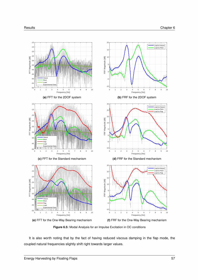
Results Chapter 6

Frequency [Hz]0 1 2 3 4 5 6 7 8 9 10

FF

T M

agni

tude

[dB

]

-60

-55

-50

-45

-40

-35

-30

-25

-20

-15

-10

HeavePitchLoadExperimental Data

(a) FFT for the 2DOF system

Frequency [Hz]0 1 2 3 4 5 6 7 8 9 10

FR

F M

agni

tude

[dB

]

-10

-5

0

5

10

15

20

Load-to-HeaveLoad-to-Pitch

(b) FRF for the 2DOF system

Frequency [Hz]0 1 2 3 4 5 6 7 8 9 10

FF

T M

agni

tude

[dB

]

-50

-45

-40

-35

-30

-25

-20

-15

-10

HeavePitchFlapLoadExperimental Data

(c) FFT for the Standard mechanism

Frequency [Hz]0 1 2 3 4 5 6 7 8 9 10

FR

F M

agni

tude

[dB

]

-10

-5

0

5

10

15

20

25

Load-to-HeaveLoad-to-PitchLoad-to-Flap

(d) FRF for the Standard mechanism

Frequency [Hz]0 1 2 3 4 5 6 7 8 9 10

FF

T M

agni

tude

[dB

]

-50

-45

-40

-35

-30

-25

-20

-15

-10


(e) FFT for the One-Way Bearing mechanism

Frequency [Hz]0 1 2 3 4 5 6 7 8 9 10

FR

F M

agni

tude

[dB

]

-10

-5

0

5

10

15

20

25


(f) FRF for the One-Way Bearing mechanism

Figure 6.5: Modal Analysis for an Impulse Excitation in OC conditions

It is also worth noting that by the fact of having reduced viscous damping in the flap mode, the

coupled natural frequencies slightly shift right towards larger values.


Chapter 6 Results

Frequency [Hz]0 1 2 3 4 5 6 7 8 9 10

FR

F M

agni

tude

[dB

]

-10

-5

0

5

10

15

20

25

30 2DOF Heave2DOF PitchStandard HeaveStandard PitchStandard FlapOne-Way Bearing HeaveOne-Way Bearing PitchOne-Way Bearing Flap

Figure 6.6: Experimental FRF for both mechanisms in OC conditions for 2DOF and 3DOF systems

With regards to the comparison between OC and SC conditions, Figure 6.7 presents the results for

the standard mechanism, showing that the amplitude of all degrees of freedom tenuously increases in

OC condition. The SC condition introduces the maximum electromagnetic damping factor, increasing the

total damping felt by the system. As such, the resonance peaks are expected to decrease in amplitude

and become wider. However, the amount of added damping is too little to clearly see this effect.

Notwithstanding, and judging by the simulations performed in the Feasibility Study, it would be ex-

pected that the impact of the SC condition in the overall system would be more significant. However, it

always depends on the system physical properties and the critical damping value. In case of the elec-

tromagnetic damping being a small fraction of the critical one, it will not significantly affect the overall

behavior of the system.

Frequency [Hz]0 1 2 3 4 5 6 7 8 9 10

FR

F M

agni

tude

[dB

]

-10

-5

0

5

10

15

20 Standard Heave OCStandard Pitch OCStandard Flap OCStandard Heave SCStandard Pitch SCStandard Flap SC

Figure 6.7: Experimental FRF for the Standard mechanism under OC and SC conditions


Results Chapter 6

Concerning the comparison between both mechanisms in SC conditions as depicted in Figure 6.8, it

is possible to unveil the same behavior spot in Figure 6.6 in OC conditions but in larger magnitude due

to the increased electromagnetic damping.

As previously concluded, the benefits of the One-Way Bearing mechanisms in terms of damping and

inertia reduction are once more evidenced, allowing for larger deflections in all degrees of freedom. As

for the SC condition, the electromagnetic damping in the system is now maximum, allowing for a larger

and noticeable difference between mechanisms.

In Figure 6.8 it is again depicted the larger and more pronounced resonance peaks for the One-Way

Bearing mechanisms. It is also worth noting that a slight shift to the right can be spotted in the One-

Way Bearing mechanism resonance frequencies, suggesting that reduced total damping increases the

resonance frequency. Similar conclusion has already been drawn in Figure 6.6 under OC conditions.

Frequency [Hz]0 1 2 3 4 5 6 7 8 9 10

FR

F M

agni

tude

[dB

]

-10

-5

0

5

10

15

20

25

30

Standard Heave SCStandard Pitch SCStandard Flap SCOne-Way Bearing Heave SCOne-Way Bearing Pitch SCOne-Way Bearing Flap SC

Figure 6.8: Experimental FRF for both mechanisms under SC conditions

6.2.3 Energy Harvesting by Forced Harmonic Excitations

The system is excited by an electromagnetic shaker at different frequencies connected to the model

by a metallic stinger. In the same way as performed in Section 6.2.1, the connection allows the singular

excitation of the heave mode.

The purpose of this study is to identify the optimal frequency at which the voltage production and

power generation are maximum for each mechanism. Both are firstly excited by a harmonic function

generated with constant input voltage and a linear frequency sweep of 0 Hz to 30 Hz in 200 seconds.

Time response is recorded and modal analysis is performed to determine the frequency at which the flap

deflection is the largest. This would therefore correspond to the largest voltage production frequency.

Afterwards, the range is narrowed first to a 0 Hz to 10 Hz interval and in the end to a 1.5 Hz interval

around the expected value, both for a sweep time of 200 seconds. This is done to refine previous


Chapter 6 Results

estimations of the optimal frequency: as the frequency sweep rate decreases, the result becomes more

trustworthy as the response approaches the steady state. The systems are then tested at their own

optimal frequency because only at this point is possible to compare them at their full potential.

The output corresponding to the largest frequency sweep is presented in Figure 6.9 for both mech-

anisms. By comparing both FRF plots in Figures 6.9b and 6.9d, one can conclude that the optimal

frequency for both mechanisms is around 5 Hz. Also, note that some of the peaks presented in the FFT

plots of figures 6.9a and 6.9c vanish on the aforementioned FRF plots. This is because some peaks are

caused by the input force which is not constant in amplitude throughout the sweep. It happens due to

system dynamics and can be explained by basic physical principles: as a system is forced into a certain

harmonic movement, it replies with an equal force in opposite direction which is read by the load cell.

This, in association with the inertial properties of the model, causes the input force not to be constant

even though the input voltage to the shaker is.

As described before, further frequency sweeps are performed in order to precisely determine the op-

timal point for energy harvesting. It is found that the One-Way Bearing mechanism has optimal frequency

of 4.06 Hz whereas the Standard mechanism has it at 4.43 Hz. Moreover, it can also be concluded that

the amplitude of the One-Way Bearing mechanism is way larger than its counterpart, suggesting that

the former achieves larger flap deflections for the equivalent input conditions. The same behavior can

be observed for both heave and pitch degrees of freedom, though with much less difference between

mechanisms.

Following the optimal frequency determination for energy harvesting, both mechanisms are tested

onto this key capability. To do so, the RMS of the signal positive stroke is performed in a 80-second time

window. Instead of a RMS to both positive and negative strokes, a single one is performed because

the One-Way Bearing is solely applied to that direction, allowing to average the voltage into a quasi-DC

voltage value. This is actually one of the purposes of this system: disposing the need for a an AC/DC

wave rectifier whilst decreasing the electromagnetic damping effects of the generator. Likewise, the

Two-Way Bearing mechanism may also be used to convert both strokes into a positive-valued voltage;

and only in that case, the RMS for the reciprocating strokes may be used.

At the optimal frequency point for each mechanism, the resistance at the generator terminals is

changed from OC to SC, passing by six other resistance values. The OC condition is represented in

this plot as 100 Ω once it was verified to exist almost no output variation between this resistance value

and the OC. Moreover, the SC condition is represented as a 0.2 Ω resistance based on the copper wire

resistivity and length. These values correctly estimate the concepts of OC and SC which resistances

ideally correspond to infinite and null respectively. Also, it confirms the theory presented in Chapter 3

which modeled the energy harvesting circuit as a voltage divider according to Equation A.20.


Results Chapter 6

Frequency [Hz]0 5 10 15 20 25 30

FF

T M

agni

tude

[dB

]

-100

-90

-80

-70

-60

-50

-40

-30

-20


(a) FFT for the Standard mechanism

Frequency [Hz]0 5 10 15 20 25 30

FR

F M

agni

tude

[dB

]

-50

-40

-30

-20

-10

0

10

20


(b) FRF for the Standard mechanism

Frequency [Hz]0 5 10 15 20 25 30

FF

T M

agni

tude

[dB

]

-100

-90

-80

-70

-60

-50

-40

-30

-20


(c) FFT for the One-Way Bearing mechanism

Frequency [Hz]0 5 10 15 20 25 30

FR

F M

agni

tude

[dB

]

-60

-50

-40

-30

-20

-10

0

10

20


(d) FRF for the One-Way Bearing mechanism

Figure 6.9: Modal Analysis for Forced Harmonic Vibrations in OC conditions

The results for this test are depicted in Figure 6.10 and clearly quantify the advantages in terms of

less damping and larger flap deflection and angular velocity into more energy harvested. In this con-

figuration, corresponding to Setup I flap configuration, both mechanisms hit the flap structural limiters,

causing the One-Way Bearing mechanism to produce 20.5 % more voltage than the Standard one in

OC conditions, and 25.0 % more power at the peak around 10 Ω.

It is worth noting that the initial problem was modeled neglecting physical properties such as friction.

Moreover, as the model scale is reduced, friction starts playing an increasingly important role. In this

situation, as the static friction in the one-way bearing is way larger than the one of the generator, the

shaft rotates in the backward direction instead of free-spinning in the forward one. This static friction is

only overtaken when the flap hits the limiter: a sudden acceleration peak generates a force vector larger

than the static friction, leading to some free-spinning. Nevertheless, as this sudden acceleration peak is

overtaken, the shaft starts moving again in the backward direction as depicted in Figure 6.11. Despite

being a consequence of the reduced scale of the model, it is possible to see that this small free-spin


Chapter 6 Results

also provokes some changing in the flap motion: it starts to be perfectly harmonic and eventually some

difference can be spot around 0 degrees of deflection, the precise point at which the release mechanism

is activated by hitting the limiters. Regardless the limitations of reduced scale models and its fragility

in terms of friction exposure, Figure 6.11 is enough to confirm the benefits of this mechanism in larger

scale applications.

Resistance [+]0 10 20 30 40 50 60 70 80 90 100

Vol

tage

[V]

0

0.02

0.04

0.06

0.08

0.1

0.12

One-Way BearingInterpolatedStandardInterpolated

(a) Voltage Production

Resistance [+]0 10 20 30 40 50 60 70 80 90 100

Pow

er [m

W]

0

0.05

0.1

0.15

0.2

0.25

0.3

0.35

0.4

0.45


(b) Power Generation

Figure 6.10: Energy Harvested under Forced Harmonic Vibrations for Setup I

Time [s]0 0.5 1 1.5 2 2.5 3

Fla

p D

efle

ctio

n [D

eg]

-20

0

20

Vol

tage

[V]

-0.4

-0.2

0

0.2

0.4

Figure 6.11: One-Way Bearing mechanism experimental effect on Voltage Production

6.3 Wind Tunnel Tests

Wind tunnel tests have the main purpose of aerodynamically characterize the physical model, aiming

at defining the flutter boundaries of the system. Flutter tests are extremely useful as they allow to study

a phenomenon that may lead to catastrophic failures in real scale wings. It occurs when the damping

provided by the structure and electromagnetic mechanism is matched by the one of external forces, such


Results Chapter 6

as the aerodynamics. This can be evaluated by recording the time response across a velocity range and

extract the damping coefficient corresponding to a damped harmonic function.

Such process is carried out to verify the accuracy of numerically estimated flutter branches, as well

as flutter velocity. That is the point above which an input disturbance into the system is no longer damped

out; instead, it can be amplified and lead to a catastrophic failure. Nonetheless, the usage of a flutter-

based energy harvesting system requires the wing to operate precisely at the flutter speed or above,

meaning that its correct estimation is of maximum importance.

Firstly, the 2DOF model response is analyzed to validate the numerical model with a simpler case.

Afterwards, complexity is introduced by adding a floating-flap to the heave-pitch model, completing a

3DOF setup with the Standard and One-Way Bearing mechanisms for both Setup I and II flap config-

urations. These configurations respectively resemble the classical flap setup, stiffened in torsion at its

hinge, and the FFF concept developed by Heinze and Karpel [2006].

Notwithstanding, the precision of this test is a critical issue. As previously referred, the velocity is not

directly measured: it is based on dynamic pressure obtained by the pressure difference between total

and static pressure values at the pitot tube, with resolution of 0.1 Pa. Moreover, to determine the velocity

based on the dynamic pressure, one has to determine the air density which depends on altitude and

room temperature. As to altitude, it is assumed to be Medium Sea Level. With respect to temperature,

it was in range of 22 ºC to 26 ºC at the experiment time, though ever-changing. The thermometer has

an associated resolution of 0.1 ºC, causing these fluctuations to perform an active role on the speed

determination.

Furthermore, the wind tunnel velocity is controlled by increasing the RPM of an induction motor that

drives a fan. The most reduced variation achieved and read by the pitot tube was in the order of 0.3

Pa (approximatelly 0.78 m/s at 23 ºC), meaning that extremely small increments in the flutter speed are

hardly achieved.

Additionally, it is experimentally verified that the flutter point extends through a certain velocity range

before the response starts to explode. Therefore, the procedure followed in this experiment was finding

the flutter velocity with help of the numerical predictions, and gradually reduce the fan RPM until the

steady state is reached. The velocity prior to the one at which the vibration damps is the flutter point.

After performing the flutter tests to validate the numerical model, the movement is hold at the flutter

point for a certain time period and the energy harvesting capabilities of both systems are evaluated for

SC and OC conditions. This would also allow to conclude about the flutter speed controllability by means

of resistance tailoring and the effect of endplates in flutter testing.


Chapter 6 Results

6.3.1 Validation

The validation study is performed by matching the numerical model and the experimental results. The

simulation is done according the p-k method by calculating the eigenvalues of the aeroelastic system in

a Python® code. It is run with no experimental data as the Theodorsen model represents the behavior

of aerodynamic forces applied to the mechanical system.

Time response is recorded and damping ratio obtained after filtering the signal with the lowpass filter

referred in Section 6.1. The procedure to obtain the equivalent damping is based on the one used in

Section 5.5.2 by running an optimization code in Matlab® to fit the experimental data to the following

equation using the Least Square Method:

e−b1t[b3 cos (2πb2t+ b5) + b4 sin (2πb2t+ b6)

]+ e−b7t

[b9 cos (2πb8t+ b11) + b10 sin (2πb8t+ b12)

]+ b13

(6.2)

where bi are the optimization parameters for the 2DOF system. As the unstable flutter branch corre-

sponds to heave, b1 matches the damping ratio, and b2 the flutter frequency. This frequency is confirmed

afterwards when compared with the FFT of the signal.

Depicted in Figure 6.12 are numerical flutter plots for the 2DOF system and a comparison with exper-

imental values. In Figure 6.12a, the average damping for heave mode experimental data based on the

damping ratio γ ≈ log(hi/hi+1)/(2π) is compared to the real part of numerically computed eigenvalues.

Concerning Figure 6.12b, the experimentally fitted frequency is compared with the imaginary part of the

eigenvalue. Lastly, Figure 6.12c shows the same plot as in 6.12a but with a dimensionless free-stream

velocity with respect to its respective flutter speed, either numerical or experimental. This allows to align

both plots and compare its shape regardless the error on the flutter point calculation.

One can conclude that flutter plots match acceptedly, with 13.2 % difference in flutter speed and 6

% in frequency when compared to the numerical model with the endplates data introduced. The error

sources may be associated to aerodynamic effects that are not precisely modeled by Theodorsen model

and 3D effects in the wind tunnel, despite endplates have been placed into the model to prevent them to

appear in the 15 mm gap between the wing tip and the wall. However, its size may not have been large

enough to prevent such effects, specially at high angles of attack. Recall that the endplates length is of

1.2 times chord length, being its dimensions limited by the displacement the model itself has inside the

test section under flutter conditions. This means that larger endplates will lead the model to hit the test

section walls.

The same procedure is now carried out for the 3DOF system with both One-Way Bearing and Stan-

dard mechanisms for OC and SC conditions, and according the Setup I and II configurations (KIβ = 0.178

Nm/rad and KIIβ = 0 Nm/rad). Once more, given the large amount of combinations, the full validation

study is performed for both mechanisms and configurations but only presented for the Setup I Standard


Results Chapter 6

Velocity [m/s]0 1 2 3 4 5 6 7 8 9 10

Dam

ping

Rat

io [-

]

-4

-3.5

-3

-2.5

-2

-1.5

-1

-0.5

0

0.5

Numerical HeaveExperimental HeaveNumerical PitchInterpolated

(a) Damping plot (b) Frequency plot

(c) Damping plot for the respective flutter speed fraction

Figure 6.12: Flutter plots for the 2DOF system

mechanism. Results for the entire range of possibilities were in fact measured and calculated and may

be consulted in Table 6.1. Damping ratio and frequency are calculated in the same way as described in

Equation 6.2, though extended to a 3DOF system.

For the Setup I Standard mechanism, the numerical flutter plots and further validation study may be

seen in Figure 6.13. In Figure 6.13a one can spot the expected numerical difference between SC and

OC conditions, as the former maximizes the electromagnetic damping and increases the magnitude of

damping ratio, corresponding to a heavily damped flap mode. Figure 6.13b also presents the expectable

behavior of reducing oscillation frequency for the SC condition. The zoom into the heave-pitch flutter

mechanism in Figure 6.13c shows the same damping behavior as previously described for the flap mode

where SC conditions imply larger damping ratio, though with a marginal decrease in flutter speed when

the referred condition is approached. To conclude, Figure 6.13d presents the dimensionless comparison


Chapter 6 Results

of both numerical and experimental flutter plots.

Velocity [m/s]0 1 2 3 4 5 6 7

Dam

ping

Rat

io [-

]

-50

-40

-30

-20

-10

0

10

Short CircuitOpen Circuit

(a) Damping plot

Velocity [m/s]0 1 2 3 4 5 6 7

Fre

quen

cy [H

z]2

3

4

5

6

7

8

9

10

11

12

HeavePitchFlap

(b) Frequency plot

(c) Zoom into the heave-pitch flutter mechanism (d) Damping plot for the respective flutter speed fraction

Figure 6.13: Flutter plots for the 3DOF system - Standard mechanism

In the end, it is possible to state that experimental results corroborate the numerical predictions,

counting with a difference of 10.1 % and 9.2 % respectively for OC and SC conditions in flutter speed,

and 6.5 % and 7.0 % in frequency. The full range of flutter testing results may be depicted in Table 6.1,

with experimental-to-numerical relative difference generally in the order of 10 %. These are acceptable

values for numerical flutter code validation purposes which align with peer-reviewed literature as in

Conner et al. [1997] which achieves a 15.0 % difference in flutter speed and 11.8 % in frequency for a

3DOF linear system.


Results Chapter 6

Table 6.1: Wind tunnel tests validation results

2DOF 3DOF

Setup I Setup II

Standard One-Way B. Standard One-Way B.

Flutter Speed [m/s] OC SC OC SC OC SC OC SCExperimental 8.54 7.63 7.54 7.79 7.80 5.28 5.28 5.39 5.44

Numerical 9.83 6.93 6.91 7.04 6.98 5.76 5.98 5.63 5.86Difference [%] 13.2 10.1 9.2 10.6 11.6 8.3 11.8 4.2 7.2

Flutter Frequency [Hz] OC SC OC SC OC SC OC SCExperimental 3.37 3.27 3.23 3.27 3.25 2.92 2.92 3.02 3.00

Numerical 3.18 3.07 3.02 3.10 3.05 2.78 2.80 2.78 2.80Difference [%] 5.9 6.5 7.0 5.4 6.7 5.1 4.2 8.5 7.0

6.3.2 Flutter Speed Control

The flutter onset controllability by changing the resistance at the generator terminals is hereafter

tested experimentally, attempting to prove the numerical predictions in Bernhammer et al. [2017a]. To

do so, both flap configurations and mechanisms are tested such that its flutter speed may be compared

with the numerical predictions in a wide range of resistances. Once more, only one case study is

presented, namely the Setup II flap configuration with the One-Way Bearing mechanism.

In Figure 6.14a, the numerical simulations are performed with the physical properties of the afore-

mentioned configuration and it may be seen that both flutter speed and frequency increase as damping

raises. Therefore it is possible to conclude that both variables may be controlled by the resistance

placed at the generator terminals as initially predicted. However, and although the aforementioned plot

has shown a 60 % increase in flutter speed (approximately from 6 m/s to 10 m/s) with decreasing resis-

tance, it is only feasible for resistances larger that 0.1 Ω, narrowing the control interval to no more than

1.2 % (Figure 6.14b). This relates with the fact that no entity but superconductors have null resistance;

even in SC conditions, electric wiring have a certain finite resistance associated to its material resistivity,

generally copper.

Nonetheless, similar simulations performed in the Fesibility Study showed a much more controllable

range of resistances. This has to do with generator internal resistance, or more precisely impedance,

which varies with the induced current frequency. Moreover, and given that the generator is actually a

brushed PM DC motor retro-used as an alternator, the resistive part of this impedance also varies as

the shaft spins. This commutator resistance is generated as the brushes travel over it and is governed

by the generator number of poles.

Overall, the experimental results show a marginal but monotonic increase in the flutter speed as the


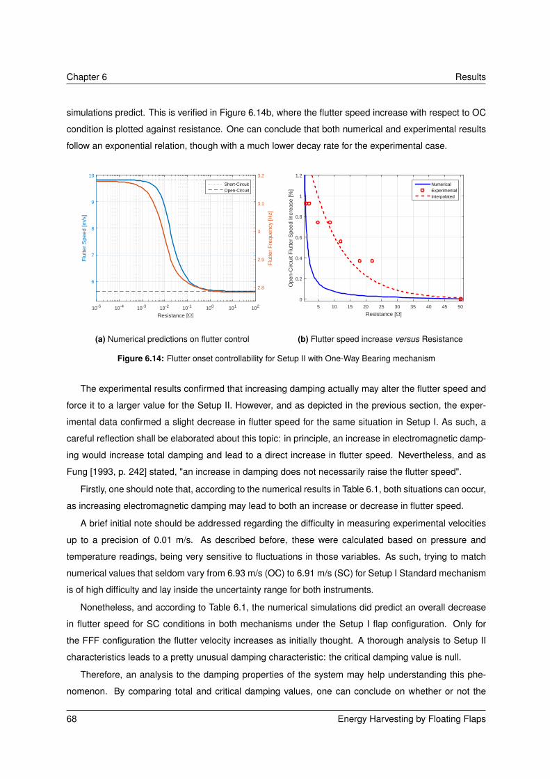
Chapter 6 Results

simulations predict. This is verified in Figure 6.14b, where the flutter speed increase with respect to OC

condition is plotted against resistance. One can conclude that both numerical and experimental results

follow an exponential relation, though with a much lower decay rate for the experimental case.

Resistance [+]10-5 10-4 10-3 10-2 10-1 100 101 102

Flu

tter

Spe

ed [m

/s]

6

7

8

9

10

Short-CircuitOpen-Circuit

Flu

tter

Fre

quen

cy [H

z]

2.8

2.9

3

3.1

3.2

(a) Numerical predictions on flutter control

Resistance [+]5 10 15 20 25 30 35 40 45 50

Ope

n-C

ircui

t Flu

tter

Spe

ed In

crea

se [%

]

0

0.2

0.4

0.6

0.8

1

1.2

NumericalExperimentalInterpolated

(b) Flutter speed increase versus Resistance

Figure 6.14: Flutter onset controllability for Setup II with One-Way Bearing mechanism

The experimental results confirmed that increasing damping actually may alter the flutter speed and

force it to a larger value for the Setup II. However, and as depicted in the previous section, the exper-

imental data confirmed a slight decrease in flutter speed for the same situation in Setup I. As such, a

careful reflection shall be elaborated about this topic: in principle, an increase in electromagnetic damp-

ing would increase total damping and lead to a direct increase in flutter speed. Nevertheless, and as

Fung [1993, p. 242] stated, "an increase in damping does not necessarily raise the flutter speed".

Firstly, one should note that, according to the numerical results in Table 6.1, both situations can occur,

as increasing electromagnetic damping may lead to both an increase or decrease in flutter speed.

A brief initial note should be addressed regarding the difficulty in measuring experimental velocities

up to a precision of 0.01 m/s. As described before, these were calculated based on pressure and

temperature readings, being very sensitive to fluctuations in those variables. As such, trying to match

numerical values that seldom vary from 6.93 m/s (OC) to 6.91 m/s (SC) for Setup I Standard mechanism

is of high difficulty and lay inside the uncertainty range for both instruments.

Nonetheless, and according to Table 6.1, the numerical simulations did predict an overall decrease

in flutter speed for SC conditions in both mechanisms under the Setup I flap configuration. Only for

the FFF configuration the flutter velocity increases as initially thought. A thorough analysis to Setup II

characteristics leads to a pretty unusual damping characteristic: the critical damping value is null.

Therefore, an analysis to the damping properties of the system may help understanding this phe-

nomenon. By comparing total and critical damping values, one can conclude on whether or not the


Results Chapter 6

system is overdamped. This conclusion may be drawn only based on the flap mode as the remaining

ones are well below their critical damping threshold.

Figure 6.15 plots the comparison for the numerically predicted total damping with respect to its critical

value for both systems analyzed before: the Setup I Standard mechanism and Setup II One-Way Bearing

mechanism. It reveals that the Setup I is below the critical damping threshold, and therefore the system

is underdamped; whereas Setup II is overdamped.

Resistance [+]0 1 2 3 4 5 6 7 8 9 10

Fla

p D

ampi

ng [N

ms/

rad]

0

0.005

0.01

0.015

0.02

0.025

0.03Total Damping Setup I StandardCritical Damping Setup I StandardTotal Damping Setup II One-WayCritical Damping Setup II One-Way

Figure 6.15: Comparison between damping characteristics for Setup I Standard mechanism and Setup II One-WayBearing mechanism

Recalling Figure 3.13 in the Feasibility Study, the same situation was identified and similar conclu-

sions were drawn: for critically damped systems, flutter speed increases with rising electromagnetic

damping; for systems below that threshold, flutter speed decreases. This is a prominent finding of this

study, confirming numerical predictions and reinforcing the FFF as a possible active flutter speed control

system by changing the resistance value.

Still about flutter speed controllability, the influence of endplates in the flutter test outcome is curiously

surprising. As one can see in Figure 6.16a, numerically and experimentally calculated flutter points with

and without endplates are plotted against resistance for the Setup I One-Way Bearing mechanism.

The numerical model according to the p-k method considers a 2D airfoil with CLα = 2π as described

by the thin airfoil theory, which conceptually corresponds to an infinite wing and experimentally to a

finite wing with long walls at the wing tip to avoid 3D effects. However, in case of wind tunnel flutter

tests, it is not possible to have the model close enough to the wall such that these undesired effects are

mitigated. Therefore, endplates are placed in order to do so. In case of insufficiently long endplates,

CLα of the wind tunnel model may drop below 2π specially at high angles of attack (pitch deflection)

which introduces some errors into the validation process. Notwithstanding, the effective length of the

endplates installed at the experimental setup is limited by the test section dimensions and the expected

pitch deflection the model would reach.


Chapter 6 Results

Likewise, the blockage ratio of 16.5 % at zero pitch angle may also pose some problems onto final

results. Such a large blockage ratio forces the flow to accelerate at the test section, leading to an artificial

increase in CLα . Moreover, and due to the dynamic nature of this phenomenon, the pitch angle would

eventually reach 10 deg, leading to an ever-increasing blockage ratio. This topic is thoroughly studied

in literature and aerodynamic correction to lift and drag coefficients may be applied to the final results.

However, as the code validation revealed that experimental results were inside the deviation range of

other similar experiments in literature, no aerodynamic data was acquired and therefore corrections to

experimental data are inapplicable.

In fact, Figure 6.16a shows that the numerical model under-predicts the experimental results. More-

over, results without endplates differ 35.6 % from numerical ones, whereas with endplates the difference

drops to 10.6 %, an acceptable value for numerical code validation. It clearly shows the influence of

placing endplates in the wind tunnel model and how it affects the flutter speed, which is somehow un-

expected given the reduced 15 mm gap that exists between the wing tip and the wall. Moreover, it is

worth noting that physical properties of the model change when endplates are removed, although that

difference would not be entirely responsible for such large deviation.

Curiously, the experimental results without endplates show the expected evolution in flutter speed

with changing resistance for underdamped systems (Setup I), whereas the results with endplates lay

on fluctuations around an approximately constant value. This can be seen in Figure 6.16b where the

model without endplates exhibits a qualitatively similar behavior to the numerically expected. Despite

that, results without endplates are merely indicative as they cannot be explained by theory used in the

numerical simulations.

Resistance [+]0 5 10 15 20 25 30 35 40

Flu

tter

Spe

ed [m

/s]

7

7.5

8

8.5

9

9.5NumericalWithout EndplatesInterpolatedWith EndplatesInterpolated

(a) Flutter speed as function of Resistance

Resistance [+]0 5 10 15 20 25 30 35 40

Sho

rt-C

ircui

t Flu

tter

Spe

ed In

crea

se [%

]

-1

-0.5

0

0.5

1

1.5

2

2.5

NumericalWithout EndplatesInterpolated (Linear)With EndplatesInterpolated

(b) Percentage increase of the respective flutter speed

Figure 6.16: Influence of endplates on flutter speed control for Setup I with One-Way Bearing mechanism


Results Chapter 6

6.3.3 Energy Harvesting

The purpose of this study is to quantify the amount of voltage and power generated by the energy

harvesting device developed for both flap configurations and mechanisms. The system oscillates at the

flutter point with constant amplitude over a period of 80 seconds across which is performed a RMS eval-

uation to the voltage signal positive stroke, following the procedure used in the Vibration Tests (Section

6.2.3). Accordingly, SC and OC resistance values respectively correspond to 0.2 Ω and 100 Ω.

For the Setup I flap configuration, Figure 6.17 shows that the One-Way Bearing mechanism pro-

duces less 16.9 % voltage than the Standard one for the same OC condition, and around 35.0 % less

power for the peak resistance. One important note that should be addressed in this Setup I is that no

mechanism induces flap deflections large enough to hit the structural limiters. This will turn out as a

detail of maximum importance.

Resistance [+]0 10 20 30 40 50 60 70 80 90 100

Vol

tage

[V]

0

0.01

0.02

0.03

0.04

0.05

0.06

0.07



Resistance [+]0 10 20 30 40 50 60 70 80 90 100

Pow

er [m

W]

0

0.05

0.1

0.15



Figure 6.17: Energy Harvested at the flutter point for Setup I

Regarding the Setup II, the FFF exhibits a completely different behavior, this time aligned with the

results from forced harmonic excitations. Figure 6.18 shows that the One-Way Bearing mechanism

produces 33.9 % more voltage and around 45.0 % more power than the Standard one. Moreover, note

that the theory presented in Chapter 3 that modeled the energy harvesting circuit as a voltage divider

according to Equation A.20 is confirmed by the aforementioned plots. On the other hand, and unlike the

previous example, in this flap configuration both mechanisms lead their flaps to hit the limiters.

A deep reflection shall be elaborated on the results obtained, specially because the Setup I provides

the opposite of initially predicted once the Standard mechanism is actually more efficient in terms of

energy harvesting. This is intrinsically related with the reduced scale of the model, something already

thoroughly explained in Section 6.2.3 when analyzing the shaker tests results.

Overall, as the model scale is reduced, friction starts playing an increasingly important role in the


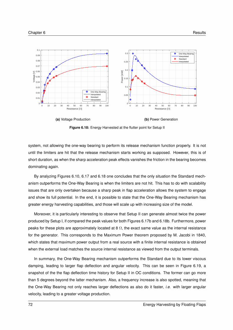
Chapter 6 Results

Resistance [+]0 10 20 30 40 50 60 70 80 90 100

Vol

tage

[V]

0

0.01

0.02

0.03

0.04

0.05

0.06

0.07

0.08

0.09

0.1



Resistance [+]0 10 20 30 40 50 60 70 80 90 100

Pow

er [m

W]

0

0.05

0.1

0.15

0.2

0.25

0.3 One-Way BearingInterpolatedStandardInterpolated


Figure 6.18: Energy Harvested at the flutter point for Setup II

system, not allowing the one-way bearing to perform its release mechanism function properly. It is not

until the limiters are hit that the release mechanism starts working as supposed. However, this is of

short duration, as when the sharp acceleration peak effects vanishes the friction in the bearing becomes

dominating again.

By analyzing Figures 6.10, 6.17 and 6.18 one concludes that the only situation the Standard mech-

anism outperforms the One-Way Bearing is when the limiters are not hit. This has to do with scalability

issues that are only overtaken because a sharp peak in flap acceleration allows the system to engage

and show its full potential. In the end, it is possible to state that the One-Way Bearing mechanism has

greater energy harvesting capabilities, and those will scale up with increasing size of the model.

Moreover, it is particularly interesting to observe that Setup II can generate almost twice the power

produced by Setup I, if compared the peak values for both Figures 6.17b and 6.18b. Furthermore, power

peaks for these plots are approximately located at 8 Ω, the exact same value as the internal resistance

for the generator. This corresponds to the Maximum Power theorem proposed by M. Jacobi in 1840,

which states that maximum power output from a real source with a finite internal resistance is obtained

when the external load matches the source internal resistance as viewed from the output terminals.

In summary, the One-Way Bearing mechanism outperforms the Standard due to its lower viscous

damping, leading to larger flap deflection and angular velocity. This can be seen in Figure 6.19, a

snapshot of the the flap deflection time history for Setup II in OC conditions. The former can go more

than 5 degrees beyond the latter mechanism. Also, a frequency increase is also spotted, meaning that

the One-Way Bearing not only reaches larger deflections as also do it faster, i.e. with larger angular

velocity, leading to a greater voltage production.


Results Chapter 6

Time [s]0 0.2 0.4 0.6 0.8 1 1.2

Fla

p D

efle

ctio

n [D

eg]

-30

-20

-10

0

10

20

30

40Standard MechanismOne-Way Bearing MechanismExperimental Data

Figure 6.19: One-Way Bearing mechanism experimental effect on Voltage Production

6.4 Concept Applicability

In this final section, one shall reflect about the concept developed and its applicability to real-world

solutions. The investigation carried out in this dissertation is a follow-up research of the one developed

by Bernhammer [2015] in his doctoral proposal about an autonomous flap for offshore wind turbines.

In that document, this concept was proposed and verified to be self-sustainable. One shall wonder

about the need of a smart structure to be energetically independent of a wind turbine, which ultimately

produces several orders of magnitude more energy than the system here presented. The reason lies

in the fact that an autonomous flap is designed to be a plug-and-play device, facilitating maintenance

carried out in remote areas by simply removing the damaged flap and introducing a new one with no

further electrical connections. Nonetheless, as this solution was previously presented and verified, and

in this dissertation project optimized, adapting such promising mechanism to other platforms urges.

The obvious candidate is the aeronautical industry, though its advantages have to be more focused

on the energy harvesting benefits, in detriment of the autonomous system capabilities. Nevertheless,

not all aircraft are suitable for this solution: heavy airframes propelled by powerful engines do not ac-

tually need such energy harvesting system as they are able to generate their own electricity by using

powerful engines. However, for low-power UAV that rely on small propeller-driven combustion engines

for power, this could be an interesting solution. One should study the independent application of the

energy harvesting mechanism as an alternative power source for the airframe, whether it would be to

generate a hybrid solution for the propulsion system or to complement an all-electric solar-powered UAV.

Note that performance issues were not a problem in wind turbines as they were fixed. However in air-

craft applications, performance studies have to be carried out to verify whether this is a solution that

increases aircraft performance.

Therefore, as a final remark of this study and with the proven feasibility and performance of the


Chapter 6 Results

One-Way Bearing mechanism alongside the validation of both codes, one can run a final simulation to

emulate the energy harvesting output of introducing a gearbox with a ratio of 25:1 in the system, as

performed in the Feasibility Study. Hence, a time-simulation is run with the same input harmonic force

as in the vibration tests, and it turned out that the mechanism is able to generate 4.1 V and produce 2.1

W of energy at an external load of 8 Ω, as depicted on Figure 6.20.

Time [s]0 10 20 30 40 50 60 70 80 90 100

Vol

tage

[V]

0

1

2

3

4

Pow

er [W

]

0

0.5

1

1.5

2

2.5

Effective VoltageEffective Power

Figure 6.20: Numerical Simulation on One-Way Bearing mechanism with GR of 25

To simulate an aircraft application, the mechanism should be considered to engage in non-critical

flight stages as loiter, which will last for 45 min in this case study. Hence, the energy produced by the

generator sums up to 1.58 Wh, which shall be stored in a battery. Given its high energy density for

lightweight applications, a LiPo battery is the logic candidate for the task. Considering a standard off-

the-shelf 3.7 V battery1 for drone applications able to withstand 1.85 Wh and weighing (Mb) 13.8 g, its

specific energyEb is of 114.5 Wh/kg. This means that, together with the generator, the energy harvesting

system weighs the total of 143 g, consisting of 0.3972 kg/m (span), meaning a 11.6 % mass increment

in the wind tunnel model when compared with one without an energy harvesting mechanism. In terms of

aerodynamic efficiency, the FFF solution presents a CL loss in the order of 2 % for low-amplitude LCO

as stated by Bernhammer et al. [2017a] when compared with a fixed flap.

Despite the weight penalty, one should evaluate whether it is worth in terms of performance increase.

In this case, that would be measured as the mass of fuel not burnt due to having harvested electrical

energy. Considering that propeller-driven UAV are seldom powered by aviation gasoline2 with specific

energy Ef of 13777.8 Wh/kg, one can estimate the mass of fuel Mf according:

Mf = MbEbEf

(6.3)

1Venom 30C 1S 500mAh 3.7V LiPo battery data: https://www.venompower.com/collections/venom-drone-batteries/products/venom-30c-1s-500mah-3-7v-lipo-micro-drone-battery-with-jst-plug

2Aviation gasoline data: https://web.archive.org/web/20100825042309/http://www.ior.com.au:80/ecflist.html


https://www.venompower.com/collections/venom-drone-batteries/products/venom-30c-1s-500mah-3-7v-lipo-micro-drone-battery-with-jst-plug

https://www.venompower.com/collections/venom-drone-batteries/products/venom-30c-1s-500mah-3-7v-lipo-micro-drone-battery-with-jst-plug

https://web.archive.org/web/20100825042309/http://www.ior.com.au:80/ecflist.html

Results Chapter 6

Thereby, the mass of saved fuel is of 0.115 g for the experimental model. This means that an airframe

with the same wing as tested at the wind tunnel would produce energy equivalent to the fuel burnt

mass aforementioned. Naturally, this value would have to be refined in order to account for the engine

efficiency and the drag penalty of the mechanism. Nevertheless, in the case of increasing the gear ratio

even more, the results may be promising.

Energy harvesting is not only advised for light aircraft. Its feasibility may be easily studied according

the proceeding aforementioned. The mechanism may either be placed in the ailerons, meaning that

they would operate either as a control surface and energy harvesting device; or slightly more inboard,

such that FFF have no other function than just harvesting energy. A good testbed for such solution is

the EU-coordinated NOVEMOR project3, where the wing mass is of 3500 kg, the empty mass of the

airframe M0 is 34340 kg and the maximum takeoff mass MTOW is of 59527 kg. It cruises at 2000 ft

with velocity of Mach 0.3, and the loiter phase is dimensioned to endure for 45 minutes, the same as

previously considered for the wind tunnel model. By placing FFF approximately at the break point such

that they are not affected by the engine nor ailerons placement, one can calculate the room available

to fit a generator at the flap hinge. Considering it to be at 75 % of the chord, that yields to a maximum

generator diameter of 21.5 cm. Then, by choosing a compliant generator and gearbox, and inserting

all the structural parameters in the simulations developed, the performance of such solution may be

assessed. Alternatively, by extrapolating the proportions obtained for the wing tunnel model, the energy

harvesting system mass is estimated to be around 406 kg, leading to 1.2 % increase in M0 and forcing a

0.7 % increase in MTOW to accommodate the heavier mechanism. However, the remaining structural

properties of such wings are difficult to determine and even harder to find publicly available, and as such

it was not possible to draw further conclusions about its feasibility. Nonetheless, if the weight ratio keeps

approximately constant with size scalability, the numerical simulation here presented has revealed a

large potential for future applications.

In the end, some concerns on the feasibility of such solutions may also be pointed out. First and

foremost, it might be too detrimental for the overall drag balance of the airplane if the flap is oscillating.

As increased drag demands for more power to fly at the same speed, a careful energy balance would

have to be carried out to assess the value of this mechanism. Moreover, certification issues would

certainly arise for having flutter so close to or even in the flight envelope. Such drawbacks are not so

critical in HAWT applications. Atmospheric conditions often present with a surplus of energy in the wind

that cannot be extracted by the rotor, which could then be used to harvest energy with these devices.

Also, certification is less of an issue.

3Project NOVEMOR: http://cordis.europa.eu/project/rcn/99991_en.html


http://cordis.europa.eu/project/rcn/99991_en.html

7 | Conclusion

Smart solutions with increasing level of system integration have been one of the recent hot subjects

in aeronautical industry. Performing SHM duties in stand-alone systems is crucial for the sustainable

development of autonomous entities. To do so, several load alleviation concepts able to self-sustain its

activity by using energy harvesting techniques have been developed so far. By exploiting self-induced

aeroelastic instabilities and deliberately put the wing in such situations, it is possible to generate energy

due to violent rotation of floating flaps.

During this research, an enhanced energy harvesting concept was developed, testing the energy

harvesting performance, the controllability of flutter speed, and expanding the solution to a broader

aeronautical scope. It was achieved while keeping experimental costs within budget by a large margin.

The main findings are presented next. Also, recommendations for future work are provided.

7.1 Achievements

This research has proved the usability of 3D-printed models in vibration and wind tunnel tests, in

one of the first-ever flutter experiments using such manufacturing technique. Also, the numerical models

developed were proved to be accurate in predicting the non-linear behavior of the system. It was exper-

imentally verified that the prediction made by Bernhammer et al. [2017a], where it was stated that flutter

speed for FFF is controllable by changing the generator external resistance, can actually occur. The

results obtained show a prominent trend: for overdamped systems, such as the FFF concepts, reducing

resistance increases the flutter speed; for the remaining, the same effect on flutter speed is achieved

by increasing resistance. As such, it is clearly shown that one can control the flutter boundary by either

adjusting the external resistance, or changing the flap torsional stiffness which rules the critical damping.

Moreover, and still with respect to the aforementioned paper, it was also realized that the negative

influence of a gearbox placed in the flap shaft to increase the energy produced can be of major im-

portance. As such, a disruptive release mechanism that mimics the ones of bicycles was developed to

allow for shaft free-spinning and reduce the inertial effects of the gearbox. A time-domain simulation was

carried out in order to include electromagnetic damping and friction according to an exponential decay


Conclusion Chapter 7

rule during the free-spinning phase. A feasibility study showed the potential of such solution.

The developed mechanism showed a 40 % reduction in viscous damping when compared to a stan-

dard reciprocating shaft with no release mechanism. This was demonstrated by the flap degree of

freedom excitation, and the results were verified by the 3DOF impulse test where the referred One-Way

Bearing mechanism evidenced less damping and larger linear and angular displacements.

This reduced damping leads to a mechanism with increased performance. Even without any gearbox,

vibration tests to the torsionally stiffened flap led to maximum values of 0.115 V and 0.4 mW produced

by the new mechanism, a 20.5 % and 25 % increase with respect to the standard one. With the code

verified, these results may be extrapolated for the presence of a gearbox.

About the wind tunnel tests, the results without any gearbox are in the order of 0.095 V and 0.3 mW

produced at the flutter onset for the FFF setup. This poses an increase of 33.9 % and 45 % relative to

the standard mechanism. It was also proven that FFF produce more energy than the torsionally stiffened

flaps, meaning that it is the optimal solution for energy harvesting.

Also, it was noted that endplates have great influence in flutter speed determination at the wind

tunnel. Without endplates, the flutter speed was 36.5 % less than the numerical value, whereas with

endplates the value dropped to 10.6 %. This is an interesting feature considering that the distance

between the wing tip and the test section wall is only 15 mm.

The aforementioned benefits come with a weight penalty: the One-Way Bearing mechanism weighs

25.7 g whereas the Standard mechanism weighs 16.1 g. This means a marginal weight increase of

0.07667 kg/m (span), or a relative increase of 0.6 % with respect to the total wind tunnel model mass.

As to an overall overview of the energy harvesting mechanism when compared with a conventional

flap mechanism for aircraft applications, numerical simulations have shown that the same system with

a Gear Ratio of 25 would be able to generate 4.1 V and produce 2.1 W. The estimated weight penalty

of the energy harvesting system is 0.3972 kg/m, meaning an 11.6 % mass increment in the wind tunnel

model when compared with one without an energy harvesting mechanism. Based on a simple analysis,

the energy harvested for a standard aircraft mission of loiter worths 0.115 g of saved fuel.

In the end, one can conclude that the new mechanism shows increased performance in the energy

harvested when compared with older solutions. Flutter speed controllability is proven and experimen-

tal tests have evaluated both FFF and non-FFF configurations. Potential applications in aeronautical

industry are unveiled.

7.2 Recommendations

During this project, typical challenges linked to both numerical and experimental tests were faced.

Despite having had autonomy in decisions, the development, production and testing of such an exper-

imental model had several inputs from more than one person. As such, it was of crucial importance to


Chapter 7 Conclusion

understand the reasoning made by other researchers, professors and technicians in order to fully exploit

their experienced pieces of advice. A lot of creative thinking and ingenuity was necessary to over-

come conceptual and experimental issues, alongside self-organization to be on schedule. Furthermore,

knowledge about different areas of expertise was required, from programming to 3D modeling, passing

by electronics and additive manufacturing, ending up in data acquisition and wind tunnel testing. These

posed a tremendous challenge where lessons were learned everyday. The accurate management of the

available time slots, budget and resources was critical for the successful experimental test campaign.

However, even in such situations, there are imperfections that should be recognized and addressed as

recommendations for future developments.

3D Printing

With respect to the 3D printing procedure and the Formlabs® Form2 usage at Delft University of

Technology, the following points may be of interest in future manufacturing of wind tunnel models:

• The 3D printer is very precise. In the case of bearing fitting, the hole diameter was only 0.1 mm

larger than the bearing, allowing for a very precise fit.

• Print diagonally if possible, because that would give the most evenly distributed resin solidification

outcome per layer and surface finishing. However, that was not always possible in this study, either

by the model being too large chordwise to fit in the inner diagonal of the cubic printing bay, or due to

the fact of such orientation would fix supporting points on the airfoil skin, spoiling its aerodynamics.

• Printing vertically brings some drawbacks. The main wing consists in a 2 mm skin blended with

ribs of several depths. The outcome revealed a seamless surface, though slightly thicker at the ribs

place. Considering the way each part is printed, from top to bottom, it may well have happened

that a heavier and recently printed rib had pulled down a not completely solidified portion of the

upcoming thinner skin, shrinking the skin before the rib.

• Poor finishing in vertically printed parts. Precisely at the points where the supports connect to the

model, the resin seems to be unable to completely solidify, creating a blurred and bumpy surface.

• Thermoplastic properties of the resin. It is expected to have brittle behavior according to its specifi-

cation, which is also verified experimentally. Nonetheless, if heated up, it is possible to completely

fold the material. To verify this, an experiment was carried where a 2 mm thick plate was heated

and successfully folded in 90 degrees. When the part cools down, it recovers its brittle behavior.

This means that, in case of a shell-like unsupported structure start to deviate from its initial angle,

one could simply correct it by heating and place it in the right spot.

• Screws, taps and nuts. Directly printing a tap in the model may well be tempting but tolerance

issues may arise. Moreover, fatigue due to plastic-metallic interaction would turn that solution

undesirable for frequently disassembled parts carrying loads . As such, the solution found was


Conclusion Chapter 7

using a metallic nut as tap and fix it in place with tight pockets previously printed in the model.

• Curved surfaces render and printing: CATIA® .stl file generator bases the curve rendering into a

triangulation method. By default, the precision is not set to its maximum to increase rendering

speed. In order to obtain satisfying results in printing, this setting must be adjusted in the settings

menu so that the output file would represent the true surface curvature.

Vibration Tests

Concerning this type of testing, the following remarks may be addressed:

• The variable-amplitude excitation force. Heave degree of freedom is excited with a voltage har-

monic function, which by its own does not imply that the input force has constant peak-to-peak

magnitude. Indeed, and as referred in the previous chapter, the load is not constant in amplitude.

This is due to the elastic behavior of the system, dynamically counteracting the input force.

• The asymmetric excitation point. The system is excited at the top part of the central shaft of

a vertically-placed aeroelastic model, which forces the structure to behave as a cantilever beam,

meaning that the bottom goes into considerably larger tip displacements. This could only be solved

with excitation at mid-span or with two synchronized shakers at the top and bottom shaft tips.

• Supporting structure: the test section is placed on a heavy table and grounded by a ratchet strap.

Likewise, extruded profiles connected to the table are used to elevate the shaker and elastic straps

are also used to fix it. Tension on those straps must be kept high in order to avoid vibration of the

supporting structure. Overall, the structure was too compliant, although it was the best solution

in such an improvised setup. A good solution for future work may pass by suspending the shaker

from a set of tensioned bungee chords, such that it can sort of float in the air.

• The heave displacement sensor considerably increases damping in the system, whereas the other

sensors do not.

• Flap shaft misalignment due to tensioned springs. The flap shaft undergoes a bending force due

to the pulley located at its top tip and tensioned springs on it. This causes misalignment of the

axle and may lead the flap to sporadicly touch the wing structure during oscillation. This can be

solved by either placing another pulley at the bottom to balance the bending force, which was not

possible because only one type of each pulley was available; or by placing the hinges closer to the

flap tips, reducing the moment arm of the bending moment.

Wind Tunnel Tests

With respect to wind tunnel testing, some remarks are addressed hereafter:

• Velocity measurement precision. The velocity magnitude is calculated based on measurements

of dynamic pressure and temperature. However, those have little precision as described during


Chapter 7 Conclusion

the test campaign. Moreover, velocity is controlled by changing the engine RPM, consisting in an

incremental increase of velocity instead of a continuous one. Also, the flutter point extends through

a certain range of velocities before going unbounded. These factors contribute to decrease the

flutter velocity precision. A more integrated measurement system would be highly recommended.

• Internal resistance of the generator. With no external resistance, the generator exhibits an internal

resistance of 8 Ω with the shaft stopped. Within a PM DC motor, this internal resistance may

even change due to resistance in the brushes and according shaft rotational velocity, spoiling the

attempt of controlling flutter speed by changing the external resistance. This, in parallel with the

external load, made the equivalent resistance to vary only between 0 Ω and 8 Ω, narrowing the

resistance range for flutter speed control. In future experiments, reducing this internal resistance

shall be of critical importance. Applying a brushless motor may be a solution.

7.3 Future Work

As to application of autonomous flaps to wind turbines, the energy harvesting mechanism developed

poses a major breakthrough in the power production, leading to an even higher ratio between the power

generated and consumed by actuators and sensors. Therefore, further steps shall be taken towards

the implementation of this solution in ever-growing experimental models such that its applicability in real

scale is undoubtedly proven in wind turbines.

As per applications to aircraft, Section 6.4 consists in a road map into future performance studies of

energy harvesting mechanisms. With promising results extrapolated from numerical simulations, these

are yet to be confirmed with data from real size wing models. As stated before, the NOVEMOR project

could be the perfect testbed for this technology, as it seeks for novel aircraft vehicle configurations, from

fluttering wings to morphing flight. For future work, it would be straightforward to evaluate an energy

harvesting mechanism in these regards, as one would only need the inertial, damping and stiffness

properties of the wing to run the simulations developed in this project. However, the drag penalty of such

flapping body may reveal as too detrimental for this solution to be developed.

Further suggestions may also conduct to motor sport industry. As broadly known, endurance and

formula prototypes already apply energy recovering systems in their models. One of the milestones in

these regards is the Porsche 919 endurance prototype which combines two energy harvesting systems:

one to produce electricity while braking, and another to do so by exploiting combustion hot gases. Adding

FFF to non-critical aerodynamic appendices as the rear diffuser may be an area of interest.

One last frontier may be the space industry, with suggestions for application in the field of exploiting

fin flutter during rocket launching. As one may see, the applicability of this ingenious solution broads

several fields of knowledge. The key lies on proving its feasibility.


Bibliography

A. Abdelkefi. Aeroelastic energy harvesting: A review. International Journal of Engineering Science,

100:112–135, 2016.

A. Abdelkefi, M. Hajj, and A. Nayfeh. Piezoelectric energy harvesting from transverse galloping of bluff

bodies. Smart Materials and Structures, 22(1):015014, 2012.

A. Abdelkefi, A. Hasanyan, J. Montgomery, D. Hall, and M. Hajj. Incident flow effects on the performance

of piezoelectric energy harvesters from galloping vibrations. Theoretical and Applied Mechanics Let-

ters, 4(2):022002, 2014.

J. Allen and A. Smits. Energy harvesting eel. Journal of Fluids and Structures, 15(3):629 – 640, 2001.

A. Barrero-Gil, G. Alonso, and A. Sanz-Andres. Energy harvesting from transverse galloping. Journal of

Sound and Vibration, 329(14):2873–2883, 2010.

A. Barrero-Gil, S. Pindado, and S. Avila. Extracting energy from vortex-induced vibrations: a parametric

study. Applied mathematical modelling, 36(7):3153–3160, 2012.

S. Beeby, M. Tudor, and N. White. Energy harvesting vibration sources for microsystems applications.

Measurement science and technology, 17(12):R175, 2006.

L. Bernhammer. Smart Wind Turbine: analysis and autonomous flap. PhD thesis, TU Delft, Delft

University of Technology, 2015.

L. Bernhammer, R. Breuker, M. Karpel, and G. Veen. Aeroelastic control using distributed floating flaps

activated by piezoelectric tabs. Journal of Aircraft, 50(3):732–740, 2013.

L. Bernhammer, R. Breuker, and M. Karpel. Energy harvesting for actuators and sensors using free-

floating flaps. Journal of Intelligent Material Systems and Structures, 28(2):163–177, 2017a.

L. Bernhammer, S. Navalkar, J. Sodja, R. Breuker, and M. Karpel. Experimental and numerical investi-

gation of an autonomous flap for load alleviation. Journal of Aircraft, pages 1–12, 2017b.


Bibliography

M. Bernitsas, K. Raghavan, Y. Ben-Simon, and E. Garcia. Vivace (vortex induced vibration aquatic

clean energy): A new concept in generation of clean and renewable energy from fluid flow. Journal of

offshore mechanics and Arctic engineering, 130(4):041101, 2008.

R. Bisplinghoff, H. Ashley, and R. Halfman. Aeroelasticity. Addison-Wesley series in mechanics. Cam-

bridge, Mass., 1955.

M. Conner, D. Tang, E. Dowell, and L. Virgin. Nonlinear behavior of a typical airfoil section with control

surface freeplay: A numerical and experimental study. Journal of Fluids and Structures, 11(1):89 –

109, 1997.

E. Crawley and J. Luis. Use of piezoelectric actuators as elements of intelligent structures. AIAA journal,

25(10):1373–1385, 1987.

D. Day and T. Walsh. Quadratic eigenvalue problems. Sandia National Laboratories, 2007.

J. Edwards. Unsteady aerodynamic modeling and active aeroelastic control. PhD thesis, Stanford

University, 1977.

M. El-Hami, P. Glynne-Jones, N.M White, M. Hill, S. Beeby, E. James, A. Brown, and J. Ross. Design

and fabrication of a new vibration-based electromechanical power generator. Sensors and Actuators

A: Physical, 92(1):335–342, 2001.

A. Erturk and D. Inman. An experimentally validated bimorph cantilever model for piezoelectric energy

harvesting from base excitations. Smart materials and structures, 18(2):025009, 2009.

M. Faraday. Experimental researches in electricity. Philosophical Transactions of the Royal Society of

London, 122:125–162, 1832.

Y. Fung. An introduction to the theory of aeroelasticity. Dover Publications, Inc., 1993.

B. Gjerek, R. Drazumeric, and F. Kosel. A novel experimental setup for multiparameter aeroelastic wind

tunnel tests. Experimental Techniques, 38(6):30–43, 2014.

O. Goushcha, H. Akaydin, N. Elvin, and Y. Andreopoulos. Energy harvesting prospects in turbulent

boundary layers by using piezoelectric transduction. Journal of Fluids and Structures, 54:823–847,

2015.

S. Guo, D. Monteros, J. Espinosa, and Y. Liu. Gust alleviation of a large aircraft with a passive twist

wingtip. Aerospace, 2(2):135–154, 2015.

J. Hartog. Mechanical Vibrations. Civil, Mechanical and Other Engineering Series. Dover Publications,

1985. ISBN 9780486647852.


Bibliography

H. Hassig. An approximate true damping solution of the flutter equation by determinant iteration. Journal

of Aircraft, 8(11):885–889, 1971.

S. Heinze and M. Karpel. Analysis and wind tunnel testing of a piezoelectric tab for aeroelastic control

applications. Journal of aircraft, 43(6):1799–1804, 2006.

D. Hodges and G. Pierce. Introduction to Structural Dynamics and Aeroelasticity. Cambridge Aerospace

Series. Cambridge University Press, 2011. ISBN 9781139499927.

R. Jones. Operational treatment of the nonuniform-lift theory in airplane dynamics. 1938.

J. Jonge and A. Nederveen. Effect of gust load alleviation on fatigue and crack growth in alclad 2024-t3.

In Effect of Load Spectrum Variables on Fatigue Crack Initiation and Propagation. ASTM International,

1980.

H. Jung and S. Lee. The experimental validation of a new energy harvesting system based on the wake

galloping phenomenon. Smart Materials and Structures, 20(5):055022, 2011.

M. Karpel. Time-domain aeroservoelastic modeling using weighted unsteady aerodynamic forces. Jour-

nal of Guidance, Control and Dynamics, 13(1), 1990.

M. Karpel. Reduced-order models for integrated aeroservoelastic optimization. Journal of Aircraft, 36

(1), 1999.

M. Le, J. Capsal, M. Lallart, Y. Hebrard, A. Ham, N. Reffe, L. Geynet, and P. Cottinet. Review on

energy harvesting for structural health monitoring in aeronautical applications. Progress in Aerospace

Sciences, 79:147–157, 2015.

D. Li, Y. Wu, A. Ronch, and J. Xiang. Energy harvesting by means of flow-induced vibrations on

aerospace vehicles. Progress in Aerospace Sciences, 86:28–62, 2016.

C. Mathis, M. Provansal, and L. Boyer. The bénard-von kármán instability: an experimental study near

the threshold. Journal de Physique Lettres, 45(10):483–491, 1984.

J. Maxwell. On physical lines of force. A dynamical theory of the electromagnetic field, pages 1875–89,

1865.

P. Meliga, J. Chomaz, and F. Gallaire. Extracting energy from a flow: An asymptotic approach using

vortex-induced vibrations and feedback control. Journal of Fluids and Structures, 27(5):861–874,

2011.

S. Navalkar, L. Bernhammer, J. Sodja, E. Solingen, G. Kuik, and J. Wingerden. Wind tunnel tests with

combined pitch and free-floating flap control: data-driven iterative feedforward controller tuning. Wind

Energy Science, 1(2):205, 2016.


Bibliography

A. Nayfeh and D. Mook. Nonlinear Oscillations. Wiley Classics Library. Wiley, 2008. ISBN

9783527617593.

B. Ng, R. Palacios, and J. Graham. Model-based aeroelastic analysis and blade load alleviation of

offshore wind turbines. International Journal of Control, pages 1–22, 2015.

B. Ng, R. Palacios, E. Kerrigan, J. Graham, and H. Hesse. Aerodynamic load control in horizontal

axis wind turbines with combined aeroelastic tailoring and trailing-edge flaps. Wind Energy, 19(2):

243–263, 2016.

M. Patil, D. Hodges, and C. Cesnik. Limit-cycle oscillations in high-aspect-ratio wings. Journal of fluids

and structures, 15(1):107–132, 2001.

B. Payne. Designing a load allevitation system for a modern civil aircraft. In ICAS Proceedings, 1986:

15th Congress of the International Council of the Aeronautical Sciences, 7-12 September 1986, Lon-

don, UK, volume 1, page 283. AIAA, 1986.

S. Perron and M. Drela. Passive gust load alleviation through bend-twist coupling of composite beams

on typical commercial airplane wings. In 54th AIAA/ASME/ASCE/AHS/ASC Structures, Structural

Dynamics, and Materials Conference, page 1490, 2013.

D. Peters, S. Karunamoorthy, and W. Cao. Finite state induced flow models part i: Two-dimensional thin

airfoil. Journal of Aircraft, 32(2):313–322, 1995.

G. Rocklin, J. Crowley, and H. Vold. A comparison of h1, h2, and hv frequency response functions. In

Proceedings of the 3rd international Modal Analysis Conference, volume 1, pages 272–278, 1985.

V. Schmidt. Piezoelectric energy conversion in windmills. In IEEE 1992 Ultrasonics Symposium Pro-

ceedings, pages 897–904 vol.2, 1992.

T. Silva and C. Marqui. Passive and hybrid piezoelectric circuits to reduce induced-atmospheric turbu-

lence vibration of a plate-like wing, 2013.

T. Theodorsen. General theory of aerodynamic instability and the mechanism of flutter. NACA Report

496, pages 413–433, 1934.

J. Thomas, M. Qidwai, and J. Kellogg. Energy scavenging for small-scale unmanned systems. Journal

of Power sources, 159(2):1494–1509, 2006.

C. Wei and X.F Jing. A comprehensive review on vibration energy harvesting: Modelling and realization.

Renewable and Sustainable Energy Reviews, 74:1–18, 2017.


A | Numerical Model

This appendix presents the complete deduction of the numerical model used to describe the physical

reality of the problem, for both frequency- and time-domain simulations developed.

A.1 System Modeling

As suggested by Theodorsen [1934] in his first famous report on aeroelastic flutter which notation

is adopted in this section, a cantilever three-dimensional high aspect ratio wing may be represented

by its geometric and inertial properties at the three-quarter point of the wing-to-tip distance for flutter

calculation purposes. This holds true for large-span non-swept wings in which its properties are kept

approximately constant spanwise. Moreover, the control surface is assumed to be rigid throughout the

chord and the elastic axis located precisely at the hinge axis of rotation.

For aeroelastic considerations, the representation of the wing may be considered as a classical

spring-damper system, having these properties associated to each degree of freedom. As depicted in

Figure 3.1, one can see that this model is decomposed in 3 motions, namely:

• h: heave, plunge or bending motion, with origin at the elastic axis, or shear center, and defined

positive for a downward vertical movement;

• α: pitch or torsional motion, with origin at the same point, the shear center, and defined positive

for clockwise torsion;

• β: control surface, aileron, rudder or flap motion, with origin at the control surface hinge line and

defined positive for clockwise rotation.

Geometrical properties of the model are also defined in Figure 3.1. The location of the elastic axis

with respect to the mid-chord point is defined as a. The center of gravity of the whole wing is located at

a distance of xα from the elastic axis, whereas the center of gravity of solely the control surface sits at a

distance xβ from its hinge line, which for instance is at a distance c from the half-chord. It is also worth

noting that all the aforementioned quantities are dimensionless variables having the half-chord value b

as a reference, and positive when measured towards the trailing edge. Moreover, damping and stiffness

properties of each degree of freedom are represented by C and K, respectively.


Appendix A

A.2 Equations of Motion

According the notation previously described, the generalized equation of motion for a standard

spring-damper system with n degrees of freedom is given by:

[M]ξ+ [C]ξ+ [K]ξ = Q (A.1)

ξ =h α β

T(A.2)

where [M] is the generalized inertia matrix, [C] the damping one, [K] the stiffness matrix and Q the

vector for the generalized applied forces. Note that these are n× n matrices, and ξ the state vector.

Applying equation A.2 to the 3DOF model, one can reach the fully defined system of equations of

motion for each independent variable:

mh+ Sαα+ Sβ β + Chh+Khh = L

Sαh+ Iαα+[Iβ + (c− a)bSβ

]β + Cαα+Kαα = Mα

Sβh+[Iβ + (c− a)bSβ

]α+ Iβ β + Cβ β +Kββ = Mβ

(A.3)

A.2.1 Inertia Terms

The inertia terms play the role of coupling the system. By inspection of equations A.2 and A.3, one

can notice that:

[M] =

m Sα Sβ

Sα Iα Iβ + (c− a)bSβ

Sβ Iβ + (c− a)bSβ Iβ

(A.4)

where m is the wing-flap mass, Sα and Sβ the static moments of the whole wing-flap or flap around the

the axis a or c respectively, and Iα and Iβ the moments of inertia around the latter axis; all the variables

mentioned are per unit of span length. Moreover, the following non-dimensional relations may be drawn

considering that ρ∞ is the air density at reference altitude.

µ =m

πρ∞b2(A.5)

xα =Sαmb

, xβ =Sβmb

(A.6)

r2α =

Iαmb2

, r2β =

Iβmb2

(A.7)

A.2.2 Damping Terms

These would be the terms responsible for attenuating the oscillating movement. In fact, there are

several damping models applicable to this problem, as the viscous and structural ones. The former is


Appendix A

incorporated into the matrix [C] as part of the damping forces and thus in phase with the velocity state

vector ξ, being the one chosen for this application. With respect to the latter, it relates with the damping

done by the structure itself, being associated with the matrix [K] in phase opposition with the displace-

ment state vector ξ. Furthermore, this system also has to deal with the electromagnetic damping due

to the generator placed at the flap hinge. As such, the damping matrix has two contributions, and by

inspection of equations A.2 and A.3, it follows that:

[C] = [Cvisc] + [Cel] =

Ch 0 0

0 Cα 0

0 0 Cβ

(A.8)

Furthermore, it is worth noting that the following non-dimensional relations may be defined consider-

ing that ωα is the uncoupled natural frequency of the pitch mode.

Γh =Chmωα

(A.9)

Γα =Cα

mb2ωα, Γβ =

Cβmb2ωα

(A.10)

Viscous Damping

The viscous model terms playing a role in the oscillatory behavior attenuation of the system are

here described. Despite some authors consider this as a negligible feature once it allows to keep the

modeling conservative, others have developed a methodology to simulate the phenomenon. That is the

case of Edwards [1977], which suggests a damping model proportional and in phase with the oscillation

velocity:

[Cvisc] =

2mωhζh 0 0

0 2Iαωαζα 0

0 0 2Iβωβζβ

(A.11)

where ω is the uncoupled natural frequency and ζ the damping coefficient for each mode. This is the

model applied to the problem once it establishes a relation with the velocity state vector ξ, producing

a higher fidelity simulation.

Structural Damping

As suggested by Fung [1993], adding additional terms to the stiffness matrix [K] is equivalent to

consider [Cst] in the first order derivative. This holds true for simple harmonic motions where the complex

eigenvalues v present a negligible damping ratio γ when compared with its frequency ω. As such, this

approximation can be shown as follows:


Appendix A

[Cst]ξ+ [K]ξ =(v[Cst] + [K]

)ξ =

((γ + iω)[Cst] + [K]

)ξ

γω≈

([K] + iω[Cst]

)ξ '

Kh(1 + 2iζh) 0 0

0 Kα(1 + 2iζα) 0

0 0 Kβ(1 + 2iζβ)

ξ (A.12)

This model creates a damping pattern associated with the displacement state vector and in phase

opposition to it due to the imaginary component. Nonetheless, this model is only presented to establish

a comparison with the viscous one. In order to avoid the approximation assumed in this damping model,

which may not always hold true for the experimental systems to be tested, the viscous damping approach

is the chosen one.

Electromagnetic Damping

The existence of a generator on the flap axis of rotation adds a non-negligible damping force when the

mechanism is harvesting energy. The time-varying magnetic field causes a counter-movement moment,

damping the oscillation. This was firstly observed by Faraday [1832] on his breakthrough discovery of

the electromagnetic induction, having named this feature as the electromotive force ε.

The referred feature will have a considerable impact on the flap mode, having a negligible effect on

the others. As such, the electromagnetic damping matrix is given by:

[Cel] =

0 0 0

0 0 0

0 0 Cel

(A.13)

The electric circuit responsible for the harvesting application may be seen in Figure 3.2. It consists

in a battery charging circuit, where R represents a variable load and L the inductance of the generator,

which will rotate in a fixed magnetic field once a brushed permanent magnet Direct Current (DC) motor

is planned to be used. Due to the presence of brushes to rectify the output current, an additional

resistive parameter r has to be considered in the generator model. According Ampère’s Circuital Law,

also generalized as the Fourth Maxwell Equation published in the famous paper by Maxwell [1865], it

follows that: ∮~B · d~l = µ0I(t)encl = µ0I(t)encl =⇒ B =

µ0

lI(t)encl (A.14)

where B is the total magnetic field, l the coil length, µ0 the magnetic permeability of vacuum, and I

the electric current. Also, the magnetic flux (Φ) on an inductor as depicted in Figure A.1 is defined in

Equation A.15, being S the cross-sectional area of the inductor, corresponding in this case to the area

of a circle.

Φ(t) =

∫∫S

~B · d~S =µ0

lSI(t)encl (A.15)


Appendix A

Figure A.1: Generator schematic

Moreover, the Faraday’s Law of Induction, also generalized as the Third Maxwell Equation, is given

as follows.

ε(t) = −dΦ

dt(A.16)

Or if considered equation A.15:

ε(t) = −µ0

lSdIencldt

= −LdIencldt

(A.17)

where L is the inductance, the inherent property of an electrical inductor.

According to the schematic on Figure 3.2, the power dissipated on the terminals of the generator is

given as follows.

P = V I =V 2

Z=< ε >2

Z(A.18)

Realizing the reduced importance of the inductive reactance, the impedance Zeq at the generator’s

terminals is:

Zeq =R(r + iωL)

R+ r + iωL≈ Rr

R+ r≡ Req (A.19)

In fact, the generator consists of a voltage divider, where the VL and VR represent the voltage at the

inductor and load terminals respectively:

VR =R

R+ rVL (A.20)

Applying Equations A.16 and A.19 in Equation A.18, one can get:

P =< dΦ/dt >

2

Req(A.21)

One can calculate the variation of the magnetic flux by means of a constant magnetic flux, also

referred to as induction coefficient φ, and by knowing the generator shaft rotational velocity. Considering

that flap movement and its first time derivative are given by:

β = β0eiωβt , β = iωββ0e

iωβt (A.22)


Appendix A

Consider an arbitrary gearbox of gear ratio GR placed between the flap and the generator such that

its output may be scaled. Hence, the rotational velocity inputing the generator is given by θ = GR · β,

the magnetic flux defined in equation A.15 can be written as follows:

Φ = BS cos θ = Φ0 cos(GR · β) (A.23)

Thus, the first derivative in time is given by the chain rule as:

dΦ

dt=dΦ

dθθ = −Φ0 sin(GR · β)︸︷︷︸

φ

GRβ = GRφβ (A.24)

As such, equation A.21 may be approximated by the equality derived in equation A.24, following that:

P ≈ (GR· < φ >)2

Reqβ2 (A.25)

In the end, and as suggested by El-Hami et al. [2001, p.337], the damping force generated by the

electromechanical coupling Fel is given as follows, and thereby one can deduce the solo element of

matrix [Cel] in equation A.13:

Fel =(GR· < φ >)2

Reqβ =⇒ Cel =

(GR· < φ >)2

Req(A.26)

Note that φ is not a constant value, depending on the shaft rotational speed and magnetic properties of

generators. The manufacturers usually publish this value as a feature of generators or DC motors, which

in this case will be used. However, the one published is for the optimal rotational speed. In case of the

operative speed differs to the optimal one, the value for the induction coefficient has to be determined

experimentally.

A.2.3 Stiffness Terms

Considering the linear elastic behavior throughout the whole spectrum of oscillating movement, the

stiffness coefficients for each degree of freedom are given as follows. It is also worth noting that this

matrix does not count with freeplay non-linearities.

[K] =

Kh 0 0

0 Kα 0

0 0 Kβ

=

mω2h 0 0

0 Iαω2α 0

0 0 Iβω2β

(A.27)


Appendix A

Moreover, the following non-dimensional relations are defined:

σh =ωhωα

, σβ =ωβωα

(A.28)

A.2.4 Generalized Aerodynamic Forces

The vector of generalized forces Q contains the whole set of forces applied to the system. Nonethe-

less, for flutter testing purposes which are predicted to occur at leveled flight, the only external forces

applied to the system are the ones related with its aerodynamics. As such, its contribution may be

derived as an differential equation accounting for the inertial, damping and stiffness terms due to the

aerodynamic contribution.

Q = [Maero]ξ+ [Caero]ξ+ [Kaero]ξ (A.29)

The article by Theodorsen [1934] introduced an aerodynamic model which allows for a more straight-

forward prediction of the non-steady phenomena described by equation A.31. Based on the linear po-

tential theory, the aerodynamic forces are approximated by sinusoidal motions using purely harmonic

data. This is done by making use of the Theodorsen Function, a complex number dependent on the

reduced frequency k = bU∞

ω, where U∞ is the free stream velocity and H(2)j (k) is the jth order Hankel

function of the second kind:

C(k) =H

(2)1 (k)

H(2)1 (k) + iH

(2)0 (k)

(A.30)

L =− 2πbC(k)ρ∞U∞

((1

2− a)bα(t) +

bT11β(t)

2π+ h(t) +

T10β(t)U∞π

+ α(t)U∞

)− b2ρ∞

(−πabα(t)− bT1β(t) + πh(t)− T4β(t)U∞ + πα(t)U∞

)Mα =2πb2C(k)ρ∞U∞

(a+

1

2

)((1

2− a)bα(t) +

bT11β(t)

2π+ h(t) +

T10β(t)U∞π

+ α(t)U∞

)

− b2ρ∞(π

(a2 +

1

8

)b2α(t)− b2 (T1(c− a) + T7) β(t) + bβ(t)U∞

(−T4(c− a) + T1 − T8 +

T11

2

)− πabh(t) + π

(1

2− a)bα(t)U∞ + (T4 + T10)β(t)U2

∞

)Mβ =− b2C(k)T12ρ∞U∞

((1

2− a)bα(t) +

bT11β(t)

2π+ h(t) +

T10β(t)U∞π

+ α(t)U∞

)

− b2ρ∞

(((a− 1

2

)T4 − T1 − 2T9

)bα(t)U∞ + 2b2T13α(t)− b2T3β(t)

π− bT1h(t)

−bT4T11β(t)U∞2π

+(T5 − T4T10)β(t)U2

∞π

)(A.31)


Appendix A

In this way, and recalling Equation A.3, one can formulate the generalized aerodynamic equations

of motion as in the set of equations A.31. Note that L is the vertical and upward lift force, Mα and Mβ

are the clockwise moments around the elastic axis and the flap hinge line respectively. The geometric T

terms as defined by Theodorsen [1934] may be found in the set of equations A.32.

T1 = −1

3

√1− c2(2 + c2) + c(arccos c), T2 = c(1− c2)−

√1− c2(1 + c2) arccos c+ c(arccos c)2

T3 = −(1

8+ c2)(arccos c)2 +

1

4c√

1− c2 arccos c(7 + 2c2)− 1

8(1− c2)(5c2 + 4)

T4 = − arccos c+ c√

1− c2, T5 = −(1− c2)− (arccos c)2 + 2c√

1− c2 arccos c

T6 = T2, T7 = −(1

8+ c2) arccos c+

1

8c√

1− c2(7 + 2c2), T8 = −1

3

√1− c2(2c2 + 1) + c arccos c

T9 =1

2

[13

(√

1− c2)3 + aT4

], T10 =

√1− c2 + arccos c, T11 = arccos c(1− 2c) +

√1− c2(2− c)

T12 =√

1− c2(2 + c)− arccos c(2c+ 1), T13 =1

2[−T7 − (c− a)T1], T14 =

1

16+

1

2ac

(A.32)

A.2.5 Matrix assembly

In order to adjust the equations of motion to dimensionless values, the new state vector is given by:

ξ =h/b α β

T(A.33)

The full matrix equation of motion is deduced in Equation A.34, considering V =U∞bωα

.

bm Sα Sβ

bSα Iα Iβ + b(c− a)Sβ

bSβ Iβ + b(c− a)Sβ Iβ

¨ξ+

bCh 0 0

0 Cα 0

0 0 Cβ

˙ξ+

bmσ2hω

2α 0 0

0 Iαω2α 0

0 0 Iβω2β

ξ =

− bmµ

abmµ

bmT1

πµ

ab2mµ − (8a2+1)b2m

8µ − 2b2mT13

πµb2mT1

πµ − 2b2mT13

πµb2mT3

π2µ

¨ξ+

− 2bCVmωα

µb((2a−1)C−1)Vmωα

µbVm(T4−CT11)ωα

πµ

(2a+1)b2CVmωαµ

b2(−4Ca2+2a+C−1)Vmωα2µ

b2Vm(−2T1+2(c−a)T4+2T8+(2aC+C−1)T11)ωα2πµ

− b2CVmT12ωα

πµb2Vm(2T1+(1−2a)T4+4T9+(2a−1)CT12)ωα

2πµb2VmT11(T4−CT12)ωα

2π2µ

˙ξ

+

0 − 2bCV 2mω2

α

µ − 2bCV 2mT10ω2α

πµ

0(2a+1)b2CV 2mω2

α

µ − b2V 2m(T4−(2aC+C−1)T10)ω2

α

πµ

0 − b2CV 2mT12ω

2α

πµ − b2V 2m(T5+T10(CT12−T4))ω2

α

π2µ

ξ(A.34)

To prepare the set of equations for numerical treatment, the first row is divided by a factor of mb,

whilst the second and third ones by mb2. The reduced matrices are thus given by Equation A.35.


Appendix A

[M] =

1 xα xβ

xα r2α r2

β + (c− a)xβ

xβ r2β + (c− a)xβ r2

β

, [C] =

Chm 0 0

0 Cαmb2 0

0 0Cβmb2

, [K] =

ω2h 0 0

0 ω2αr

2α 0

0 0 ω2βr

2β

[Maero] =

−1µ

aµ

T1

πµaµ − 8a2+1

8µ − 2T13

πµT1

πµ − 2T13

πµT3

π2µ

, [Kaero] =

0 − 2CV 2ω2

α

µ − 2CV 2T10ω2α

πµ

0(2a+1)CV 2ω2

α

µ −V2(T4−(2aC+C−1)T10)ω2

α

πµ

0 −CV2T12ω

2α

πµ −V2(T5+T10(CT12−T4))ω2

α

π2µ

[Caero] =

− 2CV ωα

µ((2a−1)C−1)V ωα

µV (T4−CT11)ωα

πµ

(2a+1)CV ωαµ

(−4Ca2+2a+C−1)V ωα2µ

V (−2T1+2(c−a)T4+2T8+(2aC+C−1)T11)ωα2πµ

−CV T12ωαπµ

V (2T1+(1−2a)T4+4T9+(2a−1)CT12)ωα2πµ

V T11(T4−CT12)ωα2π2µ

(A.35)

Considering that the aerodynamic force may be expressed by an harmonic motion in which ξ =

ξ∗evt, being v = γ + iω the complex eigenvalue, one can deduce the characteristic polynomial for the

homogeneous second order differential equation:

([M]v2 + [C]v + [K]

)ξ∗ =

([Maero]v

2 + [Caero]v + [Kaero])ξ∗ (A.36)

A.3 P-k method

Introduced by Hassig [1971], the p-k method consists in a good approximation of the true damping

when assumed that the aerodynamic forces are properly approximated by purely harmonic functions.

This means that the computation of aerodynamic matrices, initially dependent on the dimensionless

eigenvalue p =vb

U∞, can be expressed in the terms pertinent to aerodynamic force as p ' ik. As such,

by considering equation A.36 one can get:

([M∗] p2 +

1

V[C∗] p+

1

V 2[K∗] + k2[M∗aero] − ik[C∗aero]− [K∗aero]

)ξ∗ = 0 (A.37)

Equation A.37 poses a QEP due to the presence of damping associated to ξ. The associated

matrix decomposition may consist in a numerical problem due to the invariability feature of the problem

with several solutions available. This can be solved through several methods available as described in

Day and Walsh [2007]. The chosen one linearizes the equation and reduces its order by introducing a

new state variable as λ∗ = ˙ξ∗. Hence, a new system is now established:

˙ξ∗ = λ∗

[M∗] ˙λ∗ = − 1

V[C∗]λ∗ −

(1


)ξ∗

(A.38)


Appendix A

The FCL method originates the companion matrix that follows:

[Z] =

[0] [I]

−[M∗]−1

(1


)−[M∗]−1

(1

V[C∗]

) (A.39)

In this way, it is possible to solve the Linear Eigenvalue Problem that arises.

([Z]− p[I])

ξ∗λ∗

= 0 (A.40)

The p-k method reduced matrices previously presented can be assessed next.

[M∗] = [M], [C∗] =

Γh 0 0

0 Γα 0

0 0 Γβ

, [K∗] =

σ2h 0 0

0 r2α 0

0 0 σ2βr

2β

[C∗aero] =

−2Cµ

(2a−1)C−1µ

T4−CT11

πµ(2a+1)C

µ−4Ca2+2a+C−1

2µ−2T1+2(c−a)T4+2T8+(2aC+C−1)T11

2πµ

−CT12

πµ2T1+(1−2a)T4+4T9+(2a−1)CT12

2πµT11(T4−CT12)

2π2µ

[M∗aero] = [Maero], [K∗aero] =

0 − 2Cµ − 2CT10

πµ

0 (2a+1)Cµ −T4−(2aC+C−1)T10

πµ

0 −CT12

πµ −T5+T10(CT12−T4)π2µ

(A.41)

By solving Equation A.40, one obtains the eigenvalues of the 3DOF system which would then lead

to the determination of the flutter onset. However, and in order to determine which mode goes unstable,

special caution need to be taken, once mode switching seldom occurs while tracking a branch. To

prevent such, the Modal Assurance Criterion (MAC) is used. In the end, to determine the flutter velocity,

an interpolation between damping ratio and velocity values is performed when the former is found to be

a positive number, as described in Figure A.2.

Determine eigenvalues

Choose tracking mode (MAC)

γi ≥ 0 Uf =γiUi−1 − γi−1Ui

γi − γi−1

Interpolate ωf

yes

no

Figure A.2: Flowchart for the interpolation methodology


Appendix A

A.4 State Space Model

The flutter detection model successfully detects the flutter onset and would eventually be able to

estimate the time response for a linear system. However, the reality is highly non-linear.

As noticed by Bernhammer et al. [2017b], blindly increasing the gear ratio in order to generate higher

voltage values is dangerous: it would increase the moment of inertia around the hinge and therefore

larger aerodynamic forces would be needed to overcome that moment and make the flap move. With

effect, any shaft connected to a gearbox is ruled by the following equation:

Ieq = I1 +

(N1

N2

)2

I2 −→ Iβ = Iflap +GR2 · IGB (A.42)

This means that a Gear Ratio of 80:1 as used in the aforementioned paper increases 6400 times the

inertia of flap mode. As such, new solutions may be developed to avoid this inertial scaling.

Firstly, the non-linearity of the problem arises: the inertia only plays a role when the system acceler-

ates, i.e. the velocity increases. Moreover, and classifying the shaft directly connected to the gearbox as

the Standard mechanism, this plays a crucial role when the flap instantaneously stops at the edges of

the reciprocating moment and the acceleration is the largest. As one would understand, this decreases

the performance of the system, and forces the generator to produce AC voltage, which would then need

a wave rectifier in the output. In order to avoid that, innovative mechanisms that somehow reduce the

influence of the inertia and electromagnetic damping in the main shaft of the system are needed.

One of the possible solutions lay on a mechanism that resembles the one of the bicycles: the user

may pedal forwards and backwards1, but the chain is only pushed forward when the forward angular

velocity is larger than the current one. This is labeled as a ratchet mechanism or, as classified in this

study, a One-Way Bearing mechanism (Figure 3.4). It is, in fact, a bearing that only transmits the stroke

in one direction; when the shaft rotates in the opposite direction, the input to the generator free-spins

according to an exponential decay ruled by friction and electromagnetic damping.

The One-Way Bearing mechanism is considered a release mechanism, as the behavior of the shaft

after the mechanism is completely disconnected from the flap movement. This means that what hap-

pens in the system affects the input to the generator, but the contrary does not necessarily occurs: it

only affects the system if the gearbox is rotated, and it only happens when the positive stroke velocity

increases. This can be modeled as described in Algorithm 1.

Moreover, as the flap movement is transmitted by the release mechanism, it free-spins while the

negative stroke occurs. This occurs according to a decay rule once the electromagnetic damping is

present to reduce the shaft angular velocity. Also, the efficiency of the gearbox ηGB indicated by the

manufacturer is introduced to further simulate the decay ratio κ. As such, this is modeled as shown in

1Consider non-dutch bikes where pedaling backwards does absolutely nothing instead of braking


Appendix A

Algorithm 2.

In Figure A.3 one can see the several variables used to compute the algorithms aforementioned in

both a schematic and time response views. Hereafter, β defines the output of the flap mode, whilst β∗

is this same output after the release mechanism with the positive stroke only, and β′ the shaft angular

velocity as it exists the gearbox and enters the generator.

Algorithm 1 Release Mechanism

1: procedure INERTIA DECOUPLING2: if β(t) > β(t− 1) and β(t) > 0 then3: Iβ ← Iflap +GR2 · IGB

4: Cel ←(GR· < φ >)2

Req5: else6: Iβ ← Iflap7: Cel ← 0

Algorithm 2 Free-spinning shaft decay

1: procedure ELECTROMAGNETIC AND EFFI-CIENCY DECAY

2: κ← Cel2Iβωβ

+ 1− ηGB

3: if β∗(t) ≤ β∗(t− 1) and β′(t) > β∗(t) then4: β′(t)← β′(t0)e−κ(t−t0)

5: else6: β′(t)← β∗(t)

(a) Schematic

Time [s]0 0.1 0.2 0.3 0.4 0.5 0.6 0.7 0.8 0.9 1

Fla

p A

ngul

ar V

eloc

ity [r

ad/s

]

-6

-4

-2

0

2

4

6

_-_- $

_- 0

(b) Time response

Figure A.3: One-Way Bearing mechanism algorithm variables

With the physical model for the mechanism developed, one can conclude that the system is non-

linear and therefore it is not possible to perform the simulation using the eigenvalue problem solution.

Therefore, time-marching is needed to perform the task. As such, a state space model is build up

based on the equations of motions shown in A.2 and using the FCL method depicted in Equation A.39

is presented as follows.X = [A]X+ [B]uY = [C]X+ [D]u

(A.43)


Appendix A

X6×1 =

ξ∗λ∗

, u3×1 =

L0 cosωt

0

0

,[A]

6×6=

[0]

... [I]

· · · · · ·

−[M]−1[K]... −[M]−1[C]

[B]

6×3=

[0]

· · ·−[M]−1

, [C]

3×6=

[[0] ...

[I]],[D]

3×3=[0] (A.44)

The time-domain simulation developed in Matlab/Simulink® R2015a is presented in Figure A.4. For

comparison purposes, two other models were developed for the Standard and Two-Way Bearing mech-

anisms (Figure 3.4). The former is a simple model that only counts with the State Space Model block

where the shaft is directly connected to the gearbox; the latter counts with the features presented on

the One-Way Bearing mechanism plus two other saturation blocks to transform the reciprocating motion

into two strokes in the same direction.

States

u

Input Force

Derivatives

One-Way Bearing Mechanism

GR

Gearbox

Memory

f(u)

V^2/R

One-Way Bearing Mechanism old

-K-

Flux

<beta star dot>

<beta star dot old>

beta prime dot

Free-spinning shaft decay

ContinuousRMS

V_rmsContinuous

RMSP_rms

-C-

Generator Parameters

<u>

<C>

<beta dot old>

Xt

State Space Model for Release Mechanism

h/b

alpha

beta

alpha dot

h/b dot

beta dot

beta dot old

beta dot old

Powerbeta^prime dot w/ GBVoltage

beta^star dot

beta^star dot old

u

C

Figure A.4: Matlab/Simulink® model for the One-Way Bearing mechanism


B | Calibration

Prior to the experimental campaign, a set of calibration measurements have to be carried out in order

to ensure that the physical reality is correctly represented by the data acquired. As such, the procedure

applied to calibrate sensors and to determine the physical properties of the model is described in this

section.

B.1 Pitch Sensor

Calibrating an angular sensor leads to a voltage-to-angle relation. To do so, the sensor is equipped

with an indicator and the angular displacement is measured with a compass while the correspondent

voltage value is recorded. The sensitivity value obtained is of 43.215 mV/deg and can be analyzed in

Figure B.1. The output curve reveals a linear behavior in the range from -45 deg do 45 deg, an as such

is used in this interval.

B.2 Flap Sensor

The calibration procedure for the potentiometer that consists the flap sensor was the same as the

previously described for the pitch degree of freedom. The sensitivity value obtained is of 21.453 mV/deg

and can be analyzed in Figure B.2. For repeatability reasons, the calibration procedure is done 3 times,

having the curve a completely linear behavior.

B.3 Generator

The calibration procedure is done for the Forced Harmonic Excitation and Flutter Tests data obtained

with the Standard mechanism for the flap configuration Setup I, using the flap deflection and voltage

data. The induction coefficient φ is given by the following expression:

U = φβ (B.1)


Appendix B

where U is the voltage at the generator terminals, and β the flap angular velocity which matches the

shaft angular velocity for the Standard mechanism.

The flap deflection data is lowpass-filtered as described in Section 6.1 and used to obtain the angular

velocity by time differentiation as can be seen in Figure B.3a. The induction coefficient is calculated for

each time step and a median filter of 200th order is applied for noise suppression; the result can be

evaluated in Figure B.3b.

The final averaged induction coefficient value is of 18.74 mVs/rad. Note that, as a DC motor, the

manufacturer states that it produces 12 V at 10000 RPM, which means that the induction coefficient at

such speed is of 11.16 mVs/rad. This means that the referred property change with the shaft rotational

velocity, and thereby using the value suggested by the manufacturer in the numerical simulations would

have led to significant errors.

Flap Deflection [Deg]-150 -100 -50 0 50 100 150

Vol

tage

[V]

-5

-4.5

-4

-3.5

-3

-2.5

-2

-1.5

-1

-0.5

0

ExperimentalLinear Regression y = 0.043215x - 2.509192

R2 = 0.999598

Figure B.1: Pitch Sensor Calibration

Flap Deflection [Deg]0 20 40 60 80 100 120 140 160 180 200 220

Vol

tage

[V]

0

0.5

1

1.5

2

2.5

3

3.5

4

4.5

5

ExperimentalLinear Regression y = 0.021453 x + 0.150006

R2 = 0.99996

Figure B.2: Flap Sensor Calibration

Time [s]0 0.1 0.2 0.3 0.4 0.5 0.6 0.7 0.8 0.9 1

Fla

p D

efle

ctio

n [D

eg]

-30

-20

-10

0

10

20

30

Fla

p A

ngul

ar V

eloc

ity [D

eg/s

]

-750

-500

-250

0

250

500

750

(a) Flap data from Wind Tunnel Tests

Time [s]0 5 10 15 20 25 30 35 40 45 50

Indu

ctio

n C

oeffi

cien

t [V

s/ra

d]

0.018

0.0185

0.019

0.0195

0.02

0.0205

0.021

0.0215

0.022

0.0225

0.023

(b) Calibration Output from Vibration Tests

Figure B.3: Generator Calibration


Appendix B

B.4 Pitot Tube

According mass conservation law and considering constant density, the area ratio Ar between the

W-Tunnel section at which the pressure measurement is taken and the test section, as seen in Figure

B.4a, is given by the following expression:

Ar =SWT

STS≡ UTSUWT

(B.2)

where the WT subscript stands for Wind Tunnel and TS for Test Section. The experimental output gives

a 1.1010 velocity ratio which differs 3.7 % from the theoretical value based on the cross-sectional areas.

(a) Setup

Wind Tunnel Velocity [m/s]0 2 4 6 8 10 12 14 16

Tes

t Sec

tion

Vel

ocity

[m/s

]

0

2

4

6

8

10

12

14

16

18

TheoreticalExperimental

Linear Regression

y = 1.1010 x R2 = 0.99998

(b) Calibration curve

Figure B.4: Pitot Tube Calibration


Energy Harvesting by Floating Flaps Aerospace Engineering

Documents

Transcript of Energy Harvesting by Floating Flaps Aerospace Engineering