Deep-Sea Research I 103 (2015) 86–100

Contents lists available at ScienceDirect

Deep-Sea Research I

http://d0967-06

n CorrE-m1 N

journal homepage: www.elsevier.com/locate/dsri

Exchange of warming deep waters across Fram Strait

Wilken-Jon von Appen a,n, Ursula Schauer a, Raquel Somavilla a,1, Eduard Bauerfeind a,Agnieszka Beszczynska-Möller b

a Alfred Wegener Institute, Helmholtz Centre for Polar and Marine Research, Am Handelshafen 12, 27570 Bremerhaven, Germanyb Institute of Oceanology PAS, Sopot, Poland

a r t i c l e i n f o

Article history:Received 21 January 2015Received in revised form3 June 2015Accepted 9 June 2015Available online 12 June 2015

Keywords:Fram StraitGreenland Sea Deep WaterEurasian Basin Deep WaterBottom water warmingOceanic sill

x.doi.org/10.1016/j.dsr.2015.06.00337/& 2015 The Authors. Published by Elsevier

esponding author. Fax: þ49 471 4831 1797.ail address: Wilken-Jon.von.Appen@awi.de (Wow at Spanish Oceanographic Institute, Gijón,

a b s t r a c t

Current meters measured temperature and velocity on 12 moorings from 1997 to 2014 in the deep FramStrait between Svalbard and Greenland at the only deep passage from the Nordic Seas to the ArcticOcean. The sill depth in Fram Strait is 2545 m. The observed temperatures vary between the colderGreenland Sea Deep Water and the warmer Eurasian Basin Deep Water. Both end members show a linearwarming trend of 0.1170.02 °C/decade (GSDW) and 0.0570.01 °C/decade (EBDW) in agreement withthe deep water warming observed in the basins to the north and south. At the current warming rates,GSDW and EBDW will reach the same temperature of �0.71 °C in 2020. The deep water on the ap-proximately 40 km wide plateau near the sill in Fram Strait is a mixture of the two end members withboth contributing similar amounts. This water mass is continuously formed by mixing in Fram Strait andsubsequently exported out of Fram Strait. Individual measurements are approximately normally dis-tributed around the average of the two end members. Meridionally, the mixing is confined to the plateauregion. Measurements less than 20 km to the north and south have properties much closer to theproperties in the respective basins (Eurasian Basin and Greenland Sea) than to the mixed water on theplateau. The temperature distribution around Fram Strait indicates that the mean flow cannot be re-sponsible for the deep water exchange across the sill. Rather, a coherence analysis shows that energeticmesoscale flows with periods of approximately 1–2 weeks advect the deep water masses across FramStrait. These flows appear to be barotropically forced by upper ocean mesoscale variability. We concludethat these mesoscale flows make Fram Strait a hot spot of deep water mixing in the Arctic Mediterranean.The fate of the mixed water is not clear, but after the 1990s, it does not reflect the properties of Nor-wegian Sea Deep Water. We propose that it currently mostly fills the deep Greenland Sea.& 2015 The Authors. Published by Elsevier Ltd. This is an open access article under the CC BY-NC-ND

license (http://creativecommons.org/licenses/by-nc-nd/4.0/).

1. Introduction

The deep ocean circulation of the Nordic Seas and the ArcticOcean is isolated from the World Ocean below 800 m (sill depth ofthe Faroe Bank Channel). The region between the west coast ofSvalbard and the east coast of Greenland is known as Fram Strait(Fig. 1). The eastern side of Fram Strait is a wide flat area of about2500 m depth. Here we consider this plateau in Fram Strait to bethe area away from the continental slopes roughly encompassedby the 2300 m and 2700 m isobaths. The sill with a depth of2545 m according to the International Bathymetric Chart of theArctic Ocean (IBCAO, Jakobsson et al., 2012) is located just east of0°E and south of 79°N. The Greenland Sea is located to the south ofFram Strait while the Eurasian Basin of the Arctic Ocean is to the

Ltd. This is an open access article u

.-J. von Appen).Spain.

north and both are deep 3000 m( > ) basins. The waters at depthsof more than 2000 m in these basins are known as Greenland SeaDeep Water (GSDW) and Eurasian Basin Deep Water (EBDW) re-spectively (Aagaard et al., 1985; Swift and Koltermann, 1988; So-mavilla et al., 2013). The Norwegian Sea is further to the south eastof Fram Strait and contains Norwegian Sea Deep Water (NSDW) atdepths 2000 m> . Swift and Koltermann (1988) found water in theNorwegian Sea with similar temperature-salinity characteristics towhat they had measured in Fram Strait. Based on this, they hy-pothesized that mixing in the deep Fram Strait could be the originof Norwegian Sea Deep Water.

Changes in the frequency and water mass percentage of dif-ferent water masses flowing through the deep Fram Strait havebeen studied from repeated east–west CTD sections along 78 50 N° ′(Langehaug and Falck, 2012). This analysis was based on constanttemperature–salinity end member definitions derived from ob-servational studies in the 1980s (Swift and Koltermann, 1988).Specifically, no changes in the end member properties were con-sidered in the analysis of Langehaug and Falck (2012). As a result of

nder the CC BY-NC-ND license (http://creativecommons.org/licenses/by-nc-nd/4.0/).

Fig. 1. Map of the bathymetry around the Fram Strait sill from IBCAO version 3.0 (Jakobsson et al., 2012). Only water depths from 2000 m to 3000 m are shown in color tohighlight the bathymetric features relevant for the bottomwater. Based on this topographic data set, the sill is 2545 m deep and located just east of 0°E and south of 79°N; itsisobath is also drawn as a thick black line. The Høvgaard Fracture Zone (1165 m depth) and the Molloy Hole (5573 m depth) are the shallowest and deepest points in the deepFram Strait, respectively. A distance scale bar is given in the bottom right. The median locations of the deep moorings considered in this study are marked by black crosses:F5–11 and F15/16 along 78 50 N° ′ and the three Hausgarten moorings (HS, HC, HN) in the eastern Fram Strait. The extents of the zonal (along 78 50 N° ′ ) and the meridional(along 0°E) CTD sections are marked by white dashed lines. The inset in the top right corner shows the whole Arctic. The extent of the main map is shown as a red polygon inrelation to the Fram Strait (“FS”) as well as the Greenland Sea (“GS”) to the south and the Eurasian Basin (“EB”) to the north. (For interpretation of the references to color inthis figure legend, the reader is referred to the web version of this article.)

W.-J. von Appen et al. / Deep-Sea Research I 103 (2015) 86–100 87

this the analysis concludes that GSDW completely disappearedfrom Fram Strait throughout the 2000s (Langehaug and Falck,2012). However, repeated CTD stations in the Greenland Sea showthat GSDW has been warming at a (for deep waters rapid) pace ofE0.14 °C/decade (Somavilla et al., 2013) from values of �1 °C inthe 1990s to 0.8 C> − ° in the late 2000s for 2.5θ (potential tem-perature relative to 2500 dbar) around 2500 m depth which isclose to the sill depth of Fram Strait. Following the halt of deepconvection in the Greenland Sea in the early 1990s (Schlosseret al., 1991; Rhein, 1991; Meincke et al., 1992), the warming of thedeep Greenland Sea is explained by the continuous inflow of thewarmer EBDW to the Greenland Sea across Fram Strait (Aagaardet al., 1991; Somavilla et al., 2013). That is, the Greenland Sea has aheat source, but no longer a heat sink and therefore is in a non-stationary state and warms.

The exchange of deep water across Fram Strait required to ac-count for the warming (and increase in salinity) of the GreenlandSea was estimated as 0.4 Sv (1 Sv¼106 m3/s) (Somavilla et al.,2013). However, there should not be an associated net volume fluxacross Fram Strait (at least not unless there are huge and un-realistic vertical displacements of isopyncals below E2000 m inthe Arctic Ocean to the north and the Nordic Seas to the south)which implies a balancing northward transport of 0.4 Sv. The ex-change could also be achieved solely by eddy diffusion across FramStrait and no steady mean currents are required in order to explainthe warming of the deep Greenland Sea. Tracer release experi-ments in a coarse resolution numerical model (Marsh et al., 2008)showed that the flow across Fram Strait was inhibited below2100 m in the 1990s, but there was an indication of exchange andthe propagation of Greenland Sea Deep Water into the EurasianBasin in the 2010s (Y. Aksenov personal communication). Griddedvelocities from a multi-year mooring array across Fram Strait

imply a mean meridional flow in the deep Fram Strait with flow tothe north in the east and to the south in the west (Beszczynska-Möller et al., 2012). However, that depiction also corresponds to amean net southward volume transport of 1.4 Sv below 1500 m,contrary to the expectation of zero mean net meridional transport.This is due to the sparse horizontal coverage of the moorings inFram Strait. The Rossby radius of about 8 km in Fram Strait (Zhaoet al., 2015) and bottom topographic features such as submarinevalleys are not sufficiently resolved. In the upper water column ofthe eastern Fram Strait, the West Spitsbergen Current (WSC)transports warm Atlantic origin water northwards and theboundary current is barotropically unstable (Teigen et al., 2010)thereby generating eddies in the Fram Strait with a mostly baro-tropic structure. The resulting barotropic eddy field was describedboth from in situ and remote sensing observations (e.g. Jo-hannessen et al., 1987; Manley et al., 1987). This Atlantic Waterinflow to the Arctic Ocean has been observed to have warmed by0.6 °C/decade above 1000 m throughout the late 1990s and 2000s(Beszczynska-Möller et al., 2012). We note, however, that this is adistinct process unrelated to the evolution of the deep waters inFram Strait as discussed in the present study.

Straits and sills separating oceanic basins throughout the WorldOcean have received considerable attention because they influencethe interface height of isopycnals in the basins. If the horizontaldensity gradient across the sill is large, energetic flows resultdownstream of the sill that mix and entrain waters therebytransforming water masses. Examples are Denmark Strait (Niko-lopoulos et al., 2003), the Strait of Gibraltar (Price and O'NeilBaringer, 1994), and the Samoan Passage in the deep Pacific (Alfordet al., 2013). What are then the gradients across the deep FramStrait and the associated flow structure? How is the exchange ofthe deep waters across Fram Strait achieved and where does the

W.-J. von Appen et al. / Deep-Sea Research I 103 (2015) 86–10088

associated mixing take place? To answer these questions, we usethe data described in Section 2. Section 3 then presents the tem-perature trends observed in the deep Fram Strait. The meridionalextent of the mixing region is investigated in Section 4. The bot-tom velocity structure and the forcing mechanisms of the velo-cities are explained in Section 5. Finally, we close with a summaryand discussion of the fate of the mixed water in Section 6.

2. Data and methods

2.1. Moorings

From 1997 onwards, a mooring array as well as three individualmoorings have been maintained in Fram Strait (Table 1) by thephysical oceanography group of the Alfred Wegener Institute (F5–F10 and F15/F16; Beszczynska-Möller et al., 2012), the NorwegianPolar Institute (F11; de Steur et al., 2009), and the HausgartenDeep Sea Observatory group of the Alfred Wegener Institute(HS¼“Hausgarten South”, HC¼“Hausgarten Central”,HN¼“Hausgarten North”; Bauerfeind et al., 2009). Here we focuson the records from the current meters closest to the bottom.These were Aanderaa RCMs (Rotor Current Meter: RCM7 andRCM8; Doppler Current Meter: RCM11) often measuring pressureand always measuring speed, direction, and temperature; salinitywas not measured by the RCMs. Their temporal resolution rangedfrom 20 min to 2 h depending on the instruments and deploymentdurations. Pre-deployment instrument calibration at the manu-facturers was carried out as a standard procedure and achieved anaccuracy of 70.05 °C for temperature, of max(70.01 m/s,74%)for RCM7/8 and of max(70.0015 m/s,71%) for RCM11 for speed,and of 7(5–7.5)° for direction. We note that the values for tem-perature are similar to the range of the signals as observed anddescribed in this study. Post-cruise instrument calibration at themanufacturers was generally not performed. CTD profiles (seeSection 2.2 below) were taken in the vicinity of the mooring lo-cations during the mooring deployment and recovery cruises. Themoored temperature timeseries were checked for offsets and driftsby comparison to the CTD casts. If a timeseries exhibited an offsetor drift, it was removed. All temperature timeseries discussed hereare derived from multiple consecutive deployments of differentinstruments in the same location. If there had been instrumentdrifts on the order of the observed temperature trends, then re-cords from consecutive instruments would not have fit together.The fact that this was not observed increases the reliability of themeasurements as they are not just derived from a single moored

Table 1Deployment details of the 12 moorings considered in this study. Over the years, themooring locations slightly varied as indicated by the ranges. The instruments weredeployed between 10 m and 100 m above the bottom.

Mooringname

Longitude range Latitude range Instrumentdepth range(m)

Duration

F5 5 51 E 6 28 E° ′ – ° ′ 78 49 N 78 50 N° ′ – ° ′ 1993–2500 1997–2012F6 5 00 E 5 03 E° ′ – ° ′ 78 50 N 78 50 N° ′ – ° ′ 2667–2698 1997–2012F7 4 00 E 4 05 E° ′ – ° ′ 78 49 N 78 51 N° ′ – ° ′ 2302–2346 1997–2012F8 2 34 E 2 48 E° ′ – ° ′ 78 50 N 78 50 N° ′ – ° ′ 2463–2505 1997–2014F15 1 36 E 1 37 E° ′ – ° ′ 78 50 N 78 50 N° ′ – ° ′ 2504–2529 2002–2014F16 0 23 E 0 32 E° ′ – ° ′ 78 50 N 78 50 N° ′ – ° ′ 2550–2567 2002–2012F9 0 49 W 0 16 E° ′ – ° ′ 78 50 N 79 00 N° ′ – ° ′ 2489–2656 1997–2012F10 2 07 W 2 00 W° ′ – ° ′ 78 49 N 79 01 N° ′ – ° ′ 2589–2702 1997–2012F11 3 38 W 3 01 W° ′ – ° ′ 78 48 N 79 01 N° ′ – ° ′ 2126–2503 1998–2012HS 5 02 E 5 06 E° ′ – ° ′ 78 35 N 78 36 N° ′ – ° ′ 2225–2334 2004–2011HC 4 20 E 4 21 E° ′ – ° ′ 79 00 N 79 02 N° ′ – ° ′ 2521–2584 2001–2014HN 4 04 E 5 10 E° ′ – ° ′ 79 36 N 79 44 N° ′ – ° ′ 2537–2774 2004–2012

instrument with its accuracy/precision limitations. From 2010onwards, mooring HC also contained a near-bottom Seabird SBE37microcat. This provides the only mooring based salinity timeseriesin the deep Fram Strait. We also use velocity data from RCMs lo-cated in the upper water column E75 m below the surface onmooring F10.

Except for the Hausgarten moorings, the moorings are de-ployed along a zonal section along 78 50 N° ′ (Fig. 1). However, upuntil 2002, the western-most part of the array (F9–F11) was lo-cated at 79°N and at 78 50 N° ′ thereafter. For the temperaturetimeseries analysis, we consider these moorings only after theirrelocation. All of the moorings have been deployed until at least2014, but some have not been recovered or processed yet and wetherefore focus on the available records here as summarized inTable 1. The data from these moorings are available in the Pangeadatabase (von Appen et al., 2015).

2.2. CTD measurements

A zonal section of Conductivity–Temperature–Depth (CTD)profiles in Fram Strait along 78 50 N° ′ (Fig. 1) has been occupiedevery summer since 1997 as part of the mooring service cruises.Seabird 911þ systems were used and standard pre-cruise plusbottle salinity calibration was applied to all of the profiles. In 1997,1998, 1999, 2001, and 2002, a meridional section along 0°E (Fig. 1)was also occupied. The data from all of these CTD sections areavailable in the Pangea database (von Appen et al., 2015).

Deep CTD casts in the Greenland Sea and the Eurasian Basin ascompiled and presented by Somavilla et al. (2013) are also used inthis study. The averages of the CTD casts in each of the years arecomputed for the two basins (central Greenland Sea: 74°N–76°N,6°W–0°E; Eurasian Basin: 85°N–88°N, 30°E–140°E) from the dataobtained from the ICES (http://www.ocean.ices.dk) and Pangea(http://www.pangea.de) databases. Additionally, we use CTD pro-files from the World Ocean Database (http://www.nodc.noaa.gov/OC5/WOD/pr_wod.html) in the Norwegian Sea (confined by theMohns Ridge, the Jan Mayen Ridge, the Greenland-Scotland Ridge,and the continental slope of Norway).

2.3. Bathymetry

The bathymetry depicted in this study is from the InternationalBathymetric Chart of the Arctic Ocean (IBCAO) in its version 3.0(Jakobsson et al., 2012). In the region discussed in this study, theIBCAO grid at depths greater than 2000 m is entirely based onmulti-beam data (compare the source identification grids providedby the project at http://www.ibcao.org). This is due to the largenumber of ship-based expeditions to this region over the past twodecades.

2.4. Calculation of potential temperature

Throughout this study we consider the potential temperature(and likewise potential density anomaly) with respect to a re-ference pressure of 2500 dbar: 2.5θ and 2.5σ . The sill depth of FramStrait is close to this depth and most of the deep moored instru-ments are close to 2500 m making 2.5θ an adequate choice todiscuss deep exchange flows. Salinity is required to calculate po-tential temperature, but the moorings did not contain salinitymeasurements. However, the range of salinities in the deep water(34.905–34.93, Fig. 2) is very small in terms of its effect on po-tential temperature. Therefore, for the records without salinity, weuse a constant salinity of 34.92 for the calculation of potentialtemperature.

Fig. 2. Depth mean (2500–2525 m) potential temperature and salinity. The individual CTD profiles in Fram Strait (within 78 49 N 79 01 N° ′ – ° ′ , 2 30 W 5 30 E° ′ – ° ′ ) are shown as dotscolored by the year of the measurement. The means over the basins of the depth averaged (2500–2525 m) S2.5θ are shown as empty colored squares (Greenland Sea) andtriangles (Eurasian Basin). Potential density 2.5σ [kg/m3] is shown in contours. (For interpretation of the references to color in this figure legend, the reader is referred to theweb version of this article.)

W.-J. von Appen et al. / Deep-Sea Research I 103 (2015) 86–100 89

3. Trends of deep temperatures in Fram Strait

The waters in the Greenland Sea and the Eurasian Basinchanged in temperature and salinity from the mid 1990s to themid 2010s with GSDW warming and becoming saltier since thehalt of deep convection in the Greenland Sea (Somavilla et al.,2013). We use the depth average CTD properties between 2500 mand 2525 m, slightly above the sill level of 2545 m in Fram Straitand close to the depth of the mooring records, but we note thatthe results discussed here do not depend on the exact depth ofaveraging above the sill level. The depth averages (2500–2525 m)of the CTD profiles were taken here to reduce the single mea-surement noise compared to picking out a single depth (e.g. ex-actly 2500 m). The evolution of the potential temperature andsalinity averaged over the whole Greenland Sea (as defined insection 2.2) from 1994 onwards (Fig. 2) shows the clear warming(from 1 C≈ − ° to 0.8 C> − ° ) and salinity increase (from 34.905> toE34.915). The Eurasian Basin (as defined in Section 2.2) is visitedonly infrequently by research ice-breakers resulting in a smallernumber of years with basin average profiles. The available data(Fig. 2) points to a small warming of E0.05 °C over approximately20 years while a salinity trend is not detectable within the noiselevel. Comparison of individual profiles in the Eurasian Basin (notshown) confirms that the warming is occurring without a salinitychange. The warming in the Eurasian Basin reduced the in situdensity by about 0.005 kg/m3. In the Greenland Sea, the warmingwould have reduced its density at sill level by E0.02 kg/m3.However, due to the concurrent increase in salinity, the actualdensity decrease was only a bit more than 0.01 kg/m3. While in theearly 1990s, the density at sill level in the Greenland Sea washigher than in the Eurasian Basin, it was lower in the EurasianBasin in the 2010s. This might have impacts on the exchange flowacross the Fram Strait sill if the exchange flow was density driven.

The 2500–2525 m depth averages of the individual CTD casts inthe deep Fram Strait (Fig. 2) clearly show that they fall in betweenthe temperature and salinity values observed in the centralGreenland Sea and Eurasian Basin. For each of the years, themeasurements are scattered roughly along the in situ density lineswith the trend towards lighter water in the later records visible.Therefore, we consider the water masses observed in the centralbasins (GSDW¼Greenland Sea Deep Water and EBDW¼EurasianBasin Deep Water) as end members for the observations in FramStrait which at each point in time can be explained as a linearcombination of the two end members. The observations in FramStrait (Fig. 2) also show that the water in the deep Fram Strait isdistributed relatively randomly between the two end members.

The warming of the end members is also reflected in the 17years (1997–2014) potential temperature records from the sevendeep moorings (F6–10, F15/16) along the zonal section across FramStrait (Fig. 3). There is considerable year-to-year variation at thesame location associated with yearly summer turn-around of theinstruments. The timeseries vary between a warm and a cold endmember, both of which have been warming over time. As shownabove, these end members are GSDW (cold) and EBDW (warm). Ateach mooring we define the envelopes of the temperature curvesas the 2nd and the 98th percentile of the temperature observa-tions in 6 months long bins. A linear least squares trend was thenfitted to these 6 monthly temperature upper/lower estimates. Thisprocedure is adopted to deal with the fact that the temperaturerecords are close to the accuracy and precision of the instruments.The use of the 2nd and the 98th percentile accounts for the pre-cision limitation, i.e. it is expected that some of the measuredvalues are lower/higher than the real temperatures. The 6 monthslong bins account for the changing accuracies of the different in-struments (typical single instrument deployment durations of 1 or2 years), i.e. some instruments are expected to be closer to the real

Fig. 3. Potential temperature [°C] relative to 2500 dbar timeseries from 1997 to 2014 of the deep moorings F6–10 and F15/16 along the main zonal section across Fram Strait.The timeseries are unfiltered data at their raw 20 min–2 h temporal resolution. The fitted envelopes for the GSDW and the EBDW end members are shown in black (see textfor how they were constructed).

Fig. 4. Potential temperature measured by summer CTD casts along the main zonal section compared to the fitted GSDW and EBDW envelopes. The depth means (2500–2525 m) of each of the CTD profiles are shown as diamonds colored by their zonal location in the deep Fram Strait. The envelopes are identical to Fig. 3, and the mean of theenvelopes used for the definition of the normalized temperature (see Eq. (1)) is also shown. (For interpretation of the references to color in this figure legend, the reader isreferred to the web version of this article.)

W.-J. von Appen et al. / Deep-Sea Research I 103 (2015) 86–10090

value while others might be further off.The linear trend of the potential temperature of the GSDW end

member starts at �0.9870.02 °C (mean plus/minus standarddeviation of the seven estimates from the individual moorings) in1997 (January 1) and finishes at �0.7870.01 °C in 2015 (January1) while the EBDW end member starts at �0.8370.01 °C in 1997

and finishes at �0.7570.01 °C in 2015. We note that the recordsfrom the different moorings are so close to each other (in parti-cular there are also no systematic east–west differences) thatslight differences in the definition do not have a substantial impacton the estimates of the trends. The average envelopes as shown inFigs. 3 and 4 are then defined as straight lines between the mean

W.-J. von Appen et al. / Deep-Sea Research I 103 (2015) 86–100 91

starting (1997) and ending (2015) potential temperatures. Fromthis we infer potential temperature trends of 0.1170.02 °C perdecade for GSDW and 0.0570.01 °C per decade for EBDW. Thisestablishes that GSDW is warming approximately twice as fast asEBDW. At the current rates, these two water masses would havethe same potential temperature of �0.715 °C in early 2020. Pre-sumably their mixing mechanism would therefore change quali-tatively in or before 2020 and the different water masses would nolonger be detectable from temperature alone. Based on the avail-able records, a simple linear trend seems sufficient for an appro-priate description of the available temperature observations, i.e.higher order polynomials are not required.

The potential temperatures at 2500–2525 m from the zonalsummer CTD sections along 78 50 N° ′ (Fig. 4) show that most of theobservations fall in between the envelopes, with a small numberof observations above the EBDW envelope. There is no systematiczonal gradient across the deep Fram Strait (compare the colors inFig. 4) with e.g. water on one side always being warmer than onthe other side. It becomes clear that as a ship surveys the region atone point in time, it can pick out any of the situations between theend members. This complicates the interpretation of CTD sectionsfor long term trends (e.g. Langehaug and Falck, 2012) as the longterm trend is mixed with the variability on shorter time scaleswhich will be described in detail below.

The potential temperature records from the Hausgartenmoorings (Fig. 5) to the north and south of the main zonal sectiondisplay some qualitative differences from the records at themoorings on the Fram Strait plateau (Fig. 3). Again, they roughlyfall between the envelopes, but they do not reach the end mem-bers as frequently as on the plateau. From 2010 to 2014, HC wasalso equipped with a microcat achieving a much better tempera-ture resolution than the current meters.

This allows the timeseries (Fig. 6) to be described as EBDWmost of the time with intermittent events of colder water

Fig. 5. Potential temperature timeseries of the RCM current meters as in Fig. 3, but for thenvelopes for the GSDW and the EBDW end members are shown in black identical to�0.64 °C.

containing some percentage of GSDW lasting from a few hours toseveral days. There are two outliers compared to the temperaturerecords between the envelopes. At HC, higher temperatures up to

0.64 C2.5θ = − ° were observed between April 25, 2002 and August2, 2002 (Fig. 5) and during this time, there are also 17 individualrecordings ( t 2Δ = h during that deployment) clearly exceedingthe envelopes (up to C0.722.5θ = − ° ) at F6 (Fig. 3). Then on July 13,2013 and July 14, 2013, another 11 individual recordings ( t 1Δ = hduring that deployment) up to 0.64 C2.5θ = − ° were observed atHC. This temperature increase of 0.1 °C compared to the EBDWenvelope was associated with a salinity increase of 0.01 meaningthat it was not associated with a strong density anomaly. Thesetemperature outliers are due to the propagation of a dense highsalinity shelf plume through the measurement location. It origi-nated in Storfjorden at the southern tip of Svalbard and entrainedwarm Atlantic layer water resulting in the higher temperatures.The plume passed the main zonal array higher up on the con-tinental slope of Svalbard mainly in the vicinity of mooring F4, eastof F5, as is discussed in detail in Akimova et al. (2011).

4. Meridional extent of mixed waters

Water that is a mixture of the two basin end members occurs inFram Strait (Fig. 2) at 78 50 N° ′ . How far to the north and south canthese mixed waters be found and where does the mixing takeplace? To address this, we present the average of five meridionalCTD sections along 0°E (Fig. 7). Note that a few miles further westthan 0°E, the water can pass horizontally around the Høvgaardfracture zone at 2500 m depth into the Greenland Sea (Fig. 1). Thesections extend over 5-years (1997–1999, 2001–2002). The tem-perature increase over this period (Fig. 3) is evident when com-paring the individual sections. However, all sections share thequalitative spatial patterns of temperature, salinity, and densitydiscussed below.

e three Hausgarten moorings to the north and south of the main zonal section. TheFig. 3. In 2002, the Storfjorden plume reaches two short peaks of �0.67 °C and

Fig. 6. Potential temperature timeseries as in Fig. 5, but at mooring HC showing each individual measurement as a dot. Temperature was measured by current meters in thedeployment years 2008–2009 and 2009–2010. The striped horizontal lines separated by 0.05 C2.5θΔ ≈ ° correspond to the temperature resolution of the current meters.Temperature was measured by microcats with a much higher resolution in the deployment years 2010–2011, 2011–2012, 2012–2013, and 2013–2014. In 2013, the Storfjordenplume reaches a peak of �0.64 °C.

W.-J. von Appen et al. / Deep-Sea Research I 103 (2015) 86–10092

Colder fresher water is to the south of the sill and warmersaltier water to the north (Fig. 7). At E2500 m and 78°N, thetemperature and salinity in the sections (Fig. 7) is close to theGreenland Sea basin TS around 1997–2002 (compare Fig. 2).Likewise, at E2500 m and 79 40 N° ′ , the temperature and salinityin the sections corresponds to the Eurasian Basin basin TS at thosetimes. The density lines, however, are relatively flat. This impliesthat, at sill depth, there is no north-south in situ density gradientacross Fram Strait. This presentation supports and reaffirms thelarge scale temperature and salinity distribution across the NordicSeas and the Arctic Ocean as shown by Aagaard et al. (1985).However, it also highlights the small horizontal scale over whichthe transition between the two water masses (GSDW to EBDW)takes place: about 20–30 nautical miles (minutes) near the sill ofFram Strait (between about 78 40 N° ′ and 79 00 79 10 N° ′– ° ′ ).

Do the mooring records support the inference of this high lo-calization of the meridional property gradients? In order to in-vestigate the distribution of temperatures with respect to the endmembers, which are both warming at their own rates, we nor-malize the observed potential temperature Tobs(t) at time t by themean Tmean(t) of the two end members and the difference Tdiff(t)between the two end members to define a quantity called “nor-malized temperature” Tnorm(t):

T tT t T t

T t

T t T t T t

T t T t 1norm

obs mean

diff

obs EBDW GSDW

EBDW GSDW12

12

12

( ) =( ) − ( )

( )=

( ) − [ ( ) + ( )]

[ ( ) − ( )] ( )

Here TGSDW(t) and TEBDW(t) are the potential temperatures of theend members at time t. Using this definition, a normalized tem-perature of þ1 corresponds to pure EBDW (identical to being onthe EBDW envelope in Fig. 4), �1 corresponds to pure GSDW, and0 refers to water coinciding with the mean of the two envelopes asindicated in Fig. 4.

A cumulative histogram of this normalized temperature is

shown in Fig. 8. For comparison, the error function is also shownwhich is the cumulative distribution function of the normal dis-tribution. If the curves of the observed temperatures would fallonto the error function, then the temperatures were purely ran-domly distributed around the mean of the envelopes with 71standard deviation of the observations corresponding to the EBDWand GSDW envelopes.

In the western Fram Strait (F9–F10), the distributions are veryclose to the error function indicating that neither end memberdominates, but the water instead is a random mixture of the twoend members. It also shows that the pure end members them-selves occur fairly seldom. This contrasts with the visual conclu-sion that might be gained from Fig. 3 which as a result of the waythe data is plotted overemphasizes the extreme values. We alsonote that this is not a result of how the end members were defined(2nd and 98th percentiles of running temperature distributions),as this definition would equally work for a bimodal distribution inwhich case both end members would be associated with distinctpeaks in the running temperature distributions. The distributionsof the observed temperatures (Fig. 8) instead are unimodal with apeak near a normalized temperature of 0. In the central andeastern Fram Strait (F7/8, F15/16) excluding F6, the curves againare qualitatively similar to each other. However, only about 40% ofthe water is colder than the average of the envelopes and theaverage temperature is closer to EBDW than to GSDW (average ofnormalized temperature is 0.1).

From this we conclude that the water at the mooring locations(F7–10, F15/16), i.e. on the plateau in Fram Strait, is mostly amixture between the two end members. The mixing itself occursover a larger region than just near the sill. The pristine endmembers show up more frequently at F9 and F10 compared tofurther east, i.e. the individual measurements near the normalizedtemperature of �1 (the GSDW end member) are more frequent.The water in the center of the strait (moorings F7–F16) is more

Fig. 7. Meridional sections of (b) potential temperature 2.5θ [°C] and (c) salinity [] along 0°E averaged over the years 1997, 1998, 1999, 2001, and 2002. The station locations inthe respective years are marked in (a). Potential density 2.5σ [kg/m3] is overlaid in contours on both panels.

W.-J. von Appen et al. / Deep-Sea Research I 103 (2015) 86–100 93

mixed than further west. Only in the east (F6), warmer water thanat the other moorings is measured as indicated by the fact that thecurve of F6 is shifted to the right compared to the error function(Fig. 8; 20% of the observations lie above the normalized tem-perature of 1). Part of this is accounted for by the instruments at F6during the 1999–2000 and 2007–2009 deployment periods(compare Fig. 3) which probably had calibration problems.

Compared to the Hausgarten records, the records along themain zonal section are much more similar to each other. However,only a small distance to the south at HS, the record is much moredominated by GSDW (65% colder than a normalized temperatureof 0). To the north, on the other hand, HC and HN only registeredwater colder than a normalized temperature of 0 for 25% and 15%of the time, respectively. In fact, the additional microcat mea-surements with a much higher temperature resolution availablefrom 2010 to 2014 at HC (Fig. 6) show that the temperature at HCis often almost identical to the EBDW end member.

This confirms the structure of the meridional gradient as seenin the CTD sections (Fig. 7). Water that is in-between the two endmembers is prominent only in the vicinity of the Fram Straitplateau.

The distributions of the normalized temperature do not changesignificantly over time (not shown) and are always qualitativelysimilar to the error function as in Fig. 8. This means that at alltimes, there is mixed water with temperatures intermediate be-tween the temperatures of the two end members (Fig. 3).

Additionally, both end members and the mixed water warm. Fromthis we deduce that mixed water is continuously formed in andalso exported from Fram Strait. If this was not the case, i.e. mixedwater was just stagnant in Fram Strait, it would not change itstemperature and would therefore over time have a temperaturebelow the GSDW envelope. Hence, the previously formed mixedwater needs to be exported from Fram Strait and new mixed waterneeds to be formed subsequently.

The S2.5θ curves of the individual CTD profiles of the meridionalsections in 1997 and 1999 (Fig. 9) highlight that only one CTDprofile at these sections falls between the end member profilestypical of the Greenland Sea to the south and the Eurasian Basin tothe north. The “mixed water” profile in 1997 near the sill is smoothin the vertical and falls roughly between the two well definedbasin profiles. Conversely, the profile in 1999 shows evidence ofinterleaving between the two basin profiles. Its S2.5θ propertiesswitch back and forth between the two basin profiles over a re-latively short vertical distance.

Interleaving between two water columns with different TS, butroughly the same density is indicative of a low energy environ-ment (Rudels et al., 2015). If the mixing otherwise is strong, in-terleaving cannot take place (or it cannot be maintained for long).The profile in the vicinity of the sill from 1999 (Fig. 9b) is the onlyone showing a clear signature of interleaving while the other fourcentral profiles (1997/1998, 2001/2002) of the five meridionalsections are qualitatively similar to the 1997 profile (Fig. 9a) and

Fig. 8. Cumulative histograms of the normalized temperature (see Eq. (1)) of the near-bottom mooring records. Curves for the different moorings are shown in the samecolors as in Figs. 3 and 5 and the time periods over which the distributions are shown are the same as plotted in those figures. The records from the main zonal section aresolid and the Hausgarten records are dashed. Only the RCM current meter data is used here. For comparison, the error function is also shown in gray which would apply ifthe distributions were Gaussian with mean zero and standard deviation one. (For interpretation of the references to color in this figure legend, the reader is referred to theweb version of this article.)

W.-J. von Appen et al. / Deep-Sea Research I 103 (2015) 86–10094

lack an interleaving signature. This corroborates the findings fromthe distributions of the normalized temperature (Fig. 8) that mostof the water found near the sill is well mixed between the two endmembers while the two end members only infrequently show upat the sill. Hence we conclude that the mixing near the sill is re-latively strong and effective in producing a newmixed water mass.It has been speculated (Swift and Koltermann, 1988) that thismixing in Fram Strait is the source for the Norwegian Sea DeepWater. This will be discussed further in Section 6.

5. Structure of the velocities achieving the exchange acrossFram Strait

Direct measurements of turbulence in the deep Fram Strait arenot available, so we discuss what the velocity records can tell usabout the mixing and exchange. In Denmark Strait, the advectivevelocities associated with mesoscale variability (at a period ofabout 4 days; Macrander et al., 2007) can advect water parcelsacross the strait, i.e. from the basin to the north of the strait to thebasin to the south of it. Since the excursion distance of thesemesoscale motions is larger than the sill region (here the sill re-gion is defined as the region with water depths close to the silldepth), the mixing between the water masses originating from thetwo basins occurs downstream of the strait region. In otheroceanic straits (e.g. Price and O'Neil Baringer, 1994), mean flowsadvect water parcels across the sill region and the mixing alsooccurs downstream. We ask whether the situation in the deepFram Strait is similar. What drives the exchange across the sill andwhere does the mixing occur?

The exchange across Fram Strait could be due to the mean flowor due to time-variable flows. If time-variable flows are important,it is of interest to determine which frequencies contribute to the

exchange and what drives the time-variable flows. Possible drivingmechanisms for the time-variable flows include deep ocean den-sity gradients and the associated pressure gradients as well asbasin-scale externally forced motions such as Kelvin and topo-graphic Rossby waves. Finally, also the surface flows might drivethe deep velocities if the system is equivalent barotropic, i.e. if thecurrent direction, but not necessarily the speed is mostly uniformthroughout the water column. All of these mesoscale mechanismswill lead to horizontal shear and can therefore produce filamentswhich small scale processes can act upon to achieve the finalmixing. Each of these possible driving mechanisms would have aparticular signature in the velocity records as described now.

The mean near-bottom velocities in Fram Strait (Fig. 10) show astrong propensity for along-isobath flows. Northward flow prevailsin the east, in the center generally westward flow is observed, andthe flow in the west is southwards. This means that the mean-bottom flow is in a similar direction as the mean near-surface flow,however, with smaller amplitudes (compare e.g. Beszczynska-Möller et al., 2012). This suggests that the mean flow in Fram Straithas a strong equivalent barotropic component.

Hence, at the offshore foot of the West Spitsbergen Current in2500 m depth, with the flow being along topography and north-ward around 2500 m (approximate sill depth), one would expectGSDW to be advected northwards along the continental slope andto then be detectable at mooring HC prominently. However, at HC,the water is almost purely EBDW with only short intermittentpulses of colder water containing some percentage of GSDW(Fig. 8). Since GSDW is mostly absent at HC (Fig. 8), we concludethat the mean flow is rather inconsequential to the exchange ofdeep waters across Fram Strait. The mean flow appears to be lo-cally topographically steered, but does not achieve the cross-silladvection.

In order to investigate the temporal scales of motions affecting

1997

1999

Fig. 9. CTD profiles in S2.5θ -space of the meridional section along 0°E in (a) 1997 and (b) 1999. The colors of the profiles refer to their latitude. The black dots and squaresrefer to the S2.5θ of the profiles at 2000 m and 2500 m, respectively. (For interpretation of the references to color in this figure legend, the reader is referred to the webversion of this article.)

W.-J. von Appen et al. / Deep-Sea Research I 103 (2015) 86–100 95

the deep water flow, we consider the integral time scales of thealongstream and cross-stream components of the bottom velo-cities. They are estimated using a simple auto-correlation of thevelocity records. They vary between 5 days and 16 days. The per-iod of a variable flow is approximately twice its integral time scale.This means that the associated time-variable motions have longerperiods than the tidal/daily frequency band and shorter periodsthan the seasonal band. In fact, this long auto-correlation is due tonorthward or southward flow events lasting 3 days to 2 weekswhich are discernible in the original velocity timeseries (notshown).

What is the meridional excursion distance associated with thevariability in the several days band? The excursion distance of aperiodic flow during half of its period is about 1/2*period*0.9*-standard deviation of the velocity (the factor of E0.9 comes fromthe integration over a sine wave). We consider the 3–30 daysbandpass filtered bottom northward velocity timeseries (along-stream velocity timeseries show essentially the same numbers).The standard deviation in this frequency band ranges from0.025 m/s at F6 to 0.04 m/s at F10 with a roughly monotonic in-crease towards the west. For example, for a period of 20 days and astandard deviation of 0.04 m/s, the excursion distance is

Fig. 10. Near-bottom (less than 100 m above the bottom) velocities as measured by the current meters on the moorings (compare Table 1 for the latitude/longitude/depthranges) in the Fram Strait region. The mooring position is shown as a thick red dot and the record mean current vector is a thick red line pointing away from that location.The standard deviation ellipses around the mean are shown as blue lines. A scale bar of 0.1 m/s northward flow is shown in the top right corner. Individual moorings fromdifferent years that are less than 2 nautical miles apart are plotted at the same location in order to reduce the business of the figure while still maintaining a spatial view ofthe flow; for larger horizontal separations they are plotted separately. (For interpretation of the references to color in this figure legend, the reader is referred to the webversion of this article.)

W.-J. von Appen et al. / Deep-Sea Research I 103 (2015) 86–10096

approximately 34 km or a bit less than 20 min of latitude. Like-wise, for a period of 8 days and a standard deviation of 0.025 m/s,the distance is approximately 9 km or 5 min of latitude. The lati-tudinal extent of the sill is about 30 min (Fig. 1). Similarly, thelatitudinal extent over which mixed water is found in the mer-idional CTD sections is approximately 20 min (Fig. 7). It can hencebe concluded that events with periods and amplitudes at the highend of the observed spectrum can transport water across theplateau region of Fram Strait. The other more common motionsonly move the water for significant distances back and forth on theplateau. The periodic motions could also cause mixing through theinteraction of the flow with the rough bottom. Another source ofmixing may be the breaking of the M2 internal tide for which thecritical latitude (latitude at which the inertial frequency equals theM2 frequency) of 74.5°N is only a few hundred kilometers to thesouth. Tides have also been identified as a source of energy formixing on the Yermak Plateau north of the Fram Strait sill (Feret al., 2014).

What is the source of the deep ocean flows with periods of 1–3weeks? They could be due to local deep ocean dynamics or theycould be remotely forced either by upper ocean mesoscale flows orby basin scale topographic Rossby waves excited by synoptic at-mospheric forcing. If the deep ocean density gradient would drivethe deep velocities, the motions should be coherent with varia-tions in the temperature field and temperature variations shouldlead velocity variations. Conversely, deep velocity variationsleading deep temperature variations would be indicative of thedensity field being advected by the velocities driven through an-other process. If, on the other hand, the deep flows are forced bythe upper ocean, the upper ocean velocities and the deep oceanvelocities should be coherent in the vertical. Coherence betweenthe deep ocean velocities at different moorings separated by morethan a few Rossby radii would be suggestive of a forcing by basin

scale wave motions. A purely deep ocean dynamical generationmechanism would show neither of these coherent signals.

We investigate the cross-correlation of the near-bottom velo-cities and the normalized temperature. An anti-correlation at a lagof 1≈ − day (Fig. 11) is statistically significant at four of themoorings located in the western and central Fram Strait (F9/10,F15). The cross-correlation is highest for F9 and F10 in the westernFram Strait and in all cases positive velocity variations lead ne-gative temperature variations, i.e. a northward flow is followed aday later by a temperature decrease, and vice versa. This is theopposite of what would be expected for a flow field driven bydensity gradients. Hence the flow field advects the density fieldconsistent with the fact that the meridional density gradient isvery weak (Fig. 7). Since the maximum cross-correlation may notbe achieved for purely meridional flows, the velocity componentthat maximizes the absolute value of the cross-correlation wasdetermined. It varies between 34° west of north and 56° east ofnorth (Fig. 11) for the maximum anti-correlation near a lag of�1 day. That is, it is much closer to north than the mean velocitiesat the moorings (compare Fig. 10). This is a consequence of thecombined effects of the prevailing north–south temperature gra-dient and the prevailing along-topography flows. However, whilethe correlations are significant, the values of �0.3 to �0.15 aresmall indicating the presence of a lot of additional processes, i.e.the exchange processes are not the sole dominating signal as theyare in some other oceanic straits (e.g. Denmark Strait). For the easeof presentation, in the following, we only consider the meridionalcomponent of the velocity noting that the qualitative results belowdo not change when considering the component of maximumcross-correlation.

The coherence of the bottom northward velocity and the ne-gative of the normalized temperature in the western Fram Strait atF10 (Fig. 12) is significant at periods between 3 days and 30 days

Fig. 12. Coherence of bottom northward velocity and the negative of the normalized bottom temperature at mooring F10 estimated using the Thomson multitaper method.The x-axis is logarithmic. Coherences (top panel) and their phases (bottom panel) that are significant at the 95% confidence level based upon a Monte-Carlo simulation aremarked in green, non-significant ones in blue. The confidence limits around the phases are marked in red, that is, to 95% confidence, the phase is within the range indicatedby the red curves. The phases corresponding to a 1 day lag are shown as a thick black line. The timeseries have been 365 days high-pass filtered before the coherenceanalysis. (For interpretation of the references to color in this figure legend, the reader is referred to the web version of this article.)

Fig. 11. Cross-correlation of bottom velocity components and the normalized bottom temperature records at each of the moorings. The plotted correlations are the averageof the correlations of six months chunks of the unfiltered timeseries. The confidence limits have been estimated from a Monte Carlo simulation randomly varying the lagsbetween the different timeseries. The velocities have been rotated by the angle indicated in the legend in order to maximize the observed anti-correlation.

W.-J. von Appen et al. / Deep-Sea Research I 103 (2015) 86–100 97

(with the exception of a small band between 5 days and 7 daysthat might be due to random statistics). The phase is around �45°(closer to 0° for longer periods and approaching �90° for shorterperiods). Hence, the phase is always such that is corresponds to a1 day lag (black line in Fig. 12). This means that, in this frequency

band, a maximum of northward velocity is followed by a mini-mum in bottom temperature about 1 day later. This is consistentwith the E�1 day lag observed for the maximum anti-correlationbetween the velocities and the bottom temperatures (Fig. 11). Thelag of �1 day and the �45° phase offset shows that the velocities

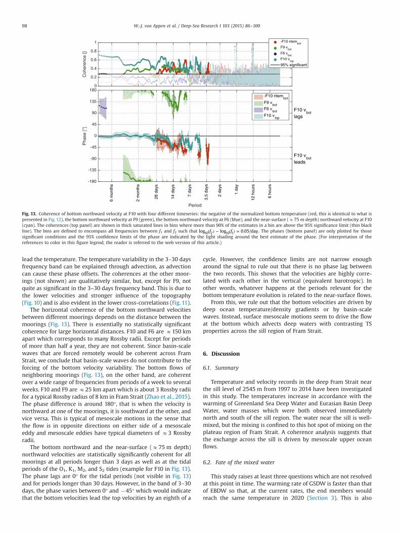
Fig. 13. Coherence of bottom northward velocity at F10 with four different timeseries: the negative of the normalized bottom temperature (red, this is identical to what ispresented in Fig. 12), the bottom northward velocity at F9 (green), the bottom northward velocity at F6 (blue), and the near-surface (E75 m depth) northward velocity at F10(cyan). The coherences (top panel) are shown in thick saturated lines in bins where more than 90% of the estimates in a bin are above the 95% significance limit (thin blackline). The bins are defined to encompass all frequencies between f1 and f2 such that f flog log 0.05/day10 2 10 1( ) − ( ) = . The phases (bottom panel) are only plotted for thosesignificant conditions and the 95% confidence limits of the phase are indicated by the light shading around the best estimate of the phase. (For interpretation of thereferences to color in this figure legend, the reader is referred to the web version of this article.)

W.-J. von Appen et al. / Deep-Sea Research I 103 (2015) 86–10098

lead the temperature. The temperature variability in the 3–30 daysfrequency band can be explained through advection, as advectioncan cause these phase offsets. The coherences at the other moor-ings (not shown) are qualitatively similar, but, except for F9, notquite as significant in the 3–30 days frequency band. This is due tothe lower velocities and stronger influence of the topography(Fig. 10) and is also evident in the lower cross-correlations (Fig. 11).

The horizontal coherence of the bottom northward velocitiesbetween different moorings depends on the distance between themoorings (Fig. 13). There is essentially no statistically significantcoherence for large horizontal distances. F10 and F6 are E150 kmapart which corresponds to many Rossby radii. Except for periodsof more than half a year, they are not coherent. Since basin-scalewaves that are forced remotely would be coherent across FramStrait, we conclude that basin-scale waves do not contribute to theforcing of the bottom velocity variability. The bottom flows ofneighboring moorings (Fig. 13), on the other hand, are coherentover a wide range of frequencies from periods of a week to severalweeks. F10 and F9 are E25 km apart which is about 3 Rossby radiifor a typical Rossby radius of 8 km in Fram Strait (Zhao et al., 2015).The phase difference is around 180°, that is when the velocity isnorthward at one of the moorings, it is southward at the other, andvice versa. This is typical of mesoscale motions in the sense thatthe flow is in opposite directions on either side of a mesoscaleeddy and mesoscale eddies have typical diameters of E3 Rossbyradii.

The bottom northward and the near-surface (E75 m depth)northward velocities are statistically significantly coherent for allmoorings at all periods longer than 3 days as well as at the tidalperiods of the O1, K1, M2, and S2 tides (example for F10 in Fig. 13).The phase lags are 0° for the tidal periods (not visible in Fig. 13)and for periods longer than 30 days. However, in the band of 3–30days, the phase varies between 0° and �45° which would indicatethat the bottom velocities lead the top velocities by an eighth of a

cycle. However, the confidence limits are not narrow enougharound the signal to rule out that there is no phase lag betweenthe two records. This shows that the velocities are highly corre-lated with each other in the vertical (equivalent barotropic). Inother words, whatever happens at the periods relevant for thebottom temperature evolution is related to the near-surface flows.

From this, we rule out that the bottom velocities are driven bydeep ocean temperature/density gradients or by basin-scalewaves. Instead, surface mesoscale motions seem to drive the flowat the bottom which advects deep waters with contrasting TSproperties across the sill region of Fram Strait.

6. Discussion

6.1. Summary

Temperature and velocity records in the deep Fram Strait nearthe sill level of 2545 m from 1997 to 2014 have been investigatedin this study. The temperatures increase in accordance with thewarming of Greeenland Sea Deep Water and Eurasian Basin DeepWater, water masses which were both observed immediatelynorth and south of the sill region. The water near the sill is well-mixed, but the mixing is confined to this hot spot of mixing on theplateau region of Fram Strait. A coherence analysis suggests thatthe exchange across the sill is driven by mesoscale upper oceanflows.

6.2. Fate of the mixed water

This study raises at least three questions which are not resolvedat this point in time. The warming rate of GSDW is faster than thatof EBDW so that, at the current rates, the end members wouldreach the same temperature in 2020 (Section 3). This is also

Fig. 14. Figure identical to Fig. 2, but also showing the means over the basin of the depth averaged (2500–2525 m) potential temperature and salinity of all CTD profiles inthe Norwegian Sea (north of 66°N and east of 7°W) as big filled circles. Limiting the domain of the Norwegian Sea to between 70°N and 73°N and east of 0°E, i.e.approximately the Lofoten Basin does not change the figure qualitatively.

W.-J. von Appen et al. / Deep-Sea Research I 103 (2015) 86–100 99

associated with a density decrease of GSDW compared to EBDW. Itis therefore to be expected that the processes at Fram Strait willqualitatively change. It is also conceivable that the EBDW warmingrate might increase as the Greenland Sea no longer cools theEurasian Basin. However, the density difference between GSDWand EBDW was observed to have changed from E�0.003 kg/m3

in the mid 1990s to E0.007 kg/m3 in the mid 2010s (Fig. 2). Evenwith this trend continuing, the density difference across the FramStrait sill would remain almost two orders of magnitude smallerthan the E0.4 kg/m3 density difference across Denmark Straitdriving the hydraulically controlled overflow there (Nikolopouloset al., 2003). Hence density driven flows across Fram Strait willremain weak for the medium term future.

The actual rate of production of mixed water in Fram Strait isanother question this study cannot answer. The absence of meancurrents advecting the mixed water masses either to the north orsouth makes it impossible to estimate this production rate withouta specific measuring campaign targeted to this question. Since themixing region is rather localized on the plateau of Fram Strait, itwould be conceivable that the rates are rather small.

The other obvious question stemming from this study is thefate of the mixed water present in the deep Fram Strait. It is notprominently present in the basins to the north or south(Figs. 2 and 8). Swift and Koltermann (1988) argued in the 1980sthat the water mixed in Fram Strait is the origin of the deep watersin the Norwegian Sea. They proposed a cyclonic transport alongthe boundary of the Greenland Sea into the Norwegian Sea.However, this does not seem to have been the case after the 1990s.The mean temperature–salinity in the Norwegian Sea between2500 m and 2525 m (Fig. 14) falls in between the GSDW and theEBDW end members in the 1990s, but is located closer to theGSDW than the mixed water in Fram Strait. This suggests thatNSDW in the 1990s might have been formed from the mixed waterin Fram Strait with more GSDW added during its passage through

the Greenland Sea. This would be consistent with the hypothesisof Swift and Koltermann (1988). However, since the mid 2000s,the Norwegian Sea temperature–salinity either agrees with theGSDW development (located on the same warming line of GSDW),or it is outside of the TS range defined by the end members and isinstead shifted towards warmer and fresher conditions thanGSDW and EBDW. Hence, the water in the Norwegian Sea in the2000s and 2010s cannot have originated in Fram Strait, but maystill be influenced by GSDW sometimes. This is consistent with theobserved reversals of the flow direction in the Jan Mayen Channelconnecting the Greenland and Norwegian Seas. The flow throughthe channel was observed to be towards the Norwegian Sea before1992 and towards the Greenland Sea afterwards, although theamplitude was much reduced in the later period (Østerhus andGammelsrød, 1999). The Fram Strait mixing product could also notbe identified in other depth levels above 2500 m or below 2525 m.Therefore, we propose that the mixed water mass formed in FramStrait might not make it around the cyclonic boundary currentloop envisioned by Swift and Koltermann (1988) and instead getsmixed into the interior Greenland Sea where it could be acting as aheat source for the warming GSDW. The fact that it is not observedin the central Greenland Sea (Fig. 14) could be due to the fact thatit is exported from Fram Strait along the East Greenland slopefurther to the west than the meridional section considered here(Fig. 7), but that it is also diluted with GSDW before reaching thecentral Greenland Sea. Especially if the actual production rates ofthe mixed water were very small, this appears to be a likelyscenario.

Acknowledgments

The authors would like to thank S. von Egan-Krieger for helpfuldiscussions. The authors would also like to thank the three

W.-J. von Appen et al. / Deep-Sea Research I 103 (2015) 86–100100

anonymous reviewers for their very thorough and helpful reviews.Support for this study was provided by the German Federal Min-istry of Education and Research (Co-operative project RACE,0F0651 D). The data sets used in this study were funded by mul-tiple different national and European projects, collected on manydifferent cruises of R/V Polarstern (ARK-XIII/3, ARK-XIV/2, ARK-XIX/3c, ARK-XIX/4b, ARK-XV/3, ARK-XVI/1, ARK-XVI/2, ARK-XVII/1,ARK-XVIII/1, ARK-XX/1, ARK-XX/2, ARK-XXI/1b, ARK-XXII/1c, ARK-XXIII/2, ARK-XXIV/1, ARK-XXIV/2, ARK-XXV/2, ARK-XXVI/1, ARK-XXVI/2, ARK-XXVII/1, ARK-XXVII/2, and ARK-XXVIII/2), R/V Merian(MSM02 and MSM29), and R/V Lance, and processed by severalindividuals at the Alfred Wegener Institute and the NorwegianPolar Institute.

References

Aagaard, K., Fahrbach, E., Meincke, J., Swift, J., 1991. Saline outflow from the ArcticOcean: its contribution to the deep waters of the Greenland, Norwegian, andIceland Seas. J. Geophys. Res.: Oceans (1978–2012) 96 (C11), 20433–20441.

Aagaard, K., Swift, J.H., Carmack, E.C., 1985. Thermohaline circulation in the ArcticMediterranean Seas. J. Geophys. Res.: Oceans 90 (C3), 4833–4846.

Akimova, A., Schauer, U., Danilov, S., Núñez-Riboni, I., 2011. The role of the deepmixing in the Storfjorden shelf water plume. Deep Sea Res. Part I: Oceanogr.Res. Pap. 58 (4), 403–414.

Alford, M.H., Girton, J.B., Voet, G., Carter, G.S., Mickett, J.B., Klymak, J.M., 2013.Turbulent mixing and hydraulic control of abyssal water in the Samoan Pas-sage. Geophys. Res. Lett. 40 (17), 4668–4674.

Bauerfeind, E., Nöthig, E.-M., Beszczynska, A., Fahl, K., Kaleschke, L., Kreker, K.,Klages, M., Soltwedel, T., Lorenzen, C., Wegner, J., 2009. Particle sedimentationpatterns in the eastern Fram Strait during 2000–2005: results from the Arcticlong-term observatory HAUSGARTEN. Deep Sea Res. Part I: Oceanogr. Res. Pap.56 (9), 1471–1487.

Beszczynska-Möller, A., Fahrbach, E., Schauer, U., Hansen, E., 2012. Variability inAtlantic water temperature and transport at the entrance to the Arctic Ocean,1997–2010. ICES J. Mar. Sci.: J. Conseil 69 (5), 852–863.

de Steur, L., Hansen, E., Gerdes, R., Karcher, M., Fahrbach, E., Holfort, J., 2009.Freshwater fluxes in the East Greenland Current: a decade of observations.Geophys. Res. Lett. 36 (23).

Fer, I., Müller, M., Peterson, A., 2014. Tidal forcing, energetics, and mixing near theYermak Plateau. Ocean Sci. Discus. 11 (5), 2245–2287.

Jakobsson, M., Mayer, L., Coakley, B., Dowdeswell, J.A., Forbes, S., Fridman, B.,Hodnesdal, H., Noormets, R., Pedersen, R., Rebesco, M., et al., 2012. The inter-national bathymetric chart of the Arctic Ocean (IBCAO) version 3.0. Geophys.

Res. Lett. 39 (12).Johannessen, J., Johannessen, O., Svendsen, E., Shuchman, R., Manley, T., Campbell,

W., Josberger, E., Sandven, S., Gascard, J., Olaussen, T., et al., 1987. MesoscaleEddies in the Fram Strait Marginal Ice Zone during the 1983 and 1984 MarginalIce Zone Experiments. J. Geophys. Res. 92 (C7), 6754–6772.

Langehaug, H.R., Falck, E., 2012. Changes in the properties and distribution of theintermediate and deep waters in the Fram Strait. Prog. Oceanogr. 96 (1), 57–76.

Macrander, A., Käse, R., Send, U., Valdimarsson, H., Jónsson, S., 2007. Spatial andtemporal structure of the Denmark Strait overflow revealed by acoustic ob-servations. Ocean Dyn. 57 (2), 75–89.

Manley, T., Hunkins, K., Villanueva, J., van Leer, J., Gascard, J., Jeannin, P., 1987.Mesoscale oceanographic processes beneath the ice of Fram Strait. Science 236(4800), 432–434.

Marsh, R., Josey, S.A., de Cuevas, B.A., Redbourn, L.J., Quartly, G.D., 2008. Mechan-isms for recent warming of the North Atlantic: insights gained with an eddy-permitting model. J. Geophys. Res.: Oceans 113 (C4).

Meincke, J., Jonsson, S., Swift, J.H., 1992. Variability of convective conditions in theGreenland Sea. In: ICES Marine Science Symposium, vol. 195, pp. 32–39.

Nikolopoulos, A., Borenäs, K., Hietala, R., Lundberg, P., 2003. Hydraulic estimates ofDenmark Strait overflow. J. Geophys. Res. 108, 3095.

Østerhus, S., Gammelsrød, T., 1999. The abyss of the Nordic Seas is warming. J. Clim.12 (11), 3297–3304.

Price, J., O'Neil Baringer, M., 1994. Outflows and deep water production by marginalseas. Prog. Oceanogr. 33 (3), 161–200.

Rhein, M., 1991. Ventilation rates of the Greenland and Norwegian Seas derivedfrom distributions of the chlorofluoromethanes F11 and F12. Deep Sea Res. PartA: Oceanogr. Res. Pap. 38 (4), 485–503.

Rudels, B., Korhonen, M., Schauer, U., Pisarev, S., Rabe, B., Wisotzki, A., 2015. Cir-culation and transformation of Atlantic water in the Eurasian Basin and thecontribution of the Fram Strait inflow branch to the Arctic Ocean heat budget.Prog. Oceanogr. 132, 128–152.

Schlosser, P., Bönisch, G., Rhein, M., Bayer, R., 1991. Reduction of deepwater for-mation in the Greenland Sea during the 1980s: evidence from tracer data.Science 251 (4997), 1054–1056.

Somavilla, R., Schauer, U., Budéus, G., 2013. Increasing amount of Arctic Ocean deepwaters in the Greenland Sea. Geophys. Res. Lett.

Swift, J.H., Koltermann, K.P., 1988. The origin of Norwegian Sea deep water. J.Geophys. Res.: Oceans 93 (C4), 3563–3569.

Teigen, S., Nilsen, F., Gjevik, B., 2010. Barotropic instability in the West SpitsbergenCurrent. J. Geophys. Res. 115 (C7), C07016.

von Appen, W.-J., Schauer, U., Somavilla Cabrillo, R., Bauerfeind, E., Beszczynska-Möller, A., 2015. Physical oceanography and current meter data from mooringand CTD measurements at Fram Strait. Pangea . http://dx.doi.org/10.1594/PANGAEA.845938.

Zhao, M., Timmermans, M.-L., Cole, S., Krishfield, R., Proshutinsky, A., Toole, J., 2015.Characterizing the eddy field in the Arctic Ocean halocline. J. Geophys. Res.:Oceans.